Adaptive process control for achieving consistent particles ...
21
Vol.:(0123456789) SN Applied Sciences (2021) 3:294 | https://doi.org/10.1007/s42452-021-04296-y Research Article Adaptive process control for achieving consistent particles’ states in atmospheric plasma spray process B. Guduri 1 · M. Cybulsky 2 · G. R. Pickrell 3 · R. C. Batra 1 Received: 27 September 2020 / Accepted: 28 January 2021 / Published online: 8 February 2021 © The Author(s) 2021 OPEN Abstract The coatings produced by an atmospheric plasma spray process (APSP) must be of uniform quality. However, the com- plexity of the process and the random introduction of noise variables such as fluctuations in the powder injection rate and the arc voltage make it difficult to control the coating quality that has been shown to depend upon mean values of powder particles’ temperature and speed, collectively called mean particles’ states (MPSs), just before they impact the substrate. Here, we use a science-based methodology to develop a stable and adaptive controller for achieving consist- ent MPSs and thereby decrease the manufacturing cost. We first identify inputs into the APSP that significantly affect the MPSs and then formulate a relationship between these two quantities. When the MPSs deviate from their desired values, the adaptive controller is shown to successfully adjust the input parameters to correct them. The performance of the controller is tested via numerical experiments using the software, LAVA-P, that has been shown to well simulate the APSP. Keywords Plasma spray process · Parameters screening · Response functions · Adaptive controller 1 Introduction The atmospheric plasma spray process (APSP) used to produce a variety of coatings such as low porosity, ther- mal barrier, wear and corrosion resistant, and functionally graded [1] is schematically shown in Fig. 1. Coatings of thickness less than a few micrometers are categorized as thin, and others as thick. Besides an APSP, coating techniques include electroplating, chemical treatments, hot dipping, chemical vapor deposition, physical vapor deposition (e.g., evaporation, puttering, ion plating), and pulsed laser deposition. Primary characteristics of coat- ing processes are summarized in Table 2.1 of Fauchais et al.’s [2] chapter. The methodology of finding significant input parameters and controlling them to produce a good quality coating described in this paper is applicable to the above-mentioned processes and to other technologies like hot forging and machining. Details are provided below only for an APSP. An APSP involves plasma formation within a gun noz- zle, particle injection into the plasma jet flowing out of the nozzle, particle heating and acceleration during their motion in the plasma, and coating formation on a substrate. Usually, a mixture of argon (Ar, ~ 30–60 slm (standard liter per minute)) and hydrogen (H 2 , ~ 0–15 slm) injected into the gun nozzle is ignited by a high-intensity arc between tips of a cathode and a water-cooled anode. The arc intensity depends on the current (~ 300–600 A), the voltage (~ 30–70 V), the distance between the anode and the cathode, their geometries, and the gun efficiency. Supplementary information The online version of this article (https://doi.org/10.1007/s42452-021-04296-y) * B. Guduri, [email protected]; R. C. Batra, [email protected] | 1 Department of Biomedical Engineering and Mechanics, Virginia Polytechnic Institute and State University, M/C 0219, Blacksburg, VA 24061, USA. 2 Rolls-Royce Corporation, Speed Code W-08, P.O. Box 420, Indianapolis, IN 46206-0420, USA. 3 Department of Materials Science and Engineering, Virginia Polytechnic Institute and State University, M/C 0237, Blacksburg, VA 24061, USA.
-
Upload
khangminh22 -
Category
Documents
-
view
1 -
download
0
Transcript of Adaptive process control for achieving consistent particles ...

Vol.:(0123456789)
SN Applied Sciences (2021) 3:294 | https://doi.org/10.1007/s42452-021-04296-y
Research Article
Adaptive process control for achieving consistent particles’ states in atmospheric plasma spray process
B. Guduri1 · M. Cybulsky2 · G. R. Pickrell3 · R. C. Batra1
Received: 27 September 2020 / Accepted: 28 January 2021 / Published online: 8 February 2021 © The Author(s) 2021 OPEN
AbstractThe coatings produced by an atmospheric plasma spray process (APSP) must be of uniform quality. However, the com-plexity of the process and the random introduction of noise variables such as fluctuations in the powder injection rate and the arc voltage make it difficult to control the coating quality that has been shown to depend upon mean values of powder particles’ temperature and speed, collectively called mean particles’ states (MPSs), just before they impact the substrate. Here, we use a science-based methodology to develop a stable and adaptive controller for achieving consist-ent MPSs and thereby decrease the manufacturing cost. We first identify inputs into the APSP that significantly affect the MPSs and then formulate a relationship between these two quantities. When the MPSs deviate from their desired values, the adaptive controller is shown to successfully adjust the input parameters to correct them. The performance of the controller is tested via numerical experiments using the software, LAVA-P, that has been shown to well simulate the APSP.
Keywords Plasma spray process · Parameters screening · Response functions · Adaptive controller
1 Introduction
The atmospheric plasma spray process (APSP) used to produce a variety of coatings such as low porosity, ther-mal barrier, wear and corrosion resistant, and functionally graded [1] is schematically shown in Fig. 1. Coatings of thickness less than a few micrometers are categorized as thin, and others as thick. Besides an APSP, coating techniques include electroplating, chemical treatments, hot dipping, chemical vapor deposition, physical vapor deposition (e.g., evaporation, puttering, ion plating), and pulsed laser deposition. Primary characteristics of coat-ing processes are summarized in Table 2.1 of Fauchais et al.’s [2] chapter. The methodology of finding significant input parameters and controlling them to produce a good
quality coating described in this paper is applicable to the above-mentioned processes and to other technologies like hot forging and machining. Details are provided below only for an APSP.
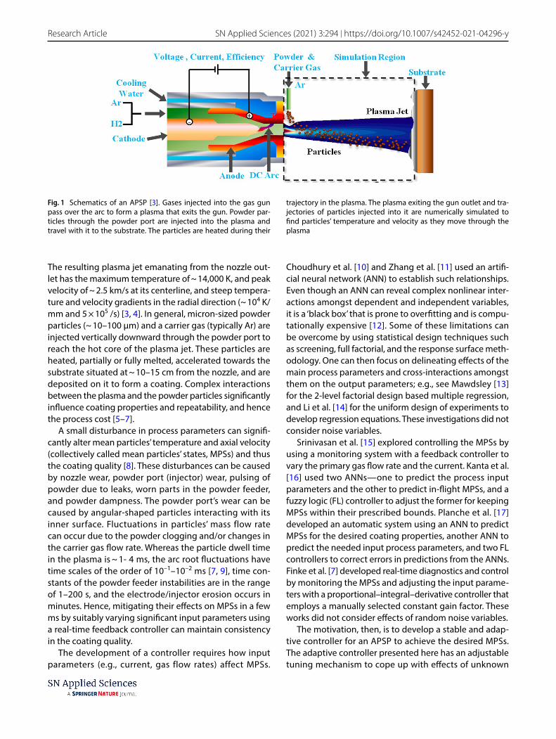
An APSP involves plasma formation within a gun noz-zle, particle injection into the plasma jet flowing out of the nozzle, particle heating and acceleration during their motion in the plasma, and coating formation on a substrate. Usually, a mixture of argon (Ar, ~ 30–60 slm (standard liter per minute)) and hydrogen (H2, ~ 0–15 slm) injected into the gun nozzle is ignited by a high-intensity arc between tips of a cathode and a water-cooled anode. The arc intensity depends on the current (~ 300–600 A), the voltage (~ 30–70 V), the distance between the anode and the cathode, their geometries, and the gun efficiency.
Supplementary information The online version of this article (https ://doi.org/10.1007/s4245 2-021-04296 -y)
* B. Guduri, [email protected]; R. C. Batra, [email protected] | 1Department of Biomedical Engineering and Mechanics, Virginia Polytechnic Institute and State University, M/C 0219, Blacksburg, VA 24061, USA. 2Rolls-Royce Corporation, Speed Code W-08, P.O. Box 420, Indianapolis, IN 46206-0420, USA. 3Department of Materials Science and Engineering, Virginia Polytechnic Institute and State University, M/C 0237, Blacksburg, VA 24061, USA.
Vol:.(1234567890)
Research Article SN Applied Sciences (2021) 3:294 | https://doi.org/10.1007/s42452-021-04296-y
The resulting plasma jet emanating from the nozzle out-let has the maximum temperature of ~ 14,000 K, and peak velocity of ~ 2.5 km/s at its centerline, and steep tempera-ture and velocity gradients in the radial direction (~ 104 K/mm and 5 × 10⁵ /s) [3, 4]. In general, micron-sized powder particles (~ 10–100 µm) and a carrier gas (typically Ar) are injected vertically downward through the powder port to reach the hot core of the plasma jet. These particles are heated, partially or fully melted, accelerated towards the substrate situated at ~ 10–15 cm from the nozzle, and are deposited on it to form a coating. Complex interactions between the plasma and the powder particles significantly influence coating properties and repeatability, and hence the process cost [5–7].
A small disturbance in process parameters can signifi-cantly alter mean particles’ temperature and axial velocity (collectively called mean particles’ states, MPSs) and thus the coating quality [8]. These disturbances can be caused by nozzle wear, powder port (injector) wear, pulsing of powder due to leaks, worn parts in the powder feeder, and powder dampness. The powder port’s wear can be caused by angular-shaped particles interacting with its inner surface. Fluctuations in particles’ mass flow rate can occur due to the powder clogging and/or changes in the carrier gas flow rate. Whereas the particle dwell time in the plasma is ~ 1- 4 ms, the arc root fluctuations have time scales of the order of 10–1–10–2 ms [7, 9], time con-stants of the powder feeder instabilities are in the range of 1–200 s, and the electrode/injector erosion occurs in minutes. Hence, mitigating their effects on MPSs in a few ms by suitably varying significant input parameters using a real-time feedback controller can maintain consistency in the coating quality.
The development of a controller requires how input parameters (e.g., current, gas flow rates) affect MPSs.
Choudhury et al. [10] and Zhang et al. [11] used an artifi-cial neural network (ANN) to establish such relationships. Even though an ANN can reveal complex nonlinear inter-actions amongst dependent and independent variables, it is a ‘black box’ that is prone to overfitting and is compu-tationally expensive [12]. Some of these limitations can be overcome by using statistical design techniques such as screening, full factorial, and the response surface meth-odology. One can then focus on delineating effects of the main process parameters and cross-interactions amongst them on the output parameters; e.g., see Mawdsley [13] for the 2-level factorial design based multiple regression, and Li et al. [14] for the uniform design of experiments to develop regression equations. These investigations did not consider noise variables.
Srinivasan et al. [15] explored controlling the MPSs by using a monitoring system with a feedback controller to vary the primary gas flow rate and the current. Kanta et al. [16] used two ANNs—one to predict the process input parameters and the other to predict in-flight MPSs, and a fuzzy logic (FL) controller to adjust the former for keeping MPSs within their prescribed bounds. Planche et al. [17] developed an automatic system using an ANN to predict MPSs for the desired coating properties, another ANN to predict the needed input process parameters, and two FL controllers to correct errors in predictions from the ANNs. Finke et al. [7] developed real-time diagnostics and control by monitoring the MPSs and adjusting the input parame-ters with a proportional–integral–derivative controller that employs a manually selected constant gain factor. These works did not consider effects of random noise variables.
The motivation, then, is to develop a stable and adap-tive controller for an APSP to achieve the desired MPSs. The adaptive controller presented here has an adjustable tuning mechanism to cope up with effects of unknown
Fig. 1 Schematics of an APSP [3]. Gases injected into the gas gun pass over the arc to form a plasma that exits the gun. Powder par-ticles through the powder port are injected into the plasma and travel with it to the substrate. The particles are heated during their
trajectory in the plasma. The plasma exiting the gun outlet and tra-jectories of particles injected into it are numerically simulated to find particles’ temperature and velocity as they move through the plasma

Vol.:(0123456789)
SN Applied Sciences (2021) 3:294 | https://doi.org/10.1007/s42452-021-04296-y Research Article
disturbances and has been designed using a model refer-ence adaptive control (MRAC) scheme based on the lin-earized dynamics of the MPSs.
2 Methods
2.1 Development of mathematical model of the problem
A major challenge in developing a science-based model of a physical problem is to capture physics relevant to all important phenomena such as the plasma jet exiting from the nozzle outlet, chemical interactions amongst the jet constituents, the drag force experienced by powder par-ticles injected into the plasma, heat transfer between par-ticles and the plasma, and plasma’s interaction with the air surrounding it. The mathematical model of the APSP developed in this paper is based on the following assump-tions. (1) The plasma jet exiting the nozzle is axisymmetric, is in local thermodynamic equilibrium, and is composed of a mixture of chemically reacting constituents with temperature-dependent thermodynamic and transport properties. (2) Chemical reactions among different spe-cies including ionization, dissociation, and recombination are considered, and the turbulence is simulated by using the standard k− ∈ model. (3) The arc voltage fluctuations in the plasma nozzle are neglected because of difficulties in expressing them in terms of gases injected into the noz-zle, the anode and the cathode materials, and the distance between them. (4) Powder particles are rigid spheres, ran-domly vary in diameter, do not interact with each other, exchange heat with the plasma, and can melt due to tem-perature rise, and the internal convection within a molten particle has a negligible effect on the heat transfer. (5) A powder particle is regarded as a point mass for simulat-ing its heating, melting, and solidification [6]. The volume fraction of the melted material is computed by considering the latent heat of melting. (6) Effects of gravity and buoy-ancy on the plasma jet and particles’ trajectories are neg-ligible as compared to that of the viscous drag forces [18, 19]. (7) The effect of the carrier gas flowing through the powder port at ~ 5 slm on the plasma jet is negligible [6].
2.1.1 Justification of assumptions
Assumption 5 considerably simplifies the analysis of heat-ing of particles, has been shown by other investigators to give fairly accurate results that are close to the experimen-tal observations, and saves considerable computational resources. Assumption 6 is reasonable because of large differences between particles’ and the plasma velocities, and drag forces are dominant. For assumption 7, we note
that even though the injection of the carrier gas and the powder particles adversely affects axisymmetry of the plasma jet near the powder injection port, however, the effect is local and the plasma jet is nearly axisymmetric away from the powder port.
The injection velocity (speed and direction) of parti-cles varying in diameters from 5 to 125 μm are randomly assigned within their pre-specified ranges to achieve the desired powder mass injection rate.
2.2 Governing equations and solution techniques
For brevity, we refer the reader to Sects. 3, 4 and 5 of Shang et al. [3] for details of the governing equations for the plasma modeled as a mixture of different constituents, and particles’ trajectories and heating. The software LAVA-P numerically solves these equations by the finite volume method over the simulation region exhibited in Fig. 1 and using the following boundary conditions (BCs) [20] for the temperature, the velocity, and the turbulence variables at the nozzle exit plane.
Here, Tf is the plasma temperature; u and v, respectively, are the radial and the axial velocity components; Ri and Ro, respectively, are the inner and the outer radii of the nozzle exit; T0 and V0 , respectively, are the plasma temperature and the axial velocity at the nozzle exit; Tw is the torch wall temperature; and k and � , respectively, are the turbulence kinetic energy and its dissipation rate. Coefficients nT and nv indicate how fast the temperature and the axial velocity decrease in the radial direction; the x-axis is in the radial direction, (�u∕�x)max equals the maximum value of the radial velocity gradient; the parameter κ determines the shape of the profile, and δ0.1 equals the jet width at the location where v = 0.1V0 . The torch wall is assumed to be rigid where no-slip condition holds [20]. T∞ represents the ambient temperature. Open boundaries and downstream boundaries are considered as either inward or outward flow conditions [20]. On the axis of symmetry, x = 0, BCs are
(1)
�y = 0andRi ≤ x ≤ R0
�∶
⎧⎪⎪⎪⎨⎪⎪⎪⎩
Tf (x, 0) =�T0 − Tw
��1 −
�x
Ri
�nT�+ Tw
u(x, 0) = 0, v(x, 0) = V0
�1 −
�x
R0
�nv�
k(x, 0) = �V0
��v
�x∕�
�u
�x
�max
�
�(x, 0) = k(x∕�0.0075�0.1∕c
3∕4�
�
�y = 0, x ≥ Ro
�∶
⎧⎪⎪⎨⎪⎪⎩
Tf (x, 0) = Tw −�T∞ − Tw
� ln (x∕Ri)ln (Ri∕Ro)
u(x, 0) = v(x, 0) = 0
k(x, 0) = 0
�(x, 0) = 0

Vol:.(1234567890)
Research Article SN Applied Sciences (2021) 3:294 | https://doi.org/10.1007/s42452-021-04296-y
u = 0 and �u�y
+�v
�x = 0. Initially, the simulation region is filled
with quiescent air at room temperature.Following [20], we choose nT and nv , and iteratively find
T0 and V0 so that the total mass flow rate and the energy output from the nozzle exit differ by less than 1%, respec-tively, from their input values into the nozzle.
For the specified powder mass injection rate, the soft-ware calculates the number of particles for a given average injection speed and assigns them a random velocity when exiting the powder port.
2.2.1 Parameter values
Values assigned to parameters are: Ri = 0.39 mm, Ro = 15 mm, the gun efficiency = 0.7, T∞ = 300 K, P∞ = 85.5 kPa, Tw = 700 K, κ = 0.015. Values of material parameters used for the zirconia (Zr) powder particles are listed in [6]. Figure s1 of the supporting information repre-sents the distribution of particles’ diameters used in simu-lations, a schematic of their trajectories in the plasma, and the location of the observation window used to measure particles’ temperature and velocity.
2.2.2 Measure of quality of computed results
The deviation of the computed results from those meas-ured experimentally is quantified by using the following L2-norm, e2 , of the difference between them.
where � represents either the temperature or a veloc-ity component. This provides the average of deviations between the computed and the experimental values of � rather than the maximum difference between them at any location. A local spike in the difference over a small distance has the same effect on e2 as a small difference over a large distance.
2.3 Finding optimal input parameters for the MPSs
Three steps involved in finding values of the process input parameters for achieving desired MPSs are screening, find-ing response functions relating significant input param-eters to the MPSs, and using a genetic algorithm (GA) to solve nonlinear algebraic response function equations for the input parameters when the MPSs are prescribed. The screening analysis ranks the influence of each process parameter on the MPSs to identify which ones should be included in developing response functions for the MPSs.
(2)e2 =
√√√√√∫(�Simulated(x) − �Experimental(x)
)2dx
∫ �2Experimental
(x)dx
To investigate statistical significance of process parameters and interactions between any two of them, a complete polynomial of at least degree 2 is needed. Here, we use a complete polynomial of degree 2, employ the analysis of variance (ANOVA) to statistically quantify the significance of various terms in the polynomial, construct an objec-tive function in terms of the two response functions (one for the mean particles’ temperature and the other for the velocity), and use an GA to find values of the signifi-cant process parameters from the response functions for desired MPSs.
2.3.1 Screening of process parameters
We use Morris’ [21] global one-factor-at-a-time (OFAT) screening method to rank their effects on the MPSs as: (1) negligible, (2) linear and additive, and (3) nonlinear and/or involved in interactions with other process parameters [21]. As explained in [21, 22], it requires calculating ele-mentary effects (EEs) of a randomly chosen value of one process parameter at a time on the MPSs. We assume that each MPS is a scalar-valued function of 7 process param-eters ui(i = 1,… , 7) that have been normalized to vary between 0 and 1. Each ui is discretized into a p – level grid {0,
1
p−1,
2
p−1,… , 1
} where p is an even integer. With
Δ ≡p
2(p−1) , the EE of the ith parameter at a randomly chosen
base point u* =(u1,… u7
) is defined by
The value of EEi(u*) equals the sensitivity of the MPS
( denoted by y in Eq.3) to the ith parameter at the base point u* . The mean, �i , and the standard deviation, �i , of the EEi of the ith process parameter are computed using
Here, u(j)(j = 1,… , r) are r randomly chosen base points, and EE(j)
i represents the EE of the ith parameter at the base
point u(j). Values of �i and �i identify process parameters that have negligible (low �i), linear (high �i and low �i ), and nonlinear and/or interactions (high �i and high �i ) effects [21, 23].
2.3.2 Identification of significant input parameters using analysis of variance (ANOVA)
The results of ANOVA are meaningful only if the input val-ues used in the design of experiments are independent of each other [24], i.e., the correlation coefficient, cr , between the input variables ξ1 and ξ2 defined by
(3)EEi(u*)=
1
Δ
[y(u1,… , ui + Δ,… , u7
)− y
(u1,… , u7
)]
(4)
�i =1
r
r∑j=1
���EE(j)
i
���; �i =
�1
r−1
r∑j=1
�EE
(j)
i− �i
�2
, i = 1,… , 7 .

Vol.:(0123456789)
SN Applied Sciences (2021) 3:294 | https://doi.org/10.1007/s42452-021-04296-y Research Article
is very small. Here, superscript (i) refers to the ith observa-tion out of n observations, and a bar superimposed on a variable indicates the mean value of n observations. The cr has the range [-1, 1], its magnitude indicate the strength and sign of the direction of the linear depend-ence between the two variables [24]. The -ve sign means that variables �1 and �2 have opposite effects.
To investigate effects of the main and the cross-interac-tions between process parameters on MPSs, we use ANOVA by considering a complete polynomial degree of 2 given by Eq. (6) to fit the computed data to the MPSs.
In Eq. (6), ymodel represents the normalized fit to the MPSs, u =
{P,Q, I, dy , PQ, PI, Pdy ,QI,Qdy , Idy , P
2,Q2, I2, d2y
} and
the vector b represents the sensitivity coefficients that quantify the effect of an element of u on the output [24]. To delineate the importance of the parameter ui0 in the array u , we define a new model
that omits the term ui0 from the sum in Eq. (6). The sum of squares (SS) associated with ui0 is given by
Here, N equals the number of samples and y the mean of the vector y . The mean squares are defined as MSi0 = SSi0∕DFi0 , where DFi0 is the degree of freedom of the parameter ui0 . The value of MSi0 is used to test the null hypothesis by calculating the F–ratio defined as Fi0 = MSi0∕MSE , where MSE is the mean squares associated with the residual error. If Fi0 is less than the standard value of its F – distribution, then the parameter ui0 is significant. The significance of terms in Eq. (6) is calculated by using the null hypothesis with 0.5% rejection, i.e., if the p-value (Probability > F) for bi is less than 0.005, then ui will be sig-nificant [25] in evaluating ymodel.
(5)cr =
∑n
i=1
��(i)
1− �1
���(i)
2− �2
��∑n
i=1
��(i)
1− �1
�2�∑n
i=1
��(i)
2− �2
�2
(6)ymodel = b0 +
14∑i=1
biui
(7)ymodel,i0= b0 +
14∑i=1,i≠i0
biui
(8)SSi0 =
N∑i=1
(y(i)
model− y
)2
−
N∑i=1
(y(i)
model, i0− y
)2
2.3.3 Finding the response functions, i.e., expressions for MPSs in terms of significant process parameters
The response functions or equivalently expressions for the MPSs in terms of significant process parameters are found by performing numerical experiments by using the full factorial approach. For the number of significant processing parameters = a and b levels for each param-eter, ba simulations are conducted. The coefficients of the response functions in Eq. (6) are estimated by using the linear regression analysis, and finding R2 where
The value of R2 close to 1 means that the model accurately captures the variability of the MPSs with the change in process parameters.
We note that Batra and Taetragool [26] used the response surface methodology and the regression analy-sis to relate MPSs to the significant input parameters.
2.3.4 Solution of nonlinear algebraic equations using the genetic algorithm
The GA explained in [27] is used to solve, within a pre-scribed error, the nonlinear Eq. (6)for the significant input parameters for desired values of the MPSs. We use the ‘ga’ toolbox in MATLAB with default values of param-eters to minimize the Error defined by
where the subscript ‘des’ represents the desired value of the variable, and P , Q and I , respectively, denote the Ar flow rate, the H2 flow rate, and the current. We accept the solution that reduces the normalized error to less than 10–6.
2.4 Development of adaptive controller
The objective is to develop an adaptive controller for the APSP to maintain MPSs within the prescribed range when the average powder injection velocity and the arc voltage change. The design criterion is to attain the desired MPSs in less than 50 ms for 20slm ≤ P ≤ 60slm, 0 ≤ Q ≤ 20slm, and 300A ≤ I ≤ 600A.
Developing the adaptive controller involves the fol-lowing five steps: a mathematical model, the system
(9)R2 =
∑N
i=1
�y(i)
model− y
�2
∑N
i=1
�y(i) − y
�2
(10)Error =
√(Tdes − T (I, P,Q)
)2+(vdes − v(I, P,Q)
)2
Vol:.(1234567890)
Research Article SN Applied Sciences (2021) 3:294 | https://doi.org/10.1007/s42452-021-04296-y
identification, controller design, implementation, and testing. These are briefly explained below.
2.4.1 Approximate mathematical model for the MPSs
We find below a relation between the inputs and the out-puts by linearizing the nonlinear dynamics of particles’ states around a known steady-state solution called an equilibrium point. Recall that a particle’s temperature is found by assuming it as a rigid sphere [3], and its motion in the plasma is affected by only the drag force exerted on it by the plasma. The particle’s acceleration, governed by Newton’s second law of motion, equals the drag force divided by its mass. That is,
where Up ={up vp wp
}T is the particle velocity vec-
tor, Uf the plasma velocity, � means mass density of the plasma, �p the particle mass density, rp the particle radius, Urel the velocity of the particle relative to that of the plasma, Urel = Uf − Up , and CD the drag coefficient.
The heating of a particle is governed by
where Vp is the particle volume, Tf the plasma temperature, Tp the particle temperature, cp the specific heat capacity, Ap the surface area of the particle, and h the heat transfer coefficient. Using Ap = 4�r2 and Vp =
4
3�r3(r equals the
particle radius) in Eqs. 11 and 12, the particle acceleration in the axial (y-) direction and its temperature are given by
(11)dUp
dt=
3
8
�
�p
CD
rp
||Urel||Urel
(12)Vp�pcpdTp
dt= Aph
(Tf − Tp
)
(13)dvp(t)
dt=
(3
8
�
�p
CD
rp
||Urel||)(−vp(t) + vf (t))
where vp(t) and vf (t) are, respectively, components of Up(t) and Uf (t) in the y-direction. Equations 13 and 14 are first-order nonlinear ordinary differential equations with vf and Tf as excitations.
To develop an approximate model for the MPSs as a function of the Ar and the H2 flow rates and the current I, we assume the following affine relations:
where c0,v ,… , c3,v and c0,T ,… , c3,T are constants.Substitution from Eq. 15 into Eqs. (13) and (14) gives
Here, ||Usrel|| equals its value in the steady-state configura-
tion around which the equations are linearized. Neglect-ing the bias terms c0,v and c0,T in Eq. (16) results in the fol-lowing multi-input multi-output (MIMO; 3 inputs and 2 outputs) state-space (SS) model for the MPSs.
Values of constants av , aT , b11, ..., b23 in Eq. 17 depend on the equilibrium point, value of ||Us
rel|| at the equilibrium
point, and are estimated using the input–output data.We will verify in Results section that Eq. 17 well repre-
sents deviations from the equilibrium point of the MPSs.
2.4.2 System identification
For estimating constants in Eq. 17, we use the following sinusoidal variations in the input variable u = P, Q or I:
(14)dTp(t)
dt=
(3h
�prpCp
)(−Tp(t) + Tf (t)
)
(15)vf (t) = c0,v + c1,vP(t) + c2,vQ(t) + c3,v I(t)
Tf (t) = c0,T + c1,T P(t) + c2,TQ(t) + c3,T I(t)
(16)
dv(t)
dt=
(3
8
�
�p
CD
rp
||Usrel||)(
−v(t) +(c1,vP(t) + c2,vQ(t) + c3,v I(t) + c0,v
))
dT (t)
dt=
(3h
�prpCp
)(−T (t) +
(c1,T P(t) + c2,T Q(t) + c3,T I(t) + c0,T
))
(17)v(t) = avv(t) + b11P(t) + b12Q(t) + b13I(t), v(0) = v0T (t) = aTv(t) + b21P(t) + b22Q(t) + b23I(t), T (0) = T0
(18)u(t) =
⎧⎪⎨⎪⎩
ub, t ≤ 10ms
ub + ua1 sin�𝜔1(t − 10)
�+ ua2 sin
�𝜔2(t − 10)
�+ ua3 sin
�𝜔3(t − 10)
�+ua4 sin
�𝜔4(t − 10)
�+ ua5 sin
�𝜔5(t − 10)
� t > 10ms
Vol.:(0123456789)
SN Applied Sciences (2021) 3:294 | https://doi.org/10.1007/s42452-021-04296-y Research Article
where ub is the base value, ua1, ua2, ua3, ua4, and ua5 are amplitudes of perturbations; �1,�2,�3,�4, and �5 are fre-quencies, and t is the time in ms. According to [28], the input variations given by Eq. 18 are sufficiently rich as they contain enough frequencies of excitation. Values of the 11 variables
(ub, ua1, ua2,… , ua5,�1,�2,…�5
) are chosen
using the Latin Hypercube sampling approach based on the normal distributions with the mean ( � ) and the stand-ard deviation ( � ). The corresponding MPSs are calculated in the observation window at a sampling time of 0.01 ms. The values of parameters in Eq. 17 are estimated by using the simulated (with LAVA-P) input–output data and the MATLAB toolbox ‘ident’ lucidly explained by Ljung [29] the prediction error method (PEM) framework, and the MAT-LAB function ‘ssest’ with the order of the system = 1, input delay = 0, form = canonical, feed through = 0, disturbance model = none, initial states = 0, and the weighting scheme for singular value decomposition = the canonical variable algorithm. The entire input-MPS data of each sample are first processed by subtracting from it the mean value. Next, the output data are smoothened by using a moving aver-age of 100 data points to reduce noise in it. The resulting input–output data are divided into two equal parts; the first part is used for estimation of parameter values and the second part for validation. The quality of model prediction is measured by the comparison index, ‘Fit,’ defined as
where y is the predicted output for the input y , y is the mean of the output, and ‖⋅‖ indicates the L2 norm (or the length) of a vector.
2.4.3 Controller design
The linearized MIMO SS model, Eq. 17, for the MPSs around an equilibrium point is rewritten as
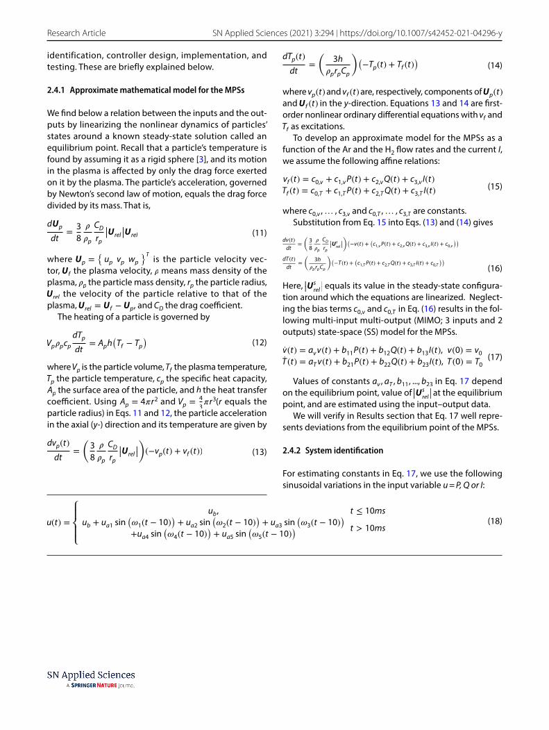
Here, y(t) = {v(t), T (t)}T i s the output vec tor, u(t) = {P(t),Q(t), I(t)}T the input vector, and matrices ‘A’ and ‘B’ depend on the equilibrium point (i.e., the operating point). We assume that matrix A is Herwitz and the plant is controllable, i.e., for any desired output ydes , there exists a sequence of inputs u(0), u(1),… , u(k) such that y(k) = ydes within an acceptable tolerance. The model reference adap-tive control (MRAC) algorithm involves two loops—the inner loop consisting of a feedback and the outer loop of an adaptive mechanism for the controller as shown in Fig. 2. Based on Eq. 20, we choose the following reference model for updating the controller gains
(19)Fit = 100
�1 −
‖y − y‖‖y − y‖
�
(20)
⎧⎪⎨⎪⎩
v(t)
T (t)
⎫⎪⎬⎪⎭
�����=y(t)
=
⎡⎢⎢⎣av 0
0 aT
⎤⎥⎥⎦
�������=A
⎧⎪⎨⎪⎩
v(t)
T (t)
⎫⎪⎬⎪⎭
�����=y(t)
+
⎡⎢⎢⎣
b11 b12 b13
b21 b22 b23
⎤⎥⎥⎦
���������������������=B
⎧⎪⎪⎨⎪⎪⎩
P(t)
Q(t)
I(t)
⎫⎪⎪⎬⎪⎪⎭
�����=u(t)
,
⎧⎪⎨⎪⎩
v(0)
T (0)
⎫⎪⎬⎪⎭=
⎧⎪⎨⎪⎩
v0
T0
⎫⎪⎬⎪⎭
(21)
�vm(t)
Tm(t)
�
���������=ym(t)
=
�amv 0
0 amT
�
�����������=Am
�vm(t)
Tm(t)
�
���������=ym(t)
+
�−amv 0 −amv
0 −amT −amT
�
�����������������������=Bm
⎧⎪⎨⎪⎩
vdes(t)
Tdes(t)
0
⎫⎪⎬⎪⎭
�������=r(t)
,
�vm(0)
Tm(0)
�=
�v0T0
�
Fig. 2 Schematic of the model reference adaptive controller (MRAC)

Vol:.(1234567890)
Research Article SN Applied Sciences (2021) 3:294 | https://doi.org/10.1007/s42452-021-04296-y
Using MPSs at the instant of a perturbation initiation as the initial conditions, the outputs vm and Tm of the refer-ence model asymptotically converge, respectively, to the desired outputs vdes and Tdes with the rate of convergence depending on the parameters amv and amT . In order for the MPSs v(t) and T (t) from LAVA-P to asymptotically track the reference outputs vm(t) and Tm(t) , we consider the follow-ing control law:
The objective is to design an adaptive law that guarantees (a) the stability of the control system (controller + process dynamics), and (b) the MPS y(t) tracks ym(t) within a small bound for all finite inputs u(t) . The theory for designing the adaptive controller is given in the supporting information. As explained there, for positive definite matrices Λ and P, we find gain matrices K (t) and L(t) by using the following adap-tive law:
2.4.4 Implementation
By assuming that the LAVA-P represents an actual plant, we discuss implementation of the adaptive controller. We
(22)
⎧⎪⎪⎨⎪⎪⎩
P(t)
Q(t)
I(t)
⎫⎪⎪⎬⎪⎪⎭
= −
⎡⎢⎢⎢⎢⎣
K11(t) K12(t)
K21(t) K22(t)
K31(t) K32(t)
⎤⎥⎥⎥⎥⎦⏟⏞⏞⏞⏞⏞⏞⏞⏞⏟⏞⏞⏞⏞⏞⏞⏞⏞⏟
=K (t)
⎧⎪⎨⎪⎩
v(t)
T (t)
⎫⎪⎬⎪⎭+
⎡⎢⎢⎢⎢⎣
L11(t) L12(t) L13(t)
L21(t) L22(t) L23(t)
L31(t) L32(t) L33(t)
⎤⎥⎥⎥⎥⎦⏟⏞⏞⏞⏞⏞⏞⏞⏞⏞⏞⏞⏞⏞⏞⏟⏞⏞⏞⏞⏞⏞⏞⏞⏞⏞⏞⏞⏞⏞⏟
=L(t)
⎧⎪⎪⎨⎪⎪⎩
vdes(t)
Tdes(t)
0
⎫⎪⎪⎬⎪⎪⎭
(23)K (t) = ΛBT
mPe(t)y(t)T , K (0) = K0
L(t) = −ΛBTmPe(t)r(t)T , L(0) = L0
assume that the MPSs reach their desired values in 50 ms, and set
for the reference model. For the tracking error to be asymptotically stable, there should exist a positive definite and symmetric matrix R such that the time derivative of the Lyapunov function (refer to the supporting material), V = −eTRe ≤ 0 [28]. A different choice of R affects the tran-sient response but not the boundedness and the asymp-totic convergence of the error. We choose
where usol =[Psol Qsol Isol
]T is the optimal solu-
tion obtained from the GA for the desired output r0 =
[vdes(0) Tdes(0) 0
]T at t = 0. For example, for
r0 =[90 2850 0
]T , usol =
[35.0 8.93 408
]T , the initial
gains from Eq. 24 are
The next step is to choose an appropriate adaptive gain matrix Λ for the APSP. The theorem presented in the sup-porting material only requires that Λ be positive definite. Lacking any systematic way to find Λ, the following form is found by trial and error:
Am =
[−0.5 0
0 −0.5
]; Bm =
[0.5 0 0.5
0 0.5 0.5
]
(24)R = I2×2, P = I2×2, K0 = 0 and L0 = usolr−10
(25)K0 =
⎡⎢⎢⎣
0 0
0 0
0 0
⎤⎥⎥⎦; L0 =
⎡⎢⎢⎣
0.0004 0.0123 0
0.0001 0.0031 0
0.0045 0.1430 0
⎤⎥⎥⎦
Fig. 3 Schematic of the proposed adaptive control scheme for an APSP
Vol.:(0123456789)
SN Applied Sciences (2021) 3:294 | https://doi.org/10.1007/s42452-021-04296-y Research Article
where �1, �2, and �3 are tuning parameters for P, Q, and I, respectively. By tuning these parameters, one can adjust the MPSs in real-time remembering that a large value of � can make the MRAC unstable.
Figure 3 shows the proposed intelligent adaptive pro-cess control scheme for the APSP to get consistent MPSs. At the start of the process, values of P, Q, and I are pre-dicted using the response function, the desired values of MPSs, and the GA. These are used to find initial estimates of the controller gains from Eq. 24 which are then used to calculate inputs from Eq. 22 to be used in LAVA-P. During the spray process, the MPSs are measured in the observa-tion window from LAVA-P at every sampling time, and the inputs are adaptively varied by the MRAC that updates the gains to minimize the tracking error using Eqs. 21 and 23 and achieve desired MPSs. The controller stops the pro-cess (or the plant) if any of the inputs reach their limiting values.
2.4.5 Testing
The proposed adaptive control scheme is tested with software LAVA-P for disturbances introduced either in the average injection velocity or in the arc voltage.
(26)Λ =
⎡⎢⎢⎣
�1 × 10⁻⁸ 0 0
0 �2 × 10⁻¹⁰ 0
0 0 �3 × 10⁻⁹
⎤⎥⎥⎦
3 Results and discussion
3.1 Validation of the software
3.1.1 Plasma flow
The Ar plasma jet profile computed using LAVA-P and the Miller SG-100 plasma gun is compared with Williamson et al.’s [30] experimental findings by using their values of the operating parameters. That is, current = 900 A, volt-age = 15.4 V, gun efficiency = 70%, Ar flow rate = 35.4 slm, nozzle inner diameter = 8 mm, and nozzle outer diame-ter = 66.6 mm. Values of T0 and V0 in Eq. 1 are estimated, respectively, as 11,000 K and 1,100 m/s. Converged values of T0, V0, �, nT , and nv that satisfy the balance of mass and power are, respectively, found to be 12,913 K, 1,092 m/s, 0.00015, 2.3, and 1.4.
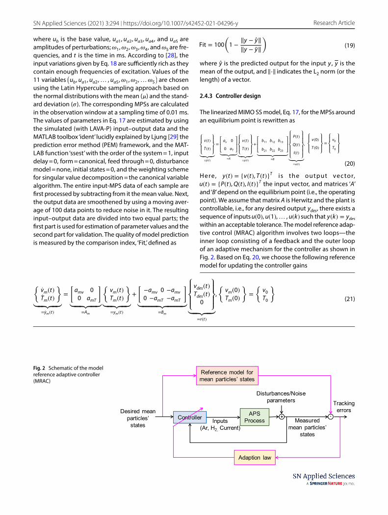
The computed and the experimental distributions of the steady-state plasma velocity and temperature along the jet axis (x = 0) and on the radial line y = 2 cm are com-pared in Fig. 4. With time t = 0, when the plasma jet exits the nozzle, the plasma was found to reach a steady state at 4 ms with at most 1% error (pointwise) in the axial velocity and the temperature in the computational domain.
3.1.2 Particles’ axial velocity and temperature
Powder particles are injected one at a time into the plasma through the powder port located at the point (x = 8 mm, y = 6 mm) at t = 5 ms, and their trajectories till t = 10 ms are recorded. The computed average values of particles’ axial velocity and temperature in the 1 cm wide window (9.5 ≤ y ≤ 10.5 cm, shown in Fig. s1 of the supporting infor-mation) at t = 9.1, 9.2 …, 9.9, 10 ms are compared in Fig. 5
Fig. 4 Comparison between the simulated and the experimental results of Williamson et al. [30]: a plasma axial velocity (e2 = 14.82%) and plasma temperature (e2 = 5.59%) distributions along the jet (y-) axis, b plasma axial velocity (e2 = 5.24%) and temperature
(e2 = 11.9%) versus the distance from the jet axis on the radial line y = 2 cm. The decaying trends along and perpendicular to the jet axis of the computed and the experimental temperatures and the axial velocities agree qualitatively and quantitatively

Vol:.(1234567890)
Research Article SN Applied Sciences (2021) 3:294 | https://doi.org/10.1007/s42452-021-04296-y
with their experimental values of Smith et al. [31]. Smith et al. [31] used a two-color pyrometer, IPP2000, and a spray pattern trajectory (SPT) sensor to measure, respectively, the average temperature and the axial velocity of particles flowing through the observation window. They empha-sized that the SPT sensor was focused on a narrow zone near the plasma jet axis but did not list coordinates of the sensor location. To compare the computed results with the experimental findings of Smith et al., they are divided into three groups based on their diameters in the ranges 30–42 µm, 56–71 µm, and 85–100 µm. The variations with the axial distance y from the nozzle of the average axial velocity and the average temperature of particles at time t = 10 ms are shown in Fig. 5a, b. The computed particle characteristics of small particles are close to those meas-ured experimentally. However, computed results for the medium and the large size particles differ from the corre-sponding experimental findings. At some axial locations, the difference in the mean axial velocities of particles in each of the two groups is about 50%. The small-sized particles have higher axial velocity because they are eas-ily accelerated by the plasma jet. The results depicted in Fig. 5b reveal that the computed average temperature of particles agrees well with that measured experimentally. The temperatures of the small-size particles are higher than that of large particles due to their in-flight motion near the hotter jet axis. The smaller size particles have melted by the time they go out of the observation win-dow and arrive at the substrate. By observing the plot (not included here) between temperature vs size of injected particles, we note that the temperature of the medium-size particles (45–65 μm) stays close to the melting point
(2,950 K) during their in-flight path. Many of the large par-ticles are only partially melted or even not melted at all. Recalling that the heating model (cf. Equation 12) regards a particle as a point mass, a large particle requires more time to be heated to the melting temperature. Larger par-ticles have low axial velocity resulting in more residence time in the plasma jet which helps in their being heated up. Also, some large particles travel farther away from the jet axis where the plasma temperature is not very high and hence are either partially melted or not melted at all depending upon their locations in the plasma jet.
3.2 Input parameters that significantly influence the MPSs
Keeping the applied voltage, the average powder injec-tion speed and the particle size fixed at 50 V, 10 m/s, and 30–100 μm, respectively, we present results of screening the seven process parameters, namely the current, the Ar flow rate, the H2 flow rate, the powder feed rate, the spray distance, and the injector location (y, x) along and perpen-dicular to the jet axis. Their minimum and maximum values considered are: current (A) 300, 600; H2 flow rate (slm) 2, 12; Ar flow rate (slm) 30, 60; powder feed rate (g/min) 10, 40; stand-off distance (cm) 7.5, 12.5; y-location of the injec-tor (cm) 0.4, 1.0, and x-location of the injector (cm) 0.6, 1.0.
3.2.1 Screening using elementary effects
We choose r = 8 in Eq. (4) and investigate the influence of the seven parameters for p = 12 and p = 20 resulting in 8 × (7 + 1) = 64 simulations needed for this study. The
Fig. 5 For particles divided in three groups of different sizes, com-parison of the computed and the experimental results for a the axial velocity and b the temperature along the axial distance. Solid lines represent mean values of particles’ axial velocity and sur-face temperature. ZrO2 particles of random sizes between 5 and
130 μm are injected into the plasma at t = 5 ms to achieve a mass rate of 20 g/min. The particle size distribution and the location of the observation window are exhibited in Fig. s1 of the supplement material

Vol.:(0123456789)
SN Applied Sciences (2021) 3:294 | https://doi.org/10.1007/s42452-021-04296-y Research Article
mean and the standard deviations of EEs of the MPSs are depicted in Fig. 6. The results associated with p = 12 and p = 20 are qualitatively similar. The stand-off distance, the powder feed rate, and the x-location of the injector are the least significant parameters since their mean EEs have low values. The y-location of the injector, the cur-rent, and the Ar flow rate have nonlinear effects and/or interactions among them as signified by high values of the mean and the standard deviation for them. The H2 flow rate has the least effect on the mean axial velocity
but a strong effect on the mean temperature. Accord-ingly, the Ar flow rate, the current, the y-location of the injector, and the H2 flow rate are considered as signifi-cant process parameters for developing the response functions.
Fig. 6 The standard deviation vs. the mean of elementary effect for normalized a mean axial velocity and b mean temperature (P = Ar flow rate, Q = H2 flow rate, I = Current, SD = Stand-off distance,
PFR = Powder feed rate, dy = y- location of the injector, and dx = x-location of the injector). High values of EEs for I, P, Q, and dy sig-nify that they are significant parameters
Table 1 ANOVA results for the quadratic fit of the mean axial velocity and the mean temperature
Parameters Degree of freedom
Mean axial velocity Mean temperature
Sum squares (SS) Mean squares (MS) F value Prob > F Sum squares (SS) Mean squares (MS)
F value Prob > F
P 1 0.962 0.962 6438.5 < 0.0001 0.442 0.442 635.2 < 0.0001Q 1 0.047 0.047 312.7 < 0.0001 0.464 0.464 667.3 < 0.0001I 1 0.402 0.402 2693.1 < 0.0001 0.377 0.377 542.4 < 0.0001dy 1 0.323 0.323 2161.1 < 0.0001 0.069 0.069 98.5 < 0.0001PQ 1 0.016 0.016 107.1 < 0.0001 0.145 0.145 208.8 < 0.0001PI 1 0.021 0.021 143.2 < 0.0001 0.225 0.225 323.2 < 0.0001Pdy 1 0.011 0.011 76.4 < 0.0001 0.111 0.111 159.2 < 0.0001QI 1 0.081 0.081 543.8 < 0.0001 0.115 0.115 165.0 < 0.0001Qdy 1 0 0 0 0.9821 0.003 0.003 4.2 0.04Idy 1 0.002 0.002 10.8 0.0011 0.188 0.188 270.3 < 0.0001P2 1 0.042 0.042 278.7 < 0.0001 0.013 0.013 19.3 < 0.0001Q2 1 0.025 0.025 169.6 < 0.0001 0.180 0.180 259.3 < 0.0001I2 1 0.064 0.064 430.2 < 0.0001 0.109 0.109 157.1 < 0.0001dy
2 1 0.016 0.015 103.7 < 0.0001 0.013 0.013 19.3 < 0.0001Error 610 0.091 0.00015 0.424 0.0011Total 624 23.1 17.5
Vol:.(1234567890)
Research Article SN Applied Sciences (2021) 3:294 | https://doi.org/10.1007/s42452-021-04296-y
3.2.2 Screening using ANOVA
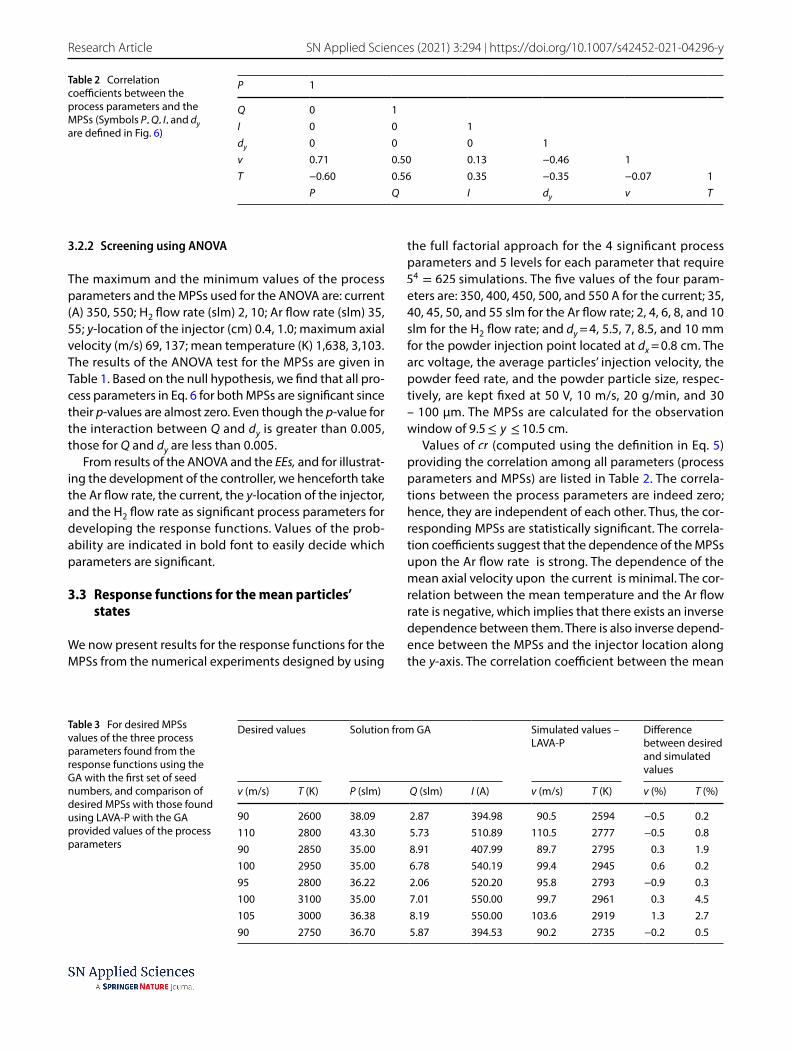
The maximum and the minimum values of the process parameters and the MPSs used for the ANOVA are: current (A) 350, 550; H2 flow rate (slm) 2, 10; Ar flow rate (slm) 35, 55; y-location of the injector (cm) 0.4, 1.0; maximum axial velocity (m/s) 69, 137; mean temperature (K) 1,638, 3,103. The results of the ANOVA test for the MPSs are given in Table 1. Based on the null hypothesis, we find that all pro-cess parameters in Eq. 6 for both MPSs are significant since their p-values are almost zero. Even though the p-value for the interaction between Q and dy is greater than 0.005, those for Q and dy are less than 0.005.
From results of the ANOVA and the EEs, and for illustrat-ing the development of the controller, we henceforth take the Ar flow rate, the current, the y-location of the injector, and the H2 flow rate as significant process parameters for developing the response functions. Values of the prob-ability are indicated in bold font to easily decide which parameters are significant.
3.3 Response functions for the mean particles’ states
We now present results for the response functions for the MPSs from the numerical experiments designed by using
the full factorial approach for the 4 significant process parameters and 5 levels for each parameter that require 54 = 625 simulations. The five values of the four param-eters are: 350, 400, 450, 500, and 550 A for the current; 35, 40, 45, 50, and 55 slm for the Ar flow rate; 2, 4, 6, 8, and 10 slm for the H2 flow rate; and dy = 4, 5.5, 7, 8.5, and 10 mm for the powder injection point located at dx = 0.8 cm. The arc voltage, the average particles’ injection velocity, the powder feed rate, and the powder particle size, respec-tively, are kept fixed at 50 V, 10 m/s, 20 g/min, and 30 – 100 μm. The MPSs are calculated for the observation window of 9.5 ≤ y ≤ 10.5 cm.
Values of cr (computed using the definition in Eq. 5) providing the correlation among all parameters (process parameters and MPSs) are listed in Table 2. The correla-tions between the process parameters are indeed zero; hence, they are independent of each other. Thus, the cor-responding MPSs are statistically significant. The correla-tion coefficients suggest that the dependence of the MPSs upon the Ar flow rate is strong. The dependence of the mean axial velocity upon the current is minimal. The cor-relation between the mean temperature and the Ar flow rate is negative, which implies that there exists an inverse dependence between them. There is also inverse depend-ence between the MPSs and the injector location along the y-axis. The correlation coefficient between the mean
Table 2 Correlation coefficients between the process parameters and the MPSs (Symbols P,Q, I, and dy are defined in Fig. 6)
P 1
Q 0 1I 0 0 1dy 0 0 0 1v 0.71 0.50 0.13 −0.46 1T −0.60 0.56 0.35 −0.35 −0.07 1
P Q I dy v T
Table 3 For desired MPSs values of the three process parameters found from the response functions using the GA with the first set of seed numbers, and comparison of desired MPSs with those found using LAVA-P with the GA provided values of the process parameters
Desired values Solution from GA Simulated values – LAVA-P
Difference between desired and simulated values
v (m/s) T (K) P (slm) Q (slm) I (A) v (m/s) T (K) v (%) T (%)
90 2600 38.09 2.87 394.98 90.5 2594 −0.5 0.2110 2800 43.30 5.73 510.89 110.5 2777 −0.5 0.890 2850 35.00 8.91 407.99 89.7 2795 0.3 1.9100 2950 35.00 6.78 540.19 99.4 2945 0.6 0.295 2800 36.22 2.06 520.20 95.8 2793 −0.9 0.3100 3100 35.00 7.01 550.00 99.7 2961 0.3 4.5105 3000 36.38 8.19 550.00 103.6 2919 1.3 2.790 2750 36.70 5.87 394.53 90.2 2735 −0.2 0.5

Vol.:(0123456789)
SN Applied Sciences (2021) 3:294 | https://doi.org/10.1007/s42452-021-04296-y Research Article
axial velocity and the mean temperature is -0.07, which implies that the mean axial velocity does not depend upon the mean temperature.
3.3.1 Response functions
The coefficients of the quadratic expression in Eq. 6 are estimated by using the linear regression analysis on the data from the full factorial approach (625 simulations) resulting in the following response functions for the MPSs.
Here, subscript ‘n’ represents the normalized param-eter with values between 0 and 1. The R2 values of 1 and 0.98, respectively, for the mean axial velocity and the
(27)vn, mod el = 0.248 + 0.476Pn + 0.105Qn + 0.308In − 0.276dy,n − 0.040PnQn + 0.047PnIn − 0.034Pndy,n
+0.091QnIn − 0.013Indy,n − 0.078P2n− 0.061Q2
n− 0.097I2
n+ 0.048d2
y,n;R2 = 1
(28)Tn, mod el = 0.651 − 0.323Pn + 0.331Qn + 0.298In − 0.127dy,n + 0.122PnQn + 0.152PnIn − 0.106Pndy,n − 0.108QnIn
−0.017Qndy,n + 0.139Indy,n − 0.044P2n− 0.162Q2
n− 0.126I2
n− 0.044d2
y,n;R2 = 0.98
mean temperature imply that the postulated expression in Eq. 6 is a good representation of the numerical data. The validity of the response functions in Eqs. 27 and 28 is tested for a new set of process parameters, and the cor-responding results are listed in Table s1 of the support-ing information. For these cases, the percentage error is less than 2%.
3.4 Values of process parameters for desired MPSs obtained by solving Eqs. 27 and 28
The solutions for arbitrarily selected values for the desired MPSs computed by minimizing the error defined
Fig. 7 Effect on the MPSs of a step variation in the a average injec-tion velocity of powder particles, and b arc voltage. The variations in the MPSs qualitatively follow variations in the powder injection
velocity and the arc voltage; they decrease with an increase in the powder injection velocity but decrease with a decrease in the arc voltage.

Vol:.(1234567890)
Research Article SN Applied Sciences (2021) 3:294 | https://doi.org/10.1007/s42452-021-04296-y
in Eq. 10 using the GA are summarized in Table 3. For a given gas gun, the powder inject port location is fixed. Hence, dy cannot be changed and we work with three significant input process parameters, namely the current, the Ar flow rate, and the H2 flow rate. Recalling that the GA solution depends upon the seed number, results for the first seed number are provided in Table 3 and those for the second set of seed numbers in the supporting information. Results from the two sets of seed numbers are similar to each other.
It is clear that the GA values of the three process param-eters provide MPSs that differ by less than 4.5% from their desired values that occurs for the desired mean axial veloc-ity = 100 m/s and the desired mean temperature = 3,100 K. We emphasize that for accurately predicting values of the three process parameters, the desired values of the MPSs should be in the range used to generate the response functions given by Eqs. 27 and 28. The desired mean par-ticles’ velocity of 3,100 m/s is outside the range employed to develop Eqs. 27 and 28.
3.5 Effect of disturbance in process parameters on mean particles’ states
Even though there are several disturbance parameters, we consider here only the powder injection velocity and the arc voltage. Their time variations and the resulting com-puted MPSs are exhibited in Fig. 7. Changes in the arc volt-age affect the power input into the nozzle that influences values of v0 and T0 in Eq. 1. Values of the other process parameters are: current = 500 A, Ar flow rate = 40 slm, H2 flow rate = 10 slm, powder feed rate = 20 g/min, powder diameter range = 30–100 μm, and the simulation sampling
time = 0.01 ms. Even though the computed MPSs are oscil-latory, the trends exhibited by their values averaged over 100 trailing points are as follows: They follow in the direc-tion of the disturbance in the powder injection velocity but in the opposite direction of the disturbance in the arc voltage.
3.6 Validation of three‑input two‑output model represented by Eq. 17
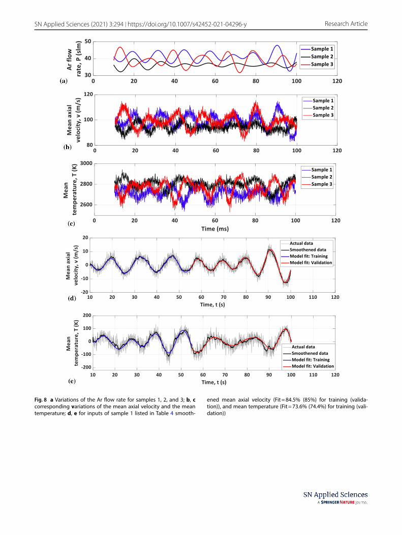
The 10 randomly generated functions u in Eq. 18 for exciting the Ar flow rate are listed in Table 4, and the cor-responding variations of inputs are shown in Fig. 8a for samples 1, 2, and 3. Subsequently, 50 new samples (their input values are omitted here) are randomly generated to verify whether or not the number of samples influences the variance of estimated parameters of the State Space (SS) models. Figure 8b,c shows time histories of the MPSs for the inputs exhibited in Fig. 8a. The predicted values from the MIMO SS model of Eq. 17 are listed in Table 5 for 10 samples. The computed MPSs for the 10 and the 50 samples are similar to each other (results for 50 samples are omitted here). For sample 1, when the data exhibited in Fig. 8b,c are smoothened by taking the moving aver-age of 100 trailing points, we get solid curves displayed in Fig. 8d.
Similar analyses are conducted for randomly generated vectors for exciting the H2 flow rate and the current. Their plots as well as those of results for the MPSs are provided in the supporting information.
Predictions from models for the MPSs agree well with those found using LAVA-P software with an average fit of 85% for training and 82% for validation for the mean axial
Table 4 Values of variables in Eq. 18 used for exciting the Ar (denoted in the table by P) flow rate
Parameters Pb Pa1 Pa2 Pa3 Pa4 Pa5 ω1P ω2P ω3P ω4P ω5P
Mean, μ 45 0 0 0 0 0 0.5 0.5 0.5 0.5 0.5S.D., σ 5 5 5 5 5 5 0.02 0.02 0.02 0.02 0.02Sample 1 41.14 1.96 1.73 −2.39 −3.43 −0.80 0.56 0.43 0.46 0.52 0.58Sample 2 36.31 −0.55 −0.98 −1.14 −1.28 −0.20 0.45 0.40 0.52 0.48 0.38Sample 3 38.97 1.42 0.54 4.36 0.43 1.81 0.69 0.36 0.48 0.58 0.29Sample 4 41.66 −1.99 −3.12 −6.90 1.14 0.96 0.37 0.51 0.38 0.41 0.47Sample 5 42.60 3.44 −1.92 2.47 1.24 −3.79 0.53 0.21 0.64 0.63 0.46Sample 6 37.84 −3.45 −0.50 0.45 3.15 2.36 0.40 0.66 0.72 0.36 0.68Sample 7 40.31 0.00 3.08 1.39 −2.20 0.20 0.47 0.55 0.55 0.26 0.41Sample 8 39.58 0.99 −1.25 −0.55 2.02 3.65 0.28 0.49 0.32 0.56 0.50Sample 9 43.66 −0.99 2.41 0.79 −0.43 −2.64 0.67 0.68 0.31 0.43 0.56Sample 10 38.57 −1.53 1.10 −1.21 −0.94 −1.24 0.62 0.59 0.60 0.71 0.72
Vol.:(0123456789)
SN Applied Sciences (2021) 3:294 | https://doi.org/10.1007/s42452-021-04296-y Research Article
Fig. 8 a Variations of the Ar flow rate for samples 1, 2, and 3; b, c corresponding variations of the mean axial velocity and the mean temperature; d, e for inputs of sample 1 listed in Table 4 smooth-
ened mean axial velocity (Fit = 84.5% (85%) for training (valida-tion)), and mean temperature (Fit = 73.6% (74.4%) for training (vali-dation))
Vol:.(1234567890)
Research Article SN Applied Sciences (2021) 3:294 | https://doi.org/10.1007/s42452-021-04296-y
velocity, and 72% for training and 66% for validation for the mean temperature.
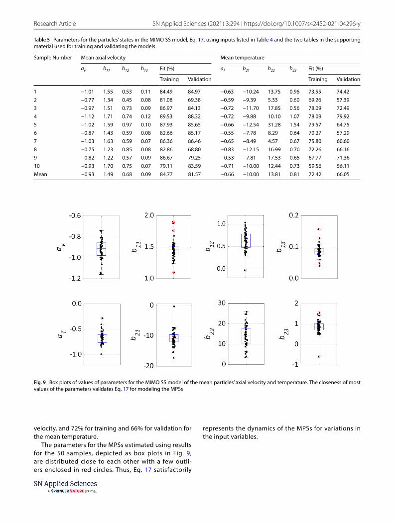
The parameters for the MPSs estimated using results for the 50 samples, depicted as box plots in Fig. 9, are distributed close to each other with a few outli-ers enclosed in red circles. Thus, Eq. 17 satisfactorily
represents the dynamics of the MPSs for variations in the input variables.
Table 5 Parameters for the particles’ states in the MIMO SS model, Eq. 17, using inputs listed in Table 4 and the two tables in the supporting material used for training and validating the models
Sample Number Mean axial velocity Mean temperature
av b11 b12 b13 Fit (%) aT b21 b22 b23 Fit (%)
Training Validation Training Validation
1 −1.01 1.55 0.53 0.11 84.49 84.97 −0.63 −10.24 13.75 0.96 73.55 74.422 −0.77 1.34 0.45 0.08 81.08 69.38 −0.59 −9.39 5.33 0.60 69.26 57.393 −0.97 1.51 0.73 0.09 86.97 84.13 −0.72 −11.70 17.85 0.56 78.09 72.494 −1.12 1.71 0.74 0.12 89.53 88.32 −0.72 −9.88 10.10 1.07 78.09 79.925 −1.02 1.59 0.97 0.10 87.93 85.65 −0.66 −12.54 31.28 1.54 79.57 64.756 −0.87 1.43 0.59 0.08 82.66 85.17 −0.55 −7.78 8.29 0.64 70.27 57.297 −1.03 1.63 0.59 0.07 86.36 86.46 −0.65 −8.49 4.57 0.67 75.80 60.608 −0.75 1.23 0.85 0.08 82.86 68.80 −0.83 −12.15 16.99 0.70 72.26 66.169 −0.82 1.22 0.57 0.09 86.67 79.25 −0.53 −7.81 17.53 0.65 67.77 71.3610 −0.93 1.70 0.75 0.07 79.11 83.59 −0.71 −10.00 12.44 0.73 59.56 56.11Mean −0.93 1.49 0.68 0.09 84.77 81.57 −0.66 −10.00 13.81 0.81 72.42 66.05
Fig. 9 Box plots of values of parameters for the MIMO SS model of the mean particles’ axial velocity and temperature. The closeness of most values of the parameters validates Eq. 17 for modeling the MPSs
Vol.:(0123456789)
SN Applied Sciences (2021) 3:294 | https://doi.org/10.1007/s42452-021-04296-y Research Article
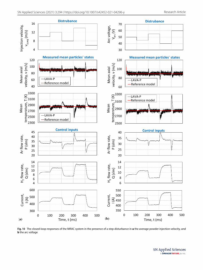
Fig. 10 The closed-loop responses of the MRAC system in the presence of a step disturbance in a the average powder injection velocity, and b the arc voltage

Vol:.(1234567890)
Research Article SN Applied Sciences (2021) 3:294 | https://doi.org/10.1007/s42452-021-04296-y
3.7 Results for the adaptive controller
Based on the knowledge gained from preliminary results, we select �1 = 2, �2 = 2 and �3 = 5 in Eq. 26 and investi-gate the performance of the proposed control scheme for the problem presented in subsection 3.5. The objective
of the MRAC is to attain the desired mean particles’ axial velocity = 90 m/s and temperature = 2,850 K within 50 ms of the introduction of a disturbance. Results depicted in Fig. 10 confirm that indeed the objective is achieved, and the proposed controller minimizes deviations in the MPSs caused by disturbances.
Fig. 11 The closed-loop control responses of the MRAC for a increasing desired mean particles’ axial velocity but decreasing mean tem-perature, and b increasing desired mean particles’ axial velocity and mean particles’ temperature

Vol.:(0123456789)
SN Applied Sciences (2021) 3:294 | https://doi.org/10.1007/s42452-021-04296-y Research Article
We now check whether the controller works when the desired MPSs vary with time that has applications for producing functionally graded coatings [7]. In this case, the performance of the controller is shown in Figs. 11 and 12 for step variations in vdes(t) and Tdes(t) , i.e., abrupt
disturbances that are kept constant afterwards. It is evi-dent that the MPSs follow outputs of the reference model.
These two examples establish the effectiveness of the designed process controller in mitigating effects of
Fig. 12 The closed-loop control responses of the MRAC for a decreasing desired mean particles’ axial velocity and mean particles’ tempera-ture, and b decreasing desired mean particles’ axial velocity but increasing mean particles’ temperature
Vol:.(1234567890)
Research Article SN Applied Sciences (2021) 3:294 | https://doi.org/10.1007/s42452-021-04296-y
disturbances. Of course, in practice disturbances are not limited to those stipulated here. Even though the control-ler will not work for all disturbances, one can use the meth-odology to design controllers for a pre-specified class of disturbances.
The real-time performance of the proposed controller will depend upon how quickly a motor can change the process input parameters, and the time lag of the plant to respond to these changes.
4 Conclusions
This paper proposes an approach to design an adaptive controller for an atmospheric plasma spray process (APSP) to get consistency in mean particles’ states (the axial veloc-ity and the temperature, MPSs) before they impact the substrate. Throughout this work, the physical tests are replaced by numerical experiments that use the software, LAVA-P, whose predictions are first shown to agree well with the experimentally measured values of particles’ velocity and temperature. From the screening analysis, the argon (Ar) and the hydrogen (H2) flow rates, the current, and the y-location of the injector are identified as significant input parameters for the MPSs. The response functions (i.e., rela-tions between the MPSs and the significant input param-eters) are first established as nonlinear algebraic equations between the four significant input parameters and the MPSs. For a given gas gun, the powder injector location is generally fixed. For desired values of the MPSs, the trial input values of Ar and H2 flow rates and the current are predicted by solving these nonlinear algebraic equations using a genetic algorithm (GA) included in MATLAB. Using equations for the evolution of particle’s axial velocity and temperature linearized around steady-state values of these variables, an adaptive controller is designed to modify the trial input values of the three process parameters to obtain desired values of the MPSs in the presence of a noise vari-able (either a disturbance in the powder injection velocity or in the arc voltage). The performance of the controller has been successfully tested for two example problems.
Additional research is needed to design a robust con-troller for mitigating effects of all noise variables and either warn the operator or shut down the process when MPSs cannot be controlled. The methodology presented here is applicable to other coating processes and manu-facturing processes such as hot forging and machining.
Acknowledgements Authors gratefully acknowledge the Sulzer Metco company giving us a tour of the facilities, allowing us to col-lect data that has not been used in this work, and general discussions related to the control of the coating process.
Compliance with ethical standards
Conflict of interest The authors declare that they have no conflict of interest.
Open Access This article is licensed under a Creative Commons Attri-bution 4.0 International License, which permits use, sharing, adap-tation, distribution and reproduction in any medium or format, as long as you give appropriate credit to the original author(s) and the source, provide a link to the Creative Commons licence, and indicate if changes were made. The images or other third party material in this article are included in the article’s Creative Commons licence, unless indicated otherwise in a credit line to the material. If material is not included in the article’s Creative Commons licence and your intended use is not permitted by statutory regulation or exceeds the permitted use, you will need to obtain permission directly from the copyright holder. To view a copy of this licence, visit http://creat iveco mmons .org/licen ses/by/4.0/.
References
1. Sampath S, Herman H, Shimoda N, Saito T (1995) Thermal spray processing of FGMs. MRS Bull 20(1):27–31
2. Fauchais PL, Heberlein JVR, Boulos MI (2014) Overview of ther-mal spray. In: Thermal spray fundamentals, Springer, pp. 17–72.
3. Shang S, Guduri B, Cybulsky M, Batra RC (2014) Effect of tur-bulence modulation on three-dimensional trajectories of powder particles in a plasma spray process. J Phys D Appl Phys 47(40):405206
4. Zhang W (2008) Integration of process diagnostics and three dimensional simulations in thermal spraying. The Graduate School, Stony Brook University, Stony Brook, NY.
5. Williamson RL, Fincke JR, Chang CH (2000) A computational examination of the sources of statistical variance in particle parameters during thermal plasma spraying. Plasma Chem Plasma Process 20(3):299–324
6. Wan YP, Prasad V, Wang G-X, Sampath S, Fincke JR (1999) Model and powder particle heating, melting, resolidification, and evaporation in plasma spraying processes. J Heat Transfer 121(3):691–699
7. Fincke JR, Swank WD, Bewley RL, Haggard DC, Gevelber M, Wroblewski D (2001) Diagnostics and control in the thermal spray process. Surf Coatings Technol 146:537–543
8. Westergård R, Erickson LC, Axen N, Hawthorne HM, Hogmark S (1998) The erosion and abrasion characteristics of alumina coat-ings plasma sprayed under different spraying conditions. Tribol Int 31(5):271–279
9. Vardelle M, Fauchais P (1999) Plasma spray processes: diagnos-tics and control? Pure Appl Chem 71(10):1909–1918
10. Choudhury TA, Hosseinzadeh N, Berndt CC (2011) Artificial Neu-ral Network application for predicting in-flight particle char-acteristics of an atmospheric plasma spray process. Surf Coat Technol 205(21–22):4886–4895
11. Zhang C et al (2009) Effect of in-flight particle characteristics on the coating properties of atmospheric plasma-sprayed 8 mol% Y2O3–ZrO2 electrolyte coating studying by artificial neural net-works. Surf Coat Technol 204(4):463–469
12. Tu JV (1996) Advantages and disadvantages of using artificial neural networks versus logistic regression for predicting medi-cal outcomes. J Clin Epidemiol 49(11):1225–1231
13. Mawdsley JR, Su YJ, Faber KT, Bernecki TF (2001) Optimization of small-particle plasma-sprayed alumina coatings using designed experiments. Mater Sci Eng A 308(1–2):189–199

Vol.:(0123456789)
SN Applied Sciences (2021) 3:294 | https://doi.org/10.1007/s42452-021-04296-y Research Article
14. Li JF et al (2003) Uniform design method for optimization of process parameters of plasma sprayed TiN coatings. Surf Coat-ings Technol 176(1):1–13
15. Srinivasan V, Sampath S, Vaidya A, Streibl T, Friis M (2006) On the reproducibility of air plasma spray process and control of particle state. J Therm Spray Technol 15(4):739–743
16. Kanta A-F, Montavon G, Berndt CC, Planche M-P, Coddet C (2011) Intelligent system for prediction and control: application in plasma spray process. Expert Syst Appl 38(1):260–271
17. Planche M-P, Liu T, Deng S, Montavon G (2014) Development of an Emulator for the Plasma Process Control. Automation, 10.
18. Cheng K, Chen X (2004) Effects of natural convection on the characteristics of long laminar argon plasma jets issuing upwards or downwards into ambient air—a numerical study. J Phys D Appl Phys 37(17):2385
19. Xu D-Y, Chen X, Pan W (2005) Effects of natural convection on the characteristics of a long laminar argon plasma jet issuing horizontally into ambient air. Int J Heat Mass Transf 48(15):3253–3255
20. Ramshaw JD, Chang CH (1992) Computational fluid dynamics modeling of multicomponent thermal plasmas. Plasma Chem plasma Process 12(3):299–325
21. Morris MD (1991) Factorial sampling plans for preliminary com-putational experiments. Technometrics 33(2):161–174
22. Campolongo F, Gabric A (1997) The parametric sensitivity of dimethylsulfide flux in the southern ocean. J Stat Comput Simul 57(1–4):337–352. https ://doi.org/10.1080/00949 65970 88118 16
23. Pujol G (2009) Simplex-based screening designs for estimating metamodels. Reliab Eng Syst Saf 94(7):1156–1160
24. Antoine GO, Batra RC (2015) Sensitivity analysis of low-velocity impact response of laminated plates. Int J Impact Eng 78:64–80
25. Saltelli A, Chan K, Scott M (2000) Sensitivity analysis. Probability and statistics series. John Wiley & Sons, New York
26. Batra RC, Taetragool U (2020) Numerical techniques to find opti-mal input parameters for achieving mean particles’ temperature and axial velocity in atmospheric plasma spray process. Sci Rep 10, Art. No. 21483
27. Tuhus-Dubrow D, Krarti M (2010) Genetic-algorithm based approach to optimize building envelope design for residential buildings. Build Environ 45(7):1574–1581
28. P. A. Ioannou and J. Sun, Robust adaptive control. Courier Corpo-ration, 2012.
29. L. Ljung and Lennart, System identification: theory for the user. Prentice Hall PTR, 1999.
30. Williamson RL, Fincke JR, Crawford DM, Snyder SC, Swank WD, Haggard DC (2003) Entrainment in high-velocity, high-temper-ature plasma jets: Part II: computational results and comparison to experiment. Int J Heat Mass Transf 46(22):4215–4228
31. Smith W, Jewett TJ, Sampafh S, Swank WD, Fincke JR (1997) Plasma Processing of Functionally Graded Materials Part I: Process Diagnostics. In: Proc. United Thermal Spray Conf, pp. 599–605.
Publisher’s Note Springer Nature remains neutral with regard to jurisdictional claims in published maps and institutional affiliations.