Authoring Consistent Landscapes with Flora and Fauna

HAL Id: hal-03245206https://hal.inria.fr/hal-03245206

Submitted on 1 Jun 2021

HAL is a multi-disciplinary open accessarchive for the deposit and dissemination of sci-entific research documents, whether they are pub-lished or not. The documents may come fromteaching and research institutions in France orabroad, or from public or private research centers.

L’archive ouverte pluridisciplinaire HAL, estdestinée au dépôt et à la diffusion de documentsscientifiques de niveau recherche, publiés ou non,émanant des établissements d’enseignement et derecherche français ou étrangers, des laboratoirespublics ou privés.

Authoring Consistent Landscapes with Flora and FaunaPierre Ecormier-Nocca, Guillaume Cordonnier, Philippe Carrez, Anne‑marie

Moigne, Pooran Memari, Bedrich Benes, Marie-Paule Cani

To cite this version:Pierre Ecormier-Nocca, Guillaume Cordonnier, Philippe Carrez, Anne‑marie Moigne, Pooran Memari,et al.. Authoring Consistent Landscapes with Flora and Fauna. ACM Transactions on Graphics,Association for Computing Machinery, 2021, �10.1145/3450626.3459952�. �hal-03245206�

https://hal.inria.fr/hal-03245206

https://hal.archives-ouvertes.fr

Authoring Consistent Landscapes with Flora and Fauna

PIERRE ECORMIER-NOCCA, LIX, Ecole Polytechnique/CNRS, Institut Polytechnique de Paris, FranceGUILLAUME CORDONNIER, ETH Zürich, Switzerland and Inria, Université Côte d’Azur, France

PHILIPPE CARREZ, Immersion Tools, France

ANNE-MARIE MOIGNE,Muséum national d’Histoire naturelle ś UMR 7194, HnHp, MNHN, UPVD, CNRS, France

POORAN MEMARI, LIX, CNRS/Ecole Polytechnique, Institut Polytechnique de Paris, FranceBEDRICH BENES, Purdue University, USAMARIE-PAULE CANI, LIX, Ecole Polytechnique/CNRS, Institut Polytechnique de Paris, France

Terrain Climatic conditions Species density maps Map of trailsResource Access Graph

On-the-fly exploration

Fig. 1. From an input terrain, climatic conditions desired proportions between competing species and their dependency through the food-chain, our algorithm

iterates on a resource access graph to compute species density maps, enabling us to extract animals’ daily paths. The resulting, consistent 3D landscape can be

explored on the fly, showing vegetation, animals, and the trails they generate. Maps can be edited at any stage using painting tools.

We present a novel method for authoring landscapes with flora and fauna

while considering their mutual interactions. Our algorithm outputs a steady-

state ecosystem in the form of density maps for each species, their daily

Authors’ addresses: Pierre Ecormier-Nocca, LIX, Ecole Polytechnique/CNRS, Insti-tut Polytechnique de Paris, Palaiseau, France, [email protected];Guillaume Cordonnier, ETH Zürich, Zürich, Switzerland, Inria, Université Côted’Azur, Sophia Antipolis, France, [email protected]; Philippe Carrez, Im-mersion Tools, Saint-Brieuc, France, [email protected]; Anne-MarieMoigne, Muséum national d’Histoire naturelle ś UMR 7194, HnHp, MNHN, UPVD,CNRS, Paris, France, [email protected]; Pooran Memari, LIX,CNRS/Ecole Polytechnique, Institut Polytechnique de Paris, Palaiseau, France, [email protected]; Bedrich Benes, Purdue University, West Lafayette, USA, [email protected]; Marie-Paule Cani, LIX, Ecole Polytechnique/CNRS, Institut Polytechniquede Paris, Palaiseau, France, [email protected].

© 2021 Copyright held by the owner/author(s). Publication rights licensed to ACM.This is the author’s version of the work. It is posted here for your personal use. Not forredistribution. The definitive Version of Record was published in ACM Transactions onGraphics, https://doi.org/10.1145/3450626.3459952.

circuits, and a modified terrain with eroded trails from a terrain, climatic

conditions, and species with related biological information. We introduce the

Resource Access Graph, a new data structure that encodes both interactions

between food chain levels and animals traveling between resources over the

terrain. A novel competition algorithm operating on this data progressively

computes a steady-state solution up the food chain, from plants to carnivores.

The user can explore the resulting landscape, where plants and animals are

instantiated on the fly, and interactively edit it by over-painting the maps.

Our results show that our system enables the authoring of consistent land-

scapes where the impact of wildlife is visible through animated animals,

clearings in the vegetation, and eroded trails. We provide quantitative vali-

dation with existing ecosystems and a user-study with expert paleontologist

end-users, showing that our system enables them to author and compare

different ecosystems illustrating climate changes over the same terrain while

enabling relevant visual immersion into consistent landscapes.

CCS Concepts: · Computing methodologies→ Procedural animation.

Additional Key Words and Phrases: Natural Phenomena, Ecosystems

ACM Trans. Graph., Vol. 40, No. 4, Article 105. Publication date: August 2021.

105:2 • Ecormier-Nocca, P. et al

ACM Reference Format:

Pierre Ecormier-Nocca, Guillaume Cordonnier, Philippe Carrez, Anne-Marie

Moigne, Pooran Memari, Bedrich Benes, and Marie-Paule Cani. 2021. Author-

ing Consistent Landscapes with Flora and Fauna. ACM Trans. Graph. 40, 4,

Article 105 (August 2021), 13 pages. https://doi.org/10.1145/3450626.3459952

1 INTRODUCTION

Beautiful landscapes result from the interaction between various

phenomena, such as climate, erosion, vegetation, and animals. While

these phenomena have a strong influence on landscape appearance,

their combined effects are not always well-understood. Only some

of them, namely climate, erosion, and plant ecosystems, were simu-

lated and combined so far. Animated fauna, essential for generating

lively landscape in movies, simulators, or games, is typically added

manually in the last stage, requiring a considerable amount of user

effort.

Our first key observation is that the presence of animals has a

critical visual impact on landscapes, even when they are out of sight.

Indeed, they shape clearings and trails through the vegetation while

compete for space and resources, which, in turn, affects erosion.

Therefore, the standard pipeline, where animals are added on top

of a terrain covered with plants, while neglecting their interactions

should be revisited.

The second key observation is that modeling a landscape where

various life forms co-exist can be done consistently without a full

simulation, and while enabling intuitive user control. Designers of

virtual environments aim at immersing the audience in a specific

ecosystem, with either real or imaginary sets of plants and animal

species, in given proportions. Similarly, immersion in a 3D ecosys-

tem that matches observed data and current hypotheses would be a

plus for experts such as biologists or paleontologists as a new way

to explore their models. While a full, simultaneous simulation of

terrain formation, vegetation, and wild-life competition would be

challenging due to the multiple time scales involved, it would also

fail to match these authoring needs, with no guarantee on the set

of surviving species and their proportions.

Our solution increases the quality of CG landscapes by generating

coherent, yet controlled ecosystemswith flora and fauna, interacting

with the terrain. It considers plants and animals as different food

chain levels, which are iteratively instantiated from lower to upper

levels. Our method allows both intuitive authoring and the on-

the-fly exploration of the resulting landscape, with consistently

positioned plants and animated animals along relevant daily paths.

In a typical use-case, the user specifies climatic conditions over

an input terrain and a set of species of plants, herbivores, and car-

nivores with optional, desired proportions after the competition.

The resulting ecosystem is then computed in the form of a set of

editable density maps for each species over the terrain. At each

level of the food chain, the impact of the generated individuals is

propagated back to the resources they consume. The paths between

them are computed, enabling to account for grazing, foraging, and

erosion along the main trails. The resulting landscape, including

both flora and animated fauna, is finally consistently instantiated

to allow interactive exploration. Fig. 1 shows an example of such

interactive authoring and exploration of a populated landscape.

We achieve these results thanks to several key choices and approx-

imations: First, in addition to the choice of species at each food-chain

level, we provide users with direct control over their proportions.

We compute the actual number of specimens and their distribution

over the terrain from this input, thanks to a new procedural competi-

tion algorithm ruled by the simplifying hypothesis that the resulting

ecosystem should be at a steady-state. Second, this algorithm builds

on a novel hierarchical data-structure, called the Resource Access

Graph (RAG), which embeds resources for each species with their

location and accessibility as a layered graph, enabling efficient, yet

consistent species instantiation over the terrain.

We claim the following contributions: 1) we introduce the RAG,

a hierarchical, biology-driven, embedded graph of resources, which

encodes local interactions among food chain levels and enables us

to model paths between resources; 2) we introduce a procedural

competition algorithm to build a fast approximation of a steady-

state ecosystem at each level of the food chain; 3) we propose a

method for the consistent, on-the-fly instantiation of plants and

animals during interactive landscape exploration.

2 RELATED WORK

We do not focus on terrain generation, and we refer the reader to

the surveys [Galin et al. 2019; Smelik et al. 2014].

Plant ecosystems have been addressedmostly by the simulation of

competition for resources. Deussen et al. [1998] first used plant com-

petition to simulate plant distributions, a work recently extended

to layered ecosystems [Makowski et al. 2019]. Various approaches

attempted to combine ecosystems with other phenomena: Benes

et al. [2011] modeled the interaction of urban layouts with plant com-

petition for resources while considering human urban management,

Gain et al. [2017] simulated and learned plant distributions and used

them as interactive brushes over a terrain, Cordonnier et al. [2017]

modeled plant interaction with terrain erosion, while [Kapp et al.

2020] trained a deep neural network to learn and generate consistent

vegetation over an input terrain. In contrast with our work, only

interaction between flora and terrain was considered, neglecting

the impact of animals on both vegetation and erosion. Moreover,

although we build on concepts from simulation methods such as

fitness [Alsweis and Deussen 2005; Gain et al. 2017] to give local

priority to dominant species, our method focuses on steady-state

ecosystems, offering control over species proportions.

Regarding fauna, the seminal works of Reynolds [1987; 1999]

introduced boids that simulate the self-synchronized movement of

a flock of birds. Models capable of making more refined decisions

based on the velocity of animated agents [Paris et al. 2007; van den

Berg et al. 2008] or their synthetic vision [López et al. 2019; Ondřej

et al. 2010] have been developed to mimic observed behaviors. Ani-

mals have also been studied to increase artistic freedom and con-

trol, especially when interacting with the environment. The works

[Wang et al. 2014; Xu et al. 2008] allow the user to control the shape

taken by a group of animals. At the same time, Ecormier-Nocca

et al. [2019] extended control to both the shape and distribution of

animals within a herd. However, while these approaches produce

visually plausible animations, they do not consider the relationship


Authoring Consistent Landscapes with Flora and Fauna • 105:3

Environmental

resources RAG0

Design Exploration

Editing

Terrain

Competition

Food-Chain

Level i

RAG i

Surplus Level 𝑖 − 1& Daily Planning

Ecosystem-Aware

Animated Landscape

For each Food Chain Level (𝑖 ∈ 0, 𝐾 )

Temperature

Moisture

Illumination

Fig. 2. System overview: After initializing resource maps, we process each food chain level, from plants to carnivores, computing the corresponding level of the

Resource Access Graph (RAG), the result of competition between species at this level, animals daily paths, and the remaining surplus of resources from the

previous level. The resulting set of density maps, together with a map of eroded trails on the terrain and daily planning for animals, are used to generate the

animated, ecosystem-aware-landscape. The user can intuitively edit results by over-painting any of the maps.

with other essential factors such as vegetation, accessibility of the

terrain, or scarcity of resources, which is one of this paper’s goals.

Competition between species modeled by biologists for both flora

and fauna, is expressed as differential equations, leading to predic-

tive, dynamic models for populations’ ecological niches, and allow-

ing decision making for global resource management. For instance,

motivated by conservation biology for ecology and environmental

analysis, [Loreau 2010] demonstrated the impact of biodiversity

on ecosystems, and [Shifley et al. 2017] provided a comprehensive

survey of dynamic models for forest landscapes. In contrast, we

are not introducing a simulation method for dynamic ecosystems.

Instead, we focus on an authoring tool to generate a landscape that

maintains ecosystem consistency while building on user input -

either imaginary or extracted from real data. This input flexibility is

also why our system does not aim to provide a complete statistical

occupancy model or a Bayesian simulation of animal population

dynamics. We refer the reader to the book [MacKenzie et al. 2017]

for a comprehensive insight into mathematical modeling of ranging

patterns and occupancy dynamics.

3 OVERVIEW

Our goal is to generate a consistent, animated landscape matching

flora and fauna either chosen by design by an artist, observed on

the terrain by a biologist, or inferred from remains - such as animal

bones and plant pollen - by a paleontologist. To match such au-

thoring needs, we introduce a novel processing pipeline (see Fig. 2)

consistently generating and embedding plants, herbivores, and car-

nivores over a given terrain, under a steady-state hypothesis.

The steady-state hypothesis postulates that the growth of popu-

lations in ecosystems is limited by two main factors: natural death

(caused by old age, disease, food shortage, climate, etc.) and the

action of predators. Without these, the population would grow ex-

ponentially every year by a species-dependent factor, called the

growth rate, and given by the average yearly production of the

species (volume produced by plants, number of newborns for ani-

mals) per unit. The yearly growth of a given population is its size

multiplied by this rate. The steady-state hypothesis states that yearly

deaths precisely compensate for annual growth for each species

in the ecosystem. In particular, no more than the yearly growth

of a species can be used as a resource for another species. We call

surplus the annual amount of such resource finally unused and

supposed to naturally die over the year.

3.1 Knowledge, Input and, Output

Biological knowledge about living species embedded in our system

was extracted from a plant database [Tela-Botanica DB] and an

animal species database [Animal-Diversity-Web DB]. It includes the

set of yearly resources required for each species (minerals, light,

and water for plants, water, and food for animals), the minimal and

maximal temperature a plant can bear, the average motion speed of

animals, and their ability to climb slopes and cross rivers.

Knowledge about the set of necessary resources for species is

used to classify them into food-chain levels, where species from

a given level feed on the previous level and serve themselves as re-

sources for the next level. In our implementation, we only consider

vegetation, herbivores, and carnivores as distinct food-chain levels,

but generalizing our method to more levels would be straightfor-

ward. Extension to complex ecosystems with food-graphs instead

of linear food-chains is discussed in Section 7.

User input includes a digital elevation model describing the tar-

geted terrain, together with all the necessary information to com-

pute local environmental resources for plants, namely a minerals

map, the terrain orientation, latitude, altitude, and the extreme tem-

peratures at sea level - describing the targeted climate. We adapted

themethod from [Gain et al. 2017] to extract yearlymoisture, extreme

temperatures, and sun-light maps over the terrain from this input.

The user may alternatively directly provide the maps. The user also

lists the set of species they would like to see in their ecosystem,

together with the optional, desired proportions between species at

the same food-chain level.

The output is a set of maps representing the density of presence of

each species over the terrain, and a map of eroded trails. In contrast

with the maps used for plants, we use piece-wise constant maps for



animals to represent their ability to move anywhere within species-

specific confinement regions, delimited by natural frontiers such

as rivers or cliffs that the animals cannot cross. Since herds have

non-uniform probabilities of presence over these regions depending

on the location of resources, we also compute daily itineraries to

model their typical routes. This output is finally used to generate an

animated landscape populated with plants and animals of various

species, with clearly distinguishable trails.

3.2 Concept of Resource Access Graph

Key to our solution is a novel data structure, a hierarchical directed

graph called the Resource Access Graph (RAG). It encodes the

interactions between species at different levels of the food chain

and their embedding onto the terrain. See Fig. 3.

At each level i of the hierarchy, RAG nodes are the individual

resources available for the set of species at level i of the food chain,

together with their embedding on the terrain. To match the steady-

state hypothesis, resources are set to surplus from the previous food

chain level, representing the amount that can be consumed with no

impact on the ecosystem equilibrium. The embedding of a resource

node is the region of the map where it can be found, e.g., the region

covered by a grass meadow, or the confinement region between a

river and a cliff, where a herd of herbivores grazes. As the name

"resource access graph" indicates, RAG edges - labeled by indicators

of species - encode the ability of a given species to travel between

resource nodes and are labeled with the average traveling time. Note

that we use an oriented graph for the RAG because the abilities and

traveling times up or down a slope are different.

The RAG hierarchy expresses that each species may be a resource

for other species, and should thus be encoded as a higher-level

resource node; e.g., antelopes confined in a sub-region of the terrain

between a large river and a cliff are food resource to wolves, so the

strongly connected component of the RAG they travel in to graze,

will correspond to an individual resource node at the next level of

the RAG, granted that these antelopes produced some surplus.

3.3 Processing Pipeline

The processing pipeline (Fig. 2) consists of progressively computing

the RAG from the bottom to the top of the food chain. The solution

to competition and positioning of species at the previous food-

chain level is used while calculating the next one. Density maps and

traveling edges in the RAG are then used to generate the output.

More precisely, the first level of the RAG, RAG0 (i.e., environmen-

tal resources for plants), is initialized by considering each map’s cell

as an individual node. Then, for each level i up the food chain:(1) The associated level of the RAG, encoding resources for species,

their location over the terrain, and their accessibility, is built;

(2) Competition at food chain level i is solved using a new, proce-

dural method to compute steady-state results that best match

the desired proportion of species specified by the user;

(3) Daily paths between resources are generated for each animal

species, and surplus maps describing unused resources from

the previous level of the food-chain are computed.Finally, the paths in the RAG are refined, combined and exported

as a map of eroded trails over the terrain. The collection of species

density-maps and daily paths for animals are processed to generate

the ecosystem, where surpluses are displayed in the form of denser

or higher plants (depending on the species) or more youths among

animal herds, to inform users about the liveliness of the ecosystem.

Users can interactively explore the resulting animated landscape

and further tune it by editing density maps from any food-chain

level. While increasing the density of species may not match realism

due to insufficient resources (a warning is displayed), decreasing

them is always possible and will propagate up and down the food-

chain for consistency (fewer resources at the next level, more surplus

at the previous one). Such editing can be used to model external

events such as death due to fire or diseases.

4 COMPETITION BETWEEN SPECIES

Species at the same food chain level compete for resources. The

second step of the processing pipeline consists of computing a set

of density maps describing how species settle in different terrain

regions, given the locally available resources for which they compete.

To allow authoring, user-defined target proportions between species

can be accounted for, although this may result in less populated

ecosystems. Without such proportions, species which best fit local

resources are favored in each region. In both cases, our solution

ensures that all survival conditions are met.

4.1 Survival Constraints

Among the information found in environmental and biological

databases, some features can be extracted whatever the species

(flora or fauna), and their resources (environmental resource, flora

or fauna). Our solution is based on the list of features below (see

supplemental documents for the values used for each species).

A population unit for a given species is a small group of the

specimen that live together. We define it, for flora, as the least dense

group of individual plants that may span a single grid-cell of the

terrain, and for fauna, as the smallest typical herd, a herd being

defined as a group of animals traveling together. Solitary animals

(e.g., a bear) are considered as herds of size one.

The consumed resource c(s, r ) for a species s and a resource r

denotes the amount of r a unit of s typically consumes annually, and

which is therefore not available anymore for other species. Note that

in the case of temperature, a resource to plants, this amount is set

to zero since flora’s presence has a negligible effect on temperature.

The temporal variation [rmin, rmax ] of a resource r , is the in-

terval between the minimum and maximum amounts of r available

over a year (e.g., the interval spanned by temperature, seen as a re-

source to plants; or the interval between zero and the yearly growth

of grass, for a meadow used as a resource for herbivores). Note that

for resources with seasonal changes, we use more detailed data if

the data is available. For example, we use temporal variations at the

scale of a month for temperature and precipitations.

The fitness range, for each species s with respect to a resource

r ∈ R(s) (their set of necessary resources), is the interval F (s, r ) =

[Fmin (s, r ), Fmax (s, r )], between minimum and maximum values

of r for which the growth of species is not limited by the environ-

ment.



𝑅𝑅𝑅𝑅𝐺𝐺0 𝑅𝑅𝑅𝑅𝐺𝐺1 𝑅𝑅𝑅𝑅𝐺𝐺2Cliff River

Fig. 3. Concept of Resource Access Graph showing surplus nodes colored per species. RAG0 encodes resources for plants. RAG1 encodes resources for

herbivores such as meadows and river banks. Antelopes can cross the river only at a ford and are trapped by cliffs, leading to three confinement regions.

RAG2 encodes resources for carnivores, here wolves feeding on antelopes. The connected components of RAG1 where antelopes produce surplus (bottom and

right ones) are merged as resource nodes in RAG2. Edges express the fact that wolves can go up and down cliffs, with different traveling times.

A confinement region for s is a part of the terrain from which

specimens cannot exit due to lack of mobility for plants, and to

obstacles such as cliffs, rivers, or too dense vegetation for animals.

Given these definitions, any created population unit of a species

s should survive on local resources provided by their confinement

region. The more yearly variations of local resources fit within the

fitness ranges for s , the more s will tend to settle in this specific

region. Simultaneously, the settlement should not be allowed if

these intervals do not overlap. Lastly, population units of s should

only be created if a yearly amount c(s, r ) of each resource can be

reserved for them. Our solution ensures the consistency of the

created ecosystems by maintaining these constraints.

4.2 Local Species’s Fitness Score

Let us consider a region where the set of resources r ∈ R for species

at a given food-chain level can be found. To compute which of these

species are the most likely to settle there, we calculate a fitness

score fit(s,R) for each of them in the following way.

For each resource r ∈ R, we compute the fraction of the species’

fitness range F (s, r ) that lies within the annual variation ryear of

the corresponding resource. Since the sparsest resource determines

the ability for s to settle there, we use the minimum of these values,

leading to:

fit(s,R) = minr ∈R

(

min (Fmax (s, r ), rmax ) −max (Fmin (s, r ), rmin )

(rmax − rmin )

)

,

When the monthly temporal variations are provided (e.g., for

temperature), we use several terms per resource in the minimum

above. This results in a continuous score 0 <= fit(s,R) <= 1, where

zero indicates that s cannot survive, while one shows a perfect fit,

all resource variations being within the species’ fitness ranges).

4.3 Competition Algorithm

Let us now consider a terrain divided into a set of confinement

regionsCj , each with its resources Rj . We denote q(r ,Cj ) the annual

available amount of r ∈ Rj in the region Cj .

Note that the same set of regions needs to be used for all species.

When the traveling abilities are different among species at this level

of the food chain (e.g., goat vs. bison), we use the finest partition of

the terrain, computed as the intersection of species-specific confine-

ment regions. In this case, the created population units are assigned

to the species’ original confinement regions.

Competition considering target proportions of species. Starting from

zero densities over the terrain, we successively, tentatively, increase

by one the number of population units in each species. Our greedy

solution only retains the one, among these attempts, that brings the

system the closest to the desired proportions. The newly created

unit is then added to the best-adapted confinement regionCj on the

terrain, i.e., considering only the Cj with strictly positive fit(s,Rj ),

we sort them by decreasing values, and use the first one, if any,

where ∀r ∈ Rj ,q(r ,Cj ) > c(s, r ). If this succeeds, the population

unit is created in Cj , and the amounts q(r ,Cj ) are decreased by

c(s, r ), for each resource r ∈ Rj . This process is repeated until no

new population unit can be created.

ALGORITHM 1: Competition algorithm with target proportions

Input: Set of species s ∈ FCL and their proportions

Output: Density map for each s ∈ FCL

repeat

Select s that would bring FCL closest to target proportions;

Compute fit(s) in each confinement region C for s ;

Select C with highest fitness;

Increase density of s in C ;

Decrease accordingly the available resources in C ;

until not enough resources to increase density;

Competition without target proportions. For each confinement

region Cj : Starting from zero, we iteratively increase the number of

population units (and accordingly decrease the amount of available

resources), choosing species with highest strictly positive fitness

f it(s,Rj ) matching ∀r ∈ Rj ,q(r ,Cj ) > c(s, r ). We stop when there

are not enough remaining resources in Cj .

Discussion. Although we reuse at a coarser grain (annually for

animals), some of the concepts introduced for plant-ecosystems,

such as asymmetric competition and fitness score [Alsweis and

Deussen 2005; Gain et al. 2017], our method strongly differs from



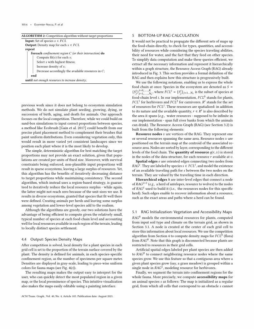
ALGORITHM 2: Competition algorithm without target proportions

Input: Set of species s ∈ FCL

Output: Density map for each s ∈ FCL

repeat

foreach confinement region C (or their intersection) do

Compute fit(s) for each s ;

Select s with highest fitness;

Increase density of s ;

Decrease accordingly the available resources in C ;

end

until not enough resources to increase density;

previous work since it does not belong to ecosystem simulation

methods. We do not simulate plant seeding, growing, dying, or

succession of birth, aging, and death for animals. Our approach

focuses on the local competition. Therefore, while we could build on

sand-box simulations to input correct proportions between species,

a method like Ecobrush [Gain et al. 2017] could benefit from our

precise plant placement method to complement their brushes that

paint uniform distributions. Even considering vegetation only, this

would result in more varied yet consistent landscapes since we

position each plant where it is the most likely to develop.

The simple, deterministic algorithm for best matching the target

proportions may not provide an exact solution, given that popu-

lations are created per units of fixed size. Moreover, with survival

constraints being enforced, non-plausible input proportions will

result in sparse ecosystems, leaving a large surplus of resources. Yet,

this algorithm has the benefits of iteratively decreasing distance

to target proportions while maintaining consistency. The second

algorithm, which instead uses a region-based strategy, is guaran-

teed to iteratively reduce the local resource surplus - while again,

the latter might not reach zero because of the unit sizes we use. It

results in diverse ecosystems, granted that species that fit well there

were defined. Creating animals per herds and leaving some surplus

among vegetation and lower-level species add to the realism.

Although the algorithms are greedy, our two solutions have the

advantage of being efficient to compute given the relatively small,

typical number of species at each food-chain level and accounting

well for local resources available in each region of the terrain, leading

to locally distinct species settlement.

4.4 Output: Species Density Maps

After competition is solved, local density for a plant species in each

grid cell is set to the proportion of the terrain surface covered by the

plant. The density is defined for animals, in each species-specific

confinement region, as the number of specimens per square meter.

Densities are displayed in gray-scale, leading to piece-wise uniform

colors for fauna maps (see Fig. 4(c)).

The resulting maps makes the output easy to interpret for the

user, who can quickly detect the most populated region in a given

map, or the local preeminence of species. This intuitive visualization

also makes the maps easily editable using a painting interface.

5 BOTTOM-UP RAG CALCULATION

It would not be practical to propagate the different sets of maps up

the food-chain directly, to check for types, quantities, and accessi-

bility of resources while considering the species traveling abilities,

their need for water, and the fact that they feed on other species.

To simplify data computation and make these queries efficient, we

extract all the necessary information and represent it hierarchically

within a graph structure, the Resource Access Graph (RAG) already

introduced in Fig. 3. This section provides a formal definition of the

RAG and then explains how this structure is progressively built.

We use the following notations, enabling us to express the whole

food chain at once: Species in the ecosystem are denoted as S =

{Sij }i=0, ...,Kj=1, ...,Ni

, where FCLi = {Sij }j=1..Niis the subset of species at

food-chain level i . In our implementation, FCL0 stands for plants,

FCL1 for herbivores and FCL2 for carnivores. Ri stands for the set

of resources for FCLi . These resources are spatialized: in addition

to its nature and the available quantity, r ∈ Ri is also described by

the area it spans (e.g., water resources - supposed to be infinite in

our implementation - span full river banks from which the animals

can drink). The Resource Access Graph (RAG) (see Section 3.2) is

built from the following elements:

Resource nodes v are vertices of the RAG. They represent one

or several resources spanning the same area. Resource nodes v are

positioned on the terrain map at the centroid of the associated re-

source area. Nodes are sorted by layer, corresponding to the different

levels of the food chain. The quantity of resource q(r ,v) is stored

in the nodes of the data-structure, for each resource r available at v .

Spatial edges e are oriented edges connecting two nodes from

RAGi . They are labeled by species s ∈ FCLi , and model the existence

of an available traveling path for s between the two nodes on the

terrain. They are valued by the traveling time in each direction.

Hierarchical edges h are inter-level edges that connect a node

of RAGi+1 (e.g., a herd of antelopes, resource to wolves) to the nodes

of RAGi used to build it (i.e., the resources nodes for this specific

herd). Such edges enable to recover information about a resource,

such as the exact areas and paths where a herd can be found.

5.1 RAG Initialization: Vegetation and Accessibility Maps

RAG0 models the environmental resources for plants, computed

from input soil type and climate on the terrain grid, as shown in

Section 3.1. A node is created at the center of each grid cell to

store this information about local resources. We use the competition

algorithm from Section 4 to compute density maps for FCL0 (flora)

from RAG0. Note that this graph is disconnected because plants are

restricted to resources in their grid cells.

Artificial spatial edges labeled per plant species are then added

to RAG0 to connect neighboring resource nodes where the same

species grow. We use this feature so that a contiguous area where a

given plant species grow (say, a grass meadow) is grouped within a

single node in RAG1, modeling resource for herbivores.

Finally, we segment the terrain into confinement regions for the

whole fauna. More precisely, we compute accessibility maps for

an animal species s as follows: The map is initialized as a regular

grid, from which all cells that correspond to an obstacle s cannot



(a) Individual resources (b) Resource nodes (c) Accessibility map

(per species)

(d) Final 𝑅𝐴𝐺𝑖Fig. 4. RAG i : Spatialized resources (a) are converted into species resource nodes (b), and accessibility maps are computed (c). All the nodes lying in the

same colored region in (c) are finally connected by an edge labeled by the species (d). Although they span areas of arbitrary shapes, we improved salience by

depicting spatialized resources as ellipses whose color, size, and location, respectively correspond to the nature, quantity, and centroid of the resource.

cross (e.g., deep water, steep slopes, overly dense vegetation, identi-

fied using species-dependent thresholds) are marked as such. We

then use an iterative flood-fill algorithm to compute connected com-

ponents among the remaining cells. In Fig. 4 (c), obstacles appear in

white while each region is uniquely colored.

5.2 Creating RAGi+1 from RAGi and FCLi Density Maps

Resource nodes and hierarchical edges. RAGi+1 denotes a resource

graph for animals. We first create water nodes (e.g., banks of a

lake or a river from where animals can drink). We then use the

information from RAGi to add a node per available localized food

source among FCLi (either plants or other animals), as follows:

For each species sij ∈ FCLi , let us consider the restriction of

RAGi to nodes where sij is present and the spatial edges labeled

with this species. We use the density map for sij resulting from

competition in FCLi (Section 4) to test the species’ presence. The

strongly connected components of this oriented sub-graph indicate

regions where this specific sij , now seen as a resource, is available.

Therefore, we merge each strongly connected component into a sin-

gle node v ∈ RAGi+1 to represent this resource. The area associated

with v (e.g., the area covered by a plant, or the confinement region

where the herd of animals resides) is extracted from sij ’s density

map. To preserve the ecosystem’s steady-state, we set q(r ,v), rep-

resenting the amount of available resource, to the annual growth

of sij in this area (computed by multiplying the number of a local

specimen by the species’ growth rate). Finally, hierarchical edges

are created to connect v to the nodes from RAGi used to define it.

Spatial edges. They are labeled by each species si+1j of animal

in FCLi+1. They are created by connecting, in both directions, all

pairs of nodes (centers of ellipses in Fig. 4 (b)) that lie in the same

confinement region for si+1j , i.e., correspond to points of the same

color in si+1j ’s accessibility map.

Finally, each directed edge (v1, v2) is valued by a traveling time

t ij (v1,v2), where i, j indicate the species, as follows: We run a short-

est path algorithm on the terrain grid to calculate the best path from

v1 to v2, taking terrain slope and the species mobility into account.

The edges of the grid that exceed the species-dependent steepness

threshold are removed before this computation, and their length

(representing traveling time) is set from the slope. This results in

curved paths that take the topography of the terrain into account.

Note that both these shortest paths and their associated traveling

times may differ in each direction (animal species being typically

able to go down steep slopes, but not to climb them straight). The val-

ues t ij (v1,v2) allow to use RAG layers for planning daily itineraries

for herds. In contrast, more precise traveling speed are used when

instantiating individual animals on refined paths (Section 6).

6 ECOSYSTEM-AWARE LANDSCAPES

6.1 Map of Eroded Trails

Trails are the first clue of animals’ presence in a landscape, since

fauna is often out of sight. Therefore, before instantiating the ecosys-

tem in 3D, we generate a set of trails, which are eroded according to

their cumulative probability of being used. This is done by evaluating

the time spent by each animal at each RAG nodes in a confinement

region, assigning probabilities of fauna presence to spatial edges,

and finally, refining these edges into trails.

We consider a herd h of species s confined in a region C . The

probability thath is present at a resource nodev depends on both the

needs of s for resources r ∈ R(s) and the available quantities q(r ,v).

Assuming that the animal uniformly consumes r from all RAG nodes

in C that provide it and that the proportion of the time the herd

stays on r is proportional to the ratio of the annual consumption

of r to their total amount of necessary resources, c (s,R(s)), we set

the probability of the presence of s at v to:

Ps (v) =∑

r ∈R(s)

(

q(r ,v)

q(r ,C)·

c(s, r )

c(s,R(s))

)

, (1)

where q(r ,C) is the total quantity of r available in the region C .



Let us now consider the herd’s probability of traveling along a

spatial edge (v,v ′) between two RAG nodes in C . The approximate

traveling time ts (v,v′) that values this edge tells us whether the herd

is likely to use this direct path or if it prefers traveling through other

resource nodes. Therefore, we express the probability Ps (v′ | v) for

a herd at v to use the spatial edge (v,v ′) as the probability of going

tov ′ weighted by the inverse of the direct traveling time (to express

the fact that longer paths are less likely to be used), divided by the

weighted probability to go to another resource instead:

Ps (v′ | v) =

t−1s (v,v′) · Ps (v

′)∑

v ′′

(

t−1s (v,v′′) · Ps (v ′′)

) . (2)

The impact of each species s on the trail’s erosion inC between v

and v ′ is proportional to the total mass of specimens that traveled

on this spatial edge during a year. We make use of the probabilities

in Eqns(1-2), considering as well the number of specimen ∥s∥ in C

and their average massms , to evaluate it:

wvv ′ =

∑

s

ms · | |s | |(

Ps (v) · Ps (v′ | v) + Ps (v

′) · Ps (v | v′))

. (3)

Note that wvv ′ stands for the cumulative weight of animals that

traveled either from v to v ′, or from v ′ to v .

Then we compute the map of eroded trails by using an undirected

version of the RAG, where edges are valued by the weights wvv ′ .

We initiate the eroded trails as the shortest path on the terrain

corresponding to the edge of highest wvv ′ and then iteratively

extend it both on the terrain and in the RAG by adding the adjacent

edges of highest weights at each end. This longest contiguous route

from portions of trails, starting from themost used ones, is smoothed

using spline curves. We repeat this process until all RAG edges

are processed. This leads to a tree or graph structure for trails.

See Fig. 5 (left), where each segment’s color intensity reflects the

frequency of its usage, and is set proportional to the weight. Note

that the presence and reuse of several main trails often observed

on natural terrains, shows the need for animals to pass through the

same locations, either because the resources are abundant there or

because the environment forces a passage through a specific spot.

Animals scatter to the other resources from these main trails.

To make the trails visually salient during interactive exploration,

we subtract them from the vegetation density maps for consistency,

slightly carve the terrain based on the associated weight, and render

them using muddy or rocky textures (see Figs. 1 and 5).

6.2 Daily Planning and Instantiation of Animals in 3D

Adaily-planning for a herdh of species s , is a sorted list Planninд(h) =

{(

v1, t1, t′1))

, . . . ,(

vn, tn, t′n ))

} of the successively visited RAG nodes

of their confinement region, together the times in and out each node.

Computing such plannings for herds is essential for 3D instantiation.

To evaluate how many resource nodes can be successively visited

by h in a single day, we use the approximate traveling times ts (v,v′)

on the spatial edges of the RAG and estimate the duration of stay at

a given node. While in real life, the typical time a herd would spend

on a resource may follow complex species-specific laws, our model

lacks this specialized zoological knowledge. We instead estimate

Fig. 5. Animal trails or a map (left) and the selected region during 3D

exploration (right). This example, that uses the Grand Canyon DEM, shows

how trails branch, going both left and right, as well as down to the valley.

the average stay time ts (v) according to the species’ needs and the

amount of resource (proportional to yearly growth) at this node.

To prevent too many animals from being at the same spot at the

same time, our semi-random planning algorithm uses the concept

of node capacity, defined as the maximal number of animals a

node can host (in our implementation, it is proportional to the area

associated to the node). We also prioritize the mandatory resources

that each species needs to access every day (such as water).

The process, summarized in Algo. 3, develops as follows: At time

T = 0, we initialize Planninд(h) to an empty list, and set the list index

j = 1. Giving priority to mandatory resources, we randomly select a

resource r , and the most probable node v not already fully occupied

by other herds where r can be found, based on the probabilities

Ps (v), or on Ps (vj−1 | v) if there was already a node vj−1 in the

list. We then decrease the capacity of v by the size of the herd,

update the current time to T = ts (vj−1,v) (arrival at v) and insert

(v,T ,T + ts (v)) as node j of Planninд(h). We update the time again

to T = T + ts (v) (departure from v), and restart the process, until

the time exceeds the period of the day when this species is awake.

Since daily plannings are solved up the food chain, the position

of v above is replaced, for carnivores, by the current position of the

herd they are tracking, extracted from its planning. This allows for

quite consistent interactions, where carnivores can be seen following

herds of herbivores. See Fig. 7, top.

The computed daily-planning nodes are then used as intermediate

goals for the trajectory of the herd. Path information previously

computed to estimate the traveling time between resources are

reused, assembled and refined using spline curves to produce a

smooth result. The effective speed of each herd along their trajectory

is set from the species’ zoological characteristics.

During the authoring session, the result is visualized as 2D herd

motion on a map, where the user clicks on resources to edit trajecto-

ries. This visualization also enables users to quickly select the areas

of interest they would like to explore.

During exploration, individual animals are instantiated on the

fly, depending camera position and viewing angle. They are ani-

mated using the algorithm from Reynolds [1987], which prevents

collisions and generates some relative motion within the herd. Note



ALGORITHM 3: Daily planning algorithm for herds of species s .

Input: list of herds of species s ∈ FCLi , RAG i , ∀r , t (s , r )

Output: daily planning of all herds of species s .

foreach herd h of species s do

Planninд(h) ← ∅ ; counter ← 0 ; j ← 1;

sort r by c(s , r )’s importance in descending order;

repeat

if ∃r mandatory and not covered yet then

sample an available v ∈ RAG i containing r from the

probability distribution Ps (v);

else

sample any available v ∈ RAG i from Ps (v);

end

vj ← v ; tj ← counter ; t ′j ← counter + ts (v);

Planninд(h) ← (vj , tj , t′j );

decrease available space at vj ;

counter ← counter + ts (v) + es (vj , vj−1);

j ← j + 1;

until counter > length of an active day of species s ;

end

Fig. 6. Final maps, with trajectories of species in the Tautavel valley (France),

including herbivores (green), wolves (black), and bears (brown). The vegeta-

tion is colored according to the main biome: mountainous (yellow), Mediter-

ranean (orange), river-related (blue) and ubiquitous (green).

that this simple implementation, sufficient for 3D illustration in this

paper’s context, does not take species-specific herd shapes into ac-

count [Ecormier-Nocca et al. 2019], leaving space for improvement.

Fig. 7. Top left: Daily plannings for a herd of moose (green) and a group

of wolves chasing them (black). Note that they reach the river at the same

time (red square), while the wolves are chasing other herds the rest of the

day. Top right and bottom: A bear, moose and wolves on their daily paths.

7 RESULTS AND DISCUSSION

7.1 Implementation, Performance, and Results

We computed all maps using Python on a desktop with an Intel

Xeon E5 processor and 32GB of RAM. We ran 3D instantiation

and exploration on an NVidia Quadro M2000, using Unity to allow

real-time performance, although at the cost of visual realism.

We focused onmedium-scale terrains of 16 km2, using e.g., 4, 000×

4, 000 DEM grids with a resolution of 1m2 per cell. The biological

and zoological data is provided as supplemental material. We im-

ported specific plant and animal models into Unity to match the

different species required for the case studies.

Qualitative results. Fig. 13 shows density maps for plants and

animals, where darker colors indicate higher densities. Fig. 5 depicts

animal trails. Fig. 7 shows daily plannings and 3D instantiation of

various animals. See the companion video for more results.

Computational time. (Table 1). Generating the full ecosystem

takes on average 15 minutes, with 5 minutes for vegetation (where

we use monthly temporal variations) and 5-10 minutes for the pre-

computation of animal paths between resources. Density maps for

animals are then generated in a few seconds. Therefore, our method

allows interactive editing through map over-painting, with a re-

generation time ranging from a few seconds to a few minutes, de-

pending on the stage at which the user is making changes. Once

maps, textures, and daily itineraries are uploaded on Unity, the

exploration runs at interactive rates.

7.2 Validation

The quantitative evaluation includes ablation studies to check the im-

portance of the different parameters in our models. We also compare

with previous work, and with real data and models from experts.



(a) Moisture independent (b) Illumination independent (c) Temperature independent (d) Final result

Fig. 8. Ablation study for vegetation. We show the regions with the 5% highest densities of plants (all species considered), to ease comparison.

Table 1. Computational time

Name Cells Species Flora Fauna Trails Total

Mild 40962 18/7 1400s 25s 126s 1551s

Ice-age 40962 18/7 1400s 24s 135s 1559s

Grand Canyon 30722 3/7 64s 4s 12s 76s

Bright Angel 3902 18/7 3s 3s 2s 8s

(a) (b) (c)

Fig. 9. Impact of animals. Top: Surplus maps (accumulated surplus of eight

grass species) without (a) and with (b) fauna. The difference map (c) shows

that herbivores have a strong impact in the valley and highlights trails.

Bottom: Landscape without (left) and with (right) fauna.

Ablation studies. We studied the impact of plant resources by

removing one resource at a time (Fig. 8). As expected, with no need

for moisture (a), dense vegetation settles on well-lit, south-facing

cliffs. Without any need for sun-light (b), the vegetation gets denser

where moisture is abundant. Finally, without temperature bounds,

the vegetation gets thicker at the top of the cliff.

We then studied the impact of fauna on the landscape (Fig. 9).

Comparison of surplus maps demonstrates the impact of herbivores

on their grass resource and the emergence of trails. Note that more

grass resource is consumed close to the river and away from cliffs.

The results demonstrate the validity and impact of individual pa-

rameters in the system for plants and animals.

Comparison with previous work. Previous work focused only on

plant ecosystems, so the quantitative comparisons below are lim-

ited to vegetation. We experimented on the same terrain (extracted

from the Grand-Canyon DEM data) and similar climate and species

(Fig. 10). Since we did not import any preferred proportion between

species in the experiment, density maps were computed using the

second algorithm from Sect. 4.3. Results show that, although our

procedural solution is not a simulation method, it achieves a consis-

tent proportion of species and is quite precise in their placement

(note, particularly, the denser trees at the bottom of the valley and

the vegetation along stream beds).

(a) Gain [2017] (b) Cordonnier [2017] (c) Our Method

(e) Cordonnier [2017] (f) Our Method

Fig. 10. Top: Vegetation density map. (a) Original result from [Gain et al.

2017], where a circular brush was used to remove some of the dense vegeta-

tion on the plateau at the bottom right. (b) Method from [Cordonnier et al.

2017] with the same environment but only three species (grass, shrub and

trees). (c) Our results in similar conditions. Bottom: Resulting landscape,

where our result (e) was enhanced with fauna and their trails.



Comparison with real ecosystems. Data about the proportions of

species in natural ecosystems and their localization at the terrain

scale are not readily available. We confirmed this observation by

contacting several professional teams of biologists. To provide a

comparison with real data, we extracted from a satellite image a

map of trails in a current almost wild landscape, Bright Angel valley.

This enabled us to compare the trails we compute with real data. See

Fig. 11. Although different, our trails look plausible, given that they

are computed, in our model, to account for herds grazing activities.

Bright Angel valley

- Our 3D result (top)

- Real (bottom)

Trail map

- Our trails (white)

- Real ones (black)

Fig. 11. Comparison with real data, using trails (left) and a photograph

(right). Note that we used the real image as a background in our render.

Comparison with expert’s data and models. We conducted a case

study with an expert paleontologist (co-author of this paper) on

the valley of Tautavel (France), studied for many years from re-

mains (plant seeds, pollen, animal bones, etc.) extracted from a cave.

Focusing on a mild, cold, and humid climate -500,000 years ago, fa-

voring the development of forests, we used the expert’s knowledge

about species proportions for both flora and fauna as an input to

our system, and then compared with the flora and fauna mobility

maps the experts already produced. Note that fauna included at

this period several massive species of herbivores such as bison, elk,

deer, reindeer, and mouflon, as well as bear and wolf. Their mobility

in the valley and on the plateau was inferred by the expert based

on zoological knowledge of current, similar species. We call the

resulting ecosystem mild climate in our results.

Fig. 12 compares the expert maps with our results. We grouped

vegetation density maps per biome (set of species adapted to specific

conditions) and rendered them as the experts did to ease comparison.

We also created the same way-points in and out the valley and the

same fords over the river before simulating the ecosystem’s animal

layers, enabling animals’ access to resources to be consistent with

the expert’s hypotheses. The expert was impressed by the excellent

match between the animals mobility results. They also stressed

that when creating their flora map, three experts of different biomes

worked together for four hours, while our system generated a similar

looking map in a matter of minutes.

To provide a quantitative comparison between the flora maps,

we computed, for each biome, the area of the intersection between

the region they marked and ours, over the area of their union. This

lead to the following similarity percentages: Mountainous: 67.8%,

Ubiquist: 69.5%, River-related: 36.4%, Mediterranean: 24.8%.

We then discussed the main differences with the expert, leading to

the following remarks: First, more river-related plant species appear

in our map (blue color along stream beds), because the experts only

considered the main river. Second, the Mediterranean biome (orange

and striped orange/green, top-left of the maps) appears at the north-

west of the plateau in their map, but at the south of the same plateau

in ours. The expert interpreted this as an oversight on their end,

since they did not consider the higher sun-exposure with access to

water sources offered by south slopes, making them more adequate.

Fauna mobility

Expert’s (black) and Ours (white)

Experts’s flora map

Our results for flora

Fig. 12. Comparison with expert’s maps for flora (left) and fauna (right).

Left: color/stripes in blue, green, orange, and yellow stand respectively for

river-related species, ubiquitous species, Mediterranean and mountainous

biomes. Right: Our animal trails (white), added onto the expert’s map.

Our systemwas then used to model an older ecosystem, which we

called ice-age (around the year -550,000), corresponding to a glacial

period when the freezing and dry climate was harsher to vegetation.

Our density maps, based on different species proportions from the

expert, are depicted in Fig. 13. They enabled the expert to visually

study the difference between the way plants and animals settle in

the valley under the two different climates, with a highly different

spread of trees, and contrasted fauna.

7.3 User Study

To validate the use of our system as an authoring tool, we conducted

a user study with both natural scientists and computer graphics

practitioners. The first experiment was conducted with a team of

nine paleontologists with expertise ranging from geology to plant

biology and zoology. The second experiment was conducted with

a group of ten experienced graphics users, including four profes-

sionals in animation, cinema, video games, and museography, plus

five doctoral students and one intern in the field. Using the terrain



Herbs Shrubs Trees

Mild

Ice-age

Reindeer Elk Wolf

Mild

Ice-age

Fig. 13. Comparisons for vegetation (top) and animals (bottom), between

mild climate and ice-age. The top-right map shows that a dense forest

developed north of the valley in the mild climate, reducing local growth

of shrubs, while fewer trees could survive in the ice-age, mostly on south

slopes. The animal density maps (white to brown as density increases) show

that the increased amount of reindeer (from 2% to 70% of the fauna) in

ice-age allowed them to colonize a much larger region. Wolves (only 1% in

the ice-age) settled on the side of the river where preys were abundant.

and set of plant species from the mild climate (enabling to use of

pre-computed access maps for animals), users were allowed to input

any proportion of animal species and explore the resulting maps. We

briefly showed them the authoring and re-computation workflow

and drove them through a five minutes exploration of the original

mild landscape. Participants were then asked to mark completeness,

user control, and visual realism and invited to leave any comment.

Results of the two experiments are depicted in Fig. 14. Paleon-

tologists (upper row) were enthusiastic to use the system as an

authoring and exploration tool, enabling them to check and validate

their hypotheses visually. They also commented on the large saving

of the expert’s time, with readily available yet precise maps. On

average, they rated the system’s completeness as 3.9 out of 5, asking

about the missing species in our prototype (indeed, we omitted

including hippo, lynx, fox, and smaller animals). They rated user

control as 4.1 out of 5, being already used to paint over density

maps to indicate regions. Finally, they rated realism as 4 out of 5,

mentioning that an improvement would be to develop interfaces

enabling them to add more information of the fly and refine the

input, such as adding more species (being used to static maps, they

did not mention any lack of visual realism during 3D exploration).

Fig. 14. Results of the user studies ran with nine experts in paleontology

(top) and ten experienced graphics users (bottom), who ranged their own

expertise as respectively (2, 4, 5) and (3, 4, 5) out of 5.

The second experiment (bottom of Fig. 14) showed the same

general trend. Since, this time, participants were CG practitioners,

they were more interested in artistic authoring. They mentioned

some possible improvements in user control such as enabling direct

tuning of trails and animal trajectories, or the ability to control the

time of the day, the season and weather conditions (our prototype

always shows late morning in a sunny, early summer). Among end-

users, an expert Unity practitioner commented about the time it

usually takes to create animals trajectories and animation with the

standard framework. While the Unity engine would help generating

distributions of plants (and possibly static animals) matching the

input densities, manually creating the way-points for 120 herds of 7

species would have taken at least 10 hours of tedious work.

7.4 Limitations and Discussion

While validation emphasized the consistency of our method and

its potential to save time and effort when authoring consistent,

animated landscapes, our approach still suffers several limitations.

As already stressed, our model is by construction unable to model

any dynamic competition between species. Moreover, our proce-

dural solution only approximates a steady-state ecosystem (e.g., if

the surplus is fully consumed up the food chain, the species serv-

ing as a resource will be considered experiencing no natural death

this given year); and realism of results may heavily depend on the

user-specified proportions between species used for authoring.

Moreover, several factors for realism were neglected: Larger and

more complex food chains with birds, smaller animal species, and

marine resources would have to be considered for completeness.

This would require to extended the method to food-chains with



branches, which is fortunately straightforwards, since computations

could still be processed by layers. The realism of the generated land-

scape could also be improved in many ways, e.g., modeling damage

made on trees at proximity of trails taken by massive animals. More

importantly, the way we model the interactions between species

remains limited. Indeed, we do not handle cooperation between

species [Courchamp et al. 2008], e.g., insects serving as pollinators

for vegetation, or fauna’s droppings helping to fertilize soil. Model-

ing such cooperation would create loops in the food-chain, which

our current pipeline cannot handle. A possible, manual solution is

for the user to re-inject some of the computed maps at a lower level

of the food-chain during authoring: For instance, we re-injected a

map computed as the sum of the animal densities in the ice-age

of Fig. 13 as an input resource for vegetation, to show that the latter

then becomes sparser in areas with little fauna. See Fig. 15. How-

ever, in turn, the new vegetation map will affect animals, and the

process would need to be iterated, resulting in a dynamic ecosystem,

without any theoretical guarantee of convergence.

Fig. 15. Comparison betweenmild climate (left), ice-age (center), and ice-age

where fauna fertilizes soil (loop in the food-chain) which affects vegetation.

8 CONCLUSION AND FUTURE WORK

We presented a method to create and instantiate a consistent, ani-

mated ecosystem over a terrain, enabling us to capture for the first

time the impact of fauna on vegetation and erosion. Our method

relies on a layered graph of available resources to progressively pop-

ulate a steady-state ecosystem, built to match user-desired propor-

tions. Starting with the terrain and other environmental resources,

we iteratively solve competition at each food chain level. Our so-

lution enables interactive authoring and the instantiation method

allows real-time exploration of the resulting, animated landscape.

We expect designers of imaginary virtual worlds for movies or

games and scientists willing to visualize and explore past, present, or

future ecosystems, to share an interest in our method. In this context,

enabling users to specify proportions of species not only at a given

steady-state but also at specific points along a time-line would be an

excellent extension for future work. The challenge would then be

to create intermediate landscapes, showing the transition between

two successive, predefined states. In addition to being useful for

artistic story-telling, this could be a great tool for scientists, as a

way to control and visualize time-evolving landscapes.

Another possible future research direction is to extend our linear

food chain model to a generalized graph that would allow for a more

accurate representation of the relationships between species.

Lastly, coupling our system with a standard, prey-predator simu-

lation would bring several benefits: It would allow predicting con-

sistent evolving ecosystems, with dynamic proportions of species,

while enabling to stop at any point in time and launch a 3D explo-

ration of the associated, animated landscape. This could be achieved

by considering long-term evolution as a succession of quasi-steady

states and using predicted proportions from the dynamic simulation

at a given time as an input to our terrain-embedded solution.

ACKNOWLEDGMENTS

We would like to thank all the participants of the ANR SCHOPPER

project for their contributions, and Gowtham Harihara for the 3D

animal models. This research was funded in part by National Sci-

ence Foundation grant #10001387, Functional Proceduralization of

3D Geometric Models.

REFERENCESM. Alsweis and O. Deussen. 2005. Modeling and Visualization of symmetric and

asymmetric plant competition. In Eurographics Workshop on Natural Phenomena.Animal-Diversity-Web. DB. https://animaldiversity.org/. Accessed: 2020-01-22.Bedrich Benes, Michel Abdul Massih, Peter Jarvis, Dadniel G. Aliaga, and Carlos A.

Vanegas. 2011. Urban Ecosystem Design. In I3D. 167ś174.Guillaume Cordonnier, Eric Galin, James Gain, Bedrich Benes, Eric Guérin, Adrien Pey-

tavie, and Marie-Paule Cani. 2017. Authoring landscapes by combining ecosystemand terrain erosion simulation. ACM Trans. Graph. 36, 4 (2017), 134.

Franck Courchamp, Ludek Berec, and Joanna Gascoigne. 2008. Allee effects in ecologyand conservation. Oxford University Press.

Oliver Deussen, Pat Hanrahan, Bernd Lintermann, Radomir Měch, Matt Pharr, and Prze-myslaw Prusinkiewicz. 1998. Realistic Modeling and Rendering of Plant Ecosystems.In Proc. of Sigg. (SIGGRAPH ’98). ACM, 275ś286.

Pierre Ecormier-Nocca, Julien Pettré, Pooran Memari, and Marie-Paule Cani. 2019.Image-based authoring of herd animations. Computer Animation and Virtual Worlds30, 3-4 (2019).

James Gain, Harry Long, Guillaume Cordonnier, and Marie-Paule Cani. 2017. EcoBrush:Interactive Control of Visually Consistent Large-Scale Ecosystems. Eurographics 36(2017).

Eric Galin, Eric Guérin, Adrien Peytavie, Guillaume Cordonnier, Marie-Paule Cani,Bedrich Benes, and James Gain. 2019. A Review of Digital Terrain Modeling. Com-puter Graphics Forum 38, 2 (2019).

Konrad Kapp, James Gain, Eric Guérin, Eric Galin, and Adrien Peytavie. 2020. Data-driven authoring of large-scale ecosystems. ACM TOG 39, 6 (2020), 1ś14.

Michel Loreau. 2010. From populations to ecosystems: Theoretical foundations for a newecological synthesis (MPB-46). Vol. 50. Princeton University Press.

Axel López, François Chaumette, Eric Marchand, and Julien Pettré. 2019. Characternavigation in dynamic environments based on optical flow. Computer GraphicsForum 38, 2 (2019).

Darryl I MacKenzie, James D Nichols, J Andrew Royle, Kenneth H Pollock, LarissaBailey, and James E Hines. 2017. Occupancy estimation and modeling: inferringpatterns and dynamics of species occurrence. Elsevier.

Milosz Makowski, Torsten Hädrich, Jan Scheffczyk, Dominic L. Michels, Sören Pirk,and Wojtek Palubicki. 2019. Synthetic Silviculture: Multi-scale Modeling of PlantEcosystems. ACM Trans. Graph. 38, 4 (2019).

Jan Ondřej, Julien Pettré, Anne-Hélène Olivier, and Stéphane Donikian. 2010. Asynthetic-vision based steering approach for crowd simulation. ACM Transactionson Graphics 29, 4 (July 2010), 1.

Sébastien Paris, Julien Pettré, and Stéphane Donikian. 2007. Pedestrian Reactive Navi-gation for Crowd Simulation: a Predictive Approach. Computer Graphics Forum 26,3 (Sept. 2007), 665ś674. https://doi.org/10.1111/j.1467-8659.2007.01090.x

Craig W. Reynolds. 1987. Flocks, herds and schools: A distributed behavioral model.ACM SIGGRAPH Computer Graphics 21, 4 (Aug. 1987), 25ś34.

Craig W Reynolds. 1999. Steering Behaviors For Autonomous Characters. 21.Stephen R Shifley, Hong S He, Heike Lischke, Wen J Wang, Wenchi Jin, Eric J Gustafson,

Jonathan R Thompson, Frank R Thompson, William D Dijak, and Jian Yang. 2017.The past and future of modeling forest dynamics: from growth and yield curves toforest landscape models. Landscape ecology 32, 7 (2017), 1307ś1325.

Ruben Smelik, Tim Tutenel, Rafael Bidarra, and Bedrich Benes. 2014. A Survey onProcedural Modelling for Virtual Worlds. Computer Graphics Forum 33, 6 (2014).

Tela-Botanica. DB. https://www.tela-botanica.org/. Accessed: 2020-01-22.Jur van den Berg, Ming Lin, and Dinesh Manocha. 2008. Reciprocal Velocity Obstacles

for real-time multi-agent navigation. IEEE, 1928ś1935.Xinjie Wang, Linling Zhou, Zhigang Deng, and Xiaogang Jin. 2014. Flock morphing

animation. Computer Animation and Virtual Worlds 25, 3-4 (May 2014), 351ś360.Jiayi Xu, Xiaogang Jin, Yizhou Yu, Tian Shen, and Mingdong Zhou. 2008. Shape-

constrained flock animation. Computer Animation and Virtual Worlds 19, 3-4 (2008).


Authoring Consistent Landscapes with Flora and Fauna

Documents

Transcript of Authoring Consistent Landscapes with Flora and Fauna