arX

iv:0

810.

4055

v1 [

quan

t-ph

] 22

Oct

200

8

Self-consistent characterization of light statistics

Maria Bondani∗

National Laboratory for Ultrafast and Ultraintense Optical Science - C.N.R.-I.N.F.M.

and C.N.I.S.M., U.d.R. Como, I-22100, Como, Italy

Alessia Allevi

C.N.I.S.M., U.d.R. Como, I-22100, Como, Italy

Andrea Agliati

Dipartimento di Fisica e Matematica,

Universita degli Studi dell’Insubria, I-22100, Como, Italy

Alessandra Andreoni

Dipartimento di Fisica e Matematica, Universita degli Studi dell’Insubria

and C.N.I.S.M., U.d.R. Como, I-22100, Como, Italy

Abstract

We demonstrate the possibility of a self-consistent characterization of the photon-number statistics of

a light field by using photoemissive detectors with internalgain simply endowed with linear input/output

responses. The method can be applied to both microscopic andmesoscopic photon-number regimes. The

detectors must operate in the linear range without need of photon-counting capabilities.

PACS numbers:

∗Electronic address: maria.bondani@uninsubria.it

1

I. INTRODUCTION

Although the measurement of photon-number statistics gives an incomplete description of the

optical state, it can be helpful to provide fundamental information on the nature of any optical field

and hence to discriminate between light of different kinds,either in the classical or non-classical

domain.

Measuring the photon-number statistics is a difficult task as it requires a complete knowledge of

the entire detection process. In some situations, the evaluation of the first two statistical momenta

can be enough for characterizing light statistics. In particular, mean value and variance, combined

into the Fano factor, can discriminate between different statistics, even if sometimes the evaluation

of higher order momenta is necessary.

In this paper we demonstrate that it is possible to determinethe photon-number statistics by

means of a direct intensity measurement performed with linear photodetectors endowed with in-

ternal gain. In order to bypass the problem of calibrating the detector, we devise a measurement

technique that takes advantage of the linearity propertiesof the detector and is based on the mea-

surement of the same state at different mean numbers of photons. In this way we simultaneously

obtain the calibration of the detection chain and the reconstruction of the photoelectron statistics.

Our technique has the additional advantage of being applicable to fields in the mesoscopic

intensity regime (less than 1000 photons), which is scarcely explored.

The competing techniques for determining the photon-number distributions are for instance:

tomography with homodyne detection [1, 2, 3], measurement with internal-gain photodetectors

able to resolve peaks of different photoelectron numbers, plus analysis of peak integrals in order

to reconstruct the photoelectron number distribution [4].Drawbacks of the latter approach are: the

low-limit in the mean number of detected photons due to the low quantum efficiency; the need of

independent calibration of the detector; the need of a guesson the statistics to which the data must

be fitted, as there is no direct indication from the measurement [4]. If the measurements are per-

formed with linear photodiodes lacking internal gain, the drawbacks is the low-limit to the mean

number of detected photons (p-i-n photodiodes can detect down to one thousand photons upon

external amplification [5, 6]). A further alternative is represented by ON/OFF measurements com-

bined with maximum likelihood reconstruction [7]. SectionII presents the theoretical model we

will use to interpret the experimental data, Section III describes the experimental setup used for the

measurements and Section IV presents the technique for analyzing the data and the experimental

2

BS

(T = ηηηη )ideal (ηηηη = 1)

photodetectorlight field

(elP m( )ph

P n ( )B m,n

amplification/

conversion

)P m ( )outP v

conversion

(αααα)

FIG. 1: Sketch of the theoretical equivalent of a photodetector with η < 1 endowed with internal gain,

whose output signal is also externally processed to achievean overall amplification by a factorα.

results. Finally we draw some conclusions.

II. THEORY

We can model the detection process as a two step process: photodetection by the photocathode

and amplification (both internal to the detector and external) (see Fig. 1).

We start from the observation that a real photodetector, having quantum efficiencyη < 1,

behaves like a perfect detector (η = 1) preceded by a beam spitter (BS) with transmittanceT = η

[7, 9]. The photodetection process can thus be described as the convolution of the photon statistics

with the Bernoullian action of the BS [8, 9]. The statistics of the number of photoelectrons emitted

by the photocathode,Pel(m), is thus linked to the statistics of the number of photons,Pph(n), by

Pel(m) =

∞∑

n=m

B(m, n)Pph(n) =

∞∑

n=m

n

m

ηm(1 − η)n−mPph(n) . (1)

If we limit our analysis to the first two momenta of the distributions, the links between the statistics

of photons and photoelectrons are given by [9]

m = ηn ; σ2el(m) = η2σ2

ph(n) + η(1 − η)n , (2)

wheren =∑

∞

n=0 Pph(n)n is the mean value andσ2ph(n) =

∑

∞

n=0 Pph(n)(n − n)2 is the variance.

The same notation is adopted for photoelectrons.

A complete description of the amplification process requires the detailed knowledge, for each

particular detector, of the amplification mechanism. However for the present discussion we limit

ourselves to those detectors and to those operating regimesin which the amplification process can

be simply considered as linear: we adopt a strongly simplifying approach in which the spread of

the single photoelectron peak in the detector output is negligible as compared to its mean value.

The relation linking the statistics of photoelectrons to that of the voltage outputs, even at the end

3

(a)523 nm

BBO 420 nm349 nm

(b)(b)

D

(c)523 nm

D

MFF

420 nmPMT/HPD

MFF

SGI

ADCPC ADCPC

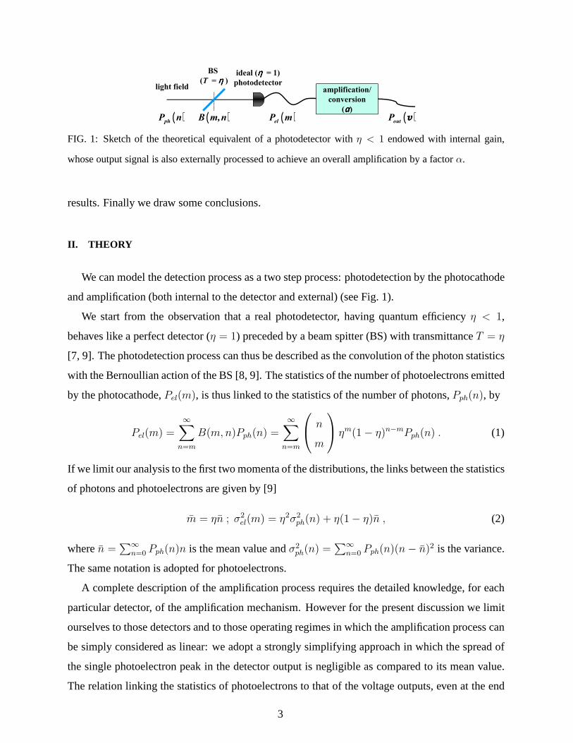
FIG. 2: Sketch of the experimental setup. Left: light sources: (a) coherent state, (b) multimode thermal state

and (c) multimode pseudo-thermal state. D, rotating ground-glass diffuser; BBO, type I nonlinear crystal.

Right: measuring apparatus: F, variable neutral density filter; MF, multimode fiber; PMT/HPD, detectors

with internal gain; SGI, synchronous gated integrator; ADC, analog-to-digital converter.

of the electronic chain external to the detector, is then

Pout(v) =1

αPel(αm) , (3)

beingα the amplification/conversion coefficient given by the overall amplification process and

signal-processing electronics. Quite obviously, Eq. (3) shows that in general the distribution of the

output voltage values is different from that of the photoelectrons. For the first two momenta of the

distributions, the experimental final outputs are given by [9]

v = αm ; σ2out(v) = α2σ2

el(m) , (4)

where the symbols are defined as above.

The most difficult task to be performed for reconstructingPel from Pout is the experimental

determination of the parameterα in Eq. (3). This task can be tackled by following a procedure

based on repeated measurements of the same state of light at different values of the quantum

efficiency by inserting neutral filters in front of the detector. In particular we evaluate the following

quantity

Fv =σ2

out(v)

v=

α2[

η2σ2ph(n) + η (1 − η) n

]

αηn= αηF + α (1 − η) = αηQ + α, (5)

whereF = σ2ph(n)/n is the Fano-factor that we have re-written asF = 1+Q, Q being the Mandel

Q-factor [10]. We observe thatFv is linearly dependent onη and thatα can be obtained as the

4

SGI

ADC

F

PMT

SGIMF

PC

HPD

SGI

MF

523 nm

BS

F

Nd:YLF

FIG. 3: Sketch of the experimental setup for the comparison between PMT and HPD. Nd:YLF, laser source;

BS, beam splitter; F, variable neutral density filter; MF, multimode fiber; PMT/HPD, detectors with internal

gain; SGI, synchronous gated integrator; ADC, analog-to-digital converter.

limit of Fv atη → 0. By multiplying and dividing byn we get

Fv =Q

nv + α , (6)

which now expressesFv as a function of the mean value of the measured output voltage. Note

that v varies because of the variation ofη and not because of the change in the measured state

(Q/n remains the same). The expression in Eq. (6) is general and all the information about the

specific state under measurement is contained in the angularcoefficientQ/n = (σ2ph(n) − n)/n2,

which is zero for Poissonian light, positive for classical super-Poissonian light and negative for

nonclassical sub-Poissonian light. By measuring the same light state at different values ofv and

evaluatingFv, we can directly obtain the value ofα and the ratioQ/n. Of course, different light

states may have, for some values of the parameters, the same value ofQ/n and this prevents the

possibility of the unique determination of the light statistics. Nevertheless, if an assumption can

be made on the statistics of the measured light, the method allows one to check it immediately.

The expected expressions ofFv for the states presented in this paper will be given in Section IV,

where the results are discussed.

III. EXPERIMENTS

In Fig. 2 we show the adopted experimental setup. The light from the specific source to be

investigated is collected by a multimode fiber (100µm core diameter, OZ Optics, Canada). As the

detector we used either a photomultiplier tube (PMT, 8850, Burle Industries, maximum quantum

efficiencyη = 0.24 at 400 nm) or a hybrid photodiode module (HPD, H8236-40, Hamamatsu,

Japan, maximum quantum efficiencyη = 0.40 at 550 nm). Both detectors are endowed with

partial photon resolving capability and are linear over a wide range of intensities. The current

5

outputs of the detectors are integrated (SGI, Stanford Research Systems), sampled and digitized

(ADC, National Instruments). The final outputs are then recorded by a computer.

As a preliminary check of the performances of the detectors,we simultaneously measured the

light at the two outputs of a 50% beam splitter (BS in Fig. 3) dividing a ps-pulsed coherent beam at

523 nm. The light was obtained from the second harmonics of a Nd:YLF continuous-wave mode-

locked laser amplified at 500 Hz repetition rate (High-Q Laser Production). In Fig. 4 we show a

typical pulse-height spectrum of the PMT (a) and of the HPD (b). The zero value of the output

voltagev is set at the mean value of the response to dark of each detector, which was measured

independently (seee.g.the horizontal scale in Figs. 4 (a) and (b)).

A standard procedure for analyzing a pulse-height-spectrum is to find a suitable fit obtained

as a multiple convolution of the function best fitting the single-photon peak [4]. The procedure

allows the reconstruction of a limited number of peaks (thatdepend on the resolving capabilities

of the detectors) and fails in analyzing more intense fields when the pulse-height spectrum does

not show well recognizable peaks.

The pulse-height spectrum of the detectors lose the peak structure as soon as the field intensity

becomes mesoscopic, still remaining proportional to the field intensity.

In Fig. 5 we show several pulse height spectra recorded by thePMT (a) and by the HPD (b)

in the same configuration of Fig. 3, in which neutral density filters are inserted on the beam path

before the beam splitter. In Fig. 5 (c) we plot the mean values of the output voltage as a function

of the transmittance of the filters: the difference between the two curves reflects the difference in

the overall quantum efficiency of the two detectors at 523 nm.The linearity will play a key role in

the analysis procedure described in Section IV.

6

3.0

2.5

3.0

2.0

2.5PMT coherent light

1.5

2.0

out

1.0

1.5Pout

0.5

1.0

0.0 0.5 1.0 1.5 2.0 2.5 3.00.0

0.5

(a)

0.0 0.5 1.0 1.5 2.0 2.5 3.00.0

v (Volt)

1.0

1.0

0.8 HPD coherent light

0.6

out

0.4

Pout

0.2

0.0 0.5 1.0 1.5 2.0 2.5 3.0 3.5 4.00.0

(b)

0.0 0.5 1.0 1.5 2.0 2.5 3.0 3.5 4.00.0

v (Volt)

FIG. 4: Typical pulse-height spectrum measured with the PMT(a) and with the HPD (b) simultaneously

recorded at the outputs of a 50% beam splitter, dividing a ps-pulsed coherent beam at 523 nm.

IV. RESULTS AND ANALYSIS

We measured different light fields characterized by different statistics and at wavelengths that

were chosen so as to match the highest quantum efficiencies ofthe detectors at best. The aim

of the measurements is to identify the type of light field, to determine the overall amplifica-

tion/conversion coefficientα and to reconstruct the statistics of the photoelectrons. The steps

of the experimental procedure are: 1) to measure the same field at different attenuations of the

neutral density filters (the actual position of the filters depends on the specific measurement); 2) to

7

10

8PMT coherent light

6

out

4

Pout

2

(a)

0.0 0.5 1.0 1.5 2.00

(a)

0.0 0.5 1.0 1.5 2.00

v (Volt)

2.0

1.5HPD coherent light

1.0

out

1.0Pout

0.5

(b)

0 1 2 3 4 5 6 70.0

(b)

0 1 2 3 4 5 6 70.0

v (Volt)

8 PMT HPD

6

HPD

4

6

(Volt)

4

v (Volt)

2

(c)

0.0 0.5 1.0

0(c)

0.0 0.5 1.0

T

FIG. 5: Pulse height spectra recorded by the PMT (a) and by the HPD (b) in the same configuration of Fig. 4

at different values of the transmittance of the neutral density filters. (c): Mean value of the output voltage as

a function of the filters’ transmittance. The difference in the angular coefficient reflect the different overall

detection efficiency of the two arms.

8

1.0 multimode thermal light

coherent lightµµµµ = 5.2

0.8

coherent light

0.6

0.8

(Volt)

0.6

αααα = 0.356

Fv (Volt)

0.4

0.0 0.5 1.0 1.5 2.0 2.5 3.00.2

αααα = 0.358

0.0 0.5 1.0 1.5 2.0 2.5 3.00.2

v (Volt)

FIG. 6: Plot of the Fano factor,Fv , for the output voltage as a function of the mean voltagev for different

light states: pulsed coherent field at 523 nm (dots) and pulsed multimode thermal field at 420 nm (squares).

evaluate the mean value and the variance of the output voltage; 3) to plot the experimental values

of Fv (see Eq. (5)) as a function of the mean valuev; 4) to fit the plot to a straight line, thus

obtain the value of theα factor, and to find, according to one of the theoretical models, the param-

eters of the photoelectron distribution; 5) to use the fitting parameters to recover the photoelectron

statistics.

First of all we consider the measurements performed on ps-pulsed coherent light at 523 nm

obtained as above (see Fig. 2 (a)). For a coherent field we expect a Poissonian photon-number

distribution

Pph(n) =nn

n!exp(−n) , (7)

for which mean value and variance aren. Note also that the photoelectron distribution obtained

by applying Eq. (1) to Eq. (7) remains Poissonian, so thatPel(m) = Pph(n) with the substitution

n → m. The Fano factor for the final output voltage becomes

Fv = α , (8)

independent of the mean valuev. The experimental results obtained with the PMT are shown in

Fig. 6 (full circles). The linear fit givesα = (0.358 ± 0.002) V.

The second kind of measurements is on the multimode thermal light given, as sketched in Fig. 2

(b), by a blue portion (420 nm) of the down conversion parametric fluorescence produced by a type-

9

I BBO crystal pumped by the third harmonics pulses (349 nm) ofthe same Nd:YLF laser [5, 6].

The expected photon-number distribution is given by the convolution of µ independent thermal

modes [8]

Pph(n) =(n + µ − 1)!

n! (µ − 1)! (n/µ + 1)µ (µ/n + 1)n , (9)

for which the mean value isn and the variance isσ(2)ph (n) = n (n/µ + 1). As in the case of coherent

light, the photoelectron distribution obtained by applying Eq. (1) to Eq. (9) remains multimode

thermal and againPel(m) = Pph(n). The Fano factor for the final output voltage turns out to be

Fv =v

µ+ α , (10)

that is linear in the mean value. The experimental results obtained with the PMT are shown in

Fig. 6 (squares). Their fit to Eq. (10) givesµ = 5.2 ± 0.1 andα = (0.356 ± 0.006) V. Note that,

as these measurements were made in the same experimental conditions as those on the coherent

field, the two values obtained forα are very similar to each other.

We now use the fitting parameters to recover the photoelectron statistics. We divide the voltage

output by the value ofα to convert it to photoelectrons and then re-bin the obtaineddistributions

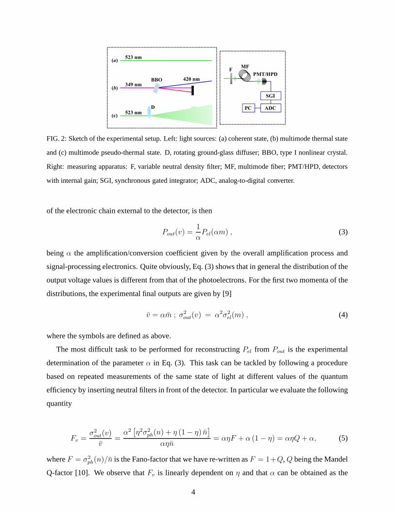
in unitary bins. In Fig. 7 we show the photoelectron distributions,Pel,exp for coherent light (a)

and for multimode thermal light (b) reconstructed from some of the data sets used to obtain the

calibration. The dots in the figure are the theoretical curves,Pel (Poissonian and multimode ther-

mal, respectively), evaluated at the measured mean values,by using the parameters,α or α andµ,

obtained from the fits to Eqs. (8) and (10), respectively.

In the figures the values of the fidelity [11] of the reconstructed distributions,

f =∞

∑

m=1

√

Pel,exp(m)Pel(m) , (11)

are also displayed indicating the good quality of the reconstruction.

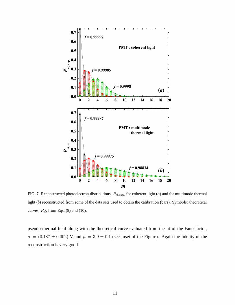
The same kind of measurements were repeated by using the HPD.To optimize the detection

efficiency we exploited the light produced by the second harmonics of the Nd:YLF laser. Accord-

ing to the setup depicted in Fig. 2 (c), the laser light was passed through a rotating ground glass

diffuser to obtain a pseudo-thermal speckle pattern [12]. The light, selected with a pin-hole so

as to transmit a number of coherence areas, was then delivered to the detector by a multimode

fiber. The photon-number statistics of the detected field follows the multimode thermal statis-

tics in Eq. (9). In Fig. 8 we plot the reconstructed photoelectron distribution for the multimode

10

0.7

0.6

0.7f = 0.99992

0.5PMT : coherent light

0.4

el, exp

0.2

0.3Pel,

f = 0.99985

0.1

0.2

(a)f = 0.9998

0 2 4 6 8 10 12 14 16 18 200.0

0.1(a)

f = 0.9998

0 2 4 6 8 10 12 14 16 18 200.0

m

0.7

0.6

0.7

f = 0.99987

0.5PMT : multimode

thermal light

0.4

el, ex

p

0.2

0.3

f = 0.99975

Pel,

0.1

0.2

f = 0.98834

f = 0.99975

(b)

0 2 4 6 8 10 12 14 16 18 200.0

0.1 f = 0.98834(b)

0 2 4 6 8 10 12 14 16 18 200.0

m

FIG. 7: Reconstructed photoelectron distributions,Pel,exp, for coherent light (a) and for multimode thermal

light (b) reconstructed from some of the data sets used to obtain the calibration (bars). Symbols: theoretical

curves,Pel, from Eqs. (8) and (10).

pseudo-thermal field along with the theoretical curve evaluated from the fit of the Fano factor,

α = (0.187 ± 0.002) V and µ = 3.9 ± 0.1 (see Inset of the Figure). Again the fidelity of the

reconstruction is very good.

11

0.3

µµµµ = 3.90.3

f = 0.9997

(Volt)

µµµµ = 3.9

0.20.2

αααα = 0.187

Fv (Volt)

0.1

0.0 0.1 0.2 0.3 0.4 0.5

Pel, exp

αααα = 0.187

v (Volt)

0.1 HPD : multimode

pseudo-thermal light

P

0.00 2 4 6 8 10 12 14 16 18 20

0.0

m

FIG. 8: Reconstructed photoelectron distribution,Pel,exp, for pulsed multimode pseudo-thermal light at

523 nm (bars). The displayed data set is one of those used to obtain the calibration. Symbols: theoretical

curve,Pel, calculated from Eq. (10) with the number of modes (µ = 3.9) evaluated from the fit of the Fano

factor (see Inset). Inset: plot of the Fano factor,Fv, for the output voltage as a function of the mean voltage

v.

V. CONCLUSIONS

We have demonstrated that it is possible to implement a self-consistent procedure to recover

the distribution of photoelectrons that avoids calibration of the photodetectors. The procedure

employs the evaluation of the Fano factor at different values of the mean photon numbers of the

field to be characterized. The procedure has been satisfactorily tested on coherent and multimode

thermal light. The next step will be to investigate less trivial optical states, such as those generated

by the mixing of different fields [13], in order to extend the validity of the method.

12

Aknowledgements

The Authors thank Sergio Cova (Politecnico di Milano) for fruitful discussions.

Present address of A. Agliati is: Quanta System, Solbiate Olona (VA), Italy.

[1] M. Munroe, D. Boggavarapu, M. E. Anderson and M. G. Raymer, Phys. Rev. A52 R924-R927 (1995).

[2] Y. Zhang, K. Kasai and M. Watanabe, Opt. Lett.27 1244-1246 (2002).

[3] M. Raymer, M. Beck inQuantum states estimation, M.G.A. Paris and J.Rehacek Eds., Lect. Not.

Phys.649 (Springer, Berlin-Heidelberg, 2004).

[4] G. Zambra, M. Bondani, A.S. Spinelli, F. Paleari and A. Andreoni, Rev. Sci. Instrum.75 2762-2765

(2004).

[5] F. Paleari, A. Andreoni, G. Zambra and M. Bondani, Opt. Express12, 2816-2824 (2004).

[6] M. Bondani, A. Allevi, G. Zambra, M. G. A. Paris and A. Andreoni, Phys. Rev. A76 013833 (2007).

[7] G. Zambra, A. Andreoni, M. Bondani, M. Gramegna, M. Genovese, G. Brida, A. Rossi and M.G.A.

Paris, Phys. Rev. Lett.95 063602 (2005).

[8] L. Mandel and E. Wolf,Optical Coherence and Quantum Optics(Cambrige University Press, New

York, NY, 1995).

[9] A. Agliati, M. Bondani, A. Andreoni, G. De Cillis and M.G.A. Paris, J. Opt. B7 S652-S663 (2005).

[10] L. Mandel, Opt. Lett.4 205-207 (1979).

[11] R. Jozsa, J. Mod. Opt.41 2315-2323 (1994).

[12] F. T. Arecchi, Phys. Rev. Lett.15 912-916 (1965).

[13] G. Zambra, A. Allevi, A. Andreoni and M. G. A. Paris, Int.J. Quantum Inf.5 305-309. (2007).

13