
Essentials of Statistics
103
-
Upload
independent -
Category
Documents
-
view
0 -
download
0
Transcript of Essentials of Statistics


Download free ebooks at bookboon.com
3
Statistics © 2010 David Brink & Ventus Publishing ApS ISBN 978-87-7681-408-3

Download free ebooks at bookboon.com
Ple
ase
clic
k th
e ad
vert
Statistics
4
Contents
Contents Indhold
1 Preface 11
2 Basic concepts of probability theory 122.1 Probability space, probability function, sample space, event . . . . . . . . . . . . 122.2 Conditional probability . . . . . . . . . . . . . . . . . . . . . . . . . . . . . . . 122.3 Independent events . . . . . . . . . . . . . . . . . . . . . . . . . . . . . . . . . 142.4 The Inclusion-Exclusion Formula . . . . . . . . . . . . . . . . . . . . . . . . . 142.5 Binomial coefficients . . . . . . . . . . . . . . . . . . . . . . . . . . . . . . . . 162.6 Multinomial coefficients . . . . . . . . . . . . . . . . . . . . . . . . . . . . . . 17
3 Random variables 183.1 Random variables, definition . . . . . . . . . . . . . . . . . . . . . . . . . . . . 183.2 The distribution function . . . . . . . . . . . . . . . . . . . . . . . . . . . . . . 183.3 Discrete random variables, point probabilities . . . . . . . . . . . . . . . . . . . 193.4 Continuous random variables, density function . . . . . . . . . . . . . . . . . . 203.5 Continuous random variables, distribution function . . . . . . . . . . . . . . . . 203.6 Independent random variables . . . . . . . . . . . . . . . . . . . . . . . . . . . 203.7 Random vector, simultaneous density, and distribution function . . . . . . . . . . 21
4 Expected value and variance 214.1 Expected value of random variables . . . . . . . . . . . . . . . . . . . . . . . . 214.2 Variance and standard deviation of random variables . . . . . . . . . . . . . . . 224.3 Example (computation of expected value, variance, and standard deviation) . . . 234.4 Estimation of expected value µ and standard deviation σ by eye . . . . . . . . . 234.5 Addition and multiplication formulae for expected value and variance . . . . . . 244.6 Covariance and correlation coefficient . . . . . . . . . . . . . . . . . . . . . . . 24
5 The Law of Large Numbers 265.1 Chebyshev’s Inequality . . . . . . . . . . . . . . . . . . . . . . . . . . . . . . . 265.2 The Law of Large Numbers . . . . . . . . . . . . . . . . . . . . . . . . . . . . . 265.3 The Central Limit Theorem . . . . . . . . . . . . . . . . . . . . . . . . . . . . . 265.4 Example (distribution functions converge to Φ) . . . . . . . . . . . . . . . . . . 27
6 Descriptive statistics 276.1 Median and quartiles . . . . . . . . . . . . . . . . . . . . . . . . . . . . . . . . 276.2 Mean value . . . . . . . . . . . . . . . . . . . . . . . . . . . . . . . . . . . . . 286.3 Empirical variance and empirical standard deviation . . . . . . . . . . . . . . . . 286.4 Empirical covariance and empirical correlation coefficient . . . . . . . . . . . . 29
7 Statistical hypothesis testing 297.1 Null hypothesis and alternative hypothesis . . . . . . . . . . . . . . . . . . . . . 297.2 Significance probability and significance level . . . . . . . . . . . . . . . . . . . 29
2
Stand out from the crowdDesigned for graduates with less than one year of full-time postgraduate work experience, London Business School’s Masters in Management will expand your thinking and provide you with the foundations for a successful career in business.
The programme is developed in consultation with recruiters to provide you with the key skills that top employers demand. Through 11 months of full-time study, you will gain the business knowledge and capabilities to increase your career choices and stand out from the crowd.
Applications are now open for entry in September 2011.
For more information visit www.london.edu/mim/ email [email protected] or call +44 (0)20 7000 7573
Masters in Management
London Business SchoolRegent’s ParkLondon NW1 4SAUnited KingdomTel +44 (0)20 7000 7573Email [email protected]/mim/
Fast-track your career

Download free ebooks at bookboon.com
Ple
ase
clic
k th
e ad
vert
Statistics
5
Contents
Indhold
1 Preface 11
2 Basic concepts of probability theory 122.1 Probability space, probability function, sample space, event . . . . . . . . . . . . 122.2 Conditional probability . . . . . . . . . . . . . . . . . . . . . . . . . . . . . . . 122.3 Independent events . . . . . . . . . . . . . . . . . . . . . . . . . . . . . . . . . 142.4 The Inclusion-Exclusion Formula . . . . . . . . . . . . . . . . . . . . . . . . . 142.5 Binomial coefficients . . . . . . . . . . . . . . . . . . . . . . . . . . . . . . . . 162.6 Multinomial coefficients . . . . . . . . . . . . . . . . . . . . . . . . . . . . . . 17
3 Random variables 183.1 Random variables, definition . . . . . . . . . . . . . . . . . . . . . . . . . . . . 183.2 The distribution function . . . . . . . . . . . . . . . . . . . . . . . . . . . . . . 183.3 Discrete random variables, point probabilities . . . . . . . . . . . . . . . . . . . 193.4 Continuous random variables, density function . . . . . . . . . . . . . . . . . . 203.5 Continuous random variables, distribution function . . . . . . . . . . . . . . . . 203.6 Independent random variables . . . . . . . . . . . . . . . . . . . . . . . . . . . 203.7 Random vector, simultaneous density, and distribution function . . . . . . . . . . 21
4 Expected value and variance 214.1 Expected value of random variables . . . . . . . . . . . . . . . . . . . . . . . . 214.2 Variance and standard deviation of random variables . . . . . . . . . . . . . . . 224.3 Example (computation of expected value, variance, and standard deviation) . . . 234.4 Estimation of expected value µ and standard deviation σ by eye . . . . . . . . . 234.5 Addition and multiplication formulae for expected value and variance . . . . . . 244.6 Covariance and correlation coefficient . . . . . . . . . . . . . . . . . . . . . . . 24
5 The Law of Large Numbers 265.1 Chebyshev’s Inequality . . . . . . . . . . . . . . . . . . . . . . . . . . . . . . . 265.2 The Law of Large Numbers . . . . . . . . . . . . . . . . . . . . . . . . . . . . . 265.3 The Central Limit Theorem . . . . . . . . . . . . . . . . . . . . . . . . . . . . . 265.4 Example (distribution functions converge to Φ) . . . . . . . . . . . . . . . . . . 27
6 Descriptive statistics 276.1 Median and quartiles . . . . . . . . . . . . . . . . . . . . . . . . . . . . . . . . 276.2 Mean value . . . . . . . . . . . . . . . . . . . . . . . . . . . . . . . . . . . . . 286.3 Empirical variance and empirical standard deviation . . . . . . . . . . . . . . . . 286.4 Empirical covariance and empirical correlation coefficient . . . . . . . . . . . . 29
7 Statistical hypothesis testing 297.1 Null hypothesis and alternative hypothesis . . . . . . . . . . . . . . . . . . . . . 297.2 Significance probability and significance level . . . . . . . . . . . . . . . . . . . 29
2
© U
BS
2010
. All
rig
hts
res
erve
d.
www.ubs.com/graduates
Looking for a career where your ideas could really make a difference? UBS’s
Graduate Programme and internships are a chance for you to experience
for yourself what it’s like to be part of a global team that rewards your input
and believes in succeeding together.
Wherever you are in your academic career, make your future a part of ours
by visiting www.ubs.com/graduates.
You’re full of energyand ideas. And that’s just what we are looking for.

Download free ebooks at bookboon.com
Ple
ase
clic
k th
e ad
vert
Statistics
6
Contents
7.3 Errors of type I and II . . . . . . . . . . . . . . . . . . . . . . . . . . . . . . . . 307.4 Example . . . . . . . . . . . . . . . . . . . . . . . . . . . . . . . . . . . . . . . 30
8 The binomial distribution Bin(n, p) 308.1 Parameters . . . . . . . . . . . . . . . . . . . . . . . . . . . . . . . . . . . . . . 308.2 Description . . . . . . . . . . . . . . . . . . . . . . . . . . . . . . . . . . . . . 318.3 Point probabilities . . . . . . . . . . . . . . . . . . . . . . . . . . . . . . . . . . 318.4 Expected value and variance . . . . . . . . . . . . . . . . . . . . . . . . . . . . 328.5 Significance probabilities for tests in the binomial distribution . . . . . . . . . . 328.6 The normal approximation to the binomial distribution . . . . . . . . . . . . . . 328.7 Estimators . . . . . . . . . . . . . . . . . . . . . . . . . . . . . . . . . . . . . . 338.8 Confidence intervals . . . . . . . . . . . . . . . . . . . . . . . . . . . . . . . . 34
9 The Poisson distribution Pois(λ) 359.1 Parameters . . . . . . . . . . . . . . . . . . . . . . . . . . . . . . . . . . . . . . 359.2 Description . . . . . . . . . . . . . . . . . . . . . . . . . . . . . . . . . . . . . 359.3 Point probabilities . . . . . . . . . . . . . . . . . . . . . . . . . . . . . . . . . . 359.4 Expected value and variance . . . . . . . . . . . . . . . . . . . . . . . . . . . . 359.5 Addition formula . . . . . . . . . . . . . . . . . . . . . . . . . . . . . . . . . . 369.6 Significance probabilities for tests in the Poisson distribution . . . . . . . . . . . 369.7 Example (significant increase in sale of Skodas) . . . . . . . . . . . . . . . . . . 369.8 The binomial approximation to the Poisson distribution . . . . . . . . . . . . . . 379.9 The normal approximation to the Poisson distribution . . . . . . . . . . . . . . . 379.10 Example (significant decrease in number of complaints) . . . . . . . . . . . . . . 389.11 Estimators . . . . . . . . . . . . . . . . . . . . . . . . . . . . . . . . . . . . . . 389.12 Confidence intervals . . . . . . . . . . . . . . . . . . . . . . . . . . . . . . . . 39
10 The geometrical distribution Geo(p) 3910.1 Parameters . . . . . . . . . . . . . . . . . . . . . . . . . . . . . . . . . . . . . . 3910.2 Description . . . . . . . . . . . . . . . . . . . . . . . . . . . . . . . . . . . . . 3910.3 Point probabilities and tail probabilities . . . . . . . . . . . . . . . . . . . . . . 3910.4 Expected value and variance . . . . . . . . . . . . . . . . . . . . . . . . . . . . 41
11 The hypergeometrical distribution HG(n, r,N) 4111.1 Parameters . . . . . . . . . . . . . . . . . . . . . . . . . . . . . . . . . . . . . . 4111.2 Description . . . . . . . . . . . . . . . . . . . . . . . . . . . . . . . . . . . . . 4111.3 Point probabilities and tail probabilities . . . . . . . . . . . . . . . . . . . . . . 4111.4 Expected value and variance . . . . . . . . . . . . . . . . . . . . . . . . . . . . 4211.5 The binomial approximation to the hypergeometrical distribution . . . . . . . . . 4211.6 The normal approximation to the hypergeometrical distribution . . . . . . . . . . 42
3
© Deloitte & Touche LLP and affiliated entities.
360°thinking.
Discover the truth at www.deloitte.ca/careers
© Deloitte & Touche LLP and affiliated entities.
360°thinking.
Discover the truth at www.deloitte.ca/careers
© Deloitte & Touche LLP and affiliated entities.
360°thinking.
Discover the truth at www.deloitte.ca/careers © Deloitte & Touche LLP and affiliated entities.
360°thinking.
Discover the truth at www.deloitte.ca/careers

Download free ebooks at bookboon.com
Ple
ase
clic
k th
e ad
vert
Statistics
7
Contents
7.3 Errors of type I and II . . . . . . . . . . . . . . . . . . . . . . . . . . . . . . . . 307.4 Example . . . . . . . . . . . . . . . . . . . . . . . . . . . . . . . . . . . . . . . 30
8 The binomial distribution Bin(n, p) 308.1 Parameters . . . . . . . . . . . . . . . . . . . . . . . . . . . . . . . . . . . . . . 308.2 Description . . . . . . . . . . . . . . . . . . . . . . . . . . . . . . . . . . . . . 318.3 Point probabilities . . . . . . . . . . . . . . . . . . . . . . . . . . . . . . . . . . 318.4 Expected value and variance . . . . . . . . . . . . . . . . . . . . . . . . . . . . 328.5 Significance probabilities for tests in the binomial distribution . . . . . . . . . . 328.6 The normal approximation to the binomial distribution . . . . . . . . . . . . . . 328.7 Estimators . . . . . . . . . . . . . . . . . . . . . . . . . . . . . . . . . . . . . . 338.8 Confidence intervals . . . . . . . . . . . . . . . . . . . . . . . . . . . . . . . . 34
9 The Poisson distribution Pois(λ) 359.1 Parameters . . . . . . . . . . . . . . . . . . . . . . . . . . . . . . . . . . . . . . 359.2 Description . . . . . . . . . . . . . . . . . . . . . . . . . . . . . . . . . . . . . 359.3 Point probabilities . . . . . . . . . . . . . . . . . . . . . . . . . . . . . . . . . . 359.4 Expected value and variance . . . . . . . . . . . . . . . . . . . . . . . . . . . . 359.5 Addition formula . . . . . . . . . . . . . . . . . . . . . . . . . . . . . . . . . . 369.6 Significance probabilities for tests in the Poisson distribution . . . . . . . . . . . 369.7 Example (significant increase in sale of Skodas) . . . . . . . . . . . . . . . . . . 369.8 The binomial approximation to the Poisson distribution . . . . . . . . . . . . . . 379.9 The normal approximation to the Poisson distribution . . . . . . . . . . . . . . . 379.10 Example (significant decrease in number of complaints) . . . . . . . . . . . . . . 389.11 Estimators . . . . . . . . . . . . . . . . . . . . . . . . . . . . . . . . . . . . . . 389.12 Confidence intervals . . . . . . . . . . . . . . . . . . . . . . . . . . . . . . . . 39
10 The geometrical distribution Geo(p) 3910.1 Parameters . . . . . . . . . . . . . . . . . . . . . . . . . . . . . . . . . . . . . . 3910.2 Description . . . . . . . . . . . . . . . . . . . . . . . . . . . . . . . . . . . . . 3910.3 Point probabilities and tail probabilities . . . . . . . . . . . . . . . . . . . . . . 3910.4 Expected value and variance . . . . . . . . . . . . . . . . . . . . . . . . . . . . 41
11 The hypergeometrical distribution HG(n, r,N) 4111.1 Parameters . . . . . . . . . . . . . . . . . . . . . . . . . . . . . . . . . . . . . . 4111.2 Description . . . . . . . . . . . . . . . . . . . . . . . . . . . . . . . . . . . . . 4111.3 Point probabilities and tail probabilities . . . . . . . . . . . . . . . . . . . . . . 4111.4 Expected value and variance . . . . . . . . . . . . . . . . . . . . . . . . . . . . 4211.5 The binomial approximation to the hypergeometrical distribution . . . . . . . . . 4211.6 The normal approximation to the hypergeometrical distribution . . . . . . . . . . 42
3

Download free ebooks at bookboon.com
Statistics
8
Contents
12 The multinomial distribution Mult(n, p1, . . . , pr) 4312.1 Parameters . . . . . . . . . . . . . . . . . . . . . . . . . . . . . . . . . . . . . . 4312.2 Description . . . . . . . . . . . . . . . . . . . . . . . . . . . . . . . . . . . . . 4312.3 Point probabilities . . . . . . . . . . . . . . . . . . . . . . . . . . . . . . . . . . 4412.4 Estimators . . . . . . . . . . . . . . . . . . . . . . . . . . . . . . . . . . . . . . 44
13 The negative binomial distribution NB(n, p) 4413.1 Parameters . . . . . . . . . . . . . . . . . . . . . . . . . . . . . . . . . . . . . . 4413.2 Description . . . . . . . . . . . . . . . . . . . . . . . . . . . . . . . . . . . . . 4513.3 Point probabilities . . . . . . . . . . . . . . . . . . . . . . . . . . . . . . . . . . 4513.4 Expected value and variance . . . . . . . . . . . . . . . . . . . . . . . . . . . . 4513.5 Estimators . . . . . . . . . . . . . . . . . . . . . . . . . . . . . . . . . . . . . . 45
14 The exponential distribution Exp(λ) 4514.1 Parameters . . . . . . . . . . . . . . . . . . . . . . . . . . . . . . . . . . . . . . 4514.2 Description . . . . . . . . . . . . . . . . . . . . . . . . . . . . . . . . . . . . . 4514.3 Density and distribution function . . . . . . . . . . . . . . . . . . . . . . . . . . 4614.4 Expected value and variance . . . . . . . . . . . . . . . . . . . . . . . . . . . . 46
15 The normal distribution 4615.1 Parameters . . . . . . . . . . . . . . . . . . . . . . . . . . . . . . . . . . . . . . 4615.2 Description . . . . . . . . . . . . . . . . . . . . . . . . . . . . . . . . . . . . . 4715.3 Density and distribution function . . . . . . . . . . . . . . . . . . . . . . . . . . 4715.4 The standard normal distribution . . . . . . . . . . . . . . . . . . . . . . . . . . 4715.5 Properties of Φ . . . . . . . . . . . . . . . . . . . . . . . . . . . . . . . . . . . 4815.6 Estimation of the expected value µ . . . . . . . . . . . . . . . . . . . . . . . . . 4815.7 Estimation of the variance σ2 . . . . . . . . . . . . . . . . . . . . . . . . . . . . 4815.8 Confidence intervals for the expected value µ . . . . . . . . . . . . . . . . . . . 4915.9 Confidence intervals for the variance σ2 and the standard deviation σ . . . . . . . 5015.10Addition formula . . . . . . . . . . . . . . . . . . . . . . . . . . . . . . . . . . 50
16 Distributions connected with the normal distribution 5016.1 The χ2 distribution . . . . . . . . . . . . . . . . . . . . . . . . . . . . . . . . . 5016.2 Student’s t distribution . . . . . . . . . . . . . . . . . . . . . . . . . . . . . . . 5116.3 Fisher’s F distribution . . . . . . . . . . . . . . . . . . . . . . . . . . . . . . . 52
17 Tests in the normal distribution 5317.1 One sample, known variance, H0 : µ = µ0 . . . . . . . . . . . . . . . . . . . . . 5317.2 One sample, unknown variance, H0 : µ = µ0 (Student’s t test) . . . . . . . . . . 5317.3 One sample, unknown expected value, H0 : σ2 = σ2
0 . . . . . . . . . . . . . . . 5417.4 Example . . . . . . . . . . . . . . . . . . . . . . . . . . . . . . . . . . . . . . . 5617.5 Two samples, known variances, H0 : µ1 = µ2 . . . . . . . . . . . . . . . . . . . 5617.6 Two samples, unknown variances, H0 : µ1 = µ2 (Fisher-Behrens) . . . . . . . . 5717.7 Two samples, unknown expected values, H0 : σ2
1 = σ22 . . . . . . . . . . . . . . 57
4
Download free ebooks at bookboon.com
Statistics
9
Contents
17.8 Two samples, unknown common variance, H0 : µ1 = µ2 . . . . . . . . . . . . . 5817.9 Example (comparison of two expected values) . . . . . . . . . . . . . . . . . . . 59
18 Analysis of variance (ANOVA) 6018.1 Aim and motivation . . . . . . . . . . . . . . . . . . . . . . . . . . . . . . . . . 6018.2 k samples, unknown common variance, H0 : µ1 = · · · = µk . . . . . . . . . . . 6018.3 Two examples (comparison of mean values from three samples) . . . . . . . . . 61
19 The chi-squared test (or χ2 test) 6319.1 χ2 test for equality of distribution . . . . . . . . . . . . . . . . . . . . . . . . . 6319.2 The assumption of normal distribution . . . . . . . . . . . . . . . . . . . . . . . 6519.3 Standardized residuals . . . . . . . . . . . . . . . . . . . . . . . . . . . . . . . 6519.4 Example (women with five children) . . . . . . . . . . . . . . . . . . . . . . . . 6519.5 Example (election) . . . . . . . . . . . . . . . . . . . . . . . . . . . . . . . . . 6719.6 Example (deaths in the Prussian cavalry) . . . . . . . . . . . . . . . . . . . . . . 68
20 Contingency tables 7020.1 Definition, method . . . . . . . . . . . . . . . . . . . . . . . . . . . . . . . . . 7020.2 Standardized residuals . . . . . . . . . . . . . . . . . . . . . . . . . . . . . . . 7120.3 Example (students’ political orientation) . . . . . . . . . . . . . . . . . . . . . . 7120.4 χ2 test for 2 × 2 tables . . . . . . . . . . . . . . . . . . . . . . . . . . . . . . . 7320.5 Fisher’s exact test for 2 × 2 tables . . . . . . . . . . . . . . . . . . . . . . . . . 7320.6 Example (Fisher’s exact test) . . . . . . . . . . . . . . . . . . . . . . . . . . . . 74
21 Distribution-free tests 7421.1 Wilcoxon’s test for one set of observations . . . . . . . . . . . . . . . . . . . . . 7521.2 Example . . . . . . . . . . . . . . . . . . . . . . . . . . . . . . . . . . . . . . . 7621.3 The normal approximation to Wilcoxon’s test for one set of observations . . . . . 7721.4 Wilcoxon’s test for two sets of observations . . . . . . . . . . . . . . . . . . . . 7721.5 The normal approximation to Wilcoxon’s test for two sets of observations . . . . 78
22 Linear regression 7922.1 The model . . . . . . . . . . . . . . . . . . . . . . . . . . . . . . . . . . . . . . 7922.2 Estimation of the parameters β0 and β1 . . . . . . . . . . . . . . . . . . . . . . 7922.3 The distribution of the estimators . . . . . . . . . . . . . . . . . . . . . . . . . . 8022.4 Predicted values yi and residuals ei . . . . . . . . . . . . . . . . . . . . . . . . . 8022.5 Estimation of the variance σ2 . . . . . . . . . . . . . . . . . . . . . . . . . . . . 8022.6 Confidence intervals for the parameters β0 and β1 . . . . . . . . . . . . . . . . . 8022.7 The determination coefficient R2 . . . . . . . . . . . . . . . . . . . . . . . . . . 8122.8 Predictions and prediction intervals . . . . . . . . . . . . . . . . . . . . . . . . . 8122.9 Overview of formulae . . . . . . . . . . . . . . . . . . . . . . . . . . . . . . . . 8222.10Example . . . . . . . . . . . . . . . . . . . . . . . . . . . . . . . . . . . . . . . 82
A Overview of discrete distributions 86
5

Download free ebooks at bookboon.com
Statistics
10
Contents
B Tables 87B.1 How to read the tables . . . . . . . . . . . . . . . . . . . . . . . . . . . . . . . 87B.2 The standard normal distribution . . . . . . . . . . . . . . . . . . . . . . . . . . 89B.3 The χ2 distribution (values x with Fχ2(x) = 0.500 etc.) . . . . . . . . . . . . . . 92B.4 Student’s t distribution (values x with FStudent(x) = 0.600 etc.) . . . . . . . . . 94B.5 Fisher’s F distribution (values x with FFisher(x) = 0.90) . . . . . . . . . . . . . 95B.6 Fisher’s F distribution (values x with FFisher(x) = 0.95) . . . . . . . . . . . . . 96B.7 Fisher’s F distribution (values x with FFisher(x) = 0.99) . . . . . . . . . . . . . 97B.8 Wilcoxon’s test for one set of observations . . . . . . . . . . . . . . . . . . . . . 98B.9 Wilcoxon’s test for two sets of observations, α = 5% . . . . . . . . . . . . . . . 99
C Explanation of symbols 100
D Index 102
6

Download free ebooks at bookboon.com
Statistics
11
Preface
1 Preface
Many students find that the obligatory Statistics course comes as a shock. The set textbook isdifficult, the curriculum is vast, and secondary-school maths feels infinitely far away.
“Statistics” offers friendly instruction on the core areas of these subjects. The focus is overview.And the numerous examples give the reader a “recipe” for solving all the common types of exer-cise. You can download this book free of charge.
11

Download free ebooks at bookboon.com
Statistics
12
Basic concepts of probability theory
2 Basic concepts of probability theory
2.1 Probability space, probability function, sample space, event
A probability space is a pair (Ω, P ) consisting of a set Ω and a function P which assigns to eachsubset A of Ω a real number P (A) in the interval [0, 1]. Moreover, the following two axioms arerequired to hold:
1. P (Ω) = 1,
2. P (⋃∞
n=1 An) =∑∞
n=1 P (An) if A1, A2, . . . is a sequence of pairwise disjoint subsets of Ω.
The set Ω is called a sample space. The elements ω ∈ Ω are called sample points and the subsetsA ⊆ Ω are called events. The function P is called a probability function. For an event A, thereal number P (A) is called the probability of A.
From the two axioms the following consequences can be deduced:
3. P (Ø) = 0,
4. P (A\B) = P (A) − P (B) if B ⊆ A,
5. P (A) = 1 − P (A),
6. P (A) P (B) if B ⊆ A,
7. P (A1 ∪ · · · ∪ An) = P (A1) + · · · + P (An) if A1, . . . , An are pairwise disjoint events,
8. P (A ∪ B) = P (A) + P (B) − P (A ∩ B) for arbitrary events A and B.
EXAMPLE. Consider the set Ω = 1, 2, 3, 4, 5, 6. For each subset A of Ω, define
P (A) =#A
6,
where #A is the number of elements in A. Then the pair (Ω, P ) is a probability space. One canview this probability space as a model for the for the situation “throw of a dice”.
EXAMPLE. Now consider the set Ω = 1, 2, 3, 4, 5, 6×1, 2, 3, 4, 5, 6. For each subset A of Ω,define
P (A) =#A
36.
Now the probability space (Ω, P ) is a model for the situation “throw of two dice”. The subset
A = (1, 1), (2, 2), (3, 3), (4, 4), (5, 5), (6, 6)
is the event “a pair”.
2.2 Conditional probability
For two events A and B the conditional probability of A given B is defined as
P (A | B) :=P (A ∩ B)
P (B).
12

Download free ebooks at bookboon.com
Ple
ase
clic
k th
e ad
vert
Statistics
13
Basic concepts of probability theory
We have the following theorem called computation of probability by division into possible causes:Suppose A1, . . . , An are pairwise disjoint events with A1 ∪ · · · ∪ An = Ω. For every event B itthen holds that
P (B) = P (A1) · P (B | A1) + · · · + P (An) · P (B | An) .
EXAMPLE. In the French Open final, Nadal plays the winner of the semifinal between Federerand Davydenko. A bookmaker estimates that the probability of Federer winning the semifinal is75%. The probability that Nadal can beat Federer is estimated to be 51%, whereas the probabilitythat Nadal can beat Davydenko is estimated to be 80%. The bookmaker therefore computes theprobability that Nadal wins the French Open, using division into possible causes, as follows:
P (Nadal wins the final) = P (Federer wins the semifinal)×P (Nadal wins the final|Federer wins the semifinal)+P (Davydenko wins the semifinal)×P (Nadal wins the final|Davydenko wins the semifinal)
= 0.75 · 0.51 + 0.25 · 0.8= 58.25%
A N N O N C E
13
your chance to change the worldHere at Ericsson we have a deep rooted belief that the innovations we make on a daily basis can have a profound effect on making the world a better place for people, business and society. Join us.
In Germany we are especially looking for graduates as Integration Engineers for • Radio Access and IP Networks• IMS and IPTV
We are looking forward to getting your application!To apply and for all current job openings please visit our web page: www.ericsson.com/careers
Download free ebooks at bookboon.com
Statistics
14
Basic concepts of probability theory
2.3 Independent events
Two events A and B are called independent, if
P (A ∩ B) = P (A) · P (B) .
Equivalent to this is the condition P (A | B) = P (A), i.e. that the probability of A is the same asthe conditional probability of A given B.
Remember: Two events are independent if the probability of one of them is not affected byknowing whether the other has occurred or not.
EXAMPLE. A red and a black dice are thrown. Consider the events
A: red dice shows 6,B: black dice show 6.
SinceP (A ∩ B) =
136
=16· 16
= P (A) · P (B) ,
A and B are independent. The probability that the red dice shows 6 is not affected by knowinganything about the black dice.
EXAMPLE. A red and a black dice are thrown. Consider the events
A: the red and the black dice show the same number,B: the red and the black dice show a total of 10.
SinceP (A) =
16
, but P (A | B) =13
,
A and B are not independent. The probability of two of a kind increases if one knows that the sumof the dice is 10.
2.4 The Inclusion-Exclusion Formula
Formula 8 on page 12 has the following generalization to three events A, B, C:
P (A∪B∪C) = P (A)+P (B)+P (C)−P (A∩B)−P (A∩C)−P (B∩C)+P (A∩B∩C) .
This equality is called the Inclusion-Exclusion Formula for three events.
EXAMPLE. What is the probability of having at least one 6 in three throws with a dice? Let A1 bethe event that we get a 6 in the first throw, and define A2 and A3 similarly. Then, our probabilitycan be computed by inclusion-exclusion:
P = P (A1 ∪ A2 ∪ A3)= P (A1) + P (A2) + P (A3) − P (A1 ∩ A2) − P (A1 ∩ A3) − P (A2 ∩ A3)
+P (A1 ∩ A2 ∩ A3)
=16
+16
+16− 1
62− 1
62− 1
62+
163
≈ 41%
14
Download free ebooks at bookboon.com
Statistics
15
Basic concepts of probability theory
The following generalization holds for n events A1, A2, . . . , An with union A = A1 ∪ · · · ∪ An:
P (A) =∑
i
P (Ai) −∑i<j
P (Ai ∩ Aj) +∑
i<j<k
P (Ai ∩ Aj ∩ Ak) − · · · ± P (A1 ∩ · · · ∩ An) .
This equality is called the Inclusion-Exclusion Formula for n events.
EXAMPLE. Pick five cards at random from an ordinary pack of cards. We wish to compute theprobability P (B) of the event B that all four suits appear among the 5 chosen cards.
For this purpose, let A1 be the event that none of the chosen cards are spades. Define A2, A3,and A4 similarly for hearts, diamonds, and clubs, respectively. Then
B = A1 ∪ A2 ∪ A3 ∪ A4 .
The Inclusion-Exclusion Formula now yields
P (B) =∑
i
P (Ai) −∑i<j
P (Ai ∩ Aj) +∑
i<j<k
P (Ai ∩ Aj ∩ Ak) − P (A1 ∩ A2 ∩ A3 ∩ A4) ,
that is
P (B) = 4 ·
(395
)
(525
) − 6 ·
(265
)
(525
) + 4 ·
(135
)
(525
) − 0 ≈ 73.6%
We thus obtain the probability
P (B) = 1 − P (B) = 26.4%
EXAMPLE. A school class contains n children. The teacher asks all the children to stand up andthen sit down again on a random chair. Let us compute the probability P (B) of the event B thateach pupil ends up on a new chair.
We start by enumerating the pupils from 1 to n. For each i we define the event
Ai : pupil number i gets his or her old chair
ThenB = A1 ∪ · · · ∪ An .
Now P (B) can be computed by the Inclusion-Exclusion Formula for n events:
P (B) =∑
i
P (Ai) −∑i<j
P (Ai ∩ Aj) + · · · ± P (A1 ∩ · · · ∩ An) ,
thus
P (B) =
(n
1
)1n−
(n
2
)1
n(n − 1)+ · · · ±
(n
n
)1n!
= 1 − 12!
+ · · · ± 1n!
15

Download free ebooks at bookboon.com
Ple
ase
clic
k th
e ad
vert
Statistics
16
Basic concepts of probability theory
We concludeP (B) = 1 − P (B) =
12!
− 13!
+14!
− · · · ± 1n!
It is a surprising fact that this probability is more or less independent of n: P (B) is very close to37% for all n ≥ 4.
2.5 Binomial coefficients
The binomial coefficient
(n
k
)(read as “n over k”) is defined as
(n
k
)=
n!k!(n − k)!
=1 · 2 · 3 · · ·n
1 · 2 · · · k · 1 · 2 · · · (n − k)
for integers n and k with 0 k n. (Recall the convention 0! = 1.)The reason why binomial coefficients appear again and again in probability theory is the fol-
lowing theorem:
The number of ways of choosing k elements from a set of n elements is
(n
k
).
A N N O N C E
16
We will turn your CV into an opportunity of a lifetime
Do you like cars? Would you like to be a part of a successful brand?We will appreciate and reward both your enthusiasm and talent.Send us your CV. You will be surprised where it can take you.
Send us your CV onwww.employerforlife.com

Download free ebooks at bookboon.com
Statistics
17
Basic concepts of probability theory
For example, the number of subsets with 5 elements (poker hands) of a set with 52 elements (apack of cards) is equal to (
525
)= 2598960 .
An easy way of remembering the binomial coefficients is by arranging them in Pascal’s tri-angle where each number is equal to the sum of the numbers immediately above:
(00
)1
(10
) (11
)1 1
(20
) (21
) (22
)1 2 1
(30
) (31
) (32
) (33
)1 3 3 1
(40
) (41
) (42
) (43
) (44
)1 4 6 4 1
(50
) (51
) (52
) (53
) (54
) (55
)1 5 10 10 5 1
(60
) (61
) (62
) (63
) (64
) (65
) (66
)1 6 15 20 15 6 1
......
One notices the rule (n
n − k
)=
(n
k
), e.g.
(107
)=
(103
).
2.6 Multinomial coefficients
The multinomial coefficients are defined as(n
k1 · · · kr
)=
n!k1! · · · kr!
for integers n and k1, . . . , kr with n = k1 + · · ·+ kr. The multinomial coefficients are also calledgeneralized binomial coefficients since the binomial coefficient
(n
k
)
is equal to the multinomial coefficient (n
k l
)
with l = n − k.
17
Download free ebooks at bookboon.com
Statistics
18
Rancom variables
3 Random variables
3.1 Random variables, definition
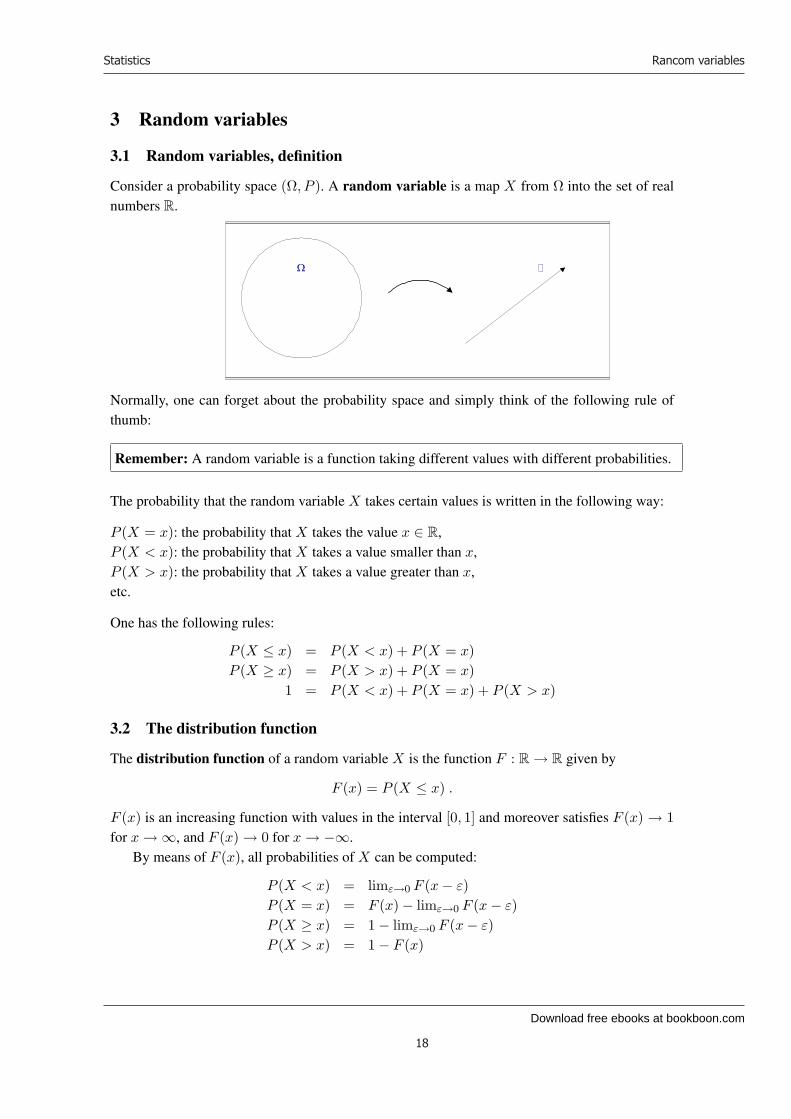
Consider a probability space (Ω, P ). A random variable is a map X from Ω into the set of realnumbers R.
Normally, one can forget about the probability space and simply think of the following rule ofthumb:
Remember: A random variable is a function taking different values with different probabilities.
The probability that the random variable X takes certain values is written in the following way:
P (X = x): the probability that X takes the value x ∈ R,P (X < x): the probability that X takes a value smaller than x,P (X > x): the probability that X takes a value greater than x,etc.
One has the following rules:
P (X ≤ x) = P (X < x) + P (X = x)P (X ≥ x) = P (X > x) + P (X = x)
1 = P (X < x) + P (X = x) + P (X > x)
3.2 The distribution function
The distribution function of a random variable X is the function F : R → R given by
F (x) = P (X ≤ x) .
F (x) is an increasing function with values in the interval [0, 1] and moreover satisfies F (x) → 1for x → ∞, and F (x) → 0 for x → −∞.
By means of F (x), all probabilities of X can be computed:
P (X < x) = limε→0 F (x − ε)P (X = x) = F (x) − limε→0 F (x − ε)P (X ≥ x) = 1 − limε→0 F (x − ε)P (X > x) = 1 − F (x)
18
3 Random variables
3.1 Random variables, definition
Consider a probability space (Ω, P ). A random variable is a map X from Ω into the set of realnumbers R.
Normally, one can forget about the probability space and simply think of the following rule ofthumb:
Remember: A random variable is a function taking different values with different probabilities.
The probability that the random variable X takes certain values is written in the following way:
P (X = x): the probability that X takes the value x ∈ R,P (X < x): the probability that X takes a value smaller than x,P (X > x): the probability that X takes a value greater than x,etc.
One has the following rules:
P (X ≤ x) = P (X < x) + P (X = x)P (X ≥ x) = P (X > x) + P (X = x)
1 = P (X < x) + P (X = x) + P (X > x)
3.2 The distribution function
The distribution function of a random variable X is the function F : R → R given by
F (x) = P (X ≤ x) .
F (x) is an increasing function with values in the interval [0, 1] and moreover satisfies F (x) → 1for x → ∞, and F (x) → 0 for x → −∞.
By means of F (x), all probabilities of X can be computed:
P (X < x) = limε→0 F (x − ε)P (X = x) = F (x) − limε→0 F (x − ε)P (X ≥ x) = 1 − limε→0 F (x − ε)P (X > x) = 1 − F (x)
18
Ω

Download free ebooks at bookboon.com
Ple
ase
clic
k th
e ad
vert
Statistics
19
Rancom variables
3.3 Discrete random variables, point probabilities
A random variable X is called discrete if it takes only finitely many or countably many values.For all practical purposes, we may define a discrete random variable as a random variable takingonly values in the set 0, 1, 2, . . . . The point probabilities
P (X = k)
determine the distribution of X . Indeed,
P (X ∈ A) =∑k∈A
P (X = k)
for any A ⊆ 0, 1, 2, . . . . In particular we have the rules
P (X ≤ k) =∑k
i=0 P (X = i)
P (X ≥ k) =∑∞
i=k P (X = i)
The point probabilities can be graphically illustrated by means of a pin diagram:
A N N O N C E
19

Download free ebooks at bookboon.com
Statistics
20
Rancom variables
3.4 Continuous random variables, density function
A random variable X is called continuous if it has a density function f(x). The density function,usually referred to simply as the density, satisfies
P (X ∈ A) =∫
t∈Af(t)dt
for all A ⊆ R. If A is an interval [a, b] we thus have
P (a ≤ X ≤ b) =∫ b
af(t)dt .
One should think of the density as the continuous analogue of the point probability function in thediscrete case.
3.5 Continuous random variables, distribution function
For a continuous random variable X with density f(x) the distribution function F (x) is given by
F (x) =∫ x
−∞f(t)dt .
The distribution function satisfies the following rules:
P (X ≤ x) = F (x)
P (X ≥ x) = 1 − F (x)
P (|X| ≤ x) = F (x) − F (−x)
P (|X| ≥ x) = F (−x) + 1 − F (x)
3.6 Independent random variables
Two random variables X and Y are called independent if the events X ∈ A and Y ∈ B are in-dependent for any subsets A, B ⊆ R. Independence of three or more random variables is definedsimilarly.
Remember: X and Y are independent if nothing can be deduced about the value of Y fromknowing the value of X .
20
P(X=k)
2 3 4 5 6 7
0,2
0,1
0
Download free ebooks at bookboon.com
Statistics
21
Expected value and variance
EXAMPLE. Throw a red dice and a black dice and consider the random variables
X: number of pips of red dice,Y : number of pips of black dice,Z: number of pips of red and black dice in total.
X and Y are independent since we can deduce nothing about X by knowing Y . In contrast, X
and Z are not independent since information about Z yields information about X (if, for example,Z has the value 10, then X necessarily has one of the values 4, 5 and 6).
3.7 Random vector, simultaneous density, and distribution function
If X1, . . . , Xn are random variables defined on the same probability space (Ω, P ) we call X =(X1, . . . , Xn) an (n-dimensional) random vector. It is a map
X : Ω → Rn .
The simultaneous (n-dimensional) distribution function is the function F : Rn → [0, 1] given by
F(x1, . . . , xn) = P (X1 ≤ x1 ∧ · · · ∧ Xn ≤ xn) .
Suppose now that the Xi are continuous. Then X has a simultaneous (n-dimensional) densityf : Rn → [0,∞[ satisfying
P (X ∈ A) =∫
x∈Af(x) dx
for all A ⊆ Rn. The individual densities fi of the Xi are called marginal densities, and we obtainthem from the simultaneous density by the formula
f1(x1) =∫
Rn−1
f(x1, . . . , xn) dx2 . . . dxn
stated here for the case f1(x1).
Remember: The marginal densities are obtained from the simultaneous density by “integratingaway the superfluous variables”.
4 Expected value and variance
4.1 Expected value of random variables
The expected value of a discrete random variable X is defined as
E(X) =∞∑
k=1
P (X = k) · k .
The expected value of a continuous random variable X with density f(x) is defined as
E(X) =∫ ∞
−∞f(x) · x dx .
Often, one uses the Greek letter µ (“mu”) to denote the expected value.
21

Download free ebooks at bookboon.com
Ple
ase
clic
k th
e ad
vert
Statistics
22
Expected value and variance
4.2 Variance and standard deviation of random variables
The variance of a random variable X with expected value E(X) = µ is defined as
var(X) = E((X − µ)2) .
If X is discrete, the variance can be computed thus:
var(X) =∞∑
k=0
P (X = k) · (k − µ)2 .
If X is continuous with density f(x), the variance can be computed thus:
var(X) =∫ ∞
−∞f(x)(x − µ)2 dx .
The standard deviation σ (“sigma”) of a random variable X is the square root of the variance:
σ(X) =√
var(X) .
A N N O N C E
22
Maersk.com/Mitas
e Graduate Programme for Engineers and Geoscientists
Month 16I was a construction
supervisor in the North Sea
advising and helping foremen
solve problems
I was a
hes
Real work International opportunities
ree work placementsal Internationaorree wo
I wanted real responsibili I joined MITAS because

Download free ebooks at bookboon.com
Statistics
23
Expected value and variance
4.3 Example (computation of expected value, variance, and standard deviation)
EXAMPLE 1. Define the discrete random variable X as the number of pips shown by a certaindice. The point probabilities are P (X = k) = 1/6 for k = 1, 2, 3, 4, 5, 6. Therefore, the expectedvalue is
E(X) =6∑
k=1
16· k =
1 + 2 + 3 + 4 + 5 + 66
= 3.5 .
The variance is
var(X) =6∑
k=1
16· (k − 3.5)2 =
(1 − 3.5)2 + (2 − 3.5)2 + · · · + (6 − 3.5)2
6= 2.917 .
The standard deviation thus becomes
σ(X) =√
2.917 = 1.708 .
EXAMPLE 2. Define the continuous random variable X as a random real number in the interval[0, 1]. X then has the density f(x) = 1 on [0, 1]. The expected value is
E(X) =∫ 1
0x dx = 0.5 .
The variance is
var(X) =∫ 1
0(x − 0.5)2 dx = 0.083 .
The standard deviation isσ =
√0.083 = 0.289 .
4.4 Estimation of expected value µ and standard deviation σ by eye
If the density function (or a pin diagram showing the point probabilities) of a random variable isgiven, one can estimate µ and σ by eye. The expected value µ is approximately the “centre ofmass” of the distribution, and the standard deviation σ has a size such that more or less two thirdsof the “probability mass” lie in the interval µ ± σ.
23
(x)
µ-r µ µ+r
0,2
0,1

Download free ebooks at bookboon.com
Statistics
24
Expected value and variance
4.5 Addition and multiplication formulae for expected value and variance
Let X and Y be random variables. Then one has the formulae
E(X + Y ) = E(X) + E(Y )E(aX) = a · E(X)var(X) = E(X2) − E(X)2
var(aX) = a2 · var(X)var(X + a) = var(X)
for every a ∈ R. If X and Y are independent, one has moreover
E(X · Y ) = E(X) · E(Y )var(X + Y ) = var(X) + var(Y )
Remember: The expected value is additive. For independent random variables, the expected valueis multiplicative and the variance is additive.
4.6 Covariance and correlation coefficient
The covariance of two random variables X and Y is the number
Cov(X, Y ) = E((X − EX)(Y − EY )) .
One hasCov(X, X) = var(X)Cov(X, Y ) = E(X · Y ) − EX · EY
var(X + Y ) = var(X) + var(Y ) + 2 · Cov(X, Y )
The correlation coefficient ρ (“rho”) of X and Y is the number
ρ =Cov(X,Y )
σ(X) · σ(Y ),
where σ(X) =√
var(X) and σ(Y ) =√
var(Y ) are the standard deviations of X and Y . It ishere assumed that neither standard deviation is zero. The correlation coefficient is a number in theinterval [−1, 1]. If X and Y are independent, both the covariance and ρ equal zero.
Remember: A positive correlation coefficient implies that normally X is large when Y large, andvice versa. A negative correlation coefficient implies that normally X is small when Y is large,and vice versa.
EXAMPLE. A red and a black dice are thrown. Consider the random variables
X: number of pips of red dice,Y : number of pips of red and black dice in total.
24

Download free ebooks at bookboon.com
Ple
ase
clic
k th
e ad
vert
Statistics
25
Expected value and variance
If X is large, Y will normally be large too, and vice versa. We therefore expect a positive correla-tion coefficient. More precisely, we compute
E(X) = 3.5E(Y ) = 7
E(X · Y ) = 27.42σ(X) = 1.71σ(Y ) = 2.42
The covariance thus becomes
Cov(X, Y ) = E(X · Y ) − E(X) · E(Y ) = 27.42 − 3.5 · 7 = 2.92 .
As expected, the correlation coefficient is a positive number:
ρ =Cov(X, Y )
σ(X) · σ(Y )=
2.921.71 · 2.42
= 0.71 .
A N N O N C E
25
By 2020, wind could provide one-tenth of our planet’s electricity needs. Already today, SKF’s innovative know-how is crucial to running a large proportion of the world’s wind turbines.
Up to 25 % of the generating costs relate to mainte-nance. These can be reduced dramatically thanks to our systems for on-line condition monitoring and automatic lubrication. We help make it more economical to create cleaner, cheaper energy out of thin air.
By sharing our experience, expertise, and creativity, industries can boost performance beyond expectations.
Therefore we need the best employees who can meet this challenge!
The Power of Knowledge Engineering
Brain power
Plug into The Power of Knowledge Engineering.
Visit us at www.skf.com/knowledge

Download free ebooks at bookboon.com
Statistics
26
The Law of Large Numbers
5 The Law of Large Numbers
5.1 Chebyshev’s Inequality
For a random variable X with expected value µ and variance σ2, we have Chebyshev’s Inequal-ity:
P (|X − µ| ≥ a) ≤ σ2
a2
for every a > 0.
5.2 The Law of Large Numbers
Consider a sequence X1, X2, X3, . . . of independent random variables with the same distributionand let µ be the common expected value. Denote by Sn the sums
Sn = X1 + · · · + Xn .
The Law of Large Numbers then states that
P
(∣∣∣∣Sn
n− µ
∣∣∣∣ > ε
)→ 0 for n → ∞
for every ε > 0. Expressed in words:
The mean value of a sample from any given distribution converges to the expected value of thatdistribution when the size n of the sample approaches ∞.
5.3 The Central Limit Theorem
Consider a sequence X1, X2, X3, . . . of independent random variables with the same distribution.Let µ be the common expected value and σ2 the common variance. It is assumed that σ2 is positive.Denote by S′
n the normed sums
S′n =
X1 + · · · + Xn − nµ
σ√
n.
By “normed” we understand that the S′n have expected value 0 and variance 1. The Central Limit
Theorem now states thatP (S′
n ≤ x) → Φ(x) for n → ∞
for all x ∈ R, where Φ is the distribution function of the standard normal distribution (see section15.4):
Φ(x) =∫ x
−∞
1√2π
e−12t2dt .
The distribution function of the normed sums S′n thus converges to Φ when n converges to ∞.
This is a quite amazing result and the absolute climax of probability theory! The surprisingthing is that the limit distribution of the normed sums is independent of the distribution of the Xi.
26
Download free ebooks at bookboon.com
Statistics
27
Descriptive statistics
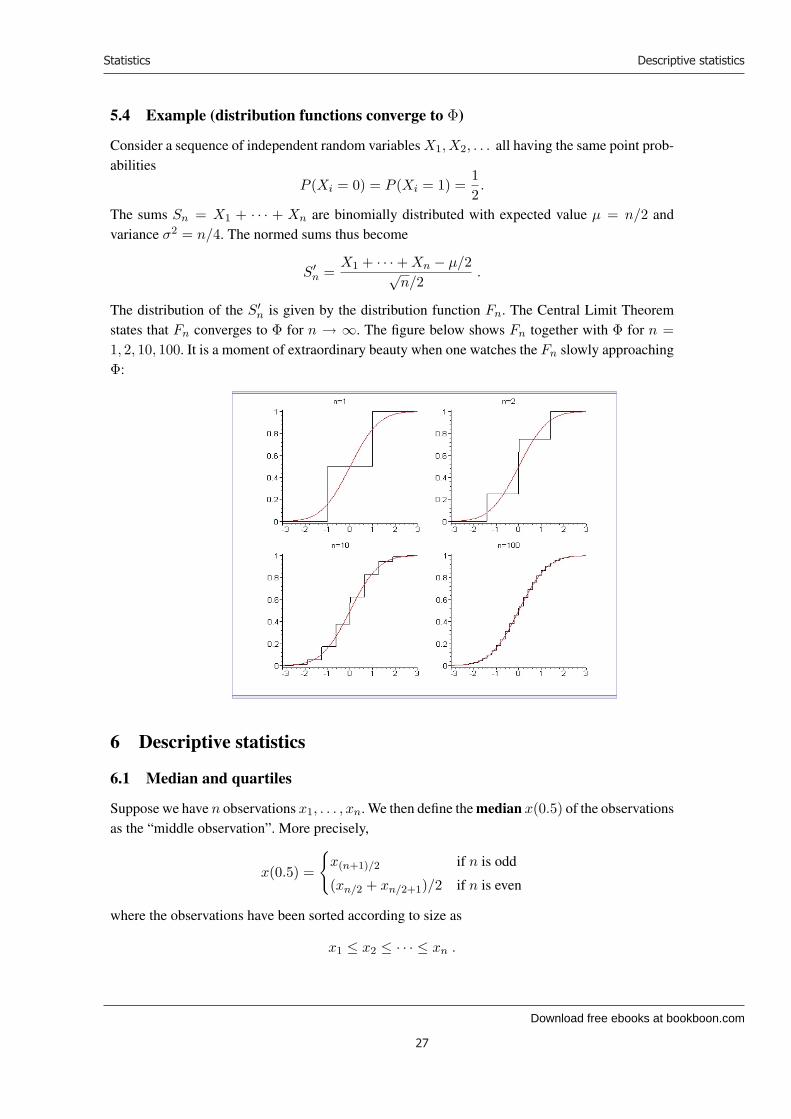
5.4 Example (distribution functions converge to Φ)
Consider a sequence of independent random variables X1, X2, . . . all having the same point prob-abilities
P (Xi = 0) = P (Xi = 1) =12.
The sums Sn = X1 + · · · + Xn are binomially distributed with expected value µ = n/2 andvariance σ2 = n/4. The normed sums thus become
S′n =
X1 + · · · + Xn − µ/2√n/2
.
The distribution of the S′n is given by the distribution function Fn. The Central Limit Theorem
states that Fn converges to Φ for n → ∞. The figure below shows Fn together with Φ for n =1, 2, 10, 100. It is a moment of extraordinary beauty when one watches the Fn slowly approachingΦ:
6 Descriptive statistics
6.1 Median and quartiles
Suppose we have n observations x1, . . . , xn. We then define the median x(0.5) of the observationsas the “middle observation”. More precisely,
x(0.5) =
x(n+1)/2 if n is odd
(xn/2 + xn/2+1)/2 if n is even
where the observations have been sorted according to size as
x1 ≤ x2 ≤ · · · ≤ xn .
27

Download free ebooks at bookboon.com
Ple
ase
clic
k th
e ad
vert
Statistics
28
Descriptive statistics
Similarly, the lower quartile x(0.25) is defined such that 25% of the observations lie belowx(0.25), and the upper quartile x(0.75) is defined such that 75% of the observations lie belowx(0.75).
The interquartile range is the distance between x(0.25) and x(0.75), i.e. x(0.75)−x(0.25).
6.2 Mean value
Suppose we have n observations x1, . . . , xn. We define the mean or mean value of the observa-tions as
x =∑n
i=1 xi
n
6.3 Empirical variance and empirical standard deviation
Suppose we have n observations x1, . . . , xn. We define the empirical variance of the observa-tions as
s2 =∑n
i=1(xi − x)2
n − 1.
A N N O N C E
28
Are you considering aEuropean business degree?LEARN BUSINESS at university level. We mix cases with cutting edge research working individually or in teams and everyone speaks English. Bring back valuable knowledge and experience to boost your career.
MEET a culture of new foods, music and traditions and a new way of studying business in a safe, clean environment – in the middle of Copenhagen, Denmark.
ENGAGE in extra-curricular activities such as case competitions, sports, etc. – make new friends among cbs’ 18,000 students from more than 80 countries.
See what we look likeand how we work on cbs.dk

Download free ebooks at bookboon.com
Statistics
29
Statistical hypothesis testing
The empirical standard deviation is the square root of the empirical variance:
s =
√∑ni=1(xi − x)2
n − 1.
The greater the empirical standard deviation s is, the more “dispersed” the observations are aroundthe mean value x.
6.4 Empirical covariance and empirical correlation coefficient
Suppose we have n pairs of observations (x1, y1), . . . , (xn, yn). We define the empirical covari-ance of these pairs as
Covemp =∑n
i=1(xi − x)(yi − y)n − 1
.
Alternatively, Covemp can be computed as
Covemp =∑n
i=1 xiyi − nxy
n − 1.
The empirical correlation coefficient is
r =empirical covariance
(empirical standard deviation of the x)(empirical standard deviation of the y)=
Covemp
sxsy.
The empirical correlation coefficient r always lies in the interval [−1, 1].
Understanding of the empirical correlation coefficient. If the x-observations are independent ofthe y-observations, then r will be equal or close to 0. If the x-observations and the y-observationsare dependent in such a way that large x-values usually correspond to large y-values, and viceversa, then r will be equal or close to 1. If the x-observations and the y-observations are dependentin such a way that large x-values usually correspond to small y-values, and vice versa, then r willbe equal or close to –1.
7 Statistical hypothesis testing
7.1 Null hypothesis and alternative hypothesis
A statistical test is a procedure that leads to either acceptance or rejection of a null hypothesisH0 given in advance. Sometimes H0 is tested against an explicit alternative hypothesis H1.
At the base of the test lie one or more observations. The null hypothesis (and the alternativehypothesis, if any) concern the question which distribution these observations were taken from.
7.2 Significance probability and significance level
One computes the significance probability P , that is the probability – if H0 is true – of obtainingan observation which is as extreme, or more extreme, than the one given. The smaller P is, theless plausible H0 is.
29

Download free ebooks at bookboon.com
Statistics
30
The binomial distribution Bin(n,p)
Often, one chooses a significance level α in advance, typically α = 5%. One then rejects H0
if P is smaller than α (and one says, “H0 is rejected at significance level α”). If P is greater thanα, then H0 is accepted (and one says, “H0 is accepted at significance level α” or “H0 cannot berejected at significance level α”).
7.3 Errors of type I and II
We speak about a type I error if we reject a true null hypothesis. If the significance level is α,then the risk of a type I error is at most α.
We speak about a type II error if we accept a false null hypothesis.The strength of a test is the probability of rejecting a false H0. The greater the strength, the
smaller the risk of a type II error. Thus, the strength should be as great as possible.
7.4 Example
Suppose we wish to investigate whether a certain dice is fair. By “fair” we here only understandthat the probability p of a six is 1/6. We test the null hypothesis
H0 : p =16
(the dice is fair)
against the alternative hypothesis
H1 : p >16
(the dice is biased)
The observations on which the test is carried out are the following ten throws of the dice:
2, 6, 3, 6, 5, 2, 6, 6, 4, 6 .
Let us in advance agree upon a significance level α = 5%. Now the significance probability P
can be computed. By “extreme observations” is understood that there are many sixes. Thus, P isthe probability of having at least five sixes in 10 throws with a fair dice. We compute
P =10∑
k=5
(10k
)(1/6)k(5/6)10−k = 0.015
(see section 8 on the binomial distribution). Since P = 1.5% is smaller than α = 5%, we rejectH0. If the same test was performed with a fair dice, the probability of committing a type I errorwould be 1.5%.
8 The binomial distribution Bin(n, p)
8.1 Parameters
n: number of triesp: probability of success
In the formulae we also use the “probability of failure” q = 1 − p.
30

Download free ebooks at bookboon.com
Ple
ase
clic
k th
e ad
vert
Statistics
31
The binomial distribution Bin(n,p)
8.2 Description
We carry out n independent tries that each result in either success or failure. In each try theprobability of success is the same, p. Consequently, the total number of successes X is binomiallydistributed, and we write X ∼ Bin(n, p). X is a discrete random variable and takes values in theset 0, 1, . . . , n.
8.3 Point probabilities
For k ∈ 0, 1, . . . , n, the point probabilities in a Bin(n, p) distribution are
P (X = k) =(
n
k
)· pk · qn−k .
See section 2.5 regarding the binomial coefficients
(n
k
).
EXAMPLE. If a dice is thrown twenty times, the total number of sixes, X , will be binomiallydistributed with parameters n = 20 and p = 1/6. We can list the point probabilities P (X = k)
A N N O N C E
31
www.simcorp.com
MITIGATE RISK REDUCE COST ENABLE GROWTH
The financial industry needs a strong software platformThat’s why we need you
SimCorp is a leading provider of software solutions for the financial industry. We work together to reach a common goal: to help our clients
succeed by providing a strong, scalable IT platform that enables growth, while mitigating risk and reducing cost. At SimCorp, we value
commitment and enable you to make the most of your ambitions and potential.
Are you among the best qualified in finance, economics, IT or mathematics?
Find your next challenge at www.simcorp.com/careers

Download free ebooks at bookboon.com
Statistics
32
The binomial distribution Bin(n,p)
and the cumulative probabilities P (X ≥ k) in a table (expressed as percentages):
k 0 1 2 3 4 5 6 7 8 9P (X = k) 2.6 10.4 19.8 23.8 20.2 12.9 6.5 2.6 0.8 0.2P (X ≥ k) 100 97.4 87.0 67.1 43.3 23.1 10.2 3.7 1.1 0.3
8.4 Expected value and variance
Expected value: E(X) = np.
Variance: var(X) = npq.
8.5 Significance probabilities for tests in the binomial distribution
We perform n independent experiments with the same probability of success p and count thenumber k of successes. We wish to test the null hypothesis H0 : p = p0 against an alternativehypothesis H1.
H0 H1 Significance probabilityp = p0 p > p0 P (X ≥ k)p = p0 p < p0 P (X ≤ k)p = p0 p = p0
∑l P (X = l)
where in the last line we sum over all l for which P (X = l) ≤ P (X = k).
EXAMPLE. A company buys a machine that produces microchips. The manufacturer of the ma-chine claims that at most one sixth of the produced chips will be defective. The first day themachine produces 20 chips of which 6 are defective. Can the company reject the manufacturer’sclaim on this background?
SOLUTION. We test the null hypothesis H0 : p = 1/6 against the alternative hypothesis H1 :p > 1/6. The significance probability can be computed as P (X ≥ 6) = 10.2% (see e.g. the tablein section 8.3). We conclude that the company cannot reject the manufacturer’s claim at the 5%level.
8.6 The normal approximation to the binomial distribution
If the parameter n (the number of tries) is large, a binomially distributed random variable X
will be approximately normally distributed with expected value µ = np and standard deviationσ =
√npq. Therefore, the point probabilities are approximately
P (X = k) ≈ ϕ
(k − np√
npq
)· 1√
npq
where ϕ is the density of the standard normal distribution, and the tail probabilities are approxi-mately
P (X ≤ k) ≈ Φ
(k + 1
2 − np√
npq
)
32
Download free ebooks at bookboon.com
Statistics
33
The binomial distribution Bin(n,p)
P (X ≥ k) ≈ 1 − Φ
(k − 1
2 − np√
npq
)
where Φ is the distribution function of the standard normal distribution (Table B.2).
Rule of thumb. One may use the normal approximation if np and nq are both greater than 5.
EXAMPLE (continuation of the example in section 8.5). After 2 weeks the machine has produced200 chips of which 46 are defective. Can the company now reject the manufacturer’s claim thatthe probability of defects is at most one sixth?
SOLUTION. Again we test the null hypothesis H0 : p = 1/6 against the alternative hypothesisH1 : p > 1/6. Since now np ≈ 33 and nq ≈ 167 are both greater than 5, we may use the normalapproximation in order to compute the significance probability:
P (X ≥ 46) ≈ 1 − Φ
(46 − 1
2 − 33.3√
27.8
)≈ 1 − Φ(2.3) ≈ 1.1%
Therefore, the company may now reject the manufacturer’s claim at the 5% level.
8.7 Estimators
Suppose k is an observation from a random variable X ∼ Bin(n, p) with known n and unknownp. The maximum likelihood estimate (ML estimate) of p is
p =k
n.
This estimator is unbiased (i.e. the expected value of the estimator is p) and has variance
var(p) =pq
n.
The expression for the variance is of no great practical value since it depends on the true (un-known) probability parameter p. If, however, one plugs in the estimated value p in place of p, onegets the estimated variance
p(1 − p)n
.
EXAMPLE. We consider again the example with the machine that has produced twenty microchipsof which the six are defective. What is the maximum likelihood estimate of the probability param-eter? What is the estimated variance?
SOLUTION. The maximum likelihood estimate is
p =620
= 30%
and the variance of p is estimated as
0.3 · (1 − 0.3)20
= 0.0105 .
33

Download free ebooks at bookboon.com
Ple
ase
clic
k th
e ad
vert
Statistics
34
The binomial distribution Bin(n,p)
The standard deviation is thus estimated to be√
0.0105 ≈ 0.10. If we presume that p lies withintwo standard deviations from p, we may conclude that p is between 10% and 50%.
8.8 Confidence intervals
Suppose k is an observation from a binomially distributed random variable X ∼ Bin(n, p) withknown n and unknown p. The confidence interval with confidence level 1 − α around the pointestimate p = k/n is
[p − u1−α/2
√p(1 − p)
n, p + u1−α/2
√p(1 − p)
n
].
Loosely speaking, the true value p lies in the confidence interval with the probability 1 − α.The number u1−α/2 is determined by Φ(u1−α/2) = 1 − α/2 where Φ is the distribution
function of the standard normal distribution. It appears e.g. from Table B.2 that with confidencelevel 95% one has
u1−α/2 = u0.975 = 1.96 .
EXERCISE. In an opinion poll from the year 2015, 62 out of 100 persons answer that they intendto vote for the Green Party at the next election. Compute the confidence interval with confidence
A N N O N C E
34
Download free ebooks at bookboon.com
Statistics
35
The Poisson distribution Pois(λ)
level 95% around the true percentage of Green Party voters.
SOLUTION. The point estimate is p = 62/100 = 0.62. A confidence level of 95% yields α =0.05. Looking up in the table (see above) gives u0.975 = 1.96. We get
1.96
√0.62 · 0.38
100= 0.10 .
The confidence interval thus becomes
[0.52 , 0.72] .
So we can say with a certainty of 95% that between 52% and 72% of the electorate will vote forthe Green Party at the next election.
9 The Poisson distribution Pois(λ)
9.1 Parameters
λ: Intensity
9.2 Description
Certain events are said to occur spontaneously, i.e. they occur at random times, independentlyof each other, but with a certain constant intensity λ. The intensity is the average number ofspontaneous events per time interval. The number of spontaneous events X in any given concretetime interval is then Poisson distributed, and we write X ∼ Pois(λ). X is a discrete randomvariable and takes values in the set 0, 1, 2, 3, . . . .
9.3 Point probabilities
For k ∈ 0, 1, 2, 3 . . . the point probabilities in a Pois(λ) distribution are
P (X = k) =λk
k!exp(−λ) .
Recall the convention 0! = 1.
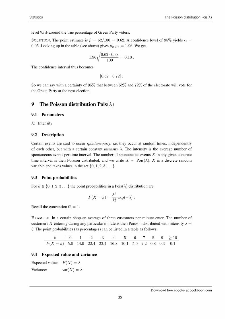
EXAMPLE. In a certain shop an average of three customers per minute enter. The number ofcustomers X entering during any particular minute is then Poisson distributed with intensity λ =3. The point probabilities (as percentages) can be listed in a table as follows:
k 0 1 2 3 4 5 6 7 8 9 ≥ 10P (X = k) 5.0 14.9 22.4 22.4 16.8 10.1 5.0 2.2 0.8 0.3 0.1
9.4 Expected value and variance
Expected value: E(X) = λ.
Variance: var(X) = λ.
35
Download free ebooks at bookboon.com
Statistics
36
The Poisson distribution Pois(λ)
9.5 Addition formula
Suppose that X1, . . . , Xn are independent Poisson distributed random variables. Let λi be theintensity of Xi, i.e. Xi ∼ Pois(λi). Then the sum
X = X1 + · · · + Xn
will be Poisson distributed with intensity
λ = λ1 + · · · + λn ,
i.e. X ∼ Pois(λ).
9.6 Significance probabilities for tests in the Poisson distribution
Suppose that k is an observation from a Pois(λ) distribution with unknown intensity λ. We wishto test the null hypothesis H0 : λ = λ0 against an alternative hypothesis H1.
H0 H1 Significance probabilityλ = λ0 λ > λ0 P (X ≥ k)λ = λ0 λ < λ0 P (X ≤ k)λ = λ0 λ = λ0
∑l P (X = l)
where the summation in the last line is over all l for which P (X = l) ≤ P (X = k).If n independent observations k1, . . . , kn from a Pois(λ) distribution are given, we can treat
the sum k = k1 + · · · + kn as an observation from a Pois(n · λ) distribution.
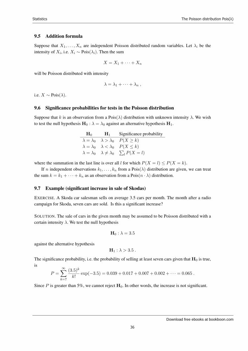
9.7 Example (significant increase in sale of Skodas)
EXERCISE. A Skoda car salesman sells on average 3.5 cars per month. The month after a radiocampaign for Skoda, seven cars are sold. Is this a significant increase?
SOLUTION. The sale of cars in the given month may be assumed to be Poisson distributed with acertain intensity λ. We test the null hypothesis
H0 : λ = 3.5
against the alternative hypothesisH1 : λ > 3.5 .
The significance probability, i.e. the probability of selling at least seven cars given that H0 is true,is
P =∞∑
k=7
(3.5)k
k!exp(−3.5) = 0.039 + 0.017 + 0.007 + 0.002 + · · · = 0.065 .
Since P is greater than 5%, we cannot reject H0. In other words, the increase is not significant.
36

Download free ebooks at bookboon.com
Ple
ase
clic
k th
e ad
vert
Statistics
37
The Poisson distribution Pois(λ)
9.8 The binomial approximation to the Poisson distribution
The Poisson distribution with intensity λ is the limit distribution of the binomial distribution withparameters n and p = λ/n when n tends to ∞. In other words, the point probabilities satisfy
P (Xn = k) → P (X = k) for n → ∞
for X ∼ Pois(λ) and Xn ∼ Bin(n, λ/n). In real life, however, one almost always prefers to usethe normal approximation instead (see the next section).
9.9 The normal approximation to the Poisson distribution
If the intensity λ is large, a Poisson distributed random variable X will to a good approximationbe normally distributed with expected value µ = λ and standard deviation σ =
√λ. The point
probabilities therefore are
P (X = k) ≈ ϕ
(k − λ√
λ
)· 1√
λ
where ϕ(x) is the density of the standard normal distribution, and the tail probabilities are
P (X ≤ k) ≈ Φ
(k + 1
2 − λ√
λ
)
A N N O N C E
37
Do you want your Dream Job?
More customers get their dream job by using RedStarResume than any other resume service.
RedStarResume can help you with your job application and CV.
Go to: Redstarresume.com
Use code “BOOKBOON” and save up to $15
(enter the discount code in the “Discount Code Box”)

Download free ebooks at bookboon.com
Statistics
38
The Poisson distribution Pois(λ)
P (X ≥ k) ≈ 1 − Φ
(k − 1
2 − λ√
λ
)
where Φ is the distribution function of the standard normal distribution (Table B.2).
Rule of thumb. The normal approximation to the Poisson distribution applies if λ is greater thannine.
9.10 Example (significant decrease in number of complaints)
EXERCISE. The ferry Deutschland between Rødby and Puttgarten receives an average of 180complaints per week. In the week immediately after the ferry’s cafeteria was closed, only 112complaints are received. Is this a significant decrease?
SOLUTION. The number of complaints within the given week may be assumed to be Poissondistributed with a certain intensity λ. We test the null hypothesis
H0 : λ = 180
against the alternative hypothesisH1 : λ < 180 .
The significance probability, i.e. the probability of having at most 112 complaints given H0, canbe approximated by the normal distribution:
P = Φ
(112 + 1
2 − 180√
180
)= Φ(−5.03) < 0.0001 .
Since P is very small, we can clearly reject H0. The number of complaints has significantlydecreased.
9.11 Estimators
Suppose k1, . . . kn are independent observations from a random variable X ∼ Pois(λ) with un-known intensity λ. The maximum likelihood estimate (ML estimate) of λ is
λ = (k1 + · · · + kn)/n .
This estimator is unbiased (i.e. the expected value of the estimator is λ) and has variance
var(λ) =λ
n.
More precisely, we havenλ ∼ Pois(nλ) .
If we plug in the estimated value λ in λ’s place, we get the estimated variance
var(λ) =λ
n.
38
Download free ebooks at bookboon.com
Statistics
39
The geometrical distribution Geo(p)
9.12 Confidence intervals
Suppose k1, . . . , kn are independent observations from a Poisson distributed random variable X ∼Pois(λ) with unknown λ. The confidence interval with confidence level 1 − α around the pointestimate λ = (k1 + · · · + kn)/n is
λ − u1−α/2
√λ
n, λ + u1−α/2
√λ
n
.
Loosely speaking, the true value λ lies in the confidence interval with probability 1 − α.The number u1−α/2 is determined by Φ(u1−α/2) = 1 − α/2, where Φ is the distribution
function of the standard normal distribution. It appears from, say, Table B.2 that
u1−α/2 = u0.975 = 1.96
for confidence level 95%.
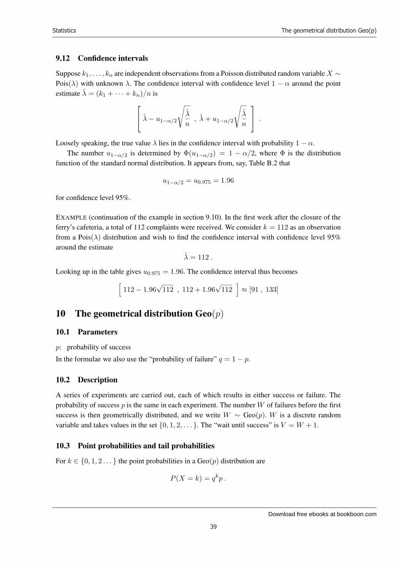
EXAMPLE (continuation of the example in section 9.10). In the first week after the closure of theferry’s cafeteria, a total of 112 complaints were received. We consider k = 112 as an observationfrom a Pois(λ) distribution and wish to find the confidence interval with confidence level 95%around the estimate
λ = 112 .
Looking up in the table gives u0.975 = 1.96. The confidence interval thus becomes[
112 − 1.96√
112 , 112 + 1.96√
112]≈ [91 , 133]
10 The geometrical distribution Geo(p)
10.1 Parameters
p: probability of success
In the formulae we also use the “probability of failure” q = 1 − p.
10.2 Description
A series of experiments are carried out, each of which results in either success or failure. Theprobability of success p is the same in each experiment. The number W of failures before the firstsuccess is then geometrically distributed, and we write W ∼ Geo(p). W is a discrete randomvariable and takes values in the set 0, 1, 2, . . . . The “wait until success” is V = W + 1.
10.3 Point probabilities and tail probabilities
For k ∈ 0, 1, 2 . . . the point probabilities in a Geo(p) distribution are
P (X = k) = qkp .
39

Download free ebooks at bookboon.com
Ple
ase
clic
k th
e ad
vert
Statistics
40
The geometrical distribution Geo(p)
In contrast to most other distributions, we can easily compute the tail probabilities in the geomet-rical distribution:
P (X ≥ k) = qk .
EXAMPLE. Pin diagram for the point probabilities in a geometrical distribution with probabilityof success p = 0.5:
A N N O N C E
40
0.5
0.4
0.3
0.2
0.1
0 1 2 3 4 5 6
P(X=k)
k
Challenging? Not challenging? Try more
Try this...
www.alloptions.nl/life

Download free ebooks at bookboon.com
Statistics
41
The hypergeometrical distribution HG(n,r,N)
10.4 Expected value and variance
Expected value: E(W ) = q/p.
Variance: var(W ) = q/p2.
Regarding the “wait until success” V = W + 1, we have the following useful rule:
Rule. The expected wait until success is the reciprocal probability of success: E(V ) = 1/p.
EXAMPLE. A gambler plays lotto each week. The probability of winning in lotto, i.e. the proba-bility of guessing correctly seven numbers picked randomly from a pool of 36 numbers, is
p =(
367
)−1
≈ 0.0000001198 .
The expected wait until success is thus
E(V ) = p−1 =(
367
)weeks = 160532 years .
11 The hypergeometrical distribution HG(n, r, N)
11.1 Parameters
r: number of red balls
s: number of black balls
N : total number of balls (N = r + s)
n: number of balls picked out (n ≤ N )
11.2 Description
In an urn we have r red balls and s black balls, in total N = r + s balls. We now pick outn balls from the urn, randomly and without returning the chosen balls to the urn. Necessarilyn ≤ N . The number of red balls Y amongst the balls chosen is then hypergeometrically dis-tributed and we write Y ∼ HG(n, r, N). Y is a discrete random variable with values in the set0, 1, . . . ,minn, r.
11.3 Point probabilities and tail probabilities
For k ∈ 0, 1, . . . ,minn, r the point probabilities of a HG(n, r,N) distribution are
P (Y = k) =
(r
k
)·
(s
n − k
)
(N
n
) .
41

Download free ebooks at bookboon.com
Statistics
42
The hypergeometrical distribution HG(n,r,N)
EXAMPLE. A city council has 25 members of which 13 are Conservatives. A cabinet is formed bypicking five council members at random. What is the probability that the Conservatives will haveabsolute majority in the cabinet?
SOLUTION. We have here a hypergeometrically distributed random variable Y ∼ HG(5, 13, 25)and have to compute P (Y ≥ 3). Let us first compute all point probabilities (as percentages):
k 0 1 2 3 4 5P (Y = k) 1.5 12.1 32.3 35.5 16.1 2.4
The sought-after probability thus becomes
P (Y ≥ 3) = 35.5% + 16.1% + 2.4% = 54.0%
11.4 Expected value and variance
Expected value: E(Y ) = nr/N .
Variance: var(Y ) = nrs(N − n)/(N2(N − 1)).
11.5 The binomial approximation to the hypergeometrical distribution
If the number of balls picked out, n, is small compared to both the number of red balls r and thenumber of black balls s, it becomes irrelevant whether the balls picked out are returned to the urnor not. We can thus approximate the hypergeometrical distribution by the binomial distribution:
P (Y = k) ≈ P (X = k)
for Y ∼ HG(n, r, N) and X ∼ Bin(n, r/N). In practice, this approximation is of little valuesince it is as difficult to compute P (X = k) as P (Y = k).
11.6 The normal approximation to the hypergeometrical distribution
If n is small compared to both r and s, the hypergeometrical distribution can be approximated bythe normal distribution with the same expected value and variance.
The point probabilities thus become
P (Y = k) ≈ ϕ
k − nr/N√
nrs(N − n)/(N2(N − 1))
· 1√
nrs(N − n)/(N2(N − 1))
where ϕ is the density of the standard normal distribution. The tail probabilities become
P (Y ≤ k) ≈ Φ
k + 1
2 − nr/N√nrs(N − n)/(N2(N − 1))
42
Download free ebooks at bookboon.com
Ple
ase
clic
k th
e ad
vert
Statistics
43
The multinomial distribution Mult(n, p1,...pr)
P (Y ≥ k) ≈ 1 − Φ
k − 1
2 − nr/N√nrs(N − n)/(N2(N − 1))
where Φ is the distribution function of the standard normal distribution (Table B.2).
12 The multinomial distribution Mult(n, p1, . . . , pr)
12.1 Parameters
n: number of triesp1: 1st probability parameter...pr: rth probability parameter
It is required that p1 + · · · + pr = 1.
12.2 Description
We carry out n independent experiments each of which results in one out of r possible outcomes.The probability of obtaining an outcome of type i is the same in each experiment, namely pi. Let
A N N O N C E
43
Download free ebooks at bookboon.com
Statistics
44
The negative binomial distribution NB(n,p)
Si denote the total number of outcomes of type i. The random vector S = (S1, . . . , Sr) is thenmultinomially distributed and we write S ∼ Mult(n, p1, . . . , pr). S is discrete and takes values inthe set (k1, . . . kr) ∈ Zr | ki ≥ 0 , k1 + · · · + kr = n.
12.3 Point probabilities
For k1 + · · · + kr = n the point probabilities of a Mult(n, p1, . . . , pr) distribution are
P (S = (k1, . . . , kr)) =
(n
k1 · · · kr
)·
r∏i=1
pkii
EXAMPLE. Throw a dice six times and, for each i, let Si be the total number of i’s. ThenS = (S1, . . . , S6) is a multinomially distributed random vector: S ∼ Mult(6, 1/6, . . . , 1/6).The probability of obtaining, say, exactly one 1, two 2s, and three sixes is
P (S = (1, 2, 0, 0, 0, 3)) =
(6
1 2 0 0 0 3
)· (1/6)1 · (1/6)2 · (1/6)3 ≈ 0.13%
Here, the multinomial coefficient (see also section 2.6) is computed as(
61 2 0 0 0 3
)=
6!1!2!0!0!0!3!
=72012
= 60 .
12.4 Estimators
Suppose k1, . . . , kr is an observation from a random vector S ∼ Mult(n, p1, . . . , pr) with knownn and unknown pi. The maximum likelihood estimate of pi is
pi =ki
n.
This estimator is unbiased (i.e. the estimator’s expected value is pi) and has variance
var(pi) =pi(1 − pi)
n.
13 The negative binomial distribution NB(n, p)
13.1 Parameters
n: number of tries
p: probability of success
In the formulae we also use the letter q = 1 − p.
44
Download free ebooks at bookboon.com
Statistics
45
The exponential distribution (λ)
13.2 Description
A series of independent experiments are carried out each of which results in either success orfailure. The probability of success p is the same in each experiment. The total number X of failuresbefore the n’th success is then negatively binomially distributed and we write X ∼ NB(n, p). Therandom variable X is discrete and takes values in the set 0, 1, 2, . . . .
The geometrical distribution is the special case n = 1 of the negative binomial distribution.
13.3 Point probabilities
For k ∈ 0, 1, 2 . . . the point probabilities of a NB(k, p) distribution are
P (X = k) =(
n + k − 1n − 1
)· pn · qk .
13.4 Expected value and variance
Expected value: E(X) = nq/p.
Variance: var(X) = nq/p2.
13.5 Estimators
The negative binomial distribution is sometimes used as an alternative to the Poisson distributionin situations where one wishes to describe a random variable taking values in the set 0, 1, 2, . . . .
Suppose k1, . . . , km are independent observations from a NB(n, p) distribution with unknownparameters n and p. We then have the following estimators:
n =k2
s2 − k, p =
k
s2
where k and s2 are the mean value and empirical variance of the observations.
14 The exponential distribution Exp(λ)
14.1 Parameters
λ: Intensity
14.2 Description
In a situation where events occur spontaneously with the intensity λ (and where the number ofspontaneous events in any given time interval thus is Pois(λ) distributed), the wait T betweentwo spontaneous events is exponentially distributed and we write T ∼ Exp(λ). T is a continuousrandom variable taking values in the interval [0,∞[.
45

Download free ebooks at bookboon.com
Ple
ase
clic
k th
e ad
vert
Statistics
46
The normal distribution
14.3 Density and distribution function
The density of the exponential distribution is
f(x) = λ · exp(−λx) .
The distribution function isF (x) = 1 − exp(−λx) .
14.4 Expected value and variance
Expected value: E(T ) = 1/λ.
Variance: var(T ) = 1/λ2.
15 The normal distribution
15.1 Parameters
µ: expected value
σ2: variance
Remember that the standard deviation σ is the square root of the variance.
A N N O N C E
46
Stand out from the crowdDesigned for graduates with less than one year of full-time postgraduate work experience, London Business School’s Masters in Management will expand your thinking and provide you with the foundations for a successful career in business.
The programme is developed in consultation with recruiters to provide you with the key skills that top employers demand. Through 11 months of full-time study, you will gain the business knowledge and capabilities to increase your career choices and stand out from the crowd.
Applications are now open for entry in September 2011.
For more information visit www.london.edu/mim/ email [email protected] or call +44 (0)20 7000 7573
Masters in Management
London Business SchoolRegent’s ParkLondon NW1 4SAUnited KingdomTel +44 (0)20 7000 7573Email [email protected]/mim/
Fast-track your career
Download free ebooks at bookboon.com
Statistics
47
The normal distribution
15.2 Description
The normal distribution is a continuous distribution. If a random variable X is normally distribut-ed, then X can take any values in R and we write X ∼ N(µ, σ2).
The normal distribution is the most important distribution in all of statistics. Countless natu-rally occurring phenomena can be described (or approximated) by means of a normal distribution.
15.3 Density and distribution function
The density of the normal distribution is the function
f(x) =1√
2πσ2exp
(−(x − µ)2
2σ2
).
It is symmetric, i.e.f(−x) = f(x) .
The distribution function of the normal distribution
F (x) =∫ x
−∞
1√2πσ2
exp(−(t − µ)2
2σ2
)dt
is difficult to compute. Instead, one uses the formula
F (x) = Φ(
x − µ
σ
)
where Φ is the distribution function of the standard normal distribution which can be looked up inTable B.2. From the table the following fact appears:
Fact: In a normal distribution, about 68% of the probability mass lies within one standard devi-ation from the expected value, and about 95% of the probability mass lies within two standarddeviations from the expected value.
15.4 The standard normal distribution
A normal distribution with expected value µ = 0 and variance σ2 = 1 is called a standard normaldistribution. The standard deviation in a standard normal distribution equals 1 (obviously). Thedensity ϕ(t) of a standard normal distribution is
ϕ(t) =1√2π
exp(−1
2t2
).
The distribution function Φ of a standard normal distribution is
Φ(x) =∫ x
−∞
1√2π
exp(−1
2t2
)dt .
On can look up Φ in Table B.2.
47
Download free ebooks at bookboon.com
Statistics
48
The normal distribution
15.5 Properties of Φ
The distribution function Φ of a standard normally distributed random variable X ∼ N(0, 1)satisfies
P (X ≤ x) = Φ(x)
P (X ≥ x) = Φ(−x)
P (|X| ≤ x) = Φ(x) − Φ(−x)
P (|X| ≥ x) = 2 · Φ(−x)
Φ(−x) = 1 − Φ(x)
15.6 Estimation of the expected value µ
Suppose x1, x2, . . . , xn are independent observations of a random variable X ∼ N(µ, σ2). Themaximum likelihood estimate (ML estimate) of µ is
µ =x1 + · · · + xn
n.
This is simply the mean value and is written x. The mean value is an unbiased estimator of µ (i.e.the estimator’s expected value is µ). The variance of the mean value is
var2(x) =σ2
n.
More precisely, x is itself normally distributed:
x ∼ N(µ,σ2
n) .
15.7 Estimation of the variance σ2
Suppose x1, . . . , xn are independent observations of a random variable X ∼ N(µ, σ2). Normally,the variance σ2 is estimated by the empirical variance
s2 =∑
(xi − x)2
n − 1.
The empirical variance s2 is an unbiased estimator of the true variance σ2.
Warning: The empirical variance is not the maximum likelihood estimate of σ2. The maximumlikelihood estimate of σ2 is ∑
(xi − x)2
n
but this is seldom used since it is biased and usually gives estimates which are too small.
48

Download free ebooks at bookboon.com
Ple
ase
clic
k th
e ad
vert
Statistics
49
The normal distribution
15.8 Confidence intervals for the expected value µ
Suppose x1, . . . , xn are independent observations of a normally distributed random variable X ∼N(µ, σ2) and that we wish to estimate the expected value µ. If the variance σ2 is known, theconfidence interval for µ with confidence level 1 − α is as follows:
[x − u1−α/2
σ√n
, x + u1−α/2σ√n
].
The number u1−α/2 is determined by Φ(u1−α/2) = 1 − α/2 where Φ is the distribution functionof the standard normal distribution. It appears from, say, Table B.2 that
u1−α/2 = u0.975 = 1.96
for confidence level 95%.If the variance σ2 is unknown, the confidence interval for µ with confidence level 1 − α is
[x − t1−α/2(n − 1)
√s2
n, x + t1−α/2(n − 1)
√s2
n
]
where s2 is the empirical variance (section 6.3). The number t1−α/2 is determined by F (u1−α/2) =1 − α/2, where F is the distribution function of Student’s t distribution with n − 1 degrees of
A N N O N C E
49
© U
BS
2010
. All
rig
hts
res
erve
d.
www.ubs.com/graduates
Looking for a career where your ideas could really make a difference? UBS’s
Graduate Programme and internships are a chance for you to experience
for yourself what it’s like to be part of a global team that rewards your input
and believes in succeeding together.
Wherever you are in your academic career, make your future a part of ours
by visiting www.ubs.com/graduates.
You’re full of energyand ideas. And that’s just what we are looking for.

Download free ebooks at bookboon.com
Statistics
50
Distribution connected with the normal distribution
freedom. It appears from, say, Table B.4 that
n 2 3 4 5 6 7 8 9 10 11 12t1−α/2 12.7 4.30 3.18 2.78 2.57 2.45 2.36 2.31 2.26 2.23 2.20
for confidence level 95%.
15.9 Confidence intervals for the variance σ2 and the standard deviation σ
Suppose x1, . . . , xn are independent observations of a normally distributed random variable X ∼N(µ, σ2). The confidence interval for the variance σ2 with confidence level 1 − α is:
[(n − 1)s2
χ2α/2
,(n − 1)s2
χ21−α/2
]
where s2 is the empirical variance (section 6.3). The numbers χ2α/2 and χ2
1−α/2 are determinedby F (χ2
α/2) = α/2 and F (χ21−α/2) = 1 − α/2 where F is the distribution function of the χ2
distribution with n − 1 degrees of freedom (Table B.3).Confidence intervals for the standard deviation σ with confidence level 1 − α are computed
simply by taking the square root of the limits of the confidence intervals for the variance:[ √
(n − 1)s2
χ2α/2
,
√(n − 1)s2
χ21−α/2
]
15.10 Addition formula
A linear function of a normally distributed random variable is itself normally distributed. If, inother words, X ∼ N(µ, σ2) and a, b ∈ R (a = 0), then
aX + b ∼ N(aµ + b, a2σ2) .
The sum of independent normally distributed random variables is itself normally distributed.If, in other words, X1, . . . , Xn are independent with Xi ∼ N(µi, σ
2i ), then we have the addition
formulaX1 + · · · + Xn ∼ N(µ1 + · · · + µn, σ2
1 + · · · + σ2n) .
16 Distributions connected with the normal distribution
16.1 The χ2 distribution
Let X1, . . . , Xn ∼ N(0, 1) be independent standard normally distributed random variables. Thedistribution of the sum of squares
Q = X21 + · · · + X2
n
is called the χ2 distribution with n degrees of freedom. The number of degrees of freedom iscommonly symbolized as df .
50

Download free ebooks at bookboon.com
Statistics
51
Distribution connected with the normal distribution
A χ2 distributed random variable Q with df degrees of freedom has expected value
E(Q) = df
and variancevar(Q) = 2 · df .
The density of the χ2 distribution is
f(x) = K · xdf2−1 · e−
x2
where df is the number of degrees of freedom and K is a constant. In practice, one doesn’t usethe density, but rather looks up the distribution function in Table B.3. The graph below shows thedensity function with df = 1, 4, 10, 20 degrees of freedom.
16.2 Student’s t distribution
Let X be a normally distributed random variable with expected value µ and variance σ2. Let therandom variables X and S2 be the mean value and empirical variance, respectively, of a sampleconsisting of n observations from X . The distribution of
T =X − µ√
S2/n
is then independent of both µ and σ2 and is called Student’s t distribution with n− 1 degrees offreedom.
A t distributed random variable T with df degrees of freedom has expected value
E(T ) = 0
for df ≥ 2, and variance
var(T ) =df
df − 2
for df ≥ 3.The density of the t distribution is
f(x) = K ·(
1 +x2
df
)−(df+1)/2
51
df=1
df=4
df=10
df=20

Download free ebooks at bookboon.com
Ple
ase
clic
k th
e ad
vert
Statistics
52
Distribution connected with the normal distribution
where df is the number of degrees of freedom and K is a constant. In practice, one doesn’t usethe density, but rather looks up the distribution function in Table B.4. The graph below showsthe density of the t distribution with df = 1, 2, 3 degrees of freedom and additionally the densityϕ(x) of the standard normal distribution. As it appears, the t distribution approaches the standardnormal distribution when df → ∞.
16.3 Fisher’s F distribution
Let X1 and X2 be independent normally distributed random variables with the same variance. Fori = 1, 2 let the random variable S2
i be the empirical variance of a sample of size ni from Xi. The
A N N O N C E
52
df=3
df=2
df=1
(x)ϕ
© Deloitte & Touche LLP and affiliated entities.
360°thinking.
Discover the truth at www.deloitte.ca/careers
© Deloitte & Touche LLP and affiliated entities.
360°thinking.
Discover the truth at www.deloitte.ca/careers
© Deloitte & Touche LLP and affiliated entities.
360°thinking.
Discover the truth at www.deloitte.ca/careers © Deloitte & Touche LLP and affiliated entities.
360°thinking.
Discover the truth at www.deloitte.ca/careers
Download free ebooks at bookboon.com
Statistics
53
Tests in the normal distribution
distribution of the quotient
V =S2
1
S22
is called Fisher’s F distribution with n1 − 1 degrees of freedom in the numerator and n2 − 1degrees of freedom in the denominator.
The density of the F distribution is
f(x) = K · xdf1/2−1
(df2 + df1x)df/2
where K is a constant, df1 the number of degrees of freedom in the numerator, df2 the numberof degrees of freedom in the denominator, and df = df1 + df2. In practice, one doesn’t use thedensity, but rather looks up the distribution function in Table B.5.
17 Tests in the normal distribution
17.1 One sample, known variance, H0 : µ = µ0
Let there be given a sample x1, . . . , xn of n independent observations from a normal distributionwith unknown expected value µ and known variance σ2. We wish to test the null hypothesis
H0 : µ = µ0 .
For this purpose, we compute the statistic
u =√
n(x − µ0)σ
=∑n
i=1 xi − nµ0√nσ2
.
The significance probability now appears from the following table, where Φ is the distributionfunction of the standard normal distribution (Table B.2).
Alternative Significancehypothesis probability
H1 : µ > µ0 Φ(−u)H1 : µ < µ0 Φ(u)H1 : µ = µ0 2 · Φ(−|u|)
Normally, we reject H0 if the significance probability is less than 5%.
17.2 One sample, unknown variance, H0 : µ = µ0 (Student’s t test)
Let there be given a sample x1, . . . , xn of n independent observations from a normal distributionwith unknown expected value µ and unknown variance σ2. We wish to test the null hypothesis
H0 : µ = µ0 .
For this purpose, we compute the statistic
t =√
n(x − µ0)s
=∑n
i=1 xi − nµ0√n · s2
,
53

Download free ebooks at bookboon.com
Statistics
54
Tests in the normal distribution
where s2 is the empirical variance (see section 6.3).The significance probability now appears from the following table where FStudent is the dis-
tribution function of Student’s t distribution with df = n − 1 degrees of freedom (Table B.4).
Alternative Significancehypothesis probabilityH1 : µ > µ0 1 − FStudent(t)H1 : µ < µ0 1 − FStudent(−t)H1 : µ = µ0 2 · (1 − FStudent(|t|))
Normally, we reject H0 if the significance probability is less than 5%.
EXAMPLE. The headmaster of a school wishes to confirm statistically that his students have per-formed significantly miserably in the 2008 final exams. For this purpose, n = 10 students arepicked at random. Their final scores are
x1 x2 x3 x4 x5 x6 x7 x8 x9 x10
7.6 7.7 7.5 5.8 5.7 7.9 5.4 6.7 7.9 9.4
The national average for 2008 is 8.27. It is reasonable to assume that the final scores are normallydistributed. However, the variance is unknown. Therefore, we apply Student’s t test to test the nullhypothesis
H0 : µ = 8.27
against the alternative hypothesisH1 : µ < 8.27 .
We compute the mean value of the observations as x = 7.17 and the empirical standard deviationas s = 1.26. We obtain the statistic
t =√
10(7.17 − 8.27)1.26
= −2.76 .
Looking up in Table B.4 under df = n−1 = 9 degrees of freedom gives a significance probability
1 − FStudent(−t) = 1 − FStudent(2.76)
between 1% and 2.5%. We may therefore reject H0 and confirm the headmaster’s assumption thathis students have performed significantly poorer than the rest of the country.
17.3 One sample, unknown expected value, H0 : σ2 = σ20
THEOREM. Let there be given n independent observations x1, . . . , xn from a normal distributionwith variance σ2. The statistic
q =(n − 1)s2
σ2=
∑ni=1(xi − x)2
σ2
is then χ2 distributed with df = n − 1 degrees of freedom (here s2 is the empirical variance).
54

Download free ebooks at bookboon.com
Ple
ase
clic
k th
e ad
vert
Statistics
55
Tests in the normal distribution
Let there be given a sample x1, . . . , xn of n independent observations from a normal distributionwith unknown expected value µ and unknown variance σ2. We wish to test the null hypothesis
H0 : σ2 = σ20 .
For this purpose, we compute the statistic
q =(n − 1)s2
σ20
=∑n
i=1(xi − x)2
σ20
where s2 is the empirical variance.The significance probability can now be read from the following table where Fχ2 is the distri-
bution function of the χ2 distribution with df = n − 1 degrees of freedom (Table B.3).
Alternative Significancehypothesis probabilityH1 : σ2 > σ2
0 1 − Fχ2(q)H1 : σ2 < σ2
0 Fχ2(q)H1 : σ2 = σ2
0 2 · minFχ2(q), 1 − Fχ2(q)
Normally, H0 is rejected if the significance probability is smaller than 5%.
Note: In practice, we always test against the alternative hypothesis H1 : σ2 > σ20 .
A N N O N C E
55

Download free ebooks at bookboon.com
Statistics
56
Tests in the normal distribution
17.4 Example
Consider the following twenty observations originating from a normal distribution with unknownexpected value and variance:
91 97 98 112 91 97 116 108 108 100107 98 92 103 100 99 98 104 104 97
We wish to test the null hypothesis
H0: the standard deviation is at most 5 (i.e. the variance is at most 25)
against the alternative hypothesis
H1: the standard deviation is greater than 5 (i.e. the variance is greater than 25).
The empirical variance is found to be s2 = 45.47 and we thus find the statistic
q =(20 − 1) · 45.47
52= 34.56 .
By looking up in Table B.3 under df = 19 degrees of freedom, we find a significance probabilityaround 2%. We can thus reject H0.
(Actually, the observations came from a normal distribution with expected value µ = 100 andstandard deviation σ = 6. The test is thus remarkably sensitive.)
17.5 Two samples, known variances, H0 : µ1 = µ2
Let there be given a sample x1, . . . , xn from a normal distribution with unknown expected valueµ1 and known variance σ2
1 . Let there in addition be given a sample y1, . . . , ym from a normaldistribution with unknown expected value µ2 and known variance σ2
2 . It is assumed that the twosamples are independent of each other.
We wish to test the null hypothesis
H0 : µ1 = µ2 .
For this purpose, we compute the statistic
u =x − y√
σ21/n + σ2
2/m.
The significance probability is read from the following table where Φ is the distribution functionof the standard normal distribution (Table B.3).
Alternative Significancehypothesis probabilityH1 : µ1 > µ2 Φ(−u)H1 : µ1 < µ2 Φ(u)H1 : µ1 = µ2 2 · Φ(−|u|)
Normally, we reject H0 if the significance probability is smaller than 5%.
Note: In real life, the preconditions of this test are rarely met.
56

Download free ebooks at bookboon.com
Statistics
57
Tests in the normal distribution
17.6 Two samples, unknown variances, H0 : µ1 = µ2 (Fisher-Behrens)
Let the situation be as in section 17.5, but suppose that the variances σ21 and σ2
2 are unknown. Theproblem of finding a suitable statistic to test the null hypothesis
H0 : µ1 = µ2
is called the Fisher-Behrens problem and has no satisfactory solution.If n, m > 30, one can re-use the test from section 17.5 with the alternative statistic
u∗ =x − y√
s21/n + s2
2/m
where s21 and s2
2 are the empirical variances of the x’s and y’s, respectively.
17.7 Two samples, unknown expected values, H0 : σ21 = σ2
2
Let there be given a sample x1, . . . , xn from a normal distribution with unknown expected valueµ1 and unknown variance σ2
1 . In addition, let there be given a sample y1, . . . , ym from a normaldistribution with unknown expected value µ2 and unknown variance σ2
2 . It is assumed that thetwo samples are independent of each other.
We wish to test the null hypothesis
H0 : σ1 = σ2 .
For this purpose, we compute the statistic
v =s21
s22
=empirical variance of the x’sempirical variance of the y’s
.
Further, put
v∗ = max
v,1v
.
The significance probability now appears from the following table where FFisher is the distributionfunction of Fisher’s F distribution with n − 1 degrees of freedom in the numerator and m − 1degrees of freedom in the denominator (Table B.5).
Alternative Significancehypothesis probabilityH1 : σ2
1 > σ22 1 − FFisher(v)
H1 : σ21 < σ2
2 1 − FFisher(1/v)H1 : σ2
1 = σ22 2 · (1 − FFisher(v∗))
Normally, H0 is rejected if the significance probability is smaller than 5%.If H0 is accepted, the common variance σ2
1 = σ22 is estimated by the “pooled” variance
s2pool =
∑ni=1(xi − x)2 +
∑mi=1(yi − y)2
n + m − 2=
(n − 1)s21 + (m − 1)s2
2
n + m − 2.
57

Download free ebooks at bookboon.com
Ple
ase
clic
k th
e ad
vert
Statistics
58
Tests in the normal distribution
17.8 Two samples, unknown common variance, H0 : µ1 = µ2
Let there be given a sample x1, . . . , xn from a normal distribution with unknown expected valueµ1 and unknown variance σ2. In addition, let there be given a sample y1, . . . , ym from a normaldistribution with unknown expected value µ2 and the same variance σ2. It is assumed that thetwo samples are independent of each other.
We wish to test the null hypothesis
H0 : µ1 = µ2 .
For this purpose, we compute the statistic
t =x − y√
(1/n + 1/m)s2pool
where s2pool is the “pooled” variance as given in section 17.7.
The significance probability now appears from the following table where FStudent is the dis-
A N N O N C E
58
your chance to change the worldHere at Ericsson we have a deep rooted belief that the innovations we make on a daily basis can have a profound effect on making the world a better place for people, business and society. Join us.
In Germany we are especially looking for graduates as Integration Engineers for • Radio Access and IP Networks• IMS and IPTV
We are looking forward to getting your application!To apply and for all current job openings please visit our web page: www.ericsson.com/careers

Download free ebooks at bookboon.com
Statistics
59
Tests in the normal distribution
tribution function of Student’s t distribution with n + m − 2 degrees of freedom (Table B.4).
Alternative Significancehypothesis probabilityH1 : µ1 > µ2 1 − FStudent(t)H1 : µ1 < µ2 1 − FStudent(−t)H1 : µ1 = µ2 2 · (1 − FStudent(|t|))
Normally, H0 is rejected if the significance probability is smaller than 5%.
17.9 Example (comparison of two expected values)
Suppose we are given seven independent observations from a normally distributed random vari-able X:
x1 = 26 , x2 = 21 , x3 = 15 , x4 = 7 , x5 = 15 , x6 = 28 , x7 = 21
and also four independent observations from a normally distributed random variable Y :
y1 = 29 , y2 = 31 , y3 = 17 , y4 = 22 .
We wish to test the hypothesisH0 : E(X) = E(Y ) .
In order to be able to test this, we need to test first whether X and Y have the same variance.We therefore test the auxiliary hypothesis
H∗0 : var(X) = var(Y )
against the alternativeH∗
1 : var(X) = var(Y ) .
For this purpose, we compute the statistic
v =s21
s22
=52.341.6
= 1.26
as in section 17.7, as well as
v∗ = max
v,1v
= 1.26 .
Looking up in Table B.5 with 7 − 1 = 6 degrees of freedom in the numerator and 4 − 1 = 3degrees of freedom in the denominator shows that the significance probability is clearly greaterthan 20%, and we may therefore accept the auxiliary hypothesis H∗
0.Now we return to the test of H0 against the alternative hypothesis
H1 : E(X) = E(Y ) .
The “pooled” variance is found to be
s2pool =
6s21 + 3s2
2
9= 48.8 .
59

Download free ebooks at bookboon.com
Statistics
60
Analysis of variance (ANOVA)
The statistic thereby becomes
t =x − y√
(1/7 + 1/4)s2pool
=19 − 24.8√
(1/7 + 1/4)48.8= −1.31 .
Therefore, the significance probability is found to be
2 · (1 − FStudent(|t|)) = 2 · (1 − FStudent(1.31)) ≈ 2 · (1 − 0.90) = 20%
by looking up Student’s t distribution with 7 + 4 − 2 = 9 degrees of freedom in Table B.4.Consequently, we cannot reject H0.
18 Analysis of variance (ANOVA)
18.1 Aim and motivation
Analysis of variance, also known as ANOVA, is a clever method of comparing the mean valuesfrom more than two samples. Analysis of variance is a natural extension of the tests in the previouschapter.
18.2 k samples, unknown common variance, H0 : µ1 = · · · = µk
Let X1, . . . , Xk be k independent, normally distributed random variables, with expected valuesµ1, . . . , µk and common variance σ2. From each Xi, let there be given a sample consisting of ni
observations. Let xj and s2j be mean value and empirical variance of the sample from Xj .
We wish to test the null hypothesis
H0 : µ1 = · · · = µk
against all alternatives. For this purpose, we estimate the common variance σ2 in two differentways.
The variance estimate within the samples is
s2I =
1n − k
k∑j=1
(nj − 1)s2j .
The variance estimate between the samples is
s2M =
1k − 1
k∑j=1
nj(xj − x)2 .
s2I estimates σ2 regardless of whether H0 is true or not. s2
M only estimates σ2 correctly if H0 istrue. If H0 is false, then s2
M estimates too high.Now consider the statistic
v =s2M
s2I
.
60

Download free ebooks at bookboon.com
Ple
ase
clic
k th
e ad
vert
Statistics
61
Analysis of variance (ANOVA)
The significance probability is1 − FFisher(v)
where FFisher is the distribution function of Fisher’s F distribution with k − 1 degrees of freedomin the numerator and n − k degrees of freedom in the denominator (Table B.5).
18.3 Two examples (comparison of mean values from three samples)
Let three samples be given:
sample 1: 29, 28, 29, 21, 28, 22, 22, 29, 26, 26
sample 2: 22, 21, 18, 28, 23, 25, 25, 28, 23, 26
sample 3: 24, 23, 26, 20, 33, 23, 26, 24, 27, 22
It is assumed that the samples originate from independent normal distributions with commonvariance. Let µi be the expected value of the i’th normal distribution. We wish to test the nullhypothesis
H0 : µ1 = µ2 = µ3 .
(As a matter of fact, all the observations originate from a normal distribution with expected value25 and variance 10, so the test shouldn’t lead to a rejection of H0.) We thus have k = 3 sampleseach consisting of ni = 10 observations, a total of n = 30 observations. A computation gives thefollowing variance estimate within the samples:
s2I = 10.91
and the following variance estimate between the samples:
s2M = 11.10
(Since we know that H0 is true, both s2I and s2
M should estimate σ2 = 10 well, which they alsoindeed do.) Now we compute the statistic:
v =s2M
s2I
=11.1010.91
= 1.02 .
Looking up in Table B.5 under k − 1 = 2 degrees of freedom in the numerator and n − k = 27degrees of freedom in the denominator shows that the significance probability is more than 10%.The null hypothesis H0 cannot be rejected.
Somewhat more carefully, the computations can be summed up in a table as follows:
61
We will turn your CV into an opportunity of a lifetime
Do you like cars? Would you like to be a part of a successful brand?We will appreciate and reward both your enthusiasm and talent.Send us your CV. You will be surprised where it can take you.
Send us your CV onwww.employerforlife.com

Download free ebooks at bookboon.com
Statistics
62
Analysis of variance (ANOVA)
Sample number 1 2 329 22 2428 21 2329 18 2621 28 2028 23 3322 25 2322 25 2629 28 2426 23 2726 26 22
Mean value xj 26.0 23.9 24.8Empirical variance s2
j 10.22 9.88 12.62
x = 24.9 (grand mean value)
s2I = (s2
1 + s22 + s2
3)/3 = 10.91 (variance within samples)
s2M = 5
∑(xj − x)2 = 11.10 (variance between samples)
v = s2M/s2
I = 1.02 (statistic)
A N N O N C E
62

Download free ebooks at bookboon.com
Statistics
63
The chi-squared test (or x2 test)
If we add 5 to all the observations in sample 3, we get the following table instead:
Sample number 1 2 329 22 2928 21 2829 18 3121 28 2528 23 3822 25 2822 25 3129 28 2926 23 3226 26 27
Mean value xj 26.0 23.9 29.8Empirical variance s2
j 10.22 9.88 12.62
x = 26.6 (grand mean value)
s2I = (s2
1 + s22 + s2
3)/3 = 10.91 (variance within samples)
s2M = 5
∑(xj − x)2 = 89.43 (variance between samples)
v = s2M/s2
I = 8.20 (statistic)
Note how the variance within the samples doesn’t change, whereas the variance between thesamples is now far too large. Thus, the statistic v = 8.20 also becomes large and the significanceprobability is seen in Table B.5 to be less than 1%. Therefore, we reject the null hypothesis H0 ofequal expected values (which was also to be expected, since H0 is now manifestly false).
19 The chi-squared test (or χ2 test)
19.1 χ2 test for equality of distribution
The reason why the χ2 distribution is so important is that it can be used to test whether a givenset of observations comes from a certain distribution. In the following sections, we shall see manyexamples of this. The test, which is also called Pearson’s χ2 test or χ2 test for goodness of fit, iscarried out as follows:
1. First, divide the observations into categories. Let us denote the number of categories by k andthe number of observations in the i’th category by Oi. The total number of observations is thusn = O1 + · · · + Ok.
2. Formulate a null hypothesis H0. This null hypothesis must imply what the probability pi is thatan observation belongs to the i’th category.
63

Download free ebooks at bookboon.com
Ple
ase
clic
k th
e ad
vert
Statistics
64
The chi-squared test (or x2 test)
3. Compute the statistic
χ2 =k∑
i=1
(Oi − Ei)2
Ei.
As mentioned, Oi is the observed number in the i’th category. Further, Ei is the expected numberin the i’th category (expected according to the null hypothesis, that is): Ei = npi. Incidentally,the statistic χ =
√χ2 is sometimes called the discrepancy.
4. Find the significance probability
P = 1 − F (χ2)
where F = Fχ2 is the distribution function of the χ2 distribution with df degrees of freedom(look up in Table B.3). H0 is rejected if P is smaller than 5% (or whatever significance level onechooses). The number of degrees of freedom is normally df = k−1, i.e. one less than the numberof categories. If, however, one uses the observations to estimate the probability parameters pi ofthe null hypothesis, df becomes smaller.
Remember: Each estimated parameter costs one degree of freedom.
Note: It is logical to reject H0 if χ2 is large, because this implies that the difference between the
A N N O N C E
64

Download free ebooks at bookboon.com
Statistics
65
The chi-squared test (or x2 test)
observed and the expected numbers is large.
19.2 The assumption of normal distribution
Since the χ2 test rests upon a normal approximation, it only applies provided there are not too fewobservations.
Remember: The χ2 test applies if the expected number Ei is at least five in each category. If,however, there are more than five categories, an expected number of at least three in each categorysuffices.
19.3 Standardized residuals
If the null hypothesis regarding equality of distribution is rejected by a χ2 test, this was becausesome of the observed numbers deviated widely from the expected numbers. It is then interestingto investigate exactly which observed numbers are extreme. For this purpose, we compute thestandardized residuals
ri =Oi − npi√npi(1 − pi)
=Oi − Ei√Ei(1 − pi)
for each category. If the null hypothesis were true, each ri would be normally distributed withexpected value µ = 0 and standard deviation σ = 1. Therefore:
Remember: Standardized residuals numerically greater than 2 are signs of an extreme observednumber.
It can very well happen that standardized residuals numerically greater than 2 occur even thoughthe χ2 test does not lead to rejection of the null hypothesis. This does not mean that the null hy-pothesis should be rejected after all. In particular when one has a large number of categories, itwill not be unusual to find some large residuals.
Warning: Only compute the standardized residuals if the null hypothesis has been rejected by aχ2 test.
19.4 Example (women with five children)
EXERCISE. A hospital has registered the sex of the children of 1045 women who each have fivechildren. Result:
Oi
5 girls 584 girls + 1 boy 1493 girls + 2 boys 3052 girls + 3 boys 3031 girl + 4 boys 1625 boys 45
65

Download free ebooks at bookboon.com
Statistics
66
The chi-squared test (or x2 test)
Test the hypothesis H0 that, at every birth, the probability of a boy is the same as the probabilityof a girl.
SOLUTION. If H0 is true, the above table consists of 1045 observations from a Bin(5, 1/2) distri-bution. The point probabilities in a Bin(5, 1/2) distribution are
pi
5 girls 0.03134 girls + 1 boy 0.15633 girls + 2 boys 0.31252 girls + 3 boys 0.31251 girl + 4 boys 0.15635 boys 0.0313
The expected numbers Ei = 1045 · pi then become
Ei
5 girls 32.74 girls + 1 boy 163.33 girls + 2 boys 326.62 girls + 3 boys 326.61 girl + 4 boys 163.35 boys 32.7
The statistic is computed:
χ2 =(58 − 32.7)2
32.7+
(149 − 163.3)2
163.3+
(305 − 326.6)2
326.6+
(303 − 326.6)2
326.6+
(162 − 163.3)2
163.3+
(45 − 32.7)2
32.7= 28.6 .
Since the observations are divided into six categories, we compare the statistic with the χ2 distri-bution with df = 6− 1 = 5 degrees of freedom. Table B.3 shows that the significance probabilityis well below 0.5%. We can therefore with great confidence reject the hypothesis that the boy-girlratio is Bin(5, 1/2) distributed.
Let us finally compute the standardized residuals:
ri
5 girls 4.54 girls + 1 boy –1.23 girls + 2 boys –1.42 girls + 3 boys –1.61 girl + 4 boys –0.15 boys 2.2
We note that it is the numbers of women with five children of the same sex which are extreme andmake the statistic large.
66

Download free ebooks at bookboon.com
Ple
ase
clic
k th
e ad
vert
Statistics
67
The chi-squared test (or x2 test)
19.5 Example (election)
EXERCISE. At the election for the Danish parliament in February 2005, votes were distributedamong the parties as follows (as percentages):
A B C F O V Ø others25.8 9.2 10.3 6.0 13.3 29.0 3.4 3.0
In August 2008, an opinion poll was carried out in which 1000 randomly chosen persons wereasked which party they would vote for now. The result was:
A B C F O V Ø others242 89 98 68 141 294 43 25
Has the popularity of the different parties changed since the election?
SOLUTION. We test the null hypothesis H0 that the result of the opinion poll is an observationfrom a multinomial distribution with k = 8 categories and probability parameters pi as given inthe table above. The expected observations (given the null hypothesis) are:
A B C F O V Ø others258 92 103 60 133 290 34 30
A N N O N C E
67
Maersk.com/Mitas
e Graduate Programme for Engineers and Geoscientists
Month 16I was a construction
supervisor in the North Sea
advising and helping foremen
solve problems
I was a
hes
Real work International opportunities
ree work placementsal Internationaorree wo
I wanted real responsibili I joined MITAS because

Download free ebooks at bookboon.com
Statistics
68
The chi-squared test (or x2 test)
Now we compute the statistic χ2:
χ2 =8∑
i=1
(Oi − Ei)2
Ei=
(242 − 258)2
258+ · · · + (25 − 30)2
30= 6.15 .
By looking up in Table B.3 under the χ2 distribution with df = 8 − 1 = 7 degrees of freedom, itis only seen that the significance probability is below 50%. Thus, we have no statistical evidenceto conclude that the popularity of the parties has changed.
Let us ignore the warning in section 19.3 and compute the standardized residuals. For categoryA, for example, we find
r =242 − 1000 · 0.258√1000 · 0.258 · 0.742
= −1.16 .
Altogether we get
A B C F O V Ø others–1.16 –0.33 –0.52 1.06 0.74 0.28 1.57 –0.93
Not surprisingly, all standardized residuals are numerically smaller than 2.
19.6 Example (deaths in the Prussian cavalry)
In the period 1875–1894 the number of deaths caused by horse kicks was registered in 10 of theregiments of the Prussian cavalry. Of the total of 200 “regiment-years”, there were 109 years withno deaths, 65 years with one death, 22 years with two deaths, three years with three deaths, andone year with four deaths. We wish to investigate whether these numbers come from a Poissondistribution Pois(λ).
In order to get expected numbers greater than five (or at least to come close to that), we groupthe years with three and four deaths into a single category and thus obtain the following observednumbers Oi of years with i deaths:
i Oi
0 1091 652 22
≥ 3 4
The intensity λ is estimated as λ = 122/200 = 0.61, since there were a total of 122 deaths duringthe 200 regiment-years. The point probabilities of a Pois(0.61) distribution are
i pi
0 0.5431 0.3312 0.101
≥ 3 0.024
68

Download free ebooks at bookboon.com
Ple
ase
clic
k th
e ad
vert
Statistics
69
The chi-squared test (or x2 test)
The expected numbers thus become
i Ei
0 108.71 66.32 20.2
≥ 3 4.8
The reader should let himself be impressed by the striking correspondence between expected andobserved numbers. It is evidently superfluous to carry the analysis any further, but let us computethe statistic anyway:
χ2 =(109 − 108.7)2
108.7+
(65 − 66.3)2
66.3+
(22 − 20.2)2
20.2+
(4 − 4.8)2
4.8= 0.3 .
Since there are four categories and we have estimated one parameter using the data, the statisticshould be compared with the χ2 distribution with df = 4 − 1 − 1 = 2 degrees of freedom. Asexpected, Table B.3 shows a significance probability well above 50%.
Incidentally, the example comes from Ladislaus von Bortkiewicz’s 1898 book Das Gesetz derkleinen Zahlen.
A N N O N C E
69
By 2020, wind could provide one-tenth of our planet’s electricity needs. Already today, SKF’s innovative know-how is crucial to running a large proportion of the world’s wind turbines.
Up to 25 % of the generating costs relate to mainte-nance. These can be reduced dramatically thanks to our systems for on-line condition monitoring and automatic lubrication. We help make it more economical to create cleaner, cheaper energy out of thin air.
By sharing our experience, expertise, and creativity, industries can boost performance beyond expectations.
Therefore we need the best employees who can meet this challenge!
The Power of Knowledge Engineering
Brain power
Plug into The Power of Knowledge Engineering.
Visit us at www.skf.com/knowledge

Download free ebooks at bookboon.com
Statistics
70
Contingency tables
20 Contingency tables
20.1 Definition, method
Suppose that a number of observations are given and that the observations are divided into cate-gories according to two different criteria. The number of observations in each category can thenbe displayed in a contingency table. The purpose of the test presented here is to test whether thereis independence between the two criteria used to categorize the observations.
METHOD. Let there be given an r × s table, i.e. a table with r rows and s columns:
a11 a12 . . . . . . a1s
a21 a22 . . . . . . a2s
......
...
......
...
ar1 ar2 . . . . . . ars
It has row sums Ri =∑s
j=1 aij , column sums Sj =∑r
i=1 aij , and total sum
N =∑i,j
aij .
These are the observed numbers O. The row probabilities are estimated as
pi· =Ri
N,
and the column probabilities as
p·j =Sj
N.
If there is independence between rows and columns, the cell probabilities can be estimated as
pij = pi·p·j =RiSj
N2.
We can thus compute the expected numbers E:
R1S1N
R1S2N . . . . . . R1Ss
N
R2S1N
R2S2N . . . . . . R2Ss
N
......
...
......
...
RrS1N
RrS2N . . . . . . RrSs
N
70
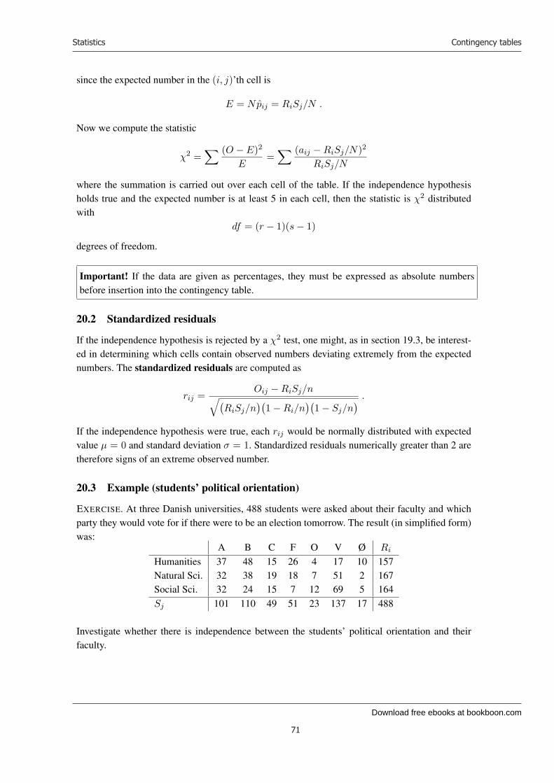
Download free ebooks at bookboon.com
Statistics
71
Contingency tables
since the expected number in the (i, j)’th cell is
E = Npij = RiSj/N .
Now we compute the statistic
χ2 =∑ (O − E)2
E=
∑ (aij − RiSj/N)2
RiSj/N
where the summation is carried out over each cell of the table. If the independence hypothesisholds true and the expected number is at least 5 in each cell, then the statistic is χ2 distributedwith
df = (r − 1)(s − 1)
degrees of freedom.
Important! If the data are given as percentages, they must be expressed as absolute numbersbefore insertion into the contingency table.
20.2 Standardized residuals
If the independence hypothesis is rejected by a χ2 test, one might, as in section 19.3, be interest-ed in determining which cells contain observed numbers deviating extremely from the expectednumbers. The standardized residuals are computed as
rij =Oij − RiSj/n√(
RiSj/n)(
1 − Ri/n)(
1 − Sj/n) .
If the independence hypothesis were true, each rij would be normally distributed with expectedvalue µ = 0 and standard deviation σ = 1. Standardized residuals numerically greater than 2 aretherefore signs of an extreme observed number.
20.3 Example (students’ political orientation)
EXERCISE. At three Danish universities, 488 students were asked about their faculty and whichparty they would vote for if there were to be an election tomorrow. The result (in simplified form)was:
A B C F O V Ø Ri
Humanities 37 48 15 26 4 17 10 157Natural Sci. 32 38 19 18 7 51 2 167Social Sci. 32 24 15 7 12 69 5 164Sj 101 110 49 51 23 137 17 488
Investigate whether there is independence between the students’ political orientation and theirfaculty.
71

Download free ebooks at bookboon.com
Ple
ase
clic
k th
e ad
vert
Statistics
72
Contingency tables
SOLUTION. We are dealing with a 3 × 7 table and perform a χ2 test for independence. First, theexpected numbers
E =RiSj
488are computed and presented in a table:
A B C F O V ØHumanities 32.5 35.4 15.8 16.4 7.4 44.1 5.5Natural Sci. 34.6 37.6 16.8 17.5 7.9 46.9 5.8Social Sci. 33.9 37.0 16.5 17.1 7.7 46.0 5.7
Now the statistic
χ2 =∑ (O − E)2
E
can be computed, since the observed numbers O are the numbers in the first table:
χ2 =(37 − 32.5)2
32.5+ · · · + (5 − 5.7)2
5.7= 60.9 .
The statistic is to be compared with a χ2 distribution with df = (3 − 1)(7 − 1) = 12 degrees offreedom. Table B.3 shows that the significance probability is well below 0.1%, and we therefore
A N N O N C E
72
Are you considering aEuropean business degree?LEARN BUSINESS at university level. We mix cases with cutting edge research working individually or in teams and everyone speaks English. Bring back valuable knowledge and experience to boost your career.
MEET a culture of new foods, music and traditions and a new way of studying business in a safe, clean environment – in the middle of Copenhagen, Denmark.
ENGAGE in extra-curricular activities such as case competitions, sports, etc. – make new friends among cbs’ 18,000 students from more than 80 countries.
See what we look likeand how we work on cbs.dk

Download free ebooks at bookboon.com
Statistics
73
Contingency tables
confidently reject the independence hypothesis.
Let us now compute the standardized residuals to see in which cells the observed numbers areextreme. We use the formula for rij in section 20.2 and get
A B C F O V ØHumanities 1.1 2.9 –0.2 3.0 –1.6 –5.8 2.4Natural Sci. –0.6 0.1 0.7 0.2 –0.4 0.9 –2.0Social Sci. –0.5 –3.0 –0.5 –3.2 1.9 4.9 –0.4
We find that there are extreme observations in many cells.
20.4 χ2 test for 2 × 2 tables
A contingency table with two rows and two columns is called a 2×2 table. Let us write theobserved numbers as follows:
a b
c d
The statistic thus becomes
χ2 =(
ad − bc
N
)2 (1
E11+
1E12
+1
E21+
1E22
)
where N = a+b+c+d is the total number of observations, and Eij is the expected number in theij’th cell. The statistic χ2 is to be compared with the χ2 distribution with df = (2−1)(2−1) = 1degree of freedom.
If we wish to perform a one-sided test of the independence hypothesis, the statistic
u =(
ad − bc
N
) √(1
E11+
1E12
+1
E21+
1E22
)
is used instead. Under the independence hypothesis, u will be standard normally distributed.
20.5 Fisher’s exact test for 2 × 2 tables
Given a 2 × 2 table, nothing stands in the way of using the χ2 test, but there is a better test in thissituation called Fisher’s exact test. Fisher’s exact test does not use any normal approximation,and may therefore still be applied when the number of expected observations in one or more ofthe cells is smaller than five.
METHOD. Let there be given a 2×2 table:
a b
c d
with row sums R1 = a+ b and R2 = c+d and column sums S1 = a+ c and S2 = b+d and totalsum N = R1 + R2 = S1 + S2 = a + b + c + d. We test the independence hypothesis H0 against
73
Download free ebooks at bookboon.com
Statistics
74
Distribution-free costs
the alternative hypothesis H1 that the “diagonal probabilities” p11 and p22 are greater than whatthey would have been had there been independence. (This situation can always be arranged byswitching the rows if necessary.) The conditional probability of obtaining exactly the 2×2 tableabove, given that the row sums are R1 and R2, and that the column sums are S1 and S2, is
Pconditional =R1!R2!S1!S2!N ! a! b! c! d!
.
The significance probability in Fisher’s exact test is the sum of Pconditional taken on all 2×2 tableswith the same row and column sums as in the given table, and which are at least as extreme as thegiven table:
PFisher =minb,c∑
i=0
R1!R2!S1!S2!N ! (a + i)! (b − i)! (c − i)! (d + i)!
.
The independence hypothesis H0 is rejected if PFisher is smaller than 5% (or whatever signifi-cance level one has chosen).
ADDENDUM: If a two-sided test is performed, i.e. if one does not test against any specific alter-native hypothesis, the significance probability becomes 2 · PFisher. It is then necessary that the2×2 table is written in such a way that the observed numbers in the diagonal are greater than theexpected numbers (this can always be obtained by switching the rows if necessary).
20.6 Example (Fisher’s exact test)
In a medical experiment concerning alternative treatments, ten patients are randomly divided intotwo groups with five patients in each. The patients in the first group receive acupuncture, whilethe patients in the other group receive no treatment. It is then seen which patients are fit or ill atthe end of the experiment. The result can be presented in a 2 × 2 table:
fit illacupuncture 4 1no treatment 2 3
The significance probability in Fisher’s exact test is computed as
PFisher =1∑
i=0
5! 5! 6! 4!10! (4 + i)! (1 − i)! (2 − i)! (3 + i)!
= 26% .
With such a large significance probability, there is no evidence that acupuncture had any effect.
21 Distribution-free tests
In all tests considered so far, we have known something about the distribution from which thegiven samples originated. We knew, for example, that the distribution was a normal distributioneven though we didn’t know the expected value or the standard deviation.
Sometimes, though, one knows nothing at all about the underlying distribution. It then be-comes necessary to use a distribution-free test (also known as a non-parametric test). The twoexamples considered in this chapter are due to Frank Wilcoxon (1892–1965).
74

Download free ebooks at bookboon.com
Ple
ase
clic
k th
e ad
vert
Statistics
75
Distribution-free costs
21.1 Wilcoxon’s test for one set of observations
Let there be given n independent observations d1, . . . , dn from an unknown distribution. We testthe null hypothesis
H0: The unknown distribution is symmetric around 0.
Each observation di is given a rank which is one of the numbers 1, 2, . . . , n. The observationwith the smallest numerical value is assigned rank 1, the observation with the second smallestnumerical value is assigned rank 2, etc. Now define the statistics
t+ =∑
(ranks corresponding to positive di),
t− =∑
(ranks corresponding to negative di).
(One can check at this point whether t+ + t− = n(n + 1)/2; if not, one has added the numbersincorrectly.) If H0 holds true, then t+ and t− should be more or less equal. When to reject H0
depends on which alternative hypothesis is tested against.
If we test H0 against the alternative hypothesis
H1: The unknown distribution primarily gives positive observations,
then H0 is rejected if t− is extremely small. Choose a significance level α and consult Table B.8
A N N O N C E
75
www.simcorp.com
MITIGATE RISK REDUCE COST ENABLE GROWTH
The financial industry needs a strong software platformThat’s why we need you
SimCorp is a leading provider of software solutions for the financial industry. We work together to reach a common goal: to help our clients
succeed by providing a strong, scalable IT platform that enables growth, while mitigating risk and reducing cost. At SimCorp, we value
commitment and enable you to make the most of your ambitions and potential.
Are you among the best qualified in finance, economics, IT or mathematics?
Find your next challenge at www.simcorp.com/careers

Download free ebooks at bookboon.com
Statistics
76
Distribution-free costs
under n and α. If t− is smaller than or equal to the table value, H0 is rejected. If t− is greater thanthe table value, H0 is accepted.
If we test H0 against the alternative hypothesis
H1: The unknown distribution primarily gives negative observations,
then H0 is rejected if t+ is extremely small. Choose a significance level α and consult Table B.8under n and α. If t+ is smaller than or equal to the table value, H0 is rejected. If t+ is greater thanthe table value, H0 is accepted.
If we don’t test H0 against any particular alternative hypothesis, the null hypothesis is rejectedif the minimum t := mint+, t− is extremely small. Choose a significance level α and consultTable B.8 under n and α/2 (if, for example, we choose the significance level α = 5%, then welook up in the table under n and 0.025). If t is smaller than or equal to the table value, we rejectH0. If t is greater than the table value, we accept H0.
The above test applies in particular when two sets of observations x1, . . . , xn and y1, . . . , yn
are given and di is the difference between the “before values” xi and the “after values” yi, i.e.di = xi − yi. If there are only random, unsystematic differences between the before and aftervalues, it follows that the di’s are distributed symmetrically around 0.
21.2 Example
An experiment involving ten patients is carried out to determine whether physical exercise lowersblood pressure. At the beginning of the experiment, the patients’ blood pressures are measured.These observations are denoted x1, . . . , x10. After a month of exercise, the blood pressures aremeasured again. These observations are denoted y1, . . . , y10. We now test the null hypothesis
H0: Physical exercise has no influence on blood pressure. The ten differences di = xi − yi aretherefore distributed symmetrically around 0,
against the alternative hypothesis
H1: Physical exercise causes the blood pressure to decrease. The ten differences di are thereforeprimarily positive.
We compute the ranks and t+ and t−:
Person 1 2 3 4 5 6 7 8 9 10Before xi 140 125 110 130 170 165 135 140 155 145After yi 137 137 102 104 172 125 140 110 140 126Difference di 3 –12 8 26 –2 40 –5 30 15 19Rank 2 5 4 8 1 10 3 9 6 7
t+ = 2 + 4 + 6 + 7 + 8 + 9 + 10 = 46,
t− = 1 + 3 + 5 = 9.
76

Download free ebooks at bookboon.com
Statistics
77
Distribution-free costs
We shall reject H0 if t− = 9 is extremely small. Table B.8 with significance level α = 5% showsthat “extremely small” means 10. Conclusion: The test shows that the null hypothesis H0 mustbe rejected against the alternative hypothesis H1 at significance level 5%.
21.3 The normal approximation to Wilcoxon’s test for one set of observations
Table B.8 includes values up to n = 50. If the number of observations is greater, a normal dis-tribution approximation can be applied. Indeed, if the null hypothesis is true, the statistic t+ isapproximately normally distributed with expected value
µ =n(n + 1)
4
and standard deviation
σ =
√n(n + 1)(2n + 1)
24.
The significance probability is therefore found by comparison of the statistic
z =t+ − µ
σ
with Table B.2 of the standard normal distribution.
EXAMPLE. Let us use the normal approximation to find the significance probability in the previousexample (even though n here is smaller than 50 and the approximation therefore is not highlyprecise). We get µ = 27.5 and σ = 9.81. The statistic therefore becomes z = 1.89, which givesa significance probability of 2.9%. The conclusion is thus the same, namely that H0 is rejected atsignificance level 5%.
21.4 Wilcoxon’s test for two sets of observations
Suppose we have two sets x1, . . . , xn and y1, . . . , ym of independent observations. We test thenull hypothesis
H0: The observations come from the same distribution.
Each of the n + m observations is assigned a rank which is one of the numbers 1, 2, . . . , n + m.The observation with the smallest numerical value is assigned rank 1, the observation with thesecond smallest numerical value is assigned rank 2, etc. Define the statistic
tx =∑
(ranks of the xi’s).
Whether H0 is rejected or not depends on which alternative hypothesis we test against.
If we test H0 against the alternative hypothesis
H1: The xi’s are primarily smaller than the yi’s,
then H0 is rejected if tx is extremely small. Look up in Table B.9 under n and m. If tx is smallerthan or equal to the table value, then H0 is rejected at significance level α = 5%. If tx is greater
77

Download free ebooks at bookboon.com
Ple
ase
clic
k th
e ad
vert
Statistics
78
Distribution-free costs
than the table value, then H0 is accepted at significance level α = 5%.
If we test H0 against the alternative hypothesis
H1: The xi’s are primarily greater than the yi’s,
then one has to switch the roles of xi’s and yi’s and continue as described above.
If we don’t test H0 against any particular alternative hypothesis, then the null hypothesis is reject-ed if the minimum
t := mintx, n(n + m + 1) − tx
is extremely small. Look up in Table B.9 under n and m. If t is smaller than or equal to the tablevalue, then H0 is rejected at significance level α = 10%. If t is greater than the table value, thenH0 is accepted at significance level 10%.
21.5 The normal approximation to Wilcoxon’s test for two sets of observations
Table B.9 applies for moderate values of n and m. If the number of observations is greater, onecan use a normal distribution approximation. Indeed, if the null hypothesis holds true, the statistic
A N N O N C E
78
Download free ebooks at bookboon.com
Statistics
79
Linear regression
tx is approximately normally distributed with expected value
µ =n(n + m + 1)
2
and standard deviation
σ =
√nm(n + m + 1)
12.
The significance probability is then found by comparing the statistic
z =tx − µ
σ
with Table B.2 of the standard normal distribution.
22 Linear regression
22.1 The model
Suppose we have a sample consisting of n pairs of observations
(x1, y1), (x2, y2), . . . , (xn, yn) .
We propose the model that each yi is an observation from a random variable
Yi = β0 + β1xi + Ei
where the Ei’s are independent normally distributed random variables with expected value 0 andcommon variance σ2. Thus we can express each yi as
yi = β0 + β1xi + ei
where ei is an observation from Ei. We call yi the response variable, xi the declaring variableand ei the remainder term.
22.2 Estimation of the parameters β0 and β1
Let x be the mean value of the xi’s and y the mean value of the yi’s. Define the sum of productsof errors as
SPExy =n∑
i=1
(xi − x)(yi − y)
and the sum of squares of errors as
SSEx =n∑
i=1
(xi − x)2
The parameters β0 and β1 of the regression equation are now estimated as
β1 =SPExy
SSEx
β0 = y − β1x
79

Download free ebooks at bookboon.com
Statistics
80
Linear regression
22.3 The distribution of the estimators
If the model’s assumptions are met, the estimator β0 is normally distributed with expected valueβ0 (the estimator thus is unbiased) and variance σ2(1/n + x2/SSEx). In other words, it holdsthat
β0 ∼ N
(β0, σ
2
(1n
+x2
SSEx
)).
Moreover, the estimator β1 is normally distributed with expected value β1 (this estimator is there-fore unbiased too) and variance σ2/SSEx. In other words, it holds that
β1 ∼ N
(β1,
σ2
SSEx
).
22.4 Predicted values yi and residuals ei
From the estimates β0 and β1, the predicted value of yi can be computed for each i as
yi = β0 + β1xi .
The i’th residual ei is the difference between the actual value yi and the predicted value yi:
ei = yi − yi .
The residual ei is an estimate of the remainder term ei.
22.5 Estimation of the variance σ2
We introduce the sum of squares of residuals as
SSR =n∑
i=1
e2i .
The variance σ2 of the remainder terms is now estimated as
s2 =SSR
n − 2.
This estimator is unbiased (but different from the maximum likelihood estimator).
22.6 Confidence intervals for the parameters β0 and β1
After estimating the parameters β0 and β1, we can compute the confidence intervals with confi-dence level 1 − α around the estimates β0 and β1. These are
β0 ± t1−α/2s
√1n
+x2
SSEx
β1 ± t1−α/2s√
SSEx
The number t1−α/2 is determined by F (u1−α/2) = 1 − α/2, where F is the distribution functionof Student’s t distribution with n − 1 degrees of freedom (see also section 15.8).
80

Download free ebooks at bookboon.com
Ple
ase
clic
k th
e ad
vert
Statistics
81
Linear regression
22.7 The determination coefficient R2
In order to investigate how well the model with the estimated parameters describes the actualobservations, we compute the determination coefficient
R2 =SSEy − SSR
SSEy.
R2 lies in the interval [0, 1] and measures the part of the variation of the yi’s which the modeldescribes as a linear function of the xi’s.
Remember: The greater the determination coefficient R2 is, the better the model describes theobservations.
22.8 Predictions and prediction intervals
Let there be given a real number x0. The function value
y0 = β0 + β1x0
is then estimated, or predicted, asy0 = β0 + β1x0 .
A N N O N C E
81
Do you want your Dream Job?
More customers get their dream job by using RedStarResume than any other resume service.
RedStarResume can help you with your job application and CV.
Go to: Redstarresume.com
Use code “BOOKBOON” and save up to $15
(enter the discount code in the “Discount Code Box”)

Download free ebooks at bookboon.com
Statistics
82
Linear regression
The confidence interval, or prediction interval, with confidence level 1 − α around the estimatey0 is
y0 ± t1−α/2s
√1 +
1n
+(x0 − x)2
SSEx.
The number t1−α/2 is determined by F (u1−α/2) = 1 − α/2, where F is the distribution functionof Student’s t distribution with n − 2 degrees of freedom (see also section 15.8).
22.9 Overview of formulaeSx =
∑ni=1 xi The sum of the xi’s
x = Sx/n The mean value of the xi’s
SSx =∑n
i=1 x2i The sum of the squares of the xi’s
SSEx =∑n
i=1(xi − x)2 = SSx − S2x/n The sum of the squares of the errors
s2x = SSEx/(n − 1) Empirical variance of the xi’s
SPxy =∑n
i=1 xiyi The sum of the products
SPExy =∑n
i=1(xi − x)(yi − y) = SPxy − SxSy/n The sum of the products of the errors
β1 = SPExy/SSEx The estimate of β1
β0 = y − β1x The estimate of β0
yi = be0 + β1xi Predicted value of yi
ei = yi − yi The i’th residual
SSR =∑n
i=1 e2i = SSEy − SPE2
xy/SSEx The sum of the squares of the residuals
s2 = SSR/(n − 2) The estimate σ2
R2 = 1 − SSR/SSEy The determination coefficient
22.10 Example
EXERCISE. It is claimed that the temperature in the Andes Mountains decreases by six degrees per1000 metres. The following temperatures were measured simultaneously at ten different localities
82

Download free ebooks at bookboon.com
Statistics
83
Linear regression
in the same region:Altitude xi Temperature yi
(metres) (degrees)500 15
1000 141500 112000 62500 –13000 23500 04000 –44500 –85000 –14
We use a linear regression modelyi = β0 + β1xi + ei
where the remainder terms ei are independent normally distributed with expected value 0 and thesame (unknown) variance σ2.
1) Estimate the parameters β0 and β1.
2) Determine the confidence interval with confidence level 95% for β1.
3) Can the hypothesis H0 : β1 = −0.006 be accepted?
4) To how large degree can the difference of temperature be explained as a linear function of thealtitude?
SOLUTION. First we perform the relevant computations:
Sx =∑10
i=1 xi = 27500 Sy =∑10
i=1 yi = 21
x = Sx/10 = 2750 y = Sy/10 = 2.1
SSx =∑10
i=1 x2i = 96250000 SSy =
∑10i=1 y2
i = 859
SSEx = SSx − S2x/10 = 20625000 SSEy = SSy − S2
y/10 = 814.9
SPxy =∑10
i=1 xiyi = −68500 SPExy = SPxy − SxSy/10 = −126250
β1 = SPExy/SSEx = −0.0061 β0 = y − β1x = 18.9
SSR = SSEy − SPE2xy/SSEx = 42.1 s2 = SSR/8 = 5.26
R2 = 1 − SSR/SSEy = 0.948
1) It appears directly from the computations that the estimates of β0 and β1 are
β0 = 18.9 , β1 = −0.0061 .
83

Download free ebooks at bookboon.com
Ple
ase
clic
k th
e ad
vert
Statistics
84
Linear regression
2) Table B.4, under df = 10 − 1 = 9 degrees of freedom, shows that t0.975 = 2.26 (see alsosection 15.8). The confidence interval around β1 thus becomes
[−0.0061 − 2.26
√5.26√
20625000, −0.0061 + 2.26
√5.26√
20625000
]= [−0.0072 , −0.0050] .
3) The hypothesis H0 : β1 = −0.006 is accepted, since this value lies within the confidenceinterval.
4) The part of the temperature difference describable as a linear function of the altitude is nothingother than the determination coefficient
R2 = 94.8% .
The fact that R2 is large (close to 100%) shows that the actual temperatures are quite close to thosepredicted. This also appears from the figure below, which shows that the actual temperatures arevery close to the regression line:
A N N O N C E
84Challenging? Not challenging? Try more
Try this...
www.alloptions.nl/life

Download free ebooks at bookboon.com
Statistics
86
Overview of discrete distributions
A Overview of discrete distributions
Distribution Description Values Point proba-bilities
Meanvalue
Variance
BinomialdistributionBin(n, p)
Number ofsuccesses inn tries
k = 0, 1, . . . , n
(n
k
)pkqn−k np npq
PoissondistributionPois(λ)
Number ofspontaneousevents in atime interval
k = 0, 1, . . . λk
k! e−λ λ λ
GeometricaldistributionGeo(p)
Numberof fail-ures beforesuccess
k = 0, 1, . . . qkp q/p q/p2
Hyper-geometricaldistributionHG(n, r, N)
Number ofred ballsamong n
balls
k = 0, . . .. . . ,minn, r
(r
k
)(s
n − k
)
(N
n
) nr/N nrs(N−n)N2(N−1)
NegativebinomialdistributionNB(n, p)
Numberof failuresbefore then’th success
k = 0, 1, . . .
(n + k − 1
n − 1
)· pn · qk nq/p nq/p2
Multi-nomial-distributionMult(n, . . . )
Numberof samplepoints ofeach type
(k1, . . . , kr)where∑
ki = n
(n
k1 · · · kr
)·∏
pkii — —
86
Download free ebooks at bookboon.com
Ple
ase
clic
k th
e ad
vert
Statistics
87
Tables
B Tables
B.1 How to read the tables
Table B.2 gives values of the distribution function
Φ(u) =∫ u
−∞
1√2π
exp(−1
2t2
)dt
of the standard normal distribution.
Table B.3 gives values of x for which the distribution function F = Fχ2 of the χ2 distributionwith df degrees of freedom takes the values F (x) = 0.500, F (x) = 0.600, etc.
Table B.4 gives values of x for which the distribution function F = FStudent of Student’s t distri-bution with df degrees of freedom takes the values F (x) = 0.600, F (x) = 0.700, etc.
Table B.5, Table B.6 and Table B.7 give values of x for which the distribution function F =FFisher of Fisher’s F distribution with n degrees of freedom in the numerator (top line) andm degrees of freedom in the denominator (leftmost column) takes the values F (x) = 0.90,F (x) = 0.95, and F (x) = 0.99, respectively.
A N N O N C E
87

Download free ebooks at bookboon.com
Statistics
88
Tables
Table B.8 and Table B.9 give critical values for Wilcoxon’s tests for one and two sets of observa-tions. See Chapter 21 for further details.
88
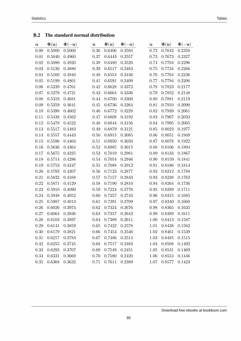
Download free ebooks at bookboon.com
Statistics
89
Tables
B.2 The standard normal distribution
u Φ(u) Φ(−u)0.00 0.5000 0.50000.01 0.5040 0.49600.02 0.5080 0.49200.03 0.5120 0.48800.04 0.5160 0.48400.05 0.5199 0.48010.06 0.5239 0.47610.07 0.5279 0.47210.08 0.5319 0.46810.09 0.5359 0.46410.10 0.5398 0.46020.11 0.5438 0.45620.12 0.5478 0.45220.13 0.5517 0.44830.14 0.5557 0.44430.15 0.5596 0.44040.16 0.5636 0.43640.17 0.5675 0.43250.18 0.5714 0.42860.19 0.5753 0.42470.20 0.5793 0.42070.21 0.5832 0.41680.22 0.5871 0.41290.23 0.5910 0.40900.24 0.5948 0.40520.25 0.5987 0.40130.26 0.6026 0.39740.27 0.6064 0.39360.28 0.6103 0.38970.29 0.6141 0.38590.30 0.6179 0.38210.31 0.6217 0.37830.32 0.6255 0.37450.33 0.6293 0.37070.34 0.6331 0.36690.35 0.6368 0.3632
u Φ(u) Φ(−u)0.36 0.6406 0.35940.37 0.6443 0.35570.38 0.6480 0.35200.39 0.6517 0.34830.40 0.6554 0.34460.41 0.6591 0.34090.42 0.6628 0.33720.43 0.6664 0.33360.44 0.6700 0.33000.45 0.6736 0.32640.46 0.6772 0.32280.47 0.6808 0.31920.48 0.6844 0.31560.49 0.6879 0.31210.50 0.6915 0.30850.51 0.6950 0.30500.52 0.6985 0.30150.53 0.7019 0.29810.54 0.7054 0.29460.55 0.7088 0.29120.56 0.7123 0.28770.57 0.7157 0.28430.58 0.7190 0.28100.59 0.7224 0.27760.60 0.7257 0.27430.61 0.7291 0.27090.62 0.7324 0.26760.63 0.7357 0.26430.64 0.7389 0.26110.65 0.7422 0.25780.66 0.7454 0.25460.67 0.7486 0.25140.68 0.7517 0.24830.69 0.7549 0.24510.70 0.7580 0.24200.71 0.7611 0.2389
u Φ(u) Φ(−u)0.72 0.7642 0.23580.73 0.7673 0.23270.74 0.7704 0.22960.75 0.7734 0.22660.76 0.7764 0.22360.77 0.7794 0.22060.78 0.7823 0.21770.79 0.7852 0.21480.80 0.7881 0.21190.81 0.7910 0.20900.82 0.7939 0.20610.83 0.7967 0.20330.84 0.7995 0.20050.85 0.8023 0.19770.86 0.8051 0.19490.87 0.8078 0.19220.88 0.8106 0.18940.89 0.8133 0.18670.90 0.8159 0.18410.91 0.8186 0.18140.92 0.8212 0.17880.93 0.8238 0.17620.94 0.8264 0.17360.95 0.8289 0.17110.96 0.8315 0.16850.97 0.8340 0.16600.98 0.8365 0.16350.99 0.8389 0.16111.00 0.8413 0.15871.01 0.8438 0.15621.02 0.8461 0.15391.03 0.8485 0.15151.04 0.8508 0.14921.05 0.8531 0.14691.06 0.8554 0.14461.07 0.8577 0.1423
89
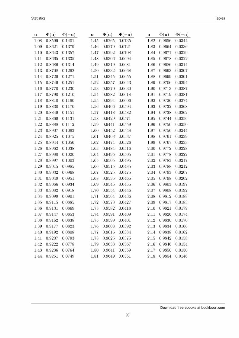
Download free ebooks at bookboon.com
Statistics
90
Tables
u Φ(u) Φ(−u)1.08 0.8599 0.14011.09 0.8621 0.13791.10 0.8643 0.13571.11 0.8665 0.13351.12 0.8686 0.13141.13 0.8708 0.12921.14 0.8729 0.12711.15 0.8749 0.12511.16 0.8770 0.12301.17 0.8790 0.12101.18 0.8810 0.11901.19 0.8830 0.11701.20 0.8849 0.11511.21 0.8869 0.11311.22 0.8888 0.11121.23 0.8907 0.10931.24 0.8925 0.10751.25 0.8944 0.10561.26 0.8962 0.10381.27 0.8980 0.10201.28 0.8997 0.10031.29 0.9015 0.09851.30 0.9032 0.09681.31 0.9049 0.09511.32 0.9066 0.09341.33 0.9082 0.09181.34 0.9099 0.09011.35 0.9115 0.08851.36 0.9131 0.08691.37 0.9147 0.08531.38 0.9162 0.08381.39 0.9177 0.08231.40 0.9192 0.08081.41 0.9207 0.07931.42 0.9222 0.07781.43 0.9236 0.07641.44 0.9251 0.0749
u Φ(u) Φ(−u)1.45 0.9265 0.07351.46 0.9279 0.07211.47 0.9292 0.07081.48 0.9306 0.06941.49 0.9319 0.06811.50 0.9332 0.06681.51 0.9345 0.06551.52 0.9357 0.06431.53 0.9370 0.06301.54 0.9382 0.06181.55 0.9394 0.06061.56 0.9406 0.05941.57 0.9418 0.05821.58 0.9429 0.05711.59 0.9441 0.05591.60 0.9452 0.05481.61 0.9463 0.05371.62 0.9474 0.05261.63 0.9484 0.05161.64 0.9495 0.05051.65 0.9505 0.04951.66 0.9515 0.04851.67 0.9525 0.04751.68 0.9535 0.04651.69 0.9545 0.04551.70 0.9554 0.04461.71 0.9564 0.04361.72 0.9573 0.04271.73 0.9582 0.04181.74 0.9591 0.04091.75 0.9599 0.04011.76 0.9608 0.03921.77 0.9616 0.03841.78 0.9625 0.03751.79 0.9633 0.03671.80 0.9641 0.03591.81 0.9649 0.0351
u Φ(u) Φ(−u)1.82 0.9656 0.03441.83 0.9664 0.03361.84 0.9671 0.03291.85 0.9678 0.03221.86 0.9686 0.03141.87 0.9693 0.03071.88 0.9699 0.03011.89 0.9706 0.02941.90 0.9713 0.02871.91 0.9719 0.02811.92 0.9726 0.02741.93 0.9732 0.02681.94 0.9738 0.02621.95 0.9744 0.02561.96 0.9750 0.02501.97 0.9756 0.02441.98 0.9761 0.02391.99 0.9767 0.02332.00 0.9772 0.02282.01 0.9778 0.02222.02 0.9783 0.02172.03 0.9788 0.02122.04 0.9793 0.02072.05 0.9798 0.02022.06 0.9803 0.01972.07 0.9808 0.01922.08 0.9812 0.01882.09 0.9817 0.01832.10 0.9821 0.01792.11 0.9826 0.01742.12 0.9830 0.01702.13 0.9834 0.01662.14 0.9838 0.01622.15 0.9842 0.01582.16 0.9846 0.01542.17 0.9850 0.01502.18 0.9854 0.0146
90

Download free ebooks at bookboon.com
Statistics
91
Tables
u Φ(u) Φ(−u)2.19 0.9857 0.01432.20 0.9861 0.01392.21 0.9864 0.01362.22 0.9868 0.01322.23 0.9871 0.01292.24 0.9875 0.01252.25 0.9878 0.01222.26 0.9881 0.01192.27 0.9884 0.01162.28 0.9887 0.01132.29 0.9890 0.01102.30 0.9893 0.01072.31 0.9896 0.01042.32 0.9898 0.01022.33 0.9901 0.00992.34 0.9904 0.00962.35 0.9906 0.00942.36 0.9909 0.00912.37 0.9911 0.00892.38 0.9913 0.00872.39 0.9916 0.00842.40 0.9918 0.00822.41 0.9920 0.00802.42 0.9922 0.00782.43 0.9925 0.00752.44 0.9927 0.00732.45 0.9929 0.00712.46 0.9931 0.00692.47 0.9932 0.00682.48 0.9934 0.00662.49 0.9936 0.00642.50 0.9938 0.00622.51 0.9940 0.00602.52 0.9941 0.00592.53 0.9943 0.00572.54 0.9945 0.00552.55 0.9946 0.0054
u Φ(u) Φ(−u)2.56 0.9948 0.00522.57 0.9949 0.00512.58 0.9951 0.00492.59 0.9952 0.00482.60 0.9953 0.00472.61 0.9955 0.00452.62 0.9956 0.00442.63 0.9957 0.00432.64 0.9959 0.00412.65 0.9960 0.00402.66 0.9961 0.00392.67 0.9962 0.00382.68 0.9963 0.00372.69 0.9964 0.00362.70 0.9965 0.00352.71 0.9966 0.00342.72 0.9967 0.00332.73 0.9968 0.00322.74 0.9969 0.00312.75 0.9970 0.00302.76 0.9971 0.00292.77 0.9972 0.00282.78 0.9973 0.00272.79 0.9974 0.00262.80 0.9974 0.00262.81 0.9975 0.00252.82 0.9976 0.00242.83 0.9977 0.00232.84 0.9977 0.00232.85 0.9978 0.00222.86 0.9979 0.00212.87 0.9979 0.00212.88 0.9980 0.00202.89 0.9981 0.00192.90 0.9981 0.00192.91 0.9982 0.00182.92 0.9982 0.0018
u Φ(u) Φ(−u)2.93 0.9983 0.00172.94 0.9984 0.00162.95 0.9984 0.00162.96 0.9985 0.00152.97 0.9985 0.00152.98 0.9986 0.00142.99 0.9986 0.00143.00 0.9987 0.00133.10 0.9990 0.00103.20 0.9993 0.00073.30 0.9995 0.00053.40 0.9997 0.00033.50 0.9998 0.00023.60 0.9998 0.00023.70 0.9999 0.00013.80 0.9999 0.00013.90 1.0000 0.00004.00 1.0000 0.0000
91
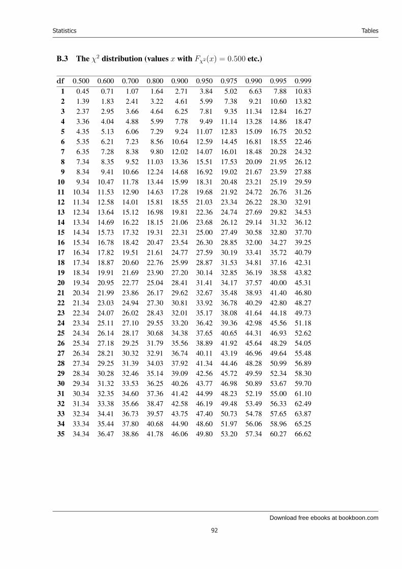
Download free ebooks at bookboon.com
Statistics
92
Tables
B.3 The χ2 distribution (values x with Fχ2(x) = 0.500 etc.)
df 0.500 0.600 0.700 0.800 0.900 0.950 0.975 0.990 0.995 0.9991 0.45 0.71 1.07 1.64 2.71 3.84 5.02 6.63 7.88 10.832 1.39 1.83 2.41 3.22 4.61 5.99 7.38 9.21 10.60 13.823 2.37 2.95 3.66 4.64 6.25 7.81 9.35 11.34 12.84 16.274 3.36 4.04 4.88 5.99 7.78 9.49 11.14 13.28 14.86 18.475 4.35 5.13 6.06 7.29 9.24 11.07 12.83 15.09 16.75 20.526 5.35 6.21 7.23 8.56 10.64 12.59 14.45 16.81 18.55 22.467 6.35 7.28 8.38 9.80 12.02 14.07 16.01 18.48 20.28 24.328 7.34 8.35 9.52 11.03 13.36 15.51 17.53 20.09 21.95 26.129 8.34 9.41 10.66 12.24 14.68 16.92 19.02 21.67 23.59 27.88
10 9.34 10.47 11.78 13.44 15.99 18.31 20.48 23.21 25.19 29.5911 10.34 11.53 12.90 14.63 17.28 19.68 21.92 24.72 26.76 31.2612 11.34 12.58 14.01 15.81 18.55 21.03 23.34 26.22 28.30 32.9113 12.34 13.64 15.12 16.98 19.81 22.36 24.74 27.69 29.82 34.5314 13.34 14.69 16.22 18.15 21.06 23.68 26.12 29.14 31.32 36.1215 14.34 15.73 17.32 19.31 22.31 25.00 27.49 30.58 32.80 37.7016 15.34 16.78 18.42 20.47 23.54 26.30 28.85 32.00 34.27 39.2517 16.34 17.82 19.51 21.61 24.77 27.59 30.19 33.41 35.72 40.7918 17.34 18.87 20.60 22.76 25.99 28.87 31.53 34.81 37.16 42.3119 18.34 19.91 21.69 23.90 27.20 30.14 32.85 36.19 38.58 43.8220 19.34 20.95 22.77 25.04 28.41 31.41 34.17 37.57 40.00 45.3121 20.34 21.99 23.86 26.17 29.62 32.67 35.48 38.93 41.40 46.8022 21.34 23.03 24.94 27.30 30.81 33.92 36.78 40.29 42.80 48.2723 22.34 24.07 26.02 28.43 32.01 35.17 38.08 41.64 44.18 49.7324 23.34 25.11 27.10 29.55 33.20 36.42 39.36 42.98 45.56 51.1825 24.34 26.14 28.17 30.68 34.38 37.65 40.65 44.31 46.93 52.6226 25.34 27.18 29.25 31.79 35.56 38.89 41.92 45.64 48.29 54.0527 26.34 28.21 30.32 32.91 36.74 40.11 43.19 46.96 49.64 55.4828 27.34 29.25 31.39 34.03 37.92 41.34 44.46 48.28 50.99 56.8929 28.34 30.28 32.46 35.14 39.09 42.56 45.72 49.59 52.34 58.3030 29.34 31.32 33.53 36.25 40.26 43.77 46.98 50.89 53.67 59.7031 30.34 32.35 34.60 37.36 41.42 44.99 48.23 52.19 55.00 61.1032 31.34 33.38 35.66 38.47 42.58 46.19 49.48 53.49 56.33 62.4933 32.34 34.41 36.73 39.57 43.75 47.40 50.73 54.78 57.65 63.8734 33.34 35.44 37.80 40.68 44.90 48.60 51.97 56.06 58.96 65.2535 34.34 36.47 38.86 41.78 46.06 49.80 53.20 57.34 60.27 66.62
92

Download free ebooks at bookboon.com
Statistics
93
Tables
df 0.500 0.600 0.700 0.800 0.900 0.950 0.975 0.990 0.995 0.99936 35.34 37.50 39.92 42.88 47.21 51.00 54.44 58.62 61.58 67.9937 36.34 38.53 40.98 43.98 48.36 52.19 55.67 59.89 62.88 69.3538 37.34 39.56 42.05 45.08 49.51 53.38 56.90 61.16 64.18 70.7039 38.34 40.59 43.11 46.17 50.66 54.57 58.12 62.43 65.48 72.0540 39.34 41.62 44.16 47.27 51.81 55.76 59.34 63.69 66.77 73.4041 40.34 42.65 45.22 48.36 52.95 56.94 60.56 64.95 68.05 74.7442 41.34 43.68 46.28 49.46 54.09 58.12 61.78 66.21 69.34 76.0843 42.34 44.71 47.34 50.55 55.23 59.30 62.99 67.46 70.62 77.4244 43.34 45.73 48.40 51.64 56.37 60.48 64.20 68.71 71.89 78.7545 44.34 46.76 49.45 52.73 57.51 61.66 65.41 69.96 73.17 80.0846 45.34 47.79 50.51 53.82 58.64 62.83 66.62 71.20 74.44 81.4047 46.34 48.81 51.56 54.91 59.77 64.00 67.82 72.44 75.70 82.7248 47.34 49.84 52.62 55.99 60.91 65.17 69.02 73.68 76.97 84.0449 48.33 50.87 53.67 57.08 62.04 66.34 70.22 74.92 78.23 85.3550 49.33 51.89 54.72 58.16 63.17 67.50 71.42 76.15 79.49 86.6651 50.33 52.92 55.78 59.25 64.30 68.67 72.62 77.39 80.75 87.9752 51.33 53.94 56.83 60.33 65.42 69.83 73.81 78.62 82.00 89.2753 52.33 54.97 57.88 61.41 66.55 70.99 75.00 79.84 83.25 90.5754 53.33 55.99 58.93 62.50 67.67 72.15 76.19 81.07 84.50 91.8755 54.33 57.02 59.98 63.58 68.80 73.31 77.38 82.29 85.75 93.1756 55.33 58.04 61.03 64.66 69.92 74.47 78.57 83.51 86.99 94.4657 56.33 59.06 62.08 65.74 71.04 75.62 79.75 84.73 88.24 95.7558 57.33 60.09 63.13 66.82 72.16 76.78 80.94 85.95 89.48 97.0459 58.33 61.11 64.18 67.89 73.28 77.93 82.12 87.17 90.72 98.3260 59.33 62.13 65.23 68.97 74.40 79.08 83.30 88.38 91.95 99.6161 60.33 63.16 66.27 70.05 75.51 80.23 84.48 89.59 93.19 100.8962 61.33 64.18 67.32 71.13 76.63 81.38 85.65 90.80 94.42 102.1763 62.33 65.20 68.37 72.20 77.75 82.53 86.83 92.01 95.65 103.4464 63.33 66.23 69.42 73.28 78.86 83.68 88.00 93.22 96.88 104.7265 64.33 67.25 70.46 74.35 79.97 84.82 89.18 94.42 98.11 105.9966 65.33 68.27 71.51 75.42 81.09 85.96 90.35 95.63 99.33 107.2667 66.33 69.29 72.55 76.50 82.20 87.11 91.52 96.83 100.55 108.5368 67.33 70.32 73.60 77.57 83.31 88.25 92.69 98.03 101.78 109.7969 68.33 71.34 74.64 78.64 84.42 89.39 93.86 99.23 103.00 111.0670 69.33 72.36 75.69 79.71 85.53 90.53 95.02 100.43 104.21 112.32
93
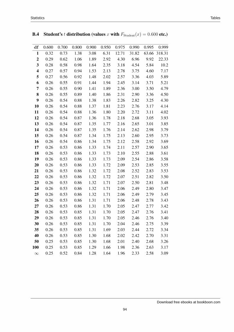
Download free ebooks at bookboon.com
Statistics
94
Tables
B.4 Student’s t distribution (values x with FStudent(x) = 0.600 etc.)
df 0.600 0.700 0.800 0.900 0.950 0.975 0.990 0.995 0.9991 0.32 0.73 1.38 3.08 6.31 12.71 31.82 63.66 318.312 0.29 0.62 1.06 1.89 2.92 4.30 6.96 9.92 22.333 0.28 0.58 0.98 1.64 2.35 3.18 4.54 5.84 10.24 0.27 0.57 0.94 1.53 2.13 2.78 3.75 4.60 7.175 0.27 0.56 0.92 1.48 2.02 2.57 3.36 4.03 5.896 0.26 0.55 0.91 1.44 1.94 2.45 3.14 3.71 5.217 0.26 0.55 0.90 1.41 1.89 2.36 3.00 3.50 4.798 0.26 0.55 0.89 1.40 1.86 2.31 2.90 3.36 4.509 0.26 0.54 0.88 1.38 1.83 2.26 2.82 3.25 4.30
10 0.26 0.54 0.88 1.37 1.81 2.23 2.76 3.17 4.1411 0.26 0.54 0.88 1.36 1.80 2.20 2.72 3.11 4.0212 0.26 0.54 0.87 1.36 1.78 2.18 2.68 3.05 3.9313 0.26 0.54 0.87 1.35 1.77 2.16 2.65 3.01 3.8514 0.26 0.54 0.87 1.35 1.76 2.14 2.62 2.98 3.7915 0.26 0.54 0.87 1.34 1.75 2.13 2.60 2.95 3.7316 0.26 0.54 0.86 1.34 1.75 2.12 2.58 2.92 3.6917 0.26 0.53 0.86 1.33 1.74 2.11 2.57 2.90 3.6518 0.26 0.53 0.86 1.33 1.73 2.10 2.55 2.88 3.6119 0.26 0.53 0.86 1.33 1.73 2.09 2.54 2.86 3.5820 0.26 0.53 0.86 1.33 1.72 2.09 2.53 2.85 3.5521 0.26 0.53 0.86 1.32 1.72 2.08 2.52 2.83 3.5322 0.26 0.53 0.86 1.32 1.72 2.07 2.51 2.82 3.5023 0.26 0.53 0.86 1.32 1.71 2.07 2.50 2.81 3.4824 0.26 0.53 0.86 1.32 1.71 2.06 2.49 2.80 3.4725 0.26 0.53 0.86 1.32 1.71 2.06 2.49 2.79 3.4526 0.26 0.53 0.86 1.31 1.71 2.06 2.48 2.78 3.4327 0.26 0.53 0.86 1.31 1.70 2.05 2.47 2.77 3.4228 0.26 0.53 0.85 1.31 1.70 2.05 2.47 2.76 3.4129 0.26 0.53 0.85 1.31 1.70 2.05 2.46 2.76 3.4030 0.26 0.53 0.85 1.31 1.70 2.04 2.46 2.75 3.3935 0.26 0.53 0.85 1.31 1.69 2.03 2.44 2.72 3.3440 0.26 0.53 0.85 1.30 1.68 2.02 2.42 2.70 3.3150 0.25 0.53 0.85 1.30 1.68 2.01 2.40 2.68 3.26
100 0.25 0.53 0.85 1.29 1.66 1.98 2.36 2.63 3.17∞ 0.25 0.52 0.84 1.28 1.64 1.96 2.33 2.58 3.09
94

Download free ebooks at bookboon.com
Statistics
95
Tables
B.5 Fisher’s F distribution (values x with FFisher(x) = 0.90)
1 2 3 4 5 6 7 8 9 101 39.86 49.50 53.59 55.83 57.24 58.20 58.91 59.44 59.86 60.192 8.53 9.00 9.16 9.24 9.29 9.33 9.35 9.37 9.38 9.393 5.54 5.46 5.39 5.34 5.31 5.28 5.27 5.25 5.24 5.234 4.54 4.32 4.19 4.11 4.05 4.01 3.98 3.95 3.94 3.925 4.06 3.78 3.62 3.52 3.45 3.40 3.37 3.34 3.32 3.306 3.78 3.46 3.29 3.18 3.11 3.05 3.01 2.98 2.96 2.947 3.59 3.26 3.07 2.96 2.88 2.83 2.78 2.75 2.72 2.708 3.46 3.11 2.92 2.81 2.73 2.67 2.62 2.59 2.56 2.549 3.36 3.01 2.81 2.69 2.61 2.55 2.51 2.47 2.44 2.42
10 3.29 2.92 2.73 2.61 2.52 2.46 2.41 2.38 2.35 2.3211 3.23 2.86 2.66 2.54 2.45 2.39 2.34 2.30 2.27 2.2512 3.18 2.81 2.61 2.48 2.39 2.33 2.28 2.24 2.21 2.1913 3.14 2.76 2.56 2.43 2.35 2.28 2.23 2.20 2.16 2.1414 3.10 2.73 2.52 2.39 2.31 2.24 2.19 2.15 2.12 2.1015 3.07 2.70 2.49 2.36 2.27 2.21 2.16 2.12 2.09 2.0616 3.05 2.67 2.46 2.33 2.24 2.18 2.13 2.09 2.06 2.0317 3.03 2.64 2.44 2.31 2.22 2.15 2.10 2.06 2.03 2.0018 3.02 2.62 2.42 2.29 2.20 2.13 2.08 2.04 2.00 1.9819 3.01 2.61 2.40 2.27 2.18 2.11 2.06 2.02 1.98 1.9620 3.00 2.59 2.38 2.25 2.16 2.09 2.04 2.00 1.96 1.9421 2.98 2.57 2.36 2.23 2.14 2.08 2.02 1.98 1.95 1.9222 2.97 2.56 2.35 2.22 2.13 2.06 2.01 1.97 1.93 1.9023 2.96 2.55 2.34 2.21 2.11 2.05 1.99 1.95 1.92 1.8924 2.95 2.54 2.33 2.19 2.10 2.04 1.98 1.94 1.91 1.8825 2.94 2.53 2.32 2.18 2.09 2.02 1.97 1.93 1.89 1.8726 2.93 2.52 2.31 2.17 2.08 2.01 1.96 1.92 1.88 1.8627 2.92 2.51 2.30 2.17 2.07 2.00 1.95 1.91 1.87 1.8528 2.92 2.50 2.29 2.16 2.06 2.00 1.94 1.90 1.87 1.8429 2.91 2.50 2.28 2.15 2.06 1.99 1.93 1.89 1.86 1.8330 2.90 2.49 2.28 2.14 2.05 1.98 1.93 1.88 1.85 1.8231 2.90 2.48 2.27 2.14 2.04 1.97 1.92 1.88 1.84 1.8132 2.89 2.48 2.26 2.13 2.04 1.97 1.91 1.87 0.84 1.8133 2.89 2.47 2.26 2.12 2.03 1.96 1.91 1.86 1.83 1.8034 2.88 2.47 2.25 2.12 2.02 1.96 1.90 1.86 1.82 1.7935 2.88 2.46 2.25 2.11 2.02 1.95 1.90 1.85 1.82 1.79
95
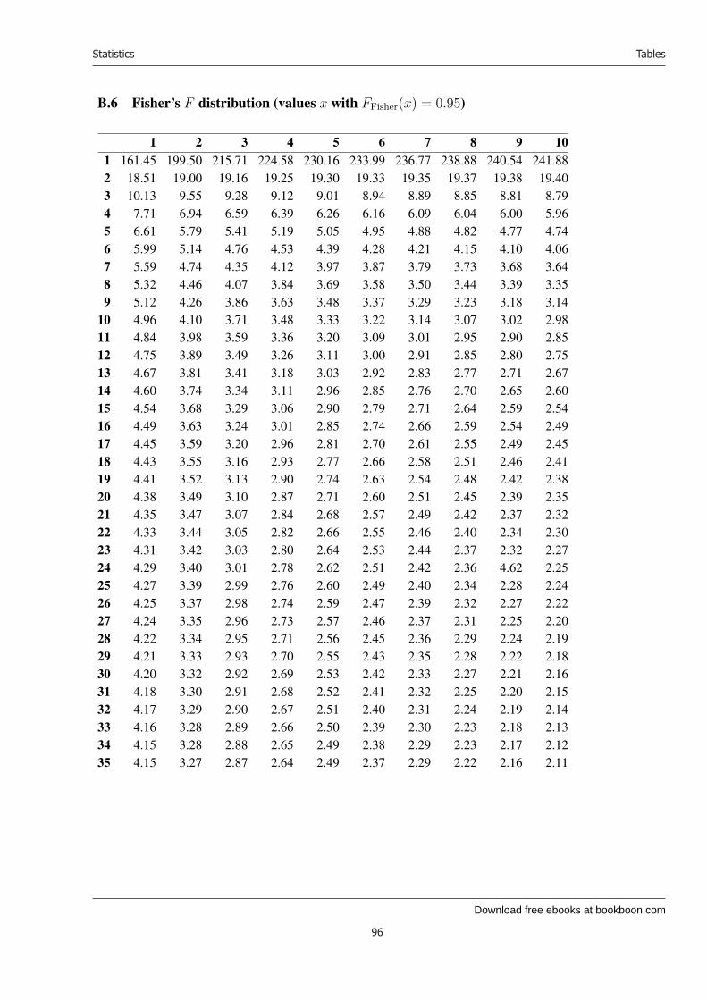
Download free ebooks at bookboon.com
Statistics
96
Tables
B.6 Fisher’s F distribution (values x with FFisher(x) = 0.95)
1 2 3 4 5 6 7 8 9 101 161.45 199.50 215.71 224.58 230.16 233.99 236.77 238.88 240.54 241.882 18.51 19.00 19.16 19.25 19.30 19.33 19.35 19.37 19.38 19.403 10.13 9.55 9.28 9.12 9.01 8.94 8.89 8.85 8.81 8.794 7.71 6.94 6.59 6.39 6.26 6.16 6.09 6.04 6.00 5.965 6.61 5.79 5.41 5.19 5.05 4.95 4.88 4.82 4.77 4.746 5.99 5.14 4.76 4.53 4.39 4.28 4.21 4.15 4.10 4.067 5.59 4.74 4.35 4.12 3.97 3.87 3.79 3.73 3.68 3.648 5.32 4.46 4.07 3.84 3.69 3.58 3.50 3.44 3.39 3.359 5.12 4.26 3.86 3.63 3.48 3.37 3.29 3.23 3.18 3.14
10 4.96 4.10 3.71 3.48 3.33 3.22 3.14 3.07 3.02 2.9811 4.84 3.98 3.59 3.36 3.20 3.09 3.01 2.95 2.90 2.8512 4.75 3.89 3.49 3.26 3.11 3.00 2.91 2.85 2.80 2.7513 4.67 3.81 3.41 3.18 3.03 2.92 2.83 2.77 2.71 2.6714 4.60 3.74 3.34 3.11 2.96 2.85 2.76 2.70 2.65 2.6015 4.54 3.68 3.29 3.06 2.90 2.79 2.71 2.64 2.59 2.5416 4.49 3.63 3.24 3.01 2.85 2.74 2.66 2.59 2.54 2.4917 4.45 3.59 3.20 2.96 2.81 2.70 2.61 2.55 2.49 2.4518 4.43 3.55 3.16 2.93 2.77 2.66 2.58 2.51 2.46 2.4119 4.41 3.52 3.13 2.90 2.74 2.63 2.54 2.48 2.42 2.3820 4.38 3.49 3.10 2.87 2.71 2.60 2.51 2.45 2.39 2.3521 4.35 3.47 3.07 2.84 2.68 2.57 2.49 2.42 2.37 2.3222 4.33 3.44 3.05 2.82 2.66 2.55 2.46 2.40 2.34 2.3023 4.31 3.42 3.03 2.80 2.64 2.53 2.44 2.37 2.32 2.2724 4.29 3.40 3.01 2.78 2.62 2.51 2.42 2.36 4.62 2.2525 4.27 3.39 2.99 2.76 2.60 2.49 2.40 2.34 2.28 2.2426 4.25 3.37 2.98 2.74 2.59 2.47 2.39 2.32 2.27 2.2227 4.24 3.35 2.96 2.73 2.57 2.46 2.37 2.31 2.25 2.2028 4.22 3.34 2.95 2.71 2.56 2.45 2.36 2.29 2.24 2.1929 4.21 3.33 2.93 2.70 2.55 2.43 2.35 2.28 2.22 2.1830 4.20 3.32 2.92 2.69 2.53 2.42 2.33 2.27 2.21 2.1631 4.18 3.30 2.91 2.68 2.52 2.41 2.32 2.25 2.20 2.1532 4.17 3.29 2.90 2.67 2.51 2.40 2.31 2.24 2.19 2.1433 4.16 3.28 2.89 2.66 2.50 2.39 2.30 2.23 2.18 2.1334 4.15 3.28 2.88 2.65 2.49 2.38 2.29 2.23 2.17 2.1235 4.15 3.27 2.87 2.64 2.49 2.37 2.29 2.22 2.16 2.11
96
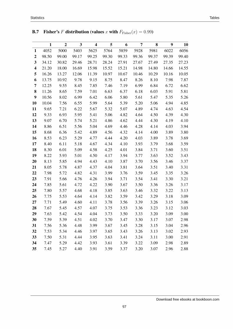
Download free ebooks at bookboon.com
Statistics
97
Tables
B.7 Fisher’s F distribution (values x with FFisher(x) = 0.99)
1 2 3 4 5 6 7 8 9 101 4052 5000 5403 5625 5764 5859 5928 5981 6022 60562 98.50 99.00 99.17 99.25 99.30 99.33 99.36 99.37 99.39 99.403 34.12 30.82 29.46 28.71 28.24 27.91 27.67 27.49 27.35 27.234 21.20 18.00 16.69 15.98 15.52 15.21 14.98 14.80 14.66 14.555 16.26 13.27 12.06 11.39 10.97 10.67 10.46 10.29 10.16 10.056 13.75 10.92 9.78 9.15 8.75 8.47 8.26 8.10 7.98 7.877 12.25 9.55 8.45 7.85 7.46 7.19 6.99 6.84 6.72 6.628 11.26 8.65 7.59 7.01 6.63 6.37 6.18 6.03 5.91 5.819 10.56 8.02 6.99 6.42 6.06 5.80 5.61 5.47 5.35 5.26
10 10.04 7.56 6.55 5.99 5.64 5.39 5.20 5.06 4.94 4.8511 9.65 7.21 6.22 5.67 5.32 5.07 4.89 4.74 4.63 4.5412 9.33 6.93 5.95 5.41 5.06 4.82 4.64 4.50 4.39 4.3013 9.07 6.70 5.74 5.21 4.86 4.62 4.44 4.30 4.19 4.1014 8.86 6.51 5.56 5.04 4.69 4.46 4.28 4.14 4.03 3.9415 8.68 6.36 5.42 4.89 4.56 4.32 4.14 4.00 3.89 3.8016 8.53 6.23 5.29 4.77 4.44 4.20 4.03 3.89 3.78 3.6917 8.40 6.11 5.18 4.67 4.34 4.10 3.93 3.79 3.68 3.5918 8.30 6.01 5.09 4.58 4.25 4.01 3.84 3.71 3.60 3.5119 8.22 5.93 5.01 4.50 4.17 3.94 3.77 3.63 3.52 3.4320 8.13 5.85 4.94 4.43 4.10 3.87 3.70 3.56 3.46 3.3721 8.05 5.78 4.87 4.37 4.04 3.81 3.64 3.51 3.40 3.3122 7.98 5.72 4.82 4.31 3.99 3.76 3.59 3.45 3.35 3.2623 7.91 5.66 4.76 4.26 3.94 3.71 3.54 3.41 3.30 3.2124 7.85 5.61 4.72 4.22 3.90 3.67 3.50 3.36 3.26 3.1725 7.80 5.57 4.68 4.18 3.85 3.63 3.46 3.32 3.22 3.1326 7.75 5.53 4.64 4.14 3.82 3.59 3.42 3.29 3.18 3.0927 7.71 5.49 4.60 4.11 3.78 3.56 3.39 3.26 3.15 3.0628 7.67 5.45 4.57 4.07 3.75 3.53 3.36 3.23 3.12 3.0329 7.63 5.42 4.54 4.04 3.73 3.50 3.33 3.20 3.09 3.0030 7.59 5.39 4.51 4.02 3.70 3.47 3.30 3.17 3.07 2.9831 7.56 5.36 4.48 3.99 3.67 3.45 3.28 3.15 3.04 2.9632 7.53 5.34 4.46 3.97 3.65 3.43 3.26 3.13 3.02 2.9333 7.50 5.31 4.44 3.95 3.63 3.41 3.24 3.11 3.00 2.9134 7.47 5.29 4.42 3.93 3.61 3.39 3.22 3.09 2.98 2.8935 7.45 5.27 4.40 3.91 3.59 3.37 3.20 3.07 2.96 2.88
97

Download free ebooks at bookboon.com
Statistics
98
Tables
B.8 Wilcoxon’s test for one set of observationsn 0.005 0.010 0.025 0.0505 − − − 06 − − 0 27 − 0 2 38 0 1 3 59 1 3 5 8
10 3 5 8 1011 5 7 10 1312 7 9 13 1713 9 12 17 2114 12 15 21 2515 15 19 25 3016 19 23 29 3517 23 27 34 4118 27 32 40 4719 32 37 46 5320 37 43 52 6021 42 49 58 6722 48 55 65 7523 54 62 73 8324 61 69 81 9125 68 76 89 10026 75 84 98 11027 83 92 107 119
n 0.005 0.010 0.025 0.05028 91 101 116 13029 100 110 126 14030 109 120 137 15131 118 130 147 16332 128 140 159 17533 138 151 170 18734 148 162 182 20035 159 173 195 21336 171 185 208 22737 182 198 221 24138 194 211 235 25639 207 224 249 27140 220 238 264 28641 233 252 279 30242 247 266 294 31943 261 281 310 33644 276 296 327 35345 291 312 343 37146 307 328 361 38947 322 345 378 40748 339 362 396 42649 355 379 415 44650 373 397 434 466
98

Download free ebooks at bookboon.com
Statistics
99
Tables
B.9 Wilcoxon’s test for two sets of observations, α = 5%
m = 1 2 3 4 5 6 7 8 9 10 11 12 13 14 15n = 1 0 0 0 0 0 0 0 0 0 0 0 0 0 0 0
2 2 2 2 2 3 3 3 4 4 4 4 5 5 6 63 5 5 6 6 7 8 8 9 10 10 11 11 12 13 134 9 9 10 11 12 13 14 15 16 17 18 19 20 21 225 14 15 16 17 19 20 21 23 24 26 27 28 30 31 336 20 21 23 24 26 28 29 31 33 35 37 38 40 42 447 27 28 30 32 34 36 39 41 43 45 47 49 52 54 568 35 37 39 41 44 46 49 51 54 56 59 62 64 67 699 44 46 49 51 54 57 60 63 66 69 72 75 78 81 84
10 54 56 59 62 66 69 72 75 79 82 86 89 92 96 9911 65 67 71 74 78 82 85 89 93 97 100 104 108 112 11612 77 80 83 87 91 95 99 104 108 112 116 120 125 129 13313 90 93 97 101 106 110 115 119 124 128 133 138 142 147 15214 104 108 112 116 121 126 131 136 141 146 151 156 161 166 17115 119 123 127 132 138 143 148 153 159 164 170 175 181 186 19216 135 139 144 150 155 161 166 172 178 184 190 196 201 207 21317 152 156 162 168 173 179 186 192 198 204 210 217 223 230 23618 170 175 180 187 193 199 206 212 219 226 232 239 246 253 25919 190 194 200 207 213 220 227 234 241 248 255 262 270 277 28420 210 214 221 228 235 242 249 257 264 272 279 287 294 302 31021 231 236 242 250 257 265 272 280 288 296 304 312 320 328 33622 253 258 265 273 281 289 297 305 313 321 330 338 347 355 36423 276 281 289 297 305 313 322 330 339 348 357 366 374 383 39224 300 306 313 322 330 339 348 357 366 375 385 394 403 413 42225 325 331 339 348 357 366 375 385 394 404 414 423 433 443 453
99

Download free ebooks at bookboon.com
Statistics
100
Explanation of symbols
C Explanation of symbols
A, B,C eventsΩ sample spaceP probability function, significance probabilityP (A|B) conditional probability of A given B
∩, ∪ intersection, union∧, ∨ and, orA ⊆ Ω A is a subset of Ωω ∈ Ω ω belongs to ΩA complement of the set A
A\B difference of the sets A and B (“A minus B”)f : Ω → R f is a map from Ω into R:= equals by definition|x| absolute value of x (e.g. | − 2| = 2)N, Z, R the set of natural, integral, real numbersØ the empty set[0,∞[ the interval x ∈ R | x ≥ 0X, Y random variablesE(X) the expected value of X
var(X) the variance of X
Cov(X, Y ) the covariance of X and Y
µ expected valueσ2 varianceσ standard deviationBin binomial distributionPois Poisson distributionGeo geometrical distributionHG hypergeometrical distributionMult multinomial distributionNB negative binomial distributionExp exponential distributionN normal distributions2 empirical variances empirical standard deviationF (x) distribution functionf(x) density functionΦ(x) distribution function of standard normal distributionϕ(x) density function of standard normal distributionn number of observations or triesλ intensity (in a Poisson process)R2 determination coefficient
100

Download free ebooks at bookboon.com
Ple
ase
clic
k th
e ad
vert
Statistics
101
Explanation of symbols
ρ correlation coefficientx, y mean valuedf number of degrees of freedom
101
Stand out from the crowdDesigned for graduates with less than one year of full-time postgraduate work experience, London Business School’s Masters in Management will expand your thinking and provide you with the foundations for a successful career in business.
The programme is developed in consultation with recruiters to provide you with the key skills that top employers demand. Through 11 months of full-time study, you will gain the business knowledge and capabilities to increase your career choices and stand out from the crowd.
Applications are now open for entry in September 2011.
For more information visit www.london.edu/mim/ email [email protected] or call +44 (0)20 7000 7573
Masters in Management
London Business SchoolRegent’s ParkLondon NW1 4SAUnited KingdomTel +44 (0)20 7000 7573Email [email protected]/mim/
Fast-track your career

Download free ebooks at bookboon.com
Statistics
102
Index
Indeksaccept, 29addition formula, 24addition formula for normal distribution, 50alternative hypothesis, 29analysis of variance, 60ANOVA, 60automobiles, 36auxiliary hypothesis, 59
binomial coefficient, 16binomial distribution, 30black balls, 41Bortkiewicz, Ladislaus von, 69
cabinet, 42Central Limit Theorem, 26Chebyshev’s inequality, 26chi-squared, 63chi-squared distribution, 50city council, 42conditional probability, 12contingency table, 70continuous random variable, 20correlation coefficient, 24covariance, 24cumulative probabilities, 32
declaring variable, 79density, 20density function, 20determination coefficient, 81discrepancy, 64discrete random variable, 19disjoint events, 12distribution function, 18distribution-free test, 74division into possible causes, 13
empirical correlation coefficient, 29empirical covariance, 29empirical standard deviation, 28
empirical variance, 28equality of distribution, 63errors (of type I and II), 30event, 12expected number, 64expected value, 21, 24exponential distribution, 45
F distribution, 52Fisher’s exact test, 73Fisher’s F, 52Fisher-Behrens problem, 57French Open, 13
generalized binomial coefficients, 17geometrical distribution, 39Gesetz der kleinen Zahlen, 69goodness of fit, 63Green Party, 34
hypergeometrical distribution, 41
inclusion-exclusion, 14independent events, 14independent random variables, 20intensity, 35, 45interquartile range, 28
Law of Large Numbers, 26linear regression, 79lower quartile, 28
marginal density, 21mean, 28mean value, 28median, 27moment of extraordinary beauty, 27multinomial coefficients, 17multinomial distribution, 43multiplication formula, 24
negative binomial distribution, 44non-parametric test, 74
103
Index

Statistics
103
Index
normal distribution, 46normed sum, 26null hypothesis, 29
observed number, 64
parameter, 30Pascal’s triangle, 17Pearson’s test, 63pin diagram, 19point probability, 19Poisson distribution, 35pooled variance, 57predicted value, 80probability function, 12probability of failure, 30probability of success, 30probability space, 12Prussian cavalry, 68
quartile, 28
random variables, 18random vector, 21rank, 74red balls, 41regression, 79reject, 29remainder term, 79residual, 80response variable, 79
sample point, 12sample space, 12school class, 15significance level, 29significance probability, 29simple linear regression, 79simultaneous density, 21simultaneous distribution function, 21Skoda, 36spontaneous event, 35, 45standard deviation, 22standard normal distribution, 47
standardized residuals, 65, 71strength, 30Student’s t, 51
t distribution, 51test, 29throw of a dice, 12toss of a coin, 27two-times-two table, 73type I and II, 30
unbiased estimator, 33upper quartile, 28urn, 41
variance, 22, 24variance between samples, 60variance within samples, 60
Wilcoxon’s test, 74
104