15Nonparametric Statistics

571

CHAPTER OUTLINE

LEARNING OBJECTIVES

After careful study of this chapter, you should be able to do the following:1. Determine situations where nonparametric procedures are better alternatives to the t-test and

ANOVA2. Use one- and two-sample nonparametric tests3. Use nonparametric alternatives to the single-factor ANOVA4. Understand how nonparametric tests compare to the t-test in terms of relative efficiency

Answers for most odd numbered exercises are at the end of the book. Answers to exercises whosenumbers are surrounded by a box can be accessed in the e-text by clicking on the box. Completeworked solutions to certain exercises are also available in the e-Text. These are indicated in theAnswers to Selected Exercises section by a box around the exercise number. Exercises are alsoavailable for some of the text sections that appear on CD only. These exercises may be found withinthe e-Text immediately following the section they accompany.

15-1 INTRODUCTION

15-2 SIGN TEST

15-2.1 Description of the Test

15-2.2 Sign Test for Paired Samples

15-2.3 Type II Error for the Sign Test

15-2.4 Comparison to the t-Test

15-3 WILCOXON SIGNED-RANK TEST


15-3.2 Large-Sample Approximation

15-3.3 Paired Observations


15-4 WILCOXON RANK-SUM TEST




15-5 NONPARAMETRIC METHODS INTHE ANALYSIS OF VARIANCE

15-5.1 Kruskal-Wallis Test

15-5.2 Rank Transformation

15NonparametricStatistics

c15.qxd 5/8/02 8:21 PM Page 571 RK UL 6 RK UL 6:Desktop Folder:TEMP WORK:PQ220 MONT 8/5/2002:Ch 15:

572 CHAPTER 15 NONPARAMETRIC STATISTICS

15-1 INTRODUCTION

Most of the hypothesis-testing and confidence interval procedures discussed in previous chap-ters are based on the assumption that we are working with random samples from normal popu-lations. Traditionally, we have called these procedures parametric methods because they arebased on a particular parametric family of distributions—in this case, the normal. Alternately,sometimes we say that these procedures are not distribution-free because they depend on the as-sumption of normality. Fortunately, most of these procedures are relatively insensitive to slightdepartures from normality. In general, the t- and F-tests and the t-confidence intervals will haveactual levels of significance or confidence levels that differ from the nominal or advertised lev-els chosen by the experimenter, although the difference between the actual and advertised levelsis usually fairly small when the underlying population is not too different from the normal.

In this chapter we describe procedures called nonparametric and distribution-freemethods, and we usually make no assumptions about the distribution of the underlying pop-ulation other than that it is continuous. These procedures have actual level of significance � orconfidence level 100(1 � �)% for many different types of distributions. These procedureshave considerable appeal. One of their advantages is that the data need not be quantitative butcan be categorical (such as yes or no, defective or nondefective) or rank data. Another advan-tage is that nonparametric procedures are usually very quick and easy to perform.

The procedures described in this chapter are competitors of the parametric t- and F-procedures described earlier. Consequently, it is important to compare the performance ofboth parametric and nonparametric methods under the assumptions of both normal and non-normal populations. In general, nonparametric procedures do not utilize all the informationprovided by the sample. As a result, a nonparametric procedure will be less efficient than thecorresponding parametric procedure when the underlying population is normal. This loss ofefficiency is reflected by a requirement of a larger sample size for the nonparametric proce-dure than would be required by the parametric procedure in order to achieve the same power.On the other hand, this loss of efficiency is usually not large, and often the difference in sam-ple size is very small. When the underlying distributions are not close to normal, nonparamet-ric methods have much to offer. They often provide considerable improvement over thenormal-theory parametric methods.

Generally, if both parametric and nonparametric methods are applicable to a particularproblem, we should use the more efficient parametric procedure. However, the assumptions forthe parametric method may be difficult or impossible to justify. For example, the data may be inthe form of ranks. These situations frequently occur in practice. For instance, a panel of judgesmay be used to evaluate 10 different formulations of a soft-drink beverage for overall quality,with the “best’’ formulation assigned rank 1, the “next-best’’ formulation assigned rank 2, and soforth. It is unlikely that rank data satisfy the normality assumption. Many nonparametric meth-ods involve the analysis of ranks and consequently are ideally suited to this type of problem.

15-2 SIGN TEST


The sign test is used to test hypotheses about the median of a continuous distribution.The median of a distribution is a value of the random variable X such that the probabilityis 0.5 that an observed value of X is less than or equal to the median, and the probability is0.5 that an observed value of X is greater than or equal to the median. That is,P1X � �̃2 � P1X � �̃2 � 0.5.

�̃


15-2 SIGN TEST 573

Since the normal distribution is symmetric, the mean of a normal distribution equals themedian. Therefore, the sign test can be used to test hypotheses about the mean of a normal dis-tribution. This is the same problem for which we used the t-test in Chapter 9. We will discussthe relative merits of the two procedures in Section 15-2.4. Note that, although the t-test wasdesigned for samples from a normal distribution, the sign test is appropriate for samples fromany continuous distribution. Thus, the sign test is a nonparametric procedure.

Suppose that the hypotheses are

(15-1)

The test procedure is easy to describe. Suppose that X1, X2, . . . , Xn is a random sample fromthe population of interest. Form the differences

(15-2)

Now if the null hypothesis is true, any difference is equally likelyto be positive or negative. An appropriate test statistic is the number of these differences thatare positive, say R�. Therefore, to test the null hypothesis we are really testing that thenumber of plus signs is a value of a binomial random variable that has the parameter p � 1�2. A P-value for the observed number of plus signs r� can be calculated directly from the bino-mial distribution. For instance, in testing the hypotheses in Equation 15-1, we will reject H0 infavor of H1 only if the proportion of plus signs is sufficiently less than 1�2 (or equivalently,whenever the observed number of plus signs r� is too small). Thus, if the computed P-value

is less than or equal to some preselected significance level �, we will reject H0 and concludeH1 is true.

To test the other one-sided hypothesis

(15-3)

we will reject H0 in favor of H1 only if the observed number of plus signs, say r�, is large or,equivalently, whenever the observed fraction of plus signs is significantly greater than 1�2.Thus, if the computed P-value

is less than �, we will reject H0 and conclude that H1 is true.The two-sided alternative may also be tested. If the hypotheses are

(15-4)H1: �� 0

H0: �� 0

P � P aR� � r� when p �12b

H1: �� 0

H0: �� 0

P � P aR� � r� when p �12b

Xi � ��0H0: �� 0

Xi � ��0, i � 1, 2, . . . , n

H1: �� 0

H0: �� 0



we should reject if the proportion of plus signs is significantly different (eitherless than or greater than) from 1�2. This is equivalent to the observed number of plus signs r�

being either sufficiently large or sufficiently small. Thus, if r� � n�2 the P-value is

and if r� n�2 the P-value is

If the P-value is less than some preselected level �, we will reject H0 and conclude that H1 is true.

EXAMPLE 15-1 Montgomery, Peck, and Vining (2001) report on a study in which a rocket motor is formed bybinding an igniter propellant and a sustainer propellant together inside a metal housing. Theshear strength of the bond between the two propellant types is an important characteristic. Theresults of testing 20 randomly selected motors are shown in Table 15-1. We would like to testthe hypothesis that the median shear strength is 2000 psi, using � � 0.05.

This problem can be solved using the eight-step hypothesis-testing procedure introducedin Chapter 9:

1. The parameter of interest is the median of the distribution of propellant shear strength.

2.

3.

4. � � 0.05

H1: �� 2000 psi

H0: �� 2000 psi

P � 2P aR� � r� when p �12b

P � 2P aR� � r� when p �12b

H0: �� 0�

Table 15-1 Propellant Shear Strength Data

Observation Shear Strength Differencesi xi xi � 2000 Sign

1 2158.70 �158.70 �

2 1678.15 �321.85 �

3 2316.00 �316.00 �

4 2061.30 �61.30 �

5 2207.50 �207.50 �

6 1708.30 �291.70 �

7 1784.70 �215.30 �

8 2575.10 �575.10 �

9 2357.90 �357.90 �

10 2256.70 �256.70 �

11 2165.20 �165.20 �

12 2399.55 �399.55 �

13 1779.80 �220.20 �

14 2336.75 �336.75 �

15 1765.30 �234.70 �

16 2053.50 �53.50 �

17 2414.40 �414.40 �

18 2200.50 �200.50 �

19 2654.20 �654.20 �

20 1753.70 �246.30 �


15-2 SIGN TEST 575

5. The test statistic is the observed number of plus differences in Table 15-1, or r� � 14.

6. We will reject H0 if the P-value corresponding to r� � 14 is less than or equal to � � 0.05.

7. Computations: Since r� � 14 is greater than n�2 � 20�2 � 10, we calculate the P-value from

8. Conclusions: Since P � 0.1153 is not less than � � 0.05, we cannot reject the nullhypothesis that the median shear strength is 2000 psi. Another way to say this is thatthe observed number of plus signs r� � 14 was not large or small enough to indi-cate that median shear strength is different from 2000 psi at the � � 0.05 level ofsignificance.

It is also possible to construct a table of critical values for the sign test. This table isshown as Appendix Table VII. The use of this table for the two-sided alternative hypothesis inEquation 15-4 is simple. As before, let R� denote the number of the differences ( ) thatare positive and let R� denote the number of these differences that are negative. Let R � min (R�, R�). Appendix Table VII presents critical values r*� for the sign test that ensure that P(type I error) � P (reject H0 when H0 is true) � � for � � 0.01, � � 0.05 and � � 0.10. Ifthe observed value of the test statistic r � r*�, the null hypothesis should berejected.

To illustrate how this table is used, refer to the data in Table 15-1 that was used inExample 15-1. Now r� � 14 and r� � 6; therefore, r � min (14, 6) � 6. From AppendixTable VII with n � 20 and � � 0.05, we find that r*0.05 � 5. Since r � 6 is not less than orequal to the critical value r*0.05 � 5, we cannot reject the null hypothesis that the median shearstrength is 2000 psi.

We can also use Appendix Table VII for the sign test when a one-sided alternativehypothesis is appropriate. If the alternative is reject if r� � r*�;if the alternative is reject if r� � r*�. The level of significance ofa one-sided test is one-half the value for a two-sided test. Appendix Table VII shows theone-sided significance levels in the column headings immediately below the two-sidedlevels.

Finally, note that when a test statistic has a discrete distribution such as R does in the signtest, it may be impossible to choose a critical value r*� that has a level of significance exactlyequal to �. The approach used in Appendix Table VII is to choose r*� to yield an � that is asclose to the advertised significance level � as possible.

Ties in the Sign TestSince the underlying population is assumed to be continuous, there is a zero probability thatwe will find a “tie”—that is, a value of Xi exactly equal to . However, this may sometimeshappen in practice because of the way the data are collected. When ties occur, they should beset aside and the sign test applied to the remaining data.

�0�

H0: �� 0H1: �� 0,H0: �� 0H1: �� 0,

H0: �� 0

Xi � ��0

� 0.1153

� 2 a20

r�14 a20

rb 10.52r 10.5220�r

P � 2P aR� � 14 when p �12b

c15.qxd 5/8/02 8:21 PM 75 RK UL 6 RK UL 6:Desktop Folder:TEMP WORK:PQ220 MONT 8/5/2002:Ch 15:


The Normal ApproximationWhen p � 0.5, the binomial distribution is well approximated by a normal distribution whenn is at least 10. Thus, since the mean of the binomial is np and the variance is np(1 � p), thedistribution of R� is approximately normal with mean 0.5n and variance 0.25n whenever n ismoderately large. Therefore, in these cases the null hypothesis can be tested usingthe statistic

H0: �� 0

(15-5)Z0 �R� � 0.5n

0.51n

The two-sided alternative would be rejected if the observed value of the test statistic, and the critical regions of the one-sided alternative would be chosen to reflect the

sense of the alternative. (If the alternative is , reject H0 if z0 z�, for example.)

EXAMPLE 15-2 We will illustrate the normal approximation procedure by applying it to the problem inExample 15-1. Recall that the data for this example are in Table 15-1. The eight-step proce-dure follows:

1. The parameter of interest is the median of the distribution of propellant shear strength.

2.

3.

4. � � 0.05

5. The test statistic is

6. Since � � 0.05, we will reject H0 in favor of H1 if

7. Computations: Since r� � 14, the test statistic is

8. Conclusions: Since z0 � 1.789 is not greater than z0.025 � 1.96, we cannot reject thenull hypothesis. Thus, our conclusions are identical to those in Example 15-1.

15-2.2 Sign Test for Paired Samples

The sign test can also be applied to paired observations drawn from continuous populations.Let (X1j, X2j), j � 1, 2, . . . , n be a collection of paired observations from two continuous pop-ulations, and let

Dj � X1j � X2j j � 1, 2, . . . , n

z0 �14 � 0.51202

0.5220� 1.789

0 z0 0 z0.025 � 1.96.

z0 �r� � 0.5n

0.51n

H1: �� 2000 psi

H0: �� 2000 psi

H1: �� 0

0 z0 0 z��2


15-2 SIGN TEST 577

be the paired differences. We wish to test the hypothesis that the two populations have acommon median, that is, that . This is equivalent to testing that the median of thedifferences . This can be done by applying the sign test to the n observed differencesdj, as illustrated in the following example.

EXAMPLE 15-3 An automotive engineer is investigating two different types of metering devices for anelectronic fuel injection system to determine whether they differ in their fuel mileageperformance. The system is installed on 12 different cars, and a test is run with each meter-ing device on each car. The observed fuel mileage performance data, corresponding differ-ences, and their signs are shown in Table 15-2. We will use the sign test to determine whetherthe median fuel mileage performance is the same for both devices using � � 0.05. The eight-step-procedure follows:

1. The parameters of interest are the median fuel mileage performance for the twometering devices.

2. , or, equivalently,

3. , or, equivalently,

4. � � 0.05

5. We will use Appendix Table VII to conduct the test, so the test statistic is r �min(r�, r�).

6. Since � � 0.05 and n � 12, Appendix Table VII gives the critical values as r*0.05 � 2.We will reject H0 in favor of H1 if r � 2.

7. Computations: Table 15-2 shows the differences and their signs, and we note thatr� � 8, r� � 4, and so r � min(8, 4) � 4.

8. Conclusions: Since r � 4 is not less than or equal to the critical value r*0.05 � 2, wecannot reject the null hypothesis that the two devices provide the same median fuelmileage performance.

H1: �D� 0H1: ��1 �2

�H0: �D

� � 0H0: ��1 � �2�

�D� � 0

�1� � �2

�

Table 15-2 Performance of Flow Metering Devices

Metering Device

Car 1 2 Difference, dj Sign

1 17.6 16.8 0.8 �

2 19.4 20.0 �0.6 �

3 19.5 18.2 1.3 �

4 17.1 16.4 0.7 �

5 15.3 16.0 �0.7 �

6 15.9 15.4 0.5 �

7 16.3 16.5 �0.2 �

8 18.4 18.0 0.4 �

9 17.3 16.4 0.9 �

10 19.1 20.1 �1.0 �

11 17.8 16.7 1.1 �

12 18.2 17.9 0.3 �



15-2.3 Type II Error for the Sign Test

The sign test will control the probability of type I error at an advertised level � for testing the nullhypothesis for any continuous distribution. As with any hypothesis-testing procedure,it is important to investigate the probability of a type II error, . The test should be able to effec-tively detect departures from the null hypothesis, and a good measure of this effectiveness is thevalue of for departures that are important. A small value of implies an effective test procedure.

In determining , it is important to realize not only that a particular value of , say ,must be used but also that the form of the underlying distribution will affect the calculations. Toillustrate, suppose that the underlying distribution is normal with � � 1 and we are testing thehypothesis versus . (Since in the normal distribution, this is equiv-alent to testing that the mean equals 2.) Suppose that it is important to detect a departure from

to . The situation is illustrated graphically in Fig. 15-1(a). When the alternativehypothesis is true (H1: ), the probability that the random variable X is less than or equal tothe value 2 is

Suppose we have taken a random sample of size 12. At the � � 0.05 level, Appendix Table VIIindicates that we would reject if r� � r*0.05 � 2. Therefore, is the probability thatwe do not reject when in fact , or

� 1 � a2

x�0 a12

xb 10.15872x10.8413212�x � 0.2944

�� 3H0: �� 2H0: �� 2

p � P1X � 22 � P1Z � �12 � �1�12 � 0.1587

�� 3�� 3�� 2

�� H1: �� 2H0: �� 2

��0 � ��

H0: ��

x6543210–1

= 1σ

0.1587

x543210–1

= 1σ

Under H1 : µ = 3∼Under H0 : µ = 2∼

(a)

µ = 2∼ µ = 2.89

Under H0 : µ = 2∼

2 µ = 4.33

Under H1 : µ = 3∼

(b)

0.3699

xx

Figure 15-1 Calcula-tion of for the signtest. (a) Normal distributions. (b)Exponential distributions.


15-2 SIGN TEST 579

If the distribution of X had been exponential rather than normal, the situation would be asshown in F and the probability that the random variable X is less than or equalto the valuis 3, the m

In this case

Thus, area to theity distributribution.

15-2.4 Comparison to the

If the unde

have signifigions for tcase. Whe

), thtribution hered a testWilcoxon compares

� � ��

H0: ��

EXERCISES FOR SECTION 1

15-1. Ten samples were taken fromelectronics manufacturing process, amined. The sample pH values are 7.96.95, 7.05, 7.35, 7.25, 7.42. Manuflieves that pH has a median value ofindicate that this statement is correc� � 0.05 to investigate this hypothethis test.

15-2. The titanium content in an important determinant of strength. A reveals the following titanium conten

8.32, 8.05, 8.93, 8.65, 8.25, 8.46, 8.58.30, 8.71, 8.75, 8.60, 8.83, 8.50, 8.3


ig. 15-1(b),
e x � 2 when (note that when the median of an exponential distributionean is 4.33) is
,

for the sign test depends not only on the alternative value of but also on the right of the value specified in the null hypothesis under the population probabil-tion. This area is highly dependent on the shape of that particular probability dis-

t-Test

rlying population is normal, either the sign test or the t-test could be used to test. The t-test is known to have the smallest value of possible among all tests thatcance level � for the one-sided alternative and for tests with symmetric critical re-

he two-sided alternative, so it is superior to the sign test in the normal distributionn the population distribution is symmetric and nonnormal (but with finite meane t-test will have a smaller (or a higher power) than the sign test, unless the dis-as very heavy tails compared with the normal. Thus, the sign test is usually consid- procedure for the median rather than as a serious competitor for the t-test. Thesigned-rank test discussed in the next section is preferable to the sign test and

well with the t-test for symmetric distributions.

0

��

� 1 � a2

x�0 a12

xb 10.36992x10.6301212�x � 0.8794

p � P1X � 22 � �2

0

14.33

e�1

4.33x dx � 0.3699

�� 3

5-2

a plating bath used in annd the bath pH was deter-1, 7.85, 6.82, 8.01, 7.46,

acturing engineering be- 7.0. Do the sample datat? Use the sign test withsis. Find the P-value for

aircraft-grade alloy is ansample of 20 test couponst (in percent):

2, 8.35, 8.36, 8.41, 8.42,8, 8.29, 8.46

The median titanium content should be 8.5%. Use the sign testwith � � 0.05 to investigate this hypothesis. Find the P-valuefor this test.

15-3. The impurity level (in ppm) is routinely measured inan intermediate chemical product. The following data wereobserved in a recent test:

2.4, 2.5, 1.7, 1.6, 1.9, 2.6, 1.3, 1.9, 2.0, 2.5, 2.6, 2.3, 2.0, 1.8,1.3, 1.7, 2.0, 1.9, 2.3, 1.9, 2.4, 1.6

Can you claim that the median impurity level is less than 2.5 ppm? State and test the appropriate hypothesis using thesign test with � � 0.05. What is the P-value for this test?


15-4. Consider the data in Exercise 15-1. Use the normalapproximation for the sign test to test versus

What is the P-value for this test?

15-5. Consider the compressive strength data in Exercise8-26.(a) Use the sign test to investigate the claim that the median

strength is at least 2250 psi. Use � � 0.05.(b) Use the normal approximation to test the same hypothesis

that you formulated in part (a). What is the P-value forthis test?

15-6. Consider the margarine fat content data in Exercise 8-25. Use the sign test to test versus

, with � � 0.05. Find the P-value for the teststatistic and use this quantity to make your decision.


, with � � 0.05. What is the P-value for this test?


. What is the P-value for this test?

15-9. Two different types of tips can be used in a Rockwellhardness tester. Eight coupons from test ingots of a nickel-based alloy are selected, and each coupon is tested twice, oncewith each tip. The Rockwell C-scale hardness readings areshown in the following table. Use the sign test with � � 0.05to determine whether or not the two tips produce equivalenthardness readings.

H1: �� 2.5H0: �� 2.5

H1: �� 8.5H0: �� 8.5

H1: �� 17.0H0: �� 17.0

H1: �� 7.0.H0: �� 7.0

Coupon Tip 1 Tip 2

1 63 60

2 52 51

3 58 56

4 60 59

5 55 58

6 57 54

7 53 52

8 59 61

Drying Times (in hr)

Panel Formulation 1 Formulation 2

1 1.6 1.8

2 1.3 1.5

3 1.5 1.5

4 1.6 1.7

5 1.7 1.6

6 1.9 2.0

7 1.8 2.1

8 1.6 1.7

9 1.4 1.6

10 1.8 1.9

11 1.9 2.0

12 1.8 1.9

13 1.7 1.5

14 1.5 1.7

15 1.6 1.6

16 1.4 1.2

17 1.3 1.6

18 1.6 1.8

19 1.5 1.6

20 1.8 2.0

Inspector Caliper 1 Caliper 2

1 0.265 0.264

2 0.265 0.265

3 0.266 0.264

4 0.267 0.266

5 0.267 0.267

6 0.265 0.268

7 0.267 0.264

8 0.267 0.265

9 0.265 0.265

10 0.268 0.267

11 0.268 0.268

12 0.265 0.269

15-11. Use the normal approximation to the sign test for thedata in Exercise 15-10. What conclusions can you draw?

15-12. The diameter of a ball bearing was measured by 12inspectors, each using two different kinds of calipers. Theresults were as follows:

15-10. Two different formulations of primer paint can beused on aluminum panels. The drying time of these two for-mulations is an important consideration in the manufacturingprocess. Twenty panels are selected; half of each panel ispainted with primer 1, and the other half is painted withprimer 2. The drying times are observed and reported in thefollowing table. Is there evidence that the median dryingtimes of the two formulations are different? Use the sign testwith � � 0.01.

Is there a significant difference between the medians of thepopulation of measurements represented by the two samples?Use � � 0.05.


15-3 WILCOXON SIGNED-RANK TEST 581

15-3 WILCOXON SIGNED-RANK TEST

The sign test makes use only of the plus and minus signs of the differences between the ob-servations and the median (or the plus and minus signs of the differences between theobservations in the paired case). It does not take into account the size or magnitude of thesedifferences. Frank Wilcoxon devised a test procedure that uses both direction (sign) and mag-nitude. This procedure, now called the Wilcoxon signed-rank test, is discussed and illus-trated in this section.

The Wilcoxon signed-rank test applies to the case of symmetric continuous distribu-tions. Under these assumptions, the mean equals the median, and we can use this procedure totest the null hypothesis that m 5 m0. We now show how to do this.


We are interested in testing H0: � � �0 against the usual alternatives. Assume that X1, X2, . . . , Xn is a random sample from a continuous and symmetric distribution with mean (andmedian) �. Compute the differences Xi � �0, i � 1, 2, . . . , n. Rank the absolute differences

in ascending order, and then give the ranks the signs of theircorresponding differences. Let W� be the sum of the positive ranks and W� be the absolutevalue of the sum of the negative ranks, and let W � min(W�, W�). Appendix Table VIII con-tains critical values of W, say w*�. If the alternative hypothesis is , then if the ob-served value of the statistic w � w*�, the null hypothesis H0: � � �0 is rejected. AppendixTable VIII provides significance levels of � � 0.10, � � 0.05, � � 0.02, � � 0.01 for thetwo-sided test.

For one-sided tests, if the alternative is H1: � � �0, reject H0: � � �0 if w� � w*�; and ifthe alternative is H1: � �0, reject H0: � � �0 if w� � w*�. The significance levels for one-sided tests provided in Appendix Table VIII are � � 0.05, 0.025, 0.01, and 0.005.

H1: � �0

0 Xi � �0 0 , i � 1, 2, . . . , n

��0

15-13. Consider the blood cholesterol data in Exercise 10-39. Use the sign test to determine whether there is any dif-ference between the medians of the two groups of measure-ments, with � � 0.05. What practical conclusion would youdraw from this study?

15-14. Use the normal approximation for the sign test forthe data in Exercise 15-12. With � � 0.05, what conclusionscan you draw?

15-15. Use the normal approximation to the sign test forthe data in Exercise 15-13. With � � 0.05, what conclusionscan you draw?

15-16. The distribution time between arrivals in a telecom-munication system is exponential, and the system managerwishes to test the hypothesis that minutes versus

minutes.(a) What is the value of the mean of the exponential distribu-

tion under ?(b) Suppose that we have taken a sample of n � 10 observa-

tions and we observe r� � 3. Would the sign test reject H0

at � � 0.05?

H0: �� 3.5

H1: �� 3.5H0: �� 3.5

(c) What is the type II error probability of this test if ?

15-17. Suppose that we take a sample of n � 10 measure-ments from a normal distribution with � � 1. We wish to testH0: � � 0 against H1: � � 0. The normal test statistic is

( ), and we decide to use a critical region of 1.96(that is, reject H0 if z0 � 1.96).(a) What is � for this test?(b) What is for this test, if � � 1?(c) If a sign test is used, specify the critical region that gives

an � value consistent with � for the normal test.(d) What is the value for the sign test, if � � 1? Compare

this with the result obtained in part (b).

15-18. Consider the test statistic for the sign test inExercise 15-9. Find the P-value for this statistic.

15-19. Consider the test statistic for the sign test in Exercise15-10. Find the P-value for this statistic. Compare it to the P-value for the normal approximation test statistic computedin Exercise 15-11.

��1nZ0 � X �

4.5��

c15.qxd 8/6/02 2:36 PM Page 581


Observation Difference xi � 2000 Signed Rank

16 �53.50 �14 �61.30 �21 �158.70 �3

11 �165.20 �418 �200.50 �55 �207.50 �67 �215.30 �7

13 �220.20 �815 �234.70 �920 �246.30 �1010 �256.70 �116 �291.70 �123 �316.00 �132 �321.85 �14

14 �336.75 �159 �357.90 �16

12 �399.55 �1717 �414.40 �188 �575.10 �19

19 �654.20 �20

EXAMPLE 15-4 We will illustrate the Wilcoxon signed-rank test by applying it to the propellant shear strengthdata from Table 15-1. Assume that the underlying distribution is a continuous symmetric dis-tribution. The eight-step procedure is applied as follows:

1. The parameter of interest is the mean (or median) of the distribution of propellantshear strength.

2. H0: � � 2000 psi

3. H1: � � 2000 psi

4. � � 0.05


6. We will reject H0 if w � w*0.05 � 52 from Appendix Table VIII.

7. Computations: The signed ranks from Table 15-1 are shown in the following table:

w � min1w�, w�2

The sum of the positive ranks is w� � (1 � 2 � 3 � 4 � 5 � 6 � 11 � 13 � 15 �16 � 17 � 18 � 19 � 20) � 150, and the sum of the absolute values of the negativeranks is w� � (7 � 8 � 9 � 10 � 12 � 14) � 60. Therefore,

8. Conclusions: Since w � 60 is not less than or equal to the critical value w0.05 � 52,we cannot reject the null hypothesis that the mean (or median, since the population isassumed to be symmetric) shear strength is 2000 psi.

w � min1150, 602 � 60


15-3 WILCOXON SIGNED-RANK TEST 583

Ties in the Wilcoxon Signed-Rank TestBecause the underlying population is continuous, ties are theoretically impossible, althoughthey will sometimes occur in practice. If several observations have the same absolute magni-tude, they are assigned the average of the ranks that they would receive if they differed slightlyfrom one another.


If the sample size is moderately large, say n 20, it can be shown that W� (or W�) hasapproximately a normal distribution with mean

and variance

Therefore, a test of H0: � � �0 can be based on the statistic

�2W� �

n1n � 12 12n � 1224

�W� �n1n � 12

4

(15-6)Z0 �W� � n1n � 12�42n1n � 12 12n � 12�24

An appropriate critical region for either the two-sided or one-sided alternative hypotheses canbe chosen from a table of the standard normal distribution.

15-3.3 Paired Observations

The Wilcoxon signed-rank test can be applied to paired data. Let (X1j, X2j), j � 1, 2, . . . , n bea collection of paired observations from two continuous distributions that differ only with re-spect to their means. (It is not necessary that the distributions of X1 and X2 be symmetric.) Thisassures that the distribution of the differences Dj � X1j � X2j is continuous and symmetric.Thus, the null hypothesis is H0: �1 � �2, which is equivalent to H0: �D � 0. We initially con-sider the two-sided alternative H1: �1 � �2 (or H1: �D � 0).

To use the Wilcoxon signed-rank test, the differences are first ranked in ascending order oftheir absolute values, and then the ranks are given the signs of the differences. Ties are assignedaverage ranks. Let W� be the sum of the positive ranks and W� be the absolute value of the sumof the negative ranks, and W � min(W�, W�). If the observed value w � w*�, the null hypoth-esis H0: �1 � �2 (or H0: �D � 0) is rejected where w*� is chosen from Appendix Table VIII.

For one-sided tests, if the alternative is H1: �1 �2 (or H1: �D 0), reject H0 if w� � w*�;and if H1: �1 � �2 (or H1: �D � 0), reject H0 if w� � w*�. Be sure to use the one-sided testsignificance levels shown in Appendix Table VIII.

EXAMPLE 15-5 We will apply the Wilcoxon signed-rank test to the fuel-metering device test data used previouslyin Example 15-3. The eight-step hypothesis-testing procedure can be applied as follows:

1. The parameters of interest are the mean fuel mileage performance for the two meter-ing devices.



2. H0: �1 � �2 or, equivalently, H0: �D � 0

3. H1: �1 � �2 or, equivalently, H1: �D � 0

4. � � 0.05


where w� and w� are the sums of the positive and negative ranks of the differencesin Table 15-2.

6. Since � � 0.05 and n � 12, Appendix Table VIII gives the critical value as w*0.05 � 13.We will reject H0: �D � 0 if w � 13.

7. Computations: Using the data in Table 15-2, we compute the following signed ranks:

w � min1w�, w�2

Car Difference Signed Rank

7 �0.2 �112 0.3 28 0.4 36 0.5 42 �0.6 �54 0.7 6.55 �0.7 �6.51 0.8 89 0.9 9

10 �1.0 �1011 1.1 113 1.3 12

Note that w� � 55.5 and w� � 22.5. Therefore,

8. Conclusions: Since w � 22.5 is not less than or equal to w*0.05 � 13, we cannot reject thenull hypothesis that the two metering devices produce the same mileage performance.


When the underlying population is normal, either the t-test or the Wilcoxon signed-rank testcan be used to test hypotheses about �. As mentioned earlier, the t-test is the best test in suchsituations in the sense that it produces a minimum value of for all tests with significancelevel �. However, since it is not always clear that the normal distribution is appropriate, andsince in many situations it is inappropriate, it is of interest to compare the two procedures forboth normal and nonnormal populations.

Unfortunately, such a comparison is not easy. The problem is that for the Wilcoxonsigned-rank test is very difficult to obtain, and for the t-test is difficult to obtain for nonnormaldistributions. Because type II error comparisons are difficult, other measures of comparisonhave been developed. One widely used measure is asymptotic relative efficiency (ARE).

w � min155.5, 22.52 � 22.5


15-4 WILCOXON RANK-SUM TEST 585

15-4 WILCOXON RANK-SUM TEST

Suppose that we have two independent continuous populations X1 and X2 with means �1 and�2. Assume that the distributions of X1 and X2 have the same shape and spread and differ only(possibly) in their locations. The Wilcoxon rank-sum test can be used to test the hypothesisH0: �1 � �2. This procedure is sometimes called the Mann-Whitney test, although the Mann-Whitney test statistic is usually expressed in a different form.


Let X11, X12, . . . , and X21, X22, . . . , be two independent random samples of sizes n1 �n2 from the continuous populations X1 and X2 described earlier. We wish to test the hypotheses

H1: �1 �2

H0: �1 � �2

X2n2X1n1

15-20. Consider the data in Exercise 15-1 and assume thatthe distribution of pH is symmetric and continuous. Use theWilcoxon signed-rank test with � � 0.05 to test the hypothe-sis H0: � � 7 against H1: � � 7.

15-21. Consider the data in Exercise 15-2. Suppose that thedistribution of titanium content is symmetric and continuous.Use the Wilcoxon signed-rank test with � � 0.05 to test thehypothesis H0: � � 8.5 versus H1: � � 8.5.

15-22. Consider the data in Exercise 15-2. Use the large-sample approximation for the Wilcoxon signed-rank test to testthe hypothesis H0: � � 8.5 versus H1: � � 8.5. Use � � 0.05.Assume that the distribution of titanium content is continuousand symmetric.

15-23. Consider the data in Exercise 15-3. Use the Wilcoxonsigned-rank test to test the hypothesis H0: � � 2.5 ppm versusH1: � � 2.5 ppm with � � 0.05. Assume that the distribution ofimpurity level is continuous and symmetric.

15-24. Consider the Rockwell hardness test data inExercise 15-9. Assume that both distributions are continuousand use the Wilcoxon signed-rank test to test that the meandifference in hardness readings between the two tips is zero.Use � � 0.05.

15-25. Consider the paint drying time data in Exercise 15-10.Assume that both populations are continuous, and use theWilcoxon signed-rank test to test that the difference in meandrying times between the two formulations is zero. Use � � 0.01.

15-26. Apply the Wilcoxon signed-rank test to the meas-urement data in Exercise 15-12. Use � � 0.05 and as-sume that the two distributions of measurements are contin-uous.

15-27. Apply the Wilcoxon signed-rank test to the blood cho-lesterol data from Exercise 10-39. Use � � 0.05 and assume thatthe two distributions are continuous.

EXERCISES FOR SECTION 15-3

The ARE of one test relative to another is the limiting ratio of the sample sizes necessary toobtain identical error probabilities for the two procedures. For example, if the ARE of one testrelative to the competitor is 0.5, when sample sizes are large, the first test will require twice aslarge a sample as the second one to obtain similar error performance. While this does not tellus anything for small sample sizes, we can say the following:

1. For normal populations, the ARE of the Wilcoxon signed-rank test relative to thet-test is approximately 0.95.

2. For nonnormal populations, the ARE is at least 0.86, and in many cases it will exceedunity.

Although these are large-sample results, we generally conclude that the Wilcoxon signed-ranktest will never be much worse than the t-test and that in many cases where the population is non-normal it may be superior. Thus, the Wilcoxon signed-rank test is a useful alternate to the t-test.



The test procedure is as follows. Arrange all n1 � n2 observations in ascending order ofmagnitude and assign ranks to them. If two or more observations are tied (identical), use themean of the ranks that would have been assigned if the observations differed.

Let W1 be the sum of the ranks in the smaller sample (1), and define W2 to be the sum ofthe ranks in the other sample. Then,

(15-7)

Now if the sample means do not differ, we will expect the sum of the ranks to be nearly equalfor both samples after adjusting for the difference in sample size. Consequently, if the sums ofthe ranks differ greatly, we will conclude that the means are not equal.

Appendix Table IX contains the critical value of the rank sums for � � 0.05 and � � 0.01assuming the two-sided alternative above. Refer to Appendix Table IX with the appropriatesample sizes n1 and n2, and the critical value w� can be obtained. The null H0: �1 � �2 isrejected in favor of H1: �1 � �2 if either of the observed values w1 or w2 is less than or equalto the tabulated critical value w�.

The procedure can also be used for one-sided alternatives. If the alternative is H1: �1 � �2,reject H0 if w1 � w�; for H1: �1 �2, reject H0 if w2 � w�. For these one-sided tests, the tabu-lated critical values w� correspond to levels of significance of � � 0.025 and � � 0.005.

EXAMPLE 15-6 The mean axial stress in tensile members used in an aircraft structure is being studied. Two alloysare being investigated. Alloy 1 is a traditional material, and alloy 2 is a new aluminum-lithium al-loy that is much lighter than the standard material. Ten specimens of each alloy type are tested,and the axial stress is measured. The sample data are assembled in Table 15-3. Using � = 0.05, wewish to test the hypothesis that the means of the two stress distributions are identical.

We will apply the eight-step hypothesis-testing procedure to this problem:

1. The parameters of interest are the means of the two distributions of axial stress.

2. H0: �1 � �2

3. H1: �1 � �2

4. � � 0.05

5. We will use the Wilcoxon rank-sum test statistic in Equation 15-7,

6. Since � � 0.05 and n1 � n2 � 10, Appendix Table IX gives the critical value as w0.05 �78. If either w1 or w2 is less than or equal to w0.05 � 78, we will reject H0: �1 � �2.

w2 �1n1 � n22 1n1 � n2 � 12

2� w1

W2 �1n1 � n22 1n1 � n2 � 12

2� W1

Table 15-3 Axial Stress for Two Aluminum-Lithium Alloys

Alloy 1 Alloy 2

238 psi 3254 psi 3261 psi 3248 psi3195 3229 3187 32153246 3225 3209 32263190 3217 3212 32403204 3241 3258 3234


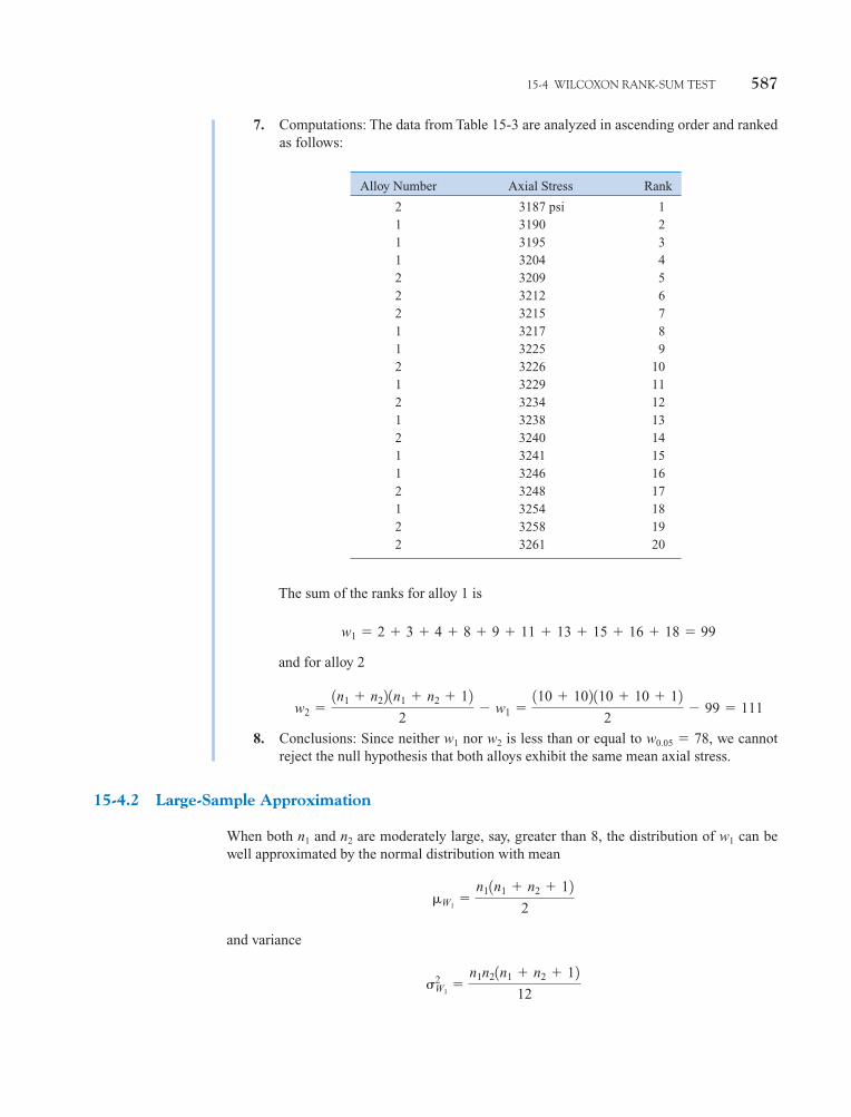
Alloy Number Axial Stress Rank

2 3187 psi 11 3190 21 3195 31 3204 42 3209 52 3212 62 3215 71 3217 81 3225 92 3226 101 3229 112 3234 121 3238 132 3240 141 3241 151 3246 162 3248 171 3254 182 3258 192 3261 20

15-4 WILCOXON RANK-SUM TEST 587

7. Computations: The data from Table 15-3 are analyzed in ascending order and rankedas follows:

The sum of the ranks for alloy 1 is

and for alloy 2

8. Conclusions: Since neither w1 nor w2 is less than or equal to w0.05 � 78, we cannotreject the null hypothesis that both alloys exhibit the same mean axial stress.


When both n1 and n2 are moderately large, say, greater than 8, the distribution of w1 can bewell approximated by the normal distribution with mean

and variance

�2W1

�n1n21n1 � n2 � 12

12

�W1�

n11n1 � n2 � 122

w2 �1n1 � n22 1n1 � n2 � 12

2� w1 �

110 � 102 110 � 10 � 122

� 99 � 111

w1 � 2 � 3 � 4 � 8 � 9 � 11 � 13 � 15 � 16 � 18 � 99



15-28. An electrical engineer must design a circuit to deliverthe maximum amount of current to a display tube to achieve suf-ficient image brightness. Within her allowable design constraints,she has developed two candidate circuits and tests prototypes ofeach. The resulting data (in microamperes) are as follows:

Circuit 1: 251, 255, 258, 257, 250, 251, 254, 250, 248

Circuit 2: 250, 253, 249, 256, 259, 252, 260, 251

Use the Wilcoxon rank-sum test to test H0: �1 � �2 against thealternative H1: �1 > �2. Use � � 0.025.

15-29. One of the authors travels regularly to Seattle,Washington. He uses either Delta or Alaska. Flight delays aresometimes unavoidable, but he would be willing to give mostof his business to the airline with the best on-time arrivalrecord. The number of minutes that his flight arrived late forthe last six trips on each airline follows. Is there evidence thateither airline has superior on-time arrival performance? Use � � 0.01 and the Wilcoxon rank-sum test.

Delta: 13, 10, 1, �4, 0, 9 (minutes late)

Alaska: 15, 8, 3, �1, �2, 4 (minutes late)

15-30. The manufacturer of a hot tub is interested in testingtwo different heating elements for his product. The elementthat produces the maximum heat gain after 15 minutes wouldbe preferable. He obtains 10 samples of each heating unit andtests each one. The heat gain after 15 minutes (in �F) follows.

Is there any reason to suspect that one unit is superior to theother? Use � � 0.05 and the Wilcoxon rank-sum test.

Unit 1: 25, 27, 29, 31, 30, 26, 24, 32, 33, 38

Unit 2: 31, 33, 32, 35, 34, 29, 38, 35, 37, 30

15-31. Use the normal approximation for the Wilcoxonrank-sum test for the problem in Exercise 15-28. Assume that� � 0.05. Find the approximate P-value for this test statistic.

15-32. Use the normal approximation for the Wilcoxonrank-sum test for the heat gain experiment in Exercise 15-30.Assume that � � 0.05. What is the approximate P-value forthis test statistic?

15-33. Consider the chemical etch rate data in Exercise 10-21.Use the Wilcoxon rank-sum test to investigate the claim thatthe mean etch rate is the same for both solutions. If � � 0.05,what are your conclusions?

15-34. Use the Wilcoxon rank-sum test for the pipe deflec-tion temperature experiment described in Exercise 10-20. If � � 0.05, what are your conclusions?

15-35. Use the normal approximation for the Wilcoxonrank-sum test for the problem in Exercise 10-21. Assume that� � 0.05. Find the approximate P-value for this test.

15-36. Use the normal approximation for the Wilcoxonrank-sum test for the problem in Exercise 10-20. Assume that� � 0.05. Find the approximate P-value for this test.


Therefore, for n1 and n2 8, we could use

(15-8)Z0 �W1 � �W1

�W1

as a statistic, and the appropriate critical region is , depending on whether the test is a two-tailed, upper-tail, or lower-tail test.


In Section 15-3.4 we discussed the comparison of the t-test with the Wilcoxon signed-ranktest. The results for the two-sample problem are identical to the one-sample case. That is,when the normality assumption is correct, the Wilcoxon rank-sum test is approximately 95%as efficient as the t-test in large samples. On the other hand, regardless of the form of the dis-tributions, the Wilcoxon rank-sum test will always be at least 86% as efficient. The efficiencyof the Wilcoxon test relative to the t-test is usually high if the underlying distribution has heav-ier tails than the normal, because the behavior of the t-test is very dependent on the samplemean, which is quite unstable in heavy-tailed distributions.

0 z0 0 z�/2, z0 z�, or z0 � �z�


15-5 NONPARAMETRIC METHODS IN THE ANALYSIS OF VARIANCE 589

15-5 NONPARAMETRIC METHODS IN THE ANALYSIS OF VARIANCE

15-5.1 Kruskal-Wallis Test

The single-factor analysis of variance model developed in Chapter 13 for comparing apopulation means is

(15-9)

In this model, the error terms �ij are assumed to be normally and independently distributed withmean zero and variance �2. The assumption of normality led directly to the F-test described inChapter 13. The Kruskal-Wallis test is a nonparametric alternative to the F-test; it requires onlythat the �ij have the same continuous distribution for all factor levels i � 1, 2, . . . , a.

Suppose that is the total number of observations. Rank all N observationsfrom smallest to largest, and assign the smallest observation rank 1, the next smallestrank 2, . . . , and the largest observation rank N. If the null hypothesis

is true, the N observations come from the same distribution, and all possible assignments ofthe N ranks to the a samples are equally likely, we would expect the ranks 1, 2, . . . , N to bemixed throughout the a samples. If, however, the null hypothesis H0 is false, some sampleswill consist of observations having predominantly small ranks, while other samples will con-sist of observations having predominantly large ranks. Let Rij be the rank of observation Yij,and let Ri. and . denote the total and average of the ni ranks in the ith treatment. When thenull hypothesis is true,

and

The Kruskal-Wallis test statistic measures the degree to which the actual observed averageranks . differ from their expected value (N � 1)�2. If this difference is large, the nullhypothesis H0 is rejected. The test statistic is

Ri

E1Ri.2 �1ni

ani

j�1E1Rij2 �

N � 12

E1Rij2 �N � 1

2

Ri

H0: �1 � �2 � . . . � �a

N � g ai�1 ni

Yij � � � �i � �ij e i � 1, 2, . . . , a

j � 1, 2, . . . , ni

(15-10)H �12

N1N � 12 aa

i�1ni aRi. �

N � 12b2



An alternative computing formula that is occasionally more convenient is

(15-11)H �12

N1N � 12 aa

i�1

R2i .

ni� 31N � 12

We would usually prefer Equation 15-11 to Equation 15-10 because it involves the rank totalsrather than the averages.

The null hypothesis H0 should be rejected if the sample data generate a large value forH. The null distribution for H has been obtained by using the fact that under H0 each pos-sible assignment of ranks to the a treatments is equally likely. Thus, we could enumerateall possible assignments and count the number of times each value of H occurs. This hasled to tables of the critical values of H, although most tables are restricted to small samplesizes ni. In practice, we usually employ the following large-sample approximation.Whenever H0 is true and either

a � 3 and ni � 6 for i � 1, 2, 3

a 3 and ni � 5 for i � 1, 2, . . . , a

H has approximately a chi-square distribution with a � 1 degrees of freedom. Since large val-ues of H imply that H0 is false, we will reject H0 if the observed value

The test has approximate significance level �.

Ties in the Kruskal-Wallis TestWhen observations are tied, assign an average rank to each of the tied observations. Whenthere are ties, we should replace the test statistic in Equation 15-11 by

(15-12)

where ni is the number of observations in the ith treatment, N is the total number of observa-tions, and

(15-13)

Note that S 2 is just the variance of the ranks. When the number of ties is moderate, there willbe little difference between Equations 15-11 and 15-12 and the simpler form (Equation 15-11)may be used.

EXAMPLE 15-7 Montgomery (2001) presented data from an experiment in which five different levels ofcotton content in a synthetic fiber were tested to determine whether cotton content has anyeffect on fiber tensile strength. The sample data and ranks from this experiment are shown inTable 15-4. We will apply the Kruskal-Wallis test to these data, using � � 0.01.

S2 �1

N � 1 c a

a

i�1ani

j�1R2

ij �N1N � 122

4d

H �1

S2 c aa

i�1

R2i .

ni�

N1N � 1224

d

h � �2�,a�1



Since there is a fairly large number of ties, we use Equation 15-12 as the test statistic.From Equation 15-13 we find

and the test statistic is

Since h � 13.28, we would reject the null hypothesis and conclude that treatmentsdiffer. This same conclusion is given by the usual analysis of variance F-test.

15-5.2 Rank Transformation

The procedure used in the previous section whereby the observations are replaced by theirranks is called the rank transformation. It is a very powerful and widely useful technique.If we were to apply the ordinary F-test to the ranks rather than to the original data, we wouldobtain

as the test statistic. Note that as the Kruskal-Wallis statistic H increases or decreases, F0 alsoincreases or decreases. Now, since the distribution of F0 is approximated by the F-distribution,

F0 �H� 1a � 12

1N � 1 � H2� 1N � a2

�0.01,42

� 19.06

� 1

53.54 c5245.7 �

25126224

d

h �1

s2 c aa

i�1

r2i .ni

�N1N � 122

4d

� 53.54

�124

c5510 �2512622

2d

s2 �1

N � 1 c a

a

i�1ani

j�1r2

ij �N1N � 122

4d

Table 15-4 Data and Ranks for the Tensile Testing Experiment

Percentageof Cotton ri.

15 y1j 7 7 15 11 9ranks r1j 2.0 2.0 12.5 7.0 4.0 27.5

20 y2j 12 17 12 18 18ranks r2j 9.5 14.0 9.5 16.5 16.5 66.0

25 y3j 14 18 18 19 19ranks r3j 11.0 16.5 16.5 20.5 20.5 85.0

30 y4j 19 25 22 19 23ranks r4j 20.5 25.0 23.0 20.5 24.0 113.0

35 y5j 7 10 11 15 11ranks r5j 2.0 5.0 7.0 12.5 7.0 33.5




15-37. Montgomery (2001) presented the results of an ex-periment to compare four different mixing techniques on thetensile strength of portland cement. The results are shown inthe following table. Is there any indication that mixing tech-nique affects the strength? Use � � 0.05.

MixingTechnique Tensile Strength (lb/in.2)

1 3129 3000 2865 2890

2 3200 3000 2975 3150

3 2800 2900 2985 3050

4 2600 2700 2600 2765

15-38. An article in the Quality Control Handbook, 3rd edi-tion (McGraw-Hill, 1962) presents the results of an experimentperformed to investigate the effect of three different conditioningmethods on the breaking strength of cement briquettes. The dataare shown in the following table. Using � � 0.05, is there anyindication that conditioning method affects breaking strength?

ConditioningMethod Breaking Strength (lb/in.2)

1 553 550 568 541 537

2 553 599 579 545 540

3 492 530 528 510 571

15-39. In Statistics for Research (John Wiley & Sons,1983), S. Dowdy and S. Wearden presented the results of anexperiment to measure the performance of hand-held chainsaws. The experimenters measured the kickback anglethrough which the saw is deflected when it begins to cut a 3-inch stock synthetic board. Shown in the following table are

deflection angles for five saws chosen at random from each offour different manufacturers. Is there any evidence that themanufacturers’ products differ with respect to kickback angle?Use � � 0.01.

Manufacturer Kickback Angle

A 42 17 24 39 43

B 28 50 44 32 61

C 57 45 48 41 54

D 29 40 22 34 30

15-40. Consider the data in Exercise 13-2. Use theKruskal-Wallis procedure with � � 0.05 to test for differ-ences between mean uniformity at the three different gas flowrates.

15-41. Find the approximate P-value for the test statisticcomputed in Exercise 15-37.

15-42. Find the approximate P-value for the test statisticcomputed in Exercise 15-40.

Supplemental Exercises

15-43. The surface finish of 10 metal parts produced in agrinding process is as follows: (in microinches): 10.32, 9.68,9.92, 10.10, 10.20, 9.87, 10.14, 9.74, 9.80, 10.26. Do the datasupport the claim that the median value of surface finish is 10microinches? Use the sign test with � � 0.05. What is the P-value for this test?

15-44. Use the normal appoximation for the sign test forthe problem in Exercise 15-43. Find the P-value for this test.What are your conclusions if � � 0.05?

15-45. Fluoride emissions (in ppm) from a chemical plantare monitored routinely. The following are 15 observations

the Kruskal-Wallis test is approximately equivalent to applying the usual analysis of varianceto the ranks.

The rank transformation has wide applicability in experimental design problems for whichno nonparametric alternative to the analysis of variance exists. If the data are ranked and the or-dinary F-test is applied, an approximate procedure results, but one that has good statisticalproperties. When we are concerned about the normality assumption or the effect of outliers or“wild” values, we recommend that the usual analysis of variance be performed on both theoriginal data and the ranks. When both procedures give similar results, the analysis of varianceassumptions are probably satisfied reasonably well, and the standard analysis is satisfactory.When the two procedures differ, the rank transformation should be preferred since it is lesslikely to be distorted by nonnormality and unusual observations. In such cases, the experi-menter may want to investigate the use of transformations for nonnormality and examine thedata and the experimental procedure to determine whether outliers are present and why theyhave occurred.


MIND-EXPANDING EXERCISES


based on air samples taken randomly during one month of pro-duction: 7, 3, 4, 2, 5, 6, 9, 8, 7, 3, 4, 4, 3, 2, 6. Can you claimthat the median fluoride impurity level is less than 6 ppm?State and test the appropriate hypotheses using the sign testwith � � 0.05. What is the P-value for this test?

15-46. Use the normal approximation for the sign test forthe problem in Exercise 15-45. What is the P-value for thistest?

15-47. Consider the data in Exercise 10-42. Use the signtest with � � 0.05 to determine whether there is a differencein median impurity readings between the two analyticaltests.

15-48. Consider the data in Exercise 15-43. Use theWilcoxon signed-rank test for this problem with � � 0.05.What hypotheses are being tested in this problem?

15-49. Consider the data in Exercise 15-45. Use theWilcoxon signed-rank test for this problem with � � 0.05.What conclusions can you draw? Does the hypothesis you aretesting now differ from the one tested originally in Exercise15-45?

15-50. Use the Wilcoxon signed-rank test with � � 0.05 forthe diet-modification experiment described in Exercise 10-41.State carefully the conclusions that you can draw from thisexperiment.

15-51. Use the Wilcoxon rank-sum test with � � 0.01 forthe fuel-economy study described in Exercise 10-83. What

conclusions can you draw about the difference in meanmileage performance for the two vehicles in this study?

15-52. Use the large-sample approximation for the Wilcoxonrank-sum test for the fuel-economy data in Exercise 10-83. Whatconclusions can you draw about the difference in means if � � 0.01? Find the P-value for this test.

15-53. Use the Wilcoxon rank-sum test with � � 0.025 forthe fill-capability experiment described in Exercise 10-85.What conclusions can you draw about the capability of the twofillers?

15-54. Use the large-sample approximation for theWilcoxon rank-sum test with � � 0.025 for the fill-capabilityexperiment described in Exercise 10-85. Find the P-value forthis test. What conclusions can you draw?

15-55. Consider the contact resistance experiment inExercise 13-31. Use the Kruskal-Wallis test to test for differ-ences in mean contact resistance among the three alloys. If � �0.01, what are your conclusions? Find the P-value for this test.

15-56. Consider the experiment described in Exercise 13-28.Use the Kruskal-Wallis test for this experiment with � � 0.05.What conclusions would you draw? Find the P-value forthis test.

15-57. Consider the bread quality experiment in Exercise13-35. Use the Kruskal-Wallis test with � � 0.01 to analyze thedata from this experiment. Find the P-value for this test. Whatconclusions can you draw?

15-58. For the large-sample approximation to theWilcoxon signed-rank test, derive the mean and stan-dard deviation of the test statistic used in the procedure.

15-59. Testing for Trends. A turbocharger wheel ismanufactured using an investment-casting process. Theshaft fits into the wheel opening, and this wheel openingis a critical dimension. As wheel wax patterns are formed,the hard tool producing the wax patterns wears. This maycause growth in the wheel-opening dimension. Tenwheel-opening measurements, in time order of produc-tion, are 4.00 (millimeters), 4.02, 4.03, 4.01, 4.00, 4.03,4.04, 4.02, 4.03, 4.03.(a) Suppose that p is the probability that observation

Xi�5 exceeds observation Xi. If there is no upward ordownward trend, Xi�5 is no more or less likely to ex-ceed Xi or lie below Xi. What is the value of p?

(b) Let V be the number of values of i for whichXi�5 Xi. If there is no upward or downward trend

in the measurements, what is the probability distri-bution of V?

(c) Use the data above and the results of parts (a) and(b) to test H0: there is no trend, versus H1: there isupward trend. Use � � 0.05.

Note that this test is a modification of the sign test. Itwas developed by Cox and Stuart.

15-60. Consider the Wilcoxon signed-rank test, andsuppose that n � 5. Assume that H0: � � �0 is true.(a) How many different sequences of signed ranks are

possible? Enumerate these sequences.(b) How many different values of W� are there? Find

the probability associated with each value of W�.(c) Suppose that we define the critical region of the test

to be to reject H0 if w� w*� and w*� � 13. What isthe approximate � level of this test?

(d) Does this exercise show how the critical values for theWilcoxon signed-rank test were developed? Explain.



In the E-book, click on anyterm or concept below togo to that subject.

Asymptotic relativeefficiency

Kruskal-Wallis test

Nonparametric ordistribution freeprocedures

Normal approximationto nonparametrictests

Paired observations

RanksRank transformation in

ANOVASign testTests on the mean of a

symmetric continu-ous distribution

Tests on the median ofa continuousdistribution

Wilcoxon rank-sum testWilcoxon signed-rank

test

IMPORTANT TERMS AND CONCEPTS


15Nonparametric Statistics

Documents

Transcript of 15Nonparametric Statistics