Consistent Query Answering under Spatial Semantic Constraints

arX

iv:1

106.

1478

v1 [

cs.D

B]

8 Ju

n 20

11

Consistent Query Answering under Spatial SemanticConstraints

M. Andrea RodrıguezUniversidad de Concepcion, Chile

[email protected]

Leopoldo Bertossi∗

Carleton University, [email protected]

Monica CaniupanUniversidad del Bıo-Bıo, [email protected]

Abstract

Consistent query answering is an inconsistency tolerant approach to obtaining semantically correct an-swers from a database that may be inconsistent with respect to its integrity constraints. In this workwe formalize the notion of consistent query answer for spatial databases and spatial semantic integrityconstraints. In order to do this, we first characterize conflicting spatial data, and next, we define admissi-ble instances that restore consistency while staying closeto the original instance. In this way we obtaina repair semantics, which is used as an instrumental conceptto define and possibly derive consistentquery answers. We then concentrate on a class of spatial denial constraints and spatial queries for whichthere exists an efficient strategy to compute consistent query answers. This study applies inconsistencytolerance in spatial databases, rising research issues that shift the goal from the consistency of a spatialdatabase to the consistency of query answering.

1 Introduction

Consistency in database systems is defined as the satisfaction by a database instance of a set of integrity con-straints (ICs) that restricts the admissible database states. Although consistency is a desirable and usuallyenforced property of databases, it is not uncommon to find inconsistent spatial databases due to data inte-gration, unforced integrity constraints, legacy data, or time lag updates. In the presence of inconsistencies,there are alternative courses of action: (a) ignore inconsistencies, (b) restore consistency via updates on thedatabase, or (c) accept inconsistencies, without changingthe database, but compute the “consistent or cor-rect” answers to queries. For many reasons, the first two alternatives may not be appropriate [6], speciallyin the case of virtual data integration [5], where centralized and global changes to the data sources are notallowed. The latter alternative has been investigated in the relational case [4, 10]. In this paper we explorethis approach in the spatial domain, i.e., for spatial databases and with respect to spatial semantic integrityconstraints (SICs).

Extracting consistent data from inconsistent databases could be qualified as an “inconsistency tolerant”approach to querying databases. A piece of data will be part of a consistent answer if it is not logicallyrelated to the inconsistencies in the database with respectto its set of ICs. We introduce this idea using aninformal and simple example.

∗Faculty Fellow of the IBM Center for Advanced Studies. Also affiliated to Universidad de Concepcion, Chile.

1

http://arxiv.org/abs/1106.1478v1

Example 1 Consider a database instance with a relationLandP, denoting land parcels, with a thematicattribute (idl), and a spatial attribute,geometry, of data typepolygon. An IC stating that geometries oftwo different land parcels must be disjoint or just touch, i.e., they cannot internally intersect, is expected tobe satisfied. However, the instance in Figure 1 does not satisfy this IC and therefore it is inconsistent: theland parcels with idlsidl2 andidl3 overlap. Notice that these geometries are partially in conflict and whatis not in conflict can be considered as consistent data.

LandPidl geometryidl1 g1idl2 g2idl3 g3

Figure 1: An inconsistent spatial database

Suppose that a query requests all land parcels whose geometries intersect with a query window, whichrepresents the spatial region shown in Figure 1 as a rectangle with dashed borders. Although the databaseinstance is inconsistent, we can still obtain useful and meaningful answers. In this case, only the intersectionof g2 andg3 is in conflict, but the rest of both geometries can be considered consistent and should be partof any “database repair” if we decide to restore consistencyby means of minimal geometric changes. Thus,since the non-conflicting parts of geometriesg2 andg3 intersect the query window, we would expect ananswer including land parcels with identitiesidl1 , idl2 andidl3 . ✷

If we just concentrate on (in)consistency issues in databases (leaving aside consistent query answering fora moment), we can see that, in contrast to (in)consistency handling in relational databases, that has beenlargely investigated, not much research of this kind has been done for spatial databases. In particular, thereis not much work around the formalization of semantic spatial ICs, satisfaction of ICs, and checking andmaintenance of ICs in the spatial domain. However, some papers address the specification of some kinds ofintegrity constraints [8, 20], and checking topological consistency at multiple representations and for dataintegration [13, 14, 31].

More recently, [12] proposes qualitative reasoning with description logic to describe consistency be-tween geographic data sets. In [22] a set of abstract relations between entity classes is defined; and theycould be used to discover redundancies and conflicts in sets of SICs. A proposal for fixing (changing)spatial database instances under different types of spatial inconsistencies is given in [29]. According to it,changes are applied over geometries in isolation; that is, they are not analyzed in combination with multipleSICs. In [27] some issues around query answering under violations of functional dependencies involvinggeometric attributes were raised. However, the problem of dealing with an inconsistent spatial database,while still obtaining meaningful answers, has not been systematically studied so far.

Consistent query answering (CQA) from inconsistent databases as a strategy of inconsistent tolerancehas an extensive literature (cf. [4, 6, 10] for surveys). It was introduced and studied in the context ofrelational database in [2]. They defined consistent answersto queries as those that are invariant under all theminimal forms of restoring consistency of the original database. Thus, the notion ofrepair of an instancewith respect to a set of ICs becomes a fundamental concept fordefining consistent query answers. Arepairsemantics defines the admissible and consistent alternative instances to an inconsistent database at hand.More precisely, arepair of an inconsistent relational instanceD is a consistent instanceD ′ obtained fromD by deleting or inserting whole tuples. The set of tuples by which D andD ′ differ is minimal under set

2

inclusion [2]. Other types of repair semantics have been studied in the relational case. For example, in[16, 32] repairs are obtained by allowing updates of attribute values in tuples.

In comparison to the relational case, spatial databases offer new alternatives and challenges when defin-ing a repair semantics. This is due, in particular, to the useof complex attributes to represent geometries,their combination with thematic attributes, and the natureof spatial (topological) relations.

In this work we define a repair semantics for spatial databases with respect to a subset of spatial semanticintegrity constraints (a.k.a. topo-semantic integrity constraints) [29], which impose semantic restrictions ontopological predicates and combinations thereof. In particular, we treat spatial semantic integrity constraintsthat can be expressed by denials constraints. For example, they can specify that “two land parcels cannotinternally intersect”. This class of constraints are neither standardized nor integrated into current spatialdatabase management systems (DBMSs); they rather depend onthe application, and must be defined andhandled by the database developers. They are very importantbecause they capture the semantics of theintended models. Spatial semantic integrity constraints will be simply calledspatial integrity constraints(SICs). Other spatial integrity constraints [11] aredomain (topological or geometric) constraints, and theyrefer to the geometry, topology, and spatial relations of the spatial data types. One of them could specify that“polygons must be closed”. Many of these geometric constraints are now commonly integrated into spatialDBMSs [23].

A definition of a repair semantics for spatial DBs and CQA for spatial range queries was first proposedin [28], where we discussed the idea of shrinking geometriesto solve conflicting tuples and applied toCQA for range queries. In this paper we complement and extendour previous work with the followingmain contributions: (1) We formalize the repair semantics of a spatial database instance under violationsof SICs. This is done through virtual changes of geometries that participate in violations of SICs. Unlike[28], we identify the admissible local transformations andwe use them to provide an inductive definitionof database repair. (2) Based on this formalization, a consistent answer to a spatial query is defined as ananswer obtained from all the admissible repairs. Extendingthe results in [28], we now define CQA not onlyfor range but also for spatial join queries. (3) Although therepair semantics and consistent query answerscan be defined for a fairly broad class of SICs and queries, as it becomes clear soon, naive algorithms forcomputing consistent answers on the basis of the computation of all repairs are of exponential time. Forthis reason, CQA for a relevant subset of SICs and range and join queries is done via acore computation.This amounts to querying directly the intersection of all repairs of an inconsistent database instance, butwithout actually computing the repairs. We show cases wherethis core can be specified as a view of theoriginal, inconsistent database. (4) We present an experimental evaluation with real and synthetic data setsthat compares the cost of CQA with the cost of evaluating queries directly over the inconsistent database(i.e., ignoring inconsistencies).

The rest of the paper is organized as follows. In Section 2 we describe the spatial data model uponwhich we define the repair semantics and consistent query answers. A formal definition of repair for spatialinconsistent databases under SICs is introduced in Section3. In Section 4 we define consistent answersto conjunctive queries. We analyze in particular the cases of range and join queries with respect to theircomputational properties. This leads us, in Section 5, to propose polynomial time algorithms (in data com-plexity) for consistent query answering with respect to a relevant class of SICs and queries. An experimentalevaluation of the cost of CQA is provided in Section 6. Final conclusions and future research directions aregiven in Section 7.

3

2 Preliminaries

Current models of spatial database are typically seen as extensions of the relational data model (known asextended-relational or object-relational models) with the definition of abstract data types to specify spatialattributes. We now introduce a general spatio-relational database model that includes spatio-relational pred-icates (they could also be purely relational) and spatial ICs. It uses some of the definitions introduced in[25]. The model is independent of the geometric data model (e.g. Spaghetti [30], topological [18, 30], raster[19], or polynomial model [24]) underlying the representation of spatial data types.

A spatio-relational database schema is of the formΣ = (U ,A,R, T ,O,B), where: (a)U is the possiblyinfinite database domain of atomic thematic values. (b)A is a set of thematic, non-spatial, attributes. (c)R is a finite set of spatio-relational predicates whose attributes belong toA or are spatial attributes. Spatialattributes take admissible values inP(Rm), the power set ofRm, for anm that depends on the dimensionof the spatial attribute. (d)T is a fixed set of binary spatial predicates, with a built-in interpretation. (e)O is a fixed set of geometric operators that take spatial arguments, also with a built-in interpretation. (f)Bis a fixed set of built-in relational predicates, like comparison predicates, e.g.<,>,=, 6=, which apply tothematic attribute values.

Each database predicateR ∈ R has a typeτ(R) = [n,m], with n,m ∈ N, indicating the numbern ofthematic attributes, and the spatial dimensionm of the single spatial attribute (it takes values inP(Rm)).1 InExample 1,τ(LandP) = [1, 2], since it has one thematic attribute (idl ) and one spatial attribute (geometry )defined by a 2D polygon. In this work we assume that each relationR has a key of the form (1) formed bythematic attributes only:

∀x1x2x3s1s2 (R(x1, x2; s1) ∧R(x1, x3; s2) → (x2 = x3 ∧ s1 = s2)), (1)

where thexi are sequences of distinct variables representing thematicattributes ofR, and thesi are variablesfor geometric attributes. Heres1 = s2 means geometric equality; that is, the identity of two geometries.

A database instanceD of a spatio-relational schemaΣ is a finite collection of ground atoms (orspatialdatabase tuples) of the formR(c1, ..., cn; s), whereR ∈ R, 〈c1, ..., cn〉 ∈ Un contains the thematic attributevalues, ands ∈ Ad ⊆ P(Rm), whereAd is the class of admissible geometries (cf. below). The extensionin a particular instance of a spatio-relational predicate is a subset ofUn × Ad . For simplicity, and to fixideas, we will consider the case wherem = 2.

Among the different abstraction mechanisms for modelling single spatial objects, we concentrate onregions for modelling real objects that have an extent. Theyare useful in a broad class of applications inGeographic Information Systems (GISs). More specifically,our model will be compatible with the specifi-cation of spatial operators (i.e., spatial relations or geometric operations) as found in current spatial DBMSs[23]. Following current implementations of DBMSs, regionscould be defined as finite sets of polygons that,in their turn, are defined through their vertices. This wouldmake regions finitely representable. However, inthis work geometries will be treated at a more abstract level, which is independent of the spatial model usedfor geometric representation. In consequence, an admissible geometry of the Euclidean plane is either theempty geometry,g⊘, which corresponds to the empty subset of the plane, or is a closed and bounded regionwith a positive area. It holdsg⊘ ∩ g = g ∩ g⊘ = g⊘, for every regiong. From now on, empty geometriesand regions ofR2 are calledadmissible geometries and they form the classAd .

Geometric attributes are complex data types, and their manipulation may have an important effect onthe computational cost of certain algorithms and algorithmic problems. As usual, we are interested indata

1For simplicity, we use one spatial attribute, but it is not difficult to consider a greater number of spatial attributes.

4

complexity, i.e., in terms of the size of the database. Thesize of a spatio-relational database can be definedas a function of the number of tuples and the representation size of geometries in those tuples.

We concentrate on binary (i.e., two-ary) spatial predicates that represent topological relations betweenregions. They have a fixed semantics, and become the elements ofT . There are eight basic binary rela-tions over regions ofR2: Overlaps (OV ), Equals (EQ), CoveredBy (CB), Inside (IS ), Covers (CV ),Includes (IC ), Touches (TO), andDisjoint (DJ ) [15, 26].2 The semantics of the topological relationsfollows the point-set topology defined in [15], which is not defined for empty geometries. We will applythis semantics to our non-empty admissible geometries. Forthe case of the empty set, a separate definitionwill be given below. According to [15], an atomT (x, y) becomes true if four conditions are simultaneouslytrue. Those conditions are expressed in terms of emptyness (∅) and non-emptyness (¬∅) of the intersectionof their boundaries (δ) and interiors (◦). The definitions can be found in Table 1. For example, for non-empty regionsx, y, TO(x, y) is true iff all of δ(x) ∩ δ(y) 6= ∅, ◦(x) ∩ ◦(y) = ∅, δ(x) ∩ ◦(y) = ∅, and◦(x) ∩ δ(y) = ∅ simultaneously hold.

Relation δ(x) ∩ δ(y) ◦(x) ∩ ◦(y) δ(x) ∩ ◦(y) ◦(x) ∩ δ(y)DJ(x,y) ∅ ∅ ∅ ∅TO(x,y) ¬∅ ∅ ∅ ∅EQ(x,y) ¬∅ ¬∅ ∅ ∅IS(x,y) ∅ ¬∅ ¬∅ ∅CB(x,y) ¬∅ ¬∅ ¬∅ ∅IC(x,y) ∅ ¬∅ ∅ ¬∅CV(x,y) ¬∅ ¬∅ ∅ ¬∅OV(x,y) ¬∅ ¬∅ ¬∅ ¬∅

Table 1: Definition of topological relations between regions based on point-set topology

In this work we exclude the topological relationDisjoint from T . This decision is discussed in Section 3,where we introduce the repair semantics. In addition to the basic topological relations, we consider threederived relations that exist in current SQL languages and can be logically defined in terms of the otherbasic predicates:Intersects (IT ), Within (WI ), andContains (CO). We also introduce a forth relation,IIntersects (II), that holds when the interiors of two geometries intersect.It can be logically defined asthe disjunction ofOverlaps , Within andContains (cf. Figure 2). For all the topological relations inT ,their converse (inverse) relation is within the set. Some ofthem are symmetric, likeEquals, Touches , andOverlaps . For the non-symmetric relations, the converse relation ofCoveredBy is Covers , of Inside isIncludes , and ofWithin isContains .

As mentioned before, the formal definitions of the topological relations [15, 26] do not consider theempty geometry as an argument. Indeed, at the best of our knowledge, no clear semantics for topologicalpredicates with empty geometries exists. However, in our case we extent the definitions in order to dealwith this case. This will allow us to use a classical bi-valued logic, where atoms are always true or false,but never undefined. According to our extended definition, for anyT ∈ T , T (g1, g2) is false ifg1 = g⊘ org2 = g⊘. In particular,IS (g, g⊘) is false, for every admissible regiong. In order to make comparisons withthe empty region, we will introduce and use a special predicate IsEmpty(·) on admissible geometries, such

2The names of relations chosen here are in agreement with the names used in current SQL languages [23], but differ slightlyfrom the names found in the research literature. The relations found in current SQL languages are represented in Figure 2withthick borders.

5

Figure 2: Subsumption lattice of topological relations between regions: OV (Overlaps), CB (CoveredBy),IS (Inside), EQ (Equals), CV (Covers), IC (Includes), TO (Touches), DJ (Disjoint), IT (Intersects), II (IIn-tersects), WI (Within), and CO (Contains).

thatIsEmpty(s) is true iff s = g⊘.Notice that the semantics of the topological predicates, even for non-empty regions, may differ from the

intuitive set-theoretic semantics one could assign to them. For example, for an admissible and non-emptygeometryg, OV (g, g) is false (due to the conditions in the last two columns in Table 1). In consequence,the constraint∀x∀s 6=g⊘¬(R(x; s) ∧OV (s, s)) is satisfied.

Given a database instance, additional spatial informationis usually computed from the explicit geometricdata by means of the spatial operators inO associated withΣ. Some relevant operators are:Area, Union(binary), Intersection , Difference, Buffer , andUnion Aggregation (GeomUnion).3 (Cf. [23] for thecomplete set of spatial predicates defined within the Open GIS Consortium.) There are several spatialoperators used in this work; however, we will identify a particular subsetOa of spatial operators inO, i.e.,Oa ⊆ O, which will be defined for all admissible geometries and usedto shrink geometries with the purposeof restoring consistency, as we describe in Section 3.

Definition 1 The setOa of admissible operations contains the following geometric operations on admissi-ble geometriesg andg′:

(1) Difference(g, g′) is the topological closure of the set-difference.(2)Buffer(g, d) is the geometry obtained by buffering a distanced aroundg, whered is a distance unit.

Buffer(g, d) returns a closed regiong containing geometryg, such that every point in the boundary ofg isat a distanced from some point of the boundary ofg. In particular,Buffer(g⊘, d) = g⊘. ✷

Notice that these operators, when applied to admissible geometries, produce admissible geometries.

Remark 1 The value ofd in Definition 1 is instance dependent. It should be precomputed from the spatialinput data. For this work, we considerd to be a fixed value associated with the minimum distance betweengeometries in the cartographic scale of the database instance. ✷

3OperatorGeomUnion returns the geometry that represents the point set union of all geometries in a given set, an operatoralso known as a spatial aggregation operator. Although thisfunction is part of SQL for several spatial databases (Postgres/PostGIS,Oracle), it is not explicitly defined in the OGC specification[23].

6

LandPidl name owner geometryidl1 n1 o1 g1idl2 n2 o2 g2idl3 n3 o3 g3

Buildingidb geometryidb1 g4idb2 g5

Figure 3: A spatial database instance

A schemaΣ determines a many-sorted, first-order (FO) languageL(Σ) of predicate logic. It can be usedto syntactically characterize and express SICs. For simplicity, we concentrate ondenial SICs,4 which aresentences of the form:

∀ 6=g∅ s∀x ¬(m∧

i=1

Ri(xi; si) ∧ ϕ ∧n∧

j=1

Tj(vj , wj)). (2)

Here,s = s1 · · · sm, x = x1 · · · xm are finite sequences of geometric and thematic variables, respectively,and0 < m,n ∈ N. Thus, eachxi is a finite tuple of thematic variables and will be treated as aset ofattributes, such thatxi ⊆ xj means that the variables inxi area also variables inxj. Also, ∀x stands for∀x1 · · · ∀xm; and∀ 6=g∅ s stands for∀s1 · · · ∀sm, with the universal quantifiers ranging over all the non-emptyadmissible geometries (i.e. regions). Here,vj , wj ∈ s, R1, . . . , Rm ∈ R, ϕ is a formula containing built-inatoms over thematic attributes, andTj ∈ T . A constraint of the form (2) prohibits certain combinations ofdatabase atoms. Since topological predicates for empty geometries are always false, the restricted quantifi-cation over non-empty geometries in the constraints could be eliminated. However, we do not want to makethe satisfaction of the constraints rely on our particular definition of the topological predicates for the emptyregion. In this way, our framework becomes more general, robust and modular, in the sense that it wouldbe possible to redefine the topological predicates for the empty region without affecting our approach andresults.

Example 2 Figure 3 shows an instance for the schemaR = {LandP(idl , name , owner ; geometry),Building(idb; geometry)}. Dark rectangles represent buildings and white rectanglesrepresents land parcels.In LandP , the thematic attributes areidl ,name andowner , whereasgeometry is the spatial attribute ofdimension2. Similarly forBuilding , which has onlyidl as a thematic attribute.

The following sentences are denial SICs: (The symbol∀ stands for the universal closure of the formulathat follows it.)

∀¬(LandP (idl1, n1, o1; s1) ∧ LandP (idl2, n2, o2; s2) ∧ idl1 6= idl2 ∧ IIntersects(s1, s2)). (3)

∀¬(Building(idb; s1) ∧ LandP(idl, n, o; s2) ∧Overlaps(s1, s2)). (4)

The SIC (3) says that geometries of land parcels with different ids cannot internally intersect (i.e., theycan only be disjoint or touch). The SIC (4) establishes that building blocks cannot (partially) overlap landparcels. ✷

4Denial constraints are easier to handle in the relational case as consistency with respect to them is achieved by tuple deletionsonly [6].

7

A database instanceD for schemaΣ can be seen as an interpretation structure for the languageL(Σ). Fora setΨ of SICs inL(Σ), D |= Ψ denotes that each of the constraints inΨ is true in (or satisfied by)D . Inthis case, we say thatD is consistent with respect toΨ. Correspondingly,D is inconsistent with respect toΨ, denotedD 6|= Ψ, when there is aψ ∈ Ψ that isviolated by D , i.e., not satisfied byD . The instance inExample 2 is consistent with respect to its SICs.

In what follows, we will assume that the setΨ of SICs under consideration is logically consistent; i.e.,that there exists a non-empty database instanceD (not necessarily the one at hand), such thatD |= Ψ. Forexample, any set of SICs containing a constraint of the form∀ 6=g∅s∀x ¬(R(x; s)∧Equals(s, s)) is logicallyinconsistent. The analysis of whether a set of SICs is logically consistent or not is out of the scope of thiswork.

3 A Repair Semantics

Different alternatives for update-based consistency restoration of spatial databases are discussed in [28]. Oneof the key criteria to decide about the update to apply is minimality of geometric changes. Another importantcriteria may be the semantics of spatial objects, which makes changes over the geometry of one type of objectmore appropriate than others. For this work, the repair semantics is a rule applied automatically. It assumesthat no previous knowledge about the quality and relevance of geometries exists and, therefore, it assumesthat geometries are all equally important.

On the basis on the minimality condition on geometric changes and the monotonicity property of sometopological predicates [28], we propose to solve inconsistencies with respect to SICs of the form (2) throughshrinking of geometries. Notice that this repair semanticswill be used as an instrumental concept to formal-ize consistent query answers (no actual modification over the database occurs). As such, it defines what partof the geometry is not in conflict with respect to a set of integrity constraints and can, therefore, be part of aconsistent answer.

Shrinking geometries eliminates conflicting parts of geometries without adding new uncertain geome-tries by enlargement. In this way, we are considering a proper subset of the possible changes to fix spatialdatabases proposed in [29]. We disregard translating objects, because they will carry potentially new con-flicts; and also creating new objects (object splitting), because we would have to deal with null or unknownthematic attributes.

The SICs of the form (2) exclude the topological predicateDisjoint. The reason is that falsifying anatomDJ (g1, g2) by shrinking geometries is not possible, unless we make one of them empty. However,doing so would heavily depend upon our definition of this topological predicate for empty regions. Sincewe opted for not making our approach and results depend on this particular definition, we prefer to excludethe Disjoint predicate from our considerations. The study of other repair semantics that sensibly includesthe topological predicateDisjoint will be left for future work.

Technically, a databaseD violates a constraint∀x1x2∀ 6=g⊘s1s2 ¬(R1(x1; s1) ∧ R2(x2; s2) ∧ ϕ ∧T (s1, s2)), with T ∈ T ,5 when there are data valuesa1, a2, g1, g2, with g1, g2 6= g⊘, for the variablesin the constraint such that(R1(x1; s1) ∧R2(x2; s2) ∧ ϕ ∧ T (s1, s2)) becomes true in the database underthose values. This is denoted withD |= (R1(x1; s1) ∧ R2(x2; s2) ∧ ϕ ∧ T (s1, s2)) [a1, a2, g1, g2]. Whenthis is the case, it is possible to restore consistency ofD by shrinkingg1 or g2 such thatT (g1, g2) becomesfalse.

5For simplicity and without lost of generality, in the examples we consider denial constraints with at most two spatio-relationalpredicates and one topological predicate. However, a denial constraint of the form (2) may have more spatio-relationalpredicatesand topological predicates.

8

We can compare geometries, usually an original geometry andits shrunk version, by means of a distancefunction that refers to their areas. We assume thatarea ∈ O is an operator that computes the area of ageometry.

Definition 2 For regionsg1, g2, δ(g1, g2) = area(Difference(g1, g2) ∪Difference(g2, g1)). ✷

Since we will compare a regiong1 with a regiong2 obtained by shrinkingg1, it will hold δ(g1, g2) ≥ 0. In-deed, when comparingg2 ⊆ g1

6, the distance function can be simplified byδ(g1, g2) = area(Difference(g1, g2)).We will assume that it is possible to compare geometries through the distance function by correlating theirtuples, one by one. This requires a correspondence between instances.

Definition 3 Let D ,D ′ be database instances of schemaΣ. D ′ is (D , fD ′)-indexed if fD ′ is a bijectivefunction fromD to D ′, such that, for allc1, . . . , cn, s: fD ′(R(c1, . . . , cn; s)) = R(c1, . . . , cn; s

′), for someregions′. ✷

In a (D , fD ′)-indexed instanceD ′ we can compare tuples one by one with their counterparts in instanceD .In particular, we can see how the geometric attribute valuesdiffer. In some cases there is an obvious functionfD ′ , for example, when there is a key from a subset ofA to the spatial attributeS, or when relations have asurrogate key for identification of tuples. In these cases wesimply use the notion ofD -indexed. When thecontext is clear, we also usef instead offD ′ .

Example 3 (example 2 cont.) Consider the relational schemaLandP(idl , name, owner ; geometry). Forthe instanceD given in Example 2, the following instanceD ′ is (D , f )-indexed


Here,f(LandP(idl1, n1, a1; g1)) = LandP(idl1, n1, a1; g7), etc. ✷

When restoring consistency, it may be necessary to considerdifferent combinations of tuples and SICs.Eventually, we should obtain a new instance, hopefully consistent, that we have to compare to the originalinstance in terms of their distance.

Definition 4 LetD ,D ′ be spatial database instances over the same schemaΣ, with D ′ (D , f)-indexed. Thedistance ∆(D ,D ′) betweenD andD ′ is the numerical value∆(D , D ′) = Σt∈Dδ(ΠS(t), ΠS(f(t))),whereΠS(t) is the projection of tuplet on its spatial attributeS. ✷

Now it is possible to define a “repair semantics”, which is independent of the geometric operators used toshrink geometries.

Definition 5 Let D be a spatial database instance over schemaΣ, Ψ a set of SICs, such thatD 6|= Ψ. (a)An s-repair of D with respect toΨ is a database instanceD ′ overΣ, such that: (i)D ′ |= Ψ. (ii) D ′ is(D , f)-indexed. (iii) For every tupleR(c1, . . . , cn; g) ∈ D , if f(R(c1, . . . , cn; g)) = R(c1, . . . , cn; g

′), theng′ ⊆ g. (b) A minimal s-repair D ′ of D is a repair ofD such that, for every repairD ′′ of D , it holds∆(D ,D ′′) ≥ ∆(D ,D ′). ✷

6⊆ stands for geometric inclusion

9

Proposition 1 If D is consistent with respect toΨ, thenD is also its only minimal s-repair.

Proof: ForD ′ = D , it holds: (i)D ′ |= Ψ, (ii) D ′ is (D , f)-indexed, (iii) for every tupleR(c1, . . . , cn; g) ∈D , if f(R(c1, . . . , cn; g)) = R(c1, . . . , cn; g

′), theng′ = g. In this case,∆(D ,D ′) = 0. Any other con-sistent instanceD ′′ obtained by shrinking any ofD ’s geometries and still obtaining admissible geometriesgives∆(D ,D ′′) > 0. ✷

This is an “ideal and natural” repair semantics that defines acollection of semantic repairs. The defini-tion is purely set-theoretic and topological in essence. Itis worth exploring the properties of this semanticsand its impact on properties of consistent query answers (asinvariant under minimal s-repairs) and on log-ical reasoning about them. However, for a given database instance we may have a continuum and infinitenumber of s-repairs since between two points we have an infinite number of points, which we want to avoidfor representational and computational reasons.

In this work we will consider an alternative repair semantics that is more operational in nature (cf.Definition 8), leaving the previous one for reference. Thisoperational definition of repair makes it possibleto deal with repairs in current spatial DBMSs and in terms of standard geometric operators (cf. Lemma 1).Under this definition, there will always be a finite number of repairs for a given instance. Consistency willbe restored by applying a finite sequence of admissible transformation operations to conflicting geometries.

It is easy to see that each true relationship (atom) of the form T (g1, g2), with T ∈ T , can be falsifiedby applying an admissible transformation inOa to g1 or g2. Actually, they can be falsified in acanonicalway. These canonical falsification operations for the different topological atoms are presented in Table 2.They have the advantages of: (a) being defined in terms of the admissible operators, (b) capturing the repairprocess in terms of the elimination of conflicting parts of geometries, and (c) changing one of the geometriesparticipating in a conflict.

More specifically, in Table 2 we indicate, for each relationT ∈ T , alternative operations that falsifya true atom of the formT (g1, g2). Each of them makes changes on one of the geometries, leavingtheother geometry unchanged. The list ofcanonical transformations in this table prescribes particular ways ofapplying the admissible operators of Definition 1. Later on,they will also become theadmissible or legalways of transforming geometries with the purpose of restoring consistency.

For example, Table 2 shows that forOverlaps(OV ), there are in principle four ways to make false anatomOverlaps(g1, g2) that is true. These are the alternatives 1. to 4. in that entry, where alternatives 1. and2. change geometryg1; and alternatives 3. and 4. change geometryg2. Only one of these alternatives thatsatisfies its condition is expected to be chosen to falsify the atom. A minimal way to change a geometrydepends on the relative size between overlapping and non-overlapping areas: (i) when the overlapping areabetweeng1 andg2 is smaller than or equal to their non-overlapping areas, a minimal change over geometryg1 isDifference(g1, g2), and overg2 isDifference(g2, g1) (cases 1. and 3. forOV in Table 2). (ii) When thenon-overlapping areas ofg1 or g2 are smaller than the overlapping area, a minimal change overgeometryg1is Difference(g1, Difference(g1, g2)), and over geometryg2 is Difference(g2, Difference(g2, g1)) (cases2. and 4. forOV in Table 2).

For the case whenEquals(g1, g2) is true, the transformations in Table 2 make either geometry, g1 or g2empty to falsify the atom. However, there are other alternatives that by shrinking geometries would achievethe same result, but also producing smaller changes in termsof the affected area. A natural candidate updateconsists in applying the transformationg′1 = Difference(g1,Buffer(Boundary(g2), d)) (similarly and alter-natively forg2). In this case, we just take away fromg1 the part of the internal area of widthd surroundingthe boundary ofg1, to make it different fromg2. We did not follow this alternative for practical reasons:having two geometries that are topologically equal could, in many cases, be the result of duplicate data, and

10

Pred.T A true atomT (g1, g2) becomes a false atomT (g′1, g′2) with

OV 1. If area(g1 ∩ g2) ≤ area(g1 r g2):g′1 = Difference(g1, g2), g′2 = g2.

2. If area(g1 ∩ g2) > area(g1 r g2):g′1 = Difference(g1,Difference(g1, g2)), g′2 = g2.

3. If area(g1 ∩ g2) ≤ area(g2 r g1):g′2 = Difference(g2, g1), g′1 = g1.


IS ,CB 1. If area(g1 ∩ g2) ≤ area(g2 r g1):g′2 = Difference(g2, g1), g′1 = g1.


3. g′1 = Difference(g1, g2), g′2 = g2.

IC ,CV 1. If area(g1 ∩ g2) ≤ area(g1 r g2):g′1 = Difference(g1, g2), g′2 = g2.


3. g′2 = Difference(g2, g1), g′1 = g1.

I I,WI,CO 1. g′1 = Difference(g1, g2), g′2 = g2.2. g′2 = Difference(g2, g1), g′1 = g1.

TO, IT 1. g′1 = Difference(g1, buffer(g2, d)), g′2 = g2.2. g′2 = Difference(g2, buffer(g1, d)), g′1 = g1.(See Remark 1 for definition ofd)

EQ 1. g′1 = g⊘, g′2 = g2.2. g′2 = g⊘, g′1 = g1.

Table 2: Admissible transformations

one of them should be eliminated. Moreover, this alternative, in comparison with the officially adopted inthis work, may create new conflicts with respect to other SICs. Avoiding them whenever possible will beused later, when designing a polynomial algorithm for CQA based on the core of an inconsistent databaseinstance (see Section 5).

Table 2 shows thatTouches andIntersects are predicates for which the eliminated area is not completelydelimited by the real boundary of objects. Actually, we needto separate the touching boundaries. We do so

11

by buffering a distanced around one of the geometries and taking the overlapping partfrom the other one.7

The following result is obtained directly from Table 2.

Lemma 1 For each topological predicateT ∈ T and true ground atomT (g1, g2), there are geometriesg′1, g

′2 obtained by means of the corresponding admissible transformation in Table 2, such thatT (g′1, g

′2)

becomes false. ✷

The following definition defines, for each geometric predicateT , a binary geometric operatortrT such that,if T (g1, g2) is true, thentrT (g1, g2) returns a geometryg′1 such thatT (g′1, g2) becomes false. The definitionis based on the transformations that affect geometryg1 in Table 2.

Definition 6 Let T ∈ T be a topological predicate. We define an admissible transformation operatortrT :Ad × Ad → Ad as follows:

(a) If T (g1, g2) is false, thentrT (g1, g2) := g1.

(b) If T (g1, g2) is true, then:

trT (g1, g2) :=

{

Difference(g1, g2) if area(g1 ∩ g2) ≤ area(g1 r g2)Difference(g1,Difference(g1, g2)), otherwise

for T ∈ {OV, IC,CV };

trT (g1, g2) := Difference(g1, g2), for T ∈ {IS,CB, II,WI,CO};

trT (g1, g2) := Difference(g1,Buffer(g2, d)) for T ∈ {TO, IT};

trT (g1, g2) := g⊘ for T ∈ {EQ}. ✷

It can be easily verified that the admissible operationstrT , applied to admissible geometries, produce ad-missible geometries. They can be seen as macros defined in terms of the basic operations in Definition 1,and inspired by Table 2. The idea is that the operatortrT takes(g1, g2), for which T (g1, g2) is true, andmakes the latter false by transformingg1 into g′1, i.e.,T (g′1, g2) becomes false.

Definition 6 can also be used to formalize the transformations on geometryg2 indicated in Table 2. First,notice that for the converse predicateT c of predicateT it holds:T c(g1, g2) true iff T (g2, g1). Secondly, theconverse of a transformation operator can be defined by(trT )c := tr (T

c). In consequence, we can applytrT

c

to (g2, g1), obtaining the desired transformation of geometryg2. In this way, all the cases in Table 2are covered. For example, if we want to make false a true atomInside(g1, g2), we can applytrIS(g1, g2),but alsotrIC(g2, g1).

Example 4 Table 3 illustrates the application of the admissible transformations to restore consistency ofpredicatesT ∈ {Overlaps,Touches}. The dashed boundary is the result of applyingBuffer(g, d). ✷

We now define the notion ofaccessible instance that results from an original instance, after applying admis-sible transformation operations to geometries. The application of sequences of operators solves violationsof SICs. Accordingly, the accessible instances are defined by induction.

7The buffer operator does not introduce new points in the geometric representation of objects, but it translates the boundary adistanced outwards.

12

T (g1, g2) Original TrT (g1, g2) TrT (g2, g1)

OV

TO

Table 3: Examples of admissible transformations

Definition 7 LetD be a database instance.D ′ is anaccessible instance from D (with respect to a finite setof SICsΨ), if D ′ is obtained after applying, a finite number of times, the following inductive rules (any ofthem, when applicable):(1). D ′ = D .(2). There is an accessible instanceD0 from D , such that, for someψ ∈ Ψ with a topological predicateT ,D0 6|= ψ8 through tuplesR1(a1; g1) andR2(a2; g2) in D0, for whichT (g1, g2) is true; and

(a)D ′ = D0 r {R1(a1, g1)} ∪ {R1(a1, trT(g1, g2))}, or

(b) D ′ = D0 r {R2(a2, g2)} ∪ {R2(a2, trT c

(g2, g1))}. ✷

Example 5 Consider the database instance in Figure 4(a) that is inconsistent with respect to SIC (3). Anaccessible instance from this inconsistent database is in Figure 4(b), where onlyg1 has changed. This canbe expressed in the following way:LandP (idl1, n1, o1; g′1) = LandP (idl1, n1, o1; tr

II(tr II(g1, g2), g3)).✷

Given a databaseD , possibly inconsistent, we are interested in those accessible instancesD ′ that are consis-tent, i.e.,D ′ |= Ψ. Even more, having the repairs in mind, we have to make sure that admissible instancesfrom D can still be indexed withD .

Proposition 2 Let D ′ be an accessible instance fromD . Then,D ′ is f -indexed toD via an index functionf , that can be defined by induction onD ′.

Proof: To simplify the presentation, we will assume thatD has an index (or surrogate key)i0, that is aone-to-one mapping fromD to an initial segment[1, N ] of N. LetD ′ be an accessible instance fromD . WedefineiD ′(R(a; g)) ∈ N for tuples inD ′ by induction onD ′:(1). If D ′ = D andR(a; g) ∈ D , iD ′(R(a; g)) = i0(R(a; g)).(2). If there is an accessible instanceD0 fromD andD0 6|= ψ ∈ Ψ through the atomsR1(a1; g1),R2(a2; g2),andT (g1, g2) with T andT c the converse relation ofT :

8ψ may have more than one topological predicate.

13


(a)

LandPidl name owner geometryidl1 n1 o1 g′

1

idl2 n2 o2 g2idl3 n3 o3 g3

(b)

Figure 4: An accessible instance: (a) original instance, and (b) accessible transformation (geometry withthick boundary changed)

(a) D ′ = D0 r {R1(a1, g1)} ∪ {R1(a1, trT (g1, g2))}, andiD ′(R1(a1; tr

T (g1, g2))) = iD0(R1(a1, g1))

andiD ′(R2(a2; g2)) = iD0(R2(a2, g2)), or

(b) D ′ = D0 r {R2(a2, g2)} ∪ {R2(a2, trT c

(g2, g1))}, andiD ′(R1(a1; g1)) = iD0(R1(a1, g1)) and

iD ′(R2(a2; trT c

(g2, g1))) = iD0(R2(a2, g2)). ✷

Any two accessible instancesD ′ andD ′′ can be indexed viaD in a natural way, and thus, they can be com-pared tuple by tuple. In the following, we will assume, when comparing any two accessible instances in thisway, that there is such an underlying index functionf . Now we give the definition of operational repair.

Definition 8 Let D be an instance over schemaΣ andΨ a finite set of SICs. (a) Ano-repair of D withrespect toΨ is an instanceD ′ that is accessible fromD , such thatD ′ |= Ψ. (b) A minimal o-repair D ′ of Dis an o-repair ofD such that, for every o-repairD ′′ of D , ∆(D ,D ′′) ≥ ∆(D ,D ′). (c) Rep(D ,Ψ) denotesthe set of minimal o-repairs ofD with respect toΨ. ✷

The distances∆(D ,D ′′) and∆(D ,D ′) in this definition are relative to the corresponding index functions,whose existence is guaranteed by Proposition 2. Unless otherwise stated, this is the repair semantics werefer to in the remainder of the paper, in particular, in the definition of consistent query answer in Section4. In consequence, in the following a repair is an o-repair, and the same applies to minimal repairs. Evenmore, whenever we refer to repairs, we should understand that minimal repairs are intended.

Example 6 Consider database schema in Example 2. The instanceD in Figure 5 is inconsistent with respectto the SICs (3) and (4), because the land parcels with geometriesg2 andg3 overlap, and so do the land parcelswith geometriesg2 andg4. Likewise, buildings with geometryg5 andg6 partially overlap land parcels withgeometriesg1 andg2, respectively.

14

LandPidl name owner geometryidl1 n1 o1 g1idl2 n2 o2 g2idl3 n3 o3 g3idl4 n4 o4 g4


Figure 5: Inconsistent database instance

(a) (b)

Figure 6: Minimal repairs

Figure 6 shows the two minimal repairs ofD . In them, the regions with thicker boundaries are the re-gions that have their geometries changed. For the minimal repair in Figure 6(a), the inconsistency involvinggeometriesg2 andg3 is repaired by applyingDifference(g2 , g3 ) to g2, i.e., removing fromg2 the wholeoverlapping geometry, and keeping the geometry ofg3 as originally. Notice that due to the interaction be-tween integrity constraints, if we applyDifference(g3 , g2 ) to g3, i.e., we remove the whole overlappingarea fromg3, we still have an inconsistency, because the building with geometryg6 will continue partiallyoverlapping geometriesg2 andg3. Thus, this change will require an additional transformation to ensure thatg6 is completely covered or inside ofg3.

In the same minimal repair (Figure 6(a)), the inconsistencybetweeng2 andg4 is repaired by shrinkingg2, eliminating its area that overlapsg4. This is obtained by applyingDifference(g2 , g4 ) to g2. Finally,the inconsistency betweeng1 andg5 is repaired by removing fromg5 its part that does not overlap withgeometryg1. In principle, we could have repaired this inconsistency byeliminating the overlapping regionbetweeng1 andg5, but this is not a minimal change.

In the second minimal repair (Figure 6(b)), geometriesg2 andg5 undergo the same changes than thosein the first minimal repair (Figure 6(a)), but the inconsistency betweeng2 andg4 is restored by eliminatinggeometryg4, i.e., applyingDifference (g4, g2) = g⊘. ✷

Notice that, by applying admissible transformation operators to restore consistency, the whole part of ageometry that is in conflict with respect to another geometryis removed. In consequence, given that thereare finitely many geometries in the database instance and finitely many SICs, a finite number of applicationsof admissible transformations are sufficient to restore consistency. This contrasts with the s-repair semantics,which can yield even a continuum of possible consistency-restoration transformations. Keeping the numberof repairs finite may be crucial for certain mechanisms for computing consistent query answers, as thoseas we will show in the next sections. Actually, we will use existing geometric operators as implemented inspatial DBMSs in order to capture and compute the consistency-restoring geometric transformations. Thiswill be eventually used to obtain consistent query answers for an interesting class of spatial queries and SICsin Section 5.2.

15

LandPidl name owner geometryidl1 n1 o1 g1idl2 n2 o2 g2


Figure 7: An inconsistent database instance

(a) (b)

Figure 8: Minimal repairs: (a) minimal s-repair and (b) minimal o-repairs (thick boundaries show geometriesthat have changed)

Despite the advantages of using o-repairs, the following example shows that an o-repair may not beminimal under the s-repair semantics.

Example 7 The instanceD in Figure 7 is inconsistent with respect to the SICs (3) and (4), because the landparcels with geometriesg1 andg2 internally intersect and buildings with geometryg3 andg4 overlap landparcels with geometriesg1 andg2, respectively.

Figures 8(a) and (b) show the minimal s-repair (Definition 5)and o-repairs ofD (Definition 8), respec-tively. In them, the regions with thicker boundaries are theregions that had their geometries changed. Here,by applying s-repair semantics we obtain one minimal repair(Figure 8(a)) that takes the partial conflictingparts from both land parcelsg1 andg2 in conflict, and leave unchanged the geometries of buildingsg3 andg4. Instead, for the o-repair semantics, each repair takes thewhole conflicting parts from one of the landparcelsg1 or g2 in order to satisfy SIC (3), and to satisfy SIC (4), each repair eliminates the conflict betweenthe new version ofg1 and buildingg3 or between the new version ofg2 and buildingg4. This makes up tofour possible o-repairs (Figure 8(b)), which are not minimal with respect to the single s-repair. ✷

S-repairs may take away only parts of a geometry that participate in a conflict. On the other side, they do notforce a conflicting geometry to become empty in cases where o-repairs would do so. For instance, considera true atomEquals(g1, g2) that has to be falsified. A s-repair can be obtained by shrinking one of the twogeometries just a little, without making it empty. However,by using admissible transformations, we canonly falsify this atom by making one of the geometries empty.In this case, a minimal o-repair is not aminimal s-repair.

Proposition 3 Let D be a database instance, andΨ a set of SICs. Then the following properties for o-repairs hold: (a) IfD is consistent with respect toΨ, thenD is its only minimal o-repair. (b) IfD ′ is an(D , f)-indexed o-repair ofD andf(R(a; g)) = R(a; g′), theng′ ⊆ g. (c) The set of o-repair forD is finiteand non-empty.

Proof: (a) By the inductive definition of o-repair, an admissible transformation operator is applied to ageometryg wheng is in conflict with other geometryg′ in D . Since a consistent database instance does not

16

Figure 9: Example of a region’s boundary after geometric transformation

contain conflicting tuples, none of the transformations operators is applicable and the consistent databaseinstance is its only o-repair.(b) The application of each admissible transformationtrT (g1, g2), with T ∈ T , has five possible outcomes:g1, g⊘, Difference(g1, g2), Difference(g1,Difference(g1, g2)), orDifference(g1,Buffer(g2, d)). Then, bydefinition of operatorDifference (cf. Definition 1),trT (g1, g2) ⊆ g1.(c)D has a finite numberN of tuples; andΨ, a finite number of integrity constraints. In consequence, there isa finite number of conflicts, i.e., sets of tuples that simultaneously participate in the violation of one elementψ of Ψ via their geometries. Each of these conflicts are solved by shrinking some of those geometries.Each application of an operatorO, chosen for a finite set of them, according to the inductive definition ofo-repair solves an existing conflict by falsifying at least one of theT -atoms in a ground instance ofψ. Inprinciple, the application of such an operatorO may produce new conflicts; however, it strictly decreasesthe total geometrical area of the database instance. More precisely, ifA(D′) := ΣR(t;g)∈D′area(g), thenA(D′) > A(O(D′)), whereO(D′) is the instance resulting from the conflict resolving operatorO toD′. Inparticular,A0 is the areaA(D) of the original instanceD.

Now we reason by induction on the structure of o-repairs. Theapplication of a one-conflict solvingoperatorO to an instanceDn−1 produces an instanceDn with A(Dn) < A(Dn−1). Moreover,A(Dn−1)−A(Dn) > ǫ > 0, whereǫ represents a lower bound of the area reduction at each inductive step.

We claim that, due to our repair semantics, this lower boundǫ depends on the initial instanceD, andnot onn. In order to prove this, let us first remark that an admissibleregion is fully determined by itsboundaries. Now we prove that the regions in any accessible instance depend on the regions in the originaldatabase instance, or, more precisely, by the boundaries delimiting those regions. We prove it by inductionon the number of inductive steps of the definition of accessible instances.

First, we prove that it works for the first repair transformation on the original database instance. Letg′1 = TrT (g1, g2) be the first transformation applied on regiong1 to create the accessible instanceD1 fromthe original database instanceD . For T ∈ T \ {TO , IT}, and following the definitions of admissibletransformations in Table 2, the geometryg′1 is eitherg⊘ or a region whose boundary is formed by partsof the boundaries that limit regionsg1 andg2 (see example of overlapping regions in Figure 9). ForT ∈{TO , IT}, g′1 is formed by parts of the boundary of regiong1 and the boundary created by bufferingdaroundg2. So, in this case, the boundary ofg′1 depends exclusively on the boundaries ofg1 andg2, and ofthe constantd.

Let assume that the geometries in an accessible instanceDn obtained aftern inductive steps areg⊘ orregions whose boundaries depend on the original instance. In then + 1 inductive step, another transforma-tion g′i = TrT

′

(gi, gj) is applied. Following the definition of admissible transformations,g′i becomes thegeometryg⊘ or a region whose boundary is formed by part of the boundary ofgi and part of the boundaryof gj , as in the first inductive step. Thus,g′i also depends on the original database instance. This establishesour claim.

17

Now, by the Archimedean property of real numbers, there is a numberM such thatA0−Mǫ < 0. Thus,after a finite number of iterations (i.e. applications of conflict-solving operators), we reach a consistentinstance or an instance with area0, i.e. all of whose geometries are empty, which would be consistent too.

Notice that the numberM provides an upper bound on the number of times we can apply operators toproduce a repair. At each point we have a finite number of choices. So, the overall number of o-repairs thatcan be produced is finite. ✷

The following example shows that, even when applying admissible transformations, there may be expo-nentially many minimal repairs in the size of the database, aphenomenon already observed with relationalrepairs with respect to functional dependencies [6].

Example 8 Consider the schema in Example 2, and the SIC (3). The database instance containsn spatialtuples, as shown in Figure 10. There aren−1 overlappings andn overlapping geometries.

Figure 10: Exponential number of repairs

In order to solve each of those overlaps, we have the options of shrinking either one of the two regionsinvolved. We have2n−1 possible minimal repairs. ✷

The following remark is important when estimating the data complexity of repairs, because, in this case, datacomplexity does not only depend on the number of tuples, but also on the size of geometric representations.

Remark 2 Transformation operators that make geometries empty reduce the size of geometric representa-tions. Any other admissible transformation operatortrT (g1, g2) shrinksg1, and usesg1 andg2 to definethe new boundary ofg1. Thus, we are using, in a simple manner, the original geometric representation (e.g.points in the boundaries of the original geometries) to define a new geometry. It is clearly the case that thereis a polynomial upper bound on the size of the representationof a new geometry in an o-repair in terms ofthe size of the original database, including representations of geometric regions. ✷

4 Consistent Query Answers

We can use the concept of minimal repairs as an auxiliary concept to define, and possibly compute, consistentanswers to a relevant class of queries inL(Σ).

A general conjunctive query is of the form:

Q(v) : ∃y(R1(x1; s1) ∧ · · · ∧Rn(xn; sn) ∧ ϕ), (5)

wherev = (⋃

i(xi ∪{si}))r y are the free variables, andϕ is a conjunction of built-in atoms over thematicattributes or over spatial attributes that involve topological predicates inT and geometric operators inO.We also add asafety condition, requiring that variables inϕ also appear in some of theRi. For example, thefollowing is a conjunctive query:

Q(x, y; s) : ∃s1s2(R(x; s1) ∧R(y; s2) ∧ Intersects(s1, s2) ∧ x 6= y ∧ s = Difference(s1, s2)).

18

We will consider the simpler but common and relevant class ofconjunctive queries that areoperator free,i.e., conjunctive queries of the form (5) whereϕ does not contain geometric operators. We will also studyin more detail two particular classes of conjunctive queries:

(a) Spatial range queries are of the form

Q(u; s) : ∃z(R(x; s) ∧ T (s,w)), (6)

with w a spatial constant, andz ⊆ x. This is a “query window”, and its free variables are those inu = (xr z) or in {s}.

(b) Spatial join queries are of the form

Q(u; s1, s2) : ∃z(R1(x1; s1) ∧R2(x2; s2) ∧ T (s1, s2)), (7)

with T ∈ T , andz ⊆ x1 ∪ x2. The free variables are those inu = ((x1 ∪ x2)r z) or in {s1, s2}.

We callbasic conjunctive queries to queries of the form (6) or (7) withT ∈ {IIntersects, Intersects}.

Remark 3 Notice that for these two classes of queries we project on allthe geometric attributes. We willalso assume that the free variables correspond to a set of attributes ofR with its key of the form (1). Moreprecisely, for range queries, the attributes associated with u contain the key ofR. For join queries,u ∩ x1andu∩x2 contain the key for relationsR1,R2, respectively. This is a common situation in spatial databases,where a geometry is retrieved together with its key values. ✷

Given a queryQ(x; s), with free thematic variablesx and free geometric variabless, a sequence of the-matic/spatial constants〈c; g〉 is an answer to the query in instanceD if and only if D |= Q(c; g), that is thequeryQ becomes true inD as a formula when its free variablesx, s are replaced by the constants inc, g,respectively. We denote withQ(D) the set of answers toQ in instanceD .

Example 9 Figure 11 shows an instance for the schemaR = {LandP(idl ; geometry), Building(idb;geometry)}. Here, idl , idb are keys for their relations. Dark rectangles represent buildings, and whiterectangles represent land parcels. The queriesQ1 andQ2 below are a range and a join query, respectively.For the former, the spatial constant is the spatial window shown in Figure 11, namely the (closed) polygonobtained by joining the four points in order indicated in thequery.

Q1(idb; g) : Building(idb; g) ∧

Intersects(g, ([x1, y1], [x2, y1], [x2, y2], [x1, y2], [x1, y1])).

Q2(idl, idl′; g, g′) : LandP(idb; g) ∧ LandP (idb′; g′) ∧ Touches(g, g′).

The answer toQ1 is 〈idb2; g5〉. The answers toQ2 are:{〈idl1, idl2; g1, g2〉, 〈idl2, idl3; g2, g3〉, 〈idl1, idl3;g1, g3〉, 〈idl2, idl1; g2, g1〉, 〈idl3, idl2; g3, g2〉, 〈idl3, idl1; g3, g1〉}. ✷

Now we define the notion of consistent answer to a conjunctivequery.

Definition 9 Consider an instanceD , a setΨ of SICs, and a conjunctive queryQ(x; s). A tuple of the-matic/geometric constants〈c1, . . . , cm; g1, . . . , gl〉 is a consistent answer to Q with respect toΨ if: (a)For everyD ′ ∈ Rep(D ,Ψ), there existg′1, . . . , g

′l such thatD ′ |= Q(c1, . . . , cm; g′1, . . . , g

′l). (b) gi is the

intersection over all regionsg′i that satisfy (a) and are correlated to the same tuple inD .9 Con(Q,D ,Ψ)denotes the set of consistent answers toQ in instanceD with respect toΨ. ✷

9Via the correlation functionf , cf. Definition 3.

19

LandPidl geometryidl1 g1idl2 g2idl3 g3


Figure 11: Example of a range query

idl geometryidl1 g1idl2 g′2idl3 g3

Figure 12: Consistent answers

SinceQ is operator free, the regionsg′i appear in relations of the repairs, and thenf−1 can be applied.However, due to the intersection of geometries, the geometries in a consistent answer may not belong to theoriginal instance or to any of its repairs.

In contrast to the definition of consistent answer to a relational query [2], where a consistent answer isan answer in every repair, here we have an aggregation of query answers via the geometric intersection andgrouped-by thematic tuples. This definition is similar in spirit to consistent answers to aggregate relationalqueries with group-by [3, 9, 17].

This definition of consistent answer allows us to obtain moresignificative answers than in the relationalcase, because when shrinking geometries, we cannot expect to have, for a fixed tuple of thematic attributevalues, the same geometry in every repair. If we did not use the intersection of geometries, we might lose ornot have consistent answers due to the lack of geometries in common among repairs.

Example 10 (example 6 cont.) Consider the spatial range queryQ(idl ; geometry ) : ∃name owner (LandP(idl ,name, owner ; geometry) ∧

Intersects(geometry , ([x1, y1], [x2, y1], [x2, y2], [x1, y2], [x1, y1])),which is expressed in the SQL language as:

SELECT idl , geometry

FROM LandP

WHERE Intersects(geometry , ([x1, y1], [x2, y1], [x2, y2], [x1, y2], [x1, y1])).

Now, consider the two minimal repairs in Figure 6. In them, objectsidl1 andidl3 do not change geometries,whereas objectidl2 does, fromg2 to g′2, g

′′2 , resp. (cf. Figure 6(a), (b), resp.).

From the first repair we get the following (usual) answers to the query:〈idl1; g1〉, 〈idl2; g′2〉, 〈idl3; g3〉.From the second repair, we obtain〈idl1; g1〉, 〈idl 2; g′′2 〉, 〈idl3; g3〉. The consistent answers are the tuplesshown in Figure 12, where the answers obtained in the repairsare grouped by anidl in common, and theassociated geometries are intersected. In this figure, the geometry with thicker lines corresponds to theintersection of geometries obtained from different repairs.

From a practical point of view, the consistent query answer could include additional information aboutthe degree in which geometries differ from their corresponding original geometries. For example, for the

20

LandP∗

idl1 n1 o1 g∗1idl2 n2 o2 g∗2idl3 n3 o3 g∗3idl4 n4 o4 g⊘

Building∗

idb1 g∗5idb2 g∗6

Figure 13: The core of an instance

answer〈idl2; g′2〉, an additional information could be the relative difference between areasg2 andg′2, whichis calculated byδ(g2, g′2)/area(g2). ✷

5 Core-Based CQA

The definition of consistent query answer relies on the auxiliary notion of minimal repair. However, since wemay have a large number of repairs, computing consistent answers by computing, materializing, and finallyquerying all the repairs must be avoided whenever there are more efficient mechanisms at hand. Along theselines, in this section we present a methodology for computing consistent query answers to a subclass ofconjunctive queries with respect to certain kind of SICs. Itworks in polynomial time (in data complexity),and does not require the explicit computation of the database repairs.

We start by defining thecore , which is a single database instance associated with the class of repairs.We will use the core to consistently answer a subclass of conjunctive queries. Intuitively, the core is the“geometric intersection” of the repairs, which is obtainedby intersecting the geometries in the differentrepair instances that correlate to the same thematic tuple.

Definition 10 For an instanceD and a setΨ of SICs, thecore of D is the instanceD⋆ given by D∗ :={R(a; g⋆) | R ∈ R, there isR(a; g) ∈ D andg⋆ =

⋂

{g′ | R(a; g′) ∈ D ′ for some D ′ ∈ Rep(D ,Ψ)and R(a; g′) = fD ′(R(a; g))}}. Here,fD ′ is the correlation function forD ′.10

✷

Sometimes we will refer toD⋆ by⋂g

Rep(D ,Ψ). However, it cannot be understood as the set-theoreticintersection of the repairs ofD . Rather it is a form of geometric intersection of geometriesbelonging todifferent repairs and grouped by common thematic attributes. It is important to remark that the keys ofrelations remain in the repairs, and therefore they appear in the core of a dimension instance.

Example 11 Figure 13 shows thecore of the database instance in Figure 5 considering the repairsin Fig-ure 6. Here,g∗2 results from the geometric intersection of geometriesg′2 andg′′2 of the minimal repairs inFigure 6. Similarly,g∗5 is g′5, because the latter is shared by both minimal repairs in Figure 6. Geometryg4becomesg⊘ in the core. All other geometries in the core are unchanged with respect to geometries in theoriginal database instance. ✷

Notice the resemblance between the definitions of consistent answer and the core. Actually, it is easy to seethatD⋆ =

⋃

R∈R Con(QR,D ,Ψ), where the queryQR(x; s) : R(x; s) asks for the tuples in relationR.Thecore is defined as the geometric intersection of all database repairs. However, as we will show, for

a subset of SICs we can actually determine thecore without computing these repairs. This is possible for

10Here,⋂

is a set-theoretic intersection of geometries.

21

SICs of the form:

∀x1x2s1s2¬(R(x1; s1) ∧ R(x2; s2) ∧ x′1 6= x′2 ∧ T (s1 , s2 )), (8)

whereT ∈ {IIntersects, Intersects,Equals}, x′1 ⊆ x1, x′2 ⊆ x2, and bothx′1 andx′2 are the key ofR. Inthese SICs there are two occurrences of the same database predicate in the same SIC. The following exampleillustrates this class of SICs.

Example 12 For the schemaR = {County(idc, name; geometry), Lake(idl ; geometry)}, with idc thekey ofCounty andidl the key ofLake, the following SICs are of the form (8):

∀¬(County(idc1, n1; s1) ∧ County(idc2, n2; s2) ∧ idc1 6= idc2 ∧ IIntersects(s1, s2)). (9)

∀¬(Lake(idl1; s1) ∧ Lake(idl2; s2) ∧ idl1 6= idl2 ∧ Intersects(s1, s2)). (10)

✷

Remark 4 This subset of SICs has the following properties, which willbe useful when trying to computethe repairs and the core:

(i) Two SICs of the form (8) over the same database predicate are redundant due to the semantic in-terrelation of the topological predicatesIIntersects, Intersects, andEquals: only the constraint thatcontains the weakest topological predicate has to be considered. For example,Intersects is weakerthanIIntersects, andIIntersects is weaker thanEquals.

(ii) Conflicts between tuples with respect to SICs of the form(8) are determined by the intersection oftheir geometries. The conflict between two tuplesR(a1; g1) andR(a2; g2) is solved by applying asingle admissible transformation operatortrT (g1, g2) (or trT

c

(g2, g1)) that modifiesg1 (or g2), andmakesT (g1, g2) (andT c(g2, g1)) false.

(iii) Solving conflicts with respect to a SIC of the form (8) isindependent from solving a conflict withrespect to another SIC of form (8) over a different database predicate.

(iv) Solving a conflict between two tuples with respect to a SIC of the form (8) does not introduce newconflicts. This is due to the definition of admissible transformations and the monotonicity property ofpredicatesIIntersects andIntersects, which prevent a shrunk geometry (or even an empty geometry)from participating in a new conflict with an existing geometry in the database (cf. Example 13).

(v) For any two geometriesg1 and g2 in conflict with respect to a SIC of the form (8), there alwaysexist two repairs, one with the shrunk version ofg1, and another with the shrunk version ofg2. Thisguarantees that there exists a minimal repair that containsa minimum version of a geometry whose itsgeometric intersections with original geometries in conflict have been eliminated (cf. Lemma 2). Asa consequence, the core can be computed by taking from a geometry all its intersections with othergeometries in conflict, disregarding the order in which these intersections are eliminated.

This property is not guaranteed for other kinds of SICs. For instance, consider Example 6 with theinstance in Figure 5 and its corresponding repairs in Figure6. Althoughg6 was originally in conflictwith respect tog2, there is no minimal repair where geometryg6 is shrunk. ✷

We illustrate some of these properties with the following example.

22

Countyidl name geometryidc1 n1 g1idc2 n2 g2idc3 n3 g3idc4 n4 g4idc4 n5 g5

Lakeidl geometryidl1 g6idl2 g7

Figure 14: An inconsistent database with SICs of the form (8)

Example 13 (example 12 cont.) Consider the inconsistent instance in Figure 14. In it, counties with geome-triesg1, g2 andg3 are inconsistent with respect to SIC (9), because they internally intersect. Also, countyg3 internally intersects with geometryg4. Lakes with geometriesg6 andg7 violate SIC (10), because theyintersect (actually they touch).

Conflicts with respect to SICs (9) and (10) can be solved in an independent way, since they do not sharepredicates (cf. Remark 4(iii)). To obtain a repair, consider first SIC (9) and the conflict betweeng2 andg3, which is solved by applyingtrII (g2, g3) or trII (g3, g2). Any of these alternative transformations do notproduce geometries that could be in conflict with other geometries unless they were originally in conflict (cf.Remark 4(iv)). For instance, if we applytrII (g3, g2) we obtain a new geometryg′3 that will be in conflictwith geometriesg1 andg4. These conflicts are not new, sinceg3 was originally in conflict with these twogeometries. Even more, by shrinkingg2 or g3, none of the modified geometries could be in conflict withg5. In addition, although by makingg′3 = trII (g3, g2) we also solve the conflict betweeng1 andg3, this isonly accomplished due to the fact the conflicting part ofg3 andg1 has been already eliminated fromg′3 (cf.Remark 4(v)).

Figure 15 shows the sixteen possible minimal repairs that are obtained by considering the eight possibleways in which conflicts with respect to SIC (9) are solved, in combination with the two possible ways inwhich conflicts with respect to SIC (10) are solved. In this figure thick boundaries represent geometries thathave changed. Notice that in this figure we only showg′21 and notg′22 , since the later corresponds to theempty geometry which is then omitted in the corresponding repairs. The core for this database instance isshown in Figure 16. ✷

It is possible to use a tree to represent all the versions thata geometryg may take in the repairs. The root ofthat tree is the original geometryg, the leaves are all the possible versions of theg in the minimal repairs.The internal nodes represent partial transformations applied tog as different conflicts in whichg participatesare solved. For illustration, Figure 17 shows the tree that represents the possible different versions ofg3 inthe minimal repairs for the inconsistent instance in Figure14. Notice that a leaf in this tree represents aversion ofg3 in a repair, which is not necessarily a minimum geometry. Forinstance, in Figure 17 theminimum version ofg3 is g′31 . For all other non-minimum versions ofg3 in the leaves, conflicting areas aretaken from other geometries. For example, geometryg′36 results by keepingg3 as originally and shrinkinggeometriesg1, g2 andg4.

The following lemma establishes that when a geometryg is involved in conflicts of SICs of the form (8),there exists a version ofg in the repairs that is minimum with respect to set-theoretic(geometric) inclusion.This result is useful to show that the minimum version ofg is the one that will be in the core.

We need to introduce the setGR,Ψ(a, g) that contains, for a given tupleR(a; g) in a database instanceD , all the possible versions of geometryg in the minimal repairs ofD .

Definition 11 Let D a database instance, a setΨ of SICs of the form (8) and a fixed tupleR(a; g) ∈ D .

23

Figure 15: The sixteen possible repairs of Example 13

County∗

idl name geometryidc1 n1 g′

11

idc2 n2 g⊘idc3 n3 g′31idc4 n4 g′

41

idc4 n5 g′51

Lake∗

idl geometryidl1 g′

61

idl2 g′71

Figure 16: The core of Example 13

Figure 17: A tree-based representation of derived geometries fromg3 in some of the possible minimalrepairs (thick boundaries represent geometries that have changed)

Then,GR,Ψ(a, g) = {g′|R(a; g′) ∈ D ′,D ′ ∈ Rep(D ,Ψ)}, f−1(R(a; g′)) = R(a; g). ✷

Lemma 2 The set of geometriesGR,Ψ(a, g) has a minimum elementgmin under set-theoretic inclusion.

Proof: By properties of SICs of the form (8), for each conflict in whichR(a; g) ∈ D participates, we can

24

or cannot shrinkg. This leads to a combination of possible transformations over geometryg that can berepresented in a binary tree as shown in Figure 17. So, we havea non-empty set of geometriesGR,Ψ(a, g).

In this tree, we always have a path from the root to a leaf in which the geometry is always shrunk; that is,all conflicting areas are eliminated fromg. The leaf geometry in this path (repair) is the minimum geometrygmin. ✷

Corollary 1 Consider a database instanceD , a setΨ of SICs of the form (8), and a fixed tupleR(a; g) ∈ D .Forgmin, the minimum geometry inGR,Ψ(a, g), it holdsR(a; gmin) ∈ D⋆.

Proof: Direct from Lemma 2 and the definition of the core as a geometric intersection. ✷

5.1 Properties of the Core

In this section we establish that for the set of SICs of the form (8), and basic conjunctive queries, it ispossible to compute consistent answers on the basis of the core of an inconsistent instance, avoiding thecomputation of queries in every minimal repair. This is established in Theorems 1 and 2, respectively.

Theorem 1 For an instanceD , a setΨ of SICs of the form (8), and a basic spatial range queryQ(u; s), itholds〈a; g〉 ∈ Con(Q,D ,Ψ) if and only if 〈a; g〉 ∈ Q(D∗).

Proof: The projection of range queries always includes the key of the relation in the result. Thus, if〈a, g〉 ∈Con(Q,D ,Ψ), then for everyD ′ ∈ Rep(D ,Ψ), there existsR(b; g′), such thata ⊆ b, f−1(R(b; g′)) =R(b; g) andR(b; g) ∈ D , whereT (g′, w) is true for the spatial constantw of the range query andg =

⋂

g′

with the intersection ranging over allg′.By Lemma 2, there exists tupleR(b; gmin) ∈ D ′ ∈ Rep(D ,Ψ) with gmin ∈ GR,Ψ(b; g). If 〈a; g〉 ∈

Con(Q,D ,Ψ), with a ⊆ b, g =⋂

g′ = gmin. Also, it must happen that〈a; gmin〉 ∈ Q(D ′). Then byCorollary 1,〈a; gmin〉 ∈ Q(D⋆), and therefore〈a; g〉 ∈ Q(D⋆).

In the other direction, if〈a, g∗〉 ∈ Q(D∗) (with D∗ =⋂g

Rep(D ,Ψ)), then there exists a tupleR(b; g∗) ∈ D∗, with a ⊆ b and g∗ 6= g⊘. By the monotonicity ofT ∈ {Intersects, IIntersects}, ifT (g∗, w) is true, then for all geometriesg′ in R(b; g′) ∈ Rep(D ,Ψ), with gmin ⊆ g′, g′ 6= g⊘, T (g′, w) isalso true. Then, by Lemma 2 and Corollary 1,g∗ =

⋂

g′ = gmin and〈a, g∗〉 ∈ Con(Q,D ,Ψ). ✷

A similar result can be obtained for basic join queries, i.e., queries that consider two database predicates(not necessarily different). Notice that for a SICϕ of the form (8) with a database predicateR and a basicjoin query of the form (7) withR = R1 = R2, the consistent answers do not contain information fromtuples that were originally in conflict. This is because by solving conflicts with respect toϕ, all possibleintersections between tuples inR will be eliminated (a basic join query asks for geometries that intersect).

The following example illustrates how to compute consistent answers to basic join queries. This examplewill also illustrate the proof of Theorem 2.

Example 14 (example 13 cont.) Consider the following basic join query posed to the instanceD in Exam-ple 13. It is asking for the identifiers and geometries of counties and lakes that internally intersect.

Q(idc, idl; g1, g2) : ∃n(County(idc, n; g1) ∧ Lake(idl; g2) ∧ IIntersects(g1, g2)).

25

The consistent answer to this query is〈idc3, idl2; g′31, g′71〉. Without using the core, this answer is obtained

by intersecting all answers obtained from every possible minimal repair. The geometries in the repairs ofD with respect toΨ (SICs (9) and (10)) can be partitioned into the following sets: GCounty,Ψ(idc1, n1; g1) ={g′11 , g

′12},GCounty,Ψ(idc2, n2; g2) = {g⊘, g

′21 , g

′22}, GCounty,Ψ(idc3, n3; g3) = {g′31 , g

′32 , g

′33 , g

′34 , g

′35 , g

′36},

GCounty,Ψ(idc4, n4; g4) = {g′41 , g′42}, GCounty,Ψ(idc5, n5; g5) = {g′51}, GLake,Ψ(idl6; g6) = {g′61 , g

′62},

GLake,Ψ(idl7; g7) = {g′71 , g′72}. The minimum geometries in these seven sets areg′11 , g⊘ (corresponding to

the update of geometryg′2), g′31 , g′41 , g′51 , g′61 , andg′71 , respectively.Also, for the database predicatesCounty andLake, there are two sets containing the possible extensions

of them in the repairs:{County(D ′)|D ′ ∈ Rep(D ,Ψ)}, containing the eight versions of counties (firsteight versions of counties in Figure 15); and{Lake(D ′)|D ′ ∈ Rep(D ,Ψ)}, with the two instances of lakes(one with geometriesg′62 andg′71 , and the other with geometriesg′61 andg′72 in Figure 15). Note that the pos-sible minimal repairs contain combinations of geometries in setsGCounty,Ψ (idc, n; g) andGLake,Ψ(idl; g).In particular, there exists a repair that combines the minimum geometriesg′31 andg′61 , and another repairthat combinesg′31 andg′71 .

If the topological predicate in the basic join query is satisfied by the combination of two minimumgeometries, then other versions of these geometries in other repairs (which geometrically include the min-imum geometries) will also satisfy it. In this example,g′31 and g′71 intersect and, by the monotonicityproperty of predicateIIntersects, all other versions ofg3 andg7 in other repairs also intersect. As result,〈idc3, idl2; g

′31 , g

′71〉 is an answer to the query. Finally, by Corollary 1,g′31 andg′71 are in the core of the

database instance and, therefore,〈idc3, idl2; g′31 , g

′71〉 is also an answer to the query over the core. ✷

Theorem 2 For an instanceD , a setΨ of SICs of the form (8), and a basic spatial join queryQ(x1, x2; s1, s2),it holds〈a1, a2, g1, g2〉 ∈ Con(Q,D ,Ψ) if and only if 〈a1, a2, g1, g2〉 ∈ Q(D∗).

Proof: The projection of join queries also includes keys. Thus, if〈a1, a2; g1, g2〉 ∈ Con(Q,D ,Ψ), thenwe have tuplesR1(b1; g

′1) ∈ D ′, R2(b2; g

′2) ∈ D ′, for everyD ′ ∈ Rep(D ,Ψ) with a1 ⊆ b1, a2 ⊆ b2, and

T (g′1, g′2) true forT in Q. Thus,g1 is the intersection of all thoseg′1, andg2 is the intersection of all those

g′2.First, note that ifR1 = R2, only tuples that were not originally in conflict may be in theanswer. These

tuples will be trivially in the core, because no geometric transformations over their geometries are applied.Thus, their geometries will be in the answer, if and only if, they satisfy the topological predicate in the query.

By the property (iii) of SICs of the form (8) (cf. Remark 4), solving conflicts on two different databasepredicatesR1 andR2 are independent. Let us assume that{R1(D

′)|D ′Rep(D ,Ψ)} and{R2(D′)|D ′Rep(D ,

Ψ)} are the different extensions of predicatesR1 andR2 in all possible minimal repairs. Then,Rep(D ,Ψ)contains database instances that result from the combination of these two sets. Consequently, and usingLemma 2, for two givenb1 andb2, there exists a repairD ′ ∈ Rep(D ,Ψ) such thatR1(b1; g

′1min

) ∈ D ′ andR2(b2; g

′2min

) ∈ D ′, whereg′1minis minimum inGR1,Ψ(b1, g1) andg′2min

is minimum inGR2,Ψ(b2, g2).We now prove that if〈a1, a2; g1, g2〉 ∈ Con(Q,D ,Ψ), then〈a1, a2; g1, g2〉 ∈ Q(D∗). By definition of

consistent answer, if〈a1, a2; g1, g2〉 ∈ Con(Q,D ,Ψ), then〈a1, a2, g′1min, g′2min

〉 ∈ Q(D ′). By Corollary 1,〈a1, a2; g1, g2〉 ∈ Q(D∗), with g1 = g′1min

andg2 = g′2min.

In the other direction, if〈a1, a2, g∗1 , g∗2〉 ∈ Q(D∗), then〈a1, a2, g∗1 , g

∗2〉 ∈ Con(Q,D ,Ψ). By Corol-

lary 1, g∗1 = g′1minandg∗2 = g′2min

, andR1(b1; g′1min

) ∈ D∗ andR2(b2; g′2min

) ∈ D∗. Then, by mono-tonicity property of predicateT ∈ {Intersects, IIntersects} in Q, if T (g′1, g

′2) is true, it is also true for

all R1(b1; g′′1 ) ∈ D ′′ and inR2(b2; g

′′2 ) ∈ D ′′, with D ′′ ∈ Rep(D ,Ψ) andg′1min

⊆ g′′1 andg′2min⊆ g′′2 .

Therefore,〈a1, a2, g∗1 , g∗2〉 ∈ Con(Q,D ,Ψ). ✷

26

(a) (b)

(c) (d)

Figure 18: Core vs. consistent answers

The previous theorems tell us that we can obtain consistent answer to basic conjunctive queries by directand usual query evaluation on the single instanceD⋆, the core of D . This does not hold for non-basicconjunctive queries as the following example shows.

Example 15 Consider a database instance with a database predicateR whose geometric attribute valuesare shown in Figure 18(a). This database instance is inconsistent with respect to a SIC that specifies thatgeometries cannot overlap. Let us now consider a range queryof the form∃y(R(x; g) ∧ Touches(g, s)),wheres is a user defined spatial window, andy ⊆ x. Figure 18(b) shows the query over the intersection ofall repairs (thecore), obtaining geometriesg∗1 andg∗2 , from where onlyg∗1 touchess. Figures 18(c) and (d)show the query over each repair, separately. The answer fromthe repair in (c) isg′1, and repair (d) does notreturn an answer because none of the geometries in this repair touchess. Their intersection, therefore, isempty and differs from the answer obtained from thecore. This difference is due to the fact that the querywindow s touches geometryg′1 in only one of the repairs. ✷

5.2 Computing the Core

We now give a characterization of the core of a database instance for a set of SICs of the form (8), which isnot explicitly based on the computation of minimal repairs.This equivalent and alternative characterizationof the core allows us to compute the core without having to compute all the minimal repairs.

To simplify the notation, we introduce a logical formula that captures a conflict around a tuple of relationR ∈ D and a SIC of the form (8) with topological predicateT :

∀x1x2s1s2(ConflD ,R,T (x1, s1, x2, s2) ≡ (R(x1; s1) ∧ R(x2; s2) ∧ x1 6= x2 ∧ T (s1, s2))). (11)

Definition 12 LetD be a database instance andΨ a set of SICs of the form (8). For thecore D⋆ of D withrespect toΨ, it holdsD⋆ = D⋆

IIntersects ∩D⋆Intersects ∩D⋆

Equal , where:

(a) D⋆IIntersects = {R(a;Difference(g, t)) |R(a; g) ∈ D , t =

⋃

{g′ | for everyR(b, g′) ∈ D such thatD |=ConflD ,R,IIntersects(a, g, b, g

′)}}, where⋃

is thegeomUnion operator that calculates the geometricunion (spatial aggregation) of geometries.

27

(b) D⋆Intersects = {R(a;Difference(g, t)) | R(a; g) ∈ D , t =

⋃

{Buffer(g′, d) | for every R(b, g′) ∈D such thatD |= ConflD ,R,Intersects(a, g, b, g

′)}}.

(c) D⋆Equal = {R(a; g) |R(a, g) ∈ D , it does not exists(R(b, g) ∈ D ,D |= ConflD ,R,Equal (a, g, b, g))}.

✷

Notice thatt is the union of all the geometries that are in conflict with a given geometryg. It is obtained byusing the spatial aggregation operatorgeomUnion.

Now, we give the specification of the cores:D⋆Intersects , D

⋆IIntersects ,

11 andD⋆Equal as views in a spatial

SQL language.12 In the following specification, we assume a database instanceD with a relational predicateR(id ; geometry ) and primary keyid. The following specification shows that our methodologies couldbe implemented on top of current spatial database management systems. In particular, the definition ofD⋆

Intersects uses a fixed valued that represents the minimum distance between geometries inthe cartographicscale of the database instance. The intersection of these views makesD⋆.

Table 4 shows three views that enables to compute the core of the database with a database predicateR(idl ; geometry).

Example 16 (example 10 cont.) The example considers only the relationLandP with primary keyidl andthe SIC (3) of Example 2. We want to consistently answer the query of Example 11, i.e.,∃name owner (LandP(idl, name, owner; geometry) ∧ I Intersects(geometry, ([x1, y1], [x2, y1], [x2, y2], [x1, y2], [x1, y1])).

To answer this query, we generate a view of thecore applying the definition in Table 4. That is, weeliminate from each geometry the union of conflicting regions with respect to each land parcel. In this case,the conflicting geometries forg2 areg3 andg4; for geometryg3 is g2; and for geometryg4 is g2. This is thedefinition of the core in SQL:

CREATE VIEW Core

AS (SELECT l1.idl AS idl, l1.name ASname, l1.owner AS owner,

difference(l1.geometry, geomunion(l2.geometry)) AS geometry

FROM LandP AS l1, LandP AS l2

WHERE l1.idl <> l2.idl AND Intersects(l1.geometry, l2.geometry) AND

NOTTouches(l1.geometry, l2.geometry)

GROUP BY l1.idl, l1.name, l1.owner, l1.geometry

UNION

SELECT l1.idl AS idl, l1.name AS name, l1.owner AS owner, l1.geometry AS geometry

FROM LandP AS l1

WHERE NOT EXISTS(SELECTl2.idl, l2.geometry

FROMLandP AS l2

WHEREl1.idl <> l2.idl AND Intersects(l1.geometry, l2.geometry) AND

NOTTouches(l1.geometry, l2.geometry)))

We now can pose the query to the core to compute the consistentanswer to the original query:

11In current SQL LanguageI Intersects(g1, g2) = Intersects(g1, g2) AND NOTTouches(g1, g2) = Overlaps(g1, g2)ORW ithin(g1, g2) ORC ontains(g1, g2) ORTouches(g1, g2).

12Optimizations to the SQL statements are possible by using materialized views and avoiding double computation of join opera-tions.

28

D⋆

Intersects

CREATE VIEW Core Intersects

AS (SELECT r1 .id AS id , difference(r1 .geometry ,Buffer(geomunion(r2 .geometry), d)) AS geometry

FROM R AS r1, R AS r2WHERE r1 .id <> r2 .id AND

Intersects(r1 .geometry , r2 .geometry)GROUP BY r1 .id , r1 .geometry

UNIONSELECT r1 .id AS id , r1 .geometry AS geometry

FROM R AS r1WHERE NOT EXISTS (SELECTr2 .id , r2 .geometry

FROMR AS r2WHEREr1 .id <> r2 .id ANDIntersects(r1 .geometry, r2.geometry)))

D⋆

IIntersects

CREATE VIEW Core IIntersects

AS (SELECT r1 .id AS id , difference(r1 .geometry ,geomunion(r2 .geometry)) AS geometry

FROM R AS r1, R AS r2WHERE r1 .id <> r2 .id AND

Intersects(r1 .geometry , r2 .geometry) ANDNOT Touches(r1 .geometry , r2 .geometry)

GROUP BY r1 .id , r1 .geometry

UNIONSELECT r1 .id AS id , r1 .geometry AS geometry


FROMR AS r2WHEREr1 .id <> r2 .id ANDIntersects(r1 .geometry , r2 .geometry) ANDNOT Touches(r1 .geometry , r2 .geometry)))

D⋆

Equal

CREATE VIEW Core Equal

AS (SELECT r1 .id AS id , r1 .geometry AS geometry


FROMR AS r2WHEREr1 .id <> r2 .id ANDEquals(r1 .geometry , r2 .geometry)))

Table 4: SQL statements to compute views forD⋆Intersects , D

⋆IIntersects , andD⋆

Equal

SELECT idl ,name, owner , geometry (12)

FROM Core

WHERE Intersects(geometry , ([x1, y1], [x2, y1], [x2, y2], [x1, y2], [x1, y1]))

The answer is shown in Figure 12. This query is a classic selection from theCore view. ✷

This core-based method allows us to compute consistent answers in polynomial (quadratic) time (in datacomplexity) in cases where there can be exponentially many repairs. In Example 8, where we have2n−1

minimal repairs, we can apply the queryQ over thecore, and we only have to compute the difference ofa geometry with respect to the union of all other geometries in conflict. This corresponds to a polynomialtime algorithm of order polynomial with respect to the size of the database instance.

29

6 Experimental Evaluation

In this section we analyze the results of the experimental evaluation we have done of the core-based CQAusing synthetic and real data sets. The experiment includesa scalability analysis that compares the cost ofCQA with increasing numbers of conflicting tuples and increasing sizes of database instances. We com-pare these results with respect to the direct evaluation of basic conjunctive queries over the inconsistentdatabase (i.e., ignoring inconsistencies). The latter reflects the additional cost of computing consistent an-swers against computing queries that ignore inconsistencies.

6.1 Experimental Setup

We create synthetic databases to control the size of the database instance and the number of conflictingtuples. We use a database schema consisting of a single predicateR(id; geometry), whereid is the numerickey andgeometry is a spatial attribute of type polygon. We create three sets of synthetic database instancesby considering SICs of the form (8) with different topological predicates:

Set SIC

Equals ∀ ¬(R(x1; s1) ∧ R(x2; s2) ∧ x1 6= x2 ∧ Equals(s1 , s2 ))

Intersects ∀ ¬(R(x1; s1) ∧ R(x2; s2) ∧ x1 6= x2 ∧ Intersects(s1 , s2 ))

IIntersects ∀ ¬(R(x1; s1) ∧ R(x2; s2) ∧ x1 6= x2 ∧ IIntersects(s1 , s2 ))

For each set we create five consistent instances including 5,000, 10,000, 20,000, 30,000, and 40,000 tuplesof homogeneously distributed spatial objects whose geometries are rectangles (i.e., 5 points per geometricrepresentation of rectangles). Then, we create inconsistent instances with respect to the corresponding SICsin each set with 5%, 10%, 20%, 30%, and 40% of tuples in conflict. For database instances with a SIC andtopologicalEquals, we create inconsistencies by duplicating geometries in a percentage of geometries. Fordatabase instances with a SIC and topologicalIIntersects , we create inconsistencies by making geometriesoverlap. Finally, for database instances with a SIC and topological Intersects , we create inconsistencies bymaking a percentage of geometries to touch.

Due to the spatial distribution of rectangles in the sets, the cores for database instances with SICs usingtopological predicates in{Intersects, IIntersects} have the same numbers of points in their geometricrepresentations than their original instances. For the setof database instances with SICs using topologicalpredicateEquals, the numbers of points in the geometric representations of their cores are less than in theoriginal databases, because we eliminate geometries as we restore consistency. Thus, we are not introducingadditional storage costs in our experiments.

To have a better understanding of the computational cost of CQA, we also evaluate the cost of CQA overreal and free available data of administrative boundaries of Chile [1]. Chilean administrative boundaries havecomplex shapes with many islands, specially, in the South ofChile (e.g., a region can have 891 islands). Forthe real database, we have two predicatesCounties andProvinces . Notice that, at the conceptual label,Provinces are aggregations ofCounties . In this experiment, however, we have used the source data asitis, creating separated tables forCounties andProvinces with independent spatial attributes. For this realdatabase, we consider SIC of the form:∀ ¬(R(x1; s1) ∧ R(x2; s2) ∧ x1 6= x2 ∧ IIntersects(s1 , s2 )),with R beingCounties or Provinces .

Table 5 summaries the data sets for the experimental evaluation. The percentage of inconsistency is cal-culated as the number of tuple in any conflict over the total number of tuples. The geometric representationsize is calculated as the number of points in the boundaries of a region.

30

Source Name Tuples Inconsistency (%) Geometric representation size

Synthetic Equals 5,000-40,000 5-40 25,000-200,000IIntersects 5,000-40,000 5-40 25,000-200,000Intersects 5,000-40,000 5-40 25,000-200,000

Real Provinces 52 59 35,436Counties 307 12.7 72,009

Table 5: Data sets of the experimental evaluation

We measure the computational cost in terms of seconds neededto compute the SQL statement on a QuadCore Xeon X3220 of 2.4 GHz, 1066 MHz, and 4 GB in RAM. We use as spatial DBMS PostgreSQL 8.3.5with PostGIS 1.3.5.

6.2 Experimental Results

Figure 19 shows the cost of the core computation for the different synthetic database instances. To makethis experimental evaluation easier and faster, we used materialized views so that we computed only oncethe core and applied queries on this core’s view. However, weadded the computational cost of the core toeach individual query result to have a better understandingof the cost of applying CQA.

The time cost of computing the core for inconsistent databases with respect to a SIC with a topologicalpredicateEquals decreases as the number of tuples in conflicts increases, since the core eliminates geome-tries in conflict and, therefore, these empty geometries arethen ignored in geometric computations. The costof computing the core is largely due to the spatial join givenby the topological predicate of a SIC, whichcould decrease using more efficient algorithms and spatial indexing structures.

Figure 19: Time cost of the core computation for different SICs, different levels of inconsistency, anddifferent sizes of databases instances

For the synthetic database instance, Figures 20 and 21 show the cost rate between computing a CQAwith respect to simple range or join queries (with the spatial predicateIntersects) that ignore inconsistencies.

31

Range queries use a random query window created by a rectangle whose side is equivalent to 1% of the totallength in each dimension. Notice that the time cost of computing a range query for a database instancewith 10,000 was approximately 15 ms, which, in average, was 900 times less than computing a join query.These reference values exhibit linear and quadratic growthfor range and join queries, respectively, as weconsider increasing sizes of database instances. The computational cost of CQA to join queries include thecomputation of the core; however, this cost could be amortized if we use a materialized view of the corefor computing more than one join query. In the time cost of CQAfor range queries, we have optimizedthe computation by applying the core-computation over a subset of tuples previously selected by the queryrange. This optimization is not possible for join queries, since no spatial window can constrain the possiblegeometries in the answer.

Figure 20: Relative cost of CQA to range queries

The results indicate that CQA to a range query can cost 100 times the cost of a simple query. This isprimarily due to the join computation of the core. Indeed, when comparing the CQA to a join query, weonly duplicate the relative cost, and in the best case, keep the same cost. However, join queries have asignificant larger computational cost. Notice that the computation cost for a CQA to range query is around60s in the worst case (40,000 tuples). With exception of cases when the core contains empty geometries, thepercentage of inconsistencies does not affect drasticallythe results.

We also evaluate the scalability of the CQA cost to range queries in function of the size of the querywindow (i.e., spatial window). In Figure 22 we show the relative CQA cost to range queries on a syntheticdatabase instance with 10,000 tuples and range queries whose random spatial windows varied from 1% to5% of the size in each dimension. The results indicate that the relative cost increases logarithmical as weincrease the size of the query window. Also, only for database instances with a SIC and topological predicateEquals , the relative cost suffers some variation across differentpercentages of inconsistencies, primarily,due to the elimination of geometries in the database.

Finally, we applied the core-based computation of CQA to thereal database instances in Table 5. Table 6summaries the results obtained with these data, which were in agreement with the results obtained with thesynthetic database instances. In this table,∆Points represents the relative difference in the size of the geo-

32

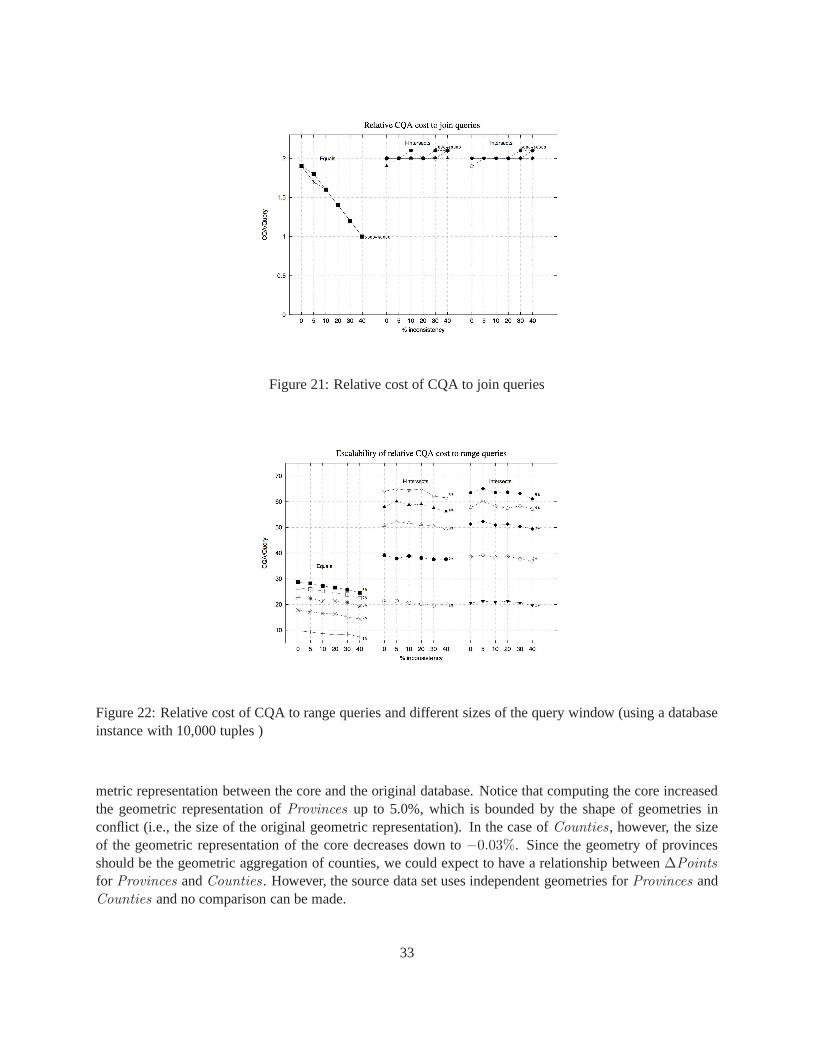
Figure 21: Relative cost of CQA to join queries

Figure 22: Relative cost of CQA to range queries and different sizes of the query window (using a databaseinstance with 10,000 tuples )

metric representation between the core and the original database. Notice that computing the core increasedthe geometric representation ofProvinces up to 5.0%, which is bounded by the shape of geometries inconflict (i.e., the size of the original geometric representation). In the case ofCounties, however, the sizeof the geometric representation of the core decreases down to −0.03%. Since the geometry of provincesshould be the geometric aggregation of counties, we could expect to have a relationship between∆Points

for Provinces andCounties . However, the source data set uses independent geometries for Provinces andCounties and no comparison can be made.

33

Range JoinData ∆ Points Core Simple CQA Simple CQA

Provinces +5.0% 17.7 0.04 0.25 29.8 63.4Counties -0.03%0 18.1 0.1 2.1 40.6 55.7

Table 6: CQA cost with real data (costs of core and queries in seconds)

7 Conclusions

We have formalized a repair semantics and consistency queryanswers for spatial databases with respectto SICs. The repair semantics is used as an auxiliary conceptfor handling inconsistency tolerance andcomputing consistent answers to spatial queries. It is based on updates that shrink geometries of objects,even at the point of deleting geometries for some exceptional cases, as for predicateDisjoint. Geometriesare virtually updated applying admissible geometric operators, which are available in most spatial DBMSs.

By restricting ourselves to the application of the admissible transformations, we have a finite number ofpossibilities for making a pair of geometries consistent with respect to a SIC. However, there may still beexponentially many repairs for a given instance and set of SICs. With the purpose of avoiding to computeand query all repairs, we have identified cases of SICs and conjunctive (range and join) queries where theconsistent answers can be obtained by posing a standard query to a single view of the original instance. Thisview is equivalent to the intersection of all possible minimal repairs, what we called thecore of a databaseinstance, which for a subset of SICs can be computed in polynomial time without determining each repair.

An experimental evaluation of the core-based computation of CQA reveals that answering range querieshas a cost that varies drastically in function of the topological predicates in SICs and the number of tuplesin the database instance, reaching up to 100 times the cost ofa simple range query. This is mainly due tothe spatial join involved in computing the core. For join queries, instead, the cost of CQA is the doubleof a simple join query. These results do not use optimizations with spatial indexing, which has been leftfor future work. Even more, they assume that we have to compute the core for each query, which could beoptimized by using materialized views.

This work leaves many problems open. Most prominently, computability and complexity issues haveto be explored. For example, some interesting decision problems are deciding if non trivial repairs (i.e.,not obtained by cancellation of geometries) exist for an instance and a set of SICs, or deciding whether ornot a particular instance is a repair of an inconsistent database instance. The complexity of deciding if aspatio-relational tuple is a consistent answer is also open. As in the relational case, we expect to find hardcases for all these problems. For them, it would be interesting to obtain lower complexity approximationalgorithms.

We have considered only regions to represent spatial objects. A natural extension of this work wouldbe to define a repair semantics for other spatial abstractions, such as polylines, points, networks, and soon. We would also like to explore not only denial SICs, but also other classes of semantic ICs, and othertypes of repair semantics that include solving conflicts with respect to a topological predicateDisjoint.This includes also the possibility of considering combinations of spatial with relational constraints, e.g.functional dependencies and referential ICs.

Acknowledgments

This project is partially funded by FONDECYT, Chile, grant number 1080138. Part of this research wasdone when L. Bertossi was invited to the Universidad de Concepcion and Universidad del Bıo-Bıo. Monica

34

Caniupan received funding from FONDECYT, Chile, grant number 11070186. Leopoldo Bertossi has alsobeen partially funded by an NSERC Discovery Grant (#315682).

References

[1] A LBERS, C. Gisdata chile, administrative boundaries since 2007.http://www.rulamahue.cl/mapoteca/catalogos/chile.html, 2009.

[2] A RENAS, M., BERTOSSI, L., AND CHOMICKI , J. Consistent query answers in inconsistent databases.In 18th ACM Symposium on Principles of Database Systems PODS’99 (1999), ACM Press, pp. 68–79.

[3] A RENAS, M., BERTOSSI, L., AND CHOMICKI , J. Scalar aggregation in fd-inconsistent databases. InProc. International Conference on Database Theory (2001), Springer LNCS 1973, pp. 39–53.

[4] BERTOSSI, L. Consistent query answering in databases.ACM Sigmod Record 35, 2 (2006), 68–76.

[5] BERTOSSI, L., AND BRAVO, L. Consistent query answers in virtual data integration systems. InInconsistency Tolerance (2005), vol. 3300 ofLecture Notes in Computer Science, Springer, pp. 42–83.

[6] BERTOSSI, L., AND CHOMICKI , J. Logics for Emerging Applications of Databases. Springer, 2003,ch. Query Answering in Inconsistent Databases, pp. 43–83.

[7] BERTOSSI, L., HUNTER, A., AND SCHAUB, T., Eds. Inconsistency Tolerance (2005), vol. 3300 ofLecture Notes in Computer Science, Springer.

[8] BORGES, K., LAENDER, A., AND DAVIS, C. Spatial integrity constraints in object oriented geo-graphic data modeling. InACM International Symposium on Advances in GIS (1999), ACM Press,pp. 1–6.

[9] CANIUPAN , M. Optimizing and Implementing Repair Programs for Consistent Query Answering inDatabases. PhD thesis, Carleton University, Department of Computer Science, 2007.

[10] CHOMICKI , J. Consistent query answering: Five easy pieces. InInternational Conference onDatabase Theory ICDT’07 (2007), vol. LNCS 4353, Springer-Verlag, pp. 1–17.

[11] COCKCROFT, S. A taxonomy of spatial integrity constraints.GeoInfomatica 1, 4 (1997), 327–343.

[12] DUCKHAM , M., L INGHAM , J., MASON, K. T., AND WORBOYS, M. F. Qualitative reasoning aboutconsistency in geographic information.Inf. Sci. 176, 6 (2006), 601–627.

[13] EGENHOFER, M., CLEMENTINE, E., AND FELICE, P. D. Evaluating inconsistency among multiplerepresentations. InSpatial Data Handling (1995), pp. 901–920.

[14] EGENHOFER, M., AND SHARMA , J. Assessing the consistency of complete and incomplete topolog-ical information.Geographical Systems 1 (1993), 47–68.

[15] EGENHOFER, M. J., AND FRANZOSA, R. D. Point set topological relations.International Journal ofGeographical Information Systems 5 (1991), 161–174.

35

http://www.rulamahue.cl/mapoteca/catalogos/chile.html

[16] FRANCONI, E., PALMA , A. L., LEONE, N., PERRI, S., AND SCARCELLO, F. Census data repair:a challenging application of disjunctive logic programming. In LPAR (2001), R. Nieuwenhuis andA. Voronkov, Eds., vol. 2250 ofLecture Notes in Computer Science, Springer, pp. 561–578.

[17] FUXMAN , A., FAZLI , E., AND M ILLER , R. J. Conquer: Efficient management of inconsistentdatabases. InSIGMOD Conference (2005), F.Ozcan, Ed., ACM, pp. 155–166.

[18] GUTING, R. H. Graphdb: Modeling and querying graphs in databases. In VLDB (1994), J. B. Bocca,M. Jarke, and C. Zaniolo, Eds., Morgan Kaufmann, pp. 297–308.

[19] GUTING, R. H., AND SCHNEIDER, M. Realm-based spatial data types: The rose algebra.VLDB J. 4,2 (1995), 243–286.

[20] HADZILACOS, T., AND TRYFONA, N. A model for expressing topological integrity constraints in geo-graphic databases. InSpatio-Temporal Reasoning (1992), A. U. Frank, I. Campari, and U. Formentini,Eds., vol. 639 ofLecture Notes in Computer Science, Springer, pp. 252–268.

[21] KUIJPERS, B., PAREDAENS, J., AND DEN BUSSCHE, J. V. On topological elementary equivalenceof spatial databases. InICDT (1997), F. N. Afrati and P. G. Kolaitis, Eds., vol. 1186 ofLecture Notesin Computer Science, Springer, pp. 432–446.

[22] M AS, S. Reasoning on spatial semantic integrity constraints. In COSIT (2007), S. Winter, M. Duck-ham, L. Kulik, and B. Kuipers, Eds., vol. 4736 ofLecture Notes in Computer Science, Springer,pp. 285–302.

[23] OPENGIS. Opengis simple features specification for sql. Tech. rep.,Open GIS Consortium, 1999.

[24] PAREDAENS, J., DEN BUSSCHE, J. V., AND GUCHT, D. V. Towards a theory of spatial databasequeries. InPODS (1994), ACM Press, pp. 279–288.

[25] PAREDAENS, J., AND KUIJPERS, B. Data models and query languages for spatial databases.DataKnowl. Eng. 25, 1-2 (1998), 29–53.

[26] RANDELL , D. A., CUI , Z., AND COHN, A. G. A spatial logic based on regions and connection. InKR (1992), pp. 165–176.

[27] RODRIGUEZ, M. A. Inconsistency issues in spatial databases. InInconsistency Tolerance (2005),vol. 3300 ofLecture Notes in Computer Science, Springer, pp. 237–269.

[28] RODRIGUEZ, M. A., BERTOSSI, L., AND CANIUPAN , M. An inconsistency tolerant approach toquerying spatial databases. InACM-GIS (2008), W. G. Aref, M. Mokbel, and M. Schneider, Eds.,ACM.

[29] SERVIGE, S., PURICELLI , T., AND LAURINI , R. A methodology for spatial consistency improvementof geographic databases.GeoInformatica 4 (2000), 7–24.

[30] THOMPSON, D., AND LAURINI , R. Fundamentals of Spatial Information Systems. No. 37 in APIC.Academic Press, 1992.

[31] TRYFONA, N., AND EGENHOFER, M. Consistency among parts and aggregates: A computationalmodel.Transactions on GIS 1, 1 (1997), 189–206.

36

[32] WIJSEN, J. Database repairing using updates.ACM Trans. Database Syst. 30, 3 (2005), 722–768.

37

Consistent Query Answering under Spatial Semantic Constraints

Documents

Transcript of Consistent Query Answering under Spatial Semantic Constraints