International Journal of Computational Geometry & Applicationsc World Scienti�c Publishing CompanyQUERY-SENSITIVE RAY SHOOTINGJOSEPH S. B. MITCHELL�Department of Applied Mathematics and StatisticsUniversity of Stony Brook, Stony Brook, NY 11794{3600, USADAVID M. MOUNTyDepartment of Computer Science and Institute for Advanced Computer StudiesUniversity of Maryland, College Park, MD 20742, USAandSUBHASH SURIzDeptartment of Computer ScienceWashington University, St. Louis, MO 63130{4899, USAReceived (received date)Revised (revised date)Communicated by Editor's nameABSTRACTRay (segment) shooting is the problem of determining the �rst intersection betweena ray (directed line segment) and a collection of polygonal or polyhedral obstacles. Inorder to process queries e�ciently, the set of obstacle polyhedra is usually preprocessedinto a data structure. In this paper we propose a query-sensitive data structure for rayshooting, which means that the performance of our data structure depends on the localgeometry of obstacles near the query segment. We measure the complexity of the localgeometry near the segment by a parameter called the simple cover complexity, denotedby scc(s) for a segment s. Our data structure consists of a subdivision that partitionsthe space into a collection of polyhedral cells, each of O(1) complexity. We answer asegment shooting query by walking along the segment through the subdivision. Our �rstresult is that, for any �xed dimension d, there exists a simple hierarchical subdivisionin which no query segment s intersects more than O(scc(s)) cells. Our second resultshows that in two dimensions such a subdivision of size O(n) can be constructed in timeO(n logn), where n is the total number of vertices in all the obstacles.1. IntroductionRay shooting is the problem of determining the �rst intersection of a ray with aset of obstacles. This is a fundamental problem in computational geometry because�jsbm@ams.sunysb.edu; Partially supported by grants from Boeing Computer Services, HughesAircraft, Air Force O�ce of Scienti�c Research contract AFOSR{91{0328, and by NSF GrantsECSE{8857642 CCR{9204585, and CCR{9504192.ymount@cs.umd.edu; Partially supported by NSF Grant CCR{9310705.zsuri@cs.wustl.edu. 1

of its important applications in areas such as ray tracing21 and Monte Carlo ap-proaches to radiosity in computer graphics,33 and motion tracking in virtual realityapplications.23 Since many ray shooting queries may be applied to a given set ofobstacles, it is desirable to preprocess the obstacles so that query processing is ase�cient as possible. Throughout this paper, we assume that obstacles are modeledby disjoint polyhedra.1.1. Previous ResultsThe problem of ray shooting in a simple polygon with n vertices has been studiedby Chazelle and Guibas,16 Chazelle et al.,15 Goodrich and Tamassia,22 and Hersh-berger and Suri.24 The main result for this special case of the problem is that rayshooting queries can be answered in O(logn) time with an O(n) size data structure.The recent approaches of Refs. 15,24 are based on constructing triangulations of low\stabbing number".The problem appears to be signi�cantly more di�cult for multiple polygons. Allof the known methods for achieving O(logn) query time require (n2) space. Thebest results known using linear or near-linear space give a query time of roughlyO(pn logn); see Chazelle et al.,15 and Hershberger and Suri.24 Several other papersalso achieve sublinear query time with sub-quadratic space; Agarwal,1, Cheng andJanardan,17;18 and Overmars, Schipper, and Sharir.29Predictably, the quality of the results degrades quickly as the dimension of theunderlying space increases beyond two. In three dimensions, the best methods toachieve O(logn) query time require O(n4+�) space, for any positive � > 0.6;10 Sev-eral tradeo�s between space and query time are possible.3;5;9;10;30;32 In particular,the best known query time with near-linear (O(n1+�)) space is O(n3=4) time, forany � > 0.4In contrast with the two-dimensional case, there are no ray shooting results indimensions three or higher based on subdivisions of low stabbing number. Indeed,some recent lower bound results of Agarwal, Aronov and Suri2 indicate that suchsubdivisions are not possible in higher dimensions. Speci�cally, they show that thereexist (nonconvex) n-vertex polyhedra in three dimensions whose every (Steiner)triangulation intersects some ray in (n) points. More generally, for every k > 0,there exists a collection of k disjoint convex polyhedra such that no matter howone triangulates their common exterior, some ray always intersects (k + logn)simplices.1.2. A Query-Sensitive ApproachOne of the shortcomings of the type of analysis used in the results above isthat it fails to account for the geometric structure of the obstacle set and queryray. Analyses based solely upon input size cannot account for the fact that thereexist con�gurations of obstacles and rays for which solving ray shooting queries isintuitively very easy, and others for which it is quite a bit more complicated. Prac-tical experience suggests that worst-case scenarios are rare for many applications.2

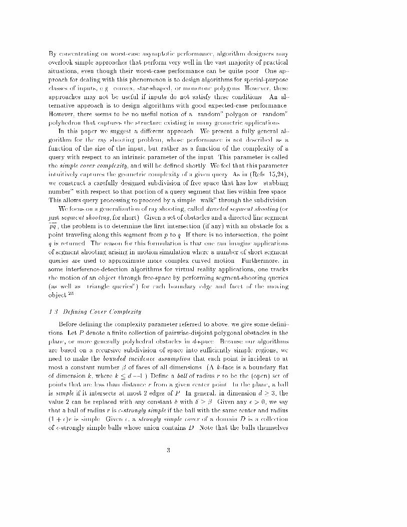
By concentrating on worst-case asymptotic performance, algorithm designers mayoverlook simple approaches that perform very well in the vast majority of practicalsituations, even though their worst-case performance can be quite poor. One ap-proach for dealing with this phenomenon is to design algorithms for special-purposeclasses of inputs, e.g. convex, star-shaped, or monotone polygons. However, theseapproaches may not be useful if inputs do not satisfy these conditions. An al-ternative approach is to design algorithms with good expected-case performance.However, there seems to be no useful notion of a \random" polygon or \random"polyhedron that captures the structure existing in many geometric applications.In this paper we suggest a di�erent approach. We present a fully general al-gorithm for the ray shooting problem, whose performance is not described as afunction of the size of the input, but rather as a function of the complexity of aquery with respect to an intrinsic parameter of the input. This parameter is calledthe simple cover complexity, and will be de�ned shortly. We feel that this parameterintuitively captures the geometric complexity of a given query. As in (Refs. 15,24),we construct a carefully designed subdivision of free space that has low \stabbingnumber" with respect to that portion of a query segment that lies within free space.This allows query processing to proceed by a simple \walk" through the subdivision.We focus on a generalization of ray shooting, called directed segment shooting (orjust segment shooting, for short). Given a set of obstacles and a directed line segment�!pq , the problem is to determine the �rst intersection (if any) with an obstacle for apoint traveling along this segment from p to q. If there is no intersection, the pointq is returned. The reason for this formulation is that one can imagine applicationsof segment shooting arising in motion simulation where a number of short segmentqueries are used to approximate more complex curved motion. Furthermore, insome interference-detection algorithms for virtual reality applications, one tracksthe motion of an object through free-space by performing segment-shooting queries(as well as \triangle queries") for each boundary edge and facet of the movingobject.231.3. De�ning Cover ComplexityBefore de�ning the complexity parameter referred to above, we give some de�ni-tions. Let P denote a �nite collection of pairwise-disjoint polygonal obstacles in theplane, or more generally polyhedral obstacles in d-space. Because our algorithmsare based on a recursive subdivision of space into su�ciently simple regions, weneed to make the bounded incidence assumption that each point is incident to atmost a constant number � of faces of all dimensions. (A k-face is a boundary atof dimension k, where k � d� 1.) De�ne a ball of radius r to be the (open) set ofpoints that are less than distance r from a given center point. In the plane, a ballis simple if it intersects at most 2 edges of P . In general, in dimension d � 3, thevalue 2 can be replaced with any constant � with � � �. Given any � > 0, we saythat a ball of radius r is �-strongly simple if the ball with the same center and radius(1 + �)r is simple. Given �, a strongly simple cover of a domain D is a collectionof �-strongly simple balls whose union contains D. Note that the balls themselves3

cover D, but each expansion by (1 + �) is simple. Finally, the simple cover com-plexity of D with respect to �, denoted scc�(D), is de�ned to be the cardinality ofthe smallest strongly simple cover of D. We will use the term complexity for short.When used in asymptotic bounds, we will omit the \�" subscript, since, as will beshown in Lemma 1, it a�ects the complexity by only a constant factor.Fig 1(a) shows a strongly simple cover of size 6 for a directed line segment (theheavy line). The � value is 1=4. Solid circles are the balls of the cover, and dashedcircles are balls of radius (1 + �)r.(a) (b)Figure 1: Strongly simple cover complexity and C-complexity.The reason that we use a (1+�) factor in the de�nition of simple cover complexityis that a query segment could be covered by only two balls, while there may be (n)obstacle vertices arbitrarily close to the segment. Consider, for example, two openunit balls whose centers are in�nitessimally less than distance 2 apart. The segmentjoining their centers is covered by the balls, but there may be many obstacles thatare arbitrarily close to the region where these two balls intersect. Thus the value �serves a role in making the size of the cover complexity insensitive to small geometricperturbations.Intuitively, it is easy to see that a segment that is short and well separated fromall obstacles will have a smaller complexity than a segment that grazes the boundaryof the obstacles. In this sense, we feel that this complexity measure is a reasonablere ection of the intrinsic di�culty of solving a segment shooting query. Observethat this complexity measure is invariant under rigid transformations of the plane(translation, rotation, uniform scaling); however, it is not invariant under generalnonsingular a�ne transformations (for example, nonuniform scaling and shearing),since balls may not be preserved under these transformations.It is possible to strengthen the notion of cover complexity to simple connectedregions of space. First, observe that given any ball B, the obstacle set subdividesthe points lying within this ball into various connected components, which we callC-balls (where \C" stands for connected). More formally, consider points p and qlying within B. We say that p can reach q within B if there is a path from p to q4

that lies entirely within B and does not intersect any obstacle. Reachability withinB de�nes an equivalence partition of B into connected components. De�ne a C-ballto be any such connected component of any ball. A C-ball is simple if its boundaryintersects at most 2 edges of P (or, more generally, at most � faces, in higherdimensions). Because each C-ball is associated with a ball, the center and radiusof a C-ball are de�ned to be the center and radius, respectively, of the associatedball. Note that if one ball contains another, then its connected components containthe connected components of the other. Given any � > 0, a C-ball of radius r is�-strongly C-simple if the C-ball with the same center and radius (1+ �)r is simple.Based on this notion of C-simplicity, we can derive a notion of C-complexity, as wedid above. We use cscc�(D) to denote the C-complexity of a domain D.Clearly any ball that is simple is also C-simple, and thus the C-complexity of anobject is not greater than its complexity. However, C-complexity may be smaller.For example, as shown in Figure 1(b), the C-complexity of the segment shown inpart (a) is only 4. Intuitively, C-complexity is a more appropriate measure of thecomplexity of a ray shooting query, since obstacles that lie on the far side of anobstacle edge should not a�ect query processing, no matter how close they may beto the query segment.1.4. Statement of Main ResultsWe present three principal results. First, for ray shooting queries in arbitrarydimensions, we analyze the performance of a hierarchical spatial subdivision, calleda smoothed k-d subdivision. This subdivision is related to the well-known quadtreedata structure, and is based more speci�cally on a data structure called a PM k-dtree, described by Samet.31 Samet gives an analysis of the maximum depth of thistree in terms of the ratio between the diameter of the obstacle set and the minimumseparation distance between nonadjacent vertices and edges. Various authors havederived relationships between the size of quadtrees for representing shapes andintrinsic properties of the shape (perimeter or, more generally, surface area) andthe accuracy of the representation.20;26 We show that the size of a smoothed k-d subdivision is proportional to the simple cover complexity of the obstacle-freespace. This result in itself is interesting because this complexity measure, whileless intuitive than perimeter, is independent of the accuracy of representation (andunlike standard quadtrees, there is no loss of precision in our representation). Wealso show that the number of cells of the subdivision that are stabbed by a querysegment is proportional to the simple cover complexity of the query segment. Weshow that the hierarchical subdivision can be used to locate the origin-point of thedirected query segment in time O(log Rr ), after which we can trace the segmentthrough the subdivision in time O(scc(s)) to answer the shooting query, where s isthe query segment, scc(s) is the simple cover complexity of the initial obstacle-freeportion of s, r is the radius of the largest strongly simple ball containing the originof s, and R is the diameter of the obstacle set.Second, we extend the bounds above on the stabbing number to C-complexityby introducing a variation of the smoothed k-d subdivision, called a reduced k-d5

subdivision.Our �nal result involves ray shooting in the plane. We assume we are given acollection of polygonal obstacles with n vertices total. We show that in O(n logn)time, it is possible to produce a subdivision of the plane, called the reduced box-decomposition subdivision, of size O(n), such that segment shooting queries can beanswered in time O(logn+ cscc(s)), where cscc(s) is the C-simple cover complexityof the obstacle-free portion of the query segment. The O(logn) term is the timeneeded for point location, and O(cscc(s)) term is the bound on the number of cellsof the subdivision stabbed by the query segment.1.5. A Technical LemmaBefore describing our algorithms we mention one technical fact. The de�nitionof simplicity is based on a parameter � > 0, which is independent of n. The exactchoice of � a�ects only the constant factors in our bounds, as shown by the followingresult. So, in the remainder of the paper, we omit references to � when derivingasymptotic bounds.Lemma 1 Let 0 < � < �0, and let D be some domain in dimension d. There is aconstant (depending on �, �0 and the dimension d) such thatscc�(D) � scc�0 (D) � � scc�(D):The same result holds for C-complexity as well.Proof. We present the proof in the plane for simplicity, but the generalizationto arbitrary dimensions is straightforward. We will derive a very loose bound on . The �rst inequality is trivial, since if the expansion of a ball in any cover by(1 + �0) is simple, then an expansion by only (1 + �) is certainly simple. To provethe second inequality, let B be a simple cover with respect to �. We will show thatwe can cover each ball B 2 B with at most smaller balls whose expansions by(1 + �0) are contained within an expansion of B by (1 + �). Let r denote the radiusof B. Let r0 = r�2(1 + �0) :Cover B with a minimal set of squares (hypercubes, in general), arranged in agrid, whose diagonals are of length 2r0. Enclose each square of this grid within aball of radius r0. Observe that the resulting set of balls covers B. If we grow anyone of these balls by (1 + �0), every point in the resulting ball lies within distance2r0(1 + �0) = r� of the boundary of B, and hence lies within the expansion of B by(1 + �). Thus each of these balls is (1 + �) strongly simple. Finally observe thatthe number of newly formed balls is equal to the number of grid squares needed tocover B. This is not more than the number of grid squares of diagonal length 2r0(side length r0p2) needed to cover a square of side length 2r. It is easy to verifythat this is at most � 2rr0p2�2 = �4(1 + �0)�p2 �2 :6

In general, the exponent and constant factors depend on the dimension d. Letting be this constant completes the proof. Clearly, this construction can be generalizedto C-simple balls as well. 22. A Simple ApproachIn this section we give a query-sensitive analysis of a simple, practical decompo-sition strategy, which illustrates the essential features of the more complex methodand its analysis that will be presented in the following section. The decompositionproduces a subdivision of space called a smoothed k-d subdivision, and is based onthe PM k-d tree and PM quadtree decompositions described by Samet.31 We havechosen the binary k-d subdivision over the more well known 2d-ary quadtree sub-division for the practical reason that it results in a somewhat smaller number ofregions, especially in higher dimensions.We begin by assuming that we are given a set of polyhedral obstacles in d-dimensional space, represented simply by the set of its faces (of all dimensions).As mentioned in the introduction, we assume that faces bounding these obstaclesare simple in the sense that each point is incident to at most a constant number �of faces of all dimensions. We also assume that the obstacles are contained withina minimal bounding hypercube. (Such a hypercube is easy to construct in lineartime.) This hypercube is our initial box. A box is said to be crowded if it intersectsmore than � faces. (In general any constant threshold at least as large as � can bechosen.) If a box is crowded, then it is split by a hyperplane passing through thecenter of the box and perpendicular to its longest side. (Ties for the longest sidecan be broken arbitrarily.)Each split replaces a box by two smaller boxes. Since we start with a hypercube,and each split cuts through the midpoint of the longest side of a box, it follows thateach box is \fat" in the sense that the ratio between its longest and shortest side isat most 2.The splitting process naturally de�nes a binary tree called a k-d tree. Theoriginal box is the parent of the resulting two boxes in this tree. The splittingprocess terminates when no remaining boxes are crowded. The resulting leaf boxes,called cells, form a subdivision of space, each of which contains a constant numberof obstacle boundary elements. (The cells correspond to the leaves of the binarytree modeling our hierarchical decomposition. The boxes corresponding to internalnodes of the tree are not cells, although they are a useful conceptual device inour proofs.) The internal nodes of the resulting binary tree each contain datadescribing the splitting plane. Each leaf node contains pointers to the obstacleboundary elements that overlap the associated cell.The splitting process eventually terminates, because of the bounded incidenceassumption. However, the number of cells in the subdivision depends on the geo-metric placement of the obstacles, and it cannot be bounded only as a function ofn, the number of obstacle faces.To support segment shooting queries, we make one modi�cation, which we callsmoothing. Intuitively, smoothing involves additional splitting of the rectangles7

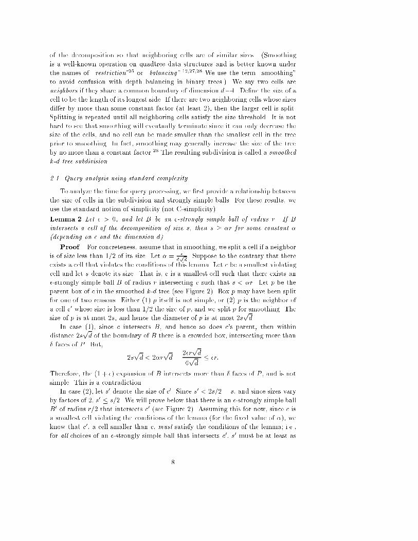
of the decomposition so that neighboring cells are of similar sizes. (Smoothingis a well-known operation on quadtree data structures and is better known underthe names of \restriction"25 or \balancing".12;27;28 We use the term \smoothing"to avoid confusion with depth balancing in binary trees.) We say two cells areneighbors if they share a common boundary of dimension d�1. De�ne the size of acell to be the length of its longest side. If there are two neighboring cells whose sizesdi�er by more than some constant factor (at least 2), then the larger cell is split.Splitting is repeated until all neighboring cells satisfy the size threshold. It is nothard to see that smoothing will eventually terminate since it can only decrease thesize of the cells, and no cell can be made smaller than the smallest cell in the treeprior to smoothing. In fact, smoothing may generally increase the size of the treeby no more than a constant factor.28 The resulting subdivision is called a smoothedk-d tree subdivision.2.1. Query analysis using standard complexityTo analyze the time for query processing, we �rst provide a relationship betweenthe size of cells in the subdivision and strongly simple balls. For these results, weuse the standard notion of simplicity (not C-simplicity).Lemma 2 Let � > 0, and let B be an �-strongly simple ball of radius r. If Bintersects a cell of the decomposition of size s, then s � �r for some constant �(depending on � and the dimension d).Proof. For concreteness, assume that in smoothing, we split a cell if a neighboris of size less than 1/2 of its size. Let � = �6pd . Suppose to the contrary that thereexists a cell that violates the conditions of this lemma. Let c be a smallest violatingcell and let s denote its size. That is, c is a smallest cell such that there exists an�-strongly simple ball B of radius r intersecting c such that s < �r. Let p be theparent box of c in the smoothed k-d tree (see Figure 2). Box p may have been splitfor one of two reasons. Either (1) p itself is not simple, or (2) p is the neighbor ofa cell c0 whose size is less than 1/2 the size of p, and we split p for smoothing. Thesize of p is at most 2s, and hence the diameter of p is at most 2spd.In case (1), since c intersects B, and hence so does c's parent, then withindistance 2spd of the boundary of B there is a crowded box, intersecting more than� faces of P . But, 2spd < 2�rpd = 2�rpd6pd � �r:Therefore, the (1 + �) expansion of B intersects more than � faces of P , and is notsimple. This is a contradiction.In case (2), let s0 denote the size of c0. Since s0 < 2s=2 = s, and since sizes varyby factors of 2, s0 � s=2. We will prove below that there is an �-strongly simple ballB0 of radius r=2 that intersects c0 (see Figure 2). Assuming this for now, since c isa smallest cell violating the conditions of the lemma (for the �xed value of �), weknow that c0, a cell smaller than c, must satisfy the conditions of the lemma; i.e.,for all choices of an �-strongly simple ball that intersects c0, s0 must be at least as8

’B

ε(1+ )’B

’c

ε

p

(1+ )B

B

cFigure 2: Proof of Lemma 2.1.large as � times the radius of the ball. Thus, we haves2 � s0 � �r2 ;implying that s � �r, contradicting our earlier hypothesis.To prove the existence of B0, �rst observe that since the size of c0 is at most s=2,its diameter is at most spd=2. Since c0 is a neighbor of p, and since p intersects B,c0 lies entirely within distance 2spd+ spd=2 � 3spd of the boundary of B. Thereexists a ball B0 of radius r=2 that intersects c0 and is at no point further than 3spdfrom the boundary of B. The expansion of B0 by (1 + �) lies within distance r�=2from the boundary of B0. Hence this expansion of B0 lies within distance3spd+ r�2 < 3�rpd+ r�2 = 3r�pd6pd + r�2 = r�2 + r�2 = r�of the boundary of B. Thus the expansion of B0 lies entirely within the expansionof B, implying that B0 is simple. 2Lemma 3 Given an �-strongly simple ball B of radius r, the number of cells thatintersect B in the subdivision is bounded above by a constant (depending on � andthe dimension d).Proof. By Lemma 2, the size of a cell intersecting B is bounded from belowby �r. Because the cells of the subdivision are disjoint and fat, the number of suchcells intersecting B is bounded above by the number of disjoint hypercubes of onehalf this side length that can be packed around (inside or touching) B, which by asimple packing argument is on the order of 1=�d. 2Lemma 4 Let q be a point in the enclosing hypercube of the obstacle set of sidelength R. If q is located in a strongly simple ball of radius r, then we can locate thecell containing q in time O(log(R=r)). (Constant factors depend on d and �.)Proof. The search for q is a simple descent through the smoothed k-d tree.With every d levels of descent, the size of the associated regions decreases by afactor of 1/2. Thus, if the search continues for k steps, then the search terminates9

at a region that contains q and whose size s obeys s � R2bk=dc . But Lemma 2 impliesthat s � �r, for a constant �, so that k = O(log(R=r)). 2Segment shooting queries are processed by �rst locating the cell containing theorigin of the segment, and then walking along the segment, cell by cell, throughthe subdivision. Because neighboring cells di�er in size by a constant amount, andbecause the ratio of the longest to shortest side of each cell is bounded by 2, itfollows that the number of neighbors of a given cell is at most a constant dependingon the dimension. From the fact that each cell contains a constant number ofobstacle boundary elements, it follows that each cell can be tested for intersectionwith the query segment in constant time, and hence the time to perform this walkis proportional to the number of cells visited. Let scc(s) denote the simple covercomplexity of a segment s (more precisely, the complexity of the obstacle-free initialsubsegment of s), and let B be a strongly simple cover for s. By Lemma 3, thenumber of subdivision cells intersecting each ball in B is a constant, and hence,since these balls cover s, the number of subdivision cells traversed by s is O(jBj) =O(scc(s)). By combining this with the previous lemma, it follows that segmentshooting queries can be answered in O((logR=r) + scc(s)) time. Constant factorsvary with the dimension d.By a similar argument, the number of cells in the subdivision is O(scc(P )),where scc(P ) denotes the simple cover complexity of the obstacle-free space. Thereason is that each ball of the cover overlaps at most a constant number of cellsof the smoothed subdivision. Since each cell contains only a constant number ofboundary elements, the size of the �nal subdivision is O(scc(P )). From this wehave the following analysis of the smoothed k-d tree subdivision.Theorem 1 Let P be a collection of polyhedral obstacles satisfying the boundedincidence assumption, and let R denote the side length of the smallest hypercubeenclosing P . The smoothed k-d subdivision is a subdivision of size O(scc(P )) suchthat given any directed query segment s, whose origin lies within a strongly simpleball of radius r, the query can be answered in O((logR=r) + scc(s)) time.We do not consider preprocessing time in our analysis, because it depends onthe implementation of the underlying primitive operation of e�ciently determiningwhich obstacle faces intersect the boxes of the decomposition. This depends on therepresentation and complexity of the faces making up the obstacles. If we assumethat obstacle faces are of bounded complexity (e.g. through triangulation) then thisprimitive operation can be performed in O(1) time for each box/face pair. Thisprovides a trivial preprocessing time bound of O(n � scc(P )), where n is the numberof obstacle faces. In Section 3, we show that this can be improved considerably inthe plane.2.2. A Modi�cation using C-complexityIn this section we extend the results of the previous section to the stronger notionof C-complexity. We do this by coarsening the smoothed k-d subdivision, resultingin a subdivision that we call a reduced k-d subdivision. This subdivision will be of10

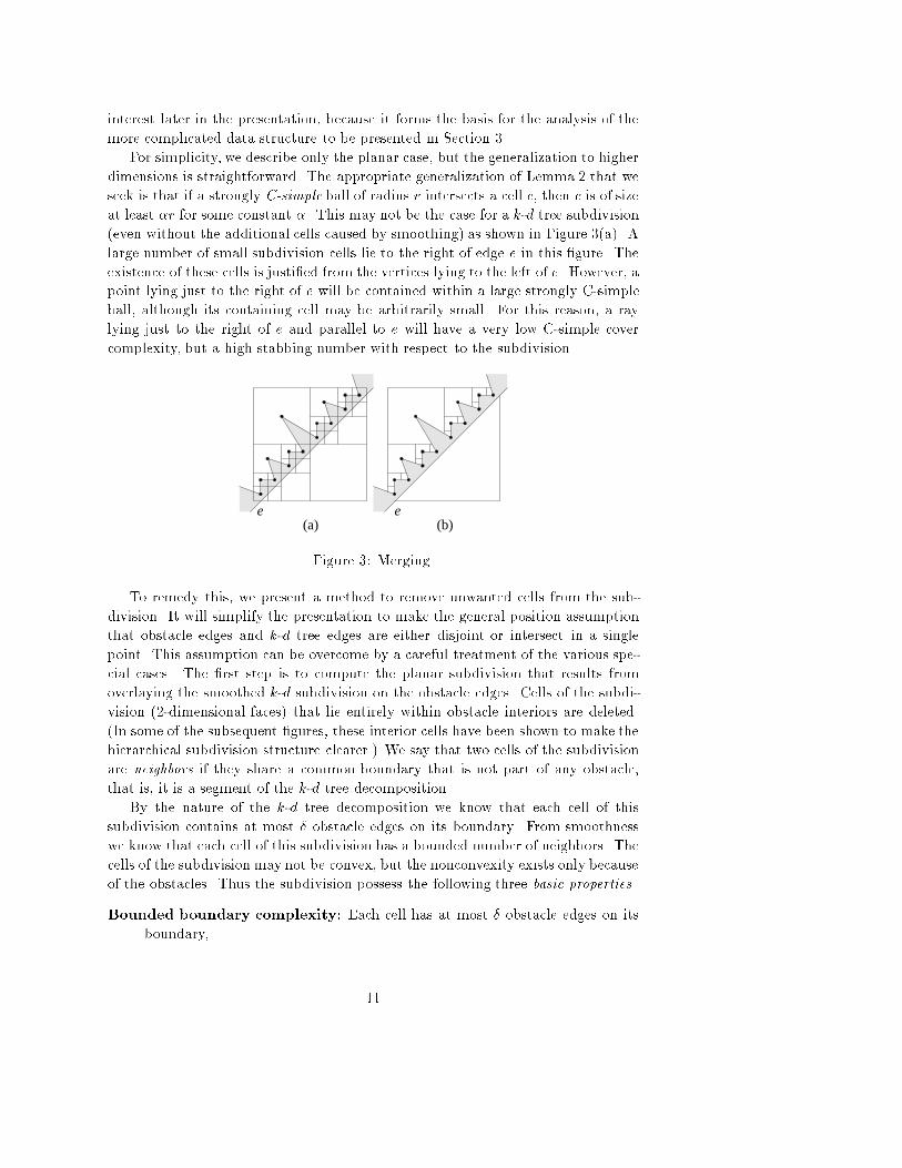
interest later in the presentation, because it forms the basis for the analysis of themore complicated data structure to be presented in Section 3.For simplicity, we describe only the planar case, but the generalization to higherdimensions is straightforward. The appropriate generalization of Lemma 2 that weseek is that if a strongly C-simple ball of radius r intersects a cell c, then c is of sizeat least �r for some constant �. This may not be the case for a k-d tree subdivision(even without the additional cells caused by smoothing) as shown in Figure 3(a). Alarge number of small subdivision cells lie to the right of edge e in this �gure. Theexistence of these cells is justi�ed from the vertices lying to the left of e. However, apoint lying just to the right of e will be contained within a large strongly C-simpleball, although its containing cell may be arbitrarily small. For this reason, a raylying just to the right of e and parallel to e will have a very low C-simple covercomplexity, but a high stabbing number with respect to the subdivision.(b)(a)

e eFigure 3: Merging.To remedy this, we present a method to remove unwanted cells from the sub-division. It will simplify the presentation to make the general position assumptionthat obstacle edges and k-d tree edges are either disjoint or intersect in a singlepoint. This assumption can be overcome by a careful treatment of the various spe-cial cases. The �rst step is to compute the planar subdivision that results fromoverlaying the smoothed k-d subdivision on the obstacle edges. Cells of the subdi-vision (2-dimensional faces) that lie entirely within obstacle interiors are deleted.(In some of the subsequent �gures, these interior cells have been shown to make thehierarchical subdivision structure clearer.) We say that two cells of the subdivisionare neighbors if they share a common boundary that is not part of any obstacle,that is, it is a segment of the k-d tree decomposition.By the nature of the k-d tree decomposition we know that each cell of thissubdivision contains at most � obstacle edges on its boundary. From smoothnesswe know that each cell of this subdivision has a bounded number of neighbors. Thecells of the subdivision may not be convex, but the nonconvexity exists only becauseof the obstacles. Thus the subdivision possess the following three basic properties.Bounded boundary complexity: Each cell has at most � obstacle edges on itsboundary, 11

Bounded neighborhood size: Each cell has at most a constant number, �, ofneighboring cells, andRelative convexity: A line segment that intersects none of the obstacles intersectsa cell in a single segment.We essentially \undo" some of the splits performed by the smoothed k-d treedecomposition, by merging neighboring regions, as long as C-simplicity and smooth-ness are not violated. In particular we apply the followingmerging procedure. Everynonobstacle edge in the subdivision is a subsegment of some splitting segment inthe underlying k-d tree. The splitting segments of the k-d tree are in 1{1 correspon-dence with the internal nodes of the tree. Working from the leaves of the k-d tree tothe root, the merging procedure attempts to merge neighboring cells by removingedges of the subdivision that correspond to splitting segments in the k-d tree.Initially all cells are considered eligible for merging, and each cell is associatedwith the leaf box of the k-d tree that contains it. Working from the bottom (leaflevel) to the top of the k-d tree, we consider neighboring cells of the subdivisionthat are eligible for merging, and whose associated boxes of the k-d tree are siblings,separated by a common splitting segment. We consider the connected componentsof space that would result if this splitting segment of the k-d tree were removed, andthe cells on either side were merged. This is called a trial merge. For each of thesemerged connected components, if the component satis�es the three basic propertieslisted above, then the cells are replaced with their union in the subdivision, thuslocally undoing the decomposition step. (Only the �rst two basic properties need betested explicitly. It is easy to see that relative convexity is preserved by the natureof the merging process.) A single splitting segment may separate many connectedcomponents, and the trial merge may succeed for some components and fail forothers. When two cells are successfully merged, the merged cell is associated withthe parent box in the k-d tree, and it becomes eligible for subsequent merging.Otherwise the cells are not merged, and are not eligible for future merging.If a cell is associated with one of the two k-d tree boxes that are being merged,but it is not incident to the splitting segment, then it is treated as though it hassucceeded with a trivial merge with an empty cell. In particular, it is associatedwith the parent box in the k-d tree, and continues to be eligible for merging.For example, Figures 4 (a) and (b) illustrate the e�ect of a trial merge; the sixcells a; b1; b2; c1; c2, and c3 are replaced by the three connected components a, b andc. The cell b = b1 [ b2 violates the complexity bound (assuming at most 2 obstacleedges are permitted), and so they are not merged. On the other hand, assumingthat c1; c2; c3 are all eligible for merging, they are merged into a single cell c. (Ifany of the three were ineligible, then none of them would be merged.) Cell a is notincident to the splitting segment, and so succeeds in a trivial merge. Consequently,cells a and c become eligible for subsequent merging. The k-d tree node associatedwith cells a and c is the entire square. The result of this merging step is shown inFigure 4(c).The end result of the merging process is called a reduced k-d subdivision. Each12

a

b

c

bb

a

12

c

c

bb

a

c

12

1

2

3c

Initial Configuration.

(a)

Trial Merge.

(b)

Final Configuration.

(c)Figure 4: Merging procedure.cell in this subdivision satis�es the three basic cell properties listed above. Eachcell is a connected component of some box of the smoothed k-d tree (because wemerge all connected neighboring cells or none of them). These cells are maximalin the sense that the corresponding connected component of the parent box in thek-d would violate the three properties above. We de�ne the size of a cell to be thesize (length of the longest side) of the associated box of the k-d tree. Because cellsare subsets (connected components) of their associated k-d boxes, the Euclideandiameter of a cell may be arbitrarily small compared to its size (as seen with cell ain Figure 4(c)). We now give the appropriate generalization of Lemma 2.Lemma 5 Let � > 0, and let B be an �-strongly C-simple ball of radius r, and letS be a reduced k-d subdivision. If B intersects a cell of S of size s, then s � �r forsome constant � (depending on the strong cover bound � and the dimension).Proof. The value of � is the same as in Lemma 2. Our proof is based onconsidering just the obstacle edges incident to the C-simple ball, and then reducingto Lemma 2.Consider the (1 + �) expansion of B. Let P 0 denote the obstacle vertices andedges of P that are incident to this connected component. For the sake of analysis,consider an alternative (in�nitely large) smoothed k-d subdivision S0 for P 0, thatstarts with the same initial enclosing square that was used for the original k-d tree,but in which any box that lies all or partially outside of the (1 + �) expansion of Bis split. (Thus merging has been applied to S but not applied to S0.) A cell of S0has nonzero size only if it lies entirely within the (1 + �) expansion of B. (This isillustrated Figure 5, where S is shown in (a), and S0 is shown (b). Cells have beensplit if they intersect more than two obstacle edges.)We claim that the box associated with any cell c of S that intersects B cannot beproperly contained within any of the cells of S0. (And, in particular, the situationillustrated in the �gure could not arise.) Suppose that this were so and considerthe smallest such cell c. Let b be the associated box of the smoothed k-d tree,and suppose that b is properly contained within some box b0 of S0. Because bothdecompositions started with the same bounding square, b0 is a proper ancestor of b(in the abstract k-d ordering of boxes). Therefore, b0 contains not only b, but alsothe merge of b with its sibling box in the k-d tree. But, because b0 has nonzero13

(a) (b)

cb b’Figure 5: Proof of Lemma 5.size, it lies entirely within the (1 + �) expansion of B, and hence is not crowdedwith respect to P 0. It follows that the resulting connected component has boundedboundary complexity with respect to P . Therefore, boundary complexity could notbe an impediment to the merge of b and its sibling.We also claim that the sizes (and hence number) of c's neighbors cannot be animpediment to the merger. The reason is that the obstacles of P 0 located within the(1+�) expansion of B are the same for the two k-d trees, and we have constructed P 0so that any cell extending outside of the expansion will be split. S cannot subdividecells for smoothing purposes any �ner than this.Finally, we claim that relative convexity is not violated by the merger. This isan immediate consequence of the nature of the merging process. Since none of thethree merging properties are violated, c would have been merged with its neighbor,yielding the contradiction.Because the box associated with c cannot be properly contained within any ofthe cells of S0, and because the size of a cell is based on the size of its associatedbox, we may apply Lemma 2 to cells of S0, to establish the same lower bound of �ron the size of c. 2Lemma 6 Given an �-strongly C-simple ball B of radius r, the number of cells ofthe reduced k-d subdivision that intersect B is bounded above by a constant (depend-ing on �, �, and the dimension d).Proof. By Lemma 5, the size of a cell intersecting B is bounded from belowby �r. This means that the size of the associated box in the k-d tree is boundedby this value. It follows from Lemma 3 that there are a constant number of boxes.To complete the proof, it su�ces to show that given any box b in the smoothed k-dtree, there are at most a constant number of cells of the reduced k-d subdivisionassociated with b that intersect B. This is true because each cell of the reducedk-d tree is a connected component of its associated box in the smoothed k-d tree.Because B is strongly C-simple, there are a constant number of edges incident toB, and hence a constant number of connected components of b intersect B. 2This leads the main result of this section. Because we have replaced the hierar-chical k-d structure with a more general subdivision (based on connected compo-14

nents), the point location time bound of O(logR=r) does not necessarily hold.Theorem 2 Let P be a collection of polyhedral obstacles satisfying the boundedincidence assumption. The reduced k-d subdivision subdivides space into O(cscc(P ))cells each of bounded complexity, such that a line segment s that does not intersectany obstacle intersects O(cscc(s)) cells of the subdivision.The method of �rst constructing the re�ned k-d structure and then coarseningthrough merging may seem unnecessarily complicated. Obviously a more directapproach is to keep track of the connected components throughout the constructionprocess, and avoid the additional splits. We have presented this particular approachbecause it more closely parallels the presentation in the next section, where it isnot as clear how to implement the direct approach e�ciently.In summary, the smoothed k-d subdivision and the reduced k-d subdivision havethe advantages of simplicity and ease of generalization to higher dimensions. It isunfortunate that it is not possible to bound the space or preprocessing time forthese data structures purely in terms of a function of input size. In the next sectionwe show that it is possible to do so when obstacles lie in the plane.3. The Planar CaseIn this section we modify the simple reduced k-d subdivision given in the previoussection to handle segment shooting for a set P of polygonal obstacles in the plane.We call the resulting structure a reduced box-decomposition subdivision. Our goalwill be to prove the following main theorem. We assume throughout this sectionthat the bound of at most two obstacle edges is used in the de�nition of C-simplicity.Theorem 3 Let P be a collection of disjoint polygonal obstacles in the plane, with atotal of n vertices. A reduced box-decomposition subdivision of size O(n) can be builtin O(n logn) time, such that given this data structure, segment shooting queries fora query segment s can be answered in O(logn+ cscc(s)) time, where cscc(s) is thestrong C-simple cover complexity of the initial obstacle-free portion of s.Interestingly, the subdivision presented here has a number of similarities to thequality mesh triangulations of Bern, Eppstein, and Gilbert,12 and Mitchell andVavasis.27 Since there are no restrictions on the geometric structure of our subdivi-sion, we can provide the space and preprocessing time improvements listed above.(In mesh generation, the size of the triangulation generally depends on the geo-metric structure of the input.) The construction of the reduced box-decompositionsubdivision involves a number of steps. They are presented in each of the followingsubsections.3.1. Box-DecompositionPreprocessing begins with a hierarchical subdivision similar to the PM k-d tree,described in the last section. To achieve linear space, it is necessary to modify thedecomposition procedure. The decomposition begins as an adaptation of a standarddecompositionmethod, called box-decomposition. This basic concept was introducedby Clarkson19 and has appeared in a number of di�erent varieties.8;11;13;34 The15

initial subdivision is based solely on the vertices of the obstacle set. We do notrequire that our subdivision be a cell complex, since there may be vertices lying inthe interior of edges; however, the number of vertices in the interior of any edge willbe a constant. Thus, we can easily augment such a subdivision into a cell complexor a triangulation with a linear number of additional Steiner points.As with the PM k-d tree, the decomposition is hierarchical and naturally as-sociated with a binary tree, called the box-decomposition tree. Each node of thebox-decomposition tree corresponds to one of two types of objects called enclo-sures: (1) a box, which is a rectangle with the property that the ratio of the longestto shortest side is at most 2, and (2) a doughnut, which is the set theoretic di�er-ence of two boxes, an inner box contained within an outer box. It will simplify thepresentation to assume that inner boxes are always square. The size of a box isde�ned to be the length of its longest side, and the size of a doughnut is the size ofits outer box. We assume that the obstacles have been scaled to lie within a unitsquare.The root of the tree is associated with the enclosing unit square. Inductively, weassume that the point set to be decomposed (initially the set of all obstacle vertices)is contained within a box. If there is at most one vertex, then the decompositionterminates here. Otherwise we consider a horizontal or vertical line that bisectsthe longer side of the box. (Ties can be broken arbitrarily, but in our exampleswe assume that the vertical split is made �rst.) If there exists at least one vertexon either side of this splitting line, then this line is used to split the box into twoidentical boxes. We partition the vertices according to which of the two boxes theylie in and recursively subdivide each. (Vertices that lie on the splitting line may beplaced on either side of the splitting plane.) This process is called splitting.Without the provision above that there exists a vertex on each side of the split-ting line, the splitting process could result in an arbitrarily long series of trivialsplits, in which no vertices are separated from any other, and this in turn couldresult in a subdivision of size greater than O(n).To avoid this, a di�erent decomposition step called shrinking may be performed.Shrinking consists of �rst �nding the smallest quadtree box that contains all thevertices. By a quadtree box, we mean any square that could be generated by somerepeated application of the quadtree subdivision rule, which, starting with the initialbounding square, recursively subdivides a square into four identical squares of halfthe side length. Such boxes have side lengths that are powers of 1=2, and a box ofside length 1=2k has vertex coordinates that are multiples of 1=2k. The minimumquadtree box surrounding a given rectangle can be computed in constant timeassuming a model of computation where integer logarithm, integer division, andbitwise exclusive-or operations are supported in O(1) time on the coordinates8.(The restriction of using quadtree boxes simpli�es the presentation of the smoothingoperation, to be described later. It can be overcome with a somewhat more exiblede�nition of boxes and shrinking.14)If the smallest quadtree box enclosing the vertices is su�ciently small comparedto the current box, we apply a shrinking operation rather than splitting. Shrinking16

produces two enclosures. One is the inner box containing the vertices, and the otheris the surrounding doughnut, which contains no vertices. The doughnut becomes aleaf in the decomposition tree, and the subdivision process is applied recursively tothe inner box. See Figure 6(a) for an illustration of the decomposition. Doughnutsare indicated with double lines.(a) (b) (c)

Initial box-decomposition. Buffer zones. Decomposition with zones.Figure 6: Box-decomposition with bu�er zones.This subdivision is modeled by a binary tree, called the box-decomposition tree,where each internal node has two children (either the left and right side from asplit, or the doughnut and inner box from a shrink). The leaves of this tree de�ne asubdivision of the plane into boxes and doughnuts. These are called basic enclosures.Box-decomposition can be performed in O(n logn) time and produces a tree of sizeO(n) (see e.g. Refs. 8,13).Remark: Although shrinking is crucial to proving the desired space bounds inworst-case scenarios, it should be mentioned that it is rarely needed in practicalsituations. Shrinking is only needed when obstacle vertices form extremely tightclusters, when compared to the distance to the nearest points lying outside the clus-ter. Furthermore, shrinking complicates the smoothing process, described below.Under the practical assumption that the number of trivial splits does not exceedO(n), all the results of this paper hold without the need for shrinking.3.2. SmoothingTo handle segment shooting queries we will need to smooth the subdivision asin the Section 2.2. The presence of shrinking requires that this be done carefully, inorder to keep the size of the resulting data structure from growing by more than aconstant factor. The problem is that shrinking, by its very nature, introduces neigh-boring enclosures of signi�cantly di�erent sizes. Thus, the operations of shrinkingand smoothing are incompatible in some sense. Although the result may consist ofboxes of signi�cantly di�erent sizes, the goal of smoothing is that each box has aconstant number of neighboring boxes.Smoothing is performed in two phases. The �rst phase of smoothing is to sur-round the inner box of each doughnut with a bu�er zone of eight identical boxes17

(these are the shaded boxes in Figure 6(b)). If the inner box touches the bound-ary of the outer box, then these boxes may spill over into neighboring enclosures.In the case of spill-over, these boxes may already be a part of the decomposition,and no further action is needed. If spill-over occurs, and these boxes are not partof the decomposition, then this neighbor will need to be decomposed by applyingeither splitting or shrinking appropriately, until we have produced a legal box-decomposition that contains both the boxes of the original box-decomposition andthese new bu�er boxes.This further decomposition can be implemented in the same O(n logn) timeas box-decomposition. In particular, think of each newly created bu�er box as anew \fat" obstacle vertex. Then a simple modi�cation of box-decomposition on theunion of the obstacle vertices and these new fat points can be applied. Observe thatby our choice of bu�er boxes as quadtree boxes, if a bu�er box is properly containedwithin a box of the decomposition, and this box is split, then the bu�er box willlie entirely to one side or the other of the splitting line. If a bu�er box containsmore than one obstacle vertex, then the bu�er box will be created as an internalnode in the decomposition tree, and it will continue to be subdivided. Becausethe original tree had O(n) boxes, there are O(n) bu�er boxes, and hence the �naldecomposition will have O(n) total size. The result of the decomposition with bu�erzones is illustrated in Figure 6(c).De�ne a neighbor of a basic enclosure to be any other basic enclosure such thatthe two share a common line segment on their boundaries. The second phase ofsmoothing is to determine whenever two neighboring enclosures di�er in size bymore than some constant factor (at least 2). In such a case, the larger enclosure isrepeatedly split (never shrunk), until the di�erence in size falls below this factor.However, there are two important exceptions. First, inner boxes do not induceneighboring enclosures to be split. The inner boxes of the original decompositionare surrounded by bu�er zones, so this does not apply to them. It applies to anyinner box that was generated as part of the decomposition with the bu�er boxes.Second, splitting that is induced from an inner in the original decomposition isallowed to propagate into its bu�er zone, but not beyond there. This exception isimportant so that the bu�er zone enclosures surrounding a small inner box do notinduce a much larger surrounding doughnut to split (for otherwise we will lose thespace savings achieved by shrinking).When splitting is applied to a shrinking node, the doughnut is split. As men-tioned above, because we have chosen inner boxes to be quadtree boxes, observethat the inner box will lie entirely to one side or the other of each splitting line.Thus, after splitting a doughnut, there will be a new smaller doughnut with thesame inner box, and a regular box (which will contain no vertices). As the dough-nut is split and becomes smaller, if its size becomes su�ciently close to the size ofits inner box, we can just replace the shrink with a small number of splits.In Figure 7(a) we show the output of the �rst smoothing phase. (This is thesame as Figure 6(c).) Bu�er zone enclosures are shaded. In (b) we show the�nal decomposition produced by the second smoothing phase. Splits are performed18

(a) (b)Decomposition with zones. After smoothing.Figure 7: Smoothing: Second step.if the di�erence in size between an enclosure and its neighbor exceeds a factorof 2. As before, vertical splits are performed before horizontal splits when bothsides are of equal length. Observe that the shaded enclosures in (b) do not inducelarger neighboring enclosures to be split, but unshaded enclosures do induce largerneighbors to be split, whether shaded or not.To implement this phase of the smoothing process, we assume the algorithmmaintains, for each side of each enclosure, a list of pointers to the neighboringenclosures, called a neighbor list. This is a doubly-linked list sorted along the sideof the enclosure. These lists are cross-indexed, so that an enclosure can locate theentries in its neighbor's neighbor lists that refer back to it.This phase is implemented in a bottom-up manner, working from small en-closures to larger enclosures. Enclosures can be stored in a fast priority queueaccording to size, so the smallest current enclosure can be extracted in logarithmictime. When a small enclosure identi�es a su�ciently large neighboring enclosure,it induces the neighbor to split. When an enclosure is split, the neighbor lists ofthe two sides that were split need to be split as well. This is done by applyinga dovetailing search simultaneously inward from both sides of both neighbor lists,until �nding the splitting points on each of the lists. (Thus there are four searchesrunning simultaneously.) When the splitting points are known, each list is split intotwo sublists (in constant time). The subenclosure having the larger total numberof neighbors along the split edges retains the name of the original enclosure. Theother subenclosure is given a new name, and the cross-index links are accessed toupdate the neighbor lists of all its neighboring enclosures.The reason for using dovetailing search and renaming the subenclosure withthe smaller number of neighbors is to achieve the desired running time. Considera single split, and let n1 and n2 denote the number of neighbors of each the twosubenclosures after splitting. Assume without loss of generality that n1 � n2. Theimportant aspect of this splitting process is that this split can be performed inO(n1) time. This is true because the dovetailing search will identify the splittingpoint in this time, and because only this subenclosure is renamed, its neighbor'sneighbor lists can all be updated in O(n1) time. It follows from standard arguments19

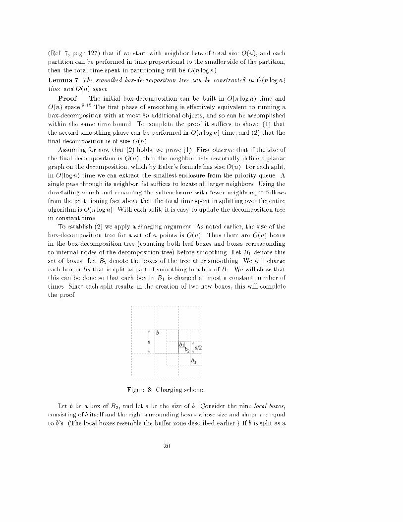
(Ref. 7, page 127) that if we start with neighbor lists of total size O(n), and eachpartition can be performed in time proportional to the smaller side of the partition,then the total time spent in partitioning will be O(n logn).Lemma 7 The smoothed box-decomposition tree can be constructed in O(n logn)time and O(n) space.Proof. The initial box-decomposition can be built in O(n logn) time andO(n) space.8;13 The �rst phase of smoothing is e�ectively equivalent to running abox-decomposition with at most 8n additional objects, and so can be accomplishedwithin the same time bound. To complete the proof it su�ces to show: (1) thatthe second smoothing phase can be performed in O(n logn) time, and (2) that the�nal decomposition is of size O(n).Assuming for now that (2) holds, we prove (1). First observe that if the size ofthe �nal decomposition is O(n), then the neighbor lists essentially de�ne a planargraph on the decomposition, which by Euler's formula has size O(n). For each split,in O(logn) time we can extract the smallest enclosure from the priority queue. Asingle pass through its neighbor list su�ces to locate all larger neighbors. Using thedovetailing search and renaming the subenclosure with fewer neighbors, it followsfrom the partitioning fact above that the total time spent in splitting over the entirealgorithm is O(n logn). With each split, it is easy to update the decomposition treein constant time.To establish (2) we apply a charging argument. As noted earlier, the size of thebox-decomposition tree for a set of n points is O(n). Thus there are O(n) boxesin the box-decomposition tree (counting both leaf boxes and boxes correspondingto internal nodes of the decomposition tree) before smoothing. Let B1 denote thisset of boxes. Let B2 denote the boxes of the tree after smoothing. We will chargeeach box in B2 that is split as part of smoothing to a box of B1. We will show thatthis can be done so that each box in B1 is charged at most a constant number oftimes. Since each split results in the creation of two new boxes, this will completethe proof.s/2

sb

b

1b2

3

bFigure 8: Charging scheme.Let b be a box of B2, and let s be the size of b. Consider the nine local boxes,consisting of b itself and the eight surrounding boxes whose size and shape are equalto b's. (The local boxes resemble the bu�er zone described earlier.) If b is split as a20

result of smoothing, we make the assertion that b exists in B2 either because b is anode in B1 or because at least one of b's local boxes is in B1 and contains a smallbox that eventually induced b to split as a part of smoothing.Assuming the assertion for now, we show how to complete the proof. We chargeeach box in B2 that is split to this local box in B1. Since each box in B1 can beassessed charges only by itself and the surrounding 8 boxes, it follows that each boxof B1 is charged at most 9 times, and hence jB2j � 9jB1j.All that remains is to prove the assertion. We prove this by induction on thesize of the enclosures, working from smaller to larger enclosures. The reason thatb was split is either (1) because b was already split in B1 or (2) because thereis a neighboring enclosure of size no greater than s=4 that induced b to split insmoothing. In the �rst case, the claim is trivially true. In the second case, considerthe neighboring box b1 that induced b to split (see Fig 8).Recall that if a smaller box is created as part of a bu�er zone or as part ofshrinking, then the smoothing rules would not allow such a box to induce a largerneighboring box to be split. Thus, starting with the nearest common ancestor of band b1, the path to b1 in the decomposition tree can only consist of splits. At somepoint along this decomposition path, there must exist an ancestor b2 of b1 that is a1=2-scale copy of b. Clearly b2 is a neighbor of b.By the induction hypothesis, either b2 is a node in B1 or at least one of b2'slocal boxes is in B1, and contains a small box that eventually induced b2 to split asa part of smoothing. In the former case, we are done, because then an ancestor ofb2 is a local box of b1. Otherwise, let b3 be this local box of b2. As above, we canargue that b3 arose along a decomposition path containing only splits. Since b2 andb3 are both 1/2-scale copies of c, and they share a common boundary point witheach other, it follows that b3 has an ancestor in B1 among b's local boxes. Thiscompletes the proof of the assertion. 2The bound on the constant factor arising in the previous proof is not tight. Tightbounds on the size of smoothed quadtree subdivisions under various smoothing ruleshave been established by Moore.28 However, our result does not follow fromMoore'sanalysis because of shrinking.Lemma 8 After smoothing, the number of neighbors of any basic enclosure is O(1).Proof. Consider a basic enclosure c of size s. Each basic enclosure is formedfrom an outer and possibly an inner box. Hence c has at most eight sides. Firstconsider neighbors incident to the outer box. There can be at most a constantnumber of neighbors whose size is within a constant factor of s. If a neighboris signi�cantly smaller, then we claim that this neighbor is a bu�er box, whichwas added after the initial point decomposition. To see this, observe that theneighbor could not be generated by a series of splits alone, for otherwise smoothingwould induce c to split. Also the neighbor could not be an inner box of the initialdecomposition, for otherwise its bu�er zone would extend into c, causing c itself tobe decomposed. Thus, this neighbor is a bu�er box. It is easy to see (Figure 9(a))that, no matter how densely points are arranged within an inner box, after thesmoothing process has terminated, the outer side of each bu�er box can be split21

at most once. Furthermore, an outer box can have at most a constant number ofbu�er box neighbors. A worst-case example is shown in Figure 9(b), where each ofthe neighboring enclosures of half the size of the outer box, and each contributes 3bu�er boxes along the common boundary.(a) (b)Figure 9: Propagation of smoothing and number of neighboring enclosures.Second, we consider neighbors of c's inner box. We claim that these neighboringenclosures consist of a constant number of bu�er boxes. If c's inner box had anypoints, then c would have an inner box in the initial decomposition, and so thisinner box would have been surrounded by eight bu�er boxes. On the other hand, ifc had no inner box after the initial decomposition, then the only way that it couldacquire an inner box is because the neighbors incident to c's outer box had bu�erboxes that spilled over into c. We have argued that c's outer box has at most aconstant number of neighbors, and hence there can be at most a constant numberof bu�er boxes that spilled over into c. As before, the outer edge of each of theseboxes can be split at most once, implying that each side of c's inner box is incidentto a constant number of enclosures. 2The worst-case bound suggested by this proof is quite pessimistic. The dualgraph of the subdivision is a planar graph, implying that each enclosure on averagehas less than 6 neighbors. From the proof we know that splitting induced from aninner box can cause the outer edge of each bu�er box to be split at most once. Ifthe outer edge of a bu�er box edge is split more than once in smoothing, then weknow that this splitting has originated from some other source, and is allowed topropagate outside the bu�er zone.Because of the doughnuts, basic enclosures may not be convex; indeed, the ver-tices of an inner box of a doughnut are re ex vertices. We can make the overallsubdivision convex by extending the left and right (vertical) sides of each inner boxuntil they contact the boundary of the outer box. This subdivides each doughnutinto four rectangles. Observe that this increases the stabbing number of any di-rected segment by at most a constant factor, and so has no signi�cant e�ect on thecomplexity arguments to be made later. This also has a nice e�ect of reducing eachshrink operation to 4 horizontal/vertical split operations (although the splits do notpass through the midpoint of the enclosures). Thus, the resulting subdivision is arecursive binary space partition, using only horizontal and vertical cuts.22

Here is a summary of the construction up to this point.(1) Build a box-decomposition tree for the point set consisting of the obstaclevertices.(2) For each inner box of a shrinking operation in the box-decomposition, createa bu�er zone of 8 identical surrounding boxes. Treating the bu�er boxes as fatpoints, build a box-decomposition tree for the union of the obstacle verticesand bu�er boxes.(3) Given the box-decomposition tree for the point set and bu�er boxes, buildthe cross-indexed neighbor lists for each side of each enclosure by a traversalof the tree. Omit from this list inner boxes from neighboring enclosures andbu�er boxes from their neighbors outside the bu�er zone.(4) While the priority queue is not empty, smooth the subdivision by performingthe following steps until the priority queue is empty.(a) Extract the smallest enclosure cmin from the priority queue.(b) For each of its larger neighbors c, do the following until the sizes of c andcmin di�er by at most a �xed constant factor (e.g. 2).(i) Split c along its longest side.(ii) Partition the neighbor lists of c by a dovetailing search.(iii) Let c0 denote the subenclosure with the fewer neighbors. Createneighbor lists for c0 by deleting the appropriate elements from theneighbor lists of c and adding them to c0.(iv) Access the neighbors of c0, and update their neighbor lists appropri-ately.(v) Insert c0 into the priority queue. Adjust the priority of c, accordingto its new size.(vi) If c0 is the neighbor of cmin, then let c c0.(5) Replace each doughnut by at most four boxes by extending the vertical seg-ments passing through the left and right sides of each inner box.3.3. Adding Obstacle EdgesTo complete the description of the decomposition algorithm, we introduce theobstacle edges. The problem with simply adding the obstacle edges to the box-decomposition is that the number of intersections between obstacle edges and box-decomposition edges may be as large O(n2). To guarantee that the number ofintersections is linear in n, we apply a simple trimming procedure, which trimseach edge of the smoothed box-decomposition subdivision at its �rst and last in-tersection with an obstacle boundary. Let us assume that both the obstacle setand box-decomposition have been preprocessed (by standard means|e.g., trape-zoidization, and a point location data structure) to support horizontal and vertical23

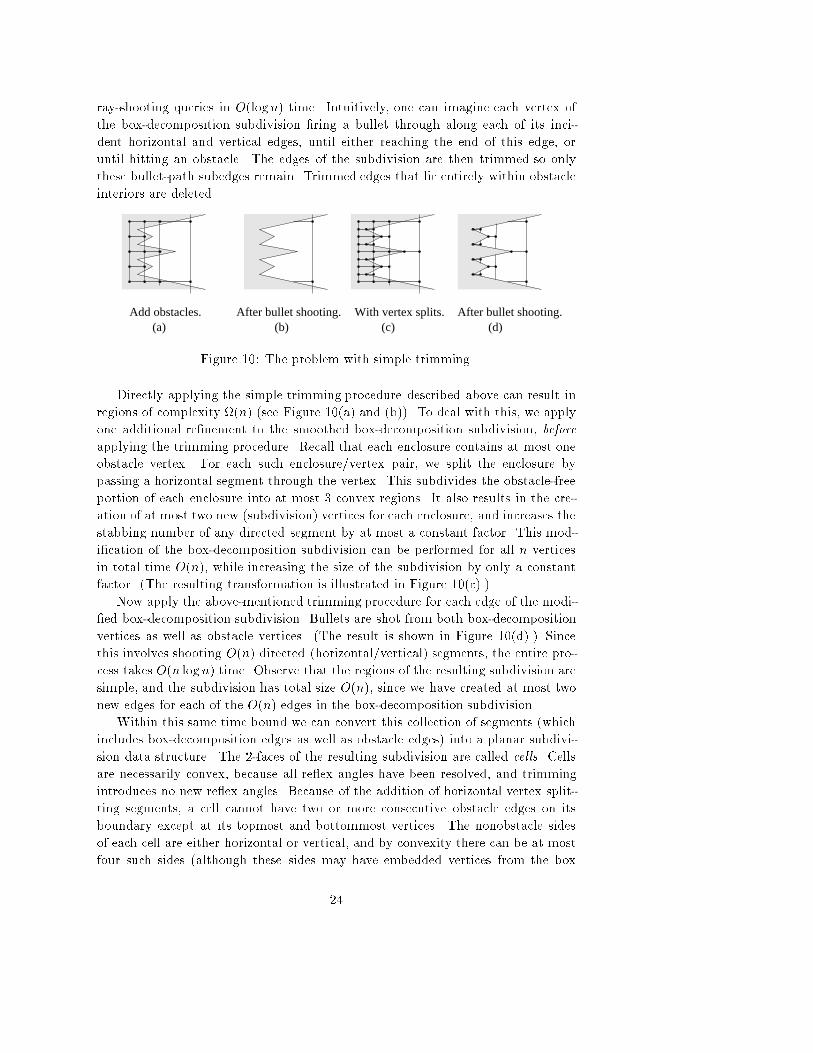
ray-shooting queries in O(logn) time. Intuitively, one can imagine each vertex ofthe box-decomposition subdivision �ring a bullet through along each of its inci-dent horizontal and vertical edges, until either reaching the end of this edge, oruntil hitting an obstacle. The edges of the subdivision are then trimmed so onlythese bullet-path subedges remain. Trimmed edges that lie entirely within obstacleinteriors are deleted.(a) (b) (c) (d)

Add obstacles. After bullet shooting. With vertex splits. After bullet shooting.Figure 10: The problem with simple trimming.Directly applying the simple trimming procedure described above can result inregions of complexity (n) (see Figure 10(a) and (b)). To deal with this, we applyone additional re�nement to the smoothed box-decomposition subdivision, beforeapplying the trimming procedure. Recall that each enclosure contains at most oneobstacle vertex. For each such enclosure/vertex pair, we split the enclosure bypassing a horizontal segment through the vertex. This subdivides the obstacle-freeportion of each enclosure into at most 3 convex regions. It also results in the cre-ation of at most two new (subdivision) vertices for each enclosure, and increases thestabbing number of any directed segment by at most a constant factor. This mod-i�cation of the box-decomposition subdivision can be performed for all n verticesin total time O(n), while increasing the size of the subdivision by only a constantfactor. (The resulting transformation is illustrated in Figure 10(c).)Now apply the above-mentioned trimming procedure for each edge of the modi-�ed box-decomposition subdivision. Bullets are shot from both box-decompositionvertices as well as obstacle vertices. (The result is shown in Figure 10(d).) Sincethis involves shooting O(n) directed (horizontal/vertical) segments, the entire pro-cess takes O(n logn) time. Observe that the regions of the resulting subdivision aresimple, and the subdivision has total size O(n), since we have created at most twonew edges for each of the O(n) edges in the box-decomposition subdivision.Within this same time bound we can convert this collection of segments (whichincludes box-decomposition edges as well as obstacle edges) into a planar subdivi-sion data structure. The 2-faces of the resulting subdivision are called cells. Cellsare necessarily convex, because all re ex angles have been resolved, and trimmingintroduces no new re ex angles. Because of the addition of horizontal vertex split-ting segments, a cell cannot have two or more consecutive obstacle edges on itsboundary except at its topmost and bottommost vertices. The nonobstacle sidesof each cell are either horizontal or vertical, and by convexity there can be at mostfour such sides (although these sides may have embedded vertices from the box24

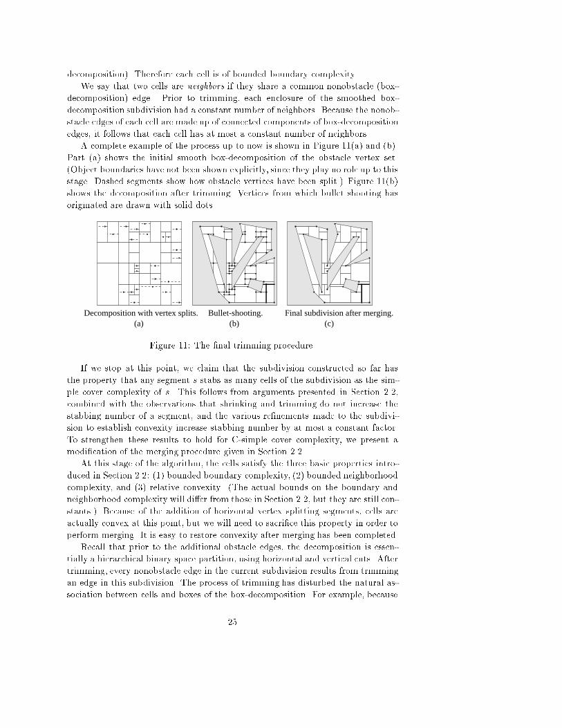
decomposition). Therefore each cell is of bounded boundary complexity.We say that two cells are neighbors if they share a common nonobstacle (box-decomposition) edge. Prior to trimming, each enclosure of the smoothed box-decomposition subdivision had a constant number of neighbors. Because the nonob-stacle edges of each cell are made up of connected components of box-decompositionedges, it follows that each cell has at most a constant number of neighbors.A complete example of the process up to now is shown in Figure 11(a) and (b).Part (a) shows the initial smooth box-decomposition of the obstacle vertex set.(Object boundaries have not been shown explicitly, since they play no role up to thisstage. Dashed segments show how obstacle vertices have been split.) Figure 11(b)shows the decomposition after trimming. Vertices from which bullet shooting hasoriginated are drawn with solid dots.(a) (b) (c)

Bullet-shooting. Final subdivision after merging.Decomposition with vertex splits.Figure 11: The �nal trimming procedure.If we stop at this point, we claim that the subdivision constructed so far hasthe property that any segment s stabs as many cells of the subdivision as the sim-ple cover complexity of s. This follows from arguments presented in Section 2.2,combined with the observations that shrinking and trimming do not increase thestabbing number of a segment, and the various re�nements made to the subdivi-sion to establish convexity increase stabbing number by at most a constant factor.To strengthen these results to hold for C-simple cover complexity, we present amodi�cation of the merging procedure given in Section 2.2.At this stage of the algorithm, the cells satisfy the three basic properties intro-duced in Section 2.2: (1) bounded boundary complexity, (2) bounded neighborhoodcomplexity, and (3) relative convexity. (The actual bounds on the boundary andneighborhood complexity will di�er from those in Section 2.2, but they are still con-stants.) Because of the addition of horizontal vertex splitting segments, cells areactually convex at this point, but we will need to sacri�ce this property in order toperform merging. It is easy to restore convexity after merging has been completed.Recall that prior to the additional obstacle edges, the decomposition is essen-tially a hierarchical binary space partition, using horizontal and vertical cuts. Aftertrimming, every nonobstacle edge in the current subdivision results from trimmingan edge in this subdivision. The process of trimming has disturbed the natural as-sociation between cells and boxes of the box-decomposition. For example, because25

of trimming, a single corridor-like cell lying between two long parallel obstacle edgesmay cut through an arbitrarily large number of boxes of the box decomposition,and similarly a single box of the decomposition may be intersected by an arbitrarilylarge number of such thin corridors. In general, each cell is a connected componentof the union of some number of boxes in the box-decompositionThe merging procedure operates in a similar manner as the one presented inSection 2.2. Initially all cells are eligible for merging. The box-decompositionsplitting segments are traversed in a bottom-up fashion (starting with the leaves ofthe hierarchy). Each splitting segment has at most two components in the tree (oneshot from each endpoint). For each component of each splitting segment considerthe two incident cells on either side of this segment. If both cells are eligible formerging, and the union of the two cells satis�es the three basic properties, thenthe cells are merged into a single cell (e�ectively erasing the splitting segment). Asmentioned earlier, it su�ces to test only the �rst two basic properties, because thethird follows as a consequence of the merging process. Otherwise the cells are notmerged, and neither cell is eligible for subsequent merging. Because cells are ofconstant complexity, merging can be performed in time proportional to the size ofthe subdivision, which is O(n).We call this �nal subdivision the reduced box-decomposition subdivision for theset of obstacles. (See Figure 11(c) for an illustration of this subdivision.) The�nal step of preprocessing is to compute a point location data structure for thissubdivision. Here is a summary of the construction described in this section.(1) Given the box-decomposition tree for the obstacle vertex set, augment thisdecomposition by adding a horizontal splitting segment through each vertex.(2) Preprocess the obstacle set for horizontal and vertical bullet-shooting queriesby computing a horizontal and vertical trapezoidization and a point locationstructure for each.(3) For each edge of the augmented subdivision, shoot a bullet along the edgeinward from each of its endpoints. Create a subdivision consisting only of theobstacle edges, and the obstacle-free bullet-path subedges.(4) Mark every cell of this subdivision as eligible for merging.(5) Working from the bottom of the decomposition hierarchy to the top, for eachcomponent of each splitting segment, if the two cells incident to the splittingsegment are both eligible for merging, then consider the union of these twocells.(a) If this merged cell is incident to at most a given constant number ofobstacle edges, and to a given constant number of neighboring cells thenreplace the two cells with their union.(b) Otherwise, mark both cells ineligible for further merging.(6) Compute a point location data structure for the resulting subdivision.26

3.4. AnalysisIn this section we show that the number of cells that a query segment stabs inthe reduced box-decomposition subdivision is proportional to the C-simple covercomplexity of the segment. The absence of the hierarchical k-d structure makes itdi�cult to generalize Lemma 5, which was used for the reduced k-d subdivision.Our analysis will be based on showing that each cell of the reduced k-d subdivisionpresented in Section 2.2 intersects at most a constant number of cells in the reducedbox-decomposition subdivision presented above. Then, the desired result will followfrom the stabbing bounds on the reduced k-d subdivision established in Theorem 2.Lemma 9 Consider a set P of disjoint polygonal obstacles in the plane, and twosubdivisions: the reduced k-d subdivision S, and the reduced box-decomposition sub-division S0, both starting with the same bounding square. Then each cell of S inter-sects a constant number of cells S0.Proof. We assume for concreteness that in both subdivisions, cells are mergedonly if the number of incident obstacle edges is at most two. A cell may generallyhave (a constant number) more than two incident edges before merging, but sucha cell may not acquire any more incident edges through merging.Consider a cell c of S. Let b be the box in the k-d tree associated with c. Recallfrom Section 2.2 that c is a connected component of b. (Figure 12(a) shows thereduced k-d subdivision S and (b) shows the reduced box-decomposition subdivisionS0. We have indicated that box b has been further subdivided due to the presence ofobstacles that are not shown in the �gure. Note that in general the two subdivisionswill not be the same.)c’

’’c

b b

c

(a) (b)

k-d subdivision Box-decomposition subdivision.Figure 12: Proof of Lemma 9.First we consider whether box b exists in S0. Because both subdivisions startedwith the same bounding square, either (1) b is a box in the box-decomposition, (2)b is contained within the outer box of some shrinking decomposition, or (3) b iscontained within some leaf box. Case (3) can be reduced to case (2) by thinkingof each leaf box as an outer box with no inner box. We show how to reduce case(2) to case (1). Recall that the doughnut region of each shrinking operation ispartitioned into at most 4 rectangular cells to resolve the nonconvex angles of the27

doughnut. Because c is incident to at most two obstacle edges, it follows that theintersection of c with the doughnut consists of only a constant number of connectedcomponents. The processes of trimming and merging can only reduce this numberfurther. Thus, the S0 cannot have more than O(1) cells that overlap the intersectionof c with the doughnut. To complete the proof it su�ces to consider the cells of S0that overlap the inner box, which is a box in both subdivisions. If the inner boxdoes not intersect c then we are done. Otherwise, let us restrict b to be this innerbox, and restrict c to its intersection with b.At this point we may assume that b is a box in both the k-d tree subdivisionand in the box-decomposition, and the cell c of the reduced k-d subdivision is aconnected component of b incident to at most two obstacle edges. Consider thebox-decomposition tree prior to merging, and consider any cell of this subdivisionthat intersects c.We consider two cases. First, if the cell of the trimmed subdivision is partiallyexterior to b, then it follows that this cell intersects the boundary of b along asplitting segment that contains no vertices of the box-decomposition. (For example,c00 in Figure 12(b).) This is true because the existence of a single vertex of the boxdecomposition along the intersection region would result in a bullet �ring along thisedge. Since there are at most two obstacle edges intersecting c, there can be atmost two untrimmed segments along the intersection of c with the boundary of b,and hence there can only be at most two such partially exterior cells.In the second case, the cell of the trimmed subdivision, denoted c0, is entirelyinterior to b (see Figure 12(b)). We claim that after merging, all of these cellswill be merged, leaving at most one such cell (implying that the situation shown inFigure 12(b) cannot occur.) Among all the cells that are entirely interior to b, selectc0 to be any one that is separated from a neighbor by the lowest level edge in thebox-decomposition tree. Because this edge is at the lowest level, it follows that theproperties of bounded neighborhood size and partial convexity cannot be violated bythe merger. (The bounded neighborhood size can only be violated when neighborsare signi�cantly small, implying the existence of a lower level neighboring edge.Partial convexity is a simple consequence of the facts that merging is performed ina bottom-up manner in the decomposition tree.) We argue that bounded boundarycomplexity cannot be an impediment to merging either. To see this, �rst note that ifboth cells are entirely interior to b, then because c is incident to only two edges, themerger contains only two obstacle edges, and hence cannot violate the complexitybound. On the other hand, suppose the neighbor of c0, denoted c00, is partiallyexterior to b (as in Figure 12(b)). As noted above, c00 can be partially exterior to bonly if it used both of the obstacle edges of c to trim part of b's boundary. Since c0is entirely interior to b, it can intersect only a subset of the edges that c00 intersects,and hence their merger does not violate the complexity bound. 2Combining this result with Theorem 2, it follows immediately that if a segments intersects no obstacles, then it intersects O(cscc(s)) cells in the decomposition.From the comments made throughout the presentation, it follows that the total sizeof the subdivision is O(n) and the total preprocessing time is O(n logn).28

Query processing involves two steps. Given a directed segment s, we �rst applya point location algorithm to determine the cell containing the origin of the seg-ment in O(logn) time. Once this cell is known, the algorithm simply walks fromone cell to the next until either reaching the destination of the segment, or untilencountering an obstacle edge. This can be done in time proportional to the num-ber of cells traversed, since each cell is bounded by a constant number of edges andhas a constant number of neighboring cells. Since the traced portion of the querysegment intersects no obstacles, the time needed to trace the segment is O(cscc(s)).Therefore, we have established Theorem 3.4. ConclusionsWe have presented a query-sensitive approach to segment shooting queries,where the running time of the algorithm is described in terms of an intrinsic geomet-ric property of the query segment, called simple cover complexity, which intuitivelycaptures the inherent complexity of processing the query. We feel that a query-sensitive analysis can provide a more accurate insight into the running time of analgorithm than may be available from a worst-case analysis.One of the major challenges of this type of analysis is the methodological prob-lem of selecting parameters that do a good job of identifying the natural sourcesof complexity in a query. Obviously, there is the danger of �rst deriving a pooralgorithm and then attempting to justify its performance in terms of some unnat-ural parameter. For geometric problems, parameters should be invariant undergeometric transformations under which the problem itself is invariant. Parame-ters should intuitively re ect the complexity of the query, and should be small for\typical" cases in practice. For example, it should be clear to a potential user ofthe algorithm whether a particular class of inputs of interest will likely produceunacceptably large parameter values. Also, parameter values should be reasonablyrobust to small perturbations in input coordinates.Although we feel that the complexity measure chosen here does a good job ofcapturing the intuitive complexity of ray shooting, there are two respects in whichour complexity measure could be improved. First, the \strongness" in the covercomplexity (parameterized by �) is an obvious source of unwanted complexity inthe de�nitions. Although we showed that the actual value of � > 0 is irrelevant tothe asymptotic analysis, it would be desirable to dispense with it altogether. Thesecond shortcoming is that, although the measure is invariant under rigid geometrictransformation, it is not invariant under general nonsingular a�ne transformations.In general it can be shown that, the degradation in the parameter value is propor-tional to the \thinness" of the image of the unit sphere under such a transformation.However, the ray shooting problem is invariant under all nonsingular a�ne trans-formations. It would be interesting to develop an approach that is sensitive to anatural parameter that is invariant under all such transformations.Another interesting generalization is that of directed curve shooting. This prob-lem has application in the area of motion simulation. Obviously the method pre-sented here is easy to modify for tracing curves, given access to a primitive that29

determines the earliest intersection of the curve and a line segment (or generally ad�1 dimensional polyhedron of bounded complexity). One property of lines that weuse implicitly in our analysis is that the obstacle-free portion of the query segmentcan intersect each convex cell of the subdivision in a single connected component.If the curves are su�ciently simple that a curve intersects a convex polyhedral cellof bounded complexity in a constant number of components, then all the results ofthis paper apply to these curves as well.AcknowledgementsWe thank Robin Flatland for spotting a bug in the decomposition algorithm,and the referees for their detailed comments and suggestions, which signi�cantlyimproved the paper.References1. P. K. Agarwal. A deterministic algorithm for partitioning arrangements of lines andits applications. In Proc. 5th Annu. ACM Sympos. Comput. Geom., pages 11{22,1989.2. P. K. Agarwal, B. Aronov, and S. Suri. Stabbing triangulations by lines in threedimensions. In Proc. 11th ACM Sympos. Comput. Geom., pages 267{276, 1995.3. P. K. Agarwal and J. Matou�sek. Ray shooting and parametric search. SIAM J.Comput., 22(4):794{806, 1993.4. P. K. Agarwal and J. Matou�sek. On range searching with semi-algebraic sets. Dis-crete Comput. Geom., 11:393{418, 1994.5. P. K. Agarwal and M. Sharir. Ray shooting amidst convex polytopes in three di-mensions. In Proc. 4th ACM-SIAM Sympos. Discrete Algorithms, pages 260{270,1993.6. P. K. Agarwal and M. Sharir. Applications of a new space-partitioning technique.Discrete Comput. Geom., 9:11{38, 1993.7. A. V. Aho, J. E. Hopcroft, and J. D. Ullman. The Design and Analysis of ComputerAlgorithms. Addison-Wesley, Reading, MA, 1974.8. S. Arya, D. M. Mount, N. S. Netanyahu, R. Silverman, and A. Wu. An optimalalgorithm for approximate nearest neighbor searching. In Proc. 5th ACM-SIAMSympos. Discrete Algorithms, pages 573{582, 1994.9. M. de Berg. Ray Shooting, Depth Orders and Hidden Surface Removal, volume 703of Lecture Notes in Computer Science. Springer-Verlag, Berlin, 1993.10. M. de Berg, D. Halperin, M. Overmars, J. Snoeyink, and M. van Kreveld. E�-cient ray shooting and hidden surface removal. In Proc. 7th Annu. ACM Sympos.Comput. Geom., pages 21{30, 1991.11. M. Bern. Approximate closest-point queries in high dimensions. Inform. Process.Lett., 45:95{99, 1993.12. M. Bern, D. Eppstein, and J. Gilbert. Provably good mesh generation. In Proc.31st Annu. IEEE Sympos. Found. Comput. Sci., pages 231{241, 1990.13. P. B. Callahan and S. R. Kosaraju. A decomposition of multi-dimensional point-setswith applications to k-nearest-neighbors and n-body potential �elds. In Proc. 24thAnnu. ACM Sympos. Theory Comput., pages 546{556, 1992.30

14. P. B. Callahan and S. R. Kosaraju. Algorithms for dynamic closest-pair and n-body potential �elds. In Proc. 6th ACM-SIAM Sympos. Discrete Algorithms, pages263{272, 1995.15. B. Chazelle, H. Edelsbrunner, M. Grigni, L. Guibas, J. Hershberger, M. Sharir,and J. Snoeyink. Ray shooting in polygons using geodesic triangulations. In Proc.18th Internat. Colloq. Automata Lang. Program., volume 510 of Lecture Notes inComputer Science, pages 661{673. Springer-Verlag, 1991.16. B. Chazelle and L. J. Guibas. Visibility and intersection problems in plane geometry.In Proc. 1st Annu. ACM Sympos. Comput. Geom., pages 135{146, 1985.17. S. W. Cheng and R. Janardan. Space-e�cient ray shooting and intersection search-ing: Algorithms, dynamization and applications. In Proc. 2nd ACM-SIAM Sympos.Discrete Algorithms, pages 7{16, 1991.18. S. W. Cheng and R. Janardan. Algorithms for ray-shooting and intersection search-ing. J. Algorithms, 13:670{692, 1992.19. K. L. Clarkson. Fast algorithms for the all nearest neighbors problem. In Proc. 24thAnnu. IEEE Sympos. Found. Comput. Sci., pages 226{232, 198320. C. R. Dyer. The space e�ciency of quadtrees, Computer Graphics and Image Pro-cessing, 19:335{348, 1982.21. A. S. Glassner. An Introduction to Ray Tracing. Academic Press, San Deigo, CA,1989.22. M. T. Goodrich and R. Tamassia. Dynamic ray shooting and shortest paths viabalanced geodesic triangulations. In Proc. 9th Annu. ACM Sympos. Comput.Geom., pages 318{327, 1993.23. M. Held, J. T. Klosowski, and J. S. B. Mitchell. Evaluation of collision detectionmethods from virtual reality y-throughs. In Proc. 7th Canad. Conf. Comput.Geom., pages 205{210, 1995.24. J. Hershberger and S. Suri. A pedestrian approach to ray shooting: Shoot a ray,take a walk. J. Algorithms, 18:403{431, 1995.25. B. Von Herzen and A. H. Barr. Accurate triangulations of deformed, intersectingsurfaces. Computer Graphics, 21(4):103{110, July 1987.26. G. M. Hunter and K. Steiglitz. Operations on images using quad trees, IEEE Trans.on Pattern Analysis and Machine Intelligence, 1:145{153, 1979.27. S. A. Mitchell and S. A. Vavasis. Quality mesh generation in three dimensions. InProc. 8th Annu. ACM Sympos. Comput. Geom., pages 212{221, 1992.28. D. W. Moore. Simplicial mesh generation with applications. Ph.D. thesis, Dept.Comput. Sci., Cornell Univ., Ithaca, NY, 1992. Report 92-1322.29. M. Overmars, H. Schipper, and M. Sharir. Storing line segments in partition trees.BIT, 30:385{403, 1990.30. M. Pellegrini. Ray shooting on triangles in 3-space. Algorithmica, 9:471{494, 1993.31. H. Samet. The Design and Analysis of Spatial Data Structures. Addison-Wesley,Reading, MA, 1990.32. O. Schwarzkopf. Ray shooting in convex polytopes. In Proc. 8th Annu. ACMSympos. Comput. Geom., pages 286{295, 1992.33. F. X. Sillion and C. Puech. Radiosity and Global Illumination. Morgan Kaufmann,San Francisco, 1994.34. P. M. Vaidya. An O(n log n) algorithm for the all-nearest-neighbors problem. Dis-crete Comput. Geom., 4:101{115, 1989.31