An Improved Model Selection Heuristic for AUC

Shaomin Wu1, Peter Flach2, and Cesar Ferri3

1 Cranfield University, United KingdomShaomin.Wu@cranfield.ac.uk

2 University of Bristol, United KingdomPeter.Flach@bristol.ac.uk

3 Universitat Politecnica de Valencia, Spaincferri@dsic.upv.es

Abstract. The area under the ROC curve (AUC) has been widely used to mea-sure ranking performance for binary classification tasks. AUC only employs theclassifier’s scores to rank the test instances; thus, it ignores other valuable in-formation conveyed by the scores, such as sensitivity to small differences in thescore values. However, as such differences are inevitable across samples, ignor-ing them may lead to overfitting the validation set when selecting models withhigh AUC. This problem is tackled in this paper. On the basis of ranks as wellas scores, we introduce a new metric called scored AUC (sAUC), which is thearea under the sROC curve. The latter measures how quickly AUC deterioratesif positive scores are decreased. We study the interpretation and statistical prop-erties of sAUC. Experimental results on UCI data sets convincingly demonstratethe effectiveness of the new metric for classifier evaluation and selection in thecase of limited validation data.

1 Introduction

In the data mining and machine learning literature, there are many learning algorithmsthat can be applied to build candidate models for a binary classification task. Such mod-els can be decision trees, neural networks, naive Bayes, or ensembles of these models.As the performance of the candidate models may vary over learning algorithms, effec-tively selecting an optimal model is vitally important. Hence, there is a need for metricsto evaluate the performance of classification models.

The predicted outcome of a classification model can be either a class decision suchas positive and negative on each instance, or a score that indicates the extent to whichan instance is predicted to be positive or negative. Most models can produce scores; andthose that only produce class decisions can easily be converted to models that producescores [3,11]. In this paper we assume that the scores represent likelihoods or posteriorprobabilities of the positive class.

The performance of a classification model can be evaluated by many metrics suchas recall, accuracy and precision. A common weakness of these metrics is that theyare not robust to the change of the class distribution. When the ratio of positive tonegative instances changes in a test set, a model may no longer perform optimally,or even acceptably. The ROC (Receiver Operating Characteristics) curve, however, isinvariant to changes in class distribution. If the class distribution changes in a test set,

J.N. Kok et al. (Eds.): ECML 2007, LNAI 4701, pp. 478–489, 2007.c© Springer-Verlag Berlin Heidelberg 2007

An Improved Model Selection Heuristic for AUC 479

but the underlying class-conditional distributions from which the data are drawn staythe same, the ROC curve will not change. It is defined as a plot of a model’s truepositive rate on the y-axis against its false positive rate on the x-axis, and offers anoverall measure of model performance, regardless of the different thresholds used. TheROC curve has been used as a tool for model selection in the medical area since thelate 1970s, and was more recently introduced to evaluate machine learning algorithms[9,10].

The area under the ROC curve, or simply AUC, aggregates the model’s behaviourfor all possible decision thresholds. It can be estimated under parametric [13], semi-parametric [6] and nonparametric [5] assumptions. The nonparametric estimate of theAUC is widely used in the machine learning and data mining research communities.It is the summation of the areas of the trapezoids formed by connecting the points onthe ROC curve, and represents the probability that a randomly selected positive in-stance will score higher than a randomly selected negative instance. It is equivalent tothe Wilcoxon-Mann-Whitney (WMW) U statistic test of ranks [5]. Huang and Ling [8]argue that AUC is preferable as a measure for model evaluation over accuracy.

The nonparametric estimate of the AUC is calculated on the basis of the ranks of thescores. Its advantage is that it does not depend on any distribution assumption that iscommonly required in parametric statistics. Its weakness is that the scores are only usedto rank instances, and otherwise ignored. The AUC, estimated simply from the ranks ofthe scores, can remain unchanged even when the scores change. This can lead to a lossof useful information, and may therefore produce sub-optimal results.

In this paper we argue that, in order to evaluate the performance of binary classifi-cation models, both ranks and scores should be combined. A scored AUC metric is in-troduced for estimating the performance of models based on their original scores. Thepaper is structured as follows. Section 2 reviews ways to evaluate scoring classifiers,including AUC and Brier score, and gives a simple and elegant algorithm to calculateAUC. Section 3 introduces the scored ROC curve and the new scored AUC metric, andinvestigates its properties. In Section 4 we present experimental results on 17 data setsfrom the UCI repository, which unequivocally demonstrate that validation sAUC is su-perior to validation AUC and validation Brier score for selecting models with high testAUC when limited validation data is available. Section 5 presents the main conclusionsand suggests further work. An early version of this paper appeared as [12].

2 Evaluating Classifiers

There are a number of ways of evaluating the performance of scoring classifiers over atest set. Broadly, the choices are to evaluate its classification performance, its rankingperformance, or its probability estimation performance. Classification performance isevaluated by a measure such as accuracy, which is the proportion of test instances thatis correctly classified. Probability estimation performance is evaluated by a measuresuch as mean squared error, also called the Brier score, which can be expressed as∑x(p(x)− p(x))2, where p(x) is the estimated probability for instance x, and p(x) is 1if x is positive and 0 if x is negative. The calculation of both accuracy and Brier score isan O(n) operation, where n is the size of the test set.

480 S. Wu, P. Flach, and C. Ferri

Ranking performance is evaluated by sorting the test instances on their score, whichis an O(n logn) operation. It thus incorporates performance information that neither ac-curacy nor Brier score can access. There are a number of reasons why it is desirable tohave a good ranker, rather than a good classifier or a good probability estimator. One ofthe main reasons is that accuracy requires a fixed score threshold, whereas it may be de-sirable to change the threshold in response to changing class or cost distributions. Goodaccuracy obtained with one threshold does not imply good accuracy with another. Fur-thermore, good performance in both classification and probability estimation is easilyobtained if one class is much more prevalent than the other. For these reasons we preferto evaluate ranking performance. This can be done by constructing an ROC curve.

An ROC curve is generally defined as a piecewise linear curve, plotting a model’strue positive rate on the y-axis against its false positive rate on the x-axis, evaluatedunder all possible thresholds on the score. For a test set with t test instances, the ROCcurve will have (up to) t linear segments and t + 1 points. We are interested in thearea under this curve, which is well-known to be equivalent to the Wilcoxon-Mann-Whitney sum of ranks test, and estimates the probability that a randomly chosen positiveis ranked before a randomly chosen negative. AUC can be calculated directly from thesorted test instances, without the need for drawing an ROC curve or calculating ranks,as we now show.

Denote the total number of positive instances and negative instances by m and n,respectively. Let {y1, . . . ,ym} be the scores predicted by a model for the m positives,and {x1, . . . ,xn} be the scores predicted by a model for the n negatives. Assume both yi

and x j are within the interval [0,1] for all i = 1,2, ...,m and j = 1,2, ...,n; high scoresare interpreted as evidence for the positive class. By a slight abuse of language, wewill sometimes use positive (negative) score to mean ‘score of a positive (negative)instance’.

AUC simply counts the number of pairs of positives and negatives such that theformer has higher score than the latter, and can therefore be defined as follows:

θ =1

mn

m

∑i=1

n

∑j=1

ψi j (1)

where ψi j is 1 if yi − x j > 0, and 0 otherwise. Let Za be the sequence produced bymerging {y1, . . . ,ym} and {x1, . . . ,xn} and sorting the merged set in ascending order (soa good ranker would put the positives after the negatives in Za), and let ri be the rank ofyi in Za. Then AUC can be expressed in terms of ranks as follows:

θ =1

mn

(m

∑i=1

ri −m(m+ 1)

2

)=

1mn

m

∑i=1

(ri − i) =1

mn

m

∑i=1

ri−i

∑t=1

1 (2)

Here, ri − i is the number of negatives before the ith positive in Za, and thus AUC is the(normalised) sum of the number of negatives before each of the m positives in Za.

Dually, let Zd be the sequence produced by sorting {y1, . . . ,ym} ∪ {x1, . . . ,xn} indescending order (so a good ranker would put the positives before the negatives in Zd).We then obtain

θ =1

mn

n

∑j=1

(s j − j) =1

mn

n

∑j=1

s j− j

∑t=1

1 (3)

An Improved Model Selection Heuristic for AUC 481

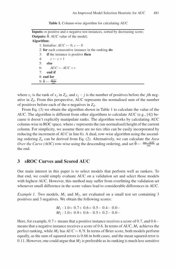
Table 1. Column-wise algorithm for calculating AUC

Inputs: m positive and n negative test instances, sorted by decreasing score;Outputs: θ: AUC value of the model;Algorithm:

1: Initialise: AUC ← 0, c ← 02: for each consecutive instance in the ranking do3: if the instance is positive then4: c ← c+15: else6: AUC ← AUC +c7: end if8: end for9: θ ← AUC

mn

where s j is the rank of x j in Zd , and s j − j is the number of positives before the jth neg-ative in Zd . From this perspective, AUC represents the normalised sum of the numberof positives before each of the n negatives in Zd .

From Eq. (3) we obtain the algorithm shown in Table 1 to calculate the value of theAUC. The algorithm is different from other algorithms to calculate AUC (e.g., [4]) be-cause it doesn’t explicitly manipulate ranks. The algorithm works by calculating AUCcolumn-wise in ROC space, where c represents the (un-normalised) height of the currentcolumn. For simplicity, we assume there are no ties (this can be easily incorporated byreducing the increment of AUC in line 6). A dual, row-wise algorithm using the ascend-ing ordering Za can be derived from Eq. (2). Alternatively, we can calculate the AreaOver the Curve (AOC) row-wise using the descending ordering, and set θ ← mn−AOC

mn atthe end.

3 sROC Curves and Scored AUC

Our main interest in this paper is to select models that perform well as rankers. Tothat end, we could simply evaluate AUC on a validation set and select those modelswith highest AUC. However, this method may suffer from overfitting the validation setwhenever small difference in the score values lead to considerable differences in AUC.

Example 1. Two models, M1 and M2, are evaluated on a small test set containing 3positives and 3 negatives. We obtain the following scores:

M1 : 1.0+ 0.7+ 0.6+ 0.5− 0.4− 0.0−M2 : 1.0+ 0.9+ 0.6− 0.5+ 0.2− 0.0−

Here, for example, 0.7+ means that a positive instance receives a score of 0.7, and 0.6−means that a negative instance receives a score of 0.6. In terms of AUC, M1 achieves theperfect ranking, while M2 has AUC = 8/9. In terms of Brier score, both models performequally, as the sum of squared errors is 0.66 in both cases, and the mean squared error is0.11. However, one could argue that M2 is preferable as its ranking is much less sensitive

482 S. Wu, P. Flach, and C. Ferri

0 0.1 0.2 0.3 0.4 0.5 0.6 0.7 0.8 0.9 10

0.1

0.2

0.3

0.4

0.5

0.6

0.7

0.8

0.9

1

()

M1

M2

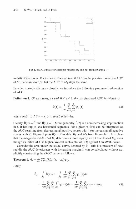
Fig. 1. sROC curves for example models M1 and M2 from Example 1

to drift of the scores. For instance, if we subtract 0.25 from the positive scores, the AUCof M1 decreases to 6/9, but the AUC of M2 stays the same.

In order to study this more closely, we introduce the following parameterised versionof AUC.

Definition 1. Given a margin τ with 0 ≤ τ ≤ 1, the margin-based AUC is defined as

θ(τ) =1

mn

m

∑i=1

n

∑j=1

ψi j(τ) (4)

where ψi j(τ) is 1 if yi − x j > τ, and 0 otherwise.

Clearly, θ(0) = θ, and θ(1) = 0. More generally, θ(τ) is a non-increasing step functionin τ. It has (up to) mn horizontal segments. For a given τ, θ(τ) can be interpreted asthe AUC resulting from decreasing all positive scores with τ (or increasing all negativescores with τ). Figure 1 plots θ(τ) of models M1 and M2 from Example 1. It is clearthat the margin-based AUC of M1 deteriorates more rapidly with τ than that of M2, eventhough its initial AUC is higher. We call such a plot of θ(τ) against τ an sROC curve.

Consider the area under the sROC curve, denoted by θs. This is a measure of howrapidly the AUC deteriorates with increasing margin. It can be calculated without ex-plicitly constructing the sROC curve, as follows.

Theorem 1. θs = 1mn ∑m

i=1 ∑nj=1(yi − x j)ψi j .

Proof

θs =∫ 1

0θ(τ)dτ =

∫ 1

0

1mn

m

∑i=1

n

∑j=1

ψi j(τ)dτ

=1

mn

m

∑i=1

n

∑j=1

∫ 1

0ψi j(τ)dτ =

1mn

m

∑i=1

n

∑j=1

(yi − x j)ψi j (5)

An Improved Model Selection Heuristic for AUC 483

Thus, just as θ is the area under the ROC curve, θs is the area under the sROC curve; wecall it scored AUC (sAUC). An equivalent definition of sAUC was introduced in [12],and independently by Huang and Ling, who refer to it as soft AUC [7]. Its interpretationas the area under the sROC curve is, to the best of our knowledge, novel. The sROCcurve depicts the stability of AUC with increasing margins, and sAUC aggregates thisover all margins into a single statistic.

Whereas in Eq. (1) the term ψi j is an indicator that only reflects the ordinal com-parison between the scores, (yi − x j)ψi j in Eq. (5) measures how much yi is larger thanx j. Notice that, by including the ordinal term, we combine information from both ranksand scores. Indeed, if we omit ψi j from Eq. (5) the expression reduces to 1

m ∑mi=1 yi −

1n ∑n

i=1 xi = M+ −M−; i.e., the difference between the mean positive and negative scores.This measure (a quantity that takes scores into account but ignores the ranking) isinvestigated in [2].

We continue to analyse the properties of sAUC. Let R+ = 1m ∑m

i=1ri−i

n yi be theweighted average of the positive scores, weighted by the proportion of negatives thatare correctly ranked relative to each positive. Similarly, let R− = 1

n ∑nj=1

s j− jm x j be the

weighted average of the negative scores, weighted by the proportion of positives thatare correctly ranked relative to each negative (i.e., the height of the column under theROC curve). We then have the following useful reformulation of sAUC.

Theorem 2. θs = R+ − R−.

Proof

θs =1

mn

m

∑i=1

n

∑j=1

(yi − x j)ψi j =1

mn

m

∑i=1

n

∑j=1

yiψi j −1

mn

m

∑i=1

n

∑j=1

x jψi j =

=1

mn

m

∑i=1

ri−i

∑j=1

yi −1

mn

n

∑j=1

s j− j

∑i=1

x j =1m

m

∑i=1

ri − in

yi −1n

n

∑j=1

s j − j

mx j = R+ − R−

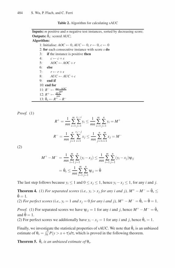
This immediately leads to the algorithm for calculating θs in Table 2. The algorithmcalculates R+ column-wise as in the AUC algorithm (Table 1), and the complement ofR− row-wise (so that the descending ordering can be used in both cases).

Example 2. Continuing Example 1, we have

M1: R+ = 0.77, R− = 0.3 and θs = 0.47;M2: R+ = 0.74, R− = 0.2 and θs = 0.54.

We thus have that M2 is somewhat better in terms of sAUC than M1 because, eventhough its AUC is lower, it is robust over a larger range of margins.

The following theorems relate θs, θ and M+ − M−.

Theorem 3. (1) R+ ≤ M+ and R− ≤ M−.(2) M+ − M− ≤ θs ≤ θ.

484 S. Wu, P. Flach, and C. Ferri

Table 2. Algorithm for calculating sAUC

Inputs: m positive and n negative test instances, sorted by decreasing score;Outputs: θs: scored AUC;Algorithm:

1: Initialise: AOC ← 0, AUC ← 0, r ← 0, c ← 02: for each consecutive instance with score s do3: if the instance is positive then4: c ← c+ s5: AOC ← AOC + r6: else7: r ← r + s8: AUC ← AUC +c9: end if10: end for11: R− ← mr−AOC

mn12: R+ ← AUC

mn13: θs ← R+ −R−

Proof. (1)

R+ =1

mn

m

∑i=1

ri−i

∑j=1

yi ≤ 1mn

m

∑i=1

n

∑j=1

yi = M+

R− =1

mn

n

∑j=1

s j− j

∑i=1

x j ≤ 1mn

n

∑j=1

m

∑i=1

x j = M−

(2)

M+ − M− =1

mn

m

∑i=1

n

∑j=1

(yi − x j) ≤ 1mn

m

∑i=1

n

∑j=1

(yi − x j)ψi j

= θs ≤ 1mn

m

∑i=1

n

∑j=1

ψi j = θ

The last step follows because yi ≤ 1 and 0 ≤ x j ≤ 1, hence yi − x j ≤ 1, for any i and j.

Theorem 4. (1) For separated scores (i.e., yi > x j for any i and j), M+ − M− = θs ≤θ = 1.(2) For perfect scores (i.e., yi = 1 and x j = 0 for any i and j), M+ − M− = θs = θ = 1.

Proof. (1) For separated scores we have ψi j = 1 for any i and j, hence M+ − M− = θs

and θ = 1.(2) For perfect scores we additionally have yi − x j = 1 for any i and j, hence θs = 1.

Finally, we investigate the statistical properties of sAUC. We note that θs is an unbiasedestimate of θs =

∫ 10 P(y > x + τ)dτ, which is proved in the following theorem.

Theorem 5. θs is an unbiased estimate of θs.

An Improved Model Selection Heuristic for AUC 485

Proof. From Eq. (5), we have

E(θs) = E

[1

mn

m

∑i=1

n

∑j=1

∫ 1

0ψi j(τ)dτ

]=

∫ 1

0

(E

[1

mn

m

∑i=1

n

∑j=1

ψi j(τ)

])dτ

=∫ 1

0P(y > x + τ)dτ

The variance of the estimate θs can be obtained using the method of DeLong et al. [1](we omit the proof due to lack of space).

Theorem 6. The variance of θs is estimated by

var(θs) =n − 1

mn(m− 1)

m

∑i=1

(1n

n

∑j=1

(yi − xi)ψi j − θs

)2

+m− 1

mn(n − 1)

n

∑j=1

(1m

m

∑i=1

(yi − xi)ψi j − θs

)2

.

4 Experimental Evaluation

Our experiments to evaluate the usefulness of sAUC for model selection are describedin this section. Our main conclusion is that sAUC outperforms AUC and BS (Brierscore) for selecting models, particularly when validation data is limited. We attributethis to sAUC having a lower variance than AUC and BS. Consequently, validation setvalues generalise better to test set values.

In the first experiment, we generated two artificial data sets (A and B) of 100 exam-ples, each labelled with a ‘true’ probability p which is uniformly sampled from [0,1].Then, we label the instances (+ if p ≥ 0.5, − otherwise). Finally, we swap the classesof 10 examples of data set A, and of 11 examples of data set B. We then construct‘models’ MA and MB by giving them access to the ‘true’ probabilities p, and recordwhich one is better (either MA on data set A or MB on data set B). For example, bythresholding p at 0.5, MA has accuracy 90% on data set A, and MB has accuracy 89%on data set B. We then add noise to obtain ‘estimated’ probabilities in the followingway: p′ = p+ k ∗U(−0.5,0.5), where k is a noise parameter, and U(−0.5,0.5) obtainsa pseudo-random number between −0.5 and 0.5 using a uniform distribution (if thecorrupted values are > 1 or < 0, we set them to 1 and 0 respectively).

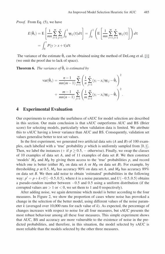
After adding noise, we again determine which model is better according to the fourmeasures. In Figure 2, we show the proportion of cases where noise has provoked achange in the selection of the better model, using different values of the noise param-eter k (averaged over 10,000 runs for each value of k). As expected, the percentage ofchanges increases with respect to noise for all four measures, but sAUC presents themost robust behaviour among all these four measures. This simple experiment showsthat AUC, BS and accuracy are more vulnerable to the existence of noise in the pre-dicted probabilities, and therefore, in this situation, the model selected by sAUC ismore reliable than the models selected by the other three measures.

486 S. Wu, P. Flach, and C. Ferri

Fig. 2. The effect of noise in the probability estimates on four model selection measures

We continue reporting our experiments with real data. We use the three metrics(AUC, sAUC and BS) to select models on the validation set, and compare them usingthe AUC values on the test set. 17 two-class data sets are selected from the UCI repos-itory for this purpose. Table 3 lists their numbers of attributes, numbers of instances,and relative size of the majority class.

Table 3. UCI data sets used in the experiments (larger data sets used in separate experiment inbold face)

# Data set #Attrs #Exs %Maj.Class1 Monk1 6 556 50.002 Monk2 6 601 65.723 Monk3 6 554 55.414 Kr-vs-kp 36 3,196 52.225 Tic-tac-toe 9 958 64.206 Credit-a 15 690 55.517 German 20 1,000 69.408 Spam 57 4,601 60.599 House-vote 16 435 54.25

# Data set #Attrs #Exs %Maj.Class10 Breast Cancer 9 286 70.2811 Breast-w 9 699 65.5212 Colic 22 368 63.0413 Heart-statlog 13 270 59.5014 Sick 29 3,772 93.8715 Caravan 85 5,822 94.0216 Hypothyroid 25 3,163 95.2217 Mushroom 22 8,124 51.80

The configuration of the experiments is as follows. We distinguish between smalldata sets (with up to 1,000 examples) and larger data sets. For the 11 small data sets, werandomly split the whole data set into two equal-sized parts. One half is used as trainingset; the second half is again split into 20% validation set and 80% test set. In order to ob-tain models with sufficiently different performance, we train 10 different classifiers withthe same learning technique (J48 unpruned with Laplace correction, Naive Bayes, andLogistic Regression, all from Weka) over the same training data, by randomly removingthree attributes before training. We select the best model according to three measures:AUC, sAUC and BS using the validation set. The performance of each selected modelis assessed by AUC on the test set. Results are averaged over 2000 repetitions of this

An Improved Model Selection Heuristic for AUC 487

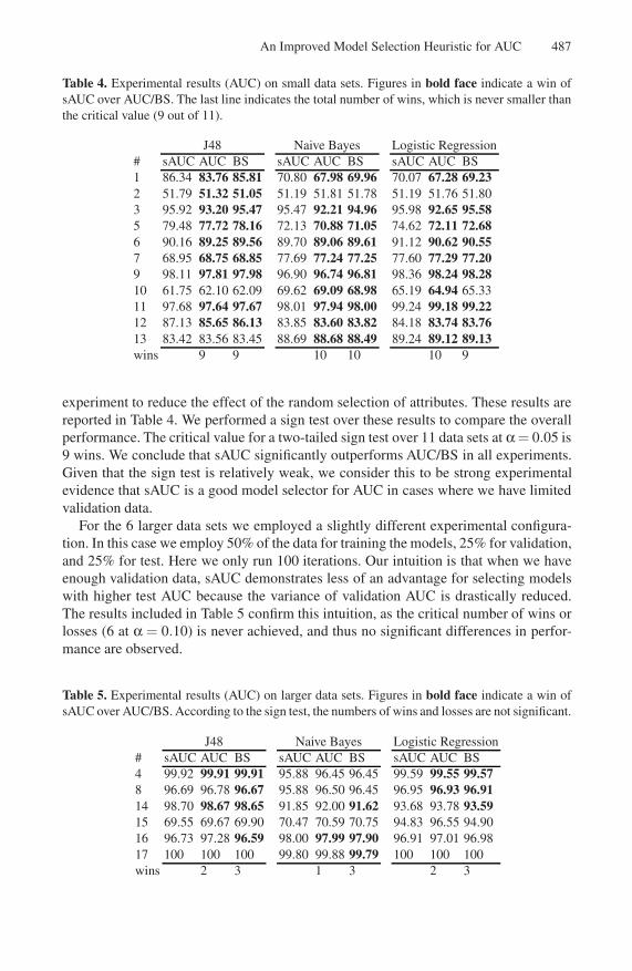
Table 4. Experimental results (AUC) on small data sets. Figures in bold face indicate a win ofsAUC over AUC/BS. The last line indicates the total number of wins, which is never smaller thanthe critical value (9 out of 11).

J48 Naive Bayes Logistic Regression# sAUC AUC BS sAUC AUC BS sAUC AUC BS1 86.34 83.76 85.81 70.80 67.98 69.96 70.07 67.28 69.232 51.79 51.32 51.05 51.19 51.81 51.78 51.19 51.76 51.803 95.92 93.20 95.47 95.47 92.21 94.96 95.98 92.65 95.585 79.48 77.72 78.16 72.13 70.88 71.05 74.62 72.11 72.686 90.16 89.25 89.56 89.70 89.06 89.61 91.12 90.62 90.557 68.95 68.75 68.85 77.69 77.24 77.25 77.60 77.29 77.209 98.11 97.81 97.98 96.90 96.74 96.81 98.36 98.24 98.2810 61.75 62.10 62.09 69.62 69.09 68.98 65.19 64.94 65.3311 97.68 97.64 97.67 98.01 97.94 98.00 99.24 99.18 99.2212 87.13 85.65 86.13 83.85 83.60 83.82 84.18 83.74 83.7613 83.42 83.56 83.45 88.69 88.68 88.49 89.24 89.12 89.13wins 9 9 10 10 10 9

experiment to reduce the effect of the random selection of attributes. These results arereported in Table 4. We performed a sign test over these results to compare the overallperformance. The critical value for a two-tailed sign test over 11 data sets at α = 0.05 is9 wins. We conclude that sAUC significantly outperforms AUC/BS in all experiments.Given that the sign test is relatively weak, we consider this to be strong experimentalevidence that sAUC is a good model selector for AUC in cases where we have limitedvalidation data.

For the 6 larger data sets we employed a slightly different experimental configura-tion. In this case we employ 50% of the data for training the models, 25% for validation,and 25% for test. Here we only run 100 iterations. Our intuition is that when we haveenough validation data, sAUC demonstrates less of an advantage for selecting modelswith higher test AUC because the variance of validation AUC is drastically reduced.The results included in Table 5 confirm this intuition, as the critical number of wins orlosses (6 at α = 0.10) is never achieved, and thus no significant differences in perfor-mance are observed.

Table 5. Experimental results (AUC) on larger data sets. Figures in bold face indicate a win ofsAUC over AUC/BS. According to the sign test, the numbers of wins and losses are not significant.

J48 Naive Bayes Logistic Regression# sAUC AUC BS sAUC AUC BS sAUC AUC BS4 99.92 99.91 99.91 95.88 96.45 96.45 99.59 99.55 99.578 96.69 96.78 96.67 95.88 96.50 96.45 96.95 96.93 96.9114 98.70 98.67 98.65 91.85 92.00 91.62 93.68 93.78 93.5915 69.55 69.67 69.90 70.47 70.59 70.75 94.83 96.55 94.9016 96.73 97.28 96.59 98.00 97.99 97.90 96.91 97.01 96.9817 100 100 100 99.80 99.88 99.79 100 100 100wins 2 3 1 3 2 3

488 S. Wu, P. Flach, and C. Ferri

Fig. 3. Scatter plots of test AUC vs. validation AUC (left) and test AUC vs. validation sAUC(right) on the Credit-a data set.

Finally, Figure 3 shows two scatter plots of the models obtained for the Credit-a dataset, the first one plotting test AUC against validation AUC, and the second one plottingtest AUC against validation sAUC. Both plots include a straight line obtained by linearregression. Since validation sAUC is an underestimate of validation AUC (Theorem 3),it is not surprising that validation sAUC is also an underestimate of test AUC. ValidationAUC appears to be an underestimate of test AUC on this data set, but this may be causedby the outliers on the left. But what really matters in these plots is the proportion ofvariance in test AUC not accounted for by the linear regression (which is 1−g2, whereg is the linear correlation coefficient). We can see that this is larger for validation AUC,particularly because of the vertical lines observed in Figure 3 (left). These lines indicatehow validation AUC fails to distinguish between models with different test AUC. Thisphenomenon particularly occurs for a number of models with perfect ranking on thevalidation set. Since sAUC takes the scores into account, and since these models donot have perfect scores on the validation set, the same phenomenon is not observed inFigure 3 (right).

5 Conclusions

The ROC curve is useful for visualising the performance of scoring classification mod-els. ROC curves contain a wealth of information about the performance of one or moreclassifiers, which can be utilised to improve their performance and for model selection.For example, Provost and Fawcett [10] studied the application of model selection inROC space when target misclassification costs and class distributions are uncertain.

In this paper we introduced the scored AUC (sAUC) metric to measure the perfor-mance of a model. The difference between AUC and scored AUC is that the AUConly uses the ranks obtained from scores, whereas the scored AUC uses both ranks andscores. We defined sAUC as the area under the sROC curve, which shows how quicklyAUC deteriorates if the positive scores are decreased. Empirically, sAUC was found toselect models with larger AUC values then AUC itself (which uses only ranks) or theBrier score (which uses only scores).

An Improved Model Selection Heuristic for AUC 489

Evaluating learning algorithms can be regarded as a process of testing the diversityof two samples, that is, a sample of the scores for positive instances and that for negativeinstances. As the scored AUC takes advantage of both the ranks and the original valuesof samples, it is potentially a good statistic for testing the diversity of two samples,in a similar vein as the Wilcoxon-Man-Whitney U statistic. Preliminary experimentssuggest that sAUC has indeed higher power than WMW. Furthermore, while this paperonly investigates sAUC from the non-parametric perspective, it is worthwhile to studyits parametric properties. We plan to investigate these further in future work.

Acknowledgments

We thank Jose Hernandez-Orallo and Thomas Gartner for useful discussions. We wouldalso like to thank the anonymous reviewers for their helpful comments.

References

1. DeLong, E.R., DeLong, D.M., Clarke-Pearson, D.L.: Comparing the areas under two or morecorrelated receiver operating characteristic curves: a nonparametric approach. Biometrics 44,837–845 (1988)

2. Ferri, C., Flach, P., Hernandez-Orallo, J., Senad, A.: Modifying ROC curves to incorporatepredicted probabilities. In: Proceedings of the Second Workshop on ROC Analysis in Ma-chine Learning (ROCML’05) (2005)

3. Fawcett, T.: Using Rule Sets to Maximize ROC Performance. In: Proc. IEEE Int’l Conf. DataMining, pp. 131–138 (2001)

4. Fawcett, T.: An introduction to ROC analysis. Pattern Recognition Let. 27-8, 861–874 (2006)5. Hanley, J.A., McNeil, B.J.: The Meaning and Use of the AUC Under a Receiver Operating

Characteristic (ROC) Curve. Radiology 143, 29–36 (1982)6. Hsieh, F., Turnbull, B.W.: Nonparametric and Semiparametric Estimation of the Receiver

Operating Characteristic Curve. Annals of Statistics 24, 25–40 (1996)7. Huang, J., Ling, C.X.: Dynamic Ensemble Re-Construction for Better Ranking. In: Proc. 9th

Eur. Conf. Principles and Practice of Knowledge Discovery in Databases, pp. 511–518(2005)

8. Huang, J., Ling, C.X.: Using AUC and Accuray in Evaluating Learing Algorithms. IEEETransactions on Knowledge and Data Engineering 17, 299–310 (2005)

9. Provost, F., Fawcett, T., Kohavi, R.: Analysis and Visualization of Classifier Performance:Comparison Under Imprecise Class and Cost Distribution. In: Proc. 3rd Int’l Conf. Knowl-edge Discovery and Data Mining, pp. 43–48 (1997)

10. Provost, F., Fawcett, T.: Robust Classification for Imprecise Environments. Machine Learn-ing 42, 203–231 (2001)

11. Provost, F., Domingos, P.: Tree Induction for Probability-Based Ranking. Machine Learn-ing 52, 199–215 (2003)

12. Wu, S.M., Flach, P.: Scored Metric for Classifier Evaluation and Selection. In: Proceedingsof the Second Workshop on ROC Analysis in Machine Learning (ROCML’05) (2005)

13. Zhou, X.H., Obuchowski, N.A., McClish, D.K.: Statistical Methods in Diagnostic Medicine.John Wiley and Sons, Chichester (2002)