NBER WORKING PAPER SERIES

HEURISTIC THINKING AND LIMITED ATTENTION IN THE CAR MARKET

Nicola LaceteraDevin G. Pope

Justin R. Sydnor

Working Paper 17030http://www.nber.org/papers/w17030

NATIONAL BUREAU OF ECONOMIC RESEARCH1050 Massachusetts Avenue

Cambridge, MA 02138May 2011

We are grateful to seminar participants at the Second Annual Behavioral Economics Conference, NBERSummer Institute, FTC Microeconomics Conference, Case Western Reserve, Drexel, Harvard, Melbourne,MIT, Sydney, Toronto, UC Berkeley, UT Dallas, and the Wharton School for helpful comments andsuggestions. Special thanks to Susan Helper, Glenn Mercer and Jim Rebitzer for help obtaining dataand advice on the auto industry. Financial support was provided by The Fishman Davidson Centerand The International Motor Vehicle Program. Part of this research was performed while Nicola Laceteraand Justin Sydnor were at the Economics Department at Case Western Reserve University, and DevinPope was at the Wharton School of the University of Pennsylvania. The views expressed herein arethose of the authors and do not necessarily reflect the views of the National Bureau of Economic Research.

NBER working papers are circulated for discussion and comment purposes. They have not been peer-reviewed or been subject to the review by the NBER Board of Directors that accompanies officialNBER publications.

© 2011 by Nicola Lacetera, Devin G. Pope, and Justin R. Sydnor. All rights reserved. Short sectionsof text, not to exceed two paragraphs, may be quoted without explicit permission provided that fullcredit, including © notice, is given to the source.

Heuristic Thinking and Limited Attention in the Car MarketNicola Lacetera, Devin G. Pope, and Justin R. SydnorNBER Working Paper No. 17030May 2011JEL No. D03,D12,L62

ABSTRACT

Can heuristic information processing affect important product markets? We explore whether the tendencyto focus on the left-most digit of a number affects how used car buyers incorporate odometer valuesin their purchase decisions. Analyzing over 22 million wholesale used-car transactions, we find substantialevidence of this left-digit bias; there are large and discontinuous drops in sale prices at 10,000-milethresholds in odometer mileage, along with smaller drops at 1,000-mile thresholds. We obtain estimatesfor the inattention parameter in a simple model of this left-digit bias. We also investigate whether thisheuristic behavior is primarily attributable to the final used-car customers or the used-car salesmenwho buy cars in the wholesale market. The evidence is most consistent with partial inattention by finalcustomers. We discuss the significance of these results for the literature on inattention and point toother market settings where this type of heuristic thinking may be important. Our results suggest thatinformation-processing heuristics may be important even in markets with large stakes and where informationis easy to observe.

Nicola LaceteraUniversity of TorontoRotman School of Management105 St. George Street, Room 265Toronto, ON M5S 2E9and NBERnicola.lacetera@utoronto.ca

Devin G. PopeBooth School of BusinessUniversity of Chicago5807 South Woodlawn AvenueChicago, IL 60637and NBERdevin.pope@chicagobooth.edu

Justin R. SydnorUniversity of Wisconsin School of Business, ASRMI975 University Ave, Room 5287Madison, WI 53726jsydnor@bus.wisc.edu

An online appendix is available at:http://www.nber.org/data-appendix/w17030

1

1. Introduction

Although economic models are usually based on the assumption that agents are unconstrained in

their ability to process information, economists have long recognized that individuals have limited

cognitive abilities (Simon, 1955). An extensive literature on heuristics and biases, originating

primarily in psychology, has shown that people often use simple cognitive shortcuts when

processing information, leading to systematic biases in decision making.1 There is large evidence on

the nature of these heuristics from surveys and laboratory experiments, but there has been much less

research exploring whether these cognitive limitations impact important market settings.

In this paper, we study the effects of heuristic information processing in the used-car

market. We investigate whether the market is affected by consumers exhibiting a heuristic known as

left-digit bias when they incorporate odometer mileages into their decision process. Left-digit bias is

the tendency to focus on the left-most digit of a number while partially ignoring other digits

(Korvost and Damian, 2008; Poltrock and Schwartz, 1984). We develop a simple model of left-digit

bias patterned after the model of inattention presented by DellaVigna (2009). The model predicts

that, if consumers use this heuristic when processing odometer values, cars will exhibit

discontinuous drops in value at mileage thresholds where left digits change (e.g., 10,000-mile marks).

Using a rich and novel dataset on more than 22 million used-car transactions from wholesale

auctions, we show that there are clear threshold effects at 10,000-mile marks. These discontinuous

drops in value are evident in simple graphs of the raw data. For example, cars with odometer values

between 79,900 and 79,999 miles are sold on average for approximately $210 more than cars with

odometer values between 80,000 and 80,100 miles, but for only $10 less than cars with odometer

readings between 79,800 and 79,899. Regression analyses show significant price discontinuities at

each 10,000-mile threshold from 10,000 to 100,000 miles. The size of the discontinuities is similar

across each threshold, consistently on the order of $150 to $200. Consistent with our model, we also

find smaller price discontinuities at 1,000-mile thresholds.

The left-digit bias we identify in this paper not only influences wholesale prices but also

affects supply decisions. If sellers are savvy and aware of threshold effects, they will have an

incentive to bring cars to auction before the vehicle‟s mileage crosses a threshold. Indeed we show

that there are large volume spikes in cars before 10,000-mile thresholds.

1 See Gilovich, Griffin, and Kahneman (2002) for a review.

2

These volume spikes, however, also make the task of identifying unbiased estimates of the

price drops at thresholds more difficult. Because of the seller response to threshold effects, it is

necessary to account for potential selection in our analysis, and we do so in several different ways.

First, we present our findings after controlling for selection on observables, including fixed effects

for the combination of make, model, model year, body style of a car, and auction year. In our most

restrictive specification, we are able to identify the impact of crossing a 10,000-mile threshold by

comparing cars of the same make, model, model year, body style, and that are brought to auction by

the same seller in a given year. We also run our analyses separately for different types of sellers at the

auctions. All of the buyers at the wholesale auctions are licensed used-car dealers, but sellers can be

both car dealers and companies with fleets of cars, such as leasing companies and rental-car

companies. We show that the selection varies considerably across these seller types and yet we find

similar price discontinuities for both types. We also discuss additional selection issues and present a

range of evidence suggesting that unobserved heterogeneity is unlikely to affect our findings.

We perform further checks in order to allay concerns that the observed threshold effects

might be a result of institutional features related to the used car market. The results are robust to

considering a number of alternative explanations, such as the potential for odometer tampering and

the structure of car warranties. We also test a secondary prediction of our model; because inattention

leads to discontinuous changes in perceived mileage around thresholds, the price discontinuities at

these thresholds should be larger for cars that are depreciating at a faster rate (i.e., those more

affected by mileage changes). Indeed we find larger price discontinuities for cars that depreciate

quickly (e.g., Hummers) than for cars that depreciate slowly (e.g., Honda Accords). Finally, we use a

smaller sample from Canadian data to construct a type of placebo test. We find price discontinuities

in Canadian used-car auctions at the 10,000-kilometer marks, but not at the 10,000-mile marks.

The particular setting of our study – the wholesale used-car market – allows us to at least

partially investigate the influence of heuristic information processing on different economic agents.

The price discontinuities in the wholesale market may arise because used-car dealers who buy at the

auctions recognize that their final customers will exhibit the left-digit bias and purchase cars at the

auction accordingly. It is also possible, however, that it is the used car dealers themselves who are

subject to the left-digit bias. It is not easy to disentangle these cases because there is little

observational difference between the two. However, we can address whether inattention seems to be

driven primarily by used-car dealers or final customers. A range of evidence – including volume

patterns, purchase patterns for experienced versus inexperienced dealers at the auctions, pricing

3

dynamics right before thresholds, and data from an online retail used-car market – are all suggestive

that our findings are driven by limited attention of the final used-car customers.

Our research is related to a growing body of literature that studies how inattention impacts

market outcomes. Gabaix and Laibson‟s (2006) work on shrouded attributes and Mullainathan,

Schwartzstein, and Shleifer‟s (2008) work on coarse thinking provide general frameworks for the

type of inattention we consider here. Our paper is also related to recent empirical work by Chetty,

Looney, and Kroft (2009), Finkelstein (2009), Hossain and Morgan (2006), Brown, Hossain, and

Morgan (2010), Lee and Malmendier (forthcoming), Englmaier and Schmoller (2008, 2009), and

Pope (2009). These papers find evidence of consumer inattention in market settings.2 Most of this

existing evidence comes from settings where certain product attributes are shrouded or hidden in

some way. Even in the cases within this literature where relevant information is not hidden, there is

a sense that people would “need to know” to look for or use the information. For example,

Englmaier and Schmoller (2008, 2009) and Pope (2009) show that people tend to use convenient

summary measures in market settings even when finer-level information underlying that summary

measure is informative and readily available.3 In our study, odometer mileage is not shrouded and is

clearly being used by market participants to determine their willingness to pay for a car. Our results

suggest that a natural information-processing heuristic can limit the extent to which market

participants incorporate even the information they are actively observing. As such, our findings

expand the implications of the literature on limited attention in market settings. Furthermore, used

cars are valuable durable goods, and buyers typically invest significant time and effort in the process

of buying them.4 This suggests that information-processing heuristics can be important beyond

settings where consumers are making quick and unconsidered decisions.

Our paper is also linked to this existing literature because we use the same modeling

framework for inattention and use our data to generate structural estimates of the inattention

parameter. In our benchmark specification we estimate a value for the inattention parameter of 0.31,

which in our setting implies that approximately 30% of the reduction in value caused by increased

2 For evidence of the effects of limited attention in financial markets, see Cohen and Frazzini (2008), DellaVigna and Pollet (2007, 2009), and Hirshleifer, Lim, and Teoh (2009). 3 Englmaier and Schmoller (2009), is particularly related to our work, as they show that the asking prices for used cars in an online market adjust discontinuously to registration-year changes even though there is information available on the website about the exact date of first registration for a car. They, too, find sizeable economic magnitudes of inattention in the used car market. 4 For example, JD Powers‟ Autoshopper.com Study for 2003 reports that the average amount of time automotive internet shoppers spent shopping for cars was over 5 hours, and that these customers visited, on average, over 10 different websites before making their purchase decision.

4

mileage on a car will occur at salient mileage thresholds. Although the degree of inattention is likely

to be context-specific, we can compare our estimate of inattention to those elaborated by

DellaVigna (2009). He reports estimates of the inattention parameter ranging from 0.18 to 0.45 for

the work of Hosain and Morgan (2006) on inattention to shipping charges on Ebay, from 0.46 to

0.59 for the study of DellaVigna and Pollet (2007) on inattention to earnings announcements, and

0.75 for the field experiment of Chetty, Looney, and Kroft (2009) on non-transparent sales taxes.

Finally, our paper is related to the literature on 99-cent pricing (Basu, 1997, 2006; Ginzberg,

1936), which typically assumes left-digit bias causes the prevalence of prices ending with 99 cents

(e.g., $3.99).5 Our work provides a somewhat cleaner setting in which to test the impacts of this

heuristic on market outcomes. In most models of 99-cent pricing, a rational-expectations

equilibrium results when all firms use 99-cent pricing; therefore, all customers expect such pricing

and cannot benefit from paying attention to the full price. Thus, inattention can lead to 99-cent

pricing, but ubiquitous 99-cent pricing can also cause rational inattention. In contrast, our paper

analyzes a market where buyers could benefit from timing their purchases around thresholds. The

durable-good nature of used cars also ensures that anyone who buys a car with mileage just below a

threshold will soon see that car cross the threshold. In this paper, therefore, we are able to get a

sense of the cost that a given car buyer incurs due to inattention generated by left-digit bias.

The paper proceeds as follows. Section 2 provides a simple model of left-digit bias and

discusses its predictions for used-car values and wholesale-auction prices in a competitive

environment. Section 3 describes the data used in our analyses and presents summary statistics.

Section 4 presents our empirical results, including a variety of robustness checks and additional

analyses. Section 5 reports our estimates of the level of inattention, while Section 6 discusses the

incidence of inattention on the different actors in the used-car market. We conclude the paper in

Section 7 with a brief discussion of the broader implications of this research for other industries and

settings, and of the question whether we should think of this as a case of “rational inattention.”

2. Model

In order to structure our thinking about the left-digit bias and its effects in the used-car market, we

lay out a simple model of consumer inattention to a continuous quality metric, and then incorporate

it into a market setting for used cars.

5 Prices of initial public offerings also seem to converge on integer values (Kandel et al., 2001; Bradley et al., 2004).

5

2.1 Consumer inattention to continuous metrics

Our model follows the frameworks developed by Chetty et al. (2009), DellaVigna (2009) and

Finkelstein (2009), where an individual pays full attention to the visible component of a relevant

variable and only partial attention to the more opaque component of that variable. We apply this

approach to model how people with a left-digit bias process numbers. Any number can be broken

down as the sum of its assorted base-10 digits. Consistent with the left-digit bias reported in a

number of studies (Korvost and Damian, 2008; Poltrock and Schwartz, 1984), we assume that the

left-most digit of a number that a person observes is fully processed whereas the person may display

(partial) inattention to digits further to the right.

Formally, let m be an observed continuous quality metric (in our case miles), H be the base-

10 power of the left-most, non-zero digit of m, and dH be the value of that digit, such that

{1,2,...,9}Hd . The perceived metric is then given by:

, (1)

where is the inattention parameter. As an example, consider the case where m takes on the

value 49,000. From Equation 1, this would be processed as

We can consider how different the perceived measure will be on either side of a left-digit

change by focusing on how changes as the metric m ranges from, say, 40,000 to 50,000. As long

as m is below 50,000, the decision-maker will perceive a change of (1-θ) for every 1-unit increase in

m. However, when crossing over the threshold from 49,999 to 50,000, the change in perceived value

will be 1 + θ*9,999 or, in the limit, θ*10,000. The change in the left digit brings the perceived

measure in line with its actual value (because all digits except for the left-most one are zero) and

induces a discontinuous change in the perceived value.

Figure 1 shows the effect that this inattention would have in the basic case in which the

perceived value of a product is a linear function of the perceived metric :

(2)

We assume a negative slope (as expressed by ) to match the used-car setting and demonstrate

how this value function would look over a range of m from 60,000 to 100,000. The graph shows that

the perceived value displays discontinuities at each 10,000 threshold. Because the value function is

linear, the size of these discontinuities is constant and equal to (αθ)*10,000.

In the case of used cars, then, Figure 1 reveals a few basic predictions of the model. First,

and most importantly, if customers are inattentive to digits in the mileage (i.e., θ >0), there will be

6

discontinuities in the perceived value of cars at 10,000-mile thresholds. In the limit as θ goes to 1

and consumers are attentive only to the left-most digit, the value function will be a step function.

The second prediction is that, if the linear-value function holds, the size of these discontinuities will

be constant across thresholds changes of the same size that induce a change in the left-most digit.

Also, cars with a steeper slope of depreciation (i.e., larger ) will have larger price discontinuities.

Finally, holding fixed the inattention parameter, the model here predicts the same discontinuous

drop in prices at the 100,000 mark that is observed at the 10,000 marks from 10,000 through 90,000.

Since the 10,000-mile marks after 100,000 involve changes in digits beyond the left-most, the

discontinuities at those points may differ from the 10,000-mile marks prior to 100,000. Of course,

there is no reason to suspect a priori that the exact functional form in Equation 1 is appropriate. In

particular Equation 1 assumes that the individual is equally inattentive to all digits past the left-most

digit. A reasonable alternative would be decreasing attention to digits further to the right. This could

be captured by a reformulation of Equation 1 to:

. (3)

As an example, consider the number 49,900 and assume that 1=2; using Equation 3, this would be

processed as . With this specification, unlike

Equation 1, we would expect to see discontinuities at each digit threshold, with smaller

discontinuities for smaller thresholds. Although not a primary focus of this paper, our empirical

analysis allows us to shed light on the extent of increasing inattention to “smaller” digits.

This model has the implication that limited attention always results in the perceived mileage

being less than or equal to the actual mileage. Although that feature matches our intuition about the

nature of left-digit bias, an alternative would be to assume that individuals act as if the perceived

mileage were equal to some benchmark like the midpoint of a range (e.g., 9,500). All of the basic

predictions of the model would hold in this alternative framework. The absolute values of the

perceived worth of the car would be affected by the exact nature of inattention, but the relative

values would not, and it is the prediction on relative values that we test empirically.6

To provide more direct support for the mechanism behind our conceptual approach to the

left-digit bias, we provide evidence from a survey that we conducted with undergraduate students,

where they were provided information about two hypothetical compact cars. The mileage of these

6 This distinction could matter, in our empirical setting if car dealers can selectively de-bias customers. In that case, dealers

could point out the true mileage to buyers who perceived mileage to be higher than it actually is. We suspect that this type of selective de-biasing is difficult in practice. Empirically such a dynamic should produce price schedules that are convex within 10,000-mileage bands and we see no evidence of that pattern.

7

cars was randomized across 4 different mileage pairs (62,113 and 89,847; 62,847 and 89,113; 69,113 and

82,847; and 69,847 and 82,113). After stating which car they were more likely to purchase, the

information about the cars disappeared and students were asked to recall the exact mileage of each

car they had just seen, or to guess a number that was as close as possible to the actual mileage if they

did not recall it. Although this recall task is not identical to the mental process a car buyer may

follow when purchasing a used car, the results are broadly consistent with our framework. Students

exhibited a left-digit bias in that they were able to recall the first digit of the mileage over 90% of the

time, the second digit just over 50% of the time, and the remaining digits less than 15% of the time.

Moreover, participants consistently underestimated mileage for cars with true mileages approaching

a 10,000-mile threshold (69,113, 69,847, 89,113, 89,847). Cars just above a 10,000-mile threshold

(62,113, 62,847, 82,113, 82,847) showed slight overestimation of mileage.7

2.2 Application to the used-car market

We now include this heuristic into a basic framework of competitive retail used-car markets and

auction-based wholesale markets. We show that, in such an environment, the observed market

prices of cars with different mileage exhibit the same patterns as the individual-level value function.

Consider a market with N consumers interested in purchasing at most one used car; all

consumers have the same value function based on perceived mileage given by Equation 2.8

Assume these consumers observe all available used cars in the market at posted prices and purchase

the car that gives them the highest surplus. There is a competitive retail used-car market with an

arbitrarily large number of car dealers. These dealers purchase cars at competitive, ascending-bid

(i.e., English-style), wholesale auctions and resell them to the consumers. There are M cars with

varying mileage available at the wholesale auctions. Each of these cars has a reserve price of zero.9

As long as M ≤ N, there will not be an oversupply of cars and the market will be well-behaved.

In this environment, the (unique) equilibrium will be characterized by all cars being sold, at a

price equal to the perceived consumer-value function . With car dealers driven to zero profits,

the price of a car at the auction will be equal to the price to the final consumer. If the equilibrium

price were above for any arbitrary mileage m, cars of that mileage would not sell and a dealer

would have an incentive to lower the price. Further, as long as M ≤ N, if the equilibrium retail price

7 The online appendix reports a full description and statistics from the experiment. 8 We keep with the linear case here only for simplicity. The results do not depend on a linear value function. 9 This simplifying assumption matches roughly with the behavior of fleet/lease sellers we describe in the next section.

8

were below for some m, a dealer could set a price above the going market price and make a

profit, which would violate the zero-profit assumption.

Although we use a representative-agent framework here, the model can be generalized to

cases where consumers have heterogeneous demands. If consumers vary in their willingness to pay

for all cars (i.e., variation in K ), it can be shown that the market prices will reflect the perceived

value function of the marginal (i.e., Mth highest K) consumer. Similarly, if there is heterogeneity in

the degree of inattention (i.e., variation in θ) of the final customers, the observed market prices will

reflect the degree of inattention of the marginal buyer (i.e., Mth highest θ).10

3. Data

The data for this study come from one of the largest operators of wholesale used-car auctions in the

United States. The auction process starts when a seller brings a car to the one of the company‟s 89

auction facilities that hold auctions once or twice a week. Only licensed used-car dealers can

participate. Most sites have between 4 and 7 auction lanes operating simultaneously. Once on the

auction block, the car dealers bid for cars in a standard oral ascending-price auction that lasts around

2 minutes per car. The highest bidder receives the car and can take it back to his used-car lot by

himself or arrange delivery through independent agencies that operate at the auctions.

Our dataset contains information about the auction outcome and other details for each car

brought to auction from January 2002 through September 2008. Table 1 provides summary statistics

for some of the key variables in the data. The full data set is comprised of just over 27 million cars.

For each car we observe the make, model, body style, model year, and odometer mileage as well as

an identifier for the seller of the car. We also observe whether the car sold at auction and the selling

price. The average car is 4 years old with about 57,000 miles on the odometer. Just over 82% of all

cars brought to auction sell, with an average price of $10,301.

Although all of the buyers at the auctions are used-car dealers, there is more diversity in the

type of sellers. There are two major classes of sellers: car dealers and fleet/lease. A typical dealer sale

might involve a new-car dealer bringing a car to auction that she received via trade-in and does not

wish to sell on her own lot. The fleet/lease category includes cars from rental-car companies,

university or corporate fleets, and cars returned to leasing companies at the end of the lease period.

Table 1 breaks down the key variables by these two major seller categories. About 56% of cars in

10 To get the law of one price to hold, we make the usual assumption that high-value customers purchase first.

9

our dataset come from the dealer category. Dealer cars tend to be a bit older and have higher

mileage than fleet/lease cars. Possibly due to having better outside options for selling cars, dealer

cars are less likely to sell at auction; 96% of fleet/lease cars versus 71% of dealer cars.

A number of details of the market give us confidence that the empirical results below reflect

responses to car mileage by market participants and are not driven by institutional features of the

auctions. First, the auction company‟s business model is based on charging fees to auction

participants, but these fees are not a direct function of the mileage of the car. Second, cars are not

sorted into auction lanes or grouped together based on mileage. Finally, and importantly, the used-

car dealers who purchase cars at the auction clearly observe the exact continuous mileage on a car.

This information is prominently displayed on a large screen that lists information about the car that

is currently on the block and the dealers can also look into the car to see the odometer.

4. Discontinuity Estimates

4.1 Graphical analysis

Raw Prices. We begin the empirical analysis with a simple plot of the raw price data as a function

of mileage using information on the over 22 million cars that were sold at auctions during our

sample period. In Figure 2, each dot shows the average sale price for cars in a 500-mile mileage bin,

starting at 1,000 miles. There is a dot for the average price of cars with 1,000 through 1,499 miles,

then a dot for cars with 1,500 to 1,999 miles, and so on through 125,000 miles. The vertical lines in

the graph indicate each 10,000-mile mark. As one would expect, average prices decrease with

increasing mileage. Within each 10,000-mile band, average prices decline quite smoothly. However,

there are clear and sizeable discontinuities in average prices at nearly all 10,000-mile marks.

With no other explanation for the importance of 10,000-mile thresholds, these results

strongly suggest a role for inattention in this market. Yet although this analysis establishes that

mileage thresholds matter, estimating how much they matter requires further investigation. For

example, sellers may decide to bring cars to the auction before they cross a mileage threshold. To

the extent that this behavior could differ by seller types or by the type of car (e.g., luxury vs.

economy), the estimated size of price discontinuities will be biased. As such, it is necessary to

account for these selection issues.

Volume. Figure 3 graphs the volume of cars brought to the auction using the full dataset

and the same 500-mile bins from Figure 2. The first aspect to notice is the presence of peculiar

patterns in the 30,000 to 50,000 range; as we discuss in more detail below, this pattern is largely

10

driven by dynamics of lease cars. Setting those patterns aside for now, it is clear that there are spikes

in volume right before the 10,000-mile thresholds at each threshold starting at 60,000 miles. These

patterns lend further support for the importance of mileage thresholds in the market and suggest

that at least some sellers of used cars are aware of the inattention-induced price discontinuities.

However, these results also make it clear that it is necessary to account for selection before obtaining

estimates of the size of price discontinuities.

Residual Prices. The primary concern with interpreting the magnitude of price

discontinuities in the graph in Figure 2 is that the cars on either side of the thresholds may differ in

observable characteristics such as make, model, and age. Other than mileage, these characteristics of

a car are the primary determinants of prices. In order to account for these differences, we regress the

price of sold cars on fixed effects for the combination of make (e.g., Honda), model (e.g., Accord),

body style (e.g., EX Sedan), model year, and auction year. We also include a 7th-order polynomial in

mileage to account for continuous patterns of mileage depreciation.11 We then obtain a residual price

for each car based on this regression prediction. Figure 4 repeats the graphs in Figure 2 using these

residuals.12 This figure is much smoother than Figure 2 since the effect of different car types has

been netted out. The price discontinuities remain. In fact, they become more uniform (~$150-$200

each) and are evident at every threshold (although very small at 110,000 miles).

Fleet/Lease vs. Dealer. Another area of potentially relevant selection is the seller type. As

we mentioned in Section 3, there are two distinct categories of sellers in the data: car dealers and

fleet/lease companies. Recall that fleet/lease companies tend to have somewhat newer cars than do

the dealers, bring cars in larger lots, and set low reserve prices. The auctions are also typically

organized so that the fleet/lease cars run in separate lanes from those of the dealers.13 These

differences suggest that we should conduct our analysis separately for the two seller types.

Because the low reserve prices used by fleet/lease sellers more closely mirror our theoretical

discussion in Section 2, we begin with this category and then move to the dealer cars. Figure 5

repeats the same residual analysis from Figure 4 but now restricts cars to those in the fleet/lease

11 The 7th-order polynomial was chosen based on significance levels in regressions of price on mileage and visual checks of predicted values vs. raw data patterns. We have also run more “local” regressions by restricting the sample to various subsets (e.g., 25,000 to 35,000 mile cars), which does not require the parametric assumptions to be as strong and find nearly identical results. 12 Rather than plotting the exact residual prices, we add the estimated polynomial in miles and a constant back into the residual so that Figure 4 is visually similar to Figure 2. Note that the range of prices in Figure 4 ($7,000 to $14,000) is less than that of Figure 2. This is because we are plotting residual prices after removing fixed effects such as age. 13 Car dealers who bid on cars at the auction can freely and easily move from lane to lane within the auction houses.

11

category. The results are very similar to those with the full sample of cars, again showing

pronounced discontinuities at the 10,000-mile marks.

Figure 6 shows the probability of a car selling (Panel A) and the volumes of cars sold (Panel

B) by mileage for these cars in the fleet/lease category. This figure confirms our discussion from

Section 3 that the fleet/lease cars are sold with low reservation prices; the probability of selling is

nearly 1 across most of the mileage range. Furthermore, this probability does not vary around the

10,000-mile thresholds. The fact that these selling probabilities are very high and smooth through

the 10,000-mile marks gives us confidence that the inattention-effects that we observe are not driven

by variations in sale probabilities and that estimates of the price discontinuities can be obtained

without the complication of considering a two-stage selling process. Looking at the volume patterns

for fleet/lease cars, we see that this category has a good deal of variation in volume for cars with less

than 50,000 miles. This reflects institutional features of this segment of the car market. In particular,

there is a large spike in sales volume around the 36,000-mile mark, due to the prevalence of 3-year

leases with 12,000-mile-per-year limits.14 However, the patterns smooth out for higher mileages; in

particular, there are no volume spikes at the 50,000, 70,000, 80,000, or 90,000 thresholds. Since we

observe price discontinuities at each of these mileage marks, we are confident that the size of the

discontinuities in the residual graph (Figure 5) is not biased by selection.

Turning to the dealer category, Figure 7 repeats this residual price analysis for dealer-sold

cars. This graph is almost identical to Figure 5 for the fleet/lease category, showing consistent

discontinuities of very similar magnitude to those in the fleet/lease category. Figure 8 shows the

probability-of-sale and volume-of-sales patterns for the dealer category. The probability of a sale for

this category, Panel A, is in the 60% to 70% range, significantly lower than it is for the fleet/lease

cars. This difference reflects the higher reservation prices used by dealers. The modest upward slope

of this probability fits with the fact that many of these cars are sold at auction by dealers who

specialize in new and late-model used cars. For cars with higher mileage, the outside option of these

dealers likely falls relative to that of the used-car dealers who are buying cars at auction.

The volume pattern for the dealers is particularly interesting and shows consistent peaks

right before the 10,000-mile thresholds. This clearly suggests that these mileage thresholds influence

market behavior. Importantly, however, we find that once we control for the characteristics of the

car being sold, the pricing patterns by mileage are consistent with those of the fleet/lease category

14 The spike around 48,000 miles likely reflects 4-year/48,000-mile leases whereas the smaller spike around 60,000 could be driven in part by 5-year leases.

12

(where these volume spikes do not occur). This consistency fits with our theoretical discussion in

Section 2. In our model, the distribution of mileage across cars in the used-car market does not

affect the relative prices of cars with different mileage. Hence, although it is important to account

for selection on car-type that might be correlated with these volume spikes, these spikes that occur

before thresholds should not, and do not seem to, affect the estimated discontinuities.

1,000-Mile Discontinuities. The pricing figures presented thus far allow us to investigate

whether discontinuities also occur at 1,000-mile thresholds. When looking at the residual price

figures, an interesting pattern emerges: dots in the figures tend to move in pairs. Each dot represents

a 500-mile mileage bin, and, therefore, pairs of dots represent cars within 1,000 miles. The fact that

dots move in pairs is evidence, then, of small price discontinuities at 1,000-mile thresholds. To

illustrate this in more detail, Figure 9 plots the average residual sale price of cars within 50-mile bins

for all of the cars in our dataset. Since the data can become noisy when looking within 50-mile bins,

we pool the data so that each dot represents the average residual for a bin that is a given distance

from the nearest threshold. For example, the first dot in the figure represents the average residual

value of all cars whose mileage falls between 10,000-10,050, 20,000-20,050, …, on through 110,000-

110,050. In this way, all of the data can be condensed into a 10,000-mile range. The figure clearly

demonstrates breaks that occur at several of the 1,000-mile thresholds. The two largest of these

breaks occur at the 5,000- and 9,000-mile marks. Regression analysis indicates that the value of a car

drops, on average, by approximately $20 as it passes over a 1,000-mile threshold.

4.2 Regression analysis

Having established the existence of consistent price discontinuities at 10,000-mile thresholds using

this largely non-parametric approach, we turn now to regression analysis to establish numerical

estimates of the price discontinuities. Throughout, we run our regressions separately for the

fleet/lease and dealer categories.15 Motivated by the literature on regression discontinuity designs

(see Lee and Lemieux, 2009 for an overview), we employ the following regression specification:

(4)

15 While the graphical analysis used all of the data in our sample, our regression analyses only use a 20% random sample of data from each year due to computing constraints.

13

The dependent variable in our primary regression is the sale price for cars that sold at an auction.16

The function f(milesi) is a flexible function of mileage intended to capture smooth patterns in how

cars depreciate with mileage. The regression also includes a series of indicator variables (expressed

with Ds in the equation above) for whether mileage has crossed a given threshold. We are interested

in the βj coefficients, which can be interpreted as the discontinuous changes in price (all else

constant) that occur as cars cross a particular 10,000-mile threshold. In this way, the specification

allows us to estimate the price discontinuities separately at each 10,000-mile threshold. Finally, Xi

includes characteristics of the particular car being sold (make, model, etc.).

Table 2 presents the regression results for the fleet/lease cars. The first column controls only

for a 7th-order polynomial in mileage and the mileage-threshold indicators and provides estimates of

the price discontinuities before any corrections for selection on observables. Given the size of our

dataset, the coefficients are generally highly statistically significant. The majority of the coefficient

estimates are negative, which is consistent with our theory of inattention. However, they vary

substantially, and a few (e.g., at 30,000 miles) are even significantly positive. Columns 2 through 7 in

the table add increasingly restrictive fixed effects to the model. Column 2 adds a control for the age

of the car and all but one of the coefficient estimates become negative. Columns 3, 4, and 5 report

estimates after adding make, model, and body of the car, respectively, to the fixed effects. Thus, by

Column 5, identification of the model is coming from observing different mileages of cars of the

same make, model, body style, and age. In fact, the regression in Column 5 estimates the threshold

discontinuities that we observed in Figure 5. Once these controls are included in the model, all of

the coefficient estimates are negative, and all but one is highly statistically significant. The

coefficients are similar across thresholds with an un-weighted average across thresholds of -$157.

While the results in Column 5 control for both the type of car and the car‟s age, which likely

captures most of the selection that would affect market prices, we strengthen the controls further in

Column 6 by adding a control for auction location to the fixed effect and in Column 7 by adding a

control for seller identifier. Thus, the identification of the parameter estimates in Column 7 comes

from the same seller selling identical types of cars that differ in mileage at the same auction.17 These

controls do not change the coefficient estimates meaningfully, and the stability of the estimates from

16 We have also run regressions with log(price) as the dependent variable. While the results are all qualitatively similar, the goodness of fit is somewhat worse with logs than with levels. 17 Of course, while the identification is driven by variation in mileage for a given car from a given seller, the size of the discontinuities at different mileage thresholds will be affected by a different mix of cars. That is, since the variation in mileage for a given car of a given age is sizeable but not huge, it is unlikely that any one car/seller combination could be used to tightly identify threshold discontinuities across the entire range that we analyze.

14

Columns 4 through 7 suggests that controlling for the model and age of the car accounts for most of

the relevant selection.

Table 3 presents the same analysis for the dealer category. In Column 1, before controls are

included, the estimates of price discontinuities at the 10,000-mile thresholds are all negative and

generally very large. Once controls are included, however, the estimated discontinuities for the

dealer cars are very close to those obtained for the fleet/lease cars. In fact, if we compare the un-

weighted average of discontinuity estimates in Column 5 for these categories, we see that it is $173

for dealer cars and $157 for fleet/lease cars. Increasing the controls by including auction location

and seller fixed effects does not meaningfully affect the results.

4.3 Robustness checks and alternative explanations

In this section, we address a number of alternative explanations and factors that might affect our

findings and that the econometric specification developed above would not fully control for.

Differences across Time. The estimates presented in Tables 2 and 3 come from data

pooled across all of the years in our sample. We also ran regressions cutting the data by the different

years and present these results in Appendix Tables 1 and 2. Average discontinuities in each year

range from $134 to $170 for fleet/lease cars and from $160 to $180 for dealer cars. As a percentage

of the average price per year, the discontinuities are quite stable over time, ranging between 1.6%

and 1.2%, though this percentage is slightly lower in the last two years of the data.

Heterogeneity across Car Models. We have also run regressions separately for the 8 most

popular cars in our data in terms of volume sold. Although there is heterogeneity in the average

discontinuity price across these car makes (which we discuss further below), we find large and

significant discontinuities for each of the car types. These results are available in Appendix Table 3.

Selection on Unobservables. The regression analyses in Section 4.2 yield very stable

estimates of significant price discontinuities at the mileage thresholds that, we believe, account for

the impacts of selection on the size of discontinuities. Nonetheless, it is worth asking whether there

are sources of unobserved heterogeneity around the mileage thresholds that may cause bias. There

are a number of reasons to feel confident that this is not the case. First, selection on unobservables

may not be such a large concern in this setting since market prices can only be influenced by factors

that are observable to participants at the auctions, and our data capture most of the relevant

information. Second, the similarity of the estimates obtained for the two different seller categories

gives us confidence in the estimates. This is especially convincing given that at many of the 10,000-

15

mile thresholds there is no apparent selection for the fleet/lease vehicles. Third, one of the reasons

we are concerned about selection is that we observe volume spikes for the dealer cars around the

thresholds. However, notice that, although volume spikes and dives right before and after the

thresholds, it is relatively stable elsewhere. This might make us worry that selection is heavily

influencing average prices right around the thresholds. Yet in Figures 4, 5, and 7, we see that the

discontinuities are not driven solely by points right around the thresholds; the entire price schedule

shifts down after each threshold. Finally, it is worth considering the nature of the selection effects

that are revealed through our regression analysis. In the dealer category, the effects of selection seem

to bias the estimates in a uniform way; all of the coefficients in the first column are strongly negative

and become smaller, in absolute value, once selection is accounted for. Despite the stability of the

estimates across increasing controls, one might be concerned that some bias still exists. However,

for the fleet/lease category, the changes in the coefficient estimates as we add controls do not

change in a systematic direction. Some of the estimated discontinuities become less negative, but

others started out positive and then became negative in other specifications. These patterns, when

coupled with the consistency of the estimates across the seller categories, give us confidence in the

discontinuity estimates.

Warranties. Another important concern on our findings is the possibility that expiring new-

car warranties may produce price discontinuities at 10,000-mile thresholds. It is first worth noting

that warranties would not necessarily cause a discontinuous drop in price. The value of a warranty

likely diminishes at a smooth rate as a car approaches the warranty threshold. However, it is possible

that, when adverse selection is a concern, having a warranty with even just a few hundred miles left

could give a discontinuous increase to the value of a car because it could defray the possible cost of

purchasing a car that is soon revealed to be a lemon. We gathered information about warranties

during our sample period for the largest car brands (Chevrolet, Ford, Toyota, Nissan, and Honda).

Across these makes, some type of warranty existed at the 36k, 50k, 60k, and 100k mile marks.

Importantly, there were no warranties at the 10k, 20k, 30k, 40k, 70k, 80k, 90k, and 120k mile marks,

where we find significant discontinuities. This and the fact that we do not observe a significant

discontinuity at 36,000 miles suggest that our results are not being driven by warranties. Further,

warranties clearly cannot explain discontinuities at 1,000-mile marks.

Published Price Information. In the U.S., there are a number of sources of information

that potential customers could investigate in order to form their expectations of the price of a used

car. The leading providers of such information are Kelly Blue Book and Edmunds.com, which both

16

offer information on average retail-level, used-car sale prices. If the data that these firms provide

strongly influences purchasing behavior, then how they present information could conceivably

influence market prices. We collected data on a number of cars from both the Kelley Blue Book and

Edmunds websites for a range of mileage. Some discontinuities are present in the price data from

the Kelley Blue Book, but they do not occur consistently at the 10,000 mile marks. In the case of

Edmunds.com, a smoothing algorithm is used that would lead consumers to expect price schedules

that have no discontinuities by mileage at all.

Odometer Tampering. The actual mileage on a car may be different than the mileage

indicated by the odometer if cheating is occurring in the market. For example, some sellers might

anticipate 10,000-mile discontinuities and manipulate the odometer so as to report a mileage below a

threshold. Though we find no evidence of odometer tampering in our data – for example, cars right

before 10,000-mile thresholds are not older than expected – this phenomenon could potentially

explain some of the volume patterns observed in the data. Notice, however, that odometer

tampering would likely bias down the estimates that we find if buyers were aware that some cars

before a threshold had more miles on them than the odometers indicated.

Canadian Data. According to our framework, price discontinuities are a result of consumer

inattention when processing numbers. Therefore, none of the results should depend on the unit of

measure in which the numbers are reported. We have a smaller set of data for auctions that the

company ran in Canada (N=289,055), where odometers report kilometers rather than miles,

between 2002 and 2005. In regressions analyses, 8 out of 12 of the coefficients on the 10,000-

kilometer dummy variables are negative and statistically significant. The average size of the

discontinuities is -CAN$184, which is comparable to results with U.S. data.18

5. Estimating the Inattention Parameter

In this section we generate estimates of the inattention parameter () from our model in Section 2.

To clarify the logic of this estimation, we first present linear approximations (Section 5.1) and then

turn to the structural estimates (Section 5.2).

18 As a placebo test, we also include dummy variables for 10,000-mile thresholds (by converting kilometer values to miles) in the regressions. None of the 10,000-mile threshold dummies are significant at conventional levels. Further details and figures from this additional analysis are available in the online appendix.

17

5.1 Linear approximations

Recall from Section 2 (and Figure 1) that, for the simple linear case, the size of the estimated price

discontinuity at a 10,000-mile threshold should be approximately equal to , where is the

slope of the value function with respect to actual miles (true depreciation). This slope ( ) can be

observed by drawing a line through the value function at the 10,000-mile thresholds. In the residual

graphs in Figures 5 and 7, one can obtain an estimate of by drawing lines between the dots

centered on the threshold points. For the fleet/lease category, the average slope across these points

is -0.047 and for the dealer cars it is -0.060. Using the average discontinuity estimates discussed

above yields an estimate of θ equal to

for the fleet/lease estimation and

for the dealer estimation.

For the linear case, the inattention parameter has a natural interpretation in our setting.

From Equations (1) and (2), the overall decrease in a car‟s value between any two given 10,000-mile

intervals is given by The discontinuity at a 10,000-mile mark is Therefore, the

value of θ gives the fraction of the reduction of value across mileage that occurs at 10,000-mile

thresholds. As such, the results here suggest that approximately 30% of the depreciation that a car

experiences due to mileage increases occurs discontinuously at 10,000-mile thresholds.

In Section 4.3, we mentioned that there is heterogeneity in the size of the price

discontinuities across car types. Our model of inattention predicts this heterogeneity. As noted in

Section 2, under a constant level of inattention, cars that depreciate at a faster rate (i.e., have a large

) should have larger discontinuities. The intuition is as follows. Imagine an extreme case of a car

type that depreciates by almost nothing between 20,000 and 30,000 miles. The perceived value that

an inattentive buyer will place on this car type when it has 29,999 miles will not be very different

than at 30,000 miles. By contrast, a car that depreciates very steeply will result in an inattentive buyer

placing very large differences in value around a 10,000-mile threshold. To test this prediction, we

estimate the average 10,000-mile price discontinuity for each of the 250 most popular (highest

volume sold) car models in our dataset. We also estimate the linear parameter of depreciation

separately for each of these models. We find significant heterogeneity in depreciation rates across car

types. For example, the cars that depreciated fastest included BMW series, Mercedes Benz classes,

Chevy Corvette, Jaguar, and the Hummer H2, as opposed to such vehicles as Honda Accord, Ford

Escort, and Hyundai Accent that had lower depreciation rates. Figure 10 reports a scatter plot of the

depreciation rate ( ) and the average 10,000-mile discontinuity for the 250 car types. We find a

18

significant positive correlation between depreciation rate and threshold discontinuities (p <.001).

This graph also provides a second way of estimating the size of the inattention parameter θ. The

model predicts that the points in this scatter plot should lie along a ray from the origin with a slope

equal to θ. The linear fit through this scatter plot has an intercept that is not statistically different

from zero and an estimate of θ (the slope) of 0.3, which is nearly identical to the estimates above.19

5.2 Structural estimation of the inattention parameter

We now turn to a direct estimation of the inattention parameter based on the structural specification

of our model, as from Equation 2 in Section 2. Again we allow for non-linear depreciation in

mileage by having a car‟s value depend on a 7th-order polynomial in perceived mileage ( :

(5)

The perceived mileage can be rewritten as ( , where again is the inattention parameter, m

is the car‟s true mileage and mr is the “mileage remainder” after subtracting off the mileage based on

the left-most digit. For example, for m = 12,345, this mileage remainder would be 2,345. Therefore

Equation (5) can be rewritten as:

(6)

We use non-linear least squares estimation to obtain estimates of the parameters in Equation 6.

Because it is difficult to account for car-specific factors using fixed effects in non-linear least-squares

estimation, we use a two step procedure to obtain these estimates. First, we obtain estimates for the

car-specific valuations (K) for each car by running regression specifications as in Section 4, where the

estimates of K come from the fixed effects. We subtract these estimates of K from the sale price to

form a residual that nets out the car-specific valuation, just as in Figures 4, 5 and 7. We then

perform non-linear least squares regressions of that residual on the 7th-order polynomial of (

, which give us estimates of the seven parameters and of . As the discussion of the model

in Section 2 and Section 5.1 both highlight, is identified by the discontinuities in prices around

mileage thresholds and their interaction with the depreciation ( parameters) at that point.

For the full sample of cars (both fleet/lease and dealer categories) using fixed effects that are

a combination of make, model, body-style and age (as in Column 5 of Tables 2 and 3), we estimate

to be 0.31 with a standard error of 0.01. This corresponds almost exactly to the linear

approximations above. For each of the regression specifications reported in Tables 2 and 3, we

19 This estimate is robust to the exclusion of outliers in the scatter plot.

19

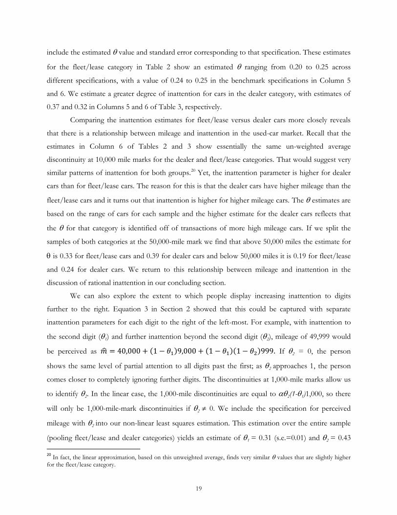
include the estimated value and standard error corresponding to that specification. These estimates

for the fleet/lease category in Table 2 show an estimated ranging from 0.20 to 0.25 across

different specifications, with a value of 0.24 to 0.25 in the benchmark specifications in Column 5

and 6. We estimate a greater degree of inattention for cars in the dealer category, with estimates of

0.37 and 0.32 in Columns 5 and 6 of Table 3, respectively.

Comparing the inattention estimates for fleet/lease versus dealer cars more closely reveals

that there is a relationship between mileage and inattention in the used-car market. Recall that the

estimates in Column 6 of Tables 2 and 3 show essentially the same un-weighted average

discontinuity at 10,000 mile marks for the dealer and fleet/lease categories. That would suggest very

similar patterns of inattention for both groups.20 Yet, the inattention parameter is higher for dealer

cars than for fleet/lease cars. The reason for this is that the dealer cars have higher mileage than the

fleet/lease cars and it turns out that inattention is higher for higher mileage cars. The estimates are

based on the range of cars for each sample and the higher estimate for the dealer cars reflects that

the for that category is identified off of transactions of more high mileage cars. If we split the

samples of both categories at the 50,000-mile mark we find that above 50,000 miles the estimate for

is 0.33 for fleet/lease cars and 0.39 for dealer cars and below 50,000 miles it is 0.19 for fleet/lease

and 0.24 for dealer cars. We return to this relationship between mileage and inattention in the

discussion of rational inattention in our concluding section.

We can also explore the extent to which people display increasing inattention to digits

further to the right. Equation 3 in Section 2 showed that this could be captured with separate

inattention parameters for each digit to the right of the left-most. For example, with inattention to

the second digit (1) and further inattention beyond the second digit (2), mileage of 49,999 would

be perceived as If 2 = 0, the person

shows the same level of partial attention to all digits past the first; as 2 approaches 1, the person

comes closer to completely ignoring further digits. The discontinuities at 1,000-mile marks allow us

to identify 2. In the linear case, the 1,000-mile discontinuities are equal to 2(1-1)1,000, so there

will only be 1,000-mile-mark discontinuities if 2 0. We include the specification for perceived

mileage with 2 into our non-linear least squares estimation. This estimation over the entire sample

(pooling fleet/lease and dealer categories) yields an estimate of 1 = 0.31 (s.e.=0.01) and 2 = 0.43

20

In fact, the linear approximation, based on this unweighted average, finds very similar values that are slightly higher for the fleet/lease category.

20

(s.e.=0.04). With a linear depreciation rate () of 0.05, these estimates predict 1,000-mile

discontinuities of approximately $15, which is in line with the averages reported above. These

estimates suggest that attention continues to decrease after the second digit.

6. Understanding the incidence of the bias

Because our data come from the wholesale market, a natural question is: Who is inattentive? Do the

observed patterns reflect inattention on the part of final customers or rather the inattention of the

dealers themselves? Like our theoretical framework in Section 2, most work in “behavioral industrial

organization” starts from the premise that rational firms operate with an awareness of (and

sometimes the ability to exploit) the biases of customers. Part of the motivation for that benchmark

is that previous studies have shown that biases may be attenuated when agents accumulate market

experience (List, 2003). On the other hand, there is evidence that auction settings may exacerbate

biases, since it will often be the most biased agents who win auctions (Lee and Malmendier,

forthcoming; Malmendier and Szeidl, 2008). This raises the possibility that the inattention to mileage

in this market could stem from the professional dealers purchasing at auction. Parsing out the

incidence of bias in this market is challenging because if the end customers display inattention, it will

be difficult to distinguish between a savvy used-car dealer who purchases cars with an awareness of

this bias and an un-savvy used-car dealer who happens to share the same bias as his end customers.

In this section we present a range of cuts designed to investigate whether the price discontinuities

seem to be driven primarily by used-car dealers or final customers.

A starting point for this analysis is to look for evidence of these types of discontinuity

patterns in the car market outside of wholesale auctions. We collected limited volume data from

Cars.com, a leading automotive-classifieds website targeted to final customers.21 These data reveal

the presence of similar volume spikes at mileages just before the 10,000-mile thresholds. While these

date lack information on ultimate sale prices, these patterns are at least suggestive that the

inattention effects we observe in our data are not simply a wholesale-auction phenomenon.

Within our data, one approach to investigating the incidence of bias is to exploit the

variation in auction experience of the used-car dealers at the auction. Consider the possibility that

the used-car dealers, but not the final customers, are inattentive. This would imply that cars with

mileage just below a threshold are overpriced at the auction relative to what they can be sold for in

21 Further details are available in the online appendix.

21

the retail market. In this case, we might expect that more experienced dealers would have learned to

avoid the costly bias and would be more likely to purchase cars just above 10,000-mile thresholds.

Hence, we would expect the fraction of cars purchased by experienced buyers to jump up at the

10,000-mile thresholds. On the other hand, assume that the bias is driven by the final customers. If

some of the inexperienced car dealers are unaware of inattention effects, they will wrongly believe

that prices will be smooth across mileage thresholds. In this case, they will perceive cars before

thresholds to be overpriced relative to those past the thresholds and could be expected to cluster

more on the post-threshold cars. Hence, we would expect the share of cars purchased by

experienced dealers to fall at the thresholds.

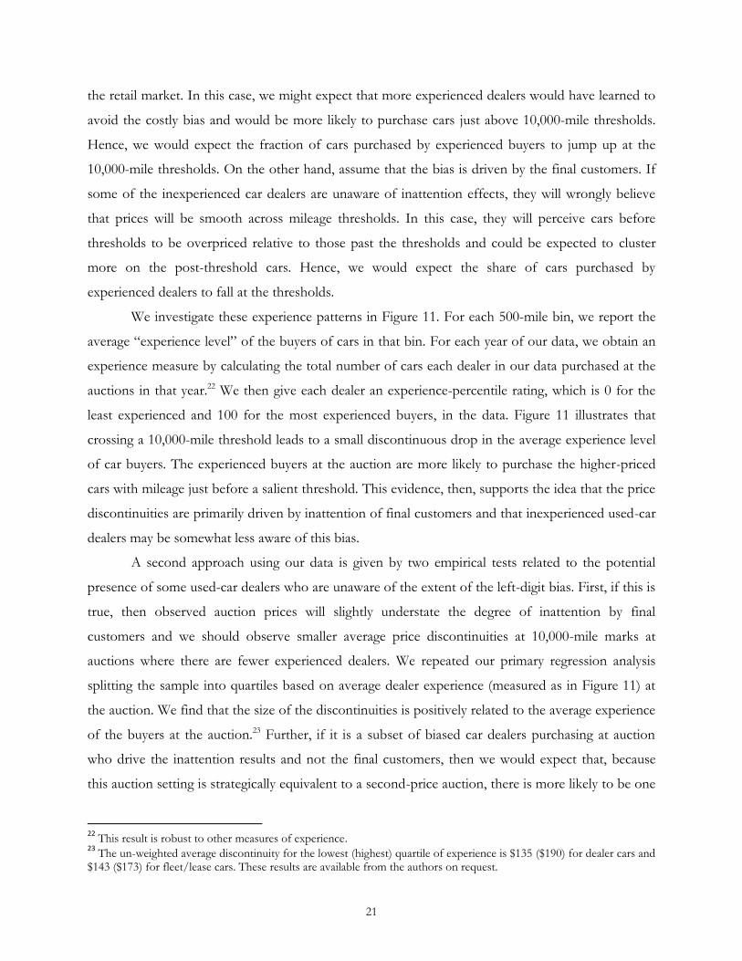
We investigate these experience patterns in Figure 11. For each 500-mile bin, we report the

average “experience level” of the buyers of cars in that bin. For each year of our data, we obtain an

experience measure by calculating the total number of cars each dealer in our data purchased at the

auctions in that year.22 We then give each dealer an experience-percentile rating, which is 0 for the

least experienced and 100 for the most experienced buyers, in the data. Figure 11 illustrates that

crossing a 10,000-mile threshold leads to a small discontinuous drop in the average experience level

of car buyers. The experienced buyers at the auction are more likely to purchase the higher-priced

cars with mileage just before a salient threshold. This evidence, then, supports the idea that the price

discontinuities are primarily driven by inattention of final customers and that inexperienced used-car

dealers may be somewhat less aware of this bias.

A second approach using our data is given by two empirical tests related to the potential

presence of some used-car dealers who are unaware of the extent of the left-digit bias. First, if this is

true, then observed auction prices will slightly understate the degree of inattention by final

customers and we should observe smaller average price discontinuities at 10,000-mile marks at

auctions where there are fewer experienced dealers. We repeated our primary regression analysis

splitting the sample into quartiles based on average dealer experience (measured as in Figure 11) at

the auction. We find that the size of the discontinuities is positively related to the average experience

of the buyers at the auction.23 Further, if it is a subset of biased car dealers purchasing at auction

who drive the inattention results and not the final customers, then we would expect that, because

this auction setting is strategically equivalent to a second-price auction, there is more likely to be one

22

This result is robust to other measures of experience. 23

The un-weighted average discontinuity for the lowest (highest) quartile of experience is $135 ($190) for dealer cars and $143 ($173) for fleet/lease cars. These results are available from the authors on request.

22

of these biased agents bidding on a car when the market is “thicker”, and price discontinuities

should be larger.24 To investigate this issue, we replicated our regression analysis splitting the sample

into the top and bottom quartile of auction “thickness” defined as the number of cars auctioned that

day, the number of unique buyers at the auction, and the ratio of unique buyers to cars.25 The first

two measures are highly correlated and both cuts reveal slightly higher average discontinuities on

busy auction days. However, the differences are small and we find no gradient when we cut by

quartiles of thickness as defined as the ratio of unique buyers to cars.26

Another approach to identifying the incidence of the bias is to look at cars that are very close

to passing over a threshold. Since the used-car dealer often drives the car back to his/her lot after

the auction and since customers can test drive a vehicle, a car that is within a few miles of a 10,000-

mile threshold may pass over the threshold prior to being sold to a final customer.27 Thus, if dealers

are savvy, we would expect car values to drop several miles before a 10,000-mile threshold rather

than dropping precipitously at the exact 10,000-mile marks. Figure 9 provides evidence that car

values do drop significantly prior to reaching a 10,000-mile threshold. The last dot in Figure 9 is the

value of cars that are within 50 miles of a 10,000-mile threshold. This dot illustrates that the average

value of a car that is within 50 miles of a threshold drops by ~$60. Although not conclusive, this is

again suggestive evidence that dealers are somewhat savvy and that it is the final customers who are

inattentive to mileage. Note, however, that prices do not fully drop before the threshold, which

leaves open the possibility of some degree of inattention by buyers at the auction.

A final question is whether sellers at the auctions appear to be aware of these inattention

effects. There is little evidence that the fleet/lease sellers adjust their behavior to these threshold

effects because they uniformly set low reserve prices and do not show systematic volume spikes

around the thresholds. The volume patterns for dealer cars, however, clearly suggest that some of

these sellers are aware of the threshold effects. Since many of the cars that dealers sell at auctions

come from trade-ins on their lots, these volume patterns could, however, be driven by individuals

who decide to trade in their cars (perhaps quite rationally) before the thresholds. The probability

graphs for the different seller types, however, also provide some hints that some of the dealers who

sell cars at the auctions may be unaware of the threshold effects. Recall that the probability graphs

24 This test was suggested by the work of Malmendier and Szeidl (2008), who discuss the possibility that auction settings are a place for sellers to “fish for fools”. 25 This analysis was done splitting by quartiles within auction location. 26 These results are available from the authors on request. 27 Our discussions with used-car dealers suggest they are aware of these discontinuities. One dealer explained that while salespeople can drive cars from the lot, everyone is instructed to avoid driving a car over a 10,000-mile threshold.

23

for the fleet/lease cars are uniformly high and smooth through the thresholds, revealing that there is

no systematic drop in demand for cars at the thresholds in the auctions. Yet a close look at the

probability graphs for the dealer category shows that there seem to be slight drops in the probability

of dealer cars selling at the thresholds. This could be consistent with some dealer sellers being

unaware of the inattention of final used-car customers. Since the dealers set reservation prices that

are at times binding, if some fraction of these sellers are unaware of threshold effects, they may fail

to adjust their reserve prices downward enough at thresholds. This in turn could lead to drops in the

probability of sales for these dealers at the thresholds. We have run regression results on the

probability of sale using the above-mentioned framework and find some suggestive evidence of

drops in probability of sale at 10,000-mile marks for the dealer sellers.28 However, the results are

weak at many thresholds and are suggestive at best.

Taken together, these results are consistent with a view that the incidence of bias in this

market likely rests primarily with the final customers, but that there may also be some degree of

heterogeneity in the awareness of that bias on the part of the professional suppliers in the market.

7. Discussion

We find strong evidence for the hypothesis that partial inattention to mileage has a significant

impact on the used-car market. Without a model of inattention, it would be difficult to even

understand some of the basic descriptive statistics regarding the prices and quantities of cars sold.

Because of the size of the car market, this simple heuristic leads to a large amount of mispricing.

Our estimates of the difference between observed selling prices and the prices that we would expect

under full attention suggest that there was approximately $2.4 billion worth of mispricing due to

inattention in our full dataset. Additionally, the supply decisions of hundreds of thousands of cars

were affected by this heuristic (e.g., sold right before a 10,000-mile threshold). Although it is likely

that these distortions largely result in transfers between market participants rather than large

economic inefficiencies, it is striking that this simple heuristic can so profoundly shape the nature of

a reasonably competitive, high-value durable-goods market.

We anticipate that the left-digit bias could be widespread. More generally, heuristic numeric

processing might impact a range of other settings, in particular environments where inferences are

made based on continuous quality metrics. Examples include hiring or admissions decisions based

28 The results of these regressions are available upon request.

24

on GPAs and test scores, the evaluation of companies based on financial reports (e.g., revenues), the

treatment of medical test results, and how the public reacts to government spending programs.

There remains a question of whether this inattention should be thought of as an irrational

bias or a (boundedly) rational calculation in the face of mental processing constraints. The answer

likely depends on how broadly one considers the question of the appropriateness of the heuristic. In

general the left-digit bias is likely a reasonable heuristic in the face of cognitive processing

constraints. However, in this setting the ex-ante costs of inattention relative to a full-attention

benchmark are on the order of $75 and anyone purchasing a car near a threshold will very quickly

see a drop in value of approximately $150. Given that mileage information is easy to obtain, it seems

unlikely, then, that the heuristic corresponds with a rational expected cost-benefit analysis narrowly

within this market. Perhaps a more relevant question than whether heuristics are boundedly rational

in absolute terms is whether people employ heuristics more when they are more appropriate. Our

evidence on that issue is somewhat mixed. On one hand, we observe that the estimates of the

inattention parameter are higher for higher mileage cars. Given that marginal mileage is more

important for low-mileage cars than for high-mileage cars, this result would be consistent with a

bounded-rationality interpretation that buyers rely more on the left-digit heuristics in settings where

it is less costly to do so. On the other hand, when we look across car types, comparing those that

depreciate more quickly versus those that depreciate more slowly, we find relatively similar levels of

attention, which would suggest that the heuristic is not being deployed “optimally”. Englmaier and

Schmoller (2008) explore closely related issues of inattention in an online gaming market and find

that even when relevant information becomes more salient and available, participants still do not pay

full attention to it, which also suggests that the application of information processing heuristics do

not always respond strongly to the environment. Ultimately, it seems to us that the use of limited

attention heuristics, such as the left-digit bias, is a generally sensible human tendency, but one that

does not always fit with modern economic settings. One direction for future research, then, is to

explore what types of situations and cues cause people to modify their use of these heuristics.

References

Basu, K., 1997: “Why Are So Many Goods Priced to End in Nine? And Why This Practice Hurts Producers?,” Economics Letters, 53, 41-4.

Basu, K., 2006: “Consumer Cognition and Pricing in the Nines in Oligopolistic Markets,” Journal of Economics and Management Strategy, 15, 1, 125-41.

25

Bradley, D.J., Cooney, J.W., Jordan, B.D. and Singh, A.K., 2004: "Negotiation and the IPO Offer Price: A Comparison of Integer vs. Non-Integer IPOs," Journal of Financial and Quantitative Analysis, 39, 3, 517-40.

Chetty, R., Looney, A. and Kroft, K., 2009: “Salience and Taxation: Theory and Evidence,” American Economic Review, 99, 4, 1145-77.

Cohen, L. and Frazzini, A., 2008: “Economic Links and Predictable Returns,” Journal of Finance, 63, 4, 1977-2011.

DellaVigna, S., 2009: “Psychology and Economics: Evidence from the Field,” Journal of Economic Literature, 47, 2, 315-72.

DellaVigna, S. and Pollet, J.M., 2007: “Demographics and Industry Returns,” American Economic Review, 97, 1167-702.

DellaVigna, S. and Pollet., J.M., 2009: “Investor Inattention and Friday Earnings Announcements,” Journal of Finance, 64, 2, 709-749.

Englmaier, F. and Schmoller, A., 2008: “Does Bidding for Complex Goods Reflect All Relevant Information? Field Evidence from Online Gaming,” University of Munich, Working Paper.

Englmaier, F. and Schmoller, A., 2009: “The Evaluation of Complex Goods: Evidence from Online Car Sales,” University of Munich, Working Paper.

Finkelstein, A., 2009: “EZ-Tax: Tax Salience and Tax Rates,” Quarterly Journal of Economics, 124, 3, 969-1010. Gabaix, X. and Laibson, D., 2006: “Shrouded Attributes, Consumer Myopia, and Information Suppression in

Competitive Markets,” Quarterly Journal of Economics, 121, 2, 505-40. Gilovich, T., Griffin, D. and D. Kahneman, editors, 2002: Heuristics and Biases: The Psychology of Intuitive

Judgement, New York: Cambridge University Press. Ginzberg, E., 1936: “Customary Prices,” American Economic Review, 26, 2, 296. Hirshleifer, D., Lim, S.S. and Teoh, S.H., forthcoming: “Driven to Distraction: Extraneous Events and

Underreaction to Earning News,” Journal of Finance, 63, 5, 2287-2323. Hossain, T. and Morgan, J., 2006: “…Plus Shipping and Handling: Revenue (Non) Equivalence in Field

Experiments on eBay,” B.E. Journals in Economic Analysis and Policy: Advances in Economic Analysis and Policy, 6, 2, 1-27.

Kahn, C., Pennacchi, G. and Sopranzetti, B., 1999:“Bank Deposit Rate Clustering: Theory and Empirical Evidence,” Journal of Finance, 54, 6, 2185-214.

Kandel, S., Sarig, O. and Wahl, A., 2001: "Do Investors Prefer Round Stock Prices? Evidence from Israeli IPO Auctions," Journal of Banking and Finance, 25, 1543-51.

Korvost, M. and Damian, M.F., 2008: “The Differential Influence of Decades and Units on Multidigit Comparison,” Quarterly Journal of Experimental Psychology, 61, 8, 1250-64. Lee, D. and Lemieux, T., 2009: “Regression Discontinuity Designs in Economics,” NBER Working Paper

14723. Lee, Y.H. and Malmendier, U., forthcoming: “The Bidder‟s Curse,” American Economic Review. List, J.A., 2003: “Does Market Experience Eliminate Market Anomalies?,” Quarterly Journal of Economics , 118,

1, 41-71. Malmendier, U. and Szeidl, A., 2008: “Fishing for Fools,” working paper, UC-Berkeley. Mullainathan, S., Schwartzstein, J. and and Shleifer, A., 2008: “Coarse Thinking and Persuasion,” Quarterly

Journal of Economics, 123, 2, 577-619. Poltrock, S.E. and Schwartz, D.R., 1984: “Comparative Judgments of Multidigit Numbers,” Journal of

Experimental Psychology, 10, 1, 32-45. Pope, D.G., 2009: “Reacting to Rankings: Evidence from „America‟s Best Hospitals‟,” Journal of Health

Economics, 28, 1154-65. Simon, H.A., 1955: “A Behavioral Model of Rational Choice,” Quarterly Journal of Economics, 69, 1, 99-118.

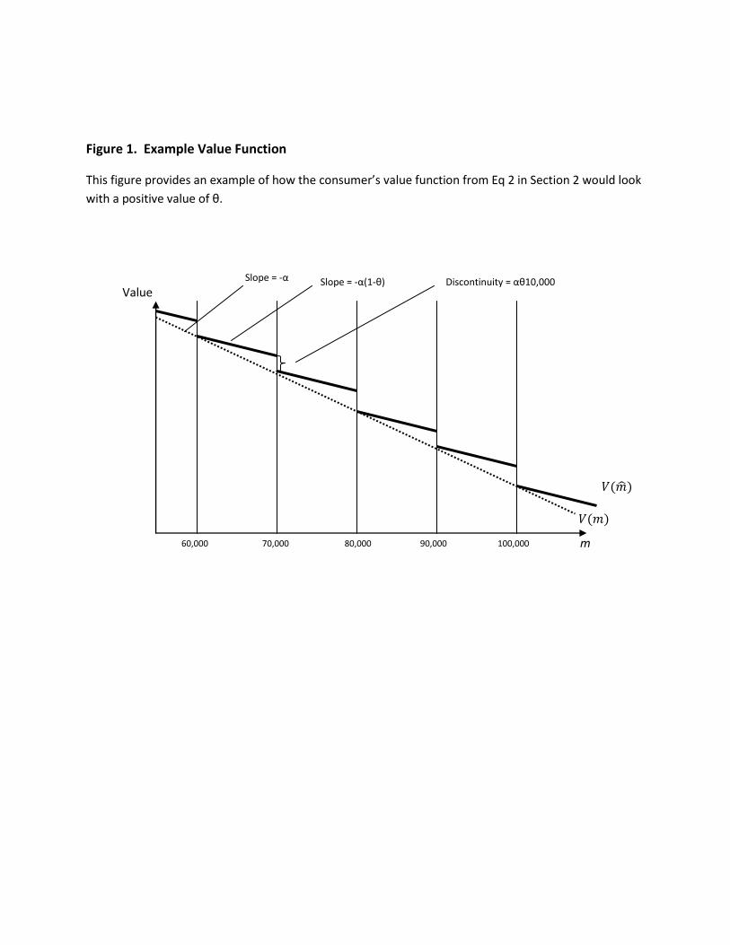
Figure 1. Example Value Function

This figure provides an example of how the consumer’s value function from Eq 2 in Section 2 would look

with a positive value of θ.

Discontinuity = αθ10,000 Slope = -α(1-θ) Slope = -α

Value

60,000 70,000 80,000 90,000 100,000 m

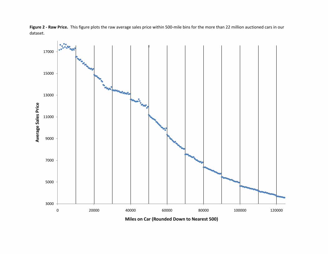
Figure 2 - Raw Price. This figure plots the raw average sales price within 500-mile bins for the more than 22 million auctioned cars in our

dataset.

3000

5000

7000

9000

11000

13000

15000

17000

0 20000 40000 60000 80000 100000 120000

Ave

rage

Sal

es P

rice

Miles on Car (Rounded Down to Nearest 500)

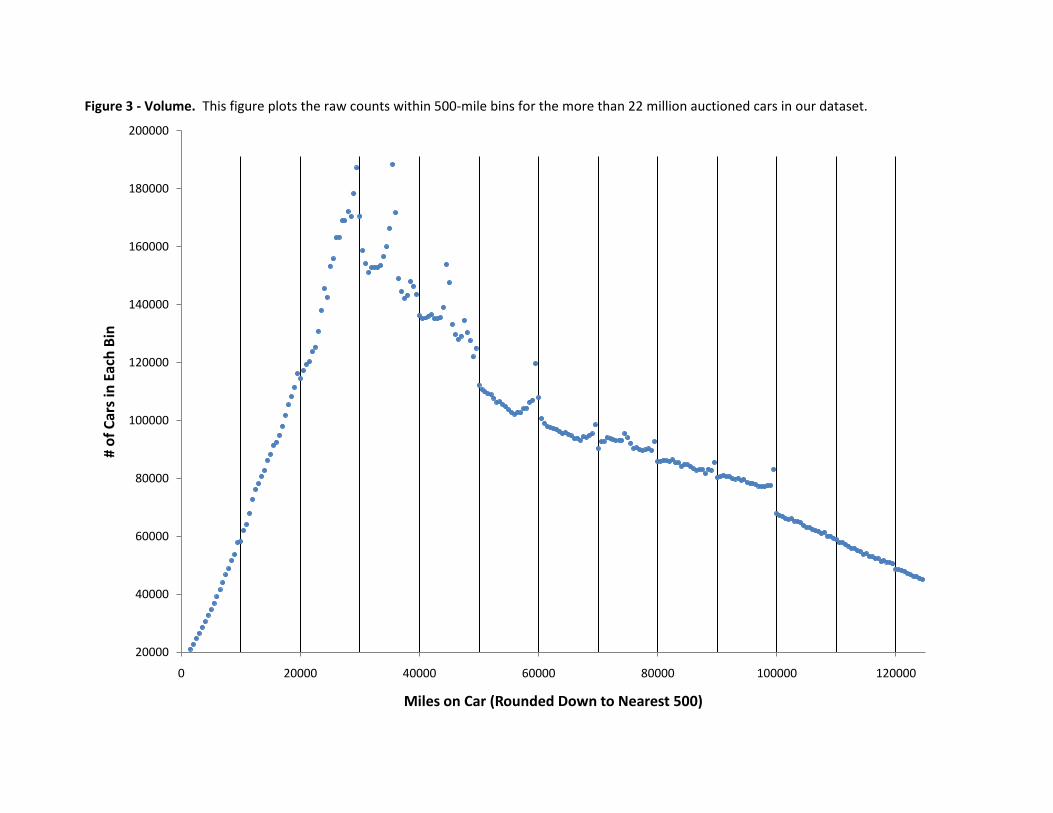
Figure 3 - Volume. This figure plots the raw counts within 500-mile bins for the more than 22 million auctioned cars in our dataset.

20000

40000

60000

80000

100000

120000

140000

160000

180000

200000

0 20000 40000 60000 80000 100000 120000

# o

f C

ars

in E

ach

Bin

Miles on Car (Rounded Down to Nearest 500)

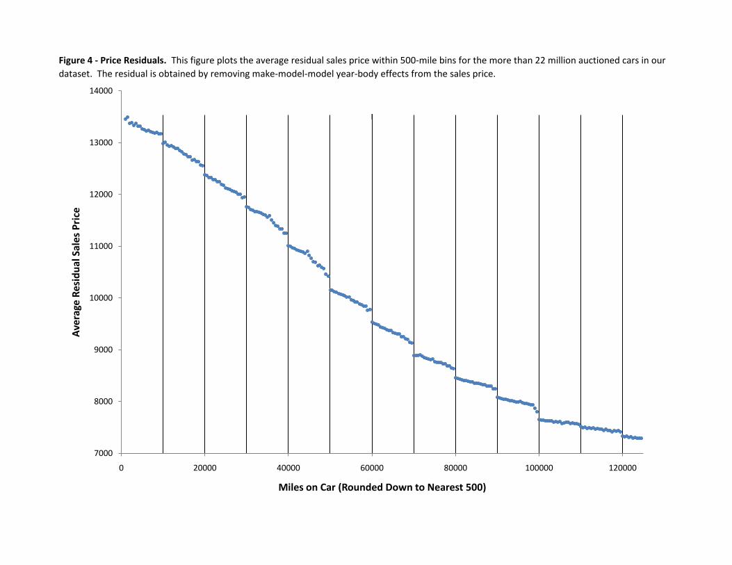
Figure 4 - Price Residuals. This figure plots the average residual sales price within 500-mile bins for the more than 22 million auctioned cars in our

dataset. The residual is obtained by removing make-model-model year-body effects from the sales price.

7000

8000

9000

10000

11000

12000

13000

14000

0 20000 40000 60000 80000 100000 120000

Ave

rage

Res

idu

al S

ales

Pri

ce

Miles on Car (Rounded Down to Nearest 500)

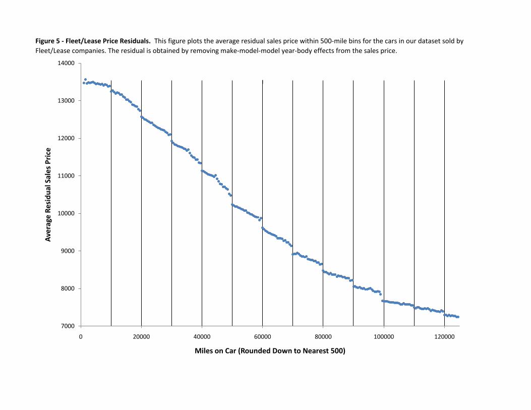
Figure 5 - Fleet/Lease Price Residuals. This figure plots the average residual sales price within 500-mile bins for the cars in our dataset sold by

Fleet/Lease companies. The residual is obtained by removing make-model-model year-body effects from the sales price.

7000

8000

9000

10000

11000

12000

13000

14000

0 20000 40000 60000 80000 100000 120000

Ave

rage

Res

idu

al S

ales

Pri

ce

Miles on Car (Rounded Down to Nearest 500)

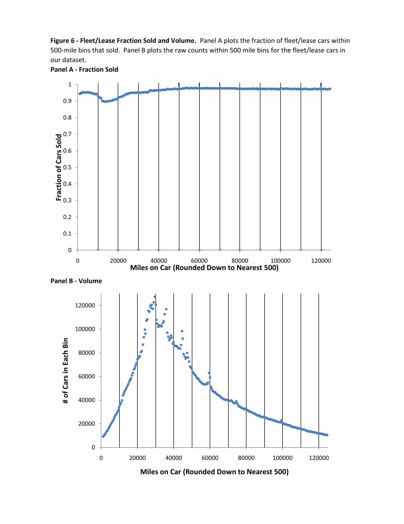
Panel A - Fraction Sold

Panel B - Volume

Figure 6 - Fleet/Lease Fraction Sold and Volume. Panel A plots the fraction of fleet/lease cars within

500-mile bins that sold. Panel B plots the raw counts within 500 mile bins for the fleet/lease cars in

our dataset.

0

0.1

0.2

0.3

0.4

0.5

0.6

0.7

0.8

0.9

1

0 20000 40000 60000 80000 100000 120000

Frac

tio

n o

f C

ars

Sold

Miles on Car (Rounded Down to Nearest 500)

0

20000

40000

60000

80000

100000

120000

0 20000 40000 60000 80000 100000 120000

# o

f C

ars

in E

ach

Bin

Miles on Car (Rounded Down to Nearest 500)

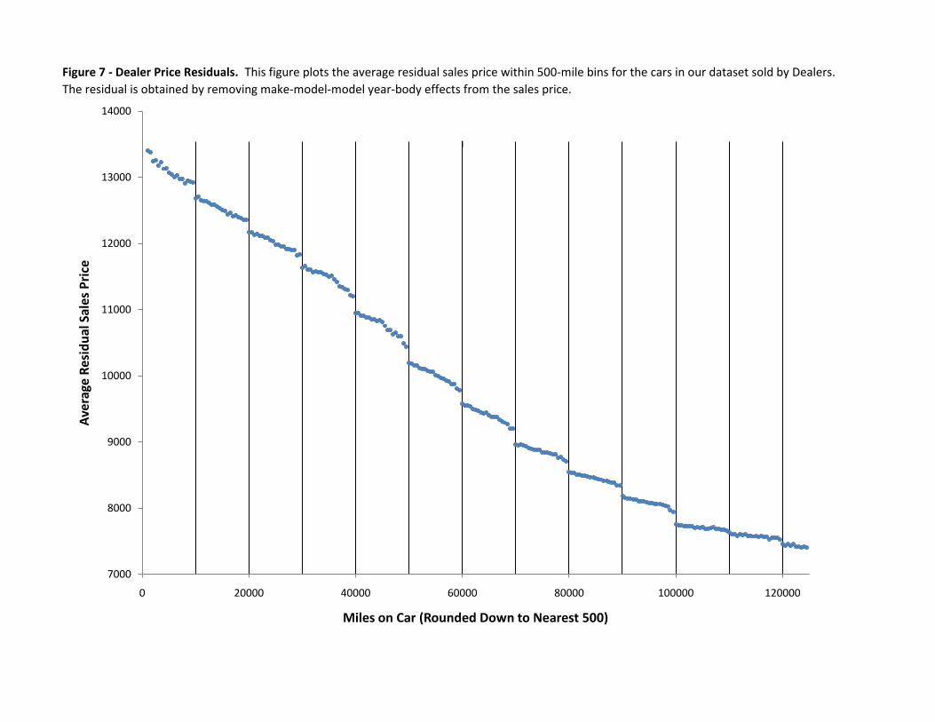
Figure 7 - Dealer Price Residuals. This figure plots the average residual sales price within 500-mile bins for the cars in our dataset sold by Dealers.

The residual is obtained by removing make-model-model year-body effects from the sales price.

7000

8000

9000

10000

11000

12000

13000

14000

0 20000 40000 60000 80000 100000 120000

Ave

rage

Res

idu

al S

ales

Pri

ce

Miles on Car (Rounded Down to Nearest 500)

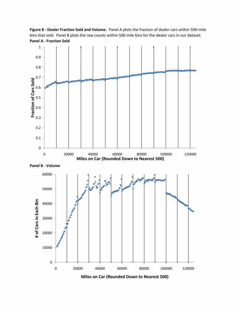
Panel A - Fraction Sold

Panel B - Volume

Figure 8 - Dealer Fraction Sold and Volume. Panel A plots the fraction of dealer cars within 500-mile

bins that sold. Panel B plots the raw counts within 500 mile bins for the dealer cars in our dataset.

0

0.1

0.2

0.3

0.4

0.5

0.6

0.7

0.8

0.9

1

0 20000 40000 60000 80000 100000 120000

Frac

tio

n o

f C

ars

Sold

Miles on Car (Rounded Down to Nearest 500)

0

10000

20000

30000

40000

50000

60000

0 20000 40000 60000 80000 100000 120000

# o

f C

ars

in E

ach

Bin

Miles on Car (Rounded Down to Nearest 500)

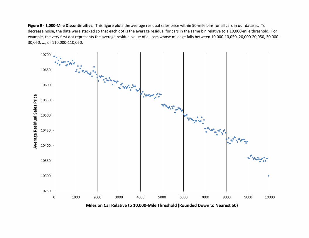
Figure 9 - 1,000-Mile Discontinuities. This figure plots the average residual sales price within 50-mile bins for all cars in our dataset. To

decrease noise, the data were stacked so that each dot is the average residual for cars in the same bin relative to a 10,000-mile threshold. For

example, the very first dot represents the average residual value of all cars whose mileage falls between 10,000-10,050, 20,000-20,050, 30,000-

30,050, ..., or 110,000-110,050.

10250

10300

10350

10400

10450

10500

10550

10600

10650

10700

0 1000 2000 3000 4000 5000 6000 7000 8000 9000 10000

Ave

rage

Res

idu

al S

ales

Pri

ce

Miles on Car Relative to 10,000-Mile Threshold (Rounded Down to Nearest 50)

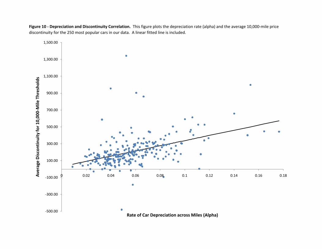
Figure 10 - Depreciation and Discontinuity Correlation. This figure plots the depreciation rate (alpha) and the average 10,000-mile price

discontinuity for the 250 most popular cars in our data. A linear fitted line is included.

-500.00

-300.00

-100.00

100.00

300.00

500.00

700.00

900.00

1,100.00

1,300.00

1,500.00

0 0.02 0.04 0.06 0.08 0.1 0.12 0.14 0.16 0.18Ave

rage

Dis

con

tin

uit

y fo

r 1

0,0

00

-Mile

Th

resh

old

s

Rate of Car Depreciation across Miles (Alpha)

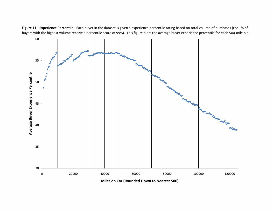
Figure 11 - Experience Percentile. Each buyer in the dataset is given a experience percentile rating based on total volume of purchases (the 1% of

buyers with the highest volume receive a percentile score of 99%). This figure plots the average buyer experience percentile for each 500-mile bin.

30

35

40

45

50

55

60

0 20000 40000 60000 80000 100000 120000

Ave

rage

Bu

yer

Exp

erie

nce

Per

cen

tile

Miles on Car (Rounded Down to Nearest 500)

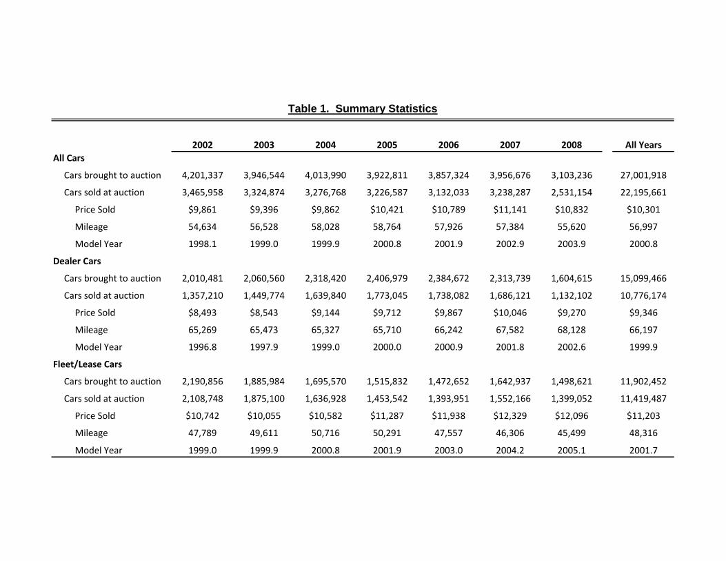
2002 2003 2004 2005 2006 2007 2008 All Years

All Cars

Cars brought to auction 4,201,337 3,946,544 4,013,990 3,922,811 3,857,324 3,956,676 3,103,236 27,001,918

Cars sold at auction 3,465,958 3,324,874 3,276,768 3,226,587 3,132,033 3,238,287 2,531,154 22,195,661

Price Sold $9,861 $9,396 $9,862 $10,421 $10,789 $11,141 $10,832 $10,301

Mileage 54,634 56,528 58,028 58,764 57,926 57,384 55,620 56,997

Model Year 1998.1 1999.0 1999.9 2000.8 2001.9 2002.9 2003.9 2000.8

Dealer Cars

Cars brought to auction 2,010,481 2,060,560 2,318,420 2,406,979 2,384,672 2,313,739 1,604,615 15,099,466

Cars sold at auction 1,357,210 1,449,774 1,639,840 1,773,045 1,738,082 1,686,121 1,132,102 10,776,174

Price Sold $8,493 $8,543 $9,144 $9,712 $9,867 $10,046 $9,270 $9,346

Mileage 65,269 65,473 65,327 65,710 66,242 67,582 68,128 66,197

Model Year 1996.8 1997.9 1999.0 2000.0 2000.9 2001.8 2002.6 1999.9

Fleet/Lease Cars

Cars brought to auction 2,190,856 1,885,984 1,695,570 1,515,832 1,472,652 1,642,937 1,498,621 11,902,452

Cars sold at auction 2,108,748 1,875,100 1,636,928 1,453,542 1,393,951 1,552,166 1,399,052 11,419,487

Price Sold $10,742 $10,055 $10,582 $11,287 $11,938 $12,329 $12,096 $11,203

Mileage 47,789 49,611 50,716 50,291 47,557 46,306 45,499 48,316

Model Year 1999.0 1999.9 2000.8 2001.9 2003.0 2004.2 2005.1 2001.7

Table 1. Summary Statistics

(1) (2) (3) (4) (5) (6) (7)Avg. Discontinuity Size -131.8 -164.1 -141.9 -154.5 -156.8 -161.6 -168.8Estimated Theta 0.22 0.22 0.20 0.24 0.25 0.24 0.22

[.01] [.01] [.01] [.01] [.01] [.01] [.01]

MT 10k miles -22.2 -81.6 -151.2*** -45.9* -56.1** -41.1* -56.6**[73.8] [73.1] [52.6] [27.3] [22.4] [23.1] [26.9]

MT 20k miles -191.2*** -190.2*** -113.4*** -149.6*** -157.8*** -158.5*** -135.8***[40.1] [39.7] [28.0] [14.1] [11.6] [12.1] [14.1]

MT 30k miles 218.2*** 63.1** 45.5** -94.5*** -84.7*** -101.7*** -101.0***[26.1] [25.8] [17.9] [9.3] [7.8] [8.2] [10.0]

MT 40k miles -87.4*** -83.7*** -122.9*** -160.7*** -181.9*** -175.8*** -181.1***[29.3] [28.9] [19.6] [10.2] [8.7] [9.1] [11.2]

MT 50k miles -653.2*** -574.8*** -312.5*** -268.9*** -289.3*** -305.6*** -317.9***[29.9] [29.1] [20.0] [10.9] [9.4] [10.0] [13.3]

MT 60k miles -416.8*** -450.2*** -291.6*** -226.0*** -207.0*** -211.3*** -201.3***[31.6] [30.6] [21.8] [12.4] [11.0] [11.5] [16.1]

MT 70k miles 111.4*** 27.4 -125.6*** -212.6*** -215.6*** -214.0*** -213.6***[31.5] [30.2] [22.3] [13.2] [11.8] [12.4] [18.6]

MT 80k miles -4.3 -19.6 -133.6*** -213.7*** -216.6*** -216.0*** -210.8***[31.5] [29.7] [23.0] [14.4] [13.1] [14.2] [22.9]

MT 90k miles -284.7*** -245.8*** -205.2*** -185.4*** -185.8*** -211.8*** -241.9***[34.7] [32.4] [25.5] [16.2] [14.8] [16.3] [27.0]

MT 100k miles -305.9*** -347.8*** -266.7*** -167.2*** -154.0*** -160.5*** -174.2***[34.1] [31.3] [25.7] [17.3] [16.1] [18.5] [32.1]

MT 110k miles 153.5*** 67.2* 6.8 -5.2 -3 11.1 15.2[40.9] [37.8] [30.9] [20.2] [18.6] [22.8] [40.6]

MT 120k miles -98.4* -133.7*** -32.3 -123.9*** -129.5*** -153.6*** -206.6***[54.3] [48.9] [40.9] [28.1] [26.3] [34.3] [63.5]

7th-Order Miles Poly X X X X X X X

Fixed Effects

None Age Age*MakeAge*Make*

Model

Age*Make*

Model*Body

Age*Make*

Model*Body*A

uction

Age*Make*Mod

el*Body*Auctio

n*Seller_ID

R-Squared 0.224 0.257 0.632 0.895 0.926 0.960 0.974

Observations 2,337,851 2,337,851 2,337,851 2,337,851 2,337,851 2,337,851 2,337,851

** p < .05; *** p < .01

Table 2. The Impact of 10,000-Miles-Driven Discontinuities on Price - Fleet/Lease Only

Dependent Variable: Auction Price for Car Sale

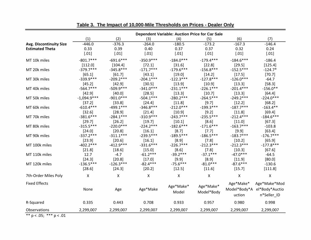
(1) (2) (3) (4) (5) (6) (7)Avg. Discontinuity Size -446.0 -376.3 -264.0 -180.5 -173.2 -167.3 -146.4Estimated Theta 0.33 0.39 0.40 0.37 0.37 0.32 0.24

[.01] [.01] [.01] [.01] [.01] [.01] [.01]

MT 10k miles -801.7*** -691.6*** -350.9*** -184.0*** -179.4*** -184.6*** -186.4[112.0] [104.4] [72.1] [31.6] [22.8] [29.5] [125.4]

MT 20k miles -379.7*** -345.8*** -171.7*** -179.6*** -156.8*** -152.5*** -124.7*[65.1] [61.7] [43.1] [19.0] [14.2] [17.5] [70.7]

MT 30k miles -339.9*** -209.2*** -204.1*** -122.3*** -127.8*** -126.0*** -64.7[45.2] [42.9] [30.5] [13.9] [10.9] [13.3] [58.3]

MT 40k miles -564.7*** -509.9*** -341.0*** -231.1*** -226.1*** -201.4*** -156.0**[42.9] [40.0] [28.5] [13.3] [10.7] [13.3] [64.4]

MT 50k miles -1,094.9*** -901.0*** -504.1*** -280.2*** -264.5*** -249.2*** -224.0***[37.2] [33.8] [24.4] [11.8] [9.7] [12.2] [68.2]

MT 60k miles -610.4*** -499.1*** -346.8*** -212.0*** -199.3*** -187.7*** -163.4**[32.6] [28.9] [21.4] [10.9] [9.2] [11.8] [69.4]

MT 70k miles -381.6*** -284.1*** -310.9*** -243.7*** -235.5*** -212.4*** -184.6***[29.7] [26.2] [19.7] [10.1] [8.6] [11.0] [67.3]

MT 80k miles -315.5*** -220.0*** -224.2*** -182.6*** -171.6*** -163.7*** -103.8[24.0] [20.8] [16.1] [8.7] [7.7] [9.9] [63.4]

MT 90k miles -337.2*** -311.1*** -239.5*** -189.5*** -186.5*** -183.7*** -176.7***[23.9] [20.6] [16.1] [8.9] [7.8] [10.2] [65.9]

MT 100k miles -402.2*** -412.9*** -331.6*** -226.7*** -212.3*** -212.3*** -177.8***[21.8] [18.6] [15.0] [8.6] [7.8] [10.3] [67.6]

MT 110k miles 12.7 -4.7 -61.2*** -39.2*** -37.1*** -47.0*** -64.5[24.3] [20.8] [17.0] [9.9] [8.9] [11.9] [80.0]

MT 120k miles -136.5*** -126.3*** -82.4*** -75.6*** -81.0*** -87.6*** -130.6[28.6] [24.3] [20.2] [12.5] [11.6] [15.7] [111.8]

7th-Order Miles Poly X X X X X X X

Fixed Effects

None Age Age*MakeAge*Make*

Model

Age*Make*

Model*Body

Age*Make*

Model*Body*A

uction

Age*Make*Mod

el*Body*Auctio

n*Seller_ID

R-Squared 0.335 0.443 0.708 0.933 0.957 0.980 0.998

Observations 2,299,007 2,299,007 2,299,007 2,299,007 2,299,007 2,299,007 2,299,007

** p < .05; *** p < .01

Table 3. The Impact of 10,000-Mile Thresholds on Prices - Dealer Only

Dependent Variable: Auction Price for Car Sale