arX

iv:0

807.

0354

v4 [

quan

t-ph

] 2

9 Ja

n 20

10

.

A study of heuristic guesses for adiabatic quantum computation

Alejandro Perdomo,1 Salvador E. Venegas-Andraca,2, 1 and Alan Aspuru-Guzik1

1Department of Chemistry and Chemical Biology,Harvard University, 12 Oxford Street, 02138, Cambridge, MA

2Quantum Information Processing Group. Tecnologico de Monterrey Campus Estado deMexico. Carretera Lago Gpe. Km 3.5, Atizapan de Zaragoza, Edo. Mexico, Mexico

Adiabatic quantum computation (AQC) is a universal model for quantum computation whichseeks to transform the initial ground state of a quantum system into a final ground state encodingthe answer to a computational problem. AQC initial Hamiltonians conventionally have a uniformsuperposition as ground state. We diverge from this practice by introducing a simple form ofheuristics: the ability to start the quantum evolution with a state which is a guess to the solutionof the problem. With this goal in mind, we explain the viability of this approach and the neededmodifications to the conventional AQC (CAQC) algorithm. By performing a numerical study onhard-to-satisfy 6 and 7 bit random instances of the satisfiability problem (3-SAT), we show howthis heuristic approach is possible and we identify that the performance of the particular algorithmproposed is largely determined by the Hamming distance of the chosen initial guess state withrespect to the solution. Besides the possibility of introducing educated guesses as initial states, thenew strategy allows for the possibility of restarting a failed adiabatic process from the measuredexcited state as opposed to restarting from the full superposition of states as in CAQC. The outcomeof the measurement can be used as a more refined guess state to restart the adiabatic evolution.This concatenated restart process is another heuristic that the CAQC strategy cannot capture.

PACS numbers: 03.67.Lx, 03.67.Ac, 03.65.-w

I. INTRODUCTION

Adiabatic quantum computation (AQC) [1] is apromising paradigm of quantum computation because ofits robustness [2, 3], and its intuitive mapping from NP-complete and NP-hard problems to potentially realizableHamiltonians [1, 4–6]. Adiabatic quantum computing isattractive because relevant optimization problems suchas lattice models for protein folding can be readily for-mulated [7].AQC algorithms involve the specification of a time-

dependent Hamiltonian,

H(t) = hi(t) + hdriving(t) + hf (t), (1)

This Hamiltonian has three important functions: (1)

The initial Hamiltonian, Hi ≡ H(0), encodes a groundstate that is easy to prepare and that is used as the ini-tial state for the quantum evolution. (2) The driving

Hamiltonian, hdriving(t), is responsible for mediating thetransformation of the initial ground state to any of otherstate. (3) The final Hamiltonian, Hf ≡ H(τ), is prob-lem dependent and its ground state encodes the solu-tion, |ψsolution〉, to the computational problem. In theideal case of a process being fully adiabatic, evolutionunder H(t) will keep the quantum state, |ψ(t)〉, in the

ground state of H(t) throughout 0 < t < τ . If thiscondition is met, the final state at t = τ should coin-cide with the ground state of the final Hamiltonian, Hf ,i.e., |ψ(τ)〉 = |ψsolution〉, if the process is adiabatic. Themeasurement at t = τ will provide the solution to thecomputational problem.

Since the original proposal by Farhi et al [1], a sig-nificant amount of progress has been made towards thedesign of final Hamiltonians for different computation-ally intractable problems such as NP-complete problems.For example, in this paper we provide a detailed descrip-tion of the construction of final Hamiltonian for the 3-SAT problem. In previous work, we described the re-spective construction of the final Hamiltonian for an NP-hard problem of interest in biology, the protein foldingproblem, which consists of finding the minimum energyconfiguration of a chain of interacting amino acids in a

lattice [7]. Several choices for hdriving have been sug-gested. Farhi et al [1] proposed what we call in this work

the conventional form used for hdriving(t): a linear ramp,

hdriving(t) = (1− t/τ)Hdriving , (2)

In Farhi et al ’s scheme the term hi(t) can be defined

as Hi ≡ hdriving(t = 0) = Hdriving, namely, the term

Hdriving serves as the initial Hamiltonian Hi when its in-tensity is completely turned on at t = 0, and drives thequantum evolution until it is completely turned off att = τ . The final Hamiltonian is turned on with the func-tional form hf(t) = (t/τ)Hf . Scheduling the adiabaticevolution with this linear interpolation is not compulsory,thus different proposals have been studied such as the useof non-linear time-profile for auxiliary Hamiltonians [8]and optimal geodesic paths [9].The question of whether AQC, or in general quan-

tum computers, can be used for efficiently solving NP-complete problems is a difficult open question. Lessonsthat have been learned [10] include that a poor choice

2

of the initial Hamiltonian such as the one-dimensionalprojector as selected in Refs. [11] and [12], will lead in-efficient AQC algorithms. Therefore, it is important toconsider different strategies which might allow an escapefrom bottlenecks or trap states which might limit the useof AQC [13].

When attempting to tackle combinatorial and opti-mization problems with classical computers, a commonapproach to cope with intractability and NP-completeproblems [14, 15], is to employ heuristic algorithms as analternative to exhaustive search which scales exponen-tially with system size. In quantum computation, Hogg[16, 17] introduced heuristic techniques in quantum al-gorithms. He showed that using information about thestructure of the problem as a heuristic guide can be usedto enhance the performance of quantum search comparedto the scheme proposed by Grover [18]. Hogg’s proposalwas suggested for the gate model for quantum computa-tion, but to our knowledge, there are no studies of heuris-tics in AQC. The purpose of this paper is to examine thefollowing questions: How can we incorporate heuristicsin AQC? Is there any advantage by doing so? What arethe modifications to CAQC proposal from an algorithmicand experimental point of view?

a. Initial state selection. The simplest form ofheuristics we could think of is to start the quantum evo-lution from a quantum state which is a guess to the solu-tion, but this possibility is not available in any of the pro-posals for AQC. Physical intuition as well as constraintswithin the problem can be used to make an educatedguess. To illustrate our idea, let’s use a lattice modelfor protein folding [7] as an example. For this model, aneducated guess for the initial state would be to choose abit string which encodes an initial position for the aminoacids in the spatial lattice such that no two amino acidsare on top of each other, and that they are connected ac-cording to the sequence defining the protein to be folded.Conversely, CAQC would begin the computation with aquantum superposition of all possible states of the com-putational basis. This choice of initial state contains ab-surd configurations like all amino acids on top of eachother, or assignments referring to configurations of aminoacids which are fully disconnected or not properly linkedaccording to the protein sequence. We conjecture herethat the presence of these “non-sensical” states might actas trap states, making a smooth transition towards thedesired final ground state more difficult and therefore in-creasing the time required for an adiabatic evolution. Inother fields of computer science, physics and chemistry,one might also use classical methods or a mean field ap-proach to find approximate solutions to be employed aseducated guesses. For example, in the context of quan-tum simulation, a Hartree-Fock solution may be used asthe initial state for an adiabatic preparation of an exactmolecular wave function [19–22].

In quantum mechanics, preparing a desired state is nota trivial task [23, 24] and it is not always possible to de-terministically prepare a state from a superposition state

by measurement. For NP-complete classical problems,like the 3-satisfiability problem (3-SAT) [14, 15] studiedhere, the simplest guess for the initial state is that ofchoosing one of the possible assignments from the so-lution space. We present a strategy which allows to de-sign experimentally-realizable initial Hamiltonians whoseground state corresponds to the desired guess as the ini-tial quantum state. This is essential for studying the im-portance of choosing a guess state instead of having fullsuperposition of states as in CAQC [1]. In an algorithmlike the one proposed here, both the initial guess and thefinal solution will be states of the computational basis.Therefore, the overlap between them is zero, unless onehas guessed the right solution or the guess is included inthe subspace of solutions, which is very unlikely. Regard-less of this counterintuitive choice, 〈ψguess|ψsolution〉 = 0,we show that using this kind of heuristics can be of ad-vantage. Even in the case of choosing the initial stateby random guessing there is potential for outperformingCAQC.

b. Restarting the evolution. Notice that the methoddescribed here not only allows to begin the evolution froma guess state, but also allows for the possibility of restart-ing a failed AQC calculation from the measured state.This state can be used as a refined guess to restart theadiabatic evolution. An adiabatic processes is an ide-alized concept because real experiments have to be runin finite time and therefore there will always be prob-ability of measuring a non-desired excited state whichdoes not encode the solution to the computational task.The possibility of restarting the quantum evolution usingthe measured state as a guess is a feature which is notavailable in any of the AQC proposals to date, to ourknowledge.

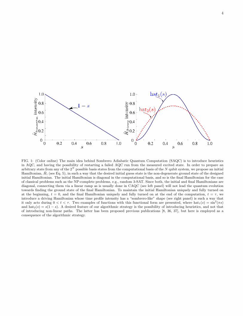
The incorporation of heuristics in AQC essentially in-volves two modifications to CAQC. We address bothchanges; the first modification involves the design of ini-tial Hamiltonians for arbitrary guess states. The secondmodifications involves the change of the time profile ofthe driving Hamiltonian from the linear ramp to a non-linear time dependence with a “sombrero-like” time pro-file (see Fig. 1). Note that this second change is not themain point of the paper since non-linear paths had beenproposed before [8]. Also, it is not our purpose to ex-plore what is the optimal selection for the driving term.It must be emphasized that the “sombrero-like” time pro-file is an essential feature needed if one is interested inthe kind of heuristics we describe here, but this is not thecase in the conventional way of doing AQC where it wasused for auxiliary Hamiltonian terms [8]. Because of thisdistinctive feature and with the purpose of differentiatingour heuristic strategy proposed with CAQC, we will referto our method as Sombrero Adiabatic Quantum Compu-tation (SAQC). The name should be associated with thealgorithmic strategy (selection of initial guess, design ofinitial Hamiltonian and sombrero-like profile for the driv-ing Hamiltonian) which aims to incorporate heuristics inAQC, not only to the use of non-linear paths in AQC.

3

The paper is divided as follows: in Section II, we re-view the CAQC approach. Section III introduces the ba-sic elements of the new implementation, SAQC. Finally,in Section IV, we present numerical calculations compar-ing the performance of both the CAQC and the SAQCalgorithms based on the minimum gap, gmin, of their re-spective time-dependent Hamiltonians driving their cor-responding time evolutions.

II. CONVENTIONAL ADIABATIC QUANTUMCOMPUTATION (CAQC)

The goal of AQC algorithms is that of transformingan initial ground state |ψ(0)〉 into a final ground state|ψ(τ)〉, which encodes the answer to the problem. Thisis achieved by evolving the corresponding physical sys-tem according to the Schrodinger equation with a time-dependent Hamiltonian H(t). The AQC algorithm re-lies on the quantum adiabatic theorem [25–35], whichstates that if the quantum evolution is initialized with theground state of the initial Hamiltonian, the time prop-agation of this quantum state will remain very close tothe instantaneous ground state |ψg(t)〉 for all t ∈ [0, τ ],

whenever H(t) varies slowly throughout the propagationtime t ∈ [0, τ ]. This holds under the assumption thatthe ground state manifold does not cross the energy lev-els which lead to excited states of the final Hamiltonian.Here, we denote by ground state manifold the first mcurves associated with the lowest eigenvalue of the time-dependent Hamiltonian for t ∈ [0, τ ], where m is thedegeneracy of the final Hamiltonian ground state. Anexample of m = 2, is shown in Fig. 5 of Ref. [7].

Conventionally the adiabatic evolution path is the lin-ear sweep of s ∈ [0, 1], where s = t/τ :

H(s) = (1 − s)Htransverse + sHf . (3)

Htransverse (see Eq. 9 below) is usually chosen suchthat its ground state is a uniform superposition ofall possible 2n computational basis vectors, for thecase of an n−qubit system. Here, we choose thespin states {|qi = 0〉 , |q = 1〉}, which are the eigenvec-tors of σz

i with eigenvalues +1 and -1, respectively,as the basis vectors. Then the initial ground state is|ψg(0)〉 = 1√

2n

∑

qi∈{0,1} |qn〉 |qn−1〉 · · · |q2〉 |q1〉. Such an

initial ground state is usually assumed to be easy to pre-pare, for example, by imposing a global transverse field.Since each state encodes a possible solution, this initialstate assigns equal probability to all possible solutions tothe computational problem.

III. SOMBRERO ADIABATIC QUANTUMCOMPUTATION (SAQC)

For SAQC, the time-dependent Hamiltonian can bewritten as:

Hsombrero = (1− s)Hi + hat(s)Hdriving + sHf . (4)

We want the non-degenerate ground state of the ini-tial Hamiltonian Hi to encode a guess to the solution,and the driving term, Hdriving , to couple the states inthe computational basis. The function hat(s) is zero atthe beginning and end of the adiabatic path; thereforeHdriving acts only in the range s ∈ (0, 1) in a “sombrero-

like” time dependence (see Fig. 1), which allows Hi (Hf )to be fully turned on at the beginning (end) of the com-putation.

A. Design of the initial Hamiltonian for the guessstate

As preparing an arbitrary initial non-degenerateground state for adiabatic evolution is not a trivial task,we focus on easy to prepare initial guesses that consist ofone of the states in the computational basis. The strat-egy proposed builds initial Hamiltonians such that theinitial guess corresponds to the non-degenerate groundstate of the initial Hamiltonian, as it is required by AQC.Additionally, this ground state would be non-degenerate.Let us denote the states of the computational basis of

an N qubit system as |qN 〉 |qN−1〉 · · · |q1〉 ≡ |qN · · · q1〉where qn ∈ {0, 1}. The proposed initial Hamiltonian,whose ground state corresponds to an arbitrary initialguess state of the form |xN · · ·x1〉, can be written as

Hi =N∑

n=1

(

xnI + qn(1 − 2xn))

=N∑

n=1

hxn, (5)

where each xn is a boolean variable, xn ∈ {0, 1}, whileq ≡ 1

2(I − σz) is a quantum operator acting on the n-th

qubit of the multipartite Hilbert space HN ⊗ HN−1 ⊗· · · ⊗ Hn ⊗ · · · ⊗ H1. The operator qn is given by

qn = IN ⊗ IN−1 ⊗ · · · ⊗ (q)n ⊗ · · · ⊗ I1, (6)

where q is placed in the nth position and the identityoperators act on the rest of the Hilbert space.The states constituting the computational basis, |0〉

and |1〉, are eigenvectors of σz with eigenvalues +1 and−1, and therefore they are also eigenstates of the oper-ator q with eigenvalues 0 and 1 respectively. The logicbehind the initial Hamiltonian in Eq. 5 then is clear: if

xn = 0, then hxn=0 = qn but in the case of xn = 1, then

hxn=1 = I − qn.As an example, suppose one has a four qubit system,

and one wishes to initialize the adiabatic computation

4

FIG. 1: (Color online) The main idea behind Sombrero Adiabatic Quantum Computation (SAQC) is to introduce heuristicsin AQC, and having the possibility of restarting a failed AQC run from the measured excited state. In order to prepare anarbitrary state from any of the 2N possible basis states from the computational basis of the N qubit system, we propose an initialHamiltonian, Hi (see Eq. 5), in such a way that the desired initial guess state is the non-degenerate ground state of the designedinitial Hamiltonian. The initial Hamiltonian is diagonal in the computational basis, and so is the final Hamiltonian for the caseof classical problems such as the NP-complete problems, e.g., random 3-SAT. Since both, the initial and final Hamiltonians arediagonal, connecting them via a linear ramp as is usually done in CAQC (see left panel) will not lead the quantum evolutiontowards finding the ground state of the final Hamiltonian. To maintain the initial Hamiltonian uniquely and fully turned onat the beginning, t = 0, and the final Hamiltonian uniquely and fully turned on at the end of the computation, t = τ , weintroduce a driving Hamiltonian whose time profile intensity has a “sombrero-like” shape (see right panel) is such a way thatit only acts during 0 < t < τ . Two examples of functions with this functional form are presented, where hat1(s) = sin2(πs)and hat2(s) = s(1− s). A desired feature of our algorithmic strategy is the possibility of introducing heuristics, and not thatof introducing non-linear paths. The latter has been proposed previous publications [8, 36, 37], but here is employed as aconsequence of the algorithmic strategy.

5

with the state |x4 = 1, x3 = 0, x2 = 1, x1 = 0〉 ≡ |1010〉which one may choose either randomly or as an educatedguess to the solution. According to Eq. 5, the initialHamiltonian for the |1010〉 guess state should be con-structed as

Hi = hx4+ hx3

+ hx2+ hx1

= (I − q4) + q3 + (I − q2) + q1,(7)

and, clearly

Hi |1010〉 =(

(I − q4) + q3 + (I − q2) + q1

)

|1010〉= 0 |1010〉 .

(8)

In general, the 2N states of the computational ba-sis are all eigenstates of Hi, and it can be easily veri-fied that the spectrum of Hi are energies contained in{0, · · · , N}. As required, the ground state is also non-degenerate. The other states will have an eigenenergywhich equals their Hamming distance to the ground stateof the initial Hamiltonian.

B. Driving Hamiltonian

The encoding of an educated or a random guess intoHi (Eq. 5) makes both Hi and Hf (Eq. 4) diagonal in

the computational basis. Therefore, connecting Hi andHf with a linear ramp (as in Eq. 3), namely, omitting the

operator Hdriving in the quantum evolution, would yieldzero probability of obtaining the state that encodes theunknown solution to the problem starting from the initialguess state. To avoid such a situation, Hdriving must in-

troduce non-diagonal terms in Hsombrero (see Eq. 4) thatallows the initial state to transform from any arbitraryguess into the solution.In order to make a fair comparison between CAQC and

SAQC (see Eq. 3 and Eq. 4), we set

Hdriving = Htransverse = δ

N∑

n=1

qxn, (9)

in Eq. 4, where qxn stands for the quantum operator qx

acting on the nth qubit of the multipartite Hilbert spaceHN ⊗ HN−1 ⊗ · · · ⊗ Hn ⊗ · · · ⊗ H1. The operator qxn is

given by IN ⊗ IN−1 ⊗ · · · ⊗ (qx)n ⊗ · · · ⊗ I1, where the

operator qx ≡ 12(I − σx) has been placed in the nth posi-

tion, and the Ii’s are identity operators. From a physicalpoint of view, the Hamiltonians Hdriving and Htransverse

can be related to a transverse magnetic field. The in-tensity of these Hamiltonians is tuned by varying the δparameter. If we set δ to be the same for both adiabaticalgorithms, all the dependence of the transverse field in-tensity lies on functions (1 − s) in Eq. 3 and hat(s) inEq. 4. A reasonable requirement for a fair comparison

between CAQC and SAQC is that they both provide thesame average intensity of the transverse magnetic fieldin s ∈ [0, 1]. A choice of hat(s) with the same average∫ 1

0hat(s)ds =

∫ 1

0(1− s)ds = 1/2, is hat(s) = 3s(1− s).

Even though nonlinear evolutions have been proposedin previous articles [8, 36, 37], our hat(s) function canbe as simple or as complicated as desired, as long ashat(0) = hat(1) = 0 is fulfilled. There is plenty of roomto optimize the performance by choosing a more conve-nient hat(s) for the adiabatic evolution, we emphasizethat the additional advantage of SAQC is the possibil-ity of choosing an initial guess. In the next section wepresent some results obtained based on one of the simplenonlinear function hat(s) = 3s(1−s) and discuss the per-formance of both CAQC and SAQC for random 3-SATinstances.

IV. HAMILTONIANS FOR 3-SAT, NUMERICALCALCULATIONS AND DISCUSSION

In order to provide a proof of concept for SAQC andto test the potential usefulness of both random and ed-ucated guesses in adiabatic evolution, we performed anumerical study on hard-to-satisfy 6- and 7-variable in-stances of the 3-SAT problem and compared our resultswith the CAQC approach. Let us now provide a succinctintroduction to the 3-SAT problem as well as to brieflydiscuss its relevance in the fields of theoretical and ap-plied computer science.

A. Construction of final Hamiltonians forsatisfiability problems and design of numerical

calculations

The K-SAT Problem. Let A ={e1, e2, . . . , en, e1, e2, . . . , en} be a set of Booleanvariables E = {ei} and their negations E = {ei}. Letus now construct a logical proposition P , defined as

P =∧

i[(∨k

j=1 aj)] =∧

i Ci, where aj ∈ A, i.e. Pis a conjunction of clauses Ci over the set A, whereeach clause consists of the disjunction of k literals.Proposition P is a K-SAT instance and the solution ofthe K-SAT problem, for instance P , consists of findinga set of values for those binary variables upon whichP has been built (i.e. a bitstring), so that replacementof such binary variables for their corresponding binaryvalues makes P = 1, namely, proposition P is satisfied.3-SAT is a particular case of K-SAT for K=3.

For example, let us examine the following instance ofthe 3-SAT problem. Let E = {x1, x2, x3, x4, x5, x6} be aset of binary variables, and therefore the set of literals isA = E ∪ E = {x1, x2, . . . , x6, x1, x2, . . . , x6}. Consider a3-SAT instance specified by the proposition,

6

P = (x1 ∨ x4 ∨ x5) ∧ (x2 ∨ x3 ∨ x4) ∧ (x1 ∨ x2 ∨ x5)∧(x3 ∨ x4 ∨ x5) ∧ (x4 ∨ x5 ∨ x6) ∧ (x1 ∨ x3 ∨ x5)∧(x1 ∨ x2 ∨ x5) ∧ (x2 ∨ x3 ∨ x6) ∧ (x1 ∨ x2 ∨ x6)∧(x3 ∨ x5 ∨ x6) ∧ (x1 ∨ x2 ∨ x4) ∧ (x2 ∨ x3 ∨ x4)∧(x2 ∨ x5 ∨ x6) ∧ (x2 ∨ x3 ∨ x5) ∧ (x2 ∨ x3 ∨ x4)∧(x2 ∨ x3 ∨ x6) ∧ (x1 ∨ x2 ∨ x3) ∧ (x1 ∨ x4 ∨ x5)∧(x3 ∨ x4 ∨ x6) ∧ (x4 ∨ x5 ∨ x6) ∧ (x2 ∨ x3 ∨ x6)∧(x2 ∨ x5 ∨ x6) ∧ (x3 ∨ x5 ∨ x6) ∧ (x1 ∨ x3 ∨ x6)∧(x3 ∨ x5 ∨ x6) ∧ (x4 ∨ x5 ∨ x6) ∧ (x1 ∨ x2 ∨ x3)

As this example suggests, finding solutions of even amodest 3-SAT instance can become difficult quite easily(in this case, P has only one solution: x1 = 1, x2 =1, x3 = 0, x4 = 1, x5 = 0, x6 = 0.)3-SAT is an NP-complete problem [14, 15], as opposed

to 2-SAT which can be efficiently solved using a clas-sical computer. Consequently, studying the propertiesof 3-SAT is an important area of research, not only be-cause a polynomial-time solution to 3-SAT would implyP = NP, but also because 3-SAT (due to its polynomialequivalence with K-SAT) may be used to model prob-lems and procedures in theoretical computer science [38]as well as in several areas of applied computer scienceand engineering like artificial intelligence [39, 40].For the purpose of simplifying our discussion, and

without loss of generality, we randomly generated 3-SAT instances with a unique satisfying assignment (USA)and their number of clauses to number of variables ratioα ≈ 4.26. This value of α corresponds to the phase tran-sition region where hard-to-satisfy instances are expectedto be found [41, 42]. For completeness and to avoid anykind of bias in selecting this pool of instances, we selected2n different instances for every n variable case studied.More precisely, to exhaustively study the impact of dif-ferent initial guesses with respect to unique solutions inthe behavior of SAQC, we considered all 64 possible ini-tial Hamiltonians Hi (using Eq. 5) for each one of the 64randomly generated 6-variable USA instances. Similarly,we built 128 initial Hamiltonians for each 7-variable in-stance, one per possible initial guess (see Fig. 2). Theinstances were selected in such a way that their solutionshad not only a USA, but also that there was no two in-stances with the same solution.The generation of our USA 3-SAT instances took sev-

eral steps, being the first one using the SAT instancegenerator developed by [43]. Unfortunately, as this gen-erator does not warranty the production of 3-SAT in-stances with unique solutions, we took all generated 3-SAT instances and determined, by exhaustive bitstringsubstitution, whether such instances were USA or not.We iterated this process until we computed all 6-variableand 7-variable 3-SAT instances we needed.The number of qubits used in our simulations is smaller

than state-of-the-art calculations for AQC, such as thosecarried out by quantum Monte Carlo [6, 44]. Here wetrade off carrying out few large calculations on manyqubits for carrying out many calculations on fewer qubits.

We wish to answer the question: What is the the impactof the initial guess in the spectral properties of the time-dependent Hamiltonian? To answer this, we explored thespace of initial guesses in an exhaustive manner for thecase of 6-variable and 7-variable SAT instances. We runa total of 81,920 and 327,680 for 6- and 7- variables re-spectively (see Fig. 2). As shown in the same figure, wealso numerically explored the importance of the strengthof the transverse external field for the performance of thealgorithm.Final Hamiltonians Hf are instance-dependent, i.e.

the structure of each final Hamiltonian depends on theparticular structure (conjunction of clauses) of each 3-

SAT USA instance. Our final Hamiltonians Hf complywith the property that it must encode, in its ground state,the solution to the particular 3-SAT USA instance it wasdesigned for [1, 45]. The design of the final Hamiltonianinvolves an intermediate step, where a classical cost orenergy function is constructed for the particular instanceof interest. Once this energy function is expressed interms of binary variables, it can be easily transformedinto a quantum Hamiltonian by performing the mappingindicated by Eq. 6, where each classical binary variable,qn, is transformed into a quantum operator, qn. The en-ergy function, Hf , associated with the final Hamiltonian,

Hf , can be constructed as a sum of other energy func-tions, hCi

which involve only variables associated withone clause at a time,

Hf =∑

i

hCi(10)

Each hCiis designed such that it is equal to 1 if clause Ci

is unsatisfied and 0 if the clause is satisfied. Notice thatthe functions hCi

contribute to the count of unsatisfiedclauses which defines the spectrum of possible values forHf , with Hf = 0 when all clauses are satisfied.Formally, suppose A = {x1, x2, . . . , xn, x1, x2, . . . , xn}

is a set of n binary variables and their correspondingnegations, P is a 3-SAT USA instance given by P =∧

iCi, and each Ci is a disjuction of three elements of A,i.e. Ci = aα ∨ aβ ∨ aγ with aα, aβ , aγ ∈ A and indicesα, β, γ are natural numbers, not necessarily consecutive.Finally, let B = z1z2 . . . zn be a set of n bits to be sub-stituted in instance P . Then, hCi

is given by

hCi=

0, if substitution of B = z1z2 . . . znin aα ∨ aβ ∨ aγ makes Ci = 1

1, if substitution of B = z1z2 . . . znin aα ∨ aβ ∨ aγ makes Ci = 0.

To construct such a function for any arbitrary clauseCi = aα ∨ aβ ∨ aγ , it is useful to note that the onlyassignment for which Ci = 0 is when aα = 0, aβ = 0,and aγ = 0. Therefore, the function hCi

by construction,should be 1 when aα = 0, aβ = 0, and aγ = 0, and 0otherwise. It can be easily checked that

hCi= (1− aα)(1− aβ)(1− aγ), (11)

7

equals 1 when aα = 0, aβ = 0, and aγ = 0 and 0 other-wise. Recall that each aβ represents a literal and there-fore it could be representing the negation of a variable.One can always use the identity xi = 1− xi to eliminateany xi, and obtain both hCi

and Hf in terms of the xi.Consider for example the construction of the energy

function hC required for clause C = xα ∨ xβ ∨ xγ , i.e. Cis a conjunction of three negated binary variables. In thiscase, C is satisfied by all possible 3-bit bitstrings exceptfor 111 and, according to Eq. 11, the energy functionassumes the form hCi

= (1 − xα)(1 − xβ)(1 − xγ) =xαxβxγ .As a last example consider a clause of the form C =

xα ∨ xβ ∨ xγ , where C is a conjunction of three non-negated binary variables taken from set A. It is clear thatC will be satisfied by all possible 3-bit bitstrings exceptfor 000. According to Eq. 11, the energy function for thisclause C is given by hC = (1 − xα)(1 − xβ)(1 − xγ) =1− xα −xβ − xγ + xαeβ + xβxγ + xαxγ − xαxβxγ . Fromthe first equality of the previous equation, one can easilycheck that hC = 0 for all possible 3-bit combinationsexcept for hC(000) = 1, as expected.Once we have the final expression for the final classical

energy function of Eq. 10, the final Hamiltonians Hf canbe obtained using the mapping of Eq. 6, which relates theclassical binary variables with quantum operators. Sincewe selected only USA instances for our study, each Hf

has a non-degenerate ground state encoding the uniquesolution of one of our 3-SAT instances with correspondingground eigenvalue equal to zero. The final Hamiltoniansare the same for both strategies, CAQC and SAQC.The numerical results on the dependence of the

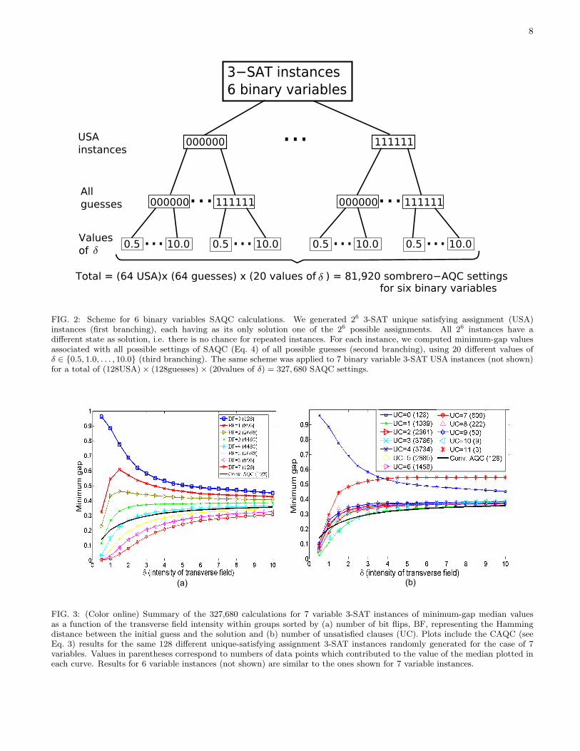
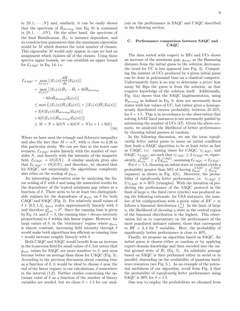
minimum-gap value, gmin, as a function of δ are shownin Fig. 3. Curves were computed by taking the medianof all bit strings that fulfilled the criteria specified inthe legend boxes; namely either to produce i unsatisfiedclauses (UC=i) when substituting the initial guess bitstring in its corresponding instance, or to be j bit flipsaway from the solution (BF=j). BF represents the wellknown Hamming distance between the solution and theinitial guess state. We focused on UC and BF because,in principle, the notion of closeness of an initial guess tothe actual solution may be defined with either parame-ter. Data corresponding to a fixed value of δ is a statis-tical representation (median) of typical gmin values thatwould be expected for hard 3-SAT instances if the guessstate belonged to a definite number of UCs or BFs un-der an experimental setup using SAQC. Such curves arecompared with the minimum gap expected for CAQC.

B. Effects of the variation in the transverse fieldintensity on the minimum energy gap

The dependence of gmin values as a function of thetransverse field intensity δ leaves open some importantquestions regarding the efficiency of adiabatic quantumalgorithms, whether CAQC or SAQC. For example, what

is the optimum value of δ which minimizes the runningtime of an adiabatic algorithm? How transferable is thisoptimum δ value among computational problems? Al-though we do not intend to do a thorough study of thisquestion in this paper, we would like to give some insightinto this question and provide a qualitative discussion ofwhat kind of results might be expected.Following closely the notation from Farhi et al [1], con-

sider H(t) = H(t/τ) = H(s), with instantaneous values

of H(s) defined by

H(s) |El(s)〉 = El(s) |El(s)〉 (12)

with

E0(s) ≤ E1(s) ≤ · · · ≤ E2N−1(s) (13)

where 2N is the dimension of the Hilbert space, andN thenumber of qubits or equivalently the number of binaryvariables in the SAT instance. According to the adiabatictheorem, if the gap between the two lowest levels, E1(s)−E0(s), is greater than zero for all 0 ≤ s ≤ 1, and taking,

τ ≫ Eg2min

(14)

with the minimum gap, gmin, defined by,

gmin = min0≤s≤1

(E1(s)− E0(s)), (15)

and E given by,

E = max0≤s≤1

|〈E1(s)|dH

ds|E0(s)〉|, (16)

then we can make the normed overlap

|〈E0(s = 1)|ψ(τ)〉| (17)

arbitrarily close to 1. In other words, the existence ofa nonzero gap guarantees that |ψ(t)〉 remains very closeto the ground state of H(t) for all 0 ≤ t ≤ τ , if τ issufficiently large.Even though we are aware of the new and more strin-

gent conditions for adiabaticity [26–35] and that Eq. 14 isjust one of the inequalities to guarantee adiabatic evolu-tion (though there is still lack of a sufficient and necessarycondition according to Ref. [46]), we will base our discus-sion on Eq. 14 to illustrate that there is nothing anoma-lous in employing the additional Hamiltonian term in thefull time-dependent Hamiltonian for SAQC. As well as inCAQC, the algorithmic complexity relies again in avoid-ing an exponentially narrowing of gmin. Along the waywe find an important observation about the scaling of therunning time as a function of the parameter δ.Let us first determine an upper bound for ESAQC

in Eq. 14. Consider the Hamiltonian in Eq. 4 withhat(s) = 3s(1−s) since this was the functional form usedfor our numerical calculations. We already discussed, atthe end of Sec. III A, that the spectrum ofHi is contained

8

3−SAT instances

6 binary variables

000000

000000 111111

0.5 10.0...

...

...

Total = (64 USA)x (64 guesses) x (20 values of ) = 81,920 sombrero−AQC settings

All

guesses

USA

instances

Values

of 0.5 10.0...

111111

000000 111111

0.5 10.0...

...

0.5 10.0...

for six binary variables

δ

δ

FIG. 2: Scheme for 6 binary variables SAQC calculations. We generated 26 3-SAT unique satisfying assignment (USA)instances (first branching), each having as its only solution one of the 26 possible assignments. All 26 instances have adifferent state as solution, i.e. there is no chance for repeated instances. For each instance, we computed minimum-gap valuesassociated with all possible settings of SAQC (Eq. 4) of all possible guesses (second branching), using 20 different values ofδ ∈ {0.5, 1.0, . . . , 10.0} (third branching). The same scheme was applied to 7 binary variable 3-SAT USA instances (not shown)for a total of (128USA)× (128guesses)× (20values of δ) = 327, 680 SAQC settings.

FIG. 3: (Color online) Summary of the 327,680 calculations for 7 variable 3-SAT instances of minimum-gap median valuesas a function of the transverse field intensity within groups sorted by (a) number of bit flips, BF, representing the Hammingdistance between the initial guess and the solution and (b) number of unsatisfied clauses (UC). Plots include the CAQC (seeEq. 3) results for the same 128 different unique-satisfying assignment 3-SAT instances randomly generated for the case of 7variables. Values in parentheses correspond to numbers of data points which contributed to the value of the median plotted ineach curve. Results for 6 variable instances (not shown) are similar to the ones shown for 7 variable instances.

9

in {0, 1, · · · , N} and, similarly, it can be easily shown

that the spectrum of Hdriving (see Eq. 9) is containedin {0, 1, · · · , δN}. On the other hand, the spectrum of

the final Hamiltonian, Hf , is instance dependent, andits construction guarantees that the maximum eigenvaluewould be M which denotes the total number of clauses.This eigenvalue M would only appear in case we had anassignment which violates all of the clauses. Using thesespectra upper bounds, we can establish an upper boundfor ESAQC in Eq. 14, i.e,

ESAQC = max0≤s≤1

∣

∣〈E1(s)|dH

ds|E0(s)〉

∣

∣

= max0≤s≤1

∣

∣〈E1(s)|Hf − Hi + 3δHdriving

− 6δsHdriving|E0(s)〉∣

∣

≤ max(∣

∣〈E1(s)|Hf |E0(s)〉∣

∣ +∣

∣〈E1(s)|Hi|E0(s)〉∣

∣

+ 3∣

∣δ〈E1(s)|Hdriving |E0(s)〉∣

∣

+ 6∣

∣δ〈E1(s)|Hdriving |E0(s)〉∣

∣

)

≤M +N + 3|δ|N + 6|δ|N = N(α+ 1 + 9|δ|)(18)

Where we have used the triangle and Schwartz inequalityand also the fact that M = αN , with α close to 4.26 inthis particular study. We can see that in the worst casescenario, ESAQC scales linearly with the number of vari-ables N , and linearly with the intensity of the magneticfield, ESAQC = O(|δ|N). A similar analysis gives alsothat ECAQC = O(|δ|N), and therefore, we showed thatfor SAQC, not surprisingly, the algorithmic complexityalso relies on the scaling of gmin.An interesting observation arise by analyzing the lin-

ear scaling of E with δ and using the numerical results forthe dependence of the typical minimum gap values as afunction of δ. There seem to be at least two distinguish-able regimes for the dependence of gmin on δ for bothCAQC and SAQC (Fig. 3). For relatively small values ofδ ∈ [0.5, 1.5], gmin scales approximately linearly with δand therefore g2min ∼ δ2. Since the running time is givenby Eq. 14, and E ∼ δ, the running time τ decays inverselyproportional to δ within this linear regime. However, forlarge values of δ, in the ‘stationary’ regime where gmin

is almost constant, increasing field intensity through δwould make both algorithms less efficient as running timeτ would increase roughly linearly with δ.Both CAQC and SAQC would benefit from an increase

in the transverse field for small values of δ, but notice thatgmin values for SAQC are more sensitive to δ, and soonbecome better on average than those for CAQC (Fig. 3).According to the previous discussion about running timeas a function of δ, it would be ideal to choose δ near theend of the linear regime; in our calculations, δ somewherein the interval (1,2). Further studies concerning the op-timum value of δ as a function of the number of binaryvariables are needed, but we chose δ = 1.5 for our anal-

ysis on the performance in SAQC and CAQC describedin the following section.

C. Performance comparison between SAQC andCAQC

The data sorted with respect to BFs and UCs showsan increase of the minimum gap, gmin, as the Hammingdistance from the initial guess to the solution decreases;the trend for UC is less apparent (see Fig. 3). Comput-ing the number of UCs produced by a given initial guesscan be done in polynomial time on a classical computer.Unfortunately there is no way to determine a priori howmany bit flips the guess is from the solution, as thatrequires knowledge of the solution itself. Additionally,Fig. 4(a) shows that the SAQC implementation, using

Hdriving as defined in Eq. 9, does not necessarily favorstates with low values of UC, but rather gives a homoge-nously distributed success probability between 25-45%,for δ = 1.5. This is in accordance to the observation thatsolving 3-SAT hard instances is not necessarily guided byminimizing the number of UCs [47]. Given the above sce-nario, we analyzed the likelihood of better performanceby choosing initial guesses at random.In the following discussion, we use the term signifi-

cantly better initial guess to mean an initial conditionthat leads a SAQC algorithm to be at least twice as fastas CAQC, i.e. running times for CAQC, τCAQC , andSAQC, τSAQC , are such that τCAQC ≥ 2 τSAQC or, equiv-

alently, gSAQCmin ≥

√2 gCAQC

min , assuming ECAQC = ESAQC .For δ = 1.5, choosing an initial state at random yields a

probability greater than 50% of having gSAQCmin ≥ gCAQC

min

(squares) as shown in Fig. 4(b). Moreover, the proba-bility of significantly better performance, i.e. τCAQC ≥2 τSAQC is ≈ 35% (triangles). With the intention of pre-dicting the performance of the SAQC protocol in thelimit of large n, the third curve (circles) was produced us-ing the following rationale: for USA instances, the num-ber of bit configurations with a given value of BF = mfollows a binomial distribution

(

nm

)

. In the limit of largen, the likelihood of choosing a state in the central regionof the binomial distribution is the highest. This obser-vation led us to concentrate on the performance of themost populated instance subsets, those that correspondto BF = 3, 4 for 7 variables. Here, the probability ofsignificantly better performance is close to 40%.Finally, we propose an algorithm based on SAQC. An

initial guess is chosen either at random or by applyingexpert-domain knowledge and then encoded into the ini-tial ground state of Hi (Eq. 5). An adiabatic passagebased on SAQC is then performed either in serial or inparallel, depending on the availability of quantum hard-ware resources (see Fig. 5.). As an example of the poten-tial usefulness of our algorithm, recall from Fig. 4 thatthe probability of significantly better performance usingSAQC is 39% for δ = 1.5.One way to employ the probabilities we obtained from

10

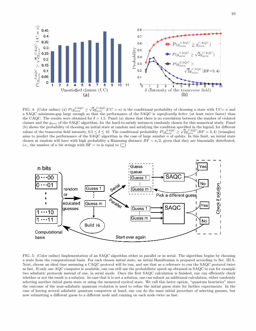
FIG. 4: (Color online) (a) P (gSAQCmin ≥

√2gCAQC

min |UC = n) is the conditional probability of choosing a state with UC= n anda SAQC minimum-gap large enough so that the performance of the SAQC is significantly better (at least twice faster) thanthe CAQC. The results were obtained for δ = 1.5. Panel (a) shows that there is no correlation between the number of violatedclauses and the gmin of the SAQC algorithm, for the hard-to-satisfy instances randomly chosen for this numerical study. Panel(b) shows the probability of choosing an initial state at random and satisfying the condition specified in the legend, for different

values of the transverse field intensity, 0.5 ≤ δ ≤ 10. The conditional probability P (gSAQCmin ≥

√2gCAQC

min |BF = 3, 4) (triangles)aims to predict the performance of the SAQC algorithm in the case of large number n of qubits. In this limit, an initial statechosen at random will have with high probability a Hamming distance BF ∼ n/2, given that they are binomially distributed,i.e., the number of n bit strings with BF = m is equal to

(

n

m

)

FIG. 5: (Color online) Implementation of an SAQC algorithm either in parallel or in serial. The algorithm begins by choosinga state from the computational basis. For each chosen initial state, an initial Hamiltonian is prepared according to Sec. IIIA.Next, choose an ideal time assuming a CAQC protocol will be run, and use that as a reference to run the SAQC protocol twiceas fast. If only one AQC computer is available, one can still use the probabilistic speed up obtained in SAQC to run for exampletwo adiabatic protocols instead of one, in serial mode. Once the first SAQC calculation is finished, one can efficiently checkwhether or not the result is a solution. In case that it is not a solution, one can submit an additional calculation, either randomlyselecting another initial guess state or using the measured excited state. We call this latter option, “quantum heuristics” sincethe outcome of the near-adiabatic quantum evolution is used to refine the initial guess state for further experiments. In thecase of having several adiabatic quantum computers at hand, one can do the same initial procedure of selecting guesses, butnow submitting a different guess to a different node and running on each node twice as fast.

11

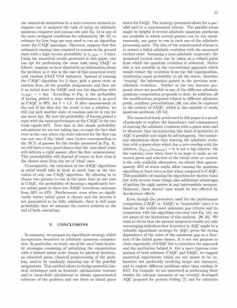
our numerical simulations in a more concrete scenario is:suppose one is assigned the task of using an adiabaticquantum computer and assume one uses Eq. 14 or any ofthe more stringent conditions for adiabaticity [26–35] toestimate for how long one may need to run an algorithmunder the CAQC paradigm. Moreover, suppose that thisestimated running time required to remain in the groundstate with a high success probability is τCAQC = 2 days.Using the numerical results presented in this paper, onecan opt for performing the same task using SAQC asfollows: suppose we have absolutely no information aboutthe problem as it was in the case of this numerical studywith random 3-SAT USA instances. Instead of runningthe CAQC algorithm for 2 days, pick a guess state atrandom from all the possible assignments and then useit as initial state for SAQC and run the algorithm withτSAQC = 1 day. According to Fig. 4, the probabilityof having picked a state whose performance is as goodas CAQC is 39%, for δ = 1.5. If after measurement atthe end of the first day the result is not a solution, westill can pick another state at random and let it run forone more day. By now the probability of having picked astate with the same performance as the CAQC in the twotrials equals 63%. Note that in this simple probabilitycalculations we are not taking into account the fact thateven in the case where the state selected for the first runwas not one of the ‘ideal’ ones (states corresponding tothe 39 % of guesses for the results presented in Fig. 4),we still have a very good chance that the ‘non-ideal’ statestill delivers a right answer after the first measurement.This probabability will depend of course on how close isthe chosen state from the set of ‘ideal’ ones.Consequently, the execution of two SAQC algorithms

in serial would take at most as much time as the exe-cution of only one CAQC algorithm. By allowing us tochoose two guesses to run in the same time as one casein CAQC, the probability of choosing a significantly bet-ter initial guess in these two SAQC executions increasesfrom 39% to 63%. Furthermore, even when no signifi-cantly better initial guess is chosen and the process isnot guaranteed to be fully adiabatic, there is still someprobability that we measure the correct solution at theend of both executions.

V. CONCLUSIONS

In summary, we propose an algorithmic strategy whichincorporates heuristics in adiabatic quantum computa-tion. In particular, we study one of the most basic heuris-tic strategies consisting of initializing the computationwith a desired initial state chosen by physical intuition,an educated guess, classical preprocessing of the prob-lem, and/or by randomly choosing one of the possibleassignments. This method allows to bridge powerful clas-sical techniques such as heuristic optimization routinesand/or mean-field calculations to obtain approximatedsolutions of the problem and use them as initial guess

states for SAQC. The strategy presented allows for a par-allel and/or a concatenated scheme. The parallel setupmight be helpful if several adiabatic quantum platformsare available in which several guesses can be run simul-taneously, one guess to run in each one of the adiabaticprocessing units. The idea of the concatenated scheme isto restart a failed adiabatic evolution with the measuredexcited state. Assuming a near-adiabatic trajectory, themeasured excited state can be taken as a refined guessfrom which the quantum evolution is restarted. Noticethis is not possible in the conventional approach whichwould restart the evolution from the full superposition,attributing equal probability to all the states, therefore“erasing” the information gained in the previous near-adiabatic evolution. Neither of the two features pro-posed above are possible in any of the different adiabaticquantum computation proposals to date. In addition, allthe modifications proposed related to different adiabaticpaths, auxiliary perturbations [48] can also be exploredin the context of SAQC, which is also suitable to studyquantum problems [49–53].

The numerical study performed in this paper is a proof-of-principle to explore the importance and consequencesof starting the adiabatic evolution with a guess state andto illustrate that incorporating this kind of heuristics inAQC is possible and might be advantageous. Our numer-ical simulations show that starting the adiabatic evolu-tion with a guess state which has a zero-overlap with thesolution, 〈φguess|φsolution〉 = 0, is not a big concern. Onthe contrary, even when there is no hope to make an ed-ucated guess and selection of the initial state at randomis the only available alternative, we obtain that approx-imately 40% of states might allow running the quantumalgorithm at least twice as fast when compared to CAQC.This possibility of running the algorithm for shorter timesbut with several trials brings also additional advantagesof getting the right answer in any intermediate measure.Moreover, these shorter runs would be less affected bydecoherence effects.

Even though the procedure used for the performancecomparison, CAQC vs. SAQC, is “reasonable” since it isbased on the widely-used minimum gap criteria and itsconnection with the algorithm run-time (see Eq. 14), weare aware of the limitations of this analysis [26–35]. Wewant to stress that the present numerical results are onlyencouraging indicators that heuristics in AQC might be avaluable algorithmic strategy for AQC, given the strongdependence of the value of the minimum gap as a func-tion of the initial guess chosen. It is not our purpose toclaim superiority of SAQC but to introduce the approachand the motivation behind it. For a more rigorous com-parison of both schemes, CAQC and SAQC, we suggestnumerical experiments which are not meant to be ex-haustive but preferably involving larger size instances,and to explore different problems other than random 3-SAT. For example, we are interested in performing thesestudies for relevant instances of our recently developedAQC proposal for protein folding [7] and for adiabatic

12

preparation of molecular ground states [19] where we ex-pect the mean-field (Hartree-Fock) solution to be a betterguess than a full superposition. Numerical propagationof the time-dependent Schrodinger equation, instead ofinspection of the minimum gap after the Hamiltoniandiagonalization, for these cases will provide a realisticsimulation of the quantum computation.Open questions to be explored further is the connec-

tions between SAQC, quantum phase transitions [54, 55],entanglement [56] and the effect of local minima [13].The performance of the adiabatic algorithm in the limitof large n is still an open question [44, 57] which needsto be explored in the context of SAQC. It is not obviousthat the same observations and conclusions/observationsmentioned above for CAQC will hold for SAQC as well.For example, we think that SAQC might be a strategyto avoid the local minima traps described in Ref. [13].From the study of the spectral properties of the ran-dom 3-SAT instances studied, we found that some initialstates have a considerably larger gap and while othersshow a considerably smaller gap when compared withCAQC. Since the initial state in CAQC is a full super-position of all the possible states or solutions, includingthe ones with a large gap and others with small gap,we conjecture here that having a full superposition willnot necessarily be the best choice, given that the pres-ence of the states with small gaps could slow down the

quantum evolution. An analysis beyond the gap criteriawould be needed to test this conjecture. Solving the time-dependent Schrodinger equation for the entire evolutionis the most straightforward, yet numerically-challengingapproach. In SAQC, the probability of obtaining thesetrap states can be avoided and even in the case of a failedevolution, the concatenated scheme may help to restartusing a better guess. In contrast, in CAQC, the full su-perposition including states with considerably small gapmight result in a bottleneck for the dynamics towards asuccessful computation. Further studies need to be doneto verify this is indeed the case.

Acknowledgments

All authors thank E. Farhi and S. Gutmann for use-ful discussions the led to Fig. 4 and related analysis.S.V.A. gratefully acknowledges P. Grasa and R. Ruedafor their support, and Tecnologico de Monterrey CampusEstado de Mexico for funding. A.P. and A.A.G gratefullyacknowledge funding from D-Wave Systems and Har-vard’s Institute for Quantum Science and Engineering.A.A.G. thanks the Army Research Office under contractW911NF-07-0304.

[1] E. Farhi, J. Goldstone, S. Gutmann, and M. Sipser,quant-ph/0001106 (2000).

[2] A. M. Childs, E. Farhi, and J. Preskill, PhysicalReview A 65, 012322.

[3] D. A. Lidar, Physical Review Letters 100, 160506(2008).

[4] E. Farhi, J. Goldstone, S. Gutmann, J. Lapan,A. Lundgren, and D. Preda, Science 292, 472 (2001).

[5] T. Hogg, Physical Review A 67, 022314 (2003).[6] A. P. Young, S. Knysh, and V. N. Smelyanskiy,

Physical Review Letters 101, 170503 (2008).[7] A. Perdomo, C. Truncik, I. Tubert-Brohman,

G. Rose, and A. Aspuru-Guzik, Physical Review A78, 012320 (2008).

[8] E. Farhi, J. Goldstone, and S. Gutmann,quant-ph/0208135 (2002).

[9] A. T. Rezakhani, W. Kuo, A. Hamma, D. A. Lidar,and P. Zanardi, Physical Review Letters 103, 080502(2009).

[10] E. Farhi, J. Goldstone, S. Gutmann, and D. Nagaj,International Journal of Quantum Information 06, 503(2008).

[11] J. Roland and N. J. Cerf, Physical Review A 65,042308 (2002).

[12] M. Znidaric and M. Horvat, Physical Review A 73,0223295 (2006).

[13] M. H. S. Amin, Physical Review Letters 100, 1305034(2008).

[14] M. Garey and D. Johnson, Computers and Intractabil-ity. A Guide to the Theory of NP-Completeness, W.H.

Freeman and Co., NY, 1979.[15] M. Sipser, Introduction to the Theory of Computation,

PWS Publishing Co., 2005.[16] T. Hogg, Physical Review Letters 80, 2473 (1998).[17] T. Hogg, Physical Review A 61, 052311 (2000).[18] L. K. Grover, Physical Review Letters 79, 325 (1997).[19] A. Aspuru-Guzik, A. D. Dutoi, P. J. Love, and

M. Head-Gordon, Science 309, 1704 (2005).[20] N. J. Ward, I. Kassal, and A. Aspuru-Guzik, The

Journal of Chemical Physics 130, 194105 (2009).[21] H. Wang, S. Kais, A. Aspuru-Guzik, and M. R.

Hoffmann, Physical Chemistry Chemical Physics 10,5388 (2008).

[22] H. Wang, S. Ashhab, and F. Nori, Physical Review A79, 042335 (2009).

[23] D. Kohen and D. J. Tannor, The Journal of ChemicalPhysics 98, 3168 (1993).

[24] D. Aharonov and A. Ta-Shma, Adiabatic quantumstate generation and statistical zero knowledge, in Pro-ceedings of the thirty-fifth annual ACM symposium onTheory of computing, pp. 20–29, San Diego, CA, USA,2003, ACM.

[25] A. Messiah, Quantum Mechanics (Physics), Dover Pub-lications, 1999.

[26] K. Marzlin and B. C. Sanders, Physical Review Let-ters 93, 160408 (2004).

[27] D. M. Tong, K. Singh, L. C. Kwek, and C. H. Oh,Physical Review Letters 98, 150402 (2007).

[28] Z. Wei and M. Ying, Physical Review A 76, 024304(2007).

13

[29] Y. Zhao, Physical Review A 77, 032109 (2008).[30] M. H. S. Amin, 0810.4335 (2008).[31] R. MacKenzie, A. Morin-Duchesne, H. Paquette,

and J. Pinel, Physical Review A 76, 044102 (2007).[32] A. Ambainis and O. Regev, quant-ph/0411152 (2004).[33] S. Jansen, M. Ruskai, and R. Seiler, Journal of Math-

ematical Physics 48, 102111 (2007).[34] J. da Wu, M. sheng Zhao, J. lan Chen, and

Y. de Zhang, 0706.0264 (2007).[35] J.-L. Chen, M. sheng Zhao, J. da Wu, and

Y. de Zhang, 0706.0299 (2007).[36] M. Andrecut and M. K. Ali, International Journal of

Theoretical Physics 43, 925931 (2004).[37] M. S. Siu, Physical Review A 75, 0623375 (2007).[38] S. Acharyya, Journal on Satisfiability, Boolean Model-

ing and Computation 4, 33 (2007).[39] I. Gent and T. Walsh, Internal report, department of

computer science, University of Strathclyde (1999).[40] M. Mezard, G. Parisi, and R. Zecchina, Science 297,

812 (2002).[41] D. Achlioptas, A. Naor, and Y. Peres, Nature 435,

759 (2005).[42] M. Mezard, T. Mora, and R. Zecchina, Physical Re-

view Letters 94, 197205 (2005).[43] Watanabe research group of Dept. of Math. and

Computing Sciences, Tokyo Inst. of Technology,http://www.is.titech.ac.jp/∼watanabe/gensat/.

[44] E. Farhi, J. Goldstone, D. Gosset, S. Gut-

mann, H. Meyer, and P. Shor, (2009),arxiv.org/abs/0909.4766.

[45] M. Znidaric, Physical Review A 71, 062305.[46] J. Du, L. Hu, Y. Wang, J. Wu, M. Zhao, and

D. Suter, Physical Review Letters 101, 060403 (2008).[47] H. Kautz and B. Selman, Discrete Applied Mathemat-

ics 155, 1514 (2007).[48] E. Farhi, J. Goldstone, and S. Gutmann,

quant-ph/0208135 (2002).[49] J. Kempe, A. Kitaev, and O. Regev, SIAM Journal

on Computing 35, 10701097 (2006).[50] S. Bravyi, quant-ph/0602108 (2006).[51] R. Oliveira and B. M. Terhal, Quantum Information

and Computation 8, 0900 (2008).[52] D. Aharonov andA. Ta-Shma, SIAM Journal on Com-

puting 37, 47 (2007).[53] A. Mizel, D. A. Lidar, and M. Mitchell, Physical

Review Letters 99, 070502 (2007).[54] R. Schutzhold and G. Schaller, Physical Review A

74, 060304 (2006).[55] J. Latorre and R. Orus, Physical Review A 69, 062302

(2004).[56] R. Orus and J. I. Latorre, Physical Review A 69,

052308 (2004).[57] A.P. Young, S. Knysh, and V. N. Smelyanskiy,

(2009), arXiv:0910.1378v1.