21 February 2021

COMPUTATION

AND

PROBLEM SOLVING

IN

UNDERGRADUATE PHYSICS

Second EditionIDL MATLAB • OCTAVE

PYTHON MAXIMA MAPLE

• MATHEMATICA • PROGRAM • FORTRAN

• C LSODE PDEs

MUDPACK • LATEX TGIF

DAVID M. COOK

Department of PhysicsLawrence University

711 E Boldt Way, SPC 24Appleton, Wisconsin 54911

Copyright c© First Edition 2000–16 by David M. CookCopyright c© Second Edition 2016–21 by David M. Cook

This work is licensed under a Creative Commons Attribution-NonCommercial-ShareAlike 4.0 International License (creativecommons.org/licenses/by-nc-sa/4.0/).Any use not permitted by this license requires authorization in writing from DavidM. Cook.

The first edition of this publication was registered with the Libraryof Congress with the call number QC20.C66.2004.

The second edition was registered with the Library of Congresswith the LCCN 2019947884. It has been assigned the ISBN9780961342968 and carries the Library of Congress call numberQC20.C66.2019.

ii

Preface to the Second Edition

Note: Usually with a second edition of a book, the preface to the first edition1 ispreserved and a short preface to the second edition is added. In the present case,the preface to the first edition required here and there a number of edits which,had they not been made, would have been perhaps a bit confusing to readers of thesecond edition. Consequently, I have elected to depart from the normal practice andsimply create a preface for the second edition, though much of its content essentiallycopies that of the preface to the first edition.

Note: Regardless of which components are included and which omitted in thisversion of Computation and Problem Solving in Undergraduate Physics, the prefaceand acknowledgements in the front matter are those from the assemblage containingall components.

Since the mid 1980’s (including the years since my official retirement in 2008), we in the Depart-ment of Physics at Lawrence University have been developing and offering curricular componentsthat

• support efforts to acquaint students with computational procedures and resources early enoughso that they will be motivated and prepared to use these resources on their own initiativewhen circumstances warrant and so that later work need not be interrupted to deal withcomputational issues as an aside to its main purposes, and

• provide students with both the background and the confidence to support informed reading ofvendor manuals, which usually do a splendid job of listing capabilities exhaustively but typi-cally burden the beginner with initially irrelevant refinements and fail to illustrate adequatelyhow even the rudimentary capabilities can be combined to perform useful tasks.

Over the years since the mid 1980s, a wide assortment of instructional materials has been draftedand redrafted. This book brings these materials together into a single publication with the hopethat it may prove useful to others who seek to achieve these same or similar objectives.2

With these objectives in mind, this book consciously focuses on helping students get started.It is not designed to be comprehensive or exhaustive, either in laying out the capabilities of anyparticular computational resource or in discussing numerical algorithms. Students must understandthroughout that they must refer regularly to vendors’ manuals and on-line help files for details beyondthose discussed in the book—details that may, in fact, be necessary for successful completion of someof the exercises. The need for that activity is noted here; repeated reminders will not be includedin the body of the book.

1The first edition was published in 2003, though it experienced a number of edits and adjustments in subsequentyears.

2The article by David M. Cook titled “Computation in Undergraduate Physics: The Lawrence Approach” andappearing in the American Journal of Physics (Am. J. Phys. 76, 321–326 (April-May 2008) describes these efforts insome detail.

iii

iv PREFACE TO THE SECOND EDITION

The book is also not a book about computational physics; it addresses uses of computationaltools. Indeed, the sophomore course at Lawrence in which students first encounter this book wouldnot in any way replace a course in computational physics. Rather, the materials treated here shouldprovide strong background for a subsequent, junior-senior level course in computational physics,which would—I believe—be substantially enhanced if students came to it already familiar with theresources on which this book concentrates.

One major difficulty in creating materials on computational topics is that different potentialusers favor different hardware platforms and software packages. Especially in the computationalarena, the variety of options and combinations is so great that any single choice (or coordinated setof choices) is bound to limit the usefulness of the product to a small subset of all potential users. Thisbook addresses that difficulty by being assembled from a wide assortment of components, some ofwhich—the generic components—will be included in all versions and others of which—those specificto particular software packages—will be included only if the potential user requests them. Thus, thespecific software and hardware discussed in the book can be tailored to the spectrum of resourcesavailable at the instructor’s site. Two versions may well differ in numerous respects. One mayinclude the generic components and the components that discuss3 IDL, MAPLE, C (with NumericalRecipes), and LATEX while another may include the generic components and the components thatfocus on MATLAB, Mathematica, and FORTRAN (including Numerical Recipes). The table ofcontents and index contain only entries from the included chapters and sections. To facilitatecommunication among users of different versions, however, chapter and section numbers and thenumbers identifying package-independent exercises are preserved in all versions. In a version thatdoes not include FORTRAN, for example, the FORTRAN sections will be omitted from Chapters 9,10, 11, 13, 14, and 15 and Chapters 12 and 16—for which FORTRAN is prerequisite—will beomitted altogether. In addition, FORTRAN-specific exercises will be omitted from the end-of-chapter exercises. Because of version-specific omissions such as those just described, there willtherefore be gaps in the chapter, section, and exercise numbers in any version that does not includeall options. In contrast, within each chapter, equation numbers, figure numbers, table numbers,and footnote numbers advance from one without gaps, and page numbers run continuously fromthe beginning of the book to the end. In consequence, the numbers assigned to identical equations,figures, tables, footnotes, and pages may differ from version to version, but the numbers assigned tochapters and sections with identical titles and the numbers assigned to identical exercises will be thesame in all versions (and will have gaps reflecting omitted chapters, sections, and exercises). Suchflexibility would be impossible were we not able to exploit features of LATEX, including the particularcapabilities of the ifthen and imakeidx packages, to assemble the PostScript and PDF files thatsubsequently can be printed to obtain each version.

Even among sites that use the same spectrum of hardware and software, however, some aspectsof local environments remain unique to individual sites. Local rules of citizenship; the features andelementary resources of the local operating system; local practices and policies governing structur-ing of public directories, assignment of accounts and passwords, backup schedules, and after-hoursaccess; licensing restrictions on proprietary software; means to launch particular application pro-grams, compile user-written FORTRAN and/or C programs, and access printers; and numerousother aspects are subject to considerable local variation. This book does not constrain local optionsin these matters. Instead, its users must draft a site-specific supplement, which we will refer to asthe Local Guide, to which individuals should refer for site-specific particulars. A LATEX templatefor that guide, specifically the one used at Lawrence, is available to users of this book, but it willrequire editing to reflect local practices. In particular, to give local sites flexibility in configuringtheir environments, we have in the book used symbols like $HEAD, $IDLHEAD, and $NRHEAD to standfor paths to the specific directories that sit at the head of particular directory trees. All such symbolsmust be expanded as described in the Local Guide when commands or statements illustrated in thebook are submitted to the user’s machine.

3Many of the packages mentioned in this list are commercial and proprietary, and the names are registered trade-marks of the respective vendors. Full contact information for all mentioned packages will be found in Appendix Z.

PREFACE TO THE SECOND EDITION v

With the broadest brush, Chapter 1 stands alone and focuses on a number of topics assumedas background for the rest of the book. The next several chapters introduce4

• Specific array processors (Chapter 2 on IDL, Chapter 3 on MATLAB, Chapter 4 on OCTAVE,Chapter 5 on PYTHON),

• Computer algebra systems (Chapter 6 on MAXIMA, Chapter 7 on MAPLE, Chapter 8 onMathematica),

• Programming languages (Chapter 9—with sections on FORTRAN and C), and• Subroutine libraries (Chapter 10 on Numerical Recipes, Chapter 12 on LSODE, Chapter 16

on MUDPACK).

The remaining chapters address several important categories of computational processing, specifi-cally

• Solving ordinary differential equations (Chapters 11 and 12),• Evaluating integrals (Chapter 13),• Finding roots (Chapter 14),• Solving partial differential equations (Chapters 15 and 16)

Each of Chapters 11, 13, 14, and 15 begins with a (generic) section in which several problems drawnfrom subareas of physics and using the computational technique on which the chapter focuses arelaid out. Each of Chapters 11, 13, and 14 then continues with

• one or more (optional) sections in which some of the identified problems are addressed withwhatever computer algebra systems are included in the version,

• a (generic) section on numerical approaches to the category of problem on which the chapterfocuses, and

• several (optional) sections in which some of the problems laid out in the first section areaddressed with whatever array processors, computer algebra systems, and programming lan-guages are included in the version.

Somewhat in contrast, Chapter 15 continues with

• a (generic) section on finite difference methods (FDMs) for solving partial differential equations,• several (optional) sections in which some of the identified problems are addressed using FDMs

with each of several tools,• a (generic) section on finite element methods (FEMs), and• several (optional) sections in which some of the identified problems are addressed using FEMs.

Every chapter in the book concludes with a collection of exercises using the techniques—both sym-bolic and numerical—of the chapter. The appendices introduce a publishing system (Appendix Aon LATEX) and a (UNIX/LINUX) program for producing drawings (Appendix B on TGIF). In time,other options than those available in this edition may be added.

The order of presentation in the book does not compel any particular order of treatment in acourse or program of self-study. To be sure, some later sections depend on some earlier sections, butthe linkages are not particularly tight. In the Lawrence context, for example, the required sophomorecourse Computational Mechanics typically covers the chapters and appendices introducing IDL,either MAPLE or Mathematica, and LATEX; and finally covers the IDL and either the MAPLE orthe Mathematica portions of the chapters on ordinary differential equations (ODEs), integration androot finding. The chapter on Numerical Recipes, the FORTRAN and/or C portions of the chapters

4 The second edition has added the shareware programs OCTAVE and PYTHON and replaced the no-longeravailable commercial program MACSYMA with the shareware program MAXIMA. The addition of OCTAVE andPYTHON explain why Chapters 4–12 in the first edition have become Chapters 6–14 in the second edition.

vi PREFACE TO THE SECOND EDITION

on programming, ODEs, integration, and root finding, the chapter on partial differential equationsand the chapters on LSODE and MUDPACK are the focus of the Lawrence elective junior/seniorcourse Computational Physics.

Despite the organization of the chapters by program or by computational technique involved,the focus throughout is on physical contexts. The materials are designed to be used in conjunctionwith intermediate level courses, not introductory courses. While the illustrations of computationalprocedures highlight significant physical contexts and most of the examples and suggested exercisesemerge from interesting physical situations, the objective is for students to become both fluentand wary in using computational resources in application to these physical situations, not to dwellexcessively on the microscopic details of numerical analysis or to teach them the underlying physics(except insofar as successful computer-based solution of problems underscores the power of thefundamental physical ideas). The students are assumed

• to have completed an introductory survey course in physics,• to have completed courses in calculus, differential equations and, to some extent, linear algebra,

and• to be embarking on intermediate-level studies in physics

as they undertake a study of this book. We focus not so much on the set up of the situations—thatis assumed to be the province of other courses—as on computer-based techniques and strategies fordetermining the solution once the set up is complete. Examples are drawn from classical mechanics,classical electricity and magnetism, thermal physics, quantum mechanics, curve fitting, DC and ACcircuit theory, optics, and several other areas.

Acknowledgements

First and foremost, I wish to acknowledge the assistance and contributions of Peter Strunk, LU ’89,Kristi R. G. Hendrickson, LU ’91, Todd G. Ruskell, LU ’91, Stephen L. Mielke, LU ’92, RuthRhodes, LU ’92, Michelle Ruprecht, LU ’92, Sandra Collins, LU ’93, Mark F. Gehrke, LU ’93, KarlJ. Geissler, LU ’94, Steven Van Metre, LU ’94, Alain Bellon, LU ’95, Peter Kelly Senecal, LU ’95,Christopher C. Schmidt, LU ’97, Michael D. Stenner, LU ’97, Mark Nornberg, LU ’98, Scot Shaw,LU ’98, Jim Truitt, LU ’98, Eric D. Moore, LU ’99, Teresa K. Hayne, LU ’00, Danica Dralus,LU, ’02, Ryan T. Peterson, LU ’03, Scott J. Kaminski, LU ’04, Michelle L. Milne, LU ’04, LaurenE. Kost, LU ’05, Claire Weiss, LU ’07, and Erik Garbacik, LU ’08—all Lawrence students who, asundergraduates, contributed during the first decade and a half to the evolution of this book andthe accompanying manual of solutions to representative exercises. While current versions in mostinstances deviate—often considerably—from the initial drafts to which these students contributed,there can be no denying that their contributions have played an important role in the evolution ofthe use of computational resources in the Lawrence curriculum and the evolution of this book. Ithank them warmly and sincerely for their assistance. All of these students have given permissionfor me to use whatever has over the years become of their contributions in this publication.

Second, I wish to acknowledge and thank several individuals who have provided reviews of draftsor otherwise assisted in the refinement of this book, including

• numerous students (beyond those specifically named in the previous paragraph) who haveenrolled in my courses over the years and who, directly and indirectly, have made commentsthat have influenced this book.

• my departmental colleagues J. Bruce Brackenridge, John R. Brandenberger, Jeffrey A. Collett,Matthew R. Stoneking, and Paul W. Fontana, who have listened to my sometimes lengthyobservations about matters computational and curricular and offered valuable criticisms.

• Wolfgang Christian (Davidson College), Robert Ehrlich (George Mason University), andA. John Mallinckrodt (California Polytechnic Institute–Pomona), each of whom participatedin a 1990 Sloan-supported conference on computation in advanced undergraduate physics thatI organized at Lawrence and each of whom as a consultant throughout the writing project hasoffered many suggestions and constructive criticisms.

• all those faculty members1 who participated in one of the NSF-supported week-long work-shops offered at Lawrence in the summers of 2001, 2002, and 2003 and who, in that context,

1In July 2001: Steve Adams (Widener University), Russel Kauffman (Muhlenberg College), Marylin Bell (LakeForest College), Lawrence A. Molnar (Calvin College), Thomas R. Greenlee (Bethel College), Elliott Moore (NewMexico Tech), Javier Hasbun (State University of West Georgia), Joelle L. Murray (Linfield College), Derrick Hylton(Spelman College), Paula C. Turner (Kenyon College), Ross Hyman (DePaul University), Scott N. Walck (LebanonValley College), William H. Ingham (James Madison University), and Tim Young (University of North Dakota). InJuly, 2002 (first workshop): Albert Batten (United States Air Force Academy), Andrea Cox LU ’91 (Beloit Col-lege), Brian Cudnik (Prairie View A and M), Craig Gunsul (Whitman College), Kevin Lee (University of Nebraska),Kam-Biu Luk (University of California, Berkeley), Daryl Macomb (Boise State University), Viktor Martisovits (Cen-tral College), Donald Miller (Central Missouri State University), Dorn Peterson (James Madison University), RobertRagan (University of Wisconsin – Lacrosse), Shafiq Rahman (Allegheny College), Rahmathullah Syed (Norwich Uni-versity), Jorge Talamantes (California State University – Bakersfield), Mark Timko (Elmhurst College), Paul Tjossem

vii

viii ACKNOWLEDGEMENTS

provided a critical examination of the evolving manuscript and offered numerous suggestionsfor improvement—in addition to finding many previously undetected typographical glitches.

• especially Javier Hasbun (State University of West Georgia)—who had students working withalmost the entire manuscript—but also William H. Ingham (James Madison University), Rus-sel Kauffman (Muhlenberg College), Joelle L. Murray (Linfield College), Shafiq Rahman (Al-legheny College), John Thompson (DePaul University), and Tim Young (University of NorthDakota), all of whom used at least portions of the growing manuscript in their teaching dur-ing the academic year 2001–02 and who collectively sent me a wide spectrum of varied andvaluable comments.

• several anonymous reviewers engaged by potential publishers as they evaluated my efforts,even though all potential publishers ultimately decided they could not provide the microscopiccustomization the book required.

Third, I wish to acknowledge considerable debt to many individuals whom I do not know butwhose contributions behind the scenes have been invaluable. Chief among these individuals are

• Donald Knuth, originator of TEX;

• Leslie Lamport, originator of LATEX;

• Han The Than, originator of pdfTEX, which provides the engine underlying pdflatex forcreating PDF files directly from LATEX source code..

• Pehong Chen and Nelson Beebe, originator and current maintainer of makeindex for preparingindices to LATEX documents;

• Enrico Gregorio, originator and current maintainer of the LATEX package imakeidx that reducesthe number of passes required to format and include an index;

• David Carlisle and Sebastian Rahtz, originators, and David Carlisle, current maintainer, ofthe LATEX package graphicx for including graphic images in LATEX documents;

• Leslie Lamport, David Carlisle and other members of the LATEX3 team, authors of the LATEXpackage ifthen for supporting conditional statements in LATEX source files;

• Sebastian Rahtz and Heiko Oberdiek, originator of the LATEX package hyperref for creatinglinked versions of documents as PDF files;

• Paul Vojta, author of xdvi, a versatile on-screen previewer for the .dvi files produced by TEXand LATEX;

• Till Tantau et. al., originators and current maintainers of the LATEX packages tikz and pgf

for creating sophisticated diagrams using LATEX-like inclusions in the source file;

• William Chia-Wei Cheng, author of TGIF, a program used to create several of the figures;

• John Bradley, author of xv, a program used to convert a few bit-mapped files into PostScript;

(Grinnell College), and John Walkup (California Polytechnic Institute – San Luis Obispo). In July, 2002 (second work-shop): Julio Blanco (California State University–Northridge), William Briscoe (George Washington University), PaulBunson (Lawrence University), Albert Chen (Oklahoma Baptist University), K. Kelvin Cheng (Texas Tech Univer-sity), Bob Davis (Taylor University), Mirela Fetea (University of Richmond), David Grumbine (St. Vincent College),Kristi Hendrickson LU ’91 (University of Puget Sound), Tom Herrmann (Eastern Oregon University), Seamus Lagan(Whittier College), Eric Lane (University of Tennessee at Chattanooga), Ernest Ma (Montclair State University),Norris Preyer (College of Charleston), Michael Schillaci (Francis Marion University), Mihir Sejpal (Earlham College),Laura Van Wormer (Hiram College), Mary Lou West (Montclair State University), and Douglas Young (Mercer Uni-versity). In July, 2003: Stephen Addison (University of Central Arkansas), Mohan Aggarwal (Alabama A&M), AnneCaraley (SUNY at Oswego), William Dieterle (California University of Pennsylvania), Timothy Duman (Universityof Indianapolis), Brett Fadem (Colby College), Michael Gray (American University), James Meyer (St. Gregory’sUniversity), Prabasaj Paul (Denison University), David Peterson (Francis Marion University), Edward Pogozelski(SUNY at Geneseo), Chandra Prayaga (University of West Florida), Bruce Richards (Oberlin College), David Seely(Albion College), Adam Smith (Hillsdale College), Walther Spjeldvik (Weber State University), Julie Talbot (StateUniversity of West Georgia), Paul Thomas (University of Wisconsin–Eau Claire), Srinivasa Venugopalan (SUNY atBinghamton), and Alma Zook (Pomona College).

ACKNOWLEDGEMENTS ix

• The many contributors to the MiKTEX project;

• The developers, authors, and maintainers of WinEdt, the text editor used during the latteryears of writing CPSUP; and

• The developers and maintainers of ps2pdf for convertingPostScript files to PDF and the de-velopers and maintainers of pdfcrop for pruning excessive white borders from PDF files.

• Radical Eye Software, which holds the copyright on dvips, a program for converting .dvi filesto PostScript.

Quite simply, this project would have been impossible without the availability of these severalprograms and utilities, each of which played a necessary role behind the scenes in preparing orprocessing the files from which, ultimately, a printable PostScript file for the finished book emerged.

Fourth, I point out that the names of several pieces of commercial software are, in fact, trade-marks or registered trademarks belonging to the vendors of those software products. Each suchtrademark is identified at its first occurrence in the text proper, and detailed contact informationfor every vendor is compiled in Appendix Z.

Fifth, I acknowledge the following specific permissions, each of which is more fully explained atthe point in the text where the permission is explicitly invoked. In particular, I thank

• The MathWorks, Inc., for permission to incorporate in this book and distribute IDL sourcecode for the routines ludiffeq 23 and ludiffeq 45, which code uses algorithms patternedafter those used in 1991 in the MATLAB routines ode23 and ode45.

• Wayne Landsman, author of the IDL routines qsimpson and trapzd in the IDL AstronomyUser’s Library, for permission to use those routines as the basis for the routines luqsimp andlutrapzd and to distribute the source code for luqsimp and lutrapzd as supplements to thisbook.

• Research Systems (later Exelis Visual Information Solutions and now part of Harris GeospatialSolutions), Incorporated, for permission to use portions of any RSI-supplied and/or edited .pro

code—most particularly evident in RSI contributions to ludiffeq 23.pro, ludiffeq 45.pro,and luqsimp.pro—and to use the IDL name and trademark.

• Numerical Recipes Software (a) for permission to use the names and calling sequences of severalNumerical Recipes routines2 at various places in this book, (b) for permission to refer to theC header files nr.h and nrutil.h and the file nrutil.c containing assorted utilities used byvarious C recipes, and (3) for permission to use the names and calling sequences of several IDLroutines that are derived from Numerical Recipes routines (and for the use of which ResearchSystems Incorporated has permission from Numerical Recipes Software).

• William Chia-Wei Cheng, author of TGIF, for permission to reproduce in the appendix on thatprogram several of the icons used in its many screen displays.

Sixth, I wish to acknowledge and thank the W. M. Keck Foundation for three grants [#880969(1988), #931248 (1993), #011795 (2001)], the National Science Foundation for three grants [USE-8851685 (ILI–1988), DUE-9350667 (ILI-1993), and DUE-9952285 (CCLI-EMD-2000)], and LawrenceUniversity for matching and other support.3 A small conference held at Lawrence in 1990 andsupported by the Alfred P. Sloan Foundation stimulated thinking among the participants aboutuses of computers in upper-division undergraduate physics. All of these grants have contributed

2Specifically flmoon, xflmoon, caldat, julday, xjulday, avevar, xavevar, rk4, xrk4, rkqs, rkck, mmid, bsstep,rkdumb, odeint, trapzd, xtrapzd, qtrap, xqtrap, qsimp, qromb, polint, rtbis, xrtbis, rtnewt, xrtnewt, rtsafe,xrtsafe, zbrak, gaussj, ludcmp, lubksb, tridag, svdcmp, svbksb, mnewt, newt, and broydn (both in FORTRAN andin C).

3Any opinions, findings, and conclusions or recommendations expressed in this book are those of the author anddo not necessarily reflect the views of any of these granting foundations or agencies.

x ACKNOWLEDGEMENTS

in many ways to the developments at Lawrence that have culminated in the writing of this book.In particular, the NSF CCLI-EMD grant made in February, 2000, supported my sabbatical while Ifinalized the text of this book. That grant also supported three week-long summer faculty workshopsthat have, on the one hand, provided constructive feedback on a succession of drafts and, on theother hand, enhanced awareness nationally of this book and of the developments at Lawrence.

Finally (and most important of all), I wish to express deep gratitude for the decades duringwhich my wife, Cynthia, has shown patience, understanding, and support beyond any possibility ofmy ever fully knowing. In truth, I do not know how to thank her.

Disclaimer

The statements described in the various chapters of this book have been tested extensively but havecertainly not been tested with all versions of all software packages on all possible platforms withall possible versions of the underlying operating systems. Differences from version to version ofthe software packages, from operating system to operating system, and from platform to platformexist. This brief section identifies the versions of the various programs that have been tested and theoperating systems and platforms on which those tests have been carried out. That the behavior ofother combinations of version, operating system, and platform will conform in every detail to thatherein described can, of course, not be guaranteed. One can, however, have some confidence thatthe behavior in combinations not explicitly tested will not differ enormously from that describedherein—except that newer versions of a software package may well have features not implemented inearlier versions (and occasionally a feature or specific syntax available in an earlier version has beenremoved altogether from more recent versions). With reasonable confidence, one can presume thatthe commands and syntax and features described in this book will work on other platforms withthe tested versions of the programs and with subsequent versions. Statements herein that exploitfeatures implemented for the first time in the tested versions will, of course, not be accepted in earlierversions, but those “glitches” should not be numerous or extensive. Where, in the months and yearssince the original draft was created, I have become aware of such glitches, I have made appropriateupdates and subsequent productions have incorporated those updates.1 Nothing, however, assuresthat I have identified all such glitches.

That disclaimer having been stated, I now present for each program a brief tally of the version(s)tested and the platform(s) and operating system(s) on which those tests have been carried out:

• The Mathematica details herein apply specifically to Mathematica Version 11.3 on a Hewlett-Packard platform running Windows 7 and a Hewlett-Packard platform running the Fedora 17implementation of LINUX. The Mathematica sections have also been spot-checked with Math-ematica 12.0 on a Hewlett-Packard platform running Windows 10.

• The OCTAVE details herein apply specifically to

OCTAVE Version 4.0.0 on a Hewlett-Packard platform running Windows 7, OCTAVE Version 3.6.3 on a Hewlett-Packard platform running the Fedora 17 implemen-

tation of LINUX, and OCTAVE Version 4.0.3 on a Hewlett-Packard platform running the Fedora 25 implemen-

tation of LINUX.

1The date of production of each version of CPSUP is displayed at the top of the cover page on that version. I havemaintained a dated list of edits made to the source files, so changes made after the date of production of a particularversion of CPSUP and a subsequent production of that version can readily be identified for anyone who wishes toupdate an outdated production. Generally, updated productions fairly promptly replace the previous production atpsrc.aapt.org/curricula/cpsup. Versions dated between 10 and 31 January 2021 provide the base. Edits madeafter 31 January 2021 are recorded in the file of edits.

xi

xii DISCLAIMER

OCTAVE Version 4.2.2 has been spot-checked on a Hewlett-Packard platform running Win-dows 7, and OCTAVE Versions 4.0.0 and 5.2.0 have been spot-checked on a Hewlett-Packardplatform running Windows 10.

• The Numerical Recipes details in Chapter 10 apply specifically for Version 2.10 and have beentested only on a Hewlett-Packard platform running the Fedora 17 implementation of LINUX.

• The LATEX details in Appendix A apply specifically to LATEX 2ε with the MiKTEX implemen-tation on a Hewlett-Packard platform running Windows 7 and on a Hewlett-Packard platformrunning Windows 10. LATEX normally responds to the same source code on all platforms.

Table of Contents

Preface to the Second Edition iii

Acknowledgements vii

Disclaimer xi

Table of Contents xiii

1 Preliminaries 11.1 An Orientation to Computers . . . . . . . . . . . . . . . . . . . . . . . . . . . . . . . . . . 2

1.1.1 A Simple Responsive Machine . . . . . . . . . . . . . . . . . . . . . . . . . . . . 31.1.2 Character Codes . . . . . . . . . . . . . . . . . . . . . . . . . . . . . . . . . . . 41.1.3 The ASCII Character Set . . . . . . . . . . . . . . . . . . . . . . . . . . . . . . 51.1.4 Representation of Data in a Computer . . . . . . . . . . . . . . . . . . . . . . . 6

1.2 Files and Directories . . . . . . . . . . . . . . . . . . . . . . . . . . . . . . . . . . . . . . . 81.3 Operating Systems . . . . . . . . . . . . . . . . . . . . . . . . . . . . . . . . . . . . . . . . 91.4 Glossary, Conventions, and Understandings . . . . . . . . . . . . . . . . . . . . . . . . . . 91.5 Assumed Background . . . . . . . . . . . . . . . . . . . . . . . . . . . . . . . . . . . . . . 11

1.5.1 The Gamma Function . . . . . . . . . . . . . . . . . . . . . . . . . . . . . . . . 121.5.2 The Laplace Transform . . . . . . . . . . . . . . . . . . . . . . . . . . . . . . . 13

1.6 Licensing Issues . . . . . . . . . . . . . . . . . . . . . . . . . . . . . . . . . . . . . . . . . 14

4 Introduction to OCTAVE 154.1 Beginning an OCTAVE Session . . . . . . . . . . . . . . . . . . . . . . . . . . . . . . . . 164.2 Basic Entities in OCTAVE . . . . . . . . . . . . . . . . . . . . . . . . . . . . . . . . . . . 17

4.2.1 Data Types . . . . . . . . . . . . . . . . . . . . . . . . . . . . . . . . . . . . . . 174.2.2 Variable Names . . . . . . . . . . . . . . . . . . . . . . . . . . . . . . . . . . . . 174.2.3 Assignment of Values to Variables . . . . . . . . . . . . . . . . . . . . . . . . . 184.2.4 Commands . . . . . . . . . . . . . . . . . . . . . . . . . . . . . . . . . . . . . . 18

4.3 A Sampling of OCTAVE Capabilities . . . . . . . . . . . . . . . . . . . . . . . . . . . . . 194.3.1 Creating and Examining Arrays . . . . . . . . . . . . . . . . . . . . . . . . . . 194.3.2 Simple Mathematical Manipulations . . . . . . . . . . . . . . . . . . . . . . . . 224.3.3 Matrix Manipulations . . . . . . . . . . . . . . . . . . . . . . . . . . . . . . . . 234.3.4 Solving Linear Equations . . . . . . . . . . . . . . . . . . . . . . . . . . . . . . 244.3.5 A First Graph . . . . . . . . . . . . . . . . . . . . . . . . . . . . . . . . . . . . 25

4.4 Properties, Objects, and Handles . . . . . . . . . . . . . . . . . . . . . . . . . . . . . . . 284.5 Saving and Retrieving the OCTAVE Session . . . . . . . . . . . . . . . . . . . . . . . . . 304.6 Loops, Logical Expressions, and Conditionals . . . . . . . . . . . . . . . . . . . . . . . . 324.7 Reading Data from a File . . . . . . . . . . . . . . . . . . . . . . . . . . . . . . . . . . . 354.8 On-line Help . . . . . . . . . . . . . . . . . . . . . . . . . . . . . . . . . . . . . . . . . . . 374.9 m-Files . . . . . . . . . . . . . . . . . . . . . . . . . . . . . . . . . . . . . . . . . . . . . . 374.10 Eigenvalues and Eigenvectors . . . . . . . . . . . . . . . . . . . . . . . . . . . . . . . . . 414.11 Graphing Scalar Functions of One Variable . . . . . . . . . . . . . . . . . . . . . . . . . . 43

4.11.1 The Basic Strategy . . . . . . . . . . . . . . . . . . . . . . . . . . . . . . . . . 434.11.2 Marking Points: . . . . . . . . . . . . . . . . . . . . . . . . . . . . . . . . . . . 434.11.3 Plotting Several Graphs on One Set of Axes . . . . . . . . . . . . . . . . . . . . 444.11.4 Polar Plots and Custom Axes . . . . . . . . . . . . . . . . . . . . . . . . . . . . 45

xiii

xiv TABLE OF CONTENTS

4.11.5 Multiple Plots On a Page . . . . . . . . . . . . . . . . . . . . . . . . . . . . . . 464.11.6 Plotting Experimental Data . . . . . . . . . . . . . . . . . . . . . . . . . . . . 47

4.12 Making Hard Copy . . . . . . . . . . . . . . . . . . . . . . . . . . . . . . . . . . . . . . . 494.12.1 . . . of Text . . . . . . . . . . . . . . . . . . . . . . . . . . . . . . . . . . . . . . . 494.12.2 . . . of Graphs . . . . . . . . . . . . . . . . . . . . . . . . . . . . . . . . . . . . . 49

4.13 Graphing Scalar Functions of Two Variables . . . . . . . . . . . . . . . . . . . . . . . . . 514.13.1 A Preliminary: The Function meshgrid . . . . . . . . . . . . . . . . . . . . . . 514.13.2 Surface Plots: The Function mesh . . . . . . . . . . . . . . . . . . . . . . . . . 524.13.3 Shaded Surfaces: The Function surf . . . . . . . . . . . . . . . . . . . . . . . . 554.13.4 Contour Plots: The Function contour . . . . . . . . . . . . . . . . . . . . . . . 574.13.5 The Functions meshc, surfc, and surfl . . . . . . . . . . . . . . . . . . . . . . 594.13.6 Functions of Two Variables in Polar Coordinates . . . . . . . . . . . . . . . . . 59

4.14 Graphing Scalar Functions of Three Variables . . . . . . . . . . . . . . . . . . . . . . . . 604.14.1 Reduction to Two-Dimensional Displays . . . . . . . . . . . . . . . . . . . . . . 614.14.2 Isosurfaces . . . . . . . . . . . . . . . . . . . . . . . . . . . . . . . . . . . . . . 64

4.15 Graphing Vector Fields . . . . . . . . . . . . . . . . . . . . . . . . . . . . . . . . . . . . . 664.15.1 The Function quiver . . . . . . . . . . . . . . . . . . . . . . . . . . . . . . . . . 674.15.2 More Elaborate Displays . . . . . . . . . . . . . . . . . . . . . . . . . . . . . . . 674.15.3 Three-Dimensional Vector Fields . . . . . . . . . . . . . . . . . . . . . . . . . . 69

4.16 Animation . . . . . . . . . . . . . . . . . . . . . . . . . . . . . . . . . . . . . . . . . . . . 694.17 Advanced Graphing Features . . . . . . . . . . . . . . . . . . . . . . . . . . . . . . . . . . 71

4.17.1 Fonts . . . . . . . . . . . . . . . . . . . . . . . . . . . . . . . . . . . . . . . . . 714.17.2 Space Curves . . . . . . . . . . . . . . . . . . . . . . . . . . . . . . . . . . . . . 734.17.3 Using Multiple Windows . . . . . . . . . . . . . . . . . . . . . . . . . . . . . . . 744.17.4 Customizing Axes . . . . . . . . . . . . . . . . . . . . . . . . . . . . . . . . . . 75

4.18 Miscellaneous Occasionally Useful Tidbits . . . . . . . . . . . . . . . . . . . . . . . . . . 764.18.1 Specifying Directories . . . . . . . . . . . . . . . . . . . . . . . . . . . . . . . . 774.18.2 Deleting Variables No Longer Needed . . . . . . . . . . . . . . . . . . . . . . . . 774.18.3 OCTAVE’s Current Directory . . . . . . . . . . . . . . . . . . . . . . . . . . . 774.18.4 OCTAVE’s Search Path . . . . . . . . . . . . . . . . . . . . . . . . . . . . . . . 784.18.5 Customizing OCTAVE . . . . . . . . . . . . . . . . . . . . . . . . . . . . . . . 784.18.6 Restoring OCTAVE’s Initial State . . . . . . . . . . . . . . . . . . . . . . . . . 794.18.7 The Command format . . . . . . . . . . . . . . . . . . . . . . . . . . . . . . . . 794.18.8 Reading Data from the Keyboard . . . . . . . . . . . . . . . . . . . . . . . . . . 794.18.9 Writing Data to the Screen . . . . . . . . . . . . . . . . . . . . . . . . . . . . . 794.18.10 Exiting from Procedures . . . . . . . . . . . . . . . . . . . . . . . . . . . . . . . 80

4.19 References . . . . . . . . . . . . . . . . . . . . . . . . . . . . . . . . . . . . . . . . . . . . 814.20 Exercises . . . . . . . . . . . . . . . . . . . . . . . . . . . . . . . . . . . . . . . . . . . . . 81

4.20.1 Writing OCTAVE Statements . . . . . . . . . . . . . . . . . . . . . . . . . . . . 814.20.2 Finding Eigenvalues and Eigenvectors . . . . . . . . . . . . . . . . . . . . . . . 824.20.3 Graphing Scalar Functions of a Single Variable . . . . . . . . . . . . . . . . . . 834.20.4 Graphing Scalar Functions of Two Variables . . . . . . . . . . . . . . . . . . . . 854.20.5 Graphing Scalar Functions of Three Variables . . . . . . . . . . . . . . . . . . 864.20.6 Graphing Two-Dimensional Vector Fields . . . . . . . . . . . . . . . . . . . . . 874.20.7 Animation . . . . . . . . . . . . . . . . . . . . . . . . . . . . . . . . . . . . . . . 89

8 Introduction to MATHEMATICA 918.1 Beginning a Mathematica Session . . . . . . . . . . . . . . . . . . . . . . . . . . . . . . . 928.2 On-Line Help . . . . . . . . . . . . . . . . . . . . . . . . . . . . . . . . . . . . . . . . . . 938.3 Basic Entities in Mathematica . . . . . . . . . . . . . . . . . . . . . . . . . . . . . . . . . 948.4 Variable Names in Mathematica . . . . . . . . . . . . . . . . . . . . . . . . . . . . . . . . 948.5 Expressions in Mathematica . . . . . . . . . . . . . . . . . . . . . . . . . . . . . . . . . . 958.6 Assigning Values to Variables; Defining Functions . . . . . . . . . . . . . . . . . . . . . . 968.7 Creating and Examining Lists . . . . . . . . . . . . . . . . . . . . . . . . . . . . . . . . . 998.8 Using Mathematica . . . . . . . . . . . . . . . . . . . . . . . . . . . . . . . . . . . . . . . . 100

8.8.1 . . . for Arithmetic . . . . . . . . . . . . . . . . . . . . . . . . . . . . . . . . . . . 1018.8.2 . . . for Algebra . . . . . . . . . . . . . . . . . . . . . . . . . . . . . . . . . . . . 1028.8.3 . . . for Complex Variables . . . . . . . . . . . . . . . . . . . . . . . . . . . . . . 1058.8.4 . . . for Trigonometry . . . . . . . . . . . . . . . . . . . . . . . . . . . . . . . . . 1078.8.5 . . . for Algebraic Equations . . . . . . . . . . . . . . . . . . . . . . . . . . . . . 108

TABLE OF CONTENTS xv

8.8.6 . . . for Manipulating Vectors and Matrices . . . . . . . . . . . . . . . . . . . . 1108.8.7 . . . for Basic Calculus . . . . . . . . . . . . . . . . . . . . . . . . . . . . . . . . 1118.8.8 . . . for Laplace Transforms . . . . . . . . . . . . . . . . . . . . . . . . . . . . . 1148.8.9 . . . for Ordinary Differential Equations . . . . . . . . . . . . . . . . . . . . . . 1158.8.10 . . . for Vector Calculus . . . . . . . . . . . . . . . . . . . . . . . . . . . . . . . 119

8.9 Packages . . . . . . . . . . . . . . . . . . . . . . . . . . . . . . . . . . . . . . . . . . . . . 1218.10 Loops, Logical Expressions, and Conditionals . . . . . . . . . . . . . . . . . . . . . . . . 1228.11 Command Files . . . . . . . . . . . . . . . . . . . . . . . . . . . . . . . . . . . . . . . . . 1248.12 High-Resolution Graphing . . . . . . . . . . . . . . . . . . . . . . . . . . . . . . . . . . . 1268.13 Making Hard Copy . . . . . . . . . . . . . . . . . . . . . . . . . . . . . . . . . . . . . . . . 129

8.13.1 . . . from the NBI . . . . . . . . . . . . . . . . . . . . . . . . . . . . . . . . . . . 1308.13.2 . . . from the TBI . . . . . . . . . . . . . . . . . . . . . . . . . . . . . . . . . . . 132

8.14 Output in LATEX Format . . . . . . . . . . . . . . . . . . . . . . . . . . . . . . . . . . . . 1328.15 Animation . . . . . . . . . . . . . . . . . . . . . . . . . . . . . . . . . . . . . . . . . . . . 1338.16 Using the Notebook . . . . . . . . . . . . . . . . . . . . . . . . . . . . . . . . . . . . . . . 1348.17 Customizations . . . . . . . . . . . . . . . . . . . . . . . . . . . . . . . . . . . . . . . . . 1358.18 Miscellaneous Occasionally Useful Tidbits . . . . . . . . . . . . . . . . . . . . . . . . . . 136

8.18.1 Turning off Messages . . . . . . . . . . . . . . . . . . . . . . . . . . . . . . . . . 1368.18.2 Specifying Directories . . . . . . . . . . . . . . . . . . . . . . . . . . . . . . . . 1368.18.3 Default Directory . . . . . . . . . . . . . . . . . . . . . . . . . . . . . . . . . . 1368.18.4 Search Path . . . . . . . . . . . . . . . . . . . . . . . . . . . . . . . . . . . . . 1378.18.5 Displaying and Changing Default Options . . . . . . . . . . . . . . . . . . . . . 1378.18.6 Placing Text in Graphs . . . . . . . . . . . . . . . . . . . . . . . . . . . . . . . 1388.18.7 Space Curves . . . . . . . . . . . . . . . . . . . . . . . . . . . . . . . . . . . . . 1388.18.8 Directing Plot to Separate Window . . . . . . . . . . . . . . . . . . . . . . . . . 139

8.19 References . . . . . . . . . . . . . . . . . . . . . . . . . . . . . . . . . . . . . . . . . . . . 1408.20 Exercises . . . . . . . . . . . . . . . . . . . . . . . . . . . . . . . . . . . . . . . . . . . . . 140

9 Introduction to Programming 1519.1 Components of a Programming Language . . . . . . . . . . . . . . . . . . . . . . . . . . 152

9.1.1 Variables, Variable Names, and Use of Memory . . . . . . . . . . . . . . . . . . 1529.1.2 Essential Action Statements . . . . . . . . . . . . . . . . . . . . . . . . . . . . 1539.1.3 Logical Expressions and Conditions . . . . . . . . . . . . . . . . . . . . . . . . . 1549.1.4 Syntactic Wrinkles . . . . . . . . . . . . . . . . . . . . . . . . . . . . . . . . . . 1559.1.5 Essential Control Structures . . . . . . . . . . . . . . . . . . . . . . . . . . . . . 156

9.2 Sample Short Algorithms . . . . . . . . . . . . . . . . . . . . . . . . . . . . . . . . . . . . 1609.3 Two Larger Algorithms . . . . . . . . . . . . . . . . . . . . . . . . . . . . . . . . . . . . . 162

9.3.1 Solving Laplace’s Equation . . . . . . . . . . . . . . . . . . . . . . . . . . . . . 1629.3.2 File Output/Input . . . . . . . . . . . . . . . . . . . . . . . . . . . . . . . . . . 164

9.4 Solving Laplace’s Equation with FORTRAN . . . . . . . . . . . . . . . . . . . . . . . . . 1679.5 Additional Features of FORTRAN . . . . . . . . . . . . . . . . . . . . . . . . . . . . . . . 172

9.5.1 Multi-Way Selection . . . . . . . . . . . . . . . . . . . . . . . . . . . . . . . . . 1729.5.2 Reading Data from Keyboard . . . . . . . . . . . . . . . . . . . . . . . . . . . . 1729.5.3 Additional Loops . . . . . . . . . . . . . . . . . . . . . . . . . . . . . . . . . . . 1739.5.4 Subroutines, Functions, and Common Storage . . . . . . . . . . . . . . . . . . 173

9.6 Solving Laplace’s Equation with C . . . . . . . . . . . . . . . . . . . . . . . . . . . . . . 1759.7 Additional Features of C . . . . . . . . . . . . . . . . . . . . . . . . . . . . . . . . . . . . 179

9.7.1 Multi-Way Selection . . . . . . . . . . . . . . . . . . . . . . . . . . . . . . . . . 1799.7.2 Reading Data from Keyboard . . . . . . . . . . . . . . . . . . . . . . . . . . . . 1809.7.3 Additional Loops . . . . . . . . . . . . . . . . . . . . . . . . . . . . . . . . . . . 1809.7.4 Functions and Global Variables . . . . . . . . . . . . . . . . . . . . . . . . . . . 181

9.10 Solving Laplace’s Equation with OCTAVE . . . . . . . . . . . . . . . . . . . . . . . . . . 1829.12 Creating and Storing Two-Dimensional Scalar Arrays . . . . . . . . . . . . . . . . . . . . 182

9.12.1 . . . with FORTRAN . . . . . . . . . . . . . . . . . . . . . . . . . . . . . . . . . 1839.12.2 . . . with C . . . . . . . . . . . . . . . . . . . . . . . . . . . . . . . . . . . . . . 1849.12.5 . . . with OCTAVE . . . . . . . . . . . . . . . . . . . . . . . . . . . . . . . . . . 186

9.13 Creating and Storing Three-Dimensional Scalar Arrays . . . . . . . . . . . . . . . . . . . 1879.13.1 . . . with FORTRAN . . . . . . . . . . . . . . . . . . . . . . . . . . . . . . . . . 1889.13.2 . . . with C . . . . . . . . . . . . . . . . . . . . . . . . . . . . . . . . . . . . . . 1899.13.5 . . . with OCTAVE . . . . . . . . . . . . . . . . . . . . . . . . . . . . . . . . . . 189

xvi TABLE OF CONTENTS

9.14 Creating and Storing Two-Dimensional Vector Arrays . . . . . . . . . . . . . . . . . . . . 1909.14.1 . . . with FORTRAN . . . . . . . . . . . . . . . . . . . . . . . . . . . . . . . . . 1919.14.2 . . . with C . . . . . . . . . . . . . . . . . . . . . . . . . . . . . . . . . . . . . . 1929.14.5 . . . with OCTAVE . . . . . . . . . . . . . . . . . . . . . . . . . . . . . . . . . . 193

9.15 Creating and Storing Three-Dimensional Vector Arrays . . . . . . . . . . . . . . . . . . . 1959.15.1 . . . with FORTRAN . . . . . . . . . . . . . . . . . . . . . . . . . . . . . . . . . 1969.15.2 . . . with C . . . . . . . . . . . . . . . . . . . . . . . . . . . . . . . . . . . . . . 1979.15.5 . . . with OCTAVE . . . . . . . . . . . . . . . . . . . . . . . . . . . . . . . . . . 197

9.16 Reading Files . . . . . . . . . . . . . . . . . . . . . . . . . . . . . . . . . . . . . . . . . . . 1989.16.1 . . . with FORTRAN . . . . . . . . . . . . . . . . . . . . . . . . . . . . . . . . . 1989.16.2 . . . with C . . . . . . . . . . . . . . . . . . . . . . . . . . . . . . . . . . . . . . . 1999.16.5 . . . with OCTAVE . . . . . . . . . . . . . . . . . . . . . . . . . . . . . . . . . . 200

9.17 References . . . . . . . . . . . . . . . . . . . . . . . . . . . . . . . . . . . . . . . . . . . . 2019.18 Exercises . . . . . . . . . . . . . . . . . . . . . . . . . . . . . . . . . . . . . . . . . . . . . 2019.A Listing of irrad.f . . . . . . . . . . . . . . . . . . . . . . . . . . . . . . . . . . . . . . . . 2089.B Listing of irrad.c . . . . . . . . . . . . . . . . . . . . . . . . . . . . . . . . . . . . . . . . 2099.C Listing of lugen list.m (OCTAVE) . . . . . . . . . . . . . . . . . . . . . . . . . . . . . . 2119.D Listing of pdens.f . . . . . . . . . . . . . . . . . . . . . . . . . . . . . . . . . . . . . . . . 2139.E Listing of pdens.c . . . . . . . . . . . . . . . . . . . . . . . . . . . . . . . . . . . . . . . . 2159.F Listing of wavegd.f . . . . . . . . . . . . . . . . . . . . . . . . . . . . . . . . . . . . . . . 2179.G Listing of wavegd.c . . . . . . . . . . . . . . . . . . . . . . . . . . . . . . . . . . . . . . . 2199.H Listing of quadpole.f . . . . . . . . . . . . . . . . . . . . . . . . . . . . . . . . . . . . . . 2219.I Listing of quadpole.c . . . . . . . . . . . . . . . . . . . . . . . . . . . . . . . . . . . . . . 2239.J Listing of luread list.m (OCTAVE) . . . . . . . . . . . . . . . . . . . . . . . . . . . . . 2259.K Listing of read irrad.f . . . . . . . . . . . . . . . . . . . . . . . . . . . . . . . . . . . . 2269.L Listing of read irrad.c . . . . . . . . . . . . . . . . . . . . . . . . . . . . . . . . . . . . 227

10 Introduction to Numerical Recipes 22910.1 The Numerical Recipes Directory Tree . . . . . . . . . . . . . . . . . . . . . . . . . . . . . 22910.2 Using FORTRAN Recipes . . . . . . . . . . . . . . . . . . . . . . . . . . . . . . . . . . . . 23010.3 Using C Recipes . . . . . . . . . . . . . . . . . . . . . . . . . . . . . . . . . . . . . . . . . 23210.4 Exercises . . . . . . . . . . . . . . . . . . . . . . . . . . . . . . . . . . . . . . . . . . . . . 233

11 Solving Ordinary Differential Equations 23511.1 Sample Problems . . . . . . . . . . . . . . . . . . . . . . . . . . . . . . . . . . . . . . . . . 236

11.1.1 Projectile in a Viscous Medium . . . . . . . . . . . . . . . . . . . . . . . . . . . 23611.1.2 Radioactive Decay . . . . . . . . . . . . . . . . . . . . . . . . . . . . . . . . . . 23911.1.3 Exponential and Logistic Growth . . . . . . . . . . . . . . . . . . . . . . . . . . 24011.1.4 Forced, Driven, Damped Harmonic Oscillation . . . . . . . . . . . . . . . . . . 24011.1.5 An LRC Resonant Circuit . . . . . . . . . . . . . . . . . . . . . . . . . . . . . . 24211.1.6 Coupled Oscillators . . . . . . . . . . . . . . . . . . . . . . . . . . . . . . . . . 24211.1.7 Motion under Central Forces . . . . . . . . . . . . . . . . . . . . . . . . . . . . 24311.1.8 Standing Waves in a String . . . . . . . . . . . . . . . . . . . . . . . . . . . . . 24511.1.9 The Schrodinger Equation in One Dimension . . . . . . . . . . . . . . . . . . . 246

11.2 Laplace Transforms . . . . . . . . . . . . . . . . . . . . . . . . . . . . . . . . . . . . . . . 24711.5 Solving ODEs Symbolically with Mathematica . . . . . . . . . . . . . . . . . . . . . . . . 248

11.5.1 Projectile in a Viscous Medium . . . . . . . . . . . . . . . . . . . . . . . . . . . 24911.5.2 Logistic Growth . . . . . . . . . . . . . . . . . . . . . . . . . . . . . . . . . . . . 25111.5.3 Damped Harmonic Oscillator . . . . . . . . . . . . . . . . . . . . . . . . . . . . 25211.5.4 Chain Radioactive Decay . . . . . . . . . . . . . . . . . . . . . . . . . . . . . . 25211.5.5 Coupled Oscillators . . . . . . . . . . . . . . . . . . . . . . . . . . . . . . . . . 25511.5.6 Standing Waves in a String . . . . . . . . . . . . . . . . . . . . . . . . . . . . . 25611.5.7 Infinite Depth Quantum Well . . . . . . . . . . . . . . . . . . . . . . . . . . . . 25911.5.8 Finding Solutions by Series Methods . . . . . . . . . . . . . . . . . . . . . . . . 259

11.6 Algorithms for Solving ODEs Numerically . . . . . . . . . . . . . . . . . . . . . . . . . . . 26211.6.1 Euler’s Method . . . . . . . . . . . . . . . . . . . . . . . . . . . . . . . . . . . . 26211.6.2 Improved Euler Method . . . . . . . . . . . . . . . . . . . . . . . . . . . . . . . 26411.6.3 Runge-Kutta Methods . . . . . . . . . . . . . . . . . . . . . . . . . . . . . . . . 26611.6.4 Assessing Accuracy . . . . . . . . . . . . . . . . . . . . . . . . . . . . . . . . . 26811.6.5 Adaptive Methods . . . . . . . . . . . . . . . . . . . . . . . . . . . . . . . . . . 269

TABLE OF CONTENTS xvii

11.6.6 Multistep Methods . . . . . . . . . . . . . . . . . . . . . . . . . . . . . . . . . . 27011.9 Solving ODEs Numerically with OCTAVE . . . . . . . . . . . . . . . . . . . . . . . . . . 271

11.9.1 Using Elementary Commands . . . . . . . . . . . . . . . . . . . . . . . . . . . 27111.9.2 Defining ODEs for OCTAVE . . . . . . . . . . . . . . . . . . . . . . . . . . . . 27311.9.3 The Procedure lsode . . . . . . . . . . . . . . . . . . . . . . . . . . . . . . . . 27511.9.4 Chain Radioactive Decay . . . . . . . . . . . . . . . . . . . . . . . . . . . . . . 27611.9.5 Damped Harmonic Oscillator . . . . . . . . . . . . . . . . . . . . . . . . . . . . 27911.9.6 Planetary Orbits . . . . . . . . . . . . . . . . . . . . . . . . . . . . . . . . . . . 28011.9.7 Standing Waves in a String . . . . . . . . . . . . . . . . . . . . . . . . . . . . . 28411.9.8 The Quantum Harmonic Oscillator . . . . . . . . . . . . . . . . . . . . . . . . . 28711.9.9 Changing Lsode Options . . . . . . . . . . . . . . . . . . . . . . . . . . . . . . 29211.9.10 M-files in the Public Library . . . . . . . . . . . . . . . . . . . . . . . . . . . . . 294

11.13 Solving ODEs Numerically with Mathematica . . . . . . . . . . . . . . . . . . . . . . . . . 29511.14 Solving ODEs Numerically with FORTRAN . . . . . . . . . . . . . . . . . . . . . . . . . 297

11.14.1 FORTRAN Programs from Scratch . . . . . . . . . . . . . . . . . . . . . . . . . 29711.14.2 Using Numerical Recipes . . . . . . . . . . . . . . . . . . . . . . . . . . . . . . 299

11.15 Solving ODEs Numerically with C . . . . . . . . . . . . . . . . . . . . . . . . . . . . . . 30411.15.1 C Programs from Scratch . . . . . . . . . . . . . . . . . . . . . . . . . . . . . . 30411.15.2 Using Numerical Recipes . . . . . . . . . . . . . . . . . . . . . . . . . . . . . . 306

11.16 Exercises . . . . . . . . . . . . . . . . . . . . . . . . . . . . . . . . . . . . . . . . . . . . . 31111.16.1 . . . using Symbolic Methods . . . . . . . . . . . . . . . . . . . . . . . . . . . . . 31111.16.2 . . . using Numerical Methods . . . . . . . . . . . . . . . . . . . . . . . . . . . . 31511.16.3 . . . using Numerical Recipes . . . . . . . . . . . . . . . . . . . . . . . . . . . . . 318

11.A Listing of decay.f . . . . . . . . . . . . . . . . . . . . . . . . . . . . . . . . . . . . . . . . 32011.B Listing of decayrk4.f . . . . . . . . . . . . . . . . . . . . . . . . . . . . . . . . . . . . . . 32111.C Listing of decayrkqs.f . . . . . . . . . . . . . . . . . . . . . . . . . . . . . . . . . . . . . 32211.D Listing of decay.c . . . . . . . . . . . . . . . . . . . . . . . . . . . . . . . . . . . . . . . . 32311.E Listing of decayrk4.c . . . . . . . . . . . . . . . . . . . . . . . . . . . . . . . . . . . . . . 32411.F Listing of decayrkqs.c . . . . . . . . . . . . . . . . . . . . . . . . . . . . . . . . . . . . . 325

13 Evaluating Integrals 32713.1 Sample Problems . . . . . . . . . . . . . . . . . . . . . . . . . . . . . . . . . . . . . . . . 327

13.1.1 One-Dimensional Trajectories . . . . . . . . . . . . . . . . . . . . . . . . . . . . 32713.1.2 Center of Mass . . . . . . . . . . . . . . . . . . . . . . . . . . . . . . . . . . . . 32813.1.3 Moment of Inertia; Radius of Gyration . . . . . . . . . . . . . . . . . . . . . . 32913.1.4 The Large Amplitude Simple Pendulum . . . . . . . . . . . . . . . . . . . . . . 33013.1.5 Statistical Data Analysis . . . . . . . . . . . . . . . . . . . . . . . . . . . . . . . 33113.1.6 The Cornu Spiral . . . . . . . . . . . . . . . . . . . . . . . . . . . . . . . . . . 33213.1.7 Electric and Magnetic Fields and Potentials . . . . . . . . . . . . . . . . . . . . 33213.1.8 Quantum Probabilities . . . . . . . . . . . . . . . . . . . . . . . . . . . . . . . 33413.1.9 Expansion in Orthogonal Functions . . . . . . . . . . . . . . . . . . . . . . . . . 334

13.4 Evaluating Integrals Symbolically with Mathematica . . . . . . . . . . . . . . . . . . . . 33513.4.1 Relativistic Motion Under a Constant Force . . . . . . . . . . . . . . . . . . . . 33613.4.2 Center of Mass . . . . . . . . . . . . . . . . . . . . . . . . . . . . . . . . . . . . 33713.4.3 Moment of Inertia; Radius of Gyration . . . . . . . . . . . . . . . . . . . . . . . 33813.4.4 Electrostatic Potential of a Finite Line Charge . . . . . . . . . . . . . . . . . . 33813.4.5 The Helmholtz Coil . . . . . . . . . . . . . . . . . . . . . . . . . . . . . . . . . . 34013.4.6 Period of a Pendulum: Correction as Amplitude Grows . . . . . . . . . . . . . . 34413.4.7 Fourier Coefficients for Half-Rectified Signal . . . . . . . . . . . . . . . . . . . . 345

13.5 Algorithms for Numerical Integration . . . . . . . . . . . . . . . . . . . . . . . . . . . . . 34813.5.1 Newton-Cotes Quadrature . . . . . . . . . . . . . . . . . . . . . . . . . . . . . . 34813.5.2 Rearrangements for Computational Efficiency . . . . . . . . . . . . . . . . . . . 34913.5.3 Assessing Error . . . . . . . . . . . . . . . . . . . . . . . . . . . . . . . . . . . . 35113.5.4 Iterative and Adaptive Algorithms . . . . . . . . . . . . . . . . . . . . . . . . . 35313.5.5 Gaussian Quadrature . . . . . . . . . . . . . . . . . . . . . . . . . . . . . . . . . 353

13.8 Evaluating Integrals Numerically with OCTAVE . . . . . . . . . . . . . . . . . . . . . . . 35613.8.1 Using Elementary Commands . . . . . . . . . . . . . . . . . . . . . . . . . . . 35613.8.2 Built-In Integration Routines . . . . . . . . . . . . . . . . . . . . . . . . . . . . 35913.8.3 Moment of Inertia . . . . . . . . . . . . . . . . . . . . . . . . . . . . . . . . . . 36213.8.4 Quantum Probabilities . . . . . . . . . . . . . . . . . . . . . . . . . . . . . . . . 363

xviii TABLE OF CONTENTS

13.8.5 Integrals as Functions of the Upper Limit . . . . . . . . . . . . . . . . . . . . . 36413.8.6 The Error Function . . . . . . . . . . . . . . . . . . . . . . . . . . . . . . . . . . 36413.8.7 The Cornu Spiral . . . . . . . . . . . . . . . . . . . . . . . . . . . . . . . . . . . 36413.8.8 Integrals as Functions of an Internal Parameter . . . . . . . . . . . . . . . . . . 36613.8.9 The Off-Axis Electrostatic Potential of Two Rings . . . . . . . . . . . . . . . . 367

13.12 Evaluating Integrals Numerically with Mathematica . . . . . . . . . . . . . . . . . . . . . 36813.12.1 Quantum Probability . . . . . . . . . . . . . . . . . . . . . . . . . . . . . . . . . 37013.12.2 The Error Function . . . . . . . . . . . . . . . . . . . . . . . . . . . . . . . . . . 37013.12.3 The Off-Axis Electrostatic Potential of Two Rings . . . . . . . . . . . . . . . . 371

13.13 Evaluating Integrals Numerically with FORTRAN . . . . . . . . . . . . . . . . . . . . . . 37213.13.1 Writing Programs from Scratch . . . . . . . . . . . . . . . . . . . . . . . . . . . 37213.13.2 Using Numerical Recipes . . . . . . . . . . . . . . . . . . . . . . . . . . . . . . 374

13.14 Evaluating Integrals Numerically with C . . . . . . . . . . . . . . . . . . . . . . . . . . . 37813.14.1 Writing Programs from Scratch . . . . . . . . . . . . . . . . . . . . . . . . . . . 37813.14.2 Using Numerical Recipes . . . . . . . . . . . . . . . . . . . . . . . . . . . . . . 380

13.15 Exercises . . . . . . . . . . . . . . . . . . . . . . . . . . . . . . . . . . . . . . . . . . . . . 38313.15.1 . . . using Symbolic Methods . . . . . . . . . . . . . . . . . . . . . . . . . . . . . 38313.15.2 . . . using Numerical Methods . . . . . . . . . . . . . . . . . . . . . . . . . . . . 38613.15.3 . . . using Numerical Recipes . . . . . . . . . . . . . . . . . . . . . . . . . . . . . 390

13.A Listing of trapezoidal.f . . . . . . . . . . . . . . . . . . . . . . . . . . . . . . . . . . . . 39213.B Listing of trapezoidal.c . . . . . . . . . . . . . . . . . . . . . . . . . . . . . . . . . . . . 393

14 Finding Roots 39514.1 Sample Problems . . . . . . . . . . . . . . . . . . . . . . . . . . . . . . . . . . . . . . . . 395

14.1.1 Classical Turning Points . . . . . . . . . . . . . . . . . . . . . . . . . . . . . . . 39614.1.2 A Max-Min Problem: Equilibrium Points . . . . . . . . . . . . . . . . . . . . . 39614.1.3 Natural Frequencies of Oscillating Systems . . . . . . . . . . . . . . . . . . . . 39714.1.4 Range of Projectile in Viscous Medium . . . . . . . . . . . . . . . . . . . . . . 39814.1.5 Energy Levels in a Quantum Well . . . . . . . . . . . . . . . . . . . . . . . . . . 401

14.2 Symbolic Approaches . . . . . . . . . . . . . . . . . . . . . . . . . . . . . . . . . . . . . . 40214.5 Finding Roots Symbolically with Mathematica . . . . . . . . . . . . . . . . . . . . . . . . 403

14.5.1 Classical Turning Points . . . . . . . . . . . . . . . . . . . . . . . . . . . . . . . 40414.5.2 Equilibrium Points . . . . . . . . . . . . . . . . . . . . . . . . . . . . . . . . . . 40414.5.3 Natural Frequencies . . . . . . . . . . . . . . . . . . . . . . . . . . . . . . . . . 40514.5.4 Range of Projectile in Viscous Medium . . . . . . . . . . . . . . . . . . . . . . . 406

14.6 Algorithms for Finding Roots Numerically . . . . . . . . . . . . . . . . . . . . . . . . . . 40814.6.1 The Method of Bisection . . . . . . . . . . . . . . . . . . . . . . . . . . . . . . . 40814.6.2 Newton’s Method . . . . . . . . . . . . . . . . . . . . . . . . . . . . . . . . . . . 40914.6.3 Other Methods . . . . . . . . . . . . . . . . . . . . . . . . . . . . . . . . . . . . 40914.6.4 Assessing Accuracy . . . . . . . . . . . . . . . . . . . . . . . . . . . . . . . . . . 410

14.9 Finding Roots Numerically with OCTAVE . . . . . . . . . . . . . . . . . . . . . . . . . . 41114.9.1 Classical Turning Points . . . . . . . . . . . . . . . . . . . . . . . . . . . . . . . 41314.9.2 Natural Frequencies . . . . . . . . . . . . . . . . . . . . . . . . . . . . . . . . . 41414.9.3 Range of Projectile . . . . . . . . . . . . . . . . . . . . . . . . . . . . . . . . . . 41514.9.4 Energy Levels in Quantum Well . . . . . . . . . . . . . . . . . . . . . . . . . . . 418

14.13 Finding Roots Numerically with Mathematica . . . . . . . . . . . . . . . . . . . . . . . . 42014.13.1 Classical Turning Points . . . . . . . . . . . . . . . . . . . . . . . . . . . . . . . 42314.13.2 Range of Projectile . . . . . . . . . . . . . . . . . . . . . . . . . . . . . . . . . . 42314.13.3 Energy Levels in Quantum Well . . . . . . . . . . . . . . . . . . . . . . . . . . . 424

14.14 Finding Roots Numerically with FORTRAN . . . . . . . . . . . . . . . . . . . . . . . . . 42714.14.1 FORTRAN Programs from Scratch . . . . . . . . . . . . . . . . . . . . . . . . . 42714.14.2 Using Numerical Recipes . . . . . . . . . . . . . . . . . . . . . . . . . . . . . . 430

14.15 Finding Roots Numerically with C . . . . . . . . . . . . . . . . . . . . . . . . . . . . . . . 43414.15.1 C Programs from Scratch . . . . . . . . . . . . . . . . . . . . . . . . . . . . . . 43414.15.2 Using Numerical Recipes . . . . . . . . . . . . . . . . . . . . . . . . . . . . . . 436

14.16 Solving Simultaneous Equations . . . . . . . . . . . . . . . . . . . . . . . . . . . . . . . . 44014.16.1 Systems of Linear Equations . . . . . . . . . . . . . . . . . . . . . . . . . . . . . 44014.16.2 Systems of Nonlinear Equations . . . . . . . . . . . . . . . . . . . . . . . . . . . 444

14.17 Exercises . . . . . . . . . . . . . . . . . . . . . . . . . . . . . . . . . . . . . . . . . . . . . 44614.17.1 . . . using Symbolic Methods . . . . . . . . . . . . . . . . . . . . . . . . . . . . . 446

TABLE OF CONTENTS xix

14.17.2 . . . using Numerical Methods . . . . . . . . . . . . . . . . . . . . . . . . . . . . 44814.17.3 . . . using Numerical Recipes . . . . . . . . . . . . . . . . . . . . . . . . . . . . . 45114.17.4 Finding More than One Unknown . . . . . . . . . . . . . . . . . . . . . . . . . . 452

14.A Listing of OCTAVE Function lubisect.m . . . . . . . . . . . . . . . . . . . . . . . . . . 45614.B Listing of bisect.f . . . . . . . . . . . . . . . . . . . . . . . . . . . . . . . . . . . . . . . 45714.C Listing of bisect.c . . . . . . . . . . . . . . . . . . . . . . . . . . . . . . . . . . . . . . . 458

A Introduction to LATEX 459A.1 Creating a Simple Document . . . . . . . . . . . . . . . . . . . . . . . . . . . . . . . . . . 460

A.1.1 Structuring a LATEX Source File . . . . . . . . . . . . . . . . . . . . . . . . . . 460A.1.2 Creating a PostScript File . . . . . . . . . . . . . . . . . . . . . . . . . . . . . 462A.1.3 Creating a PDF File . . . . . . . . . . . . . . . . . . . . . . . . . . . . . . . . . 463A.1.4 Displaying the Document on the Screen . . . . . . . . . . . . . . . . . . . . . . 464A.1.5 Printing the Document . . . . . . . . . . . . . . . . . . . . . . . . . . . . . . . . 464

A.2 Specification of Global Style: The Preamble . . . . . . . . . . . . . . . . . . . . . . . . . 465A.3 In-Text Specification of Local Style . . . . . . . . . . . . . . . . . . . . . . . . . . . . . . 467

A.3.1 Type Style . . . . . . . . . . . . . . . . . . . . . . . . . . . . . . . . . . . . . . . 467A.3.2 Type Size . . . . . . . . . . . . . . . . . . . . . . . . . . . . . . . . . . . . . . . 468A.3.3 White Space . . . . . . . . . . . . . . . . . . . . . . . . . . . . . . . . . . . . . . 469A.3.4 Environments . . . . . . . . . . . . . . . . . . . . . . . . . . . . . . . . . . . . 470A.3.5 LATEX Packages . . . . . . . . . . . . . . . . . . . . . . . . . . . . . . . . . . . . 471A.3.6 Miscellaneous Other Capabilities . . . . . . . . . . . . . . . . . . . . . . . . . . 471

A.4 Including Equations . . . . . . . . . . . . . . . . . . . . . . . . . . . . . . . . . . . . . . . 472A.5 Including Lists . . . . . . . . . . . . . . . . . . . . . . . . . . . . . . . . . . . . . . . . . . 473A.6 Including Tables . . . . . . . . . . . . . . . . . . . . . . . . . . . . . . . . . . . . . . . . . 474A.7 Including Illustrations . . . . . . . . . . . . . . . . . . . . . . . . . . . . . . . . . . . . . 476

A.7.1 Using Cut and Paste . . . . . . . . . . . . . . . . . . . . . . . . . . . . . . . . 476A.7.2 Using the graphicx Package . . . . . . . . . . . . . . . . . . . . . . . . . . . . 477A.7.3 Using the tikz Package . . . . . . . . . . . . . . . . . . . . . . . . . . . . . . . 479A.7.4 Using the picture Environment and pict2e Package . . . . . . . . . . . . . . 482

A.8 Including TOC, LOF, and LOT . . . . . . . . . . . . . . . . . . . . . . . . . . . . . . . . 482A.9 Including an Index . . . . . . . . . . . . . . . . . . . . . . . . . . . . . . . . . . . . . . . 483A.10 Including Hyperlinks . . . . . . . . . . . . . . . . . . . . . . . . . . . . . . . . . . . . . . 485A.11 Converting .eps and .ps Files to .pdf . . . . . . . . . . . . . . . . . . . . . . . . . . . . 486A.12 Using Conditional Expressions in LATEX . . . . . . . . . . . . . . . . . . . . . . . . . . . . 488A.13 Error Messages Generated by LATEX . . . . . . . . . . . . . . . . . . . . . . . . . . . . . . 489A.14 The Page Previewer for .dvi Files . . . . . . . . . . . . . . . . . . . . . . . . . . . . . . . 490A.15 The Spell Checker in UNIX . . . . . . . . . . . . . . . . . . . . . . . . . . . . . . . . . . . 491A.16 A Sample Document . . . . . . . . . . . . . . . . . . . . . . . . . . . . . . . . . . . . . . 492A.17 Miscellaneous Other Features . . . . . . . . . . . . . . . . . . . . . . . . . . . . . . . . . 493A.18 References . . . . . . . . . . . . . . . . . . . . . . . . . . . . . . . . . . . . . . . . . . . . 500A.19 Exercises . . . . . . . . . . . . . . . . . . . . . . . . . . . . . . . . . . . . . . . . . . . . . 501A.A Listings . . . . . . . . . . . . . . . . . . . . . . . . . . . . . . . . . . . . . . . . . . . . . . 504

A.A.1 . . . for Windows . . . . . . . . . . . . . . . . . . . . . . . . . . . . . . . . . . . 504A.A.2 . . . for UNIX . . . . . . . . . . . . . . . . . . . . . . . . . . . . . . . . . . . . . 505A.A.3 . . . for Windows and UNIX . . . . . . . . . . . . . . . . . . . . . . . . . . . . . 506

Z Contacting Software Vendors 507

Index 511

xx TABLE OF CONTENTS

Chapter 1

Preliminaries

Over the past two decades, acquaintance with computational approaches to problems—and with thecomputational resources that facilitate those approaches—has come to be critically important forsuccess in the sciences. This book aims to develop familiarity with a variety of computational toolsand techniques in application particularly to problems in physics. Rather than selecting a singleapplication program, we presume that productive use of contemporary computational resourcesrequires acquaintance with several different sorts of tools, including1

• an array processing program (e.g., IDL r©, MATLAB r©, OCTAVE, PYTHON, . . .);

• a computer algebra system (e.g., MAPLE r©, Mathematica r©, MAXIMA, . . .);

• a standard scientific programming language (e.g., FORTRAN, C, PYTHON, . . .), both forprogramming ab initio and, more particularly, for creating driving programs to invoke publiclyor commercially available subroutines; and

• a tool for graphical visualization of scalar and vector functions of one, two, and three indepen-dent variables (e.g., IDL, MATLAB, OCTAVE, PYTHON, MAXIMA, MAPLE, Mathematica,. . .).

Further, to make effective use of these tools, the user must

• be acquainted with the main capabilities of at least one operating system (e.g., UNIX, Win-dows, Macintosh OS, . . .),

• be fluent in the use of a text editor (e.g., gedit, xemacs, vim, winedt, . . .) and of a programfor creating drawings (e.g., tgif, . . .), and

• of a publishing package (e.g., TEXlive, LATEX, MiKTEX, OzTEX, . . .) capable of formattingelaborate equations, incorporating PostScript figures, creating symbolic references within doc-uments, generating tables of contents and indices, . . ..

This book introduces intermediate-level physics students to a selected spectrum of these tools, helpsthem learn enough of the tools’ capabilities to know what the tools can do, and builds their confidenceboth in using the tools and in reading vendor-supplied documentation. Ultimately, we expect thatstudents launched into the computational world as sophomores, say, will, as juniors and seniors,

1Many of the specific examples in this list are identified by names that are trademarks belonging to the vendor ofthe identified software and registered in the United States Patent and Trademark Office. Those that the author knowsto have that status are identified with the symbol r© at the first occurrence of the name. Full contact information forthe vendors of the software (and the owners of the trademarks) is compiled in Appendix Z.

1

2 CHAPTER 1. PRELIMINARIES

be motivated to use computational resources intelligently and successfully on their own initiative,whenever it seems to them appropriate to exploit those tools. As a resource, the computer shouldparallel the library; this book aims to help students develop the skills to support that view.2

In this book, the ultimate objective described in the previous paragraph is pursued in severalsteps:

1. You learn to manipulate the system you have and to work efficiently with whatever text editoris available. For the most part, this step is the task of the Local Guide.

2. You learn the basic commands for one or more tools (how to start the tool, how to stop the tool,how to construct the primary entities—mathematical expressions, numerical arrays, . . .—onwhich the tool works, how to manipulate those entities, how to generate output—both textualand graphical—from the tool, etc.). This step is the business of the first portion of this bookand of the appendices.

3. You learn ways in which these tools can be used to advantage to address prototype problemsin a variety of areas of physics. This step is the business of the second portion of this book,each chapter of which begins by describing several representative problems that involve aparticular type of computation (solving ODEs, integrating, finding roots, . . .). Then, eachchapter addresses those problems with a succession of computational tools, some symbolic,some numeric—exploiting graphical displays whenever appropriate to the exercise at hand.Each chapter concludes with numerous exercises to direct your own further study of the toolsand techniques addressed in the chapter.

You need not, of course, complete all of one step before proceeding to some of the next step. Onceyou have learned to manipulate your computer system and use an available text editor, you can pickand choose the tools and examples of greatest—or most immediate—interest to you. To be sure,some portions of earlier chapters are prerequisite to some portions of later chapters, but the linkagesare neither deep nor extensive. Thus, you can hop around in this book as your needs and interestsdictate.

In the remainder of this chapter, we address several general items relating to the design anduse of computers and to the structure of this book. Here and there, specific items may well be sitedependent. Thus, as a companion to this book, you must obtain from your local site administratora copy of the Local Guide, which supplements this book with detailed information that relatesspecifically to your site.

Be aware, in particular, that many of the chapters in this book are at least in part tutorial innature. Full study of the material here presented requires you to replicate the illustrated “conversa-tions” with the computer. To do so, you must—of course—be logged into an appropriate computersystem, as described in the Local Guide. This paragraph, however, is the only point in the book atwhich the wisdom of being logged in is explicitly mentioned.

1.1 An Orientation to Computers

We begin by inventing (at least some aspects of) a computer, in the process motivating some of itsmain features and discussing briefly a few important underlying concepts and structures.

2Uses of internet resources are conspicuously absent from the list of skills in this opening paragraph. While suchuses are playing an increasingly important role both in education and in professional life, they are explicitly excludedfrom the purview of this book.

1.1. AN ORIENTATION TO COMPUTERS 3

1.1.1 A Simple Responsive Machine

Consider first a typewriter. In broad outline, its user commands the printing mechanism (hereafterprinter) to perform a desired sequence of actions by pressing the corresponding sequence of keys onthe keyboard. Most keys cause the printer to print a particular character on the paper and advancethe printhead to its next position. When the key labeled ‘a’ is pressed, for example, the character‘a’ is printed on the paper and the printhead is advanced; when the shift key is held down whilethe key labeled ‘5’ is pressed (sometimes denoted 〈SHIFT/5〉), the character ‘%’ is printed and theprinthead is advanced; etc. A few keys command the printer to perform other actions. Pressingthe space bar, for example, advances the printhead without printing a visible character. (Actually,it is useful to think that the space character, denoted 〈SP〉, has been “printed”.) Pressing the keylabeled RETURN “prints” the carriage return character (denoted 〈CR〉), which moves the printheadto the beginning of the line and advances or feeds the paper one line further along.

We can, however, imagine a more general “typewriter”—i.e., a computer—in which an obedientand instructable “agent”—hereafter the central processing unit (CPU)—has been interposed betweenthe keyboard and the printer. Further, let us build this expanded machine so that (a) pressing akey at the keyboard sends a (probably electrical) code identifying that key to the CPU and (b) theprinter interprets and responds to each code received from the CPU. This machine reverts to ouroriginal typewriter if we tell the CPU to carry out or execute the statements or commands3

LOOP

Read code from keyboard

Send code to printer

END_LOOP

The action of the machine in response to representative key strokes would then be described asfollows:

• When the key labeled ‘a’ is pressed, the keyboard sends the code for the character ‘a’ to theCPU, which then transmits that code to the printer.

• When the shift key is held down while the key labeled ‘5’ is pressed, the keyboard sends thecode for the character ‘%’ to the CPU, which then transmits that code to the printer.

• When the space bar is pressed, the keyboard sends the code for the character 〈SP〉 to the CPU,which then transmits that code to the printer.

• When the key labeled RETURN is pressed, the keyboard sends the code for the character〈CR〉 to the CPU, which then transmits that code to the printer.

In the first three cases, the printer displays the character identified by the received code and alsoadvances the printhead. In the fourth case, the printer should both return the printhead and feedthe paper. In fact, most printers treat returning the printhead and feeding the paper as two distinctoperations. Receipt of the code for the character 〈CR〉 will effect the former operation; receipt ofa different code, that for the line-feed character 〈LF〉, will effect the latter. While it is convenientto have a single keystroke at the keyboard accomplish both operations, most printers must receivetwo separate codes to accomplish the desired action. Thus, we must tell the CPU that receipt ofthe code for the character 〈CR〉 from the keyboard must trigger the sending of the codes for thepair of characters 〈CR〉〈LF〉 to the printer. To simulate a typewriter, we must embellish the abovestatements to4

3The special words LOOP and END LOOP bracket a group or block of instructions that are as a block to be executedrepeatedly. We shall here ignore concerns about stopping the loop.

4The special words IF, THEN, and END IF convey a conditional execution of one or more statements. The state-ment(s) between the THEN and the END IF will be executed only if the condition following the IF is true when theentire construction is encountered.

4 CHAPTER 1. PRELIMINARIES

PROGRAM TYPEWRITER

LOOP

Read code from keyboard

Send code to printer

IF code is that for <CR>

THEN Send code for <LF> to printer

END_IF

END_LOOP

END_PROGRAM

In this listing, we have introduced the word program to identify a complete set of instructions for theperformance of some task, and we have introduced the special words PROGRAM and END PROGRAM tobracket a program. We have also provided a way to designate an appropriate name for the program.

Note that, while a particular code is always associated with a character, not all codes areassociated with printing characters. Non-printing characters are called control characters. Whenreceived by a printer (or other peripheral device), they result not in the display of a particular symbolbut in the performance of some other function. We have already met 〈CR〉 and 〈LF〉. Other controlcharacters familiar to the user of an ordinary typewriter are the backspace 〈BS〉, which causes theprinthead to back up one space; the horizontal tab 〈HT〉, which causes the printhead to advance tothe next pre-set (horizontal) tab position; and the vertical tab 〈VT〉, which advances the paper tothe next preset (vertical) tab position.

1.1.2 Character Codes

To facilitate visualizing the codes seen by the CPU, imagine that the CPU receives its signals by“looking at” a row of eight light bulbs.5,6 Further, declare that pressing a particular key on thekeyboard turns some of the bulbs on and leaves the rest off, and endow the CPU with a capacity tosense which bulbs are on and which off. If we represent a light bulb that is off by the symbol 0 anda light bulb that is on by the symbol 1, then we can convey a particular pattern by a string of eight0’s and 1’s. The string 10011101, for example, represents the sequence on-off-off-on-on-on-off-on.

Although a particular pattern of 0’s and 1’s unambiguously conveys the character associatedwith it, it is useful to interpret this pattern alternatively as an integer in the binary (base-2) numbersystem—a system in which only the two characters 0 and 1 are used to express numbers. In themore familiar decimal (base-10) number system, the digits of an integer reckoned from right to leftare the 1’s digit (10 to the zero power), the 10’s digit (10 to the first power), the 100’s digit (10squared), etc. Similarly, in the binary number system, the bits in an eight-bit integer, again reckonedfrom right to left, are the 1’s bit (2 to the zero power), the 2’s bit (2 to the first power), the 4’s bit(2 squared), the 8’s bit (2 cubed), the 16’s bit (2 to the fourth power), the 32’s bit (2 to the fifthpower), the 64’s bit (2 to the sixth power), and the 128’s bit (2 to the seventh power). Just as thedecimal integer 324 means

3× 102 + 2× 101 + 4× 100

the binary integer 10011101 means

1× 27 + 0× 26 + 0× 25 + 1× 24 + 1× 23 + 1× 22 + 0× 21 + 1× 20

or, converting to decimal,

1× 128 + 0× 64 + 0× 32 + 1× 16 + 1× 8 + 1× 4 + 0× 2 + 1× 1 = 157

5The number eight is, of course, arbitrary but conventional. Because computers work internally in the binary(base-2) number system, powers of two—8 = 23—are especially convenient.

6Actually, the codes will be sent as a stream of bits, each of which is an electrical voltage level that will be either“high” or “lo”, often said to be “on” or “off”.

1.1. AN ORIENTATION TO COMPUTERS 5

The largest three-digit decimal integer is 999; the largest eight-bit binary integer is 11111111, whichtranslates to the decimal integer 255.

An array of eight bits—called a byte—can assume 256 different patterns or values (00000000,00000001, 00000010, ..., 11111111). Our choice of the byte for internal coding therefore permitsus to distinguish 256 codes. Internally , the CPU sees only binary patterns (light bulbs that areon or off; electrical signals that are either high or low; areas on a magnetic tape that are eithermagnetized or unmagnetized; etc.), and these patterns are conveniently represented by sequences ofbits. Externally , binary integers are cumbersome, so various more compact representations are oftenused. The binary pattern can be interpreted as a decimal integer (as above), but the conversionfrom binary to decimal is awkward. A more convenient but still compact notation involves groupingthe bits in an eight-bit binary integer in the pattern xx-xxx-xxx and using the eight symbols 0, 1,2, . . ., 7 to represent the three-bit binary integers 000, 001, 010, 011, 100, 101, 110, and 111. Theinteger 10011101, for example, would then have the translation

10011101 = 10-011-101 = 235

into this octal (base-8) number system. (The first grouping has only two bits and hence can have onlythe values 0, 1, 2, or 3.) Here, the octal integer 235 is interpreted in decimal as 2×82+3×81+5×80 =2 × 64 + 3 × 8 + 5 × 1 = 157. The largest eight-bit binary integer 11111111 has the representation377 in octal. This is, of course, the same integer as 255 (decimal).

A still more compact representation of an eight-bit binary integer involves dividing the byteinto two four-bit nybbles. Then, with the representation 0000=0, 0001=1, 0010=2, 0011=3, 0100=4,0101=5, 0110=6, 0111=7, 1000=8, 1001=9, 1010=A, 1011=B, 1100=C, 1101=D, 1110=E, and1111=F, the binary integer can be represented by two “digits”. For example, the integer 10011101= 1001-1101 = 9D. This representation expresses the integer in a base-16 or hexidecimal numbersystem. The largest eight-bit binary integer 11111111 has the translation FF into hexadecimal, avalue to be compared with 377 in octal and 255 in decimal.

1.1.3 The ASCII Character Set

The code transmitted by a particular key on the keyboard is determined by the electrical structure ofthe keyboard, not by the label on the key. A given key transmits a particular code regardless of thelabel on the key. Likewise, a code received by a printer identifies, for example, a particular orientationof the printwheel regardless of what character happens to be embossed on the finger at that position.The codes merely identify positions on the keyboard or orientations of the printwheel; no code hasany necessary connection with any particular character, and in some contexts associations otherthan the conventional are adopted.

There are, however, a number of conventional associations of codes with characters. The mostcommonly used scheme is the American Standard Code for Information Interchange (ASCII, pro-nounced ass′-key). In this code, characters are associated with eight-bit binary patterns. Whilethe second 128 of the 256 distinguishable patterns [i.e., characters 128–255 (decimal)] have a vari-ety of assignments to characters, the first 128 patterns [i.e., characters 0–128 (decimal)] have thestandard assignments enumerated in Table 1.1. The control characters (non-printing characters) allhave (decimal) ASCII codes in the range 0–31. Further, the ASCII code for each uppercase letter is32 less than the code for the corresponding lowercase letter; i.e., turning off the 32-bit in the codefor a lowercase letter generates the code for the corresponding uppercase letter. Finally, the ASCIIcode for a control character is 64 less than the code for the associated uppercase letter; i.e., turningoff the 64-bit in the code for an uppercase letter (say C) generates the code for the correspondingcontrol character (〈CTRL/C〉). Numerical digits occur in ascending order and before the charactersin the alphabet; punctuation marks and other symbols (+, -, *, /, @, |, [, . . .) are distributed wherethe previous assignments leave gaps.

6 CHAPTER 1. PRELIMINARIES

1.1.4 Representation of Data in a Computer

A computer consisting of no more than a keyboard, a CPU with only the above described capabilities,and a printer would, of course, be of little value. Let us expand our computer by adding an internalstorage capacity (memory and auxiliary hard disks7) consisting of individual cells, each identifiedby its address, which simply counts the cell’s position from the first cell, and each capable of storing(the code for) a single character. Further, let us endow the CPU with an ability to write codesto and read codes from individual cells in this memory. We understand that a (new) code writteninto a cell always replaces or overwrites the (previous) contents of that cell, thereby rendering theprevious contents no longer retrievable. We declare, however, that reading a code from a cell doesnot change the contents of the cell.

Typical present-day computers will have a capacity to store an enormous number of bytes—gigabytes, even terrabytes—of information. As we have described it so far, each byte stores aneight-bit pattern of 0’s and 1’s, each pattern being associated with a particular (printing or control)character. The association with characters, however, is not the only possible interpretation of theinformation stored in one or more bytes of a computer’s memory. Several other interpretations arenecessary. Beyond the association of eight-bit patterns with characters (and successions of suchpatterns with character strings), the CPU might represent integers of various sizes by interpreting

• an eight-bit byte as an unsigned eight-bit integer, assigning its 256 different patterns to the(positive) integers ranging (in decimal) from 0 to 255.

• an eight-bit byte as a signed eight-bit integer, assigning its 256 different patterns to the (neg-ative and positive) integers ranging (in decimal) from −128 to +127. (The range is notsymmetric because we must assign one of the patterns to the integer 0.) The highest order bitnormally conveys the sign of the value and the remaining seven bits convey the value, thoughthe connection between bit patterns and values—especially negative values—is not always asstraightforward as one might naively assume.8

• a sixteen-bit combination of two consecutive bytes as an unsigned sixteen-bit integer, with its2562 = 65536 values assigned to the (positive) integers ranging (in decimal) from 0 to 65536.

• a sixteen-bit combination of two consecutive bytes as a signed sixteen-bit integer, with its 65536values assigned to the (positive) integers ranging (in decimal) from −32768 to +32767.

• a 32-bit combination of four consecutive bytes as an unsigned 32-bit integer, with its655362 = 4294967296 values assigned to the (positive) integers ranging (in decimal) from0 to 4294967296.

• a 32-bit combination of four consecutive bytes as a signed 32-bit integer, with its 4294967296values assigned to the (positive) integers ranging (in decimal) from −2147483684 to+2147483683.

Some architectures even use 64-bit unsigned and signed integers to expand the range of availableintegers even further.

Especially for scientific computations, integers alone will not suffice. Computers provide forstorage of numbers with decimal points and exponents by designing the CPU to interpret

• a 32-bit combination of four consecutive bytes as a single-precision floating point number. Inthe IEEE standard for this format, eight bits (one byte) are assigned to store the proper

7For purposes of this discussion we will ignore the very considerable differences between (volatile) memory and(non-volatile) hard disks.

8Negative values are frequently stored in what is called two’s-complement form, a discussion of which is beyondthe needs or scope of this book. (The two’s complement notation is adopted because it simplifies algorithms thatperform arithmetic on signed integers.)

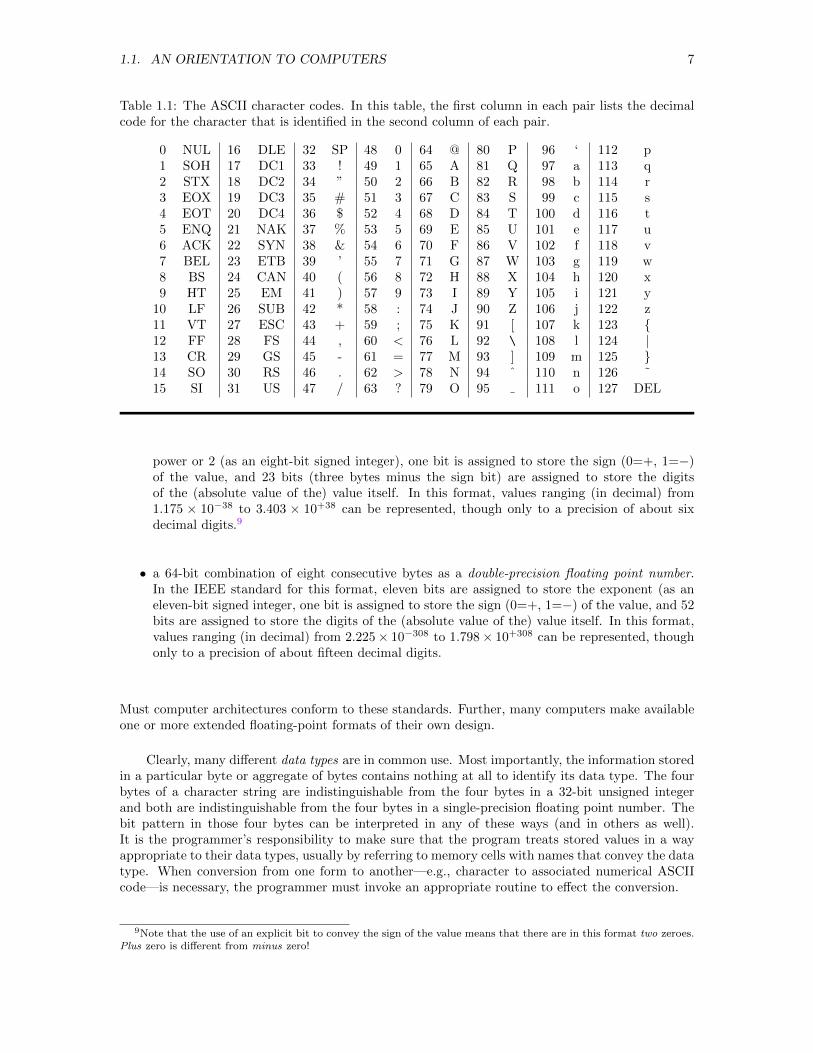
1.1. AN ORIENTATION TO COMPUTERS 7

Table 1.1: The ASCII character codes. In this table, the first column in each pair lists the decimalcode for the character that is identified in the second column of each pair.

0 NUL 16 DLE 32 SP 48 0 64 @ 80 P 96 ‘ 112 p1 SOH 17 DC1 33 ! 49 1 65 A 81 Q 97 a 113 q2 STX 18 DC2 34 ” 50 2 66 B 82 R 98 b 114 r3 EOX 19 DC3 35 # 51 3 67 C 83 S 99 c 115 s4 EOT 20 DC4 36 $ 52 4 68 D 84 T 100 d 116 t5 ENQ 21 NAK 37 % 53 5 69 E 85 U 101 e 117 u6 ACK 22 SYN 38 & 54 6 70 F 86 V 102 f 118 v7 BEL 23 ETB 39 ’ 55 7 71 G 87 W 103 g 119 w8 BS 24 CAN 40 ( 56 8 72 H 88 X 104 h 120 x9 HT 25 EM 41 ) 57 9 73 I 89 Y 105 i 121 y

10 LF 26 SUB 42 * 58 : 74 J 90 Z 106 j 122 z11 VT 27 ESC 43 + 59 ; 75 K 91 [ 107 k 123 12 FF 28 FS 44 , 60 < 76 L 92 \ 108 l 124 |13 CR 29 GS 45 - 61 = 77 M 93 ] 109 m 125 14 SO 30 RS 46 . 62 > 78 N 94 ˆ 110 n 126 ˜15 SI 31 US 47 / 63 ? 79 O 95 111 o 127 DEL

power or 2 (as an eight-bit signed integer), one bit is assigned to store the sign (0=+, 1=−)of the value, and 23 bits (three bytes minus the sign bit) are assigned to store the digitsof the (absolute value of the) value itself. In this format, values ranging (in decimal) from1.175 × 10−38 to 3.403 × 10+38 can be represented, though only to a precision of about sixdecimal digits.9

• a 64-bit combination of eight consecutive bytes as a double-precision floating point number.In the IEEE standard for this format, eleven bits are assigned to store the exponent (as aneleven-bit signed integer, one bit is assigned to store the sign (0=+, 1=−) of the value, and 52bits are assigned to store the digits of the (absolute value of the) value itself. In this format,values ranging (in decimal) from 2.225× 10−308 to 1.798× 10+308 can be represented, thoughonly to a precision of about fifteen decimal digits.

Must computer architectures conform to these standards. Further, many computers make availableone or more extended floating-point formats of their own design.

Clearly, many different data types are in common use. Most importantly, the information storedin a particular byte or aggregate of bytes contains nothing at all to identify its data type. The fourbytes of a character string are indistinguishable from the four bytes in a 32-bit unsigned integerand both are indistinguishable from the four bytes in a single-precision floating point number. Thebit pattern in those four bytes can be interpreted in any of these ways (and in others as well).It is the programmer’s responsibility to make sure that the program treats stored values in a wayappropriate to their data types, usually by referring to memory cells with names that convey the datatype. When conversion from one form to another—e.g., character to associated numerical ASCIIcode—is necessary, the programmer must invoke an appropriate routine to effect the conversion.

9Note that the use of an explicit bit to convey the sign of the value means that there are in this format two zeroes.Plus zero is different from minus zero!

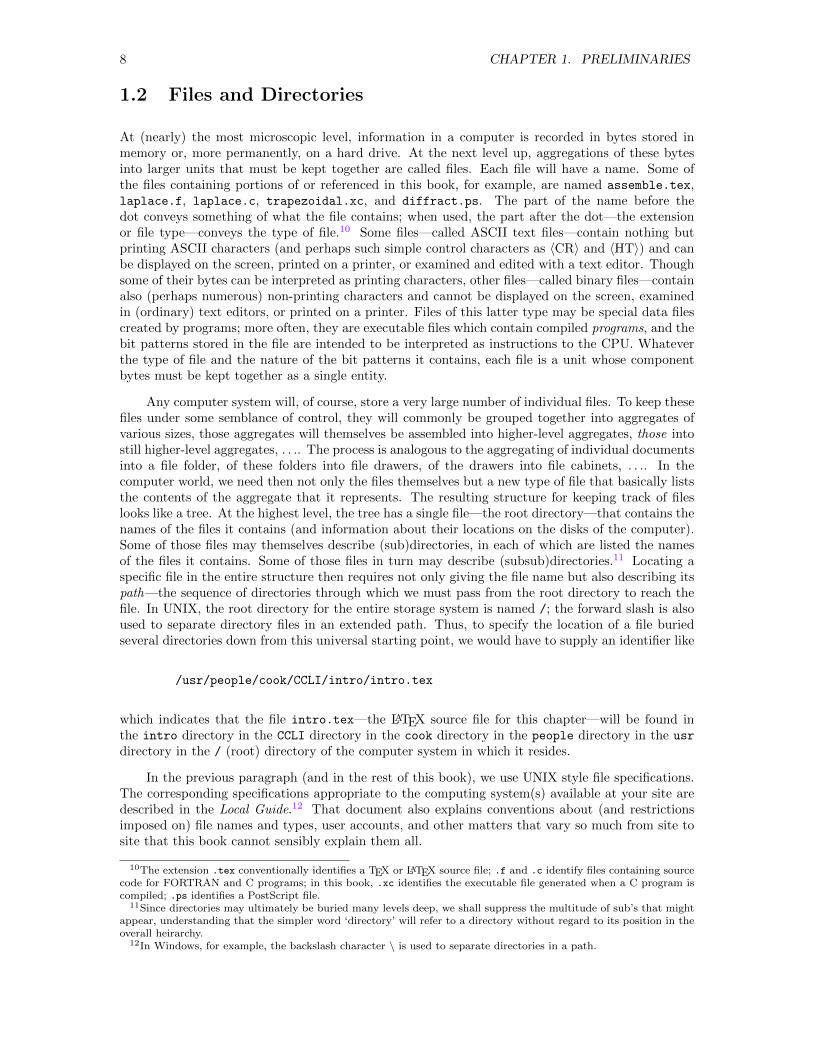
8 CHAPTER 1. PRELIMINARIES

1.2 Files and Directories

At (nearly) the most microscopic level, information in a computer is recorded in bytes stored inmemory or, more permanently, on a hard drive. At the next level up, aggregations of these bytesinto larger units that must be kept together are called files. Each file will have a name. Some ofthe files containing portions of or referenced in this book, for example, are named assemble.tex,laplace.f, laplace.c, trapezoidal.xc, and diffract.ps. The part of the name before thedot conveys something of what the file contains; when used, the part after the dot—the extensionor file type—conveys the type of file.10 Some files—called ASCII text files—contain nothing butprinting ASCII characters (and perhaps such simple control characters as 〈CR〉 and 〈HT〉) and canbe displayed on the screen, printed on a printer, or examined and edited with a text editor. Thoughsome of their bytes can be interpreted as printing characters, other files—called binary files—containalso (perhaps numerous) non-printing characters and cannot be displayed on the screen, examinedin (ordinary) text editors, or printed on a printer. Files of this latter type may be special data filescreated by programs; more often, they are executable files which contain compiled programs, and thebit patterns stored in the file are intended to be interpreted as instructions to the CPU. Whateverthe type of file and the nature of the bit patterns it contains, each file is a unit whose componentbytes must be kept together as a single entity.

Any computer system will, of course, store a very large number of individual files. To keep thesefiles under some semblance of control, they will commonly be grouped together into aggregates ofvarious sizes, those aggregates will themselves be assembled into higher-level aggregates, those intostill higher-level aggregates, . . .. The process is analogous to the aggregating of individual documentsinto a file folder, of these folders into file drawers, of the drawers into file cabinets, . . .. In thecomputer world, we need then not only the files themselves but a new type of file that basically liststhe contents of the aggregate that it represents. The resulting structure for keeping track of fileslooks like a tree. At the highest level, the tree has a single file—the root directory—that contains thenames of the files it contains (and information about their locations on the disks of the computer).Some of those files may themselves describe (sub)directories, in each of which are listed the namesof the files it contains. Some of those files in turn may describe (subsub)directories.11 Locating aspecific file in the entire structure then requires not only giving the file name but also describing itspath—the sequence of directories through which we must pass from the root directory to reach thefile. In UNIX, the root directory for the entire storage system is named /; the forward slash is alsoused to separate directory files in an extended path. Thus, to specify the location of a file buriedseveral directories down from this universal starting point, we would have to supply an identifier like

/usr/people/cook/CCLI/intro/intro.tex

which indicates that the file intro.tex—the LATEX source file for this chapter—will be found inthe intro directory in the CCLI directory in the cook directory in the people directory in the usr

directory in the / (root) directory of the computer system in which it resides.

In the previous paragraph (and in the rest of this book), we use UNIX style file specifications.The corresponding specifications appropriate to the computing system(s) available at your site aredescribed in the Local Guide.12 That document also explains conventions about (and restrictionsimposed on) file names and types, user accounts, and other matters that vary so much from site tosite that this book cannot sensibly explain them all.

10The extension .tex conventionally identifies a TEX or LATEX source file; .f and .c identify files containing sourcecode for FORTRAN and C programs; in this book, .xc identifies the executable file generated when a C program iscompiled; .ps identifies a PostScript file.

11Since directories may ultimately be buried many levels deep, we shall suppress the multitude of sub’s that mightappear, understanding that the simpler word ‘directory’ will refer to a directory without regard to its position in theoverall heirarchy.

12In Windows, for example, the backslash character \ is used to separate directories in a path.

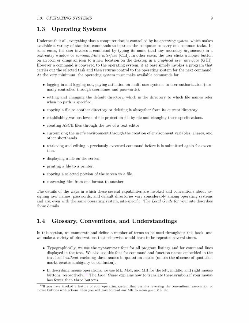
1.3. OPERATING SYSTEMS 9

1.3 Operating Systems

Underneath it all, everything that a computer does is controlled by its operating system, which makesavailable a variety of standard commands to instruct the computer to carry out common tasks. Insome cases, the user invokes a command by typing its name (and any necessary arguments) in atext-entry window or command-line interface (CLI). In other cases, the user clicks a mouse buttonon an icon or drags an icon to a new location on the desktop in a graphical user interface (GUI).However a command is conveyed to the operating system, it at base simply invokes a program thatcarries out the selected task and then returns control to the operating system for the next command.At the very minimum, the operating system must make available commands for

• logging in and logging out, paying attention on multi-user systems to user authorization (nor-mally controlled through usernames and passwords).

• setting and changing the default directory, which is the directory to which file names referwhen no path is specified.

• copying a file to another directory or deleting it altogether from its current directory.

• establishing various levels of file protection file by file and changing those specifications.

• creating ASCII files through the use of a text editor.

• customizing the user’s environment through the creation of environment variables, aliases, andother shorthands.

• retrieving and editing a previously executed command before it is submitted again for execu-tion.

• displaying a file on the screen.

• printing a file to a printer.

• copying a selected portion of the screen to a file.

• converting files from one format to another.

The details of the ways in which these several capabilities are invoked and conventions about as-signing user names, passwords, and default directories vary considerably among operating systemsand are, even with the same operating system, site-specific. The Local Guide for your site describesthose details.

1.4 Glossary, Conventions, and Understandings

In this section, we enumerate and define a number of terms to be used throughout this book, andwe make a variety of observations that otherwise would have to be repeated several times.

• Typographically, we use the typewriter font for all program listings and for command linesdisplayed in the text. We also use this font for command and function names embedded in thetext itself without enclosing these names in quotation marks (unless the absence of quotationmarks creates ambiguity or confusion).

• In describing mouse operations, we use ML, MM, and MR for the left, middle, and right mousebuttons, respectively.13 The Local Guide explains how to translate these symbols if your mousehas fewer than three buttons.

13If you have invoked a feature of your operating system that permits reversing the conventional association ofmouse buttons with actions, then you will have to read our MR to mean your ML, etc.

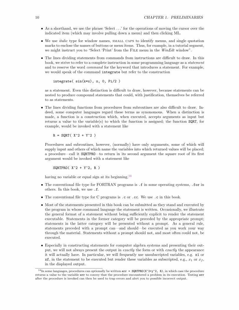
10 CHAPTER 1. PRELIMINARIES

• As a shorthand, we use the phrase ‘Select . . .’ for the operations of moving the cursor over theindicated item (which may involve pulling down a menu) and then clicking ML.

• We use italic type for window names, small caps to identify menus, and single quotationmarks to enclose the names of buttons or menu items. Thus, for example, in a tutorial segment,we might instruct you to “Select ‘Print’ from the File menu in the WinEdt window”.

• The lines dividing statements from commands from instructions are difficult to draw. In thisbook, we strive to refer to a complete instruction in some programming language as a statementand to reserve the word command for the keyword that introduces a statement. For example,we would speak of the command integrate but refer to the construction

integrate( sin(k*x), x, 0, Pi/2 )

as a statement. Even this distinction is difficult to draw, however, because statements can benested to produce compound statements that could, with justification, themselves be referredto as statements.

• The lines dividing functions from procedures from subroutines are also difficult to draw. In-deed, some computer languages regard these terms as synonomous. When a distinction ismade, a function is a construction which, when executed, accepts arguments as input butreturns a value to the variable(s) to which the function is assigned; the function SQRT, forexample, would be invoked with a statement like

R = SQRT( X^2 + Y^2 )

Procedures and subroutines, however, (normally) have only arguments, some of which willsupply input and others of which name the variables into which returned values will be placed;a procedure—call it SQRTPRO—to return in its second argument the square root of its firstargument would be invoked with a statement like

SQRTPRO( X^2 + Y^2, R )

having no variable or equal sign at its beginning.14

• The conventional file type for FORTRAN programs is .f in some operating systems, .for inothers. In this book, we use .f.

• The conventional file type for C programs is .c or .cc. We use .c in this book.

• Most of the statements presented in this book can be submitted as they stand and executed bythe program in whose command language the statement is written. Occasionally, we illustratethe general format of a statement without being sufficiently explicit to render the statementexecutable. Statements in the former category will be preceded by the appropriate prompt;statements in the latter category will be presented without a prompt. As a general rule,statements preceded with a prompt can—and should—be executed as you work your waythrough the material. Statements without a prompt should not, and most often could not, beexecuted.

• Especially in constructing statements for computer algebra systems and presenting their out-put, we will not always present the output in exactly the form or with exactly the appearanceit will actually have. In particular, we will frequently use unsubscripted variables, e.g. x1 orxf, in the statement to be executed but render these variables as subscripted, e.g., x1 or xf ,in the displayed output.

14In some languages, procedures can optionally be written err = SQRTPRO(X^2+y^2, R), in which case the procedurereturns a value to the variable err to convey that the procedure encountered a problem in its execution. Testing err

after the procedure is invoked can then be used to trap errors and alert you to possible incorrect output.

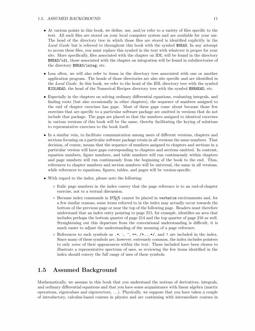
1.5. ASSUMED BACKGROUND 11

• At various points in this book, we define, use, and/or refer to a variety of files specific to thetext. All such files are stored on your local computer system and are available for your use.The head of the directory tree in which those files are stored is identified explicitly in theLocal Guide but is referred to throughout this book with the symbol $HEAD. In any attemptto access these files, you must replace this symbol in the text with whatever is proper for yoursite. More specifically, files associated with the chapter on IDL will be found in the directory$HEAD/idl, those associated with the chapter on integration will be found in subdirectories ofthe directory $HEAD/integ, etc.

• Less often, we will also refer to items in the directory tree associated with one or anotherapplication program. The heads of those directories are also site specific and are identified inthe Local Guide. In this book, we refer to the head of the IDL directory tree with the symbol$IDLHEAD, the head of the Numerical Recipes directory tree with the symbol $NRHEAD, etc.

• Especially in the chapters on solving ordinary differential equations, evaluating integrals, andfinding roots (but also occasionally in other chapters), the sequence of numbers assigned tothe end of chapter exercises has gaps. Most of these gaps come about because those fewexercises that are specific to a particular software package are omitted in versions that do notinclude that package. The gaps are placed so that the numbers assigned to identical exercisesin various versions of this book will be the same, thereby facilitating the keying of solutionsto representative exercises to the book itself.

• In a similar vein, to facilitate communication among users of different versions, chapters andsections focusing on a particular software package retain in all versions the same numbers. Thatdecision, of course, means that the sequence of numbers assigned to chapters and sections in aparticular version will have gaps corresponding to chapters and sections omitted. In contrast,equation numbers, figure numbers, and table numbers will run continuously within chaptersand page numbers will run continuously from the beginning of the book to the end. Thus,references to chapter numbers and section numbers will be universal, the same in all versions,while references to equations, figures, tables, and pages will be version-specific.

• With regard to the index, please note the following:

Italic page numbers in the index convey that the page reference is to an end-of-chapterexercise, not to a textual discussion.

Because index commands in LATEX cannot be placed in verbatim environments and, fora few similar reasons, some items referred to in the index may actually occur towards thebottom of the previous page or near the top of the following page. Readers must thereforeunderstand that an index entry pointing to page 215, for example, identifies an area thatincludes perhaps the bottom quarter of page 214 and the top quarter of page 216 as well.Straightening out this departure from the conventional understanding is difficult; it ismuch easier to adjust the understanding of the meaning of a page reference.

References to such symbols as .*, :, ^, ==, /*...*/, and ! are included in the index.Since many of these symbols are, however, extremely common, the index includes pointersto only some of their appearances within the text. Those included have been chosen toillustrate a representative spectrum of uses, so reviewing the few items identified in theindex should convey the full range of uses of these symbols.

1.5 Assumed Background

Mathematically, we assume in this book that you understand the notions of derivatives, integrals,and ordinary differential equations and that you have some acquaintance with linear algebra (matrixoperations, eigenvalues and eigenvectors, . . .). Physically, we suppose that you have taken a coupleof introductory, calculus-based courses in physics and are continuing with intermediate courses in

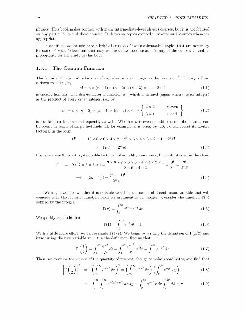
12 CHAPTER 1. PRELIMINARIES

physics. This book makes contact with many intermediate-level physics courses, but it is not focusedon any particular one of those courses. It draws on topics covered in several such courses wheneverappropriate.

In addition, we include here a brief discussion of two mathematical topics that are necessaryfor some of what follows but that may well not have been treated in any of the courses viewed asprerequisite for the study of this book.

1.5.1 The Gamma Function

The factorial function n!, which is defined when n is an integer as the product of all integers fromn down to 1, i.e., by

n! = n× (n− 1)× (n− 2)× (n− 3)× · · · × 2× 1 (1.1)

is usually familiar. The double factorial function n!!, which is defined (again when n is an integer)as the product of every other integer, i.e., by

n!! = n× (n− 2)× (n− 4)× (n− 6)× · · · ×

4× 2 n even

3× 1 n odd

(1.2)

is less familiar but occurs frequently as well. Whether n is even or odd, the double factorial canbe recast in terms of single factorials. If, for example, n is even, say 10, we can recast its doublefactorial in the form

10!! = 10× 8× 6× 4× 2 = 25 × 5× 4× 3× 2× 1 = 25 5!

=⇒ (2n)!! = 2n n! (1.3)

If n is odd, say 9, recasting its double factorial takes mildly more work, but is illustrated in the chain

9!! = 9× 7× 5× 3× 1 =9× 8× 7× 6× 5× 4× 3× 2× 1

8× 6× 4× 2=

9!

8!!=

9!

24 4!

=⇒ (2n+ 1)!! =(2n+ 1)!

2n n!(1.4)

We might wonder whether it is possible to define a function of a continuous variable that willcoincide with the factorial function when its argument is an integer. Consider the function Γ(ν)defined by the integral

Γ(ν) =

∫ ∞0

tν−1 e−t dt (1.5)

We quickly conclude that

Γ(1) =

∫ ∞0

e−t dt = 1 (1.6)

With a little more effort, we can evaluate Γ(1/2). We begin by writing the definition of Γ(1/2) andintroducing the new variable x2 = t in the definition, finding that

Γ

(1

2

)=

∫ ∞0

e−t√tdt =

∫ ∞0

e−x2

xx dx =

∫ ∞0

e−x2

dx (1.7)

Then, we examine the square of the quantity of interest, change to polar coordinates, and find that[Γ

(1

2

)]2=

(∫ ∞0

e−x2

dx

)2

=

(∫ ∞0

e−x2

dx

)(∫ ∞0

e−y2

dy

)(1.8)

=

∫ ∞0

∫ ∞0

e−(x2+y2) dx dy =

∫ ∞0

e−r2

r dr

∫ 2π

0

dφ = π (1.9)

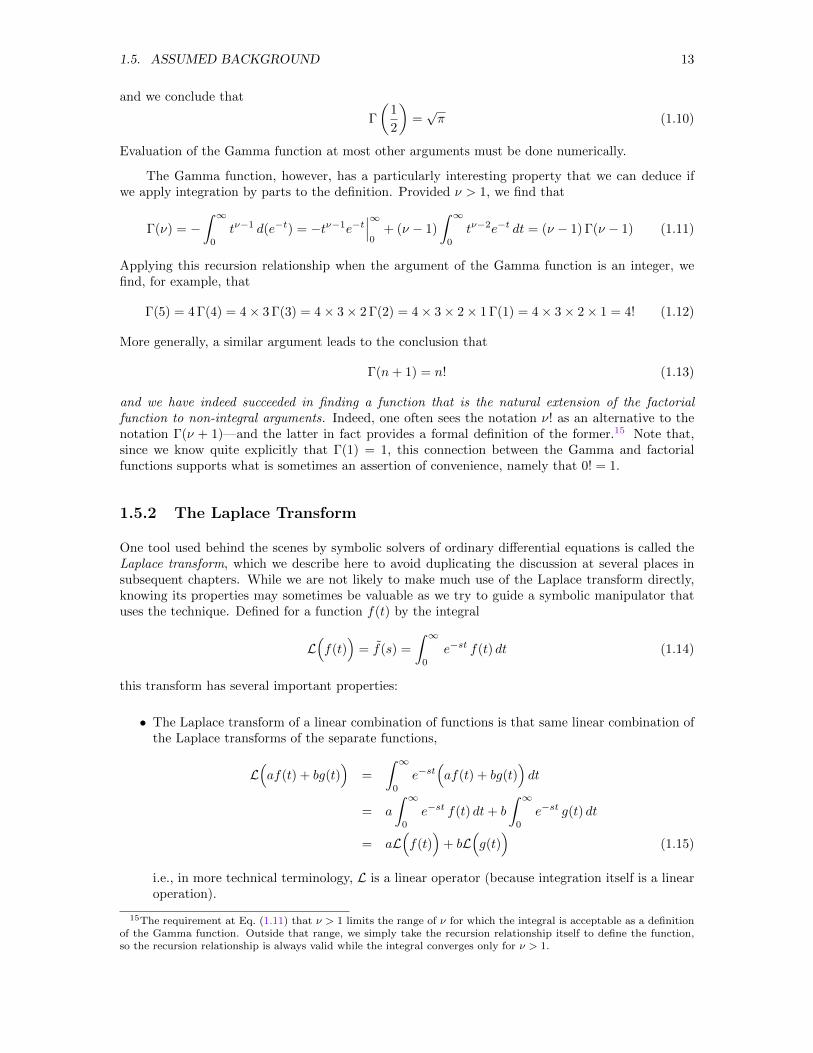
1.5. ASSUMED BACKGROUND 13

and we conclude that

Γ

(1

2

)=√π (1.10)

Evaluation of the Gamma function at most other arguments must be done numerically.

The Gamma function, however, has a particularly interesting property that we can deduce ifwe apply integration by parts to the definition. Provided ν > 1, we find that

Γ(ν) = −∫ ∞0

tν−1 d(e−t) = −tν−1e−t∣∣∣∞0

+ (ν − 1)

∫ ∞0

tν−2e−t dt = (ν − 1) Γ(ν − 1) (1.11)

Applying this recursion relationship when the argument of the Gamma function is an integer, wefind, for example, that

Γ(5) = 4 Γ(4) = 4× 3 Γ(3) = 4× 3× 2 Γ(2) = 4× 3× 2× 1 Γ(1) = 4× 3× 2× 1 = 4! (1.12)

More generally, a similar argument leads to the conclusion that

Γ(n+ 1) = n! (1.13)

and we have indeed succeeded in finding a function that is the natural extension of the factorialfunction to non-integral arguments. Indeed, one often sees the notation ν! as an alternative to thenotation Γ(ν + 1)—and the latter in fact provides a formal definition of the former.15 Note that,since we know quite explicitly that Γ(1) = 1, this connection between the Gamma and factorialfunctions supports what is sometimes an assertion of convenience, namely that 0! = 1.

1.5.2 The Laplace Transform

One tool used behind the scenes by symbolic solvers of ordinary differential equations is called theLaplace transform, which we describe here to avoid duplicating the discussion at several places insubsequent chapters. While we are not likely to make much use of the Laplace transform directly,knowing its properties may sometimes be valuable as we try to guide a symbolic manipulator thatuses the technique. Defined for a function f(t) by the integral

L(f(t)

)= f(s) =

∫ ∞0

e−st f(t) dt (1.14)

this transform has several important properties:

• The Laplace transform of a linear combination of functions is that same linear combination ofthe Laplace transforms of the separate functions,

L(af(t) + bg(t)

)=

∫ ∞0

e−st(af(t) + bg(t)

)dt

= a

∫ ∞0

e−st f(t) dt+ b

∫ ∞0

e−st g(t) dt

= aL(f(t)

)+ bL

(g(t)

)(1.15)

i.e., in more technical terminology, L is a linear operator (because integration itself is a linearoperation).

15The requirement at Eq. (1.11) that ν > 1 limits the range of ν for which the integral is acceptable as a definitionof the Gamma function. Outside that range, we simply take the recursion relationship itself to define the function,so the recursion relationship is always valid while the integral converges only for ν > 1.

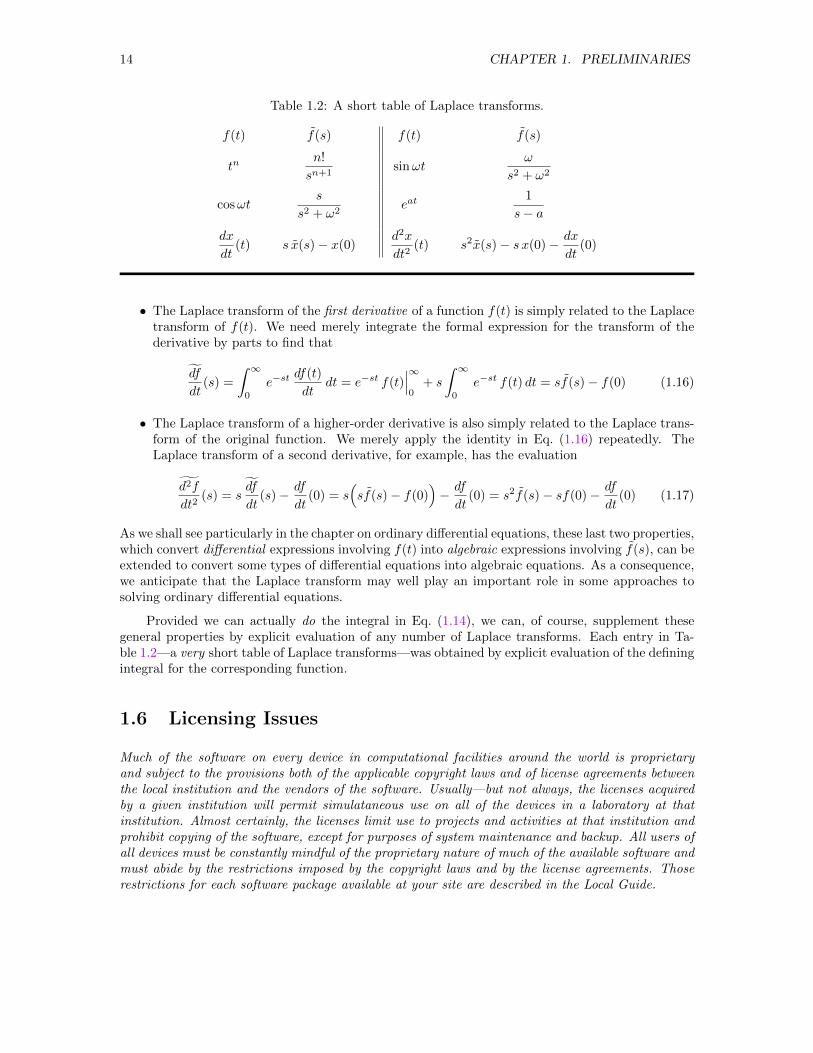
14 CHAPTER 1. PRELIMINARIES

Table 1.2: A short table of Laplace transforms.

f(t) f(s) f(t) f(s)

tnn!

sn+1sinωt

ω

s2 + ω2

cosωts

s2 + ω2eat

1

s− adx

dt(t) s x(s)− x(0)

d2x

dt2(t) s2x(s)− s x(0)− dx

dt(0)

• The Laplace transform of the first derivative of a function f(t) is simply related to the Laplacetransform of f(t). We need merely integrate the formal expression for the transform of thederivative by parts to find that

df

dt(s) =

∫ ∞0

e−stdf(t)

dtdt = e−st f(t)

∣∣∣∞0

+ s

∫ ∞0

e−st f(t) dt = sf(s)− f(0) (1.16)

• The Laplace transform of a higher-order derivative is also simply related to the Laplace trans-form of the original function. We merely apply the identity in Eq. (1.16) repeatedly. TheLaplace transform of a second derivative, for example, has the evaluation

d2f

dt2(s) = s

df

dt(s)− df

dt(0) = s

(sf(s)− f(0)

)− df

dt(0) = s2f(s)− sf(0)− df

dt(0) (1.17)

As we shall see particularly in the chapter on ordinary differential equations, these last two properties,which convert differential expressions involving f(t) into algebraic expressions involving f(s), can beextended to convert some types of differential equations into algebraic equations. As a consequence,we anticipate that the Laplace transform may well play an important role in some approaches tosolving ordinary differential equations.

Provided we can actually do the integral in Eq. (1.14), we can, of course, supplement thesegeneral properties by explicit evaluation of any number of Laplace transforms. Each entry in Ta-ble 1.2—a very short table of Laplace transforms—was obtained by explicit evaluation of the definingintegral for the corresponding function.

1.6 Licensing Issues

Much of the software on every device in computational facilities around the world is proprietaryand subject to the provisions both of the applicable copyright laws and of license agreements betweenthe local institution and the vendors of the software. Usually—but not always, the licenses acquiredby a given institution will permit simulataneous use on all of the devices in a laboratory at thatinstitution. Almost certainly, the licenses limit use to projects and activities at that institution andprohibit copying of the software, except for purposes of system maintenance and backup. All users ofall devices must be constantly mindful of the proprietary nature of much of the available software andmust abide by the restrictions imposed by the copyright laws and by the license agreements. Thoserestrictions for each software package available at your site are described in the Local Guide.

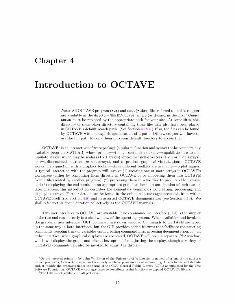
Chapter 4

Introduction to OCTAVE

Note: All OCTAVE program (*.m) and data (*.dat) files referred to in this chapterare available in the directory $HEAD/octave, where (as defined in the Local Guide)$HEAD must be replaced by the appropriate path for your site. At some sites, thisdirectory or some other directory containing these files may also have been placedin OCTAVE’s default search path. (See Section 4.18.4.) If so, the files can be foundby OCTAVE without explicit specification of a path. Otherwise, you will have touse the full path to copy them into your default directory to access them.

OCTAVE1 is an interactive software package (similar in function and syntax to the commerciallyavailable program MATLAB) whose primary—though certainly not only—capabilities are to ma-nipulate arrays, which may be scalars (1×1 arrays), one-dimensional vectors (1×n or n×1 arrays),or two-dimensional matrices (m × n arrays), and to produce graphical visualizations. OCTAVEworks in conjunction with a graphics toolkit—three different toolkits are available—to plot figures.A typical interaction with the program will involve (1) creating one or more arrays in OCTAVE’sworkspace (either by computing them directly in OCTAVE or by importing them into OCTAVEfrom a file created by another program), (2) processing them in some way to produce other arrays,and (3) displaying the end results in an appropriate graphical form. In anticipation of such uses inlater chapters, this introduction describes the elementary commands for creating, processing, anddisplaying arrays. Further details can be found in the online help messages accessible from withinOCTAVE itself (see Section 4.8) and in assorted OCTAVE documentation (see Section 4.19). Weshall refer to this documentation collectively as the OCTAVE manuals.

Two user interfaces to OCTAVE are available. The command-line interface (CLI) is the simplerof the two and runs directly in a shell window of the operating system. When available2 and invoked,the graphical user interface (GUI) comes up in its own window. Commands to OCTAVE are typedin the same way in both interfaces, but the GUI provides added features that facilitate constructingcommands, keeping track of variables used, creating command files, accessing documentation, . . .. Ineither interface, when graphical displays are requested, OCTAVE will open a separate Plot window,which will display the graph and offer a few options for adjusting the display, though a variety ofOCTAVE commands can also be invoked to adjust the display.

1Octave, created primarily by John W. Eaton of the University of Wisconsin, is named after one of the author’sformer professors, Octave Levenspiel and is a freely available program at www.octave.org. One is free to redistributeand/or modify the programs under the terms of the GNU General Public Library (GPL) as published by the FreeSoftware Foundation. OCTAVE encourages users to contribute useful functions to expand OCTAVE’s library.

2The GUI is not available on all platforms.

15

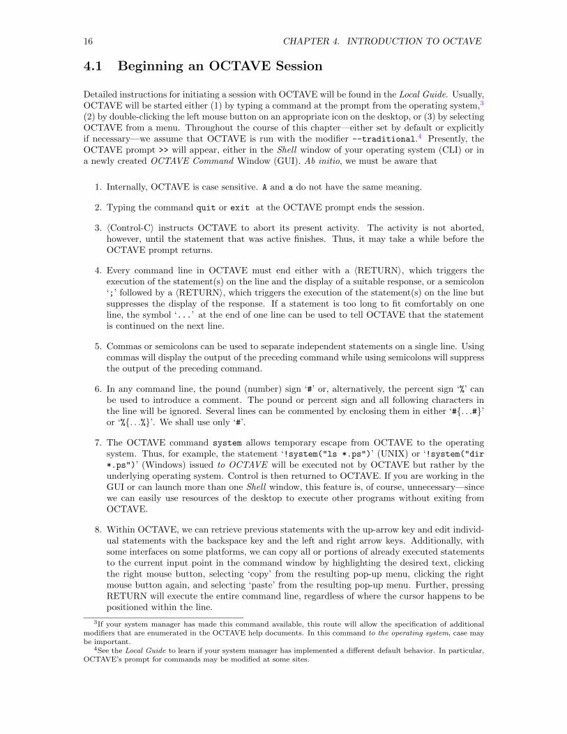
16 CHAPTER 4. INTRODUCTION TO OCTAVE

4.1 Beginning an OCTAVE Session

Detailed instructions for initiating a session with OCTAVE will be found in the Local Guide. Usually,OCTAVE will be started either (1) by typing a command at the prompt from the operating system,3

(2) by double-clicking the left mouse button on an appropriate icon on the desktop, or (3) by selectingOCTAVE from a menu. Throughout the course of this chapter—either set by default or explicitlyif necessary—we assume that OCTAVE is run with the modifier --traditional.4 Presently, theOCTAVE prompt >> will appear, either in the Shell window of your operating system (CLI) or ina newly created OCTAVE Command Window (GUI). Ab initio, we must be aware that

1. Internally, OCTAVE is case sensitive. A and a do not have the same meaning.

2. Typing the command quit or exit at the OCTAVE prompt ends the session.

3. 〈Control-C〉 instructs OCTAVE to abort its present activity. The activity is not aborted,however, until the statement that was active finishes. Thus, it may take a while before theOCTAVE prompt returns.

4. Every command line in OCTAVE must end either with a 〈RETURN〉, which triggers theexecution of the statement(s) on the line and the display of a suitable response, or a semicolon‘;’ followed by a 〈RETURN〉, which triggers the execution of the statement(s) on the line butsuppresses the display of the response. If a statement is too long to fit comfortably on oneline, the symbol ‘...’ at the end of one line can be used to tell OCTAVE that the statementis continued on the next line.

5. Commas or semicolons can be used to separate independent statements on a single line. Usingcommas will display the output of the preceding command while using semicolons will suppressthe output of the preceding command.

6. In any command line, the pound (number) sign ‘#’ or, alternatively, the percent sign ‘%’ canbe used to introduce a comment. The pound or percent sign and all following characters inthe line will be ignored. Several lines can be commented by enclosing them in either ‘#. . .#’or ‘%. . .%’. We shall use only ‘#’.

7. The OCTAVE command system allows temporary escape from OCTAVE to the operatingsystem. Thus, for example, the statement ‘!system("ls *.ps")’ (UNIX) or ‘!system("dir*.ps")’ (Windows) issued to OCTAVE will be executed not by OCTAVE but rather by theunderlying operating system. Control is then returned to OCTAVE. If you are working in theGUI or can launch more than one Shell window, this feature is, of course, unnecessary—sincewe can easily use resources of the desktop to execute other programs without exiting fromOCTAVE.

8. Within OCTAVE, we can retrieve previous statements with the up-arrow key and edit individ-ual statements with the backspace key and the left and right arrow keys. Additionally, withsome interfaces on some platforms, we can copy all or portions of already executed statementsto the current input point in the command window by highlighting the desired text, clickingthe right mouse button, selecting ‘copy’ from the resulting pop-up menu, clicking the rightmouse button again, and selecting ‘paste’ from the resulting pop-up menu. Further, pressingRETURN will execute the entire command line, regardless of where the cursor happens to bepositioned within the line.

3If your system manager has made this command available, this route will allow the specification of additionalmodifiers that are enumerated in the OCTAVE help documents. In this command to the operating system, case maybe important.

4See the Local Guide to learn if your system manager has implemented a different default behavior. In particular,OCTAVE’s prompt for commands may be modified at some sites.

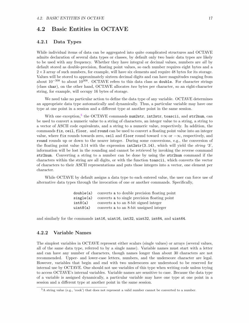
4.2. BASIC ENTITIES IN OCTAVE 17

4.2 Basic Entities in OCTAVE

4.2.1 Data Types

While individual items of data can be aggregated into quite complicated structures and OCTAVEadmits declaration of several data types or classes, by default only two basic data types are likelyto be used with any frequency. Whether they have integral or decimal values, numbers are all bydefault stored as double-precision, floating point values, so each number requires eight bytes and a2× 3 array of such numbers, for example, will have six elements and require 48 bytes for its storage.Values will be stored to approximately sixteen decimal digits and can have magnitudes ranging fromabout 10−308 to about 10308. OCTAVE refers to this data class as double. For character strings(class char), on the other hand, OCTAVE allocates two bytes per character, so an eight-characterstring, for example, will occupy 16 bytes of storage.

We need take no particular action to define the data type of any variable. OCTAVE determinesan appropriate data type automatically and dynamically. Thus, a particular variable may have onetype at one point in a session and a different type at another point in the same session.

With one exception,5 the OCTAVE commands num2str, int2str, toascii, and str2num, canbe used to convert a numeric value to a string of characters, an integer value to a string, a string toa vector of ASCII code equivalents, and a string to a numeric value, respectively. In addition, thecommands fix, ceil, floor, and round can be used to convert a floating point value into an integervalue, where fix rounds towards zero, ceil and floor round toward +∞ or −∞, respectively, andround rounds up or down to the nearer integer. During some conversions, e.g., the conversion ofthe floating point value 3.14 with the expression int2str(3.14), which will yield the string ‘3’,information will be lost in the rounding and cannot be retrieved by invoking the reverse commandstr2num. Converting a string to a number can be done by using the str2num command if thecharacters within the string are all digits, or with the function toascii, which converts the vectorof characters to their ASCII representations and puts those integers into a vector, one element percharacter.

While OCTAVE by default assigns a data type to each entered value, the user can force use ofalternative data types through the invocation of one or another commands. Specifically,

double(a) converts a to double precision floating pointsingle(a) converts a to single precision floating pointint8(a) converts a to an 8-bit signed integeruint8(a) converts a to an 8-bit unsigned integer

and similarly for the commands int16, uint16, int32, uint32, int64, and uint64.

4.2.2 Variable Names

The simplest variables in OCTAVE represent either scalars (single values) or arrays (several values,all of the same data type, referred to by a single name). Variable names must start with a letterand can have any number of characters, though names longer than about 30 characters are notrecommended. Upper- and lower-case letters, numbers, and the underscore character are legal.However, variables that begin and end with two underscores are understood to be reserved forinternal use by OCTAVE. One should not use variables of this type when writing code unless tryingto access OCTAVE’s internal variables. Variable names are sensitive to case. Because the data typeof a variable is assigned dynamically, a particular variable may have one type at one point in asession and a different type at another point in the same session.

5A string value (e.g., ’cook’) that does not represent a valid number cannot be converted to a number.

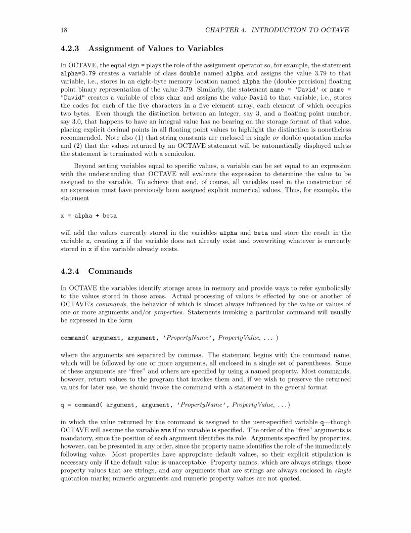
18 CHAPTER 4. INTRODUCTION TO OCTAVE

4.2.3 Assignment of Values to Variables

In OCTAVE, the equal sign = plays the role of the assignment operator so, for example, the statementalpha=3.79 creates a variable of class double named alpha and assigns the value 3.79 to thatvariable, i.e., stores in an eight-byte memory location named alpha the (double precision) floatingpoint binary representation of the value 3.79. Similarly, the statement name = ’David’ or name =

"David" creates a variable of class char and assigns the value David to that variable, i.e., storesthe codes for each of the five characters in a five element array, each element of which occupiestwo bytes. Even though the distinction between an integer, say 3, and a floating point number,say 3.0, that happens to have an integral value has no bearing on the storage format of that value,placing explicit decimal points in all floating point values to highlight the distinction is nonethelessrecommended. Note also (1) that string constants are enclosed in single or double quotation marksand (2) that the values returned by an OCTAVE statement will be automatically displayed unlessthe statement is terminated with a semicolon.

Beyond setting variables equal to specific values, a variable can be set equal to an expressionwith the understanding that OCTAVE will evaluate the expression to determine the value to beassigned to the variable. To achieve that end, of course, all variables used in the construction ofan expression must have previously been assigned explicit numerical values. Thus, for example, thestatement

x = alpha + beta

will add the values currently stored in the variables alpha and beta and store the result in thevariable x, creating x if the variable does not already exist and overwriting whatever is currentlystored in x if the variable already exists.

4.2.4 Commands

In OCTAVE the variables identify storage areas in memory and provide ways to refer symbolicallyto the values stored in those areas. Actual processing of values is effected by one or another ofOCTAVE’s commands, the behavior of which is almost always influenced by the value or values ofone or more arguments and/or properties. Statements invoking a particular command will usuallybe expressed in the form

command( argument, argument, ’PropertyName’, PropertyValue, ... )

where the arguments are separated by commas. The statement begins with the command name,which will be followed by one or more arguments, all enclosed in a single set of parentheses. Someof these arguments are “free” and others are specified by using a named property. Most commands,however, return values to the program that invokes them and, if we wish to preserve the returnedvalues for later use, we should invoke the command with a statement in the general format

q = command( argument, argument, ’PropertyName’, PropertyValue, ...)

in which the value returned by the command is assigned to the user-specified variable q—thoughOCTAVE will assume the variable ans if no variable is specified. The order of the “free” arguments ismandatory, since the position of each argument identifies its role. Arguments specified by properties,however, can be presented in any order, since the property name identifies the role of the immediatelyfollowing value. Most properties have appropriate default values, so their explicit stipulation isnecessary only if the default value is unacceptable. Property names, which are always strings, thoseproperty values that are strings, and any arguments that are strings are always enclosed in singlequotation marks; numeric arguments and numeric property values are not quoted.

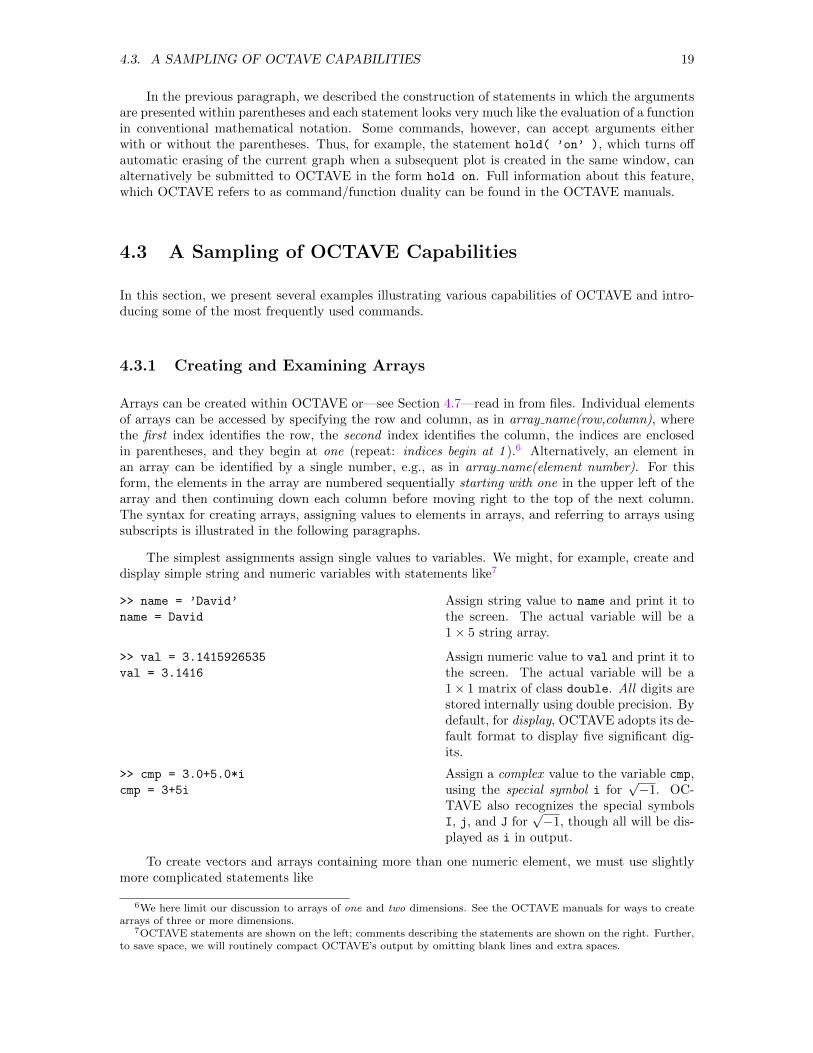
4.3. A SAMPLING OF OCTAVE CAPABILITIES 19

In the previous paragraph, we described the construction of statements in which the argumentsare presented within parentheses and each statement looks very much like the evaluation of a functionin conventional mathematical notation. Some commands, however, can accept arguments eitherwith or without the parentheses. Thus, for example, the statement hold( ’on’ ), which turns offautomatic erasing of the current graph when a subsequent plot is created in the same window, canalternatively be submitted to OCTAVE in the form hold on. Full information about this feature,which OCTAVE refers to as command/function duality can be found in the OCTAVE manuals.

4.3 A Sampling of OCTAVE Capabilities

In this section, we present several examples illustrating various capabilities of OCTAVE and intro-ducing some of the most frequently used commands.

4.3.1 Creating and Examining Arrays

Arrays can be created within OCTAVE or—see Section 4.7—read in from files. Individual elementsof arrays can be accessed by specifying the row and column, as in array name(row,column), wherethe first index identifies the row, the second index identifies the column, the indices are enclosedin parentheses, and they begin at one (repeat: indices begin at 1 ).6 Alternatively, an element inan array can be identified by a single number, e.g., as in array name(element number). For thisform, the elements in the array are numbered sequentially starting with one in the upper left of thearray and then continuing down each column before moving right to the top of the next column.The syntax for creating arrays, assigning values to elements in arrays, and referring to arrays usingsubscripts is illustrated in the following paragraphs.

The simplest assignments assign single values to variables. We might, for example, create anddisplay simple string and numeric variables with statements like7

>> name = ’David’

name = David

Assign string value to name and print it tothe screen. The actual variable will be a1× 5 string array.

>> val = 3.1415926535

val = 3.1416

Assign numeric value to val and print it tothe screen. The actual variable will be a1× 1 matrix of class double. All digits arestored internally using double precision. Bydefault, for display, OCTAVE adopts its de-fault format to display five significant dig-its.

>> cmp = 3.0+5.0*i

cmp = 3+5i

Assign a complex value to the variable cmp,using the special symbol i for

√−1. OC-

TAVE also recognizes the special symbolsI, j, and J for

√−1, though all will be dis-

played as i in output.

To create vectors and arrays containing more than one numeric element, we must use slightlymore complicated statements like

6We here limit our discussion to arrays of one and two dimensions. See the OCTAVE manuals for ways to createarrays of three or more dimensions.

7OCTAVE statements are shown on the left; comments describing the statements are shown on the right. Further,to save space, we will routinely compact OCTAVE’s output by omitting blank lines and extra spaces.

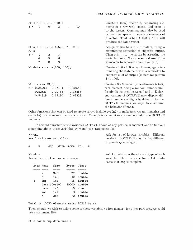
20 CHAPTER 4. INTRODUCTION TO OCTAVE

>> b = [ 1 0 3 7 10 ]

b = 1 0 3 7 10

Create a (row) vector b, separating ele-ments in a row with spaces, and print itto the screen. Commas may also be usedrather than spaces to separate elements ofa vector. That is b=[ 1,0,3,7,10 ] willproduce the same vector.

>> a = [ 1,2,3; 4,5,6; 7,8,9 ];

>> a

a = 1 2 3

4 5 6

7 8 9

Assign values to a 3 × 3 matrix, using aterminating semicolon to suppress output.Then print it to the screen by asserting thevariable name. Note the second use of thesemicolon to separate rows in an array.

>> data = zeros(100, 100); Create a 100×100 array of zeros, again ter-minating the statement with a semicolon tosuppress a lot of output (indices range from1 to 100).

>> z = rand(3,3)

z = 0.35298 0.67494 0.34545

0.52633 0.29788 0.16883

0.54319 0.69170 0.69323

Create a 3×3 matrix (nine elements total),each element being a random number uni-formly distributed between 0 and 1. Differ-ent versions of OCTAVE may display dif-ferent numbers of digits by default. See theOCTAVE manuals for ways to customizethe behavior of rand.

Other functions that can be used to create arrays include eye(n) (to make an n×n unit matrix) andmagic(n) (to make an n×n magic square). Other famous matrices are enumerated in the OCTAVEmanuals.

To remind ourselves of the variables OCTAVE knows at any particular moment and to find outsomething about those variables, we would use statements like

>> who

*** local user variables:

a b cmp data name val z

Ask for list of known variables. Differentversions of OCTAVE may display differentexplanatory messages.

>> whos

Variables in the current scope:

Attr Name Size Bytes Class

==== ==== ==== ===== =====

a 3x3 72 double

b 1x5 40 double

c cmp 1x1 16 double

data 100x100 80000 double

name 1x5 5 char

val 1x1 8 double

z 3x3 72 double

Total is 10030 elements using 80213 bytes

Ask for details on the size and type of eachvariable. The c in the column Attr indi-cates that cmp is complex.

Then, should we wish to delete some of these variables to free memory for other purposes, we coulduse a statement like

>> clear b cmp data name z

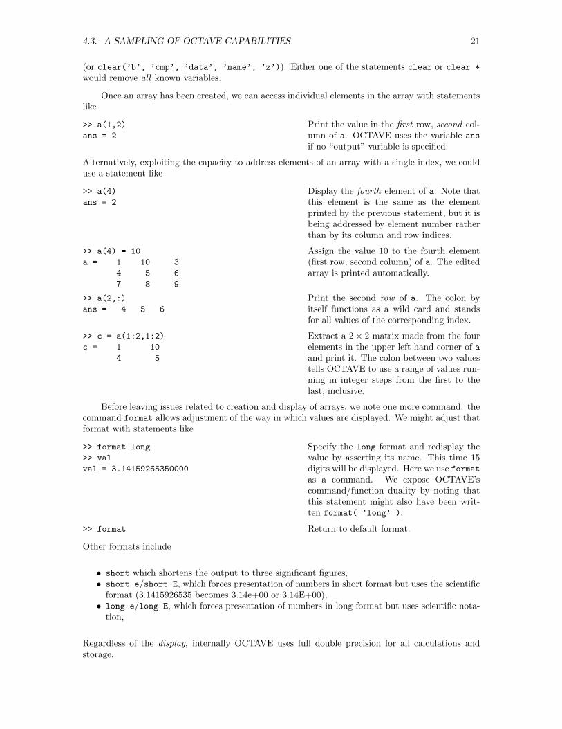
4.3. A SAMPLING OF OCTAVE CAPABILITIES 21

(or clear(’b’, ’cmp’, ’data’, ’name’, ’z’)). Either one of the statements clear or clear *

would remove all known variables.

Once an array has been created, we can access individual elements in the array with statementslike

>> a(1,2)

ans = 2

Print the value in the first row, second col-umn of a. OCTAVE uses the variable ans

if no “output” variable is specified.

Alternatively, exploiting the capacity to address elements of an array with a single index, we coulduse a statement like

>> a(4)

ans = 2

Display the fourth element of a. Note thatthis element is the same as the elementprinted by the previous statement, but it isbeing addressed by element number ratherthan by its column and row indices.

>> a(4) = 10

a = 1 10 3

4 5 6

7 8 9

Assign the value 10 to the fourth element(first row, second column) of a. The editedarray is printed automatically.

>> a(2,:)

ans = 4 5 6

Print the second row of a. The colon byitself functions as a wild card and standsfor all values of the corresponding index.

>> c = a(1:2,1:2)

c = 1 10

4 5

Extract a 2× 2 matrix made from the fourelements in the upper left hand corner of aand print it. The colon between two valuestells OCTAVE to use a range of values run-ning in integer steps from the first to thelast, inclusive.

Before leaving issues related to creation and display of arrays, we note one more command: thecommand format allows adjustment of the way in which values are displayed. We might adjust thatformat with statements like

>> format long

>> val

val = 3.14159265350000

Specify the long format and redisplay thevalue by asserting its name. This time 15digits will be displayed. Here we use formatas a command. We expose OCTAVE’scommand/function duality by noting thatthis statement might also have been writ-ten format( ’long’ ).

>> format Return to default format.

Other formats include

• short which shortens the output to three significant figures,• short e/short E, which forces presentation of numbers in short format but uses the scientific

format (3.1415926535 becomes 3.14e+00 or 3.14E+00),• long e/long E, which forces presentation of numbers in long format but uses scientific nota-

tion,

Regardless of the display, internally OCTAVE uses full double precision for all calculations andstorage.

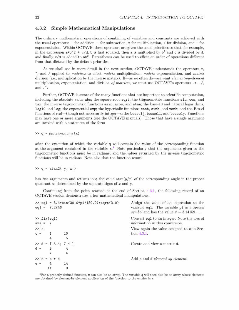
22 CHAPTER 4. INTRODUCTION TO OCTAVE

4.3.2 Simple Mathematical Manipulations

The ordinary mathematical operations of combining of variables and constants are achieved withthe usual operators: + for addition, - for subtraction, * for multiplication, / for division, and ^ forexponentiation. Within OCTAVE, these operators are given the usual priorities so that, for example,in the expression a*b^2 + c/d, b is first squared, then a is multiplied by b2 and c is divided by d,and finally c/d is added to ab2. Parentheses can be used to effect an order of operations differentfrom that dictated by the default priorities.

As we shall see in more detail in the next section, OCTAVE understands the operators *,^, and / applied to matrices to effect matrix multiplication, matrix exponentiation, and matrixdivision (i.e., multiplication by the inverse matrix). If—as we often do—we want element-by-elementmultiplication, exponentiation, and division of matrices, we must use OCTAVE’s operators .*, ./,and .^.

Further, OCTAVE is aware of the many functions that are important to scientific computation,including the absolute value abs; the square root sqrt; the trigonometric functions sin, cos, andtan; the inverse trigonometric functions asin, acos, and atan; the base-10 and natural logarithms,log10 and log; the exponential exp; the hyperbolic functions cosh, sinh, and tanh; and the Besselfunctions of real—though not necessarily integer—order besselj, besseli, and bessely. Functionsmay have one or more arguments (see the OCTAVE manuals). Those that have a single argumentare invoked with a statement of the form

>> q = function name(x)

after the execution of which the variable q will contain the value of the corresponding functionat the argument contained in the variable x.8 Note particularly that the arguments given to thetrigonometric functions must be in radians, and the values returned by the inverse trigonometricfunctions will be in radians. Note also that the function atan2

>> q = atan2( y, x )

has two arguments and returns in q the value atan(y/x) of the corresponding angle in the properquadrant as determined by the separate signs of x and y.

Continuing from the point reached at the end of Section 4.3.1, the following record of anOCTAVE session demonstrates a few mathematical manipulations:

>> eq1 = 8.4*sin(30.0*pi/180.0)*sqrt(3.0)

eq1 = 7.2746

Assign the value of an expression to thevariable eq1. The variable pi is a specialsymbol and has the value π = 3.14159 . . ..

>> fix(eq1)

ans = 7

Convert eq1 to an integer. Note the loss ofinformation in this conversion.

>> c

c = 1 10

4 5

View again the value assigned to c in Sec-tion 4.3.1.

>> d = [ 3 4; 7 4 ]

d = 3 4

7 4

Create and view a matrix d.

>> e = c + d

e = 4 14

11 9

Add c and d element by element.

8For a properly defined function, x can also be an array. The variable q will then also be an array whose elementsare obtained by element-by-element application of the function to the entries in x.

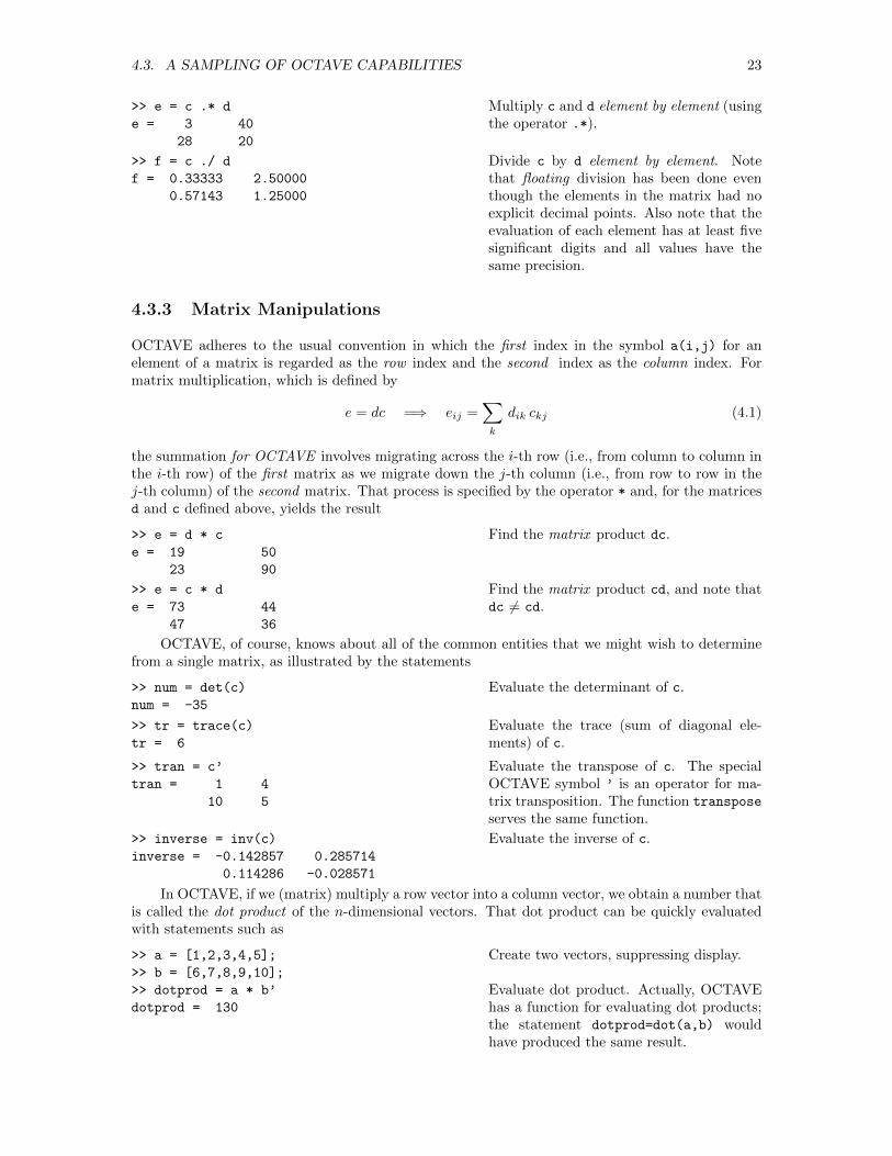
4.3. A SAMPLING OF OCTAVE CAPABILITIES 23

>> e = c .* d

e = 3 40

28 20

Multiply c and d element by element (usingthe operator .*).

>> f = c ./ d

f = 0.33333 2.50000

0.57143 1.25000

Divide c by d element by element. Notethat floating division has been done eventhough the elements in the matrix had noexplicit decimal points. Also note that theevaluation of each element has at least fivesignificant digits and all values have thesame precision.

4.3.3 Matrix Manipulations

OCTAVE adheres to the usual convention in which the first index in the symbol a(i,j) for anelement of a matrix is regarded as the row index and the second index as the column index. Formatrix multiplication, which is defined by

e = dc =⇒ eij =∑k

dik ckj (4.1)

the summation for OCTAVE involves migrating across the i-th row (i.e., from column to column inthe i-th row) of the first matrix as we migrate down the j-th column (i.e., from row to row in thej-th column) of the second matrix. That process is specified by the operator * and, for the matricesd and c defined above, yields the result

>> e = d * c

e = 19 50

23 90

Find the matrix product dc.

>> e = c * d

e = 73 44

47 36

Find the matrix product cd, and note thatdc 6= cd.

OCTAVE, of course, knows about all of the common entities that we might wish to determinefrom a single matrix, as illustrated by the statements

>> num = det(c)

num = -35

Evaluate the determinant of c.

>> tr = trace(c)

tr = 6

Evaluate the trace (sum of diagonal ele-ments) of c.

>> tran = c’

tran = 1 4

10 5

Evaluate the transpose of c. The specialOCTAVE symbol ’ is an operator for ma-trix transposition. The function transpose

serves the same function.

>> inverse = inv(c)

inverse = -0.142857 0.285714

0.114286 -0.028571

Evaluate the inverse of c.

In OCTAVE, if we (matrix) multiply a row vector into a column vector, we obtain a number thatis called the dot product of the n-dimensional vectors. That dot product can be quickly evaluatedwith statements such as

>> a = [1,2,3,4,5];

>> b = [6,7,8,9,10];

>> dotprod = a * b’

dotprod = 130

Create two vectors, suppressing display.

Evaluate dot product. Actually, OCTAVEhas a function for evaluating dot products;the statement dotprod=dot(a,b) wouldhave produced the same result.

24 CHAPTER 4. INTRODUCTION TO OCTAVE

Since the two vectors a and b are created as row vectors, the second factor in the dot productmust be transposed to convert it into a column vector before the matrix product is evaluated. Asone might expect, OCTAVE also has the analogous function cross for cross products, though thatoperation is meaningful only for vectors with three components.

4.3.4 Solving Linear Equations

OCTAVE’s matrix operations provide a quick route to solve simultaneous linear equations. Suppose,for example, we had the equations

2x1 + 5x2 + 3x3 = 3− x1 + 3x2 − 4x3 = −4

x1 − x2 = 1or

2 5 3−1 3 −4

1 −1 0

x1x2x3

=

3−4

1

(4.2)

where the matrix expression uses the usual convention for matrix multiplication. We would enterand verify the coefficient matrix and the vector of inhomogenities with the statements

>> a = [ 2.0,5.0,3.0; -1.0,3.0,-4.0; 1.0,-1.0,0.0 ]

a = 2 5 3

-1 3 -4

1 -1 0

>> b = [ 3.0; -4.0; 1.0 ]

b = 3

-4

1

Then, recognizing in the abstract that ax = b implies that x = a−1b, we might—though, from anumerical perspective, this approach is not recommended for any but the smallest systems—seek asolution with the statements

>> ainv = inv(a);

>> x = ainv * b

x = 0.85294

-0.14706

0.67647

This solution correctly solves the original equations, as hand substitution—and the statement[a*x, b]—will confirm.

Actually, OCTAVE includes another operator that further facilitates the task of solving simul-taneous linear equations. The solution a−1b could be seen as the end result of dividing the vectorb by the matrix a from the left side. OCTAVE uses the operator \ to convey this meaning. Thus,once a and b have been defined as above, the single statement

>> x = a\b

x = 0.85294

-0.14706

0.67647

yields the same result.

To carry this exposition just one step further, we might have written the equations of interestin the alternative form (

x1 x2 x3

) 2 −1 15 3 −13 −4 0

=(

3 −4 1)

(4.3)

4.3. A SAMPLING OF OCTAVE CAPABILITIES 25

i.e., in the form xC=b, where x and b are now row vectors (and C—notice—is the transpose of A).In this case, the solution would be found by evaluating x=bC−1, i.e. by multiplying b from the rightby the inverse of C (or dividing b from the right by C). The OCTAVE statements

>> c = [ 2,-1,1; 5,3,-1; 3,-4,0 ];

>> b = [ 3, -4, 1 ];

>> x = b/c

x = 0.85294 -0.14706 0.67647

yield the result we have already obtained, though the vectors are now row vectors rather than columnvectors. We could have also used c=a’; (or c = transpose(a)) and b=b’; or b = transpose(b))to get the requisite transposed matrices.

4.3.5 A First Graph

OCTAVE’s commands also facilitate the graphing of known univariate functions. First, we needa vector of values—usually, but not necessarily, equally spaced—spanning the domain of the inde-pendent variable from some starting point to some ending point. In the first instance, OCTAVEuses the colon operator ‘:’ for this purpose. For example, we might create simple vectors with thestatements

>> y = [ 0 : 1 : 5 ]

y = 0 1 2 3 4 5

Create a row vector whose first element is0, each of whose subsequent elements differsfrom its predecessor by 1, and whose lastelement does not exceed 5.

>> yy = [ -3 : 2 : 6 ]

yy = -3 -1 1 3 5

Create a second row vector whose first ele-ment is −3, each of whose subsequent ele-ments differs from its predecessor by 2, andwhose last element does not exceed 6. Thesquare brackets in this statement can beomitted.

More to the point in preparing to graph a function of a variable x, we might use a statement like

>> x = [ 0.0 : 0.1 : 10.0 ]; Create a third row vector whose first ele-ment is 0.0, each of whose subsequent ele-ments differs from its predecessor by 0.1,and whose last element does not exceed10.0. Output of this 101-element vector issuppressed with the terminating semicolon.

or we might create the same vector using the OCTAVE function linspace in a statement like

>> x = linspace( 0.0, 10.0, 101 );

Here, the arguments are, in order, the starting value, the ending value, and the number of points tobe equally distributed in the interval between the starting and the ending values, including the twobounding points. Thus, the number of segments into which the interval is divided is one less thanthe value of the third argument.

If, for example, we want a graph of the hyperbolic cosine function using 100 divisions over theinterval −3.0 ≤ x ≤ 3.0, we might use the OCTAVE statements

>> dx = 6.0 / 100.0; Determine segment size when a line oflength 6 is divided into 100 segments.

26 CHAPTER 4. INTRODUCTION TO OCTAVE

>> x = [ -3.0 : dx : 3.0 ]; Create a vector of 101 equally spaced valuesranging from −3.0 to 3.0. We could alsohave used the statement

x = linspace( -3.0, 3.0, 101);

>> y = cosh( x ); Assign to each element of a vector y thehyperbolic cosine of the corresponding ele-ment of x.

To draw the graph, OCTAVE passes the command to a subsidiary plotting toolkit. At least threesuch toolkits (qt, gnuplot, and fltk) are available in the standard distribution of OCTAVE. Beforegraphing anything, we need to find out what toolkits are available and select one, which is achievedby the statements

>> graphics_toolkit()

ans = qt

>> available_graphics_toolkits

ans =

[1,1] = fltk

[1,2] = gnuplot

[1,3] = qt

>> graphics_toolkit( "gnuplot" )

>> graphics_toolkit( ’qt’ )

Ask for default toolkit. The default may bedifferent with different platforms.Report available toolkits. Different ver-sions of OCTAVE on different platformsmay have different options.

Select gnuplot, particularly if you ulti-mately want to incorporate Greek letters inPostScript files that are output.9

Restore default, which we will use unless weneed Greek letters.

After selecting a graphics toolkit, we can invoke the plot command with the single statement

>> plot( x, y ) Plot y versus x, drawing straight line seg-ments to connect the points whose coordi-nates are provided in the two vectors. Notethat the vector containing values of the in-dependent variable is the first argument.

The last command invokes the selected graphics toolkit, and opens a new window, the Figure window,which shows the graph created by these statements. By default, the axes are drawn as a borderaround the graph and the graph itself is rendered in blue. A copy of the graph produced is shownin Fig. 4.1.

Taking control of some of the defaults adopted by the command plot or otherwise embellishingthe graph can be accomplished in several ways. We might, for example,

• use the command axis with a four-component vector as argument to specify the desired ranges(xmin, xmax) on the x axis and (ymin, ymax) on the y axis.

• use the command title to place a title on the graph.

• use the commands xlabel and ylabel to put labels on the x and y axes.

• use the command grid to replace short tics along the axes with full grid lines.

• use the command set, which will set properties controlling the characteristics of a componentof a graph, and the command gca, which specifically selects the axes in the current graph asthe operative component.10

9See Section 4.17.1 for ways to incorporate Greek letters; see Section 4.12 for ways to output PostScript and PDFfiles. Note also (1) that either single or double quotation marks can be used and (2) that, once a toolkit has beenselected, that choice remains in effect until the session is ended or until it is explicitly changed.

10Specifically, gca returns a handle—see Section 4.4—identifying the axes in the current graph.

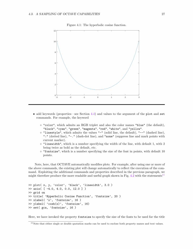
4.3. A SAMPLING OF OCTAVE CAPABILITIES 27

Figure 4.1: The hyperbolic cosine function.

-3 -2 -1 0 1 2 30

2

4

6

8

10

12

• add keywords (properties—see Section 4.4) and values to the argument of the plot and set

commands. For example, the keyword

"color", which admits an RGB triplet and also the color names "blue" (the default),"black", "cyan", "green", "magenta", "red", "white", and "yellow". "linestyle", which admits the values "-" (solid line, the default), "--" (dashed line),":" (dotted line), "-." (dash-dot line), and "none" (suppress line and mark points withcurrent marker). "linewidth", which is a number specifying the width of the line, with default 1, with 2

being twice as bold as the default, etc. "fontsize", which is a number specifying the size of the font in points, with default 10

points.

Note, here, that OCTAVE automatically modifies plots. For example, after using one or more ofthe above commands, the existing plot will change automatically to reflect the execution of the com-mand. Exploiting the additional commands and properties described in the previous paragraph, wemight therefore produce the more readable and useful graph shown in Fig. 4.2 with the statements11

>> plot( x, y, ’color’, ’black’, ’linewidth’, 3.0 )

>> axis( [ -4.0, 4.0, 0.0, 12.0 ] )

>> grid on

>> title( ’Hyperbolic Cosine Function’, ’fontsize’, 20 )

>> xlabel( ’x’, ’fontsize’, 16 )

>> ylabel( ’cosh(x)’, ’fontsize’, 16)

>> set( gca, ’fontsize’, 16 )

Here, we have invoked the property fontsize to specify the size of the fonts to be used for the title

11Note that either single or double quotation marks can be used to enclose both property names and text values.

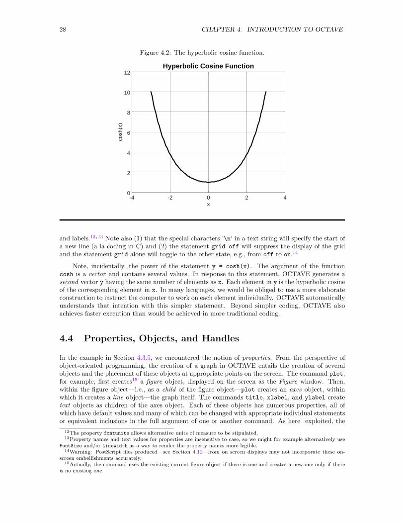
28 CHAPTER 4. INTRODUCTION TO OCTAVE

Figure 4.2: The hyperbolic cosine function.

-4 -2 0 2 40

2

4

6

8

10

12

x

cosh

(x)

Hyperbolic Cosine Function

and labels.12,13 Note also (1) that the special characters ’\n’ in a text string will specify the start ofa new line (a la coding in C) and (2) the statement grid off will suppress the display of the gridand the statement grid alone will toggle to the other state, e.g., from off to on.14

Note, incidentally, the power of the statement y = cosh(x). The argument of the functioncosh is a vector and contains several values. In response to this statement, OCTAVE generates asecond vector y having the same number of elements as x. Each element in y is the hyperbolic cosineof the corresponding element in x. In many languages, we would be obliged to use a more elaborateconstruction to instruct the computer to work on each element individually. OCTAVE automaticallyunderstands that intention with this simpler statement. Beyond simpler coding, OCTAVE alsoachieves faster execution than would be achieved in more traditional coding.

4.4 Properties, Objects, and Handles

In the example in Section 4.3.5, we encountered the notion of properties. From the perspective ofobject-oriented programming, the creation of a graph in OCTAVE entails the creation of severalobjects and the placement of these objects at appropriate points on the screen. The command plot,for example, first creates15 a figure object, displayed on the screen as the Figure window. Then,within the figure object—i.e., as a child of the figure object—plot creates an axes object, withinwhich it creates a line object—the graph itself. The commands title, xlabel, and ylabel createtext objects as children of the axes object. Each of these objects has numerous properties, all ofwhich have default values and many of which can be changed with appropriate individual statementsor equivalent inclusions in the full argument of one or another command. As here exploited, the

12The property fontunits allows alternative units of measure to be stipulated.13Property names and text values for properties are insensitive to case, so we might for example alternatively use

FontSize and/or LineWidth as a way to render the property names more legible.14Warning: PostScript files produced—see Section 4.12—from on screen displays may not incorporate these on-

screen embellishments accurately.15Actually, the command uses the existing current figure object if there is one and creates a new one only if there

is no existing one.

4.4. PROPERTIES, OBJECTS, AND HANDLES 29

properties color, linewidth, and fontsize are among those which the user can change in thisway.16

With the substance of the previous paragraph in mind, we could create the graph in Fig. 4.2much more deliberately with the statements

>> figure

>> axes(’fontsize’, 14, ’xlim’, [-4.0,4.0], ’ylim’, [0.0,12.0])

>> line( x, y, ’color’, ’black’, ’linewidth’, 4 )

>> grid on

>> title( ’Hyperbolic Cosine Function’, ’fontsize’, 20 )

>> xlabel( ’x’, ’fontsize’, 16 )

>> ylabel( ’cosh(x)’, ’fontsize’, 16 )

Here, we have used the command figure to create the figure object, the command axes to createan axes object within the figure object, and the command line to place the graph itself withinthe axes. Further, we have exploited several OCTAVE properties to take control of some of thecharacteristics of the resulting display.

Yet another way to achieve control over the properties of a display is to exploit the handlesOCTAVE assigns to the objects in the display. Normally, these handles are not displayed. We can,however, capture those handles for the figure object, the axes object, line objects, and text objectsas they are created. The statements17

>> hf = figure

>> ha = axes

>> hl = line( x, y )

>> htitle = title(’Hyperbolic Cosine Function’ )

for example, create the various objects with default properties store the handles for these objects inthe indicated variables, and (if not terminated with a semicolon) display the value of the automat-ically generated handle for the corresponding object. Once the handles are available, statementslike

>> get( hf )

>> get( ha )

>> get( hl )

>> get( htitle )

will display all possible properties and their current values, and statements like

>> set( hf )

>> set( ha )

>> set( hl )

>> set( htitle )

will reveal not only the default value (in braces) but also all legal values for each property. Moresignificantly, statements like

16In a departure from OCTAVE’s normal case-sensitive feature, the property names in the contexts of these com-mands are not case sensitive. While we did not exploit that feature in Section 4.3.5, occasionally for easy reading wewill set the first letter of each new word in the property name in upper case. We will, however, index all entirely inlower case.

17Arguments specifying properties can, of course, be included in these statements. We omit them for the sake of thecurrent example—and so that the get commands used shortly will reveal the default values of the several properties.

30 CHAPTER 4. INTRODUCTION TO OCTAVE

>> set( ha, ’FontSize’, 14, ’XLim’, [-4.0,4.0], ’YLim’, [0.0,12.0], ...

’XGrid’, ’on’, ’YGrid’, ’on’ )

>> set( hl, ’Color’, ’black’, ’LineWidth’, 4 )

>> set( htitle, ’FontSize’, 20 )

allow manipulation of individual properties after the object has been created.

Sometimes, we will forget to save handles that we will subsequently need. OCTAVE’s commandsgcf, which returns the handle of the current figure object, and gca, which returns the handle ofthe current axes object, are provided to help us recover some of those handles without having torecreate the entire display. Thus, for example, the statements

>> ha = gca

>> htitle = get( gca, ’Title’ )

will retrieve the corresponding handles for the axes object and the text object containing the title,respectively, while the statements

>> set( gcf, ’Color’, ’red’ )

>> set( gca, ’FontSize’, 14, ’XLim’, [-4.0,4.0], ’YLim’, [0.0,12.0], ...

’XGrid’, ’on’, ’YGrid’, ’on’ )

will set the background (border) color for the current figure object to red and adjust several propertiesin the current axes object without requiring us to know the handles of those objects. These functionsare especially valuable when the display is created with plot, since plot returns only a handle ofthe line created after the figure and axes objects have been created.

4.5 Saving and Retrieving the OCTAVE Session

The command save in OCTAVE will save some or all of the variables in OCTAVE’s workspace. Forexample, the statement

>> save "example.oct" a b c

saves the variables a, b, and c in a file named example.oct in the default directory.18,19 If novariables are specified, then the command save saves all of the variables currently in the OCTAVEworkspace.

Saved variables can be retrieved using the load command. To restore the file just saved, forexample, we would use the statement20

>> load "example.oct"

which loads into the OCTAVE workspace all of the variables saved in the file example.oct and giveseach the name it had originally, overwriting any existing variables with the same names.

In the first instance, the function save saves OCTAVE variables in ASCII text files. Sometimeswe may want to save the data in a more compact binary form, a task that can be accomplishedusing a switch. For example, the statements

18The default directory is also referred to as the current directory.19See Section 4.18.4 for a fuller discussion of this directory and of means to change it.20If the default directory is unclear or ill-defined, specification of the full path to the file may be needed.

4.5. SAVING AND RETRIEVING THE OCTAVE SESSION 31

>> save -binary "example.bin" a b c

>> save -mat-binary "example.mat" a b c

will save the values of the variables a, b, and c in OCTAVE compact binary format and in theMATLAB Version 6 compact binary format, respectively. The variables to be saved are separatedby spaces and come after the filename specification. To restore the files saved in this way, we woulduse the statements

>> load "example.bin"

>> load "example.mat"

which load into the OCTAVE workspace all of the variables saved in the file example.bin orexample.mat and gives each the name it had originally, overwriting any variables with the samename.

At a lower level of coding, OCTAVE also makes available several commands for working withfiles directly. For example, suppose we had a 5 × 5 array of integers stored in a variable a. Then,the statements

>> id = fopen( ’textexample.dat’, ’w’ );

>> fprintf( id, ’%5d %5d %5d %5d %5d\n’, a );

>> status = fclose( id );

will write the values in that variable as ASCII text. First, the command fopen opens a file in thedefault directory for writing (’w’),21 gives it the name textexample.dat, prepares it to receivedata, and associates with it a unique Logical U nit N umber (LUN), which—through the variableid—is used in subsequent references to this file. The variable a is then written to the file with thecommand fprintf, whose arguments specify the file, the format—see next paragraph—to be usedin structuring each line of output, and the variable(s) to output. Finally, the file associated withthe assigned id is closed.

Format specification is achieved with a string that resembles what would be used in C. In thestring above, the specification %5d indicates that the value should be output as an integer (d-format)right-justified (default) in a field 5 characters wide.22 In addition, we have stipulated display of fivevalues per line by inserting the new line character \n after the fifth item. The spaces in the formatstring stipulate that each five-character field in the line should be separated from the following fieldwith two spaces. Further, the string specifying the format is scanned repeatedly until all values ina have been output.

The resulting ASCII text file may then be read by any application that respects the structureOCTAVE gives to the file. Reading the file into OCTAVE at some later date cannot, however, bedone with the load command. Instead, the more elaborate process with the statements

>> b = zeros( 5, 5 );

>> id = fopen( ’textexample.dat’, ’r’ );

>> b = fscanf( id, ’%5d’, [5,5] );

>> status = fclose( id );

Create array of proper size.Open file for reading.Read data as a 5× 5 array into b.Close file.

21Alternatives to ’w’ are ’r’ for reading an existing file and ’a’ for appending to an existing file.22Had the file contained floating point values, we would have needed other specifiers. The specifier %n.m f formats

the number in ordinary decimal notation and right-justifies it in a field n characters wide with m digits after thedecimal point), and the specifier %n.m e formats the number in scientific notation (E-format) and right-justifies it ina field n characters wide with m digits after the decimal point). The formats %d, %f, and %e give OCTAVE authorityto pick the finer details as appropriate to each number. Clearly, we need to know something about the nature of thevalues to be written to the file before a sensible format specifier can be constructed. Further information is availablein Section 4.7 and in the OCTAVE manuals.

32 CHAPTER 4. INTRODUCTION TO OCTAVE

The resulting array b will be the same as the original array that was written into the file. Note,incidentally, that the format string %5d will be read repeatedly until all 25 items of data have beenread; there is no need to structure a more elaborate format string.23

One important warning about the structure of the file is necessary. For the example in thissection, we assumed that we had a 5 × 5 matrix. In writing the elements of that matrix into thespecified file, OCTAVE will step down the first column of the matrix, which contains five values,writing those values one at a time into the first row in the file. Then, OCTAVE will step down thesecond column, writing its five values in turn into the second row of the file. The process continuesuntil the last column has been placed in the last row of the file. In effect, the matrix in the file is thetranspose of the matrix in OCTAVE’s workspace. When this file is read back into OCTAVE by theprocedure in the previous paragraph, this transposition will be undone and the array in OCTAVEwill be identical to the original array, though (here) with a new name. If read into some other tool,care may be necessary on this front.

Please also be aware that detailed formatting of input and output is a very complicated task.Full information is in the OCTAVE manuals.

A final means to write OCTAVE output to a file uses the command diary, which saves toa file everything that is printed in the OCTAVE command window. The one argument to thiscommand names the file and will be a string. For example, to save a session in which we illustratethe differences among the several matrix products, we might execute the statements24

>> diary matrix_diary.dat [or diary( ’matrix diary.dat’ )] Opendiary file in default directory.

>> a = [ 1,3,0; 3,7,2; 0,2,4 ]

a = 1 3 0

3 7 2

0 2 4

>> b = [ 1,2,3; 4,5,6; 7,8,9 ]

1 2 3

4 5 6

7 8 9

Create and display two matrices.

>> c = a .* b

c = 1 6 0

12 35 12

0 16 36

Multiply matrices element by element.

>> d = a * b

d = 13 17 21

45 57 69

36 42 48

Multiply matrices as matrices.

>> diary off [or diary( ’off’ )] Close the file.

Once generated, the file produced by diary can easily be edited in a text editor or incorporated inother documents.

4.6 Loops, Logical Expressions, and Conditionals

Among the most ubiquitous programming structures is the loop, which provides a means by whicha statement or block of statements can be executed some number of times, typically with smallchanges controlled by a loop index. Several such structures are available in OCTAVE. The simplest

23When the file was written, since we wanted the data to appear in five rows of five each and we needed to includethe new line stipulation, we did need the more elaborate format string.

24Quotation marks are not needed around the file name, though they can be used without generating an error.

4.6. LOOPS, LOGICAL EXPRESSIONS, AND CONDITIONALS 33

is the for loop. Storing the squares of the integers from 1 to 10 in a vector, for example, is readilyaccomplished with the statements25,26

>> for i = 1:10

x(i) = i^2;

end

>> x

x = 1 4 9 16 25 36 49 64 81 100

The for/end statement (which logically is a single statement) steps through all values—integersfrom 1 through 10, inclusive—of the loop index i, calculating their squares and storing each in theproper element of x,27 and the statement x simply displays the end result.28 We make two furtherobservations: (1) If the vector x already exists in OCTAVE’s workspace with more than 10 elements,this loop will simply install new values in the first ten elements of the existing array and will leaveall other elements untouched; a safer procedure would be to invoke the statement clear x beforeexecuting the loop; (2) OCTAVE will also correctly execute the single-line presentation

>> for i = 1:10 x(i) = i^2; end

though the semicolon could be replaced with a comma had we wanted to display the vector x aseach element is added.

With an embellishment of the index, the loop can even be stepped by something other thanone, as in the statements

>> clear x

>> for i = 1:2:10 x(i) = i^2; end

>> x

x = 1 0 9 0 25 0 49 0 81

In this version, only elements 1, 3, 5, 7, and 9 are computed; elements 2, 4, 6, and 8 are assigned thevalues 0, and element 10 is not created, since the loop is not executed for that value of the index.

If we wanted not only to fill the vector x but also to see the values and the indices individually asthey are computed, we would have to incorporate both the calculation and the display in the loop, i.e.,we would have to place two statements in the loop. Since OCTAVE takes all statements betweenthe keyword for and the keyword end to be in the loop, we need merely place both statementsbetween those keywords, placing each on a new line or—alternatively—separating them on a singleline with a comma (or a semicolon—if the output is to be suppressed). Taking the second option,we would achieve the desired objective with the statements

>> clear x

>> for i = 1:2:10 x(i) = i^2; [i, x(i)], end

ans = 1 1

ans = 3 9

25Note that use of i for the loop index will override OCTAVE’s default understanding of i as√−1. The default

meaning will be restored by the statement clear i.26The coding here illustrated requires OCTAVE to adjust the size of the array x with each added value as the loop

unfolds, a process that slows the execution. A more efficient coding would preallocate space for the entire array witha statement like x = zeros(1,10), which creates the 1 × 10 vector of zeros and eliminates the overhead of repeatedextension of the array by one element.

27Without the semicolon after the statement in the for loop, we would have been presented at each step with adisplay of the values stored in x at that step.

28Alternatively, of course, we might have invoked the statements y=1:10 followed by x=y.^2, but these statementswould not have illustrated the explicit construction of a loop.

34 CHAPTER 4. INTRODUCTION TO OCTAVE

ans = 5 25

ans = 7 49

ans = 9 81

In addition to the for loop, in which we must know ahead of time how many times the loop is tobe executed, OCTAVE provides other loops that are capable of deciding when to stop by monitoringthe progress of the loop. A while loop to accomplish one of the above tasks might be structured inthe form

>> clear x

>> i = 0; while i < 10 i=i+1; x(i) = i^2; end

>> x

x = 1 4 9 16 25 36 49 64 81 100

To construct this while loop, the index i is first initialized to zero. Then, as each pass throughthe loop begins, that index is tested to see whether it has yet reached the value 10, at which pointthe loop terminates. Because the index is incremented by one with each pass through the loop,ultimately the loop will, in fact, terminate.

In constructing the while loop in the previous paragraph, we used OCTAVE’s operator <

(less than) to express our first logical condition. OCTAVE, of course, possesses the standard sixsuch operators: < (less than), > (greater than), == (equal to), ~= or != (not equal to), <= (lessthan or equal to), and >= (greater than or equal to). In addition, the operators ~ and ! togglelogical values between ‘true’ and ‘false’, so, for example, the condition i < 10 is equivalent to thecondition ~(i >= 10). Finally, Boolean algebra on logical expressions is facilitated by the operators&& (logical and) and || (logical or). OCTAVE also has the operators & and | for the complementaryelement-by-element logical conditions and the functions and, or, not, and xor.

Within OCTAVE, logical conditions have values and, if set to a variable, each such conditionwill create a 1× 1 array of class logical. Only two values, however, are allowed: 1 for true and 0for false. The statements

>> i = 5;

>> v = [ i < 10, i == 10, i > 10 ]

v = 1 0 0

(v = [ true, false, false ]) reveal those possibilities.

Logical conditions appear not only in controlling loops but also in structuring branches in a se-quence of statements. As with most programming languages, OCTAVE also possesses if/else/endand if/else/elseif/end constructs, though the else and elseif clauses can be omitted if theyare not required. Thus, for example, the statement

>> for i = 1:10

if x(i) < 0.0

x(i) = -x(i);

end

end

will replace each negative element in a vector x with the corresponding positive value and thestatement

>> if a > 0

b = a

else

b = -a

end

4.7. READING DATA FROM A FILE 35

will set b equal to the absolute value of a (though the function abs will do so more easily). Asin the previous paragraphs, we could—with careful use of commas or semicolons—compact thesestatements onto fewer lines than here used.

4.7 Reading Data from a File

Frequently, we need to read data into OCTAVE from an appropriately structured ASCII file, whichmay have been written by another program or created with a text editor. Procedures for readingsuch files into OCTAVE are described in this section. Before the data can be read, OCTAVE needsinformation about the type of data and the size and number of arrays in the file. If the file has anyheaders, OCTAVE needs to be told where to start reading the real data.

We illustrate the process with the ASCII file radio.dat, which was created by a FORTRANprogram that simulates the decay of a radioactive material into a material that is itself unstable.If this file simply contained a single array of numbers, we could read it with the command load asdescribed in Section 4.5. Unfortunately, the file begins with a single line containing labels as textand continues with 201 additional lines, each containing four numerical values, each separated fromthe next with one or more spaces.29 The first value in each line is a time, and the second, third,and fourth values are the quantities of the initial material, the intermediate material, and the final(stable) material, respectively, at that time.30 We read the data from this file with the statements

>> id = fopen(’radio.dat’, ’r’);

>> ln = fgetl(id);

>> quantity = fscanf( id, ’%f’, [4,201] );

>> status = fclose(id);

>> quantity = quantity’;

Open the file for reading, assign id.Read the first line from file.Read data. The 4 × 201 array quantity

will be created and expanded as the dataare read.Close file.Transpose to 201× 4 array.

The first line of the file is now stored in the (string) variable ln (and we shall pay no further attentionto it), and, with the transposition,31 the numerical values in the file are stored in the 201 row ×4 column array quantity. We might, for example, plot the time evolution of the quantities of thethree materials with the statements

>> plot( quantity(:,1), quantity(:,2), ’color’, ’black’, ’linewidth’, 3 )

>> hold on

>> plot( quantity(:,1), quantity(:,3), ’color’, ’black’, ’linewidth’, 3 )

>> plot( quantity(:,1), quantity(:,4), ’color’, ’black’, ’linewidth’, 3 )

>> text( 2.5, 850.0, ’A’, ’fontsize’, 16 )

>> text( 2.5, 300.0, ’B’, ’fontsize’, 16 )

>> text( 40.0, 800.0, ’C’, ’fontsize’, 16 )

>> set( gca, ’fontsize’, 16 )

>> hold off

The first of these statements selects the graphics toolkit. The second plots the quantity of theinitial material (quantity(:,2), the second column of the array) versus time (quantity(:,1),the first column of the array). Since we executed the statement hold on, the fourth and fifthstatements overplot graphs of the quantities of the second and third materials versus time. Finally,the statements invoking the command text, in which locations are expressed in the coordinates ofthe graph, place the labels A, B, and C at appropriate points on the graph. Several new features ofOCTAVE have been introduced in this example:

29Commas or tabs can also be used to separate values in a line.30Do not fail to copy this file into your directory and examine its structure with a text editor.31Remember that OCTAVE will read the rows of the file into the columns of the array.

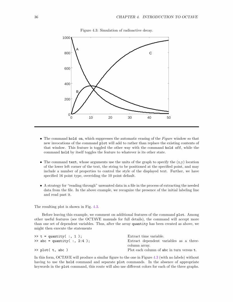
36 CHAPTER 4. INTRODUCTION TO OCTAVE

Figure 4.3: Simulation of radioactive decay.

0 10 20 30 40 500

200

400

600

800

1000

A

B

C

• The command hold on, which suppresses the automatic erasing of the Figure window so thatnew invocations of the command plot will add to rather than replace the existing contents ofthat window. This feature is toggled the other way with the command hold off, while thecommand hold by itself toggles the feature to whatever is its other state.

• The command text, whose arguments use the units of the graph to specify the (x,y) locationof the lower left corner of the text, the string to be positioned at the specified point, and mayinclude a number of properties to control the style of the displayed text. Further, we havespecified 16 point type, overriding the 10 point default.

• A strategy for “reading through” unwanted data in a file in the process of extracting the neededdata from the file. In the above example, we recognize the presence of the initial labeling lineand read past it.

The resulting plot is shown in Fig. 4.3.

Before leaving this example, we comment on additional features of the command plot. Amongother useful features (see the OCTAVE manuals for full details), the command will accept morethan one set of dependent variables. Thus, after the array quantity has been created as above, wemight then execute the statements

>> t = quantity( :, 1 );

>> abc = quantity( :, 2:4 );

>> plot( t, abc )

Extract time variable.Extract dependent variables as a three-column array.Plot each column of abc in turn versus t.

In this form, OCTAVE will produce a similar figure to the one in Figure 4.3 (with no labels) withouthaving to use the hold command and separate plot commands. In the absence of appropriatekeywords in the plot command, this route will also use different colors for each of the three graphs.

4.8. ON-LINE HELP 37

4.8 On-line Help

OCTAVE provides a way for users to request help while in an OCTAVE session. As we have alreadyseen, we can obtain information about the current status of the OCTAVE workspace or specificinformation regarding one or more of the variables stored in that workspace with the commandswho and whos, perhaps with additional arguments specifying the particular variables about whichinformation is desired. The statement

help function

e.g., help plot, help axis, and help meshgrid, will display detailed information on the specifiedcommand directly in the GUI command window or in the CLI Shell window. In many cases thedocumentation more than fills the available screen. In some versions of OCTAVE, the entire helpmessage is displayed. In other versions, only a screen full will be displayed at a time, and typing f

or the space bar will advance to the next screen, typing b will go back to the previous screen, andtyping q will exit the help message and return to the OCTAVE prompt.

In addition, the entirety of OCTAVE’s documentation is available online at their websitewww.octave.org, which can be accessed from an item in the Help menu in the GUI.

4.9 m-Files

Any command file called by OCTAVE is saved as an m-file, so named because the file itself byconvention is named with a file type ‘.m’. A command file may be a function file, which defines afunction or procedure controlled by arguments and effecting isolation of all variables internal to thefunction, or simply a batch execution file or script, which contains a succession of statements thatwe might alternatively type directly at the command line. OCTAVE makes available many built-infunctions. We have already introduced several (plot, fopen, inv, zeros, fix, sin, cosh, sqrt,. . .). Others include functions for drawing histograms, creating common statistical representations,producing colormaps and creating common matrices.

OCTAVE’s built-in functions can be supplemented with user-written scripts and functions. Thescript is the simpler of these options. We merely create a file containing exactly the statements wemight otherwise type, one at a time, interactively. For example, we might create a file containingthe lines listed in Table 4.1. Then, after this file has been stored with the name plotradio.m (say)in a directory that is in OCTAVE’s search path (see Section 4.18 and the Local Guide), the singlestatement32

>> plotradio

will instruct OCTAVE to execute each of these statements in turn and ultimately produce the graphwe have already shown in Fig. 4.3. Especially when we are doing several similar tasks or developingand debugging an extended sequence of statements, the creation of a script, which can be easilyedited, saved, and then reexecuted, can be an immense time saver. Indeed, the ’Editor’ tab in theGUI facilitates this process.

We can also define customized procedures and functions. The reserved word function onthe first non-blank line of a file informs OCTAVE that a user-defined function follows. As withscripts, every user-defined function file should be named with the file type ‘.m’. For example, thestatements listed in Table 4.233,34 define a function that plots the function funct (which must

32When no file type is specified, the file type ‘.m’ is assumed by default.33Since the function luplot assigns no value to the variable fct, we could have omitted that variable (and the

following equal sign) altogether in the first line of the file defining the function or, alternatively we could haveconveyed the absence of a returned value by replacing fct = with [] =.

34See the last paragraph of this section for a discussion of the significance of the comments before the first executablestatement in this file.

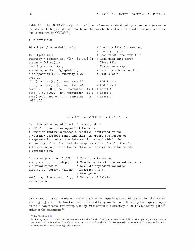
38 CHAPTER 4. INTRODUCTION TO OCTAVE

Table 4.1: The OCTAVE script plotradio.m. Comments introduced by a number sign can beincluded in the file; everything from the number sign to the end of the line will be ignored when theline is executed by OCTAVE.)

# plotradio.m

id = fopen(’radio.dat’, ’r’); # Open the file for reading,

# assigning id

ln = fgetl(id); # Read first line from file

quantity = fscanf( id, ’%f’, [4,201] ); # Read data into array

status = fclose(id); # Close file

quantity = quantity’; # Transpose array

graphics_toolkit( ’gnuplot’ ); # Select graphics toolkit

plot(quantity(:,1), quantity(:,2)) # Plot A vs t

hold on

plot(quantity(:,1), quantity(:,3)) # Add B vs t

plot(quantity(:,1), quantity(:,4)) # Add C vs t

text( 2.5, 850.0, ’A’, ’fontsize’, 16 ) # Label A

text( 2.5, 300.0, ’B’, ’fontsize’, 16 ) # Label B

text( 40.0, 800.0, ’C’, ’fontsize’, 16 ) # Label C

hold off

Table 4.2: The OCTAVE function luplot.m.

function fct = luplot(funct, N, start, stop)

# LUPLOT - Plots user-specified function.

# Function luplot is passed a function identified by the

# (string) variable funct and then, in order, the number of

# segments into which the interval is to be divided, the

# starting value of x, and the stopping value of x for the plot.

# It returns a plot of the function but assigns no value to the

# variable fct.

dx = ( stop - start ) / N; # Calculate increment

x = [ start : dx : stop ]; # Create vector of independent variable

y = feval(funct,x); # Evaluate dependent variable

plot(x, y, "color", "black", "linewidth", 2 );

# Plot graph

set( gca, ’fontsize’, 16 ); # Set size of labels

endfunction

be enclosed in quotation marks), evaluating it at N+1 equally spaced points spanning the intervalstart ≤ x ≤ stop. The function itself is invoked by typing luplot followed by the requisite argu-ments in parentheses. For example, if luplot is stored in a directory in OCTAVE’s search path,35

either of the statements36

35See Section 4.18.36 The symbol @ in this context creates a handle for the function whose name follows the symbol, which handle

then points to the function. The older notation ’cos’ still works but is now regarded as obsolete. In these and similarcontexts, we shall use the @ sign throughout.

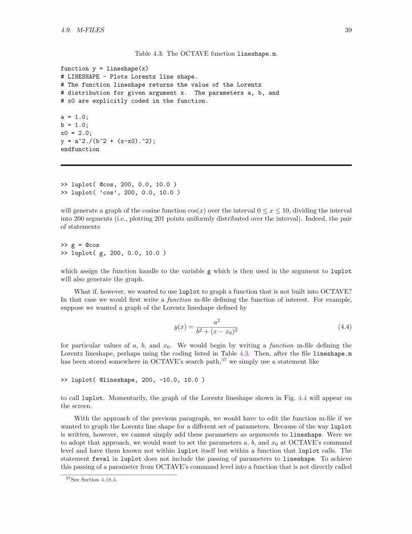
4.9. M-FILES 39

Table 4.3: The OCTAVE function lineshape.m.

function y = lineshape(x)

# LINESHAPE - Plots Lorentz line shape.

# The function lineshape returns the value of the Lorentz

# distribution for given argument x. The parameters a, b, and

# x0 are explicitly coded in the function.

a = 1.0;

b = 1.0;

x0 = 2.0;

y = a^2./(b^2 + (x-x0).^2);

endfunction

>> luplot( @cos, 200, 0.0, 10.0 )

>> luplot( ’cos’, 200, 0.0, 10.0 )

will generate a graph of the cosine function cos(x) over the interval 0 ≤ x ≤ 10, dividing the intervalinto 200 segments (i.e., plotting 201 points uniformly distributed over the interval). Indeed, the pairof statements

>> g = @cos

>> luplot( g, 200, 0.0, 10.0 )

which assign the function handle to the variable g which is then used in the argument to luplot

will also generate the graph.

What if, however, we wanted to use luplot to graph a function that is not built into OCTAVE?In that case we would first write a function m-file defining the function of interest. For example,suppose we wanted a graph of the Lorentz lineshape defined by

y(x) =a2

b2 + (x− x0)2(4.4)

for particular values of a, b, and x0. We would begin by writing a function m-file defining theLorentz lineshape, perhaps using the coding listed in Table 4.3. Then, after the file lineshape.m

has been stored somewhere in OCTAVE’s search path,37 we simply use a statement like

>> luplot( @lineshape, 200, -10.0, 10.0 )

to call luplot. Momentarily, the graph of the Lorentz lineshape shown in Fig. 4.4 will appear onthe screen.

With the approach of the previous paragraph, we would have to edit the function m-file if wewanted to graph the Lorentz line shape for a different set of parameters. Because of the way luplot

is written, however, we cannot simply add these parameters as arguments to lineshape. Were weto adopt that approach, we would want to set the parameters a, b, and x0 at OCTAVE’s commandlevel and have them known not within luplot itself but within a function that luplot calls. Thestatement feval in luplot does not include the passing of parameters to lineshape. To achievethis passing of a parameter from OCTAVE’s command level into a function that is not directly called

37See Section 4.18.4.

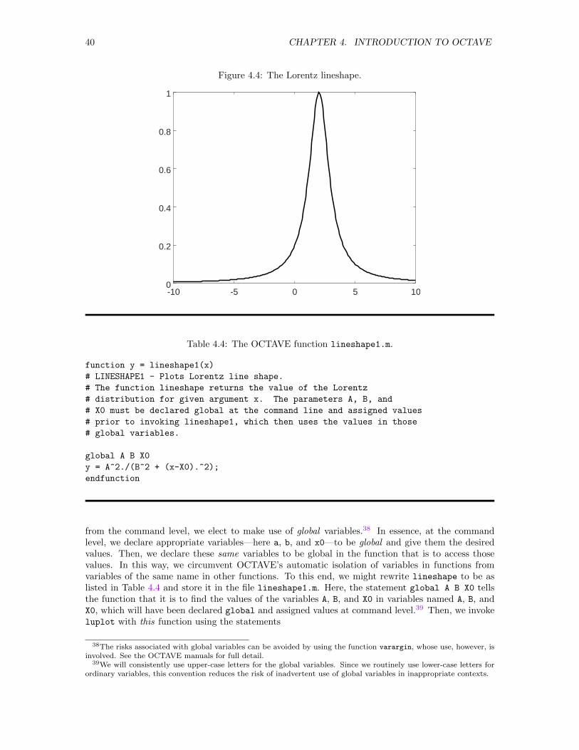
40 CHAPTER 4. INTRODUCTION TO OCTAVE

Figure 4.4: The Lorentz lineshape.

-10 -5 0 5 100

0.2

0.4

0.6

0.8

1

Table 4.4: The OCTAVE function lineshape1.m.

function y = lineshape1(x)

# LINESHAPE1 - Plots Lorentz line shape.

# The function lineshape returns the value of the Lorentz

# distribution for given argument x. The parameters A, B, and

# X0 must be declared global at the command line and assigned values

# prior to invoking lineshape1, which then uses the values in those

# global variables.

global A B X0

y = A^2./(B^2 + (x-X0).^2);

endfunction

from the command level, we elect to make use of global variables.38 In essence, at the commandlevel, we declare appropriate variables—here a, b, and x0—to be global and give them the desiredvalues. Then, we declare these same variables to be global in the function that is to access thosevalues. In this way, we circumvent OCTAVE’s automatic isolation of variables in functions fromvariables of the same name in other functions. To this end, we might rewrite lineshape to be aslisted in Table 4.4 and store it in the file lineshape1.m. Here, the statement global A B X0 tellsthe function that it is to find the values of the variables A, B, and X0 in variables named A, B, andX0, which will have been declared global and assigned values at command level.39 Then, we invokeluplot with this function using the statements

38The risks associated with global variables can be avoided by using the function varargin, whose use, however, isinvolved. See the OCTAVE manuals for full detail.

39We will consistently use upper-case letters for the global variables. Since we routinely use lower-case letters forordinary variables, this convention reduces the risk of inadvertent use of global variables in inappropriate contexts.

4.10. EIGENVALUES AND EIGENVECTORS 41

>> global A B X0

>> A = 1.0; B = 1.0; X0 = 2.0;

>> luplot( @lineshape1, 200, -10.0, 10.0)

Declare global variables.Set parameters.Graph function.

and produce again the graph shown in Fig. 4.4. This time, however, our approach is more flexible,since we can more easily change the values of the parameters and produce another graph.

The above m-files have made use of OCTAVE’s capacity for self-documentation. We have againintroduced comments with number signs.40 In function m-files, comment lines that precede the firstexecutable line in the file have special significance. The statement41

lookfor CharacterString

searches the first comment line of every m-file that it finds and displays every such line containingthe specified character string. Further, the statement42

help FileName

displays all comments preceding the first executable statement. The commands lookfor and help

will thus automatically include any user-added m-files in their scope, provided each such file isstructured with appropriate comments at its beginning. The wisdom of documenting user-writtenfunctions thoroughly cannot be overstressed, and this particular feature of MATLAB makes it easyto keep the documentation coordinated with—and in the same file as—the coding itself.

4.10 Eigenvalues and Eigenvectors

Eigenvalues and eigenvectors of symmetric matrices figure prominently in many physical contexts(finding quantum mechanical energies and energy shifts, studying small amplitude oscillations, . . .).The OCTAVE function eig takes as arguments the name of the matrix whose eigenvalues andeigenvectors are desired. The function returns either the eigenvalues or the eigenvectors and theeigenvalues, depending on the structure of the variable to which its output is directed. To findeigenvalues alone, we need only create the matrix and invoke eig with statements like

>> A = [ 1,3,0; 3,7,2; 0,2,4 ]

A = 1 3 0

3 7 2

0 2 4

>> evals = eig(A)

evals = -0.38932

3.44685

8.94246

Define matrix whose eigenvalues are soughtand display it.

Invoke eig to find eigenvalues.

If, however, we want both the eigenvectors and the eigenvalues, we would use a statement like

>> [evecs,evals] = eig(A)

evecs = 0.89123 -0.31066 0.33046

-0.41273 -0.25338 0.87490

0.18806 0.91613 0.35403

evals = -0.38932 0 0

0 3.44685 0

0 0 8.94246

40Alternatively, percent signs could be used.41Quotation marks around CharacterString are not necessary but can be included.42Quotation marks around FileName are not necessary but can be included.

42 CHAPTER 4. INTRODUCTION TO OCTAVE

With this statement, each column of the array evecs is one of the normalized eigenvectors of thematrix A; the eigenvalues are returned in a diagonal matrix.

The format of the output makes it easy to verify that the results are correct. We want theeigenvalues and eigenvectors to satisfy the simple equation

Ax = λx (4.5)

where λ is an eigenvalue and x is the corresponding eigenvector. For the first eigenvalue andeigenvector, we find that

>> lambda = evals(1,1);

>> x = evecs(:,1);

>> [A * x, lambda * x]

ans = -0.346968 -0.346968

0.160683 0.160683

-0.073215 -0.073215

Extract first eigenvalue.Extract first eigenvector.Construct two-column array with left sideof Eq. (4.5) as first column and right sideas second column.

Inspection shows that these results are the same. Similar statements focusing on the second andthird eigenvalues will confirm those results as well.

Alternatively, we can verify all eigenvalues and eigenvectors at the same time. To obtain theleft hand side of Eq. (4.5), we simply evaluate

>> lhs = A * evecs

lhs = -0.346968 -1.070789 2.955169

0.160683 -0.873354 7.823774

-0.073215 3.157761 3.165941

To obtain the right hand side, however, we must recognize that the diagonal character of the matrixof eigenvalues means that we must evaluate the product in a seemingly unnatural order, specifically

>> rhs = evecs * evals

rhs = -0.346968 -1.070789 2.955169

0.160683 -0.873354 7.823774

-0.073215 3.157761 3.165941

to have each column in the result be the product of the corresponding column in evecs times theproper eigenvalue in evals. Comparison of these two matrices confirms the correctness of all threeeigenvalues and eigenvectors at once. Indeed, knowing that internal arithmetic is done in doubleprecision, we might even examine the differences between these two sides with the statement

>> rhs - lhs

ans = 1.0e-15 * -0.11102 -0.66613 -0.88818

1.13798 1.33227 -0.88818

-0.86042 1.33227 0.88818

where the premultiplier 10−15 applies to all values.43 Evidently, the two matrices, whose values areon the order of 1, differ by values on the order of 10−15—surely equal within the roundoff errorsendemic to (double precision) computer calculations.44

OCTAVE’s command eig works on matrices that must, of course, be square, but need not besymmetric or real.

43The precise form of this output may vary from version to version and platform to platform. In all cases, however,the values will be zero within computer roundoff.

44Note that these last results are largely determined by round-off errors within the computer and may well differfrom computer to computer. In all cases, the results will be negligibly small.

4.11. GRAPHING SCALAR FUNCTIONS OF ONE VARIABLE 43

4.11 Graphing Scalar Functions of One Variable

The most common—and simplest—graph is a two-dimensional plot of a function of one variable, agraph of dependent variable versus independent variable. As we have already seen in Section 4.3.5,the basic command for producing such a graph is plot, which—in its simplest form—has the syntax

>> plot( independent variable, dependent variable )

where the two arguments identify vectors in which values of the variables to be plotted are stored.The graph itself is constructed by drawing straight line segments connecting consecutive pointsidentified in the vectors. Both vectors must, of course, have the same number of elements.

The action of plot can, however, be modified by stipulating values for one or more properties.We have already introduced a number of functions used to embellish graphs including title, xlabel,ylabel, grid, hold, and text. Other properties and functions will be introduced as the need forthem arises.

4.11.1 The Basic Strategy

As a first example, suppose that we desire a graph of the magnetic field on the z axis of a circularcurrent loop in the xy plane. As a function of position, this field is given in dimensionless form by

B(z) =1

(1 + z2)3/2(4.6)

Suppose that we want a graph over the interval −4.0 ≤ z ≤ 4.0 with 100 divisions of the interval(101 points plotted). We would then execute the OCTAVE statements

>> dz = 8.0/100.0;

>> z = [ -4.0 : dz : 4.0 ];

>> B = (1.0 + z.^2).^(-1.5);

>> plot( z, B, ’color’, ’black’, ’linewidth’, 2 )

>> set( gca, ’fontsize’, 14 )

>> title( ’Magnetic Field on z axis’, ’fontsize’, 20 )

>> xlabel( ’Dimensionless Position’, ’fontsize’, 16 )

>> ylabel( ’Magnetic Field’, ’fontsize’, 16 )

Set increment between points.Create vector of 101 values in interval.Evaluate B, also a vector of 101 values.

Plot graph.Enlarge tic labels.Title graph.Label horizontal axis.Label vertical axis.

where the functions title, xlabel, and ylabel and the fontsize property have the effects describedin Sections 4.3.5 and 4.12. This sequence of statements will produce the graph shown in Fig. 4.5.

4.11.2 Marking Points:

Sometimes, we may wish to mark the individual points in a graph with a distinct symbol. Thealternative version

>> plot( z, B, "color", "black", "." )

of the above plot command will plot a dot at each point and suppress the lines connecting thesedots. A version explicitly using the marker property, i.e.,

>> plot( z, B, "color", "black", "marker", "." )

will plot a dot at each point and also connect the dots with lines. The wide variety of availablemarkers is shown in Table 4.5. Additional marker properties include

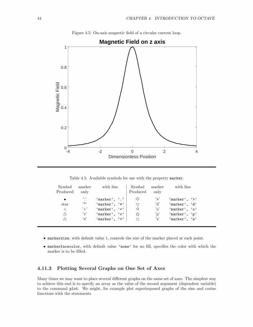
44 CHAPTER 4. INTRODUCTION TO OCTAVE

Figure 4.5: On-axis magnetic field of a circular current loop.

-4 -2 0 2 40

0.2

0.4

0.6

0.8

1

Dimensionless Position

Mag

netic

Fie

ld

Magnetic Field on z axis

Table 4.5: Available symbols for use with the property marker.

Symbol marker with line Symbol marker with lineProduced only Produced only

• ’.’ ’marker’, ’.’ 3 ’>’ ’marker’, ’>’

star ’*’ ’marker’, ’*’ 5 ’d’ ’marker’, ’d’

+ ’+’ ’marker’, ’+’ ’o’ ’marker’, ’o’

4 ’v’ ’marker’, ’v’ D ’p’ ’marker’, ’p’

4 ‘<’ ’marker’, ’<’ 2 ’s’ ’marker’, ’s’

• markersize, with default value 1, controls the size of the marker placed at each point.

• markerfacecolor, with default value ’none’ for no fill, specifies the color with which themarker is to be filled.

4.11.3 Plotting Several Graphs on One Set of Axes

Many times we may want to place several different graphs on the same set of axes. The simplest wayto achieve this end is to specify an array as the value of the second argument (dependent variable)to the command plot. We might, for example plot superimposed graphs of the sine and cosinefunctions with the statements

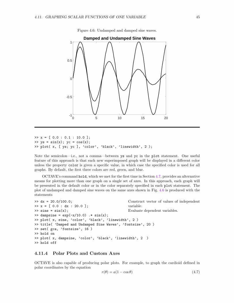
4.11. GRAPHING SCALAR FUNCTIONS OF ONE VARIABLE 45

Figure 4.6: Undamped and damped sine waves.

0 5 10 15 20-1

-0.5

0

0.5

1Damped and Undamped Sine Waves

>> x = [ 0.0 : 0.1 : 10.0 ];

>> ys = sin(x); yc = cos(x);

>> plot( x, [ ys; yc ], ’color’, ’black’, ’linewidth’, 2 );

Note the semicolon—i.e., not a comma—between ys and yc in the plot statement. One usefulfeature of this approach is that each new superimposed graph will be displayed in a different colorunless the property color is given a specific value, in which case the specified color is used for allgraphs. By default, the first three colors are red, green, and blue.

OCTAVE’s command hold, which we met for the first time in Section 4.7, provides an alternativemeans for plotting more than one graph on a single set of axes. In this approach, each graph willbe presented in the default color or in the color separately specified in each plot statement. Theplot of undamped and damped sine waves on the same axes shown in Fig. 4.6 is produced with thestatements

>> dx = 20.0/100.0;

>> x = [ 0.0 : dx : 20.0 ];

>> sine = sin(x);

>> dampsine = exp(-x/10.0) .* sin(x);

>> plot( x, sine, ’color’, ’black’, ’linewidth’, 2 )

>> title( ’Damped and Undamped Sine Waves’, ’fontsize’, 20 )

>> set( gca, ’fontsize’, 16 )

>> hold on

>> plot( x, dampsine, ’color’, ’black’, ’linewidth’, 2 )

>> hold off

Construct vector of values of independentvariable.Evaluate dependent variables.

4.11.4 Polar Plots and Custom Axes

OCTAVE is also capable of producing polar plots. For example, to graph the cardioid defined inpolar coordinates by the equation

r(θ) = a(1− cos θ) (4.7)

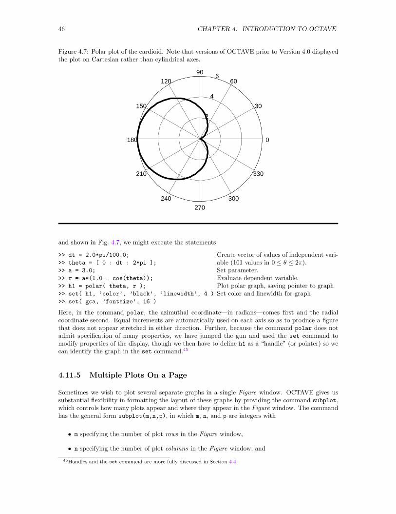
46 CHAPTER 4. INTRODUCTION TO OCTAVE

Figure 4.7: Polar plot of the cardioid. Note that versions of OCTAVE prior to Version 4.0 displayedthe plot on Cartesian rather than cylindrical axes.

2

4

6

0

30

60

90

120

150

180

210

240

270

300

330

and shown in Fig. 4.7, we might execute the statements

>> dt = 2.0*pi/100.0;

>> theta = [ 0 : dt : 2*pi ];

>> a = 3.0;

>> r = a*(1.0 - cos(theta));

>> h1 = polar( theta, r );

>> set( h1, ’color’, ’black’, ’linewidth’, 4 )

>> set( gca, ’fontsize’, 16 )

Create vector of values of independent vari-able (101 values in 0 ≤ θ ≤ 2π).Set parameter.Evaluate dependent variable.Plot polar graph, saving pointer to graphSet color and linewidth for graph

Here, in the command polar, the azimuthal coordinate—in radians—comes first and the radialcoordinate second. Equal increments are automatically used on each axis so as to produce a figurethat does not appear stretched in either direction. Further, because the command polar does notadmit specification of many properties, we have jumped the gun and used the set command tomodify properties of the display, though we then have to define h1 as a “handle” (or pointer) so wecan identify the graph in the set command.45

4.11.5 Multiple Plots On a Page

Sometimes we wish to plot several separate graphs in a single Figure window. OCTAVE gives ussubstantial flexibility in formatting the layout of these graphs by providing the command subplot,which controls how many plots appear and where they appear in the Figure window. The commandhas the general form subplot(m,n,p), in which m, n, and p are integers with

• m specifying the number of plot rows in the Figure window,

• n specifying the number of plot columns in the Figure window, and

45Handles and the set command are more fully discussed in Section 4.4.

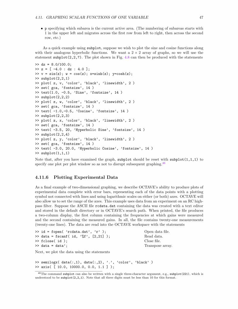
4.11. GRAPHING SCALAR FUNCTIONS OF ONE VARIABLE 47

• p specifying which subarea is the current active area. (The numbering of subareas starts with1 in the upper left and migrates across the first row from left to right, then across the secondrow, etc.)

As a quick example using subplot, suppose we wish to plot the sine and cosine functions alongwith their analogous hyperbolic functions. We want a 2 × 2 array of graphs, so we will use thestatement subplot(2,2,?). The plot shown in Fig. 4.8 can then be produced with the statements

>> dz = 8.0/100.0;

>> z = [ -4.0 : dz : 4.0 ];

>> v = sin(z); w = cos(z); x=sinh(z); y=cosh(z);

>> subplot(2,2,1)

>> plot( z, v, ’color’, ’black’, ’linewidth’, 2 )

>> set( gca, ’fontsize’, 14 )

>> text(1.0, -0.5, ’Sine’, ’fontsize’, 14 )

>> subplot(2,2,2)

>> plot( z, w, ’color’, ’black’, ’linewidth’, 2 )

>> set( gca, ’fontsize’, 14 )

>> text( -1.0,-0.5, ’Cosine’, ’fontsize’, 14 )

>> subplot(2,2,3)

>> plot( z, x, ’color’, ’black’, ’linewidth’, 2 )

>> set( gca, ’fontsize’, 14 )

>> text( -3.5, 20, ’Hyperbolic Sine’, ’fontsize’, 14 )

>> subplot(2,2,4)

>> plot( z, y, ’color’, ’black’, ’linewidth’, 2 )

>> set( gca, ’fontsize’, 14 )

>> text( -3.0, 20.0, ’Hyperbolic Cosine’, ’fontsize’, 14 )

>> subplot(1,1,1)

Note that, after you have examined the graph, subplot should be reset with subplot(1,1,1) tospecify one plot per plot window so as not to disrupt subsequent graphing.46

4.11.6 Plotting Experimental Data

As a final example of two-dimensional graphing, we describe OCTAVE’s ability to produce plots ofexperimental data complete with error bars, representing each of the data points with a plottingsymbol not connected with lines and using logarithmic scales on either (or both) axes. OCTAVE willalso allow us to set the range of the axes. This example uses data from an experiment on an RC high-pass filter. Suppose the ASCII file rcdata.dat containing the data was created with a text editorand stored in the default directory or in OCTAVE’s search path. When printed, the file producesa two-column display, the first column containing the frequencies at which gains were measuredand the second containing the measured gains. In all, the file contains twenty-one measurements(twenty-one lines). The data are read into the OCTAVE workspace with the statements

>> id = fopen( ’rcdata.dat’, ’r’ );

>> data = fscanf( id, ’%f’, [2,21] );

>> fclose( id );

>> data = data’;

Open data file.Read data.Close file.Transpose array.

Next, we plot the data using the statements

>> semilogx( data(:,1), data(:,2), ’.’, ’color’, ’black’ )

>> axis( [ 10.0, 10000.0, 0.0, 1.1 ] );

46The command subplot can also be written with a single three-character argument, e.g., subplot(221), which isunderstood to be subplot(2,2,1). Note that all three digits must be less than 10 for this format.

48 CHAPTER 4. INTRODUCTION TO OCTAVE

Figure 4.8: Graphs of sine, cosine, hyperbolic sine, and hyperbolic cosine on the interval −4 ≤ x ≤ 4.

-4 -2 0 2 4-1

-0.5

0

0.5

1

Sine

-4 -2 0 2 4-1

-0.5

0

0.5

1

Cosine

-4 -2 0 2 4-30

-20

-10

0

10

20

30

Hyperbolic Sine

-4 -2 0 2 40

5

10

15

20

25

30

Hyperbolic Cosine

>> title( ’Experimental Data for High Pass Filter’, ’fontsize’, 20 )

>> xlabel( ’Frequency’, ’fontsize’, 16 )

>> ylabel( ’Gain (Vout/Vin)’, ’fontsize’, 16 )

>> set( gca, ’fontsize’, 16 )

These statements plot the values in the second column of the array data (gain measurements, thedependent variable) versus the values in the first column (frequency measurements, the independentvariable), specifying that a logarithmic scale be used on the x axis and a linear scale on the y axis.47

Further, the stand-alone argument ’.’ in the semilogx command results in a graph in which thepoints are marked with a bold dot but no line is drawn.48 The full graph, whose beginnings havebeen created by the above statements (and whose completion will be described in what follows), ispresented in Fig. 4.9.

A graph of experimental data, however, is not complete without error bars. OCTAVE’s com-mands for making errorbars involve the statements

>> unc = data(:,2)*0.05;

>> hold on

>> errorbar( data(:,1), data(:,2), unc, ’.k’);

Compute +/- uncertainties at 5%.Hold existing plot.Draw error bars at each point, suppressingline with ’.’

After calculating the uncertainties, we invoke the OCTAVE command errorbar, providing the xand y coordinates, the uncertainty at each point, and the marker style to be used.49

A graph of experimental data should also include a plot of predicted theoretical results. The

47Three plotting combinations make use of logarithmic axes, the commands being semilogx for a logarithmic scaleon the x axis only, semilogy for a logarithmic scale on the y axis only, and loglog for logarithmic scales on both axes.

48See Section 4.11.2.49You can learn about the wide variety of arguments accepted by the errorbar command by examining what is

displayed by the command help errorbar.

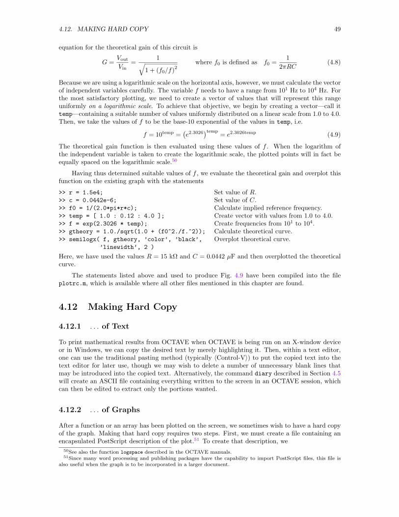
4.12. MAKING HARD COPY 49

equation for the theoretical gain of this circuit is

G =VoutVin

=1√

1 + (f0/f)2

where f0 is defined as f0 =1

2πRC(4.8)

Because we are using a logarithmic scale on the horizontal axis, however, we must calculate the vectorof independent variables carefully. The variable f needs to have a range from 101 Hz to 104 Hz. Forthe most satisfactory plotting, we need to create a vector of values that will represent this rangeuniformly on a logarithmic scale. To achieve that objective, we begin by creating a vector—call ittemp—containing a suitable number of values uniformly distributed on a linear scale from 1.0 to 4.0.Then, we take the values of f to be the base-10 exponential of the values in temp, i.e.

f = 10temp =(e2.3026

)temp= e2.3026temp (4.9)

The theoretical gain function is then evaluated using these values of f . When the logarithm ofthe independent variable is taken to create the logarithmic scale, the plotted points will in fact beequally spaced on the logarithmic scale.50

Having thus determined suitable values of f , we evaluate the theoretical gain and overplot thisfunction on the existing graph with the statements

>> r = 1.5e4;

>> c = 0.0442e-6;

>> f0 = 1/(2.0*pi*r*c);

>> temp = [ 1.0 : 0.12 : 4.0 ];

>> f = exp(2.3026 * temp);

>> gtheory = 1.0./sqrt(1.0 + (f0^2./f.^2));

>> semilogx( f, gtheory, ’color’, ’black’,

’linewidth’, 2 )

Set value of R.Set value of C.Calculate implied reference frequency.Create vector with values from 1.0 to 4.0.Create frequencies from 101 to 104.Calculate theoretical curve.Overplot theoretical curve.

Here, we have used the values R = 15 kΩ and C = 0.0442 µF and then overplotted the theoreticalcurve.

The statements listed above and used to produce Fig. 4.9 have been compiled into the fileplotrc.m, which is available where all other files mentioned in this chapter are found.

4.12 Making Hard Copy

4.12.1 . . . of Text

To print mathematical results from OCTAVE when OCTAVE is being run on an X-window deviceor in Windows, we can copy the desired text by merely highlighting it. Then, within a text editor,one can use the traditional pasting method (typically 〈Control-V〉) to put the copied text into thetext editor for later use, though we may wish to delete a number of unnecessary blank lines thatmay be introduced into the copied text. Alternatively, the command diary described in Section 4.5will create an ASCII file containing everything written to the screen in an OCTAVE session, whichcan then be edited to extract only the portions wanted.

4.12.2 . . . of Graphs

After a function or an array has been plotted on the screen, we sometimes wish to have a hard copyof the graph. Making that hard copy requires two steps. First, we must create a file containing anencapsulated PostScript description of the plot.51 To create that description, we

50See also the function logspace described in the OCTAVE manuals.51Since many word processing and publishing packages have the capability to import PostScript files, this file is

also useful when the graph is to be incorporated in a larger document.

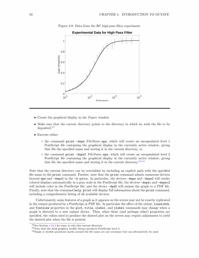
50 CHAPTER 4. INTRODUCTION TO OCTAVE

Figure 4.9: Data from the RC high-pass filter experiment.

101

102

103

104

0

0.2

0.4

0.6

0.8

1

Frequency

Gai

n (V

out/V

in)

Experimental Data for High Pass Filter

• Create the graphical display in the Figure window.

• Make sure that the current directory points to the directory in which we wish the file to bedeposited.52

• Execute either

the command print -deps FileName.eps, which will create an encapsulated level 1PostScript file containing the graphical display in the currently active window, givingthat file the specified name and storing it in the current directory, or

the command print -deps2 FileName.eps, which will create an encapsulated level 2PostScript file containing the graphical display in the currently active window, givingthat file the specified name and storing it in the current directory.53,54

Note that the current directory can be overridden by including an explicit path with the specifiedfile name in the print command. Further, note that the print command admits numerous devicesbeyond eps and -deps2 in the -d option. In particular, the devices -deps and -deps2 will rendercolored displays automatically in a gray scale in the PostScript file; the devices -depsc and -depsc2

will include color in the PostScript file; and the device -dpdf will output the graph to a PDF file.Finally, note that the command help print will display full information about the print command,including a comprehensive listing of all available devices.

Unfortunately, some features of a graph as it appears on the screen may not be exactly replicatedin the output produced by a PostScript or PDF file. In particular the effect of the color, linewidth,and fontsize properties in the plot, title, xlabel, and ylabel commands may change when agraph is directed to a new output device. Thus, when these (and perhaps other) properties arespecified, the values used to produce the desired plot on the screen may require adjustment to yieldthe desired plot when the file is printed.

52See Section 4.18.3 for ways to edit this current directory.53Note that the fltk graphics toolkit always produces PostScript level 3.54Single or double quotation marks around the file name are not necessary but can alternatively be used.

4.13. GRAPHING SCALAR FUNCTIONS OF TWO VARIABLES 51

4.13 Graphing Scalar Functions of Two Variables

Suppose the function we wish to explore graphically is a function of two independent variables, forexample,

z(x, y) = sin(2πx) sin(3πy) (4.10)

which defines the shape of the [2, 3] mode of oscillation for a square membrane, or

I(ξ, η) =

(sin ξ

ξ

)2(sin η

η

)2

(4.11)

which is related to the intensity in the diffraction pattern produced by a square aperture. In graphinga function of a single variable, we used as input to plot the values of the function at a selected setof (regularly or irregularly spaced) values spanning the desired range of that variable. Here, we needas input to any graphing routine the values of the function at a regular,55 two-dimensional grid ofselected points (xij , yij) or (ξij , ηij) covering the portion of the xy or ξη plane within which we seekto display the function graphically. In the broadest of terms, our task then will involve three steps:

1. Create two arrays, one (x, xi, . . .) containing the first coordinate (x, ξ, . . .) of all the points inthe grid and the other (y, eta, . . .) containing the second coordinate (y, η, . . .) of those points.

2. Evaluate the function over that grid, i.e., generate the array containing values of the dependentvariable at the points identified in the arrays containing the independent variables. BecauseOCTAVE processes arrays element by element, a single statement, which would have the forms

z = sin( 2.0*pi*x ) .* sin( 3.0*pi*y );

I = (sin(xi)./xi)^2 .* (sin(eta)./eta)^2;

for the functions in Eqs. (4.10) and (4.11), will usually suffice.

3. Invoke one or another graphical display routine, specifying the array (z, I, . . .) containing thedependent variable as input and perhaps specifying one or more further arguments to controldetails of the display.

In this section, we describe how to create the necessary arrays containing values of the independentvariables and then illustrate how to create different displays of these functions using mesh, surf,contour, and pol2cart.

4.13.1 A Preliminary: The Function meshgrid

In OCTAVE, the two-dimensional analog of the statement x = [ start : dx : stop ] is providedby the command meshgrid, which creates a pair of two-dimensional arrays, one containing the xcoordinates of a grid of points uniformly spaced in a region of the xy plane and the other containingthe y coordinates of points in that grid. Thus, for example, the statement

>> [x,y] = meshgrid( -3.0:2.0:3.0, -1.0:0.5:1.0 );

creates the arrays56

55With more than one independent variable, the use of irregular grids poses a particularly imposing challenge forcreating the ultimate display. We elect to limit our discussion to a regular grid of values for the independent variable.

56Note that the division of the x interval [-3.0,3.0] into three segments results in four values in the array (i.e.,−3,−1, 1, 3). In the same manner, the division of the y interval [-1.0,1.0] into four segments results in five values(−1,−0.5, 0, 0.5, 1).

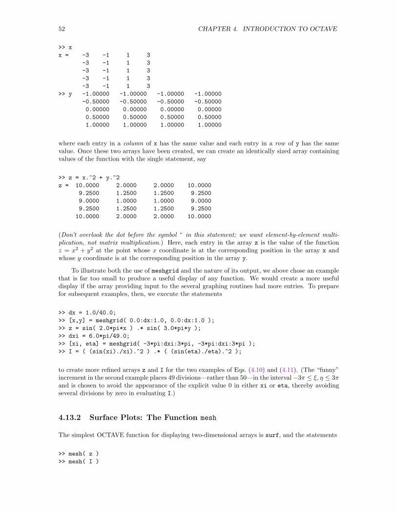
52 CHAPTER 4. INTRODUCTION TO OCTAVE

>> x

x = -3 -1 1 3

-3 -1 1 3

-3 -1 1 3

-3 -1 1 3

-3 -1 1 3

>> y -1.00000 -1.00000 -1.00000 -1.00000

-0.50000 -0.50000 -0.50000 -0.50000

0.00000 0.00000 0.00000 0.00000

0.50000 0.50000 0.50000 0.50000

1.00000 1.00000 1.00000 1.00000

where each entry in a column of x has the same value and each entry in a row of y has the samevalue. Once these two arrays have been created, we can create an identically sized array containingvalues of the function with the single statement, say

>> z = x.^2 + y.^2

z = 10.0000 2.0000 2.0000 10.0000

9.2500 1.2500 1.2500 9.2500

9.0000 1.0000 1.0000 9.0000

9.2500 1.2500 1.2500 9.2500

10.0000 2.0000 2.0000 10.0000

(Don’t overlook the dot before the symbol ^ in this statement; we want element-by-element multi-plication, not matrix multiplication.) Here, each entry in the array z is the value of the functionz = x2 + y2 at the point whose x coordinate is at the corresponding position in the array x andwhose y coordinate is at the corresponding position in the array y.

To illustrate both the use of meshgrid and the nature of its output, we above chose an examplethat is far too small to produce a useful display of any function. We would create a more usefuldisplay if the array providing input to the several graphing routines had more entries. To preparefor subsequent examples, then, we execute the statements

>> dx = 1.0/40.0;

>> [x,y] = meshgrid( 0.0:dx:1.0, 0.0:dx:1.0 );

>> z = sin( 2.0*pi*x ) .* sin( 3.0*pi*y );

>> dxi = 6.0*pi/49.0;

>> [xi, eta] = meshgrid( -3*pi:dxi:3*pi, -3*pi:dxi:3*pi );

>> I = ( (sin(xi)./xi).^2 ) .* ( (sin(eta)./eta).^2 );

to create more refined arrays z and I for the two examples of Eqs. (4.10) and (4.11). (The “funny”increment in the second example places 49 divisions—rather than 50—in the interval−3π ≤ ξ, η ≤ 3πand is chosen to avoid the appearance of the explicit value 0 in either xi or eta, thereby avoidingseveral divisions by zero in evaluating I.)

4.13.2 Surface Plots: The Function mesh

The simplest OCTAVE function for displaying two-dimensional arrays is surf, and the statements

>> mesh( z )

>> mesh( I )

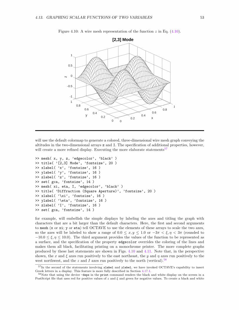
4.13. GRAPHING SCALAR FUNCTIONS OF TWO VARIABLES 53

Figure 4.10: A wire mesh representation of the function z in Eq. (4.10).

00.2

0.4y

0.60.8

1

-1

0x

-0.5

z 0

0.5

1

10.8

[2,3] Mode

0.20.4

0.6

will use the default colormap to generate a colored, three-dimensional wire mesh graph conveying thealtitudes in the two-dimensional arrays z and I. The specification of additional properties, however,will create a more refined display. Executing the more elaborate statements57

>> mesh( x, y, z, ’edgecolor’, ’black’ )

>> title( ’[2,3] Mode’, ’fontsize’, 20 )

>> xlabel( ’x’, ’fontsize’, 16 )

>> ylabel( ’y’, ’fontsize’, 16 )

>> zlabel( ’z’, ’fontsize’, 16 )

>> set( gca, ’fontsize’, 14 )

>> mesh( xi, eta, I, ’edgecolor’, ’black’ )

>> title( ’Diffraction (Square Aperture)’, ’fontsize’, 20 )

>> xlabel( ’\xi’, ’fontsize’, 16 )

>> ylabel( ’\eta’, ’fontsize’, 16 )

>> zlabel( ’I’, ’fontsize’, 16 )

>> set( gca, ’fontsize’, 14 )

for example, will embellish the simple displays by labeling the axes and titling the graph withcharacters that are a bit larger than the default characters. Here, the first and second argumentsto mesh (x or xi; y or eta) tell OCTAVE to use the elements of these arrays to scale the two axes,so the axes will be labeled to show a range of 0.0 ≤ x, y ≤ 1.0 or −3π < ξ, η < 3π (rounded to−10.0 ≤ ξ, η ≤ 10.0). The third argument provides the values of the function to be represented asa surface, and the specification of the property edgecolor overrides the coloring of the lines andmakes them all black, facilitating printing on a monochrome printer. The more complete graphsproduced by these last statements are shown in Figs. 4.10 and 4.11. Note that, in the perspectiveshown, the x and ξ axes run positively to the east northeast, the y and η axes run positively to thewest northwest, and the z and I axes run positively to the north (vertical).58

57In the second of the statements involving xlabel and ylabel, we have invoked OCTAVE’s capability to insertGreek letters in a display. This feature is more fully described in Section 4.17.1.

58Note that using the device -deps in the print command renders the black and white display on the screen in aPostScript file that uses red for positive values of z and ξ and green for negative values. To create a black and white

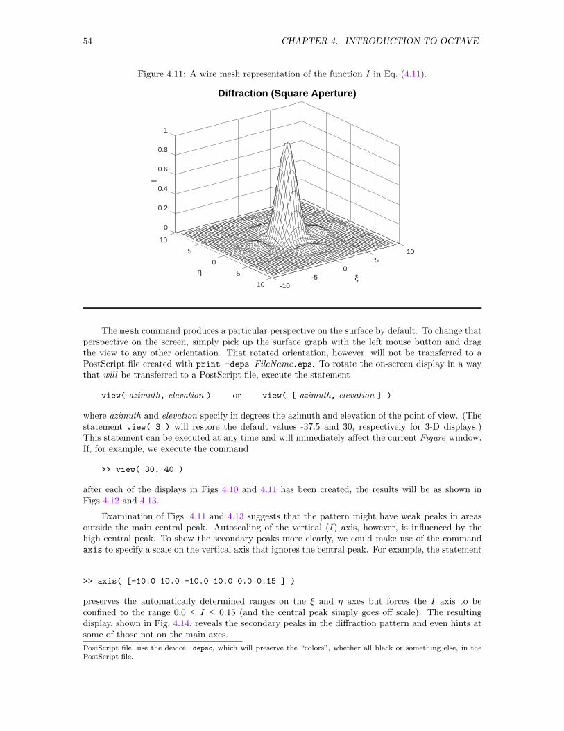
54 CHAPTER 4. INTRODUCTION TO OCTAVE

Figure 4.11: A wire mesh representation of the function I in Eq. (4.11).

-10

-5η0

5

10

0

-10

0.2

0.4

I

0.6

0.8

1

ξ

50

-5

10

Diffraction (Square Aperture)

The mesh command produces a particular perspective on the surface by default. To change thatperspective on the screen, simply pick up the surface graph with the left mouse button and dragthe view to any other orientation. That rotated orientation, however, will not be transferred to aPostScript file created with print -deps FileName.eps. To rotate the on-screen display in a waythat will be transferred to a PostScript file, execute the statement

view( azimuth, elevation ) or view( [ azimuth, elevation ] )

where azimuth and elevation specify in degrees the azimuth and elevation of the point of view. (Thestatement view( 3 ) will restore the default values -37.5 and 30, respectively for 3-D displays.)This statement can be executed at any time and will immediately affect the current Figure window.If, for example, we execute the command

>> view( 30, 40 )

after each of the displays in Figs 4.10 and 4.11 has been created, the results will be as shown inFigs 4.12 and 4.13.

Examination of Figs. 4.11 and 4.13 suggests that the pattern might have weak peaks in areasoutside the main central peak. Autoscaling of the vertical (I) axis, however, is influenced by thehigh central peak. To show the secondary peaks more clearly, we could make use of the commandaxis to specify a scale on the vertical axis that ignores the central peak. For example, the statement

>> axis( [-10.0 10.0 -10.0 10.0 0.0 0.15 ] )

preserves the automatically determined ranges on the ξ and η axes but forces the I axis to beconfined to the range 0.0 ≤ I ≤ 0.15 (and the central peak simply goes off scale). The resultingdisplay, shown in Fig. 4.14, reveals the secondary peaks in the diffraction pattern and even hints atsome of those not on the main axes.

PostScript file, use the device -depsc, which will preserve the “colors”, whether all black or something else, in thePostScript file.

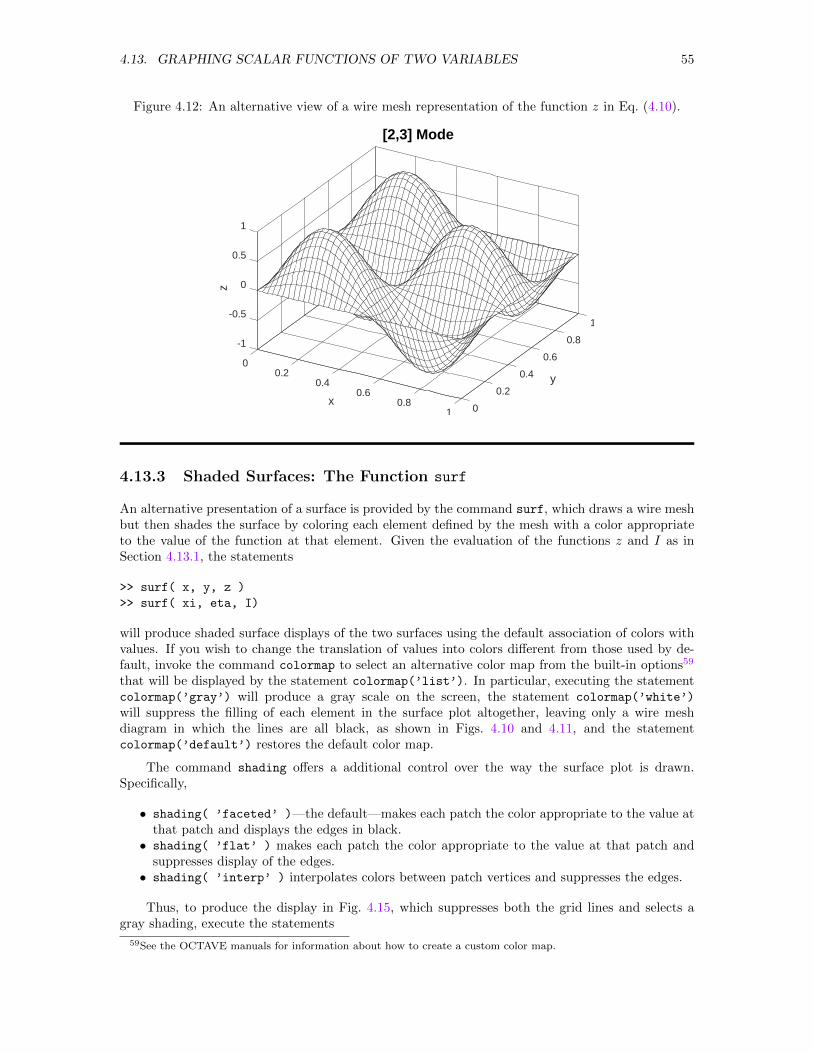
4.13. GRAPHING SCALAR FUNCTIONS OF TWO VARIABLES 55

Figure 4.12: An alternative view of a wire mesh representation of the function z in Eq. (4.10).

y

x

-1

-0.5

z 0

0.5

1

0.60.8

0.20

0.4

[2,3] Mode

0.4

0.6

0.8

1

1 0

0.2

4.13.3 Shaded Surfaces: The Function surf

An alternative presentation of a surface is provided by the command surf, which draws a wire meshbut then shades the surface by coloring each element defined by the mesh with a color appropriateto the value of the function at that element. Given the evaluation of the functions z and I as inSection 4.13.1, the statements

>> surf( x, y, z )

>> surf( xi, eta, I)

will produce shaded surface displays of the two surfaces using the default association of colors withvalues. If you wish to change the translation of values into colors different from those used by de-fault, invoke the command colormap to select an alternative color map from the built-in options59

that will be displayed by the statement colormap(’list’). In particular, executing the statementcolormap(’gray’) will produce a gray scale on the screen, the statement colormap(’white’)

will suppress the filling of each element in the surface plot altogether, leaving only a wire meshdiagram in which the lines are all black, as shown in Figs. 4.10 and 4.11, and the statementcolormap(’default’) restores the default color map.

The command shading offers a additional control over the way the surface plot is drawn.Specifically,

• shading( ’faceted’ )—the default—makes each patch the color appropriate to the value atthat patch and displays the edges in black.

• shading( ’flat’ ) makes each patch the color appropriate to the value at that patch andsuppresses display of the edges.

• shading( ’interp’ ) interpolates colors between patch vertices and suppresses the edges.

Thus, to produce the display in Fig. 4.15, which suppresses both the grid lines and selects agray shading, execute the statements

59See the OCTAVE manuals for information about how to create a custom color map.

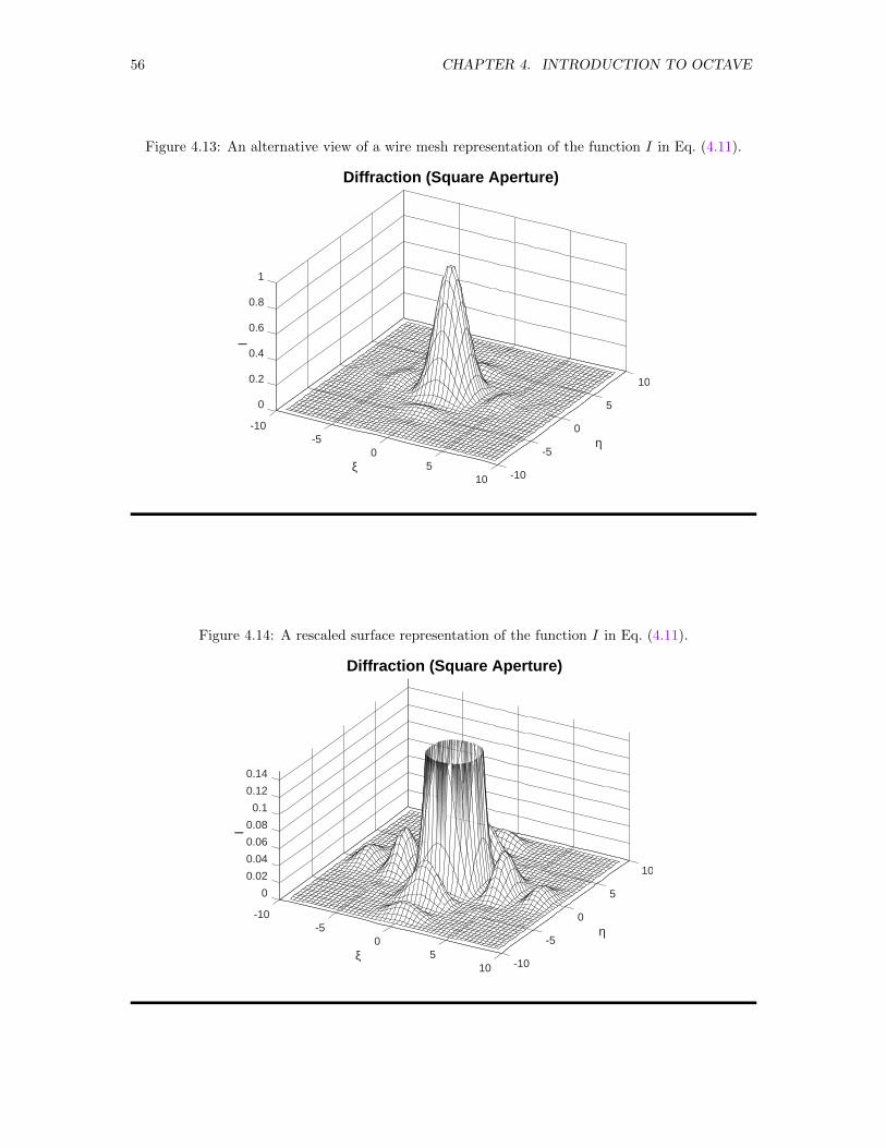
56 CHAPTER 4. INTRODUCTION TO OCTAVE

Figure 4.13: An alternative view of a wire mesh representation of the function I in Eq. (4.11).

0

0.2

0.4

I

0.6

0.8

1

η

ξ

-5-10

50

Diffraction (Square Aperture)

10

5

0

-5

-1010

Figure 4.14: A rescaled surface representation of the function I in Eq. (4.11).

0.1

0.12

0.14

0

0.02

0.04

0.06

I 0.08

ξ

η0

-5-10

510 -10

-5

Diffraction (Square Aperture)

10

5

0

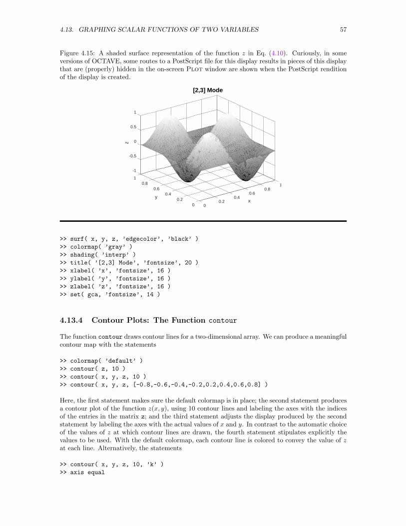
4.13. GRAPHING SCALAR FUNCTIONS OF TWO VARIABLES 57

Figure 4.15: A shaded surface representation of the function z in Eq. (4.10). Curiously, in someversions of OCTAVE, some routes to a PostScript file for this display results in pieces of this displaythat are (properly) hidden in the on-screen Plot window are shown when the PostScript renditionof the display is created.

00.2

0.4y

0.60.8

1

-1

0x

-0.5

z 0

0.5

1

10.8

[2,3] Mode

0.20.4

0.6

>> surf( x, y, z, ’edgecolor’, ’black’ )

>> colormap( ’gray’ )

>> shading( ’interp’ )

>> title( ’[2,3] Mode’, ’fontsize’, 20 )

>> xlabel( ’x’, ’fontsize’, 16 )

>> ylabel( ’y’, ’fontsize’, 16 )

>> zlabel( ’z’, ’fontsize’, 16 )

>> set( gca, ’fontsize’, 14 )

4.13.4 Contour Plots: The Function contour

The function contour draws contour lines for a two-dimensional array. We can produce a meaningfulcontour map with the statements

>> colormap( ’default’ )

>> contour( z, 10 )

>> contour( x, y, z, 10 )

>> contour( x, y, z, [-0.8,-0.6,-0.4,-0.2,0.2,0.4,0.6,0.8] )

Here, the first statement makes sure the default colormap is in place; the second statement producesa contour plot of the function z(x, y), using 10 contour lines and labeling the axes with the indicesof the entries in the matrix z; and the third statement adjusts the display produced by the secondstatement by labeling the axes with the actual values of x and y. In contrast to the automatic choiceof the values of z at which contour lines are drawn, the fourth statement stipulates explicitly thevalues to be used. With the default colormap, each contour line is colored to convey the value of zat each line. Alternatively, the statements

>> contour( x, y, z, 10, ’k’ )

>> axis equal

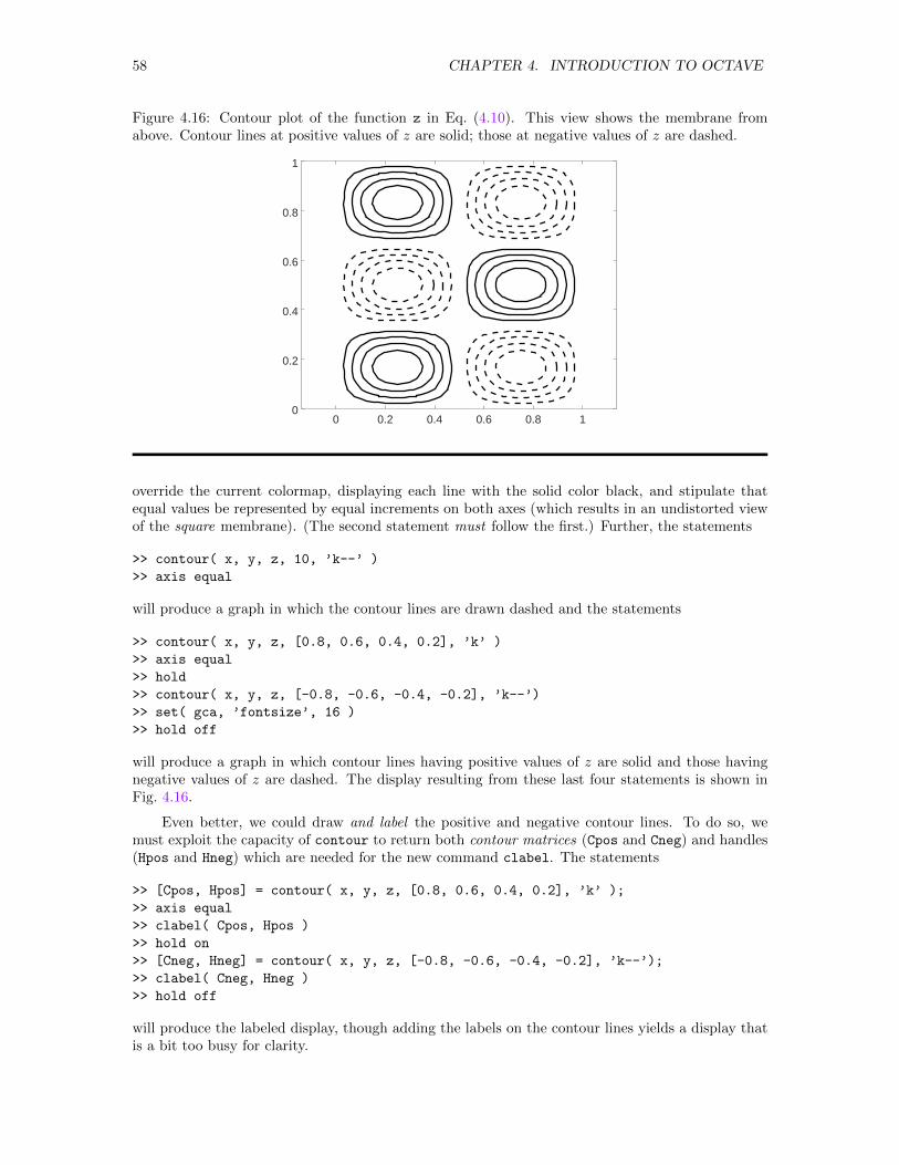
58 CHAPTER 4. INTRODUCTION TO OCTAVE

Figure 4.16: Contour plot of the function z in Eq. (4.10). This view shows the membrane fromabove. Contour lines at positive values of z are solid; those at negative values of z are dashed.

0.8

0.6

0.4

0.2

010.80.60.40.20

1

override the current colormap, displaying each line with the solid color black, and stipulate thatequal values be represented by equal increments on both axes (which results in an undistorted viewof the square membrane). (The second statement must follow the first.) Further, the statements

>> contour( x, y, z, 10, ’k--’ )

>> axis equal

will produce a graph in which the contour lines are drawn dashed and the statements

>> contour( x, y, z, [0.8, 0.6, 0.4, 0.2], ’k’ )

>> axis equal

>> hold

>> contour( x, y, z, [-0.8, -0.6, -0.4, -0.2], ’k--’)

>> set( gca, ’fontsize’, 16 )

>> hold off

will produce a graph in which contour lines having positive values of z are solid and those havingnegative values of z are dashed. The display resulting from these last four statements is shown inFig. 4.16.

Even better, we could draw and label the positive and negative contour lines. To do so, wemust exploit the capacity of contour to return both contour matrices (Cpos and Cneg) and handles(Hpos and Hneg) which are needed for the new command clabel. The statements

>> [Cpos, Hpos] = contour( x, y, z, [0.8, 0.6, 0.4, 0.2], ’k’ );

>> axis equal

>> clabel( Cpos, Hpos )

>> hold on

>> [Cneg, Hneg] = contour( x, y, z, [-0.8, -0.6, -0.4, -0.2], ’k--’);

>> clabel( Cneg, Hneg )

>> hold off

will produce the labeled display, though adding the labels on the contour lines yields a display thatis a bit too busy for clarity.

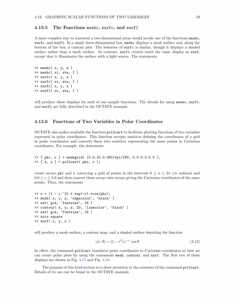
4.13. GRAPHING SCALAR FUNCTIONS OF TWO VARIABLES 59

4.13.5 The Functions meshc, surfc, and surfl

A more complex way to represent a two-dimensional array would invoke one of the functions meshc,surfc, and surfl. In a single three-dimensional box, meshc displays a mesh surface and, along thebottom of the box, a contour plot. The behavior of surfc is similar, though it displays a shadedsurface rather than a mesh surface. In contrast, surfl creates much the same display as surf,except that it illuminates the surface with a light source. The statements

>> meshc( x, y, z )

>> meshc( xi, eta, I )

>> surfc( x, y, z )

>> surfc( xi, eta, I )

>> surfl( x, y, z )

>> surfl( xi, eta, I )

will produce these displays for each of our sample functions. The details for using meshc, surfc,and surfl are fully described in the OCTAVE manuals.

4.13.6 Functions of Two Variables in Polar Coordinates

OCTAVE also makes available the function pol2cart to facilitate plotting functions of two variablesexpressed in polar coordinates. This function accepts matrices defining the coordinates of a gridin polar coordinates and converts them into matrices representing the same points in Cartesiancoordinates. For example, the statements

>> [ phi, r ] = meshgrid( (0.0:10.0:360)*pi/180, 0.0:0.2:5.0 );

>> [ x, y ] = pol2cart( phi, r );

create arrays phi and r conveying a grid of points in the intervals 0 ≤ φ ≤ 2π (in radians) and0.0 ≤ r ≤ 5.0 and then convert those arrays into arrays giving the Cartesian coordinates of the samepoints. Then, the statements

>> z = (1 - r.^2).* exp(-r).*cos(phi);

>> mesh( x, y, z, ’edgecolor’, ’black’ )

>> set( gca, ’fontsize’, 16 )

>> contour( x, y, z, 20, ’linecolor’, ’black’ )

>> set( gca, ’fontsize’, 16 )

>> axis square

>> surf( x, y, z )

will produce a mesh surface, a contour map, and a shaded surface depicting the function

z(r, θ) = (1− r2) e−r cos θ (4.12)

In effect, the command pol2cart translates polar coordinates to Cartesian coordinates so that wecan create polar plots by using the commands mesh, contour, and surf. The first two of thesedisplays are shown in Fig. 4.17 and Fig. 4.18.

The purpose of this brief section is to draw attention to the existence of the command pol2cart.Details of its use can be found in the OCTAVE manuals.

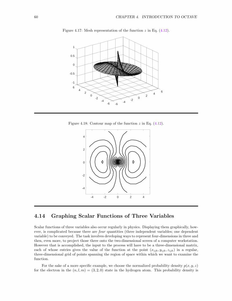
60 CHAPTER 4. INTRODUCTION TO OCTAVE

Figure 4.17: Mesh representation of the function z in Eq. (4.12).

0.5

1

-1

-0.5

0

6

02

4

-2-2

0

-4-6 -6

-4

64

2

Figure 4.18: Contour map of the function z in Eq. (4.12).

-4 -2 0 2 4

-4

-2

0

2

4

4.14 Graphing Scalar Functions of Three Variables

Scalar functions of three variables also occur regularly in physics. Displaying them graphically, how-ever, is complicated because there are four quantities (three independent variables; one dependentvariable) to be conveyed. The task involves developing ways to represent four-dimensions in three andthen, even more, to project those three onto the two-dimensional screen of a computer workstation.However that is accomplished, the input to the process will have to be a three-dimensional matrix,each of whose entries gives the value of the function at the point (xijk, yijk, zijk) in a regular,three-dimensional grid of points spanning the region of space within which we want to examine thefunction.

For the sake of a more specific example, we choose the normalized probability density p(x, y, z)for the electron in the (n, l,m) = (3, 2, 0) state in the hydrogen atom. This probability density is

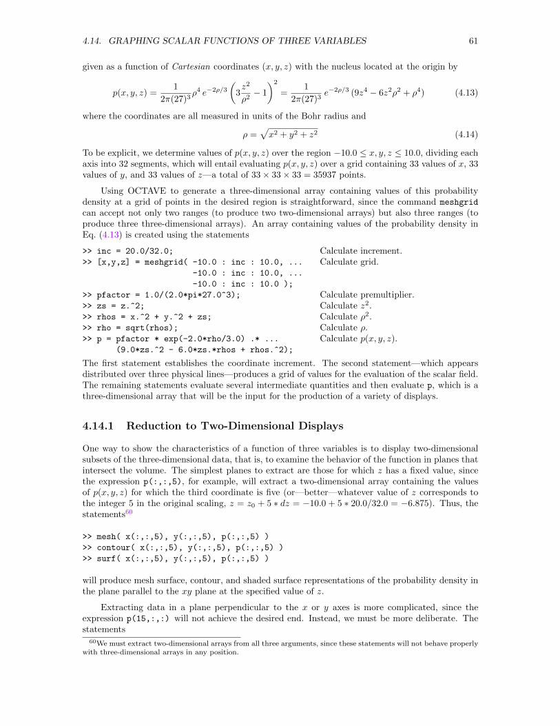
4.14. GRAPHING SCALAR FUNCTIONS OF THREE VARIABLES 61

given as a function of Cartesian coordinates (x, y, z) with the nucleus located at the origin by

p(x, y, z) =1

2π(27)3ρ4 e−2ρ/3

(3z2

ρ2− 1

)2

=1

2π(27)3e−2ρ/3 (9z4 − 6z2ρ2 + ρ4) (4.13)

where the coordinates are all measured in units of the Bohr radius and

ρ =√x2 + y2 + z2 (4.14)

To be explicit, we determine values of p(x, y, z) over the region −10.0 ≤ x, y, z ≤ 10.0, dividing eachaxis into 32 segments, which will entail evaluating p(x, y, z) over a grid containing 33 values of x, 33values of y, and 33 values of z—a total of 33× 33× 33 = 35937 points.

Using OCTAVE to generate a three-dimensional array containing values of this probabilitydensity at a grid of points in the desired region is straightforward, since the command meshgrid

can accept not only two ranges (to produce two two-dimensional arrays) but also three ranges (toproduce three three-dimensional arrays). An array containing values of the probability density inEq. (4.13) is created using the statements

>> inc = 20.0/32.0;

>> [x,y,z] = meshgrid( -10.0 : inc : 10.0, ...

-10.0 : inc : 10.0, ...

-10.0 : inc : 10.0 );

>> pfactor = 1.0/(2.0*pi*27.0^3);

>> zs = z.^2;

>> rhos = x.^2 + y.^2 + zs;

>> rho = sqrt(rhos);

>> p = pfactor * exp(-2.0*rho/3.0) .* ...

(9.0*zs.^2 - 6.0*zs.*rhos + rhos.^2);

Calculate increment.Calculate grid.

Calculate premultiplier.Calculate z2.Calculate ρ2.Calculate ρ.Calculate p(x, y, z).

The first statement establishes the coordinate increment. The second statement—which appearsdistributed over three physical lines—produces a grid of values for the evaluation of the scalar field.The remaining statements evaluate several intermediate quantities and then evaluate p, which is athree-dimensional array that will be the input for the production of a variety of displays.

4.14.1 Reduction to Two-Dimensional Displays

One way to show the characteristics of a function of three variables is to display two-dimensionalsubsets of the three-dimensional data, that is, to examine the behavior of the function in planes thatintersect the volume. The simplest planes to extract are those for which z has a fixed value, sincethe expression p(:,:,5), for example, will extract a two-dimensional array containing the valuesof p(x, y, z) for which the third coordinate is five (or—better—whatever value of z corresponds tothe integer 5 in the original scaling, z = z0 + 5 ∗ dz = −10.0 + 5 ∗ 20.0/32.0 = −6.875). Thus, thestatements60

>> mesh( x(:,:,5), y(:,:,5), p(:,:,5) )

>> contour( x(:,:,5), y(:,:,5), p(:,:,5) )

>> surf( x(:,:,5), y(:,:,5), p(:,:,5) )

will produce mesh surface, contour, and shaded surface representations of the probability density inthe plane parallel to the xy plane at the specified value of z.

Extracting data in a plane perpendicular to the x or y axes is more complicated, since theexpression p(15,:,:) will not achieve the desired end. Instead, we must be more deliberate. Thestatements

60We must extract two-dimensional arrays from all three arguments, since these statements will not behave properlywith three-dimensional arrays in any position.

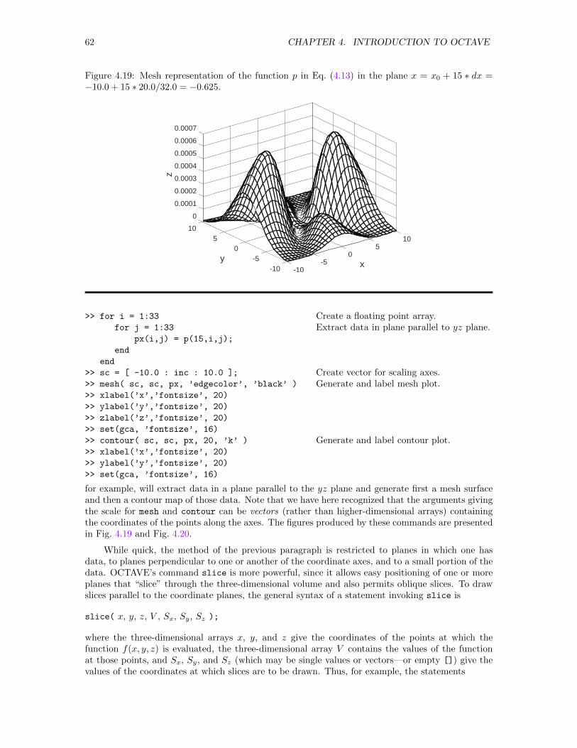
62 CHAPTER 4. INTRODUCTION TO OCTAVE

Figure 4.19: Mesh representation of the function p in Eq. (4.13) in the plane x = x0 + 15 ∗ dx =−10.0 + 15 ∗ 20.0/32.0 = −0.625.

-10-5y

05

10

0

-10

0.0001

0.0002

z 0.0003

0.0004

0.0005

0.0006

0.0007

x-50

510

>> for i = 1:33

for j = 1:33

px(i,j) = p(15,i,j);

end

end

>> sc = [ -10.0 : inc : 10.0 ];

>> mesh( sc, sc, px, ’edgecolor’, ’black’ )

>> xlabel(’x’,’fontsize’, 20)

>> ylabel(’y’,’fontsize’, 20)

>> zlabel(’z’,’fontsize’, 20)

>> set(gca, ’fontsize’, 16)

>> contour( sc, sc, px, 20, ’k’ )

>> xlabel(’x’,’fontsize’, 20)

>> ylabel(’y’,’fontsize’, 20)

>> set(gca, ’fontsize’, 16)

Create a floating point array.Extract data in plane parallel to yz plane.

Create vector for scaling axes.Generate and label mesh plot.

Generate and label contour plot.

for example, will extract data in a plane parallel to the yz plane and generate first a mesh surfaceand then a contour map of those data. Note that we have here recognized that the arguments givingthe scale for mesh and contour can be vectors (rather than higher-dimensional arrays) containingthe coordinates of the points along the axes. The figures produced by these commands are presentedin Fig. 4.19 and Fig. 4.20.

While quick, the method of the previous paragraph is restricted to planes in which one hasdata, to planes perpendicular to one or another of the coordinate axes, and to a small portion of thedata. OCTAVE’s command slice is more powerful, since it allows easy positioning of one or moreplanes that “slice” through the three-dimensional volume and also permits oblique slices. To drawslices parallel to the coordinate planes, the general syntax of a statement invoking slice is

slice( x, y, z, V , Sx, Sy, Sz );

where the three-dimensional arrays x, y, and z give the coordinates of the points at which thefunction f(x, y, z) is evaluated, the three-dimensional array V contains the values of the functionat those points, and Sx, Sy, and Sz (which may be single values or vectors—or empty []) give thevalues of the coordinates at which slices are to be drawn. Thus, for example, the statements

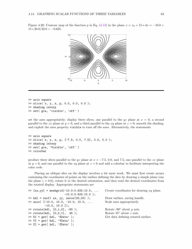
4.14. GRAPHING SCALAR FUNCTIONS OF THREE VARIABLES 63

Figure 4.20: Contour map of the function p in Eq. (4.13) in the plane x = x0 + 15 ∗ dx = −10.0 +15 ∗ 20.0/32.0 = −0.625.

-10 -5 0 5 10-10

-5

0

5

10

x

y

>> axis square

>> slice( x, y, z, p, 0.0, 0.0, 0.0 );

>> shading interp

>> set( gca, ’visible’, ’off’ )

set the axes appropriately; display three slices, one parallel to the yz plane at x = 0, a secondparallel to the zx plane at y = 0, and a third parallel to the xy plane at z = 0; smooth the shading;and exploit the axes property visible to turn off the axes. Alternatively, the statements

>> axis square

>> slice( x, y, z, p, [-7.5, 0.0, 7.5], 0.0, 0.0 );

>> shading interp

>> set( gca, ’Visible’, ’off’ )

>> colorbar

produce three slices parallel to the yz plane at x = −7.5, 0.0, and 7.5, one parallel to the zx planeat y = 0, and one parallel to the xy plane at z = 0 and add a colorbar to facilitate interpreting thecolor code.

Placing an oblique slice on the display involves a bit more work. We must first create arrayscontaining the coordinates of points on the surface defining the slice by drawing a simple plane (saythe plane z = 0.0), rotate it to the desired orientation, and then read the desired coordinates fromthe rotated display. Appropriate statements are

>> [xx,yy] = meshgrid(-10.0:0.625:10.0, ...

-10.0:0.625:10.0 );

>> hdl = surf( xx, yy, zeros(33,33) );

>> axis( [-10.0, 10.0, -10.0, 10.0, ...

-10.0, 10.0 ]);

>> rotate(hdl, [0,1,0], -90 );

>> rotate(hdl, [0,0,1], 45 );

>> XI = get( hdl, ’XData’ );

>> YI = get( hdl, ’YData’ );

>> ZI = get( hdl, ’ZData’ );

Create coordinates for drawing xy plane.

Draw surface, saving handle.Scale axes appropriately.

Rotate -90 about y axis.Rotate 45 about z axis.Get data defining rotated surface.

64 CHAPTER 4. INTRODUCTION TO OCTAVE

Figure 4.21: Oblique slices through the function p in Eq. (4.13).

0

0.0006

0.0004

0.0002

Here we have used the handle hdl to the surface several times, first in the command rotate (whichrotates the identified object by the angle in the third argument about the axis whose direction isgiven by the (vector) second argument) and then in the command get (which reads coordinates ofpoints defining the rotated surface into an appropriately structured array).

With the arrays XI, YI, and ZI now in hand, we can generate the desired display with theadditional statements

>> close all

>> slice( x, y, z, p, XI, YI, ZI )

>> hold on

>> slice( x, y, z, p, 0.0, 0.0, [] );

>> shading interp

>> colorbar

>> axis square

>> set( gca, ’Visible’, ’off’ )

>> colormap( ’gray’ )

>> hold off

Remove Figure window.Draw oblique slice.Suppress erase.Add “ordinary” slices, suppressing anyparallel to the xy plane.Set shading.Add colorbar.Equalize axes.Turn off display of axes.Set gray scale.

Figure 4.21 shows the display produced by these statements, though the black and white renditionpales by comparison with the color rendition on the screen.

4.14.2 Isosurfaces

Another method of viewing a three-dimensional scalar field is to look at isosurfaces, or sets oflocations at which the function has a constant value. In our present example, we locate and displaya surface of constant probability density with the statements

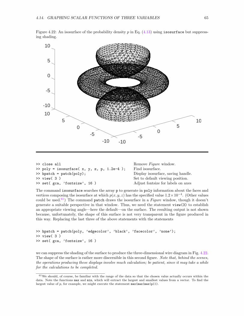
4.14. GRAPHING SCALAR FUNCTIONS OF THREE VARIABLES 65

Figure 4.22: An isosurface of the probability density p in Eq. (4.13) using isosurface but suppress-ing shading.

-10-5

05

10

-10

-10

-5

0

5

10

-50

510

>> close all

>> poly = isosurface( x, y, z, p, 1.2e-4 );

>> hpatch = patch(poly);

>> view( 3 )

>> set( gca, ’fontsize’, 16 )

Remove Figure window.Find isosurface.Display isosurface, saving handle.Set to default viewing position.Adjust fontsize for labels on axes

The command isosurface searches the array p to generate in poly information about the faces andvertices composing the isosurface at which p(x, y, z) has the specified value 1.2×10−4. (Other valuescould be used.61) The command patch draws the isosurface in a Figure window, though it doesn’tgenerate a suitable perspective in that window. Thus, we need the statement view(3) to establishan appropriate viewing angle—here the default—on the surface. The resulting output is not shownbecause, unfortunately, the shape of this surface is not very transparent in the figure produced inthis way. Replacing the last three of the above statements with the statements

>> hpatch = patch(poly, ’edgecolor’, ’black’, ’facecolor’, ’none’);

>> view( 3 )

>> set( gca, ’fontsize’, 16 )

we can suppress the shading of the surface to produce the three-dimensional wire diagram in Fig. 4.22.The shape of the surface is rather more discernible in this second figure. Note that, behind the scenes,the operations producing these displays involve much calculation; be patient, since it may take a whilefor the calculations to be completed.

61We should, of course, be familiar with the range of the data so that the chosen value actually occurs within thedata. Note the functions max and min, which will extract the largest and smallest values from a vector. To find thelargest value of p, for example, we might execute the statement max(max(max(p))).

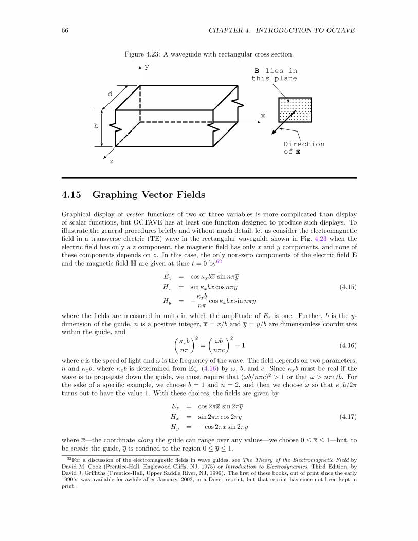
66 CHAPTER 4. INTRODUCTION TO OCTAVE

Figure 4.23: A waveguide with rectangular cross section.

x

y

z

Directionof E

B lies inthis plane

b

d

4.15 Graphing Vector Fields

Graphical display of vector functions of two or three variables is more complicated than displayof scalar functions, but OCTAVE has at least one function designed to produce such displays. Toillustrate the general procedures briefly and without much detail, let us consider the electromagneticfield in a transverse electric (TE) wave in the rectangular waveguide shown in Fig. 4.23 when theelectric field has only a z component, the magnetic field has only x and y components, and none ofthese components depends on z. In this case, the only non-zero components of the electric field Eand the magnetic field H are given at time t = 0 by62

Ez = cosκxbx sinnπy

Hx = sinκxbx cosnπy (4.15)

Hy = −κxbnπ

cosκxbx sinnπy

where the fields are measured in units in which the amplitude of Ez is one. Further, b is the y-dimension of the guide, n is a positive integer, x = x/b and y = y/b are dimensionless coordinateswithin the guide, and (

κxb

nπ

)2

=

(ωb

nπc

)2

− 1 (4.16)

where c is the speed of light and ω is the frequency of the wave. The field depends on two parameters,n and κxb, where κxb is determined from Eq. (4.16) by ω, b, and c. Since κxb must be real if thewave is to propagate down the guide, we must require that (ωb/nπc)2 > 1 or that ω > nπc/b. Forthe sake of a specific example, we choose b = 1 and n = 2, and then we choose ω so that κxb/2πturns out to have the value 1. With these choices, the fields are given by

Ez = cos 2πx sin 2πy

Hx = sin 2πx cos 2πy (4.17)

Hy = − cos 2πx sin 2πy

where x—the coordinate along the guide can range over any values—we choose 0 ≤ x ≤ 1—but, tobe inside the guide, y is confined to the region 0 ≤ y ≤ 1.

62For a discussion of the electromagnetic fields in wave guides, see The Theory of the Electromagnetic Field byDavid M. Cook (Prentice-Hall, Englewood Cliffs, NJ, 1975) or Introduction to Electrodynamics, Third Edition, byDavid J. Griffiths (Prentice-Hall, Upper Saddle River, NJ, 1999). The first of these books, out of print since the early1990’s, was available for awhile after January, 2003, in a Dover reprint, but that reprint has since not been kept inprint.

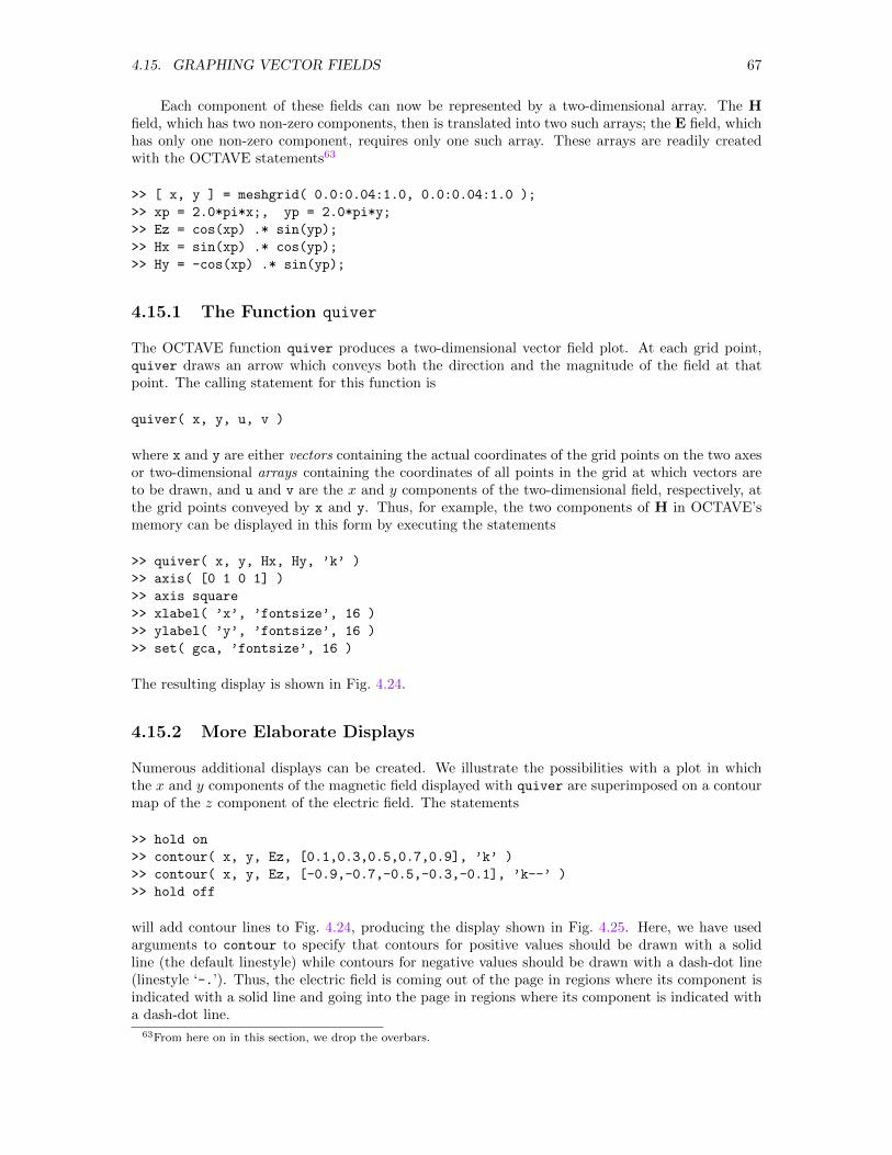
4.15. GRAPHING VECTOR FIELDS 67

Each component of these fields can now be represented by a two-dimensional array. The Hfield, which has two non-zero components, then is translated into two such arrays; the E field, whichhas only one non-zero component, requires only one such array. These arrays are readily createdwith the OCTAVE statements63

>> [ x, y ] = meshgrid( 0.0:0.04:1.0, 0.0:0.04:1.0 );

>> xp = 2.0*pi*x;, yp = 2.0*pi*y;

>> Ez = cos(xp) .* sin(yp);

>> Hx = sin(xp) .* cos(yp);

>> Hy = -cos(xp) .* sin(yp);

4.15.1 The Function quiver

The OCTAVE function quiver produces a two-dimensional vector field plot. At each grid point,quiver draws an arrow which conveys both the direction and the magnitude of the field at thatpoint. The calling statement for this function is

quiver( x, y, u, v )

where x and y are either vectors containing the actual coordinates of the grid points on the two axesor two-dimensional arrays containing the coordinates of all points in the grid at which vectors areto be drawn, and u and v are the x and y components of the two-dimensional field, respectively, atthe grid points conveyed by x and y. Thus, for example, the two components of H in OCTAVE’smemory can be displayed in this form by executing the statements

>> quiver( x, y, Hx, Hy, ’k’ )

>> axis( [0 1 0 1] )

>> axis square

>> xlabel( ’x’, ’fontsize’, 16 )

>> ylabel( ’y’, ’fontsize’, 16 )

>> set( gca, ’fontsize’, 16 )

The resulting display is shown in Fig. 4.24.

4.15.2 More Elaborate Displays

Numerous additional displays can be created. We illustrate the possibilities with a plot in whichthe x and y components of the magnetic field displayed with quiver are superimposed on a contourmap of the z component of the electric field. The statements

>> hold on

>> contour( x, y, Ez, [0.1,0.3,0.5,0.7,0.9], ’k’ )

>> contour( x, y, Ez, [-0.9,-0.7,-0.5,-0.3,-0.1], ’k--’ )

>> hold off

will add contour lines to Fig. 4.24, producing the display shown in Fig. 4.25. Here, we have usedarguments to contour to specify that contours for positive values should be drawn with a solidline (the default linestyle) while contours for negative values should be drawn with a dash-dot line(linestyle ‘-.’). Thus, the electric field is coming out of the page in regions where its component isindicated with a solid line and going into the page in regions where its component is indicated witha dash-dot line.

63From here on in this section, we drop the overbars.

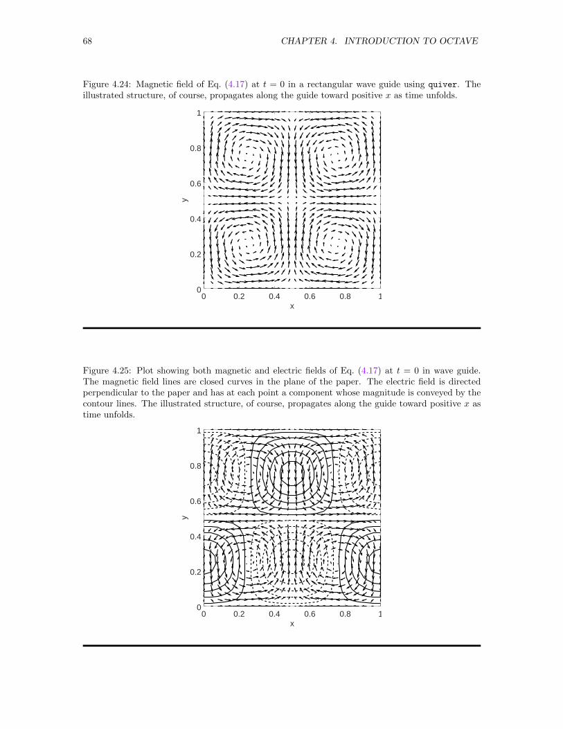
68 CHAPTER 4. INTRODUCTION TO OCTAVE

Figure 4.24: Magnetic field of Eq. (4.17) at t = 0 in a rectangular wave guide using quiver. Theillustrated structure, of course, propagates along the guide toward positive x as time unfolds.

0 0.2 0.4 0.6 0.8 10

0.2

0.4

0.6

0.8

1

x

y

Figure 4.25: Plot showing both magnetic and electric fields of Eq. (4.17) at t = 0 in wave guide.The magnetic field lines are closed curves in the plane of the paper. The electric field is directedperpendicular to the paper and has at each point a component whose magnitude is conveyed by thecontour lines. The illustrated structure, of course, propagates along the guide toward positive x astime unfolds.

0 0.2 0.4 0.6 0.8 10

0.2

0.4

0.6

0.8

1

x

y

4.16. ANIMATION 69

4.15.3 Three-Dimensional Vector Fields

When a vector field has non-zero components in more than two coordinate directions, a pictureof the field is much harder to draw and even more difficult to interpret without the aid of a toolthat will allow easy viewing of the picture from a variety of viewing angles. One can, of course, usequiver to draw pictures of the projections of the field in any given plane into that plane. In addition,OCTAVE provides the function quiver3 (see the OCTAVE manuals) for drawing a picture similarto those produced by quiver, but drawing short vectors at points in three-dimensional space. Theprimary input to quiver3 is a sextet of three-dimensional arrays giving the x, y, and z coordinatesof the points at which vectors are to be drawn and the x, y, and z components of the vector fieldat those points. The exploration of these capabilities is left to the exercises. Remember that themouse can be used to rotate 3D-graphs produced by OCTAVE in the Figure window.

4.16 Animation

Along with all of the image processing and graphing capabilities, more recent versions of OCTAVEcan also display a sequence of images in rapid succession to produce an animated display.64 Inessence, one creates each image in turn in an appropriately sized window, reads each window as abit-map into an element of an appropriately sized array, and then displays each of those images inturn.

To illustrate this process, we use a data file containing 41 33× 33 arrays, each of which conveysthe displacement of an L-shaped membrane at a particular moment in time.65 The statementscreating a three-dimensional byte array containing the 41 images in the animation are

>> id = fopen(’ldrum.dat’, ’r’);

>> x = [ 0.0 : 1.0/32.0 : 1.0 ];

>> for j=1:41

disp = fscanf( id, ’%f’, [33,33] );

mesh( x, x, disp’, ’EdgeColor’, ’black’ )

axis( [ 0.0 1.0 0.0 1.0 -0.25 0.25 ] )

M(j) = getframe;

end

>> status = fclose( id );

Open data file.Create vector of x values.For each of 41 frames:

Read array from file.Create display with transposed array.66

Standardize axes.Read display as bit map.

Close file.

At this point, the array M, whose class (struct) is new, contains all of the images stored as bit mapsso they can be displayed one after the other in quick succession.67

Several options for displaying the images can be invoked. All use the command movie but withdifferent arguments. The statement

>> movie( M );

displays each image in the array M one after another from beginning to end and then stops. Thestatement

64Necessary routines for easy animation were not present in Version 4 of OCTAVE. They have been added in Version5.2 and may have been included in some versions before Version 5.2.

65The file was created by using lsode—the Livermore solver for ordinary differential equations—to effect a numericalsolution of the wave equation for the membrane.

66Here, we have used the shorthand symbol ’ to transpose disp rather than the longer function transpose. Strictly,the symbol ’ effects the evaluation of the adjoint—the transposed complex conjugate—of the matrix. When theelements are all real, however, the adjoint and the transpose are the same. If we wanted to transpose a matrix ofcomplex elements without complex conjugation, we would use transpose or the special symbol ‘.’’.

67Actually, each element of M is itself structured, having two components M(j).cdata, which contains the image,and M(j).colormap, which has no function in OCTAVE and is included for compability with MATLAB.

70 CHAPTER 4. INTRODUCTION TO OCTAVE

>> movie( M, 15 );

exploits an optional (integer) argument to effect a 15-fold display of the full sequence of images,68

and the statement

>> movie( M, [ 15 1 3 5 7 9 ] );

will display images 1, 3, 5, 7, and 9 in succession, 15 times over. As a special case, the statement

>> movie( M, [ 1 23 ] );

for example, will display image 23 once. Since that image is then left in the Figure window, thisversion of the command allows display of a single image for close examination. Finally, the statement

>> movie( M, [15 1 3 5 7 9], 2 );

exploits a further argument that controls the speed of the display—here set to 2 frames per second.As with all OCTAVE commands, we can use 〈CONTROL-C〉 to interrupt a movie before it is finished,though the OCTAVE Command window must be the active window for this action to succeed.

The sequence of statements described in the previous paragraph ultimately displays a successionof images, each of which is separately defined in the input data. An alternative procedure is bettersuited to the task of creating an animation that can be generated by explicit transformation of asingle image in some simple way. In this case, only the data defining the initial image need besupplied. OCTAVE can then generate all remaining images from that initial image. For example,generating an animated display showing the simple harmonic motion of one of the normal modesof a square drumhead is especially easy if we have data on its initial shape. We simply create asuccession of images, each generated from the initial image by multiplying all values defining thatimage by cos 2πt, where t is stepped in equal increments from 0 to 1 so the multiplier runs over oneperiod.69 For example, to display the sinusoidal motion of a square drumhead whose initial shapeis given by

u(x, y, 0) = sin 2πx sin 3πy, 0 ≤ x, y ≤ 1

we might start with the statements

>> [ x, y ] = meshgrid( 0.0:0.04:1.0, ...

0.0:0.04:1.0 );

>> u = sin(2*pi*x) .* sin(3*pi*y);

>> t = [ 0.0 : 0.025 : 1.0 ];

>> for j = 1:41

disp = u*cos(2*pi*t(j));

mesh( x, y, disp, ’EdgeColor’, ’black’ );

axis( [ 0.0 1.0 0.0 1.0 -1.0 1.0 ] );

M(j)=getframe;

end

Create array describing initial shape.

Create values of time.For each of 41 images:

Calculate data for image.Create display.Standardize axes.Read display as bit map.

At this point, the necessary images are stored in the (structured) array M. From here, the animateddisplay itself can be created with the command movie as described in the previous paragraph. Wesimply have generated the necessary input data by calculating it from the initial shape rather thanby reading it from a file.

68If the integer is positive, the movie is played forward the specified number of times; if the integer is negative, thesequence of frames is played alternately forward and backward until the cycle—once forward and once backward—hasbeen repeated |integer| times.

69Whether we stop one image short of t = 1 or include the image for t = 1 depends on how the animation is to beshown. If the display moves forward from the first to the last image and then moves backward from the last to thefirst, the image for t = 1 should be included. If the display moves forward from the first to the last image and thenjumps abruptly back to the first image, the image for t = 1 should be omitted. We here assume the first mode ofdisplay.

4.17. ADVANCED GRAPHING FEATURES 71

4.17 Advanced Graphing Features

In this section, we describe some of OCTAVE’s more sophisticated capabilities. Because theseroutines are more involved than those previously described, it would be best to master the basicgraphics routines before moving on to these examples.

4.17.1 Fonts

Among the most useful of OCTAVE’s auxiliary features is a capability to choose characters froma wide variety of standard fonts (including Roman, Italic, Greek), to display bold characters andcommon mathematical symbols, and to position characters as subscripts and superscripts. Theexamples in this subsection are intended to introduce some of OCTAVE’s capabilities but are in noway a substitute for careful reading of the OCTAVE manuals.

At base, the appearance of characters created by those commands that place characters on thescreen are determined by several properties, including

• color, which can be specified by predefined words like red, yellow, green, blue, magenta,cyan, black, and white or, alternatively, by a three-component vector whose componentsrange between 0 and 1 and give, in order, the proportion of red ([1 0 0]), green ([0 1 0]), andblue ([0 0 1]) in the output.

• fontangle, which is normal by default but can be changed to italic or oblique.

• fontname, which can assume any of the values AvantGarde, Bookman, Courier, Helvetica,Helvetica-Narrow, NewCenturySchlbk, Palatino, Symbol, Times-Roman, ZapfChancery,and ZapfDingbats. OCTAVE substitutes Courier for any name not in this list.

• fontsize, which is expressed in fontunits (points by default).

• fontunits, which is points by default but can be changed to inches, centimeters,normalized, or pixels.

• fontweight, which is normal by default but can be changed to light, demi, or bold.

• interpreter, which is tex by default but can be changed to none. The value latex is plannedbut not yet implemented. When the tex option is active, a fair number of TEX and LATEXcommands can be included in character strings. Note that all toolkits recognize these TEXcommands for display on screen but proper interpretation in PostScript and PDF files producedwith the print command is not guaranteed (and may vary with the version of OCTAVE inuse).70 As with TEX and LATEX, the characters and can be used to limit the scope of acommand. In this context, strings need to be presented in single quotation marks.

These properties are set in the axes object, and can be changed by appropriate specificationsin the command axes, e.g., in the statement

axes( ’fontname’, ’palatino’, ’fontsize’, 16, ’xlim’, [0.0 10.0], ...

’ylim’, [-1.0 1.0] )

hold on

which will create the axes and label them and then prevent them from being overridden in a subse-quent plot command. Alternatively, after axes have been created by execution of some other graphicscommand, e.g., plot, these properties can be set by analogous specifications with the command set(

gca, ...), e.g.,

70See the OCTAVE manuals for your version of OCTAVE for details.

72 CHAPTER 4. INTRODUCTION TO OCTAVE

set( gca, ’fontname’, ’palatino’, ’fontsize’, 16, ’xlim’, ...

[0.0 10.0], ’ylim’, [-1.0 1.0] )

Through inheritance, the specifications in the previous paragraph affect all characters in allchildren of the associated axes object. Some of those children, however, have their own copies of thespecified properties. Statements like

hdl = get( gca, ’title’ )

set( hdl, ’fontname’, ’symbol’, ... )

report the handle for the text object containing—here—the title in the current axes object and thenset the indicated properties of that object away from those inherited from the parent axes object.

The methods for changing fonts described in the previous two paragraphs affect the font for anentire object (title, axis label, . . .). When we wish to change the font for a few characters within astring that is otherwise to be displayed in the default font, we must stipulate the font changes withcommands embedded in quoted strings. For example, the (illustrative but mildly silly) statement

>> title( ’This \fontsize12\alpha\beta is a Title’, ’fontsize’, 20 )

will produce a title in which the words ‘This’ and ‘a Title’ will be presented in the default fontat 20 pt while—in a LATEX-style notation—the Greek characters αβ will be presented in 12 ptcharacters. Here, braces play two roles: (1) they enclose the arguments of the command \fontsizeand (2) they limit the scope of the change in font.71,72

Several other Greek letters and mathematical symbols are available with commands that mimicthose used in LATEX. All lower case Greek letters73 (including \vartheta, \varpi, \varsigma, and\varphi) can be inserted with a command like \alpha (letter name in lower case preceded by abackslash); all upper case Greek letters except those that look like upper case Roman letters (e.g.,A, B, and H) can be inserted with a command like \Gamma (letter name with initial letter in uppercase preceded by a backslash). Some of the other available symbols are listed in Table 4.6. Thus,for example, the statement

title(’\alpha\leq\surd(\beta^2+\gamma^2)’, ’fontsize’, 20 )

will produce the title α ≤√

(β2 + γ2). We have here also illustrated that superscripts can beproduced with the character ^; subscripts are created with the character _. Should either of thesecharacters be literally needed in the output, the quoted text must include \_ or \^.

Two further points: (1) While in-string selection of fontname and fontsize can be accom-plished with the commands \fontname and \fontsize, parallel in-string specification of fontweight(normal, bold, demi, light) and fontangle (normal, italic, oblique) is not available. Instead, wemust use one of \bf, \sl, \it, and \rm to produce bold, slanted, italic, and Roman (normal) styles,respectively, and—to limit the scope of the indicated change—we enclose the characters in braces,e.g., \bf BoldWord(s). (2) The characters _, ^, \, , and have been given special meanings;should we actually wish to display these characters in a title or label, we precede each in the quotedstring with a backslash, i.e., we produce these characters by including \_, \^, \\, \, and \,respectively, in the quoted string.

In Section 4.13.2, we have already seen one use of this capability. We present one more example.Let us embellish the graph of the magnetic field first presented in Fig. 4.5 by (1) changing the font

71Those familiar with LATEX will identify this role with a similar role played by braces in that text-processingsystem.

72Note that proper interpretation of the LATEX-style specifications will not occur if the string is enclosed in doublequotation marks unless the backslashes are also doubled.

73Omicron is produced with \o, not \omicron.

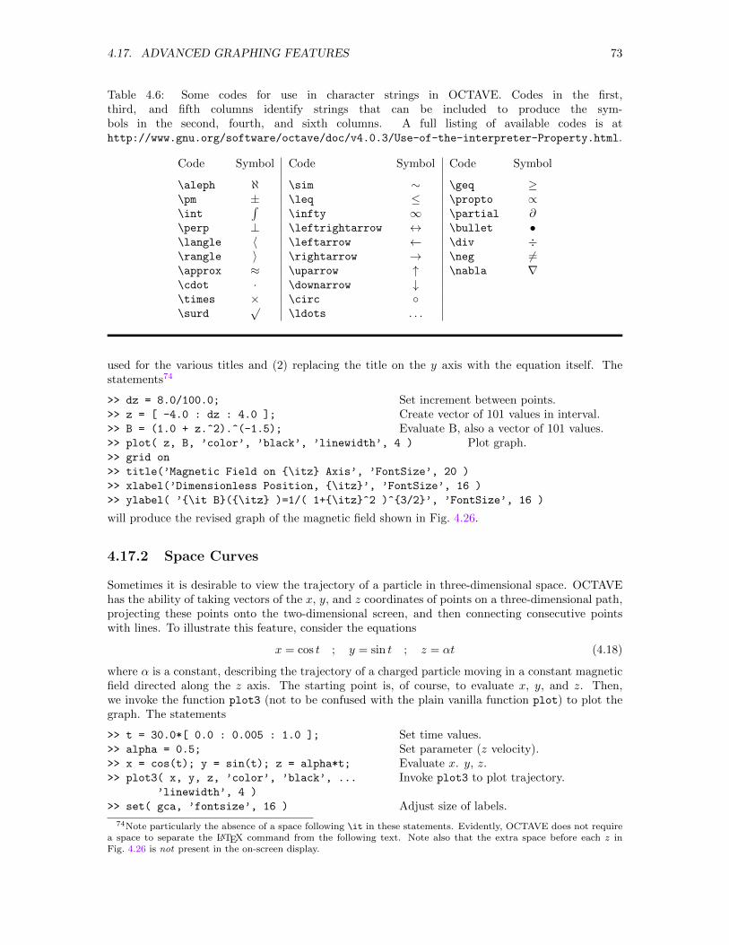
4.17. ADVANCED GRAPHING FEATURES 73

Table 4.6: Some codes for use in character strings in OCTAVE. Codes in the first,third, and fifth columns identify strings that can be included to produce the sym-bols in the second, fourth, and sixth columns. A full listing of available codes is athttp://www.gnu.org/software/octave/doc/v4.0.3/Use-of-the-interpreter-Property.html.

Code Symbol Code Symbol Code Symbol

\aleph ℵ \sim ∼ \geq ≥\pm ± \leq ≤ \propto ∝\int

∫\infty ∞ \partial ∂

\perp ⊥ \leftrightarrow ↔ \bullet •\langle 〈 \leftarrow ← \div ÷\rangle 〉 \rightarrow → \neg 6=\approx ≈ \uparrow ↑ \nabla ∇\cdot · \downarrow ↓\times × \circ \surd

√\ldots . . .

used for the various titles and (2) replacing the title on the y axis with the equation itself. Thestatements74

>> dz = 8.0/100.0;

>> z = [ -4.0 : dz : 4.0 ];

>> B = (1.0 + z.^2).^(-1.5);

>> plot( z, B, ’color’, ’black’, ’linewidth’, 4 )

>> grid on

>> title(’Magnetic Field on \itz Axis’, ’FontSize’, 20 )

>> xlabel(’Dimensionless Position, \itz’, ’FontSize’, 16 )

>> ylabel( ’\it B(\itz )=1/( 1+\itz^2 )^3/2’, ’FontSize’, 16 )

Set increment between points.Create vector of 101 values in interval.Evaluate B, also a vector of 101 values.

Plot graph.

will produce the revised graph of the magnetic field shown in Fig. 4.26.

4.17.2 Space Curves

Sometimes it is desirable to view the trajectory of a particle in three-dimensional space. OCTAVEhas the ability of taking vectors of the x, y, and z coordinates of points on a three-dimensional path,projecting these points onto the two-dimensional screen, and then connecting consecutive pointswith lines. To illustrate this feature, consider the equations

x = cos t ; y = sin t ; z = αt (4.18)

where α is a constant, describing the trajectory of a charged particle moving in a constant magneticfield directed along the z axis. The starting point is, of course, to evaluate x, y, and z. Then,we invoke the function plot3 (not to be confused with the plain vanilla function plot) to plot thegraph. The statements

>> t = 30.0*[ 0.0 : 0.005 : 1.0 ];

>> alpha = 0.5;

>> x = cos(t); y = sin(t); z = alpha*t;

>> plot3( x, y, z, ’color’, ’black’, ...

’linewidth’, 4 )

>> set( gca, ’fontsize’, 16 )

Set time values.Set parameter (z velocity).Evaluate x. y, z.Invoke plot3 to plot trajectory.

Adjust size of labels.

74Note particularly the absence of a space following \it in these statements. Evidently, OCTAVE does not requirea space to separate the LATEX command from the following text. Note also that the extra space before each z inFig. 4.26 is not present in the on-screen display.

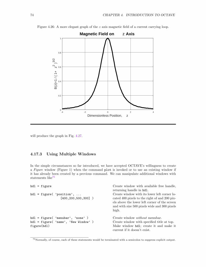
74 CHAPTER 4. INTRODUCTION TO OCTAVE

Figure 4.26: A more elegant graph of the z axis magnetic field of a current carrying loop.

-4 -2 0 2 40

0.2

0.4

0.6

0.8

1

Dimensionless Position, z

B(z

)=1

/ ( 1

+z2

)3/

2

Magnetic Field on z Axis

will produce the graph in Fig. 4.27.

4.17.3 Using Multiple Windows

In the simple circumstances so far introduced, we have accepted OCTAVE’s willingness to createa Figure window (Figure 1) when the command plot is invoked or to use an existing window ifit has already been created by a previous command. We can manipulate additional windows withstatements like75

hdl = figure

hdl = figure( ’position’, ...

[400,200,500,300] )

Create window with available free handle,returning handle in hdl.Create window with its lower left corner lo-cated 400 pixels to the right of and 200 pix-els above the lower left corner of the screenand with size 500 pixels wide and 300 pixelshigh.

hdl = figure( ’menubar’, ’none’ )

hdl = figure( ’name’, ’New Window’ )

figure(hdl)

Create window without menubar.Create window with specified title at top.Make window hdl; create it and make itcurrent if it doesn’t exist.

75Normally, of course, each of these statements would be terminated with a semicolon to suppress explicit output.

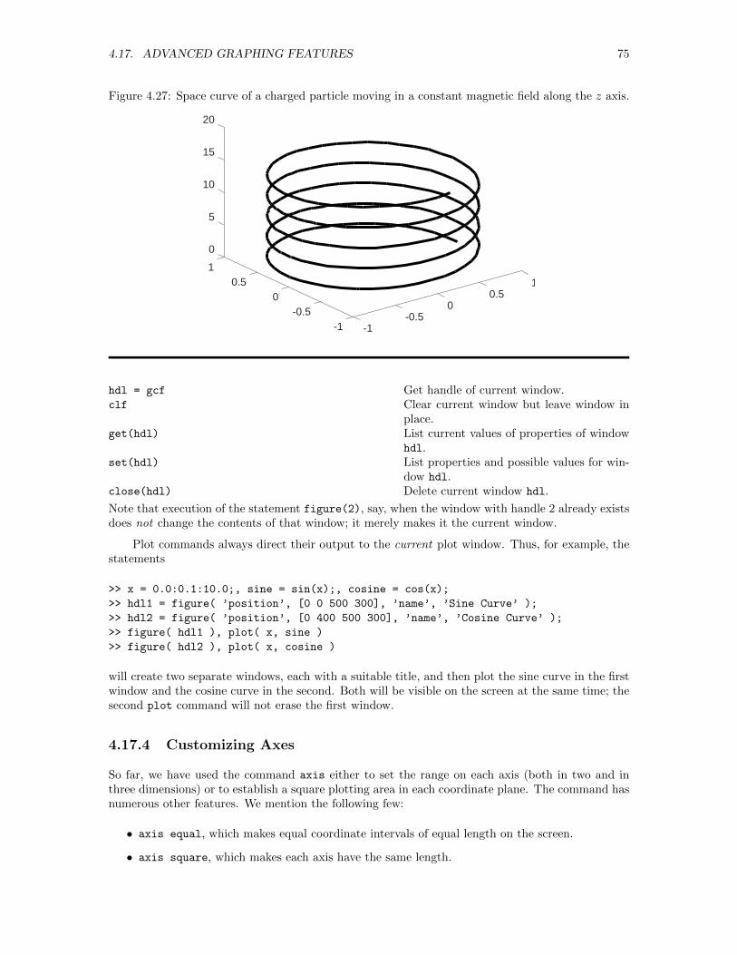
4.17. ADVANCED GRAPHING FEATURES 75

Figure 4.27: Space curve of a charged particle moving in a constant magnetic field along the z axis.

-1-0.5

00.5

1

-1

0

5

10

15

20

-0.50

0.51

hdl = gcf

clf

get(hdl)

set(hdl)

close(hdl)

Get handle of current window.Clear current window but leave window inplace.List current values of properties of windowhdl.List properties and possible values for win-dow hdl.Delete current window hdl.

Note that execution of the statement figure(2), say, when the window with handle 2 already existsdoes not change the contents of that window; it merely makes it the current window.

Plot commands always direct their output to the current plot window. Thus, for example, thestatements

>> x = 0.0:0.1:10.0;, sine = sin(x);, cosine = cos(x);

>> hdl1 = figure( ’position’, [0 0 500 300], ’name’, ’Sine Curve’ );

>> hdl2 = figure( ’position’, [0 400 500 300], ’name’, ’Cosine Curve’ );

>> figure( hdl1 ), plot( x, sine )

>> figure( hdl2 ), plot( x, cosine )

will create two separate windows, each with a suitable title, and then plot the sine curve in the firstwindow and the cosine curve in the second. Both will be visible on the screen at the same time; thesecond plot command will not erase the first window.

4.17.4 Customizing Axes

So far, we have used the command axis either to set the range on each axis (both in two and inthree dimensions) or to establish a square plotting area in each coordinate plane. The command hasnumerous other features. We mention the following few:

• axis equal, which makes equal coordinate intervals of equal length on the screen.

• axis square, which makes each axis have the same length.

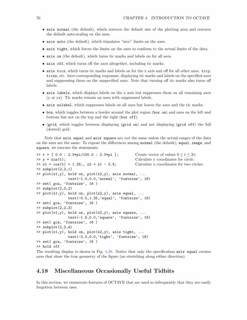
76 CHAPTER 4. INTRODUCTION TO OCTAVE

• axis normal (the default), which restores the default size of the plotting area and restoresthe default auto-scaling on the axes.

• axis auto (the default), which stipulates “nice” limits on the axes.

• axis tight, which forces the limits on the axes to conform to the actual limits of the data.

• axis on (the default), which turns tic marks and labels on for all aces.

• axis off, which turns off the axes altogether, including tic marks.

• axis ticx, which turns tic marks and labels on for the x axis and off for all other axes. ticy,ticxz, etc. have corresponding responses, displaying tic marks and labels on the specified axesand suppressing them on the unspecified axes. Note that turning off tic marks also turns offlabels.

• axis labelx, which displays labels on the x axis but suppresses them on all remaining axes(y or yz). Tic marks remain on axes with suppressed labels.

• axis nolabel, which suppresses labels on all axes but leaves the axes and the tic marks.

• box, which toggles between a border around the plot region (box on) and axes on the left andbottom but not on the top and the right (box off).

• (grid, which toggles between displaying (grid on) and not displaying (grid off) the full(dotted) grid.

Note that axis equal and axis square are not the same unless the actual ranges of the dataon the axes are the same. To expose the differences among normal (the default), equal, image, andsquare, we execute the statements

>> t = [ 0.0 : 2.0*pi/100.0 : 2.0*pi ];

>> y = sin(t);

>> x1 = cos(t) + 1.25;, x2 = x1 - 2.5;

>> subplot(2,2,1)

>> plot(x1,y), hold on, plot(x2,y), axis normal, ...

text(-1.0,0.0,’normal’, ’fontsize’, 16)

>> set( gca, ’fontsize’, 16 )

>> subplot(2,2,2)

>> plot(x1,y), hold on, plot(x2,y), axis equal, ...

text(-0.5,1.25,’equal’, ’fontsize’, 16)

>> set( gca, ’fontsize’, 16 )

>> subplot(2,2,3)

>> plot(x1,y), hold on, plot(x2,y), axis square, ...

text(-1.5,0.0,’square’, ’fontsize’, 16)

>> set( gca, ’fontsize’, 16 )

>> subplot(2,2,4)

>> plot(x1,y), hold on, plot(x2,y), axis tight, ...

text(-2.0,0.0,’tight’, ’fontsize’, 16)

>> set( gca, ’fontsize’, 16 )

>> hold off

Create vector of values 0 ≤ t ≤ 2π.Calculate y coordinates for circle.Calculate x coordinates for two circles.

The resulting display is shown in Fig. 4.28. Notice that only the specification axis equal createsaxes that show the true geometry of the figure (no stretching along either direction).

4.18 Miscellaneous Occasionally Useful Tidbits

In this section, we enumerate features of OCTAVE that are used so infrequently that they are easilyforgotten between uses.

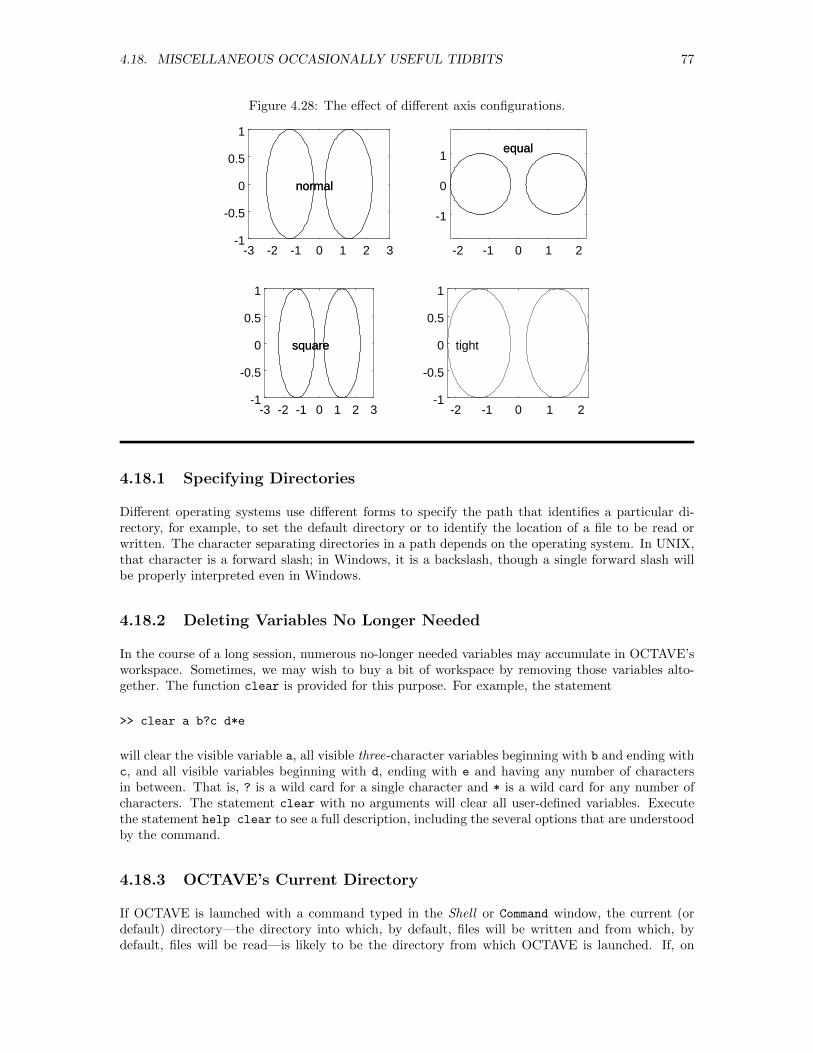
4.18. MISCELLANEOUS OCCASIONALLY USEFUL TIDBITS 77

Figure 4.28: The effect of different axis configurations.

-3 -2 -1 0 1 2 3-1

-0.5

0

0.5

1

normalnormal

-2 -1 0 1 2

-1

0

1

-3 -2 -1 0 1 2 3-1

-0.5

0

0.5

1

squaresquare

-2 -1 0 1 2-1

-0.5

0

0.5

1

tight

equalequal

4.18.1 Specifying Directories

Different operating systems use different forms to specify the path that identifies a particular di-rectory, for example, to set the default directory or to identify the location of a file to be read orwritten. The character separating directories in a path depends on the operating system. In UNIX,that character is a forward slash; in Windows, it is a backslash, though a single forward slash willbe properly interpreted even in Windows.

4.18.2 Deleting Variables No Longer Needed

In the course of a long session, numerous no-longer needed variables may accumulate in OCTAVE’sworkspace. Sometimes, we may wish to buy a bit of workspace by removing those variables alto-gether. The function clear is provided for this purpose. For example, the statement

>> clear a b?c d*e

will clear the visible variable a, all visible three-character variables beginning with b and ending withc, and all visible variables beginning with d, ending with e and having any number of charactersin between. That is, ? is a wild card for a single character and * is a wild card for any number ofcharacters. The statement clear with no arguments will clear all user-defined variables. Executethe statement help clear to see a full description, including the several options that are understoodby the command.

4.18.3 OCTAVE’s Current Directory

If OCTAVE is launched with a command typed in the Shell or Command window, the current (ordefault) directory—the directory into which, by default, files will be written and from which, bydefault, files will be read—is likely to be the directory from which OCTAVE is launched. If, on

78 CHAPTER 4. INTRODUCTION TO OCTAVE

the other hand, OCTAVE is launched by double-clicking ML on an icon, the current directory willtypically be the user’s home directory, though that can be changed by a statement in a suitablestart-up file (see Section 4.18.5). In the GUI, the identity of the current directory is conveyed ina text-entry box in the toolbar at the top of the window and can be edited by changing the entryin that box, either by browsing in the drop-down menu available in that box, by explicitly typingthe desired directory in the box, or by selecting from the folders displayed in the panel immediatelybelow that box. In all interfaces, the identity of the current directory can be displayed with theUNIX-style command pwd and changed with the UNIX-style command cd. When this directory isunknown or ill-defined, including a full specification of a path in a file name is necessary.

4.18.4 OCTAVE’s Search Path

Whenever an explicit path is not specified for a file that OCTAVE must read (either data file orm-file), the program looks in a succession of directories. By default, that path contains the currentworking directory (see Section 4.18.3) followed by several directories distributed with OCTAVE,including directories, subdirectories, and subndirectories in76

$OCTAVEHEAD/octave-version

The command path or path() with no arguments will display a list of the directories in the currentsearch path. The command

• addpath adds one or more directories to the current search path.• rmpath removes one or more directories from the current search path.• genpath replaces the current search path with a new search path containing one or more

specified directories.• restoredefaultpath re-establishes the default search path.

See the online help or execute help path for more on how to modify the search path.

4.18.5 Customizing OCTAVE

The configuration of OCTAVE can be customized in several ways. First, the system manager candefine two system-wide startup files, specifically77

$OCTAVEHEAD/octave-version/share/octave/site/m/startup/octaverc and

$OCTAVEHEAD/octave-version/share/octave/version/m/startup/octaverc

These files allow the system manager to customize all versions of OCTAVE (the first file) and modifythat customization for specific versions (the second file). They can be changed only by the systemmanager, but they can be opened and viewed by any user. When OCTAVE is launched by any user,the first of these files is executed and then the second is executed.

Additionally, individual users can change the default font and font size, specify additionalstartup modifiers, and perhaps modify other attributes of OCTAVE in the file ~/.octaverc in theuser’s home directory and the file .octaverc located in the current working directory. These twofiles are user created. The one in the home directory is executed right after the system manager’sfiles are executed and, finally, the one in the current directory is executed.78 This structure forces

76The symbol $OCTAVEHEAD, whose value will vary from site to site, must be replaced by the actual path as describedin the Local Guide.

77The value of $OCTAVEHEAD varies from site to site. See the Local Guide.78If the current directory is, in fact, the user’s home directory, the local startup file is read only once.

4.18. MISCELLANEOUS OCCASIONALLY USEFUL TIDBITS 79

the user to accept initially whatever the system manager dictates but then to modify those dictatesto customize OCTAVE differently for each current directory in which OCTAVE is used. With thissequence, the system manager can enforce features for all users but individual users can override orembellish the system manager’s dictates to match their specific needs.

4.18.6 Restoring OCTAVE’s Initial State

This section is reserved for a description of how to restore OCTAVE’s initial state without exitingand re-entering the program. Until that capacity has been implemented, exiting and re-enteringOCTAVE will achieve the desired reinitialization, though that process will also lose anything in theediting window of the GUI (unless that content has been saved in an external file before exiting fromOCTAVE).

4.18.7 The Command format

Beyond the formats noted in Section 4.3.1, OCTAVE also accepts the statements

>> format compact

>> format loose

the first of which causes OCTAVE to use less space in output it directs to the screen and the secondof which restores the default. Numerous additional specifications of the format can be found byexecuting the command help format.

4.18.8 Reading Data from the Keyboard

Occasionally, and perhaps especially in M-files, we may wish to prompt for keyboard entry of one ormore values by displaying a message on the screen and then read those values from the keyboard.The OCTAVE command input achieves this objective. Its syntax is illustrated in the statement

x = input( ’Enter the value of x: ’ )

Here, the argument of the command defines the prompting message and the value entered—whichmay be a single value or a set of values—will be assigned to the variable x. If the command isterminated with a semicolon, output of the entered value to the screen will be suppressed. If two ormore values are to be entered, then the statement requesting the entry would be

pos = input( ’Enter x and y coordinates: ’ )

and, separated by space(s) or a comma, the values will be entered in a single line and enclosed insquare brackets. In this case, the value assigned to pos will be a vector.

4.18.9 Writing Data to the Screen

In OCTAVE, many statements not terminated by a semicolon will display output on the screen auto-matically. If one wishes more control over the format of the output, simply omitting the terminatingsemicolons will not be enough. The code segments

80 CHAPTER 4. INTRODUCTION TO OCTAVE

disp(’This is a message.’)

a = [0.0 10.0; 0.1 15.0; 0.2 18.0];

disp( ’ t (s) x (cm)’ )

disp( a )

a11 = num2str(a(1,1), ’%4.1f’);

a12 = num2str(a(1,2), ’%5.1f’);

str = [’When t = ’, a11, ’ s, x = ’, a12, ’ cm.’];

disp( str )

fprintf( 1, ’When t = %4.1f s, x = %5.1f cm.\n’, a(1,1), a(1,2) )

Display a text message.

Display the 3× 2 array a with labels on thecolumns but without formatting of the val-ues. It will take a bit of experimentation toinsert appropriate spaces to line everythingup vertically in the output.

Format numbers as strings with num2str.

Construct output as single string.Display concatenated string.

illustrate use of the two commands—disp and fprintf—to send more carefully formatted infor-mation to the screen. All will display the desired information without the identifier ans =. Notethat, in the use of fprintf, the file identifier 1 points to the screen and the associated file is alwaysopen; it does not require explicit opening or closing. The command disp is particularly useful incommand files when on-screen messages about progress are desired.

4.18.10 Exiting from Procedures

Most often, invoked procedures and loops will run to completion and exit normally to the callingprogram. Sometimes, perhaps in response to a trapped error, it may be desired to exit from aprocedure or a loop prematurely. Two statements—break and return—are available to achievethese ends. The statement break is used to exit from a (single) loop to execute the statementfollowing the loop. Suppose, for example, one has a vector A containing n integers and one wishesto find the square of the first even integer in the vector. The coding

for i = 1:n

if 2*fix( A(i)/2 ) == A(i)

break;

endif

endfor

result = A(i)^2

will step systematically through the components of A, testing each to see if it is even, and stoppingwhen it encounters the first even component. At that point, the program exits the for loop andexecutes the statement following the endfor. Time is not spent examining entries in A that followthat first even entry.

OCTAVE provides the statement return to exit prematurely from a running procedure orfunction. For example, the coding

if den == 0

disp(’ERROR: Division by zero encountered. Execution terminated.’ )

return

endif

encountered during execution will display the error message and return control immediately towhatever level called the procedure of function.

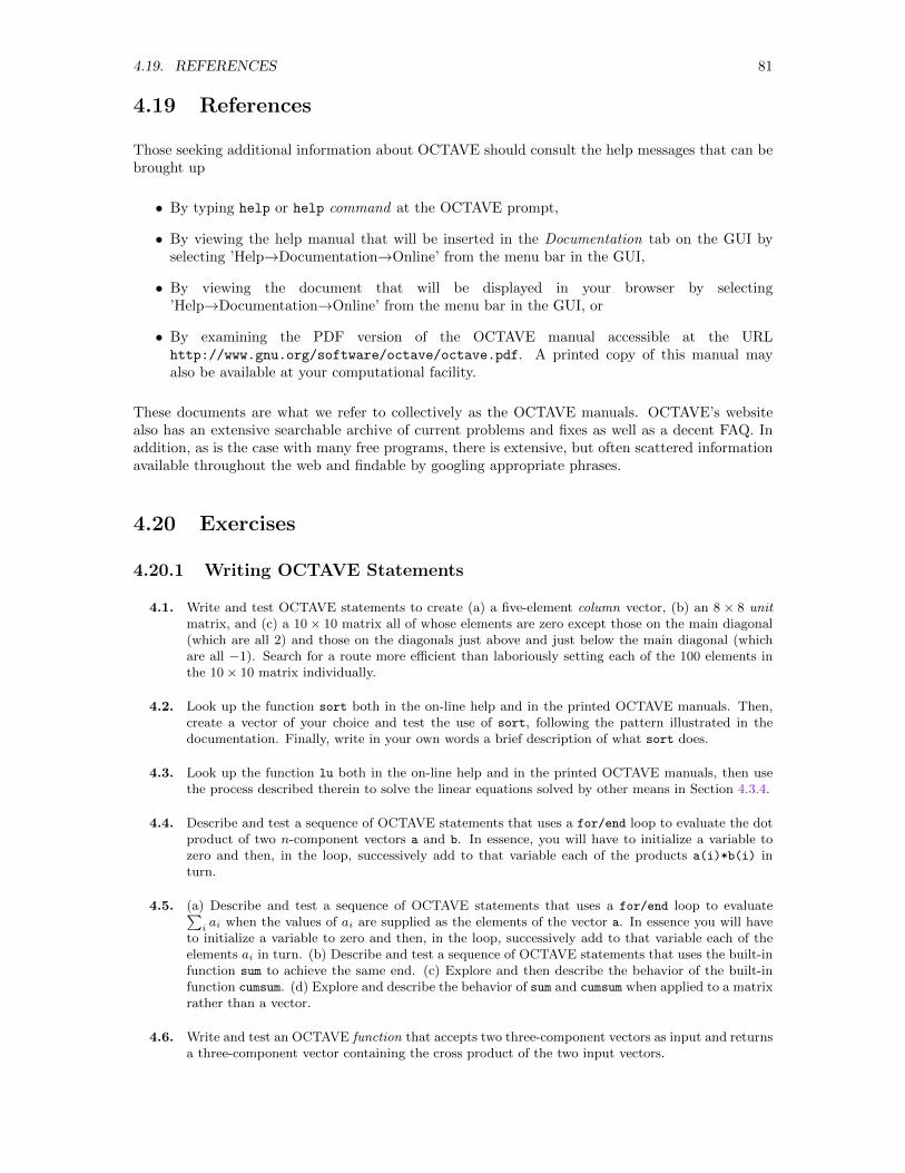
4.19. REFERENCES 81

4.19 References

Those seeking additional information about OCTAVE should consult the help messages that can bebrought up

• By typing help or help command at the OCTAVE prompt,

• By viewing the help manual that will be inserted in the Documentation tab on the GUI byselecting ’Help→Documentation→Online’ from the menu bar in the GUI,

• By viewing the document that will be displayed in your browser by selecting’Help→Documentation→Online’ from the menu bar in the GUI, or

• By examining the PDF version of the OCTAVE manual accessible at the URLhttp://www.gnu.org/software/octave/octave.pdf. A printed copy of this manual mayalso be available at your computational facility.

These documents are what we refer to collectively as the OCTAVE manuals. OCTAVE’s websitealso has an extensive searchable archive of current problems and fixes as well as a decent FAQ. Inaddition, as is the case with many free programs, there is extensive, but often scattered informationavailable throughout the web and findable by googling appropriate phrases.

4.20 Exercises

4.20.1 Writing OCTAVE Statements

4.1. Write and test OCTAVE statements to create (a) a five-element column vector, (b) an 8 × 8 unitmatrix, and (c) a 10× 10 matrix all of whose elements are zero except those on the main diagonal(which are all 2) and those on the diagonals just above and just below the main diagonal (whichare all −1). Search for a route more efficient than laboriously setting each of the 100 elements inthe 10× 10 matrix individually.

4.2. Look up the function sort both in the on-line help and in the printed OCTAVE manuals. Then,create a vector of your choice and test the use of sort, following the pattern illustrated in thedocumentation. Finally, write in your own words a brief description of what sort does.

4.3. Look up the function lu both in the on-line help and in the printed OCTAVE manuals, then usethe process described therein to solve the linear equations solved by other means in Section 4.3.4.

4.4. Describe and test a sequence of OCTAVE statements that uses a for/end loop to evaluate the dotproduct of two n-component vectors a and b. In essence, you will have to initialize a variable tozero and then, in the loop, successively add to that variable each of the products a(i)*b(i) inturn.

4.5. (a) Describe and test a sequence of OCTAVE statements that uses a for/end loop to evaluate∑iai when the values of ai are supplied as the elements of the vector a. In essence you will have

to initialize a variable to zero and then, in the loop, successively add to that variable each of theelements ai in turn. (b) Describe and test a sequence of OCTAVE statements that uses the built-infunction sum to achieve the same end. (c) Explore and then describe the behavior of the built-infunction cumsum. (d) Explore and describe the behavior of sum and cumsum when applied to a matrixrather than a vector.

4.6. Write and test an OCTAVE function that accepts two three-component vectors as input and returnsa three-component vector containing the cross product of the two input vectors.

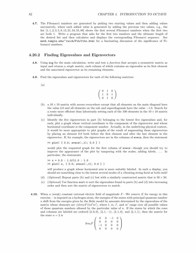
82 CHAPTER 4. INTRODUCTION TO OCTAVE

4.7. The Fibonacci numbers are generated by picking two starting values and then adding valuessuccessively, where each added value is generated by adding the previous two values, e.g., thelist [1, 1, 2, 3, 5, 8, 13, 21, 34, 55, 89] shows the first several Fibonacci numbers when the first twoare both 1. Write a program that asks for the first two numbers and the ultimate length ofthe desired list and then calculates and displays the corresponding Fibonacci sequence. Seemath.temple.edu/~reich/Fib/fibo.html for a fascinating discussion of the significance of Fi-bonacci numbers.

4.20.2 Finding Eigenvalues and Eigenvectors

4.8. Using eig for the main calculation, write and test a function that accepts a symmetric matrix asinput and returns a single matrix, each column of which contains an eigenvalue as its first elementand the associated eigenvector as its remaining elements.

4.9. Find the eigenvalues and eigenvectors for each of the following matrices:

(a) (0 1 01 0 10 1 0

)

(b) a 10× 10 matrix with zeroes everywhere except that all elements on the main diagonal havethe value 2.0 and all elements on the sub and superdiagonals have the value −1.0. Search fora route more efficient than laboriously setting each of the 100 elements in the 10× 10 matrixindividually.

(c) Identify the five eigenvectors in part (b) belonging to the lowest five eigenvalues and, foreach, plot a graph whose vertical coordinate is the component of the eigenvector and whosehorizontal coordinate is the component number. Actually, in the underlying physical context,it would be more appropriate to plot graphs of the result of augmenting these eigenvectorsby placing an element 0.0 both before the first element and after the last element in theeigenvector. If, for example, the eigenvectors are in the columns of evecs, then the statement

>> plot( [ 0.0; evecs(:,1); 0.0 ] )

would plot the requested graph for the first column of evecs—though you should try toimprove the appearance of the plot by tampering with the scales, adding labels, . . .. Inparticular, the statements

>> x = 0.0 : 1.0/11.0 : 1.0

>> plot( x, [ 0.0; evecs(:,1); 0.0 ] )

will produce a graph whose horizontal axis is more suitably labeled. In such a display, youshould see something close to the lowest several modes of a vibrating string fixed at both ends!

(d) (Optional) Repeat parts (b) and (c) but with a similarly constructed matrix that is 50× 50.

(e) (Optional) Use function sort to sort the eigenvalues found in parts (b) and (d) into increasingorder and then sort the matrix of eigenvectors to match.

4.10. When a (weak) constant external electric field of magnitude F—We reserve E for energy in thisexercise.—is imposed on a hydrogen atom, the energies of the states with principal quantum numbern shift from the energies given by the Bohr model by amounts determined by the eigenvalues of thematrix whose elements are 〈nlm|eF z|nl′m′〉, where l, m, l′, and m′ range over all possible valuesof those quantum numbers allowed by the particular value of n. If the states by which the rowsand columns are labeled are ordered |2, 0, 0〉, |2, 1,−1〉, |2, 1, 0〉, and |2, 1, 1〉, then the matrix forthe state n = 2 is

3ea0F

0 0 −1 00 0 0 0−1 0 0 00 0 0 0

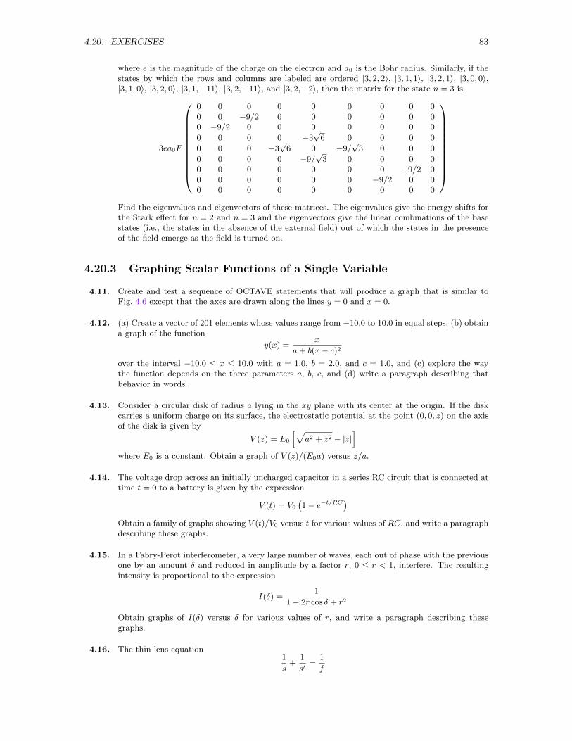
4.20. EXERCISES 83

where e is the magnitude of the charge on the electron and a0 is the Bohr radius. Similarly, if thestates by which the rows and columns are labeled are ordered |3, 2, 2〉, |3, 1, 1〉, |3, 2, 1〉, |3, 0, 0〉,|3, 1, 0〉, |3, 2, 0〉, |3, 1,−11〉, |3, 2,−11〉, and |3, 2,−2〉, then the matrix for the state n = 3 is

3ea0F

0 0 0 0 0 0 0 0 00 0 −9/2 0 0 0 0 0 00 −9/2 0 0 0 0 0 0 0

0 0 0 0 −3√

6 0 0 0 0

0 0 0 −3√

6 0 −9/√

3 0 0 0

0 0 0 0 −9/√

3 0 0 0 00 0 0 0 0 0 0 −9/2 00 0 0 0 0 0 −9/2 0 00 0 0 0 0 0 0 0 0

Find the eigenvalues and eigenvectors of these matrices. The eigenvalues give the energy shifts forthe Stark effect for n = 2 and n = 3 and the eigenvectors give the linear combinations of the basestates (i.e., the states in the absence of the external field) out of which the states in the presenceof the field emerge as the field is turned on.

4.20.3 Graphing Scalar Functions of a Single Variable

4.11. Create and test a sequence of OCTAVE statements that will produce a graph that is similar toFig. 4.6 except that the axes are drawn along the lines y = 0 and x = 0.

4.12. (a) Create a vector of 201 elements whose values range from −10.0 to 10.0 in equal steps, (b) obtaina graph of the function

y(x) =x

a+ b(x− c)2

over the interval −10.0 ≤ x ≤ 10.0 with a = 1.0, b = 2.0, and c = 1.0, and (c) explore the waythe function depends on the three parameters a, b, c, and (d) write a paragraph describing thatbehavior in words.

4.13. Consider a circular disk of radius a lying in the xy plane with its center at the origin. If the diskcarries a uniform charge on its surface, the electrostatic potential at the point (0, 0, z) on the axisof the disk is given by

V (z) = E0

[√a2 + z2 − |z|

]where E0 is a constant. Obtain a graph of V (z)/(E0a) versus z/a.

4.14. The voltage drop across an initially uncharged capacitor in a series RC circuit that is connected attime t = 0 to a battery is given by the expression

V (t) = V0

(1− e−t/RC

)Obtain a family of graphs showing V (t)/V0 versus t for various values of RC, and write a paragraphdescribing these graphs.

4.15. In a Fabry-Perot interferometer, a very large number of waves, each out of phase with the previousone by an amount δ and reduced in amplitude by a factor r, 0 ≤ r < 1, interfere. The resultingintensity is proportional to the expression

I(δ) =1

1− 2r cos δ + r2

Obtain graphs of I(δ) versus δ for various values of r, and write a paragraph describing thesegraphs.

4.16. The thin lens equation1

s+

1

s′=

1

f

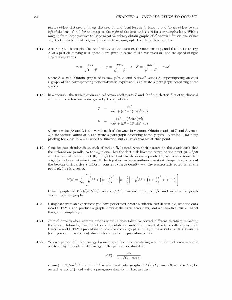
84 CHAPTER 4. INTRODUCTION TO OCTAVE

relates object distance s, image distance s′, and focal length f . Here, s > 0 for an object to theleft of the lens, s′ > 0 for an image to the right of the lens, and f > 0 for a converging lens. With sranging from large positive to large negative values, obtain graphs of s′ versus s for various valuesof f (both positive and negative), and write a paragraph describing these graphs.

4.17. According to the special theory of relativity, the mass m, the momentum p, and the kinetic energyK of a particle moving with speed v are given in terms of the rest mass m0 and the speed of lightc by the equations

m =m0√1− β2

; p =m0u√1− β2

; K =m0c

2√1− β2

−m0c2

where β = v/c. Obtain graphs of m/m0, p/m0c, and K/m0c2 versus β, superimposing on each

a graph of the corresponding non-relativistic expression, and write a paragraph describing thesegraphs.

4.18. In a vacuum, the transmission and reflection coefficients T and R of a dielectric film of thickness dand index of refraction n are given by the equations

T =4n2

4n2 + (n2 − 1)2 sin2(κd)

R =(n2 − 1)2 sin2(κd)

4n2 + (n2 − 1)2 sin2(κd)

where κ = 2πn/λ and λ is the wavelength of the wave in vacuum. Obtain graphs of T and R versusλ/d for various values of n and write a paragraph describing these graphs. Warning : Don’t tryplotting too close to λ = 0 since the function sin(κd) gives trouble at that point.

4.19. Consider two circular disks, each of radius R, located with their centers on the z axis such thattheir planes are parallel to the xy plane. Let the first disk have its center at the point (0, 0, b/2)and the second at the point (0, 0,−b/2) so that the disks are separated by a distance b and theorigin is halfway between them. If the top disk carries a uniform, constant charge density σ andthe bottom disk carries a uniform, constant charge density −σ, the electrostatic potential at thepoint (0, 0, z) is given by

V (z) =σ

2ε0

[√R2 +

(z − b

2

)2

−∣∣∣z − b

2

∣∣∣−√R2 +(z +

b

2

)2

+

∣∣∣z +b

2

∣∣∣]

Obtain graphs of V (z)/(σR/2ε0) versus z/R for various values of b/R and write a paragraphdescribing these graphs.

4.20. Using data from an experiment you have performed, create a suitable ASCII text file, read the datainto OCTAVE, and produce a graph showing the data, error bars, and a theoretical curve. Labelthe graph completely.

4.21. Journal articles often contain graphs showing data taken by several different scientists regardingthe same relationship, with each experimentalist’s contribution marked with a different symbol.Describe an OCTAVE procedure to produce such a graph and, if you have suitable data available(or if you can invent some), demonstrate that your procedure works.

4.22. When a photon of initial energy E0 undergoes Compton scattering with an atom of mass m and isscattered by an angle θ, the energy of the photon is reduced to

E(θ) =E0

1 + ξ(1 + cos θ)

where ξ = E0/mc2. Obtain both Cartesian and polar graphs of E(θ)/E0 versus θ, −π ≤ θ ≤ π, for

several values of ξ, and write a paragraph describing these graphs.

4.20. EXERCISES 85

4.23. A charged particle moves along the z axis with speed v. When the particle passes through theorigin, the magnitude of the electric field produced by the particle is given by the expression

E(θ) =q

4πε0r2

1− β2(1 + β2 sin2 θ

)3/2where θ is the polar angle of the observation point, r is the radial coordinate at that point, andβ = v/c (c is the speed of light). Obtain graphs of E/(q/4πε0r

2) versus θ for various values of βon the interval −π ≤ θ ≤ π, and write a paragraph describing these graphs.

4.24. The intensity of the interference pattern produced by four slits illuminated by light of wavelengthλ when each slit is separated from the next by a distance a is given by

I(δ) = cos2 δ (1 + cos δ)

where δ = (2πa sin θ)/λ). Obtain both Cartesian and polar graphs of I versus θ on the interval−π/2 ≤ θ ≤ π/2 for various values of λ/a, and write a paragraph describing these graphs.

4.20.4 Graphing Scalar Functions of Two Variables

4.25. The Planck radiation law gives the expression

u(λ, T ) =8πch

λ5

1

ech/λkT − 1

for the distribution of energy in the radiation emitted by a black body. Here, c is the speed of light,h is Planck’s constant, k is Boltzmann’s constant, λ is the wavelength of the radiation, and T is theabsolute temperature. Using appropriate dimensionless units, plot this function (a) as a functionof λ for several T and (b) as a surface over the λT -plane. Write a paragraph about the way thepeak changes in position, height, and width as T changes. Hint : Choose a reference wavelengthλ0 arbitrarily and recast the expression in terms of the dimensionless variable Λ = λ/λ0. Then,note that T0 = ch/(λ0k) has the dimensions of temperature and re-express the temperature T interms of the dimensionless quantity τ = T/T0. (You might find it informative to evaluate T0 forλ0 = 550 nm.) With these changes, the expression to be plotted can be recast in the form

u(λ, T )

8πch/λ50

=1/Λ5

e1/Λτ − 1

and the question now becomes one of plotting this quantity using the dimensionless variables Λ andτ .

4.26. A solenoid of length L and circular cross-section of radius a lies with its axis along the z axis andits center at the origin. When the solenoid carries a current, the magnetic field at the point (0, 0, z)on the axis of the solenoid is given by

B(z) =1

2B0

[z + L/2√

a2 + (z + L/2)2− z − L/2√

a2 + (z − L/2)2

]where B0 is the magnetic field at the center when a L, i.e., when the solenoid is effectivelyinfinite in length. Plot graphs showing B(z)/B0 (a) as a function of z/L for various values of a/L,(b) as a surface over the (z/L)(a/L) plane, and (c) as a contour over the (z/L)(a/L) plane. Writea paragraph describing these graphs.

4.27. Consider two circular current loops, each of radius a and lying with its center on and its planeperpendicular to the z axis. The first loop is centered at the point (0, 0, b) and the second loop iscentered at the point (0, 0,−b). The axial component of the magnetic field at the point (0, 0, z) isgiven by the equation

B(z) =1

2B0

(a2 + b2

)3/2 [ 1[a2 + (z + b)2

]3/2 +1[

a2 + (z − b)2]3/2

]

86 CHAPTER 4. INTRODUCTION TO OCTAVE

where B0 is the magnetic field at the origin. Plot graphs showing B(z)/B0 (a) as a function of z/afor various values of b/a, (b) as a surface over the (z/a)(b/a) plane, and (c) as a contour over the(z/a)(b/a) plane. Write a paragraph describing these graphs.

4.28. In an LRC circuit of resonant frequency ω0, the current I is given as a function of frequency ω by

I =I0√

1 +Q2

(Ω− 1

Ω

)2

where Ω = ω/ω0. Plot I/I0 (a) as a function of Ω for various values of the quality factor Q and (b)as a surface over the ΩQ-plane. Write a paragraph describing these graphs.

4.29. A spherical potato of radius a is taken from the refrigerator at 0 C and placed in an oven at200 C. The temperature u(r, t) at a point a distance r from the center of the potato at time t isgiven by

u(r, t)

u0= 1− 2

∞∑n=1

j0(βnr/a)

βn j1(βn)e−κβ

2nt/(ca

2)

where κ is the thermal conductivity of the potato, c is its heat capacity per unit volume, j0(x) andj1(x) are the zeroth- and first-order spherical Bessel functions, and βn is the n-th root of j0(x), i.e.,j0(βn) = 0. Obtain graphs of u(r, t)/u0 as a function of r/a for various values of t. Obtain also agraph of the temperature u(0, t) at the center of the potato as a function of t and determine howlong it takes the potato to bake if, by being baked, one means that the temperature at the centerhas risen to 175 C, i.e., to a value such that u(0, t)/u0 = 0.875. Hints: (1) Note that

j0(x) =sinx

x; j1(x) =

sinx

x2− cosx

x

Thus, the n-th root of j0(x) is βn = nπ. (2) Express times in units of ca2/κ but then, takingthe radius of the potato to be a = 0.05 m and taking κ and c for the potato to be those of water[κ = 0.63 J/(m s K), and c = 4.2 × 106 J/(K m3)], determine the unit in which your answers areexpressed, both in seconds and in hours. (3) Experiment a bit, but note that the exponential factordecays more rapidly as n increases, so truncation of the infinite series at some point is probably inorder.

4.30. At a particular time, a planet of mass M is located at the origin in the xy plane and a moon of massM/3 is located at a point a distance R from the planet on the x axis. The gravitational potentialenergy of a spaceship of mass m at the point (x, y, z) is then given by

V (x, y, z) = − GmM√x2 + y2 + z2

− GmM/3√(x−R)2 + y2 + z2

Using OCTAVE, obtain surface plots and contour maps of this potential energy in the xy plane(i.e., the plane z = 0) and in the planes z = 0.1R and z = 0.5R. Suggestion: Recast the functionin dimensionless form by measuring x, y, and z in units of R and V (x, y, z) in units of GmM/R.

4.20.5 Graphing Scalar Functions of Three Variables

4.31. Using either mesh or contour slices, explore at least one of the three-dimensional scalar fields

p3,1,0(x, y, z) =8

(27)2πρ2(

1− ρ

6

)2

e−2ρ/3 cos2 θ

p3,1,1(x, y, z) =4

(27)2πρ2(

1− ρ

6

)2

e−2ρ/3 (1− cos2 θ)

p3,2,1(x, y, z) =3

(27)3πρ4 e−2ρ/3 cos2 θ (1− cos2 θ)

p3,2,2(x, y, z) =3

4(27)3πρ4 e−2ρ/3 (1− cos2 θ)2

4.20. EXERCISES 87

giving the probability density for the hydrogen states (n, l,m) = (3, 1, 0), (n, l,m) = (3, 1, 1),(n, l,m) = (3, 2, 1), and (n, l,m) = (3, 2, 2). These fields are expressed in dimensionless form, whereρ is the radial coordinate in units of the Bohr radius. In terms of the Cartesian coordinates x, y, z,ρ =

√x2 + y2 + z2 and cos θ = z/ρ. Hint : To avoid divisions by zero, recast the expressions in

terms of (x, y, z) explicitly before evaluating any of them numerically.

4.32. The (gauge) pressure p(x, y, z, t) inside a cubical box located in the region 0 ≤ x, y, z ≤ a is givenby

p(x, y, z, t) = A sinlπx

asin

mπy

asin

nπz

acosωlmnt

where l, m, and n are positive integers. Obtain several presentations of the pressure distributioninside this box at t = 0 and at t = π/ωlmn for several different values of l, m, and n.

4.20.6 Graphing Two-Dimensional Vector Fields

4.33. Suppose the functions Fx(x, y) and Fy(x, y) give the x and y components of a vector field at thepoint (x, y) in the xy plane. A very crude algorithm for determining the coordinates of points onthe field line that starts at the point (x0, y0) would entail the operations

xold <-- x0

yold <-- y0

ds <-- chosen step sizeLOOP

FX <-- Fx(xold,yold)FY <-- Fy(xold,yold)FM <-- SQRT( FX^2 + FY^2 )

xnew <-- xold + ds*FX/FM

ynew <-- yold + ds*FY/FM

Draw line from (xold,yold) to (xnew,ynew)

xold <-- xnew

yold <-- ynew

EXIT_LOOP WHEN DONE

END_LOOP

Set starting point.

Choose step.Start loop to generate steps.Calculate components of force.

Calculate magnitude of force.Step dx along force line.

Draw segment of force line.Shift focus to new point.

Repeat.

Cast the loop in this algorithm as an OCTAVE procedure trace field that would be called witha statement like

>> trace_field( xold, yold, ds, n )

where xold and yold convey the desired starting point for a field line, ds conveys the desired stepsize, and n stipulates the number of steps to be taken before completing the line and returningto the calling program. Though we might ultimately want to provide a means to define the fieldoutside of the tracing procedure, for purposes of this exercise suppose that the field of interest isgiven by

Fx(x, y) =x− 1.5

[(x− 1.5)2 + y2]3/2− x+ 1.5

[(x+ 1.5)2 + y2]3/2

Fy(x, y) =y

[(x− 1.5)2 + y2]3/2− y

[(x+ 1.5)2 + y2]3/2

which—in unspecified units—gives the electric field produced in the xy plane by two point charges,one of relative strength +1 located at (x, y) = (1.5, 0) and the other of relative strength −1 locatedat (x, y) = −(1.5, 0). As a first pass, suppose we are interested in the field only in the region−1 ≤ x, y ≤ 1 but, once you have your program operating successfully, you can relax that constraint.(Be aware, however, in relaxing the constraint that your algorithm will probably give troubles ifyou try to plot too close to either of the point charges.) When executed, trace field is to draw thefield line that starts at the specified point and continues until n steps have been made. Structure

88 CHAPTER 4. INTRODUCTION TO OCTAVE

your procedure so that its execution does not erase the current plot, i.e., so that you can executeit repeatedly with different starting points to build up a full map of the field of interest. Optional :Refine the procedure so that

(a) the loop is terminated not only after execution of a fixed number of steps but also when thefield line has gone out of bounds, approaches too closely to a singular point, or returns to apoint too close to its starting point (closed field line),

(b) it obtains its field definitions from two functions whose names are supplied as arguments whenit is called, and/or

(c) it uses a more refined predictor-corrector algorithm in which the values xnew and ynew deter-mined above are instead regarded as xpred and ypred, the field is calculated at that predictedpoint, and then a final step to xnew and ynew is made from xold and yold by using the averageof the fields at the points (xold, yold) and (xpred, ypred). Hints: You may want to use thecommand plot with the keyword nodata set to true to establish the axes before beginningto trace any field lines.

4.34. Since equipotential curves are perpendicular to the field lines representing the associated (conser-vative) force field, an algorithm for tracing equipotential curves in two dimensions differs from thealgorithm described in the previous exercise only by arranging for the stepping to occur at rightangles to the calculated field rather than in the direction of the field. That objective is accomplishedby replacing the two statements evaluating xnew and ynew in the algorithm in the previous exercisewith the statements

xnew <-- xold - ds*FY/FM

ynew <-- yold + ds*FX/FM

Following a pattern similar to that described in the previous exercise, cast the loop in this algorithmas an OCTAVE procedure trace equipot that would be called with a statement like

>> trace_equipot( xold, yold, ds, n )

where xold and yold convey the desired starting point for the equipotential curve, ds conveys thedesired step size, and n stipulates the number of steps to be taken before completing the curveand returning to the calling program. Then, explore the equipotential curves depicting the field onwhich the previous exercise focussed.

4.35. Sometimes, interest can be focussed on the magnitude of the vector field rather than on the fullfield. A command like

MAG = sqrt( Hx.^2 + Hy.^2 )

for example, will generate an array MAG containing the magnitudes of the magnetic field at eachavailable grid point. This array then conveys a scalar field that can be displayed by any of themethods described in Section 4.13. Explore the magnetic field given in Eq. (4.16) in this way.

4.36. Read the OCTAVE manuals about the procedure quiver3. Then use quiver3 to explore the velocityfield

v(x, y, z) = ω(−y i + x j) + α k

(which happens not to depend on z) for various values of ω and α. Then write a paragraph ortwo describing the field. Reassurance: Diagrams of vector fields in three dimensions are not easyto fathom. Do not be dismayed if the pictures you generate are initially mysterious. Hint : Inestablishing a scale, you may find it useful to assume a length scale a, recast the field in the form

v = aω(−ya

i +x

aj)

+ α k =⇒ v

aω=(−ya

i +x

aj)

+α

aωk

and try to draw graphs of the field v/aω as functions of the parameter α/aω in the space whoseaxes are labeled x/a, y/a, and z/a.

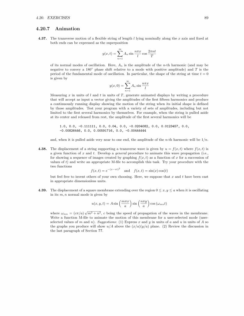
4.20. EXERCISES 89

4.20.7 Animation

4.37. The transverse motion of a flexible string of length l lying nominally along the x axis and fixed atboth ends can be expressed as the superposition

y(x, t) =

∞∑n=1

An sinnπx

lcos

2πnt

T

of its normal modes of oscillation. Here, An is the amplitude of the n-th harmonic (and may benegative to convey a 180 phase shift relative to a mode with positive amplitude) and T is theperiod of the fundamental mode of oscillation. In particular, the shape of the string at time t = 0is given by

y(x, 0) =

∞∑n=1

An sinnπx

l

Measuring x in units of l and t in units of T , generate animated displays by writing a procedurethat will accept as input a vector giving the amplitudes of the first fifteen harmonics and producea continuously running display showing the motion of the string when its initial shape is definedby those amplitudes. Test your program with a variety of sets of amplitudes, including but notlimited to the first several harmonics by themselves. For example, when the string is pulled asideat its center and released from rest, the amplitude of the first several harmonics will be

1.0, 0.0, -0.111111, 0.0, 0.04, 0.0, -0.0204082, 0.0, 0.0123457, 0.0,

-0.00826446, 0.0, 0.00591716, 0.0, -0.00444444

and, when it is pulled aside very near to one end, the amplitude of the n-th harmonic will be 1/n.

4.38. The displacement of a string supporting a transverse wave is given by u = f(x, t) where f(x, t) isa given function of x and t. Develop a general procedure to animate this wave propagation (i.e.,for showing a sequence of images created by graphing f(x, t) as a function of x for a succession ofvalues of t) and write an appropriate M-file to accomplish this task. Try your procedure with thetwo functions

f(x, t) = e−(x−vt)2 and f(x, t) = sin(x) cos(t)

but feel free to invent others of your own choosing. Here, we suppose that x and t have been castin appropriate dimensionless units.

4.39. The displacement of a square membrane extending over the region 0 ≤ x, y ≤ a when it is oscillatingin its m,n normal mode is given by

u(x, y, t) = A sin(mπx

a

)sin(nπy

a

)cos (ωmnt)

where ωmn = (cπ/a)√m2 + n2, c being the speed of propagation of the waves in the membrane.

Write a function M-file to animate the motion of this membrane for a user-selected mode (user-selected values of m and n). Suggestions: (1) Express x and y in units of a and u in units of A sothe graphs you produce will show u/A above the (x/a)(y/a) plane. (2) Review the discussion inthe last paragraph of Section ??.

90 CHAPTER 4. INTRODUCTION TO OCTAVE

Chapter 8

Introduction to MATHEMATICA

Note: All program (.m) files referred to in this chapter are available in the directory$HEAD/mathematica, where (as defined in the Local Guide) $HEAD must be replacedby the appropriate path for your site. At some sites, this directory or some otherdirectory containing these files may also have been placed in Mathematica’s defaultsearch path. If so, the files can be found by Mathematica without explicit specifi-cation of a path. Otherwise, you will have to use the full path to copy them intoyour default directory to access them.

Conceived and developed by Stephen Wolfram and first released to the public in June of 1988,Mathematica r© is a large program for manipulating expressions symbolically.1 Mathematica canperform symbolic algebra; evaluate derivatives, integrals, and Taylor series; solve algebraic anddifferential equations; manipulate complex numbers; find eigenvalues and eigenvectors; produce two-and three-dimensional graphs; and accomplish numerous other tasks. In this chapter, we describesome ways by which expressions can be defined for Mathematica and then illustrate some of thestatements by which Mathematica can be instructed to manipulate these expressions. Users shouldalso work through the on-line help messages within Mathematica itself and, in particular, look atthe examples with which most on-line help messages conclude (Section 8.2). Further details canbe found in printed and on-line Mathematica documentation (Section 8.19). We shall refer to thisdocumentation collectively as the Mathematica manuals.

Two user interfaces to Mathematica are provided, a text-based interface (TBI), which givesdirect access to the Mathematica kernel, and a notebook interface (NBI), which displays equationsin a more elegant form, offers assistance for those who have trouble remembering the commands,and has a notebook capability to facilitate documentation. In essence, the TBI gives the user directaccess to the Mathematica kernel while the NBI is simply a front-end that facilitates construction ofstatements that the NBI then formulates properly and passes on to the kernel, which may actuallybe running on a different (and perhaps faster) computer than is used for the front-end. In thisbook, we assume that the user is working in the NBI. We will, however, describe the structure ofinput statements without addressing the ways in which the NBI facilitates assembling them,2 so thestatements we describe can equally well be submitted to the TBI. We shall present Mathematicaoutput with the approximate appearance it will have in the NBI.

Except where occasionally noted otherwise, for the rest of this book, information provided de-scribes the NBI explicitly and may not accurately reflect the behavior of the TBI.

1Mathematica is a registered trademark of and also a commercially available program produced and marketedby Wolfram Research, Inc., of Champaign, Illinois. (See Appendix Z for full contact information.) Its use at anyparticular site is subject to the provisions of whatever license that site has negotiated with Wolfram Research, Inc.The terms of that license are explained in the Local Guide.

2See the Mathematica manuals for information about how to use templates, palettes, and other aids available inthe NBI.

91

92 CHAPTER 8. INTRODUCTION TO MATHEMATICA

8.1 Beginning a Mathematica Session

Detailed instructions for initiating a session with Mathematica will be found in the Local Guide. Ingeneral, Mathematica will be started either (1) by typing the command mathematica for the NBI(or math for the TBI) at the prompt from the operating system,3 (2) by double-clicking ML on anappropriate icon on the desktop, or (3) by selecting ‘Mathematica’ (or an equivalent phrase) froma menu.4 Presently, an introductory screen offering a number of options will appear. Opening theNew Document drop-down menu and selecting the option ‘Notebook’ produces a blank notebooktitled ‘Untitled-1’ and a cursor—but no prompting character(s). We must from the outset be awarethat

1. Labels, e.g., ‘In[12]:=’ for input and ‘Out[12]=’ for output, will appear after a statement hasbeen submitted to Mathematica.

2. Internally, Mathematica is case sensitive, i.e., Mathematica treats upper and lower case lettersas distinct. By convention, built-in Mathematica commands use names whose initial letter iscapitalized.

3. By default, Mathematica formats input statements using Wolfram Language input. Otherformats can be selected by opening the menu accessed by the ’+’ sign that appears at the topof the notebook.

4. Lines of Mathematica code can be terminated in any of three ways, depending on whether wewant to

(a) submit the statement for execution and instruct Mathematica to display its response, inwhich case we terminate the statement by typing 〈SHIFT/ENTER〉 on the main keyboardor by typing 〈ENTER〉 on the numeric keypad.5

(b) submit the statement for execution and instruct Mathematica to suppress explicit displayof its response, in which case we terminate the statement with a semicolon followed by〈SHIFT/ENTER〉 on the main keyboard or 〈ENTER〉 on the numeric keypad.

(c) continue entering the statement on a new line, in which case we terminate the line bytyping simply 〈ENTER〉, but we must be clever in exploiting this feature. Mathematicawill expect additional input only if the part entered before typing 〈ENTER〉 is incomplete.To enter the statement a + b + c on two lines, for example, we could not break it afterthe b but we could break it after either of the + signs.

5. Two or more statements can be placed in a single physical line by separating the statementswith semicolons, though output will be suppressed for all but the last statement in the line(unless it is followed by a semicolon).

6. To abort execution of a statement by the Mathematica kernel and return Mathematica to astate from which new statements can be entered, either type 〈ALT/.〉 or, alternatively,

• Select the block containing the statement whose execution is to be terminated by clickingML on the corresponding bracket at the right end of the screen,

• Open the Evaluation menu from the menu bar across the top of the notebook, and• Select ‘Abort Evaluation’ from that menu.

There may be a short delay during which Mathematica will clean up its workspace beforeactually “prompting” for fresh input.

3In this command to the operating system, case may be important.4Access to Mathematica is controlled by a license manager. When Mathematica is started, the license manager

checks to make sure that a license is available. If no license is available (or the license manager happens not tobe running), the desired session will not start. Restarting a stopped license manager requires action by the systemadministrator.

5On some keyboards the 〈ENTER〉 key will be labeled 〈RETURN〉.

8.2. ON-LINE HELP 93

7. Typing the statement Quit[] whenever Mathematica is ready for input cleans Mathematica’sworkspace and reinitializes its internal statement counter but does not close the notebook orreturn control to the operating system. To exit altogether from Mathematica, select ‘Exit’ fromthe File menu or click ML on the ‘×’ button in the upper right corner above the Mathematicamenu bar. If the notebook contains unsaved content, a pop-up box will give you the option ofsaving that content before Mathematica actually returns control to the computer’s operatingsystem.

8. To close the current notebook without exiting from Mathematica, select ‘Close’ from the Filemenu. If, after closing a notebook, you open a new notebook by selecting ‘New→Notebook’from the File menu or ‘Notebook’ from the Mathematica opening screen, statement numbers inthat new notebook will continue from where they left off in the closed notebook. To reinitializethe internal statement counter, execute the statement Quit[], preferably before closing thefirst notebook but alternatively right after opening the new notebook.

9. The Mathematica command Run[ "OSCommand" ] effects temporary escape from Mathe-matica to the underlying operating system (OS) to effect execution of OSCommand by thatoperating system. Control is then returned to Mathematica. The resulting output (if any) isdisplayed in the command window from which Mathematica was launched.6

10. Although the feature can be disabled, by default some types of error detected by Mathematica’sfront end will produce an audible beep. For further information about that beep when it occurs,select ‘Why the beep?’ from the Help menu.

8.2 On-Line Help

Mathematica provides extensive on-line help. Users can enter a hypertext browser by selecting‘Wolfram Documentation’ (or some equivalent phrasing) from the Help menu. The browser canbe used to search for an item by entering the name of the item in the text entry box at the top ofthe browser and then clicking ML on the magnifying glass next to the text entry box; presently, adescription of the item will appear. Alternatively, we can navigate the hierarchy of help messages byopening various submenus represented by colored boxes in the window that pops up when ‘WolframDocumentation’ is selected.

Alternatively, information about a particular item can be obtained simply by typing a questionmark ?—which must be the first character on the line—followed by the name of the item aboutwhich information is sought (e.g., ?Sin) whenever Mathematica is prepared to accept input. Thisaction brings up an inline brief description of the specified item, including a link—the symbol >>—whose selection will bring up the full documentation for the item sought. Beginning a line with twoquestion marks, e.g. ??Sin, appends to the message produced by one question mark a statementabout the attributes assigned to the specified symbol.

Finally, when a specific Mathematica symbol is highlighted in a notebook, selecting ‘Find Se-lected Function’ from the Help menu will bring up the full documentation for that function.

Items in the on-line help library that describe specific Mathematica commands typically includenot only a description of the function and syntax of the command but also examples of the properuse of the command and links to further details and related topics at other points in the on-linemessages. Many of the examples contain active statements that can be edited and reexecuted fromwithin the help message. Your attention is drawn particularly to the on-line help messages for thecommands D, Integrate, Simplify, Expand, Factor, Solve, Sum, and DSolve.

6In the NBI on any platform of course, this feature is unnecessary, since we can easily use resources of the desktop toexecute other programs without exiting from Mathematica. Indeed, any output produced by Run[ "OSCommand" ]

executed from the NBI will be displayed in a pop-up Shell window which, however, will promptly disappear when thecommand ends.

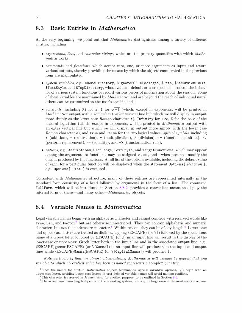
94 CHAPTER 8. INTRODUCTION TO MATHEMATICA

8.3 Basic Entities in Mathematica

At the very beginning, we point out that Mathematica distinguishes among a variety of differententities, including

• expressions, lists, and character strings, which are the primary quantities with which Mathe-matica works;

• commands and functions, which accept zero, one, or more arguments as input and returnvarious outputs, thereby providing the means by which the objects enumerated in the previousitem are manipulated;

• system variables, e.g., $HomeDirectory, $IgnoreEOF, $Packages, $Path, $RecursionLimit,$TextStyle, and $TopDirectory, whose values—default or user-specified—control the behav-ior of various system functions or record various pieces of information about the session. Someof these variables are maintained by Mathematica and are beyond the reach of individual users;others can be customized to the user’s specific ends.

• constants, including Pi for π, I for√−1 (which, except in exponents, will be printed in

Mathematica output with a somewhat thicker vertical line but which we will display in outputmore simply as the lower case Roman character i), Infinity for +∞, E for the base of thenatural logarithm (which, except in exponents, will be printed in Mathematica output withan extra vertical line but which we will display in output more simply with the lower caseRoman character e), and True and False for the two logical values. special symbols, including+ (addition), - (subtraction), * (multiplication), / (division), := (function definition), /.

(perform replacement), == (equality), and -> (transformation rule).

• options, e.g., Assumptions, PlotRange, TextStyle, and TargetFunctions, which may appearamong the arguments to functions, may be assigned values, and—when present—modify theoutput produced by the functions. A full list of the options available, including the default valueof each, for a particular function will be displayed when the statement Options[ Function ],e.g., Options[ Plot ] is executed.

Consistent with Mathematica structure, many of these entities are represented internally in thestandard form consisting of a head followed by arguments in the form of a list. The commandFullForm, which will be introduced in Section 8.8.2, provides a convenient means to display theinternal form of these—and many other—Mathematica objects.

8.4 Variable Names in Mathematica

Legal variable names begin with an alphabetic character and cannot coincide with reserved words likeTrue, Sin, and Factor7 but are otherwise unrestricted. They can contain alphabetic and numericcharacters but not the underscore character.8 Within reason, they can be of any length.9 Lower-caseand upper-case letters are treated as distinct. Typing 〈ESCAPE〉 (or \[) followed by the spelled-outname of a Greek letter followed by 〈ESCAPE〉 (or ]) in an input line will result in the display of thelower-case or upper-case Greek letter both in the input line and in the associated output line, e.g.,〈ESCAPE〉gamma〈ESCAPE〉 (or \[Gamma]) in an input line will produce γ in the input and outputlines while 〈ESCAPE〉Gamma〈ESCAPE〉 (or \[CapitalGamma]) will produce Γ.

Note particularly that, in almost all situations, Mathematica will assume by default that anyvariable to which no explicit value has been assigned represents a complex quantity.

7Since the names for built-in Mathematica objects (commands, special variables, options, . . .) begin with anupper-case letter, avoiding upper-case letters in user-defined variable names will avoid naming conflicts.

8This character is reserved in Mathematica for another purpose, to be outlined in Section 8.6.9The actual maximum length depends on the operating system, but is quite large even in the most restrictive case.

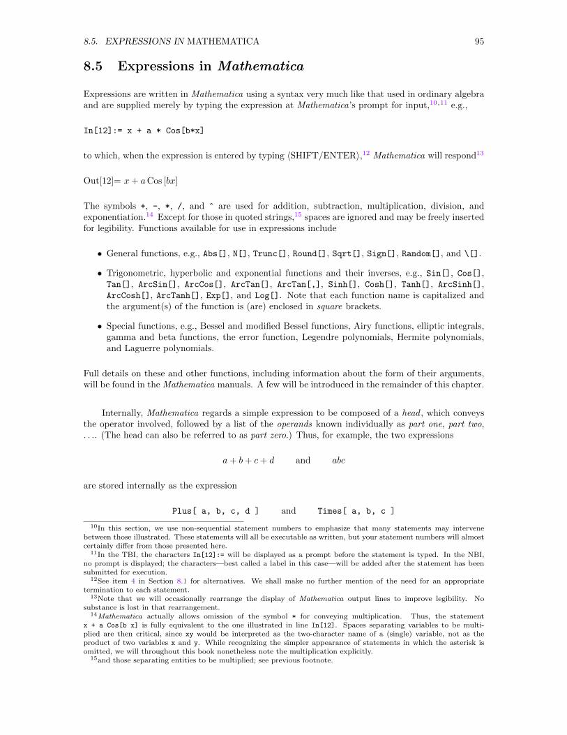
8.5. EXPRESSIONS IN MATHEMATICA 95

8.5 Expressions in Mathematica

Expressions are written in Mathematica using a syntax very much like that used in ordinary algebraand are supplied merely by typing the expression at Mathematica’s prompt for input,10,11 e.g.,

In[12]:= x + a * Cos[b*x]

to which, when the expression is entered by typing 〈SHIFT/ENTER〉,12 Mathematica will respond13

Out[12]= x+ aCos [bx]

The symbols +, -, *, /, and ^ are used for addition, subtraction, multiplication, division, andexponentiation.14 Except for those in quoted strings,15 spaces are ignored and may be freely insertedfor legibility. Functions available for use in expressions include

• General functions, e.g., Abs[], N[], Trunc[], Round[], Sqrt[], Sign[], Random[], and \[].

• Trigonometric, hyperbolic and exponential functions and their inverses, e.g., Sin[], Cos[],Tan[], ArcSin[], ArcCos[], ArcTan[], ArcTan[,], Sinh[], Cosh[], Tanh[], ArcSinh[],ArcCosh[], ArcTanh[], Exp[], and Log[]. Note that each function name is capitalized andthe argument(s) of the function is (are) enclosed in square brackets.

• Special functions, e.g., Bessel and modified Bessel functions, Airy functions, elliptic integrals,gamma and beta functions, the error function, Legendre polynomials, Hermite polynomials,and Laguerre polynomials.

Full details on these and other functions, including information about the form of their arguments,will be found in the Mathematica manuals. A few will be introduced in the remainder of this chapter.

Internally, Mathematica regards a simple expression to be composed of a head , which conveysthe operator involved, followed by a list of the operands known individually as part one, part two,. . .. (The head can also be referred to as part zero.) Thus, for example, the two expressions

a+ b+ c+ d and abc

are stored internally as the expression

Plus[ a, b, c, d ] and Times[ a, b, c ]

10In this section, we use non-sequential statement numbers to emphasize that many statements may intervenebetween those illustrated. These statements will all be executable as written, but your statement numbers will almostcertainly differ from those presented here.

11In the TBI, the characters In[12]:= will be displayed as a prompt before the statement is typed. In the NBI,no prompt is displayed; the characters—best called a label in this case—will be added after the statement has beensubmitted for execution.

12See item 4 in Section 8.1 for alternatives. We shall make no further mention of the need for an appropriatetermination to each statement.

13Note that we will occasionally rearrange the display of Mathematica output lines to improve legibility. Nosubstance is lost in that rearrangement.

14Mathematica actually allows omission of the symbol * for conveying multiplication. Thus, the statementx + a Cos[b x] is fully equivalent to the one illustrated in line In[12]. Spaces separating variables to be multi-plied are then critical, since xy would be interpreted as the two-character name of a (single) variable, not as theproduct of two variables x and y. While recognizing the simpler appearance of statements in which the asterisk isomitted, we will throughout this book nonetheless note the multiplication explicitly.

15and those separating entities to be multiplied; see previous footnote.

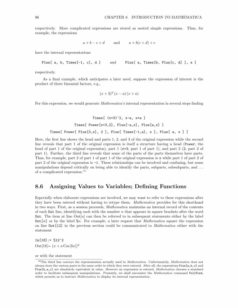
96 CHAPTER 8. INTRODUCTION TO MATHEMATICA

respectively. More complicated expressions are stored as nested simple expressions. Thus, forexample, the expressions

a+ b− c+ d and a+ b(c+ d) + e

have the internal representations

Plus[ a, b, Times[-1, c], d ] and Plus[ a, Times[b, Plus[c, d] ], e ]

respectively.

As a final example, which anticipates a later need, suppose the expression of interest is theproduct of three binomial factors, e.g.,

(x+ 3)2 (x− a) (x+ a)

For this expression, we would generate Mathematica’s internal representation in several steps finding

Times[ (x+3)^2, x-a, x+a ]

Times[ Power[x+3,2], Plus[-a,x], Plus[a,x] ]

Times[ Power[ Plus[3,x], 2 ], Plus[ Times[-1,a], x ], Plus[ a, x ] ]

Here, the first line shows the head and parts 1, 2, and 3 of the original expression while the secondline reveals that part 1 of the original expression is itself a structure having a head (Power; thehead of part 1 of the original expression), part 1 (x+3; part 1 of part 1), and part 2 (2; part 2 ofpart 1). Further, the third line reveals that some of the parts of the parts themselves have parts.Thus, for example, part 2 of part 1 of part 1 of the original expression is x while part 1 of part 2 ofpart 2 of the original expression is -1. These relationships can be involved and confusing, but somemanipulations depend critically on being able to identify the parts, subparts, subsubparts, and . . .of a complicated expression.16

8.6 Assigning Values to Variables; Defining Functions

Especially when elaborate expressions are involved, we may want to refer to these expressions afterthey have been entered without having to retype them. Mathematica provides for this shorthandin two ways. First, as a session proceeds, Mathematica maintains an internal record of the contentsof each Out line, identifying each with the number n that appears in square brackets after the wordOut. The item at line Out[n] can then be referred to in subsequent statements either by the labelOut[n] or by the label %n. For example, a later request that Mathematica square the expressionon line Out[12] in the previous section could be communicated to Mathematica either with thestatement

In[18]:= %12^2

Out[18]= (x+ aCos [bx])2

or with the statement

16The third line conveys the representation actually used in Mathematica. Unfortunately, Mathematica does notalways store the various parts in the same order in which they were entered. After all, the expressions Plus[a,b,c] andPlus[b,a,c] are absolutely equivalent in value. However an expression is entered, Mathematica chooses a standardorder to facilitate subsequent manipulations. Presently, we shall encounter the Mathematica command FullForm,which permits us to instruct Mathematica to display its internal representation.

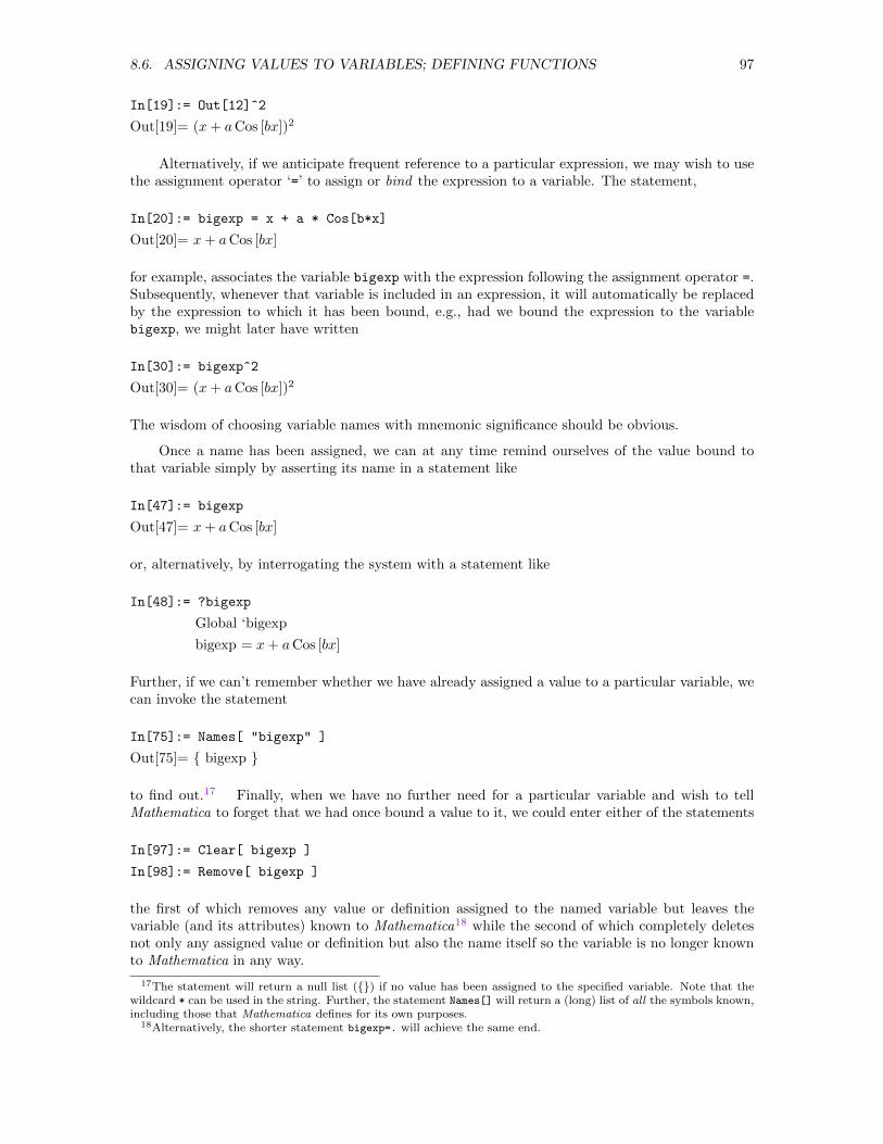
8.6. ASSIGNING VALUES TO VARIABLES; DEFINING FUNCTIONS 97

In[19]:= Out[12]^2

Out[19]= (x+ aCos [bx])2

Alternatively, if we anticipate frequent reference to a particular expression, we may wish to usethe assignment operator ‘=’ to assign or bind the expression to a variable. The statement,

In[20]:= bigexp = x + a * Cos[b*x]

Out[20]= x+ aCos [bx]

for example, associates the variable bigexp with the expression following the assignment operator =.Subsequently, whenever that variable is included in an expression, it will automatically be replacedby the expression to which it has been bound, e.g., had we bound the expression to the variablebigexp, we might later have written

In[30]:= bigexp^2

Out[30]= (x+ aCos [bx])2

The wisdom of choosing variable names with mnemonic significance should be obvious.

Once a name has been assigned, we can at any time remind ourselves of the value bound tothat variable simply by asserting its name in a statement like

In[47]:= bigexp

Out[47]= x+ aCos [bx]

or, alternatively, by interrogating the system with a statement like

In[48]:= ?bigexp

Global ‘bigexp

bigexp = x+ aCos [bx]

Further, if we can’t remember whether we have already assigned a value to a particular variable, wecan invoke the statement

In[75]:= Names[ "bigexp" ]

Out[75]= bigexp

to find out.17 Finally, when we have no further need for a particular variable and wish to tellMathematica to forget that we had once bound a value to it, we could enter either of the statements

In[97]:= Clear[ bigexp ]

In[98]:= Remove[ bigexp ]

the first of which removes any value or definition assigned to the named variable but leaves thevariable (and its attributes) known to Mathematica18 while the second of which completely deletesnot only any assigned value or definition but also the name itself so the variable is no longer knownto Mathematica in any way.

17The statement will return a null list () if no value has been assigned to the specified variable. Note that thewildcard * can be used in the string. Further, the statement Names[] will return a (long) list of all the symbols known,including those that Mathematica defines for its own purposes.

18Alternatively, the shorter statement bigexp=. will achieve the same end.

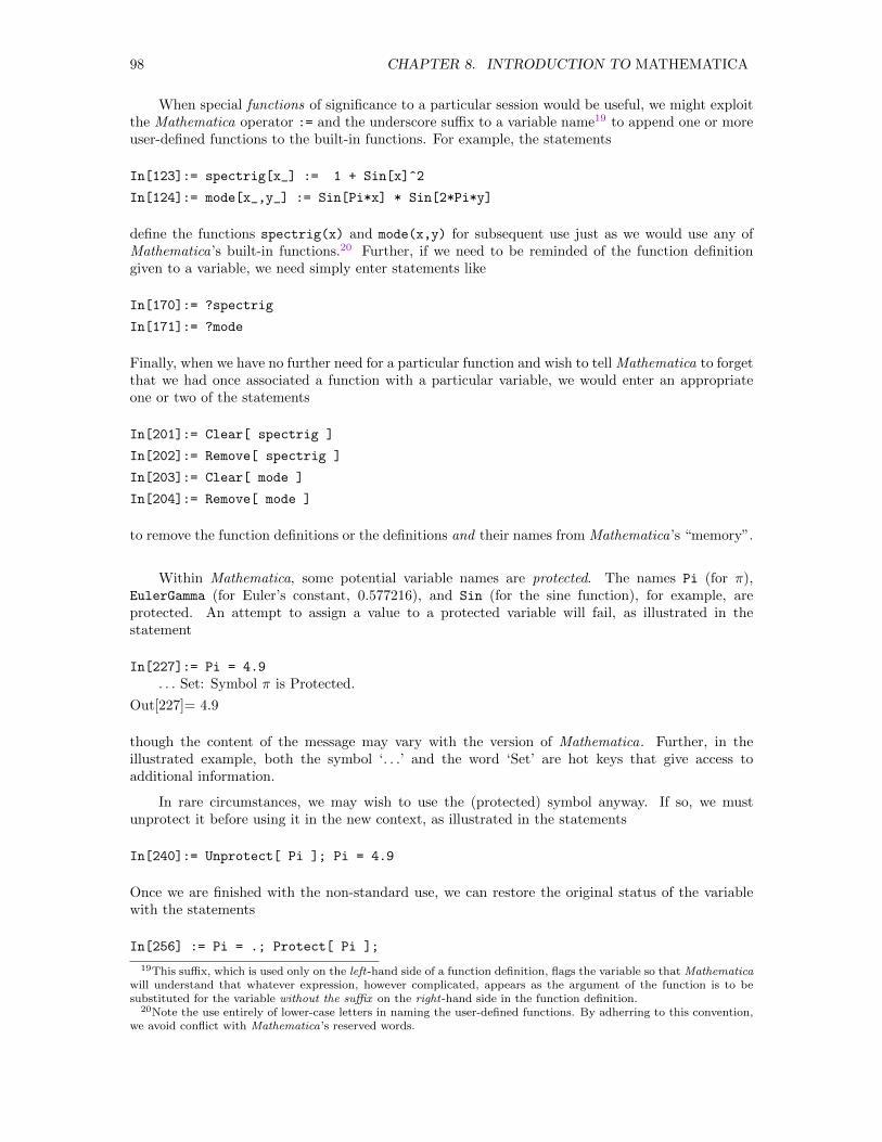
98 CHAPTER 8. INTRODUCTION TO MATHEMATICA

When special functions of significance to a particular session would be useful, we might exploitthe Mathematica operator := and the underscore suffix to a variable name19 to append one or moreuser-defined functions to the built-in functions. For example, the statements

In[123]:= spectrig[x_] := 1 + Sin[x]^2

In[124]:= mode[x_,y_] := Sin[Pi*x] * Sin[2*Pi*y]

define the functions spectrig(x) and mode(x,y) for subsequent use just as we would use any ofMathematica’s built-in functions.20 Further, if we need to be reminded of the function definitiongiven to a variable, we need simply enter statements like

In[170]:= ?spectrig

In[171]:= ?mode

Finally, when we have no further need for a particular function and wish to tell Mathematica to forgetthat we had once associated a function with a particular variable, we would enter an appropriateone or two of the statements

In[201]:= Clear[ spectrig ]

In[202]:= Remove[ spectrig ]

In[203]:= Clear[ mode ]

In[204]:= Remove[ mode ]

to remove the function definitions or the definitions and their names from Mathematica’s “memory”.

Within Mathematica, some potential variable names are protected. The names Pi (for π),EulerGamma (for Euler’s constant, 0.577216), and Sin (for the sine function), for example, areprotected. An attempt to assign a value to a protected variable will fail, as illustrated in thestatement

In[227]:= Pi = 4.9

. . . Set: Symbol π is Protected.

Out[227]= 4.9

though the content of the message may vary with the version of Mathematica. Further, in theillustrated example, both the symbol ‘. . .’ and the word ‘Set’ are hot keys that give access toadditional information.

In rare circumstances, we may wish to use the (protected) symbol anyway. If so, we mustunprotect it before using it in the new context, as illustrated in the statements

In[240]:= Unprotect[ Pi ]; Pi = 4.9

Once we are finished with the non-standard use, we can restore the original status of the variablewith the statements

In[256] := Pi = .; Protect[ Pi ];

19This suffix, which is used only on the left-hand side of a function definition, flags the variable so that Mathematicawill understand that whatever expression, however complicated, appears as the argument of the function is to besubstituted for the variable without the suffix on the right-hand side in the function definition.

20Note the use entirely of lower-case letters in naming the user-defined functions. By adherring to this convention,we avoid conflict with Mathematica’s reserved words.

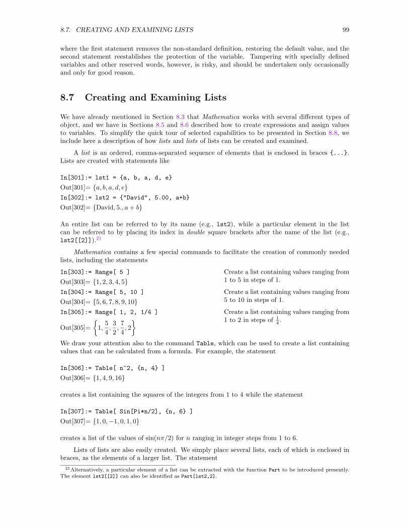
8.7. CREATING AND EXAMINING LISTS 99

where the first statement removes the non-standard definition, restoring the default value, and thesecond statement reestablishes the protection of the variable. Tampering with specially definedvariables and other reserved words, however, is risky, and should be undertaken only occasionallyand only for good reason.

8.7 Creating and Examining Lists

We have already mentioned in Section 8.3 that Mathematica works with several different types ofobject, and we have in Sections 8.5 and 8.6 described how to create expressions and assign valuesto variables. To simplify the quick tour of selected capabilities to be presented in Section 8.8, weinclude here a description of how lists and lists of lists can be created and examined.

A list is an ordered, comma-separated sequence of elements that is enclosed in braces ....Lists are created with statements like

In[301]:= lst1 = a, b, a, d, e

Out[301]= a, b, a, d, eIn[302]:= lst2 = "David", 5.00, a+b

Out[302]= David, 5., a+ b

An entire list can be referred to by its name (e.g., lst2), while a particular element in the listcan be referred to by placing its index in double square brackets after the name of the list (e.g.,lst2[[2]]).21

Mathematica contains a few special commands to facilitate the creation of commonly neededlists, including the statements

In[303]:= Range[ 5 ]

Out[303]= 1, 2, 3, 4, 5In[304]:= Range[ 5, 10 ]

Out[304]= 5, 6, 7, 8, 9, 10In[305]:= Range[ 1, 2, 1/4 ]

Out[305]=

1,

5

4,

3

2,

7

4, 2

Create a list containing values ranging from1 to 5 in steps of 1.

Create a list containing values ranging from5 to 10 in steps of 1.

Create a list containing values ranging from1 to 2 in steps of 1

4 .

We draw your attention also to the command Table, which can be used to create a list containingvalues that can be calculated from a formula. For example, the statement

In[306]:= Table[ n^2, n, 4 ]

Out[306]= 1, 4, 9, 16

creates a list containing the squares of the integers from 1 to 4 while the statement

In[307]:= Table[ Sin[Pi*n/2], n, 6 ]

Out[307]= 1, 0,−1, 0, 1, 0

creates a list of the values of sin(nπ/2) for n ranging in integer steps from 1 to 6.

Lists of lists are also easily created. We simply place several lists, each of which is enclosed inbraces, as the elements of a larger list. The statement

21Alternatively, a particular element of a list can be extracted with the function Part to be introduced presently.The element lst2[[2]] can also be identified as Part[lst2,2].

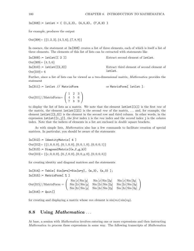
100 CHAPTER 8. INTRODUCTION TO MATHEMATICA

In[308]:= lstlst = 1,2,3, 4,5,6, 7,8,9

for example, produces the output

Out[308]= 1, 2, 3, 4, 5, 6, 7, 8, 9

In essence, the statement at In[308] creates a list of three elements, each of which is itself a list ofthree elements. The elements of this list of lists can be extracted with statements like

In[309]:= lstlst[[ 2 ]]

Out[309]= 4, 5, 6In[310]:= lstlst[[2,3]]

Out[310]= 6

Extract second element of lstlst.

Extract third element of second element oflstlst.

Further, since a list of lists can be viewed as a two-dimensional matrix, Mathematica provides thestatement

In[311]:= lstlst // MatrixForm

Out[311]//MatrixForm=

1 2 34 5 67 8 9

or MatrixForm[ lstlst ].

to display the list of lists as a matrix. We note that the element lstlst[[1]] is the first row ofthe matrix, the element lstlst[[2]] is the second row of the matrix, . . . and, for example, theelement lstlst[[2,3]] is the element in the second row and third column. In other words, in theexpression lstlst[[i,j]], the first index i is the row index and the second index j is the columnindex. Note that the indices of elements in a list are enclosed in double square brackets.

As with simple lists, Mathematica also has a few commands to facilitate creation of specialmatrices. In particular, you should be aware of the statements

In[312]:= IdentityMatrix[ 4 ]

Out[312]= 1, 0, 0, 0, 0, 1, 0, 0, 0, 0, 1, 0, 0, 0, 0, 1In[313]:= DiagonalMatrix[e,f,g,h]

Out[313]= e, 0, 0, 0, 0, f, 0, 0, 0, 0, g, 0, 0, 0, 0, h

for creating identity and diagonal matrices and the statements

In[314]:= Table[ Sin[m*x]*Sin[n*y], m,3, n,3 ];

In[315]:= MatrixForm[ % ]

Out[315]//MatrixForm =

Sin [x] Sin [y] Sin [x] Sin [2y] Sin [x] Sin [3y]Sin [2x] Sin [y] Sin [2x] Sin [2y] Sin [2x] Sin [3y]Sin [3x] Sin [y] Sin [3x] Sin [2y] Sin [3x] Sin [3y]

In[316]:= Quit[]

for creating and displaying a matrix whose mn element is sin(mx) sin(ny).

8.8 Using Mathematica . . .

At base, a session with Mathematica involves entering one or more expressions and then instructingMathematica to process these expressions in some way. The following transcripts of Mathematica

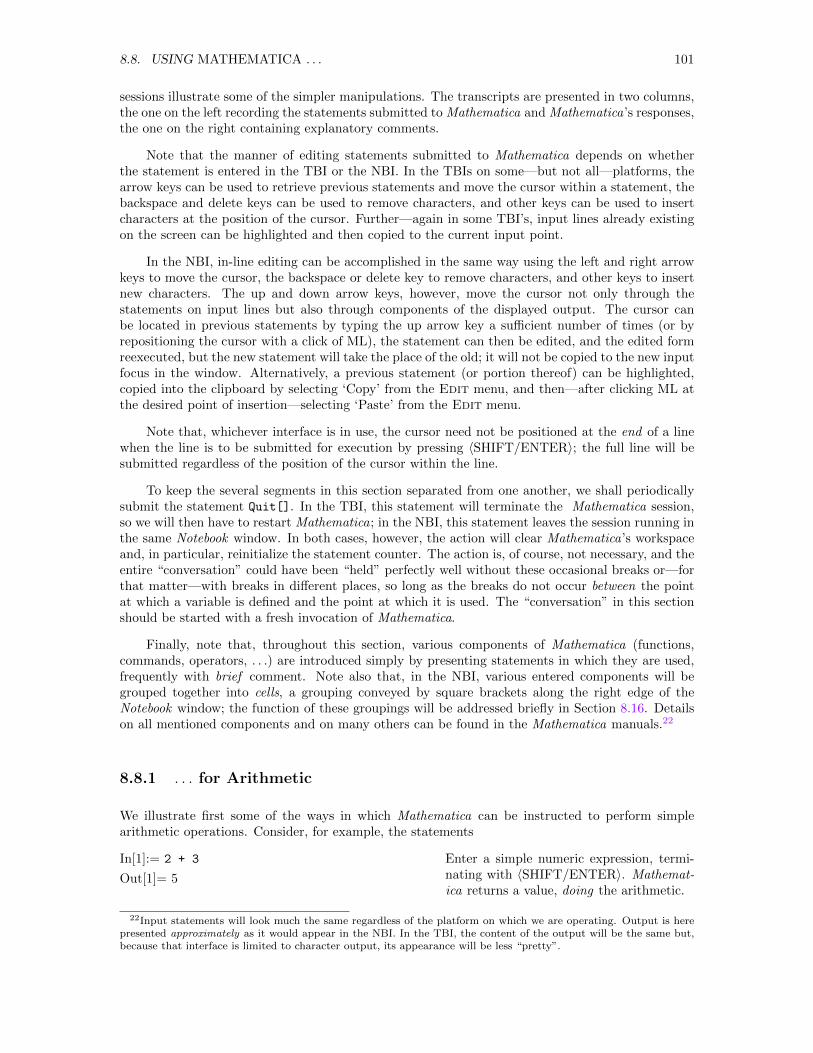
8.8. USING MATHEMATICA . . . 101

sessions illustrate some of the simpler manipulations. The transcripts are presented in two columns,the one on the left recording the statements submitted to Mathematica and Mathematica’s responses,the one on the right containing explanatory comments.

Note that the manner of editing statements submitted to Mathematica depends on whetherthe statement is entered in the TBI or the NBI. In the TBIs on some—but not all—platforms, thearrow keys can be used to retrieve previous statements and move the cursor within a statement, thebackspace and delete keys can be used to remove characters, and other keys can be used to insertcharacters at the position of the cursor. Further—again in some TBI’s, input lines already existingon the screen can be highlighted and then copied to the current input point.

In the NBI, in-line editing can be accomplished in the same way using the left and right arrowkeys to move the cursor, the backspace or delete key to remove characters, and other keys to insertnew characters. The up and down arrow keys, however, move the cursor not only through thestatements on input lines but also through components of the displayed output. The cursor canbe located in previous statements by typing the up arrow key a sufficient number of times (or byrepositioning the cursor with a click of ML), the statement can then be edited, and the edited formreexecuted, but the new statement will take the place of the old; it will not be copied to the new inputfocus in the window. Alternatively, a previous statement (or portion thereof) can be highlighted,copied into the clipboard by selecting ‘Copy’ from the Edit menu, and then—after clicking ML atthe desired point of insertion—selecting ‘Paste’ from the Edit menu.

Note that, whichever interface is in use, the cursor need not be positioned at the end of a linewhen the line is to be submitted for execution by pressing 〈SHIFT/ENTER〉; the full line will besubmitted regardless of the position of the cursor within the line.

To keep the several segments in this section separated from one another, we shall periodicallysubmit the statement Quit[]. In the TBI, this statement will terminate the Mathematica session,so we will then have to restart Mathematica; in the NBI, this statement leaves the session running inthe same Notebook window. In both cases, however, the action will clear Mathematica’s workspaceand, in particular, reinitialize the statement counter. The action is, of course, not necessary, and theentire “conversation” could have been “held” perfectly well without these occasional breaks or—forthat matter—with breaks in different places, so long as the breaks do not occur between the pointat which a variable is defined and the point at which it is used. The “conversation” in this sectionshould be started with a fresh invocation of Mathematica.

Finally, note that, throughout this section, various components of Mathematica (functions,commands, operators, . . .) are introduced simply by presenting statements in which they are used,frequently with brief comment. Note also that, in the NBI, various entered components will begrouped together into cells, a grouping conveyed by square brackets along the right edge of theNotebook window; the function of these groupings will be addressed briefly in Section 8.16. Detailson all mentioned components and on many others can be found in the Mathematica manuals.22

8.8.1 . . . for Arithmetic

We illustrate first some of the ways in which Mathematica can be instructed to perform simplearithmetic operations. Consider, for example, the statements

In[1]:= 2 + 3

Out[1]= 5

Enter a simple numeric expression, termi-nating with 〈SHIFT/ENTER〉. Mathemat-ica returns a value, doing the arithmetic.

22Input statements will look much the same regardless of the platform on which we are operating. Output is herepresented approximately as it would appear in the NBI. In the TBI, the content of the output will be the same but,because that interface is limited to character output, its appearance will be less “pretty”.

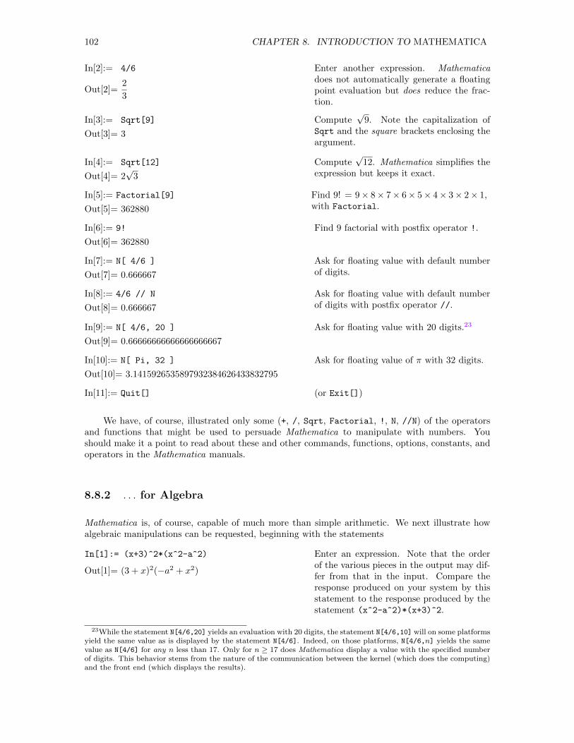
102 CHAPTER 8. INTRODUCTION TO MATHEMATICA

In[2]:= 4/6

Out[2]=2

3

Enter another expression. Mathematicadoes not automatically generate a floatingpoint evaluation but does reduce the frac-tion.

In[3]:= Sqrt[9]

Out[3]= 3

Compute√

9. Note the capitalization ofSqrt and the square brackets enclosing theargument.

In[4]:= Sqrt[12]

Out[4]= 2√

3

Compute√

12. Mathematica simplifies theexpression but keeps it exact.

In[5]:= Factorial[9]

Out[5]= 362880

Find 9! = 9× 8× 7× 6× 5× 4× 3× 2× 1,with Factorial.

In[6]:= 9!

Out[6]= 362880

Find 9 factorial with postfix operator !.

In[7]:= N[ 4/6 ]

Out[7]= 0.666667

Ask for floating value with default numberof digits.

In[8]:= 4/6 // N

Out[8]= 0.666667

Ask for floating value with default numberof digits with postfix operator //.

In[9]:= N[ 4/6, 20 ]

Out[9]= 0.66666666666666666667

Ask for floating value with 20 digits.23

In[10]:= N[ Pi, 32 ]

Out[10]= 3.1415926535897932384626433832795

Ask for floating value of π with 32 digits.

In[11]:= Quit[] (or Exit[])

We have, of course, illustrated only some (+, /, Sqrt, Factorial, !, N, //N) of the operatorsand functions that might be used to persuade Mathematica to manipulate with numbers. Youshould make it a point to read about these and other commands, functions, options, constants, andoperators in the Mathematica manuals.

8.8.2 . . . for Algebra

Mathematica is, of course, capable of much more than simple arithmetic. We next illustrate howalgebraic manipulations can be requested, beginning with the statements

In[1]:= (x+3)^2*(x^2-a^2)

Out[1]= (3 + x)2(−a2 + x2)

Enter an expression. Note that the orderof the various pieces in the output may dif-fer from that in the input. Compare theresponse produced on your system by thisstatement to the response produced by thestatement (x^2-a^2)*(x+3)^2.

23While the statement N[4/6,20] yields an evaluation with 20 digits, the statement N[4/6,10] will on some platformsyield the same value as is displayed by the statement N[4/6]. Indeed, on those platforms, N[4/6,n] yields the samevalue as N[4/6] for any n less than 17. Only for n ≥ 17 does Mathematica display a value with the specified numberof digits. This behavior stems from the nature of the communication between the kernel (which does the computing)and the front end (which displays the results).

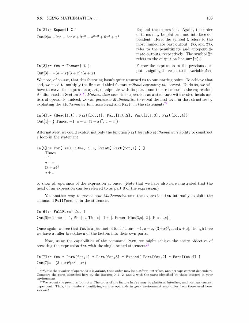
8.8. USING MATHEMATICA . . . 103

In[2]:= Expand[ % ]

Out[2]= −9a2 − 6a2x+ 9x2 − a2x2 + 6x3 + x4

Expand the expression. Again, the orderof terms may be platform and interface de-pendent. Here, the symbol % refers to themost immediate past output. (%% and %%%

refer to the penultimate and antepenulti-mate outputs, respectively. The symbol %nrefers to the output on line Out[n].)

In[3]:= fct = Factor[ % ]

Out[3]= −(a− x)(3 + x)2(a+ x)

Factor the expression in the previous out-put, assigning the result to the variable fct.

We note, of course, that this factoring hasn’t quite returned us to our starting point. To achieve thatend, we need to multiply the first and third factors without expanding the second. To do so, we willhave to carve the expression apart, manipulate with its parts, and then reconstruct the expression.As discussed in Section 8.5, Mathematica sees this expression as a structure with nested heads andlists of operands. Indeed, we can persuade Mathematica to reveal the first level in that structure byexploiting the Mathematica functions Head and Part in the statements24

In[4]:= Head[fct], Part[fct,1], Part[fct,2], Part[fct,3], Part[fct,4]

Out[4]= Times, −1, a− x, (3 + x)2, a+ x

Alternatively, we could exploit not only the function Part but also Mathematica’s ability to constructa loop in the statement

In[5]:= For[ i=0, i<=4, i++, Print[ Part[fct,i] ] ]

Times−1a− x(3 + x)2

a+ x

to show all operands of the expression at once. (Note that we have also here illustrated that thehead of an expression can be referred to as part 0 of the expression.)

Yet another way to reveal how Mathematica sees the expression fct internally exploits thecommand FullForm, as in the statement

In[6]:= FullForm[ fct ]

Out[6]= Times[ −1, Plus[ a, Times[−1,x] ], Power[ Plus[3,x], 2 ], Plus[a,x] ]

Once again, we see that fct is a product of four factors [−1, a−x, (3 +x)2, and a+x], though herewe have a fuller breakdown of the factors into their own parts.

Now, using the capabilities of the command Part, we might achieve the entire objective ofrecasting the expression fct with the single nested statement25

In[7]:= fct = Part[fct,1] * Part[fct,3] * Expand[ Part[fct,2] * Part[fct,4] ]

Out[7]= −(3 + x)2(a2 − x2)

24While the number of operands is invariant, their order may be platform, interface, and perhaps context dependent.Compare the parts identified here by the integers 0, 1, 2, and 3 with the parts identified by those integers in yourenvironment.

25We repeat the previous footnote: The order of the factors in fct may be platform, interface, and perhaps contextdependent. Thus, the numbers identifying various operands in your environment may differ from those used here.Beware!

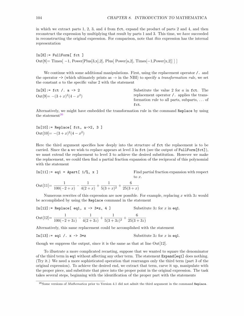
104 CHAPTER 8. INTRODUCTION TO MATHEMATICA

in which we extract parts 1, 2, 3, and 4 from fct, expand the product of parts 2 and 4, and thenreconstruct the expression by multiplying that result by parts 1 and 3. This time, we have succeededin reconstructing the original expression. For comparison, note that this expression has the internalrepresentation

In[8]:= FullForm[ fct ]

Out[8]= Times[ −1, Power[Plus[3,x],2], Plus[ Power[a,2], Times[−1,Power[x,2]] ] ]

We continue with some additional manipulations. First, using the replacement operator /. andthe operator -> (which ultimately prints as → in the NBI) to specify a transformation rule, we setthe constant a to the specific value 2 with the statement

In[9]:= fct /. a -> 2

Out[9]= −(3 + x)2(4− x2)

Substitute the value 2 for a in fct. Thereplacement operator /. applies the trans-formation rule to all parts, subparts, . . . offct.

Alternatively, we might have embedded the transformation rule in the command Replace by usingthe statement26

In[10]:= Replace[ fct, a->2, 3 ]

Out[10]= −(3 + x)2(4− x2)

Here the third argument specifies how deeply into the structure of fct the replacement is to becarried. Since the a we wish to replace appears at level 3 in fct (see the output of FullForm[fct]),we must extend the replacement to level 3 to achieve the desired substitution. However we makethe replacement, we could then find a partial fraction expansion of the reciprocal of this polynomialwith the statement

In[11]:= eq1 = Apart[ 1/%, x ] Find partial fraction expansion with respectto x.

Out[11]=1

100(−2 + x)− 1

4(2 + x)+

1

5(3 + x)2+

6

25(3 + x)

Numerous rewrites of this expression are now possible. For example, replacing x with 3z wouldbe accomplished by using the Replace command in the statement

In[12]:= Replace[ eq1, x -> 3*z, 4 ] Substitute 3z for x in eq1.

Out[12]=1

100(−2 + 3z)− 1

4(2 + 3z)+

1

5(3 + 3z)2+

6

25(3 + 3z)

Alternatively, this same replacement could be accomplished with the statement

In[13]:= eq1 /. x -> 3*z Substitute 3z for x in eq1.

though we suppress the output, since it is the same as that at line Out[12].

To illustrate a more complicated recasting, suppose that we wanted to square the denominatorof the third term in eq1 without affecting any other term. The statement Expand[eq1] does nothing.(Try it.) We need a more sophisticated operation that rearranges only the third term (part 3 of theoriginal expression). To achieve the desired end, we extract that term, carve it up, manipulate withthe proper piece, and substitute that piece into the proper point in the original expression. The tasktakes several steps, beginning with the identification of the proper part with the statements

26Some versions of Mathematica prior to Version 4.1 did not admit the third argument in the command Replace.

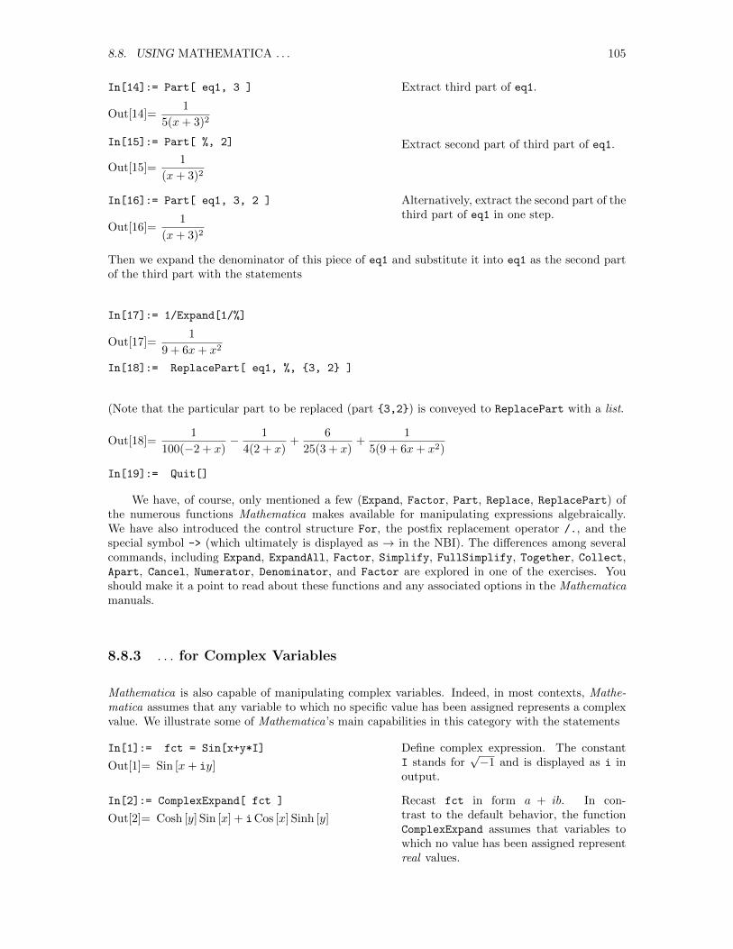
8.8. USING MATHEMATICA . . . 105

In[14]:= Part[ eq1, 3 ]

Out[14]=1

5(x+ 3)2

In[15]:= Part[ %, 2]

Out[15]=1

(x+ 3)2

Extract third part of eq1.

Extract second part of third part of eq1.

In[16]:= Part[ eq1, 3, 2 ]

Out[16]=1

(x+ 3)2

Alternatively, extract the second part of thethird part of eq1 in one step.

Then we expand the denominator of this piece of eq1 and substitute it into eq1 as the second partof the third part with the statements

In[17]:= 1/Expand[1/%]

Out[17]=1

9 + 6x+ x2

In[18]:= ReplacePart[ eq1, %, 3, 2 ]

(Note that the particular part to be replaced (part 3,2) is conveyed to ReplacePart with a list.

Out[18]=1

100(−2 + x)− 1

4(2 + x)+

6

25(3 + x)+

1

5(9 + 6x+ x2)

In[19]:= Quit[]

We have, of course, only mentioned a few (Expand, Factor, Part, Replace, ReplacePart) ofthe numerous functions Mathematica makes available for manipulating expressions algebraically.We have also introduced the control structure For, the postfix replacement operator /., and thespecial symbol -> (which ultimately is displayed as → in the NBI). The differences among severalcommands, including Expand, ExpandAll, Factor, Simplify, FullSimplify, Together, Collect,Apart, Cancel, Numerator, Denominator, and Factor are explored in one of the exercises. Youshould make it a point to read about these functions and any associated options in the Mathematicamanuals.

8.8.3 . . . for Complex Variables

Mathematica is also capable of manipulating complex variables. Indeed, in most contexts, Mathe-matica assumes that any variable to which no specific value has been assigned represents a complexvalue. We illustrate some of Mathematica’s main capabilities in this category with the statements

In[1]:= fct = Sin[x+y*I]

Out[1]= Sin [x+ iy]

Define complex expression. The constantI stands for

√−1 and is displayed as i in

output.

In[2]:= ComplexExpand[ fct ]

Out[2]= Cosh [y] Sin [x] + iCos [x] Sinh [y]

Recast fct in form a + ib. In con-trast to the default behavior, the functionComplexExpand assumes that variables towhich no value has been assigned representreal values.

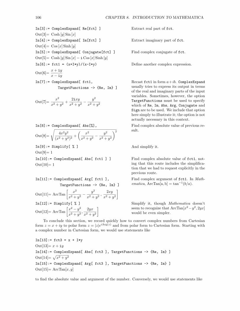
106 CHAPTER 8. INTRODUCTION TO MATHEMATICA

In[3]:= ComplexExpand[ Re[fct] ]

Out[3]= Cosh [y] Sin [x]

In[4]:= ComplexExpand[ Im[fct] ]

Out[4]= Cos [x] Sinh [y]

In[5]:= ComplexExpand[ Conjugate[fct] ]

Out[5]= Cosh [y] Sin [x]− iCos [x] Sinh [y]

Extract real part of fct.

Extract imaginary part of fct.

Find complex conjugate of fct.

In[6]:= fct1 = (x+I*y)/(x-I*y)

Out[6]=x+ iy

x− iy

In[7]:= ComplexExpand[ fct1,

TargetFunctions -> Re, Im ]

Out[7]=x2

x2 + y2+

2ixy

x2 + y2− y2

x2 + y2

Define another complex expression.

Recast fct1 in form a+ ib. ComplexExpandusually tries to express its output in termsof the real and imaginary parts of the inputvariables. Sometimes, however, the optionTargetFunctions must be used to specifywhich of Re, Im, Abs, Arg, Conjugate andSign are to be used. We include that optionhere simply to illustrate it; the option is notactually necessary in this context.

In[8]:= ComplexExpand[ Abs[%],

Out[8]=

√4x2y2

(x2 + y2)2+

(x2

x2 + y2− y2

x2 + y2

)2

In[9]:= Simplify[ % ]

Out[9]= 1

Find complex absolute value of previous re-sult.

And simplify it.

In[10]:= ComplexExpand[ Abs[ fct1 ] ]

Out[10]= 1

Find complex absolute value of fct1, not-ing that this route includes the simplifica-tion that we had to request explicitly in theprevious route.

In[11]:= ComplexExpand[ Arg[ fct1 ],

TargetFunctions -> Re, Im ]

Out[11]= ArcTan

[x2

x2 + y2− y2

x2 + y2,

2xy

x2 + y2

]Find complex argument of fct1. In Math-ematica, ArcTan[a,b] = tan−1(b/a).

In[12]:= Simplify[ % ]

Out[12]= ArcTan

[x2 − y2

x2 + y2,

2yx

x2 + y2

] Simplify it, though Mathematica doesn’tseem to recognize that ArcTan[x2−y2, 2yx]would be even simpler.

To conclude this section, we record quickly how to convert complex numbers from Cartesianform z = x+ iy to polar form z = |z|eiArg(z) and from polar form to Cartesian form. Starting witha complex number in Cartesian form, we would use statements like

In[13]:= fct3 = x + I*y

Out[13]= x+ iy

In[14]:= ComplexExpand[ Abs[ fct3 ], TargetFunctions -> Re, Im ]

Out[14]=√x2 + y2

In[15]:= ComplexExpand[ Arg[ fct3 ], TargetFunctions -> Re, Im ]

Out[15]= ArcTan[x, y]

to find the absolute value and argument of the number. Conversely, we would use statements like

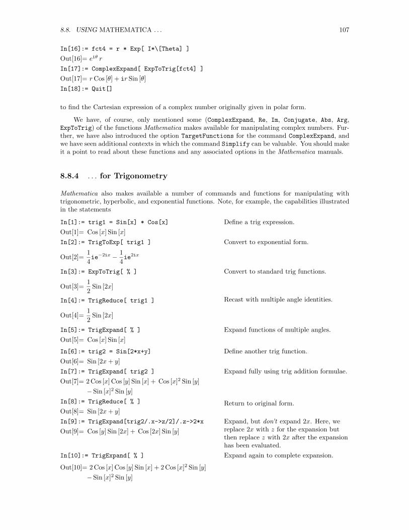
8.8. USING MATHEMATICA . . . 107

In[16]:= fct4 = r * Exp[ I*\[Theta] ]

Out[16]= eiθ r

In[17]:= ComplexExpand[ ExpToTrig[fct4] ]

Out[17]= rCos [θ] + ir Sin [θ]

In[18]:= Quit[]

to find the Cartesian expression of a complex number originally given in polar form.

We have, of course, only mentioned some (ComplexExpand, Re, Im, Conjugate, Abs, Arg,ExpToTrig) of the functions Mathematica makes available for manipulating complex numbers. Fur-ther, we have also introduced the option TargetFunctions for the command ComplexExpand, andwe have seen additional contexts in which the command Simplify can be valuable. You should makeit a point to read about these functions and any associated options in the Mathematica manuals.

8.8.4 . . . for Trigonometry

Mathematica also makes available a number of commands and functions for manipulating withtrigonometric, hyperbolic, and exponential functions. Note, for example, the capabilities illustratedin the statements

In[1]:= trig1 = Sin[x] * Cos[x]

Out[1]= Cos [x] Sin [x]

In[2]:= TrigToExp[ trig1 ]

Out[2]=1

4ie−2ix − 1

4ie2ix

Define a trig expression.

Convert to exponential form.

In[3]:= ExpToTrig[ % ]

Out[3]=1

2Sin [2x]

In[4]:= TrigReduce[ trig1 ]

Out[4]=1

2Sin [2x]

Convert to standard trig functions.

Recast with multiple angle identities.

In[5]:= TrigExpand[ % ]

Out[5]= Cos [x] Sin [x]

Expand functions of multiple angles.

In[6]:= trig2 = Sin[2*x+y]

Out[6]= Sin [2x+ y]

In[7]:= TrigExpand[ trig2 ]

Out[7]= 2 Cos [x] Cos [y] Sin [x] + Cos [x]2 Sin [y]

−Sin [x]2 Sin [y]

In[8]:= TrigReduce[ % ]

Out[8]= Sin [2x+ y]

In[9]:= TrigExpand[trig2/.x->z/2]/.z->2*x

Out[9]= Cos [y] Sin [2x] + Cos [2x] Sin [y]

In[10]:= TrigExpand[ % ]

Out[10]= 2 Cos [x] Cos [y] Sin [x] + 2 Cos [x]2 Sin [y]

−Sin [x]2 Sin [y]

Define another trig function.

Expand fully using trig addition formulae.

Return to original form.

Expand, but don’t expand 2x. Here, wereplace 2x with z for the expansion butthen replace z with 2x after the expansionhas been evaluated.

Expand again to complete expansion.

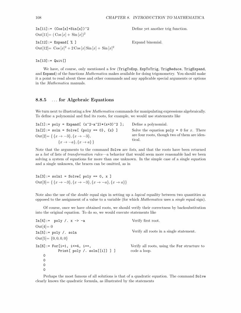
108 CHAPTER 8. INTRODUCTION TO MATHEMATICA

In[11]:= (Cos[x]+Sin[x])^2

Out[11]= ( Cos [x] + Sin [x])2Define yet another trig function.

In[12]:= Expand[ % ]

Out[12]= Cos [x]2 + 2 Cos [x] Sin [x] + Sin [x]2Expand binomial.

In[13]:= Quit[]

We have, of course, only mentioned a few (TrigToExp, ExpToTrig, TrigReduce, TrigExpand,and Expand) of the functions Mathematica makes available for doing trigonometry. You should makeit a point to read about these and other commands and any applicable special arguments or optionsin the Mathematica manuals.

8.8.5 . . . for Algebraic Equations

We turn next to illustrating a few Mathematica commands for manipulating expressions algebraically.To define a polynomial and find its roots, for example, we would use statements like

In[1]:= poly = Expand[ (x^2-a^2)*(x+3)^2 ];

In[2]:= soln = Solve[ poly == 0, x ]

Out[2]= x→ −3, x→ −3,x→ −a, x→ a

Define a polynomial.

Solve the equation poly = 0 for x. Thereare four roots, though two of them are iden-tical.

Note that the arguments to the command Solve are lists, and that the roots have been returnedas a list of lists of transformation rules—a behavior that would seem more reasonable had we beensolving a system of equations for more than one unknown. In the simple case of a single equationand a single unknown, the braces can be omitted, as in

In[3]:= soln1 = Solve[ poly == 0, x ]

Out[3]= x→ −3, x→ −3, x→ −a, x→ a

Note also the use of the double equal sign in setting up a logical equality between two quantities asopposed to the assignment of a value to a variable (for which Mathematica uses a single equal sign).

Of course, once we have obtained roots, we should verify their correctness by backsubstitutioninto the original equation. To do so, we would execute statements like

In[4]:= poly /. x -> -a

Out[4]= 0

In[5]:= poly /. soln

Out[5]= 0, 0, 0, 0

Verify first root.

Verify all roots in a single statement.

In[6]:= For[i=1, i<=4, i++,

Print[ poly /. soln[[i]] ] ]

0

0

0

0

Verify all roots, using the For structure tocode a loop.

Perhaps the most famous of all solutions is that of a quadratic equation. The command Solve

clearly knows the quadratic formula, as illustrated by the statements

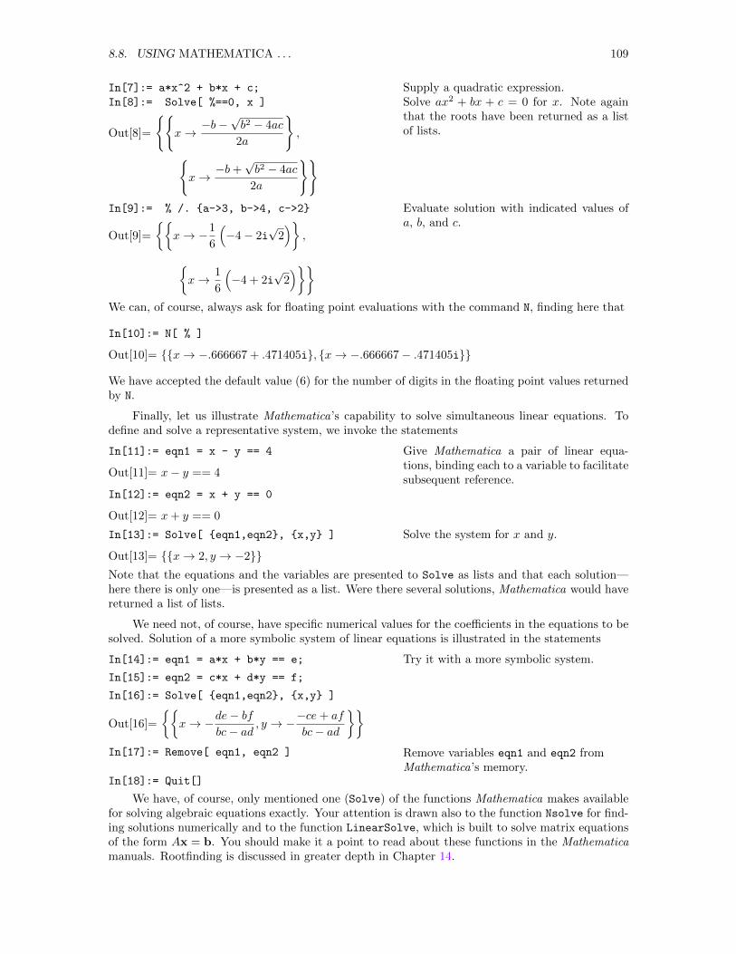
8.8. USING MATHEMATICA . . . 109

In[7]:= a*x^2 + b*x + c;

In[8]:= Solve[ %==0, x ]

Out[8]=

x→ −b−

√b2 − 4ac

2a

,

x→ −b+

√b2 − 4ac

2a

Supply a quadratic expression.Solve ax2 + bx + c = 0 for x. Note againthat the roots have been returned as a listof lists.

In[9]:= % /. a->3, b->4, c->2

Out[9]=

x→ −1

6

(−4− 2i

√2)

,

x→ 1

6

(−4 + 2i

√2)

Evaluate solution with indicated values ofa, b, and c.

We can, of course, always ask for floating point evaluations with the command N, finding here that

In[10]:= N[ % ]

Out[10]= x→ −.666667 + .471405i, x→ −.666667− .471405i

We have accepted the default value (6) for the number of digits in the floating point values returnedby N.

Finally, let us illustrate Mathematica’s capability to solve simultaneous linear equations. Todefine and solve a representative system, we invoke the statements

In[11]:= eqn1 = x - y == 4

Out[11]= x− y == 4

In[12]:= eqn2 = x + y == 0

Out[12]= x+ y == 0

Give Mathematica a pair of linear equa-tions, binding each to a variable to facilitatesubsequent reference.

In[13]:= Solve[ eqn1,eqn2, x,y ]

Out[13]= x→ 2, y → −2

Solve the system for x and y.

Note that the equations and the variables are presented to Solve as lists and that each solution—here there is only one—is presented as a list. Were there several solutions, Mathematica would havereturned a list of lists.

We need not, of course, have specific numerical values for the coefficients in the equations to besolved. Solution of a more symbolic system of linear equations is illustrated in the statements

In[14]:= eqn1 = a*x + b*y == e;

In[15]:= eqn2 = c*x + d*y == f;

In[16]:= Solve[ eqn1,eqn2, x,y ]

Out[16]=

x→ −de− bf

bc− ad, y → −−ce+ af

bc− ad

In[17]:= Remove[ eqn1, eqn2 ]

In[18]:= Quit[]

Try it with a more symbolic system.

Remove variables eqn1 and eqn2 fromMathematica’s memory.

We have, of course, only mentioned one (Solve) of the functions Mathematica makes availablefor solving algebraic equations exactly. Your attention is drawn also to the function Nsolve for find-ing solutions numerically and to the function LinearSolve, which is built to solve matrix equationsof the form Ax = b. You should make it a point to read about these functions in the Mathematicamanuals. Rootfinding is discussed in greater depth in Chapter 14.

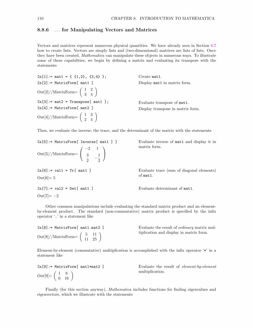
110 CHAPTER 8. INTRODUCTION TO MATHEMATICA

8.8.6 . . . for Manipulating Vectors and Matrices

Vectors and matrices represent numerous physical quantities. We have already seen in Section 8.7how to create lists. Vectors are simply lists and (two-dimensional) matrices are lists of lists. Oncethey have been created, Mathematica can manipulate these objects in numerous ways. To illustratesome of these capabilities, we begin by defining a matrix and evaluating its transpose with thestatements

In[1]:= mat1 = 1,2, 3,4 ;

In[2]:= MatrixForm[ mat1 ]

Out[2]//MatrixForm=

(1 23 4

)In[3]:= mat2 = Transpose[ mat1 ];

In[4]:= MatrixForm[ mat2 ]

Out[4]//MatrixForm=

(1 32 4

)

Create mat1.

Display mat1 in matrix form.

Evaluate transpose of mat1.

Display transpose in matrix form.

Then, we evaluate the inverse, the trace, and the determinant of the matrix with the statements

In[5]:= MatrixForm[ Inverse[ mat1 ] ]

Out[5]//MatrixForm=

−2 1

3

2−1

2

Evaluate inverse of mat1 and display it inmatrix form.

In[6]:= val1 = Tr[ mat1 ]

Out[6]= 5

Evaluate trace (sum of diagonal elements)of mat1.

In[7]:= val2 = Det[ mat1 ]

Out[7]= −2

Evaluate determinant of mat1.

Other common manipulations include evaluating the standard matrix product and an element-by-element product. The standard (non-commutative) matrix product is specified by the infixoperator ‘.’ in a statement like

In[8]:= MatrixForm[ mat1.mat2 ]

Out[8]//MatrixForm=

(5 1111 25

) Evaluate the result of ordinary matrix mul-tiplication and display in matrix form.

Element-by-element (commutative) multiplication is accomplished with the infix operator ‘*’ in astatement like

In[9]:= MatrixForm[ mat1*mat2 ]

Out[9]=

(1 66 16

) Evaluate the result of element-by-elementmultiplication.

Finally (for this section anyway), Mathematica includes functions for finding eigenvalues andeigenvectors, which we illustrate with the statements

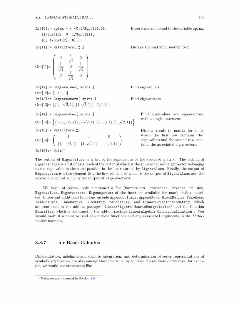
8.8. USING MATHEMATICA . . . 111

In[10]:= spinx = 0,1/Sqrt[2],0,

1/Sqrt[2], 0, 1/Sqrt[2],

0, 1/Sqrt[2], 0 ;

In[11]:= MatrixForm[ % ]

Out[11]=

0

1√2

0

1√2

01√2

01√2

0

Enter a matrix bound to the variable spinx.

Display the matrix in matrix form.

In[12]:= Eigenvalues[ spinx ]

Out[12]= −1, 1, 0In[13]:= Eigenvectors[ spinx ]

Out[13]= 1,−√

2, 1, 1,√

2, 1−1, 0, 1

Find eigenvalues.

Find eigenvectors.

In[14]:= Eigensystem[ spinx ]

Out[14]=−1, 0, 1, 1,−

√2, 1, −1, 0, 1, 1,

√2, 1

In[15]:= MatrixForm[%]

Out[15]=

(−1 1 0

1,−√

2, 1 1,√

2, 1 −1, 0, 1

)In[16]:= Quit[]

Find eigenvalues and eigenvectorswith a single statement.

Display result in matrix form, inwhich the first row contains theeigenvalues and the second row con-tains the associated eigenvectors.

The output of Eigenvalues is a list of the eigenvalues of the specified matrix. The output ofEigenvectors is a list of lists, each of the latter of which is the (unnormalized) eigenvector belongingto the eigenvalue in the same position in the list returned by Eigenvalues. Finally, the output ofEigensystem is a two-element list, the first element of which is the output of Eigenvalues and thesecond element of which is the output of Eigenvectors.

We have, of course, only mentioned a few (MatrixForm, Transpose, Inverse, Tr, Det,Eigenvalues, Eigenvectors, Eigensystem) of the functions available for manipulating matri-ces. Important additional functions include AppendColumns, AppendRows, BlockMatrix, TakeRows,TakeColumns, TakeMatrix, SubMatrix, ZeroMatrix, and LinearEquationsToMatrix, whichare contained in the add-on package27 LinearAlgebra‘MatrixManipulation‘ and the functionNormalize, which is contained in the add-on package LinearAlgebra‘Orthogonalization‘. Youshould make it a point to read about these functions and any associated arguments in the Mathe-matica manuals.

8.8.7 . . . for Basic Calculus

Differentiation, indefinite and definite integration, and determination of series representations ofsymbolic expressions are also among Mathematica’s capabilities. To evaluate derivatives, for exam-ple, we would use statements like

27Packages are discussed in Section 8.9.

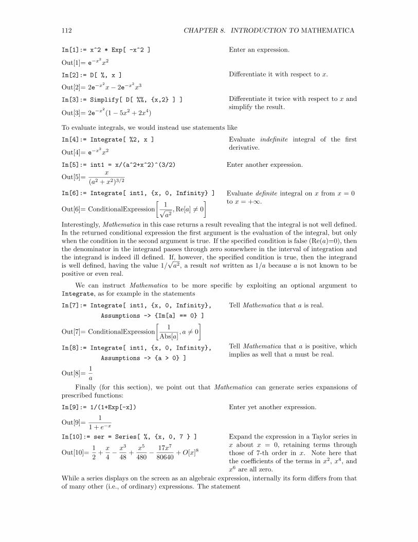
112 CHAPTER 8. INTRODUCTION TO MATHEMATICA

In[1]:= x^2 * Exp[ -x^2 ]

Out[1]= e−x2

x2

In[2]:= D[ %, x ]

Out[2]= 2e−x2

x− 2e−x2

x3

In[3]:= Simplify[ D[ %%, x,2 ] ]

Out[3]= 2e−x2

(1− 5x2 + 2x4)

Enter an expression.

Differentiate it with respect to x.

Differentiate it twice with respect to x andsimplify the result.

To evaluate integrals, we would instead use statements like

In[4]:= Integrate[ %2, x ]

Out[4]= e−x2

x2

Evaluate indefinite integral of the firstderivative.

In[5]:= int1 = x/(a^2+x^2)^(3/2)

Out[5]=x

(a2 + x2)3/2

In[6]:= Integrate[ int1, x, 0, Infinity ]

Out[6]= ConditionalExpression

[1√a2,Re[a] 6= 0

]

Enter another expression.

Evaluate definite integral on x from x = 0to x = +∞.

Interestingly, Mathematica in this case returns a result revealing that the integral is not well defined.In the returned conditional expression the first argument is the evaluation of the integral, but onlywhen the condition in the second argument is true. If the specified condition is false (Re(a)=0), thenthe denominator in the integrand passes through zero somewhere in the interval of integration andthe integrand is indeed ill defined. If, however, the specified condition is true, then the integrandis well defined, having the value 1/

√a2, a result not written as 1/a because a is not known to be

positive or even real.

We can instruct Mathematica to be more specific by exploiting an optional argument toIntegrate, as for example in the statements

In[7]:= Integrate[ int1, x, 0, Infinity,

Assumptions -> Im[a] == 0 ]

Out[7]= ConditionalExpression

[1

Abs[a], a 6= 0

]In[8]:= Integrate[ int1, x, 0, Infinity,

Assumptions -> a > 0 ]

Out[8]=1

a

Tell Mathematica that a is real.

Tell Mathematica that a is positive, whichimplies as well that a must be real.

Finally (for this section), we point out that Mathematica can generate series expansions ofprescribed functions:

In[9]:= 1/(1+Exp[-x])

Out[9]=1

1 + e−x

Enter yet another expression.

In[10]:= ser = Series[ %, x, 0, 7 ]

Out[10]=1

2+x

4− x3

48+

x5

480− 17x7

80640+O[x]8

Expand the expression in a Taylor series inx about x = 0, retaining terms throughthose of 7-th order in x. Note here thatthe coefficients of the terms in x2, x4, andx6 are all zero.

While a series displays on the screen as an algebraic expression, internally its form differs from thatof many other (i.e., of ordinary) expressions. The statement

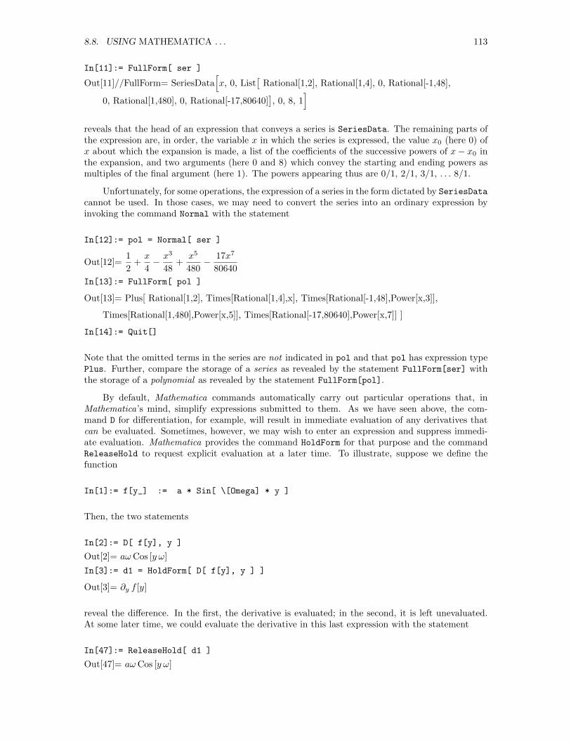
8.8. USING MATHEMATICA . . . 113

In[11]:= FullForm[ ser ]

Out[11]//FullForm= SeriesData[x, 0, List

[Rational[1,2], Rational[1,4], 0, Rational[-1,48],

0, Rational[1,480], 0, Rational[-17,80640]], 0, 8, 1

]reveals that the head of an expression that conveys a series is SeriesData. The remaining parts ofthe expression are, in order, the variable x in which the series is expressed, the value x0 (here 0) ofx about which the expansion is made, a list of the coefficients of the successive powers of x− x0 inthe expansion, and two arguments (here 0 and 8) which convey the starting and ending powers asmultiples of the final argument (here 1). The powers appearing thus are 0/1, 2/1, 3/1, . . . 8/1.

Unfortunately, for some operations, the expression of a series in the form dictated by SeriesData

cannot be used. In those cases, we may need to convert the series into an ordinary expression byinvoking the command Normal with the statement

In[12]:= pol = Normal[ ser ]

Out[12]=1

2+x

4− x3

48+

x5

480− 17x7

80640

In[13]:= FullForm[ pol ]

Out[13]= Plus[ Rational[1,2], Times[Rational[1,4],x], Times[Rational[-1,48],Power[x,3]],

Times[Rational[1,480],Power[x,5]], Times[Rational[-17,80640],Power[x,7]] ]

In[14]:= Quit[]

Note that the omitted terms in the series are not indicated in pol and that pol has expression typePlus. Further, compare the storage of a series as revealed by the statement FullForm[ser] withthe storage of a polynomial as revealed by the statement FullForm[pol].

By default, Mathematica commands automatically carry out particular operations that, inMathematica’s mind, simplify expressions submitted to them. As we have seen above, the com-mand D for differentiation, for example, will result in immediate evaluation of any derivatives thatcan be evaluated. Sometimes, however, we may wish to enter an expression and suppress immedi-ate evaluation. Mathematica provides the command HoldForm for that purpose and the commandReleaseHold to request explicit evaluation at a later time. To illustrate, suppose we define thefunction

In[1]:= f[y_] := a * Sin[ \[Omega] * y ]

Then, the two statements

In[2]:= D[ f[y], y ]

Out[2]= aωCos [y ω]

In[3]:= d1 = HoldForm[ D[ f[y], y ] ]

Out[3]= ∂y f [y]

reveal the difference. In the first, the derivative is evaluated; in the second, it is left unevaluated.At some later time, we could evaluate the derivative in this last expression with the statement

In[47]:= ReleaseHold[ d1 ]

Out[47]= aωCos [y ω]

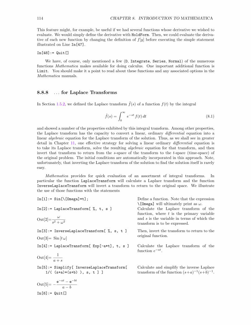
114 CHAPTER 8. INTRODUCTION TO MATHEMATICA

This feature might, for example, be useful if we had several functions whose derivative we wished toevaluate. We would simply define the derivative with HoldForm. Then, we could evaluate the deriva-tive of each new function by changing the definition of f [y] before executing the simple statementillustrated on Line In[47].

In[48]:= Quit[]

We have, of course, only mentioned a few (D, Integrate, Series, Normal) of the numerousfunctions Mathematica makes available for doing calculus. One important additional function isLimit. You should make it a point to read about these functions and any associated options in theMathematica manuals.

8.8.8 . . . for Laplace Transforms

In Section 1.5.2, we defined the Laplace transform f(s) of a function f(t) by the integral

f(s) =

∫ ∞0

e−st f(t) dt (8.1)

and showed a number of the properties exhibited by this integral transform. Among other properties,the Laplace transform has the capacity to convert a linear, ordinary differential equation into alinear algebraic equation for the Laplace transform of the solution. Thus, as we shall see in greaterdetail in Chapter 11, one effective strategy for solving a linear ordinary differential equation isto take its Laplace transform, solve the resulting algebraic equation for that transform, and theninvert that transform to return from the s-space of the transform to the t-space (time-space) ofthe original problem. The initial conditions are automatically incorporated in this approach. Note,unfortunately, that inverting the Laplace transform of the solution to find the solution itself is rarelyeasy.

Mathematica provides for quick evaluation of an assortment of integral transforms. Inparticular the function LaplaceTransform will calculate a Laplace transform and the functionInverseLaplaceTransform will invert a transform to return to the original space. We illustratethe use of those functions with the statements

In[1]:= Sin[\[Omega]*t];

In[2]:= LaplaceTransform[ %, t, s ]

Out[2]=ω

s2 + ω2

Define a function. Note that the expression\[Omega] will ultimately print as ω.Calculate the Laplace transform of thefunction, where t is the primary variableand s is the variable in terms of which thetransform is to be expressed.

In[3]:= InverseLaplaceTransform[ %, s, t ]

Out[3]= Sin [t ω]

Then, invert the transform to return to theoriginal function.

In[4]:= LaplaceTransform[ Exp[-a*t], t, s ]

Out[4]=1

a+ s

Calculate the Laplace transform of thefunction e−at.

In[5]:= Simplify[ InverseLaplaceTransform[

1/( (s+a)*(s+b) ), s, t ] ]

Out[5]= −e−at − e−bt

a− bIn[6]:= Quit[]

Calculate and simplify the inverse Laplacetransform of the function (s+a)−1(s+b)−1.

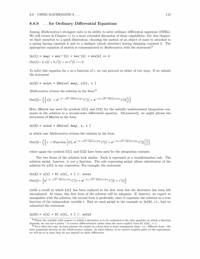
8.8. USING MATHEMATICA . . . 115

8.8.9 . . . for Ordinary Differential Equations

Among Mathematica’s strongest suits is its ability to solve ordinary differential equations (ODEs).We will return in Chapter 11 to a more extended discussion of those capabilities. For this chapter,we limit ourselves to a quick illustration, choosing the motion of an object of mass m attached toa spring having constant k and to a dashpot (shock absorber) having damping constant b. Theappropriate equation of motion is communicated to Mathematica with the statement28

In[1]:= deq1 = m*x’’[t] + b*x’[t] + k*x[t] == 0

Out[1]= k x[t] + b x′[t] +mx′′[t] == 0

To solve this equation for x as a function of t, we can proceed in either of two ways. If we submitthe statement

In[2]:= soln1 = DSolve[ deq1, x[t], t ]

Mathematica returns the solution in the form29

Out[2]=

x[t]→ e(−b−√b2−4km)t/2m C[1] + e(−b+

√b2−4km)t/2m C[2]

Here, DSolve has used the symbols C[1] and C[2] for the initially undetermined integration con-stants in the solution to a second-order differential equation. Alternatively, we might phrase theinvocation of DSolve in the form

In[3]:= soln2 = DSolve[ deq1, x, t ]

in which case Mathematica returns the solution in the form

Out[3]=

x→ Function[t, e(−b−

√b2−4km)t/2m C[1] + e(−b+

√b2−4km)t/2m C[2]

]where again the symbols C[1] and C[2] have been used for the integration contants.

The two forms of the solution look similar. Each is expressed as a transformation rule. Thesolution soln1, however, is not a function. The rule expressing soln1 allows substitution of thesolution for x[t] in any expression. For example, the statement

In[4]:= x[t] + D[ x[t], t ] /. soln1

Out[4]=e(−b−

√b2−4km)t/2m C[1] + e(−b+

√b2−4km)t/2m C[2] + x′[t]

yields a result in which x[t] has been replaced in the first term but the derivative has been leftunevaluated. At times, this first form of the solution will be adequate. If, however, we expect tomanipulate with the solution, the second form is preferable, since it expresses the solution as a truefunction of the independent variable t. Had we used soln2 in the example at In[4], i.e., had wesubmitted the statement

In[5]:= x[t] + D[ x[t], t ] /. soln2

28When the variable with respect to which a derivative is to be evaluated is the only quantity on which a functiondepends, we can use a prime ′ to convey differentiation rather than the more explicit form D[ x[t], t ].

29As is often the case, we here present the output in a form that is more transparent than—i.e., different from—theform presented directly in the Mathematica output. In what follows, if we extract explicit parts of the expressions,we will do so in ways that do not depend on these differences.

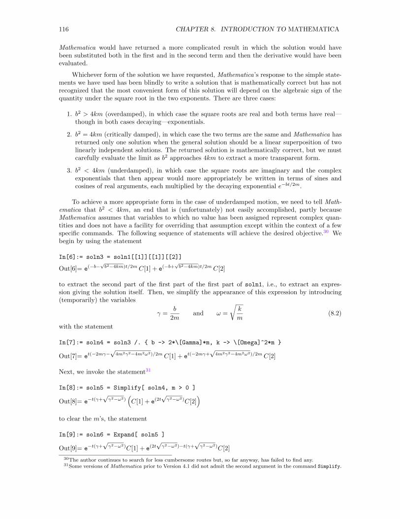
116 CHAPTER 8. INTRODUCTION TO MATHEMATICA

Mathematica would have returned a more complicated result in which the solution would havebeen substituted both in the first and in the second term and then the derivative would have beenevaluated.

Whichever form of the solution we have requested, Mathematica’s response to the simple state-ments we have used has been blindly to write a solution that is mathematically correct but has notrecognized that the most convenient form of this solution will depend on the algebraic sign of thequantity under the square root in the two exponents. There are three cases:

1. b2 > 4km (overdamped), in which case the square roots are real and both terms have real—though in both cases decaying—exponentials.

2. b2 = 4km (critically damped), in which case the two terms are the same and Mathematica hasreturned only one solution when the general solution should be a linear superposition of twolinearly independent solutions. The returned solution is mathematically correct, but we mustcarefully evaluate the limit as b2 approaches 4km to extract a more transparent form.

3. b2 < 4km (underdamped), in which case the square roots are imaginary and the complexexponentials that then appear would more appropriately be written in terms of sines andcosines of real arguments, each multiplied by the decaying exponential e−bt/2m.

To achieve a more appropriate form in the case of underdamped motion, we need to tell Math-ematica that b2 < 4km, an end that is (unfortunately) not easily accomplished, partly becauseMathematica assumes that variables to which no value has been assigned represent complex quan-tities and does not have a facility for overriding that assumption except within the context of a fewspecific commands. The following sequence of statements will achieve the desired objective.30 Webegin by using the statement

In[6]:= soln3 = soln1[[1]][[1]][[2]]

Out[6]= e(−b−√b2−4km)t/2m C[1] + e(−b+

√b2−4km)t/2m C[2]

to extract the second part of the first part of the first part of soln1, i.e., to extract an expres-sion giving the solution itself. Then, we simplify the appearance of this expression by introducing(temporarily) the variables

γ =b

2mand ω =

√k

m(8.2)

with the statement

In[7]:= soln4 = soln3 /. b -> 2*\[Gamma]*m, k -> \[Omega]^2*m

Out[7]= et(−2mγ−√

4m2γ2−4m2ω2)/2m C[1] + et(−2mγ+√

4m2γ2−4m2ω2)/2m C[2]

Next, we invoke the statement31

In[8]:= soln5 = Simplify[ soln4, m > 0 ]

Out[8]= e−t(γ+√γ2−ω2)

(C[1] + e(2t

√γ2−ω2)C[2]

)to clear the m’s, the statement

In[9]:= soln6 = Expand[ soln5 ]

Out[9]= e−t(γ+√γ2−ω2)C[1] + e(2t

√γ2−ω2)−t(γ+

√γ2−ω2)C[2]

30The author continues to search for less cumbersome routes but, so far anyway, has failed to find any.31Some versions of Mathematica prior to Version 4.1 did not admit the second argument in the command Simplify.

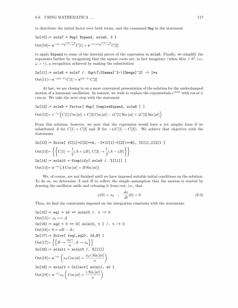
8.8. USING MATHEMATICA . . . 117

to distribute the initial factor over both terms, and the command Map in the statement

In[10]:= soln7 = Map[ Expand, soln6, 3 ]

Out[10]= e−tγ−t√γ2−ω2

C[1] + e−tγ+t√γ2−ω2

C[2]

to apply Expand to some of the internal pieces of the expression in soln6. Finally, we simplify theexponents further by recognizing that the square roots are, in fact imaginary (when 4km > b2, i.e.,ω > γ), a recognition achieved by making the substitution

In[11]:= soln8 = soln7 /. Sqrt[\[Gamma]^2-\[Omega]^2] -> I*a

Out[11]= e−iat−tγC[1] + eiat−tγC[2]

At last, we are closing in on a more convenient presentation of the solution for the underdampedmotion of a harmonic oscillation. In essence, we wish to replace the exponentials e±iat with cos at±i sin at. We take the next step with the statement

In[12]:= soln9 = Factor[ Map[ ComplexExpand, soln8 ] ]

Out[12]= e−tγ(C[1] Cos [at] + C[2] Cos [at]− iC[1] Sin [at] + iC[2] Sin [at]

)From this solution, however, we note that the expression would have a yet simpler form if wesubstituted A for C[1] + C[2] and B for −i(C[1] − C[2]). We achieve that objective with thestatements

In[13]:= Solve[ C[1]+C[2]==A, -I*(C[1]-C[2])==B, C[1],C[2] ]

Out[13]=

C[1]→ 1

2(A+ iB), C[2]→ 1

2(A− iB)

In[14]:= soln10 = Simplify[ soln9 /. %[[1]] ]

Out[14]= e−tγ(ACos [at] +B Sin [at]

)We, of course, are not finished until we have imposed suitable initial conditions on the solution.

To do so, we determine A and B to reflect the simple assumption that the motion is started bydrawing the oscillator aside and releasing it from rest, i.e., that

x(0) = x0 ;dx

dt(0) = 0 (8.3)

Then, we find the constraints imposed on the integration constants with the statements

In[15]:= eq1 = x0 == soln10 /. t -> 0

Out[15]= x0 == A

In[16]:= eq2 = 0 == D[ soln10, t ] /. t -> 0

Out[16]= 0 = aB −AγIn[17]:= Solve[ eq1,eq2, A,B ]

Out[17]=

B → x0γ

a,A→ x0

In[18]:= soln11 = soln10 /. %[[1]]

Out[18]= e−tγ(x0 Cos [at] +

x0γ Sin [at]

a

)In[19]:= soln12 = Collect[ soln11, x0 ]

Out[19]= e−tγx0

(Cos [at] +

γ Sin [at]

a

)

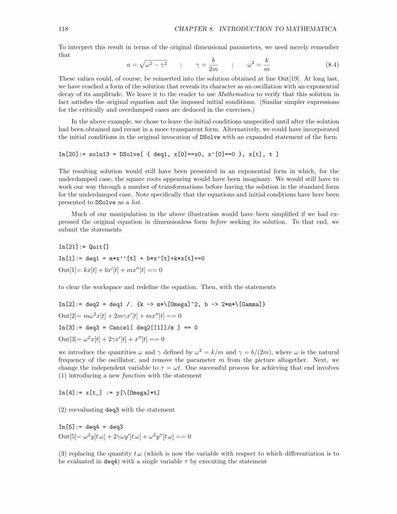
118 CHAPTER 8. INTRODUCTION TO MATHEMATICA

To interpret this result in terms of the original dimensional parameters, we need merely rememberthat

a =√ω2 − γ2 ; γ =

b

2m; ω2 =

k

m(8.4)

These values could, of course, be reinserted into the solution obtained at line Out[19]. At long last,we have reached a form of the solution that reveals its character as an oscillation with an exponentialdecay of its amplitude. We leave it to the reader to use Mathematica to verify that this solution infact satisfies the original equation and the imposed initial conditions. (Similar simpler expressionsfor the critically and overdamped cases are deduced in the exercises.)

In the above example, we chose to leave the initial conditions unspecified until after the solutionhad been obtained and recast in a more transparent form. Alternatively, we could have incorporatedthe initial conditions in the original invocation of DSolve with an expanded statement of the form

In[20]:= soln13 = DSolve[ deq1, x[0]==x0, x’[0]==0 , x[t], t ]

The resulting solution would still have been presented in an exponential form in which, for theunderdamped case, the square roots appearing would have been imaginary. We would still have towork our way through a number of transformations before having the solution in the standard formfor the underdamped case. Note specifically that the equations and initial conditions have here beenpresented to DSolve as a list.

Much of our manipulation in the above illustration would have been simplified if we had ex-pressed the original equation in dimensionless form before seeking its solution. To that end, wesubmit the statements

In[21]:= Quit[]

In[1]:= deq1 = m*x’’[t] + b*x’[t]+k*x[t]==0

Out[1]= kx[t] + bx′[t] +mx′′[t] == 0

to clear the workspace and redefine the equation. Then, with the statements

In[2]:= deq2 = deq1 /. k -> m*\[Omega]^2, b -> 2*m*\[Gamma]

Out[2]= mω2x[t] + 2mγx′[t] +mx′′[t] == 0

In[3]:= deq3 = Cancel[ deq2[[1]]/m ] == 0

Out[3]= ω2x[t] + 2γx′[t] + x′′[t] == 0

we introduce the quantities ω and γ defined by ω2 = k/m and γ = b/(2m), where ω is the naturalfrequency of the oscillator, and remove the parameter m from the picture altogether. Next, wechange the independent variable to τ = ωt. One successful process for achieving that end involves(1) introducing a new function with the statement

In[4]:= x[t_] := y[\[Omega]*t]

(2) reevaluating deq3 with the statement

In[5]:= deq4 = deq3

Out[5]= ω2y[t ω] + 2γωy′[t ω] + ω2y′′[t ω] == 0

(3) replacing the quantity t ω (which is now the variable with respect to which differentiation is tobe evaluated in deq4) with a single variable τ by executing the statement

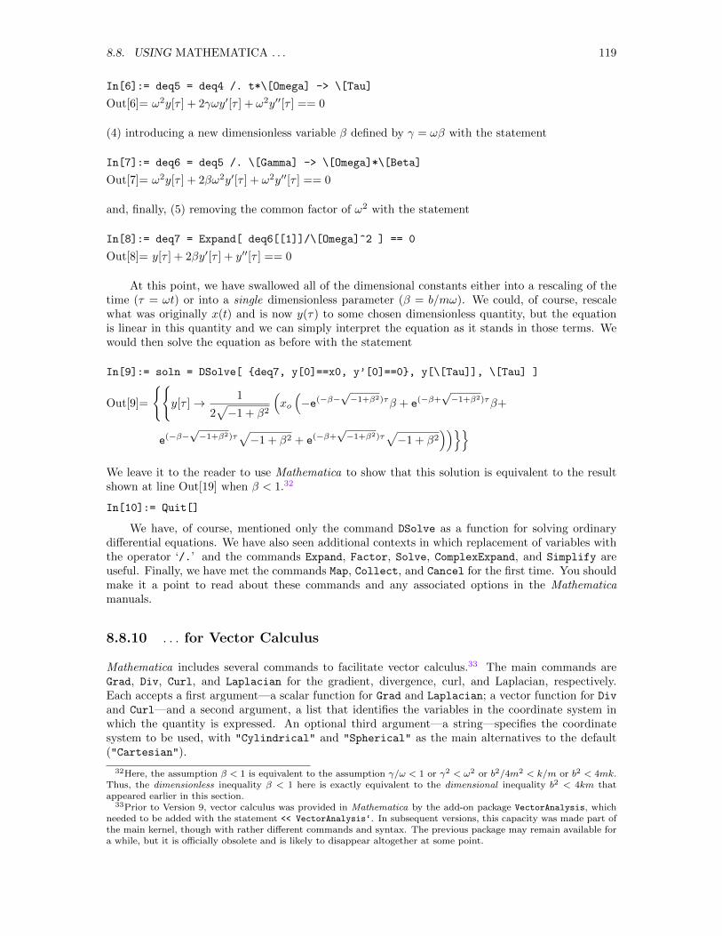
8.8. USING MATHEMATICA . . . 119

In[6]:= deq5 = deq4 /. t*\[Omega] -> \[Tau]

Out[6]= ω2y[τ ] + 2γωy′[τ ] + ω2y′′[τ ] == 0

(4) introducing a new dimensionless variable β defined by γ = ωβ with the statement

In[7]:= deq6 = deq5 /. \[Gamma] -> \[Omega]*\[Beta]

Out[7]= ω2y[τ ] + 2βω2y′[τ ] + ω2y′′[τ ] == 0

and, finally, (5) removing the common factor of ω2 with the statement

In[8]:= deq7 = Expand[ deq6[[1]]/\[Omega]^2 ] == 0

Out[8]= y[τ ] + 2βy′[τ ] + y′′[τ ] == 0

At this point, we have swallowed all of the dimensional constants either into a rescaling of thetime (τ = ωt) or into a single dimensionless parameter (β = b/mω). We could, of course, rescalewhat was originally x(t) and is now y(τ) to some chosen dimensionless quantity, but the equationis linear in this quantity and we can simply interpret the equation as it stands in those terms. Wewould then solve the equation as before with the statement

In[9]:= soln = DSolve[ deq7, y[0]==x0, y’[0]==0, y[\[Tau]], \[Tau] ]

Out[9]=

y[τ ]→ 1

2√−1 + β2

(xo

(−e(−β−

√−1+β2)τβ + e(−β+

√−1+β2)τβ+

e(−β−√−1+β2)τ

√−1 + β2 + e(−β+

√−1+β2)τ

√−1 + β2

))We leave it to the reader to use Mathematica to show that this solution is equivalent to the resultshown at line Out[19] when β < 1.32

In[10]:= Quit[]

We have, of course, mentioned only the command DSolve as a function for solving ordinarydifferential equations. We have also seen additional contexts in which replacement of variables withthe operator ‘/.’ and the commands Expand, Factor, Solve, ComplexExpand, and Simplify areuseful. Finally, we have met the commands Map, Collect, and Cancel for the first time. You shouldmake it a point to read about these commands and any associated options in the Mathematicamanuals.

8.8.10 . . . for Vector Calculus

Mathematica includes several commands to facilitate vector calculus.33 The main commands areGrad, Div, Curl, and Laplacian for the gradient, divergence, curl, and Laplacian, respectively.Each accepts a first argument—a scalar function for Grad and Laplacian; a vector function for Divand Curl—and a second argument, a list that identifies the variables in the coordinate system inwhich the quantity is expressed. An optional third argument—a string—specifies the coordinatesystem to be used, with "Cylindrical" and "Spherical" as the main alternatives to the default("Cartesian").

32Here, the assumption β < 1 is equivalent to the assumption γ/ω < 1 or γ2 < ω2 or b2/4m2 < k/m or b2 < 4mk.Thus, the dimensionless inequality β < 1 here is exactly equivalent to the dimensional inequality b2 < 4km thatappeared earlier in this section.

33Prior to Version 9, vector calculus was provided in Mathematica by the add-on package VectorAnalysis, whichneeded to be added with the statement << VectorAnalysis‘. In subsequent versions, this capacity was made part ofthe main kernel, though with rather different commands and syntax. The previous package may remain available fora while, but it is officially obsolete and is likely to disappear altogether at some point.

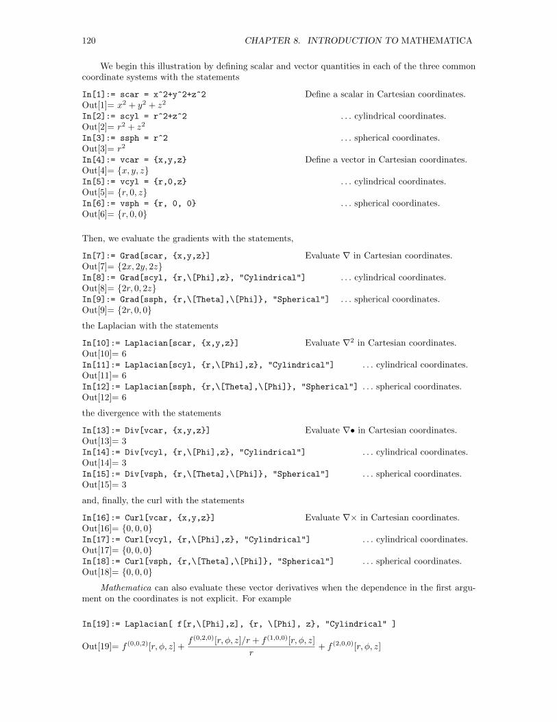
120 CHAPTER 8. INTRODUCTION TO MATHEMATICA

We begin this illustration by defining scalar and vector quantities in each of the three commoncoordinate systems with the statements

In[1]:= scar = x^2+y^2+z^2

Out[1]= x2 + y2 + z2

In[2]:= scyl = r^2+z^2

Out[2]= r2 + z2

In[3]:= ssph = r^2

Out[3]= r2

In[4]:= vcar = x,y,z

Out[4]= x, y, zIn[5]:= vcyl = r,0,z

Out[5]= r, 0, zIn[6]:= vsph = r, 0, 0

Out[6]= r, 0, 0

Define a scalar in Cartesian coordinates.

. . . cylindrical coordinates.

. . . spherical coordinates.

Define a vector in Cartesian coordinates.

. . . cylindrical coordinates.

. . . spherical coordinates.

Then, we evaluate the gradients with the statements,

In[7]:= Grad[scar, x,y,z]

Out[7]= 2x, 2y, 2zIn[8]:= Grad[scyl, r,\[Phi],z, "Cylindrical"]

Out[8]= 2r, 0, 2zIn[9]:= Grad[ssph, r,\[Theta],\[Phi], "Spherical"]

Out[9]= 2r, 0, 0

Evaluate ∇ in Cartesian coordinates.

. . . cylindrical coordinates.

. . . spherical coordinates.

the Laplacian with the statements

In[10]:= Laplacian[scar, x,y,z]

Out[10]= 6In[11]:= Laplacian[scyl, r,\[Phi],z, "Cylindrical"]

Out[11]= 6In[12]:= Laplacian[ssph, r,\[Theta],\[Phi], "Spherical"]

Out[12]= 6

Evaluate ∇2 in Cartesian coordinates.

. . . cylindrical coordinates.

. . . spherical coordinates.

the divergence with the statements

In[13]:= Div[vcar, x,y,z]

Out[13]= 3In[14]:= Div[vcyl, r,\[Phi],z, "Cylindrical"]

Out[14]= 3In[15]:= Div[vsph, r,\[Theta],\[Phi], "Spherical"]

Out[15]= 3

Evaluate ∇• in Cartesian coordinates.

. . . cylindrical coordinates.

. . . spherical coordinates.

and, finally, the curl with the statements

In[16]:= Curl[vcar, x,y,z]

Out[16]= 0, 0, 0In[17]:= Curl[vcyl, r,\[Phi],z, "Cylindrical"]

Out[17]= 0, 0, 0In[18]:= Curl[vsph, r,\[Theta],\[Phi], "Spherical"]

Out[18]= 0, 0, 0

Evaluate ∇× in Cartesian coordinates.

. . . cylindrical coordinates.

. . . spherical coordinates.

Mathematica can also evaluate these vector derivatives when the dependence in the first argu-ment on the coordinates is not explicit. For example

In[19]:= Laplacian[ f[r,\[Phi],z], r, \[Phi], z, "Cylindrical" ]

Out[19]= f (0,0,2)[r, φ, z] +f (0,2,0)[r, φ, z]/r + f (1,0,0)[r, φ, z]

r+ f (2,0,0)[r, φ, z]

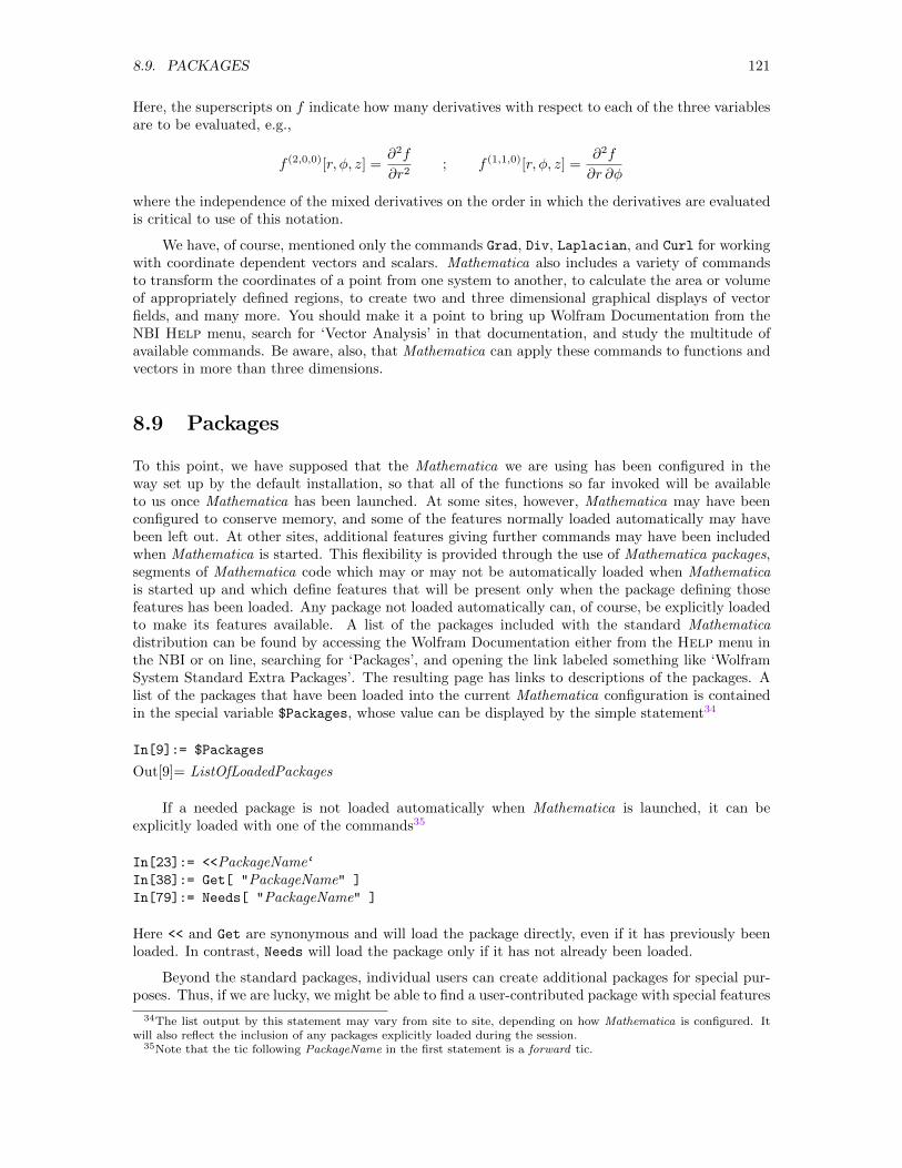
8.9. PACKAGES 121

Here, the superscripts on f indicate how many derivatives with respect to each of the three variablesare to be evaluated, e.g.,

f (2,0,0)[r, φ, z] =∂2f

∂r2; f (1,1,0)[r, φ, z] =

∂2f

∂r ∂φ

where the independence of the mixed derivatives on the order in which the derivatives are evaluatedis critical to use of this notation.

We have, of course, mentioned only the commands Grad, Div, Laplacian, and Curl for workingwith coordinate dependent vectors and scalars. Mathematica also includes a variety of commandsto transform the coordinates of a point from one system to another, to calculate the area or volumeof appropriately defined regions, to create two and three dimensional graphical displays of vectorfields, and many more. You should make it a point to bring up Wolfram Documentation from theNBI Help menu, search for ‘Vector Analysis’ in that documentation, and study the multitude ofavailable commands. Be aware, also, that Mathematica can apply these commands to functions andvectors in more than three dimensions.

8.9 Packages

To this point, we have supposed that the Mathematica we are using has been configured in theway set up by the default installation, so that all of the functions so far invoked will be availableto us once Mathematica has been launched. At some sites, however, Mathematica may have beenconfigured to conserve memory, and some of the features normally loaded automatically may havebeen left out. At other sites, additional features giving further commands may have been includedwhen Mathematica is started. This flexibility is provided through the use of Mathematica packages,segments of Mathematica code which may or may not be automatically loaded when Mathematicais started up and which define features that will be present only when the package defining thosefeatures has been loaded. Any package not loaded automatically can, of course, be explicitly loadedto make its features available. A list of the packages included with the standard Mathematicadistribution can be found by accessing the Wolfram Documentation either from the Help menu inthe NBI or on line, searching for ‘Packages’, and opening the link labeled something like ‘WolframSystem Standard Extra Packages’. The resulting page has links to descriptions of the packages. Alist of the packages that have been loaded into the current Mathematica configuration is containedin the special variable $Packages, whose value can be displayed by the simple statement34

In[9]:= $Packages

Out[9]= ListOfLoadedPackages

If a needed package is not loaded automatically when Mathematica is launched, it can beexplicitly loaded with one of the commands35

In[23]:= <<PackageName‘In[38]:= Get[ "PackageName" ]

In[79]:= Needs[ "PackageName" ]

Here << and Get are synonymous and will load the package directly, even if it has previously beenloaded. In contrast, Needs will load the package only if it has not already been loaded.

Beyond the standard packages, individual users can create additional packages for special pur-poses. Thus, if we are lucky, we might be able to find a user-contributed package with special features

34The list output by this statement may vary from site to site, depending on how Mathematica is configured. Itwill also reflect the inclusion of any packages explicitly loaded during the session.

35Note that the tic following PackageName in the first statement is a forward tic.

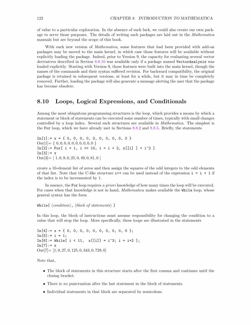
122 CHAPTER 8. INTRODUCTION TO MATHEMATICA

of value to a particular exploration. In the absence of such luck, we could also create our own pack-age to serve those purposes. The details of writing such packages are laid out in the Mathematicamanuals but are beyond the scope of this book.

With each new version of Mathematica, some features that had been provided with add-onpackages may be moved to the main kernel, in which case those features will be available withoutexplicitly loading the package. Indeed, prior to Version 9, the capacity for evaluating several vectorderivatives described in Section 8.8.10 was available only if a package named VectorAnalysis wasloaded explicitly. Starting with Version 9, those features were built into the main kernel, though thenames of the commands and their syntax suffered revision. For backward compatibility, the originalpackage is retained in subsequent versions, at least for a while, but it may in time be completelyremoved. Further, loading the package will also generate a message alerting the user that the packagehas become obsolete.

8.10 Loops, Logical Expressions, and Conditionals

Among the most ubiquitous programming structures is the loop, which provides a means by which astatement or block of statements can be executed some number of times, typically with small changescontrolled by a loop index. Several such structures are available in Mathematica. The simplest isthe For loop, which we have already met in Sections 8.8.2 and 8.8.5. Briefly, the statements

In[1]:= x = 0, 0, 0, 0, 0, 0, 0, 0, 0, 0

Out[1]= 0, 0, 0, 0, 0, 0, 0, 0, 0, 0 In[2]:= For[ i = 1, i <= 10, i = i + 2, x[[i] ] = i^2 ]

In[3]:= x

Out[3]= [ 1, 0, 9, 0, 25, 0, 49, 0, 81, 0 ]

create a 10-element list of zeros and then assign the squares of the odd integers to the odd elementsof that list. Note that the C-like structure i++ can be used instead of the expression i = i + 1 ifthe index is to be incremented by 1.

In essence, the For loop requires a priori knowledge of how many times the loop will be executed.For cases when that knowledge is not in hand, Mathematica makes available the While loop, whosegeneral syntax has the form

While[ 〈condition〉, 〈block of statements〉 ]

In this loop, the block of instructions must assume responsibility for changing the condition to avalue that will stop the loop. More specifically, these loops are illustrated in the statements

In[4]:= x = 0, 0, 0, 0, 0, 0, 0, 0, 0, 0 ;

In[5]:= i = 1;

In[6]:= While[ i < 11, x[[i]] = i^3; i = i+2 ];

In[7]:= x

Out[7]= [1, 0, 27, 0, 125, 0, 343, 0, 729, 0]

Note that,

• The block of statements in this structure starts after the first comma and continues until theclosing bracket.

• There is no punctuation after the last statement in the block of statements.

• Individual statements in that block are separated by semicolons.

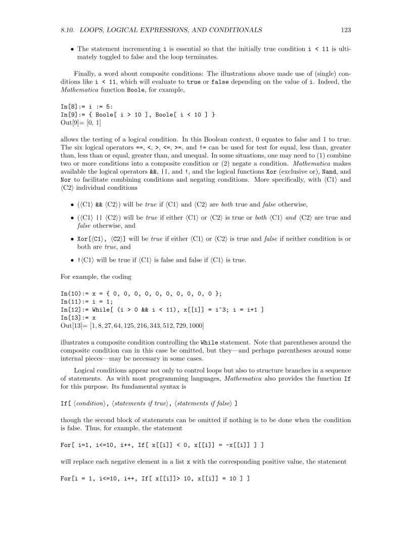
8.10. LOOPS, LOGICAL EXPRESSIONS, AND CONDITIONALS 123

• The statement incrementing i is essential so that the initially true condition i < 11 is ulti-mately toggled to false and the loop terminates.

Finally, a word about composite conditions: The illustrations above made use of (single) con-ditions like i < 11, which will evaluate to true or false depending on the value of i. Indeed, theMathematica function Boole, for example,

In[8]:= i := 5:

In[9]:= Boole[ i > 10 ], Boole[ i < 10 ]

Out[9]= [0, 1]

allows the testing of a logical condition. In this Boolean context, 0 equates to false and 1 to true.The six logical operators ==, <, >, <=, >=, and != can be used for test for equal, less than, greaterthan, less than or equal, greater than, and unequal. In some situations, one may need to (1) combinetwo or more conditions into a composite condition or (2) negate a condition. Mathematica makesavailable the logical operators &&, ||, and !, and the logical functions Xor (exclusive or), Nand, andNor to facilitate combining conditions and negating conditions. More specifically, with 〈C1〉 and〈C2〉 individual conditions

• (〈C1〉 && 〈C2〉) will be true if 〈C1〉 and 〈C2〉 are both true and false otherwise,

• (〈C1〉 || 〈C2〉) will be true if either 〈C1〉 or 〈C2〉 is true or both 〈C1〉 and 〈C2〉 are true andfalse otherwise, and

• Xor[〈C1〉, 〈C2〉] will be true if either 〈C1〉 or 〈C2〉 is true and false if neither condition is orboth are true, and

• !〈C1〉 will be true if 〈C1〉 is false and false if 〈C1〉 is true.

For example, the coding

In(10):= x = 0, 0, 0, 0, 0, 0, 0, 0, 0, 0 ;

In(11):= i = 1;

In[12]:= While[ (i > 0 && i < 11), x[[i]] = i^3; i = i+1 ]

In[13]:= x

Out[13]= [1, 8, 27, 64, 125, 216, 343, 512, 729, 1000]

illustrates a composite condition controlling the While statement. Note that parentheses around thecomposite condition can in this case be omitted, but they—and perhaps parentheses around someinternal pieces—may be necessary in some cases.

Logical conditions appear not only to control loops but also to structure branches in a sequenceof statements. As with most programming languages, Mathematica also provides the function If

for this purpose. Its fundamental syntax is

If[ 〈condition〉, 〈statements if true〉, 〈statements if false〉 ]

though the second block of statements can be omitted if nothing is to be done when the conditionis false. Thus, for example, the statement

For[ i=1, i<=10, i++, If[ x[[i]] < 0, x[[i]] = -x[[i]] ] ]

will replace each negative element in a list x with the corresponding positive value, the statement

For[i = 1, i<=10, i++, If[ x[[i]]> 10, x[[i]] = 10 ] ]

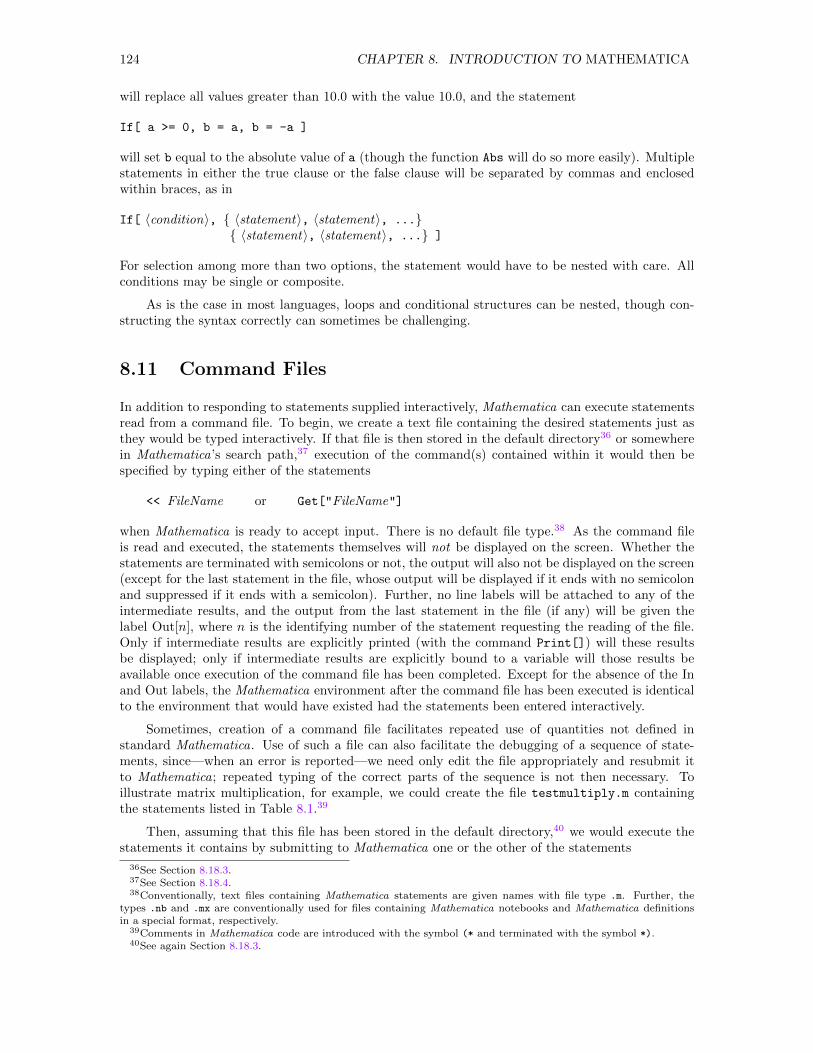
124 CHAPTER 8. INTRODUCTION TO MATHEMATICA

will replace all values greater than 10.0 with the value 10.0, and the statement

If[ a >= 0, b = a, b = -a ]

will set b equal to the absolute value of a (though the function Abs will do so more easily). Multiplestatements in either the true clause or the false clause will be separated by commas and enclosedwithin braces, as in

If[ 〈condition〉, 〈statement〉, 〈statement〉, ... 〈statement〉, 〈statement〉, ... ]

For selection among more than two options, the statement would have to be nested with care. Allconditions may be single or composite.

As is the case in most languages, loops and conditional structures can be nested, though con-structing the syntax correctly can sometimes be challenging.

8.11 Command Files

In addition to responding to statements supplied interactively, Mathematica can execute statementsread from a command file. To begin, we create a text file containing the desired statements just asthey would be typed interactively. If that file is then stored in the default directory36 or somewherein Mathematica’s search path,37 execution of the command(s) contained within it would then bespecified by typing either of the statements

<< FileName or Get["FileName"]

when Mathematica is ready to accept input. There is no default file type.38 As the command fileis read and executed, the statements themselves will not be displayed on the screen. Whether thestatements are terminated with semicolons or not, the output will also not be displayed on the screen(except for the last statement in the file, whose output will be displayed if it ends with no semicolonand suppressed if it ends with a semicolon). Further, no line labels will be attached to any of theintermediate results, and the output from the last statement in the file (if any) will be given thelabel Out[n], where n is the identifying number of the statement requesting the reading of the file.Only if intermediate results are explicitly printed (with the command Print[]) will these resultsbe displayed; only if intermediate results are explicitly bound to a variable will those results beavailable once execution of the command file has been completed. Except for the absence of the Inand Out labels, the Mathematica environment after the command file has been executed is identicalto the environment that would have existed had the statements been entered interactively.

Sometimes, creation of a command file facilitates repeated use of quantities not defined instandard Mathematica. Use of such a file can also facilitate the debugging of a sequence of state-ments, since—when an error is reported—we need only edit the file appropriately and resubmit itto Mathematica; repeated typing of the correct parts of the sequence is not then necessary. Toillustrate matrix multiplication, for example, we could create the file testmultiply.m containingthe statements listed in Table 8.1.39

Then, assuming that this file has been stored in the default directory,40 we would execute thestatements it contains by submitting to Mathematica one or the other of the statements

36See Section 8.18.3.37See Section 8.18.4.38Conventionally, text files containing Mathematica statements are given names with file type .m. Further, the

types .nb and .mx are conventionally used for files containing Mathematica notebooks and Mathematica definitionsin a special format, respectively.

39Comments in Mathematica code are introduced with the symbol (* and terminated with the symbol *).40See again Section 8.18.3.

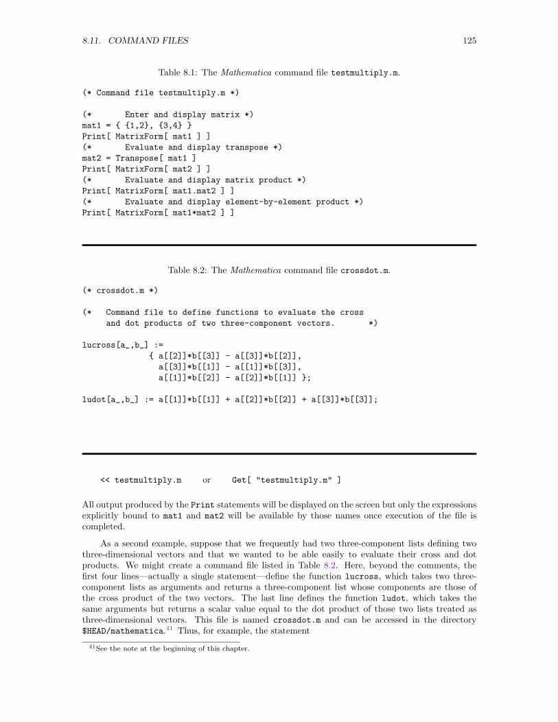
8.11. COMMAND FILES 125

Table 8.1: The Mathematica command file testmultiply.m.

(* Command file testmultiply.m *)

(* Enter and display matrix *)

mat1 = 1,2, 3,4

Print[ MatrixForm[ mat1 ] ]

(* Evaluate and display transpose *)

mat2 = Transpose[ mat1 ]

Print[ MatrixForm[ mat2 ] ]

(* Evaluate and display matrix product *)

Print[ MatrixForm[ mat1.mat2 ] ]

(* Evaluate and display element-by-element product *)

Print[ MatrixForm[ mat1*mat2 ] ]

Table 8.2: The Mathematica command file crossdot.m.

(* crossdot.m *)

(* Command file to define functions to evaluate the cross

and dot products of two three-component vectors. *)

lucross[a_,b_] :=

a[[2]]*b[[3]] - a[[3]]*b[[2]],

a[[3]]*b[[1]] - a[[1]]*b[[3]],

a[[1]]*b[[2]] - a[[2]]*b[[1]] ;

ludot[a_,b_] := a[[1]]*b[[1]] + a[[2]]*b[[2]] + a[[3]]*b[[3]];

<< testmultiply.m or Get[ "testmultiply.m" ]

All output produced by the Print statements will be displayed on the screen but only the expressionsexplicitly bound to mat1 and mat2 will be available by those names once execution of the file iscompleted.

As a second example, suppose that we frequently had two three-component lists defining twothree-dimensional vectors and that we wanted to be able easily to evaluate their cross and dotproducts. We might create a command file listed in Table 8.2. Here, beyond the comments, thefirst four lines—actually a single statement—define the function lucross, which takes two three-component lists as arguments and returns a three-component list whose components are those ofthe cross product of the two vectors. The last line defines the function ludot, which takes thesame arguments but returns a scalar value equal to the dot product of those two lists treated asthree-dimensional vectors. This file is named crossdot.m and can be accessed in the directory$HEAD/mathematica.41 Thus, for example, the statement

41See the note at the beginning of this chapter.

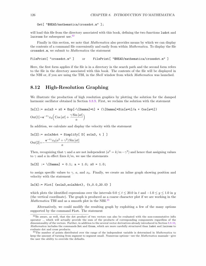
126 CHAPTER 8. INTRODUCTION TO MATHEMATICA

Get[ "$HEAD/mathematica/crossdot.m" ];

will load this file from the directory associated with this book, defining the two functions ludot andlucross for subsequent use.42

Finally in this section, we note that Mathematica also provides means by which we can displaythe contents of a command file conveniently and easily from within Mathematica. To display the filecrossdot.m, we submit to Mathematica the statement

FilePrint[ "crossdot.m" ] or FilePrint[ "$HEAD/mathematica/crossdot.m" ]

Here, the first form applies if the file is in a directory in the search path and the second form refersto the file in the directory associated with this book. The contents of the file will be displayed inthe NBI or, if you are using the TBI, in the Shell window from which Mathematica was launched.

8.12 High-Resolution Graphing

We illustrate the production of high resolution graphics by plotting the solution for the dampedharmonic oscillator obtained in Section 8.8.9. First, we reclaim the solution with the statement

In[1]:= soln3 = x0 * Exp[-\[Gamma]*t] * (\[Gamma]*Sin[a*t]/a + Cos[a*t])

Out[1]=e−tγx0

(Cos [at] +

γ Sin [at]

a

)In addition, we calculate and display the velocity with the statement

In[2]:= soln3dot = Simplify[ D[ soln3, t ] ]

Out[2]=−e−tγx0(a2 + γ2) Sin [at]

a

Then, recognizing that γ and a are not independent (a2 = k/m−γ2) and hence that assigning valuesto γ and a in effect fixes k/m, we use the statements

In[3] := \[Gamma] = 0.1; a = 1.0; x0 = 1.0;

to assign specific values to γ, a, and x0. Finally, we create an inline graph showing position andvelocity with the statement

In[4]:= Plot[ soln3,soln3dot, t,0.0,20.0 ]

which plots the identified expressions over the intervals 0.0 ≤ t ≤ 20.0 in t and −1.0 ≤ y ≤ 1.0 in y(the vertical coordinate). The graph is produced as a coarse character plot if we are working in theMathematica TBI and as a smooth plot in the NBI.43

Alternatively, we could modify the resulting graph by exploiting a few of the many optionssupported by the command Plot. The statement

42Be aware, as well, that the dot product of two vectors can also be evaluated with the non-commutative infixoperator ., which will actually provide the sum of the products of corresponding components regardless of thedimensionality of the vectors. Further, in addition to the several vector derivatives already introduced in Section 8.8.10,Mathematica includes the commands Dot and Cross, which are more carefully structured than ludot and lucross toevaluate dot and cross products.

43The number of points distributed over the range of the independent variable is determined in Mathematica tokeep the amount of turning from segment to segment small. Numerous options—see the Mathematica manuals—givethe user the ability to override the defaults.

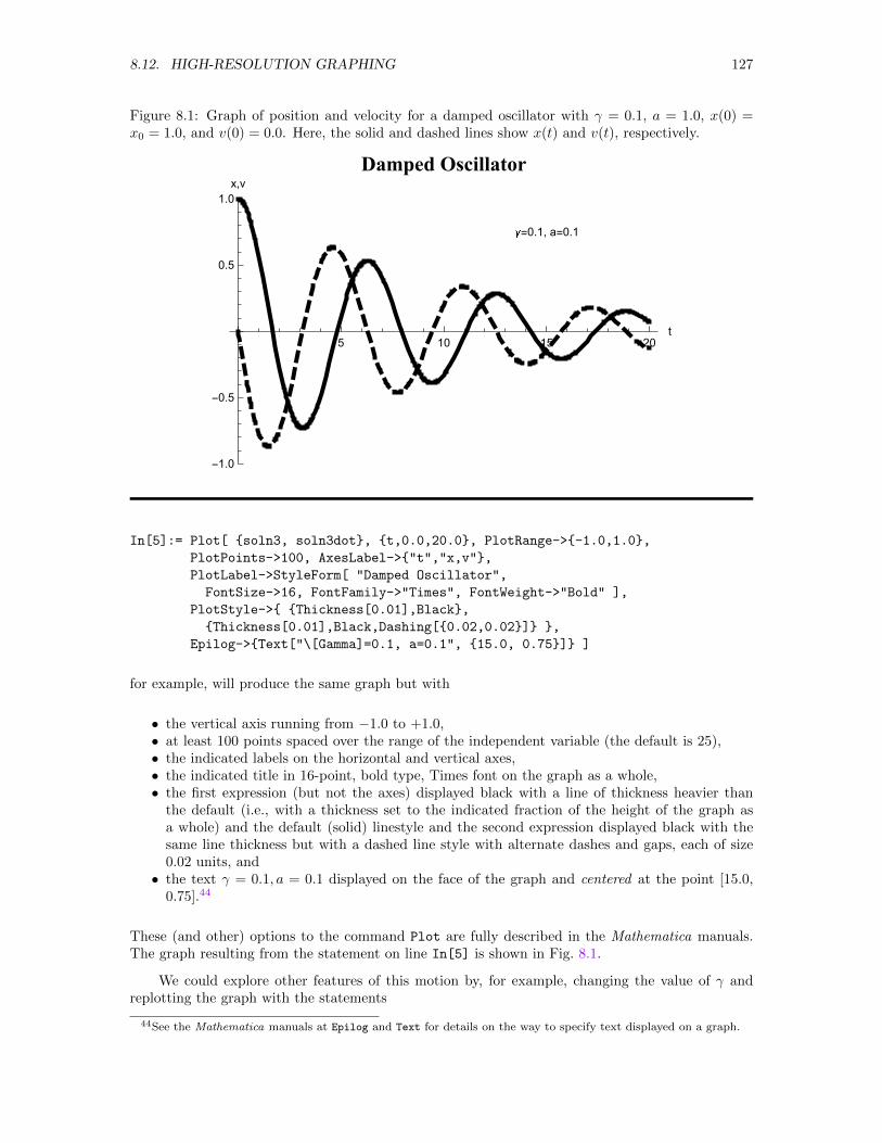
8.12. HIGH-RESOLUTION GRAPHING 127

Figure 8.1: Graph of position and velocity for a damped oscillator with γ = 0.1, a = 1.0, x(0) =x0 = 1.0, and v(0) = 0.0. Here, the solid and dashed lines show x(t) and v(t), respectively.

5 10 15 20t

-1.0

-0.5

0.5

1.0

x,v

Damped Oscillator

=0.1, a=0.1

In[5]:= Plot[ soln3, soln3dot, t,0.0,20.0, PlotRange->-1.0,1.0,

PlotPoints->100, AxesLabel->"t","x,v",

PlotLabel->StyleForm[ "Damped Oscillator",

FontSize->16, FontFamily->"Times", FontWeight->"Bold" ],

PlotStyle-> Thickness[0.01],Black,

Thickness[0.01],Black,Dashing[0.02,0.02] ,

Epilog->Text["\[Gamma]=0.1, a=0.1", 15.0, 0.75] ]

for example, will produce the same graph but with

• the vertical axis running from −1.0 to +1.0,• at least 100 points spaced over the range of the independent variable (the default is 25),• the indicated labels on the horizontal and vertical axes,• the indicated title in 16-point, bold type, Times font on the graph as a whole,• the first expression (but not the axes) displayed black with a line of thickness heavier than

the default (i.e., with a thickness set to the indicated fraction of the height of the graph asa whole) and the default (solid) linestyle and the second expression displayed black with thesame line thickness but with a dashed line style with alternate dashes and gaps, each of size0.02 units, and

• the text γ = 0.1, a = 0.1 displayed on the face of the graph and centered at the point [15.0,0.75].44

These (and other) options to the command Plot are fully described in the Mathematica manuals.The graph resulting from the statement on line In[5] is shown in Fig. 8.1.

We could explore other features of this motion by, for example, changing the value of γ andreplotting the graph with the statements

44See the Mathematica manuals at Epilog and Text for details on the way to specify text displayed on a graph.

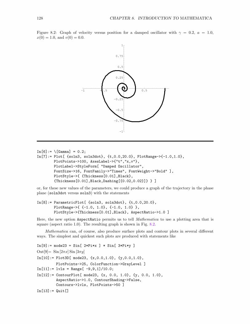
128 CHAPTER 8. INTRODUCTION TO MATHEMATICA

Figure 8.2: Graph of velocity versus position for a damped oscillator with γ = 0.2, a = 1.0,x(0) = 1.0, and v(0) = 0.0.

-1 -0.5 0.5 1

-1

-0.75

-0.5

-0.25

0.25

0.5

0.75

1

In[6]:= \[Gamma] = 0.2;

In[7]:= Plot[ soln3, soln3dot, t,0.0,20.0, PlotRange->-1.0,1.0,

PlotPoints->100, AxesLabel->"t","x,v",

PlotLabel->StyleForm[ "Damped Oscillator",

FontSize->16, FontFamily->"Times", FontWeight->"Bold" ],

PlotStyle-> Thickness[0.01],Black,

Thickness[0.01],Black,Dashing[0.02,0.02] ]

or, for these new values of the parameters, we could produce a graph of the trajectory in the phaseplane (soln3dot versus soln3) with the statements

In[8]:= ParametricPlot[ soln3, soln3dot, t,0.0,20.0,

PlotRange-> -1.0, 1.0, -1.0, 1.0 ,

PlotStyle->Thickness[0.01],Black, AspectRatio->1.0 ]

Here, the new option AspectRatio permits us to tell Mathematica to use a plotting area that issquare (aspect ratio 1.0). The resulting graph is shown in Fig. 8.2.

Mathematica can, of course, also produce surface plots and contour plots in several differentways. The simplest and quickest such plots are produced with statements like

In[9]:= mode23 = Sin[ 2*Pi*x ] * Sin[ 3*Pi*y ]

Out[9]= Sin [2πx] Sin [3πy]

In[10]:= Plot3D[ mode23, x,0.0,1.0, y,0.0,1.0,

PlotPoints->25, ColorFunction->GrayLevel ]

In[11]:= lvls = Range[ -9,9,1]/10.0;

In[12]:= ContourPlot[ mode23, x, 0.0, 1.0, y, 0.0, 1.0,

AspectRatio->1.0, ContourShading->False,

Contours->lvls, PlotPoints->50 ]

In[13]:= Quit[]

8.13. MAKING HARD COPY . . . 129

Figure 8.3: Surface plot of the function z(x, y) = sin(2πx) sin(3πy).

0

0.25

0.5

0.75

1 0

0.25

0.5

0.75

1

-1

-0.5

0

0.5

1

0

0.25

0.5

0.75

Line In[9] here defines the expression to be displayed. Line In[10] produces a surface plot with25 points (default 15) along each axis and coloring set to a gray scale (since we anticipate blackand white printing in this book). Finally, line In[11] defines the values at which contour lines aretoo be drawn (from −0.9 to 0.9 in steps of 0.1) and line In[12] produces a contour map at thoselevels (option Contours) with shading turned off, the aspect ratio adjusted so that the display willbe square, and the function evaluated at 50 points along each axis. The resulting graphs are shownin Figs. 8.3 and 8.4.

We have, of course, only mentioned a few (Plot, ParametricPlot, Plot3D, and ContourPlot)of the functions and only some (PlotRange, PlotPoints, AxesLabel, PlotLabel, PlotStyle,FontSize, FontWeight, ColorFunction, AspectRatio, ContourShading, and Contours) of theoptions that modify the behavior of these functions. Several other functions for producing graphicaldisplays and numerous additional options are available. You should make it a point to read aboutthese functions and the associated options in the Mathematica manuals. In particular, note that thestatement Options[Function]45 will return a list of all of the options that affect Function, attachingto each its current default value.

8.13 Making Hard Copy . . .

The method used to make hard copy of all or part of a Mathematica dialog depends on whether theTBI or the NBI is in use; whether the material to be output is textual or graphical; whether thegraphical material is inline or in a separate window; whether the output is to go directly to a printeror to a PostScript, ASCII, HTML, or . . . file; and whether we are working on a UNIX, Windows, orMacintosh platform. In the following subsections we address each of several possibilities in turn.

45See Section 8.18.5 for a fuller discussion.

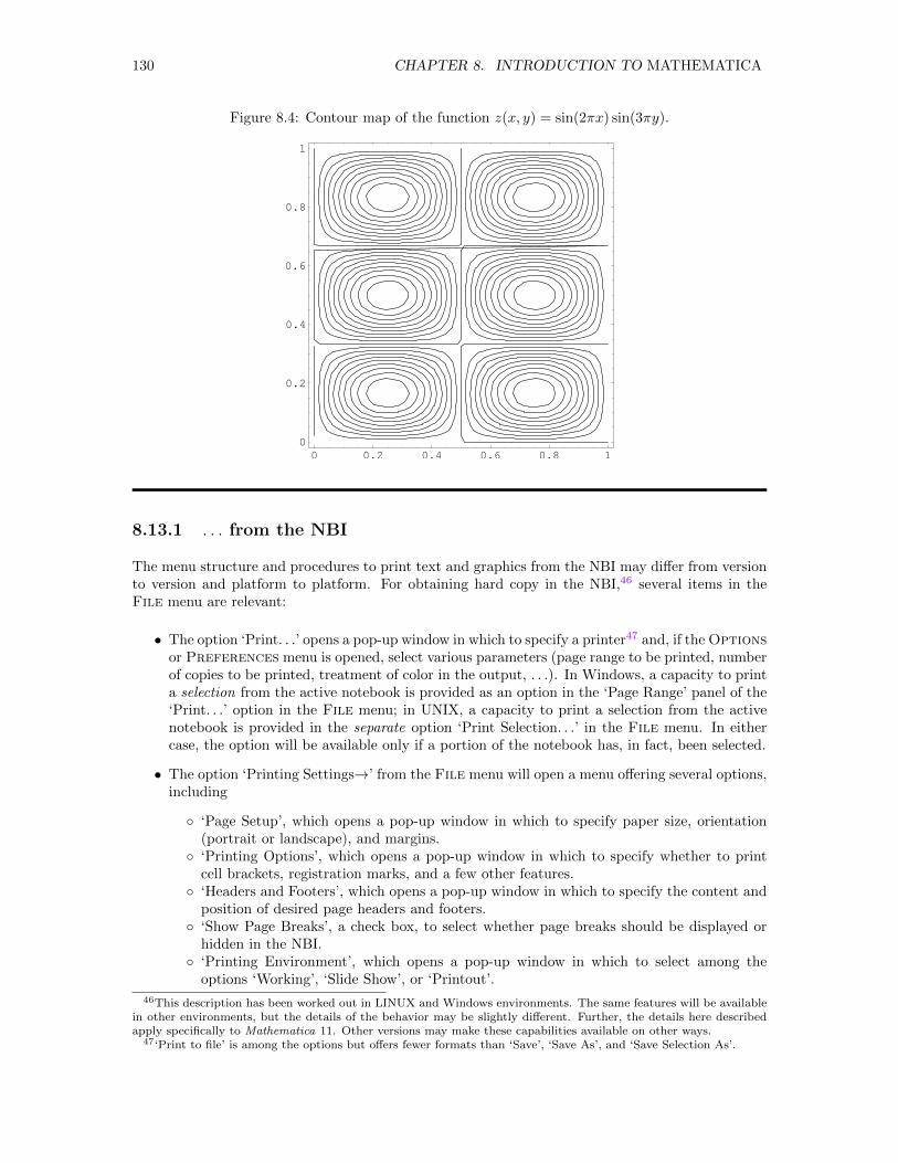
130 CHAPTER 8. INTRODUCTION TO MATHEMATICA

Figure 8.4: Contour map of the function z(x, y) = sin(2πx) sin(3πy).

0 0.2 0.4 0.6 0.8 10

0.2

0.4

0.6

0.8

1

8.13.1 . . . from the NBI

The menu structure and procedures to print text and graphics from the NBI may differ from versionto version and platform to platform. For obtaining hard copy in the NBI,46 several items in theFile menu are relevant:

• The option ‘Print. . .’ opens a pop-up window in which to specify a printer47 and, if the Optionsor Preferences menu is opened, select various parameters (page range to be printed, numberof copies to be printed, treatment of color in the output, . . .). In Windows, a capacity to printa selection from the active notebook is provided as an option in the ‘Page Range’ panel of the‘Print. . .’ option in the File menu; in UNIX, a capacity to print a selection from the activenotebook is provided in the separate option ‘Print Selection. . .’ in the File menu. In eithercase, the option will be available only if a portion of the notebook has, in fact, been selected.

• The option ‘Printing Settings→’ from the File menu will open a menu offering several options,including

‘Page Setup’, which opens a pop-up window in which to specify paper size, orientation(portrait or landscape), and margins.

‘Printing Options’, which opens a pop-up window in which to specify whether to printcell brackets, registration marks, and a few other features.

‘Headers and Footers’, which opens a pop-up window in which to specify the content andposition of desired page headers and footers.

‘Show Page Breaks’, a check box, to select whether page breaks should be displayed orhidden in the NBI.

‘Printing Environment’, which opens a pop-up window in which to select among theoptions ‘Working’, ‘Slide Show’, or ‘Printout’.

46This description has been worked out in LINUX and Windows environments. The same features will be availablein other environments, but the details of the behavior may be slightly different. Further, the details here describedapply specifically to Mathematica 11. Other versions may make these capabilities available on other ways.

47‘Print to file’ is among the options but offers fewer formats than ‘Save’, ‘Save As’, and ‘Save Selection As’.

8.13. MAKING HARD COPY . . . 131

• The option ‘Print Preview. . .’ displays on screen what will ultimately be printed. That on-screen display will be produced in an Adobe Reader window from which a PDF file can, ofcourse, be saved.

• The options ‘Save. . .’, ‘Save As. . .’, and ‘Save Selection As. . .’, each of which brings up abrowser in which you can identify the directory in which all or the selected part of a notebookshould be saved, the name to give the resulting file, and the file type to be used. Availablefile types include tex, ps, eps, pdf, and html, though not all types are available with alloptions. In particular, the filetype ps is available with ‘Save. . .’ and ‘Save As. . .’ and the filetype eps is available with ‘Save Selection As’. The resulting file can then be printed directlyor incorporated in a more extensive document.

These routes to output information include the Mathematica-generated labels for all included ele-ments of the notebook.

Mathematica also provides a facility for writing a description of a specified graphic object (notthe entire notebook) into a file. We simply need to inform Mathematica of the form of the driver itis to use in creating the file, the name it is to give the file, and any controlling options. For example,with graph the label of the graphics display to be output to a file, either of the statements

Export[ "trial.eps", graph, "EPS" ]

which determines the format of the output file from the third argument, or

Export[ "trial.eps", graph ]

which determines the format of the output file from the extension in the file name,48 will tell Math-ematica to convert the graphic object identified by the variable graph into encapsulated PostScriptand write that description to the file trial.eps in the default directory.49 When displayed on acomputer screen with ghostview, an EPS file creates a display that includes a number of controllingbuttons surrounding the graph itself. These surrounding buttons are not included in PDF or JPEGfiles, nor do they appear, for example, when the EPS file is incorporated in a LATEX document. Thisroute to exporting a graph does not include Mathematica-generated output labels in the file.

Note, however, that in some contexts Mathematica may not always transcribe all characters inthe text in the on-screen graphic (e.g., in labels on the axes or in titles) into the proper PostScriptcharacters. Unless some Mathematica-specific fonts have been made available to the program thatwill interpret the PostScript file, opening and closing parentheses, the forward slash, and probablyother characters may be rendered in unexpected forms when the resulting PostScript file is printed orviewed on the screen. In exporting graphics, we must either be sure that the appropriate Mathematicafonts are known by the program(s) that will display the file, or we must constrain Mathematica asit produces the graphic by limiting its choice of fonts for use in the graphic. The former routeis complicated (and necessary if, for example, Greek letters are to be included in the exportedtext).50 While not always satisfactory, the latter route is far simpler; it involves the stipulation ofan additional option in the command producing the graphic. For the sake of a quick illustration, wesimply note that the statements

graph = Plot[ Sin[t], t, 0, 10, AxesLabel->"sin(t)", "x/a",

FormatType->OutputForm ]

Export[ "trial.eps", graph, "EPS" ]

will produce an encapsulated PostScript file in which the parentheses and the slash in the labels onthe axes will be properly rendered, even when the specific Mathematica fonts are not available tothe program that will display trial.eps.

48Other available formats include "PDF" (file type pdf and "JPEG" (file type jpeg. A full list is stored in the systemvariable $ExportFormats.

49See Section 8.18.3.50For details, see the Mathematica manuals.

132 CHAPTER 8. INTRODUCTION TO MATHEMATICA

8.13.2 . . . from the TBI

Printing of text displayed in the TBI is most simply accomplished by using the cutting and pastingcapabilities of the operating system to transfer that character information into a text file, which canthen be edited in a standard text editor and sent to an available printer with the standard commandsto the operating system (or perhaps by selecting appropriate options from a menu available withthe editor).

Graphics commands like Plot may not produce very satisfactory on-screen results when exe-cuted in the TBI. Even so, if it is given a variable name, a graphic object can still be written intoa file as high-resolution graphic for subsequent printing. As in the previous section, we simply needto inform Mathematica of the form of the driver it is to use in creating the file, the name it is togive the file, and any controlling options. For example, either of the statements

Export[ "trial.eps", graph, "EPS" ]

or

Export[ "trial.eps", graph ]

will tell Mathematica to convert the graphic object identified by the variable graph into encapsulatedPostScript and write that description to the file trial.eps in the default directory.

8.14 Output in LATEX Format

A particularly useful feature of Mathematica is its ability to write LATEX versions of expressionsto the screen or into a file. Full details are laid out in the Mathematica manuals. In brief, thestatement51

TeXForm[ expr1 ]

for example, converts the specified expression into LATEX format and displays it on the screen (fromwhere standard cut and paste operations—when they are available—can move the description towherever we might want it). Alternatively, either of the statements

TeXForm[ expr1 ] >> FileNamePut[ TeXForm[ expr1 ], "FileName" ]

will create a new (ASCII) file and write the LATEX description of the indicated expression intothat file, overwriting any existing file by the same name. To append the LATEX description of theexpression to an existing file, one or the other of the statements

TeXForm[ expr1 ] >>> FileNamePutAppend[ TeXForm[ expr1 ], "FileName" ]

is necessary. Once created, this file can, of course, be edited or incorporated into other LATEXdocuments.

Automatic translation of arbitrary expressions into LATEX is a daunting task. While fairlysophisticated, the Mathematica translator is not perfect. Edits will often be necessary to “correct”the translator’s glitches. In particular, the translator writes only the LATEX description of the

51Note the upper -case X in the third character.

8.15. ANIMATION 133

equation to the screen or into the file. It does not place the equation in a LATEX equation environmentor otherwise embellish the description with additional LATEX constructs that may be necessaryfor creation of the ultimate document. These formatting instructions will have to be suppliedthrough manual editing of the file created by Mathematica. Further, even more subtle edits may benecessary.52 Conveniently, variables named \[Gamma] and \[CapitalGamma], for example, will beproperly translated into \gamma and \Gamma.

Even more generally, if we have created a Mathematica notebook in the NBI, we can outputthat notebook in its entirety (including the textual sections) into a LATEX file by

• Selecting ‘Save as . . .’ from the File menu,• Selecting the LATEX option in the text entry box labeled ‘Files of type:’,• Specifying the desired file name in the text entry box labeled ‘File name:’,• Browsing to the desired directory, and• Clicking ML on ‘Save’.

The file will be written into the specified directory. The resulting file is a complete LATEX sourcefile with all necessary packages and new command definitions in its preamble. If the content of thisfile is to be incorporated into another LATEX source file, some of the commands at its beginning andend will have to be stripped off but any \usepackage and \newcommand commands not already inthe destination file must be copied from the Mathematica-produced file.53

8.15 Animation

The Mathematica command Animate facilitates the creation of animated displays in the NBI. Thesimple statement

Animate[ Plot[Sin[Pi*x]*Cos[2*Pi*t], x,0.0,1.0,

PlotRange-> 0.0,1.0,-1.0,1.0 ], t, 0.0, 1.0, 0.05 ]

will, for example, display the fundamental mode of a vibrating string, keeping the axes the samesize throughout all frames. A more complicated animation, display of the 23 mode of a squaremembrane, is produced by the statement

Animate[ Plot3D[Sin[2*Pi*x]*Sin[3*Pi*y]*Cos[2*Pi*t], x,0.0,1.0, y,0.0,1.0,

PlotRange-> 0.0,1.0,0.0,1.0,-1.0,1.0], t,0.0,1.0,0.05,

AnimationRate-> 0.1]

In both cases, the button labeled ‘Pause’ in the window displaying the animation will stop theanimation and allow subsequent statements to be submitted to Mathematica.

Unfortunately, the command Animate has too many possibilities and options for full discussionhere. Details can be found in the Mathematica manuals.

52For example, output of the Mathematica expression Sin[x+y]/Cos[x-y] with TeXForm yielded the correct butunintended result \sin (x+y) \sec (x-y). Note also the unnecessary spaces after sin and cos.

53LATEX files written by some earlier versions of Mathematica make use of several Mathematica-specific LATEXcommands which are defined in the Mathematica-supplied LATEX package named notebook2e and the LATEX-suppliedpackage named latexsym. The files defining these packages must be accessible on your computer system before aMathematica-produced LATEX source file can be processed and printed. The file latexsym.sty is probably availablewithout effort on your part. If the file notebook2e.sty has not been placed where LATEX can find it automatically, youmay have to copy it from the directory $MATHEMHEAD/SystemFiles/ IncludeFiles/TeX/texmf/tex/latex/wolfram, inwhich it was placed when Mathematica was installed on your system.

134 CHAPTER 8. INTRODUCTION TO MATHEMATICA

8.16 Using the Notebook

Within the NBI, the window in which Mathematica commands are entered has full capabilities as anotebook, which means in particular that it can contain textual sections, e.g., documentation andmotivation, as well as executable Mathematica commands. Notebooks are constructed out of cells,which may contain executable Mathematica statements (and the associated output)—the only cellswe have so far seen—or may contain text. For purposes of organizing larger documents, these cellscan themselves be assembled into sections and subsections, much in the way a conventional bookwould be assembled.

Suppose we already have on screen a Mathematica notebook containing a few Mathematicastatements and their output. Note, in particular, that each statement and its output embracestwo cells, one containing the input statement and the other containing the associated Mathematicaresponse. The input cell is marked at the right side of the Notebook window with a closing squarebracket whose upper corner contains also a diagonal line, and the output cell is similarly markedexcept that the bracket also has a short horizontal line below the diagonal line. Further, the twocells are themselves grouped together at the right side of the Notebook window with a closing squarebracket that has no adornments at its corners. Finally, note that double clicking ML on the outersquare bracket will “close” the pair, hiding the output and leaving only the input statement. In thisarrangement, the outer bracket now has half an arrowhead at its lower end to indicate that the cellhas been closed. Double clicking ML on the outer bracket when it is in this state will reopen thecell.

Now, suppose that we want to precede each statement with an explanatory paragraph. Wecould achieve that end for one of the statements by

1. Moving the cursor to the position at which a new cell is desired, placing it so that it becomesa horizontal I-beam.

2. Clicking ML to create a horizontal line (cell insertion bar) across the screen.

3. Selecting ‘Text’ from the Style submenu of the Format menu.

4. Typing the desired text, using the various options in the Format menu to specify font, typesize, type style, alignment, . . .. As you start typing, a new cell will be created for the typedtext. This cell will be bracketed on the right with a square bracket that has a short horizontalline below its top bar—the identifier of a text cell.

This process can, of course, be repeated to provide a textual description for each of the remainingstatements.

In essence, the previous paragraph provides all we need to know to add documentation as anintrinsic part of a notebook. As our notebooks grow in size, however, we may wish to organize theircontents into appropriate structural units and provide titles. To those ends, we need simply noticethat the Style submenu of the Format menu contains numerous items beyond the one introducedin the previous paragraph. Positioning the cursor at the point of a desired textual insertion, clickingML to create a horizontal line (cell insertion bar) across the screen, and then selecting some otheritem (Title, Subtitle, Section, Subsection, . . .) from the Style submenu of the Format menuwill then set Mathematica to create a cell of the selected style when we begin typing. Further,Mathematica will select a type size and weight appropriate to the selected cell style and, for sectionsand subsections, will place a marker at the beginning of the line to draw attention to its status inclarifying the structure of the document. Note also that, as a document is divided into sections andsubsections, the bars along the right edge become more numerous, reflecting the divisions createdby the inserted sections and subsections.

For example, to add a title to the entire document, we create an insertion bar at the verybeginning of the document, select ‘Title’ from the Style submenu of the Format menu, and type

8.17. CUSTOMIZATIONS 135

the text of the title. Then, selecting this cell by highlighting its bracket at the right edge of thescreen, we can adjust the font, type style, type size, alignment, and several other properties byappropriate selections from submenus accessible in the Format menu.

Mathematica output in this notebook can, of course, always be quickly regenerated by executingthe statements. Frequently, we may wish to suppress the presence of that output in the actualnotebook. We can

• remove selected items of output by selecting the items to be removed and then selecting ‘Cut’from the Edit menu.

• remove all output from the notebook by selecting ‘Delete All Output’ from the Cell menu.

Finally, we note that, after all the work of creating a notebook, the notebook itself can besaved by selecting ‘Save’ from the File menu and, in the resulting pop-up window, specifying thefile name (conventional file type .nb) and the directory, and clicking ML on the ‘Save’ button. Ina later session, the worksheet can be loaded into Mathematica by selecting ‘Open’ from the Filemenu and identifying the file to be opened in the pop-up browser.

This short section can, of course, not do full justice to the wide spectrum of features of Math-ematica’s notebook interface. You must work with it, explore the menus in the NBI, and read theMathematica manuals

8.17 Customizations

When Mathematica is started up, the configuration both of the kernel and of the front-end is de-fined by a number of default specifications built into the program, by statements in an assortment ofsystem-wide initialization files and by statements in several user-created initialization files. Specifi-cally,54

• The file $BaseDirectory/Kernel/init.m configures the Mathematica kernel for all users andthe file $BaseDirectory/FrontEnd/init.m configures the Mathematica front-end for all users.These files are maintained by the system manager and can be viewed but not edited by indi-vidual users.

• The file $UserBaseDirectory/Kernel/init.m modifies the configuration of the kernel estab-lished by the system-wide file and must be explicitly created by the individual user.

• The file $UserBaseDirectory/FrontEnd/init.m modifies the configuration of the front-endestablished by the system-wide file but is not created directly by the user. Instead, Mathe-matica maintains this file to reflect changes made via statements executed by Mathematica.

These files are simply command files—see Section 8.11—that can contain any statement that mightotherwise be typed interactively. Be aware, however, that none of the statements or their responseswill be displayed as the initialization file(s) is (are) read. Even so, for example, variables to whichvalues are assigned and the features defined by packages read in will be available when reading ofthe file has been completed. As Mathematica is started, the system-wide files are executed and thenthe user-created file is executed. Thus, the user-created file can be used to override statements inthe system-wide file, should that be desired. Together, these files—if they exist at all—define thedefault configuration set up by Mathematica when finally it is ready to accept input.

54Here, the system variable $BaseDirectory identifies the top directory in the hierarchy in which the Mathematicstructure is stored and the system variable $UserBaseDirectory identifies the top directory in which user-createdconfiguration files are stored. Both of these directories may be hidden.

136 CHAPTER 8. INTRODUCTION TO MATHEMATICA

8.18 Miscellaneous Occasionally Useful Tidbits

In this section, we comment on a number of other features that are occasionally useful. Full details,of course, are available in the Mathematica manuals.

8.18.1 Turning off Messages

Many of Mathematica’s messages can be suppressed by executing the command Off[...] andturned back on by executing the command On[...]. Here, the ellipses stand for the name of themessage. For example, to turn off display of the message that alerts you that a symbol you havejust typed is nearly the same as some other symbol that you may have intended to type, you canexecute the statement

Off[General::Spell1]

though full turning off of these messages may also require execution of the statement

Off[General::Spell]

These messages can be turned on again with the statements

On[General::Spell1]

On[General::Spell]

The system variable $MessageGroups stores a list of the existing message groups (the piece of theargument before the double colon).

8.18.2 Specifying Directories

Different operating systems use different forms to specify the path that identifies a particular di-rectory, for example, to set the default directory or to identify the location of a file to be read orwritten. Within Mathematica, commands for performing these operations should separate directo-ries in a path with the structure that is native to the operating system in use (e.g., forward slashin UNIX, backslash in Windows). For convenience, and to simplify command files to be used withseveral operating systems, Mathematica will translate forward slashes into the appropriate separatorfor the operating system in use.

8.18.3 Default Directory

The default directory or current working directory in Mathematica is set when Mathematica islaunched. Unless an initialization file has been created with a command that changes that directory,it will probably be the user’s home directory or the directory from which Mathematica was launchedby a command at a Shell prompt. The command Directory[] will cause the display of the currentdefault directory. As illustrated by the statements

SetDirectory[]

SetDirectory[".."]

SetDirectory["progs"]

SetDirectory["/apps/MATHEM/userprogs"]

Set directory to user’s home directory.Set directory to the parent of currentdirectory.Set directory to progs subdirectory ofcurrent directory.Set directory to indicated directory.

8.18. MISCELLANEOUS OCCASIONALLY USEFUL TIDBITS 137

the command SetDirectory allows dynamic specification of the current working directory in avariety of ways. Note that the separator between successive directories in a path varies from op-erating system to operating system. The illustrated separator is the one used in UNIX.55 Fur-ther information about these commands will be found in the Mathematica manuals. Further, thestatement FileNames[] will display a list of the files in the current directory and the statementFileNames["*.m"] will display a list of all files in that directory with filetype .m. If the file is notin the default directory, then its full path must be specified as part of the filename.

8.18.4 Search Path

Whenever an explicit path is not specified for a file that Mathematica is to read, the program looksin a sequence of directories defined by the search path. The initial search path is defined in a Math-ematica initialization file or, in the absence of such a file, by Mathematica itself. The initial searchpath is site-specific and is identified in the Local Guide. If not defined by an initialization file, thepath is likely to contain, in order, a few specific Mathematica directories in the user’s home directory,the default directory, the user’s home directory, and finally a succession of directories descendingfrom the directory $MATHEMHEAD. The system variable $Path contains a list of the directories in thecurrent search path. Thus, the statement $Path will display that list, and statements like56

Prepend[ $Path, "/usr/share/CPSUP/mathematica" ]

Append[ $Path, "/usr/local/packages" ]

Insert[ $Path, "/usr/local/temp", 5 ]

will create a new value for the list $Path, that new value containing all of the elements of the originallist in the original order but having the indicated directory at the beginning, at the end, or in thefifth position, respectively. Similarly, statements like

Delete[ $Path, 5 ]

ReplacePart[ $Path, "/usr/local/myfiles", 7 ]

will create a new value for the list $Path by removing altogether the element in the fifth position orby replacing the element in the seventh position with the indicated directory, respectively.

8.18.5 Displaying and Changing Default Options

In the course of introducing several commands, we have learned that the precise effect of many com-mands depends on the values of associated options. Initially, we accepted Mathematica’s defaults.Then we learned that arguments like

OptionName -> NewValue

(e.g., PlotRange -> -1.0,1.0) can be used within a command to override the default value forthe indicated option, but only for that execution of the command. If the default value is to beoverridden for all subsequent executions of the associated command, however, changing the defaultwith a statement like

SetOptions[ CommandName, OptionName -> NewValue ]

55See Section 8.18.2.56For definiteness, we use the UNIX form for indicating paths. Remember that the precise form in which paths are

specified depends on the operating system. The form appropriate at your site is described in the Local Guide.

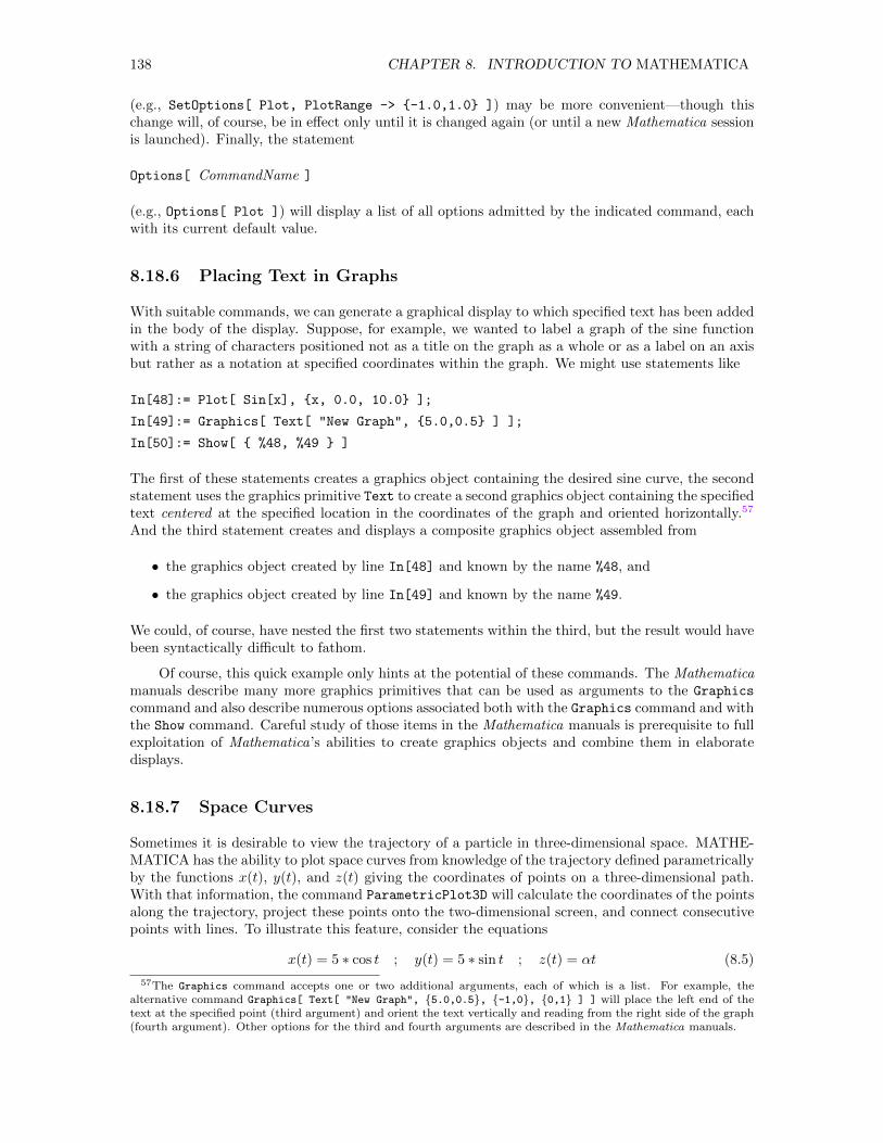
138 CHAPTER 8. INTRODUCTION TO MATHEMATICA

(e.g., SetOptions[ Plot, PlotRange -> -1.0,1.0 ]) may be more convenient—though thischange will, of course, be in effect only until it is changed again (or until a new Mathematica sessionis launched). Finally, the statement

Options[ CommandName ]

(e.g., Options[ Plot ]) will display a list of all options admitted by the indicated command, eachwith its current default value.

8.18.6 Placing Text in Graphs

With suitable commands, we can generate a graphical display to which specified text has been addedin the body of the display. Suppose, for example, we wanted to label a graph of the sine functionwith a string of characters positioned not as a title on the graph as a whole or as a label on an axisbut rather as a notation at specified coordinates within the graph. We might use statements like

In[48]:= Plot[ Sin[x], x, 0.0, 10.0 ];

In[49]:= Graphics[ Text[ "New Graph", 5.0,0.5 ] ];

In[50]:= Show[ %48, %49 ]

The first of these statements creates a graphics object containing the desired sine curve, the secondstatement uses the graphics primitive Text to create a second graphics object containing the specifiedtext centered at the specified location in the coordinates of the graph and oriented horizontally.57

And the third statement creates and displays a composite graphics object assembled from

• the graphics object created by line In[48] and known by the name %48, and

• the graphics object created by line In[49] and known by the name %49.

We could, of course, have nested the first two statements within the third, but the result would havebeen syntactically difficult to fathom.

Of course, this quick example only hints at the potential of these commands. The Mathematicamanuals describe many more graphics primitives that can be used as arguments to the Graphics

command and also describe numerous options associated both with the Graphics command and withthe Show command. Careful study of those items in the Mathematica manuals is prerequisite to fullexploitation of Mathematica’s abilities to create graphics objects and combine them in elaboratedisplays.

8.18.7 Space Curves

Sometimes it is desirable to view the trajectory of a particle in three-dimensional space. MATHE-MATICA has the ability to plot space curves from knowledge of the trajectory defined parametricallyby the functions x(t), y(t), and z(t) giving the coordinates of points on a three-dimensional path.With that information, the command ParametricPlot3D will calculate the coordinates of the pointsalong the trajectory, project these points onto the two-dimensional screen, and connect consecutivepoints with lines. To illustrate this feature, consider the equations

x(t) = 5 ∗ cos t ; y(t) = 5 ∗ sin t ; z(t) = αt (8.5)

57The Graphics command accepts one or two additional arguments, each of which is a list. For example, thealternative command Graphics[ Text[ "New Graph", 5.0,0.5, -1,0, 0,1 ] ] will place the left end of thetext at the specified point (third argument) and orient the text vertically and reading from the right side of the graph(fourth argument). Other options for the third and fourth arguments are described in the Mathematica manuals.

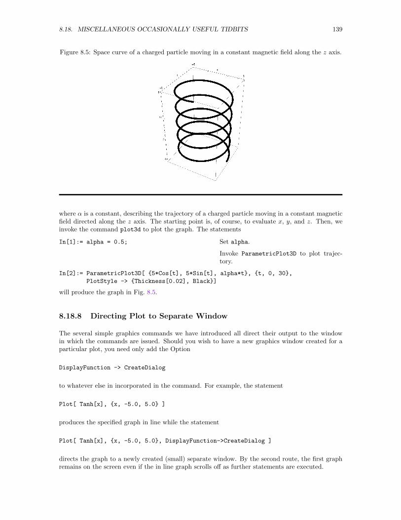
8.18. MISCELLANEOUS OCCASIONALLY USEFUL TIDBITS 139

Figure 8.5: Space curve of a charged particle moving in a constant magnetic field along the z axis.

where α is a constant, describing the trajectory of a charged particle moving in a constant magneticfield directed along the z axis. The starting point is, of course, to evaluate x, y, and z. Then, weinvoke the command plot3d to plot the graph. The statements

In[1]:= alpha = 0.5;

In[2]:= ParametricPlot3D[ 5*Cos[t], 5*Sin[t], alpha*t, t, 0, 30,

PlotStyle -> Thickness[0.02], Black]

Set alpha.

Invoke ParametricPlot3D to plot trajec-tory.

will produce the graph in Fig. 8.5.

8.18.8 Directing Plot to Separate Window

The several simple graphics commands we have introduced all direct their output to the windowin which the commands are issued. Should you wish to have a new graphics window created for aparticular plot, you need only add the Option

DisplayFunction -> CreateDialog

to whatever else in incorporated in the command. For example, the statement

Plot[ Tanh[x], x, -5.0, 5.0 ]

produces the specified graph in line while the statement

Plot[ Tanh[x], x, -5.0, 5.0, DisplayFunction->CreateDialog ]

directs the graph to a newly created (small) separate window. By the second route, the first graphremains on the screen even if the in line graph scrolls off as further statements are executed.

140 CHAPTER 8. INTRODUCTION TO MATHEMATICA

8.19 References

In this chapter, we have introduced only the most important features of Mathematica. A fulldescription of all commands and features is contained in the Mathematica manuals, including

• several documents and resources as described in Section 8.2.

• a number of documents, links to which can be found by entering “Mathematica help” in thesearch window of your browser. In particular, you should find links to

the official Mathematica documentation at http://reference.wolfram.com/language/,which brings up on line the same documentation available from the Help menu in theNBI, and

many other official and unofficial documents.

• a number of books and on-line materials describing a wide spectrum of uses of Mathematica ina variety of disciplines and for a variety of specific purposes. A list of such books can be found,among other places, from the links http://www.wolfram.com/mathematica/resources/ andhttp://www.wolfram.com/books/ at the Wolfram Research website or by searching on-linecommercial book stores (Amazon, Barnes and Noble, . . .) for the keyword Mathematica.

• more specific documents on particular Mathematica commands, links to which can be foundby entering “CommandName in MATHEMATICA”, e.g., “integrate in MATHEMATICA’ inthe search window of your browser.

The user is urged to browse in these materials, being alert not only to the available functions butalso to the assorted option variables and keywords that modify their behavior.

While on-line documentation has largely superseded printed documentation in the last decade,several now largely outdated but still potentially valuable printed materials can be found. Specifi-cally, your local library may include one or more copies of

• Getting Started with Mathematica Version # under (operating system), (Wolfram Media, Inc.),which contains installation instructions and a brief description of the issues with which a userof Mathematica must be familiar from the very beginning.

• Stephen Wolfram, The Mathematica Book , Fifth (or earlier) Edition (Wolfram Media, Inc.,and Cambridge University Press, 1988, 1991, 1996, 1999, 2003), which contains a tour of thecapabilities of Mathematica, an introduction to the practical use of Mathematica, an exhaustivediscussion of the design principles underlying Mathematica, a treatment of more advancedtopics, several pages of formulae, a section of color plates showing a spectacular array ofgraphical displays, and a comprehensive set of appendices listing and describing essentiallyall commands, options, special variables, and other objects that play a role somewhere inMathematica. This tome of nearly 1500 pages in a single binding is massive and exhaustive.

• Mathematica Version # Standard Add-on Packages (Wolfram Media, Inc., 1996, 1999), whichcontains detailed descriptions of all components in all of the standard add-on packages.

8.20 Exercises

8.1. Read the Mathematica manuals to find out how the commands Expand, Factor, Apart, andSimplify differ from one another and then invent several examples that will reveal those differences.To help you get started, you might find it useful to compare the effect of each of these commandson the expressions

8.20. EXERCISES 141

(a)x

a+ b+

y

a+ b(b) (a+ b)(c+ d) + (a+ b)e

(c) (x+ y)(z + w) (d) a(b+ c(d+ e))

(e)x

a+ b+

y

c+ d(f)

(a− x)2

(a2 − 2ax+ x2)3/2

but you will probably have to invent other examples as well to reveal as many of the differencesas you can. Write two or three paragraphs in which you describe the action of each of thesecommands and the differences among them. Creating a table showing the results of applying eachof the commands to each expression you select might be a useful support for your comparison.

8.2. Use Mathematica to convert each of the expressions in the left-hand column in the table below intothe expression in the associated right-hand column:

(a)(a− x)2

(a2 − 2ax+ x2)3/2=⇒ 1

|x− a|

(b) sinh( ln(x+√x2 + a2)− ln(a) ) =⇒ x

a

(c)1

x+√y

=⇒x−√yx2 − y

Write two or three paragraphs in which you describe your efforts, including some indication ofapproaches that were not successful. Don’t be overly concerned about the order of terms withinvarious sets of parentheses; that order is particularly difficult to control. Focus instead on creatingthe general form of each desired result.

8.3. Use Mathematica to convert each of the expressions in the left-hand column in the table below intothe expression in the associated right-hand column:

(a)d

dx

(x2e−x

2)

=⇒ −2x(x2 − 1)e−x2

(b) sin(√a2(a+ 3x) + x2(3a+ x) + y) =⇒ sin((a+ x)3/2 + y)

(c) cg + cf + b2d+ 2abd+ a2d+ b2c+ 2abc+ a2c =⇒ (a+ b)2(c+ d) + c(f + g)

(d) a e(−b+iω)t + a e(−b−iω)t =⇒ a e−bt (e−iωt + eiωt)

(e) a e(−b+iω)t + a e(−b−iω)t =⇒ 2 a e−bt cos(ωt)

(f) x2 + y2 + z2 − 2a(x+ y) + 2a2 =⇒ (x− a)2 + (y − a)2 + z2

In several cases, you may need to invoke Part, ReplacePart, and/or FullForm, but other commandswill surely also be needed. Invoke microscopic dissection of the expressions only as a last resort.Write two or three paragraphs in which you describe your efforts, including some indication ofapproaches that were not successful. Don’t be overly concerned about the order of terms withinvarious sets of parentheses in the final form; that order is particularly difficult to control. Focusinstead on creating the general form of each desired result.

8.4. In Section 8.8.9, we set up the differential equation for a damped harmonic oscillator but thenpursued the solution only for the underdamped case. Repeat the solution for the underdampedcase and then find also the solutions for the critically damped and overdamped cases. Describe thedifferences in the physical behavior for the three cases.

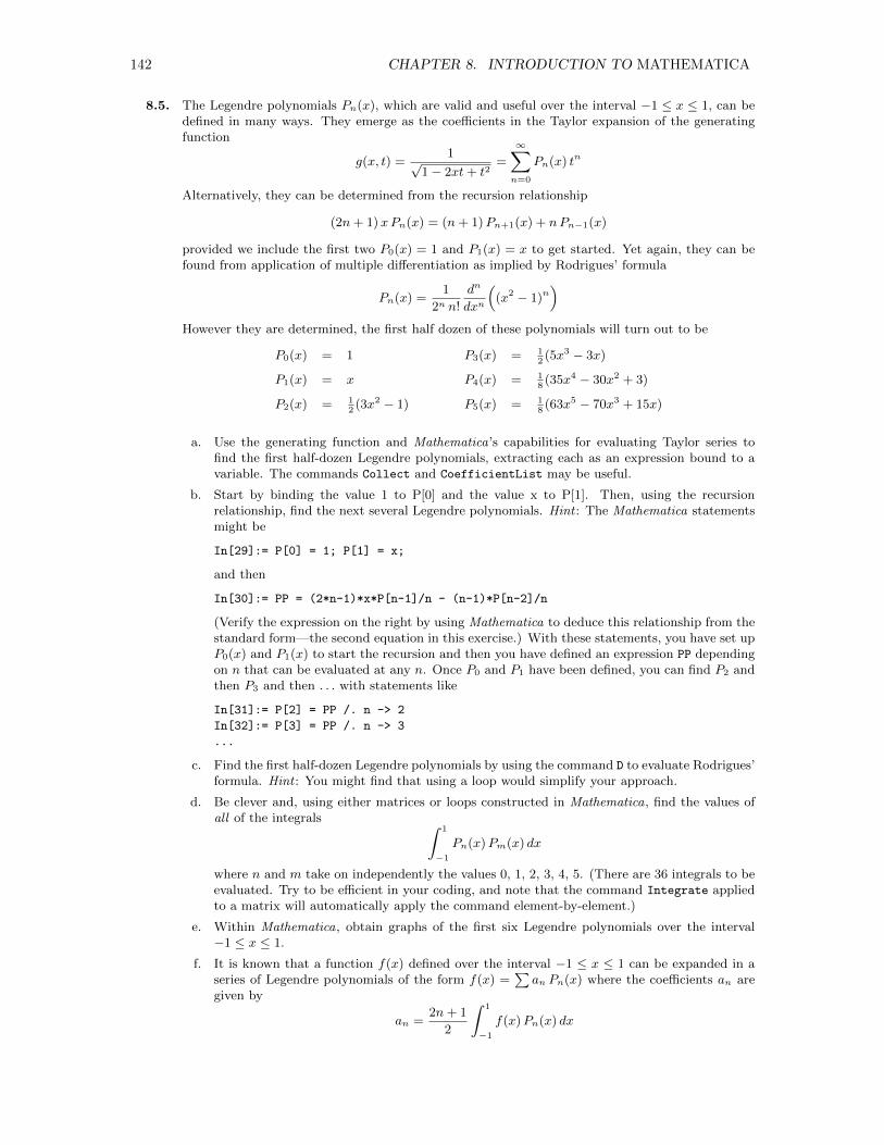
142 CHAPTER 8. INTRODUCTION TO MATHEMATICA

8.5. The Legendre polynomials Pn(x), which are valid and useful over the interval −1 ≤ x ≤ 1, can bedefined in many ways. They emerge as the coefficients in the Taylor expansion of the generatingfunction

g(x, t) =1√

1− 2xt+ t2=

∞∑n=0

Pn(x) tn

Alternatively, they can be determined from the recursion relationship

(2n+ 1)xPn(x) = (n+ 1)Pn+1(x) + nPn−1(x)

provided we include the first two P0(x) = 1 and P1(x) = x to get started. Yet again, they can befound from application of multiple differentiation as implied by Rodrigues’ formula

Pn(x) =1

2n n!

dn

dxn

((x2 − 1)n

)However they are determined, the first half dozen of these polynomials will turn out to be

P0(x) = 1 P3(x) = 12(5x3 − 3x)

P1(x) = x P4(x) = 18(35x4 − 30x2 + 3)

P2(x) = 12(3x2 − 1) P5(x) = 1

8(63x5 − 70x3 + 15x)

a. Use the generating function and Mathematica’s capabilities for evaluating Taylor series tofind the first half-dozen Legendre polynomials, extracting each as an expression bound to avariable. The commands Collect and CoefficientList may be useful.

b. Start by binding the value 1 to P[0] and the value x to P[1]. Then, using the recursionrelationship, find the next several Legendre polynomials. Hint : The Mathematica statementsmight be

In[29]:= P[0] = 1; P[1] = x;

and then

In[30]:= PP = (2*n-1)*x*P[n-1]/n - (n-1)*P[n-2]/n

(Verify the expression on the right by using Mathematica to deduce this relationship from thestandard form—the second equation in this exercise.) With these statements, you have set upP0(x) and P1(x) to start the recursion and then you have defined an expression PP dependingon n that can be evaluated at any n. Once P0 and P1 have been defined, you can find P2 andthen P3 and then . . . with statements like

In[31]:= P[2] = PP /. n -> 2

In[32]:= P[3] = PP /. n -> 3

...

c. Find the first half-dozen Legendre polynomials by using the command D to evaluate Rodrigues’formula. Hint : You might find that using a loop would simplify your approach.

d. Be clever and, using either matrices or loops constructed in Mathematica, find the values ofall of the integrals ∫ 1

−1

Pn(x)Pm(x) dx

where n and m take on independently the values 0, 1, 2, 3, 4, 5. (There are 36 integrals to beevaluated. Try to be efficient in your coding, and note that the command Integrate appliedto a matrix will automatically apply the command element-by-element.)

e. Within Mathematica, obtain graphs of the first six Legendre polynomials over the interval−1 ≤ x ≤ 1.

f. It is known that a function f(x) defined over the interval −1 ≤ x ≤ 1 can be expanded in aseries of Legendre polynomials of the form f(x) =

∑an Pn(x) where the coefficients an are

given by

an =2n+ 1

2

∫ 1

−1

f(x)Pn(x) dx

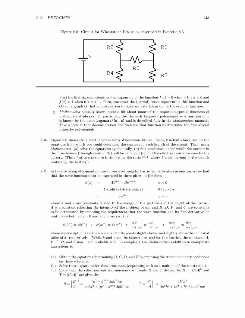
8.20. EXERCISES 143

Figure 8.6: Circuit for Wheatstone Bridge as described in Exercise 8.6.

V

R1R2

R3R4R5

Find the first six coefficients for the expansion of the function f(x) = 0 when −1 < x < 0 andf(x) = 1 when 0 < x < 1. Then, construct the (partial) series representing this function andobtain a graph of that approximation to compare with the graph of the original function.

g. Mathematica actually knows quite a bit about many of the important special functions ofmathematical physics. In particular, the the n-th Legendre polynomial as a function of xis known by the name LegendreP[n, x] and is described fully in the Mathematica manuals.Take a look at that documentation and then use that function to determine the first severalLegendre polynomials.

8.6. Figure 8.6 shows the circuit diagram for a Wheatstone bridge. Using Kirchoff’s laws, set up theequations from which you could determine the currents in each branch of the circuit. Then, usingMathematica, (a) solve the equations symbolically, (b) find conditions under which the current inthe cross branch (through resistor R5) will be zero, and (c) find the effective resistance seen by thebattery. (The effective resistance is defined by the ratio V/I, where I is the current in the branchcontaining the battery.)

8.7. In the scattering of a quantum wave from a rectangular barrier in particular circumstances, we findthat the wave function must be expressed in three pieces in the form

ψ(x) = Aeikx +Be−ikx x < 0

= D cosh(κx) + F sinh(κx) 0 < x < w

= Ceikx x > w

where k and κ are constants related to the energy of the particle and the height of the barrier,A is a constant reflecting the intensity of the incident beam, and B, D, F , and C are constantsto be determined by imposing the requirement that the wave function and its first derivative becontinuous both at x = 0 and at x = w, i.e., that

ψ(0−) = ψ(0+) ; ψ(w−) = ψ(w+) ;dψ

dx

∣∣∣0−

=dψ

dx

∣∣∣0+

;dψ

dx

∣∣∣w−

=dψ

dx

∣∣∣w+

where superscript plus and minus signs identify points slightly below and slightly above the indicatedvalue of x, respectively. (While k and κ can be taken to be real for this barrier, the constants A,B, C, D, and F may—and probably will—be complex.) Use Mathematica’s abilities to manipulateexpressions to

(a) Obtain the equations determining B, C, D, and F by imposing the stated boundary conditionson these solutions.

(b) Solve those equations for those constants (expressing each as a multiple of the constant A).(c) Show that the reflection and transmission coefficients R and T defined by R = |B/A|2 and

T = |C/A|2 are given by

R =

∣∣∣BA

∣∣∣2 =(κ2 + k2)2 sinh2 κw

4κ2k2 + (κ2 + k2)2 sinh2 κw; T =

∣∣∣CA

∣∣∣2 =4k2κ2

4κ2k2 + (κ2 + k2)2 sinh2 κw

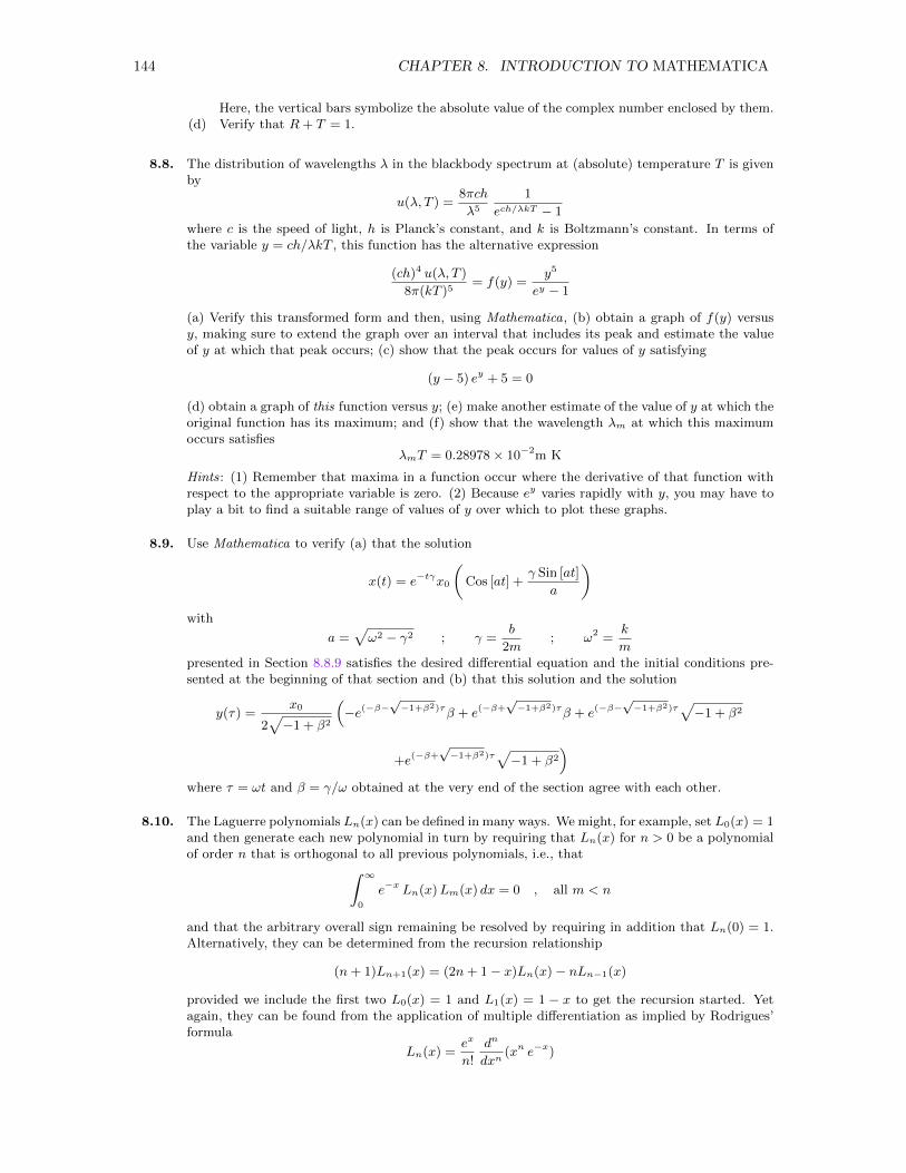
144 CHAPTER 8. INTRODUCTION TO MATHEMATICA

Here, the vertical bars symbolize the absolute value of the complex number enclosed by them.(d) Verify that R+ T = 1.

8.8. The distribution of wavelengths λ in the blackbody spectrum at (absolute) temperature T is givenby

u(λ, T ) =8πch

λ5

1

ech/λkT − 1

where c is the speed of light, h is Planck’s constant, and k is Boltzmann’s constant. In terms ofthe variable y = ch/λkT , this function has the alternative expression

(ch)4 u(λ, T )

8π(kT )5= f(y) =

y5

ey − 1

(a) Verify this transformed form and then, using Mathematica, (b) obtain a graph of f(y) versusy, making sure to extend the graph over an interval that includes its peak and estimate the valueof y at which that peak occurs; (c) show that the peak occurs for values of y satisfying

(y − 5) ey + 5 = 0

(d) obtain a graph of this function versus y; (e) make another estimate of the value of y at which theoriginal function has its maximum; and (f) show that the wavelength λm at which this maximumoccurs satisfies

λmT = 0.28978× 10−2m K

Hints: (1) Remember that maxima in a function occur where the derivative of that function withrespect to the appropriate variable is zero. (2) Because ey varies rapidly with y, you may have toplay a bit to find a suitable range of values of y over which to plot these graphs.

8.9. Use Mathematica to verify (a) that the solution

x(t) = e−tγx0

(Cos [at] +

γ Sin [at]

a

)with

a =√ω2 − γ2 ; γ =

b

2m; ω2 =

k

mpresented in Section 8.8.9 satisfies the desired differential equation and the initial conditions pre-sented at the beginning of that section and (b) that this solution and the solution

y(τ) =x0

2√−1 + β2

(−e(−β−

√−1+β2)τβ + e(−β+

√−1+β2)τβ + e(−β−

√−1+β2)τ

√−1 + β2

+e(−β+√−1+β2)τ

√−1 + β2

)where τ = ωt and β = γ/ω obtained at the very end of the section agree with each other.

8.10. The Laguerre polynomials Ln(x) can be defined in many ways. We might, for example, set L0(x) = 1and then generate each new polynomial in turn by requiring that Ln(x) for n > 0 be a polynomialof order n that is orthogonal to all previous polynomials, i.e., that∫ ∞

0

e−x Ln(x)Lm(x) dx = 0 , all m < n

and that the arbitrary overall sign remaining be resolved by requiring in addition that Ln(0) = 1.Alternatively, they can be determined from the recursion relationship

(n+ 1)Ln+1(x) = (2n+ 1− x)Ln(x)− nLn−1(x)

provided we include the first two L0(x) = 1 and L1(x) = 1 − x to get the recursion started. Yetagain, they can be found from the application of multiple differentiation as implied by Rodrigues’formula

Ln(x) =ex

n!

dn

dxn(xn e−x)

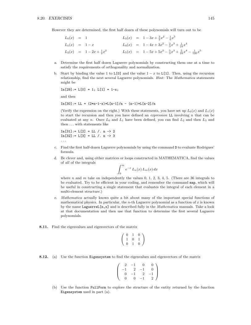
8.20. EXERCISES 145

However they are determined, the first half dozen of these polynomials will turn out to be

L0(x) = 1 L3(x) = 1− 3x+ 32x2 − 1

6x3

L1(x) = 1− x L4(x) = 1− 4x+ 3x2 − 23x3 + 1

24x4

L2(x) = 1− 2x+ 12x2 L5(x) = 1− 5x+ 5x2 − 5

3x3 + 5

24x4 − 1

120x5

a. Determine the first half dozen Laguerre polynomials by constructing them one at a time tosatisfy the requirements of orthogonality and normalization.

b. Start by binding the value 1 to L[0] and the value 1− x to L[1]. Then, using the recursionrelationship, find the next several Laguerre polynomials. Hint : The Mathematica statementsmight be

In[29]:= L[0] = 1; L[1] = 1-x;

and then

In[30]:= LL = (2*n-1-x)*L[n-1]/n - (n-1)*L[n-2]/n

(Verify the expression on the right.) With these statements, you have set up L0(x) and L1(x)to start the recursion and then you have defined an expression LL involving n that can beevaluated at any n. Once L0 and L1 have been defined, you can find L2 and then L3 andthen . . . with statements like

In[31]:= L[2] = LL /. n -> 2

In[32]:= L[3] = LL /. n -> 3

...

c. Find the first half-dozen Laguerre polynomials by using the command D to evaluate Rodrigues’formula.

d. Be clever and, using either matrices or loops constructed in MATHEMATICA, find the valuesof all of the integrals ∫ ∞

0

e−x Ln(x)Lm(x) dx

where n and m take on independently the values 0, 1, 2, 3, 4, 5. (There are 36 integrals tobe evaluated. Try to be efficient in your coding, and remember the command map, which willbe useful in constructing a single statement that evaluates the integral of each element in amulti-element structure.)

e. Mathematica actually knows quite a bit about many of the important special functions ofmathematical physics. In particular, the n-th Laguerre polynomial as a function of x is knownby the name LaguerreL[n,x] and is described fully in the Mathematica manuals. Take a lookat that documentation and then use that function to determine the first several Laguerrepolynomials.

8.11. Find the eigenvalues and eigenvectors of the matrix(0 1 01 0 10 1 0

)

8.12. (a) Use the function Eigensystem to find the eigenvalues and eigenvectors of the matrix 2 −1 0 0−1 2 −1 0

0 −1 2 −10 0 −1 2

(b) Use the function FullForm to explore the structure of the entity returned by the function

Eigensystem used in part (a).

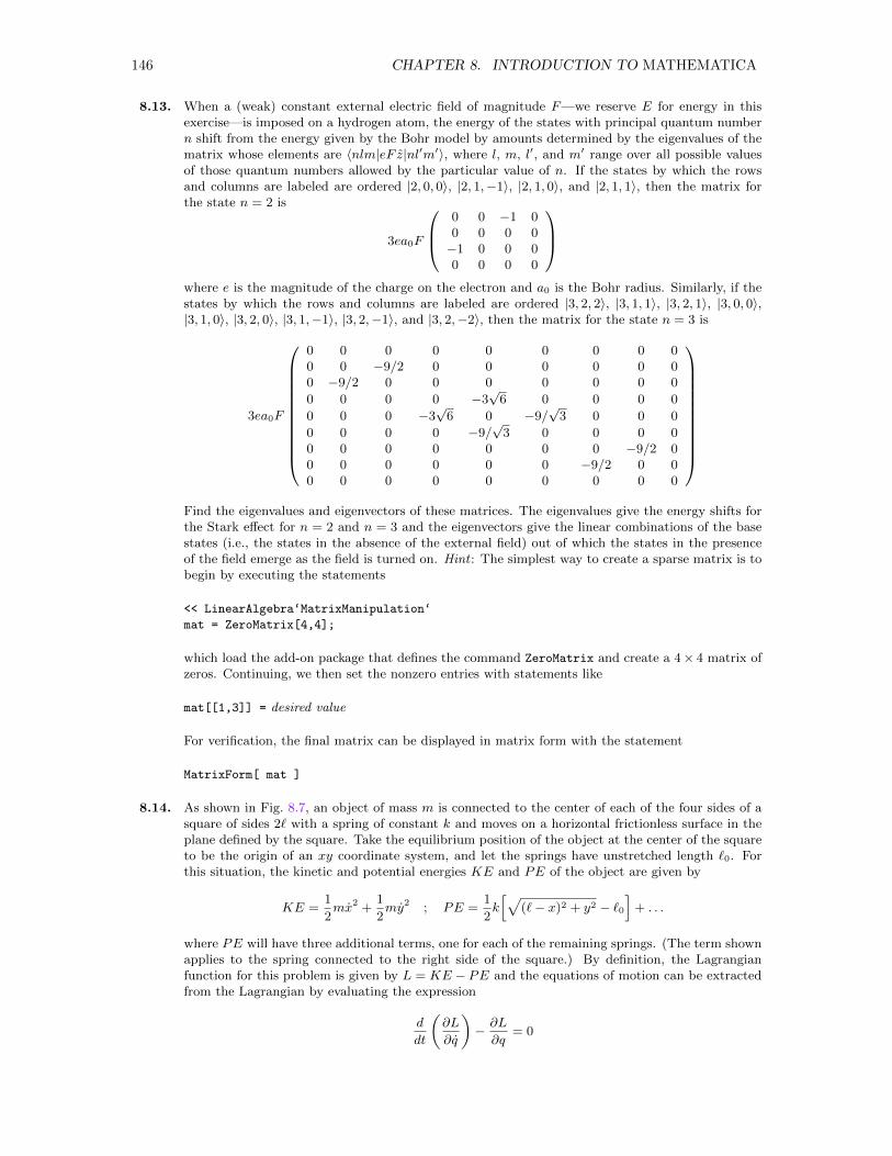
146 CHAPTER 8. INTRODUCTION TO MATHEMATICA

8.13. When a (weak) constant external electric field of magnitude F—we reserve E for energy in thisexercise—is imposed on a hydrogen atom, the energy of the states with principal quantum numbern shift from the energy given by the Bohr model by amounts determined by the eigenvalues of thematrix whose elements are 〈nlm|eF z|nl′m′〉, where l, m, l′, and m′ range over all possible valuesof those quantum numbers allowed by the particular value of n. If the states by which the rowsand columns are labeled are ordered |2, 0, 0〉, |2, 1,−1〉, |2, 1, 0〉, and |2, 1, 1〉, then the matrix forthe state n = 2 is

3ea0F

0 0 −1 00 0 0 0−1 0 0 00 0 0 0

where e is the magnitude of the charge on the electron and a0 is the Bohr radius. Similarly, if thestates by which the rows and columns are labeled are ordered |3, 2, 2〉, |3, 1, 1〉, |3, 2, 1〉, |3, 0, 0〉,|3, 1, 0〉, |3, 2, 0〉, |3, 1,−1〉, |3, 2,−1〉, and |3, 2,−2〉, then the matrix for the state n = 3 is

3ea0F

0 0 0 0 0 0 0 0 00 0 −9/2 0 0 0 0 0 00 −9/2 0 0 0 0 0 0 0

0 0 0 0 −3√

6 0 0 0 0

0 0 0 −3√

6 0 −9/√

3 0 0 0

0 0 0 0 −9/√

3 0 0 0 00 0 0 0 0 0 0 −9/2 00 0 0 0 0 0 −9/2 0 00 0 0 0 0 0 0 0 0

Find the eigenvalues and eigenvectors of these matrices. The eigenvalues give the energy shifts forthe Stark effect for n = 2 and n = 3 and the eigenvectors give the linear combinations of the basestates (i.e., the states in the absence of the external field) out of which the states in the presenceof the field emerge as the field is turned on. Hint : The simplest way to create a sparse matrix is tobegin by executing the statements

<< LinearAlgebra‘MatrixManipulation‘

mat = ZeroMatrix[4,4];

which load the add-on package that defines the command ZeroMatrix and create a 4× 4 matrix ofzeros. Continuing, we then set the nonzero entries with statements like

mat[[1,3]] = desired value

For verification, the final matrix can be displayed in matrix form with the statement

MatrixForm[ mat ]

8.14. As shown in Fig. 8.7, an object of mass m is connected to the center of each of the four sides of asquare of sides 2` with a spring of constant k and moves on a horizontal frictionless surface in theplane defined by the square. Take the equilibrium position of the object at the center of the squareto be the origin of an xy coordinate system, and let the springs have unstretched length `0. Forthis situation, the kinetic and potential energies KE and PE of the object are given by

KE =1

2mx2 +

1

2my2 ; PE =

1

2k[√

(`− x)2 + y2 − `0]

+ . . .

where PE will have three additional terms, one for each of the remaining springs. (The term shownapplies to the spring connected to the right side of the square.) By definition, the Lagrangianfunction for this problem is given by L = KE − PE and the equations of motion can be extractedfrom the Lagrangian by evaluating the expression

d

dt

(∂L

∂q

)− ∂L

∂q= 0

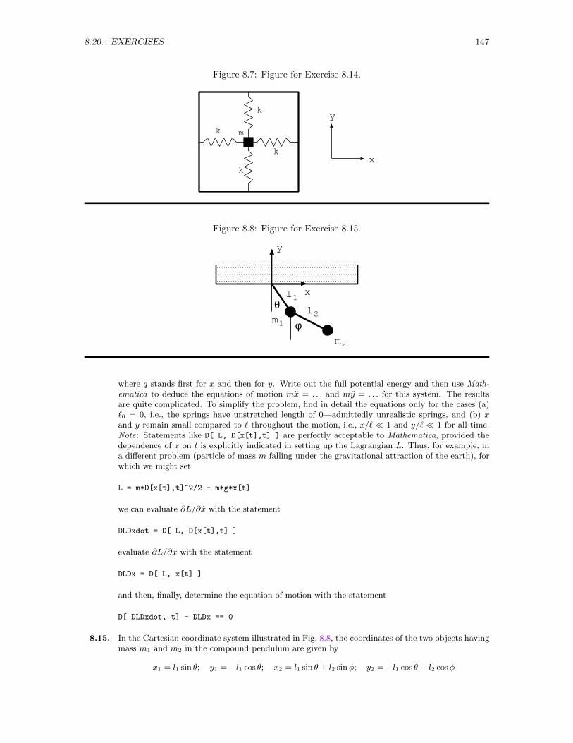
8.20. EXERCISES 147

Figure 8.7: Figure for Exercise 8.14.

k

k

k

k m

x

y

Figure 8.8: Figure for Exercise 8.15.

θ

φ

l1l2

m1

m2

x

y

where q stands first for x and then for y. Write out the full potential energy and then use Math-ematica to deduce the equations of motion mx = . . . and my = . . . for this system. The resultsare quite complicated. To simplify the problem, find in detail the equations only for the cases (a)`0 = 0, i.e., the springs have unstretched length of 0—admittedly unrealistic springs, and (b) xand y remain small compared to ` throughout the motion, i.e., x/` 1 and y/` 1 for all time.Note: Statements like D[ L, D[x[t],t] ] are perfectly acceptable to Mathematica, provided thedependence of x on t is explicitly indicated in setting up the Lagrangian L. Thus, for example, ina different problem (particle of mass m falling under the gravitational attraction of the earth), forwhich we might set

L = m*D[x[t],t]^2/2 - m*g*x[t]

we can evaluate ∂L/∂x with the statement

DLDxdot = D[ L, D[x[t],t] ]

evaluate ∂L/∂x with the statement

DLDx = D[ L, x[t] ]

and then, finally, determine the equation of motion with the statement

D[ DLDxdot, t] - DLDx == 0

8.15. In the Cartesian coordinate system illustrated in Fig. 8.8, the coordinates of the two objects havingmass m1 and m2 in the compound pendulum are given by

x1 = l1 sin θ; y1 = −l1 cos θ; x2 = l1 sin θ + l2 sinφ; y2 = −l1 cos θ − l2 cosφ

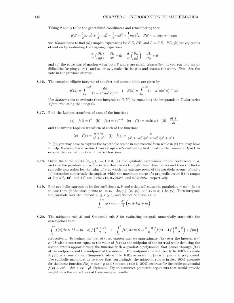
148 CHAPTER 8. INTRODUCTION TO MATHEMATICA

Taking θ and φ to be the generalized coordinates and remembering that

KE =1

2m1x

21 +

1

2m1y

21 +

1

2m2x

22 +

1

2m2y

22 ; PE = m1gy1 +m2gy2

use Mathematica to find (a) (simple) expressions for KE, PE, and L = KE−PE, (b) the equationsof motion by evaluating the Lagrange equations

d

dt

(∂L

∂θ

)− ∂L

∂θ= 0;

d

dt

(∂L

∂φ

)− ∂L

∂φ= 0

and (c) the equations of motion when both θ and φ are small. Suggestion: If you run into majordifficulties keeping l1 6= l2 and m1 6= m2, make the lengths and masses the same. Note: See thenote in the previous exercise.

8.16. The complete elliptic integrals of the first and second kinds are given by

K(k) =

∫ π/2

0

dφ

(1− k2 sin2 φ)1/2; E(k) =

∫ π/2

0

(1− k2 sin2 φ)1/2 dφ

Use Mathematica to evaluate these integrals to O(k6) by expanding the integrands in Taylor seriesbefore evaluating the integrals.

8.17. Find the Laplace transform of each of the functions

(a) f(t) = tn (b) f(t) = t e−at (c) f(t) = cosh(at) (d)df(t)

dt

and the inverse Laplace transform of each of the functions

(e) f(s) =a+ bs

s2 + ω2(f) f(s) =

a

(s2 + 9ω2)(s2 + 4ω2)(s2 + ω2)

In (c), you may have to express the hyperbolic cosine in exponential form while in (f) you may haveto help Mathematica’s routine InverseLaplaceTransform by first invoking the command Apart toexpand the desired function in partial fractions.

8.18. Given the three points (xi, yi), i = 1, 2, 3, (a) find symbolic expressions for the coefficients a, b,and c of the parabola y = ax2 + bx+ c that passes through these three points and then (b) find asymbolic expression for the value of x at which the extreme point of the parabola occurs. Finally,(c) determine numerically the angle at which the maximum range of a projectile occurs if the rangesat θ = 39, 40, and 41 are 0.7251744, 0.729383, and 0.7258887, respectively.

8.19. Find symbolic expressions for the coefficients a, b, and c that will cause the parabola y = ax2+bx+cto pass through the three points (x1 = x2 − δx, y1), (x2, y2), and x3 = x2 + δx, y3). Then integratethe parabola over the interval x1 ≤ x ≤ x3 and deduce Simpson’s rule∫ x3

x1

y(x) dx =δx

3

(y1 + 4y2 + y3

)8.20. The midpoint rule M and Simpson’s rule S for evaluating integrals numerically start with the

assumptions that∫ b

a

f(x) dx ≈M = (b− a) f(a+ b

2

);

∫ b

a

f(x) dx ≈ S =b− a

6

(f(a) + 4 f

(a+ b

2

)+ f(b)

)respectively. To deduce the first of these expressions, we approximate f(x) over the interval a ≤x ≤ b with a constant equal to the value of f(x) at the midpoint of the interval while deducing thesecond entails approximating the function with a quadratic polynomial that passes through f(x)at the endpoints and the midpoint of the interval. The midpoint rule will clearly be 100% accurateif f(x) is a constant and Simpson’s rule will be 100% accurate if f(x) is a quadratic polynomial.Use symbolic manipulation to show that, surprisingly, the midpoint rule is in fact 100% accuratefor the linear function f(x) = mx+p and Simpson’s rule is 100% accurate for the cubic polynomialf(x) = cx3 + dx2 + ex + g! Optional : Try to construct geometric arguments that would provideinsight into the correctness of these analytic results.

8.20. EXERCISES 149

8.21. Using Mathematica, obtain graphs of the potential

U(x) = −U0a2(a2 + x2)

8a4 + x4

and the associated force. Note that the expression for the potential is simpler to plot if you plotnot U(x) versus x but rather U(x)/U0 versus x = x/a, i.e., rewrite the function in the form

U(x)

U0= −1 + x2

8 + x4

You should be able to find a similar dimensionless version of the expression giving the force.

8.22. Using Mathematica, find complete (symbolic) solutions to each of the following problems, and useMathematica also to verify that the solutions you obtain actually do satisfy the original ODE andinitial conditions.

a.d2x

dt2= a, x(0) = x0, v(0) = v0, where a is constant, i.e., find position as a function of time

for a particle moving under the action of a constant force and launched with arbitrary initialconditions.

b. md2x

dt2= −eE0 cos(ωt + θ), x(0) = x0, v(0) = v0, i.e., find position as a function of time for

a charged particle moving under the action of a sinusoidal force and launched with arbitraryinitial conditions.

c. md2x

dt2= −mg + b

(dx

dt

)2

, x(0) = 0, v(0) = 0, i.e., find position as a function of time for a

particle released from rest at the origin and allowed to fall freely under the action of gravityand a viscous retarding force proportional to the square of the speed.

d. the differential equations

md2x

dt2= −bdx

dtand m

d2z

dt2= −mg − bdz

dt

for the motion of a projectile moving under gravity in a viscous medium when the motionstarts at the origin with the initial velocity v = vx0 i + vz0 k.

8.23. Using the functions Grad, Laplacian, Div, and Curl defined in Section 8.8.10,

a. Evaluate the gradient of (i.e., the negative of the force field associated with) each of thefunctions

V1(x, y, z) =1

(x2 + y2 + z2)1/2V2(x, y, z) =

z

(x2 + y2 + z2)3/2

V3(x, y, z) =2z2 − x2 − y2

(x2 + y2 + z2)5/2V4(x, y, z) =

e−a(x2+y2+z2)1/2

(x2 + y2 + z2)1/2

of the Cartesian variables (x, y, z).

b. Verify that each field obtained in part (a) is conservative by showing that the curl of each iszero.

c. With r = x i + y j + z k, show (1) that ∇× r = 0 and (2) that ∇ • r = 3.

d. With V5(x, y, z) = x2 + y2 + z2, show that ∇2V5(x, y, z) = ∇ •∇V5(x, y, z) = 6.

e. Show that ∇2V1(x, y, z) = 0. (Note: Except at x = y = z = 0.)

f. Evaluate the Laplacian of V4(x, y, z), ∇2V4(x, y, z).

8.24. Using the functions Grad, Laplacian, Div, and Curl defined in Section 8.8.10,

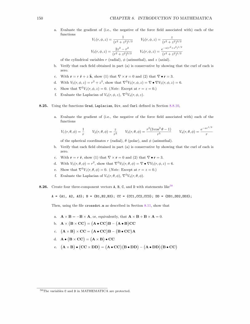
150 CHAPTER 8. INTRODUCTION TO MATHEMATICA

a. Evaluate the gradient of (i.e., the negative of the force field associated with) each of thefunctions

V1(r, φ, z) =1

(r2 + z2)1/2V2(r, φ, z) =

z

(r2 + z2)3/2

V3(r, φ, z) =2z2 − r2

(r2 + z2)5/2V4(r, φ, z) =

e−a(r2+z2)1/2

(r2 + z2)1/2

of the cylindrical variables r (radial), φ (azimuthal), and z (axial).

b. Verify that each field obtained in part (a) is conservative by showing that the curl of each iszero.

c. With r = r r + z k, show (1) that ∇× r = 0 and (2) that ∇ • r = 3.

d. With V5(r, φ, z) = r2 + z2, show that ∇2V5(r, φ, z) = ∇ •∇V5(r, φ, z) = 6.

e. Show that ∇2V1(r, φ, z) = 0. (Note: Except at r = z = 0.)

f. Evaluate the Laplacian of V4(r, φ, z), ∇2V4(r, φ, z).

8.25. Using the functions Grad, Laplacian, Div, and Curl defined in Section 8.8.10,

a. Evaluate the gradient of (i.e., the negative of the force field associated with) each of thefunctions

V1(r, θ, φ) =1

rV2(r, θ, φ) =

z

r3V3(r, θ, φ) =

r2(3 cos2 θ − 1)

r5V4(r, θ, φ) =

e−ar1/2

r

of the spherical coordinates r (radial), θ (polar), and φ (azimuthal).

b. Verify that each field obtained in part (a) is conservative by showing that the curl of each iszero.

c. With r = r r, show (1) that ∇× r = 0 and (2) that ∇ • r = 3.

d. With V5(r, θ, φ) = r2, show that ∇2V5(r, θ, φ) = ∇ •∇V5(r, φ, z) = 6.

e. Show that ∇2V1(r, θ, φ) = 0. (Note: Except at r = z = 0.)

f. Evaluate the Laplacian of V4(r, θ, φ), ∇2V4(r, θ, φ).

8.26. Create four three-component vectors A, B, C, and D with statements like58

A = A1, A2, A3; B = B1,B2,B3; CC = CC1,CC2,CC3; DD = DD1,DD2,DD3;

Then, using the file crossdot.m as described in Section 8.11, show that

a. A×B = −B×A, or, equivalently, that A×B + B×A = 0.

b. A×(B×CC

)=(A •CC

)B−

(A •B

)CC

c.(A×B

)×CC =

(A •CC

)B−

(B •CC

)A

d. A •(B×CC

)=(A×B

)•CC

e.(A×B

)•(CC×DD

)=(A •CC

)(B •DD

)−(A •DD

)(B •CC

)

58The variables C and D in MATHEMATICA are protected.

Chapter 9

Introduction to Programming

In this chapter, we address the task of composing sets of statements1 that will cause an obedient,efficient, and very literal servant (i.e., computer) to perform exactly the task intended by the master(i.e., programmer). A general strategy by which a particular task can be accomplished in a finite(though perhaps large) number of steps is called an algorithm. A specific expression of an algorithmin a suitable language is called a program. Hence, this chapter is about designing algorithms andimplementing them in programs. More specifically, it is about designing algorithms for the per-formance of tasks that will ultimately be assigned to a computer and about implementing thosealgorithms in several possible computer languages.

Designing algorithms and implementing them in programs that direct a computer to performvarious tasks is really not very different from designing algorithms and implementing them in pro-grams that direct a baker to bake a cake, a knitter to knit a sweater, or a cab driver to drive fromthe airport to the hotel. In the aggregate, an algorithm will obtain all necessary inputs, manipulatethose inputs in some way, and produce the required outputs. Each step in the process must be sys-tematically specified using elementary statements, each of which means only one thing to the servant(person or computer) that will perform the task. Some of the appropriate elementary statements—particularly the action statements that specify simple actions—will vary with the general type oftask to be performed. “Mix” and “whip”, for example, are among the elementary action statementsthat must be understood by the baker of cakes; “knit”, “purl”, and “cast on” must be part of thevocabulary of a knitter of sweaters; while “turn right” and “follow interstate 90 west” are actionstatements for the cab driver.

The performance of even simple tasks, however, entails the execution of suitable action state-ments in the right order. The complete description of an algorithm must therefore indicate not onlywhich actions are to be performed but also the order of their performance. Those aspects of analgorithm that specify the order of performance of action statements are called control structures.

A language for specifying algorithms must therefore provide not only elementary action state-ments, which vary with the general type of task to be performed, but also control structures, whichare more universal than the action statements. In the first two sections of this chapter, we focusparticularly on identifying fundamental control structures and illustrating their role in several simplealgorithms. In later sections, we explain how the general structures introduced in the first sectionare implemented in standard languages. More detailed information about various languages may befound in the references listed in Section 9.17.

1Individual instructions in a computer language are usually called statements, and we use that word throughoutthis book.

151

152 CHAPTER 9. INTRODUCTION TO PROGRAMMING

9.1 Components of a Programming Language

While we could code programs directly in the binary language that computers use internally, theprocess would be slow, tedious, prone to error, and resistant to debugging. As an alternative, awide assortment of high-level languages has been developed. Using a chosen high-level language,the programmer creates an ASCII file containing the source code, which lays out what the computermust do to accomplish the desired task. Then, that source code must be translated into machinecode—a task that a computer equipped with the proper translating program can do for itself.

Actually, there are two approaches to this translation. In the first, the computer interprets thesource code, which means that each statement in the code is translated by the computer each timethe statement is executed; execution is slow but the process for us is simple: we write the sourcecode and run the program. In the second approach, the computer first compiles the source code intobinary object code, and then links the object code with an assortment of system routines and possiblyadditional user-written routines. Only after compilation and linking have been completed can theresulting binary or executable file actually be run. This second approach is more complicated for us,since we must both write the source code and then compile and link it. The advantages are twofold:(1) the final executable file is stored in the machine and can be run any number of times withoutrepeating compilation and linking; and (2) execution of compiled code is faster than execution whenthe code is interpreted.

The prospective user of a computer need only learn how to construct the source code in whateverlanguage is to be used. While the detailed syntax of the statements that can be constructed dependsvery much on the language chosen, certain common elements can be identified. In particular, alllanguages provide ways to make use of computer memory, to obtain input and display output, andto control the flow of execution within the program. In this section, we describe those commonelements as a prelude to laying out the details for specific languages in later sections.

9.1.1 Variables, Variable Names, and Use of Memory

Computers provide a means for working with data. The data, however, must be accessible to thecentral processing unit (CPU), which is the part of the hardware that directs and controls all actionscarried out by the computer. Let us, therefore, endow the CPU with a capacity to reserve an availablememory cell (or a contiguous succession of them if one cell is not large enough) and assign to it(them) a variable name, which we specify. Throughout the execution of the program, the assignedname then refers to this unique cubbyhole in the machine’s memory.

While the details vary from language to language, we suppose here that we can choose variablenames freely, subject only to the constraints that

• the first character must be a letter2 (a–z; A–Z),

• subsequent characters can be chosen from the letters (a–z; A–Z), the digits (0–9), and theunderscore character ( ), and

• the several special words (keywords, e.g., IF, DO, UNTIL, . . .) that we shall introduce in subse-quent sections are reserved (or protected) and cannot be used as variable names.

While we do not explicitly impose a length limit on variable names, shorter names are preferred,simply because longer names take longer to type, take more space in the line, and, taken to extremes,result in program listings that are difficult to read. Generally, of course, we want to choose variablenames that help us remember the significance of the quantity the name identifies.

2Some languages are case-sensitive and others are not. For our general discussion, we shall assume case insensitivity,so A and a are indistinguishable in variable names.

9.1. COMPONENTS OF A PROGRAMMING LANGUAGE 153

Even in the generic discussion of this section, however, we shall pay attention to the datatype of each quantity represented. In Chapter 1, we distinguished floating point numbers, integers,and character strings from one another in several ways. In structuring programs, we must remainalways aware of this distinction. Further, the computer in interpreting or compiling our source codemust either make assumptions or be told the data type of each variable we use. Some languages(e.g., Pascal, C) require an explicit declaration of variable names and associated data types beforethe name can be used. Other languages (e.g., BASIC, FORTRAN) exploit implicit data typingby looking to the composition of the variable name to determine the intended data type—thoughmore recent versions of FORTRAN, for example, also admit explicit data typing. Still others (e.g.,IDL, MATLAB, OCTAVE) assign a data type dynamically and automatically on the basis of thevalue assigned to the variable. In our general discussion, we shall adopt a convention that keeps usconsciously aware of data type every time we use a variable name. Following the pattern actuallyused in BASIC, we shall take variable names with no appended suffix to represent floating pointnumbers, variable names with an appended percent sign % to represent integers, and variable nameswith an appended dollar sign $ to represent character strings. Occasionally, we shall use an appendedat sign @ to stand for any one of these three possibilities (no suffix, %, or $). Thus, in the pseudocodewe are defining, the names x, position, and field identify memory cells for floating point values,the names I%, count%, and lower limit% are valid names for cells storing integers, the names word$and first name$ are valid names for cells storing strings, and item@ identifies a quantity of anytype.

The variables we have discussed so far are scalar or unstructured variables; each variable namestands for a single floating point number, integer, or character string. In scientific uses especially,we frequently want to refer to an aggregate of numbers (the three components of a position vector,the nine elements of a 3× 3 matrix, . . .). To that end, the array is among the structured variablesavailable in all scientific programming languages. An array may be one-dimensional (a vector),two-dimensional (an m × n matrix), or even higher dimensional. As a structured entity, an arrayis identified by a single name, e.g., data, values%, or names$, depending on the data type of theelements of the array. Individual elements are identified by attaching an integer index or indicesto the array name, e.g., data(I%,J%), values%(4%), or names$(12%). All by itself, the name ofa scalar is sufficient to tell the compiler how much memory to reserve to store the scalar value.For arrays, however, we can’t simply use the name when it is first needed. In most languages, thesource code must also convey how large the array will become during the execution of the programbecause the interpreter or compiler must set aside adequate memory to store the array before theinterpretation or compilation can be completed. Thus, a program that uses arrays must include inits source code a directive informing the compiler or interpreter of the maximum dimensions of thearray. In our generic discussion, we shall use a statement like

DIMENSION data(4%,251%), values%(8%), names$(25%)

to convey the number of elements in each array to the interpreter or compiler. From the beginning,be aware that some standard languages by default use array indices that run upwards from the value1% while others start the indices at the value 0%. In both cases, the statement above creates an arrayvalues%, for example, with eight elements. In the first case, the indices run from 1% to 8% while inthe second case they run from 0% to 7%.

9.1.2 Essential Action Statements

The CPU must also be able to respond to a minimum collection of action statements to permitthe assignment of values to variables, the performance of elementary arithmetic, and the transferof information from and to a standard I/O device.3 We shall use the following special symbols andwords for these operations:

3We confine our attention initially to data transfers from the keyboard and to the screen, postponing until later adiscussion of the use of files.

154 CHAPTER 9. INTRODUCTION TO PROGRAMMING

• Assign a value to a named memory location:

〈variable〉 ←− 〈expression determining value to be assigned〉

e.g.,4

val ←− sin(pi*x)

count% ←− count% + 1%

first name$ ←− "David"

etc. Any valid arithmetic expression utilizing the symbols + for addition (or string concate-nation), - for subtraction, * for multiplication, / for division, and ˆ for exponentiation canappear on the right hand side of the assignment symbol ←−. Further, most computer lan-guages make available a wide variety of standard functions (sin, cos, atan, sqrt, exp, . . .) tofacilitate scientific computation.

• Obtain a value from the keyboard and store it in a (named) memory cell:

READ PROMPT="Enter first name: ", first_name$

• Transmit a value from a (named) memory cell and/or a (quoted) literal message to the screen:

WRITE "The value of the integral is ", value, "."

We here recognize one further necessary refinement. In the above, we have simply requestedinformation from the keyboard or directed output to the screen. Most programming languages willaccept such simple statements, adopting a default format in which to expect the input or producethe output. Almost always, we will wish to exert some control over that format, and the standardlanguages provide means to give us that control. At base, we want to be able to dictate howmany character positions should be occupied by the number, whether the number is to be outputas an integer or as a decimal number, whether the decimal number is to be presented in scientificor conventional notation, how many digits are to be placed after the decimal point, whether thenumber is to be rounded, . . .. Further, we may want to create blank lines in the output, ignoreblank lines in the input, or clear the screen. Since this list is (almost) endless, the task of describingthe format in which input will be presented to the computer and specifying the format in which thecomputer should produce its output is among the most complicated tasks the programmer confronts.Unfortunately, different languages adopt significantly different ways to provide this facility. Hence,detailed discussion beyond this brief recognition of a need is best postponed until we discuss specificlanguages.

9.1.3 Logical Expressions and Conditions

Frequently, the CPU will need to make a decision on the basis of currently available information,performing different tasks depending on that decision. Usually, these decisions are binary. Atbase, the computer decides whether a particular logical proposition is true or false. Further, thepropositions so examined are usually cast as a comparison of two quantities to determine how theywould be ordered in some standard ordering sequence (numeric, alphabetic, . . .). The six simplecomparisons we might want to code and the circumstances under which the computer will judgeeach to be true are enumerated in Table 9.1.

4We declare that integer constants shall be explicitly identified with a trailing percent sign and that string constantsshall be enclosed in double quotation marks. Some languages use single quotation marks, while others will accepteither (provided they are paired).

9.1. COMPONENTS OF A PROGRAMMING LANGUAGE 155

Table 9.1: Simple logical expressions and the circumstances under which each is true. Rememberthat we have introduced the suffix @ to indicate any of the standard data types.

〈condition〉 true if

A@ = B@ A@ is the same as B@ (A@ equals B@)A@ < B@ A@ occurs before B@ in some collating sequence (e.g., numerical order, al-

phabetical order) (A@ less than B@)A@ > B@ A@ occurs after B@ in that collating sequence (A@ greater than B@)A@ <> B@ A@ differs from B@ (A@ not equal to B@)A@ <= B@ A@ occurs before or is the same as B@ (A@ less than or equal to B@)A@ >= B@ A@ occurs after or is the same as B@ (A@ greater than or equal to B@)

Table 9.2: Truth tables for OR and AND.

Proposition Truth Value Proposition Truth Value

true OR true true true AND true true

true OR false true true AND false false

false OR true true false AND true false

false OR false false false AND false false

Two additional capabilities are standard in computer languages. First, we endow our CPU withthe ability to interpret compound conditions constructed out of simpler conditions either with theoperator OR or the operator AND. A truth table showing the result of connecting each possible logicalvalue with each of these operators is presented in Table 9.2. Second, we introduce the ability tonegate a condition with the operator NOT, i.e., we introduce the expression

NOT 〈condition〉

which we define to be true if 〈condition〉 is false and false if 〈condition〉 is true.

Further (and finally), we recognize that we may occasionally find a need for a variable—aBoolean variable—that can assume only the two values true and false. Recognizing that differentlanguages treat these variables differently, let us symbolize such a variable generically with a suffix?. Thus, for example, we might at some point code a statement like

EQUAL? ←− N@ = M@

in response to which the computer will assess whether N@ is equal to M@ and set EQUAL? to true

or false, depending on the outcome of that assessment. With this expansion of our language,conditions might be expressed not only by the comparisons illustrated in Table 9.1 but also by thesimple assertion of a single Boolean variable or by a logical expression involving combinations ofcomparisons and/or assertions of Boolean variables. Note, incidentally, that the statement in thisparagraph reveals why computer languages must have a different symbol for assignment than fortesting equality.5

9.1.4 Syntactic Wrinkles

In some programming contexts, we will find it convenient—and sometimes even necessary—to conveyadditional information about the structure of the code to the CPU. We might wish

5We have used ←− and =. In later sections, we will identify the symbols used in other languages.

156 CHAPTER 9. INTRODUCTION TO PROGRAMMING

• to place more than one statement on a single physical line. In our generic code, we shall usethe character ‘;’ to separate individual statements on a single line. The three lines of codeearly in Section 9.1.2 might be combined in one line with the coding

val ←− sin(pi*x); count% ←− count% + 1%; first name$ ←− "David"

• to spread a single statement over more than one physical line. In our generic code, we shalluse the symbol → at the end of a line to indicate that the statement continues on the nextline. Thus, for example, the two-line statement

U(I%,J%) ←− 0.25 * ( U(I%+1%, J%) + U(I%-1%, J%) →+ U(I%, J%+1%) + U(I%, J%-1%) )

is to be seen as a single statement.6

• to group several statements together to form a block of statements so that they can be properlytreated when the block is placed in a context in which the interpreter or compiler is expectinga single statement. In our generic code, we shall use the keywords BEGIN BLOCK and END BLOCK

to “bracket” the several statements that we wish the compiler or interpreter to see as a single(compound) statement. For example, the coding

BEGIN BLOCK

val ←− sin(pi*x)

count% ←− count% + 1%

first name$ ←− "David"

END BLOCK

would group the three statements as a unit.

Different languages differ significantly in the way these three situations are coded. We shall be moreexplicit in subsequent sections as we address each language in turn.

9.1.5 Essential Control Structures

Four main control structures7 are generally provided in standard computer languages and figuresignificantly in the smooth expression of algorithms:

• Sequence, which is conveyed by the order of the statements in the algorithm.

• Two-way selection, expressed generically with a statement like8,9

6Remember that spaces not in quoted strings are ignored by the compiler.7Since the CASE structure can be expressed in terms of nested IF-THEN-ELSE structures and the IF-THEN-ELSE

structure is simply a CASE structure with only two cases, there are really only three fundamental structures (sequence,selection, and repetition). General theorems in computer science prove that no task will require more than these fewcontrol structures.

8The structure of this single statement is sufficiently distinctive—it is not complete until the keyword END IF isencountered—that we need not use the symbol → described in Section 9.1.4 to indicate that the statement is spreadover several physical lines.

9 We use the exclamation point to introduce comments. Judicious use of such comments, irrelevant though theymay be to the computer, can clarify the algorithm for the human reader of the listing. To be useful, a commentshould amplify the meaning of, or clarify the role of, the commented statement. The statement

CNT% ←− 0% ! Set CNT% to 0%

for example, might as well be uncommented, since the comment really says no more than can be inferred from thestatement itself.

9.1. COMPONENTS OF A PROGRAMMING LANGUAGE 157

IF 〈condition〉THEN 〈block1 of statements〉 ! the THEN clauseELSE 〈block2 of statements〉 ! the ELSE clause

END IF

Here 〈block1 of statements〉 is executed when 〈condition〉 is true and 〈block2 of statements〉 isexecuted when 〈condition〉 is false. The ELSE clause may be omitted altogether if 〈block2 ofstatements〉 is null. The flow diagram in Fig. 9.1(a) is often used to convey this structure.

• Multi-way selection10

CASEOF 〈condition1〉 DO 〈block1 of statements〉OF 〈condition2〉 DO 〈block2 of statements〉OF 〈condition3〉 DO 〈block3 of statements〉...OF OTHERS DO 〈blockO of statements〉

END CASE

In executing this overall statement, the computer will test each condition in turn, execute theblock of statements associated with the first true condition it encounters, and then jump out ofthe CASE structure.11 The OTHERS clause may be omitted altogether if 〈blockO of statements〉is null. The flow diagram in Fig. 9.1(b) is often used to convey this structure.

• Repetition

LOOP

〈block1 of statements〉EXIT LOOP WHEN 〈condition〉〈block2 of statements〉

END LOOP

Here, the statements in the body of the loop are executed repeatedly until 〈condition〉, whichis tested at the indicated point in the loop, becomes true. Looping will continue forever unlessrepeated execution of the statements eventually causes 〈condition〉 to become true. The flowdiagram in Fig. 9.1(c) is often used to convey this structure.

In some more recent languages, the explicit construction of a loop is in some cases not necessary.For example, suppose we have a vector X containing N% elements and we wish to create a secondvector Y, each of whose elements is—say—the sine of the corresponding element in X. In thecoding we have so far described, we would achieve this objective with an explicit loop involvingthe statements

I% ←− 0%

LOOP

I% ←− I% + 1%

Y(I%) ←− sin( X(I%) )

EXIT_LOOP WHEN I%=N%

END_LOOP

10As with the previous structure, the structure of this single statement is sufficiently distinctive—it is not completeuntil the keyword END CASE is encountered—that we need not use the symbol → described in Section 9.1.4 to indicatethat the statement is spread over several physical lines.

11Not all compilers adopt this strategy. Some will execute the blocks associated with every true condition in thestructure.

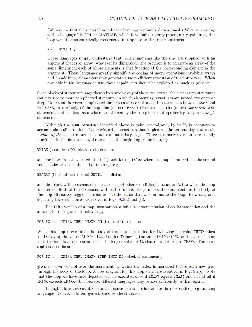
158 CHAPTER 9. INTRODUCTION TO PROGRAMMING

(We assume that the vectors have already been appropriately dimensioned.) Were we workingwith a language like IDL or MATLAB, which have built in array processing capabilities, thisloop would be automatically constructed in response to the single statement

Y ←− sin( X )

These languages simply understand that, when functions like the sine are supplied with anargument that is an array (whatever its dimension), the program is to compute an array of thesame dimension, each of whose elements is that function of the corresponding element in theargument. These languages greatly simplify the coding of many operations involving arraysand, in addition, almost certainly generate a more efficient execution of the entire task. Whenavailable in the language in use, these capabilities should be exploited as much as possible.

Since blocks of statements may themselves involve any of these structures, the elementary structurescan give rise to more complicated structures in which elementary structures are nested two or moredeep. Note that, however complicated the THEN and ELSE clauses, the statements between CASE andEND CASE, or the body of the loop, the (outer) IF-END IF statement, the (outer) CASE-END CASE

statement, and the loop as a whole are all seen by the compiler or interpreter logically as a singlestatement.

Although the LOOP structure identified above is quite general and, by itself, is adequate toaccommodate all situations that might arise, structures that implement the terminating test in themiddle of the loop are rare in actual computer languages. Three alternative versions are usuallyprovided. In the first version, the test is at the beginning of the loop, e.g.,

WHILE 〈condition〉 DO 〈block of statements〉

and the block is not executed at all if 〈condition〉 is false when the loop is entered. In the secondversion, the test is at the end of the loop, e.g.,

REPEAT 〈block of statements〉 UNTIL 〈condition〉

and the block will be executed at least once, whether 〈condition〉 is true or false when the loopis entered. Both of these versions will lead to infinite loops unless the statements in the body ofthe loop ultimately toggle the condition to the value that will terminate the loop. Flow diagramsdepicting these structures are shown in Figs. 9.2(a) and (b).

The third version of a loop incorporates a built-in incrementation of an integer index and theautomatic testing of that index, e.g.,

FOR I% ←− IMIN% THRU IMAX% DO 〈block of statements〉

When this loop is executed, the body of the loop is executed for I% having the value IMIN%, thenfor I% having the value IMIN%+1%, then for I% having the value IMIN%+2%, and . . ., continuinguntil the loop has been executed for the largest value of I% that does not exceed IMAX%. The moresophisticated form

FOR I% ←− IMIN% THRU IMAX% STEP INC% DO 〈block of statements〉

gives the user control over the increment by which the index is increased before each new passthrough the body of the loop. A flow diagram for this loop structure is shown in Fig. 9.2(c). Notethat the loop we have here depicted will be executed once if IMIN% equals IMAX% and not at all ifIMIN% exceeds IMAX%—but beware; different languages may behave differently in this regard.

Though it is not essential, one further control structure is standard in all scientific programminglanguages. Conveyed in our generic code by the statement

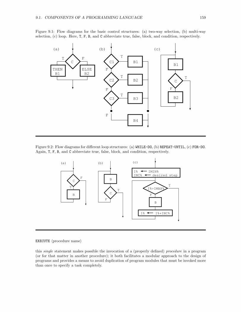
9.1. COMPONENTS OF A PROGRAMMING LANGUAGE 159

Figure 9.1: Flow diagrams for the basic control structures: (a) two-way selection, (b) multi-wayselection, (c) loop. Here, T, F, B, and C abbreviate true, false, block, and condition, respectively.

C

THEN B1

C

C1

C2

C3

ELSE B2

B1

B3

B2

(a)

B4

(b)

B1

B2

(c)

T

T

T

T F

F

F

F

T

F

Figure 9.2: Flow diagrams for different loop structures: (a) WHILE-DO, (b) REPEAT-UNTIL, (c) FOR-DO.Again, T, F, B, and C abbreviate true, false, block, and condition, respectively.

C

B

B

(a)

T

F

C

B

(b)

T

F

I% IMIN%INC% desired step

I%>IMAX%

I% I%+INC%

(c)

T

F

EXECUTE 〈procedure name〉

this single statement makes possible the invocation of a (properly defined) procedure in a program(or for that matter in another procedure); it both facilitates a modular approach to the design ofprograms and provides a means to avoid duplication of program modules that must be invoked morethan once to specify a task completely.

160 CHAPTER 9. INTRODUCTION TO PROGRAMMING

9.2 Sample Short Algorithms

Large algorithms for accomplishing complex tasks are frequently constructed by combining varioussmaller algorithms. In this section, we enumerate several program fragments that may serve asbuilding blocks for the construction of larger algorithms.

1. Exchange the values stored in A@ and B@:12

TEMP@ ←− A@

A@ ←− B@

B@ ←− TEMP@

! Save value in A@

! Copy B@ to A@

! Copy original A@ from TEMP@

The temporary memory cell TEMP@ saves the original value of A@ so that it is still retrievableafter the value of B@ has been copied into cell A@, overwriting the original contents of cell A@.

2. Stopping a loop with a sentinel [and counting]:

SENTINEL@ ←− 〈agreed-upon special value〉[COUNT% ←− 0%]

LOOP

READ ITEM@

EXIT LOOP WHEN ITEM@ = SENTINEL@

〈Statements processing ITEM@〉[COUNT% ←− COUNT% + 1%]

END LOOP

If the statements enclosed in [. . .] are included, then when the loop is completed the variableCOUNT% will have as its value the number of values of ITEM@ processed. Note that the positionin the sequence at which COUNT% is incremented is critical. As a general rule, counters shouldbe started at the value zero before anything happens and incremented by one immediatelyafter each of the events to be counted. More often than not, the end result of thoughtless orunsystematic positioning of the incrementation will be a final count that is off by one, one wayor the other.

3. Stopping a loop by counting up:

NUMBER_OF_TIMES% ←− 〈desired number of executions〉COUNTER% ←− 0%

LOOP

EXIT LOOP WHEN COUNTER% = NUMBER OF TIMES%

〈block of statements〉COUNTER% = COUNTER% + 1%

END LOOP

Again, careful initialization of the counter and careful positioning of its incrementation arecritical to avoiding off-by-one errors.

4. Stopping a loop by counting down:

TIMES_REMAINING% ←− 〈desired number of executions〉LOOP

EXIT LOOP WHEN TIMES REMAINING% = 0%

〈block of statements〉TIMES_REMAINING% ←− TIMES_REMAINING% - 1%

END LOOP

12Note again the use of the character ! to flag comments. See footnote 9.

9.2. SAMPLE SHORT ALGORITHMS 161

This coding has a small advantage over the previous coding because it requires only one variable(TIMES_REMAINING) to control the loop. Note, however, that the initial value of that variableis irrecoverably lost by the time execution of the loop has been completed.

5. Summing [and counting]:

SENTINEL ←− 〈agreed-upon special value〉SUM ←− 0.0

[COUNT% ←− 0%]

LOOP

READ ITEM

EXIT LOOP WHEN ITEM = SENTINEL

SUM ←− SUM + ITEM

[COUNT% ←− COUNT% + 1%]

END LOOP

WRITE "The sum is "; SUM

This algorithm for adding numbers involves the same steps you would use to accomplish thetask on a pocket calculator: initialize the accumulator to 0.0, enter each new value in turn,push the ‘add’ button after each entry, stop after the last value has been processed, andread the final value in the accumulator. Note the explicit decimal point in the floating pointconstant 0.0. Since some compilers and interpreters in some circumstances will treat numericalconstants without explicit decimal points as integers, possibly producing unintended results,13

prudence dictates habitually placing an explicit decimal point in all integer constants thatare in fact to be treated as floating point values. In the present situation, the variable SUM isimplicitly declared to be a floating point variable, so the statement SUM ←− 0 would result inan internal conversion of the integer value 0 to the floating point value 0.0, but it nonethelesspays to be cautious.

6. Finding extreme, stopping with a sentinel:

SENTINEL@ ←− 〈agreed-upon special value〉READ (first) ITEM@ from list

EXTREME@ ←− ITEM@

LOOP

READ (next) ITEM@ from list

EXIT LOOP WHEN ITEM@ = SENTINEL@

IF ITEM@ and EXTREME@ are out of order

THEN EXTREME@ ←− ITEM@

END IF

END LOOP

WRITE "The extreme value is "; EXTREME@

While this procedure can be executed with no a priori knowledge of the number of items andno special assumptions about the list to come, it has the disadvantage of requiring the firstitem of the list to be treated differently from the subsequent items. [Questions to the reader:(1) Does this procedure behave sensibly if the sentinel is entered as the first item? How mightyou improve the procedure on that score? Should you bother? (2) What error would occur inthe output if the EXIT LOOP WHEN statement were placed just before the END LOOP statement?]

13For example, 5/2 = 2 in integer arithmetic; 5.0/2.0 = 2.5 in floating point arithmetic.

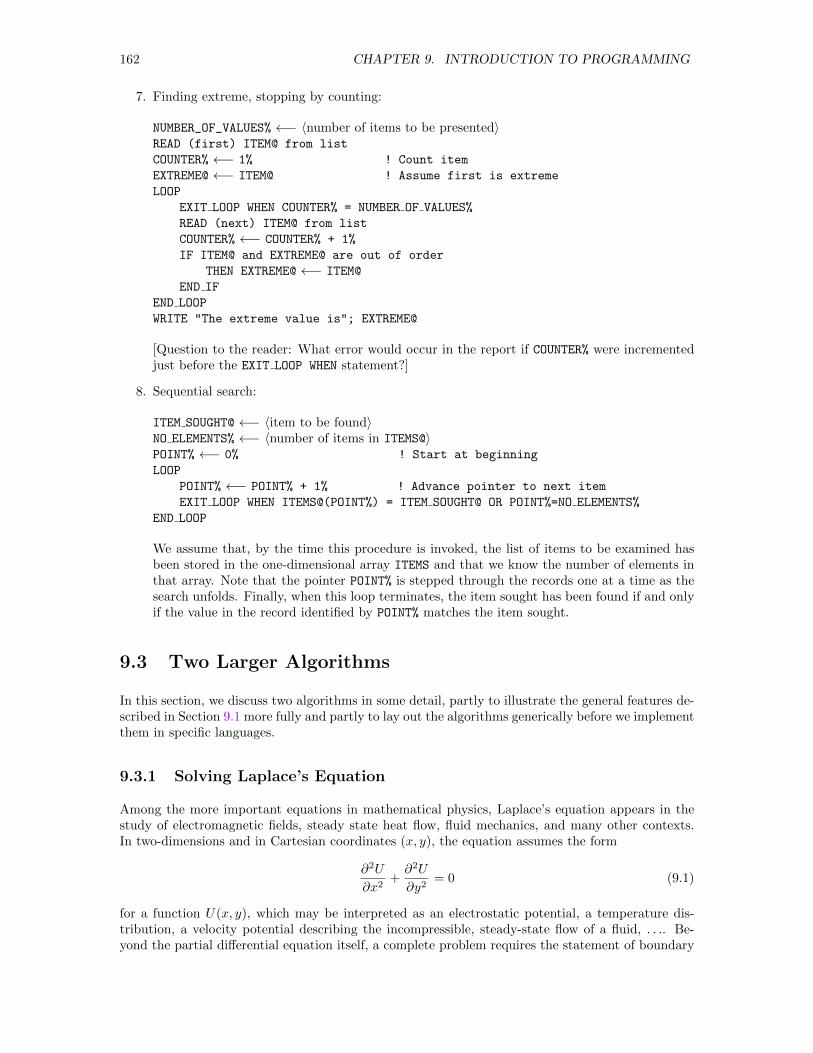
162 CHAPTER 9. INTRODUCTION TO PROGRAMMING

7. Finding extreme, stopping by counting:

NUMBER_OF_VALUES% ←− 〈number of items to be presented〉READ (first) ITEM@ from list

COUNTER% ←− 1% ! Count item

EXTREME@ ←− ITEM@ ! Assume first is extreme

LOOP

EXIT LOOP WHEN COUNTER% = NUMBER OF VALUES%

READ (next) ITEM@ from list

COUNTER% ←− COUNTER% + 1%

IF ITEM@ and EXTREME@ are out of order

THEN EXTREME@ ←− ITEM@

END IF

END LOOP

WRITE "The extreme value is"; EXTREME@

[Question to the reader: What error would occur in the report if COUNTER% were incrementedjust before the EXIT LOOP WHEN statement?]

8. Sequential search:

ITEM SOUGHT@ ←− 〈item to be found〉NO ELEMENTS% ←− 〈number of items in ITEMS@〉POINT% ←− 0% ! Start at beginning

LOOP

POINT% ←− POINT% + 1% ! Advance pointer to next item

EXIT LOOP WHEN ITEMS@(POINT%) = ITEM SOUGHT@ OR POINT%=NO ELEMENTS%

END LOOP

We assume that, by the time this procedure is invoked, the list of items to be examined hasbeen stored in the one-dimensional array ITEMS and that we know the number of elements inthat array. Note that the pointer POINT% is stepped through the records one at a time as thesearch unfolds. Finally, when this loop terminates, the item sought has been found if and onlyif the value in the record identified by POINT% matches the item sought.

9.3 Two Larger Algorithms

In this section, we discuss two algorithms in some detail, partly to illustrate the general features de-scribed in Section 9.1 more fully and partly to lay out the algorithms generically before we implementthem in specific languages.

9.3.1 Solving Laplace’s Equation

Among the more important equations in mathematical physics, Laplace’s equation appears in thestudy of electromagnetic fields, steady state heat flow, fluid mechanics, and many other contexts.In two-dimensions and in Cartesian coordinates (x, y), the equation assumes the form

∂2U

∂x2+∂2U

∂y2= 0 (9.1)

for a function U(x, y), which may be interpreted as an electrostatic potential, a temperature dis-tribution, a velocity potential describing the incompressible, steady-state flow of a fluid, . . .. Be-yond the partial differential equation itself, a complete problem requires the statement of boundary

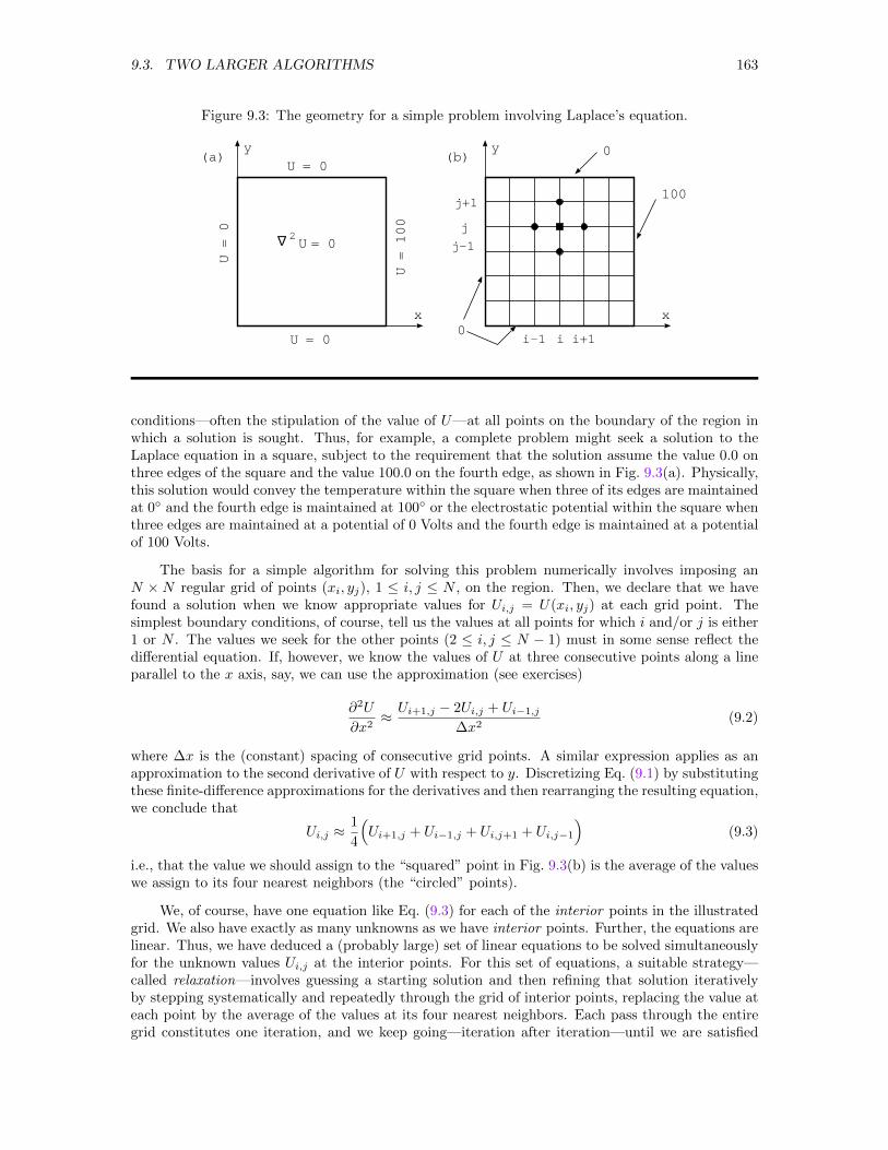
9.3. TWO LARGER ALGORITHMS 163

Figure 9.3: The geometry for a simple problem involving Laplace’s equation.

x

y

∆

U = 02

U = 0

U= 100

x

y 0

0

100

i i+1i-1

j

j+1

j-1

(a) (b)U = 0

U= 0

conditions—often the stipulation of the value of U—at all points on the boundary of the region inwhich a solution is sought. Thus, for example, a complete problem might seek a solution to theLaplace equation in a square, subject to the requirement that the solution assume the value 0.0 onthree edges of the square and the value 100.0 on the fourth edge, as shown in Fig. 9.3(a). Physically,this solution would convey the temperature within the square when three of its edges are maintainedat 0 and the fourth edge is maintained at 100 or the electrostatic potential within the square whenthree edges are maintained at a potential of 0 Volts and the fourth edge is maintained at a potentialof 100 Volts.

The basis for a simple algorithm for solving this problem numerically involves imposing anN × N regular grid of points (xi, yj), 1 ≤ i, j ≤ N , on the region. Then, we declare that we havefound a solution when we know appropriate values for Ui,j = U(xi, yj) at each grid point. Thesimplest boundary conditions, of course, tell us the values at all points for which i and/or j is either1 or N . The values we seek for the other points (2 ≤ i, j ≤ N − 1) must in some sense reflect thedifferential equation. If, however, we know the values of U at three consecutive points along a lineparallel to the x axis, say, we can use the approximation (see exercises)

∂2U

∂x2≈ Ui+1,j − 2Ui,j + Ui−1,j

∆x2(9.2)

where ∆x is the (constant) spacing of consecutive grid points. A similar expression applies as anapproximation to the second derivative of U with respect to y. Discretizing Eq. (9.1) by substitutingthese finite-difference approximations for the derivatives and then rearranging the resulting equation,we conclude that

Ui,j ≈1

4

(Ui+1,j + Ui−1,j + Ui,j+1 + Ui,j−1

)(9.3)

i.e., that the value we should assign to the “squared” point in Fig. 9.3(b) is the average of the valueswe assign to its four nearest neighbors (the “circled” points).

We, of course, have one equation like Eq. (9.3) for each of the interior points in the illustratedgrid. We also have exactly as many unknowns as we have interior points. Further, the equations arelinear. Thus, we have deduced a (probably large) set of linear equations to be solved simultaneouslyfor the unknown values Ui,j at the interior points. For this set of equations, a suitable strategy—called relaxation—involves guessing a starting solution and then refining that solution iterativelyby stepping systematically and repeatedly through the grid of interior points, replacing the value ateach point by the average of the values at its four nearest neighbors. Each pass through the entiregrid constitutes one iteration, and we keep going—iteration after iteration—until we are satisfied

164 CHAPTER 9. INTRODUCTION TO PROGRAMMING

that the process has converged satisfactorily.14 Supposing that we seek a solution on a 15× 15 gridof points, we make a first pass at constructing an algorithm to implement this overall strategy bylisting the statements

DIMENSION U(15%,15%)

Set U(I%,J%) ←− 0.0 for all values of I%, J%Set U(15%,J%) ←− 100.0 for all values of J%FOR ITCNT% ←− 1% THRU 30% DO Conduct one iterationWrite solution to output device

Here, we (1) reserve adequate space for the necessary array, (2) establish a starting solution in thatarray, (3) set the boundary conditions, (4) conduct 30 iterations, and (5) display the solution.

To refine the crude statements in the above algorithm, we would have to expand the impliedloops. Indeed, since we are working with a two-dimensional array, stepping through all elementsof the array (either in assigning initial values or in iterating once through the array) will require adouble loop. Thus, we might express this algorithm more explicitly as

DIMENSION U(15%,15%)

FOR I% ←− 1% THRU 15% DO

FOR J% ←− 1% THRU 15% DO U(I%,J%) ←− 0.0

FOR J% ←− 1% THRU 15% DO

U(15%,J%) ←− 100.0

! Prepare array of proper size

! Set all elements of array to 0.0

! Correct values on right edge

FOR ITCNT% ←− 1% THRU 30% DO

FOR I% ←− 2% THRU 14% DO

FOR J% ←− 2% THRU 14% DO

U(I%,J%) ←− 0.25 * ( U(I%+1%, J%) →+ U(I%-1%, J%) + U(I%, J%+1%) →+ U(I%, J%-1%) )

FOR I% ←− 1% THRU 15% DO

FOR J% ←− 1% THRU 15% DO WRITE U(I%,J%)

! Iterate 30 times

! Conduct one iteration

! Write solution to output device

We shall refine this algorithm even further as, later in this chapter, we implement it in variouscomputer languages.

9.3.2 File Output/Input

The most convenient and flexible way to make a permanent record of numerical data is to store itin an ASCII file. Among other advantages, such files can be created in any number of ways, theycan be examined with ordinary text editors, and they facilitate importing the data into whatevergraphical package provides the best visualization of the specific features we wish to see. Most oftenthe data are naturally organized into one or more two- or three-dimensional arrays, which frequentlyrepresent scalar or vector fields. In this section, we declare a standardized file format for the storageof these arrays and discuss a general algorithm by which files so structured can be created. In latersections, we describe how to implement this algorithm in various computer languages. Of course,the data file as an intermediary is unnecessary if generation and display occur in the same program.These files are especially useful when data generated in one program are to be transferred to anotherprogram for display and/or when a program-independent permanent record of the data is desired.

14The most common criterion of convergence involves comparing values until no element in one iterate differs fromits counterpart in the next iterate by more than some predetermined tolerance. Developing suitable (and reliable)criteria for determining when satisfactory convergence has been achieved, however, is difficult. Because we are herefocusing on programming aspects rather than algorithmic refinements, we shall ignore the issue of convergence for themoment. We shall return to it at appropriate points in later chapters.

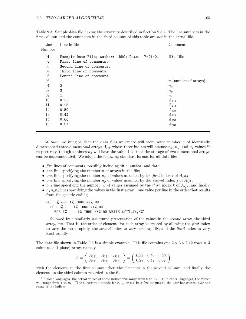
9.3. TWO LARGER ALGORITHMS 165

Table 9.3: Sample data file having the structure described in Section 9.3.2. The line numbers in thefirst column and the comments in the third column of this table are not in the actual file.

Line Line in file CommentNumber

01: Example Data File; Author: DMC; Date: 7-21-01 ID of file02: First line of comments.

03: Second line of comments.

04: Third line of comments.

05: Fourth line of comments.

06: 1 n (number of arrays)07: 2 nx08: 3 ny09: 1 nz10: 0.33 A111

11: 0.28 A211

12: 0.50 A121

13: 0.42 A221

14: 0.66 A131

15: 0.57 A231

At base, we imagine that the data files we create will store some number n of identicallydimensioned three-dimensional arrays Aijk whose three indices will assume nx, ny, and nz values,15

respectively, though at times nz will have the value 1 so that the storage of two-dimensional arrayscan be accommodated. We adopt the following standard format for all data files:

• five lines of comments, possibly including title, author, and date;• one line specifying the number n of arrays in the file;• one line specifying the number nx of values assumed by the first index i of Aijk;• one line specifying the number ny of values assumed by the second index j of Aijk;• one line specifying the number nz of values assumed by the third index k of Aijk; and finally• nxnynz lines specifying the values in the first array—one value per line in the order that results

from the generic coding

FOR K% ←− 1% THRU NZ% DO

FOR J% ←− 1% THRU NY% DO

FOR I% ←− 1% THRU NX% DO WRITE A(I%,J%,K%)

—followed by a similarly structured presentation of the values in the second array, the thirdarray, etc. That is, the order of elements for each array is created by allowing the first indexto vary the most rapidly, the second index to vary next rapidly, and the third index to varyleast rapidly.

The data file shown in Table 9.3 is a simple example. This file contains one 2 × 3 × 1 (2 rows × 3columns × 1 plane) array, namely

A =

(A111 A121 A131

A211 A221 A231

)=

(0.33 0.50 0.660.28 0.42 0.57

)with the elements in the first column, then the elements in the second column, and finally theelements in the third column recorded in the file.

15In some languages, the actual values of these indices will range from 0 to n∗ − 1; in other languages, the valueswill range from 1 to n∗. (The subscript ∗ stands for x, y, or z.) In a few languages, the user has control over therange of the indices.

166 CHAPTER 9. INTRODUCTION TO PROGRAMMING

To be even more explicit, we would have to surround the basic output statement presentedabove with statements that dimension arrays appropriately, calculate (or otherwise determine) thevalues to insert in the arrays, prepare the file for access, and close the file after the last datum hasbeen written to the file. To illustrate, suppose we seek to explore the two-dimensional scalar fieldgiven in the xy plane by the function f(x, y). Then, generating the desired file involves two mainsteps: (1) creation of an internal array containing values of the function at a grid of points overlayedon the region of interest in the xy plane and (2) writing those values into a suitably labeled filestructured as described earlier in this section. Though it may take a bit of exploration to decide onsuitable ranges for the independent variable, let us here decide to examine the function in the regiondefined by xmin ≤ x ≤ xmax and ymin ≤ y ≤ ymax and to divide the x interval with nx grid pointsinto nx − 1 segments and the y interval with ny grid points into ny − 1 segments. First, we preparevariables and arrays with the statements

DIMENSION ARRAY(nx,ny)NARR% ←− 1%

NX% ←− nxNY% ←− nyNZ% ←− 1%

DX ←− (xmax − xmin)/(nx − 1)DY ←− (ymax − ymin)/(ny − 1)

! Prepare array for values

! Set number of arrays

! Set number of grid points

! in each coordinate

! Set increments

Then, we evaluate the function f(x, y) with the double loop expressed in the code

FOR J% ←− 1% THRU NY% DO

BEGIN BLOCK

YF ←− ymin + (J%-1%)*DY

FOR I% ←− 1% THRU NX% DO

BEGIN BLOCK

XF ←− xmin + (I%-1%)*DX

ARRAY(I%,J%) ←− f(XF,YF)END BLOCK

END BLOCK

Finally, we establish communication between the file and the program (in the jargon, we attach thefile to the program on a selected channel), write the necessary labels and values to the file, anddisconnect (i.e., detach the file from the program with the statements16

ATTACH FILE 〈filename〉 ON CHANNEL 1 FOR WRITING

WRITE TO CHANNEL 1, "Line of explanation (Title, Author, Date?)"

WRITE TO CHANNEL 1, "Line of explanation"

WRITE TO CHANNEL 1, "Line of explanation"

WRITE TO CHANNEL 1, "***"

WRITE TO CHANNEL 1, "***"

WRITE TO CHANNEL 1, NARR%

WRITE TO CHANNEL 1, NX%

WRITE TO CHANNEL 1, NY%

WRITE TO CHANNEL 1, NZ%

FOR J% ←− 1% TO NY% DO FOR I% ←− 1% TO NX% DO WRITE TO CHANNEL 1, ARRAY(I%,J%)

CLOSE FILE ON CHANNEL 1

Here, the first statement identifies the file and assigns to it a number—any number will do17—tobe used for subsequent reference to the file. Next, the first five WRITE statements send five lines of

16A new file will be created, overwriting any existing file by the specified name. Some programming languages mayprovide a warning if an existing file will be deleted.

17Be aware that some languages reserve a few channel numbers for special ”files”, e.g., the keyboard or the screen.

9.4. SOLVING LAPLACE’S EQUATION WITH FORTRAN 167

comments, all five of which must be physically present even if fewer than five are needed to containnecessary information about the file. Then, the sixth WRITE statement writes the number of arraysto the file, the seventh and eighth write the x and y dimensions to the file, and the ninth writes thez dimension to the file. Finally, the double loop writes the elements of the array to the file in theproper order, and the last statement makes sure the file is properly detached from the program sothat it can be accessed by other programs.

Instead of writing data to a file, we frequently will need to read data from a file, perhaps as ameans to import data generated by one program for use in a different program. Slight modificationof the ATTACH and READ statements introduced earlier provide for that action. Specifically, thestatements

ATTACH FILE 〈filename〉 ON CHANNEL 1 FOR READING

READ FROM CHANNEL 1, Comma-separated list of variables for storage of values...

CLOSE FILE ON CHANNEL 1

Here, the first statement opens an existing file for reading (and displays an error if the specified filedoes not exist), the remaining statements save the last read the information in the file and stores itin the specified variables, and the last statement detaches the file when, presumably all data havebeen read. Note that the structure of the READ statements must reflect the structure of the file,and the variables specified must have the data types of the values to be read. Normally, the READ

statement reads a line at a time, but in some languages each READ statement reads as many valuesas needed to complete the list of variables, however these values are distributed over lines.

In the remaining sections of this chapter, we shall implement the two algorithms described inthis section in different languages and, especially for the second algorithm, in a variety of differentcontexts.

9.4 Solving Laplace’s Equation with FORTRAN

Note: All FORTRAN programs (*.f) and FORTRAN-created data files (* f.dat)referred to in this chapter are available in the directory $HEAD/fortran, where (asdefined in the Local Guide) $HEAD must be replaced by the appropriate path foryour site.

Rather than systematically laying out features of FORTRAN as a programming language beforepresenting a program, we elect to present a simple program illustrating several of those features andthen comment thereon. A FORTRAN program implementing the algorithm laid out in Section 9.3.1for solving Laplace’s equation is presented in Table 9.4. Note the following about this program:

• Except for characters within quoted strings, FORTRAN is insensitive to case.

• Lines with a C in the first character position are comments. Further, while it is not standardFORTRAN, most FORTRAN compilers will accept comments introduced with an exclamationpoint.

• Legal variable names in FORTRAN begin with a letter, which may be followed by any numberof characters chosen from the letters A–Z, the numeric digits 0–9, and—in extended FORTRAN-77—the underscore , the dollar sign $, and the period ‘.’. Note, however, that in standardFORTRAN-77 only six characters are allowed and further that in extended FORTRAN char-acters beyond the thirty-second will be ignored by the compiler.

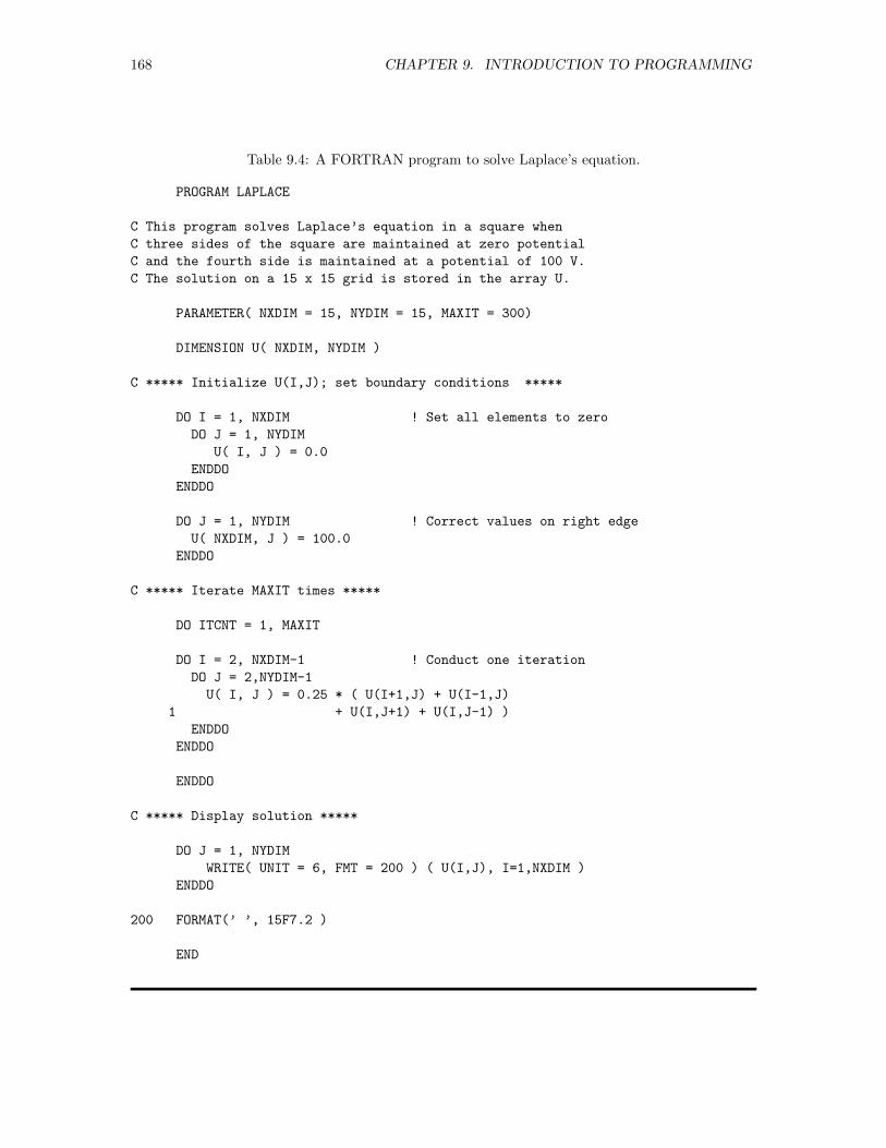
168 CHAPTER 9. INTRODUCTION TO PROGRAMMING

Table 9.4: A FORTRAN program to solve Laplace’s equation.

PROGRAM LAPLACE

C This program solves Laplace’s equation in a square when

C three sides of the square are maintained at zero potential

C and the fourth side is maintained at a potential of 100 V.

C The solution on a 15 x 15 grid is stored in the array U.

PARAMETER( NXDIM = 15, NYDIM = 15, MAXIT = 300)

DIMENSION U( NXDIM, NYDIM )

C ***** Initialize U(I,J); set boundary conditions *****

DO I = 1, NXDIM ! Set all elements to zero

DO J = 1, NYDIM

U( I, J ) = 0.0

ENDDO

ENDDO

DO J = 1, NYDIM ! Correct values on right edge

U( NXDIM, J ) = 100.0

ENDDO

C ***** Iterate MAXIT times *****

DO ITCNT = 1, MAXIT

DO I = 2, NXDIM-1 ! Conduct one iteration

DO J = 2,NYDIM-1

U( I, J ) = 0.25 * ( U(I+1,J) + U(I-1,J)

1 + U(I,J+1) + U(I,J-1) )

ENDDO

ENDDO

ENDDO

C ***** Display solution *****

DO J = 1, NYDIM

WRITE( UNIT = 6, FMT = 200 ) ( U(I,J), I=1,NXDIM )

ENDDO

200 FORMAT(’ ’, 15F7.2 )

END

9.4. SOLVING LAPLACE’S EQUATION WITH FORTRAN 169

• For the most part, we shall exploit FORTRAN’s capability for implicit data typing, where avariable whose name begins with I, J, K, L, M, or N will be understood to represent an integerwhile a variable whose name begins with any other letter will be understood to represent a(single-precision) floating point number.

Extended FORTRAN-77 also admits explicit data typing (and dimensioning), where variabledeclarations like

REAL IMAP, LETTER(20)

DOUBLE PRECISION X, Y

CHARACTER A

INTEGER ROOT, Z(30,50)

specify the indicated variables as having the indicated data type and can, as for example inthe first statement, override the implied implicit type for a particular variable. Any variablesnot explicitly typed will be typed in accordance with the rules for implicit data typing unlessthe program includes the statement

IMPLICIT NONE

in which case the compiler will complain if it encounters a variable that has not been explicitlytyped.

• Statements can begin no earlier than the seventh character position in the line and cannotextend past the 72-nd character position.18

• A FORTRAN program begins with a statement PROGRAM 〈ProgramName〉 and concludes withthe statement END.

• The statement beginning PARAMETER provides a means to assign a character string to a symbolsuch that subsequent use of the symbol triggers a literal replacement of the symbol with theassigned character string. These symbols are not variables, since they cannot be assigneddifferent values during execution of the program. The PARAMETER statement provides a wayto bring together at the beginning of a program all those quantities whose value may changefrom time to time and place them at a point where they are easy to find in the listing so thatchanging the value means editing the file in only one place.

• FORTRAN uses the symbols +, -, *, /, and ** for addition, subtraction, multiplication,division, and exponentiation (raising to a power).

• In FORTRAN, the indices of elements of arrays are enclosed in ordinary parentheses and runupwards from 1. Thus, for example, an array dimensioned with the statement DIMENSION

U(15,15) will have elements running from U(1,1) to U(15,15) with 15 values for each index.

• FORTRAN uses the equal sign for assignment. The operators .gt., .ge., .lt., .le., .eq.,and .ne. are used in logical expressions to symbolize greater than, greater than or equal to,less than, less than or equal to, equal to, and not equal to, respectively; the operators .and.,.or., and .not. symbolize AND, OR, and NOT, respectively.

• A FORTRAN loop is introduced with the keyword DO and terminated with the keyword ENDDO.The loops in this sample program are counted loops, a feature conveyed by following the key-word DO with an integer variable name and a range of values to be assumed by the integer.A third (optional) element in that comma-separated list specifies the increment between suc-cessive values of the index; the default increment is 1. The (current) value of the index is

18This feature is a hangover from the days of punched cards, when the first six and the last 8 character positionson a card with 80 character positions were assigned other meanings.

170 CHAPTER 9. INTRODUCTION TO PROGRAMMING

compared with the upper limit at the beginning of the loop and the incrementation of the in-dex takes place after the statements in the body of the loop have been executed. Terminationoccurs as soon as the current value of the index exceeds the upper limit. Thus, the loop willbe executed once if the upper limit is initially equal to the initial index and not at all if theupper limit is smaller than the initial index as the loop is started.

• Any character placed in the sixth character position in the line will be interpreted as meaningthat the statement on that line is to be viewed as a continuation of the statement on theprevious line.

• The one WRITE statement directs its output to channel 6, which is the screen (and is always“attached”—FORTRAN uses the verb “open”—and hence need not be explicitly attached anddetached (i.e., opened and closed).

• The format of the output produced by the WRITE statement is specified in the FORMAT statementthat has the label 200 placed in the first five character positions, to which the second argumentin the first set of parentheses in the WRITE statement refers. This specific FORMAT statementtells the compiler that it should first send to the output destination a space (the quotedspace as the first argument).19 Then, in the line to be output, there will be fifteen—the15 in the designation 15F7.2—floating point numbers, each presented in ordinary decimalnotation—the F—right-justified in a field (region) that is seven characters wide—the 7—withthe number rounded to have two digits—the 2—after the decimal point in its presentation. Inthis particular problem, we know that all values should be positive and no value will be largerthan 100.20 Thus, with the specified format, the largest value will be displayed as 100.00,right-justified in a seven-character field. Since this number requires six character positions,there will be at least one space between consecutive entries in each line of output.21,22

• The WRITE statement producing the output appears to be embedded in a single loop (theloop on the index J). The argument to the WRITE statement in the second set of parentheses,however, contains an implied loop on the index I. We might alternatively have written thedouble loop

DO J = 1, NYDIM

DO I = 1, NXDIM

WRITE( UNIT = 6, FMT = 200 ) U(I,J)

ENDDO

ENDDO

200 FORMAT(’ ’, F7.2 )

but the result would have been to use a new line for each value in the array.

19When FORTRAN was developed, output was almost always to a line printer, and the first character in each lineof output was not printed. Rather, it was interpreted by the printer as a control character—new line, double space,skip to new page, depending on the character. The character telling the printer to start a new line was a space. Thus,we must assure that the first character sent in each line will be a space, which will not be printed. The techniqueshown here is one of the ways to achieve that objective.

20Solutions to Laplace’s equation can never have in the interior a value larger than the largest value nor smallerthan the smallest value on the boundary.

21If we had to allow for the possibility of values ranging downward to -100, we would need one more characterposition (F8.2) to provide the position for a possible minus sign and guarantee at least one space between anypossible consecutive entries in each line.

22One alternative to the F format is I, which is used for integers, e.g., 4I10 for four integers each-right justifiedin a field ten characters wide. Another alternative, used particularly when the size of floating-point numbers variesconsiderably or is unknown a priori, is E, which outputs floating point numbers in scientific notation, e.g., 3E15.6 forthree such numbers right-justified in fields fifteen characters wide, presented with six digits after the decimal point(and formatted—depending on the compiler—either with one digit or a zero before the decimal point). The formatE15.6, for example, will present the number 100.00 as 0.100000E 03 or 1.000000E 02, requiring in both cases twelvecharacter positions of the fifteen specified by the format.

9.4. SOLVING LAPLACE’S EQUATION WITH FORTRAN 171

• Note that, in the loop generating the output, for each J, I migrates through its several values.Thus, the rows in the output are labeled by values of J, i.e., of y, and the columns in theoutput are labeled by values of I, i.e. of x.

This program is stored in a file named laplace.f in the directory $HEAD/fortran. Once thatfile has been copied to the default directory, it can be compiled, linked, and run with commands asdescribed in the Local Guide. In UNIX, those commands might be23

f77 -o laplace.xf laplace.f

./laplace.xf

In response to these commands to the operating system, the program will be executed and theoutput—15 lines of 15 numbers each—will be displayed on the screen.24

The solution displayed on the screen when the program is run is, of course, difficult to interpret(and would be even more so if we had solved the equation on a finer grid). Anticipating that wemight want to import the output of this program into another—possibly a plotting—program, wemight wish to direct the output to a file rather than to the screen. In UNIX, we could use the simplestatement

./laplace.xf > laplace_f.dat

to achieve that end without having to edit and recompile the program at all. Alternatively, andmore generally, we would have to replace the output portion of the program with code that opens afile, writes the output to that file, and then closes the file. We might, for example, edit laplace.f

by replacing the loop(s) containing the WRITE statement with the statements

OPEN( UNIT = 1, FILE = ’laplace_f.dat’, STATUS = ’NEW’ )

DO J = 1, NYDIM

WRITE( UNIT = 1, FMT = 200 ) ( U(I,J), I=1,NXDIM )

ENDDO

CLOSE( UNIT = 1 )

200 FORMAT(’ ’, 15F7.2 )

where we have simply added the OPEN and CLOSE statements and edited the WRITE statement tospecify the unit (channel) on which we opened the file. The program so edited is stored in the filelaplace file.f in the directory $HEAD/fortran. Once copied to the default directory, it can becompiled, linked, and run as with laplace.f above (see the Local Guide). In the end, the outputfile laplace f.dat will be created in the default directory.

A graphical display of the resulting file could be generated by OCTAVE by issuing to OCTAVEthe statements25

>> id = fopen( ’laplace_f.dat’, ’r’ );

>> u = fscanf( id, ’%f’, [15,15] );

>> status = fclose( id );

>> mesh( u’ );

>> surf( u’ );

Open file.Read in solution.Close file.Display solution as mesh surface.Display solution as a shaded surface.

23Throughout this book, we shall assume that we are using the FORTRAN-77 routines in a UNIX environment.In UNIX, f90 and f95 would invoke the FORTRAN-90 and FORTRAN-95, respectively In other operating systems,the FORTRAN compiler might be invoked with the command fortran or gfortran, and the characters ./ may ormay not be necessary to launch an executable program in the current directory. Further detail on how to invoke theFORTRAN compiler and run an executable program in your environment will be described in the Local Guide.

24Incidentally, note that, if necessary, execution of a FORTRAN program can usually be aborted by typing〈CONTROL/C〉.

25While the file produced by FORTRAN has rows labeled by y and columns labeled by x, reading that file intoOCTAVE creates a file in which the columns are labeled by y and the rows by x. The transposition in the mesh andsurface commands is necessary to have the proper associations of columns and rows with x and y.

172 CHAPTER 9. INTRODUCTION TO PROGRAMMING

9.5 Additional Features of FORTRAN

The example program in the previous section has not provided a vehicle for illustrating a fewadditional important capabilities of the language. We here address those features.

9.5.1 Multi-Way Selection

The basic decision-making structure in FORTRAN involves key words, conditions, and actions inthe general pattern conveyed by the listing

IF 〈condition1〉 THEN〈block1 of statements〉

ELSE IF 〈condition2〉 THEN〈block2 of statements〉

...ELSE IF 〈conditionn〉 THEN〈blockn of statements〉

ELSE

〈catch-all block of statements〉END IF

Test 〈condition1〉.Execute 〈block1〉 and exit when 〈condition1〉 is true.Test 〈condition2〉 (if 〈condition1〉 is false).Execute 〈block2〉 and exit when 〈condition2〉 is true.

Test 〈conditionn〉 (if 〈condition(n− 1)〉 is false).Execute 〈blockn〉 and exit when 〈conditionn〉 is true.

Execute 〈catch-all block〉 and exit when all conditionsare false.

Two-way selection is, of course, simply a version of multi-way selection in which there is only onecondition in this sequence. Further, the ELSE clause can be omitted if it would contain no statements,and the keywords in this structure bracket the various blocks of statements so no additional blockingstructure is necessary. The blocks can contain any number of statements, each on its own line, andthe conditions can be logical variables, single logical expressions, or compound logical expressions.

If it should happen that the ELSE clause in a two-way selection is null and the THEN clausecontains only a single statement, then the coding

IF 〈condition〉 THEN〈block1 of statements〉

END IF

can be simplified to

IF 〈condition〉 〈Single FORTRAN statement〉

9.5.2 Reading Data from Keyboard

Data can be read from the keyboard in FORTRAN with a variety of statements. In the simplestapproach, we might use the command write to print a prompting message conveying the itemwanted and then the command read to read that item from the keyboard and store it in a suitablevariable with statements like

WRITE( *, * ) ’Suitable prompting message: ’

READ( *, * ) VALUE

where we have allowed the compiler to choose the default input and output devices (first asteriskin each statement; unit 6 for the write statement; unit 5 for the read statement). Further, thecompiler will automatically identify the prompting message as a string and the entered value as afloating point value (second asterisk in each statement). The statements

9.5. ADDITIONAL FEATURES OF FORTRAN 173

WRITE( UNIT=*, FMT=* ) ’Suitable prompting message: ’

READ( UNIT=*, FMT=* ) VALUE

are equivalent, though they use keywords to make explicit the function of the two asterisks.

While it is probably wise to use “free” format on input so we don’t have to be too careful aboutthe position of the input in the line, we might at times want to specify the format of the outputmore specifically, for example, with a statement like26

WRITE( UNIT=*, FMT=’(1X,A)’ ) ’Suitable prompting message: ’

or with a pair of statements like

WRITE( UNIT=*, FMT=157 ) ’Suitable prompting message: ’

157 FORMAT( ’ ’, A )

Finally, note that two values would be entered in response to the prompting message if the readstatement were coded like

READ( *, * ) VALUE, INDEX

The values would be separated by one or more spaces, one or more tabs, or simply a comma. In thisspecific example, of course, the first value would be stored as a single-precision floating point valuewhile the second would be converted to an integer if necessary and stored as an integer.

9.5.3 Additional Loops

Standard FORTRAN-77 does not have any loops beyond the do/enddo loop already introduced.Extended versions of FORTRAN, however, may possess other structures.27 The loop

DO WHILE 〈condition〉〈block of statements〉

ENDDO

which executes 〈block of statements〉 repeatedly as long as 〈condition〉 remains true is a particularlycommon extension.

9.5.4 Subroutines, Functions, and Common Storage

As with most computer languages, FORTRAN also admits the possibility of creating new com-mands/functions through the use subprograms. In essence, a subprogram is a self-contained segmentof code that is given a name of its own and that can be invoked in another program with a singlestatement. Subprograms come in two types, In outline, we define a subroutine with a structure like

26Beyond the formats F, E, and I described in footnote 22, the descriptor A conveys to the compiler that it is toread characters from the input line. If only A is specified, the compiler reads and counts characters until 〈RETURN〉is typed; if the format descriptor takes the form An, the compiler reads n characters.

27Check your local FORTRAN manual for the features of the FORTRAN compiler available at your site.

174 CHAPTER 9. INTRODUCTION TO PROGRAMMING

SUBROUTINE SubName( Arg1, Arg2, . . . )Statements coding the desired action.

RETURN

END

Here, SubName is a user-assigned name for the subroutine, and Arg1, Arg2, . . . are the names of thevariables that communicate between the calling program and the subroutine, either by providinginput to the subroutine or providing values returned to the calling program. All other variables in thesubroutine are invisible to the calling program (and can, in fact, have the same names as variablesin the calling program without generating conflict). The statements defining the subroutine mustappear together in the listing of a full program but they can be placed either before or after themain program. Once in place, the subroutine itself can be invoked at any point in the program withthe single statement

CALL SubName( Arg1, Arg2, . . . )

This time, the arguments can be either variable names identifying the storage location for values tobe submitted to (or returned by) the subroutine or, for quantities input to the subroutine, they canbe actual values. Further, while the order of the arguments is critical to the proper interpretation ofeach, the variable names used in invoking a subroutine need not be—and in general will not be—thesame as those used in defining the subroutine in the first place. Data types and dimensions mustmatch, but names need not.

The second type of subprogram is called a function and allows us to supplement the standardfunctions built into FORTRAN. A function is defined with a structure like

FUNCTION FuncName( Arg1, Arg2, . . . )Statements coding the desired function.FuncName = 〈value to be returned〉

RETURN

END

Here, FuncName is the user-assigned name for the function, and the arguments can only be used forinput to the function. In contrast to subroutines, which are called simply by asserting their names,user-defined functions are invoked with a statement like

VarName = FuncName( Arg1, Arg2, . . . )

where VarName is the name of the variable into which the function will deposit the result it returnsto the invoking program.

In later chapters, we will at times find it necessary to “sneak” values of some variables into asubroutine or function without using the “official” arguments. Named common storage is designedto permit that operation. We simply invoke a directive such as28

COMMON /ArbitraryName/ Var1, Var2, . . .

which tells the compiler to store the values of the indicated variables in a special area of memoryto which it assigns the specified name. Though only the order, the dimensions and the data types,not the actual names of the variables must be the same, similar statements must appear in eachsubprogram that needs access to the identified variables. In this way, any one of the subprogramscontaining the directive COMMON can have access to values placed in the common area by any otherof those subprograms.

28Note, incidentally, that the slashes enclosing the name of the common area are part of the syntax; they must bethere.

9.6. SOLVING LAPLACE’S EQUATION WITH C 175

9.6 Solving Laplace’s Equation with C

Note: All C programs (*.c) and C-created data files (* c.dat) referred to in thischapter are available in the directory $HEAD/cc, where (as defined in the LocalGuide) $HEAD must be replaced by the appropriate path for your site.

Rather than systematically laying out features of C as a programming language before presentinga program, we elect to present a simple program illustrating several of those features and thencomment thereon. A C program implementing the algorithm laid out in Section 9.3.1 for solvingLaplace’s equation is presented in Table 9.5. Note the following about this program:

• C is sensitive to case.

• Comments are introduced with the characters /* and terminated with the characters */.

• Directives to the compiler are introduced with the character #. Only a very small set of built-inroutines is included without explicit request. If we want to do any I/O at all, we must explicitlyinclude the standard I/O header file stdio.h with the first include statement. Further, usingeven simple mathematical operations requires explicit inclusion of the math header file math.h.

• The compiler directives beginning #define provide a means to assign character strings tosymbols such that subsequent use of the symbol triggers a literal replacement of the symbolwith the assigned character string. These symbols are not variables, since they cannot beassigned different values during execution of the program. This compiler directive providesa way to bring together at the beginning of a program all those quantities whose value maychange from time to time and place them at a point where they are easy to find in the listingso that changing the value means editing the file in only one place.

• The main program is introduced with the statement main().

• Every C statement must be terminated with a semicolon. Thus, statements can be freelyspread over several lines. The compiler doesn’t take the statement to be complete until itencounters the semicolon. The semicolon can also be used to separate distinct statementsplaced physically on the same line.

• Legal variable names—the C term is identifier—begin with a letter, which may be followedby any number of characters chosen from the letters A–Z, the letters a–z, the numeric digits0–9, and the underscore , which is regarded as a letter (so it can also be a first character inan identifier). Though the feature varies among compilers, we can count on at least the first31 characters being recognized.

• C uses explicit data typing, so all variables to be used must be declared as float or int

(integer) or char (character) or . . ..

• C uses the symbols +, -, *, and / for addition, subtraction, multiplication, and division.

• To raise a variable to a power in C, we must invoke the function pow, which has two arguments,the first identifying the variable to be raised to a power and the second specifying the power.For example, x2 would, in C, be coded as pow(x,2.0). Further, pow is not defined unless theheader file math.h has been included.

• The indices of elements of arrays are enclosed in square brackets and each index has its ownset of brackets. Further, the dimensioning of an array is incorporated in the statement thatdeclares the variable. Array indices run upwards from 0 and an array declared, for example,as float U[15][15]; will have elements running from U[0][0] to U[14][14] with 15 valuesfor each index.

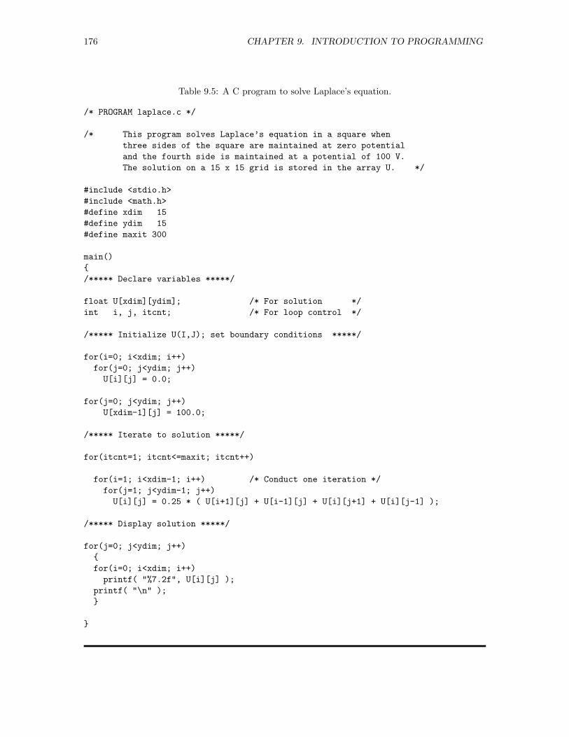
176 CHAPTER 9. INTRODUCTION TO PROGRAMMING

Table 9.5: A C program to solve Laplace’s equation.

/* PROGRAM laplace.c */

/* This program solves Laplace’s equation in a square when

three sides of the square are maintained at zero potential

and the fourth side is maintained at a potential of 100 V.

The solution on a 15 x 15 grid is stored in the array U. */

#include <stdio.h>

#include <math.h>

#define xdim 15

#define ydim 15

#define maxit 300

main()

/***** Declare variables *****/

float U[xdim][ydim]; /* For solution */

int i, j, itcnt; /* For loop control */

/***** Initialize U(I,J); set boundary conditions *****/

for(i=0; i<xdim; i++)

for(j=0; j<ydim; j++)

U[i][j] = 0.0;

for(j=0; j<ydim; j++)

U[xdim-1][j] = 100.0;

/***** Iterate to solution *****/

for(itcnt=1; itcnt<=maxit; itcnt++)

for(i=1; i<xdim-1; i++) /* Conduct one iteration */

for(j=1; j<ydim-1; j++)

U[i][j] = 0.25 * ( U[i+1][j] + U[i-1][j] + U[i][j+1] + U[i][j-1] );

/***** Display solution *****/

for(j=0; j<ydim; j++)

for(i=0; i<xdim; i++)

printf( "%7.2f", U[i][j] );

printf( "\n" );

9.6. SOLVING LAPLACE’S EQUATION WITH C 177

• C uses the equal sign for assignment. The operators >, >=, <, <=, ==, and != are used in logicalexpressions to symbolize greater than, greater than or equal to, less than, less than or equalto, equal to, and not equal to, respectively; the operators &&, ||, and ! symbolize AND, OR,and NOT, respectively.

• A counted C loop is introduced with the keyword for, which is followed by three argumentsenclosed in parentheses and separated by semicolons. The first of these arguments (e.g., i=0)identifies the loop index and initializes it, the second (e.g., i<xdim) specifies the conditionwhich must be true for the loop to continue, and the third (e.g., i++, which is a shorthandfor i=i+1) specifies (cryptically) that the index is to be incremented by one with each passthrough the loop. The condition is tested at the beginning of the loop and the incrementationof the index takes place after the statements in the body of the loop have been executed. Thus,on the first pass through the loop, the statements are executed with the initial value of theindex, and the loop will not be executed at all if the condition is false for the initial value ofthe index. Note that consecutive arguments are separated by a semicolon.

• The printf statement directs its output to the standard output device, which is the screen[and is always “attached”—C uses the verb “open”—and hence need not be explicitly attachedand detached (i.e., opened and closed)].

• The first argument in the printf statement is a quoted string that conveys not only charactersto be transmitted literally to the output device but also specifications effecting the formattingof the value(s) of the variable(s) that is (are) listed in the second and subsequent arguments.In particular, the notation \n transmits the control character to start a new line.

• The format of the output produced by the printf statement is specified by inclusions in theopening character string, each of which is introduced by a percent sign %. The specification%7.2f, for example, stipulates that the number to be displayed should be displayed in ordinarydecimal notation—the f—right-justified in a field (region) that is seven characters wide—the7—with the number rounded to have two digits—the 2—after the decimal point. In thisparticular problem, we know that all values should be positive and no value will be largerthan 100.29 Thus, with the specified format, the largest value will be displayed as 100.00,right-justified in a seven-character field. Since this number requires six character positions,there will be at least one space between consecutive entries in each line of output.30,31

• The printf statement that sends a single value of U to the screen is embedded in the innerloop in the output section of this program. Note that that loop runs 15 times and that nonew-line character is included in the format string in that inner loop. The new-line characteris supplied once in the outer loop for every complete execution of that inner loop. Thus, a newline will be started only after each group of fifteen values has been output by the inner loop.

• In C, opening and closing braces ( and ) are used to group statements together into blocks.Note in particular that the entire program is enclosed within the opening brace in the lineimmediately following the phrase main() and the closing brace in the very last line of thelisting. The one other block in this program is in the display section where two statements (a

29Solutions to Laplace’s equation can never have in the interior a value larger than the largest value nor smallerthan the smallest value on the boundary.

30If we had to allow for the possibility of values ranging downward to -100, we would need one more characterposition (%8.2f) to provide the position for a possible minus sign and guarantee at least one space between anypossible consecutive entries in each line.

31One alternative to the f format is d, which is used for integers, e.g., %8d for an integer to be right-justified ina field eight characters wide. Another alternative, used particularly when the size of floating-point numbers variesconsiderably or is unknown a priori, is e, which outputs floating point numbers in scientific notation, e.g., %15.6e

for a floating point number to be right-justified in fields fifteen characters wide, presented with six digits after thedecimal point (and formatted—depending on the compiler—either with one digit or a zero before the decimal point).The format %15.6e, for example, will present the number 100.00 as 0.100000e 03 or 1.000000e 02, requiring in bothcases twelve character positions of the fifteen specified by the format. Further, note that the simpler specifications%f, %d, and %e will allow the compiler to make its own judgment about the appropriate field sizes.

178 CHAPTER 9. INTRODUCTION TO PROGRAMMING

for loop and the statement printf("\n"); must be blocked together to form the “object” ofthe outer for loop.

• Note that, in the loop generating the output, for each j, i migrates through its several values.Thus, the rows in the output are labeled by values of j, i.e., of y, and the columns in theoutput are labeled by values of i, i.e. of x.

This program is stored in a file named laplace.c in the directory $HEAD/cc. Once that filehas been copied to the default directory, it can be compiled, linked, and run with commands asdescribed in the Local Guide. In UNIX, those commands might be32

cc -o laplace.xc laplace.c

./laplace.xc

In response to these commands to the operating system, the program will be executed and theoutput—15 lines of 15 numbers each—will be displayed on the screen.33

The solution displayed on the screen when the program is run is, of course, difficult to interpret(and would be even more so if we had solved the equation on a finer grid). Anticipating that wemight want to import the output of this program into another—possibly a plotting—program, wemight wish to direct the output to a file rather than to the screen. In UNIX and in a Windowscommand window, we could use the simple statement

./laplace.xc > laplace_c.dat

to achieve that end without having to edit and recompile the program at all. Alternatively, andmore generally, we would have to replace the output portion of the program with code that opens afile, writes the output to that file, and then closes the file. We might, for example, edit laplace.c

in two ways. First we would add the statement

FILE *fptr; /* For file pointer */

to the declaration section, thereby identifying a variable to play the role of a file pointer. Second,we would replace the output section with the statements

fptr=fopen( "laplace_c.dat", "w" );

for(j=0; j<ydim; j++)

for(i=0; i<xdim; i++)

fprintf( fptr, "%7.2f", U[i][j] );

fprintf( fptr, "\n" );

fclose( fptr );

using fopen to open the file for writing (the "w") and to associate it with the pointer fptr, fprintf(rather than printf) to write everything to the file, and finally fclose to close the file. Exceptfor the added first argument, the fprintf statement is structured in the same way as the printf

statement. The program so edited is stored in the file laplace file.c in the directory $HEAD/cc.Once copied to the default directory, it can be compiled, linked, and run as with laplace.c above

32Throughout this book, we shall assume that we are working in a UNIX environment, though cc is fairly standardfor invoking the C compiler. In other operating systems, the characters ./ may or may not be necessary to launch anexecutable program in the current directory. Further detail on how to invoke the C compiler and run an executableprogram in your environment will be described in the Local Guide.

33Incidentally, note that, if necessary, execution of a C program can usually be aborted by typing 〈CONTROL/C〉.

9.7. ADDITIONAL FEATURES OF C 179

(see the Local Guide). In the end, the output file laplace c.dat will be created in the defaultdirectory.

A graphical display of the data in the resulting file could be generated by OCTAVE by issuingto OCTAVE the statements34

>> id = fopen( ’laplace_c.dat’, ’r’ );

>> u = fscanf( id, ’%f’, [15,15] );

>> status = fclose( id );

>> mesh( u’ );

>> surf( u’ );

Open file.Read in solution.Close file.Display solution as mesh surface.Display solution as a shaded surface.

9.7 Additional Features of C

The example program in the previous section has not provided a vehicle for illustrating a fewadditional important capabilities of the language. We here address those features.

9.7.1 Multi-Way Selection

The basic decision-making structure in C involves keywords, conditions, and actions in the generalpattern conveyed by the listing

if 〈condition1〉〈block1 of statements〉

else if 〈condition2〉〈block2 of statements〉

...else if 〈conditionn〉〈blockn of statements〉

else

〈catch-all block of statements〉

Test 〈condition1〉.Execute 〈block1〉 and exit when 〈condition1〉 true.Test 〈condition2〉 (if 〈condition1〉 false).Execute 〈block2〉 and exit when 〈condition2〉 true.

Test 〈conditionn〉 (if 〈condition(n− 1〉 false).Execute 〈blockn〉 and exit when 〈conditionn〉 true.

Execute 〈catch-all block〉 and exit when all conditionsfalse.

In this construction, if a particular block of statements consists of a single statement, it can simplybe presented in the proper position in the structure (terminated, of course, with a semicolon). Whena block requires more than one logical statement, the statements as a group must be enclosed inbraces so the compiler will treat them logically as a single statement. Further, two-way selection issimply a version of multi-way selection in which there is only one condition in this sequence, and thefinal else clause can be omitted if it contains no statements. The blocks can contain any numberof statements, each terminated with a semicolon, and the conditions can be logical variables, singlelogical expressions, or compound logical expressions.

The above chain of if-else-if structures is a bit awkward. As an alternative, C also providesthe structure

34While the file produced by C has rows labeled by y and columns labeled by x, reading that file into MATLABcreates a file in which the columns are labeled by y and the rows by x. The transposition in the mesh and surface

commands is necessary to have the proper associations of columns and rows with x and y.

180 CHAPTER 9. INTRODUCTION TO PROGRAMMING

switch 〈expression〉case 〈constant-expression1〉: 〈block1 of statements〉case 〈constant-expression2〉: 〈block2 of statements〉...case 〈constant-expressionn〉: 〈blockn of statements〉default: 〈block-def of statements〉

Here, the expression following the keyword switch must yield an integer value. When that integermatches the value of one of the constant expressions distinguishing a case, the statements in thatcase will be executed. If no case is satisfied, the statements in the default case will be executed,though the default case can be omitted altogether if specific actions are to be coded only for thecases explicitly mentioned.

9.7.2 Reading Data from Keyboard

Data can be read from the keyboard in C with a variety of statements. In the simplest approach,we might use the command printf to print a prompting message conveying the item wanted andthen the command scanf to read that item from the keyboard and store it in a suitable variablewith statements like

printf( "\nSuitable prompting message: " );

scanf( "%f", &value );

(Note the ampersand preceding the variable name; it makes sure that the argument refers explicitlyto the address of the memory cell(s) in which the value of the variable is to be stored and must bepresent for proper functioning.) Finally, note that, when coded like

scanf( "%f %d", &value, &index );

two values would be entered in response to the prompting message, the values being separated by oneor more spaces or by one or more tabs. In this specific example, of course, the two variables wouldpreviously have been declared as a single-precision floating point value and an integer, respectively.

9.7.3 Additional Loops

Beyond the for loop, C makes available a while loop and a do/while loop. The while loop placesthe condition controlling the loop at the beginning and is coded with a structure like

while 〈condition〉〈block of statements〉

where each statement in the block must—as always—be terminated with a semicolon and, exceptwhen it consists of a single statement, the block must be enclosed in braces. The statements in theblock will be executed repeatedly as long as 〈condition〉 remains true, and the loop will be infiniteunless the action of the statements in the loop ultimately turns the condition to false.

The do/while loop places the condition controlling the loop at the end and is coded with astructure like

9.7. ADDITIONAL FEATURES OF C 181

do

〈block of statements〉while 〈condition〉;

where each statement in the block must—as always—be terminated with a semicolon and, exceptwhen it consists of a single statement, the block must be enclosed in braces. The statements in theblock will be executed repeatedly as long as 〈condition〉 remains true, and the loop will be infiniteunless the action of the statements in the loop ultimately turns the condition to false.

9.7.4 Functions and Global Variables

As with most computer languages, C also admits the possibility of creating new commands/functionsthrough the use functions. In essence, a function is a self-contained segment of code that is given aname of its own and that can be invoked in another program with a single statement. In outline,we define a function with a structure like

dt FuncName( dt1 Arg1, dt2 Arg2, . . . )

Statements coding the desired action.

Here, dt specifies the data type of the value returned by the function (and may be void if no valueis returned); FuncName is a user-selected name for the function; and dt1, dt2, . . . specify the datatypes of the arguments Arg1, Arg2, . . ., which are the names of the variables that communicate(either by providing input to the function or providing values returned to the calling program)between the calling program and the function. All other variables in the function are invisible to thecalling program (and can, in fact, have the same names as variables in the calling program withoutcausing confusion). The statements defining the function must appear together in the listing of afull program and each function definition must appear in the listing before its first invocation withinthe total program unless the compiler is alerted to its later presence in the listing with a statementthat simply repeats the first line of the function definition. Once in place, the function itself can beinvoked at any point in the program with the single statement

FuncName( Arg1, Arg2, . . . )

This time, the arguments can be variable names identifying the storage location for the values to besubmitted to the function or they can be actual values. Further, while the order of the arguments iscritical to the proper interpretation of each, the variable names used in invoking a function need notbe—and in general will not be—the same as those used in defining the function in the first place.Data types and dimensions must match, but names need not.

If the data type of the function is not void, then somewhere—often at the very end—in thefunction definition there must appear a statement of the form

return 〈expression giving value to be returned〉

Then, the function would be invoked with a statement of the form

VarName = FuncName( Arg1, Arg2, . . . )

where VarName is the name of a variable of the appropriate data type into which the value returnedby the function is to be stored.

182 CHAPTER 9. INTRODUCTION TO PROGRAMMING

In later chapters, we will at times find it necessary to “sneak” values of some variables into afunction without using the “official” arguments. To do so in C, we must make use of global variables,which are declared by placing the declarations early in the listing and, in particular, outside andbefore any of the functions that will make use of them. Once the declarations have been so positioned,the variables by the names declared are known everywhere and can be used by those names anywherein the listing. While they are needed in some circumstances (see later chapters), global variables aredangerous and must be used sparingly. Once declared, they are known everywhere and must not beused unless their global meaning is intended. Ignoring this rule can result in unpleasant, perhapseven disastrous, interactions among portions of the code that are supposed to be independent.

9.10 Solving Laplace’s Equation with OCTAVE

The algorithm described in Section 9.3.1 is readily implemented in OCTAVE with the statements

>> u = zeros(15,15); u(:,15)=100.0;

>> for itcnt = 1:30

for i = 2:14

for j = 2:14

u(i,j)=0.25*( u(i+1,j)+u(i-1,j)+u(i,j+1)+u(i,j-1) );

end

end

end

Here, the two statements on the first line establish a 15×15 matrix of zeros and adjust the values inthe final column to the stipulated boundary values. Then, the remaining statement (which containsthree nested for loops and occupies seven physical lines) executes 30 iterations (the outermost forloop) of the double loop it contains. The innermost statement simply expresses the substance ofEq. (9.3). Note that the inner loops do not include points on the boundary of the region in whicha solution is sought, so the values in the array u at its “edges” are left alone throughout the 30iterations.

Once the solution has been completed, of course, we could display it on the screen with anynumber of statements, the simplest of which probably are

>> mesh( u )

or

>> surf( u )

though these could be embellished by exploiting additional arguments and commands to rescale theaxes, select alternate colors, label the display, etc.

9.12 Creating and Storing Two-Dimensional Scalar Arrays

We turn now to the storage of one or more arrays representing scalar and vector fields in files withthe structure described in Section 9.3.2. Suppose, first, that we wish to explore the two-dimensionalscalar field representing the irradiance produced by Fraunhofer diffraction at a square aperture andgiven analytically by the expression

I(x, y) = I0

(sinx

x

)2(sin y

y

)2

(9.4)

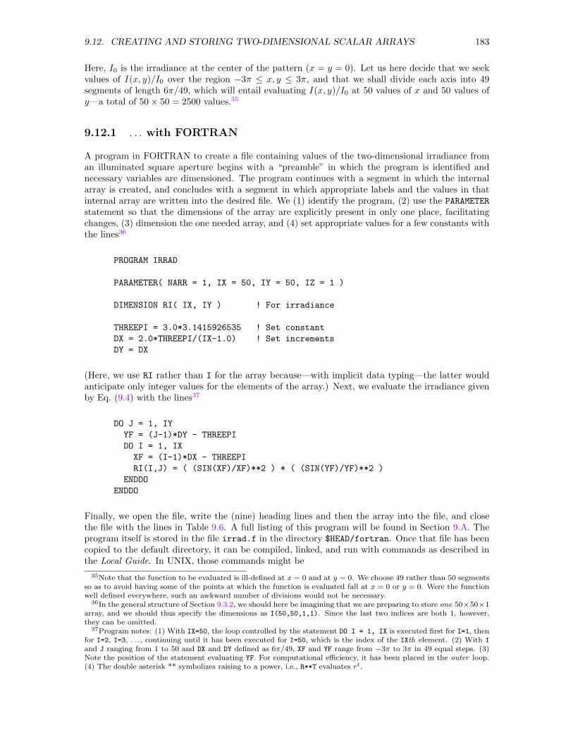
9.12. CREATING AND STORING TWO-DIMENSIONAL SCALAR ARRAYS 183

Here, I0 is the irradiance at the center of the pattern (x = y = 0). Let us here decide that we seekvalues of I(x, y)/I0 over the region −3π ≤ x, y ≤ 3π, and that we shall divide each axis into 49segments of length 6π/49, which will entail evaluating I(x, y)/I0 at 50 values of x and 50 values ofy—a total of 50× 50 = 2500 values.35

9.12.1 . . . with FORTRAN

A program in FORTRAN to create a file containing values of the two-dimensional irradiance froman illuminated square aperture begins with a “preamble” in which the program is identified andnecessary variables are dimensioned. The program continues with a segment in which the internalarray is created, and concludes with a segment in which appropriate labels and the values in thatinternal array are written into the desired file. We (1) identify the program, (2) use the PARAMETER

statement so that the dimensions of the array are explicitly present in only one place, facilitatingchanges, (3) dimension the one needed array, and (4) set appropriate values for a few constants withthe lines36

PROGRAM IRRAD

PARAMETER( NARR = 1, IX = 50, IY = 50, IZ = 1 )

DIMENSION RI( IX, IY ) ! For irradiance

THREEPI = 3.0*3.1415926535 ! Set constant

DX = 2.0*THREEPI/(IX-1.0) ! Set increments

DY = DX

(Here, we use RI rather than I for the array because—with implicit data typing—the latter wouldanticipate only integer values for the elements of the array.) Next, we evaluate the irradiance givenby Eq. (9.4) with the lines37

DO J = 1, IY

YF = (J-1)*DY - THREEPI

DO I = 1, IX

XF = (I-1)*DX - THREEPI

RI(I,J) = ( (SIN(XF)/XF)**2 ) * ( (SIN(YF)/YF)**2 )

ENDDO

ENDDO

Finally, we open the file, write the (nine) heading lines and then the array into the file, and closethe file with the lines in Table 9.6. A full listing of this program will be found in Section 9.A. Theprogram itself is stored in the file irrad.f in the directory $HEAD/fortran. Once that file has beencopied to the default directory, it can be compiled, linked, and run with commands as described inthe Local Guide. In UNIX, those commands might be

35Note that the function to be evaluated is ill-defined at x = 0 and at y = 0. We choose 49 rather than 50 segmentsso as to avoid having some of the points at which the function is evaluated fall at x = 0 or y = 0. Were the functionwell defined everywhere, such an awkward number of divisions would not be necessary.

36In the general structure of Section 9.3.2, we should here be imagining that we are preparing to store one 50×50×1array, and we should thus specify the dimensions as I(50,50,1,1). Since the last two indices are both 1, however,they can be omitted.

37Program notes: (1) With IX=50, the loop controlled by the statement DO I = 1, IX is executed first for I=1, thenfor I=2, I=3, . . ., continuing until it has been executed for I=50, which is the index of the IXth element. (2) With I

and J ranging from 1 to 50 and DX and DY defined as 6π/49, XF and YF range from −3π to 3π in 49 equal steps. (3)Note the position of the statement evaluating YF. For computational efficiency, it has been placed in the outer loop.(4) The double asterisk ** symbolizes raising to a power, i.e., R**T evaluates rt.

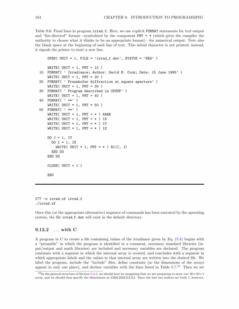
184 CHAPTER 9. INTRODUCTION TO PROGRAMMING

Table 9.6: Final lines in program irrad.f. Here, we use explicit FORMAT statements for text outputand “list-directed” format—symbolized by the component FMT = * (which gives the compiler theauthority to choose what it thinks to be an appropriate format)—for numerical output. Note alsothe blank space at the beginning of each line of text. This initial character is not printed; instead,it signals the printer to start a new line.

OPEN( UNIT = 1, FILE = ’irrad_f.dat’, STATUS = ’NEW’ )

WRITE( UNIT = 1, FMT = 10 )

10 FORMAT( ’ Irradiance; Author: David M. Cook; Date: 15 June 1995’ )

WRITE( UNIT = 1, FMT = 20 )

20 FORMAT( ’ Fraunhofer diffraction at square aperture’ )

WRITE( UNIT = 1, FMT = 30 )

30 FORMAT( ’ Program described in CPSUP’ )

WRITE( UNIT = 1, FMT = 40 )

40 FORMAT( ’ **’ )

WRITE( UNIT = 1, FMT = 50 )

50 FORMAT( ’ **’ )

WRITE( UNIT = 1, FMT = * ) NARR

WRITE( UNIT = 1, FMT = * ) IX

WRITE( UNIT = 1, FMT = * ) IY

WRITE( UNIT = 1, FMT = * ) IZ

DO J = 1, IY

DO I = 1, IX

WRITE( UNIT = 1, FMT = * ) RI(I, J)

END DO

END DO

CLOSE( UNIT = 1 )

END

f77 -o irrad.xf irrad.f

./irrad.xf

Once this (or the appropriate alternative) sequence of commands has been executed by the operatingsystem, the file irrad f.dat will exist in the default directory.

9.12.2 . . . with C

A program in C to create a file containing values of the irradiance given by Eq. (9.4) begins witha “preamble” in which the program is identified in a comment, necessary standard libraries (in-put/output and math libraries) are included and necessary variables are declared. The programcontinues with a segment in which the internal array is created, and concludes with a segment inwhich appropriate labels and the values in that internal array are written into the desired file. Welabel the program, include the “include” files, define constants (so the dimensions of the arraysappear in only one place), and declare variables with the lines listed in Table 9.7.38 Then we set

38In the general structure of Section 9.3.2, we should here be imagining that we are preparing to store one 50×50×1array, and we should thus specify the dimensions as I[50][50][1][1]. Since the last two indices are both 1, however,

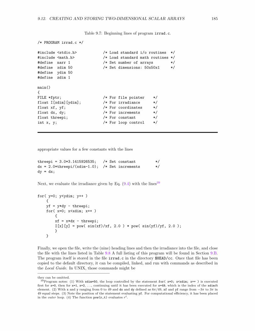
9.12. CREATING AND STORING TWO-DIMENSIONAL SCALAR ARRAYS 185

Table 9.7: Beginning lines of program irrad.c.

/* PROGRAM irrad.c */

#include <stdio.h> /* Load standard i/o routines */

#include <math.h> /* Load standard math routines */

#define narr 1 /* Set number of arrays */

#define xdim 50 /* Set dimensions: 50x50x1 */

#define ydim 50

#define zdim 1

main()

FILE *fptr; /* For file pointer */

float I[xdim][ydim]; /* For irradiance */

float xf, yf; /* For coordinates */

float dx, dy; /* For increments */

float threepi; /* For constant */

int x, y; /* For loop control */

appropriate values for a few constants with the lines

threepi = 3.0*3.1415926535; /* Set constant */

dx = 2.0*threepi/(xdim-1.0); /* Set increments */

dy = dx;

Next, we evaluate the irradiance given by Eq. (9.4) with the lines39

for( y=0; y<ydim; y++ )

yf = y*dy - threepi;

for( x=0; x<xdim; x++ )

xf = x*dx - threepi;

I[x][y] = pow( sin(xf)/xf, 2.0 ) * pow( sin(yf)/yf, 2.0 );

Finally, we open the file, write the (nine) heading lines and then the irradiance into the file, and closethe file with the lines listed in Table 9.8 A full listing of this program will be found in Section 9.B.The program itself is stored in the file irrad.c in the directory $HEAD/cc. Once that file has beencopied to the default directory, it can be compiled, linked, and run with commands as described inthe Local Guide. In UNIX, those commands might be

they can be omitted.39Program notes: (1) With xdim=50, the loop controlled by the statement for( x=0; x<xdim; x++ ) is executed

first for x=0, then for x=1, x=2, . . ., continuing until it has been executed for x=49, which is the index of the xdimthelement. (2) With x and y ranging from 0 to 49 and dx and dy defined as 6π/49, xf and yf range from −3π to 3π in49 equal steps. (3) Note the position of the statement evaluating yf. For computational efficiency, it has been placedin the outer loop. (4) The function pow(r,t) evaluates rt.

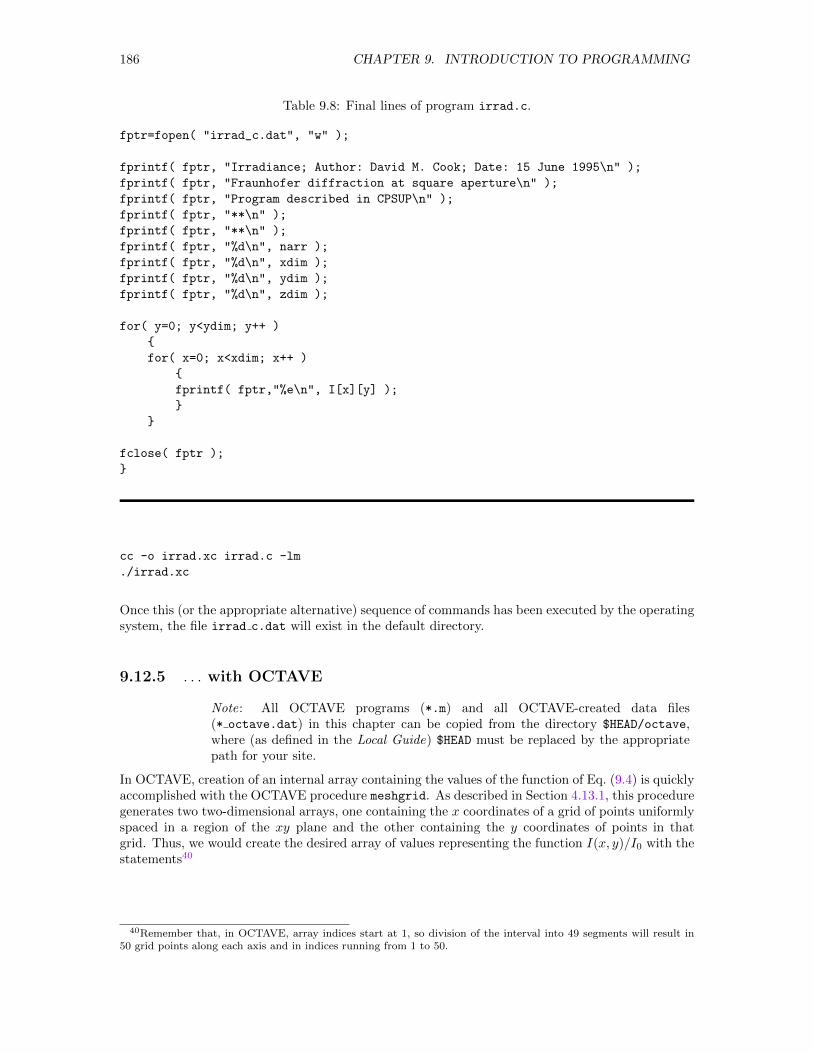
186 CHAPTER 9. INTRODUCTION TO PROGRAMMING

Table 9.8: Final lines of program irrad.c.

fptr=fopen( "irrad_c.dat", "w" );

fprintf( fptr, "Irradiance; Author: David M. Cook; Date: 15 June 1995\n" );

fprintf( fptr, "Fraunhofer diffraction at square aperture\n" );

fprintf( fptr, "Program described in CPSUP\n" );

fprintf( fptr, "**\n" );

fprintf( fptr, "**\n" );

fprintf( fptr, "%d\n", narr );

fprintf( fptr, "%d\n", xdim );

fprintf( fptr, "%d\n", ydim );

fprintf( fptr, "%d\n", zdim );

for( y=0; y<ydim; y++ )

for( x=0; x<xdim; x++ )

fprintf( fptr,"%e\n", I[x][y] );

fclose( fptr );

cc -o irrad.xc irrad.c -lm

./irrad.xc

Once this (or the appropriate alternative) sequence of commands has been executed by the operatingsystem, the file irrad c.dat will exist in the default directory.

9.12.5 . . . with OCTAVE

Note: All OCTAVE programs (*.m) and all OCTAVE-created data files(* octave.dat) in this chapter can be copied from the directory $HEAD/octave,where (as defined in the Local Guide) $HEAD must be replaced by the appropriatepath for your site.

In OCTAVE, creation of an internal array containing the values of the function of Eq. (9.4) is quicklyaccomplished with the OCTAVE procedure meshgrid. As described in Section 4.13.1, this proceduregenerates two two-dimensional arrays, one containing the x coordinates of a grid of points uniformlyspaced in a region of the xy plane and the other containing the y coordinates of points in thatgrid. Thus, we would create the desired array of values representing the function I(x, y)/I0 with thestatements40

40Remember that, in OCTAVE, array indices start at 1, so division of the interval into 49 segments will result in50 grid points along each axis and in indices running from 1 to 50.

9.13. CREATING AND STORING THREE-DIMENSIONAL SCALAR ARRAYS 187

>> inc = 6.0*pi/49.0;

>> [x,y] = meshgrid(-3.0*pi:inc:3.0*pi, -3.0*pi:inc:3.0*pi);

>> I = ( (sin(x)./x).^2 ) .* ( (sin(y)./y).^2 );

This array can be written to a file having the format described in Section 9.3.2 by using theLawrence-written M-file lugen list.m.41 The statement

>> lugen_list( I )

calls lugen list and tells OCTAVE to write the array I, which must already exist in the OCTAVEworkspace, to a file. Before accomplishing its main objective, lugen list requests input of

• the name of the file into which the array is to be written,• a brief title for the data,• the author’s (owner’s) name,• the date, and• four lines of comments.

Each of these pieces of information is a string, which therefore must be enclosed in single quotationmarks as it is entered in response to its prompt. All default strings that are not null are indicatedin square brackets in the prompting messages. For example, the “conversation” that would save thevalues of irradiance in the array I might be

>> lugen_list( I )

All entries are strings and must be enclosed

in single quotation marks.

File name [untitled.dat]: ’irrad_octave.dat’

Title : ’Irradiance’

Author : ’David M. Cook’

Date : ’19 June 2001’

Comment 1 [**]: ’Fraunhofer diffraction at square aperture’

Comment 2 [**]: ’Program described in CPSUP’

Comment 3 [**]:

Comment 4 [**]:

File ’irrad_octave.dat’ saved successfully!

When 〈RETURN〉 is typed after the fourth line of comments, lugen list writes the data into thespecified file in the default directory and displays a message indicating successful completion of thataction on the screen.42

9.13 Creating and Storing Three-Dimensional Scalar Arrays

As an example of a three-dimensional scalar function, we choose the normalized probability densityp(x, y, z) for the electron in the (n, l,m) = (3, 2, 0) state in the hydrogen atom. This probability

41A commented listing of this m-file is presented in Section 9.C.42A Lawrence-written OCTAVE procedure for reading files written by lugen list.m is described in Section 9.16.5.

188 CHAPTER 9. INTRODUCTION TO PROGRAMMING

density is given as a function of Cartesian coordinates (x, y, z) with the nucleus located at the originby

p(x, y, z) =1

2π(27)3ρ4 e−2ρ/3

(3z2

ρ2− 1

)2

=1

2π(27)3e−2ρ/3 (9z4 − 6z2ρ2 + ρ4) (9.5)

where the coordinates are all measured in units of the Bohr radius and

ρ =√x2 + y2 + z2 (9.6)

This function of three variables is commonly visualized either by focusing on the function in variousplanes intersecting the three-dimensional volume (thereby reducing the display to a family of two-dimensional displays) or by displaying various contour surfaces. Programs producing such displaysneed a three-dimensional array of values as input. Suppose, then, we anticipated using some graphicalvisualization program to explore the quantum probability given by Eq. (9.6). Let us decide todetermine values of p(x, y, z) over the region −10 ≤ x, y, z ≤ 10, dividing each axis into 29 segments,which will entail evaluating p(x, y, z) at 30 values of x, 30 values of y, and 30 values of z—a total of30× 30× 30 = 27000 values.

Since the programs discussed in this section differ very little from those presented in Section 9.12,we elect here to include full code only in the listings in the appendices. We comment in the textonly on major differences and subtleties.

9.13.1 . . . with FORTRAN

A FORTRAN program for creating and storing a three-dimensional scalar array is similar to theprogram presented in Section 9.12.1. We need one 30× 30× 30 array, each element of which is theprobability density at the corresponding point in the three-dimensional space. The program, a fulllisting of which will be found in Section 9.D, is named pdens.f and contains sections

• Identifying the program.

• Setting parameters for the number of arrays, the dimensions of each array, the ranges ofcoordinates on the three axes, and the lowest coordinate on each axis.

• Dimensioning the one 30 × 30 × 30 array needed for the probability density and evaluatingseveral useful constants.

• Evaluating the probability density given by Eq. (9.5). Basically, we need three loops, oneranging over each coordinate from its initial value [X0,Y0,Z0] to its final value [X0,Y0,Z0] +

[XRANGE,YRANGE,ZRANGE]. In the present case, it is convenient (and computationally efficient)to evaluate each coordinate and then its square as far from the center of the loop as possibleand then to evaluate the radial coordinate and its square before evaluating the probabilitydensity itself.

• Opening the file, writing the heading lines and the probability densities into the file, andclosing the file.

As with previous programs, pdens.f can be copied from the directory $HEAD/fortran into yourown directory, compiled, linked, and run or—should this be necessary for your application—editedbefore being compiled, linked, and run to create the desired file.43 Once the program has beenexecuted, the file pdens f.dat will exist in the default directory.

43For instructions on how to compile and run the program, see Section 9.12.1 and the Local Guide.

9.13. CREATING AND STORING THREE-DIMENSIONAL SCALAR ARRAYS 189

9.13.2 . . . with C

A C program for creating and storing the necessary three-dimensional scalar array is similar to theprogram presented in Section 9.12.2. We need one 30× 30× 30 array, each element of which is theprobability density at the corresponding point in the three-dimensional space. The program, a fulllisting of which will be found in Section 9.E, is named pdens.c and contains sections

• Identifying the program, including standard libraries, defining constants, and declaring neces-sary variables. To facilitate translating integers x, y, and z into the corresponding real coordi-nates xf, yf, and zf, we introduce symbols [xrange,yrange,zrange] for the interval on eachaxis and [x0,y0,z0] for the lowest value of each coordinate. Further, since only one array isto be stored, the array P for the probability densities is dimensioned at P[30][30][30] ratherthan at P[30][30][30][1]. Finally, we introduce variables xs, ys, and zs for the squares ofthe coordinates and rho and rhos for the radial coordinate and its square.

• Evaluating the probability density given by Eq. (9.5). Basically, we need three loops, oneranging over each coordinate from its initial value [x0,y0,z0] to its final value [x0,y0,z0] +

[xrange,yrange,zrange]. In the present case, it is convenient (and computationally efficient)to evaluate each coordinate and then its square as far from the innermost loop as possible andthen to evaluate the radial coordinate and its square before evaluating the probability densityitself.

• Opening the file, writing the heading lines and the probability densities into the file, andclosing the file.

As with previous programs, pdens.c can be copied from the directory $HEAD/cc into your owndirectory, compiled, linked, and run or—should this be necessary for your application—edited beforebeing compiled, linked, and run to create the desired file.44 Once the program has been executed,the file pdens c.dat will exist in the default directory.

9.13.5 . . . with OCTAVE

The procedure for using OCTAVE to generate three-dimensional scalar arrays is similar to themethod described in Section 9.12.5. The array representing the probability density in Eq. (9.5) iscreated using the OCTAVE statements

>> inc = 20.0/29.0;

>> [x,y,z] = meshgrid( -10.0:inc:10.0, -10.0:inc:10.0, -10.0:inc:10.0 );

>> pfactor = 1.0/(2.0*pi*27.0*27.0*27.0);

>> zs = z.*z;

>> rhos = x.^2 + y.^2 + zs;

>> rho = sqrt(rhos);

>> P = pfactor * exp(-2*rho/3) .* (9*zs.^2 - 6*zs.*rhos + rhos.^2);

The first two lines produce a grid of values for the evaluation of the scalar field. Here, x, y, and z

each ranges from −10.0 to 10.0, and the interval is divided into 29 segments, so the arrays x, y, z,zs, rhos, rho, and P have dimensions 30×30×30. The remaining lines evaluate several intermediatequantities and then evaluate P. Finally, with the statement

>> lugen_list( P )

44For instructions on how to compile and run the program, see Section 9.12.2 and the Local Guide.

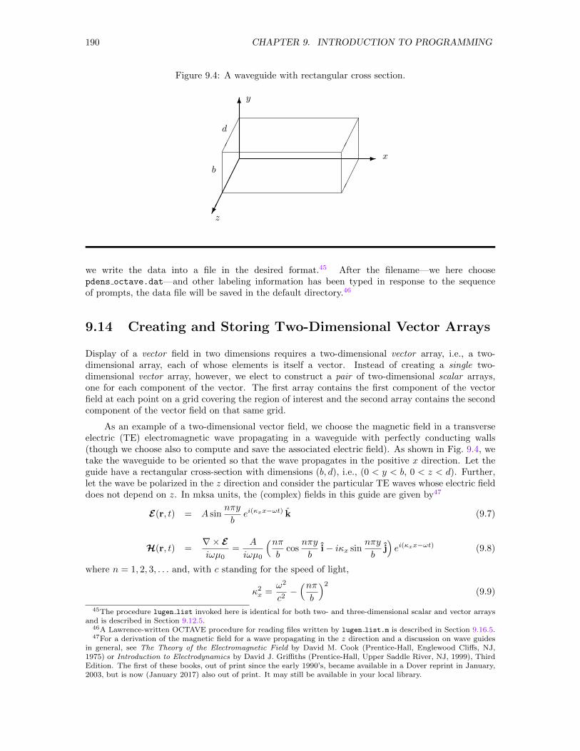
190 CHAPTER 9. INTRODUCTION TO PROGRAMMING

Figure 9.4: A waveguide with rectangular cross section.

- x

6y

z

b

d

we write the data into a file in the desired format.45 After the filename—we here choosepdens octave.dat—and other labeling information has been typed in response to the sequenceof prompts, the data file will be saved in the default directory.46

9.14 Creating and Storing Two-Dimensional Vector Arrays

Display of a vector field in two dimensions requires a two-dimensional vector array, i.e., a two-dimensional array, each of whose elements is itself a vector. Instead of creating a single two-dimensional vector array, however, we elect to construct a pair of two-dimensional scalar arrays,one for each component of the vector. The first array contains the first component of the vectorfield at each point on a grid covering the region of interest and the second array contains the secondcomponent of the vector field on that same grid.

As an example of a two-dimensional vector field, we choose the magnetic field in a transverseelectric (TE) electromagnetic wave propagating in a waveguide with perfectly conducting walls(though we choose also to compute and save the associated electric field). As shown in Fig. 9.4, wetake the waveguide to be oriented so that the wave propagates in the positive x direction. Let theguide have a rectangular cross-section with dimensions (b, d), i.e., (0 < y < b, 0 < z < d). Further,let the wave be polarized in the z direction and consider the particular TE waves whose electric fielddoes not depend on z. In mksa units, the (complex) fields in this guide are given by47

E(r, t) = A sinnπy

bei(κxx−ωt) k (9.7)

H(r, t) =∇× Eiωµ0

=A

iωµ0

(nπb

cosnπy

bi− iκx sin

nπy

bj)ei(κxx−ωt) (9.8)

where n = 1, 2, 3, . . . and, with c standing for the speed of light,

κ2x =ω2

c2−(nπb

)2(9.9)

45The procedure lugen list invoked here is identical for both two- and three-dimensional scalar and vector arraysand is described in Section 9.12.5.

46A Lawrence-written OCTAVE procedure for reading files written by lugen list.m is described in Section 9.16.5.47For a derivation of the magnetic field for a wave propagating in the z direction and a discussion on wave guides

in general, see The Theory of the Electromagnetic Field by David M. Cook (Prentice-Hall, Englewood Cliffs, NJ,1975) or Introduction to Electrodynamics by David J. Griffiths (Prentice-Hall, Upper Saddle River, NJ, 1999), ThirdEdition. The first of these books, out of print since the early 1990’s, became available in a Dover reprint in January,2003, but is now (January 2017) also out of print. It may still be available in your local library.

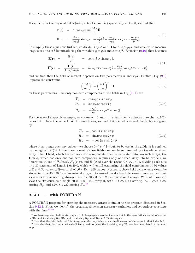
9.14. CREATING AND STORING TWO-DIMENSIONAL VECTOR ARRAYS 191

If we focus on the physical fields (real parts of E and H) specifically at t = 0, we find that

E(r) = A cosκxx sinnπy

bk

H(r) =Anπ

ωµ0bsinκxx cos

nπy

bi− Aκx

ωµ0cosκxx sin

nπy

bj

(9.10)

To simplify these equations further, we divide E by A and H by Anπ/ωµ0b, and we elect to measurelengths in units of b by introducing the variables y = y/b and x = x/b. Equation (9.10) then becomes

E(r) =E(r)

A= cosκxb x sinnπ y k

H(r) =H(r)

Anπ/ωµ0b= sinκxb x cosnπ y i− κxb

nπcosκxb x sinnπ y j

(9.11)

and we find that the field of interest depends on two parameters n and κxb. Further, Eq. (9.9)imposes the constraint (

κxb

nπ

)2

=

(ωb

nπc

)2

− 1 (9.12)

on these parameters. The only non-zero components of the fields in Eq. (9.11) are

Ez = cosκxb x sinnπ y

Hx = sinκxb x cosnπ y (9.13)

Hy = −κxbnπ

cosκxb x sinnπ y

For the sake of a specific example, we choose b = 1 and n = 2, and then we choose ω so that κxb/2πturns out to have the value 1. With these choices, we find that the fields we seek to display are givenby

Ez = cos 2π x sin 2π y

Hx = sin 2π x cos 2π y (9.14)

Hy = − cos 2π x sin 2π y

where x can range over any values—we choose 0 ≤ x ≤ 1—but, to be inside the guide, y is confinedto the region 0 ≤ y ≤ 1. Each component of these fields can now be represented by a two-dimensionalarray. The H field, which has two non-zero components, then is translated into two such arrays; theE field, which has only one non-zero component, requires only one such array. To be explicit, wedetermine values of Hx(x, y), Hy(x, y), and Ez(x, y) over the region 0 ≤ x, y ≤ 1, dividing each axisinto 30 segments of length 1.0/29.0, which will entail evaluating the field components at 30 valuesof x and 30 values of y—a total of 30× 30 = 900 values. Normally, these field components would bestored in three 30×30 two-dimensional arrays. Because of our declared file format, however, we mustview ourselves as needing storage for three 30× 30× 1 three-dimensional arrays. We shall, however,view the structure as a single 30 × 30 × 1 × 3 array H, with H(*,*,1,1) storing Hx, H(*,*,1,2)storing Hy, and H(*,*,1,3) storing Ez.

48

9.14.1 . . . with FORTRAN

A FORTRAN program for creating the necessary arrays is similar to the program discussed in Sec-tion 9.12.1. First, we identify the program, dimension necessary variables, and set various constantswith the lines49,50

48We have supposed indices starting at 1. In languages where indices start at 0, the associations would, of course,be H(*,*,0,0) storing Hx, H(*,*,0,1) storing Hy , and H(*,*,0,2) storing Ez .

49Note that the third index of H is always one, the only value when the dimension of the array in that index is 1.50Note also that, for computational efficiency, various quantities involving only XF have been calculated in the outer

loop.

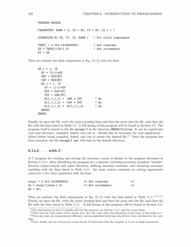
192 CHAPTER 9. INTRODUCTION TO PROGRAMMING

PROGRAM WAVEGD

PARAMETER( NARR = 3, IX = 30, IY = 30, IZ = 1 )

DIMENSION H( IX, IY, IZ, NARR ) ! For field components

TWOPI = 2.0*3.1415926535; ! Set constant

DX = TWOPI/(IX-1.0) ! Set increments

DY = DX

Then we evaluate the field components in Eq. (9.14) with the lines

DO I = 1, IX

XF = (I-1)*DX

SXF = SIN(XF)

CXF = COS(XF)

DO J = 1, IY

YF = (J-1)*DY

SYF = SIN(YF)

CYF = COS(YF)

H(I,J,1,1) = SXF * CYF ! Hx

H(I,J,1,2) = -CXF * SYF ! Hy

H(I,J,1,3) = -H(I,J,1,2) ! Ez

ENDDO

ENDDO

Finally, we open the file, write the (nine) heading lines and then the array into the file, and close thefile with the lines listed in Table 9.9 A full listing of this program will be found in Section 9.F. Theprogram itself is stored in the file wavegd.f in the directory $HEAD/fortran. It can be copied intoyour own directory, compiled, linked, and run or—should this be necessary for your application—edited before being compiled, linked, and run to create the desired file.51 Once the program hasbeen executed, the file wavegd f.dat will exist in the default directory.

9.14.2 . . . with C

A C program for creating and storing the necessary arrays is similar to the program discussed inSection 9.12.2. After identifying the program in a comment, including necessary standard “include”libraries (input/output and math libraries), defining assorted constants, and declaring necessaryvariables with the lines listed in Table 9.10. the main routine continues by setting appropriatevalues for a few other quantities with the lines

twopi = 2.0*3.1415926535; /* Set constant */

dx = twopi/(xdim-1.0) /* Set increments */

dy = dx;

Then we evaluate the field components in Eq. (9.14) with the lines listed in Table 9.11.52,53,54

Finally, we open the file, write the (nine) heading lines and then the array into the file, and close thefile with the lines listed in Table 9.12. A full listing of this program will be found in Section 9.G.

51For instructions on how to compile and run the program, see Section 9.12.1 and the Local Guide.52Note that the third index of H is always zero, the only value when the dimension of the array in that index is 1.53Note also that, for computational efficiency, various quantities involving only xf have been calculated in the outer

loop.54Note, finally, the use of braces to create blocks of statements that the compiler is to see as single statements.

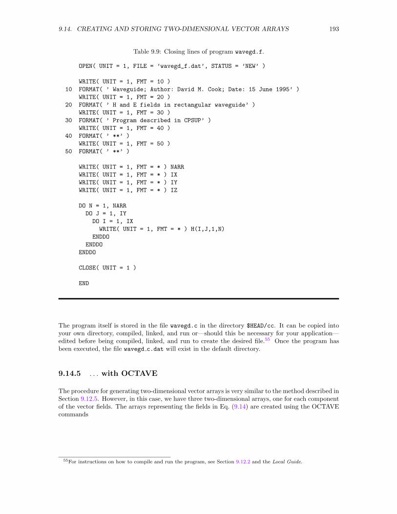
9.14. CREATING AND STORING TWO-DIMENSIONAL VECTOR ARRAYS 193

Table 9.9: Closing lines of program wavegd.f.

OPEN( UNIT = 1, FILE = ’wavegd_f.dat’, STATUS = ’NEW’ )

WRITE( UNIT = 1, FMT = 10 )

10 FORMAT( ’ Waveguide; Author: David M. Cook; Date: 15 June 1995’ )

WRITE( UNIT = 1, FMT = 20 )

20 FORMAT( ’ H and E fields in rectangular waveguide’ )

WRITE( UNIT = 1, FMT = 30 )

30 FORMAT( ’ Program described in CPSUP’ )

WRITE( UNIT = 1, FMT = 40 )

40 FORMAT( ’ **’ )

WRITE( UNIT = 1, FMT = 50 )

50 FORMAT( ’ **’ )

WRITE( UNIT = 1, FMT = * ) NARR

WRITE( UNIT = 1, FMT = * ) IX

WRITE( UNIT = 1, FMT = * ) IY

WRITE( UNIT = 1, FMT = * ) IZ

DO N = 1, NARR

DO J = 1, IY

DO I = 1, IX

WRITE( UNIT = 1, FMT = * ) H(I,J,1,N)

ENDDO

ENDDO

ENDDO

CLOSE( UNIT = 1 )

END

The program itself is stored in the file wavegd.c in the directory $HEAD/cc. It can be copied intoyour own directory, compiled, linked, and run or—should this be necessary for your application—edited before being compiled, linked, and run to create the desired file.55 Once the program hasbeen executed, the file wavegd c.dat will exist in the default directory.

9.14.5 . . . with OCTAVE

The procedure for generating two-dimensional vector arrays is very similar to the method described inSection 9.12.5. However, in this case, we have three two-dimensional arrays, one for each componentof the vector fields. The arrays representing the fields in Eq. (9.14) are created using the OCTAVEcommands

55For instructions on how to compile and run the program, see Section 9.12.2 and the Local Guide.

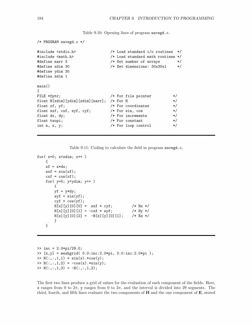
194 CHAPTER 9. INTRODUCTION TO PROGRAMMING

Table 9.10: Opening lines of program wavegd.c.

/* PROGRAM wavegd.c */

#include <stdio.h> /* Load standard i/o routines */

#include <math.h> /* Load standard math routines */

#define narr 3 /* Set number of arrays */

#define xdim 30 /* Set dimensions: 30x30x1 */

#define ydim 30

#define zdim 1

main()

FILE *fptr; /* For file pointer */

float H[xdim][ydim][zdim][narr]; /* For H */

float xf, yf; /* For coordinates */

float sxf, cxf, syf, cyf; /* For sin, cos */

float dx, dy; /* For increments */

float twopi; /* For constant */

int n, x, y; /* For loop control */

Table 9.11: Coding to calculate the field in program wavegd.c.

for( x=0; x<xdim; x++ )

xf = x*dx;

sxf = sin(xf);

cxf = cos(xf);

for( y=0; y<ydim; y++ )

yf = y*dy;

syf = sin(yf);

cyf = cos(yf);

H[x][y][0][0] = sxf * cyf; /* Hx */

H[x][y][0][1] = -cxf * syf; /* Hy */

H[x][y][0][2] = -H[x][y][0][1]; /* Ez */

>> inc = 2.0*pi/29.0;

>> [x,y] = meshgrid( 0.0:inc:2.0*pi, 0.0:inc:2.0*pi );

>> H(:,:,1,1) = sin(x).*cos(y);

>> H(:,:,1,2) = -cos(x).*sin(y);

>> H(:,:,1,3) = -H(:,:,1,2);

The first two lines produce a grid of values for the evaluation of each component of the fields. Here,x ranges from 0 to 2π, y ranges from 0 to 2π, and the interval is divided into 29 segments. Thethird, fourth, and fifth lines evaluate the two components of H and the one component of E, stored

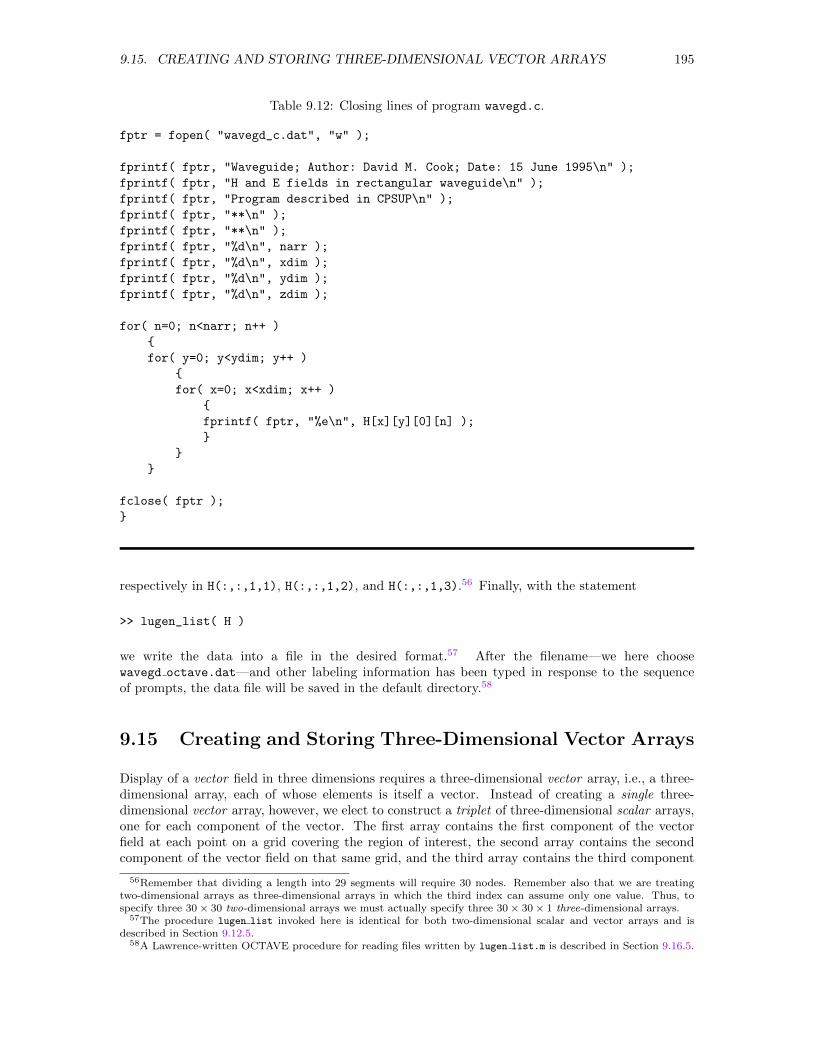
9.15. CREATING AND STORING THREE-DIMENSIONAL VECTOR ARRAYS 195

Table 9.12: Closing lines of program wavegd.c.

fptr = fopen( "wavegd_c.dat", "w" );

fprintf( fptr, "Waveguide; Author: David M. Cook; Date: 15 June 1995\n" );

fprintf( fptr, "H and E fields in rectangular waveguide\n" );

fprintf( fptr, "Program described in CPSUP\n" );

fprintf( fptr, "**\n" );

fprintf( fptr, "**\n" );

fprintf( fptr, "%d\n", narr );

fprintf( fptr, "%d\n", xdim );

fprintf( fptr, "%d\n", ydim );

fprintf( fptr, "%d\n", zdim );

for( n=0; n<narr; n++ )

for( y=0; y<ydim; y++ )

for( x=0; x<xdim; x++ )

fprintf( fptr, "%e\n", H[x][y][0][n] );

fclose( fptr );

respectively in H(:,:,1,1), H(:,:,1,2), and H(:,:,1,3).56 Finally, with the statement

>> lugen_list( H )

we write the data into a file in the desired format.57 After the filename—we here choosewavegd octave.dat—and other labeling information has been typed in response to the sequenceof prompts, the data file will be saved in the default directory.58

9.15 Creating and Storing Three-Dimensional Vector Arrays

Display of a vector field in three dimensions requires a three-dimensional vector array, i.e., a three-dimensional array, each of whose elements is itself a vector. Instead of creating a single three-dimensional vector array, however, we elect to construct a triplet of three-dimensional scalar arrays,one for each component of the vector. The first array contains the first component of the vectorfield at each point on a grid covering the region of interest, the second array contains the secondcomponent of the vector field on that same grid, and the third array contains the third component

56Remember that dividing a length into 29 segments will require 30 nodes. Remember also that we are treatingtwo-dimensional arrays as three-dimensional arrays in which the third index can assume only one value. Thus, tospecify three 30× 30 two-dimensional arrays we must actually specify three 30× 30× 1 three-dimensional arrays.

57The procedure lugen list invoked here is identical for both two-dimensional scalar and vector arrays and isdescribed in Section 9.12.5.

58A Lawrence-written OCTAVE procedure for reading files written by lugen list.m is described in Section 9.16.5.

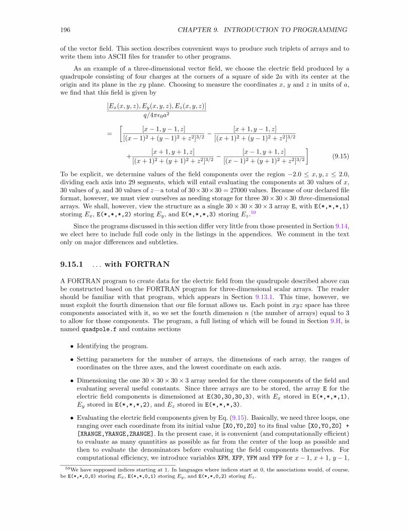
196 CHAPTER 9. INTRODUCTION TO PROGRAMMING

of the vector field. This section describes convenient ways to produce such triplets of arrays and towrite them into ASCII files for transfer to other programs.

As an example of a three-dimensional vector field, we choose the electric field produced by aquadrupole consisting of four charges at the corners of a square of side 2a with its center at theorigin and its plane in the xy plane. Choosing to measure the coordinates x, y and z in units of a,we find that this field is given by

[Ex(x, y, z), Ey(x, y, z), Ez(x, y, z)]

q/4πε0a2

=

[[x− 1, y − 1, z]

[(x− 1)2 + (y − 1)2 + z2]3/2− [x+ 1, y − 1, z]

[(x+ 1)2 + (y − 1)2 + z2]3/2

+[x+ 1, y + 1, z]

[(x+ 1)2 + (y + 1)2 + z2]3/2− [x− 1, y + 1, z]

[(x− 1)2 + (y + 1)2 + z2]3/2

](9.15)

To be explicit, we determine values of the field components over the region −2.0 ≤ x, y, z ≤ 2.0,dividing each axis into 29 segments, which will entail evaluating the components at 30 values of x,30 values of y, and 30 values of z—a total of 30×30×30 = 27000 values. Because of our declared fileformat, however, we must view ourselves as needing storage for three 30× 30× 30 three-dimensionalarrays. We shall, however, view the structure as a single 30× 30× 30× 3 array E, with E(*,*,*,1)

storimg Ex, E(*,*,*,2) storing Ey, and E(*,*,*,3) storing Ez.59

Since the programs discussed in this section differ very little from those presented in Section 9.14,we elect here to include full code only in the listings in the appendices. We comment in the textonly on major differences and subtleties.

9.15.1 . . . with FORTRAN

A FORTRAN program to create data for the electric field from the quadrupole described above canbe constructed based on the FORTRAN program for three-dimensional scalar arrays. The readershould be familiar with that program, which appears in Section 9.13.1. This time, however, wemust exploit the fourth dimension that our file format allows us. Each point in xyz space has threecomponents associated with it, so we set the fourth dimension n (the number of arrays) equal to 3to allow for those components. The program, a full listing of which will be found in Section 9.H, isnamed quadpole.f and contains sections

• Identifying the program.

• Setting parameters for the number of arrays, the dimensions of each array, the ranges ofcoordinates on the three axes, and the lowest coordinate on each axis.

• Dimensioning the one 30× 30× 30× 3 array needed for the three components of the field andevaluating several useful constants. Since three arrays are to be stored, the array E for theelectric field components is dimensioned at E(30,30,30,3), with Ex stored in E(*,*,*,1),Ey stored in E(*,*,*,2), and Ez stored in E(*,*,*,3).

• Evaluating the electric field components given by Eq. (9.15). Basically, we need three loops, oneranging over each coordinate from its initial value [X0,Y0,Z0] to its final value [X0,Y0,Z0] +

[XRANGE,YRANGE,ZRANGE]. In the present case, it is convenient (and computationally efficient)to evaluate as many quantities as possible as far from the center of the loop as possible andthen to evaluate the denominators before evaluating the field components themselves. Forcomputational efficiency, we introduce variables XFM, XFP, YFM and YFP for x− 1, x+ 1, y− 1,

59We have supposed indices starting at 1. In languages where indices start at 0, the associations would, of course,be E(*,*,0,0) storing Ex, E(*,*,0,1) storing Ey , and E(*,*,0,2) storing Ez .

9.15. CREATING AND STORING THREE-DIMENSIONAL VECTOR ARRAYS 197

and y+1, respectively; variables XFMS, XFPS, YFMS, YFPS, and ZFS for (x−1)2, (x+1)2, (y−1)2,(y + 1)2, and z2, respectively; and variables RMM, RMP, RPM and RPP for the four denominatorsin Eq. 9.15.

• Opening the file, writing the heading lines and the field components into the file, and closingthe file.

As with previous programs, quadpole.f can be copied from the directory $HEAD/fortran into yourown directory, compiled, linked, and run or—should this be necessary for your application—editedbefore being compiled, linked, and run to create the desired file.60 Once the program has beenexecuted, the file quadpole f.dat will exist in the default directory.

9.15.2 . . . with C

A C program for creating and storing three-dimensional vector arrays is similar to the other Cprograms presented so far, in particular the three-dimensional scalar program in Section 9.13.2.This time, however, we must exploit the fourth dimension that our file format allows us. Each pointin xyz space has three components associated with it, so we set the fourth dimension n (the numberof arrays) equal to 3 to allow for those components. The program, a full listing of which will befound in Section 9.I, is named quadpole.c and contains sections

• Identifying the program, including standard libraries, defining constants, and declaring nec-essary variables. To facilitate translating integers x, y, and z into the corresponding real co-ordinates xf, yf, and zf, we introduce symbols [xrange,yrange,zrange] for the interval oneach axis and [x0,y0,z0] for the lowest value of each coordinate. Since three arrays are to bestored, the array E for the electric field components is dimensioned at E[30][30][30][3], withEx stored in E[*][*][*][0], Ey stored in E[*][*][*][1], and Ez stored in E[*][*][*][2].Finally, we introduce variables xfm, xfp, yfm and yfp for x− 1, x+ 1, y− 1, and y+ 1, respec-tively; variables xfms, xfps, yfms, yfps, and zfs for (x− 1)2, (x+ 1)2, (y− 1)2, (y+ 1)2, andz2, respectively; and variables rmm, rmp, rpm and rpp for the four denominators in Eq. 9.15.

• Evaluating the electric field components given by Eq. (9.15). Basically, we need three loops, oneranging over each coordinate from its initial value [x0,y0,z0] to its final value [x0,y0,z0] +

[xrange,yrange,zrange]. In the present case, it is convenient (and computationally efficient)to evaluate as many quantities as possible as far from the center of the loop as possible andthen to evaluate the denominators before evaluating the field components themselves.

• Opening the file, writing the heading lines and the field components into the file, and closingthe file.

As with previous programs, quadpole.c can be copied from the directory $HEAD/cc into your owndirectory, compiled, linked, and run or—should this be necessary for your application—edited beforebeing compiled, linked, and run to create the desired file.61 Once the program has been executed,the file quadpole c.dat will exist in the default directory.

9.15.5 . . . with OCTAVE

The procedure for using OCTAVE to generate three-dimensional vector arrays is very similar to themethod described in Section 9.14.5. In this case, however, we must create three three-dimensionalarrays, corresponding to the components of the three-dimensional vector. The array representingthe components of the E-field given by Eq (9.15) is created using the OCTAVE statements

60For instructions on how to compile and run the program, see Section 9.12.1 and the Local Guide.61For instructions on how to compile and run the program, see Section 9.12.2 and the Local Guide.

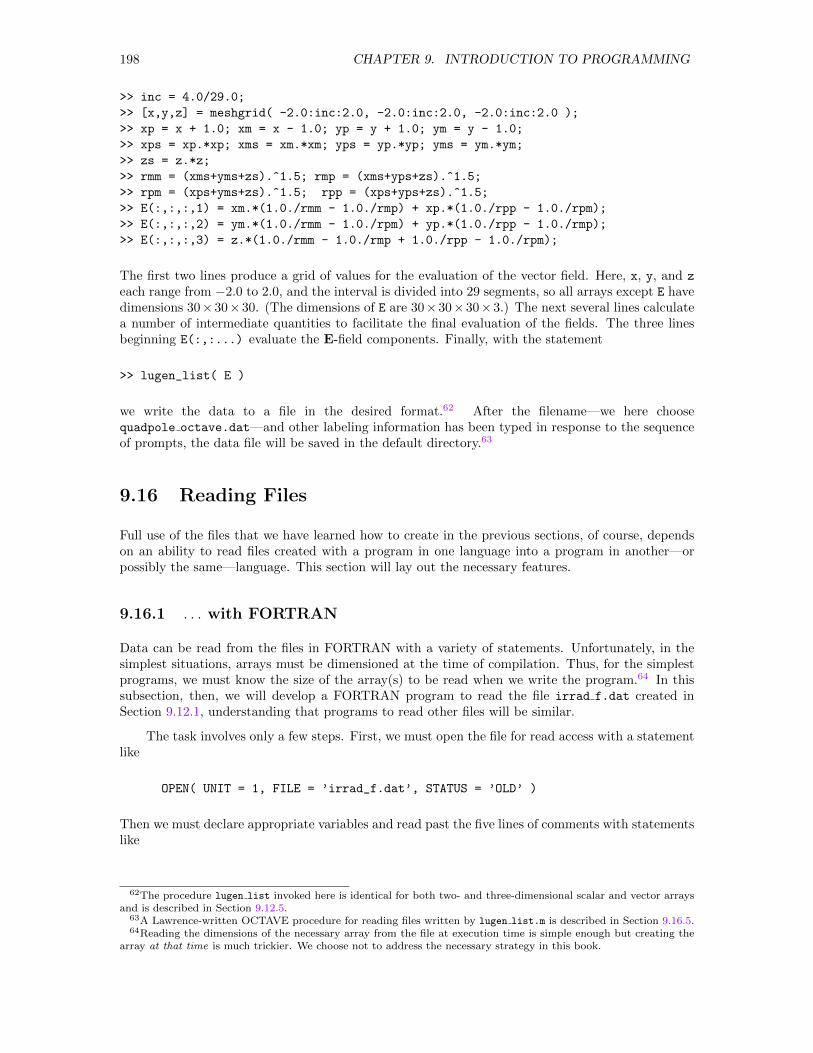
198 CHAPTER 9. INTRODUCTION TO PROGRAMMING

>> inc = 4.0/29.0;

>> [x,y,z] = meshgrid( -2.0:inc:2.0, -2.0:inc:2.0, -2.0:inc:2.0 );

>> xp = x + 1.0; xm = x - 1.0; yp = y + 1.0; ym = y - 1.0;

>> xps = xp.*xp; xms = xm.*xm; yps = yp.*yp; yms = ym.*ym;

>> zs = z.*z;

>> rmm = (xms+yms+zs).^1.5; rmp = (xms+yps+zs).^1.5;

>> rpm = (xps+yms+zs).^1.5; rpp = (xps+yps+zs).^1.5;

>> E(:,:,:,1) = xm.*(1.0./rmm - 1.0./rmp) + xp.*(1.0./rpp - 1.0./rpm);

>> E(:,:,:,2) = ym.*(1.0./rmm - 1.0./rpm) + yp.*(1.0./rpp - 1.0./rmp);

>> E(:,:,:,3) = z.*(1.0./rmm - 1.0./rmp + 1.0./rpp - 1.0./rpm);

The first two lines produce a grid of values for the evaluation of the vector field. Here, x, y, and z

each range from −2.0 to 2.0, and the interval is divided into 29 segments, so all arrays except E havedimensions 30×30×30. (The dimensions of E are 30×30×30×3.) The next several lines calculatea number of intermediate quantities to facilitate the final evaluation of the fields. The three linesbeginning E(:,:...) evaluate the E-field components. Finally, with the statement

>> lugen_list( E )

we write the data to a file in the desired format.62 After the filename—we here choosequadpole octave.dat—and other labeling information has been typed in response to the sequenceof prompts, the data file will be saved in the default directory.63

9.16 Reading Files

Full use of the files that we have learned how to create in the previous sections, of course, dependson an ability to read files created with a program in one language into a program in another—orpossibly the same—language. This section will lay out the necessary features.

9.16.1 . . . with FORTRAN

Data can be read from the files in FORTRAN with a variety of statements. Unfortunately, in thesimplest situations, arrays must be dimensioned at the time of compilation. Thus, for the simplestprograms, we must know the size of the array(s) to be read when we write the program.64 In thissubsection, then, we will develop a FORTRAN program to read the file irrad f.dat created inSection 9.12.1, understanding that programs to read other files will be similar.

The task involves only a few steps. First, we must open the file for read access with a statementlike

OPEN( UNIT = 1, FILE = ’irrad_f.dat’, STATUS = ’OLD’ )

Then we must declare appropriate variables and read past the five lines of comments with statementslike

62The procedure lugen list invoked here is identical for both two- and three-dimensional scalar and vector arraysand is described in Section 9.12.5.

63A Lawrence-written OCTAVE procedure for reading files written by lugen list.m is described in Section 9.16.5.64Reading the dimensions of the necessary array from the file at execution time is simple enough but creating the

array at that time is much trickier. We choose not to address the necessary strategy in this book.

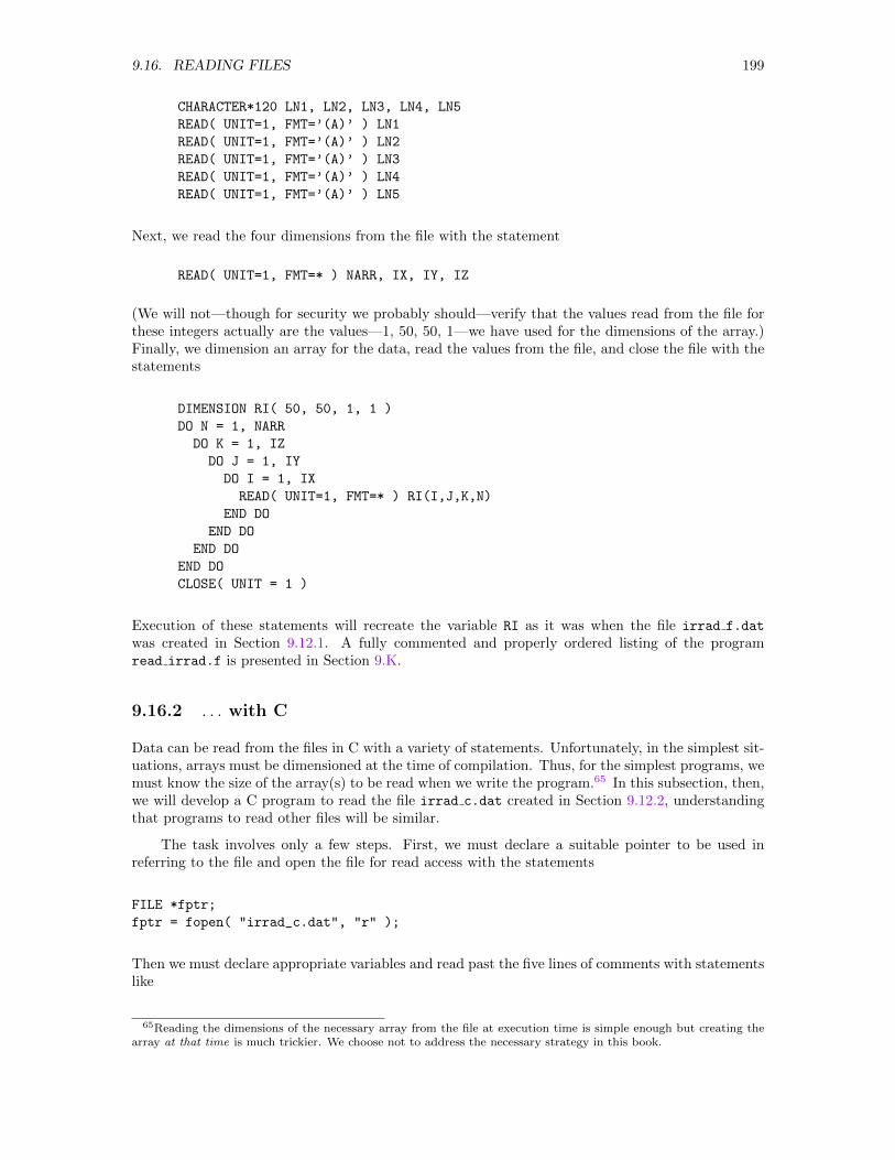
9.16. READING FILES 199

CHARACTER*120 LN1, LN2, LN3, LN4, LN5

READ( UNIT=1, FMT=’(A)’ ) LN1

READ( UNIT=1, FMT=’(A)’ ) LN2

READ( UNIT=1, FMT=’(A)’ ) LN3

READ( UNIT=1, FMT=’(A)’ ) LN4

READ( UNIT=1, FMT=’(A)’ ) LN5

Next, we read the four dimensions from the file with the statement

READ( UNIT=1, FMT=* ) NARR, IX, IY, IZ

(We will not—though for security we probably should—verify that the values read from the file forthese integers actually are the values—1, 50, 50, 1—we have used for the dimensions of the array.)Finally, we dimension an array for the data, read the values from the file, and close the file with thestatements

DIMENSION RI( 50, 50, 1, 1 )

DO N = 1, NARR

DO K = 1, IZ

DO J = 1, IY

DO I = 1, IX

READ( UNIT=1, FMT=* ) RI(I,J,K,N)

END DO

END DO

END DO

END DO

CLOSE( UNIT = 1 )

Execution of these statements will recreate the variable RI as it was when the file irrad f.dat

was created in Section 9.12.1. A fully commented and properly ordered listing of the programread irrad.f is presented in Section 9.K.

9.16.2 . . . with C

Data can be read from the files in C with a variety of statements. Unfortunately, in the simplest sit-uations, arrays must be dimensioned at the time of compilation. Thus, for the simplest programs, wemust know the size of the array(s) to be read when we write the program.65 In this subsection, then,we will develop a C program to read the file irrad c.dat created in Section 9.12.2, understandingthat programs to read other files will be similar.

The task involves only a few steps. First, we must declare a suitable pointer to be used inreferring to the file and open the file for read access with the statements

FILE *fptr;

fptr = fopen( "irrad_c.dat", "r" );

Then we must declare appropriate variables and read past the five lines of comments with statementslike

65Reading the dimensions of the necessary array from the file at execution time is simple enough but creating thearray at that time is much trickier. We choose not to address the necessary strategy in this book.

200 CHAPTER 9. INTRODUCTION TO PROGRAMMING

char ln1[120], ln2[120], ln3[120], ln4[120], ln5[120];

int narr, ix, iy, iz;

fgets( ln1, 120, fptr );

fgets( ln2, 120, fptr );

fgets( ln3, 120, fptr );

fgets( ln4, 120, fptr );

fgets( ln5, 120, fptr );

Next, we declare appropriate variables and read the four dimensions from the file with the statements

int narr, ix, iy, iz;

fscanf( fptr, "%d %d %d %d", narr, ix, iy, iz );

(We will not—though for security we probably should—verify that the values read from the file forthese integers actually are the values—1, 50, 50, 1—we have used for the dimensions of the array.)Finally, we declare an appropriate array for the data, declare integers for the loop indices, read thevalues from the file, and close the file with the statements

int n, i, j, k;

float I[50][50][1][1];

for( n=0; n<narr; n++ )

for( k=0; k<iz; k++ )

for( j=0; j<iy; j++ )

for( i=0; i<ix; i++ )

fscanf( fptr, "%g", &I[i][j][k][n] );

fclose( fptr );

Execution of these statements will recreate the variable I as it was when the file irrad c.dat

was created in Section 9.12.2. A fully commented and properly ordered listing of the programread irrad.c is presented in Section 9.L.

9.16.5 . . . with OCTAVE

The Lawrence-generated OCTAVE function luread list parallels the OCTAVE functionlugen list first described in Section 9.12.5 and provides the facility for reading into OCTAVE anyfile created in the format described in Section 9.3.2, whether the files were created with OCTAVEor some other program. We simply execute the statement

Var = luread_list( ’FileName’ )

where FileName is the name of the file containing the data to be read (including the file type) andVar is the name of the variable into which the data are to be placed when read. For example, thestatement

>> I = luread_list( ’irrad_octave.dat’ );

will recreate the variable I as it was when the file irrad matlab.dat was created in Section 9.12.5.As it executes, luread list displays the descriptive lines that were placed at the beginning of thefile when it was created. The procedure luread list.m that defines this function is presented inSection 9.J.

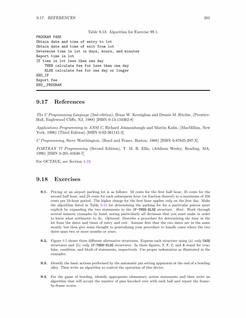
9.17. REFERENCES 201

Table 9.13: Algorithm for Exercise 99.1.PROGRAM PARK

Obtain date and time of entry to lot

Obtain date and time of exit from lot

Determine time in lot in days, hours, and minutes

Report time in lot

IF time in lot less than one day

THEN calculate fee for less than one day

ELSE calculate fee for one day or longer

END_IF

Report fee

END__PROGRAM

9.17 References

The C Programming Language (2nd edition), Brian W. Kernighan and Dennis M. Ritchie, (Prentice-Hall, Englewood Cliffs, NJ, 1988) [ISBN 0-13-110362-8]

Applications Programming in ANSI C, Richard Johnsonbaugh and Martin Kalin, (MacMillan, NewYork, 1996) (Third Edition) [ISBN 0-02-361141-3]

C Programming, Steve Worthington, (Boyd and Fraser, Boston, 1988) [ISBN 0-87835-297-X]

FORTRAN 77 Programming (Second Edition), T. M. R. Ellis, (Addison Wesley, Reading, MA,1990) [ISBN 0-201-41638-7]

For OCTAVE, see Section 4.19.

9.18 Exercises

9.1. Pricing at an airport parking lot is as follows: 50 cents for the first half hour, 35 cents for thesecond half hour, and 25 cents for each subsequent hour (or fraction thereof) to a maximum of 250cents per 24-hour period. The higher charge for the first hour applies only on the first day. Makethe algorithm listed in Table 9.13 for determining the parking fee for a particular patron moreexplicit by expanding the two statements in the IF-THEN-ELSE structure. Hint : Work throughseveral numeric examples by hand, noting particularly all decisions that you must make in orderto know what arithmetic to do. Optional : Describe a procedure for determining the time in thelot from the dates and times of entry and exit. Assume first that the two dates are in the samemonth, but then give some thought to generalizing your procedure to handle cases where the twodates span two or more months or years.

9.2. Figure 9.5 shows three different alternative structures. Express each structure using (a) only CASE

structures and (b) only IF-THEN-ELSE structures. In these figures, T, F, C, and B stand for true,false, condition, and block of statements, respectively. Use proper indentation as illustrated in theexamples.

9.3. Identify the basic actions performed by the automatic pin setting apparatus at the end of a bowlingalley. Then write an algorithm to control the operation of this device.

9.4. For the game of bowling, identify appropriate elementary action statements and then write analgorithm that will accept the number of pins knocked over with each ball and report the frame-by-frame scores.

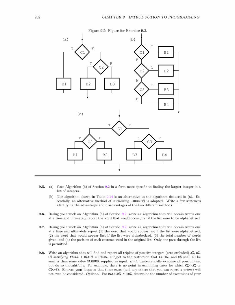
202 CHAPTER 9. INTRODUCTION TO PROGRAMMING

Figure 9.5: Figure for Exercise 9.2.

C1

B1

C2

C1

C2

C3

B2 B3

B1

B3

B2

(a)

B4

(b)

C1

C2 C3

B1 B3B2 B4

(c)

T

T

T

T

T T

T

T F

F

F F

F

F

F

F

9.5. (a) Cast Algorithm (6) of Section 9.2 in a form more specific to finding the largest integer in alist of integers.

(b) The algorithm shown in Table 9.14 is an alternative to the algorithm deduced in (a). Es-sentially, an alternative method of initializing LARGEST% is adopted. Write a few sentencesidentifying the advantages and disadvantages of the two different methods.

9.6. Basing your work on Algorithm (6) of Section 9.2, write an algorithm that will obtain words oneat a time and ultimately report the word that would occur first if the list were to be alphabetized.

9.7. Basing your work on Algorithm (6) of Section 9.2, write an algorithm that will obtain words oneat a time and ultimately report (1) the word that would appear last if the list were alphabetized,(2) the word that would appear first if the list were alphabetized, (3) the total number of wordsgiven, and (4) the position of each extreme word in the original list. Only one pass through the listis permitted.

9.8. Write an algorithm that will find and report all triplets of positive integers (zero excluded) A%, B%,C% satisfying A%*A% + B%*B% = C%*C%, subject to the restriction that A%, B%, and C% shall all besmaller than some value MAXNUM% supplied as input. Hint : Systematically examine all possibilities,but do so thoughtfully. For example, there is no point in examining cases for which C%<=A% orC%<=B%. Express your loops so that these cases (and any others that you can reject a priori) willnot even be considered. Optional : For MAXNUM% = 20%, determine the number of executions of your

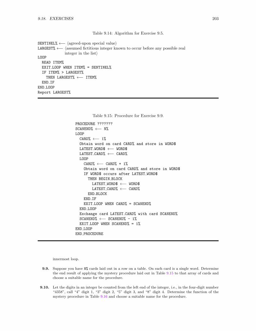
9.18. EXERCISES 203

Table 9.14: Algorithm for Exercise 9.5.

SENTINEL% ←− 〈agreed-upon special value〉LARGEST% ←− 〈assumed fictitious integer known to occur before any possible real

integer in the list〉LOOP

READ ITEM%

EXIT LOOP WHEN ITEM% = SENTINEL%

IF ITEM% > LARGEST%

THEN LARGEST% ←− ITEM%

END IF

END LOOP

Report LARGEST%

Table 9.15: Procedure for Exercise 9.9.

PROCEDURE ???????

SCANEND% ←− N%

LOOP

CARD% ←− 1%

Obtain word on card CARD% and store in WORD$

LATEST WORD$ ←− WORD$

LATEST CARD% ←− CARD%

LOOP

CARD% ←− CARD% + 1%

Obtain word on card CARD% and store in WORD$

IF WORD$ occurs after LATEST WORD$

THEN BEGIN BLOCK

LATEST WORD$ ←− WORD$

LATEST CARD% ←− CARD%

END BLOCK

END IF

EXIT LOOP WHEN CARD% = SCANEND%

END LOOP

Exchange card LATEST CARD% with card SCANEND%

SCANEND% ←− SCANEND% - 1%

EXIT LOOP WHEN SCANEND% = 1%

END LOOP

END PROCEDURE

innermost loop.

9.9. Suppose you have N% cards laid out in a row on a table. On each card is a single word. Determinethe end result of applying the mystery procedure laid out in Table 9.15 to that array of cards andchoose a suitable name for the procedure.

9.10. Let the digits in an integer be counted from the left end of the integer, i.e., in the four-digit number“4358”, call “4” digit 1, “3” digit 2, “5” digit 3, and “8” digit 4. Determine the function of themystery procedure in Table 9.16 and choose a suitable name for the procedure.

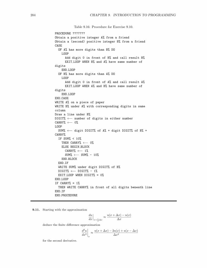
204 CHAPTER 9. INTRODUCTION TO PROGRAMMING

Table 9.16: Procedure for Exercise 9.10.

PROCEDURE ???????

Obtain a positive integer A% from a friend

Obtain a (second) positive integer B% from a friend

CASE

OF A% has more digits than B% DO

LOOP

Add digit 0 in front of B% and call result B%

EXIT LOOP WHEN B% and A% have same number of

digits

END LOOP

OF B% has more digits than A% DO

LOOP

Add digit 0 in front of A% and call result A%

EXIT LOOP WHEN A% and B% have same number of

digits

END LOOP

END CASE

WRITE A% on a piece of paper

WRITE B% under A% with corresponding digits in same

column

Draw a line under B%

DIGIT% ←− number of digits in either number

CARRY% ←− 0%

LOOP

SUM% ←− digit DIGIT% of A% + digit DIGIT% of B% +

CARRY%

IF SUM% < 10%

THEN CARRY% ←− 0%

ELSE BEGIN BLOCK

CARRY% ←− 1%

SUM% ←− SUM% - 10%

END BLOCK

END IF

WRITE SUM% under digit DIGIT% of B%

DIGIT% ←− DIGIT% - 1%

EXIT LOOP WHEN DIGIT% = 0%

END LOOP

IF CARRY% = 1%

THEN WRITE CARRY% in front of all digits beneath line

END IF

END PROCEDURE

9.11. Starting with the approximation

du

dx

∣∣∣x+ 1

2∆x≈ u(x+ ∆x)− u(x)

∆x

deduce the finite difference approximation

d2u

dx2

∣∣∣∣x

≈ u(x+ ∆x)− 2u(x) + u(x−∆x)

∆x2

for the second derivative.

9.18. EXERCISES 205

9.12. Write, compile, and test a program that asks for the input of a temperature in Celsius and printsout the corresponding temperature in Fahrenheit. To make it a bit more of a challenge, write theprogram in such a way that it asks repeatedly for Celsius temperatures until the temperature 9999is entered, at which point the program terminates smoothly.

9.13. (a) Copy laplace file.f from $HEAD/fortran to your directory, naming it laplace15 file.f.Then compile, link, and run laplace15 file.f to generate the file laplace f.dat, which youshould rename laplace15 f.dat.

(b) Produce the program laplace29 file.f by copying laplace15 file.f to the new file andediting the new file so that the program, when run, generates a solution on a 29× 29 grid.

(c) Compile, link, and run laplace29 file.f and rename the output file to laplace30 f.dat.

(d) Import both laplace15 f.dat and laplace30 f.dat into an available program for graphicalvisualization and then

i. generate a graphical display of each solution, either a contour map in the xy plane or asurface plot over the xy plane (or perhaps both). In either case (or both cases), makesure the axes are labeled correctly with the proper coordinate values. Warning : This latterrequirement is a bit subtle. Beware.

ii. develop a way to compare the two solutions at those grid points that are common to thetwo and display the differences graphically.

(e) Copy the file laplace29 file.f to a new name—your choice—and then edit that file so thatthe program it conveys monitors the change from one iteration to the next and displays onthe screen the maximum absolute value of the change that occurs during the course of eachiteration.

(f) Edit the last program again so that iteration is stopped when the maximum change falls belowa tolerance that is specified as input when the program is run (or—to prevent infinite loops—when the number of iterations exceeds some maximum value). Arrange for the program todisplay the number of iterations carried out when the solution finally converges. Compile,link, and run this last program and explore the way the number of iterations varies with thetolerance specified. Was 300 iterations as a trial in the original programs vast overkill?

9.14. (a) Copy laplace file.c from $HEAD/cc to your directory, naming it laplace15 file.c. Thencompile, link, and run laplace15 file.f to generate the file laplace c.dat, which you shouldrename laplace15 c.dat.

(b) Produce the program laplace29 file.f by copying laplace15 file.c to the new file andediting the new file so that the program, when run, generates a solution on a 29× 29 grid.

(c) Compile, link, and run laplace29 file.f and rename the output file to laplace30 f.dat.

(d) Import both laplace15 c.dat and laplace30 c.dat into an available program for graphicalvisualization and then

i. generate a graphical display of each solution, either a contour map in the xy plane or asurface plot over the xy plane (or perhaps both). In either case (or both cases), makesure the axes are labeled correctly with the proper coordinate values. Warning : This latterrequirement is a bit subtle. Beware.

ii. develop a way to compare the two solutions at those grid points that are common to thetwo and display the differences graphically.

(e) Copy the file laplace29 file.c to a new name—your choice—and then edit that file so thatthe program it conveys monitors the change from one iteration to the next and displays onthe screen the maximum absolute value of the change that occurs during the course of eachiteration.

(f) Edit the last program again so that iteration is stopped when the maximum change falls belowa tolerance that is specified as input when the program is run (or—to prevent infinite loops—when the number of iterations exceeds some maximum value). Arrange for the program todisplay the number of iterations carried out when the solution finally converges. Compile,link, and run this last program and explore the way the number of iterations varies with thetolerance specified. Was 300 iterations as a trial in the original programs vast overkill?

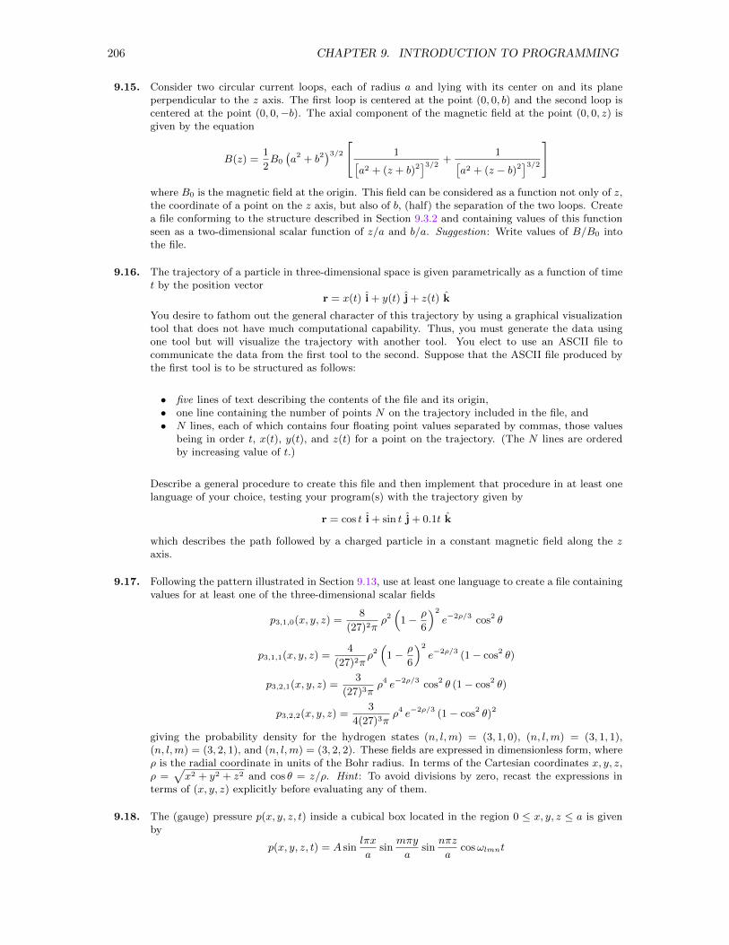
206 CHAPTER 9. INTRODUCTION TO PROGRAMMING

9.15. Consider two circular current loops, each of radius a and lying with its center on and its planeperpendicular to the z axis. The first loop is centered at the point (0, 0, b) and the second loop iscentered at the point (0, 0,−b). The axial component of the magnetic field at the point (0, 0, z) isgiven by the equation

B(z) =1

2B0

(a2 + b2

)3/2 [ 1[a2 + (z + b)2

]3/2 +1[

a2 + (z − b)2]3/2

]where B0 is the magnetic field at the origin. This field can be considered as a function not only of z,the coordinate of a point on the z axis, but also of b, (half) the separation of the two loops. Createa file conforming to the structure described in Section 9.3.2 and containing values of this functionseen as a two-dimensional scalar function of z/a and b/a. Suggestion: Write values of B/B0 intothe file.

9.16. The trajectory of a particle in three-dimensional space is given parametrically as a function of timet by the position vector

r = x(t) i + y(t) j + z(t) k

You desire to fathom out the general character of this trajectory by using a graphical visualizationtool that does not have much computational capability. Thus, you must generate the data usingone tool but will visualize the trajectory with another tool. You elect to use an ASCII file tocommunicate the data from the first tool to the second. Suppose that the ASCII file produced bythe first tool is to be structured as follows:

• five lines of text describing the contents of the file and its origin,• one line containing the number of points N on the trajectory included in the file, and• N lines, each of which contains four floating point values separated by commas, those values

being in order t, x(t), y(t), and z(t) for a point on the trajectory. (The N lines are orderedby increasing value of t.)

Describe a general procedure to create this file and then implement that procedure in at least onelanguage of your choice, testing your program(s) with the trajectory given by

r = cos t i + sin t j + 0.1t k

which describes the path followed by a charged particle in a constant magnetic field along the zaxis.

9.17. Following the pattern illustrated in Section 9.13, use at least one language to create a file containingvalues for at least one of the three-dimensional scalar fields

p3,1,0(x, y, z) =8

(27)2πρ2(

1− ρ

6

)2

e−2ρ/3 cos2 θ

p3,1,1(x, y, z) =4

(27)2πρ2(

1− ρ

6

)2

e−2ρ/3 (1− cos2 θ)

p3,2,1(x, y, z) =3

(27)3πρ4 e−2ρ/3 cos2 θ (1− cos2 θ)

p3,2,2(x, y, z) =3

4(27)3πρ4 e−2ρ/3 (1− cos2 θ)2

giving the probability density for the hydrogen states (n, l,m) = (3, 1, 0), (n, l,m) = (3, 1, 1),(n, l,m) = (3, 2, 1), and (n, l,m) = (3, 2, 2). These fields are expressed in dimensionless form, whereρ is the radial coordinate in units of the Bohr radius. In terms of the Cartesian coordinates x, y, z,ρ =

√x2 + y2 + z2 and cos θ = z/ρ. Hint : To avoid divisions by zero, recast the expressions in

terms of (x, y, z) explicitly before evaluating any of them.

9.18. The (gauge) pressure p(x, y, z, t) inside a cubical box located in the region 0 ≤ x, y, z ≤ a is givenby

p(x, y, z, t) = A sinlπx

asin

mπy

asin

nπz

acosωlmnt

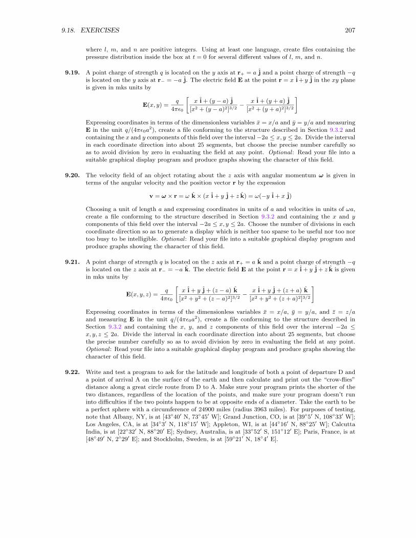
9.18. EXERCISES 207

where l, m, and n are positive integers. Using at least one language, create files containing thepressure distribution inside the box at t = 0 for several different values of l, m, and n.

9.19. A point charge of strength q is located on the y axis at r+ = a j and a point charge of strength −qis located on the y axis at r− = −a j. The electric field E at the point r = x i + y j in the xy planeis given in mks units by

E(x, y) =q

4πε0

[x i + (y − a) j

[x2 + (y − a)2]3/2− x i + (y + a) j

[x2 + (y + a)2]3/2

]Expressing coordinates in terms of the dimensionless variables x = x/a and y = y/a and measuringE in the unit q/(4πε0a

2), create a file conforming to the structure described in Section 9.3.2 andcontaining the x and y components of this field over the interval−2a ≤ x, y ≤ 2a. Divide the intervalin each coordinate direction into about 25 segments, but choose the precise number carefully soas to avoid division by zero in evaluating the field at any point. Optional : Read your file into asuitable graphical display program and produce graphs showing the character of this field.

9.20. The velocity field of an object rotating about the z axis with angular momentum ω is given interms of the angular velocity and the position vector r by the expression

v = ω × r = ω k× (x i + y j + z k) = ω(−y i + x j)

Choosing a unit of length a and expressing coordinates in units of a and velocities in units of ωa,create a file conforming to the structure described in Section 9.3.2 and containing the x and ycomponents of this field over the interval −2a ≤ x, y ≤ 2a. Choose the number of divisions in eachcoordinate direction so as to generate a display which is neither too sparse to be useful nor too nortoo busy to be intelligible. Optional : Read your file into a suitable graphical display program andproduce graphs showing the character of this field.

9.21. A point charge of strength q is located on the z axis at r+ = a k and a point charge of strength −qis located on the z axis at r− = −a k. The electric field E at the point r = x i + y j + z k is givenin mks units by

E(x, y, z) =q

4πε0

[x i + y j + (z − a) k

[x2 + y2 + (z − a)2]3/2− x i + y j + (z + a) k

[x2 + y2 + (z + a)2]3/2

]Expressing coordinates in terms of the dimensionless variables x = x/a, y = y/a, and z = z/aand measuring E in the unit q/(4πε0a

2), create a file conforming to the structure described inSection 9.3.2 and containing the x, y, and z components of this field over the interval −2a ≤x, y, z ≤ 2a. Divide the interval in each coordinate direction into about 25 segments, but choosethe precise number carefully so as to avoid division by zero in evaluating the field at any point.Optional : Read your file into a suitable graphical display program and produce graphs showing thecharacter of this field.

9.22. Write and test a program to ask for the latitude and longitude of both a point of departure D anda point of arrival A on the surface of the earth and then calculate and print out the “crow-flies”distance along a great circle route from D to A. Make sure your program prints the shorter of thetwo distances, regardless of the location of the points, and make sure your program doesn’t runinto difficulties if the two points happen to be at opposite ends of a diameter. Take the earth to bea perfect sphere with a circumference of 24900 miles (radius 3963 miles). For purposes of testing,note that Albany, NY, is at [4340′ N, 7345′ W]; Grand Junction, CO, is at [395′ N, 10833′ W];Los Angeles, CA, is at [343′ N, 11815′ W]; Appleton, WI, is at [4416′ N, 8825′ W]; CalcuttaIndia, is at [2232′ N, 8820′ E]; Sydney, Australia, is at [3352′ S, 15112′ E]; Paris, France, is at[4849′ N, 229′ E]; and Stockholm, Sweden, is at [5921′ N, 184′ E].

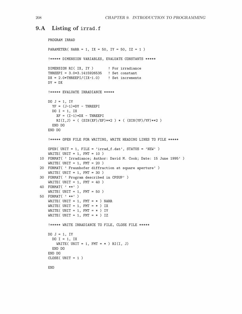
208 CHAPTER 9. INTRODUCTION TO PROGRAMMING

9.A Listing of irrad.f

PROGRAM IRRAD

PARAMETER( NARR = 1, IX = 50, IY = 50, IZ = 1 )

!***** DIMENSION VARIABLES, EVALUATE CONSTANTS *****

DIMENSION RI( IX, IY ) ! For irradiance

THREEPI = 3.0*3.1415926535 ! Set constant

DX = 2.0*THREEPI/(IX-1.0) ! Set increments

DY = DX

!***** EVALUATE IRRADIANCE *****

DO J = 1, IY

YF = (J-1)*DY - THREEPI

DO I = 1, IX

XF = (I-1)*DX - THREEPI

RI(I,J) = ( (SIN(XF)/XF)**2 ) * ( (SIN(YF)/YF)**2 )

END DO

END DO

!***** OPEN FILE FOR WRITING, WRITE HEADING LINES TO FILE *****

OPEN( UNIT = 1, FILE = ’irrad_f.dat’, STATUS = ’NEW’ )

WRITE( UNIT = 1, FMT = 10 )

10 FORMAT( ’ Irradiance; Author: David M. Cook; Date: 15 June 1995’ )

WRITE( UNIT = 1, FMT = 20 )

20 FORMAT( ’ Fraunhofer diffraction at square aperture’ )

WRITE( UNIT = 1, FMT = 30 )

30 FORMAT( ’ Program described in CPSUP’ )

WRITE( UNIT = 1, FMT = 40 )

40 FORMAT( ’ **’ )

WRITE( UNIT = 1, FMT = 50 )

50 FORMAT( ’ **’ )

WRITE( UNIT = 1, FMT = * ) NARR

WRITE( UNIT = 1, FMT = * ) IX

WRITE( UNIT = 1, FMT = * ) IY

WRITE( UNIT = 1, FMT = * ) IZ

!***** WRITE IRRADIANCE TO FILE, CLOSE FILE *****

DO J = 1, IY

DO I = 1, IX

WRITE( UNIT = 1, FMT = * ) RI(I, J)

END DO

END DO

CLOSE( UNIT = 1 )

END

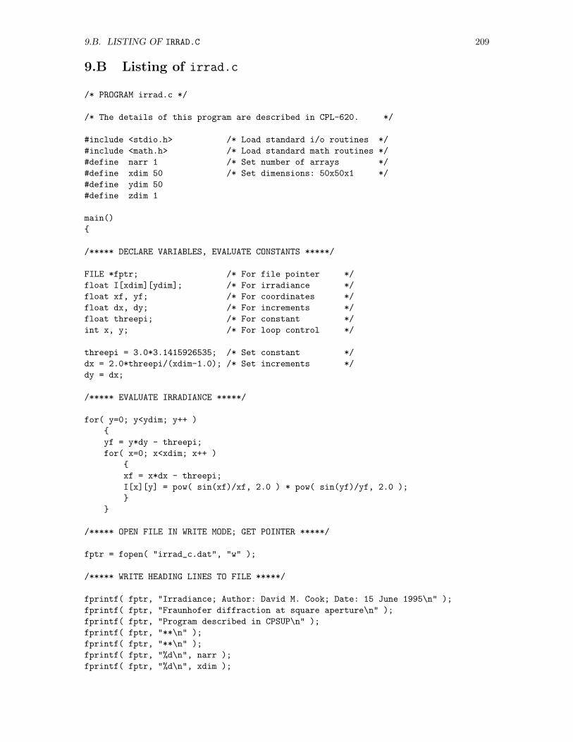
9.B. LISTING OF IRRAD.C 209

9.B Listing of irrad.c

/* PROGRAM irrad.c */

/* The details of this program are described in CPL-620. */

#include <stdio.h> /* Load standard i/o routines */

#include <math.h> /* Load standard math routines */

#define narr 1 /* Set number of arrays */

#define xdim 50 /* Set dimensions: 50x50x1 */

#define ydim 50

#define zdim 1

main()

/***** DECLARE VARIABLES, EVALUATE CONSTANTS *****/

FILE *fptr; /* For file pointer */

float I[xdim][ydim]; /* For irradiance */

float xf, yf; /* For coordinates */

float dx, dy; /* For increments */

float threepi; /* For constant */

int x, y; /* For loop control */

threepi = 3.0*3.1415926535; /* Set constant */

dx = 2.0*threepi/(xdim-1.0); /* Set increments */

dy = dx;

/***** EVALUATE IRRADIANCE *****/

for( y=0; y<ydim; y++ )

yf = y*dy - threepi;

for( x=0; x<xdim; x++ )

xf = x*dx - threepi;

I[x][y] = pow( sin(xf)/xf, 2.0 ) * pow( sin(yf)/yf, 2.0 );

/***** OPEN FILE IN WRITE MODE; GET POINTER *****/

fptr = fopen( "irrad_c.dat", "w" );

/***** WRITE HEADING LINES TO FILE *****/

fprintf( fptr, "Irradiance; Author: David M. Cook; Date: 15 June 1995\n" );

fprintf( fptr, "Fraunhofer diffraction at square aperture\n" );

fprintf( fptr, "Program described in CPSUP\n" );

fprintf( fptr, "**\n" );

fprintf( fptr, "**\n" );

fprintf( fptr, "%d\n", narr );

fprintf( fptr, "%d\n", xdim );

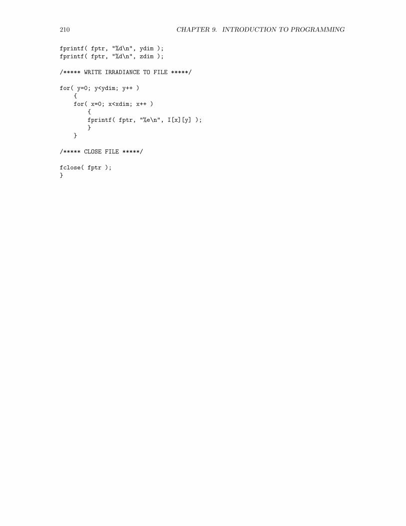
210 CHAPTER 9. INTRODUCTION TO PROGRAMMING

fprintf( fptr, "%d\n", ydim );

fprintf( fptr, "%d\n", zdim );

/***** WRITE IRRADIANCE TO FILE *****/

for( y=0; y<ydim; y++ )

for( x=0; x<xdim; x++ )

fprintf( fptr, "%e\n", I[x][y] );

/***** CLOSE FILE *****/

fclose( fptr );

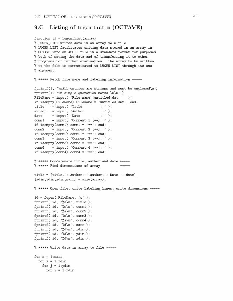
9.C. LISTING OF LUGEN LIST.M (OCTAVE) 211

9.C Listing of lugen list.m (OCTAVE)

function [] = lugen_list(array)

% LUGEN_LIST writes data in an array to a file

% LUGEN_LIST facilitates writing data stored in an array in

% OCTAVE into an ASCII file in a standard format for purposes

% both of saving the data and of transferring it to other

% programs for further examination. The array to be written

% to the file is communicated to LUGEN_LIST through its one

% argument.

% ***** Fetch file name and labeling information *****

fprintf(1, ’\nAll entries are strings and must be enclosed\n’)

fprintf(1, ’in single quotation marks.\n\n’ )

FileName = input( ’File name [untitled.dat]: ’ );

if isempty(FileName) FileName = ’untitled.dat’; end;

title = input( ’Title : ’ );

author = input( ’Author : ’ );

date = input( ’Date : ’ );

comm1 = input( ’Comment 1 [**]: ’ );

if isempty(comm1) comm1 = ’**’; end;

comm2 = input( ’Comment 2 [**]: ’ );

if isempty(comm2) comm2 = ’**’; end;

comm3 = input( ’Comment 3 [**]: ’ );

if isempty(comm3) comm3 = ’**’; end;

comm4 = input( ’Comment 4 [**]: ’ );

if isempty(comm4) comm4 = ’**’; end;

% ***** Concatenate title, author and date *****

% ***** Find dimensiions of array *****

title = [title,’; Author: ’,author,’; Date: ’,date];

[xdim,ydim,zdim,narr] = size(array);

% ***** Open file, write labeling lines, write dimensions *****

id = fopen( FileName, ’w’ );

fprintf( id, ’%s\n’, title );

fprintf( id, ’%s\n’, comm1 );

fprintf( id, ’%s\n’, comm2 );

fprintf( id, ’%s\n’, comm3 );

fprintf( id, ’%s\n’, comm4 );

fprintf( id, ’%d\n’, narr );

fprintf( id, ’%d\n’, xdim );

fprintf( id, ’%d\n’, ydim );

fprintf( id, ’%d\n’, zdim );

% ***** Write data in array to file *****

for n = 1:narr

for k = 1:zdim

for j = 1:ydim

for i = 1:xdim

212 CHAPTER 9. INTRODUCTION TO PROGRAMMING

fprintf( id, ’%g\n’, array(i,j,k,n) );

end

end

end

end

% ***** Close file; print message to screen *****

status = fclose( id );

fprintf(1, [’\nFile ’’’,FileName,’’’ saved successfully!\n’] )

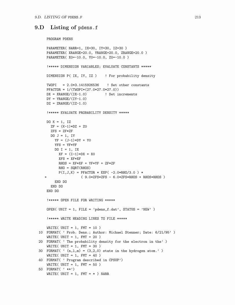
9.D. LISTING OF PDENS.F 213

9.D Listing of pdens.f

PROGRAM PDENS

PARAMETER( NARR=1, IX=30, IY=30, IZ=30 )

PARAMETER( XRANGE=20.0, YRANGE=20.0, ZRANGE=20.0 )

PARAMETER( X0=-10.0, Y0=-10.0, Z0=-10.0 )

!***** DIMENSION VARIABLES; EVALUATE CONSTANTS *****

DIMENSION P( IX, IY, IZ ) ! For probability density

TWOPI = 2.0*3.1415926536 ! Set other constants

PFACTOR = 1/(TWOPI*(27.0*27.0*27.0))

DX = XRANGE/(IX-1.0) ! Set increments

DY = YRANGE/(IY-1.0)

DZ = ZRANGE/(IZ-1.0)

!***** EVALUATE PROBABILITY DENSITY *****

DO K = 1, IZ

ZF = (K-1)*DZ + Z0

ZFS = ZF*ZF

DO J = 1, IY

YF = (J-1)*DY + Y0

YFS = YF*YF

DO I = 1, IX

XF = (I-1)*DX + X0

XFS = XF*XF

RHOS = XF*XF + YF*YF + ZF*ZF

RHO = SQRT(RHOS)

P(I,J,K) = PFACTOR * EXP( -2.0*RHO/3.0 ) *

+ ( 9.0*ZFS*ZFS - 6.0*ZFS*RHOS + RHOS*RHOS )

END DO

END DO

END DO

!***** OPEN FILE FOR WRITING *****

OPEN( UNIT = 1, FILE = ’pdens_f.dat’, STATUS = ’NEW’ )

!***** WRITE HEADING LINES TO FILE *****

WRITE( UNIT = 1, FMT = 10 )

10 FORMAT( ’ Prob. Dens.; Author: Michael Stenner; Date: 6/21/95’ )

WRITE( UNIT = 1, FMT = 20 )

20 FORMAT( ’ The probability density for the electron in the’ )

WRITE( UNIT = 1, FMT = 30 )

30 FORMAT( ’ (n,l,m) = (3,2,0) state in the hydrogen atom.’ )

WRITE( UNIT = 1, FMT = 40 )

40 FORMAT( ’ Program described in CPSUP’)

WRITE( UNIT = 1, FMT = 50 )

50 FORMAT( ’ **’)

WRITE( UNIT = 1, FMT = * ) NARR

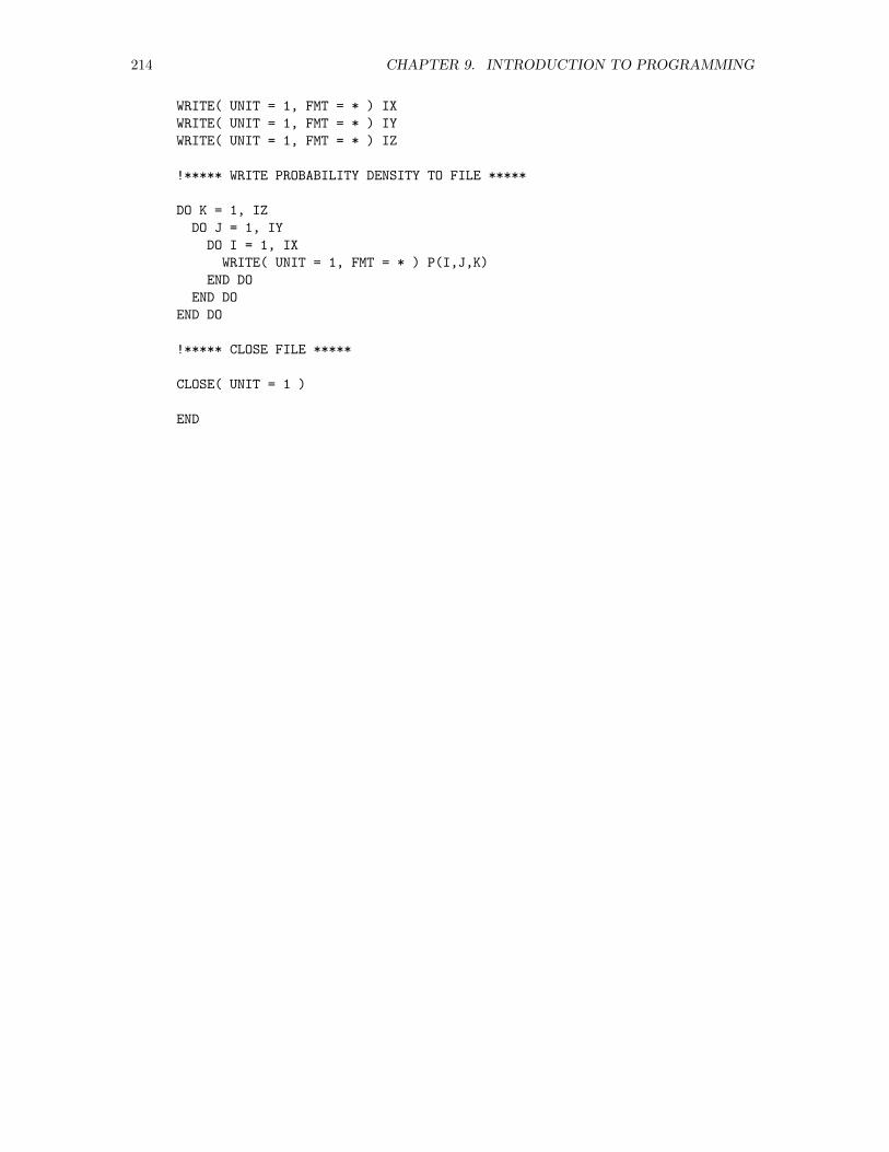
214 CHAPTER 9. INTRODUCTION TO PROGRAMMING

WRITE( UNIT = 1, FMT = * ) IX

WRITE( UNIT = 1, FMT = * ) IY

WRITE( UNIT = 1, FMT = * ) IZ

!***** WRITE PROBABILITY DENSITY TO FILE *****

DO K = 1, IZ

DO J = 1, IY

DO I = 1, IX

WRITE( UNIT = 1, FMT = * ) P(I,J,K)

END DO

END DO

END DO

!***** CLOSE FILE *****

CLOSE( UNIT = 1 )

END

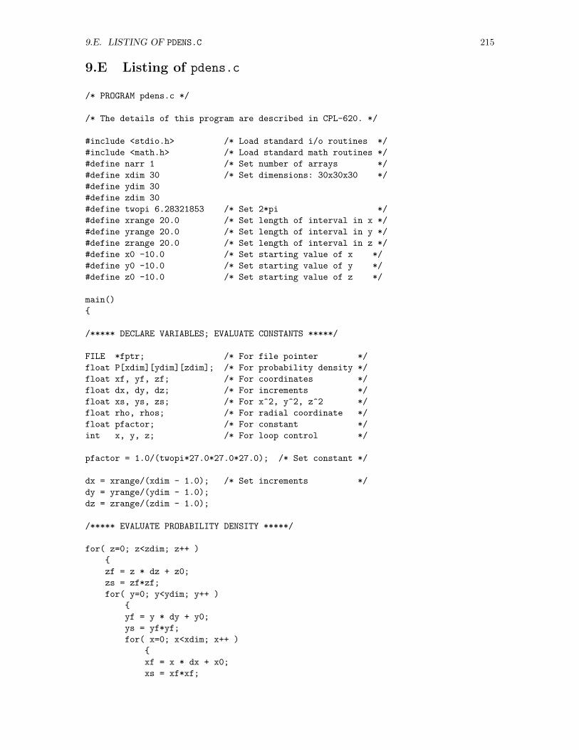
9.E. LISTING OF PDENS.C 215

9.E Listing of pdens.c

/* PROGRAM pdens.c */

/* The details of this program are described in CPL-620. */

#include <stdio.h> /* Load standard i/o routines */

#include <math.h> /* Load standard math routines */

#define narr 1 /* Set number of arrays */

#define xdim 30 /* Set dimensions: 30x30x30 */

#define ydim 30

#define zdim 30

#define twopi 6.28321853 /* Set 2*pi */

#define xrange 20.0 /* Set length of interval in x */

#define yrange 20.0 /* Set length of interval in y */

#define zrange 20.0 /* Set length of interval in z */

#define x0 -10.0 /* Set starting value of x */

#define y0 -10.0 /* Set starting value of y */

#define z0 -10.0 /* Set starting value of z */

main()

/***** DECLARE VARIABLES; EVALUATE CONSTANTS *****/

FILE *fptr; /* For file pointer */

float P[xdim][ydim][zdim]; /* For probability density */

float xf, yf, zf; /* For coordinates */

float dx, dy, dz; /* For increments */

float xs, ys, zs; /* For x^2, y^2, z^2 */

float rho, rhos; /* For radial coordinate */

float pfactor; /* For constant */

int x, y, z; /* For loop control */

pfactor = 1.0/(twopi*27.0*27.0*27.0); /* Set constant */

dx = xrange/(xdim - 1.0); /* Set increments */

dy = yrange/(ydim - 1.0);

dz = zrange/(zdim - 1.0);

/***** EVALUATE PROBABILITY DENSITY *****/

for( z=0; z<zdim; z++ )

zf = z * dz + z0;

zs = zf*zf;

for( y=0; y<ydim; y++ )

yf = y * dy + y0;

ys = yf*yf;

for( x=0; x<xdim; x++ )

xf = x * dx + x0;

xs = xf*xf;

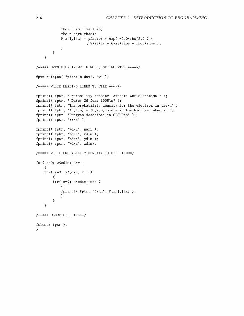
216 CHAPTER 9. INTRODUCTION TO PROGRAMMING

rhos = xs + ys + zs;

rho = sqrt(rhos);

P[x][y][z] = pfactor * exp( -2.0*rho/3.0 ) *

( 9*zs*zs - 6*zs*rhos + rhos*rhos );

/***** OPEN FILE IN WRITE MODE; GET POINTER *****/

fptr = fopen( "pdens_c.dat", "w" );

/***** WRITE HEADING LINES TO FILE *****/

fprintf( fptr, "Probability density; Author: Chris Schmidt;" );

fprintf( fptr, " Date: 26 June 1995\n" );

fprintf( fptr, "The probability density for the electron in the\n" );

fprintf( fptr, "(n,l,m) = (3,2,0) state in the hydrogen atom.\n" );

fprintf( fptr, "Program described in CPSUP\n" );

fprintf( fptr, "**\n" );

fprintf( fptr, "%d\n", narr );

fprintf( fptr, "%d\n", zdim );

fprintf( fptr, "%d\n", ydim );

fprintf( fptr, "%d\n", xdim);

/***** WRITE PROBABILITY DENSITY TO FILE *****/

for( z=0; z<zdim; z++ )

for( y=0; y<ydim; y++ )

for( x=0; x<xdim; x++ )

fprintf( fptr, "%e\n", P[x][y][z] );

/***** CLOSE FILE *****/

fclose( fptr );

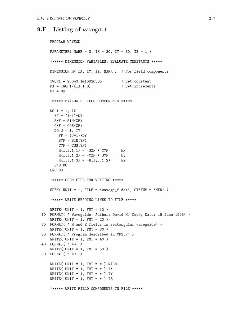
9.F. LISTING OF WAVEGD.F 217

9.F Listing of wavegd.f

PROGRAM WAVEGD

PARAMETER( NARR = 3, IX = 30, IY = 30, IZ = 1 )

!***** DIMENSION VARIABLES; EVALUATE CONSTANTS *****

DIMENSION H( IX, IY, IZ, NARR ) ! For field components

TWOPI = 2.0*3.1415926535 ! Set constant

DX = TWOPI/(IX-1.0) ! Set increments

DY = DX

!***** EVALUATE FIELD COMPONENTS *****

DO I = 1, IX

XF = (I-1)*DX

SXF = SIN(XF)

CXF = COS(XF)

DO J = 1, IY

YF = (J-1)*DY

SYF = SIN(YF)

CYF = COS(YF)

H(I,J,1,1) = SXF * CYF ! Hx

H(I,J,1,2) = -CXF * SYF ! Hy

H(I,J,1,3) = -H(I,J,1,2) ! Ez

END DO

END DO

!***** OPEN FILE FOR WRITING *****

OPEN( UNIT = 1, FILE = ’wavegd_f.dat’, STATUS = ’NEW’ )

!***** WRITE HEADING LINES TO FILE *****

WRITE( UNIT = 1, FMT = 10 )

10 FORMAT( ’ Waveguide; Author: David M. Cook; Date: 15 June 1995’ )

WRITE( UNIT = 1, FMT = 20 )

20 FORMAT( ’ H and E fields in rectangular waveguide’ )

WRITE( UNIT = 1, FMT = 30 )

30 FORMAT( ’ Program described in CPSUP’ )

WRITE( UNIT = 1, FMT = 40 )

40 FORMAT( ’ **’ )

WRITE( UNIT = 1, FMT = 50 )

50 FORMAT( ’ **’ )

WRITE( UNIT = 1, FMT = * ) NARR

WRITE( UNIT = 1, FMT = * ) IX

WRITE( UNIT = 1, FMT = * ) IY

WRITE( UNIT = 1, FMT = * ) IZ

!***** WRITE FIELD COMPONENTS TO FILE *****

218 CHAPTER 9. INTRODUCTION TO PROGRAMMING

DO N = 1, NARR ! Write H to file

DO J = 1, IY

DO I = 1, IX

WRITE( UNIT = 1, FMT = * ) H(I,J,1,N)

END DO

END DO

END DO

!***** CLOSE FILE *****

CLOSE( UNIT = 1 )

END

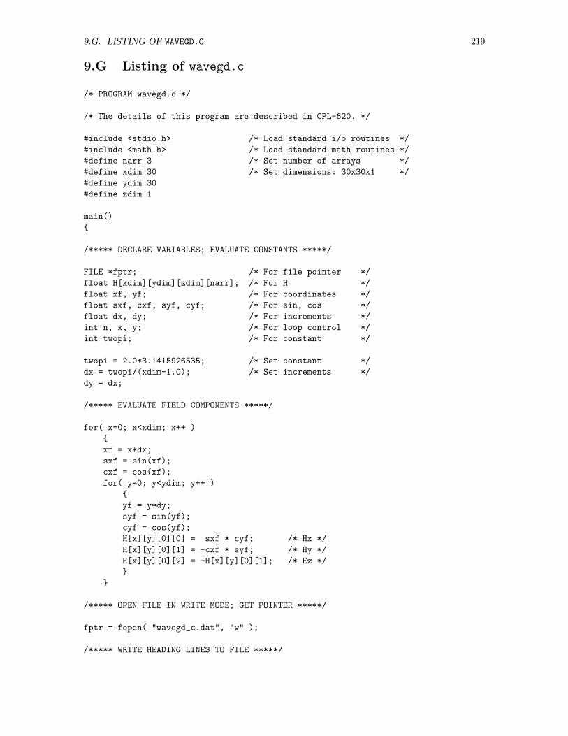
9.G. LISTING OF WAVEGD.C 219

9.G Listing of wavegd.c

/* PROGRAM wavegd.c */

/* The details of this program are described in CPL-620. */

#include <stdio.h> /* Load standard i/o routines */

#include <math.h> /* Load standard math routines */

#define narr 3 /* Set number of arrays */

#define xdim 30 /* Set dimensions: 30x30x1 */

#define ydim 30

#define zdim 1

main()

/***** DECLARE VARIABLES; EVALUATE CONSTANTS *****/

FILE *fptr; /* For file pointer */

float H[xdim][ydim][zdim][narr]; /* For H */

float xf, yf; /* For coordinates */

float sxf, cxf, syf, cyf; /* For sin, cos */

float dx, dy; /* For increments */

int n, x, y; /* For loop control */

int twopi; /* For constant */

twopi = 2.0*3.1415926535; /* Set constant */

dx = twopi/(xdim-1.0); /* Set increments */

dy = dx;

/***** EVALUATE FIELD COMPONENTS *****/

for( x=0; x<xdim; x++ )

xf = x*dx;

sxf = sin(xf);

cxf = cos(xf);

for( y=0; y<ydim; y++ )

yf = y*dy;

syf = sin(yf);

cyf = cos(yf);

H[x][y][0][0] = sxf * cyf; /* Hx */

H[x][y][0][1] = -cxf * syf; /* Hy */

H[x][y][0][2] = -H[x][y][0][1]; /* Ez */

/***** OPEN FILE IN WRITE MODE; GET POINTER *****/

fptr = fopen( "wavegd_c.dat", "w" );

/***** WRITE HEADING LINES TO FILE *****/

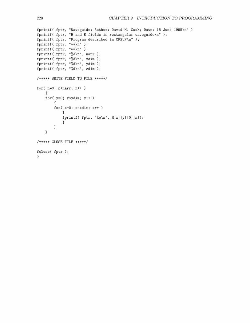
220 CHAPTER 9. INTRODUCTION TO PROGRAMMING

fprintf( fptr, "Waveguide; Author: David M. Cook; Date: 15 June 1995\n" );

fprintf( fptr, "H and E fields in rectangular waveguide\n" );

fprintf( fptr, "Program described in CPSUP\n" );

fprintf( fptr, "**\n" );

fprintf( fptr, "**\n" );

fprintf( fptr, "%d\n", narr );

fprintf( fptr, "%d\n", xdim );

fprintf( fptr, "%d\n", ydim );

fprintf( fptr, "%d\n", zdim );

/***** WRITE FIELD TO FILE *****/

for( n=0; n<narr; n++ )

for( y=0; y<ydim; y++ )

for( x=0; x<xdim; x++ )

fprintf( fptr, "%e\n", H[x][y][0][n]);

/***** CLOSE FILE *****/

fclose( fptr );

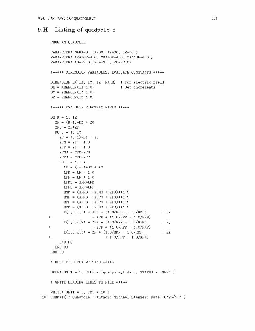
9.H. LISTING OF QUADPOLE.F 221

9.H Listing of quadpole.f

PROGRAM QUADPOLE

PARAMETER( NARR=3, IX=30, IY=30, IZ=30 )

PARAMETER( XRANGE=4.0, YRANGE=4.0, ZRANGE=4.0 )

PARAMETER( X0=-2.0, Y0=-2.0, Z0=-2.0)

!***** DIMENSION VARIABLES; EVALUATE CONSTANTS *****

DIMENSION E( IX, IY, IZ, NARR) ! For electric field

DX = XRANGE/(IX-1.0) ! Set increments

DY = YRANGE/(IY-1.0)

DZ = ZRANGE/(IZ-1.0)

!***** EVALUATE ELECTRIC FIELD *****

DO K = 1, IZ

ZF = (K-1)*DZ + Z0

ZFS = ZF*ZF

DO J = 1, IY

YF = (J-1)*DY + Y0

YFM = YF - 1.0

YFP = YF + 1.0

YFMS = YFM*YFM

YFPS = YFP*YFP

DO I = 1, IX

XF = (I-1)*DX + X0

XFM = XF - 1.0

XFP = XF + 1.0

XFMS = XFM*XFM

XFPS = XFP*XFP

RMM = (XFMS + YFMS + ZFS)**1.5

RMP = (XFMS + YFPS + ZFS)**1.5

RPP = (XFPS + YFPS + ZFS)**1.5

RPM = (XFPS + YFMS + ZFS)**1.5

E(I,J,K,1) = XFM * (1.0/RMM - 1.0/RMP) ! Ex

+ + XFP * (1.0/RPP - 1.0/RPM)

E(I,J,K,2) = YFM * (1.0/RMM - 1.0/RPM) ! Ey

+ + YFP * (1.0/RPP - 1.0/RMP)

E(I,J,K,3) = ZF * (1.0/RMM - 1.0/RMP ! Ez

+ + 1.0/RPP - 1.0/RPM)

END DO

END DO

END DO

! OPEN FILE FOR WRITING *****

OPEN( UNIT = 1, FILE = ’quadpole_f.dat’, STATUS = ’NEW’ )

! WRITE HEADING LINES TO FILE *****

WRITE( UNIT = 1, FMT = 10 )

10 FORMAT( ’ Quadpole.; Author: Michael Stenner; Date: 6/26/95’ )

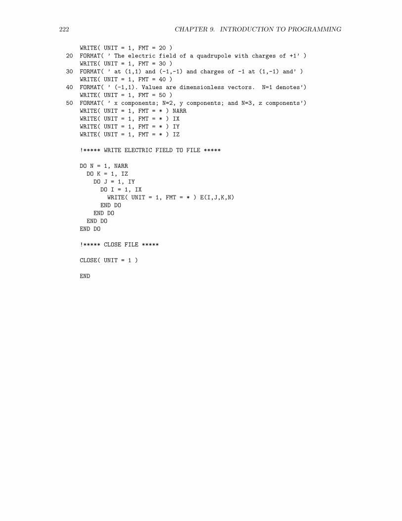
222 CHAPTER 9. INTRODUCTION TO PROGRAMMING

WRITE( UNIT = 1, FMT = 20 )

20 FORMAT( ’ The electric field of a quadrupole with charges of +1’ )

WRITE( UNIT = 1, FMT = 30 )

30 FORMAT( ’ at (1,1) and (-1,-1) and charges of -1 at (1,-1) and’ )

WRITE( UNIT = 1, FMT = 40 )

40 FORMAT( ’ (-1,1). Values are dimensionless vectors. N=1 denotes’)

WRITE( UNIT = 1, FMT = 50 )

50 FORMAT( ’ x components; N=2, y components; and N=3, z components’)

WRITE( UNIT = 1, FMT = * ) NARR

WRITE( UNIT = 1, FMT = * ) IX

WRITE( UNIT = 1, FMT = * ) IY

WRITE( UNIT = 1, FMT = * ) IZ

!***** WRITE ELECTRIC FIELD TO FILE *****

DO N = 1, NARR

DO K = 1, IZ

DO J = 1, IY

DO I = 1, IX

WRITE( UNIT = 1, FMT = * ) E(I,J,K,N)

END DO

END DO

END DO

END DO

!***** CLOSE FILE *****

CLOSE( UNIT = 1 )

END

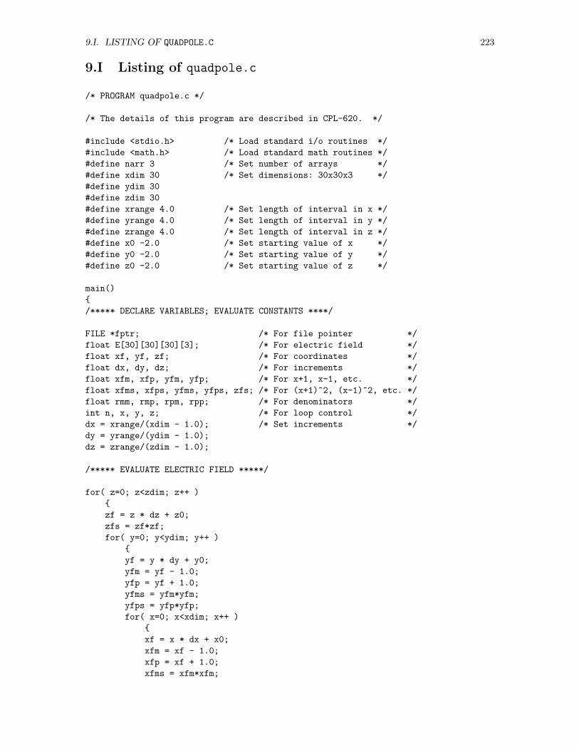
9.I. LISTING OF QUADPOLE.C 223

9.I Listing of quadpole.c

/* PROGRAM quadpole.c */

/* The details of this program are described in CPL-620. */

#include <stdio.h> /* Load standard i/o routines */

#include <math.h> /* Load standard math routines */

#define narr 3 /* Set number of arrays */

#define xdim 30 /* Set dimensions: 30x30x3 */

#define ydim 30

#define zdim 30

#define xrange 4.0 /* Set length of interval in x */

#define yrange 4.0 /* Set length of interval in y */

#define zrange 4.0 /* Set length of interval in z */

#define x0 -2.0 /* Set starting value of x */

#define y0 -2.0 /* Set starting value of y */

#define z0 -2.0 /* Set starting value of z */

main()

/***** DECLARE VARIABLES; EVALUATE CONSTANTS ****/

FILE *fptr; /* For file pointer */

float E[30][30][30][3]; /* For electric field */

float xf, yf, zf; /* For coordinates */

float dx, dy, dz; /* For increments */

float xfm, xfp, yfm, yfp; /* For x+1, x-1, etc. */

float xfms, xfps, yfms, yfps, zfs; /* For (x+1)^2, (x-1)^2, etc. */

float rmm, rmp, rpm, rpp; /* For denominators */

int n, x, y, z; /* For loop control */

dx = xrange/(xdim - 1.0); /* Set increments */

dy = yrange/(ydim - 1.0);

dz = zrange/(zdim - 1.0);

/***** EVALUATE ELECTRIC FIELD *****/

for( z=0; z<zdim; z++ )

zf = z * dz + z0;

zfs = zf*zf;

for( y=0; y<ydim; y++ )

yf = y * dy + y0;

yfm = yf - 1.0;

yfp = yf + 1.0;

yfms = yfm*yfm;

yfps = yfp*yfp;

for( x=0; x<xdim; x++ )

xf = x * dx + x0;

xfm = xf - 1.0;

xfp = xf + 1.0;

xfms = xfm*xfm;

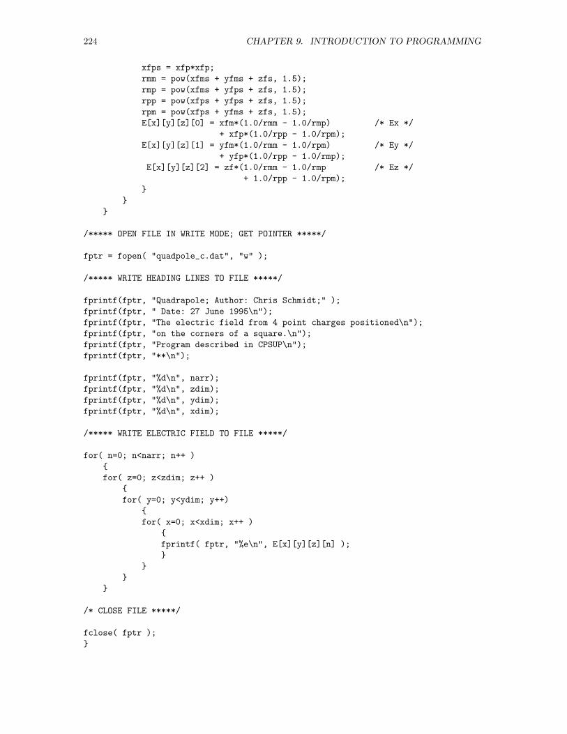
224 CHAPTER 9. INTRODUCTION TO PROGRAMMING

xfps = xfp*xfp;

rmm = pow(xfms + yfms + zfs, 1.5);

rmp = pow(xfms + yfps + zfs, 1.5);

rpp = pow(xfps + yfps + zfs, 1.5);

rpm = pow(xfps + yfms + zfs, 1.5);

E[x][y][z][0] = xfm*(1.0/rmm - 1.0/rmp) /* Ex */

+ xfp*(1.0/rpp - 1.0/rpm);

E[x][y][z][1] = yfm*(1.0/rmm - 1.0/rpm) /* Ey */

+ yfp*(1.0/rpp - 1.0/rmp);

E[x][y][z][2] = zf*(1.0/rmm - 1.0/rmp /* Ez */

+ 1.0/rpp - 1.0/rpm);

/***** OPEN FILE IN WRITE MODE; GET POINTER *****/

fptr = fopen( "quadpole_c.dat", "w" );

/***** WRITE HEADING LINES TO FILE *****/

fprintf(fptr, "Quadrapole; Author: Chris Schmidt;" );

fprintf(fptr, " Date: 27 June 1995\n");

fprintf(fptr, "The electric field from 4 point charges positioned\n");

fprintf(fptr, "on the corners of a square.\n");

fprintf(fptr, "Program described in CPSUP\n");

fprintf(fptr, "**\n");

fprintf(fptr, "%d\n", narr);

fprintf(fptr, "%d\n", zdim);

fprintf(fptr, "%d\n", ydim);

fprintf(fptr, "%d\n", xdim);

/***** WRITE ELECTRIC FIELD TO FILE *****/

for( n=0; n<narr; n++ )

for( z=0; z<zdim; z++ )

for( y=0; y<ydim; y++)

for( x=0; x<xdim; x++ )

fprintf( fptr, "%e\n", E[x][y][z][n] );

/* CLOSE FILE *****/

fclose( fptr );

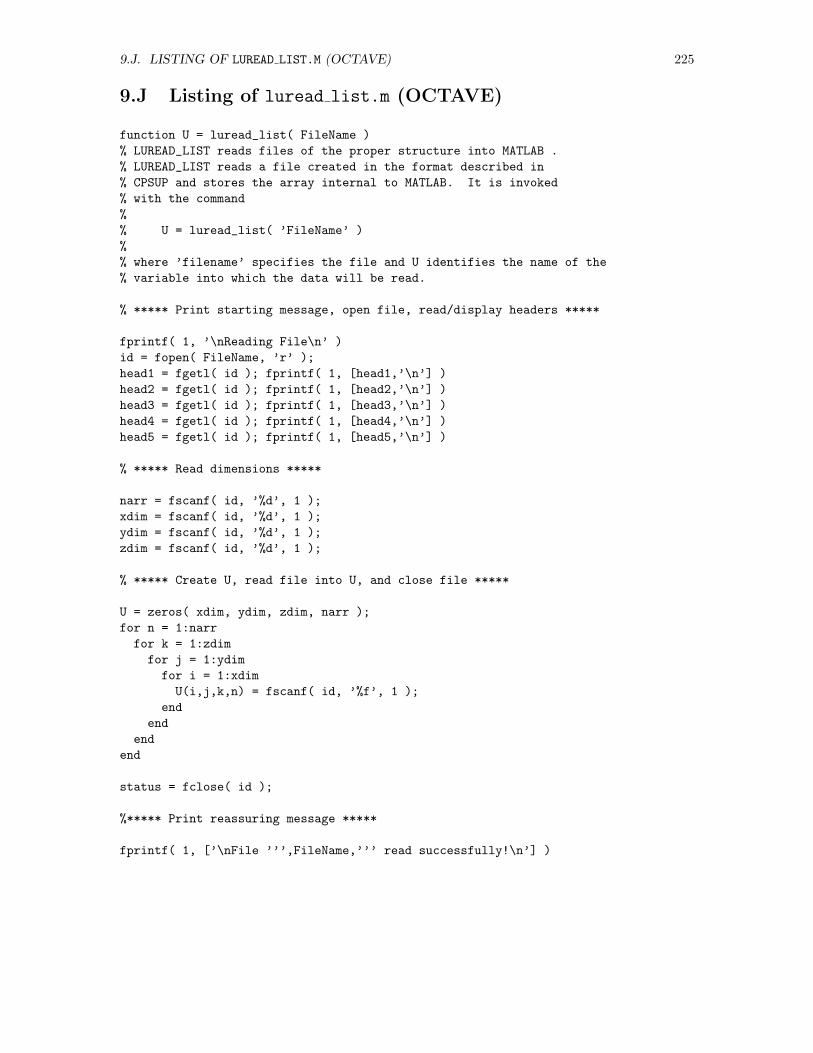
9.J. LISTING OF LUREAD LIST.M (OCTAVE) 225

9.J Listing of luread list.m (OCTAVE)

function U = luread_list( FileName )

% LUREAD_LIST reads files of the proper structure into MATLAB .

% LUREAD_LIST reads a file created in the format described in

% CPSUP and stores the array internal to MATLAB. It is invoked

% with the command

%

% U = luread_list( ’FileName’ )

%

% where ’filename’ specifies the file and U identifies the name of the

% variable into which the data will be read.

% ***** Print starting message, open file, read/display headers *****

fprintf( 1, ’\nReading File\n’ )

id = fopen( FileName, ’r’ );

head1 = fgetl( id ); fprintf( 1, [head1,’\n’] )

head2 = fgetl( id ); fprintf( 1, [head2,’\n’] )

head3 = fgetl( id ); fprintf( 1, [head3,’\n’] )

head4 = fgetl( id ); fprintf( 1, [head4,’\n’] )

head5 = fgetl( id ); fprintf( 1, [head5,’\n’] )

% ***** Read dimensions *****

narr = fscanf( id, ’%d’, 1 );

xdim = fscanf( id, ’%d’, 1 );

ydim = fscanf( id, ’%d’, 1 );

zdim = fscanf( id, ’%d’, 1 );

% ***** Create U, read file into U, and close file *****

U = zeros( xdim, ydim, zdim, narr );

for n = 1:narr

for k = 1:zdim

for j = 1:ydim

for i = 1:xdim

U(i,j,k,n) = fscanf( id, ’%f’, 1 );

end

end

end

end

status = fclose( id );

%***** Print reassuring message *****

fprintf( 1, [’\nFile ’’’,FileName,’’’ read successfully!\n’] )

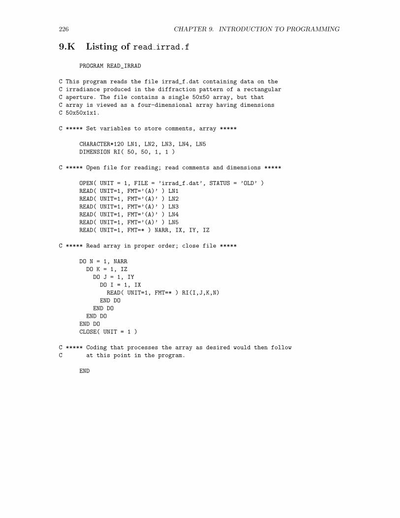
226 CHAPTER 9. INTRODUCTION TO PROGRAMMING

9.K Listing of read irrad.f

PROGRAM READ_IRRAD

C This program reads the file irrad_f.dat containing data on the

C irradiance produced in the diffraction pattern of a rectangular

C aperture. The file contains a single 50x50 array, but that

C array is viewed as a four-dimensional array having dimensions

C 50x50x1x1.

C ***** Set variables to store comments, array *****

CHARACTER*120 LN1, LN2, LN3, LN4, LN5

DIMENSION RI( 50, 50, 1, 1 )

C ***** Open file for reading; read comments and dimensions *****

OPEN( UNIT = 1, FILE = ’irrad_f.dat’, STATUS = ’OLD’ )

READ( UNIT=1, FMT=’(A)’ ) LN1

READ( UNIT=1, FMT=’(A)’ ) LN2

READ( UNIT=1, FMT=’(A)’ ) LN3

READ( UNIT=1, FMT=’(A)’ ) LN4

READ( UNIT=1, FMT=’(A)’ ) LN5

READ( UNIT=1, FMT=* ) NARR, IX, IY, IZ

C ***** Read array in proper order; close file *****

DO N = 1, NARR

DO K = 1, IZ

DO J = 1, IY

DO I = 1, IX

READ( UNIT=1, FMT=* ) RI(I,J,K,N)

END DO

END DO

END DO

END DO

CLOSE( UNIT = 1 )

C ***** Coding that processes the array as desired would then follow

C at this point in the program.

END

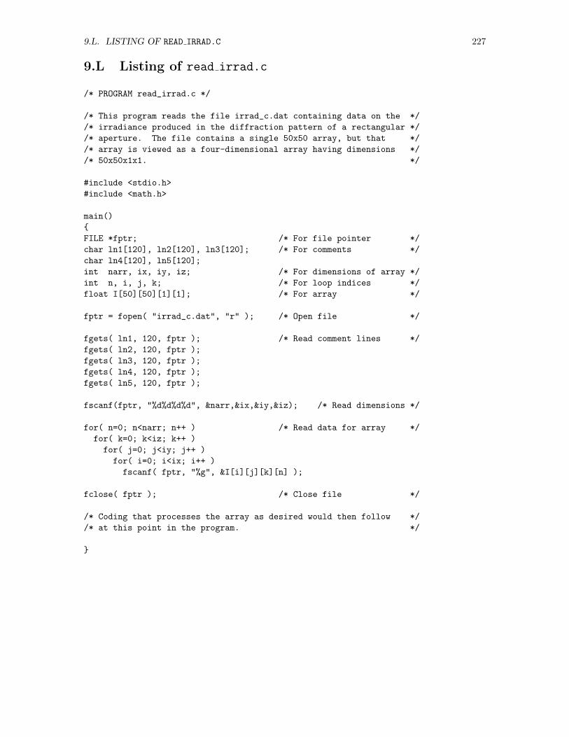
9.L. LISTING OF READ IRRAD.C 227

9.L Listing of read irrad.c

/* PROGRAM read_irrad.c */

/* This program reads the file irrad_c.dat containing data on the */

/* irradiance produced in the diffraction pattern of a rectangular */

/* aperture. The file contains a single 50x50 array, but that */

/* array is viewed as a four-dimensional array having dimensions */

/* 50x50x1x1. */

#include <stdio.h>

#include <math.h>

main()

FILE *fptr; /* For file pointer */

char ln1[120], ln2[120], ln3[120]; /* For comments */

char ln4[120], ln5[120];

int narr, ix, iy, iz; /* For dimensions of array */

int n, i, j, k; /* For loop indices */

float I[50][50][1][1]; /* For array */

fptr = fopen( "irrad_c.dat", "r" ); /* Open file */

fgets( ln1, 120, fptr ); /* Read comment lines */

fgets( ln2, 120, fptr );

fgets( ln3, 120, fptr );

fgets( ln4, 120, fptr );

fgets( ln5, 120, fptr );

fscanf(fptr, "%d%d%d%d", &narr,&ix,&iy,&iz); /* Read dimensions */

for( n=0; n<narr; n++ ) /* Read data for array */

for( k=0; k<iz; k++ )

for( j=0; j<iy; j++ )

for( i=0; i<ix; i++ )

fscanf( fptr, "%g", &I[i][j][k][n] );

fclose( fptr ); /* Close file */

/* Coding that processes the array as desired would then follow */

/* at this point in the program. */

228 CHAPTER 9. INTRODUCTION TO PROGRAMMING

Chapter 10

Introduction to Numerical Recipes

Note: If your site owns licenses for the Numerical Recipes library, files in thischapter that are components of the Numerical Recipes library can be downloadedfrom the directory $NRHEAD. Here, as defined in the Local Guide, $NRHEAD must bereplaced by the appropriate path for your site. The subdirectories in $NRHEAD areidentified in Fig. 10.1.

The Numerical Recipes package1,2 contains numerous subroutines implementing a wide varietyof numerical algorithms and provides a valuable and time-saving starting point for the writing ofprograms to carry out almost any numerical analysis. Some programming knowledge in FORTRANor C is prerequisite to successful use of the recipes. In this chapter, we provide basic informationabout the way the files in the package are stored, and we illustrate how to use those files. Additionalapplications are described in subsequent chapters. These several discussions, however, are in noway intended to comprise the ultimate document on the usage of the recipes. Full documentationis contained in two source books: Numerical Recipes: The Art of Scientific Computing (hereafterreferred to as the main source book) and Numerical Recipes: Example Book (the example sourcebook).3 These books describe not only the various methods and routines employed by the recipes butalso the mathematical theory behind them. A pair of books exists for each of several programminglanguages. In the second edition, FORTRAN (both 77 and 90), C, and C++ are supported.4

10.1 The Numerical Recipes Directory Tree

The hundreds of files that make up the Numerical Recipes package are stored in a directory treewhose head is $NRHEAD.5 As illustrated in Fig. 10.1, the full tree contains three subdirectoriesnamed recipes f, recipes c-ansi, and recipes c-kr, though not all of these subdirectories willbe present at every site. Each of these subdirectories in turn contains several (sub)subdirectories, themost significant of which are named recipes, demo, and (for the C directories) include. Further,

1The Numerical Recipes package is a commercial product marketed by Numerical Recipes Software, Cambridge,MA, 02238, and by Cambridge University Press. (See Appendix Z for full contact information.) Its use at anyparticular site is subject to the provisions of whatever license that site has negotiated with Numerical Recipes Software.The terms of that license are explained in the Local Guide.

2The names and calling sequences of the recipes are copyrighted by Numerical Recipes Software and are used inthis book with permission of Numerical Recipes Software.

3These reference works are published by Cambridge University Press; the authors are William H. Press, Saul A.Teukolsky, William T. Vetterling, and Brian P. Flannery.

4Other languages, including Pascal, LISP, Modula2, and some versions of BASIC, are still available in the firstedition. The third edition, which is not described in this chapter, is the current edition—though it supports onlyC++.

5See the Local Guide for the translation of this symbol at your site.

229

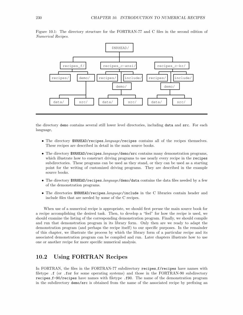
230 CHAPTER 10. INTRODUCTION TO NUMERICAL RECIPES

Figure 10.1: The directory structure for the FORTRAN-77 and C files in the second edition ofNumerical Recipes.

$NRHEAD/

recipes_f/ recipes_c-kr/recipes_c-ansi/

recipes/

demo/

include/recipes/

data/

demo/ recipes/ include/

demo/

src/ data/ src/ data/ src/

the directory demo contains several still lower level directories, including data and src. For eachlanguage,

• The directory $NRHEAD/recipes language/recipes contains all of the recipes themselves.These recipes are described in detail in the main source books.

• The directory $NRHEAD/recipes language/demo/src contains many demonstration programs,which illustrate how to construct driving programs to use nearly every recipe in the recipes

subdirectories. These programs can be used as they stand, or they can be used as a startingpoint for the writing of customized driving programs. They are described in the examplesource books.

• The directory $NRHEAD/recipes language/demo/data contains the data files needed by a fewof the demonstration programs.

• The directories $NRHEAD/recipes language/include in the C libraries contain header andinclude files that are needed by some of the C recipes.

When use of a numerical recipe is appropriate, we should first peruse the main source book fora recipe accomplishing the desired task. Then, to develop a “feel” for how the recipe is used, weshould examine the listing of the corresponding demonstration program. Finally, we should compileand run that demonstration program in its library form. Only then are we ready to adapt thedemonstration program (and perhaps the recipe itself) to our specific purposes. In the remainderof this chapter, we illustrate the process by which the library form of a particular recipe and itsassociated demonstration program can be compiled and run. Later chapters illustrate how to useone or another recipe for more specific numerical analysis.

10.2 Using FORTRAN Recipes

In FORTRAN, the files in the FORTRAN-77 subdirectory recipes f/recipes have names withfiletype .f (or .for for some operating systems) and those in the FORTRAN-90 subdirectoryrecipes f-90/recipes have names with filetype .f90. The name of the demonstration programin the subdirectory demo/src is obtained from the name of the associated recipe by prefixing an

10.2. USING FORTRAN RECIPES 231

x (presumably derived from the ‘x’ in ‘example’). Thus, for example, the first recipe found in themain source books—a recipe that calculates the dates of occurrence of the phases of the moon—iscalled flmoon and is stored in a file named flmoon.f (or, possibly, flmoon.for). The associateddemonstration file is named xflmoon.f (or, possibly, xflmoon.for). To use the demonstrationprogram,

1. We copy the program xflmoon.f into our default directory with the statement6

cp $NRHEAD/recipes_f/demo/src/xflmoon.f .

2. We copy the associated recipe flmoon.f into our default directory with the statement

cp $NRHEAD/recipes_f/recipes/flmoon.f .

3. We determine whether the program invokes recipes beyond the primary one. One way to makethis determination entails compiling and loading the program with the statement7

f77 -o xflmoon.xf xflmoon.f flmoon.f

If this statement generates no error messages, then no further recipes are needed.8 Morelikely, others will be needed. They will be identified in the error messages as “unresolved textsymbols”. In the present case, the symbols julday and caldat will be identified, so we needthe statements

cp $NRHEAD/recipes_f/recipes/caldat.f .

cp $NRHEAD/recipes_f/recipes/julday.f .

to copy these two additional files into our default directory.

A more gentle way to identify needed additional files entails examining the listings of theprogram xflmoon.f and the recipe flmoon.f, noting the statements that invoke subroutinesflmoon and caldat and function julday. Strictly, we should then examine the listings of anysubroutines so identified to see if they in turn invoke still other subroutines.

4. We compile and load the program with the statement

f77 -o xflmoon.xf xflmoon.f flmoon.f caldat.f julday.f

The order of the filenames in this statement is irrelevant. Note, incidentally, that the commandf77 will leave a succession of object files (filetype .o) in our directory. These files may bedeleted once the executable program has been created.

5. We run the program with the statement9

./xflmoon.xf

6To be specific, both here and throughout this section, we illustrate these steps with the statements that wouldbe used in UNIX to compile, link, and run the program. Other operating systems probably accomplish the same endwith different statements. Details will be found in the Local Guide.

7Throughout this book, we shall assume that we are using the FORTRAN-77 routines. Presumably, theFORTRAN-90 and FORTRAN-95 routines are used in much the same way, though the compile command in UNIXwill be f90 and f95, respectively.

8The routine xflmoon.f invokes the FORTRAN pause statement, which apparently has been discontinued in morerecent FORTRAN compilers. A warning will be generated, though it will not prevent compilation of the program ifall other requirements are met.

9Again, we are using UNIX-style statements. In some operating systems, the characters ./ preceding the name ofthe program to be executed may not be necessary.

232 CHAPTER 10. INTRODUCTION TO NUMERICAL RECIPES

The program asks for a date (and prescribes the format in which the date is to be entered) and thenprints out the dates of the next several occurrences of each of the phases of the moon.

This discussion is, of course, purely exemplary of the procedure we will have to invoke to use aparticular numerical recipe in its library form. More often, we will need to use the demonstrationprogram as a template for creating a driving program better suited to our specific purposes. Occa-sionally, we may have to edit the recipes themselves. Illustrations of these operations will be foundin Sections 11.14.2, 13.13.2, and 14.14.2.

10.3 Using C Recipes

In C, the files in the subdirectory recipes have names with filetype .c. The name of the demon-stration program in the subdirectory demo/src is obtained from the name of the associated recipeby prefixing an x (presumably derived from the ‘x’ in ‘example’). Thus, for example, the first recipefound in the main source books—a recipe that calculates the dates of occurrence of the phases ofthe moon—is called flmoon and is stored in a file named flmoon.c. The associated demonstrationfile is named xflmoon.c. To use the demonstration program,

1. We copy the program xflmoon.c into our default directory with the statement10,11

cp $NRHEAD/recipes_c-ansi/demo/src/xflmoon.c .

2. We copy the associated recipe flmoon.c into our default directory with the statement

cp $NRHEAD/recipes_c-ansi/recipes/flmoon.c .

3. We determine whether the program invokes recipes beyond the primary one. One way to makethis determination entails compiling and loading the program with the statement

cc -o xflmoon.xc xflmoon.c flmoon.c

If this statement generates no error messages, then no further recipes are needed. More likely,others will be needed; if so, they will be identified in the error messages. In the present case,the file nr.h, which is a special header file, is not found. Thus, you must copy it from itslocation in the public directory structure with the statement

cp $NRHEAD/recipes_c-ansi/include/nr.h .

Then, a repeat compilation with the statement

cc -o xflmoon.xc xflmoon.c flmoon.c

reveals a number of additional “unresolved text symbols”, including julday, caldat, nrerror,sin, floor, and ceil. The first two of these are additional needed recipes, which can be copiedwith the statements

cp $NRHEAD/recipes_c-ansi/recipes/julday.c .

cp $NRHEAD/recipes_c-ansi/recipes/caldat.c .

10To be specific, both here and throughout this section, we illustrate these steps with the statements that wouldbe used in UNIX to compile, link, and run the program. Other operating systems probably accomplish the same endwith different statements. Details will be found in the Local Guide.

11We also assume the ANSI version of C is in use. To use the KR version, simply replace the designation of thelanguage directory with recipes kr. Consult your Local Guide for the version available at your site.

10.4. EXERCISES 233

the third is a utility routine contained within a package named nrutil.c, which can be copiedwith the statement

cp $NRHEAD/recipes_c-ansi/recipes/nrutil.c .

while the remaining three are items from the standard C mathematics library m, which musttherefore be explicitly included in the compile command with the option -lm.

A more gentle way to identify needed additional files entails examining the listings of theprogram xflmoon.c and the recipe flmoon.c, noting all non-standard include files and allnon-standard procedure calls. In the present case, examining xflmoon.c reveals the inclusionof nr.h and calls to julday and caldat while examination of flmoon.c reveals invocationof nrerror (which is defined in nrutil.c), sin, floor, and ceil. Strictly, we should thenexamine the listings of any subroutines and other entities so identified to see if they in turninvoke still other subroutines. Together, these invocations identify the same spectrum ofadditional routines as those to which we were led in the first approach.

4. We compile and load the program with the statement12

cc -o xflmoon.xc xflmoon.c flmoon.c julday.c caldat.c nrutil.c -lm

Except that the component -lm should occur last in this list, the order of the filenames isotherwise irrelevant. Note, incidentally, that the cc command will leave a succession of objectfiles (filetype .o) in our directory. These files may be deleted once the executable program hasbeen created.

5. We run the program with the statement13

./xflmoon.xc

The program asks for a date (and prescribes the format in which the date is to be entered) and thenprints out the dates of the next several occurences of each of the four phases of the moon.

This discussion is, of course, purely exemplary of the procedure we will have to invoke to use aparticular numerical recipe in its library form. More often, we will need to use the demonstrationprogram as a template for creating a driving program better suited to our specific purposes. Occa-sionally, we may have to edit the recipes themselves. Illustrations of these operations will be foundin Sections 11.15.2, 13.14.2, and 14.15.2.

10.4 Exercises

10.1. The recipe julday.f calculates and prints out the Julian day number corresponding to a datesupplied to it by a suitable driving program. (a) Read what the main and example source books haveto say about this recipe and its associated demonstration program. (b) Retrieve the demonstrationprogram xjulday.f, the primary recipe julday.f, and any necessary additional files from theNumerical Recipes library, and examine the listing of the demonstration program. (c) Compileand run the library form of the program. (d) In particular, determine how old you are in daysby determining the Julian day number of your birthday and of today. Note: The file DATES.DAT

needed by the program can be copied from the directory $NRHEAD/recipes f/demo/results.

12This statement may generate a warning about conflicting data types for one or more variables. Warnings, however,do not prevent successful coompilation.

13Again, we are using UNIX-style statements. In some operating systems, the characters ./ preceding the name ofthe program to be executed may not be necessary.

234 CHAPTER 10. INTRODUCTION TO NUMERICAL RECIPES

10.2. The recipe avevar.f calculates the mean and variance of a data set supplied to it by a suitabledriving program. (a) Read what the main and example source books have to say about this recipeand its associated demonstration program. (b) Retrieve the demonstration program xavevar.f, theprimary recipe avevar.f, and any necessary additional files from the Numerical Recipes library,and examine the listing of the demonstration program. (c) Compile and run the library form of theprogram. (d) Finally, edit the driving program so that it supplies a different set of data of yourchoice to the recipe. Then compile and run your editted program.

10.3. The recipe julday.c calculates and prints out the Julian day number corresponding to a datesupplied to it by a suitable driving program. (a) Read what the main and example source books haveto say about this recipe and its associated demonstration program. (b) Retrieve the demonstrationprogram xjulday.c, the primary recipe julday.c, and any necessary additional files from theNumerical Recipes library, and examine the listing of the demonstration program. (c) Compileand run the library form of the program. (d) In particular, determine how old you are in daysby determining the Julian day number of your birthday and of today. Note: The file dates1.dat

needed by the program can be copied from the directory $NRHEAD/recipes c-ansi/demo/data.

10.4. The recipe avevar.c calculates the mean and variance of a data set supplied to it by a suitabledriving program. (a) Read what the main and example source books have to say about this recipeand its associated demonstration program. (b) Retrieve the demonstration program xavevar.c, theprimary recipe avevar.c, and any necessary additional files from the Numerical Recipes library,and examine the listing of the demonstration program. (c) Compile and run the library form of theprogram. (d) Finally, edit the driving program so that it supplies a different set of data of yourchoice to the recipe. Then compile and run your editted program.

Chapter 11

Solving Ordinary DifferentialEquations

Many fundamental laws of physics relate the rate at which the physical properties of a system changeto the properties themselves. These physical laws lead inevitably to differential equations satisfiedby the quantities describing the system. While some of these equations admit closed form, symbolicsolutions, most can be solved only through numerical approximation. We begin this chapter byidentifying several physical situations, the full addressing of which requires us to solve an ordinarydifferential equation (ODE) or a coupled set of such equations. Then we illustrate how to usesymbolic algebra systems to approach those that can be solved analytically, describe a few of manyavailable numerical algorithms (with attention to their accuracy), and—finally—describe ways tosolve representative ODEs using a variety of numerical approaches and computational tools.

Differential equations fall into many, sometimes overlapping, categories. We limit ourselvesin this chapter to ordinary differential equations, which involve only one independent variable.Most equations of interest in physics are first-order (containing no derivatives higher than the first)or second-order (containing no derivatives higher than the second), but occasionally higher orderequations may arise. Whatever their order, these equations may be linear (each term depending onthe dependent variable only through either its first power or the first power of one of its derivatives)or non-linear (at least one term violating the constraint in the previous parentheses). They maybe homogeneous (no term free of the dependent variable) or inhomogeneous (at least one term freeof the dependent variable). The coefficients may be constant or may depend on the independentvariable. Most will contain parameters characterizing the system of interest, though recasting theoriginal equations in dimensionless form may reduce the number of distinct parameters—or eveneliminate them altogether. We may be confronted with a single equation (one dependent variable)or with a system of equations (two or more dependent variables), and the members of the systemmay be coupled (more than one of the dependent variables appearing in at least one of the equations)or decoupled (no member of the system containing more than one of the dependent variables).

For complete statement of a problem, the applicable ODEs must be supplemented with auxiliaryconditions, the number of which equals the sum of the orders of the equations at hand. A singlefirst-order equation requires one condition; stipulation of the value of the dependent variable at aspecific value of the independent variable is sufficient to select a unique solution from the familyof solutions defined by the differential equation alone. A single second-order equation requires twoconditions but, in this case, we have some choices. We might, for example, stipulate the value of thedependent variable and the value of its first derivative at a single value of the independent variable,e.g., position and velocity at an initial time. In that case, we would be dealing with an initial valueproblem (IVP). Alternatively, we might stipulate the value of the dependent variable at each of twodifferent values of the independent variable, e.g, displacement of a string at each of its two ends. Inthat case, we would be dealing with a boundary value problem (BVP).

235

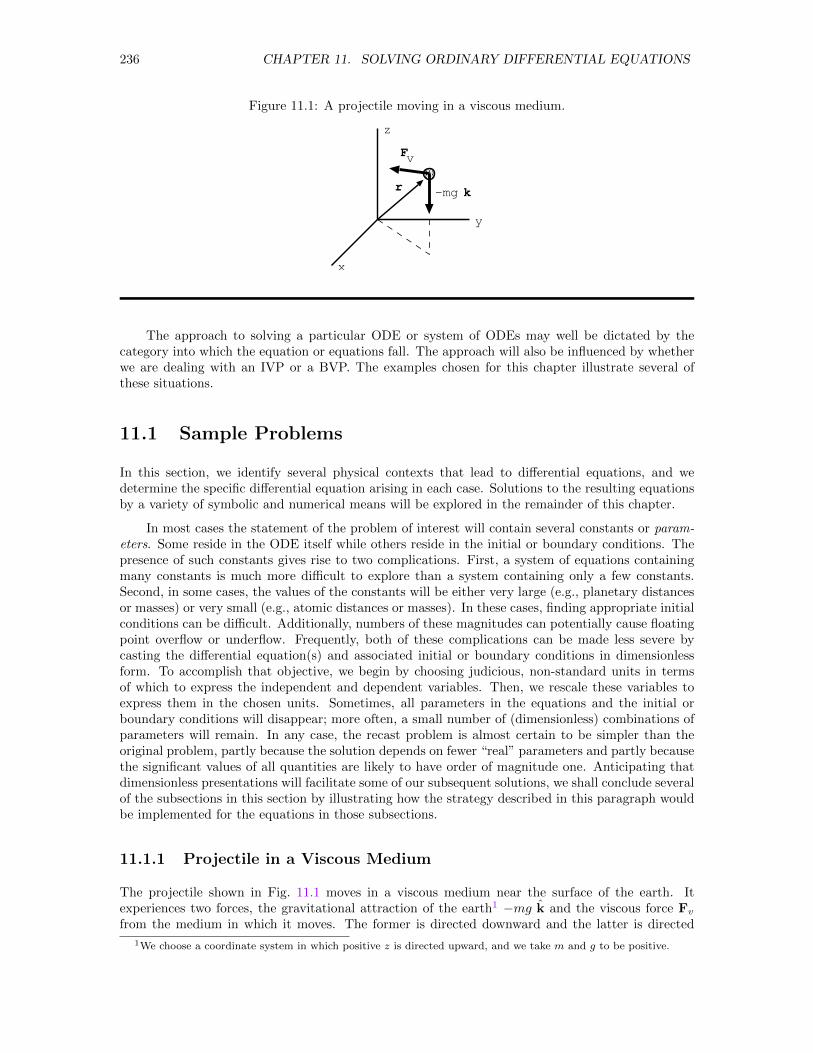
236 CHAPTER 11. SOLVING ORDINARY DIFFERENTIAL EQUATIONS

Figure 11.1: A projectile moving in a viscous medium.

x

y

z

r

Fv

-mg k

The approach to solving a particular ODE or system of ODEs may well be dictated by thecategory into which the equation or equations fall. The approach will also be influenced by whetherwe are dealing with an IVP or a BVP. The examples chosen for this chapter illustrate several ofthese situations.

11.1 Sample Problems

In this section, we identify several physical contexts that lead to differential equations, and wedetermine the specific differential equation arising in each case. Solutions to the resulting equationsby a variety of symbolic and numerical means will be explored in the remainder of this chapter.

In most cases the statement of the problem of interest will contain several constants or param-eters. Some reside in the ODE itself while others reside in the initial or boundary conditions. Thepresence of such constants gives rise to two complications. First, a system of equations containingmany constants is much more difficult to explore than a system containing only a few constants.Second, in some cases, the values of the constants will be either very large (e.g., planetary distancesor masses) or very small (e.g., atomic distances or masses). In these cases, finding appropriate initialconditions can be difficult. Additionally, numbers of these magnitudes can potentially cause floatingpoint overflow or underflow. Frequently, both of these complications can be made less severe bycasting the differential equation(s) and associated initial or boundary conditions in dimensionlessform. To accomplish that objective, we begin by choosing judicious, non-standard units in termsof which to express the independent and dependent variables. Then, we rescale these variables toexpress them in the chosen units. Sometimes, all parameters in the equations and the initial orboundary conditions will disappear; more often, a small number of (dimensionless) combinations ofparameters will remain. In any case, the recast problem is almost certain to be simpler than theoriginal problem, partly because the solution depends on fewer “real” parameters and partly becausethe significant values of all quantities are likely to have order of magnitude one. Anticipating thatdimensionless presentations will facilitate some of our subsequent solutions, we shall conclude severalof the subsections in this section by illustrating how the strategy described in this paragraph wouldbe implemented for the equations in those subsections.

11.1.1 Projectile in a Viscous Medium

The projectile shown in Fig. 11.1 moves in a viscous medium near the surface of the earth. Itexperiences two forces, the gravitational attraction of the earth1 −mg k and the viscous force Fvfrom the medium in which it moves. The former is directed downward and the latter is directed

1We choose a coordinate system in which positive z is directed upward, and we take m and g to be positive.

11.1. SAMPLE PROBLEMS 237

opposite to the velocity v. Usually, the magnitude of the viscous force is a function of the speedwith which the projectile moves, symbolically |Fv| = f(|v|). In general, if the projectile has massm, Newton’s second law yields the equation of motion

md2r

dt2= −mg k + Fv(|v|) = −mg k− f(|v|) v

|v|(11.1)

which we are to solve subject to the general initial conditions,

r(0) = r0 = x0 i + y0 j + z0 k ; v(0) = v0 = vx0 i + vy0 j + vz0 k (11.2)

Of course, we also need to know the precise dependence of the function f(|v|) on the speed ofthe projectile. In the simplest case (when the speed of the projectile is small enough), f is simplylinearly proportional to that speed, f(|v|) = b |v| (b a positive constant), and the equation of motionreduces to

md2r

dt2= −mg k− bv = −mg k− b dr

dt(11.3)

or, in component form, to

md2x

dt2= −bdx

dt; m

d2y

dt2= −bdy

dt; m

d2z

dt2= −mg − bdz

dt(11.4)

This system of equations is uncoupled, since each of the three independent variables x, y, and zsatisfies its own private equation that does not involve either of the other variables. They are second-order and linear, and the coefficients are constant. The first two are homogeneous and, because ofthe term −mg, the third is inhomogeneous. The equations involve the parameters m, b, and g, andtheir solutions will depend on these parameters and on the six initial values in Eq. (11.2).

When the speed is too large for a linear approximation to the viscous damping, we can sometimestake the viscous force to be proportional instead to the square of the speed, f = b|v|2 (b a positiveconstant, though not the same constant as in the previous paragraph). This time, the equation ofmotion reduces to

md2r

dt2= −mg k− bv|v| = −mg k− bdr

dt

√(dx

dt

)2

+

(dy

dt

)2

+

(dz

dt

)2

(11.5)

or, in component form, to

m

[d2x

dt2,d2y

dt2,d2z

dt2

]= [0, 0,−mg]− b

[dx

dt,dy

dt,dz

dt

]√(dx

dt

)2

+

(dy

dt

)2

+

(dz

dt

)2

(11.6)

This system of equations is second-order and distinctly non-linear, and its members are coupledbecause each of the equations involves all three of the dependent variables. Even if the motionoccurs in only the vertical dimension (projectile tossed straight up or, simply, released from rest andallowed to drop), the equation, which then is

md2z

dt2= −mg − bdz

dt

∣∣∣∣dzdt∣∣∣∣ (11.7)

is complicated by the absolute value in the viscous term. These equations involve the parametersm, b, and g, and their solutions will depend on these parameters and on the six initial values inEq. (11.2).

To cast these equations in a dimensionless form, we would start by choosing a unit of length, saya—which might be chosen arbitrarily, chosen to be one of the initial positions, or merely symbolizedinitially and chosen later to simplify the equations as we converge on their dimensionless form.Then, dividing by m and rescaling the dimensional coordinates by introducing the dimensionless

238 CHAPTER 11. SOLVING ORDINARY DIFFERENTIAL EQUATIONS

coordinates x = x/a, y = y/a, and z = z/a (i.e., r = r/a), we find that Eqs. (11.3) and (11.5)become

d2r

dt2= −g

ak− b

m

dr

dt(11.8)

and

d2r

dt2= −g

ak− ba

m

dr

dt

√(dx

dt

)2

+

(dy

dt

)2

+

(dz

dt

)2

(11.9)

respectively. Next, we recognize that√g/a is dimensionally a frequency.2 Hence, the variable

t = t√g/a provides a suitable rescaling of the independent variable. In terms of t, Eqs. (11.8) and

(11.9) becomed2r

dt2 = − k− b

m

√a

g

dr

dt(11.10)

and

d2r

dt2 = − k− ba

m

dr

dt

√(dx

dt

)2

+

(dy

dt

)2

+

(dz

dt

)2

(11.11)

Finally, we introduce the symbol β for the dimensionless quantity b√a/g /m in the first of these

equations and for the dimensionless quantity ba/m in the second.3 In the end, the equations indimensionless form are

d2r

dt2 = − k− β dr

dt(11.12)

and

d2r

dt2 = − k− β dr

dt

√(dx

dt

)2

+

(dy

dt

)2

+

(dz

dt

)2

(11.13)

These equations are, of course, to be solved subject to the dimensionless initial conditions

r(0) =r0a

; v(0) =dr

dt(0) =

d(r/a)

d(t√g/a)

(0) =v0√ga

(11.14)

from which we conclude that dimensionless velocities are measured in units of 4√ga.

In truth, however, these particular equations are not really second-order equations. They can bereduced to first-order equations by focusing attention on the components [vx, vy, vz] of the velocityas the dependent variables. In those terms, the three members of Eq. (11.4) become

mdvxdt

= −bvx ; mdvydt

= −bvy ; mdvzdt

= −mg − bvz (11.15)

the three members of Eq. (11.6) become

m

[dvxdt

,dvydt

,dvzdt

]= [0, 0,−mg]− b [vx, vy, vz]

√v2x + v2y + v2z (11.16)

and Eq. (11.7) becomes

mdvzdt

= −mg − bvz |vz| (11.17)

Once these first-order equations have been solved, the components of the position vector can thenbe found by solving the differential equations

dx

dt= vx ;

dy

dt= vy ;

dz

dt= vz (11.18)

2Using [. . .] to indicate “the dimensions of . . .”, we argue [g] = length/time2, [a] = length =⇒ [g/a] = time−2 =⇒[√g/a] = time−1.3Remember that b is not the same in the two instances.4Here (and in all subsequent cases where a chosen unit is identified but not checked), you should take a moment

to verify that the identified unit has the proper dimensions.

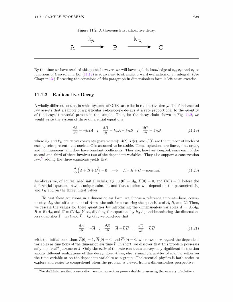
11.1. SAMPLE PROBLEMS 239

Figure 11.2: A three-nucleus radioactive decay.

A B CkA kB

By the time we have reached this point, however, we will have explicit knowledge of vx, vy, and vz asfunctions of t, so solving Eq. (11.18) is equivalent to straight-forward evaluation of an integral. (SeeChapter 13.) Recasting the equations of this paragraph in dimensionless form is left as an exercise.

11.1.2 Radioactive Decay

A wholly different context in which systems of ODEs arise lies in radioactive decay. The fundamentallaw asserts that a sample of a particular radioisotope decays at a rate proportional to the quantityof (undecayed) material present in the sample. Thus, for the decay chain shown in Fig. 11.2, wewould write the system of three differential equations

dA

dt= −kAA ;

dB

dt= kAA− kBB ;

dC

dt= kBB (11.19)

where kA and kB are decay constants (parameters); A(t), B(t), and C(t) are the number of nuclei ofeach species present; and nucleus C is assumed to be stable. These equations are linear, first-order,and homogeneous, and they have constant coefficients. They are, however, coupled, since each of thesecond and third of them involves two of the dependent variables. They also support a conservationlaw:5 adding the three equations yields that

d

dt

(A+B + C

)= 0 =⇒ A+B + C = constant (11.20)

As always we, of course, need initial values, e.g., A(0) = A0, B(0) = 0, and C(0) = 0, before thedifferential equations have a unique solution, and that solution will depend on the parameters kAand kB and on the three initial values.

To cast these equations in a dimensionless form, we choose a reference amount—here, conve-niently, A0, the initial amount of A—as the unit for measuring the quantities of A, B, and C. Then,we rescale the values for these quantities by introducing the dimensionless variables A = A/A0,B = B/A0, and C = C/A0. Next, dividing the equations by kAA0 and introducing the dimension-less quantities t = kAt and k = kB/kA, we conclude that

dA

dt= −A ;

dB

dt= A− k B ;

dC

dt= k B (11.21)

with the initial conditions A(0) = 1, B(0) = 0, and C(0) = 0, where we now regard the dependentvariables as functions of the dimensionless time t. In short, we discover that this problem possessesonly one “real” parameter k. Only the ratio of the rate constants conveys any significant distinctionamong different realizations of this decay. Everything else is simply a matter of scaling, either onthe time variable or on the dependent variables as a group. The essential physics is both easier toexplore and easier to comprehend when the problem is viewed from a dimensionless perspective.

5We shall later see that conservation laws can sometimes prove valuable in assessing the accuracy of solutions.

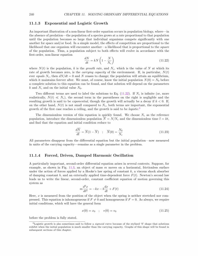
240 CHAPTER 11. SOLVING ORDINARY DIFFERENTIAL EQUATIONS

11.1.3 Exponential and Logistic Growth

An important illustration of a non-linear first-order equation occurs in population biology, where—inthe absence of predation—the population of a species grows at a rate proportional to that populationuntil the population becomes so large that individual organisms compete significantly with oneanother for space and/or food. In a simple model, the effects of competition are proportional to thelikelihood that one organism will encounter another—a likelihood that is proportional to the squareof the population. Thus, a population subject to both effects will evolve in accordance with thefirst-order, non-linear equation

dN

dt= kN

(1− N

Nc

)(11.22)

where N(t) is the population, k is the growth rate, and Nc, which is the value of N at which itsrate of growth becomes zero, is the carrying capacity of the environment. If, in particular, N(t)ever equals Nc, then dN/dt = 0 and N ceases to change; the population will attain an equilibrium,which it maintains forever after. We must, of course, know the initial population N(0) = N0 beforea complete solution to this equation can be found, and that solution will depend on the parametersk and Nc and on the initial value N0.

Two different terms are used to label the solutions to Eq. (11.22). If Nc is infinite (or, morerealistically, N(t) Nc), the second term in the parentheses on the right is negligible and theresulting growth is said to be exponential, though the growth will actually be a decay if k < 0. If,on the other hand, N(t) is not small compared to Nc, both terms are important, the exponentialgrowth of the first case reaches a ceiling, and the growth is said to be logistic.6

The dimensionless version of this equation is quickly found. We choose Nc as the referencepopulation, introduce the dimensionless population N = N/Nc and the dimensionless time t = kt,and find that the equation and initial condition reduce to

dN

dt= N(1−N) ; N(0) =

N0

Nc(11.23)

All parameters disappear from the differential equation but the initial population—now measuredin units of the carrying capacity—remains as a single parameter in the problem.

11.1.4 Forced, Driven, Damped Harmonic Oscillation

A particularly important, second-order differential equation arises in several contexts. Suppose, forexample, as shown in Fig. 11.3, an object of mass m moves on a horizontal, frictionless surfaceunder the action of forces applied by a Hooke’s law spring of constant k, a viscous shock absorberof damping constant b, and an externally applied time-dependent force F (t). Newton’s second lawleads us to write the linear, second-order, constant coefficient equation of motion governing thissystem as

md2x

dt2= −kx− bdx

dt+ F (t) (11.24)

Here, x is measured from the position of the object when the spring is neither stretched nor com-pressed. This equation is inhomogeneous if F 6= 0 and homogeneous if F = 0. As always, we requireinitial conditions, which will have the general form

x(0) = x0 ; v(0) = v0 (11.25)

before the problem is fully stated.

6Logistic growth is also sometimes said to follow a sigmoid curve because of the stylized ‘S’ shape that solutionsexhibit when the initial population is much smaller than the carrying capacity. Graphs of this shape will be found insubsequent sections of this chapter.

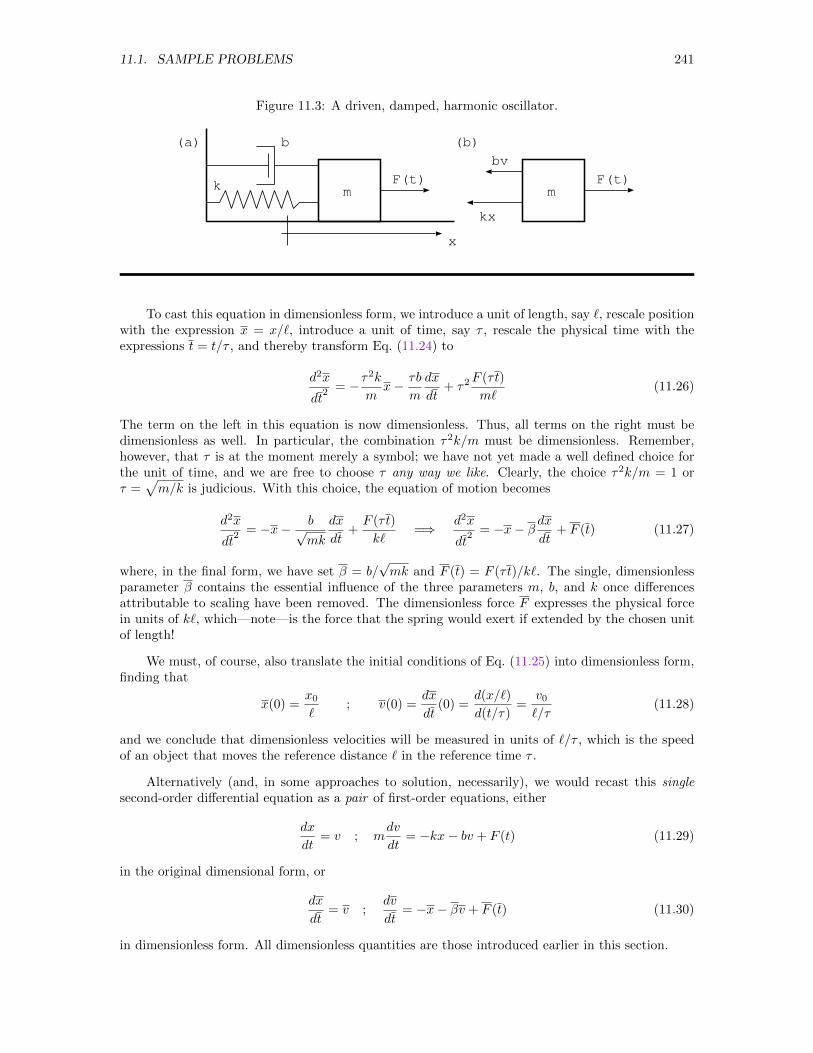
11.1. SAMPLE PROBLEMS 241

Figure 11.3: A driven, damped, harmonic oscillator.

k m

b

F(t)

x

mF(t)

kx

bv

(a) (b)

To cast this equation in dimensionless form, we introduce a unit of length, say `, rescale positionwith the expression x = x/`, introduce a unit of time, say τ , rescale the physical time with theexpressions t = t/τ , and thereby transform Eq. (11.24) to

d2x

dt2 = −τ

2k

mx− τb

m

dx

dt+ τ2

F (τt)

m`(11.26)

The term on the left in this equation is now dimensionless. Thus, all terms on the right must bedimensionless as well. In particular, the combination τ2k/m must be dimensionless. Remember,however, that τ is at the moment merely a symbol; we have not yet made a well defined choice forthe unit of time, and we are free to choose τ any way we like. Clearly, the choice τ2k/m = 1 orτ =

√m/k is judicious. With this choice, the equation of motion becomes

d2x

dt2 = −x− b√

mk

dx

dt+F (τt)

k`=⇒ d2x

dt2 = −x− β dx

dt+ F (t) (11.27)

where, in the final form, we have set β = b/√mk and F (t) = F (τt)/k`. The single, dimensionless

parameter β contains the essential influence of the three parameters m, b, and k once differencesattributable to scaling have been removed. The dimensionless force F expresses the physical forcein units of k`, which—note—is the force that the spring would exert if extended by the chosen unitof length!

We must, of course, also translate the initial conditions of Eq. (11.25) into dimensionless form,finding that

x(0) =x0`

; v(0) =dx

dt(0) =

d(x/`)

d(t/τ)=

v0`/τ

(11.28)

and we conclude that dimensionless velocities will be measured in units of `/τ , which is the speedof an object that moves the reference distance ` in the reference time τ .

Alternatively (and, in some approaches to solution, necessarily), we would recast this singlesecond-order differential equation as a pair of first-order equations, either

dx

dt= v ; m

dv

dt= −kx− bv + F (t) (11.29)

in the original dimensional form, or

dx

dt= v ;

dv

dt= −x− βv + F (t) (11.30)

in dimensionless form. All dimensionless quantities are those introduced earlier in this section.

242 CHAPTER 11. SOLVING ORDINARY DIFFERENTIAL EQUATIONS

Figure 11.4: A series RLC circuit.

L C

R

V(t)

i

q

11.1.5 An LRC Resonant Circuit

An equation mathematically identical in form to Eqs. (11.29) and (11.30) arises in the descriptionof a series RLC circuit excited by a signal generator, as shown in Fig. 11.4. If we take positivecurrent i(t) to flow clockwise and understand that q(t) represents the charge on the left plate of thecapacitor, then Kirchhoff’s loop equation and the properties of the several components lead to theequation

V (t)− Ldidt− q

C− iR = 0 =⇒ L

di

dt+ iR+

q

C= V (t) (11.31)

As it stands, this equation looks to be first order but it involves two variables i(t) and q(t). We cancomplete the statement of a problem having a unique solution by recognizing the relationship

i =dq

dt(11.32)

between i and q and supplementing what is now a pair of coupled first-order, linear, constantcoefficient, inhomogeneous equations with the general initial conditions

q(0) = q0 ;dq

dt(0) = i(0) = i0 (11.33)

Alternatively, we could substitute Eq. (11.32) into Eq. (11.31) to find the equivalent, single, second-order, linear, constant coefficient, inhomogeneous equation

Ld2q

dt2+R

dq

dt+q

C= V (t) (11.34)

The recasting of these equations in dimensionless form is left as an exercise.

Adopting the correspondences, q ⇔ x, L ⇔ m, R ⇔ b, 1/C ⇔ k, V (t) ⇔ F (t), and t ⇔ t,we can turn Eq. (11.34) into Eq. (11.24). Thus, mathematically, the driven, damped mechanicaloscillator and the RLC circuit exhibit exactly analogous behavior, and the behavior of the RLCcircuit simulates the behavior of the mechanical oscillator.7

11.1.6 Coupled Oscillators

Consider next the system shown in Fig. 11.5 consisting of two objects of equal mass m connectedalong a line, each to a fixed wall by springs of constant k and each to the other by a coupling spring

7Years ago, when digital computers were not as fast as they have come to be and smooth graphical output from adigital computer was unheard of, correspondences such as this one were the basis of the analog computer, whereon wecould easily set up electronic circuits whose behavior simulated the behavior of more expensive mechanical systems.With an analog computer, we could learn about mechanical systems by observing the real-time variation of thevoltages and currents at various points in an analogous electronic circuit.

11.1. SAMPLE PROBLEMS 243

Figure 11.5: A system of two coupled objects.

m m

k k’ k

x1 x2

Figure 11.6: An object moving in a central force.

x

y

r m

F

x

yφ

of constant k′. Let the (horizontal) surface on which these objects slide be frictionless, and let x1(t)and x2(t) be the displacement of each object from its equilibrium point. Then, Newton’s second lawyields

md2x1dt2

= −kx1 + k′(x2 − x1) ; md2x2dt2

= −kx2 − k′(x2 − x1) (11.35)

for the equations of motion. To reduce the number of parameters, however, we recast these equationsin dimensionless form by selecting a unit of length a, dividing the equations by a, setting xi/a = xi,introducing a dimensionless time variable t = ωt, where ω =

√k/m, and setting κ = k′/k. The

equations then become

d2x1

dt2 = −x1 + κ (x2 − x1) ;

d2x2

dt2 = −x2 − κ (x2 − x1) (11.36)

Initial conditions such as

x1(0) = x10 ;dx1dt

(0) = v10 ; x2(0) = x20 ;dx2dt

(0) = v20 (11.37)

complete the statement of the problem—a problem that involves a pair of coupled, linear, second-order, constant coefficient, homogeneous differential equations containing one internal parameter κ.

11.1.7 Motion under Central Forces

Consider next an object of mass m moving in the xy plane under the action of a central force8 F, asshown in Fig. 11.6. According to Newton’s second law, the position vector r of this object satisfies

8A central force is one whose direction is always away from or towards a fixed point—the force center—and whosemagnitude depends only on the distance from that point.

244 CHAPTER 11. SOLVING ORDINARY DIFFERENTIAL EQUATIONS

the differential equation

md2r

dt2= F = f(r) r (11.38)

where f(r) > 0 corresponds to a repulsive force and f(r) < 0 corresponds to an attractive force.Two articulations of this equation are in order. A more specific expression in polar coordinatesis treated in an exercise. Here, we extract its components in Cartesian coordinates (x, y). Since

r2 = x2 + y2, r = x i + y j, and

r =r

r=

x i + y j√x2 + y2

(11.39)

the Cartesian components of Eq. (11.38) are

md2x

dt2= f

(√x2 + y2

) x√x2 + y2

; md2y

dt2= f

(√x2 + y2

) y√x2 + y2

(11.40)

We have arrived at a pair of second-order, non-linear, coupled differential equations to be solvedsubject to general initial conditions of the form

x(0) = x0 ;dx

dt(0) = vx(0) = vx0 ; y(0) = y0 ;

dy

dt(0) = vy(0) = vy0 (11.41)

Everything discussed so far in this subsection applies to all central forces regardless of thespecific form or sign of f(r). To set a more specific problem, let us narrow our purview to theplanetary problem,9 in which a planet of mass m orbits a central sun of mass M . When M m,as is often the case, the sun does not move appreciably under the action of the gravitational forceexerted on it by the planet. Thus, we can treat the gravitational force on the planet as originatingin a fixed force center, in which case

f(r) = −GmMr2

= −G mM

x2 + y2(11.42)

where G is the universal gravitational constant. With this specific force, the members of Eq. (11.40)become

d2x

dt2= −GM x

(x2 + y2)3/2;

d2y

dt2= −GM y

(x2 + y2)3/2(11.43)

Particularly in the context of this problem, casting the fundamental equations in dimensionlessform is prudent. We begin by choosing a reference length, symbolized by `. Then, we express alldistances in the equations as multiples of this chosen reference by introducing the variables

x =x

`; y =

y

`; r =

r

`(11.44)

With this change, Eq. (11.43) becomes

d2x

dt2= −GM

`3x

(x2 + y2)3/2;

d2y

dt2= −GM

`3y

(x2 + y2)3/2(11.45)

Finally, we introduce the dimensionless time variable t = t√GM/`3 to find that

d2x

dt2 = − x

(x2 + y2)3/2;

d2y

dt2 = − y

(x2 + y2)3/2(11.46)

Interestingly, in Cartesian coordinates, all parameters have disappeared from the equations.

9Remember, too, that the problem of a charged particle moving in the field of another charged particle is mathe-matically identical to the planetary problem. (See exercises.)

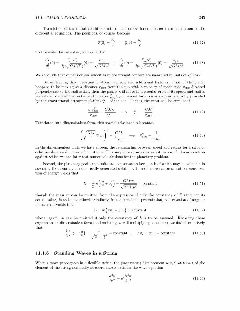
11.1. SAMPLE PROBLEMS 245

Translation of the initial conditions into dimensionless form is easier than translation of thedifferential equations. The positions, of course, become

x(0) =x0`

; y(0) =y0`

(11.47)

To translate the velocities, we argue that

dx

dt(0) =

d(x/`)

d(t√GM/l3)

(0) =vx0√GM/`

;dy

dt(0) =

d(y/`)

d(t√GM/l3)

(0) =vy0√GM/`

(11.48)

We conclude that dimensionless velocities in the present context are measured in units of√GM/`.

Before leaving this important problem, we note two additional features. First, if the planethappens to be moving at a distance rcirc from the sun with a velocity of magnitude vcirc directedperpendicular to the radius line, then the planet will move in a circular orbit if its speed and radiusare related so that the centripetal force mv2circ/rcirc needed for circular motion is exactly providedby the gravitational attraction GMm/r2circ of the sun. That is, the orbit will be circular if

mv2circrcirc

=GMm

r2circ=⇒ v2circ =

GM

rcirc(11.49)

Translated into dimensionless form, this special relationship becomes(√GM

`vcirc

)2

=GM

` rcirc=⇒ v2circ =

1

rcirc(11.50)

In the dimensionless units we have chosen, the relationship between speed and radius for a circularorbit involves no dimensional constants. This simple case provides us with a specific known motionagainst which we can later test numerical solutions for the planetary problem.

Second, the planetary problem admits two conservation laws, each of which may be valuable inassessing the accuracy of numerically generated solutions. In a dimensional presentation, conserva-tion of energy yields that

E =1

2m(v2x + v2y

)− GMm√

x2 + y2= constant (11.51)

though the mass m can be omitted from the expression if only the constancy of E (and not itsactual value) is to be examined. Similarly, in a dimensional presentation, conservation of angularmomentum yields that

L = m(xvy − yvx

)= constant (11.52)

where, again, m can be omitted if only the constancy of L is to be assessed. Recasting theseexpressions in dimensionless form (and omitting overall multiplying constants), we find alternativelythat

1

2

(v2x + v2y

)− 1√

x2 + y2= constant ; x vy − y vx = constant (11.53)

11.1.8 Standing Waves in a String

When a wave propagates in a flexible string, the (transverse) displacement u(x, t) at time t of theelement of the string nominally at coordinate x satisfies the wave equation

∂2u

∂t2= c2

∂2u

∂x2(11.54)

246 CHAPTER 11. SOLVING ORDINARY DIFFERENTIAL EQUATIONS

where c is the speed of propagation of the wave along the string. In the special case that the motionof each element is sinusoidal with frequency ω, we can write

u(x, t) = f(x) cos(ωt) (11.55)

and find, on substitution into the wave equation, that f(x), which gives the amplitude of thesinusoidal motion of the element nominally at x, satisfies

d2f

dx2+ k2f = 0 (11.56)

where k2 = ω2/c2. If, finally, the string is firmly tied down at two points, say x = 0 and x = `, thenthis second-order, homogeneous, constant-coefficient, differential equation must be solved subject tothe boundary conditions

f(0) = 0 ; f(`) = 0 (11.57)

and we conclude that waves in a string fixed at two points are described by a boundary valueproblem. Ultimately, we shall be able to find acceptable solutions only for a discrete set of specialvalues of k.

11.1.9 The Schrodinger Equation in One Dimension

A quantum mechanical particle of mass m having definite energy E and confined in one dimensionx by a potential energy V (x) is described by a wave function ψ(x) that satisfies the one-dimensionaltime-independent Schrodinger equation

− h2

2m

d2ψ

dx2+ V (x)ψ = E ψ =⇒ d2ψ

dx2+

2m

h2

(E − V (x)

)ψ = 0 (11.58)

where h is Planck’s constant divided by 2π. We anticipate subsequent exploration of two specificcases. Suppose, for example, that the potential energy is infinite except in the interval −` ≤ x ≤ +`,in which interval it is zero, i.e., suppose the particle is confined in an infinitely deep potential wellthat extends over the specified interval. Then, the wave function describing this particle must satisfythe Schrodinger equation with V = 0 inside this interval, and it must go to zero at each end of theinterval. We seek solutions to the boundary value problem

d2ψ

dx2+

2mE

h2ψ = 0 ; ψ(0) = ψ(`) = 0 (11.59)

Especially if we substitute the shorthand k2 = 2mE/h2 (or E = h2k2/2m), we recognize that thisquantum mechanical problem is mathematically identical to the classical standing wave problemdescribed in Section 11.1.8. This problem admits solutions only for a discrete set of special valuesfor k, i.e., only for special energies.

Suppose, alternatively, that we take the potential energy to be V (x) = 12kx

2, which describesthe quantum analog to the classical harmonic oscillator with spring constant k. In this case, thetime-independent Schrodinger equation becomes

d2ψ

dx2+

2m

h2

(E − 1

2kx2)ψ = 0 (11.60)

or, in dimensionless form,d2ψ

dx2+ (2ε− x2)ψ = 0 (11.61)

where ω =√k/m, ε = E/hω and x = x

√h/mω. In contrast to the infinitely deep well, the

domain for the quantum oscillator extends over the interval −∞ < x < +∞, and we must requirethat ψ(x) approach zero as x approaches either end of this interval. Numerically, infinite domains

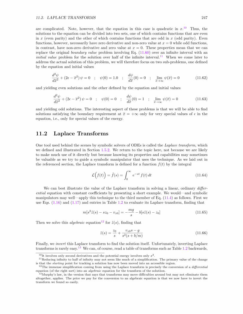
11.2. LAPLACE TRANSFORMS 247

are complicated. Note, however, that the equation in this case is quadratic in x.10 Thus, thesolutions to the equation can be divided into two sets, one of which contains functions that are evenin x (even parity) and the other of which contains functions that are odd in x (odd parity). Evenfunctions, however, necessarily have zero derivative and non-zero value at x = 0 while odd functions,in contrast, have non-zero derivative and zero value at x = 0. These properties mean that we canreplace the original boundary value problem involving Eq. (11.60) over an infinite interval with aninitial value problem for the solution over half of the infinite interval.11 When we come later toaddress the actual solution of this problem, we will therefore focus on two sub-problems, one definedby the equation and initial values

d2ψ

dx2+ (2ε− x2)ψ = 0 ; ψ(0) = 1.0 ;

dψ

dx(0) = 0 ; lim

x→∞ψ(x) = 0 (11.62)

and yielding even solutions and the other defined by the equation and initial values

d2ψ

dx2+ (2ε− x2)ψ = 0 ; ψ(0) = 0 ;

dψ

dx(0) = 1 ; lim

x→∞ψ(x) = 0 (11.63)

and yielding odd solutions. The interesting aspect of these problems is that we will be able to findsolutions satisfying the boundary requirement at x = +∞ only for very special values of ε in theequation, i.e., only for special values of the energy.

11.2 Laplace Transforms

One tool used behind the scenes by symbolic solvers of ODEs is called the Laplace transform, whichwe defined and illustrated in Section 1.5.2. We return to the topic here, not because we are likelyto make much use of it directly but because knowing its properties and capabilities may sometimesbe valuable as we try to guide a symbolic manipulator that uses the technique. As we laid out inthe referenced section, the Laplace transform is defined for a function f(t) by the integral

L(f(t)

)= f(s) =

∫ ∞0

e−st f(t) dt (11.64)

We can best illustrate the value of the Laplace transform in solving a linear, ordinary differ-ential equation with constant coefficients by presenting a short example. We would—and symbolicmanipulators may well—apply this technique to the third member of Eq. (11.4) as follows. First weuse Eqs. (1.16) and (1.17) and entries in Table 1.2 to evaluate its Laplace transform, finding that

m[s2z(s)− sz0 − vz0] = −mgs− b[sz(s)− z0] (11.65)

Then we solve this algebraic equation12 for z(s), finding that

z(s) =z0s

+vz0s− g

s2(s+ b/m)(11.66)

Finally, we invert this Laplace transform to find the solution itself. Unfortunately, inverting Laplacetransforms is rarely easy.13 We can, of course, read a table of transforms such as Table 1.2 backwards,

10It involves only second derivatives and the potential energy involves only x2.11Reducing infinity to half of infinity may not seem like much of a simplification. The primary value of the change

is that the starting point for tracking a solution has now been moved into an accessible region.12The immense simplification coming from using the Laplace transform is precisely the conversion of a differential

equation (of the right sort) into an algebraic equation for the transform of the solutiion.13Murphy’s law, in the version that says that transforms may move difficulties around but may not eliminate them

altogether, applies. The price we pay for the conversion to an algebraic equation is that we now have to invert thetransform we found so easily.

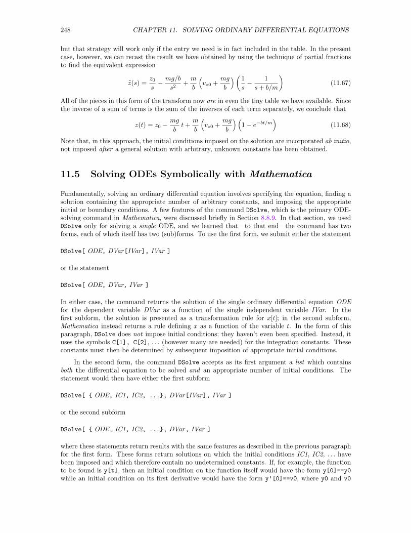
248 CHAPTER 11. SOLVING ORDINARY DIFFERENTIAL EQUATIONS

but that strategy will work only if the entry we need is in fact included in the table. In the presentcase, however, we can recast the result we have obtained by using the technique of partial fractionsto find the equivalent expression

z(s) =z0s− mg/b

s2+m

b

(vz0 +

mg

b

)(1

s− 1

s+ b/m

)(11.67)

All of the pieces in this form of the transform now are in even the tiny table we have available. Sincethe inverse of a sum of terms is the sum of the inverses of each term separately, we conclude that

z(t) = z0 −mg

bt+

m

b

(vz0 +

mg

b

)(1− e−bt/m

)(11.68)

Note that, in this approach, the initial conditions imposed on the solution are incorporated ab initio,not imposed after a general solution with arbitrary, unknown constants has been obtained.

11.5 Solving ODEs Symbolically with Mathematica

Fundamentally, solving an ordinary differential equation involves specifying the equation, finding asolution containing the appropriate number of arbitrary constants, and imposing the appropriateinitial or boundary conditions. A few features of the command DSolve, which is the primary ODE-solving command in Mathematica, were discussed briefly in Section 8.8.9. In that section, we usedDSolve only for solving a single ODE, and we learned that—to that end—the command has twoforms, each of which itself has two (sub)forms. To use the first form, we submit either the statement

DSolve[ ODE, DVar[IVar], IVar ]

or the statement

DSolve[ ODE, DVar, IVar ]

In either case, the command returns the solution of the single ordinary differential equation ODEfor the dependent variable DVar as a function of the single independent variable IVar. In thefirst subform, the solution is presented as a transformation rule for x[t]; in the second subform,Mathematica instead returns a rule defining x as a function of the variable t. In the form of thisparagraph, DSolve does not impose initial conditions; they haven’t even been specified. Instead, ituses the symbols C[1], C[2], . . . (however many are needed) for the integration constants. Theseconstants must then be determined by subsequent imposition of appropriate initial conditions.

In the second form, the command DSolve accepts as its first argument a list which containsboth the differential equation to be solved and an appropriate number of initial conditions. Thestatement would then have either the first subform

DSolve[ ODE, IC1, IC2, ..., DVar[IVar], IVar ]

or the second subform

DSolve[ ODE, IC1, IC2, ..., DVar, IVar ]

where these statements return results with the same features as described in the previous paragraphfor the first form. These forms return solutions on which the initial conditions IC1, IC2, . . . havebeen imposed and which therefore contain no undetermined constants. If, for example, the functionto be found is y[t], then an initial condition on the function itself would have the form y[0]==y0

while an initial condition on its first derivative would have the form y’[0]==v0, where y0 and v0

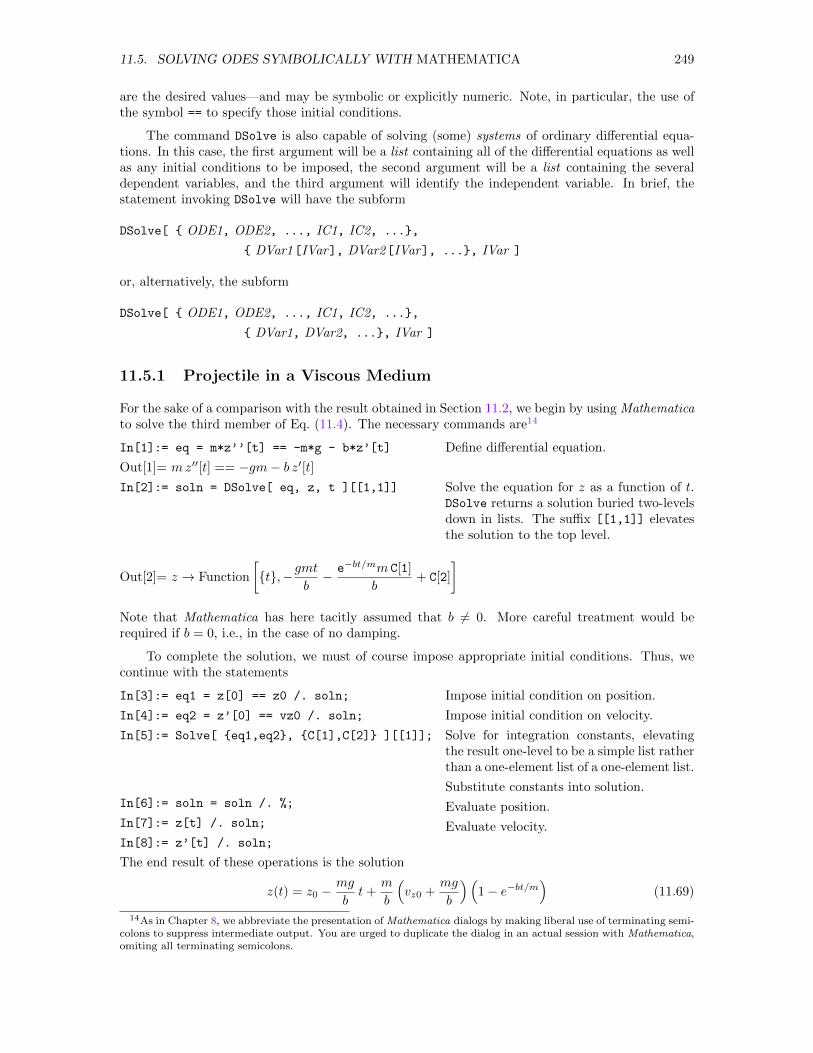
11.5. SOLVING ODES SYMBOLICALLY WITH MATHEMATICA 249

are the desired values—and may be symbolic or explicitly numeric. Note, in particular, the use ofthe symbol == to specify those initial conditions.

The command DSolve is also capable of solving (some) systems of ordinary differential equa-tions. In this case, the first argument will be a list containing all of the differential equations as wellas any initial conditions to be imposed, the second argument will be a list containing the severaldependent variables, and the third argument will identify the independent variable. In brief, thestatement invoking DSolve will have the subform

DSolve[ ODE1, ODE2, ..., IC1, IC2, ...,

DVar1[IVar], DVar2[IVar], ..., IVar ]

or, alternatively, the subform

DSolve[ ODE1, ODE2, ..., IC1, IC2, ...,

DVar1, DVar2, ..., IVar ]

11.5.1 Projectile in a Viscous Medium

For the sake of a comparison with the result obtained in Section 11.2, we begin by using Mathematicato solve the third member of Eq. (11.4). The necessary commands are14

In[1]:= eq = m*z’’[t] == -m*g - b*z’[t]

Out[1]= mz′′[t] == −gm− b z′[t]In[2]:= soln = DSolve[ eq, z, t ][[1,1]]

Define differential equation.

Solve the equation for z as a function of t.DSolve returns a solution buried two-levelsdown in lists. The suffix [[1,1]] elevatesthe solution to the top level.

Out[2]= z → Function

[t,−gmt

b− e−bt/mm C[1]

b+ C[2]

]Note that Mathematica has here tacitly assumed that b 6= 0. More careful treatment would berequired if b = 0, i.e., in the case of no damping.

To complete the solution, we must of course impose appropriate initial conditions. Thus, wecontinue with the statements

In[3]:= eq1 = z[0] == z0 /. soln;

In[4]:= eq2 = z’[0] == vz0 /. soln;

In[5]:= Solve[ eq1,eq2, C[1],C[2] ][[1]];

In[6]:= soln = soln /. %;

In[7]:= z[t] /. soln;

In[8]:= z’[t] /. soln;

Impose initial condition on position.

Impose initial condition on velocity.

Solve for integration constants, elevatingthe result one-level to be a simple list ratherthan a one-element list of a one-element list.

Substitute constants into solution.

Evaluate position.

Evaluate velocity.

The end result of these operations is the solution

z(t) = z0 −mg

bt+

m

b

(vz0 +

mg

b

)(1− e−bt/m

)(11.69)

14As in Chapter 8, we abbreviate the presentation of Mathematica dialogs by making liberal use of terminating semi-colons to suppress intermediate output. You are urged to duplicate the dialog in an actual session with Mathematica,omiting all terminating semicolons.

250 CHAPTER 11. SOLVING ORDINARY DIFFERENTIAL EQUATIONS

for the position and the solution

vz(t) = −mgb

+(vz0 +

mg

b

)e−bt/m (11.70)

for the velocity, though we have rearranged the solutions presented by Mathematica to improve theirreadability. This result for z(t) agrees fully with the result obtained in Eq. (11.68).

Wisdom suggests that we should whenever possible actually verify any solution that Mathe-matica generates. To this end, we substitute the solution into the original equation, evaluate thederivatives explicitly, and simplify the result with the statement

In[9]:= Simplify[ eq /. soln ]

Out[9]= True

To complete the verification, we check satisfaction of the initial conditions with the statement

In[10]:= Simplify[ z[0], z’[0] /. soln ]

Out[10]= z0, vz0

All is indeed well.

One further check on this solution involves examining its limit as b—the viscous damping—becomes small. For the coordinate and velocity, we find respectively that15

In[11]:= Collect[ Series[ z[t] /. soln, b, 0, 1 ], t ]

Out[11]= z0 + vz0t−1

2gt2 − bt2

2m

(vz0 −

1

3gt

)+O[b]2

In[12]:= Collect[ Series[ z’[t] /. soln, b, 0, 1 ], t ]

Out[12]= vz0 − gt−bt

m

(vz0 −

1

2gt

)+O[b]2

The terms free of b (i.e., terms in b0 = 1) clearly agree with the known results for free fall in theabsence of viscous resistance.

The solution of this problem when motion occurs in two or three of the coordinate directions isexplored in one of the exercises.

We have, of course, taken a bit longer route than necessary so as to illustrate the use of Math-ematica to find the undetermined constants in the general solution to an ODE. We could combinethe first several of our statements into an invocation of DSolve that includes the incorporation ofthe initial conditions with the statements

In[13]:= Quit[]

In[1]:= eq = m*z’’[t] == -m*g-b*z’[t];

In[2]:= soln = DSolve[ eq, z[0]==z0,

z’[0]==vz0, z, t ];

In[3]:= Quit[]

Clear Mathematica’s workspace.

Define the equation again.

Solve the equation, imposing the initial con-ditions.

These statements lead us in rather fewer steps to the result already presented in Eq. (11.69), thoughit may require extraction of the expression for the solution from soln and a subsequent applicationof Expand and Collect to reveal that agreement more clearly.

15Again, we have taken the liberty to rearrange the terms in Mathematica’s output to facilitate recognition of thelimits.

11.5. SOLVING ODES SYMBOLICALLY WITH MATHEMATICA 251

11.5.2 Logistic Growth

Consider next Eq. (11.22) governing the logistic growth of a population N in an environment withcarrying capacity Nc. We seek the solution with the Mathematica statements

In[1]:= eq = n’[t] == k*n[t]*(1-n[t]/nc);

In[2]:= soln = DSolve[ eq, n[0]==n0, n, t ]

Solve::ifun : Inverse functions are being used bySolve, so some solutions may not be round.

Out[2]=

n→ Function

[t, ektn0nc−n0 + ektn0 + nc

]In[3]:= soln = soln[[1,1]];

Enter equation. (We use n ratherthan N because N is a reserved sym-bol in Mathematica.)Solve equation for n as function oft, imposing the general initial con-dition n(0) = n0. Mathematica hasproduced a warning message that, inthis context, we can safely ignore.

Elevate function definition to toplevel.

We can verify satisfaction of the initial condition and the differential equation with the statements

In[4]:= n[0] /. soln

Out[4]= n0

In[5]:= Simplify[ eq /. soln ]

Out[5]= True

Verify satisfaction of initial condition.

Verify satisfaction of ODE.

Verifying the limit as t → ∞ is more complicated because, in the most straightforward statement,Mathematica’s command Limit will assume k to be complex and the command has no featureallowing us to tell Mathematica otherwise. Instead, we use the statements

In[6]:= qn = n[t] /. soln

Out[6]=ektn0nc

−n0 + ektn0 + nc

In[7]:= qn /. Exp[k*t] -> tmp

Out[7]=tmpn0nc

−n0 + tmpn0 + nc

to obtain an expression giving the solution and then cast that expression in terms of the singlevariable tmp for ekt. Then, since k > 0 and—hence—ekt = tmp → ∞ as t → ∞, we can determinethe solution at large t with the statement

In[8]:= Limit[ %, tmp -> Infinity ]

Out[8]= nc

As expected, the solution approaches the carrying capacity, regardless of the initial population. Thesolution therefore passes all three tests.

Let us conclude the discussion of this example by displaying the evolution of the population ina graph. We begin by casting the expression to be plotted in a dimensionless form, choosing nc asthe unit in terms of which to express the population. We have in line Out[6] already obtained theexpression to be plotted. We proceed with the statements

In[9]:= qn = qn/nc

Out[9]=ekt n0

−n0 + ekt n0 + nc

Measure population n in units of nc.

252 CHAPTER 11. SOLVING ORDINARY DIFFERENTIAL EQUATIONS

In[10]:= qn=Simplify[ qn/.n0->\[Alpha]*nc ]

Out[10]=ektα

1 + (−1 + ekt)α

Recast to measure initial population inunits of nc.

Finally, we make one further recasting to measure time in units of 1/k with the statement

In[11]:= qn = qn /. t -> \[Tau]/k

Out[11]=eτα

1 + (−1 + eτ )α

With these rescalings, we have but one parameter [physically (biologically?) the initial pop-ulation measured in units of the carrying capacity]. We produce the graph in Fig. 11.7 with thestatements

In[12]:= q1 = qn /. \[Alpha] -> 0.25;

In[13]:= q2 = qn /. \[Alpha] -> 0.5;

In[14]:= q3 = qn /. \[Alpha] -> 1.0;

In[15]:= q4 = qn /. \[Alpha] -> 2.0;

In[16]:= q5 = qn /. \[Alpha] -> 4.0;

In[17]:= Plot[ q1,q2,q3,q4,q5, \[Tau], 0.0, 5.0, PlotRange -> 0.0, 4.0,

PlotStyle -> Thickness[0.01], PlotLabel->StyleForm[ "Logistic Behavior",

FontFamily->"Times", FontSize -> 14,

FontWeight->"Bold"], AxesLabel->"kt", "n/nc" ]

Regardless of the initial population, all solutions converge monotonically on the carrying capacity(1.0 in the units we are using). Further, if we execute the statements

In[18]:= q6 = qn /. \[Alpha] -> 0.05;

In[19]:= Plot[ q6, \[Tau], 0.0, 10.0,

PlotRange -> 0.0, 1.0, PlotStyle -> Thickness[0.01],

PlotLabel->StyleForm[ "Logistic Behavior",

FontFamily->"Times", FontSize -> 14,

FontWeight->"Bold"], AxesLabel->"kt", "n/nc" ]

we generate the graph in Fig. 11.8, which shows the initial exponential growth when the populationis well below the carrying capacity but then reveals the leveling off as the population approachesthe carrying capacity.

11.5.3 Damped Harmonic Oscillator

A third example of the use of Mathematica to solve a single second-order, linear, constant-coefficient,homogeneous, ordinary differential equation was presented in Chapter 8. You are invited to reviewthe discussion of the damped harmonic oscillator in Sections 8.8.9 and 11.1.4.

11.5.4 Chain Radioactive Decay

As a first example of the use of Mathematica to solve a system of linear equations, let us determinethe behavior of the radioactive decay chain described by Eq. (11.19). For simplicity, we supposethe initial values A(0) = A0 and B(0) = C(0) = 0, i.e., we start with some A and no B or C. Thetemporal evolution of this system is found with the Mathematica statements

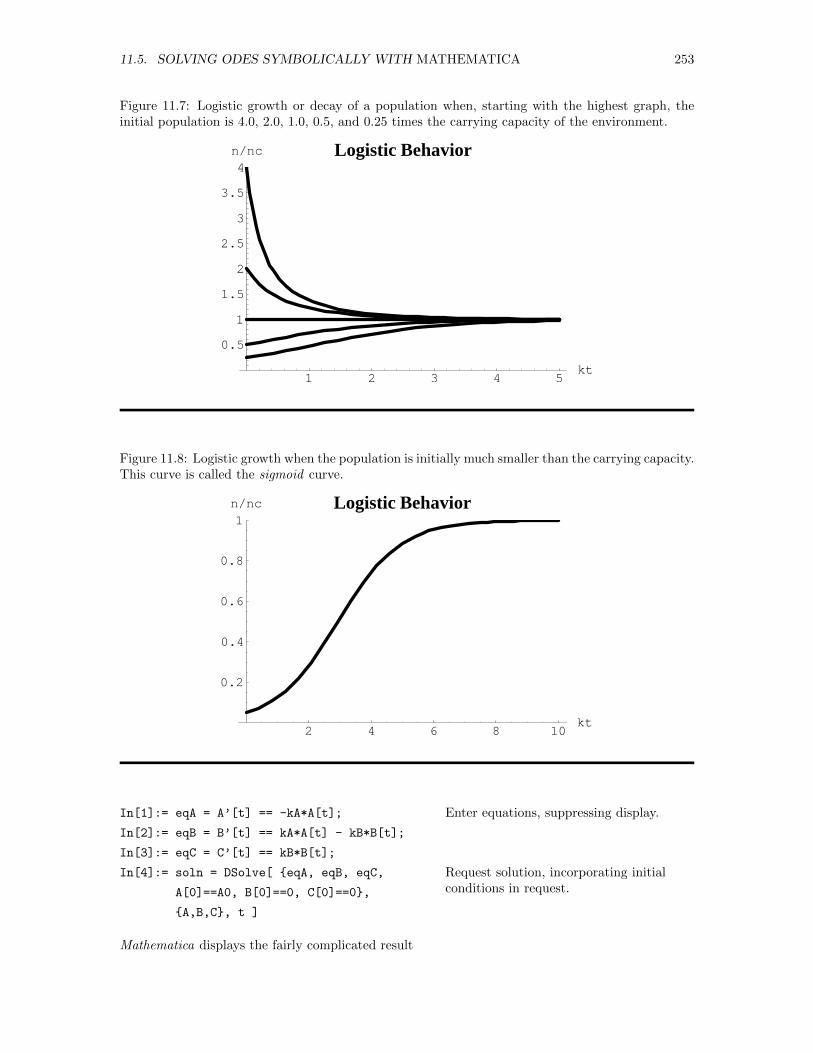
11.5. SOLVING ODES SYMBOLICALLY WITH MATHEMATICA 253

Figure 11.7: Logistic growth or decay of a population when, starting with the highest graph, theinitial population is 4.0, 2.0, 1.0, 0.5, and 0.25 times the carrying capacity of the environment.

1 2 3 4 5kt

0.5

1

1.5

2

2.5

3

3.5

4n/nc Logistic Behavior

Figure 11.8: Logistic growth when the population is initially much smaller than the carrying capacity.This curve is called the sigmoid curve.

2 4 6 8 10kt

0.2

0.4

0.6

0.8

1n/nc Logistic Behavior

In[1]:= eqA = A’[t] == -kA*A[t];

In[2]:= eqB = B’[t] == kA*A[t] - kB*B[t];

In[3]:= eqC = C’[t] == kB*B[t];

In[4]:= soln = DSolve[ eqA, eqB, eqC,

A[0]==A0, B[0]==0, C[0]==0,

A,B,C, t ]

Enter equations, suppressing display.

Request solution, incorporating initialconditions in request.

Mathematica displays the fairly complicated result

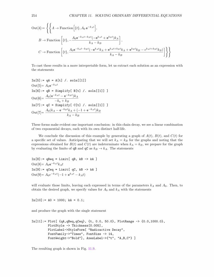
254 CHAPTER 11. SOLVING ORDINARY DIFFERENTIAL EQUATIONS

Out[4]:=

A→ Function

[t, A0 e

−kAt],

B → Function

[t,−A0e

−kAt−kBt(−ekAt + ekBt)kAkA − kB

],

C → Function

[t, A0e

−kAt−kBt(−ekAtkA + ekAt+kBtkA + ekBtkB − ekAt+kBtkB)

kA − kB

]

To cast these results in a more intrepretable form, let us extract each solution as an expression withthe statements

In[5]:= qA = A[t] /. soln[[1]]

Out[5]= A0e−kAt

In[6]:= qB = Simplify[ B[t] /. soln[[1]] ]

Out[6]=A0(e−kAt − e−kBt)kA

−ka + kBIn[7]:= qC = Simplify[ C[t] /. soln[[1]] ]

Out[7]=A0(kA − e−kBtkA + (−1 + e−kAt)kB

kA − kB

These forms make evident one important conclusion: in this chain decay, we see a linear combinationof two exponential decays, each with its own distinct half-life.

We conclude the discussion of this example by generating a graph of A(t), B(t), and C(t) fora specific set of values. Anticipating that we will set kA = kB for the graphs and noting that theexpressions obtained for B(t) and C(t) are indeterminate when kA = kB , we prepare for the graphby evaluating the limits of qB and qC as kB → kA. The statements

In[8]:= qBeq = Limit[ qB, kB -> kA ]

Out[8]= A0e−kAtkAt

In[9]:= qCeq = Limit[ qC, kB -> kA ]

Out[9]= A0e−kAt(−1 + ekAt − kAt)

will evaluate those limits, leaving each expressed in terms of the parameters kA and A0. Then, toobtain the desired graph, we specify values for A0 and kA with the statements

In[10]:= A0 = 1000; kA = 0.1;

and produce the graph with the single statement

In[11]:= Plot[ qA,qBeq,qCeq, t, 0.0, 50.0, PlotRange -> 0.0,1000.0,

PlotStyle -> Thickness[0.005],

PlotLabel->StyleForm[ "Radioactive Decay",

FontFamily->"Times", FontSize -> 14,

FontWeight->"Bold"], AxesLabel->"t", "A,B,C" ]

The resulting graph is shown in Fig. 11.9.

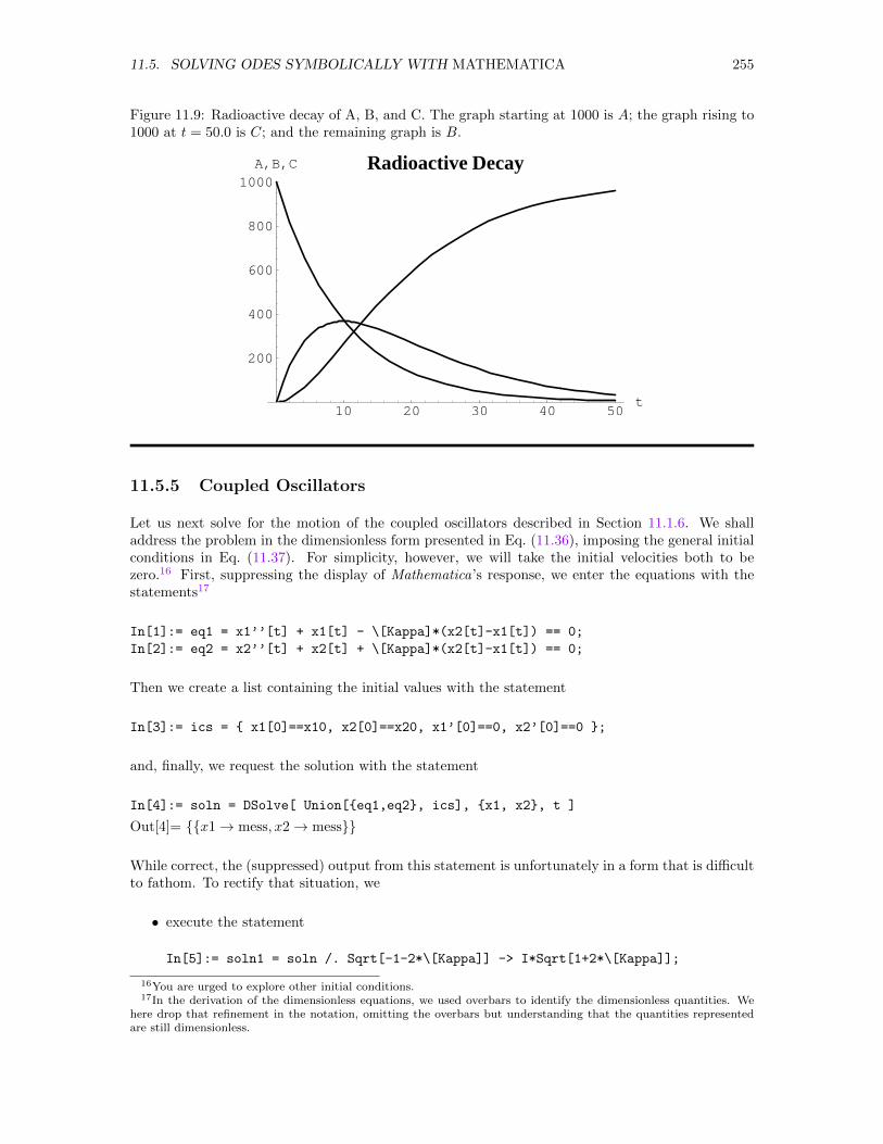
11.5. SOLVING ODES SYMBOLICALLY WITH MATHEMATICA 255

Figure 11.9: Radioactive decay of A, B, and C. The graph starting at 1000 is A; the graph rising to1000 at t = 50.0 is C; and the remaining graph is B.

10 20 30 40 50t

200

400

600

800

1000A,B,C Radioactive Decay

11.5.5 Coupled Oscillators

Let us next solve for the motion of the coupled oscillators described in Section 11.1.6. We shalladdress the problem in the dimensionless form presented in Eq. (11.36), imposing the general initialconditions in Eq. (11.37). For simplicity, however, we will take the initial velocities both to bezero.16 First, suppressing the display of Mathematica’s response, we enter the equations with thestatements17

In[1]:= eq1 = x1’’[t] + x1[t] - \[Kappa]*(x2[t]-x1[t]) == 0;

In[2]:= eq2 = x2’’[t] + x2[t] + \[Kappa]*(x2[t]-x1[t]) == 0;

Then we create a list containing the initial values with the statement

In[3]:= ics = x1[0]==x10, x2[0]==x20, x1’[0]==0, x2’[0]==0 ;

and, finally, we request the solution with the statement

In[4]:= soln = DSolve[ Union[eq1,eq2, ics], x1, x2, t ]

Out[4]= x1→ mess, x2→ mess

While correct, the (suppressed) output from this statement is unfortunately in a form that is difficultto fathom. To rectify that situation, we

• execute the statement

In[5]:= soln1 = soln /. Sqrt[-1-2*\[Kappa]] -> I*Sqrt[1+2*\[Kappa]];

16You are urged to explore other initial conditions.17In the derivation of the dimensionless equations, we used overbars to identify the dimensionless quantities. We

here drop that refinement in the notation, omitting the overbars but understanding that the quantities representedare still dimensionless.

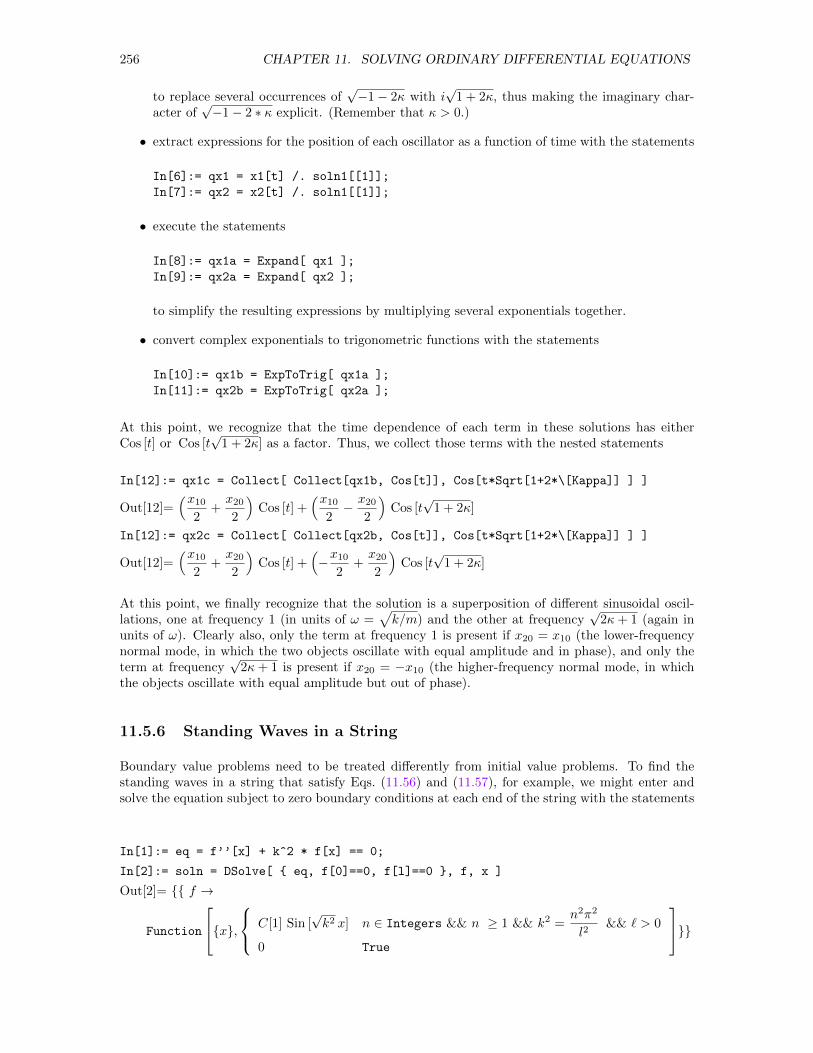
256 CHAPTER 11. SOLVING ORDINARY DIFFERENTIAL EQUATIONS

to replace several occurrences of√−1− 2κ with i

√1 + 2κ, thus making the imaginary char-

acter of√−1− 2 ∗ κ explicit. (Remember that κ > 0.)

• extract expressions for the position of each oscillator as a function of time with the statements

In[6]:= qx1 = x1[t] /. soln1[[1]];

In[7]:= qx2 = x2[t] /. soln1[[1]];

• execute the statements

In[8]:= qx1a = Expand[ qx1 ];

In[9]:= qx2a = Expand[ qx2 ];

to simplify the resulting expressions by multiplying several exponentials together.

• convert complex exponentials to trigonometric functions with the statements

In[10]:= qx1b = ExpToTrig[ qx1a ];

In[11]:= qx2b = ExpToTrig[ qx2a ];

At this point, we recognize that the time dependence of each term in these solutions has eitherCos [t] or Cos [t

√1 + 2κ] as a factor. Thus, we collect those terms with the nested statements

In[12]:= qx1c = Collect[ Collect[qx1b, Cos[t]], Cos[t*Sqrt[1+2*\[Kappa]] ] ]

Out[12]=(x10

2+x202

)Cos [t] +

(x102− x20

2

)Cos [t

√1 + 2κ]

In[12]:= qx2c = Collect[ Collect[qx2b, Cos[t]], Cos[t*Sqrt[1+2*\[Kappa]] ] ]

Out[12]=(x10

2+x202

)Cos [t] +

(−x10

2+x202

)Cos [t

√1 + 2κ]

At this point, we finally recognize that the solution is a superposition of different sinusoidal oscil-lations, one at frequency 1 (in units of ω =

√k/m) and the other at frequency

√2κ+ 1 (again in

units of ω). Clearly also, only the term at frequency 1 is present if x20 = x10 (the lower-frequencynormal mode, in which the two objects oscillate with equal amplitude and in phase), and only theterm at frequency

√2κ+ 1 is present if x20 = −x10 (the higher-frequency normal mode, in which

the objects oscillate with equal amplitude but out of phase).

11.5.6 Standing Waves in a String

Boundary value problems need to be treated differently from initial value problems. To find thestanding waves in a string that satisfy Eqs. (11.56) and (11.57), for example, we might enter andsolve the equation subject to zero boundary conditions at each end of the string with the statements

In[1]:= eq = f’’[x] + k^2 * f[x] == 0;

In[2]:= soln = DSolve[ eq, f[0]==0, f[l]==0 , f, x ]

Out[2]= f →

Function

x, C[1] Sin [

√k2 x] n ∈ Integers && n ≥ 1 && k2 =

n2π2

l2&& ` > 0

0 True

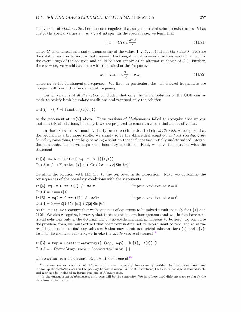
11.5. SOLVING ODES SYMBOLICALLY WITH MATHEMATICA 257

The version of Mathematica here in use recognizes that only the trivial solution exists unless k hasone of the special values k = nπ/l, n ∈ integer. In the special case, we learn that

f(x) = C1 sinnπx

`(11.71)

where C1 is undetermined and n assumes any of the values 1, 2, 3, . . . (but not the value 0—becausethe solution reduces to zero in that case—and not negative values—because they really change onlythe overall sign of the solution and could be seen simply as an alternative choice of C1). Further,since ω = kc, we would associate with this solution the frequency

ωn = knc = nπc

`= nω1 (11.72)

where ω1 is the fundamental frequency. We find, in particular, that all allowed frequencies areinteger multiples of the fundamental frequency.

Earlier versions of Mathematica concluded that only the trivial solution to the ODE can bemade to satisfy both boundary conditions and returned only the solution

Out[2]= f → Function[x, 0]

to the statement at In[2] above. These versions of Mathematica failed to recognize that we canfind non-trivial solutions, but only if we are prepared to constrain k to a limited set of values.

In those versions, we must evidently be more deliberate. To help Mathematica recognize thatthe problem is a bit more subtle, we simply solve the differential equation without specifying theboundary conditions, thereby generating a solution that includes two initially undetermined integra-tion constants. Then, we impose the boundary conditions. First, we solve the equation with thestatement

In[3] soln = DSolve[ eq, f, x ][[1,1]]

Out[3]= f → Function[x, C[1] Cos [kx] + C[2] Sin [kx]]

elevating the solution with [[1,1]] to the top level in its expression. Next, we determine theconsequences of the boundary conditions with the statements

In[4] eq1 = 0 == f[0] /. soln

Out[4]= 0 == C[1]

In[5]:= eq2 = 0 == f[l] /. soln

Out[4]= 0 == C[1] Cos [k`] + C[2] Sin [k`]

Impose condition at x = 0.

Impose condition at x = `.

At this point, we recognize that we have a pair of equations to be solved simultaneously for C[1] andC[2]. We also recognize, however, that these equations are homogeneous and will in fact have non-trivial solutions only if the determinant of the coefficient matrix happens to be zero. To completethe problem, then, we must extract that coefficient matrix, set its determinant to zero, and solve theresulting equation to find any values of k that may admit non-trivial solutions for C[1] and C[2].To find the coefficient matrix, we invoke the Mathematica statement18

In[5]:= tmp = CoefficientArrays[ eq1, eq2, C[1], C[2] ]

Out[5]= SparseArray[ mess ],SparseArray[ mess ]

whose output is a bit obscure. Even so, the statement19

18In some earlier versions of Mathematica, the necessary functionality resided in the older commandLinearEquationsToMatrices in the package LinearAlgebra. While still available, that entire package is now obsoleteand may not be included in future versions of Mathematica.

19In the output from Mathematica, all braces will be the same size. We have here used different sizes to clarify thestructure of that output.

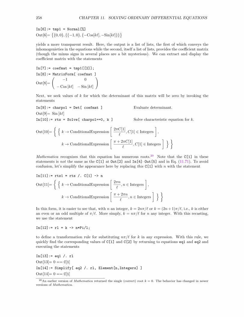
258 CHAPTER 11. SOLVING ORDINARY DIFFERENTIAL EQUATIONS

In[6]:= tmp1 = Normal[%]

Out[6]=0, 0, −1, 0, −Cos[k`],−Sin[k`]

yields a more transparent result. Here, the output is a list of lists, the first of which conveys theinhomogenieties in the equations while the second, itself a list of lists, provides the coefficient matrix(though the minus signs in several places are a bit mysterious). We can extract and display thecoefficient matrix with the statements

In[7]:= coefmat = tmp1[[2]];

In[8]:= MatrixForm[ coefmat ]

Out[8]=

(−1 0

−Cos [k`] −Sin [k`]

)

Next, we seek values of k for which the determinant of this matrix will be zero by invoking thestatements

In[9]:= charpol = Det[ coefmat ]

Out[9]= Sin [k`]

In[10]:= rts = Solve[ charpol==0, k ]

Evaluate determinant.

Solve characteristic equation for k.

Out[10]=

k → ConditionalExpression

[2πC[1]

`, C[1] ∈ Integers

],

k → ConditionalExpression

[π + 2πC[1]

`, C[1] ∈ Integers

] Mathematica recognizes that this equation has numerous roots.20 Note that the C[1] in thesestatements is not the same as the C[1] at Out[2] and In[4]–Out[5] and in Eq. (11.71). To avoidconfusion, let’s simplify the appearance here by replacing this C[1] with n with the statement

In[11]:= rts1 = rts /. C[1] -> n

Out[11]=

k → ConditionalExpression

[2πn

`, n ∈ Integers

],

k → ConditionalExpression

[π + 2πn

`, n ∈ Integers

] In this form, it is easier to see that, with n an integer, k = 2nπ/` or k = (2n+ 1)π/`, i.e., k is eitheran even or an odd multiple of π/`. More simply, k = nπ/` for n any integer. With this recasting,we use the statement

In[12]:= rl = k -> n*Pi/l;

to define a transformation rule for substituting nπ/` for k in any expression. With this rule, wequickly find the corresponding values of C[1] and C[2] by returning to equations eq1 and eq2 andexecuting the statements

In[13]:= eq1 /. rl

Out[13]= 0 == C[1]

In[14]:= Simplify[ eq2 /. rl, Element[n,Integers] ]

Out[14]= 0 == C[1]

20An earlier version of Mathematica returned the single (correct) root k = 0. The behavior has changed in newerversions of Mathematica.

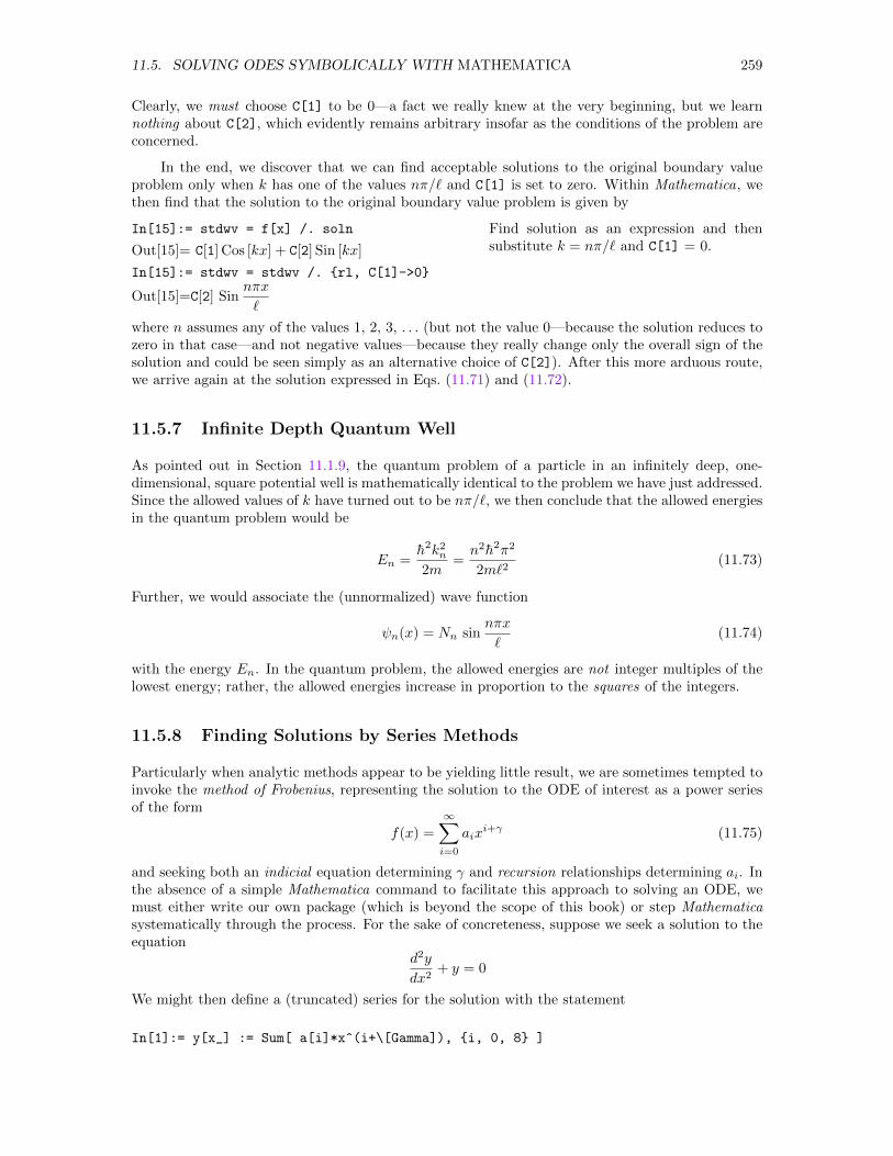
11.5. SOLVING ODES SYMBOLICALLY WITH MATHEMATICA 259

Clearly, we must choose C[1] to be 0—a fact we really knew at the very beginning, but we learnnothing about C[2], which evidently remains arbitrary insofar as the conditions of the problem areconcerned.

In the end, we discover that we can find acceptable solutions to the original boundary valueproblem only when k has one of the values nπ/` and C[1] is set to zero. Within Mathematica, wethen find that the solution to the original boundary value problem is given by

In[15]:= stdwv = f[x] /. soln

Out[15]= C[1] Cos [kx] + C[2] Sin [kx]

In[15]:= stdwv = stdwv /. rl, C[1]->0

Out[15]=C[2] Sinnπx

`

Find solution as an expression and thensubstitute k = nπ/` and C[1] = 0.

where n assumes any of the values 1, 2, 3, . . . (but not the value 0—because the solution reduces tozero in that case—and not negative values—because they really change only the overall sign of thesolution and could be seen simply as an alternative choice of C[2]). After this more arduous route,we arrive again at the solution expressed in Eqs. (11.71) and (11.72).

11.5.7 Infinite Depth Quantum Well

As pointed out in Section 11.1.9, the quantum problem of a particle in an infinitely deep, one-dimensional, square potential well is mathematically identical to the problem we have just addressed.Since the allowed values of k have turned out to be nπ/`, we then conclude that the allowed energiesin the quantum problem would be

En =h2k2n2m

=n2h2π2

2m`2(11.73)

Further, we would associate the (unnormalized) wave function

ψn(x) = Nn sinnπx

`(11.74)

with the energy En. In the quantum problem, the allowed energies are not integer multiples of thelowest energy; rather, the allowed energies increase in proportion to the squares of the integers.

11.5.8 Finding Solutions by Series Methods

Particularly when analytic methods appear to be yielding little result, we are sometimes tempted toinvoke the method of Frobenius, representing the solution to the ODE of interest as a power seriesof the form

f(x) =

∞∑i=0

aixi+γ (11.75)

and seeking both an indicial equation determining γ and recursion relationships determining ai. Inthe absence of a simple Mathematica command to facilitate this approach to solving an ODE, wemust either write our own package (which is beyond the scope of this book) or step Mathematicasystematically through the process. For the sake of concreteness, suppose we seek a solution to theequation

d2y

dx2+ y = 0

We might then define a (truncated) series for the solution with the statement

In[1]:= y[x_] := Sum[ a[i]*x^(i+\[Gamma]), i, 0, 8 ]

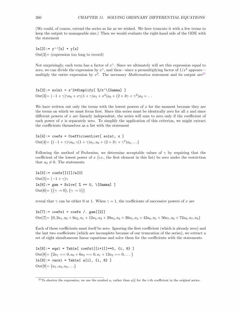
260 CHAPTER 11. SOLVING ORDINARY DIFFERENTIAL EQUATIONS

(We could, of course, extend the series as far as we wished. We here truncate it with a few terms tokeep the output to manageable size.) Then we would evaluate the right-hand side of the ODE withthe statement

In[2]:= y’’[x] + y[x]

Out[2]= (expression too long to record)

Not surprisingly, each term has a factor of xγ . Since we ultimately will set this expression equal tozero, we can divide the expression by xγ , and then—since a premultiplying factor of 1/x2 appears—multiply the entire expression by x2. The necessary Mathematica statement and its output are21

In[3]:= soln1 = x^2*Simplify[ %/x^\[Gamma] ]

Out[3]= (−1 + γ)γa0 + xγ(1 + γ)a1 + x2(a0 + (2 + 3γ + γ2)a2 + . . .

We have written out only the terms with the lowest powers of x for the moment because they arethe terms on which we must focus first. Since this series must be identically zero for all x and sincedifferent powers of x are linearly independent, the series will sum to zero only if the coefficient ofeach power of x is separately zero. To simplify the application of this criterion, we might extractthe coefficients themselves as a list with the statement

In[4]:= coefs = CoefficientList[ soln1, x ]

Out[4]= (−1 + γ)γa0, γ(1 + γ)a1, a0 + (2 + 3γ + γ2)a2, . . .

Following the method of Frobenius, we determine acceptable values of γ by requiring that thecoefficient of the lowest power of x (i.e., the first element in this list) be zero under the restrictionthat a0 6= 0. The statements

In[5]:= coefs[[1]]/a[0]

Out[5]= (−1 + γ)γ

In[6]:= gam = Solve[ % == 0, \[Gamma] ]

Out[6]= γ → 0, γ → 1

reveal that γ can be either 0 or 1. When γ = 1, the coefficients of successive powers of x are

In[7]:= coefs1 = coefs /. gam[[2]]

Out[7]= 0, 2a1, a0 + 6a2, a1 + 12a3, a2 + 20a4, a3 + 30a5, a4 + 42a6, a5 + 56a7, a6 + 72a8, a7, a8

Each of these coefficients must itself be zero. Ignoring the first coefficient (which is already zero) andthe last two coefficients (which are incomplete because of our truncation of the series), we extract aset of eight simultaneous linear equations and solve them for the coefficients with the statements

In[8]:= eqs1 = Table[ coefs1[[i+1]]==0, i, 8 ]

Out[8]= 2a1 == 0, a0 + 6a2 == 0, a1 + 12a3 == 0, . . . In[9]:= vars1 = Table[ a[i], i, 8 ]

Out[9]= a1, a2, a3, . . .

21To shorten the expression, we use the symbol ai rather than a[i] for the i-th coefficient in the original series.

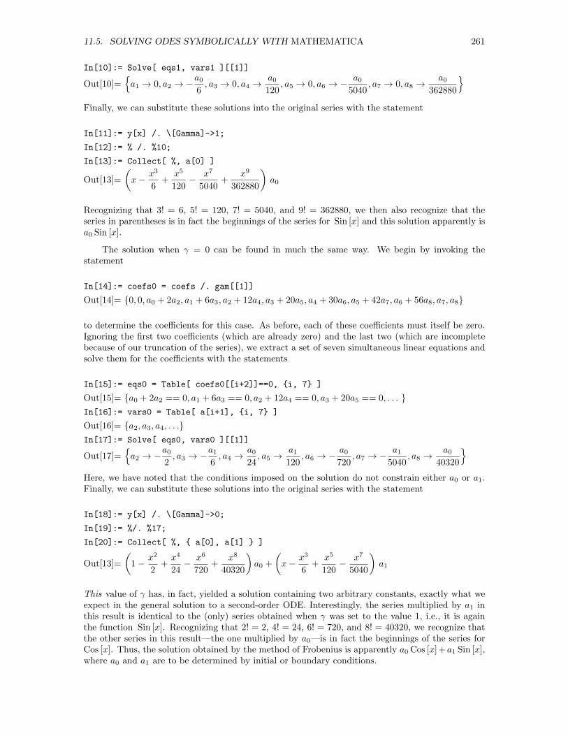
11.5. SOLVING ODES SYMBOLICALLY WITH MATHEMATICA 261

In[10]:= Solve[ eqs1, vars1 ][[1]]

Out[10]=a1 → 0, a2 → −

a06, a3 → 0, a4 →

a0120

, a5 → 0, a6 → −a0

5040, a7 → 0, a8 →

a0362880

Finally, we can substitute these solutions into the original series with the statement

In[11]:= y[x] /. \[Gamma]->1;

In[12]:= % /. %10;

In[13]:= Collect[ %, a[0] ]

Out[13]=

(x− x3

6+

x5

120− x7

5040+

x9

362880

)a0

Recognizing that 3! = 6, 5! = 120, 7! = 5040, and 9! = 362880, we then also recognize that theseries in parentheses is in fact the beginnings of the series for Sin [x] and this solution apparently isa0 Sin [x].

The solution when γ = 0 can be found in much the same way. We begin by invoking thestatement

In[14]:= coefs0 = coefs /. gam[[1]]

Out[14]= 0, 0, a0 + 2a2, a1 + 6a3, a2 + 12a4, a3 + 20a5, a4 + 30a6, a5 + 42a7, a6 + 56a8, a7, a8

to determine the coefficients for this case. As before, each of these coefficients must itself be zero.Ignoring the first two coefficients (which are already zero) and the last two (which are incompletebecause of our truncation of the series), we extract a set of seven simultaneous linear equations andsolve them for the coefficients with the statements

In[15]:= eqs0 = Table[ coefs0[[i+2]]==0, i, 7 ]

Out[15]= a0 + 2a2 == 0, a1 + 6a3 == 0, a2 + 12a4 == 0, a3 + 20a5 == 0, . . . In[16]:= vars0 = Table[ a[i+1], i, 7 ]

Out[16]= a2, a3, a4, . . .In[17]:= Solve[ eqs0, vars0 ][[1]]

Out[17]=a2 → −

a02, a3 → −

a16, a4 →

a024, a5 →

a1120

, a6 → −a0720

, a7 → −a1

5040, a8 →

a040320

Here, we have noted that the conditions imposed on the solution do not constrain either a0 or a1.Finally, we can substitute these solutions into the original series with the statement

In[18]:= y[x] /. \[Gamma]->0;

In[19]:= %/. %17;

In[20]:= Collect[ %, a[0], a[1] ]

Out[13]=

(1− x2

2+x4

24− x6

720+

x8

40320

)a0 +

(x− x3

6+

x5

120− x7

5040

)a1

This value of γ has, in fact, yielded a solution containing two arbitrary constants, exactly what weexpect in the general solution to a second-order ODE. Interestingly, the series multiplied by a1 inthis result is identical to the (only) series obtained when γ was set to the value 1, i.e., it is againthe function Sin [x]. Recognizing that 2! = 2, 4! = 24, 6! = 720, and 8! = 40320, we recognize thatthe other series in this result—the one multiplied by a0—is in fact the beginnings of the series forCos [x]. Thus, the solution obtained by the method of Frobenius is apparently a0 Cos [x] +a1 Sin [x],where a0 and a1 are to be determined by initial or boundary conditions.

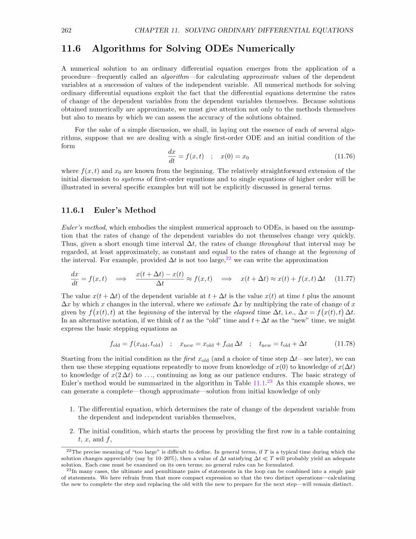
262 CHAPTER 11. SOLVING ORDINARY DIFFERENTIAL EQUATIONS

11.6 Algorithms for Solving ODEs Numerically

A numerical solution to an ordinary differential equation emerges from the application of aprocedure—frequently called an algorithm—for calculating approximate values of the dependentvariables at a succession of values of the independent variable. All numerical methods for solvingordinary differential equations exploit the fact that the differential equations determine the ratesof change of the dependent variables from the dependent variables themselves. Because solutionsobtained numerically are approximate, we must give attention not only to the methods themselvesbut also to means by which we can assess the accuracy of the solutions obtained.

For the sake of a simple discussion, we shall, in laying out the essence of each of several algo-rithms, suppose that we are dealing with a single first-order ODE and an initial condition of theform

dx

dt= f(x, t) ; x(0) = x0 (11.76)

where f(x, t) and x0 are known from the beginning. The relatively straightforward extension of theinitial discussion to systems of first-order equations and to single equations of higher order will beillustrated in several specific examples but will not be explicitly discussed in general terms.

11.6.1 Euler’s Method

Euler’s method, which embodies the simplest numerical approach to ODEs, is based on the assump-tion that the rates of change of the dependent variables do not themselves change very quickly.Thus, given a short enough time interval ∆t, the rates of change throughout that interval may beregarded, at least approximately, as constant and equal to the rates of change at the beginning ofthe interval. For example, provided ∆t is not too large,22 we can write the approximation

dx

dt= f(x, t) =⇒ x(t+ ∆t)− x(t)

∆t≈ f(x, t) =⇒ x(t+ ∆t) ≈ x(t) + f(x, t) ∆t (11.77)

The value x(t+ ∆t) of the dependent variable at t+ ∆t is the value x(t) at time t plus the amount∆x by which x changes in the interval, where we estimate ∆x by multiplying the rate of change of xgiven by f

(x(t), t

)at the beginning of the interval by the elapsed time ∆t, i.e., ∆x = f

(x(t), t

)∆t.

In an alternative notation, if we think of t as the “old” time and t+ ∆t as the “new” time, we mightexpress the basic stepping equations as

fold = f(xold, told) ; xnew = xold + fold ∆t ; tnew = told + ∆t (11.78)

Starting from the initial condition as the first xold (and a choice of time step ∆t—see later), we canthen use these stepping equations repeatedly to move from knowledge of x(0) to knowledge of x(∆t)to knowledge of x(2 ∆t) to . . ., continuing as long as our patience endures. The basic strategy ofEuler’s method would be summarized in the algorithm in Table 11.1.23 As this example shows, wecan generate a complete—though approximate—solution from initial knowledge of only

1. The differential equation, which determines the rate of change of the dependent variable fromthe dependent and independent variables themselves,

2. The initial condition, which starts the process by providing the first row in a table containingt, x, and f ,

22The precise meaning of “too large” is difficult to define. In general terms, if T is a typical time during which thesolution changes appreciably (say by 10–20%), then a value of ∆t satisfying ∆t T will probably yield an adequatesolution. Each case must be examined on its own terms; no general rules can be formulated.

23In many cases, the ultimate and penultimate pairs of statements in the loop can be combined into a single pairof statements. We here refrain from that more compact expression so that the two distinct operations—calculatingthe new to complete the step and replacing the old with the new to prepare for the next step—will remain distinct.

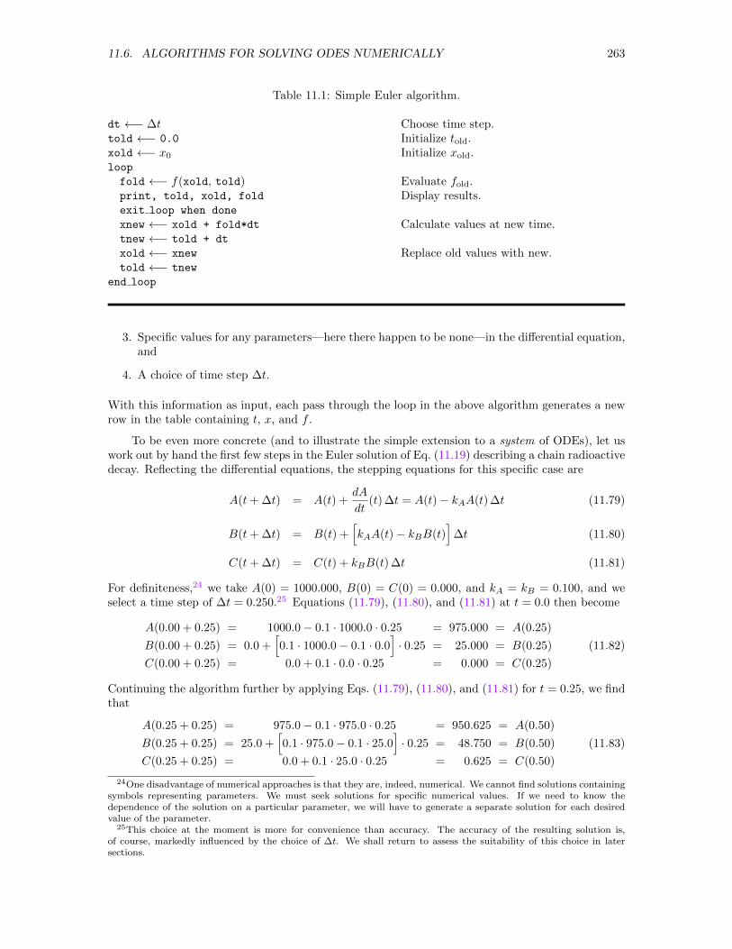
11.6. ALGORITHMS FOR SOLVING ODES NUMERICALLY 263

Table 11.1: Simple Euler algorithm.

dt ←− ∆ttold ←− 0.0

xold ←− x0loop

fold ←− f(xold, told)print, told, xold, fold

exit loop when done

xnew ←− xold + fold*dt

tnew ←− told + dt

xold ←− xnew

told ←− tnew

end loop

Choose time step.Initialize told.Initialize xold.

Evaluate fold.Display results.

Calculate values at new time.

Replace old values with new.

3. Specific values for any parameters—here there happen to be none—in the differential equation,and

4. A choice of time step ∆t.

With this information as input, each pass through the loop in the above algorithm generates a newrow in the table containing t, x, and f .

To be even more concrete (and to illustrate the simple extension to a system of ODEs), let uswork out by hand the first few steps in the Euler solution of Eq. (11.19) describing a chain radioactivedecay. Reflecting the differential equations, the stepping equations for this specific case are

A(t+ ∆t) = A(t) +dA

dt(t) ∆t = A(t)− kAA(t) ∆t (11.79)

B(t+ ∆t) = B(t) +[kAA(t)− kBB(t)

]∆t (11.80)

C(t+ ∆t) = C(t) + kBB(t) ∆t (11.81)

For definiteness,24 we take A(0) = 1000.000, B(0) = C(0) = 0.000, and kA = kB = 0.100, and weselect a time step of ∆t = 0.250.25 Equations (11.79), (11.80), and (11.81) at t = 0.0 then become

A(0.00 + 0.25) = 1000.0− 0.1 · 1000.0 · 0.25 = 975.000 = A(0.25)

B(0.00 + 0.25) = 0.0 +[0.1 · 1000.0− 0.1 · 0.0

]· 0.25 = 25.000 = B(0.25)

C(0.00 + 0.25) = 0.0 + 0.1 · 0.0 · 0.25 = 0.000 = C(0.25)

(11.82)

Continuing the algorithm further by applying Eqs. (11.79), (11.80), and (11.81) for t = 0.25, we findthat

A(0.25 + 0.25) = 975.0− 0.1 · 975.0 · 0.25 = 950.625 = A(0.50)

B(0.25 + 0.25) = 25.0 +[0.1 · 975.0− 0.1 · 25.0

]· 0.25 = 48.750 = B(0.50)

C(0.25 + 0.25) = 0.0 + 0.1 · 25.0 · 0.25 = 0.625 = C(0.50)

(11.83)

24One disadvantage of numerical approaches is that they are, indeed, numerical. We cannot find solutions containingsymbols representing parameters. We must seek solutions for specific numerical values. If we need to know thedependence of the solution on a particular parameter, we will have to generate a separate solution for each desiredvalue of the parameter.

25This choice at the moment is more for convenience than accuracy. The accuracy of the resulting solution is,of course, markedly influenced by the choice of ∆t. We shall return to assess the suitability of this choice in latersections.

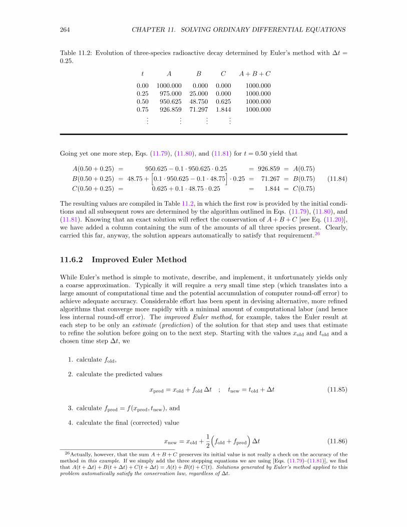
264 CHAPTER 11. SOLVING ORDINARY DIFFERENTIAL EQUATIONS

Table 11.2: Evolution of three-species radioactive decay determined by Euler’s method with ∆t =0.25.

t A B C A+B + C

0.00 1000.000 0.000 0.000 1000.0000.25 975.000 25.000 0.000 1000.0000.50 950.625 48.750 0.625 1000.0000.75 926.859 71.297 1.844 1000.000

......

......

Going yet one more step, Eqs. (11.79), (11.80), and (11.81) for t = 0.50 yield that

A(0.50 + 0.25) = 950.625− 0.1 · 950.625 · 0.25 = 926.859 = A(0.75)

B(0.50 + 0.25) = 48.75 +[0.1 · 950.625− 0.1 · 48.75

]· 0.25 = 71.267 = B(0.75)

C(0.50 + 0.25) = 0.625 + 0.1 · 48.75 · 0.25 = 1.844 = C(0.75)

(11.84)

The resulting values are compiled in Table 11.2, in which the first row is provided by the initial condi-tions and all subsequent rows are determined by the algorithm outlined in Eqs. (11.79), (11.80), and(11.81). Knowing that an exact solution will reflect the conservation of A+B+C [see Eq. (11.20)],we have added a column containing the sum of the amounts of all three species present. Clearly,carried this far, anyway, the solution appears automatically to satisfy that requirement.26

11.6.2 Improved Euler Method

While Euler’s method is simple to motivate, describe, and implement, it unfortunately yields onlya coarse approximation. Typically it will require a very small time step (which translates into alarge amount of computational time and the potential accumulation of computer round-off error) toachieve adequate accuracy. Considerable effort has been spent in devising alternative, more refinedalgorithms that converge more rapidly with a minimal amount of computational labor (and henceless internal round-off error). The improved Euler method, for example, takes the Euler result ateach step to be only an estimate (prediction) of the solution for that step and uses that estimateto refine the solution before going on to the next step. Starting with the values xold and told and achosen time step ∆t, we

1. calculate fold,

2. calculate the predicted values

xpred = xold + fold ∆t ; tnew = told + ∆t (11.85)

3. calculate fpred = f(xpred, tnew), and

4. calculate the final (corrected) value

xnew = xold +1

2

(fold + fpred

)∆t (11.86)

26Actually, however, that the sum A+B +C preserves its initial value is not really a check on the accuracy of themethod in this example. If we simply add the three stepping equations we are using [Eqs. (11.79)–(11.81)], we findthat A(t+ ∆t) +B(t+ ∆t) +C(t+ ∆t) = A(t) +B(t) +C(t). Solutions generated by Euler’s method applied to thisproblem automatically satisfy the conservation law, regardless of ∆t.

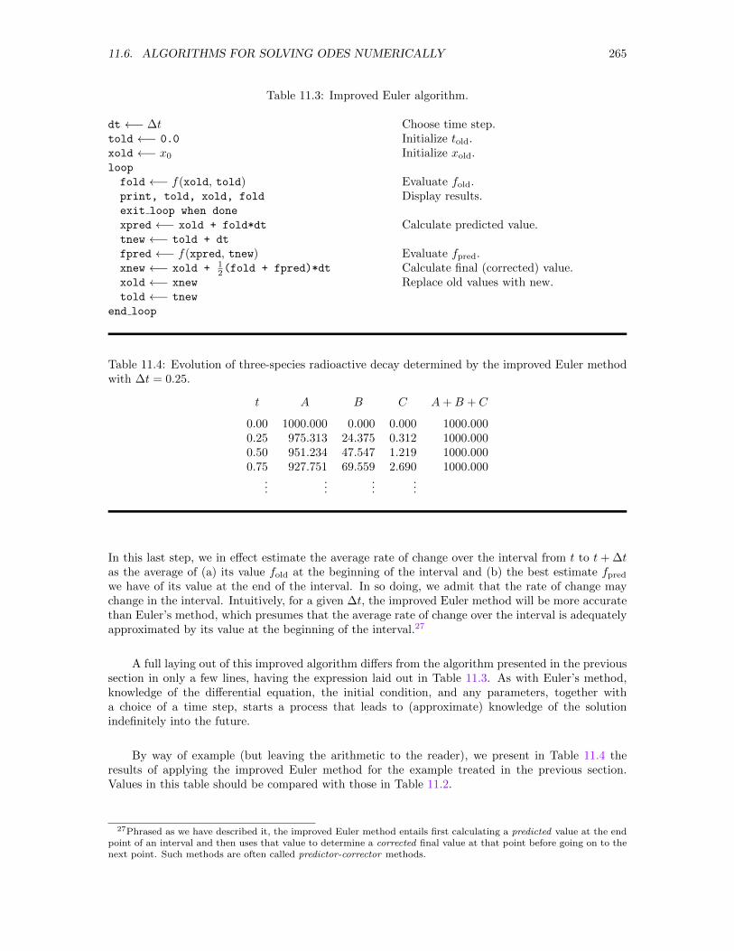
11.6. ALGORITHMS FOR SOLVING ODES NUMERICALLY 265

Table 11.3: Improved Euler algorithm.

dt ←− ∆ttold ←− 0.0

xold ←− x0loop

fold ←− f(xold, told)print, told, xold, fold

exit loop when done

xpred ←− xold + fold*dt

tnew ←− told + dt

fpred ←− f(xpred, tnew)xnew ←− xold + 1

2(fold + fpred)*dt

xold ←− xnew

told ←− tnew

end loop

Choose time step.Initialize told.Initialize xold.

Evaluate fold.Display results.

Calculate predicted value.

Evaluate fpred.Calculate final (corrected) value.Replace old values with new.

Table 11.4: Evolution of three-species radioactive decay determined by the improved Euler methodwith ∆t = 0.25.

t A B C A+B + C

0.00 1000.000 0.000 0.000 1000.0000.25 975.313 24.375 0.312 1000.0000.50 951.234 47.547 1.219 1000.0000.75 927.751 69.559 2.690 1000.000

......

......

In this last step, we in effect estimate the average rate of change over the interval from t to t+ ∆tas the average of (a) its value fold at the beginning of the interval and (b) the best estimate fpredwe have of its value at the end of the interval. In so doing, we admit that the rate of change maychange in the interval. Intuitively, for a given ∆t, the improved Euler method will be more accuratethan Euler’s method, which presumes that the average rate of change over the interval is adequatelyapproximated by its value at the beginning of the interval.27

A full laying out of this improved algorithm differs from the algorithm presented in the previoussection in only a few lines, having the expression laid out in Table 11.3. As with Euler’s method,knowledge of the differential equation, the initial condition, and any parameters, together witha choice of a time step, starts a process that leads to (approximate) knowledge of the solutionindefinitely into the future.

By way of example (but leaving the arithmetic to the reader), we present in Table 11.4 theresults of applying the improved Euler method for the example treated in the previous section.Values in this table should be compared with those in Table 11.2.

27Phrased as we have described it, the improved Euler method entails first calculating a predicted value at the endpoint of an interval and then uses that value to determine a corrected final value at that point before going on to thenext point. Such methods are often called predictor-corrector methods.

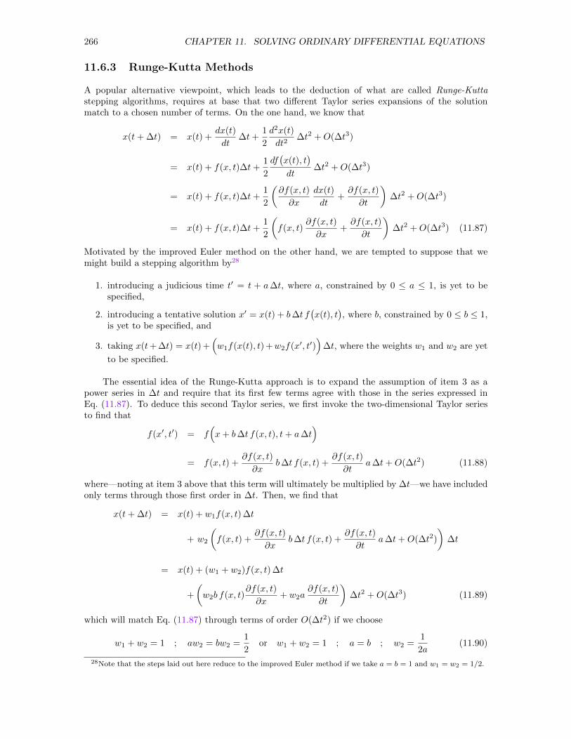
266 CHAPTER 11. SOLVING ORDINARY DIFFERENTIAL EQUATIONS

11.6.3 Runge-Kutta Methods

A popular alternative viewpoint, which leads to the deduction of what are called Runge-Kuttastepping algorithms, requires at base that two different Taylor series expansions of the solutionmatch to a chosen number of terms. On the one hand, we know that

x(t+ ∆t) = x(t) +dx(t)

dt∆t+

1

2

d2x(t)

dt2∆t2 +O(∆t3)

= x(t) + f(x, t)∆t+1

2

df(x(t), t

)dt

∆t2 +O(∆t3)

= x(t) + f(x, t)∆t+1

2

(∂f(x, t)

∂x

dx(t)

dt+∂f(x, t)

∂t

)∆t2 +O(∆t3)

= x(t) + f(x, t)∆t+1

2

(f(x, t)

∂f(x, t)

∂x+∂f(x, t)

∂t

)∆t2 +O(∆t3) (11.87)

Motivated by the improved Euler method on the other hand, we are tempted to suppose that wemight build a stepping algorithm by28

1. introducing a judicious time t′ = t + a∆t, where a, constrained by 0 ≤ a ≤ 1, is yet to bespecified,

2. introducing a tentative solution x′ = x(t) + b∆t f(x(t), t

), where b, constrained by 0 ≤ b ≤ 1,

is yet to be specified, and

3. taking x(t+ ∆t) = x(t) +(w1f(x(t), t) +w2f(x′, t′)

)∆t, where the weights w1 and w2 are yet

to be specified.

The essential idea of the Runge-Kutta approach is to expand the assumption of item 3 as apower series in ∆t and require that its first few terms agree with those in the series expressed inEq. (11.87). To deduce this second Taylor series, we first invoke the two-dimensional Taylor seriesto find that

f(x′, t′) = f(x+ b∆t f(x, t), t+ a∆t

)= f(x, t) +

∂f(x, t)

∂xb∆t f(x, t) +

∂f(x, t)

∂ta∆t+O(∆t2) (11.88)

where—noting at item 3 above that this term will ultimately be multiplied by ∆t—we have includedonly terms through those first order in ∆t. Then, we find that

x(t+ ∆t) = x(t) + w1f(x, t) ∆t

+ w2

(f(x, t) +

∂f(x, t)

∂xb∆t f(x, t) +

∂f(x, t)

∂ta∆t+O(∆t2)

)∆t

= x(t) + (w1 + w2)f(x, t) ∆t

+

(w2b f(x, t)

∂f(x, t)

∂x+ w2a

∂f(x, t)

∂t

)∆t2 +O(∆t3) (11.89)

which will match Eq. (11.87) through terms of order O(∆t2) if we choose

w1 + w2 = 1 ; aw2 = bw2 =1

2or w1 + w2 = 1 ; a = b ; w2 =

1

2a(11.90)

28Note that the steps laid out here reduce to the improved Euler method if we take a = b = 1 and w1 = w2 = 1/2.

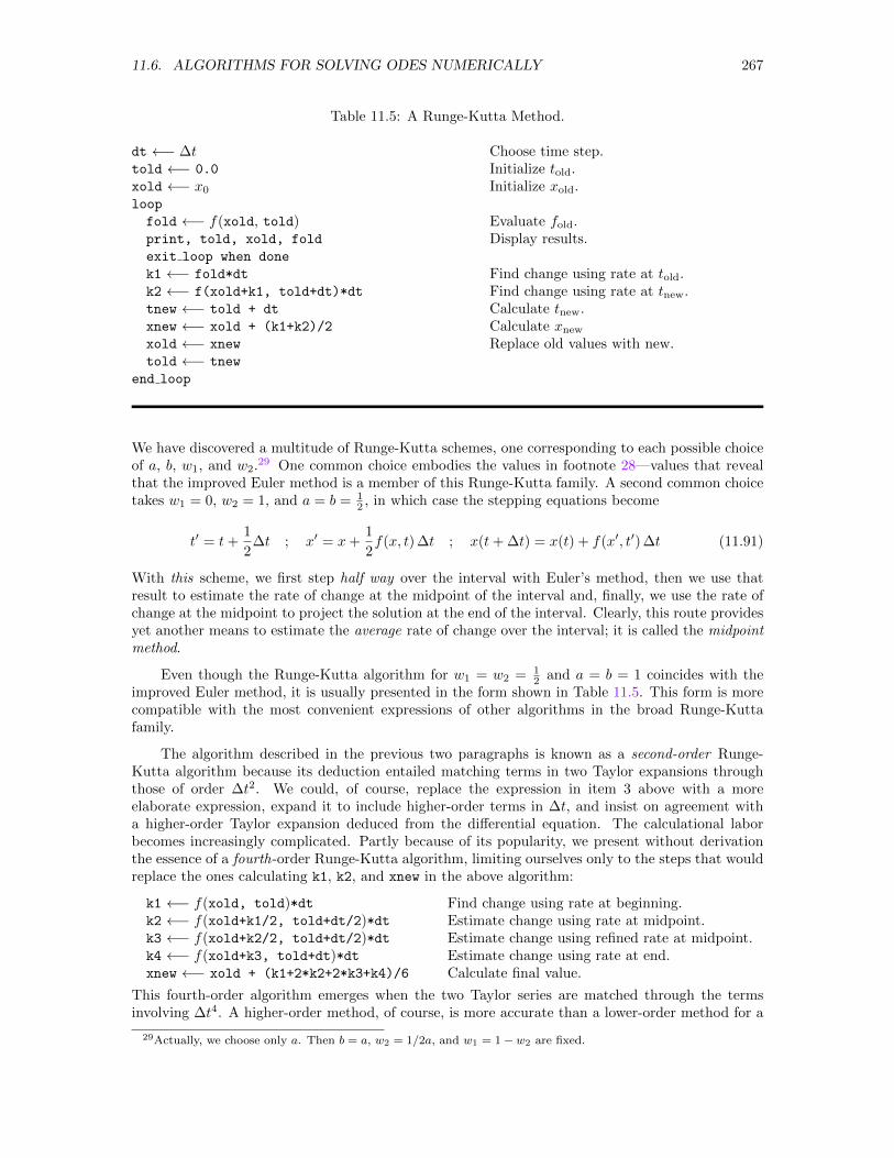
11.6. ALGORITHMS FOR SOLVING ODES NUMERICALLY 267

Table 11.5: A Runge-Kutta Method.

dt ←− ∆ttold ←− 0.0

xold ←− x0loop

fold ←− f(xold, told)print, told, xold, fold

exit loop when done

k1 ←− fold*dt

k2 ←− f(xold+k1, told+dt)*dt

tnew ←− told + dt

xnew ←− xold + (k1+k2)/2

xold ←− xnew

told ←− tnew

end loop

Choose time step.Initialize told.Initialize xold.

Evaluate fold.Display results.

Find change using rate at told.Find change using rate at tnew.Calculate tnew.Calculate xnewReplace old values with new.

We have discovered a multitude of Runge-Kutta schemes, one corresponding to each possible choiceof a, b, w1, and w2.29 One common choice embodies the values in footnote 28—values that revealthat the improved Euler method is a member of this Runge-Kutta family. A second common choicetakes w1 = 0, w2 = 1, and a = b = 1

2 , in which case the stepping equations become

t′ = t+1

2∆t ; x′ = x+

1

2f(x, t) ∆t ; x(t+ ∆t) = x(t) + f(x′, t′) ∆t (11.91)

With this scheme, we first step half way over the interval with Euler’s method, then we use thatresult to estimate the rate of change at the midpoint of the interval and, finally, we use the rate ofchange at the midpoint to project the solution at the end of the interval. Clearly, this route providesyet another means to estimate the average rate of change over the interval; it is called the midpointmethod.

Even though the Runge-Kutta algorithm for w1 = w2 = 12 and a = b = 1 coincides with the

improved Euler method, it is usually presented in the form shown in Table 11.5. This form is morecompatible with the most convenient expressions of other algorithms in the broad Runge-Kuttafamily.

The algorithm described in the previous two paragraphs is known as a second-order Runge-Kutta algorithm because its deduction entailed matching terms in two Taylor expansions throughthose of order ∆t2. We could, of course, replace the expression in item 3 above with a moreelaborate expression, expand it to include higher-order terms in ∆t, and insist on agreement witha higher-order Taylor expansion deduced from the differential equation. The calculational laborbecomes increasingly complicated. Partly because of its popularity, we present without derivationthe essence of a fourth-order Runge-Kutta algorithm, limiting ourselves only to the steps that wouldreplace the ones calculating k1, k2, and xnew in the above algorithm:

k1 ←− f(xold, told)*dtk2 ←− f(xold+k1/2, told+dt/2)*dtk3 ←− f(xold+k2/2, told+dt/2)*dtk4 ←− f(xold+k3, told+dt)*dtxnew ←− xold + (k1+2*k2+2*k3+k4)/6

Find change using rate at beginning.Estimate change using rate at midpoint.Estimate change using refined rate at midpoint.Estimate change using rate at end.Calculate final value.

This fourth-order algorithm emerges when the two Taylor series are matched through the termsinvolving ∆t4. A higher-order method, of course, is more accurate than a lower-order method for a

29Actually, we choose only a. Then b = a, w2 = 1/2a, and w1 = 1− w2 are fixed.

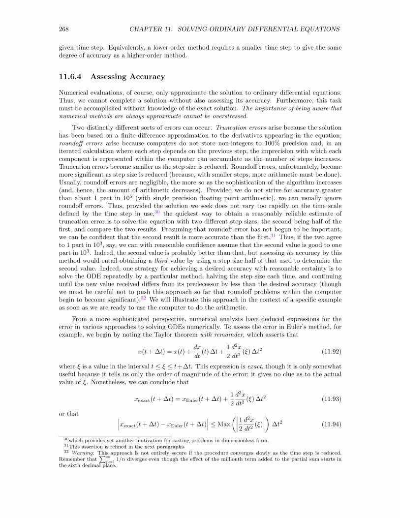
268 CHAPTER 11. SOLVING ORDINARY DIFFERENTIAL EQUATIONS

given time step. Equivalently, a lower-order method requires a smaller time step to give the samedegree of accuracy as a higher-order method.

11.6.4 Assessing Accuracy

Numerical evaluations, of course, only approximate the solution to ordinary differential equations.Thus, we cannot complete a solution without also assessing its accuracy. Furthermore, this taskmust be accomplished without knowledge of the exact solution. The importance of being aware thatnumerical methods are always approximate cannot be overstressed.

Two distinctly different sorts of errors can occur. Truncation errors arise because the solutionhas been based on a finite-difference approximation to the derivatives appearing in the equation;roundoff errors arise because computers do not store non-integers to 100% precision and, in aniterated calculation where each step depends on the previous step, the imprecision with which eachcomponent is represented within the computer can accumulate as the number of steps increases.Truncation errors become smaller as the step size is reduced. Roundoff errors, unfortunately, becomemore significant as step size is reduced (because, with smaller steps, more arithmetic must be done).Usually, roundoff errors are negligible, the more so as the sophistication of the algorithm increases(and, hence, the amount of arithmetic decreases). Provided we do not strive for accuracy greaterthan about 1 part in 105 (with single precision floating point arithmetic), we can usually ignoreroundoff errors. Thus, provided the solution we seek does not vary too rapidly on the time scaledefined by the time step in use,30 the quickest way to obtain a reasonably reliable estimate oftruncation error is to solve the equation with two different step sizes, the second being half of thefirst, and compare the two results. Presuming that roundoff error has not begun to be important,we can be confident that the second result is more accurate than the first.31 Thus, if the two agreeto 1 part in 103, say, we can with reasonable confidence assume that the second value is good to onepart in 103. Indeed, the second value is probably better than that, but assessing its accuracy by thismethod would entail obtaining a third value by using a step size half of that used to determine thesecond value. Indeed, one strategy for achieving a desired accuracy with reasonable certainty is tosolve the ODE repeatedly by a particular method, halving the step size each time, and continuinguntil the new value received differs from its predecessor by less than the desired accuracy (thoughwe must be careful not to push this approach so far that roundoff problems within the computerbegin to become significant).32 We will illustrate this approach in the context of a specific exampleas soon as we are ready to use the computer to do the arithmetic.

From a more sophisticated perspective, numerical analysts have deduced expressions for theerror in various approaches to solving ODEs numerically. To assess the error in Euler’s method, forexample, we begin by noting the Taylor theorem with remainder, which asserts that

x(t+ ∆t) = x(t) +dx

dt(t) ∆t+

1

2

d2x

dt2(ξ) ∆t2 (11.92)

where ξ is a value in the interval t ≤ ξ ≤ t+∆t. This expression is exact, though it is only somewhatuseful because it tells us only the order of magnitude of the error; it gives no clue as to the actualvalue of ξ. Nonetheless, we can conclude that

xexact(t+ ∆t) = xEuler(t+ ∆t) +1

2

d2x

dt2(ξ) ∆t2 (11.93)

or that ∣∣∣xexact(t+ ∆t)− xEuler(t+ ∆t)∣∣∣ ≤ Max

(∣∣∣∣12 d2xdt2 (ξ)

∣∣∣∣) ∆t2 (11.94)

30which provides yet another motivation for casting problems in dimensionless form.31This assertion is refined in the next paragraphs.32 Warning: This approach is not entirely secure if the procedure converges slowly as the time step is reduced.

Remember that∑∞

n=11/n diverges even though the effect of the millionth term added to the partial sum starts in

the sixth decimal place.

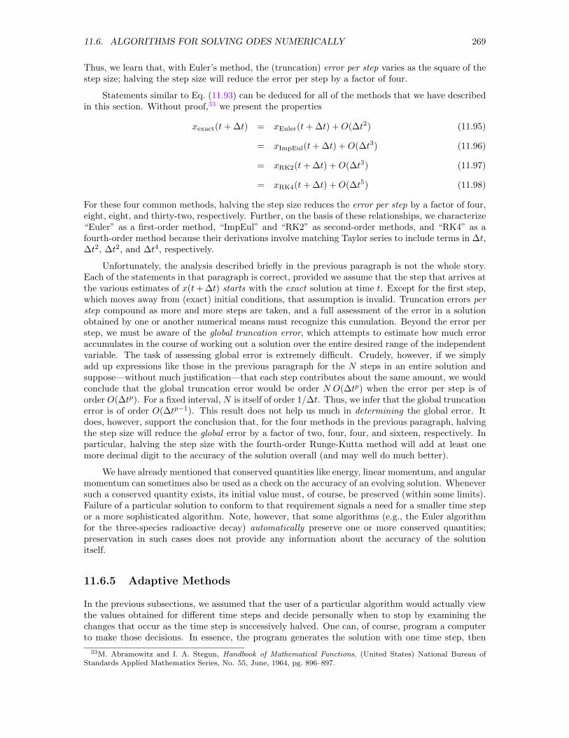
11.6. ALGORITHMS FOR SOLVING ODES NUMERICALLY 269

Thus, we learn that, with Euler’s method, the (truncation) error per step varies as the square of thestep size; halving the step size will reduce the error per step by a factor of four.

Statements similar to Eq. (11.93) can be deduced for all of the methods that we have describedin this section. Without proof,33 we present the properties

xexact(t+ ∆t) = xEuler(t+ ∆t) +O(∆t2) (11.95)

= xImpEul(t+ ∆t) +O(∆t3) (11.96)

= xRK2(t+ ∆t) +O(∆t3) (11.97)

= xRK4(t+ ∆t) +O(∆t5) (11.98)

For these four common methods, halving the step size reduces the error per step by a factor of four,eight, eight, and thirty-two, respectively. Further, on the basis of these relationships, we characterize“Euler” as a first-order method, “ImpEul” and “RK2” as second-order methods, and “RK4” as afourth-order method because their derivations involve matching Taylor series to include terms in ∆t,∆t2, ∆t2, and ∆t4, respectively.

Unfortunately, the analysis described briefly in the previous paragraph is not the whole story.Each of the statements in that paragraph is correct, provided we assume that the step that arrives atthe various estimates of x(t+ ∆t) starts with the exact solution at time t. Except for the first step,which moves away from (exact) initial conditions, that assumption is invalid. Truncation errors perstep compound as more and more steps are taken, and a full assessment of the error in a solutionobtained by one or another numerical means must recognize this cumulation. Beyond the error perstep, we must be aware of the global truncation error, which attempts to estimate how much erroraccumulates in the course of working out a solution over the entire desired range of the independentvariable. The task of assessing global error is extremely difficult. Crudely, however, if we simplyadd up expressions like those in the previous paragraph for the N steps in an entire solution andsuppose—without much justification—that each step contributes about the same amount, we wouldconclude that the global truncation error would be order N O(∆tp) when the error per step is oforder O(∆tp). For a fixed interval, N is itself of order 1/∆t. Thus, we infer that the global truncationerror is of order O(∆tp−1). This result does not help us much in determining the global error. Itdoes, however, support the conclusion that, for the four methods in the previous paragraph, halvingthe step size will reduce the global error by a factor of two, four, four, and sixteen, respectively. Inparticular, halving the step size with the fourth-order Runge-Kutta method will add at least onemore decimal digit to the accuracy of the solution overall (and may well do much better).

We have already mentioned that conserved quantities like energy, linear momentum, and angularmomentum can sometimes also be used as a check on the accuracy of an evolving solution. Wheneversuch a conserved quantity exists, its initial value must, of course, be preserved (within some limits).Failure of a particular solution to conform to that requirement signals a need for a smaller time stepor a more sophisticated algorithm. Note, however, that some algorithms (e.g., the Euler algorithmfor the three-species radioactive decay) automatically preserve one or more conserved quantities;preservation in such cases does not provide any information about the accuracy of the solutionitself.

11.6.5 Adaptive Methods

In the previous subsections, we assumed that the user of a particular algorithm would actually viewthe values obtained for different time steps and decide personally when to stop by examining thechanges that occur as the time step is successively halved. One can, of course, program a computerto make those decisions. In essence, the program generates the solution with one time step, then

33M. Abramowitz and I. A. Stegun, Handbook of Mathematical Functions, (United States) National Bureau ofStandards Applied Mathematics Series, No. 55, June, 1964, pg. 896–897.

270 CHAPTER 11. SOLVING ORDINARY DIFFERENTIAL EQUATIONS

repeatedly generates it with a succession of ever smaller time steps, comparing each new solutionwith its immediate predecessor and stopping when the absolute value of the difference is smaller thana tolerance—either absolute or relative—prescribed in advance. As a guard against an infinite loop,these algorithms should also stop if the desired tolerance has not been achieved in some maximumnumber of refinements and should print a warning when the desired tolerance has not in its judgmentbeen achieved.

Another family of algorithms aims to minimize computational labor by estimating—though themethods for doing so are often themselves approximate—the accuracy obtained at each step alongthe way to a solution.34 A trial row in the table of data is generated, and the error is assessed. If theerror is within a user-specified tolerance, the program moves on to the next row in the data table. Ifthe error exceeds the desired tolerance, the program repeats the calculation with progressively smallertime steps until the desired tolerance is achieved and only then is a new row added to the table.The procedure also contains means by which the time step is increased when the estimated error isless than the specified tolerance. Thus, the time step fluctuates as the solution unfolds, being smallwhen the solution is changing rapidly and large when the solution is changing slowly. Because ofthis feature, the procedure is said to be adaptive. Without the overlay of an elaborate interpolation,adaptive methods have the disadvantage of generating solutions at irregularly spaced times. Thatdisadvantage, however, is frequently outweighed by the substantial advantage of concentrating thecomputational effort in regions where the solution changes rapidly.35

11.6.6 Multistep Methods

All of the methods so far discussed have generated the solution at a particular point from knowledgeof the solution at a single earlier point, though many have interpolated solutions at several pointsbetween the initially known point and the desired end point; such methods are called single-stepmethods. Some of the solvers available in some software packages use multistep methods, whichreduce the need for the interpolative procedures by projecting the solution at the next point fromknowledge of the solution at several previous points. In seeking a solution to Eq. (11.76), for example,we would choose a time step ∆t and introduce the points ti = i∆t and the notation xi = x(ti) andfi = f(xi, ti). Then, supposing we already had in hand estimates of the solution at four (say) earlierpoints, we might estimate the solution at ti+1 by the formula

xi+1 = xi +∆t

24

(55fi − 59fi−1 + 37fi−2 − 9fi−3

)(11.99)

(which represents a particular fourth-order member of a family of methods known as Adams-Bashforth methods).36 In effect, we are estimating the average derivative over the intervalti+1 ≤ t ≤ ti as a weighted average of the derivatives we can compute at the four points previ-ous to the one at ti+1, all of which we would—of course—have to have in hand at the time we tookthis step.

Because they do not require interpolation within the interval over which we are stepping at anymoment, multistep methods can be computationally extremely efficient. Since we cannot use such amethod until we have in hand the solution at several—in the above example four—points, however,these methods are not self starting. We must adopt some other method to obtain from the initialvalues however many values are needed to support the multistep method. To start a solution basedon the stepping formula of Eq. (11.99), we might use a fourth-order Runge-Kutta method to obtainx1, x2, and x3 from x0. Then we could shift to the fourth-order Adams-Bashforth formula for allsubsequent points.

34Sometimes the assessment of accuracy will be based not on the generated solution itself but on some property,e.g., the energy, computed from that solution.

35In contrast, Euler’s method, for example, would require using throughout a time step small enough to generatean accurate solution in regions where the solution varies most rapidly. Consequently, too much computational effortwould be focused in regions where the solution changes slowly enough that a larger time step would be acceptable.

36See Elementary Numerical Analysis, S. D. Conte (McGraw-Hill, New York, 1965), Section 6.6.

11.9. SOLVING ODES NUMERICALLY WITH OCTAVE 271

We could, of course, simply take the result given by Eq. (11.99) as the solution at ti+1. Fora more sophisticated solution, we could regard that result as a prediction and use it in a pairedformula to “correct” the prediction. An appropriate fourth-order corrector formula is a member ofthe Adams-Moulton family, namely

xi+1 = xi +∆t

24

(9fi+1 + 19fi − 5fi−1 + fi−2

)(11.100)

Once a sufficient number of values is in hand, we could at each step invoke Eq. (11.99) to predictthe next solution and then Eq. (11.100) to refine it. We might call the resulting method the Adams-Bashforth-Moulton method.

11.9 Solving ODEs Numerically with OCTAVE

Note: All OCTAVE program (.m) files referred to in this chapter are available inthe directory $HEAD/octave, where (as defined in the Local Guide) $HEAD must bereplaced by the appropriate path for your site. At some sites, this directory orsome other directory containing these files may also have been placed in OCTAVE’sdefault search path. If so, the files can be found by OCTAVE without explicitspecification of a path. Otherwise, you will have to use the full path to copy theminto your default directory to access them.

ODEs can be solved numerically either by using OCTAVE’s elementary commands or, more simply,by invoking OCTAVE’s built-in routine lsode.

11.9.1 Using Elementary Commands

To carry the process worked out by hand in Section 11.6.1 much beyond the first few steps is ajob for a computer. Suppose, for example, we wanted to determine the Euler approximation to thesolution of Eq. (11.19) for chain radioactive decay over the time interval 0.0 ≤ t ≤ 50.0 with a timestep of ∆t = 0.25 and kA = kB = 0.1. We could exploit the capabilities of OCTAVE as follows. Weanticipate that values will be stored in arrays t, A, B, and C. Ultimately these arrays will have 201elements (time interval divided by time step = 50.0/0.25 = 200 steps, but we need an element alsofor the initial value). Initially, however, we set only the first element of each array and, of course,the parameters and the time step. Possible statements are

>> t(1) = 0.0; A(1) = 1000.0;

>> B(1) = 0.0; C(1) = 0.0;

>> kA = 0.1; kB = 0.1;

>> dt = 0.25;

Set initial values.

Set parameters.Set time step.

The solution is then calculated, time instant by time instant, with the loop

272 CHAPTER 11. SOLVING ORDINARY DIFFERENTIAL EQUATIONS

>> for i = 2:201

A(i) = A(i-1) - kA*A(i-1)*dt;

B(i) = B(i-1) + kA*A(i-1)*dt - kB*B(i-1)*dt;

C(i) = C(i-1) + kB*B(i-1)*dt;

t(i) = t(i-1) + dt;

end

which calculates each new A, B, and C using the stepping equations given in Eqs. (11.79), (11.80),and (11.81) and each new t simply by adding the time step dt to the previous t.37 The simplestatement

>> for i = 1:4

sprintf(’%6.2f %9.3f %9.4f %9.4f %9.2f\n’, ...

t(i), A(i), B(i), C(i), A(i)+B(i)+C(i) )

end

ans = 0.00 1000.000 0.0000 0.0000 1000.00

ans = 0.25 975.000 25.0000 0.0000 1000.00

ans = 0.50 950.625 48.7500 0.6250 1000.00

ans = 0.75 926.859 71.2969 1.8438 1000.00

displays the resulting solution38 and the conserved quantity A+B +C for the first few time steps.Reassuringly, the values here agree with those in Table 11.2. The more interpretable graphicaloutput of Fig. 11.10 is produced by the statements

>> plot( t, A, ’linewidth’, 3.0, ’color’, ’black’ )

>> title( ’Three-Species Decay Chain’, ’fontsize’, 16 )

>> xlabel( ’Time’, ’fontsize’, 14 )

>> ylabel( ’Number of Atoms Present’, ’fontsize’, 14 )

>> set( gca, ’fontsize’, 14 )

>> hold on

>> plot( t, B, ’linewidth’, 3.0, ’color’, ’black’, ’linestyle’, ’:’ )

>> plot( t, C, ’linewidth’, 3.0, ’color’, ’black’, ’linestyle’, ’--’ )

>> hold off

To assess the accuracy achieved by Euler’s method more completely, we repeat the above cal-culation for several different time steps, finding the representative values shown in Table 11.6. Theconvergence of A(6.0), B(6.0), and C(6.0) as ∆t is reduced by successive factors of two is apparent.Since, even at the end, the approximate solutions still seem to be changing in the units digit witheach refinement, we would be off base to claim an accuracy much smaller than ±1.0 in these values.For some purposes, of course, that accuracy may well be adequate. In particular, to the resolutionof the graph in Fig. 11.10, for example, a variation of ±1.0 in a particular vertical coordinate wouldhardly show. At the same time, we must remember that these differences may cumulate and maywell be larger at t = 50.0, for example, than they are at t = 6.0. To assess that possibility, wegenerate the entire solution via Euler’s method for three time steps (∆t = 2.0, 0.5, and 0.0625),plotting those solutions in Fig. 11.11. The comparison of the resulting graphs is described in thecaption to the figure.

A similar demonstration using the improved Euler method is left to an exercise. In particular,the values presented in Table 11.7 reflect the result of that exercise when the procedures leading

37For simplicity, we have calculated each new time by adding the time step to the previous time. If we were moreconcerned about minimizing round-off error, we would be better off replacing the last statement in the loop with thestatement t(i) = (i-1) * dt, though doing so would increase the execution time. (Multiplication takes more timethan addition.)

38We have removed several extraneous lines from the output produced by this statement.

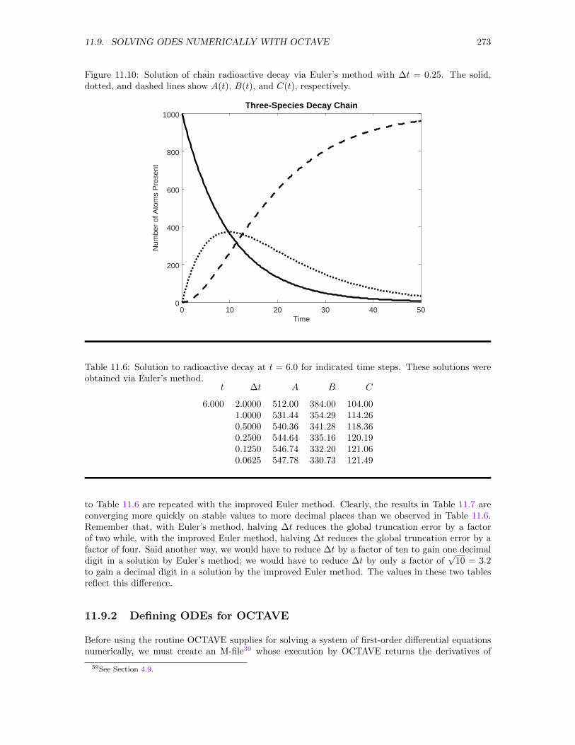
11.9. SOLVING ODES NUMERICALLY WITH OCTAVE 273

Figure 11.10: Solution of chain radioactive decay via Euler’s method with ∆t = 0.25. The solid,dotted, and dashed lines show A(t), B(t), and C(t), respectively.

0 10 20 30 40 500

200

400

600

800

1000

Time

Num

ber

of A

tom

s P

rese

nt

Three-Species Decay Chain

Table 11.6: Solution to radioactive decay at t = 6.0 for indicated time steps. These solutions wereobtained via Euler’s method.

t ∆t A B C

6.000 2.0000 512.00 384.00 104.001.0000 531.44 354.29 114.260.5000 540.36 341.28 118.360.2500 544.64 335.16 120.190.1250 546.74 332.20 121.060.0625 547.78 330.73 121.49

to Table 11.6 are repeated with the improved Euler method. Clearly, the results in Table 11.7 areconverging more quickly on stable values to more decimal places than we observed in Table 11.6.Remember that, with Euler’s method, halving ∆t reduces the global truncation error by a factorof two while, with the improved Euler method, halving ∆t reduces the global truncation error by afactor of four. Said another way, we would have to reduce ∆t by a factor of ten to gain one decimaldigit in a solution by Euler’s method; we would have to reduce ∆t by only a factor of

√10 = 3.2

to gain a decimal digit in a solution by the improved Euler method. The values in these two tablesreflect this difference.

11.9.2 Defining ODEs for OCTAVE

Before using the routine OCTAVE supplies for solving a system of first-order differential equationsnumerically, we must create an M-file39 whose execution by OCTAVE returns the derivatives of

39See Section 4.9.

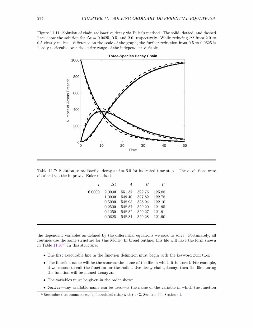
274 CHAPTER 11. SOLVING ORDINARY DIFFERENTIAL EQUATIONS

Figure 11.11: Solution of chain radioactive decay via Euler’s method. The solid, dotted, and dashedlines show the solution for ∆t = 0.0625, 0.5, and 2.0, respectively. While reducing ∆t from 2.0 to0.5 clearly makes a difference on the scale of the graph, the further reduction from 0.5 to 0.0625 ishardly noticeable over the entire range of the independent variable.

0 10 20 30 40 500

200

400

600

800

1000

Time

Num

ber

of A

tom

s P

rese

nt

Three-Species Decay Chain

Table 11.7: Solution to radioactive decay at t = 6.0 for indicated time steps. These solutions wereobtained via the improved Euler method.

t ∆t A B C

6.0000 2.0000 551.37 322.75 125.881.0000 549.40 327.82 122.780.5000 548.95 328.94 122.100.2500 548.87 329.20 121.950.1250 548.82 329.27 121.910.0625 548.81 329.28 121.90

the dependent variables as defined by the differential equations we seek to solve. Fortunately, allroutines use the same structure for this M-file. In broad outline, this file will have the form shownin Table 11.8.40 In this structure,

• The first executable line in the function definition must begin with the keyword function.

• The function name will be the same as the name of the file in which it is stored. For example,if we choose to call the function for the radioactive decay chain, decay, then the file storingthe function will be named decay.m.

• The variables must be given in the order shown.

• Derivs—any available name can be used—is the name of the variable in which the function

40Remember that comments can be introduced either with # or %. See item 6 in Section 4.1.

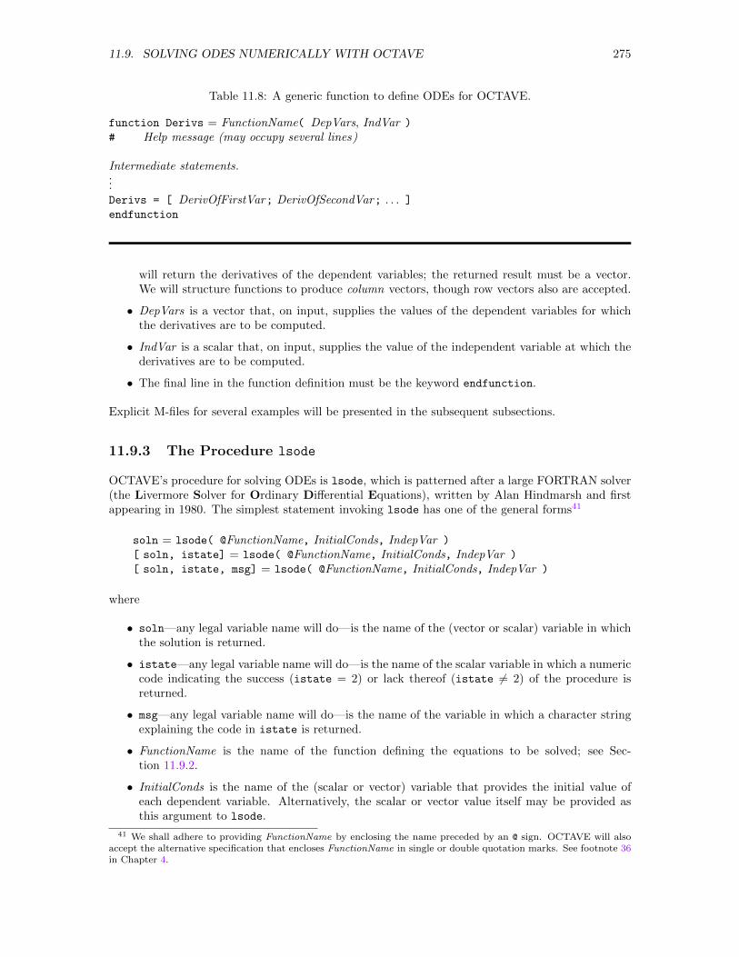
11.9. SOLVING ODES NUMERICALLY WITH OCTAVE 275

Table 11.8: A generic function to define ODEs for OCTAVE.

function Derivs = FunctionName( DepVars, IndVar )

# Help message (may occupy several lines)

Intermediate statements....Derivs = [ DerivOfFirstVar; DerivOfSecondVar; . . . ]

endfunction

will return the derivatives of the dependent variables; the returned result must be a vector.We will structure functions to produce column vectors, though row vectors also are accepted.

• DepVars is a vector that, on input, supplies the values of the dependent variables for whichthe derivatives are to be computed.

• IndVar is a scalar that, on input, supplies the value of the independent variable at which thederivatives are to be computed.

• The final line in the function definition must be the keyword endfunction.

Explicit M-files for several examples will be presented in the subsequent subsections.

11.9.3 The Procedure lsode

OCTAVE’s procedure for solving ODEs is lsode, which is patterned after a large FORTRAN solver(the Livermore Solver for Ordinary Differential Equations), written by Alan Hindmarsh and firstappearing in 1980. The simplest statement invoking lsode has one of the general forms41

soln = lsode( @FunctionName, InitialConds, IndepVar )

[ soln, istate] = lsode( @FunctionName, InitialConds, IndepVar )

[ soln, istate, msg] = lsode( @FunctionName, InitialConds, IndepVar )

where

• soln—any legal variable name will do—is the name of the (vector or scalar) variable in whichthe solution is returned.

• istate—any legal variable name will do—is the name of the scalar variable in which a numericcode indicating the success (istate = 2) or lack thereof (istate 6= 2) of the procedure isreturned.

• msg—any legal variable name will do—is the name of the variable in which a character stringexplaining the code in istate is returned.

• FunctionName is the name of the function defining the equations to be solved; see Sec-tion 11.9.2.

• InitialConds is the name of the (scalar or vector) variable that provides the initial value ofeach dependent variable. Alternatively, the scalar or vector value itself may be provided asthis argument to lsode.

41 We shall adhere to providing FunctionName by enclosing the name preceded by an @ sign. OCTAVE will alsoaccept the alternative specification that encloses FunctionName in single or double quotation marks. See footnote 36in Chapter 4.

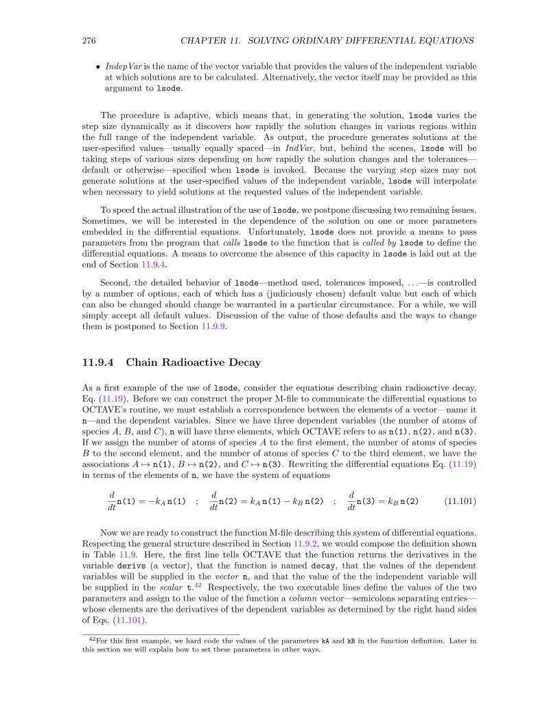
276 CHAPTER 11. SOLVING ORDINARY DIFFERENTIAL EQUATIONS

• IndepVar is the name of the vector variable that provides the values of the independent variableat which solutions are to be calculated. Alternatively, the vector itself may be provided as thisargument to lsode.

The procedure is adaptive, which means that, in generating the solution, lsode varies thestep size dynamically as it discovers how rapidly the solution changes in various regions withinthe full range of the independent variable. As output, the procedure generates solutions at theuser-specified values—usually equally spaced—in IndVar, but, behind the scenes, lsode will betaking steps of various sizes depending on how rapidly the solution changes and the tolerances—default or otherwise—specified when lsode is invoked. Because the varying step sizes may notgenerate solutions at the user-specified values of the independent variable, lsode will interpolatewhen necessary to yield solutions at the requested values of the independent variable.

To speed the actual illustration of the use of lsode, we postpone discussing two remaining issues.Sometimes, we will be interested in the dependence of the solution on one or more parametersembedded in the differential equations. Unfortunately, lsode does not provide a means to passparameters from the program that calls lsode to the function that is called by lsode to define thedifferential equations. A means to overcome the absence of this capacity in lsode is laid out at theend of Section 11.9.4.

Second, the detailed behavior of lsode—method used, tolerances imposed, . . .—is controlledby a number of options, each of which has a (judiciously chosen) default value but each of whichcan also be changed should change be warranted in a particular circumstance. For a while, we willsimply accept all default values. Discussion of the value of those defaults and the ways to changethem is postponed to Section 11.9.9.

11.9.4 Chain Radioactive Decay

As a first example of the use of lsode, consider the equations describing chain radioactive decay,Eq. (11.19). Before we can construct the proper M-file to communicate the differential equations toOCTAVE’s routine, we must establish a correspondence between the elements of a vector—name itn—and the dependent variables. Since we have three dependent variables (the number of atoms ofspecies A, B, and C), n will have three elements, which OCTAVE refers to as n(1), n(2), and n(3).If we assign the number of atoms of species A to the first element, the number of atoms of speciesB to the second element, and the number of atoms of species C to the third element, we have theassociations A 7→ n(1), B 7→ n(2), and C 7→ n(3). Rewriting the differential equations Eq. (11.19)in terms of the elements of n, we have the system of equations

d

dtn(1) = −kA n(1) ;

d

dtn(2) = kA n(1)− kB n(2) ;

d

dtn(3) = kB n(2) (11.101)

Now we are ready to construct the function M-file describing this system of differential equations.Respecting the general structure described in Section 11.9.2, we would compose the definition shownin Table 11.9. Here, the first line tells OCTAVE that the function returns the derivatives in thevariable derivs (a vector), that the function is named decay, that the values of the dependentvariables will be supplied in the vector n, and that the value of the the independent variable willbe supplied in the scalar t.42 Respectively, the two executable lines define the values of the twoparameters and assign to the value of the function a column vector—semicolons separating entries—whose elements are the derivatives of the dependent variables as determined by the right hand sidesof Eqs. (11.101).

42For this first example, we hard code the values of the parameters kA and kB in the function definition. Later inthis section we will explain how to set these parameters in other ways.

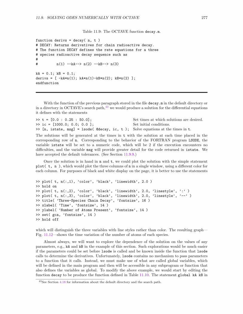
11.9. SOLVING ODES NUMERICALLY WITH OCTAVE 277

Table 11.9: The OCTAVE function decay.m.

function derivs = decay( n, t )

# DECAY: Returns derivatives for chain radioactive decay.

# The function DECAY defines the rate equations for a three

# species radioactive decay sequence such as

#

# n(1) --kA--> n(2) --kB--> n(3)

kA = 0.1; kB = 0.1;

derivs = [ -kA*n(1); kA*n(1)-kB*n(2); kB*n(2) ];

endfunction

With the function of the previous paragraph stored in the file decay.m in the default directory orin a directory in OCTAVE’s search path,43 we would produce a solution for the differential equationsit defines with the statements

>> t = [0.0 : 0.25 : 50.0];

>> ic = [1000.0; 0.0; 0.0 ];

>> [n, istate, msg] = lsode( @decay, ic, t );

Set times at which solutions are desired.Set initial conditions.Solve equations at the times in t.

The solutions will be generated at the times in t with the solution at each time placed in thecorresponding row of n. Corresponding to the behavior of the FORTRAN program LSODE, thevariable istate will be set to a numeric code, which will be 2 if the execution encounters nodifficulties, and the variable msg will provide greater detail for the code returned in istate. Wehave accepted the default tolerances. (See Section 11.9.9.)

Once the solution is in hand in n and t, we could plot the solution with the simple statementplot( t, n ), which would plot the three columns of n in a single window, using a different color foreach column. For purposes of black and white display on the page, it is better to use the statements

>> plot( t, n(:,1), ’color’, ’black’, ’linewidth’, 2.0 )

>> hold on

>> plot( t, n(:,2), ’color’, ’black’, ’linewidth’, 2.0, ’linestyle’, ’:’ )

>> plot( t, n(:,3), ’color’, ’black’, ’linewidth’, 2.0, ’linestyle’, ’--’ )

>> title( ’Three-Species Chain Decay’, ’fontsize’, 16 )

>> xlabel( ’Time’, ’fontsize’, 14 )

>> ylabel( ’Number of Atoms Present’, ’fontsize’, 14 )

>> set( gca, ’fontsize’, 14 )

>> hold off

which will distinguish the three variables with line styles rather than color. The resulting graph—Fig. 11.12—shows the time variation of the number of atoms of each species.

Almost always, we will want to explore the dependence of the solution on the values of anyparameters, e.g., kA and kB in the example of this section. Such explorations would be much easierif the parameters could be set before lsode is called and be known inside the function that lsode

calls to determine the derivatives. Unfortunately, lsode contains no mechanism to pass parametersto a function that it calls. Instead, we must make use of what are called global variables, whichwill be defined in the main program and then will be accessible in any subprogram or function thatalso defines the variables as global. To modify the above example, we would start by editing thefunction decay to be produce the function defined in Table 11.10. The statement global kA kB in

43See Section 4.18 for information about the default directory and the search path.

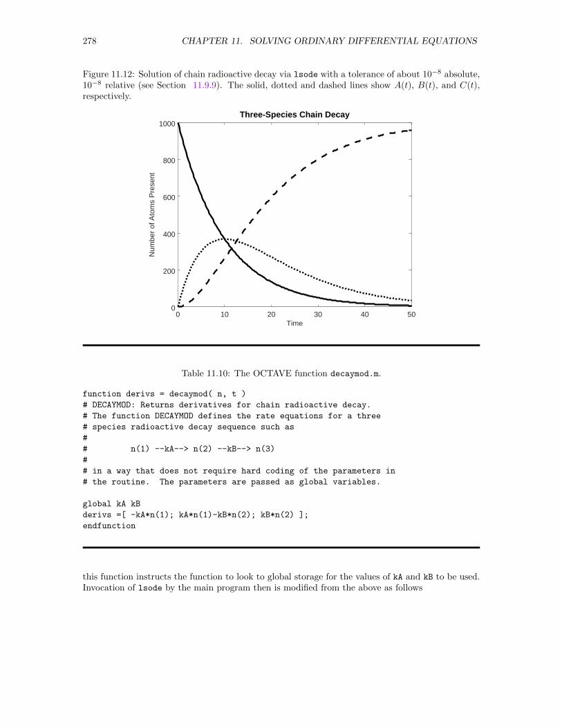
278 CHAPTER 11. SOLVING ORDINARY DIFFERENTIAL EQUATIONS

Figure 11.12: Solution of chain radioactive decay via lsode with a tolerance of about 10−8 absolute,10−8 relative (see Section 11.9.9). The solid, dotted and dashed lines show A(t), B(t), and C(t),respectively.

0 10 20 30 40 500

200

400

600

800

1000

Time

Num

ber

of A

tom

s P

rese

nt

Three-Species Chain Decay

Table 11.10: The OCTAVE function decaymod.m.

function derivs = decaymod( n, t )

# DECAYMOD: Returns derivatives for chain radioactive decay.

# The function DECAYMOD defines the rate equations for a three

# species radioactive decay sequence such as

#

# n(1) --kA--> n(2) --kB--> n(3)

#

# in a way that does not require hard coding of the parameters in

# the routine. The parameters are passed as global variables.

global kA kB

derivs =[ -kA*n(1); kA*n(1)-kB*n(2); kB*n(2) ];

endfunction

this function instructs the function to look to global storage for the values of kA and kB to be used.Invocation of lsode by the main program then is modified from the above as follows

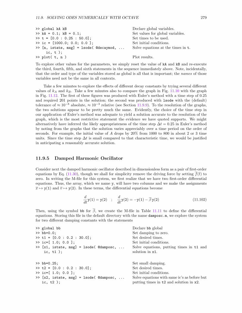
11.9. SOLVING ODES NUMERICALLY WITH OCTAVE 279

>> global kA kB

>> kA = 0.1; kB = 0.1;

>> t = [0.0 : 0.25 : 50.0];

>> ic = [1000.0; 0.0; 0.0 ];

>> [n, istate, msg] = lsode( @decaymod, ...

ic, t );

>> plot( t, n )

Declare global variables.Set values for global variables.Set times to be used.Set initial conditions.Solve equations at the times in t.

Plot results.

To explore other values for the parameters, we simply reset the value of kA and kB and re-executethe third, fourth, fifth, and sixth statements in the sequence immediately above. Note, incidentally,that the order and type of the variables stored as global is all that is important; the names of thosevariables need not be the same in all contexts.

Take a few minutes to explore the effects of different decay constants by trying several differentvalues of kA and kB . Take a few minutes also to compare the graph in Fig. 11.10 with the graphin Fig. 11.12. The first of these figures was produced with Euler’s method with a time step of 0.25and required 201 points in the solution; the second was produced with lsode with the (default)tolerance of ≈ 10−8 absolute, ≈ 10−3 relative (see Section 11.9.9). To the resolution of the graphs,the two solutions appear to be pretty much the same. Evidently, the choice of the time step inour application of Euler’s method was adequate to yield a solution accurate to the resolution of thegraph, which is the most restrictive statement the evidence we have quoted supports. We mightalternatively have inferred the likely appropriateness of the time step ∆t = 0.25 in Euler’s methodby noting from the graphs that the solution varies appreciably over a time period on the order ofseconds. For example, the initial value of A drops by 20% from 1000 to 800 in about 2 or 3 timeunits. Since the time step ∆t is small compared to that characteristic time, we would be justifiedin anticipating a reasonably accurate solution.

11.9.5 Damped Harmonic Oscillator

Consider next the damped harmonic oscillator described in dimensionless form as a pair of first-orderequations by Eq. (11.30), though we shall for simplicity remove the driving force by setting f(t) tozero. In writing the M-file for this system, we first realize that we have two first-order differentialequations. Thus, the array, which we name y, will have two columns and we make the assignmentsx 7→ y(1) and v 7→ y(2). In these terms, the differential equations become

d

dty(1) = y(2) ;

d

dty(2) = −y(1)− β y(2) (11.102)

Then, using the symbol bb for β, we create the M-file in Table 11.11 to define the differentialequations. Storing this file in the default directory with the name damposc.m, we explore the systemfor two different damping constants with the statements

>> global bb

>> bb=0.0;

>> t1 = [0.0 : 0.2 : 30.0];

>> ic=[ 1.0; 0.0 ];

>> [x1, istate, msg] = lsode( @damposc, ...

ic, t1 );

Declare bb globalSet damping to zero.Set desired times.Set initial conditions.Solve equations, putting times in t1 andsolution in x1.

>> bb=0.25;

>> t2 = [0.0 : 0.2 : 30.0];

>> ic=[ 1.0; 0.0 ];

>> [x2, istate, msg] = lsode( @damposc, ...

ic, t2 );

Set small damping.Set desired times.Set initial conditions.Solve equations with same ic’s as before butputting times in t2 and solution in x2.

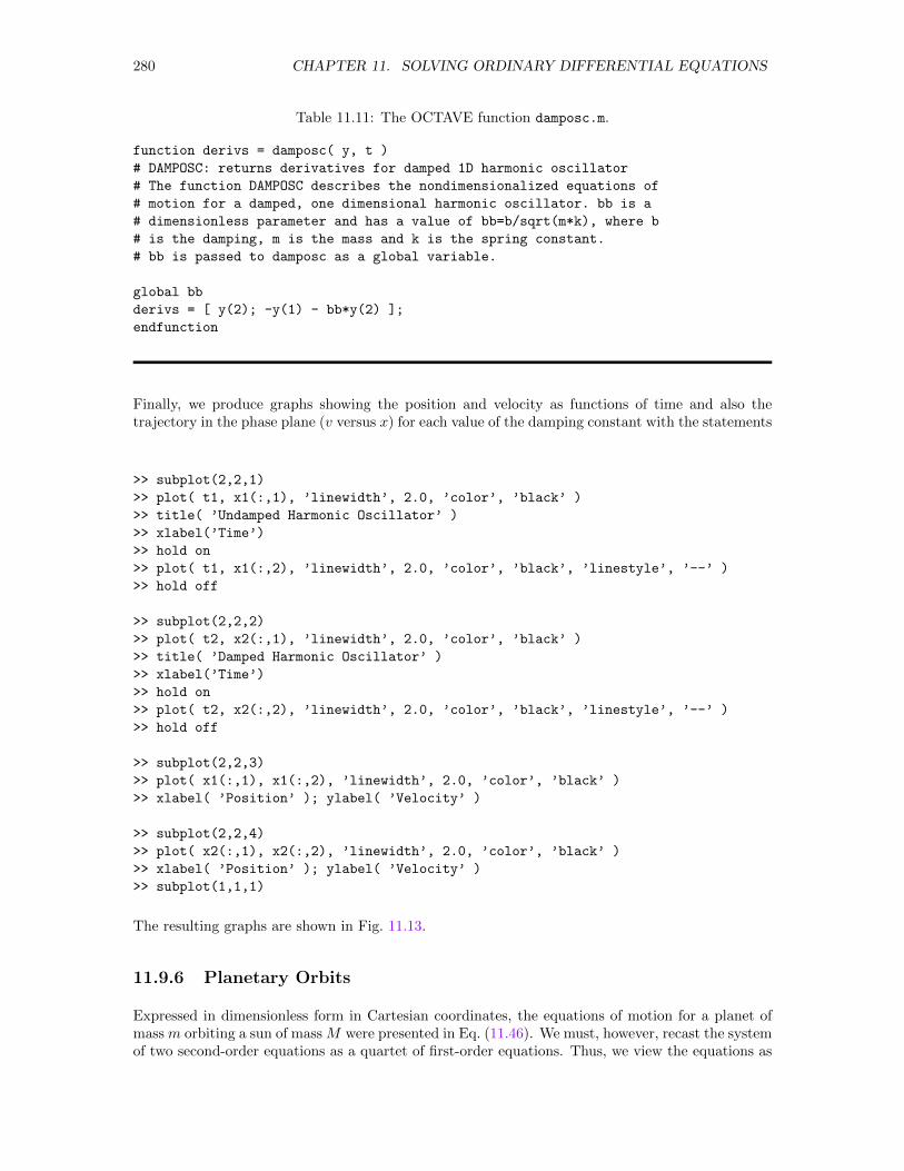
280 CHAPTER 11. SOLVING ORDINARY DIFFERENTIAL EQUATIONS

Table 11.11: The OCTAVE function damposc.m.

function derivs = damposc( y, t )

# DAMPOSC: returns derivatives for damped 1D harmonic oscillator

# The function DAMPOSC describes the nondimensionalized equations of

# motion for a damped, one dimensional harmonic oscillator. bb is a

# dimensionless parameter and has a value of bb=b/sqrt(m*k), where b

# is the damping, m is the mass and k is the spring constant.

# bb is passed to damposc as a global variable.

global bb

derivs = [ y(2); -y(1) - bb*y(2) ];

endfunction

Finally, we produce graphs showing the position and velocity as functions of time and also thetrajectory in the phase plane (v versus x) for each value of the damping constant with the statements

>> subplot(2,2,1)

>> plot( t1, x1(:,1), ’linewidth’, 2.0, ’color’, ’black’ )

>> title( ’Undamped Harmonic Oscillator’ )

>> xlabel(’Time’)

>> hold on

>> plot( t1, x1(:,2), ’linewidth’, 2.0, ’color’, ’black’, ’linestyle’, ’--’ )

>> hold off

>> subplot(2,2,2)

>> plot( t2, x2(:,1), ’linewidth’, 2.0, ’color’, ’black’ )

>> title( ’Damped Harmonic Oscillator’ )

>> xlabel(’Time’)

>> hold on

>> plot( t2, x2(:,2), ’linewidth’, 2.0, ’color’, ’black’, ’linestyle’, ’--’ )

>> hold off

>> subplot(2,2,3)

>> plot( x1(:,1), x1(:,2), ’linewidth’, 2.0, ’color’, ’black’ )

>> xlabel( ’Position’ ); ylabel( ’Velocity’ )

>> subplot(2,2,4)

>> plot( x2(:,1), x2(:,2), ’linewidth’, 2.0, ’color’, ’black’ )

>> xlabel( ’Position’ ); ylabel( ’Velocity’ )

>> subplot(1,1,1)

The resulting graphs are shown in Fig. 11.13.

11.9.6 Planetary Orbits

Expressed in dimensionless form in Cartesian coordinates, the equations of motion for a planet ofmass m orbiting a sun of mass M were presented in Eq. (11.46). We must, however, recast the systemof two second-order equations as a quartet of first-order equations. Thus, we view the equations as

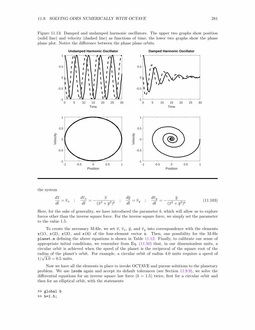
11.9. SOLVING ODES NUMERICALLY WITH OCTAVE 281

Figure 11.13: Damped and undamped harmonic oscillators. The upper two graphs show position(solid line) and velocity (dashed line) as functions of time; the lower two graphs show the phaseplane plot. Notice the difference between the phase plane orbits.

0 5 10 15 20 25 30-1

-0.5

0

0.5

1

Time

Undamped Harmonic Oscillator

0 5 10 15 20 25 30-1

-0.5

0

0.5

1

Time

Damped Harmonic Oscillator

-1 -0.5 0 0.5 1-1

-0.5

0

0.5

1

Position

Vel

ocity

-1 -0.5 0 0.5 1-1

-0.5

0

0.5

1

Position

Vel

ocity

the system

dx

dt= vx ;

dvxdt

= − x

(x2 + y2)b;

dy

dt= vy ;

dvydt

= − y

(x2 + y2)b(11.103)

Here, for the sake of generality, we have introduced the parameter b, which will allow us to exploreforces other than the inverse square force. For the inverse square force, we simply set the parameterto the value 1.5.

To create the necessary M-file, we set x, vx, y, and vy into correspondence with the elementsx(1), x(2), x(3), and x(4) of the four-element vector x. Then, one possibility for the M-fileplanet.m defining the above equations is shown in Table 11.12. Finally, to calibrate our sense ofappropriate initial conditions, we remember from Eq. (11.50) that, in our dimensionless units, acircular orbit is achieved when the speed of the planet is the reciprocal of the square root of theradius of the planet’s orbit. For example, a circular orbit of radius 4.0 units requires a speed of1/√

4.0 = 0.5 units.

Now we have all the elements in place to invoke OCTAVE and pursue solutions to the planetaryproblem. We use lsode again and accept its default tolerances (see Section 11.9.9), we solve thedifferential equations for an inverse square law force (b = 1.5) twice, first for a circular orbit andthen for an elliptical orbit, with the statements

>> global b

>> b=1.5;

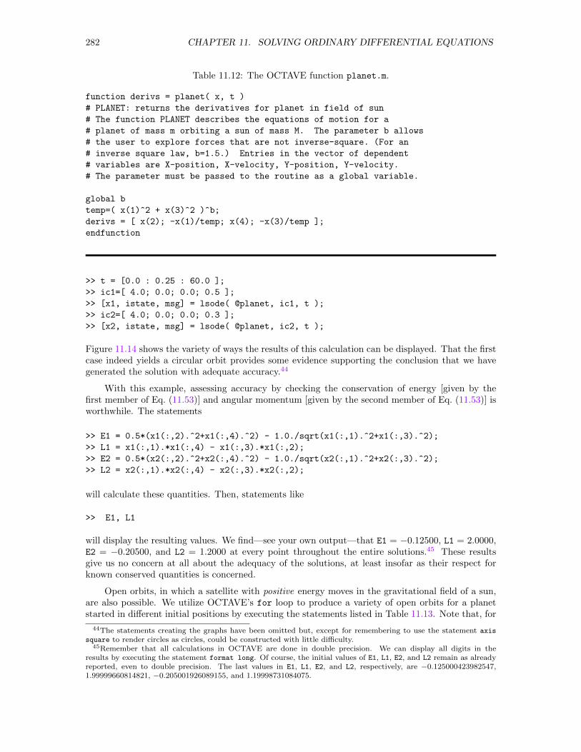
282 CHAPTER 11. SOLVING ORDINARY DIFFERENTIAL EQUATIONS

Table 11.12: The OCTAVE function planet.m.

function derivs = planet( x, t )

# PLANET: returns the derivatives for planet in field of sun

# The function PLANET describes the equations of motion for a

# planet of mass m orbiting a sun of mass M. The parameter b allows

# the user to explore forces that are not inverse-square. (For an

# inverse square law, b=1.5.) Entries in the vector of dependent

# variables are X-position, X-velocity, Y-position, Y-velocity.

# The parameter must be passed to the routine as a global variable.

global b

temp=( x(1)^2 + x(3)^2 )^b;

derivs = [ x(2); -x(1)/temp; x(4); -x(3)/temp ];

endfunction

>> t = [0.0 : 0.25 : 60.0 ];

>> ic1=[ 4.0; 0.0; 0.0; 0.5 ];

>> [x1, istate, msg] = lsode( @planet, ic1, t );

>> ic2=[ 4.0; 0.0; 0.0; 0.3 ];

>> [x2, istate, msg] = lsode( @planet, ic2, t );

Figure 11.14 shows the variety of ways the results of this calculation can be displayed. That the firstcase indeed yields a circular orbit provides some evidence supporting the conclusion that we havegenerated the solution with adequate accuracy.44

With this example, assessing accuracy by checking the conservation of energy [given by thefirst member of Eq. (11.53)] and angular momentum [given by the second member of Eq. (11.53)] isworthwhile. The statements

>> E1 = 0.5*(x1(:,2).^2+x1(:,4).^2) - 1.0./sqrt(x1(:,1).^2+x1(:,3).^2);

>> L1 = x1(:,1).*x1(:,4) - x1(:,3).*x1(:,2);

>> E2 = 0.5*(x2(:,2).^2+x2(:,4).^2) - 1.0./sqrt(x2(:,1).^2+x2(:,3).^2);

>> L2 = x2(:,1).*x2(:,4) - x2(:,3).*x2(:,2);

will calculate these quantities. Then, statements like

>> E1, L1

will display the resulting values. We find—see your own output—that E1 = −0.12500, L1 = 2.0000,E2 = −0.20500, and L2 = 1.2000 at every point throughout the entire solutions.45 These resultsgive us no concern at all about the adequacy of the solutions, at least insofar as their respect forknown conserved quantities is concerned.

Open orbits, in which a satellite with positive energy moves in the gravitational field of a sun,are also possible. We utilize OCTAVE’s for loop to produce a variety of open orbits for a planetstarted in different initial positions by executing the statements listed in Table 11.13. Note that, for

44The statements creating the graphs have been omitted but, except for remembering to use the statement axis

square to render circles as circles, could be constructed with little difficulty.45Remember that all calculations in OCTAVE are done in double precision. We can display all digits in the

results by executing the statement format long. Of course, the initial values of E1, L1, E2, and L2 remain as alreadyreported, even to double precision. The last values in E1, L1, E2, and L2, respectively, are −0.125000423982547,1.99999660814821, −0.205001926089155, and 1.19998731084075.

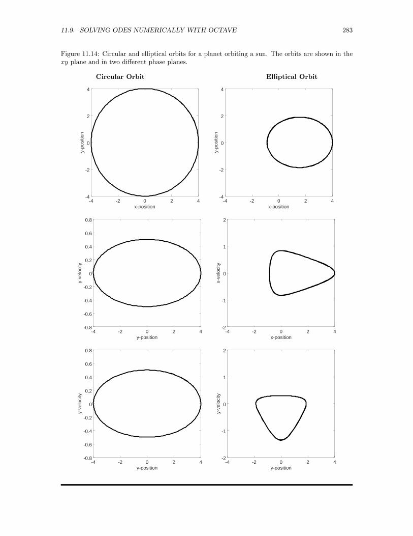
11.9. SOLVING ODES NUMERICALLY WITH OCTAVE 283

Figure 11.14: Circular and elliptical orbits for a planet orbiting a sun. The orbits are shown in thexy plane and in two different phase planes.

Circular Orbit Elliptical Orbit

-4 -2 0 2 4-4

-2

0

2

4

x-position

y-po

sitio

n

-4 -2 0 2 4-4

-2

0

2

4

x-position

y-po

sitio

n

-4 -2 0 2 4-0.8

-0.6

-0.4

-0.2

0

0.2

0.4

0.6

0.8

y-position

y-ve

loci

ty

-4 -2 0 2 4-2

-1

0

1

2

x-position

x-ve

loci

ty

-4 -2 0 2 4-0.8

-0.6

-0.4

-0.2

0

0.2

0.4

0.6

0.8

y-position

y-ve

loci

ty

-4 -2 0 2 4-2

-1

0

1

2

y-position

y-ve

loci

ty

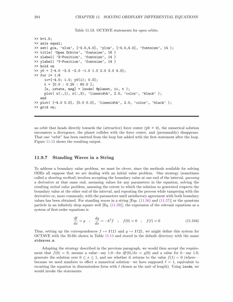
284 CHAPTER 11. SOLVING ORDINARY DIFFERENTIAL EQUATIONS

Table 11.13: OCTAVE statements for open orbits.

>> b=1.5;

>> axis equal;

>> set( gca, ’xlim’, [-4.0,4.0], ’ylim’, [-4.0,4.0], ’fontsize’, 14 );

>> title( ’Open Orbits’, ’fontsize’, 16 )

>> xlabel( ’X-Position’, ’fontsize’, 14 )

>> ylabel( ’Y-Position’, ’fontsize’, 14 )

>> hold on

>> y0 = [-4.0 -3.0 -2.0 -1.0 1.0 2.0 3.0 4.0];

>> for i= 1:8

ic=[-4.0; 1.0; y0(i); 0.0];

t = [0.0 : 0.25 : 60.0 ];

[x, istate, msg] = lsode( @planet, ic, t );

plot( x(:,1), x(:,3), ’linewidth’, 2.0, ’color’, ’black’ );

end

>> plot( [-4.0 0.0], [0.0 0.0], ’linewidth’, 2.0, ’color’, ’black’ );

>> grid on;

an orbit that heads directly towards the (attractive) force center (y0 = 0), the numerical solutionencounters a divergence, the planet collides with the force center, and (presumably) disappears.That one “orbit” has been omitted from the loop but added with the first statement after the loop.Figure 11.15 shows the resulting output.

11.9.7 Standing Waves in a String

To address a boundary value problem, we must be clever, since the methods available for solvingODEs all suppose that we are dealing with an initial value problem. One strategy (sometimescalled a shooting method) involves accepting the boundary value at one end of the interval, guessinga derivative at that same end, assuming values for any parameters in the equation, solving theresulting initial value problem, assessing the extent to which the solution so generated respects theboundary value at the other end of the interval, and repeating the process while tampering with thederivative or, more commonly, with the parameters until satisfactory agreement with both boundaryvalues has been obtained. For standing waves in a string [Eqs. (11.56) and (11.57)] or the quantumparticle in an infinitely deep square well [Eq. (11.59)], the expression of the relevant equations as asystem of first-order equations is

df

dx= g ;

dg

dx= −k2f ; f(0) = 0 ; f(`) = 0 (11.104)

Thus, setting up the correspondences f 7→ f(1) and g 7→ f(2), we might define this system forOCTAVE with the M-file shown in Table 11.14 and stored in the default directory with the namestdwaves.m.

Adopting the strategy described in the previous paragraph, we would then accept the require-ment that f(0) = 0, assume a value—say 1.0—for df(0)/dx = g(0) and a value for k—say 1.0,generate the solution over 0 ≤ x ≤ 1, and see whether it returns to the value f(1) = 0 (where—because we need numbers to effect a numerical solution—we have supposed ` = 1, equivalent torecasting the equation in dimensionless form with ` chosen as the unit of length). Using lsode, wewould invoke the statements

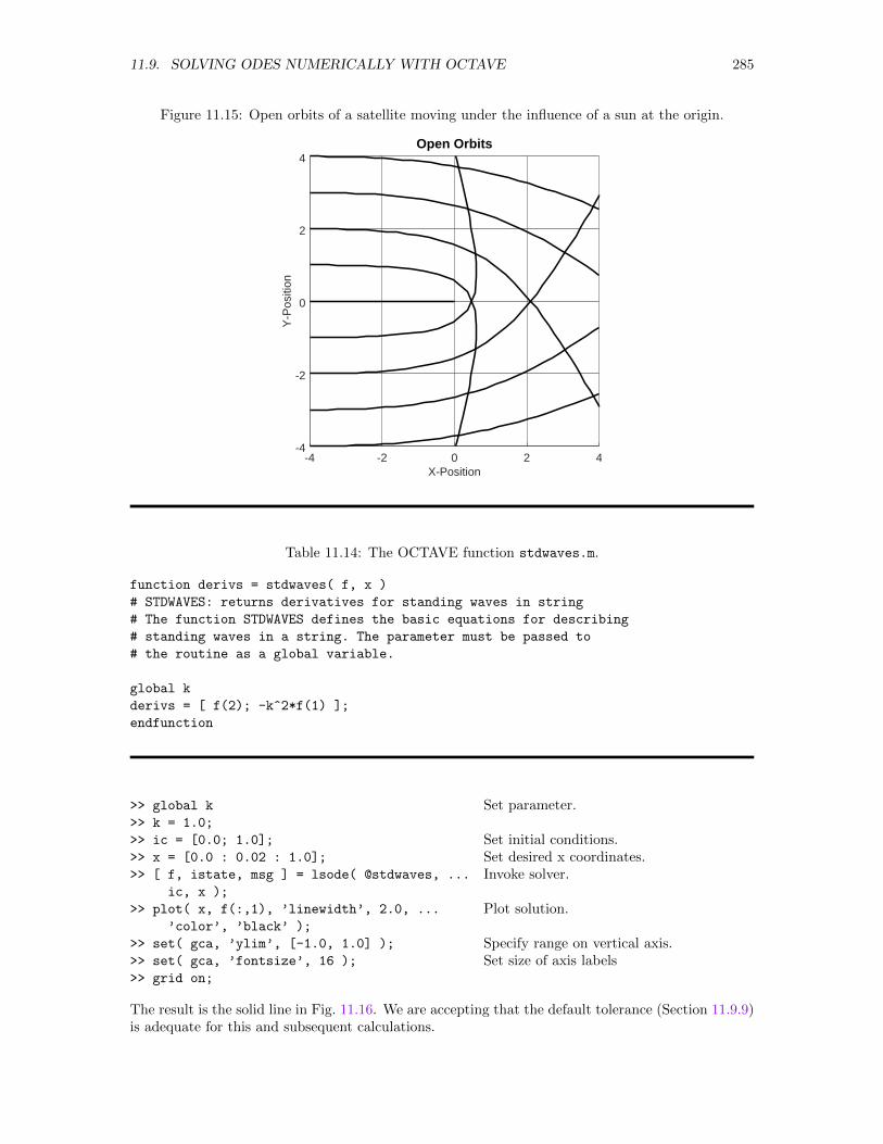
11.9. SOLVING ODES NUMERICALLY WITH OCTAVE 285

Figure 11.15: Open orbits of a satellite moving under the influence of a sun at the origin.

X-Position

4

2

0

-2

-4

Y-P

ositi

on

420-4 -2

Open Orbits

Table 11.14: The OCTAVE function stdwaves.m.

function derivs = stdwaves( f, x )

# STDWAVES: returns derivatives for standing waves in string

# The function STDWAVES defines the basic equations for describing

# standing waves in a string. The parameter must be passed to

# the routine as a global variable.

global k

derivs = [ f(2); -k^2*f(1) ];

endfunction

>> global k

>> k = 1.0;

>> ic = [0.0; 1.0];

>> x = [0.0 : 0.02 : 1.0];

>> [ f, istate, msg ] = lsode( @stdwaves, ...

ic, x );

>> plot( x, f(:,1), ’linewidth’, 2.0, ...

’color’, ’black’ );

>> set( gca, ’ylim’, [-1.0, 1.0] );

>> set( gca, ’fontsize’, 16 );

>> grid on;

Set parameter.

Set initial conditions.Set desired x coordinates.Invoke solver.

Plot solution.

Specify range on vertical axis.Set size of axis labels

The result is the solid line in Fig. 11.16. We are accepting that the default tolerance (Section 11.9.9)is adequate for this and subsequent calculations.

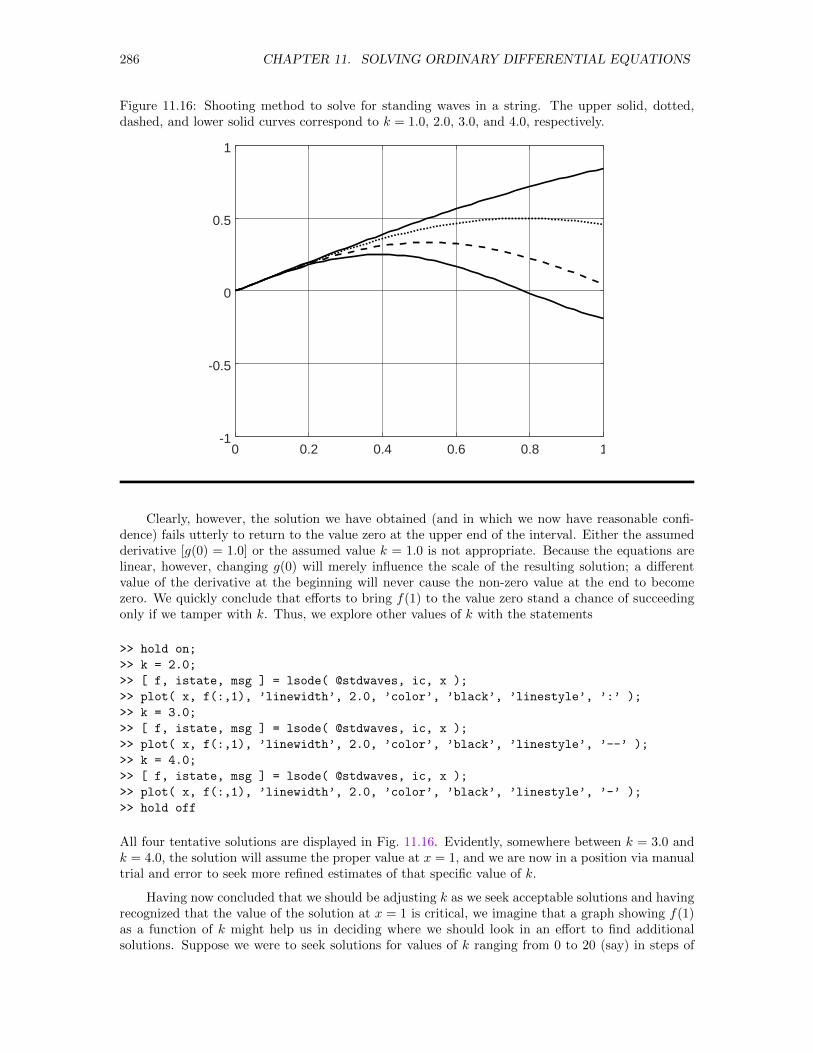
286 CHAPTER 11. SOLVING ORDINARY DIFFERENTIAL EQUATIONS

Figure 11.16: Shooting method to solve for standing waves in a string. The upper solid, dotted,dashed, and lower solid curves correspond to k = 1.0, 2.0, 3.0, and 4.0, respectively.

0 0.2 0.4 0.6 0.8 1-1

-0.5

0

0.5

1

Clearly, however, the solution we have obtained (and in which we now have reasonable confi-dence) fails utterly to return to the value zero at the upper end of the interval. Either the assumedderivative [g(0) = 1.0] or the assumed value k = 1.0 is not appropriate. Because the equations arelinear, however, changing g(0) will merely influence the scale of the resulting solution; a differentvalue of the derivative at the beginning will never cause the non-zero value at the end to becomezero. We quickly conclude that efforts to bring f(1) to the value zero stand a chance of succeedingonly if we tamper with k. Thus, we explore other values of k with the statements

>> hold on;

>> k = 2.0;

>> [ f, istate, msg ] = lsode( @stdwaves, ic, x );

>> plot( x, f(:,1), ’linewidth’, 2.0, ’color’, ’black’, ’linestyle’, ’:’ );

>> k = 3.0;

>> [ f, istate, msg ] = lsode( @stdwaves, ic, x );

>> plot( x, f(:,1), ’linewidth’, 2.0, ’color’, ’black’, ’linestyle’, ’--’ );

>> k = 4.0;

>> [ f, istate, msg ] = lsode( @stdwaves, ic, x );

>> plot( x, f(:,1), ’linewidth’, 2.0, ’color’, ’black’, ’linestyle’, ’-’ );

>> hold off

All four tentative solutions are displayed in Fig. 11.16. Evidently, somewhere between k = 3.0 andk = 4.0, the solution will assume the proper value at x = 1, and we are now in a position via manualtrial and error to seek more refined estimates of that specific value of k.

Having now concluded that we should be adjusting k as we seek acceptable solutions and havingrecognized that the value of the solution at x = 1 is critical, we imagine that a graph showing f(1)as a function of k might help us in deciding where we should look in an effort to find additionalsolutions. Suppose we were to seek solutions for values of k ranging from 0 to 20 (say) in steps of

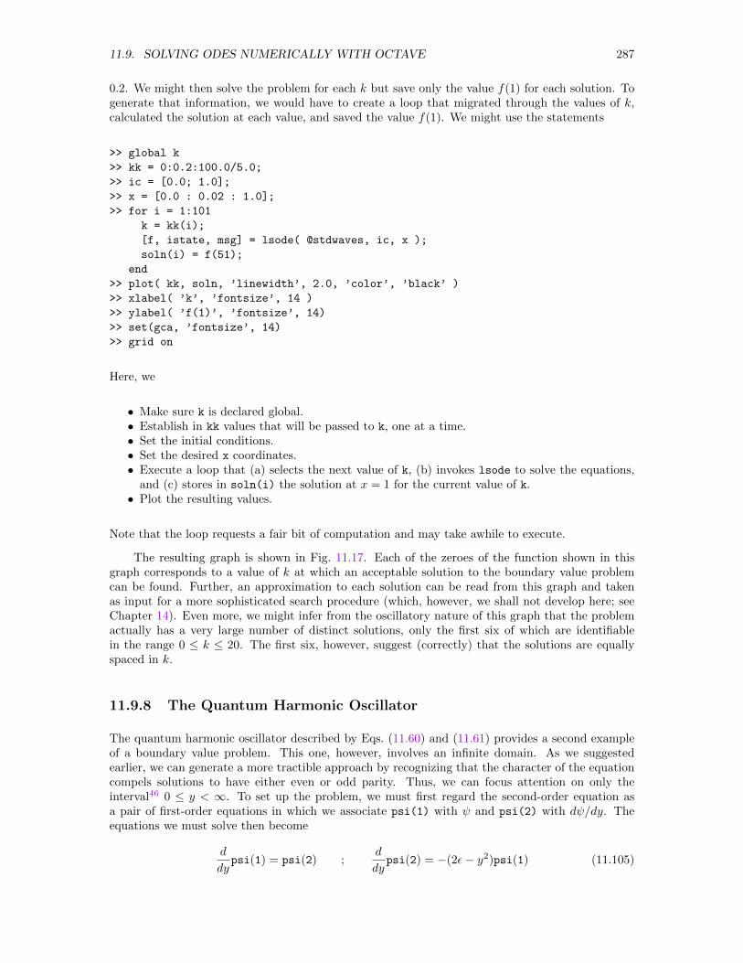
11.9. SOLVING ODES NUMERICALLY WITH OCTAVE 287

0.2. We might then solve the problem for each k but save only the value f(1) for each solution. Togenerate that information, we would have to create a loop that migrated through the values of k,calculated the solution at each value, and saved the value f(1). We might use the statements

>> global k

>> kk = 0:0.2:100.0/5.0;

>> ic = [0.0; 1.0];

>> x = [0.0 : 0.02 : 1.0];

>> for i = 1:101

k = kk(i);

[f, istate, msg] = lsode( @stdwaves, ic, x );

soln(i) = f(51);

end

>> plot( kk, soln, ’linewidth’, 2.0, ’color’, ’black’ )

>> xlabel( ’k’, ’fontsize’, 14 )

>> ylabel( ’f(1)’, ’fontsize’, 14)

>> set(gca, ’fontsize’, 14)

>> grid on

Here, we

• Make sure k is declared global.• Establish in kk values that will be passed to k, one at a time.• Set the initial conditions.• Set the desired x coordinates.• Execute a loop that (a) selects the next value of k, (b) invokes lsode to solve the equations,

and (c) stores in soln(i) the solution at x = 1 for the current value of k.• Plot the resulting values.

Note that the loop requests a fair bit of computation and may take awhile to execute.

The resulting graph is shown in Fig. 11.17. Each of the zeroes of the function shown in thisgraph corresponds to a value of k at which an acceptable solution to the boundary value problemcan be found. Further, an approximation to each solution can be read from this graph and takenas input for a more sophisticated search procedure (which, however, we shall not develop here; seeChapter 14). Even more, we might infer from the oscillatory nature of this graph that the problemactually has a very large number of distinct solutions, only the first six of which are identifiablein the range 0 ≤ k ≤ 20. The first six, however, suggest (correctly) that the solutions are equallyspaced in k.

11.9.8 The Quantum Harmonic Oscillator

The quantum harmonic oscillator described by Eqs. (11.60) and (11.61) provides a second exampleof a boundary value problem. This one, however, involves an infinite domain. As we suggestedearlier, we can generate a more tractible approach by recognizing that the character of the equationcompels solutions to have either even or odd parity. Thus, we can focus attention on only theinterval46 0 ≤ y < ∞. To set up the problem, we must first regard the second-order equation asa pair of first-order equations in which we associate psi(1) with ψ and psi(2) with dψ/dy. Theequations we must solve then become

d

dypsi(1) = psi(2) ;

d

dypsi(2) = −(2ε− y2)psi(1) (11.105)

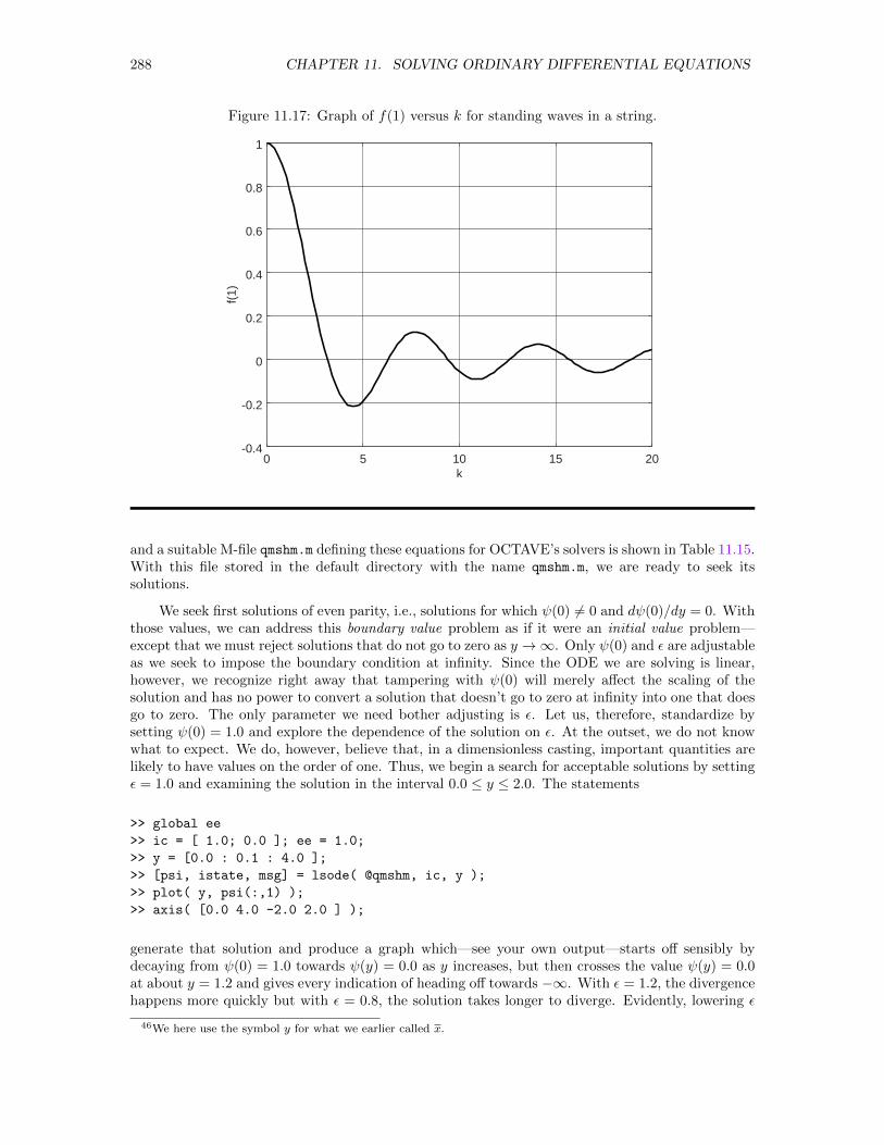
288 CHAPTER 11. SOLVING ORDINARY DIFFERENTIAL EQUATIONS

Figure 11.17: Graph of f(1) versus k for standing waves in a string.

0 5 10 15 20-0.4

-0.2

0

0.2

0.4

0.6

0.8

1

k

f(1)

and a suitable M-file qmshm.m defining these equations for OCTAVE’s solvers is shown in Table 11.15.With this file stored in the default directory with the name qmshm.m, we are ready to seek itssolutions.

We seek first solutions of even parity, i.e., solutions for which ψ(0) 6= 0 and dψ(0)/dy = 0. Withthose values, we can address this boundary value problem as if it were an initial value problem—except that we must reject solutions that do not go to zero as y →∞. Only ψ(0) and ε are adjustableas we seek to impose the boundary condition at infinity. Since the ODE we are solving is linear,however, we recognize right away that tampering with ψ(0) will merely affect the scaling of thesolution and has no power to convert a solution that doesn’t go to zero at infinity into one that doesgo to zero. The only parameter we need bother adjusting is ε. Let us, therefore, standardize bysetting ψ(0) = 1.0 and explore the dependence of the solution on ε. At the outset, we do not knowwhat to expect. We do, however, believe that, in a dimensionless casting, important quantities arelikely to have values on the order of one. Thus, we begin a search for acceptable solutions by settingε = 1.0 and examining the solution in the interval 0.0 ≤ y ≤ 2.0. The statements

>> global ee

>> ic = [ 1.0; 0.0 ]; ee = 1.0;

>> y = [0.0 : 0.1 : 4.0 ];

>> [psi, istate, msg] = lsode( @qmshm, ic, y );

>> plot( y, psi(:,1) );

>> axis( [0.0 4.0 -2.0 2.0 ] );

generate that solution and produce a graph which—see your own output—starts off sensibly bydecaying from ψ(0) = 1.0 towards ψ(y) = 0.0 as y increases, but then crosses the value ψ(y) = 0.0at about y = 1.2 and gives every indication of heading off towards −∞. With ε = 1.2, the divergencehappens more quickly but with ε = 0.8, the solution takes longer to diverge. Evidently, lowering ε

46We here use the symbol y for what we earlier called x.

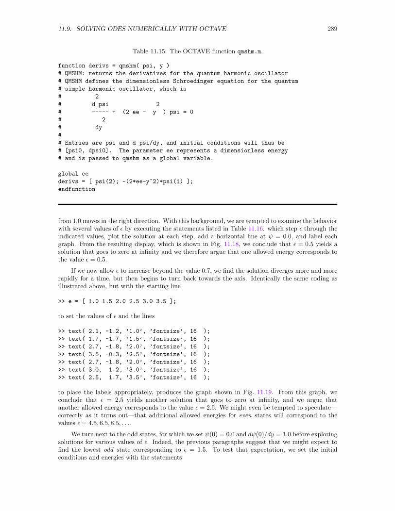
11.9. SOLVING ODES NUMERICALLY WITH OCTAVE 289

Table 11.15: The OCTAVE function qmshm.m.

function derivs = qmshm( psi, y )

# QMSHM: returns the derivatives for the quantum harmonic oscillator

# QMSHM defines the dimensionless Schroedinger equation for the quantum

# simple harmonic oscillator, which is

# 2

# d psi 2

# ----- + (2 ee - y ) psi = 0

# 2

# dy

#

# Entries are psi and d psi/dy, and initial conditions will thus be

# [psi0, dpsi0]. The parameter ee represents a dimensionless energy

# and is passed to qmshm as a global variable.

global ee

derivs = [ psi(2); -(2*ee-y^2)*psi(1) ];

endfunction

from 1.0 moves in the right direction. With this background, we are tempted to examine the behaviorwith several values of ε by executing the statements listed in Table 11.16. which step ε through theindicated values, plot the solution at each step, add a horizontal line at ψ = 0.0, and label eachgraph. From the resulting display, which is shown in Fig. 11.18, we conclude that ε = 0.5 yields asolution that goes to zero at infinity and we therefore argue that one allowed energy corresponds tothe value ε = 0.5.

If we now allow ε to increase beyond the value 0.7, we find the solution diverges more and morerapidly for a time, but then begins to turn back towards the axis. Identically the same coding asillustrated above, but with the starting line

>> e = [ 1.0 1.5 2.0 2.5 3.0 3.5 ];

to set the values of ε and the lines

>> text( 2.1, -1.2, ’1.0’, ’fontsize’, 16 );

>> text( 1.7, -1.7, ’1.5’, ’fontsize’, 16 );

>> text( 2.7, -1.8, ’2.0’, ’fontsize’, 16 );

>> text( 3.5, -0.3, ’2.5’, ’fontsize’, 16 );

>> text( 2.7, -1.8, ’2.0’, ’fontsize’, 16 );

>> text( 3.0, 1.2, ’3.0’, ’fontsize’, 16 );

>> text( 2.5, 1.7, ’3.5’, ’fontsize’, 16 );

to place the labels appropriately, produces the graph shown in Fig. 11.19. From this graph, weconclude that ε = 2.5 yields another solution that goes to zero at infinity, and we argue thatanother allowed energy corresponds to the value ε = 2.5. We might even be tempted to speculate—correctly as it turns out—that additional allowed energies for even states will correspond to thevalues ε = 4.5, 6.5, 8.5, . . ..

We turn next to the odd states, for which we set ψ(0) = 0.0 and dψ(0)/dy = 1.0 before exploringsolutions for various values of ε. Indeed, the previous paragraphs suggest that we might expect tofind the lowest odd state corresponding to ε = 1.5. To test that expectation, we set the initialconditions and energies with the statements

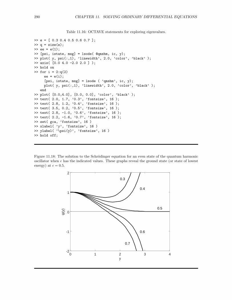
290 CHAPTER 11. SOLVING ORDINARY DIFFERENTIAL EQUATIONS

Table 11.16: OCTAVE statements for exploring eigenvalues.

>> e = [ 0.3 0.4 0.5 0.6 0.7 ];

>> q = size(e);

>> ee = e(1);

>> [psi, istate, msg] = lsode( @qmshm, ic, y);

>> plot( y, psi(:,1), ’linewidth’, 2.0, ’color’, ’black’ );

>> axis( [0.0 4.0 -2.0 2.0 ] );

>> hold on

>> for i = 2:q(2)

ee = e(i);

[psi, istate, msg] = lsode ( ’qmshm’, ic, y);

plot( y, psi(:,1), ’linewidth’, 2.0, ’color’, ’black’ );

end

>> plot( [0.0,4.0], [0.0, 0.0], ’color’, ’black’ );

>> text( 2.0, 1.7, ’0.3’, ’fontsize’, 16 );

>> text( 2.8, 1.2, ’0.4’, ’fontsize’, 16 );

>> text( 3.5, 0.2, ’0.5’, ’fontsize’, 16 );

>> text( 2.8, -1.0, ’0.6’, ’fontsize’, 16 );

>> text( 2.2, -1.6, ’0.7’, ’fontsize’, 16 );

>> set( gca, ’fontsize’, 16 )

>> xlabel( ’y’, ’fontsize’, 16 )

>> ylabel( ’\psi(y)’, ’fontsize’, 16 )

>> hold off;

Figure 11.18: The solution to the Schrodinger equation for an even state of the quantum harmonicoscillator when ε has the indicated values. These graphs reveal the ground state (or state of lowestenergy) at ε = 0.5.

0 1 2 3 4-2

-1

0

1

2

y

ψ(y

)

0.3

0.4

0.5

0.6

0.7

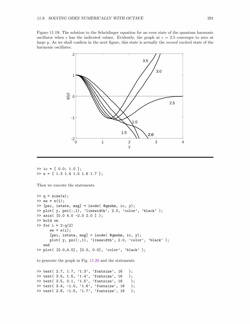
11.9. SOLVING ODES NUMERICALLY WITH OCTAVE 291

Figure 11.19: The solution to the Schrodinger equation for an even state of the quantum harmonicoscillator when ε has the indicated values. Evidently, the graph at ε = 2.5 converges to zero atlarge y. As we shall confirm in the next figure, this state is actually the second excited state of theharmonic oscillator.

0 1 2 3 4-2

-1

0

1

2

y

ψ(y

)

1.0

1.5 2.0

2.5

2.0

3.0

3.5

>> ic = [ 0.0; 1.0 ];

>> e = [ 1.3 1.4 1.5 1.6 1.7 ];

Then we execute the statements

>> q = size(e);

>> ee = e(1);

>> [psi, istate, msg] = lsode( @qmshm, ic, y);

>> plot( y, psi(:,1), ’linewidth’, 2.0, ’color’, ’black’ );

>> axis( [0.0 4.0 -2.0 2.0 ] );

>> hold on

>> for i = 2:q(2)

ee = e(i);

[psi, istate, msg] = lsode( @qmshm, ic, y);

plot( y, psi(:,1), ’linewidth’, 2.0, ’color’, ’black’ );

end

>> plot( [0.0,4.0], [0.0, 0.0], ’color’, ’black’ );

to generate the graph in Fig. 11.20 and the statements

>> text( 2.7, 1.7, ’1.3’, ’fontsize’, 16 );

>> text( 3.5, 1.5, ’1.4’, ’fontsize’, 16 );

>> text( 3.5, 0.1, ’1.5’, ’fontsize’, 16 );

>> text( 3.4, -1.0, ’1.6’, ’fontsize’, 16 );

>> text( 2.8, -1.5, ’1.7’, ’fontsize’, 16 );

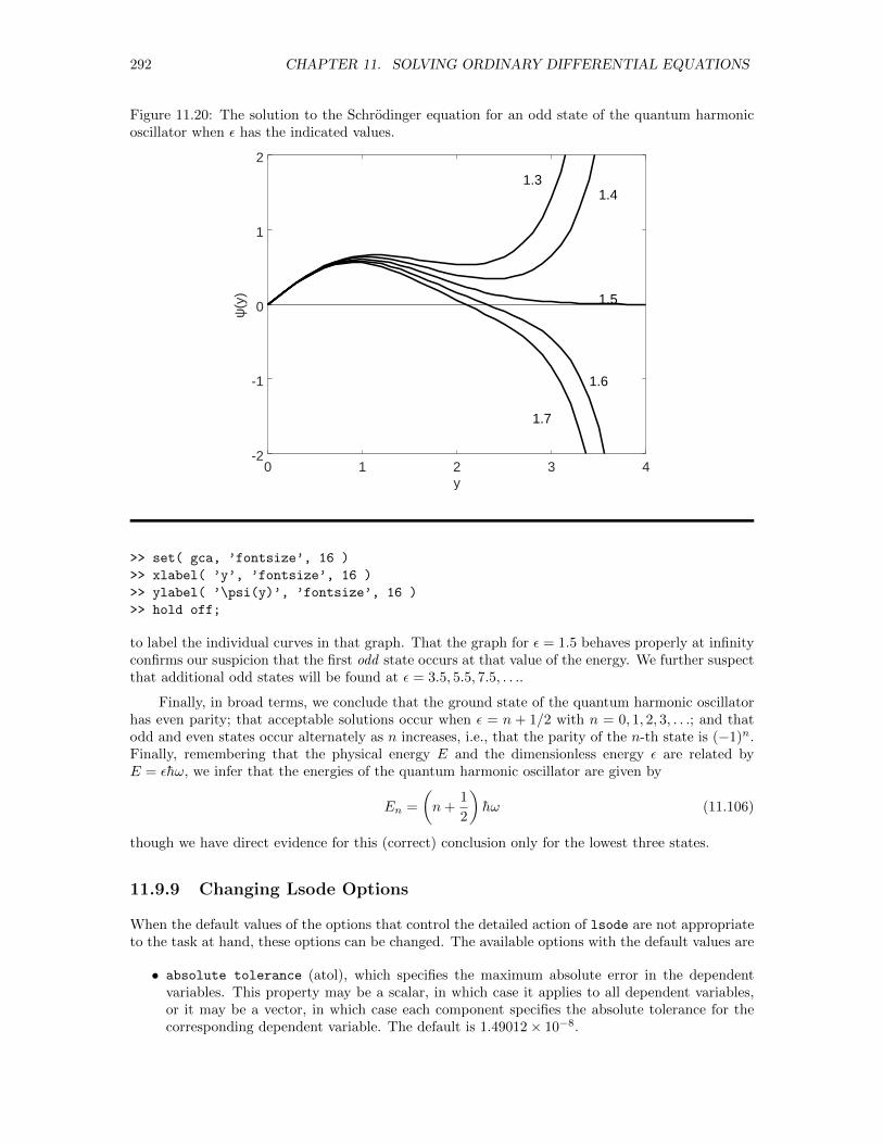
292 CHAPTER 11. SOLVING ORDINARY DIFFERENTIAL EQUATIONS

Figure 11.20: The solution to the Schrodinger equation for an odd state of the quantum harmonicoscillator when ε has the indicated values.

0 1 2 3 4-2

-1

0

1

2

y

ψ(y

)

1.31.4

1.5

1.6

1.7

>> set( gca, ’fontsize’, 16 )

>> xlabel( ’y’, ’fontsize’, 16 )

>> ylabel( ’\psi(y)’, ’fontsize’, 16 )

>> hold off;

to label the individual curves in that graph. That the graph for ε = 1.5 behaves properly at infinityconfirms our suspicion that the first odd state occurs at that value of the energy. We further suspectthat additional odd states will be found at ε = 3.5, 5.5, 7.5, . . ..

Finally, in broad terms, we conclude that the ground state of the quantum harmonic oscillatorhas even parity; that acceptable solutions occur when ε = n + 1/2 with n = 0, 1, 2, 3, . . .; and thatodd and even states occur alternately as n increases, i.e., that the parity of the n-th state is (−1)n.Finally, remembering that the physical energy E and the dimensionless energy ε are related byE = εhω, we infer that the energies of the quantum harmonic oscillator are given by

En =

(n+

1

2

)hω (11.106)

though we have direct evidence for this (correct) conclusion only for the lowest three states.

11.9.9 Changing Lsode Options

When the default values of the options that control the detailed action of lsode are not appropriateto the task at hand, these options can be changed. The available options with the default values are

• absolute tolerance (atol), which specifies the maximum absolute error in the dependentvariables. This property may be a scalar, in which case it applies to all dependent variables,or it may be a vector, in which case each component specifies the absolute tolerance for thecorresponding dependent variable. The default is 1.49012× 10−8.

11.9. SOLVING ODES NUMERICALLY WITH OCTAVE 293

• relative tolerance (rtol), which specifies the maximum relative error in the dependentvariables. This property can be only a scalar, and it applies to all dependent variables. Thedefault is 1.49012× 10−8.

• integration method, which is a string specifying which of the available methods is to beused. Two options are provided, the distinction being whether the system of equations is stiffor non-stiff,47 specifically

adams or non-stiff—the two values for the option are synonyms—for solving equationsthat are not stiff, and

bdf (backward differential formula) or stiff—the two values for the option are againsynonyms—for solving equations that are stiff, though this method will also work fornon-stiff equations.

Method non-stiff requires no Jacobian matrix; method stiff will use a supplied Jacobianmatrix (see the OCTAVE manuals) or, absent that Jacobian, will use finite difference methodsto compute the Jacobian. The default method is stiff.

• initial step size, which specifies a starting value for the step size, which is then adjustedas the adaptive procedure works out the solution. The default is −1, which tells OCTAVE tomake its own choice.

• maximum order, which limits how extensively the procedure will be refined as the solution isworked out. Except for the Adams method (for which the value can be between 1 and 12),this option must be between 1 and 5, inclusive. The default is −1, which tells OCTAVE tomake its own choice.

• maximum step size, which specifies the largest step size the solver is to use. The default is−1, which tells OCTAVE to make its own choice.

• minimum step size, which, if specified, overrides the default value of 0.

• step limit, which, if specified, overrides the default maximum number—100,000—of steps.

The two tolerances are both taken into account as OCTAVE assesses convergence. Specifically,OCTAVE seeks to keep the absolute value of the local error in each of the returned values of thedependent variables no bigger than the quantity

|local error in x(i)| ≤ rtol*|x(i)| + atol(i), all i

where x(i) is the returned value of the solution at every step along the way. Typically, when thesolution is close to zero, the absolute tolerance provides the controlling criterion while, when thesolution is well away from zero, the relative tolerance may dominate over the absolute tolerance.Either (but certainly not both) of these tolerances can be set to zero, in which case the other providesthe controlling criterion throughout the solution. Be warned, however: if the absolute tolerance is setto zero, convergence may be difficult when the solution itself is close to zero (since a small fractionof zero—relative tolerance—may result in excessive computation).

If we choose to establish values different from the defaults for any of these options, we woulddo so with the command lsode options, e.g.,

lsode_options( ’integration method’, ’adams’ )

47When the solution changes very rapidly over a short time interval but a solution is sought over a much longertime interval, the equation(s) is (are) said to be stiff. Not every system of equations falls into this category.

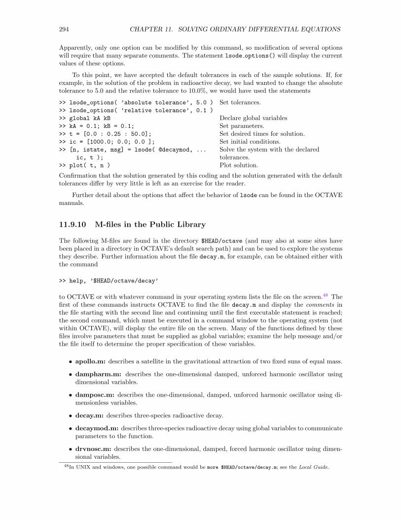
294 CHAPTER 11. SOLVING ORDINARY DIFFERENTIAL EQUATIONS

Apparently, only one option can be modified by this command, so modification of several optionswill require that many separate comments. The statement lsode options() will display the currentvalues of these options.

To this point, we have accepted the default tolerances in each of the sample solutions. If, forexample, in the solution of the problem in radioactive decay, we had wanted to change the absolutetolerance to 5.0 and the relative tolerance to 10.0%, we would have used the statements

>> lsode_options( ’absolute tolerance’, 5.0 )

>> lsode_options( ’relative tolerance’, 0.1 )

>> global kA kB

>> kA = 0.1; kB = 0.1;

>> t = [0.0 : 0.25 : 50.0];

>> ic = [1000.0; 0.0; 0.0 ];

>> [n, istate, msg] = lsode( @decaymod, ...

ic, t );

>> plot( t, n )

Set tolerances.

Declare global variablesSet parameters.Set desired times for solution.Set initial conditions.Solve the system with the declaredtolerances.Plot solution.

Confirmation that the solution generated by this coding and the solution generated with the defaulttolerances differ by very little is left as an exercise for the reader.

Further detail about the options that affect the behavior of lsode can be found in the OCTAVEmanuals.

11.9.10 M-files in the Public Library

The following M-files are found in the directory $HEAD/octave (and may also at some sites havebeen placed in a directory in OCTAVE’s default search path) and can be used to explore the systemsthey describe. Further information about the file decay.m, for example, can be obtained either withthe command

>> help, ’$HEAD/octave/decay’

to OCTAVE or with whatever command in your operating system lists the file on the screen.48 Thefirst of these commands instructs OCTAVE to find the file decay.m and display the comments inthe file starting with the second line and continuing until the first executable statement is reached;the second command, which must be executed in a command window to the operating system (notwithin OCTAVE), will display the entire file on the screen. Many of the functions defined by thesefiles involve parameters that must be supplied as global variables; examine the help message and/orthe file itself to determine the proper specification of these variables.

• apollo.m: describes a satellite in the gravitational attraction of two fixed suns of equal mass.

• dampharm.m: describes the one-dimensional damped, unforced harmonic oscillator usingdimensional variables.

• damposc.m: describes the one-dimensional, damped, unforced harmonic oscillator using di-mensionless variables.

• decay.m: describes three-species radioactive decay.

• decaymod.m: describes three-species radioactive decay using global variables to communicateparameters to the function.

• drvnosc.m: describes the one-dimensional, damped, forced harmonic oscillator using dimen-sional variables.

48In UNIX and windows, one possible command would be more $HEAD/octave/decay.m; see the Local Guide.

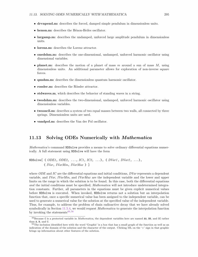
11.13. SOLVING ODES NUMERICALLY WITH MATHEMATICA 295

• drvnpend.m: describes the forced, damped simple pendulum in dimensionless units.

• henon.m: describes the Henon-Heiles oscillator.

• largamp.m: describes the undamped, unforced large amplitude pendulum in dimensionlessunits.

• lorenz.m: describes the Lorenz attractor.

• onedshm.m: describes the one-dimensional, undamped, unforced harmonic oscillator usingdimensional variables.

• planet.m: describes the motion of a planet of mass m around a sun of mass M , usingdimensionless units. An additional parameter allows for exploration of non-inverse squareforces.

• qmshm.m: describes the dimensionless quantum harmonic oscillator.

• rossler.m: describes the Rossler attractor.

• stdwaves.m, which describes the behavior of standing waves in a string.

• twodshm.m: describes the two-dimensional, undamped, unforced harmonic oscillator usingdimensionless variables.

• twooscil.m: describes a system of two equal masses between two walls, all connected by threesprings. Dimensionless units are used.

• vandpol.m: describes the Van der Pol oscillator.

11.13 Solving ODEs Numerically with Mathematica

Mathematica’s command NDSolve provides a means to solve ordinary differential equations numer-ically. A full statement using NDSolve will have the form

NDSolve[ ODE1, ODE2, ..., IC1, IC2, ..., DVar1, DVar2, ...,

IVar, IVarMin, IVarMax ]

where ODE and IC are the differential equations and initial conditions, DVar represents a dependentvariable, and IVar, IVarMin, and IVarMax are the independent variable and the lower and upperlimits on the range in which the solution is to be found. In this case, both the differential equationsand the initial conditions must be specified; Mathematica will not introduce undetermined integra-tion constants. Further, all parameters in the equations must be given explicit numerical valuesbefore NDSolve is executed. When invoked, NDSolve returns not a solution but an interpolationfunction that, once a specific numerical value has been assigned to the independent variable, can beused to generate a numerical value for the solution at the specified value of the independent variable.Thus, for example, to address the problem of chain radioactive decay that we have already solvedsymbolically in Section 11.5.4, we would request Mathematica to generate the interpolation functionby invoking the statements49,50

49Because C is a protected variable in Mathematica, the dependent variables here are named AA, BB, and CC ratherthan A, B, and C.

50The inclusion identified here with the word ‘Graphic’ is a box that has a small graph of the function as well as anindication of the domain of the solution and the character of the output. Clicking ML on the ‘+’ sign in that graphicbrings up information about other features of the solution.

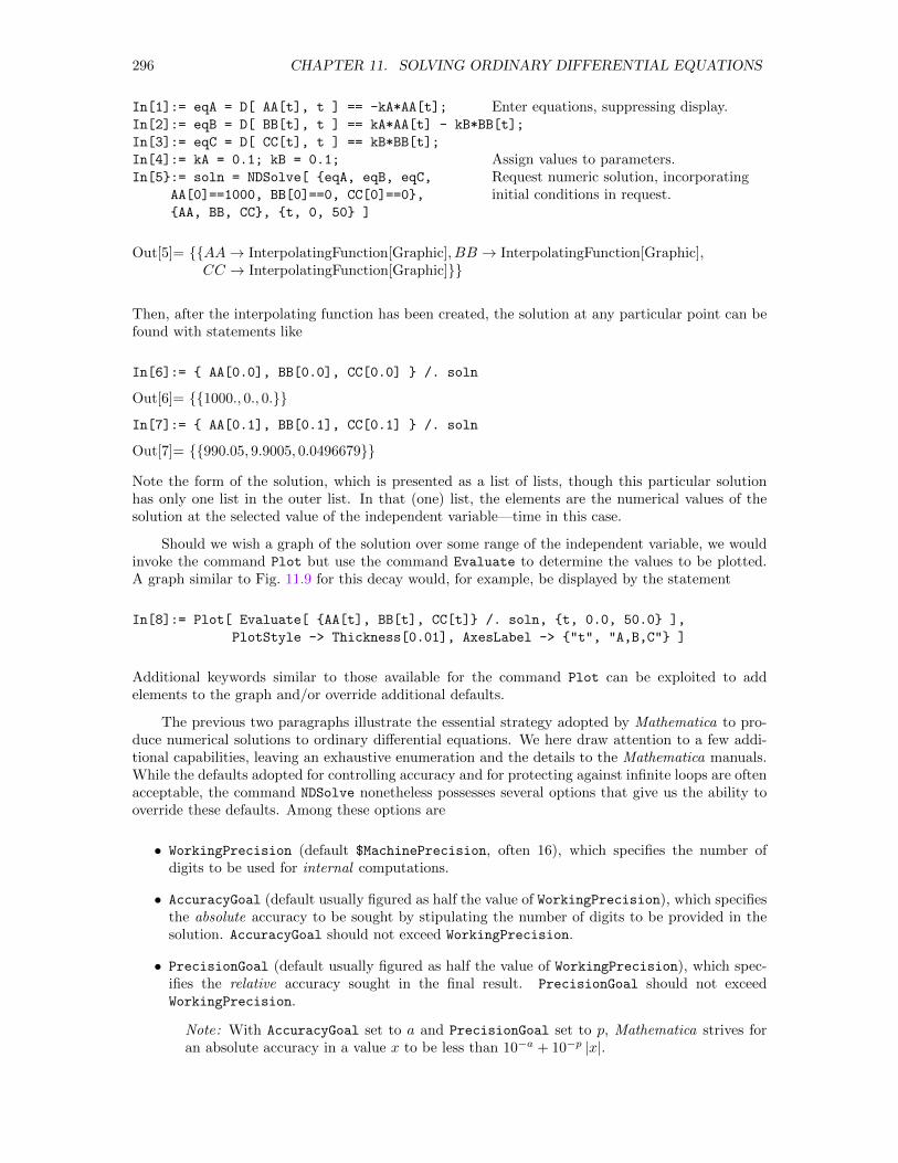
296 CHAPTER 11. SOLVING ORDINARY DIFFERENTIAL EQUATIONS

In[1]:= eqA = D[ AA[t], t ] == -kA*AA[t];

In[2]:= eqB = D[ BB[t], t ] == kA*AA[t] - kB*BB[t];

In[3]:= eqC = D[ CC[t], t ] == kB*BB[t];

In[4]:= kA = 0.1; kB = 0.1;

In[5:= soln = NDSolve[ eqA, eqB, eqC,

AA[0]==1000, BB[0]==0, CC[0]==0,

AA, BB, CC, t, 0, 50 ]

Enter equations, suppressing display.

Assign values to parameters.Request numeric solution, incorporatinginitial conditions in request.

Out[5]= AA→ InterpolatingFunction[Graphic], BB → InterpolatingFunction[Graphic],CC → InterpolatingFunction[Graphic]

Then, after the interpolating function has been created, the solution at any particular point can befound with statements like

In[6]:= AA[0.0], BB[0.0], CC[0.0] /. soln

Out[6]= 1000., 0., 0.

In[7]:= AA[0.1], BB[0.1], CC[0.1] /. soln

Out[7]= 990.05, 9.9005, 0.0496679

Note the form of the solution, which is presented as a list of lists, though this particular solutionhas only one list in the outer list. In that (one) list, the elements are the numerical values of thesolution at the selected value of the independent variable—time in this case.

Should we wish a graph of the solution over some range of the independent variable, we wouldinvoke the command Plot but use the command Evaluate to determine the values to be plotted.A graph similar to Fig. 11.9 for this decay would, for example, be displayed by the statement

In[8]:= Plot[ Evaluate[ AA[t], BB[t], CC[t] /. soln, t, 0.0, 50.0 ],

PlotStyle -> Thickness[0.01], AxesLabel -> "t", "A,B,C" ]

Additional keywords similar to those available for the command Plot can be exploited to addelements to the graph and/or override additional defaults.

The previous two paragraphs illustrate the essential strategy adopted by Mathematica to pro-duce numerical solutions to ordinary differential equations. We here draw attention to a few addi-tional capabilities, leaving an exhaustive enumeration and the details to the Mathematica manuals.While the defaults adopted for controlling accuracy and for protecting against infinite loops are oftenacceptable, the command NDSolve nonetheless possesses several options that give us the ability tooverride these defaults. Among these options are

• WorkingPrecision (default $MachinePrecision, often 16), which specifies the number ofdigits to be used for internal computations.

• AccuracyGoal (default usually figured as half the value of WorkingPrecision), which specifiesthe absolute accuracy to be sought by stipulating the number of digits to be provided in thesolution. AccuracyGoal should not exceed WorkingPrecision.

• PrecisionGoal (default usually figured as half the value of WorkingPrecision), which spec-ifies the relative accuracy sought in the final result. PrecisionGoal should not exceedWorkingPrecision.

Note: With AccuracyGoal set to a and PrecisionGoal set to p, Mathematica strives foran absolute accuracy in a value x to be less than 10−a + 10−p |x|.

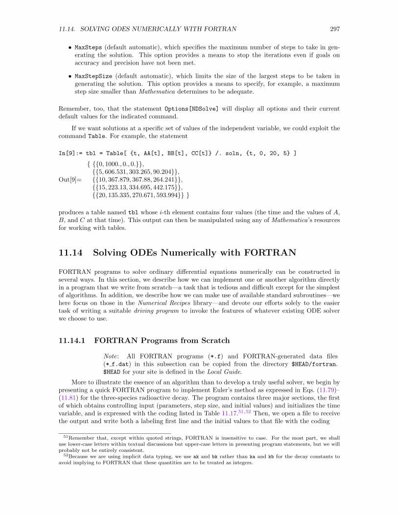
11.14. SOLVING ODES NUMERICALLY WITH FORTRAN 297

• MaxSteps (default automatic), which specifies the maximum number of steps to take in gen-erating the solution. This option provides a means to stop the iterations even if goals onaccuracy and precision have not been met.

• MaxStepSize (default automatic), which limits the size of the largest steps to be taken ingenerating the solution. This option provides a means to specify, for example, a maximumstep size smaller than Mathematica determines to be adequate.

Remember, too, that the statement Options[NDSolve] will display all options and their currentdefault values for the indicated command.

If we want solutions at a specific set of values of the independent variable, we could exploit thecommand Table. For example, the statement

In[9]:= tbl = Table[ t, AA[t], BB[t], CC[t] /. soln, t, 0, 20, 5 ]

Out[9]=

0, 1000., 0., 0.,5, 606.531, 303.265, 90.204,10, 367.879, 367.88, 264.241,15, 223.13, 334.695, 442.175,20, 135.335, 270.671, 593.994

produces a table named tbl whose i-th element contains four values (the time and the values of A,B, and C at that time). This output can then be manipulated using any of Mathematica’s resourcesfor working with tables.

11.14 Solving ODEs Numerically with FORTRAN

FORTRAN programs to solve ordinary differential equations numerically can be constructed inseveral ways. In this section, we describe how we can implement one or another algorithm directlyin a program that we write from scratch—a task that is tedious and difficult except for the simplestof algorithms. In addition, we describe how we can make use of available standard subroutines—wehere focus on those in the Numerical Recipes library—and devote our efforts solely to the easiertask of writing a suitable driving program to invoke the features of whatever existing ODE solverwe choose to use.

11.14.1 FORTRAN Programs from Scratch

Note: All FORTRAN programs (*.f) and FORTRAN-generated data files(* f.dat) in this subsection can be copied from the directory $HEAD/fortran.$HEAD for your site is defined in the Local Guide.

More to illustrate the essence of an algorithm than to develop a truly useful solver, we begin bypresenting a quick FORTRAN program to implement Euler’s method as expressed in Eqs. (11.79)–(11.81) for the three-species radioactive decay. The program contains three major sections, the firstof which obtains controlling input (parameters, step size, and initial values) and initializes the timevariable, and is expressed with the coding listed in Table 11.17.51,52 Then, we open a file to receivethe output and write both a labeling first line and the initial values to that file with the coding

51Remember that, except within quoted strings, FORTRAN is insensitive to case. For the most part, we shalluse lower-case letters within textual discussions but upper-case letters in presenting program statements, but we willprobably not be entirely consistent.

52Because we are using implicit data typing, we use ak and bk rather than ka and kb for the decay constants toavoid implying to FORTRAN that these quantities are to be treated as integers.

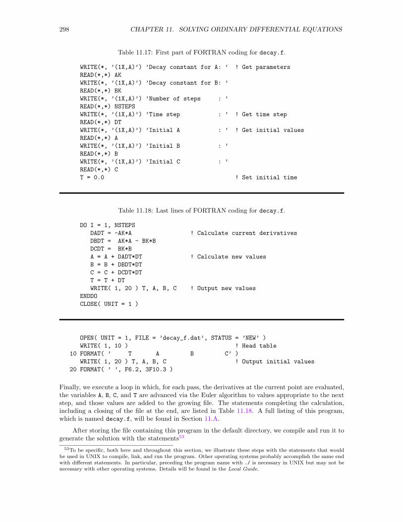
298 CHAPTER 11. SOLVING ORDINARY DIFFERENTIAL EQUATIONS

Table 11.17: First part of FORTRAN coding for decay.f.

WRITE(*, ’(1X,A)’) ’Decay constant for A: ’ ! Get parameters

READ(*,*) AK

WRITE(*, ’(1X,A)’) ’Decay constant for B: ’

READ(*,*) BK

WRITE(*, ’(1X,A)’) ’Number of steps : ’

READ(*,*) NSTEPS

WRITE(*, ’(1X,A)’) ’Time step : ’ ! Get time step

READ(*,*) DT

WRITE(*, ’(1X,A)’) ’Initial A : ’ ! Get initial values

READ(*,*) A

WRITE(*, ’(1X,A)’) ’Initial B : ’

READ(*,*) B

WRITE(*, ’(1X,A)’) ’Initial C : ’

READ(*,*) C

T = 0.0 ! Set initial time

Table 11.18: Last lines of FORTRAN coding for decay.f.

DO I = 1, NSTEPS

DADT = -AK*A ! Calculate current derivatives

DBDT = AK*A - BK*B

DCDT = BK*B

A = A + DADT*DT ! Calculate new values

B = B + DBDT*DT

C = C + DCDT*DT

T = T + DT

WRITE( 1, 20 ) T, A, B, C ! Output new values

ENDDO

CLOSE( UNIT = 1 )

OPEN( UNIT = 1, FILE = ’decay_f.dat’, STATUS = ’NEW’ )

WRITE( 1, 10 ) ! Head table

10 FORMAT( ’ T A B C’ )

WRITE( 1, 20 ) T, A, B, C ! Output initial values

20 FORMAT( ’ ’, F6.2, 3F10.3 )

Finally, we execute a loop in which, for each pass, the derivatives at the current point are evaluated,the variables A, B, C, and T are advanced via the Euler algorithm to values appropriate to the nextstep, and those values are added to the growing file. The statements completing the calculation,including a closing of the file at the end, are listed in Table 11.18. A full listing of this program,which is named decay.f, will be found in Section 11.A.

After storing the file containing this program in the default directory, we compile and run it togenerate the solution with the statements53

53To be specific, both here and throughout this section, we illustrate these steps with the statements that wouldbe used in UNIX to compile, link, and run the program. Other operating systems probably accomplish the same endwith different statements. In particular, preceding the program name with ./ is necessary in UNIX but may not benecessary with other operating systems. Details will be found in the Local Guide.

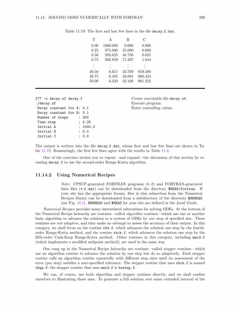
11.14. SOLVING ODES NUMERICALLY WITH FORTRAN 299

Table 11.19: The first and last few lines in the file decay f.dat.

T A B C

0.00 1000.000 0.000 0.0000.25 975.000 25.000 0.0000.50 950.625 48.750 0.6250.75 926.859 71.297 1.844...

......

...49.50 6.651 33.769 959.58049.75 6.485 33.091 960.42450.00 6.323 32.426 961.252

f77 -o decay.xf decay.f

./decay.xf

Decay constant for A: 0.1

Decay constant for B: 0.1

Number of steps : 200

Time step : 0.25

Initial A : 1000.0

Initial B : 0.0

Initial C : 0.0

Create executable file decay.xf.Execute program.Enter controlling values.

The output is written into the file decay f.dat, whose first and last few lines are shown in Ta-ble 11.19. Reassuringly, the first few lines agree with the results in Table 11.2.

One of the exercises invites you to repeat—and expand—the discussion of this section by re-casting decay.f to use the second-order Runge-Kutta algorithm.

11.14.2 Using Numerical Recipes

Note: CPSUP-generated FORTRAN programs (*.f) and FORTRAN-generateddata files (* f.dat) can be downloaded from the directory $HEAD/fortran. Ifyour site has the appropriate license, files in this subsection from the NumericalRecipes library can be downloaded from a subdirectory of the directory $NRHEAD

(see Fig. 10.1). $NRHEAD and $HEAD for your site are defined in the Local Guide.

Numerical Recipes provides many interrelated subroutines for solving ODEs. At the bottom ofthe Numerical Recipe heirarchy are routines—called algorithm routines—which use one or anotherbasic algorithm to advance the solution to a system of ODEs by one step of specified size. Theseroutines are not adaptive, and they make no attempt to assess the accuracy of their output. In thiscategory, we shall focus on the routine rk4.f, which advances the solution one step by the fourth-order Runge-Kutta method, and the routine rkck.f, which advances the solution one step by thefifth-order Cash-Karp Runge-Kutta method. Other routines in this category, including mmid.f

(which implements a modified midpoint method), are used in the same way.

One rung up in the Numerical Recipe heirarchy are routines—called stepper routines—whichuse an algorithm routine to advance the solution by one step but do so adaptively. Each stepperroutine calls an algorithm routine repeatedly with different step sizes until its assessment of theerror (per step) satisfies a user-specified tolerance. The stepper routine that uses rkck.f is namedrkqs.f; the stepper routine that uses mmid.f is bsstep.f.

We can, of course, use both algorithm and stepper routines directly, and we shall confineourselves to illustrating those uses. To generate a full solution over some extended interval of the

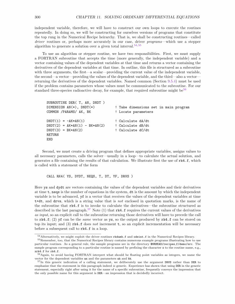
300 CHAPTER 11. SOLVING ORDINARY DIFFERENTIAL EQUATIONS

independent variable, therefore, we will have to construct our own loops to execute the routinesrepeatedly. In doing so, we will be constructing for ourselves versions of programs that constitutethe top rung in the Numerical Recipe heirarchy. That is, we shall be constructing routines—calleddriver routines or, perhaps more accurately in our case, driver programs—which use a stepperalgorithm to generate a solution over a given total interval.54,55

To use an algorithm or stepper routine, we have two responsibilities. First, we must supplya FORTRAN subroutine that accepts the time (more generally, the independent variable) and avector containing values of the dependent variables at that time and returns a vector containing thederivatives of the dependent variables at that time. In outline, this file is structured as a subroutinewith three arguments, the first—a scalar—providing the current value of the independent variable,the second—a vector—providing the values of the dependent variable, and the third—also a vector—returning the derivatives of the dependent variables. Named common (Section 9.5.4) must be usedif the problem contains parameters whose values must be communicated to the subroutine. For ourstandard three-species radioactive decay, for example, that required subroutine might be56

SUBROUTINE DER( T, AN, DNDT )

DIMENSION AN(*), DNDT(*) ! Take dimensions set in main program

COMMON /PARAMS/ AK, BK ! Locate parameters

DNDT(1) = -AK*AN(1) ! Calculate dA/dt

DNDT(2) = AK*AN(1) - BK*AN(2) ! Calculate dB/dt

DNDT(3) = BK*AN(2) ! Calculate dC/dt

RETURN

END

Second, we must create a driving program that defines appropriate variables, assigns values toall necessary parameters, calls the solver—usually in a loop—to calculate the actual solution, andgenerates a file containing the results of that calculation. We illustrate first the use of rk4.f, whichis called with a statement of the form

CALL RK4( YS, DYDT, NEQS, T, DT, YF, DRVS )

Here ys and dydt are vectors containing the values of the dependent variables and their derivativesat time t, neqs is the number of equations in the system, dt is the amount by which the independentvariable is to be advanced, yf is a vector that receives the values of the dependent variables at timet+dt, and drvs, which is a string value that is not enclosed in quotation marks, is the name ofthe subroutine that rk4.f is to invoke to calculate the derivatives—the subroutine structured asdescribed in the last paragraph.57 Note (1) that rk4.f requires the current values of the derivativesas input, so an explicit call to the subroutine returning those derivatives will have to precede the callto rk4.f; (2) yf can be the same vector as ys, so the output produced by rk4.f can be stored ontop its input; and (3) rk4.f does not increment t, so an explicit incrementation will be necessarybefore a subsequent call to rk4.f in a loop.

54Alternatively, we might exploit the driver routines rkdumb.f and odeint.f in the Numerical Recipes library.55Remember, too, that the Numerical Recipes library contains numerous example programs illustrating how to use

particular routines. As a general rule, the sample programs are in the directory $NRHEAD/recipes f/demo/src. Thesample program corresponding to a particular routine is named by prefixing the character x to the routine name, e.g.,xrk4.f for rk4.f.

56Again, to avoid having FORTRAN interpret what should be floating point variables as integers, we name thevector for the dependent variables an and the parameters ak and bk.

57In this generic indication of a calling statement, we deliberately use the argument DRVS rather than DER toemphasize that the statement in this paragraph indeed is generic. Experience has shown that using DER in the genericstatement, especially right after using it for the name of a specific subroutine, frequently conveys the impression thatthe only possible name for this argument is DER—an impression that is decidedly incorrect.

11.14. SOLVING ODES NUMERICALLY WITH FORTRAN 301

A possible driving program to use subroutine der (which we have written) and subroutine rk4.f(supplied in the Numerical Recipes library) would have three major sections. First we dimensionvariables, assign values to the parameters, and initialize variables with the statements

DIMENSION AN(3), DNDT(3) ! Dimension vectors

COMMON /PARAMS/ AK, BK ! Locate parameters

AK = 0.1 ! Set parameters

BK = 0.1

DT = 0.25 ! Set time step

AN(1) = 1000.0 ! Initialize dependent variables

AN(2) = 0.0

AN(3) = 0.0

T = 0.0 ! Set initial time

Then, we open a file to receive the output and write both a labeling first line and the initial valuesto that file with the statements

OPEN( UNIT = 1, FILE = ’decayrk4_f.dat’, STATUS = ’NEW’ )

WRITE( 1, 10 )

10 FORMAT(’ T A B C’ )

WRITE( 1, 20 ) T, AN(1), AN(2), AN(3)

20 FORMAT(’ ’, F6.2, 3F10.3 )

Finally, we execute a loop in which, for each pass, the derivatives at the start of the current intervalare evaluated, rk4.f is called to advance the solution (placing its output on top of its input tofacilitate the next call), the time is incremented, and the new values are added to the growing file.The statements completing the calculation, including closing the file at the end, are

DO I = 1, 200

CALL DER( T, AN, DNDT )

CALL RK4( AN, DNDT, 3, T, DT, AN, DER)

T = T + DT

WRITE( 1, 20 ) T, AN(1), AN(2), AN(3)

ENDDO

CLOSE( UNIT = 1 )

A full listing of this program, which is named decayrk4.f, will be found in Section 11.B.

For the sake of an explicit example, we have chosen above to address three-species radioactivedecay. Starting from scratch with the intention to use rk4.f, we obtain the actual solution andstore it in the file decayrk4 f.dat by

1. Creating the driving program decayrk4.f and the subroutine der using an available texteditor (or copying the files from the directory $HEAD/fortran).

2. Copying the recipe rk4.f from the directory $NRHEAD/recipes f/recipes to the default di-rectory.

3. Compiling and linking the executable module with the statement

f77 -o decayrk4.xf decayrk4.f rk4.f

4. Running the program with the statement ./decayrk4.xf.

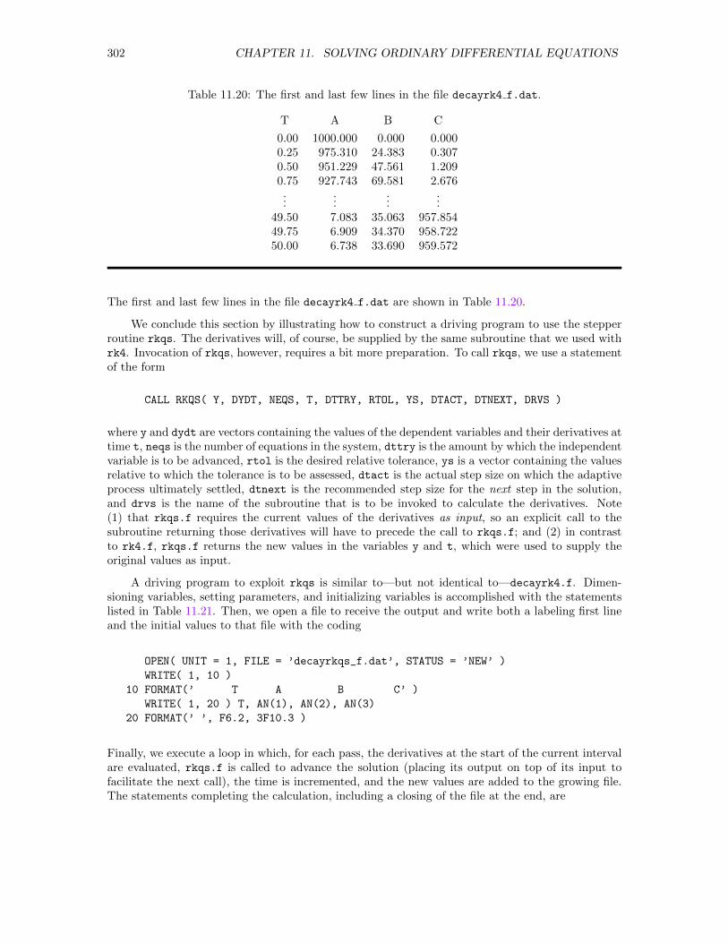
302 CHAPTER 11. SOLVING ORDINARY DIFFERENTIAL EQUATIONS

Table 11.20: The first and last few lines in the file decayrk4 f.dat.

T A B C

0.00 1000.000 0.000 0.0000.25 975.310 24.383 0.3070.50 951.229 47.561 1.2090.75 927.743 69.581 2.676...

......

...49.50 7.083 35.063 957.85449.75 6.909 34.370 958.72250.00 6.738 33.690 959.572

The first and last few lines in the file decayrk4 f.dat are shown in Table 11.20.

We conclude this section by illustrating how to construct a driving program to use the stepperroutine rkqs. The derivatives will, of course, be supplied by the same subroutine that we used withrk4. Invocation of rkqs, however, requires a bit more preparation. To call rkqs, we use a statementof the form

CALL RKQS( Y, DYDT, NEQS, T, DTTRY, RTOL, YS, DTACT, DTNEXT, DRVS )

where y and dydt are vectors containing the values of the dependent variables and their derivatives attime t, neqs is the number of equations in the system, dttry is the amount by which the independentvariable is to be advanced, rtol is the desired relative tolerance, ys is a vector containing the valuesrelative to which the tolerance is to be assessed, dtact is the actual step size on which the adaptiveprocess ultimately settled, dtnext is the recommended step size for the next step in the solution,and drvs is the name of the subroutine that is to be invoked to calculate the derivatives. Note(1) that rkqs.f requires the current values of the derivatives as input, so an explicit call to thesubroutine returning those derivatives will have to precede the call to rkqs.f; and (2) in contrastto rk4.f, rkqs.f returns the new values in the variables y and t, which were used to supply theoriginal values as input.

A driving program to exploit rkqs is similar to—but not identical to—decayrk4.f. Dimen-sioning variables, setting parameters, and initializing variables is accomplished with the statementslisted in Table 11.21. Then, we open a file to receive the output and write both a labeling first lineand the initial values to that file with the coding

OPEN( UNIT = 1, FILE = ’decayrkqs_f.dat’, STATUS = ’NEW’ )

WRITE( 1, 10 )

10 FORMAT(’ T A B C’ )

WRITE( 1, 20 ) T, AN(1), AN(2), AN(3)

20 FORMAT(’ ’, F6.2, 3F10.3 )

Finally, we execute a loop in which, for each pass, the derivatives at the start of the current intervalare evaluated, rkqs.f is called to advance the solution (placing its output on top of its input tofacilitate the next call), the time is incremented, and the new values are added to the growing file.The statements completing the calculation, including a closing of the file at the end, are

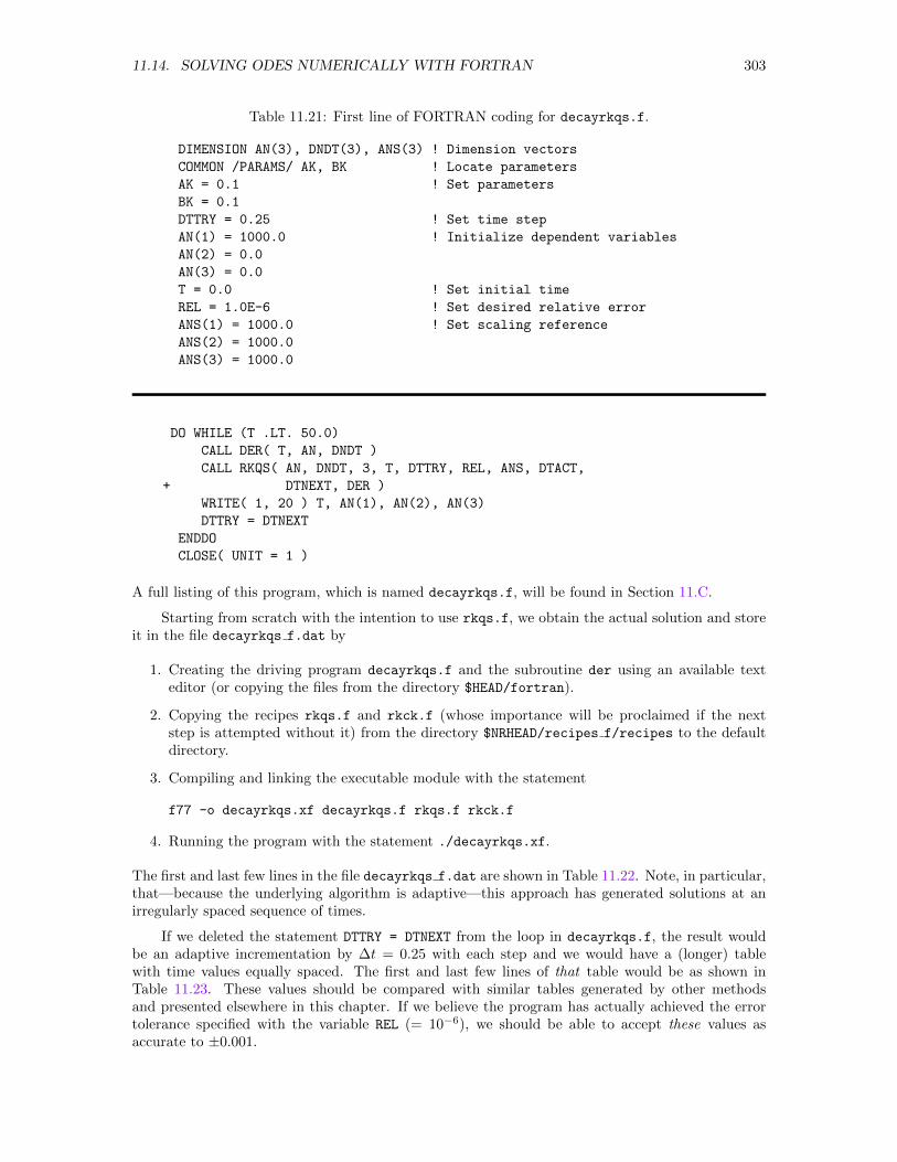
11.14. SOLVING ODES NUMERICALLY WITH FORTRAN 303

Table 11.21: First line of FORTRAN coding for decayrkqs.f.

DIMENSION AN(3), DNDT(3), ANS(3) ! Dimension vectors

COMMON /PARAMS/ AK, BK ! Locate parameters

AK = 0.1 ! Set parameters

BK = 0.1

DTTRY = 0.25 ! Set time step

AN(1) = 1000.0 ! Initialize dependent variables

AN(2) = 0.0

AN(3) = 0.0

T = 0.0 ! Set initial time

REL = 1.0E-6 ! Set desired relative error

ANS(1) = 1000.0 ! Set scaling reference

ANS(2) = 1000.0

ANS(3) = 1000.0

DO WHILE (T .LT. 50.0)

CALL DER( T, AN, DNDT )

CALL RKQS( AN, DNDT, 3, T, DTTRY, REL, ANS, DTACT,

+ DTNEXT, DER )

WRITE( 1, 20 ) T, AN(1), AN(2), AN(3)

DTTRY = DTNEXT

ENDDO

CLOSE( UNIT = 1 )

A full listing of this program, which is named decayrkqs.f, will be found in Section 11.C.

Starting from scratch with the intention to use rkqs.f, we obtain the actual solution and storeit in the file decayrkqs f.dat by

1. Creating the driving program decayrkqs.f and the subroutine der using an available texteditor (or copying the files from the directory $HEAD/fortran).

2. Copying the recipes rkqs.f and rkck.f (whose importance will be proclaimed if the nextstep is attempted without it) from the directory $NRHEAD/recipes f/recipes to the defaultdirectory.

3. Compiling and linking the executable module with the statement

f77 -o decayrkqs.xf decayrkqs.f rkqs.f rkck.f

4. Running the program with the statement ./decayrkqs.xf.

The first and last few lines in the file decayrkqs f.dat are shown in Table 11.22. Note, in particular,that—because the underlying algorithm is adaptive—this approach has generated solutions at anirregularly spaced sequence of times.

If we deleted the statement DTTRY = DTNEXT from the loop in decayrkqs.f, the result wouldbe an adaptive incrementation by ∆t = 0.25 with each step and we would have a (longer) tablewith time values equally spaced. The first and last few lines of that table would be as shown inTable 11.23. These values should be compared with similar tables generated by other methodsand presented elsewhere in this chapter. If we believe the program has actually achieved the errortolerance specified with the variable REL (= 10−6), we should be able to accept these values asaccurate to ±0.001.

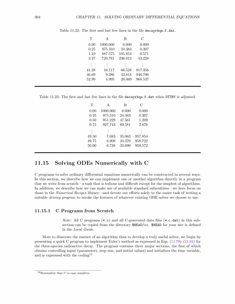
304 CHAPTER 11. SOLVING ORDINARY DIFFERENTIAL EQUATIONS

Table 11.22: The first and last few lines in the file decayrkqs f.dat.

T A B C

0.00 1000.000 0.000 0.0000.25 975.310 24.383 0.3071.19 887.575 105.854 6.5713.27 720.761 236.012 43.228...

......

...41.28 16.117 66.528 917.35646.69 9.386 43.818 946.79652.99 4.995 26.469 968.537

Table 11.23: The first and last few lines in the file decayrkqs f.dat when DTTRY is adjusted.

T A B C

0.00 1000.000 0.000 0.0000.25 975.310 24.383 0.3070.50 951.229 47.561 1.2090.75 927.743 69.581 2.676...

......

...49.50 7.083 35.063 957.85449.75 6.909 34.370 958.72250.00 6.738 33.690 959.572

11.15 Solving ODEs Numerically with C

C programs to solve ordinary differential equations numerically can be constructed in several ways.In this section, we describe how we can implement one or another algorithm directly in a programthat we write from scratch—a task that is tedious and difficult except for the simplest of algorithms.In addition, we describe how we can make use of available standard subroutines—we here focus onthose in the Numerical Recipes library—and devote our efforts solely to the easier task of writing asuitable driving program to invoke the features of whatever existing ODE solver we choose to use.

11.15.1 C Programs from Scratch

Note: All C programs (*.c) and all C-generated data files (* c.dat) in this sub-section can be copied from the directory $HEAD/cc. $HEAD for your site is definedin the Local Guide.

More to illustrate the essence of an algorithm than to develop a truly useful solver, we begin bypresenting a quick C program to implement Euler’s method as expressed in Eqs. (11.79)–(11.81) forthe three-species radioactive decay. The program contains three major sections, the first of whichobtains controlling input (parameters, step size, and initial values) and initializes the time variable,and is expressed with the coding58

58Remember that C is case sensitive.

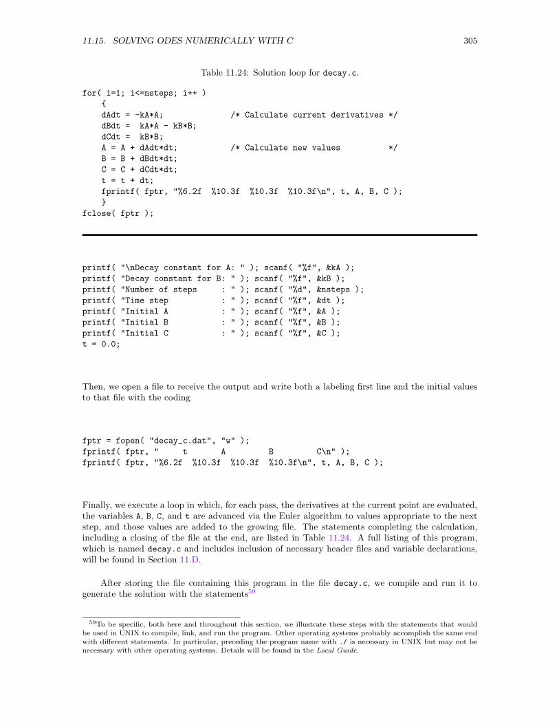
11.15. SOLVING ODES NUMERICALLY WITH C 305

Table 11.24: Solution loop for decay.c.

for( i=1; i<=nsteps; i++ )

dAdt = -kA*A; /* Calculate current derivatives */

dBdt = kA*A - kB*B;

dCdt = kB*B;

A = A + dAdt*dt; /* Calculate new values */

B = B + dBdt*dt;

C = C + dCdt*dt;

t = t + dt;

fprintf( fptr, "%6.2f %10.3f %10.3f %10.3f\n", t, A, B, C );

fclose( fptr );

printf( "\nDecay constant for A: " ); scanf( "%f", &kA );

printf( "Decay constant for B: " ); scanf( "%f", &kB );

printf( "Number of steps : " ); scanf( "%d", &nsteps );

printf( "Time step : " ); scanf( "%f", &dt );

printf( "Initial A : " ); scanf( "%f", &A );

printf( "Initial B : " ); scanf( "%f", &B );

printf( "Initial C : " ); scanf( "%f", &C );

t = 0.0;

Then, we open a file to receive the output and write both a labeling first line and the initial valuesto that file with the coding

fptr = fopen( "decay_c.dat", "w" );

fprintf( fptr, " t A B C\n" );

fprintf( fptr, "%6.2f %10.3f %10.3f %10.3f\n", t, A, B, C );

Finally, we execute a loop in which, for each pass, the derivatives at the current point are evaluated,the variables A, B, C, and t are advanced via the Euler algorithm to values appropriate to the nextstep, and those values are added to the growing file. The statements completing the calculation,including a closing of the file at the end, are listed in Table 11.24. A full listing of this program,which is named decay.c and includes inclusion of necessary header files and variable declarations,will be found in Section 11.D.

After storing the file containing this program in the file decay.c, we compile and run it togenerate the solution with the statements59

59To be specific, both here and throughout this section, we illustrate these steps with the statements that wouldbe used in UNIX to compile, link, and run the program. Other operating systems probably accomplish the same endwith different statements. In particular, preceding the program name with ./ is necessary in UNIX but may not benecessary with other operating systems. Details will be found in the Local Guide.

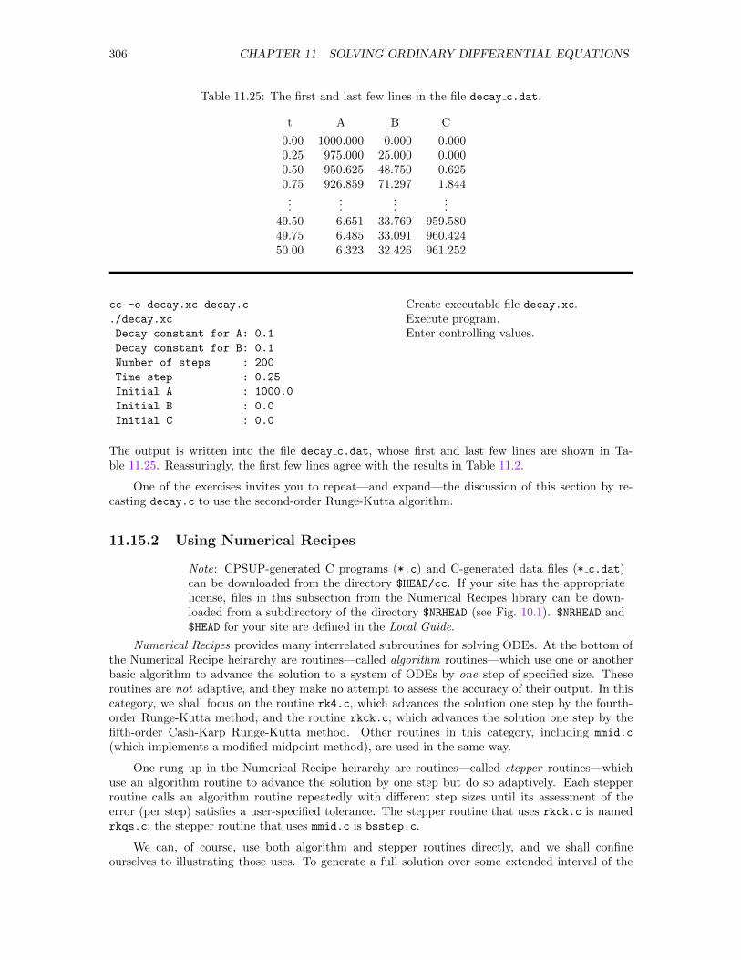
306 CHAPTER 11. SOLVING ORDINARY DIFFERENTIAL EQUATIONS

Table 11.25: The first and last few lines in the file decay c.dat.

t A B C

0.00 1000.000 0.000 0.0000.25 975.000 25.000 0.0000.50 950.625 48.750 0.6250.75 926.859 71.297 1.844...

......

...49.50 6.651 33.769 959.58049.75 6.485 33.091 960.42450.00 6.323 32.426 961.252

cc -o decay.xc decay.c

./decay.xc

Decay constant for A: 0.1

Decay constant for B: 0.1

Number of steps : 200

Time step : 0.25

Initial A : 1000.0

Initial B : 0.0

Initial C : 0.0

Create executable file decay.xc.Execute program.Enter controlling values.

The output is written into the file decay c.dat, whose first and last few lines are shown in Ta-ble 11.25. Reassuringly, the first few lines agree with the results in Table 11.2.

One of the exercises invites you to repeat—and expand—the discussion of this section by re-casting decay.c to use the second-order Runge-Kutta algorithm.

11.15.2 Using Numerical Recipes

Note: CPSUP-generated C programs (*.c) and C-generated data files (* c.dat)can be downloaded from the directory $HEAD/cc. If your site has the appropriatelicense, files in this subsection from the Numerical Recipes library can be down-loaded from a subdirectory of the directory $NRHEAD (see Fig. 10.1). $NRHEAD and$HEAD for your site are defined in the Local Guide.

Numerical Recipes provides many interrelated subroutines for solving ODEs. At the bottom ofthe Numerical Recipe heirarchy are routines—called algorithm routines—which use one or anotherbasic algorithm to advance the solution to a system of ODEs by one step of specified size. Theseroutines are not adaptive, and they make no attempt to assess the accuracy of their output. In thiscategory, we shall focus on the routine rk4.c, which advances the solution one step by the fourth-order Runge-Kutta method, and the routine rkck.c, which advances the solution one step by thefifth-order Cash-Karp Runge-Kutta method. Other routines in this category, including mmid.c

(which implements a modified midpoint method), are used in the same way.

One rung up in the Numerical Recipe heirarchy are routines—called stepper routines—whichuse an algorithm routine to advance the solution by one step but do so adaptively. Each stepperroutine calls an algorithm routine repeatedly with different step sizes until its assessment of theerror (per step) satisfies a user-specified tolerance. The stepper routine that uses rkck.c is namedrkqs.c; the stepper routine that uses mmid.c is bsstep.c.

We can, of course, use both algorithm and stepper routines directly, and we shall confineourselves to illustrating those uses. To generate a full solution over some extended interval of the

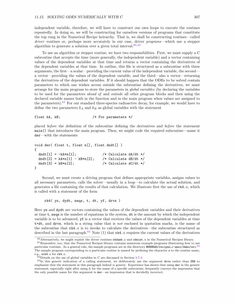
11.15. SOLVING ODES NUMERICALLY WITH C 307

independent variable, therefore, we will have to construct our own loops to execute the routinesrepeatedly. In doing so, we will be constructing for ourselves versions of programs that constitutethe top rung in the Numerical Recipe heirarchy. That is, we shall be constructing routines—calleddriver routines or, perhaps more accurately in our case, driver programs—which use a stepperalgorithm to generate a solution over a given total interval.60,61

To use an algorithm or stepper routine, we have two responsibilities. First, we must supply a Csubroutine that accepts the time (more generally, the independent variable) and a vector containingvalues of the dependent variables at that time and returns a vector containing the derivatives ofthe dependent variables at that time. In outline, this file is structured as a subroutine with threearguments, the first—a scalar—providing the current value of the independent variable, the second—a vector—providing the values of the dependent variable, and the third—also a vector—returningthe derivatives of the dependent variables. If it should happen that the ODEs to be solved containparameters to which one wishes access outside the subroutine defining the derivatives, we mustarrange for the main program to store the parameters in global variables (by declaring the variablesto be used for the parameters ahead of and outside all other program blocks and then using thedeclared variable names both in the function and in the main program when values are assigned tothe parameters).63 For our standard three-species radioactive decay, for example, we would have todefine the two parameters kA and kB as global variables with the statement

float kA, kB; /* For parameters */

placed before the definition of the subroutine defining the derivatives and before the statementmain() that introduces the main program. Then, we might code the required subroutine—name itder—with the statements

void der( float t, float n[], float dndt[] )

dndt[1] = -kA*n[1]; /* Calculate dA/dt */

dndt[2] = kA*n[1] - kB*n[2]; /* Calculate dB/dt */

dndt[3] = kB*n[2]; /* Calculate dC/dt */

Second, we must create a driving program that defines appropriate variables, assigns values toall necessary parameters, calls the solver—usually in a loop—to calculate the actual solution, andgenerates a file containing the results of that calculation. We illustrate first the use of rk4.c, whichis called with a statement of the form

rk4( ys, dydt, neqs, t, dt, yf, drvs )

Here ys and dydt are vectors containing the values of the dependent variables and their derivativesat time t, neqs is the number of equations in the system, dt is the amount by which the independentvariable is to be advanced, yf is a vector that receives the values of the dependent variables at timet+dt, and drvs, which is a string value that is not enclosed in quotation marks, is the name ofthe subroutine that rk4.c is to invoke to calculate the derivatives—the subroutine structured asdescribed in the last paragraph.64 Note (1) that rk4.c requires the current values of the derivatives

60Alternatively, we might exploit the driver routines rkdumb.c and odeint.c in the Numerical Recipes library.61Remember, too, that the Numerical Recipes library contains numerous example programs illustrating how to use

particular routines. As a general rule, the sample programs are in the directory $NRHEAD/recipes c-ansi/demo/src.62

The sample program corresponding to a particular routine is named by prefixing the character x to the routine name,e.g., xrk4.c for rk4.c.

63Details on the use of global variables in C are discussed in Section 9.7.4.64In this generic indication of a calling statement, we deliberately use the argument drvs rather than DER to

emphasize that the statement in this paragraph indeed is generic. Experience has shown that using der in the genericstatement, especially right after using it for the name of a specific subroutine, frequently conveys the impression thatthe only possible name for this argument is der—an impression that is decidedly incorrect.

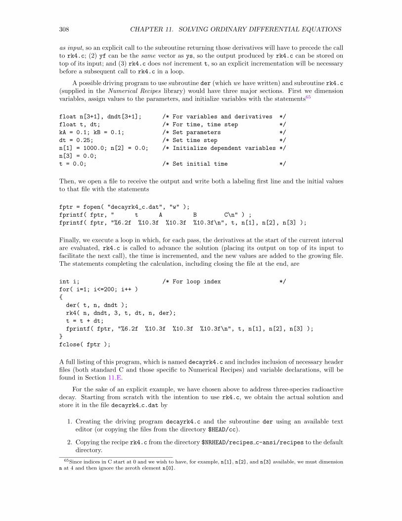
308 CHAPTER 11. SOLVING ORDINARY DIFFERENTIAL EQUATIONS

as input, so an explicit call to the subroutine returning those derivatives will have to precede the callto rk4.c; (2) yf can be the same vector as ys, so the output produced by rk4.c can be stored ontop of its input; and (3) rk4.c does not increment t, so an explicit incrementation will be necessarybefore a subsequent call to rk4.c in a loop.

A possible driving program to use subroutine der (which we have written) and subroutine rk4.c(supplied in the Numerical Recipes library) would have three major sections. First we dimensionvariables, assign values to the parameters, and initialize variables with the statements65

float n[3+1], dndt[3+1]; /* For variables and derivatives */

float t, dt; /* For time, time step */

kA = 0.1; kB = 0.1; /* Set parameters */

dt = 0.25; /* Set time step */

n[1] = 1000.0; n[2] = 0.0; /* Initialize dependent variables */

n[3] = 0.0;

t = 0.0; /* Set initial time */

Then, we open a file to receive the output and write both a labeling first line and the initial valuesto that file with the statements

fptr = fopen( "decayrk4_c.dat", "w" );

fprintf( fptr, " t A B C\n" ) ;

fprintf( fptr, "%6.2f %10.3f %10.3f %10.3f\n", t, n[1], n[2], n[3] );

Finally, we execute a loop in which, for each pass, the derivatives at the start of the current intervalare evaluated, rk4.c is called to advance the solution (placing its output on top of its input tofacilitate the next call), the time is incremented, and the new values are added to the growing file.The statements completing the calculation, including closing the file at the end, are

int i; /* For loop index */

for( i=1; i<=200; i++ )

der( t, n, dndt );

rk4( n, dndt, 3, t, dt, n, der);

t = t + dt;

fprintf( fptr, "%6.2f %10.3f %10.3f %10.3f\n", t, n[1], n[2], n[3] );

fclose( fptr );

A full listing of this program, which is named decayrk4.c and includes inclusion of necessary headerfiles (both standard C and those specific to Numerical Recipes) and variable declarations, will befound in Section 11.E.

For the sake of an explicit example, we have chosen above to address three-species radioactivedecay. Starting from scratch with the intention to use rk4.c, we obtain the actual solution andstore it in the file decayrk4 c.dat by

1. Creating the driving program decayrk4.c and the subroutine der using an available texteditor (or copying the files from the directory $HEAD/cc).

2. Copying the recipe rk4.c from the directory $NRHEAD/recipes c-ansi/recipes to the defaultdirectory.

65Since indices in C start at 0 and we wish to have, for example, n[1], n[2], and n[3] available, we must dimensionn at 4 and then ignore the zeroth element n[0].

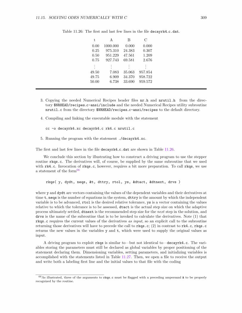
11.15. SOLVING ODES NUMERICALLY WITH C 309

Table 11.26: The first and last few lines in the file decayrk4 c.dat.

t A B C

0.00 1000.000 0.000 0.0000.25 975.310 24.383 0.3070.50 951.229 47.561 1.2090.75 927.743 69.581 2.676...

......

...49.50 7.083 35.063 957.85449.75 6.909 34.370 958.72250.00 6.738 33.690 959.572

3. Copying the needed Numerical Recipes header files nr.h and nrutil.h from the direc-tory $NRHEAD/recipes c-ansi/include and the needed Numerical Recipes utility subroutinenrutil.c from the directory $NRHEAD/recipes c-ansi/recipes to the default directory.

4. Compiling and linking the executable module with the statement

cc -o decayrk4.xc decayrk4.c rk4.c nrutil.c

5. Running the program with the statement ./decayrk4.xc.

The first and last few lines in the file decayrk4 c.dat are shown in Table 11.26.

We conclude this section by illustrating how to construct a driving program to use the stepperroutine rkqs.c. The derivatives will, of course, be supplied by the same subroutine that we usedwith rk4.c. Invocation of rkqs.c, however, requires a bit more preparation. To call rkqs, we usea statement of the form66

rkqs( y, dydt, neqs, &t, dttry, rtol, ys, &dtact, &dtnext, drvs )

where y and dydt are vectors containing the values of the dependent variables and their derivatives attime t, neqs is the number of equations in the system, dttry is the amount by which the independentvariable is to be advanced, rtol is the desired relative tolerance, ys is a vector containing the valuesrelative to which the tolerance is to be assessed, dtact is the actual step size on which the adaptiveprocess ultimately settled, dtnext is the recommended step size for the next step in the solution, anddrvs is the name of the subroutine that is to be invoked to calculate the derivatives. Note (1) thatrkqs.c requires the current values of the derivatives as input, so an explicit call to the subroutinereturning those derivatives will have to precede the call to rkqs.c; (2) in contrast to rk4.c, rkqs.creturns the new values in the variables y and t, which were used to supply the original values asinput.

A driving program to exploit rkqs is similar to—but not identical to—decayrk4.c. The vari-ables storing the parameters must still be declared as global variables by proper positioning of thestatement declaring them. Dimensioning variables, setting parameters, and initializing variables isaccomplished with the statements listed in Table 11.27. Then, we open a file to receive the outputand write both a labeling first line and the initial values to that file with the coding

66As illustrated, three of the arguments to rkqs.c must be flagged with a preceding ampersand & to be properlyrecognized by the routine.

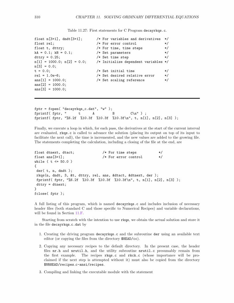
310 CHAPTER 11. SOLVING ORDINARY DIFFERENTIAL EQUATIONS

Table 11.27: First statements for C Program decayrkqs.c.

float n[3+1], dndt[3+1]; /* For variables and derivatives */

float rel; /* For error control */

float t, dttry; /* For time, time steps */

kA = 0.1; kB = 0.1; /* Set parameters */

dttry = 0.25; /* Set time step */

n[1] = 1000.0; n[2] = 0.0; /* Initialize dependent variables */

n[3] = 0.0;

t = 0.0; /* Set initial time */

rel = 1.0e-6; /* Set desired relative error */

ans[1] = 1000.0; /* Set scaling reference */

ans[2] = 1000.0;

ans[3] = 1000.0;

fptr = fopen( "decayrkqs_c.dat", "w" );

fprintf( fptr, " t A B C\n" ) ;

fprintf( fptr, "%6.2f %10.3f %10.3f %10.3f\n", t, n[1], n[2], n[3] );

Finally, we execute a loop in which, for each pass, the derivatives at the start of the current intervalare evaluated, rkqs.c is called to advance the solution (placing its output on top of its input tofacilitate the next call), the time is incremented, and the new values are added to the growing file.The statements completing the calculation, including a closing of the file at the end, are

float dtnext, dtact; /* For time steps */

float ans[3+1]; /* For error control */

while ( t <= 50.0 )

der( t, n, dndt );

rkqs(n, dndt, 3, &t, dttry, rel, ans, &dtact, &dtnext, der );

fprintf( fptr, "%6.2f %10.3f %10.3f %10.3f\n", t, n[1], n[2], n[3] );

dttry = dtnext;

fclose( fptr );

A full listing of this program, which is named decayrkqs.c and includes inclusion of necessaryheader files (both standard C and those specific to Numerical Recipes) and variable declarations,will be found in Section 11.F.

Starting from scratch with the intention to use rkqs, we obtain the actual solution and store itin the file decayrkqs c.dat by

1. Creating the driving program decayrkqs.c and the subroutine der using an available texteditor (or copying the files from the directory $HEAD/cc).

2. Copying any necessary recipes to the default directory. In the present case, the headerfiles nr.h and nrutil.h, and the utility subroutine nrutil.c presumably remain fromthe first example. The recipes rkqs.c and rkck.c (whose importance will be pro-claimed if the next step is attempted without it) must also be copied from the directory$NRHEAD/recipes c-ansi/recipes.

3. Compiling and linking the executable module with the statement

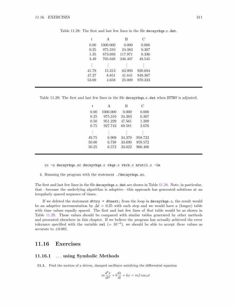
11.16. EXERCISES 311

Table 11.28: The first and last few lines in the file decayrkqs c.dat.

t A B C

0.00 1000.000 0.000 0.0000.25 975.310 24.383 0.3071.35 873.693 117.971 8.3363.49 705.048 246.407 48.545...

......

...41.79 15.313 63.993 920.69447.27 8.851 41.841 949.30753.69 4.658 25.009 970.333

Table 11.29: The first and last few lines in the file decayrkqs c.dat when DTTRY is adjusted.

t A B C

0.00 1000.000 0.000 0.0000.25 975.310 24.383 0.3070.50 951.229 47.561 1.2090.75 927.743 69.581 2.676...

......

...49.75 6.909 34.370 958.72250.00 6.738 33.690 959.57250.25 6.572 33.022 960.406

cc -o decayrkqs.xc decayrkqs.c rkqs.c rkck.c nrutil.c -lm

4. Running the program with the statement ./decayrkqs.xc.

The first and last few lines in the file decayrkqs c.dat are shown in Table 11.28. Note, in particular,that—because the underlying algorithm is adaptive—this approach has generated solutions at anirregularly spaced sequence of times.

If we deleted the statement dttry = dtnext; from the loop in decayrkqs.c, the result wouldbe an adaptive incrementation by ∆t = 0.25 with each step and we would have a (longer) tablewith time values equally spaced. The first and last few lines of that table would be as shown inTable 11.29. These values should be compared with similar tables generated by other methodsand presented elsewhere in this chapter. If we believe the program has actually achieved the errortolerance specified with the variable rel (= 10−6), we should be able to accept these values asaccurate to ±0.001.

11.16 Exercises

11.16.1 . . . using Symbolic Methods

11.1. Find the motion of a driven, damped oscillator satisfying the differential equation

md2x

dt2+ b

dx

dt+ kx = mf cosωt

312 CHAPTER 11. SOLVING ORDINARY DIFFERENTIAL EQUATIONS

subject to the general initial conditions

x(0) = x0 ;dx

dt(0) = v0

and then determine the particular initial values that might be imposed so that the transient partof the solution is wiped out from the beginning, i.e., so that the motion is identically the steady-state motion from the moment the oscillator is set into motion. Assume that the oscillator isunderdamped. (Note that, so that m will ultimately appear only in conjunction with b and k, wehave chosen to define f as a force per unit mass rather than simply a force.)

11.2. Take away the walls and the two springs connecting the blocks to the walls in the system of Fig. 11.5,let the masses be different (m1 and m2, say) and denote the constant of the one spring by k. Supposethe blocks are constrained to move along a straight line. Measuring from an arbitrarily selectedorigin on that line, let the coordinates of the particles be x1 and x2, respectively. The equations ofmotion for this system are

m1d2x1

dt2= k(x2 − x1) ; m2

d2x2

dt2= −k(x2 − x1)

Let the system be put into motion with arbitrary initial conditions

x1(0) = x10 ; x2(0) = x20 ;dx1(0)

dt= v10 ;

dx2(0)

dt= v20

Solve this initial-value problem for x1(t) and x2(t) and then examine the behavior of the particularquantities

X(t) =m1x1(t) +m2x2(t)

m1 +m2and Y (t) = x2(t)− x1(t)

which are, respectively, the position of the center of mass of the system and the position of thesecond block relative to the first block.

11.3. Study the behavior of the system that results when the the system shown in Fig. 11.5 is extendedto contain three objects coupled in a line. Take the four springs all to have the same spring constantbut allow for the possibility that the middle object may have a mass different from that of the twooutside objects. Your examination should include at least the following:

• Find both the natural frequencies of the normal modes of oscillation and the initial conditionsthat will excite the system exclusively in each of the normal modes, determining particularlythe frequencies as a function of the ratio of the two masses. To display your results, draw adiagram something like a quantum energy level diagram that shows the way the three naturalfrequencies vary as the middle mass goes from being rather smaller than the two outer massesto being rather larger than the outer two masses. As initial conditions, it will be sufficient torelease the objects from rest at individually arbitrary displacements. You are, however, quitelikely to have to help with the inverse Laplace transforms, since your symbolic manipulatormay be unable to deal with the inverse Laplace transform of an expression like

As+Bs3

αs4 + βs2 + γ= s

(A+Bs2

αs4 + βs2 + γ

)The denominator looks quartic in s but is better seen as quadratic in s2. If you introducez = s2 temporarily, factor the resulting denominator, and then do a partial fraction expansion,you can end up with the alternative form

s

(A+Bs2

αs4 + βs2 + γ

)= s

(R

s2 +R′+

Q

s2 +Q′

)=

Rs

s2 +R′+

Qs

s2 +Q′

whose inverse Laplace transform is easier to find. (Indeed, even Table 1.2 is adequate to thetask.) Finding the constants R, A, R′ and Q′ is part of the exercise; the expressions are notpretty. The lesson: Symbolic manipulators frequently need help from someone who reallyknows where the calculation is going.

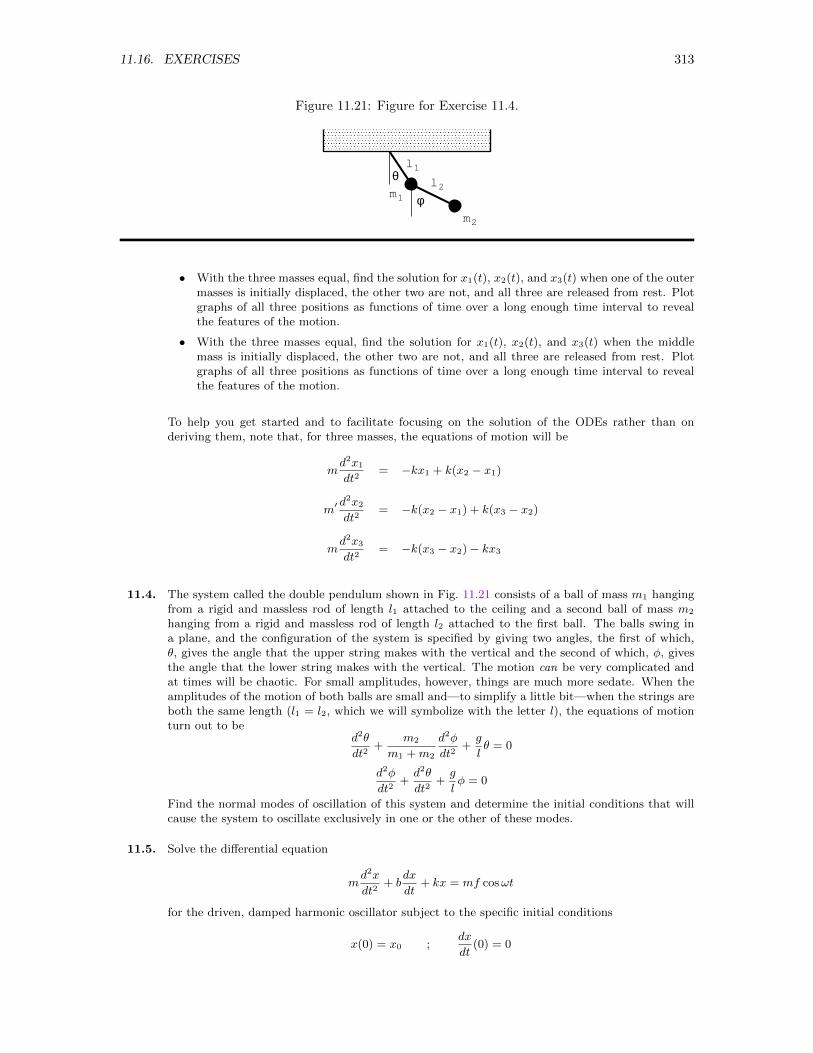
11.16. EXERCISES 313

Figure 11.21: Figure for Exercise 11.4.

θ

φ

l1l2

m1

m2

• With the three masses equal, find the solution for x1(t), x2(t), and x3(t) when one of the outermasses is initially displaced, the other two are not, and all three are released from rest. Plotgraphs of all three positions as functions of time over a long enough time interval to revealthe features of the motion.

• With the three masses equal, find the solution for x1(t), x2(t), and x3(t) when the middlemass is initially displaced, the other two are not, and all three are released from rest. Plotgraphs of all three positions as functions of time over a long enough time interval to revealthe features of the motion.

To help you get started and to facilitate focusing on the solution of the ODEs rather than onderiving them, note that, for three masses, the equations of motion will be

md2x1

dt2= −kx1 + k(x2 − x1)

m′d2x2

dt2= −k(x2 − x1) + k(x3 − x2)

md2x3

dt2= −k(x3 − x2)− kx3

11.4. The system called the double pendulum shown in Fig. 11.21 consists of a ball of mass m1 hangingfrom a rigid and massless rod of length l1 attached to the ceiling and a second ball of mass m2

hanging from a rigid and massless rod of length l2 attached to the first ball. The balls swing ina plane, and the configuration of the system is specified by giving two angles, the first of which,θ, gives the angle that the upper string makes with the vertical and the second of which, φ, givesthe angle that the lower string makes with the vertical. The motion can be very complicated andat times will be chaotic. For small amplitudes, however, things are much more sedate. When theamplitudes of the motion of both balls are small and—to simplify a little bit—when the strings areboth the same length (l1 = l2, which we will symbolize with the letter l), the equations of motionturn out to be

d2θ

dt2+

m2

m1 +m2

d2φ

dt2+g

lθ = 0

d2φ

dt2+d2θ

dt2+g

lφ = 0

Find the normal modes of oscillation of this system and determine the initial conditions that willcause the system to oscillate exclusively in one or the other of these modes.

11.5. Solve the differential equation

md2x

dt2+ b

dx

dt+ kx = mf cosωt

for the driven, damped harmonic oscillator subject to the specific initial conditions

x(0) = x0 ;dx

dt(0) = 0

314 CHAPTER 11. SOLVING ORDINARY DIFFERENTIAL EQUATIONS

by explicitly taking the Laplace transform of the equation, solving that result for the Laplacetransform of the solution, and then inverting that transform to obtain the solution itself.

11.6. Among the simplest of differential equations is the equation

d2x

dt2+ ω2x = 0

that describes a simple harmonic oscillator. Generate a series solution to this equation and thenverify that the solution thus generated agrees with the known solution

x(t) = A cosωt+B sinωt

where A and B are constants determined by the initial conditions.

11.7. Find a symbolic solution for all three components for the motion of a projectile in a linear, viscousmedium, when the initial conditions are general, i.e., solve Eq. (11.4) subject to the initial conditionsin Eq. (11.2). Since the equations are uncoupled, you can solve each individually. Alternatively,you can solve the three equations simultaneously as a system. Solve them both ways. Once youhave the solutions in hand, verify that they satisfy the original equations and initial conditions.Finally, explore their limits for small b.

11.8. Recast Eq. (11.34) for the LRC circuit in dimensionless form, measuring charge in units of q0 andfinding a suitable unit in terms of which to measure time.

11.9. Reflecting Coulomb’s law, the equation of motion for a particle carrying charge q moving in the(fixed) electrostatic field of a charge Q is

md2r

dt2=

qQ

4πε0

r

r3

Here, the force center is assumed to be at the origin, r is the position vector of the particle, andthe equation is written in mksa units. Write this equation of motion out in Cartesian coordinates,cast it in dimensionless form, and determine the correspondences that must be adopted to convertthe equations for an orbit in an electrostatic field into those for the orbit in a gravitational field,i.e., into Eq. (11.46).

11.10. Recast the system of six first-order equations in the last paragraph of Section 11.1.1 in dimensionlessform, both when the viscous term is linear in the velocity and when it is quadratic in the velocity.Appropriate units for this recasting can be inferred from the discussion earlier in that section.

11.11. Translate the entire discussion—both dimensional and dimensionless—of the planetary problem inSection 11.1.7 from Cartesian coordinates (x, y) to polar coordinates (r, φ), where x = r cosφ andy = r sinφ. That is

(a) Show that the polar components of the equations of motion in the first instance are

m

[d2r

dt2− r(dφ

dt

)2]

= f(r) ; m

(rd2φ

dt2+ 2

dφ

dt

dr

dt

)= 0

(b) Recognizing that

d

dt

(mr2 dφ

dt

)= m

(r2 d

2φ

dt2+ 2r

dr

dt

dφ

dt

)show that

mr2 dφ

dt= constant = L =⇒ dφ

dt=

L

mr2

and then that

md2r

dt2= f(r) +

L2

mr3

Here, L = m(x0vy0−y0vx0) is the angular momentum of the object; L is constant throughoutthe motion. (In polar coordinates, we would first solve this single, second-order, non-linear,

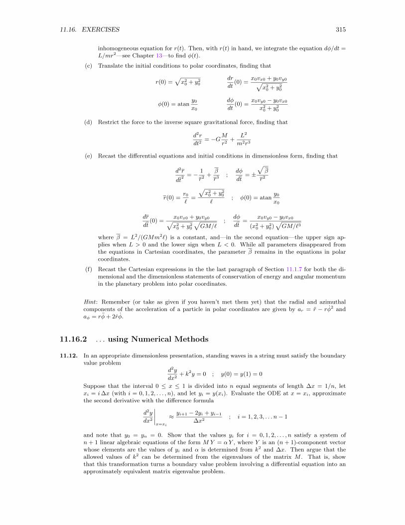
11.16. EXERCISES 315

inhomogeneous equation for r(t). Then, with r(t) in hand, we integrate the equation dφ/dt =L/mr2—see Chapter 13—to find φ(t).

(c) Translate the initial conditions to polar coordinates, finding that

r(0) =√x2

0 + y20

dr

dt(0) =

x0vx0 + y0vy0√x2

0 + y20

φ(0) = atany0

x0

dφ

dt(0) =

x0vy0 − y0vx0

x20 + y2

0

(d) Restrict the force to the inverse square gravitational force, finding that

d2r

dt2= −GM

r2+

L2

m2r3

(e) Recast the differential equations and initial conditions in dimensionless form, finding that

d2r

dt2

= − 1

r2+β

r3;

dφ

dt= ±

√β

r2

r(0) =r0

`=

√x2

0 + y20

`; φ(0) = atan

y0

x0

dr

dt(0) =

x0vx0 + y0vy0√x2

0 + y20

√GM/`

;dφ

dt=

x0vy0 − y0vx0

(x20 + y2

0)√GM/`3

where β = L2/(GMm2`) is a constant, and—in the second equation—the upper sign ap-plies when L > 0 and the lower sign when L < 0. While all parameters disappeared fromthe equations in Cartesian coordinates, the parameter β remains in the equations in polarcoordinates.

(f) Recast the Cartesian expressions in the the last paragraph of Section 11.1.7 for both the di-mensional and the dimensionless statements of conservation of energy and angular momentumin the planetary problem into polar coordinates.

Hint : Remember (or take as given if you haven’t met them yet) that the radial and azimuthalcomponents of the acceleration of a particle in polar coordinates are given by ar = r − rφ2 andaφ = rφ+ 2rφ.

11.16.2 . . . using Numerical Methods

11.12. In an appropriate dimensionless presentation, standing waves in a string must satisfy the boundaryvalue problem

d2y

dx2+ k2y = 0 ; y(0) = y(1) = 0

Suppose that the interval 0 ≤ x ≤ 1 is divided into n equal segments of length ∆x = 1/n, letxi = i∆x (with i = 0, 1, 2, . . . , n), and let yi = y(xi). Evaluate the ODE at x = xi, approximatethe second derivative with the difference formula

d2y

dx2

∣∣∣∣x=xi

≈ yi+1 − 2yi + yi−1

∆x2; i = 1, 2, 3, . . . n− 1

and note that y0 = yn = 0. Show that the values yi for i = 0, 1, 2, . . . , n satisfy a system ofn + 1 linear algebraic equations of the form M Y = αY , where Y is an (n + 1)-component vectorwhose elements are the values of yi and α is determined from k2 and ∆x. Then argue that theallowed values of k2 can be determined from the eigenvalues of the matrix M . That is, showthat this transformation turns a boundary value problem involving a differential equation into anapproximately equivalent matrix eigenvalue problem.

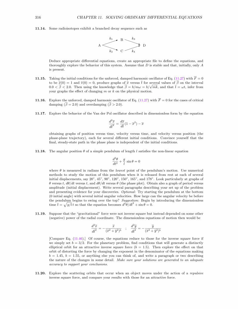
316 CHAPTER 11. SOLVING ORDINARY DIFFERENTIAL EQUATIONS

11.14. Some radioisotopes exhibit a branched decay sequence such as

A

C

B

D1

PPPPq

PPPPq

1

k1

k2

k3

k4

Deduce appropriate differential equations, create an appropriate file to define the equations, andthoroughly explore the behavior of this system. Assume that D is stable and that, initially, only Ais present.

11.15. Taking the initial conditions for the unforced, damped harmonic oscillator of Eq. (11.27) with F = 0to be x(0) = 1 and v(0) = 0, produce graphs of x versus t for several values of β on the interval0.0 < β < 2.0. Then using the knowledge that β = b/mω = b/

√mk, and that t = ωt, infer from

your graphs the effect of changing m or k on the physical motion.

11.16. Explore the unforced, damped harmonic oscillator of Eq. (11.27) with F = 0 for the cases of criticaldamping (β = 2.0) and overdamping (β > 2.0).

11.17. Explore the behavior of the Van der Pol oscillator described in dimensionless form by the equation

d2x

dt2

=dx

dt(1− x2)− x

obtaining graphs of position versus time, velocity versus time, and velocity versus position (thephase-plane trajectory), each for several different initial conditions. Convince yourself that thefinal, steady-state path in the phase plane is independent of the initial conditions.

11.18. The angular position θ of a simple pendulum of length l satisfies the non-linear equation

d2θ

dt2+g

lsin θ = 0

where θ is measured in radians from the lowest point of the pendulum’s motion. Use numericalmethods to study the motion of this pendulum when it is released from rest at each of severalinitial displacements, say 20, 45, 90, 120, 150, 165, and 178. Look particularly at graphs ofθ versus t, dθ/dt versus t, and dθ/dt versus θ (the phase plot). Obtain also a graph of period versusamplitude (initial displacement). Write several paragraphs describing your set up of the problemand presenting evidence for your discoveries. Optional : Try starting the pendulum at the bottom(0 initial angle) with several initial angular velocities. How large can the angular velocity be beforethe pendulum begins to swing over the top? Suggestion: Begin by introducing the dimensionlesstime t =

√g/l t so that the equation becomes d2θ/dt

2+ sin θ = 0.

11.19. Suppose that the “gravitational” force were not inverse square but instead depended on some other(negative) power of the radial coordinate. The dimensionless equations of motion then would be

d2x

dt2

= − x

(x2 + y2)b;

d2y

dt2

= − y

(x2 + y2)b

[Compare Eq. (11.46).] Of course, the equations reduce to those for the inverse square force ifwe simply set b = 3/2. For the planetary problem, find conditions that will generate a distinctlyelliptical orbit for an attractive inverse square force (b = 1.5). Then explore the effect on thatorbit of distorting the force by changing the exponent in the denominator of the equations makingb = 1.45, b = 1.55, or anything else you can think of, and write a paragraph or two describingthe nature of the changes in some detail. Make sure your solutions are generated to an adequateaccuracy to support your conclusions.

11.20. Explore the scattering orbits that occur when an object moves under the action of a repulsiveinverse square force, and compare your results with those for an attractive force.

11.16. EXERCISES 317

11.21. Deduce the equations of motion for a space ship of mass m coasting freely in the xy plane under thegravitational influence of two suns, each of mass M and located respectively at (R, 0) and (−R, 0).Then express the equations in dimensionless form and, creating all necessary files, thoroughlyexplore the motion of this space ship. In particular, you might search for an orbit that loops like afigure-eight around the two suns and/or you might see if your approach predicts what you wouldexpect intuitively if you start the spaceship from rest at a point on the perpendicular bisector ofthe line joining the two suns. Make sure your solutions are generated to an adequate accuracy.

11.22. Suppose a particle of charge q and mass m is injected into a region of space containing constant,crossed electric and magnetic fields E = Exi and B = Bzk. In vector form, the equation of motionfor this particle is

md2r

dt2= qE + q

dr

dt×B

Verify the equations of motion

md2x

dt2= qEx + qBz

dy

dt; m

d2y

dt2= −qBz

dx

dt; m

d2z

dt2= 0

for the specific fields of this exercise, express them in dimensionless form (note that ω = qBz/m isa frequency and Ex/Bz is a velocity), and thoroughly explore the behavior of the particle in thissituation. Try to understand the motion intuitively. Hint : You should find that, in terms of anarbitrarily selected unit of length `, the equations involve a single parameter qEx/(mω

2`), whichcan alternatively be written as (Ex/Bz)/(ω`) — the ratio of the velocity Ex/Bz determined by thefields to the characteristic velocity implied by your choice of a length unit and the frequency ω.Note that this exercise actually has more than one parameter, since the initial components of thevelocity—probably expressed in units of ω`—also influence the solution.

11.23. A particle having mass m and carrying charge q moves in the xy-plane while experiencing an electricfield given by E(x, y) = −αy j, where α is a constant. Assume that α and q are both positive.With r = x i + y j, the vector equation of motion for this particle then is

md2r

dt2= −qαy j

(a) Show that, in component form, the equations of motion for this particle are

d2x

dt2= 0 ;

d2y

dt2= −αq

my = −by

(b) With b a global parameter, create an appropriate file to define these equations for the ODE-solver in an available numerical/graphical tool. (c) Use that tool to obtain graphs of the trajectoriesin the xy-plane of several particles projected from the origin at different angles and with differentspeeds. (d) Speculate on a use for this field.

11.24. An important system in the early study of chaos is described by the Lorenz equations

dx

dt= a(y − x)

dy

dt= −xz + bx− y

dz

dt= xy − cz

Create an appropriate file defining these equations and then thoroughly explore the behavior of thissystem. Graphs of y versus x, z versus x, and z versus y when a = 10.0, b = 28.0 and c = 8.0/3.0under the initial conditions x0 = 1.0, y0 = 0.0, and z0 = 0.0 are particularly interesting. Whilegraphs of y versus x, z versus x, and z versus y are interesting, the true beauty of the trajectory isbest seen using a three-dimensional space curve. Be sure to examine the path from several differentvantage points in the space around the path, an objective most easily accomplished if the displayof the path allows rotation of the path on the screen.

318 CHAPTER 11. SOLVING ORDINARY DIFFERENTIAL EQUATIONS

11.25. Recast the program decay.f so that it invokes (a) the improved Euler method and (b) the second-order Runge-Kutta method rather than Euler’s method to solve the problem of three-species decay.Then, compile and test your programs. Give particular attention to exploring the accuracy of thesolution by using several different time steps. Further, compare the accuracy obtained for varioustime steps with that obtained for the same time steps using Euler’s method.

11.26. Recast the program decay.c so that it invokes (a) the improved Euler method and (b) the second-order Runge-Kutta method rather than Euler’s method to solve the problem of three-species decay.Then, compile and test your programs. Give particular attention to exploring the accuracy of thesolution by using several different time steps. Further, compare the accuracy obtained for varioustime steps with that obtained for the same time steps using Euler’s method.

11.27. The dynamics of the chemical reaction

A + B C + D

is governed by the equations

dA

dt= −kfAB + krCD

dB

dt= −kfAB + krCD

dC

dt= kfAB − krCD

dD

dt= kfAB − krCD

where A(t), B(t), C(t), and D(t) are the concentrations of each molecule in the reaction vessel,and kf and kr are the forward and reverse rate constants, respectively. Suppose that the reactionis started with A(0) = A0, B(0) = B0, and C(0) = D(0) = 0. Cast the equations in dimensionlessform, using A0 as the unit of concentration and kfA0t as the dimensionless time. Then explorethe behavior of the system as a function of the initial concentration of B, measured in units ofA0 and the reverse rate constant, measured in units of kf . Look particularly at the dependence ofthe ultimate equilibrium on these parameters. Make sure your results are generated to adequateaccuracy.

11.28. In classical ecology, the interaction between a predator and a prey, with populations x(t) and y(t),respectively, is modeled with the equations

dx

dt= −k1x+ k2xy ;

dy

dt= k3y − k4xy

where k1 and k3 are parameters describing the way each population would evolve in the absenceof the other and k2 and k4 are parameters describing strength of the interaction between the twospecies, which we take to be proportional to the likelihood of an encounter between a member of onespecies and a member of the other species. Depending on the parameters and the initial populationsx(0) = x0, y(0) = y0, the system may approach a stable equilibrium or, alternatively, one or theother of the populations may become extinct. Explore this system to determine conditions underwhich each of these circumstances occurs and write a paragraph or two describing your findings.Make sure your results are generated to an accuracy adequate to support your conclusions.

11.29. Examine the undamped, unforced harmonic oscillator carefully, using at least two different methodsand several time steps. Monitor the accuracy of your solution by monitoring the constancy of theenergy of the oscillator given (in dimensional form) by E = 1

2mv2 + 1

2kx2.

11.16.3 . . . using Numerical Recipes

Note: Numerical recipes can, of course, also be used for any of theexercises in Section 11.16.2.

11.31. Read the book Numerical Recipes to discover how to use the routine odeint and then use it tostudy three-species radioactive decay.

11.16. EXERCISES 319

11.32. Read the book Numerical Recipes to discover how to use the routine mmid and then use it to studythree-species radioactive decay.

11.33. Use two different numerical recipes of your choice to study the logistic growth of a population.

11.34. Study the damped, unforced harmonic oscillator using (a) rk4 and (b) rkqs. Consider under-damped, critical, and overdamped cases.

11.35. Use (a) rk4 and (b) rkqs to study both bound and unbound orbits in the inverse square gravitationalforce.

11.36. Choose one of the exercises from Section 11.16.2 and address it using at least one numerical recipe.

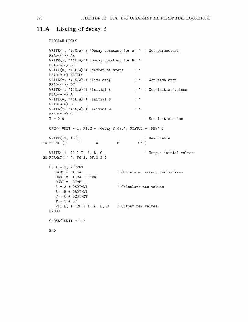
320 CHAPTER 11. SOLVING ORDINARY DIFFERENTIAL EQUATIONS

11.A Listing of decay.f

PROGRAM DECAY

WRITE(*, ’(1X,A)’) ’Decay constant for A: ’ ! Get parameters

READ(*,*) AK

WRITE(*, ’(1X,A)’) ’Decay constant for B: ’

READ(*,*) BK

WRITE(*, ’(1X,A)’) ’Number of steps : ’

READ(*,*) NSTEPS

WRITE(*, ’(1X,A)’) ’Time step : ’ ! Get time step

READ(*,*) DT

WRITE(*, ’(1X,A)’) ’Initial A : ’ ! Get initial values

READ(*,*) A

WRITE(*, ’(1X,A)’) ’Initial B : ’

READ(*,*) B

WRITE(*, ’(1X,A)’) ’Initial C : ’

READ(*,*) C

T = 0.0 ! Set initial time

OPEN( UNIT = 1, FILE = ’decay_f.dat’, STATUS = ’NEW’ )

WRITE( 1, 10 ) ! Head table

10 FORMAT( ’ T A B C’ )

WRITE( 1, 20 ) T, A, B, C ! Output initial values

20 FORMAT( ’ ’, F6.2, 3F10.3 )

DO I = 1, NSTEPS

DADT = -AK*A ! Calculate current derivatives

DBDT = AK*A - BK*B

DCDT = BK*B

A = A + DADT*DT ! Calculate new values

B = B + DBDT*DT

C = C + DCDT*DT

T = T + DT

WRITE( 1, 20 ) T, A, B, C ! Output new values

ENDDO

CLOSE( UNIT = 1 )

END

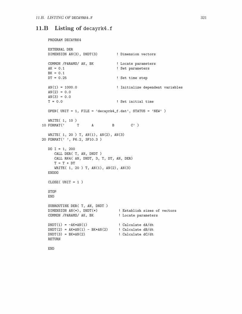
11.B. LISTING OF DECAYRK4.F 321

11.B Listing of decayrk4.f

PROGRAM DECAYRK4

EXTERNAL DER

DIMENSION AN(3), DNDT(3) ! Dimension vectors

COMMON /PARAMS/ AK, BK ! Locate parameters

AK = 0.1 ! Set parameters

BK = 0.1

DT = 0.25 ! Set time step

AN(1) = 1000.0 ! Initialize dependent variables

AN(2) = 0.0

AN(3) = 0.0

T = 0.0 ! Set initial time

OPEN( UNIT = 1, FILE = ’decayrk4_f.dat’, STATUS = ’NEW’ )

WRITE( 1, 10 )

10 FORMAT(’ T A B C’ )

WRITE( 1, 20 ) T, AN(1), AN(2), AN(3)

20 FORMAT(’ ’, F6.2, 3F10.3 )

DO I = 1, 200

CALL DER( T, AN, DNDT )

CALL RK4( AN, DNDT, 3, T, DT, AN, DER)

T = T + DT

WRITE( 1, 20 ) T, AN(1), AN(2), AN(3)

ENDDO

CLOSE( UNIT = 1 )

STOP

END

SUBROUTINE DER( T, AN, DNDT )

DIMENSION AN(*), DNDT(*) ! Establish sizes of vectors

COMMON /PARAMS/ AK, BK ! Locate parameters

DNDT(1) = -AK*AN(1) ! Calculate dA/dt

DNDT(2) = AK*AN(1) - BK*AN(2) ! Calculate dB/dt

DNDT(3) = BK*AN(2) ! Calculate dC/dt

RETURN

END

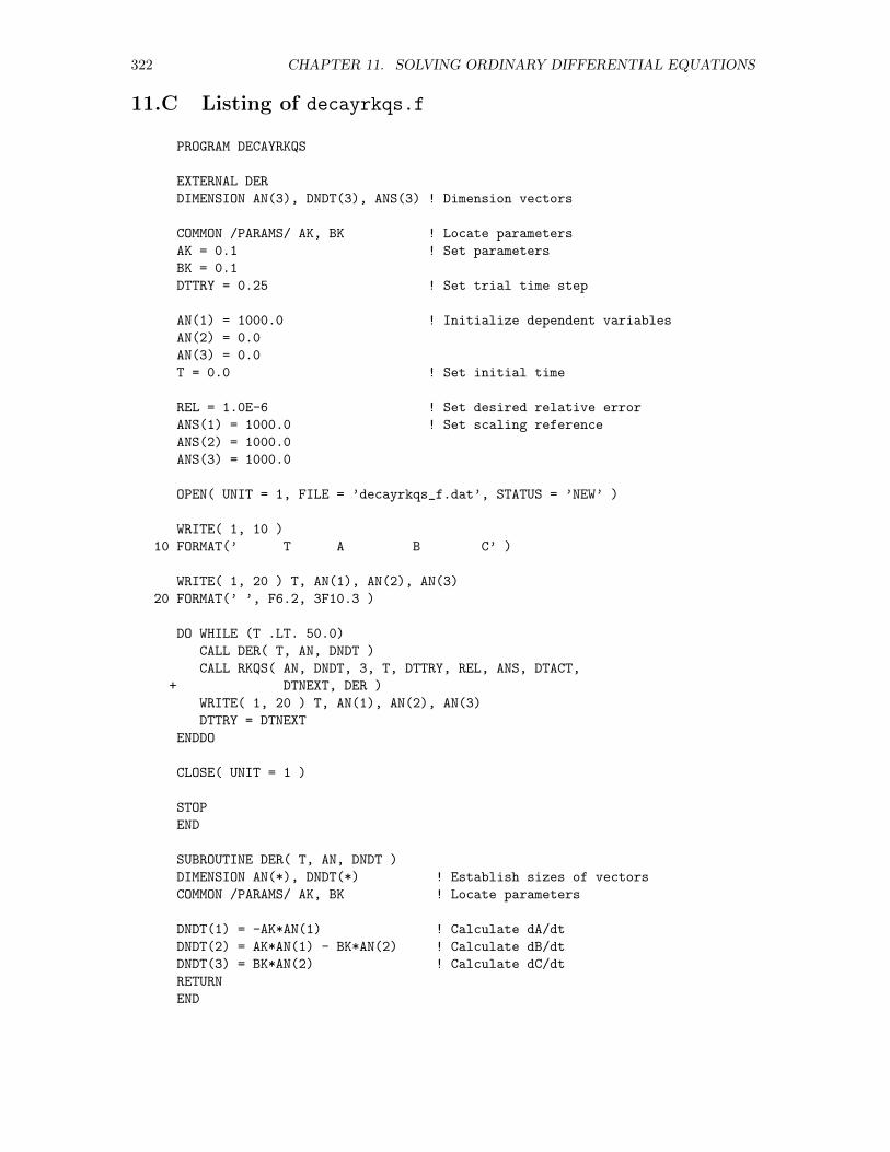
322 CHAPTER 11. SOLVING ORDINARY DIFFERENTIAL EQUATIONS

11.C Listing of decayrkqs.f

PROGRAM DECAYRKQS

EXTERNAL DER

DIMENSION AN(3), DNDT(3), ANS(3) ! Dimension vectors

COMMON /PARAMS/ AK, BK ! Locate parameters

AK = 0.1 ! Set parameters

BK = 0.1

DTTRY = 0.25 ! Set trial time step

AN(1) = 1000.0 ! Initialize dependent variables

AN(2) = 0.0

AN(3) = 0.0

T = 0.0 ! Set initial time

REL = 1.0E-6 ! Set desired relative error

ANS(1) = 1000.0 ! Set scaling reference

ANS(2) = 1000.0

ANS(3) = 1000.0

OPEN( UNIT = 1, FILE = ’decayrkqs_f.dat’, STATUS = ’NEW’ )

WRITE( 1, 10 )

10 FORMAT(’ T A B C’ )

WRITE( 1, 20 ) T, AN(1), AN(2), AN(3)

20 FORMAT(’ ’, F6.2, 3F10.3 )

DO WHILE (T .LT. 50.0)

CALL DER( T, AN, DNDT )

CALL RKQS( AN, DNDT, 3, T, DTTRY, REL, ANS, DTACT,

+ DTNEXT, DER )

WRITE( 1, 20 ) T, AN(1), AN(2), AN(3)

DTTRY = DTNEXT

ENDDO

CLOSE( UNIT = 1 )

STOP

END

SUBROUTINE DER( T, AN, DNDT )

DIMENSION AN(*), DNDT(*) ! Establish sizes of vectors

COMMON /PARAMS/ AK, BK ! Locate parameters

DNDT(1) = -AK*AN(1) ! Calculate dA/dt

DNDT(2) = AK*AN(1) - BK*AN(2) ! Calculate dB/dt

DNDT(3) = BK*AN(2) ! Calculate dC/dt

RETURN

END

11.D. LISTING OF DECAY.C 323

11.D Listing of decay.c

/* PROGRAM decay.c */

#include <stdio.h>

#include <math.h>

main()

/***** Declare variables *****/

FILE *fptr; /* For file pointer */

float kA, kB; /* For parameters */

float t, A, B, C; /* For independent, dependent variables */

float dAdt, dBdt, dCdt; /* For derivatives */

float dt; /* For time increment */

int i, nsteps; /* Loop index, limit */

/***** Get parameters, time step, initial values *****/

printf( "\nDecay constant for A: " ); scanf( "%f", &kA );

printf( "Decay constant for B: " ); scanf( "%f", &kB );

printf( "Number of steps : " ); scanf( "%d", &nsteps );

printf( "Time step : " ); scanf( "%f", &dt );

printf( "Initial A : " ); scanf( "%f", &A );

printf( "Initial B : " ); scanf( "%f", &B );

printf( "Initial C : " ); scanf( "%f", &C );

t = 0.0;

/***** Open file, write label and initial values *****/

fptr = fopen( "decay_c.dat", "w" );

fprintf( fptr, " t A B C\n" );

fprintf( fptr, "%6.2f %10.3f %10.3f %10.3f\n", t, A, B, C );

/***** Solve equations, writing results to file *****/

for( i=1; i<=nsteps; i++ )

dAdt = -kA*A; /* Calculate current derivatives */

dBdt = kA*A - kB*B;

dCdt = kB*B;

A = A + dAdt*dt; /* Calculate new values */

B = B + dBdt*dt;

C = C + dCdt*dt;

t = t + dt;

fprintf( fptr, "%6.2f %10.3f %10.3f %10.3f\n", t, A, B, C );

/***** Close file *****/

fclose( fptr );

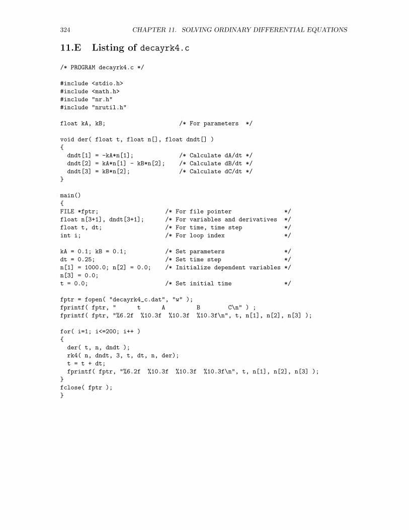
324 CHAPTER 11. SOLVING ORDINARY DIFFERENTIAL EQUATIONS

11.E Listing of decayrk4.c

/* PROGRAM decayrk4.c */

#include <stdio.h>

#include <math.h>

#include "nr.h"

#include "nrutil.h"

float kA, kB; /* For parameters */

void der( float t, float n[], float dndt[] )

dndt[1] = -kA*n[1]; /* Calculate dA/dt */

dndt[2] = kA*n[1] - kB*n[2]; /* Calculate dB/dt */

dndt[3] = kB*n[2]; /* Calculate dC/dt */

main()

FILE *fptr; /* For file pointer */

float n[3+1], dndt[3+1]; /* For variables and derivatives */

float t, dt; /* For time, time step */

int i; /* For loop index */

kA = 0.1; kB = 0.1; /* Set parameters */

dt = 0.25; /* Set time step */

n[1] = 1000.0; n[2] = 0.0; /* Initialize dependent variables */

n[3] = 0.0;

t = 0.0; /* Set initial time */

fptr = fopen( "decayrk4_c.dat", "w" );

fprintf( fptr, " t A B C\n" ) ;

fprintf( fptr, "%6.2f %10.3f %10.3f %10.3f\n", t, n[1], n[2], n[3] );

for( i=1; i<=200; i++ )

der( t, n, dndt );

rk4( n, dndt, 3, t, dt, n, der);

t = t + dt;

fprintf( fptr, "%6.2f %10.3f %10.3f %10.3f\n", t, n[1], n[2], n[3] );

fclose( fptr );

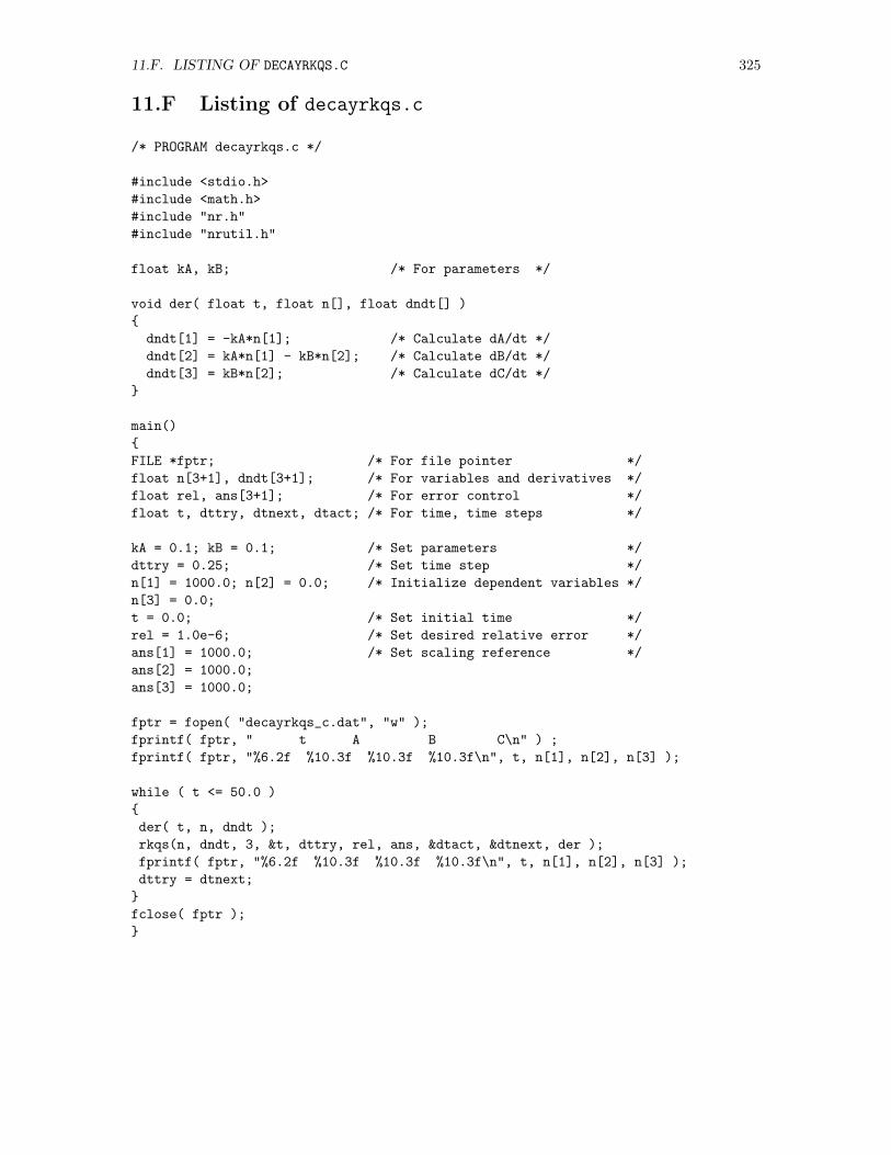
11.F. LISTING OF DECAYRKQS.C 325

11.F Listing of decayrkqs.c

/* PROGRAM decayrkqs.c */

#include <stdio.h>

#include <math.h>

#include "nr.h"

#include "nrutil.h"

float kA, kB; /* For parameters */

void der( float t, float n[], float dndt[] )

dndt[1] = -kA*n[1]; /* Calculate dA/dt */

dndt[2] = kA*n[1] - kB*n[2]; /* Calculate dB/dt */

dndt[3] = kB*n[2]; /* Calculate dC/dt */

main()

FILE *fptr; /* For file pointer */

float n[3+1], dndt[3+1]; /* For variables and derivatives */

float rel, ans[3+1]; /* For error control */

float t, dttry, dtnext, dtact; /* For time, time steps */

kA = 0.1; kB = 0.1; /* Set parameters */

dttry = 0.25; /* Set time step */

n[1] = 1000.0; n[2] = 0.0; /* Initialize dependent variables */

n[3] = 0.0;

t = 0.0; /* Set initial time */

rel = 1.0e-6; /* Set desired relative error */

ans[1] = 1000.0; /* Set scaling reference */

ans[2] = 1000.0;

ans[3] = 1000.0;

fptr = fopen( "decayrkqs_c.dat", "w" );

fprintf( fptr, " t A B C\n" ) ;

fprintf( fptr, "%6.2f %10.3f %10.3f %10.3f\n", t, n[1], n[2], n[3] );

while ( t <= 50.0 )

der( t, n, dndt );

rkqs(n, dndt, 3, &t, dttry, rel, ans, &dtact, &dtnext, der );

fprintf( fptr, "%6.2f %10.3f %10.3f %10.3f\n", t, n[1], n[2], n[3] );

dttry = dtnext;

fclose( fptr );

326 CHAPTER 11. SOLVING ORDINARY DIFFERENTIAL EQUATIONS

Chapter 13

Evaluating Integrals

Frequently the answer to an interesting question in physics is given by—or can be cast in theform of—an integral, often as a function of the upper limit or as a parameter in the integrand.Sometimes, that integral can be evaluated in closed form. More often, however, the integral isanalytically intractable and must be approached numerically. We begin this chapter by identifyingseveral physical situations, the full addressing of which requires evaluating an integral, perhaps asa function of one or more parameters. Then we illustrate how to use symbolic algebra systemsto approach those that can be evaluated analytically, describe a few of many available numericalalgorithms (with attention to their accuracy), and—finally—describe ways to evaluate representativeintegrals using a variety of numerical approaches and computational tools. When parameters areinvolved, we also illustrate how to plot graphs of the integrals as functions of those parameters.

We shall classify each integral in one of three categories, since the approach to its numericalevaluation will depend on this classification. Integrals in the first category will simply be a number;their numerical evaluation involves a single invocation of one or another basic algorithm. In morecomplicated—and more interesting—cases, the integral will be a function of a parameter, whichmay appear in the limits of integration (second category) or embedded in the integrand (thirdcategory); the numerical evaluation of these integrals as a function of the parameter will involverepeated invocation of one or another basic algorithm within a loop.

13.1 Sample Problems

In this section, we identify several physical contexts in which integrals arise, and we determine arepresentative integral for each case.

13.1.1 One-Dimensional Trajectories

The motion of a particle of mass m in one dimension under the action of a force f satisfies Newton’ssecond law, equivalent to the two equations

dp

dt= f and

dx

dt= v (13.1)

which are to be solved subject to the prescribed initial conditions x(0) = x0, v(0) = v0, and p(0) = p0.Here, x, v, and p, are the position, velocity, and momentum of the particle, respectively, and, withc standing for the speed of light, the relationship between p and v assumes one of the forms

p =mv√

1− v2/c2or p = mv (13.2)

327

328 CHAPTER 13. EVALUATING INTEGRALS

depending on whether the motion is relativistic or nonrelativistic. If the force happens to dependonly on t, the solution to these two differential equations can be expressed as the explicit integrals

p(t) = p0 +

∫ t

0

f(t′) dt′ and x(t) = x0 +

∫ t

0

v(t′) dt′ (13.3)

and the physical problem of predicting the trajectory reduces to the mathematical problem of evalu-ating two integrals, finding the momentum from the first integral in Eq. (13.3), then solving for thevelocity v(t) using the appropriate member of Eq. (13.2), and finally finding x(t) from the secondintegral in Eq. (13.3). Each integral is a function of at least one parameter—the upper limit t—andwill also depend on additional quantities (e.g., m, c, . . .) in the integrand (unless a dimensionlesscasting happens to suppress them). These integrals fall into either the second or the third of ourthree categories.

If, on the other hand, the force happens to depend only on x, we can recast the computationaltask by noting first that

d2x

dt2=dv

dt=dv

dx

dx

dt= v

dv

dx(13.4)

Then, Newton’s second law becomes

md2x

dt2= f(x) =⇒ mv

dv

dx= f(x) =⇒ mv dv = f(x) dx (13.5)

Finally, by integrating this last expression from initial values to general values at some other time,we find that

m

∫ v

v0

v′ dv′ =1

2mv2 − 1

2mv20 =

∫ x

x0

f(x′) dx′ (13.6)

and the task of finding the velocity (as a function of x) is reduced to the straight-forward evaluationof an integral. Once that integral has been evaluated, we can then predict the position by exploitingthe relationship

dx

dt= v(x) =⇒ dt =

dx

v(x)=⇒

∫ t

t0

dt′ = t− t0 =

∫ x

x0

dx′

v(x′)(13.7)

and we have reduced the second step in the solution to the evaluation of an integral as well. Bothintegrals deduced in this paragraph may have internal parameters, so they might fall into either thesecond or the third of our three categories.

13.1.2 Center of Mass

The location rcm of the center of mass of an object is given by

rcm =1

M

∫r dm (13.8)

where r locates a representative element of the object, dm is the mass of that element, M =∫dm

is the total mass of the object, and the integral extends over the region of space (volume, surface,or line) occupied by the object. More specifically, if the object lies in a plane and polar coordinates(r, φ) are appropriate, we would write this integral more explicitly in the form

rcm =1

M

∫σ(r, φ) r r dr dφ =

1

M

∫σ(r, φ)

(r cosφ i + r sinφ j

)r dr dφ (13.9)

where σ(r, φ) is the mass per unit area of the object and r dr dφ is the area of the chosen element.

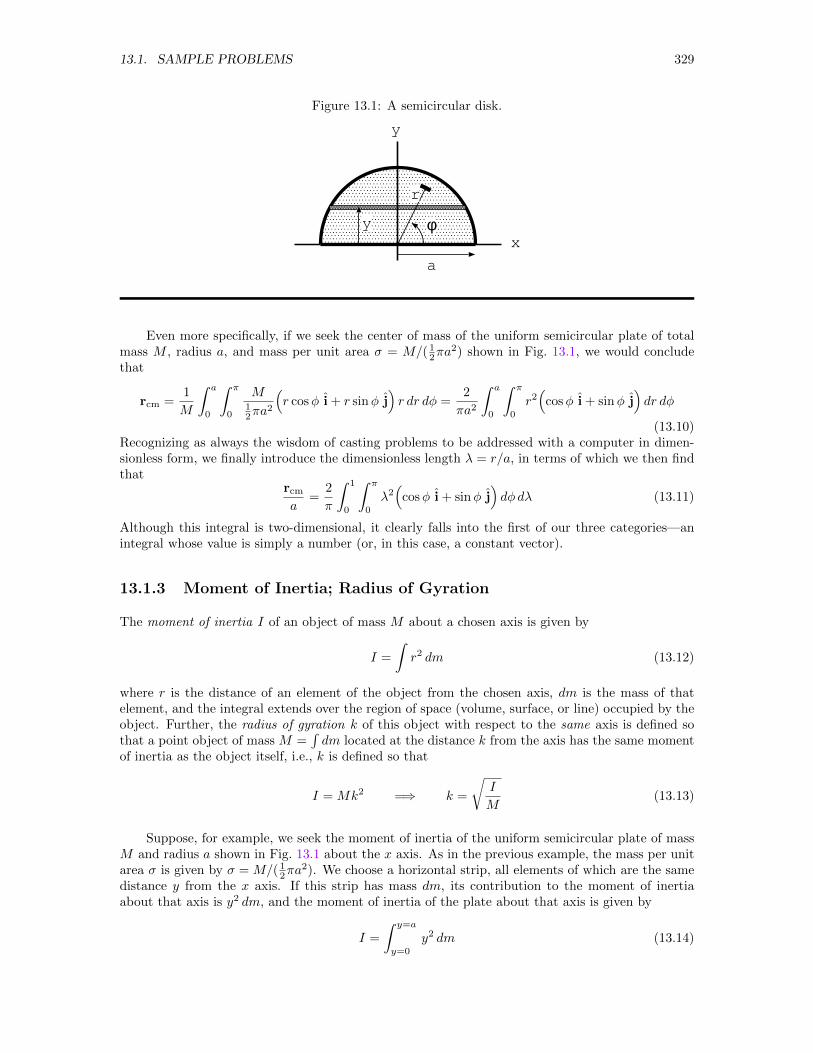
13.1. SAMPLE PROBLEMS 329

Figure 13.1: A semicircular disk.

x

y

a

y

r

φ

Even more specifically, if we seek the center of mass of the uniform semicircular plate of totalmass M , radius a, and mass per unit area σ = M/( 1

2πa2) shown in Fig. 13.1, we would conclude

that

rcm =1

M

∫ a

0

∫ π

0

M12πa

2

(r cosφ i + r sinφ j

)r dr dφ =

2

πa2

∫ a

0

∫ π

0

r2(

cosφ i + sinφ j)dr dφ

(13.10)Recognizing as always the wisdom of casting problems to be addressed with a computer in dimen-sionless form, we finally introduce the dimensionless length λ = r/a, in terms of which we then findthat

rcma

=2

π

∫ 1

0

∫ π

0

λ2(

cosφ i + sinφ j)dφ dλ (13.11)

Although this integral is two-dimensional, it clearly falls into the first of our three categories—anintegral whose value is simply a number (or, in this case, a constant vector).

13.1.3 Moment of Inertia; Radius of Gyration

The moment of inertia I of an object of mass M about a chosen axis is given by

I =

∫r2 dm (13.12)

where r is the distance of an element of the object from the chosen axis, dm is the mass of thatelement, and the integral extends over the region of space (volume, surface, or line) occupied by theobject. Further, the radius of gyration k of this object with respect to the same axis is defined sothat a point object of mass M =

∫dm located at the distance k from the axis has the same moment

of inertia as the object itself, i.e., k is defined so that

I = Mk2 =⇒ k =

√I

M(13.13)

Suppose, for example, we seek the moment of inertia of the uniform semicircular plate of massM and radius a shown in Fig. 13.1 about the x axis. As in the previous example, the mass per unitarea σ is given by σ = M/( 1

2πa2). We choose a horizontal strip, all elements of which are the same

distance y from the x axis. If this strip has mass dm, its contribution to the moment of inertiaabout that axis is y2 dm, and the moment of inertia of the plate about that axis is given by

I =

∫ y=a

y=0

y2 dm (13.14)

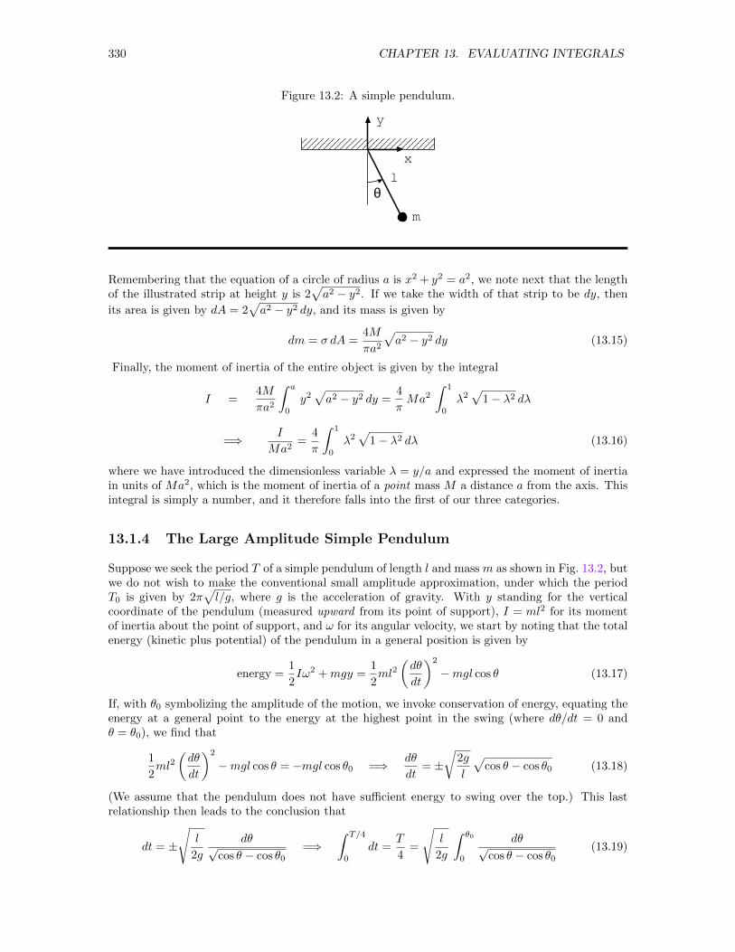
330 CHAPTER 13. EVALUATING INTEGRALS

Figure 13.2: A simple pendulum.

l

m

x

y

θ

Remembering that the equation of a circle of radius a is x2 + y2 = a2, we note next that the lengthof the illustrated strip at height y is 2

√a2 − y2. If we take the width of that strip to be dy, then

its area is given by dA = 2√a2 − y2 dy, and its mass is given by

dm = σ dA =4M

πa2

√a2 − y2 dy (13.15)

Finally, the moment of inertia of the entire object is given by the integral

I =4M

πa2

∫ a

0

y2√a2 − y2 dy =

4

πMa2

∫ 1

0

λ2√

1− λ2 dλ

=⇒ I

Ma2=

4

π

∫ 1

0

λ2√

1− λ2 dλ (13.16)

where we have introduced the dimensionless variable λ = y/a and expressed the moment of inertiain units of Ma2, which is the moment of inertia of a point mass M a distance a from the axis. Thisintegral is simply a number, and it therefore falls into the first of our three categories.

13.1.4 The Large Amplitude Simple Pendulum

Suppose we seek the period T of a simple pendulum of length l and mass m as shown in Fig. 13.2, butwe do not wish to make the conventional small amplitude approximation, under which the periodT0 is given by 2π

√l/g, where g is the acceleration of gravity. With y standing for the vertical

coordinate of the pendulum (measured upward from its point of support), I = ml2 for its momentof inertia about the point of support, and ω for its angular velocity, we start by noting that the totalenergy (kinetic plus potential) of the pendulum in a general position is given by

energy =1

2Iω2 +mgy =

1

2ml2

(dθ

dt

)2

−mgl cos θ (13.17)

If, with θ0 symbolizing the amplitude of the motion, we invoke conservation of energy, equating theenergy at a general point to the energy at the highest point in the swing (where dθ/dt = 0 andθ = θ0), we find that

1

2ml2

(dθ

dt

)2

−mgl cos θ = −mgl cos θ0 =⇒ dθ

dt= ±

√2g

l

√cos θ − cos θ0 (13.18)

(We assume that the pendulum does not have sufficient energy to swing over the top.) This lastrelationship then leads to the conclusion that

dt = ±

√l

2g

dθ√cos θ − cos θ0

=⇒∫ T/4

0

dt =T

4=

√l

2g

∫ θ0

0

dθ√cos θ − cos θ0

(13.19)

13.1. SAMPLE PROBLEMS 331

where we have integrated over one-quarter of the period (0 < t < T/4) in time and over one-quarterof the swing (0 < θ < θ0) in angle, and we have taken the positive sign because, in its motion overthis interval, the pendulum indeed has positive angular velocity. Further, we have assumed fromsymmetry that the full period T is four times the time required for the pendulum to swing from itslowest point to its highest point.

This integral can be recast in numerous ways. Anticipating an existing standard function, weinvoke the half angle identity cos θ = 1− 2 sin2(θ/2), finding that

T = 2

√l

g

∫ θ0

0

dθ√sin2(θ0/2)− sin2(θ/2)

(13.20)

We then introduce the variable φ defined by sin(θ/2) = sin(θ0/2) sinφ to find that

T (k) = 4

√l

g

∫ π/2

0

dφ√1− k2 sin2 φ

(13.21)

where the (dimensionless) parameter k = sin(θ0/2) is determined by the amplitude of the pendulum’smotion. By writing T (k), we have drawn attention in the notation to the dependence of the periodon k (and hence on the amplitude). Note also that, when the amplitude is small, k ≈ 0 and theintegral can be readily evaluated to yield that T0 = 2π

√l/g, which—reassuringly—agrees with the

known value quoted at the beginning of this subsection. Then, expressing the period T (k) in unitsof T0, we find finally that

T (k)

T0=

2

π

∫ π/2

0

dφ√1− k2 sin2 φ

=2

πK(k) (13.22)

Here, for purposes of notation alone, we have introduced the integral

K(k) =

∫ π/2

0

dφ√1− k2 sin2 φ

(13.23)

which defines a standard, tabulated function known as the complete elliptic integral of the first kind.Note that the value of this integral depends on a parameter not in a limit but in the very structureof the integrand. This integral falls into the third of our three categories.

13.1.5 Statistical Data Analysis

When repeated measurements of a single quantity are subject to a large number of individuallysmall, random fluctuations, the distribution of those measurements about their mean follows thenormal or Gaussian distribution function given by

G(x) =1√

2πσ2e−(x−µ)

2/(2σ2) (13.24)

where µ and σ are the mean and standard deviation of the distribution, respectively, and G(x) isnormalized so that

∫∞−∞G(x) dx = 1. The probability that a single measurement will lie between

µ− ασ and µ+ ασ is then given by

P (µ− ασ < x < µ+ ασ) =

∫ µ+ασ

µ−ασG(x) dx =

2√π

∫ α/√2

0

e−s2

ds = erf

(α√2

)(13.25)

where s = (x− µ)/(σ√

2) and, for purposes of notation alone, we have introduced the integral

erf(x) =2√π

∫ x

0

e−s2

ds (13.26)

332 CHAPTER 13. EVALUATING INTEGRALS

which defines a standard, tabulated function known as the error function. Thus, determining theprobability given by Eq. (13.25) boils down to evaluating an integral that depends on a parameterappearing in the upper limit, i.e., to evaluating an integral that falls into the second of our threecategories.

13.1.6 The Cornu Spiral

The two integrals

C(u) =

∫ u

0

cos

(πt2

2

)dt ; S(u) =

∫ u

0

sin

(πt2

2

)dt (13.27)

which are called the Fresnel integrals, appear in the study of Fresnel diffraction. Together, theydefine the Cornu spiral, which is a graph of S(u) versus C(u). Each is a function of its upper limitas a parameter and falls into the second of our three categories.

13.1.7 Electric and Magnetic Fields and Potentials

Among the richest sources of important—and frequently analytically intractable—integrals are therelationships in electromagnetic theory that determine fields and potentials from prescribed sources.For a distribution of static charge, for example, we identify an element of that charge dq′ located atr′ and, in mks units, we find the electric field E(r) and the electrostatic potential V (r) at the pointr by evaluating the integrals

E(r) =1

4πε0

∫r− r′

|r− r′|3dq′ and V (r) =

1

4πε0

∫dq′

|r− r′|(13.28)

which extend over all charges in the source. Similarly, for a source consisting of a steady current I ′

in a wire, we identify an element dr′ of the wire located at r′ and, in mks units, find the magneticfield B(r) and the magnetic vector potential A(r) at the point r by evaluating the integrals

B(r) =µ0

4π

∫I ′ dr′ × (r− r′)

|r− r′|3and A(r) =

µ0

4π

∫I ′ dr′

|r− r′|(13.29)

which extend over the path followed by the current.

More specifically, suppose we seek the electrostatic potential in the plane midway between twoidentical uniformly charged circular rings of radius a with their planes parallel, their axes coincident,and their centers separated by 2a. The envisioned situation is shown in Fig. 13.3. Each ring carriesa total charge Q with (linear) charge density λ. Using cylindrical coordinates (r, φ, z), we first find

the potential at the general point r = r cosφ i+r sinφ j+z k, produced by one such ring positionedin the xy plane with its center at the origin. Let r′ = a cosφ′ i+ a sinφ′ j locate an element on that(single) ring. In this notation,

r− r′ = (a cosφ− a cosφ′) i + (a sinφ− a sinφ′) j + z k (13.30)

so

|r− r′| =[(r cosφ− a cosφ′)2 + (r sinφ− a sinφ′)2 + z2

]1/2=

[r2 + a2 − 2ar cos(φ′ − φ) + z2

]1/2(13.31)

Placing these results into the second member of Eq. (13.28) and recognizing that dq′ = λa dφ′, weat last find that

Vone(r, φ, z) =1

4πε0

∫ 2π

0

λ a dφ′

[r2 + a2 − 2ar cos(φ′ − φ) + z2]1/2(13.32)

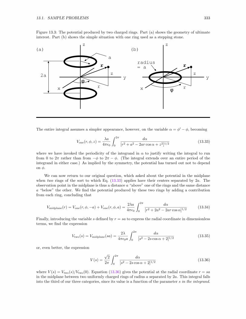
13.1. SAMPLE PROBLEMS 333

Figure 13.3: The potential produced by two charged rings. Part (a) shows the geometry of ultimateinterest. Part (b) shows the simple situation with one ring used as a stepping stone.

x

y

z

2a

a

z

rφ

r

(a)

x

y

z

z

rφ

r

(b)

radius= a

The entire integral assumes a simpler appearance, however, on the variable α = φ′ − φ, becoming

Vone(r, φ, z) =λa

4πε0

∫ 2π

0

dα

[r2 + a2 − 2ar cosα+ z2]1/2(13.33)

where we have invoked the periodicity of the integrand in α to justify writing the integral to runfrom 0 to 2π rather than from −φ to 2π − φ. (The integral extends over an entire period of theintegrand in either case.) As implied by the symmetry, the potential has turned out not to dependon φ.

We can now return to our original question, which asked about the potential in the midplanewhen two rings of the sort to which Eq. (13.33) applies have their centers separated by 2a. Theobservation point in the midplane is thus a distance a “above” one of the rings and the same distancea “below” the other. We find the potential produced by these two rings by adding a contributionfrom each ring, concluding that

Vmidplane(r) = Vone(r, φ,−a) + Vone(r, φ, a) =2λa

4πε0

∫ 2π

0

dα

[r2 + 2a2 − 2ar cosα]1/2(13.34)

Finally, introducing the variable s defined by r = sa to express the radial coordinate in dimensionlessterms, we find the expression

Vtwo(s) = Vmidplane(sa) =2λ

4πε0a

∫ 2π

0

dα

[s2 − 2s cosα+ 2]1/2(13.35)

or, even better, the expression

V (s) =

√2

2π

∫ 2π

0

dα

[s2 − 2s cosα+ 2]1/2(13.36)

where V (s) = Vtwo(s)/Vtwo(0). Equation (13.36) gives the potential at the radial coordinate r = sain the midplane between two uniformly charged rings of radius a separated by 2a. This integral fallsinto the third of our three categories, since its value is a function of the parameter s in the integrand.

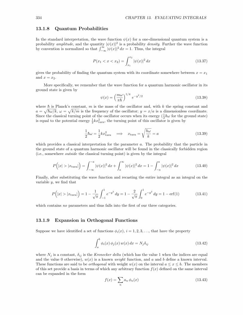
334 CHAPTER 13. EVALUATING INTEGRALS

13.1.8 Quantum Probabilities

In the standard interpretation, the wave function ψ(x) for a one-dimensional quantum system is aprobability amplitude, and the quantity |ψ(x)|2 is a probability density. Further the wave functionby convention is normalized so that

∫∞−∞ |ψ(x)|2 dx = 1. Thus, the integral

P (x1 < x < x2) =

∫ x2

x1

|ψ(x)|2 dx (13.37)

gives the probability of finding the quantum system with its coordinate somewhere between x = x1and x = x2.

More specifically, we remember that the wave function for a quantum harmonic oscillator in itsground state is given by

ψ(x) =(mωπh

)1/4e−y

2/2 (13.38)

where h is Planck’s constant, m is the mass of the oscillator and, with k the spring constant anda =

√hω/k, ω =

√k/m is the frequency of the oscillator; y = x/a is a dimensionless coordinate.

Since the classical turning point of the oscillator occurs when its energy ( 12 hω for the ground state)

is equal to the potential energy 12kx

2turn, the turning point of this oscillator is given by

1

2hω =

1

2kx2turn =⇒ xturn =

√hω

k= a (13.39)

which provides a classical interpretation for the parameter a. The probability that the particle inthe ground state of a quantum harmonic oscillator will be found in the classically forbidden region(i.e., somewhere outside the classical turning point) is given by the integral

P(|x| > |xturn|

)=

∫ −a−∞|ψ(x)|2 dx+

∫ ∞a

|ψ(x)|2 dx = 1−∫ a

−a|ψ(x)|2 dx (13.40)

Finally, after substituting the wave function and recasting the entire integral as an integral on thevariable y, we find that

P(|x| > |xturn|

)= 1− 1√

π

∫ 1

−1e−y

2

dy = 1− 2√π

∫ 1

0

e−y2

dy = 1− erf(1) (13.41)

which contains no parameters and thus falls into the first of our three categories.

13.1.9 Expansion in Orthogonal Functions

Suppose we have identified a set of functions φi(x), i = 1, 2, 3, . . ., that have the property∫ b

a

φi(x)φj(x)w(x) dx = Njδij (13.42)

where Nj is a constant, δij is the Kronecker delta (which has the value 1 when the indices are equaland the value 0 otherwise), w(x) is a known weight function, and a and b define a known interval.These functions are said to be orthogonal with weight w(x) on the interval a ≤ x ≤ b. The membersof this set provide a basis in terms of which any arbitrary function f(x) defined on the same intervalcan be expanded in the form

f(x) =∑n

an φn(x) (13.43)

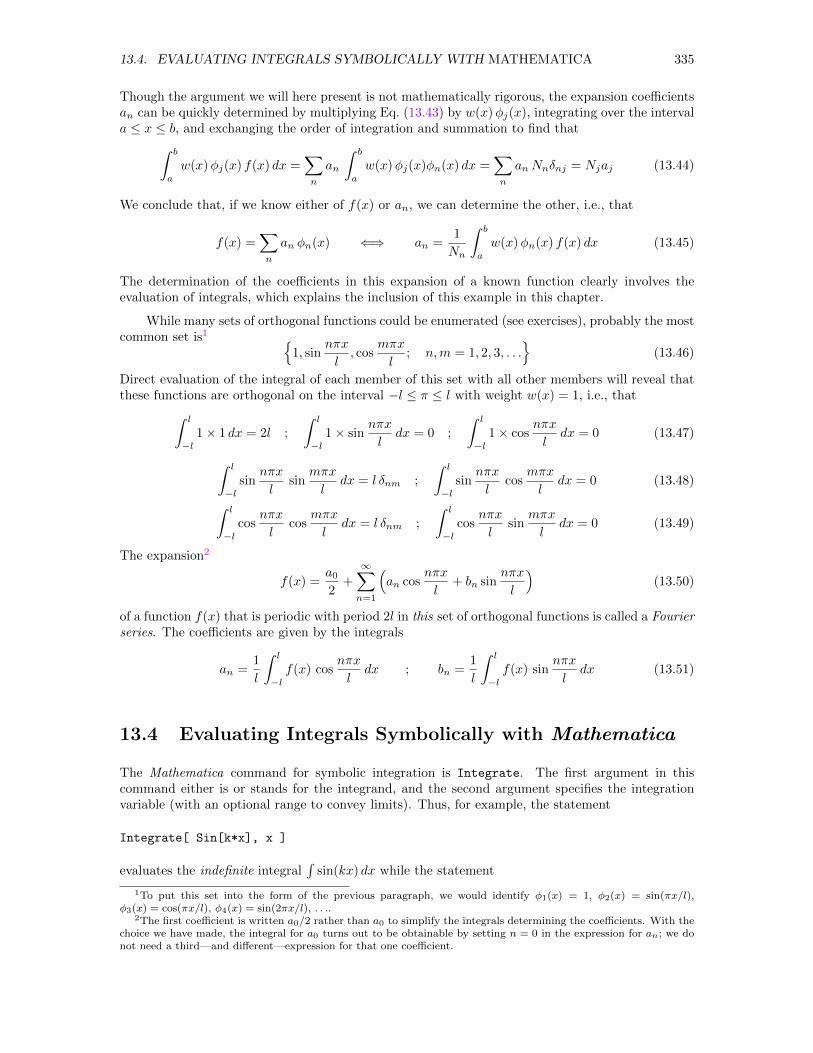
13.4. EVALUATING INTEGRALS SYMBOLICALLY WITH MATHEMATICA 335

Though the argument we will here present is not mathematically rigorous, the expansion coefficientsan can be quickly determined by multiplying Eq. (13.43) by w(x)φj(x), integrating over the intervala ≤ x ≤ b, and exchanging the order of integration and summation to find that∫ b

a

w(x)φj(x) f(x) dx =∑n

an

∫ b

a

w(x)φj(x)φn(x) dx =∑n

anNnδnj = Njaj (13.44)

We conclude that, if we know either of f(x) or an, we can determine the other, i.e., that

f(x) =∑n

an φn(x) ⇐⇒ an =1

Nn

∫ b

a

w(x)φn(x) f(x) dx (13.45)

The determination of the coefficients in this expansion of a known function clearly involves theevaluation of integrals, which explains the inclusion of this example in this chapter.

While many sets of orthogonal functions could be enumerated (see exercises), probably the mostcommon set is1

1, sinnπx

l, cos

mπx

l; n,m = 1, 2, 3, . . .

(13.46)

Direct evaluation of the integral of each member of this set with all other members will reveal thatthese functions are orthogonal on the interval −l ≤ π ≤ l with weight w(x) = 1, i.e., that∫ l

−l1× 1 dx = 2l ;

∫ l

−l1× sin

nπx

ldx = 0 ;

∫ l

−l1× cos

nπx

ldx = 0 (13.47)

∫ l

−lsin

nπx

lsin

mπx

ldx = l δnm ;

∫ l

−lsin

nπx

lcos

mπx

ldx = 0 (13.48)

∫ l

−lcos

nπx

lcos

mπx

ldx = l δnm ;

∫ l

−lcos

nπx

lsin

mπx

ldx = 0 (13.49)

The expansion2

f(x) =a02

+

∞∑n=1

(an cos

nπx

l+ bn sin

nπx

l

)(13.50)

of a function f(x) that is periodic with period 2l in this set of orthogonal functions is called a Fourierseries. The coefficients are given by the integrals

an =1

l

∫ l

−lf(x) cos

nπx

ldx ; bn =

1

l

∫ l

−lf(x) sin

nπx

ldx (13.51)

13.4 Evaluating Integrals Symbolically with Mathematica

The Mathematica command for symbolic integration is Integrate. The first argument in thiscommand either is or stands for the integrand, and the second argument specifies the integrationvariable (with an optional range to convey limits). Thus, for example, the statement

Integrate[ Sin[k*x], x ]

evaluates the indefinite integral∫

sin(kx) dx while the statement

1To put this set into the form of the previous paragraph, we would identify φ1(x) = 1, φ2(x) = sin(πx/l),φ3(x) = cos(πx/l), φ4(x) = sin(2πx/l), . . ..

2The first coefficient is written a0/2 rather than a0 to simplify the integrals determining the coefficients. With thechoice we have made, the integral for a0 turns out to be obtainable by setting n = 0 in the expression for an; we donot need a third—and different—expression for that one coefficient.

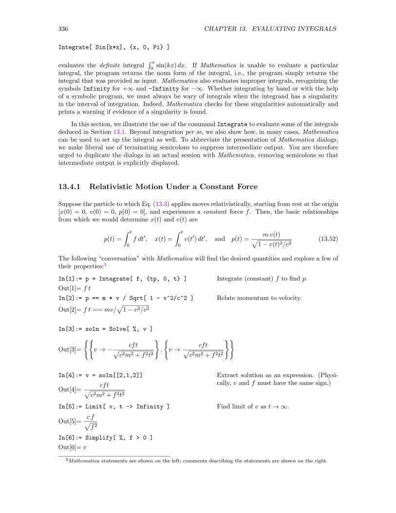
336 CHAPTER 13. EVALUATING INTEGRALS

Integrate[ Sin[k*x], x, 0, Pi ]

evaluates the definite integral∫ π0

sin(kx) dx. If Mathematica is unable to evaluate a particularintegral, the program returns the noun form of the integral, i.e., the program simply returns theintegral that was provided as input. Mathematica also evaluates improper integrals, recognizing thesymbols Infinity for +∞ and -Infinity for −∞. Whether integrating by hand or with the helpof a symbolic program, we must always be wary of integrals when the integrand has a singularityin the interval of integration. Indeed, Mathematica checks for these singularities automatically andprints a warning if evidence of a singularity is found.

In this section, we illustrate the use of the command Integrate to evaluate some of the integralsdeduced in Section 13.1. Beyond integration per se, we also show how, in many cases, Mathematicacan be used to set up the integral as well. To abbreviate the presentation of Mathematica dialogs,we make liberal use of terminating semicolons to suppress intermediate output. You are thereforeurged to duplicate the dialogs in an actual session with Mathematica, removing semicolons so thatintermediate output is explicitly displayed.

13.4.1 Relativistic Motion Under a Constant Force

Suppose the particle to which Eq. (13.3) applies moves relativistically, starting from rest at the origin[x(0) = 0, v(0) = 0, p(0) = 0], and experiences a constant force f . Then, the basic relationshipsfrom which we would determine x(t) and v(t) are

p(t) =

∫ t

0

f dt′, x(t) =

∫ t

0

v(t′) dt′, and p(t) =mv(t)√

1− v(t)2/c2(13.52)

The following “conversation” with Mathematica will find the desired quantities and explore a few oftheir properties:3

In[1]:= p = Integrate[ f, tp, 0, t ]

Out[1]= f t

In[2]:= p == m * v / Sqrt[ 1 - v^2/c^2 ]

Out[2]= f t == mv/√

1− v2/c2

Integrate (constant) f to find p.

Relate momentum to velocity.

In[3]:= soln = Solve[ %, v ]

Out[3]=

v → − cft√

c2m2 + f2t2

,

v → cft√

c2m2 + f2t2

In[4]:= v = soln[[2,1,2]]

Out[4]=cft√

c2m2 + f2t2

Extract solution as an expression. (Physi-cally, v and f must have the same sign.)

In[5]:= Limit[ v, t -> Infinity ]

Out[5]=c f√f2

In[6]:= Simplify[ %, f > 0 ]

Out[6]= c

Find limit of v as t→∞.

3Mathematica statements are shown on the left; comments describing the statements are shown on the right.

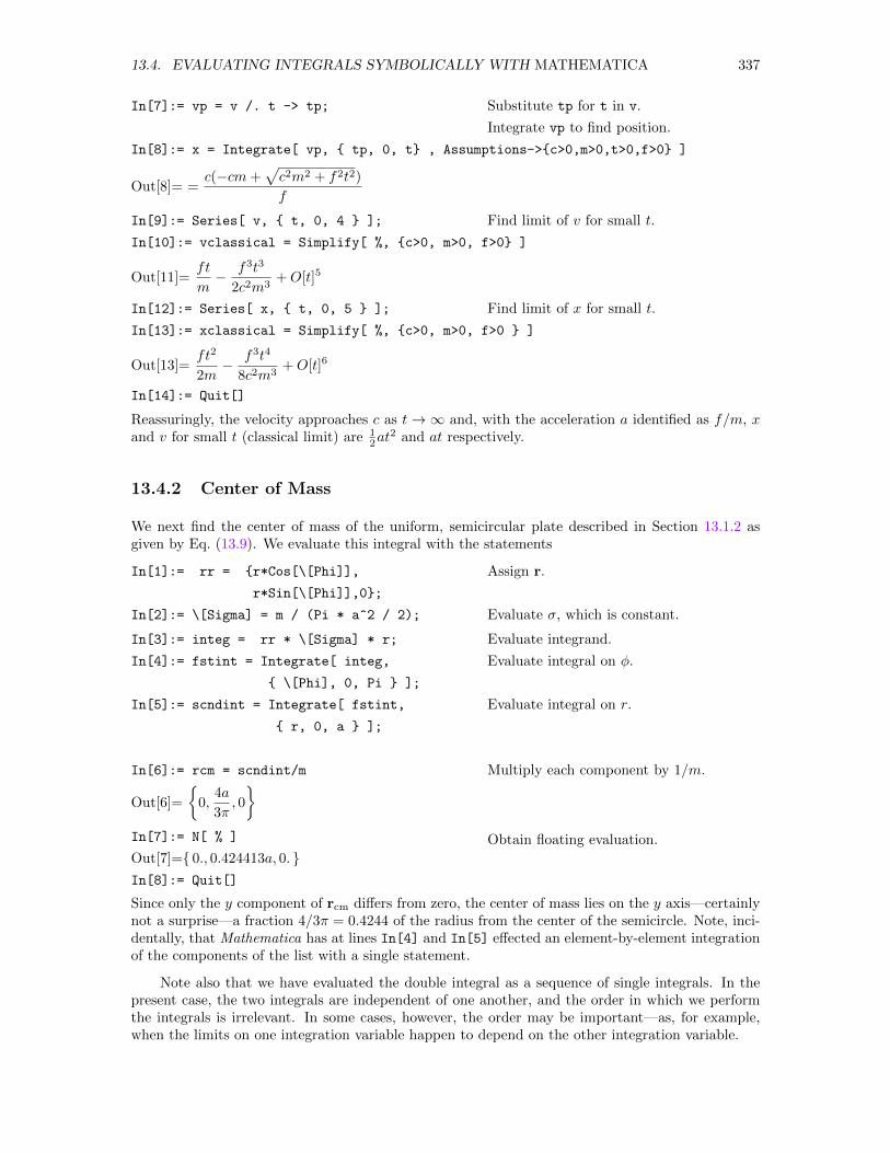
13.4. EVALUATING INTEGRALS SYMBOLICALLY WITH MATHEMATICA 337

In[7]:= vp = v /. t -> tp;

In[8]:= x = Integrate[ vp, tp, 0, t , Assumptions->c>0,m>0,t>0,f>0 ]

Out[8]= =c(−cm+

√c2m2 + f2t2)

f

Substitute tp for t in v.

Integrate vp to find position.

In[9]:= Series[ v, t, 0, 4 ];

In[10]:= vclassical = Simplify[ %, c>0, m>0, f>0 ]

Out[11]=ft

m− f3t3

2c2m3+O[t]5

Find limit of v for small t.

In[12]:= Series[ x, t, 0, 5 ];

In[13]:= xclassical = Simplify[ %, c>0, m>0, f>0 ]

Out[13]=ft2

2m− f3t4

8c2m3+O[t]6

In[14]:= Quit[]

Find limit of x for small t.

Reassuringly, the velocity approaches c as t→∞ and, with the acceleration a identified as f/m, xand v for small t (classical limit) are 1

2at2 and at respectively.

13.4.2 Center of Mass

We next find the center of mass of the uniform, semicircular plate described in Section 13.1.2 asgiven by Eq. (13.9). We evaluate this integral with the statements

In[1]:= rr = r*Cos[\[Phi]],

r*Sin[\[Phi]],0;

In[2]:= \[Sigma] = m / (Pi * a^2 / 2);

Assign r.

Evaluate σ, which is constant.

In[3]:= integ = rr * \[Sigma] * r;

In[4]:= fstint = Integrate[ integ,

\[Phi], 0, Pi ];

In[5]:= scndint = Integrate[ fstint,

r, 0, a ];

Evaluate integrand.

Evaluate integral on φ.

Evaluate integral on r.

In[6]:= rcm = scndint/m

Out[6]=

0,

4a

3π, 0

In[7]:= N[ % ]

Out[7]= 0., 0.424413a, 0. In[8]:= Quit[]

Multiply each component by 1/m.

Obtain floating evaluation.

Since only the y component of rcm differs from zero, the center of mass lies on the y axis—certainlynot a surprise—a fraction 4/3π = 0.4244 of the radius from the center of the semicircle. Note, inci-dentally, that Mathematica has at lines In[4] and In[5] effected an element-by-element integrationof the components of the list with a single statement.

Note also that we have evaluated the double integral as a sequence of single integrals. In thepresent case, the two integrals are independent of one another, and the order in which we performthe integrals is irrelevant. In some cases, however, the order may be important—as, for example,when the limits on one integration variable happen to depend on the other integration variable.

338 CHAPTER 13. EVALUATING INTEGRALS

13.4.3 Moment of Inertia; Radius of Gyration

The evaluation by Mathematica of the moment of inertia of a semicircular plate as given byEq. (13.16) is quick and straightforward. We need only the statements4

In[1]:= Integrate[ \[Lambda]^2*Sqrt[1-\[Lambda]^2], \[Lambda], 0, 1 ]

Out[1]= π/16

In[2]:= II = m*a^2*(4/Pi)*%

Out[2]=a2m

4

In[3]:= k = Simplify[ Sqrt[II/m], a>0 ]

Out[3]=a

2

In[4]:= Quit[]

to evaluate the necessary integral and find both the moment of inertia I = ma2/4 and the radius ofgyration k = a/2.

13.4.4 Electrostatic Potential of a Finite Line Charge

For a fourth example, we evaluate the electrostatic potential of a uniformly charged finite lineextending along the z axis over the interval −a ≤ z ≤ +a. The geometry is shown in Fig. 13.4.With λ representing the linear charge density on the line, dz′ giving the length of an element ofthe line, r and r′ locating the observation point and an element of the source, respectively, anddq′ = λ dz′, we deduce from Eq. (13.28) that the potential established by this source is given by

V (x, y, z) =λ

4πε0

∫ +a

−a

dz′

|r− r′|(13.53)

Electing cylindrical coordinates (r, φ, z), we set r′ = z′ k and r = r cosφ i+ r sinφ j+ z k. Then weconstruct the integrand and evaluate the integral with the statements5

In[1]:= Get[ "$HEAD/mathematica/crossdot.m" ]

In[2]:= rr = r*Cos[\[Phi]], r*Sin[\[Phi]], z ;

In[3]:= rp = 0, 0, zp ;

Define ludot and lucross.

Assign r in cylindrical coordinates.

Assign r′.

In[4]:= sep = rr - rp;

In[5]:= ludot[ sep, sep ];

In[6]:= Simplify[ % ];

Evaluate r− r′.

Evaluate |r− r′|2.

Recognize cos2 φ+ sin2 φ = 1.

In[7]:= den = Sqrt[ % ];

In[8]:= cnst = 1/( 4*Pi*\[Epsilon]0 );

In[9]:= integ = \[Lambda] * cnst / den

Bind |r− r′| to den.

Bind 1/4πε0 to cnst.

Set integrand.

Out[9]=λ

4π√r2 + (z − z′)2 ε0

Then, we find V (r, z), with r =√x2 + y2 by executing the statement

4The variable I in Mathematica is reserved for√−1, so we use II for the moment of inertia.

5 The file $HEAD/mathematica/crossdot.m was described in Section 8.11 and exists in the public directory structure.(The symbol $HEAD is defined in the Local Guide.) It defines the two functions lucross[v1, v2] and ludot[v1, v2]

for evaluating the cross and dot products of two three-component vectors when those vectors are conveyed by lists.

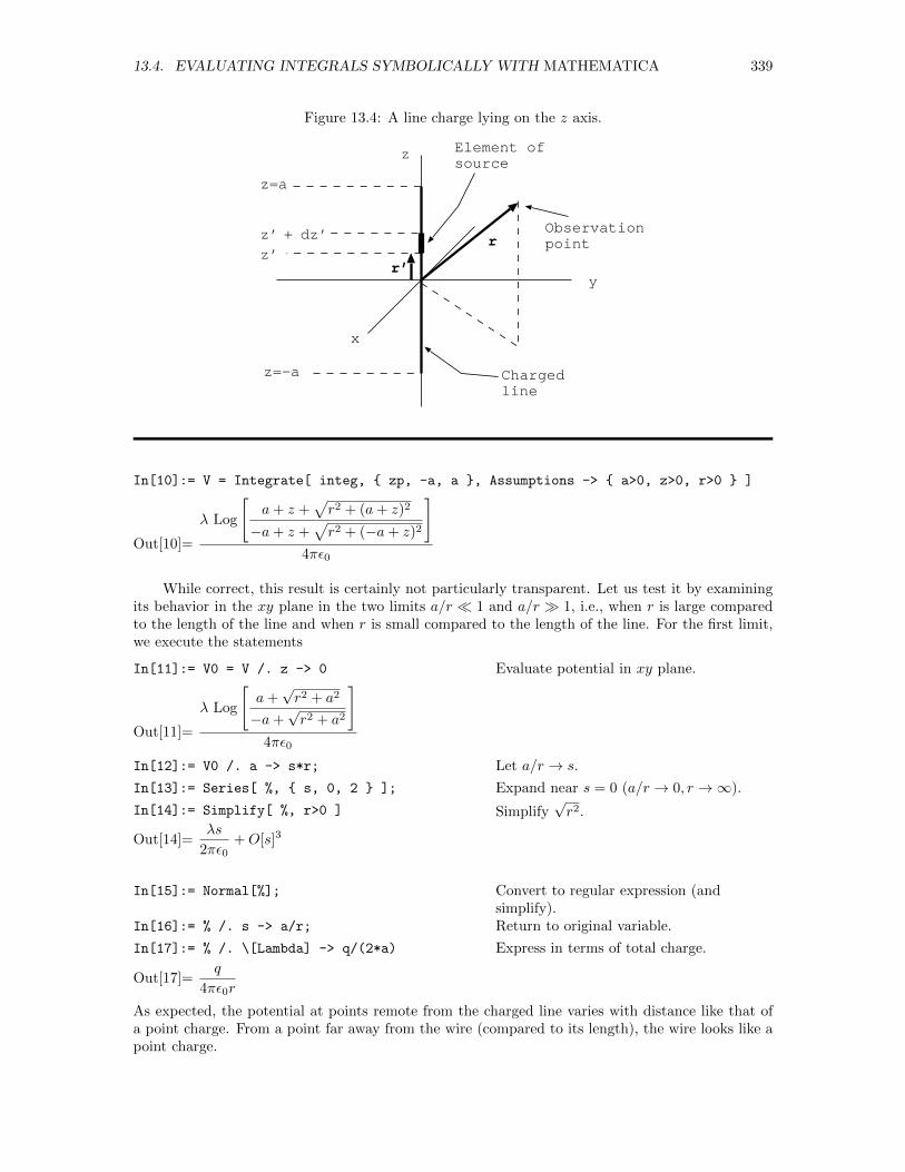
13.4. EVALUATING INTEGRALS SYMBOLICALLY WITH MATHEMATICA 339

Figure 13.4: A line charge lying on the z axis.

x

y

z

z=a

z=-a Chargedline

z’

z’ + dz’ rObservationpoint

Element ofsource

r’

In[10]:= V = Integrate[ integ, zp, -a, a , Assumptions -> a>0, z>0, r>0 ]

Out[10]=

λ Log

[a+ z +

√r2 + (a+ z)2

−a+ z +√r2 + (−a+ z)2

]4πε0

While correct, this result is certainly not particularly transparent. Let us test it by examiningits behavior in the xy plane in the two limits a/r 1 and a/r 1, i.e., when r is large comparedto the length of the line and when r is small compared to the length of the line. For the first limit,we execute the statements

In[11]:= V0 = V /. z -> 0 Evaluate potential in xy plane.

Out[11]=

λ Log

[a+√r2 + a2

−a+√r2 + a2

]4πε0

In[12]:= V0 /. a -> s*r;

In[13]:= Series[ %, s, 0, 2 ];

In[14]:= Simplify[ %, r>0 ]

Out[14]=λs

2πε0+O[s]3

Let a/r → s.

Expand near s = 0 (a/r → 0, r →∞).

Simplify√r2.

In[15]:= Normal[%];

In[16]:= % /. s -> a/r;

In[17]:= % /. \[Lambda] -> q/(2*a)

Out[17]=q

4πε0r

Convert to regular expression (andsimplify).Return to original variable.

Express in terms of total charge.

As expected, the potential at points remote from the charged line varies with distance like that ofa point charge. From a point far away from the wire (compared to its length), the wire looks like apoint charge.

340 CHAPTER 13. EVALUATING INTEGRALS

At the other extreme, when r is small compared to the length of the line, we might think toinvoke a statement like Series[V0, r,0,2]. That approach, however, is problematic because thedenominator under the logarithm in V0 is zero at r = 0 when a > 0. The expression V0 does nothave a very well behaved series expansion about the point r = 0. As an alternative, we might noticethat the numerator and denominator under the logarithm in V0 are well behaved in the vicinity ofr = 0. In particular

In[18]:= Series[-a + Sqrt[a^2+r^2], r,0,2, Assumptions->a>0];

In[19]:= T1 = Normal[ Simplify[%, a>0] ]

Out[19]=r2

2a

In[20]:= Series[a + Sqrt[a^2+r^2], r,0,2, Assumptions->a>0];

In[21]:= T2 = Normal[ Simplify[%, a>0] ]

Out[21]= 2a+r2

2a

Substituting these expansions into V0 with the statements

In[22]:= SmallR = V0 /. -a+Sqrt[a^2+r^2]->T1, a+Sqrt[a^2+r^2]->T2

Out[22]=λ

4πε0Log

[2a(2a+ r2/2a)

r2

]we find a much simpler, though approximate expression. Further, we can now see why a well-behavedseries expansion does not exist. As r becomes ever smaller, the denominator in this logarithmapproaches zero and the logarithm diverges. The numerator, however, approaches 4a2 as r → 0.Thus, we can simplify the expression further by ignoring the term r2/2a in the numerator. Thestatement

In[23]:= SmallR = SmallR /. 2*a+r^2/(2*a) -> 2*a

Out[23]=λ

4πε0Log

[4a2

r2

]In[23]:= Quit[]

effects this further simplification. Indeed, if we recognize the equivalent form,

− λ

2πε0lnr

a+λ ln 2

2πε0

we see that our result differs by a constant from the familiar logarithmic result for the potential ofa uniformly charged, infinitely long straight wire when the reference point (point of zero potential)is taken at a distance a from the wire. From a point close to the wire (compared to its length) andnear its center, the wire looks to be infinitely long.

13.4.5 The Helmholtz Coil

Next, we evaluate the magnetic field produced on the z axis by a pair of circular current loops ofarbitrary separation and demonstrate the significance of the specific separation used in the Helmholtzcoil. Strategically, we regard the pair as a superposition of two loops and seek first the magnetic fieldof a single loop. In general, the magnetic field B(r) is given by the Biot-Savart law, which is the first

13.4. EVALUATING INTEGRALS SYMBOLICALLY WITH MATHEMATICA 341

member of Eq. (13.29). If the (single) loop has radius a and lies in the xy plane with its center at theorigin, then, for an observation point on the z axis, the various vectors in the expression are given byr = sa k, where (to facilitate expressing things in dimensionless form) the z coordinate is written as

a multiple s of the radius a of the loop, r′ = a cosφ i+a sinφ j, and dr′ = (−a sinφ i+a cosφ j) dφ.Evaluation of the integrand and the integral for a single loop then proceeds with the statements6

In[1]:= Get[ "$HEAD/mathematica/crossdot.m" ];

In[2]:= r = 0, 0, s * a ;

In[3]:= rp = a*Cos[\[Phi]],a*Sin[\[Phi]],0;

In[4]:= drp = -a*Sin[\[Phi]],a*Cos[\[Phi]],0;

In[5]:= sep = r - rp;

Define lucross and ludot.

Assign r.

Assign r′.

Assign dr′.

Evaluate r− r′.

In[6]:= ludot[ sep, sep ];

In[7]:= mag2 = Simplify[ % ]

Out[7]= a2(1 + s2)

In[8]:= lucross[ drp, sep ];

In[9]:= num = Simplify[ % ]

Out[9]= a2sCos [φ], a2sSin [φ], a2

Evaluate |r− r′|2.

Recognize cos2 φ + sin2 φ = 1; setmag2 = |r− r′|2.

Evaluate dr′ × (r− r′).

Recognize cos2 φ+ sin2 φ = 1.

Finally, we bring various factors together to construct the integrand, simplify that integrand, evaluatethe integral, and recast the result in a dimensionless form with the statements

In[10]:= integ = num*\[Mu]0*i/(4*Pi*mag2^(3/2));

In[11]:= integ = Simplify[ %, a>0 ]

Out[11]=

iµ0sCos [φ]

4aπ(1 + s2)3/2,

iµ0sSin [φ]

4aπ(1 + s2)3/2,

iµ0

4aπ(1 + s2)3/2

In[12]:= B1 = Integrate[ integ,

\[Phi], 0, 2*Pi ]

Out[12]=

0, 0,

iµ0

2a(1 + s2)3/2

In[13]:= B1z = B1[[3]];

In[14]:= B1c = B1z /. s -> 0;

In[15]:= B1z = B1z / B1c

Out[15]=1

(1 + s2)3/2

Integrate around the loop.

Extract the z component.

Find field at center.

Normalize field of single loop.

At the beginning, we were interested not in the field of a single loop but in the field of a pairof loops. Thus, we next combine the fields of two separate loops, one positioned a distance ca abovethe midplane and the other positioned a distance ca below the midplane, and again normalize thefield so that it is measured in units defined by its value at the origin midway between the two loops.These objectives are accomplished with the statements

In[16]:= Bpair = (B1z /. s -> s-c) +

(B1z /. s -> s+c);

In[17]:= Bpairc = Bpair /. s -> 0;

In[18]:= Bpair = Bpair / Bpairc

Find field of two loops, one at s = c andthe other at s = −c.

Find field at center.

Normalize field of two loops.

Out[18]=1

2(1 + c2)3/2

(1

[1 + (−c+ s)2]3/2+

1

[1 + (c+ s)2]3/2

)6See footnote 5.

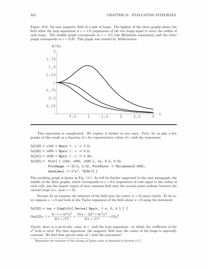
342 CHAPTER 13. EVALUATING INTEGRALS

Figure 13.5: On-axis magnetic field of a pair of loops. The highest of the three graphs shows thefield when the loop separation is c = 1.0 (separation of the two loops equal to twice the radius ofeach loop). The middle graph corresponds to c = 0.5 (the Helmholtz separation) and the lowergraph corresponds to c = 0.25. This graph was created by Mathematica.

0.5 1 1.5 2 2.5 3s

0.25

0.5

0.75

1

1.25

1.5

1.75

2B/Bc

This expression is complicated. We explore it further in two ways. First, let us plot a fewgraphs of this result as a function of s for representative values of c with the statements

In[19]:= c100 = Bpair /. c -> 1.0;

In[20]:= c050 = Bpair /. c -> 0.5;

In[21]:= c025 = Bpair /. c -> 0.25;

In[22]:= Plot[ c100, c050, c025 , s, 0.0, 3.0,

PlotRange -> 0.0, 2.0, PlotStyle -> Thickness[0.005],

AxesLabel -> "s", "B/Bc" ]

The resulting graph is shown in Fig. 13.5. As will be further supported in the next paragraph, themiddle of the three graphs, which corresponds to c = 0.5 (separation of coils equal to the radius ofeach coil), has the largest region of near constant field near the on-axis point midway between thecurrent loops (i.e., near s = 0).

Second, let us examine the behavior of the field near the center (s = 0) more closely. To do so,we suppose s→ 0 and look at the Taylor expansion of the field about s = 0 using the statement

In[23]:= tay = Simplify[ Series[ Bpair, s, 0, 4 ] ]

Out[23]= 1 +3(−1 + 4c2)s2

2(1 + c2)2+

15(1− 12c2 + 8c4)s4

8(1 + c2)4+O[s]5

Clearly there is a particular value of c—half the loop separation—at which the coefficient of thes2 term is zero! For that separation, the magnetic field near the center of the loops is especiallyconstant. We find that special value of c with the statements7

7Remember the structure of the storage of Taylor series as described in Section 8.8.7.

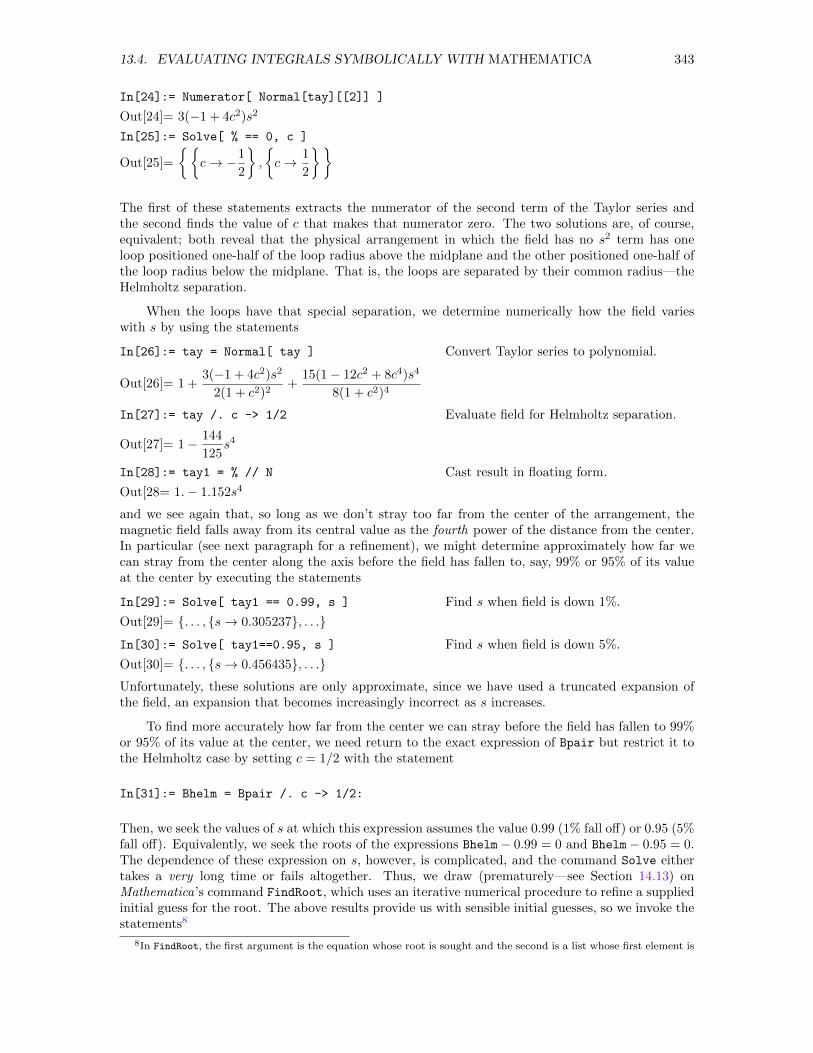
13.4. EVALUATING INTEGRALS SYMBOLICALLY WITH MATHEMATICA 343

In[24]:= Numerator[ Normal[tay][[2]] ]

Out[24]= 3(−1 + 4c2)s2

In[25]:= Solve[ % == 0, c ]

Out[25]=

c→ −1

2

,

c→ 1

2

The first of these statements extracts the numerator of the second term of the Taylor series andthe second finds the value of c that makes that numerator zero. The two solutions are, of course,equivalent; both reveal that the physical arrangement in which the field has no s2 term has oneloop positioned one-half of the loop radius above the midplane and the other positioned one-half ofthe loop radius below the midplane. That is, the loops are separated by their common radius—theHelmholtz separation.

When the loops have that special separation, we determine numerically how the field varieswith s by using the statements

In[26]:= tay = Normal[ tay ]

Out[26]= 1 +3(−1 + 4c2)s2

2(1 + c2)2+

15(1− 12c2 + 8c4)s4

8(1 + c2)4

Convert Taylor series to polynomial.

In[27]:= tay /. c -> 1/2

Out[27]= 1− 144

125s4

Evaluate field for Helmholtz separation.

In[28]:= tay1 = % // N

Out[28= 1.− 1.152s4Cast result in floating form.

and we see again that, so long as we don’t stray too far from the center of the arrangement, themagnetic field falls away from its central value as the fourth power of the distance from the center.In particular (see next paragraph for a refinement), we might determine approximately how far wecan stray from the center along the axis before the field has fallen to, say, 99% or 95% of its valueat the center by executing the statements

In[29]:= Solve[ tay1 == 0.99, s ]

Out[29]= . . . , s→ 0.305237, . . .Find s when field is down 1%.

In[30]:= Solve[ tay1==0.95, s ]

Out[30]= . . . , s→ 0.456435, . . .Find s when field is down 5%.

Unfortunately, these solutions are only approximate, since we have used a truncated expansion ofthe field, an expansion that becomes increasingly incorrect as s increases.

To find more accurately how far from the center we can stray before the field has fallen to 99%or 95% of its value at the center, we need return to the exact expression of Bpair but restrict it tothe Helmholtz case by setting c = 1/2 with the statement

In[31]:= Bhelm = Bpair /. c -> 1/2:

Then, we seek the values of s at which this expression assumes the value 0.99 (1% fall off) or 0.95 (5%fall off). Equivalently, we seek the roots of the expressions Bhelm− 0.99 = 0 and Bhelm− 0.95 = 0.The dependence of these expression on s, however, is complicated, and the command Solve eithertakes a very long time or fails altogether. Thus, we draw (prematurely—see Section 14.13) onMathematica’s command FindRoot, which uses an iterative numerical procedure to refine a suppliedinitial guess for the root. The above results provide us with sensible initial guesses, so we invoke thestatements8

8In FindRoot, the first argument is the equation whose root is sought and the second is a list whose first element is

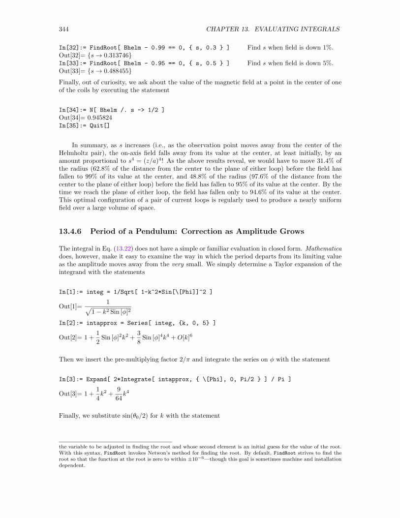
344 CHAPTER 13. EVALUATING INTEGRALS

In[32]:= FindRoot[ Bhelm - 0.99 == 0, s, 0.3 ]

Out[32]= s→ 0.313746In[33]:= FindRoot[ Bhelm - 0.95 == 0, s, 0.5 ]

Out[33]= s→ 0.488455

Find s when field is down 1%.

Find s when field is down 5%.

Finally, out of curiosity, we ask about the value of the magnetic field at a point in the center of oneof the coils by executing the statement

In[34]:= N[ Bhelm /. s -> 1/2 ]

Out[34]= 0.945824In[35]:= Quit[]

In summary, as s increases (i.e., as the observation point moves away from the center of theHelmholtz pair), the on-axis field falls away from its value at the center, at least initially, by anamount proportional to s4 = (z/a)4! As the above results reveal, we would have to move 31.4% ofthe radius (62.8% of the distance from the center to the plane of either loop) before the field hasfallen to 99% of its value at the center, and 48.8% of the radius (97.6% of the distance from thecenter to the plane of either loop) before the field has fallen to 95% of its value at the center. By thetime we reach the plane of either loop, the field has fallen only to 94.6% of its value at the center.This optimal configuration of a pair of current loops is regularly used to produce a nearly uniformfield over a large volume of space.

13.4.6 Period of a Pendulum: Correction as Amplitude Grows

The integral in Eq. (13.22) does not have a simple or familiar evaluation in closed form. Mathematicadoes, however, make it easy to examine the way in which the period departs from its limiting valueas the amplitude moves away from the very small. We simply determine a Taylor expansion of theintegrand with the statements

In[1]:= integ = 1/Sqrt[ 1-k^2*Sin[\[Phi]]^2 ]

Out[1]=1√

1− k2 Sin [φ]2

In[2]:= intapprox = Series[ integ, k, 0, 5 ]

Out[2]= 1 +1

2Sin [φ]2k2 +

3

8Sin [φ]4k4 +O[k]6

Then we insert the pre-multiplying factor 2/π and integrate the series on φ with the statement

In[3]:= Expand[ 2*Integrate[ intapprox, \[Phi], 0, Pi/2 ] / Pi ]

Out[3]= 1 +1

4k2 +

9

64k4

Finally, we substitute sin(θ0/2) for k with the statement

the variable to be adjusted in finding the root and whose second element is an initial guess for the value of the root.With this syntax, FindRoot invokes Netwon’s method for finding the root. By default, FindRoot strives to find theroot so that the function at the root is zero to within ±10−6—though this goal is sometimes machine and installationdependent.

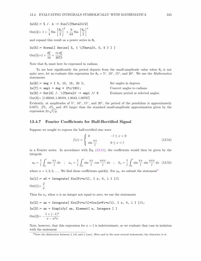
13.4. EVALUATING INTEGRALS SYMBOLICALLY WITH MATHEMATICA 345

In[4]:= % /. k -> Sin[\[Theta]0/2]

Out[4]= 1 +1

4Sin

[θ02

]2+

9

64Sin

[θ02

]4and expand this result as a power series in θ0

In[5]:= Normal[ Series[ %, \[Theta]0, 0, 5 ] ]

Out[5]=1 +θ2016

+11 θ403072

Note that θ0 must here be expressed in radians.

To see how significantly the period departs from the small-amplitude value when θ0 is notquite zero, let us evaluate this expression for θ0 = 5, 10, 15, and 20. We use the Mathematicastatements

In[6]:= deg = 5, 10, 15, 20 ;

In[7]:= ampl = deg * (Pi/180);

In[8]:= Out[4] /. \[Theta]0 -> ampl // N

Out[8]= [1.00048, 1.00191, 1.0043, 1.00767]

Set angles in degrees.

Convert angles to radians.

Evaluate period at selected angles.

Evidently, at amplitudes of 5, 10, 15, and 20, the period of the pendulum is approximately0.05%, .2%, .4%, and .8% larger than the standard small-amplitude approximation given by theexpression 2π

√l/g.

13.4.7 Fourier Coefficients for Half-Rectified Signal

Suppose we sought to express the half-rectified sine wave

f(x) =

0 −l ≤ x < 0

sinπx

l0 ≤ x < l

(13.54)

in a Fourier series. In accordance with Eq. (13.51), the coefficients would then be given by theintegrals

a0 =1

l

∫ l

0

sinπx

ldx ; an =

1

l

∫ l

0

sinπx

lcos

nπx

ldx ; bn =

1

l

∫ l

0

sinπx

lsin

nπx

ldx (13.55)

where n = 1, 2, 3, . . .. We find these coefficients quickly. For a0, we submit the statement9

In[1]:= a0 = Integrate[ Sin[Pi*x/l], x, 0, l ]/l

Out[1]=2

π

Then for an when n is an integer not equal to zero, we use the statements

In[2]:= an = Integrate[ Sin[Pi*x/l]*Cos[n*Pi*x/l], x, 0, l ]/l;

In[3]:= an = Simplify[ an, Element[ n, Integers ] ]

Out[3]= −1 + (−1)n

π − n2π

Note, however, that this expression for n = 1 is indeterminate, so we evaluate that case in isolationwith the statement

9Note the distinction between l (el) and 1 (one). Here and in the next several statements, the character is el.

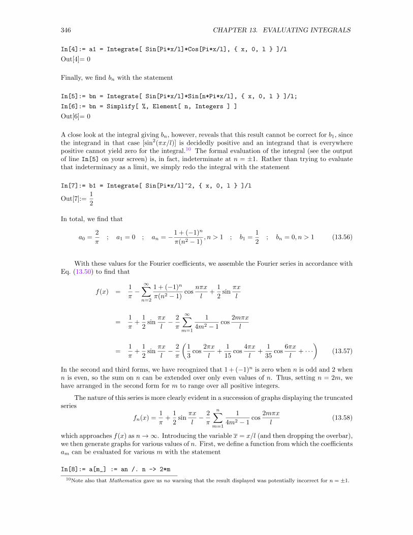
346 CHAPTER 13. EVALUATING INTEGRALS

In[4]:= a1 = Integrate[ Sin[Pi*x/l]*Cos[Pi*x/l], x, 0, l ]/l

Out[4]= 0

Finally, we find bn with the statement

In[5]:= bn = Integrate[ Sin[Pi*x/l]*Sin[n*Pi*x/l], x, 0, l ]/l;

In[6]:= bn = Simplify[ %, Element[ n, Integers ] ]

Out[6]= 0

A close look at the integral giving bn, however, reveals that this result cannot be correct for b1, sincethe integrand in that case [sin2(πx/l)] is decidedly positive and an integrand that is everywherepositive cannot yield zero for the integral.10 The formal evaluation of the integral (see the outputof line In[5] on your screen) is, in fact, indeterminate at n = ±1. Rather than trying to evaluatethat indeterminacy as a limit, we simply redo the integral with the statement

In[7]:= b1 = Integrate[ Sin[Pi*x/l]^2, x, 0, l ]/l

Out[7]:=1

2

In total, we find that

a0 =2

π; a1 = 0 ; an = −1 + (−1)n

π(n2 − 1), n > 1 ; b1 =

1

2; bn = 0, n > 1 (13.56)

With these values for the Fourier coefficients, we assemble the Fourier series in accordance withEq. (13.50) to find that

f(x) =1

π−∞∑n=2

1 + (−1)n

π(n2 − 1)cos

nπx

l+

1

2sin

πx

l

=1

π+

1

2sin

πx

l− 2

π

∞∑m=1

1

4m2 − 1cos

2mπx

l

=1

π+

1

2sin

πx

l− 2

π

(1

3cos

2πx

l+

1

15cos

4πx

l+

1

35cos

6πx

l+ · · ·

)(13.57)

In the second and third forms, we have recognized that 1 + (−1)n is zero when n is odd and 2 whenn is even, so the sum on n can be extended over only even values of n. Thus, setting n = 2m, wehave arranged in the second form for m to range over all positive integers.

The nature of this series is more clearly evident in a succession of graphs displaying the truncatedseries

fn(x) =1

π+

1

2sin

πx

l− 2

π

n∑m=1

1

4m2 − 1cos

2mπx

l(13.58)

which approaches f(x) as n→∞. Introducing the variable x = x/l (and then dropping the overbar),we then generate graphs for various values of n. First, we define a function from which the coefficientsam can be evaluated for various m with the statement

In[8]:= a[m_] := an /. n -> 2*m

10Note also that Mathematica gave us no warning that the result displayed was potentially incorrect for n = ±1.

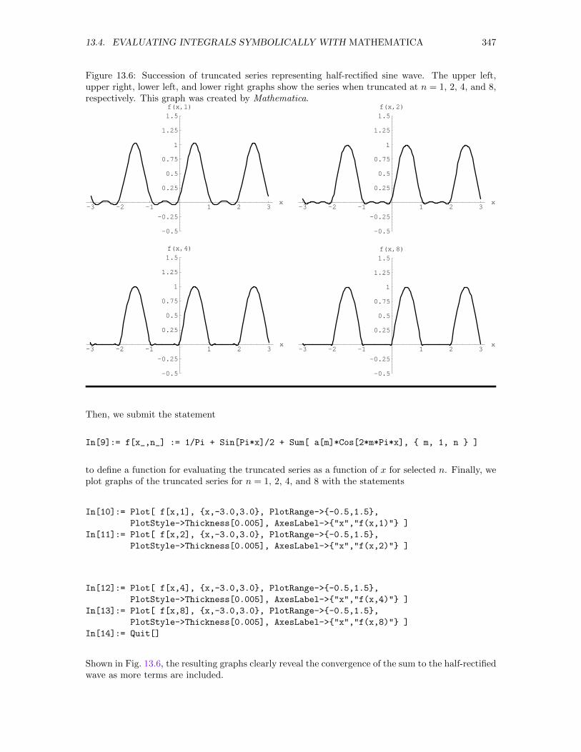
13.4. EVALUATING INTEGRALS SYMBOLICALLY WITH MATHEMATICA 347

Figure 13.6: Succession of truncated series representing half-rectified sine wave. The upper left,upper right, lower left, and lower right graphs show the series when truncated at n = 1, 2, 4, and 8,respectively. This graph was created by Mathematica.

-3 -2 -1 1 2 3x

-0.5

-0.25

0.25

0.5

0.75

1

1.25

1.5

f(x,1)

-3 -2 -1 1 2 3x

-0.5

-0.25

0.25

0.5

0.75

1

1.25

1.5

f(x,2)

-3 -2 -1 1 2 3x

-0.5

-0.25

0.25

0.5

0.75

1

1.25

1.5

f(x,4)

-3 -2 -1 1 2 3x

-0.5

-0.25

0.25

0.5

0.75

1

1.25

1.5

f(x,8)

Then, we submit the statement

In[9]:= f[x_,n_] := 1/Pi + Sin[Pi*x]/2 + Sum[ a[m]*Cos[2*m*Pi*x], m, 1, n ]

to define a function for evaluating the truncated series as a function of x for selected n. Finally, weplot graphs of the truncated series for n = 1, 2, 4, and 8 with the statements

In[10]:= Plot[ f[x,1], x,-3.0,3.0, PlotRange->-0.5,1.5,

PlotStyle->Thickness[0.005], AxesLabel->"x","f(x,1)" ]

In[11]:= Plot[ f[x,2], x,-3.0,3.0, PlotRange->-0.5,1.5,

PlotStyle->Thickness[0.005], AxesLabel->"x","f(x,2)" ]

In[12]:= Plot[ f[x,4], x,-3.0,3.0, PlotRange->-0.5,1.5,

PlotStyle->Thickness[0.005], AxesLabel->"x","f(x,4)" ]

In[13]:= Plot[ f[x,8], x,-3.0,3.0, PlotRange->-0.5,1.5,

PlotStyle->Thickness[0.005], AxesLabel->"x","f(x,8)" ]

In[14]:= Quit[]

Shown in Fig. 13.6, the resulting graphs clearly reveal the convergence of the sum to the half-rectifiedwave as more terms are included.

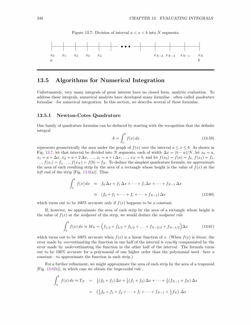
348 CHAPTER 13. EVALUATING INTEGRALS

Figure 13.7: Division of interval a < x < b into N segments.

s s sa

x0 x1 x2 x3 x4 xN−3 xN−2 xN−1 xNb

13.5 Algorithms for Numerical Integration

Unfortunately, very many integrals of great interest have no closed form, analytic evaluation. Toaddress these integrals, numerical analysts have developed many formulae—often called quadratureformulae—for numerical integration. In this section, we describe several of these formulae.

13.5.1 Newton-Cotes Quadrature

One family of quadrature formulae can be deduced by starting with the recognition that the definiteintegral

A =

∫ b

a

f(x) dx (13.59)

represents geometrically the area under the graph of f(x) over the interval a ≤ x ≤ b. As shown inFig. 13.7, let that interval be divided into N segments, each of width ∆x = (b − a)/N , let x0 = a,x1 = a+ ∆x, x2 = a+ 2 ∆x, . . ., xi = a+ i∆x, . . ., xN = b, and let f(x0) = f(a) = f0, f(x1) = f1,. . ., f(xi) = fi, . . ., f(xN ) = f(b) = fN . To deduce the simplest quadrature formula, we approximatethe area of each resulting strip by the area of a rectangle whose height is the value of f(x) at theleft end of the strip [Fig. 13.8(a)]. Thus∫ b

a

f(x) dx ≈ f0 ∆x+ f1 ∆x+ · · ·+ fi ∆x+ · · ·+ fN−1 ∆x

≈ (f0 + f1 + · · ·+ fi + · · ·+ fN−1) ∆x (13.60)

which turns out to be 100% accurate only if f(x) happens to be a constant.

If, however, we approximate the area of each strip by the area of a rectangle whose height isthe value of f(x) at the midpoint of the strip, we would deduce the midpoint rule∫ b

a

f(x) dx ≈MN =(f1/2 + f3/2 + f5/2 + . . .+ fN−3/2 + fN−1/2

)∆x (13.61)

which turns out to be 100% accurate when f(x) is a linear function of x. (When f(x) is linear, theerror made by overestimating the function in one half of the interval is exactly compensated by theerror made by underestimating the function in the other half of the interval. The formula turnsout to be 100% accurate for a polynomial of one higher order than the polynomial used—here aconstant—to approximate the function in each strip.)

For a further refinement, we might approximate the area of each strip by the area of a trapezoid[Fig. 13.8(b)], in which case we obtain the trapezoidal rule ,∫ b

a

f(x) dx ≈ TN = 12 (f0 + f1) ∆x+ 1

2 (f1 + f2) ∆x+ · · ·+ 12 (fN−1 + fN ) ∆x

=(12f0 + f1 + f2 + · · ·+ fi + · · ·+ fN−1 + 1

2fN)

∆x

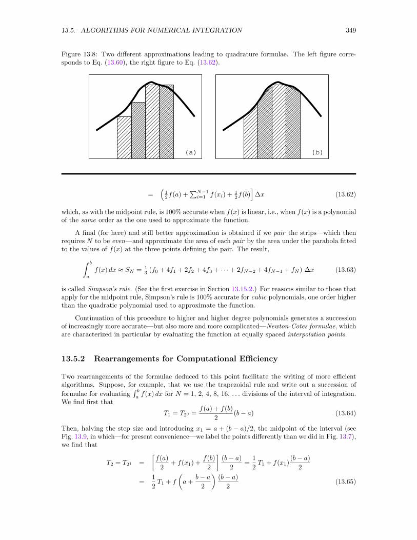
13.5. ALGORITHMS FOR NUMERICAL INTEGRATION 349

Figure 13.8: Two different approximations leading to quadrature formulae. The left figure corre-sponds to Eq. (13.60), the right figure to Eq. (13.62).

(a) (b)

=(

12f(a) +

∑N−1i=1 f(xi) + 1

2f(b)]

∆x (13.62)

which, as with the midpoint rule, is 100% accurate when f(x) is linear, i.e., when f(x) is a polynomialof the same order as the one used to approximate the function.

A final (for here) and still better approximation is obtained if we pair the strips—which thenrequires N to be even—and approximate the area of each pair by the area under the parabola fittedto the values of f(x) at the three points defining the pair. The result,∫ b

a

f(x) dx ≈ SN = 13 (f0 + 4f1 + 2f2 + 4f3 + · · ·+ 2fN−2 + 4fN−1 + fN ) ∆x (13.63)

is called Simpson’s rule. (See the first exercise in Section 13.15.2.) For reasons similar to those thatapply for the midpoint rule, Simpson’s rule is 100% accurate for cubic polynomials, one order higherthan the quadratic polynomial used to approximate the function.

Continuation of this procedure to higher and higher degree polynomials generates a successionof increasingly more accurate—but also more and more complicated—Newton-Cotes formulae, whichare characterized in particular by evaluating the function at equally spaced interpolation points.

13.5.2 Rearrangements for Computational Efficiency

Two rearrangements of the formulae deduced to this point facilitate the writing of more efficientalgorithms. Suppose, for example, that we use the trapezoidal rule and write out a succession of

formulae for evaluating∫ baf(x) dx for N = 1, 2, 4, 8, 16, . . . divisions of the interval of integration.

We find first that

T1 = T20 =f(a) + f(b)

2(b− a) (13.64)

Then, halving the step size and introducing x1 = a + (b − a)/2, the midpoint of the interval (seeFig. 13.9, in which—for present convenience—we label the points differently than we did in Fig. 13.7),we find that

T2 = T21 =

[f(a)

2+ f(x1) +

f(b)

2

](b− a)

2=

1

2T1 + f(x1)

(b− a)

2

=1

2T1 + f

(a+

b− a2

)(b− a)

2(13.65)

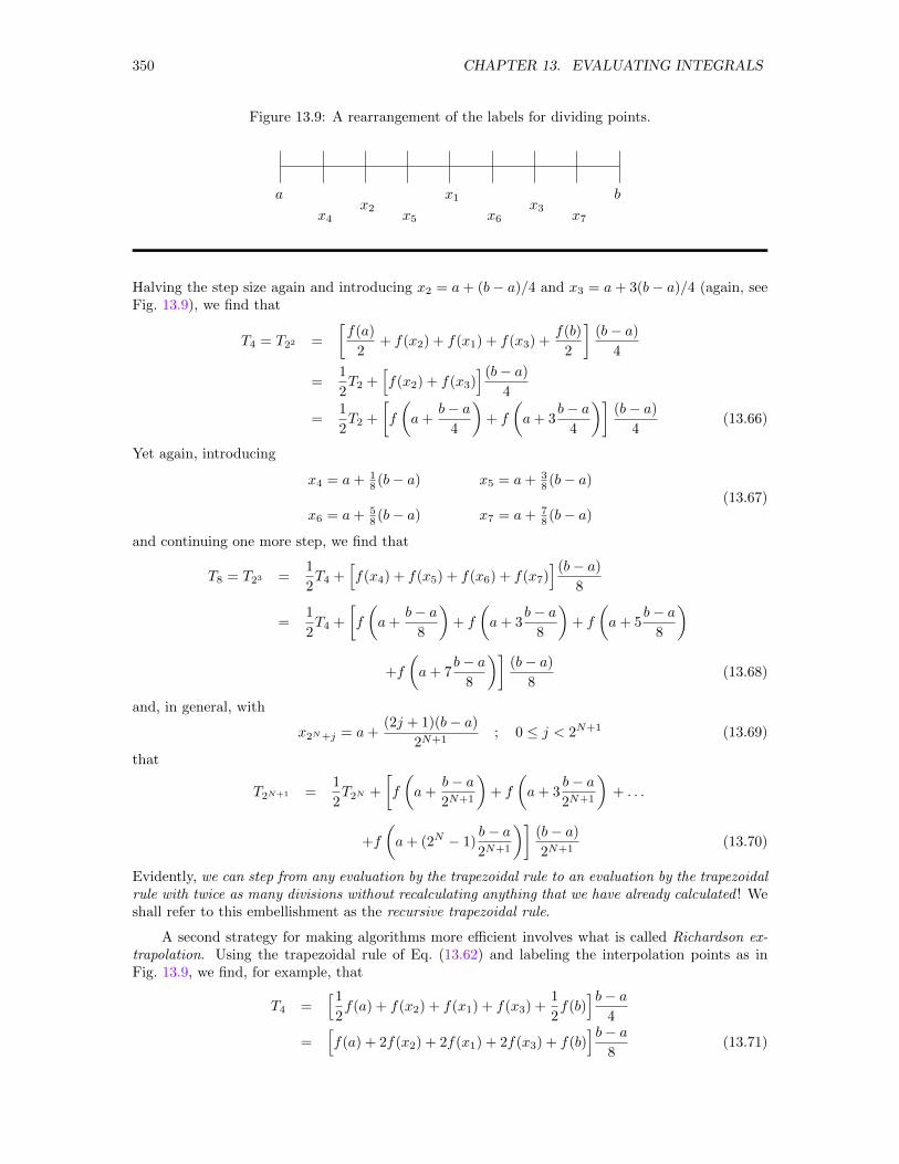
350 CHAPTER 13. EVALUATING INTEGRALS

Figure 13.9: A rearrangement of the labels for dividing points.

a

x4x2

x5

x1

x6x3

x7

b

Halving the step size again and introducing x2 = a+ (b− a)/4 and x3 = a+ 3(b− a)/4 (again, seeFig. 13.9), we find that

T4 = T22 =

[f(a)

2+ f(x2) + f(x1) + f(x3) +

f(b)

2

](b− a)

4

=1

2T2 +

[f(x2) + f(x3)

] (b− a)

4

=1

2T2 +

[f

(a+

b− a4

)+ f

(a+ 3

b− a4

)](b− a)

4(13.66)

Yet again, introducing

x4 = a+ 18 (b− a) x5 = a+ 3

8 (b− a)

x6 = a+ 58 (b− a) x7 = a+ 7

8 (b− a)(13.67)

and continuing one more step, we find that

T8 = T23 =1

2T4 +

[f(x4) + f(x5) + f(x6) + f(x7)

] (b− a)

8

=1

2T4 +

[f

(a+

b− a8

)+ f

(a+ 3

b− a8

)+ f

(a+ 5

b− a8

)

+f

(a+ 7

b− a8

)](b− a)

8(13.68)

and, in general, with

x2N+j = a+(2j + 1)(b− a)

2N+1; 0 ≤ j < 2N+1 (13.69)

that

T2N+1 =1

2T2N +

[f

(a+

b− a2N+1

)+ f

(a+ 3

b− a2N+1

)+ . . .

+f

(a+ (2N − 1)

b− a2N+1

)](b− a)

2N+1(13.70)

Evidently, we can step from any evaluation by the trapezoidal rule to an evaluation by the trapezoidalrule with twice as many divisions without recalculating anything that we have already calculated ! Weshall refer to this embellishment as the recursive trapezoidal rule.

A second strategy for making algorithms more efficient involves what is called Richardson ex-trapolation. Using the trapezoidal rule of Eq. (13.62) and labeling the interpolation points as inFig. 13.9, we find, for example, that

T4 =[1

2f(a) + f(x2) + f(x1) + f(x3) +

1

2f(b)

]b− a4

=[f(a) + 2f(x2) + 2f(x1) + 2f(x3) + f(b)

]b− a8

(13.71)

13.5. ALGORITHMS FOR NUMERICAL INTEGRATION 351

and that

T8 =

[1

2f(a) + f(x4) + f(x2) + f(x5)

+f(x1) + f(x6) + f(x3) + f(x7) +1

2f(b)

]b− a

8(13.72)

Note, in particular, the combination

4T8 − T43

=[f(a) + 4f(x4) + 2f(x2) + 4f(x5) + 2f(x1)

+4f(x6) + 2f(x3) + 4f(x7) + f(b)]( b− a

8× 3

)(13.73)

and recognize that (b − a)/8 = ∆x is the width of a single strip when the interval a < x < b isdivided into eight segments. Thus, we can write this last expression as

4T8 − T43

=[f(a) + 4f(x4) + 2f(x2) + 4f(x5) + 2f(x1)

+4f(x6) + 2f(x3) + 4f(x7) + f(b)](∆x

3

)(13.74)

which—mirabile dictu—we recognize as Simpson’s rule for evaluating the integral with 8 divisionsof the interval! We conclude that

S8 =4T8 − T4

3(13.75)

More generally, we could also conclude that

S2n =4T2n − Tn

3(13.76)

The extrapolation formula of Eq. (13.76) applied to two successive evaluations by the trapezoidalrule gives the result of evaluation by Simpson’s rule!

A subroutine for trapezoidal integration can thus be used in a very efficient algorithm forevaluating integrals by Simpson’s rule. We evaluate the integral twice by the trapezoidal rule fortwo values of n, one of which is twice the other, finding Tn and T2n. Then we find the Simpson’srule evaluation by exploiting the extrapolation formula of Eq. (13.76), which expresses the first stepin what is called Romberg integration. We do actual numerical integration only with the trapezoidalrule, and we invoke the efficiency described in the first paragraph of this subsection in doing that. Aroutine for integration via the trapezoidal rule can thus be the workhorse for many other routines.

Indeed, Romberg integration goes beyond simply generating evaluations by Simpson’s rule fromevaluations by the trapezoidal rule. Suppose we used the trapezoidal rule to generate the four valuesTn, T2n, T4n, and T8n. We could then use Eq. (13.76) to generate the three values S2n, S4n, andS8n. In Romberg integration, we next generate a pair of still more accurate values from the formulaeX4n = (16S4n−S2n)/15 and X8n = (16S8n−S4n)/15; and then we generate a further improved valuefrom the formula Y8n = (64X8n −X4n)/63. This process can, of course, be continued indefinitely—though we rarely have to go even as far as we have described.

13.5.3 Assessing Error

Numerical evaluations, of course, only approximate the integral. Two distinctly different sorts oferrors can occur. Truncation errors arise because the integral has been approximated by a finitesum; roundoff errors arise because computers do not store non-integers to 100% precision and, in theevaluation of a sum, the imprecision with which each component is represented within the computer

352 CHAPTER 13. EVALUATING INTEGRALS

can accumulate as the number of arithmetic operations increases. Truncation errors become smalleras the width of strips is reduced. Roundoff errors, unfortunately, become more significant as thewidth of strips is reduced (because, with narrower strips, more arithmetic must be done). Usually,roundoff errors are negligible, the more so as the sophistication of the algorithm increases (and,hence, the amount of arithmetic decreases). Provided we do not strive for accuracy greater thanabout 1 part in 105 or 106 (with single precision floating point arithmetic), we can usually ignoreroundoff errors. Thus, provided the function being integrated is such that the algorithm convergesfairly rapidly with decreasing strip width, the quickest way to obtain a reasonably reliable estimateof truncation error is to evaluate the integral with two different step widths, the second being half ofthe first, and compare the two results. Presuming that roundoff error has not begun to be important,we can be confident that the second result is more accurate than the first. Thus, if the two agree to1 part in 103, say, we can with reasonable confidence, assume that the second value is good to onepart in 103. Indeed, the second value is probably better than that, but assessing its accuracy by thismethod would entail obtaining a third value by using a strip width half of that used to determinethe second value.11 Indeed, one strategy for achieving a desired accuracy with reasonable certaintyis to evaluate an integral repeatedly by a particular method, halving the strip width each time, andcontinuing until the new value received differs from its predecessor by less than the desired accuracy(though we must be careful not to push this approach so far that roundoff problems within thecomputer begin to become significant).12

From a more sophisticated perspective, numerical analysts have deduced expressions for theerror in various Newton-Cotes formulae.13 For the midpoint formula of Eq. (13.61), for example,∣∣∣∣∣

∫ b

a

f(x) dx−MN

∣∣∣∣∣ =(b− a)3

24N2

∣∣∣∣d 2f

dx2

∣∣∣∣x=ξ

(13.77)

where ξ is some value of x satisfying a < ξ < b—an expression that is valid provided the functionf(x) satisfies suitable requirements on continuity. The similar expressions∣∣∣∣∣

∫ b

a

f(x) dx− TN

∣∣∣∣∣ =(b− a)3

12N2

∣∣∣∣d 2f

dx2

∣∣∣∣x=ξ

(13.78)

and ∣∣∣∣∣∫ b

a

f(x) dx− SN

∣∣∣∣∣ =(b− a)5

180N4

∣∣∣∣d 4f

dx4

∣∣∣∣x=ξ

(13.79)

can be derived for the trapezoidal rule given by Eq. (13.62) and for Simpson’s rule given byEq. (13.63), respectively. Again, ξ is a value somewhere between x = a and x = b, though itis not likely to have the same value in all three formulae.

These results do not, of course, tell us how to determine the error exactly because they don’t tellus how to determine ξ exactly. Even so, they are not entirely useless, having at least two particularvalues:

1. If it should happen in the first two cases that d 2f/dx2 = 0 or in the third case that d 4f/dx4 = 0throughout the interval of integration, then the error is zero, since the right hand side of theseexpressions gives zero for all possible values of ξ. Thus, these formulae confirm our previousassertions that the midpoint and trapezoidal rules will be 100% accurate for linear functionsand that Simpson’s rule will be 100% accurate for cubic polynomials.

11We shall make this criterion a bit more explicit in the next paragraphs.12We shall see in later sections how we might decide when roundoff has started to be significant.13These formulae may be found in several sources, including Philip J. Davis and Philip Rabinowitz, Numerical

Integration (Blaisdell Publishing Company, Waltham, MA, 1967), pp. 17, 20; and Milton Abramowitz and IreneA. Stegun, Handbook of Mathematical Functions (National Bureau of Standards Applied Mathematics Series 55,June, 1964), pp. 885ff.

13.5. ALGORITHMS FOR NUMERICAL INTEGRATION 353

2. If Dmax(i) is the maximum value of d if/dxi in the interval a < x < b, then the aboveexpressions support the inequalities∣∣∣∣∣

∫ b

a

f(x) dx−MN

∣∣∣∣∣ ≤ (b− a)3

24N2Dmax(2) (13.80)

∣∣∣∣∣∫ b

a

f(x) dx− TN

∣∣∣∣∣ ≤ (b− a)3

12N2Dmax(2) (13.81)

∣∣∣∣∣∫ b

a

f(x) dx− SN

∣∣∣∣∣ ≤ (b− a)5

180N4Dmax(4) (13.82)

(though we must keep in mind that these approximations will frequently be extremely crude,so these upper bounds may well be very conservative). Provided that problems with computerroundoff do not begin to appear, we conclude from these results that an upper bound on theerror in the midpoint and trapezoidal rules falls off like 1/N2 while that bound in Simpson’srule falls off like 1/N4. Doubling N therefore reduces the error in the midpoint and trapezoidalrules by a factor of four, while doubling N reduces the error in Simpson’s rule by a factor ofsixteen. With Simpson’s rule, every doubling of N should gain at least one more decimal pointin accuracy, so the convergence criterion described in the first paragraph in this subsection isparticularly apt when Simpson’s rule is used.

13.5.4 Iterative and Adaptive Algorithms

In the previous subsections, we assumed that the user of a particular algorithm would actually viewthe value obtained for a succession of values of N and decide personally when to stop by examiningthe changes that occur as N is successively doubled. We can, of course, program a computer tomake those decisions. One extremely common approach exploits Simpson’s rule (probably via thetrapezoidal rule and Romberg integration) to obtain S2, S4, S8, . . ., compares each new value withits predecessor and stops when the absolute value of the difference is smaller than a tolerance—eitherabsolute or relative—prescribed in advance. As a guard against an infinite loop, these algorithmsshould also stop if the desired tolerance has not been achieved in some maximum number of refine-ments and should print a warning when the desired tolerance has not been achieved. This methodis said to be iterative, because it generates a succession of results, examines each new result in turn,and repeats the process until the new result meets or exceeds the prescribed tolerance. The pointsat which the function is evaluated, however, are determined ahead of time and are not influenced atall by the nature of the specific integrand to which the algorithm is applied.

Another family of algorithms (which may be iterative or noniterative) aims to minimize com-putational labor by estimating—though the methods for doing so are often crude—the accuracyobtained with each strip as the evaluation unfolds and shrinking or enlarging that strip to achievea particular tolerance before going on to the next strip. In these adaptive methods, the points atwhich the function is evaluated are adjusted in response to the particular function being integrated.Because the assessment of accuracy at a particular strip can result either in shrinking or enlargingthe width of that—or the next—strip, adaptive methods focus the computational effort in regionswhere the function varies rapidly and give less attention to regions in which the function variesslowly.

13.5.5 Gaussian Quadrature

The approach of Gaussian quadrature to numerical integration is more complicated than the Newton-Cotes approach but significantly better in some respects. In the Gaussian approach, both the points

354 CHAPTER 13. EVALUATING INTEGRALS

at which the function is to be evaluated and the weights to be applied to each value are adjusted toachieve maximum accuracy when the function is approximated by a polynomial of a given order.

The development of a formula for Gaussian quadrature is simplified if we begin by introducinga set of m + 1 points ti, (i = 0, 1, 2, . . . ,m) that divide the interval t0 = a ≤ t ≤ b = tm into msegments, the i-th of which extends over the interval ti−1 ≤ t ≤ ti. The values ti may—but neednot—be equally spaced. In this notation, we write the integral of interest as a sum of integrals overeach segment, i.e., we write ∫ b

a

g(t) dt =

m∑i=1

∫ ti+1

ti

g(t) dt (13.83)

To facilitate the discussion, however, we rescale and translate the variable in the i-th segment byintroducing the variable x defined by

x =2t− (ti+1 + ti)

ti+1 − tior t =

ti+1 + ti2

+ti+1 − ti

2x = tmid

i +∆ti2x (13.84)

where tmidi is the coordinate at the midpoint of the i-th segment and ∆ti is the width of the i-th

segment. With this change, x ranges from −1 to +1 as t ranges from ti to ti+1, so the integrals ofinterest now assume the form∫ b

a

g(t) dt =

m∑i=1

∫ ti+1

ti

g(t) dt =

m∑i=1

∆ti2

∫ 1

−1g

(tmidi +

∆ti2x

)dx =

m∑i=1

∆ti2

∫ 1

−1fi(x) dx (13.85)

where fi(x) = g(tmidi + ∆ti x/2). In essence, then, we must evaluate an integral of the form∫ 1

−1f(x) dx (13.86)

where we omit the subscript i on f for the sake of a simpler notation. If we can find a useful numericalevaluation for the integral in this standard form, then all else can be obtained by appropriatetranslations and rescalings.

The strategy for Gaussian integration now involves selecting the number of points—say N—atwhich the function is to be evaluated in the interval −1 < x < 1, assuming an approximate formulaof the form ∫ 1

−1f(x) dx =

N∑k=1

wk f(xk) (13.87)

and then choosing both the weights wk and the points of evaluation xk to make this expression100% accurate for a polynomial of as high an order as possible. Since we have 2N parameters to bedetermined, we should be able to make this expression accurate for a polynomial of order 2N − 1with only N evaluations of the integrand.

To illustrate Gaussian integration more explicitly, let us derive a two-point formula, for whichEq. (13.87) would assume the more explicit form∫ 1

−1f(x) dx = w1 f(x1) + w2 f(x2) (13.88)

We choose w1, w2, x1 and x2 so that the formula gives the correct answer for the special cases

f(x) = 1, yielding that

∫ 1

−1dx = 2 = w1 + w2 (13.89)

f(x) = x, yielding that

∫ 1

−1x dx = 0 = w1x1 + w2x2 (13.90)

f(x) = x2, yielding that

∫ 1

−1x2 dx =

2

3= w1x

21 + w2x

22 (13.91)

f(x) = x3, yielding that

∫ 1

−1x3 dx = 0 = w1x

31 + w2x

32 (13.92)

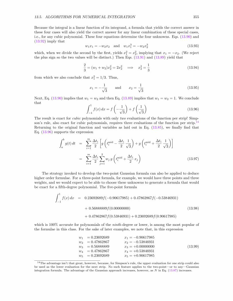
13.5. ALGORITHMS FOR NUMERICAL INTEGRATION 355

Because the integral is a linear function of its integrand, a formula that yields the correct answer inthese four cases will also yield the correct answer for any linear combination of these special cases,i.e., for any cubic polynomial. These four equations determine the four unknowns. Eqs. (13.90) and(13.92) imply that

w1x1 = −w2x2 and w1x31 = −w2x

32 (13.93)

which, when we divide the second by the first, yields x21 = x22, implying that x1 = −x2. (We rejectthe plus sign so the two values will be distinct.) Then Eqs. (13.91) and (13.89) yield that

2

3= (w1 + w2)x22 = 2x22 =⇒ x22 =

1

3(13.94)

from which we also conclude that x21 = 1/3. Thus,

x1 = − 1√3

and x2 =1√3

(13.95)

Next, Eq. (13.90) implies that w1 = w2 and then Eq. (13.89) implies that w1 = w2 = 1. We concludethat ∫ 1

−1f(x) dx = f

(− 1√

3

)+ f

(1√3

)(13.96)

The result is exact for cubic polynomials with only two evaluations of the function per strip! Simp-son’s rule, also exact for cubic polynomials, requires three evaluations of the function per strip.14

Returning to the original function and variables as laid out in Eq. (13.85), we finally find thatEq. (13.96) supports the expression∫ b

a

g(t) dt =

m∑i=1

∆ti2

[g

(tmidi − ∆ti

2

1√3

)+ g

(tmidi +

∆ti2

1√3

)]

=

m∑i=1

∆ti2

2∑j=1

wj g

(tmidi +

∆ti2xj

)(13.97)

The strategy invoked to develop the two-point Gaussian formula can also be applied to deducehigher order formulae. For a three-point formula, for example, we would have three points and threeweights, and we would expect to be able to choose these unknowns to generate a formula that wouldbe exact for a fifth-degree polynomial. The five-point formula∫ 1

−1f(x) dx = 0.23692689f(−0.90617985) + 0.47862867f(−0.53846931)

+ 0.56888889f(0.00000000) (13.98)

+ 0.47862867f(0.53846931) + 0.23692689f(0.90617985)

which is 100% accurate for polynomials of the ninth-degree or lower, is among the most popular ofthe formulae in this class. For the sake of later examples, we note that, in this expression

w1 = 0.23692689 x1 = −0.90617985w2 = 0.47862867 x2 = −0.53846931w3 = 0.56888889 x3 = +0.00000000w4 = 0.47862867 x4 = +0.53846931w5 = 0.23692689 x5 = +0.90617985

(13.99)

14The advantage isn’t that great, however, because, for Simpson’s rule, the upper evaluation for one strip could alsobe used as the lower evaluation for the next strip. No such feature applies to the two-point—or to any—Gaussianintegration formula. The advantage of the Gaussian approach increases, however, as N in Eq. (13.87) increases.

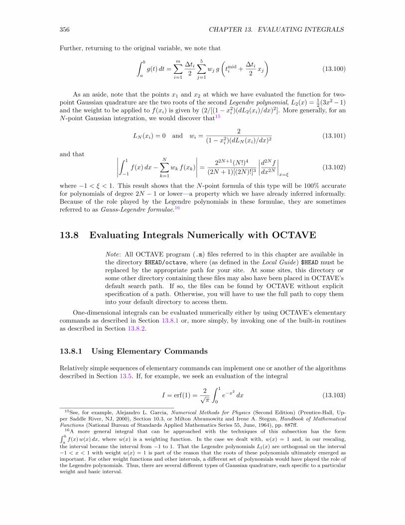
356 CHAPTER 13. EVALUATING INTEGRALS

Further, returning to the original variable, we note that∫ b

a

g(t) dt =

m∑i=1

∆ti2

5∑j=1

wj g

(tmidi +

∆ti2xj

)(13.100)

As an aside, note that the points x1 and x2 at which we have evaluated the function for two-point Gaussian quadrature are the two roots of the second Legendre polynomial, L2(x) = 1

2 (3x2− 1)and the weight to be applied to f(xi) is given by (2/[(1− x2i )(dL2(xi)/dx)2]. More generally, for anN -point Gaussian integration, we would discover that15

LN (xi) = 0 and wi =2

(1− x2i )(dLN (xi)/dx)2(13.101)

and that ∣∣∣∣∣∫ 1

−1f(x) dx−

N∑k=1

wk f(xk)

∣∣∣∣∣ =22N+1(N !)4

(2N + 1)[(2N)!]3

∣∣∣∣d2Nfdx2N

∣∣∣∣x=ξ

(13.102)

where −1 < ξ < 1. This result shows that the N -point formula of this type will be 100% accuratefor polynomials of degree 2N − 1 or lower—a property which we have already inferred informally.Because of the role played by the Legendre polynomials in these formulae, they are sometimesreferred to as Gauss-Legendre formulae.16

13.8 Evaluating Integrals Numerically with OCTAVE

Note: All OCTAVE program (.m) files referred to in this chapter are available inthe directory $HEAD/octave, where (as defined in the Local Guide) $HEAD must bereplaced by the appropriate path for your site. At some sites, this directory orsome other directory containing these files may also have been placed in OCTAVE’sdefault search path. If so, the files can be found by OCTAVE without explicitspecification of a path. Otherwise, you will have to use the full path to copy theminto your default directory to access them.

One-dimensional integrals can be evaluated numerically either by using OCTAVE’s elementarycommands as described in Section 13.8.1 or, more simply, by invoking one of the built-in routinesas described in Section 13.8.2.

13.8.1 Using Elementary Commands

Relatively simple sequences of elementary commands can implement one or another of the algorithmsdescribed in Section 13.5. If, for example, we seek an evaluation of the integral

I = erf(1) =2√π

∫ 1

0

e−x2

dx (13.103)

15See, for example, Alejandro L. Garcia, Numerical Methods for Physics (Second Edition) (Prentice-Hall, Up-per Saddle River, NJ, 2000), Section 10.3, or Milton Abramowitz and Irene A. Stegun, Handbook of MathematicalFunctions (National Bureau of Standards Applied Mathematics Series 55, June, 1964), pp. 887ff.

16A more general integral that can be approached with the techniques of this subsection has the form∫ baf(x)w(x) dx, where w(x) is a weighting function. In the case we dealt with, w(x) = 1 and, in our rescaling,

the interval became the interval from −1 to 1. That the Legendre polynomials Ll(x) are orthogonal on the interval−1 < x < 1 with weight w(x) = 1 is part of the reason that the roots of these polynomials ultimately emerged asimportant. For other weight functions and other intervals, a different set of polynomials would have played the role ofthe Legendre polynomials. Thus, there are several different types of Gaussian quadrature, each specific to a particularweight and basic interval.

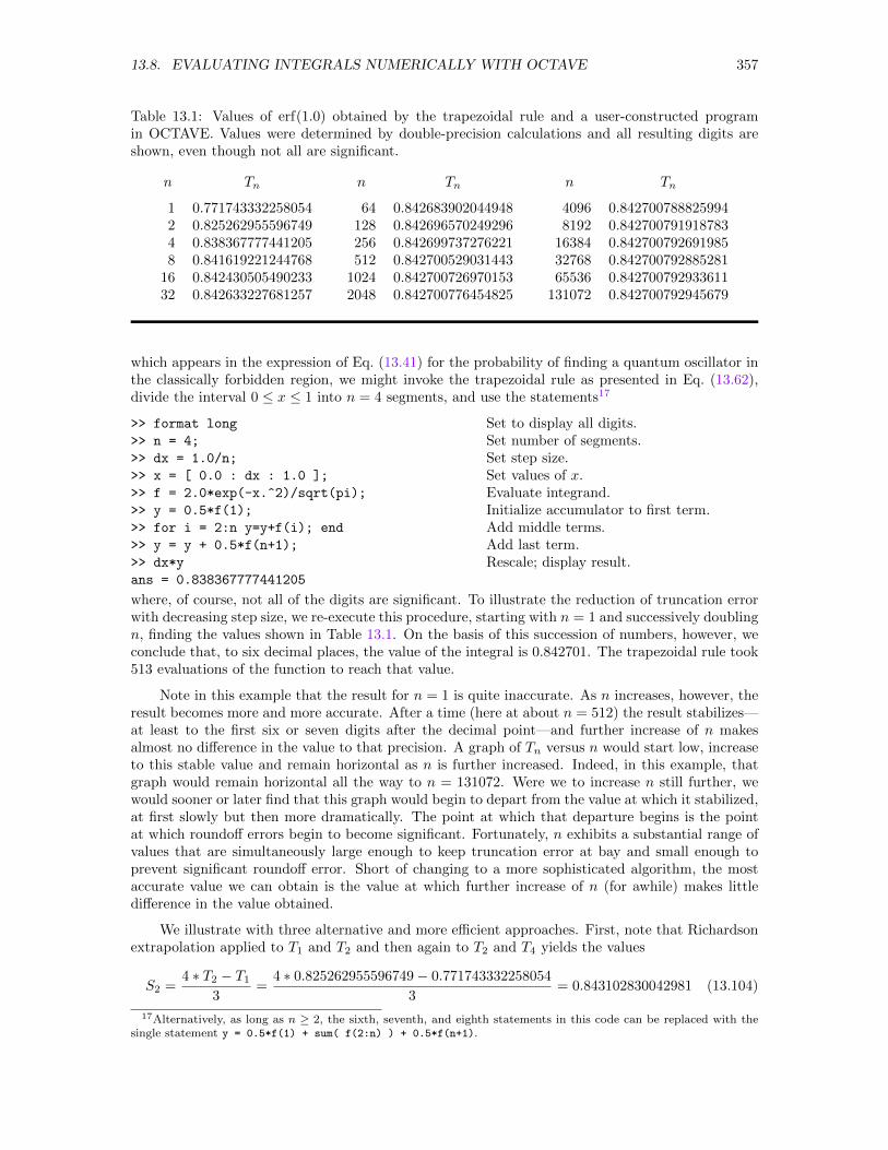
13.8. EVALUATING INTEGRALS NUMERICALLY WITH OCTAVE 357

Table 13.1: Values of erf(1.0) obtained by the trapezoidal rule and a user-constructed programin OCTAVE. Values were determined by double-precision calculations and all resulting digits areshown, even though not all are significant.

n Tn n Tn n Tn

1 0.771743332258054 64 0.842683902044948 4096 0.8427007888259942 0.825262955596749 128 0.842696570249296 8192 0.8427007919187834 0.838367777441205 256 0.842699737276221 16384 0.8427007926919858 0.841619221244768 512 0.842700529031443 32768 0.842700792885281

16 0.842430505490233 1024 0.842700726970153 65536 0.84270079293361132 0.842633227681257 2048 0.842700776454825 131072 0.842700792945679

which appears in the expression of Eq. (13.41) for the probability of finding a quantum oscillator inthe classically forbidden region, we might invoke the trapezoidal rule as presented in Eq. (13.62),divide the interval 0 ≤ x ≤ 1 into n = 4 segments, and use the statements17

>> format long

>> n = 4;

>> dx = 1.0/n;

>> x = [ 0.0 : dx : 1.0 ];

>> f = 2.0*exp(-x.^2)/sqrt(pi);

>> y = 0.5*f(1);

>> for i = 2:n y=y+f(i); end

>> y = y + 0.5*f(n+1);

>> dx*y

ans = 0.838367777441205

Set to display all digits.Set number of segments.Set step size.Set values of x.Evaluate integrand.Initialize accumulator to first term.Add middle terms.Add last term.Rescale; display result.

where, of course, not all of the digits are significant. To illustrate the reduction of truncation errorwith decreasing step size, we re-execute this procedure, starting with n = 1 and successively doublingn, finding the values shown in Table 13.1. On the basis of this succession of numbers, however, weconclude that, to six decimal places, the value of the integral is 0.842701. The trapezoidal rule took513 evaluations of the function to reach that value.

Note in this example that the result for n = 1 is quite inaccurate. As n increases, however, theresult becomes more and more accurate. After a time (here at about n = 512) the result stabilizes—at least to the first six or seven digits after the decimal point—and further increase of n makesalmost no difference in the value to that precision. A graph of Tn versus n would start low, increaseto this stable value and remain horizontal as n is further increased. Indeed, in this example, thatgraph would remain horizontal all the way to n = 131072. Were we to increase n still further, wewould sooner or later find that this graph would begin to depart from the value at which it stabilized,at first slowly but then more dramatically. The point at which that departure begins is the pointat which roundoff errors begin to become significant. Fortunately, n exhibits a substantial range ofvalues that are simultaneously large enough to keep truncation error at bay and small enough toprevent significant roundoff error. Short of changing to a more sophisticated algorithm, the mostaccurate value we can obtain is the value at which further increase of n (for awhile) makes littledifference in the value obtained.

We illustrate with three alternative and more efficient approaches. First, note that Richardsonextrapolation applied to T1 and T2 and then again to T2 and T4 yields the values

S2 =4 ∗ T2 − T1

3=

4 ∗ 0.825262955596749− 0.771743332258054

3= 0.843102830042981 (13.104)

17Alternatively, as long as n ≥ 2, the sixth, seventh, and eighth statements in this code can be replaced with thesingle statement y = 0.5*f(1) + sum( f(2:n) ) + 0.5*f(n+1).

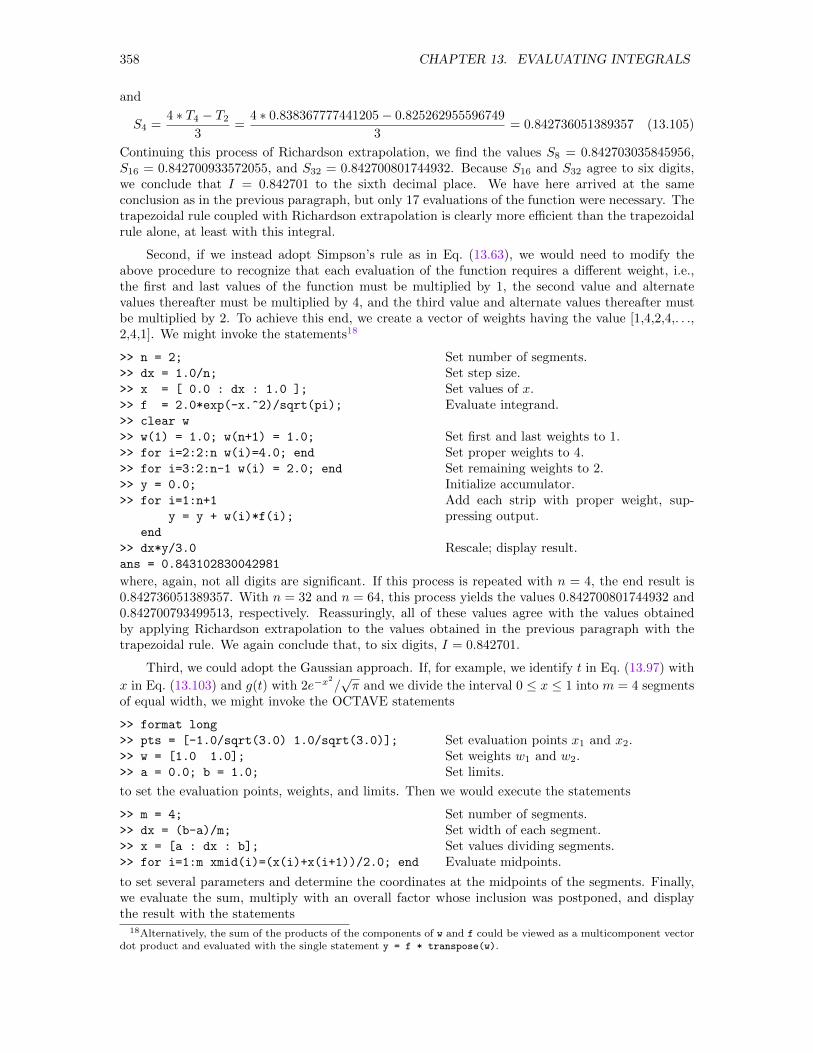
358 CHAPTER 13. EVALUATING INTEGRALS

and

S4 =4 ∗ T4 − T2

3=

4 ∗ 0.838367777441205− 0.825262955596749

3= 0.842736051389357 (13.105)

Continuing this process of Richardson extrapolation, we find the values S8 = 0.842703035845956,S16 = 0.842700933572055, and S32 = 0.842700801744932. Because S16 and S32 agree to six digits,we conclude that I = 0.842701 to the sixth decimal place. We have here arrived at the sameconclusion as in the previous paragraph, but only 17 evaluations of the function were necessary. Thetrapezoidal rule coupled with Richardson extrapolation is clearly more efficient than the trapezoidalrule alone, at least with this integral.

Second, if we instead adopt Simpson’s rule as in Eq. (13.63), we would need to modify theabove procedure to recognize that each evaluation of the function requires a different weight, i.e.,the first and last values of the function must be multiplied by 1, the second value and alternatevalues thereafter must be multiplied by 4, and the third value and alternate values thereafter mustbe multiplied by 2. To achieve this end, we create a vector of weights having the value [1,4,2,4,. . .,2,4,1]. We might invoke the statements18

>> n = 2;

>> dx = 1.0/n;

>> x = [ 0.0 : dx : 1.0 ];

>> f = 2.0*exp(-x.^2)/sqrt(pi);

>> clear w

>> w(1) = 1.0; w(n+1) = 1.0;

>> for i=2:2:n w(i)=4.0; end

>> for i=3:2:n-1 w(i) = 2.0; end

>> y = 0.0;

>> for i=1:n+1

y = y + w(i)*f(i);

end

>> dx*y/3.0

ans = 0.843102830042981

Set number of segments.Set step size.Set values of x.Evaluate integrand.

Set first and last weights to 1.Set proper weights to 4.Set remaining weights to 2.Initialize accumulator.Add each strip with proper weight, sup-pressing output.

Rescale; display result.

where, again, not all digits are significant. If this process is repeated with n = 4, the end result is0.842736051389357. With n = 32 and n = 64, this process yields the values 0.842700801744932 and0.842700793499513, respectively. Reassuringly, all of these values agree with the values obtainedby applying Richardson extrapolation to the values obtained in the previous paragraph with thetrapezoidal rule. We again conclude that, to six digits, I = 0.842701.

Third, we could adopt the Gaussian approach. If, for example, we identify t in Eq. (13.97) with

x in Eq. (13.103) and g(t) with 2e−x2

/√π and we divide the interval 0 ≤ x ≤ 1 into m = 4 segments

of equal width, we might invoke the OCTAVE statements

>> format long

>> pts = [-1.0/sqrt(3.0) 1.0/sqrt(3.0)];

>> w = [1.0 1.0];

>> a = 0.0; b = 1.0;

Set evaluation points x1 and x2.Set weights w1 and w2.Set limits.

to set the evaluation points, weights, and limits. Then we would execute the statements

>> m = 4;

>> dx = (b-a)/m;

>> x = [a : dx : b];

>> for i=1:m xmid(i)=(x(i)+x(i+1))/2.0; end

Set number of segments.Set width of each segment.Set values dividing segments.Evaluate midpoints.

to set several parameters and determine the coordinates at the midpoints of the segments. Finally,we evaluate the sum, multiply with an overall factor whose inclusion was postponed, and displaythe result with the statements

18Alternatively, the sum of the products of the components of w and f could be viewed as a multicomponent vectordot product and evaluated with the single statement y = f * transpose(w).

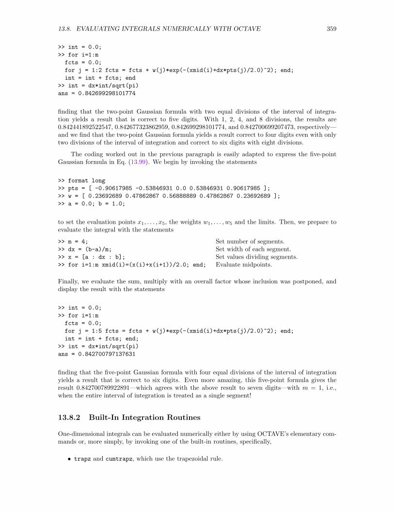
13.8. EVALUATING INTEGRALS NUMERICALLY WITH OCTAVE 359

>> int = 0.0;

>> for i=1:m

fcts = 0.0;

for j = 1:2 fcts = fcts + w(j)*exp(-(xmid(i)+dx*pts(j)/2.0)^2); end;

int = int + fcts; end

>> int = dx*int/sqrt(pi)

ans = 0.842699298101774

finding that the two-point Gaussian formula with two equal divisions of the interval of integra-tion yields a result that is correct to five digits. With 1, 2, 4, and 8 divisions, the results are0.842441892522547, 0.842677323862959, 0.842699298101774, and 0.842700699207473, respectively—and we find that the two-point Gaussian formula yields a result correct to four digits even with onlytwo divisions of the interval of integration and correct to six digits with eight divisions.

The coding worked out in the previous paragraph is easily adapted to express the five-pointGaussian formula in Eq. (13.99). We begin by invoking the statements

>> format long

>> pts = [ -0.90617985 -0.53846931 0.0 0.53846931 0.90617985 ];

>> w = [ 0.23692689 0.47862867 0.56888889 0.47862867 0.23692689 ];

>> a = 0.0; b = 1.0;

to set the evaluation points x1, . . . , x5, the weights w1, . . . , w5 and the limits. Then, we prepare toevaluate the integral with the statements

>> m = 4;

>> dx = (b-a)/m;

>> x = [a : dx : b];

>> for i=1:m xmid(i)=(x(i)+x(i+1))/2.0; end;

Set number of segments.Set width of each segment.Set values dividing segments.Evaluate midpoints.

Finally, we evaluate the sum, multiply with an overall factor whose inclusion was postponed, anddisplay the result with the statements

>> int = 0.0;

>> for i=1:m

fcts = 0.0;

for j = 1:5 fcts = fcts + w(j)*exp(-(xmid(i)+dx*pts(j)/2.0)^2); end;

int = int + fcts; end;

>> int = dx*int/sqrt(pi)

ans = 0.842700797137631

finding that the five-point Gaussian formula with four equal divisions of the interval of integrationyields a result that is correct to six digits. Even more amazing, this five-point formula gives theresult 0.842700789922891—which agrees with the above result to seven digits—with m = 1, i.e.,when the entire interval of integration is treated as a single segment!

13.8.2 Built-In Integration Routines

One-dimensional integrals can be evaluated numerically either by using OCTAVE’s elementary com-mands or, more simply, by invoking one of the built-in routines, specifically,

• trapz and cumtrapz, which use the trapezoidal rule.

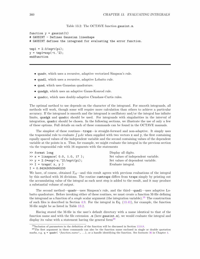
360 CHAPTER 13. EVALUATING INTEGRALS

Table 13.2: The OCTAVE function gausint.m.

function y = gausint(t)

# GAUSINT - Defines Gaussian lineshape

# GAUSINT defines the integrand for evaluating the error function.

tmp1 = 2.0/sqrt(pi);

y = tmp1*exp(-t.^2);

endfunction

• quadv, which uses a recursive, adaptive vectorized Simpson’s rule.

• quadl, which uses a recursive, adaptive Lobatto rule.

• quad, which uses Gaussian quadrature.

• quadgk, which uses an adaptive Gauss-Konrod rule.

• quadcc, which uses doubly-adaptive Clenshaw-Curtis rules.

The optimal method to use depends on the character of the integrand. For smooth integrands, allmethods will work, though some will require more calculation than others to achieve a particularaccuracy. If the integrand is smooth and the integrand is oscillatory and/or the integral has infinitelimits, quadgk and quadcc should be used. For integrands with singularities in the interval ofintegration, quadcc should be chosen. In the following sections, we illustrate the use of only a fewof these options. Full details on each of these commands can be found in the OCTAVE manuals.

The simplest of these routines—trapz—is straight-forward and non-adaptive. It simply usesthe trapezoidal rule to evaluate

∫y dx when supplied with two vectors x and y, the first containing

equally spaced values of the independent variable and the second containing values of the dependentvariable at the points in x. Thus, for example, we might evaluate the integral in the previous sectionvia the trapezoidal rule with 16 segments with the statements

>> format long

>> x = linspace( 0.0, 1.0, 17 );

>> y = 2.0*exp(-x.^2)/sqrt(pi);

>> I = trapz( x, y )

I = 0.842430505490233

Display all digits.Set values of independent variable.Set values of dependent variable.Evaluate integral.

We have, of course, obtained T16—and this result agrees with previous evaluations of the integralby this method with 16 divisions. The routine cumtrapz differs from trapz simply by printing outthe accumulating value of the integral as each next step is added to the result, and it may producea substantial volume of output.

The second method—quadv—uses Simpson’s rule, and the third—quadl—uses adaptive Lo-batto quadrature. Before invoking either of these routines, we must create a function M-file definingthe integrand as a function of a single scalar argument (the integration variable).19 The constructionof such files is described in Section 4.9. For the integral in Eq. (13.41), for example, the functionM-file might be as listed in Table 13.2.

Having stored the M-file in the user’s default directory with a name identical to that of thefunction name and with the file extension .m (here gausint.m), we would evaluate the integral anddisplay its value with a statement having the general form20

19Inclusion of parameters in the definition of the function will be discussed in Section 13.8.8.20The first argument in these commands can also be the function name enclosed in single or double quotation

marks, e.g. q = quadv( ’function name’, . . .), or a handle identifying the function. See footnote 36 in Chapter 4.

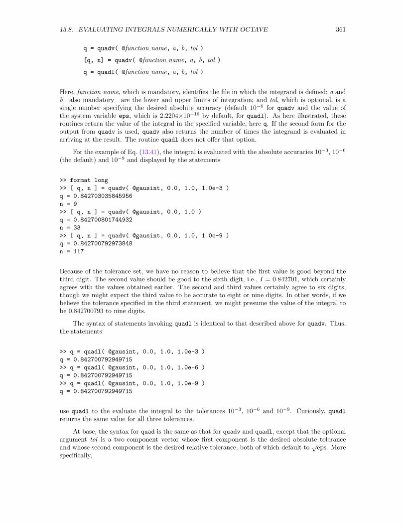
13.8. EVALUATING INTEGRALS NUMERICALLY WITH OCTAVE 361

q = quadv( @function name, a, b, tol )

[q, n] = quadv( @function name, a, b, tol )

q = quadl( @function name, a, b, tol )

Here, function name, which is mandatory, identifies the file in which the integrand is defined; a andb—also mandatory—are the lower and upper limits of integration; and tol, which is optional, is asingle number specifying the desired absolute accuracy (default 10−6 for quadv and the value ofthe system variable eps, which is 2.2204×10−16 by default, for quadl). As here illustrated, theseroutines return the value of the integral in the specified variable, here q. If the second form for theoutput from quadv is used, quadv also returns the number of times the integrand is evaluated inarriving at the result. The routine quadl does not offer that option.

For the example of Eq. (13.41), the integral is evaluated with the absolute accuracies 10−3, 10−6

(the default) and 10−9 and displayed by the statements

>> format long

>> [ q, n ] = quadv( @gausint, 0.0, 1.0, 1.0e-3 )

q = 0.842703035845956

n = 9

>> [ q, n ] = quadv( @gausint, 0.0, 1.0 )

q = 0.842700801744932

n = 33

>> [ q, n ] = quadv( @gausint, 0.0, 1.0, 1.0e-9 )

q = 0.842700792973848

n = 117

Because of the tolerance set, we have no reason to believe that the first value is good beyond thethird digit. The second value should be good to the sixth digit, i.e., I = 0.842701, which certainlyagrees with the values obtained earlier. The second and third values certainly agree to six digits,though we might expect the third value to be accurate to eight or nine digits. In other words, if webelieve the tolerance specified in the third statement, we might presume the value of the integral tobe 0.842700793 to nine digits.

The syntax of statements invoking quadl is identical to that described above for quadv. Thus,the statements

>> q = quadl( @gausint, 0.0, 1.0, 1.0e-3 )

q = 0.842700792949715

>> q = quadl( @gausint, 0.0, 1.0, 1.0e-6 )

q = 0.842700792949715

>> q = quadl( @gausint, 0.0, 1.0, 1.0e-9 )

q = 0.842700792949715

use quadl to the evaluate the integral to the tolerances 10−3, 10−6 and 10−9. Curiously, quadl

returns the same value for all three tolerances.

At base, the syntax for quad is the same as that for quadv and quadl, except that the optionalargument tol is a two-component vector whose first component is the desired absolute toleranceand whose second component is the desired relative tolerance, both of which default to

√eps. More

specifically,

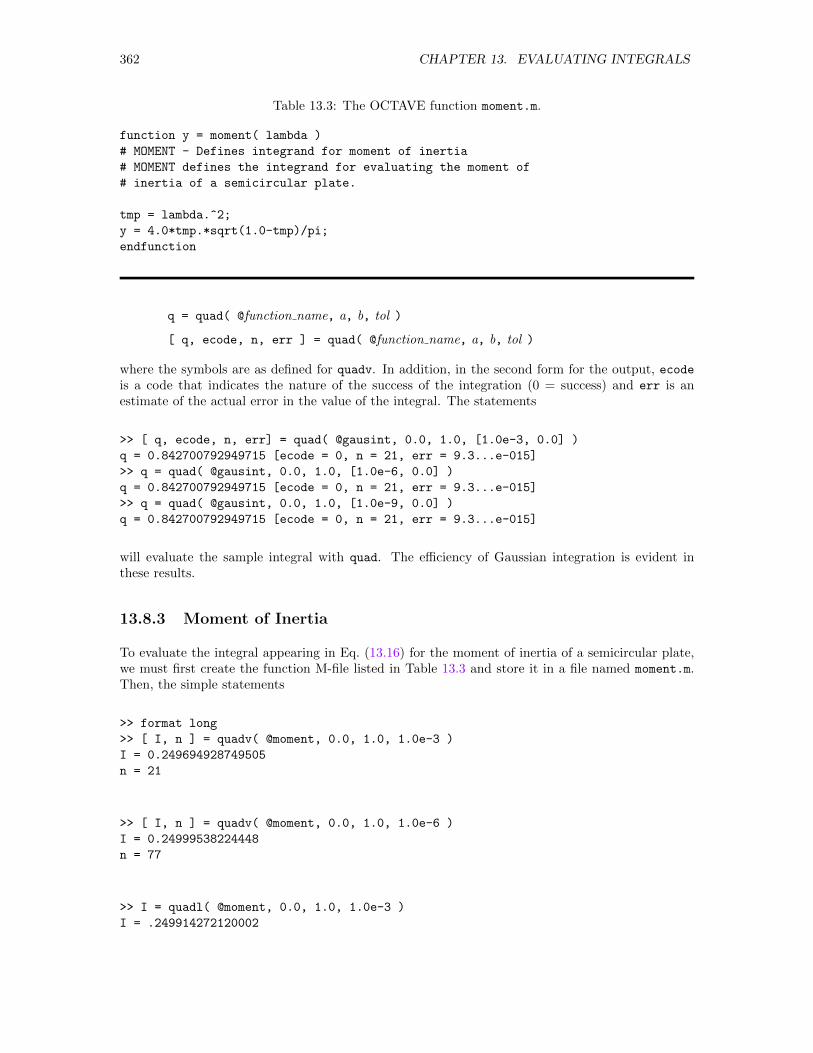
362 CHAPTER 13. EVALUATING INTEGRALS

Table 13.3: The OCTAVE function moment.m.

function y = moment( lambda )

# MOMENT - Defines integrand for moment of inertia

# MOMENT defines the integrand for evaluating the moment of

# inertia of a semicircular plate.

tmp = lambda.^2;

y = 4.0*tmp.*sqrt(1.0-tmp)/pi;

endfunction

q = quad( @function name, a, b, tol )

[ q, ecode, n, err ] = quad( @function name, a, b, tol )

where the symbols are as defined for quadv. In addition, in the second form for the output, ecodeis a code that indicates the nature of the success of the integration (0 = success) and err is anestimate of the actual error in the value of the integral. The statements

>> [ q, ecode, n, err] = quad( @gausint, 0.0, 1.0, [1.0e-3, 0.0] )

q = 0.842700792949715 [ecode = 0, n = 21, err = 9.3...e-015]

>> q = quad( @gausint, 0.0, 1.0, [1.0e-6, 0.0] )

q = 0.842700792949715 [ecode = 0, n = 21, err = 9.3...e-015]

>> q = quad( @gausint, 0.0, 1.0, [1.0e-9, 0.0] )

q = 0.842700792949715 [ecode = 0, n = 21, err = 9.3...e-015]

will evaluate the sample integral with quad. The efficiency of Gaussian integration is evident inthese results.

13.8.3 Moment of Inertia

To evaluate the integral appearing in Eq. (13.16) for the moment of inertia of a semicircular plate,we must first create the function M-file listed in Table 13.3 and store it in a file named moment.m.Then, the simple statements

>> format long

>> [ I, n ] = quadv( @moment, 0.0, 1.0, 1.0e-3 )

I = 0.249694928749505

n = 21

>> [ I, n ] = quadv( @moment, 0.0, 1.0, 1.0e-6 )

I = 0.24999538224448

n = 77

>> I = quadl( @moment, 0.0, 1.0, 1.0e-3 )

I = .249914272120002

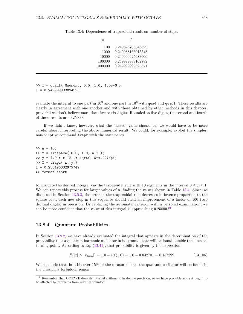
13.8. EVALUATING INTEGRALS NUMERICALLY WITH OCTAVE 363

Table 13.4: Dependence of trapezoidal result on number of steps.

n I

100 0.2496267080438291000 0.249988166015548

10000 0.249999625683606100000 0.249999988162782

1000000 0.249999999625671

>> I = quadl( @moment, 0.0, 1.0, 1.0e-6 )

I = 0.249999933894595

evaluate the integral to one part in 103 and one part in 106 with quad and quadl. These results areclearly in agreement with one another and with those obtained by other methods in this chapter,provided we don’t believe more than five or six digits. Rounded to five digits, the second and fourthof these results are 0.25000.

If we didn’t know, however, what the “exact” value should be, we would have to be morecareful about interpreting the above numerical result. We could, for example, exploit the simpler,non-adaptive command trapz with the statements

>> n = 10;

>> x = linspace( 0.0, 1.0, n+1 );

>> y = 4.0 * x.^2 .* sqrt(1.0-x.^2)/pi;

>> I = trapz( x, y )

I = 0.238496332979749

>> format short

to evaluate the desired integral via the trapezoidal rule with 10 segments in the interval 0 ≤ x ≤ 1.We can repeat this process for larger values of n, finding the values shown in Table 13.4. Since, asdiscussed in Section 13.5.3, the error in the trapezoidal rule decreases in inverse proportion to thesquare of n, each new step in this sequence should yield an improvement of a factor of 100 (twodecimal digits) in precision. By replacing the automatic criterion with a personal examination, wecan be more confident that the value of this integral is approaching 0.25000.21

13.8.4 Quantum Probabilities

In Section 13.8.2, we have already evaluated the integral that appears in the determination of theprobability that a quantum harmonic oscillator in its ground state will be found outside the classicalturning point. According to Eq. (13.41), that probability is given by the expression

P (|x| > |xturn|) = 1.0− erf(1.0) = 1.0− 0.842701 = 0.157299 (13.106)

We conclude that, in a bit over 15% of the measurements, the quantum oscillator will be found inthe classically forbidden region!

21Remember that OCTAVE does its internal arithmetic in double precision, so we have probably not yet begun tobe affected by problems from internal roundoff.

364 CHAPTER 13. EVALUATING INTEGRALS

13.8.5 Integrals as Functions of the Upper Limit

To evaluate an integral as a function of a parameter, the routine used must be invoked repeatedly ina loop. With each execution of the loop, the parameter assumes a new value and the current valuesof the parameter and of the corresponding integral are stored for later examination. This process iseasiest to implement when the parameter is the upper limit of the integral as, for example, in theintegral

g(x) =

∫ x

0

f(t) dt (13.107)

We begin by constructing a function M-file to define the integrand f(t), say integ.m. Then, sup-posing that we want to evaluate the integral as a function of its upper limit x for a ≤ x ≤ b, weinvoke the OCTAVE statements22

N = 〈appropriate value〉;x = linspace( a, b, N+1 );

for i = 1:N+1

g(i) = Routine( @integ, 0, x(i) );

end;

Set number of segments in interval.Set values for upper limit.Evaluate integral for each upper limit in x,using a chosen routine and accepting thedefault tolerance.

Upon execution of these statements, values of g(x) as a function of x for the selected values of xwill be stored in the vector g and can be further processed as desired. In particular, the statementplot(x,g)—or some embellishment thereof—will generate a graph of g versus x.23

13.8.6 The Error Function

To evaluate the error function as given by Eq. (13.26), we begin by constructing the M-file giving theintegrand. The function gausint.m defined in Section 13.8.2 can be used here also. Thus, supposingwe want x to range from 0.0 to 3.0 in steps of 0.1, we invoke the OCTAVE statements

>> N = 30;

>> x = linspace( 0.0, 3.0, N+1 );

>> for i = 1:N+1

erf(i) = quad( @gausint, 0, x(i) );

end

>> plot( x, erf, ’linewidth’, 4, ...

’color’, ’black’ )

>> title(’Error Function’, ’fontsize’, 20 )

>> xlabel( ’x’, ’fontsize’, 16 )

>> ylabel( ’erf(x)’, ’fontsize’, 16 )

>> grid on

>> set( gca, ’fontsize’, 16 )

Set graphics toolkit.Set number of segments.Specify values of upper limit.Evaluate integral for each upper limit in x,accepting defaults for keywords.

Plot error function.

Title graph.Label axes.

Turn on grid.Adjust size for labels

The resulting graph is shown in Fig. 13.10.

13.8.7 The Cornu Spiral

To determine the Cornu spiral, we use quad to generate vectors C and S containing values of thedefining integrals as given in Eq. (13.27) over a suitable range of upper limits and then plot thevalues in S versus the values in C. First we create the M-files in Table 13.5 to provide the two

22We might, of course, use quadl instead of quad in this example.23This sequence of statements actually is computationally inefficient. We might increase the efficiency by recogniz-

ing, for example, that g(x + ∆x) = g(x) +∫ x+∆x

xf(t) dt and obtain integrals for larger x by adding an appropriate

increment to already evaluated integrals for smaller x. For our present purposes, that approach unnecessarily com-plicates the algorithm of evaluation.

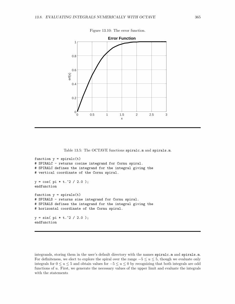
13.8. EVALUATING INTEGRALS NUMERICALLY WITH OCTAVE 365

Figure 13.10: The error function.

0 0.5 1 1.5 2 2.5 30

0.2

0.4

0.6

0.8

1

x

erf(

x)

Error Function

Table 13.5: The OCTAVE functions spiralc.m and spirals.m.

function y = spiralc(t)

# SPIRALC - returns cosine integrand for Cornu spiral.

# SPIRALC defines the integrand for the integral giving the

# vertical coordinate of the Cornu spiral.

y = cos( pi * t.^2 / 2.0 );

endfunction

function y = spirals(t)

# SPIRALS - returns sine integrand for Cornu spiral.

# SPIRALS defines the integrand for the integral giving the

# horizontal coordinate of the Cornu spiral.

y = sin( pi * t.^2 / 2.0 );

endfunction

integrands, storing them in the user’s default directory with the names spiralc.m and spirals.m.For definiteness, we elect to explore the spiral over the range −5 ≤ u ≤ 5, though we evaluate onlyintegrals for 0 ≤ u ≤ 5 and obtain values for −5 ≤ u ≤ 0 by recognizing that both integrals are oddfunctions of u. First, we generate the necessary values of the upper limit and evaluate the integralswith the statements

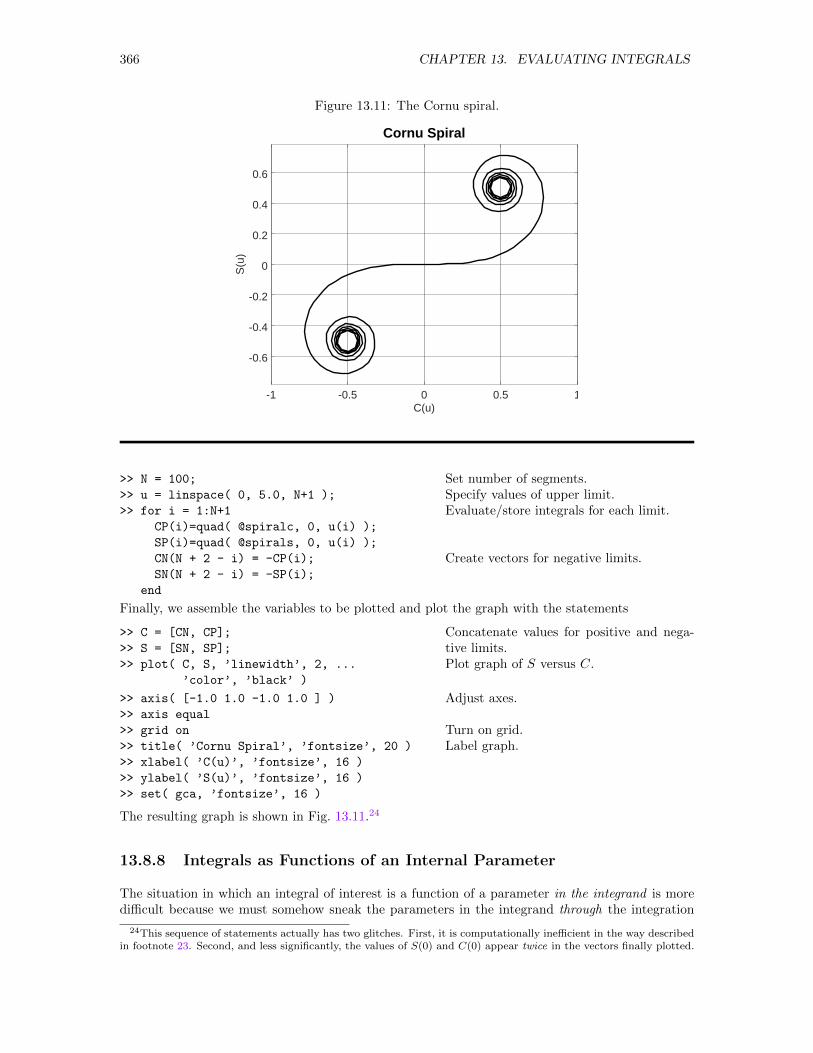
366 CHAPTER 13. EVALUATING INTEGRALS

Figure 13.11: The Cornu spiral.

1

-0.6

-0.4

-0.2

0

0.2

0.4

0.6

0.50-0.5-1C(u)

S(u

)

Cornu Spiral

>> N = 100;

>> u = linspace( 0, 5.0, N+1 );

>> for i = 1:N+1

CP(i)=quad( @spiralc, 0, u(i) );

SP(i)=quad( @spirals, 0, u(i) );

CN(N + 2 - i) = -CP(i);

SN(N + 2 - i) = -SP(i);

end

Set number of segments.Specify values of upper limit.Evaluate/store integrals for each limit.

Create vectors for negative limits.

Finally, we assemble the variables to be plotted and plot the graph with the statements

>> C = [CN, CP];

>> S = [SN, SP];

>> plot( C, S, ’linewidth’, 2, ...

’color’, ’black’ )

Concatenate values for positive and nega-tive limits.Plot graph of S versus C.

>> axis( [-1.0 1.0 -1.0 1.0 ] )

>> axis equal

>> grid on

>> title( ’Cornu Spiral’, ’fontsize’, 20 )

>> xlabel( ’C(u)’, ’fontsize’, 16 )

>> ylabel( ’S(u)’, ’fontsize’, 16 )

>> set( gca, ’fontsize’, 16 )

Adjust axes.

Turn on grid.Label graph.

The resulting graph is shown in Fig. 13.11.24

13.8.8 Integrals as Functions of an Internal Parameter

The situation in which an integral of interest is a function of a parameter in the integrand is moredifficult because we must somehow sneak the parameters in the integrand through the integration

24This sequence of statements actually has two glitches. First, it is computationally inefficient in the way describedin footnote 23. Second, and less significantly, the values of S(0) and C(0) appear twice in the vectors finally plotted.

13.8. EVALUATING INTEGRALS NUMERICALLY WITH OCTAVE 367

routine and into the function called by those routines to evaluate the integrand. One technique forachieving this objective is to exploit global variables as discussed in Section 4.9 and in Section 11.9.4.Using global variables will work with all of OCTAVE’s integration routines. Conveniently, however,quadv and quadl offer an alternative. Calls to these routines can take advantage of the existence ofadditional arguments. The full structure of statements involving these commands is

q = quadv( @function name, a, b, tol, trace, p1, p2, . . . )[ q, n ] = quadv( @function name, a, b, tol, trace, p1, p2, . . . )q = quadl( @function name, a, b, tol, trace, p1, p2, . . . )

Here—beyond the quantities already defined—a non-zero value25 for trace will display the iterative,recursive progress towards the final result as the integration proceeds,26 and p1, p2, . . . are parame-ters that will be passed by quadv or quadl to the function defining the integrand, provided that thefunction is defined with those parameters as additional arguments. To accept the default values oftol and/or trace while specifying parameters, simply set either/both to the empty matrix [].

To invoke this feature, we must do two things. First, we must define the integrand with theparameters as additional arguments to the function. The appropriate file would then have the generalformat

function y = FunctionName( x, p1, p2, p3, ... )

# Explanatory comments.Statements to evaluate integrand, using p1, p2, p3, ... for the parameters.y = integrand;

endfunction

The quantities FunctionName, x, and integrand have the same meaning as before, and the file mustbe stored with the name FunctionName.m.

Second, having defined the function M-file in this new way and stored it in the de-fault directory, we invoke OCTAVE to evaluate and display the desired integral by usingquadv or quadl with the statements p1 = ??;, p2 = ??;, p3 = ??; ...;

q = quadv( @FunctionName, a, b, [], [], ...

p1, p2, p3 )Assign values to parameters.Evaluate integral.

Note that the names of the parameters need not be the same at command level as they are in thefunction M-file. Only the position and data type of the entities must match in the two occurrences,since it is the order and type of items—not the variable names used—that provide the associationof values in the two occurrences.

13.8.9 The Off-Axis Electrostatic Potential of Two Rings

Equation (13.36) illustrates a situation in which the integral is a function of an internal parameter.For the integral in Eq. (13.36), for example, we might write the M-file listed in Table 13.6.

We store this file with the name rings.m, then invoke OCTAVE to evaluate and display thedesired integral by using quadv, say, with the statement

q = quadv( ’rings’, a, b, [], [], s )

25The value zero is interpreted as false; any other value is interpreted as true.26Number of function evaluations, left end and width of each subinterval exploited in the process, and the estimated

value of the integral over each subinterval.

368 CHAPTER 13. EVALUATING INTEGRALS

Table 13.6: The OCTAVE function rings.m.

function y = rings( phi, s )

# RINGS - Integrand for charged rings

# RINGS defines the integrand whose integral gives the

# electrostatic potential in the midplane between two

# uniformly charged circular rings.

tmp = sqrt( 2.0 ) / ( 2.0 * pi );

y = tmp ./ sqrt( 2.0 - 2.0*s.*cos(phi) + s*s );

endfunction

Since we seek to explore this integral as a function of s over, say, 0.0 ≤ s ≤ 4.0, we must generatea vector of values of s and then, in a loop, invoke quadv once for each element in that vector. Wemight use the statements

>> s = [ 0.0 : 0.1 : 4.0 ];

>> N = length(s);

>> for i = 1:N

V(i) = quadv( @rings, 0.0, 2.0*pi, ...

[], [], s(i) );

end

>> plot( s, V, ’linewidth’, 4, ...

’color’, ’black’ )

Select graphics toolkit.Specify values of parameter.Set N to number of values in s.Evaluate and store integral for each valueof the parameter.

Plot graph.

>> axis( [0.0 4.0 0.0 1.0])

>> title( ’Potential in Midplane’, ...

’fontsize’, 20 )

>> xlabel( ’s (in units of a)’, ...

’fontsize’, 16 )

>> ylabel( ’V(s) (in units of V(0))’, ...

’fontsize’, 16 )

>> grid on

>> set( gca, ’fontsize’, 16 )

Adjust axis limits.Title graph.

Label axes.

Turn grid on.

The resulting graph is shown in Fig. 13.12.

13.12 Evaluating Integrals Numerically with Mathematica

Mathematica offers at least two routes for evaluating integrals numerically. For integrals that canbe evaluated analytically, we can simply embed the command Integrate within the command N. Inresponse to the simple statement

N[ Integrate[ f, x, a, b ] ]

where f is an expression that depends on x. Mathematica first evaluates∫ baf dx symbolically and

then determines the numerical value from the symbolic result. This same statement will automati-cally invoke numerical quadrature if a symbolic result cannot be obtained (and all quantities in theintegrand have numerical values). If, however, an integral does not admit a symbolic evaluation (orwe wish a numeric evaluation even when a symbolic evaluation exists), then we would instead invokethe command NIntegrate in a statement of the form

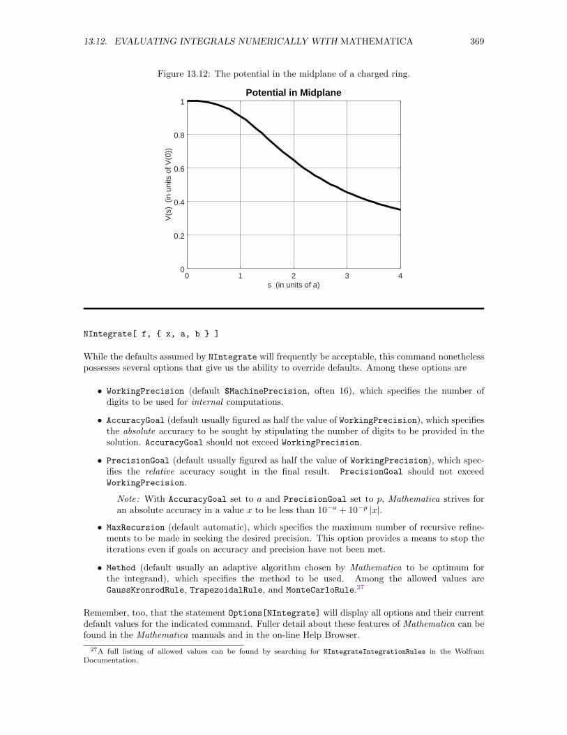
13.12. EVALUATING INTEGRALS NUMERICALLY WITH MATHEMATICA 369

Figure 13.12: The potential in the midplane of a charged ring.

0 1 2 3 40

0.2

0.4

0.6

0.8

1

s (in units of a)

V(s

) (

in u

nits

of V

(0))

Potential in Midplane

NIntegrate[ f, x, a, b ]

While the defaults assumed by NIntegrate will frequently be acceptable, this command nonethelesspossesses several options that give us the ability to override defaults. Among these options are

• WorkingPrecision (default $MachinePrecision, often 16), which specifies the number ofdigits to be used for internal computations.

• AccuracyGoal (default usually figured as half the value of WorkingPrecision), which specifiesthe absolute accuracy to be sought by stipulating the number of digits to be provided in thesolution. AccuracyGoal should not exceed WorkingPrecision.

• PrecisionGoal (default usually figured as half the value of WorkingPrecision), which spec-ifies the relative accuracy sought in the final result. PrecisionGoal should not exceedWorkingPrecision.

Note: With AccuracyGoal set to a and PrecisionGoal set to p, Mathematica strives foran absolute accuracy in a value x to be less than 10−a + 10−p |x|.

• MaxRecursion (default automatic), which specifies the maximum number of recursive refine-ments to be made in seeking the desired precision. This option provides a means to stop theiterations even if goals on accuracy and precision have not been met.

• Method (default usually an adaptive algorithm chosen by Mathematica to be optimum forthe integrand), which specifies the method to be used. Among the allowed values areGaussKronrodRule, TrapezoidalRule, and MonteCarloRule.27

Remember, too, that the statement Options[NIntegrate] will display all options and their currentdefault values for the indicated command. Fuller detail about these features of Mathematica can befound in the Mathematica manuals and in the on-line Help Browser.

27A full listing of allowed values can be found by searching for NIntegrateIntegrationRules in the WolframDocumentation.

370 CHAPTER 13. EVALUATING INTEGRALS

With this feature of Mathematica, we can evaluate our standard example in many ways. Wemight, for example, use the statement

In[1]:= N[ Integrate[ 2*Exp[-t^2]/Sqrt[Pi], t, 0, 1 ] ]

Out[1]= 0.842701

which will evaluate the integral analytically [obtaining erf(1)], evaluate the error function of argument1, and finally display the result with the default precision intrinsic to the command N. That precisioncan, of course, be adjusted with the second argument so that, for example, the statement

In[2]:= N[ Integrate[ 2*Exp[-t^2]/Sqrt[Pi], t, 0, 1 ], 20 ]

Out[2]= 0.84270079294971486934

will yield a result with 20 digits. Alternatively, we might use the statement

In[3]:= NIntegrate[ 2*Exp[-t^2]/Sqrt[Pi], t, 0, 1 ]

Out[3]= 0.842701

which jumps directly to numerical integration, probably via the (adaptive) Gauss-Kronrod method.To illustrate use of some options, we might invoke the statement

In[4]:= NIntegrate[ 2*Exp[-t^2]/Sqrt[Pi], t, 0, 1, Method -> TrapezoidalRule ]

Out[4]= 0.842701

Reassuringly, these results are all consistent with one another.

13.12.1 Quantum Probability

In the opening paragraphs of this section, we have already evaluated the integral that appears inthe determination of the probability that a quantum harmonic oscillator in its ground state will befound outside the classical turning point. According to Eq. (13.41), that probability is given by theexpression

P (|x| > |xturn|) = 1.0− erf(1.0) = 1.0− 0.842701 = .157299 (13.108)

which is (probably) correct to all of the digits shown. We conclude that in a bit over 15% of themeasurements, the quantum oscillator will be found in the classically forbidden region!

13.12.2 The Error Function

To define the function gaussian and then generate successive numerical values of the function erf(x)defined by Eq. (13.26) as x varies from 0.0 to 3.0 in steps of 0.1, we might use the statements

In[1]:= gaussian[t_] := 2*Exp[-t^2]/Sqrt[Pi]

In[2]:= uplim = Range[ 0.0, 3.0, 0.1 ];

In[3]:= For[ j=1, j<32, j++, q[j]=NIntegrate[ gaussian[t], t, 0, uplim[[j]] ] ]

The values of the upper limits in the list uplim and the values qi created by these statements mustthen be converted into a list of the coordinates of the points with a statement like

In[4]:= pts = Table[ uplim[[i]], q[i] , i, 1, 31 ];

before the graph of Fig. 13.13 can be created with the statement

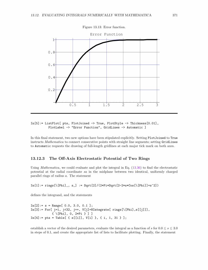
13.12. EVALUATING INTEGRALS NUMERICALLY WITH MATHEMATICA 371

Figure 13.13: Error function.

0.5 1 1.5 2 2.5 3

0.2

0.4

0.6

0.8

1

Error Function

In[5]:= ListPlot[ pts, PlotJoined -> True, PlotStyle -> Thickness[0.01],

PlotLabel -> "Error Function", GridLines -> Automatic ]

In this final statement, two new options have been stipulated explicitly. Setting PlotJoined to True

instructs Mathematica to connect consecutive points with straight line segments; setting GridLines

to Automatic requests the drawing of full-length gridlines at each major tick mark on both axes.

13.12.3 The Off-Axis Electrostatic Potential of Two Rings

Using Mathematica, we could evaluate and plot the integral in Eq. (13.36) to find the electrostaticpotential at the radial coordinate sa in the midplane between two identical, uniformly chargedparallel rings of radius a. The statement

In[1]:= rings[\[Phi]_, s_] := Sqrt[2]/(2*Pi*Sqrt[2-2*s*Cos[\[Phi]]+s^2])

defines the integrand, and the statements

In[2]:= s = Range[ 0.0, 3.0, 0.1 ];

In[3]:= For[ j=1, j<32, j++, V[j]=NIntegrate[ rings[\[Phi],s[[j]]],

\[Phi], 0, 2*Pi ] ]

In[4]:= pts = Table[ s[[i]], V[i] , i, 1, 31 ];

establish a vector of the desired parameters, evaluate the integral as a function of s for 0.0 ≤ s ≤ 3.0in steps of 0.1, and create the appropriate list of lists to facilitate plotting. Finally, the statement

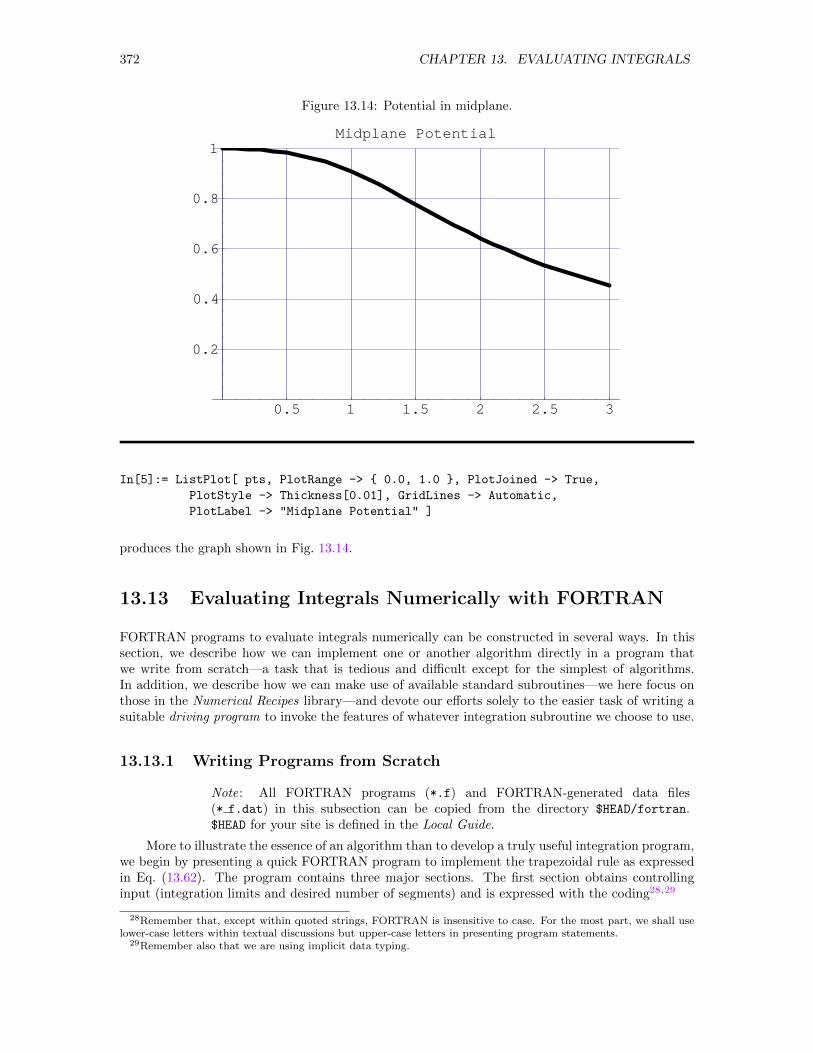
372 CHAPTER 13. EVALUATING INTEGRALS

Figure 13.14: Potential in midplane.

0.5 1 1.5 2 2.5 3

0.2

0.4

0.6

0.8

1Midplane Potential

In[5]:= ListPlot[ pts, PlotRange -> 0.0, 1.0 , PlotJoined -> True,

PlotStyle -> Thickness[0.01], GridLines -> Automatic,

PlotLabel -> "Midplane Potential" ]

produces the graph shown in Fig. 13.14.

13.13 Evaluating Integrals Numerically with FORTRAN

FORTRAN programs to evaluate integrals numerically can be constructed in several ways. In thissection, we describe how we can implement one or another algorithm directly in a program thatwe write from scratch—a task that is tedious and difficult except for the simplest of algorithms.In addition, we describe how we can make use of available standard subroutines—we here focus onthose in the Numerical Recipes library—and devote our efforts solely to the easier task of writing asuitable driving program to invoke the features of whatever integration subroutine we choose to use.

13.13.1 Writing Programs from Scratch

Note: All FORTRAN programs (*.f) and FORTRAN-generated data files(* f.dat) in this subsection can be copied from the directory $HEAD/fortran.$HEAD for your site is defined in the Local Guide.

More to illustrate the essence of an algorithm than to develop a truly useful integration program,we begin by presenting a quick FORTRAN program to implement the trapezoidal rule as expressedin Eq. (13.62). The program contains three major sections. The first section obtains controllinginput (integration limits and desired number of segments) and is expressed with the coding28,29

28Remember that, except within quoted strings, FORTRAN is insensitive to case. For the most part, we shall uselower-case letters within textual discussions but upper-case letters in presenting program statements.

29Remember also that we are using implicit data typing.

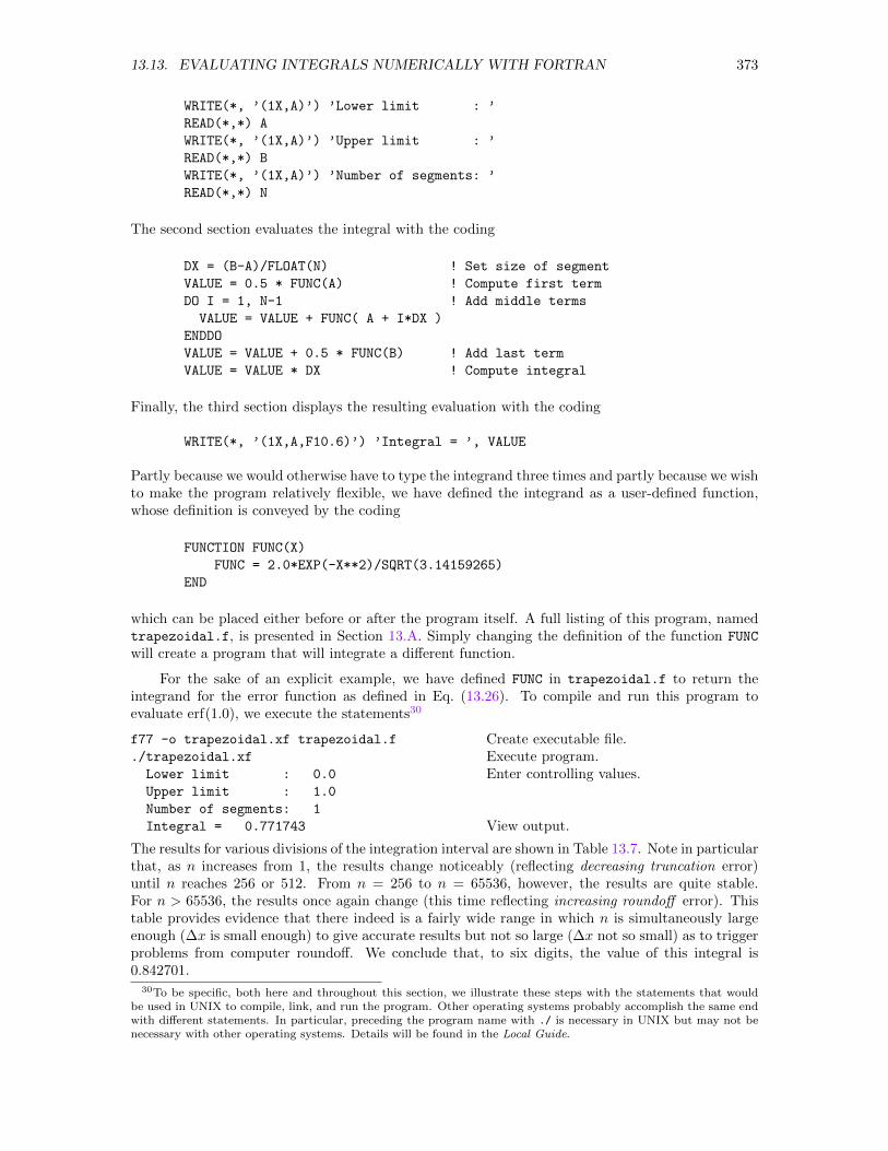
13.13. EVALUATING INTEGRALS NUMERICALLY WITH FORTRAN 373

WRITE(*, ’(1X,A)’) ’Lower limit : ’

READ(*,*) A

WRITE(*, ’(1X,A)’) ’Upper limit : ’

READ(*,*) B

WRITE(*, ’(1X,A)’) ’Number of segments: ’

READ(*,*) N

The second section evaluates the integral with the coding

DX = (B-A)/FLOAT(N) ! Set size of segment

VALUE = 0.5 * FUNC(A) ! Compute first term

DO I = 1, N-1 ! Add middle terms

VALUE = VALUE + FUNC( A + I*DX )

ENDDO

VALUE = VALUE + 0.5 * FUNC(B) ! Add last term

VALUE = VALUE * DX ! Compute integral

Finally, the third section displays the resulting evaluation with the coding

WRITE(*, ’(1X,A,F10.6)’) ’Integral = ’, VALUE

Partly because we would otherwise have to type the integrand three times and partly because we wishto make the program relatively flexible, we have defined the integrand as a user-defined function,whose definition is conveyed by the coding

FUNCTION FUNC(X)

FUNC = 2.0*EXP(-X**2)/SQRT(3.14159265)

END

which can be placed either before or after the program itself. A full listing of this program, namedtrapezoidal.f, is presented in Section 13.A. Simply changing the definition of the function FUNC

will create a program that will integrate a different function.

For the sake of an explicit example, we have defined FUNC in trapezoidal.f to return theintegrand for the error function as defined in Eq. (13.26). To compile and run this program toevaluate erf(1.0), we execute the statements30

f77 -o trapezoidal.xf trapezoidal.f

./trapezoidal.xf

Lower limit : 0.0

Upper limit : 1.0

Number of segments: 1

Integral = 0.771743

Create executable file.Execute program.Enter controlling values.

View output.

The results for various divisions of the integration interval are shown in Table 13.7. Note in particularthat, as n increases from 1, the results change noticeably (reflecting decreasing truncation error)until n reaches 256 or 512. From n = 256 to n = 65536, however, the results are quite stable.For n > 65536, the results once again change (this time reflecting increasing roundoff error). Thistable provides evidence that there indeed is a fairly wide range in which n is simultaneously largeenough (∆x is small enough) to give accurate results but not so large (∆x not so small) as to triggerproblems from computer roundoff. We conclude that, to six digits, the value of this integral is0.842701.

30To be specific, both here and throughout this section, we illustrate these steps with the statements that wouldbe used in UNIX to compile, link, and run the program. Other operating systems probably accomplish the same endwith different statements. In particular, preceding the program name with ./ is necessary in UNIX but may not benecessary with other operating systems. Details will be found in the Local Guide.

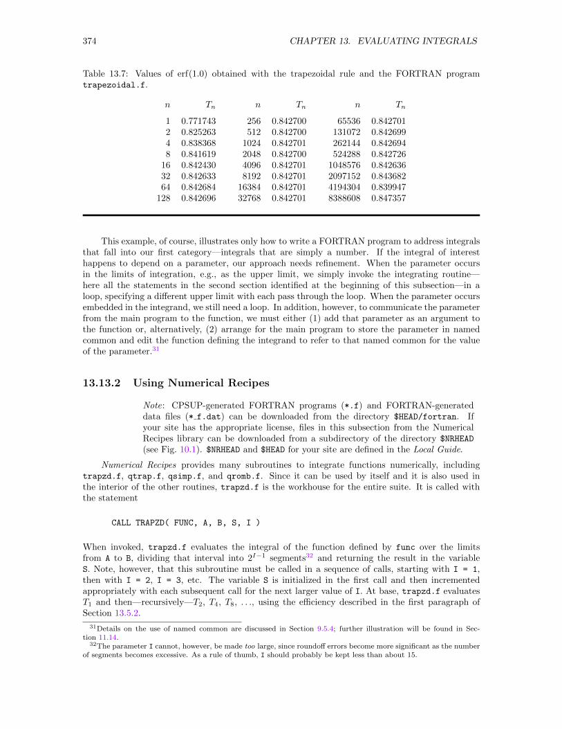
374 CHAPTER 13. EVALUATING INTEGRALS

Table 13.7: Values of erf(1.0) obtained with the trapezoidal rule and the FORTRAN programtrapezoidal.f.

n Tn n Tn n Tn

1 0.771743 256 0.842700 65536 0.8427012 0.825263 512 0.842700 131072 0.8426994 0.838368 1024 0.842701 262144 0.8426948 0.841619 2048 0.842700 524288 0.842726

16 0.842430 4096 0.842701 1048576 0.84263632 0.842633 8192 0.842701 2097152 0.84368264 0.842684 16384 0.842701 4194304 0.839947

128 0.842696 32768 0.842701 8388608 0.847357

This example, of course, illustrates only how to write a FORTRAN program to address integralsthat fall into our first category—integrals that are simply a number. If the integral of interesthappens to depend on a parameter, our approach needs refinement. When the parameter occursin the limits of integration, e.g., as the upper limit, we simply invoke the integrating routine—here all the statements in the second section identified at the beginning of this subsection—in aloop, specifying a different upper limit with each pass through the loop. When the parameter occursembedded in the integrand, we still need a loop. In addition, however, to communicate the parameterfrom the main program to the function, we must either (1) add that parameter as an argument tothe function or, alternatively, (2) arrange for the main program to store the parameter in namedcommon and edit the function defining the integrand to refer to that named common for the valueof the parameter.31

13.13.2 Using Numerical Recipes

Note: CPSUP-generated FORTRAN programs (*.f) and FORTRAN-generateddata files (* f.dat) can be downloaded from the directory $HEAD/fortran. Ifyour site has the appropriate license, files in this subsection from the NumericalRecipes library can be downloaded from a subdirectory of the directory $NRHEAD

(see Fig. 10.1). $NRHEAD and $HEAD for your site are defined in the Local Guide.

Numerical Recipes provides many subroutines to integrate functions numerically, includingtrapzd.f, qtrap.f, qsimp.f, and qromb.f. Since it can be used by itself and it is also used inthe interior of the other routines, trapzd.f is the workhouse for the entire suite. It is called withthe statement

CALL TRAPZD( FUNC, A, B, S, I )

When invoked, trapzd.f evaluates the integral of the function defined by func over the limitsfrom A to B, dividing that interval into 2I−1 segments32 and returning the result in the variableS. Note, however, that this subroutine must be called in a sequence of calls, starting with I = 1,then with I = 2, I = 3, etc. The variable S is initialized in the first call and then incrementedappropriately with each subsequent call for the next larger value of I. At base, trapzd.f evaluatesT1 and then—recursively—T2, T4, T8, . . ., using the efficiency described in the first paragraph ofSection 13.5.2.

31Details on the use of named common are discussed in Section 9.5.4; further illustration will be found in Sec-tion 11.14.

32The parameter I cannot, however, be made too large, since roundoff errors become more significant as the numberof segments becomes excessive. As a rule of thumb, I should probably be kept less than about 15.

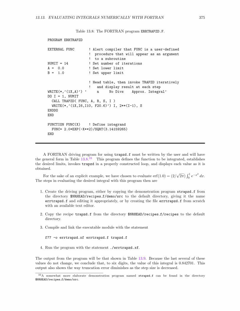
13.13. EVALUATING INTEGRALS NUMERICALLY WITH FORTRAN 375

Table 13.8: The FORTRAN program ERRTRAPZD.F.

PROGRAM ERRTRAPZD

EXTERNAL FUNC ! Alert compiler that FUNC is a user-defined

! procedure that will appear as an argument

! to a subroutine

NUMIT = 14 ! Set number of iterations

A = 0.0 ! Set lower limit

B = 1.0 ! Set upper limit

! Head table, then invoke TRAPZD iteratively

! and display result at each step

WRITE(*,’(1X,A)’) ’ n No Divs Approx. Integral’

DO I = 1, NUMIT

CALL TRAPZD( FUNC, A, B, S, I )

WRITE(*,’(1X,I6,I10, F20.6)’) I, 2**(I-1), S

ENDDO

END

FUNCTION FUNC(X) ! Define integrand

FUNC= 2.0*EXP(-X**2)/SQRT(3.14159265)

END

A FORTRAN driving program for using trapzd.f must be written by the user and will havethe general form in Table 13.8.33 This program defines the function to be integrated, establishesthe desired limits, invokes trapzd in a properly constructed loop, and displays each value as it isobtained.

For the sake of an explicit example, we have chosen to evaluate erf(1.0) = (2/√

2π)∫ 1

0e−x

2

dx.The steps in evaluating the desired integral with this program then are

1. Create the driving program, either by copying the demonstration program xtrapzd.f fromthe directory $NRHEAD/recipes f/demo/src to the default directory, giving it the nameerrtrapzd.f and editing it appropriately, or by creating the file errtrapzd.f from scratchwith an available text editor.

2. Copy the recipe trapzd.f from the directory $NRHEAD/recipes f/recipes to the defaultdirectory.

3. Compile and link the executable module with the statement

f77 -o errtrapzd.xf errtrapzd.f trapzd.f

4. Run the program with the statement ./errtrapzd.xf.

The output from the program will be that shown in Table 13.9. Because the last several of thesevalues do not change, we conclude that, to six digits, the value of this integral is 0.842701. Thisoutput also shows the way truncation error diminishes as the step size is decreased.

33A somewhat more elaborate demonstration program named xtrapzd.f can be found in the directory$NRHEAD/recipes f/demo/src.

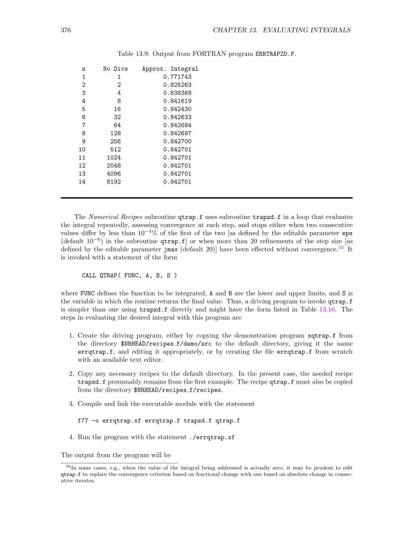
376 CHAPTER 13. EVALUATING INTEGRALS

Table 13.9: Output from FORTRAN program ERRTRAPZD.F.

n No Divs Approx. Integral

1 1 0.771743

2 2 0.825263

3 4 0.838368

4 8 0.841619

5 16 0.842430

6 32 0.842633

7 64 0.842684

8 128 0.842697

9 256 0.842700

10 512 0.842701

11 1024 0.842701

12 2048 0.842701

13 4096 0.842701

14 8192 0.842701

The Numerical Recipes subroutine qtrap.f uses subroutine trapzd.f in a loop that evaluatesthe integral repeatedly, assessing convergence at each step, and stops either when two consecutivevalues differ by less than 10−4% of the first of the two [as defined by the editable parameter eps

(default 10−6) in the subroutine qtrap.f] or when more than 20 refinements of the step size [asdefined by the editable parameter jmax (default 20)] have been effected without convergence.34 Itis invoked with a statement of the form

CALL QTRAP( FUNC, A, B, S )

where FUNC defines the function to be integrated, A and B are the lower and upper limits, and S isthe variable in which the routine returns the final value. Thus, a driving program to invoke qtrap.f

is simpler than one using trapzd.f directly and might have the form listed in Table 13.10. Thesteps in evaluating the desired integral with this program are

1. Create the driving program, either by copying the demonstration program xqtrap.f fromthe directory $NRHEAD/recipes f/demo/src to the default directory, giving it the nameerrqtrap.f, and editing it appropriately, or by creating the file errqtrap.f from scratchwith an available text editor.

2. Copy any necessary recipes to the default directory. In the present case, the needed recipetrapzd.f presumably remains from the first example. The recipe qtrap.f must also be copiedfrom the directory $NRHEAD/recipes f/recipes.

3. Compile and link the executable module with the statement

f77 -o errqtrap.xf errqtrap.f trapzd.f qtrap.f

4. Run the program with the statement ./errqtrap.xf

The output from the program will be

34In some cases, e.g., when the value of the integral being addressed is actually zero, it may be prudent to editqtrap.f to replace the convergence criterion based on fractional change with one based on absolute change in consec-utive iterates.

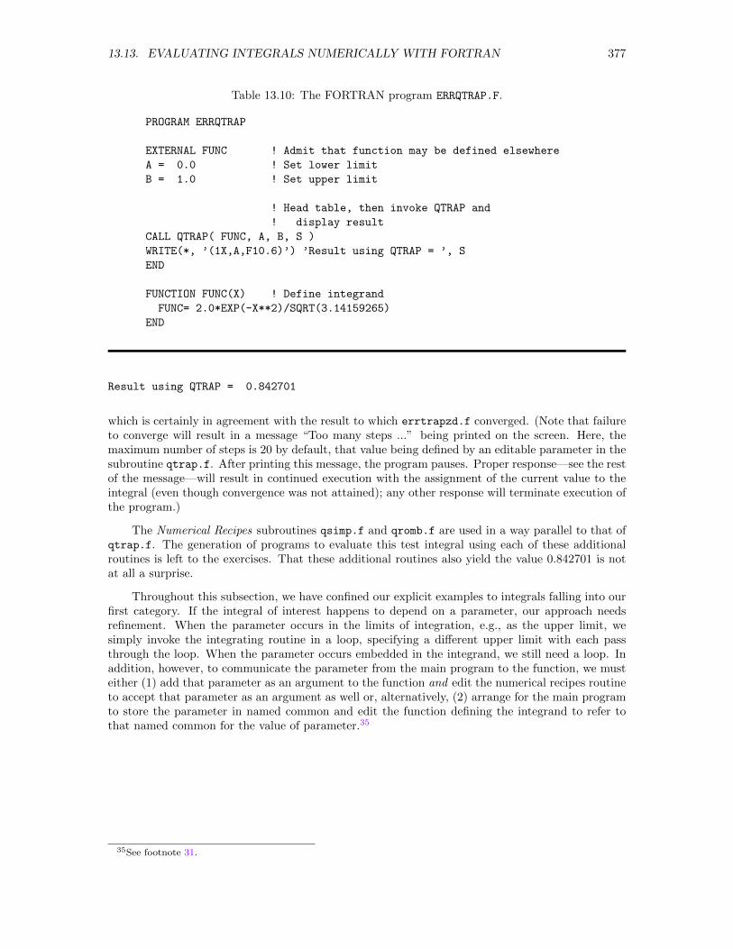
13.13. EVALUATING INTEGRALS NUMERICALLY WITH FORTRAN 377

Table 13.10: The FORTRAN program ERRQTRAP.F.

PROGRAM ERRQTRAP

EXTERNAL FUNC ! Admit that function may be defined elsewhere

A = 0.0 ! Set lower limit

B = 1.0 ! Set upper limit

! Head table, then invoke QTRAP and

! display result

CALL QTRAP( FUNC, A, B, S )

WRITE(*, ’(1X,A,F10.6)’) ’Result using QTRAP = ’, S

END

FUNCTION FUNC(X) ! Define integrand

FUNC= 2.0*EXP(-X**2)/SQRT(3.14159265)

END

Result using QTRAP = 0.842701

which is certainly in agreement with the result to which errtrapzd.f converged. (Note that failureto converge will result in a message “Too many steps ...” being printed on the screen. Here, themaximum number of steps is 20 by default, that value being defined by an editable parameter in thesubroutine qtrap.f. After printing this message, the program pauses. Proper response—see the restof the message—will result in continued execution with the assignment of the current value to theintegral (even though convergence was not attained); any other response will terminate execution ofthe program.)

The Numerical Recipes subroutines qsimp.f and qromb.f are used in a way parallel to that ofqtrap.f. The generation of programs to evaluate this test integral using each of these additionalroutines is left to the exercises. That these additional routines also yield the value 0.842701 is notat all a surprise.

Throughout this subsection, we have confined our explicit examples to integrals falling into ourfirst category. If the integral of interest happens to depend on a parameter, our approach needsrefinement. When the parameter occurs in the limits of integration, e.g., as the upper limit, wesimply invoke the integrating routine in a loop, specifying a different upper limit with each passthrough the loop. When the parameter occurs embedded in the integrand, we still need a loop. Inaddition, however, to communicate the parameter from the main program to the function, we musteither (1) add that parameter as an argument to the function and edit the numerical recipes routineto accept that parameter as an argument as well or, alternatively, (2) arrange for the main programto store the parameter in named common and edit the function defining the integrand to refer tothat named common for the value of parameter.35

35See footnote 31.

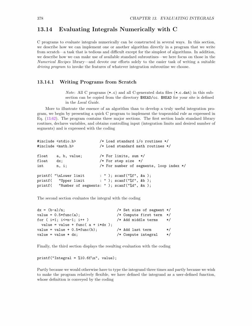
378 CHAPTER 13. EVALUATING INTEGRALS

13.14 Evaluating Integrals Numerically with C

C programs to evaluate integrals numerically can be constructed in several ways. In this section,we describe how we can implement one or another algorithm directly in a program that we writefrom scratch—a task that is tedious and difficult except for the simplest of algorithms. In addition,we describe how we can make use of available standard subroutines—we here focus on those in theNumerical Recipes library—and devote our efforts solely to the easier task of writing a suitabledriving program to invoke the features of whatever integration subroutine we choose.

13.14.1 Writing Programs from Scratch

Note: All C programs (*.c) and all C-generated data files (* c.dat) in this sub-section can be copied from the directory $HEAD/cc. $HEAD for your site is definedin the Local Guide.

More to illustrate the essence of an algorithm than to develop a truly useful integration pro-gram, we begin by presenting a quick C program to implement the trapezoidal rule as expressed inEq. (13.62). The program contains three major sections. The first section loads standard libraryroutines, declares variables, and obtains controlling input (integration limits and desired number ofsegments) and is expressed with the coding

#include <stdio.h> /* Load standard i/o routines */

#include <math.h> /* Load standard math routines */

float a, b, value; /* For limits, sum */

float dx; /* For step size */

int n, i; /* For number of segments, loop index */

printf( "\nLower limit : " ); scanf("%f", &a );

printf( "Upper limit : " ); scanf("%f", &b );

printf( "Number of segments: " ); scanf("%d", &n );

The second section evaluates the integral with the coding

dx = (b-a)/n; /* Set size of segment */

value = 0.5*func(a); /* Compute first term */

for ( i=1; i<=n-1; i++ ) /* Add middle terms */

value = value + func( a + i*dx );

value = value + 0.5*func(b); /* Add last term */

value = value * dx; /* Compute integral */

Finally, the third section displays the resulting evaluation with the coding

printf("Integral = %10.6f\n", value);

Partly because we would otherwise have to type the integrand three times and partly because we wishto make the program relatively flexible, we have defined the integrand as a user-defined function,whose definition is conveyed by the coding

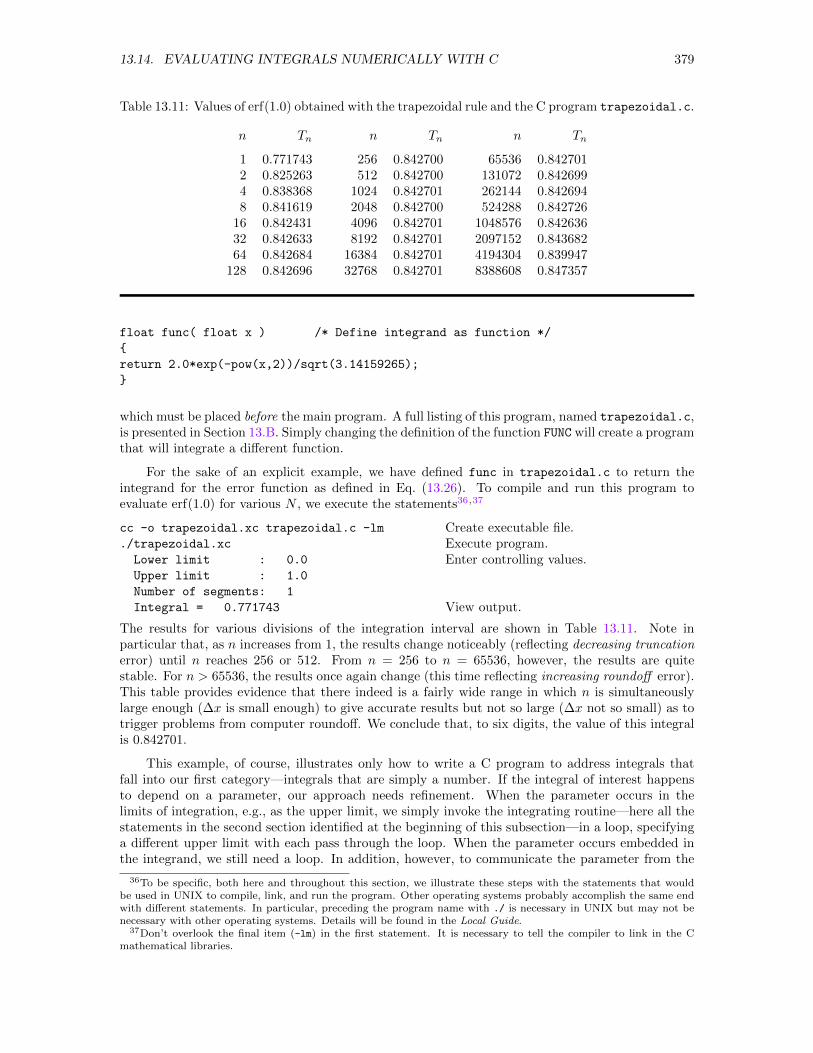
13.14. EVALUATING INTEGRALS NUMERICALLY WITH C 379

Table 13.11: Values of erf(1.0) obtained with the trapezoidal rule and the C program trapezoidal.c.

n Tn n Tn n Tn

1 0.771743 256 0.842700 65536 0.8427012 0.825263 512 0.842700 131072 0.8426994 0.838368 1024 0.842701 262144 0.8426948 0.841619 2048 0.842700 524288 0.842726

16 0.842431 4096 0.842701 1048576 0.84263632 0.842633 8192 0.842701 2097152 0.84368264 0.842684 16384 0.842701 4194304 0.839947

128 0.842696 32768 0.842701 8388608 0.847357

float func( float x ) /* Define integrand as function */

return 2.0*exp(-pow(x,2))/sqrt(3.14159265);

which must be placed before the main program. A full listing of this program, named trapezoidal.c,is presented in Section 13.B. Simply changing the definition of the function FUNC will create a programthat will integrate a different function.

For the sake of an explicit example, we have defined func in trapezoidal.c to return theintegrand for the error function as defined in Eq. (13.26). To compile and run this program toevaluate erf(1.0) for various N , we execute the statements36,37

cc -o trapezoidal.xc trapezoidal.c -lm

./trapezoidal.xc

Lower limit : 0.0

Upper limit : 1.0

Number of segments: 1

Integral = 0.771743

Create executable file.Execute program.Enter controlling values.

View output.

The results for various divisions of the integration interval are shown in Table 13.11. Note inparticular that, as n increases from 1, the results change noticeably (reflecting decreasing truncationerror) until n reaches 256 or 512. From n = 256 to n = 65536, however, the results are quitestable. For n > 65536, the results once again change (this time reflecting increasing roundoff error).This table provides evidence that there indeed is a fairly wide range in which n is simultaneouslylarge enough (∆x is small enough) to give accurate results but not so large (∆x not so small) as totrigger problems from computer roundoff. We conclude that, to six digits, the value of this integralis 0.842701.

This example, of course, illustrates only how to write a C program to address integrals thatfall into our first category—integrals that are simply a number. If the integral of interest happensto depend on a parameter, our approach needs refinement. When the parameter occurs in thelimits of integration, e.g., as the upper limit, we simply invoke the integrating routine—here all thestatements in the second section identified at the beginning of this subsection—in a loop, specifyinga different upper limit with each pass through the loop. When the parameter occurs embedded inthe integrand, we still need a loop. In addition, however, to communicate the parameter from the

36To be specific, both here and throughout this section, we illustrate these steps with the statements that wouldbe used in UNIX to compile, link, and run the program. Other operating systems probably accomplish the same endwith different statements. In particular, preceding the program name with ./ is necessary in UNIX but may not benecessary with other operating systems. Details will be found in the Local Guide.

37Don’t overlook the final item (-lm) in the first statement. It is necessary to tell the compiler to link in the Cmathematical libraries.

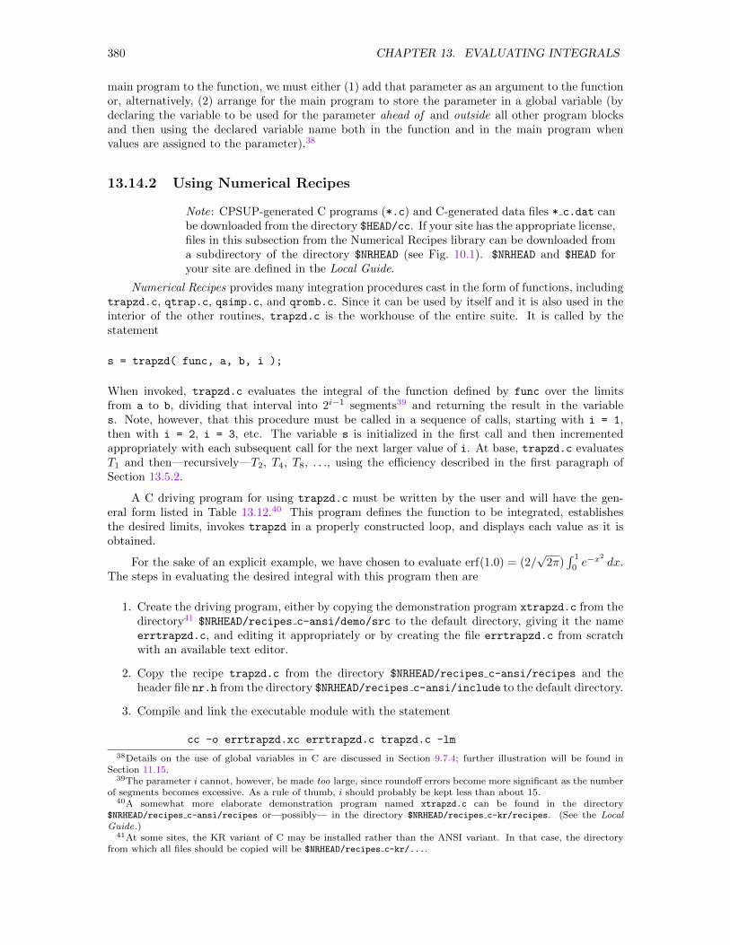
380 CHAPTER 13. EVALUATING INTEGRALS

main program to the function, we must either (1) add that parameter as an argument to the functionor, alternatively, (2) arrange for the main program to store the parameter in a global variable (bydeclaring the variable to be used for the parameter ahead of and outside all other program blocksand then using the declared variable name both in the function and in the main program whenvalues are assigned to the parameter).38

13.14.2 Using Numerical Recipes

Note: CPSUP-generated C programs (*.c) and C-generated data files * c.dat canbe downloaded from the directory $HEAD/cc. If your site has the appropriate license,files in this subsection from the Numerical Recipes library can be downloaded froma subdirectory of the directory $NRHEAD (see Fig. 10.1). $NRHEAD and $HEAD foryour site are defined in the Local Guide.

Numerical Recipes provides many integration procedures cast in the form of functions, includingtrapzd.c, qtrap.c, qsimp.c, and qromb.c. Since it can be used by itself and it is also used in theinterior of the other routines, trapzd.c is the workhouse of the entire suite. It is called by thestatement

s = trapzd( func, a, b, i );

When invoked, trapzd.c evaluates the integral of the function defined by func over the limitsfrom a to b, dividing that interval into 2i−1 segments39 and returning the result in the variables. Note, however, that this procedure must be called in a sequence of calls, starting with i = 1,then with i = 2, i = 3, etc. The variable s is initialized in the first call and then incrementedappropriately with each subsequent call for the next larger value of i. At base, trapzd.c evaluatesT1 and then—recursively—T2, T4, T8, . . ., using the efficiency described in the first paragraph ofSection 13.5.2.

A C driving program for using trapzd.c must be written by the user and will have the gen-eral form listed in Table 13.12.40 This program defines the function to be integrated, establishesthe desired limits, invokes trapzd in a properly constructed loop, and displays each value as it isobtained.

For the sake of an explicit example, we have chosen to evaluate erf(1.0) = (2/√

2π)∫ 1

0e−x

2

dx.The steps in evaluating the desired integral with this program then are

1. Create the driving program, either by copying the demonstration program xtrapzd.c from thedirectory41 $NRHEAD/recipes c-ansi/demo/src to the default directory, giving it the nameerrtrapzd.c, and editing it appropriately or by creating the file errtrapzd.c from scratchwith an available text editor.

2. Copy the recipe trapzd.c from the directory $NRHEAD/recipes c-ansi/recipes and theheader file nr.h from the directory $NRHEAD/recipes c-ansi/include to the default directory.

3. Compile and link the executable module with the statement

cc -o errtrapzd.xc errtrapzd.c trapzd.c -lm

38Details on the use of global variables in C are discussed in Section 9.7.4; further illustration will be found inSection 11.15.

39The parameter i cannot, however, be made too large, since roundoff errors become more significant as the numberof segments becomes excessive. As a rule of thumb, i should probably be kept less than about 15.

40A somewhat more elaborate demonstration program named xtrapzd.c can be found in the directory$NRHEAD/recipes c-ansi/recipes or—possibly— in the directory $NRHEAD/recipes c-kr/recipes. (See the LocalGuide.)

41At some sites, the KR variant of C may be installed rather than the ANSI variant. In that case, the directoryfrom which all files should be copied will be $NRHEAD/recipes c-kr/....

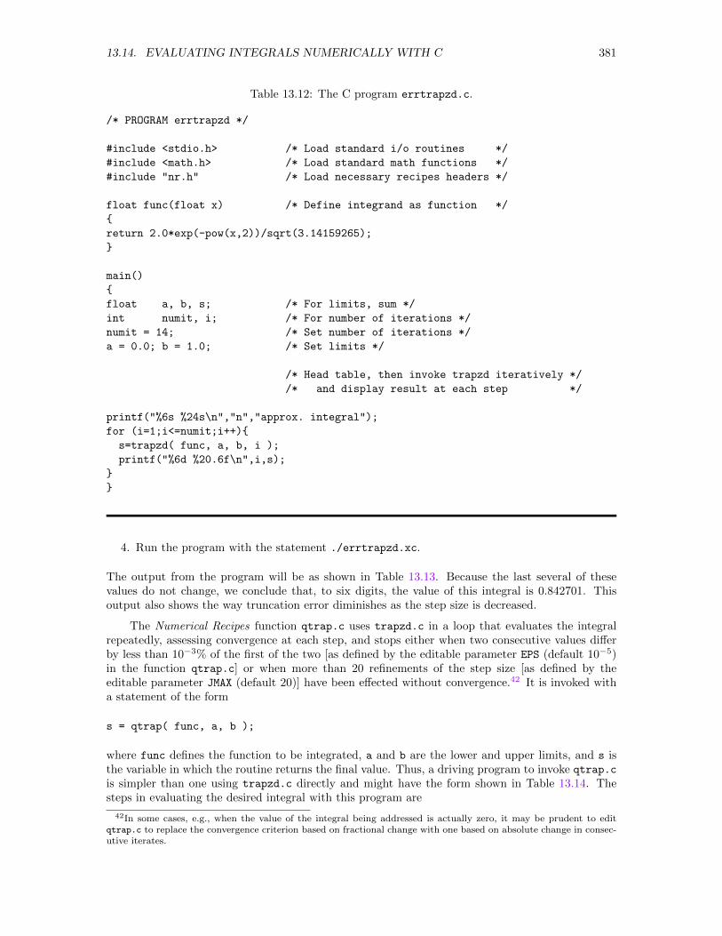
13.14. EVALUATING INTEGRALS NUMERICALLY WITH C 381

Table 13.12: The C program errtrapzd.c.

/* PROGRAM errtrapzd */

#include <stdio.h> /* Load standard i/o routines */

#include <math.h> /* Load standard math functions */

#include "nr.h" /* Load necessary recipes headers */

float func(float x) /* Define integrand as function */

return 2.0*exp(-pow(x,2))/sqrt(3.14159265);

main()

float a, b, s; /* For limits, sum */

int numit, i; /* For number of iterations */

numit = 14; /* Set number of iterations */

a = 0.0; b = 1.0; /* Set limits */

/* Head table, then invoke trapzd iteratively */

/* and display result at each step */

printf("%6s %24s\n","n","approx. integral");

for (i=1;i<=numit;i++)

s=trapzd( func, a, b, i );

printf("%6d %20.6f\n",i,s);

4. Run the program with the statement ./errtrapzd.xc.

The output from the program will be as shown in Table 13.13. Because the last several of thesevalues do not change, we conclude that, to six digits, the value of this integral is 0.842701. Thisoutput also shows the way truncation error diminishes as the step size is decreased.

The Numerical Recipes function qtrap.c uses trapzd.c in a loop that evaluates the integralrepeatedly, assessing convergence at each step, and stops either when two consecutive values differby less than 10−3% of the first of the two [as defined by the editable parameter EPS (default 10−5)in the function qtrap.c] or when more than 20 refinements of the step size [as defined by theeditable parameter JMAX (default 20)] have been effected without convergence.42 It is invoked witha statement of the form

s = qtrap( func, a, b );

where func defines the function to be integrated, a and b are the lower and upper limits, and s isthe variable in which the routine returns the final value. Thus, a driving program to invoke qtrap.c

is simpler than one using trapzd.c directly and might have the form shown in Table 13.14. Thesteps in evaluating the desired integral with this program are

42In some cases, e.g., when the value of the integral being addressed is actually zero, it may be prudent to editqtrap.c to replace the convergence criterion based on fractional change with one based on absolute change in consec-utive iterates.

382 CHAPTER 13. EVALUATING INTEGRALS

Table 13.13: Output from errtrapzd.c.

n approx. integral

1 0.771743

2 0.825263

3 0.838368

4 0.841619

5 0.842431

6 0.842633

7 0.842684

8 0.842697

9 0.842700

10 0.842701

11 0.842701

12 0.842701

13 0.842701

14 0.842701

Table 13.14: The C program errqtrap.c.

/* PROGRAM errqtrap */

#include <stdio.h> /* Load standard i/o routines */

#include <math.h> /* Load standard math routines */

#include "nr.h" /* Load necessary recipes headers */

float func(float x) /* Define integrand as function */

return 2.0*exp(-pow(x,2))/sqrt(3.14159265);

main()

float a, b, s; /* For limits, sum */

a = 0.0; b = 1.0; /* Set limits */

s = qtrap( func, a, b ); /* Evaluate integral */

printf("Result using QTRAP = %10.6f\n", s); /* Display result */

1. Create the driving program, either by copying the demonstration program xqtrap.c from thedirectory giving it the name errqtrap.c,and editing it appropriately, or by creating the fileerrqtrap.c from scratch with an available text editor.

2. Copy any necessary recipes and include files to the default directory. In the present case, theneeded recipe trapzd.c and header file nr.h presumably remain from the first example. Eachof the recipes qtrap.c and—discovered in a first (failed) attempt at compilation—nrutil.c

must be copied from the directory $NRHEAD/recipes c-ansi/recipes.

3. Compile and link the executable module with the statement

13.15. EXERCISES 383

cc -o errqtrap.xc errqtrap.c trapzd.c qtrap.c nrutil.c -lm

4. Run the program with the statement ./errqtrap.xc.

The output from the program will be

Result using QTRAP = 0.842700

which is certainly in agreement with earlier results (Note that failure to converge will result in amessage that includes “Too many steps ...” being printed on the screen. Here, the maximum numberof steps is 20 by default, that value being defined by an editable parameter in the subroutine qtrap.c.After printing this message, the subroutine returns control to the operating system.)

The Numerical Recipes procedures qsimp.c and qromb.c are used in a way quite parallel to thatof qtrap.c. The generation of programs to evaluate this test integral using each of these additionalroutines is left to the exercises. That these additional routines also yield the value 0.842701 is notat all a surprise.

Throughout this subsection, we have confined our explicit examples to integrals falling into ourfirst category. If the integral of interest happens to depend on a parameter, our approach needsrefinement. When the parameter occurs in the limits of integration, e.g., as the upper limit, wesimply invoke the integrating routine in a loop, specifying a different upper limit with each passthrough the loop. When the parameter occurs embedded in the integrand, we still need a loop. Inaddition, however, to communicate the parameter from the main program to the function, we musteither (1) add that parameter as an argument to the function and edit the numerical recipes routineto accept that parameter as an argument as well or, alternatively, (2) arrange for the main programto store the parameter in a global variable (by declaring the variable to be used for the parameterahead of and outside all other program blocks and then using the declared variable name both inthe function and in the main program when values are assigned to the parameter).43

13.15 Exercises

13.15.1 . . . using Symbolic Methods

13.1. A particle of mass m moves non-relativistically in one dimension under the action of a constantforce f . Starting with Eq. (13.3) and using symbolic integration, find the position x, velocity v,and momentum p of this particle as functions of time if x(0) = x0 and v(0) = v0.

13.2. A particle of mass m moves non-relativistically in one dimension under the action of a constantforce f . Starting with Eqs. (13.5) and (13.6) and using symbolic integration, find the position x,velocity v, and momentum p of this particle as functions of time if x(0) = x0 and v(0) = v0.

13.3. A particle of mass m moves non-relativistically in one dimension x under the action of a force givenby f(x) = −kx, where k is a (spring) constant. Starting with Eqs. (13.5) and (13.6) and usingsymbolic integration, find the position x, velocity v, and momentum p of this particle as functionsof time if x(0) = x0 > 0 and v(0) = 0.

13.4. Suppose an object of mass m moves non-relativistically in one dimension under the action of theforce f(t) = f0e

−bt, where both b and f0 are positive. Let x(0) = x0 and v(0) = v0. Use symbolicintegration to find x(t) and v(t) by evaluating the integrals in Eq. (13.3). Then, find and interpretboth the limits of these two results as t → ∞ and the Taylor expansion of these two results forsmall t.

43See footnote 38.

384 CHAPTER 13. EVALUATING INTEGRALS

13.5. The normalized Lorentz distribution function is given by

p(x) =1

π

a/2

x2 + (a/2)2

Using symbolic integration, (a) verify that∫ +∞−∞ p(x) dx = 1, (b) evaluate—as best you can—the

average x and variance σ2, defined by

x = limb→∞

∫ +b

−bx p(x) dx and σ2 = lim

b→∞

∫ +b

−b(x− x)2 p(x) dx

for this distribution, and (c) find the probability that a single, randomly selected value will lie inthe range −a ≤ x ≤ a. Finally, (d) show analytically that you should have expected the result ofpart (c) to be independent of a. Hint : Introduce the dimensionless variable λ = x/a.

13.6. Suppose some cataclysmic event stops the earth dead in its tracks and, responding to the sun’sgravitational attraction, the earth falls into the sun. Using symbolic integration, find the timerequired for the earth to fall over the middle half of its journey to the sun. Expressed in years,what is the value of this time for the earth-sun system? Hint : Since the gravitational potential is−GmM/x, conservation of energy yields

1

2m

(dx

dt

)2

−GmMx

= −GmMx0

=⇒ dx

dt= −√

2GM

√1

x− 1

x0

(The negative square root is taken because x, the distance to the sun, is known to be decreasing.)This expression then leads to the value

Tmidhalf =1√

2GM

∫ 3x0/4

x0/4

(1

x− 1

x0

)−1/2

dx

Hint : The evaluation will be simpler if you begin by recasting the problem in dimensionless terms,expressing lengths in units of x0 and times in units of

√x3

0/(2GM). To interpret the significanceof this unit of time, determine the period of a circular orbit of radius x0, which will turn out tobe 2π

√x3

0/GM . For the earth around the sun, this latter time is, of course, 1 year. Optional :Evaluate the time required for the first half of the journey, which involves a convergent but improperintegral.

13.7. According to the quantum theory, the probability that the electron in the ground state of thehydrogen atom will be found between the center of the atom and some radius r is given by

P (r) =4

a3

∫ r

0

e−2r′/ar′2dr′ = 4

∫ r/a

0

e−2ρ ρ2 dρ

where a is the Bohr radius and ρ = r′/a. Evaluate this integral symbolically. Then plot andcomment on a graph of P (r) versus r/a.

13.8. Consider a source consisting of two uniformly charged disks, each of radius a and each orientedwith its center on the z axis and its plane perpendicular to the z axis. Let one disk have its centerat (0,0,ca) and carry a positive charge density σ and the other have its center at (0,0,−ca) andcarry a negative charge density −σ. Using a symbolic program, show that the on-axis electrostaticpotential established by this source is given by

V (z) =σ

2ε0

[√a2 + (z − ca)2 − |z − ca| −

√a2 + (z + ca)2 + |z + ca|

]and then explore this potential as a function of z/a for various values of c. Hint : First find theon-axis potential of a single disk lying in the xy plane, and then construct the desired potential bysuperposition.

13.15. EXERCISES 385

13.9. In a spherically symmetric charge distribution, the charge density is a function of only the radialcoordinate, ρ(r) = ρ(r). Suppose ρ(r) = 0 for r > a. Find the electrostatic potential at a point onthe z axis, r = zk, for which z > a by setting up and evaluating the integral

V (0, 0, z) =1

4πε0

∫ρ(r′) dv′

|r− r′|

symbolically to show that V (0, 0, z) = Q/4πε0z. (Q is the total charge in the distribution.) Thisresult demonstrates formally that the potential at a point outside a spherically symmetric chargedistribution can be evaluated by regarding the charge to be concentrated at the center of thedistribution. Hint : Write r′ = x′ i + y′ j + z′ k but then use spherical coordinates to express x′,y′, and z′.

13.10. Consider a surface in the xy plane having uniform mass density σ and having the shape of a cardioidgiven in polar coordinates by the function r(φ) = a(1− cosφ). Using symbolic integration, find (a)the center of mass of this object, (b) the moment of inertia tensor of this object about the x, y,and z axes, and (c) the radius of gyration about the z axis. Hints: The center of mass is definedin Section 13.1.2; the moment of inertia tensor is a 3× 3 tensor whose ij element is given by

Iij =

∫[(x2

1 + x22 + x2

3)δij − xixj ] dm

where x1, x2, and x3 symbolize x, y, and z, respectively; δij is the Kronecker delta, which has thevalue 1 when i = j and the value 0 otherwise; and the radius of gyration is defined in Section 13.1.3.

13.11. In quantum mechanics, the two integrals

xmn =

∫ ∞−∞

ψ∗m(x)xψn(x) dx and pmn =

∫ ∞−∞

ψ∗m(x)h

i

∂

∂xψn(x) dx

are important in a variety of contexts. For a particle in an infinitely deep potential well that extendsover the region −a ≤ x ≤ a,

ψn(x) =

1√a

cosnπx

2an = 1, 3, 5, . . .

1√a

sinnπx

2an = 2, 4, 6, . . .

Using symbolic integration, show that, for these wave functions, xmn = 0 and pmn = 0 when mand n are both even or both odd and that

xmn =16a

π2(−1)(m+n+1)/2 mn

(m2 − n2)2

pmn =2ih

a(−1)(m+n+1)/2 mn

(m2 − n2)

otherwise. Note that, for purposes of translating the general integrals above to the circumstances ofthis exercise, the wave functions should both be regarded as zero outside of the interval −a ≤ x ≤ a.

13.12. The sawtooth wave is defined by

f(x) =x

l; −l ≤ x ≤ l

Use symbolic integration to find the Fourier coefficients an and bn for this function and then generategraphs showing the function given by the truncated series

ftrunc(x) =a0

2+

N∑n=1

(an cos

nπx

l+ bn sin

nπx

l

)for various values of N , including 0, 1, 2, 3, and 10.

386 CHAPTER 13. EVALUATING INTEGRALS

13.13. The Legendre polynomials Ln(x), n = 0, 1, 2, . . ., are orthogonal on the interval −1 ≤ x ≤ 1 withweight 1. In particular, ∫ 1

−1

Lm(x)Ln(x) dx =2

2n+ 1δmn

Any function defined over the interval −1 ≤ x ≤ 1 can then be expanded in the Legendre series

f(x) =

∞∑n=0

cn Ln(x)

(a) Show by hand that the coefficient cn in this expansion is given by

cn =2n+ 1

2

∫ 1

−1

f(x)Ln(x) dx

(b) Use symbolic integration to find cn for n = 0, 1, 2, 3, 4, 5 and 6 in the Legendre expansion forthe function

f(x) =

−1 −1 < x < 0

1 0 < x < 1

(c) Graph the functions defined by the partial sums∑N

n=0cn Ln(x) for N = 0, 1, 2, 3, 4, 5, and 6.

Hint : Quite possibly the symbolic program you are using has the Legendre polynomials built insomehow, and you should study its manuals to find out how to invoke them. Just in case that isn’ttrue, the first nine Legendre polynomials are

L0(x) = 1 L5(x) = 18(63x5 − 70x3 + 15x)

L1(x) = x L6(x) = 116

(231x6 − 315x4 + 105x2 − 5)

L2(x) = 12(3x2 − 1) L7(x) = 1

16(429x7 − 693x5 + 315x3 − 35x)

L3(x) = 12(5x3 − 3x) L8(x) = 1

128(6435x8 − 12012x6 + 6930x4 − 1260x2 + 35)

L4(x) = 18(35x4 − 30x2 + 3) L9(x) = 1

128(12155x9 − 25740x7 + 18018x5 − 4620x3 + 315x)

13.15.2 . . . using Numerical Methods

13.14. To deduce Simpson’s rule, we start by supposing three consecutive values f1, f2, and f3 of theintegrand, where for simplicity in notation we take the points of evaluation to be x1 = x2−∆x, x2,and x3 = x2 + ∆x. Using a symbol manipulating program to do the algebra and calculus, (a) findthe coefficients A, B, and C needed to make the parabola Ax2 + Bx + C pass through the threepoints (xi, fi), i = 1, 2, 3, (b) integrate that parabola over the interval x1 < x < x3 to find that∫ x3

x1

f(x) dx ≈∫ x3

x1

(Ax2 +Bx+ C) dx =∆x

3

(f1 + 4f2 + f3

)(c) show that this result actually gives the correct value for f(x) = x3 and, finally, (d) deducethe (extended) Simpson’s rule of Eq. (13.63). Note: Because this exercise relates to numericalalgorithms, it has been placed in with other exercises that are numerical. This exercise is symbolic,and you should use a symbol manipulating program for parts (a), (b), and (c); however, you shouldaddress part (d) by hand.

13.17. (a) Deduce the three-point Gaussian formula, for which—paralleling Eq. (13.88)—we set∫ 1

−1

f(x) dx = w1 f(x1) + w2 f(x2) + w3 f(x3)

We then choose the six quantities wi, and xi so that the expression gives an exact result forf(x) = 1, x, x2, x3, x4, and x5. (b) Verify that the interpolation points xi and weights wi are givenby Eq. (13.101) where L3(x) = (5x3 − 3x)/2.

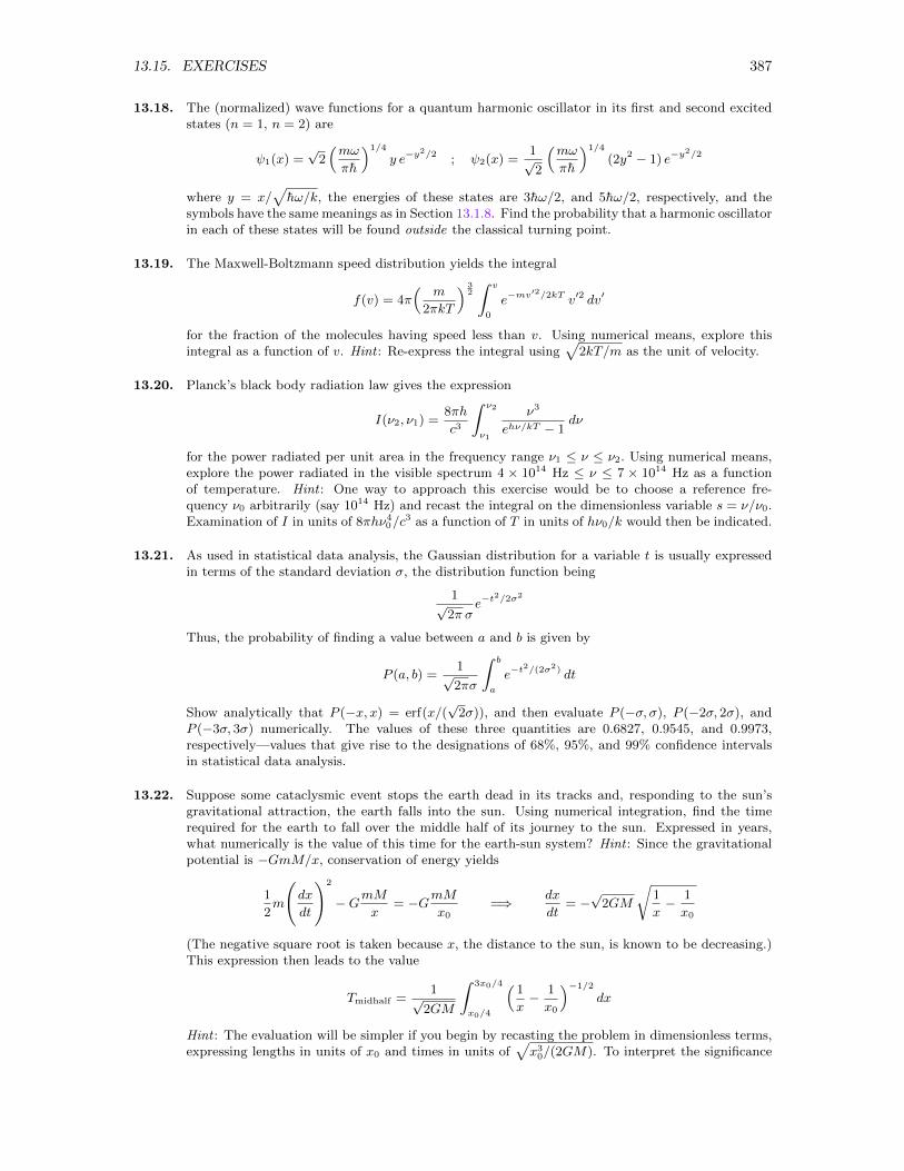
13.15. EXERCISES 387

13.18. The (normalized) wave functions for a quantum harmonic oscillator in its first and second excitedstates (n = 1, n = 2) are

ψ1(x) =√

2(mω

πh

)1/4

y e−y2/2 ; ψ2(x) =

1√2

(mω

πh

)1/4

(2y2 − 1) e−y2/2

where y = x/√hω/k, the energies of these states are 3hω/2, and 5hω/2, respectively, and the

symbols have the same meanings as in Section 13.1.8. Find the probability that a harmonic oscillatorin each of these states will be found outside the classical turning point.

13.19. The Maxwell-Boltzmann speed distribution yields the integral

f(v) = 4π(

m

2πkT

) 32

∫ v

0

e−mv′2/2kT v′2 dv′

for the fraction of the molecules having speed less than v. Using numerical means, explore thisintegral as a function of v. Hint : Re-express the integral using

√2kT/m as the unit of velocity.

13.20. Planck’s black body radiation law gives the expression

I(ν2, ν1) =8πh

c3

∫ ν2

ν1

ν3

ehν/kT − 1dν

for the power radiated per unit area in the frequency range ν1 ≤ ν ≤ ν2. Using numerical means,explore the power radiated in the visible spectrum 4 × 1014 Hz ≤ ν ≤ 7 × 1014 Hz as a functionof temperature. Hint : One way to approach this exercise would be to choose a reference fre-quency ν0 arbitrarily (say 1014 Hz) and recast the integral on the dimensionless variable s = ν/ν0.Examination of I in units of 8πhν4

0/c3 as a function of T in units of hν0/k would then be indicated.

13.21. As used in statistical data analysis, the Gaussian distribution for a variable t is usually expressedin terms of the standard deviation σ, the distribution function being

1√2π σ

e−t2/2σ2

Thus, the probability of finding a value between a and b is given by

P (a, b) =1√2πσ

∫ b

a

e−t2/(2σ2) dt

Show analytically that P (−x, x) = erf(x/(√

2σ)), and then evaluate P (−σ, σ), P (−2σ, 2σ), andP (−3σ, 3σ) numerically. The values of these three quantities are 0.6827, 0.9545, and 0.9973,respectively—values that give rise to the designations of 68%, 95%, and 99% confidence intervalsin statistical data analysis.

13.22. Suppose some cataclysmic event stops the earth dead in its tracks and, responding to the sun’sgravitational attraction, the earth falls into the sun. Using numerical integration, find the timerequired for the earth to fall over the middle half of its journey to the sun. Expressed in years,what numerically is the value of this time for the earth-sun system? Hint : Since the gravitationalpotential is −GmM/x, conservation of energy yields

1

2m

(dx

dt

)2

−GmMx

= −GmMx0

=⇒ dx

dt= −√

2GM

√1

x− 1

x0

(The negative square root is taken because x, the distance to the sun, is known to be decreasing.)This expression then leads to the value

Tmidhalf =1√

2GM

∫ 3x0/4

x0/4

(1

x− 1

x0

)−1/2

dx

Hint : The evaluation will be simpler if you begin by recasting the problem in dimensionless terms,expressing lengths in units of x0 and times in units of

√x3

0/(2GM). To interpret the significance

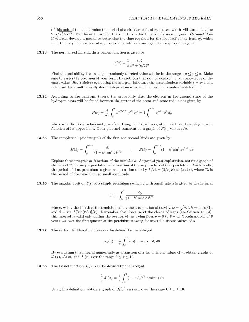
388 CHAPTER 13. EVALUATING INTEGRALS

of this unit of time, determine the period of a circular orbit of radius x0, which will turn out to be2π√x3

0/GM . For the earth around the sun, this latter time is, of course, 1 year. Optional : Seeif you can develop a means to determine the time required for the first half of the journey, whichunfortunately—for numerical approaches—involves a convergent but improper integral.

13.23. The normalized Lorentz distribution function is given by

p(x) =1

π

a/2

x2 + (a/2)2

Find the probability that a single, randomly selected value will be in the range −a ≤ x ≤ a. Makesure to assess the precision of your result by methods that do not exploit a priori knowledge of theexact value. Hint : Before evaluating the integral, introduce the dimensionless variable s = x/a andnote that the result actually doesn’t depend on a, so there is but one number to determine.

13.24. According to the quantum theory, the probability that the electron in the ground state of thehydrogen atom will be found between the center of the atom and some radius r is given by

P (r) =4

a3

∫ r

0

e−2r′/a r′2 dr′ = 4

∫ r/a

0

e−2ρ ρ2 dρ

where a is the Bohr radius and ρ = r′/a. Using numerical integration, evaluate this integral as afunction of its upper limit. Then plot and comment on a graph of P (r) versus r/a.

13.25. The complete elliptic integrals of the first and second kinds are given by

K(k) =

∫ π/2

0

dφ

(1− k2 sin2 φ)1/2; E(k) =

∫ π/2

0

(1− k2 sin2 φ)1/2 dφ

Explore these integrals as functions of the modulus k. As part of your exploration, obtain a graph ofthe period T of a simple pendulum as a function of the amplitude α of that pendulum. Analytically,the period of that pendulum is given as a function of α by T/T0 = (2/π)K( sin(α/2) ), where T0 isthe period of the pendulum at small amplitude.

13.26. The angular position θ(t) of a simple pendulum swinging with amplitude α is given by the integral

ωt =

∫ β

0

dφ

(1− k2 sin2 φ)1/2

where, with l the length of the pendulum and g the acceleration of gravity, ω =√g/l, k = sin(α/2),

and β = sin−1([sin(θ/2)]/k). Remember that, because of the choice of signs (see Section 13.1.4),this integral is valid only during the portion of the swing from θ = 0 to θ = α. Obtain graphs of θversus ωt over the first quarter of the pendulum’s swing for several different values of α.

13.27. The n-th order Bessel function can be defined by the integral

Jn(x) =1

π

∫ π

0

cos(nθ − x sin θ) dθ

By evaluating this integral numerically as a function of x for different values of n, obtain graphs ofJ0(x), J1(x), and J2(x) over the range 0 ≤ x ≤ 10.

13.28. The Bessel function J1(x) can be defined by the integral

1

xJ1(x) =

2

π

∫ 1

0

(1− u2)1/2 cos(xu) du

Using this definition, obtain a graph of J1(x) versus x over the range 0 ≤ x ≤ 10.

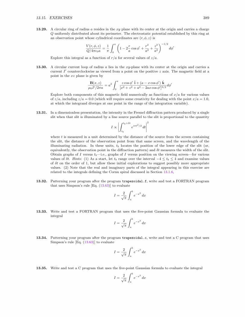
13.15. EXERCISES 389

13.29. A circular ring of radius a resides in the xy plane with its center at the origin and carries a chargeQ uniformly distributed about its perimeter. The electrostatic potential established by this ring atan observation point whose cylindrical coordinates are (r, φ, z) is

V (r, φ, z)

Q/4πε0a=

1

π

∫ π

0

(1− 2

r

acosφ′ +

r2

a2+z2

a2

)−1/2

dφ′

Explore this integral as a function of r/a for several values of z/a.

13.30. A circular current loop of radius a lies in the xy-plane with its center at the origin and carries acurrent I ′ counterclockwise as viewed from a point on the positive z axis. The magnetic field at apoint in the xz plane is given by

B(x, z)

µ0I ′/2πa= a2

∫ π

0

z cosφ′ i + (a− x cosφ′) k

[x2 + z2 + a2 − 2ax cosφ′]3/2dφ′

Explore both components of this magnetic field numerically as functions of x/a for various valuesof z/a, including z/a = 0.0 (which will require some creativity for dealing with the point x/a = 1.0,at which the integrand diverges at one point in the range of the integration variable).

13.31. In a dimensionless presentation, the intensity in the Fresnel diffraction pattern produced by a singleslit when that slit is illuminated by a line source parallel to the slit is proportional to the quantity

I ∝∣∣∣∣∫ tb+δt

tb

eiπt2/2 dt

∣∣∣∣2where t is measured in a unit determined by the distance of the source from the screen containingthe slit, the distance of the observation point from that same screen, and the wavelength of theilluminating radiation. In these units, tb locates the position of the lower edge of the slit (or,equivalently, the observation point in the diffraction pattern) and δt measures the width of the slit.Obtain graphs of I versus tb—i.e., graphs of I versus position on the viewing screen—for variousvalues of δt. Hints: (1) As a start, let tb range over the interval −4 ≤ tb ≤ 4 and examine valuesof δt on the order of 1, but allow these initial explorations to suggest possibly more appropriatevalues. (2) Note that the real and imaginary parts of the integral appearing in this exercise arerelated to the integrals defining the Cornu spiral discussed in Section 13.1.6,

13.32. Patterning your program after the program trapezoidal.f, write and test a FORTRAN programthat uses Simpson’s rule [Eq. (13.63)] to evaluate

I =2√π

∫ b

a

e−x2

dx

13.33. Write and test a FORTRAN program that uses the five-point Gaussian formula to evaluate theintegral

I =2√π

∫ b

a

e−x2

dx

13.34. Patterning your program after the program trapezoidal.c, write and test a C program that usesSimpson’s rule [Eq. (13.63)] to evaluate

I =2√π

∫ b

a

e−x2

dx

13.35. Write and test a C program that uses the five-point Gaussian formula to evaluate the integral

I =2√π

∫ b

a

e−x2

dx

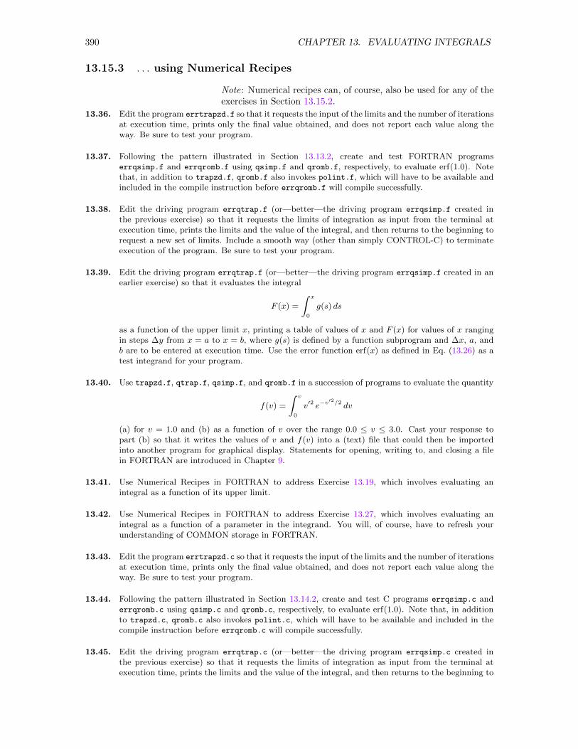
390 CHAPTER 13. EVALUATING INTEGRALS

13.15.3 . . . using Numerical Recipes

Note: Numerical recipes can, of course, also be used for any of theexercises in Section 13.15.2.

13.36. Edit the program errtrapzd.f so that it requests the input of the limits and the number of iterationsat execution time, prints only the final value obtained, and does not report each value along theway. Be sure to test your program.

13.37. Following the pattern illustrated in Section 13.13.2, create and test FORTRAN programserrqsimp.f and errqromb.f using qsimp.f and qromb.f, respectively, to evaluate erf(1.0). Notethat, in addition to trapzd.f, qromb.f also invokes polint.f, which will have to be available andincluded in the compile instruction before errqromb.f will compile successfully.

13.38. Edit the driving program errqtrap.f (or—better—the driving program errqsimp.f created inthe previous exercise) so that it requests the limits of integration as input from the terminal atexecution time, prints the limits and the value of the integral, and then returns to the beginning torequest a new set of limits. Include a smooth way (other than simply CONTROL-C) to terminateexecution of the program. Be sure to test your program.

13.39. Edit the driving program errqtrap.f (or—better—the driving program errqsimp.f created in anearlier exercise) so that it evaluates the integral

F (x) =

∫ x

0

g(s) ds

as a function of the upper limit x, printing a table of values of x and F (x) for values of x rangingin steps ∆y from x = a to x = b, where g(s) is defined by a function subprogram and ∆x, a, andb are to be entered at execution time. Use the error function erf(x) as defined in Eq. (13.26) as atest integrand for your program.

13.40. Use trapzd.f, qtrap.f, qsimp.f, and qromb.f in a succession of programs to evaluate the quantity

f(v) =

∫ v

0

v′2 e−v′2/2 dv

(a) for v = 1.0 and (b) as a function of v over the range 0.0 ≤ v ≤ 3.0. Cast your response topart (b) so that it writes the values of v and f(v) into a (text) file that could then be importedinto another program for graphical display. Statements for opening, writing to, and closing a filein FORTRAN are introduced in Chapter 9.

13.41. Use Numerical Recipes in FORTRAN to address Exercise 13.19, which involves evaluating anintegral as a function of its upper limit.

13.42. Use Numerical Recipes in FORTRAN to address Exercise 13.27, which involves evaluating anintegral as a function of a parameter in the integrand. You will, of course, have to refresh yourunderstanding of COMMON storage in FORTRAN.

13.43. Edit the program errtrapzd.c so that it requests the input of the limits and the number of iterationsat execution time, prints only the final value obtained, and does not report each value along theway. Be sure to test your program.

13.44. Following the pattern illustrated in Section 13.14.2, create and test C programs errqsimp.c anderrqromb.c using qsimp.c and qromb.c, respectively, to evaluate erf(1.0). Note that, in additionto trapzd.c, qromb.c also invokes polint.c, which will have to be available and included in thecompile instruction before errqromb.c will compile successfully.

13.45. Edit the driving program errqtrap.c (or—better—the driving program errqsimp.c created inthe previous exercise) so that it requests the limits of integration as input from the terminal atexecution time, prints the limits and the value of the integral, and then returns to the beginning to

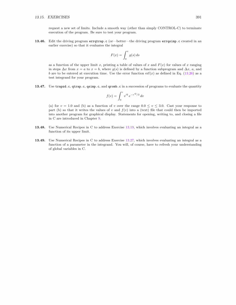
13.15. EXERCISES 391

request a new set of limits. Include a smooth way (other than simply CONTROL-C) to terminateexecution of the program. Be sure to test your program.

13.46. Edit the driving program errqtrap.c (or—better—the driving program errqsimp.c created in anearlier exercise) so that it evaluates the integral

F (x) =

∫ x

0

g(s) ds

as a function of the upper limit x, printing a table of values of x and F (x) for values of x rangingin steps ∆x from x = a to x = b, where g(s) is defined by a function subprogram and ∆x, a, andb are to be entered at execution time. Use the error function erf(x) as defined in Eq. (13.26) as atest integrand for your program.

13.47. Use trapzd.c, qtrap.c, qsimp.c, and qromb.c in a succession of programs to evaluate the quantity

f(v) =

∫ v

0

v′2 e−v′2/2 dv

(a) for v = 1.0 and (b) as a function of v over the range 0.0 ≤ v ≤ 3.0. Cast your response topart (b) so that it writes the values of v and f(v) into a (text) file that could then be importedinto another program for graphical display. Statements for opening, writing to, and closing a filein C are introduced in Chapter 9.

13.48. Use Numerical Recipes in C to address Exercise 13.19, which involves evaluating an integral as afunction of its upper limit.

13.49. Use Numerical Recipes in C to address Exercise 13.27, which involves evaluating an integral as afunction of a parameter in the integrand. You will, of course, have to refresh your understandingof global variables in C.

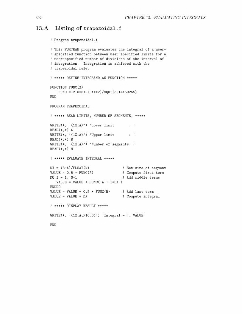
392 CHAPTER 13. EVALUATING INTEGRALS

13.A Listing of trapezoidal.f

! Program trapezoidal.f

! This FORTRAN program evaluates the integral of a user-

! specified function between user-specified limits for a

! user-specified number of divisions of the interval of

! integration. Integration is achieved with the

! trapezoidal rule.

! ***** DEFINE INTEGRAND AS FUNCTION *****

FUNCTION FUNC(X)

FUNC = 2.0*EXP(-X**2)/SQRT(3.14159265)

END

PROGRAM TRAPEZOIDAL

! ***** READ LIMITS, NUMBER OF SEGMENTS, *****

WRITE(*, ’(1X,A)’) ’Lower limit : ’

READ(*,*) A

WRITE(*, ’(1X,A)’) ’Upper limit : ’

READ(*,*) B

WRITE(*, ’(1X,A)’) ’Number of segments: ’

READ(*,*) N

! ***** EVALUATE INTEGRAL *****

DX = (B-A)/FLOAT(N) ! Set size of segment

VALUE = 0.5 * FUNC(A) ! Compute first term

DO I = 1, N-1 ! Add middle terms

VALUE = VALUE + FUNC( A + I*DX )

ENDDO

VALUE = VALUE + 0.5 * FUNC(B) ! Add last term

VALUE = VALUE * DX ! Compute integral

! ***** DISPLAY RESULT *****

WRITE(*, ’(1X,A,F10.6)’) ’Integral = ’, VALUE

END

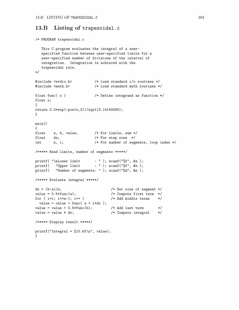
13.B. LISTING OF TRAPEZOIDAL.C 393

13.B Listing of trapezoidal.c

/* PROGRAM trapezoidal.c

This C program evaluates the integral of a user-

specified function between user-specified limits for a

user-specified number of divisions of the interval of

integration. Integration is achieved with the

trapezoidal rule.

*/

#include <stdio.h> /* Load standard i/o routines */

#include <math.h> /* Load standard math routines */

float func( x ) /* Define integrand as function */

float x;

return 2.0*exp(-pow(x,2))/sqrt(3.14159265);

main()

float a, b, value; /* For limits, sum */

float dx; /* For step size */

int n, i; /* For number of segments, loop index */

/***** Read limits, number of segments *****/

printf( "\nLower limit : " ); scanf("%f", &a );

printf( "Upper limit : " ); scanf("%f", &b );

printf( "Number of segments: " ); scanf("%d", &n );

/***** Evaluate integral *****/

dx = (b-a)/n; /* Set size of segment */

value = 0.5*func(a); /* Compute first term */

for ( i=1; i<=n-1; i++ ) /* Add middle terms */

value = value + func( a + i*dx );

value = value + 0.5*func(b); /* Add last term */

value = value * dx; /* Compute integral */

/***** Display result *****/

printf("Integral = %10.6f\n", value);

394 CHAPTER 13. EVALUATING INTEGRALS

Chapter 14

Finding Roots

In this chapter, we seek the roots of a known function f(x), i.e., we seek values of x satisfying theequation

f(x) = 0 (14.1)

If f(x) is simple, we may be able to find a closed form, analytic solution. More often, however, f(x) issufficiently complicated that approximate, numerical methods are needed. Further, many functionswill have several roots, some of which may be physically meaningless. Thus, we must learn not onlyhow to find the roots but also how to sort the physically meaningful roots from a possibly largernumber of mathematically acceptable ones, the “extras” of which are said to be spurious. We beginthis chapter by identifying several physical situations, the full addressing of which requires finding oneor more roots of some function. Then we illustrate how to use symbolic algebra systems to approachthose that can be addressed analytically, describe a few of many available numerical algorithms, anddescribe ways to find roots using a variety of numerical approaches and computational tools. Brieflyat the end, we comment about the more complicated issue of finding roots of sets of simultaneouslinear and non-linear equations. Until that point, our discussion will focus on functions of a singlevariable.

Whatever the function and whatever the approach, the first step in seeking roots should alwaysbe to learn as much as possible about the nature of the function and its roots. Further, sincenumerical methods in particular—most of them iterative—require a starting guess or guesses andwill converge more or less rapidly and reliably depending on the quality of those guesses, a prioriknowledge of the approximate location of roots is essential. Thus, we should always start by drawinga graph of f(x) in sufficient detail to reveal the approximate location of the roots of interest. Sincethe focus of this chapter is not graphing (and graphing has been fully addressed in earlier chapters),we shall carry out this step once in Section 14.1 as we present several sample problems rather thancarrying it out repeatedly in later sections.1

14.1 Sample Problems

In this section, we identify several physical contexts in which the essential computational problemis to find the roots of some function, and we obtain graphs of the appropriate functions for laterreference.

1The graphs could, of course, be produced in any number of ways. Except for Fig. 14.2 (which was produced withtgif), the graphs in Section 14.1 have all been produced with IDL. Those in each later section have been producedby whatever software is the subject of that section.

395

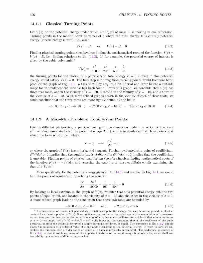
396 CHAPTER 14. FINDING ROOTS

14.1.1 Classical Turning Points

Let V (x) be the potential energy under which an object of mass m is moving in one dimension.Turning points in the motion occur at values of x where the total energy E is entirely potentialenergy (kinetic energy is zero), i.e., when

V (x) = E or V (x)− E = 0 (14.2)

Finding physical turning points thus involves finding the mathematical roots of the function f(x) =V (x) − E, i.e., finding solutions to Eq. (14.2). If, for example, the potential energy of interest isgiven by the cubic polynomial2

V (x) =x3

10000+

x2

200− x

500− 1

2(14.3)

the turning points for the motion of a particle with total energy E = 0 moving in this potentialenergy would satisfy V (x) = 0. The first step in finding those turning points would therefore be toproduce the graph of Fig. 14.1—a task that may require a bit of trial and error before a suitablerange for the independent variable has been found. From this graph, we conclude that V (x) hasthree real roots, one in the vicinity of x = −50, a second in the vicinity of x = −10, and a third inthe vicinity of x = +10. With more refined graphs drawn in the vicinity of each of these roots, wecould conclude that the three roots are more tightly bound by the limits

−50.00 < x1 < −47.50 ; −12.50 < x2 < −10.00 ; 7.50 < x3 < 10.00 (14.4)

14.1.2 A Max-Min Problem: Equilibrium Points

From a different perspective, a particle moving in one dimension under the action of the forceF = −dV/dx associated with the potential energy V (x) will be in equilibrium at those points x atwhich the force is zero, i.e., where

F = 0 =⇒ dV

dx= 0 (14.5)

or where the graph of V (x) has a horizontal tangent. Further, evaluated at a point of equilibrium,d2V/dx2 > 0 implies that the equilibrium is stable while d2V/dx2 < 0 implies that the equilibriumis unstable. Finding points of physical equilibrium therefore involves finding mathematical roots ofthe function F (x) = −dV/dx, and assessing the stability of those equilibria entails examining thesign of d2V/dx2.

More specifically, for the potential energy given in Eq. (14.3) and graphed in Fig. 14.1, we wouldfind the points of equilibrium by solving the equation

dV

dx=

3x2

10000+

x

100− 1

500= 0 (14.6)

By looking at local extrema in the graph of V (x), we infer that this potential energy exhibits twopoints of equilibrium, one located in the vicinity of x = −35 and the other in the vicinity of x = 0.A more refined graph leads to the conclusion that these two roots are bounded by

−35.0 < x4 < −30.0 and − 2.5 < x5 < 2.5 (14.7)2This function is, of course, not particularly realistic as a potential energy. We can, however, provide a physical

context for at least a portion of V (x). If we confine our attention to the region around the one minimum it possesses,we can interpret the function as the potential energy of an anharmonic oscillator, for which—if that minimum occursat x = 0—we might write V (x) = kx2/2 + ax3 while imposing the constraint that a, the coefficient of the cubicperturbation from the potential energy of a simple harmonic oscillator, be small. The expression in Eq. (14.2) simplyplaces the minimum at a different value of x and adds a constant to the potential energy. In what follows, we willexplore this function over a wider range of values of x than is physically meaningful. The pedagogic advantage ofEq. (14.2) is that it combines many of the important features of potential energy functions with, as we shall see,tractability by a variety of different approaches.

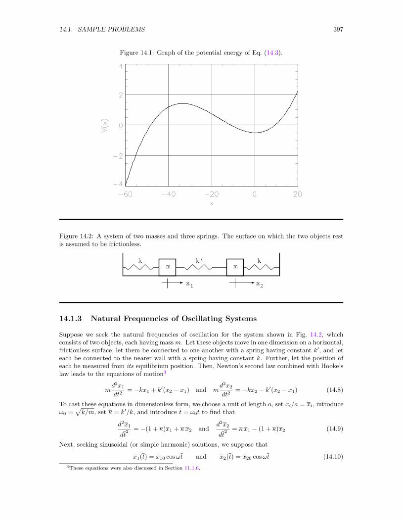
14.1. SAMPLE PROBLEMS 397

Figure 14.1: Graph of the potential energy of Eq. (14.3).

Figure 14.2: A system of two masses and three springs. The surface on which the two objects restis assumed to be frictionless.

m mk’ kk

x1 x2

14.1.3 Natural Frequencies of Oscillating Systems

Suppose we seek the natural frequencies of oscillation for the system shown in Fig. 14.2, whichconsists of two objects, each having mass m. Let these objects move in one dimension on a horizontal,frictionless surface, let them be connected to one another with a spring having constant k′, and leteach be connected to the nearer wall with a spring having constant k. Further, let the position ofeach be measured from its equilibrium position. Then, Newton’s second law combined with Hooke’slaw leads to the equations of motion3

md2x1dt2

= −kx1 + k′(x2 − x1) and md2x2dt2

= −kx2 − k′(x2 − x1) (14.8)

To cast these equations in dimensionless form, we choose a unit of length a, set xi/a = xi, introduceω0 =

√k/m, set κ = k′/k, and introduce t = ω0t to find that

d2x1

dt2 = −(1 + κ)x1 + κx2 and

d2x2

dt2 = κx1 − (1 + κ)x2 (14.9)

Next, seeking sinusoidal (or simple harmonic) solutions, we suppose that

x1(t) = x10 cosωt and x2(t) = x20 cosωt (14.10)

3These equations were also discussed in Section 11.1.6.

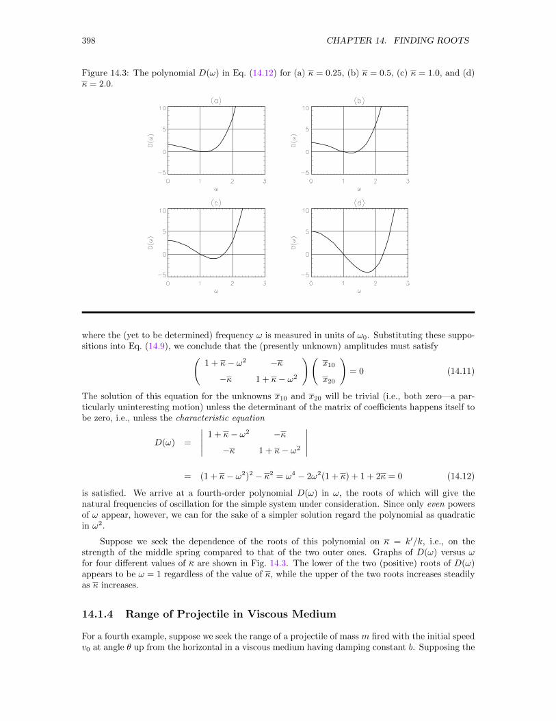
398 CHAPTER 14. FINDING ROOTS

Figure 14.3: The polynomial D(ω) in Eq. (14.12) for (a) κ = 0.25, (b) κ = 0.5, (c) κ = 1.0, and (d)κ = 2.0.

where the (yet to be determined) frequency ω is measured in units of ω0. Substituting these suppo-sitions into Eq. (14.9), we conclude that the (presently unknown) amplitudes must satisfy(

1 + κ− ω2 −κ

−κ 1 + κ− ω2

)(x10

x20

)= 0 (14.11)

The solution of this equation for the unknowns x10 and x20 will be trivial (i.e., both zero—a par-ticularly uninteresting motion) unless the determinant of the matrix of coefficients happens itself tobe zero, i.e., unless the characteristic equation

D(ω) =

∣∣∣∣∣ 1 + κ− ω2 −κ

−κ 1 + κ− ω2

∣∣∣∣∣= (1 + κ− ω2)2 − κ2 = ω4 − 2ω2(1 + κ) + 1 + 2κ = 0 (14.12)

is satisfied. We arrive at a fourth-order polynomial D(ω) in ω, the roots of which will give thenatural frequencies of oscillation for the simple system under consideration. Since only even powersof ω appear, however, we can for the sake of a simpler solution regard the polynomial as quadraticin ω2.

Suppose we seek the dependence of the roots of this polynomial on κ = k′/k, i.e., on thestrength of the middle spring compared to that of the two outer ones. Graphs of D(ω) versus ωfor four different values of κ are shown in Fig. 14.3. The lower of the two (positive) roots of D(ω)appears to be ω = 1 regardless of the value of κ, while the upper of the two roots increases steadilyas κ increases.

14.1.4 Range of Projectile in Viscous Medium

For a fourth example, suppose we seek the range of a projectile of mass m fired with the initial speedv0 at angle θ up from the horizontal in a viscous medium having damping constant b. Supposing the

14.1. SAMPLE PROBLEMS 399

projectile to move in the xy plane, with x horizontal and y vertical, we begin by invoking Newton’ssecond law4 to write the equations of motion

md2x

dt2= −bdx

dtand m

d2y

dt2= −mg − bdy

dt(14.13)

Here, g is the acceleration of gravity (which we take to be a positive number). These equations areto be solved subject to the initial values

x(0) = 0 , vx(0) = v0 cos θ , y(0) = 0 and vy(0) = v0 sin θ (14.14)

The solution to this problem—see Chapter 11 on ordinary differential equations—is

x(t) =mv0 cos θ

b

(1− e−bt/m

)(14.15)

y(t) = −mgtb

+m

b

(v0 sin θ +

mg

b

)(1− e−bt/m

)(14.16)

Finally, to find the range R, we seek the value of x at that non-zero value of t for which y(t) = 0.Thus, we need to find the non-zero solution, say t1, of the equation

−mgtb

+m

b

(v0 sin θ +

mg

b

)(1− e−bt/m

)= 0 (14.17)

and then evaluate x(t1). Equivalently, if we introduce the dimensionless time τ = bt/m and thedimensionless parameter α = bv0/(mg), the equation whose root we seek becomes

f(τ) = τ − (1 + α sin θ)(1− e−τ

)= 0 (14.18)

Once we have found the desired root, say τ1, we then determine the range R by substituting τ1 intoEq. (14.15), finding that

R(θ, α)

v20/g=

cos θ (1− e−τ1)

α=

cos θ

α(1 + α sin θ)τ1 (14.19)

The mathematical task confronting us involves finding the non-zero root of the function f(τ)defined in Eq. (14.18). More specifically, finding the angle θ at which the projectile should be firedto achieve maximum range would entail

• Choosing a value of α = bv0/(mg).• Finding the non-zero root of f(τ) for several values of θ ranging from 0 to π/2.• Calculating and plotting values of R(θ, α).• Finding the value of θ corresponding to the peak in a graph of R(θ, α) versus θ.

Note that α increases as b (the damping) increases and as v0 increases but decreases as m increases.

To gain some insight into the nature of the desired roots, we begin by plotting the family ofgraphs of f(τ) versus τ for various values of θ with fixed α. After some exploration using techniquesintroduced in earlier chapters, we arrive at the several graphs shown in Fig. 14.4. Every graphexhibits a root at τ = 0, corresponding to the moment of launch. Though it is hard to judge, eachgraph for θ = 0 also exhibits a second root at τ = 0, since a projectile launched at θ = 0 returnsto its initial altitude immediately. As the angle of launch is increased in each case, however, thesecond root moves to larger and larger values of τ . Our task in subsequent sections will be to findnumerical values for that second root for various values of α and θ, determine the range for each,and find the particular angle at which the range is greatest for a given α.

4Compare Eqs. (11.3) and (11.4).

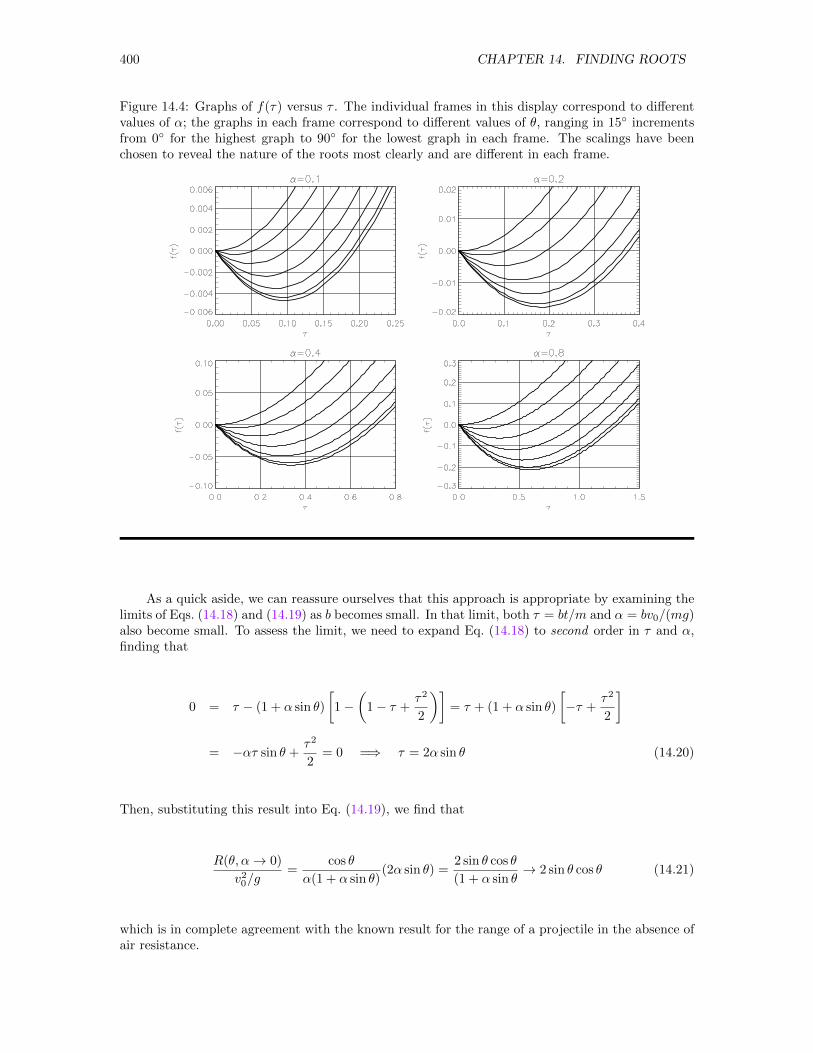
400 CHAPTER 14. FINDING ROOTS

Figure 14.4: Graphs of f(τ) versus τ . The individual frames in this display correspond to differentvalues of α; the graphs in each frame correspond to different values of θ, ranging in 15 incrementsfrom 0 for the highest graph to 90 for the lowest graph in each frame. The scalings have beenchosen to reveal the nature of the roots most clearly and are different in each frame.

As a quick aside, we can reassure ourselves that this approach is appropriate by examining thelimits of Eqs. (14.18) and (14.19) as b becomes small. In that limit, both τ = bt/m and α = bv0/(mg)also become small. To assess the limit, we need to expand Eq. (14.18) to second order in τ and α,finding that

0 = τ − (1 + α sin θ)

[1−

(1− τ +

τ2

2

)]= τ + (1 + α sin θ)

[−τ +

τ2

2

]

= −ατ sin θ +τ2

2= 0 =⇒ τ = 2α sin θ (14.20)

Then, substituting this result into Eq. (14.19), we find that

R(θ, α→ 0)

v20/g=

cos θ

α(1 + α sin θ)(2α sin θ) =

2 sin θ cos θ

(1 + α sin θ→ 2 sin θ cos θ (14.21)

which is in complete agreement with the known result for the range of a projectile in the absence ofair resistance.

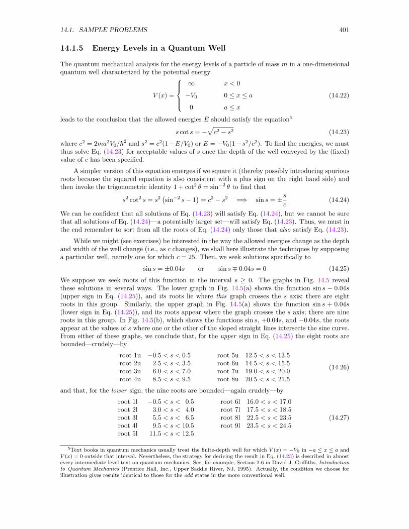
14.1. SAMPLE PROBLEMS 401

14.1.5 Energy Levels in a Quantum Well

The quantum mechanical analysis for the energy levels of a particle of mass m in a one-dimensionalquantum well characterized by the potential energy

V (x) =

∞ x < 0

−V0 0 ≤ x ≤ a

0 a ≤ x

(14.22)

leads to the conclusion that the allowed energies E should satisfy the equation5

s cot s = −√c2 − s2 (14.23)

where c2 = 2ma2V0/h2 and s2 = c2(1−E/V0) or E = −V0(1−s2/c2). To find the energies, we must

thus solve Eq. (14.23) for acceptable values of s once the depth of the well conveyed by the (fixed)value of c has been specified.

A simpler version of this equation emerges if we square it (thereby possibly introducing spuriousroots because the squared equation is also consistent with a plus sign on the right hand side) andthen invoke the trigonometric identity 1 + cot2 θ = sin−2 θ to find that

s2 cot2 s = s2(sin−2 s− 1

)= c2 − s2 =⇒ sin s = ±s

c(14.24)

We can be confident that all solutions of Eq. (14.23) will satisfy Eq. (14.24), but we cannot be surethat all solutions of Eq. (14.24)—a potentially larger set—will satisfy Eq. (14.23). Thus, we must inthe end remember to sort from all the roots of Eq. (14.24) only those that also satisfy Eq. (14.23).

While we might (see exercises) be interested in the way the allowed energies change as the depthand width of the well change (i.e., as c changes), we shall here illustrate the techniques by supposinga particular well, namely one for which c = 25. Then, we seek solutions specifically to

sin s = ±0.04s or sin s∓ 0.04s = 0 (14.25)

We suppose we seek roots of this function in the interval s ≥ 0. The graphs in Fig. 14.5 revealthese solutions in several ways. The lower graph in Fig. 14.5(a) shows the function sin s − 0.04s(upper sign in Eq. (14.25)), and its roots lie where this graph crosses the s axis; there are eightroots in this group. Similarly, the upper graph in Fig. 14.5(a) shows the function sin s + 0.04s(lower sign in Eq. (14.25)), and its roots appear where the graph crosses the s axis; there are nineroots in this group. In Fig. 14.5(b), which shows the functions sin s, +0.04s, and −0.04s, the rootsappear at the values of s where one or the other of the sloped straight lines intersects the sine curve.From either of these graphs, we conclude that, for the upper sign in Eq. (14.25) the eight roots arebounded—crudely—by

root 1u −0.5 < s < 0.5 root 5u 12.5 < s < 13.5root 2u 2.5 < s < 3.5 root 6u 14.5 < s < 15.5root 3u 6.0 < s < 7.0 root 7u 19.0 < s < 20.0root 4u 8.5 < s < 9.5 root 8u 20.5 < s < 21.5

(14.26)

and that, for the lower sign, the nine roots are bounded—again crudely—by

root 1l −0.5 < s < 0.5 root 6l 16.0 < s < 17.0root 2l 3.0 < s < 4.0 root 7l 17.5 < s < 18.5root 3l 5.5 < s < 6.5 root 8l 22.5 < s < 23.5root 4l 9.5 < s < 10.5 root 9l 23.5 < s < 24.5root 5l 11.5 < s < 12.5

(14.27)

5Text books in quantum mechanics usually treat the finite-depth well for which V (x) = −V0 in −a ≤ x ≤ a andV (x) = 0 outside that interval. Nevertheless, the strategy for deriving the result in Eq. (14.23) is described in almostevery intermediate level text on quantum mechanics. See, for example, Section 2.6 in David J. Griffiths, Introductionto Quantum Mechanics (Prentice Hall, Inc., Upper Saddle River, NJ, 1995). Actually, the condition we choose forillustration gives results identical to those for the odd states in the more conventional well.

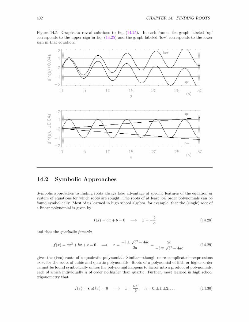
402 CHAPTER 14. FINDING ROOTS

Figure 14.5: Graphs to reveal solutions to Eq. (14.25). In each frame, the graph labeled ‘up’corresponds to the upper sign in Eq. (14.25) and the graph labeled ‘low’ corresponds to the lowersign in that equation.

14.2 Symbolic Approaches

Symbolic approaches to finding roots always take advantage of specific features of the equation orsystem of equations for which roots are sought. The roots of at least low order polynomials can befound symbolically. Most of us learned in high school algebra, for example, that the (single) root ofa linear polynomial is given by

f(x) = ax+ b = 0 =⇒ x = − ba

(14.28)

and that the quadratic formula

f(x) = ax2 + bx+ c = 0 =⇒ x =−b±

√b2 − 4ac

2a=

2c

−b∓√b2 − 4ac

(14.29)

gives the (two) roots of a quadratic polynomial. Similar—though more complicated—expressionsexist for the roots of cubic and quartic polynomials. Roots of a polynomial of fifth or higher ordercannot be found symbolically unless the polynomial happens to factor into a product of polynomials,each of which individually is of order no higher than quartic. Further, most learned in high schooltrigonometry that

f(x) = sin(kx) = 0 =⇒ x =nπ

k, n = 0,±1,±2, . . . (14.30)

14.5. FINDING ROOTS SYMBOLICALLY WITH MATHEMATICA 403

Occasionally, we will encounter an equation that looks intractable but that can be converted into atractable case with an appropriate variable transformation. The roots of the expression

f(x) =a+ x

b+ x2− c (14.31)

for example, can be found symbolically because, so long as b+ x2 6= 0, the simple recasting

a+ x

b+ x2− c = 0 =⇒ a+ x− c(b+ x2) = −cx2 + x+ a− cb = 0 (14.32)

converts the problem into one involving a quadratic polynomial. Beyond these few cases, very fewroots can be found symbolically.

14.5 Finding Roots Symbolically with Mathematica

The Mathematica command for solving a wide variety of equations is Solve. It takes two mandatoryarguments, the first giving the equation to be solved and the second specifying the variable for whicha solution is desired. Thus, the statement

In[1]:= Solve[ a*x + b == 0, x ]

Out[1]=

x→ − b

a

returns the solution x = −b/a in the form of a transformation rule and the statement

In[2]:= Solve[ a*x^2 + b*x + c == 0, x ]

Out[2]=

x→ −b−

√b2 − 4ac

2a

,

x→ −b+

√b2 − 4ac

2a

returns a list containing two solutions, each expressed as a transformation rule. The commandSolve actually also knows how to deal with cubic and quartic polynomials, though the result in themost general case is likely to be extremely involved and will be useful only if, once obtained, it isquickly converted to floating point form. The command can solve higher order polynomials only ifit recognizes a factorization into polynomials, no one of which is of order higher than quartic.

Sometimes (e.g., for roots of polynomials of order greater than three), Solve may be unable tofind explicit solutions. In those cases, Solve returns the root in the form Root[...], e.g.,

In[3]:= Solve[ a*x^6 - b*x^5 + c == 0, x ]

Out[3]=

x→ Root[c− b#15 + a#16 &, 1], x→ Root[c− b#15 + a#16 &, 2], . . .

(Here, #1 is a Mathematica-generated generic variable, Root[f,n] stands for the n-th root of thefunction f , and the ampersand identifies what precedes it as a “pure” function.6) Basically, thisresponse constitutes an admission by Mathematica that it can’t solve the specified equation sym-bolically. Fuller description of the command Solve, of a third (optional) argument that specifiesvariables to be eliminated, and of a few options that affect the behavior of the command are describedin the Mathematica manuals. Further, Mathematica will display the options and their current valuesin response to the statement Options[Solve].

6See Section 2.2.5 in The Mathematica Book (Fourth Edition).

404 CHAPTER 14. FINDING ROOTS

14.5.1 Classical Turning Points

The turning points for the potential energy in Eq. (14.3) are readily found symbolically with thestatements

In[4]:= V = x^3/10000 + x^2/200 - x/500 - 1/2;

In[5]:= soln = Solve[ V == 0 , x ]

Out[5]=x→ mess, x→ mess, x→ mess

where the indicated messes, which—because of the presence of i =√−1 here and there—will appear

superficially to be complex, are too long and too unfathomable to reproduce here. We can, however,convert this output directly to a (complex) floating point form with the statement

In[6]:= soln // N

Out[6]=x→ 9.3487 + 0.i, −48.2683− 8.88178× 10−16i, −11.0804 + 0.i

thereby reducing the messes to quantities that are more easily interpreted. The real parts of the rootshere obtained are certainly consistent with the bounds given in Eq. (14.4). Further, the assertionthat the imaginary parts of the roots are all zero is not unreasonable, given that, by default, theprecision of the command N is on the order of 10−15. Indeed, we can support this understanding ofthe imaginary part by evaluating the roots to more decimal places with the statements

In[7]:= N[ soln, 20]

Out[7]=x→ 9.3487041976000522706 + 0.× 10−20i,

−48.268267566751634131 + 0.× 10−19i,

−11.080436630848481393 + 0.× 10−20i

Even at this precision, the assertion that the imaginary parts are all zero is not unreasonable, giventhat the precision of the command N is on the order of one in the twentieth digit when its secondargument is 20.7

14.5.2 Equilibrium Points

Finding the equilibrium points for the potential energy of Eq. (14.3) is easier. We proceed from theabove dialog with the statements

7While different machines should give the same results for most of the digits in the real parts of these roots, thevalues of the imaginary parts may well be quite different from machine to machine, since those values are largely aconsequence of internal round off.

14.5. FINDING ROOTS SYMBOLICALLY WITH MATHEMATICA 405

In[8]:= dVdx = D[ V, x ];

In[9]:= Solve[ dVdx == 0, x ]

Out[9]=x→ 2

3

(−25− 8

√10),x→ 2

3

(−25 + 8

√10)

In[10]:= soln = N[ % ]

Out[10]=x→ −33.5321

,x→ 0.198814

finding first dV/dx and then finding the values of x at which dV/dx = 0. These results are consistentwith the bounds obtained in Eq. (14.7). Finally, to assess the stability of each equilibrium, weevaluate the second derivative at each equilibrium point with the statements

In[11]:= d2Vdx2 = D[ dVdx, x ];

In[12]:= d2Vdx2 /. soln

Out[12]= −0.0101193, 0.0101193In[13]:= Quit[]

concluding that the first root x = −33.5321 locates an unstable equilibrium (d2V/dx2 < 0; localmaximum in the potential energy) while the second root x = 0.198814 locates a stable equilibrium(d2V/dx2 > 0; local minimum in the potential energy).

14.5.3 Natural Frequencies

To find the natural frequencies for the coupled oscillators described in Section 14.1.3, we seek rootsof the function D(ω) defined in Eq. (14.12). Since D(ω) is, in fact, quadratic in ω2, we solve firstfor ω2—though we must substitute a single variable λ for ω2 before doing so—and then we take thesquare root of that solution with the statements8

In[1]:= d = \[Omega]^4 - 2*\[Omega]^2*(1+\[Kappa]) + 1 + 2*\[Kappa];

In[2]:= d /. \[Omega] -> Sqrt[\[Lambda]];

In[3]:= Solve[ % == 0, \[Lambda] ]

Out[3]= λ→ 1, λ→ 1 + 2κ

In[4]:= freqs = Sqrt[ \[Lambda] ] /. %

Out[4]= 1,√

1 + 2κ

Note—as must on physical grounds be the case—that the solutions obtained for λ = ω2 are bothpositive, so the square roots will be real. (We ignore the negative square roots, since they don’thave the physical significance of the positive square roots.) Note also that the first of the twofrequencies is the same for all κ but that the second increases steadily as κ—the strength of thecoupling—increases.

To make the point at the end of the last paragraph even more explicitly, we generate a graphof the two frequencies as functions of κ with the statement9

8At this point, for simplicity, we drop the overbar on κ.9Evidently, we cannot simply place the list freqs as the first argument to Plot. The first argument can be a list,

but the list must be constructed within the statement rather than outside of the statement.

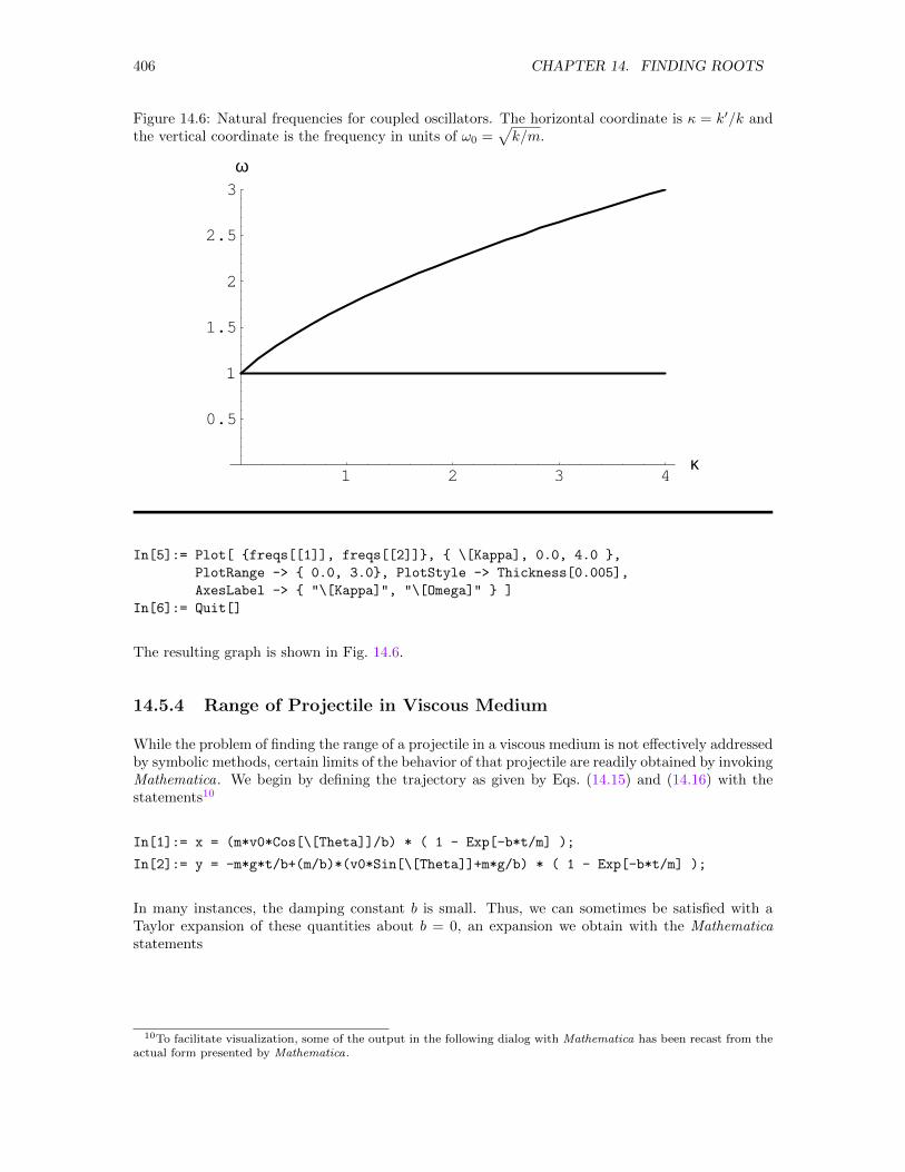
406 CHAPTER 14. FINDING ROOTS

Figure 14.6: Natural frequencies for coupled oscillators. The horizontal coordinate is κ = k′/k andthe vertical coordinate is the frequency in units of ω0 =

√k/m.

1 2 3 4κ

0.5

1

1.5

2

2.5

3ω

In[5]:= Plot[ freqs[[1]], freqs[[2]], \[Kappa], 0.0, 4.0 ,

PlotRange -> 0.0, 3.0, PlotStyle -> Thickness[0.005],

AxesLabel -> "\[Kappa]", "\[Omega]" ]

In[6]:= Quit[]

The resulting graph is shown in Fig. 14.6.

14.5.4 Range of Projectile in Viscous Medium

While the problem of finding the range of a projectile in a viscous medium is not effectively addressedby symbolic methods, certain limits of the behavior of that projectile are readily obtained by invokingMathematica. We begin by defining the trajectory as given by Eqs. (14.15) and (14.16) with thestatements10

In[1]:= x = (m*v0*Cos[\[Theta]]/b) * ( 1 - Exp[-b*t/m] );

In[2]:= y = -m*g*t/b+(m/b)*(v0*Sin[\[Theta]]+m*g/b) * ( 1 - Exp[-b*t/m] );

In many instances, the damping constant b is small. Thus, we can sometimes be satisfied with aTaylor expansion of these quantities about b = 0, an expansion we obtain with the Mathematicastatements

10To facilitate visualization, some of the output in the following dialog with Mathematica has been recast from theactual form presented by Mathematica.

14.5. FINDING ROOTS SYMBOLICALLY WITH MATHEMATICA 407

In[3]:= xb = Series[ x, b, 0, 1 ]

Out[3]= t v0 Cos [θ]− t2 v0 Cos [θ] b

2m+O[b]2

In[4]:= yb = Simplify[ Series[ y, b, 0, 1 ] ]

Out[4]:= −gt2

2+ t v0 Sin [θ] +

t2(gt− 3v0 Sin [θ])b

6m+O[b]2

We notice first—reassuringly—that the terms that are zeroth-order in b, i.e., x = v0t cos θ andy = − 1

2gt2 + v0t sin θ, are exactly what we would expect for the projectile in the absence of air

resistance. More generally, to find the range when b is small, we begin by converting the expressionto a polynomial, removing the root at t = 0, and solving for the roots of the Taylor expansion of ywith the statements

In[5]:= yb = Normal[ yb ];

In[6]:= yb = Expand[ yb/t ];

In[7]:= soln = Solve[ yb == 0, t ]

Out[7]=t→ mess, t→ mess

To sort out which of these two roots is the physically significant one, we evaluate the limit of thisexpression as b→ 0 with the statements

In[8]:= Series[ t /. soln[[1]], b, 0, 1 ];

In[9]:= Simplify[ %, m>0, g>0 ]

Out[9]:=2v0 Sin [θ]

g− 2v20 Sin [θ]2 b

3g2m+O[b]2

Find limit of first solution.

In[10]:= Series[ t /. soln[[2]], b, 0, 1 ];

In[11]:= Simplify[ %, m>0, g>0 ]

Out[11]=3m

b+v0 Sin [θ]

g+

2v20 Sin [θ]2b

3g2m+O[b]2

Find limit of second solution.

Since the second root becomes arbitrarily large as b becomes small, we must reject it on physicalgrounds. Only the first root, which we can display more fully with the statement

In[12]:= sln1 = t /. soln[[1]];

In[13]:= sln2 = Expand[ Simplify[ sln1 ] ]

Out[13]=3m

2b+

3v0 Sin [θ]

2g− m

√9g2 − 6bgv0 Sin [θ]/m+ 9b2v20 Sin [θ]2/m2

2bg

is of interest. Finally, for consistency with approximations already made, we find this root to firstorder in b with the statement

In[14]:= Series[ sln2, b, 0, 1 ];

In[15]:= tim = Simplify[ %, m>0, g>0 ]

Out[14]=2v0 Sin [θ]

g− 2v20 Sin [θ]2 b

3g2m+O[b]2

and find the range by substituting this result into the first order expression for the horizontalcoordinate with the statements

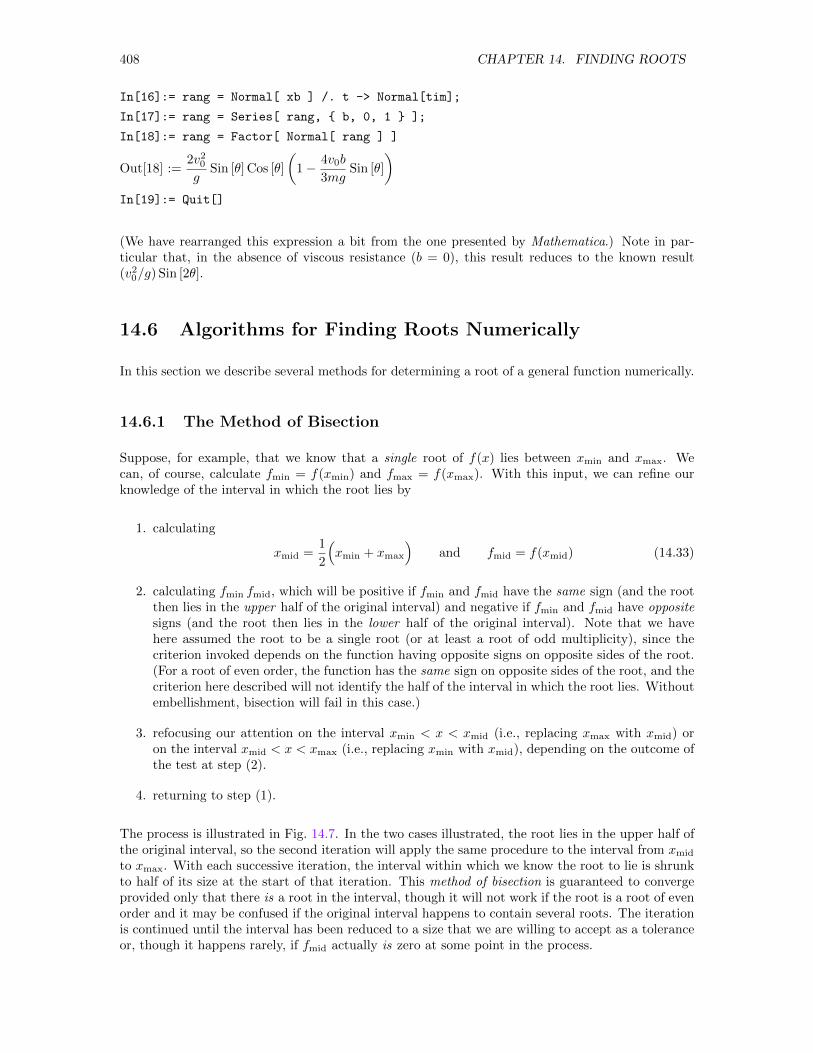
408 CHAPTER 14. FINDING ROOTS

In[16]:= rang = Normal[ xb ] /. t -> Normal[tim];

In[17]:= rang = Series[ rang, b, 0, 1 ];

In[18]:= rang = Factor[ Normal[ rang ] ]

Out[18] :=2v20g

Sin [θ] Cos [θ]

(1− 4v0b

3mgSin [θ]

)In[19]:= Quit[]

(We have rearranged this expression a bit from the one presented by Mathematica.) Note in par-ticular that, in the absence of viscous resistance (b = 0), this result reduces to the known result(v20/g) Sin [2θ].

14.6 Algorithms for Finding Roots Numerically

In this section we describe several methods for determining a root of a general function numerically.

14.6.1 The Method of Bisection

Suppose, for example, that we know that a single root of f(x) lies between xmin and xmax. Wecan, of course, calculate fmin = f(xmin) and fmax = f(xmax). With this input, we can refine ourknowledge of the interval in which the root lies by

1. calculating

xmid =1

2

(xmin + xmax

)and fmid = f(xmid) (14.33)

2. calculating fmin fmid, which will be positive if fmin and fmid have the same sign (and the rootthen lies in the upper half of the original interval) and negative if fmin and fmid have oppositesigns (and the root then lies in the lower half of the original interval). Note that we havehere assumed the root to be a single root (or at least a root of odd multiplicity), since thecriterion invoked depends on the function having opposite signs on opposite sides of the root.(For a root of even order, the function has the same sign on opposite sides of the root, and thecriterion here described will not identify the half of the interval in which the root lies. Withoutembellishment, bisection will fail in this case.)

3. refocusing our attention on the interval xmin < x < xmid (i.e., replacing xmax with xmid) oron the interval xmid < x < xmax (i.e., replacing xmin with xmid), depending on the outcome ofthe test at step (2).

4. returning to step (1).

The process is illustrated in Fig. 14.7. In the two cases illustrated, the root lies in the upper half ofthe original interval, so the second iteration will apply the same procedure to the interval from xmid

to xmax. With each successive iteration, the interval within which we know the root to lie is shrunkto half of its size at the start of that iteration. This method of bisection is guaranteed to convergeprovided only that there is a root in the interval, though it will not work if the root is a root of evenorder and it may be confused if the original interval happens to contain several roots. The iterationis continued until the interval has been reduced to a size that we are willing to accept as a toleranceor, though it happens rarely, if fmid actually is zero at some point in the process.

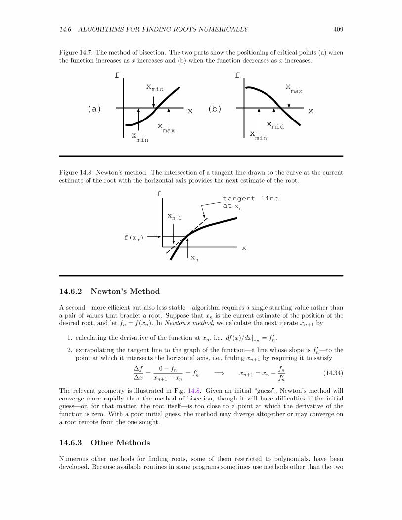
14.6. ALGORITHMS FOR FINDING ROOTS NUMERICALLY 409

Figure 14.7: The method of bisection. The two parts show the positioning of critical points (a) whenthe function increases as x increases and (b) when the function decreases as x increases.

x

xxmin

max

mid

x

f

(a) (b)

x

x

xmin

max

mid

x

f

Figure 14.8: Newton’s method. The intersection of a tangent line drawn to the curve at the currentestimate of the root with the horizontal axis provides the next estimate of the root.

x

f

xn

xn+1

tangent lineat xn

f(x )n

14.6.2 Newton’s Method

A second—more efficient but also less stable—algorithm requires a single starting value rather thana pair of values that bracket a root. Suppose that xn is the current estimate of the position of thedesired root, and let fn = f(xn). In Newton’s method, we calculate the next iterate xn+1 by

1. calculating the derivative of the function at xn, i.e., df(x)/dx|xn= f ′n.

2. extrapolating the tangent line to the graph of the function—a line whose slope is f ′n—to thepoint at which it intersects the horizontal axis, i.e., finding xn+1 by requiring it to satisfy

∆f

∆x=

0− fnxn+1 − xn

= f ′n =⇒ xn+1 = xn −fnf ′n

(14.34)

The relevant geometry is illustrated in Fig. 14.8. Given an initial “guess”, Newton’s method willconverge more rapidly than the method of bisection, though it will have difficulties if the initialguess—or, for that matter, the root itself—is too close to a point at which the derivative of thefunction is zero. With a poor initial guess, the method may diverge altogether or may converge ona root remote from the one sought.

14.6.3 Other Methods

Numerous other methods for finding roots, some of them restricted to polynomials, have beendeveloped. Because available routines in some programs sometimes use methods other than the two

410 CHAPTER 14. FINDING ROOTS

described above in detail, we include here a brief outline of the main idea in each of several othermethods:

• The secant method starts from two approximations to the root, say x1 and x2, calculatesf1 = f(x1) and f2 = f(x2), fits a straight line through the points (x1, f1) and (x2, f2), findsthe intersection point x3 of that line with the x axis, and then repeats the process with thetwo approximations x2 and x3. The method is similar to Newton’s method, except that ituses the values of the function at two points to estimate the slope of the tangent line to thefunction f(x). It does not require explicit knowledge of the derivative of f(x).

• Muller’s method is mildly more sophisticated than the secant method but involves a similaridea. It starts with three estimates of the root, say x1, x2, and x3, calculates f1 = f(x1),f2 = f(x2), and f3 = f(x3), fits a parabola to the points (x1, f1), (x2, f2), and (x3, f3), findsthe roots of that parabola using the form of the quadratic formula given second in Eq. (14.29),and finally takes as x4—which replaces x1 for the next iteration—the one root that emergeswhen the ambiguous sign in Eq. (14.29) is chosen so that the denominator has the larger ofthe two possible absolute values.

• Laguerre’s method, which is limited to polynomials, (1) recognizes that, in terms of its rootsxi, a polynomial scaled so that the coefficient of its highest order term is 1 (which has no effecton its roots) can be expressed in the form

f(x) =

n∏i

(x− xi) (14.35)

(2) finds a couple of relationships satisfied by polynomials in this form, (3) assumes withonly weak justification a priori that the root sought is isolated from all the others (which areclustered together), and (4) deduces that the next iterate xn+1 for the root sought should bedetermined from the current guess xn by

xn+1 = xn −N

G±√

(N − 1)(NH −G2)(14.36)

where the sign in the denominator is chosen so that the denominator has the larger of the twopossible absolute values, N is the order of the polynomial (equal to the number of roots), andG and H are defined by G = f ′/f and H = (f ′/f)2 − f ′′/f , each evaluated at x = xn.

14.6.4 Assessing Accuracy

As with all numerical operations, assessing the accuracy of the roots found by an algorithm isessential before we can have confidence in the roots. We can, of course, always substitute the rootwe have found into the function whose root we seek and simply notice how close to zero the valueof the function at the proposed root actually is. In the end, that comparison may provide the mostimportant test of accuracy, though whether the value f(xroot) = 0.0001, say, is “close enough” to zerorequires a judgment that would take into account the magnitude of f(x) over the important domainof x and, even more, the magnitude of the derivative of f(x) evaluated at the root.11 Certainly,that criterion provides the most accessible test we might apply. It is also a criterion that is easilyimplemented in a computer program that monitors convergence and stops automatically when theabsolute value of the function has been reduced below some specified tolerance.

We would, however, be more interested in the accuracy of the root itself, i.e., in the amount|xexact − xapprox| by which the (unknown) exact root differs from the root on which a particular

11The less steeply sloped the function at the root, the harder it is to obtain an accurate root by using the value ofthe function as a guide.

14.9. FINDING ROOTS NUMERICALLY WITH OCTAVE 411

algorithm converges. Only the method of bisection supports a clear assessment of that differencesince, at any particular step in the progress of that algorithm towards a root, we know that the root is“trapped” between two values whose separation is halved with each step in the iteration. Continuinguntil the difference |xi+1 − xi|—sometimes called the residual—between consecutive iterates is lessthan some specified tolerance guarantees that we have located the root to within that tolerance.Implemented in a computer program, an algorithm using the method of bisection can monitor theseparation of consecutive iterates and stop when that separation, either as an absolute value or as afraction of its current value, is reduced below a specified absolute or relative tolerance, respectively.

Given appropriate initial bounds, the method of bisection is guaranteed to converge on a root,but the rate of convergence is slow by comparison with other methods. Assessing the accuracyof the root itself for those other algorithms is more difficult. If, however, the convergence of thealgorithm in use is fairly rapid (and Newton’s method will usually satisfy this expectation), takingthe (absolute) accuracy of a particular iterate to be on the order of the difference between it andthe next iterate, i.e., on the order of the residual, is reasonable. For these algorithms, as with themethod of bisection, a computer implementation of a method in the category of this paragraphcan also monitor the residual and stop when it has been reduced below a specified (absolute orrelative) tolerance. For these methods, however, convergence is not guaranteed, and computerimplementations of these methods should include an alternate criterion for stopping the iteration.Such an implementation might, for example, limit the number of iterations and—to keep the userfully informed—display a warning message if the iteration is stopped because this limit is exceededrather than because the residual has been made sufficiently small. Without some such fail-safestopping criterion, these methods are in danger of iterating forever.

Beyond monitoring the value of the function or the residual, seeking a particular root by morethan one method may give some insight into the accuracy of that root. Different methods havedifferent strengths, weaknesses, and quirks. When they agree to some number of digits, we can havemore confidence in the result than we would have if we had obtained it by only one method. Whenthey disagree, we have at least a hint that the function at hand possesses some pathology that weshould perhaps attempt to understand before accepting the root we have found.

14.9 Finding Roots Numerically with OCTAVE

Note: All OCTAVE program (.m) files referred to in this chapter are available inthe directory $HEAD/octave, where (as defined in the Local Guide) $HEAD must bereplaced by the appropriate path for your site. At some sites, this directory orsome other directory containing these files may also have been placed in OCTAVE’sdefault search path. If so, the files can be found by OCTAVE without explicitspecification of a path. Otherwise, you will have to use the full path to copy theminto your default directory to access them.

Functions in OCTAVE for finding the roots of single equations include

• roots and compan, which find the roots of a polynomial by finding the eigenvalues of anassociated companion matrix. The coefficients in the polynomial may be complex. Further,whether the coefficients are complex or real, roots will find both real and complex roots. Itis invoked with a statement like

q = roots( c )

where c is a (possibly complex) vector containing the coefficients of the terms in the polynomial(highest power first), and q is a complex vector storing the returned roots. The companionfunction compan calculates the companion matrix associated with the vector of polynomial

412 CHAPTER 14. FINDING ROOTS

coefficients. While compan can be invoked separately, invocation of roots results in an invo-cation of compan behind the scenes. Roots calculates roots to the maximum precision allowedby double-precision arithmetic.

• fzero, which seeks a real root of a (single) nonlinear function—polynomial or otherwise—ofa single variable. It is invoked with statements like12

q = fzero( @func, x )

q = fzero( @func, x, options )

[q, fval, info, output] = fzero( . . . )

In these forms,

func is a string giving the name of a function M-file—built-in or user-defined—that returnsthe value of the function whose roots are sought.

x is either a scalar giving a value near the root sought or a two-component vector givingan interval within which a root is to be sought; in either case x must be numeric, notsymbolic. If x is a scalar, fzero begins by searching for an interval around x within whichfunc changes sign. Then, taking that interval (or the one specified in a two-componentvalue for x) as a start, fzero refines the interval until the absolute value of the differencebetween consecutive iterates is no bigger than the default tolerance of 2.2204 × 10−16

(which is the smallest difference detectable in double-precision floating point arithmetic).

options, which is optional, is the name of a variable that has been set to modify the defaultbehavior of fzero. For example, to change the tolerance, we must reset the property TolX

by invoking a statement like

opt = optimset( ’tolx’, 1.0e-10 );

to create a variable opt containing the desired value of tolx and then invoke fzero withthe expanded statement

q = fzero( @func, x, opt )

which replaces the default value of tolx with the newly specified value but keeps all otheroptions at their default values.13

q stores the returned root.

fval stores the value of the function at the returned root.

info stores a returned code with 1 (convergence achieved) and 0 (maximum number ofiterations or function evaluations reached without convergence) among the several possiblevalues.

output is a structure containing the number of iterations, the number of function eval-uations and two two-component vectors, one giving the final interval on the horizontalaxis within which the root was found and the other giving the interval within which thevalue of the function lies.

Note also that, should the function whose roots are sought contain parameters, their valuesmust be provided through the use of global variables.

In addition, Section 14.A contains a listing of the Lawrence-written file lubisect.m, whichdefines a OCTAVE function that uses the method of bisection. It is called with a statement of theform

12We shall adhere to providing FunctionName by preceding it with an @ sign. OCTAVE will also accept thealternative specification that encloses FunctionName in single or double quotation marks. See footnote 36 in Chapter 4.

13tolx is the most commonly used option for fzero. All available options will be displayed by the commandoptimset() with no arguments. Details on those options are available in the OCTAVE manuals.

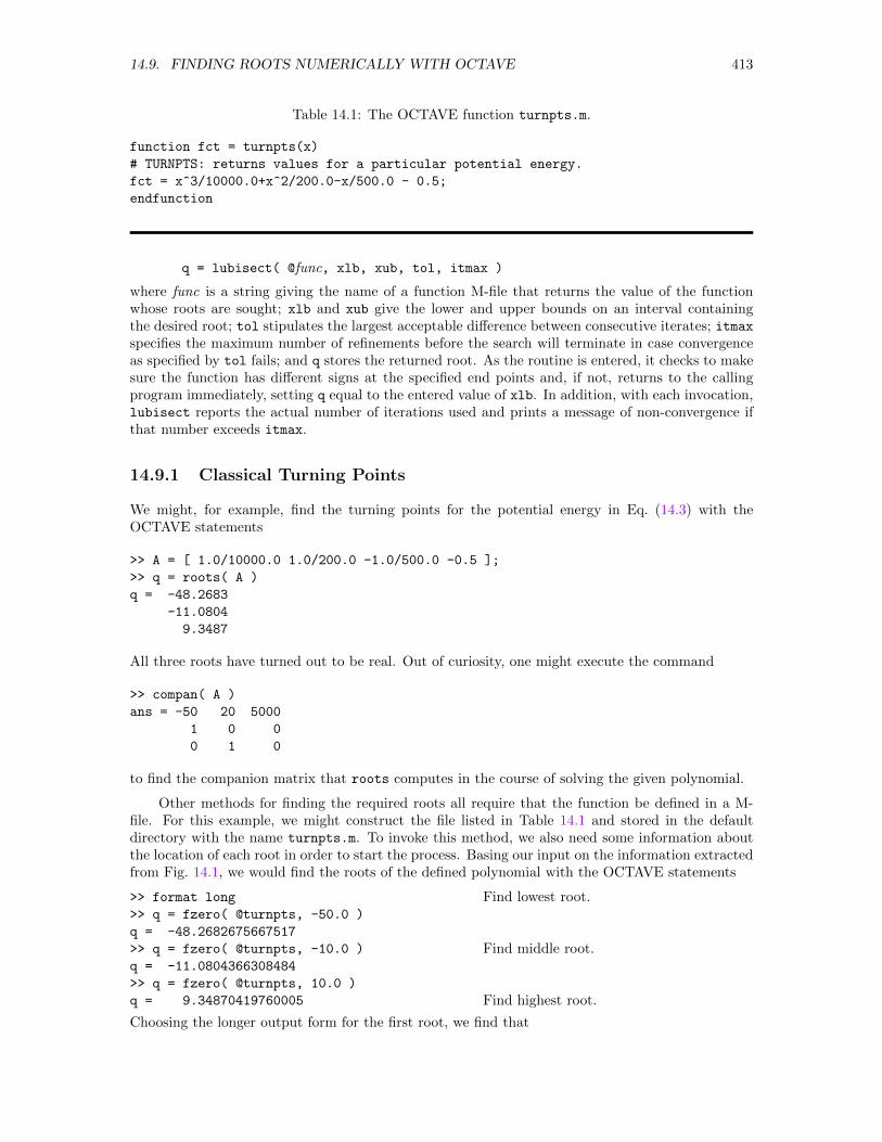
14.9. FINDING ROOTS NUMERICALLY WITH OCTAVE 413

Table 14.1: The OCTAVE function turnpts.m.

function fct = turnpts(x)

# TURNPTS: returns values for a particular potential energy.

fct = x^3/10000.0+x^2/200.0-x/500.0 - 0.5;

endfunction

q = lubisect( @func, xlb, xub, tol, itmax )

where func is a string giving the name of a function M-file that returns the value of the functionwhose roots are sought; xlb and xub give the lower and upper bounds on an interval containingthe desired root; tol stipulates the largest acceptable difference between consecutive iterates; itmaxspecifies the maximum number of refinements before the search will terminate in case convergenceas specified by tol fails; and q stores the returned root. As the routine is entered, it checks to makesure the function has different signs at the specified end points and, if not, returns to the callingprogram immediately, setting q equal to the entered value of xlb. In addition, with each invocation,lubisect reports the actual number of iterations used and prints a message of non-convergence ifthat number exceeds itmax.

14.9.1 Classical Turning Points

We might, for example, find the turning points for the potential energy in Eq. (14.3) with theOCTAVE statements

>> A = [ 1.0/10000.0 1.0/200.0 -1.0/500.0 -0.5 ];

>> q = roots( A )

q = -48.2683

-11.0804

9.3487

All three roots have turned out to be real. Out of curiosity, one might execute the command

>> compan( A )

ans = -50 20 5000

1 0 0

0 1 0

to find the companion matrix that roots computes in the course of solving the given polynomial.

Other methods for finding the required roots all require that the function be defined in a M-file. For this example, we might construct the file listed in Table 14.1 and stored in the defaultdirectory with the name turnpts.m. To invoke this method, we also need some information aboutthe location of each root in order to start the process. Basing our input on the information extractedfrom Fig. 14.1, we would find the roots of the defined polynomial with the OCTAVE statements

>> format long

>> q = fzero( @turnpts, -50.0 )

q = -48.2682675667517

>> q = fzero( @turnpts, -10.0 )

q = -11.0804366308484

>> q = fzero( @turnpts, 10.0 )

q = 9.34870419760005

Find lowest root.

Find middle root.

Find highest root.

Choosing the longer output form for the first root, we find that

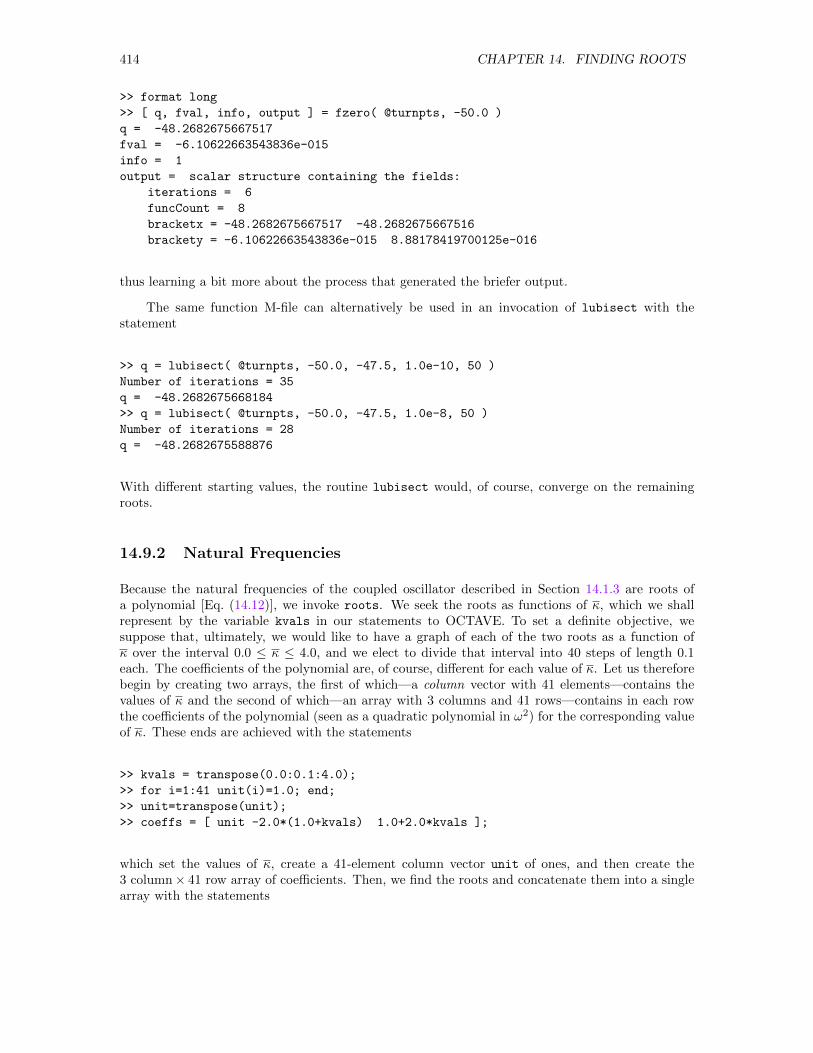
414 CHAPTER 14. FINDING ROOTS

>> format long

>> [ q, fval, info, output ] = fzero( @turnpts, -50.0 )

q = -48.2682675667517

fval = -6.10622663543836e-015

info = 1

output = scalar structure containing the fields:

iterations = 6

funcCount = 8

bracketx = -48.2682675667517 -48.2682675667516

brackety = -6.10622663543836e-015 8.88178419700125e-016

thus learning a bit more about the process that generated the briefer output.

The same function M-file can alternatively be used in an invocation of lubisect with thestatement

>> q = lubisect( @turnpts, -50.0, -47.5, 1.0e-10, 50 )

Number of iterations = 35

q = -48.2682675668184

>> q = lubisect( @turnpts, -50.0, -47.5, 1.0e-8, 50 )

Number of iterations = 28

q = -48.2682675588876

With different starting values, the routine lubisect would, of course, converge on the remainingroots.

14.9.2 Natural Frequencies

Because the natural frequencies of the coupled oscillator described in Section 14.1.3 are roots ofa polynomial [Eq. (14.12)], we invoke roots. We seek the roots as functions of κ, which we shallrepresent by the variable kvals in our statements to OCTAVE. To set a definite objective, wesuppose that, ultimately, we would like to have a graph of each of the two roots as a function ofκ over the interval 0.0 ≤ κ ≤ 4.0, and we elect to divide that interval into 40 steps of length 0.1each. The coefficients of the polynomial are, of course, different for each value of κ. Let us thereforebegin by creating two arrays, the first of which—a column vector with 41 elements—contains thevalues of κ and the second of which—an array with 3 columns and 41 rows—contains in each rowthe coefficients of the polynomial (seen as a quadratic polynomial in ω2) for the corresponding valueof κ. These ends are achieved with the statements

>> kvals = transpose(0.0:0.1:4.0);

>> for i=1:41 unit(i)=1.0; end;

>> unit=transpose(unit);

>> coeffs = [ unit -2.0*(1.0+kvals) 1.0+2.0*kvals ];

which set the values of κ, create a 41-element column vector unit of ones, and then create the3 column× 41 row array of coefficients. Then, we find the roots and concatenate them into a singlearray with the statements

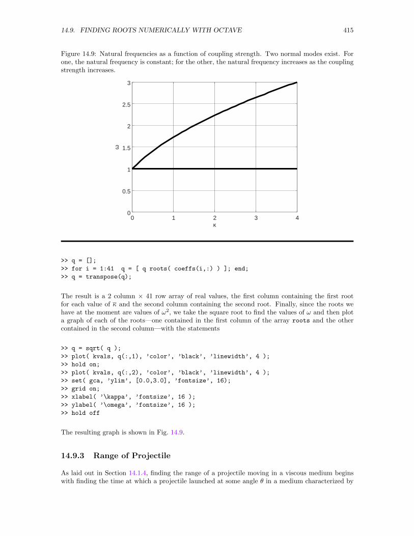
14.9. FINDING ROOTS NUMERICALLY WITH OCTAVE 415

Figure 14.9: Natural frequencies as a function of coupling strength. Two normal modes exist. Forone, the natural frequency is constant; for the other, the natural frequency increases as the couplingstrength increases.

0 1 2 3 40

0.5

1

1.5

2

2.5

3

κ

ω

>> q = [];

>> for i = 1:41 q = [ q roots( coeffs(i,:) ) ]; end;

>> q = transpose(q);

The result is a 2 column × 41 row array of real values, the first column containing the first rootfor each value of κ and the second column containing the second root. Finally, since the roots wehave at the moment are values of ω2, we take the square root to find the values of ω and then plota graph of each of the roots—one contained in the first column of the array roots and the othercontained in the second column—with the statements

>> q = sqrt( q );

>> plot( kvals, q(:,1), ’color’, ’black’, ’linewidth’, 4 );

>> hold on;

>> plot( kvals, q(:,2), ’color’, ’black’, ’linewidth’, 4 );

>> set( gca, ’ylim’, [0.0,3.0], ’fontsize’, 16);

>> grid on;

>> xlabel( ’\kappa’, ’fontsize’, 16 );

>> ylabel( ’\omega’, ’fontsize’, 16 );

>> hold off

The resulting graph is shown in Fig. 14.9.

14.9.3 Range of Projectile

As laid out in Section 14.1.4, finding the range of a projectile moving in a viscous medium beginswith finding the time at which a projectile launched at some angle θ in a medium characterized by

416 CHAPTER 14. FINDING ROOTS

Table 14.2: The OCTAVE function projectile.m.

function fct = projectile( tau )

# PROJECTILE: Evaluates function involved in projectile motion.

# The function projectile returns the value of a dimensionless

# function that plays a role in determining the range of

# a projectile fired at an elevation theta into a medium

# whose viscosity is characterized by the dimensionless

# parameter alpha. These parameters must be supplied in global

# variables.

global alpha theta

tmp = 1.0+alpha*sin(theta); # Calculate coefficient

fct = tau - tmp*(1-exp(-tau)); # Return value of f(tau)

endfunction

a (dimensionless) viscous damping coefficient α = bv0/(mg) returns to its initial altitude. In otherwords, we must find the one non-zero root of the function f(τ) defined in Eq. (14.18). Central tothe entire calculation is the function M-file listed in Table 14.2 and stored in the default directory ina file named projectile.m. For example, the upper left frame in Fig. 14.4 could have been createdby setting several preliminary variables with the statements

>> global alpha theta

>> thetavals = pi * [0.0:6.0] / 12.0;

>> tau=[0.0:0.01:2.0];

Declare global variables.Set θ = 0, 15, . . . , 90 in radians.Set values of τ .

and then executing the statements

>> alpha = 0.1;

>> theta = thetavals(1);

Set graphics toolkit.Choose α.Plot graph for θ = 0.

>> plot( tau, projectile(tau, alpha, theta ), ...

’color’, ’black’, ’linewidth’, 3.0 )

>> set( gca, ’xlim’, [0.0,0.25], ’ylim’, ...

[-0.005,0.005], ’fontsize’, 14 )

>> hold on;

Set scaling, size of labels.

>> for i=2:7

theta = thetavals(i);

plot( tau, projectile( tau, alpha, theta), ...

’color’, ’black’, ’linewidth’, 3.0 );

end

>> grid on;

Overplot graphs for θ = 15, . . . , 90.

The remaining frames in Fig. 14.4 were produced with similar statements.

For this example, we choose OCTAVE’s built-in routine fzero.14 Starting with a fresh OCTAVEsession, choosing α = 0.4, setting θ = 30 (in radians), referring to Fig. 14.4 to support the initialguess τ = 0.5, and accepting (for the moment) all defaults, we find the corresponding time of returnto the initial altitude by invoking the statements15

14The function of interest is not a polynomial, so roots is not an option. The routine lubisect would also work.15Over the initially specified interval in which the root is to be sought, the function must change sign. Consequently,

14.9. FINDING ROOTS NUMERICALLY WITH OCTAVE 417

>> global alpha theta

>> alpha = 0.4; theta = pi*30.0/180.0;

>> tau0 = [0.1 1.0];

>> q = fzero(@projectile, tau0 )

q = 0.37644

Set α and θ.

Set initial guess for root.Invoke fzero, displaying result.

The corresponding range is then given by Eq. (14.19), which we evaluate and display for the specificcase of this paragraph with the statements

>> range = cos(theta) * ( 1-exp(-q) ) / alpha

range = 0.67918

This result is expressed in units of v20/g.

To find the angle of fire to attain maximum range, we need to repeat the sample calculation ofthe previous paragraph for values of θ ranging from 0 to 90, choosing increments of 1 betweenconsecutive values of θ. Continuing in the same session with OCTAVE, we prepare for a calculationalloop with the statements16

>> thetadeg = 10.0:1.0:90.0;

>> thetarad = pi*thetadeg/180.0;

Set values of θ in degrees.Convert θ to radians.

Then, choosing α = 0.4 and noting from the first frame in Fig. 14.4 that all roots lie between τ =0.1 and τ = 1.0, we continue with the statements

>> alpha = 0.4; tau0 = [0.1 1.0];

>> soln = [];

>> for i = 1:81

theta = thetarad(i);

soln(i) = fzero( @projectile, tau0 );

end

Set α; set initial guess for root.Find root for each θ.

>> range4 = cos(thetarad).*(1-exp(-soln))/alpha;

>> plot( thetadeg, range4, ’color’, ’black’, ...

’linewidth’, 3.0 );

>> grid on;

>> set( gca, ’fontsize’, 16 );

>> xlabel(’\theta (deg)’, ’fontsize’, 16 );

>> ylabel(’R(\theta)’, ’fontsize’, 16 );

>> hold on

Evaluate R for each root.Plot R versus θ and label axes.

Repeating this process with (α = 0.1, τ0 = [0.025 0.25]), with (α = 0.2, τ0 = [0.05 0.4]), andwith (α = 0.8, τ0 = [0.2 1.5]), storing the results in range1, range2, and range8, respectively,and overplotting each on the axes created above, we finally produce Fig. 14.10. As α increases (bincreases, v0 increases, m decreases, or some combination), the maximum range (measured in unitsof v20/g) decreases and the angle of fire to achieve that range becomes shallower and shallower.

Even more specifically, we can examine the values in the four variables rangen to find themaximum range and the approximate firing angle to achieve it in each case. For example, thestatements

>> format long

>> max(range1)

for this function (see Fig. 14.4), we cannot specify a range that begins at 0.0, since the function does not have oppositesigns at the two ends of that interval.

16Because the roots for the lowest few values of θ are difficult to find, a bit of exploration was necessary beforediscovering that a successful evaluation would emerge only if the evaluations were started at θ = 10.

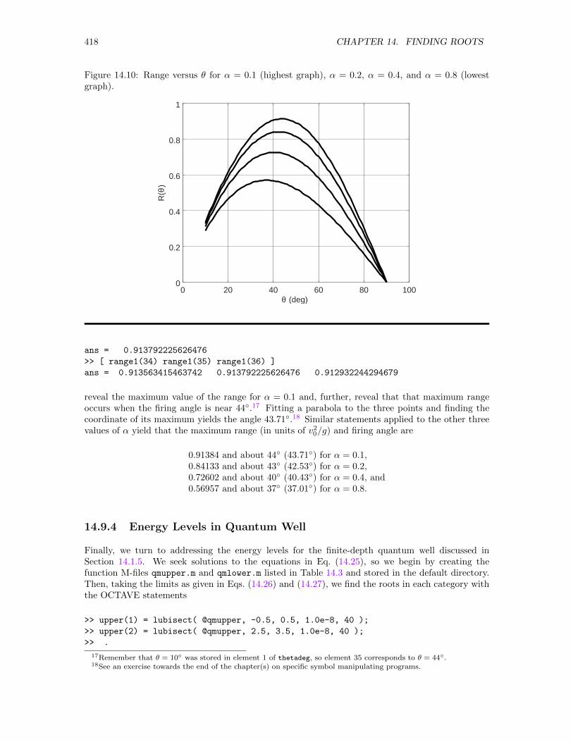
418 CHAPTER 14. FINDING ROOTS

Figure 14.10: Range versus θ for α = 0.1 (highest graph), α = 0.2, α = 0.4, and α = 0.8 (lowestgraph).

0 20 40 60 80 1000

0.2

0.4

0.6

0.8

1

θ (deg)

R(θ

)

ans = 0.913792225626476

>> [ range1(34) range1(35) range1(36) ]

ans = 0.913563415463742 0.913792225626476 0.912932244294679

reveal the maximum value of the range for α = 0.1 and, further, reveal that that maximum rangeoccurs when the firing angle is near 44.17 Fitting a parabola to the three points and finding thecoordinate of its maximum yields the angle 43.71.18 Similar statements applied to the other threevalues of α yield that the maximum range (in units of v20/g) and firing angle are

0.91384 and about 44 (43.71) for α = 0.1,0.84133 and about 43 (42.53) for α = 0.2,0.72602 and about 40 (40.43) for α = 0.4, and0.56957 and about 37 (37.01) for α = 0.8.

14.9.4 Energy Levels in Quantum Well

Finally, we turn to addressing the energy levels for the finite-depth quantum well discussed inSection 14.1.5. We seek solutions to the equations in Eq. (14.25), so we begin by creating thefunction M-files qmupper.m and qmlower.m listed in Table 14.3 and stored in the default directory.Then, taking the limits as given in Eqs. (14.26) and (14.27), we find the roots in each category withthe OCTAVE statements

>> upper(1) = lubisect( @qmupper, -0.5, 0.5, 1.0e-8, 40 );

>> upper(2) = lubisect( @qmupper, 2.5, 3.5, 1.0e-8, 40 );

>> .

17Remember that θ = 10 was stored in element 1 of thetadeg, so element 35 corresponds to θ = 44.18See an exercise towards the end of the chapter(s) on specific symbol manipulating programs.

14.9. FINDING ROOTS NUMERICALLY WITH OCTAVE 419

Table 14.3: The OCTAVE functions qmupper.m and qmlower.m.

function fct = qmupper( s )

# QMUPPER: Returns the value of sin(s)-0.04*s

fct = sin(s) - 0.04*s;

endfunction

function fct = qmlower( s )

# QMLOWER: Returns the value of sin(s)+0.04*s

fct = sin(s) + 0.04*s;

endfunction

>> .

>> upper(8) = lubisect( @qmupper, 20.5, 21.5, 1.0e-8, 40 );

>> lower(1) = lubisect( @qmlower, -0.5, 0.5, 1.0e-8, 40 );

>> lower(2) = lubisect( @qmlower, 3.0, 4.0, 1.0e-8, 40 );

>> .

>> .

>> lower(9) = lubisect( @qmlower, 23.5, 24.5, 1.0e-8, 40 );

and display them with the statement

>> upper

upper =

Columns 1 through 7

0 3.02048 6.54820 9.05419 13.11879 15.06139 19.76109

Column 8

20.99429

and the statement

>> lower

lower =

Columns 1 through 7

0 3.27288 6.03920 9.82884 12.06285 16.42478 18.04326

Columns 8 through 9

23.17778 23.86449

Remember, however, that physically acceptable solutions must satisfy not Eq. (14.25), which we havesolved, but Eq. (14.23). To determine which of these roots are physically meaningful, we substituteeach into Eq. (14.23), remembering that c = 25 for the case we have treated. The appropriatestatements to OCTAVE are

>> upper.*cos(upper)./sin(upper) + sqrt(25.0^2-upper.^2)

ans =

Columns 1 through 7

NaN 0.0000 48.254 0.0000 42.563 0.0000 30.627

Column 8

0.0000

and

420 CHAPTER 14. FINDING ROOTS

>> lower.*cos(lower)./sin(lower) + sqrt(25.0^2-lower.^2)

ans =

Columns 1 through 7

NaN 49.570 0.0000 45.974 0.0000 37.65 0.0000

Columns 8 through 9

18.739 0.0000

Only those roots of Eq. (14.25) that give zero (within the precision of our determination of theroot) on substitution into Eq. (14.23) can be accepted. We therefore must reject as spurious thevalues upper(3), upper(5), upper(7), lower(2), lower(4), lower(6), and lower(8). We alsoreject upper(1) and lower(1); they correspond to evaluation of Eq. (14.23) at s = 0 and, becauselims→0 s cot s = 1 while −

√252 − s2 = −25 when s = 0, these roots don’t satisfy the original

equation. Thus, we can assemble a single vector containing the physically meaningful roots with theOCTAVE statements

>> s = lower(2:9);

>> for i = 1:2:7 s(i)=upper(i+1); end

>> s

s = 3.0205 6.0392 9.0542 12.0628 15.0614 18.0433 20.9943 23.8645

Discard first root in lower.Replace “bad” roots in s with “good” onesin upper; display “good” roots.

Finally, remembering that we are interested not so much in the values of s but in the associatedenergies, we exploit the equation E/V0 = −(1−s2/c2) to find the allowed energies with the statements

>> energy = -( 1 - s.^2./25.0^2 )

energy =

Columns 1 through 7

-0.985403 -0.941645 -0.868835 -0.767180 -0.637047 -0.479105 -0.294784

Column 8

-0.088777

The statements

>> plot( [0.2, 1.0], [energy(1),energy(1)], ’color’, ’black’, ’linewidth’, 2.0 )

>> hold on;

>> for i=2:8 plot( [0.2,1.0], [ energy(i), energy(i) ], ...

’color’, ’black’, ’linewidth’, 2.0 ); end

>> set( gca, ’visible’, ’off’, ’ylim’, [-1.5,0.5], ’xlim’, [-0.25,1.5], ’fontsize’, 16);

>> plot( [0.0,1.2,1.2,1.5], [-1.0,-1.0,0.0,0.0], ’color’, ’black’ );

>> plot( [0.0,0.0], [-1.5,0.5], ’color’, ’black’ );

>> text( 0.05, 0.4, ’E/V_0’, ’fontsize’, 16 );

>> plot( [0.0,0.1], [0.0,0.0], ’color’, ’black’ );

>> text( -0.15, -1.0, ’-1.0’, ’fontsize’, 16 );

>> text( -0.15, 0.0, ’ 0.0’, ’fontsize’, 16 );

>> hold off

will produce the energy level diagram of Fig. 14.11. The second of these statements opens the plotwindow and draws the first energy level, the third freezes the plot window, the fourth adds theremaining levels, and the fifth adjusts the scaling. The remaining statements add labels and anoutline of the well.

14.13 Finding Roots Numerically with Mathematica

When Mathematica is able to find an analytic solution for the roots of an equation of interest,numerical values of the resulting solution can be found simply by embedding the command Solve

in the command N in a statement of the form

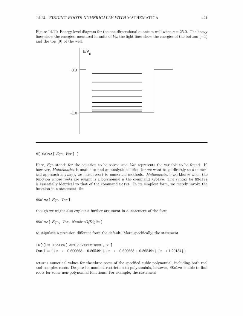
14.13. FINDING ROOTS NUMERICALLY WITH MATHEMATICA 421

Figure 14.11: Energy level diagram for the one-dimensional quantum well when c = 25.0. The heavylines show the energies, measured in units of V0; the light lines show the energies of the bottom (−1)and the top (0) of the well.

E/V0

-1.0

0.0

N[ Solve[ Eqn, Var ] ]

Here, Eqn stands for the equation to be solved and Var represents the variable to be found. If,however, Mathematica is unable to find an analytic solution (or we want to go directly to a numer-ical approach anyway), we must resort to numerical methods. Mathematica’s workhorse when thefunction whose roots are sought is a polynomial is the command NSolve. The syntax for NSolve

is essentially identical to that of the command Solve. In its simplest form, we merely invoke thefunction in a statement like

NSolve[ Eqn, Var ]

though we might also exploit a further argument in a statement of the form

NSolve[ Eqn, Var, NumberOfDigits ]

to stipulate a precision different from the default. More specifically, the statement

In[1]:= NSolve[ 3*x^3-2*x+x-4==0, x ]

Out[1]= x→ −0.600668− 0.86549i, x→ −0.600668 + 0.86549i, x→ 1.20134

returns numerical values for the three roots of the specified cubic polynomial, including both realand complex roots. Despite its nominal restriction to polynomials, however, NSolve is able to findroots for some non-polynomial functions. For example, the statement

422 CHAPTER 14. FINDING ROOTS

In[2]:= NSolve[ Cos[x]==0, x ]

Out[2]= x→ ConditionalExpression[1.(−1.5708 + 6.28319C[1]), C[1] ∈ Integers],x→ ConditionalExpression[1.(1.5708 + 6.28319C[1]), C[1] ∈ Integers]

reveals that Mathematica recognizes the equation cos(x) = 0 has many roots and successfully ifobscurely reports then all. To obtain any particular roots, we would execute statements like

In[3]:= Out[2] /. C[1] -> 0

Out[3]= x→ −1.5708, x→ 1.5708 In[4]:= Out[2] /. C[1] -> 3

Out[4]= x→ 17.2788, x→ 20.4204

C[1] can, of course, be given either positive or negative integer values. Apparently, when NSolve ispresented with a non-polynomial, it reverts to Solve followed by N, and the effort will be successfulonly if the given equation admits an analytic solution.19

When the function is not a polynomial, when it does not possess an analytic solution, or whenwe seek a numerically determined solution anyway, we must use the command FindRoot, which hasarguments specifying not only the equation to be solved and the variable sought but also one or twostarting values for an iterative search. The general syntax is

FindRoot[ Eqn, Var, Start1 ]

in which case FindRoot uses Newton’s method, or

FindRoot[ Eqn, Var, Start1, Start2 ]

in which case FindRoot uses the secant method.20 FindRoot admits several options, the mostsignificant of which are MaxIterations (default 100) to specify the maximum number of iterations touse before giving up and AccuracyGoal (default normally half of the value of WorkingPrecision)21

to stipulate the accuracy with which the function will be zero at the returned root. Thus, forexample, we might seek a particular root of cos(x) with the statement

In[3]:= FindRoot[ Cos[x] == 0, x, 4.0 ]

Out[3]= x→ 4.71239

or the statement

In[4]:= FindRoot[ Cos[x] == 0, x, 4.0, 5.0 ]

Out[4]= x→ 4.71239

a value we might recognize as 3π/2. Properly chosen, the additional stipulations in the secondargument permit us to select a particular root from the many that we know a priori exist.

Out of curiosity, let us test NSolve with a polynomial that has a multiple root. We execute thestatements

19Some earlier versions of Mathematica found only two of the many roots of cos(x) = 0, the command making itsown judgment about the interval in which to search and offering no means for us to specify some other interval. Forthe particular equation cos(x) = 0, those versions of Mathematica also displayed the warning “Solve::ifun: Inversefunctions are being used by Solve, so some solutions may not be found.

20Remember that the two starting values given to the secant method are not necessarily lower and upper boundsfor the root that will be found. If they do happen to bound a root, however, that is the root that will be found.

21The default for WorkingPrecision is $MachinePrecision, often 16.

14.13. FINDING ROOTS NUMERICALLY WITH MATHEMATICA 423

In[5]:= p1 = Expand[ (x-1)^2*(x+3)*(x-4) ];

In[6]:= NSolve[ p1==0, x ]

Out[6]= x→ −3., x→ 1.,x→ 1., x→ 4.

Create polynomial with multiple roots.

Find roots with NSolve.

Clearly, NSolve has returned all four roots of the given polynomial even though one of the threedistinct roots is a double root.

14.13.1 Classical Turning Points

To find the turning points for the potential energy in Eq. (14.3), we simply define the polynomialand invoke NSolve with the statements

In[7]:= V = x^3/10000+x^2/200-x/500-1/2;

In[8]:= NSolve[ V == 0, x ]

Out[8]= x→ −48.2683, x→ −11.0804, x→ 9.3487 In[9]:= Quit[]

These results are certainly consistent with the bounds identified in Section 14.1.1.

14.13.2 Range of Projectile

As laid out in Section 14.1.4, finding the range of a projectile moving in a viscous medium beginswith finding the time at which a projectile launched at some angle θ in a medium characterized bya (dimensionless) viscous damping coefficient α = bv0/(mg) returns to its initial altitude. In otherwords, we must find the one non-zero root of the function f(τ) defined in Eq. (14.18). To find thatroot and then the range for a particular choice of α and θ, we begin with the statements

In[1]:= rang = Cos[\[Theta]]*(1-Exp[-\[Tau]])/\[Alpha]

Out[1]=(1− e−τ ) Cos [θ]

α

In[2]:= fct = \[Tau] - (1+\[Alpha]*Sin[\[Theta]])*(1-Exp[-\[Tau]])

Out[2]= τ − (1− e−τ )(1 + α sin θ)

which define the range given by Eq. (14.19) and the auxiliary function given by Eq. (14.18). Then,we proceed with the statements

In[3]:= \[Alpha] = 0.4; \[Theta] = Pi*30.0/180.0;

In[4]:= FindRoot[ fct == 0, \[Tau], 0.2, 0.5 ]

Out[4]= τ → .376438

Choose α, θ.

Find root.

In[5]:= rang /. %

Out[5]= 0.679177

Evaluate range.

This result is expressed in units of v20/g.

To find the angle of fire to attain maximum range, we need to repeat the sample calculationof the previous paragraph for values of θ ranging from 0 to 90, choosing, say, increments of 1

between consecutive values of θ. To find the range for each of the selected values of θ, we invoke thesingle loop

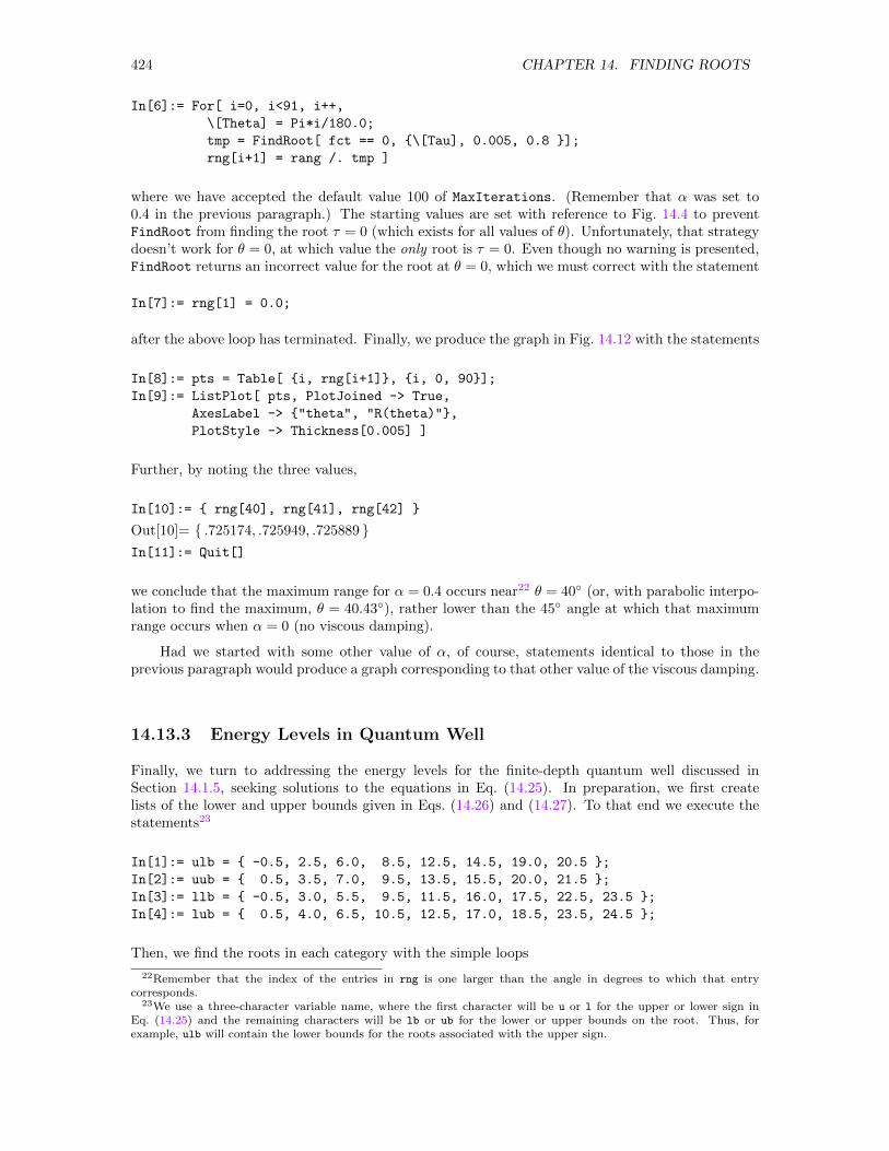
424 CHAPTER 14. FINDING ROOTS

In[6]:= For[ i=0, i<91, i++,

\[Theta] = Pi*i/180.0;

tmp = FindRoot[ fct == 0, \[Tau], 0.005, 0.8 ];

rng[i+1] = rang /. tmp ]

where we have accepted the default value 100 of MaxIterations. (Remember that α was set to0.4 in the previous paragraph.) The starting values are set with reference to Fig. 14.4 to preventFindRoot from finding the root τ = 0 (which exists for all values of θ). Unfortunately, that strategydoesn’t work for θ = 0, at which value the only root is τ = 0. Even though no warning is presented,FindRoot returns an incorrect value for the root at θ = 0, which we must correct with the statement

In[7]:= rng[1] = 0.0;

after the above loop has terminated. Finally, we produce the graph in Fig. 14.12 with the statements

In[8]:= pts = Table[ i, rng[i+1], i, 0, 90];

In[9]:= ListPlot[ pts, PlotJoined -> True,

AxesLabel -> "theta", "R(theta)",

PlotStyle -> Thickness[0.005] ]

Further, by noting the three values,

In[10]:= rng[40], rng[41], rng[42]

Out[10]= .725174, .725949, .725889 In[11]:= Quit[]

we conclude that the maximum range for α = 0.4 occurs near22 θ = 40 (or, with parabolic interpo-lation to find the maximum, θ = 40.43), rather lower than the 45 angle at which that maximumrange occurs when α = 0 (no viscous damping).

Had we started with some other value of α, of course, statements identical to those in theprevious paragraph would produce a graph corresponding to that other value of the viscous damping.

14.13.3 Energy Levels in Quantum Well

Finally, we turn to addressing the energy levels for the finite-depth quantum well discussed inSection 14.1.5, seeking solutions to the equations in Eq. (14.25). In preparation, we first createlists of the lower and upper bounds given in Eqs. (14.26) and (14.27). To that end we execute thestatements23

In[1]:= ulb = -0.5, 2.5, 6.0, 8.5, 12.5, 14.5, 19.0, 20.5 ;

In[2]:= uub = 0.5, 3.5, 7.0, 9.5, 13.5, 15.5, 20.0, 21.5 ;

In[3]:= llb = -0.5, 3.0, 5.5, 9.5, 11.5, 16.0, 17.5, 22.5, 23.5 ;

In[4]:= lub = 0.5, 4.0, 6.5, 10.5, 12.5, 17.0, 18.5, 23.5, 24.5 ;

Then, we find the roots in each category with the simple loops

22Remember that the index of the entries in rng is one larger than the angle in degrees to which that entrycorresponds.

23We use a three-character variable name, where the first character will be u or l for the upper or lower sign inEq. (14.25) and the remaining characters will be lb or ub for the lower or upper bounds on the root. Thus, forexample, ulb will contain the lower bounds for the roots associated with the upper sign.

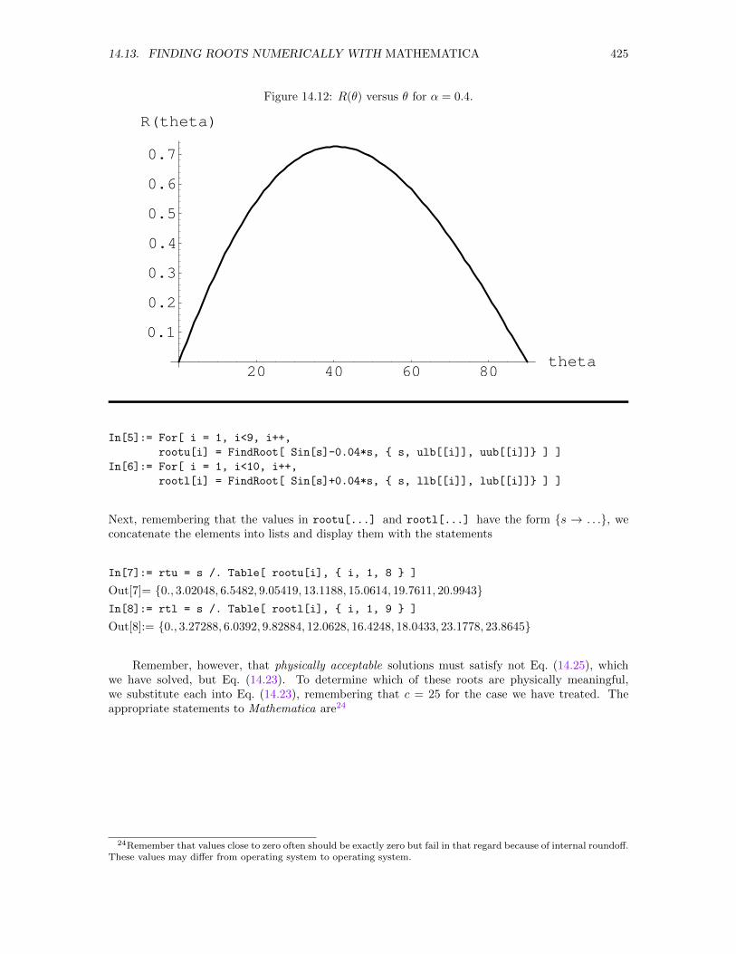
14.13. FINDING ROOTS NUMERICALLY WITH MATHEMATICA 425

Figure 14.12: R(θ) versus θ for α = 0.4.

20 40 60 80theta

0.1

0.2

0.3

0.4

0.5

0.6

0.7

R(theta)

In[5]:= For[ i = 1, i<9, i++,

rootu[i] = FindRoot[ Sin[s]-0.04*s, s, ulb[[i]], uub[[i]] ] ]

In[6]:= For[ i = 1, i<10, i++,

rootl[i] = FindRoot[ Sin[s]+0.04*s, s, llb[[i]], lub[[i]] ] ]

Next, remembering that the values in rootu[...] and rootl[...] have the form s → . . ., weconcatenate the elements into lists and display them with the statements

In[7]:= rtu = s /. Table[ rootu[i], i, 1, 8 ]

Out[7]= 0., 3.02048, 6.5482, 9.05419, 13.1188, 15.0614, 19.7611, 20.9943In[8]:= rtl = s /. Table[ rootl[i], i, 1, 9 ]

Out[8]:= 0., 3.27288, 6.0392, 9.82884, 12.0628, 16.4248, 18.0433, 23.1778, 23.8645

Remember, however, that physically acceptable solutions must satisfy not Eq. (14.25), whichwe have solved, but Eq. (14.23). To determine which of these roots are physically meaningful,we substitute each into Eq. (14.23), remembering that c = 25 for the case we have treated. Theappropriate statements to Mathematica are24

24Remember that values close to zero often should be exactly zero but fail in that regard because of internal roundoff.These values may differ from operating system to operating system.

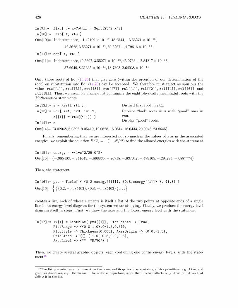
426 CHAPTER 14. FINDING ROOTS

In[9]:= f[x_] := x*Cot[x] + Sqrt[25^2-x^2]

In[10]:= Map[ f, rtu ]

Out[10]= Indeterminate,−1.42109× 10−14, 48.2544,−3.55271× 10−15,

42.5628, 3.55271× 10−14, 30.6267,−4.79616× 10−14

In[11]:= Map[ f, rtl ]

Out[11]= Indeterminate, 49.5697, 3.55271× 10−15, 45.9736,−2.84217× 10−14,

37.6949, 8.31335× 10−13, 18.7393, 2.64038× 10−11

Only those roots of Eq. (14.25) that give zero (within the precision of our determination of theroot) on substitution into Eq. (14.23) can be accepted. We therefore must reject as spurious thevalues rtu[[1]], rtu[[3]], rtu[[5]], rtu[[7]], rtl[[1]], rtl[[2]], rtl[[4]], rtl[[6]], andrtl[[8]]. Thus, we assemble a single list containing the eight physically meaningful roots with theMathematica statements

In[12]:= s = Rest[ rtl ];

In[13]:= For[ i=1, i<8, i=i+2,

s[[i]] = rtu[[i+1]] ]

In[14]:= s

Discard first root in rtl.

Replace “bad” roots in s with “good” ones inrtu.Display “good” roots.

Out[14]= 3.02048, 6.0392, 9.05419, 12.0628, 15.0614, 18.0433, 20.9943, 23.8645

Finally, remembering that we are interested not so much in the values of s as in the associatedenergies, we exploit the equation E/V0 = −(1−s2/c2) to find the allowed energies with the statement

In[15]:= energy = -(1-s^2/25.0^2)

Out[15]= −.985403,−.941645,−.868835,−.76718,−.637047,−.479105,−.294784,−.0887774

Then, the statement

In[16]:= pts = Table[ 0.2,energy[[i]], 0.8,energy[[i]] , i,8 ]

Out[16]= 0.2,−0.985403, 0.8,−0.985403 , . . .

creates a list, each of whose elements is itself a list of the two points at opposite ends of a singleline in an energy level diagram for the system we are studying. Finally, we produce the energy leveldiagram itself in steps. First, we draw the axes and the lowest energy level with the statement

In[17]:= lv[1] = ListPlot[ pts[[1]], PlotJoined -> True,

PlotRange -> 0.0,1.0,-1.5,0.5,

PlotStyle -> Thickness[0.005], AxesOrigin -> 0.0,-1.5,

GridLines -> ,-1.0,-0.5,0.0,0.5,

AxesLabel -> "", "E/V0" ]

Then, we create several graphic objects, each containing one of the energy levels, with the state-ment25

25The list presented as an argument to the command Graphics may contain graphics primitives, e.g., Line, andgraphics directives, e.g., Thickness. The order is important, since the directive affects only those primitives thatfollow it in the list.

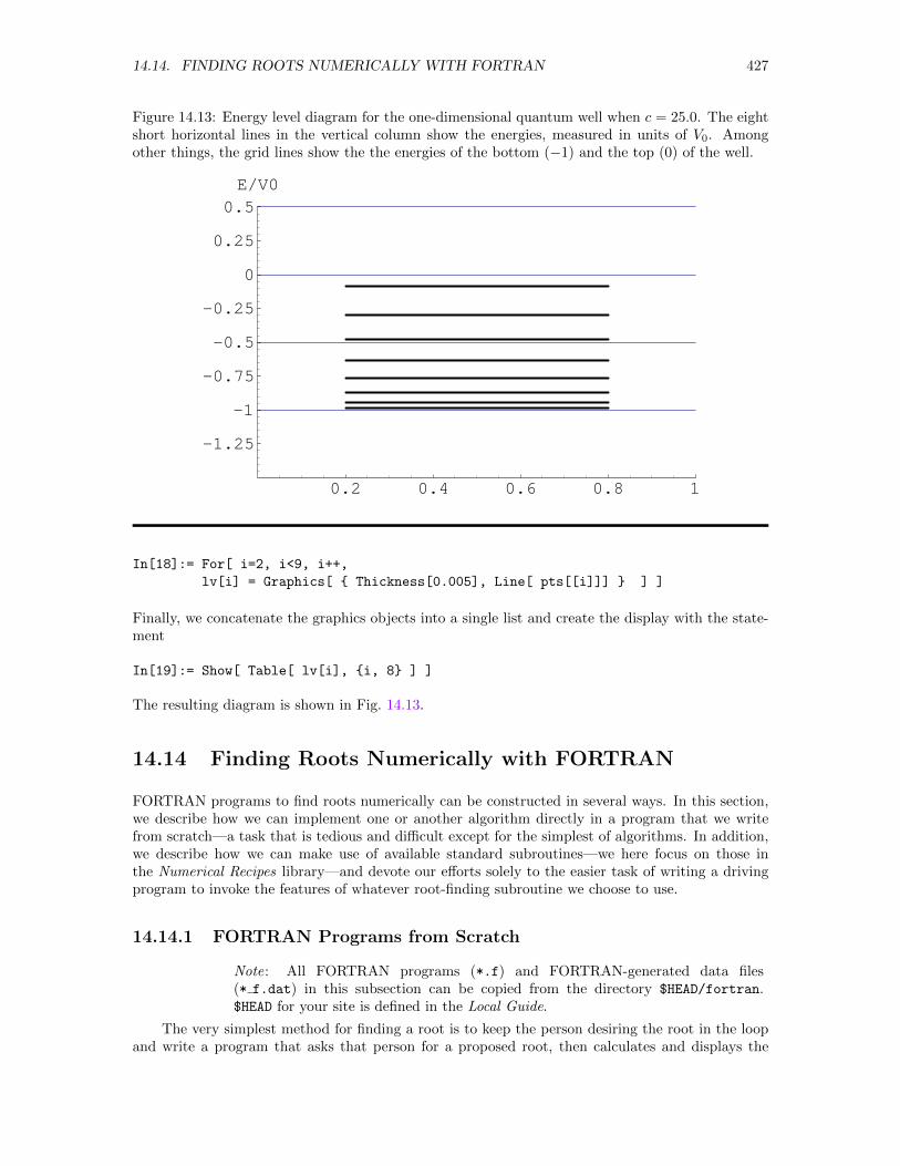
14.14. FINDING ROOTS NUMERICALLY WITH FORTRAN 427

Figure 14.13: Energy level diagram for the one-dimensional quantum well when c = 25.0. The eightshort horizontal lines in the vertical column show the energies, measured in units of V0. Amongother things, the grid lines show the the energies of the bottom (−1) and the top (0) of the well.

0.2 0.4 0.6 0.8 1

-1.25

-1

-0.75

-0.5

-0.25

0

0.25

0.5E/V0

In[18]:= For[ i=2, i<9, i++,

lv[i] = Graphics[ Thickness[0.005], Line[ pts[[i]]] ] ]

Finally, we concatenate the graphics objects into a single list and create the display with the state-ment

In[19]:= Show[ Table[ lv[i], i, 8 ] ]

The resulting diagram is shown in Fig. 14.13.

14.14 Finding Roots Numerically with FORTRAN

FORTRAN programs to find roots numerically can be constructed in several ways. In this section,we describe how we can implement one or another algorithm directly in a program that we writefrom scratch—a task that is tedious and difficult except for the simplest of algorithms. In addition,we describe how we can make use of available standard subroutines—we here focus on those inthe Numerical Recipes library—and devote our efforts solely to the easier task of writing a drivingprogram to invoke the features of whatever root-finding subroutine we choose to use.

14.14.1 FORTRAN Programs from Scratch

Note: All FORTRAN programs (*.f) and FORTRAN-generated data files(* f.dat) in this subsection can be copied from the directory $HEAD/fortran.$HEAD for your site is defined in the Local Guide.

The very simplest method for finding a root is to keep the person desiring the root in the loopand write a program that asks that person for a proposed root, then calculates and displays the

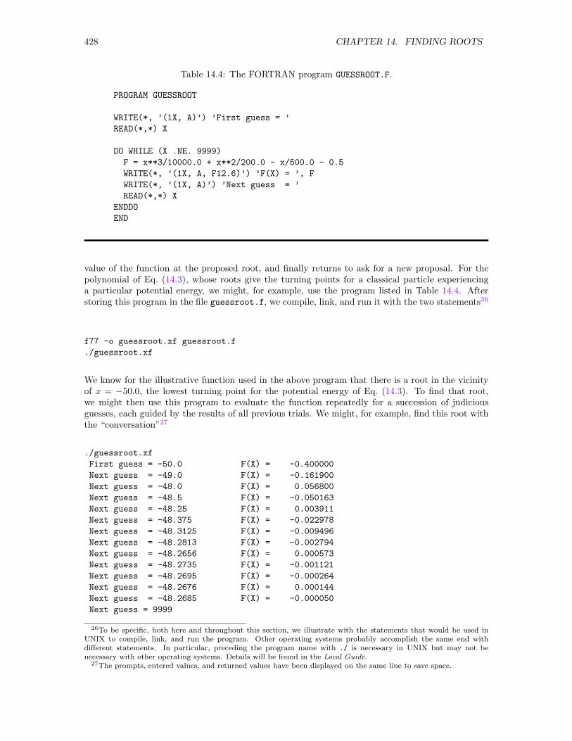
428 CHAPTER 14. FINDING ROOTS

Table 14.4: The FORTRAN program GUESSROOT.F.

PROGRAM GUESSROOT

WRITE(*, ’(1X, A)’) ’First guess = ’

READ(*,*) X

DO WHILE (X .NE. 9999)

F = x**3/10000.0 + x**2/200.0 - x/500.0 - 0.5

WRITE(*, ’(1X, A, F12.6)’) ’F(X) = ’, F

WRITE(*, ’(1X, A)’) ’Next guess = ’

READ(*,*) X

ENDDO

END

value of the function at the proposed root, and finally returns to ask for a new proposal. For thepolynomial of Eq. (14.3), whose roots give the turning points for a classical particle experiencinga particular potential energy, we might, for example, use the program listed in Table 14.4. Afterstoring this program in the file guessroot.f, we compile, link, and run it with the two statements26

f77 -o guessroot.xf guessroot.f

./guessroot.xf

We know for the illustrative function used in the above program that there is a root in the vicinityof x = −50.0, the lowest turning point for the potential energy of Eq. (14.3). To find that root,we might then use this program to evaluate the function repeatedly for a succession of judiciousguesses, each guided by the results of all previous trials. We might, for example, find this root withthe “conversation”27

./guessroot.xf

First guess = -50.0 F(X) = -0.400000

Next guess = -49.0 F(X) = -0.161900

Next guess = -48.0 F(X) = 0.056800

Next guess = -48.5 F(X) = -0.050163

Next guess = -48.25 F(X) = 0.003911

Next guess = -48.375 F(X) = -0.022978

Next guess = -48.3125 F(X) = -0.009496

Next guess = -48.2813 F(X) = -0.002794

Next guess = -48.2656 F(X) = 0.000573

Next guess = -48.2735 F(X) = -0.001121

Next guess = -48.2695 F(X) = -0.000264

Next guess = -48.2676 F(X) = 0.000144

Next guess = -48.2685 F(X) = -0.000050

Next guess = 9999

26To be specific, both here and throughout this section, we illustrate with the statements that would be used inUNIX to compile, link, and run the program. Other operating systems probably accomplish the same end withdifferent statements. In particular, preceding the program name with ./ is necessary in UNIX but may not benecessary with other operating systems. Details will be found in the Local Guide.

27The prompts, entered values, and returned values have been displayed on the same line to save space.

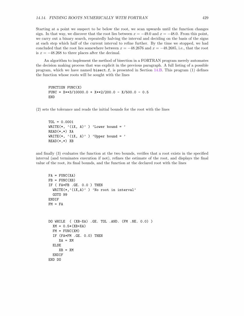
14.14. FINDING ROOTS NUMERICALLY WITH FORTRAN 429

Starting at a point we suspect to be below the root, we scan upwards until the function changessign. In that way, we discover that the root lies between x = −49.0 and x = −48.0. From this point,we carry out a binary search, repeatedly halving the interval and deciding on the basis of the signsat each step which half of the current interval to refine further. By the time we stopped, we hadconcluded that the root lies somewhere between x = −48.2676 and x = −48.2685, i.e., that the rootis x = −48.268 to three places after the decimal.

An algorithm to implement the method of bisection in a FORTRAN program merely automatesthe decision making process that was explicit in the previous paragraph. A full listing of a possibleprogram, which we have named bisect.f, is presented in Section 14.B. This program (1) definesthe function whose roots will be sought with the lines

FUNCTION FUNC(X)

FUNC = X**3/10000.0 + X**2/200.0 - X/500.0 - 0.5

END

(2) sets the tolerance and reads the initial bounds for the root with the lines

TOL = 0.0001

WRITE(*, ’(1X, A)’ ) ’Lower bound = ’

READ(*,*) XA

WRITE(*, ’(1X, A)’ ) ’Upper bound = ’

READ(*,*) XB

and finally (3) evaluates the function at the two bounds, verifies that a root exists in the specifiedinterval (and terminates execution if not), refines the estimate of the root, and displays the finalvalue of the root, its final bounds, and the function at the declared root with the lines

FA = FUNC(XA)

FB = FUNC(XB)

IF ( FA*FB .GE. 0.0 ) THEN

WRITE(*,’(1X,A)’ ) ’No root in interval’

GOTO 99

ENDIF

FM = FA

DO WHILE ( (XB-XA) .GE. TOL .AND. (FM .NE. 0.0) )

XM = 0.5*(XB+XA)

FM = FUNC(XM)

IF (FA*FM .GE. 0.0) THEN

XA = XM

ELSE

XB = XM

ENDIF

END DO

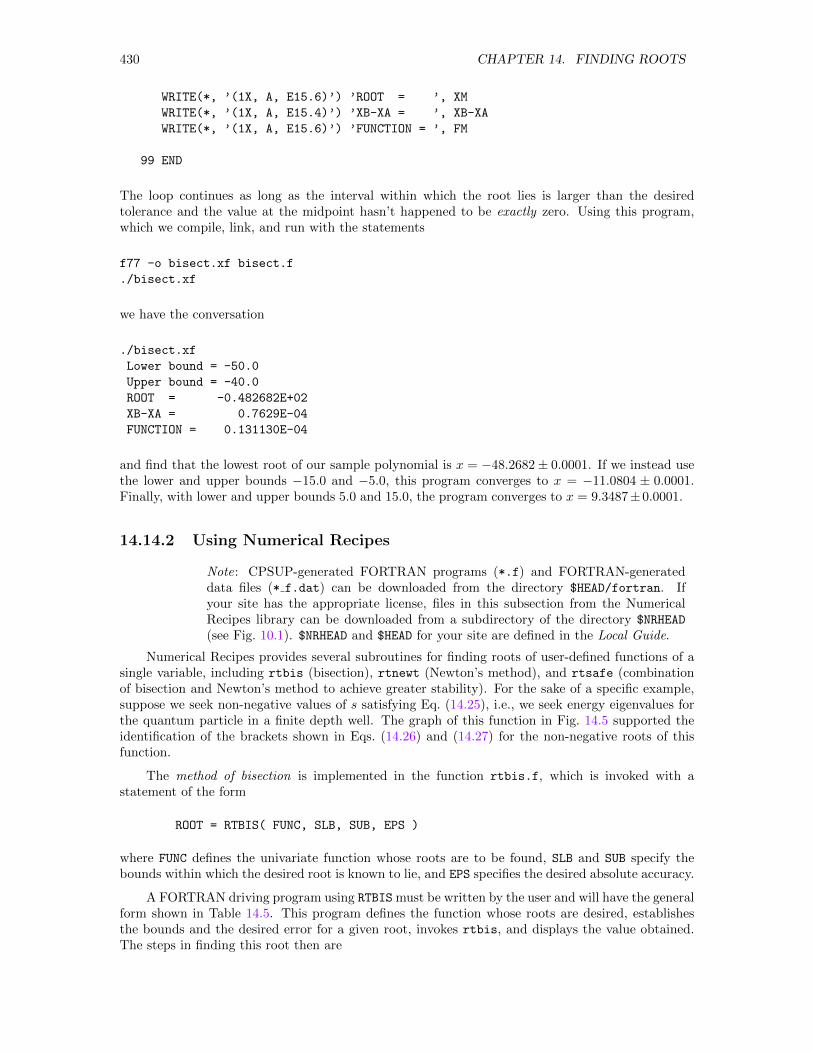
430 CHAPTER 14. FINDING ROOTS

WRITE(*, ’(1X, A, E15.6)’) ’ROOT = ’, XM

WRITE(*, ’(1X, A, E15.4)’) ’XB-XA = ’, XB-XA

WRITE(*, ’(1X, A, E15.6)’) ’FUNCTION = ’, FM

99 END

The loop continues as long as the interval within which the root lies is larger than the desiredtolerance and the value at the midpoint hasn’t happened to be exactly zero. Using this program,which we compile, link, and run with the statements

f77 -o bisect.xf bisect.f

./bisect.xf

we have the conversation

./bisect.xf

Lower bound = -50.0

Upper bound = -40.0

ROOT = -0.482682E+02

XB-XA = 0.7629E-04

FUNCTION = 0.131130E-04

and find that the lowest root of our sample polynomial is x = −48.2682± 0.0001. If we instead usethe lower and upper bounds −15.0 and −5.0, this program converges to x = −11.0804 ± 0.0001.Finally, with lower and upper bounds 5.0 and 15.0, the program converges to x = 9.3487±0.0001.

14.14.2 Using Numerical Recipes

Note: CPSUP-generated FORTRAN programs (*.f) and FORTRAN-generateddata files (* f.dat) can be downloaded from the directory $HEAD/fortran. Ifyour site has the appropriate license, files in this subsection from the NumericalRecipes library can be downloaded from a subdirectory of the directory $NRHEAD

(see Fig. 10.1). $NRHEAD and $HEAD for your site are defined in the Local Guide.

Numerical Recipes provides several subroutines for finding roots of user-defined functions of asingle variable, including rtbis (bisection), rtnewt (Newton’s method), and rtsafe (combinationof bisection and Newton’s method to achieve greater stability). For the sake of a specific example,suppose we seek non-negative values of s satisfying Eq. (14.25), i.e., we seek energy eigenvalues forthe quantum particle in a finite depth well. The graph of this function in Fig. 14.5 supported theidentification of the brackets shown in Eqs. (14.26) and (14.27) for the non-negative roots of thisfunction.

The method of bisection is implemented in the function rtbis.f, which is invoked with astatement of the form

ROOT = RTBIS( FUNC, SLB, SUB, EPS )

where FUNC defines the univariate function whose roots are to be found, SLB and SUB specify thebounds within which the desired root is known to lie, and EPS specifies the desired absolute accuracy.

A FORTRAN driving program using RTBIS must be written by the user and will have the generalform shown in Table 14.5. This program defines the function whose roots are desired, establishesthe bounds and the desired error for a given root, invokes rtbis, and displays the value obtained.The steps in finding this root then are

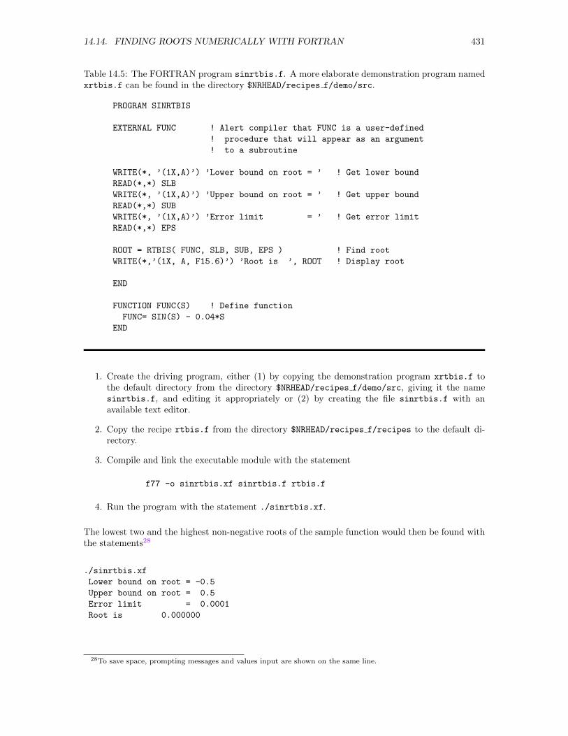
14.14. FINDING ROOTS NUMERICALLY WITH FORTRAN 431

Table 14.5: The FORTRAN program sinrtbis.f. A more elaborate demonstration program namedxrtbis.f can be found in the directory $NRHEAD/recipes f/demo/src.

PROGRAM SINRTBIS

EXTERNAL FUNC ! Alert compiler that FUNC is a user-defined

! procedure that will appear as an argument

! to a subroutine

WRITE(*, ’(1X,A)’) ’Lower bound on root = ’ ! Get lower bound

READ(*,*) SLB

WRITE(*, ’(1X,A)’) ’Upper bound on root = ’ ! Get upper bound

READ(*,*) SUB

WRITE(*, ’(1X,A)’) ’Error limit = ’ ! Get error limit

READ(*,*) EPS

ROOT = RTBIS( FUNC, SLB, SUB, EPS ) ! Find root

WRITE(*,’(1X, A, F15.6)’) ’Root is ’, ROOT ! Display root

END

FUNCTION FUNC(S) ! Define function

FUNC= SIN(S) - 0.04*S

END

1. Create the driving program, either (1) by copying the demonstration program xrtbis.f tothe default directory from the directory $NRHEAD/recipes f/demo/src, giving it the namesinrtbis.f, and editing it appropriately or (2) by creating the file sinrtbis.f with anavailable text editor.

2. Copy the recipe rtbis.f from the directory $NRHEAD/recipes f/recipes to the default di-rectory.

3. Compile and link the executable module with the statement

f77 -o sinrtbis.xf sinrtbis.f rtbis.f

4. Run the program with the statement ./sinrtbis.xf.

The lowest two and the highest non-negative roots of the sample function would then be found withthe statements28

./sinrtbis.xf

Lower bound on root = -0.5

Upper bound on root = 0.5

Error limit = 0.0001

Root is 0.000000

28To save space, prompting messages and values input are shown on the same line.

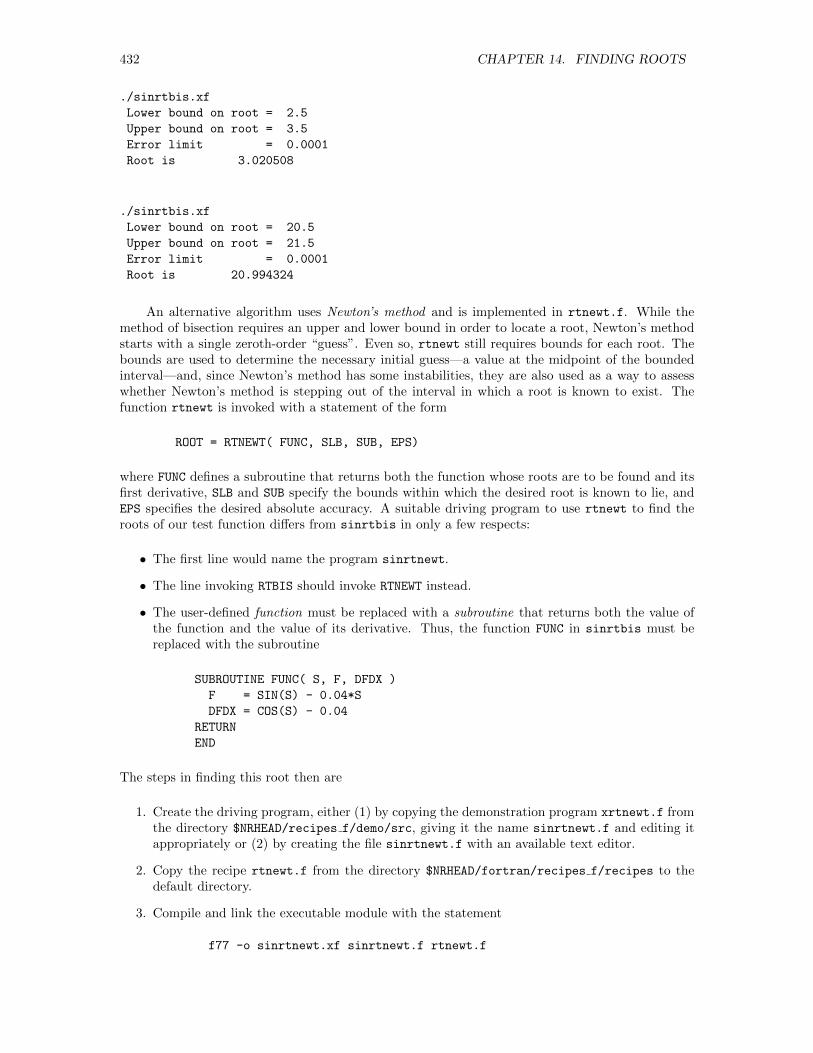
432 CHAPTER 14. FINDING ROOTS

./sinrtbis.xf

Lower bound on root = 2.5

Upper bound on root = 3.5

Error limit = 0.0001

Root is 3.020508

./sinrtbis.xf

Lower bound on root = 20.5

Upper bound on root = 21.5

Error limit = 0.0001

Root is 20.994324

An alternative algorithm uses Newton’s method and is implemented in rtnewt.f. While themethod of bisection requires an upper and lower bound in order to locate a root, Newton’s methodstarts with a single zeroth-order “guess”. Even so, rtnewt still requires bounds for each root. Thebounds are used to determine the necessary initial guess—a value at the midpoint of the boundedinterval—and, since Newton’s method has some instabilities, they are also used as a way to assesswhether Newton’s method is stepping out of the interval in which a root is known to exist. Thefunction rtnewt is invoked with a statement of the form

ROOT = RTNEWT( FUNC, SLB, SUB, EPS)

where FUNC defines a subroutine that returns both the function whose roots are to be found and itsfirst derivative, SLB and SUB specify the bounds within which the desired root is known to lie, andEPS specifies the desired absolute accuracy. A suitable driving program to use rtnewt to find theroots of our test function differs from sinrtbis in only a few respects:

• The first line would name the program sinrtnewt.

• The line invoking RTBIS should invoke RTNEWT instead.

• The user-defined function must be replaced with a subroutine that returns both the value ofthe function and the value of its derivative. Thus, the function FUNC in sinrtbis must bereplaced with the subroutine

SUBROUTINE FUNC( S, F, DFDX )

F = SIN(S) - 0.04*S

DFDX = COS(S) - 0.04

RETURN

END

The steps in finding this root then are

1. Create the driving program, either (1) by copying the demonstration program xrtnewt.f fromthe directory $NRHEAD/recipes f/demo/src, giving it the name sinrtnewt.f and editing itappropriately or (2) by creating the file sinrtnewt.f with an available text editor.

2. Copy the recipe rtnewt.f from the directory $NRHEAD/fortran/recipes f/recipes to thedefault directory.

3. Compile and link the executable module with the statement

f77 -o sinrtnewt.xf sinrtnewt.f rtnewt.f

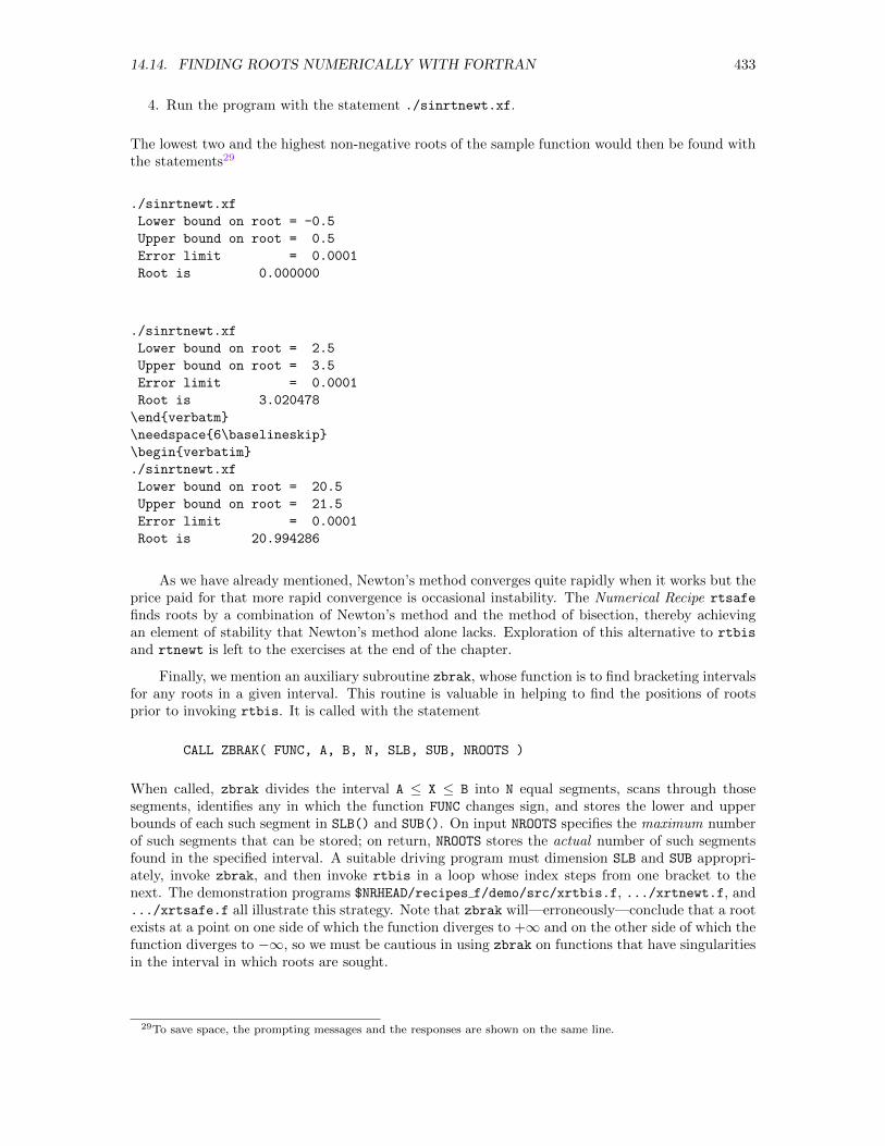
14.14. FINDING ROOTS NUMERICALLY WITH FORTRAN 433

4. Run the program with the statement ./sinrtnewt.xf.

The lowest two and the highest non-negative roots of the sample function would then be found withthe statements29

./sinrtnewt.xf

Lower bound on root = -0.5

Upper bound on root = 0.5

Error limit = 0.0001

Root is 0.000000

./sinrtnewt.xf

Lower bound on root = 2.5

Upper bound on root = 3.5

Error limit = 0.0001

Root is 3.020478

\endverbatm

\needspace6\baselineskip

\beginverbatim

./sinrtnewt.xf

Lower bound on root = 20.5

Upper bound on root = 21.5

Error limit = 0.0001

Root is 20.994286

As we have already mentioned, Newton’s method converges quite rapidly when it works but theprice paid for that more rapid convergence is occasional instability. The Numerical Recipe rtsafe

finds roots by a combination of Newton’s method and the method of bisection, thereby achievingan element of stability that Newton’s method alone lacks. Exploration of this alternative to rtbis

and rtnewt is left to the exercises at the end of the chapter.

Finally, we mention an auxiliary subroutine zbrak, whose function is to find bracketing intervalsfor any roots in a given interval. This routine is valuable in helping to find the positions of rootsprior to invoking rtbis. It is called with the statement

CALL ZBRAK( FUNC, A, B, N, SLB, SUB, NROOTS )

When called, zbrak divides the interval A ≤ X ≤ B into N equal segments, scans through thosesegments, identifies any in which the function FUNC changes sign, and stores the lower and upperbounds of each such segment in SLB() and SUB(). On input NROOTS specifies the maximum numberof such segments that can be stored; on return, NROOTS stores the actual number of such segmentsfound in the specified interval. A suitable driving program must dimension SLB and SUB appropri-ately, invoke zbrak, and then invoke rtbis in a loop whose index steps from one bracket to thenext. The demonstration programs $NRHEAD/recipes f/demo/src/xrtbis.f, .../xrtnewt.f, and.../xrtsafe.f all illustrate this strategy. Note that zbrak will—erroneously—conclude that a rootexists at a point on one side of which the function diverges to +∞ and on the other side of which thefunction diverges to −∞, so we must be cautious in using zbrak on functions that have singularitiesin the interval in which roots are sought.

29To save space, the prompting messages and the responses are shown on the same line.

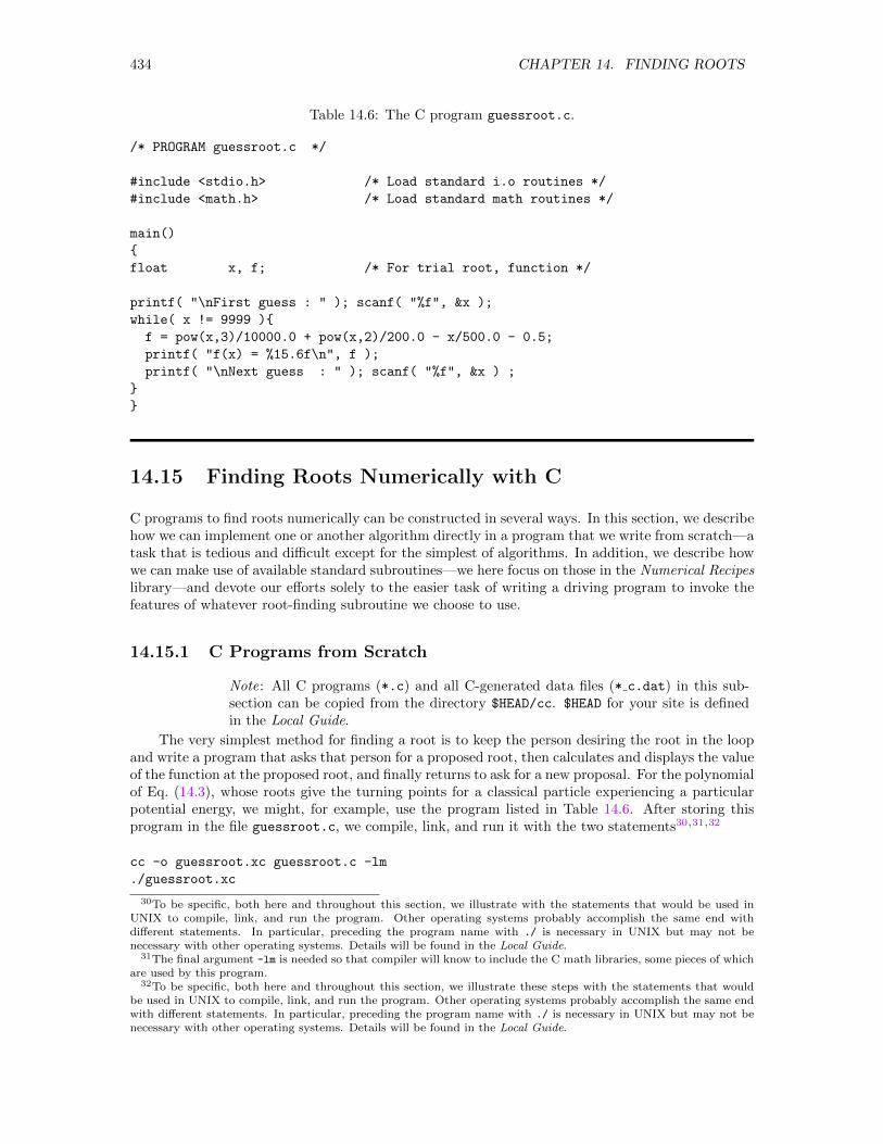
434 CHAPTER 14. FINDING ROOTS

Table 14.6: The C program guessroot.c.

/* PROGRAM guessroot.c */

#include <stdio.h> /* Load standard i.o routines */

#include <math.h> /* Load standard math routines */

main()

float x, f; /* For trial root, function */

printf( "\nFirst guess : " ); scanf( "%f", &x );

while( x != 9999 )

f = pow(x,3)/10000.0 + pow(x,2)/200.0 - x/500.0 - 0.5;

printf( "f(x) = %15.6f\n", f );

printf( "\nNext guess : " ); scanf( "%f", &x ) ;

14.15 Finding Roots Numerically with C

C programs to find roots numerically can be constructed in several ways. In this section, we describehow we can implement one or another algorithm directly in a program that we write from scratch—atask that is tedious and difficult except for the simplest of algorithms. In addition, we describe howwe can make use of available standard subroutines—we here focus on those in the Numerical Recipeslibrary—and devote our efforts solely to the easier task of writing a driving program to invoke thefeatures of whatever root-finding subroutine we choose to use.

14.15.1 C Programs from Scratch

Note: All C programs (*.c) and all C-generated data files (* c.dat) in this sub-section can be copied from the directory $HEAD/cc. $HEAD for your site is definedin the Local Guide.

The very simplest method for finding a root is to keep the person desiring the root in the loopand write a program that asks that person for a proposed root, then calculates and displays the valueof the function at the proposed root, and finally returns to ask for a new proposal. For the polynomialof Eq. (14.3), whose roots give the turning points for a classical particle experiencing a particularpotential energy, we might, for example, use the program listed in Table 14.6. After storing thisprogram in the file guessroot.c, we compile, link, and run it with the two statements30,31,32

cc -o guessroot.xc guessroot.c -lm

./guessroot.xc

30To be specific, both here and throughout this section, we illustrate with the statements that would be used inUNIX to compile, link, and run the program. Other operating systems probably accomplish the same end withdifferent statements. In particular, preceding the program name with ./ is necessary in UNIX but may not benecessary with other operating systems. Details will be found in the Local Guide.

31The final argument -lm is needed so that compiler will know to include the C math libraries, some pieces of whichare used by this program.

32To be specific, both here and throughout this section, we illustrate these steps with the statements that wouldbe used in UNIX to compile, link, and run the program. Other operating systems probably accomplish the same endwith different statements. In particular, preceding the program name with ./ is necessary in UNIX but may not benecessary with other operating systems. Details will be found in the Local Guide.

14.15. FINDING ROOTS NUMERICALLY WITH C 435

We know for the illustrative function used in the above program that there is a root in the vicinityof x = −50.0, the lowest turning point for the potential energy of Eq. (14.3). To find that root,we might then use this program to evaluate the function repeatedly for a succession of judiciousguesses, each guided by the results of all previous trials. We might, for example, find this root withthe “conversation”33

./guessroot.xc

First guess : -50.0 f(x) = -0.400000

Next guess : -49.0 f(x) = -0.161900

Next guess : -48.0 f(x) = 0.056800

Next guess : -48.5 f(x) = -0.050163

Next guess : -48.25 f(x) = 0.003911

Next guess : -48.375 f(x) = -0.022977

Next guess : -48.2813 f(x) = -0.002794

Next guess : -48.2656 f(x) = 0.000572

Next guess : -48.2735 f(x) = -0.001121

Next guess : -48.2695 f(x) = -0.000264

Next guess : -48.2676 f(x) = 0.000143

Next guess : -48.2685 f(x) = -0.000050

Next guess : 9999

Starting at a point we suspect to be below the root, we scan upwards until the function changessign. In that way, we discover that the root lies between x = −49.0 and x = −48.0. From this point,we carry out a binary search, repeatedly halving the interval and deciding on the basis of the signsat each step which half of the current interval to refine further. By the time we stopped, we hadconcluded that the root lies somewhere between x = −48.2676 and x = −48.2685, i.e., that the rootis x = −48.268 to three places after the decimal.

An algorithm to implement the method of bisection in a C program merely automates thedecision making process that was explicit in the previous paragraph. A full listing of a possibleprogram, which we have named bisect.c, is presented in Section 14.C. Beyond incorporating thenecessary header files, this program (1) defines the function whose roots will be sought with thelines

float func( float x )

return pow(x,3)/10000.0 + pow(x,2)/200.0 - x/500.0 - 0.5;

(2) declares floating variables tol, xa, xm, xb, fa, fm, and fb for the tolerance, the lower, middle,and upper values of the interval, and the values of the function at xa, xm, xb; (3) sets the toleranceand reads the initial bounds for the root with the lines

tol = 0.0001

printf( "\nLower bound = " ); scanf( "%f", &xa );

printf( "\nUpper bound = " ); scanf( "%f", &xb );

and finally (4) evaluates the function at the two bounds, verifies that a root exists in the specifiedinterval (and terminates execution if not), refines the extimate of the root, and displays the finalvalue of the root, its final bounds, and the function at the declared root with the lines

33The prompt, the entered values, and the returned values have been displayed on the same line to save space.

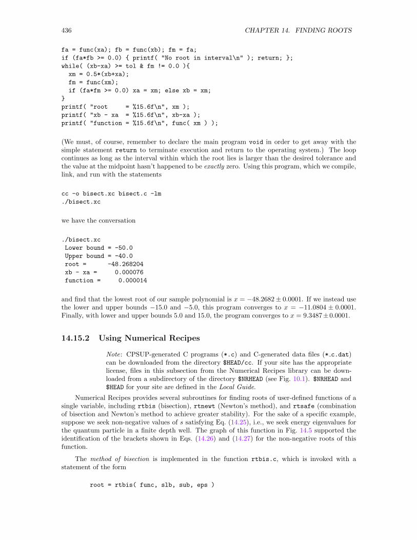
436 CHAPTER 14. FINDING ROOTS

fa = func(xa); fb = func(xb); fm = fa;

if (fa*fb >= 0.0) printf( "No root in interval\n" ); return; ;

while( (xb-xa) >= tol & fm != 0.0 )

xm = 0.5*(xb+xa);

fm = func(xm);

if (fa*fm >= 0.0) xa = xm; else xb = xm;

printf( "root = %15.6f\n", xm );

printf( "xb - xa = %15.6f\n", xb-xa );

printf( "function = %15.6f\n", func( xm ) );

(We must, of course, remember to declare the main program void in order to get away with thesimple statement return to terminate execution and return to the operating system.) The loopcontinues as long as the interval within which the root lies is larger than the desired tolerance andthe value at the midpoint hasn’t happened to be exactly zero. Using this program, which we compile,link, and run with the statements

cc -o bisect.xc bisect.c -lm

./bisect.xc

we have the conversation

./bisect.xc

Lower bound = -50.0

Upper bound = -40.0

root = -48.268204

xb - xa = 0.000076

function = 0.000014

and find that the lowest root of our sample polynomial is x = −48.2682± 0.0001. If we instead usethe lower and upper bounds −15.0 and −5.0, this program converges to x = −11.0804 ± 0.0001.Finally, with lower and upper bounds 5.0 and 15.0, the program converges to x = 9.3487±0.0001.

14.15.2 Using Numerical Recipes

Note: CPSUP-generated C programs (*.c) and C-generated data files (* c.dat)can be downloaded from the directory $HEAD/cc. If your site has the appropriatelicense, files in this subsection from the Numerical Recipes library can be down-loaded from a subdirectory of the directory $NRHEAD (see Fig. 10.1). $NRHEAD and$HEAD for your site are defined in the Local Guide.

Numerical Recipes provides several subroutines for finding roots of user-defined functions of asingle variable, including rtbis (bisection), rtnewt (Newton’s method), and rtsafe (combinationof bisection and Newton’s method to achieve greater stability). For the sake of a specific example,suppose we seek non-negative values of s satisfying Eq. (14.25), i.e., we seek energy eigenvalues forthe quantum particle in a finite depth well. The graph of this function in Fig. 14.5 supported theidentification of the brackets shown in Eqs. (14.26) and (14.27) for the non-negative roots of thisfunction.

The method of bisection is implemented in the function rtbis.c, which is invoked with astatement of the form

root = rtbis( func, slb, sub, eps )

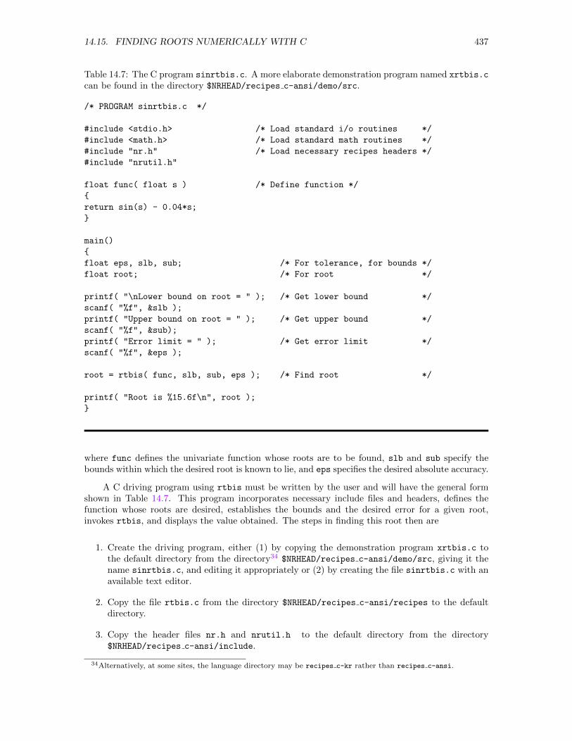
14.15. FINDING ROOTS NUMERICALLY WITH C 437

Table 14.7: The C program sinrtbis.c. A more elaborate demonstration program named xrtbis.c

can be found in the directory $NRHEAD/recipes c-ansi/demo/src.

/* PROGRAM sinrtbis.c */

#include <stdio.h> /* Load standard i/o routines */

#include <math.h> /* Load standard math routines */

#include "nr.h" /* Load necessary recipes headers */

#include "nrutil.h"

float func( float s ) /* Define function */

return sin(s) - 0.04*s;

main()

float eps, slb, sub; /* For tolerance, for bounds */

float root; /* For root */

printf( "\nLower bound on root = " ); /* Get lower bound */

scanf( "%f", &slb );

printf( "Upper bound on root = " ); /* Get upper bound */

scanf( "%f", &sub);

printf( "Error limit = " ); /* Get error limit */

scanf( "%f", &eps );

root = rtbis( func, slb, sub, eps ); /* Find root */

printf( "Root is %15.6f\n", root );

where func defines the univariate function whose roots are to be found, slb and sub specify thebounds within which the desired root is known to lie, and eps specifies the desired absolute accuracy.

A C driving program using rtbis must be written by the user and will have the general formshown in Table 14.7. This program incorporates necessary include files and headers, defines thefunction whose roots are desired, establishes the bounds and the desired error for a given root,invokes rtbis, and displays the value obtained. The steps in finding this root then are

1. Create the driving program, either (1) by copying the demonstration program xrtbis.c tothe default directory from the directory34 $NRHEAD/recipes c-ansi/demo/src, giving it thename sinrtbis.c, and editing it appropriately or (2) by creating the file sinrtbis.c with anavailable text editor.

2. Copy the file rtbis.c from the directory $NRHEAD/recipes c-ansi/recipes to the defaultdirectory.

3. Copy the header files nr.h and nrutil.h to the default directory from the directory$NRHEAD/recipes c-ansi/include.

34Alternatively, at some sites, the language directory may be recipes c-kr rather than recipes c-ansi.

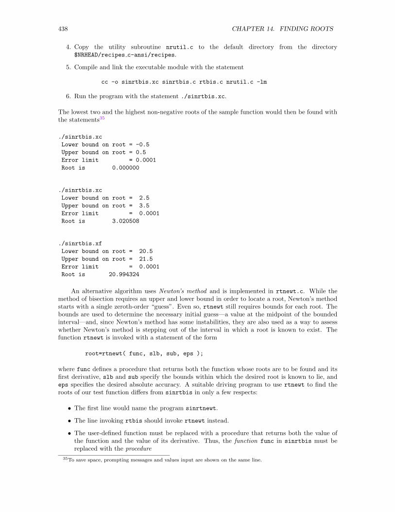
438 CHAPTER 14. FINDING ROOTS

4. Copy the utility subroutine nrutil.c to the default directory from the directory$NRHEAD/recipes c-ansi/recipes.

5. Compile and link the executable module with the statement

cc -o sinrtbis.xc sinrtbis.c rtbis.c nrutil.c -lm

6. Run the program with the statement ./sinrtbis.xc.

The lowest two and the highest non-negative roots of the sample function would then be found withthe statements35

./sinrtbis.xc

Lower bound on root = -0.5

Upper bound on root = 0.5

Error limit = 0.0001

Root is 0.000000

./sinrtbis.xc

Lower bound on root = 2.5

Upper bound on root = 3.5

Error limit = 0.0001

Root is 3.020508

./sinrtbis.xf

Lower bound on root = 20.5

Upper bound on root = 21.5

Error limit = 0.0001

Root is 20.994324

An alternative algorithm uses Newton’s method and is implemented in rtnewt.c. While themethod of bisection requires an upper and lower bound in order to locate a root, Newton’s methodstarts with a single zeroth-order “guess”. Even so, rtnewt still requires bounds for each root. Thebounds are used to determine the necessary initial guess—a value at the midpoint of the boundedinterval—and, since Newton’s method has some instabilities, they are also used as a way to assesswhether Newton’s method is stepping out of the interval in which a root is known to exist. Thefunction rtnewt is invoked with a statement of the form

root=rtnewt( func, slb, sub, eps );

where func defines a procedure that returns both the function whose roots are to be found and itsfirst derivative, slb and sub specify the bounds within which the desired root is known to lie, andeps specifies the desired absolute accuracy. A suitable driving program to use rtnewt to find theroots of our test function differs from sinrtbis in only a few respects:

• The first line would name the program sinrtnewt.

• The line invoking rtbis should invoke rtnewt instead.

• The user-defined function must be replaced with a procedure that returns both the value ofthe function and the value of its derivative. Thus, the function func in sinrtbis must bereplaced with the procedure

35To save space, prompting messages and values input are shown on the same line.

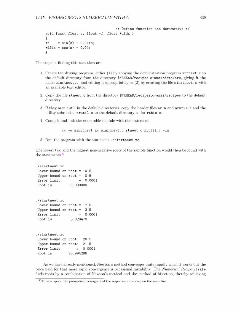
14.15. FINDING ROOTS NUMERICALLY WITH C 439

/* Define function and derivative */

void func( float s, float *f, float *dfdx )

*f = sin(s) - 0.04*s;

*dfdx = cos(s) - 0.04;

The steps in finding this root then are

1. Create the driving program, either (1) by copying the demonstration program xrtnewt.c tothe default directory from the directory $NRHEAD/recipes c-ansi/demo/src, giving it thename sinrtnewt.c, and editing it appropriately or (2) by creating the file sinrtnewt.c withan available text editor.

2. Copy the file rtnewt.c from the directory $NRHEAD/recipes c-ansi/recipes to the defaultdirectory.

3. If they aren’t still in the default directories, copy the header files nr.h and nrutil.h and theutility subroutine nrutil.c to the default directory as for rtbis.c.

4. Compile and link the executable module with the statement

cc -o sinrtnewt.xc sinrtnewt.c rtnewt.c nrutil.c -lm

5. Run the program with the statement ./sinrtnewt.xc.

The lowest two and the highest non-negative roots of the sample function would then be found withthe statements36

./sinrtnewt.xc

Lower bound on root = -0.5

Upper bound on root = 0.5

Error limit = 0.0001

Root is 0.000000

./sinrtnewt.xc

Lower bound on root = 2.5

Upper bound on root = 3.5

Error limit = 0.0001

Root is 3.020478

./sinrtnewt.xc

Lower bound on root: 20.5

Upper bound on root: 21.5

Error limit : 0.0001

Root is 20.994286

As we have already mentioned, Newton’s method converges quite rapidly when it works but theprice paid for that more rapid convergence is occasional instability. The Numerical Recipe rtsafe

finds roots by a combination of Newton’s method and the method of bisection, thereby achieving

36To save space, the prompting messages and the responses are shown on the same line.

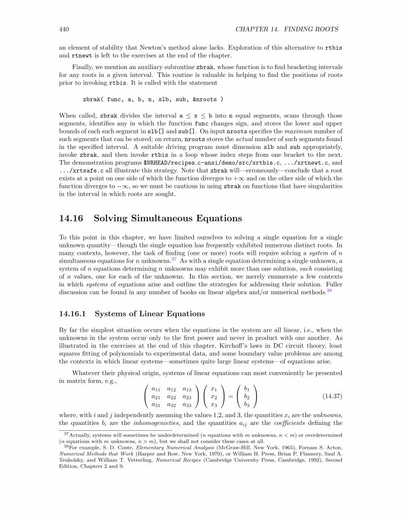
440 CHAPTER 14. FINDING ROOTS

an element of stability that Newton’s method alone lacks. Exploration of this alternative to rtbis

and rtnewt is left to the exercises at the end of the chapter.

Finally, we mention an auxiliary subroutine zbrak, whose function is to find bracketing intervalsfor any roots in a given interval. This routine is valuable in helping to find the positions of rootsprior to invoking rtbis. It is called with the statement

zbrak( func, a, b, n, slb, sub, &nroots )

When called, zbrak divides the interval a ≤ x ≤ b into n equal segments, scans through thosesegments, identifies any in which the function func changes sign, and stores the lower and upperbounds of each such segment in slb[] and sub[]. On input nroots specifies the maximum number ofsuch segments that can be stored; on return, nroots stores the actual number of such segments foundin the specified interval. A suitable driving program must dimension slb and sub appropriately,invoke zbrak, and then invoke rtbis in a loop whose index steps from one bracket to the next.The demonstration programs $NRHEAD/recipes c-ansi/demo/src/xrtbis.c, .../xrtnewt.c, and.../xrtsafe.c all illustrate this strategy. Note that zbrak will—erroneously—conclude that a rootexists at a point on one side of which the function diverges to +∞ and on the other side of which thefunction diverges to −∞, so we must be cautious in using zbrak on functions that have singularitiesin the interval in which roots are sought.

14.16 Solving Simultaneous Equations

To this point in this chapter, we have limited ourselves to solving a single equation for a singleunknown quantity—though the single equation has frequently exhibited numerous distinct roots. Inmany contexts, however, the task of finding (one or more) roots will require solving a system of nsimultaneous equations for n unknowns.37 As with a single equation determining a single unknown, asystem of n equations determining n unknowns may exhibit more than one solution, each consistingof n values, one for each of the unknowns. In this section, we merely enumerate a few contextsin which systems of equations arise and outline the strategies for addressing their solution. Fullerdiscussion can be found in any number of books on linear algebra and/or numerical methods.38

14.16.1 Systems of Linear Equations

By far the simplest situation occurs when the equations in the system are all linear, i.e., when theunknowns in the system occur only to the first power and never in product with one another. Asillustrated in the exercises at the end of this chapter, Kirchoff’s laws in DC circuit theory, leastsquares fitting of polynomials to experimental data, and some boundary value problems are amongthe contexts in which linear systems—sometimes quite large linear systems—of equations arise.

Whatever their physical origin, systems of linear equations can most conveniently be presentedin matrix form, e.g., a11 a12 a13

a21 a22 a23a31 a32 a33

x1x2x3

=

b1b2b3

(14.37)

where, with i and j independently assuming the values 1,2, and 3, the quantities xi are the unknowns,the quantities bi are the inhomogenieties, and the quantities aij are the coefficients defining the

37Actually, systems will sometimes be underdetermined (n equations with m unknowns, n < m) or overdetermined(n equations with m unknowns, n > m), but we shall not consider these cases at all.

38For example, S. D. Conte, Elementary Numerical Analysis (McGraw-Hill, New York, 1965), Fornam S. Acton,Numerical Methods that Work (Harper and Row, New York, 1970), or William H. Press, Brian P. Flannery, Saul A.Teukolsky, and William T. Vetterling, Numerical Recipes (Cambridge University Press, Cambridge, 1992), SecondEdition, Chapters 2 and 9.

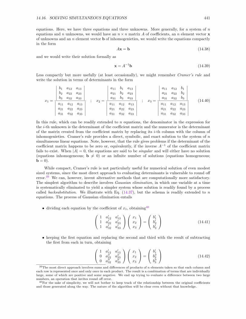
14.16. SOLVING SIMULTANEOUS EQUATIONS 441

equations. Here, we have three equations and three unknowns. More generally, for a system of nequations and n unknowns, we would have an n× n matrix A of coefficients, an n element vector xof unknowns and an n element vector b of inhomogenieties, we would write the equations compactlyin the form

Ax = b (14.38)

and we would write their solution formally as

x = A−1b (14.39)

Less compactly but more usefully (at least occasionally), we might remember Cramer’s rule andwrite the solution in terms of determinants in the form

x1 =

∣∣∣∣∣∣b1 a12 a13b2 a22 a23b3 a32 a33

∣∣∣∣∣∣∣∣∣∣∣∣a11 a12 a13a21 a22 a23a31 a32 a33

∣∣∣∣∣∣; x2 =

∣∣∣∣∣∣a11 b1 a13a21 b2 a23a31 b3 a33

∣∣∣∣∣∣∣∣∣∣∣∣a11 a12 a13a21 a22 a23a31 a32 a33

∣∣∣∣∣∣; x3 =

∣∣∣∣∣∣a11 a12 b1a21 a22 b2a31 a32 b3

∣∣∣∣∣∣∣∣∣∣∣∣a11 a12 a13a21 a22 a23a31 a32 a33

∣∣∣∣∣∣(14.40)

In this rule, which can be readily extended to n equations, the denominator in the expression forthe i-th unknown is the determinant of the coefficient matrix and the numerator is the determinantof the matrix created from the coefficient matrix by replacing its i-th column with the column ofinhomogenieties. Cramer’s rule provides a direct, symbolic, and exact solution to the system of nsimultaneous linear equations. Note, however, that the rule gives problems if the determinant of thecoefficient matrix happens to be zero or, equivalently, if the inverse A−1 of the coefficient matrixfails to exist. When |A| = 0, the equations are said to be singular and will either have no solution(equations inhomogeneous; b 6= 0) or an infinite number of solutions (equations homogeneous;b = 0).

While compact, Cramer’s rule is not particularly useful for numerical solution of even modestsized systems, since the most direct approach to evaluating determinants is vulnerable to round offerror.39 We can, however, invent alternative methods that are computationally more satisfactory.The simplest algorithm to describe involves Gaussian elimination, in which one variable at a timeis systematically eliminated to yield a simpler system whose solution is readily found by a processcalled backsubstitution. We illustrate with Eq. (14.37), but the schema is readily extended to nequations. The process of Gaussian elimination entails

• dividing each equation by the coefficient of x1, obtaining40 1 a′12 a′131 a′22 a′231 a′32 a′33

x1x2x3

=

b′1b′2b′3

(14.41)

• keeping the first equation and replacing the second and third with the result of subtractingthe first from each in turn, obtaining 1 a′12 a′13

0 a′′22 a′′230 a′′32 a′′33

x1x2x3

=

b′1b′′2b′′3

(14.42)

39The most direct approach involves sums and differences of products of n elements taken so that each column andeach row is represented once and only once in each product. The result is a combination of terms that are individuallylarge, some of which are positive and some negative. We end up trying to evaluate a difference between two largenumbers, an operation that invites round off error.

40For the sake of simplicity, we will not bother to keep track of the relationship between the original coefficientsand those generated along the way. The nature of the algorithm will be clear even without that knowledge.

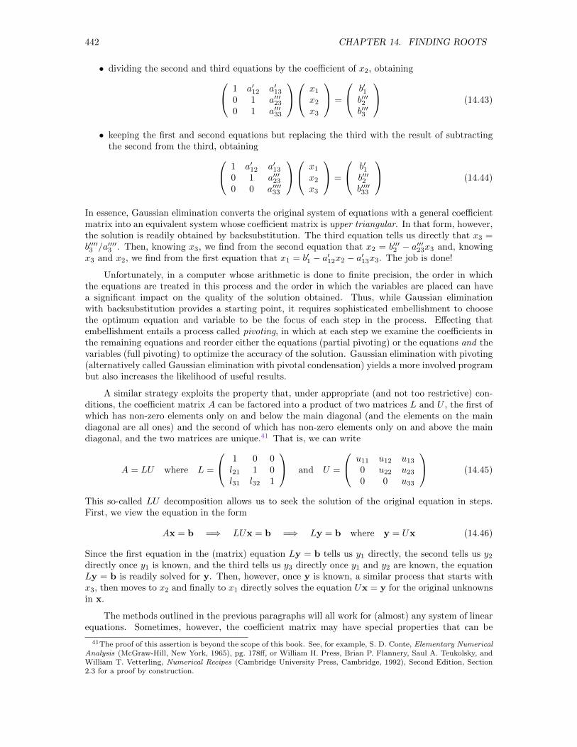
442 CHAPTER 14. FINDING ROOTS

• dividing the second and third equations by the coefficient of x2, obtaining 1 a′12 a′130 1 a′′′230 1 a′′′33

x1x2x3

=

b′1b′′′2b′′′3

(14.43)

• keeping the first and second equations but replacing the third with the result of subtractingthe second from the third, obtaining 1 a′12 a′13

0 1 a′′′230 0 a′′′′33

x1x2x3

=

b′1b′′′2b′′′′33

(14.44)

In essence, Gaussian elimination converts the original system of equations with a general coefficientmatrix into an equivalent system whose coefficient matrix is upper triangular. In that form, however,the solution is readily obtained by backsubstitution. The third equation tells us directly that x3 =b′′′′3 /a′′′′3 . Then, knowing x3, we find from the second equation that x2 = b′′′2 − a′′′23x3 and, knowingx3 and x2, we find from the first equation that x1 = b′1 − a′12x2 − a′13x3. The job is done!

Unfortunately, in a computer whose arithmetic is done to finite precision, the order in whichthe equations are treated in this process and the order in which the variables are placed can havea significant impact on the quality of the solution obtained. Thus, while Gaussian eliminationwith backsubstitution provides a starting point, it requires sophisticated embellishment to choosethe optimum equation and variable to be the focus of each step in the process. Effecting thatembellishment entails a process called pivoting, in which at each step we examine the coefficients inthe remaining equations and reorder either the equations (partial pivoting) or the equations and thevariables (full pivoting) to optimize the accuracy of the solution. Gaussian elimination with pivoting(alternatively called Gaussian elimination with pivotal condensation) yields a more involved programbut also increases the likelihood of useful results.

A similar strategy exploits the property that, under appropriate (and not too restrictive) con-ditions, the coefficient matrix A can be factored into a product of two matrices L and U , the first ofwhich has non-zero elements only on and below the main diagonal (and the elements on the maindiagonal are all ones) and the second of which has non-zero elements only on and above the maindiagonal, and the two matrices are unique.41 That is, we can write

A = LU where L =

1 0 0l21 1 0l31 l32 1

and U =

u11 u12 u130 u22 u230 0 u33

(14.45)

This so-called LU decomposition allows us to seek the solution of the original equation in steps.First, we view the equation in the form

Ax = b =⇒ LUx = b =⇒ Ly = b where y = Ux (14.46)

Since the first equation in the (matrix) equation Ly = b tells us y1 directly, the second tells us y2directly once y1 is known, and the third tells us y3 directly once y1 and y2 are known, the equationLy = b is readily solved for y. Then, however, once y is known, a similar process that starts withx3, then moves to x2 and finally to x1 directly solves the equation Ux = y for the original unknownsin x.

The methods outlined in the previous paragraphs will all work for (almost) any system of linearequations. Sometimes, however, the coefficient matrix may have special properties that can be

41The proof of this assertion is beyond the scope of this book. See, for example, S. D. Conte, Elementary NumericalAnalysis (McGraw-Hill, New York, 1965), pg. 178ff, or William H. Press, Brian P. Flannery, Saul A. Teukolsky, andWilliam T. Vetterling, Numerical Recipes (Cambridge University Press, Cambridge, 1992), Second Edition, Section2.3 for a proof by construction.

14.16. SOLVING SIMULTANEOUS EQUATIONS 443

exploited to simplify the algorithm or—important for large systems—reduce the requirements onmemory for storage of matrices and intermediate results. The coefficient matrix may be symmetric(aij = aji) or it may be sparse (only a small fraction of its elements differing from zero). In thelatter category, the matrix may be tridiagonal (non-zero elements only on the main diagonal, on thediagonal immediately above the main diagonal, and on the diagonal immediately below the maindiagonal). Special savings in storage can be achieved if the matrix happens to be both symmetricand tridiagonal, since in that case the only elements that need be stored are those on the maindiagonal and those on the diagonal immediately above the main diagonal, 2n − 1 elements ratherthan n2 elements.

The methods outlined in the previous paragraphs are also all direct methods, i.e., each leadsdirectly to the desired solution in a finite number of steps. Except for round off error, each wouldyield an exact solution to the equations at hand. When the coefficient matrix is sparse, an iterativeapproach may be computationally more efficient. Such approaches entail finding a means by whichan initial guess can be repeatedly refined until some criterion of convergence has been met. Amongthe most common such procedures applies to Laplace’s equation. As judiciously as possible, we“guess” a solution at a regular grid of points laid over the domain of the problem. Then, to carryout the first iteration, we step systematically through that grid, replacing the value at each gridpoint with the average of the values at its nearest neighbors. Then, we repeat the process with theresults of the first iteration as input, generating the second iteration, and continuing until—say—novalue changes by more than some specified tolerance. The only drawback to an iterative methodis that we have added the uncertainties associated with convergence to those potentially generatedby computer round-off. In terms of computational labor, however, the sacrifice is often worth thegains.

Finally, we merely mention the more sophisticated approach—singular value decomposition—wemust adopt if the system of equations confronting us happens to be nearly singular, in which casethe presence of computer roundoff introduces instabilities in the simpler methods.42

Each of the software packages described in this book makes available a spectrum of commandsto solve simultaneous linear equations. We here merely enumerate those commands and indicatethe general strategy each implements. We leave the descriptive details to the vendor-supplied doc-umentation, and we leave illustrative applications to the exercises at the end of the chapter.

MATHEMATICA: Within Mathematica, systems of linear equations can be solved analyticallyeither with the special command LinearSolve, which accepts the matrix of coefficients and thevector of inhomogenieties as arguments, or with the command Solve, whose arguments then are listsof the equations and the unknowns. Numerical solutions can be found by nesting either LinearSolveor Solve in the command N. While NSolve cannot handle systems of equations, FindRoot can addresssystems of equations if we simply make its first argument a list of the equations to be solved, supplyas its second argument a list containing the first variable and a starting guess for its value in thesolution, supply as its third argument a list containing the second variable and a starting guess forits value in the solution, etc.

OCTAVE: The simplest route in OCTAVE to find a numerical solution to a system of linearequations was illustrated in Section 4.3.4 and invokes either the operator \, which gives the solutionto the equation Ax=b as x = A\b, or the operator /, which give the solution to the equation xA = bas x = b/A.

NUMERICAL RECIPES in FORTRAN: For numerical solution of systems of linear equations,the FORTRAN subroutines in the Numerical Recipes library include gaussj.f, which uses Gauss-Jordan elimination (similar to Gaussian elimination); ludcmp.f and lubksb.f, which effect the LUdecomposition of the coefficient matrix and the solution of the associated system; tridag.f, whichis especially adapted to tridiagonal systems; and svdcmp.f and svbksb.f, which effect the singular

42For a full description of this technique, see William H. Press, Brian P. Flannery, Saul A. Teukolsky, and WilliamT. Vetterling, Numerical Recipes (Cambridge University Press, Cambridge, 1992), Second Edition, Section 2.6.

444 CHAPTER 14. FINDING ROOTS

value decomposition of the coefficient matrix and the solution of the associated system. All of theseroutines use direct methods.

NUMERICAL RECIPES in C: For numerical solution of systems of linear equations, the Csubroutines in the Numerical Recipes library include gaussj.c, which uses Gauss-Jordan elimination(similar to Gaussian elimination); ludcmp.c and lubksb.c, which effect the LU decomposition of thecoefficient matrix and the solution of the associated system; tridag.c, which is especially adaptedto tridiagonal systems; and svdcmp.c and svbksb.c, which effect the singular value decompositionof the coefficient matrix and the solution of the associated system. All of these routines use directmethods.

14.16.2 Systems of Nonlinear Equations

When one or more of the equations in a system to be solved is nonlinear, the task is much more dif-ficult. Occasionally, systematic elimination of one variable at a time, followed by back-substitution,will yield a solution. More often, the system is not amenable to such a simple approach. We mustresort to more involved approaches. Fitting experimental data by the method of least squares tofunctions in which the parameters do not appear linearly and finding the points of equilibrium in asystem with more than one independent variable are common sources of such problems.

Since numerical methods for finding the root (or roots) of a nonlinear system of equations are alliterative, possession of a good starting guess is imperative. In two dimensions, where the equationsto be solved are

f1(x1, x2) = 0 ; f2(x1, x2) = 0 (14.47)

we might begin by drawing a map in the (x1, x2) plane showing the zero contours of each function.The map in Fig. 14.14, for example, shows the zero contours for the two functions

f1(x1, x2) = sin

(x2120

)− cos

(x25

); f2(x1, x2) = x1 tanh(x2)− 5.0 (14.48)

The actual intersections of the dashed and solid curves near the labels A reveal two roots. Inaddition, the dashed and solid curves pass close to one another—but do not actually intersect—inthe vicinity of the labels B. The roots near A can probably be found relatively easily by an iterativesearch procedure. That there are “almost” roots near B may confuse some algorithms and, if thosepoints are close enough to the real roots near A, they might even cause difficulties in finding thereal roots.

As the number of independent variables increases, the search described in the previous paragraphwould move from intersection points of curves in a plane to intersection points of three surfaces inthree-space to intersection points of four hypersurfaces in four-space to . . .. Sometimes it may bepossible (and wise) to solve for some of the variables in terms of the others and temporarily eliminatesome variables (i.e., reduce the dimensionality of the search). The task is complicated and, beyondthe simple suggestion of striving to reduce the dimensionality, no general guidelines can be given.Any means, however devious, that can be exploited to give clues as to the existence of roots and,even better, to their whereabouts should be exploited as fully as possible before actually embarkingon a numerical search.

Once a root has been located approximately, we might adopt a brute force technique, writing aprogram that

1. Accepts a guessed solution, one value for each unknown,

2. Evaluates the functions and displays the result, and

3. Returns to step 1 for a new guess.

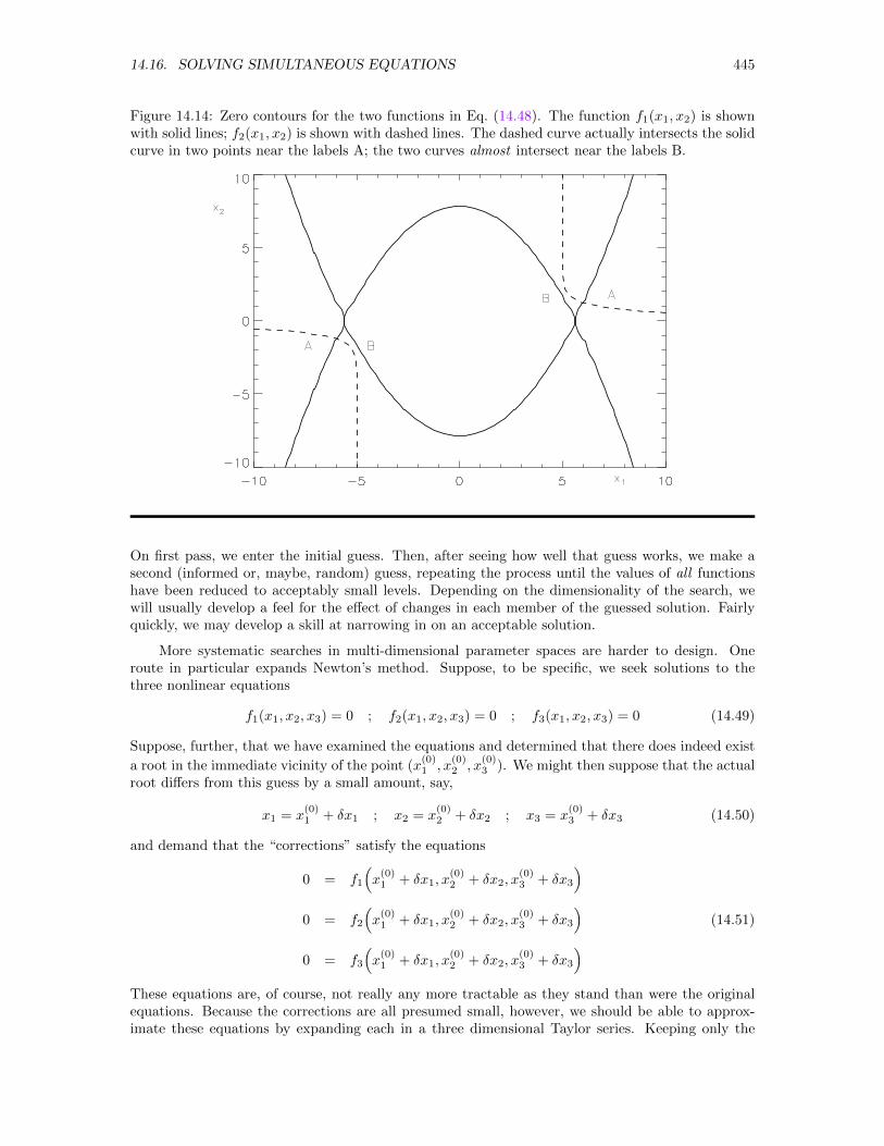
14.16. SOLVING SIMULTANEOUS EQUATIONS 445

Figure 14.14: Zero contours for the two functions in Eq. (14.48). The function f1(x1, x2) is shownwith solid lines; f2(x1, x2) is shown with dashed lines. The dashed curve actually intersects the solidcurve in two points near the labels A; the two curves almost intersect near the labels B.

On first pass, we enter the initial guess. Then, after seeing how well that guess works, we make asecond (informed or, maybe, random) guess, repeating the process until the values of all functionshave been reduced to acceptably small levels. Depending on the dimensionality of the search, wewill usually develop a feel for the effect of changes in each member of the guessed solution. Fairlyquickly, we may develop a skill at narrowing in on an acceptable solution.

More systematic searches in multi-dimensional parameter spaces are harder to design. Oneroute in particular expands Newton’s method. Suppose, to be specific, we seek solutions to thethree nonlinear equations

f1(x1, x2, x3) = 0 ; f2(x1, x2, x3) = 0 ; f3(x1, x2, x3) = 0 (14.49)

Suppose, further, that we have examined the equations and determined that there does indeed exist

a root in the immediate vicinity of the point (x(0)1 , x

(0)2 , x

(0)3 ). We might then suppose that the actual

root differs from this guess by a small amount, say,

x1 = x(0)1 + δx1 ; x2 = x

(0)2 + δx2 ; x3 = x

(0)3 + δx3 (14.50)

and demand that the “corrections” satisfy the equations

0 = f1

(x(0)1 + δx1, x

(0)2 + δx2, x

(0)3 + δx3

)0 = f2

(x(0)1 + δx1, x

(0)2 + δx2, x

(0)3 + δx3

)(14.51)

0 = f3

(x(0)1 + δx1, x

(0)2 + δx2, x

(0)3 + δx3

)These equations are, of course, not really any more tractable as they stand than were the originalequations. Because the corrections are all presumed small, however, we should be able to approx-imate these equations by expanding each in a three dimensional Taylor series. Keeping only the

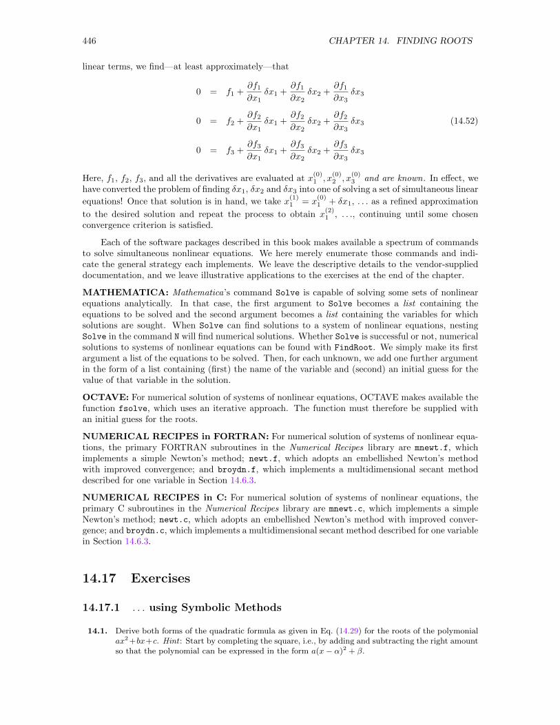
446 CHAPTER 14. FINDING ROOTS

linear terms, we find—at least approximately—that

0 = f1 +∂f1∂x1

δx1 +∂f1∂x2

δx2 +∂f1∂x3

δx3

0 = f2 +∂f2∂x1

δx1 +∂f2∂x2

δx2 +∂f2∂x3

δx3 (14.52)

0 = f3 +∂f3∂x1

δx1 +∂f3∂x2

δx2 +∂f3∂x3

δx3

Here, f1, f2, f3, and all the derivatives are evaluated at x(0)1 , x

(0)2 , x

(0)3 and are known. In effect, we

have converted the problem of finding δx1, δx2 and δx3 into one of solving a set of simultaneous linear

equations! Once that solution is in hand, we take x(1)1 = x

(0)1 + δx1, . . . as a refined approximation

to the desired solution and repeat the process to obtain x(2)1 , . . ., continuing until some chosen

convergence criterion is satisfied.

Each of the software packages described in this book makes available a spectrum of commandsto solve simultaneous nonlinear equations. We here merely enumerate those commands and indi-cate the general strategy each implements. We leave the descriptive details to the vendor-supplieddocumentation, and we leave illustrative applications to the exercises at the end of the chapter.

MATHEMATICA: Mathematica’s command Solve is capable of solving some sets of nonlinearequations analytically. In that case, the first argument to Solve becomes a list containing theequations to be solved and the second argument becomes a list containing the variables for whichsolutions are sought. When Solve can find solutions to a system of nonlinear equations, nestingSolve in the command N will find numerical solutions. Whether Solve is successful or not, numericalsolutions to systems of nonlinear equations can be found with FindRoot. We simply make its firstargument a list of the equations to be solved. Then, for each unknown, we add one further argumentin the form of a list containing (first) the name of the variable and (second) an initial guess for thevalue of that variable in the solution.

OCTAVE: For numerical solution of systems of nonlinear equations, OCTAVE makes available thefunction fsolve, which uses an iterative approach. The function must therefore be supplied withan initial guess for the roots.

NUMERICAL RECIPES in FORTRAN: For numerical solution of systems of nonlinear equa-tions, the primary FORTRAN subroutines in the Numerical Recipes library are mnewt.f, whichimplements a simple Newton’s method; newt.f, which adopts an embellished Newton’s methodwith improved convergence; and broydn.f, which implements a multidimensional secant methoddescribed for one variable in Section 14.6.3.

NUMERICAL RECIPES in C: For numerical solution of systems of nonlinear equations, theprimary C subroutines in the Numerical Recipes library are mnewt.c, which implements a simpleNewton’s method; newt.c, which adopts an embellished Newton’s method with improved conver-gence; and broydn.c, which implements a multidimensional secant method described for one variablein Section 14.6.3.

14.17 Exercises

14.17.1 . . . using Symbolic Methods

14.1. Derive both forms of the quadratic formula as given in Eq. (14.29) for the roots of the polymonialax2 +bx+c. Hint : Start by completing the square, i.e., by adding and subtracting the right amountso that the polynomial can be expressed in the form a(x− α)2 + β.

14.17. EXERCISES 447

Figure 14.15: The three-bladed lawnmower described in Exercise 14.5.

a

a

a

x

y

14.2. Find the value of x at which f(x) = ax2 + bx + c has an extremum and determine a criterioninvolving the coefficients (or some of them) for deciding whether the extremum is a maximum or aminimum. Assume that a, b, and c are real.

14.3. Find the points at which the function f(x) = ax3 + bx2 + cx + d has (local) extrema and find acriterion involving the coefficients (or some of them) that will assure that the function has threereal roots. Assume that a, b, c, and d are real.

14.4. In some quantum calculations, the need to solve the equation x(x + 1) = l(l + 1) for x arises.Find those roots, noting particularly that, since the equation is quadratic, there are two roots. Theobvious root x = l is not the only one.

14.5. Each of the three blades of a lawn mower has radius a. As shown in Fig. 14.15, the center blade isinvariably mounted somewhat in front of the two outside ones so that the areas cut by each bladecan overlap without risking collision of the blades with one another. What must be the minimumoffset x of the center of the middle blade from the line joining the centers of the two outer bladesso that their cutting paths will overlap by an amount y without collision of the blades?

14.6. For the projectile discussed in Section 14.1.4, generate a family of graphs showing τ(θ) as a functionof θ for selected fixed values of α.

14.7. In Section 14.1.4, we deduced that the range of a projectile of mass m launched with speed v0 at anangle θ up from the horizontal in a medium characterized by a (linear) viscous damping coefficientb could be found by (1) finding the non-zero root of the equation

f(τ) = τ − (1 + α sin θ)(1− e−τ ) = 0

where α = bv0/(mg), and then (2) evaluating the range from the expression

R(θ, α)

v20/g

=cos θ(1− e−τ )

α=

τ cos θ

α(1 + α sin θ)

We could view the first of these equations as defining the function τ(θ) implicitly. In principle, for agiven α, we could imagine solving the first equation explicitly for τ as a function of θ and substitutingthat solution into the second equation to find an expression for the range—again for a given α—explicitly as a function of θ alone. If we had that expression in hand, we would find the maximumrange by solving the equation dR(θ)/dθ = 0 for θ and then evaluate the range at that specific valueof θ. In the absence of that expression, we can still differentiate R(θ) implicitly, recognizing the(hidden) dependence of τ on θ, and we can differentiate f(τ). The resulting equations togethermight then be combinable in a way that would lead to a determination of the maximum rangemore directly than the route described in the text. Pursue this idea, using a symbolic manipulatingprogram as much as possible to simplify the calculation. The ultimate objective would be to deduceand test a procedure that leads to a numerical value for the maximum range of this projectile whenα is given. Note: This exercies is almost certainly difficult and potentially frustrating. The authorhas no idea whether success awaits the persistent in this endeavor.

448 CHAPTER 14. FINDING ROOTS

14.8. Find the natural frequencies for the three modes of oscillation characterizing the system that resultswhen the system shown in Fig. 14.2 is extended to contain three objects coupled in a line. Take thefour springs all to have the same spring constant but allow for the possibility that the middle objectmay have a mass m′ different from the mass m of the two outside objects. In particular, measurefrequencies in units of

√k/m and seek a graph showing the frequency of each of the modes as a

function of β = m′/m. Hint : To help you get started and to facilitate focusing on the solution ofthe ODEs rather than on deriving them, note that, for three masses, the equations of motion willbe

md2x1

dt2= −kx1 + k(x2 − x1)

m′d2x2

dt2= −k(x2 − x1) + k(x3 − x2)

md2x3

dt2= −k(x3 − x2)− kx3

14.9. In dimensionless units, the energy shifts E that occur in the states of hydrogen for n = 3 when anexternal constant electric field is turned on are given by the roots of the ninth-order polynomial

f(E) = E9 − 243

2E7 +

59049

16E5 − 531441

16E3

Find the distinct roots of this polynomial and the multiplicity of each root.

14.10. If, when divided by a single line into a square and a rectangle, the resulting smaller rectangle hasthe same aspect ratio as the original rectangle, the rectangle is called a golden rectangle and theratio of the longer to the shorter side is called the golden ratio. Rectangles having that ratio areconsidered to be particularly aesthetic and can be found in many places, including ancient Greekarchitecture and, intriguingly, in standard, present-day plastic credit cards. Express the abovedefining criterion to find a quadratic equation for the golden ratio and then solve the equation tofind that ratio.

14.17.2 . . . using Numerical Methods

14.11. Use numerical methods to solve Eq. (14.6) for the equilibrium points in the potential energy inEq. (14.3).

14.12. One way to find the square root of a (positive) number a is to find the root of the functionf(x) = x2 − a. (a) Apply Newton’s method symbolically to show that xn+1 = (xn + a/xn)/2.(b) Using a pocket calculator and starting with the guess x0 = 2, work out the first few iteratesby hand and note how quickly this algorithm converges to

√2 = 1.41421. (This algorithm is the

algorithm that most pocket calculators invoke when the square root key is pressed.) (c) Usingwhatever computational tool appeals to you, write a program that asks for the value of a, an initialguess for

√a, and a tolerance and then implements Newton’s method to find

√a, printing out each

iterate along the way and stopping automatically when successive iterates differ by less than thespecified tolerance.

14.13. For the first six Legendre polynomials Ln(x), find all roots lying in the interval −1 ≤ x ≤ 1. Thosepolynomials are

L0(x) = 1 L4(x) = 18(35x4 − 30x2 + 3)

L1(x) = x L5(x) = 18(63x5 − 70x3 + 15x)

L2(x) = 12(3x2 − 1) L6(x) = 1

16(231x6 − 315x4 + 105x2 − 5)

14.17. EXERCISES 449

14.14. The natural frequencies for the transverse vibrations of a bar of uniform cross section that haslength L and is free at both ends are given by

ωn =4K

L2

√E

ρα2n

where K is the radius of gyration of the cross section of the bar, E is Young’s modulus for thematerial of the bar, ρ is the density (mass/unit volume) of the material of the bar, and αn is asolution to the equation

tanα = ± tanhα

Find the lowest half dozen natural frequencies for this bar. [A detailed discussion of this exercisecan be found in N. H. Fletcher and T. D. Rossing, The Physics of Musical Instruments, SecondEdition (Springer-Verlag, New York, 1991), pp. 57ff.]

14.15. If the bar of the previous exercise is clamped at one end and free at the other, then the naturalfrequencies are given by the same expression except that αn is instead a solution to the equation

cotα = ± tanhα

Find the lowest half dozen natural frequencies for this bar. [A detailed discussion of this exercisecan be found in N. H. Fletcher and T. D. Rossing, The Physics of Musical Instruments, SecondEdition (Springer-Verlag, New York, 1991), pp. 57ff.]

14.16. The natural frequencies of the air in a spherical cavity are determined from the roots of the functiondjn(x)/dx, where jn(x) is the n-th order spherical Bessel function, the first three of which are

j0(x) =sinx

x; j1(x) =

sinx

x2− cosx

x; j2(x) =

(3

x3− 1

x

)sinx− 3

x2cosx

Obtain graphs of these three functions versus x, find the lowest several roots of j0(x), j1(x), andj2(x), and find also the lowest several roots of dj0(x)/dx, dj1(x)/dx, and dj2(x)/dx.

14.17. Explore the way the energy levels of the well described in Section 14.1.5 change as the parameterc, which is determined by the depth and the width of the well, increases. At base, changing cchanges the slopes of the straight lines in Fig. 14.5. As c increases and the well becomes deeper,the lines become more and more nearly horizontal and the number of energy levels increases. Seekultimately to generate a graph that shows the energy of each allowed level on the vertical axis as afunction of the parameter c along the horizontal axis.

14.18. The intensity I(x) in the diffraction pattern produced by a single slit is given by

I(x)

I0=

sin2 x

x2

where I0 is the intensity in the center and x is related to the position of the observation point awayfrom the central maximum. The zeroes in this pattern are easy to locate (they occur at x = nπ,n = 0,±1,±2, . . .). Careful location of the maxima, however, is more complicated. They don’toccur where sin2 x = 1 because of the influence of the denominator that steadily increases as xincreases. Locate the positions of the first half dozen maxima in this pattern, which—basically—isa request to find the roots of the derivative of the function (though note that not all roots correspondto maxima). Use at least three different methods and at least two different computational tools,and compare the results. Do your results confirm that the roots approach odd multiples of 1

2π as

they become large? Optional : You might also find it interesting to approximate the function with apower series expansion for sinx, keeping quite a few terms but converting the root finding probleminto that of finding the roots of a polynomial. Then, use methods for finding roots of polynomialsand see if you can come to understand how accuracy depends on how many terms you keep andwhich root you seek.

14.19. Using at least three different methods and at least two different computational tools, find thefirst half dozen roots of the zeroth-order Bessel function J0(x). Note that these roots are relatedto the radii of circular nodes in some of the vibrations of a circular membrane. The values of

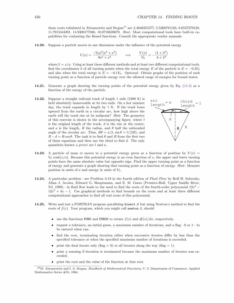
450 CHAPTER 14. FINDING ROOTS

these roots tabulated in Abramowitz and Stegun43 are 2.4048255577, 5.5200781103, 8.6537279129,11.7915344391, 14.9309177086, 18.0710639679. Hint : Most computational tools have built-in ca-pabilities for evaluating the Bessel functions. Consult the appropriate vendor manuals.

14.20. Suppose a particle moves in one dimension under the influence of the potential energy

V (x) =−V0a

2(a2 + x2)

8a4 + x4=⇒ V (x)

V0= − (1 + x2)

8 + x4

where x = x/a. Using at least three different methods and at least two different computational tools,find the coordinates x of all turning points when the total energy E of the particle is E = −0.2V0

and also when the total energy is E = −0.1V0. Optional : Obtain graphs of the position of eachturning point as a function of particle energy over the allowed range of energies for bound states.

14.21. Generate a graph showing the turning points of the potential energy given by Eq. (14.3) as afunction of the energy of the particle.

14.22. Suppose a straight railroad track of length 1 mile (5280 ft) isheld absolutely immoveable at its two ends. On a hot summerday, the track expands in length by 1 ft. If the track bowsupward from the earth in a circular arc, how high above theearth will the track rise at its midpoint? Hint : The geometryof this exercise is shown in the accompanying figure, where lis the original length of the track, d is the rise at the center,and a is the length, R the radius, and θ half the subtendedangle of the circular arc. Thus, Rθ = a/2, sin θ = l/(2R), andR− d = R cos θ. The task is to find θ and R from the first twoof these equations and then use the third to find d. The onlyquantities known a priori are l and a.

d

Rθ

lchordlength

=aarclength

=

14.23. A particle of mass m moves in a potential energy given as a function of position by V (x) =V0 cosh(x/a). Because this potential energy is an even function of x, the upper and lower turningpoints have the same absolute value but opposite sign. Find the upper turning point as a functionof energy and generate a graph showing that turning point as a function of energy. Hint : Measureposition in units of a and energy in units of V0.

14.24. A particular problem—see Problem 3-19 in the fourth edition of Fluid Flow by Rolf H. Sabersky,Allan J. Acosta, Edward G. Hauptmann, and E. M. Gates (Prentice-Hall, Upper Saddle River,NJ, 1999)—in fluid flow leads to the need to find the roots of the fourth-order polynomial 12x4 −12x3 + 4x − 1. Use graphical methods to find bounds on the roots and at least three differentcomputational approaches to find all real roots of this polynomial.

14.25. Write and test a FORTRAN program paralleling bisect.f but using Newton’s method to find theroots of f(x). Your program, which you might call newton.f, should

• use the functions FUNC and FUNCD to return f(x) and df(x)/dx, respectively.

• request a tolerance, an initial guess, a maximum number of iterations, and a flag—0 or 1—tobe entered when run.

• find the root, terminating iteration either when successive iterates differ by less than thespecified tolerance or when the specified maximum number of iterations is exceeded.

• print the final iterate only (flag = 0) or all iterates along the way (flag = 1).

• print a warning if iteration is terminated because the maximum number of iterates was ex-ceeded.

• print the root and the value of the function at that root.

43M. Abramowitz and I. A. Stegun, Handbook of Mathematical Functions, U. S. Department of Commerce, AppliedMathematics Series #55, 1964.

14.17. EXERCISES 451

14.26. Write and test a C program paralleling bisect.c but using Newton’s method to find the roots off(x). Your program, which you might call newton.c, should

• use the functions FUNC and FUNCD to return f(x) and df(x)/dx, respectively.

• request a tolerance, an initial guess, a maximum number of iterations, and a flag—0 or 1—tobe entered when run.

• find the root, terminating iteration either when successive iterates differ by less than thespecified tolerance or when the specified maximum number of iterations is exceeded.

• print the final iterate only (flag = 0) or all iterates along the way (flag = 1).

• print a warning if iteration is terminated because the maximum number of iterates was ex-ceeded.

• print the root and the value of the function at that root.

14.27. The image of a distant object produced on a viewing screen by a small aperture is actually adiffraction pattern. When the aperture is a circle of diameter d and light from the object strikesthe screen containing the aperture at normal incidence, the intensity in the diffraction pattern atangle θ from the normal is given by

I(θ)

I0=

[2J1(πd sin θ/λ)

πd sin θ/λ

]2

where I0 is the intensity at the center of the pattern, λ is the wavelength of the light illuminatingthe aperture, and J1(x) is the first order Bessel function. Using the Bessel function routine thatis assuredly built in to your computational tool (see the appropriate manuals), find the angle θ atwhich the first zero in the diffraction pattern lies, expressing that result as a multiple of λ/d. Theresulting angle expresses the angular separation of two nearby objects such that the maximum inthe diffraction pattern produced by one lies on top of the first minimum away from the maximum ofthe other. That separation is universally taken as a measure of the resolution of the optical systemcreating the images, and the condition requiring this positioning of the two maxima is called theRayleigh criterion. Hint : The angle will be small, so you can safely use the approximation sin θ ≈ θ.

14.28. The Lennard-Jones potential energyVLJ , which is given in terms of the coordinate r by the expres-sion

VLJ = 4ε

[σ12

r12− σ6

r6

]or

VLJε

= 4[

1

r12− 1

r6

]where ε and σ are constants and r = r/σ, plays a prominent role in some theories of chemicalbonding. Obtain a graph of this potential energy and then obtain graphs of the lower turning pointand the upper turning point as functions of the energy of the system over the range of energies forwhich the particle experiencing the potential energy is bound in the associated potential well.

14.17.3 . . . using Numerical Recipes

Note: Numerical recipes can, of course, also be used for any of theexercises in Section 14.17.2.

14.29. Study the demonstration programs xrtbis.f and xrtnewt.f, each of which is written so as to beable to find all roots of a given function in a specified range. Then recast each of these programs toproduce a program that will find all of the positive roots of the equation for each sign in Eq. (14.25).Write your program so that the value of c and the boundaries of the region in which roots are tobe sought are entered from the terminal at the time the program is run. Finally, test your programwith c = 25, comparing your results with those obtained in the text, and then examine other valuesof c, seeking ultimately to obtain a graph showing each root as a function of c.

14.30. Study the demonstration programs xrtbis.c and xrtnewt.c, each of which is written so as to beable to find all roots of a given function in a specified range. Then recast each of these programs toproduce a program that will find all of the positive roots of the equation for each sign in Eq. (14.25).

452 CHAPTER 14. FINDING ROOTS

Write your program so that the value of c and the boundaries of the region in which roots are tobe sought are entered from the terminal at the time the program is run. Finally, test your programwith c = 25, comparing your results with those obtained in the text, and then examine other valuesof c, seeking ultimately to obtain a graph showing each root as a function of c.

14.31. Read the Numerical Recipes books about the recipe rtsafe.f and the example program xrtsafe.f.Then recast the program sinrtbis.f (or sinrtnewt.f) to use rtsafe.f and test your program witha couple of functions of your choice.

14.32. Read the Numerical Recipes books about the recipe rtsafe.c and the example program xrtsafe.c.Then recast the program sinrtbis.c (or sinrtnewt.c) to use rtsafe.c and test your program witha couple of functions of your choice.

14.17.4 Finding More than One Unknown

14.33. In a global positioning system, the raw data from which the position is determined consists ofdistances from various reference points together with knowledge of the location of those referencepoints. In two dimensions, for example, we might try to locate our position (x, y) in a plane fromknowledge that we are a distance r1 from the point (x1, y1) and a distance r2 from the point (x2, y2).Not all values we might assign are physically meaningful. For example, there is no point that issimultaneously 20 miles from point 1 and 30 miles from point 2 if points 1 and 2 are, in fact,100 miles apart. Depending on the circumstances, there may be no points, one point, or—mostoften—two. Develop an algorithm for finding your location in two dimensions when you know yourdistance from each of two reference points whose coordinates are known, implement your algorithmin a program using whatever computational tool seems appropriate, solve two or three test problemsthat you invent, and—in particular—try to describe and defend the conditions under which two,one, or no solutions exist. Optional : Extend your entire consideration into three dimensions, whichwill require knowledge of distance from each of (at least) three known locations. Hint : Quite abit of information is available on the website www.trimble.com/gps. There is also an article in theJanuary, 1994, issue of Physics Today (“Where I Stand” by Daniel Kleppner, page 9).

14.34. Given the three points (xi, yi), i = 1, 2, 3, (a) find symbolic expressions for the coefficients a, band c of the parabola y = ax2 + bx+ c that passes through these three points and then (b) find asymbolic expression for the value of x at which the extremum point of the parabola occurs. Finally,(c) determine numerically the angle at which the maximum range of a projectile occurs if the rangesat θ = 39, 40, and 41 are 0.7251744, 0.7259484, and 0.7258887, respectively.

14.35. Kirchhoff’s laws in DC circuit theory contend that the net current flowing into any node must bezero and that the net voltage drop around any closed path in the circuit must be zero. Rememberingthat the voltage drop ∆V across a resistor r carrying current i is given by ∆V = ir and using thesymbols defined in Fig. 14.16, apply these laws to each of the circuits in the figure to generate a setof simultaneous, inhomogeneous linear equations for the unknown currents. Then, using symbolicmethods solve each case for the unknown currents. Finally, determine the effective resistance definedby Reff = V/I for each circuit. Assume that all batteries and resistors have known values and thatquantities represented in the figures with the same symbol have the same value. Warning : For evensimple circuits, Kirchhoff’s laws provide more equations than unknowns. Correctly written, theseequations are guaranteed to be consistent. The subset to be solved, however, must be carefullychosen to make sure its members are linearly independent of one another.

14.36. The file $HEAD/data/freefall.dat contains 31 lines, the i-th of which contains one numericalvalue—the value of the position xi in cm of a particle at time ti = (i− 1)/60 s. You have reason tobelieve that the set of data (ti, xi) with i = 1, 2, 3, . . . , n is described by the parabolic relationship

x = at2 + bt+ c

The method of least squares identifies the optimum values of the coefficients a, b, and c as the

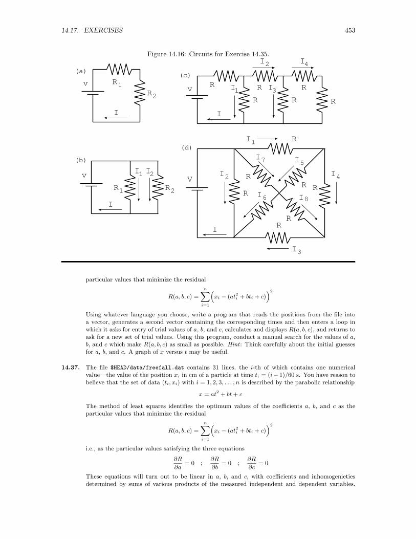
14.17. EXERCISES 453

Figure 14.16: Circuits for Exercise 14.35.

v

R2R1

I

(b)

v

R R R

RR R

I

(c)v

R2

R1

I

(a)

V

R

RRR

R

R

R

I

(d)

3

I4I2

I2I1

I1 I

I1

I2

I3

I4

5I

6I

7I

8I

particular values that minimize the residual

R(a, b, c) =

n∑i=1

(xi − (at2i + bti + c)

)2

Using whatever language you choose, write a program that reads the positions from the file intoa vector, generates a second vector containing the corresponding times and then enters a loop inwhich it asks for entry of trial values of a, b, and c, calculates and displays R(a, b, c), and returns toask for a new set of trial values. Using this program, conduct a manual search for the values of a,b, and c which make R(a, b, c) as small as possible. Hint : Think carefully about the initial guessesfor a, b, and c. A graph of x versus t may be useful.

14.37. The file $HEAD/data/freefall.dat contains 31 lines, the i-th of which contains one numericalvalue—the value of the position xi in cm of a particle at time ti = (i− 1)/60 s. You have reason tobelieve that the set of data (ti, xi) with i = 1, 2, 3, . . . , n is described by the parabolic relationship

x = at2 + bt+ c

The method of least squares identifies the optimum values of the coefficients a, b, and c as theparticular values that minimize the residual

R(a, b, c) =

n∑i=1

(xi − (at2i + bti + c)

)2

i.e., as the particular values satisfying the three equations

∂R

∂a= 0 ;

∂R

∂b= 0 ;

∂R

∂c= 0

These equations will turn out to be linear in a, b, and c, with coefficients and inhomogenietiesdetermined by sums of various products of the measured independent and dependent variables.

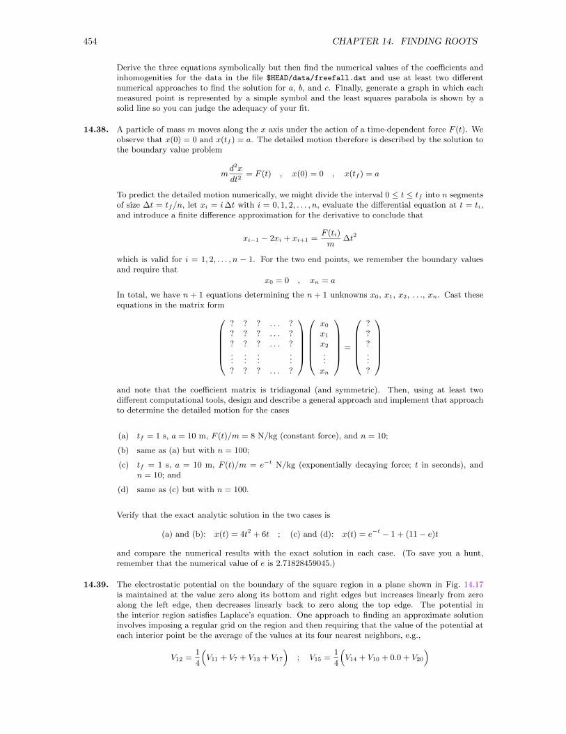
454 CHAPTER 14. FINDING ROOTS

Derive the three equations symbolically but then find the numerical values of the coefficients andinhomogenities for the data in the file $HEAD/data/freefall.dat and use at least two differentnumerical approaches to find the solution for a, b, and c. Finally, generate a graph in which eachmeasured point is represented by a simple symbol and the least squares parabola is shown by asolid line so you can judge the adequacy of your fit.

14.38. A particle of mass m moves along the x axis under the action of a time-dependent force F (t). Weobserve that x(0) = 0 and x(tf ) = a. The detailed motion therefore is described by the solution tothe boundary value problem

md2x

dt2= F (t) , x(0) = 0 , x(tf ) = a

To predict the detailed motion numerically, we might divide the interval 0 ≤ t ≤ tf into n segmentsof size ∆t = tf/n, let xi = i∆t with i = 0, 1, 2, . . . , n, evaluate the differential equation at t = ti,and introduce a finite difference approximation for the derivative to conclude that

xi−1 − 2xi + xi+1 =F (ti)

m∆t2

which is valid for i = 1, 2, . . . , n − 1. For the two end points, we remember the boundary valuesand require that

x0 = 0 , xn = a

In total, we have n + 1 equations determining the n + 1 unknowns x0, x1, x2, . . ., xn. Cast theseequations in the matrix form

? ? ? . . . ?? ? ? . . . ?? ? ? . . . ?...

......

...? ? ? . . . ?

x0

x1

x2

...xn

=

???...?

and note that the coefficient matrix is tridiagonal (and symmetric). Then, using at least twodifferent computational tools, design and describe a general approach and implement that approachto determine the detailed motion for the cases

(a) tf = 1 s, a = 10 m, F (t)/m = 8 N/kg (constant force), and n = 10;

(b) same as (a) but with n = 100;

(c) tf = 1 s, a = 10 m, F (t)/m = e−t N/kg (exponentially decaying force; t in seconds), andn = 10; and

(d) same as (c) but with n = 100.

Verify that the exact analytic solution in the two cases is

(a) and (b): x(t) = 4t2 + 6t ; (c) and (d): x(t) = e−t − 1 + (11− e)t

and compare the numerical results with the exact solution in each case. (To save you a hunt,remember that the numerical value of e is 2.71828459045.)

14.39. The electrostatic potential on the boundary of the square region in a plane shown in Fig. 14.17is maintained at the value zero along its bottom and right edges but increases linearly from zeroalong the left edge, then decreases linearly back to zero along the top edge. The potential inthe interior region satisfies Laplace’s equation. One approach to finding an approximate solutioninvolves imposing a regular grid on the region and then requiring that the value of the potential ateach interior point be the average of the values at its four nearest neighbors, e.g.,

V12 =1

4

(V11 + V7 + V13 + V17

); V15 =

1

4

(V14 + V10 + 0.0 + V20

)

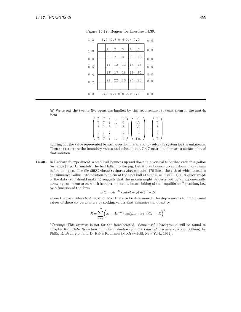
14.17. EXERCISES 455

Figure 14.17: Region for Exercise 14.39.

1 2 3 4 5

6 7 8 9 10

11 12 13 14 15

16 17 18 19 20

21 22 23 24 25

0.0

0.2

0.4

0.6

0.8

1.0

1.2 0.20.40.60.81.0 0.0

0.0

0.0

0.0

0.0

0.0

0.0

0.0 0.0 0.0 0.0 0.0

(a) Write out the twenty-five equations implied by this requirement, (b) cast them in the matrixform

? ? ? . . . ?? ? ? . . . ?? ? ? . . . ?...

......

...? ? ? . . . ?

V1

V2

V3

...V25

=

???...?

figuring out the value represented by each question mark, and (c) solve the system for the unknowns.Then (d) structure the boundary values and solution in a 7× 7 matrix and create a surface plot ofthat solution.

14.40. In Ruchardt’s experiment, a steel ball bounces up and down in a vertical tube that ends in a gallon(or larger) jug. Ultimately, the ball falls into the jug, but it may bounce up and down many timesbefore doing so. The file $HEAD/data/ruchardt.dat contains 170 lines, the i-th of which containsone numerical value—the position xi in cm of the steel ball at time ti = 0.05(i−1) s. A quick graphof the data (you should make it) suggests that the motion might be described by an exponentiallydecaying cosine curve on which is superimposed a linear sinking of the “equilibrium” position, i.e.,by a function of the form

x(t) = Ae−bt cos(ωt+ φ) + Ct+D

where the parameters b, A, ω, φ, C, and D are to be determined. Develop a means to find optimalvalues of these six parameters by seeking values that minimize the quantity

R =

N∑i=1

(xi −Ae−bti cos(ωti + φ) + Cti +D

)2

Warning : This exercise is not for the faint-hearted. Some useful background will be found inChapter 8 of Data Reduction and Error Analysis for the Physical Sciences (Second Edition) byPhilip R. Bevington and D. Keith Robinson (McGraw-Hill, New York, 1992).

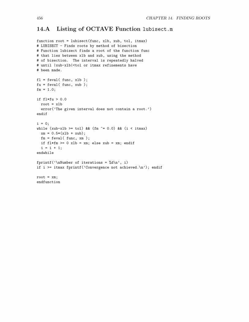
456 CHAPTER 14. FINDING ROOTS

14.A Listing of OCTAVE Function lubisect.m

function root = lubisect(func, xlb, xub, tol, itmax)

# LUBISECT - Finds roots by method of bisection

# Function lubisect finds a root of the function func

# that lies between xlb and xub, using the method

# of bisection. The interval is repeatedly halved

# until |xub-xlb|<tol or itmax refinements have

# been made.

fl = feval( func, xlb );

fu = feval( func, xub );

fm = 1.0;

if fl*fu > 0.0

root = xlb

error(’The given interval does not contain a root.’)

endif

i = 0;

while (xub-xlb >= tol) && (fm ~= 0.0) && (i < itmax)

xm = 0.5*(xlb + xub);

fm = feval( func, xm );

if fl*fm >= 0 xlb = xm; else xub = xm; endif

i = i + 1;

endwhile

fprintf(’\nNumber of iterations = %d\n’, i)

if i >= itmax fprintf(’Convergence not achieved.\n’); endif

root = xm;

endfunction

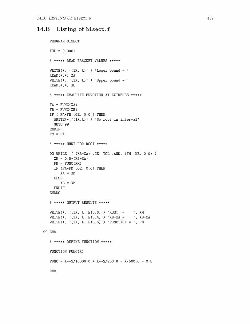
14.B. LISTING OF BISECT.F 457

14.B Listing of bisect.f

PROGRAM BISECT

TOL = 0.0001

! ***** READ BRACKET VALUES *****

WRITE(*, ’(1X, A)’ ) ’Lower bound = ’

READ(*,*) XA

WRITE(*, ’(1X, A)’ ) ’Upper bound = ’

READ(*,*) XB

! ***** EVALUATE FUNCTION AT EXTREMES *****

FA = FUNC(XA)

FB = FUNC(XB)

IF ( FA*FB .GE. 0.0 ) THEN

WRITE(*,’(1X,A)’ ) ’No root in interval’

GOTO 99

ENDIF

FM = FA

! ***** HUNT FOR ROOT *****

DO WHILE ( (XB-XA) .GE. TOL .AND. (FM .NE. 0.0) )

XM = 0.5*(XB+XA)

FM = FUNC(XM)

IF (FA*FM .GE. 0.0) THEN

XA = XM

ELSE

XB = XM

ENDIF

ENDDO

! ***** OUTPUT RESULTS *****

WRITE(*, ’(1X, A, E15.6)’) ’ROOT = ’, XM

WRITE(*, ’(1X, A, E15.4)’) ’XB-XA = ’, XB-XA

WRITE(*, ’(1X, A, E15.6)’) ’FUNCTION = ’, FM

99 END

! ***** DEFINE FUNCTION *****

FUNCTION FUNC(X)

FUNC = X**3/10000.0 + X**2/200.0 - X/500.0 - 0.5

END

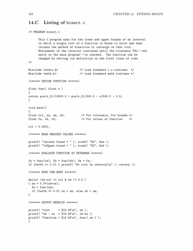
458 CHAPTER 14. FINDING ROOTS

14.C Listing of bisect.c

/* PROGRAM bisect.c

This C program asks for the lower and upper bounds of an interval

in which a single root of a function is known to exist and then

invokes the method of bisection to converge on that root.

Refinement of the interval continues until the tolerance TOL---set

early in the main program---is reached. The function can be

changed by editing its definition in the first lines of code.

*/

#include <stdio.h> /* Load standard i.o routines */

#include <math.h> /* Load standard math routines */

/****** DEFINE FUNCTION ******/

float func( float x )

return pow(x,3)/10000.0 + pow(x,2)/200.0 - x/500.0 - 0.5;

void main()

float tol, xa, xm, xb; /* For tolerance, for bounds */

float fa, fm, fb; /* For values of function */

tol = 0.0001;

/****** READ BRACKET VALUES ******/

printf( "\nLower bound = " ); scanf( "%f", &xa );

printf( "\nUpper bound = " ); scanf( "%f", &xb );

/****** EVALUATE FUNCTION AT EXTREMES ******/

fa = func(xa); fb = func(xb); fm = fa;

if (fa*fb >= 0.0) printf( "No root in interval\n" ); return; ;

/****** HUNT FOR ROOT ******/

while( (xb-xa) >= tol & fm != 0.0 )

xm = 0.5*(xb+xa);

fm = func(xm);

if (fa*fm >= 0.0) xa = xm; else xb = xm;

/****** OUTPUT RESULTS ******/

printf( "root = %15.6f\n", xm );

printf( "xb - xa = %15.6f\n", xb-xa );

printf( "function = %15.6f\n", func( xm ) );

Appendix A

Introduction to LATEX

Note: All LATEX source files (.tex, .template), all Windows batch files (.bat)program (.pro) files, and all UNIX command files (no file type) referred to in thischapter are available in the directory $HEAD/tex, where (as defined in the LocalGuide) $HEAD must be replaced by the appropriate path for your site.

During the 1970s, when Donald Knuth (a Stanford University computer scientist) was creating hismonumental, several-volume series of books on all aspects of computer science, he recognized theneed for a computer-based type-setting/word-processing system tailored to the needs of authors oftechnical manuscripts. Interrupting his main project, he developed TEX1 as the essential engineto support computerized technical type setting. The first version of TEX was made available tothe using public in 1978 and a revised (and final) version was published in 1984. Written by LeslieLamport, LATEX2 is a versatile and extensive collection of macros that sit on top of TEX and facilitateexploitation of TEX’s capabilities. Broadly, LATEX is a document preparation system that formatsequations, tables, and illustrations as easily as plain text. That the whole complex (TEX, LATEX,and many other components) has been deliberately placed in the public domain,3 that carefullytested versions exist for essentially every computing platform and operating system, and that manyscientific journals and an increasing number of publishers will accept manuscripts submitted as LATEXfiles together provide substantial incentive for learning to use this tool. Although it is not wysiwyg,4

it has powerful and sophisticated capabilities, most of which are not described in this Appendix. Weconvey only the basics with, however, the hope that we will cause you to realize that essentially anydesired formatting at all should be possible if only you can figure out how to achieve it. For furtherinformation, try surfing the web in your favorite browser and looking at the LATEX2ε User’s Guideand Reference Manual (which we will refer to as The LATEX Manual), the LATEX Companion, and/orto any of the several other TEX and LATEX books.5 The wisdom of taking fifteen minutes every nowand then to browse in these publications cannot be overstressed; as you become more skilled, thefine print and other subtleties will gradually be mLATEX:otherore and more meaningful.6

1As per Knuth’s instruction (see the first two paragraphs of Chapter 1 of The TEXbook as identified in Section A.18),TEX is pronounced ‘tech’ as in ‘technology’.

2Here, individuals disagree on the pronunciation of the ‘la’, and Leslie Lamport offers no guidance. Some saylahTEX while others say layTEX, with the emphasis on the first syllable in both cases. We simply must becomeaccustomed to each other’s preferences.

3The primary site for information (history, current plans, downloads, . . .) for TEX, LATEX, and numerous otherpublicly available components of TEX and its derivatives is the web site of the TEX Users’ Group (TUG), www.tug.org.This organization maintains CTAN (the Comprehensive TEX Archive Network), which has a handful of backbonemachines around the world and a number of mirror sites, from any of which an enormous number of files associatedwith the TEX/LATEX system can be downloaded.

4what you see is what you get.5See Section A.18 for more detailed references.6You may also find the web pages of TUG at the URL http://www.tug.org to be valuable. One link on that page

points to an engaging description of the history of the development of TEX.

459

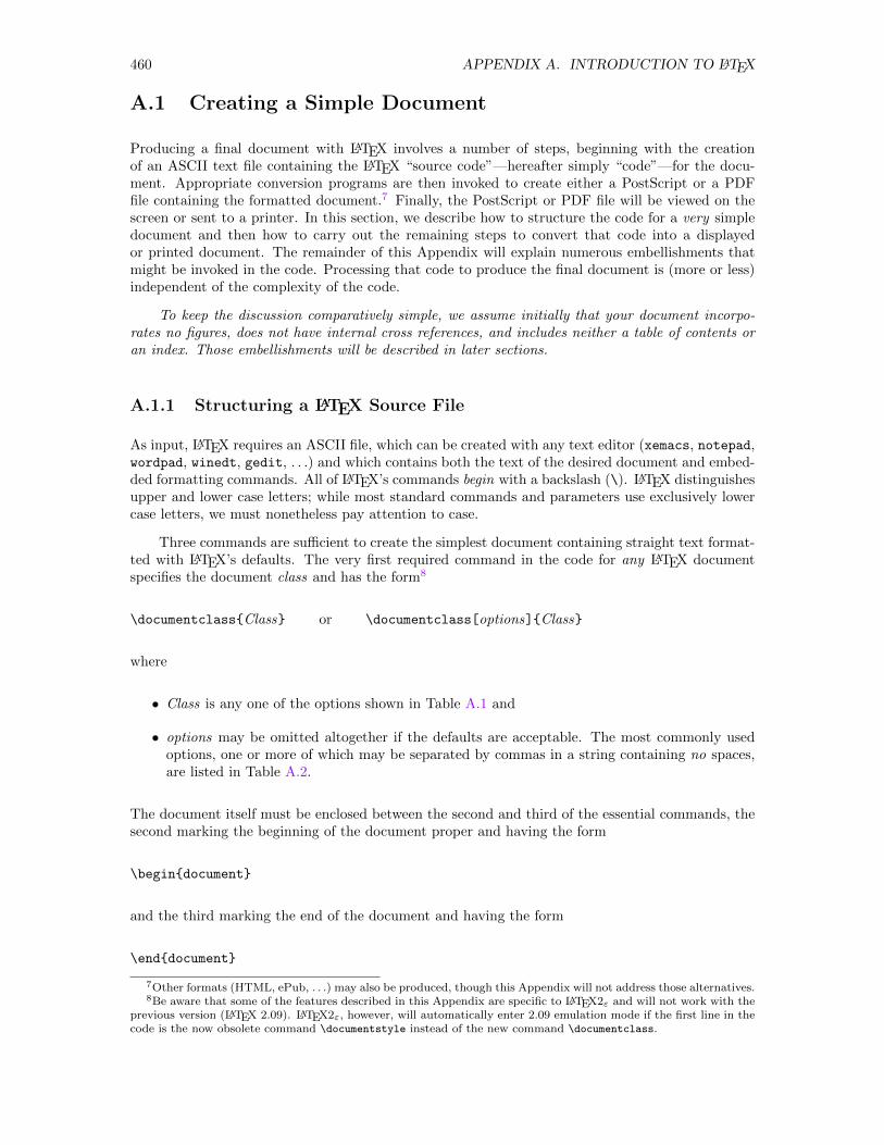
460 APPENDIX A. INTRODUCTION TO LATEX

A.1 Creating a Simple Document

Producing a final document with LATEX involves a number of steps, beginning with the creationof an ASCII text file containing the LATEX “source code”—hereafter simply “code”—for the docu-ment. Appropriate conversion programs are then invoked to create either a PostScript or a PDFfile containing the formatted document.7 Finally, the PostScript or PDF file will be viewed on thescreen or sent to a printer. In this section, we describe how to structure the code for a very simpledocument and then how to carry out the remaining steps to convert that code into a displayedor printed document. The remainder of this Appendix will explain numerous embellishments thatmight be invoked in the code. Processing that code to produce the final document is (more or less)independent of the complexity of the code.

To keep the discussion comparatively simple, we assume initially that your document incorpo-rates no figures, does not have internal cross references, and includes neither a table of contents oran index. Those embellishments will be described in later sections.

A.1.1 Structuring a LATEX Source File

As input, LATEX requires an ASCII file, which can be created with any text editor (xemacs, notepad,wordpad, winedt, gedit, . . .) and which contains both the text of the desired document and embed-ded formatting commands. All of LATEX’s commands begin with a backslash (\). LATEX distinguishesupper and lower case letters; while most standard commands and parameters use exclusively lowercase letters, we must nonetheless pay attention to case.

Three commands are sufficient to create the simplest document containing straight text format-ted with LATEX’s defaults. The very first required command in the code for any LATEX documentspecifies the document class and has the form8

\documentclassClass or \documentclass[options]Class

where

• Class is any one of the options shown in Table A.1 and

• options may be omitted altogether if the defaults are acceptable. The most commonly usedoptions, one or more of which may be separated by commas in a string containing no spaces,are listed in Table A.2.

The document itself must be enclosed between the second and third of the essential commands, thesecond marking the beginning of the document proper and having the form

\begindocument

and the third marking the end of the document and having the form

\enddocument

7Other formats (HTML, ePub, . . .) may also be produced, though this Appendix will not address those alternatives.8Be aware that some of the features described in this Appendix are specific to LATEX2ε and will not work with the

previous version (LATEX 2.09). LATEX2ε, however, will automatically enter 2.09 emulation mode if the first line in thecode is the now obsolete command \documentstyle instead of the new command \documentclass.

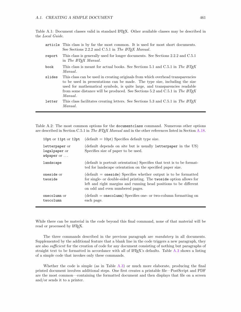
A.1. CREATING A SIMPLE DOCUMENT 461

Table A.1: Document classes valid in standard LATEX. Other available classes may be described inthe Local Guide.

article This class is by far the most common. It is used for most short documents.See Sections 2.2.2 and C.5.1 in The LATEX Manual .

report This class is generally used for longer documents. See Sections 2.2.2 and C.5.1in The LATEX Manual .

book This class is meant for actual books. See Sections 5.1 and C.5.1 in The LATEXManual .

slides This class can be used in creating originals from which overhead transparenciesto be used in presentations can be made. The type size, including the sizeused for mathematical symbols, is quite large, and transparencies readablefrom some distance will be produced. See Sections 5.2 and C.5.1 in The LATEXManual .

letter This class facilitates creating letters. See Sections 5.3 and C.5.1 in The LATEXManual .

Table A.2: The most common options for the documentclass command. Numerous other optionsare described in Section C.5.1 in The LATEX Manual and in the other references listed in Section A.18.

10pt or 11pt or 12pt (default = 10pt) Specifies default type size.

letterpaper orlegalpaper ora4paper or . . .

(default depends on site but is usually letterpaper in the US)Specifies size of paper to be used.

landscape (default is portrait orientation) Specifies that text is to be format-ted for landscape orientation on the specified paper size.

oneside ortwoside

(default = oneside) Specifies whether output is to be formattedfor single- or double-sided printing. The twoside option allows forleft and right margins and running head positions to be differenton odd and even numbered pages.

onecolumn ortwocolumn

(default = onecolumn) Specifies one- or two-column formatting oneach page.

While there can be material in the code beyond this final command, none of that material will beread or processed by LATEX.

The three commands described in the previous paragraph are mandatory in all documents.Supplemented by the additional feature that a blank line in the code triggers a new paragraph, theyare also sufficient for the creation of code for any document consisting of nothing but paragraphs ofstraight text to be formatted in accordance with all of LATEX’s defaults. Table A.3 shows a listingof a simple code that invokes only these commands.

Whether the code is simple (as in Table A.3) or much more elaborate, producing the finalprinted document involves additional steps. One first creates a printable file—PostScript and PDFare the most common—containing the formatted document and then displays that file on a screenand/or sends it to a printer.

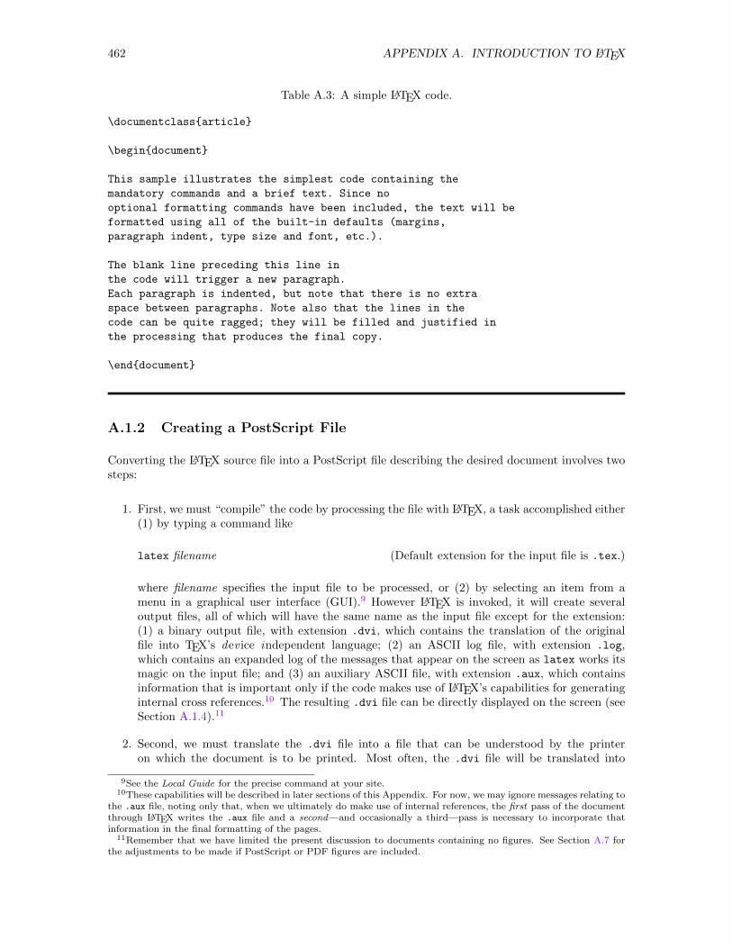
462 APPENDIX A. INTRODUCTION TO LATEX

Table A.3: A simple LATEX code.

\documentclassarticle

\begindocument

This sample illustrates the simplest code containing the

mandatory commands and a brief text. Since no

optional formatting commands have been included, the text will be

formatted using all of the built-in defaults (margins,

paragraph indent, type size and font, etc.).

The blank line preceding this line in

the code will trigger a new paragraph.

Each paragraph is indented, but note that there is no extra

space between paragraphs. Note also that the lines in the

code can be quite ragged; they will be filled and justified in

the processing that produces the final copy.

\enddocument

A.1.2 Creating a PostScript File

Converting the LATEX source file into a PostScript file describing the desired document involves twosteps:

1. First, we must “compile” the code by processing the file with LATEX, a task accomplished either(1) by typing a command like

latex filename (Default extension for the input file is .tex.)

where filename specifies the input file to be processed, or (2) by selecting an item from amenu in a graphical user interface (GUI).9 However LATEX is invoked, it will create severaloutput files, all of which will have the same name as the input file except for the extension:(1) a binary output file, with extension .dvi, which contains the translation of the originalfile into TEX’s dev ice independent language; (2) an ASCII log file, with extension .log,which contains an expanded log of the messages that appear on the screen as latex works itsmagic on the input file; and (3) an auxiliary ASCII file, with extension .aux, which containsinformation that is important only if the code makes use of LATEX’s capabilities for generatinginternal cross references.10 The resulting .dvi file can be directly displayed on the screen (seeSection A.1.4).11

2. Second, we must translate the .dvi file into a file that can be understood by the printeron which the document is to be printed. Most often, the .dvi file will be translated into

9See the Local Guide for the precise command at your site.10These capabilities will be described in later sections of this Appendix. For now, we may ignore messages relating to

the .aux file, noting only that, when we ultimately do make use of internal references, the first pass of the documentthrough LATEX writes the .aux file and a second—and occasionally a third—pass is necessary to incorporate thatinformation in the final formatting of the pages.

11Remember that we have limited the present discussion to documents containing no figures. See Section A.7 forthe adjustments to be made if PostScript or PDF figures are included.

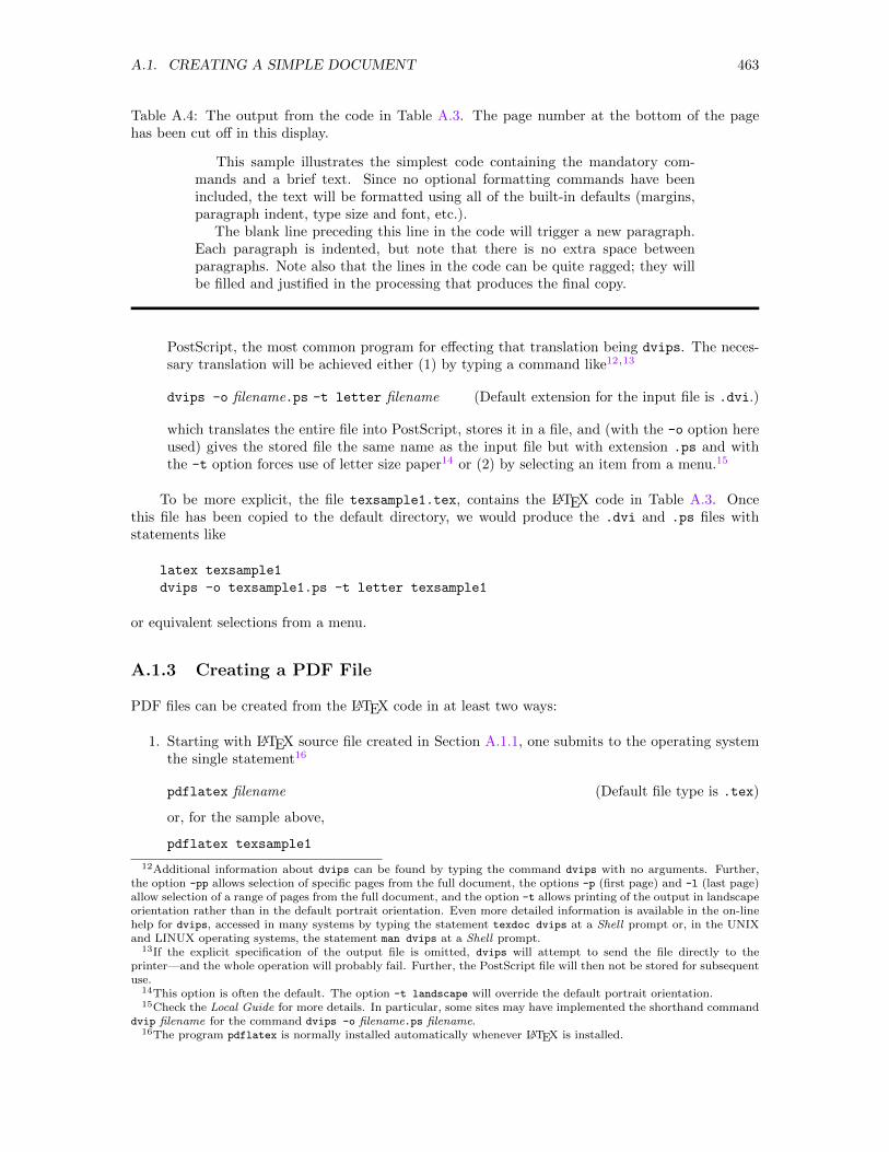
A.1. CREATING A SIMPLE DOCUMENT 463

Table A.4: The output from the code in Table A.3. The page number at the bottom of the pagehas been cut off in this display.

This sample illustrates the simplest code containing the mandatory com-mands and a brief text. Since no optional formatting commands have beenincluded, the text will be formatted using all of the built-in defaults (margins,paragraph indent, type size and font, etc.).

The blank line preceding this line in the code will trigger a new paragraph.Each paragraph is indented, but note that there is no extra space betweenparagraphs. Note also that the lines in the code can be quite ragged; they willbe filled and justified in the processing that produces the final copy.

PostScript, the most common program for effecting that translation being dvips. The neces-sary translation will be achieved either (1) by typing a command like12,13

dvips -o filename.ps -t letter filename (Default extension for the input file is .dvi.)

which translates the entire file into PostScript, stores it in a file, and (with the -o option hereused) gives the stored file the same name as the input file but with extension .ps and withthe -t option forces use of letter size paper14 or (2) by selecting an item from a menu.15

To be more explicit, the file texsample1.tex, contains the LATEX code in Table A.3. Oncethis file has been copied to the default directory, we would produce the .dvi and .ps files withstatements like

latex texsample1

dvips -o texsample1.ps -t letter texsample1

or equivalent selections from a menu.

A.1.3 Creating a PDF File

PDF files can be created from the LATEX code in at least two ways:

1. Starting with LATEX source file created in Section A.1.1, one submits to the operating systemthe single statement16

pdflatex filename (Default file type is .tex)

or, for the sample above,

pdflatex texsample1

12Additional information about dvips can be found by typing the command dvips with no arguments. Further,the option -pp allows selection of specific pages from the full document, the options -p (first page) and -l (last page)allow selection of a range of pages from the full document, and the option -t allows printing of the output in landscapeorientation rather than in the default portrait orientation. Even more detailed information is available in the on-linehelp for dvips, accessed in many systems by typing the statement texdoc dvips at a Shell prompt or, in the UNIXand LINUX operating systems, the statement man dvips at a Shell prompt.

13If the explicit specification of the output file is omitted, dvips will attempt to send the file directly to theprinter—and the whole operation will probably fail. Further, the PostScript file will then not be stored for subsequentuse.

14This option is often the default. The option -t landscape will override the default portrait orientation.15Check the Local Guide for more details. In particular, some sites may have implemented the shorthand command

dvip filename for the command dvips -o filename.ps filename.16The program pdflatex is normally installed automatically whenever LATEX is installed.

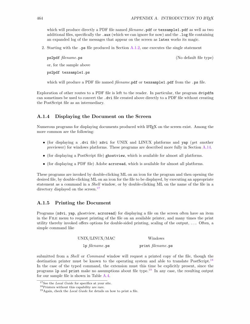
464 APPENDIX A. INTRODUCTION TO LATEX

which will produce directly a PDF file named filename.pdf or texsample1.pdf as well as twoadditional files, specifically the .aux (which we can ignore for now) and the .log file containingan expanded log of the messages that appear on the screen as latex works its magic.

2. Starting with the .ps file produced in Section A.1.2, one executes the single statement

ps2pdf filename.ps (No default file type)

or, for the sample above

ps2pdf texsample1.ps

which will produce a PDF file named filename.pdf or texsample1.pdf from the .ps file.

Exploration of other routes to a PDF file is left to the reader. In particular, the program dvipdfm

can sometimes be used to convert the .dvi file created above directly to a PDF file without creatingthe PostScript file as an intermediary.

A.1.4 Displaying the Document on the Screen

Numerous programs for displaying documents produced with LATEX on the screen exist. Among themore common are the following:

• (for displaying a .dvi file) xdvi for UNIX and LINUX platforms and yap (yet anotherpreviewer) for windows platforms. These programs are described more fully in Section A.14.

• (for displaying a PostScript file) ghostview, which is available for almost all platforms.

• (for displaying a PDF file) Adobe acroread, which is available for almost all platforms.

These programs are invoked by double-clicking ML on an icon for the program and then opening thedesired file, by double-clicking ML on an icon for the file to be displayed, by executing an appropriatestatement as a command in a Shell window, or by double-clicking ML on the name of the file in adirectory displayed on the screen.17

A.1.5 Printing the Document

Programs (xdvi, yap, ghostview, acroread) for displaying a file on the screen often have an itemin the File menu to request printing of the file on an available printer, and many times the printutility thereby invoked offers options for double-sided printing, scaling of the output, . . .. Often, asimple command like

UNIX/LINUX/MAC Windows

lp filename.ps print filename.ps

submitted from a Shell or Command window will request a printed copy of the file, though thedestination printer must be known to the operating system and able to translate PostScript.18

In the case of the typed command, the extension must this time be explicitly present, since theprograms lp and print make no assumptions about file type.19 In any case, the resulting outputfor our sample file is shown in Table A.4.

17See the Local Guide for specifics at your site.18Printers without this capability are rare.19Again, check the Local Guide for details on how to print a file.

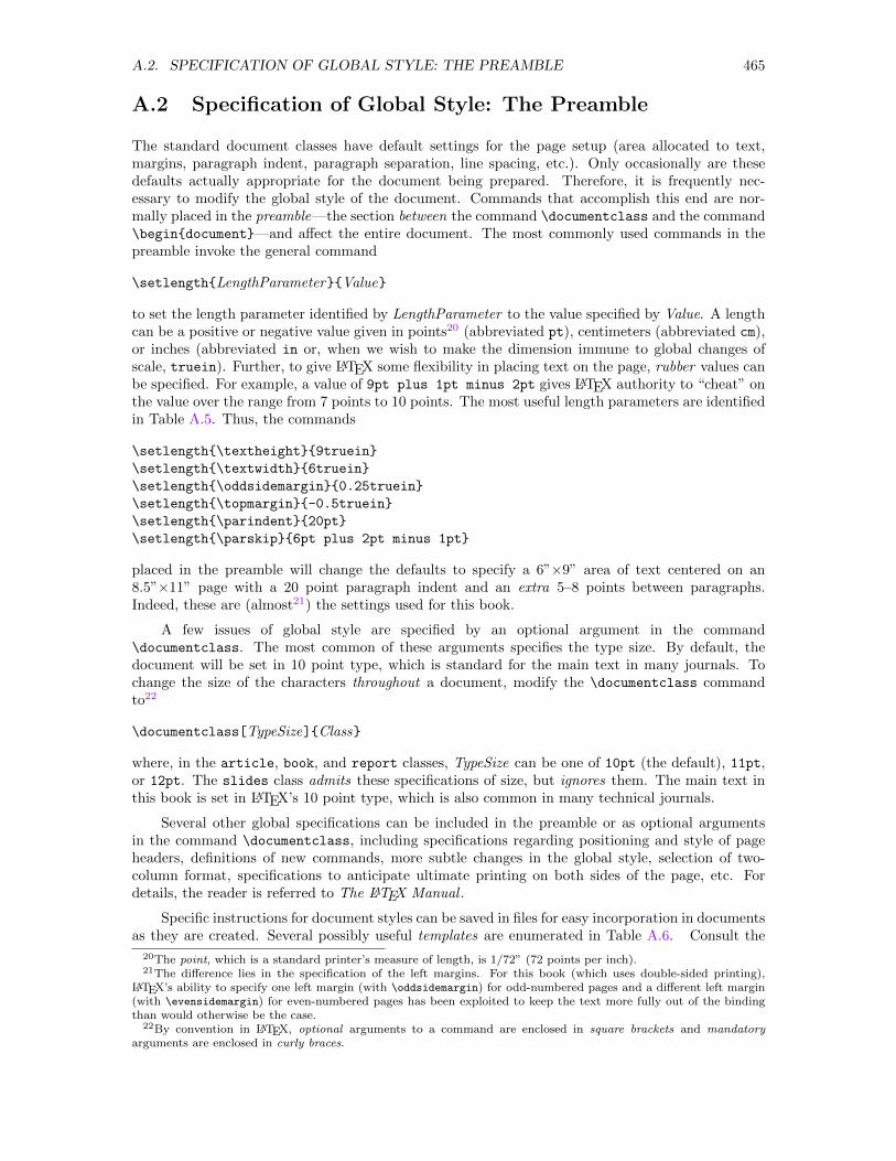
A.2. SPECIFICATION OF GLOBAL STYLE: THE PREAMBLE 465

A.2 Specification of Global Style: The Preamble

The standard document classes have default settings for the page setup (area allocated to text,margins, paragraph indent, paragraph separation, line spacing, etc.). Only occasionally are thesedefaults actually appropriate for the document being prepared. Therefore, it is frequently nec-essary to modify the global style of the document. Commands that accomplish this end are nor-mally placed in the preamble—the section between the command \documentclass and the command\begindocument—and affect the entire document. The most commonly used commands in thepreamble invoke the general command

\setlengthLengthParameterValue

to set the length parameter identified by LengthParameter to the value specified by Value. A lengthcan be a positive or negative value given in points20 (abbreviated pt), centimeters (abbreviated cm),or inches (abbreviated in or, when we wish to make the dimension immune to global changes ofscale, truein). Further, to give LATEX some flexibility in placing text on the page, rubber values canbe specified. For example, a value of 9pt plus 1pt minus 2pt gives LATEX authority to “cheat” onthe value over the range from 7 points to 10 points. The most useful length parameters are identifiedin Table A.5. Thus, the commands

\setlength\textheight9truein

\setlength\textwidth6truein

\setlength\oddsidemargin0.25truein

\setlength\topmargin-0.5truein

\setlength\parindent20pt

\setlength\parskip6pt plus 2pt minus 1pt

placed in the preamble will change the defaults to specify a 6”×9” area of text centered on an8.5”×11” page with a 20 point paragraph indent and an extra 5–8 points between paragraphs.Indeed, these are (almost21) the settings used for this book.

A few issues of global style are specified by an optional argument in the command\documentclass. The most common of these arguments specifies the type size. By default, thedocument will be set in 10 point type, which is standard for the main text in many journals. Tochange the size of the characters throughout a document, modify the \documentclass commandto22

\documentclass[TypeSize]Class

where, in the article, book, and report classes, TypeSize can be one of 10pt (the default), 11pt,or 12pt. The slides class admits these specifications of size, but ignores them. The main text inthis book is set in LATEX’s 10 point type, which is also common in many technical journals.

Several other global specifications can be included in the preamble or as optional argumentsin the command \documentclass, including specifications regarding positioning and style of pageheaders, definitions of new commands, more subtle changes in the global style, selection of two-column format, specifications to anticipate ultimate printing on both sides of the page, etc. Fordetails, the reader is referred to The LATEX Manual .

Specific instructions for document styles can be saved in files for easy incorporation in documentsas they are created. Several possibly useful templates are enumerated in Table A.6. Consult the

20The point, which is a standard printer’s measure of length, is 1/72” (72 points per inch).21The difference lies in the specification of the left margins. For this book (which uses double-sided printing),

LATEX’s ability to specify one left margin (with \oddsidemargin) for odd-numbered pages and a different left margin(with \evensidemargin) for even-numbered pages has been exploited to keep the text more fully out of the bindingthan would otherwise be the case.

22By convention in LATEX, optional arguments to a command are enclosed in square brackets and mandatoryarguments are enclosed in curly braces.

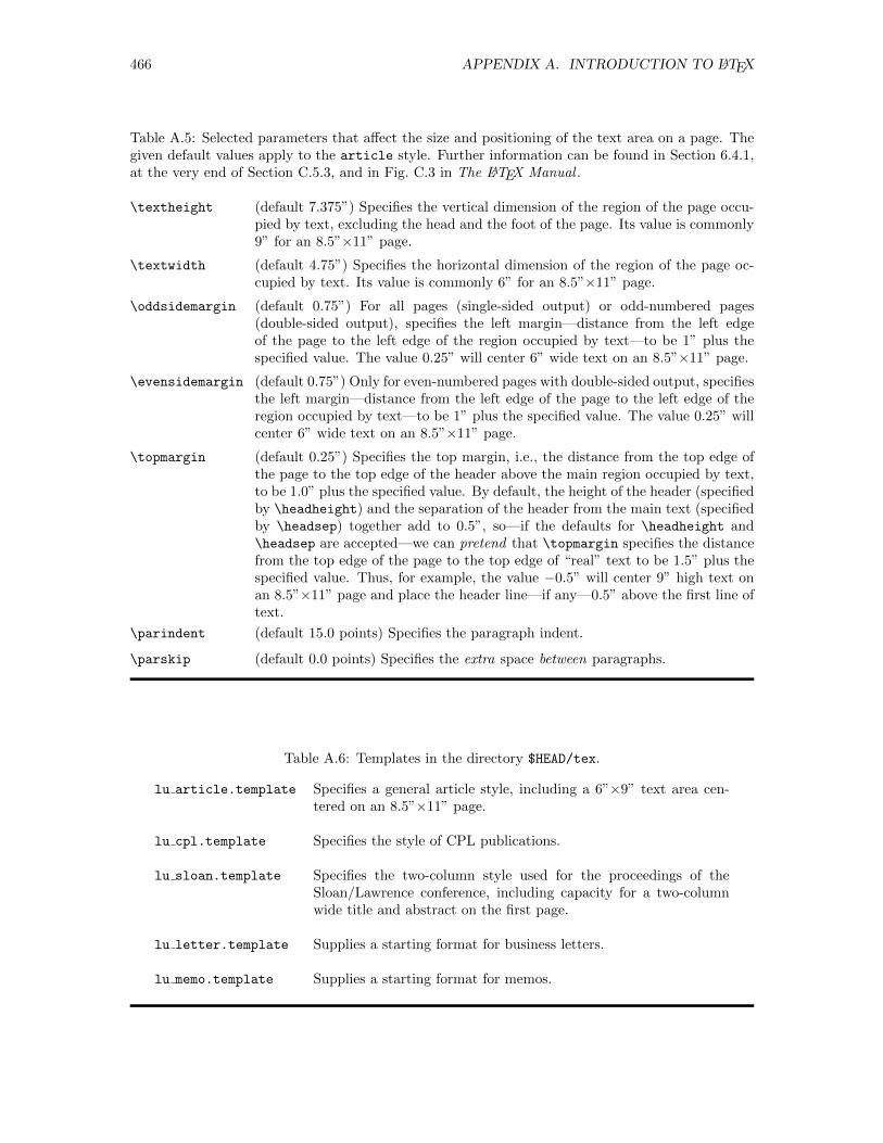
466 APPENDIX A. INTRODUCTION TO LATEX

Table A.5: Selected parameters that affect the size and positioning of the text area on a page. Thegiven default values apply to the article style. Further information can be found in Section 6.4.1,at the very end of Section C.5.3, and in Fig. C.3 in The LATEX Manual .

\textheight (default 7.375”) Specifies the vertical dimension of the region of the page occu-pied by text, excluding the head and the foot of the page. Its value is commonly9” for an 8.5”×11” page.

\textwidth (default 4.75”) Specifies the horizontal dimension of the region of the page oc-cupied by text. Its value is commonly 6” for an 8.5”×11” page.

\oddsidemargin (default 0.75”) For all pages (single-sided output) or odd-numbered pages(double-sided output), specifies the left margin—distance from the left edgeof the page to the left edge of the region occupied by text—to be 1” plus thespecified value. The value 0.25” will center 6” wide text on an 8.5”×11” page.

\evensidemargin (default 0.75”) Only for even-numbered pages with double-sided output, specifiesthe left margin—distance from the left edge of the page to the left edge of theregion occupied by text—to be 1” plus the specified value. The value 0.25” willcenter 6” wide text on an 8.5”×11” page.

\topmargin (default 0.25”) Specifies the top margin, i.e., the distance from the top edge ofthe page to the top edge of the header above the main region occupied by text,to be 1.0” plus the specified value. By default, the height of the header (specifiedby \headheight) and the separation of the header from the main text (specifiedby \headsep) together add to 0.5”, so—if the defaults for \headheight and\headsep are accepted—we can pretend that \topmargin specifies the distancefrom the top edge of the page to the top edge of “real” text to be 1.5” plus thespecified value. Thus, for example, the value −0.5” will center 9” high text onan 8.5”×11” page and place the header line—if any—0.5” above the first line oftext.

\parindent (default 15.0 points) Specifies the paragraph indent.

\parskip (default 0.0 points) Specifies the extra space between paragraphs.

Table A.6: Templates in the directory $HEAD/tex.

lu article.template Specifies a general article style, including a 6”×9” text area cen-tered on an 8.5”×11” page.

lu cpl.template Specifies the style of CPL publications.

lu sloan.template Specifies the two-column style used for the proceedings of theSloan/Lawrence conference, including capacity for a two-columnwide title and abstract on the first page.

lu letter.template Supplies a starting format for business letters.

lu memo.template Supplies a starting format for memos.

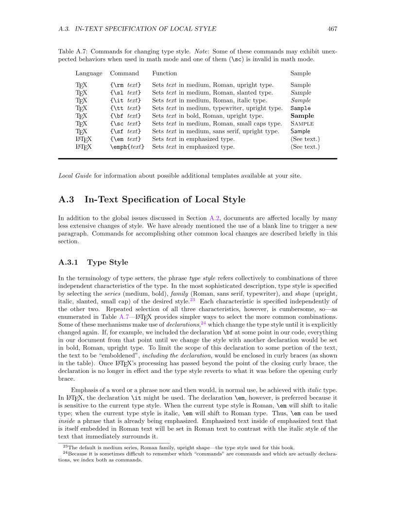
A.3. IN-TEXT SPECIFICATION OF LOCAL STYLE 467

Table A.7: Commands for changing type style. Note: Some of these commands may exhibit unex-pected behaviors when used in math mode and one of them (\sc) is invalid in math mode.

Language Command Function Sample

TEX \rm text Sets text in medium, Roman, upright type. SampleTEX \sl text Sets text in medium, Roman, slanted type. SampleTEX \it text Sets text in medium, Roman, italic type. SampleTEX \tt text Sets text in medium, typewriter, upright type. Sample

TEX \bf text Sets text in bold, Roman, upright type. SampleTEX \sc text Sets text in medium, Roman, small caps type. SampleTEX \sf text Sets text in medium, sans serif, upright type. SampleLATEX \em text Sets text in emphasized type. (See text.)LATEX \emphtext Sets text in emphasized type. (See text.)

Local Guide for information about possible additional templates available at your site.

A.3 In-Text Specification of Local Style

In addition to the global issues discussed in Section A.2, documents are affected locally by manyless extensive changes of style. We have already mentioned the use of a blank line to trigger a newparagraph. Commands for accomplishing other common local changes are described briefly in thissection.

A.3.1 Type Style

In the terminology of type setters, the phrase type style refers collectively to combinations of threeindependent characteristics of the type. In the most sophisticated description, type style is specifiedby selecting the series (medium, bold), family (Roman, sans serif, typewriter), and shape (upright,italic, slanted, small cap) of the desired style.23 Each characteristic is specified independently ofthe other two. Repeated selection of all three characteristics, however, is cumbersome, so—asenumerated in Table A.7—LATEX provides simpler ways to select the more common combinations.Some of these mechanisms make use of declarations,24 which change the type style until it is explicitlychanged again. If, for example, we included the declaration \bf at some point in our code, everythingin our document from that point until we change the style with another declaration would be setin bold, Roman, upright type. To limit the scope of this declaration to some portion of the text,the text to be “emboldened”, including the declaration, would be enclosed in curly braces (as shownin the table). Once LATEX’s processing has passed beyond the point of the closing curly brace, thedeclaration is no longer in effect and the type style reverts to what it was before the opening curlybrace.

Emphasis of a word or a phrase now and then would, in normal use, be achieved with italic type.In LATEX, the declaration \it might be used. The declaration \em, however, is preferred because itis sensitive to the current type style. When the current type style is Roman, \em will shift to italictype; when the current type style is italic, \em will shift to Roman type. Thus, \em can be usedinside a phrase that is already being emphasized. Emphasized text inside of emphasized text thatis itself embedded in Roman text will be set in Roman text to contrast with the italic style of thetext that immediately surrounds it.

23The default is medium series, Roman family, upright shape—the type style used for this book.24Because it is sometimes difficult to remember which “commands” are commands and which are actually declara-

tions, we index both as commands.

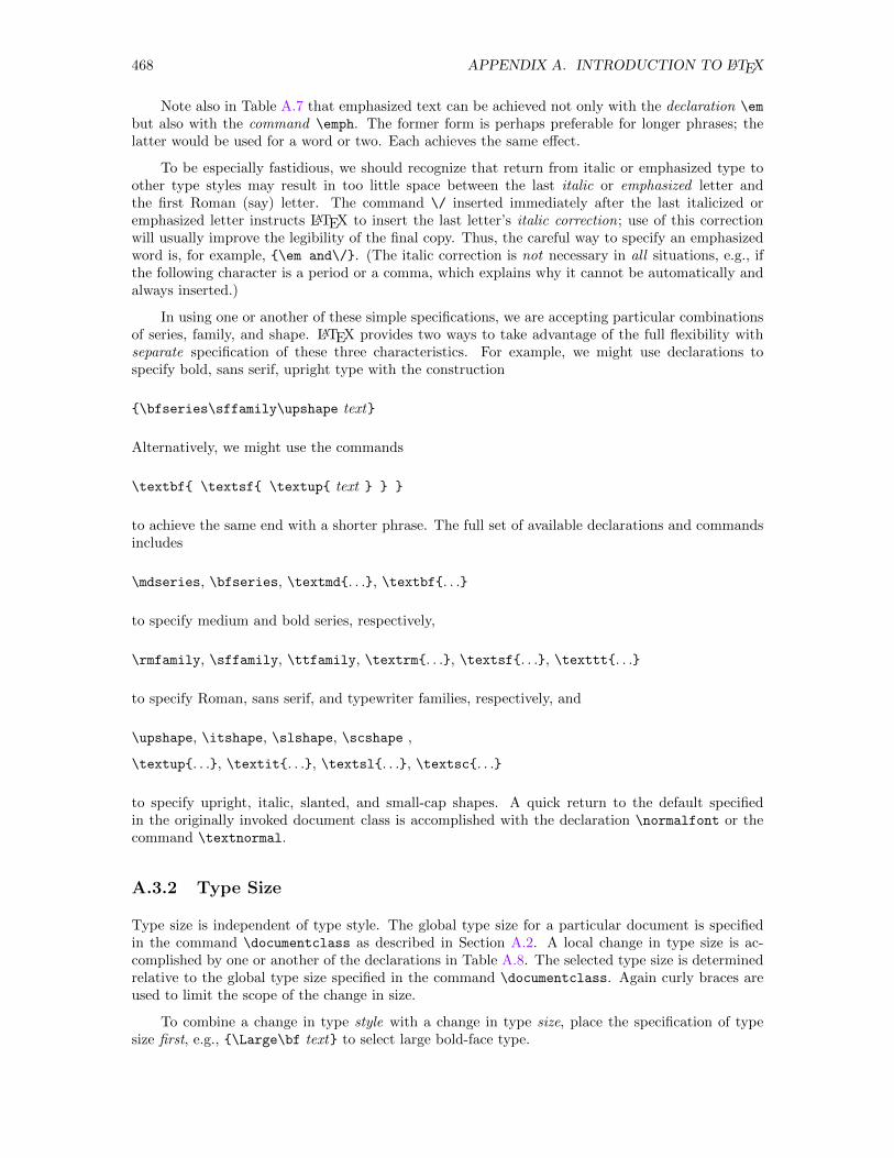
468 APPENDIX A. INTRODUCTION TO LATEX

Note also in Table A.7 that emphasized text can be achieved not only with the declaration \em

but also with the command \emph. The former form is perhaps preferable for longer phrases; thelatter would be used for a word or two. Each achieves the same effect.

To be especially fastidious, we should recognize that return from italic or emphasized type toother type styles may result in too little space between the last italic or emphasized letter andthe first Roman (say) letter. The command \/ inserted immediately after the last italicized oremphasized letter instructs LATEX to insert the last letter’s italic correction; use of this correctionwill usually improve the legibility of the final copy. Thus, the careful way to specify an emphasizedword is, for example, \em and\/. (The italic correction is not necessary in all situations, e.g., ifthe following character is a period or a comma, which explains why it cannot be automatically andalways inserted.)

In using one or another of these simple specifications, we are accepting particular combinationsof series, family, and shape. LATEX provides two ways to take advantage of the full flexibility withseparate specification of these three characteristics. For example, we might use declarations tospecify bold, sans serif, upright type with the construction

\bfseries\sffamily\upshape text

Alternatively, we might use the commands

\textbf \textsf \textup text

to achieve the same end with a shorter phrase. The full set of available declarations and commandsincludes

\mdseries, \bfseries, \textmd. . ., \textbf. . .

to specify medium and bold series, respectively,

\rmfamily, \sffamily, \ttfamily, \textrm. . ., \textsf. . ., \texttt. . .

to specify Roman, sans serif, and typewriter families, respectively, and

\upshape, \itshape, \slshape, \scshape ,

\textup. . ., \textit. . ., \textsl. . ., \textsc. . .

to specify upright, italic, slanted, and small-cap shapes. A quick return to the default specifiedin the originally invoked document class is accomplished with the declaration \normalfont or thecommand \textnormal.

A.3.2 Type Size

Type size is independent of type style. The global type size for a particular document is specifiedin the command \documentclass as described in Section A.2. A local change in type size is ac-complished by one or another of the declarations in Table A.8. The selected type size is determinedrelative to the global type size specified in the command \documentclass. Again curly braces areused to limit the scope of the change in size.

To combine a change in type style with a change in type size, place the specification of typesize first, e.g., \Large\bf text to select large bold-face type.

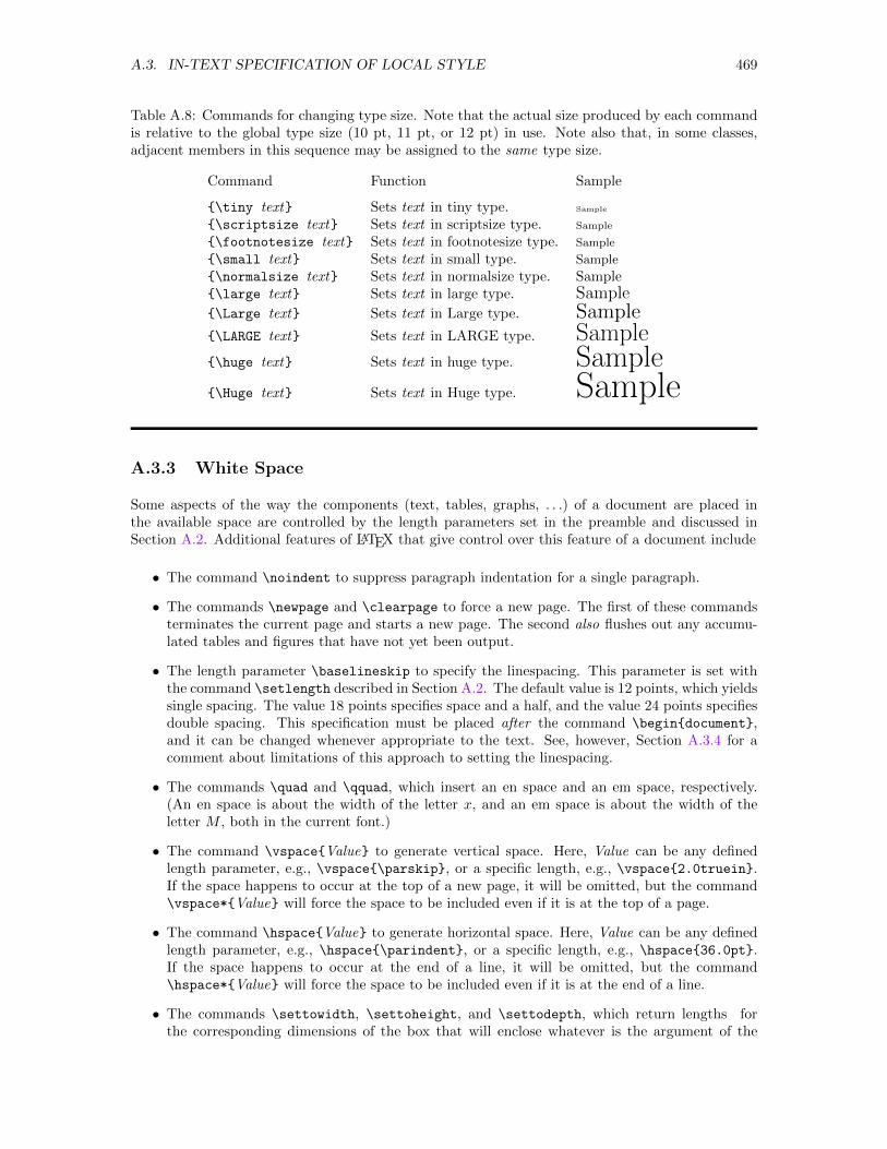
A.3. IN-TEXT SPECIFICATION OF LOCAL STYLE 469

Table A.8: Commands for changing type size. Note that the actual size produced by each commandis relative to the global type size (10 pt, 11 pt, or 12 pt) in use. Note also that, in some classes,adjacent members in this sequence may be assigned to the same type size.

Command Function Sample

\tiny text Sets text in tiny type. Sample

\scriptsize text Sets text in scriptsize type. Sample

\footnotesize text Sets text in footnotesize type. Sample

\small text Sets text in small type. Sample

\normalsize text Sets text in normalsize type. Sample\large text Sets text in large type. Sample\Large text Sets text in Large type. Sample\LARGE text Sets text in LARGE type. Sample\huge text Sets text in huge type. Sample\Huge text Sets text in Huge type. Sample

A.3.3 White Space

Some aspects of the way the components (text, tables, graphs, . . .) of a document are placed inthe available space are controlled by the length parameters set in the preamble and discussed inSection A.2. Additional features of LATEX that give control over this feature of a document include

• The command \noindent to suppress paragraph indentation for a single paragraph.

• The commands \newpage and \clearpage to force a new page. The first of these commandsterminates the current page and starts a new page. The second also flushes out any accumu-lated tables and figures that have not yet been output.

• The length parameter \baselineskip to specify the linespacing. This parameter is set withthe command \setlength described in Section A.2. The default value is 12 points, which yieldssingle spacing. The value 18 points specifies space and a half, and the value 24 points specifiesdouble spacing. This specification must be placed after the command \begindocument,and it can be changed whenever appropriate to the text. See, however, Section A.3.4 for acomment about limitations of this approach to setting the linespacing.

• The commands \quad and \qquad, which insert an en space and an em space, respectively.(An en space is about the width of the letter x, and an em space is about the width of theletter M , both in the current font.)

• The command \vspaceValue to generate vertical space. Here, Value can be any definedlength parameter, e.g., \vspace\parskip, or a specific length, e.g., \vspace2.0truein.If the space happens to occur at the top of a new page, it will be omitted, but the command\vspace*Value will force the space to be included even if it is at the top of a page.

• The command \hspaceValue to generate horizontal space. Here, Value can be any definedlength parameter, e.g., \hspace\parindent, or a specific length, e.g., \hspace36.0pt.If the space happens to occur at the end of a line, it will be omitted, but the command\hspace*Value will force the space to be included even if it is at the end of a line.

• The commands \settowidth, \settoheight, and \settodepth, which return lengths forthe corresponding dimensions of the box that will enclose whatever is the argument of the

470 APPENDIX A. INTRODUCTION TO LATEX

command. No printed output is produced by these commands. We might, for example, definea new length parameter \dblast as the width of the box accommodating two asterisks withthe two commands

\newlength\dblast

\settowidth\dblast**

and then insert the space for two asterisks (without actually displaying them) with the com-mand

\hspace\dblast

These commands are described in detail at the end of Sections 6.4.1 and C.13.1 in The LATEXManual .

A.3.4 Environments

Sometimes, the formatting to be accomplished requires a more sophisticated definition of a changethan is possible within the framework of a simple declaration or command with a few arguments.LATEX’s environments are more versatile and flexible than declarations and commands. For example,to present text in a narrower paragraph, as is conventionally done with extended quotations, wemight invoke one of the constructions

\beginquotation

Text of quotation.\endquotation

or\beginquote

Text of quotation.\endquote

Normally, the command \begin... will be placed on a line by itself, the text may spread overseveral lines, and the command \end... will be placed on a line by itself. Left and right marginsare indented equally. Unless the text includes its own formatting specifications, however, the firstconstruction will indent each new paragraph and will place no extra space between paragraphs whilethe second will place extra space between paragraphs and will not indent each new paragraph.

For a second example, if we wished to center a line or lines, we might invoke the similarconstruction

\begincenter First line \\ Second line \\ Third line \\ . . . \endcenter

Normally, the command \begin... will be placed on a line by itself, the text may spread overseveral lines, each line in the final output will in the code be separated from its predecessor with thecommand \\, and the command \end... will be placed on a line by itself.

These two examples introduce the construction called an environment, which in general has theformat

\beginEnvironmentName . . . \endEnvironmentName

We met the document environment early on. Beyond the quotation, quote, and center environ-ments, the most commonly used environments include verbatim, flushleft, flushright, itemize,enumerate, list, displaymath, equation, eqnarray, figure, table, tabular, minipage, picture,and thebibliography. Environments can be thought of as mini-documents within a document.They have default settings, but many of them possess parameters that the user can modify tocustomize the details of the environment. Further, as described in Sections 3.4 and C.8 in The

A.3. IN-TEXT SPECIFICATION OF LOCAL STYLE 471

LATEX Manual , individual users can supplement the standard set by defining additional environ-ments suited to the circumstances of the document. Individual exercises in this book, for example,are formatted by a user-defined environment.

The length parameter \baselineskip interacts in interesting ways with the formatting of textcontained within environments. Changing \baselineskip will affect only the spacing in the maintext of the document, including text in itemize, enumerate, and verbatim environments. Foot-notes, material in tabular environments, table and figure captions, and perhaps other componentswill remain single spaced unless—as described in Section C.3.2 in The LATEX Manual—the parame-ter \baselinestretch is also changed with the command \renewcommand. This additional change,however, has interesting side effects. (For example, the spacing of lines within footnotes will bechanged but the spacing between separate footnotes on the same page remains single!) Tamperingwith global style can at times have unintended (and unwanted) consequences. Beware!

A.3.5 LATEX Packages

As a publishing system, LATEX is infinitely extendable. Rather than incorporate all manner of specialtools within the basic program, its designers provided a means by which additional features couldbe added through the use of packages, the features of which can be made available in any specificcode by placing the command

\usepackage PackageName

in the preamble The LATEX Companion describes numerous packages, including amstex, babel,color, graphics, graphicx, graphpap, ifthen, latexsym, imakeidx, verbatim, pict2e, andshowidx. A brief description of many of these packages is included in Section C.5.2 of The LATEXManual . The statement texdoc PackageName at a Shell prompt also will bring up documentationon several of these packages.

In addition, some programs, especially those with notebook capabilities, have the ability to writethe contents of the notebooks into LATEX source files. Usually, those programs make use of theirown special LATEX commands and supply program-specific LATEX packages which must be accessible,either at the proper point in the LATEX directory structure or in the directory from which you runLATEX when processing a LATEX file produced by the programs. Details on those additional packageswill be found in the manuals provided by the vendors of the programs.

A.3.6 Miscellaneous Other Capabilities

Several additional capabilities merit particular comment:

• To force LATEX to keep words together on a single line and/or to prevent LATEX from insertingadditional space as it justifies a line, use a tilde ~ instead of a space between the words. Thetilde should also be used after a period that does not end a sentence. For example, we shouldtype ‘Mr.~Cook’ rather than25 ‘Mr. Cook’ in our file so as to produce ‘Mr. Cook’ rather than‘Mr. Cook’ in our output. In the second form, there is more space between the abbreviationand the name because LATEX automatically inserts extra space after each period (which isassumed to mark the end of a sentence). LATEX may add even more space in the second caseas it justifies the line between the margins.

• To generate a dash, use -, --, or ---, depending on the length of the required dash. Onehyphen produces a hyphen, as in two-column; two hyphens in a row produce a slightly longer

25The symbol ‘t’ underscores the presence of a space at the indicated point; it is not a character explicitly presentin the code.

472 APPENDIX A. INTRODUCTION TO LATEX

dash (an en dash in printers’ terminology), conventionally used to indicate ranges, e.g., 10–12;three hyphens in a row produce a still longer line (—, an em dash in printers’ terminology),sometimes called a punctuation dash and conventionally used in pairs as an alternative toparentheses. Note that none of these constructions is a minus sign −, which has yet a differentlength and is produced only in math mode. (See Section A.4.)

• To generate opening and closing (double) quotation marks, use ‘‘ and ’’, i.e., two openingor closing (single) tics in a row, respectively. Do not use the symbol " for either of thesepunctuation marks.

• To specify a footnote, use the command \footnoteText of footnote.. The specified text willbe placed at the bottom of the page and keyed to the text with an automatically generatednumber that starts with 1 at the beginning of the document.

• To start a new section, use the command \sectionTitle of Section. In the article class,section numbers start with 1 at the beginning of the document and are automatically generatedand incremented; the section number is included in the printed section title, which is displayedin a type size and font specified in the document class, and indentation will be suppressed inthe first paragraph of each new section. [The commands \subsection and \subsubsection

function in a similar way for subsections and subsubsections in the document. In the book

class, the commands \chapter and \part (an aggregation of chapters) are also available.]

• To control hyphenation, insert the command \- at the point in a word where LATEX is permittedto insert a hyphen as it fills and justifies lines. LATEX has its own rules for hyphenation, butthey are not infallible. Sometimes LATEX needs help. Note that words containing even oneindication of an optional hyphen will not be hyphenated at any other point(s) in the word.

• To suppress hyphenation of a single word altogether, place the word as the argument of an\mbox command, e.g., \mboxcustomize.

A.4 Including Equations

Most scientific documents will have equations, all of which must be specified in LATEX’s math mode.Shifting from the default text mode to math mode can be accomplished in several ways. For short,unnumbered equations or mathematical symbols that appear in a line of text, the equation or sym-bol must be enclosed in one of the two constructions \(. . . \) or $. . . $, which are equivalent. Ifwe want one or more displayed equations, with or without automatically generated equation num-bers, we need to use the form \begin. . . \end. Three standard environments use this construction.The displaymath environment centers a single equation on a line by itself, does not number theequation, and can be specified by the shortened form \[. . . \]. The equation environment cen-ters a single equation on a line by itself and numbers the equation automatically. The eqnarray

environment—see The LATEX Manual—is used for a string of equations and for long equations thatwill not fit on one line; its syntax allows vertical alignment of two or more displayed and numberedequations. To facilitate references to numbered equations produced in the equation and eqnarray

environments, LATEX provides the command \labelReferenceName for defining a symbolic labelwithin the environment and the command \refReferenceName to permit referencing the equationby its number in the text. Further, the command \pagerefReferenceName permits referencingthe page on which the equation occurs in the text.26 (Warning : The displaymath, equation, andeqnarray environments will generate error messages if they contain blank lines.)

26When these references are used, the information written into the .aux file becomes important and the code mustbe processed by latex or pdflatex twice, once to write the correct information into that file and a second time toread and make use of that information. Other environments, such as table and figure also admit a \label commandand can make use of this capability for symbolic internal references to those components. The label command canalso be used inside the argument of \part, \chapter, \section, \subsection, \subsubsection, and \footnote and inthe text following an \item command in an enumerate environment to facilitate reference to these components of thedocument.

A.5. INCLUDING LISTS 473

LATEX also has many symbols and structures, common in mathematical formulas, that can beused only in math mode. Subscripts and superscripts, roots, Greek letters, integral signs, summationsigns, the array environment, and many more are available.27 To reiterate, these symbols andstructures can only be used if LATEX is in math mode. So, to insert the symbol Θ in the finaloutput, we place the command $\Theta$ in the code.28 (Here, the first dollar sign puts LATEXin undisplayed math mode and the second returns LATEX to text mode.) Since LATEX follows itsown rules about spacing when in math mode, spaces in math mode are usually ignored. (A space,however, is necessary in such contexts as \omega t to separate the command \omega from thecharacter t.) The commands \,, \!, \:, and \; can be used in math mode to fine tune the spacesbetween elements in the equation by adding a thin space, a negative thin space, a medium space,and a thick space, respectively. It is, for example, customary to separate a differential element fromwhat precedes and follows with a thin space, e.g., (x+ y) dx dy rather than (x+ y)dxdy.29

Following the conventions for the type setting of mathematical text, all symbols in a mathenvironment are automatically italicized. The most common departure from this convention occurswith the names of the standard mathematical functions, which are conventionally set in Roman type.Special math mode commands of the form \cos and \sin should be used for these functions.30

Except for \sc, the declarations shown in Table A.7 can also be used in math mode to specifytext in something other than italic type but, in some contexts it may be preferable to use one ofthe commands \mathrm, \mathit, \mathbf, \mathtt, etc. described in Section 3.3.8 of The LATEXManual . Remember, however, that spaces are ignored in math mode, so a shift to Roman typewith the command \mathrm, for example, to include a two-word phrase, will result in the wordsrunning together unless the space command \ is used to insert an explicit space between the words.Sometimes, the better means to insert Roman text in equations is to use the command \mbox toescape temporarily to text mode.

Including bold characters in equations is especially tricky. The command \mathbf “emboldens”only some characters in the processed formula and, in particular, leaves lower case Greek symbolsin light face. The \boldmath declaration causes everything in math mode to be bold but cannotitself be invoked in math mode. To include a bold face, lower case θ, for example, we must use theconstruction

$ ... \mbox \boldmath $\theta$ ... $

where the command \mbox, which is valid in math mode, temporarily shifts to text mode so the\boldmath declaration can be invoked and the math mode expression in the argument of the com-mand \mbox will then be made bold; the bold presentation is confined by the command \mbox tothe desired part of the total expression.

A.5 Including Lists

Among the most commonly used environments are those that facilitate creation of lists, includingthe itemize environment for bulleted lists (such as the one in Section A.3.6) and the enumerate

environment for lists in which the items are lettered or numbered in sequence (such as the onein Section A.17). Each environment is introduced and terminated with the standard construction\begin . . . \end. Within the environment, each new item is introduced with the command \item.Thus, the structure might look like

27For a complete list of all symbols and the commands that create them, see Section 3.3 on Mathematical Formulasin The LATEX Manual .

28In math mode, Greek letters can be produced by commands that simply name the letter, e.g., \Theta for Θ and\omega for ω. Only the initial letter of the name is capitalized to produce an upper-case letter. Note, however, thatcommands for letters that are identical to Arabic letters, e.g., \Kappa, do not exist.

29Technically and officially, the differential element dx should be written with a Roman d and an italic x, i.e., dx,but this convention is rarely followed.

30See Table 3.9 in The LATEX Manual for a complete listing.

474 APPENDIX A. INTRODUCTION TO LATEX

\begin. . .\item Text of first item.\item Text of second item.\item Text of third item.\end. . .

The bullets and the numbers are, of course, generated automatically and, within the enumerate

environment, the numbers are automatically incremented. Details will be found in Sections 2.2.4,6.6, C.6.2, and C.6.3 in The LATEX Manual . Note in particular

• The optional argument for the command \item, which provides a means to override the au-tomatic label for that item and replace it with an explicit stipulated label. For example, thecommand \item[DMC] will cause the item to be labeled ‘DMC’ and the command \item[] willsuppress the label altogether. Note that, if the text of the item itself begins with somethingenclosed in square brackets, the command introducing that item must be written \item toprevent the text in square brackets from being interpreted as the desired label.

• The length parameters \itemsep, \parskip, and \parsep, which provide a means to overridedefault spacings within the environment.

• The way to change the “bullets” in the itemize environment. The symbols used to labelthe “bulleted” items in the various levels of nested itemize environments are created by thecommands \labelitemi, \labelitemii, \labelitemiii, and \labelitemiv. The defaultsequence for marking items at each level is •, – *, and ·. Each of these symbols can, however,be changed by redefining the corresponding command. For example, the command

\renewcommand\labelitemii$\circ$

executed in the preamble will change the symbol – to for the second level in nested itemize

environments.

• The way to change the form of the labels for each item in the enumerate environment. Thelabels at the various levels of nested enumerate environments are determined by invoking oneof the commands \theenumi, \theenumii, \theenumiii, and \theenumiv, whose action isin turn determined from the value of the corresponding one of the counters enumi, enumii,enumiii, and enumiv. The default sequence for marking items at each level is ‘1.’, ‘(a)’,‘i.’, ‘A.’, i.e., arabic number with period, lower-case letter in parentheses, lower-case Romannumber with period, and upper-case letter with period. These defaults, however, can bechanged with a command like

\renewcommand\theenumi(\Alphenumi)

which will change the labels used at the first level in enumerate environments to upper-casearabic letters in parentheses. The command \Alph could be replaced with \alph, \roman,\Roman, or \arabic to translate the underlying counter into lower-case arabic letters, lower-case Roman numbers, upper-case Roman numbers, or arabic numbers, respectively. As it turnsout, whatever is specified in the argument of the commands translating the counters, a periodwill be appended by LATEX at the first, third, and fourth levels, and enclosing parentheses willbe supplied at the second level.

A.6 Including Tables

Creation of columnar arrangements is facilitated by LATEX’s tabular environment, the details ofwhich are involved and are fully described in The LATEX Manual . The tabular environment can

A.6. INCLUDING TABLES 475

Table A.9: Format for inserting a table.

\begintable

\caption ...

\label ...

\begincenter

\begintabular clr

Row 1, Col 1 & Row 1, Col 2 & Row 1, Col 3 \\

Row 2, Col 1 & Row 2, Col 2 & Row 2, Col 3 \\

Row 3, Col 1 & Row 3, Col 2 & Row 3, Col 3

\endtabular

\endcenter

\endtable

be invoked anywhere in the code and the resulting table will be placed at the point at whichthe environment appears, perhaps even in the middle of a line of text. Conventionally, however,tables are placed at the top or bottom of the page,31 and LATEX provides the table environment tofacilitate proper placement of a table,32 though the bare table environment contains nothing otherthan its name that suggests its use for tables. Any text at all can be incorporated in the table

environment and will be placed on the page as would a table. Most commonly, however, the table

environment will embrace a tabular environment defining the table itself and will use the command\caption to specify the caption of the table and the command \label to specify a symbolic labelfor use in referring to the table within the document.33 Frequently, the tabular environment willitself be embraced in a center environment to control the horizontal placement of the table on thepage. Thus, the common structure for the code defining a table would be of the form shown inTable A.9.34,35

Here, individual elements in a row are separated from one another by ampersands, and theend of each row—except the last—is marked with the command \\. In this example, the caption,including an automatically generated phrase and number of the form ‘Table 3:’, will appear abovethe table. Positioning the commands \caption and \label after the center environment wouldplace the caption below the table. Whichever position is adopted, the command \label must appearafter the command \caption. Wherever the command \label is positioned, it will place an entry inthe .aux file so that the commands \ref and \pageref will function here as described for equationsat the beginning of Section A.4.

The illustrative argument clr of the tabular environment requires a bit more explanation.

31Actually, the command \begintable has an optional argument (\begintable[OptArg]), which can assumeany of the values h, b, or t for placement of the table at the place where the table environment appears (h, for here)or at the bottom (b) or top (t) of the page. In the absence of an explicit specification, LATEX makes its own decisionabout placement.

32If there is space on the current page when the table environment is encountered, the table will be placed on thatpage. Otherwise, the table will be placed on a subsequent page.

33The \caption and \label commands can be placed anywhere within the table environment. Captions willcommonly be placed either above or below the captioned component. In some contexts (see the warning at the endof Section A.10), placing the caption above the item is preferable.

34LATEX automatically uses the specified caption as an entry for a list of tables. There is, however, a limit to thelength of such entries. Especially long captions may generate error messages. To avoid this problem, we can—andsometimes must—exploit an optional argument to the command \caption. . . which allows the user to dictate theentry made to the list of tables. Unless a list of tables is to be generated, some authors argue that we should routinelyspecify a null value for the optional argument by writing the command \caption[]..., though we shall here notfollow that recommendation. See The LATEX Manual for details.

35See Sections 3.6 and C.10 in The LATEX Manual for much more detail on ways to line things up in columns. Noteparticularly (1) the command \multicolumn, which provides for entries that span more than one column, and (2)ways to create horizontal and vertical rulings in the table.

476 APPENDIX A. INTRODUCTION TO LATEX

In general, this argument will be a string of c’s, l’s and r’s, one for each column in the table.Each specifies the position (centered, left justified, right justified), respectively, of the entry in thecorresponding column. In the example, there are three columns, with entries in the first columncentered, entries in the second column left justified, and entries in the third column right justified.The argument is mandatory but will, of course, be a string appropriate to the table being constructedrather than the specific string clr.

By default, tables will be produced with no vertical or horizontal rulings. See Section C.10.2 inThe LATEX Manual for a description of the means to add these rulings.

A.7 Including Illustrations

Graphics displays frequently appear in technical documents. Within LATEX, means to incorporategraphics include36

• A cut and paste method (Section A.7.1).

• A method for incorporating a properly constructed PostScript or PDF file that invokes thecommand \includegraphics from the package graphicx (Section A.7.2).

• A method that exploits the tikz package of macros that facilitate describing the graphicaldisplay and its formatting in the same way that LATEX itself facilitates describing the text andits formatting (Section A.7.3).

• The built-in picture environment (Section A.7.4), which has limited capability but is some-times just the ticket for simple displays.

Most often, commands incorporating figures will be bracketed in a figure environment, whichfacilitates locating the illustration at the top or bottom of the current (or a following) page.37 Inmost cases, we need to know the final vertical extent of the figure in order to specify the size ofan appropriate space. Further, the commands \caption and \label are available to caption thefigure and to place appropriate entries in the .aux file so that the commands \ref and \pageref

will function here as described in the first paragraph of Section A.4.

A.7.1 Using Cut and Paste

The cut and paste method requires only that LATEX be instructed to set aside appropriately sizedand positioned space into which the illustration will be placed after the document has been printed.The segment of the code that creates and labels space for a figure will have the general form

\beginfigure

\caption ...

\label ...

\vspace ??.?truein

\endfigure

As illustrated here, the caption, including an automatically generated phrase and number of theform ‘Figure 3:’, will appear above the space left for the figure. Positioning the commands \captionand \label after the command \vspace would place the caption below the figure. Note also that,

36We elect here to discuss only a very few of the numerous available packages, choosing those of the broadestapplicability. Packages for drawing Feynman diagrams, organic molecules, musical scores, and many other displaysare described in The LATEX Graphics Companion.

37The figure environment also admits the optional argument described in footnote 31.

A.7. INCLUDING ILLUSTRATIONS 477

whichever position is adopted, the command \label must appear after the command \caption.For this method, you need only have printed copies of your figures.38 The format of the files usedfor the figures is irrelevant and the document can be produced with any of the methods describedin Sections A.1.2 and A.1.3.

A.7.2 Using the graphicx Package

Incorporation of graphic images in a LATEX document is viewed by LATEX as the responsibility of thedevice driver. To enable that process, LATEX allows the passing of commands to the device driver.Both the format of such commands and the variety of capabilities thus available depends entirelyon the device driver. In essence, this process uses the TEX (not LATEX) command \special, but theuser is unaware of that underlying command because it is invoked behind the scenes.

The simplest means for importing graphical displays into a LATEX document—i.e., of command-ing LATEX to pass the proper information on to the device driver—exploits the graphicx package,39

whose features are made available by including that package with the statement

\usepackagegraphicx

in the preamble of our LATEX code.40

After placing the command \usepackagegraphicx in our preamble, we incorporate the graph-ical display itself by placing a statement like

\includegraphics[height=dimension]filename

at the point where the PostScript or PDF figure defined in by the file filename is to be inserted.41

In general, the image would be centered horizontally on the page by inserting this command in acenter environment, e.g.,

\begincenter

\includegraphics[height=dimension]filename\endcenter

For example, the code42

38Appropriately translated, the substance of footnote 34 applies here to the entry placed automatically in the listof figures.

39The graphics package might also be used, but the syntax of the commands it defines is marginally less convenientthan the syntax of the parallel commands in the graphicx package, i.e. the extended graphics package.

40More generally, this statement admits an optional argument to the desired graphics driver explicitly. Frequently,that driver will be dvips and the statement would be \usepackage[dvips]graphicx, but numerous other driversexist, and many may be installed at your site. See the Local Guide for more information. For ultimate flexibility inthe formatting of graphics files, we elect to leave that choice to the default.

41If you use latex, dvips, and ps2pdf as described in Section A.1.2 and item 2 in Section A.1.3 to produce PostScriptand PDF documents, your figures must be available as .ps or .eps files, and—even if the file type is omitted in the\includegraphics command—the processing will correctly identify and incorporate the figures. If you seek to producea PDF document directly with pdflatex as described in item 1 in Section A.1.3, then—even if the file type .pdf isomitted in the\includegraphics command—the processing will correctly identify and incorporate the figures. If yourfigures are PostScript, you must use the first route to the final document; if your figures are PDF, you must use thesecond route. Software to convert PostScript figures to PDF figures and vice versa is described in Section A.11. Ifboth PostScript and PDF files exist for all figures and you omit the file type in the \includegraphics command, thenyou can use either latex or pdflatex for the processing.

42Appropriately translated, the substance of footnote 34 applies here to the entry in the list of figures.

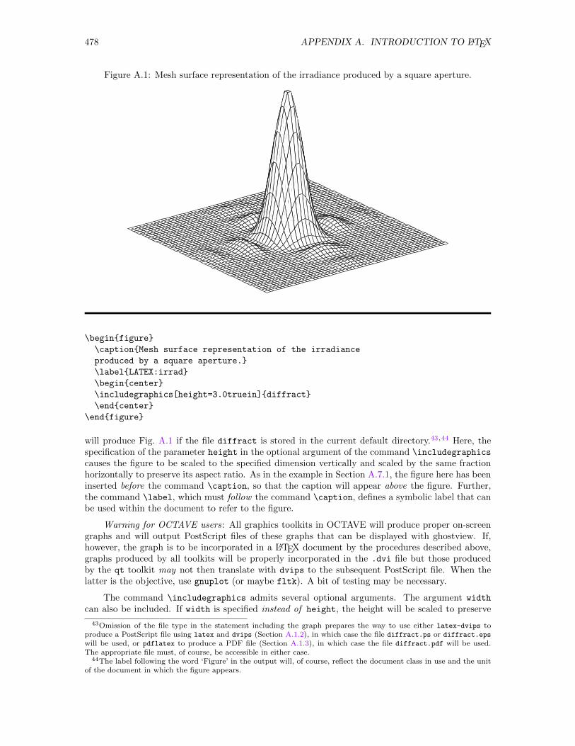
478 APPENDIX A. INTRODUCTION TO LATEX

Figure A.1: Mesh surface representation of the irradiance produced by a square aperture.

\beginfigure

\captionMesh surface representation of the irradiance

produced by a square aperture.

\labelLATEX:irrad

\begincenter

\includegraphics[height=3.0truein]diffract

\endcenter

\endfigure

will produce Fig. A.1 if the file diffract is stored in the current default directory.43,44 Here, thespecification of the parameter height in the optional argument of the command \includegraphics

causes the figure to be scaled to the specified dimension vertically and scaled by the same fractionhorizontally to preserve its aspect ratio. As in the example in Section A.7.1, the figure here has beeninserted before the command \caption, so that the caption will appear above the figure. Further,the command \label, which must follow the command \caption, defines a symbolic label that canbe used within the document to refer to the figure.

Warning for OCTAVE users: All graphics toolkits in OCTAVE will produce proper on-screengraphs and will output PostScript files of these graphs that can be displayed with ghostview. If,however, the graph is to be incorporated in a LATEX document by the procedures described above,graphs produced by all toolkits will be properly incorporated in the .dvi file but those producedby the qt toolkit may not then translate with dvips to the subsequent PostScript file. When thelatter is the objective, use gnuplot (or maybe fltk). A bit of testing may be necessary.

The command \includegraphics admits several optional arguments. The argument width

can also be included. If width is specified instead of height, the height will be scaled to preserve

43Omission of the file type in the statement including the graph prepares the way to use either latex-dvips toproduce a PostScript file using latex and dvips (Section A.1.2), in which case the file diffract.ps or diffract.eps

will be used, or pdflatex to produce a PDF file (Section A.1.3), in which case the file diffract.pdf will be used.The appropriate file must, of course, be accessible in either case.

44The label following the word ‘Figure’ in the output will, of course, reflect the document class in use and the unitof the document in which the figure appears.

A.7. INCLUDING ILLUSTRATIONS 479

the aspect ratio. If both height and width are specified, each will be respected and the aspect ratioof the figure may be distorted; specification of neither will cause the display to be produced in itsoriginal size. Arguments that allow overriding of the bounding box specified in the PostScript fileand arguments that permit clipping a portion of a fuller figure are described in The LATEX GraphicsCompanion.

A.7.3 Using the tikz Package

The tikz package, which is routinely included in present-day LATEX distributions, provides an assort-ment of LATEX macros to facilitate the drawing of simple—and even complicated—figures. Basically,the statement \usepackagetikz in the preamble followed in the document itself by statementsembedded in a tikzpicture environment will specify the desired graph and incorporate the graph ina PDF or Postscript file created as described in Sections A.1.2 and A.1.3.45 Be aware that the codeinserted in the tikzpicture environment describes the picture in the same way that LATEX providesthe text and its formatting. Just as one imagines the final formatted document as the LATEX codingis constructed, so one has to imagine the resulting picture as one constructs the descriptive codeto create it in the final document. Tikz is not a WYSIWIG drawing program like PAINT or TGIF.One of its advantages over the route described in Section A.7.2, which imports figures produced inother programs, is that the route of this section guarantees that the fonts used in the figures will beidentical to those used in the rest of the document.

The graphics system provided by tikz is impressively elaborate and versatile. As such, learningits capabilities, especially its more sophisticated capabilities, will require substantial effort. Typingthe command46

texdoc pgf

at a Shell window to your operating system will probably bring up links to a number of manu-als, including the main—and voluminous (1100-plus pages!)—manual in the file pgfmanual.pdf.Further, googling tikz will bring up links to numerous documents, including in particular a linkto pgfmanual.pdf and a link to the much more compact tutorial-style introduction in the fileminimaltikz.pdf. Once you have selected any of these items, you may in some operating systemshave to look in your Downloads folder to access the item.

This section quickly orients you to the general features of tikz without in any way pretendingto be complete. To that end, having included the statement47

\usepackagetikz

in the preamble of a document, we produce Fig. A.2 by placing the coding in Table A.10 at theappropriate point in the document itself. This coding briefly illustrates some of the more elementarycapabilities of tigz. Note specifically the following:

• Optional arguments to any tikz command are included in (square) brackets.

• By default, specified coordinates are expressed in centimeters, though any recognized LATEXunit of length can be specifically stipulated. The optional argument [x=1.0in,y=1.0in]

following \begintikzpicture changes the default to inches. Once a figure has been defined,its size can be easily altered simply by changing this optional argument.

45Note that, when displayed on the screen with xdvi or yap—see Section A.1.4—the intermediate .dvi file producedin Section A.1.2 will not contain the correct figures.

46The designation pgf—Portable Graphics Format—reflects the name of the engine underlying the entire system.47Some installations may also require inclusion of the packages pgf and xcolor.

480 APPENDIX A. INTRODUCTION TO LATEX

• Every statement must end with a semicolon. Any statement can be spread over several lineswith only the last line so terminated.

• The statement \draw [fill=black] (0,0) circle [radius=0.1]; draws a black-filled cir-cle centered at the origin and having radius 0.1 inches, thus marking the origin of the coordinatesystem.48 Available colors include red, green, blue, cyan, magenta, yellow, and many others.You can also define your own color using a command like49

\definecolorColorNamergbr, g, b

where ColorName is the name you assign to the color and r, g, b specify the r, g, and bcomponents that make up the color. Available shapes include rectangle, ellipse, and arc.50

• The statement \draw [<->, line width=2] (0,1.2)--(0,0)--(2.3,0); draws a line con-necting the specified points in the order given, i.e., draws the axes intersecting at the origin.Any number of points can be included in the path. The optional argument <-> places an arrowat both ends of the line,51 and the argument line width species the weight of the line, bydefault, in points.52

• Text is placed where specified with the statements \node at (0,1.3) \Large\bf y; and\node at (2.4,0.0) \Large\bf x;. Note that LATEX stipulations of font size and styleare recognized by tikz. Note also that the text is, by default, centered at the specified point.See the TIKZ manuals for ways to override that default positioning.

• The statement \draw [ultra thick, domain=0:2.0] plot (\x, sin(pi*\x r) ); illus-trates how to draw a smooth curve defined by a function, many of which are available withintikz. Note also the availability of the irrational number π with the simple coding pi.53

• The construction

\foreach \x in 0.0,1.0,2.0

\draw (\x,0.1 )--(\x,-0.1);

\node at (\x, -0.4)\x;;

creates a loop executing the statements enclosed in ... for each value in the list followingthe keyword in. The two loops in this code place tick marks on the axes and label those marks.Note the semicolons in this construction.

Clearly the command \draw is a versatile command that admits numerous embellishments throughthe use of keywords and/or optional arguments. Conveniently, tikz determines the size of thespace to be used in the document to reflect the size of the picture as constructed with the measuresprovided in the tikz coding.

When features of the package tikz are invoked in the LATEX code, producing the formatteddocument must be done carefully. If there are no complications (external figures, table of contents,internal references) to be incorporated, the simple statement

48Note that the default unit—here inches—for radius can be overridden with an explicit stipulation, e.g.,[radius=0.1cm].

49The command \definecolor here used is defined within the tikzpicture environment and does not require useof the LATEX package color.

50See the manuals for the details of how to specify the dimensions of these shapes.51The separate arguments -> and <- will place an arrow at the end or the beginning of the line, respectively.52The argument line width=2 could be replaced, among others, by ultra thin, very thin, thin, thick,

very thick, and ultra thick, and the default unit could be overridden with an argument like line width=0.1cm.53Another way to draw smooth curves is to use a calculational aid in another program to generate a probably long

list of coordinates for many points on the curve and then to insert that list as the argument of a \draw command.

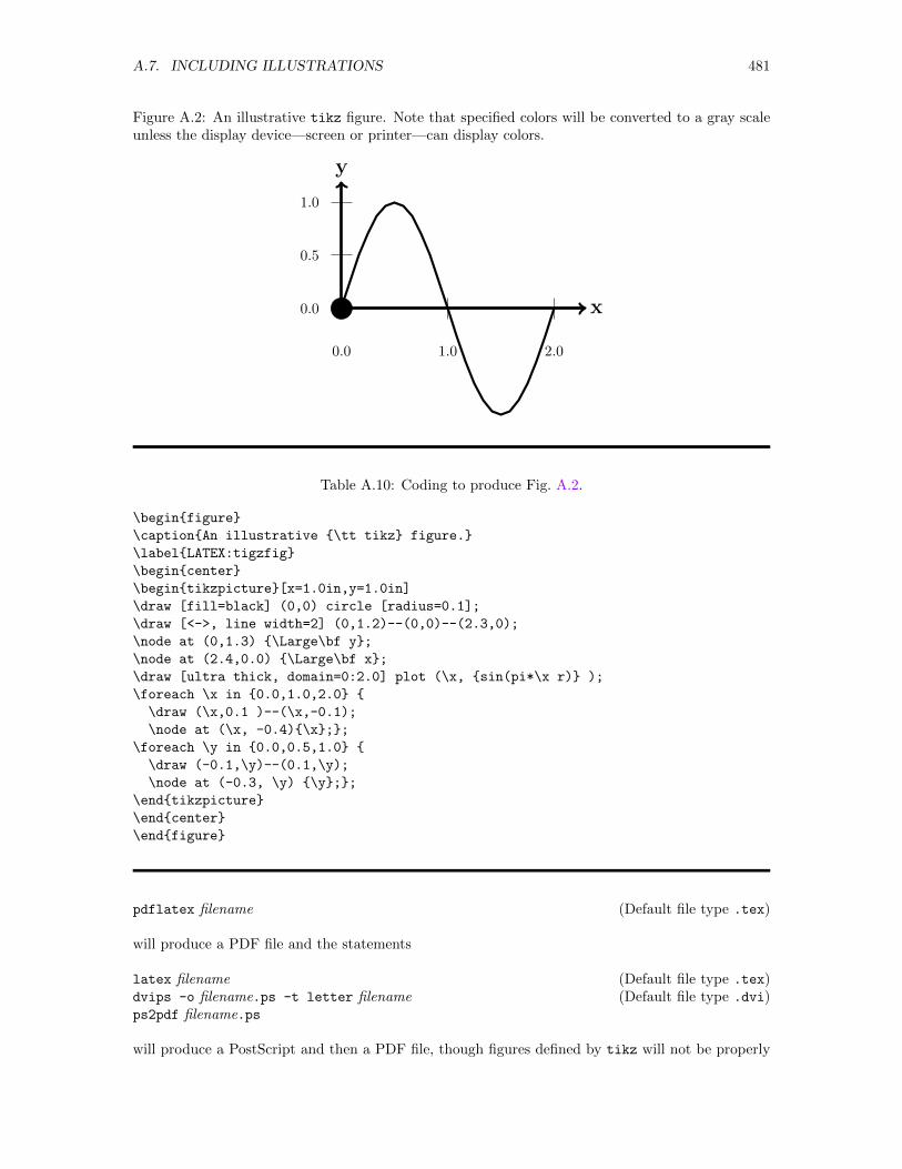
A.7. INCLUDING ILLUSTRATIONS 481

Figure A.2: An illustrative tikz figure. Note that specified colors will be converted to a gray scaleunless the display device—screen or printer—can display colors.

y

x

0.0 1.0 2.0

0.0

0.5

1.0

Table A.10: Coding to produce Fig. A.2.

\beginfigure

\captionAn illustrative \tt tikz figure.

\labelLATEX:tigzfig

\begincenter

\begintikzpicture[x=1.0in,y=1.0in]

\draw [fill=black] (0,0) circle [radius=0.1];

\draw [<->, line width=2] (0,1.2)--(0,0)--(2.3,0);

\node at (0,1.3) \Large\bf y;

\node at (2.4,0.0) \Large\bf x;

\draw [ultra thick, domain=0:2.0] plot (\x, sin(pi*\x r) );

\foreach \x in 0.0,1.0,2.0

\draw (\x,0.1 )--(\x,-0.1);

\node at (\x, -0.4)\x;;

\foreach \y in 0.0,0.5,1.0

\draw (-0.1,\y)--(0.1,\y);

\node at (-0.3, \y) \y;;

\endtikzpicture

\endcenter

\endfigure

pdflatex filename (Default file type .tex)

will produce a PDF file and the statements

latex filename (Default file type .tex)dvips -o filename.ps -t letter filename (Default file type .dvi)ps2pdf filename.ps

will produce a PostScript and then a PDF file, though figures defined by tikz will not be properly

482 APPENDIX A. INTRODUCTION TO LATEX

rendered in the intermediate .dvi file. If a table of contents or internal references or both areinvolved, two—and maybe three–passes through latex or pdflatex will be necessary. If thereare PostScript figures and no PDF figures to be incorporated, only latex will work; if there arePDF figures (and no PostScript figures) or hyperlinks to be incorporated, only pdflatex will work.Finally, if there are both PostScript and PDF files defining figures, files of one type will have to beconverted to the other type before either of these routes to a finished document will work.54

If you wish to short circuit learning detailed tikz code, you might wish to explore a WYSIWYGeditor TikzEdt that provides a graphical interface for creating figures and translates that figure intothe corresponding tikz code. This program, which is free, can be downloaded from the web sitewww.tikzedt.org. Documentation is also available at that site.

This section provides a woefully incomplete introduction intended more to wet your appetitethan to make you an expert. The effort invested to study the manuals identified in the secondparagraph of this section will be richly rewarded.

A.7.4 Using the picture Environment and pict2e Package

Finally, we merely mention the picture environment, described in Sections 7.1 and C.14.1 of TheLATEX Manual , and the supplementary pict2e package, described in The LATEX Companion. Thesecomponents add several commands that facilitate the detailed construction of at least simple graph-ical displays.

A.8 Including a Table of Contents, a List of Figures, and aList of Tables

A table of contents, a list of figures, and a list of tables can be included in the formatted documentby the commands \tableofcontents, \listoffigures, and \listoftables. Each

• results in the output of an auxiliary ASCII file of information with file type .toc, .lof, and.lot, respectively,

• requires a second pass through latex or pdflatex to incorporate the list in the finisheddocument, and

• places the list in the output at the point at which the command appears.

When these commands are invoked, each of the components of the text defined by the commands\part, \chapter, \section, \subsection, and \subsubsection will automatically generate a linein the .toc file;55 each use of the \caption command in a figure or table environment willautomatically generate a line in the .lof or .lot file. Then, in the second pass—which will alwaysbe necessary—through latex or pdflatex, these files are read and each line results in an entry inthe corresponding list.

Two commands allow explicit entry of information into one or another of these files at the pointwhere the command is inserted in the LATEX source file, specifically

• the command \addcontentslinefile unit entry

• the command \addtocontentsfile text 54See Section A.11 for details about that conversion.55Note that not all of these options are available in all document classes. For example, \part and \chapter are

available only in the book class. Note also the counters secnumdepth and tocdepth that control the depth to whichsections are numbered and the depth to which sections are catalogued in the table of contents. The default values ofthese counters can be overridden using \setcounter in the preamble.

A.9. INCLUDING AN INDEX 483

Here, file is one of toc, lof, and lot, unit is one of part, chapter, section, subsection, orsubsubsection if file is toc, figure if file is lof, and table if file is lot.

These two commands have quite different effects. The first adds a bona fide entry to thecorresponding file. For example, the line

\addcontentslinetocsubsectionSpecially marked point

will add to the table of contents an entry that is left-justified at the subsection level, contains thetext “Specially marked point”, and includes a row of dots and the appropriate page number.56 Thesecond merely adds text—no dots or page number—to the corresponding file. For example, the line

\addtocontentstoc\vspace24ptThis is a note.\vspace24pt

inserts a note preceded and followed by a bit of extra vertical space. Any textual note is left-justifiedas dictated by the section level at which it appears in the document.

Additional details about the issues discussed in this section are laid out in Sections 4.1 and C.4of The LATEX Manual. Note, in particular, the optional argument in the command \caption andthe several sectioning commands (\chapter, \section, . . .), which provide control over the entryeach command places in the table of contents, list of figures, and list of tables.

A.9 Including an Index

Among many capabilities, LATEX is able to generate an index, though not automatically. In essence,we must place the commands57

\usepackageimakeidx

\makeindex

in the preamble and the command

\printindex

at the point in the code at which the index is to be printed—usually the very end. Then, we indicatewhat items are to be indexed by placing commands like

\indexItem to be indexed

at appropriate points throughout the document. (The detailed structure of the argument to thecommand \index is described in Section 4.5 and Appendix A of The LATEX Manual .) When thefile filename.tex is processed by latex or pdflatex, the presence of these commands results in theaddition of three auxiliary ASCII files named

• filename.idx containing one line for each index entry,• filename.ilg containing a log of messages created when, behind the scenes, the idx file is

automatically processed through makeindex, and

56If you are creating a linked document, this entry in the table of contents will also appear in the navigation panelof that document.

57Earlier versions of LATEX used the package makeidx, which is still available. We here recommend using imakeidx

because it makes available a few more features than are available in the previous package and it eliminates the needto run an auxiliary program to format the index.

484 APPENDIX A. INTRODUCTION TO LATEX

• filename.ind produced by makeindex and containing the formatted index that is then readby \printindex to create the actual index in the document.

With imakeidx, the index is automatically created and incorporated in the document because anexecution of makeindex is inserted automatically at the appropriate point when latex or pdflatexis run. Errors and warnings in that step are compiled in the .ilg file (which should be examinedbecause on-screen display of those glitches may well scroll by to quickly to be comprehended).58

The above-described process yields an index in the default format. Numerous options can beexploited by adding optional arguments in the \makeindex command. For example, the command

\makeindex [options=-s ind_style, intoc]

stipulates that the style defined by the file ind style.ist should be invoked and the index shouldbe provided—argument intoc—with an entry in the table of contents. The construction of the stylefile is fully described in Section 12.4 in The LATEX Companion as identified in Section A.18.

To assist in constructing the index, an auxiliary package called showidx, which works both withlatex and with pdflatex, can be invoked to print the index entries on each page as marginal notes.This package is invoked simply by including the command

\usepackageshowidx

in the preamble, though it appears as if this command must be inserted after the \makeindex

command described above. Unfortunately, when printing in a 6”×9” area on 8.5”×11” paper(letterpaper), the marginal insertions of index entries will extend outside the edges of the pageand, in .ps and .pdf files, the portions that are off the page will not be displayed in ghostview

or acroread. Conveniently, if the .dvi file is displayed on the screen with xdvi (UNIX) or yap

(Windows), those marginal notes will be visible in their entirety, even if they extend beyond theboundaries of the page, though that route is available only if figures are provided in .ps or .eps

format. For the purposes of checking the index entries, one workaround is to shrink the area ofthe page in which printing of the text is allowed. For example, for this document, replacing thecommands

\setlength\textwidth6.0truein

\setlength\oddsidemargin0.5truein

\setlength\evensidemargin0.0truein

in the preamble with the commands

\setlength\textwidth4.0truein

\setlength\oddsidemargin1.0truein

\setlength\evensidemargin1.0truein

will shrink the text width and reset the margins so there will be space for the marginal notes. Tobe sure, the pagination of the text will also change, but at least the marginal notes will be visible,even in the .ps and .pdf files. In different situations, tampering with the above illustrated lengthparameters and, perhaps also, tampering with the length parameters \marginparwidth (which setsthe width of the marginal boxes) and \marginparsep (which sets the space between the text andthe boxes) as well as seeking ways to shrink the entire output including marginal notes on each pageas a unit may yield fruit.59

58With makeidx, a separate explicit processing of the .idx file with makeindex to produce the .ind file and a furtherpass through latex or pdflatex was necessary to include the index in the document.

59For example, the -x option to dvips can scale the size of each page output to the .ps file.

A.10. INCLUDING HYPERLINKS 485

A.10 Including Hyperlinks

Properly constructed, a LATEX source file can be used to create a PDF document that includes anavigation panel and hyperlinked references for easy viewing with a compatible PDF viewer. Only afew changes need be made to the source files so far described to turn entries in the table of contents,internal references in the body of a document, and page references in an index into hyperlinks tothe appropriate points in the document, though these features will appear only in PDF files createdvia the route described in item 1 in Section A.1.3 above. Specifically,

• the \documentclass statement at the beginning of the file must not specify any particulardriver, i.e. should be of the form \documentclassClass.

• if used at all, the \usepackagegraphicx command in the preamble must not include anyoptions specifying a graphics driver

• figures must be provided as PDF files or defined using the package tikz. PostScript descrip-tions of figures will not be properly rendered.

• the command \usepackagehyperref, perhaps with some optional arguments, must beadded in the preamble and, to make sure that other included packages do not overwrite redef-initions made by hyperref, should be the last package included.

This edited source file is then processed by pdflatex (Section A.1.3) at least twice to includehyperlinks, and tables of contents, figures, and tables. With these simple additions, a navigationpanel in the PDF file containing chapter, section, subsection, and . . . subdivisions of the documentwill be created. Further, all entries in the tables of contents, list of figures, and list of tables, allinternal references created with \ref commands, and all index entries will be converted into hotlinks within the document.

The command \usepackagehyperref in the preamble is the minimum necessary to createa hyperlinked PDF file. By default, hot links in the document will be displayed in a red box. Tooverride that default, one can exploit options in the \usepackage command. For example, thestatements,

\usepackagecolor

\definecolorMyPurplergb0.577,0.000,1.000

\usepackage[colorlinks=true,%

linkcolor=MyPurple,bookmarksnumbered=true,linktocpage=true]hyperref

in the preamble of the LATEX source file will set the stage for automatic creation of hyperlinks forall references, setting the color of those hyperlinks to MyPurple as specified by the RGB values inthe \definecolor statement and removing the enclosing box, stipulating that the bookmarks in thenavigation panels should include chapter and section numbers, and stipulating that page numbersrather than section titles should be the linked entries in the Table of Contents.60 The final PDFfile is then produced by processing the source file with pdflatex (Section A.1.3)—at least twiceand perhaps three times. To avoid error messages, all auxiliary files hanging over from a previousprocessing of the source file without hyperlinks through latex or pdflatex should be deleted beforeprocessing the file with hyperlinks.61

The files created in the user’s directory when a properly constructed .tex file with hyperlinks,index, and table of contents is processed through pdflatex to produce a linked PDF file are62

60The default value of the bookmarksnumbered and linktocpage options is false.61See item 25 in Section A.17 for ways to achieve this deletion.62We here assume you are making an index and using imakeidx. The sequence and auxiliary files will be different

if you are not making an index and/or if you are using makeidx.

486 APPENDIX A. INTRODUCTION TO LATEX

• (after first pass through pdflatex) .aux, .idx, .ilg, .ind, .log, .out, .pdf, and .toc. The.idx, .ilg, and .ind files will be present only if you are creating an index with imakeidx.The .out file contains information about hyperlinks; the rest are as described in item 1 ofSection A.1.3, in Section A.8, and in Section A.9. At this point, the PDF file does not havethe navigation panel or the table of contents but it does have the index. All of these files areASCII text files, though the PDF file may contain some non-printing characters. As such theycan all be displayed in an available text editor and understood.

• (after the second pass and, if necessary, the third pass through pdflatex) the same as in theprevious bullet, though many of those files have been updated. At this point, the navigationpanel, the internal hyperlinks, and the index have all been created.

A WARNING : Links to figures and tables will point to the line containing the caption for the figureor table. Captions for these items are perhaps better placed above the item rather than below theitem.

A CONVENIENCE : If the commands \documentclass and \usepackagegraphicx are phrasedwithout options and the files in all \includegraphics commands are presented without file type,then the file processed with latex will look for .ps and .eps graphics files and the file processedwith pdflatex will look for .pdf files. All files to be sought must, of course, exist.63 This featuremakes it easy to process the same source file both with latex and with pdflatex.

A.11 Converting .eps and .ps Files to .pdf

When files describing figures are created, it is often easier to output those files from the creatingprogram as .eps or .ps files rather than as .pdf files. Unfortunately, if you desire to produce thefinal output with pdflatex, files describing pictures need to be .pdf. PostScript files must thereforebe converted into PDF before running pdflatex. Short of asking someone who already knowshow to achieve that transfer, rummaging on the web for guidance may be a frustrating experience.Once you find the right tools, however, the process is quite simple. Basically, to convert the filesfigure.eps and figure.ps to a useful PDF file involves the two steps

1. ps2pdf figure.eps (which will yield figure.eps.pdf)ps2pdf figure.ps (which will yield figure.pdf)

2. pdfcrop figure.eps.pdf (which will yield figure.eps-crop.pdf) orpdfcrop figure.pdf (which will yield figure-crop.pdf)

Here, step 1 creates the .pdf file and step 2 removes extraneous white space around the perimeterof the first-created .pdf file. Second arguments to both ps2pdf and pdfcrop can be used to relievethe awkwardness of the file names. To simplify the process, the MS DOS batch files listed inSection A.A.1, respectively, and the UNIX Shell scripts listed in Section A.A.2, respectively, exploitthe second argument for both ps2pdf and pdfcrop to control the file names and, when executedwith statements like

MS DOS UNIX

ceps2pdf figure ./ceps2pdf figure (for .eps file)cps2pdf figure ./cps2pdf figure (for .ps file)

63See Section A.11 for a means to convert .ps and .eps. files to .pdf and vice versa.

A.11. CONVERTING .EPS AND .PS FILES TO .PDF 487

will (1) leave in the involved directory a cropped PDF file whose name figure.pdf differs from thatof the original PostScript in only the file type and (2) remove any temporary files created along theway.

The above procedure is a bit tedious if you have more than a few files to convert. If you workin a Command window (Windows) or a Shell window (UNIX), the steps

• Create a temporary directory and create the several files listed in Section A.A.1 (Windows) orA.A.2 (UNIX) and the file listed in Section A.A.3 (Windows and UNIX) into that directory.These files can be created by direct typing or they can be copied from the directory $HEAD/tex.

• Copy all .ps or all .eps files to be converted into that temporary directory. This step guardsagainst disaster should the process to come be run in the initial directory and fail.

• Create a file containing a list of the names of the .eps or .ps files in the directory. Thestatements

MS DOS UNIX

dir /b *.eps > dir.txt ls -1 *.eps > dir.txt

dir /b *.ps > dir.txt ls -1 *.ps > dir.txt

utilizing the option /b in Windows and the option -1 (one, not el) in UNIX produce the desiredfile (filename, including file type).

• Strip the file type by running the python program ExtractFileName.py (Section A.A.3). Herethe same code works in both Windows and UNIX. This action will create the file nameonly.txtcontaining only the names of the files to be converted.

• Effect the conversions by running the script rdfile with statements like

MS DOS UNIX

rdfileeps (for eps files) ./rdfileeps (for eps files)rdfileps (for ps files) ./rdfileps (for ps files)

This action will convert each file in turn from .eps or .ps to .pdf and leave no intermediatefiles in the directory.

• Delete the *.eps or *.ps files in the temporary directory.

• Move the *.pdf files to the directory from which the .eps and .ps files were moved temporarily,leaving both the original .ps and .eps files intact but adding the .pdf files, so either latex

or pdflatex can then be used to create the final document.

will accomplish that conversion

The reverse process of converting a .pdf file to .ps or .eps format is easier. Specifically, thestatements

pdftops FileName.pdf FileName.pspdftops -eps FileName.pdf FileName.eps

will effect this conversion. The task of creating scripts to automate this process when many files areto be converted is left to the reader.

488 APPENDIX A. INTRODUCTION TO LATEX

A.12 Using Conditional Expressions in LATEX

The LATEX package ifthen provides a capacity to include text and LATEX commands conditionally,i.e., depending on the state of a Boolean flag. If the package is to be used, the preamble of the LATEXsource file must contain the command

\usepackageifthen

Once that command has been processed, we must—also in the preamble—then define one or moreBoolean flags and set their values with commands like

\newbooleanFlagName\setbooleanFlagNameFlagValue

where FlagName can be any name that does not conflict with names already used and FlagValuewill be either true or false. Finally, at the point in the source file where some text is to be includedconditionally, we would place the command

\ifthenelse\booleanFlagNameText to be inserted if FlagValue is true.Text to be inserted if FlagValue is false.

Either text can be null, in which case the opening and closing braces should still appear side byside (), and either text can include LATEX commands—which will be executed—and can spreadover several lines. In particular, the text can include commands to input additional files. Indeed,the customization in CPSUP is achieved by including or excluding files depending on the state ofseveral flags. For example, in the preamble of the LATEX source file for CPSUP, the command

\usepackageifthen

appears and several flags are defined and set with commands like, for example,

\newbooleanLATEX \setbooleanLATEXtrue

Finally, the command

\ifthenelse\booleanLATEX

\inputFileName

is placed at the point where the file containing the LATEX portions of this book would be inserted.If the file identified is in the working directory, only its name need be included; otherwise, a fullpath—absolute or relative—must be specified. At this point, the LATEX Appendix will be includedif the flag is true and omitted if the flag is false.

More complicated logical operations can be constructed with the operators \and, \or, and \not.For example, if the Boolean flags NUMREC and FORTRAN are defined and set, then the compositestatement

\ifthenelse\booleanNUMREC \and \booleanFORTRAN

\inputFileName

A.13. ERROR MESSAGES GENERATED BY LATEX 489

would include FileName only if both NUMREC and FORTRAN are true.

In the effort to render files processable with either latex or pdflatex and also to create easilyeither a printable document or a linked document, the package hyperref must be invoked only whena linked document is desired. In order to avoid manual editing of the source file, one can insert inthe preamble the statements64

\usepackageifthen

\newbooleanPRINT

\typeout \typein[\trueorfalse]true (for print), false (for linked):

\ifthenelse \equal\trueorfalsetrue \or \equal\trueorfalsefalse

\setbooleanPRINT\trueorfalse

\typeout \typeoutMust be either "true" or "false". Try again. \enddocument

which define the boolean variable PRINT, ask for entry of either true or false at execution time,and terminate execution if an invalid value is entered. Then, the lines

\usepackagecolor

\ifthenelse\booleanPRINT

\definecolorMyPurplergb0.577,0.000,1.000

\usepackage[colorlinks=true, linkcolor=MyPurple]hyperref

also in the preamble, will include the package hyperref, but only if PRINT is false.

One further conditional command included in latex and pdflatex without adding a packagefacilitates testing whether a file exists. For example, the statement

\IfFileExiststest.tex\inputtest.tex

inputs test.tex if it exists and simply moves on to the next statement if it doesn’t exist. Thisstatement is useful if the file to be input is created in the first pass through latex or pdflatex

and then read in a subsequent pass. The “false” clause could alternatively be used to print an errormessage and terminate execution, e.g.,

\IfFileExiststest.tex\inputtest.tex\typeoutFile not found \enddocument

A.13 Error Messages Generated by LATEX

However carefully the code is created, sooner or later LATEX will generate an error message, whichwill have the general form

! error identificationl. number text read

text not read

?

The exclamation point is followed by a message that explains the nature of the error. The lowercase l (el) is followed (1) by the number of the line in the code at which the problem is detected

64Inclusion of the package ifthen can be omitted if it had been entered previously for other reasons.

490 APPENDIX A. INTRODUCTION TO LATEX

and (2) the text surrounding the problem.65 Finally, the question mark prompts for user input. Asimple 〈RETURN〉 at the question mark will instruct LATEX to continue to read the file unless a fatalerror has occurred (though LATEX may be forced to make assumptions in order to continue); entry ofthe character x (followed by 〈RETURN〉 will exit immediately from the program. Many errors arecaused by a missing delimiter or by failure to specify a switch to math mode before a mathematicalexpression or back to text mode after a mathematical expression. All of the reported errors mustbe identified and fixed (by editing the code) before LATEX will produce the desired finished product.A full description of the messages that may be produced as well as an enumeration of other userinputs at the ? will be found in Chapter 8 in The LATEX Manual .

A.14 The Page Previewer for .dvi Files

Since LATEX is not wysiwyg, we must use a page previewer to see exactly what our document lookslike without printing it out many, many times. The Local Guide describes the page previeweravailable at your site. UNIX systems usually provide a version of xdvi and Windows systemsusually provide a version of yap,66 but many such previewers exist and, on personal computersespecially, the previewer may be accessed by a mouse click in a GUI that also gives access to othercomponents of the LATEX package. To use this previewer, we first create the .dvi file by runningour code through LATEX as described in Section A.1. Then we enter a command like 67,68

xdvi filename or yap filename (The default extension for the input file is .dvi.)

or select an appropriate item from a menu (as described in The Local Guide). Presently, the firstpage of the document will appear on the screen. Some versions of xdvi display an array of buttonsalong the right edge of the Xdvi window; other, probably newer, versions replace those buttons withdrop-down menus and icons in a toolbar. Clicking ML on any of the various buttons or selectingitems from one of the menus effects the associated action. For xdvi and its clones, possible actionsinclude the options shown in Table A.11. In addition, (1) moving the cursor to any point in thewindow and pressing (and holding) any of the three mouse buttons will generate a magnified versionof a region whose size is determined by which button is pushed and (2) some versions of xdvi havea window along the left edge in which you can click ML on a page number to request immediatedisplay of the selected page—though note that these numbers simply count pages from the beginningof the displayed document and may not correspond to the numbers actually printed on the pages inthe document.

Beyond the controls made available through buttons and/or menus around the periphery of theXdvi window, xdvi responds to a number of keystrokes issued when the the cursor is moved intothe area displaying text. Some of these are identified in Table A.12; all are described in the xdvi

documentation, e.g., the UNIX man page.

In some environments, a GUI may provide an easy way to use the mouse to work on LATEX code,process it repeatedly with LATEX, and examine the changes with an on-screen previewer each time.In the absence of a GUI giving access to all of these features (text editor, LATEX, screen previewer,printer, . . .), one convenient strategy for using a text editor and a page previewer simultaneouslyinvolves invoking the previewer with a command like

xdvi filename & (UNIX) or yap filename & (Windows)

65The point at which LATEX encounters difficulty is conveyed by the downward displacement of the text after thatpoint, though that point is not always where the offense actually occurs.

66Y et Another Previewer67Additional information about xdvi on UNIX systems can be found in the on-line help, accessed in many systems

by typing the command man xdvi.68If explicit specification of the input file is omitted, some implementations of xdvi will bring up a browser in which

the desired .dvi file can be selected. Other versions may open the most recently displayed file, in which case thebrowser can be invoked by selecting ‘Open’ from the File menu.

A.15. THE SPELL CHECKER IN UNIX 491

Table A.11: Some of the features available through selection from menus (first column) in someversions of xdvi, through clicking ML on buttons in other versions of xdvi. The features actuallyavailable by these means may vary from version to version of xdvi.

Menu Button Action

File→Reload Reread Rereads current .dvi file.File→Quit Quit Quits previewer.Zoom→Shrink by 1 100% Displays text at full size (quite large).Zoom→Shrink by 3 33% Displays text at 33% of full size.Zoom→Shrink by 4 25% Displays text at 25% of full size.Zoom→Shrink by 6 17% Displays text at 17% of full size.Navigate→First Page First Moves to first page.Navigate→Page-10 Page-10 Moves to the tenth page before the one displayed.Navigate→Page-5 Page-5 Moves to the fifth page before the one displayed.Navigate→Prev Prev Moves to previous pageNavigate→Next Next Moves to next page.Navigate→Page+5 Page+5 Moves to the fifth page after the one displayed.Navigate→Page+10 Page+10 Moves to the tenth page after the one displayed.Navigate→Last Page Last Moves to last page.Options→PostScript View Page Allows selection among two or more options, including

displaying figures (the initial state) and replacing themwith properly sized rectangles.

File→Open File Brings up a browser for selection of new .dvi file.

Table A.12: Keystrokes for controlling xdvi.

s Size text to fit window. n Move to next page.1s (one-s) Largest text. p Move to previous page.ns Apply shrink factor n. nn Advance n pages.g Move to last page. np Back up n pages.1g (one-g) Move to first page. q Exit program.ng Move to (absolute) page n.

which will start xdvi or yap but detach it from the launching Shell window, leaving the Shellwindow free for other uses. Then, with the .tex file in a text editor detached from the launchingShell window, we can edit the text, save the edited version, use the Shell window to invoke LATEXon the edited file, and then simply click ML at an appropriate point in the displayed text to instructxdvi or yap to reread the .dvi file.69 Thus, the effect of each new set of edits can be examinedquickly without repeatedly starting and exiting from the previewer.

A.15 The Spell Checker in UNIX70

The programs ispell and aspell, either or both of which may be part of your LATEX distribution,are common spell checkers. If either is installed at your site (see the Local Guide), it can be invoked

69In some environments, rereading an updated file will happen automatically without an explicit user request.70To the author’s knowledge, no comparable stand-alone spell checker exists for Windows.

492 APPENDIX A. INTRODUCTION TO LATEX

with a command like71

ispell filename or aspell check filename

or perhaps with a mouse click in a GUI. For files with extension .tex, ispell enters its TEX modeand will not identify every TEX or LATEX command as a misspelled word. Note, however, that thesecommands are simply ignored by ispell and aspell; their correctness or legitimacy as commandsto LATEX is not assessed.

A.16 A Sample Document

The following sample document demonstrates some of the commands explained above and alsointroduces some useful commands that have not yet been mentioned. (The explanatory commentsfollowing the % sign can be included in the code but have no effect on the output produced.)

\documentclassarticle % Mandatory command; select

% default 10 point type

\setlength\textheight9truein % Set height of text area

\setlength\topmargin-0.5truein % Center text on 11’’ height

\setlength\textwidth6truein % Set width of text area

\setlength\oddsidemargin0.25truein % Center text on 8.5’’ width

\setlength\parskip6pt plus 1pt minus 1pt % Specify extra space

% between paragraphs,

% allowing LaTeX to adjust

% space 1 point up or down

\setlength\parindent40pt % Set paragraph indent

\begindocument % Mandatory command

\begincenter % Large, bold, centered title

\Large\bf A Sample Document for Your Perusal

\endcenter

\beginflushleft % Two lines; flush left

\em Author\/: J.~Q.~Student \\ % \\ forces a new line

% Note italic correction

% Tilde prevents extra space

\em Date\/: \today

\endflushleft

In this document we have used the \verb+\setlength+ commands to modify

\LaTeX’s default page setup to make fuller use of an 8.5’’$\times$11’’

page.\footnoteNote the special command $\backslash$\tt LaTeX

provided for the display of the \LaTeX ‘‘logo’’.

The title could have been generated using the three commands

\verb*+\title+\ldots\verb*++, \verb*+\author+\ldots\verb*++, and

\verb*+\date+\ldots\verb*++ before the \verb*+\begindocument+

71Additional information about ispell or aspell can be found by typing the command ispell with no argumentsor the command aspell help. Even more detailed information may be available in the on-line help, accessed in manysystems by typing the command man ispell or the command man aspell. Googling ispell or aspell will surely alsoprovide links to detailed descriptions.

A.17. MISCELLANEOUS OTHER FEATURES 493

command---i.e., in the preamble---followed by the command

\verb*+\maketitle+ after the beginning of the document. The command

\verb*?\verb*+ ... +? will cause \LaTeX to print whatever

is between the plus signs

(which could be virtually any specified character) exactly as it is.

The asterisk is optional, and it makes \LaTeX highlight the spaces that

occur inside the \verb+verbatim+ environment.

\noindent Notice that a blank line creates a new paragraph. The

\verb+\noindent+ command \em suppresses\/ the standard paragraph

indentation. In this special space we will also demonstrate some math

environment operations. Consider the equation

\beginequation

\int_0^\infty\: e^-x\, dx = 1,

\labelLATEX:demo

\endequation

where a medium sized space, specified by the command \verb+\:+, is

put between the integral sign $\int_0^\infty$, and

the integrand and a small space, specified by the command \verb+\,+,

is inserted between the integrand and the $dx$ in Eq.~(\refLATEX:demo).

The equation

\beginequation

\frac \partial e^x_0 y^2 \partial x_0 = y^2 e^x_0y^2

\endequation

demonstrates partial derivatives and fractions. Note the automatic

generation and placement of equation numbers in the output. Also note

that pages are automatically numbered, though the actual printing of

page numbers can be suppressed with the commands \verb+\pagestyle+ and

\verb+\thispagestyle+.

\enddocument % Mandatory command

The output produced when this short sample file is processed through LATEX and dvips andthen printed is shown in Table A.13, though the page header on that page is not included in theoutput. Note that, to obtain the proper internal reference to the first equation, this document mustbe processed twice by LATEX. The file itself is named texsample2.tex and can be copied from thedirectory $HEAD/tex.

A.17 Miscellaneous Other Features

LATEX has an enormous number of additional features beyond those enumerated above. In particular,be aware of

1. All of the environments listed in Section A.3.4.

2. All of the packages listed in Section A.3.5.

3. The command \today, which returns today’s date in the form “month date, year”.

4. The command \newcommand, which permits us to define commands supplementing the standardcommands. For example, the commands

\newcommand\beq\beginequation

\newcommand\eeq\endequation

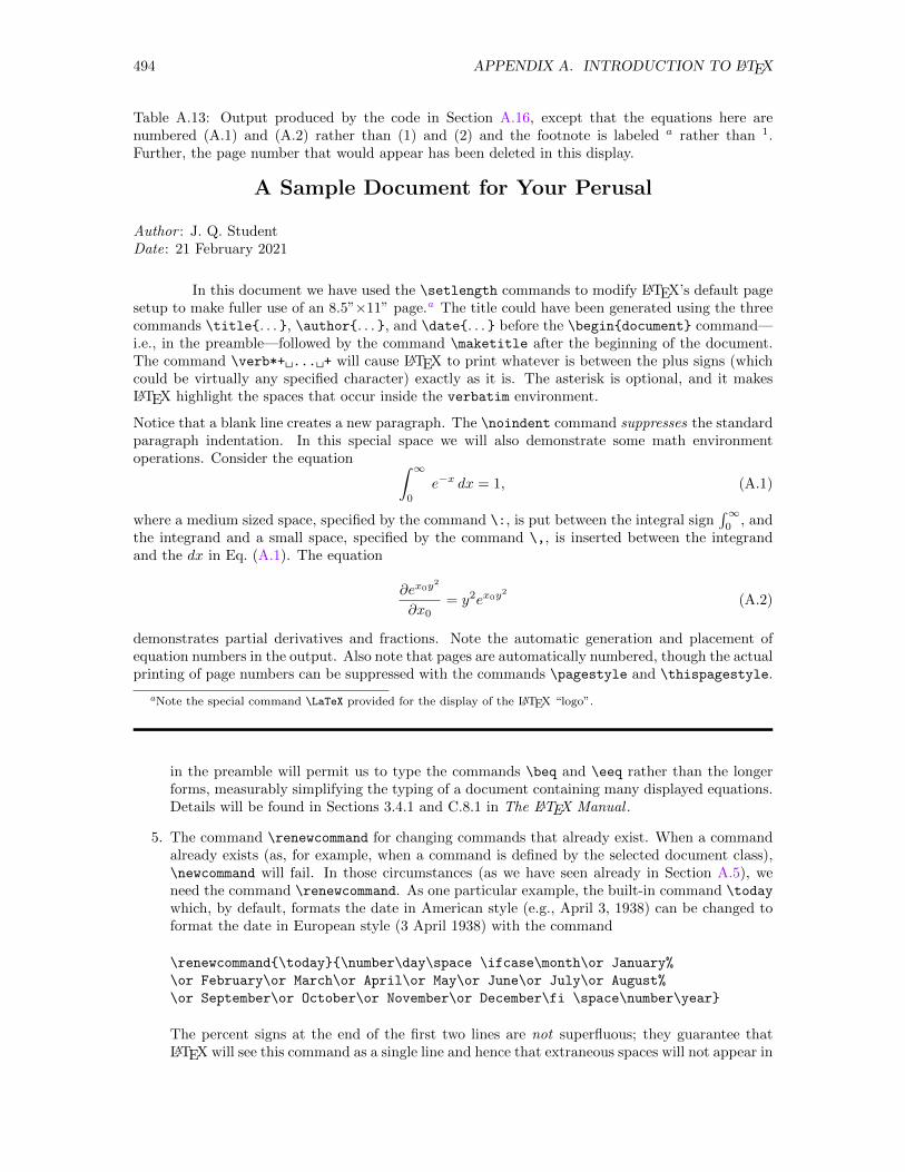
494 APPENDIX A. INTRODUCTION TO LATEX

Table A.13: Output produced by the code in Section A.16, except that the equations here arenumbered (A.1) and (A.2) rather than (1) and (2) and the footnote is labeled a rather than 1.Further, the page number that would appear has been deleted in this display.

A Sample Document for Your Perusal

Author : J. Q. StudentDate: 21 February 2021

In this document we have used the \setlength commands to modify LATEX’s default pagesetup to make fuller use of an 8.5”×11” page.a The title could have been generated using the threecommands \title. . . , \author. . . , and \date. . . before the \begindocument command—i.e., in the preamble—followed by the command \maketitle after the beginning of the document.The command \verb*+ ... + will cause LATEX to print whatever is between the plus signs (whichcould be virtually any specified character) exactly as it is. The asterisk is optional, and it makesLATEX highlight the spaces that occur inside the verbatim environment.

Notice that a blank line creates a new paragraph. The \noindent command suppresses the standardparagraph indentation. In this special space we will also demonstrate some math environmentoperations. Consider the equation ∫ ∞

0

e−x dx = 1, (A.1)

where a medium sized space, specified by the command \:, is put between the integral sign∫∞0

, andthe integrand and a small space, specified by the command \,, is inserted between the integrandand the dx in Eq. (A.1). The equation

∂ex0y2

∂x0= y2ex0y

2

(A.2)

demonstrates partial derivatives and fractions. Note the automatic generation and placement ofequation numbers in the output. Also note that pages are automatically numbered, though the actualprinting of page numbers can be suppressed with the commands \pagestyle and \thispagestyle.

aNote the special command \LaTeX provided for the display of the LATEX “logo”.

in the preamble will permit us to type the commands \beq and \eeq rather than the longerforms, measurably simplifying the typing of a document containing many displayed equations.Details will be found in Sections 3.4.1 and C.8.1 in The LATEX Manual .

5. The command \renewcommand for changing commands that already exist. When a commandalready exists (as, for example, when a command is defined by the selected document class),\newcommand will fail. In those circumstances (as we have seen already in Section A.5), weneed the command \renewcommand. As one particular example, the built-in command \today

which, by default, formats the date in American style (e.g., April 3, 1938) can be changed toformat the date in European style (3 April 1938) with the command

\renewcommand\today\number\day\space \ifcase\month\or January%

\or February\or March\or April\or May\or June\or July\or August%

\or September\or October\or November\or December\fi \space\number\year

The percent signs at the end of the first two lines are not superfluous; they guarantee thatLATEX will see this command as a single line and hence that extraneous spaces will not appear in

A.17. MISCELLANEOUS OTHER FEATURES 495

the output for occasional dates. Note also that this modification invokes TEX’s case structure,which is introduced by the \ifcase command and terminated by the \fi command.

6. The command \pagestyleStyle. Placed in the preamble, this command selects a particular(global) page style for the entire document. Recognized styles include plain, empty, headings,and myheadings. Details will be found in Sections 6.1.2 and C.5.3 in The LATEX Manual .

7. The command \thispagestyleStyle. Placed at any point, this command selects a partic-ular page style for the current page, overriding the global specification for that page alone.Recognized styles are the same as for the command \pagestyle. This command in the form\thispagestyleempty is commonly used to suppress page numbering on the first page of aseveral-page document. Details will be found in Sections 6.1.2 and C.5.3 in The LATEX Manual .

8. ReVTEX, which contains files defining the aps document class. These files have been createdby the American Institute of Physics (AIP), the American Physical Society (APS), and theOptical Society of America (OAS) and are intended for use in preparing manuscripts forultimate publication in the journals published by these organizations. Full documentation iscontained in The REVTEX Input Guide prepared by the AIP, the APS, and the OAS.72

9. The command \input, which simply inputs the file specified in its argument. Details aredescribed in Section 4.4 of The LATEX Manual .

10. The calligraphic type style for producing upper-case calligraphic letters in math mode. Thisstyle can be invoked either with the declaration \cal or the command \mathcal. It isdescribed in Sections 3.3.2, 3.3.8, and C.7.8 of The LATEX Manual .

11. Methods for placing accents over characters. For example, the command \"o will produceo, the command \~n will produce n, and the command \cc will produce c. A full listingof the possibilities will be found in Section 3.2.1 and Table 3.1 of The LATEX Manual .

12. The alltt and verbatim packages, which allow incorporation of computer code by referenceto the actual file containing the computer program itself. On the surface, it would appear as ifa file containing computer code could be incorporated into a LATEX document with the simplecommand sequence

\beginverbatim \inputFileName \endverbatim

The problem comes because the backslash that introduces the command \input will, in theverbatim environment, be treated as an ordinary character and will not be recognized asintroducing a command. If, instead, we invoke the alternative alltt environment with theLATEX commands

\beginalltt \inputFileName \endalltt

the problem is solved, since \, , , and one or two other characters are treated specially withinthe alltt environment and the embedded command \input will now be properly recognizedas a command to read the specified file into the LATEX source stream at this point. This newenvironment, however, will be available only if the alltt package is explicitly added with thecommand

\usepackagealltt

placed in the preamble to the LATEX file.

72Version 4.1, which was released in final form on 11 August 2010, is compatible with LATEX2ε. The APS websitepublish.aps.org/revtex4 (no www.) contains up-to-date information about ReVTEX4, links to an assortment ofmanuals (including one titled RevTEX4.1 Author’s Guide, and a link from which that version can be downloaded.ReVTEX is automatically included in many standard LATEX distributions.

496 APPENDIX A. INTRODUCTION TO LATEX

Actually, there is at least one situation in which the alltt environment isn’t quite up to thetask. If we want to read in a C program that specifies newline characters with \n, LATEXembellished with alltt will complain that \n is an undefined command. For this case (and, ofcourse, for the others as well), we need instead exploit the verbatim package (not environment),which is made available by placing the command

\usepackageverbatim

in the preamble. In particular, this inclusion defines a command \verbatiminput, invokedwith a statement like

\verbatiminputFileName

When the verbatim package is invoked, we also have available a new environment—thecomment environment, which can be used to “bracket” extended text that one wants to excludefrom processing by LATEX.73

13. The ten characters ($, &, , , %, #, , ~, ^, \), which have special meanings to LATEX andwill not normally be printed as characters. The first seven of these characters can be printedas characters by preceding the character with a backslash, e.g., to print $, type \$ in the code.The last three, however, are trickier because \~ and \^ are themselves commands for accentsover the following letter and \\ is the command for a new line. These last three characters can,however, be printed by invoking the constructions \verb+~+, \verb+^+, and \verb+\+. Here,the \verb command enters verbatim mode, the immediately following + sign—any charactercan be used—flags the beginning of the text to be presented in verbatim mode, and the final +sign—better, repeat of the first character—flags the end of the text to be presented in verbatimmode. The backslash can also be produced in math mode with the command $\backslash$.

In some environments and in footnotes, the command \verb is forbidden. Another way tospecify the printing of some of these special characters is to use the TEX (not LATEX) com-mand \char. In its raw form, this command simply takes a number, e.g., \char98, whichspecifies the insertion of character 98 from the current font. We can, however, also specifythe character by invoking the ‘tic’ operator, which instructs TEX to calculate the numericcode from the character itself. In particular, some of the special characters that cannot beinvoked directly can be invoked with the command \char. Thus, for example, the command\char97 will produce the character ‘a’ while the commands \char‘b, \char‘\^, \char‘\~,and \tt \char‘\\ will produce the characters ‘b’, ‘ˆ’, ‘˜’, and ‘\’, respectively. Similarly,the command \tt \char‘> will produce ‘>’, which differs in sometimes desirable ways fromthe character ‘>’ produced by $>$.

14. The commands that allow us to create boxes as described in Sections 6.4.3 and C.13.3 in TheLATEX Manual . These commands include \mbox, \makebox, \fbox, \framebox, \parbox, and\rule and the minipage environment. All of these commands “block” the contents of the boxinto a structure that LATEX sees as a single unit. The commands \fbox and \framebox alsoplace a printed rectangular box around the contents of the box created.

15. The notion of counters. In the off-the-shelf version of LATEX, each new invocation of theenumerate environment starts a counter off again at the beginning. Sometimes, we might wishto have the numbers in a new enumeration pick up from where the numbers in the previousone ended. We should, of course, achieve that objective in a way that does not depend onknowing explicitly what the starting number in the new environment should be. Basically, wehave to invent a way to tell LATEX to remember the value at which it ended and retrieve that

73The verbatim package also redefines the verbatim environment in ways, however, of little consequence unless thetext in the environment is very extensive. If the verbatim package is invoked, one particularly significant change inthe verbatim environment results in the complete ignoring of any characters following the statement \endverbatimin the same line. It is best always to place the statement \endverbatim on a line by itself.

A.17. MISCELLANEOUS OTHER FEATURES 497

value when a new environment is entered. The remembered value must be stored in a LATEXvariable called a counter, which must be defined with the command

\newcounterhold

where hold, which cannot contain numeric characters, is the name chosen for the counter.Then, the structure

\beginenumerate

\item Text of first item.\item Text of second item.\setcounterhold\valueenumi

\endenumerate

. . . Text not in enumerate environment.\beginenumerate

\setcounterenumi\valuehold

\item Text of third item.\item Text of fourth item.\setcounterhold\valueenumi

\endenumerate

will achieve the desired end. In the first enumerate environment, the counter enumi, which isused behind the scenes to keep track of the number of items, is initialized to zero. It is thenincremented by 1 with each new item. At the end of the environment, enumi stores the numberof the last item. The command \setcounter in the first environment saves the current value ofenumi in the counter hold, which survives the exit from the environment. Thus, immediatelyon entry to the second environment, we can use a “reflection” of the first use of \setcounterto restore the value that enumi had reached at the end of the first environment.

16. Parameters influencing placement of “floats” (figures and tables). Sometimes LATEX seems tohave a mind of its own with regard to placement of floating objects on the current or laterpages. Many of these “problems” can be cleared up by tampering with the default values ofthe parameters that limit the number of floats that can be put at the top or bottom of the pageor, even more, by changing the parameters that stipulate the maximum fraction of a page thatcan be devoted to floats or the minimum amount of text that must appear on a page. Theseparameters are enumerated at the end of Section C9.1 in The LATEX Manual . For single columnpresentations, the most important of these parameters are \topfraction, \bottomfraction,\textfraction, and \floatpagefraction. The command \renewcommand must be used tochange the values of these parameters.

17. The way to change section, page, figure, table, and footnote “numbering”. By default inthe article class, sections, subsections, subsubsections, pages, figures, and footnotes arelabeled with Arabic numbers, e.g., Section 3.1.2. The format of that label as determinedfrom the underlying counters section, subsection, subsubsection, page, figure, table,and footnote can be changed. If, for example, we wished the sections to be labeled withupper-case letters, the subsections with lower-case letters, and the subsubsections with arabicnumbers (the default), we would simply execute the instructions

\renewcommand\thesection\Alphsection.

\renewcommand\thesubsection\thesection\alphsubsection.

in the preamble.74 Similarly, the commands

\renewcommand\thetable\Romantable

\renewcommand\thepage\romanpage

74Note the explicit periods and the inclusion of the section “number” in the definition of the subsection “number”.

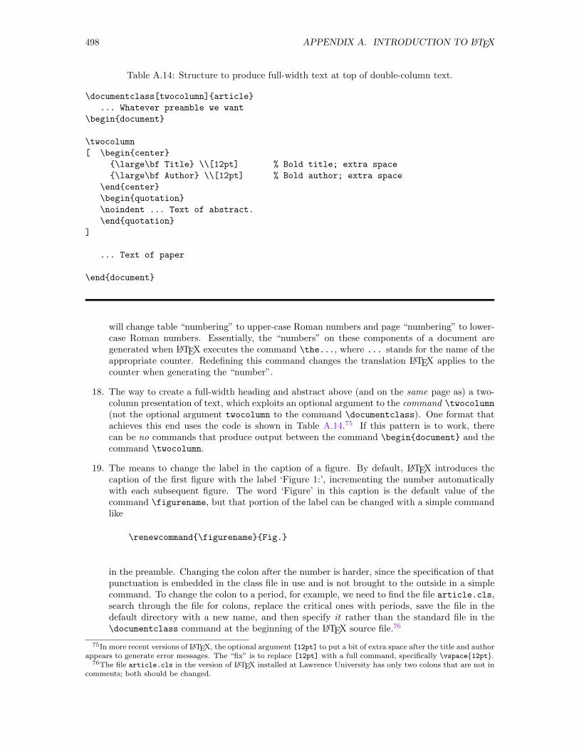
498 APPENDIX A. INTRODUCTION TO LATEX

Table A.14: Structure to produce full-width text at top of double-column text.

\documentclass[twocolumn]article

... Whatever preamble we want

\begindocument

\twocolumn

[ \begincenter

\large\bf Title \\[12pt] % Bold title; extra space

\large\bf Author \\[12pt] % Bold author; extra space

\endcenter

\beginquotation

\noindent ... Text of abstract.

\endquotation

]

... Text of paper

\enddocument

will change table “numbering” to upper-case Roman numbers and page “numbering” to lower-case Roman numbers. Essentially, the “numbers” on these components of a document aregenerated when LATEX executes the command \the..., where ... stands for the name of theappropriate counter. Redefining this command changes the translation LATEX applies to thecounter when generating the “number”.

18. The way to create a full-width heading and abstract above (and on the same page as) a two-column presentation of text, which exploits an optional argument to the command \twocolumn

(not the optional argument twocolumn to the command \documentclass). One format thatachieves this end uses the code is shown in Table A.14.75 If this pattern is to work, therecan be no commands that produce output between the command \begindocument and thecommand \twocolumn.

19. The means to change the label in the caption of a figure. By default, LATEX introduces thecaption of the first figure with the label ‘Figure 1:’, incrementing the number automaticallywith each subsequent figure. The word ‘Figure’ in this caption is the default value of thecommand \figurename, but that portion of the label can be changed with a simple commandlike

\renewcommand\figurenameFig.

in the preamble. Changing the colon after the number is harder, since the specification of thatpunctuation is embedded in the class file in use and is not brought to the outside in a simplecommand. To change the colon to a period, for example, we need to find the file article.cls,search through the file for colons, replace the critical ones with periods, save the file in thedefault directory with a new name, and then specify it rather than the standard file in the\documentclass command at the beginning of the LATEX source file.76

75In more recent versions of LATEX, the optional argument [12pt] to put a bit of extra space after the title and authorappears to generate error messages. The “fix” is to replace [12pt] with a full command, specifically \vspace12pt.

76The file article.cls in the version of LATEX installed at Lawrence University has only two colons that are not incomments; both should be changed.

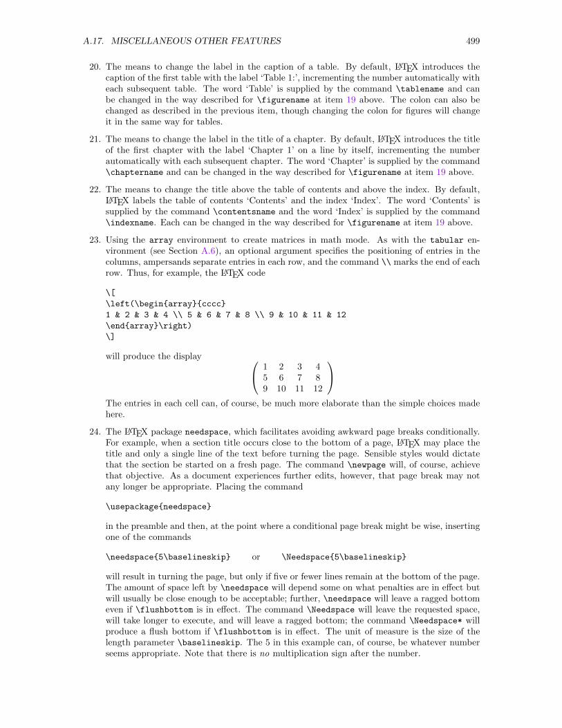
A.17. MISCELLANEOUS OTHER FEATURES 499

20. The means to change the label in the caption of a table. By default, LATEX introduces thecaption of the first table with the label ‘Table 1:’, incrementing the number automatically witheach subsequent table. The word ‘Table’ is supplied by the command \tablename and canbe changed in the way described for \figurename at item 19 above. The colon can also bechanged as described in the previous item, though changing the colon for figures will changeit in the same way for tables.

21. The means to change the label in the title of a chapter. By default, LATEX introduces the titleof the first chapter with the label ‘Chapter 1’ on a line by itself, incrementing the numberautomatically with each subsequent chapter. The word ‘Chapter’ is supplied by the command\chaptername and can be changed in the way described for \figurename at item 19 above.

22. The means to change the title above the table of contents and above the index. By default,LATEX labels the table of contents ‘Contents’ and the index ‘Index’. The word ‘Contents’ issupplied by the command \contentsname and the word ‘Index’ is supplied by the command\indexname. Each can be changed in the way described for \figurename at item 19 above.

23. Using the array environment to create matrices in math mode. As with the tabular en-vironment (see Section A.6), an optional argument specifies the positioning of entries in thecolumns, ampersands separate entries in each row, and the command \\ marks the end of eachrow. Thus, for example, the LATEX code

\[

\left(\beginarraycccc

1 & 2 & 3 & 4 \\ 5 & 6 & 7 & 8 \\ 9 & 10 & 11 & 12

\endarray\right)

\]

will produce the display 1 2 3 45 6 7 89 10 11 12

The entries in each cell can, of course, be much more elaborate than the simple choices madehere.

24. The LATEX package needspace, which facilitates avoiding awkward page breaks conditionally.For example, when a section title occurs close to the bottom of a page, LATEX may place thetitle and only a single line of the text before turning the page. Sensible styles would dictatethat the section be started on a fresh page. The command \newpage will, of course, achievethat objective. As a document experiences further edits, however, that page break may notany longer be appropriate. Placing the command

\usepackageneedspace

in the preamble and then, at the point where a conditional page break might be wise, insertingone of the commands

\needspace5\baselineskip or \Needspace5\baselineskip

will result in turning the page, but only if five or fewer lines remain at the bottom of the page.The amount of space left by \needspace will depend some on what penalties are in effect butwill usually be close enough to be acceptable; further, \needspace will leave a ragged bottomeven if \flushbottom is in effect. The command \Needspace will leave the requested space,will take longer to execute, and will leave a ragged bottom; the command \Needspace* willproduce a flush bottom if \flushbottom is in effect. The unit of measure is the size of thelength parameter \baselineskip. The 5 in this example can, of course, be whatever numberseems appropriate. Note that there is no multiplication sign after the number.

500 APPENDIX A. INTRODUCTION TO LATEX

25. The Windows batch command cleanTEX defined by the batch file

REM delete all TEX intermediate files

del *.aux *.log *.dvi *.toc *.ilg *.idx *.bak *.sav *.out *.ind

and the Unix shell script defined by the file

#!/bin/bash

# delete all TEX intermediate files

rm -f *.aux *.log *.dvi *.toc *.ilg *.idx *.bak

rm -f *.sav *.out *.ind

which facilitate removing all TEX/LATEX auxiliary files77 in the directory in which the commandor script is executed. These files can be created by direct typing or can be copied from thedirectory $HEAD/tex. The Windows file is executed by the simple statement cleanTEX at acommand window prompt, though a path to the file may be included if the file is not locatedin the directory to be purged of TEX/LATEX auxiliary files; the UNIX file is executed by thesimple statement ./cleanTEX, though the characters ./ may be replaced by the path to thefile if the file is not located in the directory to be purged of TEX/LATEX auxiliary files.

26. The Windows batch command cleanbak define by the the batch file

REM Delete .bak files

del /s *.bak

del /s *.sav

and the UNIX shell script cleanbak defined by the the file

#!/bin/bash

# Delete *.bak, *.sav, and *~ files

find . -name ’*.bak’ -exec rm \;

find . -name ’*.sav’ -exec rm \;

find . -name ’*~’ -exec rm \;

which facilitate removing all backup files78 in the directory in which the command or scriptis executed and in all subdirectories below that directory. These files can be created by directtyping or can be copied from the directory $HEAD/tex. The Windows file is executed by thesimple statement cleanbak at a command window prompt, though a path to the file may beincluded if the file is not located in the directory at the top of the tree to be purged of backupfiles; the UNIX file is executed by the simple statement ./cleanbak, though the characters ./may be replaced by the path to the file if the file is not located in the directory at the top ofthe tree to be purged of backup files.

A.18 References

As access to the web has expanded, more and more of the information that once was printed isavailable more readily on the web. Searching for help on specific issues, either on the web as awhole or (perhaps more effectively) more narrowly on the TEX Users Group site www.tug.org willyield valuable results. Further, when LATEX is installed in UNIX and UNIX-based operating systems(which includes Mac computers), the Shell command man, e.g. man hyperref, may bring up a

77Files with file types .aux, .log, .dvi, .toc, .ilg, .idx, .bak, .sav, .out, and ind.78Files with file types .bak and .sav and files for which the last character in the name is ~.

A.19. EXERCISES 501

page describing the indicated entity. In all full LATEX installations, the Shell command texdoc, e.g.texdoc hyperref, will bring up a description (though some of those descriptions are in languagesother than English).

Numerous books have also been written for a variety of audiences and with objectives rangingfrom general discussions to very specific focus on particular tasks. Among the more common booksare the following:

A Document Preparation System: LATEX User’s Guide and Reference Manual (Updated for LATEX2ε),Leslie Lamport (Addison-Wesley Publishing Co., Reading, MA, 1994). [ISBN 0-201-52983-1 or 978-0201529838] Throughout this aAppendix, this book is referred to as The LATEX Manual .

The LATEX Companion, Michel Goossens, Frank Mittelbach, et al. (Addison-Wesley Publishing Co.,Reading, MA). [ISBN 0-201-54199-8 (first edition, 1994); 0201362996 or 978-0201362992 (secondedition, 2004]

LATEX for Engineers and Scientists, David J. Buerger (McGraw-Hill Book Co., New York, 1990).[ISBN 0-07-008845-4]

The TEXbook, Donald E. Knuth (Addison-Wesley Publishing Co., Reading, MA, 1984, 1986). [ISBN0-201-13448-9 or 978-0201134483]

TEX for the Impatient, Paul W. Abrahams with Karl Berry and Kathryn A. Hargreaves (Addison-Wesley Publishing Co., Reading, MA, 1990). [ISBN 0-201-51375-7]

The LATEX Graphics Companion, Michael Goossens, Sebastian Rahtz, and Frank Mittelbach(Addison–Wesley Publishing Co., Reading, MA). [ISBN 0-201-85469-4, first edition, 1997;0321508920 or 978-0321508928, second edition, 2007]

A Guide to LATEX, Helmut Kopka and Patrick W. Daly (Addison–Wesley Publishing Co., Reading,MA). [ISBN 0-201-39825-7, third edition, 1999; 0321173856 or 978-0321173850, fourth edition, 2003]

Math Into LATEX (Third Edition), George Gratzer (Birkauser, Boston) [ISBN 0-8176-4131-9 or 978-0201433111, 2000]

The LATEX Web Companion Integrating TEX, HTML, and XML, Michael Goossens, Sebastian Rahtz,Eitan M. Gurari, and Ross Moore (Pearson Education, Inc.) [ISBN 0201433117 or 978-0201433111,1999]

Additional books will likely surface in a search for LaTeX on the Amazon or Barnes and Noblewebsites, though that search may also generate a number of hits for documents about rubber.

A.19 Exercises

A.1. Study carefully the LATEX code presented in Section A.16 and the resulting output in Table A.13,making sure you understand both the syntax of each command and the effect it produces in theoutput.

A.2. Use LATEX to write a letter to a friend. Format your letter so that it has

• a centered block at the top containing your name and address (center environment);

• a right-justified date (using \today and either \hfill or the flushright environment);

• a left-justified block containing an inside address (flushleft environment);

• a left-justified salutation;

• the body of the letter, containing more than one paragraph;

• a closing (e.g., Sincerely, With love, . . .) positioned 3.5” from the left margin; and

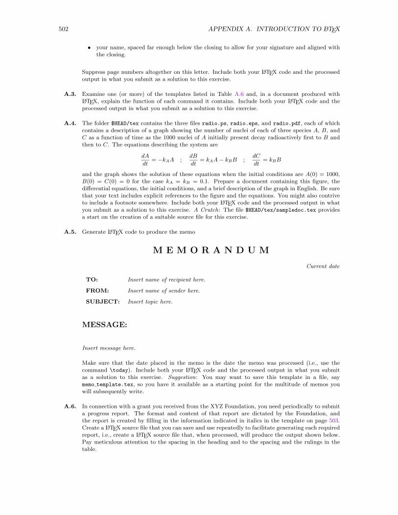
502 APPENDIX A. INTRODUCTION TO LATEX

• your name, spaced far enough below the closing to allow for your signature and aligned withthe closing.

Suppress page numbers altogether on this letter. Include both your LATEX code and the processedoutput in what you submit as a solution to this exercise.

A.3. Examine one (or more) of the templates listed in Table A.6 and, in a document produced withLATEX, explain the function of each command it contains. Include both your LATEX code and theprocessed output in what you submit as a solution to this exercise.

A.4. The folder $HEAD/tex contains the three files radio.ps, radio.eps, and radio.pdf, each of whichcontains a description of a graph showing the number of nuclei of each of three species A, B, andC as a function of time as the 1000 nuclei of A initially present decay radioactively first to B andthen to C. The equations describing the system are

dA

dt= −kAA ;

dB

dt= kAA− kBB ;

dC

dt= kBB

and the graph shows the solution of these equations when the initial conditions are A(0) = 1000,B(0) = C(0) = 0 for the case kA = kB = 0.1. Prepare a document containing this figure, thedifferential equations, the initial conditions, and a brief description of the graph in English. Be surethat your text includes explicit references to the figure and the equations. You might also contriveto include a footnote somewhere. Include both your LATEX code and the processed output in whatyou submit as a solution to this exercise. A Crutch: The file $HEAD/tex/sampledoc.tex providesa start on the creation of a suitable source file for this exercise.

A.5. Generate LATEX code to produce the memo

M E M O R A N D U M

Current date

TO: Insert name of recipient here.

FROM: Insert name of sender here.

SUBJECT: Insert topic here.

MESSAGE:

Insert message here.

Make sure that the date placed in the memo is the date the memo was processed (i.e., use thecommand \today). Include both your LATEX code and the processed output in what you submitas a solution to this exercise. Suggestion: You may want to save this template in a file, saymemo template.tex, so you have it available as a starting point for the multitude of memos youwill subsequently write.

A.6. In connection with a grant you received from the XYZ Foundation, you need periodically to submita progress report. The format and content of that report are dictated by the Foundation, andthe report is created by filling in the information indicated in italics in the template on page 503.Create a LATEX source file that you can save and use repeatedly to facilitate generating each requiredreport, i.e., create a LATEX source file that, when processed, will produce the output shown below.Pay meticulous attention to the spacing in the heading and to the spacing and the rulings in thetable.

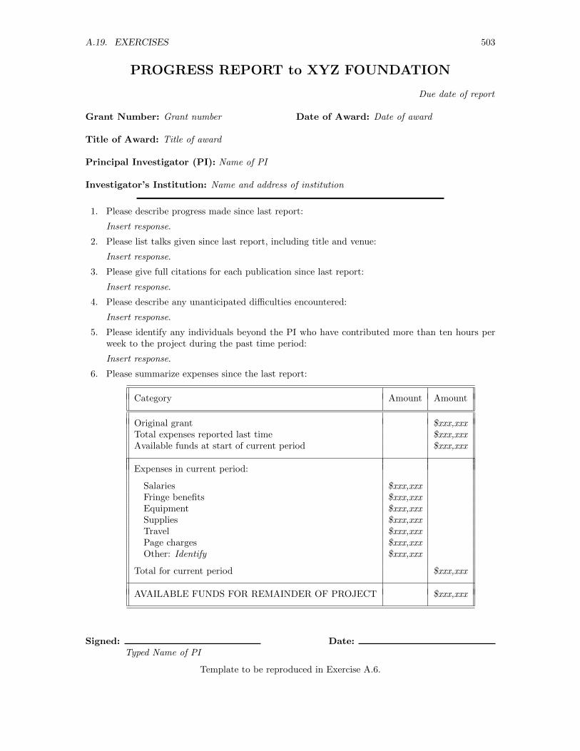
A.19. EXERCISES 503

PROGRESS REPORT to XYZ FOUNDATION

Due date of report

Grant Number: Grant number Date of Award: Date of award

Title of Award: Title of award

Principal Investigator (PI): Name of PI

Investigator’s Institution: Name and address of institution

1. Please describe progress made since last report:

Insert response.

2. Please list talks given since last report, including title and venue:

Insert response.

3. Please give full citations for each publication since last report:

Insert response.

4. Please describe any unanticipated difficulties encountered:

Insert response.

5. Please identify any individuals beyond the PI who have contributed more than ten hours perweek to the project during the past time period:

Insert response.

6. Please summarize expenses since the last report:

Category Amount Amount

Original grant $xxx,xxxTotal expenses reported last time $xxx,xxxAvailable funds at start of current period $xxx,xxx

Expenses in current period:

Salaries $xxx,xxxFringe benefits $xxx,xxxEquipment $xxx,xxxSupplies $xxx,xxxTravel $xxx,xxxPage charges $xxx,xxxOther: Identify $xxx,xxx

Total for current period $xxx,xxx

AVAILABLE FUNDS FOR REMAINDER OF PROJECT $xxx,xxx

Signed: Date:Typed Name of PI

Template to be reproduced in Exercise A.6.

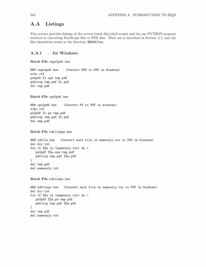
504 APPENDIX A. INTRODUCTION TO LATEX

A.A Listings

This section provides listings of the several batch files/shell scripts and the one PYTHON programinvolved in converting PostScript files to PDF files. Their use is described in Section A.8, and thefiles themselves reside in the directory $HEAD/tex.

A.A.1 . . . for Windows

Batch File ceps2pdf.bat

REM ceps2pdf.bat (Convert EPS to PDF in Windows)

echo off

ps2pdf %1.eps tmp.pdf

pdfcrop tmp.pdf %1.pdf

del tmp.pdf

Batch File cps2pdf.bat

REM cps2pdf.bat (Convert PS to PDF in Windows)

echo off

ps2pdf %1.ps tmp.pdf

pdfcrop tmp.pdf %1.pdf

del tmp.pdf

Batch File rdfileeps.bat

REM rdfile.bat (Convert each file in nameonly.txt to PDF in Windows)

del dir.txt

for /f %%a in (nameonly.txt) do (

ps2pdf %%a.eps tmp.pdf

pdfcrop tmp.pdf %%a.pdf

)

del tmp.pdf

del nameonly.txt

Batch File rdfileps.bat

REM rdfileps.bat (Convert each file in nameonly.txt to PDF in Windows)

del dir.txt

for /f %%a in (nameonly.txt) do (

ps2pdf %%a.ps tmp.pdf

pdfcrop tmp.pdf %%a.pdf

)

del tmp.pdf

del nameonly.txt

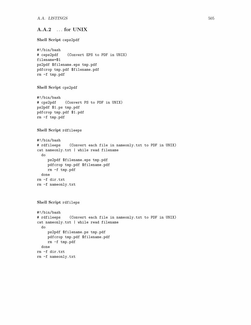
A.A. LISTINGS 505

A.A.2 . . . for UNIX

Shell Script ceps2pdf

#!/bin/bash

# ceps2pdf (Convert EPS to PDF in UNIX)

filename=$1

ps2pdf $filename.eps tmp.pdf

pdfcrop tmp.pdf $filename.pdf

rm -f tmp.pdf

Shell Script cps2pdf

#!/bin/bash

# cps2pdf (Convert PS to PDF in UNIX)

ps2pdf $1.ps tmp.pdf

pdfcrop tmp.pdf $1.pdf

rm -f tmp.pdf

Shell Script rdfileeps

#!/bin/bash

# rdfileeps (Convert each file in nameonly.txt to PDF in UNIX)

cat nameonly.txt | while read filename

do

ps2pdf $filename.eps tmp.pdf

pdfcrop tmp.pdf $filename.pdf

rm -f tmp.pdf

done

rm -f dir.txt

rm -f nameonly.txt

Shell Script rdfileps

#!/bin/bash

# rdfileeps (Convert each file in nameonly.txt to PDF in UNIX)

cat nameonly.txt | while read filename

do

ps2pdf $filename.ps tmp.pdf

pdfcrop tmp.pdf $filename.pdf

rm -f tmp.pdf

done

rm -f dir.txt

rm -f nameonly.txt

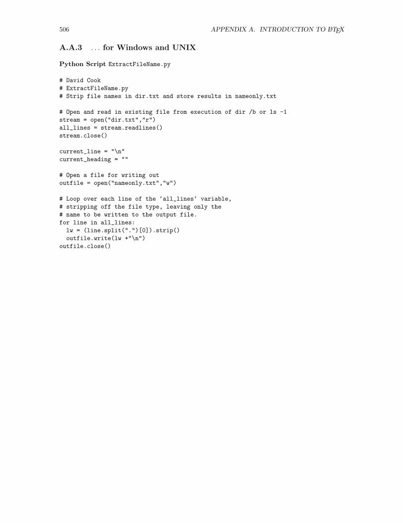
506 APPENDIX A. INTRODUCTION TO LATEX

A.A.3 . . . for Windows and UNIX

Python Script ExtractFileName.py

# David Cook

# ExtractFileName.py

# Strip file names in dir.txt and store results in nameonly.txt

# Open and read in existing file from execution of dir /b or ls -1

stream = open("dir.txt","r")

all_lines = stream.readlines()

stream.close()

current_line = "\n"

current_heading = ""

# Open a file for writing out

outfile = open("nameonly.txt","w")

# Loop over each line of the ‘all_lines‘ variable,

# stripping off the file type, leaving only the

# name to be written to the output file.

for line in all_lines:

lw = (line.split(".")[0]).strip()

outfile.write(lw +"\n")

outfile.close()

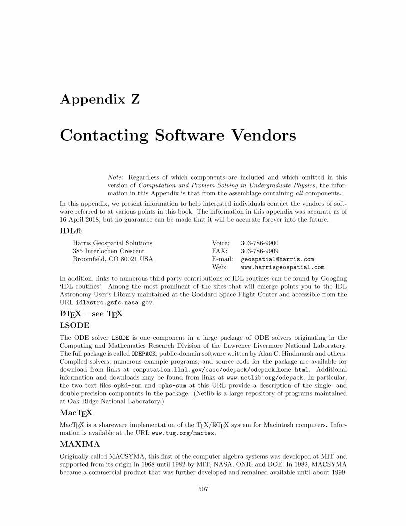
Appendix Z

Contacting Software Vendors

Note: Regardless of which components are included and which omitted in thisversion of Computation and Problem Solving in Undergraduate Physics, the infor-mation in this Appendix is that from the assemblage containing all components.

In this appendix, we present information to help interested individuals contact the vendors of soft-ware referred to at various points in this book. The information in this appendix was accurate as of16 April 2018, but no guarantee can be made that it will be accurate forever into the future.

IDL r©

Harris Geospatial Solutions385 Interlochen CrescentBroomfield, CO 80021 USA

Voice: 303-786-9900FAX: 303-786-9909E-mail: geospatial@harris.com

Web: www.harrisgeospatial.com

In addition, links to numerous third-party contributions of IDL routines can be found by Googling‘IDL routines’. Among the most prominent of the sites that will emerge points you to the IDLAstronomy User’s Library maintained at the Goddard Space Flight Center and accessible from theURL idlastro.gsfc.nasa.gov.

LATEX – see TEX

LSODE

The ODE solver LSODE is one component in a large package of ODE solvers originating in theComputing and Mathematics Research Division of the Lawrence Livermore National Laboratory.The full package is called ODEPACK, public-domain software written by Alan C. Hindmarsh and others.Compiled solvers, numerous example programs, and source code for the package are available fordownload from links at computation.llnl.gov/casc/odepack/odepack home.html. Additionalinformation and downloads may be found from links at www.netlib.org/odepack, In particular,the two text files opkd-sum and opks-sum at this URL provide a description of the single- anddouble-precision components in the package. (Netlib is a large repository of programs maintainedat Oak Ridge National Laboratory.)

MacTEX

MacTEX is a shareware implementation of the TEX/LATEX system for Macintosh computers. Infor-mation is available at the URL www.tug.org/mactex.

MAXIMA

Originally called MACSYMA, this first of the computer algebra systems was developed at MIT andsupported from its origin in 1968 until 1982 by MIT, NASA, ONR, and DOE. In 1982, MACSYMAbecame a commercial product that was further developed and remained available until about 1999.

507

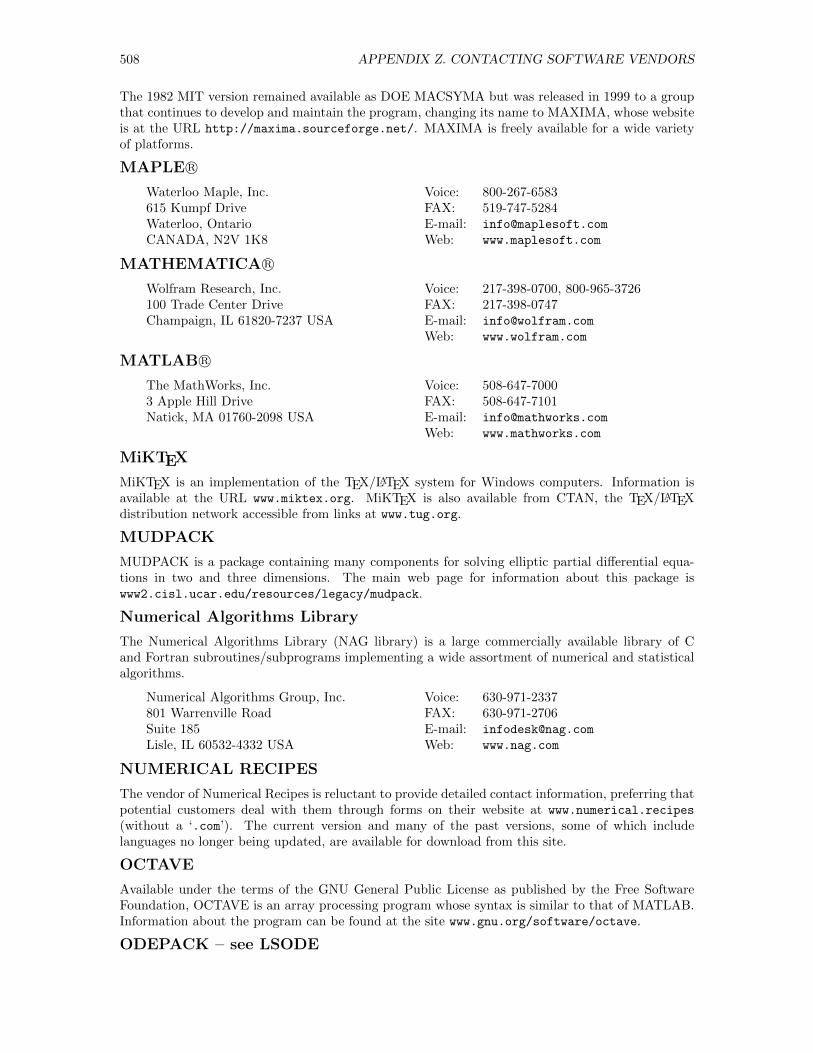
508 APPENDIX Z. CONTACTING SOFTWARE VENDORS

The 1982 MIT version remained available as DOE MACSYMA but was released in 1999 to a groupthat continues to develop and maintain the program, changing its name to MAXIMA, whose websiteis at the URL http://maxima.sourceforge.net/. MAXIMA is freely available for a wide varietyof platforms.

MAPLE r©

Waterloo Maple, Inc.615 Kumpf DriveWaterloo, OntarioCANADA, N2V 1K8

Voice: 800-267-6583FAX: 519-747-5284E-mail: info@maplesoft.com

Web: www.maplesoft.com

MATHEMATICA r©

Wolfram Research, Inc.100 Trade Center DriveChampaign, IL 61820-7237 USA

Voice: 217-398-0700, 800-965-3726FAX: 217-398-0747E-mail: info@wolfram.com

Web: www.wolfram.com

MATLAB r©

The MathWorks, Inc.3 Apple Hill DriveNatick, MA 01760-2098 USA

Voice: 508-647-7000FAX: 508-647-7101E-mail: info@mathworks.com

Web: www.mathworks.com

MiKTEX

MiKTEX is an implementation of the TEX/LATEX system for Windows computers. Information isavailable at the URL www.miktex.org. MiKTEX is also available from CTAN, the TEX/LATEXdistribution network accessible from links at www.tug.org.

MUDPACK

MUDPACK is a package containing many components for solving elliptic partial differential equa-tions in two and three dimensions. The main web page for information about this package iswww2.cisl.ucar.edu/resources/legacy/mudpack.

Numerical Algorithms Library

The Numerical Algorithms Library (NAG library) is a large commercially available library of Cand Fortran subroutines/subprograms implementing a wide assortment of numerical and statisticalalgorithms.

Numerical Algorithms Group, Inc.801 Warrenville RoadSuite 185Lisle, IL 60532-4332 USA

Voice: 630-971-2337FAX: 630-971-2706E-mail: infodesk@nag.com

Web: www.nag.com

NUMERICAL RECIPES

The vendor of Numerical Recipes is reluctant to provide detailed contact information, preferring thatpotential customers deal with them through forms on their website at www.numerical.recipes

(without a ‘.com’). The current version and many of the past versions, some of which includelanguages no longer being updated, are available for download from this site.

OCTAVE

Available under the terms of the GNU General Public License as published by the Free SoftwareFoundation, OCTAVE is an array processing program whose syntax is similar to that of MATLAB.Information about the program can be found at the site www.gnu.org/software/octave.

ODEPACK – see LSODE

APPENDIX Z. CONTACTING SOFTWARE VENDORS 509

OzTEX

OzTEX is a shareware implementation of the TEX/LATEX system for Macintosh computers. Infor-mation is available at the URL www.trevorrow.com/oztex. OzTEX is also available from CTAN,the TEX/LATEX distribution network accessible from links at www.tug.org.

PYTHON/NUMPY/MATPLOTLIB/PLOTLY/MAYAVI/SCIKIT-IMAGE

PYTHON, a high-level programming language created by Guido van Rossum, was first releasedin 1991. In execution, PYTHON programs are interpreted, not compiled. Information and freedownloads are available at the URL www.python.org. Information about various add-on modulescan be found as follows:

• The module numpy, which adds numerous mathematical capabilities (arrays, matrices, math-ematical functions, . . .) to PYTHON, is described at the URL www.numpy.org.

• The module matplotlib, which adds numerous 2D plotting capabilities and a few 3D plottingcapabilities to PYTHON, is described at the URL matplotlib.org.

• The module plotly, which provides several 3D plotting capabilities, is described at the URLplot.ly.

• The module mayavi, which provides numerous capabilities for 3D data visualisation and plot-ting, is described at the URL docs.enthought.com/mayavi/mayavi.

• The module scikit-image, which includes scimage and provides image processing capabilities,is described at the URL scikit-image.org.

There are numerous distributions of PYTHON. A popular distribution that automatically in-cludes numerous modules that might not be included in many other distributions is described atwww.anaconda.com.

TEX/LATEX/dvips/graphicx/makeindex/xdvi/dvips/...

The primary site for information (history, current plans, downloads, . . .) for TEX, LATEX, and nu-merous other publicly available components of TEX and its derivatives is the web site of the TEXUsers’ Group (TUG), www.tug.org. This organization maintains CTAN (the Comprehensive TEXArchive Network), which has a handful of backbone machines around the world and a number ofmirror sites, from any of which an enormous number of files associated with the TEX/LATEX systemcan be downloaded.

TEXlive

TEXlive is among the newer implementations of the TEX/LATEX system for all platforms. Informationabout this distribution and instructions for downloading and installing it are available from the URLwww.tug.org/texlive.

TGIF

TGIF (pronounced T-G-I-F) is a versatile program for creating two-dimensional drawings. Theprogram is Xlib-based and interactive, and it runs under X11 on LINUX and UNIX platforms (in-cluding MAC OS X and cygwin on Windows). Information (brief history, licensing understandings,instructions for downloading, . . .) about TGIF is available from the URL bourbon.usc.edu/tgif/.

Winedt

Winedt is an inexpensive ($40.00 per student user, $60 per educational user) editor for Intel-basedmachines running one or another version of Microsoft Windows. It has particular features thatmake it especially suitable for creating source files for TEX/LATEX. Information about licensing anddownloads can be found at the URL www.winedt.com. Winedt is also available from CTAN, theTEX/LATEX distribution network accessible from links at www.tug.org.

510 APPENDIX Z. CONTACTING SOFTWARE VENDORS

Xemacs

This flexible, open source text editor is available from a variety of sources and is protected underthe terms of the GNU Public License. Downloads and information about the program can be foundat the URL xemacs.sourceforge.net.

Xv

Written, maintained, and copyrighted by John Bradley, xv is an interactive image manipulationprogram that runs in X-windows. Downloads, information about the program, and informationabout licensing and registering is available at the URL www.trilon.com.

Index

The user of this index should be aware that not only textual discussions but also some of theproblems are indexed. Page numbers displayed in Roman type refer to textual discussions; pagenumbers displayed in Italic type refer to problems.

Symbols

$HEAD, 11, 15, 125, 171, 178, 183, 185, 188, 189,192, 193, 197, 271, 294, 297, 299, 301,303, 304, 306, 308, 310, 338, 356, 372,374, 378, 380, 411, 412, 427, 430, 434,436, 459

$IDLHEAD, 11$MATHEMHEAD, 137$NRHEAD, 11, 229–232, 299–301, 303, 306–310,

374–376, 380, 382, 430–433, 436, 437,439, 440

A

aborting executionin C, 178in FORTRAN, 171in MATHEMATICA, 92in OCTAVE, 16

accuracyin evaluating integrals, 351–353, 356–359,

372–374, 378–380in finding roots, 410–411in solving ODEs, 268–269, 279, 282

with conservation laws, 269, 282acroread, 464action statements, 151, 153–154Adams/Bashforth/Moulton (ABM) methods,

270–271adaptive methods

for integrals, 353for ODEs, 269–270, 299, 306

adding text to graphics, see placing text ingraphics

algorithmsdefinition, 151for a2 + b2 = c2, 202for adding, 203for bowling, 201for controlling loops, 160

for counting, 160, 161for exchange, 160for finding extremes, 161, 162for integration, 348–356for Laplace’s equation, 162for ODEs, 262–271for parking lot, 201for root finding, 408–411for searching, 162, 202for sorting, 203for summing, 161

animationin MATHEMATICA, 133in OCTAVE, 69–70

arithmetic operatorsin C, 175in FORTRAN, 169in MATHEMATICA, 95in OCTAVE, 22

array indicesin C, 175in FORTRAN, 169in MATHEMATICA, 100in OCTAVE, 19, 187in pseudocode, 153

arraysfor data storage, 164in C, 175in FORTRAN, 169in MATHEMATICA, 99in OCTAVE, 19–21in pseudocode, 153scalar, see scalar fieldsvector, see vector fields

ASCII character codes, 5ASCII text files, 8aspell, 491–492assigning values to variables

in C, 177in FORTRAN, 169

511

512 INDEX

in MATHEMATICA, 96–97in OCTAVE, 18in pseudocode, 154

B

backsubstitution, 441Bessel functions, 388, 449binary files, 8binary number system, 4–5Biot-Savart law, 341bisection, see root findingbit, 4–5black body radiation, 144, 387blocking statements, see also control structures

in C, 177in MATHEMATICA, 123in OCTAVE, 33, 34in pseudocode, 156, 166

Boolean values, see logical expressionsBoolean variables, see logical expressionsboundary value problems, 235, 246, 256–259, 454byte, 5–6

C

C, 1C commands

fclose, 186, 195, 305, 308fgets, 200fopen, 178, 186, 195, 199, 305, 308, 310fprintf, 178, 186, 195, 305, 308, 310fscanf, 200main, 175, 185, 194printf, 176, 177, 180, 305, 378, 381, 382,

434–437return, 181scanf, 180, 305, 378, 434, 435, 437

C control structuresdo/while, 180, 310for, 176–178, 185, 186, 194, 195, 200, 305,

308, 378, 381if/else, 179, 436switch/case/default, 179while, 180, 434, 436

C data typeschar, 175, 200file, 178, 185, 194, 199float, 175, 176, 185, 194, 200int, 175, 176, 185, 194, 200

C directives, 175#define, 175, 176, 185, 194#include, 175, 176, 185, 194

C functionscos, 194, 439exp, 381, 382pow, 175, 185, 381, 382, 434, 435sin, 185, 194, 437, 439sqrt, 381, 382

user-defined, 181C header files

math.h, 175, 185, 194, 378, 381, 382, 434,437

nr.h, 232, 233, 309, 310, 380–382, 437, 439nrutil.h, 309, 310, 437, 439stdio.h, 175, 185, 194, 378, 381, 382, 434,

437C programs

bisect.c, 435–436, 458decay.c, 305, 323–324decayrk4.c, 308, 324decayrkqs.c, 310, 325errqtrap.c, 381–383, 390, 391errtrapzd.c, 380–381, 390guessroot.c, 434irrad.c, 184–186, 209–210laplace.c, 176, 178laplace file.c, 178pdens.c, 189, 215–216quadpole.c, 197, 223–225read irrad.c, 227sinrtbis.c, 437sinrtnewt.c, 439trapezoidal.c, 379, 393wavegd.c, 192–193, 219–220

C special symbols\n (new line), 177, 178, 186, 195, 305, 308,

310, 378, 434–437* (multiplication), 175+ (addition), 175++ (incrementing index), 200, 378, 381- (subtraction), 175/ (division), 175/*. . .*/ (comment), 175%d (format), 177, 180, 186, 195, 200, 305,

381%e (format), 177, 186, 195%f (format), 177, 178, 180, 305, 308, 310,

381, 382, 434–437%g (format), 200%s (format), 381& (pointer), 180, 305, 310, 434, 435, 437, 440braces, 177

cardioid, 45, 385carrying capacity, 240, 251–252Cartesian coordinates

in MATHEMATICA, 149case sensitivity

in C, 175in FORTRAN, 167in MATHEMATICA, 92in OCTAVE, 16in pseudocode, 152

cc, see UNIX commandscells

in a MATHEMATICA notebook, 101center of mass

definition of, 328

INDEX 513

of cardioid, 385of semicircular plate, 329, 337

central processing unit, 3chaos

Lorenz system, 317character codes, 4–5character strings

in MATHEMATICA, 94in OCTAVE, 17

characteristic equation, 398charging capacitor, 83classification

of integrals, 327of ODEs, 235

closing notebookin MATHEMATICA, 93

colorin OCTAVE, see also OCTAVE properties,

color, edgecolor, facecolor,linecolor, 27, 29

combining statements on one linein C, 175in MATHEMATICA, 92in OCTAVE, 16, 33, 34in pseudocode, 156

command filesin MATHEMATICA, see MATHEMATICA

command filesin OCTAVE, see OCTAVE scripts

command line editingin MATHEMATICA, 101in OCTAVE, 16

command/function dualityin OCTAVE, 19, 21

commandsin C, see C commandsin FORTRAN, see FORTRAN commandsin MATHEMATICA, see MATHEMATICA

commandsin OCTAVE, see OCTAVE commandsin pseudocode, see pseudocommands

comments, see also documentationin C, 175in FORTRAN, 167in LATEX, 492in MATHEMATICA, 125in OCTAVE, 16, 38, 41in pseudocode, 156–157, 160

common storagein C, see global variablesin FORTRAN, 174, 300in OCTAVE, see global variables

compiler directives, 153in C, see C directivesin FORTRAN, see FORTRAN directivesin pseudocode, see pseudocode directives

compiling source file, see Local Guide, 152in C, 178, 186, 305, 309, 310, 379, 380, 382,

434, 436, 438, 439

in FORTRAN, 171, 184, 298, 301, 303, 373,375, 376, 428, 430–432

complex numbersin MATHEMATICA, 105–107in OCTAVE, 19

Compton scattering, 84conditions, see logical conditionsconstants

in MATHEMATICA, see MATHEMATICAconstants

in OCTAVE, see OCTAVE system variablescontact information, 507–510continuing statement on second line

in C, 175in FORTRAN, 170in MATHEMATICA, 92in OCTAVE, 16in pseudocode, 156

control characters, 4control structures

in C, see C control structuresin FORTRAN, see FORTRAN control

structuresin MATHEMATICA, see MATHEMATICA

control structuresin OCTAVE, see OCTAVE control

structuresin pseudocode, see pseudocode control

structuresconvergence criteria, 164, 268–269, 351–353,

410–411convert.eps/.ps to .pdf, 486–487convert.pdf to .eps/.ps, 487Cornu spiral, 332, 364–366coupled oscillators, 242–243, 255–256, 312CPU, see central processing unitCramer’s rule, 441cross product

in MATHEMATICA, 125–126, 150in OCTAVE, 24, 81

current directory, see also default directoryin OCTAVE, 47, 50, 77–78

curve fitting, see least squares fittingto parabola, 148, 452

customizingMATHEMATICA, 135OCTAVE, 78–79

cylindrical coordinatesin MATHEMATICA, 149

D

data analysis, 331data files

decay c.dat, 306, 323–324decay f.dat, 299, 320decayrk4 c.dat, 308, 324decayrk4 f.dat, 301, 321decayrkqs c.dat, 310, 325

514 INDEX

decayrkqs f.dat, 302, 322freefall.dat, 452, 453irrad c.dat, 184–186, 199–200, 209–210,

227irrad f.dat, 184, 198–199, 208, 226irrad octave.dat, 187, 200laplace c.dat, 178–179, 205laplace f.dat, 171, 205ldrum.dat, 69pdens c.dat, 189, 215–216pdens f.dat, 188, 213–214pdens octave.dat, 190quadpole c.dat, 197, 223–225quadpole f.dat, 197, 221–222quadpole octave.dat, 198radio.dat, 35, 37, 38rcdata.dat, 47ruchardt.dat, 455wavegd c.dat, 192–193, 219–220wavegd f.dat, 192, 217–218wavegd octave.dat, 195

data typesfloating point, 6–7integer, 6–7string, 6–7

data typingexplicit, 153implicit, 153in C, 175in FORTRAN, 169in OCTAVE, 17in pseudocode, 152–153, 155

default directory, see also current directory, 9in MATHEMATICA, 124, 131, 132, 136–137in OCTAVE, 30–32, 277, 284, 361

defining ODEsfor MATHEMATICA, 115, 249, 251, 252,

255, 256, 295for OCTAVE, 273–275

deleting functionsin MATHEMATICA, 98

deleting variablesin MATHEMATICA, 97, 98, 109in OCTAVE, 21, 33, 34

demosin MATHEMATICA, 91, 93

diffraction patterns, see also interferencepatterns, 182, 389, 449, 451

of square aperture, 51–58dimensionless casting

for plotting, 85of integrals, 329–331, 333, 341, 384, 387of ODEs, 118–119, 236–241, 243–245,

251–252, 397, 399discretizing

Laplace’s equation, 163displaying data on screen

in C, 176, 177in FORTRAN, 168, 170

in MATHEMATICA, 92in OCTAVE, 19–20in pseudocode, 154

dividing statement between lines, see continuingstatement on second line

documentation, see also commentsin MATHEMATICA notebooks, 134–135in OCTAVE m-files, 41

dot productin MATHEMATICA, 125–126, 150in OCTAVE, 23, 81

double factorial, 12drawing space curves

with MATHEMATICA, 138–139with OCTAVE, 73–74

dvipdfm, 464dvips, 463, 481

E

electric field, 332in wave guide, 66–67, 190–195of dipole, 207of quadrupole, 195–198of relativistic particle, 85

electrostatic potential, 332of charged disks, 83, 84, 384of charged rings, 332–333, 367, 371–372, 389of finite line charge, 338–340of spherically symmetric distribution, 385

elliptic integrals, 148, 331, 388em dash, 472em space, 469en dash, 472en space, 469energy levels

in quantum oscillator, see harmonicoscillator

in quantum well, 259, 401, 418–420,424–427, 449

equilibrium points, 396, 404–405equivalent resistance, 452error function, 332, 334, 356, 361, 363, 364,

370–371, 373, 375, 379, 380, 387error messages

in LATEX, 489–490Euler’s method, 262–264, 271–273, 297–299,

304–306improved, see improved Euler method

evaluating integralswith C, 378–383with FORTRAN, 372–377with MATHEMATICA, 112, 335–347,

368–372with OCTAVE, 356–368

exchange algorithm, 160executing program, see Local Guideexiting

from MATHEMATICA, 93

INDEX 515

from OCTAVE, 16expressing infinity

in MATHEMATICA, 336expressions

in MATHEMATICA, 94–96

F

f77, see UNIX commandsFabry-Perot interferometer, 83factorial, 12, 102Fibonacci numbers, 82field mapping, 87, 88finding eigenvalues/eigenvectors

with MATHEMATICA, 110–111, 145, 146with OCTAVE, 41–42, 82

finding roots, see root findingfinite difference approximations

for derivatives, 203fitting data, see curve fitting, least squares fittingfloating point number

double precision, 7single precision, 6

fonts, see also Greek lettersin OCTAVE, 71–73

formatting data files, 164–165formatting output

in C, 177, 186, 195in FORTRAN, 170in OCTAVE, 31in pseudocode, 154

FORTRAN, 1position of statements on line, 169

FORTRAN commandsclose, 184, 193, 199, 298, 301format, 173, 184, 193, 301, 302open, 171, 184, 193, 198, 298, 301, 302read, 172, 173, 199, 298, 373, 428, 429, 431write, 168, 170–173, 184, 193, 298,

301–303, 373, 375, 428–431FORTRAN control structures

call, 174, 301–303, 375, 433do while/enddo, 173, 303, 428, 429do/enddo, 168–171, 184, 192, 193, 199, 298,

301, 373, 375do/enddo , 183function/return, 174, 373, 375, 377if/then/else/endif, 172, 429program/end, 169, 183, 191–192, 375, 377,

431subroutine/return, 173, 300, 432

FORTRAN data typescharacter, 169, 199double precision, 169integer, 169real, 169

FORTRAN directivescommon, 174, 300, 301, 303dimension, 168, 183, 192, 199, 300, 301, 303

external, 375, 377, 431implicit, 169parameter, 168, 169, 183, 192

FORTRAN functionscos, 192, 432exp, 373, 375, 377sin, 183, 192, 431, 432sqrt, 373, 375, 377user-defined, 174, 431

FORTRAN programsbisect.f, 429–430, 457decay.f, 298, 320decayrk4.f, 301, 321decayrkqs.f, 303, 322errqtrap.f, 375–377, 390errtrapzd.f, 374–375, 390guessroot.f, 428irrad.f, 183–184, 208laplace.f, 168, 171laplace file.f, 171pdens.f, 188, 213–214quadpole.f, 196–197, 221–222read irrad.f, 226sinrtbis.f, 431sinrtnewt.f, 432–433trapezoidal.f, 373, 392wavegd.f, 191–192, 217–218

FORTRAN special symbols! (comments), 167* (multiplication), 169** (exponentiation), 169, 183, 373, 375, 377,

428, 429+ (addition), 169- (subtraction), 169/ (division), 169A (in format statements), 173, 298, 373, 377,

428, 429, 431C (comments), 167E (in format statements), 170F (in format statements), 170, 171, 298, 301,

302, 373, 375, 377, 431I (in format statements), 170, 375

FORTRAN subroutines, 173–174user-defined, 432

four-slit interference pattern, 85Fourier series, 335, 345–347, 385Fraunhofer diffraction, 182–187Fresnel integrals, see also Cornu spiral, 332, 389functions

in C, see C functionsin FORTRAN, see FORTRAN functionsin MATHEMATICA, see MATHEMATICA

functionsin OCTAVE, see OCTAVE functionstypical available, 154

G

gamma function, 12–13

516 INDEX

Gauss-Kronrod rule, see quadratureGaussian distribution, 331, 387Gaussian elimination, 441–442Gaussian integration, see quadraturegedit, 1ghostview, 464global positioning, 452global truncation error, see truncation error,

globalglobal variables

in C, 181–182, 307in FORTRAN, see common storagein OCTAVE, 39–41, 367

golden ratio, 448gravitational force, 244Greek letters, see also fonts

in LATEX, 472–473in MATHEMATICA, 94in OCTAVE, 53, 72

H

handlesin OCTAVE, 29–30, 64–65, 72, 74–75

hard copyfrom MATHEMATICA, 129–132from OCTAVE, 49–50

harmonic oscillator, 115–119, 141, 144, 240–241,252, 279–280, 287–292, 311, 314, 316

Helmholtz coil, 340–344help, see on-line helphexadecimal number system, 5high-pass filter, 47–49high-resolution graphing

in MATHEMATICA, 126–129in OCTAVE, 25–28, 43–49, 51–69

Hooke’s law, 397hyperlinks, 485–486

I

IDL, 1IDL contact information, 507improved Euler method, 264–265, 272indices in LATEX, 483indicial equation, 259inert commands

in MATHEMATICA, see suppressingevaluation in MATHEMATICA

inhomogenieties in linear equations, 441initial value problems, 235initialization files

in MATHEMATICA, 135in OCTAVE, 78–79

integersigned, 6unsigned, 6

interference patterns, see also diffractionpatterns

Fabry-Perot, 83from four slits, 85

internal storage of expressionsin MATHEMATICA, 95–96

interpolation points, 349, 350interpreting source code, see also Local Guide,

152interrupt

in MATHEMATICA, 92in OCTAVE, 16

ispell, 491–492

K

keywordsin OCTAVE, see OCTAVE properties

Kirchoff’s laws, 452Knuth, Donald, 459Kronecker delta, 334

L

Lagrange equationsfor 2D harmonic oscillator, 146for compound pendulum, 147

Laguerre polynomials, 144Laguerre’s method, see root findingLamport, Leslie, 459Laplace transforms, 13–14, 247–248, 313

definition, 13, 114, 247for ODEs, 247in MATHEMATICA, 114, 148

Laplace’s equation, 454in C, 175–179, 205in FORTRAN, 167–171, 205in OCTAVE, 182in pseudocode, 162–164

LATEX, 1accents in, 495counters in, 496dashes in, 471math mode in, 472–473quotation marks in, 472special characters in, 496

latex, 462, 463, 481LATEX commands

\/ (italic correction), 468\\ (new line), 470, 475\! (negative thin space), 473\, (thin space), 473\- (allow hyphen) , 472\: (medium space), 473\; (thick space), 473\addcontentsline, 482–483\addtocontents, 482–483\Alph, 474, 497\alph, 474, 497\and, 488\arabic, 474

INDEX 517

\author, 492\bf, 492\bfseries, 468\boldmath, 473\cal, 495\caption, 475, 476, 478, 481\centerline, 478\chapter, 472\chaptername, 499\char, 496\clearpage, 469\contentsname, 499\date, 492\definecolor, 485, 489\documentclass, 460, 462, 465, 486, 492\documentstyle, 460\fbox, 496\figurename, 498\footnote, 472, 492\footnotesize, 469\frac, 492\framebox, 496\hspace, 469, 470\hspace*, 469\Huge, 469\huge, 469\IfFileExists, 489\ifthenelse, 488–489\includegraphics, 476–479, 486\index, 483\indexname, 499\input, 495\int, 492\item, 473–474, 497\itshape, 468\label, 472, 475, 476, 478, 481, 492\labelitemi, 474\labelitemii, 474\labelitemiii, 474\labelitemiv, 474\LARGE, 469\Large, 469, 492\large, 469\LaTeX, 492\listoffigures, 482–483\listoftables, 482–483\makebox, 496\makeindex, 483–484\maketitle, 492\mathbf, 473\mathcal, 495\mathit, 473\mathrm, 473\mathtt, 473\mbox, 472, 473, 496\mdseries, 468\Needspace, 499\needspace, 499\newboolean, 488–489

\newcommand, 493\newcounter, 497\newlength, 470\newpage, 469\noindent, 469, 492\normalfont, 468\normalsize, 469\not, 488\or, 488\pageref, 472, 475, 476\pagestyle, 492, 495\parbox, 496\part, 472\partial, 492\printindex, 483\qquad, 469\quad, 469\ref, 472, 475, 476, 492\renewcommand, 471, 474, 494, 497, 498\rmfamily, 468\Roman, 474, 498\roman, 474, 498\rule, 496\scriptsize, 469\scshape, 468\section, 472\setboolean, 488–489\setcounter, 497\setlength, 465, 469, 492\settodepth, 469\settoheight, 469\settowidth, 470\sffamily, 468\slshape, 468\small, 469\subsection, 472\subsubsection, 472\tablename, 499\tableofcontents, 482–483\textbf, 468\textit, 468\textmd, 468\textnormal, 468\textrm, 468\textsc, 468\textsf, 468\textsl, 468\texttt, 468\textup, 468\the..., 497–498\theenumi, 474\thenumii, 474\theenumiii, 474\theenumiv, 474\thispagestyle, 492, 495\tiny, 469\title, 492\today, 493, 494\ttfamily, 468

518 INDEX

\twocolumn, 498\typein, 489\typeout, 489\upshape, 468\usepackage, 471, 477, 483\value, 497\verb, 468, 492, 496\verbatiminput, 496\vspace, 469, 476\vspace*, 469

LATEX contact information, 459, 509LATEX counters

enumi, 474, 497enumii, 474enumiii, 474enumiv, 474figure, 497footnote, 497page, 497secnumdepth, 482section, 497subsection, 497subsubsection, 497table, 497tocdepth, 482

LATEX declarations, see LATEX commandsLATEX document classes, 461

article, 465, 472book, 465, 472report, 465slides, 465

LATEX environments, 470–471\(...\) (in-line equation), 472\[...\] (displayed equation), 472$...$ (in-line equation), 472array, 499center, 470, 475, 477, 481, 492comment, 496displaymath, 472document, 461, 462, 492enumerate, 473–474, 496, 497eqnarray, 472equation, 472, 492figure, 476–479, 481flushleft, 492itemize, 473–474minipage, 496pict2e, 482picture, 476, 482quotation, 470quote, 470table, 474–476tabular, 474–476tikzpicture, 479–482

LATEX length parameters, 466\baselineskip, 469, 471\baselinestretch, 471\bottomfraction, 497\evensidemargin, 465, 484

\floatpagefraction, 497\itemsep, 474\marginparsep, 484\marginparwidth, 484\oddsidemargin, 465, 492\parindent, 465, 492\parsep, 474\parskip, 465, 474, 492\textfraction, 497\textheight, 465, 492\textwidth, 465, 484, 492\topfraction, 497\topmargin, 465, 492

LATEX Manual, 459LATEX output

from MATHEMATICA, 132–133LATEX packages, 471

alltt, 495color, 485, 489graphicx, 476–479, 485–486hyperref, 485–486, 489ifthen, 488–489imakeidx, 483–484makeidx, 483–484needspace, 499notebook2e, 133showidx, 484tikz, 476, 479–482verbatim, 495–496

LATEX page previewers, see also xdvi, yap,490–491

LATEX preamble, 465–467LATEX sample, 461–464, 492–493LATEX special symbols

’’ (closing double quotation), 472--- (em dash), 471-- (en dash), 471- (dash), 471- (minus sign), 472~ (hard space), 471‘‘ (opening double quotation), 472

LATEX templates, 466LATEX type size, 468LATEX type styles, 467–468lawn mower, 447least squares fitting, 452, 453, 455Legendre polynomials, 142, 356, 386, 448Lennard-Jones potential, 451licensing of software, 14line labels

in MATHEMATICA, 92linking object code, see Local Guide, 152lists

in MATHEMATICA, 94–96, 99–100, 255Local Guide, 2, 8, 9, 11, 14–16, 35, 37, 91, 92,

125, 135, 137, 167, 171, 175, 178, 179,183, 185, 186, 192, 193, 197, 229, 231,232, 271, 294, 297, 299, 304, 306, 338,356, 361, 372–374, 378–381, 411, 427,

INDEX 519

428, 430, 434, 436, 459, 461–465, 467,477, 490, 492

logical conditions, see logical expressionslogical expressions

in C, 177in FORTRAN, 169in LATEX, 488–489in MATHEMATICA, 123–124in OCTAVE, 34–35in pseudocode, 154–155

logical operators, see logical expressionslogical unit number (LUN)

in OCTAVE, 31logistic growth, 240, 251–252long integer

signed, 6unsigned, 6

loopsin C, 177in FORTRAN, 169in MATHEMATICA, 103, 108, 122–123in OCTAVE, 32–35in pseudocode, 157–158

Lorentz distribution, 83, 384, 388Lorentz lineshape, 39lp, see UNIX commandsLSODE contact information, 507LU decomposition, 442

M

m-files, see OCTAVE scripts, OCTAVE functionsmachine code, 152Macintosh OS, 1MacTEX

contact information, 507magnetic field, 332

in wave guide, 66–67, 88, 190–195of circular loops, 43, 85, 206, 340–344, 389of Helmholtz coil, 340–344of solenoid, 85

magnetic vector potential, 332MAPLE, 1MAPLE contact information, 508MATHEMATICA, 1mathematica, 92MATHEMATICA command files, 124–126

crossdot, 125, 150, 338, 341testmultiply, 125

MATHEMATICA commands, see alsoMATHEMATICA functions, 94

Animate, 133Apart, 104, 140, 148Append, 137Black, 127, 128Boole, 123Cancel, 118Clear, 97, 98CoefficientArrays, 257

CoefficientList, 142, 260Collect, 117, 142, 250, 256, 261ComplexExpand, 105–107, 117Conjugate, 105ContourPlot, 129Cross, 126Curl, 120, 149, 150D, 112–116, 126, 142, 145, 295, 405Dashing, 127, 128Delete, 137Det, 110, 258DiagonalMatrix, 100Directory, 136Display, 131Div, 120, 149, 150Dot, 126DSolve, 115–119, 248–261Eigensystem, 111Eigenvalues, 111Eigenvectors, 111Element, 258, 345–346Evaluate, 296Exit, 102Expand, 103–105, 108, 117, 119, 140, 256,

407, 422Export, 131, 132ExpToTrig, 106, 107, 256Factor, 103, 117, 140, 408Remove, 109FileNames, 137FilePrint, 126FindRoot, 343, 422–425, 443, 446FullForm, 103, 104, 112, 113, 141Get, 124, 125, 338, 341Grad, 120, 149, 150Graphics, 138, 426Head, 103, 113HoldForm, 113IdentityMatrix, 100Insert, 137Integrate, 112, 114, 335–347, 368, 370Inverse, 110InverseLaplaceTransform, 114, 148LaplaceTransform, 114Laplacian, 120, 149, 150Limit, 114, 251, 254, 336Line, 426LinearSolve, 109, 443ListPlot, 371, 372, 424, 426lucross, 125–126, 341ludot, 125–126, 338, 341Map, 117, 426MatrixForm, 100, 110, 146, 258N, 102, 109, 337, 343, 344, 368, 370, 404,

405, 420, 443Names, 97NDSolve, 295–297NIntegrate, 368–372

520 INDEX

Normal, 113, 114, 257, 339, 340, 343, 345,407, 408

NSolve, 109, 420–427, 443Numerator, 343Off, 136On, 136Options, 94, 129, 138ParametricPlot, 128ParametricPlot3D, 139Part, 103–105, 141Plot, 126–128, 131, 133, 138, 252, 254, 296,

342, 347, 406Plot3D, 129, 133Prepend, 137Print, 103, 108, 124–125Protect, 98Put, 132PutAppend, 132Quit, 93, 101, 102, 105, 107–109, 111, 113,

114, 118, 129, 250, 337, 405, 406Range, 99, 370, 371ReleaseHold, 114Remove, 97, 98Replace, see /., 104ReplacePart, 105, 137, 141Rest, 426Root, 403Series, 112, 114, 250, 337, 339, 340, 342,

344, 345, 407, 408SetDirectory, 136–137SetOptions, 137Show, 138, 427Simplify, 106, 112, 116, 117, 126, 140, 250,

251, 254, 258, 260, 336–342, 345–346,407

Solve, 108, 109, 117, 249, 258, 260, 261,336, 343, 403–407, 420, 443, 446

StyleForm, 127, 128, 252, 254Sum, 347Table, 99, 100, 260, 261, 297, 370, 371,

424–427TeXForm, 132Text, 127, 138Thickness, 127, 128, 252, 254, 342, 371,

372, 406, 424, 426Tr, 110Transpose, 110TrigExpand, 107, 108TrigReduce, 107, 108TrigToExp, 107Union, 255Unprotect, 98ZeroMatrix, 146

MATHEMATICA constants, 94E (2.71828. . .), 94False, 94I (√−1), 94, 105, 106, 255

Infinity (∞), 94, 112, 336Pi (π), 94, 98, 99, 102, 129, 258, 370, 424

True, 94, 250, 251MATHEMATICA contact information, 508MATHEMATICA control structures

For, 103, 108, 122–123, 370, 371, 424–426If, 112, 123–124While, 123

MATHEMATICA domainsIntegers, 258, 345

MATHEMATICA functions, see alsoMATHEMATICA commands, 94–95,97–98

Abs, 106ArcTan, 106Arg, 106ConditionalExpression, 112, 422Cos, 95, 97, 105, 107, 126, 133, 139, 256,

338, 341, 345–347, 371, 406, 422, 423Cosh, 105Cot, 426Exp, 106, 112, 114, 126, 251, 370, 406, 423Factorial, 102Im, 105, 106, 112LegendreP, 143Log, 340Re, 105, 106Sin, 98–100, 105, 107, 113, 114, 126, 129,

131, 133, 138, 139, 256, 335, 338, 341,345–347, 406, 425

Sinh, 105Sqrt, 102, 110, 117, 255, 256, 336, 338, 340,

344, 370, 371, 405, 426MATHEMATICA heads

Plus, 95, 96, 103, 104, 113Power, 96, 103, 104, 113Rational, 112, 113SeriesData, 112Times, 95, 96, 103, 104, 113

MATHEMATICA logical expressions, see logicalexpressions in MATHEMATICA

MATHEMATICA manuals, 91MATHEMATICA notebooks, 134–135MATHEMATICA options, 94

AccuracyGoal, 296, 369, 422AnimationRate, 133AspectRatio, 128, 129Assumptions, 94, 112, 337, 339, 340AxesLabel, 127, 128, 131, 252, 254, 296,

342, 347, 406, 424, 426AxesOrigin, 426Cartesian, 119–121ColorFunction, 129Contours, 129ContourShading, 129Cylindrical, 119–121DisplayFunction, 139Epilog, 127FontFamily, 127, 128, 252, 254FontSize, 127, 128, 252, 254FontWeight, 127, 128, 252, 254

INDEX 521

FormatType, 131GaussPoints, 369GridLines, 371, 372, 426MaxIterations, 422MaxRecursion, 369MaxSteps, 297MaxStepSize, 297Method, 369, 370PlotJoined, 371, 372, 424, 426PlotLabel, 127, 128, 252, 254, 371, 372PlotPoints, 127–129PlotRange, 94, 127, 128, 133, 252, 254, 342,

347, 372, 406, 426PlotStyle, 127, 128, 139, 252, 254, 296,

342, 347, 371, 372, 406, 424, 426PrecisionGoal, 296, 369Spherical, 119–121TargetFunctions, 94, 106–107TextStyle, 94Thickness, 139WorkingPrecision, 296, 369, 422

MATHEMATICA packages, 121–122LinearAlgebra

MatrixManipulation, 146MATHEMATICA special symbols

! (factorial), 102′ (differentiation), 115, 118, 249–252, 255,

256, 260(*...*) (comments), 125* (multiplication), 94, 95, 97, 102, 110+ (addition), 94, 95, 101- (subtraction), 94, 95, 102-> (transformation rule), 94, 104, 107–109,

112, 116–119, 137–138, 251, 252, 254,255, 258, 261, 339, 341–343, 345–347,405, 408

. (clear variable), 98

. (matrix multiplication), 110/ (division), 94, 95, 101/. (replacement), 94, 104, 107, 108,

115–119, 249–252, 254, 255, 257–261,296, 339, 341–343, 345, 346, 405, 407,423–425

// (convert form), 100, 102, 343, 404:= (function definition), 94, 97–98, 113, 346,

426= (assignment), 97, 99== (equality), 94, 108, 109, 112, 115, 117,

118, 249, 252, 255–257, 261, 295, 336,343, 403–405, 422, 423

? (help), 93, 97, 98?? (more help), 93[[. . .]] (element of list), 99, 100, 108, 116,

117, 249, 251, 254, 258, 260, 261, 336,370, 406, 407, 425, 426

#1 (generic variable), 403% (previous output), 100, 103, 105, 107–110,

112, 114, 261, 339, 343, 345, 405, 407,423

%% (second previous output), 103, 112%%% (third previous output), 103%n (output on line n), 96, 103, 261

(pattern), 97–98, 113, 346, 370, 371>> (direct output to file), 132>>> (append output to file), 132^ (exponentiation), 95, 97, 98, 102, 103C[1] (ODE constant), 115, 117, 248–249,

257–259C[2] (ODE constant), 115, 117, 248–249,

257–259Out[n] (output on line n), 96, 103

MATHEMATICA statementstermination of, 92

MATHEMATICA system variables, 94$BaseDirectory, 135$HomeDirectory, 94$IgnoreEOF, 94$MachinePrecision, 296, 369$MessageGroups, 136$Packages, 94, 121$Path, 94, 137$RecursionLimit, 94$TextStyle, 94$TopDirectory, 94$UserBaseDirectory, 135

mathematical functionsin C, see C functionsin FORTRAN, see FORTRAN functionsin MATHEMATICA, see MATHEMATICA

functionsin OCTAVE, see also OCTAVE functions,

OCTAVE programs, OCTAVEcommands, 22

mathematical symbolsin OCTAVE, 72

MATLAB, 1, 15MATLAB contact information, 508MATLAB system variables

ans, 18matrices

in MATHEMATICA, 99, 100, 110–111in OCTAVE, 19–24

matrix multiplicationin MATHEMATICA, 110in OCTAVE, 23–24

max-min problems, 396MAXIMA, 1MAXIMA contact information, 507Maxwell-Boltzmann distribution, 387method of bisection, see root findingmethod of Frobenius, 259–261method of least squares, see least squares fittingmidpoint method, 267midpoint rule, see quadratureMiKTEX, 1MiKTEX contact information, 508ML (left mouse button), 9MM (middle mouse button), 9

522 INDEX

moment of inertiadefinition of, 329of cardioid, 385of semicircular plate, 329, 338, 362–363

motionof membrane, 69–70, 89of string, 89

MR (right mouse button), 9MUDPACK contact information, 508Muller’s method, see root findingmulti-way selection

in C, 179–180in FORTRAN, 172in pseudocode, 157

multistep methodsfor ODEs, 270–271

N

NAG library contact information, 508named common

in C, see global variablesin FORTRAN, see common storagein OCTAVE, see global variables

natural frequenciesof spherical cavity, 449of stiff bar, 448, 449of three-mass system, 448of two-mass system, 397–398, 405–406,

414–415Newton’s method, see root findingNewton’s second law, 327, 328, 397, 399normal distribution, see Gaussian distributionnormal modes

of square membrane, 51–58of string, 89

numerical integration, see quadratureNumerical Recipes, 229–234

for ODEsalgorithm routines, 299, 306driver routines, 300, 307stepper routines, 299, 306

in C, 306–311, 436–440rtbis.c, 436–440rtnewt.c, 436, 438–440rtsafe.c, 436zbrak.c, 440broydn.c, 446bsstep.c, 306caldat.c, 232flmoon.c, 232–233gaussj.c, 444julday.c, 232lubksb.c, 444ludcmp.c, 444mmid.c, 306mnewt.c, 446newt.c, 446nrutil.c, 233, 309, 310, 382, 438, 439

qromb.c, 383, 390qsimp.c, 383, 390qtrap.c, 381–383rk4.c, 306–308rkck.c, 306rkqs.c, 306, 309–311rtsafe.c, 439svbksb.c, 444svdcmp.c, 444trapzd.c, 380–383tridag, 444

in FORTRAN, 299–303, 430–433rtbis.f, 430–433rtnewt.f, 430, 432–433rtsafe.f, 430zbrak.f, 433broydn.f, 446bsstep.f, 299caldat.f, 231flmoon.f, 230–232gaussj.f, 443julday.f, 231lubksb.f, 443ludcmp.f, 443mmid.f, 299mnewt.f, 446newt.f, 446qromb.f, 377, 390qsimp.f, 377, 390qtrap.f, 375–377rk4.f, 299–301rkck.f, 299rkqs.f, 299, 302–303rtsafe.f, 433svbksb.f, 443svdcmp.f, 443trapzd.f, 374–377tridag.f, 443

NUMERICAL RECIPES contact information,508

nybble, 5

O

object code, 152object-image relations, 83object-oriented programming, 28octal number system, 5OCTAVE, 1

current directory, 50OCTAVE command files, see OCTAVE scripts,

OCTAVE programsOCTAVE commands, see also OCTAVE

functions, OCTAVE programsaddpath, 78and, 34axes, 29, 71axis, 26, 27, 48, 54, 58, 59, 62–64, 67, 69,

70, 75–76, 284, 288, 290, 291, 366, 368

INDEX 523

ceil, 17floor, 17clabel, 58clear, 20, 33, 34, 77, 358clf, 74close, 64, 74colorbar, 63, 64colormap, 55, 57, 64compan, 411, 413contour, 51, 57–59, 61, 67cross, 24cumsum, 81det, 23diary, 32, 49disp, 79–80dot, 23double, 17eig, 82errorbar, 48exit, 16eye, 20fclose, 31, 35, 38, 47, 69, 171, 179feval, 38fgetl, 35, 38figure, 29, 74–75fix, 17, 22fopen, 31, 35, 38, 47, 69, 171, 179for matrix multiplication, 23–24format, 21, 79, 357–361, 413, 414, 417fprintf, 31, 79–80fscanf, 31, 35, 38, 47, 69, 171, 179fzero, 412–414, 417gca, 26, 27, 30, 43, 59, 61–65, 72, 272, 277,

284, 287, 290, 291, 364, 366, 368,415–417, 420

set, 67gcf, 30, 74–75general structure of, 18–19genpath, 78get, 29, 30, 63, 72, 74–75getframe, 69, 70global, 40, 277–279, 282, 284, 285,

287–289, 294, 416, 417graphics toolkit, 26, 35, 38, 43, 48, 52,

59, 61, 272, 364, 368, 415–417, 420grid, 26, 27, 29, 73, 284, 287, 364, 366, 368,

415–417quadl, 366–367help, 37, 41, 294hold, 35, 36, 38, 45, 48, 58, 64, 67, 76, 272,

277, 280, 284, 290, 291, 415, 416, 420input, 79int16, 17int2str, 17int32, 17int64, 17int8, 17inv, 23, 24isosurface, 64–65

length, 368line, 29linspace, 25, 360, 363–365load, 30–31loglog, 48logspace, 49lookfor, 41lsode, 275–279, 281–282, 284, 286–288, 290,

291, 294lsode options, 292–294lu, 81lubisect, 414, 419magic, 20max, 65, 417mesh, 51–54, 59, 61, 69, 70, 171, 179, 182meshc, 59meshgrid, 51–52, 59, 61, 63, 67, 70, 187,

189, 194, 197min, 65movie, 69–70nor, 34not, 34num2str, 17, 79–80or, 34patch, 64–65path, 78plot, 25–28, 30, 35, 36, 38, 43–45, 73, 75,

76, 272, 277, 278, 280, 284, 286–288,290, 291, 294, 364, 366, 368, 415–417,420

plot3, 73plotradio, 37plotrc, 49pol2cart, 51, 59polar, 46print, 50quad, 365quadl, 360–363quadv, 360–363, 366–368quit, 16quiver, 67quiver3, 69, 88rand, 20restoredefaultpath, 78rmpath, 78roots, 411, 413, 415rotate, 63round, 17save, 30–31semilogx, 47–49semilogy, 48set, 26, 27, 29, 30, 43, 46, 48, 59, 61–65, 67,

71, 72, 74–75, 272, 277, 284, 287, 290,291, 364, 366, 368, 415–417, 420

shading, 55–57, 62–64single, 17size, 290, 291slice, 62–64sort, 81

524 INDEX

sprintf, 272str2num, 17subplot, 46–47, 76, 280sum, 81, 357, 359surf, 51, 55–57, 59, 61, 63, 171, 179, 182surfc, 59surfl, 59system, 16text, 35, 36, 38, 47, 289–291, 420title, 26, 27, 29, 43, 45, 46, 48, 53, 57, 73,

76, 272, 277, 280, 364, 366, 368toascii, 17trace, 23transpose, 23, 25, 358, 414, 415trapz, 359–360, 363uint16, 17uint32, 17uint64, 17uint8, 17view, 54, 64–65who, 20, 37whos, 20, 37xlabel, 26, 27, 29, 43, 48, 53, 57, 67, 73,

272, 277, 280, 287, 290, 291, 364, 366,368, 415, 417

ylabel, 26, 27, 29, 43, 48, 53, 57, 67, 73,272, 277, 280, 287, 290, 291, 364, 366,368, 415, 417

zeros, 20, 33, 63, 182zlabel, 53, 57

OCTAVE contact information, 508OCTAVE control structures

break, 80for/end, 32–34, 61, 69, 81, 182, 272, 284,

287, 290, 291, 357–359, 364, 365, 368,414–417, 420

function/endfunction, 38–40, 275, 277,278, 280, 282, 285, 289, 360, 362, 365,367, 368, 413, 416, 419

if/else/elseif/end, 34return, 80while/end, 34

OCTAVE functions, see also OCTAVEcommands, OCTAVE programs, 37–41

abs, 35apollo, 294available graphics toolkits, 26built-in, 22cos, 44, 46, 47, 59, 67, 70, 73, 75, 76, 194,

365, 368, 417, 419sin, 187cosh, 26, 47dampharm, 294damposc, 280, 294decay, 277, 294decaymod, 278, 294drvnosc, 294drvnpend, 295eig, 41–42

exp, 45, 49, 59, 61, 189, 357–360, 416, 417fsolve, 446gausint, 360, 364henon, 295largamp, 295lineshape, 39–40lorenz, 295lubisect, 412–413, 456lugen list, 187, 190, 195, 198luplot, 37–41luread list, 200moment, 362onedshm, 295planet, 282, 295projectile, 416–417qmshm, 289, 295qmupper, 419rings, 368rossler, 295sin, 22, 44, 45, 47, 51, 52, 67, 70, 73, 75, 76,

187, 194, 365, 416, 419sinh, 47spiralc, 365spirals, 365sqrt, 22, 49, 61, 189, 357–360, 362, 363,

368, 415, 419stdwaves, 285, 295turnpts, 413–414twodshm, 295twooscil, 295user-defined, 37vandpol, 295

OCTAVE m-files, see OCTAVE scripts,OCTAVE functions

OCTAVE objects, 28–29OCTAVE programs, see also OCTAVE

commands, OCTAVE functionslugen list.m, 211–212luread list.m, 225

OCTAVE properties, 18–19, 28–29color, 27–30, 38, 43, 46–48, 71, 73, 272,

277, 280, 284, 286, 287, 290, 291, 364,366, 368, 415–417, 420

EdgeColor, 69edgecolor, 53, 57, 59, 61, 65facecolor, 65fontangle, 71fontname, 71–72fontsize, 27–30, 35, 38, 43, 45, 47, 48, 53,

57, 61, 64–65, 67, 71–73, 272, 277, 284,287, 290, 291, 364, 366, 368, 415–417,420

fontunits, 28, 71fontweight, 71interpreter, 71linecolor, 59linestyle, 272, 277, 280, 286linewidth, 27–30, 38, 43, 45–47, 73, 272,

277, 280, 284, 286, 287, 290, 291, 364,

INDEX 525

366, 368, 415–417, 420marker, 43–44markerfacecolor, 44markersize, 44menubar, 74name, 74, 75position, 74, 75tolx, 412visible, 62, 63, 420xdata, 63xgrid, 30xlim, 29, 30, 284, 416, 420ydata, 63ygrid, 30ylim, 29, 30, 284, 415, 416, 420zdata, 63

OCTAVE scripts, 37OCTAVE special symbols, 73

! (logical not), 34\n (new line), 28, 31, 79, 272... (continue statement on next line), 16,

29, 30, 61, 63, 71–74, 76’ (transposition), 23, 35, 47, 69’. . .’ (enclose strings), 18, 19* (multiple character wildcard), 77* (multiplication), 22–23, 32+ (addition), 22- (subtraction), 22.* (multiplication), 22, 32, 45, 51, 52, 59,

61, 67, 70, 187, 189, 194, 197, 362, 363,419

./ (division), 22, 23, 39, 40, 49, 51, 52, 187,419

.^ (exponentiation), 22, 43, 49, 52, 59, 61,73, 88, 187, 189, 197, 357, 358, 360,362, 363

/ (division), 22, 25, 443: (range), 21, 25, 51–52, 61, 194, 197,

414–417, 420; (separate rows in array), 20; (separate elements in column vector), 278,

281, 284, 288; (suppress output), 16, 20, 61, 63, 271,

272, 277, 278, 281, 284, 288, 357–360,364–366, 414–418, 420

= (assignment), 18? (single character wildcard), 77@ (function handle), 39, 275, 277–279, 281,

284, 286, 287, 290, 291, 294, 361–365,367, 368, 412–414, 416–418

# (comment), 16, 277, 278% (comment), 16%d (format), 31%e (format), 31%f (format), 31, 47, 171, 179, 272\ (division), 24, 443‘‘. . .’’ (enclose strings), 18^ (exponentiation), 22, 39, 40, 419~ (logical not), 34

for expressing conditions, 34OCTAVE symbol codes, 44OCTAVE system variables

I (√−1), 19

i (√−1), 19

J (√−1), 19

j (√−1), 19

pi (π), 22, 49, 51, 52, 61, 67, 70, 76, 187,189, 194, 357–360, 362, 363, 416, 417

on-line helpin MATHEMATICA, 93in OCTAVE, 37

ordinary differential equationswith C, 304–311with FORTRAN, 297–303with MATHEMATICA, 115–119, 248–261,

295–297with OCTAVE, 271–295

orthogonal functions, 334–335OzTEX contact information, 509

P

page previewerin LATEX, 490–491

partial fractions, 104, 148, 312passwords, see Local Guidepath (in directory tree), 8path specification

in MATHEMATICA, 136in OCTAVE, 77

PDF files, 463–464pdfcrop, 486–487pdflatex, 463, 480, 485–486pdftops, 487pendulum, simple, see simple pendulumphases of moon, 230–233pivotal condensation, 442pivoting, 442placing text in graphics

in MATHEMATICA, see MATHEMATICAcommands, Text; MATHEMATICAoptions, Epilog

in OCTAVE, see OCTAVE commands, textPlanck radiation law, 85polar coordinates

in MATHEMATICA, 106–107, 119–121in OCTAVE, 45–46, 59

population biology, 240, 251–252, 318preallocation of arrays

in OCTAVE, 33predictor-corrector methods, 265procedure, 159program, 151projectile motion, see trajectoriesproperties

in OCTAVE, see OCTAVE propertiesproprietary software, 14protected variables

526 INDEX

in MATHEMATICA, 98–99in OCTAVE, see OCTAVE special symbols,

OCTAVE system variablesps2pdf, 464, 481, 486–487pseudocode comments, 156–157, 160pseudocode control structures, 151, 156–159

CASE-END CASE, 157EXECUTE, 158FOR-THRU-DO, 158, 164–166FOR-THRU-DO-STEP, 158IF-THEN-ELSE-END IF, 3, 4, 156, 161, 162LOOP-END LOOP, 3, 4, 157, 160–162REPEAT-UNTIL, 158WHILE-DO, 158

pseudocode directivesDIMENSION, 153, 164, 166

pseudocommandsATTACH, 166CLOSE, 166READ, 154WRITE, 154, 164, 166

PYTHON, 1PYTHON scripts

ExtractFileName.py, 506

Q

Q of resonant circuit, 86quadratic formula, 108, 402, 403, 446, 448quadrature, 348–356

adaptive algorithms, 353assessing error in, 351–353, 356–359,

372–374, 378–380C programs, 378–383FORTRAN programs, 372–377Gauss-Kronrod, 370Gauss-Legendre, 356Gaussian, 353–356, 358–359, 386, 389iterative algorithms, 353midpoint rule, 148, 348Newton-Cotes, 348–353recursive trapezoidal rule, 350Romberg integration, 351roundoff error, see roundoff errorSimpson’s rule, 148, 349, 351, 355, 358, 386,

389trapezoidal rule, 348, 357, 372, 378truncation error, see truncation errorwith MATHEMATICA, 368–372with OCTAVE, 356–368

quality factor, see Q of resonant circuitquantum energy levels, see energy levelsquantum probabilities, 334

in hydrogen atom, 60, 86, 187–190, 206,384, 388

of harmonic oscillator, 334, 363, 370, 387quantum scattering, 143quantum wave function, see wave function

R

radioactive decay, 35–36, 38, 239, 252–254,263–265, 271–273, 276–279, 297–311,316, 318

radius of gyrationdefinition of, 329of cardioid, 385of semicircular plate, 338

railroad problem, 450range of projectiles, see trajectoriesRayleigh criterion, 451reaction kinetics, 318reading data

from filesin C, 199–200in FORTRAN, 198–199in OCTAVE, 35–36, 200in pseudocode, 167

from keyboardin C, 180in FORTRAN, 172–173in OCTAVE, 79in pseudocode, 154

recastingalgorithms, 202control structures, 201

recursion relationship, 259redirection of output in UNIX, 171, 178reflection at dielectric film, 84relativity

mass/momentum/energy, 84motion under constant force, 336–337

relaxation, 163–164residual, 411resonance

in LRC circuit, 86, 242, 314restoring initial state

in MATHEMATICA, 101in OCTAVE, 79

returning to command levelin MATHEMATICA, 92in OCTAVE, 16

returning to operating systemfrom MATHEMATICA, 93from OCTAVE, 16

ReVTEX, 495Richardson extrapolation, 350, 357Rodriques’ formula, 142Romberg integration, see quadratureroot finding

accuracy in, 410–411by bisection, 408, 412–413, 429–432,

435–438by Laguerre’s method, 410by Muller’s method, 410by Newton’s method, 409, 422, 432–433,

438–439, 445–446, 448, 450, 451by secant method, 410, 422by trial and error, 427–429, 434–435,

444–445

INDEX 527

in C, 436–440, 446in FORTRAN, 430–433, 446in MATHEMATICA, 403–408, 420–427, 446in OCTAVE, 411–420, 443, 446

roundoff errorin numerical quadrature, 351in ODEs, 268

rubber lengths in LATEX, 465Ruchardt’s experiment, 455Runge-Kutta methods, 266–268running program, see Local Guide

S

saving files, see writing data to filesscalar fields

three-dimensional, 187–190in C, 189in FORTRAN, 188in OCTAVE, 189–190

two-dimensional, 182–187in C, 184–186in FORTRAN, 183–184in OCTAVE, 186–187

Schrodinger equation, 246–247, 259, 287–292,401, 418–420

search pathin MATHEMATICA, 137in OCTAVE, 35, 78

secant method, see root findingseparating statements on one line

in C, 175in MATHEMATICA, 92in OCTAVE, 16, 33, 34in pseudocode, 156

series solutions to ODEs, 259–261shooting method, 284sigmoid curve, 240, 253simple pendulum, 316, 330, 344–345, 388Simpson’s rule, see quadraturesimultaneous equations

by direct methods, 443by iterative methods, 443linear, 440–444nonlinear, 444–446

singular equations, 441singular value decomposition, 443solving Laplace’s equation, see Laplace’s

equationsolving linear equations, 440–444

in MATHEMATICA, 109in OCTAVE, 24–25

solving ODEswith C, 304–311with FORTRAN, 297–303with MATHEMATICA, 248–261, 295–297with OCTAVE, 271–295

source code, 152spawning to operating system

from OCTAVE, 16special symbols

in C, see C special symbolsin FORTRAN, see FORTRAN special

symbolsin MATHEMATICA, see MATHEMATICA

special symbolsin OCTAVE, see OCTAVE special symbols

spherical coordinatesin MATHEMATICA, 150

spurious roots, 395, 401, 420, 426stable equilibrium, 396standing waves

in cube, 87, 206in string, 245–246, 256–259, 284–287, 315

Stark effect, 82, 146, 448startup files, see initialization filesstructure of data files, 164–165subroutines

in C, see C functionsin FORTRAN, see FORTRAN subroutinesin MATHEMATICA, see MATHEMATICA

functionsin OCTAVE, see OCTAVE functions,

OCTAVE programssuppressing evaluation

in MATHEMATICA, 113–114suppressing output

in MATHEMATICA, 92in OCTAVE, 16, 20

T

tablesin LATEX, 474–476

Taylor seriesfor solving ODEs, 266–269for solving simultaneous equations, 445in MATHEMATICA, 112, 142, 148

termination of statementsin C, 175in MATHEMATICA, 92in OCTAVE, 16in pseudocode, 156

TEX, 459, 467TEX contact information, 459, 509TEX output

from MATHEMATICA, see LATEX outputtexdoc, 479, 500TEXlive, 1TEXlive contact information, 509text editors, see Local Guidetext in graphics, see placing text in graphicsTGIF, 1TGIF contact information, 509thermal equilibrium, 86thin lens equation, 83tikz, 479–482tikz commands

528 INDEX

\definecolor, 480\draw, 480–481\foreach, 480, 481\node, 480, 481\x, 480, 481

trajectories, 327double pendulum, 313earth falling into sun, 384, 387exponentially decaying force, 383in central forces, 243–245, 280–284, 316, 317in constant magnetic field, 73, 138, 206in Coulomb field, 314in crossed E and B, 317in viscous medium, 236–239, 249–250, 314,

398–399, 406–408, 415–418, 423–424,447

simple harmonic oscillator, 383under constant force, 336–337, 383

transformation rulesin MATHEMATICA, 104, 108, 248, 258

transmission at dielectric film, 84transpose

in MATHEMATICA, 110, 125in OCTAVE, 23

trapezoidal rule, see quadraturetree-structured directories, 8tridiagonal systems, 443, 454truncation error

global, 269in midpoint formula, 352in numerical quadrature, 351, 375, 381in ODEs, 268, 272–273in Simpson’s rule, 352in trapezoidal rule, 352, 357, 373, 379per step, 269

truth table, 155turning points, 334, 363, 387, 396, 404, 413–414,

423, 428–430, 435–436, 450two’s complement notation, 6two-way selection

in C, 179, 436in FORTRAN, 172, 429in MATHEMATICA, 123–124in OCTAVE, 34–35in pseudocode, 156

U

UNIX, 1UNIX commands

aspell, 491–492cc, 178, 232, 233, 305, 309, 310, 435, 436,

438, 439cleanbak, 500cleanTEX, 500cp, 231–233dvipdfm, 464dvips, 463

f77, 171, 231, 298, 301, 303, 373, 375, 428,430–432

f90, 171f95, 171ispell, 491–492latex, 462, 463lp, 464ls, 487pdfcrop, 486–487pdflatex, 463pdftops, 487ps2pdf, 464texdoc, 479xdvi, 464

UNIX shell scriptsceps2pdf, 486–487, 505cleanbak, 500cleanTEX, 500cps2pdf, 486–487, 505rdfileeps, 487, 505rdfileps, 487, 505

UNIX special symbols> (output redirection), 171, 178

UNIX tutorial, see Local Guideunstable equilibrium, 396user accounts, see Local Guideuser-defined commands, see command filesuser-defined functions

in C, see C functionsin FORTRAN, see FORTRAN functionsin MATHEMATICA, see MATHEMATICA

functionsin OCTAVE, see OCTAVE functions

user-defined subroutinesin C, see C functionsin FORTRAN, see FORTRAN subroutines

V

Van der Pol oscillator, 316variable names

in C, 175in FORTRAN, 167, 169in MATHEMATICA, 94in OCTAVE, 17in pseudocode, 152

vector arraysthree-dimensional, 195–198two-dimensional, 190–195

vector calculuswith MATHEMATICA, 119–121

vector fieldsthree-dimensional

in C, 197in FORTRAN, 196–197in OCTAVE, 197–198

two-dimensionalin C, 192–193in FORTRAN, 191–192

INDEX 529

in OCTAVE, 193–195vector identities, 150velocity field

of rotating object, 207vim, 1viscous damping, 237, 240

W

wave function, 246–247, 287–292, 334, 385, 387Wheatstone bridge, 143Windows, 1Windows batch files

ceps2pdf.bat, 486–487, 504cleanbak.bat, 500cleanTEX.bat, 500cps2pdf.bat, 486–487, 504rdfileeps.bat, 487, 504rdfileps.bat, 487, 504

Windows commandscleanbak, 500cleanTEX, 500dir, 487dvipdfm, 464dvips, 463latex, 462, 463pdfcrop, 486–487pdflatex, 463pdftops, 487

print, 464ps2pdf, 464texdoc, 479yap, 464

Winedt, 1Winedt contact information, 509writing data to files, 206

in C, 178–179, 184–186, 189, 192–193, 197in FORTRAN, 171, 183–184, 188, 191–192,

196–197in OCTAVE, 31, 186–187, 189–190,

193–195, 197–198in pseudocode, 164–167

writing data to screenin C, 176, 177in FORTRAN, 168, 170in OCTAVE, 19–20, 79–80in pseudocode, 154

X

xdvi, 464, 490–491Xemacs, 1Xemacs contact information, 510Xv contact information, 510

Y

yap, 464, 490–491