Problem Solving through Imitation

Eng-Jon Ong ∗ Liam Ellis Richard Bowden

Centre for Vision, Speech and Signal Processing,

School of Electronics & Physical Sciences,

University of Surrey, UK

Abstract

This paper presents an approach to problem solving through imitation. It introducesthe Statistical & Temporal Percept Action Coupling (ST-PAC) System which sta-tistically models the dependency between the perceptual state of the world and theresulting actions that this state should elicit. The ST-PAC system stores a sparseset of experiences provided by a teacher. These memories are stored to allow ef-ficient recall and generalisation over novel systems states. Random exploration isalso used as a fall-back “brute-force” mechanism should a recalled experience failto solve a scenario. Statistical models are used to couple groups of percepts withsimilar actions and incremental learning used to incorporate new experiences intothe system. The system is demonstrated within the problem domain of a children’sshape sorter puzzle. The ST-PAC system provides an emergent architecture wherecompetence is implicitly encoded within the system. In order to train and evaluatesuch emergent architectures, the concept of the Complexity Chain is proposed. TheComplexity Chain allows efficient structured learning in a similar fashion to thatused in biological system and can also be used as a method for evaluating a cogni-tive system’s performance. Tests demonstrating the Complexity Chain in learningare shown in both simulated and live environments. Experimental results show thatthe proposed methods allowed for good generalisation and concept refinement froman initial set of sparse examples provided by a tutor.

Key words: Cognitive System, Complexity Chain, Learning from Imitation,Problem Solving

Preprint submitted to Elsevier 8 April 2009

1 Introduction

This paper presents an approach to learning to solve problems through imita-tion. It is demonstrated within the domain of a Children’s Shape Sorter Puzzle

(used as the primary demonstrator within the EU Project COSPAL[4]) butmany of the principles are applicable within a wider context. The basic prin-ciple is to record an incomplete set of experiences gained through tuition, toremember these experiences in a form that allows the experience to generalise,to efficiently recall appropriate experiences given an unseen scenario and torandomly explore possible solutions should a recalled experience fail to solve ascenario. New experiences either leading to failure or success are then addedto memory, allowing the systems competence to grow.

To achieve this, the paper presents the ST-PAC system (Statistical & Tem-poral Percept Action Coupling) which ties together the visual percepts (orappropriate description of the world) with the actions that should be madegiven that scenario. Percepts and actions are coupled within a statistical do-main that allows incremental learning and good generalisation. To facilitateefficient learning, the paper also presents the concept of the Complexity Chain,which, is an approach to structured learning, allowing the tutor to bootstrapthe learning process through increasing levels of complexity in a similar wayto that which is employed with children. The complexity chain is used toprovide efficient learning as well as a method to evaluate cognitive systemsperformance.

The task of developing cognitive architectures capable of associating noisy,high dimensional input spaces to appropriate responses in the agents actionspace across multiple problem domains is an important task for researches incognitive sciences, machine learning, AI and computer vision. Cognitivist ap-proaches, that rely on hard-coded knowledge or engineered rule based systems

⋆ This work has been supported by EC Grant IST-2003-004176 COSPAL andEC Grants IST-2003-004176 COSPAL and FP7/2007-2013 DIPLECS under grantagreement no 215078. This paper does not represent the opinion of the EuropeanCommunity, and the European Community is not responsible for any use whichmay be made of its contents.∗ Corresponding Author.Centre for Vision,Speech and Signal Processing, School ofElectronics & Physical Sciences, University of Surrey, Guildford, Surrey GU2 7XH,UK

Email addresses: e.ong@surrey.ac.uk ( Eng-Jon Ong ),l.ellis@surrey.ac.uk ( Liam Ellis ), r.bowden@surrey.ac.uk ( RichardBowden ).

2

have shown limited success, especially when the systems are expected to per-form in multiple domains or in domains that stray too far from the idealisedworld envisaged by the engineer.

For this reason emergent architectures, that model the world through co-determination with their environments, have become a popular paradigm [10][22]. Within the emergent paradigm, this process of co-determination, wherebythe system is defined by its environment, should result in the system identify-ing what is important and meaningful to its task. A potential downside to theemergent paradigm is the need for continuous exploratory activity that canresult in unpredictable or unwanted behaviour. It should also be noted thatin cognitivist approaches, the knowledge with which the agent makes its deci-sions can be easily understood by the engineer whereas in emergent systemsit can be difficult to interpret the learnt knowledge and/or mappings as theyare grounded in the agents own experiences as opposed to the experiences ofthe engineer [23].

The ST-PAC system encodes concepts implicitly rather than explicitly (asmore often found in traditional AI approaches), making it an emergent ar-chitecture. This makes it more flexible to adaptation but, as indicated, thisimplicit knowledge is difficult to interpret. The complexity chain goes someway to solving this difficulty as each stage of learning can be assessed indepen-dently, allowing a better understanding of the extent of knowledge encodedimplicitly.

This paper continues by discussing learning through imitation in general terms.The concept of the Complexity Chain is then introduced in section 3 followedby a specific instantiation of the Complexity Chain for the shape sorter puz-zle. Section 5 introduces the ST-PAC architecture and experiments performedon the complexity chain of Section 6 are presented. Finally, discussions areprovided in Section 7 before concluding in Section 8.

2 Learning by Imitation

Imitation plays a strong role in the development of cognitive systems. Jean-nerod identifies two broad categories of imitative phenomena: mimicry, theability to reproduce observed movements; and true imitation, the ability tounderstand the intended goal of an observed action and re-enact the actionin order to achieve the same goal [14]. In fact, as Jeannerod states, the spec-trum of imitative behaviours lies on a continuum ranging between these broadcategories. For the remainder of this paper the term imitation is used to de-scribe higher level goal oriented imitative behaviours for which a greater levelof understanding is required.

3

There are, broadly speaking, two hypotheses that explain how an agent canunderstand an action. The ’visual hypothesis’ states that action understand-ing is based on a visual analysis of the different elements that form an action.Alternatively the ’direct-matching hypothesis’ states that actions are under-stood when the visual representation of the observed action is mapped ontoour motor representation of the same action [18]. This direct-matching hypoth-esis has been supported by strong evidence from neurophysiological researchinto the mirror-neuron system. The mirror-neuron system essentially providesthe system (human/primate brain) with the capability ”to recognise actionsperformed by others by mapping the observed action on his/her own motorrepresentation of the observed action” [1].

The work presented here utilises the idea that an agent is capable of mimickingthe actions performed by others and exploits this capability with the aim ofgeneralising simple mimicry to more complex imitation of behaviours andhence towards the development of a computer architecture capable of actingappropriately in a wide range of problem domains.

This work is not concerned with modelling the mirror-neuron system, insteadit is assumed that the actions of the ”teacher” can be directly recorded bythe agent and represented in the agents own action representation i.e. that adirect matching is obtainable. Alternatively, in the work of Siskind, an attemptis made to analyse from visual data the force dynamics of a sequence andhence deduce the action performed [21]. A further example of work basedon the ’visual hypothesis’ is that of Fitzpatrick et al. who have shown thatit is possible for an agent to learn to mimic a human supervisor by firstobserving simple tasks and then, through experimentation, learning to performthe actions that make up the tasks [8]. Both these approaches deal only withexact mimicry by visual analysis, the work presented here aims to extendmimicry to more general imitation i.e. incorporating representation of purposeto weight responses generated through approximation to imitation.

The general principle behind coupling percepts to actions is that if an agentis given every possible percept a priori along with the appropriate actionthat should be performed when presented with that percept, then problemsolving becomes a simple case of recall. However, even in trivial domains thisapproach is intractable. Given an agent has obtained, through whatever meanse.g. mirror-neuron system, a collection of examples of appropriate behaviour atsome task, the problem is how to generalise over these exemplars in order thatthe system is able to solve the task regardless of small differences in the taskset-up. For example, given a number of examples of picking up a cup, how canan agent become capable of picking up the cup regardless of the orientation orlocation of the cup, i.e. how can the agent identify the important variances andinvariance’s in the perceptual domain and relate these to the action domain.For this reason, much of the context must be stripped away from experiences

4

to allow then to generalise efficiently.

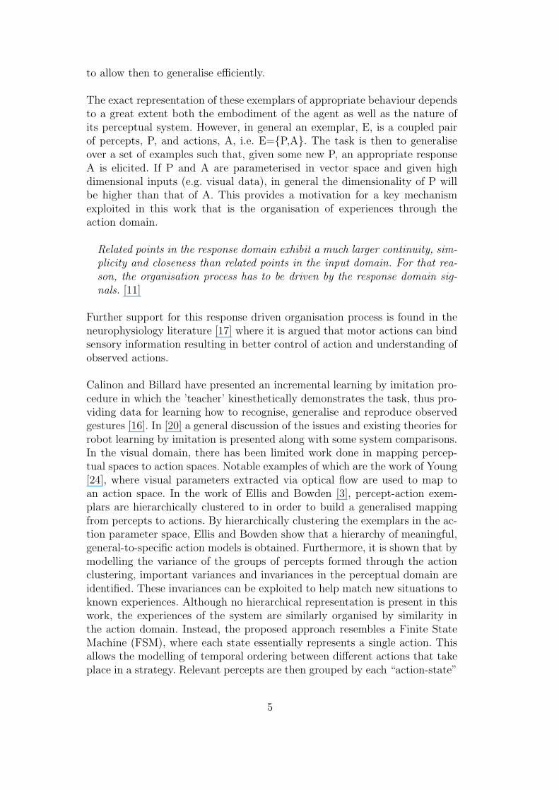
The exact representation of these exemplars of appropriate behaviour dependsto a great extent both the embodiment of the agent as well as the nature ofits perceptual system. However, in general an exemplar, E, is a coupled pairof percepts, P, and actions, A, i.e. E={P,A}. The task is then to generaliseover a set of examples such that, given some new P, an appropriate responseA is elicited. If P and A are parameterised in vector space and given highdimensional inputs (e.g. visual data), in general the dimensionality of P willbe higher than that of A. This provides a motivation for a key mechanismexploited in this work that is the organisation of experiences through theaction domain.

Related points in the response domain exhibit a much larger continuity, sim-

plicity and closeness than related points in the input domain. For that rea-

son, the organisation process has to be driven by the response domain sig-

nals. [11]

Further support for this response driven organisation process is found in theneurophysiology literature [17] where it is argued that motor actions can bindsensory information resulting in better control of action and understanding ofobserved actions.

Calinon and Billard have presented an incremental learning by imitation pro-cedure in which the ’teacher’ kinesthetically demonstrates the task, thus pro-viding data for learning how to recognise, generalise and reproduce observedgestures [16]. In [20] a general discussion of the issues and existing theories forrobot learning by imitation is presented along with some system comparisons.In the visual domain, there has been limited work done in mapping percep-tual spaces to action spaces. Notable examples of which are the work of Young[24], where visual parameters extracted via optical flow are used to map toan action space. In the work of Ellis and Bowden [3], percept-action exem-plars are hierarchically clustered to in order to build a generalised mappingfrom percepts to actions. By hierarchically clustering the exemplars in the ac-tion parameter space, Ellis and Bowden show that a hierarchy of meaningful,general-to-specific action models is obtained. Furthermore, it is shown that bymodelling the variance of the groups of percepts formed through the actionclustering, important variances and invariances in the perceptual domain areidentified. These invariances can be exploited to help match new situations toknown experiences. Although no hierarchical representation is present in thiswork, the experiences of the system are similarly organised by similarity inthe action domain. Instead, the proposed approach resembles a Finite StateMachine (FSM), where each state essentially represents a single action. Thisallows the modelling of temporal ordering between different actions that takeplace in a strategy. Relevant percepts are then grouped by each “action-state”

5

with statistical models learnt online by applying the system to increasinglymore complex problems.

3 Complexity Chain and Evaluation

When learning occurs in biological cognitive systems, many concepts are learntholistically through random exploration, however, teaching is not holistic. Achild is not given a copy of a dictionary and a thesaurus and expected tomaster language. Instead learning is staged into layers of complexity wheresimple nouns are learnt, followed by verbs, then adjectives, and eventuallymore complex concepts such as simile and metaphor. While this is ratheran extreme example, the same is true in most tutored learning scenarios: inmathematics multiplication follows subtraction, follows addition; in elemen-tary art, basic primitives such as lines, triangles and circles are mastered beforecompound shapes are constructed from the basic primitives; and in children’sshape sorting puzzles, the child typically learns to place the circle first dueto the rotational invariance before they move to more complex shapes whichinvolve higher degrees of freedom - this is shown in a study relating the com-plexity of various shape sorting problems to the ability of the child at variousstages of development [2]. In all these learning scenarios, the child is formingand evolving key concepts that will be used as the building blocks at the nextlevel of complexity. This idea of staged learning and increasing levels of com-plexity is commonly referred to as scaffolding and is prevalent within bothhuman and animal behaviour [19]. Typically, the mother will modify the en-vironment in order to make it easier for the developing child to complete thetask. Within this research, the role of the supervisor/teacher is to structurelearning to encourage the discovery/understanding of the relevant concepts,as well as establishing the necessary relationships between them for devisingsolutions. By gradually increasing the complexity and exposing new concepts,the tutor is providing weak supervision to the learning process. In many cases,this supervision may not be essential to learning (in terms of success or failure)but in most cases speeds up the learning process.

Moving through a hierarchy of complexity may involve a smooth continuoustransition, but there exist key points where moving to a more complex levelrequires the introduction of a new concept. We define the term Complexity

Chain as the discrete steps of such a learning process where each discrete levelis attached to the introduction of a new, key concept. For example, in the shapesorter scenario, initially a fix board means that no concept of a hole is required.The goal is to move shapes to predefined locations relative to the world co-ordinate frame. However, once the board can be moved or reconfigured, thereis a clear requirement for the concept of a hole. This concept must emergebefore the system can refine its concept of the goal. Another example would

6

be to train a system with a puzzle sorter that consists of holes that are basicshapes such as circles and squares. Having learnt the general rules of thegame of puzzle sorting, a new puzzle sorter with pieces and holes of differentshapes are presented to the system. The system must now adapt existing learntcompetence from the previous puzzle sorter for use in solving the new domain.

Evaluation of cognitive systems is also a difficult task. Alissandrakis et al.introduced a machine centric method of evaluation based on the number ofexceptions (e.g. non-optimal allignments or task failures) and assessed howwell this quantitative method agreed with qualitative assessments made byhuman observers and found good alignment between the evaluations. Similarly,in section 6, performance is measured naively by either success or failure inreaching the goal. However, this gives little indication as to the benefits orabilities of the system, especially in an emergent architecture where conceptsare implicitly embedded within the system. We therefore also propose thecomplexity chain as a method for evaluation. As each level of complexity isattributed to the discovery of a concept, performance at varying levels withinthe chain can be used to both assess the systems ability and efficiency atgaining competence. Within the experiments presented here, we use the degreeof random exploration at each level of the complexity chain as an indicator ofthe systems efficiency in concept refinement. We demonstrate how this can beused to evaluate the system at all levels for different parameterisations. Thefollowing section now provides an example complexity chain for the COSPAL

Shape Sorter Problem that will be used for experimentation in later chapters.

4 COSPAL Problem Domain: Shape Sorter Puzzle Complexity Hi-

erarchy

In this section, an example of a complexity hierarchy is presented. This hi-erarchy will be used specifically for the application of a shape sorter puzzle.Here, various puzzle scenarios with increasing complexity will be presented tothe system for training.

The hierarchy consists of 5 main levels (Figure 1), starting with the simplestpuzzle scenario at the top and increasing in difficulty as we progress downthe hierarchy. We will describe each level of complexity in terms of commonphysical characteristics present in the puzzle game (e.g. puzzle board is fixedon the floor):

• Level 1: Fixed holes, Subset of starting configurations

At the top level is the puzzle scenario where holes are located at fixed po-sitions (e.g. the puzzle board is nailed to the ground). Additionally, thesystem is only required to solve the puzzle from a subset of starting con-

7

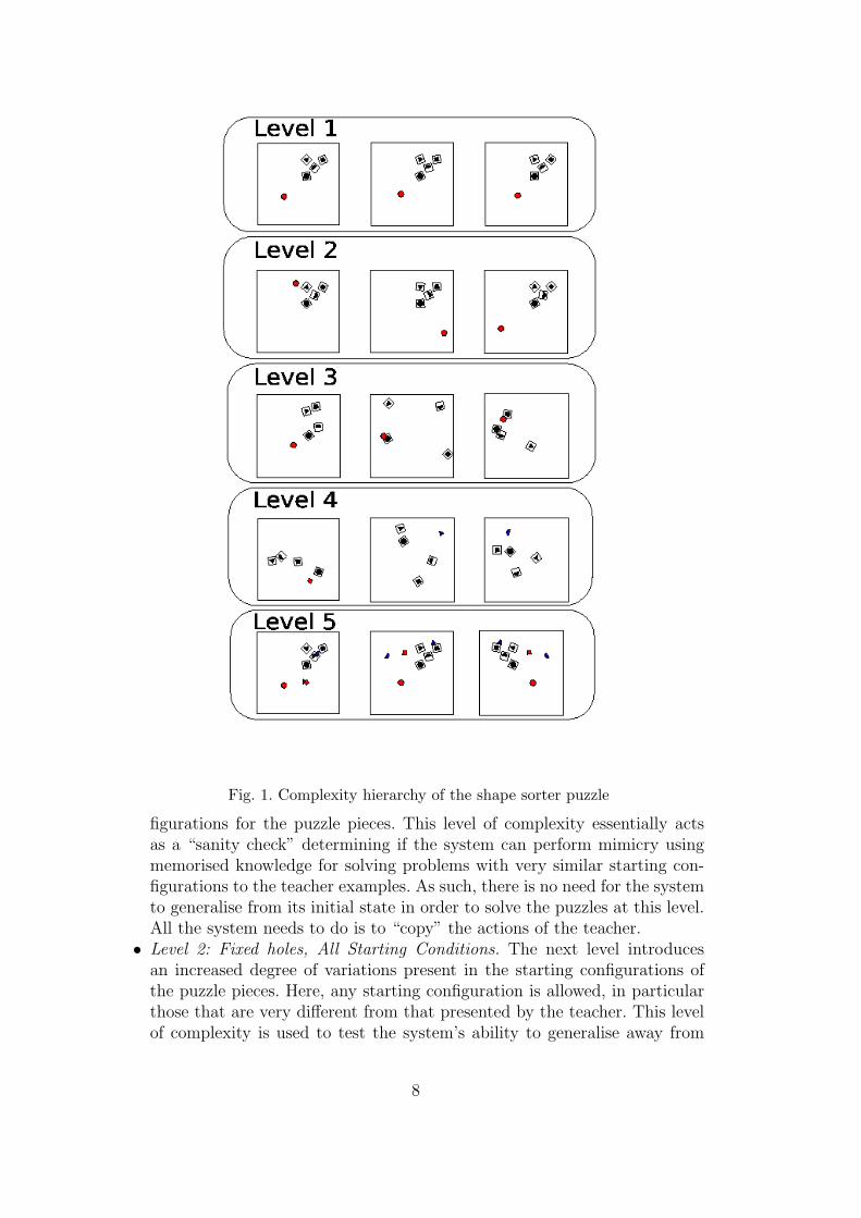
Fig. 1. Complexity hierarchy of the shape sorter puzzle

figurations for the puzzle pieces. This level of complexity essentially actsas a “sanity check” determining if the system can perform mimicry usingmemorised knowledge for solving problems with very similar starting con-figurations to the teacher examples. As such, there is no need for the systemto generalise from its initial state in order to solve the puzzles at this level.All the system needs to do is to “copy” the actions of the teacher.

• Level 2: Fixed holes, All Starting Conditions. The next level introducesan increased degree of variations present in the starting configurations ofthe puzzle pieces. Here, any starting configuration is allowed, in particularthose that are very different from that presented by the teacher. This levelof complexity is used to test the system’s ability to generalise away from

8

the problem configurations that are present in examples provided by theteacher.

• Level 3: Moveable Holes. At this level, the puzzle board holes are allowedto move arbitrarily into any positions. As a consequence, each starting con-figuration of the puzzle may have the holes at different positions and orien-tations in addition to the puzzle pieces being placed at random locations.An outcome of Level 2 of the chain is that a system may only end up mem-orising the positions of holes. The system may then solve the shape sorterpuzzle by simply moving a particularly shaped piece into a fixed location.In order to force a system away from such a strategy, moving the holes willbreak this assumption. As a result, it is then necessary for the system toutilise more relevant information to discover the concept of holes and thefeatures that identify them.

• Level 4: Different Puzzle Pieces, similar rules In this level, differently shapedand unseen puzzle pieces are presented to the system. The goal is then to beable to “recycle” available knowledge applied to known pieces to help solvethe shape sorter puzzle with the new piece. This level of the complexitychain is here to test whether any system that does puzzle solving via learntimitation can generalise to other objects with different physical character-istics. Here, the rules behind the solution remains the same (e.g. a shapedobject is required to be placed into a correctly shaped hole).

• Level 5: Simultaneous Multiple Puzzle Pieces In this level, once the systemhas learnt the ability to solve the shape sorter puzzle for various pieces, acombination of all of these pieces are presented to the system in variousrandomised starting configurations. This allows one to test the ability ofthe system to sequentially solve the entire puzzle by sequentially applyingthe appropriate strategy instantiations that were learnt from the previousfour levels.

5 Modelling Imitation using Temporal Statistics of Perception Ac-

tion Coupling

In this section, a learning framework is proposed for computationally mod-elling, learning and generating the above described strategies. This will in-volve mechanisms for committing to memory strategies for solving problems,along with the correct instantiation of using the appropriate strategy to solv-ing a particular problem. The learning framework will consist of two majorcomponents. The first is a computational model for problem solving strate-gies (Section 5.2). Here, the model will take a form that resembles a FiniteState Machine (FSM). In this model “states” are represented by an actionwithin the action sequence for a strategy. This allows us to capture the or-dered sequence of actions one needs to carry out when using a particular type

9

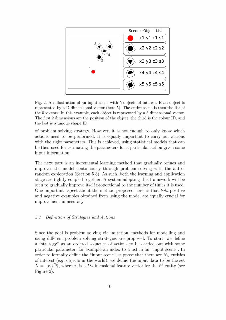
Fig. 2. An illustration of an input scene with 5 objects of interest. Each object isrepresented by a D-dimensional vector (here 5). The entire scene is then the list ofthe 5 vectors. In this example, each object is reprsented by a 5 dimensional vector.The first 2 dimensions are the position of the object, the third is the colour ID, andthe last is a unique shape ID.

of problem solving strategy. However, it is not enough to only know whichactions need to be performed. It is equally important to carry out actionswith the right parameters. This is achieved, using statistical models that canbe then used for estimating the parameters for a particular action given someinput information.

The next part is an incremental learning method that gradually refines andimproves the model continuously through problem solving with the aid ofrandom exploration (Section 5.3). As such, both the learning and applicationstage are tightly coupled together. A system adopting this framework will beseen to gradually improve itself proportional to the number of times it is used.One important aspect about the method proposed here, is that both positiveand negative examples obtained from using the model are equally crucial forimprovement in accuracy.

5.1 Definition of Strategies and Actions

Since the goal is problem solving via imitation, methods for modelling andusing different problem solving strategies are proposed. To start, we definea “strategy” as an ordered sequence of actions to be carried out with someparticular parameter, for example an index to a list in an “input scene”. Inorder to formally define the “input scene”, suppose that there are NO entitiesof interest (e.g. objects in the world), we define the input data to be the setX = {xi}NO

i=1, where xi is a D-dimensional feature vector for the ith entity (seeFigure 2).

10

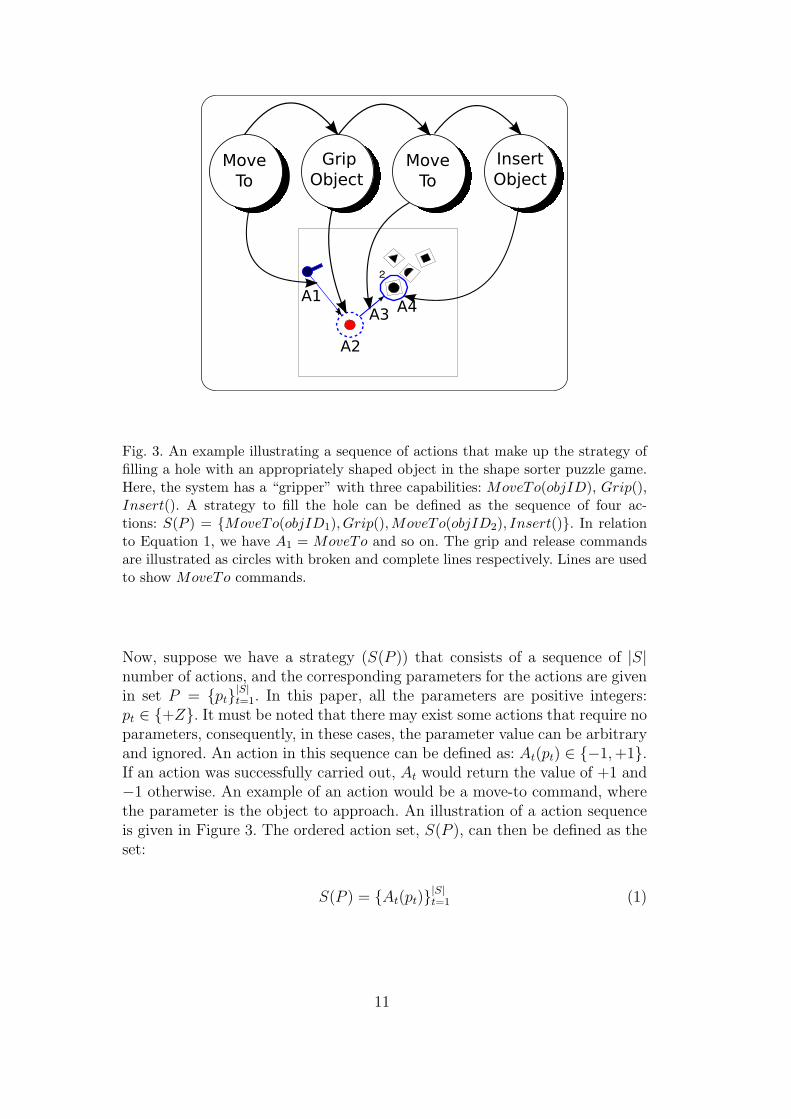
Fig. 3. An example illustrating a sequence of actions that make up the strategy offilling a hole with an appropriately shaped object in the shape sorter puzzle game.Here, the system has a “gripper” with three capabilities: MoveTo(objID), Grip(),Insert(). A strategy to fill the hole can be defined as the sequence of four ac-tions: S(P ) = {MoveTo(objID1), Grip(), MoveTo(objID2), Insert()}. In relationto Equation 1, we have A1 = MoveTo and so on. The grip and release commandsare illustrated as circles with broken and complete lines respectively. Lines are usedto show MoveTo commands.

Now, suppose we have a strategy (S(P )) that consists of a sequence of |S|number of actions, and the corresponding parameters for the actions are givenin set P = {pt}|S|t=1. In this paper, all the parameters are positive integers:pt ∈ {+Z}. It must be noted that there may exist some actions that require noparameters, consequently, in these cases, the parameter value can be arbitraryand ignored. An action in this sequence can be defined as: At(pt) ∈ {−1, +1}.If an action was successfully carried out, At would return the value of +1 and−1 otherwise. An example of an action would be a move-to command, wherethe parameter is the object to approach. An illustration of a action sequenceis given in Figure 3. The ordered action set, S(P ), can then be defined as theset:

S(P ) = {At(pt)}|S|t=1 (1)

11

5.2 Modelling Problem-Solving Strategies

This section will provide the definition and description of the computationalmodel proposed for representing problem solving strategies. An applied exam-ple of this model is given in Section 6.

In order to define the model for problem solving, we follow from the definitionof a strategy given in Eq. 1, where |S| denotes the number of actions within aparticular strategy. Our proposed model will be a set of different components.

The first set contains an ordered set of actions (A = {At(pt)}|S|t=1) as definedin the previous section. The second set contains a set of binary elements toallow us to model actions with (value of 1) and without (value of 0) param-

eters: Bt = {bt}|S|t=1, bt ∈ {0, 1}. The third is a set of feature vector weights(C = {cd}D

d=1), determining how important a particular feature is in help-ing us find solutions to a particular class of problems. When the system isinitialised, all the feature weights ct are set to 1, giving the system equal ac-cess to the information from each feature. Section 5.3.4 proposes a featureweighting method for determining the values of ct based on the outcome ofthe system in solving a problem.

An important component, is the mechanism that will be used to retrieve thecorrect parameters for each action in the strategy. This is achieved by mod-elling the statistics of plausible sets of parameters for the actions (i.e. {pt}|S|t=1}).However, it is first important to note that a given strategy can be often ap-plied to a range of similar problems. For example, the strategy for filling ahole in a shape sorter puzzle can be “recycled” for various different shapes. Toaccount for this, we define a set of action “parameter-set” statistical models(R = {Ri}|R|

i=1) that capture correct instantiations of a strategy. The numberof correct instantiations is defined as |R|. More specifically, Ri is made up ofessentially a set of Parzen windowing models, one for each action parameter.Formally, we can define it as Ri = {rit}|S|t=1, where rit:

rit(x) = Bi

|rit|∑

k=1

K(x, µitk)uitk (2)

where rit(x) is 0 when no kernel centres are available (i.e. Bi = 0). This isused when an action is associated with no parameters. When Bi is 1, theabove equation is essentially a modified Parzen window equation, where |rit|is the number of kernels in rit, µitk are the kernel centres in the tth actionparameter model, uitk ∈ {−1, +1} is the sign of the respective kernel. Here,a kernel sign u of +1 and −1 is used to record whether the respective kernelrepresents a successful or failed example respectively. The sign parameter isused to allow us to incorporate information arising from the incorrect usage of

12

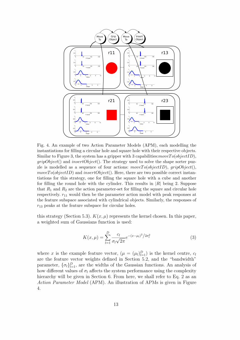
Fig. 4. An example of two Action Parameter Models (APM), each modelling theinstantiations for filling a circular hole and square hole with their respective objects.Similar to Figure 3, the system has a gripper with 3 capabilities:moveTo(objectID),gripObject() and insertObject(). The strategy used to solve the shape sorter puz-zle is modelled as a sequence of four actions: moveTo(objectID), gripObject(),moveTo(objectID) and insertObject(). Here, there are two possible correct instan-tiations for this strategy, one for filling the square hole with a cube and anotherfor filling the round hole with the cylinder. This results in |R| being 2. Supposethat R1 and R2 are the action parameter-set for filling the square and circular holerespectively. r11 would then be the parameter action model with peak responses atthe feature subspace associated with cylindrical objects. Similarly, the responses ofr13 peaks at the feature subspace for circular holes.

this strategy (Section 5.3). K(x, µ) represents the kernel chosen. In this paper,a weighted sum of Gaussians function is used:

K(x, µ) =D∑

l=1

cl

σl

√2π

e−(x−µl)2/2σ2

l (3)

where x is the example feature vector, (µ = (µl)Dl=1) is the kernel centre, cl

are the feature vector weights defined in Section 5.2, and the “bandwidth”parameter, {σl}D

l=1, are the widths of the Gaussian functions. An analysis ofhow different values of σl affects the system performance using the complexityhierarchy will be given in Section 6. From here, we shall refer to Eq. 2 as anAction Parameter Model (APM). An illustration of APMs is given in Figure4.

13

5.3 Strategy Refinement: Incremental Learning from Failure and Success

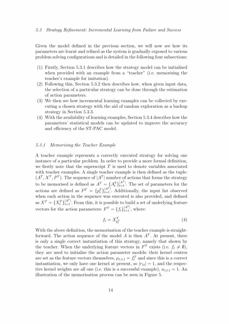
Given the model defined in the previous section, we will now see how itsparameters are learnt and refined as the system is gradually exposed to variousproblem solving configurations and is detailed in the following four subsections:

(1) Firstly, Section 5.3.1 describes how the strategy model can be initialisedwhen provided with an example from a “teacher” (i.e. memorising theteacher’s example for imitation).

(2) Following this, Section 5.3.2 then describes how, when given input data,the selection of a particular strategy can be done through the estimationof action parameters.

(3) We then see how incremental learning examples can be collected by exe-cuting a chosen strategy with the aid of random exploration as a backupstrategy in Section 5.3.3.

(4) With the availability of learning examples, Section 5.3.4 describes how theparameters’ statistical models can be updated to improve the accuracyand efficiency of the ST-PAC model.

5.3.1 Memorising the Teacher Example

A teacher example represents a correctly executed strategy for solving oneinstance of a particular problem. In order to provide a more formal definition,we firstly note that the superscript T is used to denote variables associatedwith teacher examples. A single teacher example is then defined as the tuple:(AT , XT , P T ). The sequence of |AT | number of actions that forms the strategy

to be memorised is defined as AT = {ATt }|A

T |t=1 . The set of parameters for the

actions are defined as P T = {pTt }|A

T |t=1 . Additionally, the input list observed

when each action in the sequence was executed is also provided, and defined

as XT = {XTt }|A

T |t=1 . From this, it is possible to build a set of underlying feature

vectors for the action parameters: F T = {ft}|AT |

t=1 , where:

ft = XTpT

t

(4)

With the above definition, the memorisation of the teacher example is straight-forward. The action sequence of the model A is then AT . At present, thereis only a single correct instantiation of this strategy, namely that shown bythe teacher. When the underlying feature vectors in F T exists (i.e. ft 6= ∅),they are used to initialise the action parameter models: their kernel centresare set as the feature vectors themselves, µ1,t,1 = fT

t and since this is a correctinstantiation, we only have one kernel at present, so |r1t| = 1, and the respec-tive kernel weights are all one (i.e. this is a successful example), u1,t,1 = 1. Anillustration of the memorisation process can be seen in Figure 5.

14

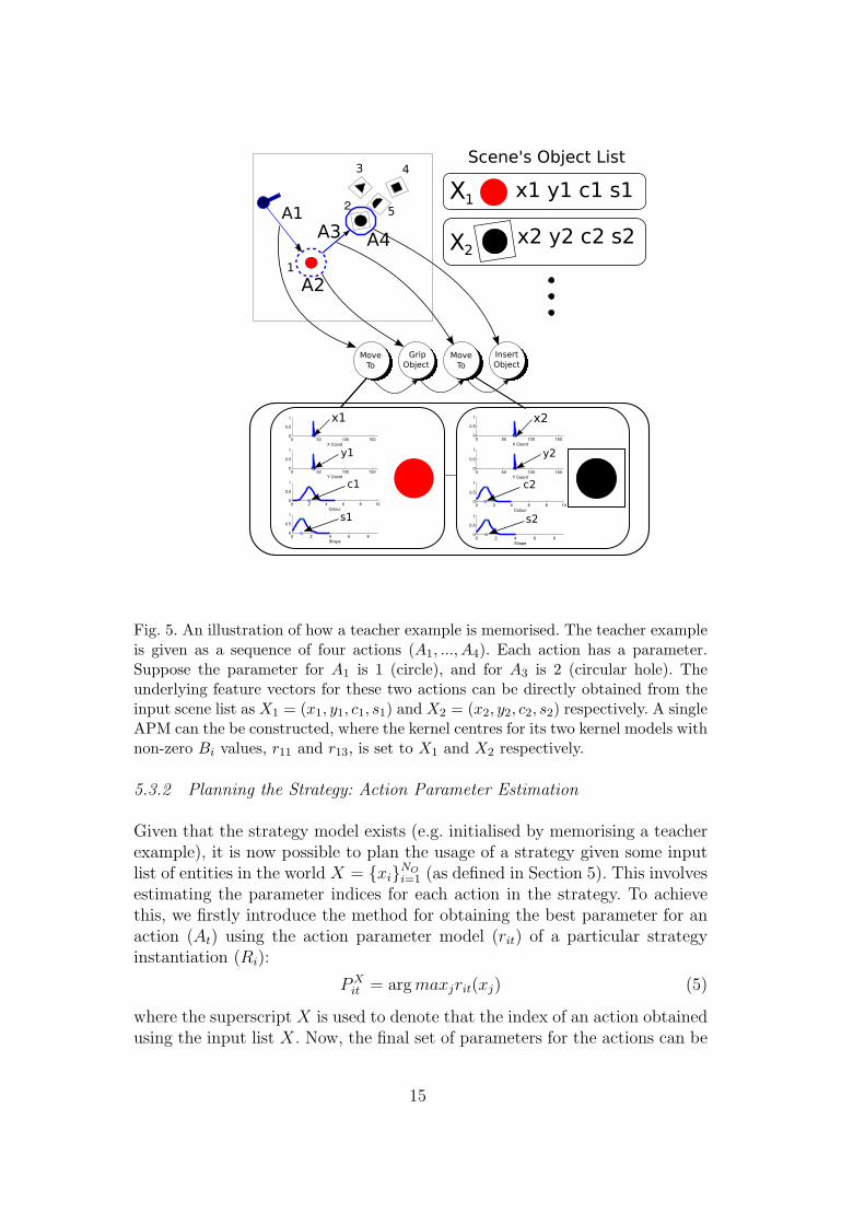
Fig. 5. An illustration of how a teacher example is memorised. The teacher exampleis given as a sequence of four actions (A1, ..., A4). Each action has a parameter.Suppose the parameter for A1 is 1 (circle), and for A3 is 2 (circular hole). Theunderlying feature vectors for these two actions can be directly obtained from theinput scene list as X1 = (x1, y1, c1, s1) and X2 = (x2, y2, c2, s2) respectively. A singleAPM can the be constructed, where the kernel centres for its two kernel models withnon-zero Bi values, r11 and r13, is set to X1 and X2 respectively.

5.3.2 Planning the Strategy: Action Parameter Estimation

Given that the strategy model exists (e.g. initialised by memorising a teacherexample), it is now possible to plan the usage of a strategy given some inputlist of entities in the world X = {xi}NO

i=1 (as defined in Section 5). This involvesestimating the parameter indices for each action in the strategy. To achievethis, we firstly introduce the method for obtaining the best parameter for anaction (At) using the action parameter model (rit) of a particular strategyinstantiation (Ri):

PXit = arg maxjrit(xj) (5)

where the superscript X is used to denote that the index of an action obtainedusing the input list X. Now, the final set of parameters for the actions can be

15

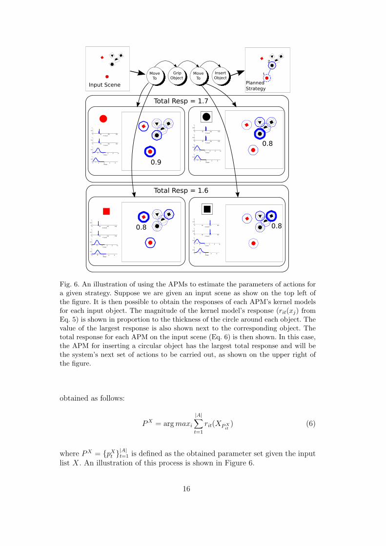
Fig. 6. An illustration of using the APMs to estimate the parameters of actions fora given strategy. Suppose we are given an input scene as show on the top left ofthe figure. It is then possible to obtain the responses of each APM’s kernel modelsfor each input object. The magnitude of the kernel model’s response (rit(xj) fromEq. 5) is shown in proportion to the thickness of the circle around each object. Thevalue of the largest response is also shown next to the corresponding object. Thetotal response for each APM on the input scene (Eq. 6) is then shown. In this case,the APM for inserting a circular object has the largest total response and will bethe system’s next set of actions to be carried out, as shown on the upper right ofthe figure.

obtained as follows:

PX = arg maxi

|A|∑

t=1

rit(XP X

it

) (6)

where PX = {pXt }|A|

t=1 is defined as the obtained parameter set given the inputlist X. An illustration of this process is shown in Figure 6.

16

5.3.3 Obtaining Learning Feedback

With the obtained parameter index set, it is now possible to execute thestrategy and obtain the relevant feedback as to whether this estimation wascorrect or wrong. One straightforward method to achieve this goal is to simplycarry out the actions in the model using the estimated parameters above (PX),and return a failed feedback if any of the actions failed to be executed (i.e.At(p

Xt ) = −1). To improve on this, random exploration will be used when

failure occurs in executing an action. More specifically, suppose that we havesuccessfully executed t− 1 actions, and the current action to be carried out isnow At(p

Xt ). Should At be unsuccessful, it is possible to then “randomly try”

all other possible parameters (i.e. indices of other entities in the input list X).

In order to incorporate random exploration into the strategy execution pro-cess, the estimated action parameter values PX are combined with randomexploration parameters in the form of an action parameter list. Formally, theaction parameter list for At is defined as:

Pt = {pXt , Qt} (7)

where Qt is the random permutation of the set {1, ..., NO}. The algorithmfor executing a planned strategy with the aid of random exploration is asfollows:

t = 1 {Initialise to start at the first action}successF = [] {Initialise list of feature vectors resulting in success}successP = [] {Initialise the correct action parameter index set}randomExFlag = 0while t ≤ |A| do

Get new updated input list X

curPt = Pt1

if curPt 6= −1 then

Pt = {Pt2, ..., P|A|} {Remove first element from set Pt}end if

if At(curPt) == 1 then

successF [t] = XcurPt

successP [t] = curPt

t = t + 1 {Go to the next action}else

randomExFlag = 1 {Note that random exploration was used}if |Pt| = 0 then

break from while loopend if

end if

end while

if t > |A| then

17

return (1, randomExFlag, successF, succesP )else

return (0, randomExFlag, PX , [])end if

The algorithm above returns a triplet: (Sf , Re, FS, PS). The success flag (Sf ∈{0, 1}) will indicate if the system was ultimately successful in solving theproblem using the strategy containing the sequence of actions A. When asuccessful instantiation of the strategy used was made (Sf = 1), we can thendetermine the exact method used with the random exploration flag (Re ∈{0, 1}). Here, Re = 0 indicates the the initial parameters estimated using theaction parameter models (Section 5.3.2) were successfully used. If Re = 1,this indicates that random exploration was used to find the correct actionparameters for solving the current problem configuration. In the frameworkproposed here, should the system fail to solve the puzzle despite using randomexploration (Sf = 0), it will be reported to the user that A represents anunsuitable strategy for solving the current problem.

5.3.4 Updating the Action Parameter Models

Using the algorithm described in the previous section, it is now possible toobtain learning information for updating the action parameter models. Wenote the update to the action parameter models will only take place if thesystem was ultimately successful in solving the problem. However, there aretwo different methods for updating the relevant APMs.

The first case is when random exploration was not used (Re = 0). This impliesthat the initial estimated parameters in Section 5.3.2 were correct. Supposethat the ith strategy instantiation (Ri) was used to obtain the correct initialaction parameters. The updating of its relevant APMs is simply an additionof a new kernel centre to it. This kernel centre will be the feature vectors givenin FS.

The second case is when random exploration was used (Re = 1). In such cases,there can be two possible causes: the first is due to the feature weights beingsuboptimal, implying the system is not utilising available information as bestas it should; the second is that the existing strategy instantiations are simplyinadequate for dealing with the problem configuration presented.

In order to decide between these two, we start by updating the feature weights(C = {cd}D

d=1) in such a way as to reduce the estimation of the wrong param-eters given the previously presented problem configuration. To achieve this,suppose that the original, incorrect, estimated action parameter set is PX ,to be used with the input list X (see Section 5.3.2). We will denote the cor-

18

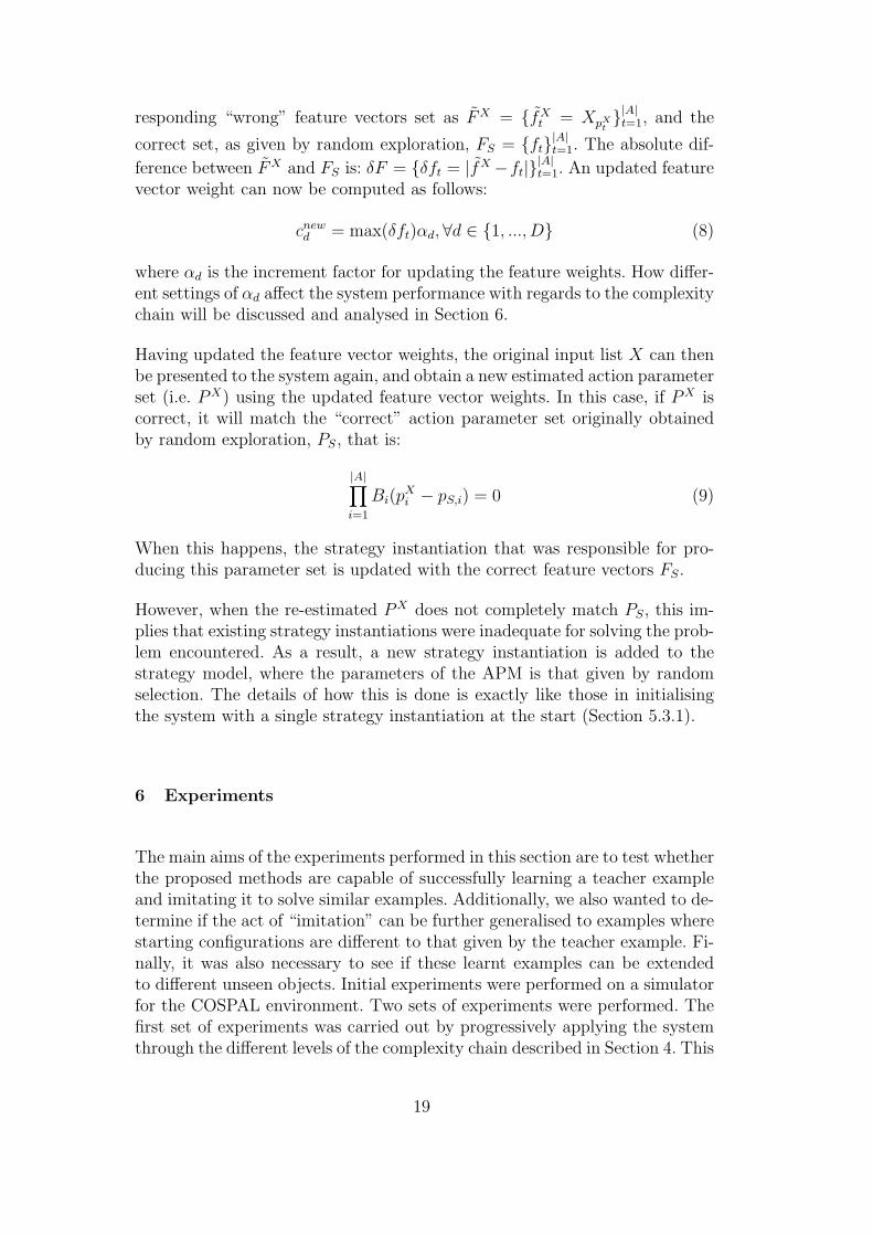
responding “wrong” feature vectors set as FX = {fXt = XpX

t}|A|

t=1, and the

correct set, as given by random exploration, FS = {ft}|A|t=1. The absolute dif-

ference between FX and FS is: δF = {δft = |fX −ft|}|A|t=1. An updated feature

vector weight can now be computed as follows:

cnewd = max(δft)αd,∀d ∈ {1, ..., D} (8)

where αd is the increment factor for updating the feature weights. How differ-ent settings of αd affect the system performance with regards to the complexitychain will be discussed and analysed in Section 6.

Having updated the feature vector weights, the original input list X can thenbe presented to the system again, and obtain a new estimated action parameterset (i.e. PX) using the updated feature vector weights. In this case, if PX iscorrect, it will match the “correct” action parameter set originally obtainedby random exploration, PS, that is:

|A|∏

i=1

Bi(pXi − pS,i) = 0 (9)

When this happens, the strategy instantiation that was responsible for pro-ducing this parameter set is updated with the correct feature vectors FS.

However, when the re-estimated PX does not completely match PS, this im-plies that existing strategy instantiations were inadequate for solving the prob-lem encountered. As a result, a new strategy instantiation is added to thestrategy model, where the parameters of the APM is that given by randomselection. The details of how this is done is exactly like those in initialisingthe system with a single strategy instantiation at the start (Section 5.3.1).

6 Experiments

The main aims of the experiments performed in this section are to test whetherthe proposed methods are capable of successfully learning a teacher exampleand imitating it to solve similar examples. Additionally, we also wanted to de-termine if the act of “imitation” can be further generalised to examples wherestarting configurations are different to that given by the teacher example. Fi-nally, it was also necessary to see if these learnt examples can be extendedto different unseen objects. Initial experiments were performed on a simulatorfor the COSPAL environment. Two sets of experiments were performed. Thefirst set of experiments was carried out by progressively applying the systemthrough the different levels of the complexity chain described in Section 4. This

19

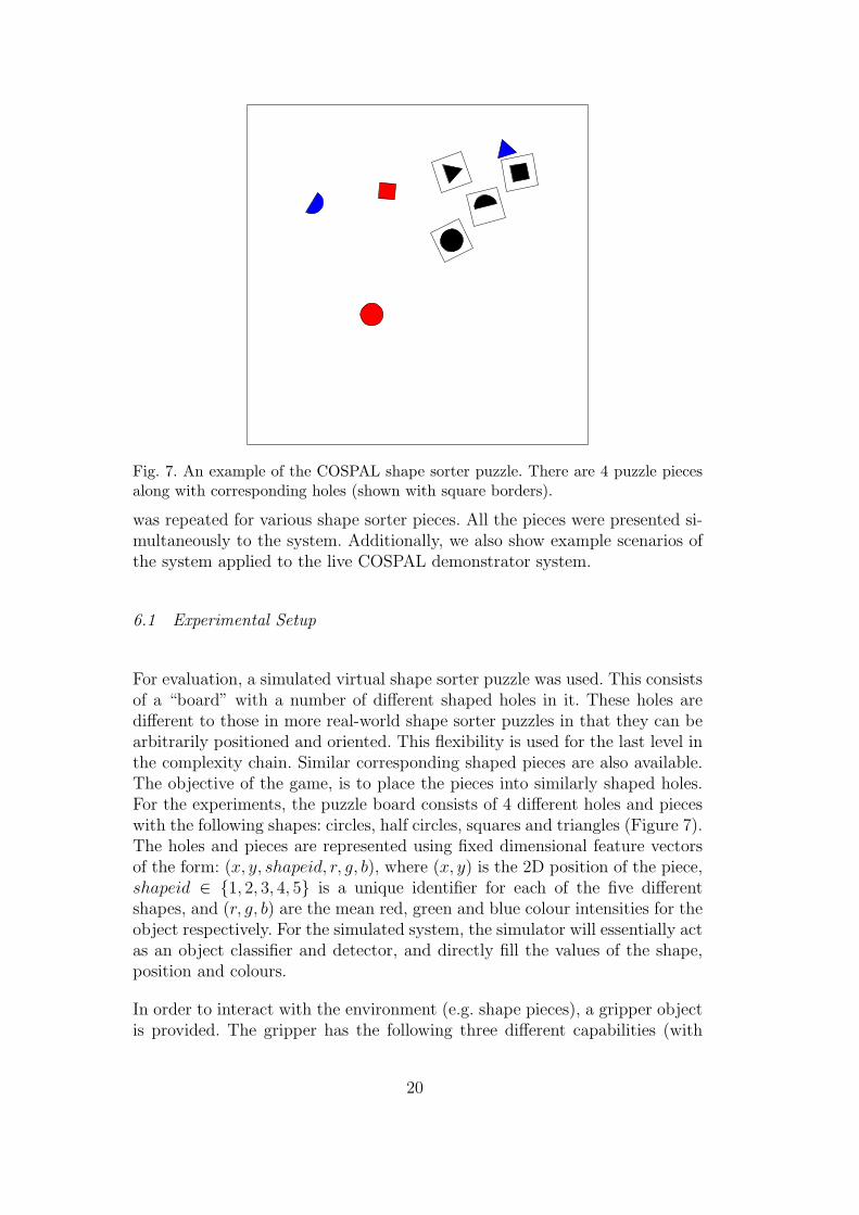
Fig. 7. An example of the COSPAL shape sorter puzzle. There are 4 puzzle piecesalong with corresponding holes (shown with square borders).

was repeated for various shape sorter pieces. All the pieces were presented si-multaneously to the system. Additionally, we also show example scenarios ofthe system applied to the live COSPAL demonstrator system.

6.1 Experimental Setup

For evaluation, a simulated virtual shape sorter puzzle was used. This consistsof a “board” with a number of different shaped holes in it. These holes aredifferent to those in more real-world shape sorter puzzles in that they can bearbitrarily positioned and oriented. This flexibility is used for the last level inthe complexity chain. Similar corresponding shaped pieces are also available.The objective of the game, is to place the pieces into similarly shaped holes.For the experiments, the puzzle board consists of 4 different holes and pieceswith the following shapes: circles, half circles, squares and triangles (Figure 7).The holes and pieces are represented using fixed dimensional feature vectorsof the form: (x, y, shapeid, r, g, b), where (x, y) is the 2D position of the piece,shapeid ∈ {1, 2, 3, 4, 5} is a unique identifier for each of the five differentshapes, and (r, g, b) are the mean red, green and blue colour intensities for theobject respectively. For the simulated system, the simulator will essentially actas an object classifier and detector, and directly fill the values of the shape,position and colours.

In order to interact with the environment (e.g. shape pieces), a gripper objectis provided. The gripper has the following three different capabilities (with

20

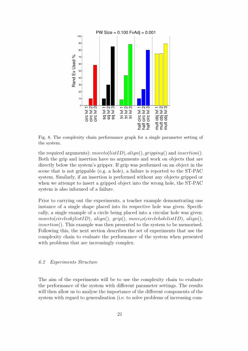
Fig. 8. The complexity chain performance graph for a single parameter setting ofthe system.

the required arguments): moveto(listID), align(), gripping() and insertion().Both the grip and insertion have no arguments and work on objects that aredirectly below the system’s gripper. If grip was performed on an object in thescene that is not grippable (e.g. a hole), a failure is reported to the ST-PACsystem. Similarly, if an insertion is performed without any objects gripped orwhen we attempt to insert a gripped object into the wrong hole, the ST-PACsystem is also informed of a failure.

Prior to carrying out the experiments, a teacher example demonstrating oneinstance of a single shape placed into its respective hole was given. Specifi-cally, a single example of a circle being placed into a circular hole was given:moveto(circleobjlistID), align(), grip(), moveto(circleholelistID), align(),insertion(). This example was then presented to the system to be memorised.Following this, the next section describes the set of experiments that use thecomplexity chain to evaluate the performance of the system when presentedwith problems that are increasingly complex.

6.2 Experiments Structure

The aim of the experiments will be to use the complexity chain to evaluatethe performance of the system with different parameter settings. The resultswill then allow us to analyse the importance of the different components of thesystem with regard to generalisation (i.e. to solve problems of increasing com-

21

plexity through imitation). Firstly, we define the performance of the systemat each level as the percentage of times random exploration was used to solvethe puzzle. In other words, it is a measure of how many times the proposedstrategy model within the system failed to provide a correct solution to sometest example. We define a puzzle to be successfully solved when there remainsno object in the scene that can be gripped (i.e. all the puzzle pieces have beenplaced into their respective holes).

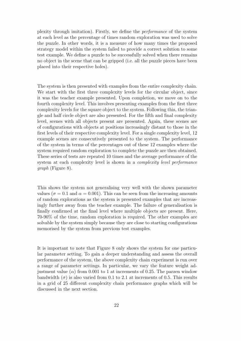
The system is then presented with examples from the entire complexity chain.We start with the first three complexity levels for the circular object, sinceit was the teacher example presented. Upon completion, we move on to thefourth complexity level. This involves presenting examples from the first threecomplexity levels for the square object to the system. Following this, the trian-gle and half circle object are also presented. For the fifth and final complexitylevel, scenes with all objects present are presented. Again, these scenes areof configurations with objects at positions increasingly distant to those in thefirst levels of their respective complexity level. For a single complexity level, 12example scenes are consecutively presented to the system. The performanceof the system in terms of the percentages out of these 12 examples where thesystem required random exploration to complete the puzzle are then obtained.These series of tests are repeated 10 times and the average performance of thesystem at each complexity level is shown in a complexity level performance

graph (Figure 8).

This shows the system not generalising very well with the shown parametervalues (σ = 0.1 and α = 0.001). This can be seen from the increasing amountsof random explorations as the system is presented examples that are increas-ingly further away from the teacher example. The failure of generalisation isfinally confirmed at the final level where multiple objects are present. Here,70-90% of the time, random exploration is required. The other examples aresolvable by the system simply because they are close to starting configurationsmemorised by the system from previous test examples.

It is important to note that Figure 8 only shows the system for one particu-lar parameter setting. To gain a deeper understanding and assess the overallperformance of the system, the above complexity chain experiment is run overa range of parameter settings. In particular, we vary the feature weight ad-justment value (α) from 0.001 to 1 at increments of 0.25. The parzen windowbandwidth (σ) is also varied from 0.1 to 2.1 at increments of 0.5. This resultsin a grid of 25 different complexity chain performance graphs which will bediscussed in the next section.

22

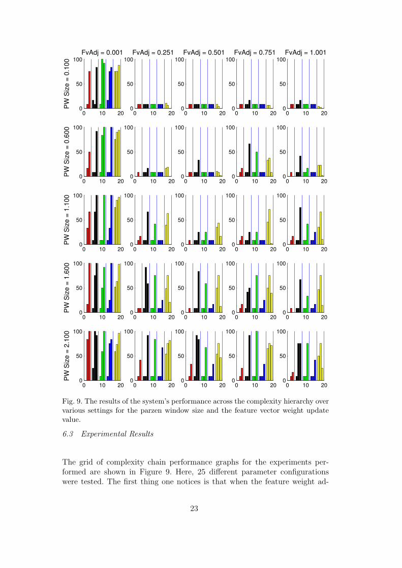
Fig. 9. The results of the system’s performance across the complexity hierarchy overvarious settings for the parzen window size and the feature vector weight updatevalue.

6.3 Experimental Results

The grid of complexity chain performance graphs for the experiments per-formed are shown in Figure 9. Here, 25 different parameter configurationswere tested. The first thing one notices is that when the feature weight ad-

23

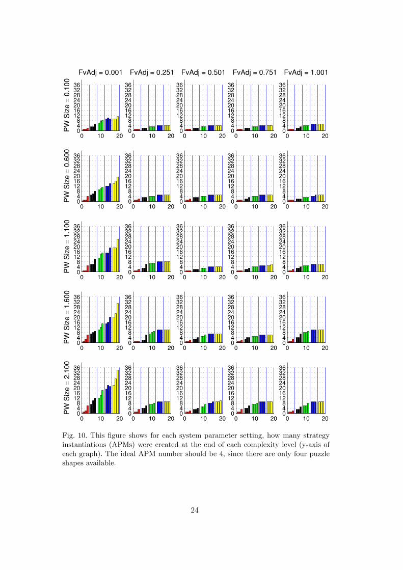
Fig. 10. This figure shows for each system parameter setting, how many strategyinstantiations (APMs) were created at the end of each complexity level (y-axis ofeach graph). The ideal APM number should be 4, since there are only four puzzleshapes available.

24

justment value is very small (0.001), regardless of the setting for the parzenwindow size, the performance of the system is on the whole poor. As the com-plexity level goes up for each of the objects, the amount of random explorationincreases as well. This is apparent for all objects, as well as the multiple ob-ject level. This is because important features are not emphasised soon enough.This results in too many APMs being created, as can be seen in Figure 10.Ideally, since there are only four different types of puzzle pieces, there shouldonly be four APMs. If too many are created, it stops any one APM’s kernelmodel from being updated frequently enough to provide a good generalisationcapability.

However, when the feature adjustment level is appropriate, from 0.251 on-wards, the performance of the system then becomes dependant on the size ofthe parzen windows. The performance of the system deteriorates as the parzenwindow size increases, as is reflected in the performance graphs with parzenwindow values of 1.1 and above.

An increase in parzen window size effectively increases the radius of the Gaus-sians in the kernel models. This will cause the feature subspaces modelledby different APMs to overlap. As a consequence, there in an increase in theambiguity of responses for memories of different strategy instantiations (mod-elled by APMs). This is not apparent in results where only one puzzle piece ispresent. However, with multiple puzzle pieces, there is an increase in the useof random exploration. This is because the system may, for example, applythe strategy instantiation of filling square objects into square holes to circleobjects, in effect putting circular objects into square holes.

6.4 Application to the Live COSPAL Demonstrator System

The proposed system was finally applied to the live COSPAL demonstratorsystem aimed at solving the shape sorter puzzle [4]. Again, the system waspresented with various configurations of the shape sorter puzzle, as structuredby the complexity chain.

The live COSPAL system is configured very closely to the simulated envi-ronment described in the previous subsections. There is a robot manipulatorthat provides the four capabilities: moveto(listID), align(), gripping() andinsertion(). The mechanisms for learning and providing the motor controlsrequired for these four capabilities are described in [13,12,15]. Additionally,numerous object detection and shape classification methods were used to pro-vide the input list representation is described in [5,6,9].

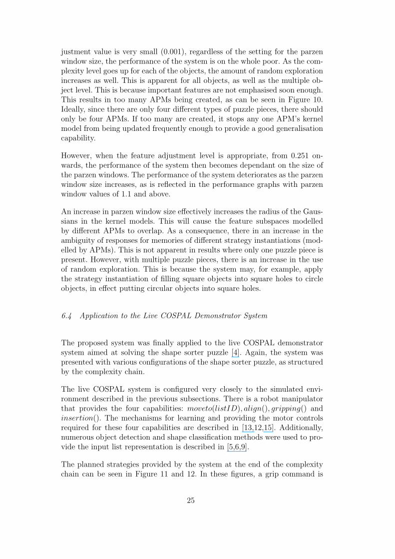
The planned strategies provided by the system at the end of the complexitychain can be seen in Figure 11 and 12. In these figures, a grip command is

25

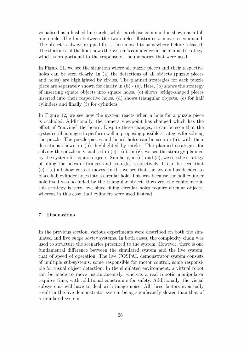
visualised as a hashed-line circle, whilst a release command is shown as a fullline circle. The line between the two circles illustrates a move-to command.The object is always gripped first, then moved to somewhere before released.The thickness of the line shows the system’s confidence in the planned strategy,which is proportional to the response of the memories that were used.

In Figure 11, we see the situation where all puzzle pieces and their respectiveholes can be seen clearly. In (a) the detections of all objects (puzzle piecesand holes) are highlighted by circles. The planned strategies for each puzzlepiece are separately shown for clarity in (b) - (e). Here, (b) shows the strategyof inserting square objects into square holes. (c) shows bridge-shaped piecesinserted into their respective holes. (d) shows triangular objects, (e) for halfcylinders and finally (f) for cylinders.

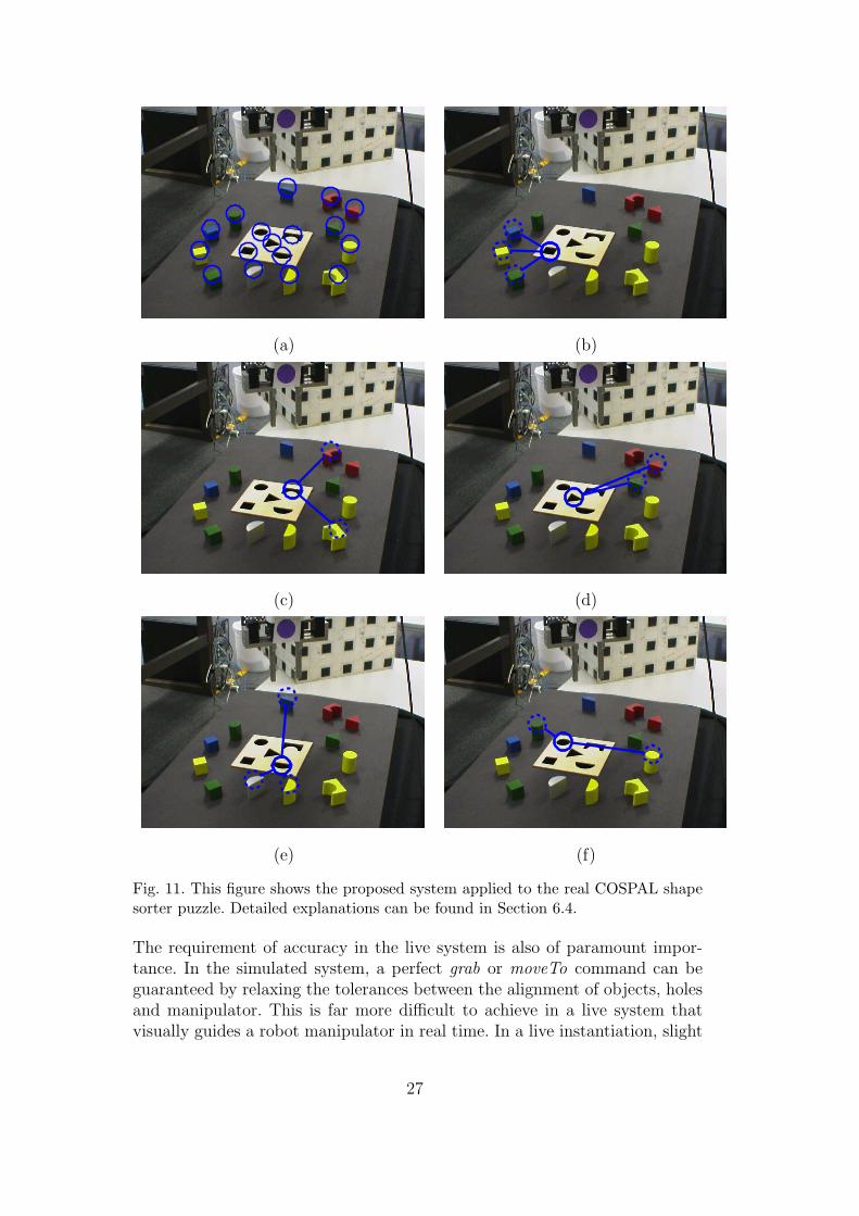
In Figure 12, we see how the system reacts when a hole for a puzzle pieceis occluded. Additionally, the camera viewpoint has changed which has theeffect of “moving” the board. Despite these changes, it can be seen that thesystem still manages to perform well in proposing possible strategies for solvingthe puzzle. The puzzle pieces and board holes can be seen in (a), with theirdetections shown in (b), highlighted by circles. The planned strategies forsolving the puzzle is visualised in (c) - (e). In (c), we see the strategy plannedby the system for square objects. Similarly, in (d) and (e), we see the strategyof filling the holes of bridges and triangles respectively. It can be seen that(c) - (e) all show correct moves. In (f), we see that the system has decided toplace half cylinder holes into a circular hole. This was because the half cylinderhole itself was occluded by the triangular object. However, the confidence inthis strategy is very low, since filling circular holes require circular objects,whereas in this case, half cylinders were used instead.

7 Discussions

In the previous section, various experiments were described on both the sim-ulated and live shape sorter systems. In both cases, the complexity chain wasused to structure the scenarios presented to the system. However, there is onefundamental difference between the simulated system and the live system,that of speed of operation. The live COSPAL demonstrator system consistsof multiple sub-systems, some responsible for motor control, some responsi-ble for visual object detection. In the simulated environment, a virtual robotcan be made to move instantaneously, whereas a real robotic manipulatorrequires time, with additional constraints for safety. Additionally, the visualsubsystems will have to deal with image noise. All these factors eventuallyresult in the live demonstrator system being significantly slower than that ofa simulated system.

26

(a) (b)

(c) (d)

(e) (f)

Fig. 11. This figure shows the proposed system applied to the real COSPAL shapesorter puzzle. Detailed explanations can be found in Section 6.4.

The requirement of accuracy in the live system is also of paramount impor-tance. In the simulated system, a perfect grab or moveTo command can beguaranteed by relaxing the tolerances between the alignment of objects, holesand manipulator. This is far more difficult to achieve in a live system thatvisually guides a robot manipulator in real time. In a live instantiation, slight

27

(a) (b)

(c) (d)

(e) (f)

Fig. 12. This figure shows the proposed system applied to another configuration ofthe real COSPAL shape sorter puzzle. Detailed explanations can be found in Section6.4.

alignment issues can cause complete failure of the system. As a result, even ifthe strategy is correct, if the robot releases a piece slightly offset (say 0.01 mm)from the centre of its respective hole, the puzzle piece can catch the edge ofthe hole does not pass through the hole successfully. This can result in failures,

28

not because of incorrect strategies from the proposed system, but because ofthe small errors in the visual and motor capabilities of the system. However,it is important to note that ultimately, this is not a problem. In such cases,random exploration is used and the proposed strategy will eventually be exe-cuted correctly. Once done, the outcome of the random exploration will matchthat initially proposed by the system, and this will only serve to strengthenand reinforce the correct memory models in the system as described in Section5.3.4. However, this process of failures due to finite alignment issues, serves tofurther slow down the operation of the live system.

Due to these factors, it is not practical with the current implementation tocarry exhaustive experimentation in the live system. The amount of time itwould have taken to complete a similar number of experiments to those per-formed in simulation is simply not feasible. However, it is a benefit of the sys-tem architecture that learning at this high symbolic level is consistent acrossdomains and lessons learnt in the simulation can be directly applied to thelive system.

8 Conclusions

To conclude, this paper proposed a system to solve problems through imita-tion. This was then applied the domain of a shape sorter puzzle within theCOSPAL system. To this end, an incomplete set of experiences provided by ateacher was memorised with the aim of being used to generalise and efficientlyrecall appropriate experiences given novel scenarios of similar problems. Addi-tionally, random exploration was also used as a fall-back “brute-force” mech-anism should a recalled experience fail to solve a scenario.

To this end, the ST-PAC system was proposed which ties together the in-put percepts (i.e. a description of the world) with the actions that should beperformed given that scenario. Statistical models were used to couple groupsof percepts with similar actions. An approach to incremental learning thatprovided good generalisation was also proposed.

Furthermore the concept of the Complexity Chain was proposed as a way ofstructuring learning and a method for evaluating a cognitive system’s per-formance. The system was tested in two types of experiments, a simulatedenvironment and a live demonstrator system. For both environments, it wasfound that the system provided a platform that allowed both generalisationsover experiences from a sparse set of memorised examples provided by a tu-tor and the capability to refine learning in light of new experiences. However,further study is needed to analyse the important differences that exist be-tween generalisation performance of the live system and that of the simulated

29

system.

References

[1] G. Buccino, F. Binkofski, L. Riggio, The mirror neuron system and actionrecognition., Brain Lang 89 (2) (2004) 370–376.

[2] T. Dichter-Blancher, N. Busch-Rossnagel, K.-J. D., Mastery motivation :Appropriate tasks for toddlers, Infant behavior and development 20 (4) (1997)545–548.

[3] L. Ellis, R. Bowden, Learning responses to visual stimuli: A generic approach,in: Proc. of the 5th International Conference on Computer Vision Systems,2007.

[4] M. Felsberg, P.-E. Forssen, A. Moe, G. Granlund, A cospal subsystem: Solving ashape-sorter puzzle, in: AAAI Fall Symposium: From Reactive to AnticipatoryCognitive Embedded Systems, 2005.

[5] M. Felsberg, P.-E. Forssen, H. Scharr, Channel smoothing: Efficient robustsmoothing of low-level signal features, IEEE Transactions of Pattern Analysisand Machine Intelligence 28 (2) (2006) 209–222.

[6] M. Felsberg, J. Hedbord, Real-time visual recognition of objects and scenesusing p-chennel matching, in: Proc. of 15th Scandinavian Conference on ImageAnalysis, 2007.

[7] M. Felsberg, J. Wiklund, E. Jonsson, A. Moe, G. Granlund, Exploratorylearning structure in artificial cognitive systems, in: International CognitiveVision Workshop, 2007.

[8] P. Fitzpatrick, From first contact to close encounters: A developmentally deepperceptual system for a humanoid robot, PhD thesis, MIT.

[9] P.-E. Forssen, A. Moe, Autonomous learning of object appearances using colourcontour frames, in: 3rd Canadian Conference on Computer and Robot Vision,2006.

[10] T. Gelder, R. Port, It’s about time: an overview of the dynamical approach tocognition, Mind as motion: explorations in the dynamics of cognition (1995)1–43.

[11] G. H. Granlund, The complexity of vision, Signal Processing 74 (1) (1999) 101–126.

[12] F. Hoppe, Local learning for visual robotic systems, Ph.D. thesis, Christian-Albrechts-Universitat zu Kiel, Institut fur Informatik (2007).

[13] F. Hoppe, G. Sommer, Fusion algorithm for locally arranged linear models, in:Proc. of 18th Int. Conf on Pattern Recognition (ICPR), 2006.

30

[14] M. Jeannerod, Motor Cognition: What Actions Tell the Self, Oxford UniversityPress, 2006.

[15] F. Larsson, E. Jonsson, M. Felsberg, Visual servoing for floppy robots usinglwpr, in: RoboMat, 2007.

[16] C. L. Nehaniv, K. Dautenhahn, Imitation and social learning in robots, humansand animals : behavioural, social and communicative dimensions, CambridgeUniversity Press, Cambridge, UK ; New York, 2007.

[17] G. Rizzolatti, M. A. Arbib, Language within our grasp, Trends in Neurosciences21 (5) (1998) 188–194.

[18] G. Rizzolatti, L. Fogassi, V. Gallese, Neurophysiological mechanisms underlyingthe understanding and imitation of action., Nat Rev Neurosci 2 (9) (2001) 661–670.

[19] J. Saunders, C. Nehaniv, K. Dautenhahn, A. Alissandrakis, Self-imitation andenvironmental scaffolding for robot teaching, International Journal of AdvancedRobotics Systems 4 (1) (2007) 109–124.

[20] J. Saunders, C. L. Nehaniv, K. Dautenhahn, What is an appropriate theoryof imitation for a robot learner?, Proc. of ECSIS Symposium on Learning andAdaptive Behaviors for Robotic Systems. (2008) 9–14.

[21] J. Siskind, Reconstructing force-dynamic models from video sequences,Artificial Intelligence 151 (1-2) (2003) 91–154.

[22] E. Thelen, L. Smith, A Dynamic Systems Approach to the Development ofPerception and Action, MIT Press, 1994.

[23] D. Vernon, G. Metta, G. Sandini, A survey of artificial cognitive systems:Implications for the autonomous development of mental capabilities incomputational agents, IEEE Transactions on Evolutionary Computation,Special Issue on Autonomous Mental Development 11 (2) (2007) 151–180.

[24] D. Young, First-order optic flow and the control of action, in: Proc. of EuropeanConference on Visual Perception, Groningen, 2000.

31