1

CIT 108

PROBLEM-SOLVING ALGORITHM

Course Team

NATIONAL OPEN UNIVERSITY OF NIGERIA

COURSE

GUIDE

2

© 2022 by NOUN Press

National Open University of Nigeria

Headquarters

University Village

Plot 91, Cadastral Zone Nnamdi Azikiwe Expressway

Jabi, Abuja

Lagos Office

14/16 Ahmadu Bello Way

Victoria Island, Lagos

e-mail: centralinfo@nou.edu.ng

URL: www.nou.edu.ng

Printed 2022

ISBN:

All rights reserved. No part of this book may be reproduced, in any form

or by any means, without permission in writing from the publisher.

3

CONTENTS PAGE

MODULE 1: PROBLEM-SOLVING STRATEGIES

UNIT 1: ROADMAP TO SOLVING PROBLEM:

TYPICAL STRATEGIES ………………………………………………….. 4

UNIT 2: THE PROBLEM SOLVING PROCESS…………………………. 13

UNIT 3: COMPUTATIONAL APPROACHES TO

PROBLEM SOLVING…………………………………………………….. 25

MODULE 2: ROLE OF ALGORITHMS IN PROBLEM SOLVING

UNIT 1: ABSTRACTION AS A PROBLEM SOLVING TOOL…………. 34

UNIT 2: ALGORITHMS………………………………………………….. 42

UNIT 3: FLOWCHARTS…………………………………………………. 56

UNIT 4: PSEUDOCODE………………………………………………….. 69

MODULE 3: IMPLEMENTATION STRATEGIES

UNIT 1: RECURSION……………………………………………….…… 78

UNIT 2: CONTROL STRUCTURES: SELECTION AND ITERATION 90

UNIT 3: DECOMPOSITION AND MODULARISATION…………..….. 105

UNIT 4: TESTING AND DEBUGGING…………………………………. 114

4

MODULE 1: PROBLEM-SOLVING STRATEGIES

UNIT 1: ROADMAP TO SOLVING PROBLEM: TYPICAL STRATEGIES

CONTENTS

1.0 Introduction

2.0 Objectives

3.0 Main Content

3.1 Problem-solving strategies defined

3.2 Importance of Understanding Multiple Problem-solving Strategies

3.3 Trial and Error

3.4 Algorithm and Heuristic

3.5 Means-Ends Analysis

3.6 Other Problem-solving Strategies

4.0 Conclusion

5.0 Summary

6.0 Tutor-Marked Assignments

7.0 References/Further Reading

1.0 INTRODUCTION

People face problems every day—usually, multiple problems throughout the day. Sometimes

these problems are straightforward, sometimes, however, the problems we encounter are more

complex. For example, say you have a work deadline, and you must mail a printed copy of a

report to your supervisor by the end of the business day. The report is time-sensitive and must

be sent overnight. You finished the report last night, but your printer will not work today. What

should you do? First, you need to identify the problem and then apply a strategy for solving the

problem.

Practicing different problem-solving strategies can help professionals develop efficient

solutions to challenges they encounter at work and in their everyday lives. Each industry,

business and career has its own unique challenges, which means employees may implement

different strategies to solve them. If you are interested in learning how to solve problems more

effectively, then understanding how to implement several common problem-solving strategies

may benefit you. In the sections that follow, we discuss what problem-solving strategies are,

why they are important and list several examples of problem-solving strategies you can try.

5

2.0 OBJECTIVES

By the end of this unit, you will be able to:

• define problem solving strategies

• define algorithm and heuristic and their role in problem solving

• describe typical common problem solving strategies

• explain some common roadblocks to effective problem solving.

3.0 MAIN CONTENT

3.1 Problem-solving strategies defined

When people are presented with a problem—whether it is a complex mathematical problem or

a broken printer, how do you solve it? Before finding a solution to the problem, the problem

must first be clearly identified. After that, one of many problem solving strategies can be

applied, hopefully resulting in a solution.

A problem-solving strategy is a plan used to find a solution or overcome a challenge. Different

strategies have different action plans associated with them. For example, a well-known strategy

is trial and error. Each problem-solving strategy includes multiple steps to provide you with

helpful guidelines on how to resolve a business problem or industry challenge. Effective

problem-solving requires you to identify the problem, select the right process to approach it

and follow a plan tailored to the specific issue you are trying to solve.

3.2 Importance of Understanding Multiple Problem-solving Strategies

Problems themselves can be classified into two different categories known as ill-defined and

well-defined problems (Schacter, 2009). Ill-defined problems represent issues that do not have

clear goals, solution paths, or expected solutions whereas well-defined problems have specific

goals, clearly defined solutions, and clear expected solutions. Problem solving often

incorporates logical reasoning and interpretation of meanings behind the problem, and also in

many cases require abstract thinking and creativity in order to find novel solutions. Various

methods of studying problem solving exist including introspection, simulation, computer

modelling, and experimentation.

Understanding how a variety of problem-solving strategies work is important because different

problems typically require you to approach them in different ways to find the best solution. By

mastering several problem-solving strategies, you can more effectively select the right plan of

action when faced with challenges in the future. This can help you solve problems faster and

develop stronger critical thinking skills.

6

3.3 Trial and Error

A trial-and-error approach to problem-solving involves trying a number of different solutions

and ruling out those that do not work. This approach can be a good option if you have a very

limited number of options available. In terms of a broken printer for example, one could try

checking the ink levels, and if that doesn’t work, you could check to make sure the paper tray

isn’t jammed. Or maybe the printer isn’t actually connected to a laptop. When using trial and

error, one would continue to try different solutions until the problem is solved. Although trial

and error is not typically one of the most time-efficient strategies, it is a commonly used one.

3.4 Algorithm and Heuristic

A common type of strategy is an algorithm. An algorithm is a problem-solving formula that

provides you with step-by-step instructions used to achieve a desired outcome (Kahneman,

2011). You can think of an algorithm as a recipe with highly detailed instructions that produce

the same result every time they are performed. Algorithms are used frequently in our everyday

lives, especially in computer science. When you run a search on the Internet, search engines

like Google use algorithms to decide which entries will appear first in your list of results.

Facebook also uses algorithms to decide which posts to display on your newsfeed. Can you

identify other situations in which algorithms are used?

A heuristic is another type of problem solving strategy. While an algorithm must be followed

exactly to produce a correct result, a heuristic is a general problem-solving framework (Tversky

& Kahneman, 1974). You can think of these as mental shortcuts that are used to solve problems.

A “rule of thumb” is an example of a heuristic. Such a rule saves the person time and energy

when making a decision, but despite its time-saving characteristics, it is not always the best

method for making a rational decision. Different types of heuristics are used in different types

of situations, but the impulse to use a heuristic occurs when one of five conditions is met

(Pratkanis, 1989):

• When one is faced with too much information

• When the time to make a decision is limited

• When the decision to be made is unimportant

• When there is access to very little information to use in making the decision

• When an appropriate heuristic happens to come to mind in the same moment

Working backwards is a useful heuristic in which you begin solving the problem by focusing

on the end result. It is common to use the working backwards heuristic to plan the events of

your day on a regular basis, probably without even thinking about it.

7

Another useful heuristic is the practice of accomplishing a large goal or task by breaking it into

a series of smaller steps. Students often use this common method to complete a large research

project or long essay for school. For example, students typically brainstorm, develop a thesis

or main topic, research the chosen topic, organize their information into an outline, write a

rough draft, revise and edit the rough draft, develop a final draft, organize the references list,

and proofread their work before turning in the project. The large task becomes less

overwhelming when it is broken down into a series of small steps.

3.5 Means-Ends Analysis

This strategy involves choosing and analysing an action at a series of smaller steps to move

closer to the goal. One example of means-end analysis can be found by using the Tower of

Hanoi paradigm. This paradigm can be modelled as a word problem.

The actual Tower of Hanoi problem consists of three rods sitting vertically on a base with a

number of disks of different sizes that can slide onto any rod. The puzzle starts with the disks

in a neat stack in ascending order of size on one rod, the smallest at the top making a conical

shape. The objective of the puzzle is to move the entire stack to another rod obeying the

following rules:

1. Only one disk can be moved at a time.

2. Each move consists of taking the upper disk from one of the stacks and placing it on

top of another stack or on an empty rod.

3. No larger disc may be placed on top of a smaller disk.

With 3 disks, the puzzle can be solved in 7 moves. The minimal moves required to solve a

Tower of Hanoi puzzle is 2n – 1, where 𝑛 is the number of disks. For example, if there were 14

disks in the tower, the minimum amount of moves that could be made to solve the puzzle would

be 214 – 1 = 16,383 moves. There are various ways of approaching the Tower of Hanoi or its

related problems in addition to the approaches listed above including an iterative solution,

recursive solution, non-recursive solution, a binary and Gray-code solutions, and graphical

representations.

An iterative solution entails moving the smallest pieces over one, then moving the next over

one and if there is no tower position in the chosen direction you are moving to, move the pieces

to the opposite end, but then continue to move in the same direction. By doing this one will

complete the puzzle in the minimum amount of moves when there are 3 disks. Recursive

solutions represent recognizing that the puzzle can be broken down into a series of sub

8

problems to each of which the same general solving procedures apply, and then the total

solution can be found by putting together the sub solutions. Non-recursive solutions entail

recognizing that the procedures required to solve the problem have many regularities such as

when counting the moves starting at 1, position of the disk in the series to be moved during

move 𝑚 represents the number of times 𝑚 can be divided by 2 which indicates that every odd

move involves the smallest disk. This allows for the following algorithm:

1) Move the smallest disk to the peg that it has not recently come from.

2) Move another disk legally (there will only be one possibility).

A binary and Gray solutions describe disk move numbers in binary notation (base-2) where

there is only one binary digit (a bit) for each disk and the most significant (leftmost bit)

represents the largest disk. A bit with a different value to the previous one means that the

corresponding disk is one position to the left or right of the previous one.

Graphical representations, as their name imply, represent visual presentations of conditions

that can be modelled in order to view the most efficient and effective solutions. A common

graph for the Tower of Hanoi is represented by a unidirectional, pyramid shaped graph, where

different nodes (pieces within each level of the graph) represent distributions of disks and the

edges represent moves, as shown below.

Figure 1-1: Graphical representation of nodes (circles) and moves (lines) of

Tower of Hanoi.

9

Table 1-1: Commonly Used Problem-Solving Strategies

Method Description Example

Trial and error Continue trying different

solutions until problem is

solved

Restarting phone, turning off

WiFi, turning off Bluetooth

in order to determine why

your phone is

malfunctioning

Algorithm Step-by-step problem-

solving formula

Instruction manual for

installing new software on

your computer

Heuristic General problem-solving

framework

Working backwards;

breaking a task into steps

Means-ends analysis Analysing a problem at

series of smaller steps to

move closer to the goal

Envisioning the ultimate

goal and determining the

best strategy for attaining it

in the current situation

3.6 Other Problem-solving Strategies

Here are some examples of problem-solving strategies that may equally be adopted to see

which works best for you in different situations:

i. Use past experience

Take the time to consider if you have encountered a similar situation to your current problem

in the past. This can help draw connections between different events. Ask yourself how you

approached the previous situation and adapt those solutions to the problem currently being

solved. For example, a company trying to market a new clothing line may consider

marketing tactics they have previously used, such as magazine advertisements, influencer

campaigns or social media advertisements. By analysing what tactics have worked in the

past, they can create a successful marketing campaign again.

ii. Bring in a facilitator

If one is trying to solve a complex problem with a group of other people, bringing in a

facilitator can help increase efficiency and mediate collaboration. Having an impartial third

party can help a group stay on task, document the process and have a more meaningful

conversation. Consider inviting a facilitator to your next group meeting to help generate

better solutions.

10

iii.Develop a decision matrix for evaluation

If multiple solutions are developed for a problem, one may need to determine which one is

the best. A decision matrix can be an excellent tool to help you approach this task because

it allows you to rank potential solutions. Some factors you can analyse when ranking each

potential solution are:

• Timeliness

• Risk

• Manageability

• Expense

• Practicality

• Effectiveness

After having decided which factors to include, use them to rank each potential solution by

assigning a weighted value of 0 to 10 in each of these areas. For example, one solution may

receive a score of 10 in the timeliness factor because it meets all the requirements, while

another solution may only receive a seven. Having ranked each of the potential solutions

based on these factors, add up the total number of points each solution received. The solution

with the highest number of points should meet the most important criteria.

iv. Ask your peers for help

Getting opinions from peers can expose new perspectives and unique solutions. Friends,

families or colleagues may have different experiences, ideas and skills that may contribute

to finding the best solution to a problem. Consider asking a diverse range of colleagues or

peers to share what they would do if they were in your situation. Even if you don't end up

taking one of their suggestions, the conversation may help you process your ideas and arrive

at a new solution.

v.Step away from the problem

Finally, if the problem being worked on does not need an immediate solution, consider

stepping away from it for a short period of time. You can do this literally by taking a walk

to help clear your mind or figuratively by setting the problem aside for a few days until you

are ready to approach it again. Allowing yourself time to rest, exercise and take care of your

own well-being can make solving the problem easier when you come back to it because you

may feel energised and focused.

11

4.0 CONCLUSION

Of course, problem-solving is not a flawless process. There are a number of different obstacles

that can interfere with the ability to solve a problem quickly and efficiently. These include

functional fixedness, irrelevant information, and assumptions.

When dealing with a problem, people often make assumptions about the constraints and

obstacles that prevent certain solutions. Functional fixedness is the tendency to view problems

only in their customary manner. It prevents people from fully seeing all of the different options

that might be available to find a solution. It is important to distinguish between information

that is relevant to the issue and irrelevant data that can lead to faulty solutions. When a problem

is very complex, the easier it is to focus on misleading or irrelevant information. Mental set

makes people to only want to use solutions that have worked in the past rather than looking for

alternative ideas. It can often work as a heuristic, making it a useful problem-solving tool.

However, it can also lead to inflexibility, making it more difficult to find effective solutions.

5.0 SUMMARY

In this unit you learnt that:

• Problem-solving strategies which may include multiple steps in order to proffer

solution to business problem or industrial challenges.

• Effective problem-solving requires you to identify the problem, select the right process

to approach it and follow a plan tailored to the specific issue you are trying to solve

• Understanding the strategies of proffering solutions to problem through trial and error,

algorithm, heuristic and means-ends analysis.

• Applying Tower of Hanoi to solve strategy which involves choosing and analysing an

action at a series of smaller steps to move closer to the goal

6.0 TUTOR-MARKEDASSIGNMENT

a. Identify the difference between ill-defined problem and well-defined problems

b. Explain how the following methods for solving algorithmic problem: introspection,

simulation, computer modelling, and experimentation.

c. Describe how the following methods: Trial and error, Algorithm, Heuristic and Means-

ends analysis can be applied in proffering solution to problems

d. Use a diagram to describe the application of Tower of Hanoi in choosing and analysing an

action at a series of smaller steps to move closer to the goal

12

7.0 REFERENCES / FURTHER READINGS

Ball, J. (2010). Educational equity for children from diverse language backgrounds: mother

tongue-based bilingual or multilingual education in the early years: summary.

Brookhart, S. M. (2010). How to assess higher-order thinking skills in your classroom:

ASCD.

Spielman, R. M., Dumper, K., Jenkins, W., Lacombe, A., Lovett, M., & Perlmutter, M.

(2021). Problem Solving. Psychology-H5P Edition.

Treffinger, D. J., Isaksen, S. G., & Stead-Dorval, K. B. (2006). Creative problem solving: An

introduction: Prufrock Press Inc.

13

UNIT 2 THE PROBLEM SOLVING PROCESS

CONTENTS

1.0 Introduction

2.0 Objectives

3.0 Main Content

3.1 Computer as a model of computation

3.2 Understanding the Problem

3.3 Formulating a Model

3.4 Developing an Algorithm

3.5 Writing the Program

3.6 Testing the Program

3.7 Evaluating the Solution

4.0 Conclusion

5.0 Summary

6.0 Tutor-Marked Assignments

7.0 References/Further Reading

1.0 INTRODUCTION

Regardless of the area of study, computer science is all about solving problems with computers.

The problems that we want to solve can come from any real-world problem or perhaps even

from the abstract world. We need to have a standard systematic approach to solving problems.

Since we will be using computers to solve problems, it is important to first understand the

computer’s information processing model. The model shown in Fig. 1-1 below assumes a

single CPU (Central Processing Unit). Many computers today have multiple CPUs, so it can

be imagined the above model being duplicated multiple times within the computer.

14

Figure 1-1: Simplified Model of a Uniprocessor Computer

A typical single CPU computer processes information as shown in the diagram. Problems are

solved using a computer by obtaining some kind of user input (e.g., keyboard/mouse

information or game control movements), then processing the input and producing some kind

of output (e.g., images, text, sound). Sometimes the incoming and outgoing data may be in the

form of hard drives or network devices.

2.0 OBJECTIVES

By the end of this unit, you will be able to:

• Understand the computer as a model of computation

• Explain the problem solving process in detail

• Apply the problem solving paradigm to routine elementary problems

Input devices

Sto

rage/

Net

work

dev

ices

15

3.0 MAIN CONTENT

3.1 Computer as a model of computation

In regards to problem solving, we will apply the above model in that we will assume that we

are given some kind of input information that we need to work with in order to produce some

desired output as solution. However, the above model is quite simplified. For larger and more

complex problems, we need to iterate (i.e., repeat) the input/process/output stages multiple

times in sequence, producing intermediate results along the way that solve part of our problem,

but not necessarily the whole problem. For simple computations, the above model is sufficient.

Since it is the “problem solving” part of the process that is the main focus in this unit, more

attention will be devoted to this. Among the many definitions for “problem solving”, the

following will be adopted in this unit:

Definition 1-1: Problem Solving is the sequential process of analysing information related

to a given situation and generating appropriate response options.

In solving a problem, there are some well-defined steps to be followed. For example, consider

how the input/process/output works on a simple problem:

Example: Calculate the average grade for all students in a class.

1. Input: get all the grades … possibly by typing them in via the keyboard or by reading

them from a USB flash drive or hard disk.

2. Process: add them all up and compute the average grade.

3. Output: output the answer to either the monitor, to the printer, to the USB flash drive

or hard disk … or a combination of any of these devices.

It is noted that the problem is easily solved by simply getting the input, computing something

and producing the output. We now examine the steps to problem solving within the context of

the above example.

3.2 Understand the Problem

It sounds strange, but the first step to solving any problem is to make sure that one

understands the problem about to be solved. One needs to know:

What input data/information is available?

▪ What does the data/information represent?

▪ In what format is the data/information?

▪ What is missing in the data provided?

▪ Does the person solving the problem have everything needed?

16

▪ What output information needs to be produced?

▪ In what format should the result be: text, picture, graph?

▪ What are the other requirements needed for computation?

In the example given above, it is understood that the input is a bunch of grades. But we need

to understand the format of the grades. Each grade might be a number from 0 to 100 or it may

be a letter grade from A to F. If it is a number, the grade might be a whole integer like 73 or it

may be a real number like 73.42. We need to understand the format of the grades in order to

solve the problem.

We also need to consider missing grades. What if we do not have the grade for every student:

for instance, some were away during the test? Should we be able to include that person in our

average (i.e., they received 0) or ignore them when computing the average? We also need to

understand what the output should be. Again, there is a formatting issue. Should the output be

a whole or real number or a letter grade? Do we want to display a pie chart with the average

grade? The choice is ours.

Finally, one needs to understand the kind of processing that must be performed on the data.

This leads to the next step.

3.3 Formulating a Model

The next step is to understand the processing part of the problem. Many problems break down

into smaller problems that require some kind of simple mathematical computations in order to

process the data. In the example given, the average of the incoming grades is to be computed.

A model (or formula) is thus needed for computing the average of a bunch of numbers. If there

is no such “formula”, one must be developed. Often, however, the problem breaks down into

simple computations that is well understood. Sometimes, one can look up certain formulas in

a book or online if there is a hitch.

In order to come up with a model, we need to fully understand the information available to us.

Assuming that the input data is a bunch of integers or real numbers 𝑥1, 𝑥2, ⋯ , 𝑥𝑛 representing

a grade percentage, the following computational model may apply:

𝐴𝑣𝑒𝑟𝑎𝑔𝑒1 = (𝑥1 + 𝑥2 + 𝑥3 + ⋯ + 𝑥𝑛)/𝑛

where the result will be a number from 0 to 100.

That is very straight forward, assuming that the formula for computing the average of a bunch

of numbers is known. However, this approach will not work if the input data is a set of letter

grades like B-, C, A+, F, D-, etc., because addition and division cannot be performed on the

17

letters. This problem solving step must figure out a way to produce an average from such letters.

Thinking is required.

After some thought, we may decide to assign an integer number to the incoming letters as

follows:

𝐴+ = 12𝐴 = 11 𝐴− = 10

𝐵+ = 9𝐵 = 8𝐵− = 7

𝐶+ = 6𝐶 = 5𝐶− = 4

𝐷+ = 3𝐷 = 2𝐷− = 1

𝐹 = 0

If it is assumed that these newly assigned grade numbers are 𝑦1, 𝑦2, ⋯ , 𝑦𝑛, then the following

computational model may be used:

𝐴𝑣𝑒𝑟𝑎𝑔𝑒2 = (𝑦1 + 𝑦2 + 𝑦3 + ⋯ + 𝑦𝑛)/𝑛

where the result will be a number from 0 to 12.

As for the output, if it is to be represented as a percentage, then 𝐴𝑣𝑒𝑟𝑎𝑔𝑒1 can either be used

directly or one may use (𝐴𝑣𝑒𝑟𝑎𝑔𝑒2/12), depending on the input that we had originally. If a

letter grade is preferred as output, then one may need to use (𝐴𝑣𝑒𝑟𝑎𝑔𝑒1/100 ∗ 12) or

(𝐴𝑣𝑒𝑟𝑎𝑔𝑒1 ∗ 0.12) or 𝐴𝑣𝑒𝑟𝑎𝑔𝑒2 and then map that to some kind of “lookup table” that allows

one to look up a grade letter according to a number from 0 to 12.

The main point to understand this step in the problems solving process is that it is all about

figuring out how to make use of the available data to compute an answer.

3.4 Develop an Algorithm

Having understood the problem and formulated a model, it is time to come up with a precise

plan of what the computer is expected to do.

Definition 1-2: Algorithm is a precise sequence of instructions for solving a problem.

Some of the more complex algorithms may be considered randomized algorithms or non-

deterministic algorithms where the instructions are not necessarily in sequence and may not

even have a finite number of instructions. However, the above definition will apply for all

algorithms that will be discussed in this course.

To develop an algorithm, the instructions must be represented in a way that is understandable

to a person who is trying to figure out the steps involved. Two commonly used representations

for an algorithm is by using (1) pseudo code, or (2) flowcharts. Consider the following example

for solving the problem of a broken lamp. First is the example in a flowchart, and then in

pseudocode.

18

Pseudocode

1. IF lamp works, go to step 7.

2. Check if lamp is plugged in.

3. IF not plugged in, plug in lamp.

4. Check if bulb is burnt out.

5. IF blub is burnt, replace bulb.

6. IF lamp doesn’t work buy new lamp.

7. Quit ... problem is solved.

Note: pseudocode is a simple and concise sequence of English-like instructions to solve a

problem.

Pseudocode is often used as a way of describing a computer program to someone who doesn’t

understand how to program a computer. When learning to program, it is important to write

pseudocode because it helps to clearly understand the problem that one is trying to solve. It

also helps avoid getting bogged down with syntax details (i.e., like spelling mistakes) when

writing the program later (see step 4).

Although flowcharts can be visually appealing, pseudocode is often the preferred choice for

algorithm development because:

▪ It can be difficult to draw a flowchart neatly, especially when mistakes are made.

No

Yes

Yes

No

Figure 1-2: Flowchart for a broken Lamp

Lamp not working

Lamp

plugged

in?

Plug in Lamp

Bulb

burned

out?

Replace Bulb

Buy new Lamp

19

▪ Pseudocode fits more easily on a page of paper.

▪ Pseudocode can be written in a way that is very close to real program code, making it

easier later to write the program (i.e., in step 4).

▪ Pseudocode takes less time to write than drawing a flowchart.

Pseudocode will vary according to whoever writes it. That is, one person’s pseudocode is often

quite different from that of another person. However, there are some common control structures

(i.e., features) that appear whenever pseudocode is written. These features are shown along

with some examples:

▪ Sequence: Listing instructions step-by-step in order (often numbered)

▪ Condition: Making a decision and doing one thing or something else depending on

the outcome of the decision.

• Repetition: repeating something a fixed number of times or until some condition

occurs

• Storage: storing information for use in instructions further down the list

1. Make sure switch is turned on

2. Check if lamp is plugged in

3. Check if bulb is burned out

4. ……

If lamp is not plugged in

then plug it in

If bulb is burned out

then replace bulb

Else buy new lamp

Repeat

get a new light bulb

put it in the lamp

Until lamp works or no more bulbs left

Repeat 3 times

Unplug lamp

Plug into different socket

…..

x ← a new bulb

count ← 8

20

• Transfer of Control: being able to go to a specific step when needed

Note:

• The bold in the above examples highlights the specific control structure.

• For the condition and repetition structures, the portion of the pseudocode that is part of

the condition or the repeat loop are indented a bit in order to make it clear that these

kinds of inner steps that belong to that structure. Braces ({ }) may also be used to

indicate what is in or out of a control structure as shown below.

The point is that there are a variety of ways to write pseudocode. The important thing to

remember is that the algorithm should be clearly explained with no ambiguity as to what order

the steps are performed in.

Whether using a flow chart of pseudocode, an algorithm should be tested by manually going

through the steps in mentally to make sure a step or a special situation is not missed out. Often,

a flaw will be found in one’s algorithm because a special situation that could arise was missed

out. Only when one is convinced that the algorithm will solve the problem, should the next step

be attempted.

Consider the previous example of finding the average of a set of 𝑛 grades stored in a file. What

would the pseudocode look like? Here is an example of what it might look like if we had the

example of 𝑛 numeric grades 𝑥1, 𝑥2, ⋯ , 𝑥𝑛 that were loaded from a file:

If bulb works

then goto step 7

If (bulb is burned out) then {

Replace bulb

}

Else {

Buy a new bulb

}

Repeat {

Get a new light bulb

Put it in the lamp

} until lamp works or no more bulbs left

Repeat 3 times {

Unplug lamp

Plug into different socket

}

21

It would be wise to run through the above algorithm with a real set of numbers. Each time an

algorithm is tested with a fixed set of input data, this is known as a test case.

Many test cases can be created. Here are some to try:

𝑛 = 5, 𝑥1 = 92, 𝑥2 = 37, 𝑥3 = 43, 𝑥4 = 12, 𝑥5 = 71… result should be 51

𝑛 = 3, 𝑥1 = 1, 𝑥2 = 1, 𝑥3 = 1……………………….… result should be 1

𝑛 = 0…………………………………………………… result should be 0

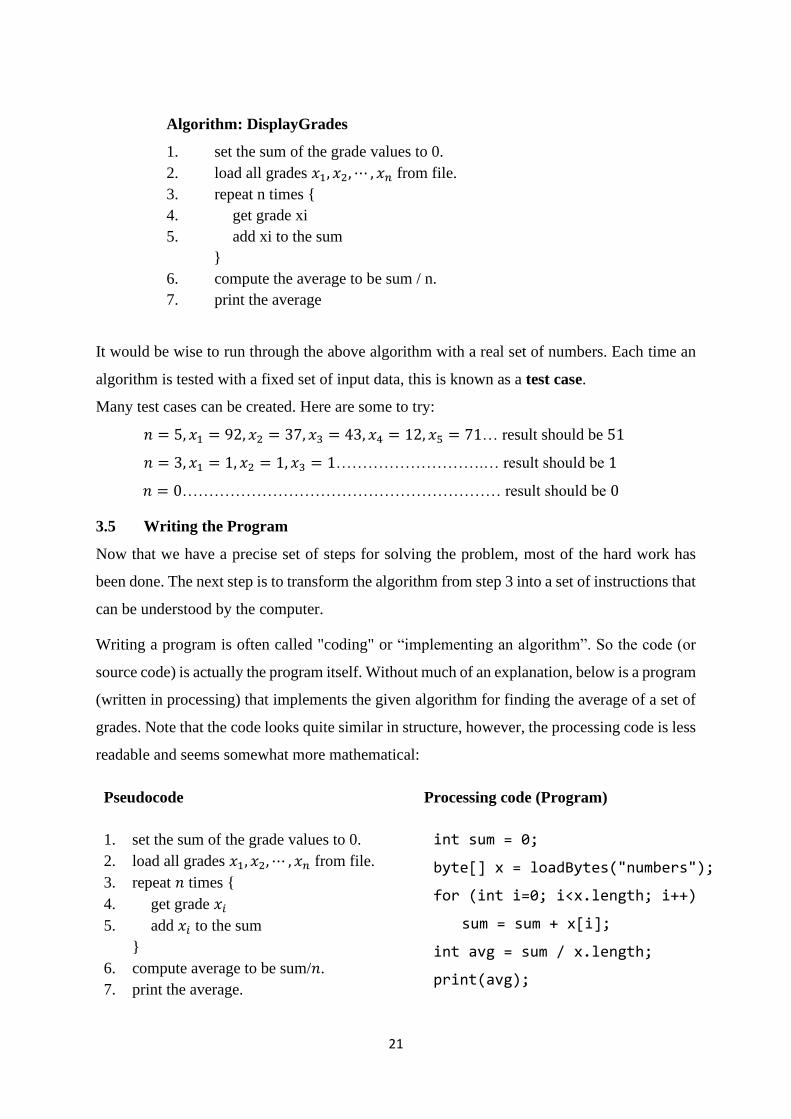
3.5 Writing the Program

Now that we have a precise set of steps for solving the problem, most of the hard work has

been done. The next step is to transform the algorithm from step 3 into a set of instructions that

can be understood by the computer.

Writing a program is often called "coding" or “implementing an algorithm”. So the code (or

source code) is actually the program itself. Without much of an explanation, below is a program

(written in processing) that implements the given algorithm for finding the average of a set of

grades. Note that the code looks quite similar in structure, however, the processing code is less

readable and seems somewhat more mathematical:

Algorithm: DisplayGrades

1. set the sum of the grade values to 0.

2. load all grades 𝑥1, 𝑥2, ⋯ , 𝑥𝑛 from file.

3. repeat n times {

4. get grade xi

5. add xi to the sum

}

6. compute the average to be sum / n.

7. print the average

Pseudocode

1. set the sum of the grade values to 0.

2. load all grades 𝑥1, 𝑥2, ⋯ , 𝑥𝑛 from file.

3. repeat 𝑛 times {

4. get grade 𝑥𝑖

5. add 𝑥𝑖 to the sum

}

6. compute average to be sum/𝑛.

7. print the average.

Processing code (Program)

int sum = 0;

byte[] x = loadBytes("numbers");

for (int i=0; i<x.length; i++)

sum = sum + x[i];

int avg = sum / x.length;

print(avg);

22

For now, the details of how to produce the above source code will not be discussed. In fact, the

source code would vary depending on the programming language that was used. Learning a

programming language may seem difficult at first, but it will become easier with practice.

The computer requires precise instructions in order to understand what it is being asked to do.

For example, removing one of the semi-colon characters (;) from the program above, will make

the computer become confused as to what it’s being asked to do because the semi-colon

characters (;) is what it understands to be the end of an instruction. Leaving one of them off

will cause the program to generate what is known as a compile-time error.

Definition 1-3: Compiling is the process of converting a program into instructions that can be

understood by the computer.

The longer a program is, the more the likelihood of having multiple compile-time errors. One

needs to fix all such compile-time errors before continuing on to the next step.

3.6 Test the Program

Once a program is written and compiles, the next task is to make sure that it solves the problem

that it was intended to solve and that the solutions are correct.

Running a program is the process of telling the computer to evaluate the compiled instructions.

When a program is run and all is well, you should see the correct output. It is possible however,

that a program works correctly for some set of input data but not for all. If the output of a

program is incorrect, it is possible that the algorithm was not properly converted into a proper

program. It is also possible that the programmer did not produce a proper algorithm back in

step 3 that handles all situations that could arise. Perhaps some instructions are performed out

of sequence. Whatever happened, such problems with the program are known as bugs.

Definition 1-4: Bugs are errors with a program that cause it to stop working or produce

incorrect or undesirable results.

It is the responsibility of the programmer to fix as many bugs in a program as are present. To

find bugs effectively, a program should be tested with many test cases (called a test suite). It is

also a good idea to have others test one’s program because they may think up situations or input

data that one may never have thought of.

Definition 1-5: Debugging is the process of finding and fixing errors in program code.

23

Debugging is often a very time-consuming “chore” when it comes to being a programmer.

However, if one painstakingly and carefully follows steps 1 through 3, this should greatly

reduce the amount of bugs in a program, thus making debugging much easier.

3.7 Evaluating the Solution

Once the program produces a result that seems correct, the original problem needs to be

reconsidered to make sure that the answer is formatted into a proper solution to the problem. It

is often the case that it may be realised that the program solution does not solve the problem

the way it is expected. It may also be realised that more steps are involved.

For example, if the result of a program is a long list of numbers, but the intent was to determine

a pattern in the numbers or to identify some feature from the data, then simply producing a list

of numbers may not suffice. There may be a need to display the information in a way that helps

visualise or interpret the results with respect to the problem; perhaps a chart or graph is needed.

It is also possible that when the results are examined, it is realised that additional data are

needed to fully solve the problem. Alternatively, the results may need to be adjusted to solve

the problem more efficiently (e.g., a game is too slow).

It is important to remember that the computer will only do what it is told to do. It is up to the

user to interpret the results in a meaningful way and determine whether or not it solves the

original problem. It may be necessary to re-do some of the steps again, perhaps going as far

back as step 1 again, if data were missing.

4.0 CONCLUSION

The decision to get a solution to any exist problem involve a cycle that consist of the following

using a Computer as a model of computation, Understanding the Problem, Formulating a

Model, Developing an Algorithm, Writing the Program, Testing the Program and finally

Evaluating the Solution.

5.0 SUMMARY

In this unit you learnt that the various stages involve in the problem solving processing: The

stages are sequential and are seven in number:

• Computer as a model of computation

• Understanding the Problem

• Formulating a Model

• Developing an Algorithm

24

• Writing the Program

• Testing the Program

• Evaluating the Solution

6.0 TUTOR-MARKEDASSIGNMENT

a. Discuss various stages that will be needed to get a problem solved.

b. How do you identify the most important stage in the problem solving process?

c. What effect will be generated if the stage that involves program writing is not observed in

the problem solving process?

d. What effect will be generated if the stage that involves program writing is not observed in

the problem solving process?

7.0 REFERENCES / FURTHER READINGS

Koren, I. (2018). Computer arithmetic algorithms: AK Peters/CRC Press.

Motwani, R., & Raghavan, P. (1995). Randomized algorithms: Cambridge university press.

Spielman, R. M., Dumper, K., Jenkins, W., Lacombe, A., Lovett, M., & Perlmutter, M. (2021).

Problem Solving. Psychology-H5P Edition.

Treffinger, D. J., Isaksen, S. G., & Stead-Dorval, K. B. (2006). Creative problem solving: An

introduction: Prufrock Press Inc.

25

UNIT 3: COMPUTATIONAL APPROACHES TO PROBLEM SOLVING

CONTENTS

1.0 Introduction

2.0 Objectives

3.0 Main Content

3.1 Brute-force Approach

3.2 Divide-and-conquer Approach

3.2.1 Example: The Merge Sort Algorithm

3.2.2 Advantages of Divide and Conquer Approach

3.2.3 Disadvantages of Divide and Conquer Approach

3.3 Dynamic Programming Approach

3.3.1 Example: Fibonacci series

3.3.2 Recursion vs Dynamic Programming

3.4 Greedy Algorithm Approach

3.4.1 Characteristics of the Greedy Algorithm

3.4.2 Motivations for Greedy Approach

3.4.3 Greedy Algorithms vs Dynamic Programming

3.5 Randomized Approach

4.0 Conclusion

5.0 Summary

6.0 Tutor-Marked Assignments

7.0 References/Further Reading

1.0 INTRODUCTION

Solving a problem involves finding a way to move from a current situation to a desired

outcome. To be able to solve a problem using computational approaches, the problem itself

needs to have certain characteristics:

• The problem needs to be clearly defined — this means that one should be able to

identify the current situation, the end goal, the possible means of reaching the end goal,

and the potential obstacles

• The problem needs to be computable — one should consider what type of calculations

are required, and if these are feasible within a reasonable time frame and processing

capacity

26

• The data requirements of the problem need to be examined, such as what types of data

the problem involves, and the storage capacity required to keep this data

• One should be able to determine if the problem can be approached using decomposition

and abstraction, as these methods are key for tackling complex problems

Once these features of the given problem are identified, an informed decision can then be made

as to whether the problem is solvable or not using computational approaches.

2.0 OBJECTIVES

By the end of this unit, you will be able to:

• Describe the various computational approaches available for solving a problem

• Classify computational approaches based on their paradigms

• Evaluate a computational approach best suited for a given problem

• Apply a computational approach to solve a problem

3.0 MAIN CONTENT

3.1 Brute-force Approach

This strategy is characterised by a lack of sophistication in terms of their approach to the

solution. It typically takes the most direct or obvious route, without attempting to minimise

the number of operations required to compute the solution.

Brute-force approach is considered quite often in the course of searching. In a searching

problem, we are required to look through a list of candidates in an attempt to find a desired

object. In many cases, the structure of the problem itself allows us to eliminate a large number

of the candidates without having to actually search through them. As an analogy, consider the

problem of trying to find a frozen pie in an unfamiliar grocery store. You would immediately

go to the frozen food aisle, without bothering to look down any of the other aisles. Thus, at the

outset of your search, you would eliminate the need to search down most of the aisles in the

store. Brute force approach, however, ignores such possibilities and naively search through all

candidates in an attempt to find the desired object. This approach is otherwise known as

exhaustive search.

Example:

Imagine a small padlock with 4 digits, each from 0-9. You forgot your combination, but you

don't want to buy another padlock. Since you can't remember any of the digits, you have to use

a brute force method to open the lock. So you set all the numbers back to 0 and try them one

27

by one: 0001, 0002, 0003, and so on until it opens. In the worst case scenario, it would take

104, or 10,000 tries to find your combination.

3.2 Divide-and-conquer Approach

In the divide and conquer strategy, a problem is solved recursively by applying three steps at

each level of the recursion: Divide, conquer, and combine.

Divide

“Divide” is the first step of the divide and conquer strategy. In this step the problem is divided

into smaller sub-problems until it is small enough to be solved. At this step, sub-problems

become smaller but still represent some part of the actual problem. As stated above, recursion

is used to implement the divide and conquer algorithm. A recursive algorithm calls itself with

smaller or simpler input values, known as the recursive case. So, when the divide step is

implemented, the recursive case is determined which will divide the problem into smaller sub-

problems.

Then comes the “conquer” step where we straightforwardly solve the sub-problems. By now,

the input has already been divided into the smallest possible parts and we’re now going to solve

them by performing basic operations. The conquer step is normally implemented with recursion

by specifying the recursive base case. Once the sub-problems become small enough that it can

no longer be divided, we say that the recursion “bottoms out” and that we’ve gotten down to

the base case. Once the base case is arrived at, the sub-problem is solved.

Combine

In this step, the solution of the sub-problems is combined to solve the whole problem. The

output returned from solving the base case will be the input of larger sub-problems. So after

reaching the base case we will begin to go up to solve larger sub-problems with input returned

from smaller sub-problems. In this step, we merge output from the conquer step to solve bigger

sub-problems. Solutions to smaller sub-problems propagate from the bottom up until they are

used to solve the whole original problem.

3.2.1 Example: The Merge Sort Algorithm

The merge sort algorithm closely follows the divide and conquer paradigm. In the merge sort

algorithm, we divide the n-element sequence to be sorted into two subsequences of 𝑛 = 2

elements each. Next, we sort the two subsequences recursively using merge sort. Finally, we

combine the two sorted subsequences to produce the sorted answer.

Let the given array be:

28

Divide the array into two halves

Again, divide each subpart recursively into two halves until you get individual elements.

Now, combine the individual elements in a sorted manner. Here, conquer and combine steps

go side by side.

3.2.2 Advantages of Divide and Conquer Algorithms

The first, and probably the most recognizable benefit of the divide and conquer paradigm is the

fact that it allows us to solve difficult problems. Being given a difficult problem can often be

discouraging if there is no idea how to go about solving it. However, with the divide and

conquer method, it reduces the degree of difficulty since it divides the problem into easily

solvable sub-problems.

29

Another advantage of this paradigm is that it often plays a part in finding other efficient

algorithms. In fact, it played a central role in finding the quick sort and merge sort algorithms.

It also uses memory caches effectively. The reason for this is the fact that when the sub-

problems become simple enough, they can be solved within a cache, without having to access

the slower main memory, which saves time and makes the algorithm more efficient. And in

some cases, it can even produce more precise outcomes in computations with rounded

arithmetic than iterative methods would.

In the divide and conquer strategy problems are divided into sub-problems that can be executed

independently from each other. Thus, making this strategy suited for parallel execution.

3.2.3 Disadvantages of Divide and Conquer Algorithms

One of the most common issues with this sort of algorithm is the fact that the recursion is slow,

which in some cases outweighs any advantages of this divide and conquer process. Another

concern with it is the fact that sometimes it can become more complicated than a basic iterative

approach, especially in cases with a large n. In other words, if someone wanted to add large

numbers together, if they just create a simple loop to add them together, it would turn out to be

a much simpler approach than it would be to divide the numbers up into two groups, add these

groups recursively, and then add the sums of the two groups together.

3.3 Dynamic Programming Approach

Dynamic programming approach is similar to divide-and-conquer in that both solve problems

by breaking it down into several sub-problems that can be solved recursively. The difference

between the two is that in the dynamic programming approach, the results obtained from

solving smaller sub-problems are reused in the calculation of larger sub-problems. Thus,

dynamic programming is a bottom-up technique that usually begins by solving the smallest

sub=problems, saving these results and then reusing them to solve larger and larger sub-

problems until the solution to the original problem is obtained. This is in contrast to the divide-

and-conquer approach, which solves problems in a top-down fashion. In this case the original

problem is solved by breaking it down into increasingly smaller sub-problems, and no attempt

is made to reuse previous results in the solution of any of the sub-problems.

It is important to realise that a dynamic programming approach is only justified if there is some

degree of overlap in the sub-problems. The underlying idea is to avoid calculating the same

result twice. This is usually accomplished by constructing a table in memory, and filling it with

30

known results as they are calculated (memoization). These results are then used to solve larger

sub-problems. Note that retrieving a given result from this table takes Θ(1) time.

Dynamic programming is often used to solve optimisation problems. In an optimisation

problem, there are typically large number of possible solutions, and each has a cost associated

with it. The goal is to find a solution that has the smallest cost (i.e., optimal solution).

3.3.1 Example: Fibonacci Series

Let's find the Fibonacci sequence up to the 5th term. A Fibonacci series is the sequence of

numbers in which each number is the sum of the two preceding ones. For example, 0,1,1, 2, 3.

Here, each number is the sum of the two preceding numbers.

Algorithm

We are calculating the Fibonacci sequence up to the 5th term.

1. The first term is 0.

2. The second term is 1.

3. The third term is sum of 0 (from step 1) and 1(from step 2), which is 1.

4. The fourth term is the sum of the third term (from step 3) and second term (from step

2) i.e. 1 + 1 = 2.

5. The fifth term is the sum of the fourth term (from step 4) and third term (from step 3)

i.e. 2 + 1 = 3.

Hence, we have the sequence 0,1,1, 2, 3. Here, we have used the results of the previous

steps as shown below. This is called a dynamic programming approach.

Let 𝑛 be the number of terms.

1. If 𝑛 ≤ 1, return 1.

2. Else return the sum of two preceding numbers.

F(0) = 0

F(1) = 1

F(2) = F(1) + F(0)

F(3) = F(2) + F(1)

F(4) = F(3) + F(2)

31

3.3.2 Recursion vs Dynamic Programming

Dynamic programming is mostly applied to recursive algorithms. This is not a coincidence,

most optimization problems require recursion and dynamic programming is used for

optimization. But not all problems that use recursion can use Dynamic Programming. Unless

there is a presence of overlapping sub-problems like in the Fibonacci sequence problem, a

recursion can only reach the solution using a divide and conquer approach. This is the reason

why a recursive algorithm like Merge Sort cannot use Dynamic Programming, because the sub-

problems are not overlapping in any way.

3.4 Greedy Algorithm Approach

In a greedy algorithm, at each decision point the choice that has the smallest immediate (i.e.,

local) cost is selected, without attempting to look ahead to determine if this choice is part of

our optimal solution to the problem as a whole (i.e., a global solution). By locally optimal, we

mean a choice that is optimal with respect to some small portion of the total information

available about a problem.

The most appealing aspect of greedy algorithm is that they are simple and efficient – typically

very little effort is required to compute each local decision. However, for general optimization

problems, it is obvious that this strategy will not always produce globally optimal solutions.

Nevertheless, there are certain optimization problems for which a greedy strategy is, in fact,

guaranteed to yield a globally optimal solution.

3.4.1 Characteristics of the Greedy Algorithm

The important characteristics of a Greedy algorithm are:

1. There is an ordered list of resources, with costs or value attributions. These quantify

constraints on a system.

2. Take the maximum quantity of resources in the time a constraint applies.

3. For example, in an activity scheduling problem, the resource costs are in hours, and the

activities need to be performed in serial order.

3.4.2 Motivations for Greedy Approach

Here are the reasons for using the greedy approach:

• The greedy approach has a few trade-offs, which may make it suitable for optimization.

• One prominent reason is to achieve the most feasible solution immediately. In the

activity selection problem (Explained below), if more activities can be done before

finishing the current activity, these activities can be performed within the same time.

32

• Another reason is to divide a problem recursively based on a condition, with no need

to combine all the solutions.

• In the activity selection problem, the “recursive division” step is achieved by scanning

a list of items only once and considering certain activities.

3.4.3 Greedy Algorithms vs Dynamic Programming

Greedy algorithms are similar to dynamic programming in the sense that they are both tools

for optimization. However, greedy algorithms look for locally optimum solutions or in other

words, a greedy choice, in the hopes of finding a global optimum. Hence greedy algorithms

can make a guess that looks optimum at the time but becomes costly down the line and do not

guarantee a globally optimum. Dynamic programming, on the other hand, finds the optimal

solution to sub-problems and then makes an informed choice to combine the results of those

sub-problems to find the most optimum solution.

3.5 Randomized Approach

This approach is dependent not only on the input data, but also on the values provided by a

random number generator. If some portion of an algorithm involves choosing between a

number of alternatives, and it is difficult to determine the optimal choice, then it is often more

effective to choose the course of action at random rather than taking the time to determine the

vest alternative. This is particularly true in cases where there are a large number of choices,

most of which are “good.”

Although randomising an algorithm will typically not improve its worst-case running time, it

can be used to ensure that no particular input always produces the worst-case behaviour.

Specifically, because the behaviour of a randomised algorithm is determined by a sequence of

random numbers, it would be unusual for the algorithm to behave the same way on successive

runs even when it is supplied with the same input data.

Randomised approaches are best suited in game-theoretic situations where we want to ensure

fairness in the face of mutual suspicion. This approach is widely used in computer and

information security as well as in various computer-based games.

4.0 CONCLUSION

Solving problems is a key professional skill. Quickly weighing up available options and taking

decisive actions to select the best computational approach to a problem is integral to efficient

performance.

33

It is important to always get the problem solving process right, avoiding taking too little time

to define the problem or generate potential solutions. A wide range of computational techniques

for problem solving exist, and each can be appropriate given the peculiarity of the problem and

the individual involved. The important skills to attain are to assess the situation independently

of any other factors and to know when to trust your own instincts and when to ask for a second

opinion on a potential solution to a problem.

5.0 SUMMARY

In this Unit computational approaches for solving a problem were discussed viz. brute force,

divide and conquer, dynamic programming, genetic algorithm and randomized. The technique

for classifying the computational approaches based on their paradigms was deliberated upon

and evaluation of various computational approach best suited for a given problem was

recommended. The conclusion of the Unit applies the computational approach to solve a

problem.

6.0 TUTOR MARKED ASSIGNMENTS

7.0 REFERENCES/FURTHER READINGS

Bellman, R. (2010). Dynamic Programming: Princeton University Press.

de Ruffieu, F. L. (2016). Divide and Conquer Book 1: Fundamental Dressage Techniques:

Xenophon Press LLC.

Mandel, R. (2015). Coercing Compliance: State-Initiated Brute Force in Today's World:

Stanford University Press.

Roughgarden, T. (2019). Algorithms Illuminated: Greedy algorithms and dynamic

programming. Part 3: Soundlikeyourself Publishing, LLC.

Zámecniková, I., & Hromkovic, J. (2006). Design and Analysis of Randomized Algorithms:

Introduction to Design Paradigms: Springer Berlin Heidelberg.

34

MODULE 2: ROLE OF ALGORITHMS IN PROBLEM SOLVING

UNIT 1: ABSTRACTION AS A PROBLEM SOLVING TOOL

CONTENTS

1.0 Introduction

2.0 Objectives

3.0 Main Content

3.1 The Concept of Abstraction

3.2 Importance of Abstraction

3.3 How to Abstract

3.4 Types of Abstraction

3.4.1 Representational Abstraction

3.4.2 Abstraction by Generalisation

3,4,3 Procedural abstraction

3.4.4 Functional Abstraction

3.4.5 3.4.5 Data Abstraction

4.0 Conclusion

5.0 Summary

6.0 Tutor-Marked Assignmen

7.0 References/Further Reading

1.0 INTRODUCTION

One of the most crucial issues associated with problem solving involves managing the

complexities of the problem solving process. Good strategies typically use some form of

abstraction as a tool for dealing with this complexity. The use of abstraction in this context

refers to the intellectual capability of considering an entity apart from any specific instance of

this entity. For example, hardware designers attempting to design a computer typically concern

themselves with the functionality of the integrated circuits they intend to use and not with the

operation of the transistors found in these integrated circuits. Abstraction skills are essential in

the construction of appropriate models, designs, and implementations that are fit for the

particular purpose at hand and is, therefore, the focus in this unit.

2.0 OBJECTIVES

35

At the end of this unit, student should be able to:

• Define abstraction as a problem aid

• Understand the importance of abstraction in problem solving

• Describe how to perform abstraction

• Explain the various types of abstraction used in problem solving

3.0 MAIN CONTENT

3.1 The Concept of Abstraction

This is the creation of well-defined interfaces to hide the inner workings of computer programs

from users. It may also be defined as the process of identifying the general characteristics

needed to solve a problem while filtering out unnecessary information. It is also described as

simplifying a process or artefact by providing what you really need, and hiding the useless

details you don't care about, thus removing unnecessary detail.

Abstraction is widely used to simplify things that may be very complex. We use abstractions

all the time, almost without thinking. For example, if you learn to drive, you will be taught that

putting your foot on the accelerator will speed up the car and putting your foot on the brake

pedal will slow it down. You will not be taught anything about how the acceleration or braking

systems actually work.

3.2 Importance of Abstraction

In computer science, abstraction is used to manage the complexity of a lot of what is designed

and created. Computer hardware is seen as components or black boxes.

The abstraction above represents a computer. It shows the names of the components and how

they interact with each other but hides the complexity of each type of component.

3.3 How to Abstract

36

In computing, when we decompose problems, we then look for patterns among and within the

smaller problems that make up the complex problem. Abstraction allows us to create a general

idea of what the problem is and how to solve it. We remove all specific detail, and any patterns

that will not help us solve the problem.

For example, the school timetable (as shown below) is an abstraction of what happens in a

typical week: it captures key information such as who is taught what subject where and by

whom, but leaves to one side further layers of complexity, such as the learning objectives and

activities planned in any individual lesson. When abstracting, we remove specific details and

keep the general relevant patterns. So, abstraction allows us to form our idea of the problem.

This idea is also known as a model. Once we have a model of our problem, we can then design

an algorithm to solve it.

3.4 Types of Abstraction

3.4.1 Representational Abstraction

Abstraction appears in many forms within computing, both in terms of techniques used to

approach problem-solving, and in the computational tools employed to develop solutions.

The maps of many metropolitan public transport systems worldwide is a classic example of a

representational abstraction. Many specific details about the lines are removed because they

are not necessary for the purpose of the map, which is to help plan a journey. What remains

when unnecessary detail has been removed is a representational abstraction, i.e. a simpler

version directed at solving a particular problem.

37

Figure 1-1: Example of a metropolitan public transport system 'map'

Many real-world objects and situations are represented in computer systems. In a flight

simulator, different planes will be represented in some way within the system. If object-

oriented programming is used, the plane will be an object with a set of properties that are

relevant to the features of the simulator. Some details will be essential, such as the weight of

the plane (as this will affect its handling). Other details, such as the material used to upholster

the seats, will be irrelevant, and these aspects will not need to be represented within the system

or model.

Computer scientists have to choose what to include in the model and what to discard. They

must ensure that they include the minimum amount of detail necessary to solve the given

problem to the required degree of accuracy.

3.4.2 Abstraction by Generalisation

When you group things in terms of a set of common characteristics, you are generalising. This

is a fundamental technique used in object-oriented programming (although it is not exclusive

to OOP) when you identify that some objects are 'kinds of' more generic objects. For example,

38

you might say that a cocker spaniel is a kind of dog. Dogs have common sets of characteristics,

such as having four legs, a tail, and ears. However, so do cats; a biologist may tell you that both

animals belong to the order Carnivora (a group that includes many other types of animal

including bears, skunks, and badgers). Generalising in this way allows code to be developed

and shared between objects.

You can also apply the technique of generalisation to the problem itself. It is often helpful to

be able to identify a problem as an example of a more general set of problems. Sometimes, this

will help you to understand quickly that the problem is non-computable, or that it is intractable.

Otherwise, if the problem can be solved, you can benefit from a solution that already exists.

3.4.3 Procedural abstraction

This type represents a computational method. One of the skills that you will develop as a

computer scientist is the ability to design a well-abstracted procedure that is generalised as far

as possible.

For example, consider the problem of calculating the surface area of a chopping board. You

write the following subroutine:

This is an example of a subroutine that is too specific. Firstly, it is bound to a specific

(command line) user interface. If you abstract away this detail, the subroutine will be

independent of the user interface, and will therefore be more general. Here is a more general

version of the same subroutine:

PROCEDURE calculate_chopping_board_area()

side1_length = INPUT("Enter length of side 1: ")

side2_length = INPUT("Enter length of side 2: ")

side1_length = STR(side1_length)

side2_length = STR(side2_length)

area = side1_length * side2_length

PRINT(area)

ENDPROCEDURE

FUNCTION calculate_chopping_board_area(side1_length, side2_length)

area = side1_length * side2_length

RETURN area

ENDFUNCTION

39

A further abstraction is to replace the name (identifier) of the subroutine with something more

general:

3.4.4 Functional Abstraction

In functional abstraction, the implementation detail of the computational method is hidden.

You can think of a function as a black box. The function will receive an input (or set of inputs),

process the input(s), and return the output. How the transformation is achieved is hidden from

the user?

Most languages will provide a set of built-in functions that can be used by the programmer. In

the previous example of a subroutine that calculates the area of a regular polygon, a maths

library is used to provide useful mathematical functions. In the example, functions were used

to provide the value of pi, to calculate the square root of a number, and to calculate the tangent

of a number.

In Python, for example, the built-in function to display a value to the console or command line

interface is print. If you code in Python, you will be familiar with typing a command such as

print ("Hello World"). You will know that the name of the function is print, and it must

be followed by a value (to print) enclosed in parentheses.

Using the Python 'help' facility, you can see the details of the interface. It is more technical

than you might expect and you will usually only need to delve into this level of documentation

when you want to do something a bit different. The first line is the name of the function and its

parameters. The remaining information is provided through a 'docstring' (a documentation

strings that provides a convenient way of documenting a functions, classes, and methods). This

provides sufficient information for the programmer to use the function, but hides all of the

other information.

3.4.5 Data Abstraction

Some data types, such as unsigned integers, are conceptually simple; others are more complex.

Data abstraction is a technique that allows you to separate the way that a compound data object

is used, from the details of how it is constructed.

FUNCTION calculate_area(side1_length, side2_length)

area = side1_length * side2_length

RETURN area

ENDFUNCTION

40

If you have studied data structures, you will be aware of the concept of a stack as an example

of an abstract data type (ADT). A stack is a last in, first out (LIFO) data structure that supports

three standard operations: push (add an item to the stack), pop (remove an item from a stack),

and peek (look at the item at the top of the stack). The abstract concept of a stack, and its

operations, can be understood without any consideration of how it is implemented. Sometimes,

you will see a stack drawn as an upright container with a single opening at the top. This

abstraction helps you to understand the LIFO nature of the structure.

With more complex data structures, data abstraction becomes more and more important to

prevent you getting caught up in the implementation detail. You will often use more than one

layer of abstraction. For example, in classic computer science theory, you will learn that the

data structure underpinning a graph is an adjacency matrix or an adjacency list. These are in

themselves abstractions. For example, consider an adjacency list. You might choose to

implement it using a dictionary or a linked list, however, a dictionary is also an abstract data

type that is conceptually a set of key–value pairs, and a linked list is a traversable sequence.

Neither abstraction tells you anything about the way that the structure will be implemented.

Only at the lowest level will the implementation detail be revealed.

4.0 CONCLUSION

Abstraction is one of the four cornerstones of computer science. It is important in the study of

computing and problem solving and involves identification of critical aspects of the problem

environment and the required system. The generalisation aspect of abstraction is seen in the

programming with the use of data abstraction. Abstraction skills are essential in the

construction of appropriate models, designs and implementation fit for the particular purpose.

5.0 SUMMARY

In this Unit the concept of abstraction and its importance in problem solving were described,

Abstraction involves the process of taking away or removing characteristics from something

in order to reduce it to a set of essential characteristics. In abstraction, essential elements are

displayed to the user and trivial elements are kept hidden. Its main goal is to handle complexity

by hiding unnecessary details from the user. In computing, when we decompose problems, we

then look for patterns among and within the smaller problems that make up the complex

problem. Abstraction allows us to create a general idea of what the problem is and how to solve

it. We remove all specific detail, and any patterns that will not help us solve the problem. There

41

are five types of abstractions namely – representational abstraction, abstraction by

generalization, procedural abstraction, functional abstraction and data abstraction

6.0 TUTOR MARKED ASSIGNMENTS

1. What is abstraction?

2. Discuss the concept and importance of abstraction

3. Describe the process needed to carry out abstraction

4. Explain the various types of abstraction used in problem solving

REFERENCES/FURTHER READINGS

Damerow, P. (1996). Abstraction and Representation Abstraction and Representation (pp. 371-

381): Springer.

Danvy, O., & Filinski, A. (1989). A functional abstraction of typed contexts: Citeseer.

Knoblock, C. A. (2012). Generating Abstraction Hierarchies: An Automated Approach to

Reducing Search in Planning: Springer US.

Liskov, B. H., & Zilles, S. N. (1975). Specification techniques for data abstractions. IEEE

Transactions on Software Engineering(1), 7-19.

42

UNIT 2: ALGORITHMS

CONTENTS

1.0 Introduction

2.0 Objectives

3.0 Main Content

3.1 The Notion of Algorithm

3.2 Reasons for Algorithm

3.3 Steps Involved in Algorithm Development

3.4 Characteristics of Algorithm

3.5 Representation of Algorithms

3.5.1 Representative Algorithms for Simple Problems

3.6 Measuring Efficiency of Algorithms

3.7 Advantages and Disadvantages of Algorithm

3.7.1 Advantages

3.7.2 Disadvantages

4.0 Conclusion

5.0 Summary

6.0 Tutor-Marked Assignments

7.0 References/Further Reading

1.0 INTRODUCTION

We all have unconsciously built up shortcuts, assumptions, and rules of thumb that we use to

help us solve everyday problems without thinking about them. For instance, take the simple

task of sorting 10 numbers. As it stands, we can take a look at them, tell pretty quickly what

the order should be, and arrange the numbers correctly. However, we’re not used to breaking

our thought process down into its individual steps and translating that to what computers can

do. For instance, computers can’t jump to general spots in a dictionary to find a word based

on its spelling. A computer has to have very specific instructions on where to start.

For beginner in the problem-solving process, it’s tricky to break that thought process down and

translate that to computable steps, since computers generally can’t make the types of judgement

calls about where in the list to start. Though like all skills, it’s learnable and that is what will

our focus in this Unit.

43

2.0 OBJECTIVES

At the end of this unit, student should be able to:

• Understand and explain the concept of algorithms

• Explain the need for algorithms and their desirable characteristics

• Describe the steps involved in developing an algorithm

• Develop algorithms for simple problems

• Evaluate different algorithms based on their efficiency

3.0 MAIN CONTENT

3.1 The Notion of Algorithm

By definition, an algorithm is an effective step-by-step procedure for solving a problem in a

finite number of steps. In other words, it is a finite set of well-defined instructions or step-by-

step description of the procedure written in human readable language for solving a given

problem. An algorithm itself is division of a problem into small steps which are ordered in

sequence and easily understandable. Algorithms are very important to the way computers

process information, because a computer program is basically an algorithm that tells computer

what specific tasks to perform in what specific order to accomplish a specific task. The same

problem can be solved with different methods. So, for solving the same problem, different

algorithms can be designed. In these algorithms, number of steps, time and efforts may vary

more or less.

For example, we might need to sort a sequence of numbers into non-decreasing order. This

problem arises frequently in practice and provides fertile ground for introducing many standard

design techniques and analysis tools. Here is how we formally define the sorting problem:

Input: A sequence of 𝑛 numbers ⟨𝑎1, 𝑎2, ⋯ , 𝑎𝑛⟩,.

Output: A reordering ⟨𝑎1′ , 𝑎2

′ , ⋯ , 𝑎𝑛′ ⟩of the input sequence such that 𝑎1

′ ≤ 𝑎2′ ≤ ⋯ ≤ 𝑎𝑛

′ .

For example, given the input sequence ⟨31; 41; 59; 26; 41; 58⟩, a sorting algorithm returns

as output the sequence ⟨26; 31; 41; 41; 58; 59⟩. Such an input sequence is called an instance

of the sorting problem. In general, an instance of a problem consists of the input (satisfying

whatever conditions are imposed in the problem statement) needed to compute a solution to

the problem.

In computer science we give a special name to the sub-algorithms. They are sometimes called

modules, functions or procedures. In fact, it is not a good idea to simply number all the sub-

algorithms but instead to give them meaningful names. As standard convention, when naming

44

a function or procedure, you should use letters, numbers and underscore (i.e., _) characters but

not any spaces or punctuation. Also, the first character in the name should be a lower case

letter. If multiple words are used as the name, each word except the first should be capitalized.

Lastly, we often use parentheses (i.e., ()) after the function or procedure name to identify it as

a sub-algorithm. You should choose meaningful names that are not too long as will be evident

in our discussion. When a sub-algorithm comes back with some kind of object or value such

as numerical result, we call the sub-algorithm a function. If the sub-algorithm does not return

any particular value, it is instead known as a procedure.

3.2 Reasons for Algorithm

A programmer writes a program to instruct the computer to do certain tasks as desired. The

computer then follows the steps written in the program code. Therefore, the programmer first

prepares a roadmap of the program to be written, before actually writing the code. Without a

roadmap, the programmer may not be able to clearly visualise the instructions to be written and

may end up developing a program which may not work as expected. Such a roadmap is nothing

but the algorithm which is the building block of a computer program.

For example, searching using a search engine, sending a message, finding a word in a

document, booking a taxi through an app, performing online banking, playing computer games,

all are based on algorithms. Writing an algorithm is mostly considered as a first step to

programming. Once we have an algorithm to solve a problem, we can write the computer

program for giving instructions to the computer in high level language. If the algorithm is

correct, computer will run the program correctly, every time. So, the purpose of using an

algorithm is to increase the reliability, accuracy and efficiency of obtaining solutions.

3.3 Steps Involved in Algorithm Development

An algorithm can be defined as “a complete, unambiguous, finite number of logical steps for

solving a specific problem “

Step1. Identification of input: For an algorithm, there are quantities to be supplied called

input and these are fed externally. The input is to be identified first for any specified

problem.

Step2: Identification of output: From an algorithm, at least one quantity is produced, called

for any specified problem.

Step3: Identify the processing operations: All the calculations to be performed in order to

lead to output from the input are to be identified in an orderly manner.

45

Step4: Processing Definiteness: The instructions composing the algorithm must be clear and

there should not be any ambiguity in them.

Step5: Processing Finiteness: If we go through the algorithm, then for all cases, the algorithm

should terminate after a finite number of steps.

Step6: Possessing Effectiveness: The instructions in the algorithm must be sufficiently basic

and in practice they can be carries out easily.

3.4 Characteristics of Algorithm

An algorithm must possess following characteristics:

1. Precision — the steps are precisely stated or defined.

2. Uniqueness — results of each step are uniquely defined and only depend on the input

and the result of the preceding steps.

3. Finiteness — the algorithm always stops after a finite number of steps.

4. Input — the algorithm receives some input.

5. Output — the algorithm produces some output.

3.5 Representation of Algorithms

Using their algorithmic thinking skills, software designers or programmers analyse the problem

and identify the logical steps that need to be followed to reach a solution. Once the steps are

identified, the need is to write down these steps along with the required input and desired

output. There are two common methods of representing an algorithm —flowchart and

pseudocode.

Either of the methods can be used to represent an algorithm while keeping in mind the

following:

• It showcases the logic of the problem solution, excluding any implementation details

• It clearly reveals the flow of control during execution of the program

Flowcharts will be discussed in Unit 3 while pseudocode will be the subject of Unit 4

3.5.1 Representative Algorithms for Simple Problems

Write an algorithm for the following

1. Write an algorithm to calculate the simple interest using the formula:

𝑆𝑖𝑚𝑝𝑙𝑒 𝑖𝑛𝑡𝑒𝑟𝑒𝑠𝑡 = 𝑃 ∗ 𝑁 ∗ 𝑅/100, Where 𝑃 is principle Amount, 𝑁 is the number of

years and 𝑅 is the rate of interest.

46

2 Write an algorithm to find the area of the triangle.

Let 𝑏, 𝑐 be the sides of the triangle 𝐴𝐵𝐶 and 𝐴 the included angle between the given sides.

3. Write an algorithm to find the largest of three numbers 𝑋, 𝑌, 𝑍.

Algorithm calculateSimpleInterset

Step 1: Read the three input quantities’ P, N and R.

Step 2: Calculate simple interest as

Simple interest = P* N* R/100

Step 3: Print simple interest.

Step 4: Stop.

Algorithm findAreaOfTriangle

Step 1: Input the given elements of the triangle namely sides 𝑏, 𝑐 and angle

between the sides 𝐴

Step 2: Area = 1

2∗ 𝑏 ∗ 𝑐 ∗ 𝑠𝑖𝑛(𝐴)

Step 3: Output the Area

Step 4: Stop.

Algorithm findLargestOfThreeNumbers

Step 1 Read the numbers 𝑋, 𝑌, 𝑍.

Step 2 If (X > Y)

big = X

Else big = Y

Step 3 If (big < Z)

big = Z

Step 4 Print big

Step 5 Stop.

47

4. Write an algorithm to find the largest data value of a set of given data values

5. Write an algorithm which will test whether a given integer value is prime or not.

6. Write algorithm to find the factorial of a given number N

Algorithm findLargestDataValue

Step 1: LARGE = 0

Step 2: read NUM

Step 3: While NUM > = 0 do

3.1 If NUM > LARGE then

3.1.1 LARGE = NUM

3.2. Read NUM

Step 4: Write “largest data value is”, LARGE

Step 5: Stop

Algorithm testForPrime

Step 1: M = 2

Step 2: read N

Step 3: MAX = SQRT (N)

Step 4: While M < = MAX do

4.1 If (M * (N/M) = N then

4.1.1 goto step 7

Step 4.2. M = M+1

Step 5: Write “number is prime”

Step 6 goto step 8

Step 7 Write “number is not a prime”

Step 8 End

Algorithm findFactorial

Step 1: PROD = 1

Step 2: I = 0

Step 3 read N

Step 4: While I < N do

4.1 I = I + 1

Step 4.2. PROD = PROD* I

Step 5: Write “Factorial of N is”, PROD

Step 6: End

48

7. Write an algorithm to calculate the perimeter and area of rectangle. Given its length and

width.

8. Write an algorithm to find sum of given data values until negative value is entered.

3.6 Measuring Efficiency of Algorithms

It may be possible to solve to problem in more than one ways, resulting in more than one

algorithm. The choice of various algorithms depends on the factors like reliability, accuracy

and easy to modify. The most important factor in the choice of algorithm is the time

requirement to execute it, after writing code in High-level language with the help of a computer.

The algorithm which will need the least time when executed is considered the best.

Consider an algorithm for drawing a house. Since the problems is a little vague, there are many

potential solutions. Here is one of them:

Algorithm calculatePerimeterAndAreaOfRectangle

Step 1: Read length and width of the rectangle

Step 2: Calculate perimeter = 2* (length + width)

Step 3: Calculate area = length *width.

Step 4: Print perimeter

Step 5 Print area

Step 6: Stop

Algorithm findSumUntilNegative

Step 1: SUM = 0

Step 2: I= 0

Step 3: read NEW VALUE4

Step 4: While NEW VALUE > = 0 do

4.1 SUM = SUM + NEW VALUE

4.1.2 I = I + 1

4.1.3. Read NEW VALUE

Step 5: Write “sum of ”, I, “ data values is”, SUM

Step 5: End

Algorithm1: DrawSimpleHouse

1. draw a square frame

2. draw a triangular roof

3. draw a door

49

Obviously, we could have made a more elaborate house, but the solution above solves the

original problem. What if this was our solution?

Which is a “better” solution? That’s not an easy question to answer. It depends on what “better”

means. If time is of the essence (e.g., as in playing a game of Pictionary) then Algorithm1

would be better because it can be drawn faster. The more elaborate house of Algorithm2 would

perhaps be “better” if visual appearance was the aim, as opposed to speed of drawing. This

example brings up an important topic in computer science called algorithm efficiency.

Definition: Algorithm efficiency is used to describe properties of an algorithm elating to

how much of various types of resources it consumes.

Normally in computer science we are interested in algorithms that are time and space efficient,

although there are also other ways (i.e., metrics) for measuring efficiency. For example,

Algorithm1 is more efficient in terms of time but it is also more efficient in terms of ink or

pencil usage as well as the amount of space that it takes on the paper. Algorithm2 may be more

efficient in terms of detailing in that, depending on the context, it may take longer for a person

to guess what the drawing is (i.e., it could be confused with a barn, shed or dog house if this

was drawn in a farm setting). In this case, the extra time taken to distinguish the house through

the drawing of the windows and chimney may result in a quicker guess.

Definition: The runtime complexity (execution time) of an algorithm is the amount of time

that it takes to complete once it has begun.

Definition: The space complexity of an algorithm is the amount of storage space that it

requires while running from start to completion.

Consider the following algorithm for setting a table:

Algorithm2: DrawMoreComplexHouse

4. draw a square frame

5. draw a triangular roof

6. draw a door

7. draw windows

8. draw chimney

9. draw smoke

10. draw land

11. draw path to door8. draw path to door

50

Why is this not an efficient real-world solution?

It is inefficient in that it requires a lot of unnecessary travelling back and forth to the cupboard

and table because it gets one glass at a time. While this may be a safer solution for a small

child, an adult would likely grab all 4 glasses at once as well as the plates and utensils.

Here is a different, though similar, algorithm.

Notice that there is nolonger a need for a repeat loop since we are getting all the glasses, plates

and utensils once. We can actually generalise the algorithm to set the table for as many guests

as we want by supplying some additional information in our functions.

Definition: A parameter is a piece of data provided as input to a function or procedure

We can supply an arbitrary number inour algorithm to specify how many place setting to set

as follows:

AlgorithmY1: SetTableFor4

1. Walk to kitchen

2. Repeat 4 times {

3. getGlass()

4. place glass on table

5. getPlate()

6. place plate on table

7. getUtensils()

8. place knife and fork on table

}

9. go back onto couch

AlgorithmY2: EfficientSetTableFor4

1 Walk to kitchen

2 getGlass()

3 place glass on table

4 getPlate()

5 place plate on table

6 getUtensils()

7 place knife and fork on table

8 go back onto couch

51

Notice that we supplied a number 8 between the parentheses of our function. This is where we

normally supply additional information (i.e., parameters) to our functions. Now our function is

clear as to how many place settings will be made, whereas AlgorithmY2 was not clear. But

what would the getGlasses() function now look like ? Here was the 1-glass version:

Now we need to specify the parameter for the function and use it within the function itself:

Notice how the parameter is now being used within the function to get the necessary glasses.

The value of n will vary according to how we call the function. For example, if we use

getGlasses(8), then within the function, 𝑛 will have the value of 8.

AlgorithmY#: EfficientSetTableFor8

1. walk to kitchen

2. getGlasses(8)

3 place glasses on table

4 getPlates(8)

5 place plates on table

6 getUtensils(8)

7 place knives and forks on table

8 go back onto couch

GetGlass()

1. go to the cupboard

2. open cupboard

3. take a glass

4. close cupboard

GetGlasses(n)

1. go to the cupboard

2. open cupboard

3. repeat n times {

4. take a glass

}

5. close cupboard

52

If we use getGlasses(4), then within the function, 𝑛 will have the value of 4. So, the value for

parameter 𝑛 will always be the number that was passed in when the function was called. For

algorithms that are the most general, we often use the letter 𝑛 as a kind of “placeholder” or

“label” to indicate that we want the algorithm to work for any number from 0 to 𝑛. The “𝑛”

itself is not a special letter, it is just commonly used. So, the statement getGlasses(n) is

indicating “get 𝑛 glasses”, where 𝑛 may be any integer number that we want.

Obviously, there is a limit as to how many glasses a person could carry. However, to describe

an algorithm in a very general way, we use n to indicate that our algorithm will work for any

number from 0 to n. Using n instead of a fixed number, also allows us to compare two

algorithms in regards to their efficiency. That is, we can often compare the number of steps

that one algorithm requires with another algorithm. For example, consider these two algorithms

for setting the table for n people:

What if we defined efficiency in this example to refer to the “number of times we walked back

and forth between the cupboard and the table”? Which algorithm is more efficient? Well each

time through the loop, AlgorithmA makes 3 trips between the cupboard and table. Since there

are 𝑛 place settings (i.e., 𝑛 times through the loop), then the whole algorithm takes 𝑛 𝑥 3, or

3𝑛, steps. What about AlgorithmB? It takes only 3 trips between the cupboard and table

altogether, regardless of how many place settings will be required. So what can we conclude?

If we are setting a place for 1 person, either algorithm is good. If setting for 2 people, then

AlgorithmB is twice more efficient than AlgorithmA since it requires half the travel between

the cupboard and table. As 𝑛 gets larger, the difference becomes more significant. For example,

if we are setting the table for 8 people, then AlgorithmA uses 8 times (total of 24) more trips

Algorithm A

1. walk to kitchen

2. repeat n times {

3. getGlass()

4. place glass on table

5. getPlate()

6. place plate on table

7. getUtensils()

8. place knife and fork on table

}

9. go back onto couch

Algorithm B

1. walk to kitchen

2. getGlasses(n)

3. place glasses on table

4. getPlates(n)

5. place plates on table

6. getUtensils(n)

7. place knives and forks on table

8. go back onto couch

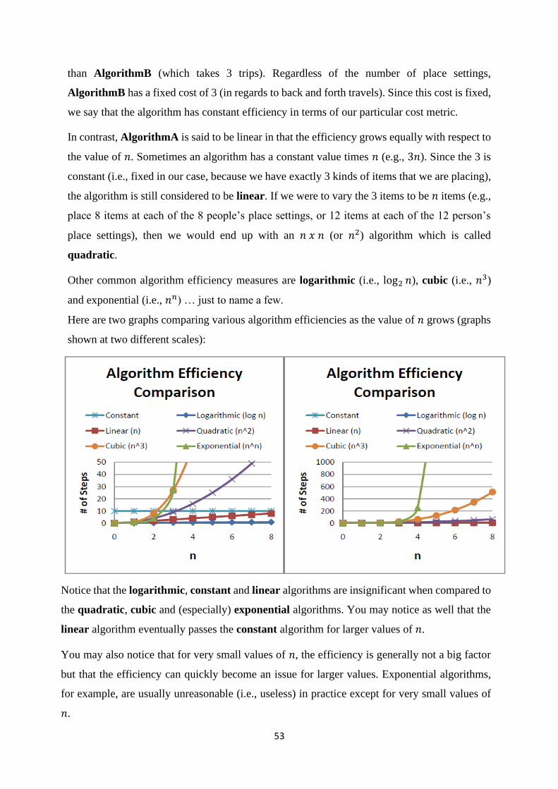
53

than AlgorithmB (which takes 3 trips). Regardless of the number of place settings,

AlgorithmB has a fixed cost of 3 (in regards to back and forth travels). Since this cost is fixed,

we say that the algorithm has constant efficiency in terms of our particular cost metric.

In contrast, AlgorithmA is said to be linear in that the efficiency grows equally with respect to

the value of 𝑛. Sometimes an algorithm has a constant value times 𝑛 (e.g., 3𝑛). Since the 3 is

constant (i.e., fixed in our case, because we have exactly 3 kinds of items that we are placing),

the algorithm is still considered to be linear. If we were to vary the 3 items to be 𝑛 items (e.g.,

place 8 items at each of the 8 people’s place settings, or 12 items at each of the 12 person’s

place settings), then we would end up with an 𝑛 𝑥 𝑛 (or 𝑛2) algorithm which is called

quadratic.

Other common algorithm efficiency measures are logarithmic (i.e., log2 𝑛), cubic (i.e., 𝑛3)

and exponential (i.e., 𝑛𝑛) … just to name a few.

Here are two graphs comparing various algorithm efficiencies as the value of 𝑛 grows (graphs

shown at two different scales):

Notice that the logarithmic, constant and linear algorithms are insignificant when compared to

the quadratic, cubic and (especially) exponential algorithms. You may notice as well that the

linear algorithm eventually passes the constant algorithm for larger values of 𝑛.

You may also notice that for very small values of 𝑛, the efficiency is generally not a big factor

but that the efficiency can quickly become an issue for larger values. Exponential algorithms,

for example, are usually unreasonable (i.e., useless) in practice except for very small values of

𝑛.

54

Logarithmic solutions are often preferred since they are significantly more efficient than even

linear algorithms. For example, if 𝑛 is 1,000,000 then a linear algorithm can take 1,000,000

steps whereas a logarithmic algorithm may take only 20 steps. Sometimes it is hard to think in

terms of an unknown number 𝑛 because we are used to working with actual concrete numbers.

3.7 Advantages and Disadvantages of Algorithm

3.7.1 Advantages

Designing an algorithm has following advantages:

1. Effective Communication: Since algorithm is written in English like language, it is

simple to understand step-by-step solution of the problems.

2. Easy Debugging: Well-designed algorithm makes debugging easy so that we can

identify logical error in the program.

3. Easy and Efficient Coding: An algorithm acts as a blueprint of a program and helps

during program development.

4. Independent of Programming Language: An algorithm is independent of

programming languages and can be easily coded using any high level language.

3.7.2 Disadvantages

An algorithm has following disadvantages:

1. Developing algorithm for complex problems would be time consuming and difficult to

understand.

2. Understanding complex logic through algorithms can be very difficult.

4.0 CONCLUSION

As a student of computer science, it is important to understand algorithms so that one can use

them properly. If you are working on a given algorithm to solve a problem, you will likely need

to be able to estimate how fast it is going to run. Such an estimate will be less accurate without

an understanding of runtime analysis. Furthermore, one needs to understand the details of the

algorithms involved so that one can predict if there are special cases in which the coding won’t

work quickly, or if it will produce unacceptable results. By developing a good understanding

of a large range of algorithms, you will be able to choose the right one for a problem and apply

it properly.

55

5.0 SUMMARY

Algorithm is a finite set of well-defined instructions or step-by-step description of the

procedure written in human readable language for solving a given problem. The purpose of

using an algorithm is to increase the reliability, accuracy and efficiency of obtaining solutions.

There are two common methods of representing an algorithm — flowchart and pseudo code.

Designing an algorithm has advantages of effective Communication, easy debugging, easy and

efficient coding and Independent of programming language> the disadvantages are in the time

consumption especially when developing complex problems and difficulty in understanding

complex logic problem

6.0 TUTOR MARKED ASSIGNMENT

1. Explain the concept of algorithms

2. Explain the need for algorithms and their desirable characteristics

3. Describe the steps involved in developing an algorithm

4. Describe the steps involved in developing simple problems algorithms

5. Evaluate different algorithms based on their efficiency

7.0 REFERENCES/FURTHER READINGS

Ergül, Ö. (2013). Guide to programming and algorithms using R: Springer.

Wilf, H. S. (2002). Algorithms and complexity: AK Peters/CRC Press.

56

UNIT 3: FLOWCHARTS

CONTENTS

1.0 Introduction

2.0 Objectives

3.0 Main Content

3.1 Concept of Flowcharts

3.2 Symbols used in Creating a Flowchart

3.2.1 Basic Symbols

3.2.2 Intermediate and Advanced Symbols

3.3 Common Types of Flowchart Types

3.4 Areas for using Flowcharts

3.5 Considerations in Flowcharting

3.6 Sample Flowcharts

3.7 Differences between Algorithm and Flowchart

3.8 Advantages of Flowcharts

4.0 Conclusion

5.0 Summary

6.0 Tutor-Marked Assignments

7.0 References/Further Reading

1.0 INTRODUCTION

A flowchart is a type of diagram that represents an algorithm, workflow or process, showing

the steps as boxes of various kinds, and their order by connecting them with arrows. This

diagrammatic representation illustrates a solution model to a given problem. Flowcharts are

used in analysing, designing, documenting or managing a process or program in various fields.

Like other types of diagrams, they help visualize what is going on and thereby help understand

a process, and perhaps also find flaws, bottlenecks, and other less-obvious features within it.

There are many different types of flowcharts, and each type has its own repertoire of boxes and

notational conventions. Common alternative names include: flowchart, process flowchart,

functional flowchart, process map, process chart, functional process chart, business process

model, process model, process flow diagram, work flow diagram, business flow diagram.

57

2.0 OBJECTIVES

At the end of this unit students should be able to:

• Understand the basic concepts of flowcharts

• Apply basic symbols and notations to create flowcharts

• Differentiate among common types of flowcharts and where they apply

• Understand the conditions that apply in the design of flowcharts

• Undertake simple flowcharting problems

3.0 MAIN CONTENT

3.1 Concept of Flowcharts

A flowchart is a visual representation of an algorithm. A flowchart is a diagram made up of

boxes, diamonds and other shapes, connected by arrows. Each shape represents a step of the

solution process and the arrow represents the order or link among the steps. It is a diagram that

shows each step or progression through a process.

A well-made flowchart can be used to break big ideas into small, bite-sized pieces that are

expressed visually, so knowing how to make one is sort of like having a universal language.

Being able to flowchart makes it possible to communicate with any stakeholder or audience,

because visuals are typically easier to understand than words. For this reason, flowcharts are a

valuable type of business diagram but can also be used for more technical fields like

manufacturing or software engineering.

3.2 Symbols Used in Creating a Flowchart

Whether you're trying to read a flowchart or creating a flowchart, knowing the most common

flowchart symbols and conventions is going to make it a lot easier. Here is a list of common

flowchart symbols you need to know, plus a rundown on some more intermediate process

symbols if you're looking for extra credit.

3.2.1 Basic Flowchart Symbols

Flowchart symbol Function Description

Start/End Also called “Terminator” symbol. It

indicates where the flow starts and ends.

Process Also called “Action Symbol,” it represents

a process, action, or a single step.

Decision A decision or branching point, usually a

yes/no or true/ false question is asked, and

58

based on the answer, the path gets split into

two branches.

Input/Output Also called data symbol, this parallelogram

shape is used to input or output data

Arrow Order of program flow of control

3.2.2 Intermediate and Advanced Flowchart Symbols

As pointed out earlier, flowcharts illustrate where data are being input and output, where

information is being stored, what decisions need to be made, and which people need to be

involved. In addition to the basic flowchart conventions, rules, and symbols, these intermediate

flowchart symbols help describe a process with even more detail.

Document Symbols

Single and multiple document icons show additional points of reference involved in a

flowchart. They may be used to indicate items like “create an invoice” or “review testing

paperwork.”

Data Symbols

Data symbols clarify where the data that the flowchart references are being stored. (You

probably won’t use the paper tape symbol, but it definitely came in handy back in the day.)

59

Input & Output Symbols

Input and output symbols show where and how data are coming in and out throughout a

process.

Merging & Connecting Symbols

Agreed-upon merging and connector symbols make it easier to connect flowcharts that span

multiple pages.

Additional Useful Flowchart Symbols

The above are a few additional symbols that prove a flowcharting prowess when put to good

use.

3.3 Common Flowchart Types

While the variations and versions of flowcharts are endless, there are four flowchart types that

are particularly popular and very versatile. These four common diagrams are great for

60

describing business, manufacturing, or administrative processes, seeing how an organization

functions, or how different departments work together.

The Process Flowchart

A process flowchart or process flow diagram is probably the most versatile of the four

commonly used flowchart types because it can be applied to virtually anything. Process flow

diagrams or process mapping can help quickly explain how something gets done in your

organization. Sometimes, these types of flowcharts use a standard language or notation, like

Business Process Modelling Notation (BPMN). Use a process flow diagram to:

• Map out roles and responsibilities within an organization to gain clarity.

• Describe the manufacturing process or inputs that go into creating a finished product.

• Draw up a proposal for a new process or project to understand its scope and steps.

• Show the way you wake up in the morning, as shown below.

The Workflow Chart or Workflow Diagram

A workflow chart shows the way a business or process functions. The below example illustrates

the steps required for a potential customer to renew a policy through a company website. This

type of workflow diagram can be used to:

• train new employees

• discover potential problem areas

• create or organize your team around a new standard operating procedure

• clarify business operations by showing a high-level overview

61

The Swimlane Flowchart

The swimlane flowchart comes in handy when one needs to show multiple flows of information

side by side. Swimlane diagrams might sound really similar to a workflow diagram, but the

key here is that it allows the creation of different categories where activity takes place. This

diagram is great for documenting a whole process that interacts with different segments of an

organization or requires collaboration among different teams.

More complicated diagrams could include five, six, or even more swimlanes, like for each

department within an organization or each role on a cross-functional team. Though the goal of

swimlanes is to clarify and simplify a flowchart, avoid adding too many lanes and keep things

simple! The diagram below illustrates the way an internal-facing department runs parallel with

an external-facing one and at what times in the process they interact with each other.

62

The Data Flowchart

A data flowchart or data flow diagram shows the way data is processed. It comes in handy

when designing or analysing a system. Although most often used for software development

and design, it can be used to analyse any type of information flow, like how information moves

through a process. The diagram below shows a typical sales funnel. In this case the “data” is

consumer behaviour.

Areas for using Flowcharts

Flowcharts are normally deployed to use in the following areas:

Sales & Marketing

In sales, flowcharts can be used to:

• Show the sales process and chart an opportunity's movement through that process

• Help identify opportunities based on data

• Guide sales representatives' decisions on pricing packages or quotes to customers

• Document policies or communications plans

A Typical Data flow diagram

Manufacturing

Flow diagrams are extremely valuable in manufacturing, where standardization and uniformity

are important. In manufacturing, they're used to:

• Show the ingredients, chemicals, or other inputs that go into the creation of a product

• Clearly illustrate the manufacturing process to show dependencies and bottlenecks

• Create a consistent quality assurance or evaluation process

63

Business Operations

Visualizing your operations will help your team perform consistently. A flow diagram can:

• Help on board employees by describing tasks or routines

• Document order and fulfilment processes

• Describe a project and identify milestones for its completion

Software Engineering or Programming

These charts can describe highly technical information in a clearer way. While coding or

working in software, diagrams can:

• Show how users navigate a page or use an application

• Describe how code is structured or organized

• Explain the flow of data through a system or a program

• Visualize an algorithm

3.5 Considerations in Flowcharting

Understanding the function of different flowcharts and when to use them is important, but so

is how you design your flowcharts. That is why flowcharts need a balance between information

and design. They need to be informative but in a way that gets the people intended to read and

use them.

Here are a few factors to consider when designing flowcharts.

Style and Design

• Direction is important. For the most part, charts should flow left-to-right or top-to-

bottom. Eyes follow this path naturally, making it easier for people looking at the

flowchart to understand them.

• Keep them on one page when possible. Charts are easier to digest when they're simple

and kept to one page. The more pages there are, the more complex the chart seems. To

be fair there might be times when you need more than one page and this is when you're

dealing with complex processes and have to be well documented. In that case, they can't

be summarized because key information might be lost.

• Use consistent sizing and spacing because uniform design makes them easier to read

and follow.

• Include a chart key. There are standard symbols that most flowcharts use. Because

these symbols are standardized, they make it easier to understand the flowchart. Also

include a key so that it is clear to people reading it the point you are passing across.

64

• Use no more than three colours. It's tempting to want to use as many colours as

possible to show a path or highlight certain information. But the truth is, the fewer

colours used, the easier it is to follow the flow of the chart.

Text and Content

• Stick to one font to make flowcharts easy to follow. Also, make sure that the fonts are

easy to read and large enough.

• Fewer words the better. Because documentation is important, don't get rid of it

completely. Instead, use flowcharts to emphasize the important parts and use the

documentation as backup with more details. Readability is important on charts so the

less words you use there, the better.

Access and Communication

• Know your audience and how to speak to them. Some flowcharts have to be more

technical than others but make sure the people reviewing them understand them. When

possible, make your charts as straightforward as possible.

Share flowcharts with the right teams. Any teams that are affected by the information in the

flowchart need to know where to find it. Set up a documentation process that ensures that the

right people see the charts. This can be specific teams or the entire company. Keep in mind, if

the entire company has access, it makes sense to offer high-level details on what is included so

that everyone viewing the charts understands them.

3.6 Sample Flowcharts

This section presents pictorial representation of some simple problems as flowcharts.

1. Draw a flowchart to solve the problem of a non-functioning light bulb

65

2. Draw a flowchart to find the square of a number

3. Draw the Flowchart to find Roots of Quadratic equation 𝑎𝑥2 + 𝑏𝑥 + 𝑐 = 0 The

coefficients 𝑎, 𝑏, 𝑐 are the input data

4. Draw a flowchart to find out the biggest of the three positive numbers.

66

5. Draw a flowchart for adding the integers from 1 to 100 and print their sum.

6. ABC company plans to give a 6% year-end bonus to each of its employees earning

N6,000 or more per month and a fixed N250/bonus to the remaining employees. Draw

a flowchart for calculating the bonus for an employee

67

3.7 Differences between Algorithm and Flowchart

3.8 Advantages of Flowcharts

1. The flowchart shows the logic of a problem displayed in pictorial fashion which

felicitates easier checking of an algorithm.

2. The Flowchart is good means of communication to other users. It is also a compact

means of recording an algorithm solution to a problem.

Algorithm

1. A method of representing the step-by-step

logical procedure for solving a problem

2. It contains step-by-step English

descriptions, each step representing a

particular operation leading to solution of

problem

3. These are particularly useful for small

problems

4. For complex programs, algorithms prove

to be inadequate

Flowchart

1. Flowchart is diagrammatic representation

of an algorithm. It is constructed using

different types of boxes and symbols.

2. The flowchart employs a series of blocks

and arrows, each of which represents a

particular step in an algorithm

3. These are useful for detailed

representations of complicated programs

4. For complex programs, Flowcharts prove

to be adequate

68

3. The flowchart allows the problem solver to break the problem into parts. These parts

can be connected to make master chart.

4. The flowchart is a permanent record of the solution which can be consulted at a later

time.

4.0 CONCLUSION

Flowcharts are simple diagrams that map out a process, so that one can easily communicate it

to other people. They are typically used to define and analyse a process, build a step-by-step

picture of it, and then standardise or improve it.

To draw a flow chart, identify the tasks and decisions that you make during a process, and write

them down in order. Then, arrange these steps in the flow chart format, using the appropriate

symbols.

Finally, check and challenge your flowchart to make sure that it accurately represents the

process, and that it shows the most efficient way of doing the job.

5.0 SUMMARY

In this Unit, the areas covered include concept of flowcharts, symbols used in creating a

flowchart (viz. basic symbols, intermediate and advanced symbols), common types of

flowchart types, areas for using flowcharts, considerations in flowcharting, sample flowcharts,

differences between algorithm and flowchart and advantages of flowcharts.

6.0 TUTOR-MARKED ASSIGNMENT

1. Draw and briefly explain five symbols commonly used in a flowchart.

2. Identify the advantages of using flowcharts.

3. Draw a flowchart to solve the problem of a non-functioning light bulb

4. Flowchart for an algorithm which gets two numbers and prints sum of their value

5. Flowchart for the problem of printing even numbers between 9 and 100

7.0 REFERENCES/FURTHER READINGS

Charntaweekhun, K., & Wangsiripitak, S. (2006). Visual programming using flowchart. Paper

presented at the 2006 International Symposium on Communications and Information

Technologies.

Davis, W. S. (2019). Logic (process) flowcharts The Information System Consultant’s

Handbook (pp. 439-448): CRC Press.

Hebb, N. (2012). Flowchart symbols defined. BreezeTree Software.

69

UNIT 4: PSEUDOCODE

CONTENTS

1.0 Introduction

2.0 Objectives

3.0 Main Content

3.1 Meaning and Definition of Pseudocode

3.2 Reasons for using Pseudocode

3.3 The main constructs of pseudocode

3.4 Rules for writing pseudocode

3.5 Advantages of pseudocode

3.6 Worked Examples

4.0 Conclusion

5.0 Summary

6.0 Tutor-Marked Assignments

7.0 References/Further Reading

1.0 INTRODUCTION

As developers or data scientists, we often go through many stages, from getting an idea to

reaching a valid, working implementation of it. We need to design/ validate an algorithm, apply

it to the problem at hand, and then test it for various input datasets.

In the initial state of solving a problem, it helps a lot if we could eliminate the hassle of having

to be bound by the syntax rules of a specific programming language when we are designing or

validating an algorithm. By doing this, we can focus our attention on the thought process behind

the algorithm, how it will/ won’t work instead of paying much attention to how correct our

syntax is.

Here is where pseudocode comes to the rescue. Pseudocode is often used in all various fields

of programming, whether it be app development, data science, or web development.

Pseudocode is a technique used to describe the distinct steps of an algorithm in a manner that

is easy to understand for anyone with basic programming knowledge.

OBJECTIVES

By the end of this unit, you will be able to:

70

• Understand the meaning and importance of pseudocode in problem solving

• Apply the rules guiding the use of pseudocodes

• Demonstrate basic skills in writing pseudocode for simple problems

3.0 MAIN CONTENT

3.1 Meaning and Definition of Pseudocode

Pseudo code is a term which is often used in programming and algorithm based fields. It is a

methodology that allows the programmer to represent the implementation of an algorithm.

Simply, we can say that it’s the cooked up representation of an algorithm. Often at times,

algorithms are represented with the help of pseudo codes as they can be interpreted by

programmers no matter what their programming background or knowledge is. Pseudo code, as

the name suggests, is a false code or a representation of code which can be understood by even

a layman with some school level programming knowledge. It’s simply an implementation of

an algorithm in the form of annotations and informative text written in plain English. It has no

syntax like any of the programming language and thus can’t be compiled or interpreted by the

computer.

Although pseudocode is a syntax-free description of an algorithm, it must provide a full

description of the algorithm’s logic so that moving from it to implementation should be merely

a task of translating each line into code using the syntax of any programming language.

3.2 Reasons for using Pseudocode

1. Better readability. Often, programmers work alongside people from other domains,

such as mathematicians, business partners, managers, and so on. Using pseudocode to

explain the mechanics of the code will make the communication between the different

backgrounds easier and more efficient.

2. Ease up code construction. When the programmer goes through the process of

developing and generating pseudocode, the process of converting that into real code

written in any programming language will become much easier and faster as well.

3. A good middle point between flowchart and code. Moving directly from the idea to

the flowchart to the code is not always a smooth ride. That’s where pseudocode presents

a way to make the transition between the different stages somewhat smoother.

4. Act as a start point for documentation. Documentation is an essential aspect of

building a good project. Often, starting documentation is the most difficult part.

However, pseudocode can represent a good starting point for what the documentation

71

should include. Sometimes, programmers include the pseudocode as a docstring at the

beginning of the code file.

5. Easier bug detection and fixing. Since pseudocode is written in a human-readable

format, it is easier to edit and discover bugs before actually writing a single line of code.

Editing pseudocode can be done more efficiently than testing, debugging, and fixing

actual code.

3.3 The main constructs of pseudocode

The core of pseudocode is the ability to represent 6 programming constructs (always written in

uppercase): SEQUENCE, CASE, WHILE, REPEAT-UNTIL, FOR, and IF-THEN-ELSE. These

constructs — also called keywords —are used to describe the control flow of the algorithm.

1. SEQUENCE represents linear tasks sequentially performed one after the other.

2. WHILE a loop with a condition at its beginning.

3. REPEAT-UNTIL a loop with a condition at the bottom.

4. FOR another way of looping.

5. IF-THEN-ELSE a conditional statement changing the flow of the algorithm.

6. CASE the generalization form of IF-THEN-ELSE.

Although these 6 constructs are the most often used ones, you can theoretically use them to

implement any algorithm. You might find yourself needing some more based on your specific

application. Perhaps the two most needed commands are:

1. Invoking classes or calling functions (using the CALL keyword).

2. Handling exceptions (using EXCEPTION, WHEN keywords).

SEQUENCE

Input: READ, OBTAIN, GET

Output: PRINT, DISPLAY, SHOW

Compute: COMPUTE

Calculate: DETERMINE

Initialise: SET, INIT

Add: INCREMENT

Subtract: DECREMENT

FOR

FOR Iteration bound

Sequence

END FOR

WHILE

WHILE condition

Sequence

ENDWHILE

CASE

CASE expression OF

Condition 1: Sequence

Condition 2: Sequence 2

….

Condition n: Sequence n

OTHERS

default sequence

ENDCASE

REPEAT-UNTIL

REPEAT

Sequence

UNTIL condition

IF-THEN-ELSE

IF condition THEN

Sequence-1

ELSE

Sequence-2

ENDIF

72

Of course, based on the field you’re working in, you might add more constructs (keywords) to

your pseudocode glossary as long as you never use these keywords as variable names and that

they are well known within your field or company.

3.4 Rules for writing pseudocode

When writing pseudocode, everyone often has their own style of presenting things out since

it’s read by humans and not by a computer; its rules are less rigorous than that of a programming

language. However, there are some simple rules that help make pseudocode more universally

understood.

1. Always capitalize the initial word (often one of the main 6 constructs).

2. Have only one statement per line.

3. Indent to show hierarchy, improve readability, and show nested constructs.

4. Always end multiline sections using any of the END keywords (ENDIF, ENDWHILE,

etc.).

5. Keep your statements programming language independent.

6. Use the naming domain of the problem, not that of the implementation. E.g., “Append

the last name to the first name” instead of “name = first+ last.”

7. Keep it simple, concise, and readable.

Following these rules help you generate readable pseudocode and be able to recognize a not

well-written one.

CALLING CLASSES/FUNCTIONS

CALL AvgAge with StudentAges

CALL Swap currentItem and TargetItem

CALL getBalance RETURNING aBalance

CALL SquareRootwith orbitHeight

RETURNING nominalOrbit

EXCEPTION HANDLING

BEGIN

Statements

EXCEPTION

WHEN exception

Statements to handle the

exception

WHEN another exception

Statements to handle the

exception

END

73

3.5 Advantages of Pseudocode

1. Improves the readability of any approach. It’s one of the best approaches to start

implementation of an algorithm.

2. Acts as a bridge between the program and the algorithm or flowchart. Also works as a

rough documentation, so the program of one developer can be understood easily when

a pseudo code is written out. In industries, the approach of documentation is essential.

And that’s where a pseudo-code proves vital.

3. The main goal of a pseudo code is to explain what exactly each line of a program should

do, hence making the code construction phase easier for the programmer.

3.6 Worked Examples

1. Write pseudocode that reads two numbers and multiplies them together and print out

their product.

2. Write pseudocode that tells a user that the number they entered is not a 5 or a 6.

3. Write pseudocode to print all multiples of 5 between 1 and 100 (including both 1 and

100).

READ 𝑛𝑢𝑚1, 𝑛𝑢𝑚2

SET product to 𝑛𝑢𝑚1* 𝑛𝑢𝑚2

Write product

READ isfive

IF (isfive = 5)

WRITE "your number is 5"

ELSE IF (isfive = 6)

WRITE "your number is 6"

ELSE

WRITE "your number is not 5 or 6"

END IF

SET x to 1

WHILE (x < 20)

WRITE x

WRITE x = x*5

ADD 1 to x

END WHILE

74

4. Write pseudocode that will count all the even numbers up to a user defined stopping

point.

5. Write pseudocode that performs the following: Ask a user to enter a number. If the

number is between 0 and 10, write the word blue. If the number is between 10 and 20,

write the word red. if the number is between 20 and 30, write the word green. If it is

any other number, write that it is not a correct colour option.

6. Write pseudocode that will perform the following.

a) Read in 5 separate numbers.

b) Calculate the average of the five numbers.

c) Find the smallest (minimum) and largest (maximum) of the five entered

numbers.

d) Write out the results found from steps b and c with a message describing what

they are

WRITE "Please enter a number"

READ color_num

IF (color_num >0 and color_num <= 10)

WRITE blue

ELSE IF (color_num >0 and color_num <=

10)

WRITE blue

ELSE IF (color_num >0 and color_num <=

10)

WRITE blue

Else

WRITE "not a correct color

option"

END IF

GET count

SET x to 0;

WHILE (x < count)

SET even to even + 2

ADD 1 to x

WRITE even

END WHILE

75

WRITE "please enter 5 numbers"

READ n1,n2,n3,n4,n5

WRITE "The average is"

SET avg to (n1+n2+n3+n4+n5)/5

WRITE avg

IF (n1 < n2)

SET max to n2

ELSE

SET max to n1

END IF

IF (n3 > max)

SET max to n3

END IF

IF(n4 > max)

SET max to n4

END IF

IF(n5 > max)

SET max to n5

WRITE "The max is"

Write max

END IF

IF (n1 > n2)

SET min to n2

ELSE

SET min to n1

END IF

IF (n3 < min)

SET min to n3

END IF

IF (n4 < min)

SET min to n4

END IF

IF (n5 < min)

SET min to n5

WRITE "The min is"

WRITE min

END IF

76

7. The HappyPetBox Company needs a program to validate customer identifiers. Valid

customer identifiers are nine characters long, ending with three uppercase letters.

Here are four examples of valid customer identifiers.

• 836154JSA

• 579317NOY

• 958375MEB

• 294713PUC

Write a pseudocode that will:

• take a potential customer identifier from the user

• if input is “Q”, allow the user to quit the program

• if the potential customer identifier is too short, then tell the user

• if the last three characters do not follow the rules, then tell the user

• allow the user to keep entering customer identifiers

Solution:

SET looping TO TRUE #used to keep the loop running until user quits

WHILE looping = TRUE DO #loop to keep asking for identifiers

RECEIVE identifier FROM (STRING) KEYBOARD

IF identifier = ‘Q’ THEN #user wants to quit

SET looping TO FALSE #loop won’t run again once condition is false

SEND ‘Bye’ TO DISPLAY

ELSE IF LENGTH (identifier) <> 9 THEN

SEND ‘The customer identifier is not nine characters long’ TO DISPLAY

ELSE` #check last 3 characters

SET badAlpha TO FALSE #change to TRUE if non-uppercase letter found

FOR count FROM 6 TO 8 DO

IF (NOT (identifier[count] >= ‘A’ AND identifier[count] <= ‘Z’))

THEN

SEND ‘Bad character in last 3 characters found’ TO DISPLAY

SET badAlpha TO TRUE

END IF

END FOR

IF badAlpha = FALSE THEN

SEND ‘Final three characters are valid’ TO DISPLAY

END IF

END IF

77

4.0 CONCLUSION

As the complexity and size of a problem increase, the need for generating pseudocode to make

writing the actual code much easier becomes more apparent. It helps the problem solver realise

possible problems or design flaws in the algorithm earlier in the development stage. Hence,

saving more time and effort on fixing bugs and avoiding errors. Moreover, pseudocode allowed

programmers to communicate more efficiently with others from different backgrounds, as it

delivers the algorithm's idea without the complexity of syntax restrictions.

A clear, concise, straightforward pseudocode can make a big difference in the road from idea

to implementation, a smooth ride for the programmer. It’s one of the overall tools

underestimated by the programming community but defiantly, needs to be utilised more.

5.0 SUMMARY

This Unit discussed Pseudocode as a methodology that allows the programmer to represent

the implementation of an algorithm. The reasons for using Pseudocode are highlighted as for

better readability, ease up code construction, a good middle point between flowchart and code,

acting as a start point for documentation, easier bug detection and fixing. Other areas covered

also includes the main constructs of pseudocode, the rules for writing pseudocode, advantages

of pseudocode and lastly worked examples were discussed

6.0 TUTOR MARKED ASSIGNMENTS

1. What is pseudocode

2. What is meant by the construct of pseudo code

7.0 REFERENCES/FURTHER READINGS

Balcazar, J. L., Diaz, J., & Gabarro, J. (2012). Structural Complexity I: Springer Berlin

Heidelberg.

Bard, J. (2018). Using Pseudocode: Instructions in Plain English: Rosen Publishing Group.

Muniswamy, V. V. (2010). Design and Analysis of Algorithms: I.K. International Publishing

House Pvt. Limited.

78

MODULE 3: IMPLEMENTATION STRATEGIES

UNIT 1: RECURSION

CONTENTS

1.0 Introduction

2.0 Objectives

3.0 Main Content

3.1 Recursion Defined

3.2 Reasons for using Recursion

3.3 The Call Stack

3.3.1 Recursion and the Stack

3.4 Avoiding Circularity in Recursion

3.5 Overhead of Recursion

3.6 Types of Recursion

4.0 Conclusion

5.0 Summary

6.0 Tutor-Marked Assignments

7.0 References/Further Reading

1.0 INTRODUCTION

Recursion is a powerful implementation technique in which a function calls itself (either

directly or indirectly) on a smaller problem of the same type in order to simplify the problem

to a solvable state. There are many different kinds of recursion, such as linear, tail, binary,

nested, and mutual. All of these will be examined in this unit since this unit is meant as an

introduction to a fairly advanced implementation strategy.

2.0 OBJECTIVES

By the end of this unit, you will be able to:

• Understand and define recursion as an implementation strategy

• Know where and when to apply recursion to implement a solution

• Determine how to avoid circularity in recursion

• Explain the inner workings of recursion and the associated overhead

79

3.0 MAIN CONTENT

3.1 Recursion Defined

Recursion is a computer programming technique involving the use of a procedure, subroutine,

function, or algorithm that calls itself in a step having a termination condition so that successive

repetitions are processed up to the critical step where the condition is met at which time the

rest of each repetition is processed from the last one called to the first. Every recursive function

must have at least two cases: the recursive case and the base case. The base case is a small

problem that we know how to solve and is the case that causes the recursion to end. The

recursive case is the more general case of the problem we're trying to solve. As an example,

with the factorial function, 𝑛!, the recursive case is n! = n*(n - 1)! and the base case is n = 1

when n = = 0 or n = = 1. The above recursion is called a linear recursion since it makes one

recursive call at a time. The loop equivalent will be presented later in the course of our

discussion:

3.2 Why the need for Recursion?

The problem illustrated above is simple, and the solution we wrote works, but it probably would

have been better just using a loop instead of bothering with recursion. Where recursion tends

to shine is in situations where the problem is a little more complex. Recursion can be applied

to pretty much any problem, but there are certain scenarios for which it’s particularly helpful.

We discuss one of these scenarios and some core ideas to keep in mind when using recursion.

A Typical Scenario: Hierarchies, Networks, or Graphs

In algorithm discussion, when we talk about a graph we are generally not talking about a chart

showing the relationship between variables but about a network of things, people, or concepts

that are connected to each other in various ways. For example, a road map could be thought of

as a graph that shows cities and how they are connected by roads. Graphs can be large, complex,

and awkward to deal with programatically. They are also very common in algorithm theory.

Luckily, working with graphs can be made much simpler using recursion. One common type

of a graph is a hierarchy, an example of which is a business’s organization chart:

80

If the above scenario is not very clear, try following it through line-by-line a few times

mentally. Remember that each time a recursive call is made, a new copy of all the local

variables is produced. This means that there will be a separate copy of counter for each call. If

that wasn’t the case, we would really mess things up when we set counter to zero at the

beginning of the function. As an exercise, consider how we could change the function to

increment a global variable instead. Hint: if we were incrementing a global variable, our

function wouldn’t need to return a value.

Mission Statements

A very important thing to consider when writing a recursive algorithm is to have a clear idea

of our function’s “mission statement.” For example, in this case it is assumed that a person

should not be counted as reporting to him or herself. This means

countEmployeesUnder(‘Betty’) will return zero. Our function’s mission statement

NAME MANAGER

Bettys Sam

Bob Sally

Dilbert Nathan

Joseph Sally

Nathan Veronica

Sally Veronica

Sam Joseph

Susan Bob

Veronica

81

might thus be “Return the count of people who report, directly or indirectly, to the person

named in employeeName – not including the person named employeeName.”

Let us think through what would have to change in order to make it so a person did count as

reporting to him or herself. First we need to make it so that if there are no people who report to

someone we return one instead of zero. This is simple — we just change the line “counter = 0″

to “counter = 1″ at the beginning of the function. This makes sense, as our function has to

return a value 1 higher than it did before. A call to countEmployeesUnder(‘Betty’) will

now return 1.

However, we have to be very careful here. We have changed our function’s mission statement,

and when working with recursion that means taking a close look at how we are using the call

recursively. For example, countEmployeesUnder(‘Sam’) would now give an incorrect

answer of 3. To see why, follow through the code: First, we will count Sam as 1 by setting

counter to 1. Then when we encounter Betty we’ll count her as 1. Then we will count the

employees who report to Betty — and that will return 1 now as well. It is clear we are double

counting Betty; our function’s “mission statement” no longer matches how we are using it. We

need to get rid of the line “counter = counter + 1″, recognising that the recursive call will now

count Betty as “someone who reports to Betty” (and thus we don’t need to count her before the

recursive call).

As our functions get more and more complex, problems with ambiguous “mission statements”

become more apparent. In order to make recursion work, we must have a very clear

specification of what each function call is doing or else we can end up with some very-difficult-

to-debug errors. Even if time is tight, it is often worth starting out by writing a comment

detailing exactly what the function is supposed to do. Having a clear “mission statement”

means that we can be confident our recursive calls will behave as expected and the whole

picture will come together correctly.

3.3 The Call Stack

When a function is called, a certain amount of memory is set aside for that function to use for

purposes such as storing local variables. This memory, called a frame, is also used by the

computer to store information about the function such as the function's address in memory; this

allows the program to return to the proper place after a function call (for example, if you write

a function that calls printf(), you would like control to return to your function after printf()

completes; this is made possible by the frame).

82

Every function has its own frame that is created when the function is called. Since functions

can call other functions, often more than one function is in existence at any given time, and

therefore there are multiple frames to keep track of. These frames are stored on the call stack,

an area of memory devoted to holding information about currently running functions.

A stack is a Last In First Out (LIFO) data structure, meaning that the last item to enter the stack

is the first item to leave hence LIFO. Compare this to a queue, or the line for the teller window

at a bank, which is a First In First Out (FIFO) data structure. The first people to enter the queue

are the first people to leave it, hence FIFO. A useful example in understanding how a stack

works is the pile of trays in a school's dining hall. The trays are stacked one on top of the other,

and the last tray to be put on the stack is the first one to be taken off.

In the call stack, the frames are put on top of each other in the stack. Adhering to the LIFO

principle, the last function to be called (the most recent one) is at the top of the stack while the

first function to be called (which should be the main() function) resides at the bottom of the

stack. When a new function is called (meaning that the function at the top of the stack calls

another function), that new function's frame is pushed onto the stack and becomes the active

frame. When a function finishes, its frame is destroyed and removed from the stack, returning

control to the frame just below it on the stack (the new top frame).

Let's take an example. Suppose we have the following functions:

We can trace the flow of functions in the program by looking at the call stack. The program

begins by calling main() and so the main() frame is placed on the stack as shown.

void main() {

johnny();

void johnny() {;

theLecture();

RecursionNotes();

}

void theLecture() {

do something...

}

void RecursionNotes() {

... do something...}

}

}

83

Figure 1:The main() frame on stack Figure 2: main() calls johnny()

The main() function then calls the function johnny() as shown above. The johnny()

function then calls the function theLecture() as shown below.

Figure 3: johnny() calls theLecture() Figure 4: theLecture() finishes execution

When the function theLecture() is finished executing, its frame is deleted from the stack

and control returns to the johnny() frame as shown in Fig.2. After regaining control,

johnny() then calls RecursionNotes().

Figure 5: johnny() calls RecursionNotes() Figure 6: RecursionNotes() finishes

execution and deleted from stack

When the function RecursionNotes() is finished executing, its frame is deleted from the

stack as shown in Fig. 6 and control returns to johnny() as before. When johnny() is

finished, its frame is deleted and control returns to main().When the main() function is done,

it is removed from the call stack as shown in Fig.7 below.

main() main()

johnny()

main()

johnny()

theLecture()

main()

johnny()

theLecture()

main()

johnny()

RecursionNotes()

main()

johnny()

RecursionNotes()

84

Figure 7: main() finishes execution,

call stack empty and program done

As there are no more functions on the call stack, and thus nowhere to return to after main()

finishes, the program is finished.

3.3.1 Recursion and the Call Stack

When using recursive techniques, functions "call themselves". If the function johnny() were

recursive, it might make a call to itself during the course of its execution. However, as

mentioned before, it is important to realise that every function called gets its own frame, with

its own local variables, its own address, etc. As far as the computer is concerned, a recursive

call is just like any other call.

3.4 Avoiding Circularity in Recursion

A crucial problem to avoid when writing recursive functions is circularity. Circularity occurs

when a point is reached in recursion where the arguments to the function are the same as with

a previous function call in the stack. If this happens, the base case will never be reached and

the recursion will continue forever, or until the computer runs out of memory and crashes,

whichever comes first.

For example, suppose we have a function:

If this function is called with the value 1, then it calls itself with the value 2, which in turn calls

itself with the value 1. See the circularity?

Sometimes it is hard to determine if a function is circular. Take the Syracuse problem, for

example, which dates back to the 1930s.

void not_smart(int value) {

if (value == 1)

return not_smart(2);

else if (value == 2)

return not_smart(1);

else return 0;

}

85

For small values of n, we know that this function is not circular, but we don't know if there is

some special value of n out there that causes this function to become circular.

Recursion might not be the most efficient way to implement an algorithm. Each time a function

is called, there is a certain amount of "overhead" that takes up memory and system resources.

When a function is called from another function, all the information about the first function

must be stored so that the computer can return to it after executing the new function.

3.5 Overhead of Recursion

Imagine what happens when the factorial function is called on some large input, say 1000. The

first function will be called with input 1000. It will call the factorial function on an input of

999, which will call the factorial function on an input of 998. Etc. Keeping track of the

information about all active functions can use many system resources if the recursion goes

many levels deep. In addition, functions take a small amount of time to be instantiated, to be

set up. If we have a lot of function calls in comparison to the amount of work each one is

actually doing, the program will run significantly slower.

To avoid this situation, one will need to decide up front whether recursion is necessary. Often,

one may decide that an iterative implementation would be more efficient and almost as easy to

code (sometimes they'll be easier, but rarely). It has been proven mathematically that any

problem that can be solved with recursion can also be solved with iteration, and vice versa.

However, there are certainly cases where recursion is a blessing, and in these instances one

should not shy away from using it. As will be seen much later, recursion is often a useful tool

when working with data structures such as trees.

As an example of how a function can be written both recursively and iteratively, consider again

the factorial function.

It was originally said that 5! = 5*4*3*2*1 and 9! = 9*8*7*6*5*4*3*2*1. Let's use this

definition instead of the recursive one to write our function iteratively. The factorial of an

integer is that number multiplied by all integers smaller than it and greater than 0.

int syracuse(int n) {

if (n == 1)

return 0;

else if (n%2 !=0)

return Syracuse(n/2);

else return 1+ syracuse(3*n+1;

}

86

This program is more efficient and should execute faster than the recursive solution above.

For mathematical problems like factorial, there is sometimes an alternative to both an iterative

and a recursive implementation: a closed-form solution. A closed-form solution is a formula

that involves no looping of any kind, only standard mathematical operations in a formula to

compute the answer. The Fibonacci function, for example, does have a closed-form solution:

This solution and implementation uses four calls to sqrt(), two calls to pow(), two additions,

two subtractions, two multiplications, and four divisions. One might argue that this is more

efficient than both the recursive and iterative solutions for large values of n. Those solutions

involve a lot of looping/repetition, while this solution does not. However, without the source

code for pow(), it is impossible to say that this is more efficient. Most likely, the bulk of the

cost of this function is in the calls to pow(). If the programmer for pow() wasn't smart about the

algorithm, it could have as many as n - 1 multiplications, which would make this solution

slower than the iterative, and possibly even the recursive, implementation.

However, there are two situations where recursion is the best solution:

1. The problem is much more clearly solved using recursion: there are many problems

where the recursive solution is clearer, cleaner, and much more understandable. As long

as the efficiency is not the primary concern, or if the efficiencies of the various solutions

are comparable, then you should use the recursive solution.

2. Some problems are much easier to solve through recursion: there are some problems

which do not have an easy iterative solution. Here you should use recursion. The

Towers of Hanoi problem is an example of a problem where an iterative solution would

be very difficult.

int factorial(int n) {

int fact=1;

if (n<0) return 0; /* error check */

for( ; n>0; n--)

fact *= n; /* return the result */

return(fact);

}

double Fib(int n){

return (5 + qrt(5))*pow(1+sqrt(5)/2,n)/10

+ (5-sqrt(5))*pow(1-sqrt(5)/2,n)/10;

}

87

Example

Consider the problem of reversing the n elements of an array, A, so that the first element

becomes the last, the second element becomes the second to the last, and so on. This problem

can be solved using linear recursion, by observing that the reversal of an array can be achieved

by swapping the first and last elements and then recursively reversing the remaining elements

in the array.

Algorithm ReverseArray(A, i, j):

Input: An array A and nonnegative integer indices i and j

Output: The reversal of the elements in A starting at index i and ending at j

if i < j then

Swap A[i] and A[j]

ReverseArray(A, i+1, j-1)

return

3.6 Types of Recursion

3.6.1 Tail Recursion

One can convert a recursive algorithm into a non-recursive algorithm and there are some

instances when this conversion can be done more easily and efficiently. Specifically, one can

easily convert algorithms that use tail recursion. An algorithm uses tail recursion if it uses linear

recursion and the algorithm makes a recursive call as its very last operation. The recursive call

must be absolutely the last thing the method does. A good example of a tail recursive function

is a function to compute the GCD, or Greatest Common Denominator, of two numbers

Linear Recursive

A linear recursive function is a function that only makes a single call to itself each time the

function runs (as opposed to one that would call itself multiple times during its execution). The

factorial function is a good example of linear recursion.

Binary Recursive

Some recursive functions don't just have one call to themselves, they have two (or more).

Functions with two recursive calls are referred to as binary recursive functions. The

mathematical combinations operation is a good example of a function that can quickly be

implemented as a binary recursive function.

88

Exponential recursion

An exponential recursive function is one that, if you were to draw out a representation of all

the function calls, would have an exponential number of calls in relation to the size of the data

set (exponential meaning if there were n elements, there would be O(an) function calls where

a is a positive number). A good example an exponentially recursive function is a function to

compute all the permutations of a data set. Let's write a function to take an array of n integers

and print out every permutation of it.

Nested Recursion

In nested recursion, one of the arguments to the recursive function is the recursive function

itself! These functions tend to grow extremely fast. A good example is the classic mathematical

function, "Ackerman's function. It grows very quickly (even for small values of x and y,

Ackermann(x,y) is extremely large) and it cannot be computed with only definite iteration

(a completely defined for() loop for example); it requires indefinite iteration (recursion, for

example).

Mutual Recursion

A recursive function doesn't necessarily need to call itself. Some recursive functions work in

pairs or even larger groups. For example, function A calls function B which calls function C

which in turn calls function A. A simple example of mutual recursion is a set of function to

determine whether an integer is even or odd.

5.0 SUMMARY

Recursive techniques can often present simple and elegant solutions to problems. However,

they are not always the most efficient. Recursive functions often use a good deal of memory

and stack space during their operation. The stack space is the memory set aside for a program

to use to keep track of all of the functions and their local states currently in the middle of

execution. Because they are easy to implement but relatively inefficient, recursive solutions

are often best used in cases where development time is a significant concern.

6.0 TUTOR MARKED ASSIGNMENTS

1. Write a recursive function that takes a number and returns the sum of all the numbers from

zero to that number.

2. Write a recursive function that takes a number as an input and returns the factorial of that

number.

89

3. Write a recursive function that takes a number ‘n’ and returns the nth number of the

Fibonacci number.

4. Write a recursive function that takes a list of numbers as an input and returns the product

of all the numbers in the list.

7.0 REFERENCES/FURTHER READINGS

Blokdyk, G. (2018). Fifo and Lifo Accounting: A Clear and Concise Reference: CreateSpace

Independent Publishing Platform.

Rubio-Sanchez, M. (2017). Introduction to Recursive Programming: CRC Press.

Wright, H. L., & Administration, U. S. S. B. (1976). LIFO: The Last-in, First-out Method of Inventory

Valuation: U.S. Small Business Administration, [Division of Finance and Investment].

90

UNIT 2: CONTROL STRUCTURES: SELECTION AND ITERATION

CONTENTS

1.0 Introduction

2.0 Objectives

3.0 Main Content

3.1 Control Structures

3.2 Selection

3.2.1 The If Statement

3.2.2 The If-Else Statement

3.3.3 SELECT CASE Statement

3.3 Iteration

3.3.1 For Loops

3.3.2 While Loops

3.3.3 Repeat Loops

4.0 Conclusion

5.0 Summary

6.0 Tutor-Marked Assignments

7.0 References/Further Reading

1.0 INTRODUCTION

To understand computer programs and learn how to make them one needed to understand their

building blocks. When a program runs, the code is read by the computer line by line from top

to bottom, and from left to right. At some point, the program may reach a situation where it

needs to make a decision such as jump to a different part of the program or re-run a certain

piece again. These decisions that affect the flow of the program’s code are known as Control

Structures.

OBJECTIVES

By the end of this unit, you will be able to:

• Explain control structures and their importance in implementation

• Apply selection control structure to implement algorithms

• Implement solutions using iteration as an alternative implementation strategy

• Combine control structures in ways that facilitate solution to the problem at hand

91

3.0 MAIN CONTENT

Control Structures

Control Structures can be considered as the building blocks of computer programs. They are

commands that enable a program to “take decisions”, following one path or another. A program

is usually not limited to a linear sequence of instructions since during its process it may

bifurcate, repeat code or bypass sections. Control Structures are the blocks that analyse

variables and choose directions in which to go based on given parameters.

The basic Control Structures in programming languages are:

• Selection (Conditionals): which are used to execute one or more statements if a

condition is met.

• Iteration (Loops): which purpose is to repeat a statement a certain number of times or

while a condition is fulfilled.

We now take a look at each one of these concepts

Selection

Selection is at the very core of programming. The idea behind them is that they allow the

control flow of the code that is executed based on different conditions in the program (e.g. an

input taken from the user, or the internal state of the machine the program is running on). In

This section will explore the If and the If-Else statements.

The If Statement

If statements execute one or more statements when a condition is met. If the testing of that

condition is TRUE, the statement gets executed. But if it is FALSE (the condition is not met),

then nothing happens. Let´s visualize it:

If statement

92

The syntax of the If statements is:

If(condition)

statements

Example

To show a simple case, let’s say you want to verify if the value of a variable (x) is positive:

In this example, first we assign the value of 4 to the variable (x) and use the “If statement” to

verify if that value is equal or greater than 0. If the test results TRUE (as in this case), the

function will print the sentence: “variable x is a positive number”.

Output

[1] "variable x is a positive number"

But since the If statement only executes a statement if the tested condition is TRUE, what

would have happened if the variable value was negative? To execute a statement on a tested

condition with a FALSE result, we need to use If-Else statement.

The If-Else Statement

This Control Structure allows a program to follow alternative paths of execution, whether a

condition is met or not.

If-Else statement

x = 4

If(x >= 0) {

Print(“variable x is a positive number”)

}

93

The syntax of “If-Else statements” is:

If(condition)

Statements

Else

statements

The else part of the instruction is optional and is only evaluated if the condition tests FALSE.

Example 1

Following our example, the previous conditional If statement is extended by adding the else

part to test if the value of a variable is positive or negative and perform an action i.e., whether

the test result is TRUE or FALSE.

In this example, a value of -4 is assigned to the variable x and use the If statement to verify if

that value is equal to or greater than 0. If the test results TRUE, the function will print the

sentence: “variable x is a positive number”. But in case the test results FALSE (as in this case),

the function continues to the alternative expression and prints the sentence: “variable x is a

negative number”.

Output

[1] "variable x is a negative number"

Example 2

Assume we need to define more than 2 conditions, as obtained in the grading of an exam. In

that case we can grade A, B, C, D or F (5 options), so, how can this be done?

If-Else statements can have multiple alternative statements. In the example below we define

an initial score, and an If-Else statement of 5 rating categories. This piece of code will go

through each condition until reaching a TRUE test result.

x = -4

If(x >= 0) {

Print(“variable x is a positive number”)

}else {

Print(“variable x is a negative number”)

}

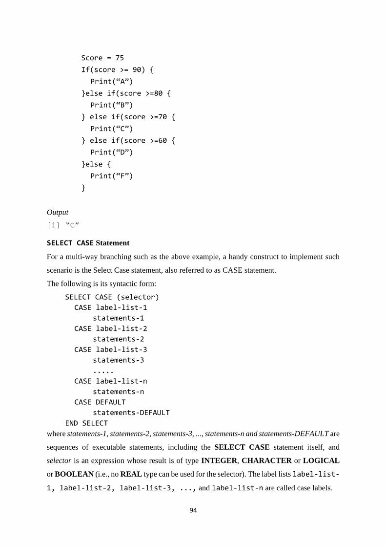
94

Output

[1] “C”

SELECT CASE Statement

For a multi-way branching such as the above example, a handy construct to implement such

scenario is the Select Case statement, also referred to as CASE statement.

The following is its syntactic form:

SELECT CASE (selector)

CASE label-list-1

statements-1

CASE label-list-2

statements-2

CASE label-list-3

statements-3

.....

CASE label-list-n

statements-n

CASE DEFAULT

statements-DEFAULT

END SELECT

where statements-1, statements-2, statements-3, ..., statements-n and statements-DEFAULT are

sequences of executable statements, including the SELECT CASE statement itself, and

selector is an expression whose result is of type INTEGER, CHARACTER or LOGICAL

or BOOLEAN (i.e., no REAL type can be used for the selector). The label lists label-list-

1, label-list-2, label-list-3, ..., and label-list-n are called case labels.

Score = 75

If(score >= 90) {

Print(“A”)

}else if(score >=80 {

Print(“B”)

} else if(score >=70 {

Print(“C”)

} else if(score >=60 {

Print(“D”)

}else {

Print(“F”)

}

95

A label-list is a list of labels, separated by commas. Each label must be one of the following

forms.

value

value-1..value-2

value-1 :

: value-2

where value, value-1 and value-2 are constants. The type of these constants must be

the same as that of the selector.

• The first form has only one value

• The second form means all values in the range of value-1 and value-2. In this form,

value-1 must be less than value-2.

• The third form means all values that are greater than or equal to value-1

• The fourth form means all values that are less than or equal to value-2

The rule of executing the SELECT CASE statement goes as follows:

1. The selector expression is evaluated

2. If the result is in label-list-i, then the sequence of statements in statements-i

are executed, followed by the statement following END SELECT

3. If the result is not in any one of the label lists, there are two possibilities:

• if CASE DEFAULT is there, then the sequence of statements in statements-

DEFAULT are executed, followed by the statement following END

SELECT

• if there is no CASE DEFAULT, the statement following END SELECT is

executed.

96

Example 3

We now re implement example 2 above using the SELECT CASE statement.

Output

[1] “C”

Note: The above syntax is generalised and there may be slight differences in the actual

implementation by specific programming languages.

Iteration (Looping)

Iteration is the automation of multi-step processes by organizing sequences of actions, and

grouping the parts that need to be repeated. Also a central part of programming, iteration (or

Looping) gives computers much of their power. They can repeat a sequence of steps as often

as necessary, and appropriate repetitions of simple steps can solve complex problems. Iteration

allows us to simplify our algorithm by stating that we will repeat certain steps until told

otherwise.

Score = 75

Select Case(score) {

Case 90..100 {

Print(“A”)

break

}

Case 80..89 {

Print(“B”)

break

}

Case 70..79 {

Print(“C”)

break

}

Case 60..69 {

Print(“D”)

break

}

Case default {

Print(“F”)

}

End Select

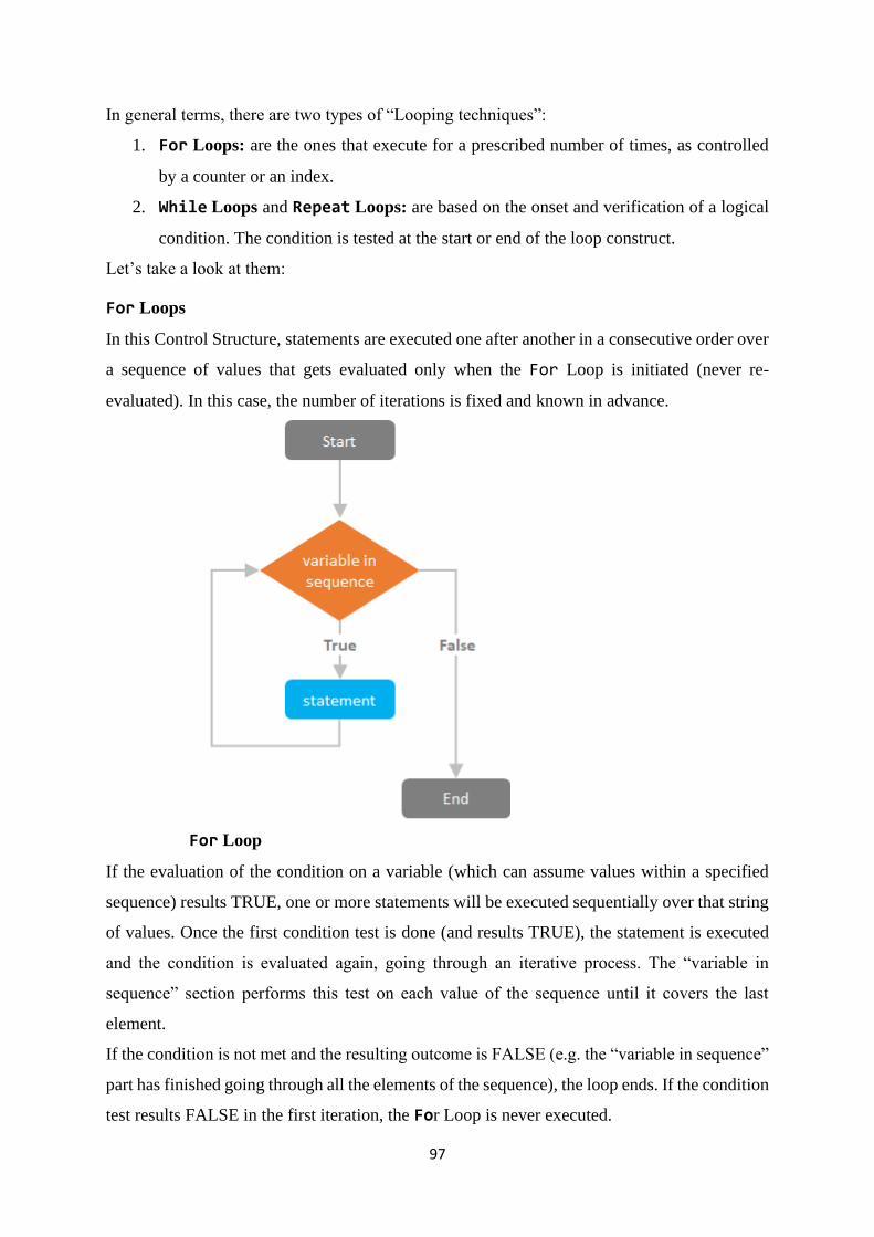
97

In general terms, there are two types of “Looping techniques”:

1. For Loops: are the ones that execute for a prescribed number of times, as controlled

by a counter or an index.

2. While Loops and Repeat Loops: are based on the onset and verification of a logical

condition. The condition is tested at the start or end of the loop construct.

Let’s take a look at them:

For Loops

In this Control Structure, statements are executed one after another in a consecutive order over

a sequence of values that gets evaluated only when the For Loop is initiated (never re-

evaluated). In this case, the number of iterations is fixed and known in advance.

For Loop

If the evaluation of the condition on a variable (which can assume values within a specified

sequence) results TRUE, one or more statements will be executed sequentially over that string

of values. Once the first condition test is done (and results TRUE), the statement is executed

and the condition is evaluated again, going through an iterative process. The “variable in

sequence” section performs this test on each value of the sequence until it covers the last

element.

If the condition is not met and the resulting outcome is FALSE (e.g. the “variable in sequence”

part has finished going through all the elements of the sequence), the loop ends. If the condition

test results FALSE in the first iteration, the For Loop is never executed.

98

The syntax of For Loops is:

For (variable-in-sequence)

statements

Example 1

To show how For Loops work, first we will create a sequence by concatenating different names

of fruits to create a list called “fruit_list”:

Fruit_list <- c(‘Apple’, ‘Kiwi’, ‘Orange’, ‘Banana’)

We will use this fruit list as the “sequence” in a For Loop, and make the it run a statement

once (print the name of each value) for each provided value in the sequence (the different fruits

in the fruit list):

Note: This example code is in Python.

This way, the outcome of the For Loop is as follows:

[1] "Apple"

[1] "Kiwi"

[1] "Orange"

[1] "Banana"

Example 2

Suppose we want to modify values, or perform calculations sequentially, we can use For Loops

to perform mathematical operations sequentially over each value of a vector (elements of the

same type, which in this case will be numerical). In this example, we will create a sequence of

numbers (from 1 to 10), and set a For Loop to calculate and print the square root of each value

in that sequence:

In this case, the outcome of the For Loop is:

[1] 1

[1] 1.414214

[1] 1.732051

[1] 2

[1] 2.236068

for (i in fruit) {

print (i)

}

for (i in c(1:10) {

print (sqrt(i))

}

99

[1] 2.449490

[1] 2.645751

[1] 2.828427

[1] 3

[1] 3.162278

You can use any type of mathematical operator over a numerical sequence, and as we will see

shortly, make all sorts of combinations between different Control Structures to reach more

complex results.

While Loops

In While Loops a condition is first evaluated, and if the result of testing that condition is

TRUE, one or more statements are repeatedly executed until that condition becomes FALSE.

While Loop

Unlike If statements, in which a condition tested as TRUE executes an expression only once

and ends, While Loops are iterative statements that execute some expression over and over

again until the condition becomes FALSE. If the condition never turns out to be FALSE, the

While Loop will go on forever and the program will crash. The other way around, if the

condition test results FALSE in the beginning of the loop, the expression will never get

executed.

The syntax of “While Loops” is:

While(condition)

statement

100

Example 1

First we will create a variable (x) and assign it the value of 1. Then we set a While Loop to

iteratively test a condition over that variable until the condition test results FALSE:

This is how it works: the initial value of the variable x is 1, so when we test the condition “is

the variable (x) less than 10?”, the result evaluates to TRUE and the expression is executed,

printing the result of the variable x, which in the first case is 1. But then something happens:

the variable x is incremented by 1 before the function ends, and in the next iteration the value

of x will be 2.

This variable reassignment is important because it will eventually reach the FALSE condition

and the loop exit (value of x = 10). Failing to change the initial conditions in a While Loop

will result into an infinite loop, causing the program to crash.

Output

[1] 1

[1] 2

[1] 3

[1] 4

[1] 5

[1] 6

[1] 7

[1] 8

[1] 9

Example 2

Have you heard of the Fibonacci sequence? This is a series of numbers with the characteristic

that the next number in the sequence is found by adding up the two numbers before it: 0, 1, 1,

2, 3, 5, 8, 13, 21,… This sequence can be found in several natural phenomena, and has different

applications in finance, music, architecture, and other disciplines.

Let’s calculate it using a While Loop.

x = 1

while(x < 10) {

print (x)

x = x+1

}

101

In this case we set a maximum value in the series as the stop condition, so that the loop

prints the Fibonacci series only for numbers below 100. When a series element (which ever it

is) becomes bigger than 100, the loop cycle ends.

Output

[1] 0

[1] 1

[1] 1

[1] 2

[1] 3

[1] 5

[1] 8

[1] 13

[1] 21

[1] 34

[1] 55

[1] 89

Repeat Loops

Closely linked to While Loops, Repeat Loops execute statements iteratively, but until a

stop condition is met. This way, statements are executed at least once, no matter what the

result of the condition is, and the loop is exited only when certain condition becomes TRUE:

a = 0

b = 1

print(a)

while(b < 100) {

print (b)

temp = a+b

a = b

b = temp

}

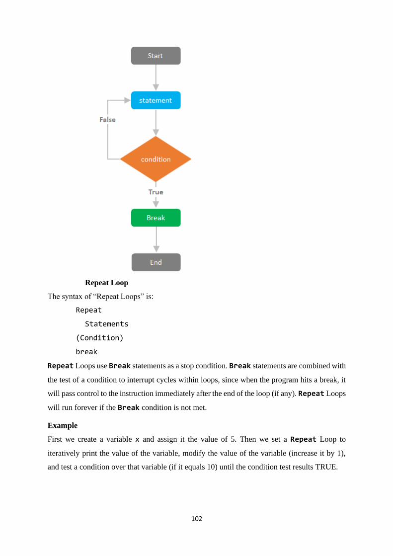
102

Repeat Loop

The syntax of “Repeat Loops” is:

Repeat

Statements

(Condition)

break

Repeat Loops use Break statements as a stop condition. Break statements are combined with

the test of a condition to interrupt cycles within loops, since when the program hits a break, it

will pass control to the instruction immediately after the end of the loop (if any). Repeat Loops

will run forever if the Break condition is not met.

Example

First we create a variable x and assign it the value of 5. Then we set a Repeat Loop to

iteratively print the value of the variable, modify the value of the variable (increase it by 1),

and test a condition over that variable (if it equals 10) until the condition test results TRUE.

103

The “breaking condition” triggers when the variable x reaches 10, and the loop ends.

Output

[1] 5

[1] 6

[1] 7

[1] 8

[1] 9

4.0 CONCLUSION

Though we have seen and explained Control Structures in isolation, they can actually be

combined anyway desired: Loops may contain several internal Loops; Conditionals may

contain Loops and Conditionals, the options are endless. You can develop advanced solutions

just by combining the Control Structures we explained in this unit. Like Minsky stated, we can

reach complex outcomes as a result of the interaction of simpler components. Control

Structures constitute the basic blocks for decision making processes in computing. They change

the flow of programs and enable us to construct complex sets of instructions out of simpler

building blocks.

5.0 SUMMARY

This Unit looked into the Control Structures. They are commands that enable a program to

“take decisions”, following one path or another. Control Structures are the blocks that analyse

variables and choose directions in which to go based on given parameters. The basic control

structure in programming language can be conditional (selection) or loop (iterations). Selection

(Conditional) is used to execute one or more statements if a condition is met. It can be executed

with the If Statement, If-Else Statement or SELECT CASE Statement and Iteration is to repeat

a statement a certain number of times or while a condition is fulfilled. Iteration can be executed

with the following statement or commands: For Loops, While Loops and Repeat Loops.

x = 5

Repeat {

print(x)

x = x+1

if(x == 10) {

break

}

}

104

6.0 TUTOR MARKED ASSIGNMENTS

1. Explain the 3 control structures in programming?

2. What are control structures in programming?

3. Which control structures are used in the algorithm? and explain their use

7.0 REFERENCES/FURTHER READINGS

Lambert, K. A., Nance, D. W., & Naps, T. L. (1997). Introduction to Computer Science with C++:

PWS Publishing Company.

Levi, A., Savas, E., Yenigün, H., Balcisoy, S., & Saygin, Y. (2006). Computer and Information Sciences

-- ISCIS 2006: 21th (i.e. 21st) International Symposium, Istanbul, Turkey, November 1-3, 2006

: Proceedings: Springer Berlin Heidelberg.

Oliver, B. (2020). The Loop: Chicken House.

Shelly, G. B., Cashman, T. J., & Gleason, K. M. (1996). QBasic: An Introduction to Programming:

Boyd & Fraser Publishing.

Warford, J. S. (2005). Computer Systems: Jones and Bartlett Pub.

105

UNIT 3: DECOMPOSITION AND MODULARISATION

CONTENTS

1.0 Introduction

2.0 Objectives

3.0 Main Content

3.1 Decomposition

3.2 Approach to Problem Decomposition

3.3 Modularisation

3.4 Motivations for Modularisation

3.5 Basic concept of Modularisation

3.5.1 Program Control Function

3.5.2 Specific Task Function

3.6 Basic Properties of Modularity

3.7 Advantages of modularisation in Programming

4.0 Conclusion

5.0 Summary

6.0 Tutor-Marked Assignments

7.0 References/Further Reading

1.0 INTRODUCTION

To design a system is to determine a set of components and inter component interface that

satisfy a specified set of requirements. Basically there are many methods to create good

designs, however every design method involves some kind of decomposition starting with a

high-level depiction of the system’s key elements and creating lower-level looks at how the

system feature and functions will fit together. No matter which design approach is used, each

kind of decomposition separates the design into parts called modules.

This unit discusses the mechanics of decomposition and modularisation, the cornerstone of

software development.

2.0 OBJECTIVES

At the end of this unit students should be able to:

• Explain the meaning of decomposition and modularisation

• Understand how to approach problem decomposition

106

• Justify the motivations for modularisation

• Describe the basic properties of modularisation

• Discuss the advantages of modularisation

3.0 MAIN CONTENT

3.1 Decomposition

When we solve computer programming problems we need to make choices about what to do

and in what order to do them. Sometimes the problem is so big or complex that we don’t know

where to start. Decomposition is when we break a problem down into smaller parts to make it

easier to tackle. Decomposition is a useful problem-solving strategy. It can help you write a

complex computer program, plan a holiday or make a model plane. Think of a mobile phone.

Mobile phones are made up of lots of different parts. Companies who make phones might make

a list of everything they need and decompose the manufacturing process so that one factory

can be making the screens while another makes batteries and another makes the phone case.

Decomposition saves a lot of time: the code for a complex program could run to many lines of

code. If a mistake was made it would take a very long time to find.

3.2 Approach to Problem Decomposition

A problem should be decomposed into modules such that each module should have only a

single responsibility. Thus, it should depend minimally on other modules. The independence

of a module can be measured using coupling and cohesion. Each module should have a clear

and focused purpose, such that its developers have a clear idea of the requirement for each

function. Its interface should be easy to understand and use, even without understanding its

implementation details. Thus its implementation details, while not only correct, should be

encapsulated and private, and that it should be changeable without affecting another module.

Furthermore, the dependency between modules should be minimised.

107

Coupling and Cohesion

Coupling is the measure of the degree of interdependence between the modules. A good

software will have low coupling while cohesion is a measure of the degree to which the

elements of the module are functionally related. It is the degree to which all elements directed

towards performing a single task are contained in the component. Basically, cohesion is the

internal glue that keeps the module together. A good software design will have high cohesion.

3.3 Modularisation

Modularisation is the process of separating the functionality of a program into independent,

interchangeable modules, such that each contains everything necessary to execute only one

aspect of the desired functionality.

A Modularised System

108

3.4 Motivations for Modularisation

One of the most prominent problems in software engineering has been how to program large

and complex pieces of software. Often, large projects involve hundreds of programmers

working on millions of lines of code. In this kind of environment, it is easy to lose track of

what particular code does, or to produce code that must be rewritten elsewhere. To avoid such

poor-planning scenarios, computer scientists began to organize around the concept of

modularisation. In this way, code becomes reusable and easier to debug and manage. The

followings are some of the major motivations.

• Ease of Debugging When debugging large programs, how and when any bugs occur can

become a mystery. This can take much of a programmer valuable time as he searches

through lines and lines of code to find out where an error occurred, and problems it causes

later in the program. If a program is designed with modularity in mind, however, then

each discrete task has its own discrete section of code. So, if there is a problem in a

particular function, the programmer knows where to look and can manage a smaller

portion of code.

• Reusable Code Modular code allows programmers to easily reuse code. If particular

tasks are sectioned off to certain functions or classes, this means that the programmer can

reuse that particular code whenever she needs to perform that task again. If code is not

organized into discrete parts, then it is harder (or impossible) to reference, separate or

implement that code in other programming contexts.

• Readability Modular code is code that is highly organized. To organize code based on

task means that the programmer can organize each piece of code based on what it does.

Then, she can easily find or reference that code based on her organization scheme.

Furthermore, other programmers working on the code can follow her organization

scheme to read the code as well. This optimizes code for use among multiple developers

with less trouble.

• Reliability All these advantages add up to one big advantage: reliability. Code that is

easier to read, easier to debug, easier to maintain and easier to share will always run

smoother with less errors. This becomes necessary when working on extremely large

projects, with hundreds of developers, all of which have to either share code or work on

code that will have to interface with other developers' code in the future. Modularization

of code is necessary to create complex software reliably.

109

3.5 Basic concept of Modularisation

One of the most important concepts of programming is the ability to group some lines of code

into a unit that can be included in our program. The original wording for this was a sub-

program. Other names include: macro, sub-routine, procedure, module and function. We are

going to use the term function for that is what they are called in most of the predominant

programming languages of today. Functions are important because they allow us to take large

complicated programs and to divide them into smaller manageable pieces. Because the function

is a smaller piece of the overall program, we can concentrate on what we want it to do and test

it to make sure it works properly.

Generally, functions fall into two categories:

1. Program Control – Functions used to simply sub-divide and control the program. These

functions are unique to the program being written. Other programs may use similar

functions, maybe even functions with the same name, but the content of the functions

are almost always very different.

2. Specific Task – Functions designed to be used with several programs. These functions

perform a specific task and thus are usable in many different programs because the other

programs also need to do the specific task. Specific task functions are sometimes

referred to as building blocks. Because they are already coded and tested, we can use

them with confidence to more efficiently write a large program.

Program Control functions normally do not communicate information to each other but use a

common area for variable storage. Specific Task functions are constructed so that data can be

communicated between the calling program piece (which is usually another function) and the

function being called. This ability to communicate data is what allows us to build a specific

task function that may be used in many programs. The rules for how the data is communicated

in and out of a function vary greatly by programming language, but the concept is the same.

The data items passed (or communicated) are called parameters. Thus the wording: parameter

passing.

3.5.1 Program Control Function

The main program piece in many programming languages is a special function with the

identifier name of main. The special or uniqueness of main as a function is that this is where

the program starts executing code and this is where it usually stops executing code. It is often

the first function defined in a program and appears after the area used for includes, other

technical items, declaration of prototypes, the listing of global constants and variables and any

110

other items generally needed by the program. The code to define the function main is provided;

however, it is not prototyped or usually called like other functions within a program.

3.5.2 Specific Task Function

We often have the need to perform a specific task that might be used in many programs.

General layout of a function in a language such as Java:

General layout of a function in a language such as Python:

In some programming languages, functions have a set of braces {} used for identifying a group

or block of statements or lines of code. Other languages use indenting or some type of begin

and end statements to identify a code block. There are normally several lines of code within a

function.

Programming languages will either have specific task functions defined before or after the main

function, depending on coding conventions for the given language.

When a function is called, its identifier name and a set of parentheses are used. You place any

data items you are passing inside the parentheses. After the program is compiled and running,

the lines of code in the main function are executed, and when it gets to the calling of a specific

task function, the control of the program moves to the function and starts executing the lines

of code in the function. When it is done with the lines of code, it will return to the place in the

program that called it (in our example the function main) and continue with the code in that

function.

3.6 Basic Properties of Modularity

The basic principle of Modularity is that systems should be built from cohesive, loosely

coupled components (modules); which means a system should be made up of different

components that are united and work together in an efficient way and such components have a

well-defined function. To define a modular system, several properties or criteria are there under

which we can evaluate a design method while considering its abilities. Some of these criteria

are given below:

<return value data type> function identifier name(<data type>

<identifier name for input value>) {

//lines of code;

return <value>;

}

def function identifier name(<identifier name for input value>):

//lines of code

return <value>

111

1. Modular Decomposability

Decomposability simply means to break down something into smaller pieces. Modular

decomposability means to break down the problem into different sub-problems in a

systematic manner. Solving a large problem is difficult sometimes, so the

decomposition helps in reducing the complexity of the problem, and sub-problems

created can be solved independently. This helps in achieving the basic principle of

modularity.

2. Modular Composability

Composability simply means the ability to combine modules that are created. It’s

actually the principle of system design that deals with the way in which two or more

components are related or connected to each other. Modular composability means to

assemble the modules into a new system that means to connect the combine the

components into a new system.

3. Modular Understandability

Understandability simply means the capability of being understood, quality of

comprehensible. Modular understandability means to make it easier for the user to

understand each module so that it is very easy to develop software and change it as per

requirement. Sometimes it’s not easy to understand the process models because of its

complexity and its large size in structure. Using modularity understandability, it

becomes easier to understand the problem in an efficient way without any issue.

4. Modular Continuity

Continuity simply means unbroken or consistent or uninterrupted connection for a long

period of time without any change or being stopped. Modular continuity means making

changes to the system requirements that will cause changes in the modules individually

without causing any effect or change in the overall system or software.

5. Modular Protection

Protection simply means to keep something safe from any harms, to protect against any

unpleasant means or damage. Modular protection means to keep safe the other modules

from the abnormal condition occurring in a particular module at run time. The abnormal

condition can be an error or failure also known as run-time errors. The side effects of

these errors are constrained within the module.

112

3.7 Advantages of modularisation in Programming

1. Manageability

One of the advantages of using this strategy is that it breaks everything down into more

manageable sections. When creating a large software program, it can be very difficult to

stay focused on a single piece of coding. However, if you break it down into individual

tasks, the job does not seem nearly as overwhelming. This helps developers stay on task

and avoid being overwhelmed by the thought that there is too much to do with a particular

project.

2. Team Programming

Another advantage of this strategy is that it allows for team programming. Instead of giving

a large job to a single programmer, you can split it up into a large team of programmers.

Each programmer can be given a specific task to complete as part of the overall program.

Then, at the end, all of the various work from the programmers is compiled to create the

program. This helps speed up the work and allows for specialization.

3. Quality

Modularization can also improve the quality of a piece of code. When you break

everything down into small parts and make each person responsible for a certain section,

it can improve the quality of each individual section. When a programmer does not have

to worry about the entire program, he can make sure that his individual piece of code is

flawless. Then, when all of the parts are combined, fewer errors are likely to be found

overall.

4.0 CONCLUSION

Modularization is essential while working in a team, maximising the problem solving strategy

and productivity. The complexity of a program can easily scale exponentially as it grows,

which is the crux of development time and productivity.

Modularization helps us break down large, complex systems into small and manageable

components. Without it, it would be difficult to handle any but the smallest programs.

The power of modularization lies in its ability in allowing code to remain flexible when facing

ever-changing requirements. Thus, we should always decompose our programs into modules

so that we can fully enjoy the benefits of modularisation.

113

5.0 SUMMARY

6.0 TUTOR MARKED ASSIGNMENTS

7.0 REFERENCES/FURTHER READINGS

114

UNIT 4: TESTING AND DEBUGGING

CONTENTS

1.0 Introduction

2.0 Objectives

3.0 Main Content

3.1 Program Testing

3.2 Types of Program Tests

3.3 Properties of Tests

3.4 Need for Program Testing

3.5 Benefits of Program Testing

3.6 Debugging

3.6.1 Importance of Debugging

3.7 Types of Errors to Debug

3.8 Common Debugging Strategies

3.9 Difference between Testing and Debugging

4.0 Conclusion

5.0 Summary

6.0 Tutor-Marked Assignments

7.0 References/Further Reading

1.0 INTRODUCTION

Every program or system, no matter how well-designed, will need some fine-tuning either to

make it conform to user requirements or improve performance. Some sort of adjustments will,

therefore, have to be made in this regard in the form of testing and debugging.

Testing means verifying correct behaviour. Testing can be done at all stages of module

development: requirements analysis, interface design, algorithm design, implementation, and

integration with other modules. Debugging, on the other hand, is a cyclic activity involving

execution testing and code correction. The testing that is done during debugging has a different

aim than final module testing. Final module testing aims to demonstrate correctness, whereas

testing during debugging is primarily aimed at locating errors. This difference has a significant

effect on the choice of testing strategies. This unit discusses this important aspect of software

development.

115

2.0 OBJECTIVES

At the end of this unit learners should be able to:

• Define and classify program tests

• Explain the desirable properties of program tests

• Appreciate the need for and benefits of program testing

• Understand the debugging process as well as types of programming errors

• Apply common strategies in the debugging process

3.0 MAIN CONTENT

3.1 Program Testing

Fundamentally, program testing is a process to check if the program or the entire system is

working same as it was supposed to do, and not working as it was not supposed to do. It is done

by the tester to identify the defects in the program or system to determine if actual result of test

case execution matches or not with expected result. It can be done using manual and automated

process. The issues are logged against all the failed cases and are communicated to the

development team for debugging and fixing. After the bug fixes the tester then retests the bug

and checks if the issues no more exist.

3.2 Types of Program Tests

Unit Test

Unit tests are low-level tests that focus on testing a specific part of the system. They are cheap

to write and fast to run. Test failures should provide enough contextual information to pinpoint

the source of the error. Unit tests should be independent and isolated; interacting with external

components increases both the scope of the tests and the time it takes for the tests to run. The

size of a unit test depends on what we are trying to do. Thinking in terms of a unit of behaviour

allows writing tests around logical blocks of code.

It is recommended to have a lot of unit tests in our test suite as this gives us confidence that

our program works as expected. Writing new code or modifying existing code might require

rewriting some of the tests. The standard practice is that the test suite should grow with our

code base. We should try to be cognizant of our test suite growing in complexity since the code

that tests our production code is also production code. Time must be taken to refactor our tests

to ensure they are efficient and effective.

116

Example

Suppose we have the following function that takes a list of words and returns the most common

word and the number of occurrences of that word:

We can test this function by creating a list, running the find_top_word() function over that list

and comparing the results of the function to the value we expect:

If we ever wanted to change the implementation of find_top_words(), we can do it without

fear. Our test ensures that the functionality of find_top_word() cannot change without causing

a test failure.

Integration Tests

Every complex application has internal and external components working together to do

something interesting. In contrast to units tests which focus on individual components,

integration tests combine various parts of the system and test them together as a group.

Integration testing can also refer to testing at service boundaries of our application, i.e. when it

goes out to the database, file system, or external API (application program interface).

By definition, integration tests are larger in scope and take longer to run than unit tests. This

means that test failures require some investigation: we know that one of the components in our

test is not working, but the failure's exact location needs to be found. This is in contrast to unit

tests which are smaller in scope and indicate exactly where things have failed. Integration tests

should be run in a production-like environment; this minimizes the chance that tests fail due to

differences in configuration.

Example

Suppose we have the following function that takes in a URL (uniform resource locator) and a

tuple of (word, occurrences). Our function creates a records and saves it to the database:

def find_top_word(words)

# Return most common word & occurrences

word_counter = Counter(words)

return word_counter.most_common(1)[0]

def test_find_top_word():

words = ["foo", "bar", "bat", "baz", "foo", "baz", "foo"]

result = find_top_word(words)

assert result[0] == "foo"

assert result[1] == 3

117

We test this function by passing in known information; the function should save the

information we entered into the database.

Our test code pulls the newly saved record from the database and confirms its fields match the

input we passed in.

Notice how this is the kind of testing we do manually to confirm things are working as

expected. Automating this test saves us from having to repeatedly check this functionality each

time a change is made to the code.

End-to-End Tests

End-to-end tests check to see if the system meets our defined business requirements. A

common test is to trace a path through the system in the same manner a user would experience.

For example, we can test a new user workflow: simulate creating an account, "clicking" the

link in the activate email, logging-in for the first time, and interacting with our web

application's tutorial modal pop-up.

We can conduct end-to-end tests through our user interface (UI) by leveraging a browser

automation tool like Selenium. This creates a dependency between our UI and our tests, which

makes our tests brittle: a change to the front-end requires us to change tests. This is not

sustainable as either our front-end will become static or our tests will not be run.

End-to-end tests are considered black box as we do not need to know anything about the

implementation in order to conduct testing. This also means that test failures provide no

def save_to_db(url, top_word):

record = TopWord()

record.url = url

record.word = top_word[0]

record.num_occurrences = top_word[1]

db.session.add(record)

db.session.commit()

return record

def test_save_to_db():

url = "http://test_url.com"

most_common_word_details = ("Python", 42)

word = save_to_db(url, most_common_word_details)

inserted_record = TopWord.query.get(word.id)

assert inserted_record.url == "http://test_url.com"

assert inserted_record.word == "Python"

assert inserted_record.num_occurrences == 42

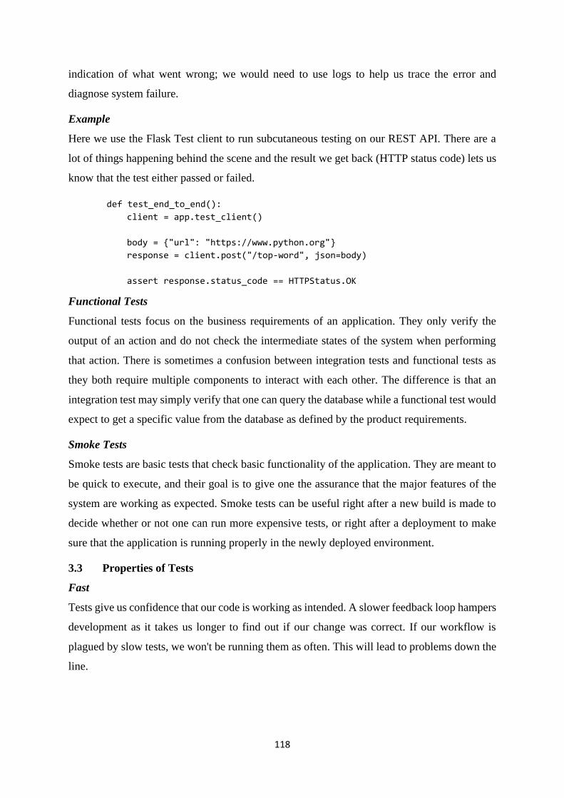
118

indication of what went wrong; we would need to use logs to help us trace the error and

diagnose system failure.

Example

Here we use the Flask Test client to run subcutaneous testing on our REST API. There are a

lot of things happening behind the scene and the result we get back (HTTP status code) lets us

know that the test either passed or failed.

Functional Tests

Functional tests focus on the business requirements of an application. They only verify the

output of an action and do not check the intermediate states of the system when performing

that action. There is sometimes a confusion between integration tests and functional tests as

they both require multiple components to interact with each other. The difference is that an

integration test may simply verify that one can query the database while a functional test would

expect to get a specific value from the database as defined by the product requirements.

Smoke Tests

Smoke tests are basic tests that check basic functionality of the application. They are meant to

be quick to execute, and their goal is to give one the assurance that the major features of the

system are working as expected. Smoke tests can be useful right after a new build is made to

decide whether or not one can run more expensive tests, or right after a deployment to make

sure that the application is running properly in the newly deployed environment.

3.3 Properties of Tests

Fast

Tests give us confidence that our code is working as intended. A slower feedback loop hampers

development as it takes us longer to find out if our change was correct. If our workflow is

plagued by slow tests, we won't be running them as often. This will lead to problems down the

line.

def test_end_to_end():

client = app.test_client()

body = {"url": "https://www.python.org"}

response = client.post("/top-word", json=body)

assert response.status_code == HTTPStatus.OK

119

Deterministic

Tests should be deterministic, i.e. the same input will always result in the same output. If tests

are non-deterministic, we have to find a way to account for random behaviour inside of our

tests. While there is definitely non-deterministic code in production (i.e. Machine Learning and

AI), we should try to make all our non-probabilistic code as deterministic as possible. There is

no point of doing additional work unless our program requires it.

Automated

We can confirm our program works by running it. This could be manually running a command

in the REPL or refreshing a webpage; in both cases, we are looking to see if our program does

what it is supposed to do. While manual testing is fine for small projects, it becomes

unmanageable as our project grows in complexity. By automating our test suite, we can quickly

verify our program works on-demand. Some developers even have their tests triggered to run

on file save.

3.4 Need for Program Testing

Human errors can cause a defect or failure at any stage of the software development life cycle.

The results are classified as trivial or catastrophic, depending on the consequences of the error.

The requirement of rigorous testing and their associated documentation during the software

development life cycle arises because of the following reasons:

1. To identify defects

2. To reduce flaws in the component or system

3. Increase the overall quality of the system

There can also be a requirement to perform software testing to comply with legal requirements

or industry-specific standards. These standards and rules can specify what kind of techniques

should we use for product development. For example, the motor, avionics, medical, and

pharmaceutical industries, etc., all have standards covering the testing of the product.

The following shows the significance of testing for a reliable and easy to use software product:

• The testing is important since it discovers defects/bugs before the delivery to the client,

which guarantees the quality of the software.

• It makes the software more reliable and easy to use.

• Thoroughly tested software ensures reliable and high-performance software operation.

For example, assume you are using a Net Banking application to transfer the amount to your

friend's account. So, you initiate the transaction, get a successful transaction message, and the

amount also deducts from your account. However, your friend confirms that his/her account

120

has not received any credits yet. Likewise, your account is also not reflecting the reversed

transaction. This will surely make you upset and leave you as an unsatisfied customer.

The question is, why did it happen? It is because of the improper testing of the net banking

application before release. Thorough testing of the website for all possible user operations

would lead to early identification of this problem. Therefore, one can fix it before releasing it

to the public for a smoother experience.

3.5 Benefits of Program Testing

A well-thought-out testing strategy paired with thorough test cases provides the following

benefits:

Modify Code with Confidence

If a program does anything of interest, it has interactions between functions, classes, and

modules. This means a single line change can break our program in unexpected ways. Tests

give us confidence in our code. By running our tests after we modify our code, we can confirm

our changes did not break existing functionality as defined by our tests.

In contrast, modifying a code base without tests is a challenge. There is no way of knowing if

things are working as intended. We are programming by the seat of our pants, which is quite a

risky proposition.

Identify Bugs Early

Bugs cost money. How much depends on when you find them. Fixing bugs gets more expensive

the further you are in the software development life cycle (SDLC).

Improve System Design

Though a bit controversial, writing code with tests in mind improves system design. A thorough

test suite shows that the developer has actually thought about the problem in some depth.

Writing tests compels you to write your own API which, hopefully results in a better interface.

3.6 Debugging

Debugging is a computer programing process for finding and resolving errors in software or a

website, often referred to as "bugs." It often requires a comprehensive procedure to identify the

reason why a bug occurred and ensure a program can run smoothly for users in the future.

Software developers and engineers often debug programs using a digital tool to view and edit

the coding language, which contains instructions for how a program works. Debugging allows

them to address individual sections of code to ensure that every part of a program operates in

an expected and optimal way.

121

3.6.1 Importance of Debugging

Debugging is important because it allows software engineers and developers to fix errors in a

program before releasing it to the public. It's a complementary process to testing, which

involves learning how an error affects a program overall. If you examine each section of code,

you can discover which variables and functions to adjust systematically. Debugging can also

improve the quality of a product, which may increase the number of positive reviews a

company receives.

3.7 Types of Errors to Debug

Here are some examples of common errors you can encounter while debugging and how to

address them:

Syntax errors

Syntax errors are grammatical interruptions in a line of code. For example, an extra bracket or

period might cause a syntax error to occur. A compiler can often recognize a syntax error then

notify you in a separate message screen about where it is in the code and how to fix it using a

debugging tool. Some compilers also highlight them when you first load the program's code

into the system.

Logic errors

Logic errors are issues in the code's algorithms. They can occur when a program's code

produces an unexpected output or causes the program to stop working. For example, adding

two number-type variables when you intended to divide them might cause a logic error. You

can resolve logic errors by using a debugging tool to carefully examine the variable causing

the issue in a line of data.

Run-time errors

Run-time errors occur when a person uses the program and they're detected by the computer

executing it. They can still appear after you finish an initial debugging process because a

computer might interpret the program's code in an unexpected way. For example, an operating

system might format code in a certain configuration that renders it unusable. To address these

errors, it's important to ensure an operating system has the information it needs to run a program

correctly.

Interface errors

Interface errors involve a disconnect in an API, which means one or both coding languages in

an API cause this error to occur. For example, an API might have certain requirements that are

only present in the code of one program. To address an interface error, compare and contrast

122

lines in your code with the other. Be sure to have records of any debugging and testing

processes you completed in the past to help streamline this step.

3.8 Common Debugging Strategies

Consider the following list of eight debugging strategies in common use:

1. Run a Debugging Feature

Most debugging tools have a particular feature that allows one to debug sections of code

using one’s own methods. This strategy might be especially helpful if the code produces

unexpected results outside of a compiler's capacity to find and address them. To use

debugging mode, identify the proper steps in your specific software. As you analyse each

error and investigate potential solutions, you can use breakpoints to focus on a specific area

of code to determine if you input the correct variables and functions.

2. Use the Scientific Method

The scientific method can be applied to the debugging process before you enter code into a

compiler. It involves an assumption you make based on collected data, then a test you design

and conduct to confirm or refute it. This strategy can help you streamline a debugging

process, as you can repeat the scientific method to each section of code. Consider developing

clear statements for your assumption so you can create a simple testing procedure.

3. Debug after Adding New Code

When you finish a section of code, consider operating it through a compiler and debugging

tool before adding a new section. Adding sections in these increments gives you the ability

to identify errors more immediately, as the bug is likely in the last section you included. It

also helps prevent one bug from causing several others to occur later on in the coding

language, which might make the debugging process more precise and efficient overall.

4. Incorporate the Backtracking Method

Sometimes one area of code can cause an error in another. When you identify an area

containing a bug, consider analysing it from the beginning until that point. Use the output

information to examine the values of the variables and determine the first place you can

observe an unexpected result. You can most likely find the cause of the error in a section of

code that precedes this result from the output, which gives you the information you need to

debug it entirely.

5. Perform the Binary Search Method

Similar to the previous strategy, the binary search method involves separating sections of

code to streamline the debugging process. This may be especially helpful if the cause of a

123

bug is at the beginning of a coding language, while the actual error is closer to the end.

Consider placing a breakpoint halfway through the code, then executing it so it pauses right

at that point. If the compiler finds similar issues occurring, then the cause likely derives

from a certain area in the tested section.

6. Classify Different Bug Types

In some debugging processes, one may find similar errors across different sections. It may

be helpful to group these errors and label them for organisational purposes. One error can

also be chosen from each group for a debugging procedure, which may show how to address

an entire group. This strategy allows debugging a large group of errors with one action,

improving the quality of one’s efforts and increasing the overall productivity.

7. Involve Static Code Analysis

Some developers and engineers prefer to use a manual debugging process before running it

on a compiler or debugger. In static analysis, you use a specific set of coding rules to frame

your evaluations, then use the data you collect to identify errors. This strategy may be

especially helpful for testing new code you intend to add.

For instance, you might use a data-flow analysis to investigate the cause of bugs or

determine some potential areas that may have bugs in the future. It's a method that software

engineers can use to analyse how variable values adjust throughout the operation of a

program. To accomplish this method, you often use a control flow graph (CFG), which

illustrates the different ways a variable might progress through a program's code.

8. Try Remote Debugging

Remote debugging involves running a program code on the software of a separate computer.

This strategy may especially be helpful if you require a debugging tool that's on another

machine in a separate location. Depending on the software's capabilities, you may be able

to debug multiple files at the same time, maximizing your overall productivity. To try a

remote debugging process, you can sync the computer system you're currently using to

debug to another by linking two servers and then opening the other system's debugging

software on your own.

124

3.9 Difference between Testing and Debugging

Testing Debugging

Testing gets started with known conditions

with expected results.

This is manual step by step unstructured and

unreliable process to find and removes a

specific bug from the system.

It performed based on the testing type which

we need to perform unit testing, integration

testing, system testing, user acceptance

testing, stress, load, performance testing etc.

It performed based on the type of bug.

Testing is the process which can be planned,

designed and executed.

Debugging is the process which cannot be so

forced.

It is the process to identify the failure of

implemented code.

It is the process to give the absolution to code

failure.

It is a demonstration of error or apparent

correctness. It is always treated as a deductive process.

Testing is the display of errors It is a deductive process

Design knowledge is not required for testing

the system under test. Any person with or

without test case can do testing.

Detailed design knowledge is definitely

required to perform debugging.

Testing can be outsourced to outside team as

well.

Debugging cannot be outsourced to outside

team. It must be done by inside development

team.

Most of the test cases in testing can be

automated. Automation in the debugging cannot possible.

Testing is the process to identify the bugs in

the system under test.

Debugging is the process to identify the root

cause of the bugs.

4.0 CONCLUSION

The importance of software testing is imperative. Program testing is a crucial component of

software product development because it improves consistency and performance. The main

benefit of testing is the identification and subsequent removal of the errors. However, testing

also helps developers and testers to compare actual and expected results in order to improve

125

quality. If the software production happens without testing it, it could be useless or sometimes

dangerous for customers. So, a tester should wear a unique hat that protects the reliability of

the software and makes it safe to use in real-life scenarios.

5.0 SUMMARY

6.0 TUTOR MARKED ASSIGNMENTS

7.0 REFERENCES/FURTHER READINGS

1. Graham, D.; Van Veenendaal, E.; Evans, I. (2008). Foundations of Software Testing.

Cengage Learning. pp. 57–58. ISBN 978-1-84480-989-9.

2. Meyer, Bertrand (2008). “Seven Principles of Software Testing” (PDF). Computer.

Vol. 41 no. 8. pp.99–101. doi:10.1109/MC.2008.306.

3. McConnell, Steve (2004). ICode Complete (2nd ed.). Microsoft Press. ISBN 978-0-

7356-1967-8.

4. Ammann, Paul; Offutt, Jeff (2008). Introduction to Software Testing. Cambridge

University Press.