Chapter 10 - Model-based Problem Solving
72
Handbook of Knowledge Representation Edited by F. van Harmelen, V. Lifschitz and B. Porter © 2008 Elsevier B.V. All rights reserved DOI: 10.1016/S1574-6526(07)03010-6 395 Chapter 10 Model-based Problem Solving Peter Struss 10.1 Introduction The development of the concept of model-based systems was an answer to the limita- tions of rule-based “expert systems”, which base problem solving (e.g., diagnosis) on a representation of experiential knowledge in a domain. These limitations are not due to the syntactic form of representing knowledge (rules), but result from the nature of the represented knowledge: termed “empirical associations” in the pioneering paper [11] or “shallow knowledge” in others. This has to be contrasted with “1st principles” knowledge (or “deep knowledge”), such as the representation of the understanding of the physical behavior of the components of a system. To illustrate this distinction and its implications by an example, consider the sim- plified electrical subsystem of a vehicle comprising the starter, the rear lights, and the head lights with their power supply (Fig. 10.1(a)). Some simple diagnostic rules for such a system, gained from experience or some analysis of the system, might be IF Engine_Does_Not_Start THEN Possible_Cause_Battery_Flat IF Engine_Does_Not_Start THEN Possible_Cause_Starter_Defect ... IF Rlights_On OR Hlights_On THEN NOT(Possible_Cause_Battery_Flat) which would allow to suspect the starter, but not the battery, if the engine does not start and the lights are on. However, they lead to wrong consequences, when we face a system with two batteries, as indicated in Fig. 10.1(b). Experience is obtained in a specific context. In our example, the specific structure of the system is compiled into the rules, it is implicit, and this is why the applicability of the last rule is limited to systems sharing the same structure or, rather, the same structural properties that underlie the rule. A rule may be reusable for the modified system (such as the first one), but the conditions for its reuse remain hidden. Fur- thermore, there is the question whether the empirical basis has the required coverage.
-
Upload
khangminh22 -
Category
Documents
-
view
1 -
download
0
Transcript of Chapter 10 - Model-based Problem Solving
Handbook of Knowledge RepresentationEdited by F. van Harmelen, V. Lifschitz and B. Porter© 2008 Elsevier B.V. All rights reservedDOI: 10.1016/S1574-6526(07)03010-6
395
Chapter 10
Model-based Problem Solving
Peter Struss
10.1 Introduction
The development of the concept of model-based systems was an answer to the limita-tions of rule-based “expert systems”, which base problem solving (e.g., diagnosis) ona representation of experiential knowledge in a domain. These limitations are not dueto the syntactic form of representing knowledge (rules), but result from the nature ofthe represented knowledge: termed “empirical associations” in the pioneering paper[11] or “shallow knowledge” in others. This has to be contrasted with “1st principles”knowledge (or “deep knowledge”), such as the representation of the understanding ofthe physical behavior of the components of a system.
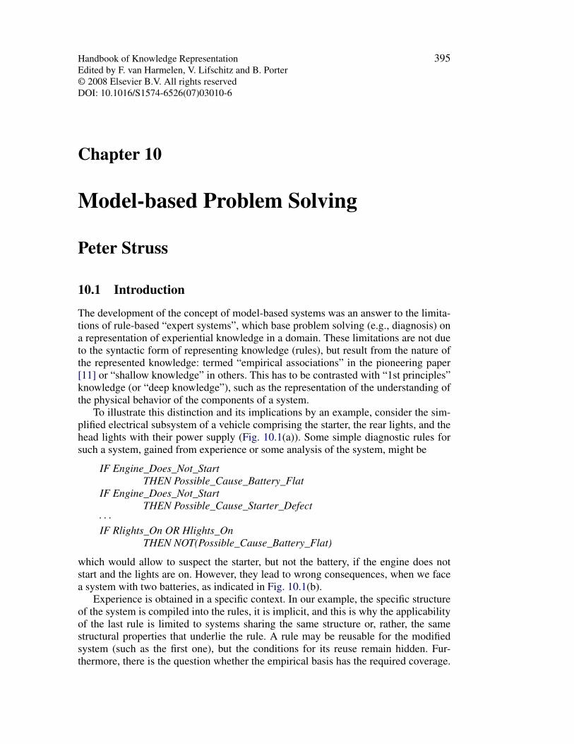
To illustrate this distinction and its implications by an example, consider the sim-plified electrical subsystem of a vehicle comprising the starter, the rear lights, and thehead lights with their power supply (Fig. 10.1(a)). Some simple diagnostic rules forsuch a system, gained from experience or some analysis of the system, might be
IF Engine_Does_Not_StartTHEN Possible_Cause_Battery_Flat
IF Engine_Does_Not_StartTHEN Possible_Cause_Starter_Defect
. . .
IF Rlights_On OR Hlights_OnTHEN NOT(Possible_Cause_Battery_Flat)
which would allow to suspect the starter, but not the battery, if the engine does notstart and the lights are on. However, they lead to wrong consequences, when we facea system with two batteries, as indicated in Fig. 10.1(b).
Experience is obtained in a specific context. In our example, the specific structureof the system is compiled into the rules, it is implicit, and this is why the applicabilityof the last rule is limited to systems sharing the same structure or, rather, the samestructural properties that underlie the rule. A rule may be reusable for the modifiedsystem (such as the first one), but the conditions for its reuse remain hidden. Fur-thermore, there is the question whether the empirical basis has the required coverage.
396 10. Model-based Problem Solving
Figure 10.1: Two variants of electrical systems in a vehicle.
Even for moderately complex systems, we cannot expect that all possible faults havealready been encountered in practice, let alone all combinations of independent faults.
More fundamentally, there may be no empirical data at all available for a particularkind of system. If we buy the latest model of a car, we would not accept the recom-mendation of a workshop mechanic that we should return with our problem next yearto give them some time to gain experience. For certain systems and failures, we wouldnot want to collect the empirical associations—think of airplanes or nuclear powerplants.
It is a constitutive feature of human intelligence to extract principled knowledgefrom experience that can be used in a different context and for other purposes, andreproducing this capability is a major challenge to AI.
Taking a second look at the example, we notice that the rules do not only havea particular context in terms of the system structure compiled into them, they alsorepresent the application of some principled knowledge to a specific task, namelydiagnosis. However, the same fragment of knowledge, such as “A flat battery doesnot provide voltage and, hence, may cause the starter not to work”, can also be used tosolve a different task, such as failure-modes-and-effects analysis (FMEA), which aimsat predicting the effect component failures have on the system function, the generationof a test that can reveal the presence of this fault, etc. In reflection of these challenges,model-based systems aim at
• representing the knowledge about a class of real-world systems as a library ofmodels with a maximum of versatility and re-use to different system instancesand for different tasks,
• providing model-based problem solving engines that support or automate theexploitation of such models to solve certain tasks.
These objectives meet urgent needs in industry, where complexity and variability ofproducts demand computer support to capturing and applying the corporate knowl-edge. Also society benefits from powerful model-based systems, e.g., in improvingthe understanding, monitoring, and influencing of ecological, environmental, and cli-mate systems.
P. Struss 397
These objectives strongly suggest the architectural principle of knowledge-basedsystems, namely a clear separation and independence of
• the domain-specific knowledge as a model-library, a declarative, decomposi-tional representation of the behavior of elementary constituents of systems inthe domain,
• the task-specific knowledge, in terms of problem solving engines that performinferences based on a model library.
Independence of these two constituents of model-based systems is not to be under-stood at a low technical level (data structures), but at a conceptual level: the modelsshould be stated in a way that is not committed to one particular task; and the problemsolving engine should avoid encoding specificities of a particular domain and, hence,be able to operate on different model libraries. This is the basis for high reusability ofboth types of modules.
Of course, in practice (in research as well as in application-oriented work) thespace of answers to the challenge has many dimensions. Perhaps more than in otherareas of knowledge representation, the diversity of real-world problems induces atremendous diversity in the proposed solutions. In this field, we are (or should be)facing systems in the real world, and there are many different kinds: electrical circuits,thermodynamic systems, water treatment plants, interacting species of flora and fauna,software, . . .Wewould like to solve tasks like system design, diagnosis, testing, repair,automated recovery, . . .
The Cartesian product systems × tasks is further expanded when researchers anddevelopers choose formalisms (ordinary differential equations, finite state machines,predicate calculus, Bond graphs, Petri-nets, . . .) and apply their favorite inferencescheme (qualitative simulation, finite constraint satisfaction, theorem proving, opti-mization, model checking, PROLOG, . . .). Although some modeling approaches seemto be more appropriate for certain classes of systems than others, the mapping sys-tems ↔ models is m : n, and so is the mapping tasks ↔ inference engines.
As a result, any attempt of a comprehensive survey is prohibitive, even when con-fined to the solution ideas, let alone implementation. However, we will try to showthat, at a certain level of abstraction, several tasks can be formalized using a smallset of inferences (which can be realized in different ways). This will be done in thefollowing section.
And we will choose a very general notion of “model” (which can be represented inmany specific ways) and discuss required or advantageous properties (Section 10.3).
The remainder of the chapter will then be structured along different tasks. Diag-nostic theories and systems (Section 10.4) will take the largest share for two reasons:diagnosis is the task with the most advanced theories and applications. On the otherhand, some of the theories and implementation principles carry over to other prob-lems as motivated in Section 10.2. We first present the foundations for a large class ofdiagnostic systems, consistency-based diagnosis based on component-oriented mod-els, but will also identify its underlying assumptions and limitations and characterizealternative approaches.
Then we discuss test generation and diagnosability analysis (Section 10.5), gener-ation of remedies (Section 10.6), and some other tasks (Section 10.7), and, finally, tryto identify some major challenges in the field.
398 10. Model-based Problem Solving
As stated before, due to the diversity of the solutions and the purpose and restric-tion of this chapter, our goal cannot be a comprehensive presentation of all proposedapproaches and systems (and not even a comprehensive list of references), but, rather,conveying the key ideas of selected solutions with some formalization and, perhaps,some hints on a possible implementation. In the selection, we give preference to solu-tions that address the important requirements of the application context in a principledand general way over approaches that are heavily influenced by specific features ofa particular application domain or that fail to reflect essential conditions of the real-world task.
10.2 Tasks
In this section, we characterize the essence of different tasks we would like to addressbased on some model. For this purpose, we are not very specific about the content ofthe model and the special form it is represented in. Requirements on the model, part ofwhich follow from this analysis, will be discussed in the next section. Here, a model isa description of the possible ways a certain system can behave. This can be a real phys-ical system or a hypothetical one (e.g., in design), a system that is in order or faulted(e.g., in diagnosis). In this section, we assume for the sake of a formal presentationthat such a model, whatever the chosen representation is, can be equivalently stated asa set of logical formulas. Of course, in practice, representations will be chosen that aremore suited for the description of physical systems. In this case, it has to be analyzedhow the logical concepts and inferences carry over to the different formalism.
As it turns out, all we expect from a model is that it can be decided whether or nota certain behavior description contradicts the model (i.e. the notion of consistency)and whether it follows from the model (entailment).
10.2.1 Situation Assessment/Diagnosis
Diagnosis is about finding out that and why something does not behave the way itshould. We have a model MODELOK of the correctly working system, a set OBS ofobservations of the actual behavior of the system, and a set GOALS specifying itsintended behavior. Then, fault detection, the first step in diagnosis, means to checkwhether the joined theory is consistent
MODELOK ∪ OBS ∪ GOALS � ⊥
or, stronger, to ask whether the GOALS are entailed:
MODELOK ∪ OBS � GOALS
We may assume that the system is well-designed, i.e., if nothing is broken, the speci-fied behavior is guaranteed to be achieved,
MODELOK � GOALS
In this case, the check is reduced to
MODELOK ∪ OBS � ⊥
P. Struss 399
If this check reveals an inconsistency, we can conclude that MODELOK does not de-scribe the system under its current physical conditions; there must be a fault. In orderto fix the problem, we need to know where the fault lies (fault localization) and/orwhat kind of fault is present (fault identification). In model-based diagnosis, this canbe stated as the task of deriving a model MODELF (or several alternative ones) thatis, at least, consistent with the observations (consistency-based diagnosis)
MODELF ∪ OBS � ⊥
or even entails them (abductive diagnosis, see Section 10.4.3).In diagnosis, the space of models that are candidates forMODELF , is not arbitrary.
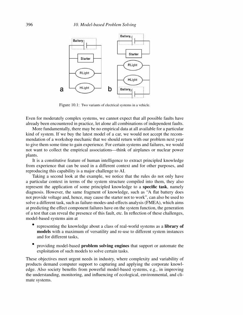
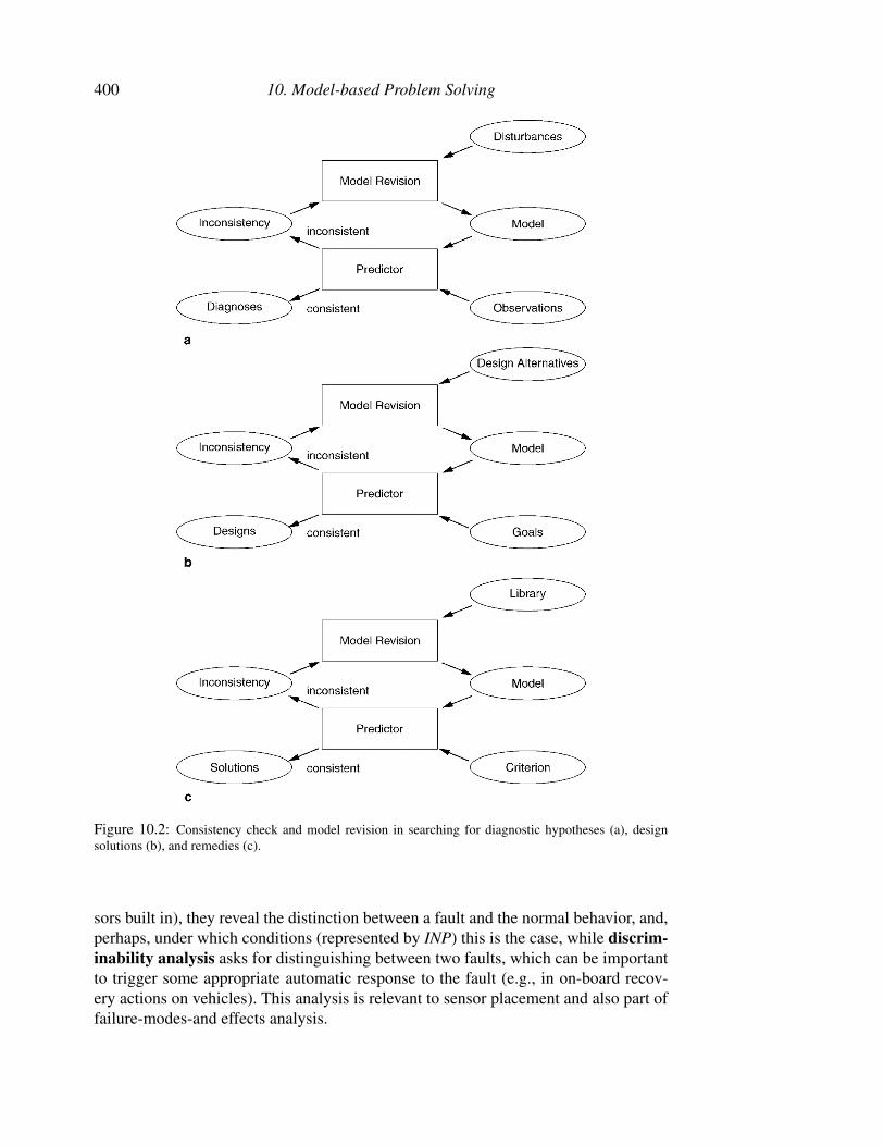
Usually, the system performed well before and is now suffering from some particularmalfunctions or disturbances. For instance, unless a major accident has happened,there will usually be one or two broken components in our car. This is why we canexpect some restricted space of models that contains the solutions we are looking for,although it will often be too large to allow for an exhaustive consistency check of allcandidates, and, hence, require search. In this search, we can exploit an ordering onthe candidate models that is induced by the degree of deviations from MODELOK ,e.g., indicated by the number of faulty components. This provides the basis for ahypothesize-and-test cycle where the new hypotheses are obtained by some elemen-tary revision of the failing candidates, e.g., by assuming a different fault, an additionalfaulty component, etc. What we need in order to realize such a search-based approachis a module that checks the consistency of the model with the given observations and acomponent that produces newmodel hypotheses by revision of inconsistent ones basedon some description of the possible disturbances in the model library (Fig. 10.2(a)). InSection 10.4, we present more details about such solutions.
10.2.2 Test Generation, Measurement Proposal, DiagnosabilityAnalysis
If diagnosis does not provide a sufficiently focused answer, more observations arerequired to help discriminating between the remaining fault hypotheses. This means,we are looking for some stimulus INP to the system such that its observed responsereveals the differences between the various hypotheses. In our model-based context,this means: given two behavior modelsMODEL1 andMODEL2, the target situation is
INP ∪ MODEL1 � OBS1
INP ∪ MODEL2 � OBS2
OBS1 ∪ OBS2 � ⊥
Test generation is the task of determining inputs INP with this property and the ap-propriate observables, in case they can vary. In testing for diagnosis, this needs to bedone for all pairs of models that represent relevant diagnoses. In end-of-line testing,MODELOK needs to be discriminated from the models of relevant faults. Measure-ment proposal can be seen as a special case, where INP is fixed by the currentsituation, and the task is focused on determining where to probe for discrimination.
Also in the design phase of a system, this analysis can be relevant. Detectabilityanalysis has to determine whether, under a given set of observables (e.g., by the sen-
400 10. Model-based Problem Solving
Figure 10.2: Consistency check and model revision in searching for diagnostic hypotheses (a), designsolutions (b), and remedies (c).
sors built in), they reveal the distinction between a fault and the normal behavior, and,perhaps, under which conditions (represented by INP) this is the case, while discrim-inability analysis asks for distinguishing between two faults, which can be importantto trigger some appropriate automatic response to the fault (e.g., in on-board recov-ery actions on vehicles). This analysis is relevant to sensor placement and also part offailure-modes-and effects analysis.
P. Struss 401
10.2.3 Design and Failure-Modes-and-Effects Analysis
The design of a system that has to generate a specified behavior demands strongly fora model-based approach, if a trial-and-error process by building physical prototypesshould be avoided or limited. Unfortunately, in the general case, it is more challengingthan diagnosis. If GOALS represents the behavior specification, then the design taskcan be solved by finding a model that entails this behavior:
MODEL � GOALS
A necessary precondition for such a solution is that it is consistent with the specifiedbehavior, which may be exploited at least in a first step to reduce the space of candidatemodels:
MODEL ∪ GOALS � ⊥
We would usually not be satisfied by a product design thatmay, but is not guaranteedto, serve its purpose. However, the consistency check may be the only possible onein early phases of the design process, which may leave open the choice of specificcomponents or parameters or even some structural properties, and it is helpful becauseit can refute certain design alternatives. Furthermore, the design process is rarely asingle jump to a solution, but approaching one by modifying previously refuted designhypotheses in a way that inconsistencies with the specification are removed. Again,we can organize this process as a search in a space of candidate models (Fig. 10.2(b)).They need to be checked for consistency with the goals and, in case of inconsistencywith the goals, revised by changing design decisions. What makes the task harder is,first of all, the nature and size of the space of possible alternatives. Usually, this spaceis much less restricted than, say, in diagnosis, where the structure of the system maybe fixed and the possible component failures limited. In design, the structure may bewhat needs to be developed and modified.
Obviously, the revision-based search can only work if there is an initial hypothesisthat can lead to a solution after a limited number of modifications. In fact, the vastmajority in industrial design is not completely innovative, but emerges from a modifi-cation of a predecessor product. And often, the structure is more or less fixed, whichturns design into the more tractable task of selecting appropriate components from agiven set (configuration) or only determining parameters of fixed component classes(parametric design).
As a special task during design, failure-modes-and-effects analysis, has gainedimportance (and is mandatory, for instance, in the aeronautics and automotive indus-tries). It is concerned with the task of making sure that, for a given design, even underthe occurrence of a fault (usually a single fault) the resulting behavior of the systemwould not be critical or even catastrophic. The analysis has to find out for a set ofgiven scenarios (e.g., the landing phase of an aircraft) and a set of relevant componentfailures whether one of the specified effects, i.e. violations of the functionality (e.g.,“landing gear not extended”), can occur. The result of this analysis may be requestedchanges of the design.
Given a model of the system behavior under the presence of a possible failure,MODELF , it has to be determined whether it entails some EFFECT in a scenariospecified by INP:
402 10. Model-based Problem Solving
INP ∪ MODELF � EFFECT
or does not exclude (is consistent with) the effect:
INP ∪ MODELF ∪ EFFECT � ⊥
10.2.4 Proposal of Remedial Actions (Repair, Reconfiguration,Recovery, Therapy)
Diagnosis is only a step towards the real goal, which is restoring the functionality ofa disturbed system, as far as it is possible. This is a trivial step, at least at the level ofinferences, if it amounts to the replacement of broken components, in which case faultlocalization provides the direct answer. In other cases, built-in structural redundancycan be exploited for reconfiguration of a system in a way that (a part of) the objectivescan be achieved despite a fault. For instance, breakers in a power network are openedand closed to provide continued power supply before the actual cause of a disturbancehas been removed. This means to determine a target state, STATE, such that
STATE ∪ MODELF � GOALS
or, in the consistency-based form,
STATE ∪ MODELF ∪ GOALS � ⊥
Reconfiguration leaves the designed structure of the system unchanged and has a well-specified, though potentially large, search space: the space of states of the switchingelements. The search can be guided by the number or cost of the required state changeswith respect to the actual states.
In the more general case, which wemay call therapy, remedial actions may have tomodify the real system in order to bring it back to a healthy state. This often holds, forinstance, for natural systems or plants that involve chemical or biological processes.Adding substances may trigger new processes and, hence, lead to a new system model:
ACTIONS ∪ MODELF � GOALS �
or, in the consistency-based form,
ACTIONS ∪ MODELF ∪ GOALS �� ⊥
GOALS � will usually be some intermediate goals, which represent the direction to-wards the ultimate GOALS. Increased irrigation of the almost destroyed Evergladeswill only after some time lead to a healthy state of the flora and fauna, if at all.
We derive the same pattern again (Fig. 10.2(c)), and the feasibility will heavily de-pend on the size and structure of the space of revisions, which in this case correspondto the available remedial actions.
10.2.5 Ingredients of Model-based Problem Solving
This attempt to analyze and formalize the core of various real-world tasks and the ex-ploitation of behavior models at a very abstract level reveals some of the fundamentaltechnical tasks that have to be addressed by any model-based solution that aims at au-tomating the respective problem solving. It also shows that they are shared across the
P. Struss 403
various tasks, which opens the chance to reuse even algorithms, although the specificnature of the models and the structure of the model space will influence the details andappropriate heuristics.
This analysis, despite its abstract nature, also leads to some fairly important re-quirements on the modeling formalism which will be discussed in the next section.
10.3 Requirements on Modeling
In the previous section, we formalized the considered tasks using notions of consis-tency and entailment. This has sometimes led to the misconception that the systemmodel has to be formulated as a logical theory (and has turned away some researchers,engineers, and users from this approach). While logic is one formalism with a precisesemantics of entailment and consistency, it is not the only one, and, in fact, it is not anappropriate modeling language for most applications of model-based reasoning. Manyapplications lie in the engineering domain, others in social, ecological, biological, etc.domains and are difficult or impossible to model in first-order logic. Fortunately, this isnot necessary. Although some widely used modeling formalisms can be translated intofirst-order logic, such as component-oriented modeling with finite domain constraints,even this is not a prerequisite for applying the problem solving engines we will dis-cuss in the subsequent sections. This is possible thanks to the architectural principle ofmodel-based systems, namely the separation of the model from the problem solvingreasoning. The latter is often described in terms of logical inferences (although someof the most important and successful systems are not) which allows to analyze andprove properties of algorithms used in solutions, whereas the model is almost neverstated in logic.
Of course, the modeling formalism has to fulfill certain theoretical and techni-cal requirements in order to support the kind of problem solving described in theprevious section, and we will now discuss these general requirements, rather thanlisting and describing candidates for modeling formalisms (algebraic and differentialequations, qualitative differential equations, constraints, difference equations, causalgraphs, rules, logic, finite state machines, Petri nets, discrete event models, Bondgraphs, . . .). This may seem to be a drawback, but it should be considered as an ad-vantage, because this perspective allows for the exploitation of ideas, methods, andalgorithms in combination with different types of models and for the choice of themodels best suited for a particular domain and problem.
There are some fundamental requirements that originate from the application con-text and imply some of the technical ones.
• Domain-oriented models: this includes the expressiveness of models and theefficiency of model-based inferences, and, often, a trade-off between these twoaspects. In contrast to a resistive circuit, a copier needs some representationof duration (of processing and transportation). A diagnosis system on-boarda vehicle needs real-time performance. Model-based failure-modes-and effectsanalysis demands for qualitative models, since it aims at determining effects ofclasses of faults with unspecified parameters.In most areas, model-based reasoning meets a set of developed and estab-
lished modeling formalisms and tools used in current practice. On the one hand,they promise to capture some of the essential features and, hence, cannot and
404 10. Model-based Problem Solving
should not be ignored by model-based systems. On the other hand, they oftenfail to provide some of the required capabilities that can be provided by AI tech-niques. Integration is often difficult, but important in order to obtain acceptanceof the domain experts and users. If AI researcher ignore these aspects, this ren-ders their work ineffective.
• Libraries of reusable models: model-based reasoning techniques rarely referto a task that is not already performed by humans, and, often, performed quitewell without an explicit representation of models. Model-based systems are onlyinteresting if they offer some improvement in this performance, in terms of thequality of the result, or in terms of the cost needed to obtain the result. In anycase, if the construction of the required model consumes more time than the tra-ditional way of solving the problem, a model-based solution is not a solution.The fact that model-based reasoning aims at capturing the basic domain knowl-edge, which can be applied to different tasks and/or systems sets the challengeto represent this knowledge as a set of re-usable model fragments. This formsthe basis for producing system models by composition of such model fragments,thus reducing the modeling efforts and time. Again, approaches that ignore thisrequirement, in treating a system model as a hand manufactured unstructuredsystem model, fail to provide a suitable basis for solutions.
Together with these requirements, the formalized tasks presented in Section 10.2 trans-late into a set of relevant theoretical and technical properties and requirements ofmodeling.
10.3.1 Behavior Prediction and Consistency Check
Whatever the preferred modeling formalism is, in order to be useful for consistency-based problem solving, it has to have at least some sort of concept of consistency and,for abductive solutions, of entailment. Given some (fraction of) a model of a system’sbehavior, it must be possible to tell whether or not it contradicts given observations,goals etc. (and to draw conclusions about unobserved features, e.g., related to goals).This is a basic requirement and one that should be met by most modeling formalisms,because they are designed for prediction, and one can compare the predicted behav-ior to the observed or intended features. Nevertheless, in designing a model-basedreasoner, it is important to precisely define the notion of inconsistency specific to aparticular model-based predictor. If it can decide that a model is inconsistent (and,perhaps, which part of the model caused the inconsistency), this suffices to enable theproblem solver to perform its task.
There may be cases where there is a continuum of compliance and contradiction,rather than a binary decision (e.g., when predictions underlie some probability distrib-ution). But, usually, there are natural thresholds that express tolerable deviations (fromnormal behavior, the design specification, etc.).
To be effective in the framework of consistency-based problem solving, complete-ness matters, i.e. its ability to detect all existing (or relevant) inconsistencies. Besidesthe fact that this can be expensive, model-based predictors can be inherently incom-plete. A numerical simulation model (say, in Matlab) may appear as an appropriatesolution in some cases (and even be readily available from engineering practice), butits fixed computational directionality may prevent the detection of all inconsistencies.
P. Struss 405
10.3.2 Validity of Behavior Modeling
The condition discussed above ensures that an inconsistency between themodel and adescription of some (real or hypothetical) situation is detectable. However, in order todraw safe conclusions about the actual system, the model has to represent its behaviorin a valid way. While this seems pretty obvious, we can, and need to be, more specific.For consistency-based problem solving, it is essential that an inconsistency betweena model and some criterion really indicates that the modeled system contradicts thecriterion. In order to avoid spurious inconsistencies, we must postulate that a modelis guaranteed to be consistent with all situations the modeled real system can ex-perience in reality. As a consequence of this requirement, appropriate models tend tobe conservative, for instance, by using the most generous tolerances of parameters. Ofcourse, it can never be satisfied in an ideal way. The application context determines thescope of such really occurring situations, and, e.g., in circuit diagnosis, there is usuallyno need to include super conductivity at low temperatures in the model. However, themodel must cover situations beyond the intended use of the component, e.g., a highervoltage caused by some defective transformer.
Again, this may appear obvious, but is sometimes hard to achieve and actually notfulfilled by many models in engineering, which are developed to work in a particularcontext and under certain environmental conditions.
10.3.3 Conceptual Modeling
Behavior prediction and consistency check refers to the behavior description,i.e. some mathematical, logical or other formalism that characterizes the state ofthe system. However, problem solvers refer to concepts of the real systems: com-ponents and their faults, design decisions, unwanted effects, unexpected substancesand processes, etc. The solution space of models is spanned by these concepts, ratherthan by the mathematical, etc. expressions constraining the respective behavior, andthe search and reasoning of the problem solver is performed in this space. Hence, theseconcepts and their relations have to be explicitly represented in model-based reason-ing systems. Actually, this is lacking in most formalisms used in mathematical andengineering modeling, and this is where AI can make an essential contribution. Thisdistinguishes, for instance, model-based diagnosis in AI from diagnosis systems incontrol engineering that perform a search in a space of mathematical models in orderto find one that matches the observations (e.g., by means of parameter identification)without any representation of the physical structure of the device, its component faults,etc.
The decomposition of a real system into its entities (components, objects, relevantprocesses, . . .) has to be made explicit and induces a structure of the behavior model.If this link between the relevant entities of the system and the behavior model is weak,then the conclusions that a model-based problem solver can draw at the conceptuallevel from a behavioral inconsistency are limited. If an equation solver only deliversthe information that the entire system model is over-determined without any referenceto a subset of component models that cause this, there is not much to be gained forlocalizing the fault.
It is clear that this feature is important for the efficient construction and mainte-nance of a model library.
406 10. Model-based Problem Solving
10.3.4 (Automated) Model Composition
Having argued for the decomposition of a system model into fragments that cor-respond to the relevant constituents, we also need the opposite: the composition ofmodel fragments in order to obtain a model of the overall system or subsystems. Moreprecisely, what we need are algorithms for automatically composing system mod-els. This is mandatory if the problem solver follows a generate-and-test strategy. If itgenerates a new hypothesis to be checked for consistency (say, a new combination offaults) then the generation of the respective model based on the model library mustnot involve the agent that usually composes models: a human modeler. Although theprinciple of modular and compositional modeling is not an invention of model-basedreasoning, it is not straightforward and not supported in many modeling environmentsused in practice. For instance, although Matlab/Simulink provides means to organizea system model in a hierarchical manner as interlinked subsystem models, the lowerlevel models cannot be arbitrarily combined because of the fixed computational direc-tionality. Even if we model the same system, but start the computation from a differentset of observed variables, the models of the subsystems are different and cannot bereused. In contrast, constraint systems ([13, 63] and Modelica [76]) are undirectedand support compositionality.
10.3.5 Genericity
Compositionality of models is not only a matter of computational or structural aspects,such as directionality and compatible variable domains. The behavior models of thesystem constituents have to be stated in a context-independent manner in order to beusable in different contexts. Otherwise, the composed model will not cover the entiresystem behavior and violate validity as discussed in Section 10.3.2. For instance, if thescope of a task includes the occurrence of fault situations (as in diagnosis or FMEA),then a component model has to cover the response of the component to this faultyenvironment, which is one reason why many models developed for control purposesare not suited for model-based diagnosis. For instance, if a pipe is connected to a checkvalve, its model must nevertheless also cover a reversed flow in order to avoid wrongpredictions and inconsistencies in case the check valve is broken. This principle hasbeen termed “no function in structure” in [17]. For systems and variable-based modelsthat treat some variables as exogenous, the requirement implies that the model mustconsider the entire Cartesian product of the respective variable domains. If it wouldnot include the response of the component to some input, it would generate a spuriousinconsistency if the respective situation appears.
Such sets of exogenous variables need not be unique for a single component. Ina valve model, we can treat pressure at both sides as such a set and determine theflow from it. However, if the flow on one side is restricted to zero by a neighboringcomponent (say, a clogged pipe), then it becomes an exogenous variable. Often, ap-proaches to using causal models (e.g., causal graphs or Bayes’ nets) suffer from asimilar deficiency, because the overall structure, the behavior of neighboring compo-nents, or certain assumptions are compiled into them. Also, the causal structure maychange, even under normal behavior: the electric motor of a tram way can intention-ally be turned into a generator and, hence, function as a brake. Even more frequently,faults modify the causal structure. Even if it is possible to capture all these variations
P. Struss 407
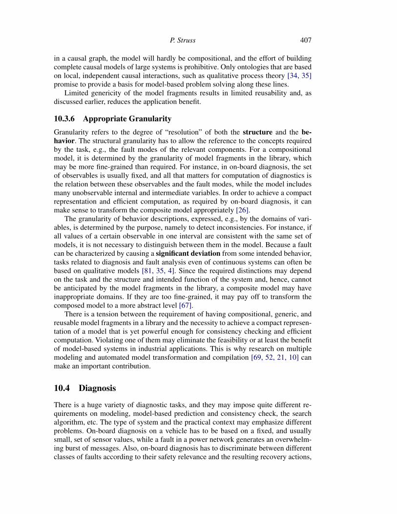
in a causal graph, the model will hardly be compositional, and the effort of buildingcomplete causal models of large systems is prohibitive. Only ontologies that are basedon local, independent causal interactions, such as qualitative process theory [34, 35]promise to provide a basis for model-based problem solving along these lines.
Limited genericity of the model fragments results in limited reusability and, asdiscussed earlier, reduces the application benefit.
10.3.6 Appropriate Granularity
Granularity refers to the degree of “resolution” of both the structure and the be-havior. The structural granularity has to allow the reference to the concepts requiredby the task, e.g., the fault modes of the relevant components. For a compositionalmodel, it is determined by the granularity of model fragments in the library, whichmay be more fine-grained than required. For instance, in on-board diagnosis, the setof observables is usually fixed, and all that matters for computation of diagnostics isthe relation between these observables and the fault modes, while the model includesmany unobservable internal and intermediate variables. In order to achieve a compactrepresentation and efficient computation, as required by on-board diagnosis, it canmake sense to transform the composite model appropriately [26].
The granularity of behavior descriptions, expressed, e.g., by the domains of vari-ables, is determined by the purpose, namely to detect inconsistencies. For instance, ifall values of a certain observable in one interval are consistent with the same set ofmodels, it is not necessary to distinguish between them in the model. Because a faultcan be characterized by causing a significant deviation from some intended behavior,tasks related to diagnosis and fault analysis even of continuous systems can often bebased on qualitative models [81, 35, 4]. Since the required distinctions may dependon the task and the structure and intended function of the system and, hence, cannotbe anticipated by the model fragments in the library, a composite model may haveinappropriate domains. If they are too fine-grained, it may pay off to transform thecomposed model to a more abstract level [67].
There is a tension between the requirement of having compositional, generic, andreusable model fragments in a library and the necessity to achieve a compact represen-tation of a model that is yet powerful enough for consistency checking and efficientcomputation. Violating one of them may eliminate the feasibility or at least the benefitof model-based systems in industrial applications. This is why research on multiplemodeling and automated model transformation and compilation [69, 52, 21, 10] canmake an important contribution.
10.4 Diagnosis
There is a huge variety of diagnostic tasks, and they may impose quite different re-quirements on modeling, model-based prediction and consistency check, the searchalgorithm, etc. The type of system and the practical context may emphasize differentproblems. On-board diagnosis on a vehicle has to be based on a fixed, and usuallysmall, set of sensor values, while a fault in a power network generates an overwhelm-ing burst of messages. Also, on-board diagnosis has to discriminate between differentclasses of faults according to their safety relevance and the resulting recovery actions,

408 10. Model-based Problem Solving
while diagnosis in the workshop only needs to identify the broken part in order to re-place it. The latter case usually involves a number of testing activities, while a hugegas turbine in a plant does not allow interruptions for carrying out experiments. Mostof the time, we are confronted with “post-mortem” diagnosis, but often, it is desir-able to perform prognostic diagnosis in order to schedule maintenance before a failureoccurs. And so forth.
Rather than outlining all specific answers to such specific requirements, we fo-cus on the presentation of some principled and sufficiently general and influentialapproaches. We will identify the underlying assumptions that confine the scope ofapplicability. Even for some fundamental work, they were often left implicit, andsometimes, the authors even seem to be unaware of them.
We first describe consistency-based diagnosis with component-oriented models,whose idea has been the basis for the analysis in Section 10.2 and contains importantprinciples and techniques, which partly carry over to other tasks. It represents probablythe largest class of implemented systems and provides a systematic framework to thecommunity for discussing variants and alternatives of the techniques.
Section 10.4.2 discusses the problem of performing diagnosis over time. We thenoutline an alternative concept, abductive diagnosis (Section 10.4.3) and consistency-based diagnosis using an alternative type of models, process-oriented diagnosis (Sec-tion 10.4.4).
10.4.1 Consistency-based Diagnosis with Component-oriented Models
The classical theory [62, 19] and realization of consistency-based diagnosis [20, 22,24, 64] consider systems that contain a fixed set of components, COMPS, that interactin a fixed structure. Furthermore, it is assumed that a disturbance of the entire systemis caused by amalfunctioning of one or more of these components. This includes theassumption that the entire system performs as intended if all components performproperly, i.e. the well-designed system assumption.
Diagnosis is then seen as the task to decide whether there are components thatare not exhibiting their intended behavior (fault detection) and to determine whichcomponents work in a fault mode (fault localization) and in which fault mode theyoperate (fault identification).
Hence, each component Ci has a set of possible associated behavior modesmodes(Ci) (usually determined by the component type), and assigning one mode toeach component provides an answer to a diagnosis problem.
Definition 10.1 (Mode assignment). Let COMPS � ⊆ COMPS.�
Ci∈COMPS �
mji (Ci), where mji ∈ modes(Ci)
is a mode assignment. It is called complete if COMPS � = COMPS.
ok(Ci) always has to be an element of modes(Ci) and characterizes uniquely theintended, normal behavior of the component. Modes are mutually exclusive,
mji(Ci) ∧mki(Ci) ⇒ j = k

P. Struss 409
which also means that all modes different from ok(Ci) represent some sort of faultybehavior:
∀mji(Ci) ∈ modes(Ci) \ {ok(Ci)}, mji(Ci) ⇒ ¬ok(Ci).
The model library LIB associates a behavior model with each mode:
mji(Ci) ⇒ modelji(Ci).
If the models are stated in terms of variables, then LIB must also contain domainaxioms for the variables, i.e., the (exclusive) disjunction of their possible values.
Then each mode assignment
MA =�
Ci∈COMPS
mji (Ci)
together with the structural description STRUCTURE, which specifies the connectionsbetween components in terms of variables shared by the components, and the libraryLIB implies a behavior modelMODEL(MA) of the entire system for the mode assign-mentMA:
LIB ∪ STRUCTURE ∪ {MA} ⇒ MODEL(MA)
Some papers use the term system description (SD) to refer to knowledge about thesystem without further specification. If we assume that there are no general restrictionson the possible mode assignments, we consider
SD = LIB ∪ STRUCTURE
which has the disadvantage of obscuring the different nature of these elements: LIBusually contains domain-specific knowledge about the behavior of components, whileSTRUCTURE is system-specific.
In the following, we will always assume that modeling has led to a proper result,i.e., SD is consistent. If the modes of the components are assumed to be independentof each other, then also MODEL(MA) is consistent for every mode assignment MA.This requires valid models, as discussed in Section 10.3.2.
In this approach, model-based diagnosis is regarded as generation of system mod-els that are consistent with the observations and amounts to generating hypothesesabout the actually present behavior modes of the components. Therefore, we define
Definition 10.2 (Consistency-based diagnosis). A complete mode assignment MA isa consistency-based diagnosis for a system description SD and a set of observationsOBS if
SD ∪ {MA} ∪ OBS � ⊥.
Fault detection
In particular, the assignment of ok to all components
MAOK =�
C∈COMPS
ok(C)
410 10. Model-based Problem Solving
specifies the normal behavior of the overall system:
LIB ∪ STRUCTURE ∪ {MAOK} ⇒ MODELOK .
The well-designed-system assumption,
MODELOK ⇒ GOALS
turns the question whether the system behaves as intended into checking whether
SD ∪ {MAOK} ∪ OBS � ⊥
which is realized by checking whether the resulting model is consistent with the ob-servations:
MODELOK ∪ OBS � ⊥.
Fault localization
If diagnosis is seen as fault localization, as, for instance, in [62, 20, 19], then this isrelated to another hidden assumption, namely that this information suffices to repairthe broken system, which is true if replacement of components is the means for re-establishing the functionality of the system. (Sometimes, fault localization may beperformed not in order to repair the system, but to identify flaws in manufacturingprocess.)
Fault localization is only interested in differentiating the broken components fromthe correctly working ones and, hence, aims at the special case of
modes(C) =�ok(C),¬ok(C)
�.
As stated above, if there are more specific fault modes, then they imply ¬ok(C).A fault localization has to hypothesize the set of broken components consistently withthe observations:
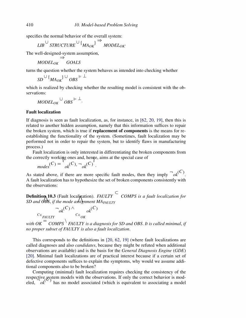
Definition 10.3 (Fault localization). FAULTY ⊂ COMPS is a fault localization forSD and OBS, if the mode assignment MAFAULTY
�
C∈FAULTY
¬ok(C) ∧�
C∈OK
ok(C)
with OK = COMPS \ FAULTY is a diagnosis for SD and OBS. It is called minimal, ifno proper subset of FAULTY is also a fault localization.
This corresponds to the definitions in [20, 62, 19] (where fault localizations arecalled diagnoses and also candidates, because they might be refuted when additionalobservations are available) and is the basis for the General Diagnosis Engine (GDE)[20]. Minimal fault localizations are of practical interest because if a certain set ofdefective components suffices to explain the symptoms, why would we assume addi-tional components also to be broken?
Computing (minimal) fault localization requires checking the consistency of therespective system models with the observations. If only the correct behavior is mod-eled, ¬ok(C) has no model associated (which is equivalent to associating a model

P. Struss 411
that does not impose any restrictions on the values of local variables). In this case,a search could be performed by eliminating the OK models of components from theentire model and checking the consistency of the remaining models. This approachwhich in practice might work in an exhaustive manner only for single or small sets offaults has actually been proposed in [12] as constraint suspension. However, there is apossibility for a more focused generation of fault localizations which has an intuitivebasis: if the windshield wipers in our car do not work, we will focus our analysis ons small subset of components, such as their motor, the connecting cables, etc., but notconsider, say, parts of the engine or of the braking system, because they do not in-fluence the observed behavior of the car. Carried over to model-based diagnosis, thismeans that the observations may not simply be inconsistent with the complete systemmodel, but with a model obtained from some partial mode assignment, which we calla conflict.
Definition 10.4 (Conflict). Let COMPS � ⊂ COMPS and
MA =�
Ci∈COMPS �
mji (Ci)
be a mode assignment such that
SD ∪ {MA} ∪ OBS � ⊥.
The negation of MA,�
Ci∈COMPS �
¬mji (Ci)
is called a conflict. It is called minimal, if it is not implied by a different conflict. It iscalled basic if
∀Ci ∈ COMPS �, mji (Ci) = ok(Ci) ∨mji (Ci) = ¬ok(Ci)
and positive, if
∀Ci ∈ COMPS �, mji (Ci) = ok(Ci).
Since [19] considers only the two basic modes, a basic conflict corresponds totheir definition of a conflict. Minimal conflicts are the most focused restrictions on thepossible combinations of modes, and non-minimal conflicts do not provide additionalinformation. Obviously, positive conflicts are important to fault localization, becausethey state that at least one of the mentioned components is broken. Even stronger, thefollowing theorems [19] states that conflicts capture exactly the available informationfor fault localization, can replace SD ∪ OBS and be used to logically characterize thesolutions.
Theorem 10.1. Let MB-CONFLICTS be the set of all minimal basic conflicts for SD∪
OBS. FAULTY ⊂ COMPS is a fault localization for SD ∪OBS iff the respective modeassignment is consistent with the minimal basic conflicts:
MB-CONFLICTS ∪ {MAFAULTY} � ⊥.
412 10. Model-based Problem Solving
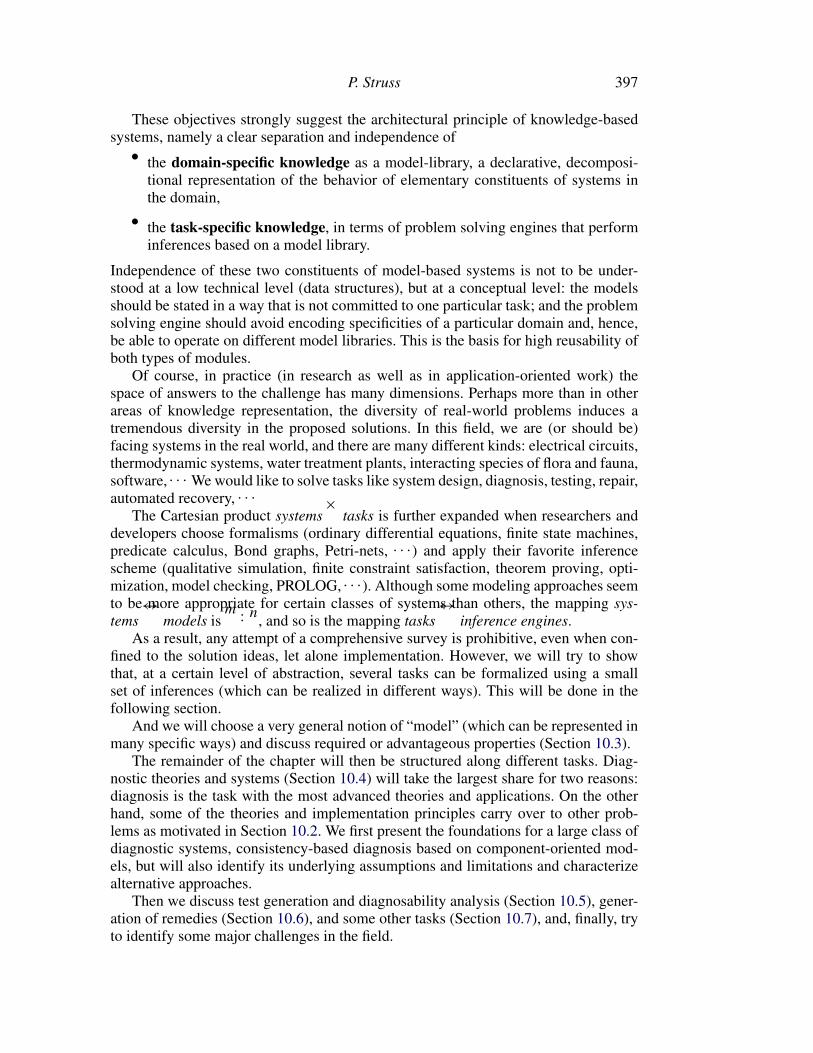
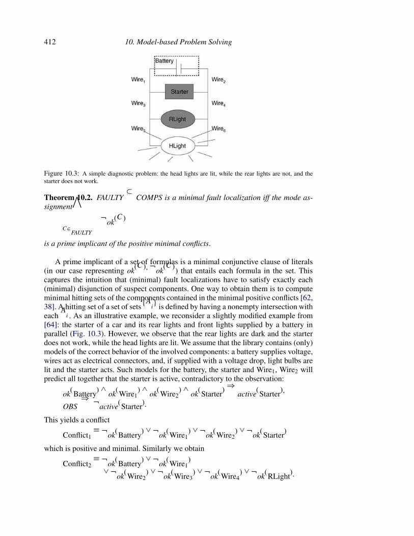
Figure 10.3: A simple diagnostic problem: the head lights are lit, while the rear lights are not, and thestarter does not work.
Theorem 10.2. FAULTY ⊂ COMPS is a minimal fault localization iff the mode as-signment
�
C∈FAULTY
¬ok(C)
is a prime implicant of the positive minimal conflicts.
A prime implicant of a set of formulas is a minimal conjunctive clause of literals(in our case representing ok(C),¬ok(C)) that entails each formula in the set. Thiscaptures the intuition that (minimal) fault localizations have to satisfy exactly each(minimal) disjunction of suspect components. One way to obtain them is to computeminimal hitting sets of the components contained in the minimal positive conflicts [62,38]. A hitting set of a set of sets {Ai} is defined by having a nonempty intersection witheach Ai . As an illustrative example, we reconsider a slightly modified example from[64]: the starter of a car and its rear lights and front lights supplied by a battery inparallel (Fig. 10.3). However, we observe that the rear lights are dark and the starterdoes not work, while the head lights are lit. We assume that the library contains (only)models of the correct behavior of the involved components: a battery supplies voltage,wires act as electrical connectors, and, if supplied with a voltage drop, light bulbs arelit and the starter acts. Such models for the battery, the starter and Wire1, Wire2 willpredict all together that the starter is active, contradictory to the observation:
ok(Battery) ∧ ok(Wire1) ∧ ok(Wire2) ∧ ok(Starter) ⇒ active(Starter),
OBS ⇒ ¬active(Starter).
This yields a conflict
Conflict1 ≡ ¬ok(Battery) ∨ ¬ok(Wire1) ∨ ¬ok(Wire2) ∨ ¬ok(Starter)
which is positive and minimal. Similarly we obtain
Conflict2 ≡ ¬ok(Battery) ∨ ¬ok(Wire1)
∨ ¬ok(Wire2) ∨ ¬ok(Wire3) ∨ ¬ok(Wire4) ∨ ¬ok(RLight).

P. Struss 413
Furthermore, the lit head lights imply the existence of a voltage drop which shouldalso cause the rear lights to be lit, leading to
Conflict3 ≡ ¬ok(HLight) ∨ ¬ok(Wire5) ∨ ¬ok(Wire6) ∨ ¬ok(RLight).
Analogously, we find
Conflict4 ≡ ¬ok(HLight) ∨ ¬ok(Wire5) ∨ ¬ok(Wire6)
∨ ¬ok(Wire3) ∨ ¬ok(Wire4) ∨ ¬ok(Starter).
In fact, these are all minimal and positive conflicts. As a side-remark, the last twoconflicts are only derived if the predictor is complete enough to reason not only in thecausal direction, but also draw conclusions from the effect, namely the lit head lights.The mode assignment
¬ok(RLight) ∧ ¬ok(Starter)
implies all conflicts and is minimal, hence a prime implicant of all positive minimalconflicts. Thus,
{RLight,Starter}
is a fault localization, in accordance with our expectation.At this point, we emphasize, that the described approach allows for
• fault localization with models of correct component behavior only, i.e. withoutany restriction on the possible faulty behaviors,
• localizing multiple faults.
This is an advantage over systems based on empirical symptom-fault associations,which require explicitly known faults and face natural limitations on known symptomsof multiple faults.
If the library does not contain fault models, there is no way to refute ¬ok(Ci),all basic conflicts are positive ones, and extending a fault localization by additionalcomponents also yields a fault localization. In general, we have [19]:
Theorem 10.3. For each fault localization FAULTY ∈ COMPS every supersetFAULTY � ⊃ FAULTY is also a fault localization iff all basic conflicts of SD ∪ OBSare positive.
In this case, the minimal fault localizations are a compact representation of all faultlocalizations, namely as a lower bound in the subset lattice of COMPS.
Fault localization with fault models
When taking a second look at the example, we notice that, while we are satisfied withthe fault localization {RLight,Starter}, we would not consider, for instance, its super-set {RLight,Starter,Battery} as a reasonable fault localization, despite Theorem 10.3.Furthermore, we notice that there are many more prime implicants of the four con-flicts, namely 21, and among them are, for instance,
¬ok(Wire1) ∧ ¬ok(Wire5)
414 10. Model-based Problem Solving
and
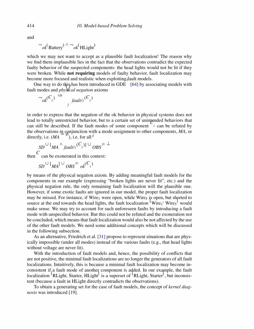
¬ok(Battery) ∧ ¬ok(HLight)
which we may not want to accept as a plausible fault localization! The reason whywe find them implausible lies in the fact that the observations contradict the expectedfaulty behavior of the suspected components: the head lights would not be lit if theywere broken. While not requiring models of faulty behavior, fault localization maybecome more focused and realistic when exploiting fault models.
One way to do this has been introduced in GDE+ [64] by associating models withfault modes and physical negation axioms
¬ok(Ci) ⇒�
j
faultji(Ci)
in order to express that the negation of the ok behavior in physical systems does notlead to totally unrestricted behavior, but to a certain set of unintended behaviors thatcan still be described. If the fault modes of some component Ci can be refuted bythe observations in conjunction with a mode assignment to other components, MA, ordirectly, i.e. (MA = ∅), i.e. for all i
SD ∪ {MA ∧ faultji(Ci)} ∪ OBS � ⊥
then C can be exonerated in this context:
SD ∪ {MA} ∪ OBS � ok(Ci)
by means of the physical negation axiom. By adding meaningful fault models for thecomponents in our example (expressing “broken lights are never lit”, etc.) and thephysical negation rule, the only remaining fault localization will the plausible one.However, if some exotic faults are ignored in our model, the proper fault localizationmay be missed. For instance, if Wire1 were open, while Wire5 is open, but shorted tosource at the end towards the head lights, the fault localization {Wire1,Wire5} wouldmake sense. We may try to account for such unforeseen faults by introducing a faultmode with unspecified behavior. But this could not be refuted and the exoneration notbe concluded, which means that fault localization would also be not affected by the useof the other fault models. We need some additional concepts which will be discussedin the following subsection.
As an alternative, Friedrich et al. [31] propose to represent situations that are phys-ically impossible (under all modes) instead of the various faults (e.g., that head lightswithout voltage are never lit).
With the introduction of fault models and, hence, the possibility of conflicts thatare not positive, the minimal fault localizations are no longer the generators of all faultlocalizations. Intuitively, this is because a minimal fault localization may become in-consistent if a fault mode of another component is added. In our example, the faultlocalization {RLight, Starter, HLight} is a superset of {RLight, Starter}, but inconsis-tent (because a fault in HLight directly contradicts the observations).
To obtain a generating set for the case of fault models, the concept of kernel diag-nosis was introduced [19].
P. Struss 415
Definition 10.5 (Kernel diagnosis). A kernel diagnosis is a minimal partial modeassignment MAk with the property that every mode assignment that extends it is con-sistent with SD ∪ OBS, i.e.
for all consistent MA holdsif MA entails MAkthen MA is a diagnosis of SD ∪ OBS.
In other words, the modes of the components not mentioned in MAk do not mat-ter. Obviously, all fault localizations are obtained from an extension of some kerneldiagnoses. Also, the kernel diagnoses can be characterized as prime implicants of allminimal conflicts.
Fault identification
Besides helping to refine fault localization, fault models provide the basis for identi-fying which particular component faults may be responsible for the disturbed systembehavior. If the list of behavior modes contains specific faults of a component (type),then the diagnoses according to the definition given above are the answer to the taskof fault identification.
However, the inclusion of explicit fault models in SD is a qualitative jump froma single system model (of the ok behavior) to a large space of models, correspond-ing to all possible mode assignments. This is important from both a technical and anapplication point of view.
Technically, it implies that many system models may have to be checked for con-sistency with observations, and for conflict-driven approaches, it means that the spaceof minimal conflicts grows. Fortunately, the application perspective implies that mostof the mode assignments are not interesting and many conflicts need not be discov-ered. To most diagnosis applications, it is not interesting to characterize the space ofall diagnoses, but to compute the most relevant ones. This is because its purpose isto provide information just enough to restore the functionality. Therefore, of course,what makes a diagnosis relevant depends on the type of system and its applicationcontext. But to be of practical interest, diagnostic theories and systems should providegeneric means to express some ranking of the expected diagnoses and algorithms toeffectively and efficiently compute the best ones under such a ranking. Unfortunately,there have not been as many theoretical contributions to this important area as to thelogical characterization and approaches assuming exhaustive computation.
The applied principle of Occam’s razor, namely not to assume more components tobe broken than necessary, is usually a fundamental criterion we would like to preservefor fault identification, as well.
Definition 10.6 (Minimal diagnosis). A diagnosis MA for SD ∪ OBS is a minimaldiagnosis, iff the corresponding fault localization
FAULTY := {Ci ∈ COMPS | ok(Ci) /∈ MA}
is minimal.
This set of minimal diagnoses may still be large and ignore additional rankingcriteria. Both a broken (open) light bulb and its pin being shorted to ground may

416 10. Model-based Problem Solving
explain why the bulb is not lit, but the shorted fault may be much more unlikely and,hence, only considered if the other one has been ruled out. We can define such ageneral preference on the modes of a component.
Definition 10.7 (Preference on modes and mode assignments). A mode preference forCi is a partial order “�” on modes(Ci):
�⊆modes(Ci)× modes(Ci),
where ok(Ci) is the maximal element and an unknown fault mode unknown(Ci), ifpresent, is the minimal element:
∀mj(Ci) ∈ modes(Ci) \ {ok(Ci)}: ok(Ci) > mj (Ci),
∀mj(Ci) ∈ modes(Ci) \ {unknown(Ci)}: mj(Ci) > unknown(Ci).
“>” is defined as
x > y :⇔ x � y ∧ ¬(y � x).
This induces a preference on mode assignments: for
MA = {mji (Ci)},
MA� = {m�ji(Ci)},
we define
MA � MA� :⇔ ∀i mji (Ci) � m�ji(Ci).
Definition 10.8 (Preferred diagnosis). A diagnosis MA is a preferred diagnosis, ifthere is no diagnosis MA� that is strictly preferred over MA
∀MA� MA� � MA ⇒ MA� = MA.
Intuitively, the definition expresses, that a certain fault modemj(Ci) should appearin a preferred diagnosisMA if
1. all mode assignments that are obtained by MA replacing mj(Ci) in MA by astrictly preferred mode m�
j (Ci) > mj (Ci) are not a diagnosis, and, of course,
2. MA is a diagnosis.
In order to characterize preferred diagnoses, [24] uses default logic [61, 5]. A (normal)default is an inference rule of the form
a : b/b
which expresses, intuitively, “If a is true, and it is consistent to assume b is true, thenb holds”. A default theory is a pair (D, P ), where P is a set of classical formulas andD a set of defaults. Since defaults may exclude each other mutually, there are different(maximal) sets of defaults applicable, which leads to different sets of conclusions,called extensions.
P. Struss 417
For instance, assuming a certain mode of a component, we cannot associate anothermode of the same component that might also be consistent. Indeed, we can encode therule that mj(Ci) should be assumed only if all its strictly preferred predecessors
prej (Ci) :=�mk(Ci) | mk(Ci) > mj (Ci)
�
have been refuted, and if mj(Ci) can be consistently assumed as a default
def ij ≡�
mk(Ci)∈prej (Ci )
¬mk(Ci) : mj(Ci)/mj (Ci).
Especially, the ok behavior will be assumed first:
: ok(Ci)/ok(Ci)
The following theorem [24] captures the intuition that these preference defaults deter-mine the preferred diagnoses:
Theorem 10.4. Let DEF = {def ij } be the set of all preference defaults. MA is apreferred diagnosis if
Cn(SD ∪ OBS ∪ MA)
is an extension of the default theory (DEF, SD ∪ OBS). Here, Cn(.) denotes the de-ductive hull:
Cn(P ) := {p | P � p}.
The theorem provides the logical characterization of (preferred) diagnoses for faultidentification and contains as a special case, namely modes(Ci) = {ok(Ci),¬ok(Ci)},the characterization for fault localizations given in [62]. The theory was implementedas the Default-based Diagnosis Engine (DDE) [25] which generates the successormode assignments for the refuted diagnosis hypotheses according to the preferencerelation and checks their consistency only if all strictly preferred diagnoses have beenrefuted. This means, in particular, if an unknown fault is included, it will only beconsidered if no other fault mode survives the consistency check, but its existenceprevents exoneration as performed in GDE+.
DDE’s preferences are local to each component and only an ordering. It does notuse preferences among modes of different components and, hence, does, for instance,not order single faults involving different components. A refinement can be obtainedby exploiting a global scale for ranking of modes, such as failure probabilities. InSHERLOCK [22], mode assignments are checked for consistency in the order of theirprobability which is obtained from the probabilities of modes (assuming their inde-pendence). Starting with a-priori probabilities, SHERLOCK recomputes probabilitieswhen new conflicts have been detected. Unknown faults can be included, usually withlow probability, and termination criteria specified, e.g., as a function of the probabil-ities of the diagnoses obtained so far. Although there is no formal characterization, itshould be clear that SHERLOCK generates a subset of the preferred diagnoses if thepreference is the order induced by mode probabilities. The core of this technique isfairly general and has been introduced as conflict-directed A* search [86].
418 10. Model-based Problem Solving
10.4.2 Computation of Diagnoses
Since diagnosis is formalized as finding a model that is consistent with the observa-tions, one might (and some authors do) suggest using any (efficient) generic algorithmthat generates a solution for
SD ∪ {MA} ∪ OBS
such as constraint satisfaction algorithms [13, 63] and SAT-solvers. However, whilemany such algorithms produce some single solution quite efficiently, their naive usemay ignore requirements and context of the real task. The same holds for the, usuallyinfeasible, attempt to compute the set of all diagnoses. Diagnosis in the real world isnot interested in a single arbitrary solution, but in finding a set of diagnoses thatfulfill some criteria dictated by the practical context of the task. Such criteriavary and can be quite complex. Minimality (with respect to cardinality or set inclu-sion) of diagnoses is only one example, which is independent of domain and task. Inreality, the relevance criteria for diagnoses are mainly determined by the ultimate ob-jective, namely re-establishing the proper system behavior at minimal cost and risk,and, hence, may vary with the means and restrictions for reaching the objective (seethe discussion in Section 10.6). Focusing on the most likely or “preferred” faults asdone in SHERLOCK [22] and GDE+ [24], respectively, reduces the risk of fixing thewrong component and, thus, the average cost. In some applications, certain highlycritical faults may have to be explicitly ruled out (e.g., to select appropriate recoveryactions based on on-board diagnosis of vehicles).
Another important requirement in many applications is due to the fact that com-puting diagnoses from observations is not a one-shot activity, but happens multipletimes in a process of gathering information through testing and observation (see Sec-tion 10.5). This has to be reflected by the requirement for algorithms that support anefficient incremental computation of diagnoses when the set of observations is ex-tended.
The design of a diagnosis algorithm has to reflect a number of choices imposed bythe respective application:
• The task: fault localization vs. fault identification.
• The models: existence or non-existence of fault models.
• Fault models: existence or non-existence of an unknown fault (with unrestrictedbehavior).
• The result: criteria for the relevance of diagnoses to be produced (rarely all).
In the theories presented above, the concept of conflicts played an important role incharacterizing the solution space. We discuss some aspects of exploiting conflicts insome more detail.
Computing fault localizations/diagnoses from conflicts
Theorem 10.2 suggests a two-step computation: first compute all minimal (positive)conflicts, then compute their prime implicants to obtain fault localizations. This is fea-sible and useful, if only theOK behavior is modeled.GDE [20] is the archetype of this
P. Struss 419
solution. The presence of fault models modifies the set of minimal positive conflicts, ifthe physical negation rule is applied (i.e. the set of fault models is considered completeand does not contain an unknown fault as inGDE+ [64]). For instance, in our example:
Conflict3 ≡ ¬ok(HLight) ∨ ¬ok(Wire5) ∨ ¬ok(Wire6) ∨ ¬ok(RLight)
is reduced to
Conflict3 ≡ ¬ok(Wire5) ∨ ¬ok(Wire6) ∨ ¬ok(RLight)
by the non-positive conflict
¬broken(HLight)
(which is obtained from the observation that HLight is lit) and the physical negationrule:
¬ok(HLight) ⇒ broken(HLight).
The introduction of fault models implies the step from a single system model (the OKmodel) to a large set of models (for all mode assignments). This is a qualitative leap,which usually makes a complete check of all mode assignments infeasible.
Computing kernel diagnoses
The concept of kernel diagnoses, introduced in Section 10.4.1, is attractive from atheoretical point of view, because it provides a generator for the set of all diagnosesin case of the existence of fault models. However, it does not offer the basis for anypractical solution, because it requires an unrestricted consistency check of mode as-signments. Also, many of the kernel diagnoses may be completely irrelevant to anypractical consideration. We illustrate this by the following example. Consider, say, 17“Equal components” Equali in series which have the modes
ok(Equali ) : ini = outi ,
neg(Equali ) : ini − 1 = outi ,
pos(Equali ) : ini + 1 = outi
and the observations
in1= 0,
out17= 1.
Then there exist 17 singleton fault localizations, namely {pos(Equali )}, which are theinteresting ones to focus on under practical considerations. The space of all fault local-izations is given by all subsets of COMPS with odd cardinality. As a consequence, theset of kernel diagnoses is identical to the set of all fault localizations, which means, inparticular, all of them are complete mode assignments. From a computational point ofview, the example also illustrates that the set of non-positive conflicts is large namelythe set of all subsets of COMPS with even cardinality and the empty set, and that de-termining them requires checking all complete mode assignments (but then, you havethe fault localizations directly).
In summary, an exhaustive computation of conflicts rarely lends itself to a compu-tational solution (except for fault localization with OK models only). However, thereis no interest in computing all diagnoses, anyway.
420 10. Model-based Problem Solving
Search for diagnoses and the exploitation of conflicts
The response to this insight is to organize the generation of relevant diagnoses assearch, instantiating and checking mode assignments only after checking those withhigher relevance. Given a criterion for (potentially dynamically) ordering mode as-signments according to their importance, one could perform some best-first search inthe space of mode assignments in a hypothesize-and-test cycle in a straightforwardmanner. However, (minimal) conflicts provide a powerful means to improve the effi-ciency of the search. This is due to the fact that a model of a mode assignment thatdoes not satisfy all existing (minimal) conflicts does not need to be instantiated andchecked for consistency with the observations. Stated differently, after each detectionof a new (minimal) conflict, the search space can be pruned by eliminating all modeassignments that imply the respective inconsistent partial mode assignment (i.e. thenegation of this conflict).
In GDE+ [24], the preference defaults serve two purposes: on the one hand, theyencode the ordering of the modes and ensure that a mode of a component is only con-sidered for consistency checking in a context if all more preferred modes have beenrefuted. On the other hand, it will not be checked, if it is already known to be inconsis-tent because it is subsumed by some previously detected inconsistency. SHERLOCK[22], which checks mode assignments according to their probabilities, also exploitsconflicts to prune the space of mode assignments. This principle has been generalizedto Conflict-directed A∗ [86] for cost functions satisfying certain criteria.
Determining (minimal) conflicts
Exploiting conflicts for computing fault localizations and pruning the search space re-quires that the consistency check delivers more than a Yes/No answer for a completemode assignment. It has to identify partial mode assignments that generate the incon-sistency, and the smaller they are, the stronger is the impact on the accuracy of the com-puted fault localization and on search space pruning. The “classical” way of findingconflicts (as in GDE, GDE+, and SHERLOCK) is by means of a propagation-basedpredictor interfaced to some dependency-recording mechanism (e.g., exploiting anAssumption-based Truth-Maintenance System, ATMS [14]). Whenever a contradic-tion (two conflicting values of a variable) is detected, the underlying behavior modesthat derived it together can be determined. Incompleteness of the predictor may leadto missing (minimal) conflicts and, hence, suboptimal fault localization (although theproper one will never be falsely refuted). However, while this works for some systems,such as combinatorial circuits, there is a vast space of system models for which prop-agation is highly incomplete or does not derive anything (resistive electrical circuits,hydraulic systems, . . .). In this case, other more complete algorithms for consistencychecking are needed, and if generic efficient ones are used (CSP, SAT, . . .), then theirutility depends on whether and to what extent they can deliver (minimal) conflicts.
Pre-compilation of models
If one does not use dependency recording or some equivalent technique, the alterna-tive is to check partial mode assignments for consistency in order to find conflicts. Butthis is a large space, and one would want to anticipate which assignments can possiblylead to the detection of a conflict. This means to decompose the system into chunks
P. Struss 421
in a way that checking these respective partial mode assignments can possibly lead toa conflict. The analysis needed for such an approach, which may be called conflict-oriented model decomposition [56], has to reflect the structure of the system and theset of observable variables. Intuitively, the task is to find sets of observations that parti-tion the system model into subsystems that can become over-determined, which oftenrequires to make certain assumptions about the model (e.g., linear functions). Thereare a number of caveats. Firstly, the approach is obviously only suited for applicationswhere the set of possible observables is fixed (and not too large), an assumption thatcan be valid for online-diagnosis of monitored or controlled systems. Secondly, thepotential conflicts can comprise quite different subsets of components for differentmode assignments, and even for different states and inputs of the system. Performingthe analysis exhaustively for all cases, particularly under the presence of fault modelsseems prohibitive. Hence, thirdly, if we use purely structurally oriented algorithms,we may fail to find the minimal potential conflicts.
There are other proposals to compile system descriptions in order to achieve bet-ter performance at diagnosis runtime. Ultimately, only the interdependencies betweenobservable variables and the mode assignments matter, whereas the overall systemmodel may contain many more intermediate and unobservable variables, especiallydue to the fact that the model is a compositional one. A straightforward step is, there-fore, to eliminate all unobservable variables from the model. This works best if the setof observable variables is fixed (and small), as, for instance, in on-board diagnosis andmonitoring systems, where the set of observables is determined by the existing sensors[26]. This has enabled the generation of a model-based on-board diagnostic system,that runs on an actual control unit of a passenger vehicle [74]. Darwiche [10] proposesto compile a system description into a special form (negation normal form) in order toachieve better performance for diagnosis tasks.
Obviously, for all such solutions holds that the complexity of the task is shiftedinto the compilation step which even may become intractable.
Hierarchical models
Another option is to represent the system to be diagnosed by a hierarchical model andapply the described techniques at each level to those subsystems that have been de-termined as suspects at the higher level. This keeps the number of components and,hence, the size of mode assignments and conflicts small. (See, e.g., [48].) While asolution along these lines is theoretically straightforward, in practice it comes at con-siderable cost and raises some problems. Obviously, we need models of subsystemsabove the level of elementary components. There are two ways to obtain them: au-tomatically or “by hand”. The latter option, though feasible in some cases, increasesthe modeling effort. The bad part is that only the models of the very bottom layerscan be expected to be reusable, the rest is likely to be system-specific. Therefore, inmost applications, the effort of creating models of higher-level components (which arehardly re-usable) manually will probably kill the economic benefit of a model-basedsolution. An automated solution is needed.
The reductionist approach implies that we can obtain the behavior models of thesubsystems in a bottom-up fashion as the composition of the models of its components,which means we face the task of automated model compilation (e.g., by transforminga constraint network to a single constraint relating state and interface variables of
422 10. Model-based Problem Solving
the aggregate and covering all observable variables). If we would like to exploit faultmodels not only at the lowest level to improve fault localization, we have a complexityproblem, because we have to generate not only the ok model of the aggregate, but alsoits fault models, which would mean compiling models of all or a selected set of modeassignments. An option is to focus on single faults (or the most probable ones) andcapture the rest by an unknown fault mode of the aggregate. Still the result can bemany fault modes for the aggregate. Often, they can be conveniently summarized bya smaller set of fault modes in a more abstract representation, but generating suchabstractions automatically is a serious challenge to automated modeling—or we areback at manual modeling.
10.4.3 Solution Scope and Limitations of Component-OrientedDiagnosis
Although what has been surveyed so far in this section has often been considered astheories and solutions to the task of diagnosis based on first principles, it turns outto be a very specific one. We need to be aware that there are a number of underlyingassumptions and limitations that confine the scope of applicability from a practicalperspective.
• Fixed, well-specified set of components: many systems in process industries(e.g., in chemical plants) and, even more so, natural systems cannot be modeledconveniently as a set of components.
• Known, fixed structure: For the types of systems just mentioned, this is alsonot satisfied. And in some devices, we might have to consider the processedobjects as components, such as sheets in a copier.
• Well-designed system: This assumes the intended functionality (“GOALS”) isimplied by the system with correct components. This is even not given for manycarefully designed artifacts: often, the parameter tolerances of components in acircuit may well allow an unintended behavior, which is just not happening dueto the statistical distribution of parameter deviations. And ecological systems arenot designed anyway and, hence, always require an explicit representation andconsideration of GOALS [41].
• Component faults only: Disturbances of the system behavior are always causedby a fault of one of the known components. However, often, the cause of amalfunction is due to some additional, unexpected object, substance, or agentintruding the system.
• No structural faults: Even if the structure of the correct device is well-specified,the fault may lie in a violation of this structure (e.g., a bridge fault) [16].
• “Crisp” faults: although the models of different faults may overlap, there is theassumption that the presence of a fault is a yes/no decision. In order to incorpo-rate degradation and “soft” faults, one would have to introduce thresholds that,perhaps artificially, distinguish a tolerable degradation from a real fault.
But there are some non-assumptions, contrary to what is sometimes believed:
P. Struss 423
• Sometimes, it is believed that consistency-based diagnosis can only work withspecific modeling formalisms, e.g., models that are expressed in, or canbe transformed into, logical formulas, such as finite constraints. Engineeringmodels do not come as logical formulas. However, the principles underlyingconsistency-based diagnosis are general. As discussed in Section 10.3, any mod-eling formalism that is suited to capture the diagnosis-relevant behavior aspectsof component modes and that has some notion of and mechanisms for check-ing the consistency of a model with observations can be used. This includesnumerical models and simulators, provided there is a way to avoid the creationof spurious inconsistencies due to noise, model inaccuracy, measurement im-precision, etc. Also, if computation is fixed to one direction (from “input” to“output”), they have to reflect the available observations what makes the sys-tem models specific and reduces their reusability, and they may suffer fromincompleteness regarding the detection of all conflicts (because this may requireinferences starting from outputs).
• In particular, it is often assumed that only static system behavior can be di-agnosed. This is not true, since neither the theory nor the technical principlesprevent the use of models that describe the dynamic behavior and of observa-tions that capture the system evolution over time. Still, the temporal dimensionintroduces some additional problems and specific answers, which will be thesubject of the next section.
Furthermore, it should be pointed out that there is a useful generalization of the theoryand the techniques if we replace “behavior modes” by “states”, where a state is theassignment of a value to a state variable of a component (in analogy to assigning aparticular mode to a component). This way, hypotheses not only about the occurrenceof faults, but also about the internal states of a system can be generated [84]. However,there is no general preference criterion (like minimality for sets of faulty components)for states, although, perhaps, for state changes.
10.4.4 Diagnosis across Time
If observations are available not just for one snapshot of system behavior, but for awhole observation period, this may strengthen the basis for diagnosis, but also triggerssome special problems to solve. Extending the basic definitions appropriately is not toodifficult. First, we have a history or sequence of observations
OBSH = {OBSi} = {{obsij (ti )}}
related to a finite set of time points ti in some time interval of interest, ti ∈ Iω. Sec-ondly, not only the behavior of the system to be diagnosed may evolve over time, butalso the behavior modes of components may change over time, i.e. faults may occurand also disappear. Therefore, in the general case, a diagnostic hypothesis is no longerone mode assignment, but a history of mode assignments
MH = {(MAk, Ik)},�
k
Ik = Iω, MAk �= MAk+1,
where MAk is a mode assignment that holds for all time points in some interval Ik =(tk, tk+1) ⊂ Iω, that is consistent with the observation history (see, e.g., [33]).
424 10. Model-based Problem Solving
Definition 10.9 (Consistency-based temporal diagnosis). A history of complete modeassignments
MH = {(MAk, Ik)}
in Iω is a consistency-based temporal diagnosis for a system description SD and anobservation history
OBSH = {{obsij (ti )}}
in Iω if
SD ∪ MH ∪ OBSH � ⊥.
This concept of a temporal diagnosis subsumes the static version in the sense thatfor each observation point, the mode assignment must be a diagnosis according toDefinition 10.2.
Definition 10.10 (State-based diagnosis). A mode history
MH = {(MAk, Ik)}
is a state-based diagnosis for
OBSH = {{obsij (ti )}}
iffor all ti holdsif ti ∈ Ikthen MAk is a diagnosis for SD and OBSi .
Lemma 10.1. If MH = {(MAk, Ik)} is a temporal diagnosis of SD andOBSH = {{obsij (ti )}},thenMH is a state-based diagnosis for SD and OBSH.
In other words, being a state-based diagnosis is a necessary condition for obtain-ing a temporal diagnosis. Amazingly enough, it is also a sufficient condition for aninteresting and large class of systems and tasks, as discussed in the following.
Whether this holds strictly, depends also on the available observations, becausesome sequence-constraints, i.e. restrictions on the possible transitions between states,may compensate for limited observability. Let us illustrate this by a trivial example.Assume we parked our car in a street in San Francisco with considerable and appliedthe park brake. When we return 10 minutes later, we find the car is no longer at theplace where we left it, but 50 m down the street in front of a wall (with some dents). Wecertainly suspect that the park brake did not do its job, despite the fact that the car wasat stand-still when we left, but also the car in front of the wall is perfectly consistentwith a well-functioning park brake. However, we can conclude that, since the positionsare different, there must have been an unobserved state in between, where the speedof the car was non-zero which contradicts the OK mode of the park brake. This case
P. Struss 425
shows that the sequence-constraints can compensate for gaps in observations in twoways: gaps in time (by conclusions for unobserved states) and regarding observablevariables (esp. derivatives, here: the speed).
Computation of temporal diagnoses
The example does not only illustrate that the sequence-constraints can be essential todiagnosis, it also sheds a light on the implication for computational considerations;We did not have to simulate the vehicle’s behavior under OK mode and the broken-park-brake mode to obtain a conclusion.
Instead, we inferred the existence of a state with speed > 0, which directly contra-dicts the OK model, while being consistent with the fault model. This illustrates: evenif we cannot drop the temporal aspects from the consistency check of different modeassignmentsMAj
SD ∪ {MAj } ∪ OBSH,
which means
state-constraintsji ∪ sequence-constraints ∪ OBSH,
without loss, this still does not force us to simulate the model of every candidate modeassignment MAj , which is likely to be impossible anyway (e.g., in our example, wedo not know when the car started to move and how). Instead, we can apply sequence-constraints first, to complement the observed history by indirect observations
OBSH ∪ sequence-constraints � OBSHext
and then perform consistency checks of
state-constraintsji ∪ OBSHext.
The computational advantage of the second solution is tremendous, since we avoidsimulation of many fault hypotheses, apply sequence-constraints only once and per-form cheaper consistency checks on states only. The most common application andexploitation of this approach is the computation of derivatives from observations toavoid simulation and obtain equivalent results (as analyzed and confirmed in [6] fornumerical models). In essence, the good message is: diagnosis of dynamic systemsdoes not require simulation.
If we perform state-based diagnosis of persistent faults as described above, then themode assignment in the temporal diagnosis has to be a prime implicant of the union ofall sets of conflicts detected at the various time points (or, rather, the minimal elementsof this union). Hence, diagnoses can be computed incrementally by adding newlydetected (minimal) conflicts for each observed snapshot. For systems that perform abest-first search, such as SHERLOCK and DDE, the set of diagnoses obtained fromone snapshot (e.g., the most probable or the preferred diagnoses) forms the set of modeassignments to be checked against the observations for the next snapshot. Whenever,based on these checks, some diagnoses are refuted and new ones are generated, thesealso ought to be checked against all previous snapshots.

426 10. Model-based Problem Solving
State-based vs. simulation-based diagnosis
When confronted with the necessity to diagnose a system whose behavior is observedand changes over time, the immediate consequence seems to be that one has to sim-ulate the behavior under different mode assignments and check for consistency withthe actual tracked behavior ([15] is an examples of such a solution). Triggered by theobservation that in applications of consistency-based diagnosis conflicts always weregenerated from observations stemming from one snapshot [23], the analysis revealedthat the underlying reasons are quite fundamental and lead to a fairly general charac-terization of preconditions for being able to refrain from simulation without affectingthe quality of the resulting diagnoses [71].
The key consideration is that many computational modeling formalisms decom-pose a description of the temporal evolution of a system into a set of restrictions thathold for the state at each time point and a part that restricts the set of possible se-quences of such states:
model = state-constraints ∪ sequence-constraints
For instance, in a numerical simulation system, the former one is an ordinary differen-tial equation, while the latter is incorporated in the integration algorithm. In this case,the specificity of model of a particular mode (assignment) is captured by the first partonly, while the second part represents general laws that apply to all models, namelythe laws of continuity, derivatives, and integration, and is shared by all possible behav-iors an their models. As a consequence, any observed behavior of a particular modeassignment will be consistent with the model, if and only if it is consistent with itsstate-constraints. This provides an intuition for why checking the individual obser-vation snapshots for consistency with the state-constraints suffices for diagnosis, andapplying sequence-constraints and simulation can be avoided. However, if the obser-vations have gaps, i.e., miss a state of the actual behavior, or the set of observablevariables is too small to reveal an inconsistency, then exploiting sequence-constraintsin simulation might compensate for it, because they could infer information aboutan intermediate state or additional information about a partially observed state (e.g.,about derivates). This consideration can be turned into a rigorous argument [71] anda foundation for solutions of high importance to industrial applications, especially iffaults are persistent. Faults are persistent if they do not vanish without repair (such asleakages or broken bulbs).
Definition 10.11 (Persistence of modes). A (fault) mode mji(Ci) is called persistentif for all temporal diagnoses {(MAk, Ik)}
∃k� mji(Ci) ∈ MAk� ⇒ ∀k > k� mji(Ci) ∈ MAk
must hold.It is called persistent in Iω if
∀k mji(Ci) ∈ MAk.
We prefer this definition over the one proposed by [60] who calls a behavior per-sistent if the output of a component is a function of its inputs (and not of time), for
P. Struss 427
two fundamental reasons: Firstly, persistence is a property of a mode, rather than ofmodel as in [60]. Continuous models that reflect noise and uncertainty often cannotbe stated in terms of functions, and a qualitative model that is obtained by abstractinga real-valued function is usually no longer a function. Secondly, there are only fewkinds of systems that can be modeled in a directional way.
In contrast, the condition concerning the commonality of sequence-constraints isa property of the model.
Definition 10.12 (Homogeneity). A model library LIB is called homogeneous, if thereexists a set sequence-constraints that links states of the system at different time pointsand is shared by all models, i.e. for all modes mji ,
modelji = state-constraintsji ∪ sequence-constraints,
and state-constraintsji contains only restrictions for each single time point.
If the above properties hold, then for persistent faults, being a state-based diagnosiscan be not only a necessary condition for a temporal diagnosis (Lemma 10.1) but alsoa sufficient one [71], i.e. MH is a temporal diagnosis for SD and OBSH if and only if
MH = {(MA, Iω)}
and MA is a state-based diagnosis for SD and OBSH. Since the sequence-constraintsdo not contribute to a consistency check at a single time point, MA is obtained as adiagnosis for SD sequence-constraints and all OBSi .
The above considerations apply, in particular, if all modeled behaviors are continu-ous. However, if the model contains discrete states and transitions between them, thenhomogeneity is usually violated, because the possible transitions are specific to a par-ticular behavior mode. For instance, transitions between states OPEN and CLOSEDdo occur in the OK model, but not for a STUCK mode.
Even more fundamentally, the homogeneity property becomes obsolete, if the per-sistence assumption is dropped. So far, we considered only models that describe thecomponent (system) behavior under each mode (assignment). In temporal diagnosis,we may want or need to model also, in which ways mode changes occur. Most at-tempts to do so make the assumption that this happens as a discrete change. Thus, theevolution of system behavior may be described by state changes within a mode andmode changes:
sequence-constraints = states-sequence-constraints
∪modes-sequence-constraints,
although many formalisms represent them in the same way, namely as discrete transi-tions.
If we make a Markov assumption, then sequence-constraints become transition-constraints, which restrict pairs of adjacent states.
Transition-based diagnosis
There are a number of approaches to incorporating transitions to fault modes in themodel, covering the spectrum from discrete-event models to models of continuous
428 10. Model-based Problem Solving
behavior. As basing such models on the concepts of states and transitions is natural,most of them are some variant of finite state machines or similar formalisms. Thereare many approaches, reflecting different types of systems, tasks, observations, tem-poral information, etc. Here, we can only provide a preliminary formal account for thecommon underlying ideas and refer to some specific instances. We represent a modelof the possible evolution of the behavior a component, Ci , as a tuple
model(Ci) = (Si, si,0, Ei, Ei,obs, Ti, Ti,F )
with
• a finite set of states, Si , which can represent operating modes under normalbehavior (e.g., a proper valve in its closed state) or faulty behavior (the valvestuck closed),
• an initial state, si,0,
• a finite set of events,Ei , which may be exogenous influences, control commands(external or internal ones), the occurrence of faults, alarms or other observables,etc.,
• the observable events, Ei,obs ⊂ Ei , which exclude, at least, the events thattrigger fault transitions (otherwise, there is no diagnostic problem),
• a finite set of transitions, Ti , shifting the system from one state to the next(deterministically or non-deterministically), based on the triggering event andpossibly generating an event:
Ti ⊂ Si × Ei × Si × Ei.
A transition t ∈ Ti may represent switches between operating modes, shifts toa fault mode, but possibly also the return to a correct behavior in case of anintermittent fault or due to some repair or reset action,
• the set of fault transitions, Ti,F ⊂ Ti , which correspond to the occurrence offaults.
Such a model uses only the simplest representation of time, namely a (partial) orderingof states. A formal specification of the semantics can be based on some temporal logiccontaining a next operator [32]. Sometimes, metric temporal information (numericalor qualitative) may be necessary and/or available.
Such component models fulfill the important requirement to be compositional.We obtain a model of a system comprising a set of concurrently active componentsCOMPS = {Ci}
MODEL = (S, s0, E,Eobs, T , TF )
as a product of the component models, where
S = S1 × · · · × Sn,
s0 = (s1,0, . . . , sn,0),
P. Struss 429
E = P��
Ei
�,
Eobs = P��
Ei,obs
�
(which means, only part of the composite event may be observable). The way tran-sitions are specified may depend on different assumptions, especially about synchro-nization of the local transitions.
A diagnosis is then, intuitively, some explanation of a sequence of observed eventsin terms of a path through the finite state machine which generates this observabletrace and can be defined as follows.
Definition 10.13 (Transition-based diagnosis). Let
MODEL = (S, s0, E,Eobs, T , TF )
be the model of a system and
OBS = (OBS1, . . . ,OBSn) ∈ Enobs
be a sequence of observations.A sequence of events
e = (e1, . . . , em) ∈ Em
is an extension of OBS, iff it contains OBS in the proper order, i.e.
(i) ∀k ∃j (k) ej (k) ∩�
i Ei,obs = OBSk ,
(ii) k1 < k2 ⇒ j (k1) < j (k2);
e is a transition-based diagnosis of (MODEL,OBS) iff
(i) e is an extension of OBS,
(ii) ∃(s1, . . . , sm) ∈ Sm ∀1 < j < m (sj−1, ej , sj , ej+1) ∈ T .
Fault detection is performed, if every diagnosis contains some fault transition. Faultidentification corresponds to the subsequence of fault transitions in a diagnosis, andfault localization is done by looking for the components where these fault transitionsoccur. Like for the snapshot case, we can apply some minimality criteria for rankingdiagnoses and fault localizations. One could also recast the definition in terms of faultevents or fault states (in the latter case with a modified minimality criterion). Thereare many directions for variations, specializations, and extensions of this perspectiveon diagnosis across time.
Diagnosis with discrete-event models
[65] uses a deterministic finite state machine without emitted events and approachesthe diagnostic problem by compiling the original finite state machine into one thatcontains only observable transitions and produces the same language in terms of ob-servations, called diagnoser. Its states represent the respective sets of nodes in theoriginal model that can be reached via paths that contain also unobservable transitions,
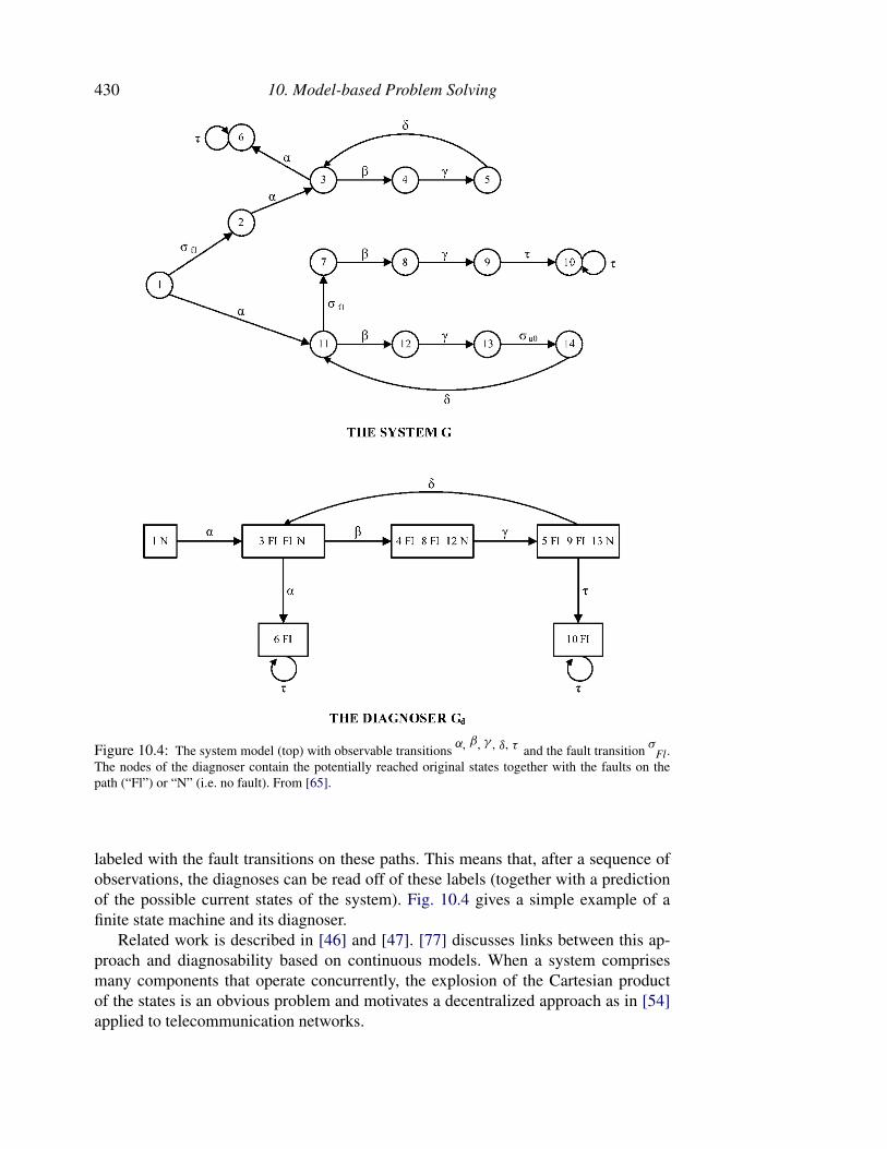
430 10. Model-based Problem Solving
Figure 10.4: The system model (top) with observable transitions α, β, γ, δ, τ and the fault transition σFl.The nodes of the diagnoser contain the potentially reached original states together with the faults on thepath (“Fl”) or “N” (i.e. no fault). From [65].
labeled with the fault transitions on these paths. This means that, after a sequence ofobservations, the diagnoses can be read off of these labels (together with a predictionof the possible current states of the system). Fig. 10.4 gives a simple example of afinite state machine and its diagnoser.
Related work is described in [46] and [47]. [77] discusses links between this ap-proach and diagnosability based on continuous models. When a system comprisesmany components that operate concurrently, the explosion of the Cartesian productof the states is an obvious problem and motivates a decentralized approach as in [54]applied to telecommunication networks.
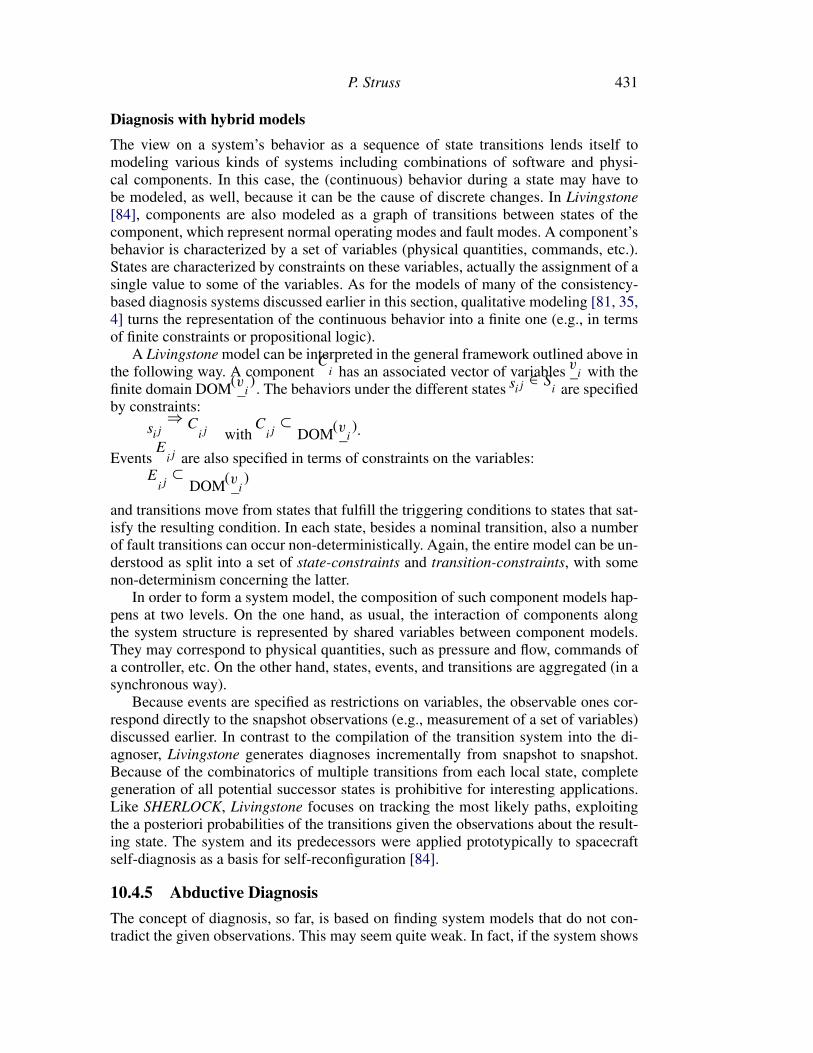
P. Struss 431
Diagnosis with hybrid models
The view on a system’s behavior as a sequence of state transitions lends itself tomodeling various kinds of systems including combinations of software and physi-cal components. In this case, the (continuous) behavior during a state may have tobe modeled, as well, because it can be the cause of discrete changes. In Livingstone[84], components are also modeled as a graph of transitions between states of thecomponent, which represent normal operating modes and fault modes. A component’sbehavior is characterized by a set of variables (physical quantities, commands, etc.).States are characterized by constraints on these variables, actually the assignment of asingle value to some of the variables. As for the models of many of the consistency-based diagnosis systems discussed earlier in this section, qualitative modeling [81, 35,4] turns the representation of the continuous behavior into a finite one (e.g., in termsof finite constraints or propositional logic).
A Livingstonemodel can be interpreted in the general framework outlined above inthe following way. A component Ci has an associated vector of variables vi with thefinite domain DOM(vi). The behaviors under the different states sij ∈ Si are specifiedby constraints:
sij ⇒ Cij with Cij ⊂ DOM(vi).
Events Eij are also specified in terms of constraints on the variables:
Eij ⊂ DOM(vi)
and transitions move from states that fulfill the triggering conditions to states that sat-isfy the resulting condition. In each state, besides a nominal transition, also a numberof fault transitions can occur non-deterministically. Again, the entire model can be un-derstood as split into a set of state-constraints and transition-constraints, with somenon-determinism concerning the latter.
In order to form a system model, the composition of such component models hap-pens at two levels. On the one hand, as usual, the interaction of components alongthe system structure is represented by shared variables between component models.They may correspond to physical quantities, such as pressure and flow, commands ofa controller, etc. On the other hand, states, events, and transitions are aggregated (in asynchronous way).
Because events are specified as restrictions on variables, the observable ones cor-respond directly to the snapshot observations (e.g., measurement of a set of variables)discussed earlier. In contrast to the compilation of the transition system into the di-agnoser, Livingstone generates diagnoses incrementally from snapshot to snapshot.Because of the combinatorics of multiple transitions from each local state, completegeneration of all potential successor states is prohibitive for interesting applications.Like SHERLOCK, Livingstone focuses on tracking the most likely paths, exploitingthe a posteriori probabilities of the transitions given the observations about the result-ing state. The system and its predecessors were applied prototypically to spacecraftself-diagnosis as a basis for self-reconfiguration [84].
10.4.5 Abductive Diagnosis
The concept of diagnosis, so far, is based on finding system models that do not con-tradict the given observations. This may seem quite weak. In fact, if the system shows
432 10. Model-based Problem Solving
Figure 10.5: A fragment of a circuit with two parallel light bulbs.
some symptoms, we may want a diagnosis that provides a causal account for them.This idea leads to a new logical definition of a diagnosis, which requires that a modellogically entails the given observations, rather than simply being consistent with them:
MODEL � OBS
[57]. However, we have to be cautious when using this definition of abductive diagno-sis. For instance, if the observations include a command “CLOSE” to the switch in thefragment of a circuit shown in Fig. 10.5, but bulb1 remains dark while bulb2 is lit, thenthe single fault in bulb1 explains the observations of the bulbs, but we do not expectit could provide a reason for switch.cmd = CLOSE. Intuitively, we want the systemresponse (the “output” variables) to be entailed, but not the exogenous features (the“input” or independent variables). The most general definition reflecting this intentionis the following.
Definition 10.14 (Abductive diagnosis). Let MODELF be a model of a fault andOBS = OBSC ∪ OBSA be a set of observations. MODELF is an abductive diagnosisiff it is consistent with OBSC and entails OBSA:
MODELF ∪ OBSC � ⊥,
MODELF ∪ OBSC � OBSA.
A complete mode assignment MA is a component-oriented abductive diagnosis for asystem description SD and a set of observations OBS iff
SD ∪ {MA} ∪ OBSC � ⊥,
SD ∪ {MA} ∪ OBSC � OBSA.
Please, note that if OBSC refers to exogenous variables, the first condition is sat-isfied by any valid model (as discussed in Section 10.3). Console and Torasso [9]discuss the consequences of different possibilities to specify OBSC and OBSA. In ourexample, we would choose
OBSC = {switch.cmd = CLOSE},
OBSA = {bulb1.light = OFF, bulb2.light = ON}.
Unfortunately, a single fault in bulb1 does not entail OBSA based on OBSC , becausethere is no information about the voltage supply and is not found as an abductivediagnosis, unless also the voltage supply is abduced.

P. Struss 433
Poole [57] raises the issue of how to represent the observations. Rather than treat-ing them as a conjunction of inputs and outputs, we could try to find an explanationfor observations stating that the input implies the output. This means in our example,we use
OBS = {switch.cmd = CLOSE⇒ (bulb1.light = OFF ∧ bulb2.light = ON)}
which would have to be entailed by an abductive diagnosis (which is again not thecase). Note that we (humans) can even obtain a diagnosis solely based on observationof the outputs:
OBS = {bulb1.light = OFF, bulb2.light = ON}
and that consistency-based diagnosis with fault models produces the proper result.Abductive diagnosis is attractive, because it provides a stronger notion of diagnosis
which seems to reflect the aspect of causality in our human conception of diagnosis.However, apart from the fact that logical entailment is generally unrelated to causal-ity, this stronger notion of diagnosis imposes stronger requirements on the modeland the possible inferences, as illustrated by the above example. When compared toconsistency-based diagnosis, the results are more sensitive to the particular represen-tation and strength of the model and the observations. If an observation states that,say, a flow at some point is positive, while a model can only predict a disjunctionflow = zero∨flow = positive (e.g., based on the model of a check valve), it would notbe an abductive diagnosis. If the domain of flow (both in the model and the observa-tion) would contain only the values negative and non-negative, then this would yieldan abductive diagnosis. However, this coarser domain may then be too weak to derivesome other predictions.
Of course, consistency-based diagnosis depends on the strength of the model, aswell, and, in particular, on the granularity of the domains. This is because this canrender the model unable to detect some of the existing conflicts. However, it is stillguaranteed that the correct diagnosis (as a mode assignment) is never excluded. Sucha guarantee cannot be obtained for abductive diagnosis.
Depending on the available observations, an abductive diagnosis may include notonly the modes, but also the current state of the system and even numerical parameters(as suggested by [57]) which makes the abduction task even harder for systems of aninteresting kind and size.
Abductive diagnosis seems to become feasible and provide some basis for meet-ing our intuition behind an explanation, if the model has causal notion embedded (asopposed to purely constraint- or equation-based behavior descriptions). In fact, manyof the examples used for explaining abductive techniques come as causal networksthat explicitly link faults to effects. As already discussed in Section 10.3, this kindof system-specific diagnosis task compiled into a system model is a non-solution todiagnostic applications (although in engineering practice, something similar is donein constructing fault trees for safety analysis), because it violates genericity, com-positionality, and reusability of the model. What is required is a modeling ontologythat captures causality and is compositional. As stated earlier, process-oriented mod-eling [34, 35, 41] is a candidate. This also paves a way to overcome some of therestrictive assumptions and limitations of component-oriented diagnosis discussed inSection 10.4.1.
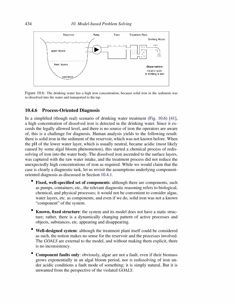
434 10. Model-based Problem Solving
Figure 10.6: The drinking water has a high iron concentration, because solid iron in the sediment wasre-dissolved into the water and transported to the tap.
10.4.6 Process-Oriented Diagnosis
In a simplified (though real) scenario of drinking water treatment (Fig. 10.6) [41],a high concentration of dissolved iron is detected in the drinking water. Since it ex-ceeds the legally allowed level, and there is no source of iron the operators are awareof, this is a challenge for diagnosis. Human analysis yields to the following result:there is solid iron in the sediment of the reservoir, which was not known before. Whenthe pH of the lower water layer, which is usually neutral, became acidic (most likelycaused by some algal bloom phenomenon), this started a chemical process of redis-solving of iron into the water body. The dissolved iron ascended to the surface layers,was captured with the raw water intake, and the treatment process did not reduce theunexpectedly high concentrations of iron as required. While we would claim that thecase is clearly a diagnostic task, let us revisit the assumptions underlying component-oriented diagnosis as discussed in Section 10.4.1.
• Fixed, well-specified set of components: although there are components, suchas pumps, containers, etc., the relevant diagnostic reasoning refers to biological,chemical, and physical processes; it would not be convenient to consider algae,water layers, etc. as components, and even if we do, solid iron was not a known“component” of the system.
• Known, fixed structure: the system and its model does not have a static struc-ture; rather, there is a dynamically changing pattern of active processes andobjects, substances, etc. appearing and disappearing.
• Well-designed system: although the treatment plant itself could be consideredas such, the notion makes no sense for the reservoir and the processes involved.The GOALS are external to the model, and without making them explicit, thereis no inconsistency.
• Component faults only: obviously, algae are not a fault, even if their biomassgrows exponentially in an algal bloom period, nor is redissolving of iron un-der acidic conditions a fault mode of something; it is simply natural. But it isunwanted from the perspective of the violated GOALS.
P. Struss 435
• No structural faults: the nature of the disturbance is a structural change in thesystem, triggering unforeseen processes.
• “Crisp” faults: even more than with respect to artifacts, healthiness of ecologi-cal and biological systems, but also process plants is often expressed in terms ofa spectrum of degradation, rather than a qualitative behavior change. Of course,in our example, the legal restrictions make it crisp.
Obviously, addressing such a diagnosis task in theory and implementation requires adifferent formalization of modeling and the diagnosis task. However, what we stickwith is the idea that the answer to the diagnosis task is given by a model that is “com-pliant” with the observations of system behavior.
The example suggests the use of process-oriented modeling. Collins [7] developsthe Process Diagnosis Engine (PDE) as abductive diagnosis on such a model. Hellerand Struss [41] present a theory of process-oriented consistency-based diagnosis, re-alized as the Generalized Diagnosis Engine (G+DE).
In a nutshell (see [34, 35, 41] for details), a process is considered as some elemen-tary phenomenon, which can be modeled independently of others and is, therefore,suited to compositional modeling. This has two consequences: one is that a processmodel has to state explicitly all preconditions for the process to occur by listing the(typed) objects that interact in a particular configuration (structural-conditions) andconstraints on involved quantities (quantity-conditions). A process can create newobjects and relations between them (structural-effects) and affects quantities of theparticipating objects (quantity-effects). The second consequence of the required com-positionality is that quantity-effects cannot all be simply stated as constraints on thequantities. This is because each (type of) process can only state a partial contributionto some overall effect. For instance, the model of the iron-redissolving process canonly state that it adds to the concentration of dissolved iron in the water layer, but itcannot claim that this concentration effectively increases, because in a particular sce-nario, there may be other, counteracting, processes active that override the effect (e.g.,oxidation of iron). In response to this, process-oriented modeling involves the conceptof influences that goes beyond mathematical modeling based on (differential) equa-tions, constraints, or first order logic. If some variable x influences a variable y, say,positively, written I+(x, y), this means basically that the derivative of y is a monotonicfunction of x:
I+(x, y) ⇔ ∃fdy
dt= f (. . . , x, . . .) ∧
df
dx> 0.
The actual value of dydtcan only be determined after all existing influences can be (e.g.,
linearly) combined. But this requires a closed-world assumption, which provides animportant hook for model revision during the search for a consistent model.
Thus, a process implies the effects, if the conditions are true:
structural-conditions ∧ quantity-conditions⇒ structural-effects ∧ quantity-effects
How can we state the diagnosis problem, which we call situation assessment, becausethere is not necessarily “something wrong”? We start with a partial description of a
436 10. Model-based Problem Solving
scenario in terms of objects, object relations, and variable values. This may includereal observations, OBS (e.g., measurements, such as “iron concentration above thresh-old”) and assumptions, ASSM (e.g., assertions that usually hold, such as “pH neutral”).The target is to construct process models that, based on propositions about structure(objects and object relations) and quantities, are consistent with OBS and, if possi-ble, with ASSM. Again, we apply Occam’s razor and prefer models that satisfy someminimality criteria. There are two orthogonal dimensions:
• do not drop more assumptions than required to obtain a consistent model,
• do not introduce more unanticipated objects than necessary in order to derive anexplanation (why assume both solid iron in the sediment and iron in an affluentto the reservoir?): the structural basis should not be larger than necessary.
We should be more precise about the latter criterion: what we would like to minimizeis the set of objects in the model that are not generated by some process, but are intro-duced without further justification by the model. In our example, the dissolved iron isan effect of the redissolving process, whereas the solid iron in the sediment does nothave an explanation in the model. Hence, the issue relates to the question of the modelboundaries: where should we stop to ask for reasons, because they are beyond whatis captured by the model library? In our case, iron in the tank requires a causal ex-planation, whereas the existence of solid iron or algae does not. We characterize thosetypes of object that sit “on the boundary” of the model as introducible. Obviously, theycomprise those that never occur as a structural effect of a process in the library. But wemay want to regards additional ones as introducible for certain problems or scenarios.
Based on this, we can give an informal definition of a process-oriented diagnosis(a formal account using default logic is described in [40]).
Definition 10.15 (Situation assessment). Let LIB be a process library, OBJ-INTROthe set of introducible objects, OBJ-OBS and OBJ-ASSM the objects mentioned inOBS and ASSM, respectively. A situation assessment for (LIB,OBS,ASSM) is a triple(STRUCTURE,QUANT,ASSM-RETR); where STRUCTURE is a set of objects, andrelations, QUANT is a set of value assignments to quantities, and ASSM-RETR ⊂
ASSM a set of assumptions such that the resulting model is consistent with the obser-vations and a subset of the assumptions:
(i) STRUCTURE ∪ QUANT ∪ LIB ∪ OBS ∪ (ASSM \ ASSM-RETR) � ⊥
The structure contains the observed objects and a subset of the assumed ones:
(ii) OBJ-OBS ⊂ STRUCTURE, OBJ-ASSM \ ASSM-RETR ⊂ STRUCTURE,
(iii) the model contains exactly the objects that are entailed by the introducibleobjects, i.e. the introducibles themselves and the ones created by processes,
(iv) (STRUCTURE ∩ OBJ-INTRO) ∪ ASSM-RETR is a (with respect to set inclu-sion) minimal set that satisfies (i) through (iii).
Different applications may require modifications to this definition which mini-mizes the set of newly introduced objects and retracted assumptions, while introduced
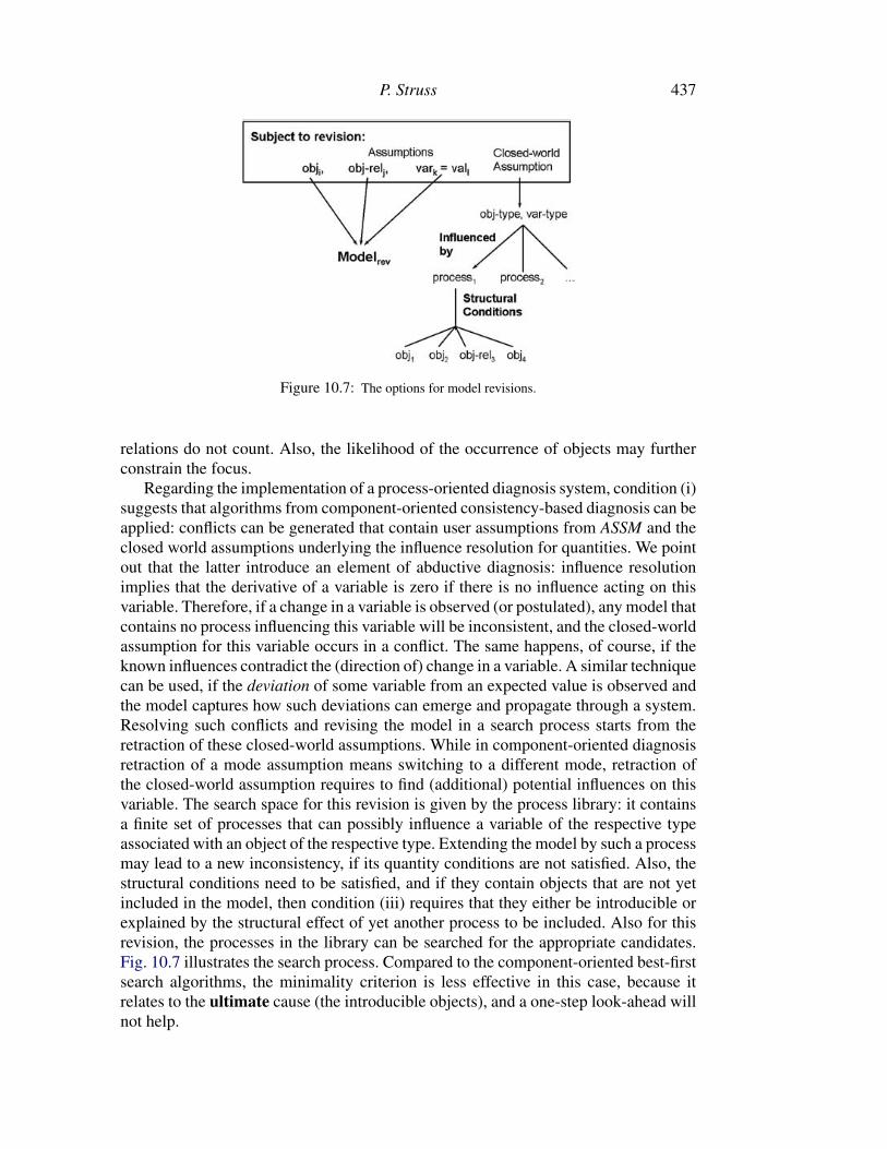
P. Struss 437
Figure 10.7: The options for model revisions.
relations do not count. Also, the likelihood of the occurrence of objects may furtherconstrain the focus.
Regarding the implementation of a process-oriented diagnosis system, condition (i)suggests that algorithms from component-oriented consistency-based diagnosis can beapplied: conflicts can be generated that contain user assumptions from ASSM and theclosed world assumptions underlying the influence resolution for quantities. We pointout that the latter introduce an element of abductive diagnosis: influence resolutionimplies that the derivative of a variable is zero if there is no influence acting on thisvariable. Therefore, if a change in a variable is observed (or postulated), any model thatcontains no process influencing this variable will be inconsistent, and the closed-worldassumption for this variable occurs in a conflict. The same happens, of course, if theknown influences contradict the (direction of) change in a variable. A similar techniquecan be used, if the deviation of some variable from an expected value is observed andthe model captures how such deviations can emerge and propagate through a system.Resolving such conflicts and revising the model in a search process starts from theretraction of these closed-world assumptions. While in component-oriented diagnosisretraction of a mode assumption means switching to a different mode, retraction ofthe closed-world assumption requires to find (additional) potential influences on thisvariable. The search space for this revision is given by the process library: it containsa finite set of processes that can possibly influence a variable of the respective typeassociated with an object of the respective type. Extending the model by such a processmay lead to a new inconsistency, if its quantity conditions are not satisfied. Also, thestructural conditions need to be satisfied, and if they contain objects that are not yetincluded in the model, then condition (iii) requires that they either be introducible orexplained by the structural effect of yet another process to be included. Also for thisrevision, the processes in the library can be searched for the appropriate candidates.Fig. 10.7 illustrates the search process. Compared to the component-oriented best-firstsearch algorithms, the minimality criterion is less effective in this case, because itrelates to the ultimate cause (the introducible objects), and a one-step look-ahead willnot help.
438 10. Model-based Problem Solving
The existing approaches along these lines (PDE [7], G+DE [41]) are performingdiagnosis in one snapshot. This is a serious limitation for many relevant diagnosisproblems, since the origin of some disturbance may already have ceased to exist, whilethe effects persist. For instance, if we expect to detect a cause for the deviation in thepH (e.g., algal bloom), the actual observation may state that there is none and rendersuch an explanation inconsistent.
Including the temporal dimension adds to the complexity issues of this approachand, together with the demand for good search heuristics makes it a real challengeto model-based diagnosis research. Any progress would contribute to a significantextension of the application scope of model-based diagnosis.
10.4.7 Model-based Diagnosis in Control Engineering
There exists another research area also called “model-based fault diagnosis and isola-tion”. It has emerged in control engineering, and, while sharing some basic common-alities with model-based diagnosis in Artificial Intelligence, involves quite differenttechniques. The common idea is to start diagnosis from the deviation of an observedbehavior from a model of correct behavior and to view a diagnostic hypothesis as amodel revision that removes this deviation. However, the techniques are purely math-ematical, and the models used are usually numerical, non-compositional black-boxmodels with a fixed (mathematical) structure, lacking an explicit conceptual layer ofmodeling and, hence, any symbolic reasoning and inferences. Partly, this reflects theapplication domain of process control and the kind of models used for this purpose. Asa consequence, the kinds of faults that can be handled are limited to those that can beexpressed as a variation of the mathematical OK-model (e.g., parameter deviations).Faults that modify the causal structure of the system and/or its mathematical structureconstitute a problem, as opposed to the model-based methods described in this chap-ter. There are several attempts to compare, relate, and combine the different types ofmodel-based diagnosis [18, 42, 1, 53].
10.5 Test and Measurement Proposal, Diagnosability Analysis
Usually, a diagnosis based on some initial set of observations does not yield a uniquediagnosis result, even under certain preference criteria, such as minimality or likeli-hood. If the model has been fully applied and cannot provide more diagnostic infor-mation, the only source for further discrimination between the remaining diagnostichypotheses is additional observations of the system behavior. This means observingadditional variables and/or performing observations of the system in a different stateor with different input. Therefore, the test generation task can be stated as determiningwhich influences on the system and which observables promise information that re-futes some of the current (diagnostic) hypotheses. A variant of this task is end-of-linetesting, i.e. performing tests of a manufactured product that are suited to confirm thatthe product is not faulted. This may seem to be a different task, but it can only beachieved by tests that are designed to refute all possible faults (since this is not feasi-ble in reality a set of plausible faults has to be selected, e.g., single faults, or the mostprobable ones). There is no way to confirm the presence of a particular behavior otherthan refuting all competing behavior hypotheses.
P. Struss 439
10.5.1 Test Generation
The core problem is to determine tests for discriminating between two possible behav-iors of a system, i.e. two models. A test has to specify
• how to stimulate the system and
• what to observe of the system’s response to this stimulus
in order to gain discriminating information. This requires fixing the possibilities ofinfluencing the system, called test inputs or stimuli in the following, and the potentialobservations, OBS.
In the most general way, testing aims at finding out which model hypothesis out of aset Hyp is correct (if any) by stimulating a system such that the available observationsof the system responses to the stimuli refute all but one hypotheses (or even all ofthem). This is captured by the following definition.
Definition 10.16 (Discriminating test input). Let
TI = {ti} be the set of possible test inputs (stimuli),
OBS = {obs} the set of possible observations (system responses), and
Hyp = {modeli} a set of hypotheses.
ti ∈ TI is called a definitely discriminating test input for Hyp if
(i) ∀modeli ∈ Hyp ∃obs ∈ OBS, ti ∧ modeli ∧ obs � ⊥
and
(ii) ∀modeli ∈ Hyp ∀obs ∈ OBSif ti ∧ modeli ∧ obs � ⊥
then ∀modelj �= modeli , ti ∧ modelj ∧ obs � ⊥.
ti is a possibly discriminating test input if
(ii�) ∀modeli ∈ Hyp ∃obs ∈ OBS such thatti ∧ modeli ∧ obs � ⊥
and ∀modelj �= modeli , ti ∧ modelj ∧ obs � ⊥.
ti is a not discriminating otherwise.
In this definition, condition (i) expresses that there exists an observable systemresponse for each hypothesis under the test input. It also implies that test inputs areconsistent with all hypotheses, i.e., we are able to apply the stimulus, because it iscausally independent of the hypotheses. Regarding the model, this corresponds to therequirement that it captures the behavior under each tuple in the Cartesian productof the domains of exogenous variables, as discussed in Section 10.3. Condition (ii)formulates the requirement that the resulting observation guarantees that at most onehypothesis will not be refuted, while (ii�) states that each hypothesis may generate anobservation that refutes all others.
Usually, one stimulus is not enough to perform the discrimination task which mo-tivates the following definition.
440 10. Model-based Problem Solving
Definition 10.17 (Discriminating test input set). {tik} = TI� ⊂ TI is called a discrim-inating test input set for Hyp = {modeli}
if ∀modeli ,modelj with modeli �= modelj∃tik ∈ TI�
such that tik is a (definitely or possibly) discriminating test inputfor {modeli ,modelj }.It is called definitely discriminating if all t ik have this property, and possibly dis-
criminating otherwise. It is called minimal if it has no proper subset TI�� ⊂ TI� whichis discriminating.
This defines what we would like to obtain. Actually computing solutions faces adifferent dimension of complexity compared to diagnosis. In diagnosis, one obser-vation of the system behavior in one situation (or a sequence of such situations) isgiven and needs to be checked for consistency with various models. For test genera-tion, the space of all situations and observations has to be searched in order to findsome that are inconsistent with at least one of the models. Intuitively, one would liketo identify the differences in the space of all possible behaviors under two or moremodels. In contrast to consistency-based diagnostic reasoning which happens at theconceptual level (e.g., component behavior modes in component-oriented diagnosis),test generation has to analyze the behavior model itself, unless we apply an algorithmthat generates test inputs and then tests them for consistency with the models.
Test generation with relational models
In the following, we outline a fairly general approach that assumes that models arerepresented as relations over a set of variables, but whose underlying ideas might beadapted to other modeling formalisms. The approach covers models that are givenby equations and implemented by constraints. It is assumed that test inputs and ob-servations can be described as value assignments to system variables. If the systemis modeled as an aggregate of components, the hypotheses to be tested are given by(usually single) faults of components. If vCi is the vector of variables local to a com-ponent Ci with a domain DOM(vCi), each possible behavior mode modeij of Ci hasan associated relation
Rij ⊆ DOM(vCi)
as a behavior model. A fault hypothesis in testing is then given by the join of therelations that correspond to a particular assignment of modes,MA, to the components:
R(MA) = ��modeij∈MA
Rij .
Once this relation is constructed, the component structure is no longer relevant. Hence,we can choose a more general relational representation which covers testing of arbi-trary hypotheses that can be stated in terms of a set of interrelated variables. Thisincludes tests that aim at identifying a state variable which is not directly observable,testing applied to systems that are modeled in a process-oriented formalism, and thedesign of experiments for checking different modeling hypotheses. Thus, the systembehavior is assumed to be characterized by a vector
vS = (v1, v2, v3, . . . , vn)
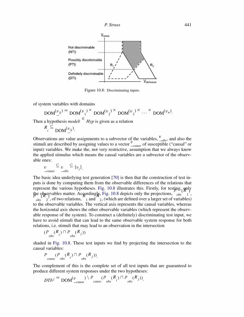
P. Struss 441
Figure 10.8: Discriminating inputs.
of system variables with domains
DOM(vS) = DOM(v1)× DOM(v2)× DOM(v3)× · · · × DOM(vn).
Then a hypothesis modeli ∈ Hyp is given as a relation
Ri ⊆ DOM(vS).
Observations are value assignments to a subvector of the variables, vobs, and also thestimuli are described by assigning values to a vector vcause of susceptible (“causal” orinput) variables. We make the, not very restrictive, assumption that we always knowthe applied stimulus which means the causal variables are a subvector of the observ-able ones:
vcause ⊆ vobs ⊆ {vi}.
The basic idea underlying test generation [70] is then that the construction of test in-puts is done by computing them from the observable differences of the relations thatrepresent the various hypotheses. Fig. 10.8 illustrates this. Firstly, for testing, onlythe observables matter. Accordingly, Fig. 10.8 depicts only the projections, pobs(R1),pobs(R2), of two relations,R1 andR2, (which are defined over a larger set of variables)to the observable variables. The vertical axis represents the causal variables, whereasthe horizontal axis shows the other observable variables (which represent the observ-able response of the system). To construct a (definitely) discriminating test input, wehave to avoid stimuli that can lead to the same observable system response for bothrelations, i.e. stimuli that may lead to an observation in the intersection
(pobs(Ri) ∩ pobs(Rj ))
shaded in Fig. 10.8. These test inputs we find by projecting the intersection to thecausal variables:
pcause(pobs(Ri) ∩ pobs(Rj )).
The complement of this is the complete set of all test inputs that are guaranteed toproduce different system responses under the two hypotheses:
DTIij = DOM(vcause) \ pcause(pobs(Ri) ∩ pobs(Rj )).

442 10. Model-based Problem Solving
Lemma 10.2. If modeli = Ri , modelj = Rj , TI = DOM(vcause), and OBS =
DOM(vobs), then DTIij is the set of all definitely discriminating test inputs for{modeli ,modelj }.
Please, note that we assume that the projections of Ri and Rj cover the entiredomain of the causal variables which corresponds to condition (i) in the definition ofthe test input.
We only mention the fact, that, when applying tests in practice, one may have toavoid certain stimuli because they carry the risk of damaging or destroying the systemor to create catastrophic effects as long as certain faults have not been ruled out. Inthis case, the admissible test inputs are given by some set Radm ⊆ DOM(vcause), andwe obtain
DTIadm,ij = Radm \ pcause(pobs(Ri) ∩ pobs(Rj )).
In a similar way as DTIij , we can compute the set of test inputs that are guaranteed tocreate indistinguishable observable responses under both hypotheses, i.e. they cannotproduce observations in the difference of the relations:
(pobs(Ri) \ pobs(Rj )) ∪ (pobs(Ri) \ pobs(Ri)).
Then the non-discriminating test inputs are
NTIij = DOM(vcause) \ pcause((pobs(Rj ) \ pobs(Ri))
∪ (pobs(Ri) \ pobs(Rj )))
All other test inputs may or may not lead to discrimination.
Lemma 10.3. The set of all possibly discriminating test inputs for a pair of hypotheses{modeli ,modelj } is given by
PTIij = DOM(vcause) \ (NTIij ∪ DTIij ).
The 12 ∗ (n2−n) sets DTIij for all pairs {modeli ,modelj }, i < j , provide the space
for constructing (minimal) discriminating test input sets.
Lemma 10.4. The (minimal) hitting sets of the set {DTIij } are the (minimal) definitelydiscriminating test input sets.
Note that Lemma 10.4 has only the purpose to characterize all discriminating testinput sets. Since we need only one test input to perform the test, which can be com-puted in linear time, we are not bothered by the complexity of computing all hittingsets.
This way, the number of tests constructed can be less than 12 ∗ (n
2− n). If the testshave a fixed cost associated, then the cheapest test set can be found among the minimalsets. However, it is worth noting that the test input sets are the minimal ones thatguarantee the discrimination among the hypotheses in Hyp. In practice, only a subsetof the tests may have to be executed, because some of them refute more hypotheses
P. Struss 443
than guaranteed (because they are a possibly discriminating test for some other pair ofhypotheses) and render other tests unnecessary.
Note that the required operations on the relations are applied to the observablevariables only (including the causal variables). The projection of the entire relationRi to this space is a step of compiling the composite model to one that directly relatesthe stimuli and the observable response. In some relevant applications, this space ispredefined and small. For instance, when testing of car subsystems exploits the on-board actuators and sensors only, this may involve some 10–20 variables or so. Theentire workshop diagnosis task has more potential probing points, but still involvesonly a small subset of the variables in the entire behavior relation Ri . Also note thatthis compiled model can be re-used for diagnosis purposes. Such a compact modelmay actually make the computation of the set {DTIij } feasible if, for instance, finiterelations representing qualitative models are used. [26] perform the computation on anordered multiple decision diagrams OMDD representation. However, the compilationstep can become expensive and practically infeasible. In cases where the completecomputation of {DTIij } is not possible, test generation can be done by search, andLemmata 10.2 and 10.4 describe the search space.
[49] assumes a model stated in first order logic, which leads to a characterization oftests as prime implicants. In [80], sets of behaviors generated by qualitative simulationof competing models are used to search for discriminating experiments.
Although the set of discriminating test inputs given by Lemma 10.4 is minimal,the individual test inputs are not necessarily minimal in the sense that they are alwaysspecified by the entire given set of observables, despite the fact that only a subset ofthe stimuli and/or a subset of the other observables may suffice to produce the samediscrimination effect. This is important for applications, since both the production ofa stimulus and the performance of an observation are actions that determine the costof testing, and justifies spending computation time on the reduction of test inputs.In [73], this is done by analysis and operations of the entire relations DTIij . Testsas prime implicants in the work of [49] already include this minimization step, butfinding them is also exponential. But, again, under economic considerations, spendingeven days of computation time pays off, if it saves only seconds for an individualtest that is carried out many times or if it allows workshop mechanics to avoid someexpensive experiments in diagnosis.
If hypotheses are given as models of mode assignments, the set of definitely dis-criminating test inputs as defined above may be empty for two models, althoughdiscrimination may be possible through several tests. This may occur when there areinternal states that cannot be observed or unambiguously inferred. As stated above,the approach can be used for state identification, as well, and the solution to the prob-lem is to make hypotheses about the (relevant) states explicit as a set Hypstate andinclude their determination in the testing. Since the new set of hypotheses becomesthe Cartesian product
Hyp� = Hyp × Hypstate
this step increases the complexity of the task like the consideration of multiple faultsdoes. Obviously, the solution is based on an assumption of persistence of states duringtesting.
444 10. Model-based Problem Solving
Intrusive testing and probing
The solutions outlined above ignore or, a least, do not explicitly treat, an importantfeature of the real task in a practical context: unless we are using only pre-establishedsensors that are reflected in the system model, performing a test involves often muchmore than manipulating the input and/or state of the systems and some passive obser-vation of its response. It may, temporarily or permanently, modify the structure of thesystem and, hence, the model. Even simply opening an electrical circuit and attachinga measurement device creates a new circuit. Other tests (e.g., in the medical domain)may even modify the system structure in an irreversible way. Hence, we do not onlyhave to consider preparatory actions like removing a cover or lifting a vehicle, butmodifications that affect the behavior of the system and, hence, have to be reflected bya change in the structure of its model. We will return to this issue in a broader contextin Section 10.6.
10.5.2 Entropy-based Test Selection
Achieving optimality with respect to the cost during repeated use of a set of tests alsorequires to take into account the likelihood of different model hypotheses. This canbe reflected in the sequence of tests or by dynamically choosing a new test based onthe result of the previous one. If we assume that each hypothesis modeli ∈ Hyp has aprobability p(modeli ), then
H = −�
modeli∈HYP
�p(modeli ) · log
�p(modeli )
��
is the entropy, a measure for the uncertainty in the information at this stage. In ourcontext, it can be understood as an estimation of the number of tests to be performedin order to identify the true model. In the component-oriented case, the initial proba-bilities could be computed as the product of the a priori probabilities of the respectivemodes (under the condition that they are independent). When choosing the next testinput, ti ∈ TI, we would like to maximize the expected information gain
H −He(ti),
where the entropy after applying ti has to be estimated over all observations that canpossibly result from ti under the different hypotheses:
He(ti) = −�
obs∈OBS(ti)
�
p(obs) ·�
modeli∈HYP
�p(modeli | obs, ti)
· log�p(modeli | obs, ti)
���
.
If a hypothesis modeli is specified by a relation Ri , then
OBS(ti) =�
i
pobs(ti �� Ri).
Finally, we include the possibility that the observation after a applying a test inputunder a hypothesis is not unique, but, instead, there is a probability distribution:
p(obs | modeli , ti).
P. Struss 445
After applying Bayes’ rule and some transformations [70], we derive the following
Probabilistic test selection strategy
In order to discriminate among hypotheses modeli ∈ Hyp, choose a test input ti and avector of observable variables vobs, such that
−�
obs∈OBS(ti)
�p(obs | ti) · log
�p(obs | ti)
��
+�
modeli∈HYP
�
p(modeli ) ·�
obs∈OBS(ti)
�p(obs | modeli , ti)
· log�p(obs | modeli , ti)
���
is maximal, where obs ∈ DOM(vobs) and the probabilities of observations are deter-mined from hypothesis-specific distributions:
p(obs | ti) =�
modeli∈HYP
�p(obs | modeli , ti) · p(modeli )
�.
There is an intuitive interpretation of the criterion used in the strategy: the first termis the entropy of the observations given the test input, which is maximal if they areequally distributed. The second term will be minimal if each model predicts uniquevalues. Together, this meets our intuition that says a test is most informative if it leadsto distinct values for the various hypotheses.
10.5.3 Probe Selection
The above strategy allows varying both, the input t i and the observable variables vobs.On the one hand, this includes the situation where the set of observables is fixed (e.g.,by the existing on-board sensors of a space craft). On the other hand, applying stimulito the system in order to gain diagnostically relevant information may not always bepossible (e.g., in plants under continuous operation or in natural systems), but infor-mation may be obtained by measuring additional variables in the given situation. Thistask which appears as probe selection, measurement proposal, and sensor placementcan be handled as a specialization of the above strategy, where the stimulus is fixedand an informative set of observable variables has to be determined.
It can be seen as a generalization of the probe selection strategy inGDE [20], whichdetermines the best individual variable vobs to be measured, based on the assumptionthat each hypothesis either implies a unique prediction of a value obsi ∈ DOM(vobs)
(defining the subsets HYPi) or no prediction at all (the subset HYPu), which is rea-sonable for the implementation based on value propagation and dependency record-ing. Furthermore, Kleer and Williams [20] use an equal distribution of values forthe hypotheses in HYPu, and, hence, estimates the probability of a measurementobsi ∈ DOM(vobs) for vobs as
p(obsi ) = p(HYPi )+1
m· p(HYPu) where m =
��DOM(vobs)
��.
446 10. Model-based Problem Solving
This transforms the criterion in the strategy to the expression
�
obsi∈DOM(vobs)
�p(obsi ) log
�p(obsi )
��+ p(Hu) · logm
which should be minimized to obtain the best next measurement. One should notethat even if no fault models are used, fault hypotheses do predict values based on themodels of the non-faulty components. If, as in GDE, an ATMS is used for recordingthe dependency of predicted values on mode assignments this delivers the basis fordetermining the sets HYPi and only the entropy computation has to be realized.
While probing helps, if the initial observations are not sufficiently discriminating,the probe selection strategy can also be beneficial in the opposite case, namely whenthere is an overwhelming amount of observations. [2] exploits it as a filter to extractrelevant information from a message burst caused by a disturbance in a power distrib-ution network.
10.5.4 Diagnosability Analysis
The question whether and how faults can be detected or discriminated from each otheris relevant already during the design phase. If design for diagnosability and, in par-ticular, placement of sensors for diagnostic purposes is a concern, variants of thetechniques described above can be applied. Also failure-modes-and-effects analysis(FMEA) includes an analysis of the detectability of a fault. In this kind of analysis,the consideration is usually not on actively influencing the system. Rather, we ex-pect discriminability analysis to answer the question “For a particular design anda chosen set of sensors, determine whether and under which circumstances the con-sidered (classes of) faults considered can be distinguished from each other (based onthe sensor readings)”. Fault detectability can be seen as a special case, namely thediscrimination of faulty behaviors from the OK behavior.
Discriminability may depend on certain external conditions and internal states ofthe system. For instance, a certain fault of a particular sensor may only show up in aspecial temperature range, and a problem in the gear box may only affect driving in2nd gear. If we replace the test inputs in the above definitions and algorithms by the setof such possible conditions, the techniques for test generation can be re-used. In [26],this is done using the relational behavior presentation. Detectability analysis has alsobeen treated for discrete-event models, by analyzing whether a fault transition resultsin a visible trace different from OK behavior (within a certain number of transitions)(see [65, 77]).
10.6 Remedy Proposal
So far, all the tasks considered were focused on obtaining and using information inorder to assess the behavior mode or state of systems, especially of systems whosebehavior deviates from the normal and intended one. However, this is never a goal initself, but only interesting as an input to some decision and action that requires thisinformation. Diagnosis is only relevant if it supports a decision (whether and) how tore-establish the functionality of the misbehaving system, at least to a possible degree.
P. Struss 447
Actually, this purpose, which varies according to the type of system and the practi-cal context of the task, ought to influence the nature of the expected diagnostic resultand also the diagnostic process itself. For instance, on-board diagnostics for a vehiclesubsystem should aim at the discrimination between classes of faults that, due to theirnature and criticality, require different immediate recovery and safety actions, whereasoff-board diagnosis of the same subsystem is focusing on discrimination between dif-ferent suspect components in order to find the ones that need to be replaced. Usually,there is no need for continued discrimination if this does not influence the choice ofthe remedial action. Although this issue is both obvious and fundamental to diagnosis,it has been mainly ignored in theoretical work, and there are (too) few contributionsto treating this means-end relationship in a general and systematic way [58].
In fact, in the context of real diagnosis work processes, the interdependency oftenbecomes even tighter, bidirectional and more complex, because the respective activ-ities become intermingled: (partial) repair actions may be carried out to support theoverall diagnosis process. As pointed out earlier, the focus on fault localization in earlywork on diagnosis can be explained by an (implicit) focus on replacement of com-ponents as the remedial action. However, component replacement is but one specialinstance of actions for moving a system back to a healthy state and, in fact, impossiblein some applications (e.g., space craft outside an orbit).
The diagnostic and testing theories and systems presented above are attempts toautomate reasoning tasks, namely to infer diagnoses from observations and to pro-pose informative observations based on the previous results. However, in particularin an industrial environment, in general, it is not these reasoning activities that areexpensive, but efforts spent on acting, such as de-assembling a device, installing mea-surement equipment, and repairing the device. Compared to this, the time and costspent on thinking is often negligible, and the result of this thinking matters only if itcontributes to optimizing the overall workflow. The chance for diagnostic solutions tobe really employed in practice is heavily reduced if they are not designed and devel-oped under this perspective. It should be noted, though, that the above considerationsapply only in a restricted way to on-board diagnostics, because they do not triggerdirectly expensive human activities.
These considerations motivate work aiming at model-based generation of propos-als for remedies, at an integrated perspective on diagnosis, testing, and applying reme-dies, and at the integration of planning with model-based problem solving. Remediescan involve a whole range of different actions that need to be reflected in model-basedsystems in different:
• replacement of components that are suspect of failing usually leaves the struc-ture of the device (and, hence, of the model) unchanged and simply changesthe behavior mode (if successful); however, sometimes, a component may bereplaced by one with different parameters or of a different type,
• reconfiguration exploits the structural redundancy of a device, which mightachieve the specified purpose in different ways and even under fault conditions.Aircraft and space craft are equipped with redundant subsystems for criticalfunctions, and power networks are huge networks of switches that enable thegeneration of different topologies with different paths between voltage sourcesand sinks; since the components that modify the topology (switches, valves, etc.)
448 10. Model-based Problem Solving
are also components, the structure of the system (and of the model) remainsunchanged, only the states of these components are affected,
• modification of operating regions is based on a system property that allowsachieving certain goals with different settings of parameters and inputs; if oneout of three heating elements in a room is not working, you may compensatefor this by increasing the set point of the other two elements [79]; again, thestructure of the device and the model remains the same,
• modification of control affects a special component, software; this step maycorrespond to implementing the previous two remedies, but it may also meanswitching to a different control regime (e.g., from closed-loop to open-loop con-trol in the case a sensor is suspect, or a control unit on a vehicle may replacean implausible value of one wheel speed sensor by some approximation gainedfrom the other three sensors),
• structural modifications cover a wide range, from inserting new components(e.g., an electrical heating element) and establishing new connections (e.g., tobridge a series of electrical connectors, one of which is open, by a cable) tointroducing ozone in a water treatment plant in order to trigger a process ofoxidation of dissolved metals in the water; all this clearly results in a model thatmight be quite different from the designed or previous one. As stated above, alsomeasurement actions may affect the structure of the system.
Some of these actions require continuing the analysis after their performance with anew model. But even those that do not, raise the question how they affect the stateof the system, i.e., about the persistence of what has been observed or inferred be-fore. What remains true after replacing a capacitor in a circuit? Some of the measuredvalues may, others may not, and redoing all measurements may be a waste of efforts.(Immediately) after adding ozone to the water, the iron concentration is still the same,but its derivative is modified due to the oxidation process. This can be seen as aninstance of problems connected to reasoning about actions (see, e.g., [45]), but thespecific context (and the existence of a model) can offer special solutions.
10.6.1 Integration of Diagnosis and Remedy Actions
The discussion above shows that, rather than considering diagnosis in isolation (as inSection 10.4), we need to model a process that
• integrates actions of testing and therapy and the inference of diagnostic hypothe-ses based on the results of such actions,
• may change the system model dynamically,
• is guided by the goal of re-establishing the original or some weakened function-ality of the system.
Thus, we have a task similar to diagnosis across time in the sense that a history ofpossible diagnoses has to be maintained and updated over time. The difference is thattransitions may be due to actions, that they may affect the system structure, and that
P. Struss 449
the intended function of the system has to be modeled and reasoned about. Producinga complete representation of all possible transitions, e.g., in terms of a finite statemachine, appears feasible only if there are no significant structural changes includedin the remedy actions, for instance, if only state changes, reset, or replacement actionsare available.
[30] proposed a general formalization of such an integrated process for component-oriented diagnosis and repair, which also takes into account that actions may fail.Slightly modifying and simplifying their proposal (assuming actions are instantaneousand cannot fail), we obtain an extension of our Definition 10.8 (Temporal diagnosis).We introduce an action history
AH =�(ACT l , tl)
�, tl ∈ Iω
and a goal history
GOALH =�(GOALm, Im)
�, Im ∈ Iω,
which allows us to express both ultimate and intermediate goals. For instance, duringthe reconfiguration of a power transportation network, one has to avoid overload ofcertain lines, and may also have to make sure that certain critical consumers are nevertemporarily cut off from power supply. For replacement and reconfiguration, actionsmodify the modes and states of components, and in the latter case, change the systemtopology within the limits determined by the redundancy in the original structure.While this leaves
SD = LIB ∪ STRUCTURE
unmodified and stable as in component-oriented diagnosis, the structure may also besubject to modification by remedial (and also measurement) actions. In this case, anextended system description SD has to comprise constraints on admissible structures.
The task is then to find a sequence of actions that is consistent with or achievesGOAL or a set thereof.
Definition 10.18 (Remedy). An action history AH is a consistency-based remedy forSD,OBSH,GOALSH and a mode history,MH if
SD ∪ MH ∪ AH ∪ OBSH ∪ GOALSH � ⊥
and an abductive remedy if
SD ∪ MH ∪ AH ∪ OBSH � GOALSH.
It is called a consistency-based (abductive) remedy of mode histories, {MHi} if it is aremedy for each MHi .
The second part of the definition reflects the fact that one may want a remedy thatis known to work even though there is no unique diagnosis.
Unless there is a pre-specified set of repair plans to choose from, a planner isneeded to generate such plans, and probabilities and cost have to be considered whenselecting some optimized plan. While [75] present a cost function for a process in-cluding measurement and replacement, [30] propose an estimation of costs of plansfor their approach that also takes into account down time of the system, which is amajor issue in several applications (e.g., power transportation systems).
450 10. Model-based Problem Solving
10.6.2 Component-oriented Reconfiguration
The idea of consistency-based diagnosis can be extended in a natural way to addressthe reconfiguration problem (see, e.g., [8]). In diagnosis, we are searching for a (mini-mal) revision,MA, of the mode assignmentMAOK that is consistent with observations:
SD ∪ {MA} ∪ OBS � ⊥,
where MA \ MAOK is minimal.In analogy, we can consider the reconfiguration problem as a search for a (mini-
mal) revision of the actual states of the reconfigurable components that is consistentwith the behavior specification of the system, GOALS. More precisely, we assume thatthere exists a subset COMPSR ⊆ COMPS of components that enable the modificationof the system topology (i.e. the interaction paths among the components) through ma-nipulation of their states. Typical examples of such components are electrical switches(e.g., breakers in a power network) and valves (e.g., in the propulsion system of aspace craft). In addition, there may be other components that can be (de-)activated,such as power generators, pumps, etc.
To support reconfiguration, the diagnosis step has to produce not only consistentmode assignments, MA, but also information about the states of the reconfigurablecomponents.
Definition 10.19 (State assignment). Let COMPS �R ⊆ COMPSR ⊆ COMPS be a
subset of the reconfigurable components. Then�
Ci∈COMPS �R
sij (Ci), where sij ∈ states(Ci)
is a state assignment. It is called complete if COMPS �R = COMPSR .
A diagnosis,MA, and a consistent (actual) state assignment SAA, i.e.
SD ∪ {MA} ∪ {SAA} ∪ OBS � ⊥
require reconfiguration if they are inconsistent with GOALS:
SD ∪ {MA} ∪ {SAA} ∪ OBS ∪ GOALS � ⊥.
If a replacement, self-healing, or reset of the broken components is not possible (i.e.MA is fixed), reconfiguration looks for a different state assignment that removes theinconsistency. The attempt to capture this intuition in a rigorous way, is not as straight-forward as it appears at a first glance. The reason for this lies in the fact that modifyingthe state assignment will also modify the values of variables (actually, that is the pur-pose) and render observed variables obsolete in the goal situation. Some observedvalues will persist, and their information may be essential for the achievement of thegoal. For instance, modifying switch positions in the power network affects voltagesand current on the connected lines, but not the output of the generators in the network,and the observation of the latter can be essential for determining an appropriate recon-figuration; after all, you do not want to connect a consumer to an inactive generator.

P. Struss 451
The problem is an instance of the frame problem that occurs in reasoning aboutaction and time. A general solution would have to be based on inferences that imple-ment the idea that “only those observations persist that are not forced to change bythe reconfiguration”. There may be domain-specific solutions that are based on an a-priori classification of persistent and non-persistent types of observations, as indicatedfor the power network example. They could also be ontology-specific, as discussedin Section 10.6.3. The following definition assumes that the set of persistent observa-tions, OBSP , can be determined in some way.
Definition 10.20 (Consistency-based reconfiguration). Let MA be a diagnosis of SDand OBS, OBSP ⊂ OBS its persistent subset, and SAA be the actual state assignmentsuch that
SD ∪ MA ∪ SAA ∪ OBS � ⊥.
A state assignment SAG that is consistent with SD, MA, OBSP and GOALS,
SD ∪ MA ∪ SAG ∪ OBSP ∪ GOALS � ⊥
is called a (consistency-based) reconfiguration for MA.It is called minimal with respect to SAA, if
SAG \ SAA
is minimal with respect to set inclusion.Let {MAi} be a set of diagnoses, and for each i0, SAM,i0 the maximal entailed
(partial) state assignment:
SD ∪ {MAi0} ∪ OBS � SAM,i0 .
SAG is called a reconfiguration for {MAi}, if it is a reconfiguration for each MAi .It is called minimal, if
SAG \�
i
SAM,i
is minimal.
There is no guarantee that, for a given diagnosis MA, a reconfiguration actuallyexists. But it does exist if and only if
SD ∪ {MA} ∪ GOALS � ⊥
(provided SD contains the domain axioms for the states).As already stated earlier in a more general way, what is really wanted is a guaran-
tee that the reconfiguration achieves the goals,
SD ∪ {MAi} ∪ {SAG} � GOALS
rather than being merely consistent with them. With both definitions, we may en-counter problems in case of insufficient observations, an incomplete predictor andconsistency check, and a weak model. The latter case may occur, for example, due to
452 10. Model-based Problem Solving
the lack of expressiveness regarding causality. For instance, in a relational behaviormodel, without further constructs, the observation of voltage being present may notbe distinguishable from stating the goal that voltage be present. The local model of anopen power line or breaker does not restrict the voltage on either side and may, hence,be consistent with the goal of a voltage request of a consumer, if the causal aspect isnot represented that there has to be a source connected to produce it.
Incomplete information
The second part (on sets of diagnoses) of Definition 10.18 reflects one important mo-tivation for the integration of diagnosis and repair, namely to avoid spending moreefforts on the diagnosis step (i.e. the identification of modes and states) than neces-sary to determine appropriate remedies. There may be competing possible diagnosesand limited information about the actual states of components, but a reconfigurationmight exist that can be shown to achieve the (or some) functionality again. For in-stance, the messages transmitted to the operator of a power network will often notenable him to localize the shorted component unambiguously, but nevertheless allowhim to re-establish power supply by a topology that does not rely on any of the suspectcomponents and, actually, he has to, within a minute or so. Later, of course, beforesending off the repair staff, one better determines the fault location as accurately aspossible, which may require more detailed (numerical) data and analysis.
These considerations mainly apply in case obtaining more discriminative observa-tions requires costly actions. In on-board diagnosis, the set of available observationsis usually fixed and basically comes for free. As pointed out earlier, it may be case,though, that the amount of data is overwhelming (but highly redundant) and requirecomputation for selecting the most informative bulk of data. In this case, which oc-curs, for instance, in the power network application, the techniques for probe selection(Section 10.5.3) can be exploited as a filter (see [2]).
Minimality and cost
The definition of a minimal reconfiguration captures the idea that a maximal numberof reconfigurable components should maintain their actual states. There can be manyreasons why this may not suffice to reflect practical requirements appropriately. Firstof all, to select the best reconfiguration, costs of (types of) reconfiguration actions haveto be considered which may differ (e.g., changing a switch position vs. turning on anew generator). Also one might prefer reversible actions over irreversible ones (suchas firing a pyro valve). Under the assumption that the cost of reconfiguration growsmonotonically with the set of actions, the set of minimal reconfigurations contains thecheapest one(s).
Secondly, our definition does not exclude the reconfiguration of components withan unknown state which could be problematic in specific cases. Thirdly, usually brokencomponents are not candidates for reconfiguration, unless they can be reset, and onemay want to ignore them.
Computation
The analogy between consistency-based reconfiguration and diagnosis expressed byDefinition 10.20 suggests how solutions to the characterization and computation of di-agnoses may carry over to reconfiguration. If, for a given (set of) mode assignment(s)
P. Struss 453
and observations, a state assignment is inconsistent with GOALS, in any reconfigu-ration at least one of the assigned states has to be modified. For instance, the set ofopen switches that together isolate a consumer from the generators produce an incon-sistency with the goal of supplying this customer, and at least one of them must beclosed. Reconfigurations can be calculated from such (minimal) “state conflicts”.
The computation of consistent mode and state assignments could be done jointly.However, the minimality (or preference) of assignments will only apply to modes,since, usually, there is no distinction between states that is analogous to “OK vs.faulty” for modes.
Since the effect of a proposed state change has to be checked for consistency ex-plicitly (changing the position of a switch may connect one consumer, but disconnectanother one, which causes an inconsistency regarding another goal), the problem isequivalent to fault identification. Search heuristics and (cost-based) preferences areimportant, and the problem has triggered the generalization of the algorithm used inSHERLOCK (see Section 10.4.1) to “conflict-directed A* search” [86].
Reconfiguration planning
What we have defined as a reconfiguration, is, stated more precisely, the goal state ofthe reconfiguration. In most cases, achieving this goal is not a straightforward task,such as simply changing switch positions in an arbitrary order. The individual statechanges may require a sequence of low level actions. Often, there are constraints onthe order of the reconfiguration actions (e.g., first activate a generator, then change thetopology). Also, (temporary) state changes that are not directly implied by the goal re-configuration may be required. This may result from intermediate goals, safety criteriaand restrictions. For instance, reconfiguration of a power network has to avoid statesthat cause an overload to individual lines. It can be the case that a perfect goal statecannot be achieved by a plan that respects all intermediate restrictions. As a result,planning is needed to turn a computed reconfiguration into a sequence of executableactions [3, 44].
10.6.3 Process-oriented Therapy Proposal
In contrast to component-oriented reconfiguration, which generates remedies exploit-ing the given system structure, a process-oriented model supports a more general classof therapies, which may include structural modifications of the system (model) [41,72].
An appropriate treatment of the problem of an increased concentration of iron indrinking water is to add some oxidizer, such as ozone or chlorine, in the plant. Thiscorresponds to an extension of the model: an object (substance) is added, triggering anoxidation process, which in turn produces a (potentially) new structural element, ironoxide, etc. Again, the search aims at a model that is consistent with therapy goals. Incontrast to diagnosis (situation assessment), the introducibles for the possible modelrevisions are not origins of disturbances, but due to human intervention. The libraryhas to contain interventions. They can be modeled as processes with conditions thatsimply correspond to the decision to perform the respective intervention. These “actiontriggers” can syntactically be introduced as objects and are the introducibles for thetherapy search. The task of finding a therapy for a given situation assessment is then
454 10. Model-based Problem Solving
formalized as a search for a (minimal) set of “action triggers” that modify the modelsuch that it becomes consistent with (or entails) the therapy goals, GOALST . Again,the question arises which part of the information about the current situation persistsand which one becomes obsolete due to the intervention. Process-oriented modelingsuggests a solution in which the stimulation of additional processes can only causecontinuous changes of quantities, i.e., the absolute values of quantities persists (andso do the existing objects), but their derivatives may change. In the water treatmentscenario, the oxidizing process does not cause a discontinuous jump of the iron con-centration below the threshold, but turns its derivative negative. In fact, this appearsto be a natural formulation of therapy goals in this context: if a quantity has an unde-sired deviation, a goal is forcing its derivative to an opposite sign. For the assumptionsASSM� in a situation assessment, their persistent part ASSM�
P needs to be determined.
Definition 10.21 (Process-oriented therapy). Let
SITP = (STRUCTURE,QUANTP ,ASSM�P ) ∪ OBS
be the persistent part of a situation assessment and the observations.A set of action triggers DEC is called a consistency-based therapy for SITP and a
set of therapy goals GOALST , if it is consistent with SITP and GOALST :
DEC ∪ SITP ∪ LIB ∪ GOALST � ⊥.
DEC is called a minimal therapy, if it is minimal with respect to set inclusion amongthe set of therapies.
Specifying the therapy goals may not be as straightforward as it appears. On theone hand, there are therapy goals related to the violated ones in the current situation(“reduce the concentration of dissolved iron”). On the other hand, a therapy shouldnot sacrifice other goals, which are maintained in the current situation (for instance,achieving a reduction of the iron concentration by stopping the pumps that transportwater into the plant is definitely in conflict with the maintenance of a certain amountof supply to the city). Secondly, it may be impossible to achieve all therapy goals ina single step, and, hence, one has to find a therapy that achieves a subset of them, amaximal one, the most critical ones, etc. In this case, a trade-off needs to be foundbetween minimizing DEC and optimizing the set of satisfied goals.
Note that decisions need to specify a location for the respective intervention. Forinstance, one needs to distinguish the (probably preferred) decision of adding an oxi-dizer in the tank from the decision to do so in the reservoir. This can be achieved byexploiting the spatial relations needed for located objects in general.
Finally, it has to be pointed out that the solution outlined here takes a static per-spective on therapy (analogously to situation assessment) and does not address the taskof planning a sequence of interventions needed to ultimately achieve a set of goals.
10.7 Other Tasks
10.7.1 Configuration and Design
In the previous sections, we mainly looked at tasks that are concerned with some faultyor unwanted behavior of a system. As we stated before, this reflects a major focus of

P. Struss 455
the field and also the fact that the existing solutions are the most advanced ones. Ata first glance, it may sound counterintuitive that handling the many ways in whichsystems might fail should be easier to solve than, for instance, a design task, in whichcommonly only the OK behavior is regarded. After all, in Section 10.2, we pointed outthe general common denominator of diagnosis and design: searching for a model thatis consistent with the observations or the goal specification, respectively. It is usefulto analyze the preconditions that make diagnosis manageable, in order to understandwhat can make design hard in general or feasible in special cases. The main reasonsare probably the following: In component-oriented diagnosis
1. the structure of the system is usually fixed. The search space defined by theconsidered fault modes of components and finite, although potentially huge.(If the structure is subject to variation, e.g., due to unforeseen component in-teractions or in process-oriented diagnosis, the task becomes more difficult tosolve),
2. there exists a good initial hypothesis (namely the OK mode assignment), andthe proper diagnosis is only a few revision steps away, due to a plausible mini-mality criterion,
3. observations can effectively reduce the search space.
In contrast, design in the most general sense includes finding an appropriate struc-ture, which turns the search space infinite in principle. This might be overcome whenthere exists a good initial design hypothesis not too far from an existing solution.This could even exist in innovative design, for instance, provided by analogy to asolution in some other domain (based on the correspondence of mechanical, electri-cal, hydraulic laws) [82, 83]. However, most real design tasks in industry are moreroutine and often provide restrictions that allow for the exploitation of the diagnos-tic techniques. In many situations, the structure of a solution is given as the one of asimilar device or a basic structure plus a limited set of possible modifications (vari-ant design). Or the structure is fixed, and the task is to refine it by specialization ofthe component types and connections and/or choice of parameters (configuration andparametric design). However, systems supporting such tasks are usually not basedon explicit behavior models of the available component types. Instead, the require-ments for achieving a certain functionality are directly expressed as interdependenciesamong component types, parameters of components, restrictions on viable structures,etc. A typical example, the configuration of telephone switching systems, is describedin [28]. A configuration CONF can be understood as a specification of the structureand parameters of a system,
CONF = STRUCTURE ∪ PARS
(in the same sense as for diagnosis) that respects all general constraints in the re-spective configuration domain, the domain description DD, and is consistent with aspecification of the configuration goals, CONFGOALS [29].
456 10. Model-based Problem Solving
Definition 10.22 (Configuration). CONF is a configuration for a domain description,DD, and configuration goals, CONFGOALS, if
DD ∪ CONF ∪ CONFGOALS � ⊥.
This suggests the analogy to diagnosis and the general design task, but emphasizesalso that DD may not fully specify the structure (contrary to SD in diagnosis), whichbecomes part of the solution to be generated.
Diagnostic techniques may be of help to generating designs in identifying the de-sign decisions underlying the inconsistency of some intermediate design result withthe GOALS (in analogy to conflicts in diagnosis). This may support the human de-signer in identifying decisions that need to be revised in order to approach a solution.
An example is work on the debugging of hardware designs in [37], which usesa VHDL (Very High Speed Integrated Circuit Hardware Description Language) todescribe the design GOALS to be checked against the simulation of a layer in thishierarchical description.
10.7.2 Failure-Modes-and-Effects Analysis
A subtask in the design process that can be supported by model-based systems isfailure-model-and-effects analysis (FMEA). The core of this task, which is widespreadand standardized to some extent in military, aeronautics, and automotive industries, isto determine the impact each possible component fault may have on the functionalityand then to assess the severity and detectability, which, together with the fault proba-bility, determines its criticality and the demand for potential design changes.
Model-based support is feasible, since the design is given and usually, the analysisconsiders only single faults (or double faults if a single fault can be masked). Asanother input to the analysis, the user can specify the relevant functions or directlythe unwanted violations of the functions, the effects, EFFECTS, as well as possibly aset of different scenarios to which the analysis should be applied.
Given a library with fault models, a fault F causes the effect, EFFECT , in a sce-nario, SCEN, if
SD ∪ {MAF } ∪ SCEN � EFFECT,
and may cause it if
SD ∪ {MAF } ∪ SCEN ∪ EFFECT � ⊥
(see [55]).Alternatively, the model-based system can compute the behavior for the OK case
and derive effects as any deviation of the fault model with respect to some functionallyrelevant variable [59].
10.7.3 Debugging and Testing of Software
At a first glance, it seems to be straightforward to apply the (component-oriented)diagnosis techniques to a special class of artifacts, namely software, and, thus, providemodel-based tools for the debugging of programs. However, a proper analysis of thetask reveals that there are substantial differences compared to diagnosis of physical
P. Struss 457
devices. While there are straightforward and justified ways to consider a program tobe structured into components (modules, functions, procedures, lines of code, . . .),a number of assumptions underlying most consistency-based diagnosis theories andtechniques (as discussed in Section 10.4.1) are violated in principle:
• Component faults only: A wrong behavior of a program often cannot beblamed to any of the existing “components”, but may be caused by some miss-ing step or computation.
• No structural faults: This is violated because of the fact stated above, but pos-sibly even for a more fundamental bug in the overall structuring of the program.
• Well-designed system: This does not hold for principled reasons: after all, de-bugging of a program becomes necessary because it is not well-designed!
While the physical device is assumed to have worked properly before some compo-nent(s) broke, the program has never performed correctly (and never will).
Stated systematically, software debugging is not a special case of diagnosis, but aninstance of the task of identifying flaws in a design. This implies, in particular, thatthe behavior specification contradicts the assumption that all system components areOK, instead of being implied by it. As a consequence, the intended behavior, GOALS,has to be made explicit and checked against the results produced by the program:
MODEL ∪ GOALS � ⊥.
The usual ways for capturing GOALS are by an explicit specification (as an abstractrepresentation of the intended behavior of the program) or, in a more fragmentary way,by a set of tests (which define an input to the system and the expected output or a clas-sification of the actual output as correct or incorrect). Any inconsistencies detected canthen be exploited by consistency-based techniques as for fault localization in physicalsystems, but under caveats that stem from the potentially violated preconditions ofthese techniques. It is not obvious that fault localization in this style delivers usefulresults in case structural bugs are present in the program.
Performing fault localization requires an appropriate representation of the struc-ture of the program. While the “components” in this structure could be directly givenby the code (lines of code, functions, . . .), the interaction among these components(the “connections”) have to be generated exploiting the syntax and semantics of therespective programming language. Further structuring (e.g., additional entities in ahierarchy) may be gained from the specification or by abstraction from the code.
Fault models, which enabled fault identification and often tighter fault localizationin case of physical devices, are hard to obtain for software and can hardly be expectedto be exhaustive, except at a very abstract level of modeling. While in the physicalworld, the behavior of a faulty (elementary) component is often fairly constrained andpredictable, the space of possible bugs in a program is spanned by the creativity ofprogrammers and, hence, practically infinite.
Despite and within these limitations, research on model-based debugging aids hasproduced encouraging results if only for small programs [43, 50, 51, 85], and alsowork on fault-model-based software testing is carried out [27].
458 10. Model-based Problem Solving
A related task is debugging of knowledge bases. In [29], consistency-based tech-niques are applied to localize faults in a knowledge base for a configuration system.Here, the GOALS are represented as a set of (positive and negative) examples.
10.8 State and Challenges
The field of model-based systems started off by building systems that exploited rea-soning from first principles instead of purely experiential knowledge. In contrast towork on diagnosis in engineering, which tends to be very domain or even device-specific, it aimed at generic solutions and focused for a while on developing a rigoroustheoretical foundation [62, 19, 69, 24]. Basically, the main part of this work was com-pleted more than ten years ago and is still quite well represented in [39].
While some work at the purely theoretical level has been continued until today, alsoconsiderable attempts were made to apply theory and technology to serious real-lifeand industrial problems during the last ten years or so (see [42, 78, 53, 59, 68, 74, 66,84]. Most of them resulted in feasibility studies and (often quite advanced) prototypes,but few solutions could be commercialized and used in every-day practice so far. Theindustrial potential of model-based systems technology has been recognized and isconsidered plausible. It offers
• a systematic way to generate and adapt solutions based on model libraries;
• model libraries as an important corporate knowledge repository whose elementscan be exploited and re-used during the entire life-cycle of a product;
• a reduction of manual work and a guaranteed coverage of a model-based solu-tion;
• the enablement of system autonomy through self-diagnosis and self-reconfigura-tion.
The existing theory and technology of model-based systems now needs to improvethe basis for a transfer into industrial applications. Some of the important issues are
• distributed/cooperative diagnosis if local diagnostic capabilities exist and needto be designed, interfaced and exploited (highly relevant, for instance, in theautomotive industries);
• diagnosis of structural faults if unanticipated interactions occur (e.g., bridgefaults in circuits);
• diagnosis of non-component-oriented systems (for instance, for applicationsin process industries or environmental/ecological applications);
• scaling up algorithms to handle large systems, for instance, by precompilationsteps.
However, the most essential current challenges appear to be the following.
P. Struss 459
Creation of a theory, methodology, and powerful tools to build libraries of(diagnostic) models
Model-building is a distinctive feature of the technology. All projects that solved aproblem relevant to industrial practice had to build component models. However, toour knowledge, none of them developed a serious library of behavior models thatcould be easily reused in another project. Only few attempts have been made todevelop a theory of building diagnostic models (e.g., [69, 67]). Especially, a well-founded theory and methodology for developing reusable model libraries is needed.For industrial applications, the creation of such libraries is crucial. If generating asystem model cannot be done easily based on a library, the model-based diagnosticalgorithms may be rendered useless, because encoding diagnostics by hand may becheaper.
What is the problem? Usually, the models used for successful projects have somespecificities of the diagnostic task, domain, or even device compiled into them. Whilethis is justified and can even be essential for obtaining an efficient solution, it pre-vents the reuse of the models even in similar applications where some of the modelingassumptions do not hold. Including the most general descriptions, which cover allpotentially relevant features of a component’s behavior in the library can lead to over-loaded models and useless predictions in each single application. For instance, a modelof a pipe in the air intake of a vehicle engine may need to include the oxygen con-centration, whereas a pipe model in the exhaust system has to propagate emissions.The model of a pipe that supplies a control valve with pressure, however, should dojust this, rather than involving the oxygen and CO2 concentration. Especially the fieldof qualitative modeling is challenged to produce solutions that are of help for effec-tively and efficiently producing libraries of reusable model fragments and generatingtailored system models using their fragments for industrial practice. Such solutionsalso have to include a methodology and tools for the distributed production and main-tenance of such libraries.
Furthermore, the challenge includes the problem of incorporating numerical dis-tinctions and models. On the one hand, many diagnostic tasks require distinctionsbetween different modes based on numerical thresholds. This enforces numerical dis-tinctions in model fragments that are not determined locally, but by a specific context,the necessary distinctions in other component models, the structure, the precision ofobservations, to name a few important factors. The second reason is that numericalmodels of systems and components often do exist in industrial practice that can andmust be exploited and placed in a well-defined relation to the more abstract diagnosticmodels.
Involving numerical models and modeling environments in model-based systemssolutions is important because they reflect current engineering practice and education,which leads to the second major prerequisite for a systematic exploitation of model-based technology in industry.
Creation of models of the problem solving tasks as work processes that enablethe integration of model-based systems into current practice and tool chains
The tasks addressed by model-based systems are not novel. Diagnosis, FMEA, test-ing, etc. are existing activities of human experts, mainly engineers, often carried out
460 10. Model-based Problem Solving
in teams or collaboration and supported by a variety of (software) tools, such as CADtools, workshop testers, FMEA-editors. A model-based system is no solution, if it isnot a solution to effectively supporting these work processes in real practice. Hardlyany product offered by model-based technologies can claim to aim at the completeautomation of some task. And even if it does, it depends on appropriate input, a modellibrary being the minimum, and it has to deliver results in a way that supports in-teraction with its environment, a physical system, human agents, or an organization.Offering real support requires, among other issues,
• that the user concepts and perspectives on the system and the task are properlyreflected in the model-based system,
• that the required input to the system can (easily) be made available in practiceand the results are of a kind and form that can be further processed by other toolsand/or people,
• that the system actually addresses the difficult or costly steps in the workflow.
The last issue is crucial to the application of a technology. The model-based prob-lem solvers of today are mostly concerned with the formalization and automation ofreasoning tasks (such as diagnosis in the above sense, test generation, etc.), but thesetasks are sometimes not too difficult or cheap. However, the actions involved in find-ing and removing faults essentially determine the costs (and downtime). An automatedsystem for workshop diagnosis will only pay off, if it helps to generate good plans forthe required activities, which reduce the costs.
What is required is a scientific analysis and formalization of the tasks and theconcepts and activities of human organizations to master them. The field now needsto move forward from developing abstract problem solving algorithms to developingmodels of work processes the algorithms and problem solvers have to be embeddedin and to studying the practical context of developing model-based solutions and, inparticular model libraries.
Acknowledgements
I would like to thank for various kinds of support, especially Gautam Biswas, Jo-han de Kleer, Oskar Dressler, Michael Esser, Alessandro Fraracci, Gerhard Friedrich,Michael Gelfond, Dominik Goby, Lukas Kuhn, Markus Stumptner, Christian Unger,Brian Williams, and Franz Wotawa. Special thanks to the editors of this handbook fortheir efforts and their patience.
Bibliography
[1] G. Biswas, M.O. Cordier, J. Lunze, M. Staroswiecki, and L. Trave-Massuyes.IEEE SMC Transactions, Part B, 34, 2005 (Special Volume on Diagnosis of Com-plex Systems: Bridging the Methodologies of the FDI and DX Communities).
P. Struss 461
[2] A. Beschta, O. Dressler, H. Freitag, M. Montag, and P. Struss. A model-basedapproach to fault localization in power transmission networks. Intelligent SystemsEngineering, 2, 1993.
[3] M. Balduccini and M. Gelfond. Diagnostic reasoning with a-Prolog. Theory andPractice of Logic Programming, 3, 2003.
[4] B. Bredeweg and P. Struss (guest eds.). Qualitative reasoning. AI Magazine, 2004.[5] G. Brewka, I. Niemela, and M. Truszczynski. Nonmonotonic reasoning. In V.
Lifschitz, B. Porter, and F. van Harmelen, editors. Handbook of Knowledge Rep-resentation. Elsevier, 2007.
[6] M. Chantler, S. Daus, T. Vikatos, and G. Coghill. The use of quantitative dynamicmodels and dependency recording engines. In 7th International Workshop onPrinciples of Diagnosis (DX-96), 1996.
[7] J.W. Collins. Process-based diagnosis: An approach to understanding novel fail-ures. PhD thesis, Institute for the Learning Sciences, Northwestern University,1993.
[8] J. Crow and J. Rushby. Model-based reconfiguration: Toward an integration withdiagnosis. In Proceedings of AAAI-91, 1991.
[9] L. Console and P. Torasso. A spectrum of logical definitions of model-based di-agnosis. Computational Intelligence, 7(3), 1991. Also in [39].
[10] A. Darwiche. Compiling devices: A structure-based approach. In Principles ofKnowledge Representation and Reasoning (KR 98), 1998.
[11] R. Davis. Expert systems: Where are we? and where do we go from here? Artifi-cial Intelligence, 3(2), 1982.
[12] R. Davis. Diagnostic reasoning based on structure and behavior. Artificial Intelli-gence, 1984. Also in [39].
[13] R. Dechter. Constraint Processing. Morgan Kaufmann, 2003.[14] J. de Kleer. An assumption-based TMS. Artificial Intelligence, 28, 1986.[15] D. Dvorak and B.J. Kuipers. Model-based monitoring of dynamic systems. In
International Joint Conference on Artificial Intelligence, 1989.[16] J. de Kleer. Modeling when connections are the problem. In Twentieth Interna-
tional Joint Conference on Artificial Intelligence, 2007.[17] J.D. de Kleer and J.S. Brown. A qualitative physics based on confluences. Artifi-
cial Intelligence, 24, 1984. Also in [81].[18] J. de Kleer and J. Kurien. Fundamentals of model-based diagnosis. In Proceed-
ings of SafeProcess03, 2003.[19] J. de Kleer, A. Mackworth, and R. Reiter. Characterizing diagnoses and systems.
Artificial Intelligence, 56, 1992.[20] J.D. de Kleer and B.C. Williams. Diagnosing multiple faults. Artificial Intelli-
gence, 31(1), 1987. Also in [39].[21] J. de Kleer and B.C. Williams. Compiling devices: Locality in a TMS. In B. Falt-
ings and P. Struss, editors. Recent Advances in Qualitative Physics. MIT Press,1992.
[22] J. de Kleer and B.C. Williams. Diagnosis with behavioral modes. In Proceedingsof the 11th International Joint Conference on Artificial Intelligence, 1993. Alsoin [39].
[23] O. Dressler. On-line diagnosis and monitoring of dynamic systems based on qual-itative models and dependency-based diagnostic engines. In Proceedings of theEuropean Conference on Artificial Intelligence, 1996.
462 10. Model-based Problem Solving
[24] O. Dressler and P. Struss. Back to defaults: Characterizing and computing diag-noses as coherent assumption sets. In Proceedings of the European Conferenceon Artificial Intelligence (ECAI-92), 1992.
[25] O. Dressler and P. Struss. Model-based diagnosis with the default-based diagnos-tic engine: Effective control strategies that work in practise. In 11th EuropeanConference on Artificial Intelligence, 1994.
[26] O. Dressler and P. Struss. A toolbox integrating model-based diagnosabilityanalysis and automated generation of diagnostics. In Proceedings of the 14th In-ternational Workshop on Principles of Diagnosis, June 2003.
[27] M. Esser and P. Struss. Fault-model-based test generation for embedded software.In International Joint Conference on Artificial Intelligence, 2007.
[28] G. Fleischanderl, G. Friedrich, A. Haselboeck, H. Schreiner, and M. Stumpt-ner. Configuring large systems using generative constraint satisfaction. IntelligentSystems Archive, 13(4), 1998.
[29] A. Felfernig, G. Friedrich, D. Jannach, and M. Stumptner. Consistency-baseddiagnosis of configuration knowledge bases. Artificial Intelligence, 152, 2004.
[30] G. Friedrich, G. Gottlob, and W. Nejdl. Formalizing the repair process. In Pro-ceedings of the 10th European conference on Artificial intelligence, 1992.
[31] G. Friedrich, G. Gottlob, and W. Nejdl. Physical impossibility instead of faultmodels. In [39], 1992.
[32] M. Fisher. Temporal representation and reasoning. In V. Lifschitz, B. Porter,and F. van Harmelen, editors. Handbook of Knowledge Representation. Elsevier,2007.
[33] G. Friedrich and F. Lackinger. Diagnosing temporal misbehavior. In IJCAI-91,1991.
[34] K. Forbus. Qualitative process theory. Artificial Intelligence, 24, 1984. Also in[81].
[35] K. Forbus. Qualitative reasoning. In Handbook of Knowledge Representation.Elsevier, 2008.
[36] B. Faltings and P. Struss. Recent Advances in Qualitative Physics. MIT Press,1992.
[37] G. Friedrich, M. Stumptner, and F. Wotawa. Model-based diagnosis of hardwaredesigns. Artificial Intelligence, 3, 1999.
[38] R. Greiner, B.A. Smith, and R.W. Wilkerson. A correction to the algorithm inReiters theory of diagnosis. Artificial Intelligence, 41, 1989.
[39] W. Hamscher, J. de Kleer, and L. Console, editors. Readings in Model-based Di-agnosis: Diagnosis of Designed Artifacts Based on Descriptions of their Structureand Function. Morgan Kaufmann, 1992.
[40] U. Heller. Process-oriented consistency-based diagnosis-theory, implementationand applications. PhD thesis, Akademische V.-G., 2001.
[41] U. Heller and P. Struss. Consistency-based problem solving for environmental de-cision support. Computer-Aided Civil and Infrastructure Engineering, 17, 2002.
[42] G. Karsai, G. Biswas, S. Narasimhan, T. Szemethy, G. Peceli, G. Simon, and T.Kovacshazy. Towards fault-adaptive control of complex dynamic systems. In T.Samad and G. Balas, editors. Software-Enabled Control: Information Technolo-gies for Dynamical Systems. Wiley–IEEE Press, 2003.
P. Struss 463
[43] D. Koeb and F. Wotawa. Fundamentals of debugging using a resolution calculus.In International Conference on Fundamental Approaches to Software Engineer-ing (FASE), LNCS, vol. 3922. Springer, 2006.
[44] P. Kim, B. Williams, and M. Abramson. Executing reactive, model-based pro-grams through graph-based temporal planning. In Proceedings of the Interna-tional Joint Conference on Artificial Intelligence, 2001.
[45] F. Lin. Situation calculus. In V. Lifschitz, B. Porter, and F. van Harmelen, editors.Handbook of Knowledge Representation. Elsevier, 2007.
[46] G. Lamperti and M. Zanella. Diagnosis of Active Systems—Principles and Tech-niques. Kluwer Academic Publisher, 2003.
[47] P. Mosterman and G. Biswas. A comprehensive methodology for building hybridmodels of physical systems. Artificial Intelligence, 121, 2000.
[48] I. Mozetic. Hierarchical model-based diagnosis. Int. J. of Man-Machine Studies,35, 1991.
[49] S. McIlraith and R. Reiter. On tests for hypothetical reasoning. In [39], 1992.[50] W. Mayer and M. Stumptner. Extending diagnosis to debug programs with ex-
ception. In IEEE Automated Software Engineering Conference, 2003.[51] W. Mayer and M. Stumptner. Abstract interpretation of programs for model-
based debugging. In International Joint Conference on Artificial Intelligence(IJCAI), 2007.
[52] P. Nayak. Automated Modeling of Physical Systems. Springer, 1995.[53] S. Narasimhan and G. Biswas. Model-based diagnosis of hybrid systems. IEEE
Trans. on Systems, Man, and Cybernetics, Part A, 37(3), 2007.[54] Y. Pencole and M.-O. Cordier. A formal framework for the decentralised diagno-
sis of large scale discrete event systems and its application to telecommunicationnetworks. Artificial Intelligence, 164, 2005.
[55] C. Picardi, L. Console, F. Berger, J. Breeman, T. Kanakis, J. Moelands, S. Col-las, E. Arbaretier, N. De Domenico, E. Girardelli, O. Dressler, P. Struss, andB. Zilbermann. AUTAS: a tool for supporting FMECA generation in aeronauticsystems. In Proceeding of the 16th European Conference on Artificial Intelli-gence, 2004.
[56] B. Pulido and C.A. Gonzalez. Possible conflicts: a compilation technique forconsistency-based diagnosis. IEEE Transactions on Systems, Man and Cyber-netics, Part B, 34(5), 2004.
[57] D. Poole. Normality and faults in logic-based diagnosis. In 11th InternationalJoint Conference on Artificial Intelligence, 1989. Also in [39].
[58] G. Provan and D. Pool. The utility of consistency-based diagnostic techniques. InProc. Second International Conference on Principles of Knowledge Representa-tion and Reasoning, 1991.
[59] C. Price. Autosteve: Automated electrical design analysis. In Proceedings ECAI-2000, 2000.
[60] O. Raiman, J. de Kleer, V. Saraswat, and M. Shirley. Characterizing non-intermittent faults. In Proceedings of AAAI-91, 1991. Also in [39].
[61] R. Reiter. A logic for default reasoning. Artificial Intelligence, 13, 1980.[62] R. Reiter. A theory of diagnosis from first principles. Artificial Intelligence, 32(1),
1987. Also in [39].[63] F. Rossi, P. van Beek, and T. Walsh. Constraint programming. In Handbook of
Knowledge Representation. Elsevier, 2008.
464 10. Model-based Problem Solving
[64] P. Struss and O. Dressler. Physical negation—integrating fault models into thegeneral diagnostic engine. In Proceedings of the International Joint Conferenceon Artificial Intelligence (IJCAI-89), 1989.
[65] M. Sampath, S. Lafortune, and D. Teneketzis. Active diagnosis of discrete-eventsystem. IEEE Transactions on Automatic Control, 43(7), 1998.
[66] P. Struss and C. Price. Model-based systems in the automotive industry. AI Mag-azine, 24, 2004.
[67] M. Sachenbacher and P. Struss. Task-dependent qualitative domain abstraction.Artificial Intelligence, 162, 2005.
[68] M. Sachenbacher, P. Struss, and R. Weber. Advances in design and implemen-tation of OBD functions for diesel injection systems based on a qualitative ap-proach to diagnosis. In SAE 2000 World Congress, Detroit, USA, 2000.
[69] P. Struss. What’s in SD? Towards a theory of modeling for diagnosis. In [39],1992.
[70] P. Struss. Testing for discrimination of diagnoses. In 5th International Workshopon Principles of Diagnosis, 1994.
[71] P. Struss. Fundamentals of model-based diagnosis of dynamic systems. In 15thInternational Joint Conference on Artificial Intelligence, 1997.
[72] P. Struss. Artificial intelligence methods for environmental decision support. Ine-Environment: Progress and Challenge, 2004.
[73] P. Struss. Automated test reduction. In 19th Int. Workshop on Qualitative Rea-soning. 16th International Workshop on Principles of Diagnosis, 2005.
[74] P. Struss. A model-based methodology for the integration of diagnosis and faultanalysis during the entire life cycle. In Proceedings Volume from the 6th IFACSymposium on Fault Detection, Supervision and Safety of Technical Processes(Safeprocess06), 2006.
[75] Y. Sun and D. Weld. A framework for model-based repair. In Proceedings ofAAAI-93, 1993.
[76] M. Tiller. Introduction to Physical Modeling with MODELICA. The SpringerInternational Series in Engineering and Computer Science, vol. 615. Springer,2001.
[77] L. Trave-Massuyes, M.O. Cordier, and X. Pucel. Comparing diagnosability inCS and DES. In Proceedings Volume from the 6th IFAC Symposium on FaultDetection, Supervision and Safety of Technical Processes (Safeprocess06), 2006.
[78] L. Trave-Massuyes and R. Milne. TIGERTM—gas turbine condition monitoringusing qualitative model-based diagnosis. IEEE Expert, 12(3), 1997.
[79] Y. Umeda, T. Tomiyama, H. Yoshikawa, and Y. Shimomura. A design methodol-ogy for self-maintenance machines. IEEE Expert: Intelligent Systems and theirApplications Archive, 9(3), 1994.
[80] I. Vatcheva, O. Bernhard, H. de Jong, and N.J.I. Mars. Experiment selection forthe discrimination of semi-quantitative models of dynamical systems. ArtificialIntelligence, 170, 2006.
[81] D. Weld and J. de Kleer. Readings in Qualitative Reasoning about Physical Sys-tems. Morgan Kaufmann, 1990.
[82] B.Williams. Interaction-based invention: Designing novel devices from first prin-ciples. In Proceedings of the National Conference on Artificial Intelligence, 1990.
[83] B.Williams. Interaction-based invention: Designing novel devices from first prin-ciples. In [36], 1992.

P. Struss 465
[84] B. Williams and P. Nayak. A model-based approach to reactive self-configuringsystems. In Proceedings of AAAI-96, 1996.
[85] F. Wotawa. On the relationship between model-based debugging and programslicing. Artificial Intelligence, 135, 2002.
[86] B. Williams and R. Ragno. Conflict-directed A* and its role in model-based em-bedded systems. Journal of Discrete Applied Math., 2003.

This page intentionally left blank