BAYESIAN MODEL SELECTION FOR

HETEROSKEDASTIC MODELS

∗Cathy W. S. Chen(1), Richard Gerlach(2), and Mike K. P. So(3)

(1)Department of Statistics, Feng Chia University, Taiwan.

(2)Econometrics and Business Statistics, University of Sydney, Australia.

(3)Information and Systems Management, Hong Kong University of Science & Technology

Abstract

It is well known that volatility asymmetry exists in financial markets. This pa-

per reviews and investigates recently developed techniques for Bayesian estimation

and model selection applied to a large group of modern asymmetric heteroskedastic

models. These include the GJR-GARCH, threshold autoregression with GARCH

errors, threshold GARCH and Double threshold heteroskedastic model with aux-

iliary threshold variables. Further we briefly review recent methods for Bayesian

model selection, such as: reversible jump Markov chain Monte Carlo, Monte Carlo

estimation via independent sampling from each model and importance sampling

methods. Seven heteroskedastic models are then compared, for three long series

of daily Asian market returns, in a model selection study illustrating the preferred

model selection method. Major evidence of nonlinearity in mean and volatility is

found, with the preferred model having a weighted threshold variable of local and

international market news.

Keywords: asymmetric volatility model; Markov chain Monte Carlo; posterior model

probability, parallel sampling.

∗Corresponding author is Cathy W. S. Chen, Department of Statistics, Feng Chia University, Taiwan.

Email: chenws@fcu.edu.tw; Ph: +886 4 24517250 ext. 4412; Fax: +886 4 24517092.

1 Introduction

The family of autoregressive conditional heteroskedastic (ARCH) models by Engle (1982)

and generalized ARCH (GARCH) by Bollerslev (1986), have become the widely accepted

volatility models. However, they only allow symmetric responses to past shocks. Poon

and Granger (2003) described a list of prominent characteristics or stylized facts for

financial time series. This includes dynamic volatility and volatility persistence, fat tailed

(compared to normality), mean stationary returns and also asymmetric volatility: in

response to past positive and negative returns.

The first asymmetric volatility model was the Exponential GARCH (EGARCH) of

Nelson (1991). Since then numerous models such as the GJR-GARCH of Glosten et

al. (1993), Threshold GARCH (TGARCH) of Zakoian (1994), and quadratic ARCH

(QGARCH) of Sendana (1995) have been proposed. Many of these are based on the

nonlinear threshold autoregressive (TAR) model of Tong (1978). Li and Li (1996) in-

troduced a double threshold ARCH (DT-ARCH) model, to capture volatility and mean

asymmetry, and this was extended to the DT-GARCH by Brooks (2001). Chen, Chiang

and So (2003) proposed an exogenous mean factor and an exogenous threshold variable in

a double threshold DTX-GARCH model, highlighting mean and volatility asymmetries in

response to US market news. Chen and So (2006) proposed a nonlinear GARCH model

that employed a weighted average of local and exogenous factors as the threshold vari-

able, also including t-distributed errors to capture fat-tailed returns. An advantage of a

weighted average threshold is that information from different markets or industries can

be combined to influence the change in regimes. The relative importance of these sources

is then assessed by the estimated weights.

The aforementioned studies have confirmed the asymmetric volatility phenomenon:

volatility in international stock markets is higher following ’bad’ local or international

market news, i.e. negative returns. They have also extended the phenomenon of asym-

metry, finding that volatility persistence, and the spillover effect of international market

news on local mean returns, are higher, and that average returns are often lower, following

bad local or international market news.

Practitioners are increasingly turning to Bayesian methods for the analysis of com-

1

plicated heteroskedastic models. This move seems due to the advent of inexpensive high

speed computers and the development of stochastic integration methodology, especially

Markov Chain Monte Carlo (MCMC) approaches. MCMC is a computationally intensive

simulation method for numerical integration developed in the 1980s, making it possible

to tackle more complex, realistic models and problems. Bayesian methods have been

successfully applied in similar nonlinear GARCH models by Geweke (1994), Bauwens

and Lubrano (1998), Vrontos, Dellaportas and Politis (2000) and many others. These

methods have the further advantage of being valid under the stationarity and positivity

parameter constraints usually required for such models (see Silvapulle and Sen 2004 for

problems with large sample theory under such constraints) and the ability to do joint

finite sample inference on all model parameters, including delay lag and threshold cut-off

level, which are alternately often estimated by information criteria (Li and Li, 1996) or

simply ascribed a value (Brooks, 2001).

However, comparison across models may not proceed in a completely similar fash-

ion, due to the fact that formal model comparison via Bayes factors remains difficult

(Berg, Meyer and Yu 2004). We briefly review three Bayesian model comparison meth-

ods, focusing on a recent sample relevant to heteroskedastic models. These include :

importance sampling to produce posterior model odds ratios, as in Geweke (1995) and

Gerlach, Carter and Kohn (1999), also applied to choose between four competing GARCH

models in Chen and So (2006) and between GARCH and stochastic volatility models in

Gerlach and Tuyl (2006); the reversible jump (RJ) MCMC method of Green (1995), ap-

plied to choose between a symmetric and nonlinear GARCH model in So, Chen and Chen

(2005), between GARCH and DTGARCH in Chen, So and Gerlach (2005) and between a

GARCH and EGARCH model in Vrontos, Dellaportas and Politis (2000); and the recent

direct posterior model probability method of Congdon (2006). All of these methods in-

volve MCMC extensions to allow estimation of either marginal model likelihoods, Bayes

factors or posterior model probabilities directly. Since in most cases, the computation

of marginal likelihoods involves high-dimensional integration, the computational time re-

quired is usually quite long; see the discussion in Carlin and Chib (1995), Chib (1995)

and Godsill (2001). Recently, however, Congdon (2006) introduced a more efficient ap-

proach to compute posterior model probabilities, following on from work in Carlin and

2

Chib (1995), Godsill (2001) and Scott (2002). We discuss these three methods and make

a recommendation on the preferred option in Section 3.

The purpose of this paper is to review model selection methods and then recommend

a method for heteroskedastic models. This method will be applied to choose between

seven competing heteroskedastic models for some financial return data. We thus intend

to find the optimal heteroskedastic model in these financial markets, and in doing so fully

investigate and analyse the apparent nonlinear behaviour in these markets.

The rest of the paper is set out as follows. Section 2 describes several nonlinear

GARCH models, and in particular a general double threshold GARCH model specification

with auxiliary variables. Section 3 discusses the three model comparison methods. Section

4 contains an analysis of returns from three major Asian stock indices, while Section 5

concludes.

2 Threshold Nonlinear Heteroskedastic Models

We consider seven modern heteroskedastic models in this paper, all with t-distributed

errors, with details given in this section.

We consider single and double threshold models, including models with no asymmetry,

only mean asymmetry, only volatility asymmetry and both mean and volatility asymme-

try. The simplest is the ARX-GARCH-t model in So, Chen and Liu (2006) which assumes

an autoregressive (AR) mean process with exogenous (X) variables. Other asymmetric

generalizations in the mean or variance equations only are also in our list. For example, the

ARX-GJR-GARCH-t model in Chen, Gerlach and So (2006), a threshold ARX or TARX-

GARCH-t model (Li and Lam 1995’s model is a particular case) and ARX-TGARCH-t

model in So, Chen and Chen (2005), where ’GJR’ stands for the asymmetric variance

specification proposed by Glosten, Jagannathan and Runkle (1993). Finally three double

threshold models are considered: a DTX-GARCH with exogenous threshold (Chen, Ger-

lach, and So, 2006), a DT-GARCH with local market or self-exciting threshold (Chen, So

and Gerlach, 2005) and a DTX-GARCH whose threshold is a linear combination of the

local and exogenous variables, as in Chen and So (2006).

Building on the work of Tong (1978), Li and Li (1996), Brooks (2001) and Chen,

3

Chiang and So (2003), Chen and So (2006) introduced the following general threshold

heteroskedastic model:

yt = φ(j)0 +

pj∑

i=1

φ(j)i yt−i +

qj∑

k=1

lj∑

i=1

ψ(j)ki xkt−i + at, if rj−1 ≤ zt−d < rj,

at =√

htεt, εti.i.d.∼ D(0, 1),

ht = α(j)0 +

dj∑

i=1

α(j)i a2

t−i +cj∑

l=1

β(j)l ht−l,

where

zt = w1z1t + · · ·+ wmzmt, 0 ≤ wi ≤ 1,m∑

i=1

wi = 1,

for j = 1, . . . , g and D(0, 1) is an i.i.d. error distribution with mean 0 and variance 1. Here

yt are the observed data; ht is the conditional volatility of yt|y1, . . . , yt−1; zt is the threshold

variable; d is a positive integer, commonly referred to as the delay lag; and the number of

regimes is set as g; the model orders pj, qj, dj, cj are non-negative integers. The threshold

values rj satisfy −∞ = r0 < r1 < . . . < rg = ∞, so the intervals [rj−1, rj), j = 1, · · · , gform a partition of the space of the threshold variable zt−d. Empirical evidence in the

literature shows that εt tends to be more fat-tailed than normal, as assumed in Li and Li

(1996), Brooks(2001); e.g. see Chen, Chiang and So (2003). Here a Student-t distribution,

standardised to have unit variance, is fitted to εt to capture this empirical leptokurtosis.

A feature of this model is that the threshold variable zt is a linear combination of

auxiliary variables zit; i = 1, . . . ,m. These can be any function of exogenous xit or

endogenous variables yt, . . . , y1. Some examples are:

1. z1t = yt and zit = xit for i > 1. w1 = 1 and wi = 0 for i > 1 give the models of Li

and Li (1996) and Brooks (2001).

2. z1t = at, instead of yt, where

at =

yt − φ

(j)0 −

pj∑

i=1

φ(j)i yt−i −

qj∑

k=1

lj∑

i=1

ψ(j)ki xkt−i

I(rj−1 ≤ zt−d < rj)

is a function of exogenous variables and yt’s and again w1 = 1 and wi = 0 for i > 1.

The GJR-GARCH model falls into this category.

3. zit = xit, the threshold is a linear combination of exogenous variables only.

4

For identifiability and stationarity, we follow Chen and So (2006) to assume that

φ(j)pj6= 0, the g autoregressive vectors (φ

(j)0 , ..., φ(j)

pj), j = 1, . . . , g, are distinct and

p∑

i=1

maxj|φ(j)

i | < 1,

where p = max{p1, ..., pg} and φ(j)i = 0 for i > pj. We also have the following standard

restrictions on the variance parameters which guarantee positivity and stationary:

α(j)0 > 0, α

(j)i , β

(j)l ≥ 0 and

∑dj

i=1 α(j)i +

∑cj

l=1 β(j)l < 1.

3 Model selection

We consider several competing parametric Bayesian models for the same observation

matrix y1,n. In Bayesian model hypothesis testing, the decision between two models Mi

versus Mj is made by posterior odds ratio:

Choose Mi if PORij > 1 where

PORij =p(Mi|y1,n)

p(Mj|y1,n)=

p(y1,n|Mi)

p(y1,n|Mj)

p(Mi)

p(Mj),

p(Mi) is the prior probability of model Mi and p(y1,n|Mi) is the marginal (or integrated)

likelihood, defined as:

p(y1,n|Mj) =∫

p(y1,n|θj,Mj)p(θj|Mj) dθj, (1)

where θj is the parameter vector for Mj and p(y1,n|θj,Mj), p(θj|Mj) are the sampling

density function and the prior density function under Mj, respectively. This method can

be applied equally well to nested or non-nested models, a clear advantage over frequentist

model selection criteria, e.g. information criteria. Without any prior information on

model choice, the prior odds ratio=1 and the PORij then becomes the well-known Bayes

factor (Kass and Raftery, 1995). When there are more than two models, the model with

highest posterior probability is chosen.

Marginal likelihoods have proven a challenge to estimate in the Bayesian and frequen-

tist literature, see Kass and Raftery (1995) for a review of the main issues. This is mainly

5

because they involve a multi-dimensional integration over the parameter space, as in (1),

which often has high dimension (being the number of parameters in the model), especially

when θj involves latent variables or many exogenous factors. For many modern statistical

models it is not possible to analytically complete this integral. Often the likelihood is not

of a known distributional form in the parameters and even if it was, non-conjugate priors

would make a closed form solution to the integral generally impossible. Kass and Raftery

(1995) recommended using a multivariate Laplacian approximation to the integrand in

(1), but this can be inaccurate for complex multi-parameter models. Thus usually the

integral is done numerically, but it has proven a challenge to do so efficiently and accu-

rately. Standard approaches like adaptive quadrature are usually not sufficient. Monte

Carlo approaches, which usually become MCMC because of the high dimension involved,

are now the common approach. Even then, before Congdon (2006), the suggested ap-

proaches were very difficult to implement and often involved the inverse of the likelihood

function, which can become numerically unstable. We review three recently suggested

methods below.

3.1 Importance sampling

To estimate the marginal likelihood for each model, we firstly consider the importance

sampling MCMC method proposed in Geweke (1995) and Gerlach, Carter and Kohn

(1999). When k ≥ t,

p(yt|y1,t−1,Mj) =

N∑i=1

p(yt|y1,t−1, θ[i]k ,Mj)/p(yt,k|y1,t−1,θ

[i]k ,Mj)

N∑i=1

1/p(yt,k|y1,t−1, θ[i]k ,Mj)

,

where θ[i]k is the ith MCMC iterate from the posterior p(θj|y1,k, Mj). This estimator can

be calculated by running separate MCMC sampling schemes while increasing the sample

size k sequentially, say k = 100, 200,. . . , n, then evaluating p(yt|y1,t−1,Mj) with k− t not

greater than the increments. An estimate of the marginal likelihood is then evaluated as:

p(y1,n|Mj) =n∏

t=1

p(yt|y1,t−1,Mj) ; j = 1, . . . , k.

This method was employed successfully in Chen and So (2006); Gerlach and Tuyl (2006)

used it to compare a range of symmetric and Markov switching GARCH and stochastic

6

volatility models; and Gerlach et al. (2006) to choose between two competing asymmetric

DT-GARCH models. However, the method is quite computationally intensive, in com-

parison to those presented next, since it requires the MCMC sampling scheme to be run

more than once (actually n/100, rounded up, times). Further, since the method involves

an inverse likelihood term in both the numerator and denominator, it can be prone to

numerical difficulties and instability, especially for smaller sample sizes k. A similar ap-

proach was adopted by Osiewalski, Pajor, and Pipien (2006) who compared bivariate

GARCH and stochastic volatility models. They computed the marginal likelihood by the

harmonic mean method of Newton and Raftery (1994):

p(y1,n|Mj) =

{∫

θj

[p(y1,n|θj,Mj)]−1dP (θj|Mj,y

1,n)

}−1

where P (θj|Mj, y1,n) denotes the posterior cumulative distribution function. The authors

pointed out that this method can be computationally very demanding, and we note it can

again be numerically unstable. There is also the possibility that the standard error does

not exist for these estimators. As such, Bayesian comparison of models may not be ideal

under this method.

3.2 Reversible-jump (RJ) MCMC method

We next consider the RJMCMC method of Green (1995) which was employed to choose

between pairs of GARCH models by Vrontos, Dellaportas and Politis (2000), So, Chen

and Chen (2005) and Chen, So and Gerlach (2005). This method adds a model indicator

to the MCMC sampling scheme and then ’jumps’ between the (potentially non-nested)

models whilst maintaining the ’detailed balance’ conditions ensuring convergence of the

Markov chain.

To apply the RJMCMC method we must choose prior specifications, a jumping rule

and proposal distributions. We consider jumps between Models Mi and Mj, requiring a

one-to-one bijective transformation between the two models. In general this bijection can

be quite complex, however, we define ui = θj and uj = θi, thus implying a simple trans-

formation Jacobian of |∂(θj ,uj)

∂(θi,ui)| = 1; ensuring the necessary condition that the dimensions

of (θi, ui) and (θj, uj) are the same. i.e. d(θi) + d(ui) = d(uj) + d(θj). Such a Jacobian

7

was employed by Vrontos, Dellaportas and Politis (2002), though others are possible. The

detailed process is as follows:

Step 1 : Simulate a proposal θj from a proposal density qi(ui);

Step 2 : The jump to Mj is accepted with the probability min{1, ℘} where

℘ =L(y1,n|Mj,θj)Π(θj|Mj)p(Mj)J(Mi, Mj)qj(uj|θj)

L(y1,n|Mi, θi)Π(θi|Mi)p(Mi)J(Mj, Mi)qi(ui|θi)

∣∣∣∣∣∂(θj, uj)

∂(θi, ui)

∣∣∣∣∣ ; (2)

If the jump is not accepted, stay in Mi and update the parameters θi.

The term L(y1,n|Mj,θj) is the likelihood for model Mj, Π(θj|Mj) is the prior distribu-

tion and p(Mj) is the prior probability for each model. We have generally set the prior

probability of a jump from model Mi to Mj to one, i.e. J(Mi, Mj) = 1 allowing jumps

at each MCMC iteration and p(Mi) = 0.5 to reflect prior model ignorance (again other

choices are viable); the reversible jump acceptance probability for such a move can then

be reduced to

min

(1,

L(y1,n|Mj, θj)Π(θj|Mj)qj(uj)

L(y1,n|Mi,θi)Π(θi|Mi)qi(ui)

),

with the kernels qi and qj being independent of θi and θj, respectively. The posterior

model probability estimate for Mj is the proportion of times the MCMC sample chose

model Mj. This method has enjoyed recent popularity in the literature, but often ap-

plied to choose between two models only. There are also many technical issues in its

implementation. The most important of these concerns the choice of proposal densities.

The method can be quite sensitive to this choice, especially in more complex models

such as those considered here, and the complexity and difficulty in implementation can

increase significantly when considering more than two models at one time. As such we

will recommend and employ in this paper the final method considered below, by Congdon

(2006).

3.3 Direct posterior model probability estimation

This method, proposed by Congdon (2006) following Carlin and Chib (1995), Godsill

(2001) and Scott (2002), again uses a Monte Carlo, but this time direct, approximation

8

to the posterior probability for each model. There is no increase in complexity for this

method as the number of models increases beyond two.

We consider K competing models for the same observation matrix y1,n, with MCMC

samples {θ(j) = (θ(j)1 , . . . , θ

(j)K ), j = M +1, N} from p(θ|y1,n) = ΠK

k=1p(θk|y1,n). A Monte

Carlo estimate of p(Mi|y1,n) is obtained as

p(Mi|y1,n) =N∑

j=M+1

p(Mi|y1,n,θ(j))/(N −M),

where

p(Mi|y1,n,θ(j)) ∝ p(y1,n|θ(j)i ,Mi)p(θ

(j)i |Mi)p(Mi), (3)

with θi are the parameters from model i; θ(j)i is the jth MCMC iterate from the posterior

distribution of model i; p(Mi) is the prior probability in favour of model i; p(Θi|Mi) is

the prior distribution for model i and p(y1,n|θ(j)i ,Mi) is the likelihood function for model

Mi. The normalising factor in (3) is the sum of the total model probabilities:

G(j)k = p(y1,n|θ(j)

k ,Mk)p(θ(j)k |Mk)p(Mk).

We could set p(Mk) = 1/K to reflect prior model ignorance. For numerical efficiency, the

calculation in (3) in practice is based on scaled versions of the likelihoods. The scaling

employs the maximum L(j)max of the model log-likelihoods at each iteration and subtracts it

from each model likelihood, i.e. = L(j)k −L(j)

max. Exponentiating the scaled log-likelihoods

then gives the scaled total model likelihoods G(j)k , so that:

P (Mi|y1,n,θ(j)) = G(j)i /

K∑

k=1

G(j)k .

As noted by Congdon (2006), ’while parallel sampling of the models is not necessary, such

a form of sampling facilitates model averaging and assessing the impact of individual

observations on the overall estimated Bayes factor.’ In summary, the estimator can be

formulated as:

p(Mi|y1,n) =∫

p(Mi,θi|y1,n)dθi =∫

P (Mi|θi, y1,n)p(θi|y1,n)dθi

≈ 1

N −M

N∑

j=M+1

P (Mi|y1,n,θ(j)i )

=1

N −M

N∑

j=M+1

p(y1,n|θ(j)i ,Mi)p(θ

(j)i |Mi)p(Mi)

∑Kk=1 p(y1,n|θ(j)

k ,Mk)p(θ(j)k |Mk)p(Mk)

.

9

This method is far simpler and less computationally intensive to employ than either

importance sampling or RJMCMC. It simply requires individual independent or parallel

MCMC samples from each model to be compared.

4 Empirical study

We illustrate the MCMC and model selection methods using the daily Nikkei 225 index,

Hang Seng index (HSI) and the Taiwan stock market index (TAIEX), all obtained from

Datastream International, from January 4, 1996, to October 17, 2006. We employ the

US S&P500 composite index return as an exogenous variable in the mean equation in

all models, and as a potential auxiliary variable for the threshold models. All subsequent

analyses are performed on the daily log returns, yt=(log pt − log pt−1) × 100, where pt

is the price index at time t. To understand the characteristics of the data, summary

statistics and time series plots are provided in Table 1 and Figure 1, respectively. The

seven competing heteroskedastic models are described as follows:

Table 1: Summary statistics: stock index returns for the period January 4, 1996, to October17, 2006.

Excess Normalityn Mean Std Skewness Kurtosis Min. Max. test*

Nikkei 225 2733 -0.0079 1.4170 -0.0374 1.9827 -7.2339 7.66048 448.29(0.0000)

Hang Seng 2594 0.0144 1.6540 0.1540 11.7140 -14.7347 17.2471 14841.16(0.0000)

TAIEX 2568 0.0076 1.5968 -0.1216 2.5147 -9.9360 8.5198 682.94(0.0000)

SP500 2733 0.02899 1.1163 -0.1053 3.4621 -7.1127 5.5732 1369.95(0.0000)

*Jarque-Bera (1987) normality test.

Model 1 is the ARX-GARCH-t model.

yt = φ0 + φ1yt−1 + ψ1xt−1 + at,

at =√

htεt, εt ∼ tν ,

10

Returns of Nikkei 225

0 500 1000 1500 2000 2500

−5

05

Returns of Hang Seng Index

0 500 1000 1500 2000 2500

−15

−10

−5

05

1015

Returns of TAIEX

0 500 1000 1500 2000 2500

−10

−5

05

Figure 1: Daily returns for the period January 4, 1996, to October 17, 2006.

ht = α0 + α1a2t−1 + β1ht−1.

Model 2 is the ARX-GJR-GARCH model. The mean equation is the same as Model 1.

The volatility is given as follows:

ht = α0 + (α1 + γS−t−1)a2t−1 + β1ht−1,

where S−t−1 =

1 if at−1 ≤ 0,

0 if at−1 > 0.

Model 3 is the TARX-GARCH model. The volatility equation is the same as Model 1.

The mean equation is given as follows:

yt =

φ(1)0 + φ

(1)1 yt−1 + ψ

(1)1 xt−1 + at, yt−d ≤ r

φ(2)0 + φ

(2)1 yt−1 + ψ

(2)1 xt−1 + at, yt−d > r.

11

Model 4 is the ARX-TGARCH model. The mean equation is the same as Model 1. The

volatility is asymmetry follows

ht =

α(1)0 + α

(1)1 a2

t−1 + β(1)1 ht−1, yt−d ≤ r

α(2)0 + α

(2)1 a2

t−1 + β(2)1 ht−1 yt−d > r.

Model 5 is the DT-GARCH-t with an exogenous threshold variable.

yt =

φ(1)0 + φ

(1)1 yt−1 + ψ

(1)1 xt−1 + at, xt−d ≤ r

φ(2)0 + φ

(2)1 yt−1 + ψ

(2)1 xt−1 + at, xt−d > r,

at =√

htεt, εt ∼ tν

ht =

α(1)0 + α

(1)1 a2

t−1 + β(1)1 ht−1, xt−d ≤ r

α(2)0 + α

(2)1 a2

t−1 + β(2)1 ht−1, xt−d > r.

Model 6 is the DT-GARCH-t with domestic threshold variable. The model is the same

as Model 5 except the threshold variable is yt−d instead of xt−d.

Finally, Model 7 is DT-GARCH-t with a weighted threshold variable.

yt =

φ(1)0 + φ

(1)1 yt−1 + ψ

(1)1 xt−1 + at, zt−d ≤ r

φ(2)0 + φ

(2)1 yt−1 + ψ

(2)1 xt−1 + at, zt−d > r,

at =√

htεt, εt ∼ tν

ht =

α(1)0 + α

(1)1 a2

t−1 + β(1)1 ht−1, zt−d ≤ r

α(2)0 + α

(2)1 a2

t−1 + β(2)1 ht−1, zt−d > r,

where zt = w1yt + w2xt, 0 ≤ wi ≤ 1, w1 + w2 = 1.

Models 3 and 4 are special cases of Model 6. Model 5 is similar to Model 6 except

that yt−d is replaced by xt−d. Model 7 is from Chen and So (2006) which formulates the

threshold variable as a linear combination of auxiliary variables. These are all asymmetric

models, with the final two being double threshold models, one with local or domestic

market return threshold and one whose threshold is a weighted combination of the local

and US market returns.

4.1 Estimation results

We implemented diagnostic tools, MCMC trace plots (or history plots) and autocorrela-

tion plots of MCMC iterates to check convergence for each model, which seemed to be

12

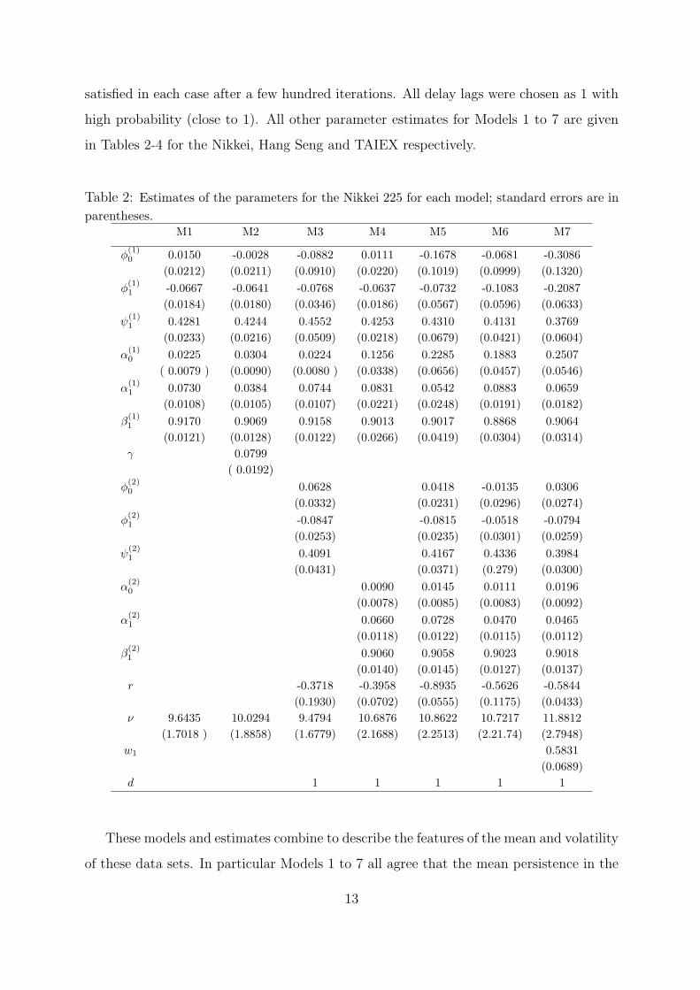
satisfied in each case after a few hundred iterations. All delay lags were chosen as 1 with

high probability (close to 1). All other parameter estimates for Models 1 to 7 are given

in Tables 2-4 for the Nikkei, Hang Seng and TAIEX respectively.

Table 2: Estimates of the parameters for the Nikkei 225 for each model; standard errors are inparentheses.

M1 M2 M3 M4 M5 M6 M7

φ(1)0 0.0150 -0.0028 -0.0882 0.0111 -0.1678 -0.0681 -0.3086

(0.0212) (0.0211) (0.0910) (0.0220) (0.1019) (0.0999) (0.1320)φ

(1)1 -0.0667 -0.0641 -0.0768 -0.0637 -0.0732 -0.1083 -0.2087

(0.0184) (0.0180) (0.0346) (0.0186) (0.0567) (0.0596) (0.0633)ψ

(1)1 0.4281 0.4244 0.4552 0.4253 0.4310 0.4131 0.3769

(0.0233) (0.0216) (0.0509) (0.0218) (0.0679) (0.0421) (0.0604)α

(1)0 0.0225 0.0304 0.0224 0.1256 0.2285 0.1883 0.2507

( 0.0079 ) (0.0090) (0.0080 ) (0.0338) (0.0656) (0.0457) (0.0546)α

(1)1 0.0730 0.0384 0.0744 0.0831 0.0542 0.0883 0.0659

(0.0108) (0.0105) (0.0107) (0.0221) (0.0248) (0.0191) (0.0182)β

(1)1 0.9170 0.9069 0.9158 0.9013 0.9017 0.8868 0.9064

(0.0121) (0.0128) (0.0122) (0.0266) (0.0419) (0.0304) (0.0314)γ 0.0799

( 0.0192)φ

(2)0 0.0628 0.0418 -0.0135 0.0306

(0.0332) (0.0231) (0.0296) (0.0274)φ

(2)1 -0.0847 -0.0815 -0.0518 -0.0794

(0.0253) (0.0235) (0.0301) (0.0259)ψ

(2)1 0.4091 0.4167 0.4336 0.3984

(0.0431) (0.0371) (0.279) (0.0300)α

(2)0 0.0090 0.0145 0.0111 0.0196

(0.0078) (0.0085) (0.0083) (0.0092)α

(2)1 0.0660 0.0728 0.0470 0.0465

(0.0118) (0.0122) (0.0115) (0.0112)β

(2)1 0.9060 0.9058 0.9023 0.9018

(0.0140) (0.0145) (0.0127) (0.0137)r -0.3718 -0.3958 -0.8935 -0.5626 -0.5844

(0.1930) (0.0702) (0.0555) (0.1175) (0.0433)ν 9.6435 10.0294 9.4794 10.6876 10.8622 10.7217 11.8812

(1.7018 ) (1.8858) (1.6779) (2.1688) (2.2513) (2.21.74) (2.7948)w1 0.5831

(0.0689)d 1 1 1 1 1

These models and estimates combine to describe the features of the mean and volatility

of these data sets. In particular Models 1 to 7 all agree that the mean persistence in the

13

Table 3: Estimates of the parameters for the Hang Seng index for each model; standard errorsare in parentheses.

M1 M2 M3 M4 M5 M6 M7

φ(1)0 0.0372 0.0283 0.0171 0.0376 0.0104 0.0206 -0.0585

(0.0206) (0.0206) (0.0661) (0.0214) (0.1599) (0.0542) (0.0911)φ

(1)1 -0.0139 -0.0102 -0.0701 -0.0106 -0.0680 -0.0862 -0.1425

(0.0181) (0.0176) (0.0431) (0.0189) (0.0509) (0.0380) (0.0472)ψ

(1)1 0.5234 0.5156 0.5582 0.5286 0.5606 0.5572 0.5562

(0.0229) (0.0223) (0.0467) (0.0236) (0.0991) (0.0446) (0.0568)α

(1)0 0.0120 0.0160 0.0120 0.0966 0.1594 0.0722 0.1033

(0.0044) (0.0052) (0.0044) (0.0281) (0.0491) (0.0294) (0.0339)α

(1)1 0.0655 0.0401 0.0660 0.1029 0.1160 0.1020 0.1082

(0.0108) (0.0108) (0.0107) (0.0222) (0.0310) (0.0210) (0.0280)β

(1)1 0.9294 0.9246 0.9289 0.8894 0.8701 0.8902 0.8805

(0.0114) (0.0119) (0.0114) (0.0241) (0.0333) (0.0222) (0.0306)γ 0.0545

(0.0169)φ

(2)0 0.0253 0.0537 0.0270 0.0365

(0.0352 ) (0.0228) (0.0256) (0.0232)φ

(2)1 0.0255 -0.0039 0.0191 0.0171

(0.0296) (0.0194) (0.0228) (0.0217)ψ

(2)1 0.4858 0.4973 0.5026 0.5125

(0.0467) (0.0333) (0.0319) (0.0280)α

(2)0 0.0061 0.0112 0.0071 0.0111

(0.0047) (0.0056) (0.0048) (0.0055)α

(2)1 0.0580 0.0607 0.0401 0.0454

(0.0130) (0.0125) (0.0119) (0.0122)β

(2)1 0.9160 0.9172 0.9395 0.9343

(0.0138) (0.0142) (0.0139) (0.0135)r -0.1322 -0.4281 -0.8831 -0.4853 -0.7037

(0.3607) (0.0922) (0.0890) (0.1901) (0.0865)ν 8.1804 8.3535 8.0297 8.6639 8.5556 8.5865 8.4692

(1.2913) (1.3853) (1.2269) (1.4695) (1.4675) (1.4759) (1.4476)w1 0.6857

(0.1648)d 2 1 1 2 2

Nikkei is small, but significant, and negative. This parameter is again always negative,

but only significant for models 6-7, for the Hang Seng index, while it is never significant

for the TAIEX, but it is largest in magnitude for Models 6-7 again. There does not seem

to be a strong asymmetric effect for the AR parameter in these markets for models 3,

5-7. These mostly negative estimates and symmetric effects are in agreement with results

14

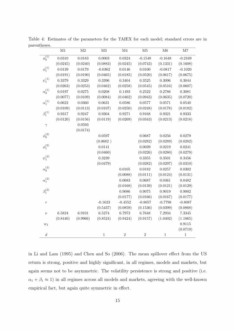
Table 4: Estimates of the parameters for the TAIEX for each model; standard errors are inparentheses.

M1 M2 M3 M4 M5 M6 M7

φ(1)0 0.0310 0.0183 0.0003 0.0324 -0.1548 -0.1648 -0.2169

(0.0245) (0.0240) (0.0883) (0.0245) (0.0743) (0.1331) (0.1608)φ

(1)1 0.0139 0.0179 -0.0362 0.0146 0.0100 -0.0817 -0.1020

(0.0191) (0.0190) (0.0465) (0.0185) (0.0520) (0.0617) (0.0675)ψ

(1)1 0.3379 0.3329 0.3396 0.3404 0.3525 0.3096 0.3044

(0.0263) (0.0253) (0.0462) (0.0258) (0.0545) (0.0516) (0.0607)α

(1)0 0.0197 0.0275 0.0208 0.1493 0.2522 0.2786 0.3081

(0.0077) (0.0109) (0.0084) (0.0462) (0.0943) (0.0635) (0.0720)α

(1)1 0.0622 0.0360 0.0631 0.0586 0.0577 0.0571 0.0540

(0.0109) (0.0113) (0.0107) (0.0250) (0.0248) (0.0178) (0.0182)β

(1)1 0.9317 0.9247 0.9304 0.9271 0.9168 0.9321 0.9333

(0.0120) (0.0156) (0.0119) (0.0269) (0.0343) (0.0213) (0.0218)γ 0.0593

(0.0174)φ

(2)0 0.0597 0.0687 0.0256 0.0279

(0.0682 ) (0.0282) (0.0289) (0.0282)φ

(2)1 0.0141 0.0039 0.0219 0.0241

(0.0460) (0.0226) (0.0280) (0.0279)ψ

(2)1 0.3239 0.3355 0.3501 0.3456

(0.0479) (0.0282) (0.0297) (0.0310)α

(2)0 0.0105 0.0182 0.0257 0.0302

(0.0088) (0.0111) (0.0124) (0.0131)α

(2)1 0.0683 0.0687 0.0461 0.0482

(0.0168) (0.0139) (0.0121) (0.0129)β

(2)1 0.9086 0.9075 0.9019 0.9002

(0.0177) (0.0166) (0.0167) (0.0177)r -0.1623 -0.4552 -0.8057 -0.7798 -0.8087

(0.5437) (0.0859) (0.1536) (0.0399) (0.0868)ν 6.5824 6.9101 6.5274 6.7973 6.7648 7.2934 7.3345

(0.8440) (0.9966) (0.8524) (0.9424) (0.9157) (1.0402) (1.1065)w1 0.9115

(0.0719)d 1 2 2 1 1

in Li and Lam (1995) and Chen and So (2006). The mean spillover effect from the US

return is strong, positive and highly significant, in all regimes, models and markets, but

again seems not to be asymmetric. The volatility persistence is strong and positive (i.e.

α1 + β1 ≈ 1) in all regimes across all models and markets, agreeing with the well-known

empirical fact, but again quite symmetric in effect.

15

Asymmetric effects also seem strong and clear in all nonlinear models in each market.

For the Nikkei and TAIEX indices, models with mean asymmetry (Models 3, 5 - 7) clearly

indicate that the mean return is lower and negative following bad news from the US or the

domestic market (or combined as in Model 7), with higher and mostly positive average

returns following good news. This is because φ(1)0 < φ

(2)0 ; φ

(1)1 ≈ φ

(2)1 ; ψ

(1)1 ≈ ψ

(2)1 in Models

3 and Models 5 to 7 in these two markets. This effect is not apparent in Hong Kong,

however. The threshold cut-offs for Models 3 to 7 were all estimated between -0.37 and

-0.9 for Nikkei; -0.13 and -0.88 for Hang Seng and -0.16 to -0.81 for Taiwan. These are

almost all significantly lower than the usual value of 0 employed in similar studies. i.e.

bad news is not ’financially significant’ until a threshold somewhat below zero and closer

to -0.5% (on average).

Asymmetric volatility was also very strong and clear across markets. In particular

volatility levels are significantly higher following bad news, as highlighted by γ > 0 in

Model 2 and α(1)0 > α

(2)0 ; α

(1)1 ≈ α

(2)1 ; β

(1)1 ≈ β

(2)1 in Models 4 to 7. It seems the asymmetric

effects are clear and apparent in the mean and variance intercept terms, but perhaps not

present at all in the other parameters, except possibly in the ARCH terms α1 in the Hang

Seng market. This is highlighted in Figures 2 and 3, showing boxplots of the MCMC

iterates for the mean parameters (Figure 2) and the volatility parameters (Figure 4)

from Model 7. From left to right, the first three boxplots are the parameters in regime

1, while the next three are from regime 2. It is quite apparent that the only clearly

significant differences between regimes are in the intercept parameters φ0 and α0, except

for differences in α1 for the Hang Seng market.

For Model 7 the weight chosen for the US return in the weighted threshold variable

is 0.58 (Nikkei) and 0.69 (Hang Seng), but these are not significantly different from 0.5.

The weight for the TAIEX was estimated to be 0.91 and significantly different to 0.5.

We should not interpret these weights too exactly, since the two threshold variables have

slightly different variances (although both on the same scale of percentage returns it is

debatable as to whether these returns should be standardised in the threshold variable,

we chose not to), however it seems each market has ’close’ to an equal effect on this

threshold variable that drives asymmetric nonlinear behaviour in Japan and Hong Kong,

but that the local TAIEX has a far stronger influence than the US in driving asymmetric

16

Figure 2: Boxplots for parameter estimates of (φ(1)0 , φ

(1)1 ψ

(1)1 , φ

(2)0 , φ

(2)1 ψ

(2)1 ) in Model 7 for the

Nikkei market.

behaviour in Taiwan, again around a significantly negative threshold value of about -0.8%.

Finally, all degrees of freedom parameters are estimated between 6 and 12 across markets

and models, far below what would be expected from normality and justifying the use of

t-distributed residuals.

4.2 Model selection results

We apply the method of Congdon (2006) to estimate posterior model probabilities for all

seven models considered in each market. These are shown in Table 5 and Figure 4. For

exposition, two additional scenarios are shown for Japan, where only the first five and

17

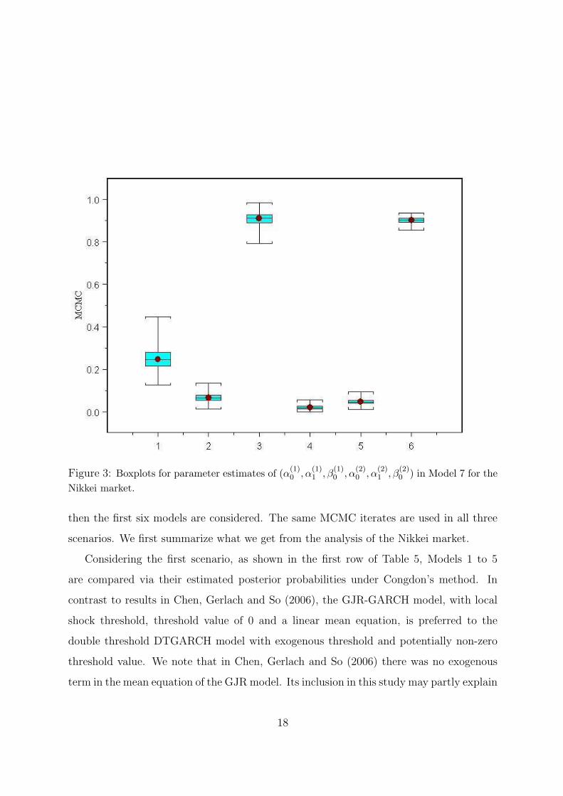
Figure 3: Boxplots for parameter estimates of (α(1)0 , α

(1)1 , β

(1)0 , α

(2)0 , α

(2)1 , β

(2)0 ) in Model 7 for the

Nikkei market.

then the first six models are considered. The same MCMC iterates are used in all three

scenarios. We first summarize what we get from the analysis of the Nikkei market.

Considering the first scenario, as shown in the first row of Table 5, Models 1 to 5

are compared via their estimated posterior probabilities under Congdon’s method. In

contrast to results in Chen, Gerlach and So (2006), the GJR-GARCH model, with local

shock threshold, threshold value of 0 and a linear mean equation, is preferred to the

double threshold DTGARCH model with exogenous threshold and potentially non-zero

threshold value. We note that in Chen, Gerlach and So (2006) there was no exogenous

term in the mean equation of the GJR model. Its inclusion in this study may partly explain

18

Table 5: Posterior probabilities for each model across the three markets.M1 M2 M3 M4 M5 M6 M7

Nikkei 225 5 candidates 0.2166 0.4076 0.1464 0.0462 0.1832Nikkei 225 6 candidates 0.1158 0.2415 0.0793 0.0221 0.1018 0.4396Nikkei 225 7 candidates 0.0637 0.1432 0.0437 0.0100 0.0492 0.2699 0.4203

Hang Seng 7 candidates 0.1328 0.2108 0.0865 0.0178 0.0597 0.2848 0.2077

TAIEX 7candidates 0.0585 0.1642 0.0513 0.0177 0.0297 0.3307 0.3479

our result, but also not exactly the same data series have been used. The DTGARCH

and symmetric GARCH are favoured next, followed closely by the TARX-GARCH, with

little weight given to the ARX-TGARCH model. This suggests that there is a strong

asymmetric ARCH effect, as described in the GJR model, driven by local market shocks.

Figure 4: The estimated posterior model probabilities for the Nikkei market, over three scenar-

ios.

Next we add the DTGARCH model with local threshold variable. While the GJR-

GARCH is still favoured as 2nd in this list, the DTGARCH is clearly the superior model

for this dataset. Little weight is given to the other four models. Again we see a strong

nonlinear local market effect, but this time the (only) model allowing for both asymmetry

19

in mean and volatility, in response to local market returns, is clearly favoured. Again we

note that a US exogenous mean effect is included in the DTGARCH model with local

threshold, again explaining our differing result from that in Chen et al (2006).

Finally we add Model 7 which allows a weighted combination of US and local returns

as the threshold. While some weight is still given to the GJR-GARCH model, the battle

is now clearly between the DTGARCH with local threshold and the DTGARCH with

weighted threshold. Model 7 (weighted threshold) wins out with posterior probability

0.42, compared to 0.27 for Model 6. The data clearly favour nonlinearity in mean and

volatility being driven by the weighted threshold variable. This makes sense from a

financial viewpoint, since this threshold uses all the news information available, i.e. local

and US returns, from the previous trading day. For the Hang Seng index and TAIEX,

we find supporting evidence that again M6 and M7 are preferable. The marginally best

model for HSI is M6, indicating that the domestic return threshold variable is slightly

more appropriate than a weighted average threshold variable. Although we find very

marginal superior performance of M7 to M6 for TAIEX, the difference is small. This is

not surprising as ω1 is so close to one in M7 that these models are almost the same in

practical applications.

5 Conclusion

We briefly review in this paper three computational methods for estimating marginal

likelihoods and highlight the advantages of Congdon (2006)’s approach for heteroskedastic

models. The proposed approach is a special case of composite space MCMC sampling

where jumps between models are not involved and so only evidence on the model ratios

need to be accumulated. The construction of proposal densities for RJMCMC are also

avoided in this approach. Seven asymmetric volatility models, which differ in the mean

structure, in the volatility structure or in the construction of the threshold variable, are

evaluated. Our results show that the weighted average threshold formulation introduced

in Chen and So (2006) is preferred for the Nikkei 225 and the TAIEX market data with

a local threshold and double threshold model also scoring highly. This latter model is

preferred for the Hang Seng index. These results can initiate new discussion on how

20

to combine information from different sources in determining regimes for asymmetric

heteroskedastic models. It is easy to apply the proposed method to compare complex

models and to the comparison of non-nested models. All the methods discussed here

can also be applied to other volatility models, like Markov switching GARCH models

and stochastic volatility models, retaining the advantages discussed. Choice of auxiliary

variables in Chen and So (2006)’s specification and the determination of the number of

regimes (beyond two) in threshold processes are important topics for further research.

Acknowledgment: C. W. S. Chen acknowledges research support from National Science

Council of Taiwan grant 95-2118-M-035-001.

References

Bauwens, L. and Lubrano, M. (1998) Bayesian inference on GARCH models using Gibbs

sampler, Econometrics Journal, 1, 23-46.

Berg, A., Meyer, R., and Yu, J. (2004) Deviance Information Criterion for Comparing

Stochastic Volatility Models. Journal of Business and Economic Statistics, 22, 107-

120.

Bollerslev, T. (1986) Generalized autoregressive heteroskedasticity. Journal of Econo-

metrics, 31, 307-327.

Brooks, C. (2001) A double-threshold GARCH Model for the French Franc/Deutschmark

Exchange Rate. Journal of Forecasting, 20, 135-143.

Carlin, B. P. and Chib, S. (1995) Bayesian model choice via Markov chain Monte Carlo.

Journal of the Royal Statistical Society, Series B, 57, 473-484.

Chen, C. W. S., Chiang, T. C. and So, M. K. P. (2003) Asymmetrical Reaction to

US Stock-return News: Evidence from Major Stock Markets Based on a Double-

Threshold Model. The Journal of Economics and Business. Special issue on Glob-

alization in the New Millennium: Evidence on Financial and Economic Integration,

55, 487-502.

21

Chen, C. W. S., Gerlach, R., and So, M. K. P. (2006) Comparison of non-nested asym-

metric heteroscedastic models, Computational Statistics & Data Analysis. Special

issue on Nonlinear Modelling & Financial econometrics, 51, 2164-2178.

Chen, C. W. S. and So, M. K. P. (2006) On a threshold heteroscedastic model. Interna-

tional Journal of Forecasting, 22, 73-89.

Chen, C. W. S., So, M. K. P. and, Gerlach, R. H.(2005) Assessing and testing for thresh-

old nonlinearity in stock returns. Australian & New Zealand Journal of Statistics,

47, 473-488.

Chib, S. (1995) Marginal likelihood from the Gibbs output. Journal of the American

Statistical Association, 90, 1313-1321.

Congdon, P. (2006) Bayesian model choice based on Monte Carlo estimates of posterior

model probabilities. Computational Statistics and Data Analysis, 50, 346-357.

Engle, R. F. (1982) Autoregressive, conditional heteroskedasticity with estimates of the

variance of United Kingdom inflation. Econometrica, 50, 987-1007.

Gerlach, R., Carter, C. K., and Kohn, R. (1999) Diagnostics for time series analysis,

Journal of Time Series Analysis, 20, 309-330.

Gerlach, R., Chen, C.W.S., Lin, S.Y., and Huang, M.H. (2006) Asymmetric responses

of international markets to trading volume’, Physica A: Statistical Mechanics and

its Applications, 360, 422-444.

Gerlach, R. and Tuyl, F. (2006) MCMC Methods for Comparing Stochastic Volatility

and GARCH Models, International Journal of Forecasting, 22, 91-107.

Glosten, L., Jagannathan, R., & Runke, D. (1993) On Relationship between the expected

value and the volatility of the nominal excess return on stocks. Journal of Finance,

487, 1779-1801.

Geweke J. (1995) Bayesian comparison of econometric models. Working Paper 532.

Research Department, Federal Reserve Bank of Minneapolis.

22

Geweke, J. (1996) Variable Selection and Model Comparison in Regression, in Bayesian

Statistics V, eds. J. Bernardo, J. Berger, A. Dawid, and A. Smith, Oxford: Oxford

University Press, 609-620.

Godsill, S. J. (2001) On the relationship between Markov chain Monte Carlo methods

for model uncertainty. Journal of Computational and Graphical Statistics, 10, 1-19.

Green, P.J. (1995) Reversible jump MCMC computation and Bayesian model determi-

nation. Biometrika, 82, 711-732.

Kass and Raftery (1995) Bayes Factors, Journal of the American Statistical Association,

90, 773-795.

Li, W. K. and Lam K. (1995) Modelling asymmetry in stock returns by a threshold

ARCH model. The Statistician 44, 333-341.

Li, C. W. and Li, W. K. (1996) On a double-threshold autoregressive heteroscedastic

time series model. Journal of Applied Econometrics, 11, 253-274.

Nelson, D. B. (1991) Conditional heteroskedasticity in asset returns: A new approach.

Econometrica, 59, 347- 370.

Newton M. A. and Raftery A. E., (1994) Approximate Bayesian inference by the weighted

likelihood bootstrap (with discussion), Journal of the Royal Statistical Society, Se-

ries B, 56, 3-48.

Osiewalski, Pajor, and Pipien (2006) Bayesian comparison of bivariate GARCH and SV

models, Acta Universitatis Lodziensis - Folia Oeconomica, forthcoming.

Poon, S.H. and Granger, C.W.J. (2003) Forecasting volatility in financial markets: A

review. Journal of Economic Literature, 41, 478-539.

Scott, S. (2002) Bayesian methods for hidden Markov models: recursive computing in

the 21st Century, Journal of the American Statistical Association, 97, 337-351.

Sentana, E. (1995) Quadratic ARCH models. Review of Economic Studies, 62, 639-661.

23

Silvapulle, M. J. and Sen, P. K. (2004) Constrained Statistical Inference: Inequality,

Order, and Shape Restrictions, Wiley, New York.

So, M. K. P., Chen, C. W. S., and Chen, M. T. (2005) A Bayesian threshold nonlinearity

test in financial time series, Journal of Forecasting, 24, 61-75.

So, M. K. P., Chen, C. W. S., and Liu, F.C. (2006) Best subset selection of autore-

gressive models with exogenous variables and generalized autoregressive conditional

heteroscedasticity errors, Journal of the Royal Statistical Society, Series C, 55, 201-

224.

So, M. K. P. and Li, W. K. (1999) Bayesian unit-root testing in stochastic volatility

models. Journal of Business & Economic Statistics, 17, 491-496.

Tong, H. (1978) On a Threshold Model in Pattern Recognition and Signal Processing,

ed. C. H. Chen, Sijhoff & Noordhoff: Amsterdam.

Vrontos, I. D., Dellaportas, P. and Politis, D. N. (2000) Full Bayesian inference for

GARCH and EGARCH models. Journal of Business & Economic Statistics, 18,

187-198.

Zakoian, J. M. (1994) Threshold heteroskedastic models. Journal of Economic Dynamics

and Control, 18, 931-955.

24