Bayesian estimationof switching ARMA modelsM. Billio, A. Monfort and C.P. RobertyCREST, INSEE, ParisR�esum�eLes mod�eles ARMA �a sauts forment un outil puissant de mod�elisation de s�eries temporellesnon-lin�eaires. Ils introduisent deux niveaux de d�ependance entre les observations, en ajoutant �a lastructure ARMA une s�el�ection markovienne des param�etres du mod�ele ARMA. La contrepartie decette puissance de mod�elisation est la compl�exit�e de la vraisemblance associ�ee. Nous proposonsici une r�esolution bay�esienne par lois noninformatives et �echantillonnage de Gibbs hybride, les�etapes de simulation conditionnelle �etant remplac�ees par des algorithmes de Hastings-Metropolis.Nous pr�esentons les �etapes de simulation en d�etail, conduisons une comparaison avec une m�ethodealternative de Chib (1996) et illustrons les bonnes performances de notre approche sur des donn�eessimul�ees et r�eelles. Cette approche permet �egalement de construire les estimateurs du maximumde vraisemblance du mod�ele par une technique proche du recuit simul�e d�evelopp�ee par Robert(1993).Mots{cl�es : Mod�ele markovien; cha�ne de Markov cach�ee; algorithme de Hastings-Metropolis;�echantillonnage de Gibbs; controle de convergence; recuit simul�e.AbstractSwitching ARMA processes have recently appeared as an e�cient modelling to nonlinear timeseries models, because they can represent multiple or heterogeneous dynamics through simplecomponents. The levels of dependence between the observations are double: at a �rst level,the parameters of the model (AR, MA or ARMA) are selected by a Markovian procedure. Ata second level, the next observation is generated according to a standard time series model.When the model involves a moving average structure, the complexity of the resulting likelihoodfunction is such that simulation techniques, like those proposed by Shephard (1994) and Billioand Monfort (1995), are necessary to derive an inference on the parameters of the model. Wepropose in this paper a Bayesian approach with a noninformative prior distribution developed inMengersen and Robert (1996) and Robert and Titterington (1996) in the setup of mixtures ofdistributions and hidden Markov models, respectively. The computation of the Bayes estimatesrelies on MCMC techniques which iteratively simulate missing states, innovations and parametersuntil convergence. The performances of the method are illustrated on both simulated examplesand real data. We show in addition how maximum likelihood estimators can be derived from theseBayes estimators through increasing replications of the original sample, following Robert (1993)and Robert and Titterington (1996). This work also extends the papers by Chib and Greenberg(1994) and Chib (1996) which deal with ARMA and hidden Markov models, respectively.Keywords: Markov model; Moving average model; Hidden Markov chain; MCMC algorithm;ARMA model; Convergence control; Prior feedback.y The third author is thankful to Marilena Barbieri for an helpful discussion.1

1. IntroductionIn a fruitful generalization of ARMA(p; q) models proposed by Hamilton (1988), theparameters of these models are speci�ed as a stochastic process driven by a state (unob-servable or hidden) Markov chain. The likelihood functions of these switching ARMA(p; q)models can be recursively computed (see Kitagawa, 1987 or Hamilton, 1989) when thejoint process made of the variables of interest and of the state process is Markovian, i.e.if q is equal to 0. When a non-trivial MA structure is present in the model, recursive al-gorithms fail because of the combinatorial explosion resulting from the computation. Forsimilar reasons, Bayesian inference is also delicate in such setups. Additional di�cultiesstem from the restrictions imposed by stationarity issues, although Jones (1987) has shownthat a reparameterisation could greatly simplify this issue. Since the hindrance is mainlydue to the non-Markovian nature of the model, a natural idea is to recover a Markovianframework by adding additional states which lead to a switching linear state space repre-sentation. In this setting, it is possible to propose simulated EM algorithms (Shephard,1994) or importance sampling algorithms based on the partial Kalman �lter (Billio andMonfort, 1995, Gouri�eroux and Monfort, 1996).In this paper, we follow a Bayesian approach based on the data augmentation principleof Tanner and Wong (1987) (see also Albert and Chib, 1993, Chib and Greenberg, 1995,and Jacquier, Polson and Rossi, 1994). However, in order to minimize the size of thestate variable, we do not attempt in this paper to get back in the Markov framework andwork directly with the initial model. We use two versions of hybrid Monte Carlo MarkovChain (MCMC) algorithms, which thus involve mixtures of Gibbs and Hastings-Metropolisalgorithms. In both versions, the data augmentation steps are identical but the simulationsof the parameters are di�erent. A �rst version systematically proposes Hastings-Metropolissteps based on approximated innovations while the other uses explicit Gibbs steps inspiredfrom Chib and Greenberg (1994) which are based on polynomial long divisions. In orderto simplify presentation and notations, we only consider MA(1) and ARMA(1,1) models,although the extension to higher orders is straightforward, but involves more cumbersomealgebraic manipulations.The prior modelling on the parameters of the di�erent models is noninformative, fol-lowing some developments of Mengersen and Robert (1996) and Robert and Titterington(1996) on mixtures of distributions and hidden Markov chains. The structure of theseswitching state models is indeed quite similar to mixture setups, with the additional dif-�culty of probabilistic dependence at both the observed and latent stages. The prior weselect is a direct extension of the noninformative prior of Mengersen and Robert (1996),1

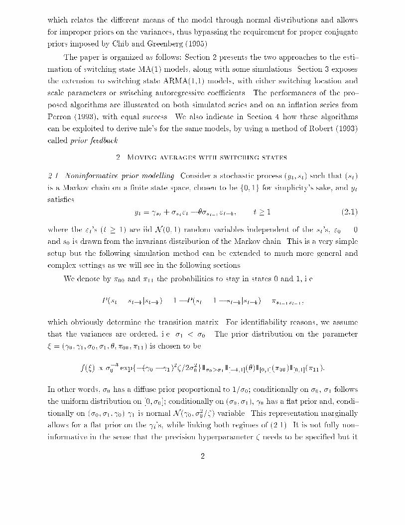
which relates the di�erent means of the model through normal distributions and allowsfor improper priors on the variances, thus bypassing the requirement for proper conjugatepriors imposed by Chib and Greenberg (1995).The paper is organized as follows: Section 2 presents the two approaches to the esti-mation of switching state MA(1) models, along with some simulations. Section 3 exposesthe extension to switching state ARMA(1,1) models, with either switching location andscale parameters or switching autoregressive coe�cients. The performances of the pro-posed algorithms are illustrated on both simulated series and on an in ation series fromPerron (1993), with equal success. We also indicate in Section 4 how these algorithmscan be exploited to derive mle's for the same models, by using a method of Robert (1993)called prior feedback.2. Moving averages with switching states.2.1. Noninformative prior modelling. Consider a stochastic process (yt; st) such that (st)is a Markov chain on a �nite state space, chosen to be f0; 1g for simplicity's sake, and ytsatis�es yt = st + �st"t � ��st�1 "t�1; t � 1 (2:1)where the "t's (t � 1) are iid N (0; 1) random variables independent of the st's, "0 = 0and s0 is drawn from the invariant distribution of the Markov chain. This is a very simplesetup but the following simulation method can be extended to much more general andcomplex settings as we will see in the following sections.We denote by �00 and �11 the probabilities to stay in states 0 and 1, i.e.P (st = st�1jst�1) = 1� P (st = 1� st�1jst�1) = �st�1st�1 ;which obviously determine the transition matrix. For identi�ability reasons, we assumethat the variances are ordered, i.e. �1 < �0. The prior distribution on the parameter� = ( 0; 1; �0; �1; �; �00; �11) is chosen to bef(�) / ��30 expf�( 0 � 1)2�=2�20gII�0>�1II[�1;1](�)II[0;1](�00)II[0;1](�11):In other words, �0 has a di�use prior proportional to 1=�0; conditionally on �0, �1 followsthe uniform distribution on [0; �0]; conditionally on (�0; �1), 0 has a at prior and, condi-tionally on (�0; �1; 0) 1 is normal N ( 0; �20=�) variable. This representation marginallyallows for a at prior on the i's, while linking both regimes of (2.1). It is not fully non-informative in the sense that the precision hyperparameter � needs to be speci�ed but it2

appears from simulation experiments that the range of values of � leading to the sameestimates is wide enough to insure stability of the method when � 2 [0:1; 1). Note alsothat the prior is invariant under a�ne transformations. Robert and Titterington (1996)show that this prior leads to a well-de�ned posterior distribution in the setup of mixturesand hidden Markov models.Extensions to larger numbers of latent classes is straightforward, in the sense that thesuccessive di�erences i � i�1 are modelled as N (0; �2i�1=�) variables. (The identifyingconstraint is then �1 > �2 : : :, as in Mengersen and Robert, 1996.)2.2. A �rst MCMC algorithm. The posterior density f(�jy0; : : : ; yT ) is of the same com-plexity as the likelihood function and cannot be directly computed. We thus follow a sim-ulation based approach. More precisely, we simulate from the joint posterior distributionf(s0; : : : ; sT ; �jy0; : : : ; yT ), using Gibbs sampling (Gelfand and Smith, 1990), i.e. simulat-ing alternately from f(s0; : : : ; sT j�; y0; : : : ; yT ) |this is the data augmentation step| andfrom f(�js0; : : : ; sT ; y0; : : : ; yT ) |this is the parameter simulation step|. However, sincesome conditional distributions cannot be directly simulated, the corresponding steps arereplaced by Hastings-Metropolis steps. For instance, this is the case for the data augmen-tation steps in both algorithms. We thus obtain hybrid algorithms in the spirit of Tierney(1994) (see also Gilks et al., 1996, or Robert, 1996). These references provide detailedinformation about Hastings-Metropolis algorithms; the main incentive for their use here isthat they allow for MCMC simulation from arbitrarily complex distributions.Although Chib and Greenberg (1994) have already developed an MCMC algorithmfor non-switching MA and ARMA models which can be extended to this setup (see x2.3),we �rst propose a new approach which comparatively involves more Hastings-Metropolissteps and less Gibbs steps. According to the current tenets on the relative virtues of Gibbsand Hastings-Metropolis methods (see, e.g., Gilks et al., 1996, Robert, 1996, or Tierney,1994), this approach is more robust, in particular because it increases the range of thechain excursions on the posterior surface, as shown below on simulations.Switching ARMA models are quite complex because of the missing data structure,namely the non observability of the latent states. As in mixture estimation, once thesestates are known, the inferential problem gets simpler. The additional complexity in thiscase is that the likelihood is still involved when the st's are known, because of the movingaverage structure. The main idea of the algorithm is to replace at various stages thetrue innovations in the likelihood with innovations computed at the previous steps, tosimulate the missing states with these pseudo-innovations and to accept the simulatedvalues based on a Hastings-Metropolis step. Besides being theoretically well-grounded,3

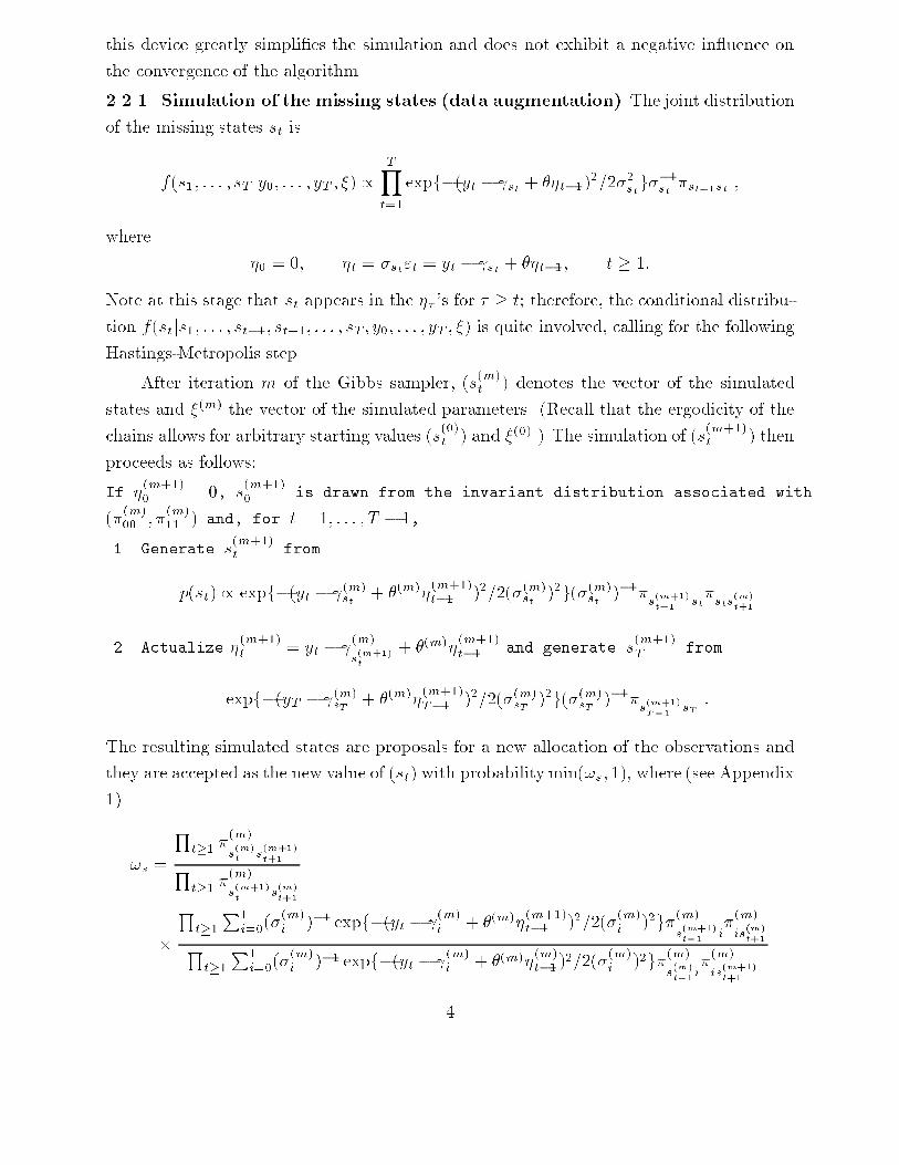
this device greatly simpli�es the simulation and does not exhibit a negative in uence onthe convergence of the algorithm.2.2.1. Simulation of the missing states (data augmentation) The joint distributionof the missing states st isf(s1; : : : ; sT jy0; : : : ; yT ; �) / TYt=1 expf�(yt � st + ��t�1)2=2�2stg��1st �st�1st ;where �0 = 0; �t = �st"t = yt � st + ��t�1; t � 1:Note at this stage that st appears in the �� 's for � � t; therefore, the conditional distribu-tion f(stjs1; : : : ; st�1; st+1; : : : ; sT ; y0; : : : ; yT ; �) is quite involved, calling for the followingHastings-Metropolis step.After iteration m of the Gibbs sampler, (s(m)t ) denotes the vector of the simulatedstates and �(m) the vector of the simulated parameters. (Recall that the ergodicity of thechains allows for arbitrary starting values (s(0)t ) and �(0).) The simulation of (s(m+1)t ) thenproceeds as follows:If �(m+1)0 = 0, s(m+1)0 is drawn from the invariant distribution associated with(�(m)00 ; �(m)11 ) and, for t = 1; : : : ; T � 1,1. Generate s(m+1)t fromp(st) / expf�(yt � (m)st + �(m)�(m+1)t�1 )2=2(�(m)st )2g(�(m)st )�1�s(m+1)t�1 st�sts(m)t+12. Actualize �(m+1)t = yt � (m)s(m+1)t + �(m)�(m+1)t�1 and generate s(m+1)T fromexpf�(yT � (m)sT + �(m)�(m+1)T�1 )2=2(�(m)sT )2g(�(m)sT )�1�s(m+1)T�1 sT :The resulting simulated states are proposals for a new allocation of the observations andthey are accepted as the new value of (st) with probability min(!s; 1), where (see Appendix1) !s = Qt�1 �(m)s(m)t s(m+1)t+1Qt�1 �(m)s(m+1)t s(m)t+1� Qt�1P1i=0(�(m)i )�1 expf�(yt � (m)i + �(m)�(m+1)t�1 )2=2(�(m)i )2g�(m)s(m+1)t�1 i�(m)is(m)t+1Qt�1P1i=0(�(m)i )�1 expf�(yt � (m)i + �(m)�(m)t�1)2=2(�(m)i )2g�(m)s(m)t�1i�(m)is(m+1)t+14

where �(m)t is iteratively de�ned by �(m)0 = 0 and�(m)t = yt � (m)s(m)t + �(m)�(m)t�1:The MCMC algorithm then proceeds by simulating the components of �(m+1), repeat-ing the same replacement of the innovations whenever necessary, namely for the means iand the coe�cient �.2.2.2. Simulation of (�00; �11) The conditional distribution of �00 is given byf(�00j�11; 0; 1; �0; �1; �; (s(m+1)t ); (yt)) / II[0;1](�00)�n0000 (1� �00)n01 ;where nij = TXt=1 IIs(m+1)t =jIIs(m+1)t�1 =i:Therefore, �00 is simulated from a beta Be(n00 + 1; n01 + 1) distribution. Similarly, �11 issimulated from a beta Be(n11 + 1; n10 + 1) distribution.2.2.3. Simulation of ( 0; 1) The conditional distribution on the means i is given byf( 0; 1j�0; �1; �; �00; �11; (st); (yt)) / exp(�12 TXt=1 ��2st (yt � st + ��t�1)2 � ( 0 � 1)2�2�20 )where �0 = 0 and �t = yt� st+��t�1 (t � 1). For �xed innovations, ~�(m)t = yt� (m)s(m+1)t +�(m)~�(m)t�1 (t � 1), where (s(m)t ) is the vector of simulated states accepted in the previousHastings{Metropolis step, this distribution gets transformed into�( 0; 1) / exp(�12 TXt=1(�(m)s(m+1)t )�2(~y(m)t � s(m+1)t )2 � 12�( 0 � 1)2(�(m)0 )�2) ;with ~y(m)t = yt + �(m)~�(m)t�1 , which suggests the following instrumental distributions for anHastings-Metropolis step: 0j 1 � N n(m)0 �y(m)0 + 1�n(m)0 + � ; (�(m)0 )2n(m)0 + �!; 1j 0 � N n(m)1 �y(m)1 + 0�(�(m)1 )2=(�(m)0 )2n(m)1 + �(�(m)1 )2=(�(m)0 )2 ; �21n(m)1 + �(�(m)1 )2=(�(m)0 )2!; (2:2)where n(m)0 = TXt=1 IIfs(m+1)t =0g; n(m)0 �y(m)0 = TXt=1 IIfs(m+1)t =0g~y(m)t ;n(m)1 = TXt=1 IIfs(m+1)t =1g; n(m)1 �y(m)1 = TXt=1 IIfs(m+1)t =1g~y(m)t : (2:3)5

The corresponding simulation of ( (m+1)0 ; (m+1)1 ) is then1. Generate from �( (m+1)0 j (m)1 ) and �( (m+1)1 j (m+1)0 ) according to (2.2);2. Accept the new value ( (m+1)0 ; (m+1)1 ) with probability min(! ; 1), where! = f( (m+1)0 ; (m+1)1 j�(m)0 ; �(m)1 ; �(m); (s(m+1)t ); (yt))f( (m)0 ; (m)1 j�(m)0 ; �(m)1 ; �(m); (s(m+1)t ); (yt))� exp8<:�12 24 (m)0 � n(m)0 �y(m+1)0 + (m+1)1 �n(m)0 + � !2� (m+1)0 � n(m)0 �y(m)0 + (m)1 �n(m)0 + � !235 (�(m)0 )�2(n(m)0 + �)�12 24 (m)1 � n(m)1 �y(m+1)1 + (m)0 �(�(m)1 )2=(�(m)0 )2n(m)1 + �(�(m)1 )2=(�(m)0 )2 !2� (m+1)1 � n(m)1 �y(m)0 + (m+1)0 �(�(m)1 )2=(�(m)0 )2n(m)1 + �(�(m)1 )2=(�(m)0 )2 !235hn(m)1 (�(m)1 )�2 + �(�(m)0 )�2i�where �y(m+1)0 and �y(m+1)1 are based on the innovations computed with ( (m+1)0 ; (m+1)1 ) asin (2.3).It appears from the simulations that the average acceptance probability in 2. is closeto 1. As stressed in the literature (see, e.g., Gelman, Gilks and Roberts, 1996, or Robert,1996), high acceptance rates in Hastings{Metropolis algorithms are linked with slow ex-ploration of the posterior distribution. We thus replace (2.2) with normal distributionswhose variances are expanded by a factor which ensures that the average acceptance rateis between :2 and :5, following Gelman et al. (1996) recommendations.2.2.4. Simulation of (�0; �1) Since the innovations �t are only functions of �; 0; 1 andof the present and past yv's and sv's, the conditional distributionf(�0; �1j 0; 1; �; �00; �11; (st); (yt)) / ��n0�30 exp(�12��20 "Xst=0(~yt � 0)2 + �( 0 � 1)2#)���n11 exp(�12��21 Xst=1(~yt � 1)2) II�0>�1provides a direct simulation step for the variances.6

Generate(�(m+1)0 )�2 � Ga0B@n(m)0 + 22 ; 12 264 Xs(m+1)t =0(~y(m)t � (m+1)0 )2 + � � (m+1)0 � (m+1)1 �23751CAII�0>�(m)1(�(m+1)1 )�2 � Ga0B@n(m)1 � 12 ; 12 Xs(m+1)t =1(~y(m)t � (m+1)1 )21CAII�(m+1)0 >�1where ~y(m)t = yt + �(m)��(m)t�1 and ��(m)t = ~y(m)t � (m+1)s(m+1)t .2.2.5. Simulation of � The simulation of �(m+1) is based onf(�j 0; 1; �0; �1; �00; �11; (st); (yt)) / exp(�12 TXt=1(yt � st + ��t�1)2��2st ) II[�1;1](�) :For �xed innovations �(m)t , the above expression leads toexp8><>:�12 " TXt=1 ��2st ��(m)t�1�2#264� + PTt=1 ��2st (yt � st)�(m)t�1PTt=1 ��2st ��(m)t�1�2 37529>=>; II[�1;1](�)Given the constraint j�j � 1, we choose the following simulation scheme1. Generate ~� � N (�(m); � (m)), with�(m) = �PTt=1 �yt � (m+1)s(m+1)t �2 �(m)t�1 ��(m+1)s(m+1)t ��2PTt=1��(m+1)s(m+1)t ��2 ��(m)t �2 ;� (m) = " TXt=1��(m+1)s(m+1)t ��2 ��(m)t�1�2#�1 :2. Take � = � ~� if j~�j < 1,1=~� otherwise. (2:4)3. Accept �(m+1) = � with probability min(!�; 1), where!� = f(�j (m+1)0 ; (m+1)1 ; �(m+1)0 ; �(m+1)1 ; �(m+1)00 ; �(m+1)11 ; (s(m+1)t ); (yt))f(�(m)j (m+1)0 ; (m+1)1 ; �(m+1)0 ; �(m+1)1 ; �(m+1)00 ; �(m+1)11 ; (s(m+1)t ); (yt))�r � (m)� (m+1) expn� (�(m)��(m+1))22� (m+1) o+ (�(m))�2 exp�� (�(m+1)�1=�(m))22� (m+1) �expn� (���(m))22� (m) o + (�)�2 exp�� (�(m)�1=�)22� (m) � ;7

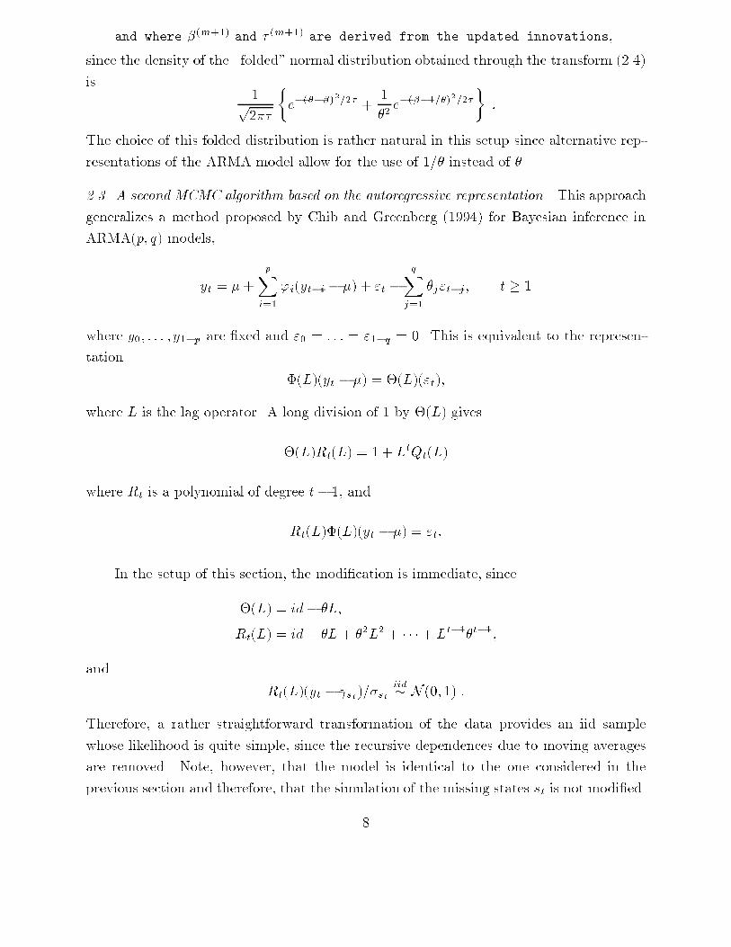
and where �(m+1) and � (m+1) are derived from the updated innovations,since the density of the \folded" normal distribution obtained through the transform (2.4)is 1p2�� �e�(���)2=2� + 1�2 e�(��1=�)2=2�� :The choice of this folded distribution is rather natural in this setup since alternative rep-resentations of the ARMA model allow for the use of 1=� instead of �.2.3. A second MCMC algorithm based on the autoregressive representation. This approachgeneralizes a method proposed by Chib and Greenberg (1994) for Bayesian inference inARMA(p; q) models,yt = �+ pXi=1 'i(yt�i � �) + "t � qXj=1 �j"t�j ; t � 1where y0; : : : ; y1�p are �xed and "0 = : : : = "1�q = 0. This is equivalent to the represen-tation �(L)(yt � �) = �(L)("t);where L is the lag operator. A long division of 1 by �(L) gives�(L)Rt(L) = 1 + LtQt(L)where Rt is a polynomial of degree t� 1, andRt(L)�(L)(yt � �) = "t:In the setup of this section, the modi�cation is immediate, since�(L) = id� �L;Rt(L) = id+ �L + �2L2 + � � �+ Lt�1�t�1;and Rt(L)(yt � st)=�st iid� N (0; 1) :Therefore, a rather straightforward transformation of the data provides an iid samplewhose likelihood is quite simple, since the recursive dependences due to moving averagesare removed. Note, however, that the model is identical to the one considered in theprevious section and therefore, that the simulation of the missing states st is not modi�ed.8

2.3.1. Simulation of ( 0; 1) The new expression for the posterior distribution of thelocation terms isf( 0; 1j�0; �1; �00; �11; �) / exp(� ( 0 � 1)2�2�20 � 12 TXt=1(Rt(L)(yt � st))2��2st )/ exp8><>:� ( 0 � 1)2�2�20 � 12 TXt=0 ��2st 24t�1Xj=0 �j (yt�j � st�j )3529>=>;/ exp8<:� ( 0 � 1)2�2�20 � 12 TXt=1 ��2st 24 0 t�1Xj=0 i0(t � j)�j+ 1 t�1Xj=0 i1(t� j)�j � t�1Xj=0 �jyt�j3529>=>;where i0(t) = II0(st) = 1� i1(t). De�ning�(t) = t�1Xj=0 �jyt�j ; !0(t) = t�1Xj=0 i0(t� j)�j and !1(t) = t�1Xj=0 i1(t� j)�j ;it is then elementary to derive thatf( 0; 1j�0; �1; �00; �11; �)) / exp�12 (� 20 "���20 + TXt=1 ��2st !20(t)#+ 21 "���20 + TXt=1 ��2st !21(t)# + 2 0 1 " TXt=1 ��2st !0(t)!1(t)� ���20 #�2 0 TXt=1 ��2st !0(t)�(t) � 2 1 TXt=1 ��2st !1(t)�(t)) ;which provides directly the full conditionals 0j 1 � N 0BBBB@ TXt=1 ��2st !0(t)�(t) + "���20 � TXt=1 ��2st !0(t)!1(t)# 1���20 + TXt=1 ��2st !20(t) ; 1���21 + TXt=0��2st !20(t)1CCCCAand 1j 0 � N 0BBBB@ TXt=1 ��2st !1(t)�(t) + "���20 � TXt=1 �2st!0(t)!1(t)# 0���20 + TXt=1 ��2st !21(t) ; 1���20 + TXt=1 ��2st !10(t)1CCCCA9

This representation of the time series thus eliminates the Hastings-Metropolis step of theprevious section. Note also that the computation of the !j(t)'s is simple, since!j(t + 1) = tX=0 ij(t + 1� `)�`= ij(t + 1) + �!j(t):2.3.2. Simulation of (�0; �1) The simulation of the variance factors is again straight-forward since ��20 � Ga�m02 ; !02 + 12( 0 � 1)2� II�0>�1 ;��21 � Ga�m12 ; !12 � II�0>�1 ;with m0 = n0 + 2; m1 = n1 � 1 and !j = Xt;st=j[Rt(L)(yt � st)]2:Despite the di�erent formulations, these conditionals are equal to the conditionals of x2.2.2.3.3. Simulation of � The conditional distribution of �,f(�j 0; 1; �0; �1; �00; �11) / exp8><>:�12 TXt=1 ��2st 24t�1Xj=0 �j (yt�j � st�j )3529>=>; II[�1;1](�);does not allow for a direct simulation and we opt, as Chib and Greenberg (1994), for aHastings-Metropolis step. Our proposal is based on the replacement of Rt(L)(yt � st)by (yt � st) + �(yt�1 � st�1 ) (t � 2) in order to get a second degree polynomial in theexponential,~f (�) / exp(�12 TXt=2 ��2st �(yt � st) + �(yt�1 � st�1 )�2) II[�1;1](�);and � is thus generated from the folded version of N (��; ��), with�� = ��� TXt=2 ��2st (yt � st)(yt�1 � st�1 ); ��1� = TXt=2 ��2st (yt�1 � st�1 )2 :We introduce in addition a variance factor '� in the above normal distribution, aiming atan acceptance rate of :3 to :5. 10

As the following section will show, the behavior of this alternative algorithm di�ersfrom the one of x2:2 and, although they usually both converge to the same value, the �rstproposal seems to perform better.2.4. Illustrations. We selected four increasingly mixed-up models to compare the behaviorof both approaches. The di�erent parameters of these models are described in Table 2.1,along with the Bayes estimates obtained by the �rst algorithm. Apart from Example 4,the second algorithm leads to the same numerical results.

0 20 40 60 80 100

-0.50.5

1.5

(10 000 iterations)

means

0 2 4 6 8 10

-0.30.0

0.906

0.918

variances

0 2 4 6 8 10

0.120

.22

0.062

probabilities

0 2 4 6 8 10

0.340

.44

0.900

0.925

MA coefficient

0 2 4 6 8 10

-0.04

0.06

[First algorithm]

means

0 2 4 6 8 10

-0.20.6

0.700

.85

variances

0 2 4 6 8 10

0.11

0.16

0.100

.25

probabilities

0 2 4 6 8 10

0.400

.55

0.60.9

MA coefficient

0 2 4 6 8 10

-0.15

0.0

0 20 40 60 80 100

[Second algorithm]Figure 2.1 { Performances of both algorithms for Sample 1. The full lines in the convergencegraphs of the di�erent parameters correspond to the �rst component (st = 0) and the dotted linesto the second component (st = 1). The simulated dataset is provided at the top of the �gure andthe estimated probability of being in state 1 for each observation is given at the bottom.

0 100 200 300 400 500

-402

4

(10 000 iterations)

means

0 2 4 6 8 10

-0.05

-0.040

.02

variances

0 2 4 6 8 10

1.251

.45

0.04

0.10

probabilities

0 2 4 6 8 10

0.89

0.92

0.45

MA coefficient

0 2 4 6 8 10

-0.85

[First algorithm]

means

0 2 4 6 8 10

-0.08

0.0

-0.06

0.02

variances

0 2 4 6 8 10

1.561

.66

0.12

0.20

probabilities

0 2 4 6 8 100.875

0.55

0.70

MA coefficient

0 2 4 6 8 10-0.760

0 100 200 300 400 500

[Second algorithm]Figure 2.2 { Performances of both algorithms for Sample 2.As shown by the convergence graphs in Figures 2.1{2.4, the �rst algorithm provides afaster convergence rate than the second one since the di�erent averages reach a stationaryvalue more rapidly in the �rst case (note that the scales are smaller for most of the graphson the left hand side.) In these graphs, the original sequence (yt) is represented at top,11

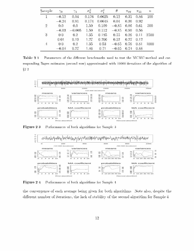
Sample 0 1 �20 �21 � �00 �11 n1 �0:12 0:94 0:176 0:0625 0:12 0:31 0:86 100�0:24 0:91 0:174 0:0648 0:04 0:36 0:922 0:0 0:0 1:59 0:109 �0:85 0:86 0:61 500�0:03 �0:005 1:50 0:112 �0:85 0:90 0:563 0:0 0:2 1:35 0:185 0:55 0:26 0:11 25000:01 0:19 1:27 0:206 0:52 0:27 0:124 0:0 0:2 1:35 0:53 �0:65 0:76 0:81 1000�0:04 0:27 1:46 0:71 �0:65 0:74 0:88Table 2.1 { Parameters of the di�erent benchmarks used to test the MCMC method and cor-responding Bayes estimates (second row) approximated with 10000 iterations of the algorithm ofx2.2.

0 500 1000 1500 2000 2500

-4-2

02

(10 000 iterations)

means

0 2 4 6 8 10

-0.020

.00.0

2

0.18

0.20

variances

0 2 4 6 8 10

1.281

.341.4

0

0.220

.260.3

0

probabilities

0 2 4 6 8 10

0.10

0.20

0.15

0.25

MA coefficient

0 2 4 6 8 10

0.516

0.520

[First algorithm]

means

0 2 4 6 8 10

-0.010

.020.0

5

0.18

0.22

variances

0 2 4 6 8 10

1.151

.251.3

5

0.180

.200.2

2

probabilities

0 2 4 6 8 10

0.22

0.28

0.34

0.040

.080.1

2

MA coefficient

0 2 4 6 8 10

0.515

0.530

[Second algorithm]Figure 2.3 { Performances of both algorithms for Sample 3.

0 200 400 600 800 1000

-4-2

02

4

(10 000 iterations) (50 000 iterations)

means

0 2 4 6 8 10

-0.05

0.10

0.05

0.20

variances

0 2 4 6 8 10

1.31.5

1.7

0.60

0.70

probabilities

0 2 4 6 8 10

0.65

0.75

0.70

0.80

0.90

MA coefficient

0 2 4 6 8 10

-0.660

-0.645

[First algorithm]

means

0 10 20 30 40 50

0.05

0.15

0.17

0.19

variances

0 10 20 30 40 50

1.41.6

1.8

0.60.8

1.0

probabilities

0 10 20 30 40 50

0.40.6

0.70

0.80

MA coefficient

0 10 20 30 40 50-0.685

-0.665

[Second algorithm]Figure 2.4 { Performances of both algorithms for Sample 4.the convergence of each average being given for both algorithms. Note also, despite thedi�erent number of iterations, the lack of stability of the second algorithm for Sample 4.12

3. ARMA models with switching states.3.1. Modi�cations of the algorithms. A straightforward extension of model (2.1) is to addan autoregressive part to the moving average dependence, as in the switching ARMA(1,1)model yt = st + '(yt�1 � st�1) + �st"t � ��st�1 "t�1; t � 1 (3:1)where y0 is �xed, "0 = 0 and s0 is drawn from the invariant distribution of the Markovchain. The above algorithms are only slightly modi�ed since the autoregressive part doesnot complexify the model. In the data augmentation part, the main idea is, as above, touse either the pseudo-innovations based on previous parameter values and current latentstates, namely at iteration m+ 1, �(m+1)0 = 0 and�(m+1)t = yt � (m)s(m+1)t � '(m) �yt�1 � (m)s(m+1)t�1 �+ �(m)�(m+1)t�1 ; t � 1or to use the polynomial autoregressive representation as in x2:3. The simulation of thelatent states s(m+1)t then proceeds as in Section 2 with obvious modi�cations, while thesimulation of the means i needs to account for the correlation structure. Consider forinstance the algorithm developed in x2.2. If we de�ne the pseudo-innovations �(m+1)t asabove (with the accepted s(m+1)t 's), we denote y(m)t = yt � '(m)yt�1 + �(m)�(m)t�1 andn(m)i = TXt=1 IIs(m+1)t =i; n(m)ij = TXt=2 IIs(m+1)t�1 =iIIs(m+1)t =j ;n(m)i y(m)i = TXt=1 IIs(m+1)t =iy(m)t ; n(m)ij y(m)ij = TXt=2 IIs(m+1)t�1 =iIIs(m+1)t =j y(m)t ;with n(m)j = n(m)0j + n(m)1j and n(m)j y(m)j = n(m)0j y(m)0j + n(m)1j y(m)1j . The proposal generationsare then 0j 1 � N ��(m)0 ; � (m)0 � ; 1j 0 � N ��(m)1 ; � (m)1 � ; (3:2)13

where(� (m)0 )�1 = (�(m)0 )�2 h� + n(m)0 + ('(m))2n(m)00 � 2'(m)n(m)00 i+ (�(m)1 )�2 �'(m)�2 n(m)01 ;(� (m)1 )�1 = (�(m)1 )�2 hn(m)1 + ('(m))2n(m)11 � 2'(m)n(m)11 i+ (�(m)0 )�2 h('(m))2n(m)10 + �i ;�(m)0 = � (m)0 h(�(m)0 )�2(n(m)0 y(m)0 + �'(m)n(m)10 + �� (m)1 � '(m)n(m)00 y(m)00 )+(�(m)1 )�2 �'(m)n(m)01 (m)1 � '(m)n(m)01 y(m)01 �i ;�(m)1 = � (m)1 h(�(m)0 )�2 n'(m)n(m)10 ( (m)0 � y(m)10 ) + (m)0 �o+(�(m)1 )�2 �n(m)1 y(m)1 � '(m)n(m)11 y(m)11 + '(m)n(m)01 (m)0 �i :The simulation of the variance factors remains almost identical, with�y(m)t = yt � '(m) �yt�1 � (m+1)s(m+1)t�1 �+ �(m)��(m)t�1replacing ~y(m)t (where ��(m)t is now based on the (m+1)j 's) and the simulation of �(m) ishardly modi�ed.The AR coe�cient is simulated fromf(') / exp(�12 TXt=1 ��2st �yt � st � '(yt�1 � st�1 ) + ��t�1�2) II[�1;1](')/ exp(�12 "'2 TXt=1 ��2st (yt�1 � st�1)2 � 2' TXt=1 ��2st (yt�1 � st�1)(yt � st + ��t�1)#)which leads to the following steps, based on pseudo-innovations ~�(m)t as above:1. Generate ' � N (�(m);$(m)) ;where($(m))�1 = TXt=2(�(m+1)s(m+1)t )�2 �yt�1 � (m+1)s(m+1)t�1 �2 ;�(m) = $(m) TXt=2(�(m+1)s(m+1)t )�2�yt � (m+1)s(m+1)t � �(m+1)~�(m)t�1��yt�1 � (m+1)s(m+1)t�1 � :2. Take ' = �' if j'j < 1,1=' otherwise.14

3. Accept '(m+1) = ' with probability min(!'; 1) where!' = exp(�12 TXt=2��(m+1)s(m+1)t ��2�yt � (m+1)s(m+1)t � '�yt�1 � (m+1)s(m+1)t�1 �+ �(m+1)�t�1�2)exp(�12 TXt=2��(m+1)s(m+1)t ��2�yt � (m+1)s(m+1)t � '(m)�yt�1 � (m+1)s(m+1)t�1 �+ �(m+1)~�(m)t�1�2)� exp�� ('(m)��)22$(m) �+ ('(m))�2 exp�� (��1='(m) )22$(m) �exp�� ('��(m))22$(m) �+ '�2 exp�� (�(m)�1=')22$(m) �where the pseudo-innovations �t are based on ', and � is derived accordingly.3.2. Illustrations. As for the switching MA models, we selected various sets of parametersto study the behavior of the MCMC algorithm and of the Bayes estimates. The three �rstsamples show a quite satisfactory result since the averages stabilize reasonably quicklyand the corresponding Bayes estimates are close to the true parameters. The last samplewas chosen for its pathological features, since the equality ' = � prevents identi�ability forboth parameters. The result is equally satisfactory since the other parameters are correctlyestimated, while the averages for ' and � are equal for most of the simulation but takelonger to stabilize. (Although these parameters are not identi�able, we observed a �xedconvergence to 0 for both in repeated simulation experiments. Note also that the otherparameters are extremely well separated and equally well estimated.) A similar althoughmore moderate phenomenon occurs in Figures 3.1 and 3.3, where the graphs for the ARand MA coe�cients have very close features.

0 50 100 150 200 250

-0.50.5

1.5

(10 000 iterations)

means

0 2 4 6 8 10

-0.16

-0.12

0.84

0.88

variances

0 2 4 6 8 10

0.120

0.130

0.136

0.144

probabilities

0 2 4 6 8 10

0.280

.300.3

2

0.280

.320.3

6 AR and MA coefficients

0 2 4 6 8 10

0.00.2

-0.20.0Figure 3.1 { Performances of the algorithm for Sample 1 of Table 3.1. The true parameter valuesare given in Table 3.1. The full lines correspond to state 0 of the latent Markov process and thedotted lines to state 1, except for the last �gure, where the full graph is for the AR coe�cientand the dotted graph for the MA coe�cient. 15

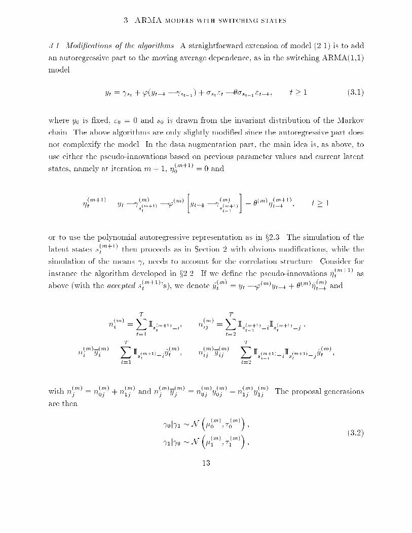
0 100 200 300 400 500

-50

5

(10 000 iterations)

means

0 2 4 6 8 10-0.0

25-0.0

15

0.005

0.020

variances

0 2 4 6 8 10

1.70

1.80

0.126

0.130

probabilities

0 2 4 6 8 10

0.160

.200.2

4

0.18

0.22

AR and MA coefficients

0 2 4 6 8 10

-0.810

-0.804

0.73

0.75Figure 3.2 { Performances of the algorithm for Sample 2 of Table 3.1.Sample 0 1 �20 �21 ' � �00 �11 n1 0:94 �0:12 0:122 0:102 0:32 0:17 0:26 0:31 2500:88 �0:11 0:147 0:132 0:22 0:06 0:28 0:312 0:0 0:0 1:59 0:109 �0:81 0:79 0:26 0:11 500�0:02 0:02 1:67 0:134 �0:81 0:76 0:24 0:193 0:0 0:2 1:35 0:185 �0:55 �0:17 0:16 0:61 2500:07 0:16 1:86 0:165 �0:52 �0:15 0:15 0:624 2:94 �1:72 0:562 0:102 0:27 0:27 0:74 0:69 1502:97 �1:75 0:454 0:112 �0:01 �0:02 0:73 0:71Table 3.1 { Parameters of the di�erent benchmarks used to test the MCMC method and corre-sponding Bayes estimates (second row).

0 50 100 150 200 250

-3-1

123

(10 000 iterations)

means

0 2 4 6 8 10

0.050

.200.3

5

0.10

0.14

0.18 variances

0 2 4 6 8 10

1.31.5

1.71.9

0.150

0.160

probabilities

0 2 4 6 8 10

0.14

0.18

0.60

0.62

AR and MA coefficients

0 2 4 6 8 10

-0.50

-0.46

-0.16

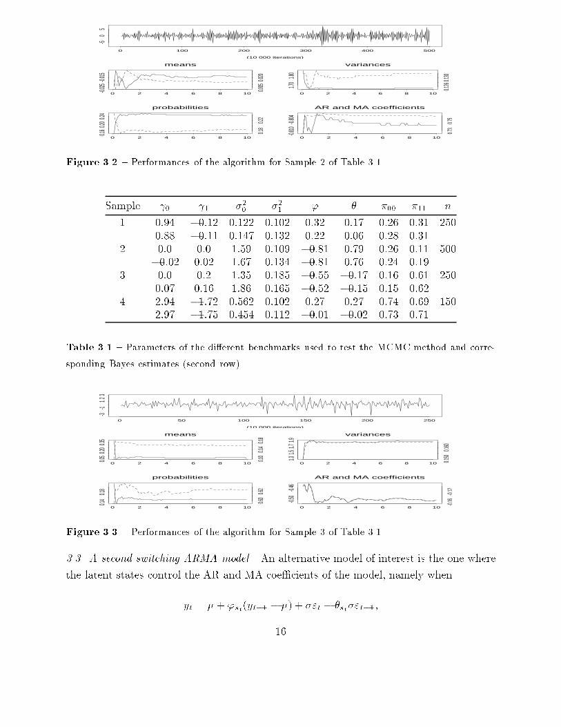
-0.12Figure 3.3 { Performances of the algorithm for Sample 3 of Table 3.1.3.3. A second switching ARMA model. An alternative model of interest is the one wherethe latent states control the AR and MA coe�cients of the model, namely whenyt = �+ 'st(yt�1 � �) + �"t � �st�"t�1;16

0 50 100 150

-20

24

(25 000 iterations)

means

0 5 10 15 20 25

2.96

3.02

-1.760

-1.740

variances

0 5 10 15 20 25

0.42

0.45

0.106

0.109

0.112

probabilities

0 5 10 15 20 25

0.730

0.745

0.760

0.700

.740.7

8

AR and MA coefficients

0 5 10 15 20 25

-0.4-0.2

0.0

-0.4-0.2

0.0Figure 3.4 { Performances of the algorithm for Sample 4 of Table 3.1.in the case of an ARMA(1; 1). Contrary to (3.1), the mean and variance parameters areconstant over the states. For simplicity's sake, we still assume that the number of statesis 2 and consider the following noninformative prior1� II[�1;1](�0)II[�1;1](�1)II[�1;1]('0)II[�1;1]('1):This setup does not allow for a simple extension of the second kind of algorithmdeveloped in x2.3 and we again focus on the �rst kind. The di�erence in the implementationis also of interest since it leads to a simpler MCMC algorithm. Indeed, the simulation ofthe latent states s(m)t remains essentially the same, namely to simulate fromP (s(m+1)t = k) / �s(m+1)t�1 k�ks(m)t+1 exp���yt � �� 'k(yt�1 � �) + �k�(m)t�1�2 =2�2�and actualize the pseudo-innovation�(m+1)t = yt � �(m) � '(m)s(m+1)t hyt�1 � �(m)i+ �(m)s(m+1)t �(m+1)t�1 :The acceptance probability of the new vector of allocations is then quite similar to theprevious ones. It is also straightforward to derive the following simulation steps for themean � and variance �.1. Simulate� � N 0BBBB@ TXt=1�1� '(m)s(m+1)t ��yt � '(m)s(m+1)t yt�1 + �(m)s(m+1)t � ~�(m)t�1TXt=1�1� '(m)s(m+1)t �2 ; ��(m)�2TXt=1�1� '(m)s(m+1)t �21CCCCA :17

2. Accept �(m+1) = � with probability min(1; !�) where!� = f(�j�(m); �(m)0 ; �(m)1 ; '(m)0 ; '(m)1 ; �(m)00 ; �(m)11 ; (s(m+1)t ); (yt))f(�(m)j�(m); �(m)0 ; �(m)1 ; '(m)0 ; '(m)1 ; �(m)00 ; �(m)11 ; (s(m+1)t ); (yt))� g(�(m)j�; �(m); �(m)0 ; �(m)1 ; '(m)0 ; '(m)1 ; �(m)00 ; �(m)11 ; (s(m+1)t ); (yt))g(�j�(m); �(m); �(m)0 ; �(m)1 ; '(m)0 ; '(m)1 ; �(m)00 ; �(m)11 ; (s(m+1)t ); (yt)) : (3:4)where g denotes the above normal density.Note that, in (3.4), the g in the numerator uses innovations based on � while the g in thedenominator is associated with �(m).3. Simulate��2 � Ga T2 ; 12 TXt=1(yt � �(m+1) � '(m)s(m+1)t (yt�1 � �(m+1)) + �(m)s(m+1)t ~�(m)t�1)2! :with ~�(m)t�1 based on �(m+1); �(m); �(m)0 ; �(m)1 ; '(m)0 ; '(m)1 and the s(m+1)t 's.The conditional distribution of ('0; '1) is given byf('0; '1) / exp(� 12�2 Xst=1(yt � �� '1(yt�1 � �) + �1�t�1)2� 12�2 Xst=0(yt � �� '0(yt�1 � �) + �0�t�1)2)and it leads to the following proposals:'0 � NF 0B@�0 Xs(m+1)t =0(yt�1 � �(m+1))(yt � �(m+1) + �(m)0 �(m)t�1); �0 ��(m+1)�21CA ;'1 � NF 0B@�1 Xs(m+1)t =1(yt�1 � �(m+1))(yt � �(m+1) + �(m)1 �(m)t�1); �1 ��(m+1)�21CA ;where NF denotes the folded normal distribution de�ned by the transform (2.4) and where�(m)t�1 is based on �(m+1); �(m+1); �(m)0 ; �(m)1 ; '(m)0 ; '(m)1 and the s(m+1)t 's, and��10 = Xs(m+1)t =0�yt�1 � �(m+1)�2 ; ��11 = Xs(m+1)t =1�yt�1 � �(m+1)�2 :18

The simulation of (�0; �1) is quite similar, the folded normal distributions being inthis case�0 � NF 0B@��0 Xs(m+1)t =0 �(m)t�1(yt � �(m+1) � '(m+1)0 (yt�1 � �(m+1))); �0 ��(m+1)�21CA ;�1 � NF 0B@��1 Xs(m+1)t =1 �(m)t�1(yt � �(m+1) � '(m+1)1 (yt�1 � �(m+1))); �1 ��(m+1)�21CA ;with ��10 = Xs(m+1)t =0(�(m)t�1)2; ��11 = Xs(m+1)t =1(�(m)t�1)2:

0 100 200 300 400 500

-10-5

05

(15 000 iterations)

AR coefficients

0 5 10 150.928

0.936

0.04

0.10

MA coefficients

0 5 10 15

-0.18

-0.14

-0.56

-0.52

probabilities

0 5 10 15

0.945

0.955

0.81

0.84

0.87 mean

0 5 10 15

-0.30

-0.20

variance

0 5 10 151.0

01.0

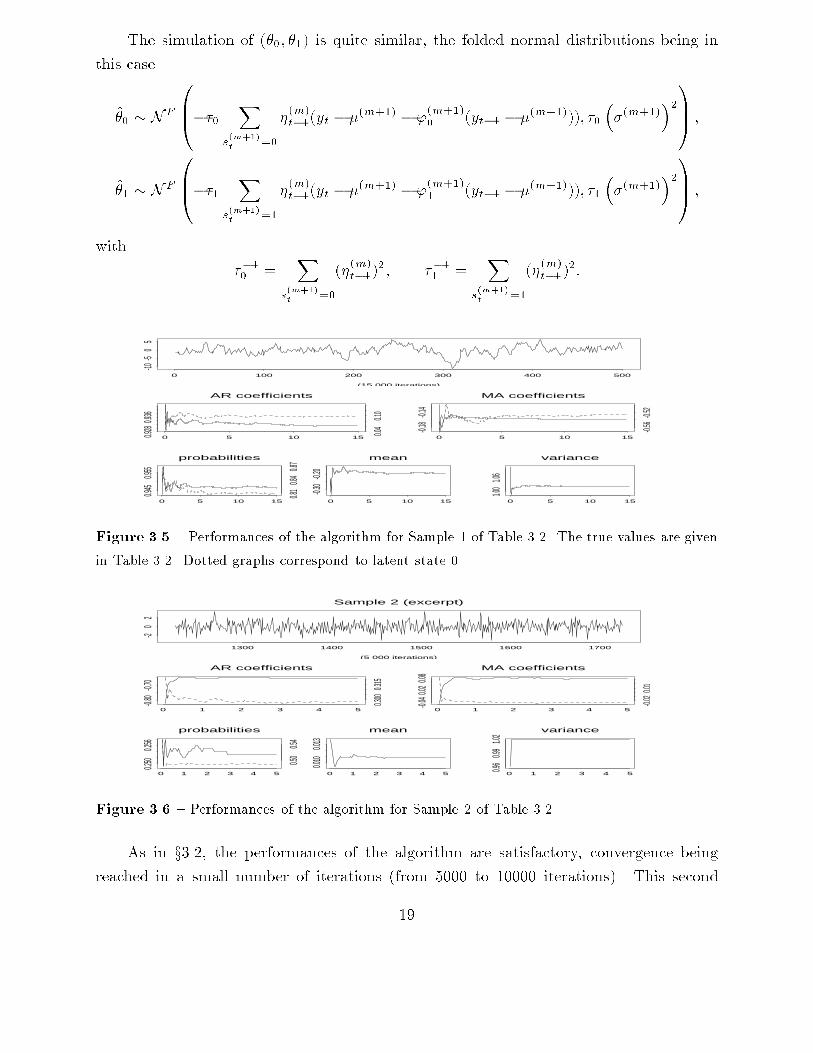
6Figure 3.5 { Performances of the algorithm for Sample 1 of Table 3.2. The true values are givenin Table 3.2. Dotted graphs correspond to latent state 0.

Sample 2 (excerpt)

1300 1400 1500 1600 1700

-20

2

(5 000 iterations)

AR coefficients

0 1 2 3 4 5

-0.80

-0.70

0.300

0.315

MA coefficients

0 1 2 3 4 5

-0.040

.020.0

8

-0.020

.01

probabilities

0 1 2 3 4 5

0.250

0.256

0.50

0.54

mean

0 1 2 3 4 5

0.010

0.013

variance

0 1 2 3 4 5

0.96

0.99

1.02Figure 3.6 { Performances of the algorithm for Sample 2 of Table 3.2.As in x3.2, the performances of the algorithm are satisfactory, convergence beingreached in a small number of iterations (from 5000 to 10000 iterations). This second19

type of switching ARMA models being more involved, the estimation of the correspondingparameters is more delicate and requires larger sample sizes to ensure a close �t for a givensample. As can be seen in Table 3.2, which describes the results of three simulations, bothlocation and scale parameters are well approximated in all cases, which is not always thecase for the AR and MA parameters or the transition probabilities.This can be attributedto the weak identi�ability of these models where an interplay between the AR and MAcoe�cients does not deeply perturbate the predictive properties of the model.Sample � �2 '0 '1 �0 �1 �00 �11 n1 0:00 1:00 0:02 0:95 �0:77 �0:07 0:79 0:94 500�0:18 1:03 0:098 0:934 �0:543 �0:154 0:82 0:942 0:00 1:00 0:32 �0:57 0:02 0:25 0:51 0:26 50000:01 1:02 0:30 �0:66 �0:02 0:08 0:49 0:253 0:00 1:00 0:33 �0:26 �0:81 0:79 0:50 0:50 2500�0:00 1:28 0:46 �0:34 �0:40 0:40 0:46 0:48Table 3.2 { Parameters of the di�erent benchmarks used to test the MCMC method and corre-sponding Bayes estimates (second row) for the dynamic switching ARMA(1,1) model.

Sample 3 (excerpt)

1300 1400 1500 1600 1700

-4-2

02

4

(25 000 iterations)

AR coefficients

0 5 10 15 20 25

0.42

0.46

-0.37-

0.35

MA coefficients

0 5 10 15 20 25

-0.44

-0.38

0.37

0.40

probabilities

0 5 10 15 20 25

0.47

0.49

0.49

0.51

mean

0 5 10 15 20 25

0.00.0

10

variance

0 5 10 15 20 25

1.285

1.300Figure 3.7 { Performances of the algorithm for Sample 3 of Table 3.2.3.4. An illustration on in ation data.The dataset corresponds to the Canadian seasonally unadjusted monthly data on theCPI from 1947 to 1993, already studied by Perron (1993). The in ation series is computedas the twelfth di�erence of the price index, and then stabilized by taking the �rst di�erence.Figure 3.8 presents both the price index and the in ation series and shows why the lastcorrection is necessary. 20

(25 000 iterations)

0 100 200 300 400 500

5010

015

0

Raw series

0 100 200 300 400 500

02

46

810

Twelfth difference series

0 5 10 15 20 25

-0.02

0.01

0.04 means

0.010

0.014

0 5 10 15 20 25

0.22

0.24

variances

0.018

50.0

200

probabilities

0 5 10 15 20 25

0.95

0.97

AR and MA coefficients

0 5 10 15 20 25

-0.66

-0.62

-0.58

-0.82

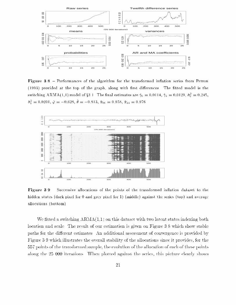
-0.78Figure 3.8 { Performances of the algorithm for the transformed in ation series from Perron(1993) provided at the top of the graph, along with �rst di�erences. The �tted model is theswitching ARMA(1,1) model of x3.1. The �nal estimates are 0 = 0:0114, 1 = 0:0129, �20 = 0:245,�21 = 0:0201, ' = �0:628, � = �0:813, �00 = 0:958, �11 = 0:976.

0 100 200 300 400 500

-3-1

123

(25 000 iterations)

0 100 200 300 400 500

050

0010

000

1500

020

000

2500

0

0 100 200 300 400 500

0.00.4

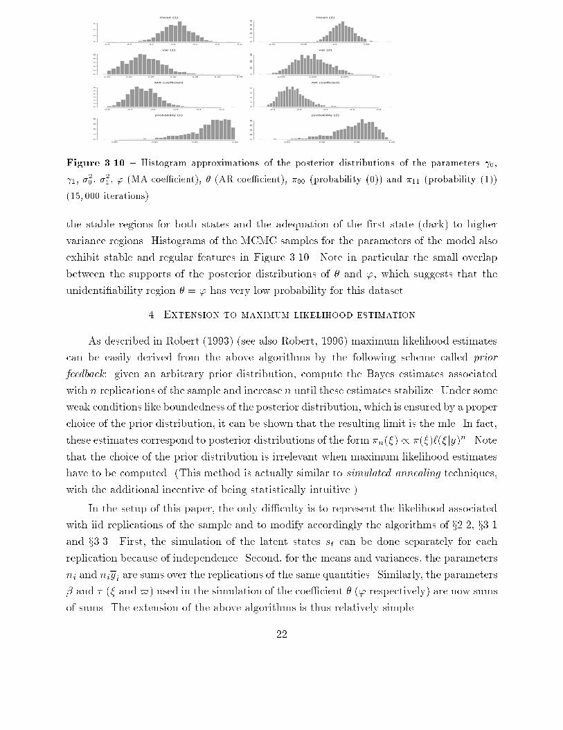
0.8Figure 3.9 { Successive allocations of the points of the transformed in ation dataset to thehidden states (dark pixel for 0 and grey pixel for 1) (middle) against the series (top) and averageallocations (bottom).We �tted a switching ARMA(1,1) on this dataset with two latent states indexing bothlocation and scale. The result of our estimation is given on Figure 3.8 which show stablepaths for the di�erent estimates. An additional assessment of convergence is provided byFigure 3.9 which illustrates the overall stability of the allocations since it provides, for the557 points of the transformed sample, the evolution of the allocation of each of these pointsalong the 25 000 iterations. When plotted against the series, this picture clearly shows21

-0.3 -0.2 -0.1 0.0 0.1 0.2 0.3

02

46

mean (1)

-0.10 -0.05 0.0 0.05

05

1015

2025

mean (2)

0.15 0.20 0.25 0.30 0.35 0.40 0.45

02

46

810

var (1)

0.015 0.020 0.025 0.030

050

100

150

var (2)

-0.8 -0.7 -0.6 -0.5 -0.4 -0.3

01

23

45

6

MA coefficient

-0.9 -0.8 -0.7 -0.6 -0.5

02

46

8

AR coefficient

0.85 0.90 0.95 1.00

05

1015

20

probability (1)

0.94 0.96 0.98 1.00

010

2030

40

probability (2)Figure 3.10 { Histogram approximations of the posterior distributions of the parameters 0, 1, �20 , �21 , ' (MA coe�cient), � (AR coe�cient), �00 (probability (0)) and �11 (probability (1))(15; 000 iterations).the stable regions for both states and the adequation of the �rst state (dark) to highervariance regions. Histograms of the MCMC samples for the parameters of the model alsoexhibit stable and regular features in Figure 3.10. Note in particular the small overlapbetween the supports of the posterior distributions of � and ', which suggests that theunidenti�ability region � = ' has very low probability for this dataset.4. Extension to maximum likelihood estimationAs described in Robert (1993) (see also Robert, 1996) maximum likelihood estimatescan be easily derived from the above algorithms by the following scheme called priorfeedback: given an arbitrary prior distribution, compute the Bayes estimates associatedwith n replications of the sample and increase n until these estimates stabilize. Under someweak conditions like boundedness of the posterior distribution, which is ensured by a properchoice of the prior distribution, it can be shown that the resulting limit is the mle. In fact,these estimates correspond to posterior distributions of the form �n(�) / �(�)`(�jy)n. Notethat the choice of the prior distribution is irrelevant when maximum likelihood estimateshave to be computed. (This method is actually similar to simulated annealing techniques,with the additional incentive of being statistically intuitive.)In the setup of this paper, the only di�culty is to represent the likelihood associatedwith iid replications of the sample and to modify accordingly the algorithms of x2.2, x3.1and x3.3. First, the simulation of the latent states st can be done separately for eachreplication because of independence. Second, for the means and variances, the parametersni and niyi are sums over the replications of the same quantities. Similarly, the parameters� and � (� and $) used in the simulation of the coe�cient � (' respectively) are now sumsof sums. The extension of the above algorithms is thus relatively simple.22

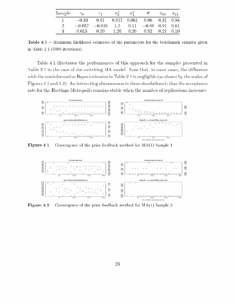
Sample 0 1 �20 �21 � �00 �111 �0:33 0:91 0:077 0:061 0:06 0:31 0:942 �0:057 �0:049 1:5 0:11 �0:86 0:91 0:613 0:013 0:20 1:26 0:20 0:52 0:27 0:10Table 4.1 { Maximum likelihood estimates of the parameters for the benchmark samples givenin Table 2.1 (5000 iterations).Table 4.1 illustrates the performances of this approach for the samples presented inTable 2.1 in the case of the switching MA model. Note that, in most cases, the di�erencewith the noninformative Bayes estimates in Table 2.1 is negligible (as shown by the scales ofFigures 4.1 and 4.2). An interesting phenomenon in these simulations is that the acceptancerate for the Hastings-Metropolis remains stable when the number of replications increases.

(5 000 iterations)

means

5 10 15

-0.335

-0.325

-0.315

0.91200

.91300.

91400.

9150 variances

5 10 15

0.080

0.090

0.100

0.0610

0.0620

probabilities

5 10 15

0.3150

.3200.32

50.330

0.931

0.933

0.935

0.937 MA coefficient

5 10 15

0.0560.

0580.06

00.062Figure 4.1 { Convergence of the prior feedback method for MA(1) Sample 1.

(5 000 iterations)

means

5 10 15 20

0.0130.

0140.01

50.016

0.19500

.19600.

19700.

1980 variances

5 10 15 20

1.260

1.264

1.268

0.2040

0.2050

0.2060

probabilities

5 10 15 20

0.2640.

2660.26

80.270

0.272

0.100

0.110

0.120

MA coefficient

5 10 15 200.5220

0.5224

0.5228Figure 4.2 { Convergence of the prior feedback method for MA(1) Sample 3.

23

ReferencesAlbert, J. and Chib, S. (1993) Bayesian inference for autoregressive time series with meanand variance subject to Markov jumps. J. Business Economic Stat. 11, 1{15.Billio, M. and Monfort, A. (1995) Switching state space models. Doc. travail CREST no.9557, Insee, Paris.Chib, S. (1994) Calculating posterior distributions and modal estimates in Markov mixturemodels. J. Econometrics, to appear.Chib, S. and Greenberg, E. (1995) Bayes inference for regression models with ARMA(p,q)errors. J. Econometrics 64, 183{206.Gelfand, A.E. and Smith, A.F.M. (1990) Sampling based approaches to calculating marginaldensities. Journal of the American Statistical Association 85, 398{409.Gelman, A., Gilks, W.R. and Roberts, G.O. (1996) E�cient Metropolis jumping rules. InBayesian Statistics 5, J.O. Berger, J.M. Bernardo, A.P. Dawid, D.V. Lindley and A.F.M.Smith (Eds.). Oxford University Press, Oxford, 599{608.Gilks, W.R., Richardson, S. and Spiegelhalter, D.I. (1996) Markov Chain Monte Carlo inPractice. Chapman and Hall, London.Gouri�eroux, C. and Monfort, A. (1996) Simulation Based Methods in Econometrics. Ox-ford University Press.Hamilton J.D. (1988), Rational-expectations econometric analysis of changes in regime:an investigation of the term structure of interest rates, Journal of Economic Dynamicsand Control, 12, 385-423.Hamilton J.D. (1989), A new approach to the economic analysis of nonstationary timeseries and the business cycle, Econometrica, 57(2), 357-384.Jaquier, E., Polson, N.G. and Rossi, P.E. (1994) Bayesian analysis of stochastic volatilitymodels (with discussion). J. Business Economic Stat. 12, 371{417.Jones, M.C. (1987) Randomly choosing parameters from the stationarity and invertibilityregion of autoregressive-moving average models. Applied Statistics (Serie C) 38, 134{138.Kim C.J. (1993), Unobserved-component time series models with Markov-switching het-eroscedasticity: changes in regime and the link between in ation rates and in ation un-certainty, Journal of Business and Economic Statistics, 113, 341-349.Kitagawa G. (1987), Non-Gaussian state-space modeling of nonstationary time series, Jour-nal of the American Statistical Association, 82, 1032-1063.24

Lee L.F. (1995), Simulation estimation of dynamic switching regression and dynamic dis-equilibrium models: some Monte Carlo results, Working Paper no. 95-12, Hong KongUniversity.Mengersen, K.L. and Robert, C.P. (1995) Testing for mixtures: a Bayesian entropic ap-proach (with discussion). In Bayesian Statistics 5, J.O. Berger, J.M. Bernardo, A.P.Dawid, D.V. Lindley and A.F.M. Smith (Eds.). Oxford: Oxford University Press.Perron P. (1993) Non-Stationarities and Non-Linearities in Canadian In ation, EconomicBehaviour and Policy Choice Under Price Stability. Proceedings of a Conference held atthe Bank of Canada in October 1993.Robert, C.P. (1993) Prior Feedback: A Bayesian approach to maximum likelihood estima-tion. Comput. Statist. 8, 279{294.Robert, C.P. (1996) M�ethodes de Monte Carlo par Cha�nes de Markov. Economica, Paris.Robert, C.P. and Titterington, M. (1996) Resampling schemes for hidden Markov modelsand their application for maximum likelihood estimation. Tech. report, Dept. of Statistics,University of Glasgow.Shephard, N. (1994) Partial non-Gaussian state space. Biometrika 81, 115{131.Tanner, M. et Wong, W. (1987) The calculation of posterior distributions by data aug-mentation. Journal of the American Statistical Association 82, 528{550.Tierney, L. (1994) Markov chains for exploring posterior distributions (avec discussion).Ann. Statist. 22, 1701{1786.25

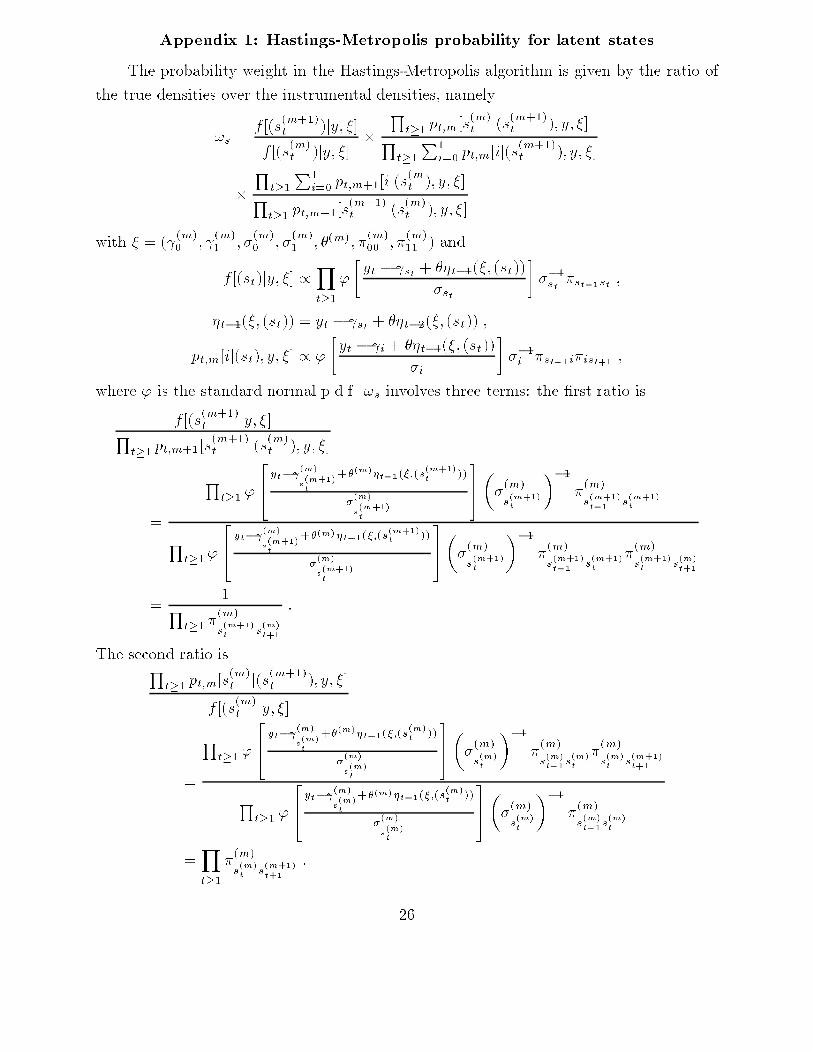
Appendix 1: Hastings-Metropolis probability for latent statesThe probability weight in the Hastings-Metropolis algorithm is given by the ratio ofthe true densities over the instrumental densities, namely!s = f [(s(m+1)t )jy; �]f [(s(m)t )jy; �] � Qt�1 pt;m[s(m)t j(s(m+1)t ); y; �]Qt�1P1i=0 pt;m[ij(s(m+1)t ); y; �]� Qt�1P1i=0 pt;m+1[ij(s(mt ); y; �]Qt�1 pt;m+1[s(m+1)t j(s(m)t ); y; �]with � = ( (m)0 ; (m)1 ; �(m)0 ; �(m)1 ; �(m); �(m)00 ; �(m)11 ) andf [(st)jy; �] /Yt�1' �yt � st + ��t�1(�; (st))�st � ��1st �st�1st ;�t�1(�; (st)) = yt � st + ��t�2(�; (st)) ;pt;m[ij(st); y; �] / ' �yt � i + ��t�1(�; (st))�i � ��1i �st�1i�ist+1 ;where ' is the standard normal p.d.f. !s involves three terms: the �rst ratio isf [(s(m+1)t jy; �]Qt�1 pt;m+1[s(m+1)t j(s(m)t ); y; �]= Qt�1 '24yt� (m)s(m+1)t +�(m)�t�1(�;(s(m+1)t ))�(m)s(m+1)t 35��(m)s(m+1)t ��1 �(m)s(m+1)t�1 s(m+1)tQt�1 '24 yt� (m)s(m+1)t +�(m)�t�1(�;(s(m+1)t ))�(m)s(m+1)t 35��(m)s(m+1)t ��1 �(m)s(m+1)t�1 s(m+1)t �(m)s(m+1)t s(m)t+1= 1Qt�1 �(m)s(m+1)t s(m)t+1 :The second ratio isQt�1 pt;m[s(m)t j(s(m+1)t ); y; �]f [(s(m)t jy; �]= Qt�1 '24 yt� (m)s(m)t +�(m)�t�1(�;(s(m)t ))�(m)s(m)t 35��(m)s(m)t ��1 �(m)s(m)t�1s(m)t �(m)s(m)t s(m+1)t+1Qt�1 '24 yt� (m)s(m)t +�(m)�t�1(�;(s(m)t ))�(m)s(m)t 35��(m)s(m)t ��1 �(m)s(m)t�1s(m)t=Yt�1�(m)s(m)t s(m+1)t+1 : 26

The third ratio isYt�1 P1i=0 pt;m+1[ij(s(m)t ); y; �]P1i=0 pt;m[ij(s(m+1)t ); y; �]= Qt�1P1i=0 ' � yt� (m)i +�(m)�t�1(�;(s(m+1)t )�(m)i ���(m)i ��1 �(m)s(m+1)t�1 i�(m)is(m)t+1Qt�1P1i=0 ' � yt� (m)i +�(m)�t�1(�;(s(m)t ))�(m)i � ��(m)i ��1 �(m)s(m)t�1i�(m)is(m+1)t+1

27