
Bayesian Optimization — — - GDR Mascot-Num
122
1/223 Bayesian Optimization — Engineering design under uncertainty using expensive-to-evaluate numerical models — Julien Bect and Emmanuel Vazquez Laboratoire des signaux et systèmes, Gif-sur-Yvette, France CEA-EDF-INRIA Numerical Analysis Summer School Université Pierre et Marie Curie (Paris VI) Paris, 2017, July 3–7 2/223 Lecture 1 : From meta-models to UQ 1.1 Introduction 1.2 Black-box modeling 1.3 Bayesian approach 1.4 Posterior distribution of a quantity of interest 1.5 Complements on Gaussian processes Lecture 2 : Bayesian optimization (BO) 2.1. Decision-theoretic framework 2.2. From Bayes-optimal to myopic strategies 2.3. Design under uncertainty References
-
Upload
khangminh22 -
Category
Documents
-
view
2 -
download
0
Transcript of Bayesian Optimization — — - GDR Mascot-Num

1/223
Bayesian Optimization
—Engineering design under uncertainty using
expensive-to-evaluate numerical models—
Julien Bect and Emmanuel Vazquez
Laboratoire des signaux et systèmes, Gif-sur-Yvette, France
CEA-EDF-INRIA Numerical Analysis Summer School
Université Pierre et Marie Curie (Paris VI)
Paris, 2017, July 3–7
2/223
Lecture 1 : From meta-models to UQ
1.1 Introduction
1.2 Black-box modeling
1.3 Bayesian approach
1.4 Posterior distribution of a quantity of interest
1.5 Complements on Gaussian processes
Lecture 2 : Bayesian optimization (BO)
2.1. Decision-theoretic framework
2.2. From Bayes-optimal to myopic strategies
2.3. Design under uncertainty
References

3/223
Lecture 1 : From meta-models to UQ
1.1 Introduction
1.2 Black-box modeling
1.3 Bayesian approach
1.4 Posterior distribution of a quantity of interest
1.5 Complements on Gaussian processes
Lecture 2 : Bayesian optimization (BO)
2.1. Decision-theoretic framework
2.2. From Bayes-optimal to myopic strategies
2.3. Design under uncertainty
References
4/223
Lecture 1 : From meta-models to UQ
1.1 Introduction
1.2 Black-box modeling
1.3 Bayesian approach
1.4 Posterior distribution of a quantity of interest
1.5 Complements on Gaussian processes

5/223
Computer-simulation based design
The numerical model might be time- or resource-consuming
Design parameters might be subject to dispersions
The system might operate under unknown conditions
6/223
Computer-simulation based design – Example
Computer simulations to design a product or a process, in particular
to find the best feasible values for design parameters (optimization problem) to minimize the probability of failure of a product
To comply with European emissions
standards, the design parameters of
combustion engines have to be carefully
optimized
The shape of intake ports controls
airflow characteristics, which have direct
impact on the performances of the engine emissions of NOx and CO
f : X ⊂ Rd → R performance as a
function of design parameters
(d = 20 ∼ 100)
Computing f (x) takes 5 ∼ 20 hours
Objective: estimate x⋆ = argmaxx f (x)
Simulation of an intake port (Navier-Stokes equ.)
(courtesy of Renault)

7/223
Lecture 1 : From meta-models to UQ
1.1 Introduction
1.2 Black-box modeling
1.3 Bayesian approach
1.4 Posterior distribution of a quantity of interest
1.5 Complements on Gaussian processes
8/223
Black-box modeling

8/223
Black-box modeling
For simplification → drop u
9/223
Black-box modeling
Let f : X → R be a real function defined on X ⊆ Rd , where
X is the input/parameter domain of the computer simulation
under study, or the factor (from Latin, “which acts”) space
f is a performance or cost function (a function of the outputs
of the computer simulation)

10/223
Black-box modeling
Let x1, . . . , xn ∈ X be n simulations points
Denote by
z1 = f (x1), . . . , zn = f (xn)
the corresp. simulation results (observations/evaluations of f )
Our objective: use the data Dn = (xi , zi)i=1...n to infer
properties about f
Example: given a new x ∈ Rd , predict the value f (x)
11/223
Black-box modeling
f is a black-box, only known through evaluation results: query
an evaluation at x , observe the result
Predict the value of f at a given x?
→ the problem is that of constructing an approximation / an
estimator fn of f from Dn
Such a fn also called a model or a meta-model (because the
numerical simulator is a model itself) of f

12/223
A simple curve fitting problem
Suppose that we are given a data set of n simulation results,
i.e., evaluations results of an unknown function f : [0, 1] → R,
at points x1, . . . , xn.
A data set of size n = 8:
0 0.2 0.4 0.6 0.8 1-2
-1.5
-1
-0.5
0
0.5
1
1.5
x
z
13/223
A simple curve fitting problem
Any approximation procedure of f consists in building a
function fn = h(·; θ) where θ ∈ Rl is a vector of parameters,
to be estimated from Dn and available prior information
Fundamental example: linear model
fn(x) = h(x , θ) =l∑
i=1
θi ri(x)
where functions ri : X → R are called regressors (e.g.,
r1(x) = 1, r2(x) = x , r3(x) = x2 . . . → polynomial model)
Most classical method to obtain a good value of b:
least squares → minimize the sum of squared errors
J(θ) =n∑
i=1
(zi − fn(xi)
)2=
n∑
i=1
(zi − h(xi ; θ))2

14/223
A simple curve fitting problem
Linear fit
0 0.2 0.4 0.6 0.8 1-2
-1.5
-1
-0.5
0
0.5
1
1.5
x
z
15/223
A simple curve fitting problem
Quadratic fit
0 0.2 0.4 0.6 0.8 1-2
-1.5
-1
-0.5
0
0.5
1
1.5
x
z
16/223
A simple curve fitting problem
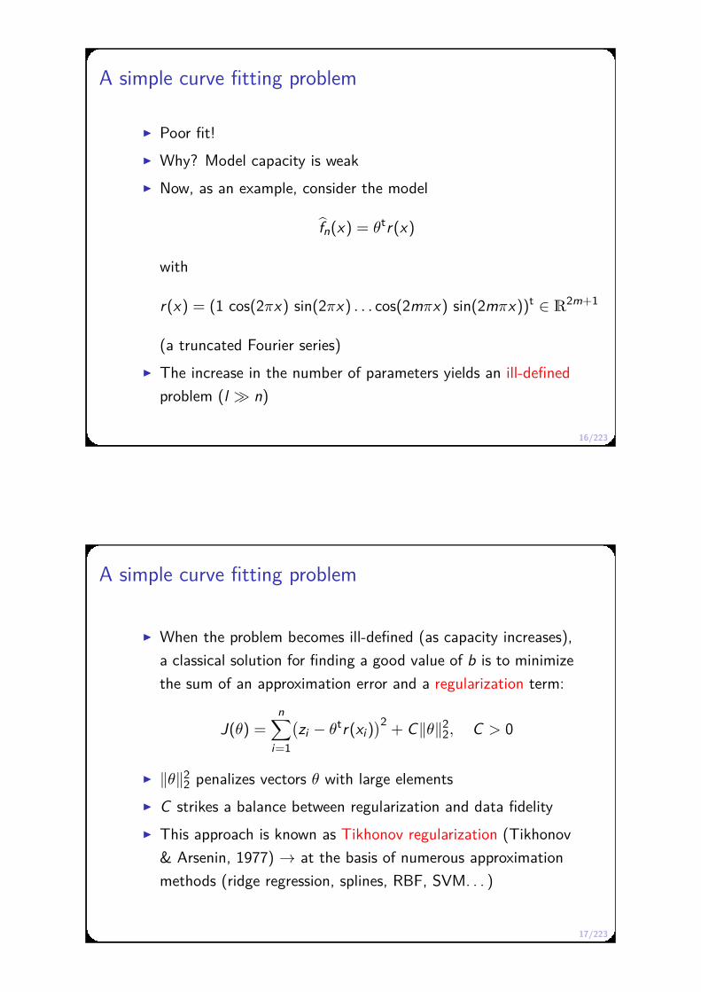
Poor fit!
Why? Model capacity is weak
Now, as an example, consider the model
fn(x) = θtr(x)
with
r(x) = (1 cos(2πx) sin(2πx) . . . cos(2mπx) sin(2mπx))t ∈ R2m+1
(a truncated Fourier series)
The increase in the number of parameters yields an ill-defined
problem (l ≫ n)
17/223
A simple curve fitting problem
When the problem becomes ill-defined (as capacity increases),
a classical solution for finding a good value of b is to minimize
the sum of an approximation error and a regularization term:
J(θ) =n∑
i=1
(zi − θtr(xi)
)2+ C‖θ‖2
2, C > 0
‖θ‖22 penalizes vectors θ with large elements
C strikes a balance between regularization and data fidelity
This approach is known as Tikhonov regularization (Tikhonov
& Arsenin, 1977) → at the basis of numerous approximation
methods (ridge regression, splines, RBF, SVM. . . )

18/223
A simple curve fitting problem
n = 8, m = 50, l = 101, C = 10−8
0 0.2 0.4 0.6 0.8 1-2
-1.5
-1
-0.5
0
0.5
1
1.5
x
z
19/223
A simple curve fitting problem
The regularization principle alone is not enough to obtain a
good approximation
As modeling capacity increases, overfitting may arise

20/223
A simple curve fitting problem
To avoid overfitting, we should try a regularization that
penalizes high frequencies more
For instance, take
‖θ‖ = θ21 +
m∑
k=1
θ22k + θ2
2k+1
(1 + (2kπ)α)2
21/223
A simple curve fitting problem
n = 8, m = 50, l = 101, C = 10−8, α = 1.3
0 0.2 0.4 0.6 0.8 1-2
-1.5
-1
-0.5
0
0.5
1
1.5
x
z

22/223
A simple curve fitting problem
From this example, we can see that the construction of a
regularization scheme should result from a procedure that
takes into account the data (using cross-validation, for
instance) an/or prior knowledge
(high frequencies ≪ low frequencies, for instance)
23/223
Black-box modeling
A large number of methods are available in the literature:
polynomial regression, splines, NN, RBF. . .
All methods are based on mixing prior information and
regularization principles
Instances of “regularization” in regression: t-tests, F-tests, ANOVA, AIC (Akaike info criterion). . . in linear
regression Early stopping in NN Regularized reproducing-kernel regression
1960 : splines, (Schoenberg 1964, Duchon 1976–1979)
1970 : ridge regression (Hoerl, Kennard)
1980 : RBF, (Micchelli 1986, Powel 1987)
1995 : SVM, (Vapnik 1995)
1997 : SVR, (Smola 1997) & semi-param SVR (Smola 1999)

24/223
Black-box modeling
How to choose a regularization scheme?
The Bayesian setting is a principled approach that makes it
possible to construct regularized regressions
25/223
Lecture 1 : From meta-models to UQ
1.1 Introduction
1.2 Black-box modeling
1.3 Bayesian approach
1.4 Posterior distribution of a quantity of interest
1.5 Complements on Gaussian processes

26/223
Why a Bayesian approach?
Objective: infer properties about f : X → R through
pointwise evaluations
Why a Bayesian approach? a principled approach to choose a regularization scheme
according to prior information through probability calculus and/or Monte Carlo simulations,
the user can infer properties about the unknown function for instance: given prior knowledge and Dn, what is the
probability that the global maximum of f is greater than a
given threshold u ∈ R?
Main idea: use a statistical model of the observations,
together with a probability model for the parameter of the
statistical model
27/223
Some reminders about probabilities
Recall that a random variable is a function that maps a sample
space Ω to an outcome space E (e.g. E = R), and that assigns
probabilities (weights) to possible outcomes
Def.
Formally, let (Ω, A, P) be a probability space, and (E , E) be a measurable
outcome space
→ a random variable X is a measurable function (Ω, A, P) → (E , E)
X is used to assign probabilities to events: for instance
P(X ∈ [0, 1]) = PX ([0, 1]) = 1/2
Case of a random variable with a density
P(X ∈ [a, b]) = PX ([a, b]) =∫ b
a
pX (x)dx
28/223
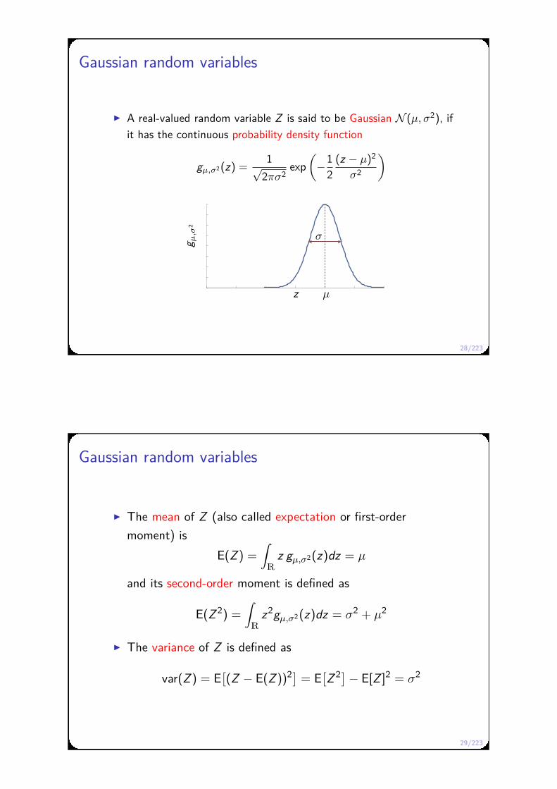
Gaussian random variables
A real-valued random variable Z is said to be Gaussian N (µ, σ2), if
it has the continuous probability density function
gµ,σ2(z) =1√
2πσ2exp
(−1
2(z − µ)2
σ2
)
z
g µ,σ
2
µ
σ
29/223
Gaussian random variables
The mean of Z (also called expectation or first-order
moment) is
E(Z ) =∫
R
z gµ,σ2(z)dz = µ
and its second-order moment is defined as
E(Z 2) =∫
R
z2gµ,σ2(z)dz = σ2 + µ2
The variance of Z is defined as
var(Z ) = E[(Z − E(Z ))2] = E
[Z 2]− E[Z ]2 = σ2

30/223
Gaussian random variables
A Gaussian variable Z can be used as a stochastic model of
some uncertain real-valued quantity
In other words, Z can be thought as a prior about some
uncertain quantity of interest
31/223
Gaussian random variables
Using a random generator, it is possible to “generate”
sample values z1, z2, . . . of our model Z → possible values for
our uncertain quantity of interest
−6 −4 −2 0 2 4 60
0.05
0.1
0.15
0.2
0.25
0.3
0.35
0.4
0.45n=1000

32/223
Bayesian model
Formally, recall that a statistical model is a triplet M = (Z, F , P)
Z → observation space (typically, Z = Rn)
F → σ-algebra on Z P → parametric family Pθ; θ ∈ Θ of probability
distributions on (Z, F)
Def.
A Bayesian model is defined by the specification of
a parametric statistical model M (model of the observations)
a prior probability distribution Π on (Θ, Ξ) → probability
model that describes uncertainty about θ before an
observation is made
33/223
Example
Suppose we repeat measurements of a quantity of interest:
z1, z2, . . . ∈ R
Model of observations: Ziiid∼ N (θ1, θ2), i = 1, . . . , n
The statistical model can formally be written as the triplet
M =(R
n, B(Rn),N (θ1, θ2)⊗n
θ1,θ2
)
Moreover, if we a assume a prior distribution about θ1 and θ2
(e.g. θ1 ∼ N (1, 1), θ2 ∼ IG(3, 2)), we obtain a
Bayesian model
From this Bayesian model (model of observations + prior), we
can compute the posterior distribution of (θ1, θ2) given
Z1, . . . , Zn (will be explained later)

34/223
Example
n = 50, θ1 = 1.2, θ2 = 0.8
sample size n=50
-1 0 1 2 3 4
zi
0
0.1
0.2
0.3
0.4p
df
prior
0 1 2
0.5
1
1.5
2posterior
0 1 2
0.5
1
1.5
2
θ1θ1
θ 2θ 2
35/223
Simple curve fitting problem from a Bayesian approach
Recall our simple curve fitting model
fn(x) = θtr(x)
with
r(x) = (1 cos(2πx) sin(2πx) . . . cos(2mπx) sin(2mπx))t ∈ R2m+1
Bayesian model?

36/223
Assume the following statistical model for the observations:
Zi = ξ(xi) + εi , i = 1, . . . , n
ξ(x) = θtr(x), x ∈ X
εiiid∼ N (0, σ2
ε)
or equivalently,
Ziiid∼ N (θtr(xi), σ2
ε), i = 1, . . . , n
Moreover, choose a prior distribution for θ:
θjindep∼ N (0, σ2
θj), j = 1, . . . , 2m + 1
The rvs Zi constitute a Bayesian model of the observations
ξ is a random function / random process → prior about f
37/223
Random process
Def.
A random process ξ : (Ω,X) → R is a collection of random
variables ξ(·, x) : Ω → R indexed by x ∈ X
Random processes can be viewed as a generalization of
random vectors
For a fixed ω ∈ Ω, the function ξ(ω, ·) : X → R is called a
sample path

38/223
In our Bayesian setting, we can say that we use a random process ξ as a stochastic model of the
unknown function f
f is viewed as as sample paths of ξ
ξ represents our knowledge about f before any evaluation has
been made the distribution Π = Pξ is a prior about f
All real functions
Prior Pξ
Unknown function f
39/223
Here, ξ(ω, ·) = θ(ω)tr(·) Fixing ω (a sample path) amounts to “choosing” a value for
the random vector θ

40/223
Example of sample paths with
θ1 ∼ N (0, 1)
θ2k , θ2k+1indep∼ N
(0, 1
1+(ω0k)α
), k = 1, . . . , m
with ω0 = 2π10 , α = 4
0 0.1 0.2 0.3 0.4 0.5 0.6 0.7 0.8 0.9 1
x
-4
-3
-2
-1
0
1
2
3
z
40/223
Example of sample paths with
θ1 ∼ N (0, 1)
θ2k , θ2k+1indep∼ N
(0, 1
1+(ω0k)α
), k = 1, . . . , m
with ω0 = 2π50 , α = 4
0 0.1 0.2 0.3 0.4 0.5 0.6 0.7 0.8 0.9 1
x
-8
-6
-4
-2
0
2
4
6
8
z

40/223
Example of sample paths with
θ1 ∼ N (0, 1)
θ2k , θ2k+1indep∼ N
(0, 1
1+(ω0k)α
), k = 1, . . . , m
with ω0 = 2π10 , α = 1.5
0 0.1 0.2 0.3 0.4 0.5 0.6 0.7 0.8 0.9 1
x
-3
-2
-1
0
1
2
3
z
41/223
Bayesian approach
The choice of a prior in a Bayesian approach reflects the
user’s knowledge about uncertain parameters
In the case of function approximation → regularity of the
function

42/223
Bayesian approach
Where shall we go now?
Objective: compute posterior distributions from data
0 0.2 0.4 0.6 0.8 1-4
-3
-2
-1
0
1
2
3
4
x
z
42/223
Bayesian approach
Where shall we go now?
Objective: compute posterior distributions from data
0 0.2 0.4 0.6 0.8 1-4
-3
-2
-1
0
1
2
3
4
x
z

42/223
Bayesian approach
Where shall we go now?
Objective: compute posterior distributions from data
0 0.2 0.4 0.6 0.8 1-4
-3
-2
-1
0
1
2
3
4
x
z
43/223
A “simplification” of the Bayesian model for the simple
curve fitting problem
ξ = θtr (our prior about f ) is a Gaussian process
Why?

44/223
Gaussian random vectors
Def.
A real-valued random vector Z = (Z1, . . . , Zd) ∈ Rd is said to be
Gaussian iff any linear combination of its components∑d
i=1 aiZi ,
with a1, . . . , ad ∈ R, is a Gaussian variable
A Gaussian random vector Z is characterized by its mean
vector, µ = (E[Z1], . . . , E[Zd ]) ∈ Rd , and the covariance of
the pairs of components (Zi , Zj), i , j ∈ 1, . . . , d,
cov(Zi , Zj) = E[(Zi − E(Zi))(Zj − E(Zj))]
If Z ∈ Rd is a Gaussian vector with mean µ ∈ R
d and
covariance matrix Σ ∈ Rd×d , we shall write Z ∼ N (µ, Σ)
45/223
Exercise: Let Z ∼ N (µ, Σ). Determine E(∑d
i=1 aiZi
)and
var(∑d
i=1 aiZi
)
The correlation coefficient of two components Zi and Zj of Z
is defined by
ρ(Zi , Zj) =cov(Zi , Zj)√var(Zi)var(Zj)
∈ [−1, 1],
→ measures the similarity between Zi and Zj

46/223
Gaussian random vectors: correlation
ρ = 0
−4 −3 −2 −1 0 1 2 3 4
−3
−2
−1
0
1
2
3
ρ = 0.8
−4 −3 −2 −1 0 1 2 3 4−4
−3
−2
−1
0
1
2
3
4
47/223
Gaussian random processes
Recall that a random process is a set ξ = ξ(x), x ∈ X of
random variables indexed by the elements of X
Gaussian random process
→ generalization of a Gaussian random vector
Def.
ξ is a Gaussian random process iff, ∀n ∈ N, ∀x1, . . . , xn ∈ X, and
∀a1, . . . , an ∈ R, the real-valued random variable
n∑
i=1
aiξ(xi)
is Gaussian

48/223
Application
If
ξ(x) = θtr(x), x ∈ X
θjindep∼ N (0, σ2
θj), j = 1, . . . , 2m + 1
then, ∀x1, . . . , xn ∈ X, and ∀a1, . . . , an ∈ R,
n∑
i=1
aiξ(xi) =∑
i
ai
(∑
j
θj rj(xi))
=∑
j
(∑
i
ai rj(xi))θj ∼ N
(0,∑
j
(∑
i
ai rj(xi))2
σ2θj
)
Thus, ξ = θtr is a Gaussian process
49/223
Gaussian random processes
A Gaussian process is characterized by its mean function
m : x ∈ X 7→ E[ξ(x)]
and its covariance function
k : (x , y) ∈ X2 7→ cov(ξ(x), ξ(y))
Notation: ξ ∼ GP (m, k)

50/223
Exercise: determine E(∑d
i=1 aiξ(xi))
and var(∑d
i=1 aiξ(xi))
What is the distribution of∑
aiξ(xi)?
→ The distribution of a linear combination of a Gaussian process
GP(m, k) can be simply obtained as a function of m and k
51/223
Application
If
ξ(x) = θtr(x), x ∈ X
θjindep∼ N (0, σ2
θj), j = 1, . . . , 2m + 1
then,
ξ ∼ GP(0, k)
with
k : (x , y) 7→∑
j
σ2θj
rj(x)rj(y)

52/223
Covariance function corresponding to
θ1 ∼ N (0, 1)
θ2k , θ2k+1indep∼ N
(0, 1
1+(ω0k)α
), k = 1, . . . , m
with ω0 = 2π10 , α = 4
-0.5 0 0.5
h
-0.8
-0.6
-0.4
-0.2
0
0.2
0.4
0.6
0.8
k
52/223
Covariance function corresponding to
θ1 ∼ N (0, 1)
θ2k , θ2k+1indep∼ N
(0, 1
1+(ω0k)α
), k = 1, . . . , m
with ω0 = 2π50 , α = 4
-0.5 0 0.5
h
-1.5
-1
-0.5
0
0.5
1
1.5
2
2.5
3
k
53/223
The covariance of a Gaussian random process
Main properties: a covariance function k is symmetric: ∀x , y ∈ X, k(x , y) = k(y , x) positive:
∀n ∈ N, ∀x1, . . . , xn ∈ X, ∀a1, . . . , an ∈ R,
n∑
i,j=1
aik(xi , xj)aj ≥ 0
In the following, we shall assume that the covariance of
ξ ∼ GP(m, k) is invariant under translations, or stationary:
k(x + h, y + h) = k(x , y), ∀x , y , h ∈ X
When k is stationary, there exists a stationary covariance
ksta : Rd → R such that
cov(ξ(x), ξ(y)) = k(x , y) = ksta(x − y)
54/223
Stationary covariances
When k is stationary, the variance
var(ξ(x)) = cov(ξ(x), ξ(x)) = k(0)
does not depend on x
The covariance function can be written as
k(x − y) = σ2ρ(x − y) ,
with σ2 = var(ξ(x)), and where ρ is the correlation function
of ξ.

55/223
Stationary covariances
The graph of the correlation function is a symmetric “bell
curve” shape
−4 −3 −2 −1 0 1 2 3 40
0.2
0.4
0.6
0.8
1
correlation range
56/223
We have, by C-S,
∀h ∈ X, |k(h)| =∣∣cov(ξ(x), ξ(x + h))
∣∣
=∣∣E[(ξ(x) − m(x))(ξ(x + h) − m(x + h))]
∣∣
≤ E((ξ(x) − m(x))2)1/2E((ξ(x + h) − m(x + h))2)1/2
= k(0)1/2k(0)1/2 = k(0)
Recall, Bochner’s spectral representation theorem
Theorem
A real function k(h), h ∈ Rd is symmetric positive iff it is the Fourier
transform of a finite positive measure, i.e.
k(h) =∫
Rd
eı(u,h)dµ(u) ,
where µ is a finite positive measure on Rd .

57/223
Gaussian process simulation
Using a random generator, it is possible to “generate” sample
paths f1, f2, . . . of a Gaussian process ξ
−2 −1 0 1 20
0.2
0.4
0.6
0.8
1
−2 −1 0 1 2−4
−2
0
2
4
−2 −1 0 1 20
0.2
0.4
0.6
0.8
1
−2 −1 0 1 2−4
−2
0
2
4
58/223
Gaussian process simulation
How to simulate sample paths of a zero-mean Gaussian random
process?
Choose a set of points x1, . . . xn ∈ X
Denote by K the n × n covariance matrix of the random
vector ξ = (ξ(x1), . . . , ξ(xn))t (NB: ξ ∼ N (0, K ))
Consider the Cholesky factorization of K
K = CC t ,
with C a lower triangular matrix (such a factorization exists
since K is a sdp matrix)
Let ε = (ε1, . . . , εn)t a Gaussian vector with εii.i.d∼ N (0, 1)
Then Cε ∼ N (0, K )

59/223
“Simplification” of the Bayesian model for the simple curve
fitting problem
Instead of choosing the model
ξ(x) = θtr(x), x ∈ X
θjindep∼ N (0, σ2
θj), j = 1, . . . , 2m + 1
simply choose a covariance function k and assume
ξ ∼ GP(0, k)
More details about how to choose k will be given below
60/223
Posterior
How to compute a posterior distribution, given the
Gaussian-process prior ξ and data?
0 0.2 0.4 0.6 0.8 1
x
-4
-3
-2
-1
0
1
2
3
4
z
61/223
Conditional distributions
Let X be a random variable modeling an unknown quantity of
interest
Assume we observe a random variable T , or a random vector
T = (T1, . . . , Tn)
Provided that T and X are not independent, T contains
information about X
Aim: define a notion of distribution of X “knowing” T
62/223
Conditional probabilities
Recall the following
Def.
Let (Ω, A, P) be a probability space. Given two events A, B ∈ Asuch that P(B) 6= 0, define the probability of A given B (or
conditional on B) by
P(A | B) =P(A ∩ B)
P(B)

63/223
The notion of conditional density
Def.
Assume that the pair (X , T ) ∈ R2 has a density p(X ,T ).
Define the conditional density of X given the event T = t by
pX |T (x | t) =
p(X ,T )(x , t)pT (t)
=p(X ,T )(x , t)∫pX ,T (x , t)dx
if pT (t) > 0
arbitrary density if pT (t) = 0.
64/223
Application
Given a Gaussian random vector Z = (Z1, Z2) ∼ N (0, Σ), what is
the distribution of Z2 “knowing” Z1? Define
pZ2|Z1 (z2|z1) =p(Z2,Z1)(z2, z1)
pZ1 (z1)=
σ1
(2π)1/2(det Σ)1/2exp(−1/2(ztΣ−1z−z2
1 /σ21))
→ Gaussian distribution!
−4 −3 −2 −1 0 1 2 3 4−4
−3
−2
−1
0
1
2
3
4
The random variable denoted
by Z2 | Z1 with density
pZ2|Z1(· | Z1) represents the
residual uncertainty about Z2
when Z1 has been observed
High correlation → small
residual uncertainty

65/223
Conditional mean/expectation
A fundamental notion: conditional expectation
Def.
Assume that the pair (X , T ) has a density p(X ,T ). Define the
conditional mean of X given T = t as
E(X | T = t)∆=∫
R
x pX |T (x |t)dx = h(t)
Def.
The random variable E(X | T ) = h(T ) is called the conditional
expectation of X given T
66/223
Conditional expectation
Why conditional expectation is an fundamental notion?
We have the following
Theorem
Under the previous assumptions, the solution of the problem
X = argminY E[(X − Y )2
]
where the minimum is taken over all functions of T is given by
X = E(X | T )
In other words, E(X | T ) is the best approximation (in the
sense of the quadratic mean) of X by a function of T

67/223
Important properties of conditional expectation
(1) E(X | T ) is a random variable depending on T → there exists
a function h such that E(X | T ) = h(T )
(2) The operator πH : X 7→ E(X | T ) is a (linear) operator of
orthogonal projection onto the space of all functions of T (for
the inner product X , Y 7→ (X , Y ) = E (XY ))
(3) Let X , Y , T ∈ L2. Then
i) ∀α ∈ R, E(αX + Y | T ) = αE(X | T ) + E(Y | T ) a.s.
ii) E(E[X | T ]) = E(X )
iii) If X ⊥⊥ T , E(X | T ) = E(X )
68/223
Conditional expectation: Gaussian random variables
Recall that the space of second-order random variables
L2(Ω, A, P) endowed with the inner product
X , Y 7→ (X , Y ) = E (XY ) is a Hilbert space
Gaussian linear space
Def.
A linear subspace G of L2(Ω, A, P) is Gaussian iff
∀X1, . . . , Xn ∈ G and ∀a1, . . . , an ∈ R the random variable∑
i aiXi is Gaussian
In what follows, assume that G is centered, i.e., each element
in G is a zero-mean random variable

69/223
Theorem (Projection theorem in centered Gaussian spaces)
Let G be a centered Gaussian space. Let X , T1, . . . , Tn ∈ G. Then
E(X | T1, . . . , Tn) is the orthogonal projection (in L2) of X on
T = spanT1, . . . , Tn.
proof Let X ∈ G be the orthogonal projection of X on T .
we have X = X + ε where ε ∈ G is orthogonal to T .
In G, orthogonality ⇔ independence. Thus, ε ⊥⊥ Ti , i = 1, . . . , n.
Then,
E(X | T1, . . . , Tn) = E(X | T1, . . . , Tn) + E(ε | T1, . . . , Tn)
= X + E(ε) = X
The result follows.
70/223
Application
Let Z = (Z1, Z2) be a zero-mean Gaussian random vector, with
covariance matrix (σ2
1 σ1,2
σ2,1 σ22
)
Then E(Z1 | Z2) is the orthogonal projection of Z1 onto Z2. Thus
E(Z1 | Z2) = λZ2
with
(Z1 − λZ2, Z2) = (Z1, Z2) − λ(Z2, Z2) = 0 .
Hence,
λ =σ1,2
σ22

71/223
Application
Let Z = (Z1, Z2) ∼ N (0, Σ) as above → recall that the cond.
distrib. of Z2 given Z1 is a Gaussian distribution
Hence Z2 | Z1 ∼ N (µ(Z1), σ(Z1)2) → µ ? σ ?
−4 −3 −2 −1 0 1 2 3 4−4
−3
−2
−1
0
1
2
3
4
µ = E(Z2 | Z1) = λZ1 with
λ = σ1,2
σ22
Using the property of the
orthogonal projection:
σ2 = E((Z2 − E(Z2 | Z1))2 | Z1
)
⊥= E
((Z2 − E (Z2 | Z1))2
)
= E((Z2 − λZ1)2
)
⊥= E ((Z2 − λZ1)Z2)
= σ22 − λσ1,2
72/223
Generalization
Exercise: Let (Z0, Z1, . . . , Zn) be a centered Gaussian vector.
Determine E (Z0 | Z1, . . . , Zn).

73/223
Application: computation of the posterior distrib. of a GP
Let ξ ∼ GP (0, k)
Assume we observe ξ at x1, . . . , xn ∈ X
Given x0 ∈ X, what is the conditional distrib.—or the
posterior distrib. in our Bayesian framework—of
ξ(x0) | ξ(x1), . . . , ξ(xn) ?
More generally, what is the posterior distribution of the
random process
ξ(·) | ξ(x1), . . . , ξ(xn) ?
74/223
Computation of the posterior distribution of a GP
Prop.
Let ξ ∼ GP (0, k). The random process ξ conditioned on
Fn = ξ(x1), . . . , ξ(xn), denoted by ξ | Fn, is a Gaussian
process with
– mean ξn : x 7→ E(ξ(x) | ξ(x1), . . . , ξ(xn))
– covariance kn : x , y 7→ E((ξ(x) − ξn(x))(ξ(y) − ξn(y))
)

75/223
Computation of the posterior distrib. of a GP
By property of the conditional expectation in Gaussian spaces,
for all x ∈ X, ξn(x) is a linear combination of ξ(x1), . . . , ξ(xn):
ξn(x) :=n∑
i=1
λi(x) ξ(xi)
Moreover, the posterior mean ξn(x) is the orthogonalprojection of ξ(x) onto spanξ(xi), i = 1, . . . , n, such that
ξn(x) = argminY E[(ξ(x) − Y )2
]→ the variance of the
prediction error is minimum E (ξn(x)) = E[E (ξ(x) | Fn)] = E(ξ(x)) = 0 → unbiased estimation
ξn(x) is the best linear predictor (BLP) of ξ(x) from
ξ(x1), . . . , ξ(xn), also called the kriging predictor of ξ(x)
76/223
Computation of the posterior distrib. of a GP
The posterior covariance, also called kriging covariance, is
given by
kn(x , y) := cov(ξ(x) − ξn(x), ξ(y) − ξn(y)
)
= k(x − y) −∑
i
λi(x) k(y − xi) .
kn is the covariance function of the error of prediction
The posterior variance of ξ, also called the kriging variance, is
defined as
σ2n(x) = var(ξ(x) − ξn(x)) = kn(x , x)
σ2n(x) is the variance of the error of prediction

77/223
Kriging equations
How to compute the weights λi(x) of the posterior
mean/kriging predictor?
Weights λi(x) are solutions of a system of linear equations
Kλ(x) = k(x)
with
– λ(x) = (λ1(x), . . . , λn(x))t
– K : n × n covariance matrix of the observation vector
– k(x): n × 1 vector with entries k(xi , x)
78/223
Kriging equations
proof

79/223
Posterior distrib. of a GP
For all x ∈ X, the random variable ξ(x) | Fn with distrib.
N (ξn(x), σ2n(x)
)represents the residual uncertainty about
ξ(x) when ξ(x1), . . . , ξ(xn) are observed
−1 −0.5 0 0.5 1−2
−1.5
−1
−0.5
0
0.5
1
1.5
2
ξn(x)
+2σn(x)
−2σn(x)
80/223
Software for kriging/GP regression
R packages BACCO Bayesian analysis of computer code software fanovaGraph Building Kriging Models from FANOVA Graphs DiceKriging DiceOptim GPareto Dice and ReDice packages MuFiCokriging Multi-Fidelity Cokriging models RobustInv Robust inversion based on GP (like KrigInv) tgp Treed Gaussian processes . . .

81/223
Software for kriging/GP regression
Matlab/GNU Octave DACE DACE, a matlab kriging toolbox. FERUM Finite Element Reliability using Matlab GPML Gaussian Processes for Machine Learning GPStuff GP Models for Bayesian analysis scalaGAUSS Kriging toolbox with a focus on large datasets Matlab Stat & ML toolbox GP regression from Mathworks STK Small (Matlab/GNU Octave) Toolbox for Kriging SUMO ooDACE Surrogate Modeling Lab UQLab Uncertainty quantification framework in Matlab
Python scikit-learn Machine learning in Python OpenTURNS Open source lib for UQ Spearmint Bayesian optimization GPy Gaussian processes framework in Python
82/223
Generalization: prediction from noisy observations
Let ξ ∼ GP(0, k) For i = 1, . . . , n, we observe Zi = ξ(xi) + εi at points xi ,
where the random variables εi model an observation noise:
εii.i.d∼ N (0, σ2)
independent from ξ
As above, the posterior mean ξn(x) of ξ(x) is obtained as the
orthogonal projection of ξ(x) on the linear subspace
spanZi , i = 1, . . . , n:
ξn(x) =n∑
i=1
λi(x)Zi
with λi(x) such that
∀i , ξ(x) − ξn(x) ⊥ Zi

83/223
Generalization: prediction from noisy observations
Thus, ∀i
E[(ξ(x) − ξn(x))Zi
]
= E [ξ(x)(ξ(xi) + εi)] −n∑
j=1
λj(x)E [(ξ(xj) + εj)(ξ(xi) + εi)]
= k(x , xi) −n∑
j=1
λj(x)(k(xj , xi) + σ2δi ,j
)
Under matrix form (exercise):
84/223
Generalization: prediction from noisy observations
−1 −0.5 0 0.5 1−2
−1.5
−1
−0.5
0
0.5
1
1.5
2
2.5
3Kriging prediction based on noisy observations
x
z

85/223
Generalization: prediction from noisy observations
We should use an approximation instead of an interpolation in
three cases:
i) The observations are noisy (obviously): the computer code is
stochastic (for instance, Monte Carlo is used) and running the
code twice does not produce the same output
ii) The output of the computer code is very irregular → a smooth
approximation is preferred
iii) The covariance matrix is ill-conditioned → adding a small
observation noise will regularize the solution of the linear
system (why?)
86/223
Lecture 1 : From meta-models to UQ
1.1 Introduction
1.2 Black-box modeling
1.3 Bayesian approach
1.4 Posterior distribution of a quantity of interest
1.5 Complements on Gaussian processes

87/223
Posterior of a quantity of interest
Using the posterior distribution of ξ, we can address questionslike
What are plausible values for ξ(x) at a given x? (obviously) What are plausible values for
∫g(ξ(x)) dµ(x) for given g
and µ? What are plausible values for the minimum M = minx ξ(x)? Where is the minimizer x⋆ = argminx ξ(x)? What is the probability that ξ(x) exceeds a given threshold? . . .
88/223
Example of a quantity of interest: the improvement
Suppose that our objective is to minimize an unknown
function f : X → R
In our Bayesian approach, we choose a GP prior ξ for f (in
other words, ξ is a model of f ) Objective: construct a sequence (X1, X2, . . .) ∈ X that
converges to X ⋆ = argminx ξ(x) Given X1, . . . , Xn+1, how to define and choose a “good” point
Xn+1 in our setting? Let mn = min1≤i≤n ξ(Xi) A “good” point x ∈ X is such that mn − ξ(x) is large Define the excursion of ξ at x below mn, a.k.a the
improvement:
In =
0 if ξ(x) > mn
mn − ξ(x) if ξ(x) ≤ mn

89/223
Example of a quantity of interest: the improvement
−1 −0.5 0 0.5 1−2
−1.5
−1
−0.5
0
0.5
1
1.5
2
ξn(x)
+2σn(x)
−2σn(x)
89/223
Example of a quantity of interest: the improvement
−1 −0.5 0 0.5 1−2
−1.5
−1
−0.5
0
0.5
1
1.5
2

89/223
Example of a quantity of interest: the improvement
−1 −0.5 0 0.5 1−2
−1.5
−1
−0.5
0
0.5
1
1.5
2
ξn(x) σn(x)
89/223
Example of a quantity of interest: the improvement
−1 −0.5 0 0.5 1−2
−1.5
−1
−0.5
0
0.5
1
1.5
2
Improvement
ξn(x)mn

90/223
Example of a quantity of interest: the improvement
Regions with high values of the posterior mean of In are
promising search regions for the minimum of ξ
The posterior mean of In may be written as
ρn(x) = E (In | ξ(X1), . . . , ξ(Xn))
=∫ mn
z=− inf(mn − z) pξ(x)|ξ(X1),...,ξ(Xn)(z) dz
= γ(mn − ξn(x), σ2n(x))
with
γ(z , s) =
√s Φ′
(z√s
)+ z Φ
(z√s
)if s > 0,
max (z , 0) if s = 0.
ρn is called the expected improvement [Mockus 78, Schonlau
et al. 96, Jones et al. 98]
91/223
Example of a quantity of interest: the improvement
−1 −0.5 0 0.5 1−2
−1
0
1
2
−1 −0.5 0 0.5 10
0.05
0.1
0.15
0.2
ξn(x)
mn
x
ρn(x
)

92/223
Insertion into an optimization algorithm
The EI algorithm: Xn+1 = argmaxx ρn(x)
−1 −0.5 0 0.5 1−2
−1
0
1
2
−1 −0.5 0 0.5 1−6
−4
−2
0
x
log 1
0ρ
n(x
)
92/223
Insertion into an optimization algorithm
The EI algorithm: Xn+1 = argmaxx ρn(x)
−1 −0.5 0 0.5 1−2
−1
0
1
2
−1 −0.5 0 0.5 1−6
−4
−2
0
x
log 1
0ρ
n(x
)

92/223
Insertion into an optimization algorithm
The EI algorithm: Xn+1 = argmaxx ρn(x)
−1 −0.5 0 0.5 1−2
−1
0
1
2
−1 −0.5 0 0.5 1−6
−4
−2
0
x
log 1
0ρ
n(x
)
93/223
Example of quantity of interest: the minimizer
Assume an unknown function f : X → R and suppose we are
interested in seeking its minimizer:
x⋆ = argminx f (x)
Choose a GP prior ξ for f . Given observations ξ(x1), . . . ξ(xn),
what is the posterior distrib. of X ⋆ = argminx ξ(x)?
Unlike In above, the distrib. of X ⋆ does not possess a
closed-form expression → resort to an empirical estimation
using conditional sample paths

94/223
Empirical posterior density of the minimizer
−1 −0.5 0 0.5 1−2
−1.5
−1
−0.5
0
0.5
1
1.5
2
2.5
94/223
Empirical posterior density of the minimizer
−1 −0.5 0 0.5 1−2
−1.5
−1
−0.5
0
0.5
1
1.5
2
2.5

94/223
Empirical posterior density of the minimizer
−1 −0.5 0 0.5 1−2
−1
0
1
2
−1 −0.5 0 0.5 10
1
2
3
x
px
⋆|F
n
94/223
Empirical posterior density of the minimizer
−1 −0.5 0 0.5 1
−2
0
2
−1 −0.5 0 0.5 10
2
4
6
x
px
⋆|F
+ n

95/223
Lecture 1 : From meta-models to UQ
1.1 Introduction
1.2 Black-box modeling
1.3 Bayesian approach
1.4 Posterior distribution of a quantity of interest
1.5 Complements on Gaussian processes
96/223
Choosing a centered Gaussian random process
How to choose the covariance function of a GP ξ ∼ N (0, k)?

97/223
Regularity properties of a random process
Def.
Given x0 ∈ Rd , a random process ξ is said to be continuous in
mean-square at x0 iff
limx→x0
E[(ξ(x) − ξ(x0))2
]= 0
Prop.
Let ξ be a second-order random process with continuous mean
function and stationary covariance function k. ξ is continuous in
mean-square iff k is continuous at zero.
98/223
Regularity properties of a random process
Def.
For x , h ∈ Rd , define the random variable
ξh(x) =ξ(x0 + h) − ξ(x0)
‖h‖
ξ is mean-square differentiable at x0 iff there exists a random
vector ∇ξ(x0) such that
limh→0
E[ (
ξh(x0) − (∇ξ(x0), h))2 ]
= 0
Prop.
Let ξ be a second-order random process with differentiable mean
function and stationary covariance function k. ξ is differentiable in
mean-square iff k is two-time differentiable at zero.

99/223
Regularity properties of a random process
Differentiability of the covariance function at the origin →mean-square differentiability of ξ
100/223
Influence of the regularity
mean-square continuity
−2 −1.5 −1 −0.5 0 0.5 1 1.5 20
0.2
0.4
0.6
0.8
1
−2 −1.5 −1 −0.5 0 0.5 1 1.5 2−4
−2
0
2
4
three-time mean-square
differentiability
−2 −1.5 −1 −0.5 0 0.5 1 1.5 20
0.2
0.4
0.6
0.8
1
−2 −1.5 −1 −0.5 0 0.5 1 1.5 2−3
−2
−1
0
1
2
101/223
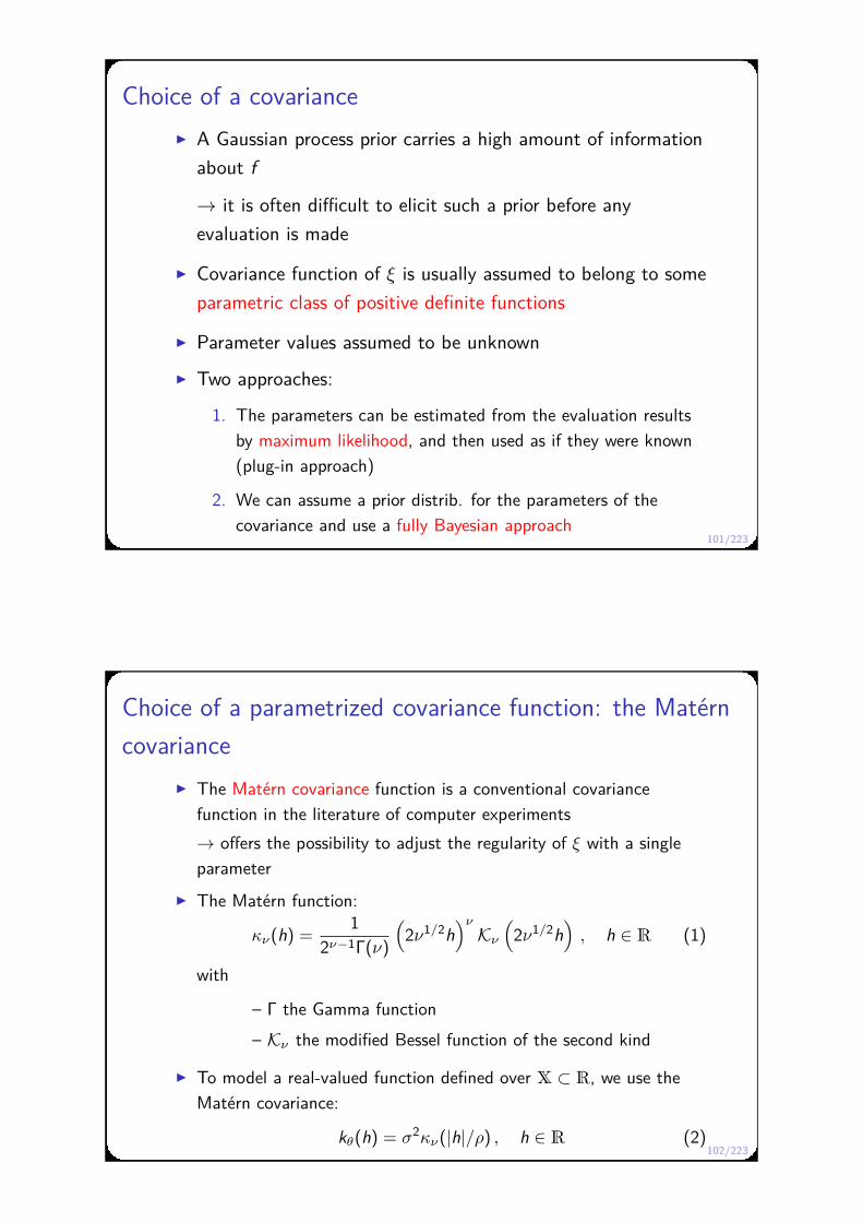
Choice of a covariance
A Gaussian process prior carries a high amount of information
about f
→ it is often difficult to elicit such a prior before any
evaluation is made
Covariance function of ξ is usually assumed to belong to some
parametric class of positive definite functions
Parameter values assumed to be unknown
Two approaches:
1. The parameters can be estimated from the evaluation results
by maximum likelihood, and then used as if they were known
(plug-in approach)
2. We can assume a prior distrib. for the parameters of the
covariance and use a fully Bayesian approach
102/223
Choice of a parametrized covariance function: the Matérn
covariance
The Matérn covariance function is a conventional covariance
function in the literature of computer experiments
→ offers the possibility to adjust the regularity of ξ with a single
parameter
The Matérn function:
κν(h) =1
2ν−1Γ(ν)
(2ν1/2h
)ν
Kν
(2ν1/2h
), h ∈ R (1)
with
– Γ the Gamma function
– Kν the modified Bessel function of the second kind
To model a real-valued function defined over X ⊂ R, we use the
Matérn covariance:
kθ(h) = σ2κν(|h|/ρ) , h ∈ R (2)

103/223
Choice of a parametrized covariance function: the Matérn
covariance
Matérn covariance in one dimension σ2 = 1, ρ = 0.8
−2 −1.5 −1 −0.5 0 0.5 1 1.5 20
0.1
0.2
0.3
0.4
0.5
0.6
0.7
0.8
0.9
1
ν = 1/2ν = 3/2ν = 9/2
ξ is p-time mean-square differentiable iff ν > p
104/223
Choice of a parametrized covariance function: the Matérn
covariance
To model a function f defined over X ⊂ Rd , with d > 1, we
use the anisotropic form of the Matérn covariance:
kθ(x , y) = σ2κν
√√√√d∑
i=1
(x[i] − y[i])2
ρ2i
, x , y ∈ R
d (3)
where x[i], y[i] denote the i th coordinate of x and y , and the
positive scalars ρi represent scale parameters
Since σ2 > 0, ν > 0, ρi > 0, i = 1, . . . , d , in practice, we
consider the vector of parameters
θ = log σ2, log ν, − log ρ1, . . . , − log ρd ∈ Rd+2
→ makes parameter estimation easier
105/223
Parameter estimation by maximum likelihood
Assume ξ is a zero-mean Gaussian process
The log-likelihood of the data ξn
= (ξ(x1), . . . , ξ(xn))t can be
written as
ℓ(ξn; θ) = −n
2log(2π)− 1
2log det K (θ)− 1
2ξ
ntK (θ)−1ξ
n, (4)
where K (θ) is the covariance matrix of ξn, which depends on
the parameter vector θ
The log-likelihood can be maximized using a gradient-based
search method
106/223
Prediction of a Gaussian process with unknown mean
function
In the domain of computer experiments, the mean of a
Gaussian process is generally written as a linear parametric
function
m(·) = βtϕ(·) , (5)
with
- β a vector of unknown parameters
- ϕ = (ϕ1, . . . , ϕl)t an l-dimensional vector of functions (in
practice, polynomials)
Simplest case: the mean function is an unknown constant m,
in which case β = m and ϕ : x ∈ X 7→ 1

107/223
Prediction of a Gaussian process with unknown mean function
Define the linear space of functions
P =
x 7→
l∑
i=1
βiϕi(x); βi ∈ R
,
Define Λ the linear space of finite-support measures on X, i.e.
λ ∈ Λ =⇒ λ =n∑
i=1
λiδxifor some n ∈ N
For f : X → R, and λ =∑n
i=1 λiδxi∈ Λ,
〈λ, f 〉 =∫
X
f dλ =n∑
i=1
λi f (xi)
Define the linear subspace ΛP⊥ ⊂ Λ of finite-support measures
vanishing on P, i.e.
λ ∈ ΛP⊥ =⇒ 〈λ, f 〉 =∫
X
fdλ =n∑
i=1
λi f (xi) = 0 , ∀f ∈ P
108/223
Prediction of a Gaussian process with unknown mean function
Let ξ be a Gaussian random process with an unknown mean in P,
and a covariance function k
For x ∈ X, the (intrinsic) kriging predictor ξn(x) of ξ(x) from
ξ(x1), . . . , ξ(xn) is the linear projection
ξn(x) =∑
i
λi(x)ξ(xi)
of ξ(x) onto spanξ(xi), i = 1, . . . , n such that the variance of the
error ξ(x) − ξn(x) is minimized, under the constraint
δx −∑
λi(x)δxi∈ ΛP⊥
i.e.,
〈δx −∑
λi(x)δxi, ϕj〉 = ϕj(x) −
∑λi(x)ϕj(xi) = 0 , j = 1, . . . , l
The requirement δx −∑λi(x)δxi∈ ΛP⊥ makes the kriging predictor
unbiased, even if the mean of ξ is unknown
109/223
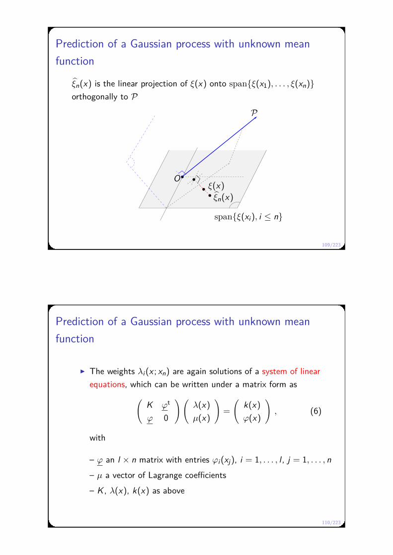
Prediction of a Gaussian process with unknown mean
function
ξn(x) is the linear projection of ξ(x) onto spanξ(x1), . . . , ξ(xn)orthogonally to P
spanξ(xi), i ≤ n
P
ξ(x)ξn(x)
O
110/223
Prediction of a Gaussian process with unknown mean
function
The weights λi(x ; xn) are again solutions of a system of linear
equations, which can be written under a matrix form as
(K ϕt
ϕ 0
)(λ(x)
µ(x)
)=
(k(x)
ϕ(x)
), (6)
with
– ϕ an l × n matrix with entries ϕi(xj), i = 1, . . . , l , j = 1, . . . , n
– µ a vector of Lagrange coefficients
– K , λ(x), k(x) as above

111/223
Prediction of a Gaussian process with unknown mean function
When the mean is unknown, the kriging covariance function (the
covariance of the error of prediction) is given by
kn(x , y) := cov(
ξ(x) − ξn(x), ξ(y) − ξn(y))
= k(x − y) − λ(x)t k(y) − µ(x)tϕ(y) .
Prop.
Let k be a covariance function and assume m ∈ P.
If
ξ | m ∼ GP (m, k)
m : x 7→ βtϕ(x), β ∼ U(Rl)then ξ | Fn ∼ GP
(ξn(·), kn(·, ·)
)
with U(Rl) the (improper) uniform distribution over Rl
→ justifies the use of kriging in a Bayesian framework provided that
the covariance function of ξ is known
112/223
Parameter estimation with unknown mean function
Objective: estimate the covariance parameters of a Gaussian
process with unknown mean
Restricted Maximum Likelihood (REML) approach →maximize the likelihood of the increments (or generalized
increments) of the data
Let ξ be a Gaussian process with an unknown mean function
in P and ξn
the random vector of observations at points xi ,
i = 1, . . . , n
Let ϕ = (ϕi(xj))l ,ni ,j=1 be the l × n matrix of basis functions of
P evaluated on x1, . . . , xn.

113/223
Parameter estimation with unknown mean function
Since the dimension of P is l , the dimension of the space of
the measures with support x1, . . . , xn that cancel out the
functions of P is n − l .
Assume an n × (n − l) matrix W with rank n − l has been
found, such that
ϕW = 0 .
(The columns of W are in the kernel of ϕ.)
Then Z = W Tξn
is a Gaussian random vector taking its
values in Rn−l , with zero mean and covariance matrix
W TK (θ)W
where K (θ) is the covariance matrix of ξn
with entries
kθ(xi − xj)
114/223
REML
The random vector Z is a contrast vector
The log-likelihood of the contrasts is given by
L(z | θ) = −n − l
2log 2π−1
2log det(W tK (θ)W )−1
2z t(W tK (θ)W )−1z .

115/223
REML
Various methods may be employed to compute the matrix W
We favor the QR decomposition of ϕT
ϕT = (Q1 | Q2)
(R
0
),
where (Q1 | Q2) is an n × n orthogonal matrix and R is a l × l
upper triangular matrix
It is trivial to check that the columns of Q2 form a basis of
the kernel of ϕ
So we may chose W = Q2
Note that W TW = In−l .
116/223
Books
M. Stein, Interpolation of Spatial Data: Some Theory for
kriging, Springer, 1999
T. Santner, B. Williams and W. Notz, The Design and
Analysis of Computer Experiments, Springer, 2003
C. Rasmussen and C. Williams, Gaussian processes for
Machine Learning, MIT Press, 2006
A. Forrester, A. Sóbester and A. Keane, Engineering
design via surrogate modelling: a practical guide, John Wiley
& Sons, 2008
117/223
Lecture 1 : From meta-models to UQ
1.1 Introduction
1.2 Black-box modeling
1.3 Bayesian approach
1.4 Posterior distribution of a quantity of interest
1.5 Complements on Gaussian processes
Lecture 2 : Bayesian optimization (BO)
2.1. Decision-theoretic framework
2.2. From Bayes-optimal to myopic strategies
2.3. Design under uncertainty
References
118/223
What is Bayesian optimization ?
“wide sense” definition
optimization using tools from Bayesian UQ
started with Harold Kushner’s paper: A New Method of
Locating the Maximum Point of an Arbitrary Multipeak Curve
in the Presence of Noise, J. Basic Engineering, 1964.

119/223
What is Bayesian optimization ?
a slightly more restrictive definition
sequential Bayesian decision theory applied to optimization
started with the work of Jonas Mockus and Antanas Žilinskas
in the 70’s, e.g., On a Bayes method for seeking an extremum,
Avtomatika i Vychislitel’naya Teknika, 1972 (in Russian)
In this lecture we adopt this second (more constructive !) definition
120/223
Lecture 2 : Bayesian optimization (BO)
2.1. Decision-theoretic framework
2.2. From Bayes-optimal to myopic strategies
2.3. Design under uncertainty

121/223
Decision-theoretic framework
Bayesian decision theory (BDT) in a nutshell a mathematical framework for decisions under uncertainty uncertainty is captured by probability distributions the “Bayesian agent” aims at minimizing the expected loss
122/223
Decision-theoretic framework (cont’d)
How does this relate to optimization ?
The agent is the optimization algorithm (or you, if you will)
Ingredients of a BDT problem
a set of all possible “states of nature” a prior distribution over the states of nature a description of the decisions we have to make and the corresponding “transitions” a loss function (or utility function)

123/223
States of nature
What are the states of nature in an optimization problem?
Short answer Everything that “nature” knows but you don’t
More practically: depends on the type of problem
1. the content of the black box (expensive numerical model)
2. for stochastic simulators: future responses of the simulator
3. design under uncertainty: the value of environmental variables
4. . . .
Notation
Ω =all possible states ω of nature
124/223
States of nature: example
Consider the following setting a deterministic numerical model input space X ⊂ R
d , output space Rp
no environmental variables in the problem
States of nature for this setting Ω =
f : X → R
p | f such that . . .
e.g., d = 1, p = 1, X = [0; 1] and Ω = C(X;R)
Until further notice, we will use this simple (but important)
setting to illustrate the basics of Bayesian optimization

125/223
Uncertainty quantification (reminder from Lecture #1)
The true state of nature ω⋆ ∈ Ω is unknown
Example (cont’d) a function f ⋆ ∈ Ω = C(X;R) is inside the black box (ω⋆ ≡ f ⋆) we don’t “know” f ⋆(x) until we run the code with input x
Bayesian approach to UQ our knowledge of ω⋆ is encoded by a probability distribution
on the set Ω of all possible ω’s technically: proba on (Ω, F) for some σ-algebra F . . .
Sequence of decisions ⇒ sequence of distributions P0, P1, . . . Pn corresponds to the agent’s beliefs after the nth decision A prior distribution P0 needs to be specified
126/223
Uncertainty quantification: example
Example (cont’d): if f is known to look more or less like this:
-1 -0.5 0 0.5 1
input variable x
-2.5
-2
-1.5
-1
-0.5
0
0.5
1
1.5
2
response z
then we can take P0 = GP(m, k)
with m ∼ U(R) and k a (stationary) Matà c©rn covariance
Gaussian process priors are commonly used because they are computationally convenient while allowing a certain modeling flexibility

127/223
Uncertainty quantification: consequences
For clarity, consider again the case of a deterministic model: an unknown function f ∈ Ω is in the black box
Given a proba P on Ω, we can compute the probability of any (measurable) statement about f
compute the expectation of any (measurable) function of f
i.e., the unknown f can be treated as random
Convenient notation
ξ = random function that represents the unknown f
we will write, e.g., En (ξ(x)) instead of∫
Ω f (x) Pn(df ) ,
128/223
Decision-theoretic framework (cont’d)
How does this relate to optimization ?
The agent is the optimization algorithm (or you, if you will)
Ingredients of a BDT problem
a set of all possible “states of nature” X
a prior distribution over the states of nature X
a description of the decisions we have to make and the corresponding “transitions” a loss function (or utility function)

129/223
Decisions
Several types of decisions in an optimization procedure: intermediate decisions stopping decision final decision
129/223
Decisions: intermediate decisions
Several types of decisions in an optimization procedure: intermediate decisions stopping decision final decision
Intermediate decisions (simple setting) running the numerical model with a given input x ∈ X
getting the corresponding output (deterministic or random)
Intermediate decisions (various extensions) parallel computing: batches of input values multi-fidelity: choosing the right fidelity level variable run-time: choosing when to stop a computation . . .

129/223
Decisions: stopping decision
Several types of decisions in an optimization procedure: intermediate decisions stopping decision final decision
Stopping decision (standard setting) a budget of evaluations, or computation time, is given the stopping decision is trivial in this case
Digression: taking the cost of observations into account? in principle, BO can deal with the stopping decision too in practice, difficult to translate into a loss (see later) some “BO papers” propose heuristic stopping rule
129/223
Decisions: final decision
Several types of decisions in an optimization procedure: intermediate decisions stopping decision final decision
Final decision (ex: single-objective minimization pb.) an estimate of the minimizer x∗ = argminx∈X f (x) and/or an estimate of the minimum M∗ = minx∈X f (x)
with X a “known” input space
Other settings multi-objective: Pareto set / Pareto front (see later), inequality constraints (see later), equality constraints (harder !), quasi-optimal region (sublevel set). . .
130/223
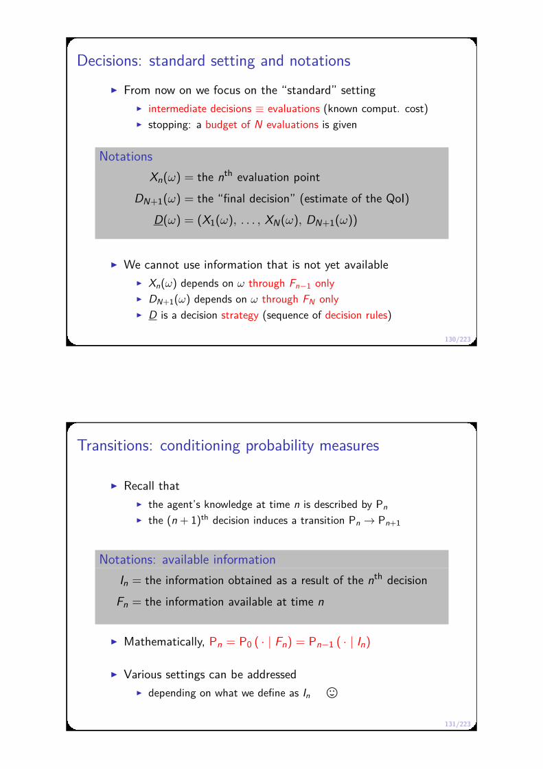
Decisions: standard setting and notations
From now on we focus on the “standard” setting intermediate decisions ≡ evaluations (known comput. cost) stopping: a budget of N evaluations is given
Notations
Xn(ω) = the nth evaluation point
DN+1(ω) = the “final decision” (estimate of the QoI)
D(ω) = (X1(ω), . . . , XN(ω), DN+1(ω))
We cannot use information that is not yet available Xn(ω) depends on ω through Fn−1 only DN+1(ω) depends on ω through FN only D is a decision strategy (sequence of decision rules)
131/223
Transitions: conditioning probability measures
Recall that the agent’s knowledge at time n is described by Pn
the (n + 1)th decision induces a transition Pn → Pn+1
Notations: available information
In = the information obtained as a result of the nth decision
Fn = the information available at time n
Mathematically, Pn = P0 ( · | Fn) = Pn−1 ( · | In)
Various settings can be addressed depending on what we define as In ,

132/223
Transitions: examples
Example (cont’d) single-output, deterministic code In = (Xn, ξ(Xn)) and Fn = (X1, ξ(X1), . . . , Xn, ξ(Xn)) ξ(Xi) = f ⋆(Xi) is the true, scalar, value of the model at Xi
Many other (interesting) settings are possible ! stochastic simulators
the output is a random draw Zn ∼ some distrib. PZn|Xn
In = (Xn, Zn) and Fn = (X1, Z1, . . . , Xn, Zn)
availability of gradients (e.g., adjoint code) batch setting and/or multiple outputs variable run-times, “simulation failures”. . .
133/223
Decision-theoretic framework (cont’d)
How does this relate to optimization ?
The agent is the optimization algorithm (or you, if you will)
Ingredients of a BDT problem
a set of all possible “states of nature” X
a prior distribution over the states of nature X
a description of the decisions we have to make X
and the corresponding “transitions” X
a loss function (or utility function)

134/223
Loss function
To guide the decisions of the Bayesian agent, we need to
specify a loss function L
Notation
L : Ω × D → R
(ω, d) 7→ L(ω, d)
where D is the set of all possible sequences of decisions
The Bayes-optimal strategy is, by definition:
D = argmin E0 (L(D))
= argmin∫
ΩL(ω, D(ω)) P0(dω)
where D ranges over all strategies
135/223
Loss function: example
Example (cont’d) Assume that we want to find the minimizer of f
d = (x1, . . . , xn, x)
with x our estimate of argmin f
A standard loss function for this situation is the linear loss:
L(f , d) = L(f , x) = f (x) − min f
(a.k.a. opportunity cost, a.k.a. instantaneous regret)
Remarks L coincides with the L1 loss of the estimator f (x)
f (x) ≥ min f ⇒ L(f , x) = |f (x) − min f |
L is a terminal loss (does not depend on X1, ξ(X1), . . .)

136/223
Decision-theoretic framework (cont’d)
How does this relate to optimization ?
The agent is the optimization algorithm (or you, if you will)
Ingredients of a BDT problem
a set of all possible “states of nature” X
a prior distribution over the states of nature X
a description of the decisions we have to make X
and the corresponding “transitions” X
a loss function (or utility function) X
Our BDT framework is complete, let’s use it ,
137/223
Lecture 2 : Bayesian optimization (BO)
2.1. Decision-theoretic framework
2.2. From Bayes-optimal to myopic strategies
2.3. Design under uncertainty

138/223
Problem statement
Assume a standard BO setting fixed budget N, terminal cost only
L(ω, d) = L(ω, dN+1)
intermediate decisions ≡ evaluations
one at a time, possibly noisy (stochastic simulator)
Fn = (X1, Z1, . . . , Xn, Zn)
Recall the Bayes-optimal strategy (algorithm):
DBayes = argminD E0 (L(DN+1))
= argminD
∫
ΩL(ω, DN+1(ω)) P0(dω)
where D ranges over all strategies D = (X1, . . . , XN , DN+1)
139/223
Problem statement
What does this DBayes look like ?
Can we actually build an optimal Bayesian algorithm ?
140/223
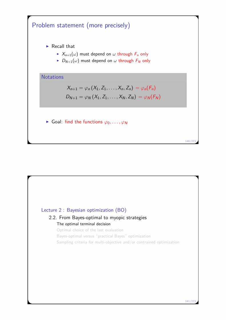
Problem statement (more precisely)
Recall that Xn+1(ω) must depend on ω through Fn only DN+1(ω) must depend on ω through FN only
Notations
Xn+1 = ϕn (X1, Z1, . . . , Xn, Zn) = ϕn(Fn)
DN+1 = ϕN (X1, Z1, . . . , XN , ZN) = ϕN(FN)
Goal: find the functions ϕ0, . . . , ϕN
141/223
Lecture 2 : Bayesian optimization (BO)
2.2. From Bayes-optimal to myopic strategiesThe optimal terminal decision
Optimal choice of the last evaluation
Bayes-optimal versus “practical Bayes” optimization
Sampling criteria for multi-objective and/or contrained optimization

142/223
Optimal terminal decision
Notation
En = E ( · | Fn) = conditional expectation with respect to Fn
= expectation with respect to the probability Pn
Consider any incomplete strategy X1, . . . XN
Claim: the optimal terminal decision is
DN+1 = ϕBayesN (X1, Z1, . . . , XN , ZN) = argmind EN (L(d))
where d runs over all possible values for the terminal decision
143/223
Optimal terminal decision: proof
Take any strategy D = (X1, . . . , XN , DN+1)
Consider the modified strategy D′ =(X1, . . . , XN , D′
N+1
)
where D′N+1 = ϕBayes
N (X1, Z1, . . . , XN , ZN)
Then, by definition of ϕBayesN ,
EN (L(DN+1)) = EN (L(d))|d=DN+1
≥ mind
EN (L(d)) = EN
(L(D′
N+1))
and thus
E0(L(DN+1)) = E0 (EN (L(DN+1)))
≥ E0(EN
(L(D′
N+1)))
= E0(L(D′N+1))

144/223
Vocabulary: posterior (Bayes) risk at time N
Define the posterior risk at time N for the decision d :
RN(d) = EN (L(d))
(“risk” is a synonym for “expected loss”)
Define the posterior Bayes risk at time N:
RBayesN = min
dRN(d)
Remember: the min attained for d = ϕBayesN (FN)
145/223
Example (cont’d): linear loss
Recall the setting goal: minimize f
dN+1 = x is an estimate of X∗(f ) = argmin f
L(f , x) = f (x) − min f
Compute the posterior risk at time N for a given x ∈ X:
RN(x) = EN (L(ξ, x)) = EN (ξ(x) − min ξ)
= ξN(x) − EN (min ξ)
Thus the optimal terminal decision is
DBayesN+1 = XBayes = argminx∈X ξN(x)

146/223
Example (cont’d): linear loss
Assume that n = N = 5 (a small budget indeed).
0 2 4 6 8 10 12-10
-5
0
5
10
input x
resp
onse
z
147/223
Example (cont’d): the L1 loss, variant
To summarize, we have for this example
XBayes = argmin ξN
RBayesN = min ξN − EN (min ξ)
Remark: in general, XBayes 6∈ X1, . . . , XN the value of the function at XBayes is not known
Variant: restrict the terminal decision to X1, . . . , XN
XBayes,1 = argminx∈X1,...,XN ξ(x)
RBayes,1N = min
i≤Nξ(Xi) − EN (min ξ)

148/223
Example (cont’d): linear loss
Assume that n = N = 5 (a small budget indeed).
0 2 4 6 8 10 12-10
-5
0
5
10
input x
resp
onse
z
Remark: the two estimates are equal when ξ does not “overshoot”
(e.g., for a Brownian motion prior)
149/223
Lecture 2 : Bayesian optimization (BO)
2.2. From Bayes-optimal to myopic strategiesThe optimal terminal decision
Optimal choice of the last evaluation
Bayes-optimal versus “practical Bayes” optimization
Sampling criteria for multi-objective and/or contrained optimization

150/223
Finding XBayesN (last evaluation point)
Let us focus now on the last evaluation point recall that D = (X1, . . . , XN−1, XN , DN+1)
Notation
En,x (Y ) will mean: “compute En(Y ), assuming that Xn+1 = x”
For example, if Y = g (X1, Z1, . . . , Xn, Zn, Xn+1, Zn+1),
En,x (Y ) = En (g (X1, Z1, . . . , Xn, Zn, x , Zx ))
where Zx denotes the result of a new evaluation at x
151/223
Finding XBayesN (last evaluation point)
Given xN ∈ X, consider the following strategy at time N − 1:
1) first, evaluate at XN = xN ,
2) then, act optimally, i.e., use DBayesN+1 = ϕBayes
N (FN)
The corresponding posterior risk at time N − 1 is
RN−1(xN) = EN−1,xN
(L(DBayes
N+1 ))
= EN−1,xN
(RBayes
N
)
Claim: the optimal decision rule for the last evaluation is
XBayesN = ϕN−1(FN−1) = argminxN∈X RN−1(xN)
Remark: RN−1 is used as a “sampling criterion”
(a.k.a. “infill criterion”, a.k.a. “merit function”. . . )

152/223
Finding XBayesN : proof
For any strategy D = (X1, . . . , XN−1, XN , DN+1),
EN−1 (L(DN+1)) = EN−1 (RN(FN , DN+1))
≥ EN−1
(RBayes
N (FN))
= RN−1(FN−1, XN−1)
Let D′ =(X1, . . . , XN−1, X ′
N , D′N+1
),
where X ′N = ϕBayes
N−1 (FN−1) and D′N+1 = ϕBayes
N (FN−1, X ′N , Z ′
N)
Then EN−1
(L(D′
N+1))
= RBayesN−1 (FN−1) ≤ RN−1(FN−1, XN−1)
Thus E0 (L(DN+1)) ≥ E0
(L(D′
N+1))
153/223
Finding XBayesN : example (cont’d)
Recall our linear loss example
XBayes = argmin ξN
RBayesN = min ξN − EN (min ξ)
Compute the posterior risk at time N − 1
RN−1(FN−1, xN) = EN−1,xN
(RBayes
N (FN))
= EN−1,xN
(min ξN
)− EN−1 (min ξ)
The optimal decision at time N − 1 is
XN = argminxNEN−1,xN
(min ξN
)
(first appears (in english) in Mockus, Tiesis & Žilinskas, 1978)

154/223
Finding XBayesN : example (cont’d)
Equivalently,
XN = argmaxxNmin ξN−1 − EN−1,xN
(min ξN
)
︸ ︷︷ ︸ρKG
N−1(xN) ≥ 0
Nowadays called the Knowledge Gradient (KG) criterion
(Frazier, Powell & co-authors, 2008, 2009, 2011)
Remarks applicable to “noisy” observations as well
a.k.a. simulation-based optimization
even with a GP prior, ρKG is not exactly computable in general idea: approx. max over a finite grid (more about that later)
155/223
Finding XBayesN : example (cont’d)
Same example as before, n = 5, but assume now that N = 6.
0 2 4 6 8 10 12-10
-5
0
5
10
0 2 4 6 8 10 120
0.2
0.4
0.6
Mockus/KG
input x
final point xN
resp
onse
zsa
mpl
ing
crit
erio
nρ
Warning: XN 6= argmax ξN−1 (uncertainty is taken into account)

156/223
Finding XBayesN : example, variant (cont’d)
Recall the following variant
XBayes,1 = argminx∈X1,...,XN ξ(x)
RBayes,1N = min
i≤Nξ(Xi) − EN (min ξ)
Set Mn = mini≤n ξ(Xi). The optimal decision at time N − 1 is
XN = argmaxxNMN−1 − EN−1,xN
(MN)
= argmaxxNEN−1
((MN−1 − ξ(xN))+
)
︸ ︷︷ ︸ρEI
n (xN) ≥ 0
This is the Expected Improvement (EI) criterion
(Mockus et al 1978; Jones, Schonlau & Wlech, 1998)
Computable analytically for GP priors ⇒ most commonly used
(for deterministic numerical models)
157/223
Finding XBayesN : example (cont’d)
Same example as before, n = 5, but assume now that N = 6.
0 2 4 6 8 10 12-10
-5
0
5
10
0 2 4 6 8 10 120
0.2
0.4
0.6
Mockus/KG
EI
input x
final point xN
resp
onse
zsa
mpl
ing
crit
erio
nρ
Warning: XN 6= argmax ξN−1 (uncertainty is taken into account)

158/223
Lecture 2 : Bayesian optimization (BO)
2.2. From Bayes-optimal to myopic strategiesThe optimal terminal decision
Optimal choice of the last evaluation
Bayes-optimal versus “practical Bayes” optimization
Sampling criteria for multi-objective and/or contrained optimization
159/223
The Bayes-optimal strategy
Recall the optimal terminal decision rule
ϕBayesN (FN) = argmind EN (L(d))
RBayesN (FN) = mind EN (L(d))
Recall the optimal rule for the last evaluation
ϕBayesN−1 (FN−1) = argminxN
EN−1,xN
(RBayes
N (FN))
RBayesN−1 (FN−1) = minxN
EN−1,xN
(RBayes
N (FN))

160/223
The Bayes-optimal strategy
The entire Bayes-optimal strategy can be written similarly: ∀n,
ϕBayesn−1 (Fn−1) = argminxn
En−1,xn
(RBayes
n (Fn))
RBayesn−1 (Fn−1) = minxn En−1,xn
(RBayes
n (Fn))
This is called backward induction (or dynamic programming)
So what ? Can we use this ?
161/223
The Bayes-optimal strategy
More explicitely, the optimal decision for the first evaluation is
X1 = argminx1E0,x1
(minx2 E1,x2
(. . .
minxNEN−1,xN
(mind EN (L(d))
)))
Very difficult to use in practice beyond N = 1 or 2 each “min” is an optim. problem that needs to be solved. . . each “En,x ” is an integral that needs to be computed. . . none of them are tractable, even for the nicest (GP) priors /

162/223
Practical Bayesian optimization: myopic strategies
Practical BO algorithms use, in general, myopic strategies a.k.a. one-step look-ahead strategies principle: make each decision as if it were the last one Bayes-optimal if N = 1, sub-optimal otherwise
For any n ≤ N, let Ln = mind En (L(d))
Generic myopic BO algorithm
For n from 0 to N − 1 Compute Xn+1 = argminx En,xn+1
(Ln+1
)
Make an evaluation at Xn+1
Output DN+1 = argmin EN (L(d))
163/223
Practical Bayesian optimization: hyper-parameters
GP models have hyper-parameters θ (variance, range, etc.) fully Bayes approach (see Benassi 2013, chap. III, and refs)
1. set up prior distributions on the hyper-parameters
2. use MCMC/SMC to sample from the posterior
plug-in approach use Pθ
n ≈ δθn
, with θn an estimator of θ (MML, LOO-CV. . . )
enough initial data is needed for this approach
Generic myopic BO algorithm with hyper-parameter estimation
Init: (space-filling) DoE of size n0 (rule of thumb: n0 = 10 d) For n from n0 to N − 1
once in a while, Estimate hyper-parameters (plug-in/fully Bayes)
Compute Xn+1 = argminx En,xn+1
(Ln+1
)
Make an evaluation at Xn+1
Output DN+1 = argmin EN (L(d))

164/223
Practical Bayesian optimization: EGO
STK demo
. . . single-objective box-constrained optimization
with the EI criterion and a plug-in approach
(a.k.a. the “EGO” algorithm) . . .
165/223
Practical Bayesian optimization: optimization
Each iteration involves an auxiliary optimization problem
Various approaches to solve it Fix grid or IID random search
OK for low-dimensional, simple problems
if accurate convergence is not needed
External solvers ex: DiceOptim → Rgenoud (genetic + gradient)
ex: Janusvekis & Le Riche (2013) → CMA-ES
Sequential Monte Carlo (Benassi, 2013; Feliot et al, 2017) sample according to a well-chosen sequence of densities
Bayesian optimization ⇒ run-time overhead depends on the model, sampling criterion, optimizer, etc. BO is appropriate for expensive-to-evaluate numerical models

166/223
Lecture 2 : Bayesian optimization (BO)
2.2. From Bayes-optimal to myopic strategiesThe optimal terminal decision
Optimal choice of the last evaluation
Bayes-optimal versus “practical Bayes” optimization
Sampling criteria for multi-objective and/or contrained optimization
167/223
Multi-objective problems
Several objective functions to be minimized: f = (f1, . . . , fp) fj : X → R, 1 ≤ j ≤ p
Pareto domination relation
z ≺ z ′ if (def)
zj ≤ z ′j for all j ≤ p,
zj < z ′j for at least one j ≤ p.
The goal is to find (estimate) the Pareto set P = x ∈ X :6 ∃x ′ ∈ X, f (x ′) ≺ f (x)
(a.k.a. set of Pareto-efficient solutions) and/or the Pareto front z ∈ R
p : ∃x ∈ P, z = f (x)(a.k.a Pareto frontier, Pareto boundary. . . )


170/223
Inequality-constrained problems
Single-objective, inequality-contrained problem: f = (fo, fc,1, . . . , fc,q), with fo : X → R, to be minimized, fc,j : X → R, 1 ≤ j ≤ q, must be ≤ 0.
Consider the following loss function
L(f , x) =
fo(x) − f ⋆o if fc(x) ≤ 0,
+∞ otherwise.
where f ⋆o = minx :fc(x)≤0 fo(x)
171/223
Inequality-constrained problems
Assuming noiseless evaluations, independent priors on objective and constraint functions, ∃i ≤ n, ξc(Xi) = fc(Xi) ≤ 0,
the following myopic criterion follows (Schonlau et al, 1998)
ρEICn (xn+1) = ρEI
o,n(xn+1) · Πqj=1Pn (ξc,j(xn+1) ≤ 0)︸ ︷︷ ︸
Proba of Feasibility (PF)
.
Implementation Easy for independent GP priors (most commonly used) Dependent priors: harder. . . (but see Williams et al, 2010)
Again, many other approaches have been proposed See Feliot et al (2017, section 2.3) and references therein

172/223
Et maintenant une page de pub !
BMOO algorithm (Feliot et al 2017) Unified EI/EHVI/EIC criterion
well-defined even when no feasible point is known
Efficient SMC technique for criterion optimization SMC = Sequential Monte Carlo
extends the work of Benassi (2013)
Announcement
Paul Feliot’s PhD defense will take place
on Wednesday, July 12, 2017, 2 PM,
at CentraleSupelec (Gif). Venez nombreux !
173/223
Miscellaneous references for further reading
Information-based BO: a different approach Risk = entropy of the minimizer See Villemonteix et al (2009), Hennig & Schueller (2012),
Hernandez-Lobáto and co-authors (2014, 2015. . . )
Aggregation-based approaches Multi-objective: ParEGO (Knowles, 2006) Constrained: Augmented Lagrangian methods
(Gramacy et al, 2016; Picheny et al, 2016)
Batch of evaluations: multi-point criteria Ginsbourger et al (2010), Chevalier & Ginsbourger (2013),
Chevalier et al (2014), Marmin et al (2015)
Noisy evaluations / stochastic simulators will be discussed in the next part ,

174/223
Lecture 2 : Bayesian optimization (BO)
2.1. Decision-theoretic framework
2.2. From Bayes-optimal to myopic strategies
2.3. Design under uncertainty
175/223
Lecture 2 : Bayesian optimization (BO)
2.3. Design under uncertaintyOverview of possible approaches
Optimization of a mean response
RBDO (and other formulations)

176/223
Design under uncertainty
Standard design optimization problem: Minimize one objective (“cost”) function fo(x) or several objective functions fo,1(x), . . . , fo,p(x) under the constraints fc,j(x) ≤ 0, 1 ≤ j ≤ q
Some objective/constraint functions are expensive to evaluate
“Design under uncertainty” framework
objective functions: fo,j(x , u), 1 ≤ j ≤ p
constraint functions: fc,j(x , u), 1 ≤ j ≤ q
where u denotes factors that the designer cannot control
177/223
(a few words on the) Worst-case approach
Principle of the worst-case (minimax) approach Define an uncertainty set U Optimize by considering the worst u ∈ U
For instance, assuming a single-objective problem:
minimize maxu∈U
fo(x , u)
If the problem has constraints, they become:
∀j ≤ q, ∀u ∈ U, fc,j(x , u) ≤ 0

178/223
Example 1: Illustration of the worst-case approach
Example: fo(x , u) = f (x + u), with u ∈ U = [−δ; δ], δ = 5
-20 -15 -10 -5 0 5 10 15 20
x
-1
-0.5
0
0.5
1
1.5
f(x)
fo(·, 0)argmin fo(·, 0)f +o
= maxu fo(x, u)argmin f +
o
Remark: very conservative, the nominal performance is ignored
178/223
Example 2: Illustration of the worst-case approach
Example: fo(x , u) = f (x + u), with u ∈ U = [−δ; δ], δ = 5
-10 -5 0 5 10 15 20
x
-2
-1.5
-1
-0.5
0
0.5
1
1.5
f(x)
fo(·, 0)argmin fo(·, 0)f +o
= maxu fo(x, u)argmin f +
o

179/223
Another example: worst-case approach for a constraint
Example: fc(x , u) = ‖x‖2 − u2
x1
x2
u0
179/223
Another example: worst-case approach for a constraint
Example: fc(x , u) = ‖x‖2 − u2, with u ∈ U = [u0 − δ; u0 + δ]
x1
x2
u0 − δ

180/223
(a few more words on the) Worst-case approach
In this lecture, we will focus on the probabilistic approach
See Marzat, Walter & Piet-Lahanier (2013, 2016) for a
“BO treatment” of the worst-case approach (using relaxation)
An issue of terminology: in the math literature, “robust optimization” refers mainly to the worst-case setting
(see Ben Tal et al (2009), Bertsimas et al (2011) and refs) the probabilistic approach is called stochastic programming
while engineers use the word “robust” for both ,
181/223
The probabilistic approach
From now, we focus on the probabilistic approach u is considered as random → U ∼ PU
can be a random vector (∈ Rm), or a more complicated object
Numerical models: two important settings stochastic simulators environmental variables
x
RNG
code Z = f (x , U) x code
u
z = f (x , u)
where f = (fo,1, . . . , fo,p, fc,1, . . . , fc,q)

182/223
The “stochastic simulator” setting
x
RNG
code Z = f (x , U)
Features of the black box U is not directly accessible only x can be chosen by the algorithm; Z = f (x , U) is observed PU is not known explicitely
“State of nature” (the things that we don’t know) the family
(PZ
x
)of conditional distributions
the RV U1, U2. . . that will be generated when running the
computer model with inputs x1, x2. . . the RV Ureal that defines the f (x , Ureal) ultimately realized
183/223
The “environmental variables” setting
x code
u
z = f (x , u)
Features of the black box the simulator remains deterministic PU is specified separately, usually explicitely the algorithm can choose (x , u) pairs to be evaluated
“State of nature” (the things that we don’t know) the deterministic function f : (x , u) 7→ f (x , u) the RV Ureal that defines the f (x , Ureal) ultimately realized
The two settings can be mixed ,

184/223
Problem formulations
Various “robust” formulations can be considered for thedesign problem, depending mainly on
the number of objective functions, the presence of (expensive-to-evaluate) constraints, and, of course, how we want to deal with Ureal.
In the following, we focus on single objective problems in the “environmental variables” setting
and discuss two important cases: optimization of the averaged objective function reliability-based design optimization (RBDO), a.k.a. “chance
constrained” optimization, and other formulations
185/223
Lecture 2 : Bayesian optimization (BO)
2.3. Design under uncertaintyOverview of possible approaches
Optimization of a mean response
RBDO (and other formulations)

186/223
Optimization of a mean response
Assume single objective f = fo, expensive to evaluate no (expensive-to-evaluate) constraints remark: cheap constraints allowed in the definition of X ⊂ R
d
“environmental variables” setting
Consider once again the L1 loss function
L ((f , ureal), x) =∣∣∣f (x , ureal) − min
xf (x , ureal)
∣∣∣
= f (x , ureal) − minx
f (x , ureal)
187/223
Optimization of a mean response
Compute the posterior risk at time N for an estimate x ∈ X
EN (L ((ξ, Ureal), x)) = EN (ξ(x , Ureal)) − EN (min ξ(·, Ureal))
= EN
(ξ(x)
)− EN (min ξ(·, Ureal))
where ξ(x) =∫
ξ(x , u) PU(du)
Same L1 risk (ignoring last term) as if we were dealing with the
Equivalent “deterministic” problem
minx
f (x), with f (x) =∫
f (x , u) PU(du)
(Remark: this formulation occurs very naturally in a BO framework ,)

188/223
Example 1: Worst-case versus probabilistic approach
Example: fo(x , u) = f (x + u), with u ∈ U = [−δ; δ], δ = 5
-20 -15 -10 -5 0 5 10 15 20
x
-1
-0.5
0
0.5
1
1.5
f(x)
fo(·, 0)argmin fo(·, 0)f +o
= maxu fo(x, u)argmin f +
o
f o
argmin f o
f o = E (fo(·, U)), with U ∼ N (0, s2), s.t. P (|U| ≤ δ) = 99.9%
188/223
Example 2: Worst-case versus probabilistic approach
Example: fo(x , u) = f (x + u), with u ∈ U = [−δ; δ], δ = 5
-10 -5 0 5 10 15 20
x
-2
-1.5
-1
-0.5
0
0.5
1
1.5
f(x)
fo(·, 0)argmin fo(·, 0)f +o
= maxu fo(x, u)argmin f +
o
f o
argmin f o
f o = E (fo(·, U)), with U ∼ N (0, s2), s.t. P (|U| ≤ δ) = 99.9%

189/223
Example 3: Three-bar truss (Koski, 1985; Das, 1997)
F1 (wind)
F2 (suspended load)
P
wD
La1 a2 a3
Design variables: x = (a1, a2, a3, w) aj : cross-section of bar j
Environmental variables: U = (F1, F2)
190/223
Example 3: Three-bar truss (Koski, 1985; Das, 1997)
Our (supposedly expensive) numerical model computes the displacement y = (y1, y2) of point P, the stress σj in each bar (1 ≤ j ≤ 3).
We will consider the following problem: minimize EU (‖y‖) under the constraints: xmin ≤ x ≤ xmax, V ≤ Vmax
Remark about constraints The constraint V ≤ Vmax is cheap to evaluate
V = a1
√L2 + w2 + a2L + a3
√L2 + (D − w)2
Additional constraints: |σj | ≤ σmax can be checked a posteriori

191/223
Breaking the “double loop”
Natural “double loop” approach outer loop: ordinary optimization algorithm applied to f
inner loop: integration (MC, quadrature. . . ) to compute f
Drawback: typically require large number of evaluations
Bayesian optimization breaks the double loop , Construct a Bayesian model for f , not f
Remark: can be achieved using other surrogate-model based
approaches (see Janusevkis & LeRiche, 2013, and refs therein)
192/223
Prior model
There are two functions of interest in this setting the one that can be observed, i.e., f : (x , u) 7→ f (x , u), and the one that want to optimize: f =
∫f (·, u) PU(du)
f is a function of f
priors cannot be specified independently
Gaussian process priors are, again, very convenient
If ξ ∼ GP(m, k)︸ ︷︷ ︸defined on X × U
, then ξ ∼ GP(mξ , kξ)︸ ︷︷ ︸
defined on X
,
withmξ (x) =
∫m(x , u) PU(du)
kξ (x , y) =x
k((x , u), (y , v)) PU(du)PU(dv)

193/223
Proof
ξ is Gaussian by linearity of the integral
Computation of the mean function: exchange∫
and E
mξ (x) = E(ξ(x)
)= E
(∫ξ(x , u) PU(du)
)
=∫
m(x , u) PU(du)
Computation of the covariance function: idem with bilinearity
kξ (x , y) = cov(ξ(x), ξ(y)
)
= cov(∫
ξ(x , u) PU(du),∫
ξ(x , v) PU(dv))
=x
k((x , u), (y , v)) PU(du)PU(dv)
194/223
Prior model (cont’d)
Actually, we can say much better:
Jointly Gaussian processes
If ξ ∼ GP(m, k), then ξ and ξ are jointly Gaussian, and
kξ,ξ((x , u), y) = cov(ξ(x , u), ξ(y)
)=∫
k((x , u), (y , v)) PU(dv)
Remark: mξ , kξ and kξ,ξ can be computed exactly if PU is discrete (PU =
∑nU
j=1 wjδuj)
if PU is (a mixture of) Gaussian(s), for some particular k
see Girard (2004) for exact formulas & approximations
Important special case: ξ(x , u) = ξ(x + u) If ξ is a GP iff ξ is a GP mξ(x , u) = m
ξ(x + u) and kξ((x , u), (u, v)) = k
ξ(x + u, y + v)

195/223
Examples 1 and 2: discretization of PU
In the two examples, ProbU = N (0, s2), with s = 1.52 P (|U| ≤ 5) ≈ 99.9%
We choose to use a regular discretization with nU = 11 points points regularly spaced on [−5; 5] weights computed using the normal cdf (using mid-points)
-6 -4 -2 0 2 4 6
x
0
0.05
0.1
0.15
0.2
0.25
exa
ct
pd
f
0
0.05
0.1
0.15
0.2
0.25
dis
cre
te a
pp
rox
196/223
Example 3: discretization of PU
Here, U =
(F1
F2
)and PU = N
((µF1
µF2
),
(σ2
F10
0 σ2F2
))
2.5 3 3.5 4 4.5 5 5.5 6 6.5
F1 10 5
4.1
4.2
4.3
4.4
4.5
4.6
4.7
4.8
F2
10 6
0.50
0.90
0.99
Monte Carlo sample of size nU = 50
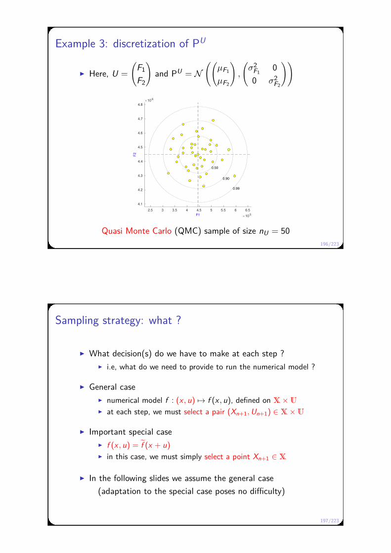
196/223
Example 3: discretization of PU
Here, U =
(F1
F2
)and PU = N
((µF1
µF2
),
(σ2
F10
0 σ2F2
))
2.5 3 3.5 4 4.5 5 5.5 6 6.5
F1 10 5
4.1
4.2
4.3
4.4
4.5
4.6
4.7
4.8
F2
10 6
0.50
0.90
0.99
Quasi Monte Carlo (QMC) sample of size nU = 50
197/223
Sampling strategy: what ?
What decision(s) do we have to make at each step ? i.e, what do we need to provide to run the numerical model ?
General case numerical model f : (x , u) 7→ f (x , u), defined on X × U
at each step, we must select a pair (Xn+1, Un+1) ∈ X × U
Important special case f (x , u) = f (x + u) in this case, we must simply select a point Xn+1 ∈ X
In the following slides we assume the general case
(adaptation to the special case poses no difficulty)

198/223
Sampling strategy: how ?
How do we build a sampling strategy for this problem ? in this lecture, we will apply the standard BO machinery
L1 loss → risk → “EI like” myopic strategy
other strategies are proposed in the literature Williams et al 2000; Janusevkis et Le Riche 2013
Entropy-based methods could be used as well
(Villemonteix et al 2009, Hennig & Schueller 2012. . . )
Assume now the L1 loss
Recall the posterior risk at time N for an estimate x ∈ X:
EN (L ((ξ, Ureal), x)) = EN
(ξ(x)
)− EN (min X ξ(·, Ureal))
199/223
Sampling strategy: one step look-ahead
Let Ln denote the expected loss that we would get if we
stopped at time n:
Ln = min X En
(ξ(x)
)− En (min X ξ(·, Ureal))
= min X mξ,n − En (min X ξ(·, Ureal))
The one-step look-ahead (myopic) strategy is
(Xn+1, Un+1) = argminxn+1,un+1En, (xn+1,un+1)
(Ln+1
)
= argminxn+1,un+1En, (xn+1,un+1)
(min X mξ,n+1
)
200/223
Sampling strategy: one step look-ahead
Equivalently,
(Xn+1, Un+1) = argmaxxn+1,un+1ρn(xn+1, un+1)
where ρn denotes the corresponding “expected improvement”
ρn(xn+1, un+1) = Ln − En, (xn+1,un+1)
(Ln+1
)
= min X mξ,n − En, (xn+1,un+1)
(min X mξ,n+1
)
Formally, looks like the KG criterion of Frazier & co, but. . .
201/223
Sampling strategy: one step look-ahead
Comparison with KG as presented in the literature
evaluations optimization
KG ξ(x) + N noise min ξ
here ξ(x , u) min ξ
There is no real difference mathematically: in both cases
1. the function to be optimized is not observable directly,
2. the evaluation results and the function to be optimized are
jointly Gaussian.
Good news: we can then derive an implementable
Approximate KG criterion as in Scott et al (2011)

202/223
Approximate KG criterion (AKG)
Let Xrefn ⊂ X denote some finite “reference set”
Let xn+1 = (xn+1, un+1). The AKG criterion is:
ρAKGn (xn+1) = min mξ,n − En, xn+1
(min mξ,n+1
)≥ 0
where the min runs over Xrefn ∪ xn+1.
Initially proposed by Scott et al (2011) under the name KGCP (“KG for continuous parameters”) with X
refn = X1, . . . , Xn
Implementation ? It is exactly computable (but not easy to compute. . . ) Available in STK (Matlab/Octave), DiceOptim (R). . .
203/223
Optimization of a mean response: demos
STK demo
. . . One dimensional illustration: examples 1 and 2 . . .
STK demo
. . . Minimization of the mean displacement
in the 3-bar truss example . . .

204/223
(a few words about) The case of stochastic simulators
Good news the same sampling criteria can be used in both cases
(environmental variables / stochastic simulators). . . . . . provided that the observations and the objective function
are jointly Gaussian.
Review/benchmark of existing criteria: Picheny et al (2013) AKG emerges has one of the most efficient criteria Huang et al (2006)’s “augmented EI” also performs well (Entropy-based criteria not benchmarked)
What about simulators with truly non-Gaussian output ? “batch trick” (CLT) see also Browne et al (2016). . .
205/223
Lecture 2 : Bayesian optimization (BO)
2.3. Design under uncertaintyOverview of possible approaches
Optimization of a mean response
RBDO (and other formulations)
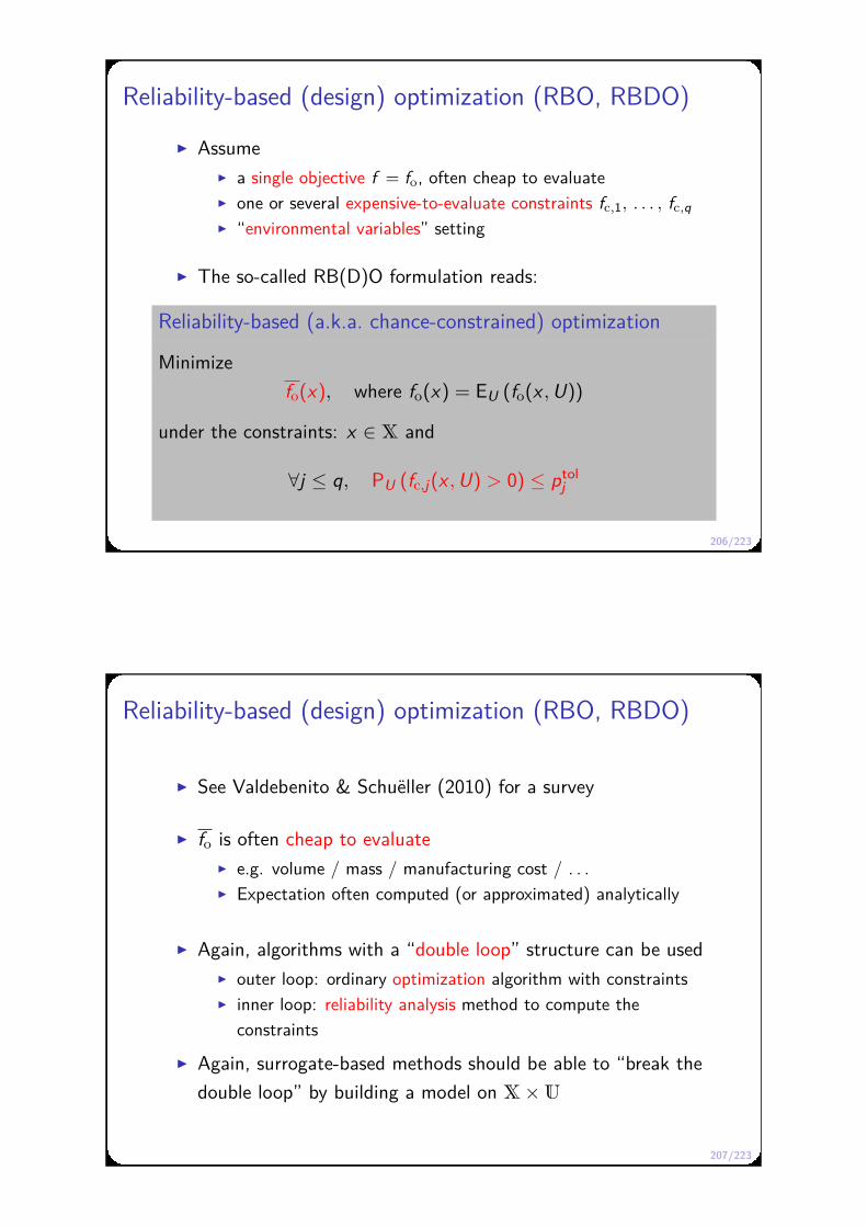
206/223
Reliability-based (design) optimization (RBO, RBDO)
Assume a single objective f = fo, often cheap to evaluate one or several expensive-to-evaluate constraints fc,1, . . . , fc,q
“environmental variables” setting
The so-called RB(D)O formulation reads:
Reliability-based (a.k.a. chance-constrained) optimization
Minimize
fo(x), where fo(x) = EU (fo(x , U))
under the constraints: x ∈ X and
∀j ≤ q, PU (fc,j(x , U) > 0) ≤ ptolj
207/223
Reliability-based (design) optimization (RBO, RBDO)
See Valdebenito & Schuëller (2010) for a survey
fo is often cheap to evaluate e.g. volume / mass / manufacturing cost / . . . Expectation often computed (or approximated) analytically
Again, algorithms with a “double loop” structure can be used outer loop: ordinary optimization algorithm with constraints inner loop: reliability analysis method to compute the
constraints
Again, surrogate-based methods should be able to “break the
double loop” by building a model on X × U

208/223
Why RBDO is harder than mean-response optimization
because the thresholds ptolj are usually small
MC-type approx. PU ≈ 1m
∑j δuj
becomes very expensive or
infeasible Dedicated techniques (e.g., FORM/SORM, IS, subset
simulation) needed for an efficient evaluation of the constraints
BO: the distribution of PU (ξc,j(x , U) > 0) is intractable Posterior mean/variance can be written as integrals (see, e.g.,
Villemonteix 2008 chap III), but. . . . . . the posterior distribution is not Gaussian even if ξc is ! Very difficult to derive Bayesian sampling criteria that can be
implemented efficiently. . .
209/223
Bayesian RBDO algorithms ?
A few GP-based algorithms have been proposed, notably: Bichon et al (2009): EGO+EGRA algorithm Dubourg and co-authors (2011a, 2011b): RBDO-N2LA
Complex, “weakly Bayesian” algorithms. . . e.g., RBDO-N2LA:
RBDO-N2LA is available in FERUM (Bourrinet et al, 2009)

210/223
RBDO and other formulations: alternative approach
A general alternative approach in two (or three) steps
1. Explore the design space efficiently using multi-objective BO,
2. Evaluate probabilities of failure, quantiles, etc. a posteriori for
non-dominated (and possibly other) solutions,
3. optionally Reduce the uncertainty on the most promising designs.
In step 1. constraints can be taken into account as objectives i.e., the contraint PU (fc,j(x , U) > 0) ≤ ptol
j
becomes: minx fc,j(x , u0) u.c. fc,j(x , u0) ≤ 0
In step 2. no new evaluations need to be carried out the posterior distribution of ξ is used to assess uncertainties
211/223
RBDO and other formulations: alternative approach
STK demo
. . . Robust design through multi-objective optimization . . .

212/223
Lecture 1 : From meta-models to UQ
1.1 Introduction
1.2 Black-box modeling
1.3 Bayesian approach
1.4 Posterior distribution of a quantity of interest
1.5 Complements on Gaussian processes
Lecture 2 : Bayesian optimization (BO)
2.1. Decision-theoretic framework
2.2. From Bayes-optimal to myopic strategies
2.3. Design under uncertainty
References
213/223
References I
Julien Bect, Emmanuel Vazquez, et al.
STK: a Small (Matlab/Octave) Toolbox for Kriging. Release 2.4.2, 2017.
URL http://kriging.sourceforge.net.
Aharon Ben-Tal, Laurent El Ghaoui, and Arkadi Nemirovski.
Robust optimization.
Princeton University Press, 2009.
Romain Benassi.
Nouvel algorithme d’optimisation bayésien utilisant une approche Monte-Carlo
séquentielle.
PhD thesis, Supélec, 2013.
Romain Benassi, Julien Bect, and Emmanuel Vazquez.
Bayesian optimization using sequential Monte Carlo.
In Learning and Intelligent Optimization. 6th International Conference, LION 6,
Paris, France, January 16-20, 2012, Revised Selected Papers, volume 7219 of
Lecture Notes in Computer Science, pages 339–342. Springer, 2012.
Dimitris Bertsimas, David B Brown, and Constantine Caramanis.
Theory and applications of robust optimization.
SIAM review, 53(3):464–501, 2011.

214/223
References II
Barron Bichon, Sankaran Mahadevan, and Michael Eldred.
Reliability-based design optimization using efficient global reliability analysis.
In 50th AIAA/ASME/ASCE/AHS/ASC Structures, Structural Dynamics, and
Materials Conference 17th AIAA/ASME/AHS Adaptive Structures Conference
11th AIAA No, page 2261, 2009.
Mickael Binois and Victor Picheny.
GPareto: Gaussian Processes for Pareto Front Estimation and Optimization.
R package version 1.0.3, 2016.
Jean-Marc Bourinet, Cécile Mattrand, and Vincent Dubourg.
A review of recent features and improvements added to FERUM software.
In H. Furuta, D. M. Frangopol, and M. Shinozuka, editors, Proc. 10th
International Conference on Structural Safety and Reliability (ICOSSAR 2009),
Osaka, Japan, September 13–17, 2009. CRC Press, 2009.
Thomas Browne, Bertrand Iooss, Loïc Le Gratiet, Jérôme Lonchampt, and
Emmanuel Remy.
Stochastic simulators based optimization by gaussian process
metamodels–application to maintenance investments planning issues.
Quality and Reliability Engineering International, 32(6):2067–2080, 2016.
215/223
References III
Clément Chevalier and David Ginsbourger.
Fast computation of the multi-points expected improvement with applications in
batch selection.
In International Conference on Learning and Intelligent Optimization, pages
59–69. Springer, 2013.
Clément Chevalier, Julien Bect, David Ginsbourger, Emmanuel Vazquez, Victor
Picheny, and Yann Richet.
Fast parallel kriging-based stepwise uncertainty reduction with application to the
identification of an excursion set.
Technometrics, 56(4):455–465, 2014.
Indraneel Das.
Nonlinear multicriteria optimization and robust optimality.
PhD thesis, Rice University, 1997.
Vincent Dubourg.
Adaptive surrogate models for reliability analysis and reliability-based design
optimization.
PhD thesis, Université Blaise Pascal-Clermont-Ferrand II, 2011.

216/223
References IV
Vincent Dubourg, Bruno Sudret, and Jean Marc Bourinet.
Reliability-based design optimization using kriging surrogates and subset
simulation.
Structural and Multidisciplinary Optimization, 44(5):673–690, 2011.
Michael Emmerich, Kyriakos C. Giannakoglou, and Boris Naujoks.
Single- and multi-objective evolutionary optimization assisted by Gaussian
random field metamodels.
IEEE Transactions on Evolutionary Computation, 10(4):421–439, 2006.
Paul Feliot, Julien Bect, and Emmanuel Vazquez.
A bayesian approach to constrained single-and multi-objective optimization.
Journal of Global Optimization, 67(1-2):97–133, 2017.
Alexander Forrester, András Sóbester, and Andy Keane.
Engineering design via surrogate modelling: a practical guide.
John Wiley & Sons, 2008.
Peter Frazier, Warren Powell, and Savas Dayanik.
The knowledge-gradient policy for correlated normal beliefs.
INFORMS journal on Computing, 21(4):599–613, 2009.
217/223
References V
Peter I Frazier, Warren B Powell, and Savas Dayanik.
A knowledge-gradient policy for sequential information collection.
SIAM Journal on Control and Optimization, 47(5):2410–2439, 2008.
David Ginsbourger, Rodolphe Le Riche, and Laurent Carraro.
Kriging is well-suited to parallelize optimization.
In Computational Intelligence in Expensive Optimization Problems, pages
131–162. Springer Science & Business Media, 2010.
Agathe Girard.
Approximate methods for propagation of uncertainty with gaussian process
models.
PhD thesis, University of Glasgow, 2004.
Robert B. Gramacy, Genetha A. Gray, Sebastien Le Digabel, Herbert K. H. Lee,
Pritam Ranjan, Garth Wells, and Stefan M. Wild.
Modeling an augmented lagrangian for blackbox constrained optimization.
Technometrics, 58(1):1–11, 2016.
Philipp Hennig and Christian J. Schuler.
Entropy search for information-efficient global optimization.
Journal of Machine Learning Research, 13(Jun):1809–1837, 2012.

218/223
References VI
José Miguel Hernández-Lobato, Matthew W. Hoffman, and Zoubin Ghahramani.
Predictive entropy search for efficient global optimization of black-box functions.
In Advances in Neural Information Processing Systems, pages 918–926, 2014.
José Miguel Hernández-Lobato, Michael A. Gelbart, Matthew W. Hoffman,
Ryan P. Adams, and Zoubin Ghahramani.
Predictive entropy search for bayesian optimization with unknown constraints.
In ICML, pages 1699–1707, 2015.
Deng Huang, Theodore T. Allen, William I. Notz, and R. Allen Miller.
Sequential kriging optimization using multiple-fidelity evaluations.
Structural and Multidisciplinary Optimization, 32(5):369–382, 2006.
Janis Janusevskis and Rodolphe Le Riche.
Simultaneous kriging-based estimation and optimization of mean response.
Journal of Global Optimization, 55(2):313–336, 2013.
Donald R. Jones, Matthias Schonlau, and William J. Welch.
Efficient global optimization of expensive black-box functions.
Journal of Global Optimization, 13(4):455–492, 1998.
219/223
References VII
Joshua Knowles.
ParEGO: A hybrid algorithm with on-line landscape approximation for expensive
multiobjective optimization problems.
IEEE Transactions on Evolutionary Computation, 10(1):50–66, 2006.
Juhani Koski.
Defectiveness of weighting method in multicriterion optimization of structures.
Communications in Applied Numerical Methods, 1(6):333–337, 1985.
Sébastien Marmin, Clément Chevalier, and David Ginsbourger.
Differentiating the multipoint expected improvement for optimal batch design.
In International Workshop on Machine Learning, Optimization and Big Data,
pages 37–48. Springer, 2015.
Julien Marzat, Eric Walter, and Hélène Piet-Lahanier.
Worst-case global optimization of black-box functions through kriging and
relaxation.
Journal of Global Optimization, 55(4):707, 2013.
Julien Marzat, Eric Walter, and Hélène Piet-Lahanier.
A new expected-improvement algorithm for continuous minimax optimization.
Journal of Global Optimization, 64(4):785–802, 2016.

220/223
References VIII
Jonas Mockus, Vytautas Tiesis, and Antanas Žilinskas.
The application of Bayesian methods for seeking the extremum.
In L. C. W. Dixon and G. P. Szegö, editors, Towards Global Optimization,
volume 2, pages 117–129, North Holland, New York, 1978.
Victor Picheny, Tobias Wagner, and David Ginsbourger.
A benchmark of kriging-based infill criteria for noisy optimization.
Structural and Multidisciplinary Optimization, 48(3):607–626, 2013.
Victor Picheny, David Ginsbourger, and Roustant Olivier et al.
DiceOptim: Kriging-Based Optimization for Computer Experiments, 2016a.
R package version 2.0, 2016.
Victor Picheny, Robert B. Gramacy, Stefan Wild, and Sebastien Le Digabel.
Bayesian optimization under mixed constraints with a slack-variable augmented
lagrangian.
In Advances in Neural Information Processing Systems, pages 1435–1443, 2016b.
Carl R. Rasmussen and Christopher K. I. Williams.
Gaussian Processes for Machine Learning.
MIT Press, 2006.
221/223
References IX
Samee Ur Rehman and Matthijs Langelaar.
Efficient infill sampling for unconstrained robust optimization problems.
Engineering Optimization, 48(8):1313–1332, 2016.
Samee Ur Rehman, Matthijs Langelaar, and Fred van Keulen.
Efficient kriging-based robust optimization of unconstrained problems.
Journal of Computational Science, 5(6):872–881, 2014.
Olivier Roustant, David Ginsbourger, and Yves Deville.
DiceKriging, DiceOptim: Two R packages for the analysis of computer
experiments by kriging-based metamodeling and optimization.
Journal of Statistical Software, 51(1), 2012.
Thomas J. Santner, Brian J. Williams, and William Notz.
The Design and Analysis of Computer Experiments.
Springer Verlag, 2003.
Matthias Schonlau, William J. Welch, and Donald R. Jones.
Global versus local search in constrained optimization of computer models.
In New Developments and Applications in Experimental Design: Selected
Proceedings of a 1997 Joint AMS-IMS-SIAM Summer Conference, volume 34 of
IMS Lecture Notes-Monographs Series, pages 11–25, 1998.
222/223
References X
Warren Scott, Peter Frazier, and Warren Powell.
The correlated knowledge gradient for simulation optimization of continuous
parameters using gaussian process regression.
SIAM Journal on Optimization, 21(3):996–1026, 2011.
Michael L. Stein.
Interpolation of Spatial Data: Some Theory for Kriging.
Springer, New York, 1999.
Marcos A. Valdebenito and Gerhart I. Schuëller.
A survey on approaches for reliability-based optimization.
Structural and Multidisciplinary Optimization, 42(5):645–663, 2010.
Emmanuel Vazquez.
Modélisation comportementale de systèmes non-linéaires multivariables par
méthodes à noyaux et applications.
PhD thesis, Univ Paris XI, Orsay, France, 2005.
Julien Villemonteix.
Optimisation de fonctions coûteuses Modèles gaussiens pour une utilisation
efficace du budget d’évaluations: théorie et pratique industrielle.
PhD thesis, Université Paris Sud-Paris XI, 2008.
223/223
References XI
Julien Villemonteix, Emmanuel Vazquez, and Éric Walter.
An informational approach to the global optimization of expensive-to-evaluate
functions.
Journal of Global Optimization, 44(4):509–534, 2009.
Brian J. Williams, Thomas J. Santner, and William I. Notz.
Sequential design of computer experiments to minimize integrated response
functions.
Statistica Sinica, pages 1133–1152, 2000.
Brian J. Williams, Thomas J. Santner, William I. Notz, and J. S. Lehman.
Sequential design of computer experiments for constrained optimization.
In Statistical Modelling and Regression Structures, pages 449–472.
Physica-Verlag HD, 2010.