
Bayesian Model Robust Designs
25
Bayesian Model Robust Designs Vincent Kokouvi Agboto * Christopher J. Nachtsheim † January 18, 2005 Abstract In industrial experiments, cost considerations will sometimes make it impractical to design experiments so that effects of all the factors can be estimated simultaneously. Therefore experimental designs are frequently constructed to estimate main effects and a few pre-specified interactions. A criticism frequently associated with the use of many optimality criteria is the specific reliance on an assumed statistical model. One way to deal with such a criticism may be to assume that instead the true model is an approximation of an unknown element of * PhD Candidate, School of Statistics, University of Minnesota, Minneapolis, MN 55455 † Professor and Chair, Operations and Management Sciences Department, Carlson School of Management, University of Minnesota, Minneapolis, MN 55455. 1
Transcript of Bayesian Model Robust Designs
Bayesian Model Robust Designs
Vincent Kokouvi Agboto∗ Christopher J. Nachtsheim †
January 18, 2005
Abstract
In industrial experiments, cost considerations will sometimes make
it impractical to design experiments so that effects of all the factors
can be estimated simultaneously. Therefore experimental designs are
frequently constructed to estimate main effects and a few pre-specified
interactions. A criticism frequently associated with the use of many
optimality criteria is the specific reliance on an assumed statistical
model. One way to deal with such a criticism may be to assume that
instead the true model is an approximation of an unknown element of
∗PhD Candidate, School of Statistics, University of Minnesota, Minneapolis, MN 55455†Professor and Chair, Operations and Management Sciences Department, Carlson
School of Management, University of Minnesota, Minneapolis, MN 55455.
1

a known set of models. In this paper, we consider a class of designs
that are robust for change in model specification.
This paper is motivated by the belief that appropriate Bayesian
approaches may also perform well in constructing model robust designs
and by the limitation of such approaches in the literature. I will
use the traditional Bayesian design method for parameter estimation
and incorporates a discrete prior probability on the set of models of
interest. Some examples and comparisons with existing approaches
will be provided.
Key Words: Optimal design, Optimal Bayesian design, General
Equivalence Theorem, Design region, Design criteria, Exchange algorithm,
Sequential and non-sequential algorithm, A-, D- and E-optimality, Exact
design, Approximate design, Model Robust Design.
1 Introduction
An experiment is a process comprised of trials where a single trial consists of
measuring the values of the r responses, or output variables y1, . . . , yr. These
response variables are believed to depend upon the values of the m factors
or explanatory variables x1, . . . , xm. However, the relationship between the
2

factors and the response variable is obscured by the presence of unobserved
random errors ε1, . . . , εr.
The basic idea in experimental design is that statistical inference about
the quantities of interest can be improved by appropriately selecting the
values of the control variables. In general these values should be chosen to
achieve small variability for the estimator of interest.
A major challenge in the general domain of statistics is the construction of
experimental designs that are optimal with respect to some criteria consistent
with the goal of the study. The derivation of these criteria involves for the
most part the specification of a model considered as the true model. However,
in most practical applications, the model is not known. Often, the true model
can then be assumed to approximate an unknown element of a known set of
models. Then a design can be derived with the requirement that it will be
robust for change in model specification. This is the issue of model robust
designs.
In this paper, we will review the notion of the optimal experimental de-
sign and the model robust optimal designs. Then, we will introduce a new
approach that uses some Bayesian ideas to construct some model robust de-
signs. I will present some concrete examples and comparisons with existing
3
approaches.
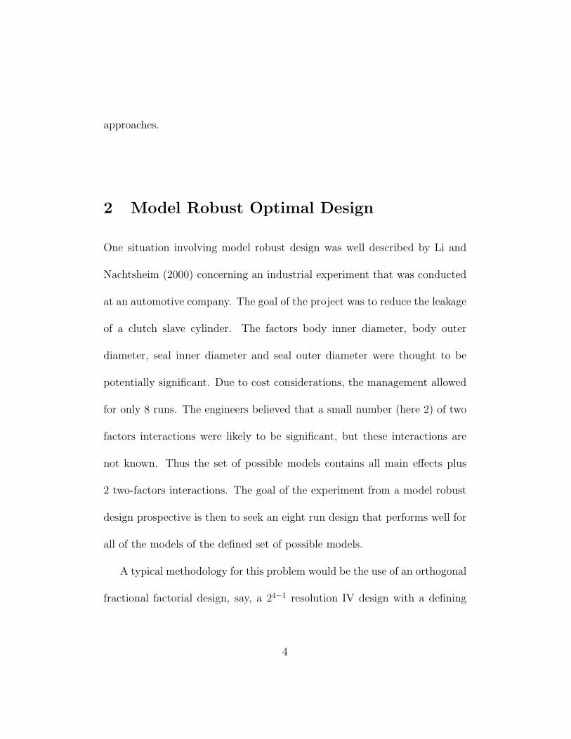
2 Model Robust Optimal Design
One situation involving model robust design was well described by Li and
Nachtsheim (2000) concerning an industrial experiment that was conducted
at an automotive company. The goal of the project was to reduce the leakage
of a clutch slave cylinder. The factors body inner diameter, body outer
diameter, seal inner diameter and seal outer diameter were thought to be
potentially significant. Due to cost considerations, the management allowed
for only 8 runs. The engineers believed that a small number (here 2) of two
factors interactions were likely to be significant, but these interactions are
not known. Thus the set of possible models contains all main effects plus
2 two-factors interactions. The goal of the experiment from a model robust
design prospective is then to seek an eight run design that performs well for
all of the models of the defined set of possible models.
A typical methodology for this problem would be the use of an orthogonal
fractional factorial design, say, a 24−1 resolution IV design with a defining
4

relation I=1234. Such a design allows the estimation of the four main effects
as well as the confounded pairs 12=34, 13=24, 14=23. However, this design
may be of great interest if it is known in advance that the only interactions
likely to be present are, for example, those involving factor 1. Since the
experimenters were seeking a design capable of estimating models containing
all main effects and any pair of two-factor interactions, the 24−1 fractional
factorial design may be misleading. Because, there are(42
)= 6 two-factor
interactions, the number of possible models that include all main effects and
2 two-factor interactions is(62
)= 15. These models are listed in in Table 1.
If we used the 24−1V I fractional factorial design, only some of the candidate
models are estimable. It turns out that models (5), (8) and (10) are not
estimable. Nachtsheim and Li (200) considered the notion of estimation ca-
pacity (EC) of a design defined as being the ratio of the number of estimable
models to the number of possible models (following Sun 1993 and Cheng,
Steinberg, and Sun 1999). They found that EC=12/15=80%. A natural
question arises: Is there a better design for which the estimation capacity is
larger than 80%?
Nachtsheim and Li (2000) developed the notion of model-robust facto-
rial designs (MRFD’s) using a frequentist approach as an alternative to the
5

Table 1: Possible models for the 24−1 resolution IV fractional factorial design
models
Model Main effects Interaction
1 1 2 3 4 12 13
2 1 2 3 4 12 14
3 1 2 3 4 12 23
4 1 2 3 4 12 24
5 1 2 3 4 12 34
6 1 2 3 4 13 14
7 1 2 3 4 13 23
8 1 2 3 4 13 24
9 1 2 3 4 13 34
10 1 2 3 4 14 23
11 1 2 3 4 14 24
12 1 2 3 4 14 34
13 1 2 3 4 23 24
14 1 2 3 4 23 34
15 1 2 3 4 24 34
6
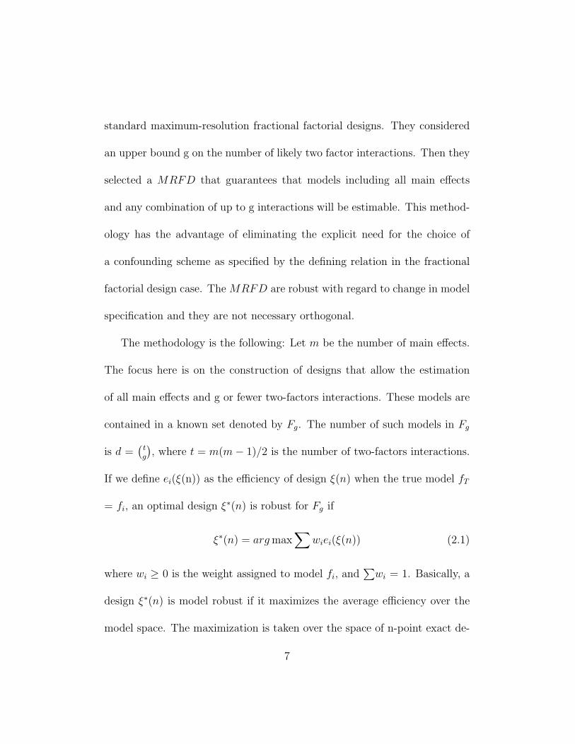
standard maximum-resolution fractional factorial designs. They considered
an upper bound g on the number of likely two factor interactions. Then they
selected a MRFD that guarantees that models including all main effects
and any combination of up to g interactions will be estimable. This method-
ology has the advantage of eliminating the explicit need for the choice of
a confounding scheme as specified by the defining relation in the fractional
factorial design case. The MRFD are robust with regard to change in model
specification and they are not necessary orthogonal.
The methodology is the following: Let m be the number of main effects.
The focus here is on the construction of designs that allow the estimation
of all main effects and g or fewer two-factors interactions. These models are
contained in a known set denoted by Fg. The number of such models in Fg
is d =(
tg
), where t = m(m− 1)/2 is the number of two-factors interactions.
If we define ei(ξ(n)) as the efficiency of design ξ(n) when the true model fT
= fi, an optimal design ξ∗(n) is robust for Fg if
ξ∗(n) = arg max∑
wiei(ξ(n)) (2.1)
where wi ≥ 0 is the weight assigned to model fi, and∑
wi = 1. Basically, a
design ξ∗(n) is model robust if it maximizes the average efficiency over the
model space. The maximization is taken over the space of n-point exact de-
7

signs. The efficiency ei will depend on the basic criterion under consideration
by the experimenter. Nachtsheim and Li considered two optimality criteria,
ECg and ICg.
For ECg −Optimality:
w1 = w2 = ... = wd = 1/d and
ei =
1 if fi is estimable,
0 otherwise.
(2.2)
For ICg −Optimality:
The efficiency ei(ξ) of the design ξ(n) for model fi is given by
ei = (Di(ξ(n))
Di(ξ∗i (n)))
1pi (2.3)
where ξ∗i (n) is the D-optimal design for model fi, Di(ξ(n)) = |X ′iXi| is the
determinant of the information matrix for design ξ(n) and model fi, pi is
the dimension of the parameter space for model fi. It is assumed that a
nonsingular optimal design ξ∗i (n) exist for each fi ∈ Fg.
Lauter (1974) proposed a number of generalized criteria, among which
was the maximization of the average, taken on the model space, of the log of
the determinant. Motivated by a similar problem concerning the estimation
of uranium content in calibration standards, Cook and Nachtsheim (1982)
8

developed the notion of model robust linear optimal design in a situation
in which, a priori, the exact degree of the polynomial regression model is
not known. DuMouchel and Jones (1994) proposed a Bayesian approach in
which they defined the notion of primary and potential models.
3 Proposed Approach to Bayesian Model Ro-
bust Design
3.1 Bayesian Optimal Design
Chaloner and Verdinelli (1995) noted that experimental design is one situa-
tion where it is meaningful within Bayesian theory to average over the sample
space. Since the sample has not yet been observed, the averaging over what
is unknown applies. Following Raiffa and Schlaifer (1961), Lindley (1956 and
1972) presented a decision-theoretic approach to the experimental design sit-
uation as follows. For a design ξ chosen from some set χ, a data y from a
sample space Y will be observed. Given y, a decision d will be chosen from
some set D. The selection of ξ and the choice of a terminal decision d con-
stitute the important parts of the process. The unknown parameters θ are
9

elements of the parameter space Θ. A general utility function is then defined
in the form of U(d,θ,ξ,y). Considering a prior distribution of p(θ) on the
parameter space, the probability distribution function of the data p(y|θ) and
the utility function (or risk function); for any design ξ, the expected utility
of the best decision is given by:
U(ξ) =
∫Y
maxdεD
∫Θ
U(d, θ, ξ,y).p(θ | y, ξ).p(y | ξ)dθdy (3.1)
The Bayesian experimental design is then the design ξ∗ maximizing U(ξ):
U(ξ∗) = maxξεχ
∫Y
maxdεD
∫Θ
U(d, θ, ξ,y).p(θ | y, ξ).p(y | ξ)dθdy (3.2)
Then the choice of the design can be regarded as a decision problem and is
equivalent to the selection of the design that maximizes the expected util-
ity with the goals ranging from estimation to prediction and so on. Lind-
ley’s (1956) work led several authors ( Stone 1959a, b; DeGroot, 1962, 1986;
Bernado, 1979) to consider the expected gain in Shannon information given
by an experiment as a utility function (Shannon, 1948). In doing so, they
proposed choosing a design that maximizes the expected gain in Shannon
information or, equivalently, maximizes the expected Kullback-Leibler diver-
gence between the posterior and the prior distributions∫ ∫
log(p(θ|y,ξ)p(θ)
)p(y, θ |
ξ)dθdy. Since the prior distribution does not depend on the optimal design
10

ξ maximizes:
U(ξ) =
∫ ∫log p(θ | y, ξ)p(y, θ | ξ)dθdy (3.3)
Consider the problem of choosing a design ξ for a normal linear regression
model. The data y are a vector of n observations, where y| θ,σ2 ∼ N
(Xθ,σ2I), θ is a vector of k unknown parameters, σ2 is known and I is the
n× n identity matrix. Let’s suppose that the prior information is such that
θ| σ2 is normally distributed with mean θ0 and variance-covariance matrix
σ2R−1, where the k × k matrix R is known. Recall the matrix X′Xn
is the
information matrix also denoted by M(ξ). The posterior distribution for θ is
also normal with mean vector θ∗ = (X ′X + R)−1(X ′y+ Rθ0) and covariance
matrix σ2D(ξ)= σ2(X ′X + R)−1; D(ξ)is a function of the design ξ and the
prior precision σ−2R. A standard calculation leads to:
U(ξ) = (−k
2) log 2π +
1
2log det(σ−2(nM(ξ) + R)) +
−k
2(3.4)
Maximizing this utility therefore reduces to maximizing the function:
φB(ξ) = det{nM(ξ) + R} = det{X ′X + R} (3.5)
This criterion is known as Bayes D-optimality.
11

3.2 Model Robust Bayesian Designs
We propose an approach based on the model robust design situation and the
general Bayesian optimal design idea that has the advantage of extending
the Bayesian D-optimality to more than one candidate model. For parame-
ter estimation purposes, a utility function based on the Shannon information
or the expected Kullback divergence between the prior and the posterior is
considered. We specify a prior probability that each model is true and con-
ditionally on this probability, prior distributions for the parameters are also
specified. We also assume that the model prior probability is independent of
the joint distribution of the the data (response variable) and the parameter
given the design.
We define this class of designs as the Bayesian Model Robust Designs
(BMRD’s) . We denote by Xi, the design matrix for the model fi for
every i ε{1, ..., d}. The prior distribution of each model fi is p(i) = wi
for each i ε{1, ..., d}. The prior distribution of the parameter θ given i is
given by θ |i ∼ N(θ0i, σ2R−1i ), where the k × k matrix Ri is known. The
posterior distribution of θ given y and i is θ|y,i, ξ ∼ N(θ∗i , σ2Di) where θ∗i
= (X ′i,ξXi,ξ + Ri)
−1(X ′iy + Riθ0i) and σ2Di = σ2(X ′
i,ξXi,ξ+Ri). We have the
requirement that∑d
i=1 wi = 1. Let µ be a counting measure associated with
12

the variable i. The expected utility function for the class of linear models
considered will be:
U(ξ) =
∫ ∫ ∫log p(θ | y, i, ξ)}p(y, θ, i | ξ)dθdyµ(di)
=
∫ ∫ ∫log p(θ | y, i, ξ)}p(y, θ | i, ξ)p(i)dθdyµ(di)
=d∑
i=1
∫ ∫log p(θ | y, i, ξ)p(y, θ | i, ξ)p(i)dθdy
=d∑
i=1
wi
∫ ∫{log p(θ | y, i, ξ)}p(y, θ | i, ξ)dθdy
=d∑
i=1
wi{−k
2log(2π)− k
2+
1
2log det(σ−2(X ′
i,ξXi,ξ + Ri)}
=d∑
i=1
wi log{det(σ−2(X ′i,ξXi,ξ + Ri))}+
d∑i=1
wi{k
2+
k
2log(2π)}
Therefore the criteria for finding the Bayesian Model Robust Optimal design
is reduced then to maximizing the function:
φBR(ξ) =d∑
i=1
wi log{det(σ−2(X ′i,ξXi,ξ + Ri))} (3.6)
3.2.1 Model Priors
The model prior is the probability assigned to each of the models of interest.
Based on prior knowledge of such experiments, this prior can be assigned
uniformly on each of the models. We denoted this as the uniform model
robust Bayesian design.
13

We can also based our choice of priors on the use of hierarchical model
priors as advocated by Chipman, Hamada and Wu (1997). The prior for all
the candidate models is derived from the prior on the main effects and the
different interactions. A vector δ of zeros and ones having the same length
as the parameter θ capture the importance of all the models.
As a simple example, consider a model including three main effects A,
B, C and three two-factor interactions AB, AC and BC. The importance
of the term AB will depend on whether whether the main effects A and B
are included or not in the model. If they are included in the model, the
interaction is more likely, otherwise, the interaction seems less plausible and
more difficult to explain. The prior on δ is then expressed as δ = (δA, ..., δBC)
as follows.
Pr(δ) = Pr(δA)Pr(δB)Pr(δC)Pr(δAB | δA, δB)Pr(δAC | δA, δC)Pr(δBC | δB, δC)
(3.7)
The conditional independence and the inheritance principle are required in
this approach. The conditional independence states that conditional on first
order terms, the second order terms (δAB,δAC ,δBC) are independent. The
main effects are also assumed to be independent. The inheritance principle
assumes that the importance of a term depends only on those from which it
14
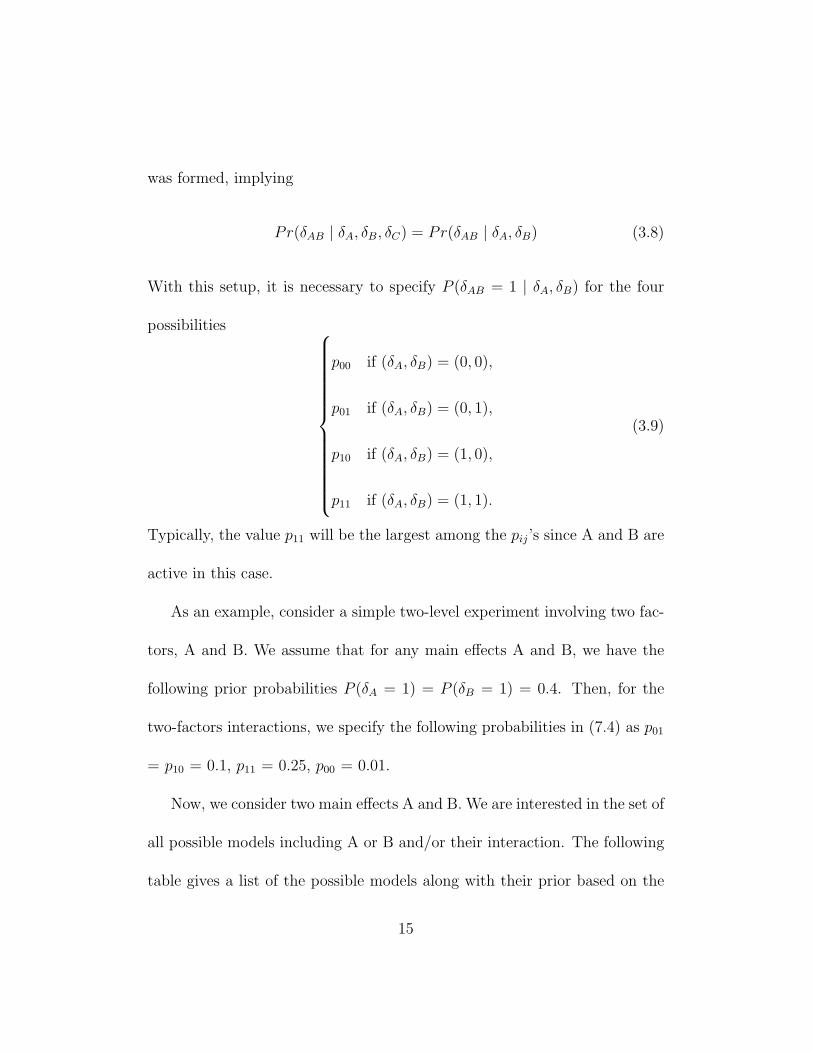
was formed, implying
Pr(δAB | δA, δB, δC) = Pr(δAB | δA, δB) (3.8)
With this setup, it is necessary to specify P (δAB = 1 | δA, δB) for the four
possibilities
p00 if (δA, δB) = (0, 0),
p01 if (δA, δB) = (0, 1),
p10 if (δA, δB) = (1, 0),
p11 if (δA, δB) = (1, 1).
(3.9)
Typically, the value p11 will be the largest among the pij’s since A and B are
active in this case.
As an example, consider a simple two-level experiment involving two fac-
tors, A and B. We assume that for any main effects A and B, we have the
following prior probabilities P (δA = 1) = P (δB = 1) = 0.4. Then, for the
two-factors interactions, we specify the following probabilities in (7.4) as p01
= p10 = 0.1, p11 = 0.25, p00 = 0.01.
Now, we consider two main effects A and B. We are interested in the set of
all possible models including A or B and/or their interaction. The following
table gives a list of the possible models along with their prior based on the
15

Table 2: Prior table for all possible models with at most two main effects
and one two factors interaction.
Models A B AB Prior Computation Prior
1 0 0 0 (0.6)2(0.99) 0.3564
2 1 0 0 (0.4)(0.6)(0.9) 0.2260
3 0 1 0 (0.4)(0.6)(0.9) 0.2260
4 0 0 1 (0.6)2(0.1) 0.0036
5 1 1 0 (0.4)2(0.75) 0.1200
6 0 1 1 (0.4)(0.6)(0.1) 0.0240
7 1 0 1 (0.4)(0.6)(0.1) 0.0240
8 1 1 1 (0.4)2(0.25) 0.0400
priors on A, B and the hierarchical priors stated above. In the table, each
model is represented by δ = (δA, δB, δAB) where δA, δB, δAB take the values 0
or 1.
3.2.2 Examples with two-level factors
Uniform model robust Bayesian design
In what follows, we consider only two-level experiments. We will use +1
16

and -1 to denote the levels of each of the factors (main effects). The known
model set in consideration is comprised of models containing m main effects
and a specified number g of two factor interactions for a specific number n
of runs. In the examples that follow, the prior distribution of the parameters
p(θ | i) follows a normal distribution with mean θ0i and variance covariance-
matrix σ2R−1i , where the k × k matrix R−1
i is the matrix c ∗ Ik×k, Ik×k is
the k × k identity matrix, k is the dimension of the parameter vector θ0i
and c is a constant. We considered an arbitrary prior p(i) given by p(i) = 1d
for each model where d is the number of candidate models considered. The
signs + and - denote respectively the high and low levels of each of the main
effects. The X’s represent the main effects of the factors in consideration in
the examples. The examples are constructed using the coordinate exchange
algorithm with 100 starting designs selected at random. The best design
among the 100 resulting designs is chosen to be the optimal design. The
design tables are stated in the Table 3 and presented in the Appendix.
The performances of the FFD, the MRFD and BMRD are assessed
using the information capacity, estimation capacity and the Bayesian model
robust-based criteria as shown in the tables 4, 5, 6 and 7.
The proposed Bayesian model robust criteria values for the Bayesian
17

Table 3: Summary table of the constructed designs
Design tables in Appendix n m g c
9 6 3 2 1, 3, 10, 100
10 6 4 1 100
11 8 4 3 1
12 8 5 2 3
Table 4: Comparison table between the FFD, MRFD and the BMRD for
n = 8, c = 10 , g = 1 and m = 4
m Designs IC1 EC1 BR1
4 FFD 1.000 1.00 8.32
4 MRFD 1.000 1.00 11.78
4 BMRD 0.7071 1.00 13.905
18
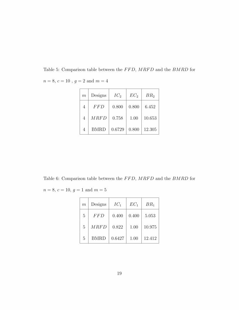
Table 5: Comparison table between the FFD, MRFD and the BMRD for
n = 8, c = 10 , g = 2 and m = 4
m Designs IC2 EC2 BR2
4 FFD 0.800 0.800 6.452
4 MRFD 0.758 1.00 10.653
4 BMRD 0.6729 0.800 12.305
Table 6: Comparison table between the FFD, MRFD and the BMRD for
n = 8, c = 10, g = 1 and m = 5
m Designs IC1 EC1 BR1
5 FFD 0.400 0.400 5.053
5 MRFD 0.822 1.00 10.975
5 BMRD 0.6427 1.00 12.412
19

Table 7: Comparison table between the FFD, MRFD and the BMRD for
n = 8, c = 10, g = 2 and m = 5
m Designs IC2 EC2 BR2
5 FFD 0.089 0.089 4.51
5 MRFD 0.508 0.733 9.73
5 BMRD 0.5540 0.9556 11.02
model robust designs exceeded all those for the Model Robust Factorial De-
signs and the Fractional Factorial Designs. The information capacity and the
estimation capacity criterion values of the Bayesian model robust designs ex-
ceed most of the values of the Fractional Factorial Designs and just few of
the values of the Model Robust Factorial Designs. Indeed, for the estimation
capacity criteria, the Bayesian model robust designs produced performed bet-
ter than the related fractional factorial designs. This is the indication that
the Bayesian model robust designs produced by the proposed approach do
well compared to designs produced by other criteria and perform sometimes
better with respect to the Model robust factorial design criterion proposed
by Li and Nachtsheim (2000). They produced reasonably good estimation
and information capacity efficiencies. The values of efficiency get better for
20

large values of m, g. However, the resulting designs are definitely sensitive
to the choice of the model and parameter priors.
Hierarchical model robust Bayesian design
Considering all the different models in the table 2 above with their re-
spective priors, the related Bayesian model robust design for n = 8 runs and
c = 10 appears in the table 12 of the Appendix. This design is balanced and
is the replicated two level two by two factorial design. It is the same as the
design produced by the model robust factorial design using the information
capacity criteria in this case.
Appendix
Table8: Uniform Design matrix for n = 6, m = 3, g = 2, c ∈ {1, 3, 10, 100}
1 - + +
2 - - +
3 + - -
4 - + -
5 + - +
6 + - -
Table9:Uniform Design matrix for n = 6, m = 4, g = 1, c = 100
21

1 + - + +
2 - - - -
3 + - - -
4 + + - +
5 + + + -
6 - + + +
Table10: Uniform Design matrix for n = 8, m = 4, g = 3, c = 1
1 - + + +
2 + - + +
3 + + + -
4 - - - +
5 + + - +
6 + - - -
7 - - + -
8 - + - -
Table11: Uniform Design matrix for n = 8, m = 5, g = 2, c = 3
22

1 - - + - -
2 + - + + -
3 + - - - +
4 + + + - -
5 - + - - +
6 - + + + +
7 - + - + -
8 - - - + +
Table12: Hierachical Design matrix for n = 8, c = 10
Design points X1 X2
1 + -
2 + +
3 + -
4 - -
5 - +
6 - -
7 + +
8 - +
23

References
K. Chaloner (1984), Optimal Bayesian experimental designs for linear mod-
els. Ann. Statist 12, 283-300.
K. Chaloner (1985), Bayesian experimental design: A review. Statistical
Science 10, 273-304.
H. Chipman, M. Hamada and C. F. J. Wu (1997), A Bayesian Variable
Selection Approach for Analyzing Designed Experiments with Complex
Aliasing. Technometrics 39, 372-381.
R. D. Cook and C. Nachtsheim (1980), A comparison of algorithm for con-
structing exact D-optimal designs. Technometrics 22, 315-324.
R. D. Cook and C. Nachtsheim (1982), Model Robust, Linear-Optimal De-
signs. Technometrics 24, 49-54.
W. DuMouchel and B. Jones (1994), A simple Bayesian modification of
D-optimal designs to reduce dependence on an assumed model. Tech-
nometrics 36, 37-47.
E. Lauter (1974), Experimental design in a class of models. Math. Opera-
tionsforsch. Statist. 5, 379-396.
24
W. Li and C. F. J. Wu (1997), Columnwise-pairwise in a class of models.
Technometrics 39, 171-179.
W. Li and C. J. Nachtsheim (2000), Model-robust factorial designs. Tech-
nometrics 42, 379-396.
25