Bayesian Computational Tools - arXiv

Bayesian Computational Tools∗

Christian P. Robert

Abstract: This chapter surveys advances in the field of Bayesian com-putation over the past twenty years, from a purely personnal viewpoint,hence containing some ommissions given the spectrum of the field. MonteCarlo, MCMC and ABC themes are thus covered here, while the rapidlyexpanding area of particle methods is only briefly mentioned and differentapproximative techniques like variational Bayes and linear Bayes methodsdo not appear at all. This chapter also contains some novel computationalentries on the double-exponential model that may be of interest per se.

Keywords and phrases: ABC algorithms, Bayesian inference, consis-tence, Gibbs sampler, MCMC methods, simulation.

1. Introduction

It has long been a bane of the Bayesian approach that the solutions it proposedwere intellectually attractive but inapplicable in practice. While some numericalanalysis solutions were suggested (see, e.g. Smith, 1984), they were not in parwith the challenges raised by handling non-standard probability densities, espe-cially in high dimensional problems. This stumbling block in the development ofthe Bayesian perspective became clear when new simulations methods appearedin the early 1990’s and the number of publications involving Bayesian methodsrised significantly (no test available!). While those methods were on principleopen to any type of inference, they primarily benefited the Bayesian paradigmas they were “ideally” suited to the core object of Bayesian inference, namely amostly intractable posterior distribution.

This chapter will not cover the historical developments of computationalmethods (see, e.g., Robert and Casella, 2011) nor the technical implementa-tion details of simulation techniques (see, e.g., Doucet et al., 2001, Robert andCasella, 2004, Robert and Casella, 2009 and Brooks et al., 2011), but insteadfocus on examples of application of those methods to Bayesian computationalchallenges. Given the limited length of the chapter, it is to be understood as asequence of illustrations of the main computational tools, rather than a compre-hensive introduction, which is to be found in the books mentioned above andbelow.

∗Christian P. Robert, CEREMADE, Universite Paris-Dauphine, 75775 Paris cedex 16,France [email protected]. Research partly supported by the Agence Nationale de laRecherche (ANR, 212, rue de Bercy 75012 Paris) through the 2012–2015 grant ANR-11-BS01-0010 “Calibration” and by a Institut Universitaire de France senior chair. C.P. Robert is alsoaffiliated as a part-time researcher with CREST, INSEE, Paris.

1

imsart-generic ver. 2009/02/27 file: BCP.tex date: June 12, 2013

arX

iv:1

304.

2048

v2 [

stat

.ME

] 1

1 Ju

n 20

13

/Bayesian Computational Tools 2

2. Some computational challenges

The starting point of a Bayesian analysis being the posterior distribution, letus recall that it is defined by the product

π(θ|x) ∝ π(θ)f(x|θ)

where θ denotes the parameter and x the data. (The symbol ∝ means that thefunctions on both sides of the symbol are proportional as functions of θ, themissing constant being a function of x, m(x).) The structures of both θ and xcan vary in complexity and dimension, although we will not discuss the non-parametric case when θ is infinite dimensional, referring the reader to Holmeset al. (2002) for an introduction. The prior distribution is most often availablein closed form, being chosen by the experimenter, while the likelihood functionf(x|θ) may be too involved to be computed even for a given pair (x, θ). In specialcases where f(x|θ) allows for a demarginalisation representation

f(x|θ) =

∫f(x, z|θ) dz ,

where g(x, z|θ) is a (manageable) probability density, we will call z the missingdata. However, the existence of such a representation does not necessarily impliesit is of any use in computations. (We will encounter both cases in Sections 4and 5.)

Since the posterior distribution is defined by

π(θ|x) = π(θ)f(x|θ)/∫

Θ

π(θ)f(x|θ) dθ

a first difficulty occurs because of the normalising constant: the denominatoris very rarely available in closed form. This is an issue only to the extent thatthe posterior density is defined up to a constant. In cases where the constantdoes not matter, inference can be easily conducted without the constant. Caseswhen the constant matters include testing and model choice, since the marginallikelihood

m(x) =

∫Θ

π(θ)f(x|θ) dθ

is central to the Bayesian procedures addressing this inferential problem. Indeed,when comparing two models against the same dataset x, the prefered Bayesiansolution (see, e.g., Robert, 2001, Chapter 5, or Jeffreys, 1939) is to use the Bayesfactor, defined as the ratio of marginal likelihoods

B12(x) =m1(x)

m2(x)=

∫Θ1π(θ1)f(x|θ1) dθ1∫

Θ2π(θ2)f(x|θ2) dθ2

,

and compared to 1 to decide which model is most supported by the data (andhow much). Such a tool—quintessential for running a Bayesian test—means that



for almost any inference problem—barring the very special case of conjugatepriors— there is a computational issue, not the most promising feature forpromoting an inferential method. This aspect has obviously been addressedby the community, see for instance Chen et al. (2000) that is entirely dedicatedto the problem of approximating normalising constants or ratios of normalisingconstants, but I regret the issue is not spelled out much more clearly as one ofthe major computational challenges of Bayesian statistics (see also Marin andRobert, 2011).

Example 1 As a benchmark, consider the case (Marin et al., 2011a) when asample (x1, . . . , xn) can be issued either from a normal N (µ, 1) distribution orfrom a double-exponential L(µ, 1/

√2) distribution with density

f0(x|µ) =1√2

exp{−√

2|x− µ|} .

(This case was suggested to us by a referee of Robert et al., 2011, howeverI should note that a similar setting opposing a normal model to (simple) ex-ponential data used as a benchmark in Ratmann (2009) for ABC algorithms.)Then, as it happens, the Bayes factor B01(x1, . . . , xn) is available in closed form,since, under a normal µ ∼ N (0, σ2) prior, the marginal likelihood for the normalmodel is given by

m1(x1, . . . , xn) =

∫(2π)−n/2

n∏i=1

exp{−(xi − µ)2/2} exp{−µ2/2σ2} dµ/√

2πσ

= (2π)−n/2 exp{−n∑i=1

(xi − xn)2/2}

×∫

exp[−{(n+ σ−2)µ2 − 2nµxn + n(xn)2}/2] dµ/√

2πσ

= (2π)−n/2 exp{−n∑i=1

(xi − xn)2/2}

× exp{−nσ−2(xn)2/2(n+ σ−2)}/σ√n+ σ−2



and, for the double-exponential model, by (assuming the sample is sorted)

m0(x1, . . . , xn) =

∫2−n/2

n∏i=1

exp{−√

2|xi − µ|} exp{−µ2/2σ2} dµ/√

2πσ

=2−n/2√

2πσ

n∑i=0

∫ xi+1

xi

i∏j=1

e√2xj−

√2µ

n∏j=i+1

e−√2xj+

√2µe−µ

2/2σ2

dµ

=2−n/2√

2πσ

n∑i=0

∫ xi+1

xi

e√2∑i

j=1 xj−√2∑n

j=i+1 xj+√2(n−2i)µe−µ

2/2σ2

dµ

= 2−n/2n∑i=0

e√2∑i

j=1 xj−√2∑n

j=i+1 xj+2(n−2i)2σ2/2

×∫ xi+1

xi

e−{µ−√2(n−2i)σ2}2/2σ2

dµ/√

2πσ

= 2−n/2n∑i=0

e√2∑i

j=1 xj−√2∑n

j=i+1 xj+(n−2i)2σ2

×[Φ({xi+1 −

√2(n− 2i)σ2}/σ)− Φ({xi −

√2(n− 2i)σ2}/σ)

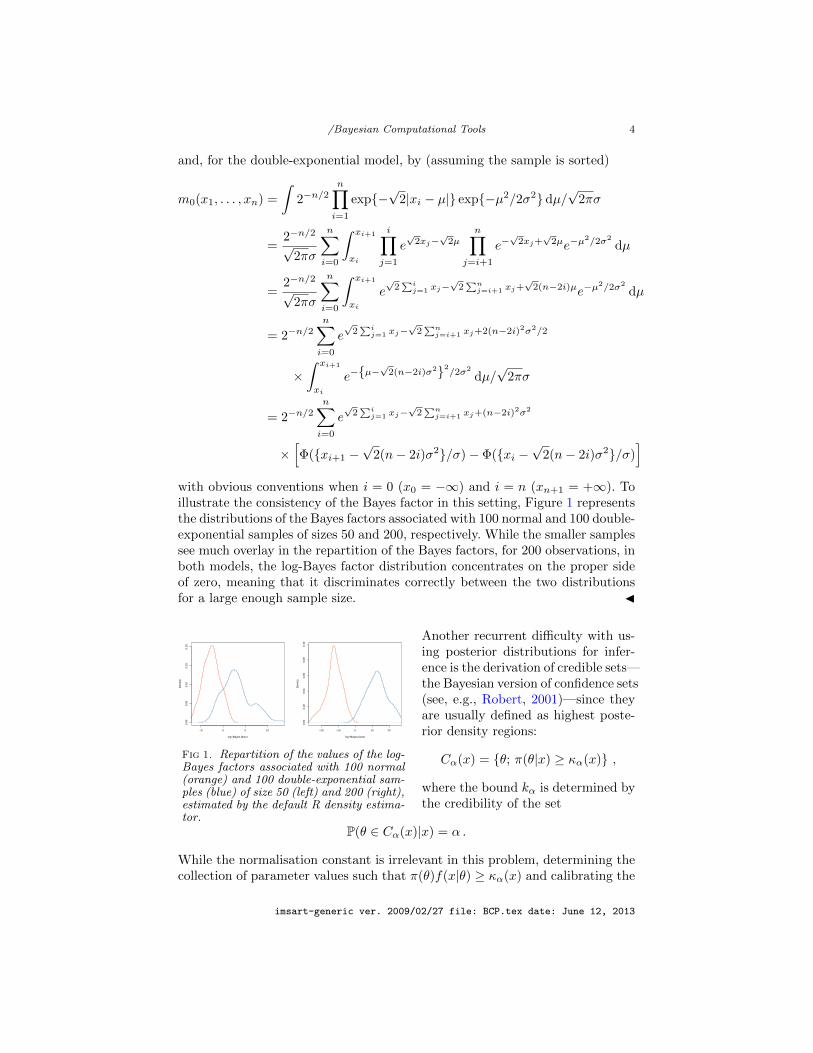
]with obvious conventions when i = 0 (x0 = −∞) and i = n (xn+1 = +∞). Toillustrate the consistency of the Bayes factor in this setting, Figure 1 representsthe distributions of the Bayes factors associated with 100 normal and 100 double-exponential samples of sizes 50 and 200, respectively. While the smaller samplessee much overlay in the repartition of the Bayes factors, for 200 observations, inboth models, the log-Bayes factor distribution concentrates on the proper sideof zero, meaning that it discriminates correctly between the two distributionsfor a large enough sample size. J

−5 0 5 10

0.00

0.05

0.10

0.15

0.20

log−Bayes factor

Den

sity

−20 −10 0 10 20

0.00

0.02

0.04

0.06

0.08

0.10

log−Bayes factor

Den

sity

Fig 1. Repartition of the values of the log-Bayes factors associated with 100 normal(orange) and 100 double-exponential sam-ples (blue) of size 50 (left) and 200 (right),estimated by the default R density estima-tor.

Another recurrent difficulty with us-ing posterior distributions for infer-ence is the derivation of credible sets—the Bayesian version of confidence sets(see, e.g., Robert, 2001)—since theyare usually defined as highest poste-rior density regions:

Cα(x) = {θ; π(θ|x) ≥ κα(x)} ,

where the bound kα is determined bythe credibility of the set

P(θ ∈ Cα(x)|x) = α .

While the normalisation constant is irrelevant in this problem, determining thecollection of parameter values such that π(θ)f(x|θ) ≥ κα(x) and calibrating the



lower bound κα(x) on the product π(θ)f(x|θ) to achieve proper coverage arenon-trivial problems that require advanced simulation methods. Once again, theissue is somehow overlooked in the literature.

While one of the major appeals of Bayesian inference is that it is not reducedto an estimation technique—but on the opposite offers a whole range of inferen-tial tools to analyse the data against the proposed model—, the computation ofBayesian estimates is nonetheless certainly one of the better addressed compu-tational issues. This is especially true for posterior moments like the posteriormean Eπ[θ|x] since they are directly represented as ratios of integrals

Eπ[θ|x] =

∫Θθπ(θ)f(x|θ) dθ∫

Θπ(θ)f(x|θ) dθ

.

The computational problem may however get involved for several reasons, in-cluding for instance

– the space Θ is not Euclidean and the problem imposes shape constraints(as in some time series models);

– the dimension of Θ is large (as in non-parametrics);– the estimator is the solution to a fixed point problem (as in the credible

set definition);– simulating from π(θ|x) is delicate or even impossible;

the latter case being in general the most challenging and thus the most studied,as the following sections will show.

3. Monte Carlo methods

Monte Carlo methods have been introduced by physicists in Los Alamos, namelyUlam, von Neumann, Metropolis, and their collaborators in the 1940’s (seeRobert and Casella, 2011). The idea behind Monte Carlo is a straightforward ap-plication of the law of large numbers, namely that, when x1, x2, . . . are i.i.d. fromthe distribution f , the empirical average

1

T

T∑t=1

h(xt)

converges (almost surely) to Ef [h(X)] when T goes to +∞. While this per-spective sounds too simple to apply to complex problems—either because thesimulation from f itself is intractable or because the variance of the empiricalaverage is too large to be manageable—, there exist more advanced exploitationsof this result that lead to efficient simulation solutions.

Example 1 (bis) Consider computing the Bayes factor

B01(x1, . . . , xn) = m0(x1, . . . , xn)/m1(x1, . . . , xn)



by simulating a sample (µ1, . . . , µT ) from the prior distribution, N (0, σ2). Theapproximation to the Bayes factor is then provided by

B01 =

T∑t=1

n∏i=1

f0(xi|µt)/ T∑

t=1

n∏i=1

f1(xi|µt) ,

given that in this special case the same prior and the same Monte Carlo samples

can be used. Figure 2 shows the convergence of B01 over T = 105 iterations,along with the true value. The method exhibits convergence. J

0 200 400 600 800 1000

0.05

00.

055

0.06

0

iterations

Fig 2. Convergence of aMonte Carlo approximationof B01(x1, . . . , xn) for a normalsample of size n = 19, along withthe true value (dash line).

The above example can also be interpretedas an illustration of importance sampling,in the sense that the prior distribution isused as an importance function in both inte-grals. We recall that importance sampling isa Monte Carlo method where the quantity ofinterest Ef [h(X)] is expressed in terms of anexpectation under the importance density g,

Ef [h(X)] = Eg[h(X)f(X)/g(X)] ,

which allows for the use of Monte Carlo sam-ples distributed from g. Although importancesampling is at the source of the particle method(Doucet et al., 2001), I will not develop thisuseful sequential method any further, but in-stead briefly introduce the notion of bridge

sampling (Meng and Wong, 1996) as it applies to the approximation of Bayesfactors

B01(x) =

∫Θ0

f0(x|θ0)π1(θ0) dθ0/∫Θ1

f1(x|θ1)π1(θ1) dθ1

(and to other ratios of integrals). This method handles the approximation ofratios of integrals over identical spaces (a severe constraint), by reweighting twosamples from both posteriors, through a well-behaved type of harmonic average.

More specifically, when Θ0 = Θ1, possibly after a reparameterisation of bothmodels to endow θ with the same meaning, we have

B01(x) =

∫Θ0

f0(x|θ)π0(θ)α(θ)π1(θ|x)dθ

/∫Θ1

f1(x|θ)π1(θ)α(θ)π0(θ|x)dθ

≈n1−1∑n1

j=1 f0(x|θ1,j)π0(θ1,j)α(θ1,j)

n0−1∑n0

j=1 f1(x|θ0,j)π1(θ0,j)α(θ0,j)



where θ0,1, . . . , θ0,n0 and θ1,1, . . . , θ1,n1 are two independent samples comingfrom the posterior distributions π0(θ|x) and π1(θ|x), respectively. (This identityholds for any function α guaranteeing the integrability of the products.) How-ever, there exists a quasi-optimal solution, as provided by Gelman and Meng(1998):

α?(θ) ∝ 1

n0π0(θ|x) + n1π1(θ|x).

While this optimum cannot be used—given that it relies on the normalisingconstants of both π0(·|x) and π1(·|x)—, a practical implication of the resultresorts to an iterative construction of α?. We gave in Chopin and Robert (2010)an alternative representation of the bridge factor that bypasses this difficulty (ifdifficulty there is!).

Example 1 (ter) If we want to apply the bridge sampling solution to the nor-mal versus double-exponential example, we need to simulate from the posteriordistributions in both models. The normal posterior distribution on µ is a normalN (nxn/(n+ σ−2), 1/(n+ σ−2)) distribution, while the double-exponential dis-tribution can be derived as a mixture of (n+ 1) truncated normal distributions,following the same track as with the computation of the marginal distributionabove. The sum obtained in the above expression of m0(x1, . . . , xn) suggestsinterpreting π0(µ|x1, . . . , xn) as (once again assuming x sorted)

n∑i=0

ωiNT(√

2(n− 2i)σ2, σ2, xi, xi+1)

where NT(δ, τ2, α, β) denotes a truncated normal distribution, that is, the nor-mal N (δ, τ2) distribution restricted to the interval (α, β), and where the weightsωi are proportional to those summed in m0(x1, . . . , xn) (see Example 1 (bis)).The outcome of one such simulation is shown in Figure 3 along with the tar-get density: as seen there, since the true posterior can be plotted against thehistogram, the fit is quite acceptable. If we start with an arbitrary estimationof B01 like b01 = 1, successive iterations produce the following values for theestimation: 11.13, 10.82, 10.82, based on 104 samples from each posterior dis-tribution (to compare with an exact ratio equal to 10.3716 and a Monte Carloapproximation of 10.55). J



µ

Den

sity

−0.10 −0.05 0.00 0.05 0.10

02

46

8

Fig 3. Histogram of 104 simulations fromthe posterior distribution associated witha double-exponential sample of size 150,along with the curve of the posterior(dashed lines).

While this bridge solution produces valu-able approximations when both param-eters θ0 and θ1 are within the sameparameter space and have the sameor similar absolute meanings (e.g., θis equal to Eθ[X] in both models), itdoes not readily apply to settings withvariable dimension parameters. In suchcases, separate approximations of theevidences, i.e. of the numerator anddenominator in B01 are requested, withthe exception of reversible jump MonteCarlo techniques (Green, 1995) pre-sented in the following section. Althoughusing harmonic means for this pur-pose as in Newton and Raftery (1994)is fraught with danger, as discussedin Neal (1994) and Marin and Robert(2011), we refer the reader to this laterpaper of ours for a model-based solu-tion using an importance function restricted to an HPD region (see also Robertand Wraith, 2009 and Weinberg, 2012). We however insist on (and bemoan) thelack of generic solution for the approximation of Bayes factors, despite thosebeing the workhorse of Bayesian model selection and hypothesis testing.

4. MCMC methodology

The above Monte Carlo techniques impose (or seem to impose) constraints onthe posterior distributions that can be approximated by simulation. Indeed,direct simulation from this target distribution is not always feasible in a (time-wise) manageable form, while importance sampling may result in very poor oreven worthless approximations, as for instance when the empirical average

1

T

T∑t=1

f(xt)

g(xt)h(xt)

suffers from an infinite variance. Finding a reliable importance function thusrequires some sufficient knowledge about the posterior density π(·|x). Markovchain Monte Carlo (MCMC) methods were introduced (also in Los Alamos)with the purpose of bypassing this requirement of an a priori knowledge onthe target distribution. On principle, they apply to any setting where π(·|x) isknown up to a normalising constant (or worse, as a marginal of a distributionon an augmented space).

As described in another chapter of this volume (Craiu and Rosenthal, 2013),MCMC methods rely on ergodic theorems, i.e. the facts that, for positive re-current Markov chains, (a) the limiting distribution of the chain is always the



stationary distribution and (b) the law of large numbers applies. The fascinat-ing feature of those algorithms is that it is straightforward to build a Markovchain (kernel) with a stationary distribution equal to the posterior distribution,even when the latter is only know up to a normalising constant. Obviously,there are caveats with this rosy tale: complex posteriors remain harder to ap-proximate than essentially Gaussian posteriors, convergence (ergodicity) mayrequire in-human time ranges or simply not agree with the limited precision ofcomputers.

For completeness’ sake, we recall here the format of a random walk Metropolis–Hastings (RWMH) algorithm (Hastings, 1970)

Algorithm 1 RWMHfor t = 1 to T do

Generate ξ ∼ ϕ(|ξ − θt−1|)Take θt = ξ with probability α = min{1, f0(x|ξ)π0(ξ)

/f0(x|θt−1)π0(θt−1)

Take θt = θt−1 otherwise.end for

●●●●●●●●●●●●●●●●●●●●●●●●●●●●●●●●●●●●●●●

●●●●

●●●●●●●●●

●●●●●●●●

●

●●●●●●●●●●●

●●●●●●●●●●●●●●●●●●●

●●●●●●●●●●●●●

●●●●●●●●●●●●●●●●●●●●●●

●●●●●●●●●●●●●●●●●●

●●●●●●●●●●●●●●●●●●●●●●●

●

●●●●●●●

●●●●●●●●●●●●●●

●●●●●●●●●●●●●●●●●●●●●●●

●●●●●●●●●●●●●●●●●●●●●●●●●●●

●●●●●●●

●●●●●●●●●●●●●●●●●●●●●●●●●●●●

●●●●●●●

●●●●●●●●●●●●●●●●●●●●●●

●●●●●●●●●●●●●●●●●●●●●●●●●●●●●●●●●●●●●●●●●●●

●●●●●●●●●●●●●●●

●●●●●●●●●●●●●●●●

●●●●●●●●●●●●●●●●●●●●

●●●●●●●●●●●●●●●●●●●●●●●●●●●●●●●●●●●●●

●●●●●●

●●●●●●●●●●●●●●●●●●●●●●●●●●●●●●●●●●●●●●●●●●●●

●●●●●●●●●●●●●●●●●●●●●●●●●●●●●●●●●●●●

●●●●●●●●●●

●●●●●●●

●

●

●●●●●

●●●●●

●●●●●●●

●●●●●●●●●●●●●●●●●●●●●●●●●●●●●●●●●●●●●●●●●●●●●●●●●●●●●●●●●●●●●●●●●●●●●●●●●●●●●

●●●●●●●●●●●●●●●●

●●●●●●●●●●●●●●●●●

●●●●●●●●●●●●●●●●●●●●●●●●●●●●●●●●●●●●●●●●●●●●●●●●●●●●●●●●●●●●●●●●●●●●●●●●●●●●

●●●●●●●●●

●●●●●●●●●●●●●●●●●●●●●●●

●●●●●●

●●●●●●●●●●●●●●●●●●●●●●●●●●●●●●

●

●●●

●●●●

●●●●●●●●●●●●●●●●●●●●●●

●●●●●●●●

●●●●●●●●●●●●●●●

●●●●●●●●●●●●

●●●●●●●●●●●●●●●●●●●●●●●●●●●●●●●●●

●●●●●●●●

●●●●●●●●●●●●●●●●●●

●●●●●●●●●

●●●●●●●

●●●●●●●●●●●●●●●●●●●●●●●●●●●●●●●●●●●●

●●●●●●●●

0 200 400 600 800 1000

−0.

2−

0.1

0.0

0.1

0.2

iterations

µ

●

●

●

●

●

●

●

●

●

●

●

●

●

●

●●

●●

●

●

●

●

●

●

●

●

●

●

●

●

●

●●

●

●

●

●

●●

●●

●

●

●

●

●

●

●

●

●

●

●

●

●

●

●

●

●

●

●

●

●

●

●

●

●

●

●

●

●

●

●

●

●

●●

●

●

●

●

●

●

●

●

●

●

●

●

●

●

●

●

●

●

●

●

●

●

●

●

●

●

●●

●

●

●

●

●

●

●

●

●●

●

●●

●

●

●

●

●

●

●

●

●

●

●

●

●

●

●

●

●

●

●

●

●

●

●

●

●

●

●

●

●

●

●

●●

●

●

●

●

●

●●

●●

●

●

●

●

●

●

●

●

●

●

●

●

●

●

●●

●

●

●●

●

●

●

●

●

●

●

●

●

●

●

●

●

●

●

●●

●

●●

●

●

●

●

●

●

●

●

●

●

●

●

●

●

●●

●

●

●

●

●

●

●

●

●●

●

●

●

●

●

●

●

●

●

●

●

●

●●

●

●

●

●

●

●

●●

●

●

●

●

●

●

●

●

●

●

●

●

●●

●

●

●

●

●

●

●

●

●

●

●

●

●

●

●

●

●

●

●

●

●

●

●

●

●

●

●

●

●

●

●

●

●●

●

●

●

●

●

●●

●

●

●●

●

●

●●

●●

●

●

●

●

●

●●

●

●

●

●

●

●

●

●

●

●●

●

●

●

●

●●●

●

●●

●

●

●

●

●

●

●

●●●

●

●

●

●

●

●

●

●

●

●●

●●

●

●

●

●

●

●

●

●

●

●

●

●●

●

●●

●

●

●

●

●●

●

●

●

●

●

●

●

●

●

●

●

●

●

●

●

●●

●●

●

●

●

●

●

●

●

●

●

●

●

●

●

●●

●

●

●

●

●

●

●

●●

●

●

●

●

●●

●

●

●

●

●

●

●

●

●

●

●

●

●

●

●

●

●

●

●

●

●●

●

●

●

●●

●●

●

●

●

●

●

●

●

●

●●

●

●

●●

●

●

●

●

●

●

●

●

●

●

●

●

●

●

●

●

●

●

●

●

●

●

●●

●

●

●

●

●

●

●

●

●

●

●

●

●

●

●

●

●

●●

●

●

●

●

●●

●

●

●

●●

●●

●

●●

●●

●

●

●

●

●

●

●

●●

●

●

●

●

●

●

●

●

●

●

●

●

●

●

●

●

●

●

●

●

●

●

●

●

●

●

●

●

●

●

●

●

●

●

●

●●

●

●

●

●

●

●

●

●

●

●

●

●

●

●●

●

●●

●●

●

●

●

●

●

●

●

●

●

●

●

●

●

●●

●

●

●

●

●

●

●

●

●

●

●

●●

●

●

●

●

●

●

●

●●

●

●

●

●

●

●●

●

●

●

●

●

●

●

●

●

●●

●

●

●●

●

●

●

●

●

●

●

●

●●

●

●

●

●

●

●

●

●

●

●

●

●

●

●

●

●

●

●

●

●●

●

●

●

●

●

●

●

●

●

●

●

●

●●

●

●

●

●

●

●

●

●

●

●

●●

●

●

●

●

●

●

●

●

●

●

●

●

●

●

●

●

●

●

●

●

●

●

●●

●

●

●

●●

●

●

●

●

●

●

●

●

●●

●

●

●

●

●

●

●

●

●

●

●

●

●

●

●

●●●

●

●●

●

●

●

●

●

●

●

●

●

●

●

●

●

●●

●

●

●

●

●

●●

●

●

●

●

●●

●●

●

●

●

●●

●●

●●

●

●

●

●

●

●

●

●

●

●●

●

●

●

●

●

●

●

●

●

●

●●

●

●●

●

●

●

●

●

●

●

●

●

●

●

●

●

●

●

●

●

●

●

●●

●

●

●

●

●

●

●

●

●

●

●●

●

●

●

●

●

●●

●

●

●●

●

●

●

●

●

●●●

●

●

●

●●

●

●

●

●

●

●

●

●

●

●

●●

●

●

●

●

●

●

●

●●

●

●●

●

●

●

●

●

●

●

●

●

●

●

●

●

●

●

●

●

●

●●

●

●

●

●

●

●

●

●

●

●●

●

●

●

●

●

●

●

●

●

●

●

●

●

●

●

●

●

●

●

●

●●●

●

●●

●

●

●●

●

●●

●●

●

●

●

●

●

●

●

●

●●●●●●●●●●●●●●●●●●●●●●●●●●●●●●●●●●●●●●●

●●●●

●●●●●●●●●

●●●●●●●●

●

●●●●●●●●●●●

●●●●●●●●●●●●●●●●●●●

●●●●●●●●●●●●●

●●●●●●●●●●●●●●●●●●●●●●

●●●●●●●●●●●●●●●●●●

●●●●●●●●●●●●●●●●●●●●●●●

●

●●●●●●●

●●●●●●●●●●●●●●

●●●●●●●●●●●●●●●●●●●●●●●

●●●●●●●●●●●●●●●●●●●●●●●●●●●

●●●●●●●

●●●●●●●●●●●●●●●●●●●●●●●●●●●●

●●●●●●●

●●●●●●●●●●●●●●●●●●●●●●

●●●●●●●●●●●●●●●●●●●●●●●●●●●●●●●●●●●●●●●●●●●

●●●●●●●●●●●●●●●

●●●●●●●●●●●●●●●●

●●●●●●●●●●●●●●●●●●●●

●●●●●●●●●●●●●●●●●●●●●●●●●●●●●●●●●●●●●

●●●●●●

●●●●●●●●●●●●●●●●●●●●●●●●●●●●●●●●●●●●●●●●●●●●

●●●●●●●●●●●●●●●●●●●●●●●●●●●●●●●●●●●●

●●●●●●●●●●

●●●●●●●

●

●

●●●●●

●●●●●

●●●●●●●

●●●●●●●●●●●●●●●●●●●●●●●●●●●●●●●●●●●●●●●●●●●●●●●●●●●●●●●●●●●●●●●●●●●●●●●●●●●●●

●●●●●●●●●●●●●●●●

●●●●●●●●●●●●●●●●●

●●●●●●●●●●●●●●●●●●●●●●●●●●●●●●●●●●●●●●●●●●●●●●●●●●●●●●●●●●●●●●●●●●●●●●●●●●●●

●●●●●●●●●

●●●●●●●●●●●●●●●●●●●●●●●

●●●●●●

●●●●●●●●●●●●●●●●●●●●●●●●●●●●●●

●

●●●

●●●●

●●●●●●●●●●●●●●●●●●●●●●

●●●●●●●●

●●●●●●●●●●●●●●●

●●●●●●●●●●●●

●●●●●●●●●●●●●●●●●●●●●●●●●●●●●●●●●

●●●●●●●●

●●●●●●●●●●●●●●●●●●

●●●●●●●●●

●●●●●●●

●●●●●●●●●●●●●●●●●●●●●●●●●●●●●●●●●●●●

●●●●●●●●

Fig 4. Values of the Markov chain(µt) (sienna) and of iid simula-tions (wheat) for 103 iterationsand a double exponential sampleof size n = 150, when using aRWMH algorithm with scale equalto 1.

Example 1 (quater) If we consider onceagain the posterior distribution on µ associ-ated with a Laplace sample, even though theexact simulation from this distribution wasimplemented in Example 1 (ter), an MCMCimplementation is readily available. Using aRWMH algorithm, with a normal distribu-tion centred at µt−1 and with scale σ, theimplementation of the method is straightfor-ward.

As shown on Figure 4, the algorithm isless efficient than an iid sampler, with an ac-ceptance rate of only 6%. However, one mustalso realise that devising the code behind thealgorithm only took five lines and a few min-utes, compared with the most elaborate con-struction behind the iid simulation! J

4.1. Gibbs sampling

A special class of MCMC methods seems to have been especially designed forBayesian hierarchical modelling (even though they do apply in a much widergenerality). Those go under the denomination of Gibbs samplers, unfortunatelynamed after Gibbs for the mundane reason that one of their initial implementa-tions was for the simulation of Gibbs random fields (in image analysis, Gemanand Geman, 1984). Indeed, Gibbs sampling addresses the case of (often) high-dimensional problems found in hierarchical models where each parameter (or



group of parameters) is endowed with a manageable full conditional posteriordistribution. (While the joint posterior is not manageable.) The principle of theGibbs sampler is then to proceed by local simulations from those full condi-tionals in a rather arbitrary order, producing a Markov chain whose stationarydistribution is the joint posterior distribution.

Let us recall that a Bayesian hierarchical model is build around a hierarchyof probabilistic dependences, each level depending only on the neighbourhoodlevels (except for global parameters that may impact all levels). For instance,

x ∼ f(x|θ1) , θ1|θ2 ∼ π1(θ1|θ2) , θ2 ∼ π2(θ2)

induces a simple hierarchical model in that x only depends on θ1 while θ2 onlydepends on θ1—i.e., x is independent of θ2 given θ1.

Examples of such structures abound:

Example 2 A typical instance is made of random effect models as in the follow-ing instance (inspired from Breslow and Clayton, 1993) of Poisson observations(i = 1, . . . , n, j = 1, . . . , Nj)

xij ∼ P(exp{µi + εij})εij ∼ N (0, %2)

µi = logmi + zTi β

β ∼ Nd(0, σ2Id)

σ2, %2 ∼ π(ω) = 1/ω

where i denotes a group or district label, j the replication index, zi a vectorof covariates, mi a population size. In this model, given the data x = {xij , i =1, . . . , n, j = 1, . . . , Nj}, a Gibbs sampler generates from the joint distributionof εij , β, σ2, and %2 by using the conditionals

εij ∼ π(εij |xij , µi, %2)

β ∼ π(β|x, ε, σ2)

%2 ∼ π(%2|ε)

σ2 ∼ π(σ2|β)

which are more or less manageable (as they may require individual Metropolis–Hasting implementations where the Poisson distribution is replaced with itsnormal approximation in the proposal). Note, however, that this simple solutionhides a potential difficulty with the choice of an improper prior on σ2 and %2.Indeed, even though the above conditionals are well-defined for all samples, itmay still be that the associated joint posterior distribution does not exist. Thisphenomenon of the improper posterior was exhibited in Casella and George(1992) and analysed in Hobert and Casella (1996). J

Example 3 A growth measurement model was applied by Potthoff and Roy(1964) to dental measurements of 11 girls and 16 boys, as a mixed-effect model.



(The dataset is available in R as orthodont in package nlme.) Compared withthe random effect models, mixed-effect models include additional random-effectterms and are more appropriate for representing clustered, and therefore de-pendent, data arising in, e.g., hierarchical, paired, or longitudinal data.) Fori = 1, . . . , n children and j = 1, . . . , r observations on each child, growth isexpressed as

a

y[1,11,1] y[1,11,4] y[2,1,1] y[2,16,1] y[2,16,4]y[2,1,4]y[1,1,4]y[1,1,1] ............ ............ ............ ............ ............ ............ ............

!2

µ1

"[1,1] "[1,11] "[2,1] "[2,16]

µ2

#1, $1#2, $2

a%2[µ]

%2[$]

Fig 5. Directed acyclic graph associated with theBayesian modelling of the growth data of Pot-thoff and Roy (1964).

yij = αi + βhitj + σ2hiεij ,

where h = (h1, . . . , hn) is a sexfactor with hi ∈ {1, 2} (1 corre-sponds to female and 2 to male)and t = (t1, . . . , tr is the vectorof ages. The random effects inthis growth model are the αi’s,which are independentN

(µhi , τ

2)

variables. The priors on the cor-responding parameters are cho-sen to be conjugate:

β1, β2 ∼ N1

(0, σ2

β

), σ2

1 , σ22 , τ

2 ∼ IG(a, a) , σ22 ∼ IG(a, a) , µ1, µ2 ∼ N1

(0, σ2

µ

),

where IG(a, a) denotes the inverse gamma distribution. Note that, while theposterior distribution is well-defined in this case, there is no garantee that thelimit exists when a goes to zero and thus that small values of a should beavoided as they do not necessarily constitute proper default values. Figure 5summarises the Bayesian model through a DAG (directed acyclic graph, see(Lauritzen, 1996)).

Thanks to this conjugacy, the full conditionals are available as standard dis-tributions (k = 1, 2):

βk ∼ N

∑rj=1 tj

∑ni=1 Ihi=k(yij − αi)σ−21

nk∑rj=1 t

2jσ−21 + σ−2β

,

nkr∑j=1

t2jσ−21 + σ−2β

−1

σ2k ∼ IG

a+ nkr/2, a+

n∑i=1

Ihi=k

r∑j=1

(yij − β1tj − αi)2/

2

µk ∼ N

((∑ni=1 Ihi=kαi) τ

−2

nkτ−2 + σ−2µ,{nkτ

−2 + σ−2µ}−1)

τ2 ∼ IG

(a+ n/2, a+

n∑i=1

(αi − µhi)2/

2

),



20000 40000 60000 80000 100000 120000

46

810

12

Iterations

Trace of beta[1]

4 6 8 10 12

0.0

0.1

0.2

0.3

0.4

N = 10000 Bandwidth = 0.16

Density of beta[1]

20000 40000 60000 80000 100000 120000

34

56

7

Iterations

Trace of beta[2]

3 4 5 6 7

0.0

0.2

0.4

0.6

N = 10000 Bandwidth = 0.08958

Density of beta[2]

20000 40000 60000 80000 100000 120000

120

160

200

Iterations

Trace of mu[1]

120 140 160 180 200

0.00

00.

015

0.03

0

N = 10000 Bandwidth = 1.974

Density of mu[1]

20000 40000 60000 80000 100000 120000

140

160

180

200

Trace of mu[2]

140 160 180 200

0.00

0.02

0.04

Density of mu[2]

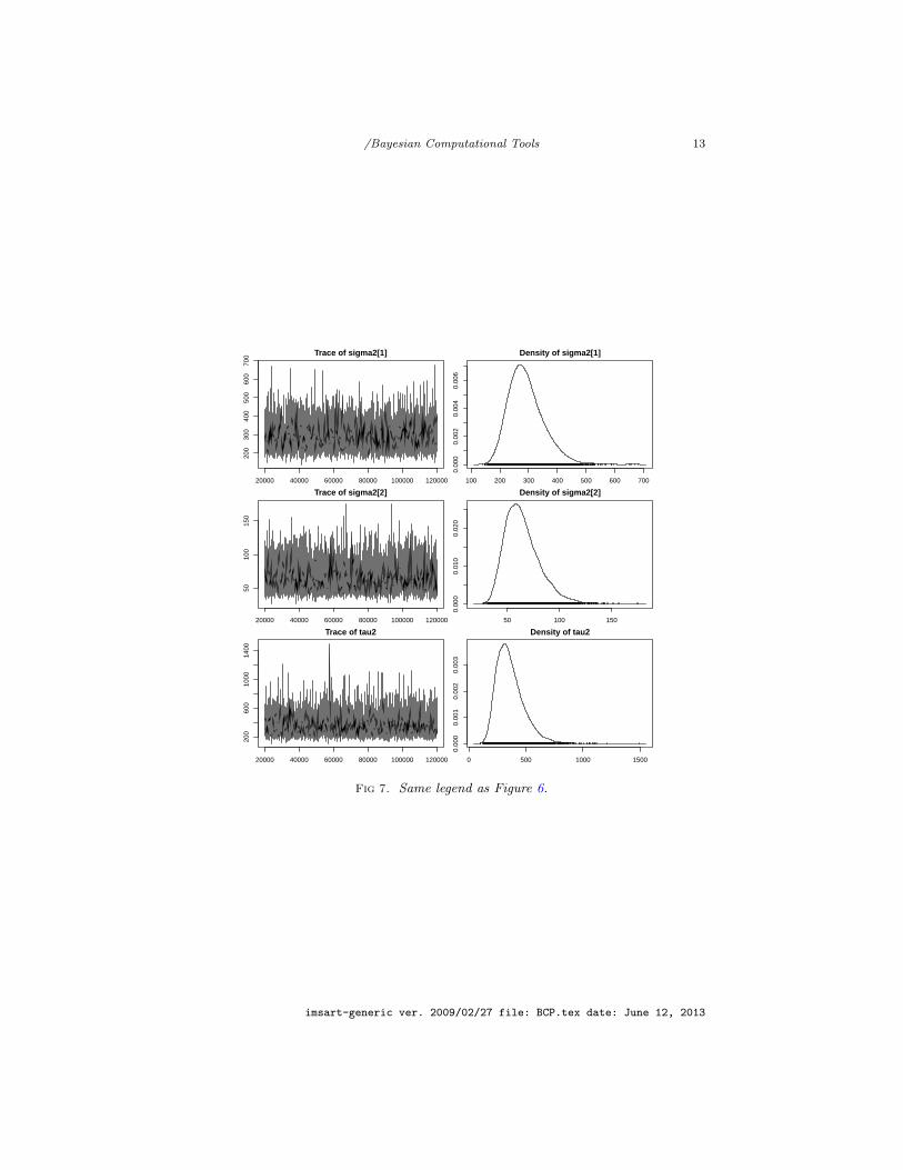
Fig 6. Evolution of the Gibbs Markov chains for some parameters of the growth mixed-effect model of Pothoff and Roy (1964) (right) and density estimate of the correspond-ing posterior distribution (right), based on 120, 000 iterations.

where nk is the number of children with sex k, and (i = 1, . . . , n)

αi ∼ N

(∑rj=1(yij − βhi

tj)σ−2hi

+ µhiτ−2

τ−2 + rσ−2hi

,{τ−2 + rσ−2hi

)−1}.

It is therefore straightforward to run the associated Gibbs sampler. Figures 6 and7 show the raw output of some parameter series, based on 120, 000 iterations.For instance, those figures show that β1 and β2 are possibly equal, as their likelyranges overlap. This does not seem to hold for µ1 and µ2. J

One of the obvious applications of the Gibbs sampler is found in graphicalmodels—an application that occurred in the early days of MCMC—since thosemodels are defined by and understood via conditional distributions rather thanthrough an unmanageable joint distribution. As detailed in Lauritzen (1996),undirected probabilistic graphs are Markov with respect to the graph structure,which means that variables indexed by a given node η of the graph only dependon variables indexed by nodes connected to η. For instance, if the vector indexed



20000 40000 60000 80000 100000 120000

200

300

400

500

600

700

Iterations

Trace of sigma2[1]

100 200 300 400 500 600 700

0.00

00.

002

0.00

40.

006

N = 10000 Bandwidth = 9.693

Density of sigma2[1]

20000 40000 60000 80000 100000 120000

5010

015

0

Iterations

Trace of sigma2[2]

50 100 150

0.00

00.

010

0.02

0

N = 10000 Bandwidth = 2.667

Density of sigma2[2]

20000 40000 60000 80000 100000 120000

200

600

1000

1400

Trace of tau2

0 500 1000 1500

0.00

00.

001

0.00

20.

003

Density of tau2

Fig 7. Same legend as Figure 6.



by the graph is Gaussian, X ∼ N (µ,Σ), the non-zero terms of Σ−1 correspond tothe edges of the graph. Applications of this modelling abound, as for instance inexperts systems (Spiegelhalter et al., 1993). Note that hierarchical Bayes modelscan be naturally associated with dependence graphs leading to DAGs and thusfall within this category as well.

4.2. Reversible-jump MCMC

Although the principles of the MCMC methodology are rather straightforwardto understand and to implement, resorting for instance to down-the-shelf tech-niques like RWMH algorithms, a more challenging setting occurs with the caseof variable dimensional problems. These problems typically occur in a Bayesianmodel choice situation, where several (or an infinity of) models are consideredat once. The resulting parameter space is a millefeuille collection of sets, withmost likely different dimensions, and moving around this space or across thoselayers is almost inevitably a computational issue. Indeed, the only case opento direct computation is the one when the posterior probabilities of the modelsunder comparison can be evaluated, resulting in a two-stage implementation,the model being chosen first and the parameters of this model being simulated“as usual”. However, as seen above, computing posterior probabilities of modelsis rarely a straightforward case. In other settings, moving around the collectionof models and within the corresponding parameter spaces must occur simulta-neously, especially when the number of models is large or infinite.

Defining a Markov chain kernel that explores the multi-layered space is chal-lenging because of the difficulty of defining a reference measure on this complexspace. However, Green (1995) came up with a solution that is rather simplexto express (if not necessarily to implement). The idea behind Green’s (1995)reversible jump solution is to take advantage of the Markovian nature of thealgorithm: since all that matters in a Markov chain is the most recent valueof the chain, exploration of a multi-layered space, represented as a direct sum(Rudin, 1976) of those spaces,

I⊕i=1

Θi ,

only involves a pair of sets Θi at each step, Θι and Θτ say. Therefore, themathematical difficulty reduces to create a connection between both spaces, dif-ficulty that is solved by Green’s (1995) via the introduction of auxiliary variablesλι and λτ in order for (θι, λι) and (θτ, λτ) to be in one-to-one correspondence,i.e. (θι, λι) = Ψ(θτ, λτ). Arbitrary distributions on λι and on λτ then come tocomplement the target distributions π(ι, θι|x) and π(τ, θτ|x). The algorithm iscall reversible because the symmetric move from (θι, λι) to (θτ, λτ) must follow(θτ, λτ) = Ψ−1(θι, λι). In other words, moves one way determine moves theother way. A schematic representation is as follows:

The important feature in the above acceptance probability is the Jacobianterm dΨ(θτ, λτ)

/d(θτ, λτ) which corresponds to the change of density in the



Algorithm 2 RJMCMfor t = 1 to T do

Given current state (ι, θι),Generate index τ from the prior probabilities π(τ).Generate λι from the auxiliary distribution πι(λι)Compute (θτ, λτ) = Ψ−1(θι, λι)Accept to switch to (ι, θι) with probability

α =π(τ, θτ|x)πτ(λτ)

π(ι, θι|x)πι(λι)

∣∣∣∣dΨ(θτ, λτ)

d(θτ, λτ)

∣∣∣∣Else reproduce (ι, θι)

end for

transformation. It is also a source of potential mistakes in the implementationof the algorithm.

The simplest version of RJMCM is when θτ = (θι, λι), i.e. when the movefrom one parameter space to the next involves adding or removing one param-eter, as for instance in estimating a mixture with an unknown number of com-ponents (Richardson and Green, 1997) or a MA(p) time series with p unknown.It can also be used with p known, as illustrated below.

Example 4 AnMA(p) time series model—where MA stands for ‘moving average’—is defined by the equations

xt =

p∑i=1

ϑiεt−i + εt t = 1, . . . ,

where the εt’s are iid N (0, σ2). While this model can be processed withoutRJMCMC, we present here a resolution explained in Marin and Robert (2007)that does not distinguish between the cases when p is known and when p isunknown.

The associated “lag polynomial” P(B) = I +∑pi=1 ϑiB

i provides a formalrepresentation of the series as xt = P(B)εt, with Iεt = εt, Bεt = εt−1, ... As apolynomial it also factorises through its roots λi as

P(B) =

p∏i=1

(I− λiB) .

While the number of roots is always p, the number of (non-conjugate) complexroots varies between 0 (meaning no complex root) and bp/2c. This representationof the model thus induces a variable dimension structure in that the parameterspace is then the product (−1, 1)r × B(0, 1)p−r/2, where B(0, 1) denotes thecomplex unit ball and r is the number of real valued roots λiB. The priordistributions on the real and (non-conjugate) complex roots are the uniformdistributions on (−1, 1) and B(0, 1), respectively. In other words,

π(λ) =1

bp/2c+ 1

∏λi∈(−1,1)

1

2I|λi|<1

∏λi 6∈R

1

πIB(0,1)(λi) , (1)



Moving around this space using RJMCMC is rather straightforward: either thenumber of real roots does not change in which case any regular MCMC stepis acceptable or the number of real roots moves up or down by a factor of 2,new roots being generated from the prior distribution, in which case the aboveRJMCMC acceptance ratio reduces to a likelihood ratio. An extra difficulty withthe MA(p) setup is that the likelihood is not available in closed form unlessthe past innovations ε0, ε−1, . . . , ε1−p are available. As explained in Marin andRobert (2007), they need to be simulated in a Gibbs step, that is, conditionalupon the other parameters with density proportional to

1−p∏t=0

exp{−ε2t/2σ2

} T∏t=1

exp

−xt − µ+

p∑j=1

ϑj εt−j

2/2σ2

,

where ε0 = ε0,. . ., ε1−p = ε1−p and (t > 0)

εt = xt − µ+

p∑j=1

ϑj εt−j .

This recursive definition of the likelihood is rather costly since it involves com-puting the εt’s for each new value of the past innovations, hence T sums of pterms. Nonetheless, the complexity O(Tp) of this representation is much moremanageable than the normal exact representation mentioned above. J

As mentioned above, the difficulty with RJMCM is in moving from the generalprinciple (which indeed allows for a generic exploration of varying dimensionspaces) to the practical implementation: when faced with a wide range of models,one needs to determine which models to pair together—they must be similarenough—and how to pair them—so that the jumps are efficient enough. Thisrequires the calibration of a large number of proposals, whose efficiency is usuallymuch lower than in single-model implementations. Whenever the number ofmodels is limited, my personal experience is that it is more efficient to runseparate (and parallel) MCMC algorithms on all models and to determine thecorresponding posterior probabilities of those models by a separate evaluation,like Chib’s (1995). (Indeed, a byproduct of the RJMCMC algorithm is to providean evaluation of the posterior probabilities of the models under comparison viathe frequencies of accepted moves to such models.) See, e.g., Lee et al. (2009) foran illustration in the setting of mixtures of distributions. We end up with a wordof caution against the misuse of probabilistic structures over those collections ofspaces, as illustrated by Congdon (2006) and Scott (2002) (Robert and Marin,2008).

5. Approximate Bayesian computation methods

This section covers some aspects of a specific computational method called Ap-proximate Bayesian computation (ABC in short), which stemmed from acute



computational problems in statistical population genetics and rised in impor-tance over the past decade. The section should be more methodological thanthe previous sections as the method is not covered in this volume, as far as Ican assess. In addition, this is a special computational method in that it hasbeen specifically developed for challenging Bayesian computational problems(and that it carries the Bayesian label within its name!). Although the reader isreferred to, e.g., Toni et al. (2009) and Beaumont (2010) for a deeper review onthis method, I will cover here different accelerating techniques and the numerouscalibration issues of selecting both the tolerance and the summary statistics.

Approximate Bayesian computation (ABC) techniques appeared at the endof the 20th Century in population genetics (Tavare et al., 1997; Pritchard et al.,1999), where scientists were faced with intractable likelihoods that MCMCmethods were simply unable to handle with the slightest amount of success.Some of those scientists developed simulation tools overcoming the jammingblock of computing the likelihood function that turned into a much more gen-eral form of approximation technique, exhibiting fundamental links with econo-metric methods such as indirect inference (Gourieroux et al., 1993). Althoughsome part of the statistical community was initially reluctant to welcome them,trusting instead massively parallelised MCMC approaches, ABC techniques arenow starting to be part of the statistical toolbox and to be accepted as aninference method per se, rather than being a poor man’s alternative to moremainstream techniques. While details about the method are provided in recentsurveys (Beaumont, 2008, 2010; Marin et al., 2011b), we expose in algorithmicterms the basics of the ABC algorithm:

Algorithm 3 ABCfor t = 1 to T do

repeatGenerate θ∗ from the prior π(·).Generate x∗ from the model f(·|θ∗).Compute the distance %(S(x0), S(x∗)).Accept θ∗ if %(S(x0), S(x∗)) < ε.

until acceptanceend for

The idea at the core of the ABC method is to replace an acceptance based onthe unavailable likelihood with one evaluating the pertinence of the parameterfrom the proximity between the data and a simulated pseudo-data. This prox-imity is using a distance or pseudo-distance %(·, ·) between a (summary) statisticS(x0) based on the data and its equivalent S(x∗ for the pseudo-data. We stressfrom this early stage that the summary statistic S is very rarely sufficient andhence that ABC looses some of the information contained in the data.

Example 4 (bis) While the MA(p) is manageable by other approaches—sincethe missing data structure is of a moderate complexity—, it provides an illustra-tion of a model where the likelihood function is not available in closed form andwhere the data can be simulated in a few lines of code given the parameter. Usingthe p first autocorrelations as summary statistics S(·), we can then simulate pa-



rameters from the prior distribution and corresponding series x∗ = (x∗1, . . . , x∗T )

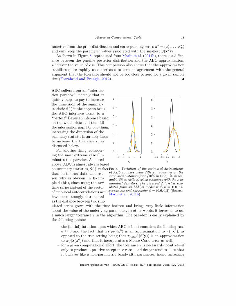
and only keep the parameter values associated with the smallest S(x∗)’s.As shown in Figure 8, reproduced from Marin et al. (2011b), there is a differ-

ence between the genuine posterior distribution and the ABC approximation,whatever the value of ε is. This comparison also shows that the approximationstabilises quite rapidly as ε decreases to zero, in agreement with the generalargument that the tolerance should not be too close to zero for a given samplesize (Fearnhead and Prangle, 2012). J

−2 −1 0 1 2

0.0

0.5

1.0

1.5

2.0

2.5

3.0

θ1

−1.0 −0.5 0.0 0.5 1.0

0.0

0.5

1.0

1.5

2.0

2.5

3.0

θ2

Fig 8. Variation of the estimated distributionsof ABC samples using different quantiles on thesimulated distances for ε (10% in blue, 1% in red,and 0.1% in yellow) when compared with the truemarginal densities. The observed dataset is sim-ulated from an MA(2) model with n = 100 ob-servations and parameter ϑ = (0.6, 0.2) (Source:Marin et al., 2011b).

ABC suffers from an “informa-tion paradox”, namely that itquickly stops to pay to increasethe dimension of the summarystatistic S(·) in the hope to bringthe ABC inference closer to a“perfect” Bayesian inference basedon the whole data and thus fillthe information gap. For one thing,increasing the dimension of thesummary statistic invariably leadsto increase the tolerance ε, asdiscussed below.

For another thing, consider-ing the most extreme case illu-minates this paradox. As notedabove, ABC is almost always basedon summary statistics, S(·), ratherthan on the raw data. The rea-son why is obvious in Exam-ple 4 (bis), since using the rawtime series instead of the vectorof empirical autocorrelations wouldhave been strongly detrimentalas the distance between two sim-ulated series grows with the time horizon and brings very little informationabout the value of the underlying parameter. In other words, it forces us to usea much larger tolerance ε in the algorithm. The paradox is easily explained bythe following points:

– the (initial) intuition upon which ABC is built considers the limiting caseε ≈ 0 and the fact that πABC(·|x0) is an approximation to π(·|x0), asopposed to the true setting being that πABC(·|S(y)) is an approximationto π(·|S(x0)) and that it incorporates a Monte Carlo error as well;

– for a given computational effort, the tolerance ε is necessarily positive—ifonly to produce a positive acceptance rate—and deeper studies show thatit behaves like a non-parametric bandwidth parameter, hence increasing



with the dimension of S while (slowly) decreasing with the sample size.

Therefore, when the dimension of the raw data is large (as for instance in thetime series setting of Example 4 bis), it is definitely not recommended to usea distance between the raw data x0 and the raw pseudo-data x∗: the curse ofdimension operates in nonparametric statistics and clearly impacts the approx-imation of π(·|x0) as to make it impossible even for moderate dimensions.

In connection with the above, it must be stressed that, in almost any imple-mentation, the ABC algorithm is not correct for at least two reasons: the datax0 is replaced with a roughened version {x∗; s%(S(x0), S(x∗)) < ε} and the useof a non-sufficient summary statistic S(· · · ). In addition, as in regular MonteCarlo approximations, a given computational effort produces a correspondingMonte Carlo error.

5.1. Selecting summaries

The choice of the summary statistic S(·) is paramount in any implementationof the ABC methodology if one does not want to end up with simulations fromthe prior distribution resulting from too large a tolerance! On the opposite, anefficient construction of S(· · · ) may result in a very efficient approximation fora given computational effort.

The literature on ABC abounds with more or less recommendable solutionsto achieve a proper selection of the summary statistic. Early studies were eitherexperimental (McKinley et al., 2009) or borrowing from external perspectives.For instance, Blum and Francois (2010) argue in favour of using neural nets intheir non-parametric modelling for the very reason that neural nets eliminateirrelevant components of the summary statistic. However, the black box featuresof neural nets also mean that the selection of the summary statistic is implicit.Another illustration of the use of external assessments is the experiment ran bySedki and Pudlo (2012) in mixing local regression (Beaumont et al., 2002) localregression tools with the BIC criterion.

In my opinion, the most accomplished (if not ultimate) development in theABC literature about the selection of the summary statistic is currently foundin Fearnhead and Prangle (2012). Those authors study the use of a summarystatistic S from a quasi-decision-theoretic perspective, evaluating the error bya quadratic loss

L(θ, d) = (θ − d)TA(θ − d) ,

where A is a positive symmetric matrix, and obtaining in addition a determina-tion of the optimal bandwidth (or tolerance) h from non-parametric evaluationsof the error. In particular, the authors argue that the optimal summary statisticis E[θ|x0] (when estimating the parameter of interest θ). For this, they noticethat the errors resulting from an ABC modelling are of three types:

– one due to the approximation of π(θ|x0) by π(θ|S(x0)),



– one due to the approximation of π(θ|S(x0)) by

πABC(θ|S(x0)) =

∫π(s)K[{s− S(x0)}/h]π(θ|s) ds∫

π(s)K[{s− S(x0)}/h] ds

where K(·) is the kernel function used in the acceptance step—which isthe indicator function I(−1,1) in the above algorithm since θ? is acceptedwith probability I(−1,1)(%(S(x0), S(x∗)/ε) in this case—,

– one due to the approximation of πABC(θ|S(x0)) by importance MonteCarlo techniques based onN simulations, which amounts to var(a(θ)|S(x0))/Nacc,if Nacc is the expected number of acceptances.

For the specific case when S(x) = E[θ|x] = θ, the expected loss satisfies

E[L(θ, θ)|x0] = trace(AΣ) + h2∫

xTAxK(x)dx + o(h2) ,

where Σ = var(θ|x0), which means that the first type error vanishes with smallh’s, given that it is equivalent to the Bayes risk based on the whole data. Fromthis decomposition of the risk, Fearnhead and Prangle (2012) derive

h = O(N−1/(4+d))

as an optimal bandwidth for the standard ABC algorithm. From a practicalperspective, using the posterior expectation E[θ|x0] as a summary statistic isobviously impossible, if only because even basic simulation from the posterioris impossible. Fearnhead and Prangle (2012) suggest using instead a two-stageprocedure:

1. Run a basic ABC algorithm to construct a non-parametric estimate ofE[θ|x0] following Beaumont et al. (2002); and

2. Use this non-parametric estimate as the summary statistic in a secondABC run.

In cases when producing the reference sample is very costly, the same samplemay be used in both runs, even though this may induce biases that will simplyadd up to the many approximative steps inherent to this procedure.

In conclusion, the literature on the topic has gathered several techniques pro-posed for other methodologies. While this perspective manages to eliminate theless relevant components of a pool of statistics, I feel the issue remains quiteopen as to which statistic should be included at the start of an ABC algorithm.The problems linked with the curse of dimensionality (“not too many”), identi-fiability (“not too few”), and ultimately precision (“as many as components ofθ”) of the approximations are far from solved and I thus foresee further majordevelopments to occur in the years to come.

5.2. ABC model choice

As stressed already above, model choice occupies a special place in the Bayesianparadigm and this for several reasons. First, the comparison of several models



compels the Bayesian modeller to construct a meta-model that includes all thesemodels under comparison as special cases. This encompassing model thus has acomplexity that is higher than the complexities of the models under comparison.Second, while Bayesian inference on models is formally straightforward, in thatit computes the posterior probabilities of the models under comparison—eventhough this raises misunderstanding and confusion in the non-Bayesian appliedcommunities, as illustrated by the series of controversies raised by Templeton(2008; 2010—, the computation of such objects often faces major computationalchallenges.

From an ABC perspective, the specificity of model selection holds as well. Atfirst sight, and in sort of predictable replication of the theoretical setting, theformal simplicity of computing posterior probabilities can be mimicked by anABC-MC (for model choice) algorithm as the following one (Toni and Stumpf,2010):

Algorithm 4 ABC-MCfor t = 1 to T do

repeatGenerate m∗ from the prior π(M = m).Generate θ∗m∗ from the prior πm∗ (·).Generate x∗ from the model fm∗ (·|θ∗m∗ ).Compute the distance %(S(x0), S(x∗)).Accept (θ∗m∗ ,m∗) if %(S(x0), S(x∗)) < ε.

until acceptanceend for

where M denotes the unknown model index, m being one of the possiblevalues, with πm the corresponding prior on the parameter θm.

●

●

●●

●

●

Gauss Laplace

0.0

0.2

0.4

0.6

0.8

1.0

n=100

●

●

●●●●●

●

●

●●

●

●

●●●

●

Gauss Laplace

0.0

0.2

0.4

0.6

0.8

1.0

n=1000

●

●

●

●●

●

Gauss Laplace

0.0

0.2

0.4

0.6

0.8

1.0

n=10000

Fig 9. Box-plots of the repartition of the ABC poste-rior probabilities that a normal (Gauss) and double-exponential (Laplace) sample is from a normal (vs.double-exponential) distribution. based on 250 replica-tions and the median as summary statistic S (Source:Marin et al., 2011a).

As a consequence, the abovealgorithm process the pair (m,θm) as a regular parameter,using the same tolerance con-dition %(S(x0), S(x∗)) < ε asthe initial ABC algorithm. Fromthe output of ABC-MC, theposterior probability π(M =m|y) can then be approximatedby the frequency of acceptancesof simulations from model m

π(M = m|y) =1

T

T∑t=1

Im(t)=m .

Improvements on this crude frequency estimate can be made using for instancea weighted polychotomous logistic regression estimate of π(M = m|y), withnon-parametric kernel weights, as in Cornuet et al. (2008).



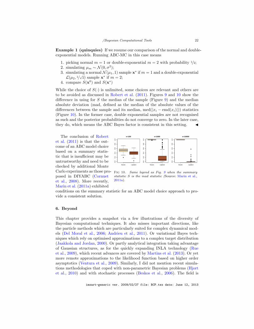
Example 1 (quinquies) If we resume our comparison of the normal and double-exponential models. Running ABC-MC in this case means

1. picking normal m = 1 or double-exponential m = 2 with probability 1/2;2. simulating µm ∼ N (0, σ2);3. simulating a normalN (µ1, 1) sample x∗ if m = 1 and a double-exponentialL(µ2, 1/

√2) sample x∗ if m = 2;

4. compare S(x0) and S(x∗)

While the choice of S(·) is unlimited, some choices are relevant and others areto be avoided as discussed in Robert et al. (2011). Figures 9 and 10 show thedifference in using for S the median of the sample (Figure 9) and the medianabsolute deviation (mad, defined as the median of the absolute values of thedifferences between the sample and its median, med(|xi − emd(xi)|)) statistics(Figure 10). In the former case, double exponential samples are not recognisedas such and the posterior probabilities do not converge to zero. In the later case,they do, which means the ABC Bayes factor is consistent in this setting. J

●

●

Gauss Laplace

0.0

0.2

0.4

0.6

0.8

1.0

n=100

●●●●●●●●●

●

●

●

●

●●

●

●

●

●●

●

Gauss Laplace

0.0

0.2

0.4

0.6

0.8

1.0

n=1000

●●●●

●

●

●

●

●

●

●

●

Gauss Laplace

0.0

0.2

0.4

0.6

0.8

1.0

n=10000

Fig 10. Same legend as Fig. 9 when the summarystatistic S is the mad statistic (Source: Marin et al.,2011a).

The conclusion of Robertet al. (2011) is that the out-come of an ABC model choicebased on a summary statis-tic that is insufficient may beuntrustworthy and need to bechecked by additional MonteCarlo experiments as those pro-posed in DIYABC (Cornuetet al., 2008). More recently,Marin et al. (2011a) exhibitedconditions on the summary statistic for an ABC model choice approach to pro-vide a consistent solution.

6. Beyond

This chapter provides a snapshot via a few illustrations of the diversity ofBayesian computational techniques. It also misses important directions, likethe particle methods which are particularly suited for complex dynamical mod-els (Del Moral et al., 2006; Andrieu et al., 2011). Or variational Bayes tech-niques which rely on optimised approximations to a complex target distribution(Jaakkola and Jordan, 2000). Or partly analytical integration taking advantageof Gaussian structures, as for the quickly expanding INLA technology (Rueet al., 2009), which recent advances are covered by Martins et al. (2013). Or yetmore remote approximations to the likelihood function based on higher orderasymptotics (Ventura et al., 2009). Similarly, I did not mention recent simula-tions methodologies that coped with non-parametric Bayesian problems (Hjortet al., 2010) and with stochastic processes (Beskos et al., 2006). The field is



expanding and the demands made by the “Big Data” crisis are simultaneouslythreatening the fundamentals of the Bayesian approach by calling for quick-and-dirty solutions and bringing new materials, by exhibiting a crucial need forhierarchical Bayes modelling. Thus, to conclude with Dickens’ (1859) openingwords, we may later consider that “it was the best of times, it was the worst oftimes, it was the age of wisdom, it was the age of foolishness”.

Acknowledgements

I am quite grateful to Jean-Michel Marin for providing some of the materialincluded in this chapter, around Example 4 and the associated figures. It shouldhave been part of the chapter on hierarchical models in our new book Bayesianessentials with R, chapter that we eventually had to abandon to its semi-bakedstatus. The section on ABC was also salvaged from another attempt at a jointsurvey for a Statistics and Biology handbook, survey that did not evolve muchfurther than my initial notes and obviously did not meet the deadline. Therefore,Jean-Michel should have been a co-author of this chapter but he repeatedlydeclined my requests to join. He is thus named co-author in absentia. Thanksto Jean-Louis Foulley, as well, who suggested using the Pothoff and Roy (1964)dataset in his ENSAI lecture notes.

References

Andrieu, C., Doucet, A. and Holenstein, R. (2011). Particle Markovchain Monte Carlo (with discussion). J. Royal Statist. Society Series B, 72(2) 269–342.

Beaumont, M. (2008). Joint determination of topology, divergence time andimmigration in population trees. In Simulations, Genetics and Human Prehis-tory (S. Matsumura, P. Forster and C. Renfrew, eds.). Cambridge: (McDon-ald Institute Monographs), McDonald Institute for Archaeological Research,134–154.

Beaumont, M. (2010). Approximate Bayesian computation in evolution andecology. Annual Review of Ecology, Evolution, and Systematics, 41 379–406.

Beaumont, M., Zhang, W. and Balding, D. (2002). Approximate Bayesiancomputation in population genetics. Genetics, 162 2025–2035.

Beskos, A., Papaspiliopoulos, O., Roberts, G. and Fearnhead, P.(2006). Exact and computationally efficient likelihood-based estimation fordiscretely observed diffusion processes (with discussion). J. Royal Statist.Society Series B, 68 333–382.

Blum, M. and Francois, O. (2010). Non-linear regression models for approx-imate Bayesian computation. Statist. Comput., 20 63–73.

Breslow, N. and Clayton, D. (1993). Approximate inference in generalizedlinear mixed models. J. American Statist. Assoc., 88 9–25.

Brooks, S., Gelman, A., Jones, G. and Meng, X. (2011). Handbook ofMarkov Chain Monte Carlo. Taylor & Francis.



Casella, G. and George, E. (1992). An introduction to Gibbs sampling.The American Statistician, 46 167–174.

Chen, M., Shao, Q. and Ibrahim, J. (2000). Monte Carlo Methods inBayesian Computation. Springer-Verlag, New York.

Chib, S. (1995). Marginal likelihood from the Gibbs output. J. AmericanStatist. Assoc., 90 1313–1321.

Chopin, N. and Robert, C. (2010). Properties of nested sampling. Biometrika,97 741–755.

Congdon, P. (2006). Bayesian model choice based on Monte Carlo estimatesof posterior model probabilities. Comput. Stat. Data Analysis, 50 346–357.

Cornuet, J.-M., Santos, F., Beaumont, M., Robert, C., Marin, J.-M.,Balding, D., Guillemaud, T. and Estoup, A. (2008). Inferring popula-tion history with DIYABC: a user-friendly approach to Approximate BayesianComputation. Bioinformatics, 24 2713–2719.

Del Moral, P., Doucet, A. and Jasra, A. (2006). Sequential Monte Carlosamplers. J. Royal Statist. Society Series B, 68 411–436.

Dickens, C. (1859). A Tale of Two Cities. London: Chapman & Hall.Doucet, A., de Freitas, N. and Gordon, N. (2001). Sequential Monte

Carlo Methods in Practice. Springer-Verlag, New York.Fearnhead, P. and Prangle, D. (2012). Semi-automatic approximate

Bayesian computation. J. Royal Statist. Society Series B, 74 419–474. (Withdiscussion.).

Gelman, A. and Meng, X. (1998). Simulating normalizing constants: Fromimportance sampling to bridge sampling to path sampling. Statist. Science,13 163–185.

Geman, S. and Geman, D. (1984). Stochastic relaxation, Gibbs distributionsand the Bayesian restoration of images. IEEE Trans. Pattern Anal. Mach.Intell., 6 721–741.

Gourieroux, C., Monfort, A. and Renault, E. (1993). Indirect inference.J. Applied Econometrics, 8 85–118.

Green, P. (1995). Reversible jump MCMC computation and Bayesian modeldetermination. Biometrika, 82 711–732.

Hastings, W. (1970). Monte Carlo sampling methods using Markov chainsand their application. Biometrika, 57 97–109.

Hjort, N., Holmes, C., Muller, P. and Walker, S. (2010). Bayesiannonparametrics. Cambridge University Press.

Hobert, J. and Casella, G. (1996). The effect of improper priors on Gibbssampling in hierarchical linear models. J. American Statist. Assoc., 91 1461–1473.

Holmes, C., Denison, D., Mallick, B. and Smith, A. (2002). Bayesianmethods for nonlinear classification and regression. John Wiley, New York.

Jaakkola, T. and Jordan, M. (2000). Bayesian parameter estimation viavariational methods. Statistics and Computing, 10 25–37.

Jeffreys, H. (1939). Theory of Probability. 1st ed. The Clarendon Press,Oxford.

Lauritzen, S. (1996). Graphical Models. Oxford University Press, Oxford.



Lee, K., Marin, J.-M., Mengersen, K. and Robert, C. (2009). Bayesianinference on mixtures of distributions. In Perspectives in Mathematical Sci-ences I: Probability and Statistics (N. N. Sastry, M. Delampady and B. Rajeev,eds.). World Scientific, Singapore, 165–202.

Marin, J., Pillai, N., Robert, C. and Rousseau, J. (2011a). Relevantstatistics for Bayesian model choice. Tech. Rep. arXiv:1111.4700.

Marin, J., Pudlo, P., Robert, C. and Ryder, R. (2011b). ApproximateBayesian computational methods. Statistics and Computing 1–14.

Marin, J. and Robert, C. (2007). Bayesian Core. Springer-Verlag, New York.Marin, J. and Robert, C. (2011). Importance sampling methods for Bayesian

discrimination between embedded models. In Frontiers of Statistical DecisionMaking and Bayesian Analysis (M.-H. Chen, D. Dey, P. Muller, D. Sun andK. Ye, eds.). Springer-Verlag, New York, 000–000.

Martins, T. G., Simpson, D., Lindgren, F. and Rue, H. (2013). Bayesiancomputing with inla: New features. Computational Statistics & Data Analysis,67 68 – 83.

McKinley, T., Cook, A. and Deardon, R. (2009). Inference in epidemicmodels without likelihoods. The International Journal of Biostatistics, 5 24.

Meng, X. and Wong, W. (1996). Simulating ratios of normalizing constantsvia a simple identity: a theoretical exploration. Statist. Sinica, 6 831–860.

Neal, R. (1994). Contribution to the discussion of “Approximate Bayesianinference with the weighted likelihood bootstrap” by Michael A. Newton andAdrian E. Raftery. J. Royal Statist. Society Series B, 56 (1) 41–42.

Newton, M. and Raftery, A. (1994). Approximate Bayesian inference bythe weighted likelihood bootstrap (with discussion). J. Royal Statist. SocietySeries B, 56 1–48.

Potthoff, R. F. and Roy, S. (1964). A generalized multivariate analysis ofvariance model useful especially for growth curve problems. Biometrika, 51313–326.

Pritchard, J., Seielstad, M., Perez-Lezaun, A. and Feldman, M.(1999). Population growth of human Y chromosomes: a study of Y chro-mosome microsatellites. Mol. Biol. Evol., 16 1791–1798.

Ratmann, O. (2009). ABC under model uncertainty. Ph.D. thesis, ImperialCollege London.

Richardson, S. and Green, P. (1997). On Bayesian analysis of mixtureswith an unknown number of components (with discussion). J. Royal Statist.Society Series B, 59 731–792.

Robert, C. (2001). The Bayesian Choice. 2nd ed. Springer-Verlag, New York.Robert, C. and Casella, G. (2004). Monte Carlo Statistical Methods. 2nd

ed. Springer-Verlag, New York.Robert, C. and Casella, G. (2009). Introducing Monte Carlo Methods with

R. Springer-Verlag, New York.Robert, C. and Casella, G. (2011). A history of Markov chain Monte Carlo—

subjective recollections from incomplete data. Statist. Science, 26 102–115.Robert, C., Cornuet, J.-M., Marin, J.-M. and Pillai, N. (2011). Lack

of confidence in ABC model choice. Proceedings of the National Academy of



Sciences, 108(37) 15112–15117.Robert, C. and Marin, J.-M. (2008). On some difficulties with a posterior

probability approximation technique. Bayesian Analysis, 3(2) 427–442.Robert, C. and Wraith, D. (2009). Computational methods for Bayesian

model choice. In MaxEnt 2009 proceedings (P. M. Goggans and C.-Y. Chan,eds.), vol. 1193. AIP.

Rudin, W. (1976). Principles of Real Analysis. McGraw-Hill, New York.Rue, H., Martino, S. and Chopin, N. (2009). Approximate Bayesian infer-

ence for latent Gaussian models using integrated nested Laplace approxima-tions. J. Royal Statist. Society Series B, 71 319–392.

Scott, S. L. (2002). Bayesian methods for hidden Markov models: recursivecomputing in the 21st Century. J. American Statist. Assoc., 97 337–351.

Sedki, M. A. and Pudlo, P. (2012). Discussion of D. Fearnhead and D.Prangle’s ”Constructing summary statistics for approximate Bayesian compu-tation: semi-automatic approximate Bayesian computation”. J. Roy. Statist.Soc. Ser. B, 74 466–467.

Smith, A. (1984). Present position and potential developments: some personalview on Bayesian statistics. J. Royal Statist. Society Series A, 147 245–259.

Spiegelhalter, D., Dawid, A., Lauritzen, S. and Cowell, R. (1993).Bayesian analysis in expert systems (with discussion). Statist. Science, 8219–283.

Tavare, S., Balding, D., Griffith, R. and Donnelly, P. (1997). Inferringcoalescence times from DNA sequence data. Genetics, 145 505–518.

Templeton, A. (2008). Statistical hypothesis testing in intraspecific phylo-geography: nested clade phylogeographical analysis vs. approximate Bayesiancomputation. Molecular Ecology, 18(2) 319–331.

Templeton, A. (2010). Coherent and incoherent inference in phylogeographyand human evolution. Proc. National Academy of Sciences, 107(14) 6376–6381.

Toni, T. and Stumpf, M. (2010). Simulation-based model selection for dynam-ical systems in systems and population biology. Bioinformatics, 26 104–110.

Toni, T., Welch, D., Strelkowa, N., Ipsen, A. and Stumpf, M. (2009).Approximate Bayesian computation scheme for parameter inference andmodel selection in dynamical systems. Journal of the Royal Society Inter-face, 6 187–202.

Ventura, L., Cabras, S. and Racugno, W. (2009). Prior distributionsfrom pseudo-likelihoods in the presence of nuisance parameters. J. AmericanStatist. Assoc., 104 768–774.

Weinberg, M. (2012). Computing the Bayes factor from a Markov chain MonteCarlo simulation of the posterior distribution. Bayesian Analysis, 7 737–770.


Bayesian Computational Tools - arXiv

Documents

Transcript of Bayesian Computational Tools - arXiv