
APPLIED COMPUTATIONAL AERODYNAMICS - Free
145
APPLIED COMPUTATIONAL AERODYNAMICS Preface Objectives These notes are intended to fill a significant gap in the literature available to students. There is a huge disparity between the aerodynamics covered in typical aerodynamics courses and the application of aerodynamic theory to design and analysis problems using computational methods. As an elective course for seniors, Applied Computational Aerodynamics provides an opportunity for students to gain insight into the methods and means by which aerodynamics is currently practiced. The specific threefold objective is: i) physical insight into aerodynamics that can arise only with the actual calculation and subsequent analysis of flowfields, ii) development of engineering judgment to answer the question �how do you know the answer is right?� and iii) establishment of a foundation for future study in computational aerodynamics; exposure to a variety of methods, terminology, and jargon. Two features are unique. First, when derivations are given, all the steps in the analysis are included. Second, virtually all the examples used to illustrate applied aerodynamics ideas were computed by the author, and were made using the codes available to the students. The exercises are an extremely important component of the course, where parts of the course are possibly best presented as a workshop, rather than as a series of formal lectures. To meet the objectives, many �old fashioned� methods are included. Using these methods a student can learn much more about aerodynamic design than by performing a few large modern calculations. For example (articulated to the author by Prof. Ilan Kroo), the vortex lattice method allows the student to develop an excellent mental picture of the flowfield. Thus these methods provide a context within which to understand Euler or Navier-Stokes calculations. Audience We presume that the reader has had standard undergraduate courses in fluid mechanics and aerodynamics. In some cases the material is repeated to illustrate issues important to computational aerodynamics. Access to a computer and the ability to program is assumed for the exercises. Warnings Computational aerodynamics is still in an evolutionary phase. Although most of the material in the early chapters is essentially well established, the viewpoint adopted in the latter chapters is necessarily a �snapshot� of the field at this time. Students that enter the field can expect to use this material as a starting point in understanding the continuing evolution of computational aerodynamics. These notes are not independent of other texts. At this point several of the codes used in the instruction are based on source codes copyrighted in other sources. Use of these codes without owning the text may be a violation of the copyright law. The traditional printed page is inadequate and obsolete for the presentation of computational aerodynamics information. The reader should be alert to advances in information presentation, and take every opportunity to make use of advanced color displays, interactive flowfield visualization and virtual environment technology. PDF créé avec la version d'essai pdfFactory www.gs2i.fr/fineprint/pdffactory.htm
-
Upload
khangminh22 -
Category
Documents
-
view
0 -
download
0
Transcript of APPLIED COMPUTATIONAL AERODYNAMICS - Free

APPLIED COMPUTATIONAL AERODYNAMICS
Preface
Objectives These notes are intended to fill a significant gap in the literature available to students. There is a huge disparity between the aerodynamics covered in typical aerodynamics courses and the application of aerodynamic theory to design and analysis problems using computational methods. As an elective course for seniors, Applied Computational Aerodynamics provides an opportunity for students to gain insight into the methods and means by which aerodynamics is currently practiced. The specific threefold objective is: i) physical insight into aerodynamics that can arise only with the actual calculation and subsequent analysis of flowfields, ii) development of engineering judgment to answer the question �how do you know the answer is right?� and iii) establishment of a foundation for future study in computational aerodynamics; exposure to a variety of methods, terminology, and jargon.
Two features are unique. First, when derivations are given, all the steps in the analysis are included. Second, virtually all the examples used to illustrate applied aerodynamics ideas were computed by the author, and were made using the codes available to the students. The exercises are an extremely important component of the course, where parts of the course are possibly best presented as a workshop, rather than as a series of formal lectures. To meet the objectives, many �old fashioned� methods are included. Using these methods a student can learn much more about aerodynamic design than by performing a few large modern calculations. For example (articulated to the author by Prof. Ilan Kroo), the vortex lattice method allows the student to develop an excellent mental picture of the flowfield. Thus these methods provide a context within which to understand Euler or Navier-Stokes calculations.
Audience We presume that the reader has had standard undergraduate courses in fluid mechanics and aerodynamics. In some cases the material is repeated to illustrate issues important to computational aerodynamics. Access to a computer and the ability to program is assumed for the exercises.
Warnings Computational aerodynamics is still in an evolutionary phase. Although most of the material in the early chapters is essentially well established, the viewpoint adopted in the latter chapters is necessarily a �snapshot� of the field at this time. Students that enter the field can expect to use this material as a starting point in understanding the continuing evolution of computational aerodynamics.
These notes are not independent of other texts. At this point several of the codes used in the instruction are based on source codes copyrighted in other sources. Use of these codes without owning the text may be a violation of the copyright law.
The traditional printed page is inadequate and obsolete for the presentation of computational aerodynamics information. The reader should be alert to advances in information presentation, and take every opportunity to make use of advanced color displays, interactive flowfield visualization and virtual environment technology.
PDF créé avec la version d'essai pdfFactory www.gs2i.fr/fineprint/pdffactory.htm

The codes available on disk provide a significant capability for skilled users. However, as discussed in the text, few computational aerodynamics codes are ever developed and tested to the level that they are bug free. They are for educational use only, and are only aides for education, not commercial programs, although they are entirely representative of codes in current use.
Acknowledgements Many friends and colleagues have influenced the contents of these notes. Specifically, they reflect many years developing and applying computational aerodynamics at Grumman, which had more than its share of top flight aerodynamicists. Initially at Grumman and now at VPI, Bernard Grossman provided access to his as yet unpublished CFD course notes. At NASA, many friends have contributed help, insight and computer programs. Nathan Kirschbaum read the notes and made numerous contributions to the content and clarity. Several classes of students have provided valuable feedback, found typographical and actual errors. They have also insisted that the notes and codes be completed. I would like to acknowledge these contributions.
W.H. Mason
PDF créé avec la version d'essai pdfFactory www.gs2i.fr/fineprint/pdffactory.htm

APPLIED COMPUTATIONAL AERODYNAMICS TEXT/NOTES W. H. Mason, [email protected] Department of Aerospace and Ocean Engineering Virginia Polytechnic Institute and State University
An electronic version of the class notes for AOE 4114, Applied Computational Aerodynamics. Portions are also used for AOE 4984, Configuration Aerodynamics. Comments are welcome, and in fact encouraged.
This is a work in progress (for over 6 years!). Starting in 1997, the material is being made available electronically using a hybrid html/acrobat approach. It appears most practical to provide a top page in html, while allowing students to download individual sections as Adobe Acrobat files. The emphasis is on subject mater, and not the multimedia framework. I have not yet been able to devote the time required to produce a modern electronic document. Also, some equations and figures may not print perfectly. Much of the material was created before the current methods and standards existed. The entire outline is provided, although not all sections are available for download yet. In some cases copyright permission has not been obtained for figures, and thus, some figures are not yet available. Chapters and Appendices will be added as they are available.
The documents are provided in an even/odd page format so they can be copied to both sides of the paper in the hardcopy version. This allows them to fit in a notebook.
Some codes are available in FORTRAN. They have very crude user interfaces, the manuals even refer to card input! In most cases, much more modern versions are available.
� 1992,1995 by W.H. Mason
Preface (html)
Volume 1: Foundations and Classical Pre-CFD Methods • Detailed Table of Contents • 1. Introduction (pdf) • 2. Getting Ready for Computational Aerodynamics: Fluid Mechanics Foundations (pdf) • 3. Computers, Codes, and Engineering (pdf) • 4. Incompressible Potential Flow Using Panel Methods (pdf) (minus a few copyrighted figures) • 5. Drag: An Introduction (pdf) (minus a few figures) • 6. Aerodynamics of 3D Lifting Surfaces through Vortex Lattice Methods (248k pdf, Mar 11, 1998)
(minus a few copyrighted figures) • 7. Applications to Configuration Aerodynamics • Appendices
o A. Geometry for Aerodynamicists (pdf) A library of airfoils for use with the codes is available, either as a Zip file or as a Stuffit file. See Appendix A for the airfoil names associated with each filename.
o B. Sources of Experimental Data for Code Validation (pdf) o C. Preparation of Written Material (pdf)
PDF créé avec la version d'essai pdfFactory www.gs2i.fr/fineprint/pdffactory.htm

o D. Pre-CFD Computational Aerodynamics Programs (html) o E. Utility Codes (html) o F. Code and Electronic Information Sources (html)
Volume 2 Applied Computational Fluid Mechanics • Detailed Table of Contents • 8. Introduction to Computational Fluid Dynamics (162k pdf file, Mar. 17, 1998) • 9. Geometry and Grids: Major Considerations in Using CA • 10. Viscous Flows in Aerodynamics • 11. Transonic Aerodynamics: Methods and Applications • 12. Supersonic and Hypersonic Aerodynamics • 13. CFD: Current Methods, Terminology and Details Required for Use • 14. Using Computational Aerodynamics: Review and Reinforcement • Appendices
o G. Computational Aerodynamics Programs (html) o H. Utility Codes (html)
These notes were produced exclusively with Macintosh technology. They were written on Macintosh computers. Word processing was done with FullWrite Professional and WriteNow. Sketches and drawings were done with Canvas. Equations were composed using MathType. Plots and Graphs were made using Kaleidagraph. Computing for examples was carried out using Language Systems FORTRAN running in the Apple Macintosh MPW shell.
PDF créé avec la version d'essai pdfFactory www.gs2i.fr/fineprint/pdffactory.htm

7/12/01 B-1
Appendix B Sources of Experimental Datafor Code Validation
Airfoil Data Sources
Some sources of airfoil geometry and experimental data for use in code evaluation are listedhere. Note that rigorous validation of codes requires very careful analysis, and an understandingof possible experimental, as well as computational, error. See the junior Aerodynamic Lab notesfor my comments on the issues involved in aerodynamic testing in wind tunnels. Hardcopies ofthe NACA reports are located in the Virginia Tech Library at DOCS Y3.N21/5:9 on the firstfloor.
BooksAbbott and von Doenhoff, Theory of Airfoil Sections. Look in the references for the originalNACA airfoil reports. Note that pressure distributions are fairly rare. See also NACA R 824.Riegels, Airfoil Sections, Butterworths, London, 1961. (English language version)
NASA Low and Medium Speed AirfoilsMcGhee, Robert J., and Beasley, William D., “Low Speed Aerodynamic Characteristics of a17-Percent-Thick Airfoil Section Designed for General Aviation Applications,” NASA TND-7428, 1973.McGhee, Robert J., Beasley, William D., and Somers, Dan M., “Low Speed AerodynamicCharacteristics of a 13-Percent-Thick Airfoil Section Designed for General AviationApplications,” NASA TM X-72697, 1975.McGhee, Robert J., and Beasley, William D., “Effects of Thickness on the AerodynamicCharacteristics of an Initial Low-Speed Family of Airfoils for General AviationApplications,” NASA TM X-72843, 1976.McGhee, Robert J., and Beasley, William D., “Low-Speed Wind-Tunnel Results for aModified 13-Percent-Thick Airfoil,” NASA TM X-74018, 1977.Barnwell, Richard W., Noonan, Kevin W., and McGhee, Robert J., “Low SpeedAerodynamic Characteristics of a 16-Percent-Thick Variable Geometry Airfoil Designed forGeneral Aviation Application,” NASA TP-1324, 1978.McGhee, Robert J., and Beasley, William D., “Wind-Tunnel Results for an Improved 21-Percent-Thick Low-Speed Airfoil Section,” NASA TM-78650, 1978.McGhee, Robert J., Beasley, William D., and Whitcomb, Richard T., “NASA Low- andMedium-Speed Airfoil Development “ NASA TM-78709, 1979.McGhee, Robert J., and Beasley, William D., “Low-Speed Aerodynamic Characteristics ofa 13-Percent-Thick Medium Speed Airfoil Designed for General Aviation Applications,”NASA TP-1498, 1979.McGhee, Robert J., and Beasley, William D., “Low Speed Aerodynamic Characteristics of a17-Percent-Thick Medium Speed Airfoil Designed for General Aviation Applications,”NASA TP-1786, 1980McGhee, Robert J., and Beasley, William D., “Wind-Tunnel Results for a Modified 17-Percent Thick Low-Speed Airfoil Section, “ NASA TP-1919, 1981. (LS(1)-0417mod)Ferris, James D., McGhee, Robert J., and Barnwell, Richard W., “Low Speed Wind-TunnelResults for Symmetrical NASA LS(1)-0013 Airfoil,” NASA TM-4003, 1987.
B-2 Applied Computational Aerodynamics
7/12/01
NASA Transonic AirfoilsWhitcomb, “Review of NASA Supercritical Airfoils,” ICAS Paper 74-10, August 1974(ICAS stands for International Council of the Aeronautical Sciences)Harris, C.D., “NASA Supercritical Airfoils,” NASA TP 2969, March 1990. See referencescontained in this report for sources of experimental data.
Laminar Flow AirfoilsSomers, Dan M., “Design and Experimental Results for a Flapped Natural-Laminar-FlowAirfoil for General Aviation Applications,” NASA TP-1865, June 1981. (NLF(1)-0215F,Lancair and Wheeler express airfoil)McGhee, Robert J., Viken, Jeffrey K., and Pfenninger, Werner, D., “Experimental Results fora Flapped Natural-Laminar Flow Airfoil With High Lift/Drag Ratio,” NASA TM-85788,1984.Sewell, W.G., McGhee, R.J., Viken, J.K., Waggoner, E.G., Walker, B.S., and Miller, B.F.,“Wind Tunnel Results for a High-Speed, Natural Laminar Flow Airfoil Designed for GeneralAviation Aircraft,” NASA TM 87602, No. 1985.
Other Low and Medium Speed Airfoils and Airfoil DataBeasley, William D., and McGhee, Robert J., “Experimental and Theoretical Low-SpeedAerodynamic Characteristics of the NACA 65(1)-213, a = 0.50, Airfoil,” NASA TMX-3160,Feb. 1975Hicks, Raymond M., “A Recontoured Upper Surface Designed to Increase the Maximum LiftCoefficient of a Modified NACA 65(0.82) (9.9) Airfoil Section,” NASA TM 85855, Feb.1984.Bingham, Gene J., and Chen, Allen Wen-shin, “Low Speed Aerodynamic Characteristics ofan Airfoil Optimized for Maximum Lift Coefficient,” NASA TN D-7071, Dec. 1971.Stivers, “Effects of Subsonic Mach Number on the Forces and Pressure Distributions on Four64A-Series Airfoil Sections at Angles of Attack as High as 28°,” NACA TN 3162, 1954.Also see TN 2096?Liebeck, R.H., “A Class of Airfoils Designed for High Lift in Incompressible Flow”, Journalof Aircraft, Oct. 1973, Vol. 10, No. 10, pp. 610-617
Multi-element Airfoil DataWenzinger, C.J., and Delano, J., “Pressure Distribution Over an NACA 23012 Airfoil with aSlotted and Plain Flap,” NACA R-633, 1938.Harris, T.A., and Lowry, J.G., “Pressure Distribution over an NACA 23012 Airfoil with aFixed Slot and a Slotted Flap,” NACA R 732, 1942.Axelson, J.A., and Stevens, G.L., “Investigation of a Slat in Several Different Positions on anNACA 64A010 Airfoil for a Wide Range of Subsonic Mach Numbers,” NACA TN 3129,March 1954.Weick, F.E., and Shortal, J.A., “The Effect of Multiple Fixed Slots and a Trailing-edge Flapon the Lift and Drag of a Clark Y Airfoil,” NACA R 427, 1932.Wentz, W.H., Jr., and Seetharam, H.C, “Development of a Fowler Flap System for a HighPerformance General Aviation Airfoil,” NASA CR-2443, 1974Seetharam, H.C., and Wentz, W.H., “Experimental Studies of Flow Separation and Stallingon a Two-Dimensional Airfoil at Low Speeds,” NASA CR-2560, 1975.
Appendix B: Data Sources B-3
7/12/01
Kelly, John A., and Hayter, N-L, F., “Lift and Pitching Moment at Low Speeds of the NACA64A010 Airfoil Section Equipped with Various Combinations of Leading Edge Slat, LeadingEdge Flap, Split Flap and Double-Slotter Flap,” NACA TN 3007, Sep. 1953. (no drag orpressure distributions)
Other data sources:
Bertin and Smith, 1st edition , page 102-102, NACA 4412, pressure distribution, 2nd edition:pg 201-202, 3rd edition: pg 221-222 (from Pinkerton, NACA R 563, 1936, but WATCHOUT! This data is not what you might think. See NACA R-646 for true 2-D data!)
Hurley, F.X., Spaid, F.W., Roos, F.W., Stivers, L.S., Jr., and Bandettini, A., “SupercriticalAirfoil Flowfield Measurements,” AIAA Paper No. 75-880, June 1975.
Three-Dimensional Data SourcesElementary body geometries: There were many tests conducted by the NACA using geometriesthat are simple to model. Similar tests were also done in the early days of NASA. The NACAreports were classified at the time, but have been declassified. A sample of cases I’ve used areincluded here:
Williams, C.V., “An Investigation of the Effects of a Geometric Twist on the AerodynamicLoading Characteristics of a 45° Sweptback Wing-Body Configuration at Transonic Speeds,”NACA RM L54H18, 1954.Runckel, J.F., and Lee, E.E., Jr., “Investigation of Transonic Speeds of the Loading Over a45° Sweptback Wing Having an Aspect Ratio of 3, Taper Ratio of 0.2, and NACA 65A004Airfoil Sections,” NASA TN D-712, 1961.Loving, D.L., and Estabrooks, B.B., “Transonic Wing Investigation in the Langley EightFoot High Speed Tunnel at High Subsonic Mach Numbers and at a Mach number of 1.2,”NACA RM L51F07, 1951.McDevitt, J.B., “An Experimental Investigation of Two Methods for Reducing TransonicDrag of Swept Wing and Body Combinations,” NACA RMA55B21, April 1955.Keener, E.R., “Pressure Measurements Obtained in Flight at Transonic Speeds for aConically Cambered Delta Wing,” NASA TM X-48, October 1959.The standard transonic test case: the ONERA M6 wing has been used in practically everytransonic code validation calculation ever published. The data is contained in AGARD AR-138 cited below.
Supercritical Wings:Harris, C.D., and Bartlett, D.W., “Tabulated Pressure Measurements on a NASASupercritical-Wing Research Airplane Model With and Without Fuselage Area-RuleAdditions at Mach 0.25 to 1.00,” NASA TM X-2634, 1972.Harris, C.D., “Wind-Tunnel Measurements of Aerodynamic Load Distribution on a NASASupercritical-WIng Research Airplane Configuration,” NASA TM X-2469, 1972.Montoya, L.C., and Banner, R.D., “F-8 Supercritical Wing Flight Pressure, Boundary Layerand Wake Measurements and Comparisons with Wind Tunnel Data,” NASA TM X-3544,March 1977.Hinson, B.L., and Burdges, K.P., “Acquisition and Application of Transonic Wing and Far-Field Test Data for Three-Dimensional Computational Method Evaluation,” AFOSR-TR-80-0421, March 1980, available from DTIC as AD A085 258. These are the Lockheed Wings A,B, and C.Keener, E.R., “Pressure Distribution Measurements on a Transonic Low-Aspect RatioWing,” NASA TM 86683, 1985. (this is the so-called Lockheed Wing C)

B-4 Applied Computational Aerodynamics
7/12/01
Keener, E.R., “Boundary Layer Measurements on a Transonic Low-Aspect Ratio Wing,”NASA TM 88214, 1986. (this is the so-called Lockheed Wing C)
Supersonic Wing Data:
D.S. Miller, E.J. Landrum, J.C. Townsend, and W.H. Mason, “Pressure and Force Data for aFlat Wing and a Warped Conical Wing Having a Shockless Recompression at Mach 1.62,”NASA TP 1759, April 1981.
J.L. Pittman, D.S. Miller, and W.H. Mason, “Fuselage and Canard Effects on an AttachedFlow, Maneuver Wing at Mach 1.62,” NASA TP 2249, February 1984
J.L. Pittman, D.S. Miller, and W.H. Mason, “Supersonic, Nonlinear, Attached-Flow WingDesign for High Lift with Experimental Validation,” NASA TP 2336, August 1984.
AGARD Test Cases
AGARD has selected test cases for CFD code validation. These cases are important because anattempt has been made to define the test conditions and any corrections required preciselyenough for use in code validation work. This is not an easy job. This also means that the airfoiltest coordinates and results are available in tabulated form in these reports. The reports include:
AGARD AR-138, “Experimental Data Base for Computer Program Assessment,”May, 1979
Two-dimensional test cases:
(1) NACA 0012, over a range of subsonic Mach and angle of attack, both force andmoment and pressure distributions,
(2) NLR QE 0.11-0.75-1.375, a symmetrical airfoil designed to be shock free at atransonic design point, Mach range from 0.30 to 0.85, all at zero angle of attack,
(3) CAST 7, pressure distributions over a range of Mach from 0.40 to 0.80, from -2° to 5°, also boundary layer measurements. No force and moment data;
(4) NLR7301, thick supercritical airfoil (16.5%), Mach from 0.30 to 0.85, a from -4°to + 4°, pressure, and force and moment;
(5) SKF 1.1/with maneuver flap, (French), Mach number from 0.50 to 1.2, force andmoment and pressure over a limited range of angle of attack;
(6) RAE 2822, surface pressure distribution, boundary layer and wake rake surveys,over a range of Mach and (this is one of the most complete sets of data in thereport),
(7) NAE 75-036-13:2, Mach range from 0.5 to 0.84, from 0 to 4° at M = 0.75, 2°for other Machs.
(8 ) MBB-A3 NASA 10% supercritical, M from 0.6 to 0.80, from 0.5° to 2.5°.
Three dimensional cases:
(1) ONERA M6, pressure distributions,
(2) ONERA AFV D, variable sweep wing,
(3) MBB-AVA Pilot Model with supercritical wing,
(4) RAE Wing A,
(5) NASA Supercritical-Wing Research Airplane Model (actually the F-8, pressuredistributions only).
Appendix B: Data Sources B-5
7/12/01
Body alone configurations:
(1) 1.5D Ogive Circular Cylinder Body, L/D = 21.5,
(2) MBB Body of revolution No. 3,
(3) 10° cone-cylinder at zero, M from 0.91 to 1.22,
(4) ONERA calibration body model C5, M from 0.6 to 1.0, zero.
AGARD AR-138-ADDENDUM, “ADDENDUM to AGARD AR No. 138, ExperimentalData Base for Computer Program Assessment,” July, 1984
Five additional three-dimensional data sets were identified and included in theADDENDUM
(B-6) Lockheed-AFOSR Wing A: Semi-span wing, M 0.62-0.84, from -2° to 5°, RE on mac: 6 million
(B-7) Lockheed-AFOSR Wing B: Semi-span wing, M: 0.70 to 0.94, from -2° to + 5°, Re on mac: 10 million
(B-8) ARA M100 Wing/body, full model, M: 0.50-0.93, from -4° to +3°, Re on mac: 3.5 million
(B-9) ARA M86 Wing/body, full model, M: 0.50-0.82, from 0° to +8°, Re on mac:2.8-3.7 million
(B-10) FFA Aircraft (SAAB A32A Lansen), M: 0.40-0.89, from 0° to +10°, Re on mac: 10-30 million
AGARD R-702, “Compendium of Unsteady Aerodynamic Measurements,” Aug. 1982.Seven test cases are defined, five airfoils and two wings. The include:Airfoils:
1. NACA 64006 with oscillating flap,
2. NACA 64A010 with oscillatory pitching,
3. NACA 0012 with oscillatory and transient pitching,
4. NLR 7301 airfoil with (i) oscillatory pitching and oscillating flap at NLR and(ii) with oscillating pitching (NASA Ames).
Wing data
1. RAE Wing A with an oscillating flap
2. NORA Model with oscillation about the swept axis.
AGARD AR-211, “Test Cases for Inviscid Flowfield Methods,” May 1985.Two dimensional test cases
NACA 0012 airfoil at (1) M = 0.80, = 1.25°,
(2) M = 0.85, = 1°,
(3) M = 0.95, = 0°,
(4) M = 1.25, = 0°,
(5) M = 1.25, = 7°,
RAE 2822 airfoil at (6) M = 0.75, = 3°,

B-6 Applied Computational Aerodynamics
7/12/01
NLR 7301 airfoil at (7) M = 0.720957, = .194°, (theoretical data)
Chiocchia-Nocilla at (8) M = 0.769, = 0°. (sharp le)
2-D Cascade test cases:HOBSON-1 (9) M = 0.476, a = 43.544°, Spacing, s/c = 1.0121HOBSON-2 (10) M = 0.575, a = 46.123°, Spacing, s/c = 0.5259
Three-dimensional cases
ONERA M6 airfoil at (11) M = 0.84, = 3.06°,
(12) M = 0.92, = 0°,
Butler wing at (13) M = 2.50, = 0°,
Dillner wing at (14) M = 1.50, = 15°,
(15) M = 0.70, = 15°,
NASA Ames swept wing at (16) M = 0.833, = 1.75°,
AGARD B at (17) M = 1.5, = 0°,
(18) M = 1.5, = 2°,
(19) M = 2.0, = 0°,
(20) M = 2.0, = 2°.
AGARD AR-303, “A Selection of Experimental Test Cases for the Validation of CFDCodes,” Aug. 1994. (in two volumes)
By now the data is much more elaborate, and there are many more cases.
A - Airfoil cases (13)
B - Wing-fuselage (6)
C - Bodies (6)
D - Delta wing class (5)
E - Aero-Propulsion/Pylon/Store (9)The data is available on floppy disks. The Virginia Tech Library has this data in the mediacenter. According to the report the data is available from the NASA Center for AerospaceInformation, 800 Elkridge Landing Road, Linthicum Heights, MD 21090-2934. Contact:NASA Access Help Desk, (301) 621-0390, fax: (301) 621-0134. However, I’m not surethat this procedure actually worked when we tried it.

10/27/97 C-1
Appendix C Preparation of Written Material
Effective engineering requires good communication skills. Documentation and presentation of
results are two important aspects of computational aerodynamics. This requires good use of both
text and graphics. This appendix provides guidelines for student aerodynamicists. The first
impression you make on the job is extremely important. Learn and practice good written
communication. That is the way bosses “up-the-line” will see your work. You cannot do good
written work without practice. This is especially true in aerodynamics, where good plots are
crucial. You can’t play in the band or on the basketball team without developing skills through
practice. It is even more important to a career to develop good graphics skills while you are in
school.
Text: Analysis and calculations must be documented with enough detail to settle any question
that arises long after the calculations are made. This includes defining the precise version of the
code used, the configuration geometric description, grid details, program input and output. Often
questions arise (sometimes years later) where the documentation is insufficient to figure out with
certainty exactly what happened. Few of us can remember specific details even after a few
months, and particularly when being grilled because something doesn’t “look right” (this is the
situation when the flight test data arrives). Two personal examples from wind tunnel testing
include inadequate documentation of the exact details of transition fixing and the sign
convention for deflection of surfaces (at high angle-of-attack it may not be at all obvious what
effect a “plus” or “minus” deflection would produce on the aerodynamic results). Good
documentation is also crucial since a typical set of computations might cost many hundreds of
thousands of dollars, and the results might be examined for effects that weren’t of specific
interest when the initial calculations were made. An unfortunate, but frequent, occurrence in
practice is that the time and budget expire before the reporting is completed. Since the report is
done last, budget overruns frequently result in poor final documentation. It is best if the
documentation can be put together while the computations are being conducted. Computational
aerodynamics work should copy wind tunnel test procedures and maintain a test notebook. This
approach can minimize the problem.
When writing a memo describing the results be accurate, neat and precise. In a page or two,
outline the problem, what you did to resolve it, and your conclusion. What do the results mean?
What are the implications for your organization? Provide key figures together with the
description of how you arrived at your conclusion. Additional details should be included in an
appendix, possibly with limited distribution. When writing your memo or report provide
specifics, not generalities, i.e., rather than “greater than,” say “12% greater than.” What do the
results mean? When writing the analysis, do not simply provide tables of numbers and demand

C-2 Applied Computational Aerodynamics Spring 1998
10/27/97
that the reader do the interpretation. You must tell the reader exactly what you think the results
mean. The conclusion to be drawn from the each figure must be precisely stated. Providing
computer program output and expecting someone else (your boss or your teacher) to examine
and interpret the results is totally unacceptable. This is the difference between an engineer and
an engineering aide.
Plots and Graphs: To make good plots using the computer, you must understand how a plot
is supposed to be made. Hand plotting defines the standards. When plotting by hand use real
graph paper. For A size (8 1/2 x 11) plots this means K&E* Cat. No. 46 1327 for 10x10 to the
half inch, and an equivalent type for 10x10 to the centimeter. There is an equivalent catalog
number for B size paper.** This is Albanene tracing paper. It is the paper that was actually used
in engineering work, and it’s expensive. The University Bookstore will stock this graph paper
until it’s no longer available (I think they keep it separated, stored under my name). You should
use it carefully, and not waste it. With high quality tracing paper, where the grid is readily visible
on the back side, you plot on the back. This allows you to make erasures and produces a better
looking plot. Orange graph paper is standard, and generally works better with copy machines,
especially when you plot on the back. Before computer data bases were used, tracing paper
allowed you to keep reference data on a set of plots and easily overlay other results for
comparison (remembering to allow for overlay comparisons by using the same scale for your
graphs).
Always draw the axis well inside the border, leaving room for labels inside the border of the
paper. Labels should be well inside the page margins. In reports, figure titles go on the bottom.
For overhead presentations, the figure titles go on the top. Data plots should contain at least:
• Reference area, reference chord and span as appropriate (include units).• Moment reference center location.• Reynolds number, Mach number, and transition information.• Configuration identification.
If the plots are not portrait style, and must be turned to use landscape style, make sure that
they are attached properly. This means placing the bottom of the figure on the right hand side of
the paper. This is exactly opposite the way output for landscape plots is output from printers.
However, this is the way it must be done.
Use proper scales: Use of “Bastard Scales” is grounds for bad grades in class and much,
much worse on the job. This means using the “1,2, or 5 rule”. It simply says that the smallest
division on the axis of the plot must be easily read. Major ticks should be separated by an * This paper is very high quality paper. With computers replacing hand plotting, this paper is beingdiscontinued by K&E. Most art supplies stores (sometimes erroneously also claiming to be engineeringsupply stores) don’t stock good graph paper. Cheap paper will not be transparent, preventing easy tracingfrom one plot to another.** Wind tunnel data, especially drag polars, are often plotted on B size paper (11 x 17).

report typos and errors to W.H. Mason Appendix C: Preparation of Material C-3
10/27/97
increment that is an even multiple of 1, 2 or 5. For example, 10, 0.2, 50 and 0.001 are all good
increments between major ticks because it makes interpolation between ticks easy. Increments of
40, 25, 0.125 and 60 are poor choices of increments, and don’t obey the 1,2, or 5 rule. The
Boeing Scale Selection Rules chart illustrates the rule, and our version of it* is included as Fig.
C-1. Label plots neatly and fully. Use good line work. In putting lines on the page, use straight
edges and ship’s curves to connect points, no freehand lines. Ship’s curves and not French
curves are used by aeronautical engineers when working with force and moment data. Some
engineering supply catalogs call them aeronautical engineering curves. Today, pressure
distributions are usually plotted directly by computer software because of the density of data.
The University Bookstore stocks at least the most common size ship’s curve. As a young
engineer, I was told that if the wind tunnel data didn’t fit the ship’s curve, the data were wrong.
More often than not this has indeed turned out to be the case!
Drag polars are traditionally plotted with CD on the abscissa or X-axis, and CL on the
ordinate or Y-axis. Moment curves are frequently included with the CL-α curve. Figure C-2
provides an example of typical force and moment data plots. The moment axis is plotted from
positive to negative, also shown in the figure. This allows the engineer to rotate the graph and
examine Cm-Cl in a “normal” way to see the slope. Study the scales on the plot. Also, the drag,
moment, and lift results typically require the use of different scales.
The traditional way to plot data and results of calculations was to use symbols for data, and a
solid line for calculated results. Recently, and very unfortunately, this style has been reversed
when comparing force and moment data. Experimental data may be much more detailed than the
computations, which may have been computed at only one or two angles of attack. Nevertheless,
I object to using lines for data, and believe that the actual data points should be shown. When
comparing pressure distributions, calculations should always be represented by lines, and the
experimental data shown as symbols. Also, recall that in aeronautics Cp is plotted with the
negative scale upward. Figure C-3 provides a typical example of a Cp plot. When connecting
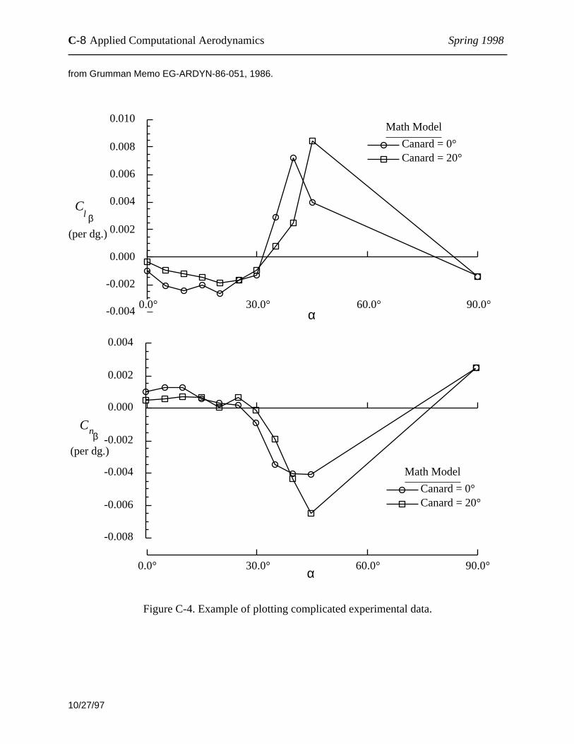
data with curves, they must pass through the data points. Connect complicated data with straight
lines, as shown in Fig. C-4. If the data points are dense, or a theory is used to compare with data,
you don’t need to draw lines between points (curves that don’t go through data points are
assumed to be theoretical results).
More comments on proper plots and graphs are contained in the engineering graphics text, by
Giesecke, eat al. (Ref. C-1). The engineer traditionally puts his initials and date in the lower right
hand corner of the plot. One problem frequently arises with plot labeling. In reports, the figure
titles go on the bottom. On view graphs and slides the figure titles go on the top. Many graphics
* This “improvement” was conceived by Joel Grassmeyer. It still requires some study.

C-4 Applied Computational Aerodynamics Spring 1998
10/27/97
packages are oriented toward placing the titles on the top. This is unacceptable in engineering
reports. Finally, tables are labeled on the top for both reports and presentations.
Engineering plots made using your computer must be of engineering quality. To do this you
have to understand the requirements given above for hand plots, and should have made enough
graphs by hand to be able to identify problems in the computer generated graphs. For force and
moment data it is often easier to make plots by hand than to figure out how to get your plotting
package to do a good job. Typical problems include poor scale selection, poor quality printout,
not being to invert the axis direction, and inability to print the experimental data as symbols and
the theory as lines. Another problem that arises is the use of color. While color is important, it
presents a major problem if the report is going to be copied for distribution. Most engineering
reports don’t make routine use of color— yet (electronic reports will make color much easier to
distribute).
Reference
C-1 Giesecke, F.E., Mitchell, A., Spencer, H.C., Hill, I.L., Loving, R.O., and Dygdon, J.T.,Principles of Engineering Graphics, Macmillan Publishing Cop., 1990, pap. 591-613.
Scale selection rules for engineering graphs
Originally devised by H.C. Higgins, The Boeing Company, re-interpreted for these notes.
1
1
1
This is a "5"
This is a "2"
This is a "1" Acceptable
Unacceptable
This is a "4"
1
Minor subdivisions of 1, 2, or 5 allow easy interpolation, and are the onlyacceptable values. A minor division of 4, for example, is very difficult to use.
2 3 4 5
2
0
0
0
0
Figure C-1. Boeing scale selection chart(based on a figure in the AIAA Student Journal, April, 1971)

report typos and errors to W.H. Mason Appendix C: Preparation of Material C-5
10/27/97
from Grumman Aero Report No. 393-82-02, April, 1982, “Experimental Pressure Distributions andAerodynamic Characteristics of a Demonstration Wing for a Wing Concept for Supersonic Maneuvering,”by W.H. Mason
-0.2
-0.1
0
0.1
0.2
0.3
0.4
0.5 -2
°0°
2°4°
6°8°
10°
12°
14°
Run
23
C L
α
M =
1.6
2
Re/
ft =
2 x
10
6cb
ar =
14.
747
in
Sref
= 3
42.1
1 in
2
Xmom
ref
= 1
6.70
1 in
fro
m w
ing
apex
tran
sist
ion
fixe
dB
asel
ine
LE
-0.0
4-0
.02
0
0.02
C M
a) lift and moment
Figure C-2. Examples of wind tunnel data plots.

C-6 Applied Computational Aerodynamics Spring 1998
10/27/97
from Grumman Aero Report No. 393-82-02, April, 1982, “Experimental Pressure Distributions andAerodynamic Characteristics of a Demonstration Wing for a Wing Concept for Supersonic Maneuvering,”by W.H. Mason
-0.2
-0.1
0.0
0.1
0.2
0.3
0.4
0.5
0.6
0.00 0.02 0.04 0.06 0.08 0.10
CL
CD
M = 1.62, Re/ft = 2 x 10⁶
cbar = 14.747 in, Sref = 342.11 in2
Xmom ref
= 16.701 in from wing apex
transistion fixed
Baseline Leading Edge
Test data, Run 23
CLdes
CD0 est
= 0.0122
Linear TheoryOptimum
Uncambered Wing, [CLtan(α - α0)]
550(goal)
632(WT data)
764
21% reduction in drag due to lift
Drag Performance of a Demonstration Wing for Supersonic Maneuvering
b) drag polar
Figure C-2. Concluded.

report typos and errors to W.H. Mason Appendix C: Preparation of Material C-7
10/27/97
1.2
0.8
0.4
0.0
-0.4
Cp
-0.8
-1.2
0.0 0.2 0.4 0.6 0.8 1.0
x/c
α = 1.875°M = .191Re = 720,000transition free
1.2
Calculated, Pgm PANELTest data, NACA R-646
NACA 4412 airfoil
Figure C-3. Example of pressure distribution plot.
C-8 Applied Computational Aerodynamics Spring 1998
10/27/97
from Grumman Memo EG-ARDYN-86-051, 1986.
-0.004
-0.002
0.000
0.002
0.004
0.006
0.008
0.010
0.0° 30.0° 60.0° 90.0°
Cl β
α
(per dg.)
-0.008
-0.006
-0.004
-0.002
0.000
0.002
0.004
0.0° 30.0° 60.0° 90.0°
Canard = 0°
Math Model
Canard = 20°
Cnβ
α
(per dg.)
Canard = 0°
Math Model
Canard = 20°
Figure C-4. Example of plotting complicated experimental data.
Appendix D Computational AerodynamicsPrograms
Several programs are used to provide insight into aerodynamics. This appendix provides the
input instructions.
D.1 PANEL*
Two dimensional incompressible, inviscid (potential) flow over NACA airfoils
using the Smith-Hess low order panel method. From Moran’s book, with modifi-
cations.
D.2 Panelv2*
An extension of PANEL to prediction of pressure distributions over arbitrary air-
foils, modification of the airfoil shape, and production of an output file for plot-
ting or use as input to a boundary layer analysis program.
D.3 LIDRAG
Computation of the induced drag of a single planar surface given the spanload
distribution. The coefficients of the assumed Fourier Series are computed using a
Fast Fourier Transform. The program was written by Dave Ives, and used in nu-
merous programs developed for the government by Grumman.
D.4 LAMDES
John Lamar’s design program, modified to find the span e for multiple and non-
planar lifting surfaces given the spanload on each surface. This is a more capable
version of LIDRAG. This code also finds the wing camber and twist required to
obtain this spanload at subsonic speeds. The code will also do an optimization
analysis, finding the minimum trimmed drag and spanload required to achieve it.
D.5 FRICTION
Computation of skin friction and form drag using turbulent flat plate skin friction
estimates, and empirical form factors. Provides a basis for zero lift drag estimates.
Includes compressibility effects and the 1977 standard atmosphere.
* This program is a modified form of a code in Moran’s book.
Tuesday, January 21, 1997 D-1

D.6 VLMpc
John Lamar’s two surface vortex lattice program, developed at NASA Langley.
The program treats two lifting surfaces using up to 200 panels. Vortex flows are
estimated using the leading edge suction analogy.
D.7 DESCAM
The camber line required to produce a specified chord load distribution is comput-
ed using the quasi-vortex lattice method. The method is valid for two dimensional
incompressible flow, and is an original program.
These codes are subject to significant revision, with the objective of becoming entirely indepen-
dent of codes obtained from copyrighted sources, so the students won’t have to own the books to
be able to use them.
D-2 Applied Computational Aerodynamics
Tuesday, January 21, 1997
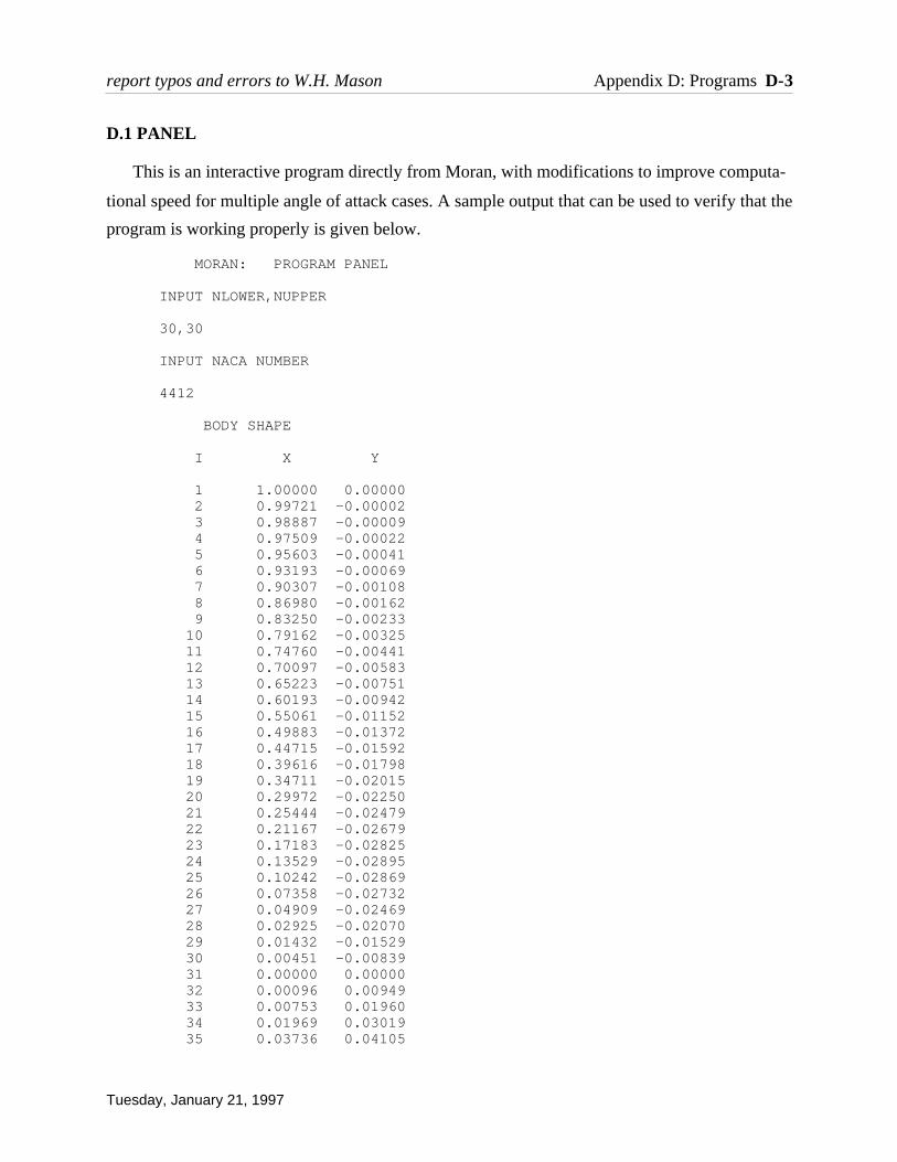
D.1 PANEL
This is an interactive program directly from Moran, with modifications to improve computa-
tional speed for multiple angle of attack cases. A sample output that can be used to verify that the
program is working properly is given below.
MORAN: PROGRAM PANEL
INPUT NLOWER,NUPPER
30,30
INPUT NACA NUMBER
4412
BODY SHAPE
I X Y
1 1.00000 0.00000 2 0.99721 -0.00002 3 0.98887 -0.00009 4 0.97509 -0.00022 5 0.95603 -0.00041 6 0.93193 -0.00069 7 0.90307 -0.00108 8 0.86980 -0.00162 9 0.83250 -0.00233 10 0.79162 -0.00325 11 0.74760 -0.00441 12 0.70097 -0.00583 13 0.65223 -0.00751 14 0.60193 -0.00942 15 0.55061 -0.01152 16 0.49883 -0.01372 17 0.44715 -0.01592 18 0.39616 -0.01798 19 0.34711 -0.02015 20 0.29972 -0.02250 21 0.25444 -0.02479 22 0.21167 -0.02679 23 0.17183 -0.02825 24 0.13529 -0.02895 25 0.10242 -0.02869 26 0.07358 -0.02732 27 0.04909 -0.02469 28 0.02925 -0.02070 29 0.01432 -0.01529 30 0.00451 -0.00839 31 0.00000 0.00000 32 0.00096 0.00949 33 0.00753 0.01960 34 0.01969 0.03019 35 0.03736 0.04105
report typos and errors to W.H. Mason Appendix D: Programs D-3
Tuesday, January 21, 1997

36 0.06039 0.05187 37 0.08856 0.06233 38 0.12157 0.07207 39 0.15904 0.08074 40 0.20054 0.08799 41 0.24556 0.09354 42 0.29354 0.09715 43 0.34387 0.09866 44 0.39593 0.09797 45 0.44833 0.09541 46 0.50117 0.09150 47 0.55392 0.08637 48 0.60599 0.08018 49 0.65679 0.07312 50 0.70577 0.06538 51 0.75240 0.05719 52 0.79617 0.04877 53 0.83663 0.04036 54 0.87334 0.03220 55 0.90594 0.02452 56 0.93409 0.01756 57 0.95751 0.01152 58 0.97597 0.00661 59 0.98928 0.00298 60 0.99731 0.00075
INPUT ALPHA IN DEGREES:
2.
PRESSURE DISTRIBUTION
I X Y CP 1 0.9986 0.0000 0.38467 2 0.9930 -0.0001 0.30343 3 0.9820 -0.0002 0.25675 4 0.9656 -0.0003 0.22763 5 0.9440 -0.0006 0.20840 6 0.9175 -0.0009 0.19523 7 0.8864 -0.0014 0.18587 8 0.8512 -0.0020 0.17886 9 0.8121 -0.0028 0.17317 10 0.7696 -0.0038 0.16801 11 0.7243 -0.0051 0.16280 12 0.6766 -0.0067 0.15713 13 0.6271 -0.0085 0.15077 14 0.5763 -0.0105 0.14373 15 0.5247 -0.0126 0.13638 16 0.4730 -0.0148 0.12985 17 0.4217 -0.0170 0.12807 18 0.3716 -0.0191 0.12602 19 0.3234 -0.0213 0.11687 20 0.2771 -0.0236 0.10199 21 0.2331 -0.0258 0.08422 22 0.1917 -0.0275 0.06568 23 0.1536 -0.0286 0.04878 24 0.1189 -0.0288 0.03693 25 0.0880 -0.0280 0.03573
D-4 Applied Computational Aerodynamics
Tuesday, January 21, 1997

26 0.0613 -0.0260 0.05561 27 0.0392 -0.0227 0.11840 28 0.0218 -0.0180 0.27208 29 0.0094 -0.0118 0.60051 30 0.0023 -0.0042 0.98725 31 0.0005 0.0047 0.62389 32 0.0042 0.0145 -0.17221 33 0.0136 0.0249 -0.59380 34 0.0285 0.0356 -0.77475 35 0.0489 0.0465 -0.86631 36 0.0745 0.0571 -0.92155 37 0.1051 0.0672 -0.95698 38 0.1403 0.0764 -0.97726 39 0.1798 0.0844 -0.98317 40 0.2231 0.0908 -0.97429 41 0.2696 0.0953 -0.94986 42 0.3187 0.0979 -0.90860 43 0.3699 0.0983 -0.84568 44 0.4221 0.0967 -0.76754 45 0.4747 0.0935 -0.69391 46 0.5275 0.0889 -0.62775 47 0.5800 0.0833 -0.56419 48 0.6314 0.0766 -0.50177 49 0.6813 0.0692 -0.43979 50 0.7291 0.0613 -0.37777 51 0.7743 0.0530 -0.31529 52 0.8164 0.0446 -0.25196 53 0.8550 0.0363 -0.18742 54 0.8896 0.0284 -0.12130 55 0.9200 0.0210 -0.05316 56 0.9458 0.0145 0.01760 57 0.9667 0.0091 0.09212 58 0.9826 0.0048 0.17280 59 0.9933 0.0019 0.26569 60 0.9987 0.0004 0.38467
AT ALPHA = 2.000
CD = -0.00078 CL = 0.73347 CM = -0.28985
Another angle of attack? (Y/N):n
STOP
report typos and errors to W.H. Mason Appendix D: Programs D-5
Tuesday, January 21, 1997

D.2 PANELV2 User's Manual
This manual describes the input for program PANELV2, an extended version of programPANEL from Moran.
This program allows input of arbitrary airfoils for analysis, modification of airfoil shapes using“bumps,” and output of a file for plotting or other analysis. The program runs interactively. Theinput file for arbitrary airfoils is given below. (the disk with the program includes sample files,identified by ending in “.pan”)
INPUT DESCRIPTION (all numeric input is in 2F10.5 format)
Card Field Variable Description1 1 Title Up to 80 characters describing the data set/case (A79)
2 1 FNUP number of X,Y pairs describing upper surface2 FNLOW " " " lower "
3 dummy card (used for descriptor in input data)
4 1 X the upper surface airfoil x/c input station2 Y the y/c value of the upper surface at this x/c
************ CARD 4 is repeated FNUP times ************
5 dummy card (used for descriptor in input data)
6 1 X the lower surface airfoil x/c input station2 Y the y/c value of the lower surface at this x/c
************ CARD 6 is repeated FNLOW times ************
Notes:
1. Airfoils are input from leading edge to trailing edge.
2. The leading edge point must be input twice: once for the upper surface and once for thelower surface descriptions.
OUTPUT FILE FORMAT
Card 1. TITLE2. Heading for output3. 4 fields: 4F10.4, this card contains
i) angle of attack, in degreesii) lift coefficientiii) moment coeficient (about the quarter chord)iv) drag coefficient from surface pressure integration (should be zero)
4. Number of points in 5. Heading for output6. 4 fields: 4F20.7 Note: this card is repeated for each control point
i) x/c, airfoil ordinateii) y/c, airfoil ordinateiii) Cp, pressure coefficientiii) Ue/Uinf, the surface velocity at x/c, y/c
D-6 Applied Computational Aerodynamics
Tuesday, January 21, 1997
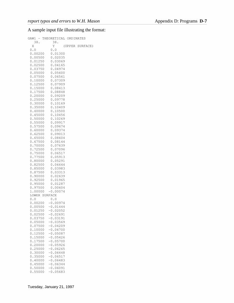
A sample input file illustrating the format:
GAW1 - THEORETICAL ORDINATES 38. 38. X Y (UPPER SURFACE) 0.0 0.0 0.00200 0.01300 0.00500 0.02035 0.01250 0.03069 0.02500 0.04165 0.03750 0.04974 0.05000 0.05600 0.07500 0.06561 0.10000 0.07309 0.12500 0.07909 0.15000 0.08413 0.17500 0.08848 0.20000 0.09209 0.25000 0.09778 0.30000 0.10169 0.35000 0.10409 0.40000 0.10500 0.45000 0.10456 0.50000 0.10269 0.55000 0.09917 0.57500 0.09674 0.60000 0.09374 0.62500 0.09013 0.65000 0.08604 0.67500 0.08144 0.70000 0.07639 0.72500 0.07096 0.75000 0.06517 0.77500 0.05913 0.80000 0.05291 0.82500 0.04644 0.85000 0.03983 0.87500 0.03313 0.90000 0.02639 0.92500 0.01965 0.95000 0.01287 0.97500 0.00604 1.00000 -0.00074 LOWER SURFACE 0.0 0.0 0.00200 -0.00974 0.00500 -0.01444 0.01250 -0.02052 0.02500 -0.02691 0.03750 -0.03191 0.05000 -0.03569 0.07500 -0.04209 0.10000 -0.04700 0.12500 -0.05087 0.15000 -0.05426 0.17500 -0.05700 0.20000 -0.05926 0.25000 -0.06265 0.30000 -0.06448 0.35000 -0.06517 0.40000 -0.06483 0.45000 -0.06344 0.50000 -0.06091 0.55000 -0.05683
report typos and errors to W.H. Mason Appendix D: Programs D-7
Tuesday, January 21, 1997

0.57500 -0.05396 0.60000 -0.05061 0.62500 -0.04678 0.65000 -0.04265 0.67500 -0.03830 0.70000 -0.03383 0.72500 -0.02930 0.75000 -0.02461 0.77500 -0.02030 0.80000 -0.01587 0.82500 -0.01191 0.85000 -0.00852 0.87500 -0.00565 0.90000 -0.00352 0.92500 -0.00248 0.95000 -0.00257 0.97500 -0.00396
1.00000 -0.00783
D-8 Applied Computational Aerodynamics
Tuesday, January 21, 1997

A sample output from PANELv2:
PROGRAM PANELv2 Revised version of Moran code modifications by W.H. Mason
INPUT NLOWER,NUPPER (nupper and nlower MUST be equal, and nupper + nlower MUST be less than 100)40,40
for internally generated ordinates, enter 0 to read an external file of ordinates, enter 11
Enter name of file to be read: gaw1.pan
Input file name:gaw1.pan File title:: GAW1 - THEORETICAL ORDINATES
NU = 38 NL = 38
Upper surface ordinates
index X/C Y/C 38 0.000000 0.000000 39 0.002000 0.013000 40 0.005000 0.020350 41 0.012500 0.030690 42 0.025000 0.041650 43 0.037500 0.049740 44 0.050000 0.056000 45 0.075000 0.065610 46 0.100000 0.073090 47 0.125000 0.079090 48 0.150000 0.084130 49 0.175000 0.088480 50 0.200000 0.092090 51 0.250000 0.097780 52 0.300000 0.101690 53 0.350000 0.104090 54 0.400000 0.105000 55 0.450000 0.104560 56 0.500000 0.102690 57 0.550000 0.099170 58 0.575000 0.096740 59 0.600000 0.093740 60 0.625000 0.090130 61 0.650000 0.086040 62 0.675000 0.081440 63 0.700000 0.076390 64 0.725000 0.070960 65 0.750000 0.065170 66 0.775000 0.059130 67 0.800000 0.052910 68 0.825000 0.046440 69 0.850000 0.039830 70 0.875000 0.033130 71 0.900000 0.026390 72 0.925000 0.019650 73 0.950000 0.012870 74 0.975000 0.006040 75 1.000000 -0.000740
report typos and errors to W.H. Mason Appendix D: Programs D-9
Tuesday, January 21, 1997
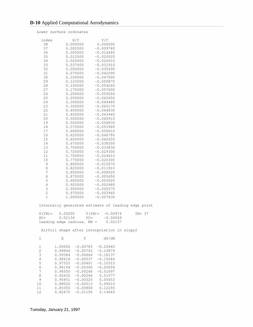
Lower surface ordinates
index X/C Y/C 38 0.000000 0.000000 37 0.002000 -0.009740 36 0.005000 -0.014440 35 0.012500 -0.020520 34 0.025000 -0.026910 33 0.037500 -0.031910 32 0.050000 -0.035690 31 0.075000 -0.042090 30 0.100000 -0.047000 29 0.125000 -0.050870 28 0.150000 -0.054260 27 0.175000 -0.057000 26 0.200000 -0.059260 25 0.250000 -0.062650 24 0.300000 -0.064480 23 0.350000 -0.065170 22 0.400000 -0.064830 21 0.450000 -0.063440 20 0.500000 -0.060910 19 0.550000 -0.056830 18 0.575000 -0.053960 17 0.600000 -0.050610 16 0.625000 -0.046780 15 0.650000 -0.042650 14 0.675000 -0.038300 13 0.700000 -0.033830 12 0.725000 -0.029300 11 0.750000 -0.024610 10 0.775000 -0.020300 9 0.800000 -0.015870 8 0.825000 -0.011910 7 0.850000 -0.008520 6 0.875000 -0.005650 5 0.900000 -0.003520 4 0.925000 -0.002480 3 0.950000 -0.002570 2 0.975000 -0.003960 1 1.000000 -0.007830
internally generated estimate of leading edge point
X(IN)= 0.00200 Y(IN)= -0.00974 IN= 37 XC= 0.02136 YC= -0.00069 leading edge radious, RN = 0.02137
Airfoil shape after interpolation in slopy2
I X Y dY/dX
1 1.00000 -0.00783 -0.20440 2 0.99846 -0.00752 -0.19879 3 0.99384 -0.00664 -0.18137 4 0.98618 -0.00537 -0.15044 5 0.97553 -0.00401 -0.10315 6 0.96194 -0.00300 -0.05058 7 0.94550 -0.00248 -0.01697 8 0.92632 -0.00246 0.01577 9 0.90451 -0.00325 0.05653 10 0.88020 -0.00513 0.09610 11 0.85355 -0.00808 0.12293 12 0.82472 -0.01195 0.14645
D-10 Applied Computational Aerodynamics
Tuesday, January 21, 1997
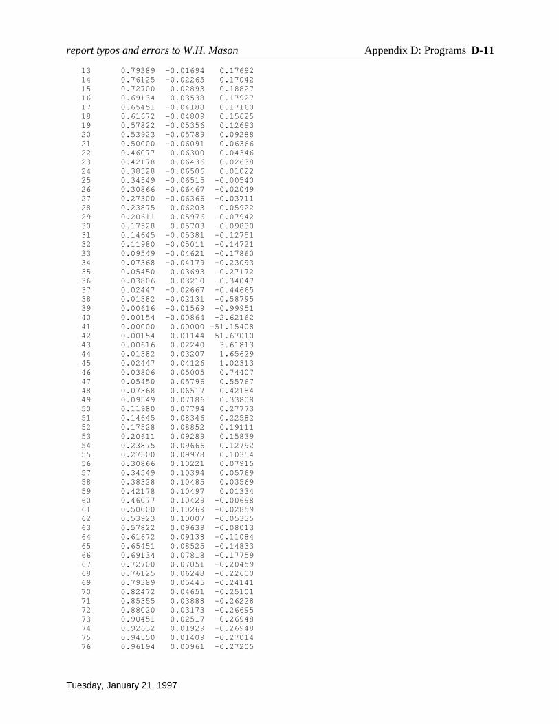
13 0.79389 -0.01694 0.17692 14 0.76125 -0.02265 0.17042 15 0.72700 -0.02893 0.18827 16 0.69134 -0.03538 0.17927 17 0.65451 -0.04188 0.17160 18 0.61672 -0.04809 0.15625 19 0.57822 -0.05356 0.12693 20 0.53923 -0.05789 0.09288 21 0.50000 -0.06091 0.06366 22 0.46077 -0.06300 0.04346 23 0.42178 -0.06436 0.02638 24 0.38328 -0.06506 0.01022 25 0.34549 -0.06515 -0.00540 26 0.30866 -0.06467 -0.02049 27 0.27300 -0.06366 -0.03711 28 0.23875 -0.06203 -0.05922 29 0.20611 -0.05976 -0.07942 30 0.17528 -0.05703 -0.09830 31 0.14645 -0.05381 -0.12751 32 0.11980 -0.05011 -0.14721 33 0.09549 -0.04621 -0.17860 34 0.07368 -0.04179 -0.23093 35 0.05450 -0.03693 -0.27172 36 0.03806 -0.03210 -0.34047 37 0.02447 -0.02667 -0.44665 38 0.01382 -0.02131 -0.58795 39 0.00616 -0.01569 -0.99951 40 0.00154 -0.00864 -2.62162 41 0.00000 0.00000 -51.15408 42 0.00154 0.01144 51.67010 43 0.00616 0.02240 3.61813 44 0.01382 0.03207 1.65629 45 0.02447 0.04126 1.02313 46 0.03806 0.05005 0.74407 47 0.05450 0.05796 0.55767 48 0.07368 0.06517 0.42184 49 0.09549 0.07186 0.33808 50 0.11980 0.07794 0.27773 51 0.14645 0.08346 0.22582 52 0.17528 0.08852 0.19111 53 0.20611 0.09289 0.15839 54 0.23875 0.09666 0.12792 55 0.27300 0.09978 0.10354 56 0.30866 0.10221 0.07915 57 0.34549 0.10394 0.05769 58 0.38328 0.10485 0.03569 59 0.42178 0.10497 0.01334 60 0.46077 0.10429 -0.00698 61 0.50000 0.10269 -0.02859 62 0.53923 0.10007 -0.05335 63 0.57822 0.09639 -0.08013 64 0.61672 0.09138 -0.11084 65 0.65451 0.08525 -0.14833 66 0.69134 0.07818 -0.17759 67 0.72700 0.07051 -0.20459 68 0.76125 0.06248 -0.22600 69 0.79389 0.05445 -0.24141 70 0.82472 0.04651 -0.25101 71 0.85355 0.03888 -0.26228 72 0.88020 0.03173 -0.26695 73 0.90451 0.02517 -0.26948 74 0.92632 0.01929 -0.26948 75 0.94550 0.01409 -0.27014 76 0.96194 0.00961 -0.27205
report typos and errors to W.H. Mason Appendix D: Programs D-11
Tuesday, January 21, 1997
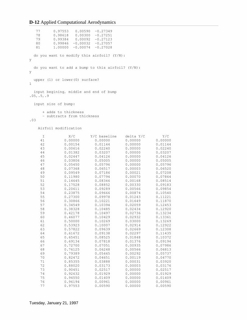
77 0.97553 0.00590 -0.27349 78 0.98618 0.00300 -0.27251 79 0.99384 0.00092 -0.27123 80 0.99846 -0.00032 -0.27057 81 1.00000 -0.00074 -0.27028
do you want to modify this airfoil? (Y/N):y
do you want to add a bump to this airfoil? (Y/N):y
upper (1) or lower(0) surface?1
input begining, middle and end of bump.05,.5,.9
input size of bump:
+ adds to thickness - subtracts from thickness.03
Airfoil modification
I X/C Y/C baseline delta Y/C Y/C 41 0.00000 0.00000 0.00000 0.00000 42 0.00154 0.01144 0.00000 0.01144 43 0.00616 0.02240 0.00000 0.02240 44 0.01382 0.03207 0.00000 0.03207 45 0.02447 0.04126 0.00000 0.04126 46 0.03806 0.05005 0.00000 0.05005 47 0.05450 0.05796 0.00000 0.05796 48 0.07368 0.06517 0.00003 0.06520 49 0.09549 0.07186 0.00021 0.07208 50 0.11980 0.07794 0.00070 0.07864 51 0.14645 0.08346 0.00168 0.08514 52 0.17528 0.08852 0.00330 0.09183 53 0.20611 0.09289 0.00566 0.09854 54 0.23875 0.09666 0.00874 0.10540 55 0.27300 0.09978 0.01243 0.11221 56 0.30866 0.10221 0.01649 0.11870 57 0.34549 0.10394 0.02059 0.12453 58 0.38328 0.10485 0.02434 0.12920 59 0.42178 0.10497 0.02736 0.13234 60 0.46077 0.10429 0.02932 0.13361 61 0.50000 0.10269 0.03000 0.13269 62 0.53923 0.10007 0.02914 0.12922 63 0.57822 0.09639 0.02669 0.12308 64 0.61672 0.09138 0.02297 0.11435 65 0.65451 0.08525 0.01848 0.10372 66 0.69134 0.07818 0.01376 0.09194 67 0.72700 0.07051 0.00935 0.07986 68 0.76125 0.06248 0.00566 0.06813 69 0.79389 0.05445 0.00292 0.05737 70 0.82472 0.04651 0.00119 0.04770 71 0.85355 0.03888 0.00031 0.03920 72 0.88020 0.03173 0.00003 0.03176 73 0.90451 0.02517 0.00000 0.02517 74 0.92632 0.01929 0.00000 0.01929 75 0.94550 0.01409 0.00000 0.01409 76 0.96194 0.00961 0.00000 0.00961 77 0.97553 0.00590 0.00000 0.00590
D-12 Applied Computational Aerodynamics
Tuesday, January 21, 1997
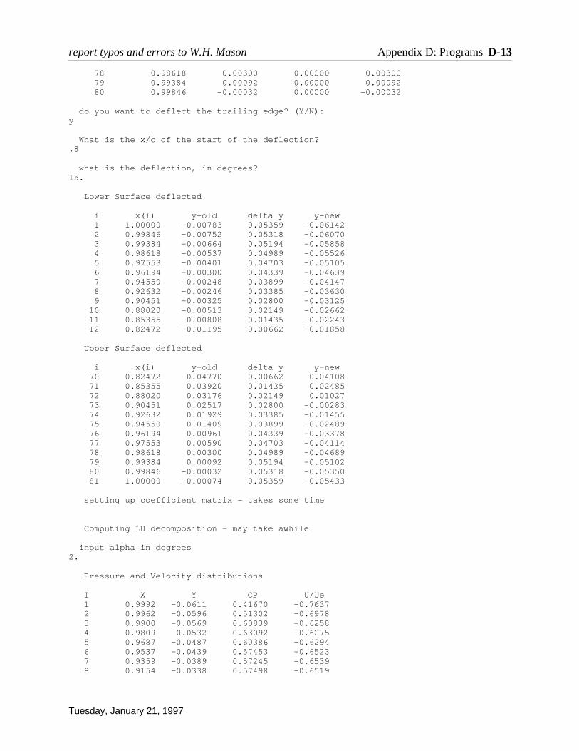
78 0.98618 0.00300 0.00000 0.00300 79 0.99384 0.00092 0.00000 0.00092 80 0.99846 -0.00032 0.00000 -0.00032
do you want to deflect the trailing edge? (Y/N):y
What is the x/c of the start of the deflection?.8
what is the deflection, in degrees?15.
Lower Surface deflected
i x(i) y-old delta y y-new 1 1.00000 -0.00783 0.05359 -0.06142 2 0.99846 -0.00752 0.05318 -0.06070 3 0.99384 -0.00664 0.05194 -0.05858 4 0.98618 -0.00537 0.04989 -0.05526 5 0.97553 -0.00401 0.04703 -0.05105 6 0.96194 -0.00300 0.04339 -0.04639 7 0.94550 -0.00248 0.03899 -0.04147 8 0.92632 -0.00246 0.03385 -0.03630 9 0.90451 -0.00325 0.02800 -0.03125 10 0.88020 -0.00513 0.02149 -0.02662 11 0.85355 -0.00808 0.01435 -0.02243 12 0.82472 -0.01195 0.00662 -0.01858
Upper Surface deflected
i x(i) y-old delta y y-new 70 0.82472 0.04770 0.00662 0.04108 71 0.85355 0.03920 0.01435 0.02485 72 0.88020 0.03176 0.02149 0.01027 73 0.90451 0.02517 0.02800 -0.00283 74 0.92632 0.01929 0.03385 -0.01455 75 0.94550 0.01409 0.03899 -0.02489 76 0.96194 0.00961 0.04339 -0.03378 77 0.97553 0.00590 0.04703 -0.04114 78 0.98618 0.00300 0.04989 -0.04689 79 0.99384 0.00092 0.05194 -0.05102 80 0.99846 -0.00032 0.05318 -0.05350 81 1.00000 -0.00074 0.05359 -0.05433
setting up coefficient matrix - takes some time
Computing LU decomposition - may take awhile
input alpha in degrees2.
Pressure and Velocity distributions
I X Y CP U/Ue 1 0.9992 -0.0611 0.41670 -0.7637 2 0.9962 -0.0596 0.51302 -0.6978 3 0.9900 -0.0569 0.60839 -0.6258 4 0.9809 -0.0532 0.63092 -0.6075 5 0.9687 -0.0487 0.60386 -0.6294 6 0.9537 -0.0439 0.57453 -0.6523 7 0.9359 -0.0389 0.57245 -0.6539 8 0.9154 -0.0338 0.57498 -0.6519
report typos and errors to W.H. Mason Appendix D: Programs D-13
Tuesday, January 21, 1997
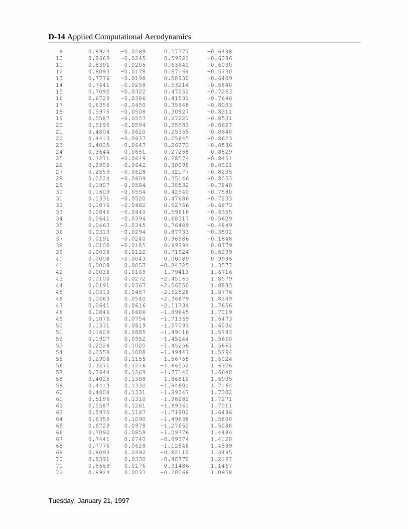
9 0.8924 -0.0289 0.57777 -0.6498 10 0.8669 -0.0245 0.59221 -0.6386 11 0.8391 -0.0205 0.63641 -0.6030 12 0.8093 -0.0178 0.67164 -0.5730 13 0.7776 -0.0198 0.58930 -0.6409 14 0.7441 -0.0258 0.53214 -0.6840 15 0.7092 -0.0322 0.47252 -0.7263 16 0.6729 -0.0386 0.41531 -0.7646 17 0.6356 -0.0450 0.35948 -0.8003 18 0.5975 -0.0508 0.30927 -0.8311 19 0.5587 -0.0557 0.27221 -0.8531 20 0.5196 -0.0594 0.25583 -0.8627 21 0.4804 -0.0620 0.25355 -0.8640 22 0.4413 -0.0637 0.25645 -0.8623 23 0.4025 -0.0647 0.26273 -0.8586 24 0.3644 -0.0651 0.27258 -0.8529 25 0.3271 -0.0649 0.28574 -0.8451 26 0.2908 -0.0642 0.30098 -0.8361 27 0.2559 -0.0628 0.32177 -0.8235 28 0.2224 -0.0609 0.35146 -0.8053 29 0.1907 -0.0584 0.38532 -0.7840 30 0.1609 -0.0554 0.42540 -0.7580 31 0.1331 -0.0520 0.47686 -0.7233 32 0.1076 -0.0482 0.52766 -0.6873 33 0.0846 -0.0440 0.59616 -0.6355 34 0.0641 -0.0394 0.68317 -0.5629 35 0.0463 -0.0345 0.76489 -0.4849 36 0.0313 -0.0294 0.87733 -0.3502 37 0.0191 -0.0240 0.96586 -0.1848 38 0.0100 -0.0185 0.99394 0.0779 39 0.0038 -0.0122 0.71924 0.5299 40 0.0008 -0.0043 0.00089 0.9996 41 0.0008 0.0057 -0.84325 1.3577 42 0.0038 0.0169 -1.79413 1.6716 43 0.0100 0.0272 -2.45163 1.8579 44 0.0191 0.0367 -2.56550 1.8883 45 0.0313 0.0457 -2.52528 1.8776 46 0.0463 0.0540 -2.36679 1.8349 47 0.0641 0.0616 -2.11734 1.7656 48 0.0846 0.0686 -1.89645 1.7019 49 0.1076 0.0754 -1.71369 1.6473 50 0.1331 0.0819 -1.57093 1.6034 51 0.1609 0.0885 -1.49116 1.5783 52 0.1907 0.0952 -1.45244 1.5660 53 0.2224 0.1020 -1.45256 1.5661 54 0.2559 0.1088 -1.49447 1.5794 55 0.2908 0.1155 -1.56755 1.6024 56 0.3271 0.1216 -1.66552 1.6326 57 0.3644 0.1269 -1.77142 1.6648 58 0.4025 0.1308 -1.86810 1.6935 59 0.4413 0.1330 -1.94601 1.7164 60 0.4804 0.1331 -1.99347 1.7302 61 0.5196 0.1310 -1.98282 1.7271 62 0.5587 0.1261 -1.89361 1.7011 63 0.5975 0.1187 -1.71802 1.6486 64 0.6356 0.1090 -1.49638 1.5800 65 0.6729 0.0978 -1.27652 1.5088 66 0.7092 0.0859 -1.09776 1.4484 67 0.7441 0.0740 -0.99374 1.4120 68 0.7776 0.0628 -1.12848 1.4589 69 0.8093 0.0492 -0.82110 1.3495 70 0.8391 0.0330 -0.48770 1.2197 71 0.8669 0.0176 -0.31486 1.1467 72 0.8924 0.0037 -0.20068 1.0958
D-14 Applied Computational Aerodynamics
Tuesday, January 21, 1997

73 0.9154 -0.0087 -0.11007 1.0536 74 0.9359 -0.0197 -0.04075 1.0202 75 0.9537 -0.0293 0.01110 0.9944 76 0.9687 -0.0375 0.03867 0.9805 77 0.9809 -0.0440 0.04913 0.9751 78 0.9900 -0.0490 0.09990 0.9487 79 0.9962 -0.0523 0.23071 0.8771 80 0.9992 -0.0539 0.41671 0.7637 I X Y CP U/Ue
AT ALPHA = 2.000
CL = 1.82147 CM(l.e.) = -0.76764 Cm(c/4) = -0.31257 CD = -0.00344 (theoretically zero)
send output to a file? (Y/N):y
enter file name: gaw1.out
enter file title: GAW 1 airfoil with upper surface mod and trailing edge deflected
Another angle of attack? (Y/N):n
STOP
The output disk file generated from the above is given here (for a 44,44 panel case):
GAW 1 airfoil with upper surface mod and trailing edge deflected Alpha CL cmc4 CD 2.0000 1.8253 -0.3139 -0.0034 90.0000000 X/C Y/C Cp U/UE 1.0000000 -0.0614198 0.4218349 -0.7603717 0.9987261 -0.0608210 0.4894220 -0.7145474 0.9949107 -0.0590636 0.5828183 -0.6458961 0.9885734 -0.0562688 0.6198552 -0.6165588 0.9797465 -0.0526529 0.6121694 -0.6227604 0.9684749 -0.0485395 0.5824285 -0.6461977 0.9548160 -0.0441873 0.5709316 -0.6550332 0.9388395 -0.0396023 0.5742147 -0.6525223 0.9206268 -0.0348995 0.5779232 -0.6496744 0.9002706 -0.0303699 0.5814999 -0.6469159 0.8778748 -0.0262270 0.5949170 -0.6364613 0.8535534 -0.0224278 0.6267794 -0.6109178 0.8274304 -0.0189073 0.7059953 -0.5422220 0.7996389 -0.0159320 0.6026480 -0.6303586 0.7703204 -0.0211078 0.5561817 -0.6661969 0.7396245 -0.0265297 0.4989320 -0.7078615 0.7077075 -0.0324513 0.4452444 -0.7448192 0.6747321 -0.0383475 0.3940417 -0.7784333 0.6408663 -0.0441870 0.3435679 -0.8102050 0.6062826 -0.0496877 0.2998845 -0.8367290 0.5711573 -0.0544341 0.2689947 -0.8549885 0.5356696 -0.0582109 0.2556977 -0.8627295 0.5000000 -0.0609100 0.2539230 -0.8637575 0.4643304 -0.0628407 0.2562625 -0.8624022 0.4288425 -0.0641589 0.2613289 -0.8594598 0.3937173 -0.0649298 0.2692938 -0.8548135 0.3591337 -0.0651852 0.2802141 -0.8484020 0.3252679 -0.0649567 0.2932411 -0.8406895 0.2922925 -0.0642823 0.3083775 -0.8316385 0.2603754 -0.0631488 0.3301547 -0.8184408
report typos and errors to W.H. Mason Appendix D: Programs D-15
Tuesday, January 21, 1997
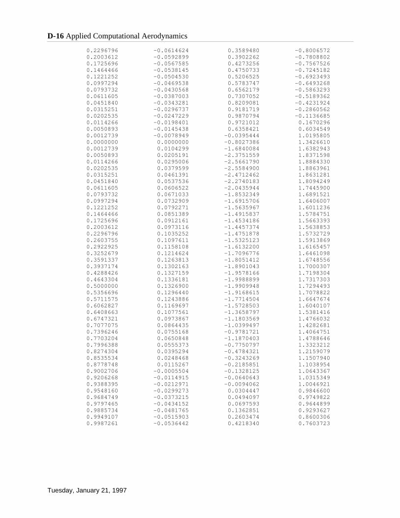
0.2296796 -0.0614624 0.3589480 -0.8006572 0.2003612 -0.0592899 0.3902262 -0.7808802 0.1725696 -0.0567585 0.4273256 -0.7567526 0.1464466 -0.0538145 0.4750733 -0.7245182 0.1221252 -0.0504530 0.5206525 -0.6923493 0.0997294 -0.0469538 0.5783747 -0.6493268 0.0793732 -0.0430568 0.6562179 -0.5863293 0.0611605 -0.0387003 0.7307052 -0.5189362 0.0451840 -0.0343281 0.8209081 -0.4231924 0.0315251 -0.0296737 0.9181719 -0.2860562 0.0202535 -0.0247229 0.9870794 -0.1136685 0.0114266 -0.0198401 0.9721012 0.1670296 0.0050893 -0.0145438 0.6358421 0.6034549 0.0012739 -0.0078949 -0.0395444 1.0195805 0.0000000 0.0000000 -0.8027386 1.3426610 0.0012739 0.0104299 -1.6840084 1.6382943 0.0050893 0.0205191 -2.3751559 1.8371598 0.0114266 0.0295006 -2.5661790 1.8884330 0.0202535 0.0379599 -2.5584900 1.8863961 0.0315251 0.0461391 -2.4712462 1.8631281 0.0451840 0.0537536 -2.2740183 1.8094249 0.0611605 0.0606522 -2.0435944 1.7445900 0.0793732 0.0671033 -1.8532349 1.6891521 0.0997294 0.0732909 -1.6915706 1.6406007 0.1221252 0.0792271 -1.5635967 1.6011236 0.1464466 0.0851389 -1.4915837 1.5784751 0.1725696 0.0912161 -1.4534186 1.5663393 0.2003612 0.0973116 -1.4457374 1.5638853 0.2296796 0.1035252 -1.4751878 1.5732729 0.2603755 0.1097611 -1.5325123 1.5913869 0.2922925 0.1158108 -1.6132200 1.6165457 0.3252679 0.1214624 -1.7096776 1.6461098 0.3591337 0.1263813 -1.8051412 1.6748556 0.3937174 0.1302163 -1.8901043 1.7000307 0.4288426 0.1327159 -1.9578166 1.7198304 0.4643304 0.1336181 -1.9988899 1.7317303 0.5000000 0.1326900 -1.9909948 1.7294493 0.5356696 0.1296440 -1.9168615 1.7078822 0.5711575 0.1243886 -1.7714504 1.6647674 0.6062827 0.1169697 -1.5728503 1.6040107 0.6408663 0.1077561 -1.3658797 1.5381416 0.6747321 0.0973867 -1.1803569 1.4766032 0.7077075 0.0864435 -1.0399497 1.4282681 0.7396246 0.0755168 -0.9781721 1.4064751 0.7703204 0.0650848 -1.1870403 1.4788646 0.7996388 0.0555373 -0.7750797 1.3323212 0.8274304 0.0395294 -0.4784321 1.2159079 0.8535534 0.0248468 -0.3243269 1.1507940 0.8778748 0.0115267 -0.2185851 1.1038954 0.9002706 -0.0005504 -0.1328125 1.0643367 0.9206268 -0.0114915 -0.0640643 1.0315349 0.9388395 -0.0212971 -0.0094062 1.0046921 0.9548160 -0.0299273 0.0304447 0.9846600 0.9684749 -0.0373215 0.0494097 0.9749822 0.9797465 -0.0434152 0.0697593 0.9644899 0.9885734 -0.0481765 0.1362851 0.9293627 0.9949107 -0.0515903 0.2603474 0.8600306 0.9987261 -0.0536442 0.4218340 0.7603723
D-16 Applied Computational Aerodynamics
Tuesday, January 21, 1997

D.3 Program LIDRAG
This program computes the span e for a single planar lifting surface given the spanload. It usesthe spanload to determine the “e” using a Fast Fourier Transform. Numerous other methodscould be used. For reference, note that the “e” for an elliptic spanload is 1.0, and the “e” for a tri-angular spanload is .72. The code is in the file LIDRAG.F. The sample input is also on the diskand is called B2LDG.INP. The program prompts the user for the name of the input file.
The program was written by Dave Ives, and entered the public domain through the codecontained in AFFDL-TR-77-122, “An Automated Procedure for Computing the ThreeDimensional Transonic Flow over Wing-Body Combinations, Including Viscous Effects,” Feb.1978.
The input is the spanload obtained from any method. The output is the Trefftz plane induceddrag e and the integral of the spanload, which produces the CL. This is the “span” e. You shouldinclude a point at η = 0 and at η = 1 you should include a point with zero spanload. See the sam-ple input for an example.
The input instruction:
Card Field Columns Variable Description
1 1 1-10 FSPN Number of spanwise stations of input2 1 1-10 ETA The spanwise location of input, y/(b/2).2 1 1-20 CCLCA The spanload, ccl/ca (the local chord times
the local lift coefficient divided by the average chord)
Note: card 2 is repeated FSPN times
Sample input: (from the output of the VLMpc sample case for the B-2, and in the fileB2LDG.INP on the disk))
20. 0.0 0.58435 0.01805 0.58435 0.06388 0.57919 0.11943 0.56800 0.17664 0.55739 0.23385 0.54709 0.30271 0.52459 0.37158 0.48623 0.42713 0.44590 0.48269 0.40097 0.53925 0.36490 0.59581 0.34718 0.65137 0.33280 0.70693 0.31865 0.76248 0.30225 0.81804 0.27971 0.86735 0.24229 0.91667 0.18494 0.97222 0.09480 1.000 0.000
report typos and errors to W.H. Mason Appendix D: Programs D-17
Tuesday, January 21, 1997
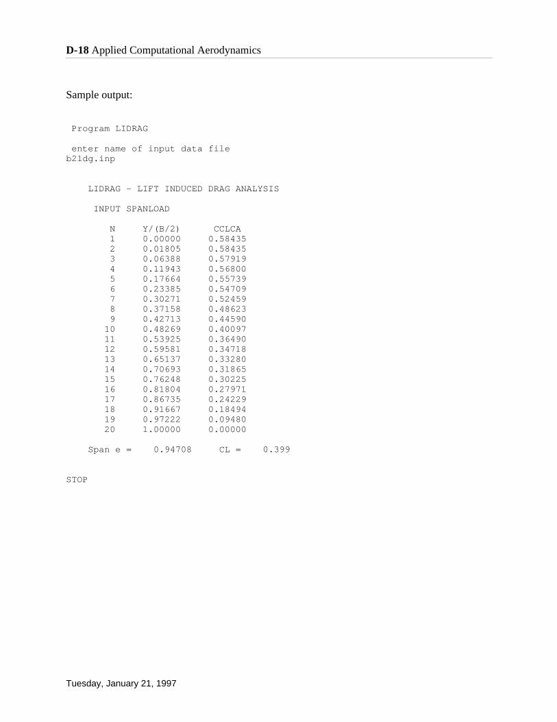
Sample output:
Program LIDRAG
enter name of input data fileb2ldg.inp
LIDRAG - LIFT INDUCED DRAG ANALYSIS
INPUT SPANLOAD
N Y/(B/2) CCLCA 1 0.00000 0.58435 2 0.01805 0.58435 3 0.06388 0.57919 4 0.11943 0.56800 5 0.17664 0.55739 6 0.23385 0.54709 7 0.30271 0.52459 8 0.37158 0.48623 9 0.42713 0.44590 10 0.48269 0.40097 11 0.53925 0.36490 12 0.59581 0.34718 13 0.65137 0.33280 14 0.70693 0.31865 15 0.76248 0.30225 16 0.81804 0.27971 17 0.86735 0.24229 18 0.91667 0.18494 19 0.97222 0.09480 20 1.00000 0.00000
Span e = 0.94708 CL = 0.399
STOP
D-18 Applied Computational Aerodynamics
Tuesday, January 21, 1997

D.4 LAMDES User’s Manual
This is the Lamar design program, LamDes2.f. It can be used as a non-planar LIDRAG to getspan e for multiple lifting surface cases when user supplies spanload. It has also been called theLamar/Mason optimization code. It finds the spanload to minimize the sum of the induced andpressure drag, including canards or winglets. It also provides the associated camber distributionfor subsonic flow. Since two surfaces are included, it can find the minimum trimmed drag whilesatisfying a pitching moment constraint.
The program will prompt you for the input file name. A sample input file called lamdes.inp is onthe disk, and the output obtained from this case is included here.
References:
J.E. Lamar, “A Vortex Latice Method for the Mean Camber Shapes of Trimmed Non-CoplanarPlanforms with Minimum Vortex Drag,” NASA TN D-8090, June, 1976.
W.H. Mason, “Wing-Canard Aerodynamics at Transonic Speeds - Fundamental Considerationson Minimum Drag Spanloads,” AIAA Paper No. 82-0097, January 1982.
Input Instructions:
The program assumes the load distribution is constant chordwise until a designated chordwise lo-cation (XCFW on the first surface and XCFT on the second surface). The loading then decreaseslinearly to the trailing edge. This corresponds to a 6 & 6A series camber distribution (the valuefor the 6A series is usually 0.8). If airfoil polars are used to model the effects of viscosity, the po-lars are input in a streamwise coordinate system. The user is responsible for adjusting them from2D to 3D.
This program uses an input file that is very similar to, but not the same as, the VLMpcv2 code. Itis based on the same geometry and coordinate system ideas. Section D.6 should be consulted fora discussion of the geometry system.
Card # Format Field Name Remarks
1 Literal DATA Title card for the data set
2 8F10.6 1 PLAN Number of lifting surfaces for theconfiguration; use 1 or 2.
2 XMREF c.g. shift from origin of input planform coordinate system (the program originally
trimmed the configuration about the input planform origin).
+ is a c.g. shift forward - is a c.g. shift aft
3 CREF reference chord of the configuration, used only to nondimensionalize thepitching moment coefficients.
4 SREF reference area of the configuration
report typos and errors to W.H. Mason Appendix D: Programs D-19
Tuesday, January 21, 1997

5 TDKLUE minimization clue= 0 - minimize induced drag only= 1 - minimize induced plus pressure drag
6 CASE options for the drag polar = 0, model polar, same a, CLmin, CD0 for each surface(see note 3 below).= 1, model polar, each surface has its own a, CLmin, CD0= 2, one general polar for entire config.= 3, one general polar for each surface
7 SPNKLU spanload clue= 0 spanload is internally computed using
the minimization= 1, no minimization is done, spanload is
read in, and e and pressure drag are computed.
Geometric/Planform Data - see the VLMpc section (D.6) for more details
Card # Format Field Name Remarks
1-P 8F10.6 1 AAN(IT) # of straight lines defining this surface
2 XS(IT) = 0. (not used in this code)
3 YS(IT) = 0. (not used in this code)
4 RTCDHT(IT) root chord height ( - is “higher”)
5 PDRG1(IT) CLmin
6 PDRG2(IT) “a”
7 PDRG3(IT) CD0
2-P 8F10.6 1 XREG X point of line segment(positive is forward)
2 YREG Y point of line segment (positive is forward)
3 DIH dihedral angle of line
4 AMCD sweep wing move code, set = 1 for thisprogram
Note: 1. Card 2-P is read in AAN + 1 times. Surface description starts at forward centerline and works outboard and around, returning to the aft centerline of the surface.
2. Cards 1-P and 2-P are read in as a set for each lifting surface (see VLM4997 for clarification)
3. The model polar is given by: Cd = a (Cl - Clmin)2 + CD0
D-20 Applied Computational Aerodynamics
Tuesday, January 21, 1997
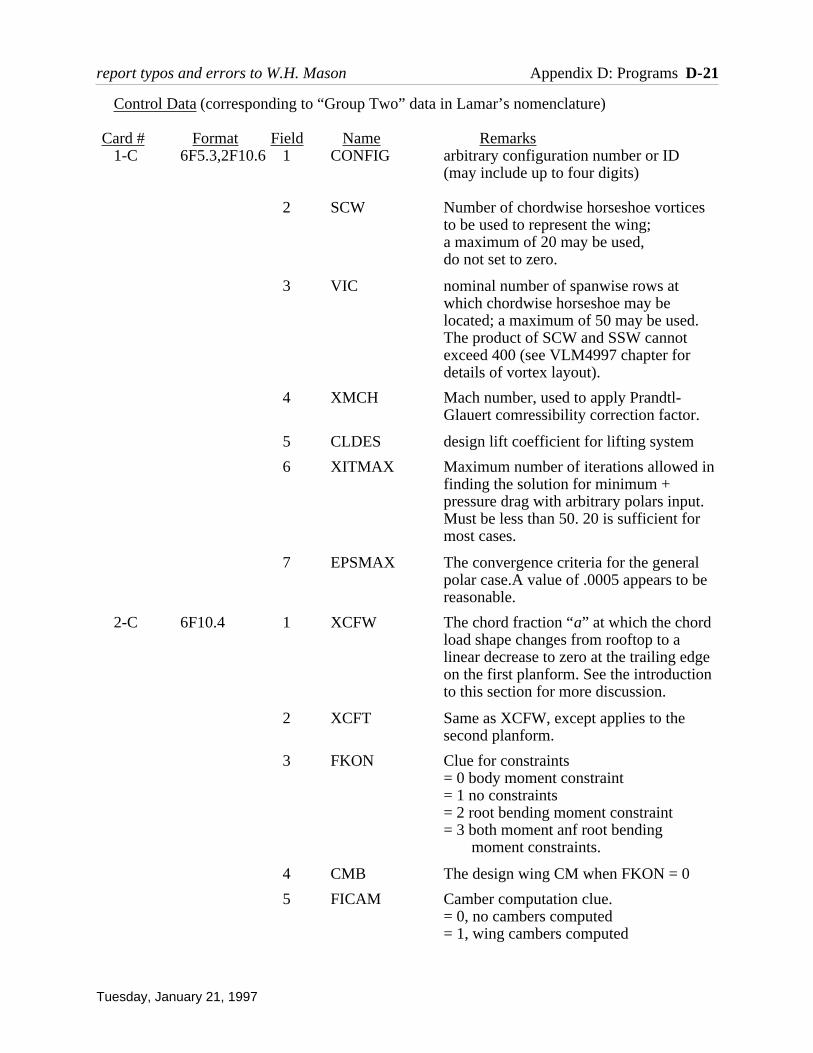
Control Data (corresponding to “Group Two” data in Lamar’s nomenclature)
Card # Format Field Name Remarks1-C 6F5.3,2F10.6 1 CONFIG arbitrary configuration number or ID
(may include up to four digits)
2 SCW Number of chordwise horseshoe vorticesto be used to represent the wing; a maximum of 20 may be used,do not set to zero.
3 VIC nominal number of spanwise rows at which chordwise horseshoe may be
located; a maximum of 50 may be used. The product of SCW and SSW cannot
exceed 400 (see VLM4997 chapter for details of vortex layout).
4 XMCH Mach number, used to apply Prandtl-Glauert comressibility correction factor.
5 CLDES design lift coefficient for lifting system
6 XITMAX Maximum number of iterations allowed in finding the solution for minimum + pressure drag with arbitrary polars input. Must be less than 50. 20 is sufficient for most cases.
7 EPSMAX The convergence criteria for the general polar case.A value of .0005 appears to be reasonable.
2-C 6F10.4 1 XCFW The chord fraction “a” at which the chord load shape changes from rooftop to a
linear decrease to zero at the trailing edge on the first planform. See the introduction to this section for more discussion.
2 XCFT Same as XCFW, except applies to the second planform.
3 FKON Clue for constraints= 0 body moment constraint= 1 no constraints= 2 root bending moment constraint= 3 both moment anf root bending moment constraints.
4 CMB The design wing CM when FKON = 0
5 FICAM Camber computation clue.= 0, no cambers computed= 1, wing cambers computed
report typos and errors to W.H. Mason Appendix D: Programs D-21
Tuesday, January 21, 1997
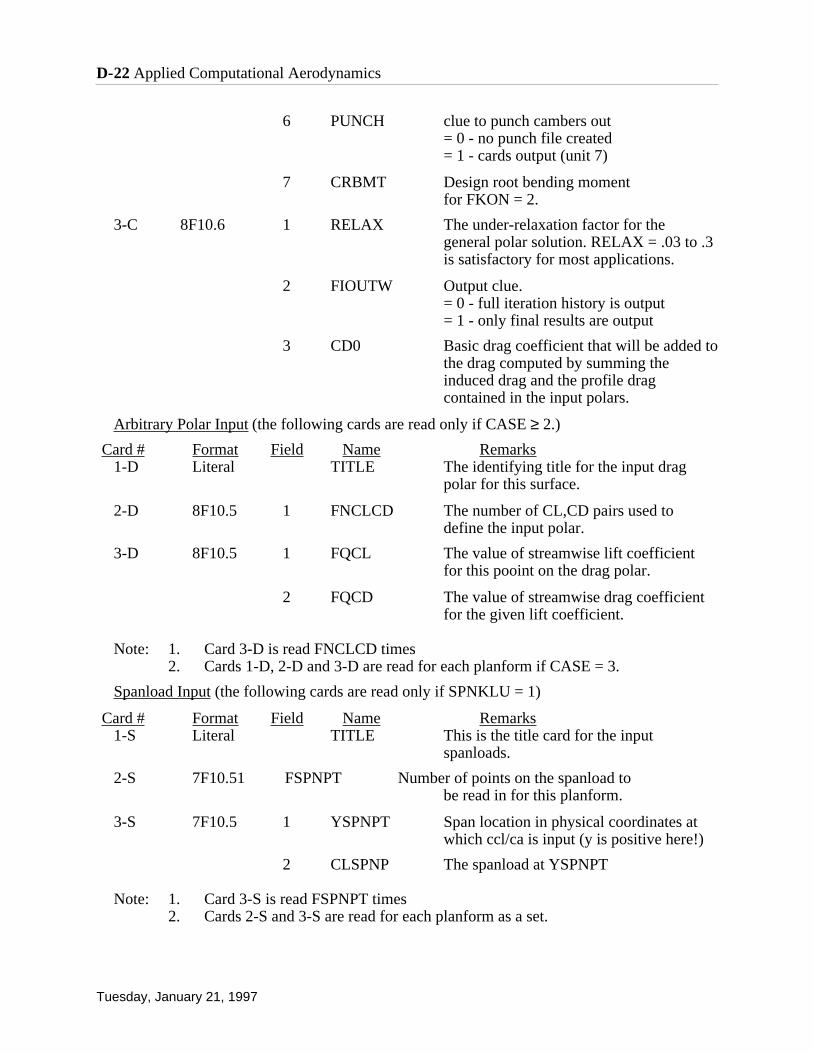
6 PUNCH clue to punch cambers out= 0 - no punch file created= 1 - cards output (unit 7)
7 CRBMT Design root bending momentfor FKON = 2.
3-C 8F10.6 1 RELAX The under-relaxation factor for the general polar solution. RELAX = .03 to .3
is satisfactory for most applications.
2 FIOUTW Output clue.= 0 - full iteration history is output= 1 - only final results are output
3 CD0 Basic drag coefficient that will be added to the drag computed by summing the
induced drag and the profile drag contained in the input polars.
Arbitrary Polar Input (the following cards are read only if CASE ≥ 2.)
Card # Format Field Name Remarks1-D Literal TITLE The identifying title for the input drag polar for this surface.
2-D 8F10.5 1 FNCLCD The number of CL,CD pairs used to define the input polar.
3-D 8F10.5 1 FQCL The value of streamwise lift coefficient for this pooint on the drag polar.
2 FQCD The value of streamwise drag coefficient for the given lift coefficient.
Note: 1. Card 3-D is read FNCLCD times2. Cards 1-D, 2-D and 3-D are read for each planform if CASE = 3.
Spanload Input (the following cards are read only if SPNKLU = 1)
Card # Format Field Name Remarks1-S Literal TITLE This is the title card for the input
spanloads.
2-S 7F10.5 1 FSPNPT Number of points on the spanload to be read in for this planform.
3-S 7F10.5 1 YSPNPT Span location in physical coordinates at which ccl/ca is input (y is positive here!)
2 CLSPNP The spanload at YSPNPT
Note: 1. Card 3-S is read FSPNPT times2. Cards 2-S and 3-S are read for each planform as a set.
D-22 Applied Computational Aerodynamics
Tuesday, January 21, 1997

Sample Input: (note: it is important to put data in proper columns!)
Lamar program sample input - revised forward swept wing 2.000 -8.000 89.50 26640. 1.0 3.0 0.0 5.000 0.0 0.0 -8.8 0.0 0.0 68.95 0.0 0.0 1.0 68.95 -34.0 49.61 -65.30 0.0 1.0 25.64 -65.30 0.0 1.0 22.25 -34.00 22.25 0.00 5.0 0.0 0.0 0.0 0.0 0.0 -25.90 0.0 0.0 1.0 -25.90 -34.0 38.10 -164.0 0.0 1.0 -2.40 -164.0 0.0 1.0-147.90 -20.0-147.90 0.01.0 10.0 20. 0.9 0.90 40.0 0.0006 0.0 0.65 0.0 -0.10 1.0 0.030 1.0 0.0 0.0 0.0 0.0drag polar on canard (conv. sec) 18.0 0.00 0.0000 0.10 0.0000 0.25 0.0002 0.30 0.00078 0.40 0.00175 0.50 0.00315 0.55 0.0040 0.60 0.00535 0.65 0.00685 0.70 0.00880 0.75 0.01125 0.80 0.01485 0.85 0.01975 0.88 0.02400 0.915 0.03600 1.00 0.0880 1.20 0.2680 1.80 0.9880 drag polar22.0 0.000 0.0003 0.200 0.0003 0.300 0.0005 0.400 0.0008 0.500 0.00125 0.600 0.00178 0.700 0.00244 0.800 0.00324 0.900 0.00442 0.950 0.00528 0.970 0.00570 0.990 0.00621 1.000 0.00650 1.020 0.00730 1.040 0.00820 1.060 0.00930 1.080 0.01090 1.100 0.01280 1.125 0.02400 1.130 0.03600 1.200 0.20400
2.000 2.12400
report typos and errors to W.H. Mason Appendix D: Programs D-23
Tuesday, January 21, 1997
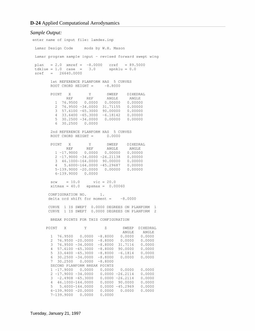
Sample Output: enter name of input file: lamdes.inp
Lamar Design Code mods by W.H. Mason
Lamar program sample input - revised forward swept wing
plan = 2.0 xmref = -8.0000 cref = 89.5000 tdklue = 1.0 case = 3.0 spnklu = 0.0 sref = 26640.0000
1st REFERENCE PLANFORM HAS 5 CURVES ROOT CHORD HEIGHT = -8.8000
POINT X Y SWEEP DIHEDRAL REF REF ANGLE ANGLE 1 76.9500 0.0000 0.00000 0.00000 2 76.9500 -34.0000 31.71155 0.00000 3 57.6100 -65.3000 90.00000 0.00000 4 33.6400 -65.3000 -6.18142 0.00000 5 30.2500 -34.0000 0.00000 0.00000 6 30.2500 0.0000
2nd REFERENCE PLANFORM HAS 5 CURVES ROOT CHORD HEIGHT = 0.0000
POINT X Y SWEEP DIHEDRAL REF REF ANGLE ANGLE 1 -17.9000 0.0000 0.00000 0.00000 2 -17.9000 -34.0000 -26.21138 0.00000 3 46.1000-164.0000 90.00000 0.00000 4 5.6000-164.0000 -45.29687 0.00000 5-139.9000 -20.0000 0.00000 0.00000 6-139.9000 0.0000
scw = 10.0 vic = 20.0 xitmax = 40.0 epsmax = 0.00060
CONFIGURATION NO. 1. delta ord shift for moment = -8.0000
CURVE 1 IS SWEPT 0.0000 DEGREES ON PLANFORM 1 CURVE 1 IS SWEPT 0.0000 DEGREES ON PLANFORM 2
BREAK POINTS FOR THIS CONFIGURATION
POINT X Y Z SWEEP DIHEDRAL ANGLE ANGLE 1 76.9500 0.0000 -8.8000 0.0000 0.0000 2 76.9500 -20.0000 -8.8000 0.0000 0.0000 3 76.9500 -34.0000 -8.8000 31.7116 0.0000 4 57.6100 -65.3000 -8.8000 90.0000 0.0000 5 33.6400 -65.3000 -8.8000 -6.1814 0.0000 6 30.2500 -34.0000 -8.8000 0.0000 0.0000 7 30.2500 0.0000 -8.8000 SECOND PLANFORM BREAK POINTS 1 -17.9000 0.0000 0.0000 0.0000 0.0000 2 -17.9000 -34.0000 0.0000 -26.2114 0.0000 3 -2.4908 -65.3000 0.0000 -26.2114 0.0000 4 46.1000-164.0000 0.0000 90.0000 0.0000 5 5.6000-164.0000 0.0000 -45.2969 0.0000 6-139.9000 -20.0000 0.0000 0.0000 0.0000 7-139.9000 0.0000 0.0000
D-24 Applied Computational Aerodynamics
Tuesday, January 21, 1997

280 HORSESHOE VORTICES USED PLANFORM TOTAL SPANWISE 1 80 8 2 200 20
10. HORSESHOE VORTICES IN EACH CHORDWISE ROW
xcfw = 0.00 xcft = 0.65 fkon = 0.00 ficam = 1.00 punch = 0.00 crbmnt = 0.000 cmb = -.10 iflag = 1
relax = 0.03 fioutw = 1.00 cd0 = 0.0000 firbm = 0.00 yrbm = 0.0000 zrbm = 0.0000
drag polar on canard (conv. sec)
there are 1.0 polars on this surface
18.0 points this polar planform 1
qcl qcd 0.0000 0.0000 0.1000 0.0000 0.2500 0.0002 0.3000 0.0008 0.4000 0.0018 0.5000 0.0032 0.5500 0.0040 0.6000 0.0054 0.6500 0.0069 0.7000 0.0088 0.7500 0.0113 0.8000 0.0148 0.8500 0.0198 0.8800 0.0240 0.9150 0.0360 1.0000 0.0880 1.2000 0.2680 1.8000 0.9880
drag polar
there are 1.0 polars on this surface
22.0 points this polar planform 2
qcl qcd 0.0000 0.0003 0.2000 0.0003 0.3000 0.0005 0.4000 0.0008 0.5000 0.0012 0.6000 0.0018 0.7000 0.0024 0.8000 0.0032 0.9000 0.0044 0.9500 0.0053 0.9700 0.0057 0.9900 0.0062 1.0000 0.0065 1.0200 0.0073 1.0400 0.0082
report typos and errors to W.H. Mason Appendix D: Programs D-25
Tuesday, January 21, 1997

1.0600 0.0093 1.0800 0.0109 1.1000 0.0128 1.1250 0.0240 1.1300 0.0360 1.2000 0.2040 2.0000 2.1240
LM = 70 IL = 71 JM = 72 IM = 73 TSPAN =-164.000 TSPANA = -65.300 BOTL = 164.000 BOL = 65.300 SNN = 1.6400 DELTYB = 3.2800 NMA(KBOT) = 50 KBOT = 2 NMA(KBIT) = 20 KBIT = 1
induced drag cd = 0.06815 pressure drag cdpt = 0.01665
induced drag cd = 0.06818 pressure drag cdpt = 0.01441
induced drag cd = 0.06827 pressure drag cdpt = 0.01255
induced drag cd = 0.06839 pressure drag cdpt = 0.01139
induced drag cd = 0.06850 pressure drag cdpt = 0.01053
induced drag cd = 0.06863 pressure drag cdpt = 0.00976
induced drag cd = 0.06876 pressure drag cdpt = 0.00915
induced drag cd = 0.06885 pressure drag cdpt = 0.00886
induced drag cd = 0.06893 pressure drag cdpt = 0.00868
induced drag cd = 0.06898 pressure drag cdpt = 0.00856
induced drag cd = 0.06902 pressure drag cdpt = 0.00847
induced drag cd = 0.06905 pressure drag cdpt = 0.00841
induced drag cd = 0.06907 pressure drag cdpt = 0.00836
induced drag cd = 0.06909 pressure drag cdpt = 0.00832
induced drag cd = 0.06911 pressure drag cdpt = 0.00829
induced drag cd = 0.06913 pressure drag cdpt = 0.00826
induced drag cd = 0.06915 pressure drag cdpt = 0.00823
induced drag cd = 0.06916 pressure drag cdpt = 0.00821
induced drag cd = 0.06917 pressure drag cdpt = 0.00819
induced drag cd = 0.06918 pressure drag cdpt = 0.00817
induced drag cd = 0.06919 pressure drag cdpt = 0.00816
induced drag cd = 0.06920 pressure drag cdpt = 0.00815
induced drag cd = 0.06921 pressure drag cdpt = 0.00814
induced drag cd = 0.06921 pressure drag cdpt = 0.00813
induced drag cd = 0.06922 pressure drag cdpt = 0.00812
induced drag cd = 0.06923 pressure drag cdpt = 0.00811
D-26 Applied Computational Aerodynamics
Tuesday, January 21, 1997

induced drag cd = 0.06923 pressure drag cdpt = 0.00810
induced drag cd = 0.06924 pressure drag cdpt = 0.00810
induced drag cd = 0.06924 pressure drag cdpt = 0.00809
induced drag cd = 0.06924 pressure drag cdpt = 0.00809
induced drag cd = 0.06925 pressure drag cdpt = 0.00808
pressure drag iteration has converged
k eps cl cdi cdp cdi+cdp 1 28.66362 0.90000 0.06815 0.01665 0.08480 2 0.05789 0.90000 0.06818 0.01441 0.08260 3 0.05278 0.90000 0.06827 0.01255 0.08082 4 0.04274 0.90000 0.06839 0.01139 0.07978 5 0.03408 0.90000 0.06850 0.01053 0.07903 6 0.03155 0.90000 0.06863 0.00976 0.07839 7 0.02773 0.90000 0.06876 0.00915 0.07791 8 0.02043 0.90000 0.06885 0.00886 0.07772 9 0.01549 0.90000 0.06893 0.00868 0.07761 10 0.01218 0.90000 0.06898 0.00856 0.07754 11 0.00994 0.90000 0.06902 0.00847 0.07749 12 0.00847 0.90000 0.06905 0.00841 0.07746 13 0.00724 0.90000 0.06907 0.00836 0.07743 14 0.00616 0.90000 0.06909 0.00832 0.07741 15 0.00519 0.90000 0.06911 0.00829 0.07740 16 0.00442 0.90000 0.06913 0.00826 0.07739 17 0.00371 0.90000 0.06915 0.00823 0.07738 18 0.00310 0.90000 0.06916 0.00821 0.07737 19 0.00263 0.90000 0.06917 0.00819 0.07736 20 0.00221 0.90000 0.06918 0.00817 0.07736 21 0.00183 0.90000 0.06919 0.00816 0.07735 22 0.00154 0.90000 0.06920 0.00815 0.07735 23 0.00131 0.90000 0.06921 0.00814 0.07734 24 0.00112 0.90000 0.06921 0.00813 0.07734 25 0.00095 0.90000 0.06922 0.00812 0.07734 26 0.00084 0.90000 0.06923 0.00811 0.07734 27 0.00076 0.90000 0.06923 0.00810 0.07733 28 0.00069 0.90000 0.06924 0.00810 0.07733 29 0.00064 0.90000 0.06924 0.00809 0.07733 30 0.00061 0.90000 0.06924 0.00809 0.07733 31 0.00057 0.90000 0.06925 0.00808 0.07733
induced + pressure drag was minimized on this run
ref. chord = 89.500 c average = 81.2195 true area = 32771.566 ref. area = 26640.000 b/2 = 164.0000 ref ar = 4.0384 true ar = 3.2828 Mach number = 0.9000
first planform cl = 0.17126 cm = 0.11493 cb = -0.01502 second planform cl = 0.72874 cm = -0.21493 cb = -0.18341
1st planform CL = 0.1713 CDP = 0.0042 CM = 0.1150 CB = -0.0151 2nd planform CL = 0.7292 CDP = 0.0038 CM = -0.2149 CB = 0.0000
no root bending moment constraint
CL DES = 0.90000 CL COMPUTED = 0.9005 CM = -0.0999 CD I = 0.06925 E = 0.9230 CDPRESS = 0.00804 CDTOTAL = 0.07729
report typos and errors to W.H. Mason Appendix D: Programs D-27
Tuesday, January 21, 1997
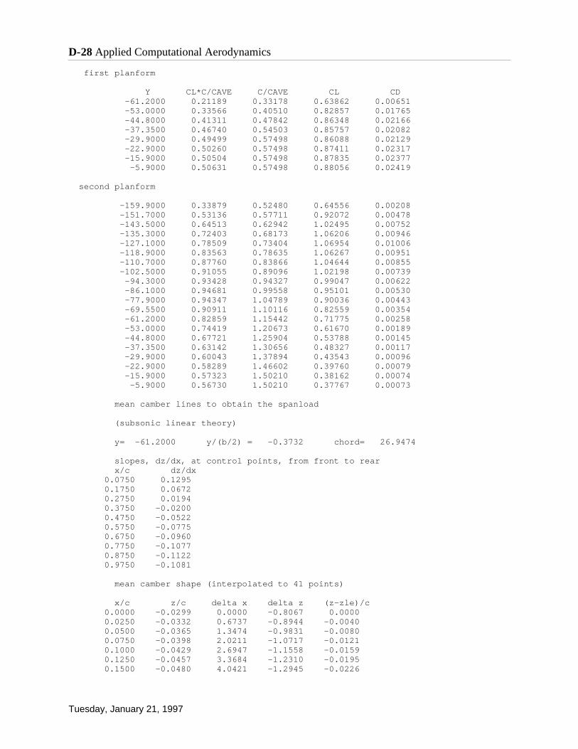
first planform
Y CL*C/CAVE C/CAVE CL CD -61.2000 0.21189 0.33178 0.63862 0.00651 -53.0000 0.33566 0.40510 0.82857 0.01765 -44.8000 0.41311 0.47842 0.86348 0.02166 -37.3500 0.46740 0.54503 0.85757 0.02082 -29.9000 0.49499 0.57498 0.86088 0.02129 -22.9000 0.50260 0.57498 0.87411 0.02317 -15.9000 0.50504 0.57498 0.87835 0.02377 -5.9000 0.50631 0.57498 0.88056 0.02419
second planform
-159.9000 0.33879 0.52480 0.64556 0.00208 -151.7000 0.53136 0.57711 0.92072 0.00478 -143.5000 0.64513 0.62942 1.02495 0.00752 -135.3000 0.72403 0.68173 1.06206 0.00946 -127.1000 0.78509 0.73404 1.06954 0.01006 -118.9000 0.83563 0.78635 1.06267 0.00951 -110.7000 0.87760 0.83866 1.04644 0.00855 -102.5000 0.91055 0.89096 1.02198 0.00739 -94.3000 0.93428 0.94327 0.99047 0.00622 -86.1000 0.94681 0.99558 0.95101 0.00530 -77.9000 0.94347 1.04789 0.90036 0.00443 -69.5500 0.90911 1.10116 0.82559 0.00354 -61.2000 0.82859 1.15442 0.71775 0.00258 -53.0000 0.74419 1.20673 0.61670 0.00189 -44.8000 0.67721 1.25904 0.53788 0.00145 -37.3500 0.63142 1.30656 0.48327 0.00117 -29.9000 0.60043 1.37894 0.43543 0.00096 -22.9000 0.58289 1.46602 0.39760 0.00079 -15.9000 0.57323 1.50210 0.38162 0.00074 -5.9000 0.56730 1.50210 0.37767 0.00073
mean camber lines to obtain the spanload
(subsonic linear theory)
y= -61.2000 y/(b/2) = -0.3732 chord= 26.9474
slopes, dz/dx, at control points, from front to rear x/c dz/dx 0.0750 0.1295 0.1750 0.0672 0.2750 0.0194 0.3750 -0.0200 0.4750 -0.0522 0.5750 -0.0775 0.6750 -0.0960 0.7750 -0.1077 0.8750 -0.1122 0.9750 -0.1081
mean camber shape (interpolated to 41 points)
x/c z/c delta x delta z (z-zle)/c 0.0000 -0.0299 0.0000 -0.8067 0.0000 0.0250 -0.0332 0.6737 -0.8944 -0.0040 0.0500 -0.0365 1.3474 -0.9831 -0.0080 0.0750 -0.0398 2.0211 -1.0717 -0.0121 0.1000 -0.0429 2.6947 -1.1558 -0.0159 0.1250 -0.0457 3.3684 -1.2310 -0.0195 0.1500 -0.0480 4.0421 -1.2945 -0.0226
D-28 Applied Computational Aerodynamics
Tuesday, January 21, 1997

0.1750 -0.0499 4.7158 -1.3456 -0.0252 0.2000 -0.0514 5.3895 -1.3857 -0.0275 0.2250 -0.0526 6.0632 -1.4166 -0.0294 0.2500 -0.0534 6.7368 -1.4399 -0.0310 0.2750 -0.0540 7.4105 -1.4563 -0.0323 0.3000 -0.0544 8.0842 -1.4660 -0.0334 0.3250 -0.0545 8.7579 -1.4689 -0.0343 0.3500 -0.0544 9.4316 -1.4651 -0.0349 0.3750 -0.0540 10.1053 -1.4548 -0.0353 0.4000 -0.0534 10.7790 -1.4383 -0.0354 0.4250 -0.0525 11.4526 -1.4160 -0.0353 0.4500 -0.0515 12.1263 -1.3884 -0.0351 0.4750 -0.0503 12.8000 -1.3556 -0.0346 0.5000 -0.0489 13.4737 -1.3181 -0.0339 0.5250 -0.0474 14.1474 -1.2760 -0.0331 0.5500 -0.0456 14.8211 -1.2297 -0.0322 0.5750 -0.0438 15.4948 -1.1794 -0.0310 0.6000 -0.0418 16.1684 -1.1254 -0.0298 0.6250 -0.0396 16.8421 -1.0679 -0.0284 0.6500 -0.0374 17.5158 -1.0074 -0.0269 0.6750 -0.0350 18.1895 -0.9440 -0.0253 0.7000 -0.0326 18.8632 -0.8781 -0.0236 0.7250 -0.0301 19.5369 -0.8100 -0.0218 0.7500 -0.0275 20.2105 -0.7400 -0.0200 0.7750 -0.0248 20.8842 -0.6682 -0.0181 0.8000 -0.0221 21.5579 -0.5950 -0.0161 0.8250 -0.0193 22.2316 -0.5205 -0.0141 0.8500 -0.0165 22.9053 -0.4452 -0.0120 0.8750 -0.0137 23.5790 -0.3696 -0.0100 0.9000 -0.0109 24.2527 -0.2942 -0.0079 0.9250 -0.0081 24.9263 -0.2196 -0.0059 0.9500 -0.0054 25.6000 -0.1458 -0.0039 0.9750 -0.0027 26.2737 -0.0728 -0.0020 1.0000 0.0000 26.9474 0.0000 0.0000
y= -53.0000 y/(b/2) = -0.3232 chord= 32.9022
slopes, dz/dx, at control points, from front to rear x/c dz/dx 0.0750 0.0783 0.1750 -0.0034 0.2750 -0.0572 0.3750 -0.0982 0.4750 -0.1306 0.5750 -0.1557 0.6750 -0.1740 0.7750 -0.1854 0.8750 -0.1898 0.9750 -0.1845
mean camber shape (interpolated to 41 points)
x/c z/c delta x delta z (z-zle)/c 0.0000 -0.1036 0.0000 -3.4093 0.0000 0.0250 -0.1056 0.8226 -3.4745 -0.0046 0.0500 -0.1076 1.6451 -3.5414 -0.0092 0.0750 -0.1097 2.4677 -3.6080 -0.0138 0.1000 -0.1115 3.2902 -3.6674 -0.0182 0.1250 -0.1128 4.1128 -3.7122 -0.0222 0.1500 -0.1136 4.9353 -3.7381 -0.0255 0.1750 -0.1138 5.7579 -3.7444 -0.0283 0.2000 -0.1135 6.5804 -3.7339 -0.0306 0.2250 -0.1128 7.4030 -3.7102 -0.0325 0.2500 -0.1117 8.2256 -3.6761 -0.0340
report typos and errors to W.H. Mason Appendix D: Programs D-29
Tuesday, January 21, 1997
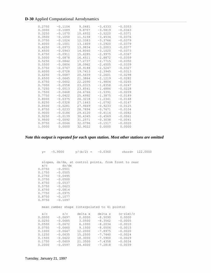
0.2750 -0.1104 9.0481 -3.6333 -0.0353 0.3000 -0.1089 9.8707 -3.5819 -0.0363 0.3250 -0.1070 10.6932 -3.5220 -0.0371 0.3500 -0.1050 11.5158 -3.4534 -0.0376 0.3750 -0.1026 12.3383 -3.3766 -0.0379 0.4000 -0.1001 13.1609 -3.2920 -0.0379 0.4250 -0.0973 13.9834 -3.2003 -0.0377 0.4500 -0.0943 14.8060 -3.1020 -0.0373 0.4750 -0.0911 15.6285 -2.9975 -0.0367 0.5000 -0.0878 16.4511 -2.8872 -0.0359 0.5250 -0.0842 17.2737 -2.7715 -0.0350 0.5500 -0.0806 18.0962 -2.6505 -0.0339 0.5750 -0.0767 18.9188 -2.5247 -0.0327 0.6000 -0.0728 19.7413 -2.3945 -0.0313 0.6250 -0.0687 20.5639 -2.2601 -0.0298 0.6500 -0.0645 21.3864 -2.1219 -0.0282 0.6750 -0.0602 22.2090 -1.9804 -0.0265 0.7000 -0.0558 23.0315 -1.8358 -0.0247 0.7250 -0.0513 23.8541 -1.6886 -0.0228 0.7500 -0.0468 24.6766 -1.5391 -0.0209 0.7750 -0.0422 25.4992 -1.3875 -0.0189 0.8000 -0.0375 26.3218 -1.2341 -0.0168 0.8250 -0.0328 27.1443 -1.0792 -0.0147 0.8500 -0.0281 27.9669 -0.9233 -0.0125 0.8750 -0.0233 28.7894 -0.7671 -0.0104 0.9000 -0.0186 29.6120 -0.6114 -0.0082 0.9250 -0.0139 30.4345 -0.4569 -0.0061 0.9500 -0.0092 31.2571 -0.3038 -0.0041 0.9750 -0.0046 32.0796 -0.1517 -0.0020 1.0000 0.0000 32.9022 0.0000 0.0000
Note this output is repeated for each span station. Most other stations are omitted
y= -5.9000 y/(b/2) = -0.0360 chord= 122.0000
slopes, dz/dx, at control points, from front to rear x/c dz/dx 0.0750 -0.0501 0.1750 -0.0505 0.2750 -0.0495 0.3750 -0.0500 0.4750 -0.0537 0.5750 -0.0623 0.6750 -0.0814 0.7750 -0.0975 0.8750 -0.1077 0.9750 -0.1097
mean camber shape (interpolated to 41 points)
x/c z/c delta x delta z (z-zle)/c 0.0000 -0.0697 0.0000 -8.5090 0.0000 0.0250 -0.0685 3.0500 -8.3562 -0.0005 0.0500 -0.0672 6.1000 -8.2034 -0.0010 0.0750 -0.0660 9.1500 -8.0506 -0.0015 0.1000 -0.0647 12.2000 -7.8975 -0.0020 0.1250 -0.0635 15.2500 -7.7440 -0.0024 0.1500 -0.0622 18.3000 -7.5900 -0.0029 0.1750 -0.0609 21.3500 -7.4358 -0.0034 0.2000 -0.0597 24.4000 -7.2818 -0.0039
D-30 Applied Computational Aerodynamics
Tuesday, January 21, 1997
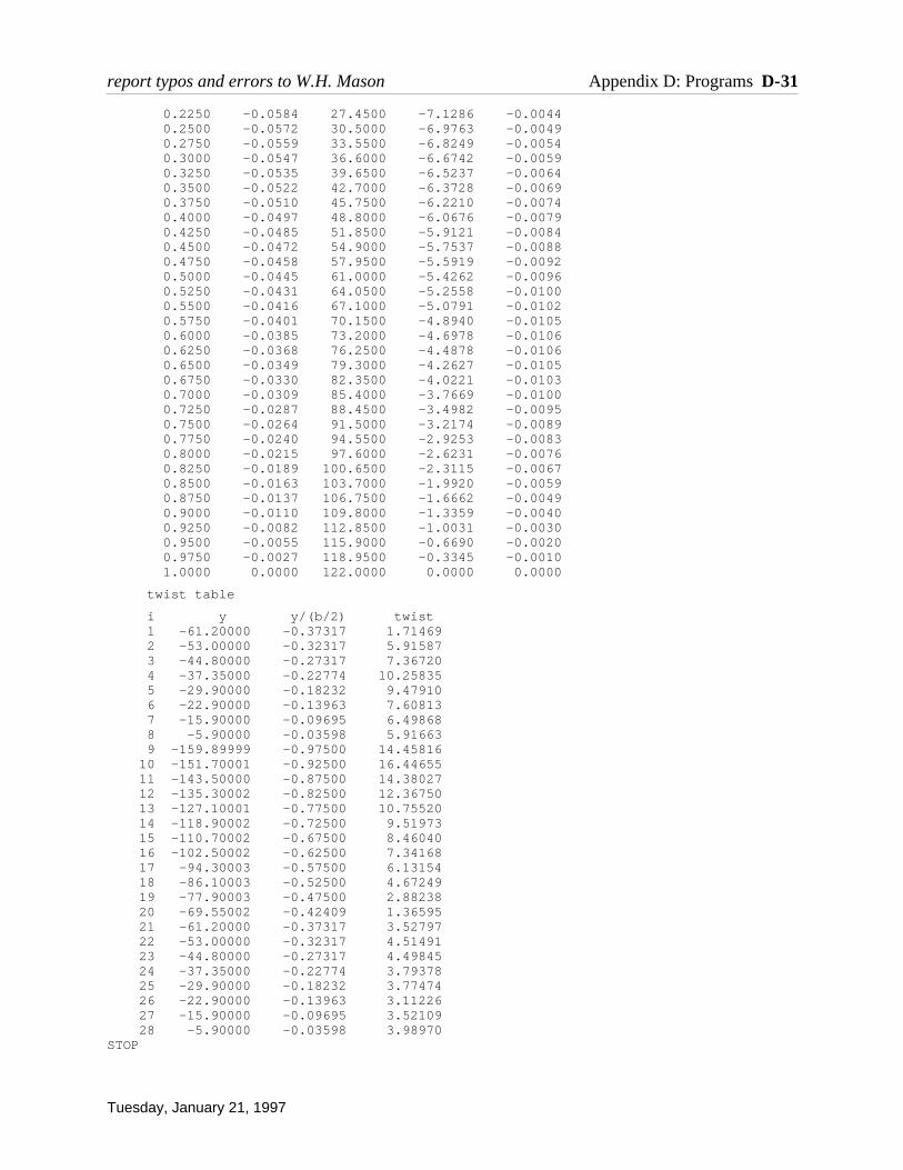
0.2250 -0.0584 27.4500 -7.1286 -0.0044 0.2500 -0.0572 30.5000 -6.9763 -0.0049 0.2750 -0.0559 33.5500 -6.8249 -0.0054 0.3000 -0.0547 36.6000 -6.6742 -0.0059 0.3250 -0.0535 39.6500 -6.5237 -0.0064 0.3500 -0.0522 42.7000 -6.3728 -0.0069 0.3750 -0.0510 45.7500 -6.2210 -0.0074 0.4000 -0.0497 48.8000 -6.0676 -0.0079 0.4250 -0.0485 51.8500 -5.9121 -0.0084 0.4500 -0.0472 54.9000 -5.7537 -0.0088 0.4750 -0.0458 57.9500 -5.5919 -0.0092 0.5000 -0.0445 61.0000 -5.4262 -0.0096 0.5250 -0.0431 64.0500 -5.2558 -0.0100 0.5500 -0.0416 67.1000 -5.0791 -0.0102 0.5750 -0.0401 70.1500 -4.8940 -0.0105 0.6000 -0.0385 73.2000 -4.6978 -0.0106 0.6250 -0.0368 76.2500 -4.4878 -0.0106 0.6500 -0.0349 79.3000 -4.2627 -0.0105 0.6750 -0.0330 82.3500 -4.0221 -0.0103 0.7000 -0.0309 85.4000 -3.7669 -0.0100 0.7250 -0.0287 88.4500 -3.4982 -0.0095 0.7500 -0.0264 91.5000 -3.2174 -0.0089 0.7750 -0.0240 94.5500 -2.9253 -0.0083 0.8000 -0.0215 97.6000 -2.6231 -0.0076 0.8250 -0.0189 100.6500 -2.3115 -0.0067 0.8500 -0.0163 103.7000 -1.9920 -0.0059 0.8750 -0.0137 106.7500 -1.6662 -0.0049 0.9000 -0.0110 109.8000 -1.3359 -0.0040 0.9250 -0.0082 112.8500 -1.0031 -0.0030 0.9500 -0.0055 115.9000 -0.6690 -0.0020 0.9750 -0.0027 118.9500 -0.3345 -0.0010 1.0000 0.0000 122.0000 0.0000 0.0000
twist table
i y y/(b/2) twist 1 -61.20000 -0.37317 1.71469 2 -53.00000 -0.32317 5.91587 3 -44.80000 -0.27317 7.36720 4 -37.35000 -0.22774 10.25835 5 -29.90000 -0.18232 9.47910 6 -22.90000 -0.13963 7.60813 7 -15.90000 -0.09695 6.49868 8 -5.90000 -0.03598 5.91663 9 -159.89999 -0.97500 14.45816 10 -151.70001 -0.92500 16.44655 11 -143.50000 -0.87500 14.38027 12 -135.30002 -0.82500 12.36750 13 -127.10001 -0.77500 10.75520 14 -118.90002 -0.72500 9.51973 15 -110.70002 -0.67500 8.46040 16 -102.50002 -0.62500 7.34168 17 -94.30003 -0.57500 6.13154 18 -86.10003 -0.52500 4.67249 19 -77.90003 -0.47500 2.88238 20 -69.55002 -0.42409 1.36595 21 -61.20000 -0.37317 3.52797 22 -53.00000 -0.32317 4.51491 23 -44.80000 -0.27317 4.49845 24 -37.35000 -0.22774 3.79378 25 -29.90000 -0.18232 3.77474 26 -22.90000 -0.13963 3.11226 27 -15.90000 -0.09695 3.52109 28 -5.90000 -0.03598 3.98970STOP
report typos and errors to W.H. Mason Appendix D: Programs D-31
Tuesday, January 21, 1997
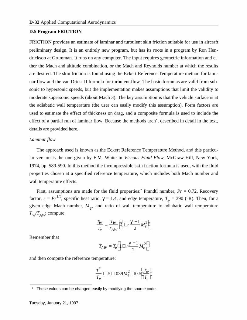
D.5 Program FRICTION
FRICTION provides an estimate of laminar and turbulent skin friction suitable for use in aircraft
preliminary design. It is an entirely new program, but has its roots in a program by Ron Hen-
drickson at Grumman. It runs on any computer. The input requires geometric information and ei-
ther the Mach and altitude combination, or the Mach and Reynolds number at which the results
are desired. The skin friction is found using the Eckert Reference Temperature method for lami-
nar flow and the van Driest II formula for turbulent flow. The basic formulas are valid from sub-
sonic to hypersonic speeds, but the implementation makes assumptions that limit the validity to
moderate supersonic speeds (about Mach 3). The key assumption is that the vehicle surface is at
the adiabatic wall temperature (the user can easily modify this assumption). Form factors are
used to estimate the effect of thickness on drag, and a composite formula is used to include the
effect of a partial run of laminar flow. Because the methods aren’t described in detail in the text,
details are provided here.
Laminar flow
The approach used is known as the Eckert Reference Temperature Method, and this particu-
lar version is the one given by F.M. White in Viscous Fluid Flow, McGraw-Hill, New York,
1974, pp. 589-590. In this method the incompressible skin friction formula is used, with the fluid
properties chosen at a specified reference temperature, which includes both Mach number and
wall temperature effects.
First, assumptions are made for the fluid properties:* Prandtl number, Pr = 0.72, Recovery
factor, r = Pr1/2, specific heat ratio, γ = 1.4, and edge temperature, Te = 390 (°R). Then, for a
given edge Mach number, Me, and ratio of wall temperature to adiabatic wall temperature
TW/TAW; compute:
.
Remember that
and then compute the reference temperature:
* These values can be changed easily by modifying the source code.
D-32 Applied Computational Aerodynamics
Tuesday, January 21, 1997
T*
Te≅ .5 + .039Me
2 + 0.5Tw
Te
TAW = Te 1+ rγ −1
2Me
2
TW
Te=
TW
TAW1 + r
γ −1
2Me
2

The Chapman-Rubesin constant based on the reference temperature and Sutherland’s viscosity
law is then computed from:
where K = 200°R for air.
Finally, the local friction coefficient (τw/q) is found from the standard Blasius formula, with
C* added,
and
which comes from
Recall that CF accounts for one side of the plate only, so that if both sides are required for a drag
estimate, then the skin friction coeficient, CD, is twice CF because the reference area is based on
one side only, i.e., Sref ≈ 1/2 Swet.
Note that the results are not sensitive to the value of edge temperature for low Mach numbers,
and therefore, an exact specification of Te is not required. This method is implemented in sub-
routine lamcf.
Turbulent flow
For turbulent flow the so-called van Driest II Method is employed. This method was selected
based on the recommendation of E.J. Hopkins and M. Inouye, contained in “An Evaluation of
Theories for Predicting Turbulent Skin Friction and Heat Transfer on Flat Plates at Supersonic
and Hypersonic Mach Numbers,” AIAA J., Vol. 9, No. 6, June 1971, pp. 993-1003. The particu-
lar algorithm is taken from NASA TN D-6945, “Charts for Predicting Turbulent Skin Friction
From the Van Driest Method (II),” also by E.J. Hopkins, and dated October 1972.
Again, assumptions are made for the fluid properties: turbulent flow recovery factor, r = .88,
specific heat ratio, γ = 1.4, and edge temperature, Te = 222 (°K). Then, for a given edge Mach
number, Me, and ratio of wall temperature to adiabatic wall temperature TW/TAW the calculation
is started by computing the following constants:
report typos and errors to W.H. Mason Appendix D: Programs D-33
Tuesday, January 21, 1997
CF =F
qx=
1
xC f ( ′ x )d ′ x
′ x =0
′ x = x
∫
CF = 2C f
C f =.664 C*
Rex
C* =T *
Te
1/ 21 + K / Te
T* / Te + K / Te
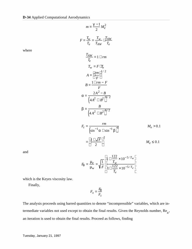
where
and
which is the Keyes viscosity law.
Finally,
The analysis proceeds using barred quantities to denote “incompressible” variables, which are in-
termediate variables not used except to obtain the final results. Given the Reynolds number, Rex,
an iteration is used to obtain the final results. Proceed as follows, finding
D-34 Applied Computational Aerodynamics
Tuesday, January 21, 1997
Fx =FθFc
Fθ =µe
µw=
1
F
1 +122
Tw×10−5/ Tw
1+ 122Te
×10−5/ Te
Fc =rm
sin−1α + sin−1 β( )2 Me > 0.1
= 1 + F2
2
Me ≤ 0.1
β =B
4 A2 + B2( )1/ 2
α =2A2 − B
4A2 + B2( )1/ 2
B =1+ rm − F
F
A =rm
F
1/ 2
Tw = F ⋅ Te
TAW
Te= 1 + rm
F =Tw
Te=
Tw
TAW⋅TAW
Te
m =γ −1
2Me
2

now solve
for .
Use as an initial guess
.
Then, Newton’s method is applied to the problem:
which becomes for this equation:
Once this iteration is completed, and is known,
Note that this value applies to one side of a plate only, so it must be doubled if the friction on
both sides is desired to account for the proper reference areas. Here again, the results are not sen-
sitive to the value of edge temperature for low Mach numbers, and the default value should be
adequate for most cases. This formula is implemented in routine turbcf.
Composite formula
When the flow is laminar and then transitions to turbulent, an estimate of the skin friction is
available from a composite of the laminar and turbulent skin friction formulas using Schlicting’s
formula (see T. Cebeci and P. Bradshaw, Momentum Transfer in Boundary Layers, McGraw-
Hill, New York, 1977, pp. 187). Given the transition position, xc/L and ReL, compute
and compute the laminar skin friction based on Rec and the turbulent skin friction twice, based
on both Reynolds numbers and then find the value that includes both laminar and turbulent flow
from:
report typos and errors to W.H. Mason Appendix D: Programs D-35
Tuesday, January 21, 1997
Rec =xc
L
ReL
CF =C FFc
C F
C Fi+1 = C F
i 1 +.242 − C F
i log Rex C Fi( ){ }
.121 + C Fi / ln10{ }
f C F( ) = 0 ⇒ C Fi+1 = C F
i −f
′ f
C F0 =
.074
R e x.20
C F
.242
C F= log R ex C F( )
R ex = Fx Re x

Several formulas are available, are all roughly equivalent, and have been evaluated extensively
for incompressible flow. They are only approximate for compressible flow.
Form factors
To include the effects of thickness, it has been found that the skin friction formulas should be
adjusted through the use of form factors. Two different factors are used in this code. For wing-
like shapes,
where t/c is the thickness ratio of of particular component. For bodies,
where d/l is the ratio of diameter to length. This is the reciprocal of the fineness ratio.
Program Operation:
Running the program, you will be prompted for the name of an input data set, the maximum
length is 15 characters. The output is sent to the screen, but can be sent to a file by changing the
value of IWRIT to something other than 6 in the main program. The sample data case on the disk
is F15.FRICTION.
INPUT
Card Field Columns Variable Description 1 1 1-60 Title Card
2 1 1-10 SREF Full Scale reference Area
2 11-20 SCALE 1./SCALE, i.e. 1/10 scale is input as 10.
3 21-30 FNCOMP number of component cards to be read in (15 max).
4 31-41 FINMD input mode: = 0.0, input Mach and altitude = 1.0, input Mach and Reynolds No. per unit length
3 1 1-16 COMP(i) Component Name
2 21-30 SWET(I) Wetted Area (i.e., top and bottom sides of the wing,and both left and right sides, the total area that is exposed to the air)
D-36 Applied Computational Aerodynamics
Tuesday, January 21, 1997
FF = 1.0 +1.5d
l
1.5
+ 50d
l
3
FF = 1.0 +1.8t
c
+ 50
t
c
4
CF = CFTURB(ReL ) −
xc
L
CFTURB
(Rec) − CFLAMRec( )[ ]
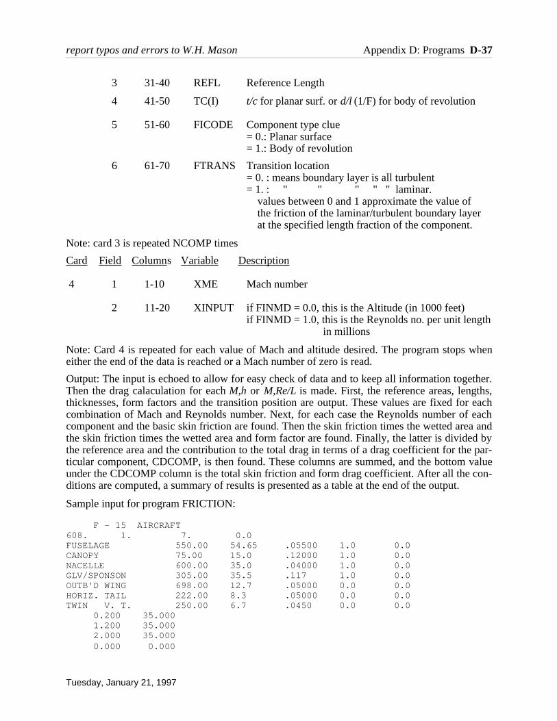
3 31-40 REFL Reference Length
4 41-50 TC(I) t/c for planar surf. or d/l (1/F) for body of revolution
5 51-60 FICODE Component type clue= 0.: Planar surface= 1.: Body of revolution
6 61-70 FTRANS Transition location= 0. : means boundary layer is all turbulent = 1. : " " " " " laminar. values between 0 and 1 approximate the value of the friction of the laminar/turbulent boundary layer
at the specified length fraction of the component.
Note: card 3 is repeated NCOMP times
Card Field Columns Variable Description
4 1 1-10 XME Mach number
2 11-20 XINPUT if FINMD = 0.0, this is the Altitude (in 1000 feet)if FINMD = 1.0, this is the Reynolds no. per unit length in millions
Note: Card 4 is repeated for each value of Mach and altitude desired. The program stops wheneither the end of the data is reached or a Mach number of zero is read.
Output: The input is echoed to allow for easy check of data and to keep all information together.Then the drag calaculation for each M,h or M,Re/L is made. First, the reference areas, lengths,thicknesses, form factors and the transition position are output. These values are fixed for eachcombination of Mach and Reynolds number. Next, for each case the Reynolds number of eachcomponent and the basic skin friction are found. Then the skin friction times the wetted area andthe skin friction times the wetted area and form factor are found. Finally, the latter is divided bythe reference area and the contribution to the total drag in terms of a drag coefficient for the par-ticular component, CDCOMP, is then found. These columns are summed, and the bottom valueunder the CDCOMP column is the total skin friction and form drag coefficient. After all the con-ditions are computed, a summary of results is presented as a table at the end of the output.
Sample input for program FRICTION:
F - 15 AIRCRAFT608. 1. 7. 0.0FUSELAGE 550.00 54.65 .05500 1.0 0.0CANOPY 75.00 15.0 .12000 1.0 0.0NACELLE 600.00 35.0 .04000 1.0 0.0GLV/SPONSON 305.00 35.5 .117 1.0 0.0OUTB'D WING 698.00 12.7 .05000 0.0 0.0HORIZ. TAIL 222.00 8.3 .05000 0.0 0.0TWIN V. T. 250.00 6.7 .0450 0.0 0.0 0.200 35.000 1.200 35.000 2.000 35.000 0.000 0.000
report typos and errors to W.H. Mason Appendix D: Programs D-37
Tuesday, January 21, 1997
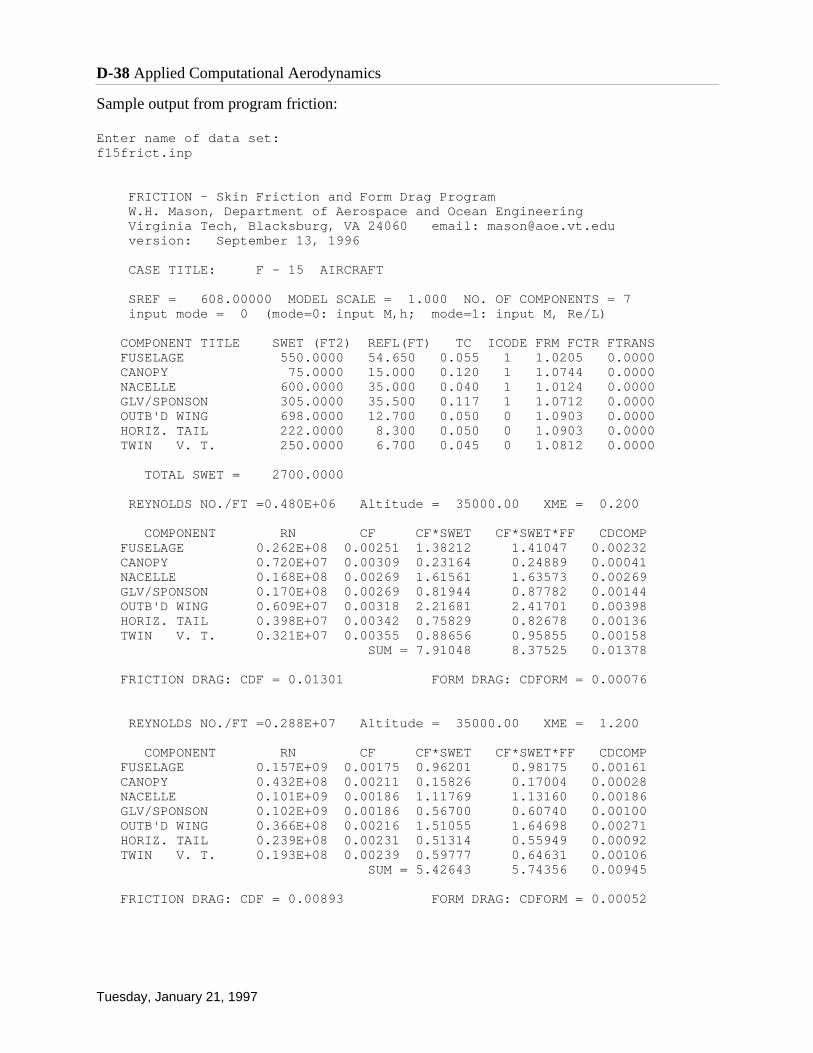
Sample output from program friction:
Enter name of data set:f15frict.inp
FRICTION - Skin Friction and Form Drag Program W.H. Mason, Department of Aerospace and Ocean Engineering Virginia Tech, Blacksburg, VA 24060 email: [email protected] version: September 13, 1996
CASE TITLE: F - 15 AIRCRAFT
SREF = 608.00000 MODEL SCALE = 1.000 NO. OF COMPONENTS = 7 input mode = 0 (mode=0: input M,h; mode=1: input M, Re/L)
COMPONENT TITLE SWET (FT2) REFL(FT) TC ICODE FRM FCTR FTRANS FUSELAGE 550.0000 54.650 0.055 1 1.0205 0.0000 CANOPY 75.0000 15.000 0.120 1 1.0744 0.0000 NACELLE 600.0000 35.000 0.040 1 1.0124 0.0000 GLV/SPONSON 305.0000 35.500 0.117 1 1.0712 0.0000 OUTB'D WING 698.0000 12.700 0.050 0 1.0903 0.0000 HORIZ. TAIL 222.0000 8.300 0.050 0 1.0903 0.0000 TWIN V. T. 250.0000 6.700 0.045 0 1.0812 0.0000
TOTAL SWET = 2700.0000
REYNOLDS NO./FT =0.480E+06 Altitude = 35000.00 XME = 0.200
COMPONENT RN CF CF*SWET CF*SWET*FF CDCOMP FUSELAGE 0.262E+08 0.00251 1.38212 1.41047 0.00232 CANOPY 0.720E+07 0.00309 0.23164 0.24889 0.00041 NACELLE 0.168E+08 0.00269 1.61561 1.63573 0.00269 GLV/SPONSON 0.170E+08 0.00269 0.81944 0.87782 0.00144 OUTB'D WING 0.609E+07 0.00318 2.21681 2.41701 0.00398 HORIZ. TAIL 0.398E+07 0.00342 0.75829 0.82678 0.00136 TWIN V. T. 0.321E+07 0.00355 0.88656 0.95855 0.00158 SUM = 7.91048 8.37525 0.01378
FRICTION DRAG: CDF = 0.01301 FORM DRAG: CDFORM = 0.00076
REYNOLDS NO./FT =0.288E+07 Altitude = 35000.00 XME = 1.200
COMPONENT RN CF CF*SWET CF*SWET*FF CDCOMP FUSELAGE 0.157E+09 0.00175 0.96201 0.98175 0.00161 CANOPY 0.432E+08 0.00211 0.15826 0.17004 0.00028 NACELLE 0.101E+09 0.00186 1.11769 1.13160 0.00186 GLV/SPONSON 0.102E+09 0.00186 0.56700 0.60740 0.00100 OUTB'D WING 0.366E+08 0.00216 1.51055 1.64698 0.00271 HORIZ. TAIL 0.239E+08 0.00231 0.51314 0.55949 0.00092 TWIN V. T. 0.193E+08 0.00239 0.59777 0.64631 0.00106 SUM = 5.42643 5.74356 0.00945
FRICTION DRAG: CDF = 0.00893 FORM DRAG: CDFORM = 0.00052
D-38 Applied Computational Aerodynamics
Tuesday, January 21, 1997
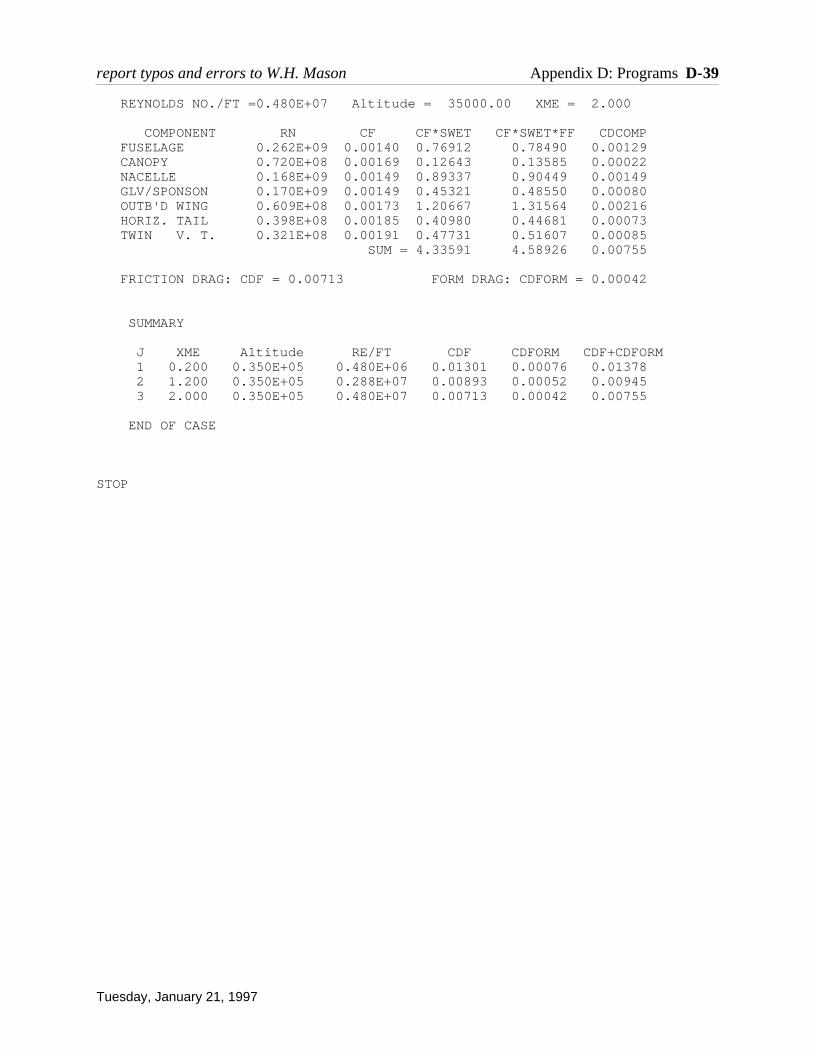
REYNOLDS NO./FT =0.480E+07 Altitude = 35000.00 XME = 2.000
COMPONENT RN CF CF*SWET CF*SWET*FF CDCOMP FUSELAGE 0.262E+09 0.00140 0.76912 0.78490 0.00129 CANOPY 0.720E+08 0.00169 0.12643 0.13585 0.00022 NACELLE 0.168E+09 0.00149 0.89337 0.90449 0.00149 GLV/SPONSON 0.170E+09 0.00149 0.45321 0.48550 0.00080 OUTB'D WING 0.609E+08 0.00173 1.20667 1.31564 0.00216 HORIZ. TAIL 0.398E+08 0.00185 0.40980 0.44681 0.00073 TWIN V. T. 0.321E+08 0.00191 0.47731 0.51607 0.00085 SUM = 4.33591 4.58926 0.00755
FRICTION DRAG: CDF = 0.00713 FORM DRAG: CDFORM = 0.00042
SUMMARY
J XME Altitude RE/FT CDF CDFORM CDF+CDFORM 1 0.200 0.350E+05 0.480E+06 0.01301 0.00076 0.01378 2 1.200 0.350E+05 0.288E+07 0.00893 0.00052 0.00945 3 2.000 0.350E+05 0.480E+07 0.00713 0.00042 0.00755
END OF CASE
STOP
report typos and errors to W.H. Mason Appendix D: Programs D-39
Tuesday, January 21, 1997

D.6 VLMpc
This manual describes the input for the pc version of John Lamar’s vortex lattice program.This program is identical to the program given in reference 2. An advanced version described inreference 4 is also available. The input data sets differ slightly between the two versions.
The code is called VLMpcv2.f on the disk, and has been modified for WATFOR. Thismeans that the output field length is limited to eighty columns. In WATFOR you may also needto invoke the NOCHECK option to prevent the program from halting because of undefined vari-ables. The code is provided with two OPEN statements near the beginning of the main program:
OPEN(5,file=infile, status=old)OPEN(6,file=outfil, status=new)
such that the input data is defined on the file infile, and the output is placed in file outfil. Theuser is prompted for the names of these files at the start of execution. Users should customize thecode to fit their preferences. The disk also contains a sample input file, YF23.IN, and a sampleoutput file, YF23.OUT.
The theory is described in references 1, 2 and 3, and the user’s manual provided here is basi-cally the instructions from references 1 and 2, with minor corrections and clarifications. Refer-ence 4 describes the advanced version, VLM4.997.
References:
1. Margason, R.J., and Lamar, J.E., “Vortex-Lattice FORTRAN Program for Estimating Subson-ic Aerodynamic Characteristics of Complex Planforms,” NASA TN D-6142, Feb., 1971.
2. Lamar, J.E., and Gloss, B. B. “Subsonic Aerodynamic Characteristics of Interacting LiftingSurfaces with Separated Flow around Sharp Edges Predicted by a Vortex-Lattice Method,”NASA TN D-7921, Sept., 1975.
3. Lamar, J.E., and Frink, N.T., “Experimental and Analytic Study of the Longitudinal Aerody-namic Characteristics of Analytically and Empirically Designed Strake-Wing Configurationsat Subcritical Speeds, “ NASA TP-1803, June 1981.
4. Lamar, J.E., and Herbert, H.E., “Production Version of the Extended NASA-Langley VortexLattice FORTRAN Computer Code,” - Vol. I - User’s Guide, NASA TM 83303, April 1982.
VLMpc User’s Guide- (from references 1, 2, and 4)
This manual contains the output details for the pc version of the NASA-Langley VortexLattice Computer Program described in reference 2. The NASA - Langley Vortex LatticeFORTRAN Program (VLMpc) is designed to estimate the subsonic aerodynamic characteristicsof up to two complex planforms. The concepts embodied in this program are mostly detailed inreferences 1 and 2.
MODELING THE CONFIGURATION
The configuration can be modeled with up to two planforms, all of which must extend to theplane of symmetry (Y = 0.0). The fuselage is represented by its planar projection; experience todate indicates that this produces acceptable global forces and moments for most wing-body-tailconfigurations.
Winglets can be modeled, but the dihedral angle must be less than 90.0 degrees and greaterthan -90.0 degrees. Both upper (positive dihedral) and lower (negative dihedral) winglets can beaccounted for in this code. The program uses as its solution surface the chord plane which may
D-40 Applied Computational Aerodynamics
Friday, November 17, 1995

be inclined due to dihedral. Moreover, the only out of "X-Y plane" displacement specificallyallowed for is dihedral. Local camber and twist is assumed to be small and can be representedby its slope projection to the local solution surface. The wind and body axes are assumed to becoincidental in the code.
RUNNING THE PROGRAM
INPUT DATA SETUP
The input data to VLM is organized into two distinct groups - group 1 defines the referenceplanform(s), and group 2 defines the details for the particular solution. An example input fol-lows the description of the input and output. The individual details of the items in the deck layoutare given in the following sections.
GROUP 1 DATA
This group of data defines the planform(s) projected into the X-Y plane, with all thecoordinates being given for the left half of the configuration (negative y values!). The axissystem is shown in Figure 1. The Y = 0 intercept coincides with the plane of symmetry and ispositive to the right of this plane. The X = 0 intercept is taken to occur along the symmetryplane of the configuration; X is positive pointing into the wind.
Important tips for modeling configurations:
Good results require that a few common rules of thumb be used in selecting the planformbreak points. The number of line segments should be minimized. Breakpoints should line upstreamwise on front and rear portions of each planform, and should line up between plan-forms. Streamwise tips should be used, and small spanwise distances should be avoided bymaking edges streamwise if they are actually very highly swept.
report typos and errors to W.H. Mason Appendix D: Programs D-41
Friday, November 17, 1995
Figure 1. Definition of axis system for VLMpc.
X
Y
Planform 1
Planform 2
1
2
34
5612
3
4
56 7
Note: X opposite standardaerodynamic convention
It is important to note that each planform can only go out to a maximum y value once, andthen return to the centerline. The program assumes that each planform is actuually a wing.Most numerical input for the group 1 data uses an 8F10.6 format . The input is as follows:
0. (Cols. 1-80) Title Card
1. (Cols. 1-10) PLAN - Number of planforms for this configuration; PLAN can assumevalues of 1.0, or 2.0.
2. (Cols.11-20) TOTAL - Number of sets of group 2 data specified for this configuration. 3. (Cols.21-30) CREF - Reference chord of the configuration. This chord is used only to
nondimensionalize the pitching-moment terms and must be greater than zero. 4. (Cols.31-40) SREF - Reference area; this is used only to nondimensionalize the comput-
ed output data such as lift and pitching moment and must always be greater than zero.
5. (Col. 41-50) CG - Center of gravity location with respect to the origin of the coordinatesystem. All moment computations are referenced to this location.
The data required to define the planform(s) is provided in the next set of group 1 cards asfollows (the number of line segments is equal to the number of points minus one):
1. (Cols.1-10) AAN - Number of line segments used to define the left half of the planform(does not include the innermost streamwise). A maximum of 24 line segments may beused per planform, and each planform must extend to the plane of symmetry. ANN is thenumber of defining point minus one.
2. (Cols.11-20) XS - X location of the pivot; use 0.0 for a fixed planform.
3. (Cols.21-30) YS - Y location of the pivot; use 0.0 for a fixed planform.
4. (Cols.31-40) RTCDHT - Vertical distance of the particular planform being read in withrespect to the reference planform root chord height; use 0. for the reference planform.
The rest of this set of data describes the breakpoints used to define the AAN line segments onthis planform. The format is 4F9.4. There are (AAN+1) breakpoints and all data subsequentlydescribed are required on all except the last card of this set; the last card uses only the first twovariables in the following list:
1. (Cols.1-9) XREG(I) - X location of the ith breakpoint. The first breakpoint is located atthe most inboard location of the leading edge for the left-hand side of this planform. Theother breakpoints are numbered around the planform perimeter in increasing order foreach intersection of lines in a counterclockwise direction.
2. (Cols.10-18) YREG(I) - Y location of the ith breakpoint. Once the absolute value of Ystarts to decrease, it cannot be increased.
3. (Cols.19-27) DIH(I) - Dihedral angle (degrees) in the Y-Z plane of the line frombreakpoint of i to i+1, positive upward. Note that along a streamwise line, the dihedralangle is not defined, so use 0.0. for these lines. Note the sign of the dihedral angle is thesame along the leading and trailing edges.
4. (Cols.28-36) AMCD - The move code; this number indicates whether the line s is on themovable panel of a variable-sweep wing. Use 1.0 for a fixed line (defaults to 1.0 if notset), or 2.0 for a movable line.
D-42 Applied Computational Aerodynamics
Friday, November 17, 1995
GROUP 2 DATA
There are four sections of group 2 data. Each section may be required or optional, dependingon the previous input, and each may have one or more input cards (lines of input). Each sectionis described individually. Care must be taken to make sure the data is in the proper column.
Section one data (always required).
[1 Card - Format (8F5.2, F10.4,F5.1,F10.4,F5.1)]
1. (Cols.1-5) CONFIG - An arbitrary configuration designation of up to 4 digits.
2. (Cols.6-10) SCW - The number of chordwise horseshoe vortices to be used at aspanwise station for each planform. The maximum value for this variable is 20. Ifvarying values of chordwise horseshoe vortices are desired due to either multipleplanforms or large discontinuities in chord across the span, the user can input a value of0. that will cause the program to expect user-supplied data at this point in the inputstream. The data are in the form of a table that contains the number of chordwisehorseshoe vortices from the tip to root, and is called TBLSCW(I). This SCW=0. optioncan only be used for planforms without dihedral and for coplanar configurations.
3. (Cols.11-15) VIC - The nominal number of spanwise stations at which chordwisehorseshoe vortices will be located. This variable must not cause more than 50 spanwisestations to be used by the program in describing the left half of the configuration. Inaddition, the product of the stations spanwise and SCW cannot exceed 200. If SCW is0., then the sum of the values in TBLSCW(I) cannot exceed 200. The use of variableVIC is discussed in references 1 and 2. VIC should always be greater than, or equal to,10. so that the near-field drag or vortex flow forces on cambered configurations can beproperly computed.
4. (Cols.16-20) MACH - Mach number; use a value other than 0.0 only if the Prandtl-Glauert compressibility correction factor is to be applied. The value used should beless than that of the critical Mach number.
5. (Cols.21-25) CLDES - Desired lift coefficient, CL,d. The number specified here isused to obtain the span load distribution at a particular lift coefficient. If the drag polaris required over a CL range from -0.1 to 1.0, use CLDES = 11.
6. (Cols.26-30) PTEST - Clp indicator; if the damping-in-roll parameter is desired, use 1.0
for this quantity. Except for the Delta Cp and Clp, all other aerodynamic data will beomitted. Use a 0. if Clp is not required. The definition is the standard one, as in Etkin,with units of radians per second:
7. (Cols.31-35) QTEST -CLq and Cmq indicator; if these stability derivatives are desired,use a 1.0 for this quantity. Except for Delta Cp, CLq, and Cmq, all other aerodynamicdata will be omitted. It should be noted that both PTEST and QTEST cannot be setequal to 1. simultaneously for a particular configuration. Use 0. if CLq and Cmq are notrequired. The definition is the standard one, as in Etkin:
report typos and errors to W.H. Mason Appendix D: Programs D-43
Friday, November 17, 1995
Clp=
∂Cl
∂pb
2U∞

, .
8. (Cols. 36-40) TWIST(1) - Twist code for the first planform. If this planform has notwist and/or camber, use a value of 0.; otherwise, specify a value of 1.
9. (Cols.41-50) SA(1) - Variable sweep angle for the first planform. Specify the leadingedge sweep-angle (in degrees) for the first movable line adjacent to the fixed portion ofthe planform. For a fixed planform, this quantity may be omitted.
10. (Cols.51-55) TWIST(2) - same, for the second planform.
11. (Cols.56-65) SA(2) - same, for the second planform.
12. (Cols.66-70) ATPCOD - Set to 0., it will cause only linear aerodynamic results to beprinted out. Set to 1., this will cause the program to print out the contributions to thelift, drag and moment from the separated flow around the leading/side edges.
Section two data is required when ATPCOD=1.* This section sets up the limits of integrationused in the computations of the wing leading-edge and side-edge suction values. Normally theselimits would be the wing root and the wing tip. However, other values could be used. Note: ifsection four data is used, this data may come after section four data - experiment if you try to usethis combination.
[1 Card - Format (4F10.6)] Card 1:
1. (Cols.1-10) YINNER(1) - Represents the Y inner for the first planform.
2. (Cols.11-20) YOUTER(1) - Represents the Y outer for the first planform.
3. (Cols.21-30) YINNER(2) - Represents the Y inner for the second planform.
4 (Cols. 31-40), YOUTER(2) - Represents the Y outer for the second planform.
Section three data is required when SCW=0. This section determines the number of spanstations for each planform, and the number of chordwise control points along each span station.This option is rarely used.
[Multiple card sets per planform - Format (F5.1,n(/16F5.1))]
Card 1:
(Cols.1-5) STA - Number of spanwise stations of horseshoe vortices on the left halfof the planform. This variable sets the number of TBLSCW values read in for thatplanform.
* Watch out about the order of input if both twist and vortex lift are used. Some students havereported problems with this. Actually, this is a somewhat rare calculation. Both twist andvortex lift should be run separately to the user’s satisfaction before they are run together.
D-44 Applied Computational Aerodynamics
Friday, November 17, 1995
CLq=
∂CL
∂qcref
2U∞
Cmq=
∂Cm
∂qcref
2U∞
Cards 2-n:
(Cols. 1-5,6-10,etc) TBLSCW(I) - Number of horseshoe vortices at each spanwisestation beginning at the station nearest the tip of the planform and proceedingtoward the station nearest the root.
These sets of STA and TBLSCW(I) cards are repeated for each planform. The sum of all theSTA values cannot exceed 100.
Section four data is required for any planform having a nonzero value for TWIST(I). Thissection determines the mean camber line slopes or angles of attack across the planform. Be care-ful here. Experience has shown that students find the proper input of this data to be very tricky.
[Multiple cards per planform - Format (8F10.6,n(8F10.6))]
(Cols.1-10,11-20,etc.) ALP - Local streamwise angles of attack, eg. camber or flapdeflection, in radians. These are the values at the control point for each horseshoe vortexon the planform when the innermost streamwise edge of the reference planform has anangle of attack of 0. degrees. The volume of this data will usually require several inputcards. For the first value on the first card, use the local angle of attack for the horseshoevortex nearest the first planform leading edge at the tip; for the second value, use theangle of attack for the horseshoe vortex immediately behind in the chordwise direction.Continue in the same manner for the rest of the horseshoe vortices at the tip. Begin a newcard for the next inboard station and input the data in the same chordwise manner.Repeat for all successive inboard spanwise stations on that planform. For each planformwith twist/camber, start the data on a new card and specify the data from the tip andproceed chordwise and then inboard, as detailed above.
OUTPUT DATA
The printed results of this computer program appear in two parts: geometry data andaerodynamic data.
GEOMETRY DATA
The geometry data are described in the order that they are found on the printout.
The first group of the data describes the basic configuration: it states the numbers of linesused to describe each planform, the root chord height, pivot position, and then lists thebreakpoints, sweep and dihedral angles, and move codes. These data are basically a listing ofinput data except that the sweep angle is computed from the input.
The second group of data describes the particular configuration for which the aerodynamicdata are being computed. Included are the configuration designation, sweep position, a listing ofthe breakpoints of the planform (X,Y, and Z), the sweep and dihedral angles, and the movecodes. The data are listed primarily for variable-sweep wings to provide a definition of theplanform where the outer panel sweep is different from that of the reference planform. The num-ber of horseshoe vortices are then described. In this code a maximum of 200 vortices can beused.
The third group of data presents a detailed description of the horseshoe vortices used torepresent the configuration. These data are listed in two sets of five columns each describing oneelemental panel of the configuration (see Figure 2) in the same order that the twist and/or camberangles of attack are to be provided.
report typos and errors to W.H. Mason Appendix D: Programs D-45
Friday, November 17, 1995
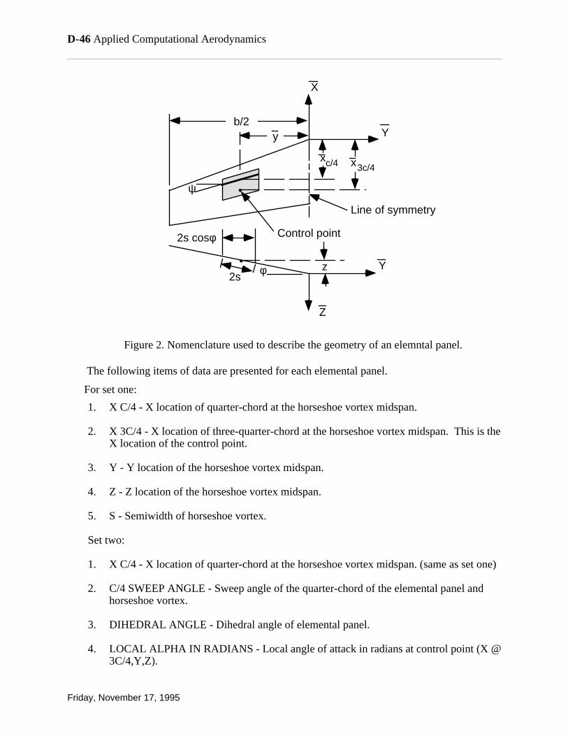
The following items of data are presented for each elemental panel.
For set one:
1. X C/4 - X location of quarter-chord at the horseshoe vortex midspan.
2. X 3C/4 - X location of three-quarter-chord at the horseshoe vortex midspan. This is theX location of the control point.
3. Y - Y location of the horseshoe vortex midspan.
4. Z - Z location of the horseshoe vortex midspan.
5. S - Semiwidth of horseshoe vortex.
Set two:
1. X C/4 - X location of quarter-chord at the horseshoe vortex midspan. (same as set one)
2. C/4 SWEEP ANGLE - Sweep angle of the quarter-chord of the elemental panel andhorseshoe vortex.
3. DIHEDRAL ANGLE - Dihedral angle of elemental panel.
4. LOCAL ALPHA IN RADIANS - Local angle of attack in radians at control point (X @3C/4,Y,Z).
D-46 Applied Computational Aerodynamics
Friday, November 17, 1995
Figure 2. Nomenclature used to describe the geometry of an elemntal panel.
b/2
X
Y
Y
Z
•
y
Control point
•
Line of symmetry
2sz
2s cosφ
xc/4 x3c/4
φ
ψ
5. DELTA CP AT DESIRED CL - ∆Cp or Net Cp normal to the surface at dihedral foreach elemental panel when the total lift is CL,d. This is located across the panel as an
average. It corresponds to the incremental lift associated with the bound vortex strengthof the particular panel:
The fourth group of data presents the following geometric results:
1. REF.CHORD - Reference chord of the configuration.
2. C AVERAGE - Average chord, cav, true configuration area divided by true span.
3. TRUE AREA - True area computed from the configuration listed in second group ofgeometry data.
4. REFERENCE AREA - User input reference area.
5. B/2 - Maximum semispan of all planforms listed in second group of geometry data.
6. REF. AR - Reference aspect ratio computed from the reference planform area and truespan.
7. TRUE AR - True aspect ratio computed from the true planform area and true span.
8. MACH NUMBER - Mach number.
AERODYNAMIC DATA
If PTEST = 1. or QTEST = 1. on the configuration card, then either Clp or CLq and Cmq are
computed and printed, followed by program termination. Otherwise, the aerodynamic data aredescribed by at least two groups of results. The first is always present, but the second dependson what is requested on the configuration card. The following items of the first group of data aregiven in the order that they are found on the printout. Note that CL ALPHA, CL(TWIST),CM/CL, CMO, CDI/CL**2 are based on the specified reference dimensions. Many of the itemsthat follow are for the complete configuration.
1. DESIRED CL - Desired lift coefficient, CL, d, specified in Input Data forcomplete configuration.
2. COMPUTED ALPHA - Angle of attack at which the desired lift is developed:CL, d/(CL ALPHA) + ALPHA at CL=O.
3. CL(WB) - That portion of desired lift coefficient developed by the planform withthe maximum span when multiple planforms are specified. When one planform isspecified, this is the desired lift coefficient. (If two planforms have the samespan, and this value is equal to the maximum, the planform used here is the latterone read in).
4. CDI AT CL(WB) - Induced drag coefficient for lift coefficient in the previousitem. When two or more planforms are specified, this is the induced dragcoefficient of only the planform with the maximum span. This result is based onthe far-field solution.
5. CDI/(CL(WB)**2) - Induced drag parameter computed from the two previousitems.
report typos and errors to W.H. Mason Appendix D: Programs D-47
Friday, November 17, 1995
∆Cp × ∆c = ∆Li , where ∆Li = ρU∞Γi

6. 1/(PI*AR REF) - Induced drag parameter for an elliptic load distribution based onreference aspect ratio.
7. CL ALPHA - Lift-curve slope per radian, and per degree.
8. CL(TWIST) - Lift coefficient due to twist and/or camber at zero angle of attack(CL,tc).
9. ALPHA AT CL=O - Angle of attack at zero lift in degrees; nonzero only whentwist and/or camber is specified.
10. Y CP - Spanwise distance in fraction of semispan from root chord to center ofpressure on the left wing panel.
11. CM/CL - Longitudinal stability parameter based on a moment center about thereference point. This is the negative of the static margin:
and the value of can be found from . 12. CMO - Pitching-moment coefficient at CL=O.
For each spanwise station, the following data are presented; from the left tip towards theroot:
1. 2Y/B - Location of midpoint of each spanwise station in fraction of wingsemispan.
The next two columns of data describe the additional (or angle of attack) wing loading at a liftcoefficient of 1. (based on the total lift achieved and the true configuration area). The thirdcolumn is the chord ratio result, and the other columns detail specific kinds of span loadings andlocal centers of pressure for the configuration.
2. SL COEF - span-load coefficient, clc/CLcav.
3. CL RATIO - Ratio of local lift to total lift, cl/CL.
4. C RATIO - Ratio of local chord to average chord, c/cav.
5. LOAD DUE TO TWIST - Distribution of span-load coefficient due to twist andcamber at 0° angle of attack for the configuration.
6. ADD. LOAD AT CL= - Distribution of additional span-load coefficient re-quired to produce zero lift when combined with lift due to twist and camber.This distribution is computed at CL,tc.
7. BASIC LOAD AT CL=0 - Basic span-load-coefficient distribution at zero liftcoefficient. These data are the difference of the previous two columns of data.
8. SPAN LOAD AT DESIRED CL - Distribution of the combination of the basicspan-load and additional span-load coefficients at the desired CL.
9. AT CL DES - X LOCATION OF LOCAL CENT PR - The X location of thelocal center of pressure for the resulting span load at CL,d as a function of 2Y/b.
D-48 Applied Computational Aerodynamics
Friday, November 17, 1995
Cmα =∂Cm
∂CL
∂CL
∂α
Cmα
CM / CLLamar =∂Cm
∂CL
The other options available as group two aerodynamic data are accessed based on the values ofCLDES and ATPCOD. For instance, with CLDES=11., and ATPCOD=0.0, the program willproduce a drag polar, CDI at CL(WB) versus CL(WB), based on the linear aerodynamics in themiddle of the first part of group one aerodynamic data. This, and other combinations, are givenin the table below, along with their purposes:
Next, the induced drag, leading-edge thrust, and suction coefficient characteristics at eachspanwise station are computed from a near-field solution for the total loading at CL,d andpresented.
1. 2y/b - the spanwise location for these results
2. L.E. SWEEP ANGLE - Leading-edge sweep angle in degrees.
3. CDII C/2B - Nondimensional section induced-drag-coefficient term.
4. CT C/2B - Nondimensional section leading-edge thrust-coefficient term.
5. CS C/2B - Nondimensional section leading-edge suction in coefficient term.
Next, the total coefficients are given:
CDII/CL**2 - Total drag coefficient over (CL,d)**2.
CT - Total leading-edge thrust coefficient.
CS - Total leading-edge suction coefficient.
Additional printout is produced for vortex flows. In particular, Kp and Kv values, andrespective centroids in both chordwise and spanwise directions, and the associated limits ofintegration for the leading- edge and side-edge values of Kv. (The item entitled "Sum of thepositive side edge contributions" which appears here on the printout is indicative of thecontribution to the side-edge forces for that particular planform which were oppositely-signed tothose that contributed in a manner to increase Kv,se. The value of Kv,se does contain these posi-tive contributions provided the sweep angle is positive. They should not be, and therefore arenot added in for the planform with a swept forward leading edge). Furthermore, aerodynamicperformance values for each planform and for the entire configuration will be listed over anangle of attack range by the use of the Polhamus Suction Analogy. The headings are explainedbelow: See the references for detailed explanations of these terms.
KP KpKVLE Kv,leKV SE Kv,seALPHA αCN CN,totCLP CL,pCLVLE CL,vleCLVSE Kv,se |sinα| |sinα| cos αCMP pitching-moment coefficient due to CL,pCMVLE pitching-moment coefficient due to CL,vleCMVSE pitching-moment coefficient due to CL,vseCM total pitching momentCD CL,tot x tanαCL**2/(PI*AR) (CL,tot)2 /(Pi*(Aspect Ratio))
report typos and errors to W.H. Mason Appendix D: Programs D-49
Friday, November 17, 1995

SAMPLE INPUT, - as developed by Bob Narducci to investigate the YF-23.
YF-23 Flaps Down2. 1. 26.8917 950.0 0.06.0 0. 0. 0. 37.80 0.0 0.0 1. 22.73 -4.35 0. 1. 14.69 -4.35 0. 1. 00.11 -21.75 0. 1.-03.24 -21.75 0. 1.-14.96 -7.86 0. 1.-14.96 0.8. 0. 0. 0.-14.96 0. 0. 1.-14.96 -7.86 43. 1.-22.00 -16.90 0. 1.-24.51 -16.90 43. 1.-29.50 -10.71 43. 1.-27.02 -7.86 0. 1.-28.36 -6.86 0. 1.-25.68 -3.85 0. 1.-29.20 0.23. 6. 13. .30 .53 0. 0. 0. 0. 1. 0. 0..1745 .1745 .1745 .1745 .1745 .1745.1745 .1745 .1745 .1745 .1745 .1745.1745 .1745 .1745 .1745 .1745 .1745.1745 .1745 .1745 .1745 .1745 .1745.1745 .1745 .1745 .1745 .1745 .1745.1745 .1745 .1745 .1745 .1745 .1745.1745 .1745 .1745 .1745 .1745 .1745.0000 .0000 .0000 .0000 .0000 .0000.0000 .0000 .0000 .0000 .0000 .0000.0000 .0000 .0000 .0000 .0000 .0000.0000 .0000 .0000 .0000 .0000 .0000.0000 .0000 .0000 .0000 .0000 .0000.0000 .0000 .0000 .0000 .0000 .0000
SAMPLE OUTPUT: The output is lengthy, but included here to help students check their codes.
This is what shows up on the screen:
enter name of data set: yf23.inenter name of output file: yf23out.manual
all output is routed to disk file computing may take quite some time
STOP
D-50 Applied Computational Aerodynamics
Friday, November 17, 1995

The output file yf23out.manual is:
vortex lattice aerodynamic computation program nasa-lrc no. a2794 by j.e. lamar and b.b. gloss
modified for watfor77 with 72 column output
YF-23 Flaps Down
geometry data
first reference planform has 6 curves
center of gravity = 0.00000 root chord height = 0.00000 variable sweep pivot position x(s) = 0.00000 y(s) = 0.00000
break points for the reference planform
point x y sweep dihedral move ref ref angle angle code
1 37.80000 0.00000 73.89906 0.00000 1 2 22.73000 -4.35000 90.00000 0.00000 1 3 14.69000 -4.35000 39.96069 0.00000 1 4 0.11000 -21.75000 90.00000 0.00000 1 5 -3.24000 -21.75000 -40.15675 0.00000 1 6 -14.96000 -7.86000 0.00000 0.00000 1 7 -14.96000 0.00000
second reference planform has 8 curves
center of gravity = 0.00000 root chord height = 0.00000 variable sweep pivot position x(s) = 0.00000 y(s) = 0.00000
break points for the reference planform
point x y sweep dihedral move ref ref angle angle code
1 -14.96000 0.00000 0.00000 0.00000 1 2 -14.96000 -7.86000 37.91007 43.00000 1 3 -22.00000 -16.90000 90.00000 0.00000 1 4 -24.51000 -16.90000 -38.87364 43.00000 1 5 -29.50000 -10.71000 41.02898 43.00000 1 6 -27.02000 -7.86000 -53.26718 0.00000 1 7 -28.36000 -6.86000 41.68077 0.00000 1 8 -25.68000 -3.85000 -42.43623 0.00000 1 9 -29.20000 0.000001
configuration no. 23.
curve 1 is swept 73.89906 degrees on planform 1
curve 1 is swept 0.00000 degrees on planform 2
report typos and errors to W.H. Mason Appendix D: Programs D-51
Friday, November 17, 1995
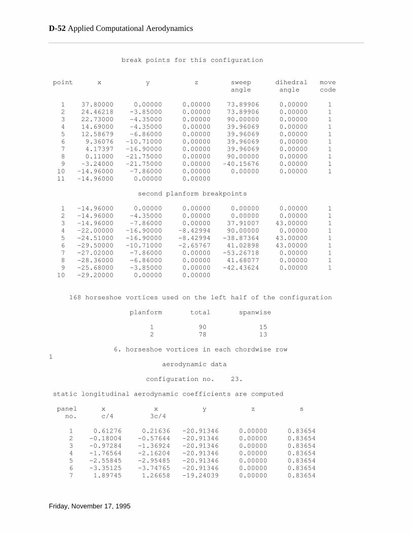
break points for this configuration
point x y z sweep dihedral move angle angle code
1 37.80000 0.00000 0.00000 73.89906 0.00000 1 2 24.46218 -3.85000 0.00000 73.89906 0.00000 1 3 22.73000 -4.35000 0.00000 90.00000 0.00000 1 4 14.69000 -4.35000 0.00000 39.96069 0.00000 1 5 12.58679 -6.86000 0.00000 39.96069 0.00000 1 6 9.36076 -10.71000 0.00000 39.96069 0.00000 1 7 4.17397 -16.90000 0.00000 39.96069 0.00000 1 8 0.11000 -21.75000 0.00000 90.00000 0.00000 1 9 -3.24000 -21.75000 0.00000 -40.15676 0.00000 1 10 -14.96000 -7.86000 0.00000 0.00000 0.00000 1 11 -14.96000 0.00000 0.00000
second planform breakpoints
1 -14.96000 0.00000 0.00000 0.00000 0.00000 1 2 -14.96000 -4.35000 0.00000 0.00000 0.00000 1 3 -14.96000 -7.86000 0.00000 37.91007 43.00000 1 4 -22.00000 -16.90000 -8.42994 90.00000 0.00000 1 5 -24.51000 -16.90000 -8.42994 -38.87364 43.00000 1 6 -29.50000 -10.71000 -2.65767 41.02898 43.00000 1 7 -27.02000 -7.86000 0.00000 -53.26718 0.00000 1 8 -28.36000 -6.86000 0.00000 41.68077 0.00000 1 9 -25.68000 -3.85000 0.00000 -42.43624 0.00000 1 10 -29.20000 0.00000 0.00000
168 horseshoe vortices used on the left half of the configuration
planform total spanwise
1 90 15 2 78 13
6. horseshoe vortices in each chordwise row1 aerodynamic data
configuration no. 23.
static longitudinal aerodynamic coefficients are computed
panel x x y z s no. c/4 3c/4
1 0.61276 0.21636 -20.91346 0.00000 0.83654 2 -0.18004 -0.57644 -20.91346 0.00000 0.83654 3 -0.97284 -1.36924 -20.91346 0.00000 0.83654 4 -1.76564 -2.16204 -20.91346 0.00000 0.83654 5 -2.55845 -2.95485 -20.91346 0.00000 0.83654 6 -3.35125 -3.74765 -20.91346 0.00000 0.83654 7 1.89745 1.26658 -19.24039 0.00000 0.83654
D-52 Applied Computational Aerodynamics
Friday, November 17, 1995

8 0.63571 0.00484 -19.24039 0.00000 0.83654 9 -0.62603 -1.25690 -19.24039 0.00000 0.83654 10 -1.88776 -2.51863 -19.24039 0.00000 0.83654 11 -3.14950 -3.78037 -19.24039 0.00000 0.83654 12 -4.41124 -5.04211 -19.24039 0.00000 0.83654 13 3.11717 2.26369 -17.65192 0.00000 0.75192 14 1.41021 0.55673 -17.65192 0.00000 0.75192 15 -0.29675 -1.15023 -17.65192 0.00000 0.75192 16 -2.00371 -2.85719 -17.65192 0.00000 0.75192 17 -3.71067 -4.56415 -17.65192 0.00000 0.75192 18 -5.41763 -6.27110 -17.65192 0.00000 0.75192 19 4.33688 3.26079 -16.06346 0.00000 0.83654 20 2.18470 1.10861 -16.06346 0.00000 0.83654 21 0.03253 -1.04356 -16.06346 0.00000 0.83654 22 -2.11965 -3.19574 -16.06346 0.00000 0.83654 23 -4.27183 -5.34792 -16.06346 0.00000 0.83654 24 -6.42401 -7.50010 -16.06346 0.00000 0.83654 25 5.62157 4.31101 -14.39038 0.00000 0.83654 26 3.00046 1.68990 -14.39038 0.00000 0.83654 27 0.37934 -0.93122 -14.39038 0.00000 0.83654 28 -2.24177 -3.55233 -14.39038 0.00000 0.83654 29 -4.86289 -6.17345 -14.39038 0.00000 0.83654 30 -7.48401 -8.79456 -14.39038 0.00000 0.83654 31 6.90626 5.36123 -12.71731 0.00000 0.83654 32 3.81621 2.27118 -12.71731 0.00000 0.83654 33 0.72616 -0.81887 -12.71731 0.00000 0.83654 34 -2.36390 -3.90892 -12.71731 0.00000 0.83654 35 -5.45395 -6.99897 -12.71731 0.00000 0.83654 36 -8.54400 -10.08903 -12.71731 0.00000 0.83654 37 7.99810 6.25380 -11.29539 0.00000 0.58538 38 4.50950 2.76521 -11.29539 0.00000 0.58538 39 1.02091 -0.72339 -11.29539 0.00000 0.58538 40 -2.46768 -4.21198 -11.29539 0.00000 0.58538 41 -5.95628 -7.70058 -11.29539 0.00000 0.58538 42 -9.44487 -11.18917 -11.29539 0.00000 0.58538 43 9.08994 7.14637 -9.87346 0.00000 0.83654 44 5.20280 3.25923 -9.87346 0.00000 0.83654 45 1.31566 -0.62790 -9.87346 0.00000 0.83654 46 -2.57147 -4.51504 -9.87346 0.00000 0.83654 47 -6.45861 -8.40218 -9.87346 0.00000 0.83654 48 -10.34575 -12.28931 -9.87346 0.00000 0.83654 49 10.18414 8.04087 -8.44846 0.00000 0.58846 50 5.89760 3.75432 -8.44846 0.00000 0.58846 51 1.61105 -0.53222 -8.44846 0.00000 0.58846 52 -2.67549 -4.81876 -8.44846 0.00000 0.58846 53 -6.96203 -9.10530 -8.44846 0.00000 0.58846 54 -11.24857 -13.39184 -8.44846 0.00000 0.58846 55 11.03750 8.77685 -7.36000 0.00000 0.50000 56 6.51620 4.25554 -7.36000 0.00000 0.50000 57 1.99489 -0.26576 -7.36000 0.00000 0.50000 58 -2.52641 -4.78706 -7.36000 0.00000 0.50000 59 -7.04772 -9.30837 -7.36000 0.00000 0.50000 60 -11.56902 -13.82967 -7.36000 0.00000 0.50000 61 12.11076 9.75678 -6.02346 0.00000 0.83654 62 7.40281 5.04883 -6.02346 0.00000 0.83654 63 2.69485 0.34087 -6.02346 0.00000 0.83654 64 -2.01311 -4.36709 -6.02346 0.00000 0.83654 65 -6.72107 -9.07505 -6.02346 0.00000 0.83654
report typos and errors to W.H. Mason Appendix D: Programs D-53
Friday, November 17, 1995

66 -11.42903 -13.78301 -6.02346 0.00000 0.83654 67 13.11855 10.67694 -4.76846 0.00000 0.41846 68 8.23532 5.79371 -4.76846 0.00000 0.41846 69 3.35210 0.91049 -4.76846 0.00000 0.41846 70 -1.53113 -3.97274 -4.76846 0.00000 0.41846 71 -6.41435 -8.85597 -4.76846 0.00000 0.41846 72 -11.29758 -13.73919 -4.76846 0.00000 0.41846 73 21.98959 18.77658 -4.10000 0.00000 0.25000 74 15.56357 12.35056 -4.10000 0.00000 0.25000 75 9.13756 5.92455 -4.10000 0.00000 0.25000 76 2.71154 -0.50147 -4.10000 0.00000 0.25000 77 -3.71447 -6.92748 -4.10000 0.00000 0.25000 78 -10.14049 -13.35350 -4.10000 0.00000 0.25000 79 25.59691 22.07023 -3.01346 0.00000 0.83654 80 18.54354 15.01685 -3.01346 0.00000 0.83654 81 11.49016 7.96347 -3.01346 0.00000 0.83654 82 4.43679 0.91010 -3.01346 0.00000 0.83654 83 -2.61659 -6.14328 -3.01346 0.00000 0.83654 84 -9.66997 -13.19666 -3.01346 0.00000 0.83654 85 31.98795 27.90552 -1.08846 0.00000 1.08846 86 23.82309 19.74066 -1.08846 0.00000 1.08846 87 15.65823 11.57580 -1.08846 0.00000 1.08846 88 7.49337 3.41094 -1.08846 0.00000 1.08846 89 -0.67149 -4.75393 -1.08846 0.00000 1.08846 90 -8.83636 -12.91879 -1.08846 0.00000 1.08846
second planform horseshoe vortex descriptions
91 -21.66854 -21.95851 -16.28819 -7.85942 0.83654 92 -22.24848 -22.53845 -16.28819 -7.85942 0.83654 93 -22.82842 -23.11839 -16.28819 -7.85942 0.83654 94 -23.40836 -23.69833 -16.28819 -7.85942 0.83654 95 -23.98830 -24.27827 -16.28819 -7.85942 0.83654 96 -24.56824 -24.85822 -16.28819 -7.85942 0.83654 97 -20.79644 -21.24802 -15.06458 -6.71838 0.83654 98 -21.69960 -22.15118 -15.06458 -6.71838 0.83654 99 -22.60276 -23.05434 -15.06458 -6.71838 0.83654 100 -23.50591 -23.95749 -15.06458 -6.71838 0.83654 101 -24.40907 -24.86065 -15.06458 -6.71838 0.83654 102 -25.31223 -25.76381 -15.06458 -6.71838 0.83654 103 -19.92434 -20.53753 -13.84097 -5.57735 0.83654 104 -21.15072 -21.76390 -13.84097 -5.57735 0.83654 105 -22.37709 -22.99028 -13.84097 -5.57735 0.83654 106 -23.60347 -24.21665 -13.84097 -5.57735 0.83654 107 -24.82984 -25.44303 -13.84097 -5.57735 0.83654 108 -26.05622 -26.66940 -13.84097 -5.57735 0.83654 109 -19.05225 -19.82704 -12.61736 -4.43631 0.83654 110 -20.60184 -21.37664 -12.61736 -4.43631 0.83654 111 -22.15143 -22.92623 -12.61736 -4.43631 0.83654 112 -23.70102 -24.47582 -12.61736 -4.43631 0.83654 113 -25.25062 -26.02541 -12.61736 -4.43631 0.83654 114 -26.80021 -27.57500 -12.61736 -4.43631 0.83654 115 -18.15451 -19.09567 -11.35778 -3.26173 0.88572 116 -20.03682 -20.97798 -11.35778 -3.26173 0.88572 117 -21.91913 -22.86029 -11.35778 -3.26173 0.88572 118 -23.80145 -24.74260 -11.35778 -3.26173 0.88572 119 -25.68376 -26.62491 -11.35778 -3.26173 0.88572 120 -27.56607 -28.50722 -11.35778 -3.26173 0.88572
D-54 Applied Computational Aerodynamics
Friday, November 17, 1995

121 -17.21404 -18.23609 -10.09819 -2.08715 0.83654 122 -19.25814 -20.28019 -10.09819 -2.08715 0.83654 123 -21.30224 -22.32430 -10.09819 -2.08715 0.83654 124 -23.34634 -24.36839 -10.09819 -2.08715 0.83654 125 -25.39045 -26.41250 -10.09819 -2.08715 0.83654 126 -27.43455 -28.45660 -10.09819 -2.08715 0.83654 127 -16.09888 -17.11008 -8.67319 -0.75832 1.11190 128 -18.12127 -19.13247 -8.67319 -0.75832 1.11190 129 -20.14366 -21.15486 -8.67319 -0.75832 1.11190 130 -22.16605 -23.17725 -8.67319 -0.75832 1.11190 131 -24.18844 -25.19963 -8.67319 -0.75832 1.11190 132 -26.21083 -27.22202 -8.67319 -0.75832 1.11190 133 -15.49042 -16.55125 -7.36000 0.00000 0.50000 134 -17.61208 -18.67292 -7.36000 0.00000 0.50000 135 -19.73375 -20.79458 -7.36000 0.00000 0.50000 136 -21.85542 -22.91625 -7.36000 0.00000 0.50000 137 -23.97708 -25.03792 -7.36000 0.00000 0.50000 138 -26.09875 -27.15958 -7.36000 0.00000 0.50000 139 -15.48730 -16.54190 -6.02346 0.00000 0.83654 140 -17.59650 -18.65109 -6.02346 0.00000 0.83654 141 -19.70569 -20.76029 -6.02346 0.00000 0.83654 142 -21.81489 -22.86949 -6.02346 0.00000 0.83654 143 -23.92408 -24.97868 -6.02346 0.00000 0.83654 144 -26.03328 -27.08788 -6.02346 0.00000 0.83654 145 -15.44074 -16.40222 -4.76846 0.00000 0.41846 146 -17.36370 -18.32518 -4.76846 0.00000 0.41846 147 -19.28666 -20.24814 -4.76846 0.00000 0.41846 148 -21.20962 -22.17110 -4.76846 0.00000 0.41846 149 -23.13258 -24.09406 -4.76846 0.00000 0.41846 150 -25.05555 -26.01703 -4.76846 0.00000 0.41846 151 -15.41594 -16.32782 -4.10000 0.00000 0.25000 152 -17.23971 -18.15159 -4.10000 0.00000 0.25000 153 -19.06347 -19.97536 -4.10000 0.00000 0.25000 154 -20.88724 -21.79912 -4.10000 0.00000 0.25000 155 -22.71100 -23.62289 -4.10000 0.00000 0.25000 156 -24.53477 -25.44665 -4.10000 0.00000 0.25000 157 -15.43854 -16.39561 -3.01346 0.00000 0.83654 158 -17.35267 -18.30974 -3.01346 0.00000 0.83654 159 -19.26681 -20.22388 -3.01346 0.00000 0.83654 160 -21.18095 -22.13802 -3.01346 0.00000 0.83654 161 -23.09509 -24.05216 -3.01346 0.00000 0.83654 162 -25.00923 -25.96630 -3.01346 0.00000 0.83654 163 -15.51187 -16.61560 -1.08846 0.00000 1.08846 164 -17.71934 -18.82308 -1.08846 0.00000 1.08846 165 -19.92681 -21.03055 -1.08846 0.00000 1.08846 166 -22.13429 -23.23802 -1.08846 0.00000 1.08846 167 -24.34176 -25.44550 -1.08846 0.00000 1.08846 168 -26.54923 -27.65297 -1.08846 0.00000 1.08846
panel x c/4 dihedral local delta no. sweep angle alpha cp at angle in rad cl= 1 0.61276 37.51921 0.00000 0.00000 1.93466 2 -0.18004 25.99276 0.00000 0.00000 0.80132 3 -0.97284 11.71110 0.00000 0.00000 0.44417 4 -1.76564 -4.17472 0.00000 0.00000 0.26877 5 -2.55845 -19.45708 0.00000 0.00000 0.16716
report typos and errors to W.H. Mason Appendix D: Programs D-55
Friday, November 17, 1995

6 -3.35125 -32.35670 0.00000 0.00000 0.09160 7 1.89745 37.51921 0.00000 0.00000 1.76990 8 0.63571 25.99275 0.00000 0.00000 0.76368 9 -0.62603 11.71110 0.00000 0.00000 0.45451 10 -1.88776 -4.17472 0.00000 0.00000 0.28471 11 -3.14950 -19.45708 0.00000 0.00000 0.17716 12 -4.41124 -32.35670 0.00000 0.00000 0.09637 13 3.11717 37.51921 0.00000 0.00000 1.61448 14 1.41021 25.99276 0.00000 0.00000 0.70163 15 -0.29675 11.71110 0.00000 0.00000 0.42928 16 -2.00371 -4.17472 0.00000 0.00000 0.27496 17 -3.71067 -19.45708 0.00000 0.00000 0.17320 18 -5.41763 -32.35670 0.00000 0.00000 0.09524 19 4.33688 37.51921 0.00000 0.00000 1.47893 20 2.18470 25.99276 0.00000 0.00000 0.65076 21 0.03253 11.71110 0.00000 0.00000 0.40415 22 -2.11965 -4.17472 0.00000 0.00000 0.26327 23 -4.27183 -19.45708 0.00000 0.00000 0.16857 24 -6.42401 -32.35670 0.00000 0.00000 0.09444 25 5.62157 37.51921 0.00000 0.00000 1.35651 26 3.00046 25.99275 0.00000 0.00000 0.60063 27 0.37934 11.71110 0.00000 0.00000 0.37829 28 -2.24177 -4.17472 0.00000 0.00000 0.25096 29 -4.86289 -19.45708 0.00000 0.00000 0.16475 30 -7.48401 -32.35670 0.00000 0.00000 0.09603 31 6.90626 37.51921 0.00000 0.00000 1.25084 32 3.81621 25.99275 0.00000 0.00000 0.55670 33 0.72616 11.71110 0.00000 0.00000 0.35540 34 -2.36390 -4.17472 0.00000 0.00000 0.24065 35 -5.45395 -19.45708 0.00000 0.00000 0.16334 36 -8.54400 -32.35670 0.00000 0.00000 0.10177 37 7.99810 37.51921 0.00000 0.00000 1.17259 38 4.50950 25.99275 0.00000 0.00000 0.52388 39 1.02091 11.71110 0.00000 0.00000 0.33913 40 -2.46768 -4.17472 0.00000 0.00000 0.23444 41 -5.95628 -19.45708 0.00000 0.00000 0.16514 42 -9.44487 -32.35670 0.00000 0.00000 0.11344 43 9.08994 37.51922 0.00000 0.00000 1.10114 44 5.20280 25.99276 0.00000 0.00000 0.49372 45 1.31566 11.71110 0.00000 0.00000 0.32473 46 -2.57147 -4.17472 0.00000 0.00000 0.22932 47 -6.45861 -19.45708 0.00000 0.00000 0.16777 48 -10.34575 -32.35669 0.00000 0.00000 0.13011 49 10.18414 37.51921 0.00000 0.00000 1.03049 50 5.89760 25.99276 0.00000 0.00000 0.46250 51 1.61105 11.71110 0.00000 0.00000 0.31155 52 -2.67549 -4.17472 0.00000 0.00000 0.22487 53 -6.96203 -19.45708 0.00000 0.00000 0.17004 54 -11.24857 -32.35670 0.00000 0.00000 0.15708 55 11.03750 38.76506 0.00000 0.00000 0.99032 56 6.51620 33.55879 0.00000 0.00000 0.44531 57 1.99489 27.64136 0.00000 0.00000 0.30956 58 -2.52641 21.00937 0.00000 0.00000 0.22725 59 -7.04772 13.73368 0.00000 0.00000 0.17350 60 -11.56902 5.97943 0.00000 0.00000 0.18265 61 12.11076 38.76506 0.00000 0.00000 0.95236 62 7.40281 33.55879 0.00000 0.00000 0.43009 63 2.69485 27.64136 0.00000 0.00000 0.31413
D-56 Applied Computational Aerodynamics
Friday, November 17, 1995
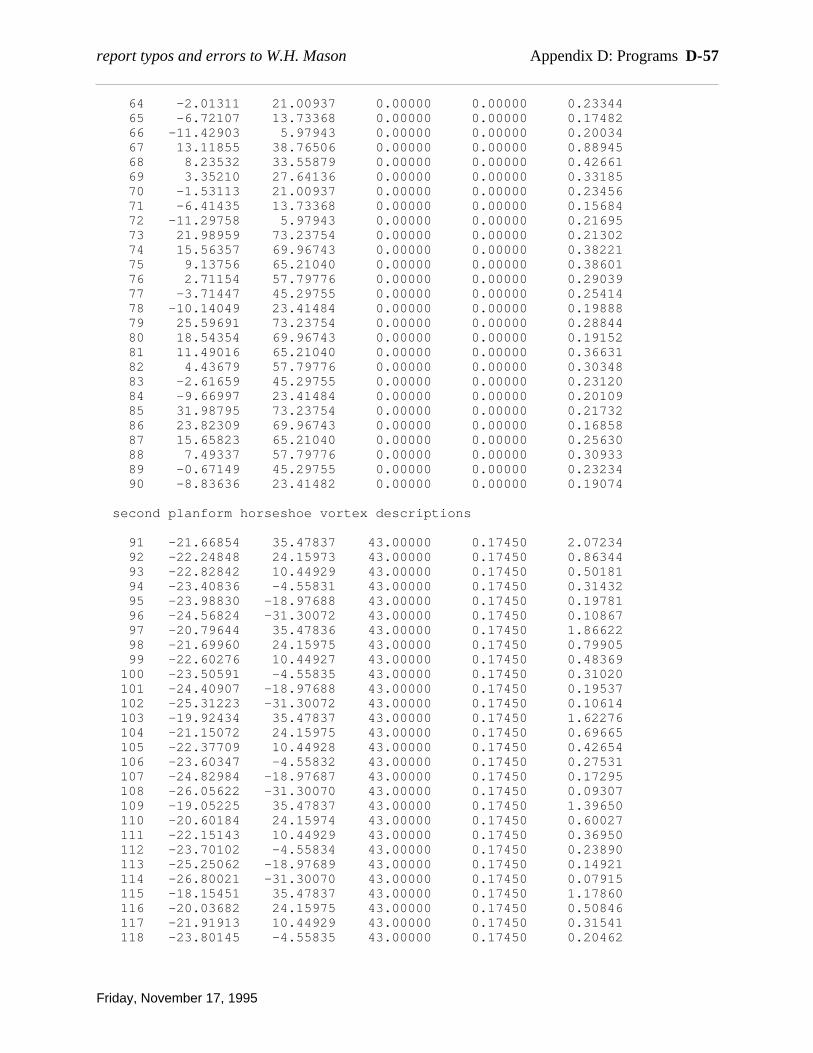
64 -2.01311 21.00937 0.00000 0.00000 0.23344 65 -6.72107 13.73368 0.00000 0.00000 0.17482 66 -11.42903 5.97943 0.00000 0.00000 0.20034 67 13.11855 38.76506 0.00000 0.00000 0.88945 68 8.23532 33.55879 0.00000 0.00000 0.42661 69 3.35210 27.64136 0.00000 0.00000 0.33185 70 -1.53113 21.00937 0.00000 0.00000 0.23456 71 -6.41435 13.73368 0.00000 0.00000 0.15684 72 -11.29758 5.97943 0.00000 0.00000 0.21695 73 21.98959 73.23754 0.00000 0.00000 0.21302 74 15.56357 69.96743 0.00000 0.00000 0.38221 75 9.13756 65.21040 0.00000 0.00000 0.38601 76 2.71154 57.79776 0.00000 0.00000 0.29039 77 -3.71447 45.29755 0.00000 0.00000 0.25414 78 -10.14049 23.41484 0.00000 0.00000 0.19888 79 25.59691 73.23754 0.00000 0.00000 0.28844 80 18.54354 69.96743 0.00000 0.00000 0.19152 81 11.49016 65.21040 0.00000 0.00000 0.36631 82 4.43679 57.79776 0.00000 0.00000 0.30348 83 -2.61659 45.29755 0.00000 0.00000 0.23120 84 -9.66997 23.41484 0.00000 0.00000 0.20109 85 31.98795 73.23754 0.00000 0.00000 0.21732 86 23.82309 69.96743 0.00000 0.00000 0.16858 87 15.65823 65.21040 0.00000 0.00000 0.25630 88 7.49337 57.79776 0.00000 0.00000 0.30933 89 -0.67149 45.29755 0.00000 0.00000 0.23234 90 -8.83636 23.41482 0.00000 0.00000 0.19074
second planform horseshoe vortex descriptions
91 -21.66854 35.47837 43.00000 0.17450 2.07234 92 -22.24848 24.15973 43.00000 0.17450 0.86344 93 -22.82842 10.44929 43.00000 0.17450 0.50181 94 -23.40836 -4.55831 43.00000 0.17450 0.31432 95 -23.98830 -18.97688 43.00000 0.17450 0.19781 96 -24.56824 -31.30072 43.00000 0.17450 0.10867 97 -20.79644 35.47836 43.00000 0.17450 1.86622 98 -21.69960 24.15975 43.00000 0.17450 0.79905 99 -22.60276 10.44927 43.00000 0.17450 0.48369 100 -23.50591 -4.55835 43.00000 0.17450 0.31020 101 -24.40907 -18.97688 43.00000 0.17450 0.19537 102 -25.31223 -31.30072 43.00000 0.17450 0.10614 103 -19.92434 35.47837 43.00000 0.17450 1.62276 104 -21.15072 24.15975 43.00000 0.17450 0.69665 105 -22.37709 10.44928 43.00000 0.17450 0.42654 106 -23.60347 -4.55832 43.00000 0.17450 0.27531 107 -24.82984 -18.97687 43.00000 0.17450 0.17295 108 -26.05622 -31.30070 43.00000 0.17450 0.09307 109 -19.05225 35.47837 43.00000 0.17450 1.39650 110 -20.60184 24.15974 43.00000 0.17450 0.60027 111 -22.15143 10.44929 43.00000 0.17450 0.36950 112 -23.70102 -4.55834 43.00000 0.17450 0.23890 113 -25.25062 -18.97689 43.00000 0.17450 0.14921 114 -26.80021 -31.30070 43.00000 0.17450 0.07915 115 -18.15451 35.47837 43.00000 0.17450 1.17860 116 -20.03682 24.15975 43.00000 0.17450 0.50846 117 -21.91913 10.44929 43.00000 0.17450 0.31541 118 -23.80145 -4.55835 43.00000 0.17450 0.20462
report typos and errors to W.H. Mason Appendix D: Programs D-57
Friday, November 17, 1995

119 -25.68376 -18.97689 43.00000 0.17450 0.12671 120 -27.56607 -31.30071 43.00000 0.17450 0.06503 121 -17.21404 38.04567 43.00000 0.17450 1.01268 122 -19.25814 38.58307 43.00000 0.17450 0.44608 123 -21.30224 39.11254 43.00000 0.17450 0.28734 124 -23.34634 39.63417 43.00000 0.17450 0.19345 125 -25.39045 40.14806 43.00000 0.17450 0.12395 126 -27.43455 40.65429 43.00000 0.17450 0.06535 127 -16.09888 38.04567 43.00000 0.17450 0.83667 128 -18.12127 38.58307 43.00000 0.17450 0.39566 129 -20.14366 39.11254 43.00000 0.17450 0.27313 130 -22.16605 39.63417 43.00000 0.17450 0.19673 131 -24.18844 40.14806 43.00000 0.17450 0.13605 132 -26.21083 40.65429 43.00000 0.17450 0.07985 133 -15.49042 -3.19570 0.00000 0.00000 0.56637 134 -17.61208 -15.59796 0.00000 0.00000 0.42340 135 -19.73375 -26.67953 0.00000 0.00000 0.31785 136 -21.85542 -35.97340 0.00000 0.00000 0.23703 137 -23.97708 -43.50610 0.00000 0.00000 0.16547 138 -26.09875 -49.53985 0.00000 0.00000 0.09394 139 -15.48730 2.12462 0.00000 0.00000 0.38372 140 -17.59650 10.50852 0.00000 0.00000 0.33354 141 -19.70569 18.46350 0.00000 0.00000 0.27610 142 -21.81489 25.74715 0.00000 0.00000 0.21449 143 -23.92408 32.23863 0.00000 0.00000 0.15167 144 -26.03328 37.92108 0.00000 0.00000 0.08438 145 -15.44074 2.12462 0.00000 0.00000 0.34990 146 -17.36370 10.50851 0.00000 0.00000 0.29853 147 -19.28666 18.46349 0.00000 0.00000 0.25906 148 -21.20962 25.74714 0.00000 0.00000 0.21134 149 -23.13258 32.23862 0.00000 0.00000 0.15849 150 -25.05555 37.92108 0.00000 0.00000 0.09723 151 -15.41594 2.12462 0.00000 0.00000 0.35024 152 -17.23971 10.50852 0.00000 0.00000 0.28116 153 -19.06347 18.46350 0.00000 0.00000 0.24782 154 -20.88724 25.74714 0.00000 0.00000 0.20712 155 -22.71100 32.23864 0.00000 0.00000 0.16006 156 -24.53477 37.92108 0.00000 0.00000 0.10421 157 -15.43854 -2.18164 0.00000 0.00000 0.32319 158 -17.35267 -10.78430 0.00000 0.00000 0.24905 159 -19.26681 -18.92465 0.00000 0.00000 0.22019 160 -21.18095 -26.34637 0.00000 0.00000 0.18542 161 -23.09509 -32.92787 0.00000 0.00000 0.14319 162 -25.00923 -38.65982 0.00000 0.00000 0.09029 163 -15.51187 -2.18164 0.00000 0.00000 0.29260 164 -17.71934 -10.78430 0.00000 0.00000 0.22016 165 -19.92681 -18.92465 0.00000 0.00000 0.19116 166 -22.13429 -26.34637 0.00000 0.00000 0.15602 167 -24.34176 -32.92787 0.00000 0.00000 0.11287 168 -26.54923 -38.65981 0.00000 0.00000 0.06313
ref. chord c average true area reference area 26.89170 31.36179 1364.23767 950.00000
b/2 ref. ar true ar mach number 21.75000 1.99184 1.38704 0.30000
D-58 Applied Computational Aerodynamics
Friday, November 17, 1995

complete configuration lift induced drag(far field solution) cl computed alpha cl(wb) cdi at cl(wb) cdi/(cl(wb)**2)
0.5300 7.6834 0.3851 0.0238 0.1608
complete configuration characteristics
cl alpha cl(twist) alpha y cp cm/cl cmo per rad per deg at cl=0 3.11731 0.05441 0.11197 -2.05798 -0.42053 0.06834 -0.07080
additional loading with cl based on s(true) -at cl des-
load add. basic span x loc dueto load load load ofstat 2y/b sl cl c twist at cl at cl at cl local coef ratio ratio = = desir cent of 0.112 0 press
1 -0.962 0.310 2.045 0.152 0.003 0.024 -0.021 0.094 -0.162 2 -0.885 0.471 1.950 0.241 0.006 0.037 -0.031 0.143 0.575 3 -0.812 0.588 1.802 0.327 0.008 0.046 -0.038 0.179 1.273 4 -0.739 0.687 1.669 0.412 0.010 0.054 -0.044 0.210 1.949 5 -0.662 0.775 1.545 0.501 0.012 0.060 -0.048 0.238 2.630 6 -0.585 0.850 1.438 0.591 0.016 0.066 -0.051 0.263 3.257 7 -0.519 0.909 1.362 0.667 0.019 0.071 -0.052 0.284 3.709 8 -0.454 0.963 1.295 0.744 0.023 0.075 -0.052 0.303 4.081 9 -0.388 1.011 1.233 0.820 0.028 0.079 -0.051 0.322 4.316 10 -0.338 1.046 1.209 0.865 0.031 0.082 -0.050 0.336 4.526 11 -0.277 1.075 1.193 0.901 0.033 0.084 -0.051 0.346 5.045 12 -0.219 1.092 1.168 0.934 0.034 0.085 -0.052 0.351 5.530 13 -0.189 1.100 0.895 1.229 0.033 0.086 -0.053 0.353 6.950 14 -0.139 1.109 0.822 1.349 0.033 0.086 -0.053 0.356 8.812 15 -0.050 1.117 0.715 1.562 0.033 0.087 -0.054 0.358 11.245
contribution of the second planform to span load distribution
16 -0.749 0.116 1.047 0.111 0.041 0.009 0.032 0.075 -22.261 17 -0.693 0.164 0.948 0.173 0.061 0.013 0.048 0.108 -21.759 18 -0.636 0.189 0.806 0.235 0.073 0.015 0.059 0.129 -21.242 19 -0.580 0.200 0.676 0.296 0.082 0.016 0.066 0.140 -20.719 20 -0.522 0.200 0.555 0.360 0.086 0.016 0.070 0.144 -20.183 21 -0.464 0.187 0.479 0.391 0.084 0.015 0.070 0.139 -19.541 22 -0.399 0.164 0.423 0.387 0.076 0.013 0.063 0.124 -18.709 23 -0.338 0.174 0.429 0.406 0.071 0.014 0.058 0.122 -18.903 24 -0.277 0.148 0.366 0.404 0.054 0.012 0.043 0.097 -19.224 25 -0.219 0.133 0.363 0.368 0.045 0.010 0.035 0.084 -19.037 26 -0.189 0.128 0.366 0.349 0.041 0.010 0.031 0.079 -18.872 27 -0.139 0.124 0.339 0.366 0.038 0.010 0.028 0.074 -19.025 28 -0.050 0.126 0.297 0.422 0.036 0.010 0.027 0.073 -19.428
report typos and errors to W.H. Mason Appendix D: Programs D-59
Friday, November 17, 1995

induced drag,leading edge thrust , suction coefficient characteristics computed at the desired cl from a near field solution
section coefficients l.e. sweep station 2y/b angle cdii c/2b ct c/2b cs c/2b 1 -0.96154 39.96069 0.00412 0.00085 0.00111 2 -0.88462 39.96069 0.00182 0.00507 0.00661 3 -0.81158 39.96069 0.00042 0.00821 0.01071 4 -0.73855 39.96069 0.00101 0.00912 0.01190 5 -0.66163 39.96069 0.00187 0.00962 0.01255 6 -0.58470 39.96069 0.00286 0.00985 0.01285 7 -0.51933 39.96069 0.00392 0.00978 0.01276 8 -0.45395 39.96069 0.00499 0.00967 0.01261 9 -0.38844 39.96069 0.00581 0.00975 0.01272 10 -0.33839 39.96069 0.00675 0.00940 0.01226 11 -0.27694 39.96069 0.00795 0.00872 0.01138 12 -0.21924 39.96069 0.00884 0.00813 0.01389 13 -0.18851 73.89906 0.00974 0.00733 0.02002 14 -0.13855 73.89906 0.01161 0.00557 0.02009 15 -0.05004 73.89906 0.02071 -0.00342 -0.01233
contribution of the second planform to the chord or drag force
16 -0.74888 37.91007 0.00645 0.00292 0.00370 17 -0.69262 37.91007 0.00477 0.00715 0.00906 18 -0.63637 37.91007 0.00430 0.00984 0.01247 19 -0.58011 37.91007 0.00588 0.00953 0.01208 20 -0.52220 37.91007 0.00755 0.00832 0.01054 21 -0.46428 37.91007 0.00901 0.00640 0.00812 22 -0.39877 37.91007 0.00956 0.00324 0.00400 23 -0.33839 0.00000 0.00665 0.00124 0.00128 24 -0.27694 0.00000 0.00449 0.00034 0.00034 25 -0.21924 0.00000 0.00408 0.00003 0.00003 26 -0.18851 0.00000 0.00389 -0.00001 -0.00001 27 -0.13855 0.00000 0.00361 0.00002 0.00002 28 -0.05004 0.00000 0.00331 0.00022 0.00022
total coefficients
cdii/cl**2= 0.15439 ct= 0.04177 cs= 0.056731
end of file encountered after configuration 23.
D-60 Applied Computational Aerodynamics
Friday, November 17, 1995
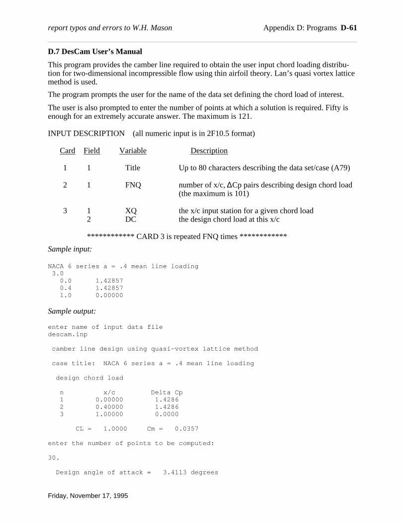
D.7 DesCam User’s Manual
This program provides the camber line required to obtain the user input chord loading distribu-tion for two-dimensional incompressible flow using thin airfoil theory. Lan’s quasi vortex latticemethod is used.
The program prompts the user for the name of the data set defining the chord load of interest.
The user is also prompted to enter the number of points at which a solution is required. Fifty isenough for an extremely accurate answer. The maximum is 121.
INPUT DESCRIPTION (all numeric input is in 2F10.5 format)
Card Field Variable Description
1 1 Title Up to 80 characters describing the data set/case (A79)
2 1 FNQ number of x/c, ∆Cp pairs describing design chord load(the maximum is 101)
3 1 XQ the x/c input station for a given chord load2 DC the design chord load at this x/c
************ CARD 3 is repeated FNQ times ************
Sample input:
NACA 6 series a = .4 mean line loading 3.0 0.0 1.42857 0.4 1.42857 1.0 0.00000
Sample output:
enter name of input data filedescam.inp
camber line design using quasi-vortex lattice method
case title: NACA 6 series a = .4 mean line loading
design chord load
n x/c Delta Cp 1 0.00000 1.4286 2 0.40000 1.4286 3 1.00000 0.0000
CL = 1.0000 Cm = 0.0357
enter the number of points to be computed:
30.
Design angle of attack = 3.4113 degrees
report typos and errors to W.H. Mason Appendix D: Programs D-61
Friday, November 17, 1995
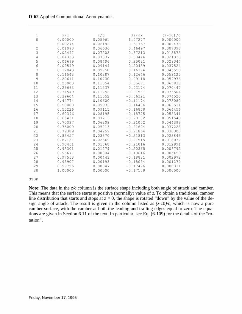
i x/c z/c dz/dx (z-z0)/c 0 0.00000 0.05961 1.07277 0.000000 1 0.00274 0.06192 0.61767 0.002478 2 0.01093 0.06636 0.46497 0.007398 3 0.02447 0.07203 0.37212 0.013875 4 0.04323 0.07837 0.30444 0.021338 5 0.06699 0.08496 0.25031 0.029344 6 0.09549 0.09144 0.20439 0.037524 7 0.12843 0.09750 0.16374 0.045550 8 0.16543 0.10287 0.12646 0.053125 9 0.20611 0.10730 0.09118 0.059976 10 0.25000 0.11054 0.05671 0.065838 11 0.29663 0.11237 0.02174 0.070447 12 0.34549 0.11252 -0.01581 0.073504 13 0.39604 0.11052 -0.06321 0.074520 14 0.44774 0.10600 -0.11174 0.073080 15 0.50000 0.09932 -0.14406 0.069511 16 0.55226 0.09115 -0.16858 0.064456 17 0.60396 0.08195 -0.18725 0.058341 18 0.65451 0.07213 -0.20102 0.051540 19 0.70337 0.06208 -0.21052 0.044399 20 0.75000 0.05213 -0.21624 0.037228 21 0.79389 0.04259 -0.21864 0.030300 22 0.83457 0.03370 -0.21813 0.023843 23 0.87157 0.02569 -0.21515 0.018032 24 0.90451 0.01868 -0.21016 0.012991 25 0.93301 0.01279 -0.20365 0.008792 26 0.95677 0.00804 -0.19616 0.005459 27 0.97553 0.00443 -0.18831 0.002972 28 0.98907 0.00193 -0.18084 0.001279 29 0.99726 0.00047 -0.17476 0.000311 30 1.00000 0.00000 -0.17179 0.000000
STOP
Note: The data in the z/c column is the surface shape including both angle of attack and camber.This means that the surface starts at positive (normally) value of z. To obtain a traditional camberline distribution that starts and stops at z = 0, the shape is rotated “down” by the value of the de-sign angle of attack. The result is given in the column listed as (z-z0)/c, which is now a purecamber surface, with the camber at both the leading and trailing edges equal to zero. The equa-tions are given in Section 6.11 of the text. In particular, see Eq. (6-109) for the details of the “ro-tation”.
D-62 Applied Computational Aerodynamics
Friday, November 17, 1995

Appendix E Utility Codes
Several utility programs are useful. This appendix provides the input instructions.
E.1 FOILGEN
Airfoil geometry generation. For airfoils with analytically defined ordinates, thisprogram produces airfoil definition data sets in the format required for PANELv2.This includes NACA 4-digit, 4-digit modified and 5-digit airfoils. In addition, theNACA 6 and 6A camber lines are available. The user can combine any combina-tion of thickness and camber lines available within these shapes. This provides awide range of airfoil definitions.
E.2 LADSON
This is the NASA program that provides a reasonable approximation to theNACA 6 and 6A series airfoils. It was written by Charles Ladson and CuylerBrooks.
E.3 CONCAM
This program provides the NACA conical camber geometry.
E.4 WNGLFT
This program provides detailed wing geometry definition for a straight line wraplofted wing.
E.5 BUMP
This code provides a means of making smooth changes to airfoil shapes. This rou-tine is included in PANELv2.
E.6 POSTp
Post processing of PANELv2 for use in CBL
E.7 STDATM
This is a subroutine that provides the 1976 standard atmosphere used in programFRICTION.
Tuesday, January 21, 1997 E-1

E.1 FOILGEN
This program is used for airfoil geometry generation. For airfoils with analytically defined ordi-nates, this program produces airfoil definition data sets in the format required for PANELv2.This includes NACA 4-digit, 4-digit modified and 5-digit airfoils. In addition, the NACA 6 and6A camber lines are available. The user can combine any combination of thickness and camberlines available within these shapes. This provides a wide range of airfoil definitions. The pro-gram runs interactively, and a sample terminal session is provided here to illustrate its use.
From terminal session:
NACA Airfoil Ordinate Generation W.H. Mason, March 15, 1992
Thickness Distribution Options:
1 - NACA 4 Digit Series 2 - NACA Modified 4 Digit Series
Select 1 or 2 :2
Input Max Thickness, T/C =.18
X/C Position of Max Thickness =.4
Input leading edge parameter:
Choose values from 0 to 9 - (6 is the 4 Series value) 7
Leading Edge Radius, rle/C = 0.04859
Trailing Edge Angle is 31.60 degrees [this is the TOTAL included angle]
Camber Distribution Options:
1 - NACA 4 Digit Series 2 - NACA 5 Digit Series 3 - NACA 6 & 6A Series
Select 1,2 or 3: 3
Design Lift Coefficient = .2
Input X/C for constant loading, A = .8
6A-series camber line ? (Y/N):y
Choose output option :
1 - Point by point 2 - Distribution
Select 1 or 2:2
Select type of distribution:
E-2 Applied Computational Aerodynamics
Tuesday, January 21, 1997

1 - Even Spacing 2 - Full Cosine (Concentrated at both LE & TE) 3 - Half Cosine (Concentrated at LE)
Choose 1, 2, or 3 :1
Number of points in distribution, (131 maximum) =21
I X/C YT/C DYT/X YC/C DYC/C XU/C(%) YU/C(%) XL/C(%) YL/C(%) 1 0.0000 0.0000 99.9999 0.0000 0.0000 0.0000 0.0000 0.0000 0.0000 2 0.0500 0.0529 0.3774 0.0036 0.0543 4.7133 5.6407 5.2867 -4.9195 3 0.1000 0.0665 0.2020 0.0060 0.0412 9.7259 7.2420 10.2741 -6.0498 4 0.1500 0.0747 0.1343 0.0078 0.0331 14.7529 8.2487 15.2471 -6.6872 5 0.2000 0.0804 0.0969 0.0093 0.0269 19.7837 8.9702 20.2163 -7.1099 6 0.2500 0.0846 0.0706 0.0105 0.0217 24.8161 9.5086 25.1839 -7.4057 7 0.3000 0.0875 0.0478 0.0115 0.0172 29.8495 9.9018 30.1505 -7.6046 8 0.3500 0.0894 0.0249 0.0122 0.0130 34.8839 10.1599 35.1161 -7.7119 9 0.4000 0.0900 0.0000 0.0128 0.0090 39.9189 10.2786 40.0811 -7.720710 0.4500 0.0893 -0.0261 0.0131 0.0051 44.9543 10.2487 45.0457 -7.620211 0.5000 0.0874 -0.0518 0.0133 0.0012 49.9894 10.0698 50.0106 -7.409612 0.5500 0.0842 -0.0769 0.0133 -0.0028 55.0236 9.7439 54.9764 -7.091513 0.6000 0.0797 -0.1017 0.0130 -0.0071 60.0564 9.2725 59.9436 -6.669214 0.6500 0.0740 -0.1259 0.0125 -0.0118 65.0871 8.6561 64.9129 -6.146515 0.7000 0.0671 -0.1498 0.0118 -0.0172 70.1156 7.8941 69.8844 -5.528716 0.7500 0.0591 -0.1731 0.0108 -0.0241 75.1424 6.9835 74.8576 -4.823117 0.8000 0.0498 -0.1960 0.0093 -0.0361 80.1796 5.9136 79.8204 -4.044118 0.8500 0.0395 -0.2184 0.0072 -0.0469 85.1847 4.6629 84.8153 -3.220019 0.9000 0.0280 -0.2404 0.0047 -0.0480 90.1343 3.2641 89.8657 -2.326420 0.9500 0.0154 -0.2619 0.0023 -0.0480 95.0740 1.7693 94.9260 -1.312021 1.0000 0.0018 -0.2830 0.0000 0.0000 100.0000 0.1800 100.0000 -0.1800I X/C YT/C DYT/X YC/C DYC/C XU/C(%) YU/C(%) XL/C(%) YL/C(%)
send output to a file? (Y/N):y
enter file name:testout.txt
enter file title:NACA 18% thick, xt=.4, I=7, 6A series cam, CLI = .2
Another case?n
STOP
The disk file generated from the session shown above is:
NACA 18% thick, xt=.4, I=7, 6A series cam, CLI = .2 21.000000 21.000000 Upper Surface 0.000000 0.000000 0.047133 0.056407 0.097259 0.072420
report typos and errors to W.H. Mason Appendix E: Utility Programs E-3
Tuesday, January 21, 1997
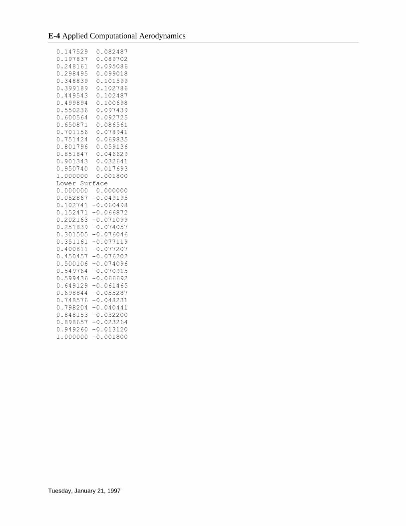
0.147529 0.082487 0.197837 0.089702 0.248161 0.095086 0.298495 0.099018 0.348839 0.101599 0.399189 0.102786 0.449543 0.102487 0.499894 0.100698 0.550236 0.097439 0.600564 0.092725 0.650871 0.086561 0.701156 0.078941 0.751424 0.069835 0.801796 0.059136 0.851847 0.046629 0.901343 0.032641 0.950740 0.017693 1.000000 0.001800 Lower Surface 0.000000 0.000000 0.052867 -0.049195 0.102741 -0.060498 0.152471 -0.066872 0.202163 -0.071099 0.251839 -0.074057 0.301505 -0.076046 0.351161 -0.077119 0.400811 -0.077207 0.450457 -0.076202 0.500106 -0.074096 0.549764 -0.070915 0.599436 -0.066692 0.649129 -0.061465 0.698844 -0.055287 0.748576 -0.048231 0.798204 -0.040441 0.848153 -0.032200 0.898657 -0.023264 0.949260 -0.013120 1.000000 -0.001800
E-4 Applied Computational Aerodynamics
Tuesday, January 21, 1997
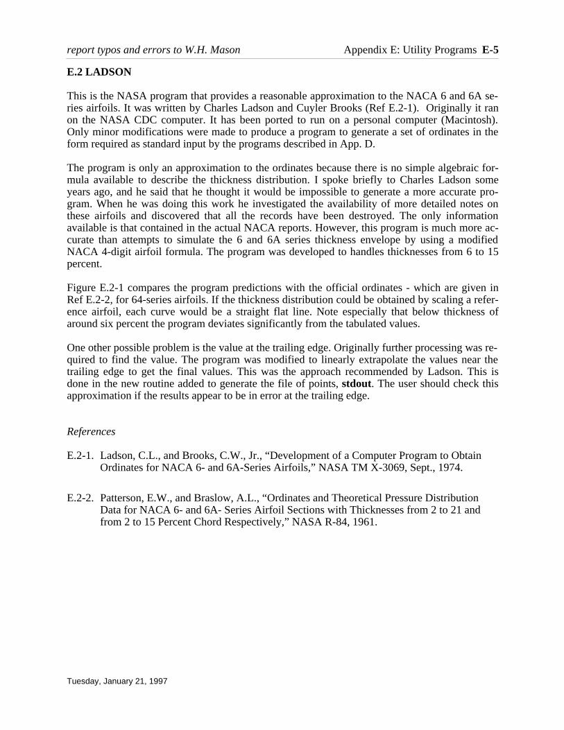
E.2 LADSON
This is the NASA program that provides a reasonable approximation to the NACA 6 and 6A se-ries airfoils. It was written by Charles Ladson and Cuyler Brooks (Ref E.2-1). Originally it ranon the NASA CDC computer. It has been ported to run on a personal computer (Macintosh).Only minor modifications were made to produce a program to generate a set of ordinates in theform required as standard input by the programs described in App. D.
The program is only an approximation to the ordinates because there is no simple algebraic for-mula available to describe the thickness distribution. I spoke briefly to Charles Ladson someyears ago, and he said that he thought it would be impossible to generate a more accurate pro-gram. When he was doing this work he investigated the availability of more detailed notes onthese airfoils and discovered that all the records have been destroyed. The only informationavailable is that contained in the actual NACA reports. However, this program is much more ac-curate than attempts to simulate the 6 and 6A series thickness envelope by using a modifiedNACA 4-digit airfoil formula. The program was developed to handles thicknesses from 6 to 15percent.
Figure E.2-1 compares the program predictions with the official ordinates - which are given inRef E.2-2, for 64-series airfoils. If the thickness distribution could be obtained by scaling a refer-ence airfoil, each curve would be a straight flat line. Note especially that below thickness ofaround six percent the program deviates significantly from the tabulated values.
One other possible problem is the value at the trailing edge. Originally further processing was re-quired to find the value. The program was modified to linearly extrapolate the values near thetrailing edge to get the final values. This was the approach recommended by Ladson. This isdone in the new routine added to generate the file of points, stdout. The user should check thisapproximation if the results appear to be in error at the trailing edge.
References
E.2-1. Ladson, C.L., and Brooks, C.W., Jr., “Development of a Computer Program to ObtainOrdinates for NACA 6- and 6A-Series Airfoils,” NASA TM X-3069, Sept., 1974.
E.2-2. Patterson, E.W., and Braslow, A.L., “Ordinates and Theoretical Pressure DistributionData for NACA 6- and 6A- Series Airfoil Sections with Thicknesses from 2 to 21 andfrom 2 to 15 Percent Chord Respectively,” NASA R-84, 1961.
report typos and errors to W.H. Mason Appendix E: Utility Programs E-5
Tuesday, January 21, 1997

a. x/c = 0.10
Fig. E.2-1 Comparison of tabulated and computed airfoil ordinate values.
b. x/c = 0.075
c. x/c = 0.050
d. x/c = 0.025
E-6 Applied Computational Aerodynamics
Tuesday, January 21, 1997
0.168
0.170
0.172
0.174
0 5 10 15
y/t, at x/c = 0.0250 (Tabulated)y/t, at x/c = 0.0250 (Pgm value)
y / t
Max t/c, %
0.230
0.235
0.240
0.245
0 5 10 15
y/t, at x/c = 0.0500 (Tabulated)y/t, at x/c = 0.0500 (Pgm value)
y / t
Max t/c, %
0.280
0.284
0.288
0.292
0 5 10 15
y/t, at x/c = 0.0750 (Tabulated)y/t, at x/c = 0.0750 (Pgm value)
y/t
Max t/c, %
0.320
0.322
0.324
0.326
0.328
0 5 10 15
y/t, at x/c = 0.1000 (Tabulated)y/t, at x/c = 0.1000 (Pgm value)
y / t
Max t/c, %
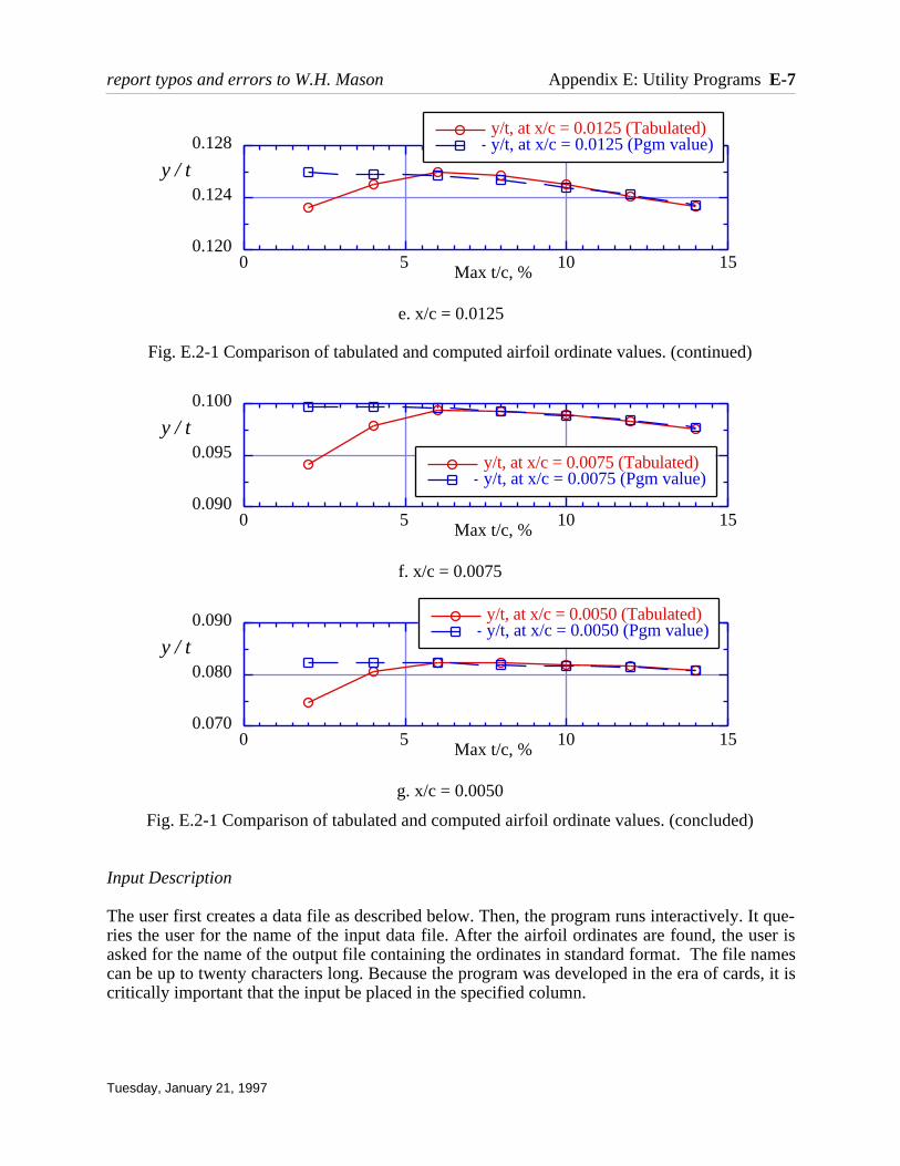
e. x/c = 0.0125
Fig. E.2-1 Comparison of tabulated and computed airfoil ordinate values. (continued)
f. x/c = 0.0075
g. x/c = 0.0050
Fig. E.2-1 Comparison of tabulated and computed airfoil ordinate values. (concluded)
Input Description
The user first creates a data file as described below. Then, the program runs interactively. It que-ries the user for the name of the input data file. After the airfoil ordinates are found, the user isasked for the name of the output file containing the ordinates in standard format. The file namescan be up to twenty characters long. Because the program was developed in the era of cards, it iscritically important that the input be placed in the specified column.
report typos and errors to W.H. Mason Appendix E: Utility Programs E-7
Tuesday, January 21, 1997
0.070
0.080
0.090
0 5 10 15
y/t, at x/c = 0.0050 (Tabulated)y/t, at x/c = 0.0050 (Pgm value)
y / t
Max t/c, %
0.090
0.095
0.100
0 5 10 15
y/t, at x/c = 0.0075 (Tabulated)y/t, at x/c = 0.0075 (Pgm value)
y / t
Max t/c, %
0.120
0.124
0.128
0 5 10 15
y/t, at x/c = 0.0125 (Tabulated)y/t, at x/c = 0.0125 (Pgm value)
y / t
Max t/c, %
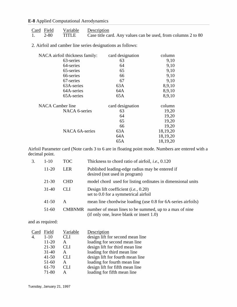
Card Field Variable Description1. 2-80 TITLE Case title card. Any values can be used, from columns 2 to 80
2. Airfoil and camber line series designations as follows:
NACA airfoil thickness family: card designation column63-series 63 9,1064-series 64 9,1065-series 65 9,1066-series 66 9,1067-series 67 9,1063A-series 63A 8,9,1064A-series 64A 8,9,1065A-series 65A 8,9,10
NACA Camber line card designation columnNACA 6-series 63 19,20
64 19,2065 19,2066 19,20
NACA 6A-series 63A 18,19,2064A 18,19,2065A 18,19,20
Airfoil Parameter card (Note cards 3 to 6 are in floating point mode. Numbers are entered with adecimal point.
3. 1-10 TOC Thickness to chord ratio of airfoil, i.e., 0.120
11-20 LER Published leading-edge radius may be entered if desired (not used in program)
21-30 CHD model chord used for listing ordinates in dimensional units
31-40 CLI Design lift coefficient (i.e., 0.20)set to 0.0 for a symmetrical airfoil
41-50 A mean line chordwise loading (use 0.8 for 6A-series airfoils)
51-60 CMBNMR number of mean lines to be summed, up to a max of nine(if only one, leave blank or insert 1.0)
and as required:
Card Field Variable Description4. 1-10 CLI design lift for second mean line
11-20 A loading for second mean line21-30 CLI design lift for third mean line31-40 A loading for third mean line41-50 CLI design lift for fourth mean line51-60 A loading for fourth mean line61-70 CLI design lift for fifth mean line71-80 A loading for fifth mean line
E-8 Applied Computational Aerodynamics
Tuesday, January 21, 1997

Card Field Variable Description5. 1-10 CLI design lift for sixth mean line
11-20 A loading for sixth mean line21-30 CLI design lift for seventh mean line31-40 A loading for seventh mean line41-50 CLI design lift for eighth mean line51-60 A loading for eighth mean line61-70 CLI design lift for ninth mean line71-80 A loading for ninth mean line
6. 1-10 CLI design lift for tenth mean line11-20 A loading for tenth mean line
Sample input:
NACA 65(1)213 A=0.5,CL=0.2 65 65 0.130 0.00 1.0 0.2 0.5 1.0
Output
The program files also contain the sample output of the program. Because the program was writ-ten many years ago, it uses 133 column output, and doesn’t fit on a normal page. The output filecorresponds to the input data set given above and also available in the program files. This caseshould be verified before further use of the program.
Eighty values of the upper and lower surface are contained in the disk file. The following is thefile generated from the sample input listed above. All numbers are output in 2F10.6 format.
NACA 65(1)213 A=0.5,CL=0.2 80.000000 80.000000 UPPER SURFACE 0.000000 0.000000 0.000294 0.004049 0.000862 0.005724 0.001472 0.007026 0.002106 0.008120 0.002756 0.009078 0.003416 0.009940 0.004095 0.010729 0.004801 0.011465 0.005750 0.012363 0.006706 0.013187 0.007668 0.013957 0.008635 0.014674 0.009605 0.015351 0.010578 0.015999 0.013509 0.017790 0.018419 0.020432 0.023349 0.022801 0.028292 0.024990 0.033243 0.027041 0.038202 0.028978 0.043167 0.030816 0.048138 0.032564 0.053113 0.034230 0.058093 0.035824 0.063077 0.037355 0.068064 0.038829 0.073053 0.040252 0.078045 0.041628
report typos and errors to W.H. Mason Appendix E: Utility Programs E-9
Tuesday, January 21, 1997
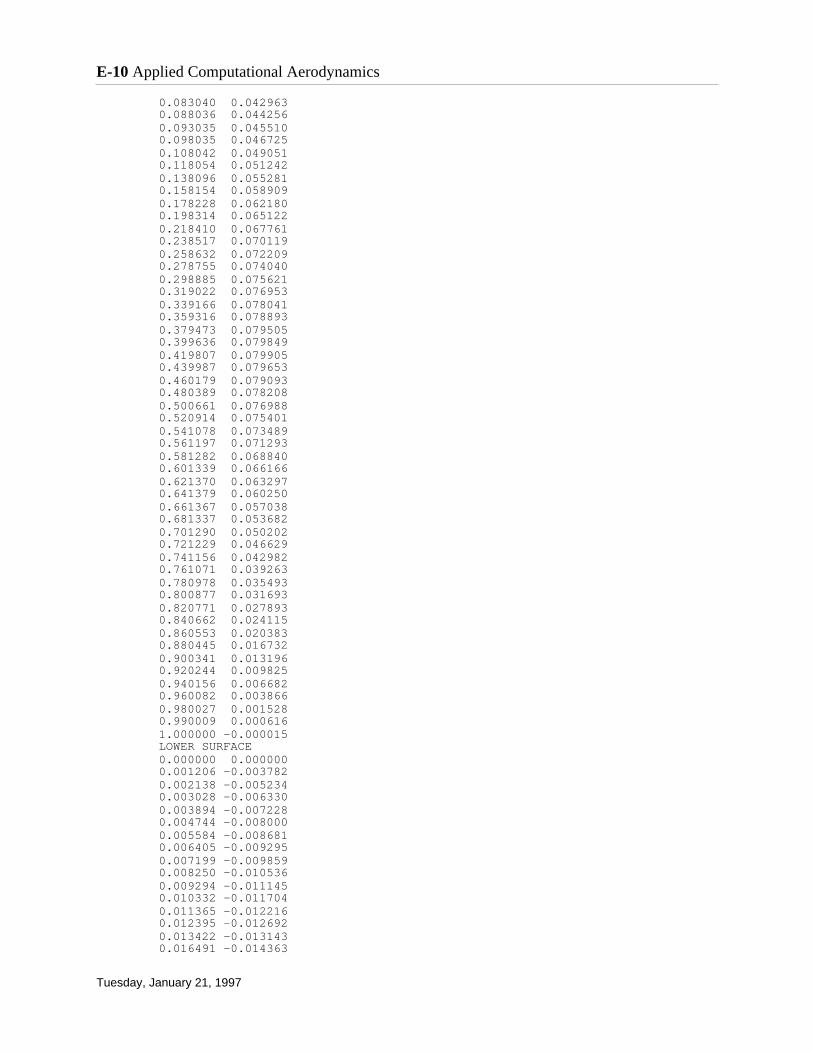
0.083040 0.042963 0.088036 0.044256 0.093035 0.045510 0.098035 0.046725 0.108042 0.049051 0.118054 0.051242 0.138096 0.055281 0.158154 0.058909 0.178228 0.062180 0.198314 0.065122 0.218410 0.067761 0.238517 0.070119 0.258632 0.072209 0.278755 0.074040 0.298885 0.075621 0.319022 0.076953 0.339166 0.078041 0.359316 0.078893 0.379473 0.079505 0.399636 0.079849 0.419807 0.079905 0.439987 0.079653 0.460179 0.079093 0.480389 0.078208 0.500661 0.076988 0.520914 0.075401 0.541078 0.073489 0.561197 0.071293 0.581282 0.068840 0.601339 0.066166 0.621370 0.063297 0.641379 0.060250 0.661367 0.057038 0.681337 0.053682 0.701290 0.050202 0.721229 0.046629 0.741156 0.042982 0.761071 0.039263 0.780978 0.035493 0.800877 0.031693 0.820771 0.027893 0.840662 0.024115 0.860553 0.020383 0.880445 0.016732 0.900341 0.013196 0.920244 0.009825 0.940156 0.006682 0.960082 0.003866 0.980027 0.001528 0.990009 0.000616 1.000000 -0.000015 LOWER SURFACE 0.000000 0.000000 0.001206 -0.003782 0.002138 -0.005234 0.003028 -0.006330 0.003894 -0.007228 0.004744 -0.008000 0.005584 -0.008681 0.006405 -0.009295 0.007199 -0.009859 0.008250 -0.010536 0.009294 -0.011145 0.010332 -0.011704 0.011365 -0.012216 0.012395 -0.012692 0.013422 -0.013143 0.016491 -0.014363
E-10 Applied Computational Aerodynamics
Tuesday, January 21, 1997
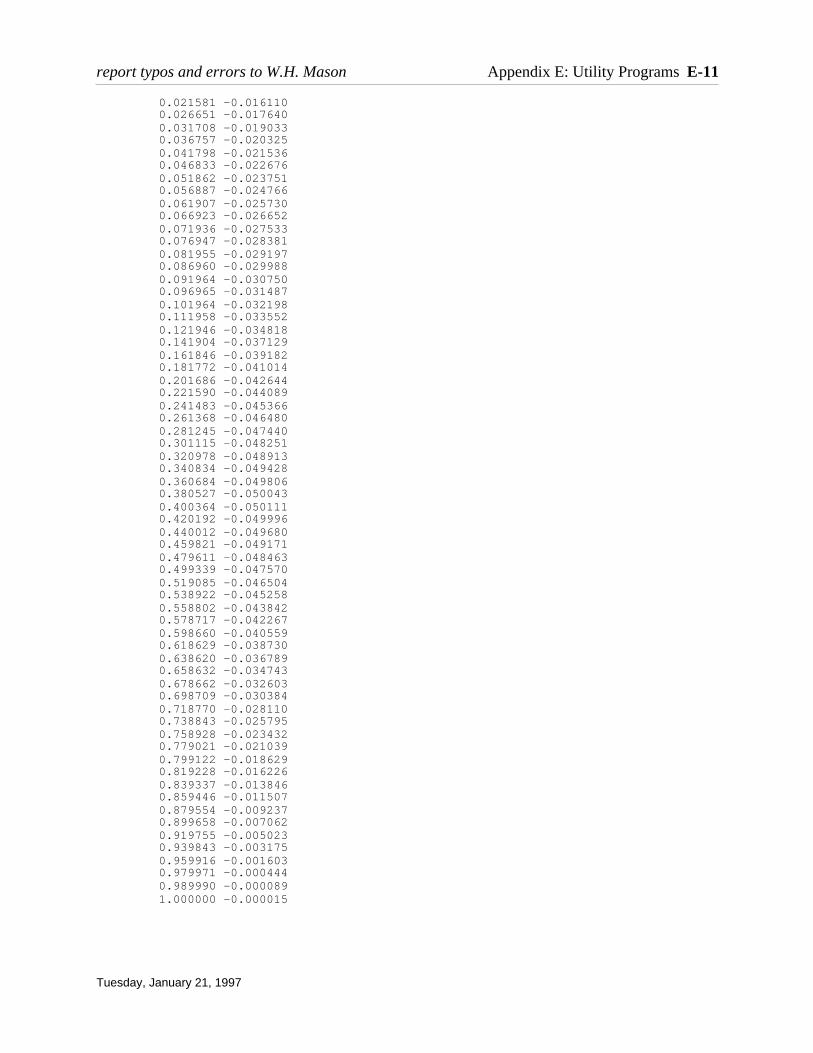
0.021581 -0.016110 0.026651 -0.017640 0.031708 -0.019033 0.036757 -0.020325 0.041798 -0.021536 0.046833 -0.022676 0.051862 -0.023751 0.056887 -0.024766 0.061907 -0.025730 0.066923 -0.026652 0.071936 -0.027533 0.076947 -0.028381 0.081955 -0.029197 0.086960 -0.029988 0.091964 -0.030750 0.096965 -0.031487 0.101964 -0.032198 0.111958 -0.033552 0.121946 -0.034818 0.141904 -0.037129 0.161846 -0.039182 0.181772 -0.041014 0.201686 -0.042644 0.221590 -0.044089 0.241483 -0.045366 0.261368 -0.046480 0.281245 -0.047440 0.301115 -0.048251 0.320978 -0.048913 0.340834 -0.049428 0.360684 -0.049806 0.380527 -0.050043 0.400364 -0.050111 0.420192 -0.049996 0.440012 -0.049680 0.459821 -0.049171 0.479611 -0.048463 0.499339 -0.047570 0.519085 -0.046504 0.538922 -0.045258 0.558802 -0.043842 0.578717 -0.042267 0.598660 -0.040559 0.618629 -0.038730 0.638620 -0.036789 0.658632 -0.034743 0.678662 -0.032603 0.698709 -0.030384 0.718770 -0.028110 0.738843 -0.025795 0.758928 -0.023432 0.779021 -0.021039 0.799122 -0.018629 0.819228 -0.016226 0.839337 -0.013846 0.859446 -0.011507 0.879554 -0.009237 0.899658 -0.007062 0.919755 -0.005023 0.939843 -0.003175 0.959916 -0.001603 0.979971 -0.000444 0.989990 -0.000089 1.000000 -0.000015
report typos and errors to W.H. Mason Appendix E: Utility Programs E-11
Tuesday, January 21, 1997
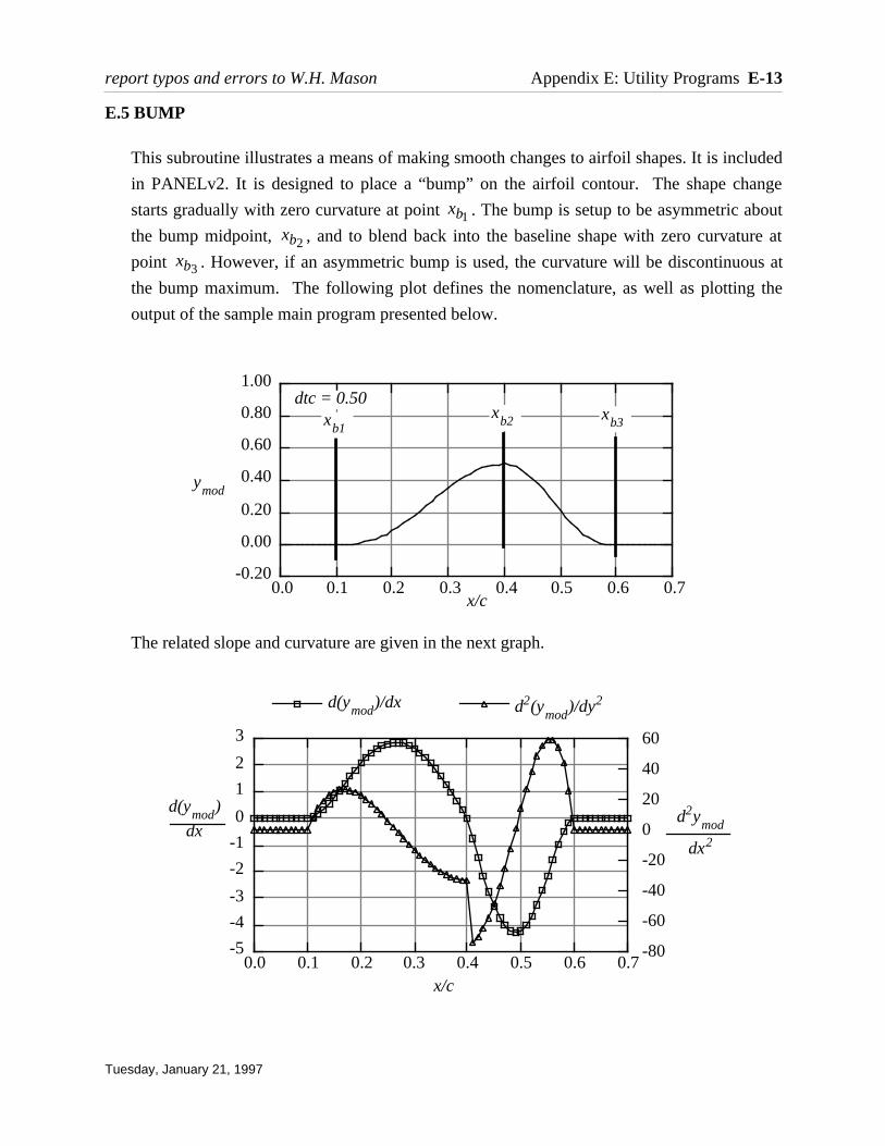
E.5 BUMP
This subroutine illustrates a means of making smooth changes to airfoil shapes. It is included
in PANELv2. It is designed to place a “bump” on the airfoil contour. The shape change
starts gradually with zero curvature at point . The bump is setup to be asymmetric about
the bump midpoint, , and to blend back into the baseline shape with zero curvature at
point . However, if an asymmetric bump is used, the curvature will be discontinuous at
the bump maximum. The following plot defines the nomenclature, as well as plotting the
output of the sample main program presented below.
The related slope and curvature are given in the next graph.
report typos and errors to W.H. Mason Appendix E: Utility Programs E-13
Tuesday, January 21, 1997
-5
-4
-3
-2
-1
0
1
2
3
-80
-60
-40
-20
0
20
40
60
0.0 0.1 0.2 0.3 0.4 0.5 0.6 0.7
d(ymod
)/dx d2(ymod
)/dy2
d(ymod
)
dxd2y
mod
dx2
x/c
-0.20
0.00
0.20
0.40
0.60
0.80
1.00
0.0 0.1 0.2 0.3 0.4 0.5 0.6 0.7
ymod
x/c
dtc = 0.50x
b1x
b2 xb3
xb3
xb2
xb1

The equation of the bump is:
where
or
This function is often called a “cubic bump” although it is clearly a sixth order polynomial.
The user should examine the subroutine to understand the transformation between the local
variable xd and the global variable xin.
Listing of subroutine bump.f:
subroutine bump(xb1,xb2,xb3,dtc,xmax,xin,ymod,ymodp,ymodpp)cc so-called cubic bump functioncc used to make mods to aero surfacescc W.H. Mason, December 1989cc xb1 - start of bump (dimensional)c xb2 - location of maximum bump height (dimensional)c xb3 - end of bump (dimensional)cc dtc - magnitude of bumpc xmax - reference length of geometrycc xin - input location to get bump valuec ymod - bump heightc ymodp - first derivative of bump wrt xinc ymodpp - second derivative of bump wrt xin
x = xin/xmax x1 = xb1/xmax x2 = xb2/xmax x3 = xb3/xmax
E-14 Applied Computational Aerodynamics
Tuesday, January 21, 1997
xd =x + x3 − 2x2( )2 x3 − x2( ) x2 < x < x3
xd =x − x1( )
2 x2 − x1( ) x1 < x < x2
d2 ymod
dxd2 = −64 ∆
t
c
6xd xd −1( ) 5xd
2 − 5xd +1( )
d ymod
dxd= −64 ∆
t
c
3xd
2 xd −1( )22xd −1( )
ymod = −64 ∆t
c
xd
3 xd −1( )3
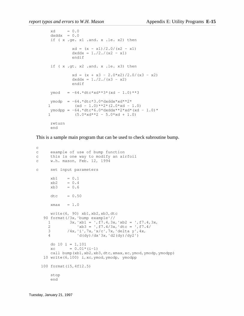
xd = 0.0 dxddx = 0.0 if ( x .ge. x1 .and. x .le. x2) then
xd = (x - x1)/2.0/(x2 - x1) dxddx = 1./2./(x2 - x1) endif
if ( x .gt. x2 .and. x .le. x3) then
xd = (x + x3 - 2.0*x2)/2.0/(x3 - x2) dxddx = 1./2./(x3 - x2) endif
ymod = -64.*dtc*xd**3*(xd - 1.0)**3
ymodp = -64.*dtc*3.0*dxddx*xd**2* 1 (xd - 1.0)**2*(2.0*xd - 1.0) ymodpp = -64.*dtc*6.0*dxddx**2*xd*(xd - 1.0)* 1 (5.0*xd**2 - 5.0*xd + 1.0)
return end
This is a sample main program that can be used to check subroutine bump.
cc example of use of bump functionc this is one way to modify an airfoilc w.h. mason, Feb. 12, 1994
c set input parameters
xb1 = 0.1 xb2 = 0.4 xb3 = 0.6
dtc = 0.50
xmax = 1.0
write(6, 90) xb1,xb2,xb3,dtc 90 format(/3x,'bump example'// 1 3x,'xb1 = ',f7.4,3x,'xb2 = ',f7.4,3x, 2 'xb3 = ',f7.4/3x,'dtc = ',f7.4/ 3 /4x,'i',7x,'x/c',7x,'delta y',4x, 4 'd(dy)/dx'3x,'d2(dy)/dy2')
do 10 i = 1,101 xc = 0.01*(i-1) call bump(xb1,xb2,xb3,dtc,xmax,xc,ymod,ymodp,ymodpp) 10 write(6,100) i,xc,ymod,ymodp, ymodpp
100 format(i5,4f12.5)
stop end
report typos and errors to W.H. Mason Appendix E: Utility Programs E-15
Tuesday, January 21, 1997
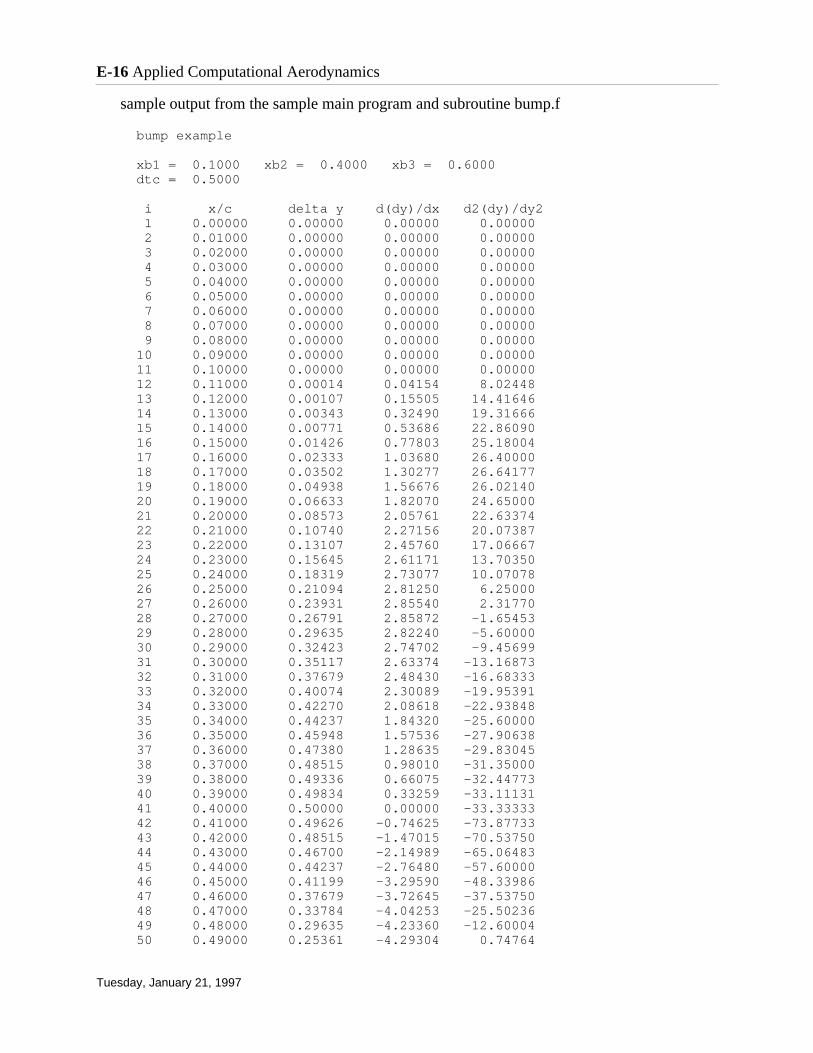
sample output from the sample main program and subroutine bump.f
bump example
xb1 = 0.1000 xb2 = 0.4000 xb3 = 0.6000 dtc = 0.5000
i x/c delta y d(dy)/dx d2(dy)/dy2 1 0.00000 0.00000 0.00000 0.00000 2 0.01000 0.00000 0.00000 0.00000 3 0.02000 0.00000 0.00000 0.00000 4 0.03000 0.00000 0.00000 0.00000 5 0.04000 0.00000 0.00000 0.00000 6 0.05000 0.00000 0.00000 0.00000 7 0.06000 0.00000 0.00000 0.00000 8 0.07000 0.00000 0.00000 0.00000 9 0.08000 0.00000 0.00000 0.00000 10 0.09000 0.00000 0.00000 0.00000 11 0.10000 0.00000 0.00000 0.00000 12 0.11000 0.00014 0.04154 8.02448 13 0.12000 0.00107 0.15505 14.41646 14 0.13000 0.00343 0.32490 19.31666 15 0.14000 0.00771 0.53686 22.86090 16 0.15000 0.01426 0.77803 25.18004 17 0.16000 0.02333 1.03680 26.40000 18 0.17000 0.03502 1.30277 26.64177 19 0.18000 0.04938 1.56676 26.02140 20 0.19000 0.06633 1.82070 24.65000 21 0.20000 0.08573 2.05761 22.63374 22 0.21000 0.10740 2.27156 20.07387 23 0.22000 0.13107 2.45760 17.06667 24 0.23000 0.15645 2.61171 13.70350 25 0.24000 0.18319 2.73077 10.07078 26 0.25000 0.21094 2.81250 6.25000 27 0.26000 0.23931 2.85540 2.31770 28 0.27000 0.26791 2.85872 -1.65453 29 0.28000 0.29635 2.82240 -5.60000 30 0.29000 0.32423 2.74702 -9.45699 31 0.30000 0.35117 2.63374 -13.16873 32 0.31000 0.37679 2.48430 -16.68333 33 0.32000 0.40074 2.30089 -19.95391 34 0.33000 0.42270 2.08618 -22.93848 35 0.34000 0.44237 1.84320 -25.60000 36 0.35000 0.45948 1.57536 -27.90638 37 0.36000 0.47380 1.28635 -29.83045 38 0.37000 0.48515 0.98010 -31.35000 39 0.38000 0.49336 0.66075 -32.44773 40 0.39000 0.49834 0.33259 -33.11131 41 0.40000 0.50000 0.00000 -33.33333 42 0.41000 0.49626 -0.74625 -73.87733 43 0.42000 0.48515 -1.47015 -70.53750 44 0.43000 0.46700 -2.14989 -65.06483 45 0.44000 0.44237 -2.76480 -57.60000 46 0.45000 0.41199 -3.29590 -48.33986 47 0.46000 0.37679 -3.72645 -37.53750 48 0.47000 0.33784 -4.04253 -25.50236 49 0.48000 0.29635 -4.23360 -12.60004 50 0.49000 0.25361 -4.29304 0.74764
E-16 Applied Computational Aerodynamics
Tuesday, January 21, 1997

51 0.50000 0.21094 -4.21875 14.06247 52 0.51000 0.16967 -4.01368 26.81011 53 0.52000 0.13107 -3.68640 38.39995 54 0.53000 0.09630 -3.25169 48.18510 55 0.54000 0.06633 -2.73105 55.46249 56 0.55000 0.04187 -2.15332 59.47264 57 0.56000 0.02333 -1.55520 59.39999 58 0.57000 0.01068 -0.98183 54.37266 59 0.58000 0.00343 -0.48735 43.46253 60 0.59000 0.00046 -0.13547 25.68523 61 0.60000 0.00000 0.00000 0.00000 62 0.61000 0.00000 0.00000 0.00000 63 0.62000 0.00000 0.00000 0.00000 64 0.63000 0.00000 0.00000 0.00000 65 0.64000 0.00000 0.00000 0.00000 66 0.65000 0.00000 0.00000 0.00000 67 0.66000 0.00000 0.00000 0.00000 68 0.67000 0.00000 0.00000 0.00000 69 0.68000 0.00000 0.00000 0.00000 70 0.69000 0.00000 0.00000 0.00000 71 0.70000 0.00000 0.00000 0.00000 (rest of the output deleted)
report typos and errors to W.H. Mason Appendix E: Utility Programs E-17
Tuesday, January 21, 1997
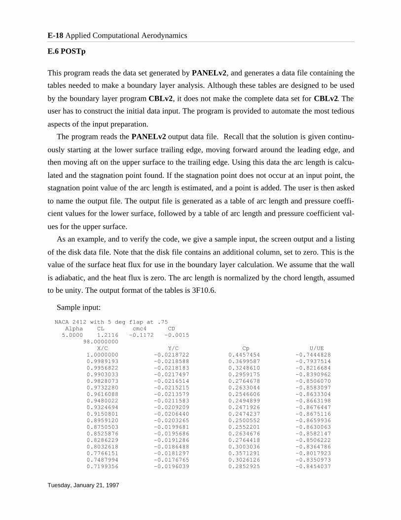
E.6 POSTp
This program reads the data set generated by PANELv2, and generates a data file containing the
tables needed to make a boundary layer analysis. Although these tables are designed to be used
by the boundary layer program CBLv2, it does not make the complete data set for CBLv2. The
user has to construct the initial data input. The program is provided to automate the most tedious
aspects of the input preparation.
The program reads the PANELv2 output data file. Recall that the solution is given continu-
ously starting at the lower surface trailing edge, moving forward around the leading edge, and
then moving aft on the upper surface to the trailing edge. Using this data the arc length is calcu-
lated and the stagnation point found. If the stagnation point does not occur at an input point, the
stagnation point value of the arc length is estimated, and a point is added. The user is then asked
to name the output file. The output file is generated as a table of arc length and pressure coeffi-
cient values for the lower surface, followed by a table of arc length and pressure coefficient val-
ues for the upper surface.
As an example, and to verify the code, we give a sample input, the screen output and a listing
of the disk data file. Note that the disk file contains an additional column, set to zero. This is the
value of the surface heat flux for use in the boundary layer calculation. We assume that the wall
is adiabatic, and the heat flux is zero. The arc length is normalized by the chord length, assumed
to be unity. The output format of the tables is 3F10.6.
Sample input: NACA 2412 with 5 deg flap at .75 Alpha CL cmc4 CD 5.0000 1.2116 -0.1172 -0.0015 98.0000000 X/C Y/C Cp U/UE 1.0000000 -0.0218722 0.4457454 -0.7444828 0.9989193 -0.0218588 0.3699587 -0.7937514 0.9956822 -0.0218183 0.3248610 -0.8216684 0.9903033 -0.0217497 0.2959175 -0.8390962 0.9828073 -0.0216514 0.2764678 -0.8506070 0.9732280 -0.0215215 0.2633044 -0.8583097 0.9616088 -0.0213579 0.2546606 -0.8633304 0.9480022 -0.0211583 0.2494899 -0.8663198 0.9324694 -0.0209209 0.2471926 -0.8676447 0.9150801 -0.0206440 0.2474237 -0.8675116 0.8959120 -0.0203265 0.2500552 -0.8659936 0.8750503 -0.0199681 0.2552201 -0.8630063 0.8525876 -0.0195686 0.2634676 -0.8582147 0.8286229 -0.0191286 0.2764418 -0.8506222 0.8032618 -0.0186488 0.3003036 -0.8364786 0.7766151 -0.0181297 0.3571291 -0.8017923 0.7487994 -0.0176765 0.3026126 -0.8350973 0.7199356 -0.0196039 0.2852925 -0.8454037
E-18 Applied Computational Aerodynamics
Tuesday, January 21, 1997
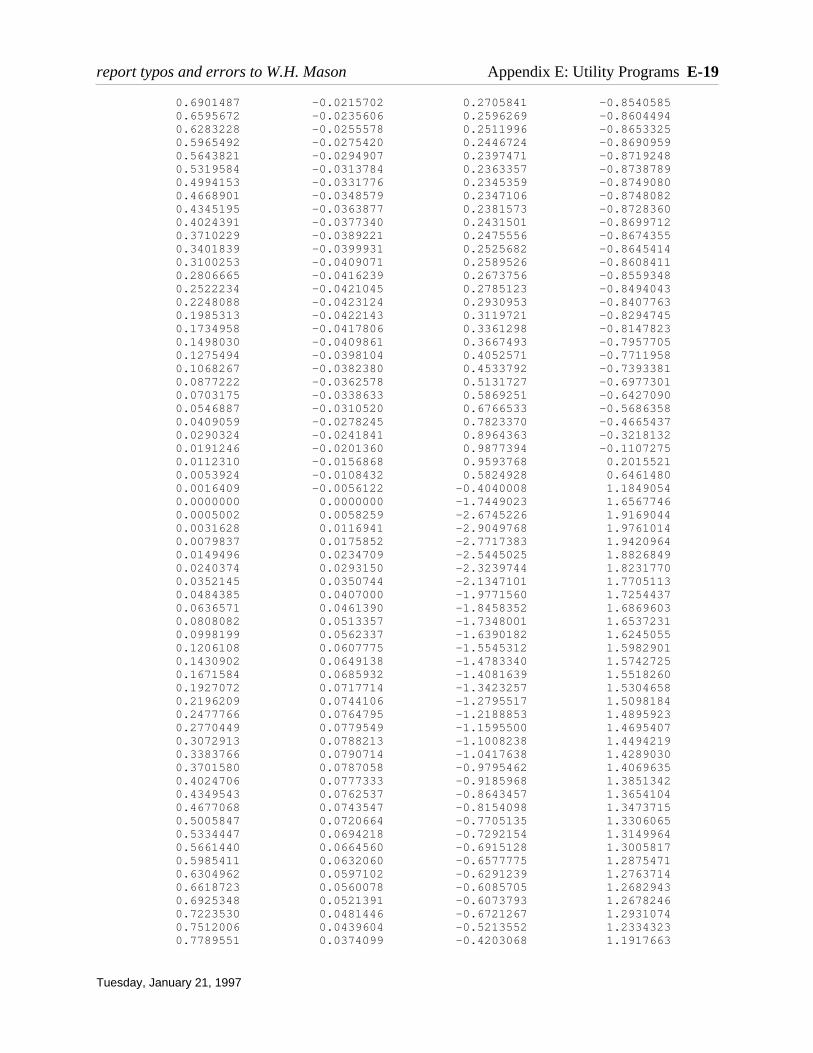
0.6901487 -0.0215702 0.2705841 -0.8540585 0.6595672 -0.0235606 0.2596269 -0.8604494 0.6283228 -0.0255578 0.2511996 -0.8653325 0.5965492 -0.0275420 0.2446724 -0.8690959 0.5643821 -0.0294907 0.2397471 -0.8719248 0.5319584 -0.0313784 0.2363357 -0.8738789 0.4994153 -0.0331776 0.2345359 -0.8749080 0.4668901 -0.0348579 0.2347106 -0.8748082 0.4345195 -0.0363877 0.2381573 -0.8728360 0.4024391 -0.0377340 0.2431501 -0.8699712 0.3710229 -0.0389221 0.2475556 -0.8674355 0.3401839 -0.0399931 0.2525682 -0.8645414 0.3100253 -0.0409071 0.2589526 -0.8608411 0.2806665 -0.0416239 0.2673756 -0.8559348 0.2522234 -0.0421045 0.2785123 -0.8494043 0.2248088 -0.0423124 0.2930953 -0.8407763 0.1985313 -0.0422143 0.3119721 -0.8294745 0.1734958 -0.0417806 0.3361298 -0.8147823 0.1498030 -0.0409861 0.3667493 -0.7957705 0.1275494 -0.0398104 0.4052571 -0.7711958 0.1068267 -0.0382380 0.4533792 -0.7393381 0.0877222 -0.0362578 0.5131727 -0.6977301 0.0703175 -0.0338633 0.5869251 -0.6427090 0.0546887 -0.0310520 0.6766533 -0.5686358 0.0409059 -0.0278245 0.7823370 -0.4665437 0.0290324 -0.0241841 0.8964363 -0.3218132 0.0191246 -0.0201360 0.9877394 -0.1107275 0.0112310 -0.0156868 0.9593768 0.2015521 0.0053924 -0.0108432 0.5824928 0.6461480 0.0016409 -0.0056122 -0.4040008 1.1849054 0.0000000 0.0000000 -1.7449023 1.6567746 0.0005002 0.0058259 -2.6745226 1.9169044 0.0031628 0.0116941 -2.9049768 1.9761014 0.0079837 0.0175852 -2.7717383 1.9420964 0.0149496 0.0234709 -2.5445025 1.8826849 0.0240374 0.0293150 -2.3239744 1.8231770 0.0352145 0.0350744 -2.1347101 1.7705113 0.0484385 0.0407000 -1.9771560 1.7254437 0.0636571 0.0461390 -1.8458352 1.6869603 0.0808082 0.0513357 -1.7348001 1.6537231 0.0998199 0.0562337 -1.6390182 1.6245055 0.1206108 0.0607775 -1.5545312 1.5982901 0.1430902 0.0649138 -1.4783340 1.5742725 0.1671584 0.0685932 -1.4081639 1.5518260 0.1927072 0.0717714 -1.3423257 1.5304658 0.2196209 0.0744106 -1.2795517 1.5098184 0.2477766 0.0764795 -1.2188853 1.4895923 0.2770449 0.0779549 -1.1595500 1.4695407 0.3072913 0.0788213 -1.1008238 1.4494219 0.3383766 0.0790714 -1.0417638 1.4289030 0.3701580 0.0787058 -0.9795462 1.4069635 0.4024706 0.0777333 -0.9185968 1.3851342 0.4349543 0.0762537 -0.8643457 1.3654104 0.4677068 0.0743547 -0.8154098 1.3473715 0.5005847 0.0720664 -0.7705135 1.3306065 0.5334447 0.0694218 -0.7292154 1.3149964 0.5661440 0.0664560 -0.6915128 1.3005817 0.5985411 0.0632060 -0.6577775 1.2875471 0.6304962 0.0597102 -0.6291239 1.2763714 0.6618723 0.0560078 -0.6085705 1.2682943 0.6925348 0.0521391 -0.6073793 1.2678246 0.7223530 0.0481446 -0.6721267 1.2931074 0.7512006 0.0439604 -0.5213552 1.2334323 0.7789551 0.0374099 -0.4203068 1.1917663
report typos and errors to W.H. Mason Appendix E: Utility Programs E-19
Tuesday, January 21, 1997

0.8054997 0.0309641 -0.3440065 1.1593130 0.8307229 0.0246744 -0.2788006 1.1308407 0.8545192 0.0185923 -0.2196457 1.1043757 0.8767895 0.0127683 -0.1642191 1.0789899 0.8974414 0.0072517 -0.1111093 1.0540917 0.9163895 0.0020905 -0.0593664 1.0292553 0.9335560 -0.0026691 -0.0082251 1.0041041 0.9488706 -0.0069838 0.0429915 0.9782681 0.9622707 -0.0108130 0.0950488 0.9512892 0.9737022 -0.0141200 0.1489126 0.9225440 0.9831185 -0.0168725 0.2061138 0.8910029 0.9904819 -0.0190429 0.2693959 0.8547539 0.9957626 -0.0206093 0.3448462 0.8094157
0.9989396 -0.0215556 0.4457439 0.7444838
Output to screen:
PGM POSTP - POST PROCESS DATA FROM PGM. PANELv2
ECHO OF INPUT DATA:
Enter name of file to be read:postp.test
Input data: NACA 2412 with 5 deg flap at .75 Alpha CL cmc4 CD 5.00000 1.21160 -0.11720 -0.00150 98.0000000 X/C Y/C Cp U/UE 1 1.0000000 -0.0218722 0.4457454 -0.7444828 2 0.9989193 -0.0218588 0.3699587 -0.7937514 3 0.9956822 -0.0218183 0.3248610 -0.8216684 4 0.9903033 -0.0217497 0.2959175 -0.8390962 5 0.9828073 -0.0216514 0.2764678 -0.8506070 6 0.9732280 -0.0215215 0.2633044 -0.8583097 7 0.9616088 -0.0213579 0.2546606 -0.8633304 8 0.9480022 -0.0211583 0.2494899 -0.8663198 9 0.9324694 -0.0209209 0.2471926 -0.8676447 10 0.9150801 -0.0206440 0.2474237 -0.8675116 11 0.8959120 -0.0203265 0.2500552 -0.8659936 12 0.8750503 -0.0199681 0.2552201 -0.8630063 13 0.8525876 -0.0195686 0.2634676 -0.8582147 14 0.8286229 -0.0191286 0.2764418 -0.8506222 15 0.8032618 -0.0186488 0.3003036 -0.8364786 16 0.7766151 -0.0181297 0.3571291 -0.8017923 17 0.7487994 -0.0176765 0.3026126 -0.8350973 18 0.7199356 -0.0196039 0.2852925 -0.8454037 19 0.6901487 -0.0215702 0.2705841 -0.8540585 20 0.6595672 -0.0235606 0.2596269 -0.8604494 21 0.6283228 -0.0255578 0.2511996 -0.8653325 22 0.5965492 -0.0275420 0.2446724 -0.8690959 23 0.5643821 -0.0294907 0.2397471 -0.8719248 24 0.5319584 -0.0313784 0.2363357 -0.8738789 25 0.4994153 -0.0331776 0.2345359 -0.8749080 26 0.4668901 -0.0348579 0.2347106 -0.8748082 27 0.4345195 -0.0363877 0.2381573 -0.8728360 28 0.4024391 -0.0377340 0.2431501 -0.8699712 29 0.3710229 -0.0389221 0.2475556 -0.8674355 30 0.3401839 -0.0399931 0.2525682 -0.8645414 31 0.3100253 -0.0409071 0.2589526 -0.8608411 32 0.2806665 -0.0416239 0.2673756 -0.8559348 33 0.2522234 -0.0421045 0.2785123 -0.8494043 34 0.2248088 -0.0423124 0.2930953 -0.8407763
E-20 Applied Computational Aerodynamics
Tuesday, January 21, 1997
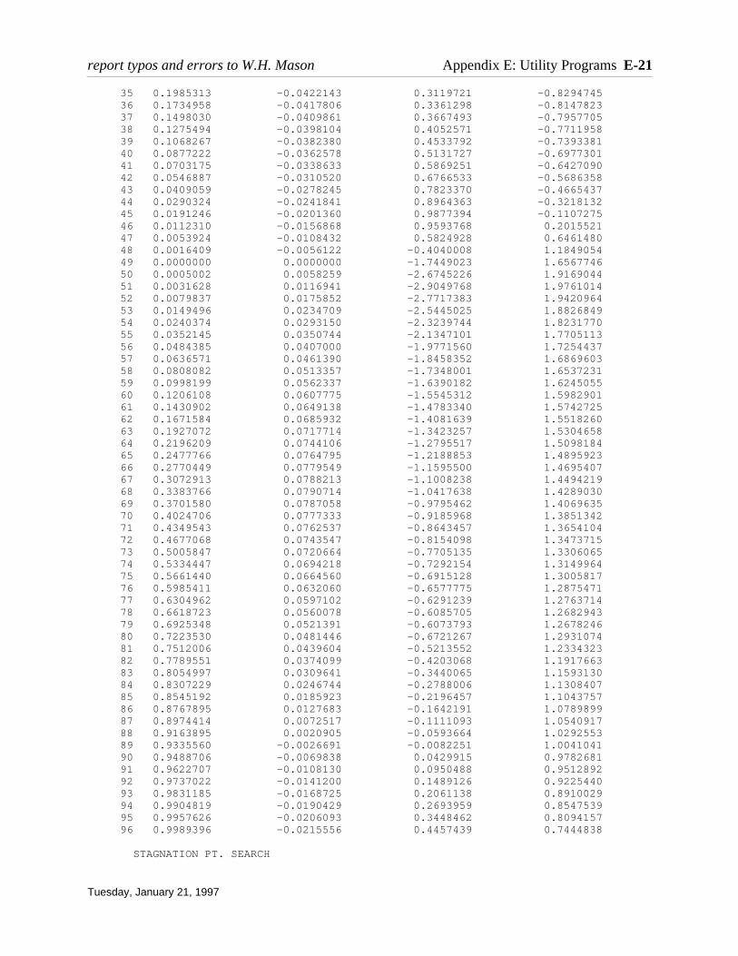
35 0.1985313 -0.0422143 0.3119721 -0.8294745 36 0.1734958 -0.0417806 0.3361298 -0.8147823 37 0.1498030 -0.0409861 0.3667493 -0.7957705 38 0.1275494 -0.0398104 0.4052571 -0.7711958 39 0.1068267 -0.0382380 0.4533792 -0.7393381 40 0.0877222 -0.0362578 0.5131727 -0.6977301 41 0.0703175 -0.0338633 0.5869251 -0.6427090 42 0.0546887 -0.0310520 0.6766533 -0.5686358 43 0.0409059 -0.0278245 0.7823370 -0.4665437 44 0.0290324 -0.0241841 0.8964363 -0.3218132 45 0.0191246 -0.0201360 0.9877394 -0.1107275 46 0.0112310 -0.0156868 0.9593768 0.2015521 47 0.0053924 -0.0108432 0.5824928 0.6461480 48 0.0016409 -0.0056122 -0.4040008 1.1849054 49 0.0000000 0.0000000 -1.7449023 1.6567746 50 0.0005002 0.0058259 -2.6745226 1.9169044 51 0.0031628 0.0116941 -2.9049768 1.9761014 52 0.0079837 0.0175852 -2.7717383 1.9420964 53 0.0149496 0.0234709 -2.5445025 1.8826849 54 0.0240374 0.0293150 -2.3239744 1.8231770 55 0.0352145 0.0350744 -2.1347101 1.7705113 56 0.0484385 0.0407000 -1.9771560 1.7254437 57 0.0636571 0.0461390 -1.8458352 1.6869603 58 0.0808082 0.0513357 -1.7348001 1.6537231 59 0.0998199 0.0562337 -1.6390182 1.6245055 60 0.1206108 0.0607775 -1.5545312 1.5982901 61 0.1430902 0.0649138 -1.4783340 1.5742725 62 0.1671584 0.0685932 -1.4081639 1.5518260 63 0.1927072 0.0717714 -1.3423257 1.5304658 64 0.2196209 0.0744106 -1.2795517 1.5098184 65 0.2477766 0.0764795 -1.2188853 1.4895923 66 0.2770449 0.0779549 -1.1595500 1.4695407 67 0.3072913 0.0788213 -1.1008238 1.4494219 68 0.3383766 0.0790714 -1.0417638 1.4289030 69 0.3701580 0.0787058 -0.9795462 1.4069635 70 0.4024706 0.0777333 -0.9185968 1.3851342 71 0.4349543 0.0762537 -0.8643457 1.3654104 72 0.4677068 0.0743547 -0.8154098 1.3473715 73 0.5005847 0.0720664 -0.7705135 1.3306065 74 0.5334447 0.0694218 -0.7292154 1.3149964 75 0.5661440 0.0664560 -0.6915128 1.3005817 76 0.5985411 0.0632060 -0.6577775 1.2875471 77 0.6304962 0.0597102 -0.6291239 1.2763714 78 0.6618723 0.0560078 -0.6085705 1.2682943 79 0.6925348 0.0521391 -0.6073793 1.2678246 80 0.7223530 0.0481446 -0.6721267 1.2931074 81 0.7512006 0.0439604 -0.5213552 1.2334323 82 0.7789551 0.0374099 -0.4203068 1.1917663 83 0.8054997 0.0309641 -0.3440065 1.1593130 84 0.8307229 0.0246744 -0.2788006 1.1308407 85 0.8545192 0.0185923 -0.2196457 1.1043757 86 0.8767895 0.0127683 -0.1642191 1.0789899 87 0.8974414 0.0072517 -0.1111093 1.0540917 88 0.9163895 0.0020905 -0.0593664 1.0292553 89 0.9335560 -0.0026691 -0.0082251 1.0041041 90 0.9488706 -0.0069838 0.0429915 0.9782681 91 0.9622707 -0.0108130 0.0950488 0.9512892 92 0.9737022 -0.0141200 0.1489126 0.9225440 93 0.9831185 -0.0168725 0.2061138 0.8910029 94 0.9904819 -0.0190429 0.2693959 0.8547539 95 0.9957626 -0.0206093 0.3448462 0.8094157 96 0.9989396 -0.0215556 0.4457439 0.7444838
STAGNATION PT. SEARCH
report typos and errors to W.H. Mason Appendix E: Utility Programs E-21
Tuesday, January 21, 1997

J X/C Y/C SARC UE/UINF CP
40 0.087722 -0.036258 0.913194 -0.697730 0.513173 41 0.070317 -0.033863 0.930764 -0.642709 0.586925 42 0.054689 -0.031052 0.946645 -0.568636 0.676653 43 0.040906 -0.027825 0.960803 -0.466544 0.782337 44 0.029032 -0.024184 0.973225 -0.321813 0.896436 45 0.019125 -0.020136 0.983934 -0.110727 0.987739 46 0.011231 -0.015687 0.993005 0.201552 0.959377 47 0.005392 -0.010843 1.000607 0.646148 0.582493 48 0.001641 -0.005612 1.007069 1.184905 -0.404001 49 0.000000 0.000000 1.012945 1.656775 -1.744902 50 0.000500 0.005826 1.018822 1.916904 -2.674523
STAG PT: XSP= 0.016326 YSP=-0.018558 SSP=0.987150 JS=45 JLE=49
E1 = 0.0032163 E2 = 0.0058546 ISTAGP = 1
OUTPUT OF POSTp RESULTS
send output to a file? (Y/N):y
enter file name:postp.out
ALPHA = 5.00000 MACH NO. = 0.10000 CL = 1.21160 CMC4 = -0.11720 CD = -0.00150 No. of upper surface values in x/c, Cp table = 52 No. of lower surface values in x/c, Cp table = 46
lower surface
J X/C Y/C S/C U/UINF CP 1 0.016326 -0.018558 0.000000 0.000000 1.000000 2 0.019125 -0.020136 0.003216 -0.110727 0.987739 3 0.029032 -0.024184 0.013925 -0.321813 0.896436 4 0.040906 -0.027825 0.026347 -0.466544 0.782337 5 0.054689 -0.031052 0.040505 -0.568636 0.676653 6 0.070317 -0.033863 0.056386 -0.642709 0.586925 7 0.087722 -0.036258 0.073956 -0.697730 0.513173 8 0.106827 -0.038238 0.093164 -0.739338 0.453379 9 0.127549 -0.039810 0.113946 -0.771196 0.405257 10 0.149803 -0.040986 0.136232 -0.795771 0.366749 11 0.173496 -0.041781 0.159938 -0.814782 0.336130 12 0.198531 -0.042214 0.184977 -0.829475 0.311972 13 0.224809 -0.042312 0.211255 -0.840776 0.293095 14 0.252223 -0.042105 0.238671 -0.849404 0.278512 15 0.280667 -0.041624 0.267118 -0.855935 0.267376 16 0.310025 -0.040907 0.296486 -0.860841 0.258953 17 0.340184 -0.039993 0.326658 -0.864541 0.252568 18 0.371023 -0.038922 0.357516 -0.867436 0.247556 19 0.402439 -0.037734 0.388954 -0.869971 0.243150 20 0.434519 -0.036388 0.421063 -0.872836 0.238157 21 0.466890 -0.034858 0.453470 -0.874808 0.234711 22 0.499415 -0.033178 0.486039 -0.874908 0.234536 23 0.531958 -0.031378 0.518631 -0.873879 0.236336 24 0.564382 -0.029491 0.551110 -0.871925 0.239747 25 0.596549 -0.027542 0.583336 -0.869096 0.244672
E-22 Applied Computational Aerodynamics
Tuesday, January 21, 1997

26 0.628323 -0.025558 0.615171 -0.865332 0.251200 27 0.659567 -0.023561 0.646480 -0.860449 0.259627 28 0.690149 -0.021570 0.677126 -0.854059 0.270584 29 0.719936 -0.019604 0.706978 -0.845404 0.285293 30 0.748799 -0.017677 0.735910 -0.835097 0.302613 31 0.776615 -0.018130 0.763733 -0.801792 0.357129 32 0.803262 -0.018649 0.790385 -0.836479 0.300304 33 0.828623 -0.019129 0.815751 -0.850622 0.276442 34 0.852588 -0.019569 0.839719 -0.858215 0.263468 35 0.875050 -0.019968 0.862186 -0.863006 0.255220 36 0.895912 -0.020327 0.883050 -0.865994 0.250055 37 0.915080 -0.020644 0.902221 -0.867512 0.247424 38 0.932469 -0.020921 0.919613 -0.867645 0.247193 39 0.948002 -0.021158 0.935147 -0.866320 0.249490 40 0.961609 -0.021358 0.948755 -0.863330 0.254661 41 0.973228 -0.021521 0.960376 -0.858310 0.263304 42 0.982807 -0.021651 0.969956 -0.850607 0.276468 43 0.990303 -0.021750 0.977452 -0.839096 0.295918 44 0.995682 -0.021818 0.982832 -0.821668 0.324861 45 0.998919 -0.021859 0.986069 -0.793751 0.369959 46 1.000000 -0.021872 0.987150 -0.744483 0.445745
upper surface
J X/C Y/C S/C U/UINF CP 1 0.016326 -0.018558 0.000000 0.000000 1.000000 2 0.011231 -0.015687 0.005855 0.201552 0.959377 3 0.005392 -0.010843 0.013457 0.646148 0.582493 4 0.001641 -0.005612 0.019919 1.184905 -0.404001 5 0.000000 0.000000 0.025795 1.656775 -1.744902 6 0.000500 0.005826 0.031672 1.916904 -2.674523 7 0.003163 0.011694 0.038141 1.976101 -2.904977 8 0.007984 0.017585 0.045770 1.942096 -2.771738 9 0.014950 0.023471 0.054900 1.882685 -2.544502 10 0.024037 0.029315 0.065711 1.823177 -2.323974 11 0.035214 0.035074 0.078289 1.770511 -2.134710 12 0.048439 0.040700 0.092662 1.725444 -1.977156 13 0.063657 0.046139 0.108826 1.686960 -1.845835 14 0.080808 0.051336 0.126748 1.653723 -1.734800 15 0.099820 0.056234 0.146382 1.624506 -1.639018 16 0.120611 0.060778 0.167665 1.598290 -1.554531 17 0.143090 0.064914 0.190523 1.574273 -1.478334 18 0.167158 0.068593 0.214871 1.551826 -1.408164 19 0.192707 0.071771 0.240618 1.530466 -1.342326 20 0.219621 0.074411 0.267661 1.509818 -1.279552 21 0.247777 0.076480 0.295894 1.489592 -1.218885 22 0.277045 0.077955 0.325200 1.469541 -1.159550 23 0.307291 0.078821 0.355459 1.449422 -1.100824 24 0.338377 0.079071 0.386546 1.428903 -1.041764 25 0.370158 0.078706 0.418330 1.406963 -0.979546 26 0.402471 0.077733 0.450657 1.385134 -0.918597 27 0.434954 0.076254 0.483175 1.365410 -0.864346 28 0.467707 0.074355 0.515983 1.347371 -0.815410 29 0.500585 0.072066 0.548940 1.330606 -0.770513 30 0.533445 0.069422 0.581907 1.314996 -0.729215 31 0.566144 0.066456 0.614740 1.300582 -0.691513 32 0.598541 0.063206 0.647300 1.287547 -0.657777 33 0.630496 0.059710 0.679446 1.276371 -0.629124 34 0.661872 0.056008 0.711040 1.268294 -0.608571 35 0.692535 0.052139 0.741946 1.267825 -0.607379 36 0.722353 0.048145 0.772030 1.293107 -0.672127 37 0.751201 0.043960 0.801185 1.233432 -0.521355 38 0.778955 0.037410 0.829706 1.191766 -0.420307 39 0.805500 0.030964 0.857022 1.159313 -0.344007
report typos and errors to W.H. Mason Appendix E: Utility Programs E-23
Tuesday, January 21, 1997

40 0.830723 0.024674 0.883018 1.130841 -0.278801 41 0.854519 0.018592 0.907579 1.104376 -0.219646 42 0.876790 0.012768 0.930598 1.078990 -0.164219 43 0.897441 0.007252 0.951975 1.054092 -0.111109 44 0.916390 0.002090 0.971613 1.029255 -0.059366 45 0.933556 -0.002669 0.989427 1.004104 -0.008225 46 0.948871 -0.006984 1.005338 0.978268 0.042992 47 0.962271 -0.010813 1.019274 0.951289 0.095049 48 0.973702 -0.014120 1.031175 0.922544 0.148913 49 0.983118 -0.016872 1.040985 0.891003 0.206114 50 0.990482 -0.019043 1.048661 0.854754 0.269396 51 0.995763 -0.020609 1.054170 0.809416 0.344846 52 0.998940 -0.021556 1.057485 0.744484 0.445744
STOP
Output disk data file: NACA 2412 with 5 deg flap at .75 5.00000 0.10000 1.21160 -0.11720 -0.00150
lower surface s/c Cp dT/dy 0.000000 1.000000 0.000000 0.003216 0.987739 0.000000 0.013925 0.896436 0.000000 0.026347 0.782337 0.000000 0.040505 0.676653 0.000000 0.056386 0.586925 0.000000 0.073956 0.513173 0.000000 0.093164 0.453379 0.000000 0.113946 0.405257 0.000000 0.136232 0.366749 0.000000 0.159938 0.336130 0.000000 0.184977 0.311972 0.000000 0.211255 0.293095 0.000000 0.238671 0.278512 0.000000 0.267118 0.267376 0.000000 0.296486 0.258953 0.000000 0.326658 0.252568 0.000000 0.357516 0.247556 0.000000 0.388954 0.243150 0.000000 0.421063 0.238157 0.000000 0.453470 0.234711 0.000000 0.486039 0.234536 0.000000 0.518631 0.236336 0.000000 0.551110 0.239747 0.000000 0.583336 0.244672 0.000000 0.615171 0.251200 0.000000 0.646480 0.259627 0.000000 0.677126 0.270584 0.000000 0.706978 0.285293 0.000000 0.735910 0.302613 0.000000 0.763733 0.357129 0.000000 0.790385 0.300304 0.000000 0.815751 0.276442 0.000000 0.839719 0.263468 0.000000 0.862186 0.255220 0.000000 0.883050 0.250055 0.000000 0.902221 0.247424 0.000000 0.919613 0.247193 0.000000 0.935147 0.249490 0.000000 0.948755 0.254661 0.000000 0.960376 0.263304 0.000000 0.969956 0.276468 0.000000
E-24 Applied Computational Aerodynamics
Tuesday, January 21, 1997

0.977452 0.295918 0.000000 0.982832 0.324861 0.000000 0.986069 0.369959 0.000000 0.987150 0.445745 0.000000
upper surface s/c Cp dT/dy 0.000000 1.000000 0.000000 0.005855 0.959377 0.000000 0.013457 0.582493 0.000000 0.019919 -0.404001 0.000000 0.025795 -1.744902 0.000000 0.031672 -2.674523 0.000000 0.038141 -2.904977 0.000000 0.045770 -2.771738 0.000000 0.054900 -2.544502 0.000000 0.065711 -2.323974 0.000000 0.078289 -2.134710 0.000000 0.092662 -1.977156 0.000000 0.108826 -1.845835 0.000000 0.126748 -1.734800 0.000000 0.146382 -1.639018 0.000000 0.167665 -1.554531 0.000000 0.190523 -1.478334 0.000000 0.214871 -1.408164 0.000000 0.240618 -1.342326 0.000000 0.267661 -1.279552 0.000000 0.295894 -1.218885 0.000000 0.325200 -1.159550 0.000000 0.355459 -1.100824 0.000000 0.386546 -1.041764 0.000000 0.418330 -0.979546 0.000000 0.450657 -0.918597 0.000000 0.483175 -0.864346 0.000000 0.515983 -0.815410 0.000000 0.548940 -0.770513 0.000000 0.581907 -0.729215 0.000000 0.614740 -0.691513 0.000000 0.647300 -0.657777 0.000000 0.679446 -0.629124 0.000000 0.711040 -0.608571 0.000000 0.741946 -0.607379 0.000000 0.772030 -0.672127 0.000000 0.801185 -0.521355 0.000000 0.829706 -0.420307 0.000000 0.857022 -0.344007 0.000000 0.883018 -0.278801 0.000000 0.907579 -0.219646 0.000000 0.930598 -0.164219 0.000000 0.951975 -0.111109 0.000000 0.971613 -0.059366 0.000000 0.989427 -0.008225 0.000000 1.005338 0.042992 0.000000 1.019274 0.095049 0.000000 1.031175 0.148913 0.000000 1.040985 0.206114 0.000000 1.048661 0.269396 0.000000 1.054170 0.344846 0.000000 1.057485 0.445744 0.000000
report typos and errors to W.H. Mason Appendix E: Utility Programs E-25
Tuesday, January 21, 1997

E.7 STDATM
This subroutine computes the 1976 standard atmosphere. It is used in program FRICTION. It
covers an altitude range from sea level to 86 kilometers (282,152 ft.). The results are found in ei-
ther English or metric units depending on the value of one of the input flags. The 1976 and 1962
standard atmospheres are identical for the first 51 kilometers above sea level.
Method of Computation
Given the geometric altitude Zin (in dimensions of either meters or feet), convert to kilom-
eters. The geopotential altitude H is then found from:
where r0 = 6356.766 kilometers (the radius of the Earth in kilometers) and Z = C1 Zin, where C1
= 0.001 if Zin is in meters, and C1 = 0.0003048 if Zin is in feet. The 1962 standard atmosphere
used a much more complicated and slightly more accurate relationship.
The inverse relation is given by
.
Once the geopotential altitude is found, the temperature is computed. The standard day tem-
perature profile is defined by seven layers, where within each layer the temperature is found by
the linear relation (T is given in degrees Kelvin):
and , and are the values at the base of the particular layer. The following table de-
fines these constants, as well as the ratio of pressure to sea level pressure, which is also needed.
i (Km) (°K) (°K/Km) P/Psl Z(ft.)
1 0. 288.15 -6.5 1.0 02 11. 216.65 0.0 2.2336x10⁻¹ 36,152.3 20. 216.65 +1.0 5.4032x10⁻² 65,8244 32. 228.65 +2.8 8.5666x10⁻³ 105,5185 47. 270.65 0.0 1.0945x10⁻³ 155,3486 51. 270.65 -2.8 6.6063x10⁻⁴ 168,6767 71. 214.65 -2.0 3.9046x10⁻⁵ 235,571- 82. - - - 282,152
E-26 Applied Computational Aerodynamics
Tuesday, January 21, 1997
LmiTbi
Hbi
HbiLmi
Tbi
T = Tbi+ Lmi
H − Hbi( )
Z =H
1− Hr0
H =Z
1+ Zr0
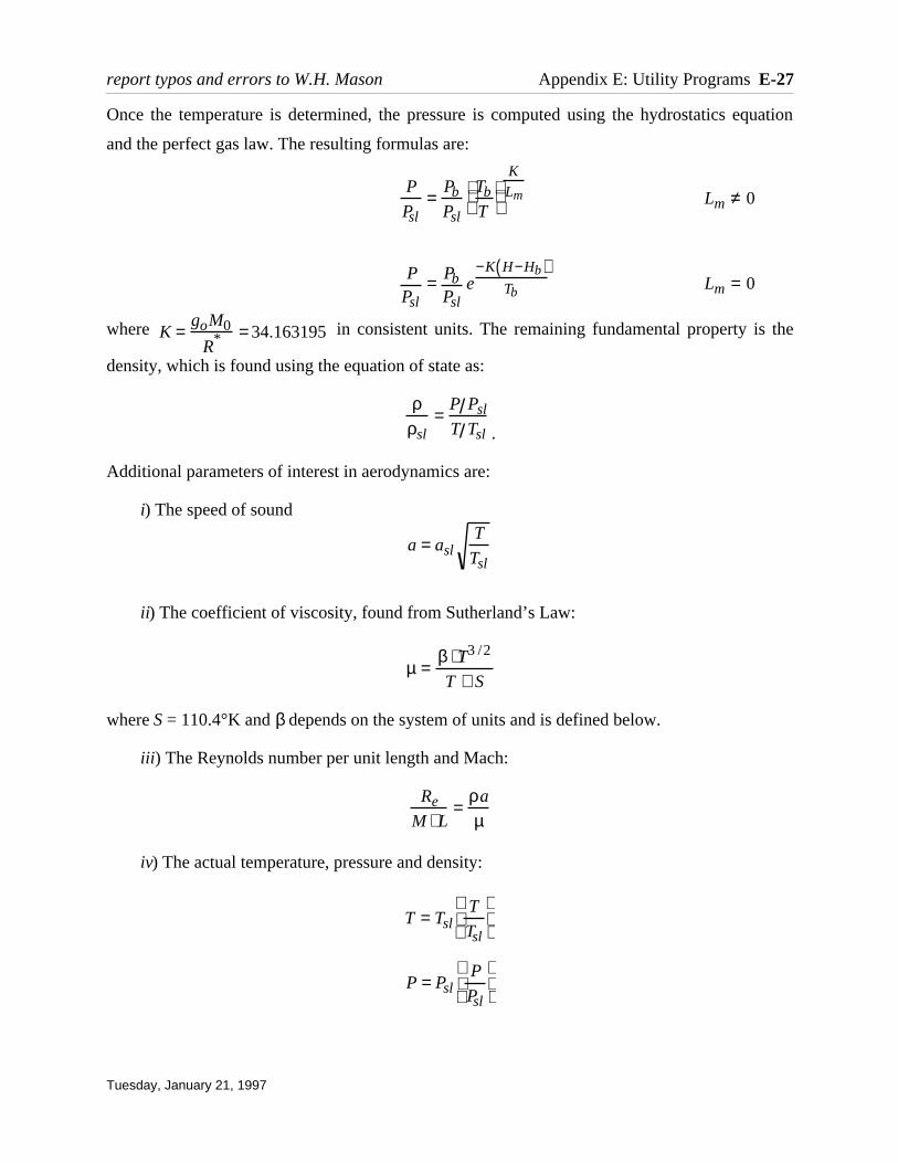
Once the temperature is determined, the pressure is computed using the hydrostatics equation
and the perfect gas law. The resulting formulas are:
where in consistent units. The remaining fundamental property is the
density, which is found using the equation of state as:
.
Additional parameters of interest in aerodynamics are:
i) The speed of sound
ii) The coefficient of viscosity, found from Sutherland’s Law:
where S = 110.4°K and β depends on the system of units and is defined below.
iii) The Reynolds number per unit length and Mach:
iv) The actual temperature, pressure and density:
report typos and errors to W.H. Mason Appendix E: Utility Programs E-27
Tuesday, January 21, 1997
P = PslP
Psl
T = TslT
Tsl
Re
M ⋅ L=
ρa
µ
µ =β ⋅ T3 /2
T + S
a = aslT
Tsl
ρρsl
=P Psl
T Tsl
K =goM0
R* = 34.163195
P
Psl=
Pb
Psl
Tb
T
K
Lm Lm ≠ 0
PPsl
= PbPsl
e−K H−Hb( )
TbLm = 0
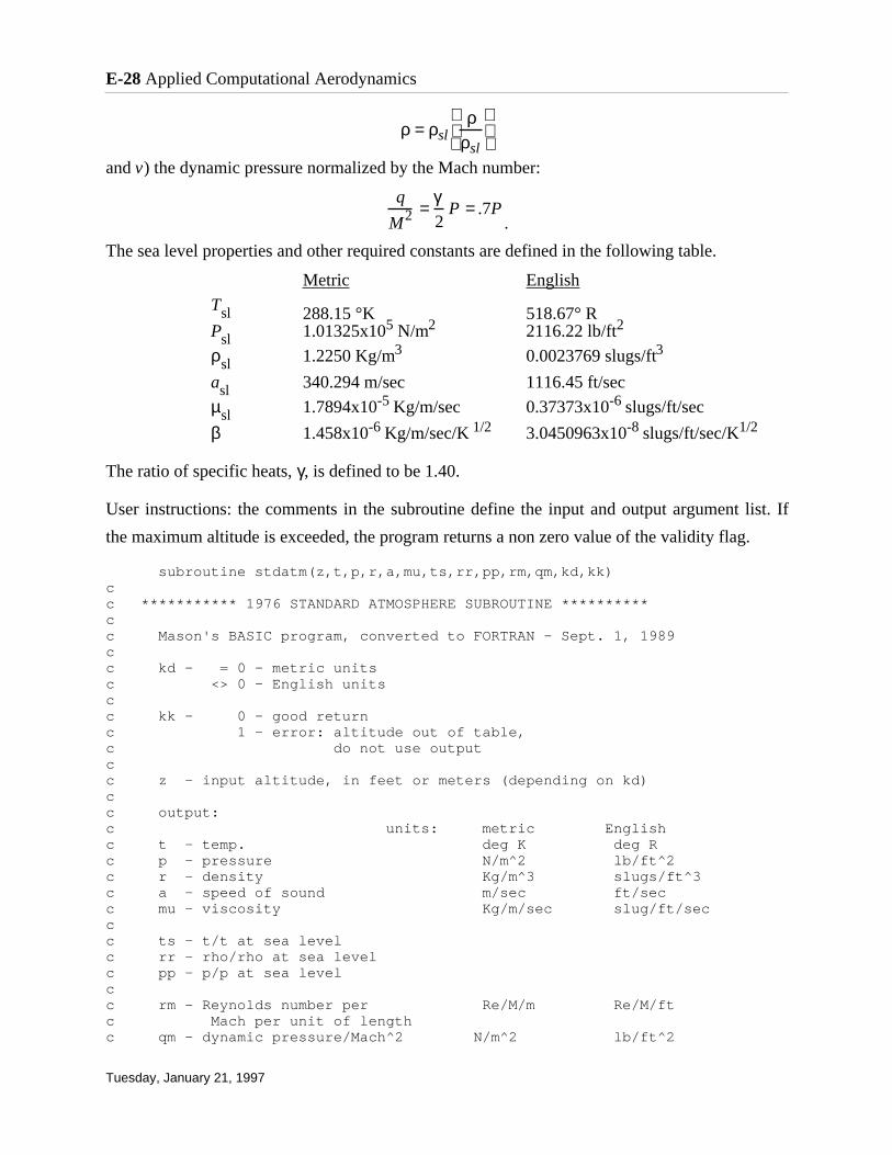
and v) the dynamic pressure normalized by the Mach number:
.
The sea level properties and other required constants are defined in the following table.
Metric English
Tsl 288.15 °K 518.67° RPsl 1.01325x10⁵ N/m2 2116.22 lb/ft2
ρsl 1.2250 Kg/m3 0.0023769 slugs/ft3
asl 340.294 m/sec 1116.45 ft/sec
µsl 1.7894x10⁻⁵ Kg/m/sec 0.37373x10⁻⁶ slugs/ft/sec
β 1.458x10⁻⁶ Kg/m/sec/K 1/2 3.0450963x10⁻⁸ slugs/ft/sec/K1/2
The ratio of specific heats, γ, is defined to be 1.40.
User instructions: the comments in the subroutine define the input and output argument list. If
the maximum altitude is exceeded, the program returns a non zero value of the validity flag.
subroutine stdatm(z,t,p,r,a,mu,ts,rr,pp,rm,qm,kd,kk)cc *********** 1976 STANDARD ATMOSPHERE SUBROUTINE **********cc Mason's BASIC program, converted to FORTRAN - Sept. 1, 1989cc kd - = 0 - metric unitsc <> 0 - English unitscc kk - 0 - good returnc 1 - error: altitude out of table,c do not use outputcc z - input altitude, in feet or meters (depending on kd)cc output:c units: metric Englishc t - temp. deg K deg Rc p - pressure N/m^2 lb/ft^2c r - density Kg/m^3 slugs/ft^3c a - speed of sound m/sec ft/secc mu - viscosity Kg/m/sec slug/ft/secc c ts - t/t at sea levelc rr - rho/rho at sea levelc pp - p/p at sea levelcc rm - Reynolds number per Re/M/m Re/M/ftc Mach per unit of lengthc qm - dynamic pressure/Mach^2 N/m^2 lb/ft^2
E-28 Applied Computational Aerodynamics
Tuesday, January 21, 1997
q
M2 =γ2
P = .7P
ρ = ρslρ
ρsl

c real k, h, mu, ml KK = 0 K = 34.163195 C1 = 3.048E-04 IF (KD .eq. 0) go to 1240 TL = 518.67 PL = 2116.22 RL = .0023769 AL = 1116.45 ML = 3.7373E-07 BT = 3.0450963E-08 GO TO 1260
1240 TL = 288.15 PL = 101325 RL = 1.225 C1 = .001 AL = 340.294 ML = 1.7894E-05 BT = 1.458E-06
1260 H = C1 * Z / (1 + C1 * Z / 6356.766) IF (H .gt. 11.0) go to 1290 T = 288.15 - 6.5 * H PP = (288.15 / T) ** ( - K / 6.5) GO TO 1420
1290 IF (H .gt. 20.0) go to 1310 T = 216.65 PP = .22336 * EXP ( - K * (H - 11) / 216.65) GO TO 1420
1310 IF (H .gt. 32.0) go to 1330 T = 216.65 + (H - 20) PP = .054032 * (216.65 / T) ** K GO TO 1420
1330 IF (H .gt. 47.0) go to 1350 T = 228.65 + 2.8 * (H - 32) PP = .0085666 * (228.65 / T) ** (K / 2.8) GO TO 1420
1350 IF( H .gt. 51.0) go to 1370 T = 270.65 PP = .0010945 * EXP ( - K * (H - 47) / 270.65) GO TO 1420
1370 IF (H .gt. 71.) go to 1390 T = 270.65 - 2.8 * (H - 51) PP = .00066063 * (270.65 / T) ** ( - K / 2.8) GO TO 1420
1390 IF (H .gt. 84.852) THEN kk = 1 write(6,200) H return END IF
report typos and errors to W.H. Mason Appendix E: Utility Programs E-29
Tuesday, January 21, 1997

T = 214.65 - 2 * (H - 71) PP = 3.9046E-05 * (214.65 / T) ** ( - K / 2)
1420 RR = PP / (T / 288.15) MU = BT * T**1.5 / (T + 110.4) TS = T / 288.15 A = AL * SQRT (TS) T = TL * TS R = RL * RR P = PL * PP RM = R * A / MU QM = .7 * P
200 format(' Out of Table in StdAtm- too high !'// 1 4x,'H =',f12.3,' > 84.852 km'/)
return end
The following sample program and output can be used to validate your subroutine:
c main program to check stdatm
c loop is done twice to get outputc suitable to include in text(80 col)
c w.h. mason, Feb. 27, 1994
real mu
kd = 1
write(6,90)
do 10 i = 1,21 z = 5000.*(i-1)
call stdatm(z,t,p,r,a,mu,ts,rr,pp,rm,qm,kd,kk)
if (kk .ne. 0) then write(6,120) stop endif
write(6,100) z,t,p,r,a,mu 10 continue
write(6,110) do 20 i = 1,21 z = 5000.*(i-1)
call stdatm(z,t,p,r,a,mu,ts,rr,pp,rm,qm,kd,kk)
if (kk .ne. 0) then write(6,160) stop endif
E-30 Applied Computational Aerodynamics
Tuesday, January 21, 1997
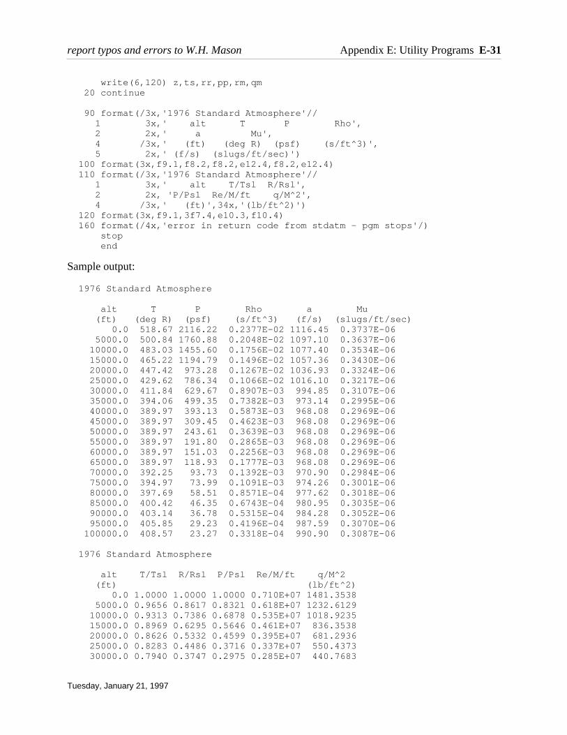
write(6,120) z,ts,rr,pp,rm,qm 20 continue
90 format(/3x,'1976 Standard Atmosphere'// 1 3x,' alt T P Rho', 2 2x,' a Mu', 4 /3x,' (ft) (deg R) (psf) (s/ft^3)', 5 2x,' (f/s) (slugs/ft/sec)') 100 format(3x,f9.1,f8.2,f8.2,e12.4,f8.2,e12.4) 110 format(/3x,'1976 Standard Atmosphere'// 1 3x,' alt T/Tsl R/Rsl', 2 2x, 'P/Psl Re/M/ft q/M^2', 4 /3x,' (ft)',34x,'(lb/ft^2)') 120 format(3x,f9.1,3f7.4,e10.3,f10.4) 160 format(/4x,'error in return code from stdatm - pgm stops'/) stop end
Sample output:
1976 Standard Atmosphere
alt T P Rho a Mu (ft) (deg R) (psf) (s/ft^3) (f/s) (slugs/ft/sec) 0.0 518.67 2116.22 0.2377E-02 1116.45 0.3737E-06 5000.0 500.84 1760.88 0.2048E-02 1097.10 0.3637E-06 10000.0 483.03 1455.60 0.1756E-02 1077.40 0.3534E-06 15000.0 465.22 1194.79 0.1496E-02 1057.36 0.3430E-06 20000.0 447.42 973.28 0.1267E-02 1036.93 0.3324E-06 25000.0 429.62 786.34 0.1066E-02 1016.10 0.3217E-06 30000.0 411.84 629.67 0.8907E-03 994.85 0.3107E-06 35000.0 394.06 499.35 0.7382E-03 973.14 0.2995E-06 40000.0 389.97 393.13 0.5873E-03 968.08 0.2969E-06 45000.0 389.97 309.45 0.4623E-03 968.08 0.2969E-06 50000.0 389.97 243.61 0.3639E-03 968.08 0.2969E-06 55000.0 389.97 191.80 0.2865E-03 968.08 0.2969E-06 60000.0 389.97 151.03 0.2256E-03 968.08 0.2969E-06 65000.0 389.97 118.93 0.1777E-03 968.08 0.2969E-06 70000.0 392.25 93.73 0.1392E-03 970.90 0.2984E-06 75000.0 394.97 73.99 0.1091E-03 974.26 0.3001E-06 80000.0 397.69 58.51 0.8571E-04 977.62 0.3018E-06 85000.0 400.42 46.35 0.6743E-04 980.95 0.3035E-06 90000.0 403.14 36.78 0.5315E-04 984.28 0.3052E-06 95000.0 405.85 29.23 0.4196E-04 987.59 0.3070E-06 100000.0 408.57 23.27 0.3318E-04 990.90 0.3087E-06
1976 Standard Atmosphere
alt T/Tsl R/Rsl P/Psl Re/M/ft q/M^2 (ft) (lb/ft^2) 0.0 1.0000 1.0000 1.0000 0.710E+07 1481.3538 5000.0 0.9656 0.8617 0.8321 0.618E+07 1232.6129 10000.0 0.9313 0.7386 0.6878 0.535E+07 1018.9235 15000.0 0.8969 0.6295 0.5646 0.461E+07 836.3538 20000.0 0.8626 0.5332 0.4599 0.395E+07 681.2936 25000.0 0.8283 0.4486 0.3716 0.337E+07 550.4373 30000.0 0.7940 0.3747 0.2975 0.285E+07 440.7683
report typos and errors to W.H. Mason Appendix E: Utility Programs E-31
Tuesday, January 21, 1997
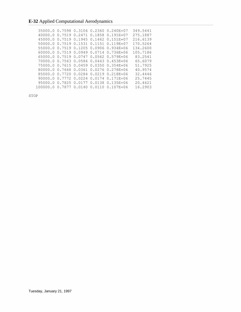
35000.0 0.7598 0.3106 0.2360 0.240E+07 349.5441 40000.0 0.7519 0.2471 0.1858 0.191E+07 275.1887 45000.0 0.7519 0.1945 0.1462 0.151E+07 216.6139 50000.0 0.7519 0.1531 0.1151 0.119E+07 170.5264 55000.0 0.7519 0.1205 0.0906 0.934E+06 134.2600 60000.0 0.7519 0.0949 0.0714 0.736E+06 105.7186 65000.0 0.7519 0.0747 0.0562 0.579E+06 83.2541 70000.0 0.7563 0.0586 0.0443 0.453E+06 65.6079 75000.0 0.7615 0.0459 0.0350 0.354E+06 51.7925 80000.0 0.7668 0.0361 0.0276 0.278E+06 40.9574 85000.0 0.7720 0.0284 0.0219 0.218E+06 32.4446 90000.0 0.7772 0.0224 0.0174 0.171E+06 25.7445 95000.0 0.7825 0.0177 0.0138 0.135E+06 20.4621 100000.0 0.7877 0.0140 0.0110 0.107E+06 16.2903
STOP
E-32 Applied Computational Aerodynamics
Tuesday, January 21, 1997

Appendix F Code and Electronic Information Sources This appendix collects a few useful sources of information. Special thanks to Philippe-Andre Tetrault for adding the actual links to the information sources. We include general numerical analysis programs, sources of aerodynamics codes, and places to look on the net for additional information.
F.1 Numerical Analysis Software A number of sources of numerical analysis subroutines are available at reasonable prices. Some are even free. Other numerical methods subroutines are expensive.
The standard source for numerical algorithms is netlib. The following information should help you get started using this resource:
Finding Numerical Analysis Software on the Web (from Tony Giunta)
The Netlib software repository is maintained by the Department of Energy's Oak Ride National Lab and the University of Tennessee at Knoxville. The software libraries in Netlib, provide computational tools, in the form of subroutines, to perform various mathematical and numerical analysis operations. Some of the packages of particular interest to engineers are LAPACK (linear algebra) and EISPACK (eigenvalue, eigenvector analysis). The software libraries come in a variety of languages. For example, LAPACK and CLAPACK libraries contain the same linear algebra routines in FORTRAN and C, respectively. Also, there are a number of libraries for C++, High-Performance FORTRAN (HPF), and FORTRAN90 subroutines, as well as parallel processing routines such as PVM and MPI.
The web site for Netlib provides a useful search tool which is the second item listed on the Netlib homepage. The directions on this home page indicate how to search for items of interest.
Note: Often, a particular subroutine uses a number of other Netlib routines in its calculations. Netlib gives the user the choice of downloading only the single subroutine or the subroutine and its dependencies. Usually it is a good idea to download all of the files unless the user is sure that only the single routine is needed.
Numerical Methods and Software, by David Kahaner, Cleve Moler and Stephen Nash, Prentice Hall, Englewood Cliffs, 1989.
This book comes with a disk containing a good collection of subroutines. These are actually comprehensive commercial grade subroutines that come from the standard public domain libraries. They are much larger routines than those in the Numerical Recipes book. Because they are much more comprehensive, I've found them to be slightly harder to use because they rely on numerous other subroutines, and collecting them sometimes takes more time. However, they also work very well. Because they are based on public domain programs, as far as I can tell, they can be distributed with your own programs without getting permission.
Numerical Recipes in FORTRAN, The Art of Scientific Computing, Second Edition by William H. Press, Saul A Teukolsky, William T. Vetterling, and Brian P. Flannery, Cambridge University Press, Cambridge, 1992.
This is the book most students use. It is available online in PostScript or Adobe Acrobat format. It contains listings of subroutines implementing the methods (recipes). The routines are brief, intended to illustrate the
PDF créé avec la version d'essai pdfFactory www.gs2i.fr/fineprint/pdffactory.htm

methods, and are not necessarily meant to be general purpose subroutines. However, my experience with them is good. Professional numerical analysts don't approve of using these routines, so be careful. Also, you cannot use them in codes you distribute. This is probably because the authors know the routines are not really a professional programming product. A disk with the programs is available for an additional cost, as is a small paperback book containing examples of the use of the programs. An edition of the book with the routines in the C language is also available, as well as an example book and disk. I have found these sources to be easy to use.
Elementary Numerical Analysis, by S.D. Conte and Carl de Boor, McGraw-Hill, New York, 2nd Ed., 1972.
This book has a number of good computer routines, including root finding, solution of equations, systems of linear algebraic equations, ordinary differential equations, quadrature and interpolation (splines).
SLATEC
This is a library of programs available electronically that are public domain. The authors of Numerical Recipes recommend the use of these routines for distribution. Once again, all the public domain libraries are closely related. However, there are not directly interchangeable, and you must be careful to not get them mixed up. SLATEC is very large.
>From the Numerical Recipes people: "If you are looking for public domain numerical software that can be redistributed freely (as Numerical Recipes *cannot*), you should look at the collections that can be obtained from NETLIB. We also recommend SLATEC as a good alternative to the commercial, and therefore restrictively licensed IMSL and NAG libraries."
• You can get the same information from the web page at http://netlib.bell-labs.com/netlib/master/readme.html
The SLATEC library, a comprehensive collection of over 1400 mathematical and statistical routines, may be of particular interest.t
Also from the Numerical Recipes gopher site, by W. Press:
The SLATEC Common Mathematical Library is an extensive public-domain FORTRAN source code library consisting of 1400 routines and 300,000 lines of code and documentation. It is developed and maintained by a consortium of Department of Energy and Department of Defense national laboratories. Version 4.0 of the library was released in December, 1992. It incorporates within itself several other public domain packages, including EISPACK, FFTPACK, QUADPACK, FNLIB, BSPLINE, SLAP, and others. It is distributed by
National Energy Software Center 9700 Cass Ave Argonne, Illinois 60439
All questions about the library should be directed there.
SLATEC's size is a problem. The routines are interconnected. To use a single routine, between 6 and 20 subsidiary routines may be required. As a public service, Numerical Recipes has put together a multiply cross-linked gopher tree. The tree allows the routines and their documentation to be located using gopher, either by subject or name. Most importantly, it allows a routine and its required subsidiary routines to be efficiently downloaded in source code form.
PDF créé avec la version d'essai pdfFactory www.gs2i.fr/fineprint/pdffactory.htm

Once in SLATEC, there are several things to remember: (1) Almost all the routines require at least several of the subroutines that have been collected in the file on the top level of the SLATEC directory called "slatec-util.f". Be sure to download this file, compile and link it with any other routines. (2) Documentation for each file (each .f file) is in a similarly-named .hdr file, in the same subject classified subdirectory of the tree. In the SLATEC library as released, the documentation is embedded in each FORTRAN file. (3) When a routine requires additional subsidiary routines, there are links to these routines in a dependencies directory, visible at the same level as the .f file. Example: to use the routine CBESJ (Bessel function of complex argument), you must download the files slatec-util.f (from the top directory), cbesj.f and cbesj.hdr (from the subject directory C10A4), and all the routines in "cbesj_dependencies" (also in C10A4).
F.2 Aerodynamics Codes See a software review for general codes useful in aerodynamics.
I also have a small set of codes available online.
F.2.1 Textbooks
Many text books contain listings illustrating the methods. They can be a valuable learning tool, although many of the codes were not written by computer scientists, and do not reflect good programming practice (remember they are included with the cost of the book, and thus are essentially free - remember you get what you pay for). In some cases graduate or even undergraduates wrote the programs. Textbooks with code listings:
Joseph A. Schetz, Boundary Layer Analysis, Prentice Hall, Englewood Cliffs, 1993.
• WALZ: The Thwaites-Walz integral method for laminar boundary layer flows • ILBLE: Explicit 2D Incompressible Laminar Boundary Layer Flows • ILBLI: Implicit 2D Incompressible Laminar Boundary Layer Flows • CLBL: Implicit numerical method, 2D Compressible Laminar Boundary Layer Flows • MOSES: The Moses integral method for 2D incompressible turbulent flows • ITBL: Incompressible Turbulent Boundary Layer, three turbulence models available:
o 1. mixing length model, o 2. eddy viscosity model, o 3. TKE model.
• ITBLS: Incompressible Turbulent Boundary Layers with stretched normal grid spacing. The Reichardt-Clauser eddy viscosity combination is used for the turbulence model.
• JETWAKE: Implicit numerical method for turbulent jets and wakes. Either a mixing length or TKE model are available for modeling turbulence.
Tuncer Cebeci and Peter Bradshaw, Momentum Transfer in Boundary Layers, Hemisphere Publishing Corp, New York, McGraw-Hill Book Company, 1977.
This book contains FORTRAN programs for:
• solution of Falkner-Skan equations • Thwaites' method • Head's method • block elimination meth. to solve 3rd order ODEs (linear or nonlinear) or parabolic PDE • thin shear layer equation solution for 2D lam. and turb. incompressible boundary layers
PDF créé avec la version d'essai pdfFactory www.gs2i.fr/fineprint/pdffactory.htm

Tuncer Cebeci and Peter Bradshaw, Physical and Computational Aspects of Convective Heat Transfer, Springer-Verlag, New York, 1984
• laminar and turbulent flows with fully developed velocity profile • solution of mass, momentum and energy equations for boundary layer flows • coupled boundary layer flows • free convection between two vertical parallel plates • wall jet and film heating • turbulent free jet • Head's method
There is also a paperback book which provides supplemental comments on these programs, as well as solutions obtained using them:
Tuncer Cebeci, Solutions Manual and Computer Programs for Physical and Computational Aspects of Convective Heat Transfer by Tuncer Cebeci and Peter Bradshaw, Springer-Verlag, New York, 1989
Jack Moran, An Introduction to Theoretical and Computational Aerodynamics, John Wiley & Sons, New York, 1984.
• RANKIN Rankine oval • DUBLET symmetric airfoil at zero angle of attack by doublet distribution JOUKOWQ shape & pressure
distribution on symmetric Joukowski airfoil at zero a • PANEL Hess-Smith panel method solution for incompressible inviscid airfoil flow • VORLAT vortex lattice method for flat unswept wing • INTGRL integral boundary layer calculation
o Thwaites' method for laminar flow o Michel's method for transition estimation o Head's method for turbulent boundary layer
• LINBVP finite difference method solution of the Sturm-Liouville problem • THINAIR finite difference solution via SOR of Laplace's Eqn. over a biconvex airfoil • HEATX explicit solution of 1-D heat equation • CRAKN Crank-Nicolson solution of 1-D heat equation • FALKSK finite difference solution of similarity solution of Falkner-Skan equation • FSKBOX Keller box method solution of the Falkner-Skan equation • BDYLAY laminar boundary layer equations for arbitrary pressure gradient. • TSDE finite difference solution of the transonic small disturbance equation
Joseph Katz and Allen Plotkin, Low-Speed Aerodynamics: From Wing Theory to Panel Methods, McGraw-Hill, Inc., 1991 Fourteen programs are in an appendix:
Two-dimensional panel methods
• 1. Grid Generator for van de Vooren airfoil shapes, includes velocity and pressure distributions
Two-dimensional panel methods based on Neumann BC
• 2. constant strength source method • 3. constant strength doublet method • 4. constant strength vortex method
PDF créé avec la version d'essai pdfFactory www.gs2i.fr/fineprint/pdffactory.htm

• 5. linear strength source method • 6. linear strength vortex method
Two-dimensional panel methods based on Dirichlet BC
• 7. constant strength doublet method • 8. constant strength source/doublet method • 9. linear strength doublet method • 10. quadratic strength doublet method
Three-dimensional programs
• 11. Influence of a 3D constant strength source/doublet element • 12. 3D vortex lattice method for rectilinear lifting surfaces (with ground effect)
Time Dependent Programs:
• 13. sudden acceleration of a flat plate at angle of attack • 14. unsteady motion of a thin rectangular lifting surface (extension to program 12)
C.B. Stribling, BASIC aerodynamics, Butterworths, London, 1984.
This book has listings of programs in BASIC, from the days way when BASIC was the primary language available on personal computers.
• ATMOS:atmospheric calculations • AIRSPEED: calculation of true airspeed and other related parameters • SPHDRAG: drag of a sphere • BALCAL: calibration of a three component wind tunnel balance • STRFUNC: evaluation of a streamfunction • STRCOORDS: streamlines of a source in a uniform stream • CYLCIRC: cylinder with circulation in a uniform stream • TRANSTRIP: positioning of wind tunnel transition strip • BOUNCALC: the reduction of experimental measurements of a boundary layer velocity profile • PLATEDRAG: the investigation of conditions in a flat plate boundary layer which is partly laminar and
partly turbulent • POHLHAUSEN: use of a Pohlhausen velocity profile to calculate conditions in a laminar boundary layer
with a specified external velocity gradient • TUNRESULT: the reduction of wind tunnel lift, pitching moment and incidence results • JOUVELPRE: the calculation of fluid speeds and pressure coefficients on the surface of a Joukowski
aerofoil with circulation at zero incidence • SOURPANL: the representation of a cylinder by a regular polygon of source panels. • THINAERO: the use of thin aerofoil theory to determine the aerodynamic properties of aerofoil sections
with prescribed camber lines • BIRDDRAG: calculation of the induced drag of birds flying in formation • DOWNWASH: investigation of the downwash field behind an aircraft wing in the wing's plane of
symmetry • MONOPLEQN: calculation of the lift and induced drag coefficients, and the spanwise loading
distribution of a specified wing, using the monoplane equation • VORLAT: application of the vortex lattice method to the calculation of lifting properties of a swept wing
PDF créé avec la version d'essai pdfFactory www.gs2i.fr/fineprint/pdffactory.htm

• DELTAWING: an investigation of the lift and drag characteristics of a slender delta wing at low Mach number
• FLOWDUCT: calculation of gas properties in compressible isentropic flow duct • MACHMETER: tabulation of corresponding values of Mach number and pressure ratio in the calibration
equation of the Machmeter • DOUBLEWED: a comparison of supersonic aerofoil theories • TIPEFFECT: calculations on the pressure distribution within the tip Mach triangle of a rectangular wing
at supersonic speeds
Joe F. Thompson, Z.U.A. Warsi, and C. Wayne Mastin, Numerical Grid Generation: Foundations and Applications, Elsevier Science Publishing Co., New York, 1985.
Model programs are included for:
• vertical interpolation • horizontal interpolation • tensor product interpolation • transfinite interpolation • hermite cubic interpolation • hyperbolic tangent interpolation • elliptic grid generation • attraction to coordinates
Patrick Knupp and Stanly Steinberg, Fundamentals of Grid Generation, CRC Press, Boca Raton, 1993.
This book comes with a disk containing examples of the methods covered in the book.
C.A.J. Fletcher, Computational Techniques for Fluid Dynamics, Springer-Verlag, Berlin, 1988.
Volume I, Fundamental and General Techniques
• DIFF: transient heat conduction (diffusion) problem • FIVOL: finite volume method applied to Laplace's equation • STURM: computation of the Sturm-Liouville equation • DUCT: viscous flow in a rectangular duct • NEWTON: flat-plate collector temperature analysis • NEWTBU: two-dimensional steady Burgers' equation • FACT/SOLVE solution of dense systems • BANFAC/BANSOL narrowly banded Gauss elimination • DIFEX numerical results for explicit schemes • DIFIM: numerical results for implicit schemes • TWDIF: generalized finite difference/finite element implementation • TRAN: convection of a temperature front • THERM: thermal entry problem • BURG numerical comparison • TWBURG: numerical solution
Volume II, Specific Techniques for Different Flow Categories
• LAGEN: generalized coordinate Laplace's equation
PDF créé avec la version d'essai pdfFactory www.gs2i.fr/fineprint/pdffactory.htm

• ALGEM: grid generation for a streamlined body • PANEL: numerical implementation of a panel method • SHOCK: propagating shock wave computation • FCT: propagating shockwave by an FCT algorithm • LAMBL: laminar boundary layer flow • DOROD: turbulent boundary layer flow • THRED: thermal entry problem
Arnold M. Kuethe and Chuen-Yen Chow, Foundations of Aerodynamics, John Wiley & Sons, New York, Fourth Edition, 1986. The fourth edition of this book has two listings of programs, in FORTRAN.
• AIRFOIL: a linearly varying vortex panel code method • FNTWING: solution of the monoplane equation of lifting line theory
R.I. Lewis, Vortex Element Methods for Fluid Dynamic Analysis of Engineering Systems, Cambridge University Press, Cambridge. These routines are in Pascal:
• 1.1 flow Past a circular cylinder including surface velocity, comparison with exact solution • 1.2 flow past a circular cylinder by the Douglas-Neumann source panel method • 1.3 flow past an ellipse, including surface velocity comparison with exact solution and streamline pattern • 2.1 calculation of flow past a cylinder with bound circulation • 2.2 flow past an ellipse with prescribed bound circulation • 2.3 potential flow past an airfoil • 2.4 potential flow through a turbomachine cascade • 4.1 calculation of complete elliptic integrals of the first and second kinds • 4.2 flow past a body of revolution • 4.3 flow past an axisymmetric cowl or duct • 4.4 flow through a contraction or diffuser • 4.5 flow past a body of revolution in a uniform stream • 5.1 potential flow through an engine intake sucked from downstream by a cylindrical duct and located in
a uniform stream (pipe flow test rig). • 5.2 potential flow through a free-vortex ducted propeller in a uniform stream • 8.1 program for experimentation with convection of vortex clouds. • 9.1 program to generate a set of random numbers and sort them. • 9.2 diffusion of a point vortex
F.2.2 Commercial vendors
This is a short list of vendors. Future versions of this appendix will contain more listings. Students should realize that some of these codes are not student programs and are (very) expensive by student standards.
AeroSoft, Inc. 1872 Pratt Drive, Suite 1275 Blacksburg, VA 24060-6363 Phone (540) 231-6125, FAX (540) 231-6137
AeroSoft sells GASP (General Aerodynamic Simulation Program), a general purpose flow solver. Primarily developed for hypersonic analysis, a particular strength is the capability to handle finite rate chemistry. However, the code can treat steady and unsteady flows across the Mach range.
PDF créé avec la version d'essai pdfFactory www.gs2i.fr/fineprint/pdffactory.htm

Analytical Methods, Inc. 2133 - 152nd Avenue N.E. Redmond, WA, 98052 Phone (206) 643-9090, FAX (206) 746-1299
AMI sells a number of codes. They include
• VSAERO, a panel method that has been developed over many years • USAERO, an extension of VSAERO, computes unsteady aero for arbitrary motion • ICE, calculates particle trajectories near aircraft for use in icing and sand-ingestion • HOVER and ROTAIR, helicopter rotor hover and climb aerodynamic performance • MGAERO, a 3D Euler method for arbitrary configurations • OMNIPLOT, OMNI3D, post processing programs for use with AMI codes • RANSTERN, 3D Reynolds Averaged Navier Stokes code, incompressible (Iowa) • XFOIL and ISES, Mark Drela's airfoil design and analysis codes. (MIT) • ZAP2D, potential flow/Navier-Stokes code for 2D airfoil analysis (uses ARC2D)
Desktop Aeronautics P.O. Box 9937 Stanford, CA 94305 Phone (415) 424-8588
These are the codes by Ilan Kroo. Currently they run on Macintosh computers, but some are available for IBM PCs. Programs currently available include:
• LinAir 1.4 - Multiple Lifting Surface Analysis Program ($200), LinAir Pro ($950). These codes treat complete configurations in subsonic flow, using a discrete Weissinger method. They include profile drag integration and Trefftz-plane induced drag calculation. They handle wing canard, aft tail, and winglet configurations. The Pro version includes asymmetric aircraft or sideslip, roll, pitch, and yaw rates, and nearfield drag calculations.
• PANDA: Program for Analysis and Design of Airfoils ($175). Subsonic, including compressibility effects via Karman-Tsien rule. Includes an integral boundary layer calculation for laminar and turbulent flow. A design option permits interactive change of airfoil geometry and display of the new pressure distribution.
• Wing Design ($50), for quick computation and plotting of lift and Cl distributions on swept, tapered, twisted wings. Wing geometry changes effects on lift, drag, moment, and load distribution are found rapidly.
• SAND-Simulation of Aircraft Nonlinear Dynamics($200). Six degree of freedom time history computation. Interactive specification of control deflections, time and position dependent wind, and built in plotting are included. User supplied subroutines for computation of nonlinear aerodynamics and/or control laws can be included (requires Absoft FORTRAN). Linear dynamics analysis displays root-locus plots.
• Aircraft Design Workshop ($295). Developed as an interactive museum exhibit, using a simple expert system to help the user meet field length, climb, range, and thrust constraints. University site licenses are available.
Public Domain Aeronautical Software 300 Potrero St. Santa Cruz, CA 95060
PDF créé avec la version d'essai pdfFactory www.gs2i.fr/fineprint/pdffactory.htm

(408) 454-9754 e-mail: [email protected]
Ralph Carmichael, who was there at the beginning as a NASA Engineer, is selling a number of programs developed under NASA funding on a CD rom. They are ready to run under MS-DOS or Windows, and come with complete source codes, descriptions, and sample cases (both input and output. The latest release is version 2.0, and sells for $150. I have used version 1.0, and had no problem running the codes on a Mac. This is a very good deal. The Applied Computational Aerodynamics Text discusses the basic theory used in these programs. Version 2.0 contains:
• Low order panel code aerodynamics (Woodward) • High order panel code aerodynamics (PanAir) • Supersonic wave drag by the area rule (Harris) • Fluid mechanis programs for Education (Benson) • Induced drag from sparse span loading (Lundry) • Wing shape for minimum induced drag (VLMD, Lamar) • Characterisitcs of the standard atmosphere (U.S. Std. 1976) • Turbulent skin friction (Sommer & Short) • Coordinates of NACA Airfoils (Ladson & Brooks) • Perspective views with hidden line removal (Hedgley)
AeroLogic 1613 Altivo Way Los Angeles, CA 90026 (213) 665-1397 (213) 953-8378 fax
AeroLogic sells the Personal Skunk Works system of codes. There are three principal components, Loftsman/P, Cmarc, and Postmarc. Loftsman is the lofting program used to develop the geometry. Cmarc is a low order panel method. It is based on the NASA Ames program PMARK, but re-written in C and setup for use on PCs. Postmark is the graphics postprocessor for Cmarc (or PMARC). This system is designed for professional use, but educational rates are available.
DARcorporation 120 East 9th Street, Suite 2 Lawrence, KS 66044 1-800-327-7144 (913) 832-0524 (913) 832-0524 fax
Although Professor Roskam's company is mainly known for aircraft design and stability and control materials, they are now selling a number of aerodynamics oriented programs, including stability and control derivative estimation software, and drag estination software. These codes are available for the Windows operating system. I have not run these codes personally, but I have seen their aircraft design code, AAA, demonstrated on unix systems, and it suggests that these codes would be good.
CFD Research Corporation 3325 Triana Blvd Huntsville, AL 35805 Phone (205) 536-6576, FAX (205) 536-6590
PDF créé avec la version d'essai pdfFactory www.gs2i.fr/fineprint/pdffactory.htm

F.3 Key Web Sites • NASA Tech Report Server • Ilan Kroo's Applied Aerodynamics Textbook • Numerical Aerodynamics Simulation (NAS) at NASA Ames • CFD Online resources: A remarkable collection
Several books are available online:
• Numerical methods for 1D compressible flows, an interactive book, by M. Manzini, CRS4, Cagliari, Italy. • Modern Numerical Methods for Fluid Flow, by Phillip Colella UC Berkeley, and Elbridge Gerry Puckett,
UC Davis o This book is available through at ftp://watt.berkeley.edu/e266/. The .ps files are standard
postscript
PDF créé avec la version d'essai pdfFactory www.gs2i.fr/fineprint/pdffactory.htm

G-1 Program THINFOIL
THINFOIL solves Laplace’s Equation by finite differences using a variety of iteration meth-
ods. It was written by Valery Razgonyaev. The iteration options include SOR, SLOR, AF1 and
AF2 to solve the algebraic equations. An unevenly spaced grid is used to concentrate grid points
near the airfoil surface, and near the leading and trailing edges of the airfoil. Notes describing the
detailed procedures and program terminology are provided after the sample terminal session.
The definitions of the input values are given in the following figure. Make sure that the value
of Xmin is negative, and that the order of input requested by the program is followed. Note that
the grid dimensions are real numbers and the number of grid points are integers. Some compilers
are very strict about this. These errors are the source of most problems encountered running the
code. Note that the airfoil is defined from x = 0 to x = 1 on y = 0. At the farfield boundaries, the
potential is set to zero, while on the plane of symmetry, y = 0, the normal velocity is set to zero
or to the value given by the thin airfoil theory boundary conditions. Running the program, maxit
is the number of iterations requested, and RELAX is the value of the over-relaxation factor, ω.
The maximum number of x grid points is 90, however, the program automatically adds points
around the boundary, so the user is prevented from exceeding 86. Similarly, the maximum num-
ber of y points is 40, but the user is limited to requesting 36. The grid is output, together with the
difference between grid points. This is done to see how the grid spacing is changing. The conver-
gence criteria is set internally. In addition, the iteration history is output every three iterations.
Study the code to find out how to change this value.
G-2 Applied Computational Aerodynamics
Thursday, April 4, 1996
Xmin 0 1 Xmax X
Y
Ymax
NUP NON NDOWN
NABOVE

The program creates a copy of the results sent to the screen on a disk file, THINAIR.OUT.
This file can then be used to make plots of the results or the convergence history.
Sample terminal session:
Program THINFOIL
Finite difference solution of the Laplace Eqn. over a biconvex airfoil
INPUT grid boundary locations; Xmin, Xmax, Ymax:-2.6,3.6,2.6
INPUT number of points upstream of airfoil, Nup:18 downstream of airfoil, Ndown:18 on the airfoil, NON:38 above the airfoil, NABOVE:24
X GRID and slope BC, fp
i x(i) x(i)-x(i-1) fp(i) 1 -0.28266E+01 0.00000E+00 2 -0.26000E+01 0.22660E+00 0.00000E+00 3 -0.23734E+01 0.22660E+00 0.00000E+00 4 -0.21485E+01 0.22488E+00 0.00000E+00 5 -0.19271E+01 0.22144E+00 0.00000E+00 6 -0.17107E+01 0.21632E+00 0.00000E+00 7 -0.15012E+01 0.20956E+00 0.00000E+00 8 -0.13000E+01 0.20119E+00 0.00000E+00 9 -0.11087E+01 0.19130E+00 0.00000E+00 10 -0.92875E+00 0.17995E+00 0.00000E+00 11 -0.76152E+00 0.16723E+00 0.00000E+00 12 -0.60828E+00 0.15324E+00 0.00000E+00 13 -0.47020E+00 0.13808E+00 0.00000E+00 14 -0.34833E+00 0.12187E+00 0.00000E+00 15 -0.24360E+00 0.10473E+00 0.00000E+00 16 -0.15680E+00 0.86801E-01 0.00000E+00 17 -0.88593E-01 0.68206E-01 0.00000E+00 18 -0.39500E-01 0.49093E-01 0.00000E+00 19 -0.98938E-02 0.29606E-01 0.00000E+00 20 0.00000E+00 0.98938E-02 0.10000E+00 21 0.17078E-02 0.17078E-02 0.99658E-01 22 0.68193E-02 0.51116E-02 0.98636E-01 23 0.15300E-01 0.84805E-02 0.96940E-01 24 0.27091E-01 0.11792E-01 0.94582E-01 25 0.42113E-01 0.15022E-01 0.91577E-01 26 0.60263E-01 0.18150E-01 0.87947E-01 27 0.81417E-01 0.21154E-01 0.83717E-01 28 0.10543E+00 0.24013E-01 0.78914E-01 29 0.13214E+00 0.26708E-01 0.73572E-01 30 0.16136E+00 0.29221E-01 0.67728E-01 31 0.19289E+00 0.31534E-01 0.61421E-01 32 0.22653E+00 0.33632E-01 0.54695E-01 33 0.26203E+00 0.35500E-01 0.47595E-01 34 0.29915E+00 0.37126E-01 0.40170E-01 35 0.33765E+00 0.38498E-01 0.32470E-01 36 0.37726E+00 0.39607E-01 0.24549E-01
report typos and errors to W.H. Mason Appendix G: Programs G-3
Thursday, April 4, 1996

37 0.41770E+00 0.40445E-01 0.16459E-01 38 0.45871E+00 0.41008E-01 0.82579E-02 39 0.50000E+00 0.41290E-01 -0.15705E-08 40 0.54129E+00 0.41290E-01 -0.82579E-02 41 0.58230E+00 0.41008E-01 -0.16459E-01 42 0.62274E+00 0.40445E-01 -0.24549E-01 43 0.66235E+00 0.39607E-01 -0.32470E-01 44 0.70085E+00 0.38498E-01 -0.40170E-01 45 0.73797E+00 0.37126E-01 -0.47595E-01 46 0.77347E+00 0.35500E-01 -0.54695E-01 47 0.80711E+00 0.33632E-01 -0.61421E-01 48 0.83864E+00 0.31534E-01 -0.67728E-01 49 0.86786E+00 0.29221E-01 -0.73572E-01 50 0.89457E+00 0.26708E-01 -0.78914E-01 51 0.91858E+00 0.24013E-01 -0.83717E-01 52 0.93974E+00 0.21154E-01 -0.87947E-01 53 0.95789E+00 0.18150E-01 -0.91577E-01 54 0.97291E+00 0.15022E-01 -0.94582E-01 55 0.98470E+00 0.11792E-01 -0.96940E-01 56 0.99318E+00 0.84805E-02 -0.98636E-01 57 0.99829E+00 0.51116E-02 -0.99658E-01 58 0.10000E+01 0.17078E-02 -0.10000E+00 59 0.10099E+01 0.98938E-02 0.00000E+00 60 0.10395E+01 0.29606E-01 0.00000E+00 61 0.10886E+01 0.49093E-01 0.00000E+00 62 0.11568E+01 0.68206E-01 0.00000E+00 63 0.12436E+01 0.86801E-01 0.00000E+00 64 0.13483E+01 0.10473E+00 0.00000E+00 65 0.14702E+01 0.12187E+00 0.00000E+00 66 0.16083E+01 0.13808E+00 0.00000E+00 67 0.17615E+01 0.15324E+00 0.00000E+00 68 0.19288E+01 0.16723E+00 0.00000E+00 69 0.21087E+01 0.17995E+00 0.00000E+00 70 0.23000E+01 0.19130E+00 0.00000E+00 71 0.25012E+01 0.20119E+00 0.00000E+00 72 0.27107E+01 0.20956E+00 0.00000E+00 73 0.29271E+01 0.21632E+00 0.00000E+00 74 0.31485E+01 0.22144E+00 0.00000E+00 75 0.33734E+01 0.22488E+00 0.00000E+00 76 0.36000E+01 0.22660E+00 0.00000E+00
Y GRID
j y(j) y(j)-y(j-1) 1 -0.55668E-02 2 0.00000E+00 0.55668E-02 3 0.55668E-02 0.55668E-02 4 0.22243E-01 0.16677E-01 5 0.49958E-01 0.27715E-01 6 0.88593E-01 0.38635E-01 7 0.13798E+00 0.49389E-01 8 0.19791E+00 0.59932E-01 9 0.26813E+00 0.70218E-01 10 0.34833E+00 0.80203E-01 11 0.43818E+00 0.89845E-01 12 0.53728E+00 0.99102E-01 13 0.64522E+00 0.10794E+00 14 0.76152E+00 0.11631E+00
G-4 Applied Computational Aerodynamics
Thursday, April 4, 1996

15 0.88570E+00 0.12418E+00 16 0.10172E+01 0.13152E+00 17 0.11555E+01 0.13830E+00 18 0.13000E+01 0.14448E+00 19 0.14500E+01 0.15005E+00 20 0.16050E+01 0.15497E+00 21 0.17643E+01 0.15923E+00 22 0.19271E+01 0.16281E+00 23 0.20928E+01 0.16569E+00 24 0.22606E+01 0.16787E+00 25 0.24300E+01 0.16932E+00 26 0.26000E+01 0.17005E+00
Iterative Scheme Options:
1 - SOR 2 - SLOR 3 - AF-1 4 - AF-2 Select option:3
Iterative Scheme Selected: - AF-1
INPUT relaxation factor: Suggested values for the ADI Relaxation Factors: AF-1 - 2.0 AF-2 - 1.333 :2
INPUT number of iterations, maxit:60
Convergence History Residual Correction ------------------------------- ------------------------------- ITER IMAX JMAX MAX AVRG IMAX JMAX MAX AVRG 1 20 2 0.3593E+02 0.3711E+01 2 2 0.0000E+00 0.0000E+00 2 22 2 0.1337E+02 0.1484E+01 22 2 0.3769E-03 0.3945E-04 3 54 3 0.5960E+01 0.7183E+00 23 2 0.4242E-03 0.5228E-04 4 53 2 0.4705E+01 0.5773E+00 24 3 0.7004E-03 0.1018E-03 5 26 3 0.1822E+01 0.2557E+00 52 2 0.1256E-02 0.2001E-03 6 50 2 0.1881E+01 0.2363E+00 27 3 0.1949E-02 0.3720E-03 7 48 2 0.5231E+00 0.1102E+00 28 2 0.2974E-02 0.6784E-03 8 50 2 0.6676E+00 0.9420E-01 29 3 0.3860E-02 0.1109E-02 9 58 2 0.2509E+00 0.3698E-01 50 2 0.3971E-02 0.1458E-02 10 65 2 0.1228E+00 0.1216E-01 17 4 0.3054E-02 0.1308E-02 11 69 2 0.4270E-01 0.4370E-02 12 2 0.1963E-02 0.8412E-03 12 2 2 0.2911E-01 0.2657E-02 7 4 0.1477E-02 0.7429E-03 13 2 2 0.8172E-02 0.7845E-03 2 2 0.2889E-06 0.2579E-07 14 2 3 0.2018E-02 0.3537E-03 2 2 0.1939E-06 0.2348E-07 15 2 2 0.2251E-02 0.3438E-03 2 5 0.2281E-06 0.5201E-07 16 2 8 0.9842E-03 0.2974E-03 2 8 0.5469E-06 0.1551E-06 17 2 2 0.2147E-02 0.3181E-03 2 8 0.1539E-05 0.4865E-06 18 2 3 0.9461E-03 0.2754E-03 2 26 0.4705E-05 0.1523E-05 19 76 2 0.2082E-02 0.2908E-03 2 26 0.1504E-04 0.4714E-05 20 2 3 0.8731E-03 0.2511E-03 2 26 0.4639E-04 0.1455E-04
report typos and errors to W.H. Mason Appendix G: Programs G-5
Thursday, April 4, 1996

21 2 2 0.1618E-02 0.2593E-03 2 26 0.1288E-03 0.4477E-04 22 2 3 0.5327E-03 0.1972E-03 2 26 0.3090E-03 0.1293E-03 23 2 2 0.7191E-03 0.1381E-03 2 26 0.6491E-03 0.3123E-03 24 2 2 0.3744E-03 0.1247E-03 76 2 0.8472E-08 0.2005E-08 25 76 3 0.2757E-03 0.1209E-03 76 2 0.1530E-07 0.6149E-08 26 2 2 0.2809E-03 0.1218E-03 76 3 0.4273E-07 0.1975E-07 27 2 3 0.2541E-03 0.1202E-03 2 2 0.1338E-06 0.6388E-07 28 2 2 0.2690E-03 0.1209E-03 2 3 0.4245E-06 0.2065E-06 29 2 3 0.2494E-03 0.1193E-03 2 2 0.1365E-05 0.6678E-06 30 2 2 0.2632E-03 0.1194E-03 2 3 0.4378E-05 0.2152E-05 31 76 3 0.2396E-03 0.1156E-03 2 2 0.1392E-04 0.6873E-05 32 76 2 0.2413E-03 0.1102E-03 2 3 0.4324E-04 0.2143E-04 33 2 3 0.1930E-03 0.9282E-04 2 2 0.1262E-03 0.6244E-04 34 2 2 0.1223E-03 0.5565E-04 2 4 0.3006E-03 0.1480E-03 35 76 2 0.1144E-03 0.5498E-04 76 2 0.1834E-08 0.8544E-09 36 2 3 0.1122E-03 0.5505E-04 76 2 0.5671E-08 0.2763E-08 37 2 2 0.1125E-03 0.5494E-04 2 3 0.1826E-07 0.8962E-08 38 2 3 0.1120E-03 0.5503E-04 2 24 0.5920E-07 0.2907E-07 39 2 2 0.1124E-03 0.5491E-04 2 24 0.1920E-06 0.9428E-07 40 2 3 0.1118E-03 0.5493E-04 2 25 0.6223E-06 0.3056E-06 41 2 2 0.1117E-03 0.5459E-04 2 26 0.2013E-05 0.9883E-06 42 2 3 0.1096E-03 0.5387E-04 2 26 0.6467E-05 0.3175E-05 43 76 2 0.1047E-03 0.5121E-04 2 26 0.2032E-04 0.9979E-05 44 2 3 0.8895E-04 0.4380E-04 2 26 0.5953E-04 0.2927E-04 45 2 2 0.5280E-04 0.2587E-04 2 26 0.1414E-03 0.6957E-04 46 2 2 0.5261E-04 0.2589E-04 2 2 0.8166E-09 0.4005E-09 47 2 3 0.5256E-04 0.2584E-04 2 2 0.2643E-08 0.1300E-08 48 2 2 0.5256E-04 0.2588E-04 2 3 0.8569E-08 0.4216E-08 49 2 3 0.5254E-04 0.2584E-04 2 2 0.2779E-07 0.1367E-07 50 76 2 0.5253E-04 0.2586E-04 2 3 0.9014E-07 0.4435E-07 51 2 3 0.5244E-04 0.2579E-04 2 2 0.2921E-06 0.1437E-06 52 2 2 0.5221E-04 0.2570E-04 2 3 0.9448E-06 0.4649E-06 53 2 3 0.5142E-04 0.2529E-04 2 2 0.3035E-05 0.1493E-05 54 2 2 0.4897E-04 0.2411E-04 2 3 0.9538E-05 0.4693E-05 55 76 3 0.4178E-04 0.2055E-04 2 2 0.2797E-04 0.1376E-04 56 2 2 0.2471E-04 0.1218E-04 2 3 0.6648E-04 0.3271E-04 57 2 2 0.2471E-04 0.1215E-04 2 2 0.3829E-09 0.1884E-09 58 76 3 0.2471E-04 0.1216E-04 76 2 0.1242E-08 0.6109E-09 59 76 2 0.2470E-04 0.1215E-04 76 3 0.4028E-08 0.1982E-08 60 76 3 0.2470E-04 0.1216E-04 2 25 0.1307E-07 0.6429E-08
PRESSURE DISTRIBUTION ON THE AIRFOIL
I x/c U Cp 21 0.00085 -0.10158 0.20316 22 0.00426 -0.08440 0.16880 23 0.01106 -0.06486 0.12972 24 0.02120 -0.04688 0.09376 25 0.03460 -0.03086 0.06171 26 0.05119 -0.01676 0.03352 27 0.07084 -0.00431 0.00861 28 0.09342 0.00679 -0.01357 29 0.11878 0.01670 -0.03340 30 0.14675 0.02556 -0.05111 31 0.17713 0.03344 -0.06687 32 0.20971 0.04039 -0.08078 33 0.24428 0.04644 -0.09289
G-6 Applied Computational Aerodynamics
Thursday, April 4, 1996

34 0.28059 0.05162 -0.10324 35 0.31840 0.05593 -0.11186 36 0.35745 0.05938 -0.11876 37 0.39748 0.06196 -0.12393 38 0.43821 0.06369 -0.12738 39 0.47936 0.06455 -0.12910 40 0.52064 0.06455 -0.12910 41 0.56179 0.06369 -0.12738 42 0.60252 0.06196 -0.12393 43 0.64255 0.05938 -0.11876 44 0.68160 0.05593 -0.11186 45 0.71941 0.05162 -0.10324 46 0.75572 0.04644 -0.09289 47 0.79029 0.04039 -0.08078 48 0.82287 0.03344 -0.06687 49 0.85325 0.02556 -0.05111 50 0.88122 0.01670 -0.03340 51 0.90658 0.00679 -0.01357 52 0.92916 -0.00431 0.00861 53 0.94881 -0.01676 0.03352 54 0.96540 -0.03086 0.06171 55 0.97880 -0.04688 0.09376 56 0.98894 -0.06486 0.12972 57 0.99574 -0.08440 0.16880 58 0.99915 -0.10158 0.20316
Additional iteration? (Y/N):n
STOP
Details of THINFOIL procedures: by Valery Razgonyaev
Basic notation: The standard or delta form of the iterative scheme is:
,where
Finite difference representation of the Laplace’s operator and residual is given by:
where
report typos and errors to W.H. Mason Appendix G: Programs G-7
Thursday, April 4, 1996
Axi , j =2
xi+1, j − x i−1, j( ) xi, j − x i−1, j( )[ ]
δyyφi, jn = Ayi, jφi , j−1
n + Byi, jφi, jn + Cyi, jφi, j+1
n
δxxφi, jn = Ax i, jφi−1, j
n + Bx i, jφi, jn + Cxi, jφ i+1, j
n
Lφi, j = δ xxφi , jn + δyyφi, j
n = 0
Ci, jn = φi, j
n+1 −φ i, jn
NCi, jn +ωLφ i, j
n = 0

and Ayi,j, Byi,j, Cyi,j are defined in similar manner. Other definitions:
and is defined in similar manner.
NX+1, NY+1 - numbers of points in x and y directions respectively.
NLE, NTE - values of the i index corresponding to LE and TE respectively.
Boundary Conditions: The boundary condition
,where
is applied on the line y = 0 for 0 < x/c < 1, while on all other boundaries:
.
The implementation of the bondary condition using so-called “dummy rows“ is discussed in the
text, and in our case we define:
for NLE< i <NTE
for 2 < i < NLE and NTE < i < NX
for 2 < i < NX
G-8 Applied Computational Aerodynamics
Thursday, April 4, 1996
φi,NY +1n = φi,NY−1
n
φi,1n = φ3, j
n
φi,1n = φ i,3
n − yi ,3 − yi,1( ) t
c
1 − 2xi ,2( )
∂φ∂n
= 0
f (x) =t
c
x
c1 −
x
c
∂φ∂n
=df
dx
δy±
δx−φi, j
n =1
xi, j − x i−1, j( ) Ex−1φi , jn
δx+φi, j
n =1
xi+1, j − xi , j( ) Ex+1φi , jn
Ey±1φi , jn = φ i, j±1
n
Ex±1φi , jn = φi±1, j
n
Bxi , j = − Axi , j + Cxi , j( )
Cxi, j =2
x i+1, j − xi−1, j( ) xi+1, j − x i, j( )[ ]
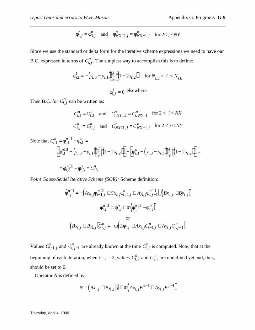
for 2< j <NY
Since we use the standard or delta form for the iterative scheme expressions we need to have our
B.C. expressed in terms of . The simplest way to accomplish this is to define:
for NLE < i < NTE
elsewhere
Then B.C. for can be written as:
for 2 < i < NX
for 2 < j < NY
Note that
Point Gauss-Seidel Iterative Scheme (SOR): Scheme definition:
or
Values and are already known at the time is computed. Note, that at the
beginning of each iteration, when i = j = 2, values and are undefined yet and, thus,
should be set to 0.
Operator N is defined by:
report typos and errors to W.H. Mason Appendix G: Programs G-9
Thursday, April 4, 1996
N = Bxi, j + Byi , j( )I + ω Axi, jEx−1 + Ayi , jE
y−1( )
C2,1nC1,2
n
Ci, jnCi, j−1
nCi−1, jn
Bxi , j + Byi, j( )Ci, jn = −ω Lφi, j + Axi , jCi−1, j
n + Ayi , jCi , j−1n( )
φi, jn+1 = φi , j
n + ω ˆ φ i, jn+1 −φ i, j
n( )
ˆ φ i, jn+1 = − Axi , jφ i−1, j
n+1 + Cxi, jφi+1, jn + Ayi, jφ i, j−1
n+1( ) / Bx i, j + Byi , j( )
= φ i,3n+1 − φi,3
n = Ci,3n
φ i,1n+1 − yi,3 − yi,1( ) t
c
1 − 2xi ,2( )
− φ i,3
n − yi,3 − yi ,1( ) t
c
1− 2xi ,2( )
=
Ci,1n = φi,1
n+1 − φi,1n =
C1, jn = C3, j
n and CNX+1, jn = CNX−1, j
n
Ci,1n = Ci,3
n and Ci,NY +1n = Ci, NY−1
n
Ci, jn
φi, j1 = 0
φi,11 = − yi,3 − yi,1( ) t
c
1 − 2xi ,2( )
Ci, jn
φ1, jn = φ3, j
n and φNX+1, jn = φNX−1, j
n

Line Gauss-Seidel Iterative Scheme (SLOR): Scheme definition:
n+1i,j=-(Axi,j*φn+1
i-1,j+Cxi,j*φni+1,j+Ayi,j*
n+1i,j-1+Cyi,j*
n+1i,j+1)/(Bxi,j+Byi,j)
or
Ayi,j*Cni,j-1+(Bxi,j+Byi,j)*Cn
i,j+Cyi,j*Cni,j+1=-ω(Lφi,j+Axi,j*Cn
i-1,j)
Value Cni-1,j is already known at the time is computed and, thus, update in i-th column is
found by inverting tridiagonal matrix. At the beginning of each iteration, when i=2, value Cn1,j is
undefined yet and, thus, should be set to 0, but at the end, when i=NX, from the B.C.
CnNX+1,j=Cn
NX-1,j. Exploitation of the B.C. for j=2 and j=NY defines Cni,1=Cn
i,3 and
Cni,NY+1=Cn
i,NY-1.
Operator N is defined by:
N=(Bxi,j+Byi,j)I+Ayi,j*Ey-1+Cyi,j*Ey+1+ωAxi,j*Ex-1
Approximate Factorisation AF-1 Iterative Scheme (ADI): Scheme definition:
(δxx-α)(δyy-α)Cni,j=ωαLφi,j
where α is a parameter.
Operator N is defined by:
The required equations are solved in two steps:
1) Invertion of the outer operator Nout=δxx -αI or sweep along i direction by letting Fni,j=(δyy-
α)Cni,j and solving directly for Fn
i,j the tridiagonal matrix equation:
Axi,j*Fni-1,j+(Bxi,j-α)*Fn
i,j+Cxi,j*Fni+1,j=ωαLφi,j
It can be shown that B.C. for function Fni,j are the same as for Cn
i,j, thus, Fn1,j=Fn
3,j and
FnNX+1,j=Fn
NX-1,j.
2) Invertion of the inner operator Nin=δyy -αI or sweep along j direction by solving directly for
Cni,j the tridiagonal matrix equation:
G-10 Applied Computational Aerodynamics
Thursday, April 4, 1996
N = L − αI −1
αδ xxδyy
Ci, jn
φi, jn+1 = φi , j
n + ω ˆ φ i, jn+1 −φ i, j
n( )ˆ φ ˆ φ
ˆ φ

Ayi,j*Cni,j-1+(Byi,j-α)*Cn
i,j+Cyi,j*Cni,j+1=Fn
i,j
with B.C. Cni,1=Cn
i,3 and Cni,NY+1=Cn
i,NY-1.
For uniform Cartesian grid and periodic B.C. the optimal value of ω is 2. To speed up
convergence Ballhaus suggests to use a sequence of parameters αk=αl(αh)(M-k)/(M-1), αl=1,
αh=4/ 2 k=1,...,M instead of one parameter α. In the code M=11 and =Y(3)-Y(2).
Approximate Factorisation AF-2 Iterative Scheme (ADI): Scheme definition:
(α-δ+x)(δyy-αδ-
x)Cni,j=-ωαLφi,j
where α is a parameter.
Operator N is defined by:
The required equations are solved in two steps:
1) Invertion of the outer operator Nout=αI-δ+x or sweep along i direction by letting Fn
i,j=(δyy-
αδ-x)Cn
i,j and solving directly for Fni,j the bidiagonal matrix equation:
(α+1/(xi+1,j-xi,j))*Fni,j-1/(xi+1,j-xi,j))*Fn
i+1,j=-ωαLφi,j
It can be shown that B.C. for function Fni,j are the same as for Cn
i,j, thus, FnNX+1,j=Fn
NX-1,j.
2) Invertion of the inner operator Nin=δyy -αδ-x or sweep along j direction by solving directly
for Cni,j the tridiagonal matrix equation:
Ayi,j*Cni,j-1+(Byi,j-α/(xi,j-xi-1,j))*Cn
i,j+Cyi,j*Cni,j+1=Fn
i,j-α/(xi,j-xi-1,j)*Cni-1,j
with B.C. Cni,1=Cn
i,3, Cni,NY+1=Cn
i,NY-1.
Value Cni-1,j becomes available before Cn
i,j is computed, except for the case i=2, when it should
be set to 0.
Suggested value of ω is 4/3. Similarly to AF-1 scheme a sequence of parameters
αk=αl(αh)(M-k)/(M-1), αl=1, αh=2/ k=1,...,M recommended by Ballhaus is used with M=11
and =Y(3)-Y(2).
report typos and errors to W.H. Mason Appendix G: Programs G-11
Thursday, April 4, 1996
∆y
∆y
N = L − αδ x+ −
1
αδx
−δ yy
∆y∆y

G.3 CBL User’s Manual
CBLv2 is the Cebeci Boundary Layer Program. The program computes the two-dimensional
compressible laminar and/or turbulent boundary layer. This code is described (with a listing) in
the reference. Dr. Tuncer Cebeci (Dept. of Aerospace Engineering, California State University -
Long Beach) makes it available for $50. The current version has been modified slightly, and the
output has been redesigned for WATFOR to limit output to 80 columns.
The code uses the Keller Box Scheme to obtain efficient solutions to the compressible boundary
layer equations. It uses the Cebeci-Smith turbulence model, an algebraic eddy viscosity model,
and can handle heat transfer cases. Some compilers will require the use of SAVE statements in
each routine.
The program will prompt you for the name of the input file. The output is written to the screen in
the version provided. This is not an interactive code and the output can be redirected to a file
once the input file is defined. Note that the boundary layer is computed at each input x station,
and no others. Make sure your input is closely spaced where details are important.
The boundary layer computation should start at the stagnation point, and follow the flow along
the upper or lower surface toward the trailing edge. This requires identifying the stagnation point
in the inviscid solution and using the geometry points x,y at each solution station to compute the
arc length along the surface from the stagnation point, which is the surface length X in the
boundary layer calculation. The utility program POSTp can be used to convert the output file
generated by PANELv2 to a form easily modified to use as input to CBLv2.
Reference
Tuncer Cebeci and Peter Bradshaw, Physical and Computational Aspects of Convective Heat
Transfer, Springer-Verlag, Berlin, 1984.
Note: This program is representative of standard programs used in industry. Experience by stu-
dents indicates that successful use of this program requires more patience than some students are
willing to use. It is very important to put the data in the proper column. When the program is
near separation the numerical iteration sometimes breaks down and the program stops with an
error message. This does not necessarily mean that the solution is invalid at previous steps.
When the pressure is specified, the boundary layer equations are singular at separation, and any
report typos and errors to W.H. Mason Appendix G: Programs G-13
Monday, January 27, 1997

numerical iteration will diverge. The program attempts to identify this situation and stop with a
message suggesting that separation has been encountered. Sometimes the solution blows up be-
fore the code message is printed. One of the most important input parameters is the initial dimen-
sionaless pressure gradient. The values of the pressure gradient should be examined to make sure
that the distribution is smooth. The code interpolates the user specified pressures to get the pres-
sure gradient using a second order polynomial which can poor estimates of the gradient if the
input data is not smooth.
INPUT FORMAT
Card 1: A80: - Data set title
Card 2: 2I3, 3F10.5
NXT - total number of x stations input (60 max)NTR - transition location station (must be > 2)
P2(1) - dimensionless pressure gradient at 1st x station,
Note: for zero pressure gradient case, P2(1) is zero, for flow that starts at a stagnation point, the local stagnation point solution assumes that the velocity
increases linearly from zero, and the value of this parameter should be one.
[good values of DETA(1), VGP: Laminar Turbulent & Lam/Turb]DETA(1) - h1, wall grid spacing: 0.2 0.01VGP - K, ratio of spacings 1.0 1.14
Card 3: 7F10.5
RMI - freestream Mach numberT0 - freestream stagnation temperature (deg. K)XLL - reference length, LRELM - Reynolds number per unit length, in millionsPR - Prandtl number (.72 for air)
heat transfer control codes [values of alpha0,alpha1], for specified: wall temp heat transfer]
ALFA0 - alpha0: 1 0ALFA1 - alpha1: 0 1
Card 4: 3F10.5, repeat card 4 NXT times
X(I) - x/L nondimensional distance along surfaceCP(I) - pressure coefficientWW(I) - dimensionless wall temp, gw, or the heat flux given by the dimensionless wall
temperature gradient of pw (depending on ALFA0, and ALFA1 values).
G-14 Applied Computational Aerodynamics
Monday, January 27, 1997
x
Ue
dUe
dx

Example of cblv2.f input (cblv2ref.inp on the disk)
upper surf. Cps from GA(W)-1 at M = .15 and 2 deg AOA 43 9 1.000 0.01 1.14 .150 200.00 1.000 6.0 .72 0.0 1.0 0.000000 1.005642 0.000000 0.004614 0.936635 0.000000 0.013224 0.549866 0.000000 0.024531 -0.084785 0.000000 0.036161 -0.708135 0.000000 0.048151 -1.025962 0.000000 0.061727 -1.198553 0.000000 0.077307 -1.272074 0.000000 0.094830 -1.240493 0.000000 0.114472 -1.187699 0.000000 0.136324 -1.137414 0.000000 0.160324 -1.082872 0.000000 0.186394 -1.042838 0.000000 0.214456 -1.010707 0.000000 0.244340 -0.977603 0.000000 0.275907 -0.950920 0.000000 0.308993 -0.927588 0.000000 0.343418 -0.908177 0.000000 0.378998 -0.891323 0.000000 0.415537 -0.873235 0.000000 0.452835 -0.857548 0.000000 0.490691 -0.845519 0.000000 0.528899 -0.831693 0.000000 0.567257 -0.813231 0.000000 0.605569 -0.785736 0.000000 0.643650 -0.732378 0.000000 0.681338 -0.660691 0.000000 0.718408 -0.579180 0.000000 0.754647 -0.493191 0.000000 0.789814 -0.408020 0.000000 0.823666 -0.331905 0.000000 0.855952 -0.257680 0.000000 0.886487 -0.187632 0.000000 0.915043 -0.124057 0.000000 0.941433 -0.067627 0.000000 0.965482 -0.019300 0.000000 0.987046 0.023179 0.000000 1.006006 0.062768 0.000000 1.022249 0.096355 0.000000 1.035669 0.123776 0.000000 1.046187 0.162320 0.000000 1.053742 0.228643 0.000000 1.058293 0.319797 0.000000
report typos and errors to W.H. Mason Appendix G: Programs G-15
Monday, January 27, 1997
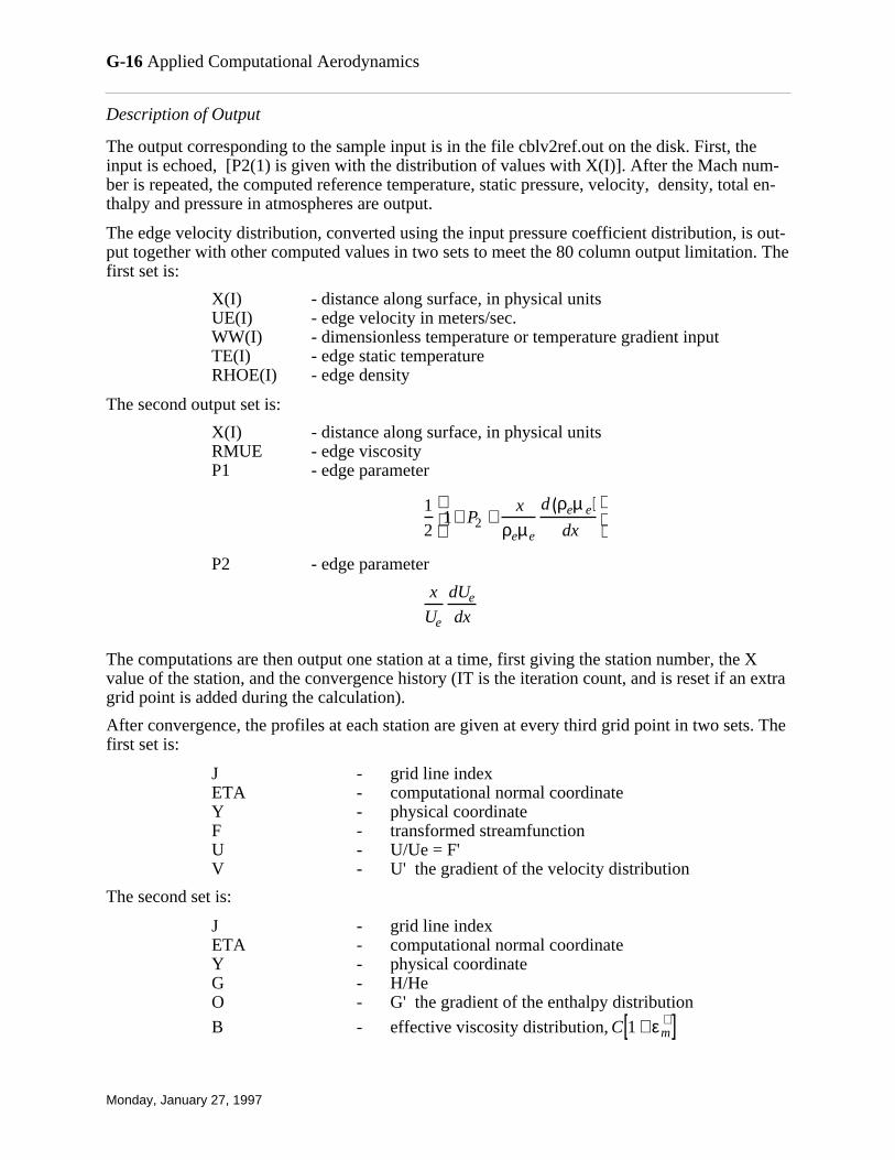
Description of Output
The output corresponding to the sample input is in the file cblv2ref.out on the disk. First, theinput is echoed, [P2(1) is given with the distribution of values with X(I)]. After the Mach num-ber is repeated, the computed reference temperature, static pressure, velocity, density, total en-thalpy and pressure in atmospheres are output.
The edge velocity distribution, converted using the input pressure coefficient distribution, is out-put together with other computed values in two sets to meet the 80 column output limitation. Thefirst set is:
X(I) - distance along surface, in physical unitsUE(I) - edge velocity in meters/sec.WW(I) - dimensionless temperature or temperature gradient inputTE(I) - edge static temperatureRHOE(I) - edge density
The second output set is:
X(I) - distance along surface, in physical unitsRMUE - edge viscosityP1 - edge parameter
P2 - edge parameter
The computations are then output one station at a time, first giving the station number, the Xvalue of the station, and the convergence history (IT is the iteration count, and is reset if an extragrid point is added during the calculation).
After convergence, the profiles at each station are given at every third grid point in two sets. Thefirst set is:
J - grid line indexETA - computational normal coordinate Y - physical coordinateF - transformed streamfunctionU - U/Ue = F'V - U' the gradient of the velocity distribution
The second set is:
J - grid line indexETA - computational normal coordinate Y - physical coordinateG - H/HeO - G' the gradient of the enthalpy distribution
B - effective viscosity distribution,
G-16 Applied Computational Aerodynamics
Monday, January 27, 1997
C 1 + εm
+[ ]
x
Ue
dUe
dx
1
21+ P2 +
x
ρeµe
d ρeµ e( )dx

and then the rest of the parameters of interest are given:
RX - local running length Reynolds numberDELS - displacement thicknessTHETA - momentum thickness
NUSSELT NO -
H - shape factor, DELS/THETACF/2 - skin frictionRDELS - Reynolds number based on displacement thickness RTHETA - Reynolds number based on momentum thickness
STANTON NO -
At the finish of the calculation the distributions of the computed quantities given above are re-peated in two sets in summary form.
The first set is:X RX DELS THETA H CF/2
The second set is:X RDELS RTHETA NUSSELT NO STANTON NO.
It is likely that separation will occur. When this happens the programs halts. When possible, sep-aration is flagged in the output, and the summary of results up to separation are printed out in thesummary.
report typos and errors to W.H. Mason Appendix G: Programs G-17
Monday, January 27, 1997
Stx =˙ q w
ρeue Hw − He( )
Nux =˙ q wx
Tw − Te( )k

G.4 TRANFOIL/TSFOIL2
These programs solve the transonic small disturbance equation. The disk contains the source
codes, sample input, and sample output.
TSDE is from Moran’s book. This program uses SLOR to solve the algebraic equations
using an evenly spaced grid for flow over a biconvex airfoil at zero angle of attack at a specified
Mach number and thickness ratio.
The input values are essentially the same as those used in program THINAIR, and are de-
fined in the following figure. Make sure that the value of XW is negative, and that the order of
input requested by the program is followed. Unlike THINAIR, where this was the source of most
problems encountered running the code, TSDE may diverge if the value of the relaxation factor
is too high, or the Mach number is too close to one. The user also specifies the Mach number,
thickness ratio, number of iterations, MAXTRY, and the relaxation factors for locally subsonic
flow (RLXSUB > 1), and supersonic flow (RLXSUP < 1).
The airfoil is defined from x = 0 to x = 1 on y = 0. At the farfield boundaries the potential is
set to zero. On the plane of symmetry, y = 0, the normal velocity is set to zero.
The maximum number of x grid points is 80. However, the program automatically adds
points around the boundary, so the user is prevented from exceeding 77. Similarly, the maximum
number of y points is 38. The convergence criteria is set internally. The iteration history is output
every ten iterations, and includes the number of supersonic points in the flowfield, NUMSUP.
G-18 Applied Computational Aerodynamics
Monday, January 27, 1997
XW 0 1 XE X
Y
YN
NUP NON NDOWN
NABOVE

Sample execution:
MORAN: PROGRAM TSDE
INPUT DX,DY: .05,.05
INPUT XW,XE,YN: -1,2,1.8
NX= 62 NY= 38 ILE= 22 ITE= 42
INPUT MACH, TAU: .82,.1
INPUT MAXTRY, RLXSUB, RLXSUP: 1000,1.8,1.0
TRIAL RMS CHANGE CHANGE RATIO XMAX YMAX MAX CHANGE NUMSUP 10 0.330E-02 0.9638 -0.2500 0.1000 0.227E-01 9 20 0.152E-02 0.9497 -0.5500 0.1000 0.657E-02 16 30 0.828E-03 0.9530 0.7500 0.0500 0.220E-02 19 40 0.647E-03 0.9849 0.7500 0.0500 0.167E-02 21 50 0.582E-03 0.9936 0.7500 0.0500 0.143E-02 22 60 0.544E-03 0.9942 0.7500 0.0500 0.114E-02 22 70 0.515E-03 0.9950 0.7500 0.0500 0.998E-03 23 80 0.490E-03 0.9949 0.7500 0.0500 0.891E-03 23 90 0.466E-03 0.9948 0.7500 0.0500 0.813E-03 23 100 0.442E-03 0.9947 0.7500 0.0500 0.753E-03 24... 900 0.539E-05 0.9945 0.8000 0.0500 0.953E-05 34 910 0.510E-05 0.9943 0.8000 0.0500 0.893E-05 34 920 0.483E-05 0.9944 0.8000 0.0500 0.845E-05 34 930 0.457E-05 0.9943 0.8000 0.0500 0.807E-05 34 940 0.433E-05 0.9943 0.8000 0.0500 0.762E-05 34 950 0.410E-05 0.9944 0.8000 0.0500 0.716E-05 34 960 0.388E-05 0.9947 0.8000 0.0500 0.679E-05 34 970 0.367E-05 0.9941 0.8000 0.0500 0.660E-05 34 980 0.348E-05 0.9950 0.8000 0.0500 0.613E-05 34 990 0.329E-05 0.9945 0.8000 0.0500 0.582E-05 341000 0.311E-05 0.9945 0.8000 0.0500 0.553E-05 34
report typos and errors to W.H. Mason Appendix G: Programs G-19
Monday, January 27, 1997

PRESSURE DISTRIBUTION ON AIRFOIL
I X CP
23 0.02500 0.23445 24 0.07500 0.05530 25 0.12500 -0.07965 26 0.17500 -0.18781 27 0.22500 -0.27958 28 0.27500 -0.36014 29 0.32500 -0.45224 30 0.37500 -0.52386 31 0.42500 -0.58545 32 0.47500 -0.64134 33 0.52500 -0.69270 34 0.57500 -0.73978 35 0.62500 -0.78178 36 0.67500 -0.81499 37 0.72500 -0.80487 38 0.77500 -0.27178 39 0.82500 -0.07417 40 0.87500 -0.02823 41 0.92500 0.08152 42 0.97500 0.24863
INPUT MAXTRY, RLXSUB, RLXSUP: 0,0,0
STOP
TSFOIL2 is also a solution of the transonic small disturbance theory. It was written by Earll
Murman, Frank Bailey and Margaret Johnson.1 However, it has significantly more capability
than TSDE. It is also bigger. It may not run on all personal computers. For comparison, consider:
TSDE TSFOIL2• 80 col. output • 133 col. output• non-lifting biconvex sections • arbitrary airfoils• evenly spaced grid points • unevenly spaced grid points• interactive input and execution • input file using NAMELIST
The input to the program is descrbed in subroutine READIN, which asks the user for the
name of the input file. The following description is from READIN. Note the default values. Two
input data sets are included to illustrate the procedure. TSFOIL was documented in NASA CR
3064, by Stephen S. Stahara, “Operational Manual for Two-Dimensional Transonic Code
TSFOIL, Decf. 1978.
1. Murman, E.M., Bailey, F.R., and Johnson, M.L., “TSFOIL — A Computer Code for Two-Dimensional Transonic Calculations, Including Wind-Tunnel Wall Effects and Wave DragEvaluation,” NASA SP-347, March 1975.
G-20 Applied Computational Aerodynamics
Monday, January 27, 1997

INPUT EXPLANATION
ALL INPUT IS READ IN THIS SUBROUTINE. THE ORDER IS AS DESCRIBEDBELOW.1.) ONE CARD OF TITLE INFORMATION. AN ?A? (ALPHANUMERIC) FORMAT
IS USED TO READ AND WRITE THIS INFORMATION. MULTIPLE CASESMAY BE RUN WITH THIS PROGRAM AND THE DATA FOR EACH CASEMUST START WITH THIS CARD. THE LAST CARD OF THE INPUT MUSTBE A CARD WITH THE WORD ?FINISHED? IN THE FIRST 8 COLUMNS.
2.) NAMELIST CONTAINING THESE PARAMETERS IS NOW READ. (SEEFORTRAN MANUAL FOR DESCRIPTION OF NAMELIST INPUT). THEBLOCK DATA SUBROUTINE SETS A DEFAULT VALUE, AS NOTED BELOW,FOR ALL OF THESE PARAMETERS.ONLY THE VALUES WHICH ARE DIFFERENT FROM THE PREVIOUS CASE(OR DEFAULT) MUST BE INCLUDED, ALTHOUGH AT LEAST ONE VALUEMUST BE INPUT BY NAMELIST FOR EACH CASE.
* (F) = FLOATING POINT ** (I) = INTEGER ** (L) = LOGICAL ** (E) = EXPONENTIAL *
DEFAULTVALUE
AMESH (L) OPTION FOR ANALYTICAL MESH CALC. .F..TRUE. X AND Y MESH VALUES ARE COMPUTED
WHEN AMESH = T, IMAXI AND JMAXISHOULD ALSO BE SUPPLIED. IMAXI ANODD NO. AND JMAXI AN EVEN NO.(81 AND 40 HAVE BEEN USED).
.FALSE. X AND Y POINTS ARE THE DEFAULTVALUES OR THE VALUES SUPPLIEDBY THE USER THRU NAMELIST.
EMACH (F) FREESTREAM MACH NUMBER. .75NOTE****EMACH MAY NOT BE = 1.0
DELTA (F) BODY THICKNESS RATIO. .115ALPHA (F) ANGLE OF ATTACK (DEGREES IF PHYS=T) .12AK (F) TRANSONIC SIMILARITY PARAMETER. 0.0
(INPUT REQUIRED ONLY IF PHYS = .F. )GAM (F) RATIO OF SPECIFIC HEATS. 1.4SIMDEF (I) SIMILARITY DEFINITION. 3
=1 COLE=2 SPREITER=3 KRUPP=4 USER
PRTFLO (I) OPTION FOR PRINT OF FINAL FLOW FIELD. 1=1 NO FLOW FIELD PRINT.=2 ALL J LINES PRINTED.=3 PRINT 3 J LINES AROUND MAXIMUM ERROR
PSTART (I) OPTION FOR INITIALIZING P ARRAY. 1=1 SET TO ZERO.=2 READ P FROM UNIT 7=3 USE P IN CORE (PREVIOUS CASE).
report typos and errors to W.H. Mason Appendix G: Programs G-21
Monday, January 27, 1997

DEFAULTVALUE
PSAVE (L) OPTION FOR SAVING RESTART BLOCK OF .F.VALUES ON UNIT 3.=.TRUE. SAVE FOR RESTART.=.FALSE. DO NOT SAVE.
FCR (L) FULLY CONSERVATIVE RELAXATION OPTION .T.=.TRUE. DIFFERENCE EQUATIONS AREFULLY CONSERVATIVE FORM.=.FALSE. DIFFERENCE EQUATIONS NOTCONSERVATIVE AT SHOCK WAVES.
KUTTA (L) KUTTA CONDITION OPTION. .T.=.TRUE. KUTTA CONDITION IS ENFORCED=.FALSE. LIFT COEFFICIENT SPECIFIED BY USER.
CLSET (F) LIFT COEFFICIENT, USED IF KUTTA .0IS FALSE.
BCFOIL (I) OPTION FOR FOIL OR BODY GEOMETRY. 3=1 NACA00XX=2 PARABOLIC ARC.=3 ORDINATES (READ LATER IN NAMELIST
IF DIFFERENT FROM DEFAULT VALUES WHICHARE FOR THE KORN AIRFOIL).
=4 JAMESON'S AIRFOIL INPUT FORMATBCTYPE (I) DESCRIBES THE TYPE OF FLOW TO BE COMPUTED. 1
=1 FREE AIR.=2 SOLID WALL.=3 FREE JET.=4 SLOTTED WALL.=5 POROUS WALL.
F (F) TUNNEL SLOT PARAMETER. 0.H (F) TUNNEL HALF HEIGHT/CHORD RATIO. 0.POR (F) WALL POROSITY FACTOR. .0PHYS (L) TYPE OF SCALING TO USE FOR I/O. .T.
=.TRUE. PHYSICALLY SCALED VALUES.=.FALSE. TRANSONICALLY SCALED VALUES
FOR PHYS = .F., ALSO INPUT VALUE FOR AK.IMAXI (I) NUMBER OF X-MESH POINTS(.LE. 100) 77JMAXI (I) NUMBER OF Y-MESH POINTS(.LE. 100) 56IMIN (I) X MESH POINT WHERE CALC IS TO START 1JMIN (I) Y MESH POINT WHERE CALC IS TO START 1ICUT (I) CONTROL FOR MESH CUT AND REFINEMENT. 2
= 0 INPUT MESH IS USED TO CONVERGENCE.= 1 INPUT MESH MAY BE CUT ONCE.= 2 INPUT MESH MAY BE CUT TWICE.
WE (F) 3 VALUES FOR RELAXATION FACTOR FOR 1.8ELIPTIC PTS. 1-ST FOR COARSE MESH, 1.92-ND FOR MED. MESH AND 3-RD FOR 1.95FINE MESH. DEFAULT VALUES ARE SUGGESTEDVALUES, IN ORDER. IF SPECIFIED IN INPUTALL THREE VALUES MUST BE GIVEN.
WCIRC (F) RELAXATION FACTOR FOR CIRCULATION. 1.0MAXIT (I) MAXIMUM NUMBER OF ITERATION CYCLE ALLOWED. 500
G-22 Applied Computational Aerodynamics
Monday, January 27, 1997

DEFAULTVALUE
CVERGE (F) CONVERGENCE CRITERION FOR RESIDUALS OF P. .00001DVERGE (F) DIVERGENCE CRITERION FOR RESIDUALS OF P. 10.RIGF (F) REIGLES RULE FOR BODY SLOPE. 0.0EPS (F) COEFFICIENT OF PXT .2IPRTER (I) CONTROL FOR FREQUENCY OF PRINT OF 10
LINE IN MESH WHERE ERROR IS LARGEST.I.E. IPRTER=10 , LINE WILL BE PRINTEDEVERY 10-TH ITERATION
NWDGE (I) CONTROL FOR VISCOUS WEDGE INCLUSION 0= 0 NO WEDGE= 1 MURMAN BUMP= 2 YOSHIHARA WEDGE
REYNLD (E) REYNOLDS NUMBER BASED ON CHORD. 4.0E+6USED WHEN NWDGE = 1
WCONST (F) WEDGE CONSTANT. USED WHEN NWDGE=1 4.0IFLAP (I) CONTROL FOR FLAP DEFLECTION. 0
FLAP INCLUDED WHEN IFLAP .NE. 0DELFLP (F) FLAP DEFLECTION ANGLE. 5.0
POSITIVE DEGREES T.E. DOWNFLPLOC (F) LOCATION OF FLAP H.L., X/C 0.77
NOTE**WHEN ARRAYS ARE READ BY NAMELIST THE FULL ARRAY MUST BESET, I.E. IF ALL VALUES ARE NOT REQUIRED THE ARRAY MAYBE FILLED USING MULTIPLE ZEROS. (N*0.0)
XU (F) ARRAY - X VALUES FOR UPPER BODY. USED IF BCFOIL = 3. KORN AIRFOIL USING ALL 100 PTS.(UPPER) AND 75 (LOWER) IS DEFAULT.
XL (F) ARRAY - X VALUES FOR LOWER BODY.YU (F) ARRAY - Y VALUES FOR UPPER BODY.YL (F) ARRAY - Y VALUES FOR LOWER BODY.NU (I) NUMBER OF POINTS TO USE FOR UPPER BODY 100NL (I) NUMBER OF POINTS TO USE FOR LOWER BODY 75
** NOTE THIS PROGRAM USES A MESH REFINEMENT METHOD FOR DECREASINGCOMPUTER TIME. FOLLOW THE RULES BELOW FOR CONSTRUCTING THEX AND Y MESH TO TAKE FULL ADVANTAGE OF THIS FEATURE.
IMAXI - ITE SHOULD BE A MULTIPLE OF 4.ITE - IMIN SHOULD BE A MULTIPLE OF 4.JMAXI - JUP + 1 SHOULD BE A MULTIPLE OF 4JLOW - JMIN + 1 SHOULD BE A MULTIPLE OF 4
(WHERE JLOW IS LAST POINT BELOW SLIT ANDJUP IS FIRST POINT ABOVE SLIT.)
WHERE ITE = I FOR X = 1.0 (OR POINT ON BODY CLOSEST TO X = 1.0).SUBROUTINE CKMESH INSPECTS THE X AND Y MESHES TO SEE IFTHIS IS TRUE AND, IF NOT, WILL MODIFY INPUT MESH IN SOME CASES.
XIN (F) ARRAY - X MESH POINTS. LIMIT 100 PTS.YIN (F) ARRAY - Y MESH POINTS. LIMIT 100 PTS.
X AND Y MESH DEFAULT VALUES ARE KRUPP BASIC GRID.
report typos and errors to W.H. Mason Appendix G: Programs G-23
Monday, January 27, 1997

The following are two sample inputs for TSFOIL2:
This dataset provides the solution to the biconvex airfoil (BCFOIL=2) that corresponds to the so-lution provided by TSDE:
TEST OF TSFOIL2, 10% thick biconvex airfoil $INP ALPHA=0.0,DELTA=0.10,EMACH=0.82 BCFOIL=2,MAXIT=1500 $END
This dataset is used to obtain the solution for the flow over an NACA 2412 airfoil at zero alphaand a Mach number of .75.
TEST OF DATA POINT INPUT CASE , NACA2412 $INP ALPHA=0.0,DELTA=0.12,EMACH=0.75 BCFOIL=3,NU=21,NL=26,MAXIT=1500 XU = 0.00000, 0.04738, 0.09730, 0.14745, 0.19772, 0.24805, 0.29842, 0.34882, 0.39923, 0.44963, 0.50000, 0.55032, 0.60059, 0.65078, 0.70090, 0.75094, 0.80089, 0.85076, 0.90055, 0.95027,1.0, YU = 0.00000, 0.03430, 0.04896, 0.05959, 0.06760, 0.07363, 0.07786, 0.08037, 0.08123, 0.07988, 0.07686, 0.07246, 0.06690, 0.06033, 0.05293, 0.04483, 0.03619, 0.02722, 0.01818, 0.00919,0.0 , XL = 0.00000, 0.00662, 0.00931, 0.01455, 0.02736, 0.05262, 0.07771, 0.10270, 0.15255, 0.20228, 0.25195, 0.30158, 0.35118, 0.40077, 0.45037, 0.50000, 0.54968, 0.59941, 0.64922, 0.69910, 0.74906, 0.79911, 0.84924, 0.89945, 0.94973,1.0 , YL = 0.00000,-0.00864,-0.01025,-0.01262,-0.01649, -0.02166,-0.02535,-0.02828,-0.03267,-0.03576, -0.03783,-0.03898,-0.03917,-0.03839,-0.03608, -0.03274,-0.02866,-0.02406,-0.01913,-0.01405, -0.00903,-0.00435,-0.00038, 0.00250, 0.00345,0.0 , $END
These files are contained on the disk as bicon.inp and N2412.inp. The corresponding output iscontained in the files bicon.out and n2412.out.
G-24 Applied Computational Aerodynamics
Monday, January 27, 1997
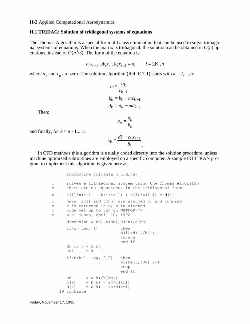
H.1 TRIDAG: Solution of tridiagonal systems of equations
The Thomas Algorithm is a special form of Gauss elimination that can be used to solve tridiago-nal systems of equations. When the matrix is tridiagonal, the solution can be obtained in O(n) op-erations, instead of O(n3/3). The form of the equation is:
where a1 and cn are zero. The solution algorithm (Ref. E.7-1) starts with k = 2,....,n:
.Then:
and finally, for k = n - 1,...,1:
.
In CFD methods this algorithm is usually coded directly into the solution procedure, unlessmachine optimized subroutines are employed on a specific computer. A sample FORTRAN pro-gram to implement this algorithm is given here as:
subroutine tridag(a,b,c,d,nn)
c solves a tridiagonal system using the Thomas Algorithmc there are nn equations, in the tridiagonal form:
c a(i)*x(i-1) + b(i)*x(i) + c(i)*x(i+1) = d(i)
c here, a(1) and c(nn) are assumed 0, and ignoredc x is returned in d, b is alteredc code set up to run on WATFOR-77c w.h. mason, April 10, 1992
dimension a(nn),b(nn),c(nn),d(nn)
if(nn .eq. 1) then d(1)=d(1)/b(1) return end if do 10 k = 2,nn km1 = k - 1
if(b(k-1) .eq. 0.0) then write(6,100) km1 stop end if
xm = a(k)/b(km1) b(k) = b(k) - xm*c(km1) d(k) = d(k) - xm*d(km1) 10 continue
H-2 Applied Computational Aerodynamics
Friday, November 17, 1995
xk =′ d k − ck xk+1
bk
xn =′ d n
bn
m = ak
bk −1
′ b k = bk − mck −1
′ d k = dk − mdk−1
aixi−1 + bixi + cixi+1 = di i = 1,K ,n

d(nn) = d(nn)/b(nn)
k = nn do 20 i = 2,nn k = nn + 1 - i d(k) = (d(k) - c(k)*d(k+1))/b(k) 20 continue
return
100 format(/3x,'diagonal element .eq. 0 in tridag at k = ',i2/)
end
A check can be made using the following main program and resulting output:
c main program to check the Tridiagonal system solver dimension a(20),b(20),c(20),d(20) n = 10 do 10 i = 1,n a(i) = -1. b(i) = 2. c(i) = -1. 10 d(i) = 0. d(1) = 1. call tridag(a,b,c,d,n) write(6,610) (i,d(i), i = 1,n) 610 format(i5,e15.7) stop end
The results are:
1 0.9090909E+00 2 0.8181819E+00 3 0.7272728E+00 4 0.6363637E+00 5 0.5454546E+00 6 0.4545454E+00 7 0.3636363E+00 8 0.2727273E+00 9 0.1818182E+00 10 0.9090909E-01
Reference
H.1-1 Conte, S.D., and deBoor, C., Elementary Numerical Analysis, McGraw-Hill, New York,1972.
report typos and errors to W.H. Mason Appendix H: Utility Programs H-3
Friday, November 17, 1995