Calhoun: The NPS Institutional Archive

Faculty and Researcher Publications Faculty and Researcher Publications

1991-03

7th Annual Review of Progress in

Applied Computational

Electromagnetics at the Naval

Postgraduate School, Monterey, CA,

March 18-22, 1991, Conference Proceedings

Monterey, California. Naval Postgraduate School

Conference Proceedings: 7th Annual Review of Progress in Applied Computational

Electromagnetics at the Naval Postgraduate School, Monterey, California, March 18-22, 1991

http://hdl.handle.net/10945/45290

AD-A241 323

CONFERENCE PROCEEDINGS

7th Annual Review of Progress In ICAPPLIED ELECTE 8

COMPUTATIONAL OCT 0 9 1991ELECTROMAGNETICS

at the 0

Naval Postgraduate School

Monterey, CA

Marchi 18-22, 1991

SYMPOSIUM PROGRAM COMMITEE CHAIRMAN

Frank Walker

Sponsored by

The Applied Computational Electromagnelics Society

and DOD/USA ECOM, USAISEC, NOSC, NPS, DOELLNL

REPRODUCED BYU.S. DEPARTMENT OF COMMERCE

NATIONAL TECHNICALINFORMATION SERVICESPRINGFIELD, VA 22161

THE NAVAL POSTGRADUATE SCHOCOL

91-06085

"L - -I ' III!,:LIl tJ L il t• .I

1992 CALL FOR PAPERS 1992The 8th Annual Review of Pro ress

In Applied Computational Electroifagnetics

SUBMISSION OF PAPERSSuggested topics for papers include

NUMERICAL METIIODS CODE DEVELOPMENT APPLICATIONSDifferential methods EM Field Codes Antenna analysisIntegral methods NEC EMCIEMIMethod of Moments GEMACS EMP/shieldingfradiation effect.;Finite Element methds Systcen Compatibility Codes Impulse and transient analysisFinite DiP =-ence inethods IEMCAP Propagation and scatteringGTDkFTrD methods SEMCAP Microwave, mm-wave componentsSpectral Domain techniques AAPG EM machines and devicesLow/High frequency issues COEDS Power transmissionTime Domain techniques Time Domain codes Accelerator designHybrid techniques Codc validation Biological interpretationPerturbadon multipole methods CAD/automeal genieration Data interpetationNew algorithm3 Graphical I/0 techniques Code studies of basic physics

TIMETABLEOctober 1st 1991:- Abstract Submission

Refereeing is carried out on the abstract whicit trust aot be more than asingle page including figures. Please supply four copies.

November 1st 1991:- Authors notified of acceptanceJanuary 15th 1992:- Submission of camera-rt•,dy copy, not. more than 8 pages inc'uding

figures. All submissions become the propelny of the SYMPOIltUM andwill not be returned. rhe author of each pape," accepted for p ablicationwill be required to provide Copyright Releises from the autl,.or tnd thesponsoring organisation to the Symposimn. Copyright Rerlease formswill be supplied at time of acceptance. The author and sponsoringorganisation will retain the right to free use of the copy protectedmaterial.For both abstract and final paper, please supply th. followingdata for the lead author - Full name, address, telephone and FAXnumber for both work and home and a brief professional biography

Cost per person for the Symposium will be $180.0 ($195.0 after March 9th 1992).

SHORT COURSESThese will cover numerical te1mniques, computational methods, surveys of EM analysis andcode us ;ge instruction. Fee for a short course is expected to be $70.00 per person for a half-day course and $120.0 for a full day, if booked before March 2nd 1992. Full detailF will bepublished by October lsi 1991.

DEMONSTRATIONSThese will cover computer demonstrations, software demonstrations, poster papers and key-note speakers.

VENDOR BOOTHS"These will cover product distribution, small company capabilities, new commercial codes.

The Applied Computational Electromagnetics Society

1992 CALL FOR PAPERS 1992

The 8th Annual Review of Progressin Applied Computational Electromagnetics

March 17- 19,1992

Naval Post Graduate School, Monterey, California

Share your knowledge and expertise with your colleaguesat the Applied Computational Electromagnetics Society's

8th Annual Review of Progress

The Annual ACES Symposium is an ideal opportunity to participate In a large gath-ering of EM analysis enthusiasts. Whether your interest is to learn or to share yourknowladge, this symposium is aimed at you. In addition to technical publication, theSymposium urganlses live demonstrations and short courses. All aspects of elec-tromagnetic computational analysis are represented.

The purpose of the Symposium is to bring analysts together to share informationand experience about the practical application of EM analysis using computationalmethods. Thero are four areas, SympsIum papers, short courses, demonstrationsand vendor booths. The NSF/lEE ECAEME (Comrputer Applications in Eiectromag-netics Education) Center will organise a special session of technical presentationsun Compute. Applications. This special session will cover topics of interest Ineducation/training, evolving computer technologies and the latest In electromagnet-ics computation and analysis. In conjunction with the special session, therewill be booths dedicated to the interchange of ideas and software. Pleasecontact Magdy Iskander for CAEME details. Contact Pat Foster for details of theother events.

1992 ACES Symposlum CAEMESymposium Chairman Administrator DirectorPat Foster Richard W Adler Magdy IskanderMicrowave and Naval Postgraduate School University of UtahAntenna Systems Code EC/AB H E Deparwtwt16 Peachfiold Road Montcry Salt Lake CityMalven, WORCS CA 93943 UT 84112WRI4 4AP, UKTel 010 44 614 574057 Tel (408) 646-2352 Tel (801) 581-6944FAX 010 44 684 573509 FAX (408) 646-2955 FAX (801) 581-5281

1992 ACFS SymposiumSponsored by: ACF.S, DODf[JSA CECOM, USAISSANOSC, NPS and DO.13AINLIn cuopenition with: The IEEE Antemias and Propagation Society, the IEEE Electromagnetic

Compatibility Society and LISNCIURSI

S......

1991 Symposium Program Committeefor the

7th Annual Review of Progress InAPPLIED COMPUTATIONAL ELECTROMAGNETICS

at theNaval Postgraduate 5zhoai

Monterey, CA k)

Symposium Chairman: Frank Ellis Walker J ,Boeing Aerospace & ElectronicsP.O. Box 3999; M/S 85-84Seattle. WA. 98124-2499(206) 773-5023

Symposium Administrator; Dr. Richard W. AdlerNaval Postgraduate School Accesiori ForCode ECIABMonterey. CA. 93943 NTIS CRA&I '(408) 646-2352 DTI1" TAG

Symposium Short Course Chairman: Dr. John Rockway J-U iii ;oil nccdNaval Ocean Systems Centel'.:;rictoNOSC/Code 805 -

San Diego, CA. 92162-5000(619)~ 55-71......... ..... .. ........ .. ...........

CAEME Director- Dr. Magdy iskander D i.: t i.Electrical Engineering Dept.............University at Utah A.~ 'Salt Lake City, UT. 84112 , --

Vendor Booth Ca-Chairman: Kathy Lee Distr-31 & CountermeasuresThe MITRE Corp.Bedford, MA. 01730(617) 271-8555

1992 Symposium Choiman: Dr. Patricra FosterMicrowave and Antenna Systems16 PeachtIela Rd.Groat Malvern, Worceslershire WRI 4 4AP. U.K.

Conference Secretary: Mrs. Pot Adler

Advisory Commrttee:. Dr. Ed Miller. Los Alamos Labs.Dr. Robert Bevensee. ConsultantDr. Haroid ýcabbagh, Sabbagli Assoc.. Inc.Jim Logan, NOSC (Univ. ot South Carolina)Dr. Ray Luebbers, Penn State Univ.Dr. Andrew Paterson. Georgia Inst. at Tech.

Statement A per telec~onDr. Richard AdlerNPC/Code EC/ABMonterey CA 93943

VENDOR BOOTHS

Commercial Companies:

Hewlett Packard

Compact Software

EEsof

CAE Soft Coip.

Sonnet Software

Antenna Software Ltd.

Denmar Inc.

Wave Tracer

CAEME Associates;

Dr. Magdy Iskander, CAEME Director, NSF/IEEE CAEME Center

Dr. Markus Zahn, CAEME Faculty, Michigan Institute of Technology (MIT)

Dr. Zvonko Fazarinc, CAEME Faculty, Stanford University

Dr. Rodney Cole, CAEME Faculty, University of California at Davis

Dr. Bob Shin, CAEME Faculty, Lincoln Lab

Dr. Jovan Lebaric., CAEME Faculty, Rose-Hulmon Institute of Technology

IV

CONFERENCE CHAIRMAI'S SUMMARY

In this year's conference we have made modest gains In planning and organization. Themost obvious change is the publication of the conference proceedings in time tar distribution atthe conference. This is clue primarily to the conscientious delivery of the papers by the authors anda super effort on the part of Dick and Pat Adler In organizing the volume and getting Itto the printerIn ilme for publlcation.

We have also arranged for advanced notice of next year's conference complete withProgram Committee. Dr. Patricia Foster of the United Kingdom will be the 1992 SymposiumChairman and Dr. Perry Wheless, Jr, of the University of Alabama is providing stateside support asthe Conference Co-Chairman. The 1992 Conference "Call for Papers' is published In theseproceedings.

It has been the Interest of ACES to promote International participation at ACES confer-ences. Thisyear we have Initiated on "international Forum' by recruiting representatives from eachof eight International regions to address tne conference and discuss topics of technical signifi..cance In their region of the world. We sincerely hope that these addresses will piomoteInternational dlu;og on technical !ssues of computational electromagnetics.

Asmany of you know, ACES hasmnatured wlth the Incorporation of the society last year. Withthis expansion comes the responsibility of economic self sufficiency. ACES has been sponsored formany years by the donations of facilities and fInanclalsupport from such organizatlonsasthe NavalPostgraduate School and Lawrence Livermore Labs. In the future, like competing technicalorganizations, ACES will be required to undergo long range fiscal planning and sound financialoperations. This year's conference Is a start, Care has been token to minimize conference costsand Improve revenues. We conservatively project more than $5,000.00 In cost savings andadditional revenues compared to past conferences. These results bring ACES closer to total selfsufficiency and allow us to consider new and novel activities such as sponsored Internationalattendees and funded computational competitions,

As a result Of negotiations with MIT, CAEME will offer a 120 minute version of the MIT videoon "Experlm,*,ntal Demonstrations for TeochIng Electrom'agnetlc Fields and Energy". In cooperationwith CAEME, ACES has purchas )d the video at cost far free distribution to each registeredconference attendee. Additional copies of the video will be available from CAEME at theconference for $10.00 ($25.00 after the conference), This iL a substantial discount compared to thecommercial value of the MIT material. Dr. Magdy iskander, CAEME director, is to be commendedfor his efforts in successfully aorrnging for the generous contribution of this MIT video material to thetechnlcal community.

With thegraclouself ortsof Dr. Magdy iskander, CAEME director, and Kathy Lee, the VendorBooth Co-Chairman, we have organized fourteen vendor booths atthisyear's conference. Six areCAEME associates und eight are commercial product vendors. These vendor booths provideexposure to products and services of interest to ACES attendees In addition to generatingconference revenues,

Another feature Is repeated thisyear with the offering of two full day and four hall day shortcourseson the Monday of conference week. We wish to express our appreciation to the 1991 ShortCourse Chairman, Dr. John Rockway, for organizing the short course curriculum. The lecturers areto be commended for the excellent quality of the short course material offered this year.

We do not have news to report at the time of this printing concerning Inclusion of ACESpapers In technicai library data bases. Dialog has been initiotedc with the IEEE and we hope to haveprogress to report at the conference.

Asa resultof the material offered In the technical papersthlsyear, we have several new ses,sions, There are three sessionsrelating to time domain analysis techniquesand solutions, Asecondnew topic Is the low frequency session that has resulted from international paper3 dealing withtransformer analysis and electrical power problems.

An added feature in the table of contents are two or three lefter keys to Indicate topic as-soclatlonsfor each paper. This Isas a result of the screening process used to place each paper Intoa technicalsession. These areIn addition to the more general session tiliesand are Intended to helpminimize confusion over the pronablilty that a tecnical paper contains multiple topics of Interestto an ACES reviewer. As an example there is a session of "NEC Antenna Analysis, in addition allconference papeiw In which NEC was used are labelled with the (NEC) key for quick Identification.We hope that these Keys will assist the reader In more quickly finding toplcs of Interest.

In conclusion let us welcome you as a conference attendee and wish you success in yoursearch for knowledge in the growing field of computational electromagnetics.

Frank Ellis Walker1991 Symposium Chairman

V!

ACES PRESIDENT'S STATEMENT

The exhilarating spring beauty and charm of the Monterey Poninsula and the hospitality ofthe Naval Postgraduate School have become synonymous with the Annual Reviews of Progress inComputational Electromagnetlcsof our Society. I take pIe>3sure In welcoming you to this7th review.I hope that you will once more share with me the appreciation of this environment while obtainingthe practical benefits of a rich technical program of papers. short courses, and display booths thatFrank Walkor and his team hove prepared for us this year.

Let me assure you that the officers and directors of ACES appreciate your participation.Your attendance at the symposium helps to make a viable and thriving technical society. To theauthors, Instructors, and chairmen my thanks for your efforts and willingness to participate in thisImportant capacity. We are most Interested In the reaction of companies and individualsparticipating In vendor displa,;s. We should like to take advantage of your experience to improveour offerings In the years to come.

I also Invite you to consider Increasing your Involvement with ACES activities. But it Ismy lopethat you will leave this year's event with your expectations fulfilled and with a .esolve to make plansto attend In 1992.

.)X. Stan KubinaACES President

1992 CONFERENCE CHAIRMAN'S STATEMENT

As chairman for the 1992 Symposium. I would like to welcome you to that event. The primaryaim of the Symposium is the Interchange of information and, although the centerpiece of theSymposium remains in the sessions given by you, the authors, there are other ways in which we canall gain. The good work of the 1991 Symposium will continue In 1992 with more short courses to bringyou all up to date with the latest techniques or leacn those starting out In this field the basic toolsof the trade. We will Identify 'hose courses suitable for training purposes. We also hope to runanother exhibition as I believe It Is In the Interests of ACES to know what programs are availablecommercially and for software Interchange. No amount of reading promotional literature canreplace conversation with suppliers and other users.

After seven years of the ACES Symposium, we can claim that it has become a notablefeature of the electromagnetic year but that does not mean that It cannot be improved upon. Ihope all ot you will consider what help you can give In organizing the SymposIum to be moresuitable for you. You do not have to volunteer to work on a committee but you con write to meto specify what you like about this Symposium or hove noticed as an omlsZon.

Pat Foster1992 Symposium Chairman

VII

IK ";--• -u' . . . u-- " z' " " • zz zm. u

MONDAY MARCH 11,6 H ORT CO URS ES

FULL-DAY COURSES: (Approximately 6 hour Course)

0830 "The ESSENCE of Electromagnetic Radiation"by Dr. Robert M. Bevensep, Consultant

0830 "The Electromagnetic Analysis of Microstrip"by Dr. James C. Rautlo, Sonnet Software

MORNING HALF-DAY COURSES:

0830 "UTD and Its Practical Applications"by Dr. Ronald J. Marhefka, The Ohio State University Electroscience Laboratory

0830 "An Overview of Several Topics in Electromagnetic Modeling"by Dr. Edmund K. Miller, Los Alamos National Laboratoryand Gerry Burke, Lawrence Livermore Notional Laboratory

AFTERNOON HALF-DAY COURSES:

1300 "Introduction to GWMACS"by Dr. Edgar L. Coffey III

1300 "Volume integral Equations and Conjugate Gradient Methods in Electromagnetic Nondestructive Evaluation'by Dr. Harold P.. Sabbagh, Sabbagh Associates, Inc.

1800 - 2030 REGISTRATION 101A Spanagel

1830 ACES BOARD OF DIRECTORS DINNER

2000 ACES BOARD OF DIRECTORS MEETING(Members Invited to observe) 122 Ingersoll

VIII

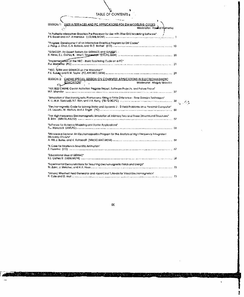
TABLE OF CONTENTS

SESSION4 1: UPiRJINTEBFCES AND PC APPLICATIONS FOR EM MPh apModeato: RQA~1 tr~hetka

'A Portable Interactive -Graphics Pta-Processor for Use with Wire-Grid Modelling Software'P.S. Exceil and A.F. Armanlous (I/O.WG.,MOM) .................... ...................... .........................

'Progress: Development of an Interactive Graphics Program tar EM Codes'J. Pang, J. Chot. C.A. Baiariis. and G.C. Barber (i10) .................................................. .......... 10

'GEMCOP: An Export System for GEMACS and GAVQE'ý -Rt. Fisher. E.L. Coffey Ill, and T. 20pwnelOrIT cZ PC,GOEM) ........................ I............................... 2

'Implemenj~ait6n of the NEC - Basic Scattering Code on a PCO'R.J. MarhdfRu (PC) ..................................... . ................................................. ........ ..... 21

-NEC, PifRM and GEMACS crr the Macintosh"P.E. Buss&k and R.W. Taylor (PC,ANT,NEC,GEM) .................................................................... 29

SESSION 2: CAEME SPECIAL SESSION ON COMPUTER APPLICATIONS IN ELECTROMAGNETL?c DUCATIiQN Moderator: Magdlylskarsder

'NSF/iEEE-'CAEME Center Activities: Progress Report, Software Prolects and Future Focus'M.. Iskander ............................................................................................................ _ 37

'Simulation of Electromragnetic Phenomena Using a Finite Difference - Time Domain Technique'KI. LI, M.A. Tassoudl, P.T. Shin, and J.A. Kong (TD,TDA$C.PC)................................... .................. 38

'Eleotrarnagnellic Code tar Solvlng Static and Dynamic 2 - D Field Problems on a P~srsonot Computer'J.E. Lebaric. M. Mellon, and J. Engel (PC).......................................................................... 56

'The High Frequency Electromagnetic Simulotiorn of Arbitrary Two and Three Dimensional Structures'B. Brim (MM.FE,AXilQ) .......................................................... .... ............................. .... 57

'Software for Antenna Modeling and Radar Applications'P.J. Hancock (ANT,PC)............................................................ ...................................... 58t

'Microwave Explorer: An Etoctramagnettcs Program for the Anaiysis of High Frequency IntegratedMlc~rostrip Circuits'A. Hill. J. Burka. and K. Kottapalil (MM.SC,MAT.MOM)............................................................. 59

'A Case for Rteatism in Scientiftic Animation'Z. Tozarino (i/O) ....................................................................................................... .. 67

'Educailonol Uses of GEMVAC'El.. Cottey Ill (GEM,MOM) ..............................................................................................

'Experimental Demonstrations far teaching Electroamgnetic Folods and Energy'M. Zathn, J. Mectrer, and H.A. Haus ............................................................... ................... 72

'Lienarc>Wlechert Field Generator and HyperCa~d Tutorials far Visual Etectroniognetics'P. Cole and D. Kroill..................................................................................... ............. ... 73

Ix

SESSION 3: INVERSE PROBLEM SOLUTIQNM Moderator: Margaret Cheney

"An lnver- aundlary Value Problem tar Maxwell's Eo~jatlons"E. Somersatb, D. lsaacson, and MI. Cheney (BV)......... .. . .. ............. ........ ............. 7

A Layer-Stripping Approach Ia impedance Imaging"MI. Cheney, D. Isacsari, E. Samersalo. and E. Isacson (By)........................................... ......... 79

'Eloctric Current Computed T ar~zp0. lsaacson, M. Ch~eeyrt-C1Jb~welt,1 yG. Glssei. and 4.0. Gable (BV.MiAT) ............................ I......87

"U~se or El 'clImpedance Imaging In Two- Phase, Gas-LIquid Flows"4.7. Lin. ý. Suzuki, L. Ovaclk. 0.0. Jones, 4.0. Newell. and MI. Cheney (BVMATBIO) ........................ 94

SESSION'4.' M PTTIC SOI.UIONS \.Moderator: Andrew .J. lerjuoll Jr.

"PrimitifrA/901t Validation tar the Signa±re Prý'dlctlan Tools Softwa-e Package"£4 ~gand A.J. TerzuotllJi. (ASYSC,NM) ....................................................... 115

"High Frequency Scattelring Code In a DIstribul~d Processing Environment"S. Suhi, A.J. Tenjuoll Jr. and G.B. Lamont (AA?ýC)..................................... ........................... 130"Simulation of SIte Obstruction Effects an the Performance of a High Gain Antenna Using NEC-BSC2"A.M. Buccisrl. 4.0. Herper, and E. Me¶ 9/(ASY.ANT.NEC)......................................................... 139'Bistatic Physical Optics Scotterlnr am, a Surface Described by an Electromagnetic ojr Acoustic Imped-R..Bo n ( S ,C V ... ... . 146

INTERNATIONAL. FORUM/

Reports tram lnterna~dtont regional Rleproseontatlvos cancerning topics at toctriical Importance In eachregion.

Great BrItain:/ Or. David Lizlus, AEA Industrial Technology, Gulharn, U.K.Western Eu0: Dr. quedlger Anders, ACES Europe Commiltee Chairman. Applied Electra.

'. magnetic Engineering, GermanyEastern Eur~pe: Or. MiVhaelo Morego. Polytechnic Institute of BucharestAustralia: Dr. Gregory Htaack, Survellance Research Laboratory, South AustratiaJapan: 0.. Chiyo Hamamuro. Mitsubishi Electronic Crorporatian, JapanChina: Or. Yuonren Qb, XVan Jialorsog University. P.R. ChiniaSouth America: Dr. J. P.A. Bastos, UnIverstdata Fedaral do Santa Catarina, BrazilAfrica: Dr. Duncan Baker, University of Pretoria, Southr Africa

SESSION 5: NLI E\VJ NgQUlIS Moderatr:ci Ronald Pogarzetski

"A Hyi4`ttlntle Element arid MorreT101 Method for Electromagnetic Scattering train inhornaganeausObjoctt'W.E. Boyse and A.A. Saldi (FE.SC.NIAT,MOM),....................... ........................ ..................... 160

"A New Esparsison Function of GMT: The Rirrgpate*4. Zhong (NMBV) ...................................................................................................... 170

"An Application at Symbolic Manipulation Software 1r Compu~tatlonal Eloctramagniselcs'P.4. Pogorselskl (NM.ASY) .................................................................................... ......... 174

"Etficient Solution at Matrtx Eauatlons in Finite Elemnrirt Modeling at Eddy Current HOE"A. Mahmaod, 0.4. Lynch, Q.H. Nguyen, und L.D. Phllipp (NMFE) .......... .................................. 184

x

'An Approx~mate (Symmetric) Combined Field Integral Equation to' lire Analysis at Scattering byConducting Bodies In the Resonance Region'L.M. Correta and A.M. Barloosa (NM.SC) ........................................ I................................... 190

*New Expansion Functions for Long Structures In the MMP-Cade'P. Leuchtmann (NM)............................................................... ...................... ............ 198

"Direct Solution af the Wave Equation Using Parallel Computational Techniques'R.G. Hohiteld. S.M. Sparagna. and 0. Sandri (NM.ANIMAT,FD) ................... ........... ... 203

.On Ws.lau Conceptual Model lor Deriving the Electromagnetic Statistics Ot Complex Cavities'Y.K Lehmr-nd and EX. Miller (NM).................... ........................................................ 22

SESSION 6: FINiTE-ELEMENT AND FINiTE DIFFR~ NQ FRQUENCY DOM,ýIN O[.IJTIONS N

-- ) - /Moderator: ciann~raltfhee

'Solution at Multi- Media Wave Propagation and Scattering Problems Using Finite Etemnents' .-Fit. Moyer Jr. and E. Schroeder (FE,SC.MAI) ............. .................. ................................... -234

'Finite Element SoltoijjjbQjjUo omo he.ýw,ý$andau Equatiorr'K.G. Herd an$.Ar-tiedossieu (FEMAT) .............................. ............ .......................... .235

'Characttiization at Anuchaic Chombers by Finito Drifference Method'5- Haita, tý. Hllotmann, and W. Wiesbects (FD,SC)......................................... ........................244

SESSION 7: MOMENT~ METHOD THEORY Moderator: Allen Glissan

'A Multi-level Enhancement at the Methrod ot Moments'K. Kotbasi and K. Demarest (MOMSC.NM) ..................................... ............................... ... 254

'On the ApplIcabitityot Pulse Expansion and Point Matching In the Mursiorri Method Soltuion at Throc Di-mensional Electromagnetic. Boundary-Value Problems'B.C. Ahn, K. Mahcodvon qpc NW. Glissan (MOM,SC.BV.NM)--------------------------------..... ....... ...265

'Recursive Algwtrihnris to Reduce tire Computational Complexity at Sculotfinri Prooloms'W.C. CHw,`Y.M. Wang, L. Guorl. and J.H. tin (MOM,SC.NM)--------------------------------..................278

"Numepo ~Solutiorr at the EFIE Using Arbrtrarily Shaped Quaridrangularf and Triorrgular EtumonilsoT. Madkand H. Singor (MOM,NM)-----------------------------------------------------292............................29

SESSION 8: MoODELING EM INERý ý LjTRA Moderator: Kenneth Demaresi

'GeneretApproach tar Treating Boundarty Cornliliuiis air Multr-Rugiorol Scatterers Using the Method atMoments'J.M .PutPutnam .S .M(M ASSCM....M..BV............................................................................. 3040

'Camparisari at Computed and Measured Resuilts for a Sinrple Man~with-Radio Model'A.W. Gltssen, 0. Kajlez, W.P. Wheless Jr., and K.H. Agar (MATBtO.NtY)--------------------------.... ... .. .320

*faatbox tar Characterizallon at Materiails'J.R. Dontest (MATSC'-....................................... . ...................................................... 329

'PoalarimetrIc Scattering and Control at Radar Crass Section of Chirat Targets at Simple Gernelrius airdAssociated Cede Developmerrt'A.K. Btrattacharyya (MAFSCBV)------------------------------------------------------344......................... ...34

X1

SkSSION 9 HIGpH tPLQUL!4CY AFPPLIý.A1IQNS AND WIRE .QBjDi1M.QDEtN r gjIQuModeictor Christopher Truernaoj

scoll~iirrf By So, Itoted C i-nule;

1)CS of Fhmndanenal Scotturers in the HFf Barr?Iruernar' S P Mi1hra, and S i Kubina (SC WG.lIO) .369

* Autcynotid Rad6ut Cekjjlatmfln 104 Wife Gild Models? -

SE ~ ~ ~ ~ ~ ~ ~ K SONt ¶11AYJfKJJ{MICflOSRIP ANTENtNAAN I.Y1Moderaoro. Fob~cii-Hurst

i~iWave Modeling c!t U Multi Layer Micro~tiip Aruly with ai Superconducting Mydsptrroi Feed Network'*S Med imik SC MOM .r389

UWA" owi r Qi Anisiarot:i Sl'iVi~l.

syrier N ~ ..aJ1 a ari S13ou1:11ror0 (%AV- SO) .. 96

-Arovisisat the Sehavior of QuaL Complex Modjs n onSssy Substrate boxed Microstrip Lines*Hurst P Prrbetich. and P Kenrirs (MMMM4C) .. . . . 403I Computer Modelling of Heibcat Slow. Wave Sliutluites lui Use in Travelling Wave tubes'

A 4 Marr..san tWG.NiC) ,.409

¶Electrrcallyhlvnvned Array Sytitheetf for Solid Stlat Raldar Application,?MAHuseri;i. B Nobie. aria M Mc Kee (ANIT.NM) . .419

I ~~~~Gulded Wave Propagation antwo D~nonsiornaICkIstersot Directly CouDled Cavity Rerao rPA SPecIOW (MM.SC.NM) ... 428

SESSION I11 ANTENNA ANALYSIS Modieratar. Asoke St-rattacharvyri

Werof a Momentn Anoillis of Cavity Backed Wire Antenna?*D C Jeno arid Et Barber (ANT.WG.MOM) . 432

"Momrent Method Modelling at the NP~rnaI Mode Hek~ll.a Antenna*y j Guo and P S Eacell (ANT.WqJdtbM) ........ 446'Inteircanorri~nson of Sevgrat Maoment Method Models of Dipolots nd Folded Dipoles'P S Eacelt anrdA Filliffiriosious (ANT.WG.MOM) .. ............... 451

'Snjiiered Hexn Antennao Paoroneter (stirnatran Using Selectirve Criterrr9' 0 *ir59 (ANY NM) 456

AU4 a. Feeld Patternu at Ultra High Gain Antenna Artays, ot Finite Size'P A Specd4ple (ANT.NM ) .. .. .... ..I. ..... .... ........ .. ......... .. ........... 471

SESSION 12. NEC ANTENNA ANALY ( - Moderator: Peter Excell

'Modedring a Sh4pbocmd Fan Antenna'L Koyca so (ANT.W G.NEC) ....... .......... ................ . 474

O0ptvnuiing Sidelabe Levels ot an Array Ubog NECCP L Houwt. C J McCoinnack. and WF Brandow III (ANI.WG,NEC) .................................... .. .... 487

411

"Using the Numer1ical Electromagnetics Code (NEC) to Calculate Magnetic Field Strength Close to aSommerfeld Ground'G . H- aa c k (A N T N EC ) ........................................................................................ ........................................ 49 3

"Re•enienn of HF Vertical Half Rnombtc Chaiacter: .otorn"W.P. Wheless Jr., M.O. Fanning, D L. Faust. and M.B. King (ANI,WG,NEC) ................................................ 507

,%.

SESSION 13: ELEi•ROMAGNETIC COMPATI'68 CLI ./MQ1 Moderator: David P. Millard

"A Survn/ of Numericci Techniques tar Modeling Sources Q ttromagnetlc Interference".H. Hulblng (MC) ................................................................. 516

Computer Aided ElecIr or-npatt~lly Analysis'D.P. Millard, J.4 o. R M. Hurkert, ard JA. t.oody CEMC,I/OPC) ........................................................ 520

SESStON 14: WF UENCY .EEL~&LQ.LJL 9 Moderator: Perry Wheless, Jr.

"Tiransle;at 4 akage Field Ir, Transformers With Saturable Mp , gnetlc Care'M .i. M ore a and A .M I. M orego CLFT .................... T. .. ................................................. .................. 529

'Finite Element Analysis at MoJ~netlc Field Dlsf!lbjin in Ferromagnetic Shields'C .V. Bala, O .C . Craiu, and M .i. M orega (LFL J , . ..........C................. IC........................................................... 534

'A Model for Dynamic Analyjja _Corantnctor"P.I. Kolterm ann, J.P.A. B s. and SR. Arrudc (LF,FE) .......................................... ................................ 540

"Eddy Current Arnlyses of the Core Plote In a Large Power Transfoarmer'Y. Q lu, W . W ang. Q . Zhang, G . Xloo, and X. LI (LF,FE) ............................................................................... 545

"Engineering •eolvablilty of Engineering Eddy-Current Problems'Z. Cheng, S. ao, D. Zhong, J. W rong, and C . Ye CLUF E) ............................................................................ 551

SESSION 15: TIME DOMAIN ML.2QEA Moderator: Gerald Burke

"Compdsan of GTD TOand MoM Scottering Computations and Transformation to the Time Domain'P.G . Elliot and ;. Kohlberg (TD,M O M ) ............ . ................................................... ............................ ...... 557

'Evaluation of Modified Log-Pertodlo..Atfennas far Transmission of Wide-Band Pulses'. ..J. Burke (I.D.NEC) ............... ,.,... ......................... ........ 567

"The Pulsed Retponse from a ParabolIc Reflector AntonnaoG R. So lo (TD ,AA SY ) ..................................................................................... .................................................. 5 77

"A Ray-Tr•cing Model to Predict Tlme-Domoln RCS Pertnrmance of a Compact Range'N. Carey. . Brumely, and A. Join (TDSC) ................. .............................. .......................... 586

SESSION 16: TRANSMISSION UNE MATRIX (IWM) TIME DOMAIN APPLICATIONS , - . /, Modeoatos Lloyo RIgqs

'A Transmisslon Line Matrix (TILM) Method Analyuls of the Separated Aperture Burled Dielectric AnomalyDetection Scheme'P.R. Hayes, L.5. Riggs, and C .A. Am azeen (TD.TLMNEC) ..................................... ................................... 699

"The Modelling of Lossy Materlala with the Sywnne~tlcal Condensed Node TLM Method'F.J. German, G.K. Gothard. and L.S. Rtggs (TD.TLMMAi) ............................................. 612

"The An - A of Passive Microwave Components Using the TLM Method'

P.R. Convay. F.J. Germ an, and L.$. Riggs (TDTLM,MAT) ................... .............. ..................................... 627

III

SESSION 17' EINITE ELEMENT AND FINITE DIFFERENC TIME DOMAIN SOLUTLQ -%Moderator: Raymond Luebers

"A New Wo hted Residual Finite Element Method for Computational Electromagnetics In the TimeDomain'J. Am broslano. S.T. Brandon. and R. Lohnsr (TD,VE) .................................................................................... 642

"Virtual Particle' Electiomagnetic Part~ale-Mesh Algorithms tar Microwave Tube Modelling'J.W . Ea stw o o d (FETD ,N M ) .............................................................................. .............................................. 655

'A New Magnetic Field Analysis for Dynamical Problem Involving Relative Dlspla(o ,en: with lime"C. Hamamura. M. Okabe. T. Ohmura. and K. Sato (TD,FE) ........................................................................ 661

"A Time Domain to Calculating Radar Cross Sections'D.W . Harm ony and G .R, Solo (TD.FD,SC ,M AT) ......................................................................................... . 666

"*A 2-D Finite-Volume Time-Domain Technlq, 'e for RCS Evaluation'R. Holland, V.P, C able, and L. W ilson (TDF. ,SC ) ................................................................................ ...... 667

"RCS Calculation for Smooth Bodies of Revolution Using FDTD"R. Luebbers, D. Steich, K. Kurrz, and F. Hunsberger (TD,FD,SCMAT) ......................................................... 682

'FDTD Wavegulde Coupling Modeling and Experimental Validation"P. Allnikula, S. Kunz, and R. Luebbers (TD,FD,V) .......................................................................................... 691

A u th o rs In d e x .................................................................................................................................................. 7 0 2

o 199. The Appl~ed Computatlonal Electromagnetics Society

XIV

KEY:

TD Time DomainSD Spectral DomainMM Millimeter wuve (microwave, microstrip, antennas)LF Luw FreqLency (power systems'

METH9QDMOM Method of MomentsFE Finite Element methodFD Finite DIM '. ince methodBV Boundary Value methodTI.M Transmission Line ModelingWG Wire Grid mrodelingASY Asymptotic solution applicationsNM New Method

AEPLICATIONE

SC Scattering (RCS)MAT MaterialsBIO Biological applicationsANT Antenna analysisMMIC Monolithic Microwave Integrated CircuitrylMC Electrornagnetlc Compatibllity, Electromagnetic Interference (EMC/EMI)V Validation110 Input/Output InterfacesPC Personal Computer applications

NEC Numerical Electromagnetics Code (NEC)GEM GEMACSIGAUGE

xv

SESSION 1 - "USER INTERFACES AND PC APPLICATIONSFOR EM MODELING CODES"

Moderator: Ronald Marhefka

A PORTABLE INTERACTIVE-GRAPHICS PRE-PROCESSOR FOR USE WITH WIRE-GRID

MODELLING SOFTWARE

P S Etell & A F Armanious*

Electrical Engineering Department, University of Bradford, West Yorkshire, UK"now at Sultan Qaboos University, Oman

An intcractive-graphics input program for wire-grid moment-mcthod modelling packages is described, Thiswas written in Fortran-77, using the standard GKS (Graphical Kernel System) graphics commands in orderto maxinise the portability and maintainability of the software. The program contains several features toease the inputting of the physical structure of the wire-grid object and its subsequent sub-division intosegments of appropriate length. The object can be visualised on a graphics screen, with or withoutannotations. The output data may be. formatted to conform to the input requirements of a number ofstandard moment-method packages.

1. Introduction

Wire-grid modelling involvcs the fictitious replaccment of continuous metallic surfaces in an arbitrary mctallicstructure with wire meshes having aperture perimeters that are small compared with a half-wavelength atthe frequency of interest. The input into a computer of the !opology of a complex metallic structure, andits conversion into a corresponding wire-grid model, is a tedious procedure that is prone to many sourcesof error. This problem has been widaly recognised, and interactive graphics input programs such asIGUANA [1] and GAUGE [2] have been developed to aid input to specific modelling programs. In addition,certain other programs designed to run on personal computers incorporate integral input graphics routines[3,4]. While these programs have many merits, they have the limitation that they can only be used on onedisplay device (an IBM-type personal computer), and they each produce output data in a format specific tooune solution program.

The lack of an all-pervading standard for computer graphics remains a very serious impediment to manyapplications. The Graphical Kernel System (GKS) was an attempt to rectify this situation and, although itsuptake has been less widespread than might have been desired, it remains one of the f,:w widely-usedgraphics standards: at the time the work reported here was commenced, it was effectively the only graphicsstandard.

It is well known to practitioners of wire-gi id moment-method modelling that it is seldom possible to placea high degree of confidence in the first results from any attempt to model a complex structure. The normalheuristic approach is to compare the initial prediction with the nearest available analytical solution in orderto check that it is fundamentally physically reasonable, and then to re-run the model with changed values ofsome ot the arbitrary parameters in order to check that the results remain stable. Despite commendableattempts by some to improve the rigour and reliability of the method, strategies of this type are likely tocontinue and it was felt that it would le very desirable if variation of the moment-method fornmulatito Andthe solution method were available as an alternative to variation of the wire-grid parameters. To this end,it was decided that the program described here should incorporate a menu of several different well-knownmoment-method packages such that the output data fiom this pre-proccisor could be formatted in such away that it was immediately usable as input to the chosen solution package.

2. The r raahical Kernel Svytein (GKS)

The Graphical Kernel System is a set of graphical software library routine.s written by an internationalworking group in the early 1980s, and published aa an international standard by ISO in 1985 [5].

. - .. .. . . .. .. . . . . .. .. .. .. . .. .. . . . . . .. . .. . . . . .. . . . . . . . . . . . . . . . . . . .. . . . . ... . .- .4

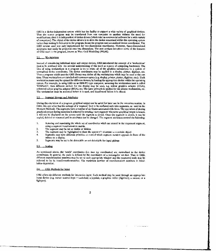
GKS is a device-independent system which has the facility to support a wide variety of graphical devices.Thus the scurce program may be transferred from one computer to another without the need formodifications, since it is independent of device drivers (which exist as commercial software for a wide varietyof computers). The object of the device drivers is to drive the device concerned within the operating systemrather than making it de.dicated to the program, hence the program uses normialiscd device coordinates. TheGKS version used was only implemei.ted for two-dimensional coordinates. However, threc-dimensiovalstructures may easily be projected onto two dimensions. The next sections introduce some of the featuresof GKS used i i the program, known as Wire Grid Modelling (WGM).

2.1 Workstations

Instead of considering individual input and output devices, GKS introduced the concept of a 'workstation'(not to be confused with the no~mal understanding of this word as a piece of coomputiag hardware). Theidea of using workstations in a program is try to relate all of the graphics calculations to a system ofnornialised device coordinates. TIhe device coordinates may be applied to a display, plotter, digitizer, etc.Thus a program which uses the GKS library may define all the workstations which may be used at the runtime. These workstations are labellcd with common names (e.g. display, printer, plotter, digiti-,zr, etc.). Eachworkstation name may be opened for diffcrcn devices, by loading the appropriate device within the operatingsystcm. For example, in using GKS on an IBM-PC-type computer, assuming the workstation used is callcd'DISPLAY', then different devices for the display may be used, e.g. colour graphics adapter (CGA),enhanced colour graphics adapter (EGA), etc. The same principle is applied for the printer workstation, etc.The workstation must be activated before. it is used, and deactivated before it is closed.

2.2 Segment Storage and Attributes

During the exe,.ution of a program, graphical output can be saved for later use in the execution session. InGKS, this ope, ation has the concept of a 'segment' (not to be confused with wire segments, as used in theMoment Method). The segments have a number of atltibutes associated with them. The operation of storinggraphical output during execution is achieved by creating.% new segment: whenever graphical output is issued,it will not be displayed on the screen until the segment is closed. Once the segment is closed, it can becopied, deleted or renamed and its attributes can be changed. The segment attributes control the follownlg:

I . Rotating and translating the whole set of coordinates which are stored in the requested segment,using a segment transformation matrix.

2. The segment may be set as visible or hidden.3. The segment may be highlighted to draw the operatr'c e-uantion sw 4 certain object.4. Segments may have different priorities 1o rcntrol which segment numbnr appears in front of the

others on a display.5. Segments may be set to be detectabl.: or cot detectable for input pickup.

As mentioned above, the 'world' cocrdilnates (i.e. user xy coordinates) are normalised to the devicecoordinates. In general, the scale is d,:lined by the coordinates of a rectangular wit.dow. Thus in GKS,different transformation numbers may be set to each appropriate window aid the requested scale may bereferred to by its traunsformatiormumbibr. The maximum number of transformation numbers is instal-lation-dependent.

2.4 QKS Methods for Input

(1KS( offers six different methods for interactive input. Each method may be used through an appropriateinput device (e.g. cursor control keys: j, t.ack-ball; a joystick; a graphics tablet (digitiycr); a miouse; or alightpen).

1. LOCATOR: used to input (xy) coordinates.2. PICK: used to pick (select) a displayed object on the screen.3. CHOICE: used to select an item from a set (menu) of alternatives.4. VALUATOR: used like a potentiometer for inputting a numerical value from a quesi-continuous

linear distribution5. STROKE: used to input a sequence of (xy) positions,6. STRING: used to input a string of characters from the keyboard.

These logical devices need to be initialised before they are used.

3. The Interactive-GranhifA Pie-Processor

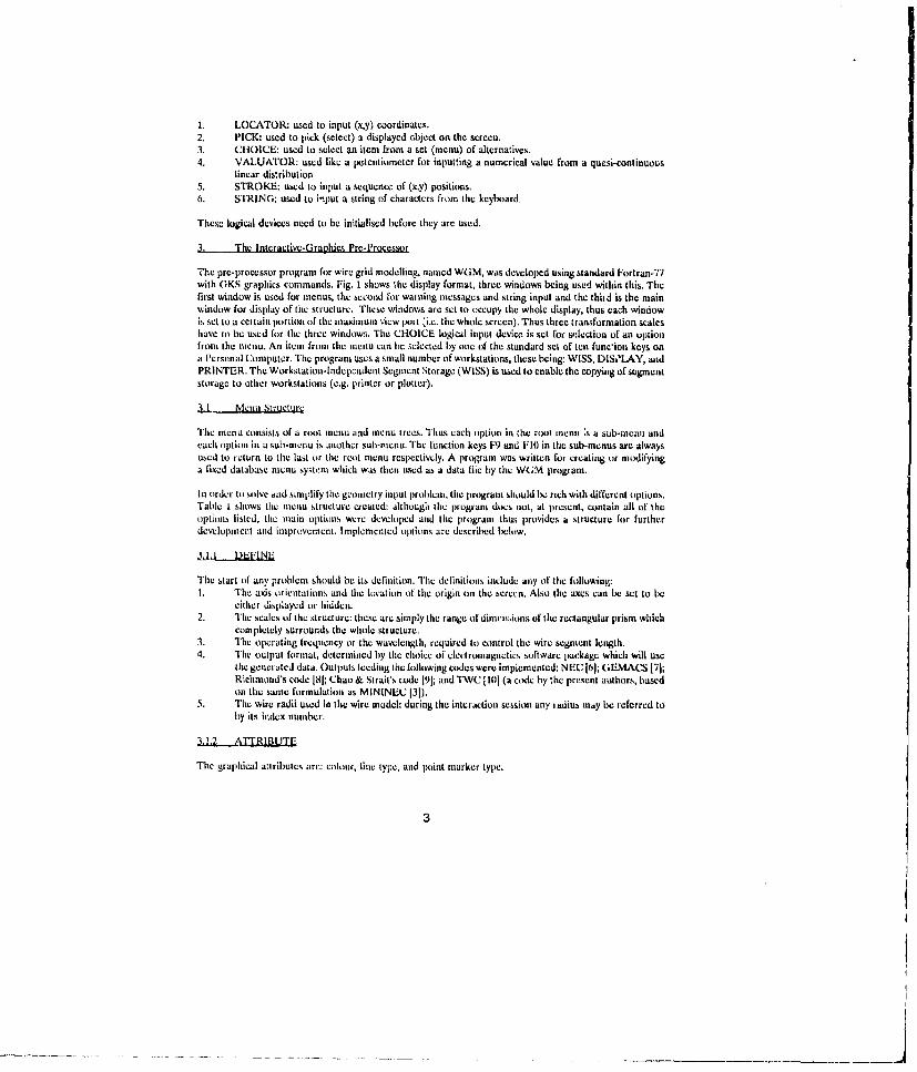
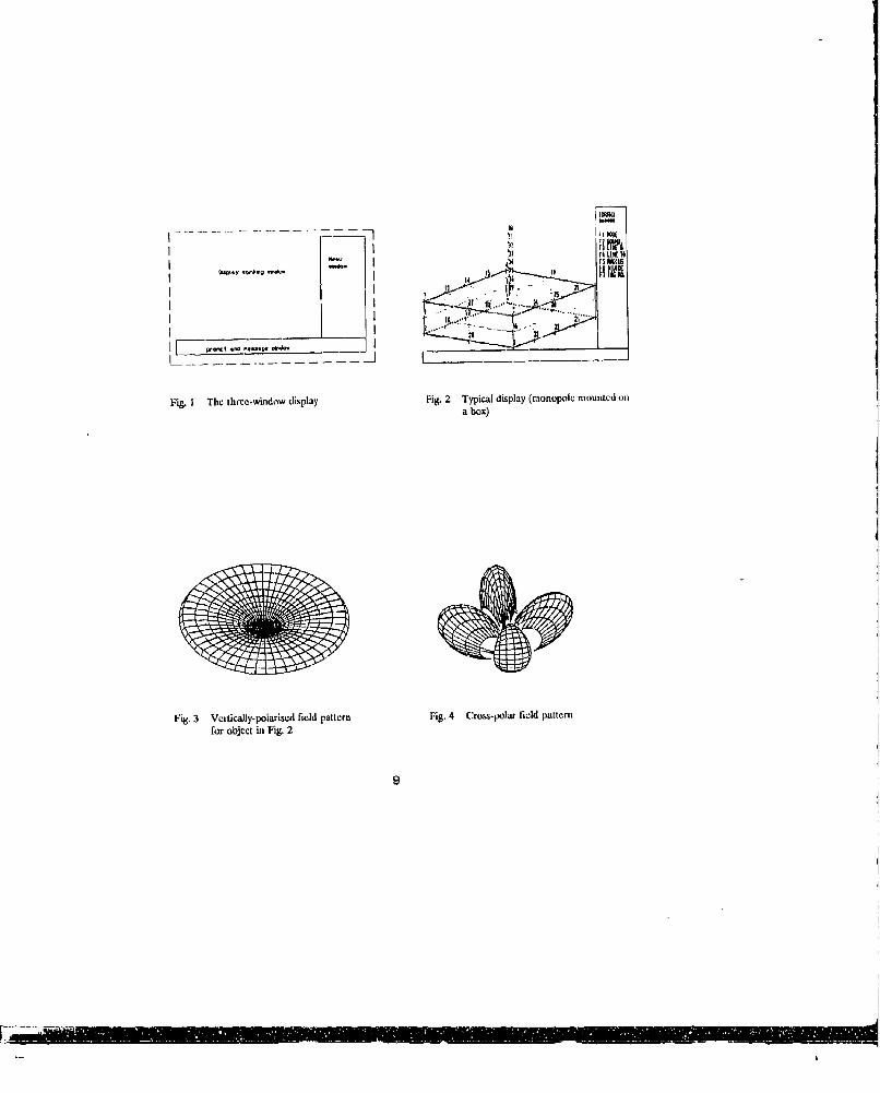
The pre-processor program for wire grid modelling, named WGM, was developed using standard Fortran-77with (iKS graphics commands. Fig. I shows ,he display format, three windows being used within this. Thefirst window is used for menus, the second for warning messages and string input and the thitd is the mainwindow for display of tite structure. These windows are set to occupy the whole display, thus each windowis set to a certain portion of the toaximurn view port i.e. the whole screen). Thus three transformation scaleshave to be used for the three windows. The CHOICE logical input device. is set for selcdtion of an Uptionfrom the menu. An item from the menu can be selected by one of the standard set of ten fune'ion keys ona Personal Computer. The program uses a small number of workstations, these being: WISS, DISOLAY, andPRINTER. The Workstation-lidepcttdent Segment Storage (WISS) is used to enable the copying of segmentstorage to other workstations (e.g. printer or plotter).

3.t Melnu Structure

The menu consists of a roo! menu and menu trees. Thus each option in the root menu ;s a sub-menn andeach option in a sub-mciu is another sub-menu. The function keys F9 and FI0 in the sub-menus are alwaysused to return to the last or the root menu respectively. A program was written for creating or modifyinga fixed database menu system which was then used as a data tile by the WGM program.

lit order to solve and simplify the gronictry input probletm, the program should b ritch with different options.Table I shows the menu structure created: although tire program does not, at present, contain all of theoptions listed, tihe main options were dcvelpcd and tihe program thus provides a structure for furtherdevelopment and improvement. Implemented options are described below.

&J, k D EFINE

The start of any problem should be its definition. The definitions include any of the following:1. The axis orientations and the location of tlte origin on the screen. Also tihe axes can be set to be

either displayed or hidden.2. The scales of the structure: these are simply the range of dimcnsions of the rectangular prism which

completely surrounds the whole structure.3. The operating frequency or the wavelength, required to control the wire segment length.4. The output format, d':tertnined by the choice of clectromugnetics software package which will use

the generated data. Oulpults leeding the following codes were implemented: NEC 161; GEMACS 171;Richmond's code 181; Chant & Strait's code 191; and TWC [110] (a code by the present authors, basedon the same formulation as MININEC 13)).

5. The wire radii used in the wire mudel: during the interaction session any radius may be referred toby its itldex number.

The graphical attributes are: colour, line type, and point marker type.

3

This is the most iwportant part of the menu and consists of the following:I. Draw point with label given by the program. The point can be entered in cartesian, cylindrical polar,

oi spherical polar coordinates. Relative coordinates can also be entered (ice. relative io previouspoint).

2. Define a structure boundary. The user may start from a point in space and thcn automatically drawa continuous boundary (which may be open or closed) through any othcr points specified.

3. Line utilities, requiring knowledge of the coordinates of onc end, line (wire) length and some otherparameter such as: line parallel to another line or a plane; line perpendicular to another line or aplane; or direction angles of the line.

4. Wire% may be created by connecting a line between two points, or between one point and a numberof points.

S. A wire may be automatically divided into a specified number of equal segments.

3JA Ul2ML

Editing the geometry is an essential fcattrc to aid rapid building of the structure.The edit menu coesists of:1. Erasing a paint or segment, or all segments having a given tog number.2. Changing a segment tag number or its ,adius; changing a point number or segment number;

changing attributes (e.g. segment colour, and displayed line type (dotted etc.) of a wire segment).3. Rotating amid duplicating the structure.

3.1.5 121SLAY

This option is designed to aid the user to exploit the maximum degree ofvisualisation possible. It has the following options:I. The structure can be viewed in one of the three major planes (i.e. x-0, y= 0, or z-0). Alternatively

the elevation angle or the view angle may be changed.2. Zoom to fit the whole structure into the whole working window.3. Display the labels of either points, or wire segments, or both.

With the Concept of the workstation, any part of the structure may be plotted easily. Thus .he user may plotthe whole structure, or any selected parts (selected by tag number, or block etc.).

This option is used to write all the segment coordinates into a file (with a format determined by the chosenclectromagnetics code). It also saves all the data entered during the interaction session asd exits from theWOM program.

312 Two-Dimensional Disnlay of Thirc-Dimensiond StratmW

Since the structures modelldl arc relatively compact, the use of perspective is not essential and a simplemethod for projection was used. in this method any three-dimensional point will be projected on the planeof the screen (which is defined by spherical view angles 0 and #, thems being the polar angles of the normalto the plane relative to the origin).

4

3.3 Database Storage of Wire Soament ParpU.a_

To avoid the problem of memory limitalion when Uoring the wire segment parameters, a binaryrandom-access file was used. The use of such a direct-acc.ss file means that the limit for the maximumnumber of segments is determined by the available disk space. Using the concept uf GKS segment storage,any point marker with its label and any line representing a wire segment are stored in separate graphicssegments. To maximise the use of available storage, data for a Point and a wire with the same input sequencenumber are stored together in a single record, even though, in general, they will not be coniected with eachother.

Note thta the program always remembers the current total Pumbcrs of wire segments and points which havebeen entered. At the end of a session, the numbers of wire segments and points are saved in some reservedrecords in the file, together with the current scale in use and the current segment attributes for new wiresegments.

34 WGM Program Structure

The WCM program starts with a menm of three options. These are to select whether to start a fresh model,to retrieve data built in a previous session, or to build a model from a NEC geometry data input file.

As explained above. 'he three-dinmensional coordinates ate mapped into two-dimensional coordinates. 1 htsany basic operation (e.g. dividing, rotating, duplic.tion) on the structure will be performed first on thethree-dimensional iepresentation and then the resulting three-din•ensional coordinates will be mapped intotwo dimensions as explained. Once the structure has been modelled, the piogram can generate all thegeometrical input data in the format required by the chosen Method of Moments computer program.

An example of the knodelling of a simple structure is given it Fig. 2, which shows a box (an idealised vehicle)with a monopole antenna mounied on the top. This model was run with NEC, using a lossy ground planleto simulate a real environment. Figs, 3 and 4 r,howv thei electric field pattern for the structure in the theta andphi polarizations reslpctivcly.

4. Conclusion

A cotputer-aided technique for inputting and displaying large gonometrical data tets has been described. Thisuses device-independent graphical software commands front the Graphical Kernel System (GYS), chosen asthe most flexible method of achieving this. Several metltdls of inputting the geomctrical data set aredesirable and these are provided in GKS. The geometry input problem was tackled by conmbining a databasesystem for the model with an interactive graphics CAD-type program such that the user interaction wastranslated into databssc query, add and update commands. As shown albove, the WGM program wasprovided with a very dt'ailcd database menu which may be extended fior further work aund requirements.

The use of GKS involves an additional aoftware library resource, but this is compensated by the omtentialportability, giving a uniform input system on any computer for which GKS drivers are available.

1. 'NEEDS, Thu Numerical Electromagnetic Engineering Design System', Monterey, ACES, 1988.

2. Lmckyer, A & Tulyathan P: 'Graphical Aids for Users of GEMACS (GA U(GE)', Proc. 4th AnnualReview of Progress in Applied Computational Electromagnetics, Monterey, 1988.

3. Rockway, J W et A: 'The MININEC System: Microcomputer Analysis of Wire Antennas', Boston:Artech House, 1988,

5l

IF _ ___- ____________

4. Djordjcvic, A R Ct al: 'Analysis of Wire Antennas and Scatterers', Boston: Arteeh House, 1990.

5. Hopgood, F R A ct al: 'Introduction to the Graphical Kernel System (GKS)', New York: AcademicPress, 1986.

6. Burke, G J & Poggi', A J: 'Numerical Electromagnetics Code (NEC)', Lawrence Livermore Nat.Lab., Report No. UCID-18834, 1981.

7. Coffey, E L & Kadlec, D L: 'General Electromagnetic Model for the Analysis of Complex Systems(GEMACS)', USAF Rome Air Development Center, Report. No. RADC-TR-87-68, 1987.

8. Richmond, J H1: 'Computer Program for Thin Wire Structures in a Homogeneous ConductingMedium', NASA Report No. CR-2399, 1974.

9. Chao, H H & Strait, B J: 'Computer Programs for Radiation and Scattering by ArbitraryConfigurations of Bent Wires', Air Force Cambridge Research Labs., Report No. AFCRL-70-0374,1970.

1t. Armanious, A F & Exccll, P S: 'Enhancements to Moment-Method Field Computation Packages',IERE Coof. on EMC, York University, 1986, pp. 191-196.

Acknowleductments

This work was funded by a studentship grant from the University of Bradford Rcsearch Committee. Somesoftware and hardware was provided by the UK Science & Engincering Research Council.

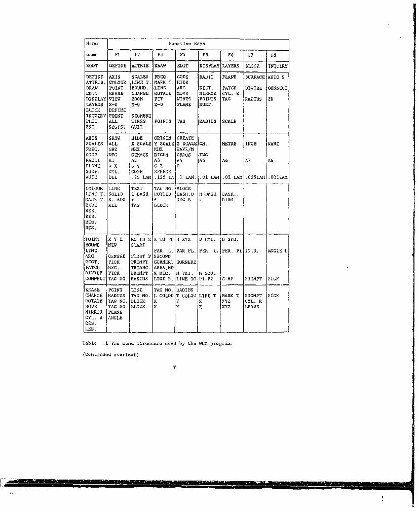
Menu Function Keys

name F1 F2 F3 F4 F5 F6 F7 F8

ROOT DEFINE ATTRIB DRAW EDIT DISPLAY LAYERS BLOCK INQUIRY

DEFINE AXIS SCALES FREQ. CODE RADII PLANE SURFACE AUTO S.ATTRIB. COLOUR LINE T. MARK T. HIDEDRAW POINT BOUND. LINE ARC RECT. PATCH DIVIDE CONNECTEDIT ERASE CHANGE ROTATE MOVE MIRROR CYL. R.DISPLAY VIEW ZOOM FIT WIRES POINTS TAG RADIUS 2DLAYERS X-0 Y-0 Z-0 PLANE SURF.BLOCK DEFINEINQUIRY POINT SEGMENTPLOT ALL WIRES POINTS TAG RADIUS SCALEEND SEG(S) QUIT

AXIS SHOW HIDE ORIGIN CRE.ATESCALES ALL X SCALE Y SCALE Z SCALE CM. METRE INCH WAVEFREQ. GIHZ MHZ KHZ WAVE/HCODE NEC GEMACS RICHM CHAOS TWCRAD1I Al A2 A3 A4 A5 A6 A7 A3PLANE A X B Y C Z DSURF. CYL. CONE SPHEREAUTO DEL .25 LAM .125 LA .1 LAM. .01 LAM .02 LAM .025LAM .OILAM

COLOUR LINE TEXT TAt' NO. BLOCKLINE T. SOLID L-DASH DOTTED GASI.D M-DASH DASH.M'ARK T. S. BOX + !* REC.B x )IAM.HIDE ALL TAG BLOCKRES.RES.RES.RES.

POINT X Y Z RO PH Z R TH PH D XYZ D GYL. D SPH.BOUND. NEW STARTLINE PAR. L. PAR PL. PER, L. PER. PL INTR, ANGLE LARC CENTRE FIRST P SECONDRECT. PICK PROMPT CORNERI CORNER2PATCH REG. TRIANG. AREANODIVIDE PICK PROMPT H REC. H TRI. M SQU.CONNECT TAG NO. RADIUS LINE B. LINE TO PI-P2 C-MP PROMPT PICK

ERASE POINT LINE TAG NO. RADIUSCHANGE RADIUS TAG NO. L COLOU T COLOU LINE T MARK T PROMPT PICKROTATE TAG NO. BLOCK X Y Z YYZ GYL. RMOVE TAG NO. BLOCK X Y Z XYZ LEAVEMIRROR PLANECYL. R ANGLERES.RES. _

Table .1 The menu scructurt used by the WGM program.

(Continued overleaf)

77

Menu Function Keys

name Fl F2 F3 F4 F5 F6 F7 F8

VIEW THETA PHI DEFAULT TH, PHzoom

FITWIRESPOINTS

TAGRADIUS2D X-O Y-O Z-0

X-0 LAYER I LAYER 2 LAYER 3 LAYER 4 LAYER 5 LAYER 6 LAYER 7 LAYER 8Y-0 LAYER I LAYER 2 LAYER 3 LAYER 4 LAYER 5 LAYER 6 LAYER 7 LAYER 8Z-0 LAYER 1 LAYER 2 LAYER 3 LAYER 4 LAYER 5 LAYER 6 LAYER 7 LAYER 8PLANE LAYER 1 LAYER 2 LAYER 3 LAYER 4 LAYER 5 LAYER 6 LAYER 7 LAYER 8SURF. LAYER 1 LAYER 2 LAYER 3 LAYER 4 LAYER 5 LAYER 6 LAYER 7 LAYER 8RES.RES.RES.

DEFINE NAMERES.RES.RES.RES.RES.RES.RES.

POINT NUMBER COOLED.SEGMENT LENGTH NUMBER DIRECT.RES.RES.RES.RES,

RES.

N~b. F9 and FL0 call up the last menu and the root menu respectively,except in root menu itself, where F9 and FlO are used for the PLOTand END menus. The word 'RES.' indicates an option reserved for afuture addition.

Table I (Continued).

I1 LIN I

_ _ _ - 2 1

L ---- -- - -- - __

Fig. I The three-wind~ow display Fig. 2 Typical display (monopokl omounted cona box)

Fig. 3 Vertikaiiy-polarised field pattern Fig. 4 Cross-polar field patternfor object in Fig. 2

I

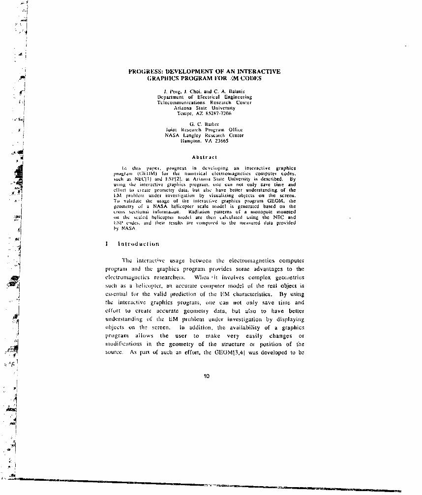
PROGRESS: DEVELOPMENT OF AN INTERACTIVE(;RAPHliCS PROGRAM FOR -"M CODES

I. Pcng. 1. Choi. and C. A. BalanisDepartment of Eectrical EngineeringTclceurnmunications Rsccatch Cc!cur

Arizona Statc UniversityTcntpe. AZ H5207-7206

G. C. BlatherJoint Rcscarch Program Off'ice

NASA Langley kcsearch Center* IHampton. VA 23665

Abstract

lo this paper, progress in devu oping an interactive graphicsprogram (G(iEO)M) for the numerical clcetomagnictics computer codes.jsuch as NIE.C I) and ESI'121, at Aiim.ona State University is described, Byusing tie interactive graphics progratm. one can not only save tiLne andclfTit to ktcaitc geometry data. but also have better undersitnding of the

NIt pr3heCml under investigation by visualizing objects on the screen.%l1 ValiddiC the usage of the iltCramtivc graphics program GEOM. the

gcomctry of a NASA helicopter scale model is generatcd based on thecross sctliunal illfornla,,Un. Radiation pattcrns o[ a monopole mountedon the scaled hceicopter noudel arc then i;alLculatcd using the NEC and[SI' c,)dcs, and iheir rcsults arc compared to the nmeasured data providedby NASA.

SI Introduction

ZThe intractive usage between the electromagnetics computer

program and the graphics program provides some advantages to theelectromagnutics researchers. When -it involves complex geometriessuch as a helit:optcr, all accurate computer model of the real object is

4 ! essential for the valid prediction of tie EM characteristics. By usingtile interactive graphics program, one can not only save time andeffort to create accurate geonsetry data, but akso to have betterunderstanding ol' the EM problem under investigation by displayingobjccts on the screen. Ih addition, the availability of a graphicsprogram allows the user to make very easily changes ormodifications in the geometry of the structure or position of the

:e7 4" source. As part of such an effort, the GEFOM13,41 was developed to be

IL 'i 10),

A

"I

Ii ~ m m . m

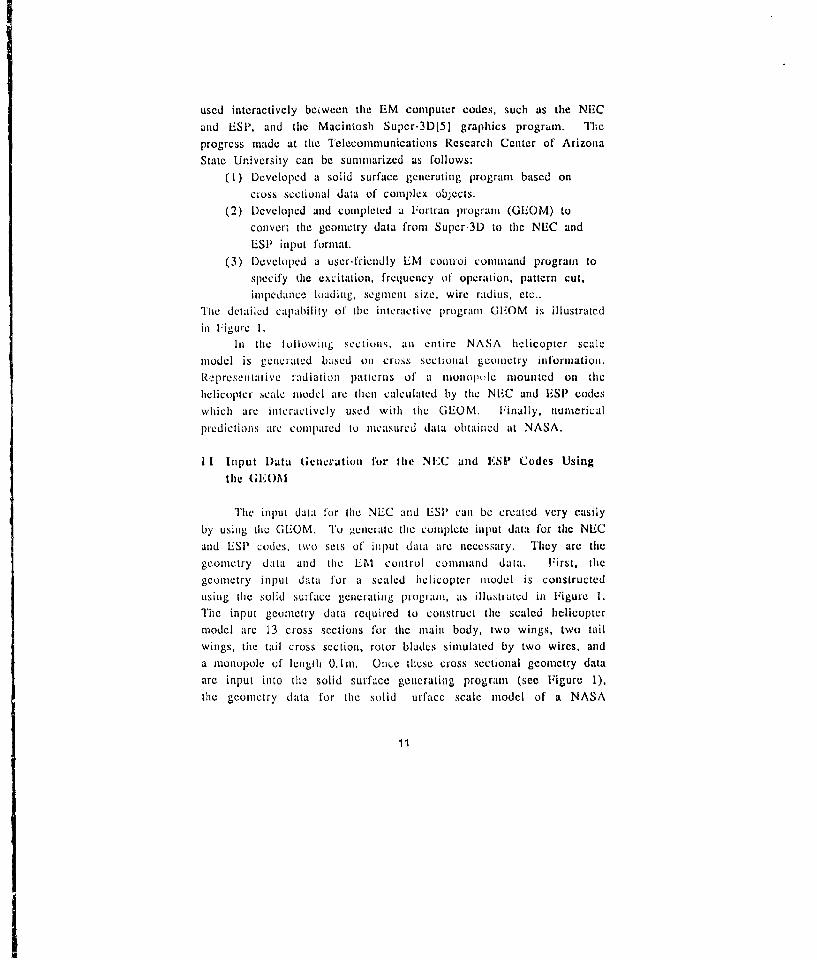
used interactively between the EM computer codes, such as the NECand ESP, and the Macintosh Super-3D[5] graphics program. Theprogress made at the Telecommunications Research Center of ArizonaState University can be sumnnarized as follows:

(I) Developed a solid surface generating program based oncross sectional data of complex objects.

(2) Developed and completed a Fortran program (GEOM) toconvert the geometry data from Supcr-3D to the NEC andESP input format.

(3) Developed a user-friendly EM controi command program tospecify •he excitation, frequency of operation, pattern cut,impedance loading, segment size, wire radius, etc..

The detailed capability of the interactive program (IEOM is illustratedin Figure 1.

In the lollowinlg sCctitiS, an entire NASA helicopter scalemodel is gencratcd based oin cross sectional geometry information.Representative radiation patterns of a monopllc mounted on tilehelicopter scale model are then calculated by the NEC and ESP codeswhich arc interactively used with the GEOM. Finally. numericalpredictions arc compared to measured data obtaincd at NASA.

II Input Data Generation for the NEC and ESP Codes Usingthe GIi•OM

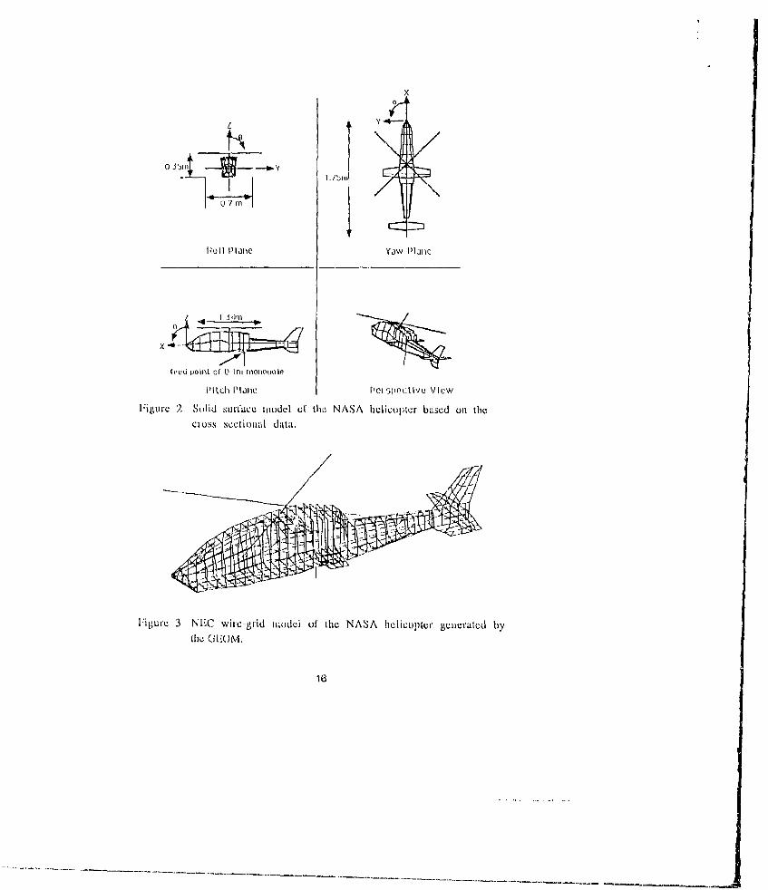
The input data for thle NEC and ESP can be created very easilyby using the GEOM. To generate the complete input datm for the NECand ESP codes, two sets of inlput data are necessary. They are thegeometry data and the EM control command data. First, tilegeometry input data for a scaled helicopter model is constructedusing the solid surface generating program, as illustrated in Figure 1.The input geometry data required to construct the scaled helicoptermodel are 13 cross sections for the main body, two wings, two tailwings, the tail cross section, rotor blades simulated by two wires, anda monopolc of length 0.mi. Once these cross sectional geometry dataare input into the solid surface generating program (see Figure 1),the geometry data for the solid urface scale model of a NASA

helicopter is gciieratud, as shown in Figure 2. Second, EM controldata (labeled as 'user input' ill Figure 1), which consist of thle,excitation type-. frequency of operation, pattern type, pattern cut,impedance loading, segment -size, wire radii of the segment, and soon1, need to ble specifie~d by the, user.

The solid surface. geometry data along with thle EM control datacanl now be. used as anl input of thle GI3OM miain program to generatethe input daut for cither the ESP1 surface, patch model (Figure 2) ortilc NEC wire-grid model (Figure; 3). Note that the wire-grid modelfor thle NLC code is generated automatically in the 013CM mainprogram. For thle NASA helicopter scale mnedcl shown inl Figures 2and 3, thev ESP~ surface patch model contains 107 surface patches andthree wires, and the NI C wire-grid model COnISists of thle total of 853wires using the segment size of 0).05x.

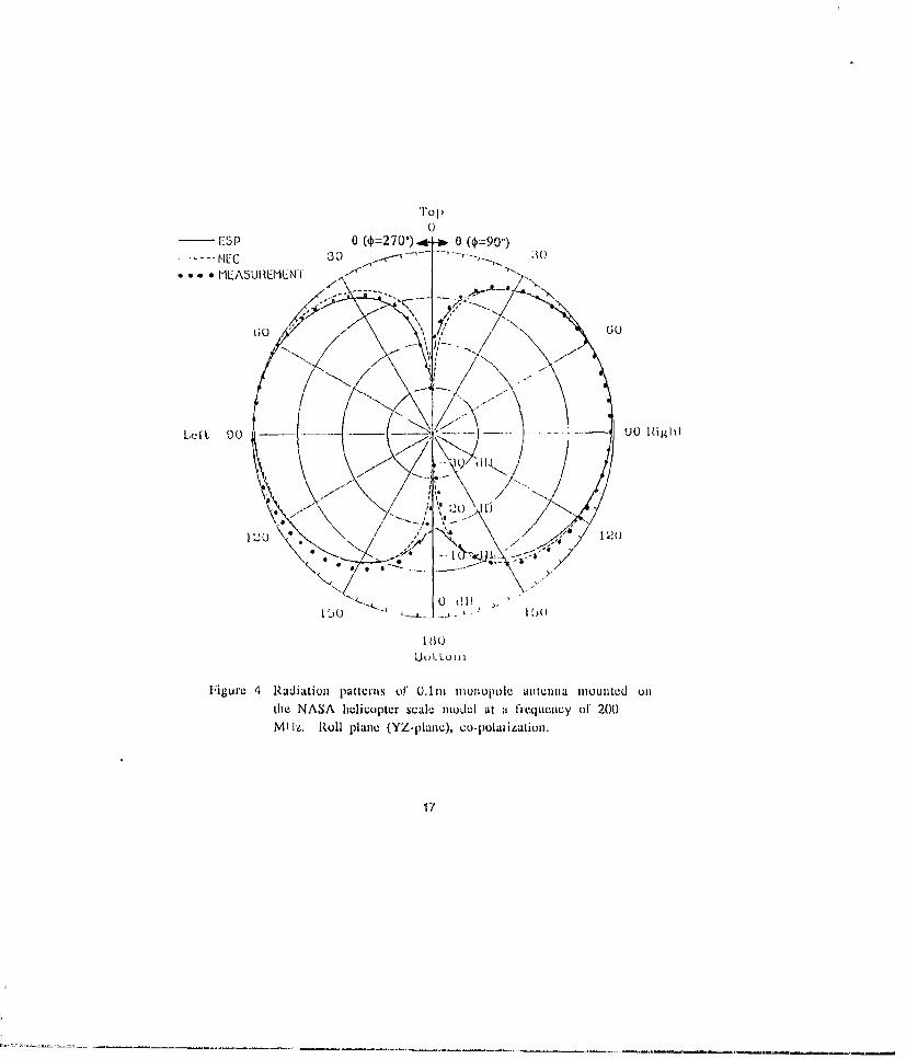
III Rudiation Patterns of' a Moniopole Mounted on theNASA Heleicopter Scale Model

The radiation patterns of a 0.1 n monopole moun ted on thleNASA helieopter scale model are. calculated using the NE'C and thleUSI' codes. Tlhe overall dimensions of' the scle d heli~op~or model areillustrated int Figure 2. In both NEC and VIS11 codes, 0.051 segmenltlength is used. After thle segmnictation, the NiE-C wire-grid model has853 wire current modes, and the. ESP codes has 1,002 plate currentmodes and 22 wire current modes.

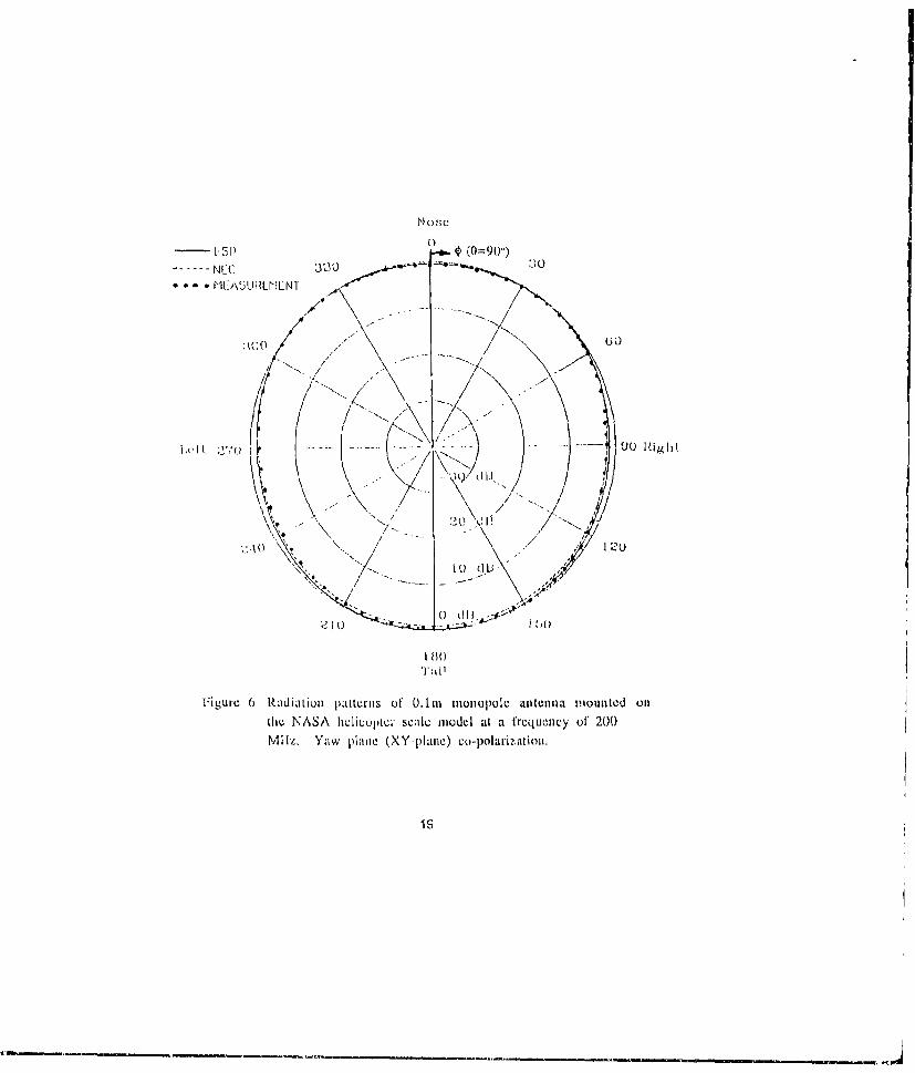
In Figures 4-f the radiation patterns (normalized gaini in dBi) of'a O.lmn monopole antenna placed at the M1P1 location (36.5 inches aftof nose) of the helicopter body are presented as a function of aspectangles. Bloth the NEC (dashed line) and the ESP1 codes (solid line) areused interactively with tile GBOM, and their results aro compared tomeasured data provided by NASA (dotted curve) in thle three majorpattern p~lanies; i.e., roll, pitch, and yaw planes. For eachi patternp~lane, only thle co-polarized patterns are plotted, Note that each dataset is normalized to its own mnaxinmum.

There exists reasonably good agreement between thecalculated and measured data. llowevem, in the roll and pitch plancs

12

the agreement between the measured data a- d the NEC calculateddata is better than that between measurements and predictions bythe ESP code. One can also notice that the symmetry property of theradiation patterns of the ESP code in the roll plane has deteriorated.This is believed to be due to the non-symmetric positioning of theoverlap current modes on the two joining patches[6]. Also, numericalefficiency of the NEC is superior to that of the ESP. In general, thisstatement is true whenever a surface patch model of the ESP coderequires many overlap current modes. To obtain the entire patternsusing the NEC code, it takes 1,278 CPU seconds on a CRAY X-MP/18sesuper computer. On the other hand, the ESP code requires 13,000CPU seconds on the same machine.

IV Conclusions

The interactive graphics program GEOM developed at theTelecommunications Research Center of Arizona State University wasused to generate the geometry of a NASA helicopter scale model. Byusing the GEOM, we not only saved time and effort to generate thecomplex geometry data but also avoided the error prone direct inputprocess. In order to validate the interactive graphics program GEOM,radiation patterns are calculated using the NEC and ESP codes whichwere used interactively with the GEOM. Despite of the complexity ofa NASA helicopter geometry under investigation, the numericalpredictions and measurements are in excellent agreement.

Presently, only a limited number of geometry and EM controlcommands are incorporated into the GEOM. More general controlcommands will be included in the code in the near future.

Acknowledgement

This work is supported by the Advanced HelicopterElectromagnetics Industrial Associates Program and NASA GrantNAG-l-1082.

13

References

[1] J. Burke and A. J. Poggio," Numerical Electromagnctics Code(NEC)-Methods of Moments Part 1, 2, and 3." Naval OceanSystems Center, San Diego, CA, NOSC TD 116, 1990.

[2j h. H. Newman, "A Usci's Manual for Electromagnetic SurfacePatch Code: ESP Version 4," The Ohio State University,llectroScienee Lab., Rep. 716199-11, Dept. of ElectricalEngineering prepared under contract Nu. NSG-1498 for NASA,Langley Research Center, Hampton, VA. Aug. 1988.

[3] C. A. Balanis et al., " Advanced Electromagnetics for HelicopterApplications," Arizona State University, TelecommunicationsResearch Center, Annual Report prepared under NASA researchgrant NAG-i-1082 and Advanced Helicopter ElectromagneticsIndustrial Associates Program, Oct. 1990.

4] J. Peng, J. Choi, and C. A. Balanis, " Automation of the GeometryData for the NEC and the ESP Using the Super-3D," Proceedings of6th Annual Review of Progress in Applied ComputationalElectromagnetics, pp. 33-38, March 1990.

[Li Super 3D, copy righted by Silicon Beach Software, 9770 CarrollCenter, Suite J, San Diego, CA 92126.

16] C. A. ]3alanis et al., "Advanced lhelicopter ElectroinagneticsAssociates Program," Quarterly Progress Report, Arizona StateUniversity, Telecommunications Research Center, June 1990.

14

Fi g ir es

L S31 d .uu' lac ditja Ci 'laiwdin'l dl.

(to let O 0 uie ItL LnV I kP[UtIw l dil[W

U [olnet Y e CenerJ IllJ Q,41 .1.11 9i j reln~ kIluial

AvllL .- If~ II I~ -11 At I'jt-

GCOI I Ha.111 IIU4I u dill tv iwinel Aj

NLC wire 011' 5ur Wce

4L. C uitlen - ___

Figure I Blolck diagram for the in~teractive usage of GU.OM anid theE~M codes,

x

Pullt Planre Yaw Minel

I 4

PI'td Plane Pcl spcttive VieowFigure 2 Sulid surface iiiudel of the NASA helicupter based on the

closs sectiounal data.

Fiue3 NLC wirec-grid model of the NASA heclicoptur generated byOwe (3E(M.

16

US (ýz=27O') 0 4=901)--- NEC .30 3*..MLA5UREMLN1I

LclL ~ ~ ~ -- ----- ----- IjjIi

I Go

I~u Loin15

Figure~ 4 ROadiationi paztcrlis ofI 0.11 zu iiilopoIe .1ntenuii niiiuuied U11tbe NASA liicIicopter scale Inoddi at a frequenicy of 200M Iz, Roll piane (YZ-plauu), co polarization.

17

TIop

- Lsp 0(fr1 0) _ 0(4 )---- N EC 31) 30

H EA5UIRCHLNT

(30

200-- ~ z. Pitch plano (€ z-pla pa15o \ ,

'l',lll I}O 5- - - (,,t

"K U l11 v

30 * 130

1110

O. . . .. .. . . . . .L, u

- LSI~ ~ (0=901)N----- NEC 300

* -* ll.J3UF&MLN]

A6

/0Rih

0) 11ig3i

M ~) l

Figure~ ~~~I 0 Raitunptejiso,0.1111/ooealenamutdu

U OwN S ilýutvsaemdlaa \rq~mc /f 200

Mllz. Yaw lalic(Xy-lalC) dopla ztol

R. Fisher Science & Engineering Associ:aicy6100 Uptown Blvd. NE, Suitt; 70X)Albuquerquc, NM 87111)

1. L. Coffey - Advanced Pilecttomaigneticr5617 Palomini Dr. NW

Albuquerque, NM 97120)

Lt. T'. Timmcrman - Phillips Lahoratory/AWEKirtland At.'B, NM 87117-6(X)8

OverviVw/Status of (;,MCOl.

The primay objectives of tlie GEMCOP program are:- Develop a user ft lendly, menu driven Wesitrol progranm for GEMACS/GAUGL- Minimize the requirements for user's knowledge of GEMACSIGAUGE

P lrovlde pre/post processing support for GEMACSiGAUGESupport script file development for execulion of user applications

- Simplify user development ol comnplux tolplogies

The original dcvelopment of GEMCOP was intended for the PC/DOS etvirotnuent. Due to increasingdemands placed on computer memory by plograms ;uch as OEMACS and (.AUGE, as well as the graphicalnature of the GEMCOP progranm, the development has been shifted from DOS to OS/2, Sintce OS/2 opc atleswith a linear address space, •gc aztd problems requiring more than the old DOS 64A0 KB limit canl besupported. lHowever, Ihis migration to the OS/2 cnviionnient place new requirements on the hardwarenecessary to run GEMCOP. An 80286, 803.8, 80486 processor is required, or a woristation calpalelu ofsupporting OS/2. The compiulcr must havc at least 2.5 MB of" RAM with 4 MB recommended. In addition,the computer will need a hard disk oif from 4,) to 60) MB) w'th IMX MB or illmotC rCcoiuncitdect.

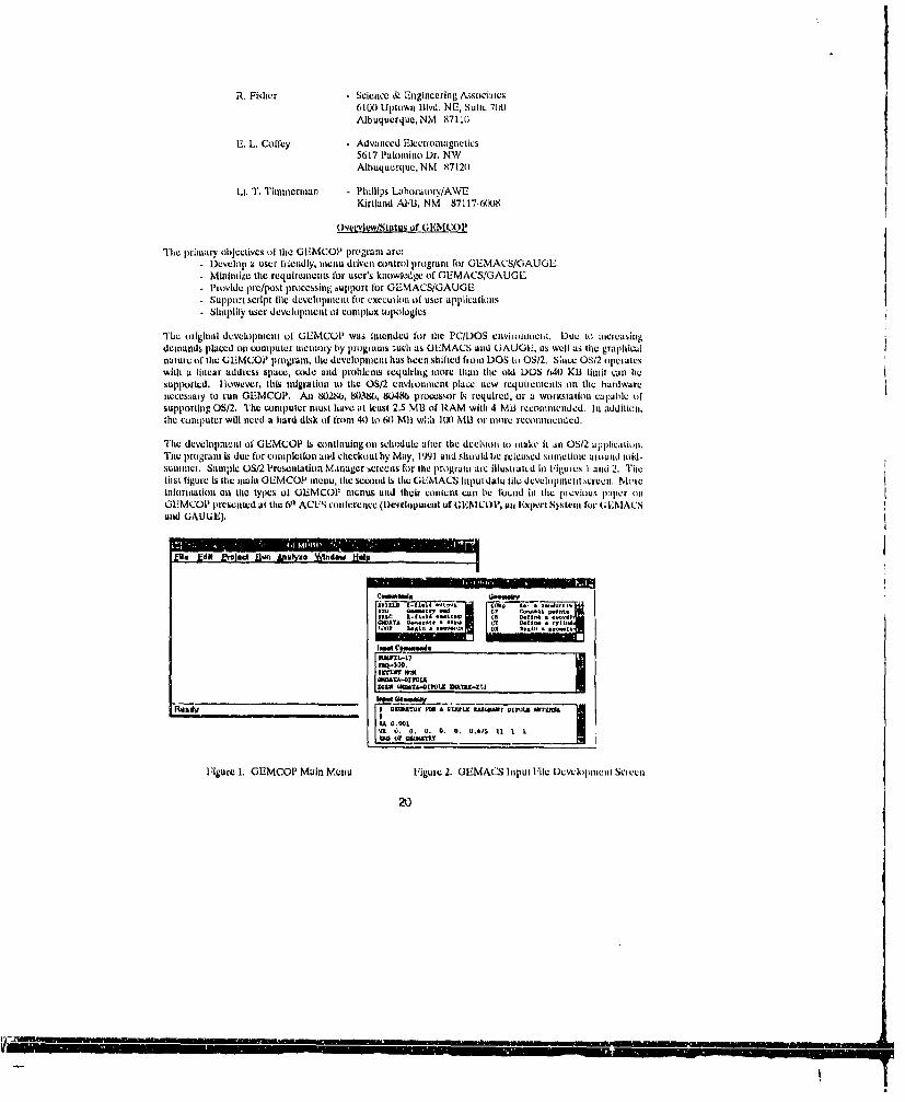
The dcvelopiment of GOMCOP is continuing on schedule after the dccision to mitake it an OS/2 application.The prtogram is due filr culipletlon and checkout by May, 1 9'91 and shotuld tie released sotmetimc awound mid-suntner. Santple OS/2 Presentation Manager scrcens for the progra.n arc Illustratcd in Figurcs I antd 2. TheIlust figure Is the nmhi OEMCOP mentu, the second is the GEMACS Input dala ile develpumencit stitch. MletInlormtatlon ost the types of CLEMCOP nwrius and their content canl be found in the pievious impel otlGEMCOP precented at the 61t ACE-S conference (DIevehlopnitint of GENlC'iP, alo Iwrt System fur (G IMAI'Sand GAUGE).

dotd) at un ii a Ydn•w *It

E le

I lctIW&mit-tOOUTIrriN?

Z-0t97 GAT".'OPOU Z VAT111-Mt

W& 1. 0. 0. 0. 0. 0.41 51 1 1

Figure 1. OUMCOP Main Menu Figure 2. GEMACS Input File Developtment Scrceen

20

9-

IMPLEMENTATION OF TIHE NEC - BASICSCATTERING CODE ON"A PC

Ronald J. MarhefkaThe Ohio State UniversityElectroScience Laboratory

1320 Kimear RoadColumbus, Ohio 43212-1191

Phone: (614)292-5752

AbstractIt is desirable to have general purpose user oriented codes run tll as mauy

machines and compilers as possible. Users prefer to change as little as possibleii the codes to get them to run on their computers, This is espccially desirablefor large codes like the NEC-BSC. Changes made to the NEC,;-BSC to make itmore easily implemeuited on PC type computers will be presented. The talk willcenter primarily on IBM compatible conmputers and several compilers, thoughother types and sizes of nmachines will be discussed. Benchmarks for the codeon lurge amd small computers will be compared.

Rerent technical enhrancenments to the code will also be outlined. Theyinclude third order plate interactions and double diffraction along with a di-electric curved surface capability (without surface waves). These chmiges willbe available in version 3.2 of the NEC-BSC.

I Introduction

A new version of the NEC-13SC has been slightly modified to take into considerationimplementation oil peraonal comnputers (PC). Modern PC hardware and softwarehas progressed in recent years to the point that they can easy be used for runningelectro mag etic codes. It is therefore, the preutise of this discussion that the [tilversiom of the NEC-13SC is to be implemented on the PC. No special version fur thePU is attemptedL The code is F|ortran 77 and only modifications to imake it easierto run on the PC without causing dilliculties on bigger im-chines are made.

First a brief overview of the capabilities of the code is presented. Specific changesthat took place for PC operation is detailed next. The hardware and software used

21

in the benchmarks are then presented. The benchmarls .,st compare various VAXcompiler options, then two IBM types and three VAX machines are compared.

II Background

The Numerical Electromagnetic Code - Basic Scattering Code (NEC-BSC) is auser-oriented computer code for the electromagnetic analysis of the radiation fromantennas in the presence of complex structures at high frequency. For many prac-tical sized structures this corresponds to UtHF and above.. The code can be used topredict near or far zone patterns of antenn'as in the presence of scattering structures,to provide the EMC or coupling between antennas in a complex environment, andto deternline potential radiation hazards. Simulation of the scattering structures isaccomplished by using combinations of perfectly conducting multiple flat plates, fi-nite elliptic cylinderb, composite cone frustums, and finite composite ellipsoids. Thecode, also, has a lirnited finite thin dielectric capability for both plates and curvedsurfaces, The analysis is based on uniform asymptotic techniques formulated internis of the Uniform Geometrical Theory of Diffraction (UTD) 11,21. This versionof the NEC-BSC is an. update to version 2 [3] and the more recent version 3.1 [4).

A sumnniary of the capabilities of Version 3.2 [5] is listed here:

* User oriented couminnd word based input structure.

o Pattern calculations.

- Near zone souarce fixed or moving.

-- Far zone observer.

- Near zone observer.

o Single or multiple frequencies.

@ Antenna to antenna spacial coupling calculations.

- Near zone receiver fixed or moving.

* Efficient representation of antennas.

- Infinitesimal Green's function representation.- Six built in antenna types.- Interpolation of table look up data.- Method of Moments code or Reflector Code interface.

22

r .. ... .. .. . . ..

"* Multiple sided flat plates.

- Separa~ted or joined.- Infinite ground plane.

- Limited dielectric plate capability (no surfuce waves).

"* Multiple curved surfaces.

- Finite elliptic cylinders.

- Multiple sectioned elliptic cone frustumns.

- Composite ellipsoids.- Ljimited dielectric curved surface capability (no surface waves).

"* UTD multiple interactions included.

- Second order plate termis including double diffraction. (restricted toPEC).

- Third order plate terms:

"* trip~le reflections"* reflection -reflection - diffraction"* reflection -diffraction - reflection"* diffraction - reflection - reflection

- First order curved surface termis only (creeping waves for PEC cylinderOnly).

- Presently no plate - cylinder interactions.

"* Individual control of every U'1D term.

a CIKS graphical codes for geoniietiy and patternis.

III Changes made for PC

The preniise as mentioned above is that P~s have gotten large enauglh to handleessientially tile Samle code as bigger machines. Ther changes needed arc, therefore,rather minliallj. Thle major task has been to reduce the size of thle larger subroutines.Many PC compilers such as Microsoft and NDP have a limit onl the number of linepsthat can be compiled at one time. This limit is proportional to the amount ofmemory in the computer. The PCs used have 4MB of memory. The practical sizefor compilation of each file seems to be around 3000 lines. Several subruutines, that

23

were originally designed to directly share information by using entry points, neededto be changed into individual subroutines. This r-iuired using more common blocksto transport thei shared information.

Next, the rode needs to be broken up into many different fRles. Usually whensending the code out, we put all our codes into one file. This makes documentationeasier, since all that needs to he done to the codes is Fortran, Link, and Run asingle file. When breaking the code up into files, it is necessary to decide whether

"4J, /to do this simply alphabetically or group files by functions. Putting subroutinestogether by functions seems better, at least for the code developer, since changes tothe code usually will be confined to fewer ffles. For the NEC-BSC this turns out,presently t- be 16 different files of various sizes.

"Fortran specific changes seemed to have been unnecessary, since the code hasbeen written in standard Fortran 77 as much as can be determined. Of course thereare always variations between compilers, but the PC compilers used seemed to be•'•' ' ]striving for Ra much com|nlatil~ility with the standard options (if the VAXes on whichSthe code was devr,,ped. One extended feature of the VAX that is used is tabs inthe beginning of line& Therse can easily be removed and usuallj are depending ondist.*ibutiota furniat. The new version 2.0 NDI' compiler seems to be 100 percentcompatible with this feature, .,there as the previous version would not work in allS~cases

The other change made centered around associating the logical unit numberswith the input and output files. In previous versions of the NEC-BSC, the rPsign-ments are left up to the user. For example, on a VAX the ASSICN or DEFINEcommands rould be used. In the new version, OPEN statements are used in thecode. The input file name is obtained after the start of the code.

On output for the P'C, it is assumed that the operating system does not supportversion numbers for files. If the user is requesting more than one output, than thecode will inquire for a new name for an output file when one already exists on thedisk. Thi's can be changed by the user if a different naming convention is desired.

IV Hardware Considerations

The suitability of PCs for many engineering applications has gi. atly progressed. Itis not necessary to restrict the code to accomodate the hardware limitations. It isassumed for an IBM compatible that a 386 type machine or better will be give bestresults

The primary machine used in this slvzdy is a 386SX, 16MIlv, 4MB IBM typecomnputer with 80387SX math co-processor and 60IMB hard disk. In addition, a

24Im

full 386, 20MHz, 4MB IBM compatible with 80387 co-processor is also used in thebenchmarks. The VAX computers used for comparisons are a VAXetation 2000,VAXstation 3100 M30, and a VAX 8550. The workstations had 8MB of memoryand are diskless being clustered into the VAX 8550. The working aet size for theVAXes are set at 1000.

The size requirements of the NEC-BSC version 3.2 on the disk are 668KB forthe Fortran source code. The NDP compiled object modules took 984KB of spaceand the execute module took 673KB. The memory requirements for running thecode are 983KB.

V Software Considerations

Several PC compilers for IBM's have been investigated. It is assumed that DOS4.0 is the operating system for the PCs. The Microsoft compiler appears to be verygood, however, it presently does not allow the code to go beyond the 640KB range.In order to accomodate the size of the NEC-BSiC V3.2, it would be necessary touse the 052 operating system. It would also have been possible to reduce the sizeof the code by removing subroutines or reducing the array sizes, however, this wasnot done.

The Lahey Fortran 77 Version 2.0 compiler with Al extended jijemory operatingenvironment was tried. This was successfully used on Version 3.1 by someone usingDOS 3. It has the advantage that the compiler is very fast and does not requirethat the code be broken up into small filea sizes. Unfortunately, the version ofLahey tried would not work on the machines used here. The extender would hangup all the machines tried by us. As near as can be determined, this is due to aincompatibility with DOS 4.0. New versions of DOS or the Lahey product mayremove Lids problem.

The compiler used for the benchmarks here is the NDP compiler and PIIARLAP 386 ASM 2.2 linker and extender. Two versions of the NDP Fortran compilerhas been tried. First, Version 1.4E/5 was used and then updated to Version 2.0.8.There was no difference in time or accuracy detected between the two versions. Thenewer version, however, is much easier to use since it is more compatible with theVAX's use of tabs. Version 2 is used here in the benchmark.. It should be notedthat it takes exactly 1 hour to compile the code on the 386SX. Presumably most ofthat time is spent in the assembler stage.

One problem arose when Windows 3.0 was installed on the 386SX machine. Thenew windows environment requires that the IIMEM driver be installed. Therepresently is a conflict between the memory handlers in NDP and Windows. It isnece-'ary to reboot the machine wvithout the !!IMEM driver to use the compiler and

25

linker. This problem is being addressed by Nfl' and hopefully will be imiproved inthe futitic.

Various individuals ave working on implementing veisions of the NEC-BSC onMACB. Unfortunately, [to data is available here. It hau been determined that someversions of compilers for MACs (Absoft MarFortran/020) do not initialize variablesto zero. The NEC-13SC huas beent checked uaing a product called LINT to findundefined variables, however, it did not detect one in the Subroutine SOURCP. Thevariable wall defined at some place in the subroutine, but the IF THEN ELSE l1gcwould hyposs it in certainl cases 16). This caused rather large errors, however, it hasbeen corrected in this version.

F'or thle VAX computers, Various Com1piler options are compiared. They presentlyare runnling VMS 5.4 with D)E(wiindoLws installed onl the workstations. The firstcompiler contfiguration is suited for tile code developer. It has thle debug Option,no optimiization, bounds checks, and all warnings options includled. The secolldand third configuration compares the optixniger versus no opitimizemr. AU otherchecks and warnings are turned off. In certain past instances, thle VAX optintizerappeared to give some trouble. No difficulties are presently being encountered. Forcomparison, it should be itoted that it takepi arcound 4-5 mninutes to compile thlecode onl thle VAXatativin 3100.

V1 Benchmarks

T1wo examples fromt thle NEC-138C User's Manuals are used in tile bencinglarkingp~rocedure. TIhe first is Example 6 which calcutlates the pattern of at dipole inl thlepresence of an eight sided box. Tilhe second is Lxanipile 19i which calculates thlepmattern of a slot on the whig of a model of a B737 aircraft. In both of these case, afar zone pattern of 3t1 data points in 1 degree increments is compunted. 'rite UTIJternms autuuiatically obtained fm-owii thle XQ commnand tire used.

The CPU times tire tbtaiued by ull ,Ing thle ,,SEC-UU', function for thle NiH'compiler and "SYS$(l;BTJPl" function for the VAX. The Lttmes are converted andpresented in minutes. T'he CPU timies are the diflerence between the saumples takenkafter the input data is read and echoed back to the user and before the: fields areoutpuit to the dink, T1he values, therefore, represent only the* time it taktes to do tileEM field calculations and does mnot included any 10.

In ternis of accuracy, all VAXes produce exactly the same results. Thie PUB'produced thle same accuracy compared to tile VAX over the five digits displayed forall slignifialcat results. The eceCptionl being thle nloise level crosst polarize.d resaults inExample 6, which is normal and expected.

26

ý(Iouzpiler opt.ous Exailzipiti I Cxml ~]LNo opt, iali chiecks 3.29 -_ f 2.25 j[No op~t, 1no cht'.cks 1.28 L 1.09JLOpt, it, ciiccks 0.4.8

J'ai~li 1 I'31 beCOiMIjma~rilg Various11 coinpilier optionis using a VAXstatiuu 3100 M30.CP'U tinieis are ill iiiminutes.

fi-imu7Ex -a I I T P_ýxilF _ 11T.__

PU 38j96SX9 3.26 3.14IfVAX 2000F 5.10 3.-01l-L1)(1 386 2.2 0 2.00VAX 3100 0.94 0.89)

LAX 8- "1 0.,10 0.38

Table 2: Tabl (it'nomipaifiizg vaiomuiis c~itilemph rs. 'The VA Xes are run using t he uiptinaUct with ill) tiicckt. CH tiiiws are ini iniiiiute.

Thle first ben licin arkti for t he two exaim0ples are rityi, uii g tlie VA Xstatii ii 311I)(1.'Iiirer Ctummpilvcr optionus uirv timed. First iail checks, ldebtig, aind no u ptii zziatiwi istised. - ccuiid all dheclia and the tiehug o11tiUomis are turnedt Off With 1110 iJ1lti Imuzti~lli.

Ill tihe Inal casie, 01 ditieksi and debug Optionis ate uff but t he optiiidzer is oil. There~sults for the three cases arc shzowniil Tab lae 1. Aiiotzingly the CI'UJ tittles withthv limecki oun differ by Over d factoi of 2. The uptniazeti hkelps by about auother25%. Of Cotirge wiicmz first runinmmmg tihe coide, it is safer to izse the butiuids drecks,Ftur jprodntietiuu iunzs, it Nvotild apiwtr learjl t~lait thlets dIJOiJI(l Ile timlruilt1 Off Itizi t)iu.opt kiiiizei utwrd.

Por (-:oniipitiui~mo bwetewz I lie varioust conmzpiil-ers, the uoitiiudzed m(inie with them

I C, i i i(.1 hieric off is umiiei ill ail tcitwi S. Thei resul ts ame slmo',ii ill TIable 2. The1m VAX2000 is slightly slower thian a VAX 780, thill izicahms that the 38GSX is runninizg veryClUtle to thei sIueeii Oif a VAX 780). The 386SX muachiine hasit 21iY slower ciii eperdthan the 3836 ;stil lias uddifioui oveorhead due to lt Ith h6 it bus winuimred to thr. 32

itbus. i his propCerly wecout0 kiyhir theiv indicated tittiie diffe renes. Tihe VAX's ti ilesli.o aie acco~untedi for by the p ii litiisied diierelczwm(e ill C PU ipeedsl Withinii reassonatblebuUid,du

27

VII Conclusions

The experience of imphume.iLing the NEC-1SC V3.2 on PQ• is presenLcd. Varioushardware and software C(Afigu.-atiuns are discussed, le nchuarks for two examuplesfrom the user's manual arc used to compitre the l'Ps to VAXes. It appears thatIPs can be effectively used to run the full up NF"C-IlSG.

References

[1 P1. II. Panlik, "'lTediiques for high-freq~rtncy problemi," in Antenna llandlmomk "'1heory,Applicatioms, and Desiqn, (Y T. lo and S. V.. Lee, eds.), chi. 4, New York: Van NostrsuidReinhold C2o. h1c., 1988.

121 W. 1). Ilurtilide anid it. J. Marhefka, "Anticiais on aircraft, ships, r any large, co mplexejvirutjipeoL," in Antenna Handlxawk: Theory, Applicahuiovs, and Design, (Y. T. ho andS. W, Lee, eds.), cit. 201, New York: VaR Nostrand Iteinhold Co. Ihc., 1988.

[3l It. J Marhelka anui W. 1). IlBurislde, "Ncimicerical dvitr iing letic c-de - h imic micaLtenligcode (versiou 2), PttrL 1: user's manual," Technical Report 712242-14, The Ohio StateUniversity blectroScience Labocratory, l)eplartment -f Electrical Engineering, Dec. 1982.Prepared under Contract No. N0f1233.7-WC-1461) for Naval Iteglonul (ontracting Of)icv,

[4) It., 1. Marhefc•a and J. W. Silvesiro, "Near zone - basic scatt.triiig rode, uset". muaimaiwiLt space statlon applicatiouns", Technical Report 716199-13, The Ohio State jiti-versity ElectroSclence Laboratory, )eplatimeut of Electrical Eugtneering, March 1989.Prepared 'moalr (rh'ut Ni,. NSG 1613 for N atotial Aevrinstlcs and Space Administra-tLion.

[51 IR. J. ?•,arhlllus, "NEC - basic scattering code, user's n uli (version 3.2)," Final lte-port "118422-4, The Ohdo State Untiversity hlectruSeleance Laouratory, D tepai-tiuet A•Electrical bnghieerinK, l)ec. 1U99. Prepared under Contract No. N60fi3U-81-C-0249 forNaval Weapons Center.

[6] G. J. Burke, "I'ersoumal c.tunuicatlons," Aug. 19901.

28

NEC, FERM & GEMACS on the Macintoshby

Paul E Bussey & Dr. Russell W. Taylnr

Introduction, Motivation and Objective

Our objective is to simplify the development of reliable ElM models for the threeanalysis codes, NEC, FWRM, and GEMACS by creating a interactive program toanalyze these models, Our experience with other data analysis/visualization codesdesigned to support these three codes has been less than completely successful.McDonnell Douglas Ilelicopter Company has had problems with IGUANA andGUAGE. The data anilysis/visualization code which supports FERM was not avail-able.

Othier similar codes do not have the santo same objective as our.:. They presentthe geometric representation, but do not easily alert the user of the potential problLmswith the model. We have endeavored to include features that will make debuggingeasier. Our verification code indicates situations which can result in incorrect inter-action matrix elements, or cause misleading results.

The Macintosh CPUs were chosen because we have developed codes on themfor other purposes, an excellent development environment is available, and thegraphical user interface is easier for new users to learn. The alternative platforms fornost of our projects are MicroVAX Ils. The newer Macs are much less expensive(espvcially for large aiunuunts of memory), as well as faster than the MicroVAXo, andthey provide greater preciioAn for floating point calculations because they use theIEI"EA standard 80 bits for real and complex calculations.

Code Installation on the Macintosh

lnstallatiorn of the three analysis codes on the Macintosh is planned, but thistask is not yet complete. NEC installed very easiiy with essentially no modifications,but GEMACS and VERM both contain code that does correctly execute on the Mac.Further information will be available at 0.!e conference regarding these installationproblems. Our approach to generating the in'ut data for our verification code is tofirst use the input data interpretation part of the analysis code without modification.

29

We have slightly modified the analysis codes so that a file is automatically writtencoIntaining the data we need as input. Reproducing the data interpretation portions ofthe analysis codes has not been attempted; we believe this approach is less prone toerrors.

Benchmarks

The benchmark results will be presented at the Conference.

"Good Practice" Violations Tests

Calculating the interaction matrix requires several integrations to be performedinvolving the Green's; function ( Equatimn 88 & 92 of NEC manual, Vol. 1 ). Since thereis no closed-form solution for these integrations, several series expansions are used(the number of terms is determined by the thin versus extended-thin wire approxima-tions ). These integrals are expanded in terms of two variables, a and 1. where a is theradius of the source segment and p is the radial distance to the observation segment,"The expansion in terms of p is used only for the self-Interaction term, while the expan-sion in a is used for all other interactions. The expansion in p was developed for thespecial case when the observation point falls inside the "cylinder" of the source seg-ment, the expansion in a is not valid in this case; however, this expansion is only usedto compute the self-interaction terms. Unfortunately, it is possible to build models inwhich observation points fall within the volume of other segments. Thenl, during thecalculation of the interaction terms, the wrong expansion is used to determine the IIn-teraction, thus producing erroneous results. We have decided to divide the modellingerrors of this type into three groups - adjaceni ,egments which Intersect at angleswhich are too small, urdntentional intersections (not in connections table), and dupli-cate segments (often generated by computer gridding routines ).

Acutes: Connected wires (identified in the connection list) were examined, themidpohit of the wire with smallest radius is found, and the distance to the other seg-ment is computed. If the distance is less than or equal to the larger radius, then theangle is too acute and the interaction evaluation will be flawed.

Bad intersections: This test only involves wires not in the connection lists. Theshortest distance between the two segmeats is first calculated under test. if this

30

distance is less than the sumi of the two radii, then an inadvertent intersection is pru-sent.

Coincident selplents: As this test is conducted onl each Segment, the connlec-tion list of each end point is searched for segmients connected at both ends of anothersegment.

Incompatible radii: For this test, radii of connected segments are compared;radii raitios ( alglsill ) greater than five are Identified.

Sh~ort, fat segments: 1 lere, the length of the segment is compared to its radius;if this ratio is less than eight for the thin wire kernel, or two for the extende~d-thin wirekernel, it is brought to the attention of the user.

Bad sources: Segmnent., are identified that are both connected to a plate and ex-cited by it source.

Other tests art- also performed which are not necessarily problems, but can indicate'hat thie data is not being interpreted as intended by the user.

Opens: Chiecks connection lists for both ends. If a coruiectoion list for either enidis emipty, then the segment is added to the opens list.

Lung seginents: I lere, the length of each wire is calculated and compared to4/10 of the highiest frequency. Any wires longer than this will be highlighted.

I low Visualiza lion/Anialysis Code Works

At thiis time, the. code MacVerify has been developed to test wire framne modelsfor C1EMACSiand NU~C. lin the futuie, it will be expanded to test surface patch miodels,aILId optics /diffraction moldels. The code Is a typical Macintosh application; it is win-douw based, and event driven. We have aitenipted to give the user as much freedom aspossible without making the interface too complicated.

After running th'E miodel thiucjU ii e iiipui inier~prehiiiiuii ktige of iii.. Jvsired

31

analysis code, the resulting testfile can oe examined using I.'NlMacVerify. 9 &

After reading in the :clectcd model, a modol displaywindow is opened, as shownand controls on tihe leit side ofthe window allow the !ses to 06401

Change the Scale dnd tUICviewinig angle of the znodcIJ. A____________ I-=________________

TIhe scale is adjusted byclicking the mouuse in either of Figivre 1. Model display windowthe arrow buttons; the arrowcom1in~g out ( ZAoom1 In ) causes the scale to inecrase, while the arrow going in (ZoomOut ) causes the scale to decrease. The amount ol change can be regulatcd With thc Useof movdifier keys as shown in Table 1. The elevation and azimuth controls work in Isimilar fashion. By piesshin on the desired sido of the "axis", the mod' l will rotate inithat direction. Againi, Tablv I shows how ON,? a-mount of change can be regulated withthe use of the mnodifier keys. In addition to the rotatior cont~rols, we have provided pop-up menu.s which cuit be used to quickly set thei view to one of the prudeffinud angles(see igure 2). In its default condition, the model will be redrawn each time cone of the

controls is activated; however, fu, larger, more invol veil models, this activity canibe qlUite timeI con1SUm1ing. IIn ord er to bypass this p roblem , we ha ve added a check-boxwhich1 Will disable thet redraIWinvt, ol tlie model Lio that specific scales or viewing angles

Table 1. Model display viewing control options

with mu~d-Iiler keysFunction ~ hf pin~~f otoZoom InI 2(X)'Y 150% 125% 1101% 1Sl0l% 175%

Zoom out 50% 6 6.3"Y 801Y 90% 95%Il 57%11Eilevation

& l' 15" ~ 100 0.1o 0.010Azimutth _____-

32

can be set. The model will be redrawn according to the final settings when the box isunchecked. The model is shown to the right of the display controls. The scroll bars onthe model display allow the user to pan across the model.

'94*• i*•.~t

ama

114

.43,

-133

Figure 2. Preset rotation an8 lepop-up menus

In order to check the model against the various modelling practices, the usermust activate the diagnostics window by selecting the Diagnostics apindow op-tion in the Diagnostics menu, or by pressing thekey combination W/. The diagnostics window,shown in Figure 3, currently has selections for eight n . 9

common modelling errors found in wire models. .,.. USince performing these tests can be quite time Qtto,,,,io.... C°I,, 0

consumnig, Ute default condition is set for all of the U U18PnI 5•"I•do.tWroo I Colo

tests to be off. Any combination of the tests can be ,... Ob,•,P.GLIGsselected by checking the appropriate boxes; the tests Shr, l o p.u rat

are then performed when the mouse is clicked in the K,,ea, t':91r UR p plY button, or when the Return or Enter keys are Lat.. rJ L3t, waom.

pressed. Each test has an associated color which can incompatible o•Psv, r@ijbe changed by double-clicking the mouse inside the ,a,,n, Ublmm•,,. bid,

colored box. Any wire segments which violate a h..,"'.. 1.01o Li

particular modelling rule will be drawn in the I

corresponding color. If a seginent violates more thanone rule, it will be drawn in the color of the last rule windowtested (top to bottom in the diagnostics window).

,33

If the user wishes to change the me"w~ 'Coa.4'.ctow: N

model related colors, he may do SO via kdc Si w.uI

the model display dialog shown in Fig-urc 4. This dialog is accessible throughthc E dit menu as the P re f erence sselection. Colors can be selected for the Fig1ure 4. Model display dialogbasic model, the background,connected" wires, and the buried wires. T1he colors are changed by double-

clicking with the mouse in the desired color Square. The_ standard color-pickerdialog will appear and the user is frk-e to choose any available color.

The model statistics window is activatedby selecting the M~odel stats olptioni in the algsfrM40mia

1)i1a 9n os t Ics menu, or by pressing X S. As ViV.4. XN Toa0nt- UMshown ill Figure 5, this window lists the *Patghise-A111 I aMNU g"Ga *HH~UN

various statistics relevant to the model, and the Surio4 Wiral Praltnt.

results of any tests performed on the model. If Hewg-oi'a certain test has not yet been performed, then"f?77 appears as the error count, anid the total 0.8611141 geanial.ingigoo.I

error count reflects only those tests which have *141 -------':::

buen performed. badC. #IM fat.. $duo - IWQH1(

Detailed information about l~individual wire segnienis is available Fiur S. Model statisticsthrough the wire data dialog (Figure 6). To windowobtaini this information, a wire segmentmust first be selected; wires are selected by clicking onl them with the mouse inthe mudel display. Th'le selected wire will then be highlighted, after which thedialog displaying the wire data can be obtained by selecting Show wired at a from the Di1a g1 us t Ic s menu, or by pressing 34 U. The wire dataincludes such information as the end points, radius, loading, sources, length( in meters and shortes t wavelength ), ecL... Thie user must click in the OK box,and press Return (or Enter )to continue.

34

S49606 "414 .969 4S r-rl

1 4 pk,t ;11 1ng. (AH e I.W114. AV MUfJINOW1 tV, 0.28a z1,28 I.18 .kI2lg, (tuew.. LA1W IY.111144 ivy, Z..m... W11l

Length H.AM111*11 ln LOW W IKIN EMI 1*1 wousingtftl1ha mm AMkuw.11)

SL944cg 11-0 VKW. M-L.Ir 1.10 LI-I~~ lit 1-L.A.01 K.CL6-C.1* U'-L-n .44 I-i u *1

Figure 6. Wire data dialog

To show all segments connected to a selwcted segment, the desired segmnent is su-lected as previously described and Lily connected segments are highlighted by selectingShow connections from the Diagnostics menu, or by pressing 39H. The high-lighlted( connejction)lS are clearedl by clicking elsvwherý Iin the model display area, or bypressing APPI lyin the display options dialog.

Ini order to facilitate model comparisons, multiple models canl be read In and dibspla~yed. D~ependling oil the available memory, up to rnine models Call be read in At oneCtimec. As eachi file is read Iin, the file name is added as a new item to the windows mnenu.The display wvindow for the last mnodel read in beconlies the active window, and the lastactive model window is deactivated. Only one model display window canl be active ata time. Otheri windiows call be activated by clickinig the mouse inl each window, by se-lecting thie file name front the Winadows mnenui, or by pressing the 39# key combinationWith the numllberll asshown inl the Wlindouws lie-lnu,

Several mecans of generating graphical output have been incorporate IntoMacVerify. Printing canl be performeLd niiteractively or files call be gerierated withlI t'GL commandsI111, or fin the l'lCT format. Printing is accomplished using standardMacintoshi methods and is selected via the Pain1t option in thle Fil~e$ mienu. lLPGL filesare gencratod by selecting the Save HPGL option Iin this mienu. This optioni creates atext file of I U'1GL commands Lo draw the cunment model in the current view. These filescanl be ported to other systems for output to lII'GL compatible devices. Choosing theSaue P ICT option Iin the File$ menu allows a PICT file of the current model display tobe ci vated. Thiis format call be read Iin by many Macintosh applications for inclusion toreports or other documents.

35

Future enhancements

The code will be enhanced to interpret closed wire frames as surfaces. Thesesurfaces will be shaded to indicate their normal direction for easier interpretation.Verification will be expanded to include tests for:

• wires that are too finew vires too close tugether

* wires too close to a plate or ground plane• plates too close together* plates with too large an aspect ratio* duplicate plates• plate surfaces that are not closed

A FEIRM interface, capable of providing error checking, will also be created,Additionally, capability for rendering GTD models will be added.

36

SESSION 2 - "CAEME SPECIAL SESSION ON COMPUTER

APPLICATIONS IN

ELECTROMAGNETIC EDUCATION"Moderator: Magdy Iskander

"THE NSF/IEEE CAEME CENTER ACTIVITIES: PROGRESS REPORT,.1 SOFTWARE PROJECTCS, AND FUTURE FOCUS"• Magdy F. Iskander

Electrical Engineering DcpartmentUniversity of Utah

Salt Lake City, Utah 84.,2

The NSF/IEEE Center for Computer Applications in Electromagnetics Education

(CAEME) was established to stimulatc, accelerate, and lead efforts in utilization of

computers and software tools to boost electromagnetics education. The Center provides

seed funds for development of educational software, publishes books of developed soft-

ware and a catalog of available packages, sponsors workshops, and organizes special

sessions in conferences, and provides an effective mechanism for distribution. Thus far,

the Center has funded a wide variety of software development projects in all areas of

educational electromagnetics, including fundamentals and visualization tools, transmission

jines, antennas, numerical techniques, waveguides, and other special ictpics in EM

interactions.

In this paper. the Center's activities will be reviewed and examples of developed EM

educational software and videos will be dem,)nstrated. ni ater's plans for becoming

self-supporting will be reviewed.and curriculum needs and future funding opportunities

will be discussed.

iThs projcct is funded by the Diviskm of Science, Engineering, and Mathematics Education, NationalSciece Fowudwiti Grnt No. USE-9Q4•l69. The Center is managed by the Executive Office of IEEE onbclalf of the Anicnna and Piopagation Society. Olv pu-icipating sockieas imd participating .•napautiinclude the I.EEE Microwave Theory and Techniques Society, the Applied Computational EM Society,Hewlet Packard. tdoola- aid EEsof.

37

,M

I

Simulation of Electromagnetic PhenomenaUsing a Finite Difference-Time Domain Technique

K. Li, M. A. Tassoudji, R. T. Shin, and J. A. Kong

Department of Electrical Engineering and ComL~puter Scienceand Research Laboratory of ElectronicsMassachusetts Institute of Technology

Cambridge, MA 02139

AbstractA finite difference-time domain (FD-TD) code for Maxwell's equations -vas de-

veloped and implemented on an IBM 380 personal computer and used to simulateand examine various electromagnetic phennomena. The FD-TD technique has po-tential to become a very useful tool for vtudents who arc learning electromagnetics.This technique is especially useful in visualizing electromagnetic phenomena, sincefields are calculated everywhere within the computational domain in time. The ID-TD code was implemented for two-dimensional geometries using rectangular gridsin conjunction with a second-order absorbing boundary condition. Both E and H-field polarizations were analyzed. Scatterers consisting of dielectric, magnetic andconducting materials were modeled and plane wave and line current sources were im-plemented. The code was used to generate color animation of various electromagneticphenomena on a personal computer: leading edge, trailing edge, and slit diffraction,creeping waves, and cavity mode excitation. Through the visualization of electro-magnetic fields, the FD-TD technique can be used effectively as an educational toolfor students learning electromagnetic wave theory.

1 IntroductionCurrently, tools which students can use to aid tlh:m in understanding and vinualizingelectromagnetic phenomena are difficult to find. In an attempt to rectify this prob-lem, we applied the finite difference-time domain (FD-TD) technique to Maxwell'sequations in order to examine various electromagnetic phenomena [1-6]. This patr-ticular method is especially helpful in visualizing electromagnetic phenomena, sinceelectric and magnetic fields are calculated everywhere within a computational domainin time. Thus, it is poisible to observe how electromagnetic fielda propagate throughspace as a function of time. By allowing student,; to visualize various electromagneticphenomena, they can develop same intuition regarding electromagnetics.

The finite difference-time domain technique was applied in the following manner.Maxwell's equations in differential form are approximated using centered differences

38

in space and timec. Thea locations at which electric aind magnetic fields are calculatedaxre positioned on somne sort of grid. Typically, the grid is eiLIher a reCtangulhaw [1)or triangular ulesh [3]. The scatterer is discretized on the grid. To begin the FD-TD simulation, all the fields within the computational, domain are initially act tozero und then the excitation is started. The electric fields are calculated in termsof the electric and magnetic fields of the previous time step. Next, the magneticfields are calculated in a similar inanuer. Boundary conditions are enforced at theouter boundary of the computational domlain and at all dielectric and conductinginterfaces. At the outer boundary u second-order absorbiag bualndary condition it;utilized in order to simulate unbounded space beyond the computational domain[7]. The tangential electric fields arc act to zero at the conductilig surfaces, and thetangential electric and magnetic fields are kept Continuous at thc dielfctric/nragueticboundcaries. Thesc steps arc essentially repeated until steady state is reache!d for asinusoidal excitution, or until transient scattered fields have propagated out of thecommputational domain fur a (jaussiasm pulse excitation.

In order to keep) the p~rograml 61iple4, Only two-dittcnsiormal. problemsd wcrc exalm-inled using a uniform reCtangular grid. Despite the fact that only two-dimensionalgeometries are considered, valnuable insight call be gained through the observationof V'D-TI) simulations of elect row agnatiu c henussiena. Also, in order to allow widedistribution of this programn, the program was written for IBJM 386 personal comnput-cru, Hoth electric iand maugnetic field polarizations were illplemented and exasnined.Scatterers can have arbitrary geouictries of finite siae which consist of peCrfect conduc-tors, dielectrics with finite conductivity, and issagnetic mtaterials with finite luagueticconductivity. The excitatiun sources include a sinusoidal plane witve, a Causosianpulse plane wave, and a line current tiource, It is possible to store any field conspo.nent at a point, a line, or in thke entire platic. When the field values over anl entirepl~ane &re stored, thme fields canl be displayed using color plots. Uy displaylng thefields for successive titte steps inl rapid succession, the propagation of the fields canbe animated.

2 Finite Difference- Time Domain Technique

2.1 Maxwell's Equaticns on Rectangular GridsIn implemuenting the finite difference-timec dowain technique, Maxwell's equationsmaust be discretized inl space amid titte. In this case, Yee's lattice, which is a rect-angular grid, is utilized because of the grid's simplicity [1]. Maxwell's; equations invector differential forki in a dielectric and magnetic mmsterisal are

OB

399

v×l = t -+ - (2)

(3)D = ,e• =e~ ,(4)

where a and v1,. aie electric and magnetic conductivitics, respectively.For two-dimenaional problemu, which are usaumed to be uniform and infinite in the

p direction, all the partial derivatives with respect to yi are equal to zero. MaxweU'sequatiuon in arbitrary homogeneous, isotropic media, for two-dimieusional problemsiu a rectangular coordinate sys;tew, decouple into the 11-field polariation,

81 k t=- -. 0 1OE Oil (5)

O -Oil A (7)Ot ;vand the E-field polarization which has dual equations [See Sectiun 2.31.

The foUllowing uutLtiou for any function of time wid space will be used in the finitedifference equations.

The partial derivatives in space and time, within Maxwell's equations, arc ap-proximated using center differeuces.

Thus, the electric and magnetic field components axe interlaced in tinie, uad arecalculated in a leap frog mainner (i.e. first. the electric fields are calculated, thenthe n'agnetic fields are calcudated, and repeat). The electric aud magnetic fieldcomponents arc interlaced spatially a half grid cell apart.

Only the H-field polarizetion will be treated explicitly because the E-field polar-ization can be treated very easily through the use of duality.

2.2 Finiite Difference Equations for the .r-FPield Polarization2.2.1 Treatment of Mree Space

For the 11-field polarization, the finite difference equations in free space, where c€ =

i4ý 1 and a --- Cr - 0 ero.

40

------.. . .................................................

l zr [E•(i -I 1, k t) ,,P~- +1-i.(,•4 )~~~3-~~~~ +, 1 (i± ~ (uI AT ( 0

E;'(i 2-) = E(,+ }.k) (11)

AT kg(i, k A,) (2AT7l (ni-k,

where '1o =/•J•(13)

'To t7 --CL = / (14)

The locultion• ef the ield coupoacuts o,, a unit cell of the rectuugular grid forthe II-field polarization are shown in F'igure 1.

2.2.2 Treutmenwt of Dielectric and Magnetic Material

The finite differenuC cqautioun in a dielectric "d wa&gnketic material are

'.4i~+~k-.~ .Y( 1 - ji,~ -1 ,,ArT/11

- [ !k . [ .)- E',(i .k)](

E" (i +,k) ~(U.] [A 2 ,] ---- k J;If~ -

(2e, -u1, jA,u'• o'(ik 1 + 3, .4- ar 1 -) v () (• 1j. .1" ' )1, ;ir I [ 1+! , k +, 1) E"(', k i 2 -- 1

-oA(2•. - v2cAr)J I a " --. A r "42 -•

41

2.2.3 Treatment of Interface, Between Two Media

At tile interface between two dielectric aad magnetic nmaterialw, the finite diffcrenceequatiou for E. miust be treated carefully [Sec Figure 21. Using the integral form ofL4 quation (2) to calculate B., yields

ChanzginS LEquutiun (18) to a finite dilference equation, yields

,E) (i' r (Aii)L 10 tA (2(,,-4 t.') -A- (i+i A a2)lo,

2.,.4 Treattment of Perfect Electric Conductor

The boundary oundition at the pcrfect electric conductor states that the tanlgetialelectric lield maust be zero. The interface between alry two wedia alw&,ys occurs atintcger ndes (i, k) [,Se Figure 31. The field locatius fur tht l-lichld pularizatiun with

ees•pct to the integer nodtes (i, k) are hltowit in Fnislre 1. The electric lields, calculatedat points oi the burface of the perfect electric cuoductor, are always tangeutil to thesurface. T'luu, in the ljoite differencc-time duinain scherme, the boundary condlition"at the perfect electric conductor' cal be satisfied by simply setting these electric lieldsequ.d to zero at cach time step.

2.2.5 Treatment of Perfect Magnetic Cunductor

At a perfect magnetic conductor the tangeitied n maguetic hiild mtust be zero. Thisboundary condition is satidied when the taugenitial electric lield at the surface of thepo'rfet maguetic conductor is calculated. One way of obtaining a difference equationfor E.L is to simplity the original problem [See Figure 4] by using image theory [SeeFigure 5]. The difference equation for E. at the interface between a perfect mugatticcotnductor and a dielectric aud magnetict malteria is given by

E.'(i.I k, L)• .4 •,k)( 7--iufr) (20)

-)J( [A (2 t, d aiju•r)I 2 2

42

The inmplenentation of perfect magnetic conductors is of particular i,.-portauce illthe E-ficld polarizatiun becaujo by duality the perfect maguetic conductor becomesthe perfect electric conductor.

2.3 Finite Difference Equations for the E-Field Polarization

All the difference equations veceded for the B-lield polarization can be easily obtainedthrough the use of duality. The difference equations used for the H-field polarizationcau be directly applied fur the i-field polarizatioua with the following substitutions.

if (21)

ii 4 -E(24)7 --4 pe (24)

a_,/ (25)o" --' a,,, (213)am -. a o"(27)

(28)

ALl the other variables remain the same.

2.4 Stability and AccuracyThe choices of Ax, Ax, snaid Ar, arc inutivated by reasons of accuracy antd stability[3,61. In geucrl, to obtain accurate results, Ax and Az ,iust be a utall frActionof the smallest wavelength in any media expected in the model or of the smallestdimeumiujn of the scatterer. For thi& problem, the spacing iln the x and z; directioiswill be equal in size.

A -AzX A (29)

To ensure the stability of this timet stelpping algorithm, A'r must satisfy the followingcondition [31.

AT 1 1 )-- = (30)

2.5 Implementation of Excitation SourceThe two basic types of sourceu, which are plane waves Aud current line sourceC, arctreated differently. Whra the excitation mource tc assumed to be either a sinumoidalor Gaussian pulse pla|e wave, the computations! douanih is neparuted into ant inner

43

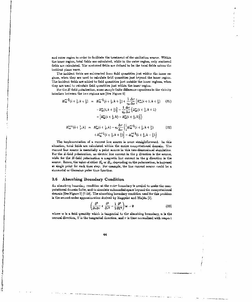
and outer region in order to facilitate the treatment of the cxcitation source. Withinthe inner region, total field, are calculated, while in the outer region, only scatteredfields are calculated. 'Ihe scattered fields axe defined to be the total fields minus theincident plane wave.

The iucldeut fields are subtracted from field quantities just within the inner re-gious, when they axe uked to calculate field quantities just beyond the inner region.The incident fields are added to field qu"titics just outside the inner regions, whenthey are used to calculate field quantities just within the inner region.

Vor the 1i-field polarization, some samuple finite difference cquations in the vicinityinterface between the two regions are [See Figure 6)

S...2b 11 Az

.- ; (, Z" ( q k * 1)

2

,, .- k) = /,(, 2,k) E#"o .. /"t(i 4 !-, k) - )(1)

- i +t ý (i k

The implementation of a current line source is nLote straightforward. In thissituation, total fields are calculated within the entire computational domain. Thucurrent line source is essentially a point source in this two-dimensioual simulation.For the E-field polariwation, an electric line current in the y direction is the source,while for the 11-fiald polarization a, magnetic line current in the 11 direction is thesource. Hlence, the value of either EI; or H4, depending on the polarization, i6 imposedat single point for each time step. For example, the line current source could be asinusoidal or Gaussian pulse time function.

2.6 Absorbing Boundary ConditionAn absorbing bowidai) conditio, at the outer boundary is needed to make the coun-putational domain finite, and to aimulate unbounded space beyond the computationaldomain (See Figure 7] [7-101. The absorbing boundary condition used for this problemis the second-order approximstioun derived by Engquist and Majda 171].

\ Onr Or2 21'P)

where w. is a field quautity which is taungetial to the absorbing boundary, n is thenormal direction, T is the tangential direction., and r is time normalised with respect

44

~~~~~~~~ . . . . . . . . .. . . . . . . . . .

to the speed of light. Trhe second-order absorbiug boundary condition works verywell for waves which aire at or near normual incidence, and not as well for waves whichare inceident at gracing angles. This second.-order absorbingl boundary condition canbc applied to all the edges of the comaputational domuain.

At the corners of the computational domain, the secoud-order absorbing boundarycondition cannot be used, sinuce the noruial and tan~gential directiond art not defined.11L trCeating the Corners, an average Of the two limitinig cases for the normal directionis used with a first-order abkiorbing boundary condition.

0 4-~q~ ±ý (34)

where it,, and ii2 are the two limiting cases fur the uo0rimal direction at the Corner.T.Ihe absorbing boundary conmbtioni at the corners is not as important as at the edges,because there is only onec point at each corner, while there arc many points on theedges. Thus, in general, using the first-urder absorbing boundary condition at thecorners will uot cause significant deterioration in the accuracy of the algoritirm.

The absorbing boundary is not reqtuired to absorb the incident plane wave, be-cause the scattered fields, froma which the IncidentL plane wave ham been analyticallyremnoved, arc calculated outside the inner rcgoun. Since 'he scattered filid radiatesfrom the taxget, the Outgoing scattered fields will not be incident on the absorbingbounudary at grazing angles, which allows the absorbing boundary condition to absorba large p)ercentage of the outgoing scattered fields.

3 Numerical Results and DiscussionVarious electromuagnetic phenuomena were examined and aiwrisned utilizing the VCD-TI) code. A few of the clectroniagnetic phenomuena which are examined in thispaper include: leading and trailing edge diffractions from a conducting strip andtheir dependentce on polarization, creeping waves arojund a conducting cylinder, andradiation from it Lune source. In each of the surface plots shown in Figures 8.11,the outlines of the ta. mgetb and the line sources will 'be represented by a uniformstuall positive height. The simie of the computational domnain used to performu thesesiMulahtionsb was 200 noudes by 2010 nodes large. The physiical size of the computationaldorraln was chosen to be 10 mecters by 111 meters.

T1he target in the first two cases is a thin perfectly electrically conducting stripwhich is in the center of the computational doraain. The strip is 3.5 meters wideand 0.1 macters thrick, The~ excitation source is a Gaussian pulh, plane wave wh~ich isincident at 7 degrees above the plane of the strip. The pulse width its 0.354 metersWiad is defined to be equal to two staudard deviations of the Gaussian pulse. Thefirst case involves the E-field lpolarizatiou and is illustrated in Figure B3. For Figure

45

8, the electric field, Eu, whichr it; porrrtrrg out of the paper, isi plotted. TIle Gauliwianpulse plane wave appvaru as a fairly utidifrn bll which stretches across tile enitirecunrpiitatrunal domain. Tile surface plot wars recorded whenl the Gaussian pulse planewave lhad already propagated neak- the end of thle strip. Tire ring, which is ccntcred atone edge of thte strip, is tiac leading edge diffraction from the edge of the strip whichwas struck first by the plane wave. T1he diffraction froml thle leadinlg edge, inl thiscase, is strong becaube there is a strong discontinuity in the electric ficld whcrr tilepulse strikes the leading edge. lire perfect electric conductor requires tile tanlgenrtiirlelectric field at the surface to be zero. Hence, whenI tile iticidenit electric field, Which isparallel to the strip's surface, strikes tire strip, a rtroug reflected wave im genleratcd iinorder to satisfy the boundary conditimns. At the trailing edge, thle boundary conditionof importance states that the current malst be conitinuous. Sinlce tile mnagnetic fieldis almuost perpendicalar to the strip, the tangential magnetic fields at the surfacewill be weak. Thrus, tlke siurface currents will also be weak, an~d there Will be littlediffraction at thle trailing edtge. The seconld cýLse, Whkich is illustrated in Figure 9,involves the 11-field polarization. lkr this case, tire mragnretic field, II., whichk is alsopoinktingK out of tl~e paper, is plotted. Thre Cattusiarr pildse plane wave hkas propagated1Iis~t thle strip), an1d How two circular rdngs can be seen. The larger ring is the leadingedge diffractionl, which is weaker thanl thle previous came because tile electric field oftile incident plane wave points nersrly perpendicularly to the strip, and causes a lesssevere discontinuit) in tire tangential electric field at the strip's surface. The sMallerring represenlts tire trailing edge dilfractiorr. Ill this case, tire surface cuirrenits will beparticularly strong beausrIE the uragrietic field is alwayti prarull to the strip's surface.lire strorrg traillrng edge diffraction is due to tile large discontinuity ini tire smrrfactccurrenrt "t tlke tranurg edge of thre strip.

Tle thrird scatterer is a pexfectly conductirng cyhkdver. Tile excitation source isagairr a Caussian pulse plane wave whrichr is incident, at Ut) degrees for the 11-fieldpolarizatsiou, TIhe cylinder has aL duirrrnter of 2.5 mreters, and %he pulse width is againU,364 tueters. Fig~ure It) illustrates the uragnetic field, 1i, as tire plane wave scattersolf the Cylin~der. Again tire incident plane wave carl be seen after it has propagatedpasrt the cylirrder, The circular arc is travelling outward away fromn Ltie cylinder aud isthe upecular reflection froma tire cylirnder. Ilrr the v:cinity of the dlridow region, wherctile cylinder blocks tire incideilt plane wave, the circular arc is still attached to theconrducting cyliuder and traveln around the back of tbe cylinder. This plreronumna is!rrowrr as a. creepirng wave. Creepinrg wavesi occur much more btrougly for the Hf-fieldpolari'Lrttiorr because stronger surface currerrts are generated which emssntially allowthe f ield.r to rermrain attached to the cylinder.

'The lash case simrply illustrates radiation from a siuipie line &;ource ilArtcactimrgwithr two p~erfectly conducting strips. The two strips lie omm tire salue line and are 1.65mretersr wide arnd 0.1 mneters tClick, anrd irre separated lby 0.4 mieterv. Tlhe line source

46

is 2 IeCters dirCctly above the space ilnbetween the two strips. The line source hasa Gaussian pulse tiILe dependeuce with a pulse width of 0.354 meters. Iln this casthe H-field polarization is !xasmined, anid Foigure 11 shows the magnetic field fH,. inthis figure, a uniform cylindrical wave can be seen emanating from the line source.The reflection off the perfectly conducting strips simply illustrates how the curvatureof the wavefrunt reverse& itself. The tieldm that pass between the two strips radiatecylindrically from the aperture illustrating slit diffractiou Vihenolena.

An additional capability of thib code is to exaluine resonant structures (e.g. cay-iSiee). Due to the limitations of the surface plots and the iuability to illclude colorplots, it ws1 not possible to show the resonant behavior of any cavities in this paper.One extremely useful aspect of this code is to calculate and display the fields in colorsuccessively in order to visually produce the propagatioza of electromagnetic waves inreal time. The typical computational tune for animation consistihg of OU} timne stepsand 10O color plots is less than 1 hour on al IBM 38( petroUnaL computer. After theFD.'I.'D computation has been completed, the actual hitmiamtion can be played backat about 5 framies per second.

4 SummaryThe FlD-TD code develuped can be used to exsmisie various electromagnetic phenuon-e Ta. The code successfully and 6ccurately predicted the interaction betwe.a varioussources and targets. Beciause the FD-TD technique has the capability to uninimatupro~pmgmtioUl, dilIFrt6,tiUon ail scattering of ClcCtrUammagu!tic waves, it is well suited Asall educationad tool for students learidng electrolmagnltic wave theory.

47

References[11 Yee, K. S. (1966), "Numerical Solution of Initial Boundary Value Problems

Involving Maxwell's Equations in Isotropic Media," IEEE Trans. AntennasPropag., Vol. AP.14, No. 8, pp. 30O-307.

[21 Li, X. (1990), "ElectromageCtic Wave Scattering by Suffa&Ce Discontinuitiem in aPerfectly Conducting Ground Planue," Msitee's Thobis, Department of E~lectri-cal bngineering and Computer Science, M. . T'., Crukabridgc, Massachusetts.

[31 Taflove, A. and M. U. Brodwin (1975), "Numerical Solution of Steady-State Elec-tromagnetic Scattering Probleis Using the Time-Dependent Maxwell's E qua-tions," IEEE' 'Trans. Microwave Theory 'Tech., Vol. MTT-23, No. 8, pp. 623-630.

14] Lrce, C. F., It. T. Shia, J. A. Kong and B. J. McCartin (1989), "A Finite Difference- Time Domain rTcchinique on Trianagular Grids," J. of Efeetromnag',. Waves uadAppl., to be publiwhed.

[51 Morgan, M. A. ed. (1900), PIER P: Finite Elemeut and Finite Diffcrence Metho•asits Bklctromaoyrie t Scattering, hluevier Science Publimhing Co., luc., New York.

161] Bayliss, A., C. 1. Goldstein, and E. Turkel (1985), "On Accuracy Conditions forthe Numerical Comuputation of Waves," J. of Computaiional Phy.ica, Val. b6,Ipp. 396-404.

[71 Engquist, B. aad A. Majda (1977), "Abborbing Boundary Conditions for theNuwer;cal Simulation of Waves," Math. q1 Comp., Vol. 31, No. 139, pp. 62.9-65~1.

(81 Mur, 0. (1981), "Absorbing Boundary Conditions for the Finiitc-Dilfercnce Ap-ptoximation of the 'i'ime-Domaiz• glectromagnetic l'ield Equations," I'EEE2uanj. Elceir tsuayn. C'ompu., Vol. kiMC-23, No. 4, pp. 377-382.

19] Bayliss, A. and E. Turkel (1980), "ltudiation Boundary Conditions for Wave-LikeEquations," Cvoimm. on P'ur and Appl. Math., Vol. 33, pp. 707-725.

1tL01 'AcfLthen, L. N. and L. lHalpern (1985), "WeU-l'useducas of One-Way Equatiousand Absorbing Boundary Conditionus," NASA Contractor Report No. 172619,Institute for Coniiputer Applications in Science and Eugineering, NASA LangleyResearch cen•ter, Hampton, Virginia.

Qii

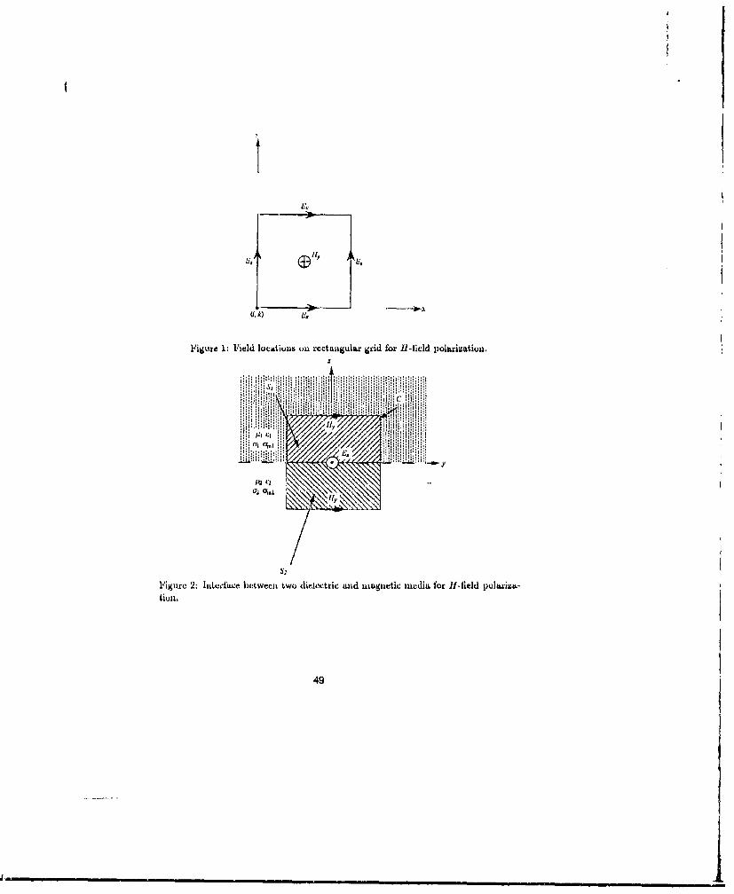
U.k)

Figura 1: Vield lucatiwiM on rectaiigulax grid for l-ficld polarization.

49

*7 (1-1LI-k) U. ki ) * U+P 1. k)x

*. i.i 1 (i&I) *(ui+ kI

F igure 3: Positioning of the perfect conductor.

a 'I"

Figure 4: Interface between a kmedia and a plerfect miagnetic conductor.

50

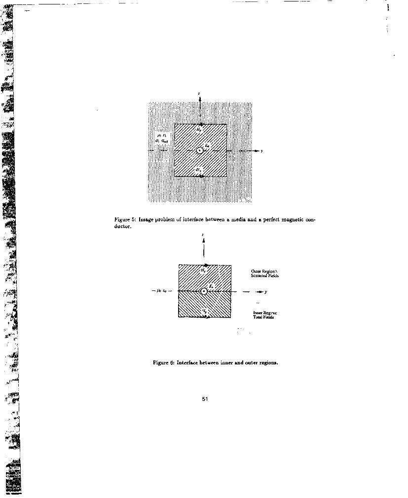
ýAic

/y

Figure 5: Image problem of interface between a media and a perfect magnetic con-ductor.

Hy Outer Region,\At flScattered Fields

'yI Teal F~ields

Figure 6: Interface between inner and outer regions.

>1 51

S--

AbsorbingB~ound±ary

CompavaHiljoa Domain

Figure 7: Absorbing boundary and computational domain.

Incident Plal... Nwev

Leading edge diffraction

Figure 8: Leading edge diffraciou from a pcrfcctly conducting strip for E-field po-

larization.

52

______ _______________________________

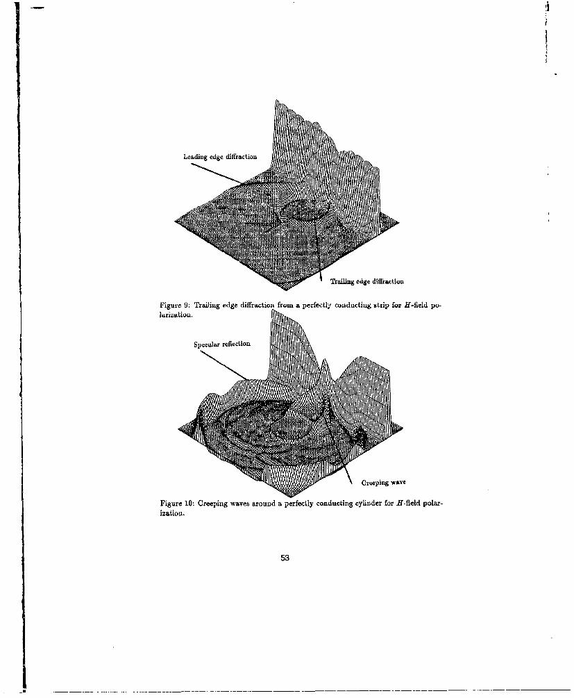
Leading edge diff'raction

Tr•aling edge diffraction

Figure 9: Trailing edge diffraction from a perfectly conducting strip for H-field po-larization.

Specular reflection

SCreeping wave

Figure 10: Creeping waves around a perfectly conducting cylinder for H-field polar-izatiou.

53

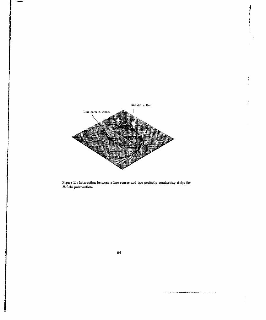
:1

Slit dilffaction

Lmxe miremit dource

Figure 11: Interaction between a line source and two perfectly conducting strips forH-field polarization.

54

I

Kevin Li received his BS and SM degrees in electrical engineering from the Mas-sachusetts Institute of Technology where he is currently puriuing his PhD in electricalengineering. Since 1990, he has been the recipient of an Air Force Laboratory Grad-uate Engineering Fellowship, His main research interests include electromagneticscattering, radar cross section prediction, and numerical techniques. Mr. Li is amember of Tau Beta Pi.

M. Ali Tassoudji received his US (1987) and MS (1989) degrees in electrical en-ginecring '.nom the University of Michigan, Ann Arbor Since 1989, he has been aresearch Usistant at the Ma'3sachusetts Institute of Tochnolugy, where he is Cuircntlyworking towards his PhD in electrical engineering. His research interests includeelectromagnetic scattering and propagation, modeling of microwave circuits, and nu-merical techniques. Mr. Tassoudji is a member of ILEEE and Eta Krppa Nu.

Robert T, Shin received his S11 (1977), SM (1980), and PhD (1984) in ElectricalEngineering fromn the Massachusetts huuti~ute of Technology. Since 1984 he has beena member of the Air Defense Techniques Group at MIT Lincoln Laboratory, as aResearch Staf and as a Senior Staff from 1989. His research interest is in the areasof electromagnetic wave scattering and propagation and theoretical model develop-nient and data iuterp,-etatioii fur microwave remote sensing. Ile is the coauthor ofT'1hcory of Microuoave R•cmotc Scnsing (Wiley, 1985). Dr. Shin is a Lueiber of TheElectruniagnetics Academy, IEEE, American Geophysical Union, Tau Beta Pi, EtaKappa Nu and Connmission F" of the International Union of Radio Science.

2in Au Kong is a Professor of Electrical Engineering and Chairman of Area IV onEnergy and Electromagnetic Systems in the Department of Electrical Engineeringand Comnputer S'.ience at the Massachusetts Institute of Techuology. His researchinterest is in the field of elcctroUnagletic wave theory and applications. ie haspublished 7 books and over 300 refereed journal and conference papers, and is theEditor of the Wiley Series in Remote Sensing, and Chief Editor of the Elsevier bookseries of Progress in Electromagnetics Research (PIER).

55

ELECTROMAGNETIC CODE FORt SOLVING STATIC AND DYNAMIC 2-D~ FIELD PROILEI;MSON A PERSONAL COMILUTER

Dr. Jovan E. Leharic, Mark Mellon and Jens L ngelRosc-Hulman Institute of Technology, 5550 Wabash Av., Terre Haute, IN 47803

"Thie Graphical Electromagnetics Code (GiEC) was developed at Rose-Ilutliman hIstitutc otTechnology with funding front the NSF/IEEE CAEME program. Thei objective of GEC is to providea user friendly graphical environment for the formulation and numerical solution of general 2-Delectromiagnetic field problems including static, harmonic, and transient analysis. The code is geartedtowards being an educational tool for the demonstration of electromagnetic field principles using thegraphical capabilities of the computer to aid in the visuali7ation of field problews. However, the codealso has advanced features that make it useful as at research tool for practicing~ electromagneticsengineers and scientists.

GLC is targeted for 286 and 386 class DOS personal computers with r-GA/ VGA gi ap~hicscapabilities, mouse, and 640k memory, but will operate on 80816 miachines as well, GIEC uses itgraphical environment with mouse and keyboard support. A field problem can be descaibed bydrawing the geometry of the problem onl the screen with the aid of a nmouse, in it manner simlilar tosome of the paint" programs common onl PC.. Thlere is support for the basic shaples such as: dot(point source), box, fine, circle, ellipse, polygon, and pie slice. The traterials used in the geoinetty canhave arbitrary permoittivity, permeability, and conductivity.Tnmteilaedfeetaedothscreen by color and pattern where they can be selected, moved, copied. etc. In addition, there issupport for creatinig material libraries of often used materials. Furthermore, there a several types Litdefault prototype sources to choose from including DC, AC, and transient type sources. GEC W1 itraNthe geonmetry and material files to disk in ASCII format for easy access and miodification by 31rdparties,

The static and harmonic analysis use FD methods to solve for electric potentials oin aregular rectangular &grids. Similarly, the transient analysis uses a Finite Difference Timne Dom-ainl(FD.TD) algorithm to calculate the time history of the electric and magnetic field onl interlaced("dual") regular rectangular grids ("'Yee-lattice"). The grid used for the computations is independentof the grid used to describe the problem geometry. Thlus, it is easy to start with quick coarse solutionsto a problem and then refine, the computation grid if necessary with no nmodifications to the Iprolblitigeometry.

Th'le computation grid is terminated by coupling the interior grid to a radiation integralformulation for the infinite exterior region. The solution process matches the I'D (or FL)-TD) andradiation integral equation solutions along the grid boundaty using an iterative process, In addition,GEC also supports the use of intinite ground planes by using image theory in the different anal'yse.

THE HIGH FREQUENCY ELECTROMAGNETIC SIMULATION OFARBITRARY TWO AND THREE DIMENSIONAL STRUCTURES

Brad BrimHewlett Packard Company

Network Measurements DivisionSanta Rosa, CA 95401

(707) 577-4798 bradb@hpnmd.hp.com

In the distant past most electromagnetic analyses were carried out analytically forcanonical structures. Integral equation techniques were preferred since approximate sourcedistributions (current or charge) or asymptotic analyses could often lead to the dominantbehavior of the true solution, This preference endured as numerical electromagnetic codeswere developed. Differential equation based and time domain algorithms have not receivedas much attention in rescaich and commercial applications. The recent significant speedimrFrovements in readily available computers has caused a refocusing of attention towardthese long neglected techniques,

Recently, many authors have reported implementation of the Finite Element Method(FEM) free of spurious solutions I l. Commercially available software packages arebeginning to incorporate these new solution techniques. One such software package avail-able from Hewlett Packard (HP85180A) is referred to as the High Frequency StructureSimulator (IIFSS). This product is biased toward the solution of arbitrary two(propagating) and three dimensional RF, microwave, and mam-wave circuits type geome-tries.

The goal of this presentation is to present to the numerical electromagnetics researcherthe capabilities of such commercially available products. A brief history of numerical elec-tromagnetics will be discussed to set the stage for the development of FEM algorithms. Ablock diagram will be presented to inform the audience of the many technical disciplinesthat constitute these numerical tools. The main focus of the talk will be the sorts of appli-cations that have been analyzed with HFSS. The results are not just propagation constants,characteristic impedances, and scattering parameters. In addition, any examples of thegr-iphictl display of two and three dimensional electromagnetic fields will be presented.These graphical displays lead both research and design users to develop a much higherunderstanding of the physical solution or how the design must be perturbed to functionproperly. The types of problems that HFSS presently addressm.. will be classified andcharacterized through example solutions and eomp;u-ison with measv'rements. Problemsthat IIFSS does not currently address will also be presented. The advankcs in 'le imple-mentation of the FEM to achieve these solutions will be discussed.

Groups such as ACES represent the pool of talent from which theoretical advanceswill conic to further develop numerical electromagnetic tools. The talk will conclude with adiscussion of research topics that should be addressed. The applicability to general areas ofnumerical techniques and the relative difficulty of these suggested topics will also beaddressed.

[1] "The Transfinite Element Method for Modeling MMIC Devices," Z. J. Cendes and J.F. Lee. IEEE MTT-S, Vol. 36, No. 12, Dec. 1988, pp, 1639-49.

57

SOFTWARE FOR ANTENNA MODELING AND RADAR APPLICATIONS

Robert J. HancockCAE Soft Corporation

P. 0. Dox, 818Rockwall, Texas 75087

T-he CAL Soft-Phased Array Analysis Systemn (CS-PA AS) computer program enablesstudents and practicing etigineers to model phased array antennas quickly, accurately, andinexpensively using a personal computer or VAX computer system. CS-PAAS simplifiesantenna model development for the novice while offering complete flexibility and advanedtechniques for the experienced user. CS-PAAS can be- used to design and analyze spcificphased arr ay configurations and determine perfonnariee sensitivity to cnnmponenlt tolerancesand other error sources.

The prugramn is primarily used for the evaluation of discrete planar arrays. These pill-nar arrays represent either electronically scanned phased array antennas or sampled dishantennaD illumlination functions evaluated in a reference plane. The program's emphiasi% isonl speed. accutracy, and versatility with easily evaluated results. The program is in amo1dular structUre which allows easy incorporation of additional capabilities. CS-PAAS isa detailed antenna simulation computer Viogramn. Written for the systems engineer. it is avalulable tool for thre design and evaluation of phased array antenna systems.

A phased array antenna system consists of a group of subsystems which arc cam-posed of various functional elements, such as powevr dividers-, phase shifters. and radia-tors. In CS-P1AAS emphasis is placed onl aCCUratCly simulallting thle f~nctiunal eleeniltsheCause the SUIme functional elements are used in many phased array antennas -- only thleparameters change. For example, most phased arrays have phase shifters but the numberof bits varies from one system to ;tnothcr.

The simulation is comprehensive. Currently, a number of different feed networkscanl be mrodeled. Tile main array can be a variety of generic shapes. A number of anmpli-tuide tapers for side lobe conuiol are also available. The element layout and radiator type canbe- specified aind a host of systemnatic and randomn errors can be included. CS-PAAS isideally suited for predicting phased array performance Sensitivity to component tolerancesand other errors.

In thle paper anr overview of dhe CS-I 3AAS computer programn and its capabilities willbe provided. Followinlg that the results from seletednintenna sy stein an alyses that wereperformed usin~g CS-P1AAS will be presented, Among those examples will be thle analysisof an interfei umeter antenna systemn and an evaluation of phased ariay perfornmance sensi-tivity to coreelated phase and amplitude errors in a corporate feed power distribution net-work.

58

Miarowave Explorer: An lleotromagnatias Program for theAnalysis of High Vrequency Integrated Miarostrip Circuits

A. Hill, J. Burke, K. KottapalliCompact Software483 McLean Blvd

Paterson NJ 07504

Abstract

This contribution describes a general electiomagneticssimulator EXPLOC1R for rectangular microstrir geometries.The analytical formulation is based on the electric fieldintegral equation which is solved by the Method of Moments.The general geometry to be analyzed consists of ametallization interface that is situated betwoen variousdielectric layers. The entire structure is enclosed in arectangular box. The electromagnetics code contains anautomatic generator for the current subsections which allowsthe convenient definition of the microstrip geometry. Anumber of examples are shown in order to demonstrate theeffect of losses, mutual coupling and box resonances.

IntroductionAccurate characterization of passive microstrip componentsis essential for the design of microwave and millimeter wavecomponents such as filters, couplers and delay lines.Typically these circuits have been modeled by subdividingthem into functional blocks like microstrip bends, junctionsand transmission lines. Models for these individual elementsare wall developed and are readily available in circuitanalysis programs. The performance of an entire circuit isobtained by cascading the individual functional blocks. Theaccess time for the electrical characteristics of eachelement is rather small which allows comple2 circuits to beanalyzed within seconds on a personal computer. In addition,the approach of cascading individual circuit elements allowsfor optimization and statistical circuit analysis withinacceptable time frames.

However, as circuit density increases certain circuitelements can no longer be treated as isolated components andtheir interaction with adjacent structures neems to be takeninto account for accurate prediction of circuit performance.A treatment of interacting elements that is based on curvefitting techniques is impractical due to the large number ofparameters associated with interacting structures. Accuratecharacterization of these cases requires a rigorous solutionto Maxwell's Equations. A number of full wave solutions have

59

been developed in the past. [1-61. The analytical foundationof most solvers is based on the integral equation approach.The unknown represents the surface current on the microstripwhich is solved for by the Method of Moments. The evaluationof the Moment Matrix and the solution of the resultinglinear system requires computation times that exceed runtimes of conventional circuit analysis programsconsiderably.

Theory

The structure of interest consists of a microstripmetallization pattern that is situated between multipledirleotric substrate layers. We analyze the configuration ina conducting box with possible lussy top and bottom cover.The tangential electric field on the microstrip is derivedfrom the transverse magnetic and transverse electric fieldcomponents. For the lossy, multilayered structure therelated Green's function is derived using the immitanceapproach [7]. After applying the appropriate boundaryconditions the integral equation for the electric field isfound to be-

E n11(x,y)=ZJ(x,y)-fJG(x I x',y I y')'J(x',y'lds' (1)

where J represents the surface current on the metal, Zrepresents the surface impedance of the metal and G is theassociated dyadic Green's function of the geometry[7). Inthe Moment Method we employ roof top functions[8] for basisand testing functions. Thanks to the evaluation of the rooftop functions in the spectral domain the convergence of thedouble infinite series is obtained at acceptable limits.Mors precisely, the upper limit for the summation is chosento be

M=2-a (2)d

where a represents the length of one side of the box and drepresents the desired spatial resolution.

An efficient technique for the evaluation of the elements oftha Moment Matrix has been published previously [9]. Thedouble summations in the formulation of the elements in theMoment Matrix are rewritten in such a form that they are

60

suited for * application of two dimensional discrete fastFourier tr.; .,forms.

in order to alleviate the burden on the part of the user analgorithm has been developed that computes the location ofthe cuirent subsections from a minimum set of informationthat is provided by the user. Instead of specifying thelocation of all the current subsections, the user is onlyrequired to specify the corners of the polygons whichdescribe the metalization structure. The program divides themetalization pattern in such a way that larger subsectionsare used on transmission line regions and smaller sectionsare used in discontinuity areas. A sample grid for amicrostrip right angle bend is shown in figure 1. Note thatas the edges of the transmission line region are approachedthe grid spacing is decreased. Also, in the discontinuityregion of tho right angle bend a higher grid density ismaintained. Due to the application of fast Fouriertransforms all grid spacings need to be a multiplo integerof the minimum grid spacing.

Results

In order to demonstrate the application of the program weanalyzed three examples. The first case demonstrates mutualcoupling effects using a microstrip filter. A next exampleshows the effect of package resonances on the performance ofa microstrip gap discontinuity. For the final example wecompute the s parameters of a losoy transmission line andcompare the results to those obtained from a two dimensionalspectral domain program (see appendix).

The circuit characteristics of the Lilters shown in figure 2are compared in figure 3. We show the transmission of amicrostrip filter for three cases. These include thefullwave results obtained from EXPLORER for the structuresof figure 2 and the results obtained from an idealizedcircuit analysis. Vor the idealized case interaction of thestubs is neglected. Note that the orientation of the stubsand the interaction beiween them has a significant effect onthe bandwidth of the filtar. These effects cannot bedescribed with conventional circuit simulators that assumeidealized conditions e.g. isolation between various circuitelements. For this example we used a 50 ohm line on anAlumina substrate. The substrate thickness and the coverheight were 0.1323mm and 2.646mm, respectively. The planarsubstrata dimensions were chosen to be 3.429mm by 6.985mmand the reference planes were placed at an offset 0.889mmfrom the wall. The stubs were 2.921mm long and wereseparated by s-0.762mm.

The next example shows the transmission of a microstrip gapwithin a frequency range where box resonances become a

61

matter of concern. The transmission is shown in figure 4.EXPLORER determtnes possible package resonant frequenciesbefore the structure is analyzed and for this case predictsthe resonant TM110 mode at fr - 10.343 Ghz. This situationis reflected in figure 4. Notice the perfect transmissionaround 10.4 GHz which is duo to the resonant package mode.W3 include the simulated results for the case where nopackage effects are considered and the trace for thisidealized case is smooth indead. For this example weselected a So Ohm microstrip line on 25 mil Alumina enclosedin a box of dimensions 19.02mm by 19.02mm. The gap with was2/3 W. The substrate and cover height were 0.635mm and3.81mm respectively.

Figure 5 compares results for the magnituda and phase of thetransmission s parameter for a loasy microstrip line usingEXPLOURE to results obtained from a two dimansional spectraldomain approach (see appendix). The agreement in thefrequency range up to 15 GHz is excellent. For themicrostrip line with w/h-l we used a 25mil Alumina substratewith a loss tangent of 1.0. The planar substrate dimensionswere chosen to be 10mm by 6mm. The line was deembecled withthe location of the reference planes at a 2.5mm offset fromthe walls. The cover height was 3.81mm.

conclusion

The electromagnetics code EXPLORER has been introduced whichis based on the fullwave solution for a boxed, multilayeredmicrostrip geometry. The code was applied to demonstrate theeffect of losses, coupling and package resonances on theelectrical characteristics of selected microstripstructures. It became apparent that the application offullwave electomagnetics computation improves the modelingaccuracy as compared to conventional circuit analysis wherethe interactions between various circuit components areneglected. The efficient numerical treatment and the factthat modern workstation computers reach larger processingspeeds makes electromagnetics simulation a realistic optionin Microwave Integrated Circuit Design.

Appen4ix

Since the two dimensional spectral domain method is wellknown and the derivation of the Green's function follows asimilar approach as used in EXPLORER, it will only beoutlined briefly.

The one dimensional curronts on the strips are expandedusing sinusoidal basis functins modified by an edgecondition term. Applying Galerkin's method along withParseval's theorem, we obtain a set of algebraic equations

62

for the unknown current coefficients. The complex value ofbeta which makes the determinant of the characteristicmatrix equal to zero is the propaqation constant.

Once the propagation constant and the expansion coefficientsare determined, the complek power flow is calculated. Thecomplex impedance of the transmission line is related to theratio of the complex power flow to the total longitudinalcurrent.

References

[1] T. Itoh, Ed., Numorical Techniques for Microwave andMillimeter Wave Passive Structures. New York: Wiley,1989.

[2] J. C. Rautio and H. F. Harrington, "An electromagnetictime-harmonic analysis of shielded m.icrostrip circuits,"IEEE Trans. Microwave Theory Tech., vol. YfT-35, pp.726-730, Aug. 1987.

[3) R. W. Jackson, "Full-wave, finite element analysis ofirregular microstrip discontinuities," IEEE Trans.Microwave Theory Tech., vol. 37, pp. 81-89, Jan. 1989.

L4) J. R. Mosig, "Arbitrarily shaped microstrip structuresand their analysis with a mixed potuntial integralequation, "IEEE Trans. Microwave Theory Tech., vol. 36,pp. 314-323, Feb. 1988.

[5] L. P. Dunleavy and P. B. Katehi, "Shielding offects ii.microstrip discontinuities," IEEE Trans. MicrowaveTheory Tech., vol. 36, pp. 1767-1774, Dec. 1988.

[6] W. Wertgen and R. H. Jansen, "Spectral iterativetechniques for the full-wave 3D analysis of (M)MICstructures," in IEEE MTT-S Int. Microwave Symp. Dig.,1988, pp. 709-712.

[7] T. Itoh, "Spectral Domain Immitance Appriach forDispersion Charactiristics of Generalized PrintedTransmission Line," IEE2 Trans. Microwave Theory Tech.,Vol. MTT-28, No 7, July 1986.

[8) A. W. Glisson and D. R. Wilton, "Simple and efficientnumerical methods for problems of elctromagneticradiation and scattering from surfaces, " IEEE Trans.Microwave Theory Tech., vol. 37, pp. 81-89, Jan. 1989.

[9) A. Hill, V. U. Tripathi, "An Efficient Algorithm forthe Three-Dimensional Analysis of Passive MicrostripComponents and Discontinuities for Microwave andMillimeter-Wave Integrated zircuits," IEEE Trans.Microwave Theory Tech., vol. 39, No 1, January 1991.

63

. m m ' , m• • m • A mI

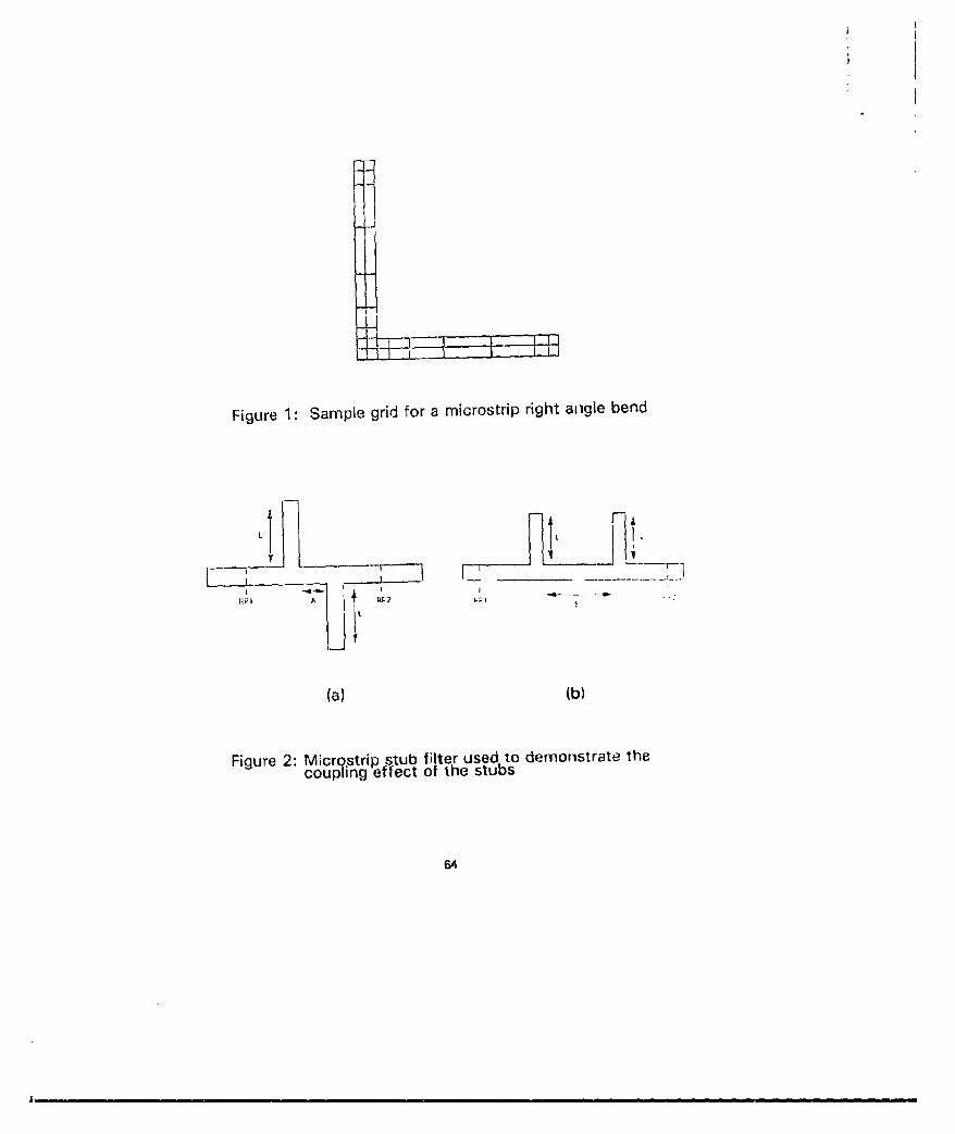
Figure 1: Sample grid for a microstrip right aiigle bend

4Pl A RP2

(a) (b)

Figure 2: MicrQstrip stub filter used to demonstrate thecoupling effect of the stubs

64

..-Figure 2(b)

Figure 3: Transmssion S21 for microstrip stub filter

_____ ___ Iincludes_____package effect

Figure 4: F~ffect 9f pac age rpsonaince oi) thetransmission ý2̀ 1 ofta microstrip gap

I6

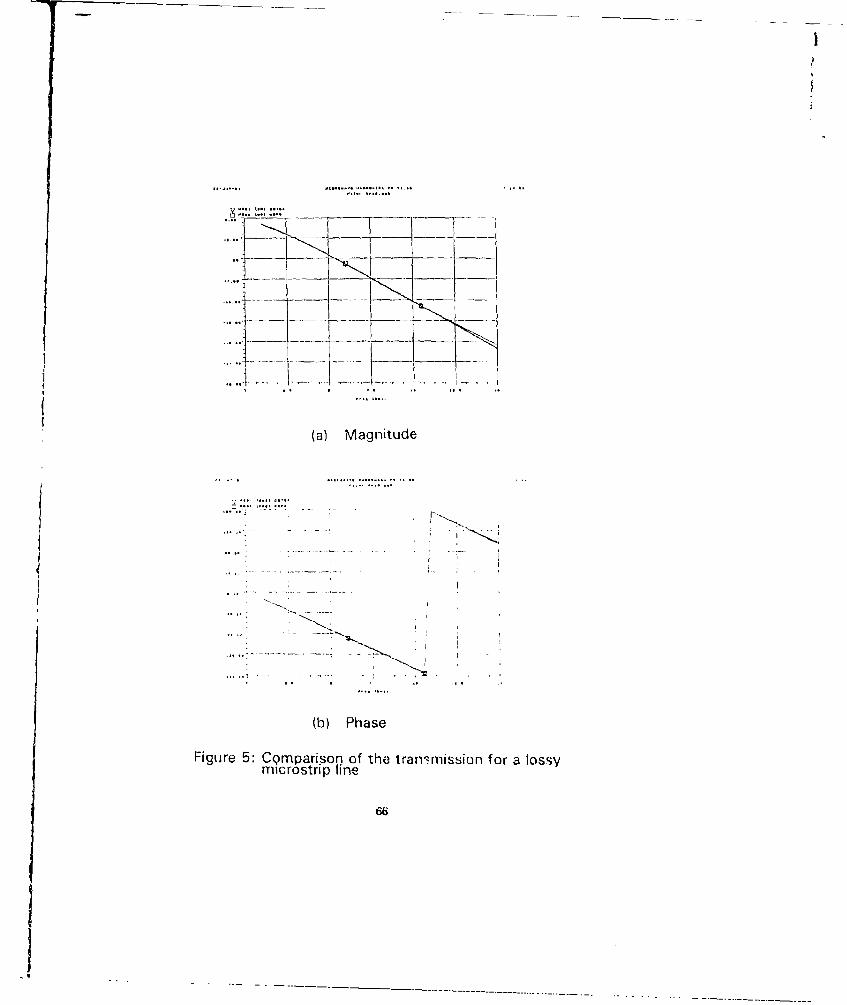
v .... ....-

(a) Magnitude

... _: .........

(b) Phase

Figure 5: CQmparison of the tran'mission for a iossymicrostrip line

66

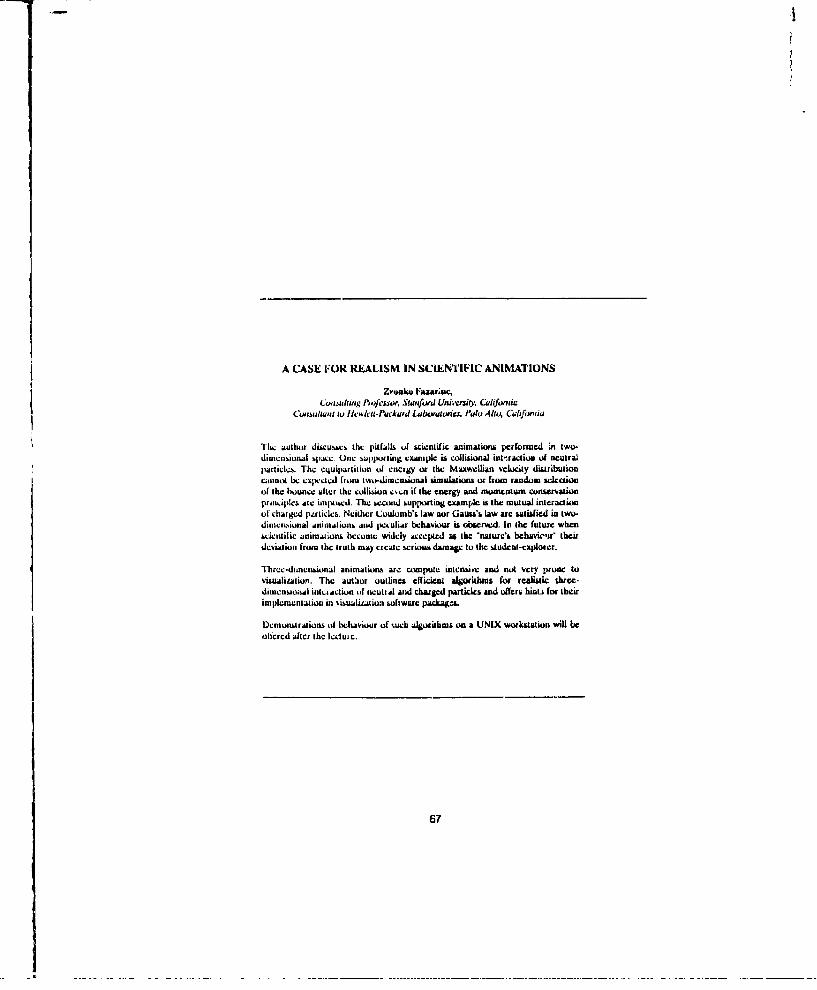
A CASE FOR REALISM IN SCIENTIFIC ANIMATIONS

ZvOnlw Fazarduc,( Czcultu;ng Ifcssor. Slatiftwd Univen•ri Califoniua

Consa•ltat to Ilcwtict..Pckurd Laborotwmieu. Palo AIto, Califontia

The author discumscs the pitfalls of scientific animations performed in two-dimensional space. One supporling cxamplc is collitional interaction of neutralparticles. The Cjquiparltiion of CneCgy or the Maxwellian velocity distributioncannot be expected front two-dimemnional simulations or from random selectionof the boun;c stiler the collision een if ehe energy and momentum conservationprinciplcs Adi impotcd. The second supporting example is the mutual inleractionof charged p-rticles. Neither Coulomb's law nor Gausrs Law arc satisfied in two-dimencsional animations and pcsuliar behaviour is observed. In the futurc when"scientific animations become widely accepted as the "natuc's behavit-r theirdeviation from the truth may create serious damage to the student-cxploter.

Three.dinensional animations at,: compute intensive and not very prone tovisualization. The author outlines efficient algorithms for realistic three-dimCnsional intrackion of ncutrl and charged particles and offeru hini. for theirimplementation in isunlization suftwarc package..

Demonstrations of behaviour of %utch algorithms on a UNIX workstation will beolfered after the Lclute .

67

*1

Educational Uses of GEM. S

by

Edgar L. Coffey, III

Advanced Electromagnetics5617 Paiomino Dr. NW

Albuquerque, New Mexico 87120

The GEMACS (General Electromagnetic Model for the Analysis of Complex Systems)computer program is well-suited to educational uses. Students can access a wide varietyof physics techniques and solution methods from a single input format. They canexamine data in a comistent output foc-mat. The purpose of this paper is to describesome of the :apabilities of GEMACS and its suitability to use in the engineeringclassroom.

Capabilities

Version 5.0 of GEMACS is a highly integrated program that supports the more commonelectromagnetic solution methods: (1) method of moments (MOM). (2) geometrical theoryof diffraction (GTD), and (3) finite differences (FD). The abundance of methods in onacomputer program facilitates its use for instructional purposes.

Method of moments supports both wire segment and surface patch elements as well aswire-patch connections. MOM wire segments can be loaded with lumped or distributedloads. The GTD capability supports multiple ray tracing interactions among a structurecomposed of plates, cylinders, end cylinder end caps. There are no hard limits to thenumber of interactions or the number of GTD modeling elements in GEMACS. GTDelements can also be loaded with an arbitrary surface impedance if desired. Finitedifferences is implemented in the frequency domain ior compatibility with the otherGEMACS modeling techniques. At present FD is restricted to interior (cavity) regions.

GEMACS also supports combinations of methods. The two most important combinationsare MOM/GTD and MOM/GTD/FD. A MOM/GTD problem contains both MOM andGTD modeling elements in the geometry. A MOM interaction matrix is generatedamong the line-of-sight interactions among the MOM elements and is then augmentedby a GTD interaction matrix obtained from ray paths that interaction with the GTOelements of the st~ucture. This is shown in figure I.

The MOM/GTD/FD hybrid permits the analysis of multiple region problems such as theone shown in Figure 2. The physics quantities (interaction matrix, excitation vector) arecomputed for each reg;on of the hybrid problem, then boundary conditions are matchedat the aperture interfaces to obtain the total problem solution.

Code Structure

GEMACS 5.0 has been structured to that the details of peripheral files, datamanagement, symbol tables, and other non-engineering items are all taken care of by theGEMACS overhead routines. This frees the user to concentrate on the problem at hand

68

S ... . . .. . . . . . . . . . ... . .. .. . . . . .

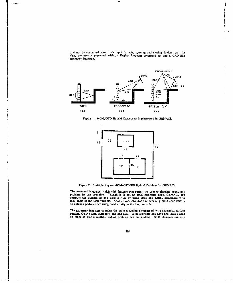
and not be concerned about data input formats, opening and closing devices, etc. Infact, the user is presented with an English language command set and a CAD-likegeometry language.

FIELD POINT

ERC ESRC

MOON GTD, EG

mmT OT TO 'U

LO T c Gr0-

ZGEN ESRC/VSRC EFIELD -GF]

(a) (b) (C)

Figure I. MOM/GTD Hybrid Concept as Implemented in GEMACS.

LU#2

IV #5 V

Figure 2. Multiple Region MOM/GTD/l*D Hybrid Problem for GEMACS.

The command language is rich with features that permit the user to simulate nearly anyproblem he can conceive. Though it is not an RCS computer code, GEMACS cancompute the backscatter and bistatic RCS by using LOOP and LASEL commands withlook angle as the loop variable. Another useL can study effects of ground conductivityon antenna performance using conductivity us the loop variab'e.

The geometry language contains the basic modeling elements of wire segments, surfacepatches, GTD plates, cylinders, and end caps. GTD eloments can have apertures placedon them so that a multiple region problem can be worked. GTD elements can also

69

i

contain one or more surface impedance areas. In addition to these basic elements, thegeometry processor allows CAD-like manipulation of the elements. A group of elementcan be defined as a modeling entity which can then be replicated by translation,rotation, or reflection. The result is a compact description of a structure that can bemore easily maintained than a structure described by a series of simple commands.

GEMACS also has the ability to restart in the middle of an execution. The GEMACScheckpoint (CHIK.PNT) command saves the state of GEMACS at any point in theexecution. GEMACS can then be restored with the restart (RSTART) command and theexecution will continue where GEMACS left off. This feature permits the uWer tocorrect errors without re-running an entire problem. But perhaps a more valuable useof this feature is the ability to utilize data from earlier runs (decomposed matrices,currents, etc.) to generate new data in later runs (different field pattern cuts). Thus aninstructor can generate the basic physics data for a class and have the students utilizethat data via CHtICPtiT/RSTART to produce the observables of interest without severelytying up computer resources.

Portability

GEMACS is written in ANSI standard FORTRAN. As such it has been easily hosted ona wide variety of host computers from an IBM PCJr to a CRAY mainframe, Thus theidentical code that is hosted on a university's central computer (for large problems) canalso reside on a student's personal computer (subject to export control restr:ctions) forsmaller (homework) problems. We have had no problem in hosting GEMACS on DOS,UNIX, and OS/2 operating systems. I must emphasize that it is the same identicalsource code for all machines and all operating systems.

Common User Interface

GEMACS users interface with tht code through the same command set regardless ofsolution method or physics techniques selected. This provides consistency in teachingand gives the user confidence that a particular command stream will indeed describe theproblem desired. Figure 3 shows sample command sets for MOM and GTD problems.Notice the similarity of the inputs.

$ tEMACS NlO INPuT EXWLENMttFIL - 17FRO - 300.SETINT ONdWGCAA - PKWEXZGEN IGWATA-NOiX ZMATRX-ZIJSRC - ESRC(W4tEX) DW"1._ti. R001. TEtIA-90. PHI-'0.SOLVE ZIJtI * SRCFLO - EFIELOCNONEX) T110. PI'0. DP.2. P2-360.END Of CONwAwDS

S nCeACS GTa INPUT EXM*'LENiUFIL * 9FAQ - 3M0.StrINT 0TeGNOATA * trDEXSRC - ESAC(GIDEM) OW-1.,O. R-1S. TIIETAM90. PHI-30.FLO * EFIELOaNbIX) 11-0. P1O. DP*2. P2-36O.EtD Of COMPAWS

Figure 3. Sample Inputs for MOM and GTD GEMACS Simulations.

70

A GEMACS Control Program (GEMCOP) is due to be released in the summer of 1991.The purpose of GEMCOP is to make GEMACS input language generation and outputresults extraction even easier than it is now. For example, GEMCOP will allow the userto extract parametric data from a collection of runs and plot those results to the user'sspecifications. For instance, one user may wish to plot current vs. frequency whileanother user may desire current vs. conductivity. If the data exist on the computer, thenGEMCOP will find the data, sort the data, and format them for plotting. Hence,multiple users may make use of the same basic physics data and not have to re-runGEMACS just because the data are scattered about among many simulstions.

Graphics Support

Though not a part of GEMACS proper, there is available a pouerful graphics processorthat works in conjunction with the GEMACS input and output streams. The GAUGE(Graphical Aids for Users of GEMACS) package contains routines for displaying.creating, and editing geometry inputs for MOM, GTD, and FD. There are otherroutines for displaying currents and fields, including the ability to color map currentsonto wires, patches, and GTD solids, Extensive visual aids such as contouring andskeleton plots permit the user to more easily grasp the significance of the physics results.For example, a log periodic antenna can be run with GEMACS at several frequencies.By color mapping the current results back onto the antenna structure, the user can seehow the longer antenna elements resonate at lower frequencies while the shorter elementswork at higher frequencies.

There are also other utilities with GAUGE that let the user define his own geometryelenments via an extensive macro language and to even translate NEC and 3SC geometryinputs into a form that can be displayed with GAUGE and executed by GEMACS.

Finally thete is a new graphics companion to GAUGE called MODELED (ModelEditor). MODELED among other things takes an existing GEMACS model and scales itto other frequencies by adding wire segments and/or patches.

Summary

We feel that GEMACS is an ideal teaching tool at the advanced undergrAduate andgraduate levels. Its richness of physics, its simple user interface, and its axtensivegraphics support make it possible for students to simulate complex problems withoutworrying about the mechanics of the underlying computer software.

71

Ii

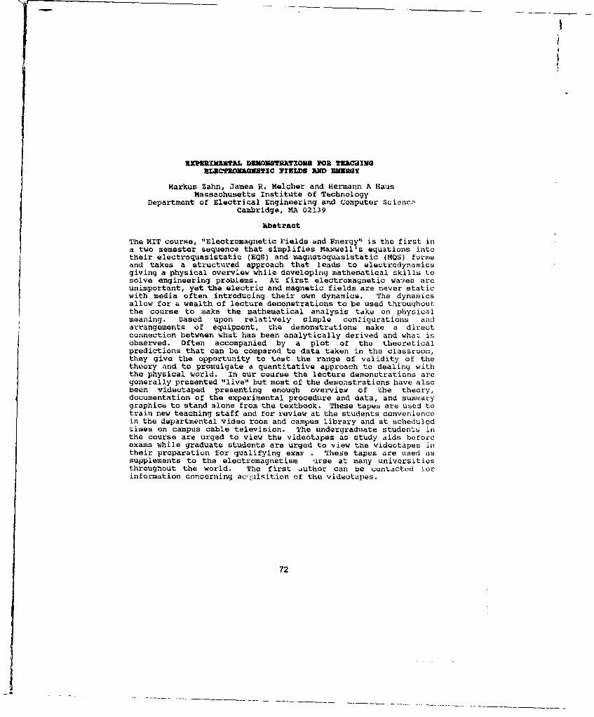
I

UX?"TFUkI TAL DNWONSTRATXIOU POR TEP1MGBLIRONIAGNTIC YIELDB AMND UMURY

Markus Zahn, James R. Melcher and Hermann A HausMassachusetts Institute of Technology

Department of Electrical Engineering and Computer SciencaCambridge, MA 02139

hbstract

The MIT course, "Electromagnetic Fields and Energy" is the first ina two semester sequence that simplifies Maxwell's equations intotheir electroquasistatic (EQS) and magnetoquasistatic (MQS) formsand takes a structured approach that leads to electrodynamicsgiving a physical overv.iew while developing mathematical skills tosolve engineering problems. At first electromagnetic waves areunimportant, yet the electric and magnetic fields are never staticwith media often introducing their own dynamics. The dynamicsallow for a wealth of lecture demonstrations to be used throughoutthe course to make the mathematical analysis take on physicalmeaning. Based upon relatively simple configurations andarrangements of equipment, the demonstrations make a directconnection between what has been analytically derived and what isobserved. Often accompanied by a plot of the theoreticalpredictions that can be compared to data taken in the classroom,they give the opportunity to test the range of validity of thetheory and to promulgate a quantitative approach to dealing withthe physical world. In cur course the lecture demonstrations aregenerally presented "live" but most of the demonstrations have alsobeen videotaped presenting enough overview of the theory,documentation of the experimental procedure and data, and summarygraphics to stand alone from the textbook. These tapes are used totrain new teaching staff and for review at the students conveniencein the departmental video room and campus library and at scheduledtimes on campus cable television. The undergraduate students inthe course are urged to view the videotapes as study aids beforeexams while graduate students are urged to view the videotapes intheir preparation for qualifying exar . These tapes are used assupplements to the electromagnetism urse at many universitiesthroughout the world. The first uuthor can be contacted forinformation concerning accquisition of the videotapes.

72

- *1

Liinard-Wiechert Field Generator&HyperCard Tutorials for Visual Electromagnetlcs

Rodney Cole & David KrullPhysics Department

University of California, Davis

Because we cannot taste, feel, or smell electric and magnetic fields, it is extremelydifficult for a student to develop an intuitive feel for the subject. It often takes years ofstudy to be able to conceptually arrive at a solution without using the powerful mathematicsof Maxwell's theory. This is a major contribution to the decrease in the number of studentschoosing electromagnetics as a career. This state of affairs led us to develop HyperCardcomputer tutorials containing animated graphics and animated derivations of equations.The goal is to link the computed graphical solutions for various arrangements of chargewith the standard mathematical techniques. The series of HyperCard tutorials starts withelcctrostatics and builds to cover radiation from c;harged particles. In using graphics thatstudents are likely to encounter in current research projects, we are building graphicalvisual skills a student is likely to use the rest of his life as well as building a visual intuitionfor electromagnetics. We will describe a computer simulator that is under development forstatic and radiated electric fields.

73

SESSION 3 - "INVERSE PROBLEM SOLUTIONS"Moderator: Margaret Cheney

fl I

AN INVERSE BOUNDARtY VALUE PROBLEM FOR MAXWELL'S EqUATIONS

Erkki Soniorsalo' , David Isaacson' and Margaret Cheney"

Department of MathematicsUniversity of Helsinki, liallituskatu 15, 00100 lielr~ink!

'Dlepartmenit of MathelmAtical SCIenlCesRtensselaer Polytechnic Institute, Troy, NY 12180

AI)STRtACTI

We consider thec problem of determining Owut elect roinagnetic properties of a body froil nuea.surenments made on the surface of tile body. We study the hill set of Mlaxwell's equations thatgovern time-harnionic electric and maglnetic fluids. The unknown parameters that wee seek to rv-conseruct from" boundary £neasuremoen ts are the miagnetic permecability pi. the electric permittivityC and tile electric Conductivity 17. The boundary mneasuremient is exhibited in form of a boundar~y uaappilag, specitically the mapping fromi the tangential comnpunents of the electric field ;u thetangential components of the miagnletic field. 71iis data call be used) to reconstruct jp. e and aapproxiniatelly, provided they deviate onily slightly fromn known couslants. We give all estimate forthe reconstruction error.

In his paper 1,21, Calder6ik considered the piroblem of determiining all approximiation to tileelectrical conidu, cvity in a bounded region it of R' front electrical mleasureniiivts made onl thesurface dil. This imptdance inwgyiny probleml hah recently been studied by a mumber of authors:Uniqueness rebulth can be found e.g. in [91, [101, [12) and [151, and numerical reocivtructiunmnethods have beeln disceissed in [11, (]1, [4], (F)]. 161, [7), It), (1111, 113] and [16]. lin these works. thim.time variation of the electruinraietic lields is nheglemcted, so that the -electrit: state uf 11 is governedby a single second-ovder elliptir partial differential equationi of electrobtatics,'

V.- avu. U.

where or is the conductivity and u i& tile electric potential. The data in the static probleum isi thleDirikhlet-to-Neusarni miap (or its hivermel that assignsB to each surface potential distributiou theLcorresilonditig current density (or vice versa).

In 114]. we study tk'e full set of Maxwell'b eqimatiul.. thlat govermm ti lme-llarkl~lloic electrit Andmagmletic fields. The inverse problem thererore involves three un~knlown cuetlicienilts We consider thlecase in which it is a bounded dornain in K". For simiplicity, we ~assuink that it 11". L' C' boundarSy.i.e.. each poinit of the boundary Oil has, a neighborhood t/ such that unfli is (' iboutorplaic Withthe upper hal1f sapse0+'. J = (X I - X 2 , r2 ) I~ X2 0). We shiall consider time electroulagnletic fiil'tls(E, 11) in it satisfying frequency domain Maxwell's equations

V A E - u.juH

74

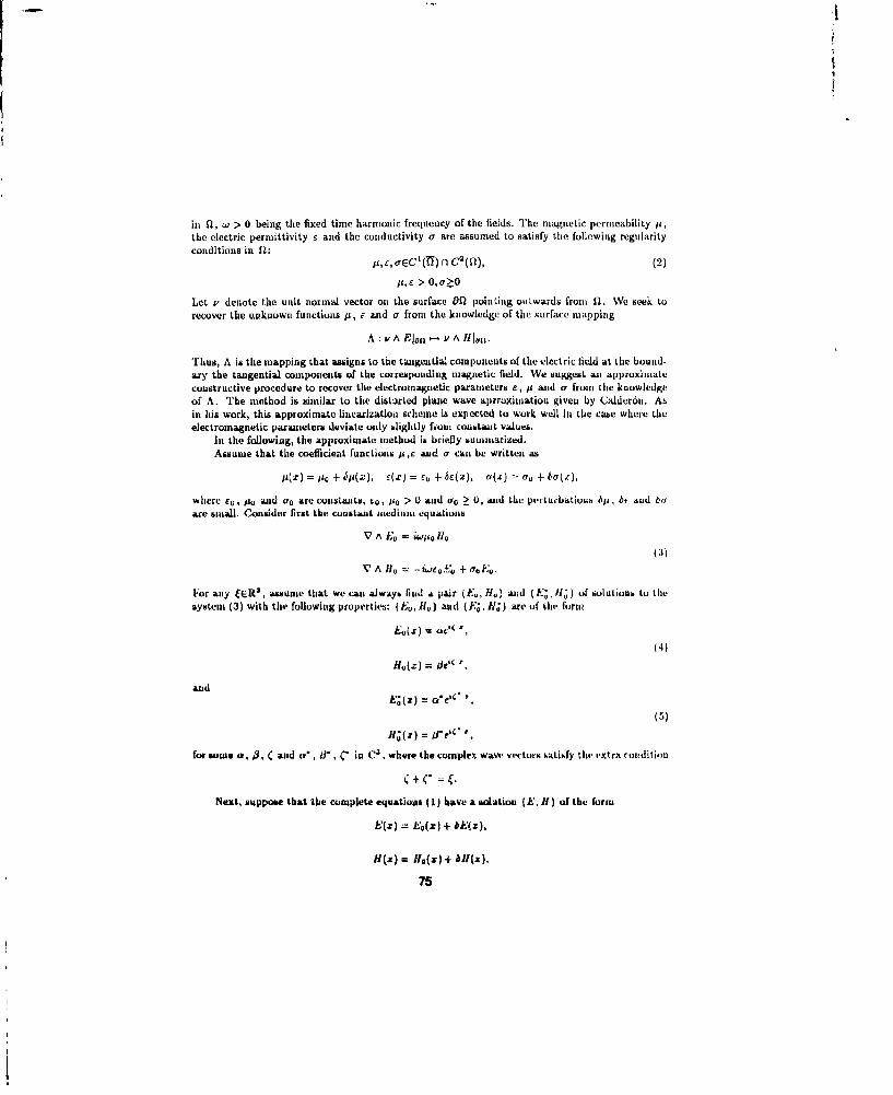
in 12, w > 0 being the fixed time harmonic frequency of the fields. The magnetic permeability it,the electric permittivity e and the conductivity or are assumed to satisfy the following regularityconditions in 12:

1,, c, crEC(?i) n C2(Ql), (2)iLr > 0,0>0

Let P denote the unit normal vector on the surface 8Qf pointing ouLwards from 12. We seek torecover the unknown functions p, c and a from the knowledge of the surface mapping

A :v A Elan " v A HIOn.

Thus, A is the mapping that assigns to the tangential components of tile electric field at the bound-ary the tangential components of the corresponding magnetic field. We suggest an approximateconstructive procedure to recover the electromagnetic parameters e, j and a from the knowledgeof A. The method is similar to the distorted plaae wave afprroxitnation given by Calder6n. AMin his work, this approximate linearization scheme is expected to work well in tile case whmere theelectromsagnetic paramneters deviate only slightly f-om constant values.

In the following, the approximate method is briefly summarized.Assume that the coefficient functions pi,E and a can be written as

11(x) = p,0 + bj(X), C(X) = CU + 66(X), O(x) = U + bar(X),

where co, , and ao are constants, cg, po > 0 and eo > U, and the perturbations bit, bf and baare small. Consider first tile constant mimedium equations

V Ao = iuwpl0s(p)

V A JI -11, .'e + aE,.

For any tER3 , ssunle that we can always filid a pair (E., H5 ) and ( 11.llý) of iolutions to thesystem (3) with the following properties: &, lie) anid (E;A, ij) are of the forirm

£telz) = oca

(4)Hz)= jie '.

ando(z) ='ce""

(5)H;(X) = £r'

for some a, 6, ( and a' ,3*, C" in C', where the comnplex wave wvctors satisfy the extra conditimn

Next, suppose that the complete equations (1) have a solution (E., H) of the form

E(z) = Lo(x) + bkh(x),

H (Z) = mo(t)+ aml(z),

75

where (Es, Hs) is the constant medium solution (4), and 6E satisfies the boundary condition

VA 6E(x)1n = 0, (G)

and what is more, the correction terms 6E and 6H are small to first order in the perturbationsbp, be and b5, denoted as

6E(x) =(b,&,6C )

Then a btraightforward calculation gives

j .(E A 11 - A H)dS = j V.(EA ̂1; - E; A )dx

j((VA E)-it -(VA 11).-E -- (VA E )-iH +(VA H).E•)dx

f f(i'~jsl.iI - iw&E.F b 4rrI >E.)dx (7)

=/a(ikbpjl4.ll, -- iwbtEo.Eý 4- 6aEe.E;)dx + V((6I,6,6o)2),

the notation above meaning that the error term iR secuud order in the perturbations bp, be adho. Using the definitiou of the fields (4)-(5) together with the boundary condition (6) we obtLhlnfron (7) the formula

d(C) = fJ(ll( A oA a)-3. + A(V A ae•r ).o'( ')dS

, , "- ,..,,- + ,,,Or.)e , vdz + O((A,bta)2 ) (8)

=-•d./f• - s•to .- E + _ o, ' + O(6p•. 60o)2 ),

the hats denoting the Fourier transforms of the corresponding functions.The approximate linearized solution of the inverse problem is obtaiued by the following steps:

(i) Fro•m the knowledge of A, compute the left hand aide of formula (b).(ii) We show that the choice of the complex veto's a, 0l. o" and dj is not unique for a given

pair C, C'. Theirefore. we can solve for the Fourier tr"aiorms of the functions 4! and br + tbtr/,.jin terms of the data and the residual term.

(iii) Apply the inverse Fourier transforu, to these equations to get an approximate solution fur6;j and hE + Jar/w.

The crucial point that nakes the above linearizatiou possible is that one can prove estimated forthe error taerm that is due to the wecond order residual term O((6,h,&)2 ) in equation (8). Theerror estimate obtainod in 1141 for the reconat ruction procedure is summarised in the theorem below.

76

In the following, V, denotes a suiooth Wiollifier, i.e., V~ E C-00L), supp t~C Jý E 1L3 I It[ • tJAndf 'ýdx = 1. It N > 03, we writc- V'N(x) =. NPip(x/N). We, denote by # the curivointiwi product offunctions, i.e., f.~,(x) f f(x - Y)YiY~d. Under the stuouthuess asbuitiptioII (2), the convolutiou&

Ov* 6ju , 'Nj * 6c and O4 v * baare reasonahle approXaiulaLiOUS of thei perturbittioins bis , b and 40

if N is large.

Theorem. Aaisuijne that

[IL up jQ(x)j = sup h

ibs niall, and for borne it, ti < tj < I, N is a lauge ijuzeber of the order (I - YI)lug( 1/ [[I .Thenthe above lin earization yields ian approxiniationi if the fujictior.x ONa * i~p. v'ý * bc and tjA * C

where the error is of the order ofuljagui~ludel IQ

Referensces

[1: D. C. Barber anrid B. IL. Browni: A ppl ied potential toin, .grapluy. J . Phyis. E~. Sci. I uutruin17 (1984) 723 733.

12]: A. P. Calder~nu: 0n an uuuvrbe bounsdary vAlue problein. Sermnnur an A'ull. rz,,jI AirnIykaAcud its Appliutivny tu o Gntusuun l'hysics-Soc. Br~hilejra de MateauiuticA. Rijo de Janeiro,65 73 ,1980.

(3]: M. Cheney, 1). lsiawsozu, J. C., Newell. S. Situhke, and J. Colble: NOSER: Au algoritluni forsolving the inverse conductivity probletti. To appear in Internal. J. linaging Systenut andTechnology.

14]: 1). G. Uihý*r, D). Issaciwin atid J.C. Newell; Thr~iry Aund perfurnia~ance of an adaptive t urreusitomnography -systeuuu. (Tit I'hiyb. Pluybiul. Meas. 9. Suppl .A ~IJ 19S 35 4

[5]: Di. G,. Gibxer. 1). lsaacson and J. C. Newell: EUcciric turrvlat .ujiiupi~itI tomography Aza,1eigeuavalukes. SIAM J. Appl. MIAth. W1 (1990) 16213 163-1.

[61: 1). lbaaeutir: Dibtinguishiability of conductivities by electric currenat t-unuputed toiuo~raph).IEEE Traub. kled. linAsgmg %1l r (19.86) 91 95.

17]: 1). lsaAcwt a"d MI. Cheney: Effect* of itueasiateiiieit precisuio and unitte utunibers o vci ltruneb ou Iiinear ainipediace iuniuhig 4-lorillinis. 1* 14ipear ini SIAMh J. ApoI Math.

181: Rt. '. Kuhnu and A. hic~ennecy; Nunoki&2fal1 iapleiuuesitailn-1 4f &~ xarationad athod forelectrical inapedazu-e inkagiuug. Preprint.

[9]: Rt Kohn and MI. Vo~eliub: 1)etermininixj conlducivityt by boutadas) nw.6aureiIwu&. t oniuuapfure A ppI. M ath. 37 (1984) 113 12D.

1101: A. Nachinau: lteconsbucLiouu fromi boundw) mneaurenwntau Aamn4. cti MAIL. 121%

(ill: J1. C- Newell, D). G. Glawr anud D. ILMacion: Au el"tric cuurrent tsfwgrapla lVLU TrAS6Ifioanwd. Lug. lIME 35 (1ISM) H~28 833-

1171: A. G. Itannu: Multjdiiezuannal inverhe prubensa and coctiplietenera of pvioduts oft "iUtosto P1W. J. Ma~th. Aaal. Appi 111 'W)e~t 211 253.

77

113]: F. Santosa and M. Vogelius" A backprojection algorithmn for electrical impedance imaging.SIAM J. Appl. Math. 50 (1990) 216-243.

[14]: E. Somersalo, D. Isazacson and M. Cheney: A linearized inverse boundary value problemfor MaxweU's equations. Manuscript (1991)

[15]: J. Sylvester and G Uhlmann: A global uniqueness theorem for an inverse boundary valueproblem. Annals of Math, 125 (1987) 153-169.

[16]: T. J. Yorkey, J. G. Webster and W. J. Tompkins: Compuring reconstruction algorithmsfor electrical impedance tomography. IEEE Trans. Biomed. Eng. BME-34 (1987) 843-852.

78

Ii

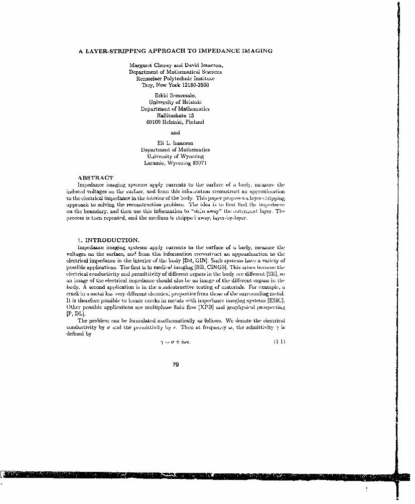
A LAYER-STRIPPING APPROACH TO IMPEDANCE IMAGING

Margaret Cheney and David Isaacson,Department of Mathematical Sciences

Rensselaer Polytechnic InstituteTroy, New York 12180-3590

Erkki Somersalo,University of Helsinki

Department of MathematicsHallituskatu 15

00100 Helsinki, Finland

and

Eli L. lsaacsonDepartment of Mathematics

University of WyonmingLaramie, Wyoming 82071

ABSTRACTImpedance imaging systems apply currents to the surface of a body, useasure time

induced voltages on the surface, and from this info ination reconstruct an approximationto the electrical impedance in the interior of the body. This paper proposes a layer-::trippingapproach to solving the reconstruction problem. The idea is to first find the imipedneceon the boundary, and then use this information to "sti'i away" the outCrmnu.t layer. Tl,process is then repeated, and the medium is strippel away, layer-by-layer.

1. INTRODUCTION.Impedance imaging systems apply currents to the surface of a body, measure the

voltages oa the surface, aiid front this information reconstruct an approximation to theelectrical impedance in the interior of the body [BB, GIN]. Such systems have a variety ofpossible applications. The first is in medical imaging [BB, CINGS]. This arises because theelectrical conductivity and permittivity of different organs in the body are different [SK], soan image of the electrical impedance should also be an image of the dilfiwerot organs ii. tiLnbody. A second application is in the njndestructive testing of materials. For example, acrack in a metal has very different electrical properties fromn those of the surrounding metal.It is therefore possible to locate cracks in metals with impedance imaging systems [ESIC].Other possible applications are mnultiphalse fluid flow 'IXPB] amd geoplhysical prospectinig[P, DL].

The problem can be formulated mathematically as fo!lows. We denote the electricalconductivity by a and the permittivity by e. Then at frequency w, the admnittivity Y isdefined by

a (1.1)

79

Sa

We assume [IC1] that the electric potential u satisfies the boundary value problem

V. y7Vu = 0 inside the body if (1.2)

Ou--• = j onthesurfacei9Q (1.3)

For existence of a soluti-on, we need also the conservation of charge conditiou

foj = 0. (1.4)

To obtain a unique solution, we need to choose a ground or referencc potential. This canbe done by means of the condition

f U = 0. 11.5)

W- may make any boundary measuremcnts we like. This means that we may specify anyj and measure the corresponding u on the boundary. The restriction of u to the boundarywe denote by v. Equivalently, we assume that we canl obtain fruit'I mcasurcments the mapIt that takes j to v. We call this map the resistive map. From knowledge of .he 111ap R,wc would like to find y.

Sylvester and Uhlmann have shown [SU] that thc map R does indeed determine Yif tl.v body is n-dimensional with n greater than two, and in the two-dimensional caseR detemincs 'Y provided that -y is close to a constant. Nachmnia [N] used the Sylvcster-Uhhmnan ideas to d. velop a constructive method for determining -y from R. This method,however, has yet to be implemented numerically.

Most of the methods that have actually made images have been of two kinds, thosebased on linearization and those based on optimization. One type of method based onlinearization is the backprojcction methodt [B1, SV], which is essentially an approximatesolution of the linearized problem. Another approach to the linearizcd pLoblem is to convertit to a moment problem [CW, BAG, AS]. Detahled analyses of the linearized probleni aregiven in [IC2] and [AS); limitations of the linear theory are discussed in [II] and [CIII, whichgive exact solutions of the linearized problem. Examples of the optimization approach areICINGS, KM, YWT1. In this paper, however, we pmrsue a different niethod ([C11, C12])that has its roots in invariant imbedding [CDK, CoK, ChK].

2. THE METHODFirst, we derive a formula that allows us to compute the resistive map in the interior

from boundary data. We then outline the layer-stripping algorithm. Section 3 contains aunexplanation of the other key idea needed.

For simplicity, we will assunte throughout that the body Rl is a disk of radius r. Ourlayer-stripping algorithun is based on understanding how the resistive map R rhanga.es rchanges. 1Below, we obtain a formula for the derivative OR/Du.

We begin by extending the definition of Rt to all r:

R(m)(-y(,, ) ,)) = u(r,',). (2.1)

80

W~e then, differunittatc (2.1) with respect to r:

5- (-r -5- +r R=)1 t (2.2)

Ili the second termn of (2.2), wve use the differential equation (1.2), written in polar coordi-tia tes: a b O t 7 O 2 35,y-) +7 -q,-, + g To ) = I)=

Finially, wc inultioly the resulting equationi by 7r, use definition (2.1), mid extrtact thc

DR(r) I R(r) R(r) 0 OR(L)+ (2.4)

Or '(r, 0) rF i 09 Of)0

Trids formula suggests. tile following algorithai for solving tliav inverse problem. I'No callit a "layer-strippinig" algorit~lni because it essenitially wvorkcs by stripping away the miedium,onec layer at a time. The admit tivi ty of oach layer is founid before. it. is strippedl away.

1) Make ineas~ureienelt R( r,j) oin the hoi tidary of tix bodn y.2) Find -y onl thle boundary' at ru.3) Make at finite dilffereneairpillroxitiIitj~ii to the' laycr-stripping fornm~ill (2.4): forsoon' sitoill Aý, writt,

Or (2.5)

4 ). RlhW( epac t by 7'( - A anId relentt starting with Ii tol 2.To Comiplete the disctussion of thi s algo intI ii , wv licedu to show how to doi step 2').

3. HO0W TO GET') ON THlE BOUNDARYThere arc a iitnumble'r of ways t- I finid -7 011 the houni dary froii ft. For extuiu ]e, it

Was showni rigorously by Koh dn mel ½ iogelii is INVI midn Sylvester aiid Ubla iiatiti [S ul that'Y and till itsn deriVa~tives On the boundary cani be obtainedl from bi ouindary nieasmaroioeiits.Ko hn and Vogehuns dlid this 1ty appjlyin~g IMLoaiEMN, highly oscillatory boundary dat a. Soch

b-iin1dii ry (LIta is nisonsli ti %'( to vai-l ti ins iii , far froii thne lnmidt alry (see also (l1 ). Thisis essenltially eqaui vabot tot t lii technuique ulsed b y SylvvSti r and U11lniaina1, Which Wasathttiii all tasymsptontic a pIsioisn of the laouiidlary ioiip 1?-'.

IHere we giv. at foriii.1 I descrit iioii of how onti inlay recover -y from the ,,ingu lar behl avioriof the kertiel (If thle inl) R?. First, we see that t his korucl is the Grieeii's funci tion G' tlihi iedby the following bounudary vttliv probtllem.t

\' ii V 1 (3.1)

OGMIOS (3.2)

G 0 . (3.3)

To see how G and R are related, we multiply (3.1i u, multiply (1 9) by G, subl,-acmtawl integrate over il. This gives us

f(GV .Vu - uV. yVG) u(x), (3.4)

where x is in Q. Using and the divcrgence theorem, we obtainf (GY o - wy aG u(x). (3.5)

The first tena of (3.5), however, vanishes by (3.2) and (1.5). This leaves

u(x) = j G(.,y)j(y)dy, (35)

which shows that for x and y on Oil, G(x, y) must be the kernel of R.The leading order singularity of G can he underqt)ood by writfing (3.1) as

-yV2 G + V.y VG = -6. (3.7)

Thus a paraametrix [G, SU] for (3.7) is Go, which satislies

YV2 G0 - -6, (3.8)

which, in the case when i is a disk, can be found explicitly:

Go(x, y) = comst.'g X - V (39)7(X)

Thui, G can bc writtenG~x,•.t = o•.log Ix - y I

G(x,!y) = eonst.----I-X - I (smoother stuff). (3.10)

This allows us to recover -y as

7(X) = Hlln const.g2 .X (3.11)

4. CONCLUSIONS"The layer-stripping algorithm has a number of possible advantages over the approx.

inmate linearizations and iterative methods that have been tried so far. First, it has nodifficulty with extraneous local minima as do optimization-type methods. Second, in lrinr-ciplc at least, it solves the full nonlinear l)roblem. Third, the ill-posedness of thue lrobldinappears in an explicit, isolated way. Fourth, it requires fewer computations (order L4 ,

82

m----

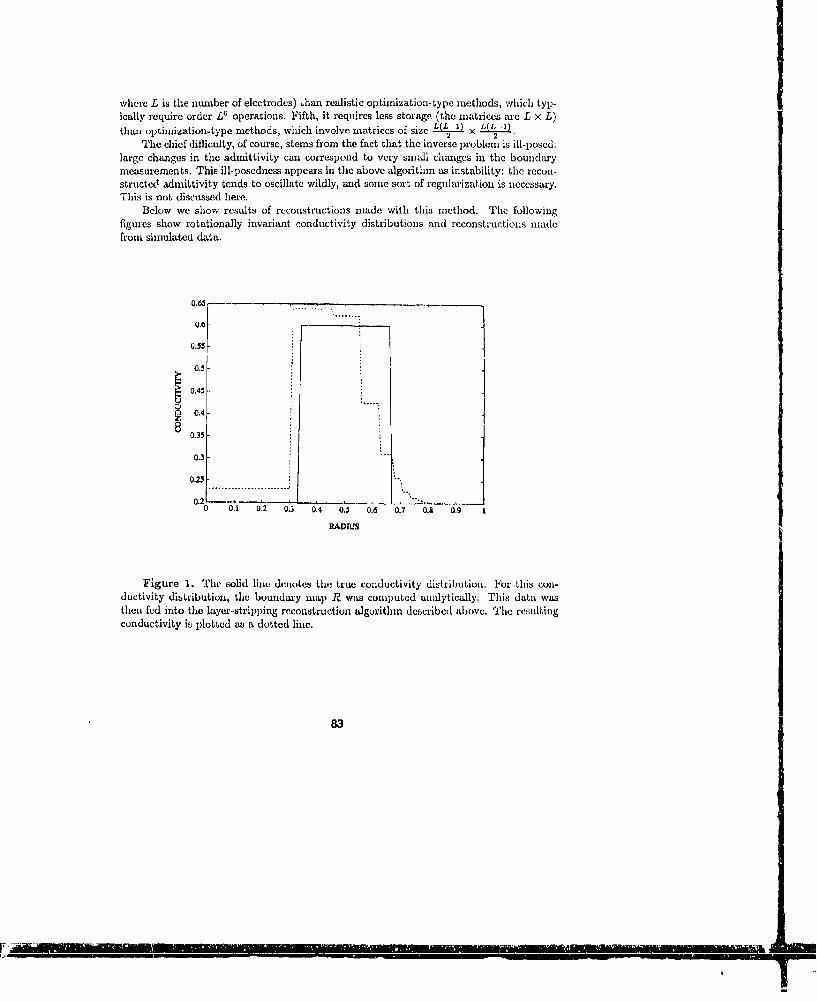
where L is the number of electrodes) thaa realistic optimization-type methods, which typ-ically require order L6 operations. Fifth, it requires less storage (the matrices are L x L)thani optimization-type methods, which involve matrices of size L x ( .

The chief difficulty, of course, stems from the fact that the inverse problem is ill-posed:large changes in the admittivity can correspond to very small changes ia the boundarymeasurements. This ill-posedness appears in the above algorithm as instability: the recon-structed admittivity tends to oscillate wildly, and some sort of regularization is necessary.This is not discussed here.

Below we show results of reconstructions made with this method. The followingfigures show rotationally invariant conductivity distributions and reconstructions madefrom simulated data.

0.65

0.6

0.55 I0.5 1.

0.45

S0.480.35

0.3-

0.25-

0.2 L"0 0.1 0.2 0.3 0.4 0.5 0.6 0.7 0.8 0.9 1

RADIUS

Figure 1. The solid line denotes the true conductivity distribution. For this con-ductivity distribution, the boundary map R was computed analytically. This data wasthen fed into the layer-stripping reconstruction algorithm described above. The resultingconductivity is plotted as a dotted line.

83

F, L

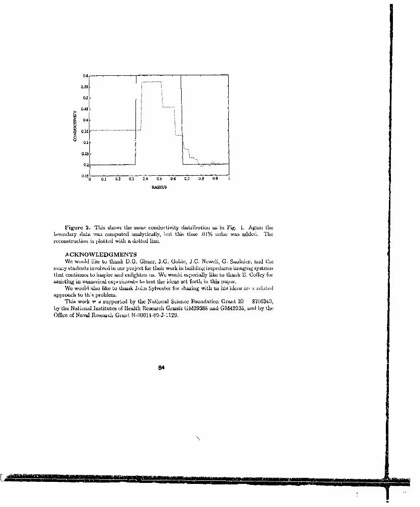
0.550.5

0.5

0.45 .

0.4

0.3-

0.25

0.20.1. "".

0 0.1 0.2 0.3 0.4 0.5 0,6 0.7 0.8 0,9 1

RADIUS

Figure 2. Tlris shows the same, conductivity distribution us in Fig. 1. Again tileboundary data wa3 computed xmalytically, but this time .11% noise was added, Therecoustructiou is plotted with a dotted line.

. CKNOWLEDGMENTSWe would like to thank D.G. Gisser, 3.G. Gobie, J.O. Newell, G. Saulhder, and the

maooy students involved in our projcet for their work in building impedaixce imaging systemsthat continues to inspire and enlighten us. We would especi;dly like to thalnk E. Coffey forassisting in numierieal experirients to test the ideas ct forth in this paper.

We would also like to thank John Sylvester for shmaing with us his ideas o0, ZL relatedapproach to thW9 problem.

This work v, s supported by the National Science Foundation Griat El 8706340,by the National Jnstitutes of Health Research Grmits GM39388 and GM42935, and by tileOffice of Naval Research Grant N-00014-89-J.-1129.

8t4

REFERENCES[AS] . A Alles and F. Swuitosa. "Stability and resolution iualysis of a linearized

problem ini electrical impl'dance tomography", Technical Report No. 90-13,Dept. of Math. Scinaces, Uaiv. of Delaware.

[DBI D.C. Barber and B.D . Brown, "Applied potential tomography", .1. Phys. E.Sci. Instrum. 17 (1984) 723-733.

[BAG] S. Berntsen, J.13. Andersen, and E. Gross, "L\ general formulation of appliedpoteUtial tomograplhy", preprint.

[CDKJ J.P. C-roucs, M.E. Davison, and R.J. Krueger, "Direct aWnd ilnvet'se sc.atteringin the time domain via invariant imbedding equations", J.. Acoust. Soc. A.m.74 (1983) 1535-1541.

[(C' P. Colli Frauzoue. "'Il probleme inverso dell'cttro..rdiografia", Boll. U.M.I.15-A (1978) 30-51; and P. Colli Franzone, L Guerri, B. Tacrardi, anud C.Viganotti, "The dirt et and ilxwei'e potential problems in electrocardiology.Numerical aipects ,4" -onte rCgularization methodis and apl.licationl to datacollected in isoatecd dog heart experiments", Pill). 222. laboratouin di AnalisiNuincrica del Comisi.hio Naziemnale delle f.ecerche, Pavia (1079).

[ChK] M. Chueney •nd G. Kristeosson. "Three- dimensional ilv,'re .scattCring: layer-stripping fornlshc antI ill po.•e(lnesS resUlILs", hivernse Problems 4 (1988) 625-642.

(Cl1] M. Cheney aMld D. Ibnlcsoli, "Layer- Strippittg, Inhvria•t 1mnbedding, andImpedance Imaging", Conl'erence Proceedings fur AMS Special Session inmemory of Dob t)Kriger, A.lbuiuverque, NNI. April, 1990 (SIAMN. Philadelphia.1991).

[C12] M. ChIeCey anld D. Isaeson. "An Overview of Inversion Algorithms for hoped-ance hmaging", Procccdings of the AMS SMzUomer Research Contlfernce.Andmh•rst. MA. Juae 1990.

[CIII M. Cl:heny, D. Isaacson, and E.L. Isaacson, "Exact solutions to a linearizedinverse boundary value problem", Inverse Problems G, 923-934 (1990).

ICINGS] M. Cheney, D. Isaacsomn, J. Newell. J. Goble, and S. Sianske, "NOSER: Analgcrithnz for solvinlg the inverbe conductivity Ipo)Ibleil", to appear in Internat.J. Imaging Systems and Technology.

(CoK] J.P. Corones tad R.J. Krueger, "Obtaining scattering kernels using invariantimbedding", J. Math. Anal. App. 95 (1983) 393-415.

[CWI T.J. Connolly and D.J.N. Wall, "Onl an inverse problem, with bounidary inca-surectents, for the steady state diffusion cip•atiou". Inverse Problens 4 (1988)pp. 995-1012.

(DL] K.A. Dynes aud R.J. Lytle, "Analysisj of electrical conductivity imaging",Geophys. 46 (1981) 1025- 1036.

[ESIC] M.1. Eggleston, R.J. Schwabe, D. Isaacson, and L.F. Coffin, "The applicationof electric current computed tomography to defect imaging in metals", in Re-view of Progress in Quantitative NDE, vcl. 9A, 455-462 ed. D.O. Thompsonand D.E. Chir•ienti (Pleuum, New York, 1989).

IG] P.R. Garabedia•n, Partial Differential Equations (Chelsea, New York, 1986).

85

L"

L

[GIN! D.G. Gisser, D. Isaacson, and ..C. Newell, "Theory and performance of anadaptive current tomography system", Clin. Phys. Physiol. Meas. 9. Suppl.A (1988) 35- 41.

[I] D. Isaacson, "Distinguishability of conductivities by electric current computedtomography", IEEE Truas. Med. Imaging MI-5, 91-95 (1986).

[IC1] D. Isaacson and M. Cheney, "Current problems in impedance imaging", inInverse Problems in Partial Differential Equations, ed. D. Colton. R. Ewing,and W. Rundell (SIAM, Philadelphia. 1990).

[IC21 D. Isaacson and M. Cheney, "Effects of measurement precision and finite num-bers of electrodes on linear impedance imaging algorithms", SIAM J. Appl.Math., in press (1991).

[II D. lsaacson and E.L. Isaacson, "Comment on Calder6a's paper: 'On an inverseboundary value problem' ", Math. of Comp. 52, 553-559 (1989).

[NJ A. IL Nachman. "Reconstruction from boundary measurements". Ann. ofMath. 128 (1988) 531-576.

[NGL] J.C. Newell, D.G. Gisser, and D. Isaacson. 'An electric current tomograph",IEEE Trans. Biomed. Engr. 35 (1988) 828-833.

[K] R. J. Krueger, "'Inverse problems for nonabsorbing media with discontinu-ous material properties", J. Math. Phys. 23 (1982) 396-404 and '"Numericalaspects of a dissipative inverse problem", IEEE Trans. Antennas and Propa-gation, AP-29 (1981) 253-261.

(NK] G. Kristensson and R.J. Krueger, "Direct and inverse scattering in the timedomain for a dissipative wave euqation". Parts 1-4. J. Math. Phys. 27 (1986)1667-1693; 28 (1987) 360-370; Inverse Problems 5 (1989) 375-388.

[(N'M) R.V. I:ohn and A. McKenney, "Numerical implementation of a variationalmethod for electrical impedance imaging". preprint.

[KV] R.V. Kohn and M. Vogelius, "Determining conductivity by boundary inea-surements", Comm. Pure ard Appl. Math. 37 (1984) 280-298.

[P] R.L. Parker, "The inverse problem of resistivity sounding". Geophysics 42(1984) 2143-2158.

[SKI H.P. Schwann and C.F. Kay, "The conductivity of living tissues", Ann. of theNYAS 65 (1957) 1007-1013.

[SUI] J. Sylvester and G. Ulinsann. "A uniqueness theorem for an inverse boundaryvalue problem in electrical prospection", Comm. Pure Appl. Math. 39 (1986)91-112; "A global uniqueness theorem for anl inverse boundary value problem",Ann. of Math., 125 (1987) 153-169; "Inverse boundary value problems at theboundary - continuous dependence", Comm. Pure and Appl. Math. 41(1988), 197-221.

]SVJ F. Santosa and M. Vogelius, "A backprojection algorithm for electrical ihped-aunce imaging", Technical Note BN 1081 (Dept. of Math., Univ. of Maryland1988)

[YWT] T.J. Yorke, J.G, Webster, and W.J. Tompkins, "Comparing reconstructionalgorithms for electrical impedance tomography", IEEE Trans. Biomed. Eng.BME-34 (1987) 843-52.

[XPB] C.G. Xie, A. Plaskowski, and M.S. Beck, "S-electrode capacitance system fortwo-component flow identification". Parts I and 2, lEE Proc. 136. Pt. A(1989) 173-190.

86

ELECTRIC CURRENT COMPUTED TOMOGRAPHY

D. Isaacson', M. Cheney', J.C. Newell', D.G. Gisser 3 , and J.C. Goble4

Rensselaer Polytechnic InstituteTroy, New York 12180-3590

Department of Mathematical Sciences2 Department of Biomedical Engineering3 Department of Electrical and Computer Systems Engineering' Department of Computer Science

ABSTRACTElectric current computed tomography (ECCT) systems apply electric currents to the

exterior of a body and measure the voltages that result on the body's surface. Using thesemeasurements as data, these systems make and display reconstructions of the electricalconductivity and permittivity inside the body.

We will discuss a simple mathematical model for this problem. We then show howmathematical considerations can improve the design of the data-collection aspect of LCCTsystems. Finally, we describe a reconstruction algorithmn that computes approximations tothe electrical conductivity and permittivity inside the body. We will also present imagesmade with this algorithm.

There are- many situations in which one would like to know the clectrical collductivityand permittivity inside a body from measurements made on the body's surface. Suchinformation is useful, for example, for the detection of cracks or flaws in metals [ESIC].The ability to obtain such information about the interior of a htuman body could lead tothe design of better electrocardiographs and defibrillators [CF, IC]. The ability to imagethe electrical properties of material flowing in a pipe could lead to a better understandingof multiphase fluid flow [XPBJ.

At present, there is only one commercial system that images the conductivity insidethe human body. This is the Applied Potential Tomography (APT) system invented byDavid Barber and Brian Brown [BE]. This pioneering system uses sixteen electrodes placedaround the circumference of the body. First a pair of electrodes is connocted to a currentsource, so that current flows in through one electrode and out through the adjacent elec-trode. These two electrodes are the "driver pair". While current is flowing through thecscetwo electrodes, the voltages at all the other electrodes are measured. Then the currentsource is connected to the next pair of electrodes (a new driver pair) and the voltagesmeasured on all the others. This process is repeated until all pairs of adjacenit electrodeshave served as driver pair. This data is then fed into a reconstruction algorithon based onbackprojoction, and a low resolution image is obtained of conductivity changes inside thebody.

One way to improve this system would be to improve its resolution. Htow can this bedone? A naive guess would be to use more cleettudes. We can see whether this will workby studying the following inathematical model.

87

aLm

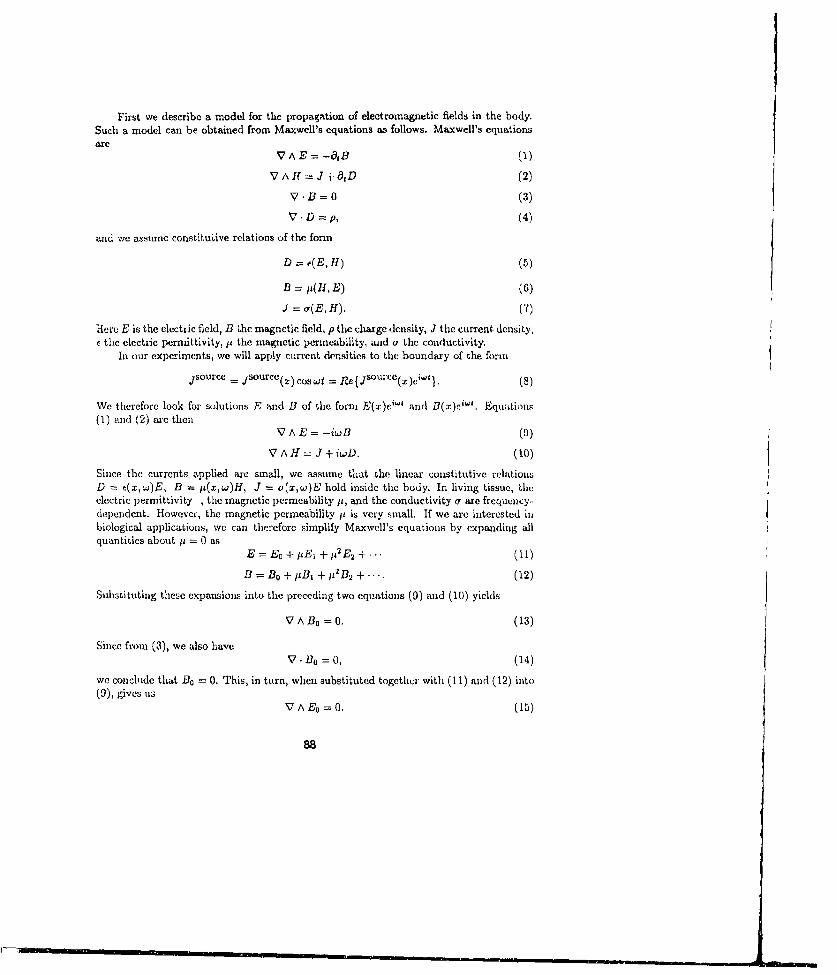
First we describe a model for the propagation of electromagnetic fields in the body.Such a model can be obtained from Maxwell's equations as follows. Maxwell's equationsare

VAE=-8B (-)VAH = J+80D (2)

V.1B=0 (3)

V. D = p, (4)

and we assume constitudve relations of the form

D - e(E,H) (5)

1 = p(H, E) (6)J = a(E, H). (7)

Here E is the electric field, B Lhc magnetic field, p the charge density, J the current. density,c the electric permittivity, p the magnetic permeability, and u the conductivity.

In our experiments, we will apply current densities to the boundary of the form

jsource = jsourcc(,)cost = Re{jsource(x)ew}. (8)

We therefore look for solutions E and B of the form E(x)ci' and B(x)5 1wd, Equations(1) and (2) are then

V A E = -iwB (9)

V A H = J + iwD. (10)

Since the currents applied are small, we assume that the linear coustitutive relationsD = e(x,w)E, B = jt(x,w)H, J = or(x,w)E hold inside the body. In living tissue, Lheelectric permittivity , the magnetic permeability it, and the conductivity or are frequency-dependent. However, the magnetic permeability 1L is very small. If we are interested inbiological applications, we can therefore simplify Maxwell's equations by expanding allquantities about p = 0 as

E E o + jE 1 + 142 E2 + (11)

B =BO +JIB, +p2B2 + ... (12)

Substituting these expansions into the preceding two equations (9) and (10) yields

VAB 0 =0. (13)

Since from (3), we also haveV. B 0 = 0, (14)

we conclude that BD = 0. This, in turn, when substituted togetlicr with (11) and (12) into(9), gives us

VAE 0 =0. (15)

88

I- • ' - II-

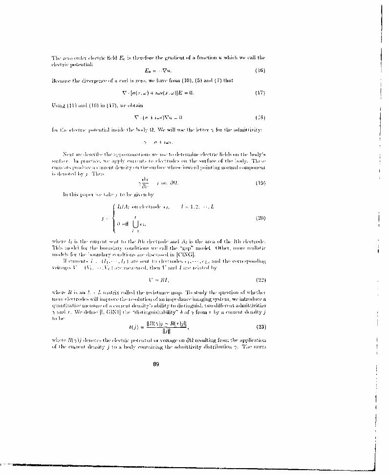
llt't'ttst'te tiltdvtrgelleii' tf it tcurl is v.tro, w W uie h fromzl (10). (3) andi (7) that

* k(~.~')4- tw~r.~]E =0. (7

U'sintg (11) intl (16) in (17). we oitttin

V +t')7~A ('8)

iVdlor b 1 hl oil OI L (19)

IIIths ;1el %I ta , 1 o ll A ri IiI?,,- rjI

tuU - 1 (20)

8ff9

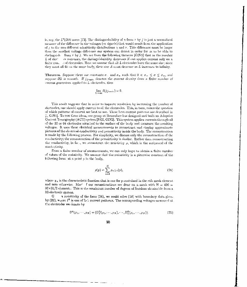
is, say, the L' (01) norn' (CI]. Th' distingnuishlobili y of -Y from T bn' j is just a normnaizediinci' rc of the difference in tile voltages (or iigini s) that would result from the applicationof j to thi two different adroittivity distributions -y and r. This differeoce must be largerthan the smallest voltage difference our system can detect in order for as to be able todistiznguish from r by j. We see from the following theorem IGIN1 that as the numberL of vie'" ,,s increases, the distinguishability decreases if one applies current only on afilite nih . ." of electrodcs. Here we assune that all L electrodes have the same size; sincethey niust II1 fit oil tfill sam10e body, tliir size A noust decrease as L increases to infinity.

Theorem. Suppose there are cesist ants a_- and ao scich that 0 < a - a < or -, 0-+i also;ppose 012 is Sllooth. If Ji ,, .a. denotes the ciireiint dc'asity Frouo a finite a rim ber of,'uiirilt genri'tors ;jppli'd to L electrodes, then1

biln (jfi, ... ) = 0.r,-~

This result suggests that in order to improve resolution by ihireasing the nuioiher of'lcctrodes, otiit should apply current to all the electrodes. This, in turn, raises the questionif which patterns of ciur'rent are best to use. These best current patterns are described in

[I, GIN1B. To test these ideas, our group at Rensselter has designed and built an AdaptiveCurrent Tomography (ACT) system [NGI, GIN2]. This system applies currents through allof the 32 or 64 electrodes attached to the surface of the body and measures the resultingvoltages. It uses these electrical measurements to reconstruct and display approximatepictures of the elc,-trical conductivity and pernnitti'vity inside the body. The reconstructionis nmade by the following process. For simplicity, we discuss only the reconstruction of theconxductivity; the reconstrectious of the lermittivity is similar. Rather than recoiistructiigthe conductivity, in fie,, we reconstruct tile resistivity p, which is the reciprocal of ileconidictivity.

Froin a, finite number of measurenments, we can only hope to obtaiii a finite numberof values of the resistivity. We assume that the resisitivity is a piecewise constatmt otf thefollowing form: at a point 1) in the body,

N

P(P) = E P P) (24)n=1

where X, is the characteristic function that is one for p contained in the nth inesh elemieitand zero otherwise. Myos' f our reconstructions are done on a mesh with N = 496 =32 x31/2 element:. This is the maximum nuniber of degrees of freedom obtainable froin a32-electrode system.

o a resisitivity of the form (24), we could solve (18) with boundary data givenby (20), w.,ere Ik is one of L-1 current patterns. The corresponding voltages rueasured atthe electrodes we denote by

uk(pi,.-.,PN) = (Ui(pi,., ',N),'- ' -,U(pi•, '',p,,)). (25)

90

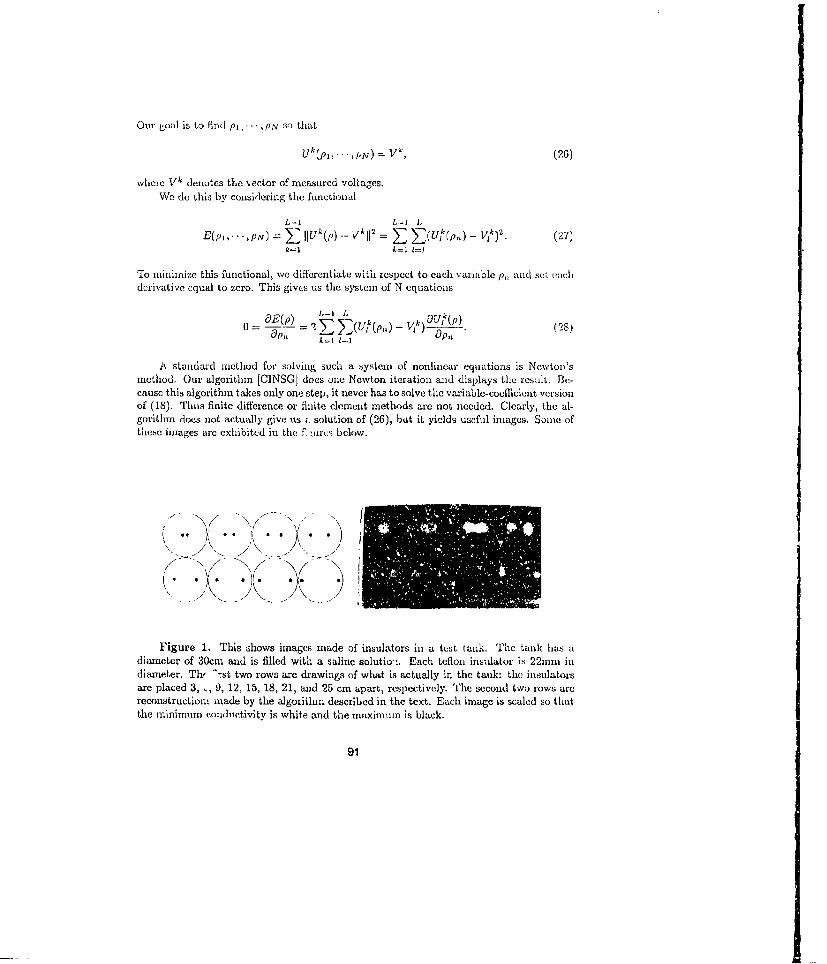
Our goal is to find Pi. 'N So that

Uk(Pl," ,N)- V', (26)

where V0 denotes the vector of measured voltages.We do this by considering the functional

L-I L-1-I L

E(p 1,, ,PN) = IIU1(Q)--VkIls = > Z(UHP,,) - vk)2. (27)k=1 k=l 1=)

To minimize this functional, we differentiate with respect to each variable p,, and set eachderivative equal to zero. This gives us the system of N equations

L-I L k.OrpM (P) = .,)_.

D__ -9 ~(~p / (28)

A standard method for solving such a system of nonlinear equations is Newton'smethod. Our algorithm [CINSGJ does one Newton iteration and displays the result. Be-cause this algorithm takes only one step, it never has to solve the variable-coefficicnt versionof (18). Thus finite difference or finite clement methods are not needed. Clearly, the al-gorithm does not actually give us r. solution of (26), but it yields useful images. Some ofthese images are exhibited in the f ,urci below.

Figure 1. This shows images made of insulators in a test tank. The tank has adiameter of 30cm and is filled with a saline solutio--. Each teflon insulator is 2211m indiameter. ThW ^-st two rows are drawings of what is actually in the tank: the insulatorsare placed 3, , 9, 12, 15, 18, 21, and 25 cm apart, respectively. The second two rows arereconstructiomn made by the algorithm described in the text. Each image is scaled so thatthe minimum conductivity is white and the maximum is black.

91

Figure 2. This shows inmages of the interior of the chest of a human volunteer.Thirty-two karaya guru electrodes were place around the chest at the level of the ,sevenththoracic vertebra (T7). The bottom right picture is a drawing of tile interior of a humanchest at level T7. Note the locations of the lungs. The top left image is a reconstruction atcomplete expiration. The top right image is a reconstruction with 1500 nil of inhaled air.Note the decrease in conductivity in the region of the lungs. Also visible in both pictures isa circumferential layer of low conductivity. This presuniably represcnts skin and fat, whichhave low conductivity. The light spots at the bottom of each image may be ribs passingthrough the image plane. The image on the lottom left is a difference image, obtained bysubtracting the top left imago from the top right one. Features that are the same in bothtop images cancel out in this process, and only features that are different remain. Thisdifference image shows conductivity changes in the lung regions as the lmugs inflate.

92

AcknowledgmentsThe work described in this talk was done in collaboration with a large number of other

people. We would especially like to thank S. Siroske, L. F. Coffin, M. Rt. Eggelston, anidR. Schwabe. This worl, was supported in part by NIH(GM 39388, GM 42935), NSF(BCS-8706340), ONR(N00014-89-J-1129), GE, and R1Pl.

References

[rB] D. C. Barher and B. H. Brown, "Applied potential tomography," J. Phys. E.Sci. Instruni. 17, 723-733 (1984).

[CI] M. Cheney and D. Isaacson, "Dist inguishability in Impedance Imaging," RPIpreprint.

[CINSG] M. Cheney, D. Isaacson, J.C. Newell, S. Simaske, and J.G. Goble, "NOSER:An Algorithm for Solving the Inverse Conductivity Problem", to appear inInternat. J. linaging Systems and Tc -.hnology.

[CING] K.-S. Chieng, D. Isaacson, J. C. Newell, and D. G. Gisser, "Electrode modelsfor electric current. computed tomography," IEEE Trails. Biomed Enigr. 30,918-924 (1989).P. Colli Franzunre, "II probleme inverse defl'elettrocardiografia," Boll. U.MI.15-A, 30-51 (1.978); and P. Colli Franzosse, L. Gucrri, 13. Taccardi, and C.Viganotti, "The direct and inverse potential problems in elect rodcardiology.Numerical aspects of some regularization methods and application to datacollected in isolated dog heart experiments," Pub. 222, laboratorio di AnalisiNumecrica del Cornsiglio Nazionale delle Ricerche, Pavia (1979).

[ESIC] M. R. Eggleston, R. J. Schwabe, D. Isaacson, and L. F. Coffin, "The appli-cation of electric current computed tomography to defect imaging in metals,"to appear in Review of Progress in Quantitative NDE, vol. 9A, 455-462, ed.D.O. Thompson and D.E. Chimenti (Plenium, New York, 1989).

[1] D. Isaacson, "Distinguishability of conductivities by electric current computedtomography," IEEE Tranls. Med. Imaging MI-6, W~-95 (1986).

uISC] D. Isaacson, E. Somersalo, and M. Cheney, "Existence and uniqueness for anelectrode model for electric current computed tomography," R.PI preprint.

[GINI] D. G. Gisser, D. Isaacson, and .J. C. Newell, "Electric current compuced to-er.-ography and eigenvalues," SIAM 3. Appl. Math 50, 1623-1634 (1990).

[GIN21 D. G. Gisser, D. Isaacson, and J. C. Newell, "Theory and performance of anadaptive current tomography system," Olin. Phys. Physiol. Mcas. 9, Suppl.A, 35-41 (1088).

[NGI] J. C. Newell, D. G. G: 2 .r, and D. Isaacson, "A:, electric current tomograph",IEEE Tranis, Biomed, Engr. 35, 828-833 (1983).

[XPB] C.C. Xie, A. Plaskowski, and M.S. Beek, "8-electrode capacitance system fortwo-con.,-uonent flow identification", Parts 1 and 2, IEE Proc. 136, Pt. A(1989) 17.3-190.

USE OF ELECIRICAL IMPEDANCE IMAGING IN TAO-PHASE, GAS-LIQUID frS

by

J.T. Lin', H. Suzuki2, L. Ovacik), O.C. Jones', J.C. Newell 5 , M. Chne 6

Center for Multiphase ResearchRensselaer Polytechnic Institute

•ray, New York 12180-3590 U.S.A.

A~b7Rr

The determination of interfacial area density in two-phase, gas-liquidflows is one of the major elements impeding significant development ofpredictive tools based on the two-fluid madel. Curr•ntly, these modelsrequire coupling of liquid and vapor at interfaces using constitutive equa-tions which do not exist in any but the w.zst rudimentary form. Workdescribed herein represents the first step towards the development of elec-trical bqjedance computed tomography (EICT) for nonintrusive determinatioiAof interfacial structure and evolution in two-phase, gas-liquid flows.

This paper summarizes the work accomplished to date towards thedevelopment of electrical impedance imaging methods for use in two-phase,gas-liquid flows. The basis for the method is presented and algorithms forimplementation are described. Both Gauss elimination and modified Jacobiconjugate gradient methods are used for matrix inversion to calculate theelectrical field from a given complex conductivity distribution and knowndistribution of applied current. Results of numerical sixailations and thefirst, non-iterative real images are encouraging.

It is felt that tcurgraphic methods such as described herein will at theleast provide rapid, nonintrusive area-averaged gas volume fraction andvolume fraction profiles within a cross section, and at best yield defini-tive data on interfacial area density, interfacial structure, and evolution,and interfacial motions.

INTFICLIMO

Virtually all present methods of predicting two-phase, gas-liquid flowbehavior for design, optimization, and safety analyses use ccnputer-based,two-fluid models where field equations are written for each phase separatelydescribing the conservation of mass, momentum, and energy. The two-fluidmodel is generally constructed by considering separately (usually with somedegree of spatial and temporal averaging to eliminate phasic fluctuationeffects) the field equations for the phases. Closure is obtained by using

Post Doctoral Research Associate2 Visiting Researcher, Energy R'osearch Laboratory, Hitachi, Ltd., JapanSGraduate StudentSProfessor of Nuclear Engineering and Engineering Physics, Director--Centerfor Multiphase ResearchProfessor of Biomedical EngineeringXAzociato Profes-or of M-thcmtical Sciences

94

appropriate constitutive equations to describe interactions at phasebonndaries--both solid and fluid.

Reasonable descriptions are currently in hand for steady-state fluid-solid boundary interactions because of their representation in terms ofglobal behavior which is readily measured. Nothing of practical value iskwn in general about fluid-fluid boundary interactions except in the mostasmple of cases involving fixed geameitric eleawnts such as planes orspheres. This is because of a complete lack of measu_•ement ability relativeto caxplex interfacial interactions.

Description of interfacial structure and evolution, as well as thegradients which control transfer of mass, mnomntum, and energy at thesejAiase boundaries is the single most important key element and the challengsfor the future of two-phase flow analysis. Indeed, msasurement and predic-tion of phase boundary structure and gradients at these boundaries is one ofthe major factors impeding development of true predictive capability forsystems involving flows of liquid and vapor or gas mixtures.

There are no methods available today which allow determination of inter-facial structure and evolution in any but the most simplistic cases. It isthe purpose of this paper to describe a concept which appears to holdpromise for determining the distribution and evolution of interfacial areadensity in two-phase, gas-liquid flows.

BACNGFUUND

IWartaznc of Intrfacial Area Iuity

On a fundamental level, it can be shown that phase change is the resultof a coabtined effect of interfacial area and its evolution, and the poten-tial gradient normal to the interface which leads to energy transfer. Bothare expected to change with time and both are equally brjtortant in the de-termination of the rate of phase change per unit volunm in liquid-vaporflows. Thus, both the potential and the interfacial area density must be ac-curately specified in order to correctly specify the phase change ratas. Inaddition, it can be stated a priori that the distribution of the interfacialstructure (traditionally termed the flow regime) is intimately involved withthe processes which affect evolution. At present, there are no methods toeither accurately predict or measure interfacial structure in liquid-vaporflows.

Ibunerm±e ¶Tdwdqaw~

There are no methods which exist to date which have proven to be adequatefor general measurement of interfacial area density in two-phase, gas-liquidflows. There are no methods known for the measurement of interfacial areadensity in any other field which can be adapted to measurements in gas-liquid flowing systems. Traditional two-phase neasurement techniques havebeen sunmmarized in various ripers, monographs and symposium volumes [e.g.,Jones and Delhaye, 1976; Hewitt, 1978; Banerjee and Lahey, 1981; andHetsron.i, 1982]. Many different physical principles have been applied inmaking local measurements, including the use of impedarce, optical, nechani-cal, thermal, and electro-chenical techniques. These have been adequatelydiscussed elsewhere and will not be reiterated herein. Whilu sawe methodsare well developed, most others are based on ad hoc application with littleunderstanding and application of Lhe actual physical mechanisms involved.

95

Moreover, most techniques are intrusive and in some cases can substantiallyaffect the flows, esspecially in metastable situations.

Light scattering, chemical, photographic, and interfacial velocitymeasurement methods have been proposed and/or utilized to obtain interfacialarea density. The light scatterinq method can be used only in pre-calibratedconditions where the flow field is a dilute suspension of one phase hamo-geneously dispersed in the other. Cheimical methods actually determine theintegral effect of the product between potential gradient and interfacialarea and can provide no definitive information on local interfacial areadensity or evolution. Photographic methods are also applicable only todilute suspensions of generally spherical elenents, At this time, measure-ment of int-rfacial velocities itself is extremely difficult in all but themost simple. 1ow-spGed systems and has not been utilized for directdetermination of interfacial area density.

Electial -naac aomptd ¶T r~xu

Research in the development of EIXr has been undertaken in the geologicalarea [c.f. Dynes and Lytle, 1981] aid in the biomedical field [c.f. Seagar,Barber, and Brown, 1987]. Most methods have used the resistive field becausethe resistivities of relevant materials are low. To date, the best of appli-cations applied to real systems produce a very fuzzy planar "picture" ofresistivity or permittivity variations but the results are encouraging.

Most EICT methods can be classified by the nrmter of poles used to make asingle measurement, and the method of excitation. Ir0-pole methods use onlytwo electrodes for both excitation and measurement whereas four-pole methodsseparate excitafýlon electrodes from those used for measurement, the measure-mant generally being a potential difference. Some feel that the four-polemethod eliminates errors due to contact resistance at excitation electrodes,but this is not clearly a benefit [Newell et al., 1988, 1989].

Price [1979], although unsuccessful, appears to have beern the first intvh biomedical field to attempt obtaining impedance tcmographs using thethree-pole method but his reported work failed. Hisi suggestion of the use of"guarding" nmwthods was followed by others, all of whom were unsuccessful[Bates et al., 1980; Schneider, 1981; Seagar #t gj., 1987]. l-rthermore, inthe three-pole method, small voltage differences are obtained by subtractingthe measured voltages leading to substantial errors (Smith, 1985].

Contact impedance was minimized by Barter et Al. [1983] using a two-polemethod and high-impedance measurxent methods, bet results were quiteblurred. Two-pole methods were also used with little success by Dynes andLytle [1981] and by Starzyk and Dai [1985].

Seagar t al. [1984] contend that the blurring of two-dimensional resultsin a continuously variable conservative field is due to nonzero effectivewave number (infinite wave length) of the applied signal. They show,however. that successful reconstructions can be made for certain classes ofpiecewise constant media (sinilar to two-phase systems), and that theprocess is relatively simple when the discrete zones are circular in shape.

There can be orders of magnitude differances between the sensitivity of agiven boundary measurenent to a fixed size body depending on its location.Similar orders difference can thus occur in the eiqenvalues of the solutionmatrix thereby making the inversion prblem severely ill-posed aid difficultto solve [Tarassenko and Rolph, 1984; Murai wid Kagawa, 1985, 1986]. Inspite of ill conditioning, good results were obtained by Wexler [1985] usingja four-pole potential method with real domain remonstructions even where

96

there were widely varying conductivities in an overall conducting nmdium--i.e., metal and plastic stiapes in a conducting water field.

Isaacson aix! coworkers [Isaacson, 1986; Isaacson and Cheney, 1989;Gisser, Isaacson, and Newell, 1987] described a iitetod to estimate the con-ditions necessary to distinguish a hcmogeneous cylindrical body of one size,centered in a cylinder of a larger size with the region between the two alsoof homogeneous electrical field structure. This was followed by uR"s et al.[1989] who also provided methods of estimating the degree of accuracy to beobtainud with digi tal conversion of data.

Barber and Brown [1984, 1985] developed an iterative back-projectioniteLhod based on linearization around a constant conductivity. This methodwas subsequently Improved upon by Santcsa and Vogelius [1988] but with mixedresults. Beck arid his co-workers (Huang, et al., 1989; Beck and Williams,1990) have also developed back plane projection methods for analysis of gas-liquid pipe flaws oa gas aid oil. A variational method developed by Kohn andVogellus [19871 is slidi lar to that of Wexler [19851 but guaranteed to con-verge. It was sheen by Kohn aid McKenney [1989], however, to produce resultsno better than those of Wexler. Murai and Kagawa [1985] used a "matrix re-gularizatlion" nieth(d based on Akatike's information criterion and elim-inatedaltogether the problus of ill-conditioning.

Yorkey, Webster, ankd 'ltxn•)kinqs (YWf') followed a different approach usingMarquardt's condit ioning method which they stated to be better than Akaike'smeethod. 'Their results appear singularly successful in inversion of two care-fully-chusen nunurical eOX(riIKnt ; (Yorkey, 1986; Yorkey and Webster, 1987;Yorkey, Webster, aind 'lkmnkins, 1985, 1986, 1987a, 1987b]. Finite elementnmethods were used to obtain accurato reconstrictionm in four iterations. Noreconstruction ot real situations has yet been reported and Kohn andMcKunney [1989] iidicate the Y1f tests were "biased by the nature of tJhsynthetic data. '

Very slow transient results were obtained by Brcwn, Barber, and Seagar[1985] when a dish of ltooted saline solution was reconstructed showing thetherial patterns ot convection. Iroun caitparison of their results withPrice's estimates of resistivity (Price, 1979] it seuons that changes of theorder of 1.5-10 u-ati were easily resolved. These results also indicate thatthere is a good potential for application of EICV methods to natural convection studies.

Finite elounet itthcxti semtn to have been singularly useful in reconstruc-tion titugraphy of electrical filIds. Starting with the suggestions of Kim,'ikxipkims, and Webster [1981], this work has been the l1.isC for the mostsuccessful inversions reported on to date [Dynes and Lytlu, 1981; Mirai andKagawa, 1985; YorkeT (ard coworkers), 1985, 1986, 1987a, 1987b].

Yorkoy _et al. exaidned several, other methods including the pertirbationmethod used by Kinm et al. [1983], the equipotential lines method used byBarber et Qi. [1983] anda by Barber and Brown [1985], the iterative equi-potential lines tethod (the original one proposed did not iterate), and thlemethod used by Wexler et al., wad shlmilarly by Kaohn and Vogelius [1987] (ie-ferenced by YWI'). Of the fivtŽ methodus tried, only the YWI fethod convergedto zero error in overall resistivity, and seeted to obtain the correctresult locally, in spite of the tact that they only utilized adjacent elec-trodes for excitation--a plattner guaranteed to produce the nost difficul.tprobletas with sensitivity. Other methods either did riot converge or con-veyged with some error.

On a conpletely separate track, Newell, Gisser, and Isaacson and theircoworkers at Rensselaer have been developing the multi-pole current

97

distribution (MPCD) method. This method has resulted from mathematicalanalysis showing the "best" application of electrical current in a radially-symmetric system to be sin(ke) and cos(ko), k=l... K where K is half thenumber of circumferential electrodes [Gisser et al. 1987; Newell et al.,1988, 1989; Fuks et Al., 1989; Isaacson and Cheney, 1989; Cheng T al.,1989]. This distribution is optimum in effect because at any instant allelectrodes are simultaneously excited and the total input current is the sumof individual electrode-pair currents thereby increasing the sensitivity anddecreasing the effects of noise in the system. Results on two-dimennionalelectrode arrays without iteration (NOSER method) are quite fuzzy but arethe equal of others described in the literature.

AMALYSIS

IkxaswLructALw1 IMeUwci

The best iterative method to present rapid convergence (Yorkey' sresistive network or YWT method) is being extended to coplex reactivenetworks. The caigitational lgical includes two parts. The first part isthe forward problem which is used to generate a voltage distribution using agiven distribution of coplex conductivity. The second part is the inverseprobles which uses the simulated (calculated) experlmental boundaiy voltagesin ca•mariuon with the measured values to reconstruct the conductivity/permittivity distribution.

The theoretical basis for the algorithm is given as follows. The steady-state governing equation for the voltage distribtition within theinhcsrgeneous and isotropic field is given by Laplaces's equation:

(1) V • (oVv) = 0

Finite element methods (M) are utilized where they are nodalized bysquares. It is assumed that each square has constant ccaplex con-ductivity/peraittivity a. it is known that this method converges to theexact solution where the element size becomes infinitesimal.

The kI4 is defined for a reactive network (Fig. 1) as W - C, where Y isthe N x N indefinite admittance-matriz, and V and C are N x P matrices. Theother parameters are defined as

N : the numer of the total nodes.P : the numter of the current excitations.M : the nunter of total elemnts.E : the number of measured electrodes on the periphery.

For the given conductivity/permittivity, the adnittance-natrix can becalculated by the assumptions of linear shape functions in the finiteelement analysis. Thn the matrix representation is

While V represents the voltages o. the n•os both inside and on theperiphery of the body, only the voltages on the periphery can be measured.A transformation T should be made to pick up the calculated voltages on theperiphery from the calculated voltages matrix Vx to form a new vector

•.1 The measured voltages on the E electrodes wfth P current excitationsare collected to form the matrix V , which V0 is also a vector. Thermare errors between the CalGula m1i VUmLaee J,1 c, Ajas.ured vlta

98

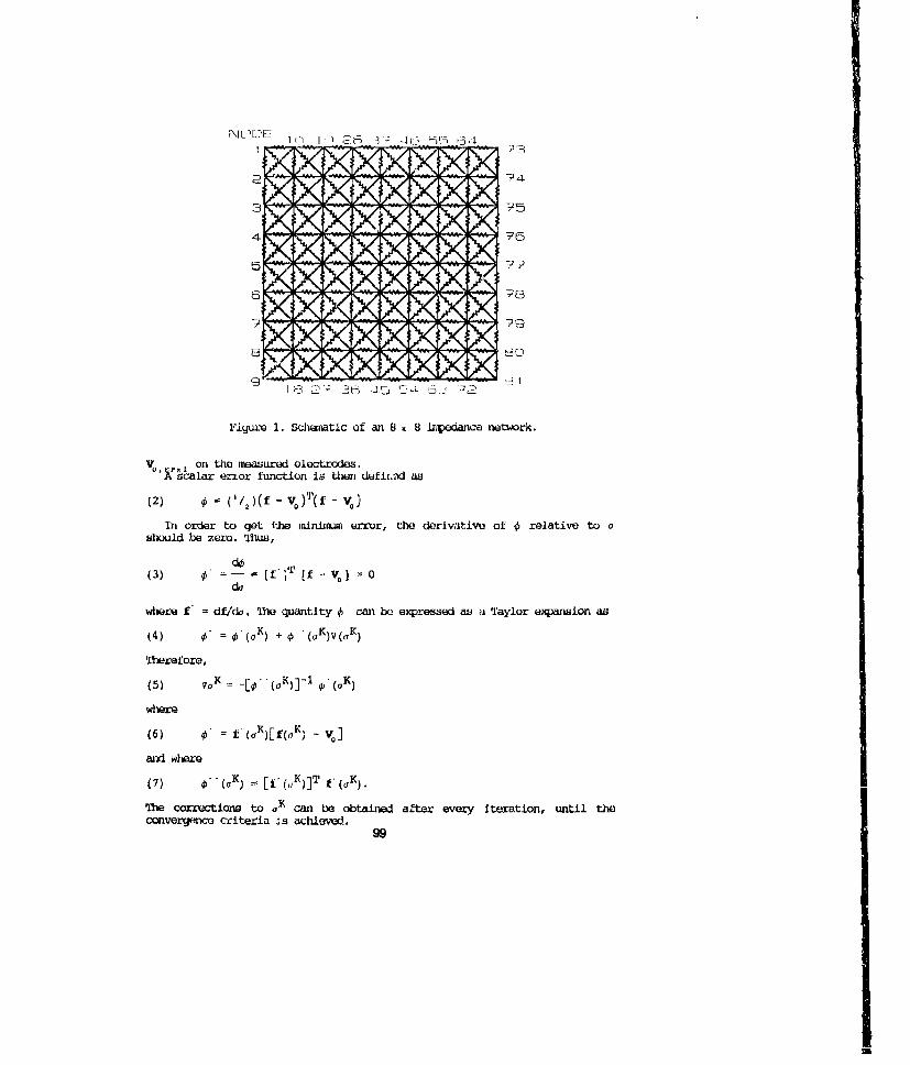
NcD IL E ~ s 324 ~~.

2 72 36 _Q-t ))7

(2 x -'2 ( -- ---~ ---

X X ---.. -- 79

should be•zer .Thus

3• t; 2 .-L ýj L 1._ .22

Figure 1. Schematic of an 8 8 Iexp edancs network.

V.whe, on the measured electrodes.s • calar erior function is themt defitL-c-d aB

(2) 0 = (t/')(f -K )T(f - VoIn order to get Q-.h minimum error, the derivative of 0 relative to a

should be zero. 'Mus,

where f df/da. Thw quantity can be expressed as a Taylor expansion as

(4) 0" = 0'"(C;K) 4.0 (UK) V(UK)

'Tne~fore,(5) •K _• o~- ,(K

where( 6 ) 1" ." (O K )[ f ( UK ,' _ W 0

and where(7) -- (UK) E [j- (.,K)] T .f ).

The corrections to a K can be obtained after every Iteration, until theconvergence criteria is achieved.

99

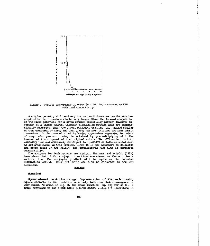
200

2

04 100

raN

0Z

5 7 5 1 1 3INUMBERS OF ITERATIONS

Figure 2. Typical convargenu of error fulction for square-array k124,with real conductivity.

A conple.x gecinistry will need many currant excitations and so the matricesrequired in the inversions can be very large. Since the forward ccRa[utationof the field potential for a given complex resistivity pattern involves in-version of a sparse matrix, Gausslan elimination methods used are computa-tionally expensive. Thus, the Jacobi conjugate gradient (JOG) method similarto that described by Carey and Oden (1984) has been utilized for real dcmaininversions. In the case of a matrix having elgonvalues separated by ordersof magnitude, preconditioning is obtained by pre-multiplying with theinverse of the diagonal of the original matrix. The JOG mothod is bothextremely fast and absolutely convergent for positive definite matrices suchas are anticipatad in this problem. Since it is not necessary to calculateand store zeros in the matrix, the computational CPJ time is decreasedsubstantially.

The accuracy for both methods are similar. liestenes and Stiefel (1952)have shown that if the conjugate directions are chosen as the unit basisvectors, then the conjugate gradient will be equivalent to GaussianElimination method. Round-off error can also be corrected in the JCGalgorithsn.

N ical

Srqzaxv-slit O•xkwUve array. Implementation of the method usingsquare elements in the resistive mode only indicates that convergence isvery rapid. As shown in Fig. 2, the error function (Eq. 12) for an 8 x 8array converges to two significawt figures occurs within 4-5 iterations in

100

agreement with the results of Yorkey (1986), and within 1 part in 10i within12 iterations where the contrast ratio is as large as 10,000:1. Aitken'smethod is also used to improve convergence speed more than a factor of 3.

(Aadwilateral--elemet arrays. An autoaeitic, quadrilateral-grid, meshgenerator was added to convert simulations of arbitrary geomeetries toequivalent square element arrays. Figure 3 shows the iteration sequenceresults for a 25-element body having a central element of high resistivityand surrounding elements of low resistivity. Gauss elimination was used toperform matrix inversions. The small square patterns are used to visuallyrepresent the degree of variation in resistivity. The dense patternrepresents material with high conductivity and low resi.tivity. The lessdense the fill pattern, the lower the conductivity. This selection was usedsince, with air/vapor and liquid systems, the air regions are called"voids." The last iteration shown is that after which no visual detection ofchanges can be made.

Figure 4 shows the variation of error function with iteration is notuniformly convergent. Nevertheless, convergence within 10 6 is obtained forcontrast ratios up to 100:1 within 15 iterations and convergence wasobtained with all contrast ratios tested up to 105 :1 in the real case.However, using Gauss elimenation for the case of complex conductivities,convergence could not be obtained for contrast ratios much over 100:1 andthe results are erratic and not well understood at this point. However, itappears that part of the problem is associated with distorted quadralateralelements where angles becuoi quite obtuse or acute. It is expected thatinmplemntation of the J3G method for inversion will substantially alter thispicture.

The relatively rapid reduction in the nunmerical value of the errnrfunction does not, however, tell the whole story. Figure 5 shows the localerror for central, middle-ring, and outer-z-ng elements as a function ofiteration. Convergence in this case is not quadratic and significant localerror can exist even with very low error in 0. Furthermore, the elementsfarthest frao the boundary are the slowest to converge due to the low degreeof sensitivity to boundary effects.

Figure 6 shows the iterativo sequence for a 64-element, near-circularbody having a ring-shaped region of high resistivity with contrast ratio of3:1. Note that the starting pattern is of uniform conductivity, identical tothat shcwn in Fig. 3. Convergence results are similar to those for the 25-element body. Note that while only 11 iterations were required for "visualconvergence," in Fig. 3, 15 iteration.s are required in this case.

Figure 7 simulates a case where liquid hugs the wall of a pipe and gasoccupies the central region, again to a resolution of 64 elements. Thestarting pattern was Identical to that shown in Fig. 3. It is seen that theoeter ring of low resistivity material converges rapidly due to the highsensitivity of electrode reaction to nearby material whereas the centralcore zones take approxizmatoly 25 iterations for visual convergence.

The results shown in Fig. 8 are. for a relatively random arrangement ofthe two resistivities resistivitles in a circular, 64-element array. Again,25 iterations are required for visual convergence of the pattern. Globalconvergence is conpared in Fig. 9 for this case (Case 1) and those shown inFig. 6 (Case 2) and Fig. 7 (Case 3). All three cases are for the 3:1 realcontrast ratio. It appears that the more complex the pattern, the moredifficult it is to obtain accuiaLe solutions.

101

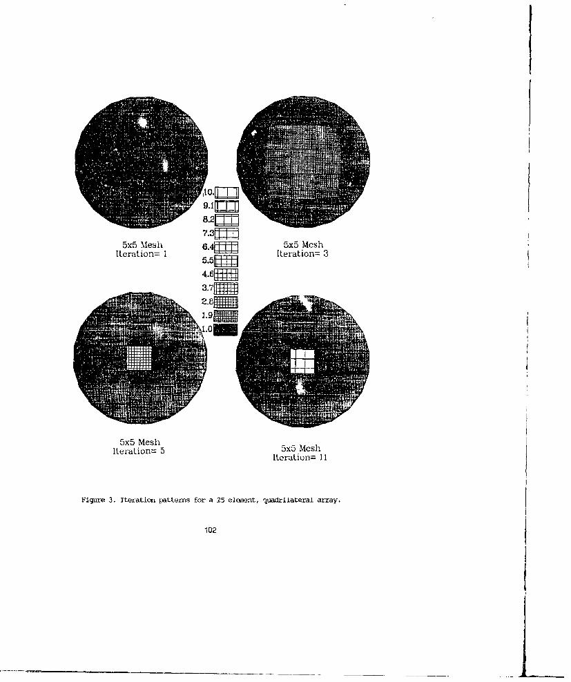
8.2r=

7.3[=

5x5 Mesh 6.4f 5x5 MeshIteration= I 5.5 f Iteration= 3

4.6fiff

3.7, Ms

Iteration= 5 5x5 Mesh

Rex'aa 5MeshesIeration= 11

Figure 3. Iteration patterns for a 25-eleiient, quadrilateral array.

102

p Backg und ResixtivAlty=1R8ulat. of Mc, utd3-1O-100

IN

Figure 4. Global convergume for a 25--elunant qupadrilateral array havingonly real cugxhKtivity ccaoniMnts.

Backgrund Pesistvityl1.OR.a.LL f cmnt~ral t~aret=LOO.O

16

Iterations

Figure 5. Lccal convarqgwv'e for a 25-element quadrilateral array havim,only real oorxucrtivity cwpopnents.

103

3.00

2.60

BxB Mesh 2.40 8x8 MeshIteration= 2 2.20 Iteration= 5

2.001.801.601.401.201.00

8xB Mesh 8x8 MeshIteration= 7 Iteration= 15

Figure 6. Iteration patterns for a 64-element array of quadrilateralelements having only real conductivi ty elements.

Rking pattern, 3:1 contrast.

104

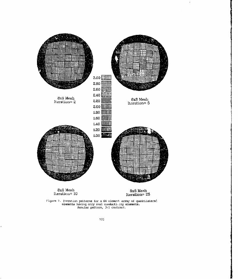
3.00•

,2.802.602.40

8x6 Mesh 2x8 MeshIteration= 2 2.20 Iteration s

2.001.801.601.40 M1.201.00

WxB Mesh 8x8 MeshIteraticn= 10 Iteration= 25

Figure 7. Iteration patterns for a 64-el•eit. array of quadrilateralelements having only real cuolducti\ ity elements.

Annular pattern, 3:1 contrast.

105

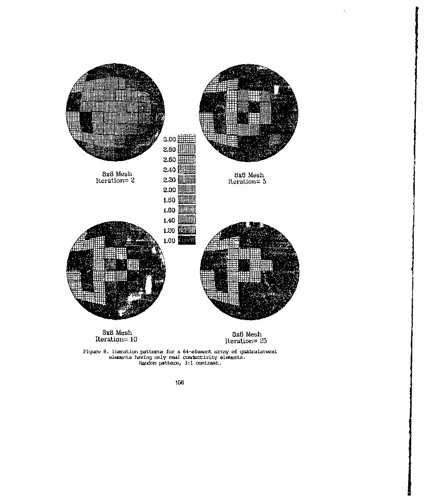
3.00 lL.802.60m

8x6 Mesh 2.40 ExM MeshIteration= 2 2.20 R Iteration= 5

2.00 mm1.501.601.40 E1.20 C1.00m

8x8 Mesh WB MeshIteration= 10 Iteration= 25

Figure 8. Iteration patterns for a 64-elewrit arcay of quadralateralelemits having only real coirductivity elements.

Pandcui pattern, 3:1 contrast.

106

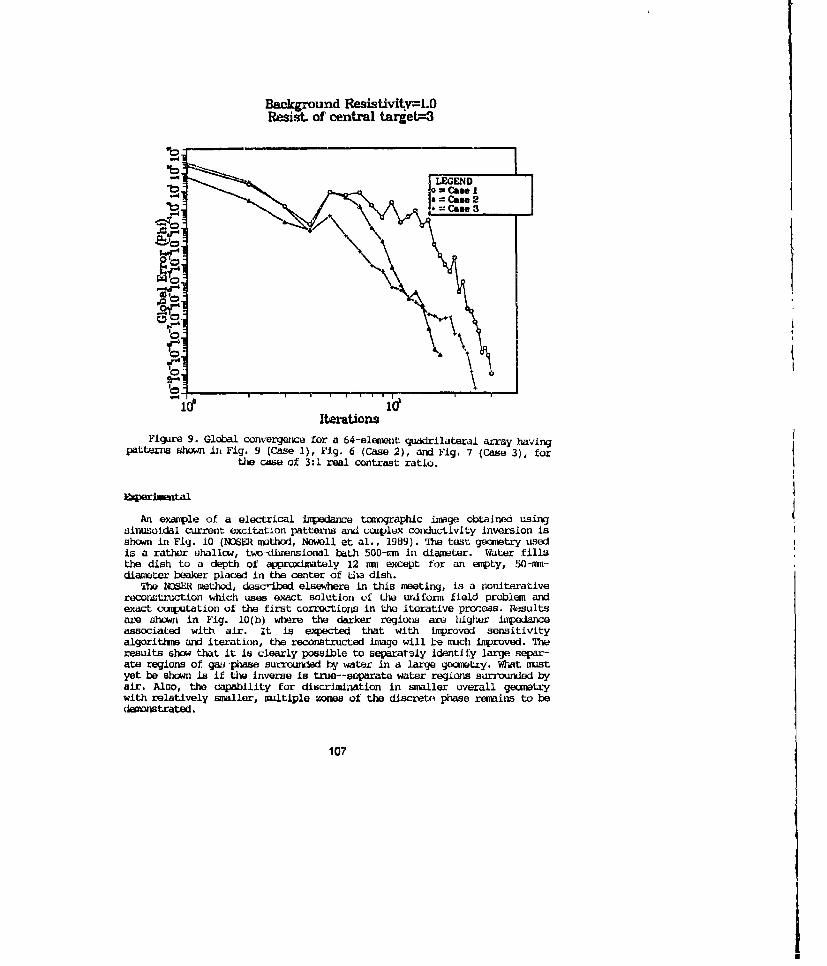
Background Resistivity--1.OResist. of central tarjet7-3

.. 4

the ~ ~ ~ ~ ~ ~ 1 cas ofs 3: elcntatrto

Fnigure 9.Gofbal elnerical fo iseanc4el n tc g aphicildage obainray usving

sinusoidal current excitation patterns axxl complex conductivity invearsion isshown in Fig. 10 (NDSM mothod, Newell ot al., 1989). "oe test gecinetry usedis a rather shallow, tvm-dimensional bath 500-sin In diameter. Water fillsthe dish to a depth of approximately 12 mmn except for an empty, 50-sm-diasmuer beaker placed in the center of the dish.

The NOSR method, desc'-ibed elsewhere in this meeting, is a noni~terativereconstruction which uses exact solution, of the uriform field problem andexact computation of the first correc-tions in the iterative process. Resultsare shown in Fig. 10(b) where the darker regions are higher impedanceassociated with air. it is expaected that with improved sensitivityalgarithins and iteratio~n, the reconstructed image will be much improved. Theresults show that it is clearly possible to separatsly identify large separ-ate regions of ga&H-phase surrouwsied by water in a large geametry. What mustyet be shown is if the inverse is true--sepaate water regions surrountled byair. Also, the capability for discrimination in smaller overall geanetrywith relatively smaller, imultiple zones of the discrete phase remains to bedemonstrated.

107

AIRWAE50 MM 300 MM

(a)

(b)

Figure 10. Ex&wV1e of electxical Iinodackce reconstruction in an airwater systemI using noniterative, cmviox coiiiuctivity ~muLhxxk. (a) gaaaatry

108

A method of using electrical impedance for imaging of two-phase fluiddistributions using inverse comrutational methods has been discussed withthe following conclusions.

1. It has been shown that the internal distribution of complexelectrical bipedance can be determined within a body by using only boundaryexcitation and muasurwvnt.

2. Square-element k114 modeling of a resistive body allows iterativeconvergence to 1% within 4-5 iterations and within 0.01% within 12iterations for all contrast ratios up to 105.

3. Quadralateral-element, adaptive grid, k'2. nMdeling was slower toiterate and more sensitive to resistivity ratio, perhaps due to the presenceof highly acute or obtuse angles distorting the equivalent square-elaewntconductivity. Local error in a given element was shown to be considerablyslonr to converge to a reasonable error. Elaeents farthest from theboundary showed slowest convergence, and more compiex situations appear torequire more interations for convergence.

4. Complex contrast ratios as large as 102 were found to convargeusing Gauss elimination for matrix inversion. Situations with largercontrast diverged.

5. Application to a practical, laboratory situation shows that evenwithout iteration, reasonable results can be obtained for ccaplexconductivity fluids.

5. Considerable development effort remains before the method will beof gen•eral utility for two-plhse, gas-liquid flows.

ACKMA•GMGMAY

This research was supporLte by the Energy Research Laboratory, Hitachi,Ltd., Hitachi-shi, Ibaraki-ken, Japan, and by the U.S. Department of Energyunder contract number DE-F007-90ER13032.

A Area (flow area if not subscripted)G Mass fluxi EnthalpyJ Square root of (-l)n Unit outward normal on the surface of a regionj Heat fluxt Time or generalized Jacobian nntrixv VelocityV Volumez Flow directioa general coordinate

Oceek

a Void fraction4 Difference indicatorSPetiLttivity4) Flux of conserved quantityS Gee, alized state equation

l09

r Volumetric source term0 Intensive conme-.ed quantityp Density0 Surface tension or conductivityT Stress tensor

SFrequencyat~cripa audxi 4~wecri*s andi OtIwm

fg Saturated liquid-vapor differencei Interfacialk Refers to phase-k£ Liquidr Relative (between liquid and vapor)s Refers to surface at interfacev Vapor

IERENCMS

Banerjee, S. and Lahey, R.T., Jr., [1984], "Advances in 'No-Phase FlowInstrumentation," Mvax~3m in Nu~lear Scierwe and TO•:d •ogy,, 13..

Barber, D.C., Brown, B.H., and Freeoton, I.L., [1983] "Imacing spatialdistributions of resistivity using applied potential tamography," Elec.Lett., 19, pg. 933-935.

Barber, D.C., and Brom, B.H., [1984] "Applied Potential 'ftieraphy," J.Phys. E: Scl. Instrum., 17, pg. 723-733.

Badxber, D.C., wid Brown, B.H., [1985] "Recent developments in appliedipotential tWIgcaphy--Al'r," in Prec. 9th Int. Conf. ifo. Pmc. Mud.Imaiging, Washington, D.C.

Bates, R.IH.T., Mckinnon, G.C., and Seager, A.D., [19801 "A limitation onsystenu tor hiiging electricol conductivity distributions," 11MR TanW.Hicui. Eng., Ii*-27, 7, pg. 418-420.

Bates, R.HI.T., [1984] "Full-wave ccuputed tomography Pt.. 1: FundamXntaltheory," IME Pmn. A, 131, pg. 610-615.

Beck, M., and Williams, R., [199(,] "Woking into Process Plant," 7hxChun. Eg.., 26 July, pg. 14-15.

IUrwn, B.H., Barber, D.C., and Seagar, A.D., [1985] "Applied potentialtoxK~graphy - clinical applications," IX Coxf. Publ. (Inst. EleLLr. Eng.),No. 257, pg. 74-78.

Bron, 13.11., and Barber, D.C., [1987] "Electrical irpedance tcmography,the constructLion and application to physiological measurent of electricalii.pedance iimeges," Modical Prog. ¶Iuxxigh Tdmology, 13, pg. 69-75.

Brown, B.H., Karatzas, T., Nakielny, R., and Clarke, R.G., [1988] "Deter-mination of upper arm nmscle and fat areas using electrical iaxedancemeasuremnts," Clin. Phys. Prhlziol, Noas. (UK), 9, 1, pg. 47-55.

110

Carey, G.F., and OWn, J.T., [1984] Finite Elamlet WAttI Amu cts:Vol. 3, Prentice-Hall, Engleweod Cliffs, N.J.

Cheng, K-S, Isaacson, D., Newell, J.C., and Gisser, D.G., [1989] "Elec-trode models for Electric Current Computed Tomography," Im-,frmw. Ricmd.Ehg., 36(9), pg. 918-924.

Dines, K.A., and Lytle, R.J., [1981] "Analysis of electrical cond.ctivityimaging," GaCiyuics, 46, pg. 1025-1036.

Fuks, L.F., Isaacson, D., Gisser, D.G., and Newell, J.C., [1989] "tamo-graphic Images of Dielectric Tissue Properties," =lE-Trans. Bicmad. Emg.,in review.

Gilbert, P., [1972] "Iterative mnthcds for the reconstruction of three-dinwlonal objects fron projections," '1. Iheoret. itolý, 36, pg. 105-117.

Gisser, D.G., Isaacson, D., and Newell, J.C., [1987] "Current Topics inInpedance Imaging," CLia. Plys. Physiol. Mses., 8, Suppl. A, pg. 39-46.

Griffiths, H., [1907] "'The inportance of phase measurenent in electricaliqpedance toawgraphy," Ph-s. Mod. Biol., 32, 11, pg. 1435-1444.

Hestenes, M.R., and Stiefel, E., [1952] "Methods of Conjugate Gradientsfor Solving Linear Systems," J. Its. MS, 49, 6, pg. 409-436.

Henderson, H.P., and Webster, J.G., [1978] "An impedance caara for spa-tially spocific measuramints of thorax," IUZ Tram. Bicmd. Hag., U*-25,pg. 250-254.

Hewitt, G.F., [1978], basurvaunt of Two-Phase Flow Parametars, AcademicPress.

Huang, S.M., Plaskowski, A.B., Xie, G.C., and Beck, M.S., [1989]"Taographic Imaging of 'Nwo-C••ponent Flow using Capacitance Sensorb," J.NWi. E: Scd. InaLm., 22, pg 173-177.

Isaacson, D., [1986] "Distinguishability of Conductivitiee bky ElectricCurrent Computed 'lTUgraphy," UM ld. Isging 0I-5, 91-95.

Isaacson, D., and Cheney, M., [1990] "Current Problems in IntedmaceImaging," in Inverse P lum in Partial •iffeorsLial Eguatibn, ). Coilton,R. Ewing, and W. Rundell, Eds., SIAM, Philadelphia.

Ishii, M., [1971]. "Therm1ally Induced Flow Instabilities in 'Nwo-PhaseMixture in Thermal Equilibrium," PhD Thesis, Georgia Institute ofTechnology.

Ishii, M., [197ýJ. ¶hlnm-Fbidd Dynamic Thury of The-Phase Flow,Eyrolle, Paris.

Jones, O.C,, Jr. and Delhaye, J.M., [1976], "Transient and StatisticalMeasutanst Techniques for Two-Phase Flows: A Critical Review," Int. J.ewlt&,4aaSi Fia, 3, 89-116.

111

Kagawa, Y., Murai, T., and Matsumoto, 0., [1983] "Finite element iter-ative technique for determining the interface boundary between Laplace aaPoisson daowins--characteristic analysis of field effect transistor," Xnt.J. Enar. ltthxks Wig., 19, pg. 315-329.

Kardous, G., [1987] "Etude de la distribution de la sensibility d'unsysteme circulaire multi-electrodes en vue de la reconstruction d'imagesd'impedance bio-electrique," PhD Thesis, Institute National dce SciencesAppliqueos de Lyon, Villeirbanne, France.

Kim, Y., Webster, J.G., and Tompkins, W.J., [1983] "Electrical impedanceimaging of the thorax," J. MKiaaaaa Power, 18, 3, pg. 245-257.

Kim, Y., '1rcrpkins, W.J., and Webter, J.G., [1982] "Medical body imagingusing electrical impedance and nonlinear reconstruction," Am. itrthmtBioen. Cant., 10, pg. 298-303.

Kohn, R.V., and Vogelius, M., [1987] "Relaxation of a Variational Methodfor Impedance Confuuted tmoigraphy," (a. Pue 'Wl. Math., 40, pg. 745-777.

Kohn, H.V., and MeKe/rey, A., [1989] "Numerical Inplawntation of aVariational Meithod for Electrical Inpedance Tuomography," Courant Instituteof Mathamatical Sciences, private cowrunication.

Kocanustataogullari, G., [1971]. "Thermo--Fluid Dynamics of Separated Two--Phase Flow," PhD Thesis, Georgia Institute of Technology.

Lin, T.F., Block, N.C., Lahey, H.T., Jr., Jones, O.C., Jr. and Mirase,M., [1985], "Muasureaent of Flow in a Horizontal Pipe Using the Pulsed Pho-ton Activation Technique," Nucl. Sat. H'fl., 91, 3.

Muirai, T., and Kagiwa, Y., (1985] "Electrical inpedance confuted tomogra-phy based on a finite eliaent nxodel," IEEE Tr•rn. Hsasd. kkg., lU-32, 3,pg. 177-184.

Murai, T., and Kagawa, Y., [1986] "lBidary elwnnt iterative techniquesfor detelidning the interface boundary between two Laplace domains-a basicstudy of inpLeance plethysnogrdphy as an inverse problem," lit. J. ?&atr.tatlxk Eng. (GB), 23, 1., pg. 35-47

Newmll, J.C., Isaacson, D., and Gisser, D.G. [1989] "Rapid Mssessamnt ofElectxode Characteristics for Impedance Lmaging," fI-Traxi., Wound. lkq.in press.

Neweil, J.C., Gisser, D.G., and Isaacson, 0., [1988] "An Electric Current'luqograph," IkEhEiTaa. Bibaxi. Exq., 35 (10), pg. 828-833.

Nakayaina, K., Yagi, W., aid Yagi, S., [1981] "Funcbswntal study on elec-trical impedance plethsLagraphy," in Prec. Vth Int. OCf. Elect. Bio-Iw-pectZ, Thkyo, August, pg. 99-102.

112

Pfeiler, M., [1981] "Ner, development in computed tcmography with refere-nce to caxipted tmiographic non-x-ray processors, [Neiere entwicklungen dercxrpvtertcwxgraphie ý.unter einbeziehung caqputertaonigraphischer nicht-R6ntgenverfahren)]," R~wEnt raxzs (17), 34, 1, pg. 3-13

Price, L.R., [1979] "Electrical Laredance computed tavgraphy (IcT): anew CT imaging technique," I•k, Trais. iucl. Sci. (USA), 16-26, 2, pg. 2736-2739.

Pfeiler, M., and Steiner, K., [1982] "Computer tomgraphlc methods ussingdifferent information carriers," J. BHelg. fPiiol., 65, 2, pg. 95-102.

Powell, H.M., Freeston, I.L., anvi Barber, D.C., [1985] "Inpedance iwagingusing a linear electrode array," IRE Ccnf. Publ. (Inst. Fittr. On.), No.257, pg. 08-92.

Sakamato, K., and KMnai, H., [1983] "A fuwdaantal study of an electricaliripadance CT algorithm," in Pruc. Vih Int. Con. Elect. Bin- lvqxK n,Tokyo, August, pg. 349-352.

Santosa, F., and Vogelius, M., [1988] "A liackprojection Algorithn forElectrical Impedance fraging," Institute for Physical Science & Technology,Univ. Maryland, Tech. Note UN-l081, July.

Seagar, A.D., Yeo, T.S., and Bates, R.H.T.,[1984] "'ill wave carputedtomography, paxrt 2: Resulutiun limiLts," Proc. lE, part A, 131, pg. 616-622.

seagar, A.D., Barber, D.C., and Brown, B.H., [19871 "Electrical ImpedanceImaging," HE Proc. 134, Pt. A, No. 2, pg. 201-210.

Shomberq, H., and Tasto, M., [1981] "Reconstruction of spatial res-istivity distribution," Phillips asXi, HaOwry, Gernmany (F1%), MSj-H 2715/81.

Smith, D.N., (1985] "Deteruination of iiqxedance using numerous sbn-uitaneous currents (DINSC) - systLit dusign and practical applications," re.QnL. Publ. (Inst. Klectr. Erg.), No. 257, pg. 69-73

Starzyk, J.A., and Dai, H., [1.985] "Elument evaluation in the resistivenetworks," Midwest Sys. Circuits Syst., 28, pg. 178-1.81

Tarassenko, L., and Iolfe, P., [1984] "lunging spatial distributions ofresistivity - an alternative approach," Electron. •ett., 20, 14, pg. 514-576.

'1rusdell, C., and 'toupin, R., 1960. "'l'he Classical Field 'hleories," inHaBnh der Physik, S. Flugge, Ed., 3, 1.

Vernier, P., and Delhaye, I.M., 1968. "Genaral Two-Phtse Flow EquationsApplied to the Thernyxdynnmics of Boiling Nuclear Reactors," FzwnjiePzreix, IV, 1-2.

Wexler, A., Fry, B., and Neiman, M.IH., j1985] "lupedance-carputed tomog-raphy algorithm aid systaii," Ajpl. Qi., 24, 23, 1N. 3985-3992.

113

Woo, H.W., and Kim, Y., [1986] "A medical imaging system with electricalIiAedanCO," Prec. Am. Omf. TO EIg. xed. Dial. Soc., 0, 1, pg. 343-346.

Yorkey, T.J., [1986] "Carparing reconstruction methods for elecLrical im-pedance tomography," Ph.D. Thesis, Dep. Elec. Comput. Eng., Univ. Wisc.,Madison, WI 53706, August.

Yorkey, T.J., and Webster, J.G., [1987] "A comparison of impedance tcim-graphic reconstruction algorithm," Clin. Phys. Physiol. W-w., 8, suppl. A,pg. 55-62.

Yorkey, T.J., Webster, J.B., ard 'ckmpkins, W.J., [1985] "Errors caused bycontact imqpdance in ipaedance inmging,' Proc. Ann. Czf. En. Wd.Rial. Smc., 7, 1, pg. 632-637

Yorkey, T.J., Webster, J.G., and Tbapkins, W.J., [1986] "An optimal im-pedance tomographiQ reconstruction algorithm," Proc. Ann. 000f. D= Eng.Ne. Diol. Soc., 8, 1, pg. 339--342.

Yorkey, T.J., Webster, J.G., and 'Ibrpkins, W.J., [1987a] "An improvedperturbation technique for electrical inpdarce imaging with sow critic-ia," I= Tn. i-. ., 34, 11, pg. 898-901.

Yorkey, T.J., Webster, J.G., and Tompkins, W.J., [1987b] "Comparing re-construction algorithms for electxical inEKL-nce toinography," Xm T .

i'd. bý, 34, 11, pg. 843, 852.

114

SESSION 4 - "ASYMPTOTIC SOLUTIONS"Moderator: Andrew Terzuoll

Primitive Target Validation for theSignature Prediction Tools

Softwaxe PackageD. J. Young, A. J. Terzuoli Jr.

Air Force Institute of TechnologyWright-Patterson AFB Ohio

February 18, 1991

1 AbstractThe Signature Prediction Tools software package' in the part of the SyntheticAperture Radar (SAR) prediction Tool (SarTool) that generates radar signaturepredictions of objects such as ground vehicles and aircraft. SarTool employs thegeometric representations of these objects and the parametric descriptions ofsenzors to calculate the full polarimetric, complex-valued radar signature dataof individual scattering component. through the use of physical optics modelsof radar backicattering. SarTool is a major component ir a model-based visionconcept of conAtructing synthetic SAR images of objects and comparing theseimages with actual sensor data of the real objects for target identification.

This paperl presents a technique to validate the individual scattering corn-ponents of SarTool. The technique consists of using SirTool to calculate thesignature data of primitive radar targets which are constructed from the scat-tering components and then comparing this data to the scattering data of thewell known physical optics (PO) equations for these radar targets with the sameinput parameters. Thes targets consist of flat platesi, right dihedral and squaretrihedral corner reflectors, and tophats. The results of the validation show closeagreement to the PO equations for the circular plate target, the scattering com-ponents consisting of the double bounce tophat, triple bounce trihedral, andsingle bounce magnitude for the rectangular plate.

tSenser Algorithm Res-arch xapert System. Contvact F3364T-87-C-1404, The Ansiyt•€Science Corparation.'This os..wcbh In epoemored by WRflO/AARA WPAFHI OH

115

2 IntroductionThe only target recognition system currently in use is the human which em-ploys photo or televisior, visual imaging systems to discern targets from the sur-rounding terrain. The limitations of a human targAt recognition system whenpresented with images generated at wavelengths other than optical frequencies,produce a requirement for an automatic target recognition system which is apart of the Synthetic Aperture Radar (SAR) or infrared imaging systems. Aproposed automatic target recognition system for SAR systems employs a com-puter program that compares an unknown SAl image to a database of SARtarget images to find a match. The problem with this system is the acquisitionof the target image database.

A proposal to solve this problem is the Model Based Vision (MBV) concept,which is based on the caiculation of synthetic SAR target image didplays by acomputer program that simulates the SAR sensor and the target/backgroundradar returns. The first part of the MBV system is the construction of a threedimensional computer model of a radar target by a solid modeling computeraided design (CAD) package. This model is constructed of radar reflectorsfrom a list that consists of single bounce reflectors; flat plate, cone, ellipsoid,ogive, and torus, as well as multiple bounce interactions; d:hedral, trihedral,tophat, and cavity. From the model, which is a database of reflectors and theirposition, a computer program calculates the polarimetric complex radar crosssection (RCS) in matrix form with respect to the angles from the SAR sensorposition for each of these simple reflectors. The RCS is then used to calculate themagnitude and phase of the response of each reflector and places this responseon the SAR image with respect to the range and range-rate coordinate frame17]. This synthetic image is a database entry of the target model at one aspectangle. A target image database is then constructed from the computer modelsof all possible targets by calculating synthetic SAR image for a multitude ofaspect angles.

The one key requirement for the success of the MBV concept is the ccrrectimplementation of the physical optics (PO) equations for the single and multiplebounce reflectors. This paper validates the implementation of the polarimetricPO equations in tht Signature Prediction Tools noftware package for a seL ofsimple radar targets consisting of flat plates, dihedrals, trihedrals, and top hats.

3 ValidationSince the procedure for validating radar targets has not been defined explicitlyin the radar community, this validation effort is limited to:

1. P0 Equations. The research for validating the PO approximation for thesimple targets has already accomplished by many researchers. These P0equations ([], [3], (4), [2], [5), [1] are encoded in FORTRAN programs that

116

if l'"tlq lt lllli t l ''li l . .... "... . .. .i.. Illm lm ligl

generate data in the form of RCS and phase vs. aspect angle for differingpolarizations for the primitives listed above.

2. SarTool Data. Primitives in SatTool are :onstructed to duplicate theparameters in the PO equations data set. The resulting data from SarToolwill be presented in the same format as the PO data.

3. Analysis. The pl )ts of the PO and SarTool for the same polarisationare superimposed. This technique shows the similarities and differencesbetween the P0 equations acd the SarTool implementation for the samcinput parameters.

4 ResultsThe orientation and conventions of the sensor viewing angles are shown in fig-ures 1- 4. Figures F and 7 show that the PO equations for the RCS of these flatplates agree perfectly with the SarTool calculations. Figure 6 reveals diffcrencesin the phase calculations in SarTool for the rectangular plate when complaredto the PO equations. The dihedral RCS plots in figures 9 and 11 also revealdifferences in the implementation of the PO equations and SarTool. The eleva-tion viewing angle (0 = 55.0 degrees) corresponds to the maximum response ofa square trihedral, Figures 13 and 15 show a near perfect agreement in the POand SarTool equations for the trihedral. The tophat plots in figures 17 and 19show a sizeable difference in the SarTool response and the PO equations. Inves-tigation into this problem reveals that SarTool does not add the single bounceresponse of the base of the tophat to the rest of the scattering components.

5 ConclusionsThis paper presents the preliminary work in the validation of the SarTool com-puter package. The conclusions of the validation of the primitive targets arepresented for SarTool version 7.03.

-. 1 Flat Plates

The analysis on the rectangular and circular plates shows that the RCS andphase of the circular plate agrees with the PO equations available in the lit-erature. The phase characteristics of the rectangular plate do not agree withthe PO equations, but the magnitude does agree. This difference in the phaseespecially at the broadside aspect angle reveals a possible problem with theimplementation of the PO equations for polygonal plates in SarTool.

117

Ir

5.2 DihedralThe analysis of the dihedyal at the maximum return angles 0 = 90 (89.9) decreesand t = 45 degrees agrees with the PO equations. The differences in the RCSand phase plots can be attributed to the addition of the two rectangular plateresponses which have incorrect phase relationships to the double bounce dihedralresponse.

5.3 TrihedralThe response of the trihedral at maximum response angle d9 = 55 degrees showsvery close agreement in the plots of SaxTool and P0 equations for the RCS forphi angles from 12 to 78 degrees. At this theta angle and phi angles, the triplebounce trihedral scattering response dominates the total target RCS. Theseplots reveal an agreement in the triple bounce equation implementation forSarTool. Once again, the phase relationship of the fiat plate$ combined with thethree double bounce dihedral responses and the triple bounce response resultsin the small disagreement of SarTool and PO calculations.

5.4 TophatThe failure of SarTool to calculate the flat plate response of the base disc of thetophat results in big disagreements with the PO equations. The section of theRCS plot where the double bounce tophat response dominates reveals a generalagreement of SarTool with the PO equations. Further study of this problem isalso required for a validation of this primitive.

References[1] Balanis, Constantine A. Advanced Engineering Eleciromagnetics. New

York: John Wiley and Sons, Inc., 1989.

[2] Blejer, Dennis J. Physical Optics Polarization Scattering Mat riz for a TopHlat Reflector. Unpublished report, Lexington MA: MIT Lincoln Labora-tory.

[3] Blejer, Dennis J. Physical Optics Polarization Scattering Maris and Iro-pulse Response of a Right Dihedral Corner Reflr.ctor. Unpublished reportNo. 47PM ADT-0052, Lexington MA: MIT Lincoln Laboratory, 1986.

[4] Blejer, Dennis J. Phyoiral Optics Polarization Scattering Matris of a Square2"ihedral Corner Reflector. Unpublished report No. 47PM-ADT-0059, Lex-ington MA: MIT Lincoln Laboratory, 1087.

lie

[5] Blejer, Dennis J. Scattering Matrisa 721uformatiooa fop Polarimeiric TargetModeling. Unpublished report No. 47PM.ADT.0057, Lxizngton MA: MITLincoln Laboratory, 1987.

[(] Knott, Eugene F. and others. Rsadar Crss Section. Norwood, MA: ArtechHouse, Inc., 19)85.

(7] Pinto, Robert and others. Senjor Algorithm Research E pert System, rm-lerin Techniczl Roport, Volume 8. Contract F33815-87-.C-1404, ReadingMA: The Analytic Sciences Corporation, May 1989,

139

z z

bY0

x --- x *

y y

Figure 1: R•ectangular and Circular Plates

z

Sa

X b

y

Figure 2: Right Dihedral

120

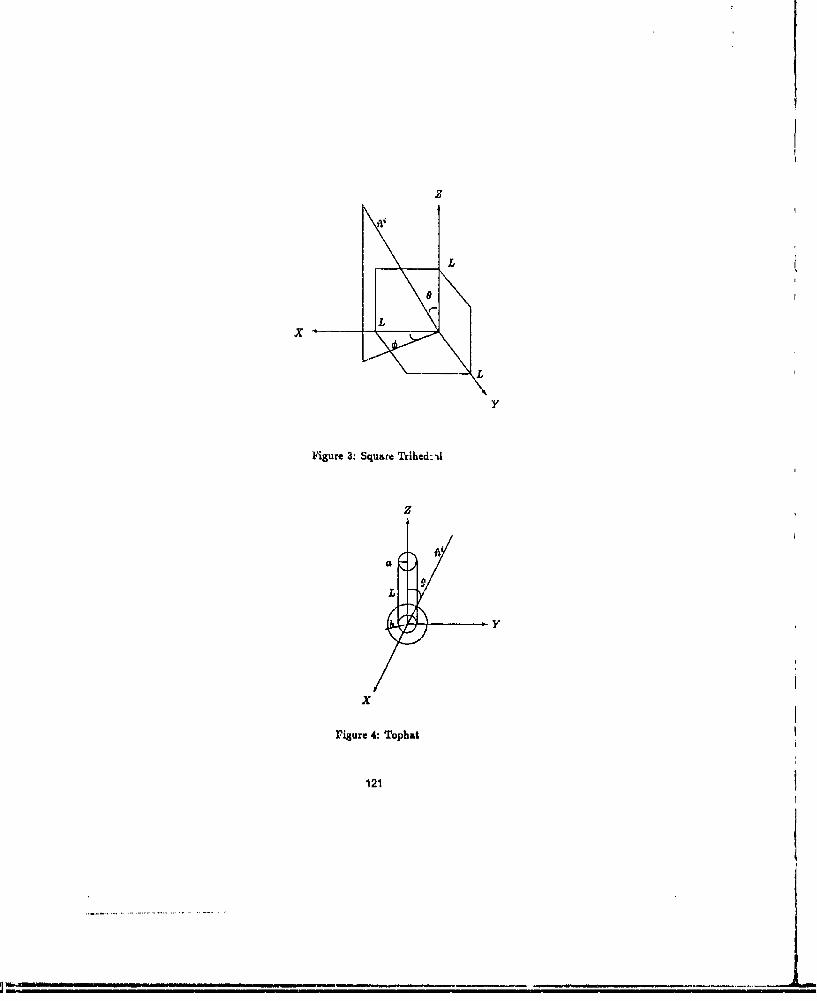
z

LL

L

L

Figure 3: Square Trihed:-L

y

x

Figure 4: Tophat

121

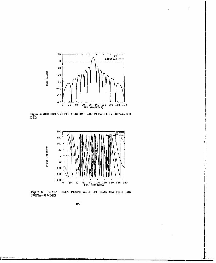
10I SarTool7

-10

1 -20

U) -30

-40

-50

-6-0 20 40 60 80 100 120 140 160 180

Pill (DEGREE.S)

Figure 5: RCS RECT. PLATE A=10 CM B=15 CM F=10 GH. THETA=89.9DEG

200 - ---

100 -\~

r 1 50 " \r 50

...........................

-150 • \

-200 L - -- -- '0 20 40 60 80 100 120 140 160 160PHIl (DEGRE.ES)

Figure 6. PHASE RECT. PLATE A=10 CM B=15 CM F=10 GHmTHETA=89.9 DEG

122

Saxaoo170 ....... .. .. .. .... ... .... ......... .... <......... ... ... .. -.... .-10

) -20

-30

-40

-50

-600 20 40 60 80 I00 120 140 160 101111 (D GIME]S)

Figure 7: RCS CIRC. PLATE RADIUS=5 CM F-10 GHx I1HETA=89.9 DEG

200 p "--sarToo7.

15o

50100

o o

U) -50

)1 -100

-150

-2000 20 40 60 80 100 120 140 160 10PHI (DEGREES)

Figure 8: PHASE CIRC. PLATE RJADIUS=5 CM F=10 GHs THETA=89.9DEG

123

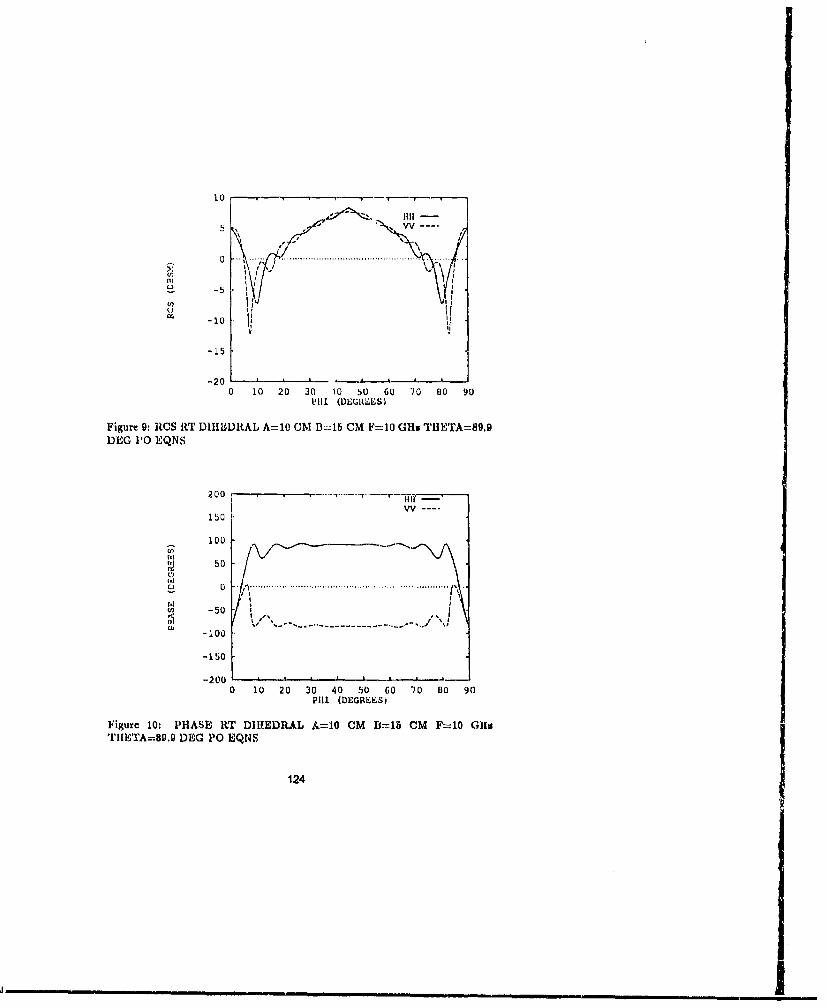
J52/• S III -- -

10

I 1 -I

-5.

-15

- 2 0 -i - ,

0 10 20 30 10 50 GO 70 "O 0 90Pill (DEI.;GR S)

Figure 9: RCS RT DIIIEDRAL A=1O CM B2:15 CM F=10 GHv 'HETA=89.9DEG P0 EQNS

200 - -, __vv ---.

150

100

50

-2 0 ... ...... .. ...... ..... .. .. .. ... ... ... ... ..Pill (D G* ('S

124in -50 Io

-- - - -- - - -- - -- -- ~ S

-2000 10 20 30 40 50 60 10 330 90

PHI (DEGRE~ES)

Figure 10: PHASE RT DIH~EDRAL J.=10 CM B=15 CM F=10 GH%TIIETA=89.9 DEC PO EQNS

124

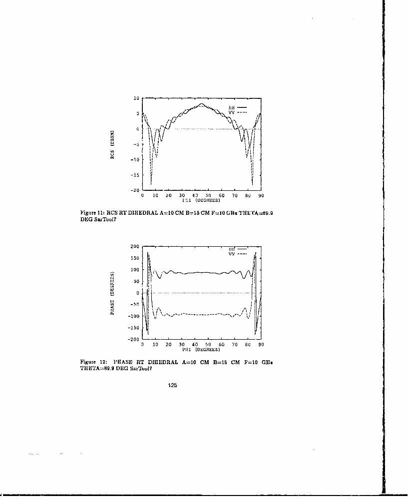
10 -

IIM

{; i! ( I .... ...... ............................. ... . .

-15-

-20 - '_ "_______________0 10 20 30 40 50 60 70 80 90N!HI (DILQGREES)

Figure 11: RCS RT DIHEDRAL A=I0 CM B-=15 CM F=10 CII. THETA=80.9DEG SarTool7

200 --

150 v

Ivv100 ,

50-. ., Il

£fl -. 'm I 1i , ,,!/

-150

-200 L---L---L--- _0 10 20 30 40 50 60 70 80 90

PIlll (DEGREES)

Figure 12: PHASE RT DIHEDRAL A=10 CM B=15 CM F=1O GlITIIETA=89.9 DEG SarTooI7

125

o ' .......... ..." ................................... 7 " •........... /

-10- -

-15

-200 10 20 30 40 50 GO 0 00 90

P-5I (DEGREES)

Figure 131 RCS SQ TRIHEDRAL L=10 CM F=10 GlI[ TIIETA=56,0 DEGPO EQNS

200 ,' ' -i T '-'- -

U,) V .. Ii\

150 vv •

rIi

S ou

50

III

-50

-150

-200 __ _ _ _ _ _ _ _ _ _ _ _0 10 20 30 40 50 60 70 80 90

PHI (DEGREES)

Figure 14: PHASE SQ TRIHEDRAL L:=IU CM F=10 GCli THETA=55,0 DEGPO EQNS

126

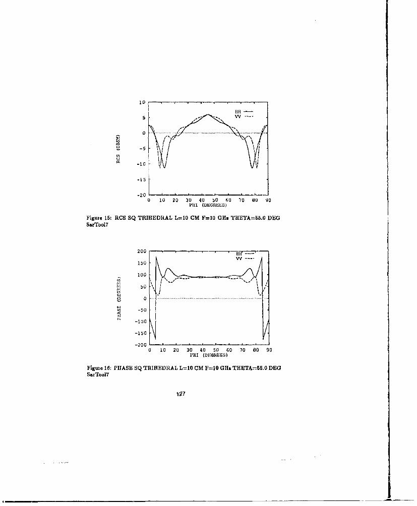
10fiIll

0 -.. . .... ..... ... :: . ... ................ .................. ". ............... '. ..

-10

-15

- 2 0 . .-. . . . . . . .0 10 20 30 40 50 60 70 80 90

PIll (DEGREES)

Figure 15: RCS SQ TRIIIEDHAL L=10 CM F-=10 GHs ThETA-55.0 DEGSarTool7

200 0- - -VV

150

100

-501,3 -I0 /-100

-150

-200 . . . . .* .0 10 20 30 40 50 60 70 60 90Pill (DEGREES)

Figure 16: PHASE SQ TRIHHDRAL L=10 CM F=10 GIL; THETA::55., DEGSarTool7

127

30

25

20IIII ---

15 vv-.

10

.)0 ... .......... • . ..............................................

-5

-200 10 20 30 40 so 60 70 Go 90

"rTHETA [DELGIIEES)

Figure 17: RCS CIRC. BA.SE TOPHIAT A=10.16 CM B=.20.32 CM L=20.32CM F=10 G~li PO EQ1NS

-10 'i'1' i200 1

100 i •t11 1

-lb . .. Ii i

50 1 0 3 1 0 6 0(09

-200

10 10 20 30 405 6 0 09

Pill (LGRIll

I,, -,o Ii ; ",Id 0 V I ..

r( 1 :1 ii ''

-200 • , , , , ,0 10 20 30 40 50 60 70l 80 90

Pill (DEGREE~S)

Figure 18: PHASE CIRC BASE TOPHAT A=10.16 CM B=20.32 CM L=-20.32CM F=10 Glis PO EQNS

128

____ ___ ____ _ _ ____ ___

30

25

20Jill -l

15 vv

In 10

o , .. ' + .......... .................. ...............................

-10

-15-20 , q .• • , i , ,!

0 10 20 30 40 50 60 70 80 90TIHETA (DEGREES)

Figure 19: RCS CIRC BASE TOPIIAT A=10.16 CM B=20.32 CM L=20.32CM F=10 G1ls SarToo17

200 -- ------- r-----. --- ,------- ---",, ,, "I " I/, ' 4,,,In 100 j \ \ I

-100 1 K'" -so I i-

-2000 10 20 30 40 50 60 70 80 90

PHI (DEGREES)

Figure 20: PHASE CIRC BASE TOPIIAT A=i0.16 CM B=20.32 CM L=20.32CM F=10 GHI SarTool7

129

High Frequency Scattering Code in a DistributedProcessing Environment *

S. Suhr, A. J. Terzuoli Jr., G. B. LamontSchool of Engineering

Air Force Institute of TechnologyWright-Patterson AFB O1 45433-6583

(513) 255-3576

AbstractThis paper describes the transformation of serial computer codes for

use in a concurrent processing environment, with in-progress results of thespecific task of porting the NECPSC sequential FORTRAN source codeto the intel iPSC' 9 /2 and iPSCG/860 hypercubes. Improved efficiencyand effectiveness should result from the use of concurrent processing onmultiple processors. The sequential code is examined and modified instages in an attempt to minimize the changes to the program interfaceand output, while maximizing performance. At each step of the transfor-mation, the modified code is executed, efficiencies compared to those ofprevious steps, and effectiveness compared to VAX serial benchmarks.

1 IntroductionThe Air Force is conducting research into quicker, more cost effective methodsfor predicting the electromagnetic scattering from complex objects of interest.One of the computer codes currently in use is the Numerical ElectromagneticCode - Basic Scattering Code (NECBSC)I. This code was developed for theVAX minicomputer and written in FORTRAN-77 for portability to most stan-dard mainframe computers. However, even on potent mainframes, any but thesimplest of problems takes considerable execution time (-hours), at a relativelyhigh cost. This research centers on the modification of the NEOBSC for exe-cution by a distributed processing computer. Before we examine this specificpkoblem, we need to examine the generic problem of porting existing serial codeto concurrent procesing environments.

"This work is sponsored by Jeffrey L. Fath of the Target Recognitlon Branch at the WrightLaboratory(WL/AARA), Wright-Fatterson APB OH

'NECBSC was developed by R.J. Marhefla and J.W. Silvestro of the Ohio State UlnivesiLtyElectroScience Laboratory, Columbus OH.

130

2 Concurrent ComputersCharacteristics of the target computer have a large impact on the approachtaken for decomposition of the source program. Concurrent processing com-puters come in many varieties. Single instruction, multiple data (SIMD) com-puters have multiple processors each with identical code, % arking on differentdata elements iii "lock-step". These machines are very appropriate for problemsinvolving matrix/array solutions such as finite-difference methods where eachprocessor would calculate the results for a single location in the grid. Multipleinstruction, multiple data (MIMD) computers have processors which may op-erate independently on different parts of the problem and/or different parts ofthe data.

When Lhe computer has a single block of memory addressable by all of theprocessors, it is referred to as "shared-memory". Each processor :an freelyexchar-t data with the others through the intervening memory. This type ofarchitt .ure lends flexibility to the programmer at the expense of hardware com-plexity/cost and fixed overhead due to memory contention and address decodingtime. When each processor has a dedicated block of memory to which it hasexclusive access, it is called 'distributed memory". This architecture is simpler,but may require data to be passed between the processors via messages, im-posing overhead. The distributed-memory architecture is appropriate for tasksthat involve routines with large amounts of processing relative to data sharing.

Given a distributed memory MIMD computer, the physical interconnectiontopology of the processors has a large impact on the suitability of the machineto the task. Each processor can be connected to all othera, but ill complexityof the hardware for even tens of processors is irpractical. A f_ nterconnec-tion scheme where each processor can communicate with each ol four neighborsis ideal for two-dimensional problems, but communications in a problem withthree or more dimensions become burdensome. The hypercube is a compro-mise architecture with a high degree of flexibility. A hypercube of dimensiond has 2d processors nodes each connected to di neighbors. This interconnectionscheme becomes unwieldy when the dimension exceeds eight (256 nodes) or so.Stated without proof: the hypercube architecture has considerable flexibility inmapping the processrs to dilffereiit types of problenm-spaces[2, 49].

3 Program DecompositionFrom a user's point of view, a vectorizing compiler is the simplest way to adaptan existing program to run on a concurcent computer. The details of the con-

.O .1 arhde n f ,rl 460m .the Usb. b ...te --- 1 -. "6c.r MI., att ltem,,,pts

to ideutify sections of the code that are appropriate for predetermined forms ofroncurrent computation. Some experts believe that vectorizing compilers pro-ducp code that is more efficient than that of skilled programmers [6, 237]. This

131

may be true for the limited concurrency of multiprocessor computers such as theCray XMP, but a compiler cannot make the sweeping changes that a program-mer could implement for more complex architectures [2, 27], and a compiler doesnot generally run a program with actual data, and this can affect performance.

There are two basic methods of manual program translation: domain decom-position and control decomposition. Domain decomposition consists of loadingidentical programs on each node and segmenting the data among the proces-sors, allowing each to perform the taWk on part of the data. This method isparticularly effective when there are loops in the serial program and the datain each loop is not dependent on the results of earlier iterations of that loop. Ifthere is no need for interprocessor communication during the calculations, theoverhead is minimized and high efficiencies are achievable. Presuming one hasa very large data set, one attempts to divide the data into equal sections andmap each to a different node. This also would seem to be the correct approachwhen the data-set is small, but the data-transfer time to load different data setsmay negate any parallelism gains, resulting in an inefficient configuration.

Control decomposition consists of dividing the program into sections, andputting different code on each processor. If there are multiple data to be pro-cessed, a pipeline can be effected, allowing concurrent processing and speedup.However, because a large data set must pus through all the nodes, there is acommunications penalty which negates potential speedup unless the computa-tions are very time-consuming relative to the data-passing required.

Once control-decomposition is chosen, a problem can be mapped to thenodes in two fundamental ways. The first is a static configuration, where all theroutines are divided among the nodes and remain fixed throughout the lifetimeof the program. The second is where "slave" nodes are loaded with programmingand data as needed by one or more "master" nodes. This type of configurationis most appropriate when the selection and order of execution of the variouspieces of code cannot be determined until run time, especially when all theroutines cannot be loaded on a node simultaneously due to memory constraints.The master-slave approach i. one of the fundamental forms of dynamic loadbalancing.

There are many tools available to aid in the decomposition, analysis, andevaluation of parallel programming efforts. One tool which assists in FORTRANcode conversion is FORGETM, an analysis tool available from Intel/Pacific-Sierra Reseaich Corp. FORGETM creates a database of program and dataentities and displays them in coherent formats to the programmer/analyst (3].Other tools range from conventional automated flowchart creators, to sophisti-cated concurrent visual debugging systenms [51.

Debugging concurrent programs is quite a bit more difficult to accomplishthan ordinary sequential programs. Since different processes are occurring si-multaneously and independently, it is possible to have a properly executingprogram give different answers on consecutive runs using the same input data.This is because the processors could be finishing in a different order after each

132

I

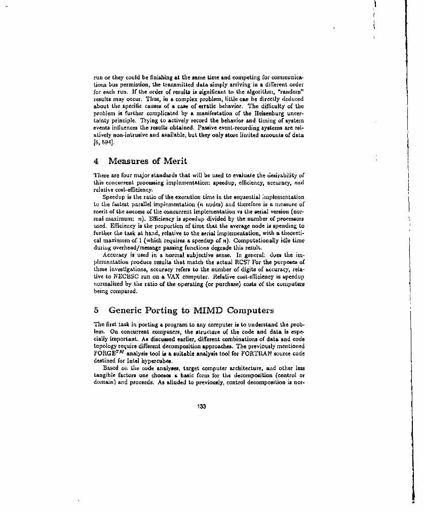
I

run or they could be finishing at the same time and competing for communica-tions bus permission, the transmitted data simply arriving in a different orderfor each run. If the order of results is significant to the algorithm, "random"results may occur. Thus, in a complex problem, little can be directly deducedabout the specific causes of a case of erratic behavior. The difficulty of theproblem is further complicated by a manife.station of the lleisenburg uncer-tainty principle. Trying to actively record the behavior and timing of systemevents influences the results obtained. Passive event-recording systems are rel-atively non-intrusive and available, but they only store limited amounts of data[5, 594].

4 Measures of MeritThere are four major standards that will be used to evaluate the desirability ofthis concurrent processing implementation: speedup, efficiency, accuracy, andrelatibe cost-efficiency.

Speedup is the ratio of the execution time in the sequential implementationto the fastest parallel implementation (n nodes) and therefore is a measure ofmerit of the success of the concurrent implementation vs the serial version (nor-mal maximum- n). Efficiency is speedup divided by the number of processorsused. Efficiency is the proportion of time that the average node is spending tofurther the task at hand, relative to the serial implementation, with a theoreti-cal maximum of 1 (which requires a speedup of n), Computationally idle timeduring overhead/message passing functions degrade this result.

Accuracy is used in a normal subjective sense. In general: does the im-plementation produce results that match the actual RCS? For the purposes ofthese investigations, accuracy refers to the number of digits of accuracy, rela-tive to NECBSC run on a VAX computer. Relative cost-efficiency is speedupnormalized by the ratio of the operating (or purchase) costs of the computersbeing compared.

5 Generic Porting to MIMD ComputersThe first task in porting a program to any computer is to understand the prob-lem. On concurrent computers, the structure of the code and data is espe-cially important. As discussed earlier, different combinations of data and codetopology require different decomposition approaches. The previously mentionedFORGETM analysis tool is a suitable analysis tool for FORTIL•AN source codedestined for Intel hypercubes.

Based oii the code analyses, target computer architecture, and other lesstangible factors one chooses a basic form for the decomposition (control ordomain) and proceeds. As alluded to previously, control decomposition is nor-

133

mally used when there is little independence among the various data elements,the routines used for a given element cannot fit in the available memory, and/orthe routines used vary depending on the data input. Domain decompositionis more appropriate for situations where different data elements may be pro-cessed independently, and the routines called are similar (or they can all residesimultaneously in each node's memory).

Given a generic decomposition method, in general, a host routine must bewritten which loads the node routine(s) and pawses the input and output datato/from the individual nodes. The routines from the serial code must be di-vided, and control routines added to control the timing of their execution, thereceiving and sending of data, and error handling. Extreme care must be takento understand the changes made, or erratic results may occur which have noapparent cause,

6 The TaskThe Air Force hItitute of Technology and the Wright Laboratory have InteliPSC)/2 and iPSC(@)/860 hypercubes. These computers are based on up to128 interconnected nodes consisting of: an Intel 80386 or i860 microprocessor,a numeric coprocessor, a separate communications processor, and 8-16 Mbytesof memory. Each node can operate as an independent, self-contained computer,autonomously perfurrming as many tasks as its memory will allow. In addition,it can communicate with its neighbors through the communications procesorand interconnection network. This allows it to coordinate its activities, sharedata, and, if necesary, load/execute new programming in order to work on adifferent piece of a given problem. This hardware allows flexibility and hightotal through ,ut while maintaining relatively low cost.

The iPSCs 's nodes are also connected to a "front-end" 80386-based com-puter. The hoat has the responsibility of sending programming and data to eachof the nodes, collecting any returned data, and serving as the conduit for allcommunications between the nodes and external entities such as the uuer, diskdrives , and other computers.

On the iPSC(), if a node needs to use data that is resident on a differentnode, it must first request the data. Then tWre possessing node must explicitlyreceive and interpret the request, and be programmed to retrieve and send therequested data back to the requestiag node in a like manner. The requestingnodi mest, again, explicitly receive the datA [1, 32]. The overhead incurred insetting up an appropriate data-link can be a hundred times longer than the timefor a typical aequential FORTRAN statement execution.

The code to be modified is NECBSC, a high-fiequency scattering code ini-tially written to evaluate antenna placement on the space station. As such, itallows multiple objects, antennas, and radiation sources to interact. It makesfar.. or near-field calculations of the energy reaching a specified observation point

134

[Initialize Data.

Raead Commands4Define Fixed Geometry

4[Loop: Volumetric Anas

i roBlkDaaoTD Tf N1:ILoop: Fixed Solu,•,ref p fine Geometry oo updst

Itooop: Pattern Cutsl

cLoop: Moving Sourcesa• I Lop: Rceiveral

L •oop: Frequ.enciesCalcnuate pIFieldsSum Field C eoineante f

I[output Resul•

Figure 1: Block Diagram of NECBSC

froin specified angles, or can compute antenna coupling. The code traces thepath from each far-zone receiving direction backwards through eaih poninlescattering path to each of the sourc~es. It also has the capability to measure thetotal near-zone. fields for a series of points along a specified path through s5pace.Antenna coupling is accomplished similarly with the receiver antenna definedin ternau of its free-fieda antenna pattern, the intensity of the fields arriving ina given direction modified by the appropriate gain. Shadowing is taken intoaccount, and diffraction terms are calculated to smooth discontinuities.

Tho NECC•,SC code iW organized with a lengLhy input parsing routine followedby a computation section composed of a series of nested do-loops, with the outerloops varying the pattern points. Inner loops calculate all the relevant scattexingterms for all of the objects and sources. A block diagram is included as Figure 1[4, 24]. Input is from a disk file conttining two-letter command codes, followed

135

- -- -

by the required data for that object, pattern, choice, etc. Multiple "runs" canbe stacked in the input deck to allow unattended continuous computing Outputis normally tabular in format with header information which echoes the inpui.deck ii: a presentable format. This standard output can be sent to the screen,printer or disk. Optionally, a file of plot data in a standard binary form can beselected.

Given the iPSC( computers as the target environment and NECBSC asthe software to be translated, the task is to distribute the problem among theprocessors such that the processors are efficiently and continually tasked (max-inium efiiciency), with a minimurn of modification to the inherent structure ofNECUSC and maintaining the program accuracy and interface.

7 MethodologyFor this task, an incremental approach to modification is indicated, in orderto minimize the potential for introducing errors into the algorithm. After eachsuccessive stage, several of the test cases provided with the NEC13SC docu-mcentation are executed and timed for comparison. The generic stages of theaInalysis/modificatioi are shown below:

"* Hun sequentially on VAX &. iPSC@ host."* Run sequentially on single iPSCO node.

"* Develop host control program.

"* Incorporate node timing routines.

a Divide domain by sweep angle, output data into n files, poutprocessmultiple data files on host.

Optional, depending on previous performance:

* Output individual lines of data via messages, concurrent insert sort onhost,

* Burst transmit output data, sort on host or free node.

* Passive balancing - rotation of starting index between nodes.

* Overt load balancing: Mensage sent on node completion, free node worksbackwards on working node's data, etc.

136

8 It-Progress ResultsThe serial NECBSC code compiled and ran successfully on a VAX, the iPSC(D/2host, and a single node of each of the /2 and the /860 computers. The onlyanoomalies were that the timing routines were incompatible with all these coin-puters, and the iPSC -5/860 32 bit precision is beLter than the VAX exampleruns in the documentation. Formal timing runs will be completed when thebasic parallel implementation is operational.

An attempt to analyze NECBSC with FORGE"M was disappointing. Themanual claims it is compatible with ]FORtR1AN 77, yet will not allow the in-clusion of data statements with complex arguments-which are allowed by all ofthe compilers used to date. The offending routines must be excluded ot modi-fied to conforni to FORGETM F77 before a database can be created. Even so,F1OR1GEIO( Ihas another bug that causes a core dump when processing some ofthe larger NECBSC files (6 files, largest; 2181(B), presumably somehow relatedto the code length or memory requirements.

The basic host prograin development is almost complete, with run-time userinput for the name of the input file, timing routines, and message passing to thenodes implemented. Only the output data-.ile collation routine remains to bewritten to complete a basic implementation. The node routines contain most ofthe original NECBSC rouLines with inussage passing and timing routines addedand the outer loop variable indexed by inode number, creating separate outputfiles for each node.

Perhaps Lhe most disappointing result to date is that indexing thb outer loopwhich spans the "volumetric angle" does not result in evenly divided outputfiles, as it ahould. The file from the first node is, consistently, approximatelyfive times as large as the remaining files. Further investigation disclosed thatthe azimuth sweep index was incremented in & loop three levels deeper in thenest ("pattern cuts" in Fig 1). Dividing the work at this point in the code wassuccessful, but the output files were indexed by other variables, depending onthe input deck; a simple fix was not evident.

Due to the large number of modifications apparently necessary, and therising risk of introducing an error into the code, we elected to back up a stepand introduce the indexing in the command processor section. This involvesmodifying several routines which initialize the indexed variables such that eachnode processes only the data points desired. With this approach, the input deckfor each node is modified to request only a portion of the problem be computedon each node. The indexing is such that each successive angular increment icon a different node in an attempt to divide up any computationally intensiveregions. An appropriate method for decomposition of the antenna couplingoption remains.

A lesser problem is that the Green Hills F77 compiler has no capability forrecording elapsed time on the host. Getting a true elapsed time would involve anassembly-language or C routine, which may not be portable between machines,

137

The timing data will therefore teflect only the process time onl the host, not thetotal elapsed time.

0 ConclusionsConcurrent computers and the iPSCD hypercubes have many ideosyncraciesthat have to be taken into account when writing or modifying code for them,but there are tools available to help in this process. One can coda from scratch,take the domain- or control-decomposition approach to sequential program con-version, or allow a commercially-available vectorizing compiler to control theparallelization taWk. In the end, it is up to the individual progranmmer to an-alyze the problem, its data, and make the controlling decisions about how tocffect the required parallelization. The specific task of modifying NEC13SC forthe AFIT and Wright Laboratory hypercubes is progresing, with anl estimatedcompletion date of 15 May 91.

Refercnces

[1] Board, Arndrew and Gary B. Lamont, "AFIT/ENG Intel Ilypercube QuickHeferenco Manual Vorsion 1.1." Class handout - EENG 689, School of En-gineering, Air Force Institute of Technology (AU), Wfight-Patterson AFB011, 0 February 1o90.

[2] Geoffrey C. Fox, et al. Solving Problems on Concurrent Processors, Vol I.Englewood Cliffs NJ: Prentice Hall, 1988.

[3] iPS60--/1 and iPSC@/860 FORGEIIM Users Guide (The FOR Gk9MUser's Guide). Beaverton OR: Intel Scientific Computers, April 1990.

[41 Marheflka, Rt. II. and 3. W. Silvestro. "Near Zone - Basic ScatteringCode User's Manual with Space Station Applications," Preliminary Version,March 1089.

[5] McDowell, Charles E and David P. Hlelmbold. "Debugging Concukreut Pro-grams," ACM Comnpuiing Survey&, 4:593-622 (December 1089).

[6] Polychronopoulous, Constantine D. "Loop Coalescing: A Compiler Trans-formation for Parallel Machines." In The Proceedings of the 1987 interna-tional Conference on Parallel Processing, pages 235-241, University ParkPA: Penn State University Press, 1987.

138

I

SIMULATION OF SITE OBSTRUCTION EFFECTS ON THE PERFORMANCEOF A HIGH6 GAIN ANTENNA USING NEC-BSC2

A.M. Bucceri, J.C, Herper and E. MertzUnisys Defense Electronics

Great Neck, NY 11020

AkLa tf - Obstructions in the field of view of an antenna result indegraded sidelobe performance and loss of gain. The degradation iscaused by antenna blockage and scattered fields. For obstacles largerthan one wavelength in cross section these fields may be efficientlycalculated using a combination of geometric optics and GTD/UTD asimplemented in NLC-USCZ code.

The evaluation of high gain antenna performance in the presence ofobstacles is presented. Modelling techniques are discussed for aspecified site and for aLennas with large apertures. An example ispresented which shows the effects of site modifications with simpleradar absorbing materials. In addition, a computer graphic simulationis presented which shows the far-field pattern perturbations as theantenna is rotated in azimuth 3600.

I-n'rgUfl.9.jl - Modern radar applications often require high gainantennas with low sidulobe performance. However the placement of theantenna on a site with obstructions can severely degrade the realizedantenna performance. Typically, for high gain antennas, thisperformance degradation can be attributed to obstructions in the nearfield which are large compared to wavelenrth. For these obstacleswhich are in the optical region, utilization of the Geometric Opticsand Geometric Theory of Diffractions/Uniform Theory of Diffraction(GlD/UTD) are the most efficient computational approaches. Thesetechniques have been impleownted in the Numerical Electromagnetic Code- Basic Scattering Code (NEC-USC2) developed at Ohio State UniversityFlectroScience Laboratory and sponsored by NOSC.

NEC-85C2 and NEC-MOM as well as other codes form the computationalcore for the antenna analysis workstation. Pre- and post-processingroutines aid in generating input files and perform far-field patternanalysis and data reduction. The edit and graphic capabilities of theApollo computer networked with the Alliant super-minicomputer as aninteractive workstation permits efficient parametric studies for therealized antenna performance in a realistic site environment.eutomated input file editing and run stream management generates asequence of far-field calculations producing a striking visualizationof the antenna performance as it is rotated through 3360 degrees inazimuth.

1.39

eaflmfl~r

________

Antenna Workstation Implementation - lechniquer, available for thesolution to the scattering of electromagnetic fields by an objectinclude: Geometric Optics (GO), Geometric Theory ofDiffraction/Uniform Theory of Diffraction (GID/UTD), Plane WaveSpectra (PWS), and the Method of Moments (MOM). These techniques relyon certain physical assumptions, each with advantages anddisadvantages in its applicability to various classes of problems.Low frequency methods such as the Method of Moments are effectivelyused for objects (or sources) whose characteristic size is in theRaiyleigh (small compared to wavelength) or Mie (resonant) regions.High frequency methods such a GTD/UTD are used 'or objects whosecharacteristic size is in the optical region (larger than awavelength). Here input models for objects can be constructed fromsimple canonical shapus (plates, cylinders, etc).

NEC-BSC2 and NEC-MOM are adumng the "engines" for the antenna analysisworkstation. The Apollo/Alliant computing envirtnments are combinedwith the advantages of page editing, program control scripts, andgraphics along with the significantly reduced execution times forcomputational y intensive simulations. An interactive workstationenvironment was implemented and is flow charted in Figure 1. Several"Shell" routines or scripts Invoke utility programs for execution,data transfer and reduction, pattern analysis, and graphics. Forexample, the shell script used to generate a sequence of input filesi'or a visuilization requires for input the seed file name, the rangeof antenna pointing angles and the angle increment. Subsequently,when executed, the input files together with the respective NEC-BSC2code omimarnd dato will be automatically generated for the visualiza-tion input file sequence. lIis and uther scripts significaritly reducethe instruction set needed by the user to display results graphically,generate visualizations and thereby allow concenLration on the designprocess in a time efficient manner.

Perform!L.v~aluation for Hic_ Gain Antenna- To demonstrate thecapabilitides of the antenna analysis workstation concept a generictopside naval arrangement, shown in Figure 2 was chosen. The dominantcontributors to antenna sidulobe degradation are large objects located-,loso to the antenna. For the determination of sidelobe performancein the azimuth plane, the scatterers are the ship's mast and twoobstacles located aft. The characteristic size for these obstructionsis grater than a wavelength allowing the use of optical methods. TheNEC-B3C2 code is well suited to this task. These obstacls arespecified as conducting cylinders and located relative to the antennaas shown in the figure,

Evaluating the geometric relationship of the obstacles and the antennaperformance requirements, it was determine that azimuth sidelobeswould be most perturbed by the scattered fields. Since this geometrylimits the interaction calculations to the azimuthal plane, theproblem is simplified to a two-dimensional analysis and the apertureof the antenna may be collapsed to an equivalent line source. Theline source model is arrayed with 52 Taylor weighted dipole sources torealize -35dr peak sidelobe level. The line 5ource array may befurther subdivided into subapertures provided that each obstacle is in

140

---

I

the far-field of the subaperture for which interactions are beingconsidered. Through this technique further significant savings incomputer run-time were achieved. Figure 3 illustrates the ideal far-fiel d azimuth pattern sirmulated by this antenna computer model and theprinted data from the automated post-processing analysis.

Pattern calculations for antenna/obstacle interactions are shown inFigure 4 for the antenna directed at each of the three dominantscatterers. These results show that significant performancedegradation occurs when the antenna is looking directly at the mastwhich is relatively large and closely located. Contributions fromthose obstacles which are smaller and mare remotely located areappreciably less.

In considering the mast as the most significant antenna performancedegrader, Figure 5 compares the realized antenna performance to theideal far-field pattern. The degradation observed in this comparisonis attributed to two dominant mechanisms. First, high near-insidelobes and gain loss result from the physical blockage in theantenna's field of view, Second, high far-out sidelobes arise fromthe scattered field of the mast. Iýor this case, the antenna gain lossis calculated to be -3.7 dB, the near-in sidelobes increase from -35dB to -11 2 dB and the RMS value for the far-out sidelobes over theregion from 306 to 1800 off the beami-pointing direction increasesignificantly from -58 dB to -33 dO.

A simple planar absorber mnounted between the antenna and mast ismodeled into the computer simulation providing a far-field pattern forconparison with tihe antenna/mast pattern in Figure 5. Although thereIs ittle improvemunt in gain loss or near-in sidelobe levels, the RMSsidelobe level for the far-out region significantly improves by -12 dUto -45 dB. The variation in RMS sidelobe level with the iawt beavingangle relative to the antenna is plotted in Figure 7 for theantenna/mast interactions, both with and without the inclusion ot theabsorbing panel, arid shows the improvement in far, out sidelobes whenthe mast is near broadside to the antenna.

__qcls.jsri - The Numerical Electromagnetic Codes; NEC..BSC2 and N (:-MOMare, integrated into the workstation environment providing efficientsimulation for a high gain antenna and its interactions with localscatterers. 1he siting study demonstrates the viability of thiscomputer tool for analyses and graphic visualizations as well asdemonstrating realized performance of a cannmon shipboard sitingsituation,Bat erences

1. R.J. Marhefka and W.D. Burnside, "Numerical Electromagnetic Code- Basic Scatterinq Codp NEC-BSC (Version 2) Part I and IIV, TheOhio State University ElectroScience Laboratory, Columbus, Ohio,1982.

2. G.J. Burke and AdJ. Poggio, "Numerical Electromagnetic Code -Method of Moments NEC.MOM Parts, I, II and III". Naval OceanSystems Center, San Diego, CA, NOSC TD116 (revised), 1980.

141

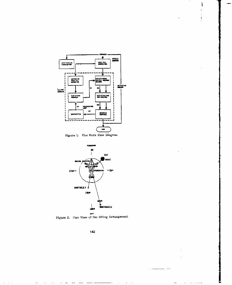
APMG

W4W ptas (IN Mftlk 11(

" N" I ",~lJ

: U IIII MIii M

1Igr 1. TheLU~u WokI'u iag

I brC I

I-s

AFTT

1424

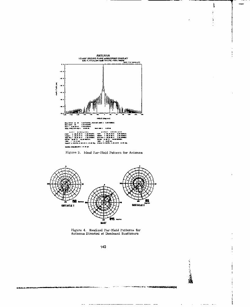
ANTENNAI.ZO0, GROUND PLANE WABSORR OVWRLAY

5ll9 PL ATCILLUM..-M TAYIL..-HOAL. SMIIM

l° IIm UUpI

.al.-•l -I .. .. .el -a.. e aa U. U. I. ii•. SN

AIMUI. (dI w .U

NA.. .llmaU I *Ul *.aa MGII.. H•IatS MIa * .M Nlia.to IM U . 10N M.M0E.

a. U U.N Ni Uv.N MsUnie.

"It. .81.411 .4..a44"M aM. "... ..FaiST a -a..a S al -1,5 MNlct, IZSI a -N.M aEl Al U.N KIUlS.aIlMIl * -Na. 046 -U. N lUll, UUMUUl * -NI.M a At aIa Na,..ll

-W, . -1.. SU6 a., - U.N v.qil. -+,N - I -I MIlm. M-It I.N Ui *M u aim.NUI} * .4l 4ila , at1 a .4515li.UZISSU a. lll&-UI. a I .IU.II Uq. fmll te l lmliS. F1IN Ml! 11W Sa.l-+

Figure 3. Ideal Far-Field Pattern for Antenna

OIITACt 08UL 2 6W..~i

* UT

MAST"

l-igure 4. Realized Far-Field Patterne forAntenna Directed at Dominant Scatterers

"143

S--.------------ ----- ~

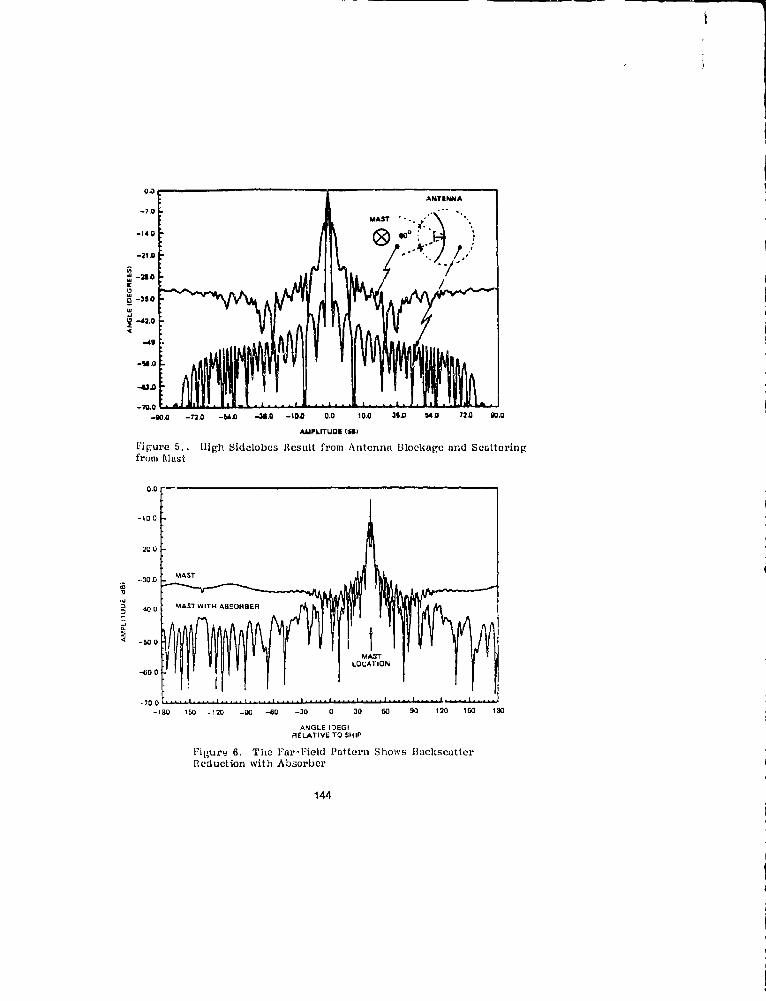
ANTINNA

-7.0MAST

-14.0

0 .0 7-200

-49

-56.0

-U3.0

-70.0 M. .T

- 80 .0 - 7 21 0 - 4 .0 - 36 . - 1 - l0 0 .0 1 0 .0 3 5 .0 14 0 7 2 .U 9 0 .0

AMPLIUE (D951

Figure 5.. High Sidelobes Result from Antenna Blockage and Scatteringfrom Mast

10.0

200

30n MAST

0 40 MAST WITH ABSORBER

MASTLOCATION

-10 -150 -¶20 -90 -80 -20 0 30 60 90 120 ISO 190

ANGLE (0601R ELATIVE To SHIP

F7igure 6. The Far-Field Pattern Shows BaekseottorReduction with Absorber

144

--30.0

REGIONMAST (3Qo-150o)

- -40.0J

w

• -46.00'Lw

SMAST WITH ABSORBER-50.u

-05.0

-- w0 0 L , . . . . . . . . . . . I . . I , , , i I , A , , , . . . . .• .0.0 10.0 20.0 30.0 40.0 60.0 60.0 70.0 80.0

t SCAN ANGLE (DE:G)RELATIVE TO MAST

MA-TLOCATION

FiNure 7. Antenna Performance for Mast With Absorber

145

_.. ._m

I

Bistatic Physical Optics Scattering from aSurface Described by an Electromagnetic or

Acoustic Impedance Boundary Condition

Robert T. BrownLockheed Advanced Development Company

Dept. 72-56, Bldg. 311, Plant B-6P. 0. Box 551

Burbank, California 91520

AbstractThe complete scattering matrix for bietatic scattering from an arbitrary

planar surface in the physical optics approximation has been obtained forthe case of a surface described by an impedance boundary condition. Theanalogous case of acoustic scattering at an impedance boundary in the localreaction approximation is shown to be identical in form to either one of tF'diagonal elements of the electromagnetic scattering matrix. The only di,'ee-ences between the acoustic and electromagnetic cases are in a factor dependingon azimuth angle and in the form of the reflection coefficient obtained fromthe Presnel equation relating impedance and reflectance. Although obtainedunder the assumption of validity of the impedance boundary condition, theresults are function# only of the complex reflection coefficients, not, the surfaceimpedance.

1 IntroductionThe most widely used computational method for predicting the Scattering of electro-magnet;c radiation from targets of arbitrary shape is that of physical optics (PO),combined with the physical theory of diffraction (PTD). The physical optics approx-imation for electromagnetic scattering is obtained from the Stratton-Chu integralequation, an exact integral form of Maxwell's equations, by replacing the integralequation with an integral over the surface of the target. In the analogous acousticscase a high-frequency approximation can be obtained from the Helmholtz integral

This work was supported bv the Defense Advanced RBsearch Prujedw Agency under contractMDA972-89-C-0014.

146

equation [1]. This paper describes the results of an investigation of the similari-ties and differences between high-frequency acoustic and electromagnetic scattering,and in particular the possibility of adApting existing high-frequency electromagneticscattering codes to the problem of predicting acoustic target strength.

2 Electromagnetic Bistatic Physical Optics For-mulation

In the physical optics approximation, the E and H fields scattered by a surface Sare given by

[f H X E,) d (1)

andHa j eo-o [i X E;T + × (f + X/O(., x )<) 2ejk.),'

Equations (1) and (2) are based on the far field approximation as well as the tangentplane approximation. The notation is the same as used by Ruck et al. [2], exceptfor a time convention ea'i. If the target surface can be described by an impedanceboundary condition, with surface impedance Z, then the total fields at the surfaceE T and Hr axe related by

fi X (f, x BT) = -Z(fi HI) (3)

or(fi x E) = ZA X (A X HT) (4)

so that (1, d (2) become

Ill. = [,ii, (• i X ET)+h(iXET) x 6ek..-r's' (5)

and H , = jwiSO • f [Zi x (fx H"') + Zo(fl x Hr) x j.]ejkrr'da9 (6)

147

.1

where Zo, = Me/re is the impedance of free apace. At the surface of the scatterertie total field, can be expressed in terms of the incident and scattered fields bymeans of the r,:flection coefficients R.L and R11, which are related to the surfaceimpedance 7 by

Z cos Oi - ZO= ZCosjO + y o (7)

and ZO cos 0i - Z

or

Z I + R, 1

-- R11

where OG is the angle of incidence measured from the normal to the surface.If now a local coordin•ate system is defined such that the scattering surface is

tangent to the (z, y) plane, with normal fi in the z direction, the complete scatteringmatrix for radiation of arbitrary polarization takes a particularly simple form. Thereflection coefficients 1:4 and R11 of Eqs. (7) and (8) describe the scattering of radi-ation polarized with B field or If field tangent to the scattering plane, respectively.That is, in Eqs. (5) and (6) either EH or Hi may be taken to be polarized in the Ojdirection. Because of the frce-space relationship between B and H this is equivalentto working with either E or H resolved into components ii the b and q directions.With this convention, a plane wave incident on the surface may be described by

R'i 'O~i- jk-r'(10)

orIHi - H0,jk-ri ' (.1)

The relationship between incident and scattered fields is then

4 (12)

andH; R11) (13)

148

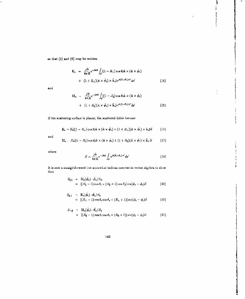
I

so that (5) and (6) may be writteu

U. R J,[ RL) coilOdsfs x (i x47rR J

+ (1 ± R± )(i, x ý,) X x ce'+t').,' (14)

and

H. --4-- - ) Coll o, x (' ,

+J~)f 7 11 (16)

If the scattering surface is planar, the scattxrcd fields bccomc

andH. Ho[. - R1I ) coss, ii × (ft x ýj) + (1 + R1i)(fi x q5.) x kjs (17)

wherc

It is now a straightforward but somewhat tedious excicise in vector algebra to showthat

S,,11 = 1 1(M ).1 ./no= [(Pill - 1)cusO, -T (Jill 4- 1)c os6,1CLc6(0. - 0j),5 (19)

s11, = E.(•,1.-,/lo= [(R-1 - 1) cos 0, cos 6, 1 (R, + 1)) sin(O. - )i)S (20)

Si, -1 . d1,10x~-- 1) Cos ,o, .s U. + (Rl + 1)] 8i,(.. - p,)s (21)

149

= [(R.L-1)cos ,+(R.L+1) oCO.1cos(#.-O,)S (22)

are the elements of the scattering matrix 3S, such that

pq = 4VIlS,•l 2 (23)

gives the cross section for any combination of receiver and transmitter polarizations.F'or a perfectly conducting surface, R±- = -1 and RII = 1, so that (19) through

(22) beconm

S11 1 = 2S cog 0, cos(O, - q,) (24)

S1 1. = -2s cos 0, cos 0. sin(O, - 0,) (25)

s,11 = 2S sin(O. - •,) (26)

SI1 L = -2S corn 6j cogs(0¶. - 0)(27)

in agreement with results previously obtained for bistatic scattering from planarperfectly conducting surfaces (3], [4].

As a further check, it can be noted that for the case of backscattcr, 0, = 01 and0j. = and Eqs (19) through (22) become

S11 11 = 2RII cos0i (28)So = 0 (29)s 0H = 0 (30)S.a = 2R. cos0j. (31)

These results do not contradict those of Ruck et al.[2], Eqs. (2.2-87) and (2.2-88),which have non-vanishing off-diagonal scattering mutrix elements. The results in [21were obtained relative to a different coordinate system than that used in the presentwork, and do reduce to the form given by Eqs. (28) through (31) when expressedin the same coordinate system.

150

3 Acoustic Bistatic Physical Optics ScatteringIn order to arrive at the acoustiz analog of the above equations it is necessary to goback ;.o the integral equation form of the scalar Ulelinholts equation analogous totihe Stratton-Chu equation for eltctromagnetice. Inl this equation the field quantityis the velocity poteatial V(r); the scattered field at a point r is given by [6], [7]

1 •) 0-t~ 0 1jVa(r) =~~ I -~'~ e~ + V(,') d. (32)

The quantity R is the magnitude of the distance from a source point r' Un the surfaceS to the observalion point r, and fi is the normal to the surface. For a haxmonicwave with time dependence eo'* the impedance boundary condition analogous toEqs. (3) and (4) for the electromagnetic case is [8]

OV jwopV0V, = Z (33)

where Z is the acoustic impedance and p is the density of the fluid outside theboundary S The normal derivative in the first term in Eq. (32) Ynay be written [5]

9 e-ikil e-a

OIL R= -jkf i.

e-j~Ao I= -jk cos 9. (34)

so that (32) becomes

V (r) L cos d V(r')° e-ds' (35)= ? f(, )- -,.,(

where k = w1/ is the wavenumber and c the soundspeed in the fluid with densityp. The quantity V(r') represents the total field at the surface. In the local reactionapproximation, analogous to the tangent plane approximation of electromagneticphysical optics, the total field at a point on the suiface way be writen as tile sumof incident and scattered fields V(r') = Vi + V, = V.(1 + 1.) related by the reflectioncoefficient [9)

151

R- Z cos Oj- PCZ coBo, - pc (36)

where Z is the acoustic impedance defined by Eq. (33). This way be solved for Zto yield

z (1+1It) pc(I - R .) c o, 0, (37)

which when substituted into (35) gives

V,(r) = L.k [(14 - 1) ios 4 (R. + 1) eos 0,1 V(r')--d,' (38)

Assuming the incident field to be the plane' wave

V,(r') = (39)

where Vo is the magnitude of the incident field, and making use of the far-fieldapproximation used in deriving Eqs. (1) and (2), we have

V.(r) V f--u [((1 -(R 1),co.o, 4 (& 1 1) Co 9 .1. .)'d•' (40)

orV. = Vo [(R. - 1),cot0, + (14 -1) cu,o.)S (41)

where S is exactly the same as Eq. (18), the physical optics integral for th,- electro-mag6metic case. Except for the aimnuthial factor cos(O. -- 0jb), EIj. (41) is the sameas either Eq. (19) or (22), the diagonal elements of the scattering nnatrix fur theelectromagnletic case.

For an acoustically soft body, Z = 0, It. =1 -1, and (41) becomes

- I = - 2S cos O, (42)

while for anl acoustically hard body, Z -4 oc, & = +1, and

V I = 2 cos 0, (413)

152

_________________________ _ __

These results arc completely analogous to the corresponding clectroiiiag*ptic ef-pressions (24) and (27). In the special case of backscatter, 0. = 0j, Oi. = •, and

V. -- 2Voi&S cos 0, (44)

again completely analogous to the corresponding electromagnetic expressions (28)or (31).

Figure 1 compares the physical optics electromagnetic and acoustic bistatic lcat-tering patterns for a square plate two wavelengths on a side. The plate is in the(z, i) plane with with sides parallel to the x and V axes. Incidence is in the (x, z)plane at 450 elevation.

4 Numerical Examples and ConclusionsFigures 2 and 3 show comparisons of the results obtaiied with the methods proscutedabove and method of moments calculations for bihtatic scattering from k. = 12 per-fectly conducting (acoustic hard and soft) circular cylinders. Figures 4 and 5 showsimilar comparisons for a ka = 12 circular cylinder with an impedance boundarycondition with Z = 10001/icl. li this case it is the TM polarization that is equiv-alent to the acoustic IBC. In three dimensiovs, comparisons were n'ade betweenmethod of moments and physical optics results for a ka = 10 sphere. Comnputa-tional models used are shown in Fig. 6, and Fig. 7 shows the principal plane cutsused for the bistatic patter-is. Results are shown in Figs. 8 and 9. Although notpresented here, all method of moments results were in essentially exact agr.ezncut.with series solutions in& both the two- and three-dimensional cases.

In view of the above results, it can be concluded that high frequency (physicaloptics) code* for bistatic electromagnetic scattering can be adapted to tihe acousticcase with only very minior changes. The changes required Ere actually siniplifica-tions, in that the acoustic analog of the electromagnetic bistatic scattering matrixis a single term, equivalent to and slightly simpler than either one of the diagoijalelemeuts of the electromagnetic matrix.

The acoustic scattering formulation should have the same rangc of validity asthe electromagnetic, with two additional caveats. The Stratton-Chu clectronagneticintegral equation, the starting point for the physical optics integrals (1) and (2) isin principle exact, as it is the integral form of Maxwell's equations. The acousticHlelmholtz equation, oil the other hand, is based on a linear approximation to whatis actually a nonlinear problem. In addition, both the electromagnetic and acousticresults are based on the validity of the impedance boundary condition. It is possiblethat this approximation has a different range of validity for the acoustic than forthe electromagnetic case.

153

It is interesting to note that although bo.- the ecoustic and electromagnetic casesstudied in the work reported here make use of the impedance boundary condition, inthe final result it is not the surface impedancu but the complex reflection coefficientsthat appear. It is possible that the results presented here have more general validitythani would be expected from the starting conditions, although this is still to bcdetermined.

References[1] J. J. Bowmia, T. 13. A. Senior and P. L. B'. Uslenghi, Electromagnetic: and Acoru-

tic Scatterintg by Simple Shapes, New York: lheinisphere Publishing Corporation,1987, p. 29.

[2] G. T. Ruck, D. E. Batrick, W. D. Stuart, and C. K. Krichbaum, Radar CrossSection Handbook, New York: Plenum Press, 1970, pp. 50-54.

[3] S. K. Chaudhuri and W.-M. Boerner, "A Polaximetric Model for the Recoveryof the Iligh-Fr,-juency Scattering Centers from Bistatic- Monostatic ScatteringMatrix Data," IEEE 2ianu. Antennae Proi, agat. vol. AP-35, pp. 87-93, 1987.

[4] R. T. Brown, "Nonspecular Nature of Physical Optics Scattering," 1990 URSINational Radio Science Meeting, Dallas, Texas, May, 1990.

[5] P. Usleaghi, "Radar Cross Section of Imperfectly Conducting Bodies at SmallWavelengths," Alta F.quenza, vol. 33, pp. 541-46, 1964.

[6] P. M. Morse and 11. Feshbach, Methods of Theurctical Physscs, New York: Mc-Graw Hill Book Company, 1953, p. 806.

[7] J. J. Bowman, T. B. A. Senior and P. L. E. Uslenghi, op. cit., p. 15.

[8] P. M. Morse and II. Feshbach, op. cit., p. 311.

[9) P. M. Morse and K. U. Ingard, Theoretical Acouitics, New York, McGraw-HillBook Company, 1968, p. 269.

154

S... .... . . .. . . . ..- . . .. .. . .. .. ...... . . . . ..... . .. .. .. . . .. ...... .. .. .. . .

z z

x x

S"Acoustlc Hr

PC Intogral NN- AcousticiHar(Acoustic Soft)

z

x x

y* /

Electromagnetic HH - Electromagnetic VV

Figure 1: Comparison of bistatic electromagnetic and acoustic scattering patternsfor a flat plate two wavelengths on a side. Edg; are parallel to the x and y "es,with incidence in the (W,:) plane at 450.

155

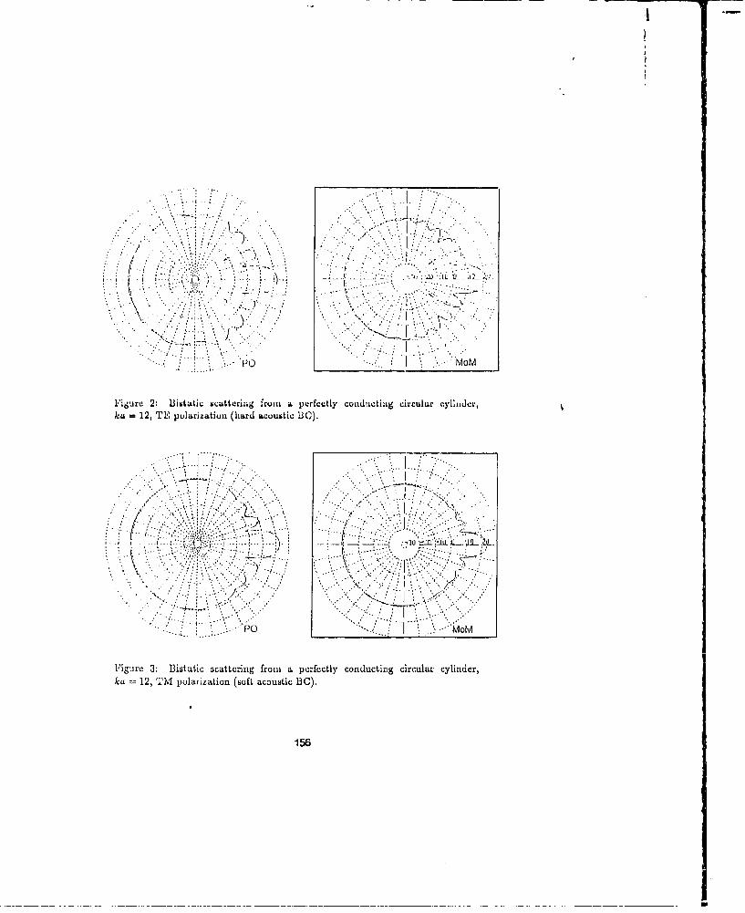
ka 12, TE, polarizationl (hard acoustic BC).

151%

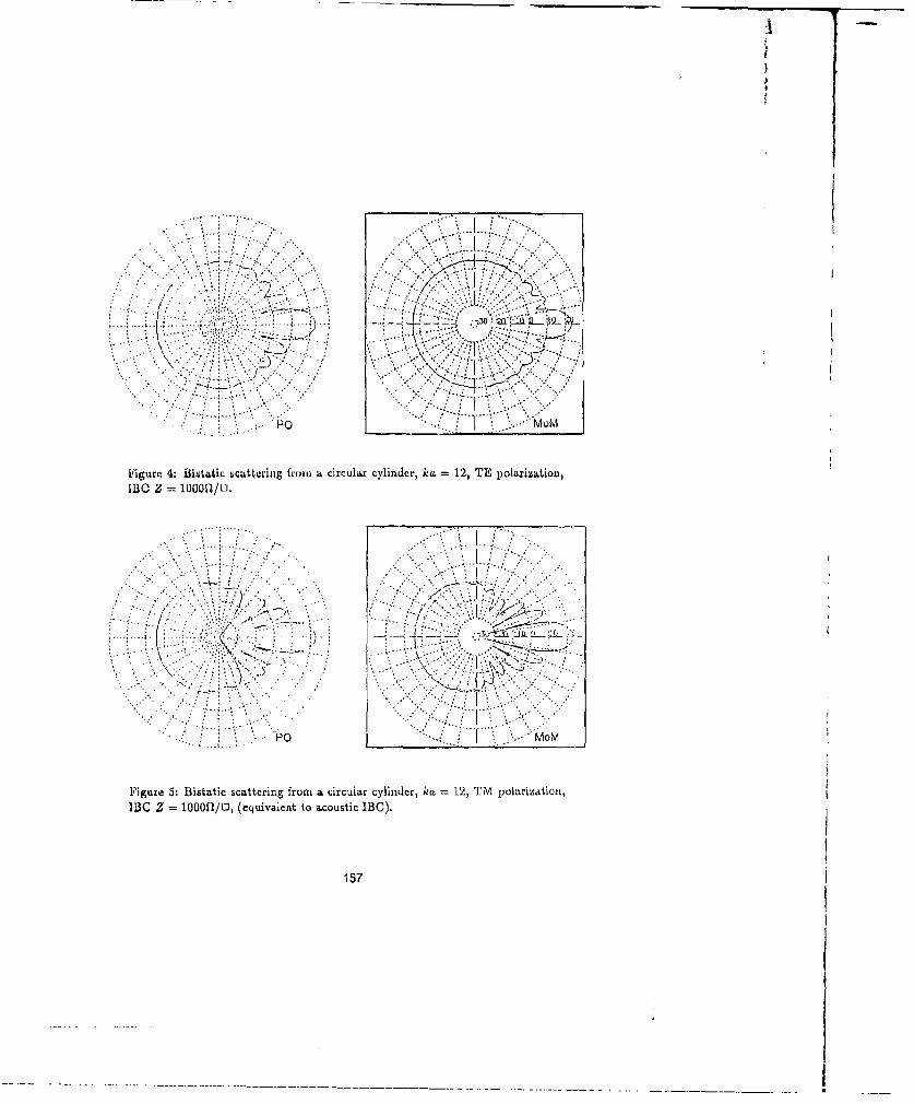
P0 MoM L-

1FigureL 5: listatic scattering from a circular cylinder, ka 12, TM polarization,I13C Z = 1OO0fl/Q, (equivalent to acoustic IBC).

157

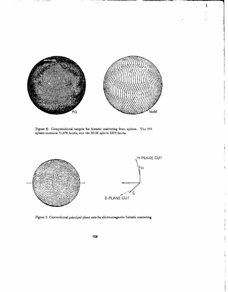
Figure 6: Oomput~tional targets for bistatic scattering from sphere. The POsphere contains 71,876 facets, and the MoM sphe~re 5392 facets.

H-PLANE CUT

H

E-PLANE CUT

Figure 7: Conventional prnicipal plane cuts for electromagnetic bistatic scattering.

P0 10

MOM

Figuiv 8: Bistatic scattering from perfectly conducting sphere, Ica=10, E planecut.

MOM

Figure 9: ilistatic scattering frc..-x perfectly cor~ductinvs sphere, ka=10, 11 plane

cut.9

SESSION 5 - "NEW TECHNIQUES"Moderator: Ronald Pogorzelskli

A HYBRID 'FINITE ELEMENT AND MOMENT METHC-D FORELECTROMAGNETIC SCATTERING FROM

INHOMOGENEOUS OBJECTS

W. E. Wlyse and A. A. SeidlLockheed Palo Alt~o Wesearch Laboratories

0/91-601 B/2563231 Hanover Street

Palo Alto, California 94304. USA

Abstruct - A hybrid finite elezrwnt formnulation for three-dimensional elec-Luiuagnetic , Uerkng is given using anl equivalent current approach. A newmethod, utilizing a body of revolution (BOR) formulation, is prtz.-ited toterminate the finite eleuwait mesh and to implement the neat field radiatimxcondition. This HOR impl1ementation utilizes Ilernsite cubic basis functionsanid a variable! no. -ber of modesi per basis function to achieve the greattest Culhputational efficiency. The comnbinjed field integral equation f'.amulation is esaa-ployed to eliwiinate non-physical resonances of the naez.1 boundary. Examplesare given showing such nion-playsic~Al resonance behavior and its eliminatiun aswell as the accuracy of the solution& generated by this hybrid finite elementmethod for bare and partially coatAi fH-rfect electrical rundurtors.

INT sIODUCTION

Finite element methods (FEM) are widely applicable to the Nolution ofMaxwell's i-quaktions fur electromnagnetic scattering. Because of t di iferentiai nature, FEM cani easily nwdel combinations of penetrable and impienetra-ble mnaterial and, in addition, these rmthods produce a iparse system matrix.Hfowever -difficulty, true for all diffetentia! methods, is in the treatment of theSonmner. id radiation condition. Local boundary conditions which maintainsparsity of the syttem matrix work beat when the animh bounda-ry is far fromntbm" scatterta [11. Having the mesh boundary fax from the scatterer greatlyincrease the number of finite element unknowns. This can generat~e Large sys-tern mistrica tor probleizo involving even rather small scatterers. Hybrid finiteele.-enit methods (IIFEM) couple the differential method to another method,ije. MOM [2, 3. 4j or modal expansion [5, 6, 71. Thiz coupling acts as a

160

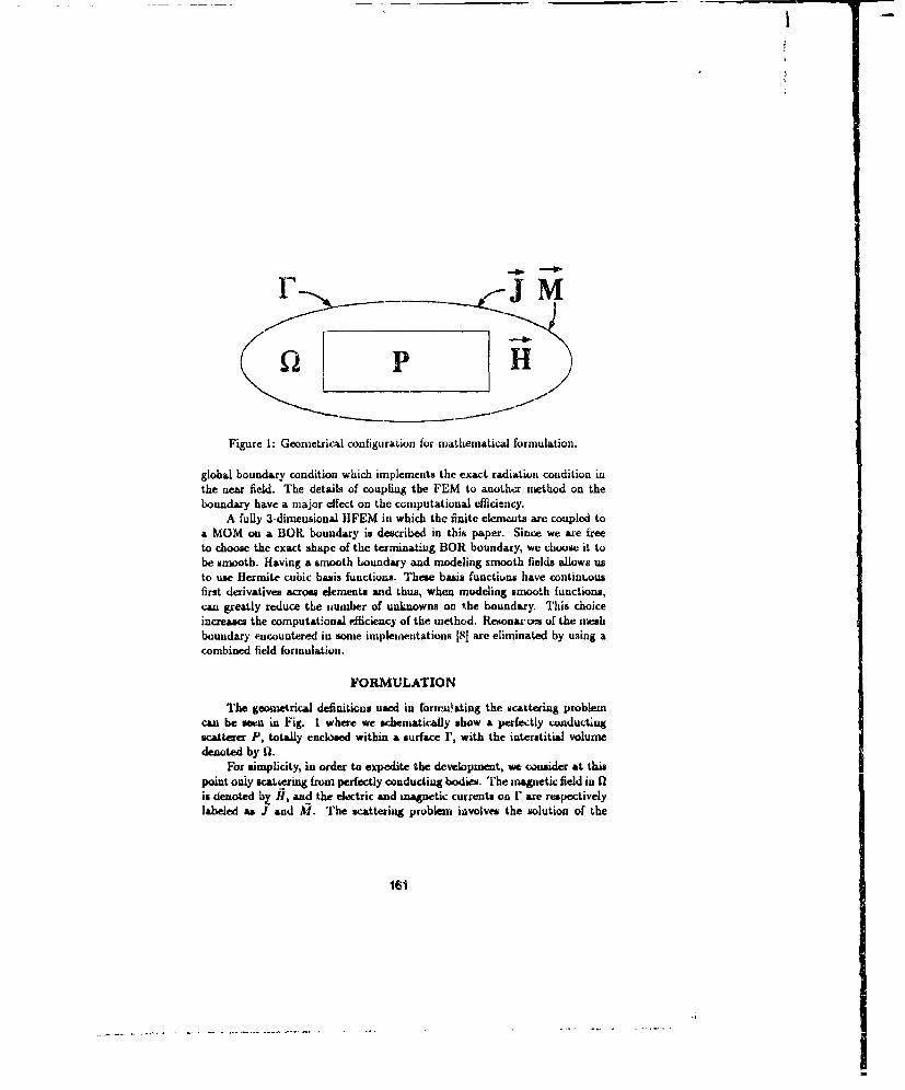
Figure 1: Geometrical configuration for mathematical formulation.

global boundary condition which implements the exact radiation condition inthe near field. The details of coupling the FEM to another method on theboundary have a major effect on the computational effilciency.

A fully 3-dimensional HFEM in which the finite elemenas are coupled toa MOM on a BOR boundary is described in this paper. Since we are freeto choose the exact shape of the terminating BOR boundary, we choose it tobe amooth. Having a smooth boundary and modeling smooth fields allows usto use Hermite cubic basis functions. These basis functiuns have contintousfirst derivatives across elements and thus, when modeling smooth functions,can greatly reduce the number of unknowns on the boundary. This choiceincreases the computational efficiency of the method. Resonarces of the meshboundary encountered in some implementations [8] are eliminated by using acombined field formulation.

FORMULATION

The geometrical definitions used in formulating the scattering problemcan be seen in Fig. 1 where we schenatically show a perfectly conductingscatterer P, totally enclosed within a surface r, with the interstitial volumedenoted by Q1.

For simplicity, in order to expedite the development, we consider at thispoint only scaering from perfectly conducting bodies. The magnetic field in f)is denoted bh H, and the electric and magnetic currents on F are respectivelylabeled as J and T. The scattering problem involves the solution of the

161

differential form of Maxwell's equations in Ri for the magnetic field H, couplingthis field to the equivalent currents f and M on r, an, ensuring that J, Mand the incident field specify a radiating solution.

The fields H, J, and M satisfy

VX-V×Xf(rl-p.,k'Hl(r) = 0for 'iED (1)

-A x V xfl/(F) - 0 forf• E P (2)Wto

fM(r) + As x V xHf(r = 0 for ý C' (3)WCoi- x fl (r) = Ofor iEr (4)

where w is the angular frequency, a time dependence e-"' is assumed, fo and f,are the free space and rejative permittivity respectively, po and p, are the freespace and relative permeability respectively, k is the free space propagationconstant, and fi denotes the unit normal to the surfacns.

The boundary condition for a perfect electrical conductor on P (Eq. 2)and for coupling the magnetic current on F (Eq. 3) are conditions on thederivative of fl and are imposed as natural boundary conditions. The bound-ary condition coupling the electric current on r (Eq. 4) is a condition on /Hitself, an essential boundary condition, and must be explicitly enforced. Let-ting 7? and 0i be test functions defined on fn and r respectively we write theweak equations

j (V X s'. (V x f)-4 -7? pod1]dV

+ . ids = 0 (5)

and

tD Xja CJ " [Y- fa xfidS 0 (6)

where the superscript ' is complex conjugation. Integration of Eq. 5 by partsreveals that it is the weak form of Eq. 1 with natural boundary conditionsEq. 2 and Eq. 3, while inspection reveals that Eq. 6 is the weak enforcenentof Eq. 4. A finite element discretization of these equations results in matrixequations which we denote by

[S] H+[C IM = 0[C]- H+[NI J = 0 (7)

162

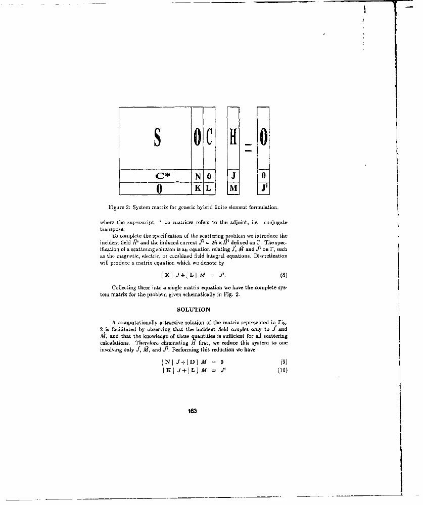
S OC H 0"c* No J 0

0 KL M

Figure 2: System matrix for generic hybrid finite element formulation.

where the superscript ' on matrices refers to the adjoint, i.e. conjugatetranspose.

To complete the specification of the scattering 2 roblezn we introduce theincident field H' and the induced current P = 2fa x H' defined on I'. The spec-ification of a scattering solution is an equation relating Jl M and J on J., suchas the magnetic, electric, or combined field integral equations. Discretizationwill produce a maatrix equation which we denote by

[ K] J+[L] M = X. (8)

Collecting these into a single matrix equation we have the complete sys-tein matrix for the problem given schematically in Fig. 2.

SOLUTION

A computationally attractive solution of the matrix represented in Fib.2 is facilitated by observing that the incident field couples only to Y and4, and that the knowledge of these quantities is sufficient for all scatteringcalculations. Therefore eliziinating H first, we reduce this system to oneinvolving only J, M, and A. Performing this reduction we have

[N] J+[D] M = 0 (9)

[K] J+[L] M = J' (10)

163

where

[D =-C S-'Ce. (11)

For general three-dimensional scatterers, the matrix D is always a dense ma-trix, independent of the method of implementing the boundary integral onr.

It is worth noting at this point that Eq. 11 implies finding multiple sparsesolutions of the matrix S. This is one of the places where limiting the numberof unknowns on the boundary becomes important, since each unknown on theboundary contributes a column to the matrix C. Thus each unknown on theboundary necessitates another sparse solution

Next, given an incident field Jý,

[L+K N-' D] M = J, (12)

is solved for M and then

[K] . = g-[L] M (13)

is solved foi J, after which the scattering may be computed. For monostaticcalculations, this is repeated for each monostatic point.

EXAMPLES

Resonance Case

Inspection of Eq. 13 reveals that it is of the 5ame frorm as the equations foundin an integral equation formulation of the scattering problem. The surface ofintegration is however not on any physical scatterer, but rather is a surfacewhere J and M arc defined and coupled to the interior solution for Ii. Neverthe less, in cavss where Eq. 13 has homogeneous solutions, resonance bchavioris observed. This is illustrated in Fig. 3 where we plot a radar cross section•(llCS), (h polarized, for a spherical conductor with a spherical mesh boundarywith ka,,e bo,,,ad, = 2.744. This corresponds to the lowest resonance of aperfectly conducting spherical cavity.

We plot the RCS computed using both the electric field and the mag-netic field integral formulation on the mesh boundary. In comparison, we alsoplot the solution from the :oml)in,(d field integral formulation and a Mim seriessolution. It is clear that while the combined field formulation and the Micseries solution arc virtually indistinguishAble the purely electric or magneticfield formulations are wildly inaccurate. This resonant behavior is due to the

164

80.0

-- Ell 1. W :

... ...... ........

4 " " 'O R T -R IN R I I. l g E r . ..... ....

0.0...... .

T.. . ...... ...... ..... .... ....I

UCRTTEflINO ANGLE (DEORFES)

Figure 3: RCS at 109 MEl for a I in. radius conducting aphere with the meshboundary terminating on a 1.2 m. sphere

manner in which we have chosen to solve the system matrix. A sub matrix ofthe system matrix is singular for this problem formulated with an electric or amagnetic integral equation, not the entirc system matrix. The way we chooseto solve the system unfortunately requires the inverse of this sub matrix. How-ever thc order in waidi we propose to solve the problem is so coniputationallyattractivc, that using a combined field approach to avoid resonant behavior isa small price to pay.

Conducting Non-BORl

In the next example we illustrate some aspects of the IIFEM nethod in detailby computing munostatic scattering from a perfc.-t co-,ductor with a non-BORgeometry, a box of dimensions 21m by 1/2sn by li at 200 MlIz. Figure 4illustrates the geometry of part of the scatterer, part of the finite element1m0esh, and the generator for the BO31 surface.

The surfaces representing one fourth of the conduction box can be sesnon the left of the figure. The line just above the surfaces of the box is thegenerator of the BOIL. The generator stays within a distance of about 1/20'thA of the box all along its length. This generatox is then revolved about thei axis, formniig the BOR mesh boundary surface which is very :lose to the

165

. . . . . . . . . . . . . . . . . .... ...... . . ..-

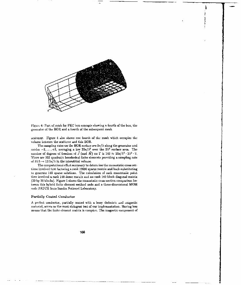
I -

Figure 4: Part of mesh for PEC box example showing a fourth of the box, thegenerator of the BOR and a fourth of the subsequent mesh

scatterer. Figure 4 also shows one fourth of the mesh which occupies thevolume between the scatterer and this BOR.

The sampling rates on the BOR surface are 5s/A along the generator andmodes -3,...,+3, averaging a low 23s/A 2 over the 3A2 surface area. Thenumber of degrees of freedom of Y (and 9') on r is 140 ; 23s/A 2 • 3A, • 2.There are 352 quadratic hexahedral finite elements providing a sampling rateof 10.5 -* 12.5s/A in the interstitial volume.

The computational effort necessary to deterxine the monostatic cross sec-tions involved first factoring a rank 12690 sparse matrix and back-substitutingto generate 140 sparse solutions. The calculation of each monostaLic pointthen involved a rank 140 dense matrix and an rank 140 block diagonal matrix(20 by 20 blocks). Figure 5 shows the monostatic cross section comparison be-tween this hybrid finite element method code and a three-dimensional MOMcude PATCH from Sandia National Laboratory.

Partially Coated Conductor

A perfect conductor, partially coated with a lossy dielectric cid ihagneticmaterial, serves as the most stringent test of our implementation. Having lossinvans that the finite element matrix is complex. The magnetic component of

166

- -----------------. . .

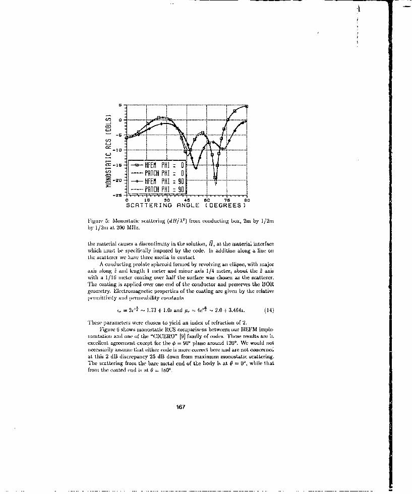
6 ............. ............. r ............ ,.............. r ............ 1......... .

LO -6 - : : .... ..... ... . ...........r _5' ........+............, ......... .......... J .' .. ........

L-)

. --- ----- ..... .................Iz _=o5 6 ýFEM PHI 098 ............ .. ..........U:. PATCH PHI 0

-25--- i, , ,- i - -- - - , ' " . . ... .....--- ------A-20 -. HFEfl PHI 90 -----

PATCH PHI 900 1i 30 4s 60 75 90SCRTTERING RNGLE [DEGREES)

Figure ,5: Monostatic scattering (dR/A 2) from conducting box, 2m by 1/2mnby 1/2m at 200 Ml'z.

the material causes a discontinuity in the solution, fi, at the material interfacewhich must be specifically imposed by the code. in additiun along a line onthe scattercr we have three inedia in contact

A conducting prolate spheroid fornied by revolving an ellipse, with majoraxis along . and length I meter and minor axis 1/4 meter, about the L axiswith a 1/16 iieter coating over half the surface was chosen as the scatterer.The coating is applied over one end of the conductor and preserves the BORgeometry. Electromagnetic properties of the coating are given by the relativepcrmnittivity and permeability constants

c, = 2c -4 1.73 + 1.0z and /•, 4eVi - 2.0 + 3.464a. (14)

These paramiieters were chosen to yield an index of refraction of 2.Figure 6 shows monostatic RCS comparisons betweern our IIHFM imple-

inictatiomi and one of the "CICERO" [9] family of codes. These results are inexcellent agreement except for the 0 = 9U' plane around 1200. We would notnecessarily assume that either code is more correct here and are not concernedat this 2 dB discrepancy 25 dlB down fromn maximum monostatic scattering.The scatterimng from the bare metal end of the body is at 0 = 0', while thatfrom the coated end is at 0 = 1800.

167

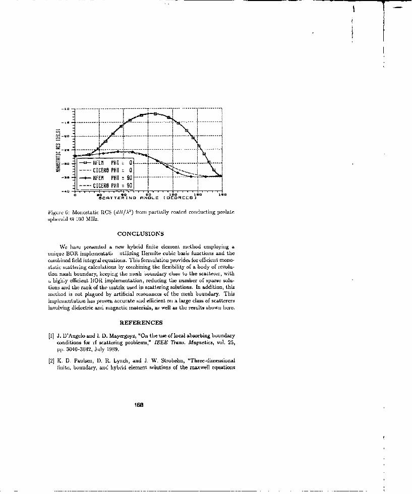
; I -I I. -

- - - -- - - --- -- - .. . . . . . . . .. . . . . . . . ------

., . ......... - •-------- - ........ i.... 'i.........-.-------..a -- HFEM PHI: 0 ----- ---- .....

CICERO PHI :0-- HFEM PHI :90--- ------

CICERO PHI = 90S 20 o so I1Ito l6O tio

SCATTERINOG RNGLE DEORErC)

l"igure 6: Monostatic RCS (dB/A'2 ) from partially coated condulcting prolafesphcroid (0 100 Mllz.

CONCLUSIONS

We have presented a new hybrid finite clement method employing aunique BOR impleinentati4 utilizing Ilermite cubic basis functions and thecombined field integral equations. This formulation provides for ceficient mono-static scattering calculations by combining the flexibility of a body of revolu-tion mesh boundary, keeping the mesh boundary close to the scatterer, witha highly efficient BOBt implementation, reducing the number of sparse solu-tions and the rank of the matrix uwed in scattering solutions. In addition, thismethod is not plagued by artificial rcsonances of the mesh boundary. Thisimplementation has proven accurate and efficient on a large class of scatterersinvolving dielectric and magnetic materials, as well as the results ahown here.

REFERENCES

[1] J. D'Angelo and I. D. Mayergoyz, "On the use of local absorbing boundaryconditions for rf scattering problems," IEEE Trans. Magnetics, vol. 25,pp. 3040-3042, July 1989.

[2] K. D. Paulsen, D. I.. Lynch, and J. W. Strobehn, "Three-dimensionalfinite, boundary, ance hybrid element solutions of the maxwell equations

168

for lossy dielectric media," IEEE Trans. Microwave Theory Tech., vol. 36,pp. 682-693, April 1988.

[3] J. Jin and V. V. Liepa, "Application of hybrid finite element method toelectromagnetic scattering from coated cylinders," IEEE Trans. AntennasPropagat., vol. 36, January 1988.

[4] W. E. Boyse and A. A. Seidl, "A hybrid finite element method for conduc-tors with thin dense coatings," Applied Computational ElectromayneticsSociety, vol. 4, pp. 59-72, Fall 1989.

[5] K. K. Mei, "UnimoisnMclt method of solving antenna and scattering prob-lems," IEEE Trans. Antennas Propagat., vol. AP-22, pp. 760-766, Novem-ber 1972.

[6] J. Lee and Z. J. Csendes, "Transfinite elements: A highly efficient pro-cedure for modeling open field problems," J. Appl. Phys., vol. 61, April1987.

[7] J. B. Keller and D. Givoli, "Exact non-reflecting boundary conditions," J.Comput. Phys., 1980.

[8] X. Yuan, D. IL Lynch, and J. W. Strohbehn, "Coupling of finite elementand moment methods for electromagnetic scattering front inhumogeneousobjects," IEEE' 7ýans. Antennas Propagat., vol. 38, pp. 386-393, March1990.

[9] L. N. Medgyesi-Mitschang, P. L. Iluddleston, and J. M. Putnam, "IRdarscattering analysis: Mathematical formulations, Vol. 1," Tech. Rep.MDCQ1230, McDonnell Douglas Research Laboratories, November 1984.

169

- --.--___

A New Expansion Function of GMT:the Ringpole

Jingliang ZiengInstitute of Fields and Waves, ETH ZUrich

CH-8092 Zarich, Switzerland

Abstact - The Ringpole is a new expansion function of GMT (Generalized MultipoleTechnique) which has a strong analytical basic and a clear physical background. ThisRingpole is suitable for calculating the fields in a domain, which has a part with a rotationalsymmetry. It has been programmed and may be used in MMP (Multiple MultiPole) programs.All the computed examples have shown, that the Ringpole can supply an excellent solutionfor die fields in the concerned domain with a massive reduction of the number of unknownparameters to be used and therefore the computation time in comparison with discreteMultipoles.

INTRODUCTION

The Generalized Multipole Technique (GMT) is a new method to solve electromagneticproblems, which has been developed in the past yeari. The MMP (Multiple MultiPole)programs are based on the GMT [1-3]. They offer fast and efficient computations of timeharmonic clectrodynamic problems with piecewise linear, homogeneous and isotropicmaterials. All kinds of examples have already proved, that the calculating results obtained byMMP programs have a good quality.In GMT, the fields inside a domain are expanded as a superposition of the fields of severalMultipoles. The unknown coefficients of these expansion functions are kletennined bymatching the fields on the boundary of the various domains at discrete points. For complexgeometrical form of a domain, many Multipoles are needed, so that the computation time, thememory requirements as well as the amount of work to create an Input file are not small.Introducing new expansion functions make it possible, ti reduce the amount of all this work.Therefore, finding new expansion functions to increase the application's domaii of GMT is amatter of particular interest.

MtJLTIPOLE - BAsIC EXPANSIONMMP programs divide the total space into several domains, each of them is linear,homogeneous and isotropic. The fields inside a domain are expanded as a sum of severalexpansion funutions.

PF = Eli

i=1

where eachf is a Multipole expansion, which is the basic expansion function of MMP. TheseMultipole expansions are the exact solutions of the Helnholtz Equation in the concerneddomain. In 3D problems they can be represented as

Nm

1713

where h., are splier~cal Harikel (or licssl) functions or thirk differentials, P'7'are Legendrefunctions or their differentials, k is wavcnumber in medium. Thei 1,lacenient of the Multipolesmust follow certain iulcs, so that the numerical lincar dependencies aniong the expansionfunctions can be avoided. Theme are also other expansion functions in MMP programs, forexamrple TEM expanisions, plane waves and waveguide modes for rectangular and circularwaveguides.Let tin, expansion.% for the fields in various domains be matched ini discrete matching pointson the boundary betwceii the domains. Gcnerally, all 6 boundary conditions for the normnaland transverse clkctric and mnagnietic fields are used. 'Ilire coefficients a,,, are dctermined bysolving the obtained equations. in the MMP programs, an overdetenrined systemn cfequations is used in ordet to improve the correctapproximation of the fields solutions.

RINGPOLLETlrc expansion functions of a Multipole have anl important character: they have a greatinfluence upon the necar region of origin and a small influence; on the far region, which can

often be neglected. Because of this behavior, the Muitipoles should be placed around thedomain, so that the whiole boundary is covered by their neighborhoods-. T'lerefore thelocations of Multipolca arc closely related to the domain formi.In order to reduce the anrount of work, there is always the possibility of separating a complexgeometry in mnany pans which are miuch simipler. Ringpole is suitable for calculating diefields in a domain, which has a part with a rotational synusretr1y. If the fields in such a domainare to be solved by GMff, many Multipoles have to be arranged onl one ring. Theircoefficients have a sinusoidal distribution. If these coefficients are transformned to Fourierseries, then the experience shows that only the first few tenins ame dominant andl the othertermis can be necglected. 71herefore, these discrete Multipoles can be replaced by a Ringpolewith each of his orders corresponding to a tenii of the Fourier series above. Thec numiber of theunknown paranieters in the problem may be massively reduced by this process.The Riiigpole is theoretical a line ring, which consists of tmany Multipoles. 'lire expansionfunctions of Ringpole can be represented roughly as

N , h e a t , ,. , , A ( ( ) /r, , ,( k r ( $ ) ) P ,' . "( c o k;O ( C ) ) ' ft ( m ( ) oAWi

where each ý corresponds a poinmt onl the ring.,r~.8~,) arc coordinates of field point inthit local coordinlate systcem with origin 1. C? (IQi indicates the distribution of Multipoles onthe ring, A(;) is a vector Operator by which the corresponding coamponenits of the expansionfunction of Multipole should be obtained. If the orienitations of the local coordinate systent arechosen correctly, the mnodrs for mj>O have only a very siiiall contribution to the total fields.which can practically be neglected. If we set up a cylindrical coordinate system with thecenter of ring as origin and change all components into a new fonn corresponding to thecylindricat coordinate system,.(lhe integration above may be reduced on account of thesymmentry by half. Thcerefore we have

= f L, , B(j, (kr(C)) P." (c"r 6(()) 'in(104(

where B(ý) is a new vector opratot, 4. is azimluthal coordinaite of fwied point ini die cylindriclcoordinate system. Siacm ;r(Qo(( and B(;) all ame the funcationg Of ý, it is at ICAst verydifficult, to find anl analytical method, by which the integration above can be treated. Thenumerical integration, which ii; used in the Rprogramn, is nhore practical.

171

In the physical ,ense, a Ringpole indicates the electric and magnetic currents along thecircumferential ring and dipole-rings polarized in axial and radial orientations. Since thismodel can cause a much more accurate field in the corresponding domain than the discreteMultipoles, the original problem can be effectively simplified by the Ringpole,

A circular metallic plate is illuminated by a plane wave with a inc;.lence of 45 degrees. Thediameter and thickness of the plate are respectively 2.4 and 0.4 wavelhngth, Figure I showsthe total near fields calculated by Ringpoles.A circular horn antenna is excited by TEl I mode at the feedwaveguide. Both near and farfields are treated with Ringpoles. The E-field Wi the hom and the patterns of the hom in E-and H-plane axe shown in Figure 2 separately.

....... , • -t - . ...... ........ + - . ..oo , ...

* l0 .. .... .. .. ... .ft 't - •.. 00" ** i

. . .... ........ 00

........... . • i ,.+ ,a . , . , , e .oo ,* -..... ...l '. 'f- XI, -, ,0..+.... -ooo.. .*.. ....

€,itI ~ ~ ~ ~ ~ ~ ~ ~ ~ ~ ~ .. ......i| *+.~.•*.O.OO.A•'tOeO'

.. if .. . . .. ..... .00.. .. c...". . .. 0 00 ..... .

...... .:;"

. . o ~ o.. . .. .. .. .. ..."t t• ,', ' , ° . '° , . .,.. .. . ..o+ .. 0 ... . . . ... . . . .. . .... ... .

,.., : ,, " ., .;', - , . .. .... .... .. . ......... ...

S.... .. % ..'.......:

Uig.1 " ic, s near a metiallic plate. LII .lop: E :ield: Rig/t lop:: H field.L.f. bottom, : Poynting vector. Right batioi: Poyntiiig fldoi in limi avcrag-.

172

-40L61I 20

.100 .20 0 90 180 -100 *90 a go IBG

Fig.2 Fiels of the lbOrn. On the top: B3 field in the tbor onEplaune (hpV) arwl F~. pane 6gtiis).On tihe houwon. Pattent of the hurm on U1-platio (leii n H-plaue (right).

CONCLUSIONRingpole can replace many discrete Multipolcs for calculating the fields in the domain, whichhas a paut with a rotational symmetry, or in the domain, which is rotational symnmetrical (thelatter one is a 3D problem for GMT). The placement of Multipoles and therefore the work tocreate a Input file can be simplified and the computation time can be massively reduced bythis process. The quality of the solution of the fields in the concerned domain supplied by theRingpole is excellent as good as by discrete Multipoles. With the help of Ringpole and allother i~ew expan-ion functions, wbich wie will treat, GMTf will be even more comfortable.

REFERENCES[1] Clh. Hafloer, The Generalized Multipole Technique for computational Olctromagncties,

Artech House, Unoflnf, 1990.[2] L. Bomiholt, MIMP-3D -- A Computer Code for Electromagnetic Scattering Tkased onl the

GMT, Thies is ETHl No. 9225, Zilnch, 1990.[3] L. Bomholt, Ch. Hafner, A MM.P Program for Computations of 3D Electromagnetic

Fields on PCs, 51h Annual Revicw of Progress in Applied ComputationalElectromagnetics (ACES), Conference Proceedings, March 1989.

173

AN APPLICATION OF SYMBOLIC MANIPULATION SOFTWAREIN COMPUTATIONAL ELECTROMAGNETICS

R. J. PogorzalskitGeneral Research Corporation

5383 Hollister AvenueSanta Barbara, CA 93160-6770

Abstract

Manu nf the expreasions which arise in the formulationscommonlW used in computational alectromagnetics are in theform of infinite series. Often these series are varu slowlWconvergent and the resulting computational burden placed on acode which makes use of them can be prohibitive. A commonseries acceleration technique is the Kummer transformationwhich involves subtraction of a series of analyticallW knownnum. Applying this technique with maximum offectivness oftenrequires significant amounts of algebra prior to coding. Thisalgebra can be carried out bW means of symbolic manipulationsoftware such an Mathematics with remarkable efficiency.Thus, hW this means, one may greatlU expand the effectivenessand breadth of applicability of such acceleration techniquesin computational electromagnaticu.

Introduction

Symbclic manipulation software performs algebraic and calculusoperations in sWmbolic form rather than numerical computationsalthough most such software is also able to nalculatenumerical results. Thus, it can function very effectively insupport of computer code development in that the expressionsleading to high level language statements can be derived usingthe symbolic capabilities and the resulting statements canbe chmckedfor coding accurecu using the numericalcapabilities of the software.

As an example of the application suggested above, we considerthe Green's function for helical structures derivod byPogorzelski C13 based on the work of Hill and Wait L]2. Theelements of this dyadic Green's function are expressed in aforminvolving several infinite series which are, for the ranqsof arguments typically encountered in method of momentsapplications, very slowly convergent. The Kummertransformation can be employed to accelerate this convergenceto an acocptable ratu. In applWing this technique, a seriesof analytically known sum is subtracted term by term from the

t Formerly with TRW Space & Technolcgy Group, One Space Park,Redondo Beach, CA 90278 where this work was begun.

174

series to be accelerated. Then, the series of differences issummed and the analWtically known sum is added to the result.The advantage of this procedure arises when the subtractedseries is chosen so that its terms rapidlU approach those ofthe series to be accelerated as the index of summationincreases. That is, the terms of the known sum should be alarge index asWmptotic expansion of the terms of the desiredsum. Derivation of the terms of this expansion can beextramelU tedious. As will be demonstrated, it is here thatsymbolic manipulation software can be of very signiFicantvalueto the electromagnetics programmer.

Analysis of Xelical Structues

In carrying out the electromagnetic analWsis of helicalstructures such as the twisted waveguide shown in Figure 1,the fields of currents disposed along helical trajectoriesaround the symmetry axis are required. These fields becomethe elements of a dyadic Green's function appropriate toformulation of the problem in terms of an integral equation.Specifically, if the structure is perfectly conducting and oneintends to use an electric field integral equation, one mustobtain expressions for three independent vector components ofthe electric field due to three independent vector componentsof the current along a helix. The coordinate systems used todefine these components is shown in Figure 2. As shown, thecurrent is expressed in radial, longitudinal (along thehelix), and transverse (across the helix) components while theelectric field is expressed in the usual cylindricalcoordinate system components, radial (p), azimuthal (q), andaxial Ct). The three electric Field components due to each ofthe three current components are the nine elements of therequired dyadic Green's function. That is,

rP - PG t GiF i

Ep ra U 6OP 95 Gt 0?• I

Gz6 and G were previously obtained by Hill and Wait 23]E3J

and theremaining elements were provided bU Pogorzelski l13.For the present demonstration we select SzZ, the axial

electric Field of a longitudinal helical filamentary current,which may be expressed in the form,

175

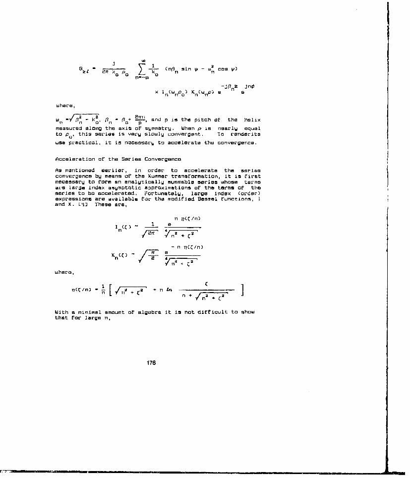
S - J • 12•z n °Po •--o(n(3 s in W - w ooV

zn -k k n n

where,

z 22nW n . 0 On -00+ -- , and p is the pitch of the helixmeasured along the axis of symmetry. When p is neacly equalto po' this series is verW slowlW convergent. To renderitsuse practical, it is nocessarU to accelerate the convergence.

Acceleration of the Series Convergence

As mentioned earlier, in order to accelerate the seriesconvergence by means of the Kummer transformation, it is firstnecessarW to form an analytically summable series whose termsare large index a5Umptotic approximations oF the terms oF theseries to be accelerated. FortunatelW, large index (order)expressions are available Cor the modified Bessel Functions, Iand K. E-3 These are,

n y?(C/n)

n e

- n rCC/n)

nI AKn(7;- - 1C

where,

(n- 1 [ ;I + --- + n t n /+Yn z I "

With a minimal amount oF algebra it is not difficult to showthat for large n,

176

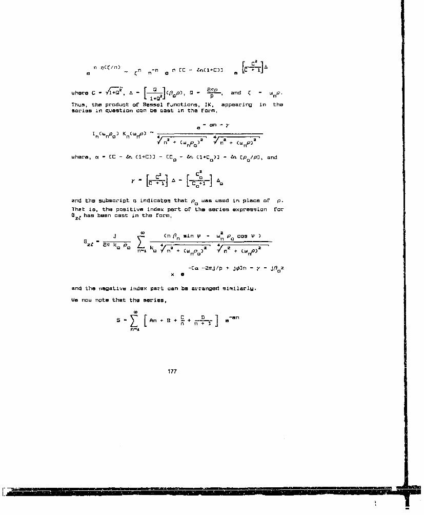
n iC/ln n -n n CC - +C1)+M ] IC J 1

where C - A- r o lCP). 0. _ and -- lip

Thus, the product of Bassel functions, IK, appearing in thesories In question can be cast in the form,

- ln -

In w' P ) Kn np) " .P 2.n n npo " -/n np)

where, e - CC - &, CI+C)] - CC - ZC (C+C o) - Z Cp /pJ, and

000

and the subscript n indicates that p0 was used in place of p.

That is, the positive index part of the series expression forazz has been cast in the form,

J j (n Pn sinV w oCos W- En n o k@zt Tk0k /22 /2

-o o n + Cw np.) n + (w n P)

-[a -2•fJlp + J3- - zx a

and the negative index part can be arranged similarlu.

We now note that the series,

OD

S ~Z " An + B + ý. + .-- een

n-,,

177

. .

possesses a closed form sum. That is,

*-an - -Ye ( I - a-, )2

S- 1n 5 - a 2n-i

-a,-an- a

z I le-a

-an

n-i

-an__-- n a 1 1 1 8 -.a

n-i

We next note that the sum S above can be approximated to ordorn by a series of the form,

n-a

Thus it becomes desirable to expand the asymptotic form of zz

givan above in this Form. That is, wu wish to obtain 4, 3, •,and ; such that to order n ,

C nnn t3sn - w2 Po cos )z

nn nn ka n2n + WnPo . na + (WnJ

with a - a - 2ujtp + JO. This in just the sort of opr itionat which symbolic manipulation software excels. In thi caseof Mathematica, one merely enters the above expression inBASIC format and issues the command,

SuriesC•,Cn, InfinitU,3)]

which instructs the software to expand the given expression in

178

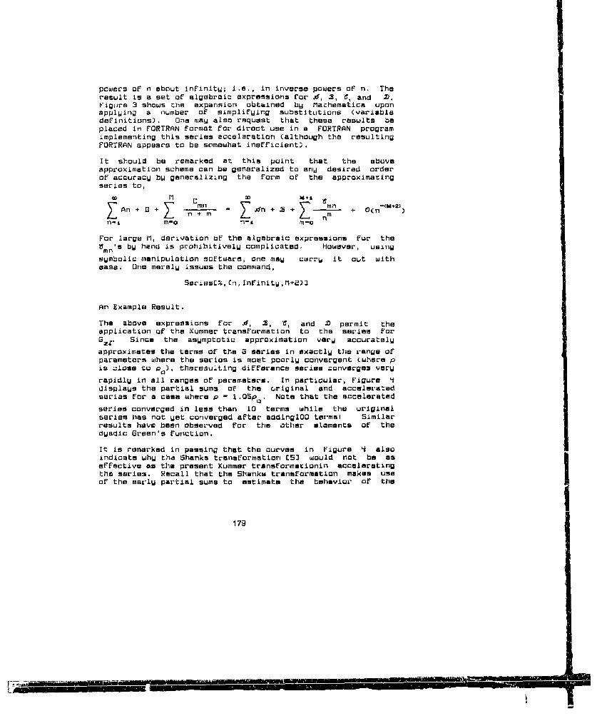
powers of n about infinitJ; i.e., in inverse powers of n. Theresult is a set of algebraic expressions for j S, 'e, and M.Figdre 3 shows the expansion obtained bW Mathematica uponapplging a number of simplifWing substitutions (variabledefinitions). One mau also request that these results beplaced in FORTRAN format for direct use in a FORTRAN programimplementing this series acceleration (although the resultingFORTRAN appears to be somewhat inefficient),

It should be remarked at this point that the aboveapproximation scheme can be generalized to ariU desired orderof accuracU bW generalizing the form of the approximatingseries to,

An + 8+mn Z fn + S +Z mn + 0(n-IM..))An+B+ n+m n m

n-i M-0 n-i M-c

For large M, derivation of the algebraic expressions fur the1 's bW hand is prohibitivalU complicated. However, usingmnsymbolic manipulation software, one maU carrW it out withease. Orne merelw issues the command,

SorieaE%,CnInfinitW,M+2}]

An Example Result.

The above expressions for 4, 2, e, and Z permit theapplication of the Kummer transformation to the series For0ZZ' Since the asemptotic approximation verW accuratelyapproximates the terms of the G series in exactlW the range ofparameters where the serius is moet poorly convergent (where pis close to pa), thereaulting difference series zonvarges verW

rapidlU in all ranges of parameters. In particular, Figure 4displags the partial sums oF the original end acceleratedsarias for a case where p - 1.05po. Note that the accelerated

series converged in less than 10 terms while the originalseries has not Uet converged after addinglO0 termsl Similarresults have been observed For the other ealments of theduadic Green's Function.

It is remarked in passing that the curves in Figure 4 alsoindicate whW the Shanks transformation CS] would not be aseffective as the present Kummer transformationin acceleratingthe series. Recall that the Shank% transeformation makes useof the earlg partial sums to estimate the behavior of the

179

m

convergence curve viewed as a so-called "numerical transient".However, as is clear from Figure 4, in this case a very largenumber of partial sums would be required before one couldaccurately estimate the oscillation rats of the convergencetransient. Thus, the Shanks transformation might requireseveral tens of terms as opposed to the Five or so termsrequired in the Kummer procedure.

Concluding Remarks.

The utility of symbolic manipulation software in programmingacceleration of series has been demonstrated in the context ofevaluation of a dyadic Green's function for helicalstructures. This nine component Green's function is suitableFor the formulation of an electric field integral equation forperfectly conducting helical structures. A corresondingdyadic applicable to combined field formulations and helicaldielectric structures would have thirtUsix elements which arethe electric and magnetic field components due to electric andmagnetic currents. The algebra involved in accelerating allof these series would be truly staggering even though dualityreduces thanumber bw half. Nevertheless, such a task is wellwithin the capacity of anyone having access to suitablesymbolic rnwnipilation software. It is concluded that suchsoftware can in many cases be an indispensible programming aidin computation electromagnetics.

183

ReFerences.

1. R. J. Pogorzelski, "On the Numerical Computation of aGreen's Function For Helical Structures," National RadioScience Meeting, May 1990, Dallas, TX.

2. J. R. Wait, "Electromagnetic Theory of the Loosely BraidedCoaxial Cable: Part I," IEEE Trans. HTT-2, 547-553, Sept.1975,

3. 0. A. Hill, "Pi'opagation Along a Coaxial Cable with aHelical Shield," IEEE Trans. MT-213, 1B-8S, Feb. 1980.

*. M. Abramowitz and I. A. Stegun, Han ok fE M mtj;&Functiona, National Bureau of Standards Applied MathematicsSeries 5S, June 1564, pg. 378, Eqns 9.7.7, 9,7,8, and 9.7.11.

5. 0. Shanks, "Non-linear Transformations of Divergeat andSlowlW Convergent Sequence5," J. Math, and Physics, •, 1955,pp. I-42.

181

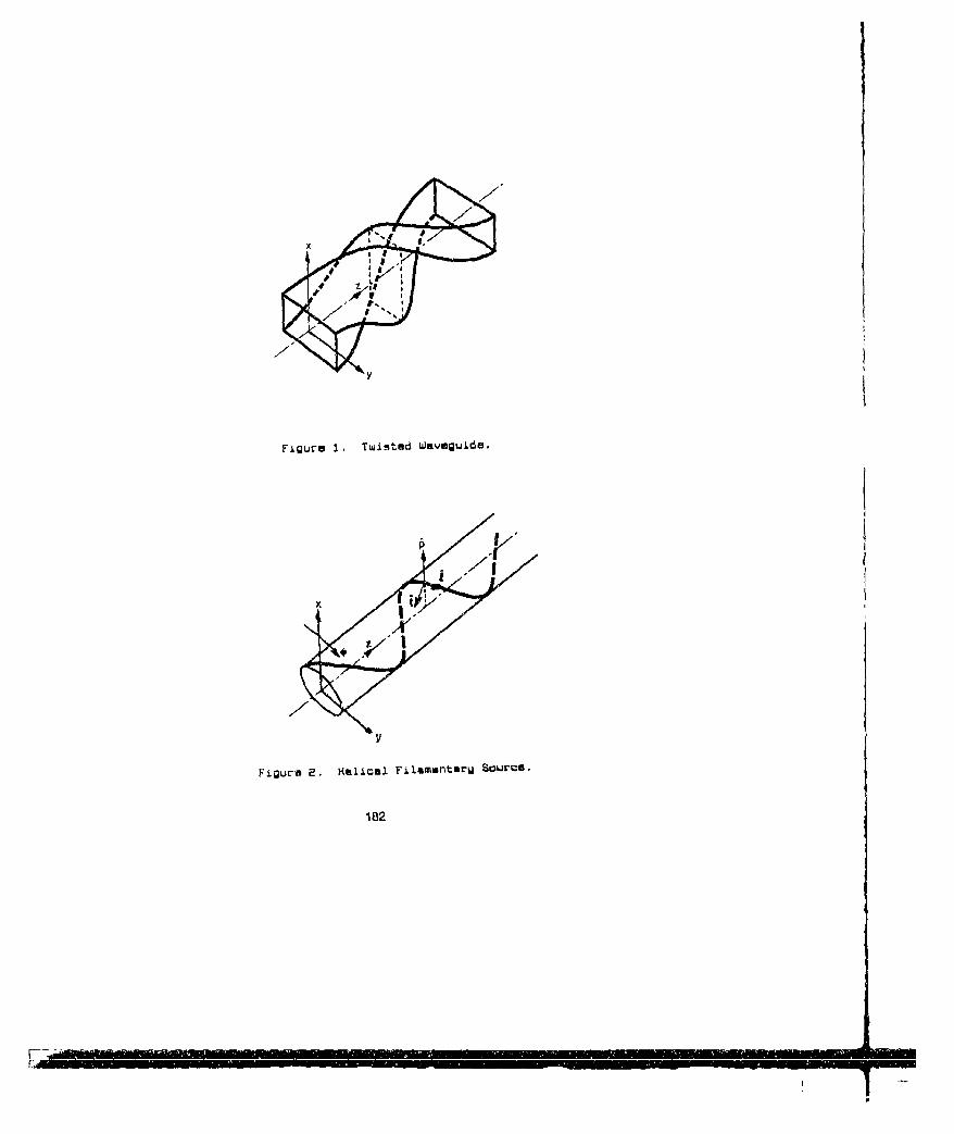
Figure I- Twisted Waveguide.

Figure E. Helical FilammntarW Source.

182

2 2 2-lb p2 r z?) c O ,

2 2 5/4 1/4-,b p2 rO ti 2 q q

114 5/4 1'4o p

2 2 q QO qO

:4 : 4 k qk zi qo

2 2 22 -lb p

2 r L O .

5,4 ./4

5,42 qO

2 42 22S b rO rO -

b p2 .------------.-......2 2 qO

4 qO

1/4 1142 q qO

2 4 2 2 2

b P2 €. . . . . . . .222 22

-- p2

I-----------

5/4 1/42, 2 q 2

114qO

Figure 3. Mathamatica Output.

PARTIAL SLIMS FOR G,

.00

"551 i OrIginal a., ?11s 0014 0l .. 4

0.012 IOn cykndoe0•.05 radon.rb (r011 cu~rtlI

0.0 1 ____I_0 20 40 40 80 100Number of IsrMS

Figure 4i. Series Convergence.

183

LI

Efficient Solution of Matrix Equations inFinite Element Modeliig of Eddy Current NDE

A Ntahrmloo. D.J. Lynch, Q.l. Nguyen, L.D. Philipp

S\V.-ahiuatrn Stir Ltliivcr'ity at Itt-Cities. Richland WA 99352

AbtIRACT Ftnite elwrienl modeling (FEM) at field!; may require matrix stzes in the range of 50,000aoty Curiirsoften wvoiv.., !arge matrices. The to 250,000 var.ables [1. 2]. Computation times aterr.Q.wiLY of the algorithm used for solving matrix several minutps to a low hours can be encountered

t•u,3,''or , is entremeit critical to tlea overall for such problems.onnitjtit:on time The puroose of this paper is to Finite element formulations genertlly produce-urvey and analyze various approaches to solving sparse, banded and symmetric matrices, since each"ratr eurations in ma~n memory and to identity the nodal variable is connected only to nodal variablesmost time elffcient approaLh within the context at which appear in the same finite element. Considerabletin.ro element formulation of two dimensional eddy savings in execution time and memory are achievedcurre:n! pioblen•s A comparison of methods used to by faking advantage oa these matrix properties.,rr-oducu boundary conditions shows the benefits ofthe I s and 0's' substitution technique over the 21. Techniques for Introducingbla,!ing factor' method Evaluation of matrix Boundary Conditions

dptontpos~tion algorithms indicates !hat CholuskyBonayC diosiu.ronrrvtron agyoethds The sindesl run thies of Ihe There are two popular techniques tar introdacing"dLod'ri.onstdoryd s modthe ed Cholresky algtofthen boundary conditions in finite element problems. One"oehnndohns baedk submdtuhion for untessenihal is reterad to as the 'blasting lactor" technrque and•..nr•..•nis.g davkped Munimum computarron tis e is the other as the -l's and O's substitution' technique

0 ,-vI:,-raiod using the miodifred Chotesky (3]. both techniques preserve the symmetry andin cirposlJun algorithm and the "I's and O's- bandadness properly at the original matrices andnou~daiy conslrron technique thus are convenient to use. We will briefly describe

tthe two techniques and then compare their relativeI. |liiirodu~tions computational efficiencies.

In the blasting factor technique, a nodal variacle.I -ile element methods have been apptied to whose value is specitied by boundary condiltozs, is

"'a"y a fferunt engineering problems In particular. multiplied by a large number, known as the blastingrhr.y hive been shown to be very useful in modeling factor The corresponding term in the vector b and theedd• ,urrent NDE (nonodestructive evaluation) diagonal term in that row of M are also multiplied bynIrrir.,ouna the blasting 'actor As an example, the folltw ong

r he tinite element method, integral or matrix shows how to effectively specify xi.ct. andVinter at dl equalutons ate solved by dividing a problem x3 ,c3 assuming that the blasting factor is much largerregion into subregions of simple form called tinite than the largest element in M.elements Nodes exist on boundaries of elements. Byisseinbling the resutting eiquations involving the Int 10 5in inCOr tnodes and the elemer1%, an equivalent problem in it i Q C3matrix algubra is formulated, The matrix equation to rin23 xi bbe solved has the general form. Mx a b where M is

2 t 222

an rinn coeffclient matrix, a is an nxl volOt' of nodal L J= m 10bunknowný,, and b is a known nyl vector. It M is a 3 i M32 m33 x 3 C3 M3a

positive definite andror non-singular matrix, then theprobleni is deterministic and has a unique vector The result of using the blasting factor in row I ofsolution a In the case ot finite element formulation of M and b is to effectively make m12 ,00 and m1,3-•. thuseddy current phenomena, the matrix equations xa-cr. Similarly m31 arid M3 2 are effectively reduced,nwclvtx have a positive deinite coefficient matrix, to 0 in row 3, making x3 - C3 .since positive definiteness of M physically corre. In the "s and O'S substilulin" technique, t thesponds to stated energy being positive for aN nte'' n Ossbttto- ahiuJi hesc,paond s to) variable xais prescribed, the ith row and ith column

For relatively large problems in finite element entries in matrix M are set to 0 and m, s set to 1. Themodeling, mote Than 95% of the computation time is non-prescribed terms in b are modified to account forconsumed by the matrix equation solver subroutne. the prescribed variable values. A simple example isThan, the efficiency of the matrix solver alqgorithm is given below which shows how a I is set to a value c,.a. ty critical to the overall computation time. In a 1 0 0 iatwo , insional eddy current problem. inatix sizes 0 rm 2 m x2 1 2nof n .OO toS000 are typical and three dlmensionaal ' j= b2 - i c

* Slt,,uiured by (lecuii' Prwer kIrcrrch |littut¢. 0 m32 '3S 3 b: - in,ltPRI. Ci2,tIrnvr RP 1570-26

184

I. _ - -- -

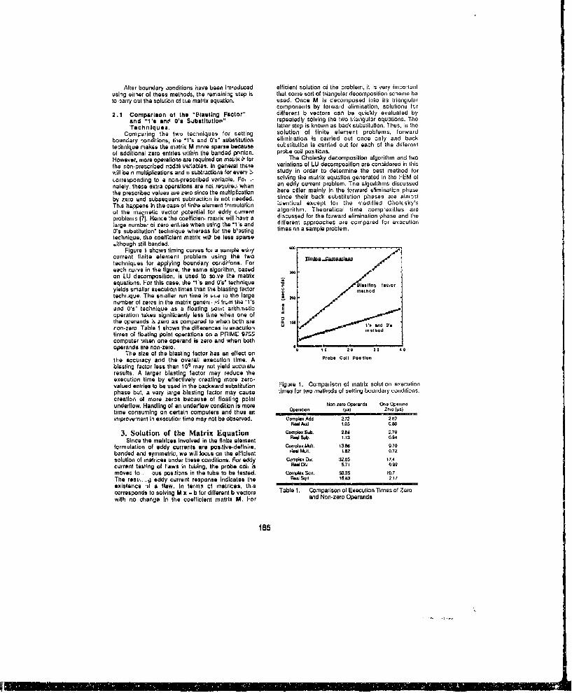
Alter boundary =.onditions have been introduced efficient solution of the problem, it is very importantusing either of these methods, the remaining step is that some sort of triangular decomposition scheme beto carry out the solution of t1he matrix equation. used. Once MI is decomposed into its triangular

components by forward elimination, solutions for2.1 Comparison of the 'Blasting Factor" different b vectors can be quickly evaluated by

and "i's and Q's Subslftutlon" repeatedly solving the two triangular equations. TheTechniques. latter step is known as back substitution. Thus, in the

Comparing the two techniques for setting solution of finite element problems, forwardbounrary =onditions, the "I's and O's' substitution elimination is carried out once only and backtechnique makes the matrix M mnre sparse because substitution is carried out for each of the dilferentof additional zero entries within the banded portion, probe coil positions.However, more operations are required on matix 6, for The Cholesky decomposition algorithm and twothe non-prescribed nodal varlables. In general thsre variations of LU decomposition are considered in thiswill be n multiplications and rn subtractions for every b- study in order to determine the best method forcorresponding to a non-prescribed variable. Fo . solving the matrix equation generated in tire FEM ofnately, these extra operations are noi required when an eddy current problem. The algorithms discussedthe prescribec values are zero since the multiplicatlion here differ mainly in the forward elimination phaseby zero and subsequent subtraction is not needed. since their back substitution phases are almostThis happens in the case of finite element fIrmulation :dentical except for the modified Choltsky'sof the macnetic vector potential for eddy current algorithm. Theoretical time complexities areproblems (7). Hence the oefficien, matrix will have a discussed for the forward elimination phase and thelarge number of zero enties when using the "i's and different approaches are compared for executionO's substitution" technique whereas for the basting times nn a sample problem.technique, the coefficient matrix wi:l be lass sparseatthough still banded.

Figure I shows timing curves for a sample edoycurrent finite element problem using the two Timing campar,..ntechniques for applying boundary conidirons. Foreach curve in the figure. the same algorithm, basedon LU decomposition, is used to solve the matrixequations. For this case, the "I's and 0's technique ~ jeain aeyielos smallar execution times than the blasting factor Xeree ordtecht ique. The smaller run time is oue to the largenumber of zeros in the matrix generi Ad Irom the "i'sand O's" technique as a floaling point arithhrrticoperation takes significantly less time when one of -the operands is zero as compared to when both are ro'non-zero. Table I shows the differences In exKcution U . molhodlimes of floating point operations on a PRIME 9755computer when one operand is zero and when bothoperands are non-zero. I" a 2 30 4,

The size of the blasting factor has an effect onthe accuracy and the overall execution time. A Probe Coll PosIlonblasting factor less than 10s may not yield accurateresults. A larger blasting factor may reduce theexecution time by effectively creating more zero-valued entries to be used in the backward substitution Figure 1. Comparison of matrix solution executionphase but, a very large blasting factor may cause times for two methods of setting boundary conditions.creation of more zeros because of floating pointunderflow. Handling of art underflow condition is more Non zero Operanie Owe Operandtime consuming on certain computers and thus an Operation (1e) Z Irotps)improvement in execution time may not be observed. Comrplex Add 2.72 262

eAl A,• 1.05 see3. Solution of the Matrix Equation Qmax Sub. 2" 2.7 7

Since the metrices Involved in the finite element Raw Sub. 1.13 0.94

formulation of eddy currents are posltfve-deflnire, ConmAeMullt. 13.86 9.70banded and symmetric, we will focus on the efficient POa ,at. S.ez 0.72solution of matrices under these conditions. For eddy Cxraix Dyv. 32.-5 t7.4current testing of flaws In tubing, the probe coil Is PnAW Dlv 5.7l 0Wmoved to ous positions in the tube to be tested. Ctompile SeI. 50.35 1s.7The res,,...q eddy current response indicates the Ree Sqrr 16.3 2.V7existence 'if a flaw, In terms of matrices, thiscorresponds to solving M x - b for different b vectors Table 1. Comparison of Execution Times of Zerowith no change In the coefficient matrix M. For and Non-zero Operands

185

[IRI ql' I1't11 " lrn' H t !r Il H I~rl lllll "M 111 l ~unu',mu l nn nl mw1

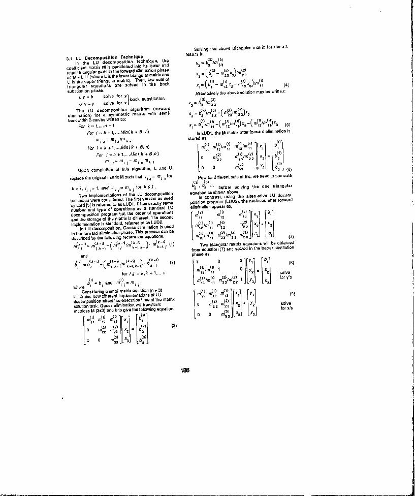
Solving the above trianguIcr matrix to( the x'S

3.1 LU Decomposition technique resul's In,

In the LU decomposition technique, the (3) (3)

coeflicient matrix M is partitioned into its lower a-id 3b 3 In 3 3

upper triangular parts in the forward elimination phase (2) (2) ' (2)

as M - L I t (whare L Is the lower triangular matrix and U2 = • 3 - m2 3 xj~in 2 2

U is the upper triangular matrix), Then, two sets of Nb(t) ' ) (1)x">nn•)

triangular equations are solved In the back x1= -1 22- ta,,) 1- (4)

substitution phase. Alternatively the above solution may be writle.l:

L y =b solve for Y back substitution (3)1 (3)

Ux =y solve for xJ x 3 =b 3 33

The LU decomposition algorithm (torward M /M (2) (M (2)

elimination) for a symmetric matrix with semi- x2= 2 I22- 23 2- 3

bandwidth B can be written as: /) (0 ( • •0)•1x - 3 m(/M W

For k--1,.i-n -1 x= b, /im11 •ni12'1in 1t 2 ( 13 11) ' (5)

For i = k + 1_._Min ( k + B. n) In LUDt, the M matrix after forward elimination is

Mt A n i lIk J A Astored as,

i /T12// 1 1 1312/11 mi

-or jkr + 1. Iik + 8.n (2) (2)21 (2)mFo = m -k o i nin2 2 (km +i , I (=)I

Upon completion of tlis algorithm, L and U 0 0 in1 33 J Lb 3 (6)

replace the original matrix M such that /,,= m, for pow for different sets of h's, we need to comoute(31 (3)

Ad, 1, 1 , and uk,=mk/for k5, . a' 3 ' before solving the one triangular

Two implementations of the LU decomposition equation as shown above.

technique were considered. The first version as used In contrast, using the alterrative LU decom

by Lord (5) is referred to as LUD1. I" has exactly same position program (LUD2). the matrices alter forward

number and type of operations as a standard LU elimination appear as,

decomposition program but the order of operations r (1) (I W inl) Ir [

and the storage of the ntatrix Is different. The second M1 il '112 (2) . rimplementation Is standard, referred to as LUD2. (1) io ) ()

In LU decomposition, Gauss elimination Is used 1 2 2 22

in the forward elimination phase. This process can be mr i 1 m r) m 22 '1 (3)

described by the following recurre;tce equatlons, 13 It 23 m22 33Jl 4J L-2 J

"m k ,k -i- r ) .k- -rI (1) Two trlaroulatr matrix equations will be obtained

i from equatlot (7) and solved In the back t,;bstitution

and phase as,

kI) (k-1) f (A-t (k- 1 0 F1 bI -. I A- /7 A -n (- ()

for IJ = k,k + 1,... a r2 ¶l 2 solve

WI (l) W) (2) 1 y) fa fy's

where Ir,= bl and rrIm -m/2

Considering a small matrix equation (n - 3) (i (l ()r

illustrates how different implementations of LU i 2 in1 I 1

decomposition aftect the execution time of the matrix (2) (2)11 " j solveus()// rjt ..solution task. Gauss eliminatIon wll transform (2 2 2

for x's

matrices M (3x3) and b to give the following equation, (3) 1/x L f

F (n b,) r ,330 1 [ Y1

FN (2) #'t'2 bx I I2(2) I(3)0 22 231 2

o 0 b W

386

This yields. For j=j i-I/= (31 i (

x3 = Y3f 3 3 1(2 2) \1m(2) in 1 1 - )=•: in 5

X2 = Y2 - In2 3 x3) 22 5=)

S(i) Wl .. INX ,- .2X - inl )/to,2 13 3- 11 (10)

The Y1, Y2 andy 3 in above equations are similar rn11 = SORT t.jI fn i(1') (2) (3) k=1 n-sbo b 2 end b3 respectively in case of LUD1.

Thus the only important difference in LUDI and LUD2 4. Comparison of Time Efficienciesis the order of the Iperations. In LUD1, divisi-r by the of Timediagonal elements mi .,ad to be done first as shown in or Algorithusequation (5), whereas in LUD2. division is the last For most computers, floating point operationsoperation. This may have a significant effect in (flops) consume considerably more tirre than integercertain situations. For example, if mil is a complex arithmetic operations. So in analyzing algorithms, allnumber with non-zero real and imaginary parts, and integer operations such as array indexing, loopthe rest of matrx is only real, then LIJD1 ,ill evaluate overhead, etc. are ignored, All three triangularX1 as. decomposition algorithms under cor ideration have a

generaltime complexityof O(n - ) } (where n istheXit b l • 2- (m13mii )X3 length of coetficient matrix M and B3 is its semi-

which inlicates one complex division, two complex bandwidth). Although the time complexities are themultiplications, and two complex additions. On the same for the three algorithms discussed in this paper,other hand, i: :;. will evaluate xs as, they yield different execution times because the type

x= ( t1?1 2 X2 - rn,3 X )lin of operations and the order of operations is different.3) 3 For example, the Cholesky algorithm uses the square

This will involve the sama number of operations but root operation whereas the LU decomposition doesnow only one division is a complex operation and not.everything else is a real operation. Hence LUD2 will Irn analyzing computational floating pointexecute measurably faster in this case. complexity for the Cholesky algorithm, the number

and type of operations in the forward elimination3.2 Cholasky L)ecomposltlon: phase ate:

in Cholesky decomposition. M is decomposed Number ofsqrt. -nsuch that M - LLT where L is a lower triangular matrix. Number of div. B(n -12) .(1,r2)B.For this decompoition to exist, the matrix M must be Number of mull. - B(n/2- 1/61+ 8f((n/2)-1/2) - (t13)63positive alfinite, and this property is guaranteed in Number of add. and sub. . n + B((3/2)n - (2/3))FEM. After performing the decomposition, the two + B2((n/2)-') - (1/3)83triangular equations are solved as, The number of floating point operations in lonwardAM a b starting matrix equation elimination phase of LU decomposition are:Number ofsqrt. -0

e Number of div. - (n-112)B - (112)132LL x a b M ir decomposed (forward slim.) Number of null. _(1/6)( + (n-i/2)B2

- (2/3tB3L y b solve for Y 1 Number of add. and sub. . (116)6B (n-l/2)B

2 - (2o)It33otefr (back substitution ) ithe floating point operations are normalized

'x - y slVi for with respect to "floating point add time", the timeefficiencies can be more comprehensively described.

For different sets of b's corresponding to Table I indicates that complex multiplication takesdFraifferent positton s of ' y currensprobdit about 5 timnes more time than complex addition.

Complex division takes 12 tlines longer and complexnecessary to sclve only the last two triangular square root takes 1S times longer. Using theseequations as L and LT remain the same. numbers as weighting factors in the flops count, the

The Cholesky decomposition algorithm for a time efficlencies can be expressed as follows: forsymmetric matrix with semi-bandwidth B is: Cholesky's decomposition :

20n + 16nR - 7.5B + SnB2 - 9.582 - 2B3for LU dect;,iposition:12nB - 5d + 6nB2 - 9B2 - 4B3Figure 2 shows a comparison of the normalized

floating point operation counts for Cholesky and LUdecompositlon for different n's arid a fixed B. Figure 3compares the two algorithms for a fixed n but different

187

B's. From figures 2 and 3, it is concluded thatCholesky decomposition yields a smaller executiontime, hence, this algorithm is optimized for the finite . UO - ........element analysis of eddy current problems. "

4.1 Modified Choleaky's Algorithm.Typically, the eddy current probe impedance is f .

the desired resuh for an FEM formulation of an eddycurrent NOE problem and this impedance can be .calculated from thie magnetic vector potential withinthe coils. The FEM code may calculate the magneticvedLor potential in every element but when the desired opotentials are available, the algorithm can be -terminated. Using these properties, the Cholesky 105algorithm was modified. The forward elimination phase aof the algorithm remains unchanged but in the back osubstitution phase, the sub-program is terminated assoon as the solution for the last desired field point is . sobtained. 1, 0 iee0 2exe IUQO 4000 4000 sees

Number of Node. ln)4.2 Comparison of Execution Times for a

Sample Problem. Figure 2. Comparison of LU and OholeskyExecution times tor an axisymmetric eddy decomposition floating point operation counts as a

current problem are given in Figure 4. which shows a function of the number of nodes for fixed sam,-comparison of 5 algorithms i.e.. LINPACK [6], LUDI, bandwidth (1-.100),LUD2, Cholesky and mtodified Cholesky on a sample"dillerantial coil in tube" problem. Front this figure, itcan be seen that LUD1, LUD2 and standard Cholaskyhave fairly close execution times. Forward elimination ,is carried out only in position 1. For the remaining , n a.o00probe coil positions, only back substitution is needed.The forward elimination phase of Cholesky is slightly 16e L U DegontooszilSDbetter than LUD2 but the back substitution phase otCholeasky is almost exactly the same as LUD2. Theslope of run time fr-r different positions of the coil is /thus tire same for LLID2 and Choleaky decomposition. tooFor the methods considered here, the modified 0Cholesky routine has the best performance since Itsback substitution phase is the shortest. Overall, an o-improvement of more than 25% was achieved by the a tomodified Cholesky routine over standard Choleaskyand LU decomposition programs.

It should also be noted that pivoting is not ,necessary in the forward elimination phase when 0 20 4 e0 a0 a 1 s sdealing with positive definite rratrives [41. Since we eml-badWldth (B)are dealing with positive definite matrices,considerable saving in time is achieved in thetriangular factorization phase. However, as a check Figure 3. Comparison of LU and Choleskyon the accuracy ol the non-pivoting methods, a decomposition floating point ooaration counts as astandard LINPACK program (sub-routines CG13FA, function of the semi-bandwidth for fixed number ofCGBSL) [61, was used to compare the results since nodes(n-3000)this routine uses pivoting. Thre execution time of theLINPACK routine is about three times largercomparedto a customized Cholesky routine for decomposition considered ifa detail. Two popular methods otand the solution of the matrix equation In this implementing boundary conditions we'o evaluated.example, but all routines maintain the same accuracy Careful comparison of "blasting factor" and the "I'sin the solution, and o's" methods showed that the latter technique

produces a more sparse intermediate matrin and5. Conclusions results ;n smaller execution times for all applicatlions

This study began when lengthy CPU times were of this finite element model,encountered while testing a two-dimensional finite A comparison of different algorithms for triangularolament code for modeling eddy current fDE. In a, decomposition was also undortaken. Theoreticalattempt to improve the time-performance of the code, ana;ys•s and actual run time performance indicatedall aspects of the matrix solution problem were that Cholusky decomposition yields better executi-n

188

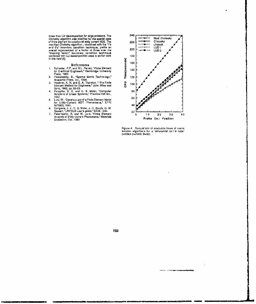
times than LU decomposition for large problems. The 240 - ,Choltsky algorithm was modified for the special Case Mod. Choleky"of finite element formulation of eddy current NDE. The 220 C Cholesky a?modified Cholesky algorithm. combined with the 'l's . '.... .. Linpack ,iand O'V boundar, condition technique, yields an ... LUD 1 *overall improvement of a factor of three over the 200 - LUD 2 ,A"blasting factor" boundary condition tachn;quecombined with LU decomposition used In earlier work 180 Pin this field [5]. "C 160 .•References 0 1

1. Sylvester, P.P. and R.L. Ferrari, 'Finite Element l.for Electrical Engineers," Cambridge Universfy -t 140 dPress, 1983. *E

2. Pissanatzky, S.. *Sparse Matrix Technology,' ; 120Academic Press, Inc., 1984.

3. Huebner, K. H. and E. A. Thornton, " The Finite " 0Element Method for Engineers." John Wiley and 100Sons, 1982, pp. 50-53.

4. Forsythe, G. E. and C. B. Moter, 'Computer 80 oSolutions of Linear Systems,' Prentice-Hall Inc.,1967. 60

5. Lord, W., 'Development of a Finite Element Modelfor Eddy-Currant NDT Phenomena,' EPRINP2026. 1981. 40

6. Dongarra, J., J., 0. B. Moair, J. R. Bunch, G. W.Stewart, "LINPACK user's guide,' SIAM, 1985. 20,

7. Palanisamy, R, and W. Lord, "Finite Element 0 10 20 30 40Analysis of Eddy Current Phenomena," MaterialsEvaluation, Oct. 1980 Probe Coil Position

Figure 4. Comparison of execution times of matrixsolution algortllnis for a "dlfforantlal coil in tube"problem (n-r.400, 0-30).

189

:-Itl = 11':L'-I "9"" lima m nana'- txrininuw mrl+"•Yl- llrdO',I " m szin'PU - f lm-m'i Pr bm"J MU - r• I1 l•I

AN APPROXIMATE (SYMMETRIC) COMBINED FIELDINTEGRAL EQUATION FOR THE ANALYSIS OF SCATTERING

BY CONDUCTING BODIES IN THlE RESONANCE REGION

Lij M~Q. Cn-ia and Afonso M. BarbosaCentro de An~l~ise e Processamento de Sinais and

Departarnento de Engenharia Electrotdcnica e de Computadores,Instituto Superior Tknico, Universidade Tkcnica de Lisboa

Av. Rovisco Pais. 1096 LISBOA CODEX, PORTUGAL

ABSTRACTA nlew integual equation, the Approximiate (Symnnetric) Combined Field Integral

Lqtuatioii, is prese'nted and used to analyze the scattering by coniductmng bodies in thc res-onaime region. It rvsults from ii linear comihinatiun of the Electric Field integral Equationwith the Approxinwitu (Symmectric) Magueichc Field Integral lEquatimn. The tuatrix asso-ciaLedl with this new equation is syinnetric, reducing CPU time and computer meumory.Conidi tioinumesmdsatrn cross sections are presented fur the sphere -and the cube,andl comipared wVithk those obtained ushig the exact integral equation. An analysis of CPU

1. INTRODUCTIONWlieii dcadiijg with the problem of scattering by eoiidudtiug hudius iii the resonaniice

regiol i, thec Combined Field IntLegrad Equationi ( CFIE) Iill (a linear combination of theL~lectric and dhe Magnetic Field Initegral E~quation~s EFIE and MFIE) ensures a uniiqutesolution ior the re~sonant frequencies. Usually, the Mlethod oif Mmunents [2] is used to solvethe CFIt, hjut CPU tine and/or computer memory mzay impose severe limnitations on the(liii~lniiois if the bodiis. TO overcome1 the-Se limuitatfions, several aI)P~rOXi~natioiis have bet-nprIOjIosd (e'.g. (31). Ill orlder to reduce CPU time and memory, the authors have recentlyiirewnmiilan Approximate (Syminet-ric) Magnetic Field Integral Equation (A(S)MFIE) [4),that generates a symmnetric initrix when Giderkin's Method [2) is used. Thisi natfix isgenerated by taking the average of the opposite coefficients (refering to the main (liagolial)of thn MFIE mnatrix, A symnicntric matrix bas two advantages: it needs less computermiemory to be stored, and its factorization time is about hialf of the value for a generalnoii-symninetrie one.

lit thiis conioiunjectioii, a new integral equation is presented, which will be referedas the Approximate (Synonetrie) Combined F'ield hitegral Equation -A(S)CFIE. As it

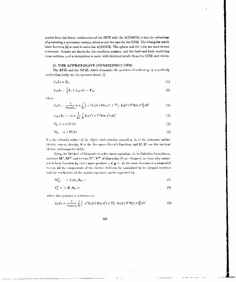
results from the linear combination of the EFIE with the A(S)MFIE, is has the advanltageof generating a symmetric matrix, which is not the case for the CFIE. The triangular patch'Oasis function [5] is used to solve the A(S)CFIE. The sphere and the cube are usedl as testseatterers. Results arc shown for the condition number, and tlu. back and forth scatteringcross sections, and( a comparisoni is mlade with identical results froin the CFIE and others.

II. THlE APPROXIMATE (SYMMETRIC) CFIEThe EFIE and the MFIE, which formulate thv prob leml (If seatterinig by a perfectly

colaudut iii body, arc (inl op~erator' forni) [1]

C.-S= Ft.. (1)

t:'IjS 'Js -1 L:,vjJsq F.,, (2)

9"J.

1 r r.

uj. = 11 ) (5)

F', x I V(r) (6)

S is the closed) siurface. of the object with ,'xterior ilorliila nm, J., is ilw uiiikmowi surfmmct'letriecIrIt dullsity, %p is the fit'e-space Greeni's fuini tiomn, a~mnd E',11' are the inceidenit

vIc'trne a od I inogliet a' fields.

Usiming 01V' het-thd of Nliiil'iints tIo soily, tuesei equationms, jil its Gumdekin folumlluation,

itiI.IicesM'5N ,Mti ' wmmd vI 'to rs V .',V" o f dlimen'Isioni N lWll ,t 1;6dmud ill tTIn) 5of a Slllf~tC('p;1tchl bausis fuiuctiomm bj,, zmiid; iolcr 1 odumct <- f, g >. As the basis filuitiOlm i5 IL tuiling(Iti~d'.'CO Lk, all till' componen('mts If 01ll ('Ictr-il fit-l~l (1111 bV CoIls(lered' ill its :1t('gI'aI el~llitionl

aujd t~ll, I'ocllicil'mlts of till IllI0.17iX 41'(j1GO11 ill lin hVI I'XJM1'551'( bly

-*< U', b,,>()

wliv11, the op-4ratlon is I-wrt ýl I

4 irwn /, [J.'i (r)P(r, r') A- Vs.- Js(r') V'qi(r, r')] Is,(

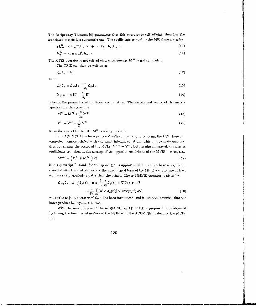
Thc Reciprocity Theorem [6] guarantees that this operator is self-adjoint, therefore theassociated. matrix is a symmetric one. The coefficients related to the MF1E are given by

:--< b./2, b, > + < CM,,b_,b_ > (10)V,ý' = < ii x IV, b,, > (1

The MFIE operator is not self-adjoint, consequently M?! is not symmetric.The CFIE em then be written as

£cJ' = Fe, (12)

where

LCJS = 4,JS + I.EJs (13)

= 1 xii' +ý -E' (14)

u beiig thie praiirwter of the linear combiiiation. The oliLtrix niid vector of the matrixcquation are thex given by

MU=MM + 1 M'" (15)Zo

Vý ý V,~~11 +-ý-" vMt + 'Lv'° (10)

As in the case of tlh-" MFIE, M` is not synimetric.The A(S)MFIE, has been jiojsixe(t. with the purpose of reducing the CPU time wulh

c'omputer mezuory related with the exact integral equation. This a;)j)roximate equationdoes uut change the vector of tile MFIE, V"1 = VA, but, as alrewly stated, the iiatrixcoefficientst are taken as the average of the opposite coefficients of (he MFIE matrix, i.e.,

MSM = (MM + MAC') /2 (17)

(the superscript 'r stands for transposed); this approximation dues iot have a siguificauterror, becaube the contribution|s of the non-integral twrm of the MFIE oprator are at leastouc order of maguitude greater than ii he others. The A(S)MFIIE operator is givwn by

•'ljs I •Js(r) -nx J,(r') f V''(r, r) dIs

+8-F fIinX Js(r')] x V'(r,r')dS' (18)

where the adjoint operator ofCM iit lim been introduced, and it has been assumed that t(einner product is a'syonmtric me.

With the saune purpose of the A(S)MFIE, an A(S)CFIE is proposed. It is obtainedby taking the linear combimntion of the EFIE with the A(S)MFIE, iistead of the MFIE,

i.e

102

£sCJs M £sNIJS + -LO£cEs (19)

or

MSC = MSM ±. a (20)zoleaving the vector unchanged, V"' = V0 . M 5 0 is symmetric (it is a linear combinationof symmetric matrices), and that fact can and will be taken into consideration in theresolution of the matrix equation, in order to achieve the desired reductions.

It is known that the MFIE may experience some difficulties when the object doesnot have a smooth surface. This fact has been confirmed for a cube, mainly when thefrequency of the incident wave is above the first resonance [7]; the solutions from theA(S)MFIE present also a significative error for the cube, in the same conditions, but for asmooth object like the sphere, the solutions from the MFIE and the A(S)MFIE arc almostidentical, eveil in the resonance region [7]. Thus, it is expected that this new A(S)CFIEmay originate solutions with some error, if the object's surface presents edges.

III. NUMERICAL RESULTSR~an's triangular patch basis function has been used to test the A(S)CFIE. The choice

of the linens combination's parameter has been a = 1-. The sphere (radius a) and the cube(side L) were used as scatterers: the sphere was modelled by 96 patches, correspondingto 144 unknowns; two models were mode for the cube, a 96 patch and a 192 patch,corresponding respectively to 144 and 288 unknowns, and designated by M144 and M288.An incident plane wa-e is considered, and its frequency manges between values that cont•xinthe first two resonances of each object (a/, = .437,0.61, L/A = .707, .866); two directionsof incidence are considered for the cube, one normal to a face and another directed to avertex, both with horirontal polarization, Fig.1. The adequate routtines of LINPA CK [8]were used to solve the matrix equations.

(a) normal incidence (b) oblique incidence

Figure 1: Cube peCrpective m according to the direction of incidence.

The condition numbers, CN, associated with the matrices of both the exact andthe "uroximate CFIS', -an he seen in Fig.2. It is confinned that they are both stable

193

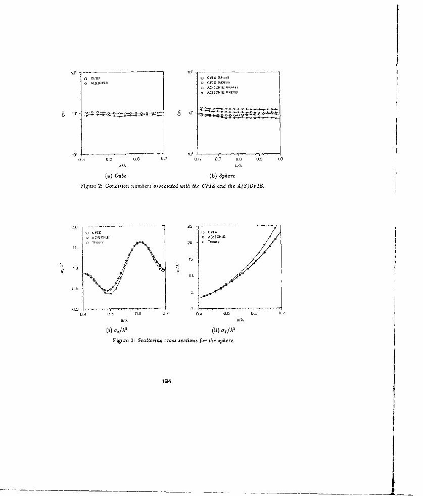
.1A(S)CFJE (M.I44i

10 (S,'I/(M tO

j0 " i 10' . . , . • . • , , • r•• -

0 ,1 0.5 0.6 0.7 0.6 0.7 0.6 0.9 10

a/fl L/

(a) Cube (b) Sphere

Ieigirv 2: C0ndition numbers associated with the CME, and the A(S)CFIE.

U CLE 0 CFIE.7, AC5)CF'1E 1 AISICIIE

1 (1 •l 01 U h ThtOCy

'<10

10.

0.0

0.4 0.5 0.6 0.7 0.4 0.5 0.6 0./

W /\2 (i X

Figure 3: Scattering cross sections for the sphere.

194

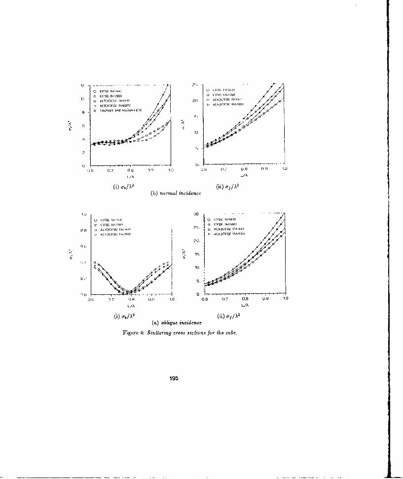
o FI ci M1441(I1lF;val

0 CFIE (MILOOD) C [.It.Im (.160

1 U A10-)CFII6' (Md"4) ?G(1 A(S)CFIE (MDIII6A(S)C1'EIMOO EF08 A(S)CFIK (DM0131

a YRUniDan and mc~iah-N[¶

G to'()a 0q . O01 1-0,

(b) normnalindec

0 VI : 1' 411II20 0 ClE 1114

VICHE ] 0'8 CYUE (W285101

P 1 Aa's. M48)L ( )FF 42

10.

0 ; )7 0U 0q 1 0.33 0.7 0.6J 0.9 1.0U/A LI

(i) a 6 /A2 (ji) aj/A2

()olqeincidence

Figure 4Scteigcross sections for tha cube.

in frequency: CN is almost constant, independently of the model. For eacix model, thecondition number related to the A(S)CFIE is slightly lower than the one of the CFIE (asimilar behavior has been noticed for the MFIE).

The back and forth scattering cross sections, a•b,oj, have been calculated, Fig.3-4. The results for the sphere arc compared with thc theoretical ones; for the cube, acomparison is made for the backscatter for the normal incidence with results from [91 (theonly available case in the literature, as far as we known). The scattering cross sectionsobtained for the sphere by the CFIE and A(S)CFIE are almost totally superimposed,although with discrepancies from the theoretical values. This means that the errors arcdue to the model, and its density, used for the sphecr, and are not a consequence of thealpproxinmtiouns made ill the integral equation. For the cube there are sonic differencesbetween. the results front the approximate and the exact equations, but there are alsodiffe•rences betwelen the two models. For each model, ab seems to he less sensitive to theapproximations thati a1 .

As ftr as the codes are concerned, only the routines for matrix calculation and fac.torization differ in both cquatints1; all the others remnain unchanged, with its CPU timedependiig, at the most, with Nt. The tbin to calculate the A(S)CFIE matrix is about90% (if the corrnjspon(ling time for the CFIE, blith dependling tit NIV; this value is dueto the fact that only the uppeicr triangle of the syneCtr" nmtxrix is stored. The itatrixfactorization ti me, Which Varies with NI, suffers also a reduction of t hle (order of 43% (theordeIr of the nuober of ope.rationts iwe"rs from NW3/3 to W' /0). Hlence tlie total CPU tintefor tht, A(S)CFIU, when crimpared withli the CGIl", ranges from 73% to 50% when N VariesI)atwiti1 100 amd 1(000, which is it sigit lfhiitit rednCt dn.

The comtjuter izctiry necessary to solve both eqiuati•s• dcpelnds mainly Oil tilstoriage of thelt matrix. Thtus, its vallte is aliost halved (from N' to N(N + 1)/2) whenioti,' twsts thw A(S)CFIE intead of Lteh CFIE. Althoughi notwadays comlputvte nmettioiy is notthat important, this is also ;a siguilicant reduction.

IV. CONCLUSIONSAn Appiroximnate (bytimetric) Coutbined Field Integral Equatitn has been presetited.

This new equattin is a linear coutbinatiomi Of the EFIE with the A(S)MFIE, previouslypresented by the authors, origihoating a sytimietric utatrix. The triangular patch basisfunction was used to assess this equation, with the cube and the sphere. As exp)'cted, theatpproximate equationt does not suffer the effects of the resonances, which can be coutliriedby the cotdition number. Good results iune obtained for the scattering cross sectiotis,specially in the case of the sphere, for which the results for the OFIE and the A(S)CFIEare almost coincident; for the cube some discrepaicies are found, but they tend to becomne

196

smaller when the patch density is increased. Therefore, one can say that the A(S)CFLEcan be used instead of the CFIE, for objects with a smooth surface; for nbjects with edgesin its suriace, is appears that some precautions must be used in the application of theapproximate equation. A reduction of about half is achieved in CPU time and computermemory.

REFERENCES[1] Poggio,A.J. and Miller,E.K., "Integral Equation Solutions of Three-Dimensional Scat-tering Problems", in Mittra,R. (cd.), "Computer Techniques for Electromagnetics ", Perg-arson Press, New York, N.Y., 1973[2] Harrington,R.'., "Field Co-npufation by Moment Method", MacMillan Comp., NewYork, N.Y., 1968[3] Chcng,D.K. and Liang,C.-C., "Thinning Technique for Moment-Method Solutions",Proc. IEEE, Vol. 71, No. 2, Feb. 1983, pp. 265-266[4] Corrcia,L.M. mid Barbosa,A.M., "An Approximate (Symncitric) Magnetic Field Inte-gral Equation for the Analysis of Scattering by Conducting Bodies", IEEE AP-S Interna-tional Symposium, Dallas, Texas, May 1990[51 Rao,S.M., Wilton,D.R. amd Glisson,A.W., "Electromagnetic Scattcring by Surfacc. ofArbitrary Shape", IEEE Trvas. Antenws Propagat., Vol. AP-30, No. 3, May 1982, pp.409-418[61 Harrington,R.F., "Timc.J1Urmonic Electromagnetic Fields", McGraw-Hill, New York,N.Y., 1901[7] Correia,L.M., "Scattering by Arbiirary Shapn Conducting ]Bodics in the Rcsonance Re-gion", (in Portuguese) Ph.D. Thesis, Instituto Superior Tinico, Technical University ofLisbon, Lisbon, Dec. 1990[8] Dongnrra,J., Buncli,J.R., Moler,C.B. and Stewart,G.13., "LINPACK Users' Guid,",SIAM Publications, Philadelphia, 1978[9J Yaghjian,A.D. and McGahn•n,ILV., "Broadside Radar Cross Section of the PerfectlyConducting Cube", IEE Tranis. Antemnnm Propagat., Vol. AP-33, No. 3, Mar. 1985, pp.321-329

"197

J

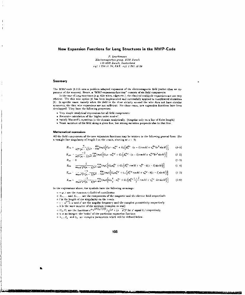
New Expansion Functions for Long Structures in the MMP-Code

P. LeischlmannElcctrovragnelrca group, ET21 Zurich

C11f-6092 Zurich, Si•zrierland#41 1 256 51 58; FAX: 441 1 261 MO 26

Summary

The MMP-code 11.2.31 uses a problem adapted expansion of the electromagnetic field (rather than an ex-parisior' of the sources). Hence, a "'IsMP-expansion-function" consists of six field components.

In the case of long structures (e.g. thin wires, edges etc.), the classica] miultipole expansions are not veryefficient. Tl'e thin wire option 141 has been implemented and successfully applied to complicated situations15). In specific cases, namely when the field in the close vicinity around the wire dots not have circularsynimetry, the thin wire expansions are not sufficient. For those cases, new expansion functions have beendevelopped. They have the following properties:

a Very simple analytical expressions for all field components:. Recursie- calculation of the 'higher order nmodes'.* Satisfy Maxwell's equations in the domain analytically. (Singular only on a line of finite length)v Weak variation of the field along a given line, but strong variation perpendicular to that line.

Mathermatical expressionsAll the field components of the new expansion functions may be written in the following general form: (fora straight line singularity of length I on the z-axis, starting at i.)

Cn - sl o " z-1 ~ - 1fke 2 sinkl)] (J1

2o g ) ,, ( ,P [Go - .s 4 , ( {;. - I)couki + y"'k'e sin k)] (1-2)

H,.: . (0-3)E(n) .... +" . ,(01 cos ki ,• kz - 1)sin k)] (1 4)

" ,.- rs'2•(n - t)!r" sin 1I o fl +

en -- - _--_ %' sin r [Guot 4 +(1 " coskl +, *k - 1) sin l) (1-5)r, . r'2• (n tog1), -CO' . < " .-

E_ ---- ý - (,) - ýE`4 G (/." oski i -.V"- rsin kl)] (1-6)..... c''(n -t)!l-" sin"''' ,o '\':" I --- ,o - .l

In the expressions above, the symbols have the following mcanings:o r, W,: are tire corrimoii cylindrical coordinateso H. and E ... are the components of the magnetic arid the electric field respectivelyo I is the length of the singularity on the 2-axisL, I _.-V1; w and E' are the angular frequency and the complex pcrmittivity respectivelyo k is the wave number of the mediunt (complex or real)o G;. GI are the functions c'0 r tu -"r/V4r0 4 (z - n•') for z' equal 0,1 respectively.o 71 is all integer: the 'order' of the particular expanlsion functiono ., f3. anid -y. are complex pararneteru which will be defined below.

198

IL

•iiFi'l'F i'IiI-~~•"i''l~l i llill iIl- "i1 Iii-ii~il~ llII lllI P't I tlI"lt~l l -[°F<:

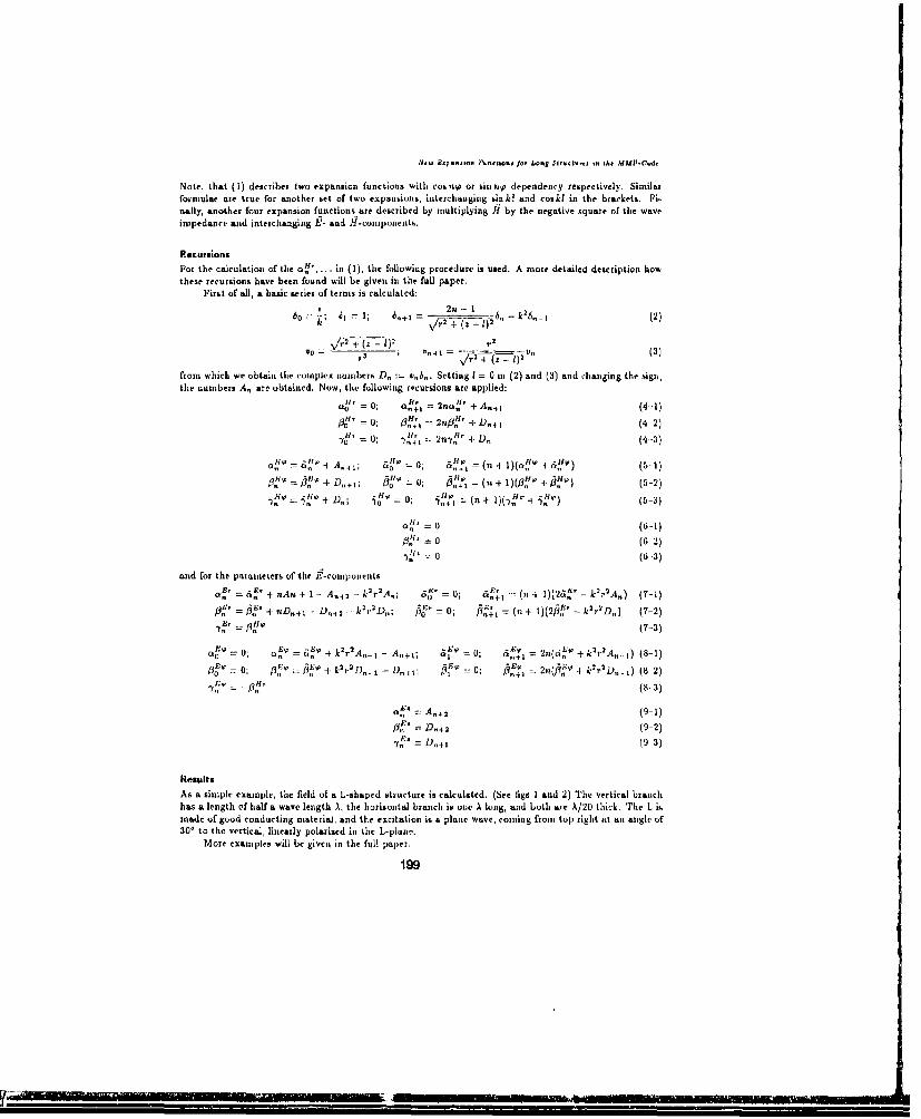
Ni. E.j1 .. o... no Jo. Long Sr-Ienrlnn i- hlt MMP.Cnd.

Note, that (1) describes two expansion functions with cosn•p or sinni dependency respectively. Similarformulae ate true for another set of two expansions, interchanging sinku and coski in the brackets. Fi-nally, another four expansion functions are described by multiplying IH by the negative square of the waveimpedance and interchanging P- and fl-components.

RecursionsFor the calculation of the ok",.. in (1), the following procedure is used. A more detailed description Isowthese recursions have been found will be given in the full paper.

First of all, a basic series of terms is calculated:I 2n - 16o j 1; 6n-- ; -= 06./)+ - (2)

WO - ,.ý + " + - V 2-- - -•),' z (3)y~P) )2

from which we obtain the complex numbers D, := v.6.. Setting I = 0 in (2) and (3) and changing the sign,the numbers A, are obtained. Now, the following recursions are applied:

.H' = 0; a"', = 2no•°' + A.+, (4-)=o' = U; On"+', = /,•1' + D,4 1 (4-2)

-t. : 0; n"' %- 2.0&r + U- (4 3)

A=. A,,,,; 6 0; o,,-1% (n , + l)(.,w+ ei',w) (5-1)

l,,+ = •"+ Dn.+,; 0; - , ,• = (r, + 1)(<1' + Pit) (5-2)on -0-,e_ -eo I,,+ +=( l ) .t ") (5-3)

o•'=0 (si-1)

0 (6 2)"=0 (6 3)

and for the parameters of the E-components

a.' = 4!' + nAn Ii-- A. 2 - k0r'A,; ."= U; "d+" i , i:)(2i ." - k',rA,,) (7-1)=3..'+n.D.j -+ D, D D - k,2r'2D.; j~' =-0; I3,t8 = fn- l)(21.3' - kmr'D,,) (7-2)

-Y!, = Hit (7-3)

a0 =o; - ýE, o = cc A+-1._.-+ A,, 41 ; 51 =0; &',"+ = 2 n ( 6 ýL + kr'A.-._) (8-1)flo3 - 0; / . . , U +- U, 4 j; +re : 0r+ D 2rr(fife - ki cU' D,) (8 2)

-e' ,(8-3)

A 2 - (9-1)D-+i U,4 2 (0-2)

= .41 (9 3)

ResultsAs a simple example, the field of a L-shaped structure is calculated. (See figs I and 2) The vertical branchhas a length of half a wave length A, the horizontal branch is one A lung, and both are A/20 thick The L ismade of good conducting material, and the excitation is a plane wave, coming from top right at an angle of300 to the vertical, linearly polarized in the L-plane.

More examples will be given in the full paper.

199

Nve. O.xnonl. Fcn.ee.o.fo,, iong Sl~i.,'v. I"the MMP-Code

- I t o .

-q w. ./ . - - "P#/PP* . - , Ipp

FiueITfi ' vn of / s I Is s ic

£tir.1 hespet toec hi hi, the trsevii ianle giv thsed stanuetur.ial shmowen ad thr e cirpidcules the iorma cith

poilent of the initaidataeous value of the V~oynLbag vec~lor

ReferencesI]] Cht. Ilaffoer, Th c tietceulized nilltpIC Lip eChnLIYUe for COIIp vjITJio io v ectornomgie ties, Artled, House,

Lumdon, 1990.(21 L. Bozinholt, MAI'..?J) -- A eomputur (Cwlc for rccttimmaytric'i sa~ctctIng based on the GUT1, Dlis.

hETII No. 92215, Zurich, 190U.13] L. Ilotnholot, P. Regli, Ch, ltifisr, 1. Lruchtim, "MMI-3D: A p akag.- for computatio. of 3U , ectro-

magnetic fields ott l'C6 and Wttrkstations," in 6th Annual Retuito of Pivogreis in Applied CovnputottotnilElecirornsogteilics (AGCES), Conference Prtw.adings, (Monterey), Mar. 1V09.

14] P. Leuclitinarin and L. Hoinholt, "Thjni Wi~e Feature for the MMI'.code,' uf functions in the MMI1-i,,etitod," in 6ih Ann~ual Rewiero of P'rogress in Applied Comtputautional Eleeironiagneiacs (ACES), Con-ference Proceedings, (Monterey), Mar. 1990.

[ii) 1. Leuchtmann, "Oin the mtodelling of the electromiagnetic field of LIMC tesL arrangemtents withthe MMPI-code," in Proceedings of ihc 5th Symposium on Electromagnetic Conmpatibsliy, (Zirict),Mar. 1991.

2W0

B-,-. t-' I. S hUPC

Q) Q- / / 11

Figurc. Thueixagaictic firld 11 vf Lli miite stuhctwe a5salo-,it fig- I-K

201

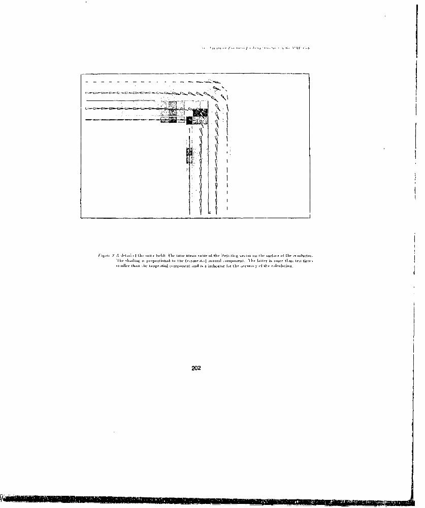
htp : A dI'Iiil I Ilt ....1 1,W Fill wi ,I'mc li -1~aI~V , lii ul ll I'nvIliIng -el, eim m Ir ,url.i,, .. k nlc

202

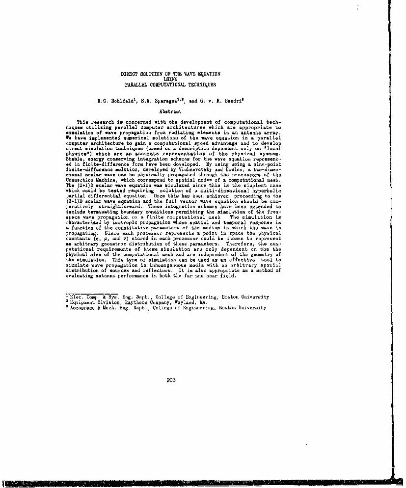
DIRECT SOLUTION OF THE WAVE EQUATIONUSING

PARALLEL COMPUTATIONAL TECHNIQUES

R.U. lohlfuld1 , S.M. Sparagna1 ', and 0. v. B. Sandri'

Abstract

This research is concerned with the development of computational tech-niques utilizing parallel computer architectures which are appropriate tosimulation of wave propagation from radiating elements in an antenna array.We have implemented numerical solutions of the wave equavion in a parallelcomputer architecture to gain a computational speed advantage and to developdirect simulation techniques (based on a description dependent only on 'localphysics') which are an accurate representation of the physical system.Stable, energy conserving integration schemes for the wave equation represent--ed in finite-difference form have been developed. By using using a ninn-pointfinite-difference solution, developed by Vichnevetsky and Bowles, a two-dimen-sional scalar wave can be physically propagated through thu processors of theConnection Machine, which correspond to spatial node.' of a computational mesh.The (2+1)D scalar wave equation was simulated since this is the simplest casewhich could be tested requiring solution of a multi-dimensional hyperbolicpartial differential equation. Once this has been achieved, proceeding to the(3+1)D scalar wave equation and the full vector wave equation should be com-paratively straightforward. These integration schemes have been extended toinclude terminating boundary conditions permitting the simulation of the free-space wave propagation on a finite computational mesh The simulation ischaracterized by isotropic propagation whose spatial and temporal response isa function of the constitutive parameters of the medium in which the wave ispropagating. Since each processor represents a point in space the physicalconstants (c, /, and g) stored in each procesnor could be chosen to representan arbitrary geometric distribution of these parameters. Therefore, the com-putational requirements of these simulation are only dependent on the thephysical size of the computational mesh and are independent of the geometry ofthe simulation. This type of simulation can be used as an effective tool tosimulate wave propagation in inhomogeneous media with an arbitrary spatialdistribution of sources and reflectors. It is also appropriate as a method ofevaluating antenna performance in both the far and near field.

flec. Comp. & Sys. Eng. Dept., College of Engineering, Boston University2 Equipment Division, Raytheon Company, Wayland, MA.£ Aerospace A Much. Eng. Dept., College of Engineering, Boston University

203

I INTRODUCTION reflecting surfaces may be establishedin an arbitrary geometry with spatialresolution equivalent to the resolut-

Finite-difference solutions of ion of the computational grid. Thushyperbolic differential equations in geometricilly complex simulations,two or more dimensions pose a dif- which treat near field and far fieldficult computational problem owinm tt. on an equivalent basis, may be consid-numerical instabilities exhibited by ered without computational penalty;discretised versions of these execution times are effectively indep-equations (Hildebrand 1968; Smith endent of these geometric issues.1985). A suitable approach for solvi- Computational rates in thin UFlop rangeng the wave equation on a spatial grid (1 GFlop = 10 floating point operat-of two dimensions [i.e. the (2+1)D ions per second) are rountinelycase] was developed by Vichnevetsky achieved.and Bowles (1982). In thin approachthe Laplacian operator is approximated In addition to our parallel imple-by an appropriate convex combination mentations, we have als3 further inve-of difference operators involving stigated the numerical properties ofneaurest neighbors and next-to-uearest the Vichnevetaky and Bosles algorithm.neighbors on the computational grid. In particular, we have addressed theThis algorithm was shown to exhibit transient behavior of tle algorithm byisotropic wave propagation, in the Z-transform techniques avd also demon-limit of an infinitely long wave strate that the algoritho is alwaystrain, despite the underlying rectang- energy-conserving at least in theulLr computational grid. mean, and for appropriate choices nf

parameters, conerves energy instanteo-We have demonstrated that this usly (i.e. at each time step).algorithm is suitable for implementat-

ion on a massively parallel computerwith processors arranged o4 a boolean II ANALYSIS Of THE FINITE DIFFERENCEhypercube, specifically on the SOLUTIONS OF THE HOMOGENEOUSConnection Machine-2 (Hillis 1985; (2+.1)D WAVE EUATION USING THEBoghosian 1990). In this implementat- NINE POINT FINITE DIFFERENCEion each point in space is mapped to o ALGORITHMparticular processor (or virtual proc-essor) and construction of the requir- 11.1 - Introductioned finite difference operators of theVichneveteky and Bowles algorithm is In this section we examine a di€c-readily accomplished by interprocessor retised model of the (2+l)D savecommunications on the boolean hyper- equation which ve have implemented oncube. In our development of thin the Connection Machine. Th3s work istechnique, we show that the wave pro- an application and extension of thepagation speed (effectively the square work of Yichnevetsky and Bowles (1982)root of the 'dielectric constant") may which was directed towards thebe assigned independently at each grid solution of the wave equation on apoint (processor) and that sources and computational mesh. We outline here

204

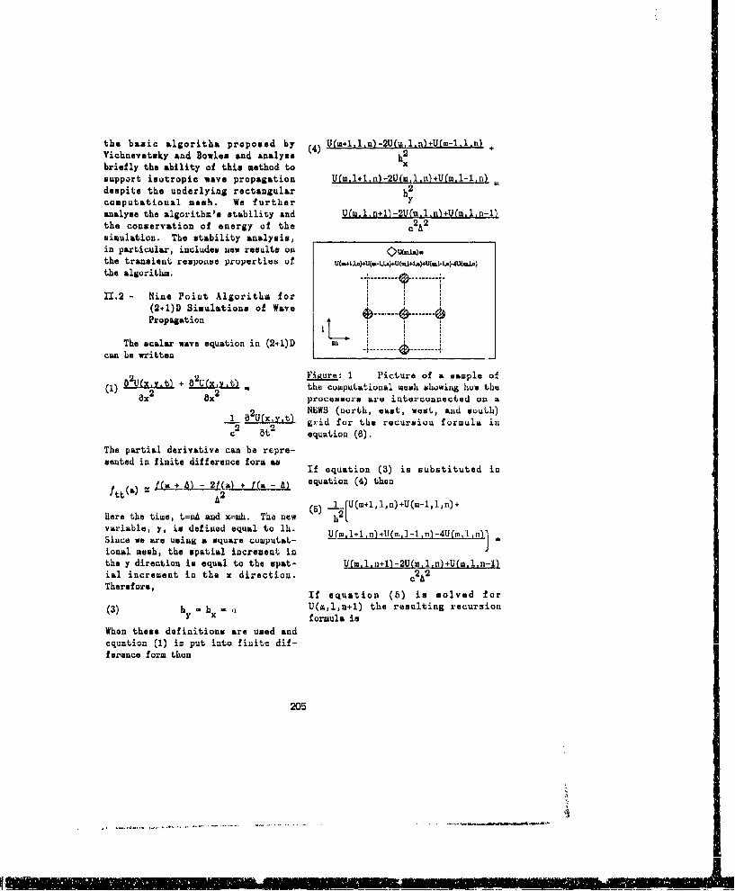
the basic algorithm proposed by (4) U(m+ll.n)-2U(ml.n)PU(m-l.l.nQ +Vichnevetsky and Bowles and analyse 2briefly the ability of this method to xsupport isotropic wave propagation U(m~l+ln)-2U(ml.n•+U(ml-in)despite the underlying rectangular h2computational mesh. We further Yanalyse the algorithm's stability and U(m.l.n+l-2U(m.l.nP+U(m.ln-l)the conservation of energy of the c2 A2

simulation. The stability analysis,in particular, includes new results onthe transient response properties of .the algorithm. ' ........ ----------

11.2 - Nine Point Algorithm for(2+1)D Simulations of WavePropagation

The scalar wave equation in (2+1)D Mcan be written -I .

(1) "2U Y 2tj + VKU "L Laura: 1 Picture of a sawple ofC) 2 = the computational mesh showing how the

Ox2 processors are interconnected on a82U(x. NEWS (north, east, west, and south)

1 ~ ) Bgrid for the recursiou formula inc 2 t 2 equation (6).

The partial derivative can be repre-sented in finite difference form ai If equation (3) in substituted in

!tt(a) a !(a + A) - 2L(a) + f(a - A) equation (4) thenA2

(5) ..-1. fU(m+1,l,n)+U(m-1,ln)+Here the time, t=-A and x--mh. The new h2variable, y, is defined equal to lh. U(w1+ln)+U(m.]ln)_4U(,ni'Since we are using a square computat-ional mesh, the spatial increment inthe y direction is equal to the spat- U(m.l.n+l)-2U(M~lqnj+U(m,l.n-1Iial increment in the x direction. c2 A2

Therefore, If equation (5) is solved for(3) h . hx = U(z,l,n+l) the resulting recursion

y xformula inWhen these definitions are used andequation (1) i= put into finite dif-ference form then

205

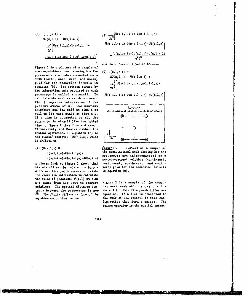
(01)U(m,,+ (8) U(m+,l1+l,n)iU(m+1,l-1,n)+2U(m,l,n) - U(m,l,n-l) + 2h

_ U(ml,n+l)-2U(,m ,znf+U(m,l,n-1)U(ml+1,n)+U(ml-1.n)-4U(m•.,n) c 2A2

and the rccursion equation becomesFigure 1 is a picture of a sample ofthe computational mesh showing how the (9) U(m,l,n+l) =processors are interconnected on a 2U(m,l,n) - U(m,l,n-i) +NEWS (north, east, west, and south)grid for the recursion formula in ,.fU~s+li+i~n•iU~m+l,1-1,n)+equation (6). The pattern formed by 2h2

the information path required by eachprocessor is called a stencil, To U(m-,I+,l )+U(m-1,l-1,n)-4U(m,l,n)calculate the next value at processorP(m,l) requires information of thepresent state of all its nearestneighbors and its self at time n as U(m41.l+ 1) LJ +U.a41.b - 1(m.1.I4.r+U(-.1-J I.n)U(waJ)

well as its past state at time n-i.If a line is connected to all the ........ .points in the stencil like the dotted iline in figure 1 they form a diamond.Viohnevetuky and Bowles dubbed the -------- --------

spatial operations in equation (6) asthe diamond operator, OU(n,l,n), which L---i s d e f i n e d a n l_ --------- --........

(7) OU(m,l,n) 2 Fisurn: 2 Picture of a sample ofU(m+l,l,n)+U(m-l,l,n)+ the computational mesh showing how the

processors are interconnected on aU(m,l+1,n)+U(m,l-l,u)-4U(m,l,n) next-to-nearest neighbor (north-east,

A closer look at figure 1 shows that north-west, south-east, and south-the stencil can be rotated to form a west) grid for the recursion formuladifferent five point recursion relat- in equation (9).ion where the information to calculatethe value of processor P(m,l) at timen+l comes from its next-to-nearest Figure 2 is a sample of the compu-neighbors. The spatial distance dis-- tational mesh which shows how thetance between the processors is now stencil for this five point differencea'. The finite difference form of the equation. If a line is connected toequation would then become the ends of the stencil in this con-

figuration they form a square. Thesquare operator is the spatial operat-

206

_ mL

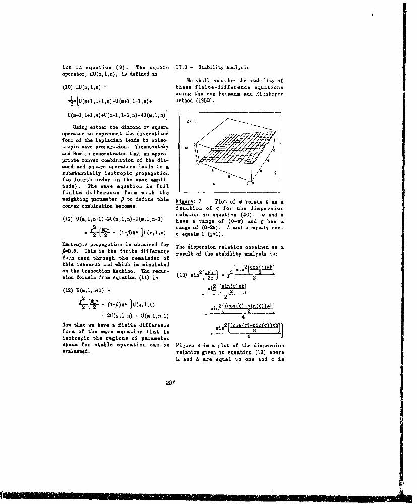
ion in equation (9). The square 11.3 - Stability Analysisoperator, jJ(m,ln), is defined as

We shall consider the stability of(10) CU(mln) these finite-difference equations

using the von Neumann and Richtmyermethod (1SO).

U(m-1,1+l,n)+U(m-l,l-ln)-4U(m,l,n) X

Using either the diamond or squareoperator to reprcosent the discretizedform of the Laplacian leads to aniso-tropic. wave propagation. Vichnevetsky--and Bowlh demonstrated that an appro-priate convex combination of the dia-zond and square operators leads to asubstantially isotropic propagation(to fourth order in the wave ampli-tude). The wave equation in fullfinite differonce form with theweighting parameter P to define this Figure: 3 Plot of w versus X as aconvex combination becomes function of 5 fot the dispersion

relation in tquation (40). w and &(1) U(s,l,n+1)-2U(e,l,n)+U(m,1,n--1) have a range of (0-sr) and ý has a

2 range of (0-2r). A and h equals one."2 L + (l-p)O" U(sln) c equals 1 (X=1).

Isotropic piopagation is obtained for The dispersion relation obtained as aP=0.5. This is the finite difference result of the stability analysis iH:f.%.m used through the remainder ofthis research and which is simulated 2f.E2co UXlon the Connection Machine. The recur- (13) . 2rwy_ 2|via 2-sian formula from equation (11) is () n L2c 2 = X - 2

(12) U(m 1 1,n+l) -i 51 Oii d r10 c 1++ ( l -_ L 2us l t 2

Zý-[ALPs + 2[Ccos(O+sin(C'ýh)

+ 2U(m,l,n) - U(m,l,n-l) + 4

Now that we have a finite difference sin2 (co(O-siii h)furs of the wave equation that is s --. 2isotropic the regions of parameterspace for stable operation can be Figure 3 is a plot of the dispersionevaluated, relation given in equation (13) where

h and A are equal to one and c is

207

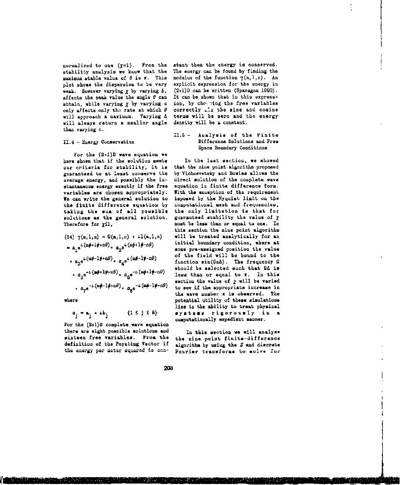
normalized to one (X=I). From the stant then the energy is conserved.stability analysis we know that the The energy can be found by finding themaximum stable value of 0 is r. This modulus of the function 7(m,l,n). Anplot shows the dispersion to be very explicit expression for the energy inweak. However varying X by varying A, (2+i)D can be written (Sparagna 1000).affects the peak value the angle 0 can It can be shown that in this express-attain, while varying X by varying c ion, by che-7ing the free variablesonly affects only the rate at which 0 correctly .Ii the sine and cosinewill approach a maximum. Varying A terms will be zero and the energywill always return a smaller angle density vill be a constant.than varying c.

11.5 - Analysis of the Finite11.4 - Energy Conservation Difference Solutions and Free

Space Boundary ConditionsFor the (2+l)D wave equation we

have shown that if the solution meets In the last section, we showedour criteria for stability, it is that the nine point algorithm proposedguaranteed to at least conserve the by Vichnevetaky and Bowles allows theaverage energy, and possibly the in- direct solution of the complete wavestantaueous energy exactly if the free equation ia finite difference form.variables are chosen appropriately. With the exception of tho requirementWe can write the general solution to imposed by the Nyquist limit on thethe finite difference equation by computational mesh and frequencies,taking the sum of all possible the only limitation is that forsolutions as the general solution. guarauteed stability the value of "Therefore for X.I, must be less than or equal to one. In

this section the nine point algorithm(14) 7(m,l,n) = U(m,l,n) 4 4l(m,l,n) will be treated analytically for an

aaew(MO+lt+nO)+ a2 e A(m+l#_nO) initial boundary condition, where at1 2some pre-assigued position the value

Cm#-lt+n-0) of the field will be bound to the+3e - + a 4 e function sin(fnA). The frequency Q

should be selected such that DA is+ae + ae less than or equal to w. In this

section the value of Z will be varied+ -a 7 m-ltnO)÷ ae-(m-l-n 0 ) to see if the appropriate increase in

the wave number x is observed. Thewhere potential utility of these simulations

lies in the ability to treat physicalaj - aj + &bj {l I j 5 8} systems rigorously in a~ coaputationally expedient manner.

For the (2+1)D complete wave equation

there are eight possible solutions and In this section we will analysesixteen free variables. From the the nine point finite-differencedefinition of the Poynting Vector if algorithm by using the Z and discretethe energy .Pt.• •--quartd i- con- Fourier transforms to solve !or

208

' • |m

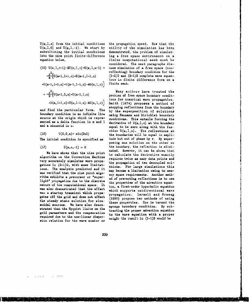
U(m,l,u) from the initial conditions the propagation speed. Now that theU(m,l,O) and U(m,l,-l). We start by utility of the simulation has beensubstituting the initial conditions demonstrated, the problem of simulat-into the nine point finite-difference ing a free space environment on aequation below, finite computational mesh must be

considered. The next paragraphs dis-(15) U(ml,n+l)-2U(m,l,n)+U(m,ln-1) = cuss simulation of a free space (non-

reflecting) boundary condition for the(1+1)D and (2+i)D complete wave equat-ions in finite difference form on a

+U(m-1,l+1,n)+U(m-1,l-1,n)-4U(m,l,n)J finite mesh.

2[ Many authors have treated the2jU(m+l,l~n)+Ucm.l,1,n) problem of free space boundary condit-ions for numerical wave propagation.

+U(m,l+1,n)+U(m,l-1,n)-4U(m,l,n)J Smith (1974) proposes a method ofstopping reflections from the boundary

and find the particular form. The by the superposition of solutionsboundary condition is an infinite line using Neumann and Dirichlet boundarysource at the origin which is repro- conditions. This entails forcing thesented as a delta function in m and 1 derivative of U(m,l,n) at the boundaryand a sinusoid in n. equal to be zero along with the fun-

ction U(m,l,n). The reflections at(15) U(0,0,n)= sin(flnA) the boundaries will be equal in ampli-The initial condition is specified as tude but out of phase by r. By super-

posing one solution on the other at(17) U(m,n,-1) = 0 the boundary, the reflection is elimi-

nated. However, it can be shown thatWe have shown that the nine point to calculate the derivative exactly

algorithm on the Connection Machine require. twice as many data points andvery accurately simulates wave propa- the propagation of two decoupled sol-gation in (2+1)D, with some limitat- utions. For large simulations thisions. The analysis predicted and it uin.Frlresmltostimay become a limitation owing to Mem-was verified that the nine point algo- ory space requirements. Another meth-rithm exhibits a precursor or 'super- od of preventing reflections is to uselight' propagation due to the discrete the properties of the advecticn squat-nature of the computational space. it ion, a first-order hyperbolic equationwas also demonstrated that the effect which supports unidirectional wavewau a startup transient which propa- propagation. Israeli and Oresaggates off the grid and does not effect (1980) propose two methods of usingthe steady state solution for uinu- these properties. One is termed thesoidal sources. We have also demon- sponge boundary condition. By sub-strated that the Nyquist limits on the tracting the proper advection equationgrid parameters and the compensation to the wave equation with a properrequired due to the non-linear disper- W'ljht the result LA (A+!)' Would 'esion relation for the wave number or

209

82U(x =t 1 8%(x.t) In (1+1)D this method is natural and(18 2 2 t 2 the easiest to implement. However, inax 2 a(2+1)D the advection equation is not

- 8U(xNt 1 fxtt linear and cannot be used. This re-Ox € t J quires that the wave be decomposed

into normal and parallel components.Any solution of the form (x-ct) would The normal components will passforce the term in parenthesis to sero through the crossover region and be-and will have no effect on the propa- come a plane wave which is now a one-gation. However, any reflection will dimensional problem and the linearbe on the other characteristic (x+ct) one-dimensional advection equation canand add a first order damping term then be applied. The parallel compon-whose magnitude is controlled hy C. ent will propagate along until it hitsThe other method is to change the the other border, which by design itsolution from the full wave equation is normal to, and can thus be termina-to the proper advection equation at ted in the same fashion.somo predetermined point interior tothe boundary. Since, for X equal to To terminate the propagating waveone, the complete wave equation and in the (2+1)D, the wave must be decom-the advection equation are equivalent posed into its normal and parallelin the proper direction, there is no components at the boundary. When thediscontinuity at the crossover point, proper advection eiquation shown isand when the wave hits the boundary it applied at thn jour boundaries of thewill not reflect. This last method is grid, this is essentially what hap-of the most utility. It will cancel pens. At the crossover point the wavethe wave completely and does not need can be represented by two orthogonal

a dedicated finite region (or termi- components. Since the advection equa-

noting zone) to cancel the wave, as tion can only take information fromcompared to the first method of space and time which is behind it (orIsraeli and Orszag which only damps towards the source), it cannot corruptthe reflection and requires a dedicat- its value from erroneous data in fronted region (which comes at the expense of it. It automatically correctlyof the simulation space). The method calculates the value of the normalof Smith cancels the wave exactly, but component. From this point on, therequires twice as many processors and propagation is along normal linescauses some problems on the deflinition which are completely decoupled fromof the edge of a reflector or dielec- each other. The parallel componenttric zone in the simulation. cannot propagate past the boundary, z

it propagates along the boundary <•.LI

The technique which is used here it hits a perpendicular boundary.is a crossover scheme where the wave Since the boundaries are normal toequation changes from the complete each other the reflection which iswave equation to the appropriate ad- parallel to one boundary willvection equation before the boundary. propagate normal to the other and beThis only requires testing which one terminated. Thu only specialof the boundaries is being approached. condition is how to handle the corners

210

where the boundaries come together. forward and backward difference formsFor this research, they have been in terminating the complete wave equa-assigned arbitrarily to one of the tion in (2+l)D. The reflections areboundaries. The error is small enough largely eliminated from the boundaryas to be unimportant except when very and the interface from the complete tohigh dynamic ranges are required. For the advection equation only causesexample, for nulls in a pattern which small perturbations at the corners,are down greater than 30dB this might which are insignificant and could behave an effect. However, there is no eliminated if the corners are treatedabsorption zone required for this specially. Now that we have developedmethod and the crossover point could the tools to simulate the wave equa-be right at the boundary. Since any tion on a computational mesh more,reflection from the boundary will complicated antennas can be examined.decay as R versus R or the inci-dent wave the effects will be greatlyreduced. Also it takes a long timebefore the cumulative efiects of four III WTLTIPLB BLEMENT SIMULATIONSpoints along the whole surface canreflect enough energy into the systemto be seen. The simulation only needs I11.1 - Introductionto run until all the wave fronts havereached the boundaries. This reduces Up to this point we have onlythe effect below the level of signifi- dealt with simulations of a singlecance. element to develop and validate the

algorithms. The real utility of theseFigure 4 demonstrates the free simulation techniques will be in the

space boundary condition. The ire- modeling of complicated antennaquency of the source is'. The geometries in inhomogeneous media. Inparameters h, A, and c are a~l equal this section we will simulateto one. The source is at processor classical antenna arrays and verifyP(63,63) and the grid is cold-booted that the beam steers and the sidelobesto be 128X128. The time mark is taken generated by the simulation areat n equals 9g. This is enough time correct. Also we can demonstrate thefor the wave to hit the boundary and ability of the simulation to modelto have propagated half way back. The both the far and near field patternscrossover points are at m and 1 equal which is analytically intractable.to 23 and 103. The corners are as-signed to the a direction. A red linedemarcates the crossover region inboth plots. There are no reflectionsand no perceivable impact on the fieldin this linear display.

We have demonstrated the effect-ivOneso and the advantages of theadvection equations using Newton's

211

nm unin momdqL J' m.

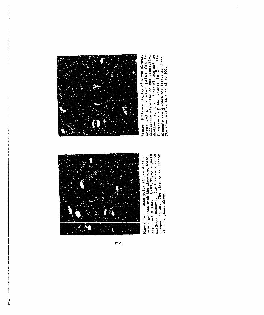
oj

4) 4. d 4 1

o

. 41 ) - 0 # ,

-4 q1 -6 c

Wq4 41

ol 1 d- Q4-.44; ;

4)

424

(~41C 42)1 4

-. a

111.2 - Phased Arrays in Homogeneous in the first simulation. The centerMedia of the two, two-dipole elements are

lOX apart where all the elements areon a line. The C.M. is configured to

The first antenna simulation is a a processor dimension of 512X512 andtwo element array witk elements spaced the geometric center is at processoreight processors (2) apart. The P(255,255). The first dipole pair isparameters are X=cA/h=l, h=l, and A=l. at processors P(171,255) andThe frequency of the source is (0) • P(179,255). The other pair is atand the source is centered at processors P(331,255) and P(330,255).processor P(63,63) on a 128X128 pro- All the elements are driven in phase.cessor configuration. One source is The frequency and all the parametersat processor P(63,67) and the other is are the same as 5- figure (5). Ifat processor P(63,89). Both sources figure 7b is compared to theare driven in phase with an amplitude calculated antenna pattern for the twoof one. Figure 5 is the linear element interferometer in Kraus anddisplay of the two element array with Carver it is seen that the peaks anda time mark at n equals 100. nulls in the pattern are identical and

the calculated and simulation patternsThe next simulation shown in fig- are identical. The goesetric pattern

ures 0[a,b] is with an eight element of cancellations in the field•inomial array. All the elements are intensity obtained is a strong2apart and the C.M. is configured verification of the validity of thiswith a 255X250 processor dimension, wave propagation simulation.The geometric center of the array isat processor P(127,127) and the ele- We have demonstrated with thesements are spaced eight processors simulations that the nine pointapart and driven in phase with a fre- algorithm accurately representsquency of . The weights on the physical antenna in homogeneous media.elements are (1-7-21-35-35-21-7-1) in The sidelobe predictions and theorder from one end of the array to the antenna gain patterns all agree withother. All the other parameters are the classical theory. In addition,the same as the last simulations ex- the structure in the near field iscept the time mark in figure (4) is at also shown where classical arrayn equal to 200. The binomial array theory approximations (treated in thehas the property of having no minor limit of Fraunhofer diffraction) breaklobes in the continuum case as shown down.in Kraus and Carver (1973). This isalso a case in the simulation towithin 20dB of the main lobe which isa good verification of the algorithm.

The last simulation shown infigures 7[a,b] is a simple two elementinterferometer. The 3imple elementwill be built from two dipoles modeled

213

I

cd.4 0PU0 Ad

Ci 4

P. bo 42 iH 0 20

4O.H n2 0 H

0) 0 0

14,

rda)W . Q 11 rHW--1. dsal .

'40-0 4 PH

OH 4 1

v4' a I- 0.0)o4 -H44wca

0 44 'd 0) .43 Q~Qt'

A2F1

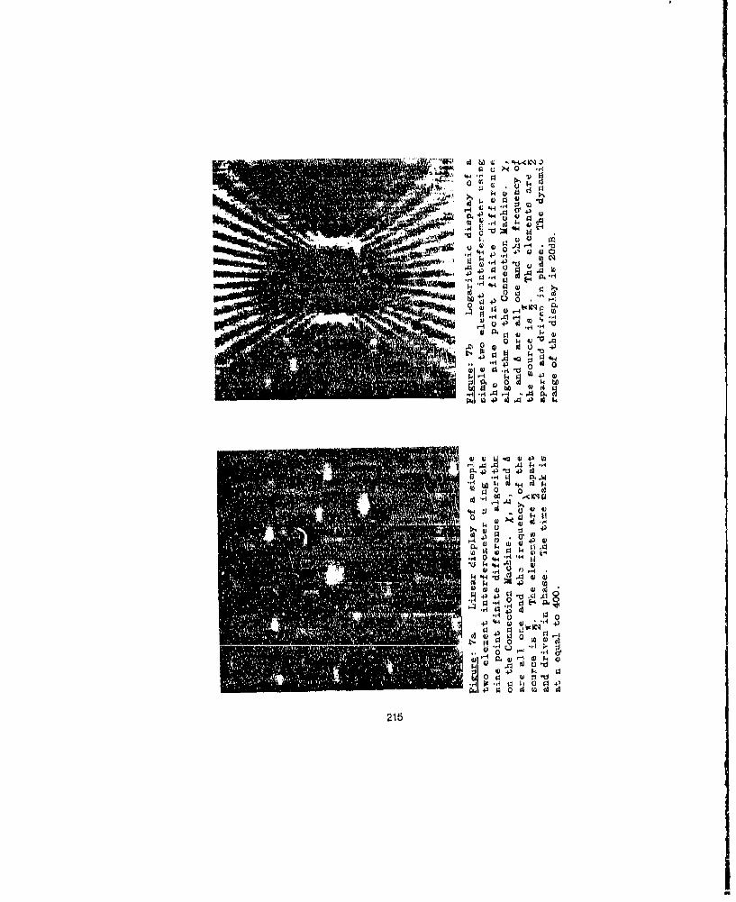
El- A 4 E-4

0

4)H 0 &, H )

0

LI 4-) . _H " A 4 V. C)4 "'

Fl rb

215

Up to this point all the attention Figure (8) shows the array withhas been on the accuracy of the simu- all the elements driven in phase and alationa and how well they represent conducting cylinder in the beam 128the physical system. Not mentioned up processors from the source with ato this point is the computational radius of 16 processors. Theadvantago and speed gained doing thene simulation shows the reflections offsimulations on a massively parallel the cylinder and the diffraction ofarchitecture like the Connection the wave around the object. TheMachine. One observation illustrating interference pattern set up by thethis advantage is the operation count object distorts the beam in therequired to do one time step of the neighborhood of the reflector. Thesimulation. Presently the (non-opt.- rxt simulation, shown in figure g,mized) code requires 14 parallel oper- has a dielectric cylinder in the beamations to advance the simulation one which is steered at 45 degroes. Thetime step. For a bl2Xt12 grid this elements are all driven out of phasewould require = 3.7 million operations with each other for this beam steer.on a serial machine. The execution The center oi the object is nottime for the simulation program is directly in the beam to illustrateeffectively independent of the distri- Snell's law as the beam is bent as itbution of sources and (as demonstrated propagates across the dielectricin the next section) of the properties boundary. The dielectric conutant (C)of the surrounding medium, is set to 10 and is compensated using

the program by the dispersion relation111.3 - P 11 as e d Ar r a y a i q to get the continuum wave number. The

Inhomogenuous Media continuum wave number is 3.160. Asthe beam passes through thedielectrLic, the wave is focused due to

All of th, work up to this point the shape of the object. In figure ghus been to develop a simulation tool the field intensity is very high onthat would allow complex antenna simu- the far side of the cylinder. Figureslationu in an inhomogeneous media. In lOa[,bJ show the simulation of auhis section the simulations have backed array. 2 behind the array is aconducting cylinders, dielectric cyl- ground plane where the field is forcediuders, and conducting planes sepa- bo sero. The ground plane is arately and in combination. The absor- wavelength longer than the array obing boundary condition is applied in each end. By placing the reflectorall the simulations and as in the last behind th4 array the reflection willsection the crossover point is alvays constructively, interfere with theten processors from the boundary. All signal propagating away from thethe simulations wi l use an eight reflector. All the elements areelement array with 2 spacing and a driven in phase in this simulation sofrequency (0) of .2 The grid that the beam will be orienteddimensions for all the simulations are broadside to the array.612X812 and the array is centered atprocessor P(255,256).

216

A ' 0 oA3 A A 0 "D .,4 4-7 +3 E 4"4 1; 43

o 4~

A- 4 v

iA4'9 4

14 4:J)0. 0m 4-o cl

.. 4 -4 A

..4$Sg A $-a

k~ U

34>40): 14 u~ 0$

% 0 1A 4 _I-I g 1 4A 4

* 4 r4.rq 14 d4$

. g 0J ;,3 Q M~

-VM 1'd 4) O0.. " 4 4

0 u

Km m mrum.OLS p k'~

0 JF4

12 0 0 aI

4:1 40 HAd

0r 13 v3A *00

s1o *xM4.0(0 r-

0 p-H 41 44

1 0 q6 qdrob *. A

4203

.,4 " a 4

430

fl 2j d 0

2184

The last simulation shown in fig-ure l1[a,b] is a combination of all We have demonstrated the spatialthree features of these simulations. isotropy, stability, and energyThe antenna is a backed array with a canueryation of the solution. It wasreflecting cylinder and a dielectric shown that the nine point algorithmcylinder in the beam with a 45 degree proposed by Vichnevetuky and Bowlesbeam steer. This simulation was per- conserves energy always in the timeformed to teat the algorithm in a average sense, and for some choices ofcomplicated medium in which both ref- parameters energy is conservedlectore and dielectrics are present. instantaneously. Waves propagateThis simulation represents a problm isotropically by t in algorithm forwhich Is analytically intractable yet, XP1 and for j , despite theit takes the tame computational re- underlying rectangular computationalsources as t'ie single element and is meah. The implementation of thisrigorous in the calculation of the algorithm on the Connection Machine,field, along with the free space boundary

termination developed from theadvection equation, was shown to be a

IV CON(LUSIONs powerful and accurate computationaltool for simulating wave propagationfrom a radiating element for very

The objectives of this paper were complicated geometries which could notto develop stable numerical solutions be solved analytically.of the hyperbolic wave equation withradiating sources which take advantage We have also demonstrated thatof the large scale parallelism of the inhomogeneous media, i.e. varyingConnection Machine. These solutions 'dielectric constant', and arbitrarymust depend only on a local physical distributions of reflectors may hecoordinate patch to take advautage of accommodated in these wave propagationone of the natural modes of inter- simulations. In particular theprocessor communication in the constitutive properties if the medium"0 onnection Machine, and more may be specified independently at eachimportantly to accurately represent point o0 the simulation apace (eachthe continuum wave equation which in virtual processor) without signifi-local and treats all spatial locations cantly increasing the run time of theequivalently. Also the algorithm must simulation. This development is ofbe iuaensitive to the simulation great importance in view of thegeometry and require minimal difficulty of obtaining exact,assumptions on the nature of the analytic solutious of ware propagationsources. A free space boundary in lahomogeneous media and the limitedsolution was also required due to the ranges of validity of variousphysical memory bounds of the approximation schemes (e.g. Born,Connection Machine. This free space WSHJ, Rayleigh approximation, etc.).boundary condition permits us tosimulate free space radiation problems In closing, future research willin machines of finite sit. be directed towards the four

219

"_4L0 0

.,4 4 )

L 4.,q 4 H0 0)

... 4W ~-4 41 Q oI¶

12 ) A44 4 4 ) *a t.

q 43 f44 -00'4 A4 91 Eb4 1

a 0 0. ?

(010

22 " 0 o

(A 44,1 0,W4,

dimensional [(3+1)D] problem and thento the vector wave equation, including Smith, GD.; 'Numerical Soluticos oftensor dielectric functions. We have Partial Differential Equations'; Nowdeveloped the tools and have proven York: Oxford University Press, 1985the algorith% so that the transitionto the next etep should not offer any Smith, W.D. (1974); 'A Nonreflectinginsuperable conceptual problems. Plane Boundary for Wave Propagation

Problems'; Journal of ComputationalPhysics, Vol: 16, pp. 492-603

Sparagna, S.M.; 'Waye PropagationWe would like to acknowledge the using Parallel Computational

invaluable help supplied by Robert Technigues'; Boston, Massachusetts:Putnam of Thinking Machine Inc. with Ph.D. Thesis, Buxton University, 1990the simulatione done on the ConnectionMachine. We would also like to thank Vichoavetsky, R., Bowles, J.B.;the Raytheon Corporwtion which funded 'Fourier Analysis of Numericalthe majority of this research through Approximations of Hyperbolican Aldo R. Miccioli Scholarship. Equations'; Philadelphia: Society for

Industrial and Applied Mathematics,1982

von Neumann, J., Lichtmyer, R.D.(1950); 'A Method for the Numerical

Boghosian, B.M. (1990); COomputational Calculation of Hydrodynamic Shocks';Physics on the Connection Machine'; J. Appl. Phym., Vol: 21, pp. 232-237Computers in Physic., Vol: 4, No: 1,,pp. 14-33

Hildebrand, F.D.; 'Finite-DifferenceEquations and Simulations'; EnglewoodCliffs, New Jersey: Prentice-HBll,198

Hillis, D. C.,; 'The ConnectionMachine'; Cambridge, Massachusetts:MIT Press, 1985

Israeli, M., Oreoas, S.A. (1980);'Approximation of Radiation BoundaryConditions'; J. Coup. Phys., Vol: 41,pp. 115-136

Kraum, J.D., Carver, K.R.;"Blectromgnestics'; New-York: McGraw-Hill Inc., 1973

221

I

• ,

ON USING A CONCEPTUAL MODEL FOR DERIVING THE ELECTROMAGNETIC

STATISTICS OF COMPLEX CAVITIES

1' H. Lehman* and E. K. Miller**

*Consultant, 3200 Carlisle NE, Albuquerque, NM, USA**Los Alamos National Laboratory, USA

ABST.ACIIt Is shown that thu components of the electromagnetic field amolitudes in a perfectlyconducting cavity with a complex shape are distributed according to a normal (Gaussian)distribution. The proof Is obtained by Invoking a virtual-cavity model which Is used forexpanding the field quantities In a complete set of orthogonal elgenvectors whoseamplitudes are shown to have a normal distribution. This result Is Independent of theeigenvalue (mode number) and the shape of the cavity, requiring only that the shape of thecavity be complex. The proof that the components of the field amplitudes have a normaldistribution follows immediately. Extensiors of the theory to cavities with losses andsources is straightforward.

INR•. UC.TIOFor many years thure has been considerable Intere'ut In the statistical properties ofelectromagnetic fields. This Interest has been fostered not only by an Inability ofaccurately predicting electromagnetic responses In complex environments, but also by thedifficulty of Interpreting and extracting usable Information from experimental data. To datealmost all attempts to characterize electromagnetic Interactions statistically have beenmade using experimental data. The success of these efforts has been mixed. Without anya priori knowledge of distribution fumntions, analysts are forced to assunme functional formsfor the distributions using a limited number of data samples. Some oi these assumeddistributions seem to work well for certain types of problems but not for all, i.e., as theyInvariably have a limited range of validity.

If statistical techniques are to be useful for characterizing electromagnetic Interactions,then one should be able to establish their range of validity using Maxwell's equationsdirectly, It this Is not possible, then statistical techniques will not have an Important placein electromagnetics because the statistics of each problem would require Independentdetermination, The number of sample:; required to do this Is prohibitive from ameasurement point of view.

"To begin a discussion concerning the statistical nature of electromagnetic fields, it isappropriate to quote from Beran and Parrent [E]:

"it should be made clear Immediately that discussions of coherence orincoherence or partial coherence (statistics) need never enter a treatise on,dsiclal aleuiro, nagnetlc theory. In tlhi classical . lctrom,-agnetlc theory,governed by Maxwell's equations, one assumes that the electric field andmagnetic field are measurable functions of position and time. In principle,one can, if one chooses, follow In detail the Instantaneous variations of theelectric or magnetic field, no matter how Intricate the boundary conditions.

2.2.,2

In many cases, however, the procedure is extremely difficult and may, infact, mask importnt physical effects ... The situation is analogous to theone arising in classical statistical mechanics. Although in principle it Ispossible to follow in detail the dynamics of the system, It often proves muchmore useful to provide a statistical description."

It is clear that statistical electromagnetics can be nothing more than a theory whichdescribes the behavior of the average values of appropriate functions of theelectromagnetic field. These functions must in some sense be measurable and forexample could include all powers of the three components of both the electric andmagnetic field; all powers of the electromagnetic field power density; or all the powers ofthe differences of the above functions when they are measured at different locations ordifferent times (spatial and temporal correlation functions).

The explicit purpose for constructing these average values Is to provide the capability forextracting useful and usable Information from measured data for those cases where theIntricate and complex nature of the measured fields masks this information. An additionalcoi slderatlon Includes those cases where small variations In the system topology or smallchanges In the excitation produce large changes In the response at specific locationswithin the system, or when small changes In the measurement location produce similarlylarge changes In the response. From a purely deterministic point of view, these situationsgive rise to a problem set which Is currently riot resolvable.

If Information is to be extracted from the average values of the appropriate functions of theelectromagnetic fields, It Is Immediately obvious that the amount of such Information will Insome sense be a strong function of the number of the average values that are determined.This fact will certainly limit the utility of an average-value theory since there Is in principlean infinite number of average values; for example, all powers of the x-component of theelectric filed. This limitation can be eliminated If It can be shown, a prlorlfrcm the physicsof the problem, that the average values of some of these functions are related to eachother through well-defined relationships. This, of course, Is found to be true In elementarystatistical mechanics. We can Imagine the state of statistical mechanics if the velocitydistribution of molecules In a box was not Maxwellian and was Instead a function of theshape ot the box. Determining the relationships between different average values Is anImportant step In any physics-based statistical theory. If these relationships exist andexhibit certain properties, then probability densities or distributions can be assigned to thefield variables and the transition from an "average-value theory" to a "statistical theory" Iscomplete.

For electromagnetIcs, no such average-value relationships had been demonstrated toexist. The deriv.ition of these relationships and their range of validity are the subject of thispaper. Our approach utilizes a conceptual, moment-method type model, from which thestatistical properties of Interest are derived, but without ever explicitly setting up or solvingthe moment-method model itself.

MATHEMATICAL PRELIMINARIESConslder a cavity wlth volumG V which is source ,a and it bounded by . perfectly,,conducting surface S of arbitrary shape. It Is well known [Schiff (2)], that the electric fieldEF(rt) and the vector potential Att) In the volume V, upon separating the space and timevariations, can be expanded In a complete set of real vector functions .k([) or

223

k.+oE(1,t) - k k •(O)P k, (1)

A(.,t) - ,k•(gqk(t) (2)

The cartesian components of the vector functions must satisfy the second-order waveequation

V2Uk.W •Uk,(r) - 0, (3)

where s denotes the cartesian coordinate, x,y,z. The vector function must also satisfyV'UkG) - 0 (4)

since there are no sources present. Also, the tangential components of the electric fieldand the vector potential must vanish on the surface S, so that

nxUdr))l, s - 0 (5)where n is a unit vector normal to the surface, Using Eqs, (3-5) and with the help ofGreen's theorem It can be shown that the uk and Uk, are orthogonal to each other or

v k'U.dv - bk',k (6)In the usual convention, k Is an eigenvalue and u Is an elgenvector.

Denoting spatial-average values by < n, then the average value of any function W(t. overthe volume V of the cavity is given by

-vW Ldv<W>

fvdvor

<W>- V '3W(L)dv (8)

For the problem defined in this section, the quantities whose average values are of Interestare functions of the electric field. These functions are the three electric field componentsEx, Ey, Ez and all of their higher-order powers. These average values are defined by

rE >- VIEft,)dv;s - x,y,7 and m - 0,1,2,... (9)In order to evaluate the averages defined in Eq. (9), it Is obvious from Eq. (1) that It will benecessmy to evaluate the average values of all the powers (Uk,s)m of the components ofthe elgenvector, or

<(Uk, l)'ý> - V Pfv(uUk,s)mdv (10)

for all k and for all in. This Is a monumental (essentially Impossible) task, unless theIntegrals given by Eq. (10) are straightforward and can be shown to be simply related forvarious values of m. In the next sections, we outline un approach that shows this Is indeedthe case for complex cavities and In fact, It Is shown that the Integrals are Independent of kand that they are just the moments of a normal probability density.ACONCEPTUA APPRQACH FOR FINDING THE EIGENVECTORSIt is well known that exact solutions of the vector Helmholtz Eq. (3) are only possible for a

224

very few canonically-shaped cavities. Thus, for cavities of arbitrary shape, no attempt ismade to find exact solutions. Instead, we seek approximate expressions for theeigenvectors. These approximate expressions are developed by expanding theeigenvectars in a set of entire-domain basis functions (EDBF). Although the choice of theEDBF is somewhat arbitrary, we choose basis functions that satisfy Eqs. (3) and (4), andselect the expi- .ion coefficients so that Eq. (5) is also satisfied.

Before outlining our approach for choosing the EDBF, we make the following observation.For cavities having canonical shapes, the cavity surfaces are defined by relationships ofthe form ý, = Ca (a = 1,2,3) where i, is a generalized coordinate and Ca is a constant.For cavities of arbitrary shape, it will not be possible to define a surface by setting one ormore of the generalized coordinates equal to a constant, Instead, we know that theeigenvector solutions must in some sense be a function of all of the dimensions of thecavity, i.e., the s.-'paration of variables that works for canonical geometries no longer holds.Our choice of basis functions must reflect this dependency.

We develop the EDBF by construction. To do this, we implement the following step6:1) We specify a cartesian coordinate system for the space occupied by

the volume V.2) We assume that the eigenvalue k of a specific eigenvector Uk(r) is

known.3) We discretize the volume V into a large number N of cubes eachhaving a volume AV = AxAyAz = (&x) 3 such that kAx ,12 and V = NAV.4) We project the six surface elements AS = (Ax)2 of each cube onto the

walls of the cavity.5) From the surface projections for each oube, we construct arectangular cavity formed by the intersections of the six orthogonal planescontaining each of the AS, The n'th rectangular cavity constructed from then'th cube has dimensions Xn, Yn, Zn and the location of one of its corners

with respect to the origin 0 of the coordinate system defined in step 1 isgiven by Ln. We refer to these rectangular cavities as "virtual cavities.6) For each virtual cavity, we choose the set of three integers (I,m,p)which yields the best approximation to the expression

2, x 2

7) We write the eigenvector Uk(L;n) for the n'ttli virtual cavity assumingthat each virtual cavity has perfectly conducting walls and that thecomponents of the elgenvalues (i.e., the virtual cavity eigenvalue) are givenby kx(n) = nl/Xn, ky(n) = nim/Yn, k (n) = nP/Zn.

8) We chonse the resulting .•(rn) to be the EDBF and write the solutionfor the eigenvuctor UkA asN

•tk(L) = nU r;n). (12)

In the next section, we implemeni the above steps and show that an elgenvector can bewritten as a sum over a large number of standing waves. The wavdvuctor on associatedwith the n'th standing wave is a function of Xn, Yn, Zn, i.e., the dimensions of the n'th virtuaicavity. Thus, the eigenvector given by Eq. (12) not only satisfies the second-order waveequation (3), the constraint equation (4) and the boundary condition (5), but it is also afunction of all of the dimensions that define the surface that bounds the volume V of spaceoccupied by the cavity.

225

REPR_3ENTING THE EIGENVECTOR SOLUTIONSWe now proceed to develop the expressions for the eigenvector aolutions using theapproach as outlined in the previous section. We begin by defining a coordinate systemhaving 0 as its origin and having an arbitrary orientation.

The aigenvalues k (i.e., the resonance frequencies) as wr" as the eigenvectors for anarbitrarily shaped cavity can be determined by using numerical techniques such aslinite-element (FEM) or finite-difference (FDM) methods. A Hamiltonian approach, beingbased on energy relationships, would be a logical starting point for using FEM while awave-equation formulation would be a natural starting point for using FDM. Eithernumerical solution method eventually would lead to matrix equations of the form

AXXux + Ayxux + Azxux + k2 ux = 0Axyuy + Ayyl-y + Azyuy + k2 uy = 0 (13)Axzuz + Ayzuz + AzzUz + k2 uz = 0

where the A's are NxN matrices, the u's are NdI vectors, and because. of reciprocity, AxyAx, etc.

The eigenvalues k are solutions ofdetlAxx + Ayx + Azx + k21 = 0,

or detlAxy + Ayy + Azy + k2 l = 0, (14)or detlAxz + Ayz + Azz + k2 l = 0.

Similarly, the eigenvectors are solutions of Eq. (13) for specific values of k consistent withthe constraint V*L~k = 0. In this fcrmulation, we are not interested in the exact, or for thatmatter explicit, values of k and Iuk, It suffices to know that they exis÷ and, in principle, theycould be determined, i.e., they are deterministic quantities. At ' point, we assume thatall of the k's are known although we do not care what their values are.

Proceeding with the prescription for determining the EDBF, we partition the volume V ofthe cavity into N cubes with each having a volume AV = (Ax) 3 such that V = NAV and kAx ,1. Next, we construct the N virtual cavities resulting from the intersections of the six planesdefined by projecting each surface element AS of a cube onto the surface of tie cavity.The parameters that define the nMh virtual cavity are thie position vector En of one of thecorners of the n'th virtual cavity with respect to the origin 0 of the coordinates of the cavityand the dimensions Xn, Yn, 41 of the virtual cavity. These parameters are deterministicalthough they are not unique since the orientation of the coordinate system is arbitrary.Note that the set of parameters that define the N virtual cavities define all of the dimensionsof the cavity.

The next. step in developing the EDBF is selecting the set of three integers l,m,p in Eq. (11)such that the best approximation is achieved. We proceed by assuming that the walls ofeach virtual cavity are parfectly conducting although, in fact, they are conducting only atthe location of each ASn. Consistent with the above assumption, then the eigenvectorUg(r;n) for the n'th virtual cavity can be written as

UQ(E;n) -= QxUxncoS[gx(x - Xn)]sin[Qy(y - yn)]sin[.Iz(z -Zn)]+ eyUynsin[,-x(x - Xn)]cOS[oy(y - yn)]sin[Qz(Z -Zn)]

226

+ ezUynsir[Qx(x - Xn)]sin[Qy(Y - Yn)]COS[2z(Z -Zn)](15)

where x = nl'/Xn, Uy = nm'/Yn, Qz = nP'/Zn, t - t2[(l'/Xn) 2 + (m'/Yn) 2 + (p'/Zn)2 ] and V',mi, p' are integers of which at least two must be different from zero. The amplitudes of theeigenvector components are not independent, but are related by the divergence conditionEq. (4) which yields

Uxn~2x + Uyngy + Uzn~ z = 0 (16)

If we consider 2j to be a vector with components Qx, Qy, yz, Eq. (16) is the condition thatUn = (UxnUyn,Uzn) is perpendicular to jQ. There are, in general two linear independentvectors that satisfy this condition, conesponding to two possible polarizations. Thesevectors may be chosen arbitrarily as long as they are not coplanar. Therefore, there isanother solution for the eigenvector which we denote by WV(;n). It is identical in form toEq. (15) with the Uxn, Uyn, UJzn replaced by Wxn, Wyn, Win such that 9-,Un = Q.'WnQn',Wn = 0, i.e. they form an orthogonal set of vectors.

Now according to the prescription for constructing the EDBF outlined above, we set I = 1,m' = m, p' = p, so that L2P - k2 and define Uk(.;n) and Wk([;n) to be these functions. Thus,the eigenvector Vk([ is given by

N

144r) - 9{ xnC°s[kgxX - x.)]sinLkyn(y - yn)]sin[k,.(z - z,)]

+ eyUyreinlkxn(X - xn)]cos[kygy - yn)]sin[kzn(z - Zn)]

+ eusin~kxn(X -xn)]sin[kly(y -Yn)1CoS[kz2 z - zn)]}(17)

with a similar expression for Wk(rW, and where kxn = nItXn, 1S'n = -nm/Yn, kzn = nP/Z-n, andk2 = R2 [(I/Xn)2 + (mjYn)2 + (p/Zn)2 ]. We note that the three Integers l,m,p that are used todefine kxn, kyn, kzn for the n'th EDBF are not necessarily the same set of three integersl',m',p' used to define the n-prime'th EDBF Thus, although

2 2 2ý 2j r12 R2 + 21 z2 j2 x2 , Y2.n n• n=C- n ..•-

and2- 2_ 2kn kn. k2

in general, I' . I, m , i, p, p, and Xn, 7, Xn, Yn' - Yn,- Z ' Zn, so thatn, , I, kn.

After further manipulation, the eigenvectors can be shown to have the form [Lehman andMiller (3)]

4N 4N

UkU) - -UnCOSU~n' (L - rn)J and W41[) - F-WncOslhn'(r - r)

(18)where )in-An = Mn'.dUn = tn-J..n = 0 and 'j~n = k2 as before but in addition we haveUn',n = An-Zn = \P for all n. The summation is from n = 1 to 4N because eachelgenvector can be written as the sum of eight plane waves or four standing waves, as

227

--- - - -. ..

shown here.

The Innerproduct Ulk14,k needed for evaluating the morments of the field components cannow be put In the form

4N 4N!W0) Uk(r) - 'UQ s[S(t - 1flCOC6&(I - 101,Y

4N if UL r U n + 4N8[~ 4N ~) + 16 1 .-

4N 4N+'+ • rc ["n -) m' 6 m - &' W1.

- H11(b) 1 H1(2) + H3 W) (19)where the identity cosAcosB - (112)[cos(A - B) + cos(A + B)] has been used.

Integrating the first term HI over the volume V of the cavity yields4N

I,-.. Hi([)dv -. .LLJIUdv - U

(20)which Is dependent only on the volume of the cavity and independent of its shape.Because of Eq. (6), we also conclude that U2 = 2/NV.

On the other hand, the values of the Integral over both H2 and H3 will depend on theshape of the cavity, or

12 'f H2(rdv - ý(SHAPE), (21)

13=fvH3()dv - 6(S HAPE). (22)The only exceptiors to Eqs. (21) and (22) will occur when the surface of the cavity hasbeen generated by some random process, for example, v random walk. For this case, 'hephases given by Jsn'Ln rmid hm-'rn will be random variabies and the standing waves willadd Incoherently so that both 12 and 13 vanish, ie. 12 = 13 f.t O

In general, the magnitude of both 12 and 13 will be strong functions of the regularity of theshape of the cavity and will have maximum values for cavities with regular shapes, Forexample, for a right.-circular rectangular cavity, the phases will be highly correlated and l2and 13 will each be on the order of Ii. For cavities having very irregular shapes, forexample the cockpit of an aircraft, the phases will be very weakly correlated and the valuesof both 12 and 13 will be very close to zero.

With this In mind, a complex cavity can be defined:"•A complex cavity is a cavity for which both 12 -It and 13 0I1 are true.,

Of course there Is no a priori way to test a cavity's oomplexity. The only way to proceed Isto assume that a cavity Is complex based on experience with other cavities and then use228

I

experimental data to justify the assumption. Any other approach must addruss the detailsof each cavity separately.

Using the above results along with the definition of a complex cavity, It Is now possible toestimate the average values of the amplitudes of the elganvectors, the results of which aregiven next.

RESULTS FROM THE AVERAGE-VALUE EVALUATIONPerforming the required Integrations to obtain the average values dWfined by <.c(U.Lk)n>

fV(Uk'uk)n'dv Is reasonably straightforward, but mathematically tedious. Therefore, weonly summarize the results here, the derivation of which is described in more detailelsewhere [Lehman and Miller (3)].

<(uk,s)n(uk,s')'l> = <(Uk,s)n><(uksu)m> for ' , s;<(wk,s (wk~s,)m, <(wk,.)n><(wk,s,)m> for s' , a:

<(uk,s)n(wk,s,)m> = 0 for all s, s', n and m:<(Uk,s)n>, - <(Wk,;S)n>,

-13-5.7.. (n -1)"n for n even,- 0 for n odd: s - x,y,z;

<,(k.Uk)n> -, <(Ak.Y.k)n>- 1,3-5.7... (2 -1) (2n 1 1)u2.n;

andu . %I(ý_Vj(23)

DERIVATION OF THE_ NDORMAL DISTRIBUI IONFrom elementary probability theory, it Is well-known that the expectation value E{x} of therandom variable x Is given by

E~x} =fxt,(x~dxwhere fx(x) Is the density (function) of the random variable x. If one considers anotherrandom variable y which is a known function of the random variable x, y = gtx), then theexpectation value E{y} of the random variable y is given [Papoulls (4)] by either

E{y= - vfy(y)dy (24)

or

E{y} - fg(x)fx(x)dx (25)where fy(y) Is the probability density of y. if it is ausuiiid that position vector r Io a randomvariable, then Ito probability density function fr(O) Is given by

fr(.- IN, if C L V andfr() - 0, otherwise.

Since the elgenvector uk,s Is a function of r, Its expectation value E{Uk,} Is given by [usingEq. (25)]

E{uk~s} =fuk,stfr(r)dv229

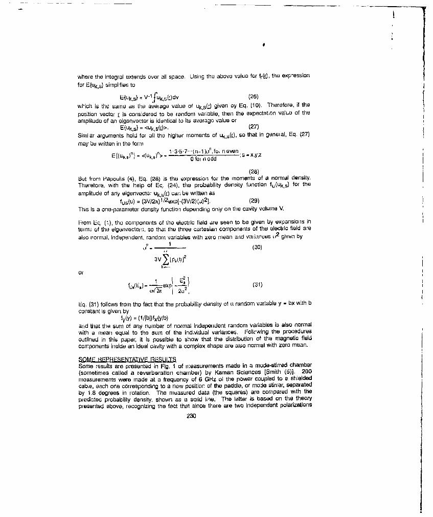
where the integral extends over all space. Using the above value for fr(r), the expressionfor E{uk,s} simplifies to

Eiuk,s} = v-lfuk,PL)dv (26)

which is the same as t0e aveiage value of uk,s( given by Eq. (10). Therefore, if theposition vector r is considered to be random variable, then the expectation value of theamplitude of an elgenventor is identical to its average value or

E{Uks} = <Uk,s()>. (27)Similar arguments hold for all the higher moments of uk,s(r), so that in geneial, Eq. (27)may be written in the form

E[uk.X -n -<(Uk,.)n>- 1- 3-5'7-(n-1o n'Xf°"oi n-ev- i ; S - x,y,z0 foi n ordd

(28)But from Papoulls (4), Eq. (28) is the ex•pression for the moments of a normal density.Theretore, with the help of Eq. (24), the probability density function fu(uks) for the

amplitude of any eigenvector uks(r) can be written asfus(U) = (3V/2n)l/ 2 exp[-(3V/2)(u)2 ]. (29)

This Is a one-parameter density function depending only on the cavity volume V.

From Eq. (1), tho components of the electric field are seen to be given by expansions Interms of the elgenvectorý;, so that the three cartesian components of the electric field arealso normal, Independent, random variablue with zero mean and wvaiances 412 given by

2 (30)

3V • [pk[t)]'

or

U19 2 - (31)

Eq. (31) follows from the fact that the probabiliky density of a random variable y bx with bconstant is given by

fy(y) = (1/IbI)fx(y/b)and that the sum of any number of normal Independent random variables Is also normalwith a mean equal to the sum of the Individual variances. Follcwlng the proceduresoutlined in this paper, it Is possible to show that the distribution of the magnetic fieldcomponents inside an ideal cavity with a complex shape are also normal with zero mean.

SOME REPRESENTATIVE RESULTSSome results are presented In Fig. 1 of measurements made In a mode-stirred chamber(sometimes called a reverberation chamber) by Kaman Sciences [Smith (5)]. 200measurements were made at a frequency of 6 GHz ei the power coupled to a. shieldedcable, each one corresponding to a new position of the paddle, or mode stirrer, separatedby 1.8 degrees in rotation. The measured data (the squares) are compared with thepredicted probability density, shown as a solid line. The latter Is based on the theorypresented above, recognizing the fact that since there are two independent polarizations

230

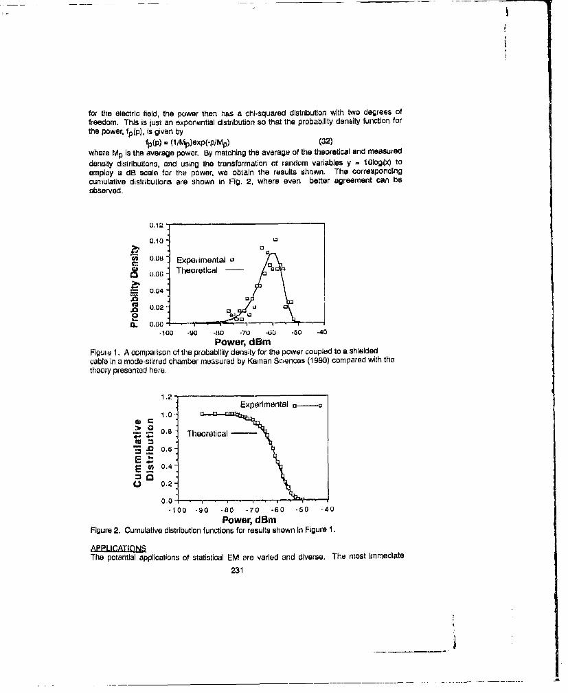
I

for the electric field, the power then has a chi-squared distribution with two degrees offreedom. This is just an exponential distribution so that the probability density function forthe power, fp(p), Is given by

fp(p) - (1/Mp)exp(-p/Mp) (32)where Mp Is the average power. By matching the average of the theoretical and measureddensity distributions, and using the transformation of random variables y - 10log(x) toemploy a dB scale for the power, we obtain the results shown. The correspondingcumulative distributions are shown In Fig. 2, where even better agreement can beobserved.

0.12

0.10

U3' 0.08 Expekimental uU.060 Theoretical -

0.04

.U2 Uu0.02

1. 0.00 .

-100 -00 -80 .70 -60 -50 -40

Power, dBmFigure 1. A comparison of the probability density for the power coupled to a shieldedcable In a mode-stirred chamber measured by Kainan Sciences (1990) compared with thetheory presented here.

1.2-Experimental 3--a

1.0o i n

.> .2 0.8 Theoretical

0.6-E•E W 0.4

C) 0.2

-100 -90 -80 -70 -60 -50 -40Power, dBm

Figure 2. Cumulative distribution functions for results shown In Figure 1.

A•_PJEL[IQThe potential applications of statistical EM are varied and diverse. The most immediate

231

I

application would be to reverberation-chamber testing, which motivated the developmentpresented here, Als9o a potential application Is the characterization of far radiation andscattered fields. Both are dlscussad briefly below.

Reverberation-Chamber Testi~gThe most Immedlat,; utilization of the theory is to all aspects of

reverberation-chamber testing, tor which several benefits could be realized. Some areasof application could Include: 1) chamber design, 2) data Interpretation, 3) data storage, 4)characterizing the response of Equipment Under Test (EUT), and 5) test design. Inaddition, a rigorous theoretical description of a of reverberation chamber's EM responsewould certainly give such measurements a firmer analytical basis.

The capability to predict the field distributions Inside a reverberation chamber wouldnaturally lead to the optimum design for a given application. In particular, questionsregarding source locations, chamber Q, source polarization, chamber dimensions, andnumbers of sources needed can be addressed In the design phase.

Having access to the statistical properties of the EM fields would greatly simplify theInterpretatlun of the measured data obtained from reverberation chamber tests. Ratherthan trying to force the Interpretation of the data Into deterministic descriptions, developingprobabilistic statements about their nature would be easier and much more meaningful.For example, quantifying the probability that the lield lovel In the test volume can exceed acertain level Is then possible.

Since most of the distributions encountered In reverberatlon chamber tests will befunctions of two parameters, the number of parameters needed to describe the results are"four, at most. These are the expected value and standard deviation, the number of tunerpositior,, and the frequency.

Using statistical techniques to characterize EUT responses has many advantages. If theequipment Is normally located In a complex cavity, for example an aircraft bay,reverberation chamber tests are a better simulation of the actual environment than areanechoic chamber tests. For this case, the only meaningful question Is 'given the averagevalue of the field or power density Inside the cavity, what Is the probability that the EUT willexperience a failure?" Using the statistical Interpretation of data obtained fromreverberation chamber tests, this question can be answered. This would not be possibleusing deterministic Interpretations of data from either reverberation or anechoic chambertests.

If the EUT Is an entire small missile for example, normally located in free space, then theadvantages of using statistical techniques are not as obvious. However, again the onlymeaningful question that can be asked Is a probabilistic one, namely, 'given a peakelectric field value, what Is the probability that the EUT will experience a fallure?" I tiesource of the uncertainty associated with this problem is the angle of Incidence andpolarization of the Incident plane wave with respect to the orientation of the EUT. Formany EUTs, the solid angle of Interest will be 4n steradlans; foi others It will be much less,particularly when only near nose-on angles of Incidernci are Important. For this problem, itIs now feasible to adjust the reverberation chamber field levels to account for the externalgain of the EUT. This procedure is possible because the functional tofen of thereverberation chamber fields are now known, and the external response of the EUT can becalculated for both plane wave and chamber fields. Since the two test methods can be

232

made equivalent, the reverberation tests are preferred, for obvious reasons.

"The statistical description of reverberation charmbers can also be used to optimize the testprocedures. For example, the data quality is proportional to the number of tuner positions.Using statistical techniques, It Is now possible to quantify the data quality (confidence) interms of this number. As a result, for many tests, the number of tuner positions could besignificantly reduced, with a corresponding reduction In the time required for themeasurement and in the amount of data that needs to be collected and processed.

In summary, a statistical description of electromagnetic responses In complex cavities hasmany advantages over deterministic descriptions. Not only does it provide a simple yetrigorous theory, but also it provides results in a form that Is easily related to systemperformance.

Far-ELeld Radiation and ScattgringThe statistics of far fields are also of Intereat. In those cases where the radiation

pattern of a large antenna or the monostatic or bistatic field scattered from a large body Isneeded, the numerical or experimental determination of the patteins. can be expensive.This is especially so when a numerical model is solved using an Iterative technique, Inwhich case the solution must be repeated for each angle of Incidence. The possibility ofstatistically characterizing the iar field from a limited number of field samples using thetheory prenentod here could substantially reduce the cost of determining neededparameters such as the expected value of the field, its variance, the most probable peakfield, etc.

Because the current modes on the Interior or exterior of a perfectly conducting,zero-thickness envelope have the same spatial variations, we expect that the analysisperformed above for cavity fluids alsould be applicable to the statistics of far radiated andscattered fluilds as well. Absuming this to be the case, It seems reasonable to expect thatthuir statistics as a function of angle should be described by the same distributions. Thispossible application represents an area of future research.

EER NCES1. Baran, M. J. and G. B. Parrent, 1964, Theorf oofP JgiaICoherence, Prentice-Hall,Englewood Cliffs, NJ.2. Schiff, Leonard I. (1955), Quantum Mechanics, McGraw-Hill Book Company, Inc., NewYork.3. Lehman and Miller (1990), *The Statistics of Electromagnetic Fields In ComplexEnvironments,' to be submi'ted for publication.4. Papoulls, A. (19651, Probability. Random Variables, and Stochastic Procese,McGraw-Hill Book Company, New York.5. Smith, Robert (19.90), Private Communication, Kaman Sciences, Colorado Springs,CO.

233

SESSION 6 - "FINITE ELEMENT AND FINITE DIFFERENCE

FREQUENCY DOMAIN SOLUTIONS

Moderator: Glenn Crabtree

SOLUTION OIF MULTI-MEDIA WAVE PROPAGATION AND SCATTERINGI'ROBLUMS USING FINITE ELEMENTS

E. Thomas Moyer Jr.Associate Piofcssor of Engineering and Applied Science

The George Washington University, SEAS/CMEEWashington, DC 20052

(202) )94-5970 ; E-Maih moyer sparko.gwu.edu

Lrvwin SchroedeiResearch Mathematician, Applied Mathenatics Division

David Taylor Research CenterBethesda, Maryland 20084

(301) 227-1b60

ABSTRACT

Problems involving horizontal and vertical electric dipole sources in a stratified mediuenvironment with vaiying clectrical conductivity and permitivity is studied. A curl-curl I1field formulation is employed which imposes the correct continuity on the field components.The U field components we calculated using Legendre Polynomial smoothing without globalaveraugig which gives rise to the correct discontinuities in the E lield vector at matemialboundaries.

Speitifc problems are examined which focuu on sources located in sea water with drivingfrequencies between 1 liz. and 100 hz. Solutions lor both the sea water and air modeled asinfinite half spac-s are compared with ailabhc refereuce solutions. Thae effects of Uinitethickness layers of ice are considered. In addition, the configuration with a finite depth ofsea water with a half space of sea bottom is also explored. Boundary conditions for thetmuncation of infinite domains are exlplored. Local expansion boundary conditions whichmunifest in high order dampers are compacd with infinite elements.

Results of the analysis are compared with available analytic solutions and are in goodagreement. In addition, the wave-8uide characteristics due to media discontinuities andinterface propagation are correctly predicted by the auialyses. H-laving established die validityand accuiacy of the formulation, extensions and difficulties vssociatd with moure complicatedsources and scattering objects in the doniain are explored.

234

i.

Ijnite Elcment Solutions to the Mass-TerisrFoirm of the Glnzburg-Ijndanu Puations

Kenneth G. HerdGE Corporate Research and Development, P.O. Box 8

Schenectady, NY 12301

George TheodossiouRcnsselaer Polytechnic Institute, Ipartment of Computer Science

Troy, NY 12180-3590

The spatial variation of the magnetic field mid supercurrents In anisotropic, type-lIsuperconductors has been successfully described using a mass-tensor form of thephcnomenological Ginzburg-Landau equaiionsl. Closed-form solutions to these equationzhave been previuusly derived in a limited range near the upper critical field of asupcrconductur by using a linearized form 2 .3 . General solutions to the nonlinearanisotrupic problem require a numerical approach. A finite element solution to the mass-tensor fonri of the Ginzburg-Landau equations in two dliriensltns is przsented herein. TheGalcrkin weighted residual approach is used to kormu!ate the clement matrices. T'h"eperiodicity of the flux lattice in type I1 superconductors allows the solution domain to belimited to a single supetuw'rert vortex cell.

Introudction

The discovery of superconductivity in layered ceramic maturials, such as Y-Ba-Cu-0, hasled to a renewed interest in the phenomenology of superconductivity in anisotroplcsystems. All known copper-oxide superconductors Wxe highly anisotropic; tha. is, theircritical current density and critical field strength vary depending upon the diretion of thetransport cunrnt or the applied magnetic field with respect to the crystal axes. Thischaracteristic is distinct from that of metallic superconductors. which generally behaveisotropically.

Strongly anisotropic superconductors have been studied previously. The influence of theanisotropy on the superconducting properties has been successfully described by theintroduction of a mass-tensor Into the well knuown Ginzburg-Landeu (G-L) equations. Ageneral solution to the anIsouopic 04.- equations produces a complete characte-ization ofthe equilibrium free energy density, the reversible magnetution, the flux lattice structure,

235

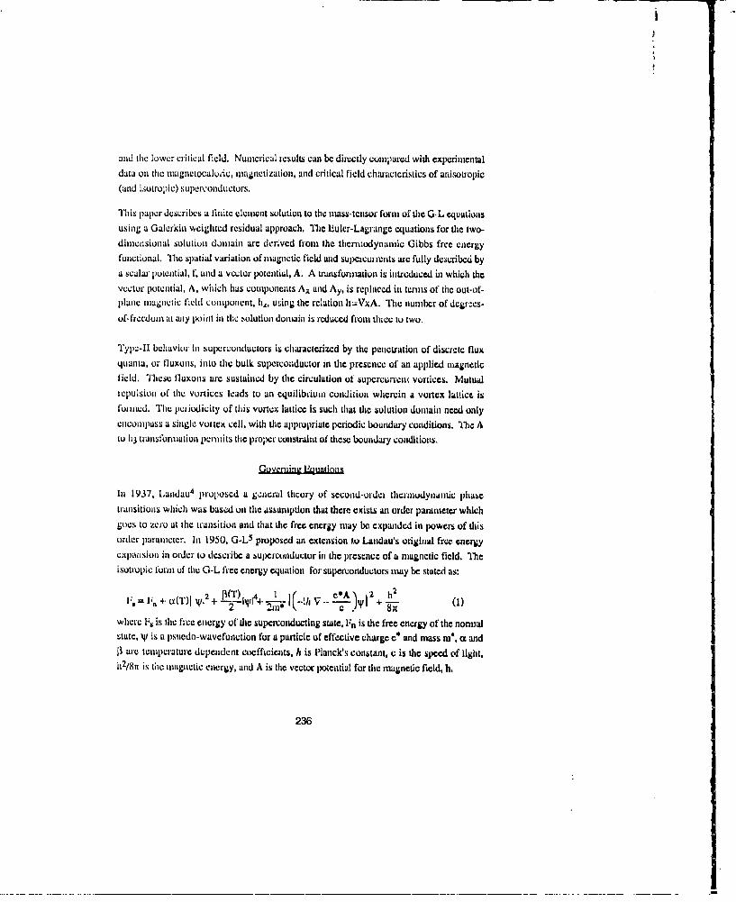
and tle lower ci-itical field. Numerical results can be directly compared with experinmntaldata on tihe nagnetocaloic, magnetization, and critical field characteristics of anisou'opic(and isotropic) superconductors.

This paper desc;ribes a finite element solution to the mass-tcnsor form of tie G-L equationsusing a Galerkin weighted residual approach, Thoe Luler-Lagrange equations for the two-dimensional solution domain are derived from the therrnodynamnic Gibbs free energyfunctional. Vlic spatial variation of magnetic field and supercursents arc fully dcscribed bya scalar potential, f, and a vector potential, A. A tnsfonmation is inlxcduced in which thevector potential, A. which has components A; and Ay, is replaced in tenns of the out-of-plane magnetic field component, hl,. using the relation hlgVxA. The number of deg-eus-of- freedomi at any point in the solution domain is reduced from three to two.

Tylic-1l behavior in superconductors is characterized by the penetration of discrete fluxquanta, or fluxons, into the bulk superconductor in die presence of an applied mra1gncticfield, These fluxons are sustained by the circulation of supercurrent vortices. Mutualrepulsion of the vortices leads to an equilibrium condition wherein a vortex lattice isfurned. The pCriudicity of this vortex lattice Is such that the solution domain need onlycncompass a single vow tex cell, with the appropriate periodic boundary conditions. Thc Ato h3 transformation permits the proper constraint of dhesc boundary conditions.

CovenfinL' Euatlons

In 1937, Landau4 proposed a general theory of second-order thernodynamic phasetransitions which was base on the assamption that there exists an order parameter whichgoes to zero at the transition and that the free energy may be expandcd in powers of thisorder parametcr. In 1950. G-L 5 proposed an extension to Landau's original free energyexpansion in order to describe a -uperconduwtor In the presence of a magnetic field. Theisotropic tomrn of the G-L free energy equation for superconductors may be stated as:

S:~, 2 tT+ P) 4 1 t' e*AS I I h2

v, = F,, + X(T)I V12 -- 1-- , - ll C I + -in (1)where F, is tile free energy of the superconductlng state, F1n is the free energy of the normal;tare, V is a psuedo-wavcfu action for a particle of effective charge c* and mass tsi, a andji arc temperature dependent coefficients, h is Planck's constant, c is the speed of light,h2/8tr is the mnagnetic energy, and A is tht vector potential for the magnetic field, h.

236

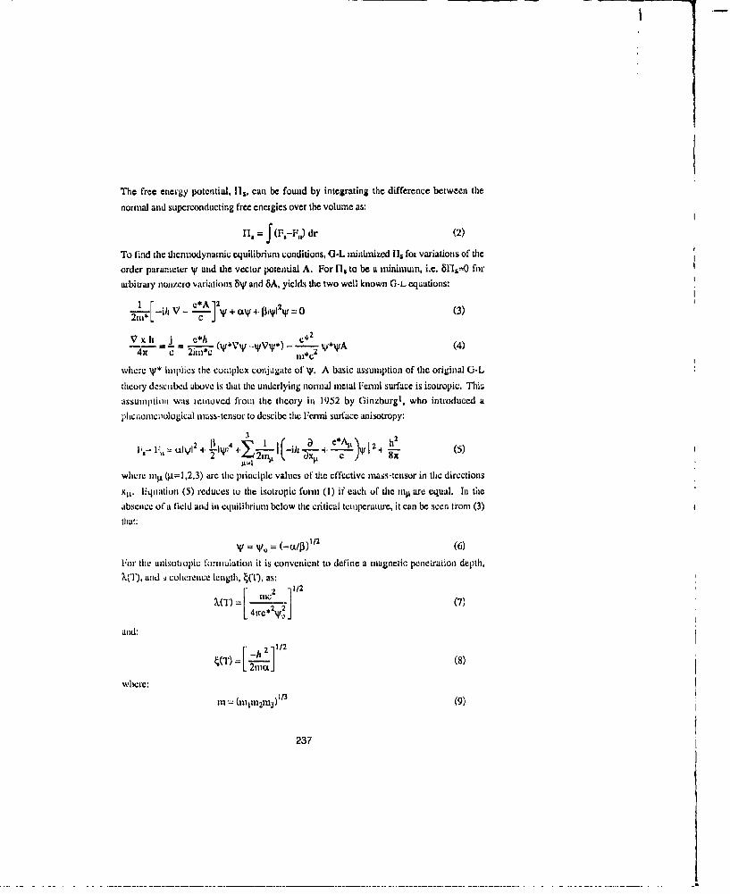
The free energy potential, 1l1, can be found by integrating the difference bctwccn the

nomial and superconducting free energies over the volume as:

I = f (F,-F.) dr (2)

To find the thermodynamic equilibrium conditions, G-L minimized f Is for variations of theorder parameter V and the vector potential A. For -l to be a minimum, i.e. 611.-H-0 foraibitrary nonz.ero variations 8V and SA, yields the two well known G-L equations:

Ftl ch *A 12 2_,,I " V + My 4- P+I+ l2V = 0 (3)

V x h Is j m *h- V* (4Vxh I = (*VV --Yvy*) - -(4)cx e 2t c W1*WA2

where "* implies the complex conjugate of l'. A basic assumption of the original G-Ltheory desciibed above is that the underlying normal metal Fenni surface is isotropic. Thisassumption was emnoved from the theory in 1952 by Ginzburgl, who introduced aplhcnumcviological mass-tensor to descibe the Fenri surface anisotropy:

3 e* 2,(dNII4=Ll~2 +Lj4 Il' I (-h a- + /Sý WI2.ijL (5)2 .1 2 7 -

where jiu1 (t= 1,2 ,3) are the principle values ef the effective mass-tensor in the directions

xll. E.qaition (5) reduces to the isotropic fonn (1) if each of the inp are equal. Inl theabsence of a field and in equilibrium below the critical telmperalure, it can be seen f rom (3)that:

V = V, = -ct!)t12(6)

For the anisotropic formulation it is convenient to define a magnelic penetration depth,X(T), and I coherence length, 4(T), as:

12=" mc. ]1

24,2 (7)X()L 4Ire* 21Jg7

and:

1/')2 L•'.• (8)

whele:mn ( 1 mn1mz•)3) (9)

237

All quantities in (5) may be expressed in a dimensionless form using a normalization inwhich length is measured in units of ý, magnetic field in units of 42 hc•4J2Tc.X (where h,is the thermodynamic critical field and 4o=hcle/), the vector potential in units of.'42hc-=-¢/2itl, and the energy density in units of hc2/4x=a 2/P. The reduced free energy

is then given by:

3F.- Fn=-Ifll +--21tf +I-E_•, • [-i'.•.x + f1)f + h (10)

where f=slyo, and x•jý is known as the effective G-L parameter. It is possible to write fin terms of a magnitude and a phase:

f = f. exp (i Y) (11)and to define the gauge--invariant quantity:

A,= A +- V ' (12)

where An is usually referred to as the superfltid velocity. Note that Ao satisfies therelation VxA 0=VxA=h. Thus (10) becomes:

32

F,-F,= f2+ lf' n[L +2

0 2 0 m. X(f'2 N-1 02] + 2 13

The Euler.-Lagrange equations may be derived by integrating (13) over the volume of thesolution domain and mi imizing with respect to the unknowns Ali and f (where the 'osubscripts will be dropped hereafter), yielding the mass-tensor form of the G-L equations:

in,12_Lj2 +A~f)= f(1-f2) (14)

aid:

-mA, -- V x (V x A)"- xl =jr, (15)

In the present development, we will restrict the supercuiTent domain to g=1,2. That is, thesupercurrents are limited to the plane defined by xi and x2 and the magnetic field has onlycomponents h3. Invoking Maxwell's relation VxA=h, (15) can be simplified as follows:

-M AA f2 - (V x h3) x4 (16)

238

Using Maxwcll's laxtioii Vxh-j, then (16) bccoivips:

:nA4e= f-. Xg L(7)MA

Solving for AA:

A -mrn

Substitute (18) intv (1'4):

- 1n:Iaf +=f(1-f) (19)

Again using Maxwell's relation Vxh=j, (15) finally becomes

2, + E--L((V x h3 x,)2=f(I-f2) (20)

This is the first of the two modified Euler-Lagrange equations. Next we eliminate At, interms of h3 in (17) by taking the cturl of both sides:

-nI... ( f2(VxA.) + 2f(VfxA A), = Vxj. (21)

Now substitute for Ail from (18):

f2 (VxAI) •-(.-f-(Vfxj,)= m(Vxj1 ,) (22)

Invoking the relations X(VxA.)=VxA=-h3, and (Vxh 3 ).x;L=jV, then:

t[h3 = E ( "f (Vfx(vxh,)'x,) - (Vx(Vx(xh3)'x,)] (23)IL

This is the second of the two modified Euler-Lagrange equations. It can be shown thatequations (20) and (23) simplify to the isotropic form, equations (3) and (4), if ml=m2.

As discussed previously, the periodicity of the vortex lattice allows the solution domain tobe restricted to a single supercurrent vortex cel. Vortex cell symmetry further allows thesolution to be limited to a quadrant of the total cell. Figure 1 illustrates the solution domainof interest, with the appropriate boundary conditions for the two unknowns, f and h3 -

239

I \

•. • TRIANGULAR

VORTEX LATTICEIN THE SUPERCURRENTPLANE

X21,

f =f.axh3= h.in Dan - = = 0

f = hfmaxh3=h b~

- =0

VORTEX f =0VORTEX h -h 0SOLUTIONCENTER: h 3= hmax DOMAIN

al- X2

Figure 1: Solution domain in the supercurrent plane with bounda y conditions,

240

Finite Element Formulation

Using the weighted residual approach, the Euler-Lagrange equations, (20) and (23), aremultiplied by a weighting function and then integrated over the solution domain. Thestrong form of equation (20) is then:

f{ m'• -1 a2f n I ah)( l ( xL a)2 ~~)d= (24)

where v is the weighting function. Applying the divergence theorem to the second-orderderivative terms produces the weak form of (24). We also introduce the substitution u=f2in order to reduce the order of the nonlinear te,-ms:

2 m l 1au 2 2v iau (n 1 1 (h 3 2

-vu(1-u)}d1 - " _[ (mX l)n dF (25)

where the nP terms are the direction cosines on the boundary r. Examining the boundaryintegral term, we see that it is in the form of the Neumann boundary condition for u, i.e. atthe vortex cell boundary:

+ -)(.-..n2 = 0 (26)wherc the m/mln terms account for the material anisotropy. The boundary integral term in(25) is identically zero on the portion of the boundary where (26) must be satisified. Onthe remainder of the boundary, the weighting function, v, is identically zero in order tosatisfy the Dirichlet conditions. The strong form of equztion (23) can be written asf ",ws, again substituting u=' 2 :

il m i Vu N2 hZ]l D.212fv _ýI ýI3 _____

___\ j h - _ ( 2 3)] -uh3 ML (27)

As before, we apply the divergence theorem to the second-order derivative terms producesthe weak form of (27):

241

rin V ( u yah 3" (y ah 3 vuh3 1

V[(LX - D"t (2XJ•+• ý)•,] dr" 0 (28)

The boundury integral terms in (28) arc in the fom of the Neumann boundary condition forh3 at dhe vortex cell boundary;

(21X 3( M2 ) n~2 + _Xa nIt =0 (29)The finite element method implics a subdivision of the domain into elements and theapproximation of the unknowns within each element in terms clement nodal values. Thescalar potential u and the magnetic field h3 may be approximated using a set of interpolationfunctions which relate the nodal point values to the disuibutions within each element:

u(xd) = N u (30)h3(xI)= M h (31)

where u and h are the vectors of the element nodal point unknowns and N and M are thevectors of interpolatio,1, or shape functions. Using the Galerkin weighted residualapproach, the weighting function, v, is of the same form as the interpolation function.Substituting into equations (26) and (28) yields, for each element:

S Ih 4 S12 u = 0 (32a)S21 b + S22 u = 0 (32b)

where:

S i =J[ (N)ý)( - . Z-N( )-(•X• •)N D)-INT(-N)]da (36)

242

I

+7

S2N = -S }2 (37)_L (, ('N T N ON .. IT N

n )( O "t IN )+jaN .. . I ''N

-NTN+(Nt•)NT Ný d.f2 (38)

The overbar terms denote the primitive variables chosen for this set of nonlinear equations,which can be solved using a Newton-Raphson iteration. A non-symmtetiic matrix solver isrequired.

Equations (32) - (38) completely define the problem fornulation. Tihe solution of theseequations for the distribution of u and h3 produces a complete characterization of theequilibrium free energy density, the vortex core eluropy, the reverible magnetization, theflux lattice struuture, and the lower critical field.

A finite el-nent solution to the two-dimensional anisotropic fbon of the G-L equations hasbeen developed. The weak form of the integral equations have been formulated with tileappropriate boundary terms. A transformation his been introduced in which the vectorpotential, A, has been rephuceer in terms of the out-of-plane magnetic field, 113, therebyreducing the number of degrees-of-lreedoin at any point in the solution domain has beenreduced from three to two. This sub-titution also enables the proper constraint of thevortex cell boundary conditions, which must be expressed in te"ms of h3, rather than A.

I. V.L. Ginzburg, Zh, Eksp. Teor. Fiz, V23, 326 (1952).

2. D.R. Tilley, Proc. Phys. Soc. London, V85, 1177 (1965).

3. V.G. Kogan and J.R. Clem, Phys. Rov. 13, V24, 2497 (1981).

4. LD, Landau. Phys, Z, Sowjet U., VI I, 11 (1937).

5. V.L. GCinzburg and L.D. Landau, Zh. Eksp. Teor. Fiz., V20, 1064 (1950).

243

S.. .. . . .. .... .......................u~a a& f......~

Characterization of Anechoic Chambers by FiniteDifference Method

Steffen Haffa*, Detlev Hollmann**, Werner Wiesbeck*

A three-dimensional muatnent of anechoic chamber problems by the finite difference method ispresented. Maxwell'% equations are solved in the frequency domain by solution of a boundary valueproblem. Tihe presented method allows to compute the field distribution of the electromagnetic fieldinside a chamber. After a description of the general formulation, including the discretization,verifications are given for the two-dimensional and the three-dimensional calculations. Examplestructures show the capabilities of the method and demonstrate the applicapability to practicalproblems.

Introduction

Anochoic chambers are used in a large frequency range. At Gl0z-frequencies the properties of thechamber can be predicted, using the reflection coefficient of the absorbers. At lower frequencics thechamber has to be treated as a cavity with lossy dielectrics at the walls. The knowledge of the fieldcoutfigurution at MHz-frequencies allows optimization of measurement condition for EMC,ieasuictcnts. A finite difference method treatment in the frequency domain is presented for theIlOssy three-dimensional structure. The computation in the frequency domrain giv"s fine frequencyresolution aod provides exact study of resonances.

S7 In

Sz~ torn/'f

1ig.l a•jochoic chalbcr aid cootdinatedetiition.

There are. several methods for solving the three-dimensional problem of computing the fielddistribution. A number of authors work on field theoretical methods, which solve the problem in the

I*lnstitut ftar Illhisfrcqucnztecinik urd Elektronik, Univcmritlt Karisruhe KaisertLr.l 2,D-75(X) Kurlsruhe,Gernnmuy

* Standard Elcktrik Lorenz AG Ostcndtr. 3. D-7530 Pforzhcim, Germany

244

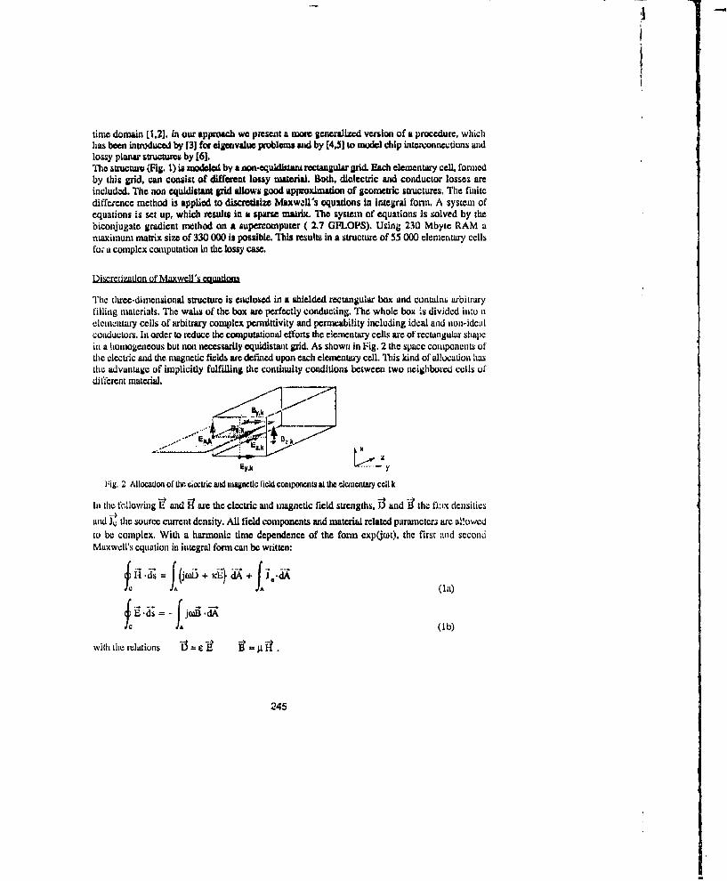
'1-

time domain [1,21. in our approach we present a mom generalized version of a procedure, whichhas been introduced by [3] for cigenvalue problems and by [4,51 t model chip inteconnections andlossy planar structures by [6].The strjcwjei (Fig. l) is modl by a non-equidldaw rectangular grid. lach clementary cell, fonnedby this grid, can consist of different lossy matial. Both, dielutric and conductor losses areincluded. The non equidistant grid allows good approximation of geometric structures. The finitedifference method is applied to discredsizc Maxw4's oquatons in integral form. A system ofequations is set up, which results in a sparse matrix. The system of equations Is solved by thebiconjugato gradient method on a supercomputer ( 2,7 GFLOPS). Using 230 Mbyte RAM amaximum matrix size of 330 000 is possible. This results in a structure of 55 000 elementary cellsfor a complex computation in the lossy case.

Discrfitzaulon of Maxwell's eouatlons

The three-dimensional struture is enclosed in a shielded rectangular box and contains arbitraryfilling materials. The walhs of the box are perfectly conducting. The whole box is divided into nelementary cells of arbitrary complex permittivity and permeability including ideal and non-idealconductors. In order to reducc the computational efforts the elementary cells are of rectangular shapein a homogeneous but non necessarily equidistant grid. As shown in Fig. 2 the space components ofthe electric and the magnetic fields are defincd upon each elementary cell. This kind of alocatioo hasthe advantage of implicitly fulfilling the continuity conditions between two neighboted cells ofdifferent material.

Ey.k _ y

Fig, 2 Allocation of tisi ckoviic anid magrctic field components at the elementary cell k

II the following lý and are the electric and magnetic field strengths, 13 and Ii the fl:ix densitiesand u the source current density. All field components and material related parameters are a owedto be complex. With a harmonic time dependence of the form exp(,jt), the first and secondMaxwell's equation in integral form can be written:

(lb)

with the relations C

245

A source free stucture is anumed. (It-O). Polarization loms (ranB) have been taken Into accountby the complex permittivity C.Applying these assumptlows to q. (1). Maxwell's equatons can be discoelsizod for any cell k by alowest order integration fonnaula. The integration plane for the eleaentary cell k arm shown in Fig.2. Combining the resulting disomdsizad equations leads to a relation baween each space componentof cell k (Exk,, Eyjk, lEz.) and the neighboring componets. thi Is visualized in Fig. 3 for the Exkcomponent.

17ig. 3 HxJk c•mponent and dependmat h componana Mining a eqitulnm of the iear systan of oquialons

Setting up the equations for all n cells of the whole structure leads to a linear system of equations(2). This niatrix equation defines a boundary value problem for the unknown electric field.

F x,kL.(Re)

IMe)

L .. (2)The right hand side is given by the exciting field. The complex values are splitted into real (Re) andiniiginary (Im) parts, thus resulting a real system of equations.The coefficient matrix [C] is spauseand consists of 27 diagonals for lossy structures (ýL real). The system of equations is solvediteratively by the biconjugate gradient nethod and leads to the electric field ;nsidc the structure.

Determination of the transvers- lectric m adtl fields inside the structure

For computation of the transverse electric field in any direction inside the structure the procedure ofthe three-dimensional case can be applied in a simplified version. no homogeneity of the fieldcomponents in z-direction, depending on the propagation constant kz. allows to eliminate the z-components by using the continuity equation.

fjod = 0 (3)

246

After sonic rearrangements this leads to the following cigenvalue problem( [ A 3 - y i ( 1 0 ( 4 a

withly = C'Jk. 4 + c+jk" 4 (4b)

that is to be solved fur 7. The cigenvectors related to each of the propagation constant k, can becomputed by solving (4a) and give the transverse fields of each mode. T"he fields arm orthogonal toeach other.Applying the orthogonality trlation• of the modal fields A.', it to the calculated field in a tangential

z-planc Et of the thrcc-dimensional structure allows a modal decomposition L7,81.

At the frequcncics under investigation Lhe chamnbr behavcs like a wavcgulde near cutoff. Thi two-dimensiounal conmpumtlon have been cheeked against analytiral solutions mid rcsults derived by odtcrmethods.

i~ ~ ~I . .=:. . ..L~_ fly+;++++

2x4 grid 4x8 grid 8x16 grd

Fig. 4 Grid divisioni of ,u waveguldo ridod witLh Woay dielectric maw.ral (,'.20 - j2); h.lght h-5,a, widlh w-,10.:8: IlW1111RUIim iOi COMISS IL

t•i- . -e--e •.6 s : Ž o ~ s 4

. . .. ,. . . . .2 X

-0 O 1 2 -3 4 5 "8015 20 25 ý0 35 4Qnomlized freqm.y / o fioqW.WY 1I

Fig. 5 R"e lvcc=Torothepropagation ounswnt Fig. 6 Cwnprsn of thiv¢.dtne, alonal rdof LMe wavejuideo m~~a two-dlmeriinal solution for

z-hoMOWD~OMs inmturc.

247

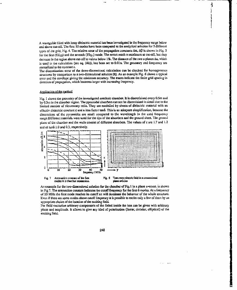
A waveguide filled with lossy dielectric material has been Investigated in the frequency range belowand above cut-off. The first 10 modes have ben compared to the analytical solution for 3 differenttypes of ihe grid, Fig. 4. The relative urror of the propagation constants AU., AD is shown in Fig. 5for the first (TEto) and the seventh (T-21) mode. The erors reach a maximum at cut-off. but theydecrease in the region above cut-off to values below 1%. The distance of the two z-plwaes 4Z, whichis used in the calculation (see eq. (4b)), has bccn set to 0.01a. The geometry and frequency arenomalized to the constant v.The diseretization error of the three-dimensional calculation can be checked for homogeneousstructures by comparison to a two-dimensional solution [8). As an example Fig. 6 shows a typicalerror and the cnvelope giving the minimum accuracy. The traces indicate the finite grid spacing indirection of propagation, which becomes larger with increasing frequency.

Auglication of the method

Fig. I shows the geomeruy of the investigated anechoic chamber. It Is discretsizcd every 0.Sm andby 0.3ra in the absorber region. The pyramidal absorbers can not be discretisized in detail due to thelimited number of elementary cells. They are modelled by sheets of dielectric material with ancffectiv dielectric constant e and a loss faetecr tan&. This Is an adequate simplification, because thedimensions of the pyramides art small compared to the wavelength in the used frequencyrange.Different materials were used for the tips of the absorbers and the ground sheet. The groundplane of the chamber and the walls consist of different absorbers. The values of e arc 1.7 and 1.2and of tun6 1.0 and 0.3. respectively.

-. ... . ....... . . . ... ..... .I... . .. . .......... ...4 ......t , tltt.nr

__j " '\ . . . •l t + ........ . ......iotit Ii t t ll ~II f l l ,I:I I

-1 \Z 'Z ..---------

-144-1-,- -. ......' V . " • • l.. ll l l ll l ll l ll , .

0 10 20 30 40 50 - yfraqnmcy MHz

Fig. 7 Attenaation constant of the fiat Fig. Traa~eao'ne ctricfdin acrosoc•uoalmodes in a chambwr rwcetion. plwane 3..m

An example for the two-dimensional solution for the chamber of Fig. 1 in a plane z-const, is shownin Fig 7. The attenuation constant indicates the cutoff frequency for the frst 6 modes. At a frequencyof 20 MHz the first mode reaches its cutoff an will dominate the behavior of the whole structure.Even if there are some modes above cutoff frequency it is possible to excite only a few of them by anappropriate choice of the location of the exciting field.For field excitation arbitrary components of the fieled inside dte box can be given with arbitraryphase and amplitude. It allows to give any kind of polarization (linear, circular, elliptical) of theexciting field.

248

I

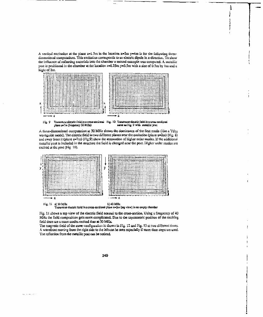
A vertical excitation at the plane z- .5m In the location x-3m y-4m is for the following threc-dimensional computations. This excitation corresponds to an electric dipole in x-dir'ction, To showthe influence of rcflecting materials into the chamber a second example was computed. A antailicpost is positioned In the chanmber at the location z-8.25m y-3.5m with a size of 0,.i1 by I in and uhight of 2m. ................

;i!!! ~ ~ ~ ~ /F" N..............X ... . ............ ... ..... .

ill. 9 I III I } II I I I II IFiig 10I t W in aL44- , l1 ' "i li't- "I ' I "rllliiI #I 1 4 4' ••# • "••• " . ,

',9'i4I4 11 l i4 l I 4l litl lll I , *l ,. . l e . . ~ t l ll.. . .. , , , , , ,, , , , , ... 41 4 .. ... .l ,. . . .: • :• :

plaine o ;,il (firoqUe4kc• 30 M•Hzr) Miloll Ui Fig. 9 Willii aminLll Pralt

A three-dimensional computation iat 30 UMiz shows the dominanice of the first model (like a "rLI, 10wtiveguld¢ mode). The electric field in two different planes near the excitation (phlae z,2m) (Vilg, S)and away hino it (plwie z-Tin) (Fig.9) show die attenuation of highecr order modles. If tihe addliioiialnietallic p'ost is included in the structure die field is changed near the post. Htghm' order modus tirexciteld at tie post (Fig, 10).

..... ,. . . . ....

S. . .. ..... ..... ..... . .:: : • !...................i;•

-.. ~ * . £:::::::::::::::

1 .......-.".. I............. .:_:-

Fig. co1mutin0Mat b) 40 MHzTrimomm, cloctric ficid in a ctv-wtoardoi plim xw2m (top view) Inl an empty clunbor

Fig. I I shows a top view of the electric field normitl to the cr'oss-se~ction. Using it frequency of 40MHz the field composition gets more complicated. Due to the aymmexric position of tme excitingfield there a t an more moidte.s ex hwted th e n at 30 Mo oeIdd

The magnetic fieIld of the s tme ctnfiurtLioa is ch.n. e dn ,l. n1ea the •p o. 1-dg..... iorde mesA wavefront moving front the right side to die left can be seen especially if more time steps &ue used.The x cilctiot i from the theliet post ( be noticed.

249

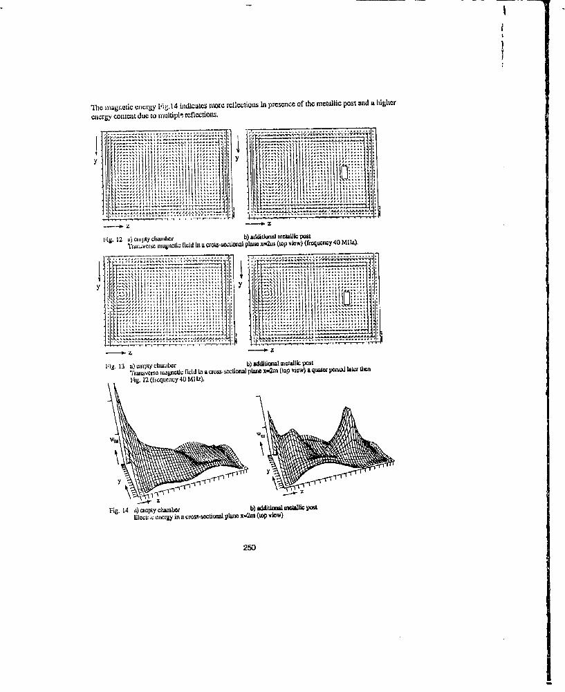
The magalctic energy Fig.14 indlcatcs more renfletions in presence of the metallic post and a higher

cnergy content duc to multipl! refleedonu.

. . . . . ................ -------- - Z

......... ... ---------------i . .. . . ".. . . I . . . . . .. . . . ... ... ......- ... I....

. . . . .....

MI*g. 12 U) c111I~y cluunber b) diunal mc*al)t poSt- - --- - - --- -"n.~vc• ,nL:ctic fi~lI inaco•l-ibI.i[laI~ pluoox-2m (top view) (frcquccy 4O MtLa),

-I-...................................

'1i .................. t............

.. .= mIII.=.==..., t. .....II== .. iI..• •...

lVig. 13 u) eiiipty chawnber. b) adigdtional nwlik.,a~ pQ;•t"1'rans.verse nilignelu field hi a cjou.=fiton• pLgaw xw• (iop view) a qLwla" penoiCX laws- ileF/ig. 12 (frcluecy 4Q MIIz).

zz

Fig. 14 a) ejnpty cilwuber b) addtidwal mellic pwtElMctrit encrgy in a crosj-sectionil p"ane x.2rm (top view)

250

I

Conluio

T7he presented method is well suiled for ccenputatltu of anecloic chambers in the frequency range ofI to 100 Mli&z The fleidblky of the Voe~try allows to Include different absorbers, devices underteat and e.g. an antenna posidosser in the comnputation. The plow of the computed three dimensionalelectric and magnetic fields and the electric and mlagnetic: energy give ln&%fations on the behavior ofthe electromagnetic field. The l&V number of discretizatice elementary cells allows an excellentmodelling of the investigated structures Q'itical frequencies can be found by two-dimensional andthree-dimensional computations. 71m position of an antenna and a de-vice under test can be optimizedfor those frequencies.

(I] W. Hocfer. 'Um Tranamission-Unea Maurix MchdW - Theory and Appllcatlons". IEEE Trans on MIT. vul. 33,pp. U82-893. Oc" £985

[21 A. Taflove. M. E. Brodwin *Nwne"ia Solsution of Steay-Staie Hlechusuagneuic Scattering lroblevnS Usifig theTime-Dopedent Maxwell's Rtlastiona'. IEEE Trarn Microw~ave Tikory Tdch., vol, MIT-23. S. 623-630. Aug.1975

313 T. WVellandc, 'Die Diskrellsicning dor Maxwell-tGleichungen". Physlkallc/e Bldutr, Bonid 42. S. 191-.201, July2986

L41 A. Christ, H. Hartriail 1, -1lsxee-Dimnumlonal Flnliweflfforence MehdW for tho Analysis of Mlcrowave-De-viceEmnbedding *.,IEEE 7ramu on AMiT vol, 35, pp. 668-.6%, Aug. 1987

L51 A. Christ. 'Strounatrixbowhrnung mitdadfinuanlorukkn Finite-Differonmi Mur Mikrowcllen.Cliip.Vcrbirsdunigcnund deren CAD-Modellie. Phs.D. Thesis, Fortschrlu-.Der., VDI~Relse 21 Ar 3, VDI Verlail Dllssewoldtc 1988

161 S. lljaffia. *Switcadah und dynanudzche Vtrfahren zur Berechniwq moauolithisch integrierter Mikiowellen-Bmlratwefiwngg. lPD-Thex~ls. Unlvashtt Karisruhe, 199

L71 1). llullinann "Feldtheoraaischa Verfahren szur Analyse dieekkirischer Resonatoren In iniegrirlenM~krowe~lknschdarwagen% PD-Thesls, Univeisltut Karisrulie, 1991

181 1). Hlltlmaann. S. Hlaffa. W. Wiosbock, "S-Paramtear Calculatdon of Arbitrary Three-Diniensional Lossy Structuresby Fianit Differeitic Methiod". ?roe. of dos Int. Coin!. on Directions 4%~ Electronsagnctic Wave Miodeling, WoberRescarch Instituto of Polytochnic University, New York. OkL 1990

251

i

Autors:

Steffen Hafas

Work m•il addreas: Institut fdI" HOchstfrcquenztechnik und Elektronik, Universitat Karlsruhe,KaiserstraBe 12, d-7500 Karlsruhe, Germany, Tel: 49-721-6082525, Fax: 29-721-691865

Home mail address: Offenburger Strale 29, D-7500 Karlmthe 51, Germany,Tel: 49-721-888190

Steffen Haffa was born in Stuttgart, Germany, in 1956. He received the Dipl.-Ing. (M.S.) degreefrom the University of Karlsruhe in 1983.From 1983 to 1986 he was employed at Richard Hirschmann Company, Stuttgart, Germany. Hewas responsible for the development of satellite receiving systems, with the main work on reflectorantennas and feed systems.From 1986 he is with the Institute for Microwaves and Electrovics at the University Karlsruhe,where he received his Dr. Ing. (Ph. D.) in 1990. His research work was on field theoreticalcomputation for device modeling and measurement at umm-wave frequencies. The main applicado'l ofhis work was on GaAs MMIC.

Detlev HollmannWork mail address: Institut fRir Htschstfrequenztechnik unf Elektronik, Universitait Karlsruhe,

Kaiserstralle 12, d-7500 Karlsruhe, Germany, Tel: 49-721-6082525, Fax: 29-721-691865

Home mail address: Scheibenhardter Weg 26, D-7500 Karlsruhe 51, Genrany,Tel: 49-721-887936

Detlev Holhnann was born in Karlsruhe, Germany, in 1960. He received the Dipi-Ing. (M.S.)degree from the University of Karluruhe in 1987.He then joined the GaAs umn-wave group at the Standard Elektrik Lorenz AG (SEL), Pforzheim,where he is responsible for network measurement and calibration. In a cooperation with the Institutfor Microwaves and Electronics at the University of Karlsruhe he currently works towards the Dr.-Ing. (Ph.D.) degree. His main research interests include numerical computation of electromnagnuticfields applied to dielectric resonator coupling on MMIC circuits, optimization methods and devicemodeling.

Werner WiesbeckWork mail address: Institut fltr Hdchstfrequenztechnik unf ilektronik, Universitgit Karlsruhe,

Kaiserstralle 12, d-7500 Karlsruhe, Germany. Tel: 49-721-6082525, Fax: 29-721-691865

Werner Wiesbeck (SM 87) was born near Munich, Germany in 1942. He received the Dipl. Ing(M.E.E.) and the Dr. Ing. (Ph. D.E.E.) degrees from the Technical University Munich in 1969 and1972 respectively.

252

From 1972 to 1983 he was with AEG-TefWunin in various paosions including head of R&D of theMicrowave Division in Flensburg and mrketng director Receiver and Directicn Finder DivisionUlin. During this time he had pomicmt responsibility for mma-wave rad receivers, direction findersand c• -•tronic warfare systenm, ". 1983 he has been director of the Institute for Microwaves andElc'tronics at the Univcity Xz..ruhe. Prei t reseach topis include radar, renmte sensing, wavepropagation and antennas. 1989 Ia spent a six month sabbatical at the let Propulsion Laborator/,Pasadena. He is engaged in several wcddng groups in electrical engineering.

253

SESSION 7- "MOMENT METHOD THEORY"Moderator: Allen G1lhon

llzlmJI________ ________.____

A Multilevel Enhancement of the Method of MomentsKhalil Kalbasi, *Kenneth R. Dernarest

Radar Systems and Remote Sensing LaboratoryDepartment of Electrical and Computer Engineering

The University of KansasLawrence, KS 66045

ABSTRACT: A multilevel formulation of the method of moments (MoM) for computing the fieldsscattered by electrically large conducting bodies Is presented. This iterative method can handle very largeMoM matrix equations efficiently, Is particularly suitable for multiple excitations, and can be adapted as a"solve" module for almost any MoM code. We have formulated the method for a model problem (the EFIEapplied to two-dimensional scatterers) successfully, and feel that it holds significant pronise for otherIntegral equations in two or three dimensions. Solutions are presented and are compared In efficiencyperformance with existing results.

INTRODUCTION

The method of moments continues to be an attractive technique for solvingelectro.ag ,tlc scattering problems. Its advantages are many and well known. Inspite If its advantages, however, the MoM is for the most part relegated to resonancerange frequencies for large scatterers. This limitation stems from the prohibitivecomputational cost associated with solving large systems of equations. As is wellknown, the computational cost of direct solvers grows as the cube the number ofunknowns, making it unsuitable for very large problems.

Iterative methods have, for many years, been seen as attractive altematives todirect solvers when matrix equations are very large. The computational cost periteration of these solvers typically grows as the total number of nonzero enties of thematrix. This has prompted the use of iterative solvers in partial differential equationformulations where the resultirg matrix is large and sparse.

Unfortunately, iterative methods, In general, have not been found particularlyeffective In MoM formulations. The reason is that the impedance matrices associatedwith electrically large scatterers tend to be huge, dense. non-hermitian, and non-symmetric. These negative features result in slowly converging, or worse yet, divergingsolutions. Clearly, iterative procedures alone will not substantially Increase the rangeof problems that MoM can address.

254

MULTILEVEL ITERATIONS

Classical linear Iterations have the general characteristic that the local (i.e., fast.or high spatial frequency) solution behavior converges rapidly, but the global (i.e.,slow, or low spatial frequency) behavior either diverges or converges slowly. The fastcomponents of the solution are extracted quickly, while it takes many iterations tocapture the slow modes. Therefore, the iteration process is selective in extractingsome modes and "filtering" the others.

Multilevel bas'd methods [1], capitalize on this selective property of the iterationprocess. The basic idea is as follows. A given geometry is first modeled with a finelevel of discretization and an iterative solver is initiated. In just a few iterations, the highfrequency modes of the solution will be quickly identified, but large low frequencyerrors will remain. At this point, the geometry is remodeled using a coarser level ofdiscretization. At this coarser level, modes that appeared to be "slow" in the fine levelnow seem to be "fast". These modes can then be quickly identified with an iterativesolver at this coarser level.

Multilevel techniques typically involve several levels of discretization. Solutionsobtained by iteration at one level can be passed either "up" to a finer level or "down" toa coarser level to take advantage of the the mode selective characteristics exhibited bythe iterative solvers at each level. Since the cost per Iteration is far less at the coarserlevels, the global characteristics of the solution can be identified at a fraction of thecost of either direct or classical iterative methods at i single level.

The key to a successful implementation of multilevel methodology to the MoM(hereafter called the multilevel moment method) is the development of basis functionsthat allow the remodeling of a given problem at different levels of discretizationconsistently and without the high cost of recalculating the Impedance matrix elements.This is addressed in the next section. After sketching the main features of thetechnique, representative results for two-dimensional conducting objects using theElectric Field Integral Equation will be presented.

lNTERLEVEL REL kTIONS

To conceive a simple two-level moment method we start with the operatorequation

L f-g, (1)

255

where L is a linear integral operetor, g is a known excitation, and the function f is to bedetermined. Starting with the usual MoM procedure, let's assume that the unknownfunction is approximated via a p'.lse basis set uf support (L.e.,iength) h. Using a Galerkinscheme, the matrix equation Zhxh. Vh is obtained. Next assume another matrix equationZHxH= VH is generated, where Hw2h is support associated with a coarser oasis andweighting set of function% Here, Zh and ZH correspond to fine and coarserepresentations of the operator L, retrpctively. The same Is true ol the vector pairs gh,gH and xh, xH.

The vectors and matrices on fine level are related to their coarse counterpartsthrough two transfer operators, [R] and [I], called restriction ard interpolationoperators, respectively. Mathematically, [R] maps a given vector from an

N-dimensional spaco to some iower dimension (say N/2). The operator [I] does theopposite task.

It is possible to generalize the transfer operators associated with a given choiceof basis and testing functions. For a Galerkln scheme, [R] and [1] are transposes ofeach other because of reciprocity. This suggests that the coarse level matrices and theright hand sides can be constructed using their representations at the fine level via theidentities

[ZH]= [R] [ Zh [] (2)

and

gH= [R) gh. (3)

As an example, If subsectional pulse functions are used In a Galerkin scheme,[R] has the following structure:

I 1 0 0 0 .. . 0 -0 0 1 1 0 .0 00 0 0 0 1 1 ... o 0

[R] .............. (4)

0 0 . . 1. 0 0 1 1 0IN-- 0 0 . , , 0 0 0 0 i i-- W Y N

Also, [I] Is the transpose of [R] multiplied by a scale factor.

258

-II

THE ALGORITHM

The multilevel algorithm starts at the finest level of discretization. Linear iterationschemes such as Gauss-Seidel or the Banded Matrix Iteration (BMI) [2] are used untilthe convergence has slowed. If we denote the iterative solution by xk and the exactsolution by x. , the error after k iterations is

ek = x Xk. (5)

"This error is related to residual (i.e., boun'dary) error, rk - v - Z Xk, via the residualequation

Z ek = rk . (6)

The residual error contains the slow modes which are not easily r9duced by theiteration process at the fine level of discietization.

Next we project rk to the coarser level, H, via the operator [R],

rH= [R] rni. (7)

The residual equation (equation 6) is then solved at this coarser level. The solution atthis level can be found by LU factorization If the number of unknowns is small, or byiteration if the number of unknowns is still relatively large. Once obtained, the coarseversion of the erroi, eH, is then interpolated via ;he interpolation operator, [I], to thefine grid level. By interpolating the error to the fine level, we can construct anapproximation to eh and call it ýh:

ah= [I] eH . (8)

A new estimate of the solution is thus obtained by adding il' to the previous estimateof the solution at the fine level

Xk lW Xk +÷h . (9)

This new estimate of the solution, xk+1, can now be used as the starting point

for a new multilevel cycle. This new estimate contains slow mode ihformation that isnot easily obtained at the firie level. It also contains fast mode errors since the coarselevel can not adequately model these. These fast mode errors can, however, be

257

removed in just a few iterations at the fine level. The iterative procedure at the finelevel once ag2in is halted when the convergence starts to stall and the error isrestricted for use in the coarse level.

OTHER CONSIDERATIONS

The scheme discussed above is a simple two-level design. It is the basis of almostall multilevel algorithms. Multilevel methods for specific problems can be devised bychoosing the iteration, the number of levels, the directions of the jumps from one levelto another (cycling), transfers between levels, . etc.

Among the linear iterative techniques, BMI [2] and Gauss-Seidel have proved tobe the most appropriate for multilevel moment method. We have successfullyimplemented the multilevel moment method using both iterations. At the coarse levels,the iterations must be convergent. When the Gauss-Seidel iteration was employed atthe line level, the Kaczmarz iteration [3] was incorporated at coarse levels toguarantee convergence. Kaczmarz iteration Is basically Gauss-Seidel applied to thehermitian form of the impedance matrix, i.e., ZaZ, where Za is tne complex transposeversion of Z. When BMI is used as the iteration on the fine level, a guaranteedconvergence at coarse levels may not be possible. This suggests that the combinationof Gauss-Seidel and Kaczmarz iterations is superior to BMI.

LU factorization is commonly employed to solve the relatively small systems ofequations at the coarsest level, although iterations could be used as well. If directsolvers are used, the factored form of the (coarsest) matrix is saved throughout theiteration. In cases of multiple excitations, the factored form of the coarsest matrix canbe used advantageously for different excitations with considerable savings incomputations.

For electromagnetic scattering problems, the coarsest discretizatlon possible islimi'ed by the characteristic wavenumber ko. The order in which the solution processjumps between the levels is controlled by the cycling scheme chosen. The morecommonly used cycling schemes, such as V and W [1], are inefficient with multilevelmoment method . The V cycle, for example, starts by iterating on the fine level and thenmoves down p steps to the coarsest level, where the problem is usually solved exactly.This scheme progresses by then moving upward, one level at a time, until the resultsare carried over to tne finest level. Therefore, one full V cycle requires visiting everylevel twice, once going down and once moving up.

258

For dense MoM matrix equations, sawtooth cycling appears to be more efficientthan V or W cycling since it visits each level only once in a cycle. Sawtooth cyclingstarts at the coarsest level and moves upward until the finest level is reached, thenjumps to the coarsest level.

The next section presents results and comparisons of the multilevel momentmethod for two-dimensional conducting bodies.

NUMERICAL RESULTS

Consider first the example of a thin, perfectly conducting corner reflector withequal and perpendicular sides. As shown in Figure la, the incident field is a TM planewave, approaching at an angle of 401, To model this geometry, we use the EFIE, withpulse basis functions and point matching on the plates [4]. The matrix equation issolved using the multilevel scheme discussed above. In all the numerical experimentspresented here, a problem is considered "solved" when a residual error of less than10-4 is obtained, corresponding to four digits of accuracy in the near field solution. Theparameters of interest such as the sampling density, the number of levels, the type ofiteration used, etc. .. , are given with the table and graphs.

The advantage of the multilevel scheme becomes apparent as the number ofunknowns, N, increases. Table 1 includes some relevant information concerning theperformance of the 3-level scheme applied to the corner reflector geometry, includingnumber of unknowns, size of the reflector side in wavelength, fill time, factor time,iteration time, and number of required cycles for convergence. As this table shows, thenumber of cycles nueded for convergence seems Independent of the number ofunknowns. (We have observod this same behavior on all geometries we have triedthus far.)

To investigate the performance of the multilevel moment method on a morecomplex scatterer, we next choose a modified NACA 0012 airfoil (Figure lb). The tip totoe length (cord length) is changed to yield different value3 of 111. In all cases, the,f"rfirng discretization on the fin4-st level was 16 points per ",. elength.

Figure 2 compares the Gauss-Seidel multilevel technique with a standardconjugate gradient solver [5] for different tip to toe lengths of the NACA airfoil. Eachcurve shows the decrease in residual error of the fine level as a function of the numberof Work Units (WU). (One WU is equal to the cost of one matrix vector multiplication atfine level, i.e., N2 complex operations). For the conjugate gradient, the nirmber of workunits required for an acceptable solution grows linearly with N. Note that this is the

259

El7

same total number of WUs as demanded by direct methods. For the multilevel momentmethod, the number of WUs is practically independent of N.

The performance of the multilevel scheme is clearly superior to conjugategradient and direct methods. Furthermore, the advantage of the multilevel momentmethod becomes more pronounced as the number of unknowns increases. Similarresults have been obtained using BMI variant of the multilevel scheme on differentgeometries, such as plates [6], and ogives.

CONCLUSIONS

In this paper we have shown the feasibility of the multilevel moment method forthe EFIE in two dimensions. For this model problem, it was shown that the multilevelmoment method is much faster than the conjugate gradient iteration applied to thediscretized matrix equation, not to mention any direct method of solution. Themultil6vel moment method also does not suffer from the divergence problemsassociated with the application of linear iterations to MoM matrix equations.Appropriate iterations for multilevel treatment of method of moment problems wereidentified, as well as the transfer operators and cycling between adjacent levels ofdiscretizations. In addition to the.e, very encouraging results were obtained whereproblems with a few thousands of unknowns are solved in less than 10 cycles of themethod. Future extensions of the method are planned as solve modules for existingMoM codes.

REFERENCES

[1] W. Hackbusch Multigrid Methods and Applications, Springer-Verlag, 1985.121 T. R. Ferguson, "Efficient Solution of Large Moment Problems: Theory and Small Problem

Results," IEEE Trans. Antennas Propagat., March 1976, pp.230-235.131 K. Tanabe, "Prolection Methods for Solving a Singular System of Linear Equations and Its

Applications," Numer, Math., 17 (1971), pp. 203-214.[4] R, F. Harrington Field Computation by Moment Methods, MacMillan Company, New Yori, 1968.[51 A. F. Peterson, R. Mitra, "Convergence of the conjugate gradient method when applied to matrix

equations representing electromagnetic scattering problems," IEEE Trans. Antennas P.-opagat..vol. AP-34, pp.1447-1454, Dec. 1986.

[6] K. Kalbasl, K. R. Dernarest, "Convergence Acceleration Techniques In the Iterative Solution ofIntegral Equation Problems, AP-S Symposium Digest, vol. 1, pp.64-68, May 1990, Dallas, Texas.

260

Figure 1

a) Uniform plane wave (TMz) incident on a thin corner reflector of finite sides.

Y

b) NACA0012 airfoil geometry with tip to toe length L. The coordinates convention1 isthe same as part a above.

261

Table 1

Performance of 3-level scheme on a corner reflector with perpendicular sides. Theincidence angle 0 was 400, Block Gauss-Seidel (BGS) was used as the i' ation on

the fine level and Kaczmarz iteration on coarser levels. The number m denotes thocoefficients per block used in BGS. On the coarsest level LU factorization wasemployed io solve the system directly. The sampling density of 16 points per X was

chosen on fine level. Number of iterations at each stop on different levels was one.

N Reflector Matrix Factor Time Total CyclesSide (X) Generation for Coarsest Iteration

Time (sec.) Level(sec.) Time (sec.)200 6.25 0.23 0.03 0.68 (m=8) 6

400 12.5 0.94 0.24 2.94 (m.8) 7

600 18.75 2.11 0.8 5.54 (m=8) 6

800 25 4.0 1.86 12.14 (m16) 6

1000 31.25 6.18 3.38 21.42 (m.8) 6

1200 37.5 9.2 5.69 28.75 (m=1 6) 7

262

_______________________________________ -

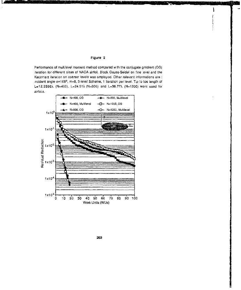
Figure 2

Performance of multilevel moment method compared with the conjugate gradient (CG)iteration for different sizes of NACA airfoil. Block Gauss-Seidel on tine level and theKaczmarz iteration on coarser levels was employed. Other relevant informations are:incident angle 0=1 650, m=8, 3-level Scheme, 1 Iteration per level. Tip to toe length ofL=1 2.2596?, (N=400), L.=24.51 X (N=800) and L=36.77% (N=1 200) were used forairfoils.

-49- N-400, CZG --- N=800, Multilevel

-.4-- N-400, Multilevel -[3-- N-1200, CG

1 xi 00 -A- N-800, CG -40-- N=1200, Multilevel

1 xi 0-1 _____ _____

0

'26

L7 -

THIS PAGE ISINTENTIONALLY

LEFT BLANK, ACCIDENTALLY.

264

On the Applicability of Pulse Expansion and Point Matchingin the Moment Method Solution of Three-Dimensional

Electromagnetic Boundary-Value Problems

Bierng C. Ahn, Karthikeyan Mahadevan, and Allen W. GlissonDepartment of Electrical Engineering

University of MississippiUniversity, MS 38677

Abstract

The use of a pulse expamsion and point natching (PEPM) scheme in the electric field integral equation(EFIE) solution of thre-diusewional, tme.harnuonuk electromagnetic boundary-value problems iu invistl•gated.Problems of electro agmnet;c scattering by a few simple conducting bodies in free space are considered. Acomparison of solutions obtained using the PUPM-UiIE scheme with those obtained using rouftop expansonfunctions and a lHne testing procedure indicates that the PEPM.EUIE scheme may not produce corr4ct results forgen•ral th|ree-dimensional geometries. An empirical explanation for the appar-nt failure of the PEPM-EFIEapproacb to EM scatering by arbitrarily lshaped scattereri is nsuglesied by studying the near field of a knownpulse-approximated current.

I. Introduction

The integr.d equation technique is still a viable method for solving a large class ofelectromagnetic boundary-value problems, even though other approaches such as the finite-element method (FEM), and the conjugate gradient fast Fourier transform method (CG-FFT) areincreasingly finding many applications in the solution of dynamic EM problems in recent years.Integral equations for EM problems are most often solved by the method of moments (MM),where the choice of the expan.ion and testing functions plays an important role in determiningthe accuracy and convergence rate of the solution. One of the most versatile and efficientexpansion and testing schemes in the MM solution of surface integral equations for a specialclass of geometries is the rooftop expansion and line testing (RELT) approach proposed byGlisson and Wilton [1]. This approach was subsequently extended by Rao, Wilton, and Glissonfor the treatment of arbitrarily shaped three-dimensional bodies [2].

The simpler pulse expansion and point matching (PEPM) approach has been widcly usedfor static EM problems, and for specific formulations and polarizations in two-dimensionaldynamic EM problems [3]. Recent work has shown that the PEPM approach can also be veryeffective for two-dimensional scattering problems modeled by the EFIE for both polarizations[4,5], but it ha- not been cmploycd with any success in the electric field surface integralequations for three-dimensional dynamic EM problems to the best of the authors' knowledge.Yet compared to the RELT approach, the PEPM scheme generally requires fewer computationsand may be more convenient in the segmentation of sonic boundary surfaces. Thus the PEPMapproach would appear to be a preferable approach when it is applicable. The analyticalmethods recently proposed by Mahadevan and Auda [6,71 for evaluating accurately the singularsurface integral involving the free-space Green's function allows one to efficiently use the PEPM

265

scheme in the surface integral eqvation.

In this paper, the applicability of the PEPM-EFIE for the solution of three-dimensionaldynamic EM problems is invesdgated by solving scattering problems involving simpleconducting bodies such as strips, thin wires, rectangular plates, and closed rectangular cylinders.In the following section, the PEPM-EFIE formulation and the numerical solution procedure arepresented. In Section III, numerical results obta;ned with the PEPM and RELT schemes arecompared and an empirical study is described whirh may explain the apparent failure of thePEPM-EFIE app;oach to model EM scattering by arbitrarily shaped scatterers.

II. PEPM-EFIE Formulation

Consider a perfectly conducting object illuminated by a prescribed incidenL field (E', H1)in free space. To obtain an integral equation for the problem, one replaces the surface S of theobject with the electric current density J induced on that surface, and enforces the boundaiycondition on the total field Et or H' to obtain

ftXEr(r) = fhX[ES(r) + E'(r)] - 0 (EFIE) (1)

fixH'(r) = ftX[H l(r) + H'(r)] = J(r) (MFII) (2)

where r is just outside S and fi is the outward normal to S. The PEPM piocedure cai be readilyapplied to (2), but it is well known that for objects with vanishing thickness (1) is still validwhile (2) fails. Therefore, it is desirable to also be able to use (1) to obtain numerical solutions.The ability to solv;, (1) is also desirable because one approach to the avoidance of internalresonance problems is the use of the combined field integral equation (CFIE) 181, which maybe formed as a linear combination of (1) and (2).

The scattered fields Es and H' are given by

ES(r) I (k2A + V4')

k2 J(r')G(rr')dS' + V [V' .J(r')]G(r,r')dS'

HS(r) = VxA = fJ(r')XVG('.r')dS' (4)"SJ

where G(r,r') = exp(-jkR)/4oR, R = Ir - r'J. aLd whiere the integral rep~eentndon on the rightside in (4) is valid for r outside S. The mixed poteuzial expression 1,3) for twe ele"ýaic ficid isoften preferred to other forms because it involves a less singular kernel. Iripiicit in tnis

266

statement, however, is the assumption that the gradient operator in (3) is evaluated only in aweighted average sense through the testing procedure. To solve (1) or (2) by the momentmethod, one next expresses the current density J in terms of an expansion function withunknown coefficients, i.e.,

NivJ J~r' = ~11cr')(5)

A testing procedure is then chosen which leads to an appropriate system of linear equations.One factor in the choice of expansion functons and testing procedure is the form of the integralequation. It has long been known that the PEPM technique is well-suited for u.e with (2),where -.valuation of the curl operation in (4) as the observation point approaches the surfacealong with (2) leads to a Fredhoirn integral equation of the second kind. It has been widelyaccepted that a smoother representation for the current density J is required for the EFIE, whi'his an integral equation of the first kind. Results obtained for two-dimensional geometries [4,5],however, have suggested that pulse basis functions may indeed be a viable alternative in theEFIE.

In this paper, only wires and a few simple conducting bcries whose. surfaces can besubdivided into a set of rectangular patches are considered. Thc exparsion functions ei in (5)are chosen to be pulses on each of the rectangular subdoinains in the PEPM approach. Thus weconsider a rectangular patch subdomain with dimensions 2WVX2W1, lying in the u-v plane witha uniform v-directed electric current density defined on it. With the origin of the coordinatesystem at the center of the patch and with (ii,v,w) as the observation point, oni obtains for thevector potential

wý w, e-jkRA = i' f 4-jrR du'dv' ; R = [(u'-u) +- (-v) 2 + w2]'" (6)

-Wv -Wu

When the field point is wi~hin the source region, the kernel in (6) is singular and a dirrctnumerical integration is impractical. In this case, the analytic expressions of Mahadevan andAuda [6] can be used, or for programming simplicity, one may extract only the singular portionof the vector potential to be evaluated analytically. In the latter case the vector potential maybe represented as

S-jkRlW. W ,A- 11I-1 du'dv' + = Ko(u,v,w;U'v')h,,w Iv,._w (7)A Jw -Jw 4-wa'----

where

K0(u,v,w;u'v') - (u'-u) en(v'-v-R) + (v'-v) fn(u'-u+R) - wtan-1 (8)

287

. -

The first term 1n (7) is then non-singular and is amenable to numerical integration. For thesecond term in (3), the divergence of the current may be represented as

V'.J(r') - +6(v'+W,) (9)

and one then obtains

H_ T (p-p')(l +JkR)e-J du' (10)ap -u 4wrR 3 v'-w,

_NI

where p-u, v, or w; p'=u',v', or w'; w'=0. Since the match point is at the center of eachrectangular element, the kernel in (10) is never singular and thus (10) can be evaluatedaccuirately by numerical integration. It is worth noting that (10) can be obtained directly fromVV A without referencc to the divergence of the discontinuous pulse basis function for thecurrent.

Results obtained in this work with the PEPM approach, which employs expressions of theform given by (6)-(10), are compared with results obtained via the RELT aproach. Forcomparison, the expansion and testing schemes used in the PEPM and RELT techniques areillustrated in Fig. 1.

Expressions similar to (7) and (10) can be obtained for the electric field due to the uniformu-directed current. The point matching of u and v components in (1) at the center of eachsegment leads to a coupled system of simultaneous equations which may be represented in matrixnotation as

[Z.1j [.1 -1 [z,] [,1] - IVJ (1. a)

[z1J [I," ] [z. ] [11 - [IVj (I lb)

where elements of the impedance matrix can be computed using expressions presented in thepreceding paragraphs. For example, expressions for Z,,v,, and V,.,, are

288

PEPM RELT

-W w -2W 2W"V V V V

12WV

-1

-_1

2W

Te stingfunction

-W Wv v

Figure 1. Cross-section representation of expansion and testing functions.

S'~m e -jkRnm- 1ud(W 4,rR,.,

1I.Z,

Ko0(u,,,,v,,,W,,1 ;u,:+u', v,,(2•)•,,-

wu.n

+€ In' [0ýUn.U-U.n-U) + ,n(VI- V. -V') +W*. VJ]

( +jkR ,) e-___,, dw '0-3 ¢'Wv.,.du

vVv, • ,, .E'(r,,,) (13)

where in and n are indices which specify the observation and source patches, respectively, andwhere Rn=[(u,,-u,-u') v- )2+w,,]A. The matrix equation for the PEPM-MFIEapproach can be obtained using similar procedures once the limit in which the observation pointapproaches the surtace has been taken to extract the principal value term. No extraction of asingular portion of the kernel is then wecessary, although careful evaluation of the integral isoften required for the nearby sources due to the rapid variation of the kernel.

IIU. PEPM-EFIE Applied to Sinple Conducting Bodies

(A) Narrow Strips and Thin Wires

The PEPM-EFIE formulation presented in the previous section and the RELT-EFIEscheme [1] have been employed to solve electromagnetic ,cattering problems involving simpleconducting bodies in free space. The current induced on a thin strip with width W that issituated parallel to the z-axis in the x-z plane and is illuminated by a normally incident plane

wave Ei= in0 e-Jky is solved by segmenting the strip into lxN rectangular elements. Although

the actual current has the [1 -(2xlW)2] -,' variation, it can be shown tnat physical quantities suchas the radar cross section and the driving point impedance can accurately be computed assuminga ýounstant current across the strip width.

Extensive numerical experiments on the convergence of the solution for strip widthsranging O.O0lX-O.1)X show that in both schemes, for a fixed strip length, a larger number ofunknowns is generally required for strips with smaller widths. For fairly long strips, aprohibitively large number of unknowns is required in the PEPM solution. As an example for

270

a 0.O1Xx4X strip, 480 unknowns was required in the PEPM, while 80 unknowns are enoughin the RELT to achieve about the same percentage error in the current. The precedingcomments also appear to hold true when multiple pulses are used to model the singular behaviorof the current on the strip edge.

The thin-wire problem can also be solved by the PEPM-EFIE scheme. In this case fora straight wire radius a, the free-space Green's function is replaced by the thin-wire (reduced)kernel

Ga 41R (14)

and the current density J, is replaced by the total current 4 =2'a-az. The surface integral in (3)now becomes a line integral and point matching along the wire axis results in expressionscorresponding to (12) and (13). The previous observations on narrow strips also appear to beappropriate for thin wires. Fig. 2 and Fig. 3 show the convergence of currents on 0. lIXO.5Xstrip and 0.01XO.5X wire, respcciively, solved using the PEPM and RELT schemes.

(B) Rectangular Plates

As one of the fundamental structures in electromagnetics, rectangular plates have receiveda fair amount of attention in recent years [9]-[13]. Fig. 4 shows the real and imaginary partsof the z-directed current on lXX IX plate solved by the PEPM and RELT schemes using lOX 10segments. Even though the real part improves with more segments, the solution obtained withthe PEPM shows significant error. The errors seem to be more pronounced for small plates.

(C) Closed Rectangular Cylinders

As an example of a closed rectangular cylinder, a 0.4xxO.4Xx0.4X closed perfectlyconducting cube is considered. The back face of the object is on the x-z plane with thecoordinate origin at its center. Fig. 5 shows the current on a path, from the center of the frontface to the center of the back face along the line of symmetry, solved by various schemes. Theexcitation is same as before and the path length s is normalized. Again the solution by thePEPM-EFIE scheme is greatly in error.

(D) An Empirical Explanation for the Apparent Failure of the PEPM-EFIE Scheme

It is puzzling that the PEPM-E-FIE seems to product correct results only for two-dimensional geometries or for slender three-dimei ;ional scatterers. For these two geometrytypes, however, the cross-polarized current component, which is excited only by the gradientof the scalar potential in (2), is either non-existent or negligible. The general success of theRELT scheme coupled with these results suggests that modeling the charge density in terma ofimpulse functions may be inappropriate. (It should be noted that the effects of impulse charges

271

I--

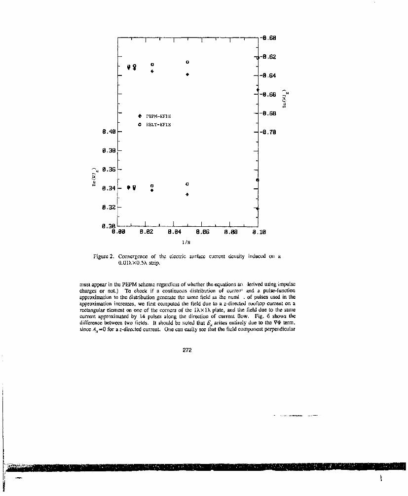
r I I I -8.68

-0.620

-- 8.64

-8.68 ..,

* PEPM-I•rlI -8.68

0 RELT-EFIE8.48 -8. TB

8,38

-• 8.36

8.34 - 9 V

0.32

8.38 L. L I I, I8.88 8.82 8.84 8.86 8.88 8,10

1/N

Figure 2. Convergence of the electric surface current density induced on a0.01XX0.5x strip.

must appear in the PEPM scheme regardless of whether the equations art lerived using impulsecharges or not.) To check if a continuous distribution of curren' and a pulse-functionapproximation to the distribution generate the same field as the numL . of pulses used in theapproximation increases, we first computed the field due to a z-directed rooftop current on arectangular element on one of the corners of the lXX IX plate, and the field due to the samecurrent approximated by 14 pulses along the direction of current flow. Fig. 6 shows thedifference between two fields. It should be noted that Ek arises entiiely due to the V-D term,since Ax=0 for a z-directed current. One can easily see that the field component perpendicular

272

I - ---

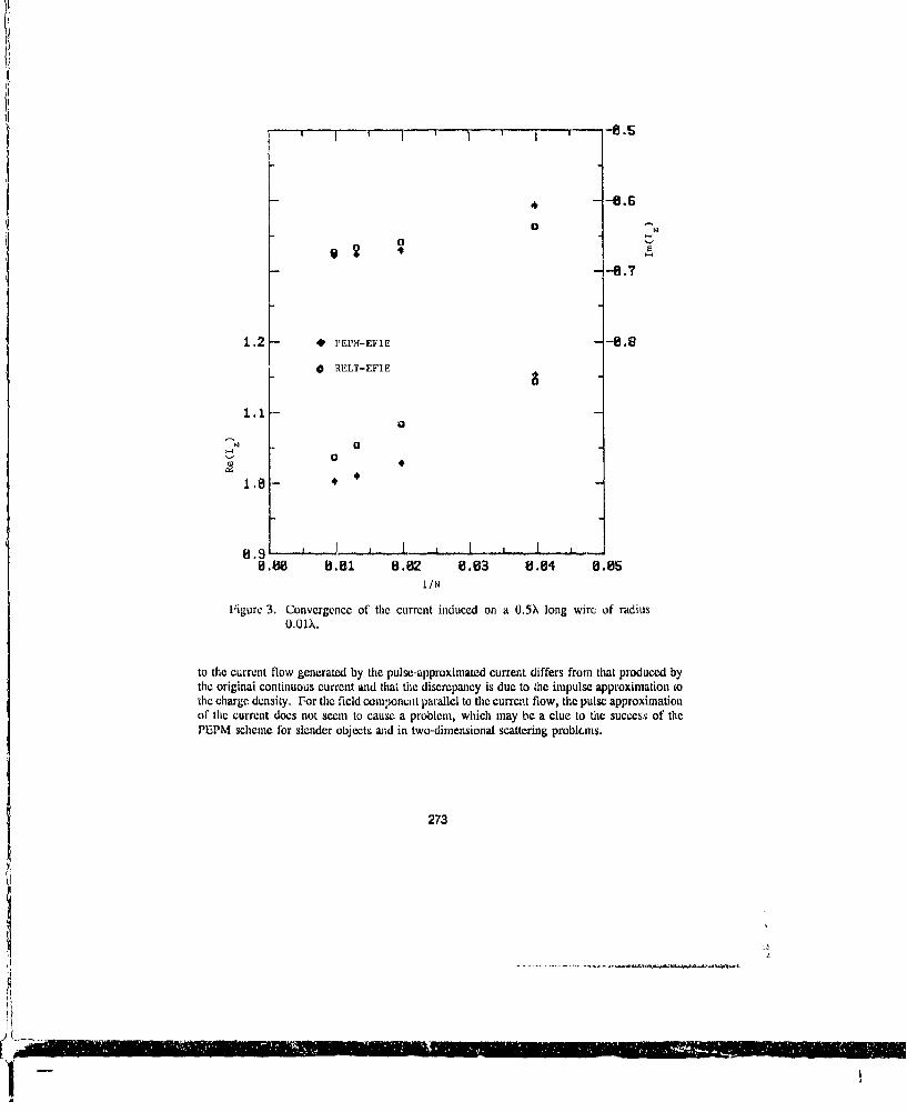
I I I 'I I -f .

4 -8.8

"-8.7

1.2 - PEPM-EF1E -8.80 RELT-EFIE

1.1

I/N

Figure 3. Convergence of the current induced on a 0.5X long wireý of radiusO.01k.

to tile current flow generated by the pul se-approxi mated current differs from that produced bytile original continuous current and that the discrepancy is due to the impulse approximation totile charge density. For the field comlnipoUt parallel to the current flow, the pulse approximation•of the current does not seem to cause a problem, which ,nay be a clue to the succes3 of thePEPM scheme for slender objects an~d in two-dimensional scattering probl(-ms.

273

8.3.

8.8 88 .2 88 .4 88,.I

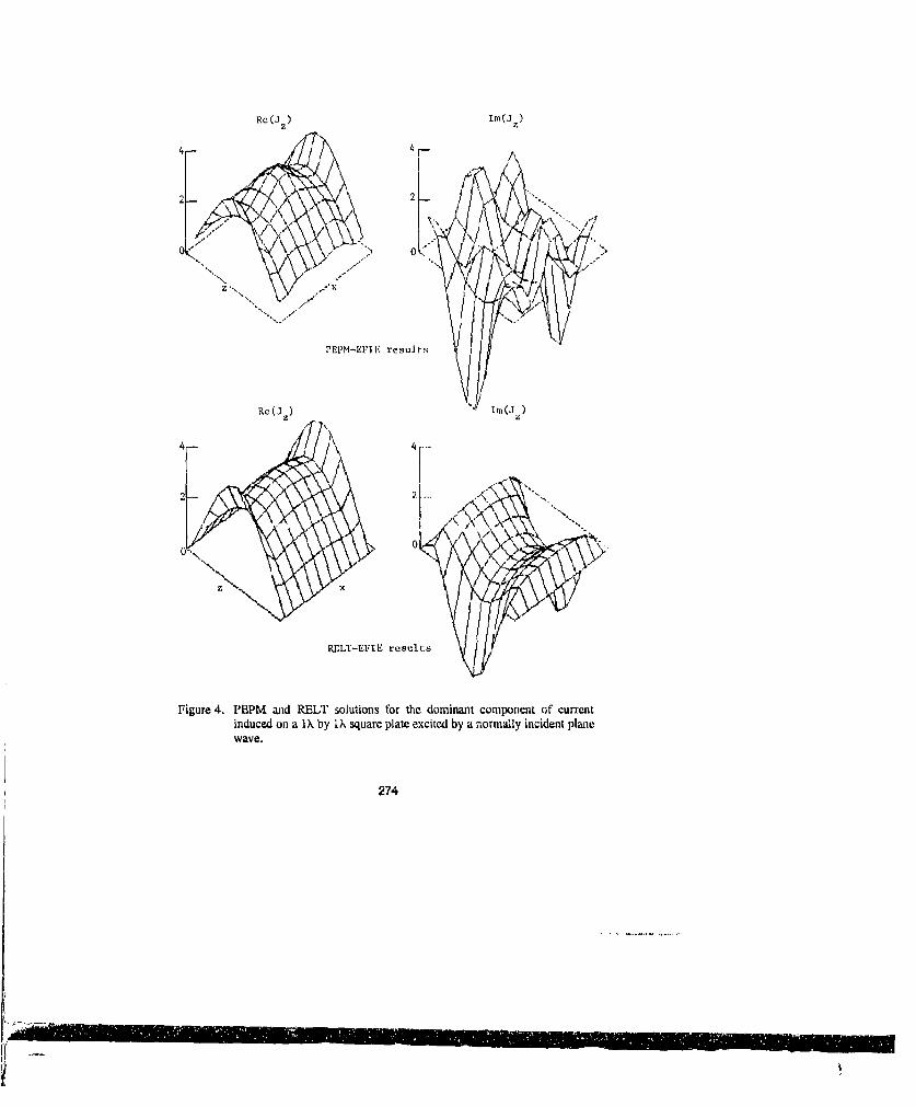
Re(J ) Im(Jz)4 4

// 0

PEPM-EFI E results ]

Re(J) ITO(az

22

RELT-EFIE results

Figure 4. PEPM and PELT solutions for the dominant component of currentinduced on a I X by 1?ý square plate excited by a normally incident planewave.

274

4..

T"lij 4' 9 l I 188

PEPM-EFIL * :* PEPM-MFIE *

"- RELT-EFIE

X RELT-MPIE -s

4, .4 -188

4 -

4 +

a ,. ' I I I I .8.8 8.2 0.4 8.5 8.8 1.8

Figure 5. Comparison of solutions obtained by various approaches for the currentinduced on a 0.4X wide cube.

IV. Summary

The use of a pulse expansion and point matching (PEPM) scheme in the electric fieldintegral equation (EFIE) solution of three-dimensional, time-harmonic electromagnetic boundary-value problems has been studied. Problems of electromagnetic scattering by a few simpleconducting bodies in flee space haw "t:ei• considered and solutions obtained using the PEPM-

275

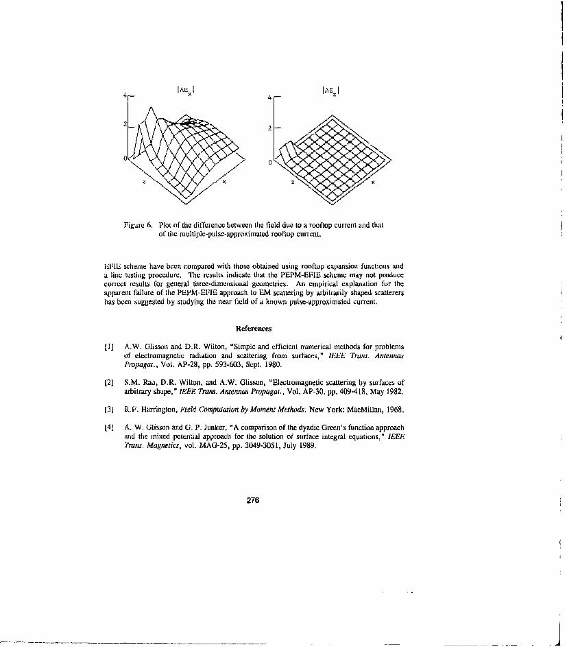
4IAE 91 AE,

2 2

00

Figure 6. Plot of the difference between the field due to a rooftop current and thatof the multiple-pulse-approximiated rooftop current.

EFIE scheine have been compared with those obtained using rooftop expansion functions anda line testing procedure. The results indicate that the PEPM-EFIE scheme may not producecorrect results for general three-dimensional geometries. An empirical explanation for theapparent failure of the PEPM-EFIE approach to EM scattering by arbitrarily shaped scatterershas been suggested by studying the near field of a known pulse-approximated current.

References

[1] A.W. Glisson and D.R. Wilton, "Simple and efficient numerical methods for problemsof electromagnetic radiation and scattering from surfaces," IEEE Trans. AntennasPropagat., Vol. AP-28, pp. 593-603, Sept. 1980.

[2] S.M. Rao, D.R. Wilton, and A.W. Glisson, "Electromagnetic scattering by surfaces ofarbitrary shape," IEEE Trans. Antennas Propagat., Vol. AP-30, pp. 409-418, May 1982.

[3] R.F. Harrington, Field Computation by Moment Methiodi. New York: MacMillan, 1968.

[4] A. W. Glisson and G. P. Junker, "A comparison of the dyadic Green's function approachand the mixed potential approach for the solution of surface integral equations," IEEETrans. Magnetics, vol. MAG-25, pp. 3049-3051, July 1989.

276

[5] P. M. Goggans and T. H. Shunmpelrt, "CFIF MM Solution for Tt- and TM Incidence ona 2-1) conducting body with dielectric. IEEE Tlran.v. Antenna Propalgat., Vol. AP-38,pp. 1645-1649. Oct. 1990.

[6] K. Mahadevan and H.A. Auda, "l-lectnroagnetic field of a rectangular patch of uniformand linear distributions of current, 1ttEU Tran.v. Antennas Propagat., Vol. AP-37, pp-1503-1509, Dec. 1989.

[7] K. Mahadevan and H.A. Auda, "On the electromagnetic field of a rectangular patch ofuniform and linear distributioi.- of current in the source region," IEEE Trais. Antenna.%Propagut., Vol. AP-38, pp. 1244-1248, Aug. 1990.

[81 1. R. Mautz and R. F. Harrington, "Il-field, F-field, and combined-field solutions forconducting bodies of revolution," AEO, vol. 32, no. 4, pp. 157-164, Apr. 1978.

[9] T.K. Sarkar, E. Arvas, and S.M. Rao, "Application of F1T7 and the conjugate gradientmethod for the solution of electromagnetic radiation from electrically large and smallconducting bodies," IEEE Trans. Anw'mias Propagat., Vol. A1P-34, pp. 635-640, May.1986.

[10] T.J. Peters, and J.L. Volakis. "Application of a conjugate gradient FM' method toscattering from thin planar matcrial plates," IEEE Than.%. Antenna.% P'opagat., Vol. AP-36, pp. 518-526, Apr. 1988.

[111 M.F. Catedra, I.G. Cuevas, and L. Nuno, "A scheme to analyze conducting places o0resonant size using the conjugate-gradient method and the fast Fourier transform," IEEE"irans. Antennas Propagat., Vol. AP-36, pp. 1744-1752, Dec. 1988.

[12] W. Sun K.M. Chen, D.P. Nyquist. and E.J. Rothwell, "Determination of the naturalmodes for a rectangular plate," IEEE Trans. Antennas Propagat., Vol. AP-38, pp. 643-652, May 1990.

[131 R. Kastoer and N. Herscovici, "A concise conjugate gradient computation of plateproblems with many excitations," IEEE Trans. Antw-nnas Propagat., Vol. AP-38, pp.1239-1243, Aug. 19S -0.

277

Recursive Algorithms to Reduce the Computational Complexity

of Scattering Problems

W. C. CREW, Y. M. WANG, L. GUREL, AND J. II. LiN*

AbstractIt has been demonstrated recently that a recursive algorithir can reduce the computa-

tional complexity (of the full scattering solution of a scattering problem in two dimensions)to O(.N2 '[5- 10]. This is faster than the conjugate gradient method applied to the method ofmoments, and yet provides a scattering soiution valid for all angles of incidence.

In this approach, a scatterer is divided into N subscatterers, and a recursive algorithmis used to construct the n + n' subscatterer solution from the n subscatterer solution. Ad-dition theorem is used ýto translate tile field among the different coordinate systems of thesubscatterers.

The algorithm has been applied to calculate scattering from a 10A diameter object.Such an object requires about 12,000 unknowns to model, but it takes only about 30 sees ona CRAY-2 to solve with the fast recursive algorithm. It is estimated that it wil' take about20 hours on the CRAY-2 to solve a similar problem with the method of moments.

We have also applied the algorithm to solve for scattering solutions from an array ofnntallic strips, and impenetrable scatterers. T'le solutions obtained are found to either agreewell with closed form solutions, or solutions fronr the method of nnoments.

1. IntroductionA problem facing computational electrornagnetics is the computational

complexity of nunserical methods used to solve for the scattering solutionof a large inhotnogeneous scatterer. The conventional method of mnomnentsrequires a matrix inversion, and hence is of O(N3 ) complexity where N isthe numtber of unknowns modeling the scatterer [1]. The conjugate gradientnmethod carn be used to reduce the computational complexity yielding an itera-tive algorithus with complexity O(N 2P) where P is the number of steps in theiteration- However, the number of steps P required depends on the conditionnumiber of the matrix equation. For ill conditioned matrices, the methodnsay not converge at all [2]. Fast Fourier transforn niethod has also beenused to exploit the convolutional nature of the scattering integral equationyielding a conjugate-gradicnt type algorithm with complexity O(PN logI N)[2,4]. However, conjugate gradient methods provide a solution for only oneincident wave only at a tinse. The algorithm has to be restarted for each newincident wave.

Recently, we have developed a fast reciir:;ive algorithm using translationformulas [5-10]. The computational complexity of the fastest of such an al-

This work is supprl,' d by National Science Foundation under grant NSF ECS-85-25891, Ollice of Naval Research under grant NOOO-14-89-J 1286. Computer time is partlyprovided by the National Center for Supercomputer Applications at the Univelsity ofIliarois.

Electromnagnetics Laboratory, Department of Electrical and Computer Engineering, Uni-versity of Illinois, Urbana, IL 6180.

278

-I

gorithm is O(N 2 ) where N is the number of unknowns used to model theproblem. A program has been developed using this fast algorithm. Compar-ison with the method of moments shows that the fast algorithm is a lot inureefficient. Moxeover, the memory requirement of this algorithm is minimal.More importantly, this algorithm solves a 10A x IA scatterer with 12,000unknowns in about 30 seconds on a CRAY-2. This time is much faster thanthat of solving a matrix equation with a similar number of unknowns. Asopposed to the conjugate gradient method, the fast algorithm provides a fullsolution valid for an incident wave at all angles of incidence. We have alsoapplied the algorithL -... -olve for scattering solutions from an array of metal-lic strips, and impenetrable scatterers, rhe solutions obtained are found toeither agree well with closed form solutions, or solutions from the method ofmoments.

2. The Recursive AlgorithmIn the fast recursive algorithm previously presented[6-10], an inhomoge-

neous scatterer is first divided into N subscatterers. The scattering solu-tion from these N subscatterers is sought recursively so that the (n + 1)-subacatterer solution is obtained from the n-subscatterer solution. The scat-tering by the subscatterers are expressed in terms of a transition matrix or1' matrix. Furthermore, an aggregate 7' matrix is defined for the ni sub-scatterers. Hence when the (n + 1)-th subscatterer is added, only a two-bodyscatterinp problem need be considered. When the scattering solution is foundfor (it + 1) jubscatterers, then an aggregate 7' matrix is defined for these scat-terers. This procedure is repeated until all the N subscatterers are exhausted.

The previous algorithm works excellently for E. polarized waves incidenton an inhuimogeneous cylinder. But for H, polarized waves, the previouslydescribed algorithm is found not to work well because of the infraction of theaddition theorem. As a generalization, Instead of adding one subscattererat each recursion, n' subscatterers could be addcd at each recursion whenthese n' subscatterers are equidistant from the origin (see Figure 1). Bydoing this, the infraction of the addition thc-orem could be avoided, and theresulting algorithm is found to work well even for 11, polarized waves. Thisgeneralized algorithm is described as follows.

Given n subscatterers, the total fiell could be written as (using the no-tation of references 5 to 10)

O(r) = Rg4'(ko, ra) , a + t'(ko, ro) .(.. (1)When n' subscatteiers are added to the previous n cluster, the total fieldcould be written as

O(r) = Rýg4((ko, ro) a + i'(k0 ,rto), r"(n+,') an+"'

+ •i '(ko, r1)" Tiq.+,)" , ." a, (2)

279

where 1 ('+.,) is the aggregate T matrix for n subscatterers in the presenctof n + n' subscatterers, and Tj(ý+n,) is the (n + n')-scatterer T matrix for thei-th subscatterer. The above constitutes a n' + 1 unknown problem wherethe unknowns are +,) and Ti(,+,,) = n + 1, .. ,n + n'. These n' + Iunknowns could be found as follows using the solution (1). Firsit, we ex-press the field from the n' subscatterers as incident field on the aggregted nsubscatterers so that

O~)= RgP'(ko, ro) -a + RgO'.(ko. ro) zi~ , ;F(.. aimt+it

+ ,P•(ko, ro) T .(.+.,)a, (3)

From Equation (1), we must have

•,(n+n,•= ý,(. ? + ,, 'T,'• +r". ) (4)

Next, we focus at the i-th subscatterer of the W' subscatterers and expressthe fields from all the other subscatterers as incident fields on the j-th sub-scatterer. By so doing, we have

O(r) = g•'gs(ko, ro)' .jo" a + R9g'(k0 , r,) 'a,, *'.(n+,)• a

-I- Rg"(ko, rj) Z•)* + a

+ 1,&(k0, rj) T 3!j(+-'o') a, (5)

where the summation for i # j is for i = n + 1, ... , n + n', for i # j. Thescattered field off the j-th subscatterer must be related to the inciOdent fieldvia the isolated scatterer T matrix for the j-th subscatterer. Consequently,we have

-2 j'•(n+rn') = •oW jl ('io +• •jo . r~t~t 4• E• .,ts(n+.,) . "•o),

Equation (4) can be used to substitute for + in (6) to yikld

i(nn+a,' (1) + .•ij" + 60i ' Ti.+nl) 'i)

+ TiY .+,+,) •3•o], = + 1,.. ,Y&+,n'. (7)

280

The above could be rearranged to yieldDT .+n'Yi-j,o = Tj.t) [a+•jo'T(,)+ZC(ao'7(,) •o,+•,)T,(.+n,)'3J,o

=n + ,,.n + n', (8)

w' [" -- " The above constitutes n' equationsfor the n' unknows Ti(,+n,) •,. It can be written more succinctly as

fl-I-rn'

E A2 ,'TI(,•÷ ')'/io=-Tj(I)'[3j0 +O'jo'(n)], j = n+, 1. ,n +a', (9)i=n-l I

where Ai Dj'i j,

Tji" ( .7(). - + ,• , j. (a)After hat-ing s-)lved (9) for + ",o, (4) could be used to find •-(n+n,)-Alternatively, (4) could be written as

n+n•.(+,)= T(,,) + • 7(n). T•• ,(,,+,) ,o (11)imn+l

for more efficient computation.When all the unknows in the n + n' subscatterer problem is solved, then

an aggregate T matrix for n + n' subscatterers can be defined asn+nI

0+,' ,+-') + E " Ti(.+•') • (12)

Consequently, (11) could be substituted into (12) to yieldn+nt

T~~' ()+ E (4fe. + Y(n). * iii .~ ' (13)i-n+1

Equations (9) and (13) permit us to find the (n+n')-subscatterer solutionfrom the n-subscatterer solution. These equations could be used recursivelyto find the N subscatterer solution from a 0 subseatterer solution. The com-putational complexity of the above algorithm could be analyzed, and it isfound t'- the computer time will grow as N' in two-dimenzions, and asN"1 3 in three dimensions. Wlan n' = 1 in the preceding algorithm, theabove algorithm reduces to reduces to the algorithm described in [8,9]*.

• The computational complexity for three Jimensional problem given in [9] is incorrect.It should also bc N'13 .

281

3. Numerical SimulationA computer program has been developed using this recursive algorithm

for computing the wave scattering solution of a large inhomogeneous objectin two dimensions for both E. and H, polarized waves. This method givesthe same solution as the method of moments for small scatterers of one or twowavelength in size. Hence, we have used the method of moments to validatethe code for a general inhomogeneous scatterer. But for large scatterers, themethod of moments is extremely inefficient due to its N' complexity.

The code has been used to calculate the scattering solution from a largecylinder which is about 10A x 10A, and comprising about 12,000 unknowns.Since the method of moments is extremely inefficient in this regime, we canonly validate our solution by comparing it with the closed form solution of acircular, homogeneous cylinder, which is solvable by harmonic expansions.

In Figure 2(a), we show the comparison of the amplitude of the solutionof scattering by an E, polarized wave using the recursive algorithm and theclosed form solution. In this case, n' need only be 1. As can be seen, theagreement is excellent.

In Figure 2(b), we show the comparison of the phase of the solution byrecursive algorithm versus the closed form solution. We observe excellentagreements except for sonic angles of observation. However, for such a wave-length, note that if the diameter of the object is changed by 0.5%, a phaseerror of about 90 is possible, and hence, the phase solution is very sensitiveto the size of the object.

In order to use the recursive algorithm, the subscatterers have to be or-dered so that they are of increasing distance from the origin [7,8,9]. We haveused the heapsort algorithm [11,12j to order the subseatterers with computertime proportional to N log, N. If a naive sorting algorithm of O(N2 ) con-plexity is used, the sorting time could constitute as much as 40% of the totalcomputer time.

On a CRAY-2 supercomputer, the 12,000 unknown problem is solvedin about 30 seconds. In this simulation, we pick M = 1, and P = 30. Thereason we have chosen M = 1 is because only the monopole term is importantfor the scattering from each subacatterer. Though the CRAY-2 has a peakperformance of about 1.7 GFLOPS, this peak is in general not attainablefor practical applications. For instance, for a simple fully vectorizable "DO"loop, the throughput of the CRAY-2 is about 100 MFLOPS unless specialprogramnning technique is used [131. In general, the throughput is about 20to 40 MFLOPS. Assuming a 30 MFLOPS throughput, and that it takes N`/3floating operations to invert an N x N matrix, and multiplying by a factor of4 for complex floating point operations, we estimate that it will take about20 hours to solve this problem by the method of moments. Figure 3 showsthe comparison of the computer time of this method versus the number ofunkowns on a CRAY-2 supercomputer. The 12,000-unknown point for themethod of moments is extrapolated since it is too expensive to solve thisproblem by such a method.

252

In this program, the isolated scatterer T matrix and the translation for-mulas are calculated as they are needed. Hence, the dominant part of thememory is used to store the grid which is proportional to the number of un-knowns N, whereas a matrix method like MOM would have required storageproportional to N'.

Table I shows the breakdown of the computer time spent in various partsof the computer program. It is seen that about 16% of the time is spent inreading in the input for the program. This could be sped up by using binarydata files for instance. Note that the memory used is about 0.385 MWord.A full matrix method as in the method of moments would have needed 290MWords of memory.

In Figures 4(a) and 4(b), we show the comparison of the solution of scat-tering of H, polarized waves by a circular dielectric cylinder using the recur-sive algorithm using mcthod of moments, recursive algoritlhn, anad analyticsolution. As can be scen, the agreement between the method of momentsand recursive algorithm is excellent while there is a small discrepancy withthe analytic solution. The discrepancies come from imperfect modeling asthe circular cylinder is divided inth subscatterers which are squares. Theresulting cylinder does not have the same surface area as tile circular cylin-der, even though they have the same cross sectional area. Since in the H.polarized wave, the electric field polarizes surface charges on the surface ofthe cylinder, the discrepant surface area could give rise to the small error.

In Figures .'(a) aid 5(b), we show the RCS of metallic strips for the E.and H, polarized waves respectively using such a recursive algorithm. The

m iatrices of the individual strips are found using the method of moments.In Figures 6(a) mid 6(b), we show the comparison of the scattering from

alm impenetrable metallic scatterer for the E, polarized wave using the re-cursive algorithm. The mnetallic wall is modeled as z-directed wires tightlypacked together. The ca-se compared in a circular metallic cylinder whereclosed form solution exists.

IV. ConclusionsAu efficient method for solving for the bolution of wave scattering fromi

a large scatterer has been developed. This method uses a minimal of coin-puter memory, and is a lot more efficient than a full integral equation solver.Moreover, it provides a full scattering solution valid for all angles of incident.This method has been used to solve a 10A x 10 A problem with about 12,000unknowns, in about 30 seconds or. a CRAY-2 supercomputer with a typicalthroughput of about 30 MFLOPS. We have also applied the algorithum to H,polarized waves showing excellent agreement with the method of moments.The algorithm could also be applied to scattering by an array of metallicstrips, or impenetrable scatterers.

The method is faster than the method of moments applied to solviagintegral equations, and unlike the finite element method, it provides a solutionthat naturally satisfies the radiation condition at infinity. Moreover, the

283

subscatterers need not have to be close together: it works both for denselypacked as well as sparsely packed subscatterers.

References[1] 11. Harrington, Field Computation by Moment Method, Malabar, FL,

1983.12] D. T. Borup, D. M. Sullivani, and 0. P. Gandhi, "Comparison of two FFT

conjugate gradient mnethod sand the finite-difference tinie-domnain methodfor the 2-dl absorption problem," IEEE 7T'aus. Microwave Theory Tech.,vol. MTT-33, no. 4, pp. 383-395, April, 1987.

1-3) C. C. Su, "Calculation of electromagnetic scattering from a dialctriccylinder using the conjugate gradicnt mnethod and FFT," IBE&J Trans..Aniennas Propag., vol. AP-33, no. 12, pp. 1418-1425, Deccember, 1987.

141 C. Y. Shen, K. J. Clover, M. 1. Sancer, and A. D. Varvatsis, "The dis-crete Fourier transform method of solving differential- integral equationsin scattering, theory," I-PEE Trans. Ant. Pro pag., vol. AP-37, no. 8, pp.1032-1041, August, 1989.

[51 W. C. Chew, "An N' algoritlnn for the multiple scattering solution ofN scatterers," Micro, Optical Tech. Letter-, vol. 2, no. 11, pp. 380-383,1989.

161 W. C. Chew, J. Friedrich, ajd R1. Geiger, "A multiple scattering solutionfor the effective permnittivity of a sphere mixture," IBEE Gcoscience andRcmote! Scnssng, vol. 28, no. 2, p. 207, 1990.

[71 Y. M. Wang and W. C. Chew, "An eflicient algorithmn for solution of ascattU~inlg problemI," Micr'o. Opt. Tech. Lett., vol. 3, no. 3, pp. 102-JOG6,March, 1900.

[8) W. C. Chew akid Y. M. Wang, "A fast algorithmn for solution of a scatter-ing probleml using a recursive aggregate tau ruatrix mnethod," MicrowaveOptical Technology Letters, vol. 3, no. 5, pp. 164-169, May 1990.

[9] W. C. Chiew, Waves and Fields, in Inhomugencous5 Media, Van NostrandRleinhold, New York, 1990.

110) Y. M. Wang and W. C. Chew, " Application of the fait recursive algorithmto a lai-ge inihomnogeneouu scatterer for TM polarization," Micro. Opt.Tech. Lctt., vol. 4, no. 3, Mardli 1991.

[1111 D. E. Knuth, Sorting and Searching: The Art of Computer Programing,vol. 3, Addison. Wesley, Reading, Mass, 1973.

[12] W. 11. Press, B. P. Flannery, S. A. Teukolsky and W. T. Vetterling, Nu-merical Ilecipes: The Art of Scientific Computing, Cambridge UniversityPress, New York, 1986.

1131 1. Diller, "Matrix intiltiplicationi benchmnarks 011 the CIIAY-2 systemn,"Dalalink (NOSA, Univ. Illinois, Urbana- Cham-paign), vol. 4, no-5, pp.16-18, May-June, 1990.

284

Table I. Breakdown of the CPU time spent for the 12,000 unknown problem usingthe fast recursive algorithm,

Percciaage of CPU Time Times_The Total CPU (second) Be-m Called

Recursive Part 44.928 14.327 1Translation Matrices 19.928 6.355 1),905

Input Data 16.176 5.158 1Bessel Functions 16.013 5.1U6 35,862

T,.) MLatrices 2.062 0.657 11,¶05Sorting 0.000 0. 193 10

Main P~rog~ram 0.287 0.092 1

Total CPU = 31.888 secondTotal Memory = 0.385 MWord

285

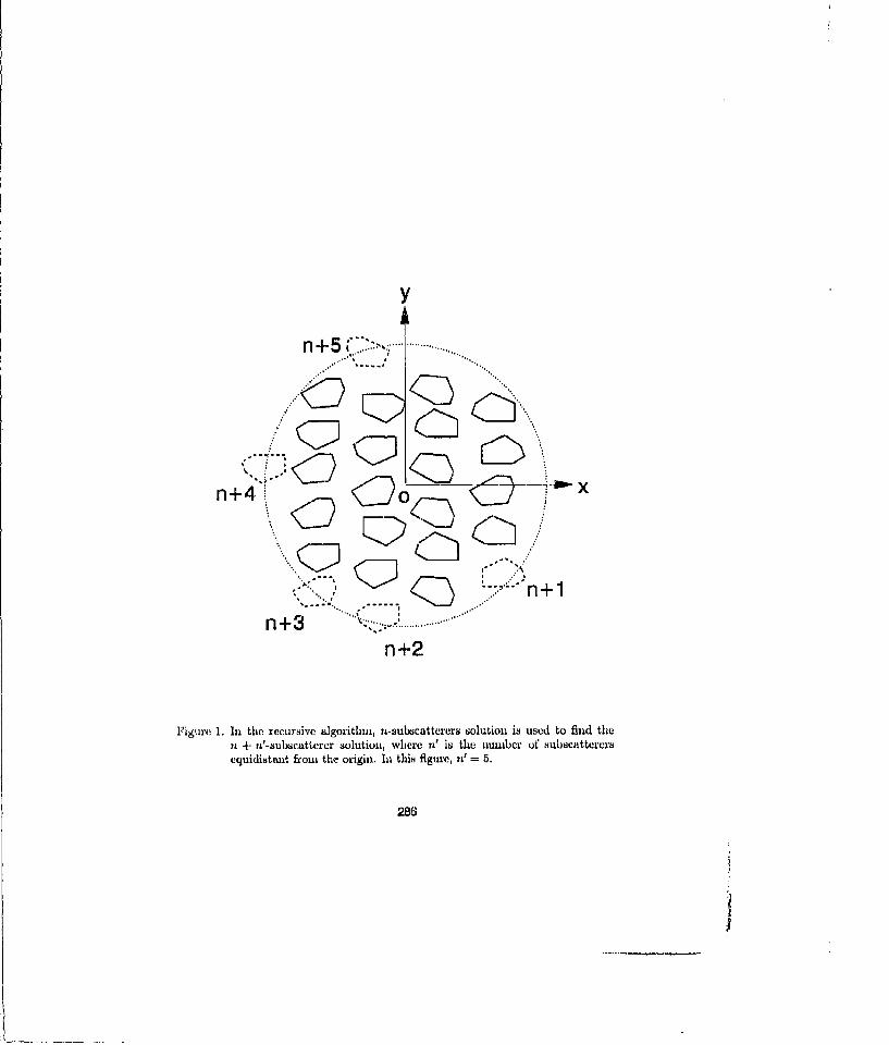
y

n + 5 .., . . ..... .......................

n+4:-c,,,,.""".'"Q

n+3"

"n+2

Figure 1. In the rccursive algorithm, u-subscattercra solution io used to find theni + n'-subsratterer solutioi•, whcre n' is the IIUmbcr of sUb8cnttetrcr8equidistant froom the origin. In this figure, n' = 6.

286

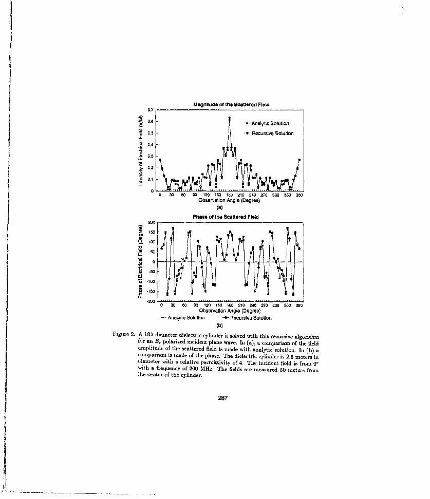
Magnitude of the Scattered Field0.7

0 .6 --- Analytic Solution6_ 0.5 --- Recursive Solution

*0.

• 0.3

0.2 .20.1

0 30 60 90 120 150 180 210 240 270 300 330 6Observation Angle (Degree)

(a)

Phase of the Scattered Field200so100

• 1 oo

s1o

0, 0

oj .50

0, . 100

0 30 60 90 120 150 160 210 240 270 300 330 360Observatlon Angle (Degree)

"- Analytic Solution --&- Recurslva Solution(b)

Figure 2. A 10A diameter dielectric cylinder is solved with this recursive algorithmfor an E• polarized incident plane wave. hi (a), a comparison of the fieldamplitude of the scattered field is nmade with analytic solution. In (b) acomparison is made of the phase. The dielectric cylinder is 2.6 meters indiameter with a relative permittivity of 4. The incident field is from 0'with a frequency of 300 MHz. The fields are measured 50 micters from.he center of the cylinder.

287

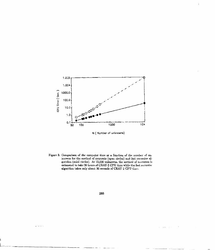
1.0E5-

S1000.0 -

,, 100.0 "

0* 0 0 ""• 10.0 O-O1.00100

0 .1 . . . . .. . . . . . . .

50 100 1000 1E4

N ( Number of unknowns)

Figure 3. Comparisou of the computer time as a. function of the number of utn-knowna for the method of moments (open circles) and fast recursive al-gorithru (solid circles). At 12,000 unknowns, the method of moments isestimated to take 20 hours of C11AY-2 CPU time while the fast rccursivcalgorithm takes only about 30 Feconds of CRAY-2 CPU tinw.

288

-B KFANXNW APIQO~m* An&M~ VouW~

0.7

01

0 .2

to1

0 100 400

___________ (a)

so

O000 -__Ot

l(b

Figure 4. Scattering of H, polarized incident plane wave using the fast recursivealgorithin, the method of moments, and analytic solution. (a) comparesthe aauplitude while (b) compares the phase. The frequency of the in-ciden~t wave is 600 M~tz. The dielectric cylinder ha~s a diameter of 0.4metet- with a relative pernuttivity of 2. The field in measured at 1 meterfio the center of the cylinder.

128

I I ' _____ -__

I , 2 1 . u i.S3 IS 2.; .

90'I2o' .- "- ' -' -• 60"YO. .

'jo3

/ Ij•,0 \ 30"

150* o (a)

210" /330-

270"

Wo.120, -6

0•

020. 0.40

ISO 0 (b)

2102

Figure 5. Comparison of the RCS of an array of strip6 computed using the gener-alized recursive algorithm (solid dots), method of moments (solid lines)and the recursive algorithm presented in references 7 (dotted lines). (a)is for E, polarized wave while (b) is for H, polarized wave. The error ofusing the old algorithm is larger for H, polarized wave.

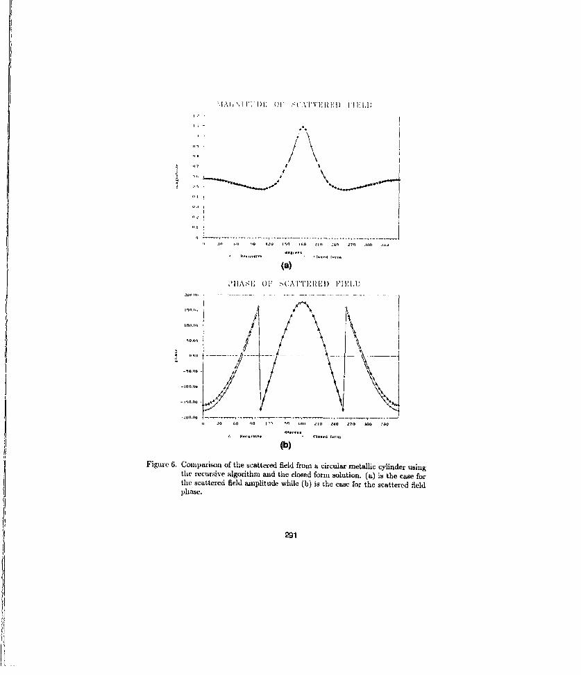
'..\ ,"l ' l~ ; (I OF ( Vl I'l.TE -, l I z II -I IE I

i1 -2 1

iIA.N OF -- ATRE I

* o Go 9 1 0 .o o .3

291nDo.

cD .40 04) *10 42 4.9u 1 ". 0 i )o 2 o -40 2')4 .h, .140O

(a)I4]IASI'l 01" .•CATJ''r~lE.I{..) 1.'!EI).1I

- i 49 -o

0 Jo 60 90 i' " 9f 400 2)o 2l 40 2'70 .bOO .•J0

L •4€ urliveCbooud Dorlia(b)Figur'e 6. Compariso•n of the scattered field from a circujar metallic cylinder using

the recursive algorithm and the closed form solution. (a) is the case forthe scattered field •anplitude while (b) is the case Zo•r the scattered fieldlphase.

291

Numerical Solution of the EFIE Using Arbitrarily-Shaped Quadrangular and Triangular Elements

T. Mader, H. SingerTechnical University Ilamburg-Harburg

Hamburg, Germany

Abstract

For the numerical solution of the EFIE by the method of moments plane triangularpatches are widely used because every three-dimensional structure can be approximatedby plane triangles. In most cases the more convenient way of surface discretization isto compose the considered structure of quadrangular patches. If only basis functionformulae for triangles are available, the quadrangles must be subdivided into triangles.'Then the total number of elements increases and also the number of unknowncurrents. In general this splitting into triangles can be avoided only if nonplanarquadrangular patches of arbitrary shape are applied.

The goal of the paper is to present current basis functions suited for arbitrarily-shapednonplanar quadrangular patches in parametric form. These basis functions can becombined with the commonly-used basis function [51 for plane triangles. Furthermore,it is shown how to extend the basis functions for plane triangles to any curvedtriangles given in a parametric formulation. Finally It is demonstrated that thedeveloped basis functions can be used to perform the connection between wire-gridsegments and surface patches.

Introduction

With the ever increasing computer power the application of the method of momentsin electromagnetic field prediction became possible not only for thin-wire arrange-ments, but also for the treatment of arbitrarily-shaped three-dimensional bodies. At thebeginning of the development the MFIE was used to handle thick-body problems, andfor thin-wire structures the EFIE 121 was prefered. The combination between thin-wire structures and thick-body structures became possible with the introduction of aspecial basis function vadid for the connection area [1].

The disadvantage concerning the MFIE is that it is only valid for closed bodies. Inorder to treat thin-shelled, open structures the researchers tried to apply the EFIE tothis problem. Difficulties were arising, because the EFIE contains not only theunknown surface current itself, but also its first derivation. Therefore it is not sufficientto assume a uniform current distribution over a surface patch, as it is possible in theMFIE solution.

Special linear basis functions for plane rectangles, the so-called roof-top functions,were introduced bv Glisson 13]. 'The resulting charge distribution is uniform over the

&7 1 whole surface patch, and it is assured that no point or line charges can occur. The-- M" important feature of this basis function is that it contains the possibility of zero surface

292

"A

charge on the whole patch. This is necessary in the low frequency range, because therethe current distribution must be solenoidal.

For the calculation of arbitrarily-shaped metallic bodies Rao [5] has devised a currentbasis function suited to plane triangular patches. Similar to the functions of Glisson[3], the current distribution is linear and the resulting charge is uniform all over thepatch. But because of the reasons mentioned above, it is useful to have a further basisfunction valid for arbitrarily-shaped quadrangles. In the following it will be shown inwhich way the functions of Glisson and Rao can be enhanced so that they match tononplanar, arbitrarily-shaped quadrangles or triangles.

A Short Review of the Basic Equations

For a better understanding of the paper at first a very short summary of the basicprinciples will be given, The EFIE, as it is applied here, has the following form:

E s f ~ p y e -R d i v ro . dSf 47I R TTh)C gS

S = surface of the conducting bodies (including wir.,,),-f = surface current or wire current, respectively,R = distance between the field and the source points.

Eq. (1) represents the electric field produced by the currents induced on the structure.The total field is given by the addition of the incident field and the scattered fieldgiven in (1). For perfect conducting bodies, the tangential component of the totalelectric field must be zero all over the body. This condition is entorced here by usingGalerkin's method with razor-blade functions as weighting functions. This results in thefollowing equation for one matching section:

fg~dF ~ici = UiI~ c (2)s s

with E, due to Eq. (1). The numerical evaluation of (2) leads to

Un =f( -c . . (' - ) .. G(R 2 ) + G(R,) R

S+ div [G(R 2 ) - G(R,)]) dS (3)

with G(R) eJkR

The meaning of the indices is indicated in Fig. 1,

293

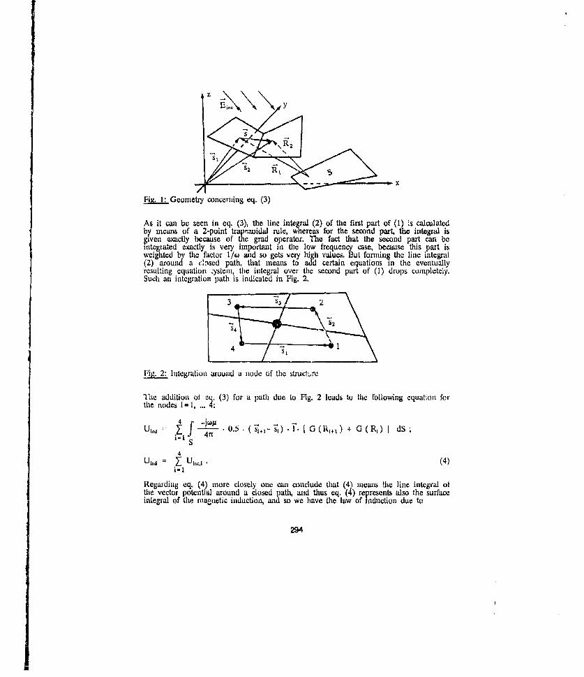
Z

71 xFig. 1: Geometry concerning eq. (3)

As it can be seen in eq. (3), the line integral (2) of the first part of (1) 's calculatedby means of a 2-point trapezoidal rule, whereas for the second part, the integral is$iven exactly because of the grad operator. The fact that the second part can beintegrated exactly is very important in the low frequency case, because this pait isweighted by the factor 11w and so gets very high values. But forming the line integral(2) around a "sed path, that means to add certain equations in the eventuallyresulting equation ýysteni, the integral over the second part of (1) drops completely.Such an integration path is indicated in Fig. 2.

3 3 2

4 - Ii

:Integration around a node of the structure

The addition of eq. (3) for a path due to Fig. 2 leads tu the following equation forthe nodes i=l, ... 4:

4 j W A -•U1,1d- i ZIf -4--- .0.5. (G(-).. [ G(l,) 4- G(R)R, dSS

4U,,,= . U,.. (4)

Ii1

Regarding eq. (4) more closely one can conclude that (4) means the line integral ofthe vector potential around a closed path, and thus eq, (4) represents also the surfaceintegral of the magnetic induction, and so we have the law of induction due to

294

u,.4= -jW. f X ds = jw. f 9 d§ with 13 = curl (A). (5)6 S

Eq. (4) proves directly that the EFIE (1) contains the. stationary case, but in this casethe current must be solenoidal. Thcrefore it is necessary that the choosen basisfunctions allow a resulting current distribution without sources. Eq. (4) together withtic basis functions described in the following section and the condit:im div(I)=O canbe used for the calculation of stationary eddy currents.

Current Basis Functions for Quadrangles

The current basis function that will be developed in this section shall be valid forevery arbitrary quadrangle given in a parametric form according to

V-= - n,). (6)With such a parametric transformation any quadrangle given in the x,Y,z coordinatesystem can be converted into a rectangle in the nm system. Because of the highregularity of the obtained patch it is now easy to define a basis function. The positionof the quadrangle in the "nm system and the choosen basis function are depicted inFig. 3.

/0 1 2F Roof-top basis function in the ),j system

The essential step in the development of a current basis function is now to find asuitable transformation of the current vectors into the three-dimensional xy,zcoordinate system. After this task has been done, one finds for the left part of theroof-top according to Fig. 3:

all(7)

with the metric coefficients

295

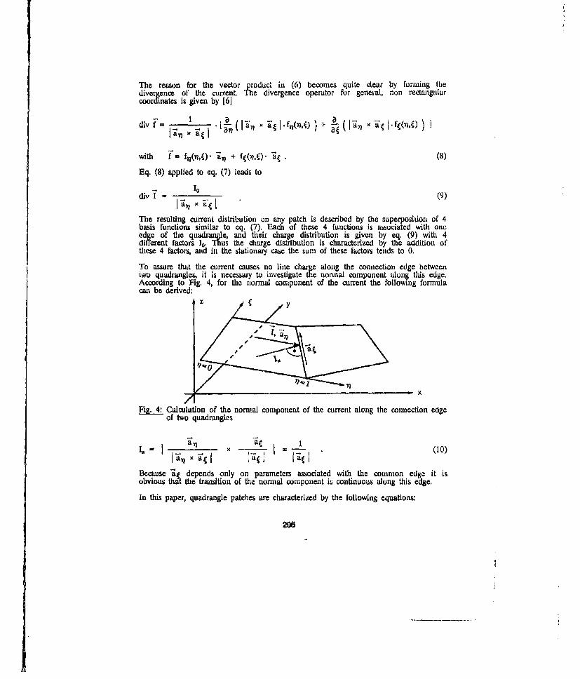
The reason for the vector product in (6) becomes quite clear by forming thediverrence of the current. The divergence operator for general, non rectangularcoordinates is given by [6)

I n-i I

with fT= f -( i n + fr(-nC)" '. (8)

Eq. (8) applied to eq. (7) leads to

div I" I° (9)

The resulting current distribution on any patch is described by the superposition of 4basis functions similar to eq. (7). Each of these 4 functions is a.sociated with oneedge of the qLiadrangle, and their charge distribution is given by eq. (9) with 4different factors 10. Thus the charge distribution is characterized by the addition ofthese 4 factors, and in the stationary case the sum of these factors tends to 0.

To assure that the current causes no line charge along the connection edge betweentwo quadrangles, it is necessary to investigate the normal component along this edge.According to Fig. 4, for the normal component of the current the following formulacan be derived:

z y

/0

- x

4: Calculation of the normal component of the current along the connection edgeof two quadrangles

i~-j I__ _ ___ 1 (10)

Because • depends only on parameters associated with the common edge it isobvious th•t the transition of the normal component is continuous along this edge.

In this paper, quadrangle patches are characterized by the following equations:

296

A2

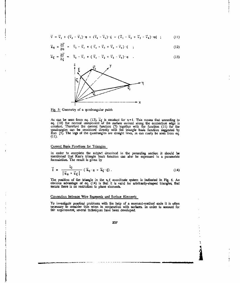
+ = V+ ( - + ) (V + (V- •2 + V3- " (11)

- an = - - + ('•,- + - " 4)' " (12)

V.1 + V1 V2 + V3 VO)n (13)

z

Fi.5 Geometry of a quadrangular patch

As can be seen from eq. (13), -• is constant for rt= . Thils means that according toeq. (10) the nor'mal component of the suifa¢.e cuirent along the connection edge isconstant. Therefore the current function (7) together with the function (11) for thequad rangles can be combined dircctly with the triangle basis function suggested by

Ru(5]. The legs of the quadrangles are straight lines, as can casily be seen from eq.(11).

Current Basis Functions for TrianglesIn order to complete the subject described in the preceding section it should bementioned that Ran's triangle basis function can also be e~xpre~ssed in a parametricformulation. The result is given by

( aI"-+ a ).(14)

The position of the triangle in the n, coordinate sytem Is indicated in Fig. 6. Anobvious advantage of .eq. (14) is that it is valid for arbitrarily-shaped triangles, thatmeans there Is no restriction to plane elements.

Cozuiection between Wire Sei•ments and Surhice ElementsTo investigate practical problems with the help of a moment-method code it is oftennecesx to consider thin wires in conjunction with surfaces. In order to account forthis requirement, several techniques have been developed.

__2

v1

½Vi

0& 1 -.. •"

STriangular patch with current filaments

The simplest technique to connect wires to surfaces is to fix them on one edge of atriangle or quadrangle. A detailed description of this niethod is given in 141.

An'alyzing practical problems, it turned out that in sonic cases it is necessary to fixwires directly on a node of a discretized structure, for exantple becanse only the exactcoordinates of the node are explicitly known in the input data, for reasons ofsyrnmetry or from other geometrical reasons. Therefore an appropriate function withreference to triangles which are connected to wires in one corner point, has to becreated. For flat tnangles, such a function cani be expressd by the relation

" "(0') - +.5'V- • .) y' -(y ) 1- x+.Ay) -Y' (X2+X3 (15)

The x',y',z' coordinate system is situated in the plane of the triangle. The geometricalquantities used in eq. (15) can be taken from Fig. 7.

Y3

ZA

2I X2

i . . ' .' 7 .mctry for a triangle connected to a wire at corner I

208

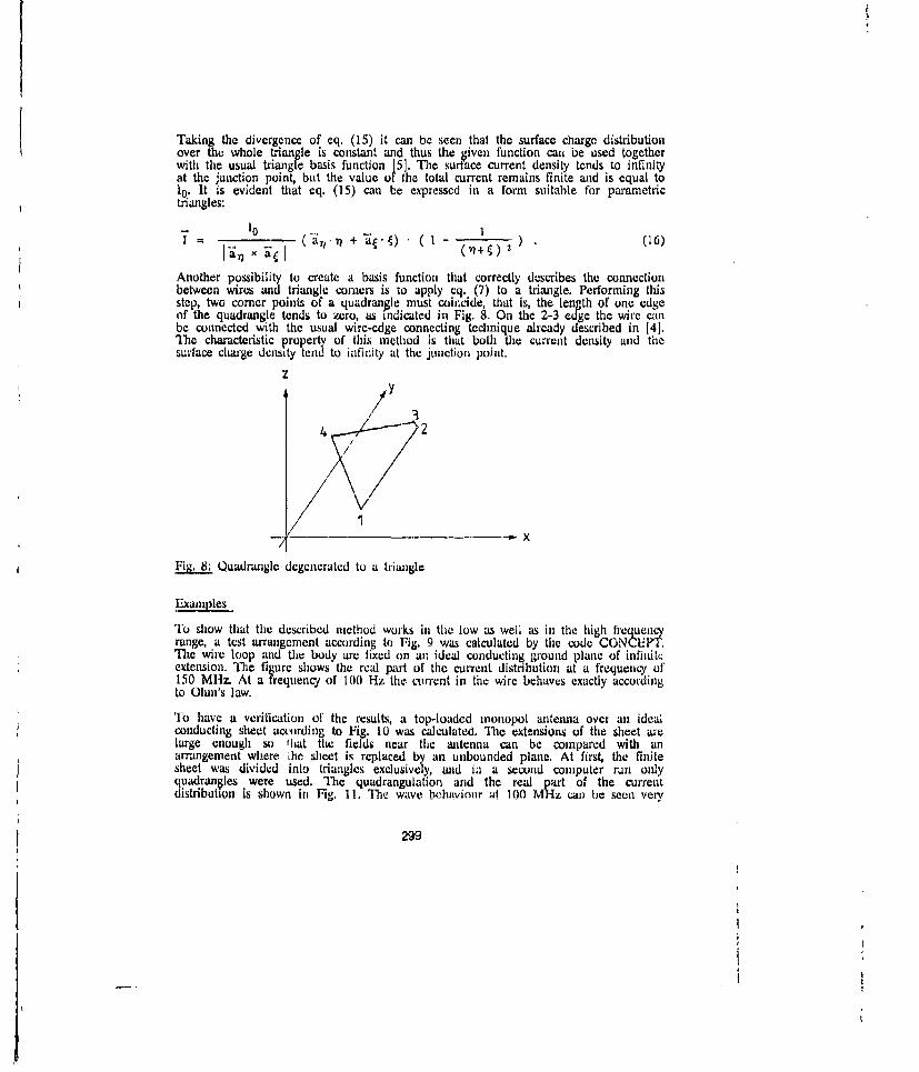
Taking the divergence of eq. (15) it can be seen that the surface charge distributionover thL whole triangle is constant and thus the given function can be used togetherwith the usual triangle basis function [5]. The surface current density tends to infinityat the junction point, but the value of the total current remains finite and is equal to10. It is evident that eq. (15) can be expressed in a form suitable for parametrictriangles:

10

Another possibility to create a basis function that correctly describes the connectionbetween wires and triangle corners is to apply eq. (7) to a triangle. Performing thisstep, two comer points of a quadrangle must coincide, that is, the length of one edgeof the quadrangle tends to zero, as indicated in Fig. 8. On the 2-3 edge the wire canbe connected with the usual wire-edge connecting technique already described in [41.The characteristic property of this method is that both the current density and thesurface charge density tend to infinity at the junction point.

zy

/ 34 2

Fig. 8: Quadrangle degenerated to a triangle

Examples

Tu show that the described method works in the low as well as in the high f'requenlcrange, a test arrangement according to Fig. 9 was calculated by the code CONCEPI.The wire loop and the body are fixed on an ideal conducting ground plane of infhiitcextension. The figure shows the real part of the current distnbutiori at a frequency of150 MHz. At a frequency of 100 Hz the current in the wire behaves exactly accordingto Olun's law.

To have a verification of the results, a top-loaded monopol antenna over an idealconducting sheet according to Fig. 10 was calculated. The extensions of the sheet arelarge enough so 'hat the fields near the antenna can be compared with anarrangement where the sheet is replaced by an unbounded plane. At first, the finitesheet was divided into triangles exclusively, and in a second computer run onlyquadrangles were used. The quadrangulation and the real part of the current

istribution is shown in Fig, 11, The wavy. bohaviomr a! 100 MHz can be seen very

299

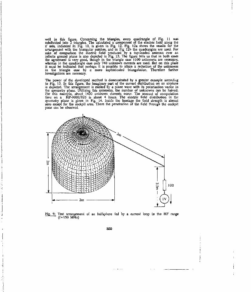
well in this figure. Concerning the triangles, every quadrangle of Fig. 11 wassubdivided into 2 triangles. The calculated x component of the electric field along thez' a"s, indicated in Fig. 10, is given in Fig. 12. Fig. 12a shows the results for thearrangement with the tiangular patches, and in Fig 12b the quadrangles are used. Forsake of comparison the electric field produced by a top-loaded antenna over aninfinite ground plane is also depicted in Fig. 12. The figure tells us that in both casesthe agreement is very good, though in the triangle case 1100 unknowns are necessary,whereas in the quadrangle case only 740 unknown currents are used. But on this placeit must be indicated that perhaps it is possible to attain a reduction of the unknownsin the triangle case by a more sophisticated triangulation. Therefore. furtherinvestigations are necessary.

The power of the developed method is demonstrated by a greater example accordingto Fig. 13, In this figure, the imaginary part of the current distribution on an airplaneis depicted. The arrangement is excited by a plane wave with its polarization vector inthe symmetry plane. Utilizing this symmetry, the number of unknowns can be halved.For this example, about 1400 unknown currents occur. The amount of computationtimte on a HP-9000/825 is about 4 hours. The electric field distribution in thesymmetry plane is given in Fig. 14. Inside the fuselage the field strength is almostzero except for the cockpit area. There the penetration of the field through the cockpitpane can be observed,

i :Test arrangement of an halfsphere fed by a current loop in the HF range(f= 1.5o M z)

300

z74

0.3-

I nI

Fig.1: Foot-point-fcd monopol antenna excited at 100 MHz

Fig 11 Rel prtof he urrntdisiibtio o th grundpZ

--orin-t- Fg----- ot-a--f-heplnq7

Fi__1 Rea opoaet of the uleetri isid utiongo triegrulnr pathe

accrdngtoFig 1, rot alfofth3 pan

realpad nbouded lan

00"

E Cu unbou ded planereal part

u u u U uP I'

>0

.C- imlaginary part4 '..C- C.u. ••' . . .

S0.0 0.5 1.0 1.5 2.0 2.5 3J.0z' In muter

Fig. 121): x component of the electric field using quadrangular patchl's

S~exciting plane wave

Fig. 13: Airplane excited by a plaLe wave of 100 Mliz

302

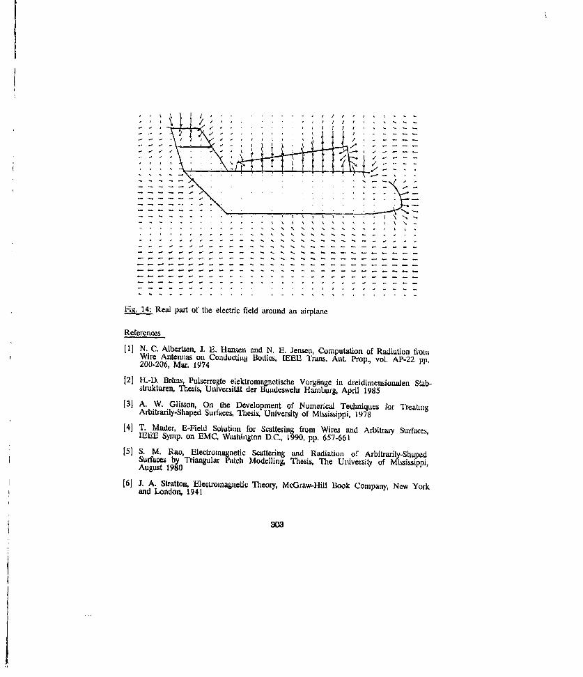
, , , / ... ....... , , , I .....

-. . . -, .• .• •- - . I II[ -/' I /. . .-. -.. . . I . . . \- •[ • .- . I .\ L -/ . . . .

Fg14 Real part of the electric field around an airplane

References

[1] N. C. Albertsen, J. E,. Hansen and N. E. Jensen, Compttion of Radiation fromWire Antennas on Conducting Bodies, IEEE Trans.Auit'. Prop., vol. AP-22 pp.200-206, Mar. 1974

[21 H.-D. Brfil-s, Puhserre~te elektromagnetische Vorgdnge in dreidimensionalen Stab-strikturen, '11.esis, Uiuversitait der Bundeswehr Hamburg, April 1985

[31 A. W. Gl.sson, On the Development of Numerical Techniques for TreatingAruitratiy-Shaped Surfaces, Thesis, University of Mississippi, 1978

[4] T. Mader, B-Field Solution for Scatte -f Wirs a-d Arbitrary Surfaces,IEEBE Sylp. on EMC, Washington D.C., 1990, pp. 657-661

[5F S. M. Rao, Electromagnetic Scattering and Radiation of' Arbitrarily-ShpedSurfaces bA Triangular Patch Modelling, Thesis, The UAiversio. of Mississippi,August 19 0

[6] J. A. Stratton, Electromagnetic Theory, McGraw-Hinl Book Company, New Yorkand London, 1941 3ei cteigaD3 Rdain fA t

SESSION 8- "MODELING EM INTERACTIONS IN MATERIALS"Moderator: Kenneth Demarest

General Approach For Treating Boundary Conditions

on Multi-Region Scatterer. Using the Method of Moments

J. M. Putnam

McDonnell Douglas Research Laboratories

Abstract

For complex geometries consisting of multiple regions with different

types of boundary conditions imposed between the regions (i.e., conducting,

dielectric, resistive, IBC, etc.), conventional method of moments (MM)

procedures can become tedious and difficult to implement. Typically, 14M

based solutions to EM scattering and radiation problems proceed as follows:

"* coupled integral equations are developed which represent the physics

of the problem

"* the boundary conditions are incorporated into the integral equations

"* the MM technique is used to reduce the integral equations to a matrix

equation.

I1i this paper, a simple technique will be presented for incorporating

different types of boundary conditions and combinations of the field

equations for scatterers with multiple homogeneous regions. Each interface

between regions is considered separately. The Stratton-Chu integral

equations representing the E and H fields on both tides of the Interface are

*This research was conducted under the McDonnsll Douglas IndependentResearch and Development program.

304

specified in terms of equivalent elect.tc (J) and magnetic (M) currents on

both sides of the interface. When the field point is located on the

interface, there are four equations in eight unknowns (E , Hi, J , M*).

These eight unknowns are expanded in a series and the MM technique is

applied, resulting in an overdetermined matrix equation. This matrix

equation is independent of the boundary condition on the interface or the

field equations which will be solved. The boundary condition and field

equations to solve are specified by three matrices which operate on the

overdetermined system, reducing it to a matrix equation of a determined

system.

Examples will be given which illustrate how existing MM formulations in

_ Jthe literature can be recast using this technique. This technique has been

,• implemented with Galerkin testing in a general purpose scattering code for

2D bodies, bodies of revolution, and arbitrary 3D bodies, consisting of

multiple regions and boundary condition types. Numerical results will be

presented which demonstrate the versatility of the method.

Introduction

The method of moments (MM) has been used extensively over the past two

* decades to solve a variety of scattering problems involving conducting and

penetrable bodies. In [1] the electric field integral equation (EFIE) is

solved for an arbitrary conducting body of revolution (BOR), end in [2] the

magnetic and combined field integral equation (MFIE and CFIE) solutions are

obta;-ted. For arbitrary homogeneous BOR geometries, th, PMCHW and Muller

formulations are given in [3]. Impedance, resistive, and magnetically

conducAng boundary condition formulations are given in [4]. The above

formulations are straightforward and easily implemented since only a single

305

. - --t ... --.. . . . . . . . - . -i . ... .. •r :~ -! _____• .. . . .. .

surface is present. For geometries with multiple surfaces, where the number

of surfaces and dielectric regions are fixed, the analysis is only slightly

more complicated. For example, in [5] a GFIE formulation is given for a

coated BOR, and in [6] five different formulations are presented for a

partially coated BOR. In [7] a general formulation is presented for axially

inhomogeneous 5OR geometries consisting of multiple conducting and

dielectric surfaces based on the EFIE and FŽCHW formulations. The notation

is complicated for the general case and the numerical implementation is not

straightforward, and is further complicated when resistive and impedance

boundary conditions are also allowed.

In this paper, e simple technique is presented for incorporating various

types of boundary conditions and field solutions into a MM solution for a

general body with multiple conducting and dielectric regions. The technique

is directly applicable to all of the formulations cited above for BOR

geometries, analogous two-dimensional geometries, and arbitrary three-

dimensional geometries. Typically the M2 is applied after the boundary

conditions have been incorporated into a set of coupled integral equations.

In the present approach, the MH is applied directly to a general set of

coupled integral equations on each surface, and then the boundary conditions

on the surface and field cq¶'ntious to test are incorporated. The technique

facilitates the incorporation of different types of boundary conditions and

field solutions into MM codes for general bodies.

Examples will be given which illustrate the technique for 2D and BOR

geometries, using overlapping triangle function expansions and Gelerkin

testing. The Galerkin testing and orthogonal nature of the current.

expansions for 2D an BCR geometries results in special matrix properties

which simplify the approach. The technique will be presented first for a

306

body consisting of a single surface, followed by some conmments on how the

technique extends to the case of multi-surface bodies.

General Integral Equations

Figuae I depicts a scattering geometry with a single homogeneous

interior region R1, In rie free-apace region R., the total electric and

magnetic fields are given by the Stratten-Chu integral equations

.* 4i 4 5 •+ 44 4+ (102 2 (r) - 4L (r) - L2 + K2 M (r)

.9 4 ) . 4 + (02 112 (r) - 11 (r) K2 J(r) -- .2 LM (r)

where Eand H' are the inicident 41actric and magnetic fields, aI te

the equivleont elect~ric and magnet.ic curen'lt~s, and the functionl O(? )

defined au

I for C C I i

0i(4) - forr C •8R (3)0 otherwise

where OR i is the boundary of region R1,

The electric and magnetic surface currents on S in general are

11 W 1is(4a) M s(4b))

and

30/

S.. ........ .... . -:-- ... .-_ 2 = ,• ..... : ; .. . ... - -- , . : -_ ., _ .-.. .. ... - - -.- ' • --- -

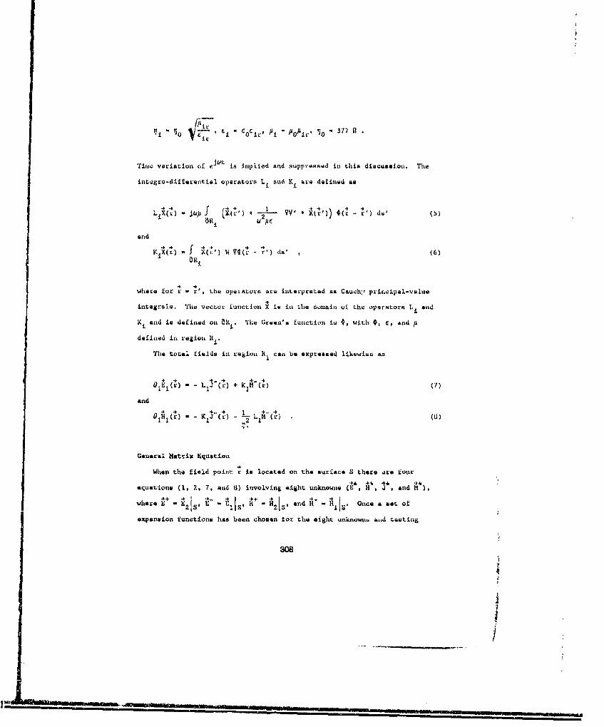
ni- no CF C 0Cjpr pi -o " 371 -

Tiimc variation of ejwt is implied and suppressed in this discussion. The

intggro-differential operators Li and Ki are defined as

LIX( .) - jtVp I ( + vv V A rr' - r' (5)

DlRi W24 t

.A& ' A€ 5

and

KIX(r) - f X(v) V V4(t - r') de' , (6)31%

44

where for r - r', the operators are interpreted as Cauc'h:r prir.cipal-valus

integrals. The vector function X is in the domain uv the operutore L and

Ki and is defined on aRi. The Green's function is t, with 0, C, and pdefined in region 11%.'

The total fields in region R I can be expressed likewise as

4 + 444 " 4_0 1E(r -- L1 Kr + (1 r)(?

and÷ .'• 1 4-•

- - K 1 (r) - j L1 I r) (h)

General Hatrix Equation

When the field point r is located on the surface S there -Are four

equations (1, 2, 7, and 8) involving eight unknowns (E , HV', e, nd ,

Wee4+ 4J ~ + 4 4- 4j4hEre 2S' E2 EI- , + - HI2S and " HA A, Once a set of

expansion functions has been chosen tot the eight unknownls ind tasting

308

4Ii

I I i I I ! i • 1/

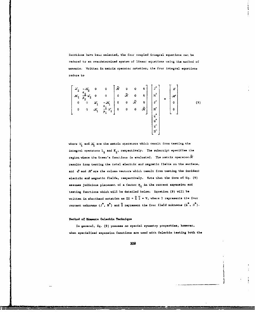
functions ha•, bs'a selected, the four coupled integral equations can be

reduced to an overdetermined system of linear equations using the mothod of

moments. Written in matrix operatoe notation, the four integral equations

reduce to , , 0 i! 001 j;'W2 1+ 0

X 2 0 0 0 0 0 M'0 0 Y V 0 0 or 0 J 0 (9)sc

0i 0 -W r 0 0 Jr0 M + -EI E N -"

H-

where ýa ndYq are tle matrix operators which result from testing the

integral operators Li and Ki, respecaively. The subscript specifies the

region where the Green's functions is evaluated. The watrix operator .9

result. from testing the total electric and magnetic fields on the surface,

end 4ead .- are the column vectors which result from uesting the incident

electric and magnetic fields, respectively. Note that the form of Eq. (9)

assumes judicious placement of a fector V0 in the current expansion end

testing functions which will be detailed below. Equation (9) will be

written in shorthand notation as ZI + Z I - V, where I represents the four

current unknowns (J , MH) and i represent the four field unknowns (E*, H*).

Method of Moments Oalerkin Technique

In goeneral, Eq. (9) possess no special symmetry properties, however,

when specialized expansion functions are used with Galerkin testing both the

300

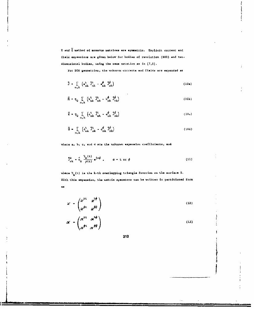
fv

Z and i method of moments matrices are symmetric. Explicit cuvrent and

field expanaicns are given below for bodies of revolution (BOR) and two-

diwuansional bodies, using the saome notation as in [7,8].

ror BOR geonietries, the uInknw currents and ftelds are expanded as

k nk nk nk 111J

M no E: (b nk k mnk nk) (1.0b)'I'k

K . r Ik nk a kI)(0C

n'k

where a, b, c, and d are the unknown expansion coefficiente, and

ka - i"(t) i

where Tk(t) is the k-th overlapping triangla function on the surface S.

With this expansion, the matrix operators can be written in partitioned form

an

... .. 1-= (12).. ... " "" . . .. ..

.t-./~Le se~

.1z (3

\wou WOO

w310

jaftý "MU_ _

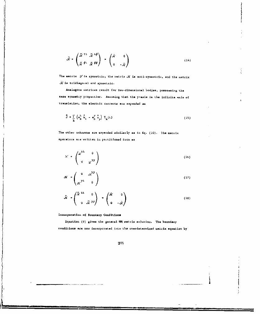
0 x ; (14)

The matrix iL' is symmatriC, the matrix X•" is anti-symnetric, and the matrix

.is tridiagooal and symlneLri;.

Analogous matrices result for two-dimensional bodies, possessing the

same nsytmetL'y prope'tiec. Aesuming that the y-axis is the infinite axis of

trallslat;ion. the electric currents are expanded an

4 4 Tk

The other unknowns are expanded similarly as in Eq. (10). Ihe matrix

operatovs aLe WL'ittnl ini paLrtitioned form am

()(17)

Ctt )Q18)

0 0•

Incorxporation of Boundary Conditions

Equation (9) gives the general tMi matrix solution. The boundary

conditions are stow incorporated into the ovardeterwined xutrix equation by

311

____________________ ____________

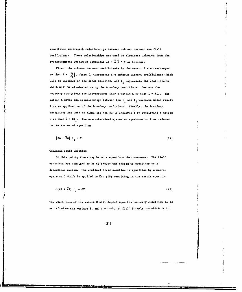
I

specifying equivalent relationships between unknown current and field

coefficients. These relationships are used to eliminate unknowns from the

overdetermined system of equations ZI + Z I - V as follows.

First, the unknown current coeoficients in the vector I are rearranged

so that I whers Il represents the unknown current coefficients which

will be retained in the final solution, end 12 represents the coefficients

which will be eliminated using the boundary conditions. Second, the

boundary conditions are incorporated into a tuatzix A so that I - Al . The

matrix A gives the relationships between the II and 12 unknowns which result

from en application of the boundary conditions. Finally, the boundary

condiLtions are used to elimi ate the fi.Id unknowns I by specifying a matrix

B so that I - BI2I The overdetermined syster of equations in thus reduced

to the sysLtem of equatiuns

(Zi - 2B) 1, - V (19)

Combined Field Solution

At this point, there may be more eqtuations than unknowns. The field

equations are combined so as to reduce the system of equations to a

determined system. The combined lield solution is specified by a matrix

operator C which is applied to Eq. (19) resulting in the matrix equation

C(ZA + 2B) Ii -CV (20)

The exact form of the matrix C will depend upon the boundary condition to be

satisfied on the surface St sumi the cobined, field formulation which is to,

312

~i

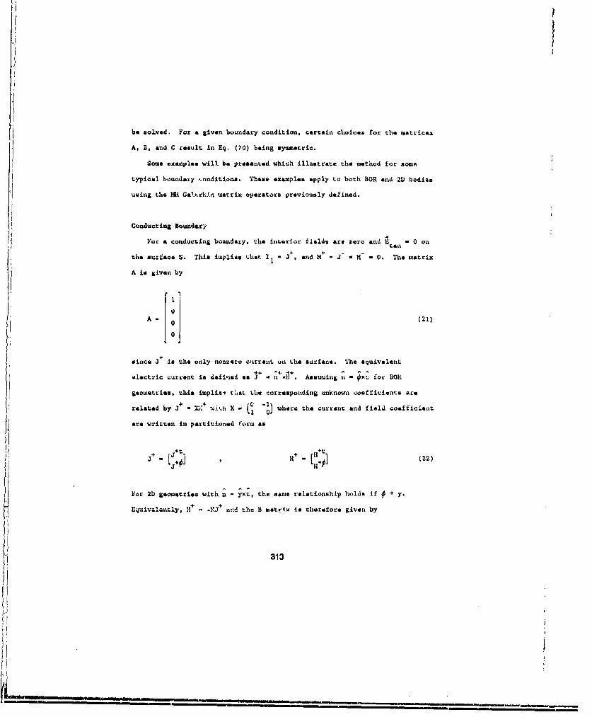
be solved. For a given boundary condition, certain choices for the matrices

A. B, and C cesult in Eq. (70) being symmetric.

Some examples will be presented which illustrate the method for some

typical boundary -. onditions. These examples apply to both BOR and 21) bodies

using the M Gal'trlk..n matrix operators previously defined.

Conducting boundar;

For a conducting boundary, the interior fields are zero and E 0 - C onl

the surfacS. This implies that I - , 3 and H+ - M - 0 - 0. The matrix

A is given by

1

0A - 0 (21)

since J+ is the only non2ero current on the surface. The equivalent.4-4+electric current 1s defimd as 3+ - 'Hx . Assuming n - • for BOR

geometries, this •plipt tIhat the corresponding unknown coefficients are

related by J3+ . ;G+ w-it h X - (~ Q ) where the current and field coefficient

are written in partitioned f-orm as

j+ [+t] + [1t+U

For 2t geometries with n - yxc, the same relationship holds if 4 y.

313

ii!

"i' !

_ _ -' ,- a... . . .

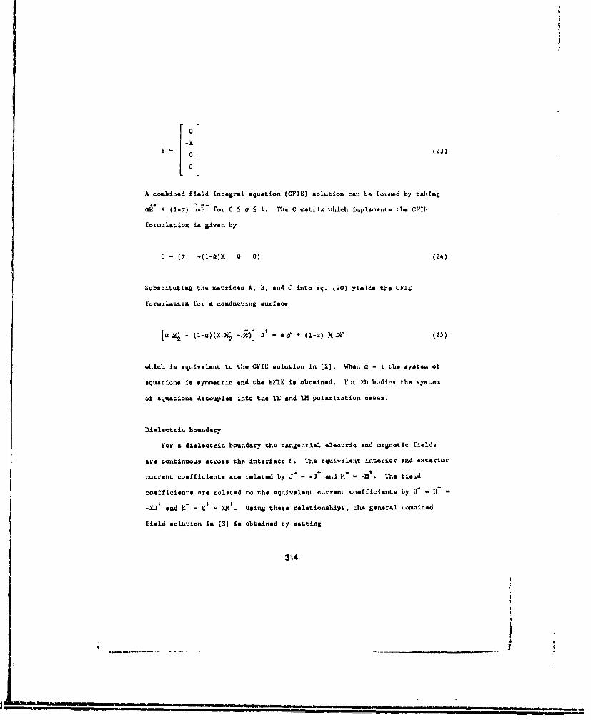
0k

B - (23)

A combined field integral equation (CFIE) eolution can be fornied by taking

OE + (1-a) nxH for 0 - a 5 1. The Q matxix %ihich implements the CFIE

foL-mulation is given by

C - (a -(1-a)X 0 0] (24)

SubsLiLuting the matrices A, H, and C into Eq. (20) yields the CFIE

formulation f"r a conducting surface

[aL2- ('-a) (X3' .&) J+ - 6 + ('-a) X Y'X (25)

which is equivalent to the CYIE solution in (2]. When c - I the system of

2quatione is syumetric end the EFIE is obtained. For 2D bodies the system

of equations decouples into the TE and TM polarization cases.

Dielectric Boundary

For a dielectric boundary the tangautial electric and magnestic fields

are continuous across the interface S. The equivalent interior and exterior

.urrent coefficients are related by J" - -Ja+ nd M- - -M+. The field

coefficiente are related to the equivalent current coefficients by H" - H -

-XJa and C- - E+ - X•H. Using these relationships, the general combined

field solution in (3] is obtained by setting

,314

NI

%I

_L- _. .. ... . . .. . . .. . . . .

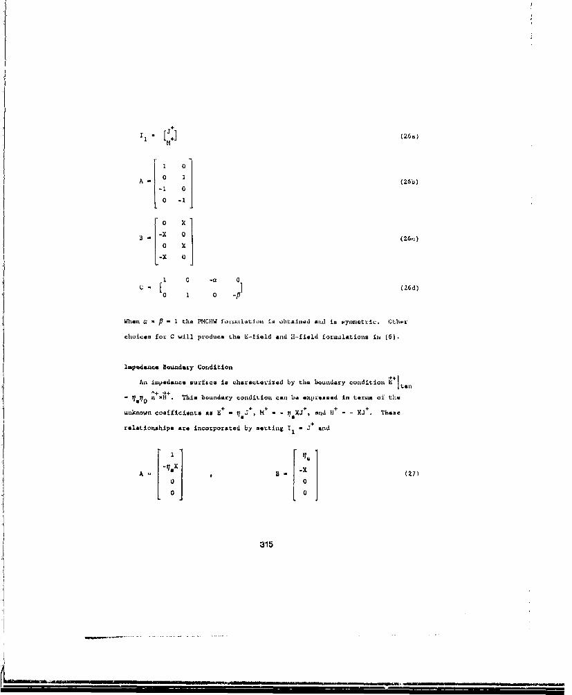
1 m +] (26a)

1 0

A 0 101 00 -1

S. 0 (2x

0X

1. 0 -a

Whenu Q * f - 1 the PMCHW furviulatitui is obtained atid is myammeltric. OthPL"

chouices foz" C will produce Lhe 1"-•ield and H-.field L'rmulationa in (6).

Iupedauce Boundary Condition

An iwpodanc, su--tce is characterized by the boundary condition t~ai^+ .0+

A) i iH . This boundary condition can be expressed in terius of the

unknown coeficientsa an E- n+, - - nBXJ+, and 11+ - -XJ+. Theme

relationahips are incorporated by 3otting 1I - s+ d

11A -la B - (27)0 0

0 0

315

The Fymmstric system of equations given in [4] is obtained if C - tA where t

indicates the transpose. Other choices for C will produce different

combined field IBC formulations.

Resistive Boundary Condition

A resistive surface is charactuiized by the boundary condi•ions .+

~+ 4+~- 1 4+"9 and n' - (II+ - II) R L These conditions can be' expressedtan tall4- 4+ -9 --++ 4+

in terms of the equivalent c:urr-ents as M _M4 and R a 0 (1+ + 4Jan

The A matrix is defined by setting

IA V I+ (28a)

j-

1 o 0

A - 0 1 (23b)

0 -1

The B matrix is obtained by noting that the boundary condition can also be4- +4 4+ 4++

written as H - -Ra + II where H 1 1tan i.110 tan tan

it 0 Ra a

-X 0 0

tR 0 R (29)

1t W

31

A uyumistric system of equations is obtained by letting C - tA. The

resulting system of equations reduces to the conducting case as R 4 0 ando

to the dielectric case as R 4 9.a

In a similar manner, the dual magnetically conducting boundary condition

can be solved, and soluLions can be obtained when both resistive and

magnetically conducting boundary conditions are imposed.

Extenaion To Multiple Surfaces

This method can be easily extended to scattering geometries which

contain multiple surfaces and homogeneous regions where each surface may be

characterized by a different type of boundary condition. For each surface,

the appropriate currents are specified by I, matrices A and B specify how

the boundary condition on the surface is incorporated into the solution, and

matrix C specifies the fields which ure tested and combined. When the

StratLon-Chu integral equations are tested, the Wand ,Vmatrix operators

must specify both the testing surface end the surface on which the

equivalent currents reside. The C matrix on the test surface defines how

the fields are co€ubined while the A matrix on the source surface defines how

the unknown currents are related.

Conclusions

A simple technique was presented for incorporating different types of

boundary conditions and combined field solutions in conjunction with a

method of moments solution. Examples were presented which illustrate that

the technique can be used to write Ml solutions for standard boundary

conditions in a compact notational form. The method allows the efficient

implementation of different boundary conditions and field formulations in MH

317

codes for multiple surfaces and regions. A formulation was presented for

treating a resistive boundary condition between two different homogeneous

dielectric regions. The dual magnetically conducting boundary condition

solution is obtained in an analogous manner. Both solutions are numerically

stable and are self consistent for limiting cases.

References

[I] J. R. Mautz and R. F. Harrington, "Radiation and scattering from bodies

of revolution," Appl. Sci. Res., vol. 20, pp. 405-435, 1969.

(2] J, R. Mautz and R. F. Harrington, "H-field, b-field, and combined-field

solutions for conducting bodies of revolution," Arch Elek. Ibertragung.,

vol. 32, pp. 157-164, 1978.

[3] J. R. Mautz and R. F. Harrington, "Electromagnetic scattering from a

homogeneous material body of revolution," Arch Elek. Ubertragung., vol.

33, pp. 71-80, 1979.

[4] L. N. Medgyesi-Mitschang and 3. M. Putnam, "Integral Equation

Formulations for Imperfectly Conducting Scatterers," IEEE Trans.

Antennas Propegat., vol. AP-33, pp. 206-214, 1985.

(5] P. L. Huddleston, L. N. Medgyesi-Hitachang, and J. M. Putnam, "Combined

field integral equation formulation for scettering by dielectrically

costed conducting bodies," IEEE Trans. Antennas Propagat., vol. AP-34,

pp. 510-520, 1986.

[6] A. A. Kishk and L. Shafai, "Different formulations for numerical

solution of single or multi.bodies of revolution with mixed boundary

conditions," IEEE Trans. Antennas Propagat., vol. AP-34, pp. 666-673,

1986.

318

p p_____ ______

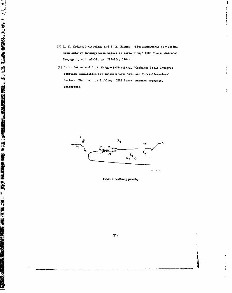
[7] L. N. Medgyesi-Mitschang and J. M. Putnam, "Electromagnetic scattering

from axially inhomogeneous bod;Les of revolution," IEEE Trans. Antennas

Propagat., vol. AP-32, pp. 797-806, 1984.

18] J. M. Puttam and L. N. Medgyesi-Mitschang, "Combined Field Integral

Equation Formulation for Inhomogeneous Two- and Three-Dimensional

Bodies: The Junction Problem," IEEE Trans. Antenna Propagat.

(accepted).

iY" R2

M+

(r2 , ti2 )

Figure 1. &attering geowmery.

319

Comparison of Computed and Measured Resultsfor a Simple Man-with-Radio Model

Allen W. Glisson Darko KajfezDept. of Electrical Engineering Dept. of Electrical Engineering

University of Mississippi University of MississippiUniversity, MS 38677 University, MS 38677

Perry Wheless K. H. (Chuck) AgarDept. of Electrical Engineering CM Engineering Co.

University of Alabama Las Cruces, NM 88047Tuscaloosa, AL 35487

Abatract

The r•dls•ia charac.terisfic at a two-way radio in tie prsenct ota simple model ofthehuman body are Investigated. The human-body model is a 14-inch PVC pipe filled with atwater. The triangular patch code PATCH is used to model the pipe YA a simple Impedance-sheetsurface, while the radio body with its antenna is modeled as a perfectly conducting plate drivenagainst a thin strip. Numerical results obtained with this model are compared with meeasreddata in the 450-470 M&I range for the radio suspended badde the water cylinder.

Introduction

"The rzdiatiou characteristics of a hand-held two-way radio are of interest for manyapplications. The effect of the human body on the radiation pattern and input impedance of theradio antenna are difficult to predict for realistic geometries. Various approaches to themodeling of similar problems have been considered, including the use of volume integralequation models and hybrid partial differential equation/integral equation models [1-5]. Whenthe fields interior to the body are of interest, a volume formulation is necessary. However, ifone is interested primarily in the input impedance and radiation characteristics of the antenna inthe presence of the body, one. might expect simpler models to be applicable. Surface integralequation (SIE) models which assume that the body is a homogeneous or layered homogeneousdielectric region [61 may prove satisfactory, particularly since the human body is lossy.Standard SIE formulations require the entire surface of the body to be modeled, however, andgenerally employ both electric and magnetic equivalent surface currents as unknowns in thenumerical formulation. For a lossy dielectric the number of unknowns may be reduced by 50%in some situations by employing the impedance boundary condition (IBC) model [7]. The IBCmodel still requires the current distribution to be modeled over the entire surface of the dielectricbody, but redluces the number of unknowns required in the model by enforcing a knownrelationship between the electric and magnetic equivalent surface current densities.

In this work we seek to employ a numerical model of intermediate complexity and to

320

Ii

,|

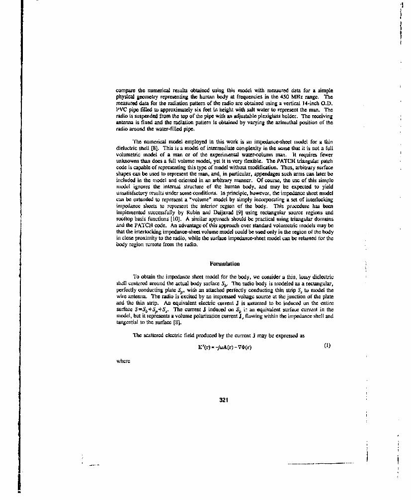
compare the numerical results obtained using this model with measured data for a simplephysical geometry representing the human body at frequencies in the 450 MHz range. Themeasured data for the radiation pattern of the radio are obtained using a vertical 14-inch O.D.PVC pipe filled to approximately six feet in height with salt water to represent the man. Theradio is suspended from the top of the pipe with an adjustable plexiglass holder. The receivingantenna is fixed and the radiation pattern is obtained by varying the azimuthal position of theradio around the water-filled pipe.

The numerical model employed in this work is an impedance-sheet model for a thindielectric shell [8]. This is a model of intermediate complexity in the senise that it is not a fullvolumetric model of a man or of the experimental water-coluni man. It requires fewerunknowns than does a full volume model, yet it is very flexible. The PATCH triangular patchcode is capable of representing this type of model without modification. Thus, arbitray surfaceshapes can be used to represent the man, and, in particular, appendages such arms can later beincluded in the model and oriented in an arbitrary manner. Of course, the usc of this simplemodel ignores the internal structure of the human body, and may be expected to yieldunsatisfactory results under some conditions. In principle, however, the impedance sheet modelcan be extended to represent a "volume" model by simply incorporating a set of interlockingimpedance sheets to represent the interior region of the body. This procedure has beenimplemented successfully by Rubin and Daijavad [91 using rectangular source regions androoftop basis functions [10]. A similar approach should be practical using triangular domainsand the PATCH code. An advantage of this approach over standard volumetric models may bethat the interlocking impedance-sheet volume model could be used only in the region of the bodyin close proximity to the radio, while the surface Impedance-sheet model can be retained for thebody region remote from the radio,

Formulation

To obtain the impedance sheet model for the body, we consider a thin, lossy dielectricshell centered around the actual body surface Sb. The radio body is modeled as a rectangular,perfectly conducting plate Sp, with an attached perfectly conducting thin stip S. to model thewire antenna, The radio is excited by an impressed voltage source at the junction of the plateand the thin strip, An equivalent electric current J is assumed to bc induced on the entiresurface S=Sb+SP+S.. The current J induced on 3b i7, an equivalent surface current in themodel, but it iepresents a volume polarization current J, flowing within the impedance shell andtangential to the surface [8].

The scattered electric field produced by the current J may be expressed as

ES(r) -jwA (r) - V4,(r) (1)

where

321

II

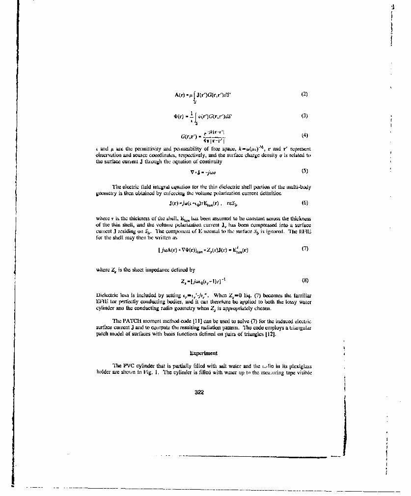
A(r) -,u J J(r')G(r,r')dS' (2)S

G(r~r') .e- wJkl-' (4)

t wid 14 are the permittivity and penneability of free spawkwe t", r and r' representobservation and souice coordinates, respectively, and the surface charge density or is related tothe surface curient J through the zquation of continuity

V.J-jw (5)jW

The electric field inLQgral uNuation for the thin dictectzic shell poitioll of the multi-budygeOUIIIVL~y is then obtaiiicd by cufuicing the volume poilarhiztion current definition

whoic T is the thickness of the shell, h ass been assumed to be constant across the thicknessof the thin shell, and the volume pularization current J~, has been compressed into a surfacecurtent J1 rediding oni SI,, The coinpoiieit of E normal to tlho suiface Sb is ignorcul. The l1lll.ftir the shell may then be written as

U wA(r) +V()rn+(Jr)-E" 111(r-) (7)

where Z, is the shiezt itpdnceiie defined by

Dielectric loss is included by settin r19~ J,' When Z.=0 EqA. (7) becores the familiarMEil foir ptrfi~ctly conducting bodies, and it can theriefore be applied to both the Lossy water

cylinder and the conducting radii) geometry when Z, is appropriately chosen.

The P'ATCH moment method code [11] can be used to solve: (7) for the itiduced electricsurface current J and to comiputc the resulting radiation pattern. The code employs a triangularpatich model of surfaces with basis functions defined on pairs of trianigles L12].

ExperisnaentThe PVC cylinder that is partially filled with salt water and the i,., ha in its plexiglass

holder are shown in Fig. 1. The cylinder is filled with water up to the nicamiiring tape visible

322

Figure 1. PVC cylinder partially filled with salt water aunJ redio in plexiglassholder used to obtain experimental data.

in the figure, Note that tie monopole antenna is partially protruding above the top of the waterlevel. The battey-operated radio is situated on a plexiglass arm, which can be manually shiftedaround tie cylinder to obtain the azniuthal radiation patteni. The relative size of the cylinderin comparison with a peron it; shown in Fig. 2. For each nmasured point, the person had tohide behind the bah'ier of absorbing material. Although this method of measuremneat may besomewhat prinutive, it nevertheless assures the absenac of all feed cables, and it also providesfor the stability and repeatability of the measurcment.. The measured points could be repeatedwith an accuracy of I dB. The rceiving log-peiodic antenna was located at a distance of 5.2mfrom the center of the cylinder.

The preliminary nimsuretents weare made with the cylinder filled with tap water, andthe final mueamurments were umade with a 0.2% solution of NaCi. The DC conductivity of thesolution wa.; mneasured to he 0.19 S/re. It is believed that the RF conductivity is about 0.5 S/n,but the exact RE measuernent has not be conducted. It was found that there was very little

IJ

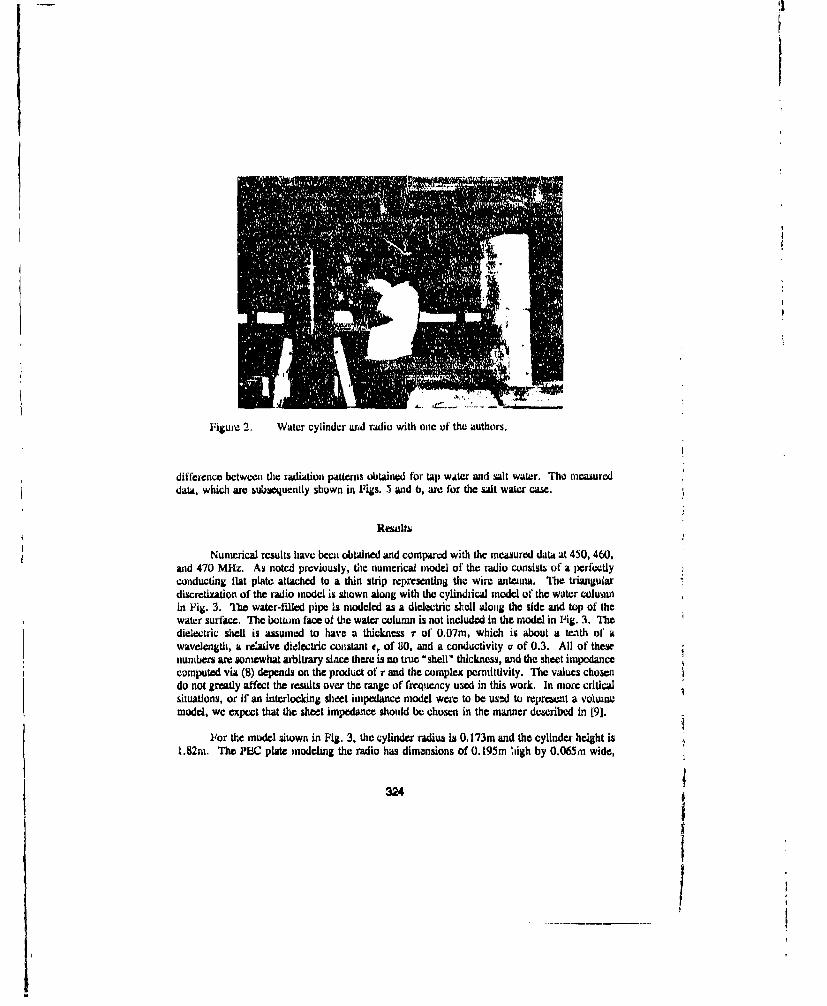
Figure 2. Water cylinder and radio with onc of the authors.

difference between the radiation patterns obtained tbr tap water and salt water. The measureddata, which are subsequently shown in Figs. .. and 6, are for the salt water case.

Rtwalts

Numerical results have been obtained and compared with the measured data at 450, 460,and 470 MHz. As noted previously, the numerical model of the tadio consists of a per'•itlyconducting flat plate attached to a thin strip representing the wire antenna. The triangulardiscretization of the radio model is shown along with tde cylindrical model of the water columnin Fig. 3. The watcr-fdled pipe Is modeled as a dielectric shell along the side and top of thewater suriace. The bottuom face of the water column is not included in the model in Fig. 3. Thedielectric shell is assumed to have a thickness r of 0.07m, which is about a tenth of awavelength, a relative dielect'ic conIstant er of 110, and a conductivity a of 0.3. All of thesenumbers arm sonmwhat arbitrary siace there is no true "shell" thickness, and the sheet impedancecomputed via (8) depends on the product of r and the complex permittivity. The values chosendo not greatly affect the results over the range of friquency used in this work. In maore criticalsituations, or if an interlocking sheet impedance model were to be usW to represent a volumemodel, we expect that the sheet impedance should be chosen in the manner described in [91.

For the model 2hown in Fig. 3, the cylinder radius is 0. 173m and the cylinder height is1.82m. The PEC plate modeling the radio has dimensions of 0. 195m Iigh by 0.065m wide,

324

_J

I4

while the antenna (strip) has dimensions of

0.197m high by 0.01O25m wide. The topcenter of the radio is positioned at (0.225425,0.0, 1.73745) meters. Bcause the cylinderis almost three wavelengths long in thefrequency range of interest, the model shownin Fig. 3 is actually a fairly crude model,particularly in the vertical dimecnsion. Themiodel shown uses 12 segmnents to model boththe vertical and azimuthal directiunN and has577 unknowns, Unfortunately, this was closeto the limit of the model size which couldconveniently be used and tests tor numericalsolution convergence were linited.

An eflort was made to obtain a betternumerical model in the vertical direction by

Figure 3. Full model of the water-filledI'VC pipe and radio geomnetry.

truncathig the cylinder while keeping the sanmenumber of unknowns. The tru•wAted model, inwhich the bottom halt of the cylindrical shell hasvx•n eliminated, is shown in Fig. 4. The cylinder

is still model using 12 scgmients in both thevertical and azimuthal directions, so the triangledensity is increased with respect to the model ofFig. 3. Truncation of the model was expexted tobe feasible due to the lossy nature of the body andthe localized excitation. Results obtained usingdifferent trutncation lengths showed only smallvariations, which is an indication that thetruncation piocess was valid.

The comparisons of measured data with theFigure 4. Truncated model of the numerical results tur the full and truncated

water-tillry pipe and radio geometries are shown in Figs. 5 amid 6,geometry. _-ectively. in the figure4, the nfinuous lineq

represent the numerical data, while the measureddata are represented by discrete symbols. The

solid line represents data for 450 MHz, the dashed line for 460 MHz, and the dotted line for 470

325

~i

MHz. For the measured data the plus (+) represents 450 MHz, the asterisk (*) 460 MHz, amdthe cross (x) and circle (o) represent two different 470 MHz trials. The agreement betwoen theexperimental and numecrical data is fairly good for both gwonctries. However, the resultsobtained with the full-cylinder model show somewhat poorer agreement with the measured dataand somewhat greater frequency sensitivity in the backward radiation direction (0,, 180"), htseems likely that this is due to the rather ceude numerical modeling of the cylindek in the verticaldirection, since the maximum edge lengths in the model may exceed one-quarter wavelength1 forthis case. The numerical results for the truncated cylinder gcoinetry agree with measured datavery well in the forward and backward directions, while some deviation is noted in the sideradiation.

0.8-

0.6 )p I

0.4 -I0.2 -

-0.4

-0.4 ..

-0.8 , -

Futgure 5. Compinso of results fr full-c.ylinder miodel Nunericail results:450 (solid lWit), 4W0 (dashed line), and 470 (dotted line) Mitz.Measuzed data: 450 (+), 460 (1), and 470 (x,o) MHz.

Sunwwry

The radiation characteristics of a two-way radio in the preseinc of a simple water-columnmodel of the humani body have beoa investigated. The human-body nodel used to obtain

W -modl hav been i opare wite.hI triangular patch 4code PATCHhas been used to model the pipe as a simple ilnipdance-shoet surface, while the radio bodiy withiits antenna is modeled as a puricct~ly conducting plate driven against a thin strip. Numericalmr~ult3 obtained with this model have been compared with measured data in the 450-47U M~iz

,32B

I

0.8

0.6

0.4 - 1

0.2

0

-(0.2 -

.0.4 -t

-0.8-

"1 L

Figure 6. Comparison of results for truncated-cylinder model. Numericalresults: 430 (solid line), 460 (dashed), and 470 (dotted) M-z.Measurod data: 450 (+), 460 (*), and 470 (x, o) MHz.

range for the rad.io suspended beside the water column and have been found to be in goodagreement. The PATCH triangular patch code used for the numerical solution is capable otrepresetitng arbitrary surface shapes and could be used in future work to represent a inorecomplex model of a man, aid, in particular, appendages such as anms could be included in themodel and oriented in an arbitrary manner. With further work the impedance sheet model canbe extended to represent a "volume" model by incorporating a set of interlocking impedancesheets to represent the interior region of the body, thus providing the ability to adjust the modelcomplexity firom a fairly simiple model to a quite complex model with the same code as the needarises.

From the applicatioas point of view, the results indicate that the radiation pattern tor a450-470 MHz portable radio in the presence of a human body shows a front-to-back ratio ofabout 4 dU, and side minima of up to 5-5.5 dB3. These results are similar to the results reportedin [2] for 165 and 250 MHz radios.

Referemcum

[1] D. Ui. Livesay and K.-M. Chen, "Electromagnetic fields induced inside arbitrarily shapedbiological bodies," IE.EE Tratu. Microwave 7heor. itch., vol. MTT-22, pp. 1273-1280,

327

_I!

I

Dc•ember 1974.

[2] J. B. Anderson and F. Hansen, "Antennas for VHIFIJHF Personal Radio: A Theoreticaland Experimental Study of Characteristics and Petormmance,* IEEE Trans. VehicularTech., vol. VT-26, pp. 349-357, Nov. 1977.

[31 D. H. Schaubert, D. R. Wilton, and A. W. Glisson, 'A tetrahedrl modeling method forelectromagnetic scattering by arbitrarily aaped inhomograrous dielectric bodies," IEEETram'. Antennas Propagat., vol. AP.32, pp. 77-85, January 1984.

[4] K. D. Paulsen, D. R. Lynch, and J. N. Strohbehn, "Thr. .-.. imensional finite, boundary,and hybrid element solutions of the Maxwell equations for lossy dielectric media," IEEETrans. Mkcrowwve Theory Tech., vol. M'IT-36, pp. 682-693, April 1988.

[5] M. A. Morgan and B. E. Welch, "The field feedback formulation for electromagneticscattering computations," IEEE Tians. Antennas Propagat., vol. AP-34, pp. 1377-1382,D.eCmber 1986

16] S. Govind, D. R. Wilton, and A. W. Glisson, "Scattering fronm inhomogeneouspcnetrable bodies of revolution," IEIE Trans. Antennas Propagat., vol. AP-32, pp.1163-1173, November 1994.

[7] L. N. Medgyesi-Mitschang and J. M. Putntain, "Integral equatlin formulations forimperfoctly conducting scatterers," IEEE Tram. Antennas Propagat., vol. AP-33, pp.206-214, February 1985.

[81 R. F. Hi'rington and J. R. Mautz, "An impedance sheet approximation for thin dielectric;shells," IEEE Trans. Antennas Propagat., vol. AP-23, pp. 531-534, July 1975.

[91 11. J. Rubin and S. Daijavad, "Radiation and scattering fronm structures involving finite-size dielectric regions," IEEE Trawu. Antennas Propagat., vol. AP-38, pp. 1863-1873,Nov. 1990.

[10J A. W. Glisson and D. R. Wilton, "Simple and tfficient numerical methods for problemsof electromagnetic radiation and scattering from surfaces," IEEE Trans. AntennuaPrapagat., vol. AP-28, pp. 593-603, Sept. 1980.

[1ll W. A. Johnson, D. R. Wilton, and k. M. Sharpe, "Modeling scattering from andradiation by arbitrarily shaped objects with the electric field integral equation triangularsurface patch code," Electromagnedtcs, vol. 10, pp. 41-63, January-June 1990.

[12] S. M. Raa, D. R. Wilton, and A. W. Glisson, "Electromagnetic scattering by surfacesof arbitrary shape," IEEE 7Trams. Antennas Propagat., vol. AP-30, pp. 409-418, May1982.

328

I;

:1

TOOLBOX FORCHARACTERIZATION OF MATERIALS

byJoan R. Dornfest

Lockheed Missile & Space CompanyResearch and Development Division

Advanced Systems Technology3251 Hanover Street

Palo Alto, California, 94304-1187

October 25, 1990

ABSTRACT

Designers need a handy tool to characterize materials forRCS (Radar Cross Section) scattering. This paper describes athree-step strategy for predicting the RCS scattering as afunction of impedance for a given shape and frequency.This strategy has been generalized to be applicable tonumerous codes.

The actions required to implement this strategy arespecified in detail. A specific code, JRMBOR, is used toillustrate and give precise definition to the processes ofimplementation. (JRMBOR was written at AtlanticAerospace Electronics Corporation in Greenbelt, Maryland.)

The software to generate multiple runs, and to compile thedata needed for plotting, as well as performing the contourgraphs, is presented. In summary, all the information forcreating a "TOOL BOX FOR C. RACT.rEIRIZATION OFMATERIALS" in a minimum amount of time is included.

329

THREE-STEP STATEGY

1. Predict the RCS for a range of impedances by running thesame RCS code multiple times. The size and shape of thebody, the frequency of the wave, and all other inputvariables remain constant except the impedance. Theoutput contains the amplitude and phase for Theta and Phifor one frequency and one impedance, but for a multiple ofincident angles.

2. Compile the information for contour plotting byselecting from the multiple outputs only the amplitute andphase for a given Incident angle.

3. Generate a contour plot for data selected to show bothamplitude and phase for a range of impedances.

ACTIONS

CREATE NEW OUTPUT

To familiarize one with the Input and output from thestandard version of JRMBOR, in Fig. 1A, a sample Input Isshown. The input data, when placed in a DCL (DigitalControl Language) command file, is used for runningJRMBOR on a VAX computer.

In Fig. 1B, a partial output of JRMOUT.DAT, the one outputfrom the standard version of JRMBOR is portrayed. Theshape Input Is a 12" x 1" cyclinder. All output fields areshown. Since the information desired for the plot programis not readily available, JRMBOR required modfluation. Tominimize the modification task and impact to other users,

330

an additional output was created, rather than modifyingthe existing one. In Fig. 10 the new output is illustrated.

ADMITTANCE

JRMBOR requires admittance, not impedance for input, butthe final contour graphs used impedance. Therefore, aprogram, CHANGZ.FOR shown in Fg. 2A, was written toconvert impedance to admittance, and enter admittanceInto the input stream at the appropriate point in theJRMBOR.COM command file. Also, the specific case of theImpedance equal to zero needed to be defined, to avoid thenon-defined case of dividing by zero.

Since JRMBOR Is required to run one hundred and seventy-six times, a command file CHANGZ.COM depicted in FIG. 2B,Is created. The new file, JRMBOR.COM, created by theCHANGZ program, is copied to another file JRMBOR1.COM(FIG. 2C), and is read by the CHANGZ program during thenext run.

MULTIPLE RUNS

The command file RUNJRM.COM, displayed in Fig. 4, submitsone hundred seventy-six runs, the desired number for thisexample. Each run Is matched with an impedance; theoutput from each run later forms one point for the contourgraph.

Impedance Is a complex number, the real component isdisplayed along the x-axis, and the imaginary componentalong the y-axis. The variable, N'JM1 when divided by tenis the smallest real component of impedance used. NUM2when divided by ten is the largest imaginary component.

331

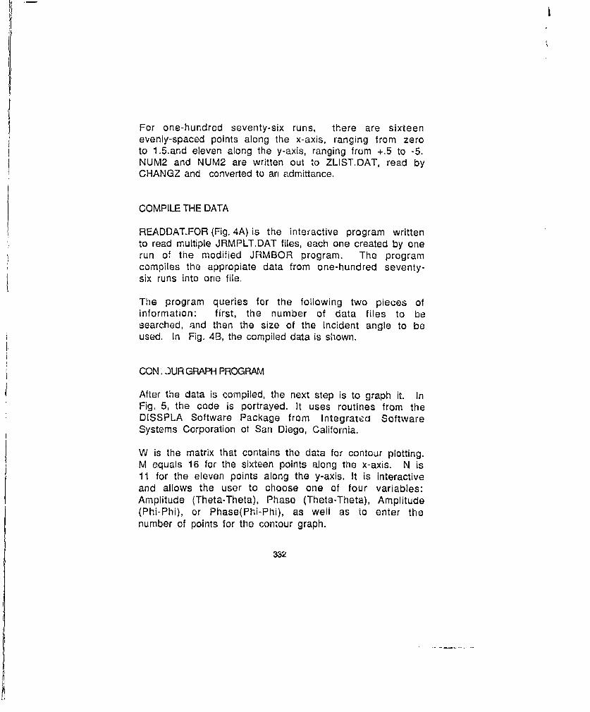
For one-hundred seventy-six runs, there are sixteenevenly-spaced points along the x-axis, ranging from zeroto 1.5.and eleven along the y-axis, ranging from +.5 to -5.NUM2 and NUM2 are written out to ZLIST.DAT, read byCHANGZ and converted to an admittance.

COMPILE THE DATA

READDAT.FOR (Fig. 4A) is the interactive program writtento read multiple JRMPLT.DAT files, each one created by onerun of the modified JRMBOR program. The programcompiles the appropiate data from one-hundred seventy-six runs into one file.

The program queries for the following two pieces ofinformation: first, the number of data files to besearched, and then the size of the incident angle to beused. In Fig. 4B, the compiled data is shown.

CON .3UR GRAPH PROGRAM

After the data is compiled, the next step is to graph it. InFig. 5, the code is portrayed. It uses routines from theDISSPLA Software Package from Integrater( SoftwareSystems Corporation of San Diego, California.

W is the matrix that contains the data for contour plotting.M equals 16 for the sixteen points along the x-axis. N is11 for the eleven points along the y-axis. It is interactiveand allows the user to choose one of four variables:Amplitude (Theta-Theta), Phase (Theta-Theta), Amplitude(Phi-Phi), or Phase(Phi-Phi), as well as to enter thenumber of points for the contour graph.

332

In addition, the program normalizes the values for the

contour by the value at (0,0), which i.s 0,0 impedance.

CONTOUR GRAPHS

The contour graph for Amplitude (tt) is shown in Fig. 6A.In a similiar roanner, the contour graph for Phase (tt) isport,'ayed in Fig. 6B. In Fig. 6C, the result is shown of thetwo graphs being overlayed, in order that the point ofintersection is noted clearly.

I

33

$!1

N ME = JRMBOR.COM%! HERE IS A SAMPLE COW:AND FILE TO RUN JRMBOR WITH SOME SAMPLE INPUT DATA.SI

S SET DEFAULT [DORNFEST. JRMTEST]9 RUN JRMBOR

0 016.67667637 0. 100.

10

3

999 11 49 2 120.0. 0. 0.0. 0.0762 0. 0.C1.EL3,0.)

5021152020. 0.0762 0. 00.00635 0.0762 0. 0.

1 49 2 0

20.00836 0.0762 0. 0.0.00836 0. 0. 0.

% EXIT

FIG. 1A. SAMPLE INPUT TO JRMBOR

334

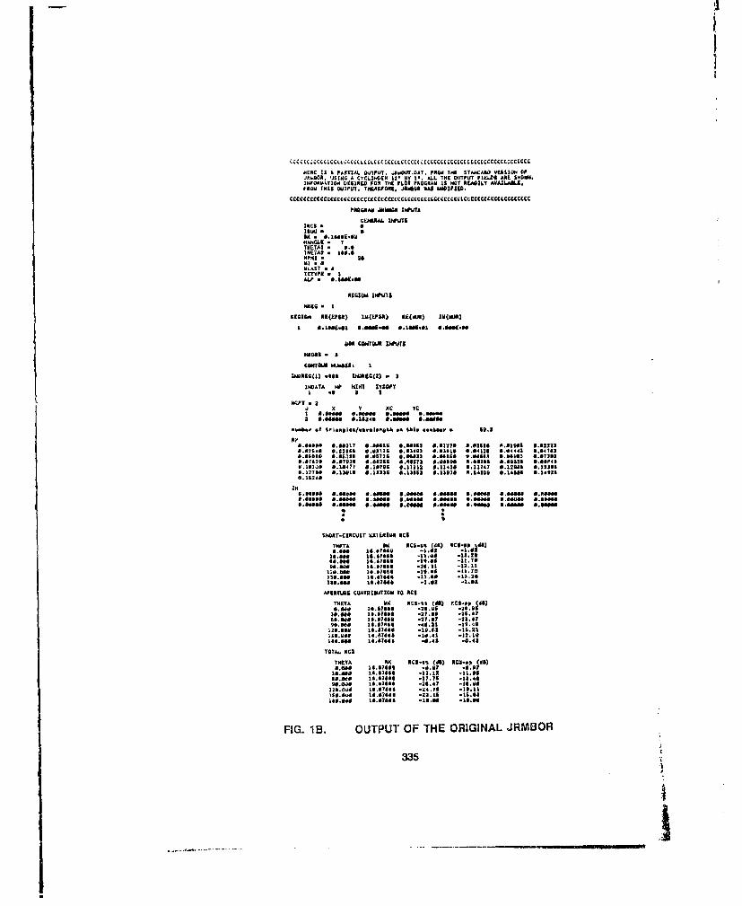
HERIE :S A PARIALTM. JPOI. .J8JAT, FROM 7.15 11AW6A3D 9545101 OF'GOA'03 -11410 A CYCL2IIC,6 )3*T- 0" . l lSOJPIIF5.~ U10811440800204 DESIRED F01 THl PLOT P004164 IS NOST OLAVILY AOAILAMA8.,

1331 THIS OUTPUTT. 185451083. .31h0 UAS WOON1208.

CCCCCCCC(cccccLcccccccccccccccccccccccIcccccIcccrcLCOCCCCCCCCCL;CCCCCCCC

PROGR8AM J18858 IWV73

IRCS 0

TIETAS .:11"!A ; 288.

ULASB 4

1 UYB. .0

REGION1 RX(EP08) 2U(EPS11) 88(WA3) 14(b&8

5.8"9.40 a. Is.36 0.60M1

1101194(l) -so& LWRI35(3) - 3

INATA P IM 1814 YZAPl1 43 0 3

W.PT . a4 0 14 xc Tc

0.8" .646e's" 2

:IN.:04 :1.111' :Z811% 8.1=23 *1213 8,5121 8.=4463 8.471&.@6610 8.0639: V.:6736 8. "&NJ 0.":668 *..gel 8.844V15 8.78

3.11,1 :.0 !M7 8,1873 8.1151 2N.301 211111 *.812" :.12M10.1,238 8.13013 8.113338 8194 .37 ,526 8138 8018.3102.148 S141

S7 a 046".

01L3-I ICU~0.78 91

2889 14.108M .1 t,8 -&211.712 .8@0 34.07383 .105 is 3.2

1 3.88 1,483: -. 8 -1.0a

APE877.33 CONT700IATZCII TO ACS

THATA ": 933'4 (',) "53-! (338.88 1a" 1 2...6 -25.8

I3.48 '.946 -27,5y -21.41

118.43 8.07311 -41:,4 -:2.0

-83.88 14089766 -8.41 -8.43

THETA MA0 313-31 do)3C-,4)8.888 ~ -1.5)4 -4.47 .8.8

8 1.88 614.748 -173 -3.40".4 la6.1sal -6.47 -.14.3

033.88 14.37988 -19.88 -08.8

FIG. 18B. OUTPUT OF THE ORIGINAL JRMBOR

335

OUTPUT OF MOD IFIED JRL(OOR PROGRAM

PILUJIAME * JRMPLT.Di.TTHE FIRSIT LANE SHOWS 'THE FREQUENCY, THE SLCOND THE ILCPEDANCcL Z A14DTHEN4 THE ADMITTANCýE Y. THXS OUTPUT WAS DUTA.INLD FOR k 12 y I CYCLINOER.THE AMP'LITUDE AND PHASE ARC L"STLD FUR TKETk AAD PHI FOR 5EVEN ANULLS.

CCCCCCCCCCCCCCCCCCCECCCCCCCCC~ccccccccccCCcCCCCCCCCCcCCCCCCCCCCCCCCCCCCCcc

WAVES 16108758 1/M

.00 -0.071 41.486 -&.271 41.59B

80.008 -11.750 .123.7z4 -13,4tr -179.99990.009- -28.416 -87.646 --16.W67 -171.2V8

120.00u -24.787 -E'I.ao9 -18.111 131.068160.0". -23.161 -166.601i *1lu,3s 89.818

1.09 -19.9M8 -138.728 -19.090 -139.720

CCCCCCCCCCCCCCCCCCCCCCCCCCCCCCCCCLCCCCCCCCCECCCCCCCCCCCcCCCCCCCCCCCcCCCECCCCCCC

FIG. 1C. NEW OUTPUT FROM THE MODIFIED JRMBOR

cC PROGRAM CHAlQZ . FORCC THIS PROGRAM ACCEPTS A NEW COUPLEX I FUR THE IMPEDA1NCE (Z)C CONVERTS 11 TO THE ADMITTANCE (Y) AND INSERTS 11N INTO THE iNPUTC QATA FILE FOR JRMBOR FOR THE CASE OF A SPECIAL CYLINDER.CC DO NOT USE IT FOR OTHERl PURPOSESIIIIC

COMPLEX Z,Y,Y1DIMENSION A(09)OPEN (UNIT.'8,NAUE.-ZLIST.DAT* ,STATUS.'OLDP)OPEN (UNIT.10,NAMF.'JRMBOR1.(O1V ,STATUS..OLD')OPEN U14 IT.It,HNAME-. IJRkWDR. COW4 STATUS-'NEW ,CARR IASECONTHOL.

L.IST,)DO 1 1..1,1/

READ8(1 104w) (A(J),.J.I,8JU)13 WRITE1 18) A(J),..-1.60)too F~kIA(08AI)

I CONTINUJEREAD$19,..) YI.RVAD90)NREAD 9,o)HANI , LA H)/0AH2 7 FLOAT (N2)/ 10.Z - CUPLX (Aid AN2)

IF(CAES Z) .iq 6 THEN

ELSEY 1.1Z

END IF

D0 2 1.1,13HEADQ(1,100)(AJ),.B)WRITE(11,190) (()J.,6

2 CONTINUEEND

FIG. 2A. CODE YO CONVERT IMPEDANCE

336

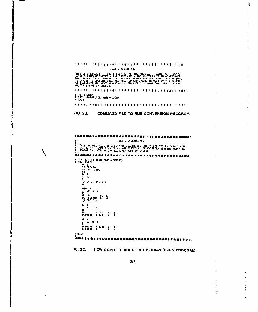
:1

j

NAME C CHANIZ.CO,THIS IS A CCMANO ,COMk ) FILE TO RUN THE PROGRAm, CHANGZ.FOR, WHICH"TAKIES A COMPLEX :iblEA3R - THE IMPEDkNCE - AND CONVERTS 1l TO AMNITT-ANCEFOR RJA•OR. THEN JR•AOR COW WHICH CONTAIXS THE DATA FOR A JRMBOR RUN,IS COPIED TO JRMkURI.COM. THE FILE. JRM8O•I.CQM, IS USeD BY CHANGZ.FORTO CALCULATE THI! NEXT ADIrTTANCE. THIS F•Ln, CHHCZ.COIA, WAS USED FORMULTIPLE RUNS OF JRUSOR.

1 RU" CHANGZI COPY JHUBOR.COM JRAONT.COI EXIT

111 lllllll~llllt Illilll~l~lllt l lllllll fliillf1 I il IlltIllli IllI I Ittlt

FIG. 2B. COMMAND FILE TO RUN CONVW"RSION PROGRAM

tIIlstlltfl$1sluhz$auzz1ss::ggsgallgagggsg$ggggig~gggggllg gggggggggglggglglg1

I1 NAME - JR.1 IRI.COM2!$I THIS COMMAND FILE IS A COPv 0F J0IE0RCOM AND IS CREATED BY CHANCZ.COM.*I CHANO1.FON READS THIS FILE, A14D WPITES A NEW MODIF"IED VElRSION WHICH IS$1 JRAMOR.COM. FOR MAXINO EULTIPLE RUIS OF J.1180.R"tI

t SET DEFAULT IDORNFEST.JFMTEST)S RUN JR.MBOR

00116.67606•37 . IR1S.

0 43 0.151(1.,e.3 (L.,0.)

999 11 99 2 12

0. 06762 0. 0.(2 .Eao,0.)

0 11 9 2 020. 0.+0782 B. 0•.

.00635 0.0762 0. 6,

1 99 2 020.,0135S 0.0762 6. 6.0.0836 S. 6. *,

I rE(IT

FIG. 2C. NEW COM FILE CREATED BY CONVERSION PROGRAM

337

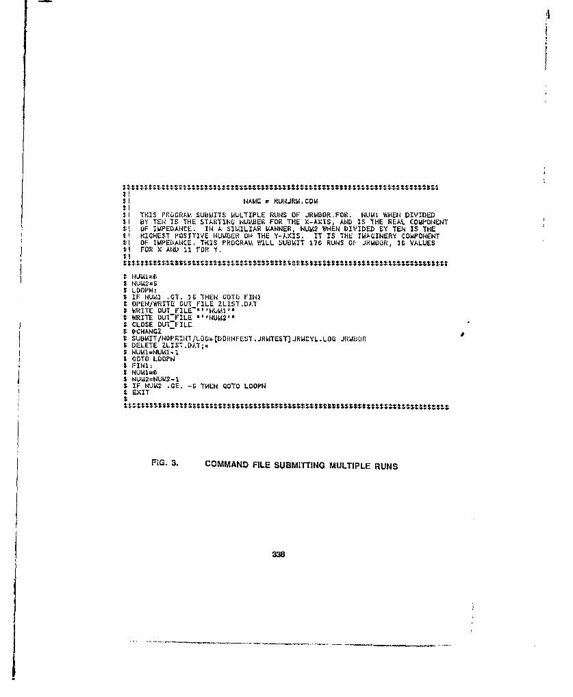
3I NAME = RUNJRM.COMSIS1 THIS PRciGRAM SUBMITS MULTIPLE RUNS OF JRMBORFOR. 1UMI WHEN DIVIDEDI.I BY TEN IS THE STARTING IqUkBER FOR THE X-AXIS, AND IS THE REAL COMPONENTI:I OF I1PEDANCE. 114 A SIIMILIAR MANNER, NU92 WHEN DIVIDED SY TEN IS THE3I HIGHEST POSTTIVE NUMBER O THE Y-AXIS. IT IS THE IMAGINERY COMPONENT$1 OF IMPEDANCE. THIS PROGRAM •ILL SUBMIT 176 RUNS OF JRUBUR, 32 VALUEST1 FOR X AND 11 FOR Y.It

t. NUM1=8,S NUL2=5t LDOPN:$ IF NUWI, .GT. 15 THEN GOTJ FIN)3 OPEN/WRITE OUT FILE ZLIST.DAT3z WRITE OUT FILEWN-lUmI)I WRITE DUI-FILE "'NUMZ"'S CLOSE OUT-FILES OCHANGZt SUBMIT/NOPRINT./LOG= [DORNFEST. JRMTEST3 ,JRMCYL. LOG JRLiWDRS DELETE ZLIST.DAT;e3; NUMIA NUMI 1t GOTO LOOPNS FNIN:t NUMI=ES NLlk12=NUM2-1I IF NUL42 .GE. -5 THEN GOTO LOOPNS EXIT

FIG. 3. COMMAND FILE SUBMITTING MULTIPLE RUNS

338

C THIS PROGRAM READS TilE MULTIPLE .IHMDUT.PLT DATA FILLS CMATEDC DURING MULTI'LL RUNS OF THE MO0DIFIED .iRMZOR PROGRAM. THISC PROGRAM WRlITES THE APPROPIATE DATA INTO ONE FILL FOR A CONTOURC PLOT PROGRAM WRITTEN USINU SOME ROUTINES PROM OISPPLA SOFTWARE,C FROM iNTBEORATEO SOFTWARE SYSTEMS CORPORATION OF SAN DIEGO,

DIMENSION ASP(2), FAIul)CNARACTER41 Al. Al, A3CI1'.RACTER.3 ACNAHACTER,14 UIGPL:N(UNIT.1,HAM4ES'CTOUPPLT.DAT' STAUS.'NEW)TYPE .,:'ENTER THE I OF DAYA VILLd IN SET TO 69 SEARCHED ((c9W)REiAD(5,) NTYPE .,'ENTER ANGLE OF INCIDENCE WANTED'REiAD($,,) ANGLE

Al CNAK(42)

11 1L'e'.N/ 100MAK1. 40 NiLUG

DOI J"N

Al- C1(AR(49. 4.110)JJ10s(JJ-J4100. 106)/180A2 tCHAR(4 .J,1 0).J1 I.(JJ-4j.JII.li30-J48. 10)1,3 . CNA.R(41.J4JlA:AIR//A2(A

OP'EN (UNITMIIa,.NAWE.0,STATUSt'OLD',tIAOILY)CALL GLTUAIA(ANGLE AZ ,AZAM1P FAZRIIITL(11,1110) RZ IAi±S.P(1) ,FIXZl *AMP(Z),FAZ(2)

TYPE ., 'ALL PILES ACCELSEP'END

.......................................

COPESUBROUTINE GL1ODATA.(ANG, X, Y,AMP, FAZ)

DIMENSION AMP (1) , FAXZ(1)READ (16, 100) OK

200) FORMATpKx,P11.1)REAO(10,IlO) Z

210 FORMAT (lI6X,E12.5,lX,E1Z.8)

YUAIMA.G ()REAQ~ ("I 22a)NA.NQ

220 FORMATCIAXI)DO 1000 I&1,NAI4O

RE.AD(1 20)lD ANG1,SIOTTJPAZTT SIGPI',PA4ZIP230 FIMACXPU.3.29,4 (P12.IX)$

IF(ANCL EQ.ANG) THEINAMP(1) . SIGYTAhAP(l) u SIOPPFAfI) - FA.ZTTPAZ (2) .PAZPPRETURN

END IFIF ([.EQ. WANG) THEN

*RITE(S,.) 'THETAX',AMG,'- NOT FOUND-

1000 CONTINUERETURNENiD

4FIG. 4A. CODE TO COMPILE DATA

cccceccccccccccccccccccccccccccccccccccccceccccc'cccc~cccccccccccccccccccccccccTHIS DATA HAS BEEN PREPAREJD FOR THE COUNTOUR PLOT PROGRAM. THE ANGLE USEDIS PRINTED FIRST. IE97, APPEARS THE REAL AND IMAG1I1EPY IkMEDANCE. AFTERIHAT 1S THE AUFLITUDE AND PHASE FOR THETA AND PHI. (THIS INFORMATIOW WOULDHAVE TO BE STRIPPED, IF YOU WER GOING TO THE DAYA.

CCCCcICCCCCCCCCECCCCCCC CCCCCCCC'C'CCCC¢cc¢cCCCCCCCCCcccCCCCCCCCCCCCCCCcCCCc

C.a60 6..00 -7.117 -22.420 -7.117 -22.4208.108 0.648 -4.017 -23.622 -6.617 -23.6210.206 6.508 -SOBS -24.533 -0.166 -24.9338,300 0.688 -9.718 -26.647 -9.718 -28.8470.486 6.581 -18.609 -26.052 -15.659 -28.0628.b" 8.500 -11.268 -38.941 -11.205 -16.9418.689 6.581 -11.969 -33.b51 -11.988 -33.5610.780 O.W58 -12.027 -18.319 -12.27 -38.1196.6"0 6.658 -13.233 -39.378 -13.233 -3W.3788.900 0.606 -.1.764 -42.647 -13.704 -42.0471.84 9.606 -14.276 -40.095 -14.275 -40.0961.180 6.606 -%4.782 -49.890 -14.762 -49.6361.208 6.58" -16.665 -53.352 -1;.866 -63.3621.308 0.508 -15.303 -57.859 -15.382 -67.0591.480 8.bo8 -16.599 -60.749 -16.599 -68.7491.508 8.608 -15.774 -64.372 -12.774 -04.3728.600 6.40M -7.276 -16.216 -7.276 -16.2100.108 8.408 -8.226 -17.52V -6.226 -17.5290.256 8.486 -9.140 -19.176 -9.140 -19.17U0.300 0.408 '-10.17 -21.138 -10.017 -21.1388.408 8.460 -10.356 -23.416 -10.955 -23.4168.186 5.400 -11.851 -2G.986 -11.861 -2C.9650.080 8.NO -12.4068 -26.88 -12.456 -28.8568.70680 .400 -13.669 -i2.014 -13.09D -22.0148.686 8.450 -13.741 -25.4C3 -13.743 -35.4436.980 0.400 -14.326 -39.114 -14.326 -39.1101.309 8.400 -14.842 -42.9R3 -14.342 -42.9931.100 8,400 -15.267 -47.620 -15.287 -47.6281.200 0.488 -16.00• -51.165 -1¶.886 -51.1651.300 5.400 -15.968 -66.314 -15.969 -66.3141.400 3.406 -16.155 -6W.430 -16.198 -60,4381,508 6.465 -16.345 -6J,406 -16.346 -83.4856,06 8.306 -7.468 -U.806 -7.486 -9.6855.180 0.238 -8.448 -11.2809 -a.468 -11.2898,200 8.200 -9.433 -13.0%9 -9.433 -13.0•90.366 0.3160 -10.36U -16.321 -10.359 -16.3218.400 8.300 -11.244 -17.806 -11.244 -11.9600.508 0.356 -12.097 -20.732 -%2.067 -26.7320.880 0.306 -12.063 -23.923 -12.593 -23.9238.780 8.308 -13.827 -27.430 -13.027 -27.4360.U0 60.300 -14.313 -11.264 -14.313 -31.2640.900 0.300 -14.933 -36.377 -14.932 .35.3771.006 8.300 -15.479 -39.736 -16.479 -39.7311.106 0.308 -15.948 -44.276 -15.944 -44.2761.20 8.30 -10.32 4 2 132• -40.9261.308 0.300 -16.826 -33.005 -10.520 -63.0551.408 0.300 -16.848 -U8.224 -18.046 -65.2241.5e8 8.360 -1.977 -82.708 -16.977 -02.7080.000 8.200 -7.689 -2.764 -7.098 -2.1646.100 0.200 -8.747 -4.542 -U.747 -4.6426.286 0.266 -9.785 -0.893 -3.780 -6.036.300 0.280 -18.748 -.J.193 -10.740 -U.-038.400 0.200 -11.876 -12.800 -11,875 -12.0800.506 6.286 -12.509 -15.159 -12.069 -'1.1556.860 8.200 -13.417 -18,086 -13.417 -18.650

6 S1.200 -6.408 -24.876 -32.618 -24.075 -22,5162,300 -0.408 -24.992 -4,069 -24.902 -48.0961.400 -0.406 -24.639 -69.485 -24.839 -69.4861.800 -0.400 -23.!91 -70.0?2 -23.911 -70.6723,006 -0.605 -9,828 47.454 -9.828 47.4048.100 -0.560 -11.191 46.787 -11.191 46.7870.200 -0,608 -12.503 44.154 -12.503 44.1840.30 -0.508 -13.813 42.1 " -13.913 42.2250.400 -3.160 -16,107 39.82 -15.187 39.823

FiG. 48. THE COIvPILED DATA

340

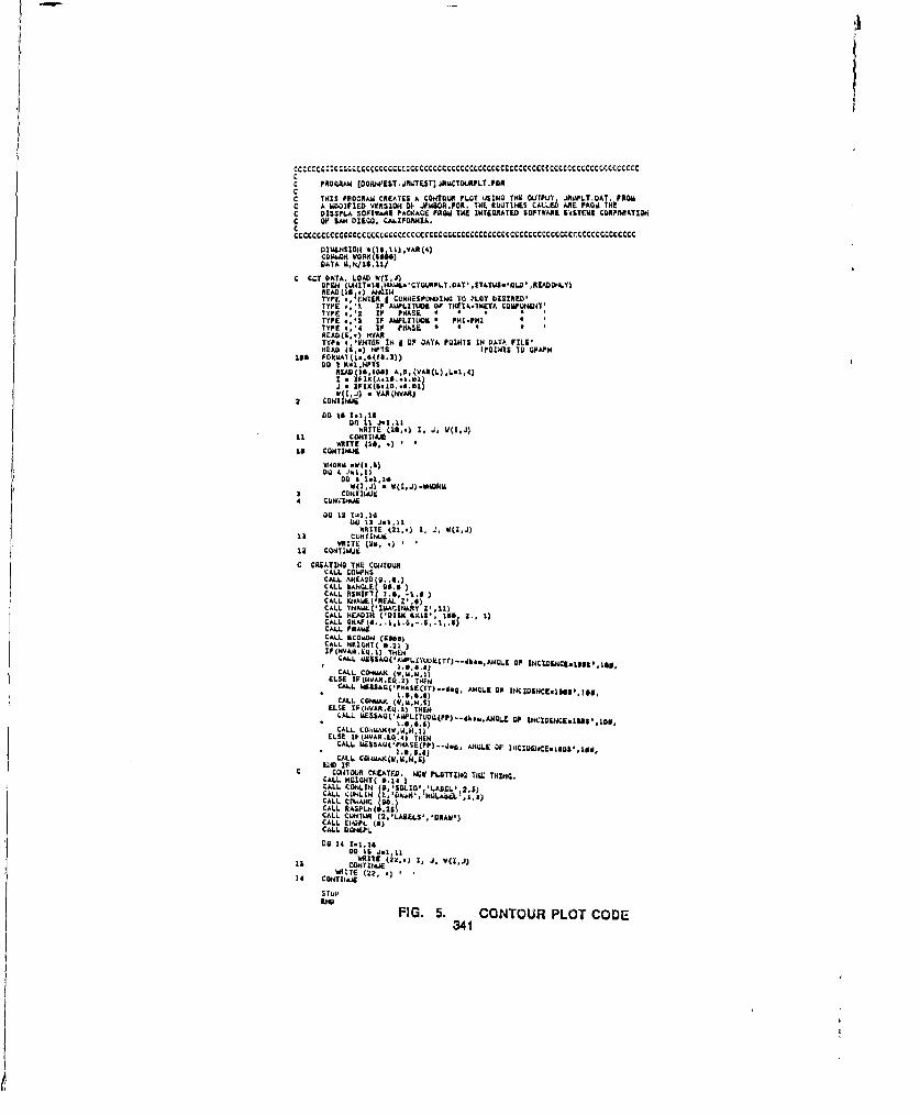
C FROCMAW CDOAN&E$T JOICTEST] JtU.CTORPILT.PFORCC T IS PROIRASi CREP.ES A CONTOUR PLOT 4451141 THE OUTPUT .JAMPLTOAT, FROM

cANMODIFIWD VERSIONI OF JFM8OR.FOR. THt ROUTINES CALLEA ARE PROS4 THEC DIOSPLA, SOFTWARE PAC14A0E FROMS HI INTIMRATED SOFTWARE 5451CN$ CORPORIATIDNIC OF SANl DIEgO, CALIFORNIA,

OIUEJ1304ISDIIs 4 11) VYAR (A)CO"NwoKK WDR"m)DATA M,N4/1641/

C CZIT DKATA LOAD 4(1,5)OPEN (1*111.16 HAS1E.'CTOUAPLT.DAT ,STATLII.'OLD' RIADODtY)ACAD(C15'.) "14154TYPE ., F.1,17AI COfI1EOFOWNINO TO PLOT DLSIRIED'TYPE ,'A If AMPLITUDE OF THETA.THKETI. COMPONENT'TYPE W2 IF08 PHASETYPE ..'3 If AMPLS1lCMD PHFI-PHITYPE.,'4 IF P44400AM OCE.0 HYARETYP. ., 'ENTER IN I OF DATA POINTS IH DATA FILE'ROA r £'.) OPTS lPOINTS TO GRPAH

itO16D(36,1O5) A5(A()L1

,O a ) VAR I(NVAR)2 D 601 mug

Do Is 1.I 1&WRITE (I9,.) 1, J4, W(O,J)

11 COHITIIIJWRITE (16, .

1a CONTIMIC

DO 0 1,16'4(1, .4) aWI,J) -*OHM

3 CCNT~iioJE4 CONTIIAJE

GD 1-01,14Do Is J-.1,11

WHITE (21,.) I, .4, 6(1,4)10 CONTNUE AJ

C CREATIN 01E140 gu

CALL SEIAHLEJ 66.6CALL OSROFTf 7.6, -1.6)CALL INANE INRA'IHR Z 6) 0CALL YEAIN (DO 615,65 .,)CALL A (-DIS 4.1.0. Is$ . a,6 )CALL P6MgCALL 600.40,4 (680s)CALL IIEIrAT( 6.21IFP(HHAI.Eq.I) THEN

CA". 4$A('ULTUET)-b.AIL OF'SCEC.gg'CALL CONWJSI (H u,0 1)ELIE OF(IEVAR.EQ.J)'THENCALL -$SIAO(' FWASIEC(TY)..d.0,. ANILE OF OHCIDIHCE.tggS'.1ea.CA1LL CG4IAIA (W,N,N,1)

ELSE IF(IIVAR.Eq.J) THEN4LALL MIESSAOC'AWPLTVOe(PF) --L.,,ENIQ,. OFONIEEIL5D13

CALL, C0146%%~~ssj1ELSIE IPQ4VAR. 9.4 ) KHENCALL. UiSIA ("FHASE (PP)..-.4.6, ANGLE Or I4I4~C.Blgg

LICALL 6 4CWSNsLtIF

C CUNTOU CREATFO. NOW FLOTYINO THE THIIIg.CALL HEOOHT( 5.14)CALL C0LONL (5SOD'LALI)CALL CONLIWN(,OANIQ a', 5CALL 01*14MG 0.CALL RAIPN (6wCALL CLINIUR (2. 'LASELO', 'DAW')CALL E144PL (5)CALL DQNIFLDo 14 1.1,11&

0D is 4.1 11WRITE ( I0.) ,J, W(I,J)is CONT1as4g

i HIT (1" 22, *

KID.FIG. 5. 31CONTOUR PLOT CODE-

INI

UIIK Z~X

PiiMSLITUUETT]dbsmEfhJGL OF INCONCEýgNE-18

...............................

9 ... ... ..

30

0.0 0.1 D.2 0.3 0.4 0.5 0.6 0.7 0.0 0.90 . 1. 1 1.2 1.3 1. 4 IA .5

FIG. 6B. CONTOUR PLOT OF APLHTUEUI4 2X

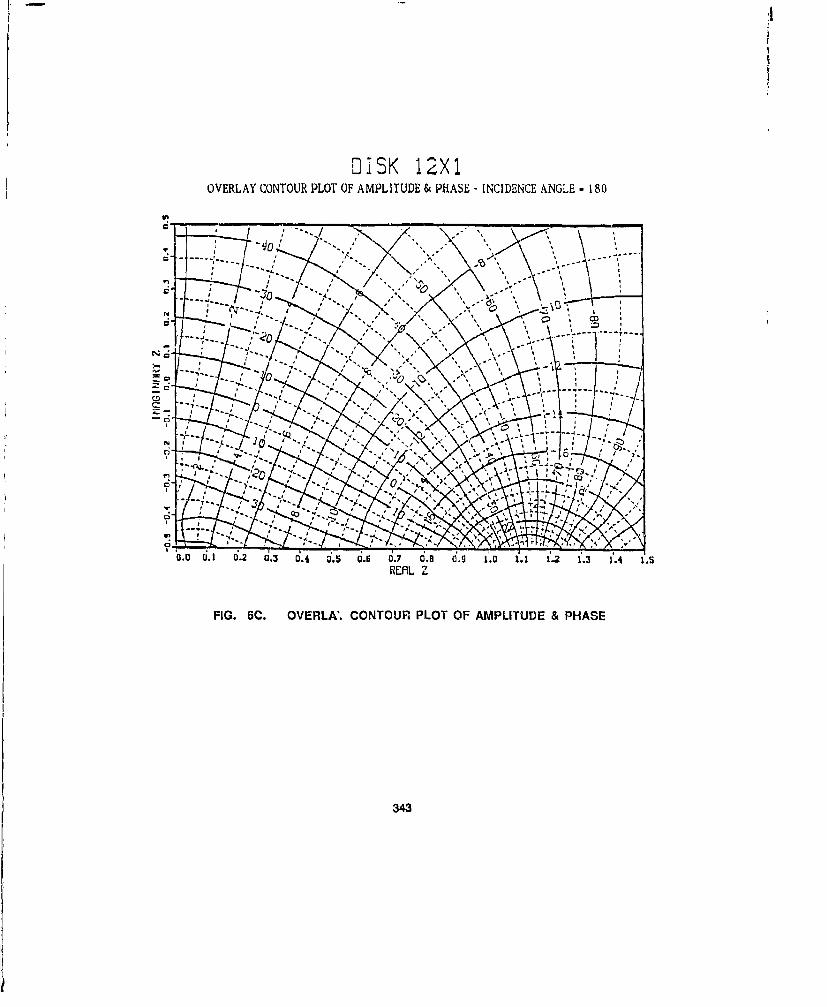
DISK 12X1OVERLAY CONTOUR PLOT OF AMPLITUDE & PHASE - INCIDENCE ANGLE - 180

FIG 6C. OVR' COTU LTO MLTD HS

343n -

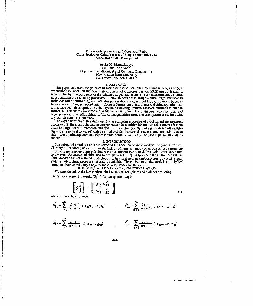
Polarimetric Scattering and Control of RadarCrc, .s Section of Chiral Targets of Simple Geometries and

Associated Code Development

Asoke K. BhattacharyyaTel: (505) 522-9468

Department of Electrical and Computer EngineeringNew Mexico State UniveisityLas Cruces, NM 88003-0002

I. ABST'RACTThis paper addresses thf- problem of electromagnetic scattering by chiral targets, namely, asphere and a cylinder and the possibility of control of radar cross section (RCS) using chirality. It

is found that by a proper choice of the radar and target parameters, one can most efficiently controltarget polarimneuic scattering properties. It may be possible to design a chiral target invisible toradar with same transmitting arid receiving polarizations since most of the energy would be trans-formed to the orthogonal polarization. Codes in Fortran for chiral sphere and chiral cylinder scat-tering have been developed. The chiral cylinder scattering problem has been extended to obliqueincidence. The codes developed are handy and easy to use, The input parameters are radar andtarget parameters including chirality. The output quantities are co and cross p1ol cross sections withany combination of parameters.

The key conclusions of this study are: (1) the scattering properties of the chiral sphere are aspectdependent (2) the cross polarization component can be considerable for a chiral scatterer (3) therecould be a significant difference in the copolar cross section (i.e. Sii and S22 are different) and alsoS It I S22 for a chiral sphere (4) with the chiral cylinder the normal or near normal scattering can berich in cross-pol component and (5) these simple chiral structures can be used as polarization trans-fonners.

II. INTRODUCTIONThe subject of chiral research has attracted the attention of sonic workers for quite sometime.

Chirality or 'handedness' stems from the lack of bilateral symmetry of an object. As a result themedium cannot support plane polarized wave but supports two oppositely rotating circularly polar-ized waves. An account of chiral research is given in [ 1,2,31. It appears to the author that still thechiral research has not matured to conclude that the chiral medium can be successfully used in radarsystems. Also, chiral codes are not readily available. The motivation of this work is to study EMscattering from chiral simple objects and develop codes for the same.

11. KEY EQUATIONS IN PROBLEM FORMULATIONWe provide below the key mathematical equations for sphere and cylinder scattering.

The far zone scattering matrix [S icj I for the sphere [4,5] is-

c ,cS21 S2 2

where the coefficients are-

n + I. -.. (.+--a nn-, ,,- brfn, nr1 I=Cnt r-n(n + 1) n= 1 n(n+ I)

2n +• 1 S'12=1 2' " (-antn-bnrn)12 / n(n + 1) (dnXc n- C n'•n) n•f=1n(n +1) n-

344

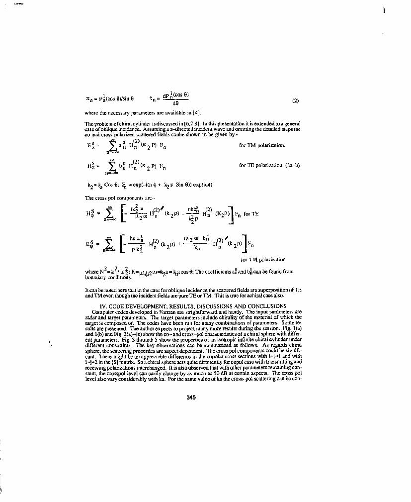
X pI(cos 0)/sin 0 n =dP In(Cos O)n dO (2)

where the necessary parameters axe available in 141.

The problem of chiral cylinder is discussed in [6,7,8]. In this presentation it is extended to a generalcase of oblique incidence. Assuming a z-directed incident wave and omitting the detailed steps theco and cross polarized scattered fields canbe shown to be given by-

E = s s (2) (12 P) for TM polarization.z n Hn 2 "F1

Hs •'•j s ~(2)( p)nfoTs = s 2)n (K 2 F forTE polarization (3a-b)

k2 = ko Cos 0; ln exp(--i(n 4t + k2 z Sin 0)) cxp(ixt)

The cross pol components are--[ li (k 2P -- • I 1 (K2 P) Fn forTE

[~ 2) nh 2" -

S [ hn a ~ (2) 1IL2o~ bn (2) "'(k p)] FS pk2 n 2P+ kzn n 2~

for TM polarization

where N2= k21 k 2; K= Llj2 ;;u=k2 a = lka cos 0; The coefficients an and bj can be found fromboundary conditions.

It can be noted here that in the case for oblique incidence the scattered fields are superposition of TEand TM even though the incident fields ame pure TE or TM. This is wuoe for achiral case also.

IV. CODE DEVELOPMENT, RESULTS, DISCUSSIONS AND CONCLUSIONSComputer codes developed in Fortran are strightforward and handy. The input parameters are

radar and target parameters. The target parameters include chirality of the material of which thetarget is composed of. The codes have been run for many combinations of parameters. Some re-sults are presented. The author expects to project many more results during the session. Fig. 1(a)and 1(b) and Fig. 2(a)--b) show theco-andcross-pol characteristics of a chiral sphere with differ-ent parameters. Fig, 3 throuph 5 show the properties of an isotropic infinite chiral cylinder underdifferent constraints. The key observations can be summarized as follows. As regards chiralsphere, the scattering properties are aspect dependent. The cross pol components could be signifi-cant. There might be an appreciable difference. in the copolar cross sections with i=ij=- and withi=j=2 in the [SI matrix. So a chiral sphere acts quite differently for copol case with transmitting andreceiving polarizations interchanged. It is also observed that with other parameters remaining con-stant, the crosspol level can easily change by as much as 50 dB at certain aspects. The cross pollevel also vary considerably with ka. For the same value of ka the cross--pol scattering can be con-

345

siderably stronger than copol scattering. As regards chiral cylinder scattering (Figs. 3 through 5)the following observations are made. The nature of variation of TE and TM cross sections are con-siderably different than an achiral case. The cross pol scattering may be considerably greater fornormal incidence than copol scattering which never happens in the case of achiral cylinders.

It appears to the author from this limited study that even a simple chiral targets like sphere andcylinder can probabily be used as a polarization transformer, a radar clutter simulator etc.

V. REFLRENCES[I] A. Lakhtakia, V. K. Varadan and V. V. Varadan- "Time-harmonic Electromagnetic Fields In aChiral Medium", Springer--Verlag, 198912] A. Lakhtakia (Ed.) -"Selected Papers On Natural Optical Activity", SPIE Milestone Series,SPIE Optical Eng. Press, 1990[3] S. Bassiri-'Elcctromagnetic Waves In Chiral Media", in H. N. Kritikos and D. L. Jaggard(Ed)-'Recent Advances In Electromagnetic Theory", Springer-Verlag, 1990[41 C. F. Bohren-"Light Scattering by an Optically Active Sphere", Chem. Phys. Lett., Vol. 29,1974, pp. 458-462[51 A. K. Bhattacharyya -"Control of Radar Cross Section and Cross-polarization Characteristicsof an Isotropic Chiral Sphere", Electronics Letters, Vol. 26, No. 14, 5th July, 1990, pp. 1066-1067[6] C. F. Bohren --"Scattering of Flecu'omagnetic Waves by an Optically Active Cylinder", Jour.Colloid Interface Science, Vol. 66, No. 1, Aug. 1978, pp. 105-109171 J. R. Wait-J"Scattering of a Plane Wave From a Circular Dielectric Cylinder at Oblique Inci-dence", Can J. Physics, Vol. 33, 1955, pp. 189-195181 A. K. BlIattacharyya-"Elcctrtmagnetic Scattering by an Isotropic Chiral Cylinder at ObliqueIncidence: Control of RCS and Cross Polarization Characteristics", Under Review in IEEE Trans.AP-S

Lectends to the Illustrations

Fig. 1: Variation of 20 Log 10 (I SýI ) with aspect angle for a chiralp1.11wit aspct ngl fora cira sphere(a) a= X; 1r =1.0 ; cr -4.0; u ---0.003; 13= 0.(X)2(b) a= X; = =1.0;cr =4.0; x = 13 = 0.002

Fig. 2: Co and Cross-polarization Characteristics of the Chiral Sphere(a) Crass Polarization Characteristics of Chiral Sphere Against Aspect Angle With Radius As aparameter; (x "0.003; D3 =.(X)2(b) Variation of Co-- and Cross-polarization Levels at 0 --0 with ka(cx =0.0(13; 1 --0.002)

sFig. 3: Log1 0 (I Eiji) Versus Aspect Angle for a Chiral Cylinder; f=10 GHz; [) = 0.0045; k 0 a =6.28; ER =2.56; R tR =1.0

Fig. 4: Log 1 0 ( I ES ij) versus ko a for a Chiral Cylinder for Normal Incidence; f= 10 GHz; 1•-0.0045; r R= 2 .56 ; it iR =1.0Fig. 5: Variation of Cross- pol Components With Chirality Parameters With 0 ='0 and 60 degrees;f=10 GHz; koa=6.28;(a) TE Polarization (b) TM Polarization

340

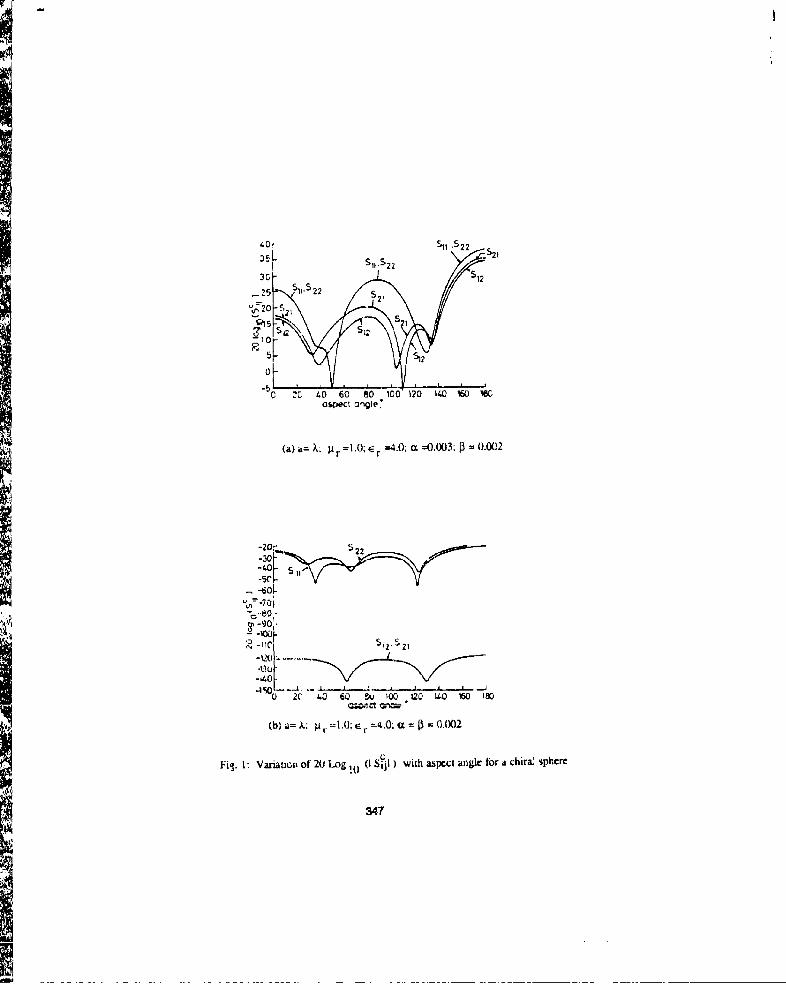
S1 _522 -_2

S".22

30Ii- j; g j:;z ja ii 2 ra phr

11 3 42

60

2-21ASL

0 20 2.0 60 80 100 120 1.0 160 iS

(a) Cross Polawzintion mhbcieris,•s of Qira Sphci• AgainsL Abpccl Angie Widi Radius As aparamctc, c• =0.003; 13 -0.002

90•70 A60

'-40 S13 5 L

S30o_ 0

-20-30

13 6AK =A

(bi Vanazmion or Co- an (".oss-p~ol•nzabon Levels at U' .0 widh k•a~ (.0003,13 ,=0.0(Y2)

Fig. 2: Co a(t Cross.-polariizatio CCharattserics of Ohc Chr.' Sphere

p348

-SO ' TK-cWOL L

copLl-CWSI&

ASPECT ANGLE IN DEGRIEES'

Fig 3: Lag (I EUIl) Versus Aspect Angir fora ChkraI Cylinder;I- 10 (Iz; ji-.OO45; k oa -628. a~ R2.56. PR -1.0

TNm-caor" A '

* ~U-*O~&PL M -

I"Tc '~n~Mossrol.

4.10 i. .',j) a; r. c.w -Of ..

340

04-to

CHIPAUTY PARAMETER(0~ 11 Polanuation

LL _ _ __ _ _ _

_j

CHIRAUTY PARAMETER jS

Fig. 5: Vanation of Cmsls pal Components With Chira~iti Pu~amcters With e .4) and 60 dEawes:f-tO G~iz, k,,a-6.28-,

350

SESSION 9- "HIGH FREQUENCY APPLICATIONS ANDWIRE GRID MODELING TECHNIQUES"

Moderator: Christopher Trueman

i

SCATTERING BY SECTORED CYLINDERSBenjamin Rulf, Grumman Corporate Research Center, Bethpage, NY 11714

Plane wave time harmonic electromagnetic scattering by a perfectly conductingsectored cylinder, shown in Figures 1(A) and (B), Is analyzed for TE and TMpolarizations. Mono and bi-static scattering cross sections are obtained for a variety ofparameter combinations. The sectored cylinder is a simple model for a body withcavities.

Th•e Problem:

The computation of scattering by large, complex and composite bodies relies onvarious techniques, such as high frequency asymptotics, finite difference approaches,and methods based on Galerkin's approach (Method of Moments). The need tovalidate the solutions obtained by these methods against some known "Canonicalproblems" is vital. For meaningful comparisons with scatterers that are non convex orhave open cavities the canonical shapes should also posses such features. Solutionsof canonical problems are also needed as benchmarks against which the speed (andother features) of various approximate methods can be compared.

Obiectives'We look for solutions of canonical problems that can model non convex bodies

and bodies with cavities. Such solutions should not require physical or geometricalapproximations or some a-priori kncwledge (such as a clever "Ansatz"). The reason isthat the physical and geometrical approximations that are required in various methodsoften give rise to errors that cannot be quantitatively estimated. Also, there are nosystematic ways for guessing a -nod "Ansatz". On the other hand, it may be possibleto find quantitative error bounds if only mathematical approximations ar- ý;c, ", suchas the summation of Infinite series or the colution of infinite systems of linearequations. Also the speed and accuracy do not depend on how good an a-prioriguess we found.

The method we use is a generalized and somewhat -implified version of [1].We shall outline the approach here, but omit many details which will appear in [2].

351

The time-harmonic C") electromagnetic field in two dimensions can be

derived from a single scalar function u(r,o). In the case of TM, or perpendicular,

polarization we let

i ldu -i duHr- = = 1 (2)Oý.U r To' O)A dr

and

(V2 +k2)= koii()

On ihb scatterer's perfectly conducting surface we enforce the Dirichlet conditionu=- on S, (4)

and on the are ora, 0 5jq01< <

u and du are continuous. (5)

We assume a plane wave excitation in the form

uin= exp[ikr cus (0- 0')] = _q,4 (0') Jn (kr) exp(in 0), (6)n=--o

qn = [i exp(-i 0')]n. (7)

The case of TE, or parallel, polarization is analogous, with (4) replaced by a Neumanncondition. The details will be given in [2].

We now write in Region 1u=uin+us (8)

352

where u~n is given by (6) and

U= An Hn (kr) exp(in •) (9)

Here All are numerical coefficients that have to be computed, and Hn (kr) is the Hankelfunction of the second kind (which assures that us satisfies the radiation condition atr.-- o-). For the Bessel and Hankel functions we use the excellent code developed byD. Amos of the Sandia National Laboratory [3]. For the asymmetric case of Figure 1(A)we write in Region 2

u Bj Fj (r,b) sin ([±j(0 + I)], (10)jrl

where Bi are numerical coefficients, andoj =.Jý, 7r=z/ 2 V/ j =1, 2,.... (11

We also choose

F1 (r,0) = J P) (p)(

where p=kr and f3rkb. These choices assure that u satisfies (4) on the conductingboundaries of Region 2, On r=a we must satisfy (5) at the interface between theregions. and (4) on the conducting body. This ir"' "s

,YJA,,it, (tx) + q,, .,, ((x)] ,.%7,(i,•) -

(13)

= j-I

0 J,,?. I, <I 01 I• .

353

I

S~(14)Bj Fj(a,b)lin[j4(t+ V)] forl< (4V,

j=1

where a=ka and f'= rracdr -

We use now the following notation for the orthogonality of the angular functions:

7C<<fnfm > f,(b)fn(4)dh, (15)

<gj,gt>= > gj ()g;(O)dO, (16)-V

<exp(-im o), sinoj•(O 4. V)]>=<M~j>. (17)

Thus<<exp(ino), exp(-imO)>>=2rySnm (18)

<sin U4(0 + ±r)], sin [t(O + V)]>= Vgjd5 (19)

< inj>= [i - j s -m) (20)

Using these relations and notation we can eliminate the coefficients Bi 'rom (13) and(14) and obtain an infinite system of linear equations for An in the form

354

Am I-n,(a)+qm Jn (a)= [A H, (a)+qn J (a)]Rmi M=0,±l,±2. (21)

Rm~ Fj1(a, b) <mj> n >(22)

If this infinite system is truncated at nwM, where M is appropriately chosen, then wehave in (21) a set of 2M+l equations which can be solved for An. -M,'n•M It can beshown that the coefficients An become very small when Inl > ka. Clearly we need toset M>ka. but we have not yet found out how to choose a minimal M for anycombination of the parameters (a, b. A and V). In all the cases we ran we saw thatwhen M=~ 2ka the solutions do not change significantly anymore. This means that wesolve 4ka+1 equations to get good accuracy. More work is needed to quantify thedependence of errors on the choice of M. We also n~eed to truncate the sum in (22) ata point j=L. It can be derived from (12), (20) and (22) that when jý >>M the sum

converges like (j])f 3. Thus, for a given angle Vl we cab choose a truncation limh Land estimate the remainder of the series (22) quite accurately. We have obtainedgood results choosing L4 Ž! 250 In all the cases we ran. The choice of L is not criticalin terms of the effect on computing time, but here too some additional experimentationis recommended.

When the scatterer is symmetric, as shown in Figure 1(B), the procedure issimilar and the result Is that Rm,n is replaced by Rm.n[1+(-l)m+nl. An analogousanalysis for the TE case will not be shown here but can be found in [2].

The scattering width (SW) is given by

355

___________ _________ _____ ____ _______ _______________i

2l

r, ' l im (2 irr) 1U., I

l 2(23)k-I YA, x.i~ + 7c2]2

n=-M

When i = ' this represents the mono-static SW, otherwise it is the bi-static SW.

We have developed a computer program called SECTOR, based on the aboveanalysis, which computes the mono or bi-static SW of sectored cylinders, symmetric orasymmetrics, for either TE or TM polarization.

To validate the results we have performed a number of tests. First, we havebuilt in with each computation of the An coefficients of a sectored cylinder acomputation of the coefficients Cn of the corresponding solid cylinder. These aregiven by

(q, n (a) I H, (a), for TIM polarization,-Cn =[qn J'(c)/ if'(a), for TE polarization. (24)

Clearly, when V is very small, ka is large, and the incident wave does not illuminatethe missing sector, we expect the numerical difference between An and Cn to be verysmall. This indeed was observed in all the tests that were run.

Another important test was the computation of the SW of a conducting strip,which is a special case of Figure I(B) when b=O and V*--> ir2. Several cases ofmono and bi-static SW of strips were compared with known solutions [4]. Agreementswere usually within 1%.

Results and Conclusions:Follwing are some figures that show computed results of the SW of large

sectored cyl nders with large cavities. Figures 2(A) and (B) show the monostatic SW of

356

a corner reflector that is embedded in a cylinder. The geometrical parameters are:a=1.0 in, b=0, psi=450 and the frequency is 1.67 GHz (ka=35), The typical wide lobesin the directions around 0=00 are apparent in both polarizations though the detailedstructures of the lobes are slightly different due to the difference in the TE and TMdiffraction phenomena. The projected aperature has a width of w =1.414 m atbroadside. Physical optics (PQ) predicts SW = kw2 = 70 in at the peak for bothpolarizations. The actual values are slightly lower as a result of interference betweenthe various field constituents i.e. reflection form the corner reflector and diffraction fromthe two edges and the smooth part of the cylinder. In both polarizations we notice asharp spike about 0 = 451. Again, according to PC prediction these peaks should be35 m for both polarizations but are in effect somewhat higher due to interferenceeffects. The computed TM peak values are closer than the TE values to the POpredicted peaks at 00 and 450. As the angle of incidence increases further, thestructure appears more and more like a solid cylinder, especially in the TM case.When the incident wave comes from the back quarter (0>1350) the missing sector is inthe deep shadow and the structure is indistinguishable from a solid cylinder. Figure3(A) shows the bistatic SW for the same corner reflector when the angle of incidence iso = o. rThe sharp spike in the forward direction (0' = 1800) is typical for a large solid

cylinder and is not much affected by the presence of the corner reflector. In order todemonstrate this we show in Figure 3(B) the ratio between the bistatic SW of thestructure and that of a solid cylinder. The corner reflector causes a large enhancementof the SW in the backward direction, but in the forward direction the ratio approachesunity, i.e. the structure is indistinguishable from a solid cylinder. Figures 4 and 5 showthe monostatic SW of a sectored cylinder with a=1.0 m, b=0.4 m, and psi=-120. Thefrequency yields ka=26 in Figure 4 and ka=42 in Figure 5. Even though it is a fairlysimple structure, the patterns are not easy to predict since they represent thecombined effects of several wave phenomena such as diffraction by smooth bodies,edge diffraction and the effects of a large open cavity. In all these figures we show theratio of the structure's SW to the SW of the corresponding solid cylinder for angles ofincidence between 0' and 900. We see that cross section enhancements of up to afactor of 5 may occur. Without this computer program it would be difficult to predict atwhat angles, frequencies or polarizations these peaks should be expected.

We conclude with the observation that the reported work, and its futuregeneralizations, serve two important purposes. One is simply to serve as an accurate

357

and reliable benchmark for testing other numerical codes that analyze scattering bycertain complex bodies. With some additional work the code SECTOR may become auseful benchmark code for large bodies with cavities, such as jet engines etc. Theother purpose, which has not been exploited yet, may be the more interesting one: bydoing an extensive parametric study of results that this program would yield we maybroaden and deepen our understanding of the various interacting wave processes thatoccur in scattering by such bodies.

References*

[1] J.B. Billingsley and G. Sinclair: "Numerical Solutions to ElectromagneticScattering from Strips, Finite Wedges and Notched Circular Cylinders", Can. J.Phys. 44. 3217-3225 (Dec. 1966).

[2] B. Rulf: "Scattering by Sectored Cylinders," submitted for publication

[3] D. Amos, ACM Trans. Math. So~tware 12 (3), 265-272 (1986)

[4] G.T. Ruck et al: "Radar Cross Section Handbook", Plenum Press, New York,1970.

358

1K,

Region 1

Realon e 1

2 xPerfect "

erfea conductor

,-'IGURE 1 (A) THE SECTORED CYLINDER

fY

f• ~Region1

Reqlon 'I Region/ 2 "X

FIGURE 1 (B) THE SYMMETRICAL SECTORED CYLINDER

359

2-0 BACKSCRTTERING CROSS SECTION OF A SECTORED C(LINDERASYMIMETRIC PERPENDICULAR POLRRIZATION

PSI - 45.000 (DEG) A - 1.000 (M) B - 0.000 {M1FREOCONST- 1.670( GiHZ GnMCONST - 0.0001 DEGREE5 1

9 - SECTORED CYLINDER SW

"2 4 -- _ _ __ _ _ _ __ _ _ _ __ _ _ _ __ _ _ _ __ _ _ _G1

0.0 15,0 30.0 40.0] 60.0 75.0 00.0 105.0 20.6 135.0 I50J.0 t65.0 180.IPHI I DEG{REES I

FIGURE 2 (A) CORNER REFLECTOR EMBEDDED IN •-CYLINDER WITH A-1.0 M,• B=0, PSI= 45 DEGREESKA=35. MONOSTATIC SW, TM POL.

360

2-0 BACKSCnTTERING CROSS SECTION OF A SECTOREO CYLINOERRSYMMIETRIC PnRPLLEL POLRRIZnTION

FSI - 45.000 (OEG) A - 1.000 (I) B " 0.000 (WiFRrOCONST- 1.6701 GKZ ) GMCONST - 0.O000 DEGREES

S , ECTORED CYLINDER 514

CA

Lo

.In

ng 9

cac-

0.0 15.0 36.0 4S.0 0.0 75.0 1oJ.o ius.n 1;0.0 135.0 o 3.O I 55. leOjP1I I ODEREE5 I

FIGURE 2 (1) SAME AS FIGURE 2 (A) BUT WITHMONOSTATIC SW, TE POL.

361

2-0 BACKSCATTERINS CROSS SECTION OF" R SECTORED CYLINDERnSYIIMETRIC PERPENDICULRR POLAR IZnTION

PSI - 45.000 (DEG) A- 1.000 IM) B - 0.000 (M1)F'REOCONST- 1.6701 GHZ I GRMCONST - 0.0001 DEGREES I

. - SECTORED CYLINOER SW

PHI I DEGREES I

FIGURE 3 (A) SAME CORNER REFLECTOR AS IN FIG. 2BISTATIC SW, TM POL.

362

,,r- -

2-0 BACKSCATTERING CROSS SECT19N OF A SECTORED CYLINDERASYMMETRIC PERPENDICULAR POLARIZATION

PSI - 45.000 (QEG| A - 1.000 1M) B - 0.000 IM)FREOCONST- 1.6701 GHZ I GRMCONST - 0.000( DEGREES I

r i - SECTORED/SOLID CYLINOER RATIO

In-Jo

"•-

,0d 1a, 0 .v 45.0 W.o '0.0 90.O ~ IO ,~o .o z3So •.0 165.0 lO,1PHI I DEGREES I

FIGURE 3 (B) RELATIVE BISTATIC SW, TM POL.

3W3

2-0 BnFCKSCr1TTLRING CROSS SECTION OF fl SECTORED CYLINDERASYMHETRIV PERPENUICULITR POLnR IZInTION

PSI - 12.0 (.FG) f - 1.0 (M) B- 0.4 (rM)FREOCONST- 1.2501 GIIZ I GnIICONST - 0.000( DEGREES I

, - SECTORED/SOLID CYLINDER RfTIO_

C•, - -_

YiU:,

0.0 10.11 20.0 0.0 401.0 10.0 60,0 70.0 0.0 9,0PlIj I DEGREES I

FIGURE 4 (A) SECTORED CYLINDER, A=1.0 M. 3=0.4 M,PS1=12 DEG., F=1.25 GHZ (KA=26), MONOSTATIC SWTM POL.

364

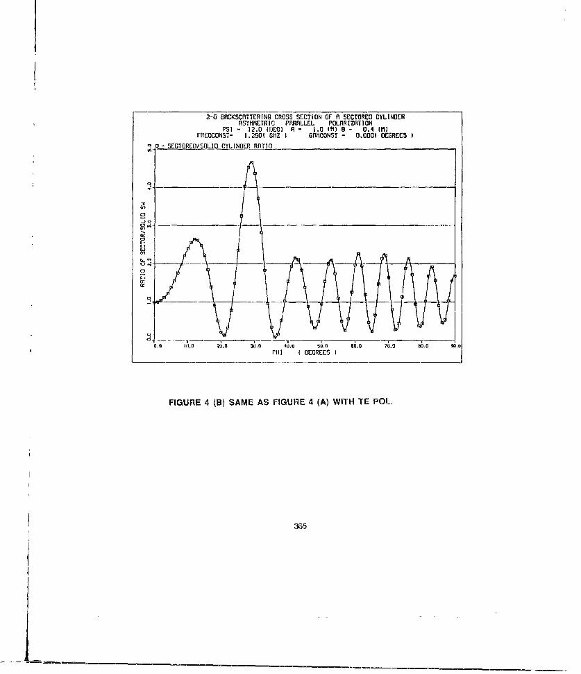
2-0 BRCKSCRTTERING CROSS SECTION OF R SECTORED CYLINDERASYMMETRIC PRRRLLEL POLnRIZRTION

PSI - 12.0 (DEC) AR- 1.0 I(I - 0.4 IIFREOCONST- 1.2501 GHZ I GFlIICONST - 0.000( DEGREES I

S SETORED/SOLD CYLINOR RnTIO___

u'

0

19

0.0 la. o 2 o. o 3 o ,0 4 o0A m a~ 60.0 70 0 19 .PillI D EGREES I

FIGURE 4 (B) SAME AS FIGURE 4 (A) WITH TE POL.

365

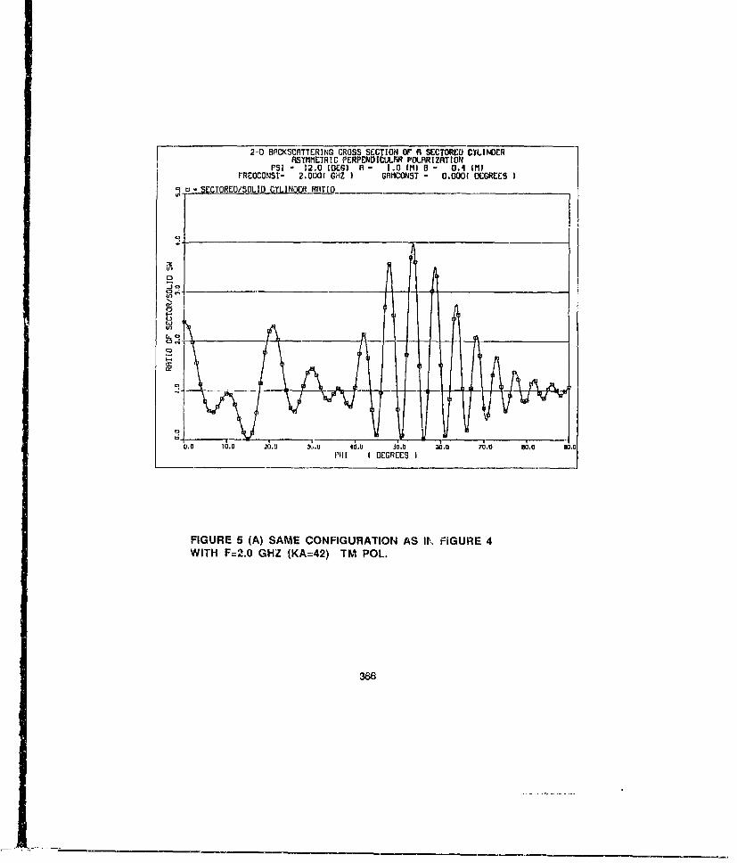
2-0 BACKSCUTTERING CROSS SECTION OF A SECTOREO CYLINOERASYMMETRIC PERPENOICULAR POLRRIZATION

PSI - 12.0 IDEG) R- 1.0 I11 B - 0.4 (M)rREOCONST- 2.0001 GHZ I GR1CONST - 0.000( DEGREES I

" - SECTORED/SOLID CYLINDER RRTIO

in

0.0 10.0 20.0 3,.a 40.0 30.0 30.0 70.0 0,0 8021Pill I DEGREES I

FIGURE 5 (A) SAME CONFIGURATION AS IK FIGURE 4WITH F=2.0 GHZ (KA=42) TM POL.

366

2-0U BACKSCnTTrCRING CROSS SCOTION OF AI SECTORED CYLINDERASYMMIETRIC PFRRLLEL POLRRIZATION

PSI - 12.0 10EG) A - 1.0 (M)1 8 - 0A 41H)FRLOCUNST- 2.000W GHZ 1 GRMCONST - 0.0001 DEGREES I

-SECTORE3/S0LIOCYLINDER RATIO

t,

co

Ed

ciW.-

0 t0 0.0 20.0 10.0 40.Ii 50.0 60.0 70.0 t0.0 o 01mill I DEGREES I

FIGURE 5 (B) SAME AS FIGURE 5 (A) WITH TE P01.

:367

THIS PAGE ISINTENTIONALLY

LEFT BLANK, ACCIDENTALLY,

368

RCS of Fundamental Scatterers in the HF Band

by C.W. Trueman', S.R. Mishra", and SJ. Kubina'* Electromagnetic Compatibility Laboratory, ** David Florida Laboratory,

Concordia University, Canadian Space Agency,7141 Sherbrooke Street West, P.O. Box 11490. Station H,

Montreal, Quebec, Ottawa, Ontario,Canada H413 IR6. Canada K2H 8S2.

Absiract-At HF frequencies a typical aircraft is comparable to the wavelength in size. Wire-gridmodelling permits a detailed representation of the aircraft geometry. A moment-method codesuch as the Numerical Electromagnetics Code determines the currents flowing over the aircraftand its radar cross-section.

This paper proposes a set of "wire-grid guidelines" for constructing grids of complex sur-faces such as aircraft. Estinmates of the frequency range over which the grid is valid are pro-vided. These guidelines are applied to model a cube, showing good agreement with the mea-sured RCS, and demonstrating the validity of the bandwidth estimate.

Aircraft carry IF antennas for communication purposes. A strip scatterer and a cylinderscatterer are modelled without and with a wire "antenna" to determine the effect of the wire onthe RCS. At frequencies making tie wire odd multiples of the quarter-wavelength, the wireagainst the strip or cylinder as "ground" is resonant, and the wire has a large effect on the RCS.Goxxd agreement between measurements and computations is shown.

IntroductionCoastal radar operating at HF frequencies has the potential of covering vast areas of ocean

from a single station. The ground wave at HF adheres to the air-ocean interface and it may bepossible to see aircraft and ships that arm "beyond the horizon" with HF ground-wave radar. Theaircraft of Fig. 1 is a complex target for the detennination of radar cross-section. The aircraft isabout 30 in long and so HF frequencies the aircraft dimensions ame comparable to the wave-length. The computer model must represent the entire aircraft, allowing each part to interactwith every other part. The aircraft carries wire antenna: for HF conmmunication. An objective ofthis work is to study the effect of the wire antennas on the radar cdoss-section of the aircraft.

Wire-grid modelling allows a detailed model of the entire aircraft to be constructed ondsolved. The surface is approximated by replacing it with a grid of thin wires. Ideally, ti;,; wiresare positioned in two orthogonal directions, subdividing the surface into square cells or meshes.The wire radius is then related to the area of the adjacent meshes by the "equal-area rule"[ 11.

The currents on a grid of thin wires can be found by solving a thin-wire electric field integ-ral equation(EFlE) by the moment metho '12,3]. This project uses the well-known "NumericalElectromagnetics Code"(NEC)[4,51. The derivation of the thin-wire. EFIE and its solution by themoment-method lead to certain restrictions which the wire-grid must satisfy. Ref. 16] collectsthese restrictions as "NEC modelling guidelines" from references [4,5,71. For the present pur-pose the essential restrictions are the following. In order that the wires be "thin", the wire radiusshould be less than .V30. Each wire must be subdivided into "segments", which are comparableto X110, although sometimes segments as long as X5 are allowable. Burkc[7] suggests that seg-ments be maintained shorter than 0. 14.. Other restrictions on the ratio of the segment length tothe wire radius, on wire junctions, and wire spacing are reviewed in reference[6].

This wk ork was supported by the DcfV.eilc Rescaich Establishment, Ottawa under contract numberW7714-9-9216/01-SZ, under the techmici' "! uervision of Dr. Tim Coyne.

369

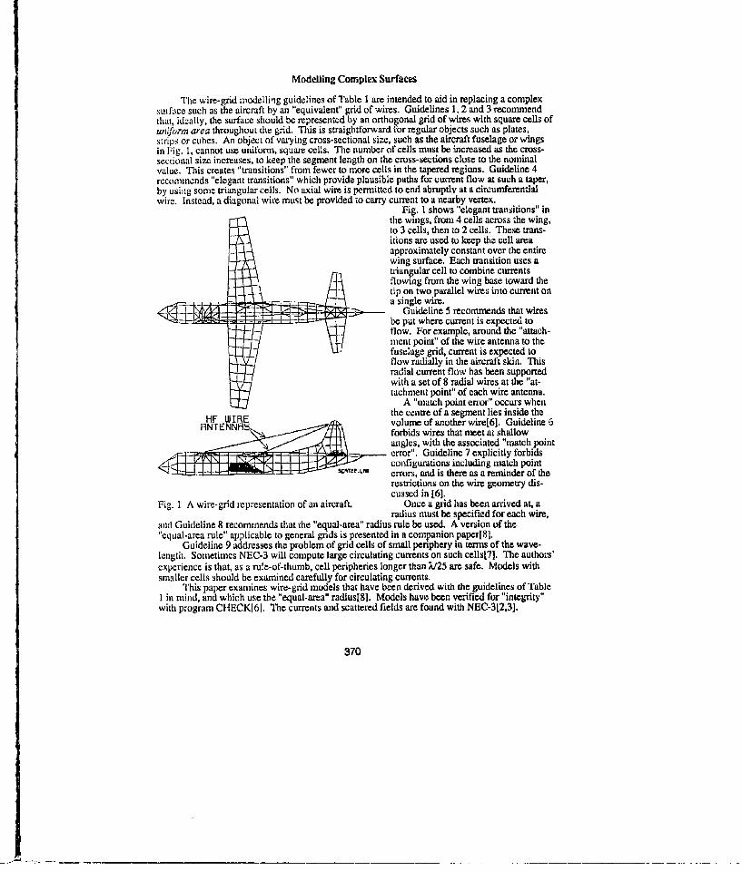
Modelling Complex Surfaces

The wire-grid modelling guidelines of Table 1 are intended to aid in replacing a complexsurface such as the aircraft by an "equivalent" grid of wires. Guidelines 1, 2 and 3 recommendthat, ideally, the surface should be represented by an orthogonal grid of wires with square cells ofuniform area throughout the grid. This is straightforward for regular objects such as plates,strips or cubes. An object of va'ying cross-sectional size, such as the aircraft fuselage or wingsin Fig. 1, cannot use uniform, square cells. The number of cells must be increased as the cross-sectional size increases, to keep the segment length on the cross-sections close to the nominalvalue. This creates "transitions" from fewer to more cells in the tapered regions. Guideline 4recommends "elegant transitions" which provide plausible paths for current flow at such a taper,by using some triangular cells. No axial wire is permitted to end abruptly at a circumferentialwire. Instead, a diagonal wire must be provided to carry current to a nearby vertex.

Fig. I shows "elegant transitions" inthe wings, from 4 cells across the wing,to 3 cells, then to 2 cells. These trans-itions are used to keep the cell areaapproximately constant over the entirewing surface. Each transition uses atriangular cell to combine currentsflowing from the wing base toward thetip on two parallel wires into current ona single wire.

Guideline 5 recommends that wiresbe put where current is expected toflow. For example, around the "attach-ment point" of the wire antenna to thefuselage grid, current is expected toflow radially in the aircraft skin. Thisradial current flow has been supportedwith a set of 8 radial wires at the "at-tachment point" of each wire antenna.

A "match point error" occurs whenthe centre of a segment lies inside theHF IWIRE "- volume of another wire[61. Guideline 6

I9NIENI9 ~forbids wires that meet at shallowangles, with the associated "match pointerror". Guideline 7 explicitly forbidsconfigurations including match pointerrors, and is there as a reminder of therestrictions on the wire geometry dis-cussed in [6].

Fig. I A wire-grid representation of an aircraft. Once a grid has been arrived at, aradius must be specified for each wire,

and Guideline 8 recommends that the "equal-area" radius rule be used. A version of the"equal-area rule" applicable to general grids is presented in a companion paper[8].

Guideline 9 addresses the problem of grid cells of small periphery in terms of the wave-length. Sometimes NEC-3 will compute large circulating currents on such cells[7l. The authors'experience is that, as a ru'e-of-thumb, cell peripheries longer than ;L/25 are safe. Models withsmaller cells should be examined carefully for circulating currents.

This paper examines wire-grid models that have been derived with the guidelines of TableI in mind, and which use the "equal-area" radius[8]. Models have been verified for "integrity"with program CHECK[6]. The currents and scattered fields are found with NEC-3[2,3].

370

Table 1WIRE GRID GUIDELINES

I Use a rectangular grid of wires oriented parallel to edges, with wires along edges.2. Choose the segment length equal to V110 at the highest frequency of the band. Keep

the area of the grid cells comparable to (X/10)2.3. Keep grid cells square. Keep the cell area constant, hence scgment length constant,

throughout the grid.4. Provide elegant transitions.5. Put wires where current is expected to flow.6. Avoid wires meeting at very shallow angles.7. Keep the center of any segment outside the volume of any other segment.8. Use the "equal-area rule" radius.9. All meshes in the grid must have peripheries longer than X/25.

Frequency Limitations

A wire-grid mesh is a valid representation of a solid object over a limited bandwidth. Thissection provides estimates of the lower and upper frequency limits.

If the shortest rtesh periphery in the model is Lm.., then the frequency where the mesh pathof length L., is X/25 is given by

12, = "- Mlz

At frequencies less than f:,ý, the currents on the model should be inspected for large currents onindividual small meshes.

Table I requires that the segments be shorter than /1J0, and thus the model has its bestperformance up to the frequency V'iven by

30 Mllz

where .-_, is the longest segment length in the model. The model is often useful up to a fre-quency where the longest segment is V]5, given by

/2) = 60 Ml

However, Burke[7] suggests that NEC's solution not be used above the frequency where thelongest segment is 0.14k.. For scattering purposes, wire-grid models often generate useful resultsat frequencies above ,), but few are useful above .,2. In a well designed wire grid, the longestsegment. A.,,, is not very much longer than the average segment length, A,.. Then as tbc fre-quency increases all the segments in the model tend to become "too long" at a similar frequency.

371

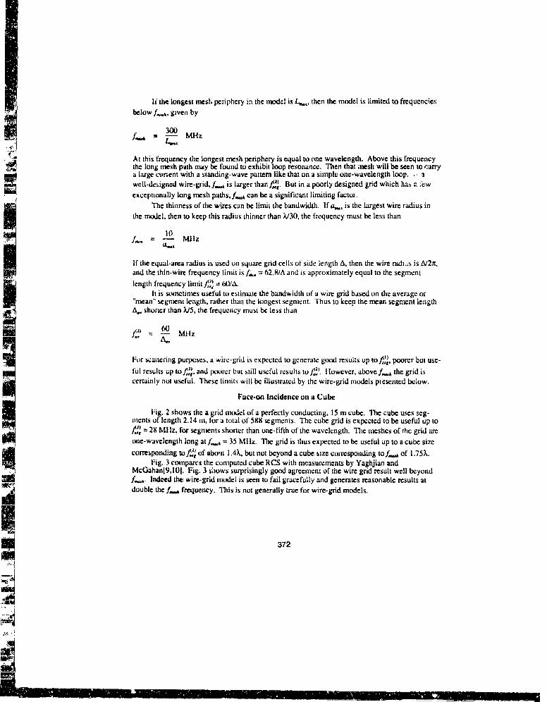
t U the longest mesh periphery in the model is L,,, then the model is limited to frequenciesbelow f_.,,, given by

300i.., MHz

At this frequency the longest mesh periphery is equal to one wavelength. Above this frequencythe long mesh pitth may be found to exhibit loop resonance. Then that onesh will be seen to rarrya large cunent with a standing-wave pattern like that on a simple one-wavelength loop. ,. awcll-dcsigned wire-grid, f_,, is larger than J(. But in a poorly designed grid which hat, z :ewexceptionally long mesh paths, f.,,%A can be a significant limiting factor.

The thinness of the wires can be limit the bandwidth. If a., is the largest wire radius inthe mo.dcl, then to keep this radius thinner than XV30, the frequency must be less than

10A"., = - M~lz

If the equal-area radius is used on square grid cells of side iength A. then the wire radi.,s is A/2n,and the thin-wire frequency limit is f,, = 62.8/A and is approximately equal to the segmentlength frequency limit Jr = 60/A.

It is sometimes useful to estimate the bandwidth of a wire grid based on the average or"mean" segment length, rather than the longest segment. Thus to keep the mean segment length4A, shorter than W5, the frequency must be less than

- MHzA-,

For scattering purposes, a wire-grid is expected to generate good results up tof,•, poorer but use-ful results up to./,,, and pxxorcr but still useful results toj."'. Hlowever, abovcfk the grid iscertainly not useful. Those limitst will be illustrated by the wire-grid models presented below.

Face-on Incidence on a Cube

Fig. 2 shows the a grid model of a perfectly conducting, 15 m cube. The cube uses seg-ments of length 2.14 m, for a total of 588 segments. The cube grid is expected to be useful up to~2), = 28 MI Iz. for segmnmts shorter than one -fifth of the wavelength. The meshes of the grid arcone-wavelength long atf.,,, = 35 Mlhz. The grid is thus expected to be useful up to acube sizecorresponding toJ of aboit l.4•, but not beyond a cube size corresponding tof.,,, of 1.75x.

Fig. 3 compares the computed cube RCS with measurements by Yaghjian andMcGahan[9,101. Fig. 3 shows surprisingly good agreement of the wire grid result well beyond",,,,. Indeed the wire-grid model is seen to fail gracefully and generates reasonable results atdouble the f.. frequency. This is not generally true for wire-grid models.

372

...

The cube cavity has a rich spectrum of internalresonances starting at size 0.707k. The wire grid

15 m CLUBE result is expected to fail at the internal resonantfrequencies of the cube, but the data of Fig. 3"shows no sign of the dramatic failure often assoc-iated with the intemal-resonance problem.

The Yaghjian and McGahan measured data ofFig. 3 was used to validate Mishra's measurementprocedure at the David Florida Laboratory(DFL).

Y The measurements are taken in a 20 foot anechoicchamber, with an HP 8510 network analyzer,using horn antennas for the 8 to 12 GHz frequency

DIRECTION OF TRIUEL range. The target is mounted on a styrofoam col-umn, and three measuements are taken: columnalone, column with reference 7 cm sphere, columnwith target. The exact Mie series solution for the

EF" ELECTRIC -IEI-.n VECTORi RCS of the sphercl3] is used to derive a correctionfactor accounting for the frequency response of thehoms and cables. Then the room and column

Fig. 2 A wire-grid of a cube with a plane response are vector-subtracted from the target pluswave incident on one face. room plus column response, to determine the RCS

of the target. The frequency range of the measure-ment will be extended with iiider-bandwidth horn antennas.

In Fig. 3, cubes of sizes 1.24 cm, 2.466 cm and 7 cm were measured from 8 to 12 Gllz toobtain the RCS in three size ranges. In all three caszs the RCS lies close to Yaghjian andMcGahan's measurement.

o o 0 Monuurod, Yaghjian & McGohonOFL MER5UREO

+ + . WIRF-GRIO MOOEL (NECV+ +,-> ÷+ .

++++ +++ 030 + +++ G+o D

'4+ '0

20 7 OFL HERSUREO

LOU eOFL MERSURE O

-a feeg fnah

0.5 1 .0 1.5 2=.0 2.5 3.0 3.5Side Length (wauelengthsI 5IPT.Lfta

Fig. 3 Comparison of wire-grid results with measured data for the cube.

373

Vertex Incidence on a Cube

Z Ludwig[ 111 reports measureaents by .lesherof the RCS of D cube with a plane wave incident

15 m CUBE upon one vertex, as shown in Fig. 4. The cube hasvertices on the z-axis and the x.axis, with theplane wave incident upon a vei tex of the cube.Fig. 5 compares th. calculated cube RCS with Fie-sher's measurements. Up to the frequency1,1where the segments am one-tenth of the wave-

y length, the agreement is very good. Between thatfrequency and the frequency ,(2) where the seg-

,JrnNOS ON ments are one-fifth wavelength, the agreement isPLRNF. WRUE ITS LERTEX poorer but the model is still useful. Above f.,,

0INC IOE IT where the meshes are longer than a wavelength,PN VERTX there is little P greement. Thus the compaison

E ON Fl VERTEX clearly demonstrates that wire-grid models shouldnot be used above fA.

Fig. 4 A plane wave incident upon onevertex of a cube.

0 , 0 Miasured iFlesher/General R•saOrcih C'orp)Wire grid model with equal-area rr,'as

- -s

dn -l•

-25

-30

-o -o

Q ~ f Cli f Ii l

0.4+ 0.U 1.2 1.6 2•.0 E•.4.

scnr,.inA Cube Side Length (wauelengthe)Fig. 5 Comparison of the wire-grid model's RCS with Flesher's measured result.

374

I!-____ll lJ F l • ltl' q ili_ 'll.......,•A,--- +_,7-Il l_

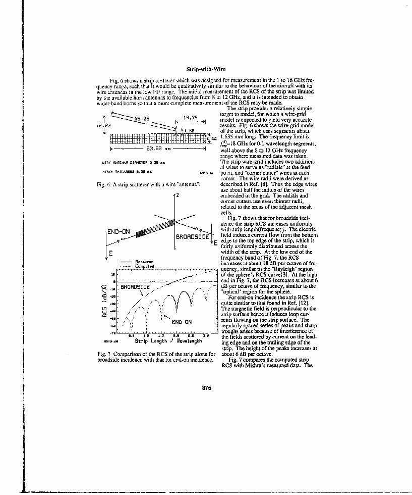
Strip-with-Wire

Fig. 6 shows a strip sc'itterer which was designed for measurement in the I to 16 GHz fre-quency range, such that it would be qualitatively similar to the behaviour of the aircraft with itswire antennas in the low IlF range. The init;al measurement of the RCS of the strip was limitedby tte available horn antennas to frequencies front 8 to 12 GHz, and it is intended to obtainwider-band horns so that a more complete measurement of the RCS may be made.

The strip provides a relativeiy simpleI Z 4 ý51 05 19.79 target to model, for which a wire-gridT - ,model is expected to yield very accurate

i2. 23 t. results. Fig. 6 shows the wire-grid model__ -K 6 of the strip, which uses segments about

M,-, 4: 6.51 1.635 mm long. The frequency limit is& I-)L 8 GHz for 0.1 wavelength segments,}€-G63.63 m, - well above the 8 to 12 GHz frequency

range where measured data was taken.WaIRt" fNt•t W r YER 8.30 ,, The strip wire-grid includes two addition-

al wires to serve as "radials" at the feed5i1RIF THIOCNESS 0.36 ,•' point, and "comer cutter" wires at tach

corner. The wire radii were derived asFig. 6 A strip scatterer with a wire "antenna". described in Ref. [8]. Thus the edge wires

use about half the tadius of the wiresembedded in the grid. The radials andcorner cutters use even thinner radii,related to the areas of the adjacent meshcells.

Fig. 7 shows that for broadside hinci-dence the strip RCS increases uniformly

v- I with strip length(frequenc:-,. The electricBROADSIDE field inducers current flow from the bottom

E edge to the top edge of the strip, which isfairly uniformly distributed across the

E width of the strip. At the low end of the-Measured frequency band of Fig. 7, the RCS

...... CMpud increases at about 18 dB per octave of fre-C . ."" .o.w.. I. .. . ,-, . .......... quency, similar to the "Rayleigh" region- "..." of the sphere's RCS curve[3]. At the high

Send in Fig. 7, the RCS increases at about 6-,. BKH(ROSIOE ... dB per octave of frequency, similar to the

N, .""optical" region for the sphere.For end-on incidence the strip RCS is

-3 -.. quite similar to that found in Ref. [12].EN" The magnetic field is peipendicular to the

(Z stip surface hence it induces loop cur-ENO ON rents flowing on the stip surface. The

"regularly spaced series of peaks and sharp- L .s •----.- •.- e. i ,.• troughs arises because of interference of. 1.3 1 5 E.0 e.5 '. the fields scattered by current on the lead-

Strip Length / Wauvlength ing edge and on the trailing edge of thestrip. The height of the peaks increases at

Fig. 7 Comparison of the RCS of the strip alone for attut 6 dB per octave.broadside incidence with that foi cld-on incidence. Fig. 7 compares the computed strip

RCS with Mishra's measured data. The

375

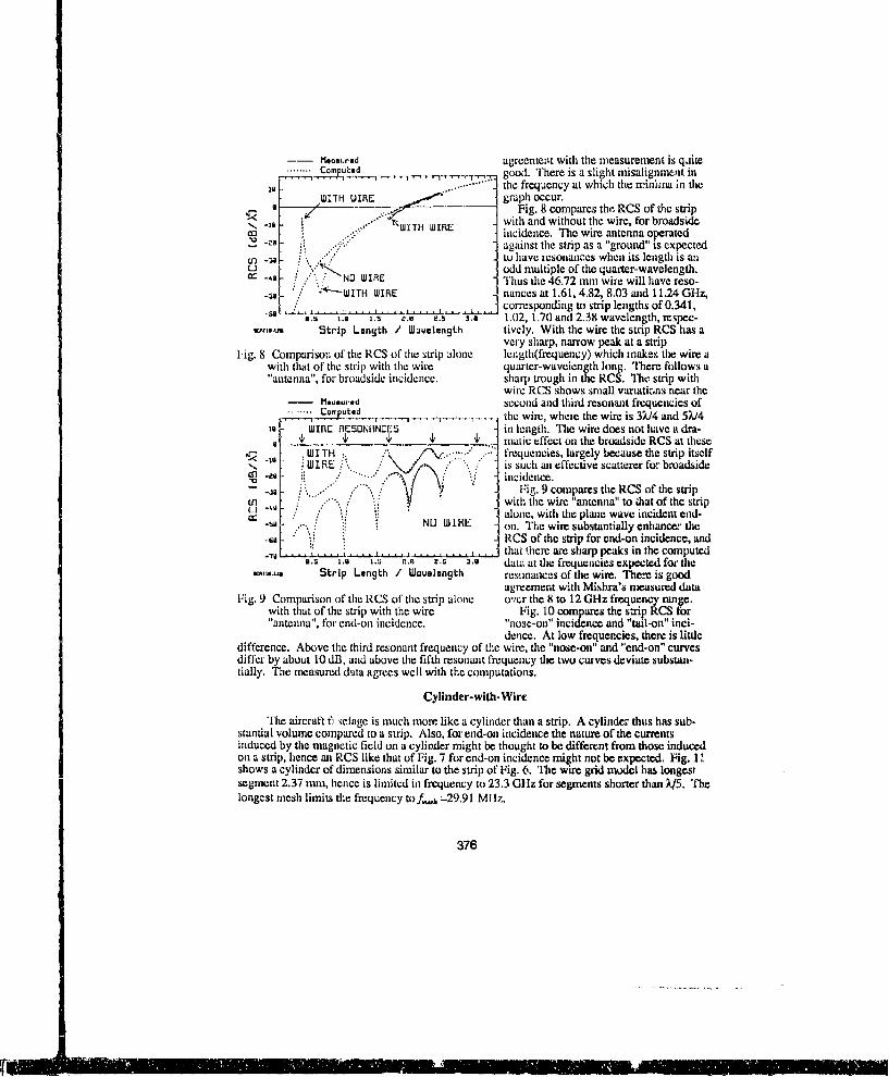
-- M~oourad agreenermt with the measurement is qjiteS........ Co kued------- good. There is a slight misalignment inS....... the frequency at which the minima in the

WITH WIRE K ...... graph occur.Fig. 8 compares th, RCS of the strip

"- 'WITH WIRE with and without the wire, for broadside.o. incidence. The wire antenna operated

against the strip as a "ground" is expected(n -3 9 to have resonances when its length is anU ' odd multiple of the quarter-wavelength.

-1. - NO WIRE Thus the 46.72 mm wire will have reso-: '-WITH WIRE nances at 1.61, 4.82, 8.03 and 11.24 GHz,

- ,",.. .. .. .. . . • , _ . corresponding to strip lengths of 0.341,1. 1.5 V. c., .s 3.8 1.02, 1.70 and 2.38 wavelength, mspee-

Strip Length / Wauelength tively. With the wire the strip RCS has avery sharp, narrow peak at a strip

lig. 8 Comparison of the RCS of the strip alone length(frequency) which makes the wire awith that of the strip with the wire quarter-wavelength long. There follows a"antenna", for broadside incidence, sharp trough in the RCS. The. strip with

wire RCS shows small variati;,ns near the- M, .u..d second and third resonant frequencies of

_. the wire, where the wire is 3;J4 and 5V/418 WIRE RESONHN•5E in length. The wire does not have a dra-

1. . 4, 4' 4 matic effect on the broadside RCS at these" "IX" ..WITH frequencies, largely because the strip itself

WIRE . is such an effective scatterer for broadside-.. incidence.- " " ".Fig. 9 compares the RCS of the strip

n ' .".with the wire 'antenna" to ihat of the stripcc NO WIRE"alone, with the plane wave incident end-

.NO WIRE on. The wire substantially enhancer theRCS of the strip for end-on incidence, and

-. .. , that ,here are sharp peaks in the computedu.5 i.., at the frequencies expected for the

Strip Length / Woauelngth resonances of the wire. Thee is goodagreement with Mishra's measured data

Fig. 9 Comparison of the RCS of the strip alone eyrir the 8 to 12 GHz frequency range.with that of the strip with the wire Fig. 10 compares the stip RCS for"antenna". for end-on incidence. "nose-on" incidence and "tail-on" inci-

dence. At low frequencies, there is littledifference. Above the third resonant frequency of the wire, the "nose-on" and "end-on" curvesdiffer by about 10 dB, and above the fifth resonant frequency the two curves deviate substan-tially. The measured data agrees well with the computations.

Cylinder-with-Wire

The aircraft fi tselage is much more like a cylinder than a strip. A cylinder thus has sub-stantial volume compared to a strip. Also, for end-on incidence the nature of the currentsinduced by the magnetic field on a cylinder might be thought to be different from those inducedon a strip, hence an RCS like that of Fig. 7 for end-on incidence might not be expected. Fig. Vshows a cylinder of dimensions similar to the strip of Fig. 6. The wire grid model has longestsegment 2.37 mm, hence is limited in frequency to 23.3 GHz for segments shorter than V5. Thelongest mesh limits the frequency tof,,h =29.91 MIz.

376

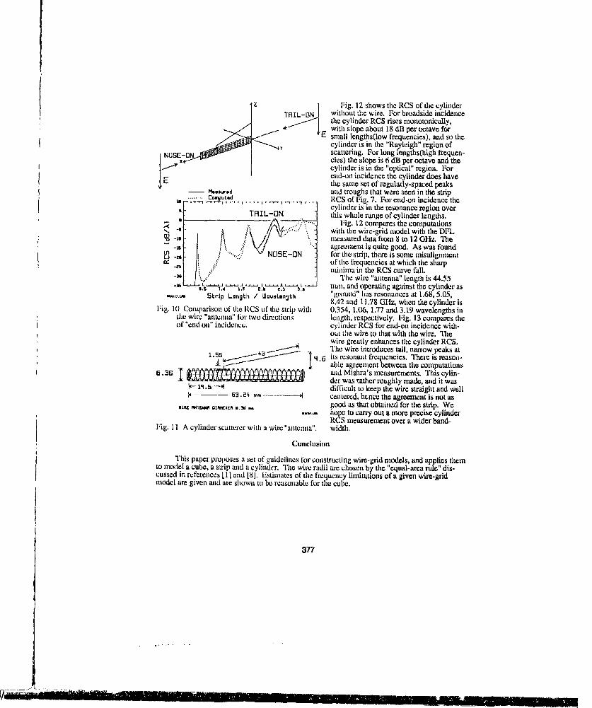
z 1 Fig. 12 shows the RCS of the cylinderTAIL-ON without the wire. For broadside incidence

the cylinder RCS rises monotonically,E with slope about 18 dB per octave forE small lengths(low frequencies), and so the

cylinder is in the "Rayleigh" region ofNO5] scattering. For long lengths(high frequen-

cies) the slope is 6 dB per octave and thecylinder is in the "optical" region. Forend-on incidence the cylinder does havethe same set of regularly-spaced peaks-- osred and troughs that were seen in the strip

........ Coted . RCS of Fig, 7. For end-on incidence thecylinder is in the resonance region over"RIL-..ON this whole range of cylinder lengths.

Fg12compares the computations./ 'with the wiie-grid model with the DFL

- measured data rum 8 to 12 GlIz. The-- -: N'-ON agreement is quite good. As was found

tr fo"-r tile strip, there is some misalignmentof the frequencies at which the sharp" "4 minima in the RCS curve fall.

The wire "antenna" length is 44.55- " L -.. I -, . • • .. , -J , mi, and operating against the cylinder as

|, 1. |.5 El 1.5 3 a

Strip Length / WIaveln 3 th "ground" has resonances at 1.68, 5.05,8.42 and 11.78 Gltz, when the cylinder is

Fig. 10 Comparison of the RCS of the sirip with 0.354, 1.06,1.77 and 3.19 wavelengths inthe wire "antenna" for two directions length, respectively. Fig. 13 compares theof "end oin" incidence, cylinder RCS for end-on incidence with-

out the wire to that with the wire. 'Iliewire greatly enhances the cylinder RCS.

4B - The wire introduces tall, narrow peaks ati .ss]• i.6 its resonant frequencies. There is reason-

able agreement between the computations6.3 and Mishra's measurements. This cylin-M-_ ~der was rather roughly made, and it was

-1. S -.-4t difficult to keep the wire straight and well-- - 63.P4 mm ----------. ,4 Cel ered, hence the agreement is not asAC ANTEMNNG OGIMET.A 8.3 good as that obtained for the strip. We

hope to carry out a more precise cylinderRCS ineasuement over a wider band-

Fig. 11 A cylinder scatterer with a wire "antenna". width.

Conclusion

This paper proposes a set of guidelines for constructing wire-grid models, and applies themto model a cube, a strip and a cylinder. Tlhe wire radii are chosen by the "equal-area rule" dis-cussed i, references [11 and [8). Estimates of the frequency limitations of a given wire-gridmodel are given and are shown to be reasonable for the cube.

377

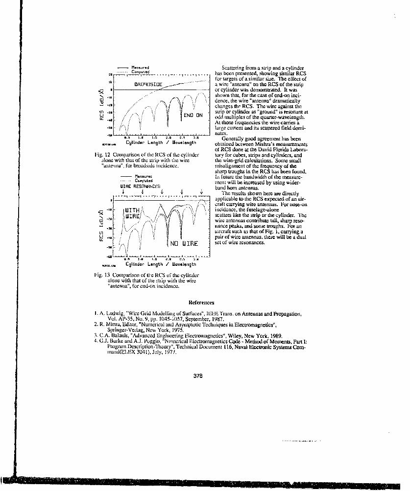
Mesu,.d Scattering from a strip and a cylinderS........ Computed26op,, ed . has been presented, showing similar RCS19 .......... for targets of a similar size. The effect of

SBRO911SI DE a wire "antenna" on the RCS of the strip8 or cylinder was demonstrated. It was

.. " shown that, for the case of end-on inci-"dence. the wire "antenna" dramaticallychanges the RCS. The wire against the.

in .-3 . strip or cylinder as "ground" is resonant at- END ON odd multiples of the quarter-wavelength.At those frequencies the wire carries alarge current and its scattered field domi-tm , .'..:i .... ... .L, .. . .... . . .. .. ares.

- ,.5 1.61 1.5• C.6 Z.9 3. Generally good agreement has beenz,., C qlinder Lengt~h / Mwaelanqgth obiained between Mishra's measurements

of RCS done at the David Florida Labora-Fig. 12 Comparison of the RCS of the cylinder tory for cubes, strips and cylinders, and

alone with that of the strip with the wire the wire-grid calculations. Some small"antenna", for broadside incidence, misalignment of the frequency of the

sharp troughs in the RCS has been found.- Mo,'sured In future the bandwidth of the measure-SCom.puted inent will be increased by using wider-CURE RESONINCEES band horn antennas.-' •, 4, 4, •, The results shown here am directly

applicable to the RCS expected of an air-caft carrying wire antennas. For niose-on

W< 1 ITH .* .cidcrnce, the fuselage-aloneUJIRL **.scatters like the strip or the cylinder. The.. . wire antennas contibute tall, sharp reso--"..38 :" nan;,cepeas., ad sonic toughs. For.,n

tn iaircraft such as that of Fig. 1, carrying a.pair of wire antennas, them will be ia dual

"NO WIR E set of wire resonances.

ti5 1AA 1.5 k .u I. 3.91.,u,. Clttndo,- Length / Wavselenth

Fig. 13 Comparison of the RCS of the cylinderalone with that of the :trip with the wie"antenna", for end•on incidence.

References

1. A. Ludwig, "Wire. Grid Modelling of Surfaces", IEEE Trans. on Antennas and Propagation,Vol. A1P-35, No. 9, pp. 1045-1057, September, 1987.

2. R. Mittra, Editor, "Numerical and Asymptotic Techniques in Electromagnetics",Springer-Verlag, New York, 1975.

3. C.A. Balanis, "Advanced Engineering Electromagnetics", Wiley, New York, 1989.4. G.J. Burke and A.J. Puggio, "Numerical E"lectromagnetics Code - Method of Moments, Part 1:

Program Description-Theory", Technical Document 116, Naval Electronic Systems Conm-n.and(ELEX 3041), July, !977.

378

It...IIIII IIII11 1 1 I I'I IItI llli ~ ll! ~ lt • !•I A

5. G.J. Burke and A.J. Poggio, "Numerical Electromagnetics Code - Method of Moments, PartIII: User's Guide", Technical Document 116, Navad Electronic Systems Command(ELEX3041), July, 1977.

6. C.W. Trueman and S.J, Kubina, "Verifying Wire-Grid Model Integrity with ProgramCHECK", Applied Computational Electromagnetics Society Journal, Vol. 5, No. 2, Win-ter, 1990.

7. G.J. Burke, "Recent Advances to NEC - Applications and Validation", Lawrence LivermoreNational Laboratory prepfint number UCRL-100651, March 3, 1989.

8. C.W. Trueman and SiJ. Kubina, "Automated Radius Calculation for Wire-Grid Models", 7thAnnual Review of Progress in Applied Computational Electromagnetics, Monterey,March, 1991.

9. A.D. Yaghjian and R.V. McGahan, "Broadside Radar Cross-Section of the Perfectly-Conducting Cube", ILEEE Trans. on Antennas and Propagation, Vol. AP-33, No. 3, March1985.

10. M.C. Cote, M.D. Woodworth and A.D. Yaghjiun, "Scattering firom the Perfectly ConductingCube", IEEE Trans. oln Antennas and Propagation, Vol. 36, No. 9, p. 1321-1329, Sept.,1988.

11. A. Ludwig, "Backscattering from a Cube", Applied Computational Electromagnetics SocietyJournal, Vol. 2, No. 2, pp. 55-74, Fall, 1987.

12. E.F. Knott, V.V. Liepa anl T.B.A. Senior, "Plates and Edges", IEEE Trans. on Antennas andPropagation, Vol. AP-19, No. 6, pp. 788-789, November, 197 .

379

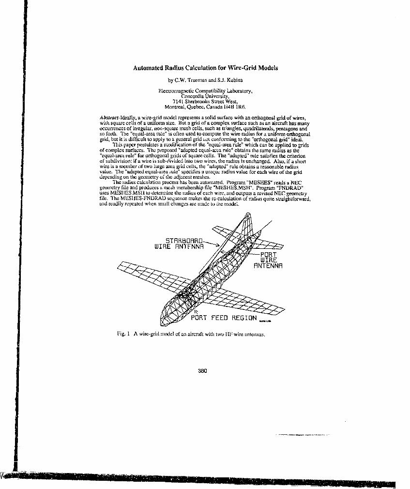
Automated Radius Calculation for Wire-Grid Models

by C.W. Trueman and S.J. Kubina

Electromagnetic Compatibility Laboratory,Concordia University,

7141 Sherbrooke Street West,Montreal, Quebec, Canada 114B IR6.

Abstract-Ideally, a wire-grid model represents a solid surface with an orthogonal grid of wires,with square cells of a uniform size. But a grid of a complex surface such as an aircraft has manyoccurrences of irregular, non-square mesh cells, such as triangles, quadrilaterals, pentagons andso forth. The "equal-area rule" is often used to compute the wire radius for a uniform orthogonalgrid, but it is difficult to apply to a general grid iot conforming to the "orthogonal grid" ideal.

This paper postulates a modification of the "equal-area rule" which can be applied to gridsof complex surfaces. The proposed "adapted equal-area rule" obtains the same radius at the"equal-area rule" for orthogonal grids of square cells. The "adapted" rule satisfies the criterionof subdivision: if a wire is sub-divided into two wires, the radius is unchanged, Also, if a shortwire is a member of two luage area grid cells, the "adapted" rule obtains a reasonable radiusvalue. The "adapted equal-area ,'ule" specifics a unique radius value for each wire of the griddepending on the geometry of the adjacent meshes.

The radius calculation process has been automatzd. Program "MESHES" reads a NECgeometry file and produces a mesh membership file "MESHES.MS11". Program "FNDRAD"uses MESIIES.MSII to determine the radius of each wire, and outputs a revised NEC geometlyfile. The MESIIES-FNDRAD sequence makes the re-calculation of radius quite straightforward,and readily repeated when small changes are made to the model.

ST R RIBRRO].-

WIRE ANTFNN9S•PORT

WIRE

PORT FEED REGION,

Fig. 1 A wire-grid model of an aircraft with two IIF wire antennas.

380

I[ llllm l

Introduction

Wire-g-.-d midels are used to calculate radiation and scattering from solid objects such ascl inders, spheres, cubes, ard less regular surfaces such as aircraft, at frequencies where tie dim-oisions are comparable to the wavelength. Fig. I shows a wire-grid model of an aircraft, to bes~lved with the Numerical Electromagnetics Codc(NEC)[ 1,21 for the antenna patterns or for

the scattered fields. Ideally, the aircraftsurfaces are to be modelled as an orthogo-

" nal grid of wires, with square cells of a uni-norig size. For the most part the fuselageand wings in Fig. 1 have been represented

awith a quasi-orthogonal grid of wires with" nearly-square cells. But where the fuselage

tapers, and where the wings taper, triangu-lar mesh cells have been used. In the feed

R a region of each ItF wire antenna, illustrated----__ __ - in Fig. 2, radial wires have been used to_t ... support radial current flow near the attach-

incus•• nt point. This subdivides die surface_ _ into triangular mesh cells. Further, the

radials themselves consist of two wires inseries, of unequal length, as shown bywires #1 and #2 in Fig. 2. Each wire of thegrid must be assigned a wire-radius before

Fig. 2 The feed region of the port wire uses the mnodel can be "run" with NEC or anoth-radial wires about the attachment point, er wire-grid analysis program. The objec-and contains triangular niesh cells. tive of this paper is to define a "r'-" forWires which arc part of the wre antenna assigning a radius which can be applied toare m'arked "a". complex grids such as those shown in Figs.

1 and 2."The "equal-arca rule"I 31 is often used to conipute the wire radius for a unifnmi orthogonalgrid, but it i3 difficult to apply to a general grid not conforning to the "orthogonal grid" ideal.This paper postulates a modification of the "equal-area rule" which can be applied to grids ofcomipl:x surfaces. The calculation of radius is then auonmated in programs called "MESHES"and "FNDRAD".

The "Eqtal-Area Rule"

Burke and Milleri4] suninarii.e the literature on wire radius for wire-grid models of sur-faces. For an orthogonal grid of wires representiing a surface, as shown in Fig. 3, the "equal-arearule" states that the radius is chosen such that total surface area of the wires in one orthogonaldirection is equal to the area of the surface. Lee, Marin and Castillol 5 show that the equal-arearadius miakes the inductance of the wires equal to the inductance of the surface. Ludwig[31shows that, for an inl Mite cylinder modelled with a uniform auray of infinite wires, theequal-area choice of radius is a[n exact solution. Paknysl 61 shows that, for scattering from a cyl-inder, the "equal-aica" radius is the value that niinimizes the field in tie interior of a wire-gridmodel of the cylindcr. But the literature offers little explicit guidance for choosing the radii for amore general grid, such as that of Figs. I or 2.

In the orthogonal grid of Fig. 3 the cells are square if A, = A2 = A, of area AI =A 2 = A2. The"equal-arca rule" radius can be interpreted to state that the wire of length A represents half thearea of patt, A, and half the area of A2 , so the radius is chosen according to

381

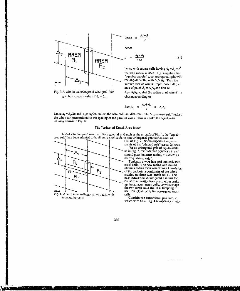
2naaA ,

2

henceA2 A, +A,

hence with square cells having A, = A2 =2

the wine radius is A/29. Fig. 4 applies the"equal-area rule" to an orthogonal grid wih"rectangular cells, with A, > A2. Then thesurface area of wire #1 represents half thearea of patch A, = AA 2 and half of

Fig. 3 A wire in an orthogonal wire grid. The A,, = AA 2 , so that the radius a, of wire #1 isgrid has square meshes if A, = A. chosen according to

A, +A22tta,A, = A2 = AA 2

hence a, = A2/27t and a2 = A,/2r, and so the wire radii are different. The "equal-area rule" makesthe wire radii proportional to the spacing of the parallel wires. This is unlike the equal radiiactually shown in Fig. 4.

The "Adapted Equal-Area Rule"

In order to compute wire radii for a general grid such as the aircraft of Fig. 1, the "equal-area rule" has been adapted to he directly applicable to non-orthogonal geometries such as

that of Fig. 2. Some important require-ments of the "adapted rule" are as follows.

For an orthogonal grid of square cells,as in Fig. 3, the "adapted equal-area rule"should give the same radius, a = AI2it, as"the "equal-area rule".

2 Typically a wire in a grid subtends twomesh cells. The new radius rule shouldSPobtain a radius for a wire from a knowledgeH ____1 of the endpoint coordinates of the wiresmaking up these two "mesh cells", The

- p ,new radius rule should yield a radius for"the wire no matter how many wires makeup the adjacent mesh cells, or what shapethe two mesh cells are. It is tempting touse Eqn. (1) directly for non-square mesh

Fig. 4 A wire in an orthogonal wire grid with cells.rectangular cells. Consider the subdivision problem, in

which wire #1 in Fig. 4 is subdivided into

382

I-,) i i'1'II 1 ilF+ i I lr+ l II IT 1l ~ llJ ' _..2 ... +!2'2 r •

two wires, illustrated by wires #3 and #4 inFig. 5. For wire #1 in Fig. 4, Eqn. (1)obtains the radius a = A)d2it. If wire #3 ofFig. 5 has length A,/2, then applying Eqn.(1) obtains a radius of a = A41rt, twice thevalue for wire #1. But subdivision shouldnot change the radius. The "adaptedequal-area rule" must give the same radiusfor the single wire, #1 in Fig. 4, or theseries connection of wires #3 and #4 in Fig.5. Further, the radius must be the same it'wires #3 and #4 are specified to NEC asone wire with two segments(one GW card)or two wires with one segment ezch(two#GW cards). Thus for the feed region of

#4~ Fig. 2, the "adapted equal-area rule" shouldget the same radius for the wires labelled"#1" and "#2".

Consider the problem of a very shortwire which subtends two meshes made upof much longer wires, shown in Fig. 6. Theradius of the short wire must not be madeunreasonably large by the "adaptedU.ho.011 tequal-area rule". Thus if Eqn. (i) wereFig. 5 Wire #1 in Fig. 4 is subdivided into applied directly to this short wire, a large

two wires, but is expected to have (A, +A2) is divided by a small A to obtain athe same radius as in Fig. 4. huge radius. Eqn. (1) must be modified to

account for the short.aess of wire length Acompared to the areas that the wire sub-tends,

An "adapted equal-area rule" is obtainedby weighting each term in Eqn. (1) with afactor comparing the length of the wiresegment, A, to the distance around themnesh periphery. Thus in Fig. 7 a wireHRE'•R fl segment of length A is a member of twomeshes, of areas A, aitj A2, and peripheries

RREA FRi L, and L. The peripheries include A. If theadjacent meshes were square, then Ashould be one-quarter of the length of theperiphery. Thus weight each term of Eqn.

• (1) with the ratio of the segment length, A,to its expected fraction of the periphery,Fig. 6 A short wire which is a member of two L14, to obtainlarge meshes.

A, A A2 A41rA(LI/4) 4nA(L2/4)

383

Then the "adapted equal-area rule" statesthat

BE1f a 4- (2XL, ..L2

For an orthogonal grid of square cells, as inFig. 3, A, = A2 = A2, and the mesh periph-eries are L, = L2 = 4A. Eqn. (2) givesa = A/2nt as required. Note that this makes

Fig. 7 The "adapted equal-area rule" uses the the total surface area of all the wires equalareas and the peripheries of the meslhes that to twice the area of the surface.each wire subtends.

Application of the Adapted Equal-Area Rule

The "adapted equal-area rule" of Eqn. (2) meets the requirement that it be readily appliedto conmplex wire grids, such as Fig. 1 or 2, v% ith many non-square cells. All that is needed is aknowledge of the wires making tp the two meshes subtending the wire whose radius is to befound.

For the rectangular grid of Fig. 4, the "adapted" rule gets a somewhat different radius fromthe original "equal-area rule". Thus for either wire #1 or wire #2 in Fig. 4, A, ý- A2 A=A2, andL, = L, - 2(A, + A2), and with Eqn. (2) the radius of hoth wire #1 and wire #2 is

AA2 .. 3)n(Al + A2)

Thus wires #1 and #2 have the same radius, as shown in Fig. 4, which is different from the"equal-area rule" value of a, = A2/2r or a, = A,/2rn. It is readily shown that a < a, but a > a2. The"adapted equal-area radius" is a compromise radius such that

1 1 1 1Ul Ca2 a a

The total surface area of all the wires is still equal to twice th.- area of the surface, but evidentlythis is different from making the total surface area of the wires in one orthogonal direction equalto tho area of the surface. Thus for best results, keep the mesh cells of the wire grid square ratherthan rectangular.

The "ada'pted equal-area rule" handles the subdivision well. Thus for wire #1 in Fig. 4, theradius is that of Eqn. (3). For wire #3 or #4 of Fig. 5, the areas and peripheries used in Eqn. (2)are identical to those used to compute the radius of wire #1, hence lead to the same radius forwire #3 or #4 as for wire #1. The "adapted rule" radius does not depend directly on the length ofthe wire whose radius is being calculated. Instead, it uses the total peripheral length of eachadjacent mesh, and the area of each adjacent mesh. Also, it does not matter whether the subdivi-sion is done with one GW card specifying two segments, or two GW cards of one segment each.

384

'iit'Iif''"' i""•"1i-1'I""lIIi • lr l''l trlPIill "I I l ~ •[ - -

Consider the short wire problem of Fig. 6. -qn. (1) uses the ratio of the mesh area to thvlwire length, A, whereas Eqn. (2) uses the ratio of the mesh area to the mesh periphery, L, andthus obtains a smaller radius. In effect, the contribution of each area to the radios of Eqn. (1) hasbeen reducud in Eqn. (2) Lv the factor A.(L/4) which is considerably less than one for geometrieslike Fig. 6. Fig. 6 is drawn to scale and shows that the "adapted equal-area radius" is a reason-able value. But a construction such as Fig. 6 embedded in a wire-grid is poor practice, grosslyviolating tile principle that as many cells as possible in a grid should be "square", all with equalareas. If the shott wire in Fig. 6 is absolutely rqquired, then the adjacent large meshes should hesubdivided into smaller mesh cells.

For wires at the edges of open surfaces, such as the wing edge wires in Fig. 1, there is onlyone mesh area to contribute to the radius. I lence the radius of edge wires is about half the valueof the radius of wires embedded in tihe grid.

Automated Mesh Search and Radius Calculation

The "adapted equal-area rule" assigns a unique radius to each wire of a wire grid, fnrmt aknowledge of the wires making up the adjacent meshes. The calculation of the wire radius

has bten automated with the processing stepsNEC INPUT FILE' shown in Fig. 8. A NEC geometry file is input to

the nesh-search program "MESI IES", to obtain a"MESI IESMSH" file, which is a list of the wires

MESH SERRCH making up meshes with each wire in the geome-try file. The user can edit the MESI IES.MSI I fileto delete meshes which he may not want to Con-tribute to the radius of a given wire. The edit stepI-MESH FILE gives the user full, detailed control over the

_MESHES•..S radius calculation. The MESIIES.MSII file isthen input to tile radius-finding program

E-ITOR "FNIDRAD", which reads which wiles make_ .meshes with each wire, and applies the "adaptedequal-area rule" to find that wire's radius. The

_ýLOTL output is a new NEC geometry file called.. ES. M S "OU'IT''UT.GW".

T'he present implementation of MESI IFSsearches for loop paths of up to 8 wires. Then aloop is identified as a "mesh" by searching forCIILCULTION "diagonal" paths across the loop. If any pathacross the loop is found which is shorter than thepaths around the loop periphery then the loop is

MODIFIED GR PHiIZs FDILES not a mesh. MESHES rejects cross-sections asNEC INPUT ) meshes because all the vertices have the same

SI x-coordinate. The current version does not tejectMODEL 3-wire and 4-wire cross-sections, which must be

DISPLRY PROGRAM manually edited out of the MEStES.MSI I file.This was done to allow cylinder endcaps to be

E O ME--SH•'S---ES modelled with 3-wire and 4-wire meshes.NEC PROGRAOM P ogram MESHES writes graphics files, fordisplay with program "MODEL"[71, "lat are use-ful in spotting errors in the wire grid, and in iden-

Fig. 8 Flow chart of processing steps in tifyitg meshes requiring modification incomputing wire radii for a NEC "MESHES.MSH". MESHES writes a graphicsgeometry file. Data files are file which identifies all the wires that are mem-enclosed in ellipses, and rectangles bets of 3-wire mieshes, and graphics files namingare programs, all tile wires that are members of 4-wire

385

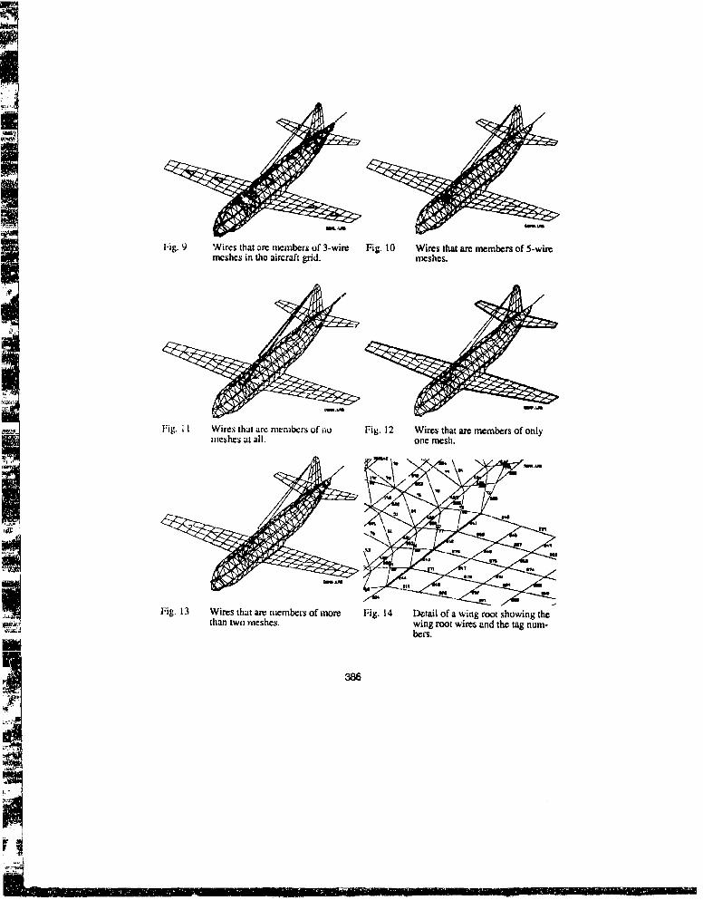
Fig. 9 Wires that ire members of' 3-wire Fig. 10 Wires that ame members of 5-wiremcshes in the aircraft grid, meshes.

Fig. I I Wires that arc memibers of no Fig. 12 Wires that are members of onlymneshes at all, one mesh.

Fig. 13 Wires that are members of more Fig. 14 Detail of a wing root showing the

than two meshes. wing root wires and the tag num-

386

meshes, 5-wire, 6-wire, 7-wire and 8-wire meshes. Thus the aircraft grid of Fig. 1 has the 3-wiremeshes shown in Fig. 9, the 5-wire meshes of Fig. 10, and no larger meshes. The user caninspect these displays from various viewing angles to look for wires that clearly should not bemembers of meshes with that number of wires. This can alert the user to errors in the modelgeometry.

To further increase the likelihood that errors in the model will be found, MESHES pro-duces additional mesh-membership graphics files. Fig. 11 shows all the wires that are membersof no meshes at all, clearly seen as the wire antennas and the wire modelling the magnetometerboom. If a wire in the grid were open-circuited at one end in error, it would be present in thisdisplay. Fig. 12 shows all wires that axe members of only one mesh, readily seen to be the edgesof the wings and the dorsal fin. Once again, errors in the grid can lead to wires being membersof this group incorrectly. Fig. 13 shows wirt ihat ae members of more than two meshes. Wingroots and fin roots are members of two fuselage meshes and of one wing or fin mesh. The filealso shows that there are three 4-wire cross-sections that need to be rejected manually.

The user edits the MESHES.MSH file to remove unwanted meshes, Each line of the filebegins with a wire's tag number, followed by a zero(O), then the tag numbers of wires makingmeshes the first mesh, a zotro, the wires making the second mesh, a zero, the third mesh, etc. Forthe wing-root wire #244 in Fig. 14, MESHES.MSH contains the line

244 0 59 67 479 0 60 68 503 0 219 248 67 10

The user simply deletes the tag numbers of unwanted meshes. For the wing root wires, such asthose in Fig. 14, our convention is that the radius of diese wires is calculated based on the twoadjacent fuselage meshes, and that the wing mesh is ignored. The user must identity and deletefrom the mesh list the tag numbers of the wing mesh. This is done by modifying the line inMESHES.MSH to ruad

244 0 59 67 479 0 60 68 503 0

Then FNDRAD will use the fuselage meshes to compute the radius of wire #244.Once the meshes have been identified and verified, it is straightforward to calculate the

wire radii using the "adapted equal-area rule". Program FNDRAD repeats the decompositioninto vertices and links(a fast step even for large models), and then for each wire reads, the firsttwo meshes from the MESHES.MSH file, and calculates a radius. If the wires specified to forna mesh in the MESIIES.MSIH file do not from a closed path, a fatal error results. This can hap-pen if the MESHES.MSH file was modified incorrectly. FNDRAD generates its own graphicsfiles of wires belonging to no meshes, to one mesh and to more than two meshes. At this stage,no wires should belong to more than two meshes, The user should display these wires to verifythat no errors were introduced in editing MESHES.MSIH.

Conclusions

This paper proposes a "adapted equal-area rule", Eqn. (2), which can be used to find aunique radius for each wire in a complex grid such as the aircraft in Fig. 1. For square meshcells, the radius obtained is the same as that specified by the "equal-area rule". The "adapted"rule has been automated into a mesh search program, MESHES, and a radius-finding program,FNDRAD.

Display of the mesh content of a wire grid with computer graphics provides a valuable toolfor checking the integrity of the grid. Certain common errors in grid geometry lead to obviously-wrong meshes, easily seen on the graphics screen. This has been an unexpected benefit of themesh search. Some grids that had 1heen extensively used over xeveral years were found to con-tain errors!

387

-NWmm

For the 681 wire, 359 vertex aircraft of Fig. 1, MESHIES takes I1I minutes 34 seconds on a25 MHz 80386 computer, with an 80387 math coprocessor, running MS-DOS. The presentimplementation of MESHES prognuin could be improved giestly in execution speed. The searchmethod is crude and redundant-it tends to find the sanmc meshes over and over again. The "diag-onal search" approach to screening n-wirc loops to find which ame meshes is effective but tendsto rc-find all the smsaller meshes. No advantage is taken of the knowledge that the fuselage gridmodels a closed surface.

Editing the MESIIES.MSIi file for the aircraft takes an experienced user about half anhour. To identify the tug numbers of meshes which must be "edited out", program MODEL isused to display the wire grid ini~udirig tag numbers, in the format of Fig. 14. Sonme users wouldlike to avoid the editing- step. Perhaps FNDRAI) could read a file of special cases, direc-ting it toignore certain meshes formed with the wing root wires. This would be convenient in making aseries of'smiall alterations to an aircraft geometry file,

After MESIIES.MSI I has been edited, running FNDRAD takes about 60 seconds for theaircraft, and produce., a NEC geomtnry file with revised wire radii.

Automated radius calculation yields a unique radius for each wire, which depends onl thelocal geometry of the wire grid. WNires subtending small meshes have thinner radii than wire%subtending full-size s.quare' mesh cells. Where the mesh is deliberately made fines, such as thefeed region of Fig. 2, ilic radius algorithm automatically tapcrs the radius in accordance with thecull areas. This refiiwnenuit in wire-grid miodclling app)))UFS to lead to more consistent conmputedresults when model,; are analysed with tnec NEC pr ogr am.

Referunces

1. G.J. Burke and A.J. lPoggio, "Nunierical Electroinagi etiir Code - Method of Moments, PastIII: User's Guide", Technical l~x-oneonem 116, Naval Ulccronic. Systems Command(IiLEX3041), July, 1977.

2. G.J. Burke and A.). l'oggio, "Numerical ELcctromagiietics Code - Method of Moments, Part 1:Frograitsiiecito-hom ehia Documnivo 116, Naval hElecronic Systems Conk-xnand(ELEX 304 1), JuLly, 1977.

3. A.C. Ludwig, "Wire (rid Moiteling nt'Surface's", IEE'ETrazis. Oki Antennas and Propagation,Vol. APl-35, No. 9, pp). 1045-1049, Sept. 19B7.

4. G.3, Burke and E.K. Milier. "A Mesh Model of a Coaxial Transmission Linle Using NEC",Sixth Applied Computational Elcctromiagne ties Symposium, Monterey, California, March19-22, 1990.

5. K.S.ll. Lece, L. Marin and J.P. Castillo, "Limitations of Wire-GCrid Modelling of a CLosed Sur-f'cc", IELEETrans. onl Electrontagntetic Conipatioility, Vol. EMC-l18, No. 3, pp. 123-129,. ugust, 1976.

0. 11, Paknys, "TIhe Near Field of a Wire Grid Model", to be puLblished in the IFFEE Trails. inAntennas and Propa gationt.

7. CW. Tlrucinan, "Prograin MODEL1 for the Display and Investigation of Wire Grid ModelGeonietries", Internal Report, Commcordi~' University E.MC Laboratory, in preparatton.

8. C.W. Tlruemian and SiJ. Kubina, "Verifying Wire-Grid Model Integrity wtth l'rograinCl IECK", Applied Comnptititional E'lectromnagnectics Society Journal, Vol. 5, No. 2, Wimi-ter, 1990.

9. 0.1. Burke, "Recent .Xdvamtees to NEC - Applications and Validationl", Lawrence LivermioreNational Laboratory prcprimtt number UCBl.I(X)65 1, March 3, 1989.

388

SESSION 10- "MICROWAVE CIRCUITS ANDMICROSTRIP ANTENNA ANALYSIS"

Moderator: Fabrics Hurst

FULL-WAVE MODELING OF A MULTI-LAYER MICROSTRIP ARRAYWITH A SUPERCONDUCTING MICROSTRIP FEED NETWORK

Jeffrey S. HerdElectromagnetics Directorate

Rome LaboratoryHanscom AFB, MA 01731-5000

(617) 377-4214

ABSTRACT

Recent developments in high temperature superconductorshave made it possible to fabricate microstrip feed lines withextremely low losses at liquid nitrogen temperatures. Thistechnology is particularly applicable to high frequencyarrays with microstrip feed networks, where ohmic lossesseverely limit the efficiency which can be obtained withconventional metals. This paper describes the analysis anddesign of a multi-layer microstrip antenna array with asuperconducting microstrip feed network. A novel geometrywill be described which integrates the array into a radome onthe vacuum shield of a cryocooler for maximum thermal and RFradiation efficiency. A multi-layer spectral domain Green'sfunction is used with the method of moments to design themicrostrip feed network and proximity coupled microstripelements for optimum impedance matching and operatingbandwidth. Experimental measurements of the proximity-coupledmicrostrip elements in a waveguide simulator are used tovalidate the analysis.

1. INTRODUCTION

The primary advantage of using superconducting metals inantanna systems appears to be the reduction of ohmic lossesin the power distribution and matching networks, particularlyat millimeter wave frequencies [13, [2], [3), [4). Forexample, the use of a superconducting feed network couldincrease the RF gain of a largo microstrip-fed array by asmuch as 20 dB at 60 GHz, as shown in figure I from [4).

This paper describes the analysis and design of amulti-layer microstrip antenna array wi.h a superconductingfeed network. A novel geometry will be described whichutilizes proximity-coupled microstrip patches integrated intoa radome on the vacuum shield of a cryocooler as shown infigure 2 for maximum bandwidth, thermal efficiency and RF

389

ir

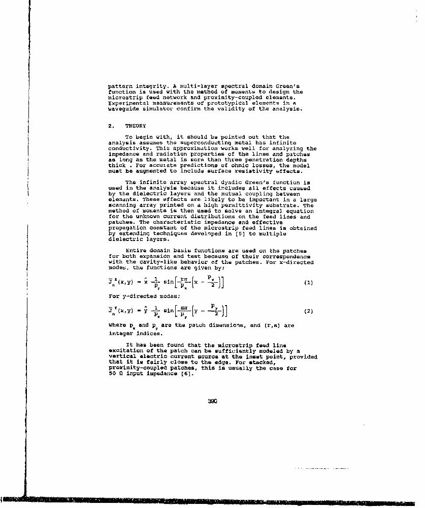
pattern integrity. A multi-layer spectral domain Green'sfunction is used with the method of moments to design themicrostrip feed network and proximity-coupled elements.Experimental measurements of prototypical elements in awaveguide simulator confirm the validity of the analysis.

2. THEORY

To begin with, it should be pointed out that theanalysis assumes the superconducting metal has infiniteconductivity. This approximation works well for analyzing theimpedance and radiation properties of the lines and patchesas long as the metal is more than three penetration depthsthick . For accurate predictions of ohmic losses, the modelmust be augmented to include surface resistivity effects.

The infinite array spectral dyadic Green's function isused in the analysis because it includes all effects causedby the dielectric layers and the mutual coupling betweenelements. These effects are likely to be important in a largescanning array printed on a high permittivity substrate. Themethod of moments is then used to solve an integral equationfor the unknown current distributions on the feed lines andpatches. The characteristic impedance and effectivepropagation constant of the microstrip feed lines is obtainedby extending techniques developed in [5] to multipledielectric layers.

Entire domain basis functions are used on the patchesfor both expansion and test because of their correspondencewith the cavity-like behavior of the patches. For x-directedmodes, the functions are given by;

-X r ru pnJ(x,y) - x -- sin [L 1 -. 2-J

For y-directed modes;

-y - 1 sir in, P2 2J(xy) - y sLn - -y ----- (

where p, and py are the patch dimensions, and (r,s) areinteger indices.

It has been found that the microstrip feed lineexcitation of the patch can be sufficiently modeled by avertical electric current source at the inset point, providedthat it is fairly close to the edge. For stacked,proximity-coupled patches, this is usually the case for50 0 input impedance [6].

Ul• Nt•d •II'NNr•Dl •i!'•"•1!I~F~~pl~lii -i ~ mw~tl , i~in•ul~llim|ll'•390 • '

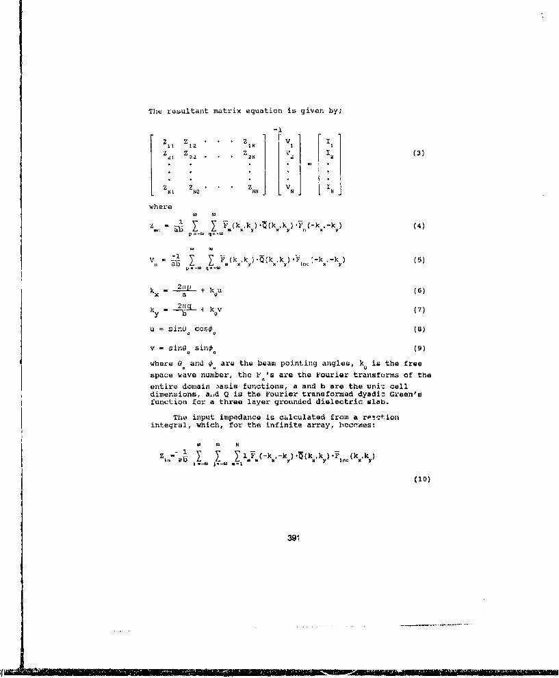
The resultant matrix equation is given by;-l

z I 2 1 N I I

z 2 Z Z.. V 2 (3)

ZNI ZN2 NN N j

wherew

z~,- x [ F(k ,k ).(k.,X ).(-k..-k (4)p=-• q=-W

Vn .(kik -)'(kik y)'Fh -kx,-k ) (5)

kX - 2T + k u (6)

ky - 27(_q__- + koV (7)

u = Gino coso (33)

V - Gino. Gino. (9)

where 0. and 0. are the beam pointing angles, ku is the freespace wave number, the F.' s are the Fourier transforms of theentire domain i•asis functions, a and b are the uni'c celldimensions, aid Q is the Fourier transformed dyadic Green'sfunction for a three layer grounded dielectric slab.

The input impedance is calculated from a rp,!ctionintegral, which, for the infinite array, beccines:

W 0) N

m-CO J. - 1 ~(10)

391

where

-jk x -jk yF (k,k)- Z e Xp yp (e)

is the Fourier transform of a vertical current source at thefeed inset point (xp,yp). All floquet series are truncatedat i-j--30, and this is found to give sufficient convergence.With the input impedance known, the scanning reflectioncoefficient is computed by;

Z,,,(O,'t) - Z ,(00,00)R(0,0) - Z1(010) + Zin(00,00 (12)z (0,0) + z(* ,o°)"*

In In

where Z (00,00) is the input impedance at broadside.

Several methods were used to check the numericalaccuracy of the computer code. First, a comparison was madebetween the input power, PV,,, and the power radiated from aunit cell, P . where;

P ,, - i - ,.i ( )

P In -. JR2(13)

and

SJ 2. Re(Lxll) ••dxdy (14)UniLt call

It was found that the values calculated from equations(13)and (14) were within one percent of one another for allscan angles except the blindness angle, and it is believedthat the computational accuracy at that scan angle isaffected by the singularity in the infinite array Green'sfunction. As a second check of the code, it was confirmedthat the boundary condition E - 0 is being satisfied bythe fields from the source and basis function expansioncurrents to within one part in a thousand.

3. EXPERIMENT

As a further validation of the theory, measurements froma waveguide simulator are used to replicate the environmentseen by an element in an infinite scanning array. Figure 3

392

shows the measured and predicted reflection coefficientversus frequency for a three layer proximity-coupled element.This example shows a 2:1 VSWR bandwidth of approximately 20%.Good agreement between theory and experiment is obtained byusing three x-directed modes (r-1,3,5) and two y-directedmodes (s-1,2) on each patch.

4. SUMMARY

A full wave analysis has been applied to a three layerproximity-coupled microstrip antenna array. The uniquegeometry provides a wide bandwidth element for use with ahigh efficiency superconducting microstrip feed network.Future work will be done to add superconductor surfaceresistivity, substrate anisotropies, and alternative elementdesigns for improved thermal shielding.

5. REFERENCES

1. R. C. Hansen, "Superconducting Antennas," IEEE Trans.Aero. and Elect. Sys. 26, no. 2, pp 345-355, 1990.

2. R. J. Dinger and D. J. White, " The Radiation Efficiencyof a Small Dipole Antenna Made from a High TemperatureSuperconductor," IEEE Antenna and Prop. Int. Symp. Dig.,Dallas, pp 724-727, 1990.

3. J. T. Williams and S. A. Long, "High TemperatureSuperconductors and their Application in Passive AntennaSystems," IEEE Antenna and Prop. Magazine, pp 7-18, Aug.1990.

4. W. G. Lyons and R. S. Withers, "Passive Microwave DeviceApplications of High Tc Superconducting Thin Films,"Microwave Journal, Vol. 33, pp. 85-102, Nov. 1990.

5. R. Jackson anI D. M. Pozar, "Full-Wave Analysis ofMicrostrip Open-End and Gap Discontinuities," IEEETrans. Microwave Theory and Tech., Vol. MTT-33, pp.1036-1042, Oct. 1985.

6. J. S. Herd, "Scanning Impedance of Proximity CoupledRectangular Microstrip Antenna Arrays," Ph.D. Dics.,E.C.E. Dept., Univ. of Mass., Sept. 1989.

393

- GAIN (406) . 20 log ()-8.665. U . 10 log (4 ijh. .6.5cm)J2 SPACING VOCO (77 K Wuppelal

70 MICROSTRIP ON 10 mil ALUMINA SUST"RAT•

so$ LOSSLESS; lb (4.2 K) -

Cu (300 K&, 1.6 Vil-cm('

30

10 -iI _0.01 0.1 1.0 10(2 ?.) (2000 X,)

XFLAT-PLATE ARRAY SIZE 0 (in)

FIGURE 1. Effect of Distributik-n Loss on Antenna ArrayGain, (from [4)).

NORMAL CONDUCTOW PA'ATC1

- VAC

h2 /-- SUPERCONDUCTING FEED LINES A14D PAC1.

SUPERCONDUC1ING GROUND PLANE (77 K) -

FIGURE 2. Superconducting Microstrip Array Geometry.

394

If, ilJEII~lilMiltII• l'~ll'll~l•lt 'i B ia n''ilIlllKl~lll- , ,

0.0

-10.0 .--- __

-20.0

R -230.0-.- __

-40. 0 -- -

-50.0 _ _

3.9 4.2 4.5 4.U 5.1 5.4 5.7 6.0

FRE~QUENCY, GHz

FIGURE 3. l~eflection Coefficient Versu,. 1ýrequency forLlemunt in a Waveguide Simulator; hh,,h 3.0. 159cm,

X -y -1.87cm, X I-Y L-1.93cm, c -c,-2.33, c.-1.0, a-3.35cm,

b=3.60cmi, - - easured, 0 - predicted.

395

MODELING OF AN ANISOTROPIC STRIPLINE

M KAMAREI, N. DAOUD, R. SALAZAR, M. BOUTHINON

L.E.M.O.-I.N.P.G,-C.N.R.S. UAR 833, BP 257, Grenoble 38016, France

lIulexing terms: anisotropic permeability, electromagnetic fields, propagation constant

A variety of substrate materials used in practice exhibit anisotropic behavior.The objective ofthis letter is to model the propagation properties of a stripline loaded with a dielectric materialwhich has an isotropic pernittivity and an anisotropic perneability,

I. IntroductionIn recent years, a variety of anisotropic materials have increasingly found numerous andimportant applications at mnicrowave frequencies. Anisotropy is either an inherent property of asubsuate material or may be acquired during the manufacturing process. It has been establishedthat when anisotropy is ignored in the development of design methods for single and coupledmicrostrip, an error is intxoduced which becomes significant for small linewidths and smiall lineseparation [1]. In certain applications of coupled line structures, anisotropy may provebeneficial in equalizing even aid odd mode phase velocities and reducing the sensitivity ofgeometry tolerance [2]. An algorithm is developed which models structures such as microstripon anisotropic substrates 131. The characteristics of single and coupled microstrips onlanisoLropic substates with a diagonal pcnnittivity tensor have been analized by Alexopoulosand Krowne 14] by using a quasistatic-mode approach. Several other anisotropic dielectricsubstrate geometries have been treated in the literature [5], 16] by using the quasistatic method.lHybrid modes have been analysed for microstrip lines with anisotropic substrates [71.T.Kitazawa and Y.Ilayashi have also analysed the propagation characteristics of strip lines withmultilayered anisotropic media L91,

This letter represents the modeling of a stripline loaded with a dielectric material which has anisotropic pcnlittivity and an anisotropic permeability as is shown below:

tl] I 12 01

L 0 0 ý,31

The relative pennittivity (-) and all the tenis of the relative pcrmeability matrix ItI] are complex.

396

We have already shown that the TEM mc'es which can exist in the bulk material, cannot

propagate when this material is placed in the stripline structure. If any energy is transferredfrom input to output in the structure, there are hybrid modes which are the origin of this

transfer. In fact, the anisotropic character of the material under study causes a coupling betweenthe longitudinal componeuts of the electric and magnetic fields.

The homogeneous property of the material and the assumption that the structure is unlimited

along ox (figure 1) permit a decoupling of the longitudinal components (E, and H,) and a

dctermination of the four transverse fields: E1 , Ey, H, and Hy. Obtaining the characteristics of

the hybrid modes with an analytical method is not possible. The numerical method which isadapted to this planax structure is the Spectral domain method which we have formulated andprogrammed. This programme, very general for the form of the anisotropic relative

permeability matrix [i], is validated for an isotropic material and a'so for a magnetic

anisotropy.

Y

X. x

figure 1

11- Study of the coupling of the longitudinal componentsWe show that the anisotropic character of the material under study caaucs a coupling between

the longitudinal components of the electric and magnetic fields. The possibility of determiningthe four transverse components depends on obtaining these longitudinal components. Thehomogeneous property of the material and the assumption that the structure is unlimited along

ox (figure 1) permit a decoupling of the longitudinal components (E, and 11;) and a

detennination of the four transverse fields E., EY, H. and Hy. We can ,he., obtain the

following:H x = B I "•+ B 2 -ý- + B 3"•ýy + B4"(2)

S H EZE z EB D Hz +B7 (2)

aE aE, aH, aH,E,= At, ;#+ A2 -W" + A3 - + A4- -

DE;, DE, i)1z aHl (3EY A5 ; A+ A6 A7 -+A 8 -;

39T

where Ai and Bi (i=l, 2, .. 8) are constants, functions of' 0, e and Ip ]. These constants are

given in annex.

The Maxwell equations permit us to obtain:

A, t[-- + -52:j| + (A2 - A5) .Ly- !-- As A 3 D11 jW33Hz (4.1)[ Dx 2 y 2 6xO x 2 0y 2

and:( )2 + + l I•-t 2T E-e4 + E, (4.2)(13 -4) _ ,B ý2 [,D2 B6axZy ax 2 ay ay a x2

"These two equations show the coupling between the longitudinal components E, and 1,. Theanisotropic character of the material is the origin of the coupling.

III- Solution of the system of coupled equationsWe suppose that the material is homogeneous and unlimited along ox and the FourierTransformation is defined below:

A(oy) = f. "A(xy) ej1XX dx , A(x,y) = H,(x,y) ou E-jx,y) (5)

With these conditions (a/ax -. ju), the system of equations (4) gives the general solutions asshown below:

C cletO' + c 2e°C + c3 eC3 ' + Cae°04

,=c lale + c2a2 + C3a3 + c4a4 e' (6)

where a, and aj 0j=1, 2,., 4) are functions of x, (o, e and [lt]. cj are constants.

IV- Numerical treatmentThe system of equqtions (2, 3. 6) give all the electromagnetic field components. The continuitycondition of the electromagnetic field on the metalized interface (y=O), permits ,U obtain arelationship between the Fourier Transformation of the tangential components of the electricfield and the cuirent density on the metallic surface as is shown below:

This equation is the tundamental equation of the Spectral domain method. The terms of [G] arethe Green's coefficients of the Spectral domain method. Each of these is a function of thefrequency, the complex propagation constant and the geometrical and physical characteristics of

398

f _ -. ,. L . 7 . . . ... . . • , - , , - - = , - ... . -

'A

the structure. In the perfect conductor, the electric field is null as is the current density in thedielectric. This particular property and the application of the Galerkin's Method, by a suitablechoice of the basis functions for J. and J. ,,ermit the solution of the fundamental equation ofthe Spectral domain method [91. This enables us to obtain the complex propagation constantand afterwards the characteristic impedance and the distribution of the electromagnetic field ofeach of the higher order modes that propagate in the structure.

V..ResultsWe have programmed all the previous steps. Our analytical and numerical treatments are

validated by using this general programme for an isotropic material (g.=gyy=ltzz=l+j0,

Py --- +jO. ,=1(0)+j0 ) in a structure which has the same geometrical characteristics as the real

structure under study (W/2h--=O.17). The obtained results are in good agreement with the oneswhich are a.rcady well known.

By using the same programme, we have studied the variation of the propagation constant(calculated by our method) as the magnetic anisotropy increases progressively, in comparison

,h the propagation constant which is obtained from the following expression:

= 2itV,•7-(8)

This is done for the several values of ý.yy (supposing that gI=l) and for the several values of

g"' (supposing that J.•=l) as shown in figures (2) and (3) respectively.

Part. f=IGHz

1.4

1.2

1,0 1- 1 MY/I.=0 2 4 6 8

figure 2

399

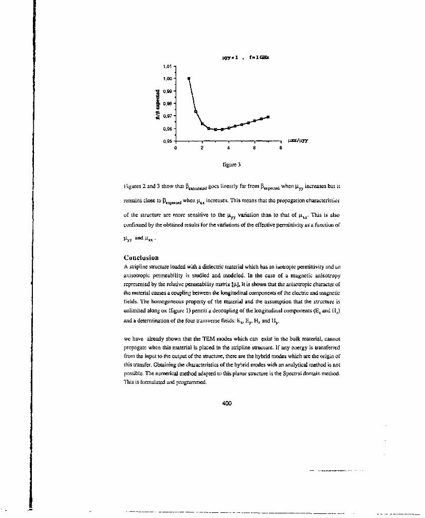
tI'yl , f-lGHU

1,011,00

0,98-

0,97-S0.97

0.96

0.95 -T- I X/AYY0 2 4 6 8

figure 3

Figures 2 and 3 show that Icatcutatod goes linearly far from P.,.,t when Py,, increases but it

remains close to DCPbCtd when p. increases. This means that the propagation characteristics

of the structure are more sensitive to the pt, variation than to that of . This is alsoconfirmed by the obtained results for the variations of the effective permittivity as a function of

ýLyy and ixx.

ConclusionA stripline structure loaded with a dielectric material which has an isotropic permittivity and .itanisotropic permeability is studied and modeled. In the case of a magnetic anisotropyrepresented by the relative permeability matrix [IA], It is shown that the anisotropic character ofthe material causes a coupling between the longitudinal components of the electric and magneticfields. The homegeneous property of the material and the assumption that the structure isunlimited along ox (figure 1) permit a decoupling of the longitudinal components (E, and I I')and a determination of the four transverse fields: E1, EY, H, and B1y.

we have already shown that the TEM modes which can exist in the bulk material, cannotpropagate when this material is placed in the stripline structure. If any eergy is transferredfrom the input to the output of the structure, there are the hybrid modes which are the origin ofthis transfer. Obtaining the characteristics of the hybrid modes with an analytical method is notpossible. Tihe numerical method adapted to this planar structure is the Spectral domain method.ihis is formulated and programmed.

400

1The realized programme, although very general for the form of the magnetic anisotropy, isvalidated for an isotropic uaterial in a sutucture which has the same. geometrical characteristicsas the real structure under study. The obtained results are in good agreement with the oneswhich are already well known.

By usi~g the same programnme we have also studied the materials with an isotropic permittivityand anisotropic pcrmeability. It is shown that the propagation characteristics of the structure arc

more sensitive to the iiyy variation than that of IjL variation.

References

11 N.G.ALEXOPOULOS:" Integrated circuit structures on anisotropic substrates."ILLE Trans. Microwave Theory Tech., vol. MTT-33, pp. 847-881, oct 1985.

12] N.G.ALEXOPOULOS, C.M.KROWNE:" Characteristics of single and couplednsicrostrips on anisotropic substrates."IEEE Trans. Microwave Theory Tech., vol, MIT-26, pp.387-393, june 1978.

[3] A.NAKATANI. N.G.ALEXOPOULOS:" Toward a generalized algorithm for themodeling of me dispersive properties of integratezd circuit structures on anisotropicsubstrates."IEEE Trans. Microwave Theory Tech., vol. MTI'-33, pp 1436-1441, december 1985,

141 N.G.ALEXOPOULOS and C.M.KROWNE:" Characteristics of single and coupledmicrostrips on anisotrupic substrates."IEEE Trans. Microwave Theory Tech., vol. M'IT-26, pp 387-393, june 1978.

15] T.KITAZAWA and Y.ItAYASItI:" Quasi-static characteristics of coplanar waveguideon a saphire substrate with its optical axis inclined."IELE Trans. Microwave Theory Tech., vol. M'Il'-30, pp 920-922, june 1982.

[61 M.IIORNO" Quasi-static characteristics of microstrip on arbitrary ttnisotropicsubstrates."Proc.LEEE vol.68, Pp 1033-1034, 1980.

171 A.M.A. UL-SHiRBINY:" Hybrid mode analysis of microstrip lines on anisotropicsubstrats."IEEE Trans. Microwave Theory Tech., vol. MTT-29, pp 1261-1265, descember 1981.

18] T.KITAZAWA and Y.HAYASHI:" Propagation characteristics tuf strip lines withmuitiiaycred anisotropic, media."IEEE Trans. Microwave Theory Tech., vol. MTT-31, pp 429-433, june 1983.

191 T I11O0t, R.MIYI'RA:" Spectral domain approch for calculating the dispersioncharacteristics of nmicrostrip lines."IEEE Tran;. on Microwave Theory and Techniques, vol. MIT-21, July 1973.

401

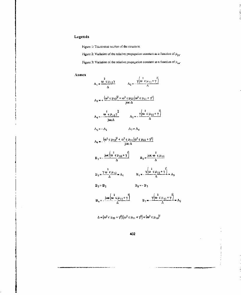
Legends

Figure 1: Transverse scction of thie structure,

Figure 2: Variation of the relative propagation constant as a function of ty.

Figure 3: Variation of the relative propagation constant as a function of t

Annex

A W0 C ýL12 'y A2 WYk2 C .L 1 1 4+ 7A (c' A2 = -2i-

(W2 C =F+ 0 A22('CAI+

2 2 2

A 0) L 127 5 , C 1122 +71A4 =. A5 _

A6 = -A A7 = A4

Aw (w2 L A12)'4U2 L IIW2 C lj2ea2 + 9

2 2 2 2_

SA B2= A

2 ( 2

A A

A u (w 2 CA 72 +Y CO) (03 C II I2 ++ 2)

402

_____________

ANALYSIS OF THE BUHAVIOUR OF QUASI COMPLEX MODES ON LOBBYSUBSTRATE BOXED MICROUTRIP LINES

F. HURET, P. PRXBETICH, P. KENNIS

Equips Electromagn6tieme 4,as CircuitsCentre Hyporfr4quenoes at Semioonduotaurs, U.h. CNRS N1 287

U.S.T.L. FLANDRUS ARTOIS59655 VZLLENEUVA D'ASCQ FRANCE

Fax. numbser20.43.49.95.

ABSTRACT:In this communication, by using spectral domain

approach improved by asymptotic expansions, we show bymcins of coupling integral values that the notion of quasicomplex modes can be introduced for lightly losisysubstratas. The quasi complex modes are particular modeswith similar bohaviour than lossless structure complexmodes.

The analysis of discontinuitins between planartransmission lines, particulary for miicrostrip lines, hasreceived a great interest from many years.Azcurate modelingof such discontinuities is of fundamental importance forsuccessful monolithic integrated circuit design.1n factincreasing circuit complexity needs very efficientnumerieal techniques in order to solve electromagnetismproblums.In this mind when mode matching method in thodiscontinuity plane is used, it is necessary to determinethe set of modes with as accuracy as possible.More ever forboxed losseless structure, it has been shown that complexmodes can occur, so that ignoring those modes would lead tonon accurate solutions [1] [2].

The properties of complex waves have been investigatedin detail, both theoretically and experimentally forshielded circular dielectric rod [3],[4) and for boxedmicrostrip lineL2).

Up to now, most of published works concern thepossibility of propagation of complex modes in losslessstructure and only a few works focuse on complex andbackuard-wave modes in loamy waveguides [5].So, whenshielded microstrip lines laid on semi-insulating or dopedsemi-conductor substrates, are considered for MKICapplications, it is necessary to investigate the evolutionof complex solutions for lossless structure, under theeffect of bulk losses in the substrate.

In this communication, by using spectral domainapproach improved by asymptotic expansions, we show bymeans of coupling integral values that the notion of quasicomplex modes can be introduced for lightly lousysubstrates. Naturally, for lousy structures all modes havecomplex propagation constant, so in our mind, the quasicomplex modes are particular modes with similar behaviour

403

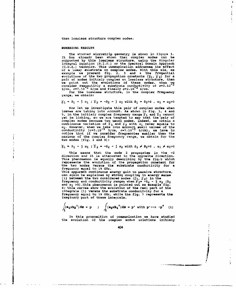
than lossless structure complex modes.

HUMERXCAL RESULTS

The studied microstrip geometry is shown in figure 1.It has already been shown that complex modes can besupported by this lossless structure, using the SingularIntegral Equation (S.I.E.) or the Spectral Domain Approach(S.D.A.) technics. This Qommunication addresses the effeutof a lousy substrate on complex modes. With this aim, asexample we present fig. 2, 3 and 4 the freqentialevolutions of the two propagation constants ('i, W2) for apair of modes initialy complex on lossless structure, thenwe point out the evolutions of these modes, when wconsider respeutivly a substrate cond4ctivity of 0-3.10S/ct, a-7.10 -S/cm and finally a-2.10 S/cm.

For the lossless structure, in the complex frequencyrange, we obtain:

1 - B 1 - Ji l; 22 - -32 - J U2 with 81 - 32>0 , QI - Q2>0

Now let us investigate this pair of complex modes whenlosses are taking into account. As shown in fig. 3, 4 and5, in the initialy complex frequency range'd1 and *2 cannotyet be linking, so we ara tempted to say that the pair ofcomplex modes becomes two usual modes. Indeed, we obtain acontinuous variation of W, and 62 with a, never equals toa2. However:, when we Sake into account small values of theconductivity (a-3.10- S/cm, o-7.10- S/cm), we have tonotice that if we consider frequencies smaller than themaximum of the complex frequency range, we obtain for thetwo modes (fig. 2 and 3):

i 3 1 - J Xl ; X2 - -32 " J Q2 with 31 1 82>0 , CI )A 02>0This means that the mode 2 propagates in the -Z

direction and it is attenuated in the opposite direction.This phenomenon is equally describing by the fig.5 whichrepresents the evolution of the propagation constant forthe two modes versus the substrate conductivity for afrequency equal to 19 GHz.This apparent continuous energy gain on pawsive structure,can again be explained by strong coupling in enerqy sense[1] between the two considered modes (%1, K2) in thefrequency and conductivity ranges when •2F -82 - J a2 (82and a2 >0).This phenomenon is pointed out as example fig.6; this curves show the evolution of the real part of theintegrals (1) versus the substrate conductivity for afrequency equal to 19 GHz, while the fig. 7 represents theimaginary part of these integrals.

is(*Ixhz2)4S - p ; - p' with p,--> -p* (1)

In this proposition of communication we have studiedthe evolution of the complex modon solutions initialy

404

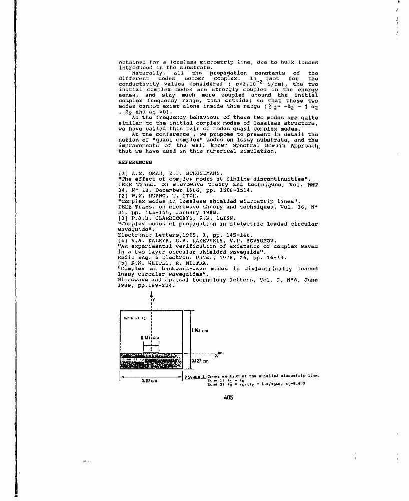
obtained for a lossless microstrip line, due to bulk lossesintroduced in the substrate.

Naturally, all the propagation constants of thedifferent modes become complex. In fact for theconductivity values considered ( a<2.10-2 S/cm), the twoinitial complex modes are strongly coupled in the energysense, and stay much more coupled around the initialcomplex frequency range, than outside; so that these twomodes cannot exist alone inside this range ( 2- -82 - Q2

,2 and a2 >0).As the frequency behaviour of these two modes are quite

similar to the initial complex modes of lossless structure,we have called this pair of modes quasi complex modes.

At the conference , we propose to present in detail thenotion of "quasi complex" modes on lossy substrate, and theimprovements of the well known Spectral Domain Approacil,that we have used in this numerical simulation.

REFERENCES

[i] A.S. OCAR, K.F. SCHUNEMANN."The effect of complex modes at finline discontinuities".IEEE Trans. on microwave theory and techniques, Vol. MMT34, N0 12, December 1986, pp. 1508-1514.r2] W.X. HUANG, T. ITOH."Complex modes in lossless shielded microstrip lines".IEEE Trans. on microwave theory and techniques, Vol. 36, N0

31, pp. 163-165, January 1988.[3] P.J.B. CLARIRICOATS, K.H. SLINN."Complex modes of propagation in dielectric loaded circularwaveguide".Electronic Letters,1965, 1, pp. 145-146.[4] V.A. KALMYK, U.3. RAYEVSKIY, V.P. YGVYUMOV."An experimental verification of existence of complex wavesin a two layer circular shielded waveguide".Radio Eng. & Electron. Phys., 1978, 26, pp. 16-19.[5) K.N. WHITES, 14. MITTHA."Complex an backward-wave modes in dielectrically loadedlossy circular waveguides".Microwave and optical technology letters, Vol. 2, N06, June1989, pp.199-204.

A

1.143 OmMIlNl cm

S6,121 erm

flguru licrons, seuti:on of tile sieldaled miutoetrip line.40ttip5[

405

re4~d/ cml u ap.m

4-

trace2 rbqurtlhy (GI~Z)

-6 - -. cormplex mode 0-

LiP! q,~3P eu i., tsn io~~ri /'- .i .j of the two modes

C rd/m (lljpjom)

4--

// it 22 A4

-4- " t1~

-6 --- comnplex modu -ti)

l'roia.4tiO~~Wstit I- *i-u of the LWQ nmud.LU

v~rous the f~qqu.sioy fuý u -7. 10 3/em.

406

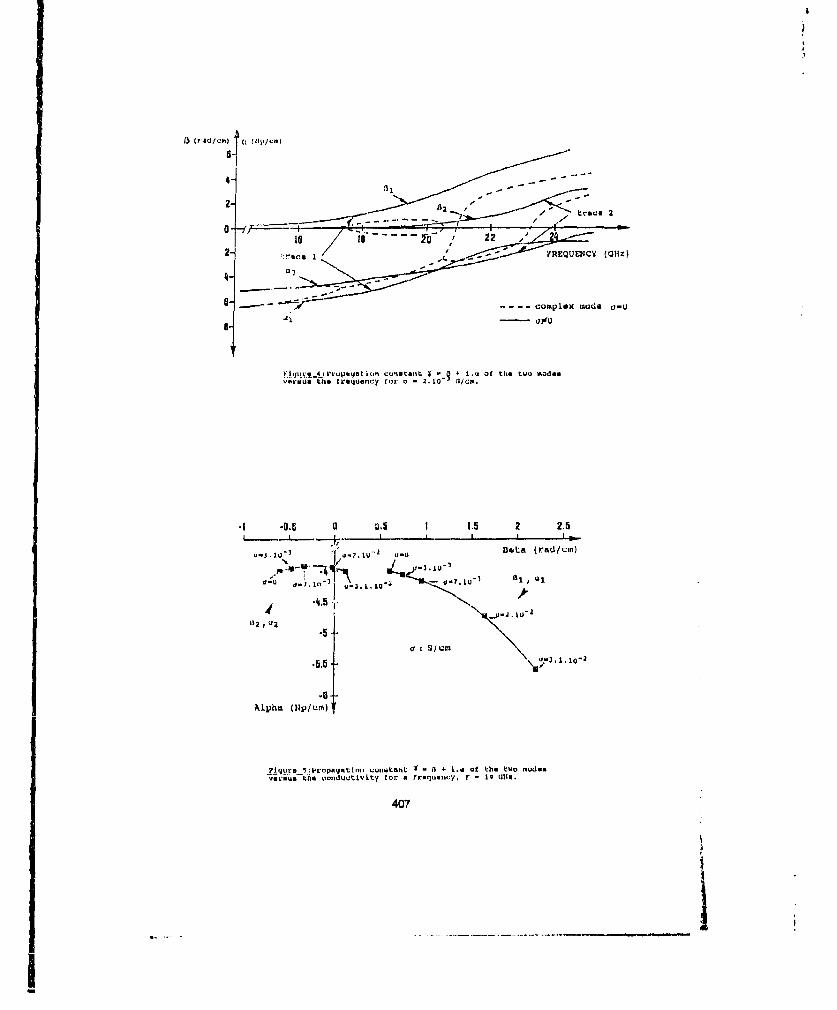
U ___ - -.. r - -- complex made O-u

VI-t'n~PJat n c~aI~ ~ - *i.. of the two Mddasvorisus the frqec fur Ua - 10.I 31/..

aI u. .5 1 1.5 2 2.5

o3. ii - ~ ~ -~ ,DIBLa (rad/cm)

/ -3ý

a I/m1

Alphd N/a m

?igjure-' I Popagatlion conwtant -It + I.e of the two modas"iriotu .%feooIdUctlvity for a frq~ny F -19 cl11i.

407

-Me- - ~ -I

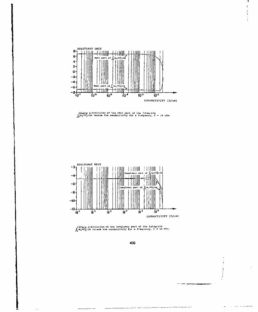
ARBITRiARY UNIT

4-2-

0-

-2

-8 -

Jill PLU - -1

coNUUwr1VV!Y (S/urn,

fyLur ojvuljitiuil, or the rqi.I part or Lht. Jntogratip

J.11 do e rou V LSU ah odu~t~ivILy for a fr..Iuanwy, r - 19 U112.

AHBIITI{AY UNIT~

-4-

-100. l

CoIIUUCTIVl'rY (S/uIC1)

)qijAo. .2ji,&V~julujw Of tile Iizalyiojiiry Part Of thM iiiteq~ralpVOLC-hj~ u S ve sttse coiouctivitY for a fraquency, F 19 Gliz.

405

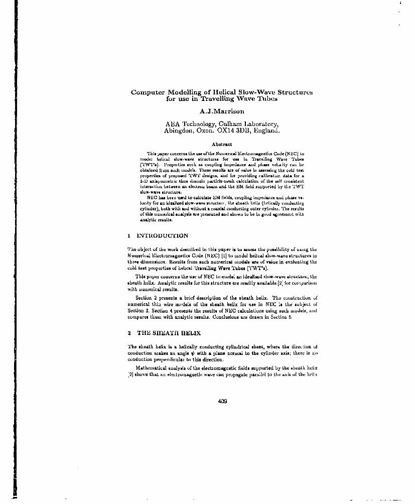
Computer Modelling of Helical Slow-Wave Structuresfor use in Travelling Wave Tubes

A.J.Marrison

AEA Tcchnology, Culham Laboratory,Abingdon, Oxon. OX14 31)B, England.

Abstract

This paper concerns the use ofthe Numerical Blectoniagcnetica Code (NE3C) tomodel helical slow-wave structurecs for use in T'avelling Wave Tubes(TWT'a). Propezticg such as coupling Ihupedance and phase velocity cal beobtained from such model., These results are of value in ascasing the cold testproperties of proposed TWT designs, and for providing calibration data for a2-1) axisyinract, c time druniain artile-ah calculation of the self consistentinteraction between alu electron beLan and the E•M field supported by the TWTslow-wave structure.

NLC has ceuu used to calculate EM fields, coupling impedancte and phase ve-loelty for an ideallsed mlow-wave structurt, the sheath helix (helically conductingcylinder), both with and without a coaxial conducting outer cylinder. 'The reault.of this nuumerical analysia are presented and shown to be in good agreemenit withanalytic results.

1 INTRODUCTION

The object of the work described in this paper is to asseas the possibility of using theNumerical Blectromagnetics Code (NEC) (1] to model helical alow-wava structures inthree dimension,. Results from such numerical models are of value In evaluating thecold test properties of helical Travelling Wave Tubes ('lWT's).

This paper concerns the use of NEC to model an idealized olow-wave structure, thesheath helix. Analytic results for this structure are readily available [2] for coviparisonwith numerical results.

Section 2 presents a brief description of the sheath helix. The construction ofnumerical thin wire models of the sheath helix for use in NEC is the subject olSection 3. Section 4 pruentet the results of NEC calculations using such models, alldcompares thum with analytic results. Conclusions are drawn In Section 5.

2 THE SIIEATII HELIX

The sheath helix i6 a helically conducting cylindrical sheet, where the diret tion ofcouduction tnakes an angle 11 with a plane normal to the cylidmer mxle; there is noconduction perpendicular to this direction.

Mathematical analysis of the electromagnetic fields supported by the sheath helix[2] ahovia that an electromagnetic wave can propagate parllel to the axis of the helix

409

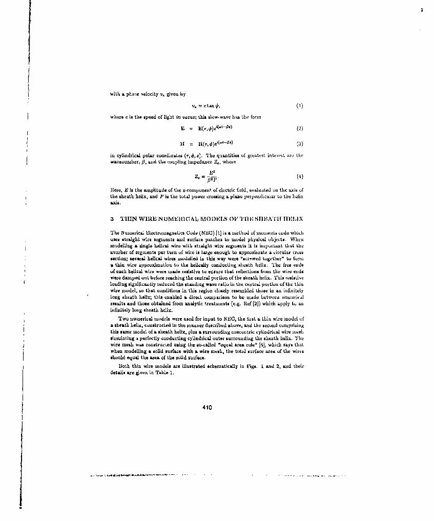
with a. phawi velocity v. given by

V.3 = C tan4,(1

where c is the speed of light ins tscuo; this slow-wave has the forisi

E = ~r,4)e'~'~1 (2)

in cylindrical polar coordinates (s',o, z). The quantities of greatest interest arothwaveiiuraber, fl, and the coupling impedance 2,, where

&zc E (4)

Here, E is the amplitude of the z-corapossent, of electric field, evaluated onl thle axis ofthe sheath helix, and P Is the total power crossing a piumss peiperndicular to the hulix

3 THIN WIRE NUMIMIUCAL MOD)ELS OF. TTIEi .SHEATHl THELI~X

The Numerical U.lectrurnagnatics Code (NEiC) 111 is a mnethod of murnenthi Lode which~uses straight wire segments and Surface patches to model physical objects. Whenmodelling a single helical wire with straight wire segmnlentb it Is Im1portant that tilenumber of aegmnento per turn of wire in large enough to approximate a circular crosssection; several helical wires modelled in this way were "scriwed together" tu formla thin wire approximation to the helically conducting sheath helix. Tire free endsof each helical wire were msade resistive to ensure that reflections from tihe wire endswere daniped out before reaching the central portion of the sheath helix. This resistiveloading signifiscantly reduced the standing wave ratio in thle central portion of thle thinwire model, so that conditions In this z%3glon closely resembled those in anl infinitelylong sheath helix; this enabled a direct COULParison to be Made beCtWeen nutuericalresults and those obtained from analytic treatments (e.g. Ref [2)) which apply tko assinfinitely Imig sheath helix.

Two numerical models were used for Input to NBiC, the first a thin wire niudel ofa sheath heli, constructed in the naunser described above, and the second conspriiiingthis same model of a sheath helix, plus a suriouviding concentric cylindrical wire mushsimulating a perfectly conducting cylindrical outer surrounding the sheath helix. Ti'lewire mesh was constructed using the so-called "equal area rule" [41, which says thatwhen modelling a solid surface with a wire meolL, thre totid surface area of the wiresshould equal the area of the solid surface.

Both thin wire urcodels are illustrated schematical~ly In Figs. I and 2, and theirdetalls are given in Table L.

410

Wire Grid Model piuLted from NXC output fileALJ Mereleot CulbcieLebeakl~rg~r

AILA ¶I00IIO

F"igure 1: Sheath helix (Model 1)

Wirm frild Model plotted frout NAG output file.AJ eW1.ee C~iAlehr-e~

Figure 2: Sheath helix with cylindrical outer (Model 2)

411

Model 1 MKo-del 2ILength of 1.6 1.6sheath helix (m) IPitch angle (7P) 11.2' 11.20Radius of 0.064 0.064sheath helix (m)Turn spacing (i) 0.08 0.08"Number of single 15 15helix copiesNumber of wire 20 20seginents per turnRadius of no outer 0.08conducting outer (m)Length of no outer 2.0conducting outer (m)Total number of 6000 13230wire segments ItI

Table 1: Model parameters

4 RESULTS AND INTERPRETATION

The thin wire model of the sheath helix was excited by applying a voltage excitation offrequency 300 MHz (with free space wavelength Ao - hiii) to each of the helical wirescomprising the model. The resulting fields and currents were calculated by NEC,both in free space and in the presence of a cylindrical wire mesh surrounding thechezth helix. Figure 3 shows the amplitude of the current oscillation induced in oneof the single helical wires plotted as a function of wire segment number (equivalentto distE.nco along the wire). The large peak in this Figure indicater the position ofthe vol'tage excit; .ion. As expected, the standing wave ratio in the central part of thewire it quite low at - 1.1 due to th.! resistive loading desrribed in Section 3.

The following Subsections present those numerical results of particular impor-tance in TWT design: namely, the axial electric fields inside the sheath helix, thewavelength, A, of the slow-wave propagating along the helix axis, and the couplingimpedance Z, . Throughout these subsections, cylindrical polar coordinates (r,O,z)will be used, with the z.axis coinciding with the helix axis.

4.1 Model 1

Figure 4 compares the values of the axial electric field, E,, computed by NEC withvalues obtained from analytic expressions [2]; the Figure shows the percentage dif-ference between computed and analytic values of Z. plutted ai a function of radialdistance from the helix axis. The computed and analytic results are seen tL be ingood agreement until sampling points approach the surface of the thin wire model at

412

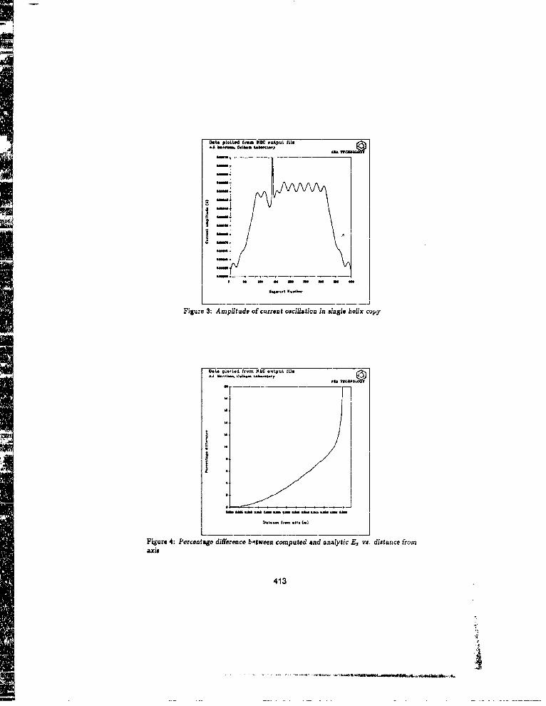
D.t. pI.LWo fro. NEC .Ltput, le 6

ale-

•,J. w ...Il. COL..n ib+r

iax-

i413unI-•

C -e4

11a-1

ha....ha il.la

Fue4:Pe~rcnae differencue btwcurent compuJ~ted and ainalytei E3 v dstnc fo

.41

- -.-.- M'U yiA

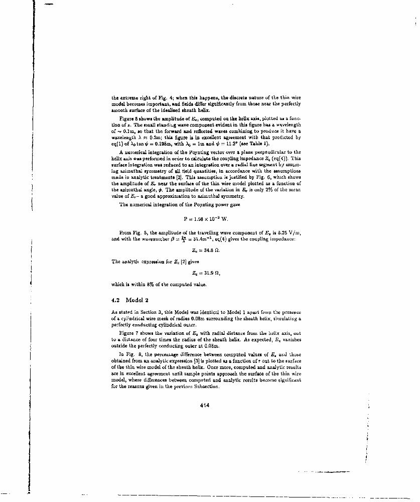
the extreme right of Fig. 4; when this happens, the discrete nature of the thin wiremodel becomes important, and fields differ sigificantly from those near the perfectlysmooth surface of the idealised sheath helix.

Figure 5 shows the amplitude of E., computed on the helix axis, plotted as a func-tion of z. The small stan'ilig wave component evident in this figure has a wavelengthof - 0.1m, so that the forward and reflected waves combining to produce it have awavelength X A 0.2m; this figure is in excellent agreement with that predicted byeq(1) of - 0 tan 0 = 0.198m, with A0 = Im and P = 11.2' (see Table 1).

A numerical integraLion of the Poynting vector over a plane perpendicular to thehelix axis was performed in order to calculate the coupling impedance Z, (eq(4)). Thissurface integration was reduced to an integration over a radial line segment by assum-ing azimuthal symmetry of all field quantities, in accordance with the assumptionsmade in analytic treatments [2]. This assumption is justified by Fig. 6, which showsthe amplitude of E, near the surface of the thin wire model plotted as a function ofthe azimuthal angle, 0, The amplitude of the variation in E, is only 2% of the meanvalue of E,- a good approximation to azimuthal symmetry.

The numerical integration of the Poynting power gave

P = 1.98 X 10-3 W.

From Fig. 5, the amplitude of the travelling wave component of E. is 8.25 V/m,and with the waeenumber f= 2 ý 31.4m- 1 , eq(4) gives the coupling impedance:

Z, = 34.8 fl,

The analytic expression for Z, [21 gives

Z, = 31.9 fl,

which is within 8% of the computed value.

4.2 Model 2

As stated in Section 3, this Model was identical to Model I apaxt from the presenceof a cylindrical wire mesh of radius 0.08m surrounding the sheath helix, simulating aperfectly conducting cylindrical outer.

Figure 7 shows the variation of E. with radial distance from the helix axis, outto a distance of four times the radius of the sheath helix. Au expected, E. vanishesoutside the perfectly conducting outer at 0.08m.

In Fig. 8, the percentage difference between computed values of E. and thoseobtained from an analytic expression [3] is plotted as a function of r out to the surfaceof the thin wire model of the sheath helix. Once more, computed and analytic resultsare in excellent agreement until sample points approach the surface of the thin wiremodel, where differences between computed and analytic results become significantfor the reasons given in the previous Subsection.

414

A'

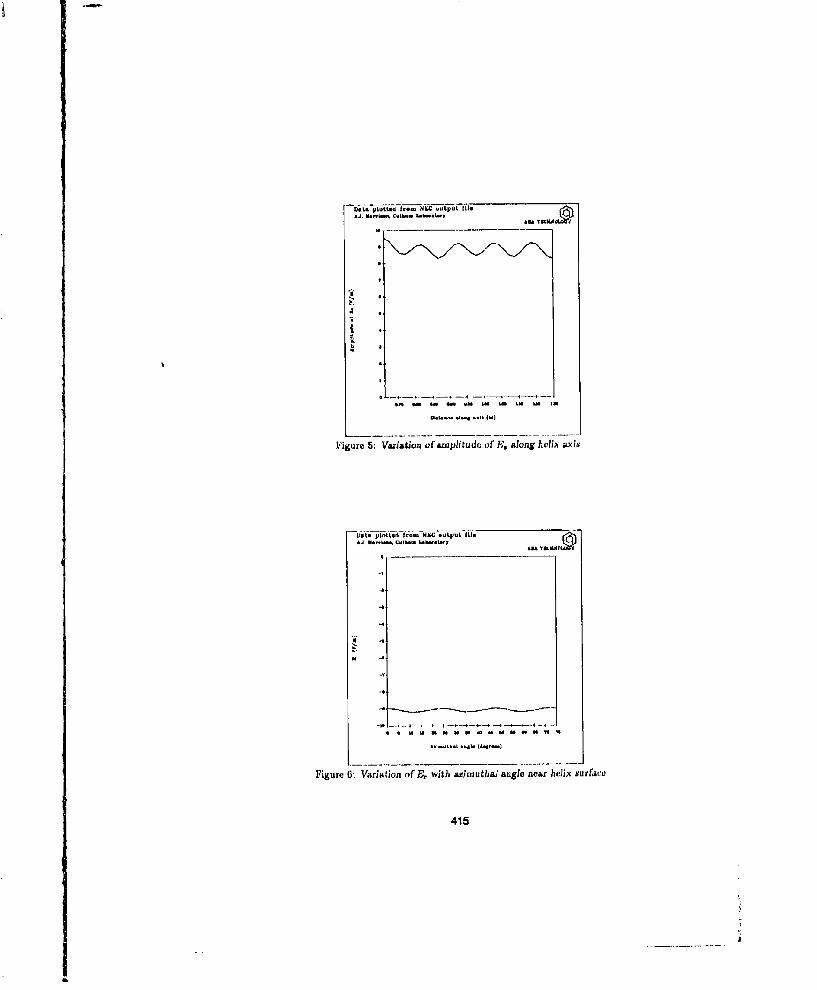
UItii plittdrm f It oulpuL Ill. M

Figu .6:Vaiatin ofw Eatr, wihainnh;age erhli urc

415a yuciu£,CI

,1.5

a a,

*fl S -il vs l £5 IS £5 5 I

.Figure 5: Varliaion olf apixilltude of F81 alonlg helix xixs

£4 MrJvlii.4l CsIM.. Iah..I.,

I 4

M 4i

N 415

-V 4

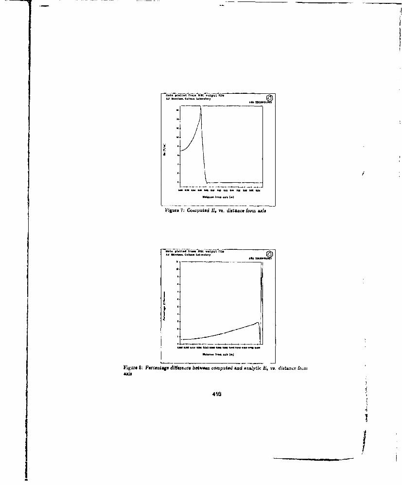
A*

Ow"4.. 1'.. W. (.1

Figure 71: Comnputsd E. vi. distance ta-ow axcis

45th pi.LLtd Im.. HUC -Lput 111.Uj. E.~Is. C41 .". &.44..p

iI!,

Figure 8: Percentage difr~c ewe optdand aualyeic B,, vs. d~ielaric from

41

Figure 9 shows the amplitude of EB, computed on the helix sais, an a function ofa. Again, there is a small atanding wave cnmponent with wavelength ,- O.1m givinga travelling wave wavelength of k 4 0.2m, In good agreament with the analytic valueof 0.202m [3].

The power flowing through a piane perpendicular to tha helix ade was calculatedby a numerical integration of the l'oynting vector in an Identical manner to thatdOecribed in the previous Subsection, giving

P = 2.94 x 10-3 W.

Figure 9 gives the amplitude of the travelling wave component of B. as 7.4 V/m, audfrom eq(4), the coupling impedance is

Z' = 18.9 0This result is within 4% of the analytic result of 19.6 ohms 13).

IThe prerrut ltsm tsec 4rtpwt .e in e r

'I

'I

have been constr-ucted from a finte number of finite helical wires. Resuls from thenumerical -odels are in good agreement with and #lytic results.

417

-omputed 0.2 0.2Wavelength(m)Analytic 0.198 0.202Wa",ehngth(n)l.rur oncomvuted wavelength 1% 1%Computed couplingimpedance (al) 34.8 18.9Analytc couplingImpedance (fl) 31.9 1g.6Error on computedcogpling impedance 8% 4%Error on computedE. In region < 8% < 3%of helix axli

Table 2: Computed and saalytic reaults

Error& in the numerical results are due to the Vidte lbugthi uf the nunmerical mnodels,which gives rise to reflected waves, and to the discrete nature of the models, whichleads to aximuthal field variations that do not appear in the idealised analytic modolof the aheath helix.

It should be remembered, however, that In a TWT design application, NBC willbe umed to model real, finite helical structures, where reflected waves Lad alimuthalfield vatriations are to bu expected; the fact that finlte numerical modehl have producedthese fiatures Is encouraging.

The work reported here gives confidence that NBC is an appropriate code formodelling helical slow-wave structures, capable of predicting the electroniagrtilc licidgwithin the strur.ture with a typical error el' ea than 5%.

6 REFLW.'NCES

[1] Burke, G.J. and Pogglo, AJ., INwnrwrical Eleacromaynetics Cod& (NEC) - Methodof Momento, Part Ill: User's Guidc, Lawrence Livecrnore National LaboratoryReport UCID 18834, JanuLry 1981.

[21 Pierce, J.R,, DTavelling Wave Tubes, D.Van Nostroad, New Yozk, 1960, pp 23-27,pp 229-232.

[31 Piechl, K., Wave propagation along a heliz with a cylindrical outer conductor,Arch. elek. Obertr. , 10, pp 195-206, 195a.

[41 Moore, J, and Pixer, R., Moment Methods in iect romagnetivm, Research StudiesPrat Ltd., U.K., 1984, p 117.

418

EL.ECTIUCALLY TRIMMED ARRAY SYNTH-ESISFOR SOLID STATE RADAR APPLICATIONS

M.A. fHussain, B. Noble, and M. McKeeGeneral Electric Research and Development Center

Schenectady, New York

1. INTRODUCTIONIn thi!i paper we briefly give results and outline a new approach to the

synthesis of electrically trinuned arrays. We use a deternninistic method to ob-tal a highly thinned space tapered array design (butterfly) for solid state raduIapplicatiolls.;

For simplicity of design and implementation we consider only space ta-pered and highly thinned arrays with uniform current distributiOl for the Cle-inents. It is well known in the literature that for random as well as space ta-pered arrays, the control of sidelubes is extremely diff icult and is predomainant-ly determhiod by the nmber of elementb in the array (Ref. [1,2]).

Low sidelobcs close to the main belan together with low averagesidelobes play a doninant part in the two-way beanl UtiliZatioLI in radar systemsin the presence of clutter. Our method allows for very strong control of thenear-in sidelobes anti soft control of the average sidelobes. Unequally spacedrows of elemniats dicourages flhe presence of grating lobes, and the sidclobesaway from the main beam follow the mathematical distributiun studied in thetheory of random arrays.

Our analysis is based on Taylor's analysis, with Woodward's method forone ditnensional case and Dobsier's representation for the circular case. In aprevious paper (Ref. [3]) we have outlined the method for ýhe circular aper-ture. In this paper we have extended the method to noncirculhr geometrie.,"The trimming of the shape is done by a simple algorithm for the location ofelements it the transverse direction. The algorithm for the determination ofthe number of elements in each row uses Taylor's theorem to avoid singulari-ties of the illumnination ftrction; at the same time it also uses asymptoticDulph-Tchcbycheff theory for the control of the zeroes near the main bcamn.

The resulLs are qtdte interesting in the sense that the algoritluu gives thedesired pattern and at the same time dictates the shape of the aperture. Theresults are given in the accompanying figures. Figure 1 gives the location of theelelhment1W i 42"La • U1 dU 4U X1UWV UIC "U•ULW•LLAUUL&U"A LUi U1C, KJL U "ill-k

eters with the near-in sidelobe controlled to 40dB; figures 3a and 3b show the.pattern disiribution for another set of parameters with near-in sidelobe controlled to 50dB.

419

______ ___

2. TWO DIMENSIONAL INIM RAL EQUATIONThe planar aperture integral equation for the illumination function leads

to the following space factor equation (using spherical coordinate 0 and )to ) , ff 1(o,,).- 4 V , +, V " " )d • ,l()

A

Where A represents area enclosed by a rectangle 2a by 2b. We assume aspecial current distribution represented as a product form J(C,'i) -gi(•)X2(r)over a rectangular area and further assume symmetric geometry. Equation (1)reduces to.

a b11 ,-4;" J i(C) cos(k u)X dtf' J2(01) cost(k vn dyj (2)

o 0

where u- sihicose v - sin•-in' Let2" N it. Mr. -cja, ?m - bl, - y. -T - y. Equation (2) can be written as:

11(9,0) - ý-ýFJ(U, ) (3)Where

F1(u) -2f;g1 (C-)cos(s)dMmud F2 (") -2;gz(J,)cos(.3U)d./a o

Above equation (3) are exactly the integrai equation solved by Taylor [4].

3. NUMEMICAL SOLUTION

In our approach we use numerical method rather than analytic methodfor the solution of the integral equation uing Woodward's synthesis tech-niques. The result are identical to those of Taylor [4]. As in Taylor's r'esult,however, the sidelobes are not of equal magnitude as was the case withDolph-Tchebycheff analysis. To make them equal we iterate around the zerosand a convergent solution Is obtained in a few iterations. The details are givenin [5] and briefly outlined below: Letgj(p) have the following Fourier expani-sion:

81(P) - P- + E OD, cos(m p) (4)2 , mIi

for O<p_<?r otlicrwiscgl(p)-O forp >r. Substituting equation (4) into

420(

,t

equation (3) we have(Do si(,r u) sb ( a r .3inr_(,4 (- LaFi(U) -2 r + D. +(

- 7r (u +" n) T (U-m) (

from (5) we have:

D.- F (M) ()

Denotinr; Ft(m) byFm, we have fiorn equation (4) ad (6):gI(p)" .-L(Fo + 2 E F. cos(, p)) (7)

Suppose that we decide that our far field pattcrn should have zeroes at n rmfor m>M, then."

gi(p) - L(F0 + 2 1'" F. cos(rn p)) (8)

This gives:

F1 (u) -,ao(u) FO + • F,. a (u) (9)M-I

where ,o(u) -sin(Cfu)/;iu

can(u)- r (u + m) + F (u(I))

From (9) and (10) we have F(n) -0 for n>M, and hence the Thylor's .ynthesistheorem is satisfied for finite value of the illumination function.*I

We normalize o that F(O)-FO - 1. Then we have M unknowns,F, F2...,FM at our disppotal to control the size of the sidelobes and the nullpoints. Also the knowledge of Fj givesggp) from equation (7). We now set up

" M orcrraponds toi*n- 1 in Taylor's paper.From here on our method dircro con-iderably from that ofT. T. Taylor. Taylor introduces a singlc

stretching parameter for shfting M+I zeroes. On thi uther hand, we uw these M degrees ul fre,-dora to form the desired pattern.

421

4

M simultaneous line algebraic equations for the determination of the F/.The details of examples are given in ref. [5]. It should be noted that the pro-duct form of the illumination function leads to extremely small sidelobes in theu-v pLane away from the axis and hence the success in rectangular designs forsolid state radars.

4. ARBITRARY SHAPE OF AN APERTURE

In general the two dimensional integral equation may be very difficult tosolve. In this section we outline another special case. We assume that J (tr) isa function of ý wnly and the apce turc can be described by fI(x).

Using the symmetry condition equation (1) can be sinplified to:

G sin (kf 1t )v)0 kv

or41I)l1(o.0) "j'J.lýrCfj C1) coskACkuO• (12)0

Comparing above equation with equation (3) we see that that the special (:asetreated here gives a sinilar equation except the illumination function has muchbroader meaning eg. for the case of uniform illumllnation we get an integralt.quation for the aperture distribution function. 11'his will now be compared tospace factor for a set of discrete elements.

5. DISCRETE DISTRIBUTION OF ELEMENTS

Consider a set of cdemnents on the x-y plane located at dx,,dyým.The usual element factor can be written us

S(od) - -+dy.) (13)

Cutiside lulg a synunetriC casc letdXi -dxm, dy.m•n-•-Lm +-I (n-1), for m - 1,...R, in -1,...N(m),andI,, - 1.Equation (13) then reduces to

422

4

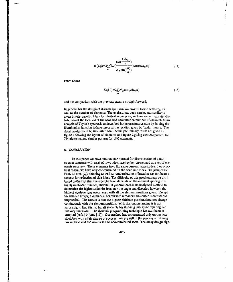
E (,€) 2"E ., 4 )cos(kdx,.u) (14)"N. sin(--)

4

From above

E• (0,0) - 2EN. cos(kCdxu) (15)

and the comparison with the previous cases is straightforward.

In general for the design of discretc synthesis we have to locate both dx,, aswell as the nuumber of elements. The analysis has .Licn carried out similar togiven in reference[3], Here for illustrative purlpse, we take sonic quadratic dis-tribution of the location of the rows and compute the number of clenients froinanalysis of Taylor's synthesis as described in the previous section by forcing theillumination function to have zeros at the location given by Taylor theory. Thcdetail analysis will be submitted soon. Some prelininary result are given infigure 1 showing the layout of elements and figure 2 giving element pattern , "744 elements and similar pattern for 1195 elements.

6. CONCLUSION

In this paper we have outlined our method for discretization of a non-circular aperture with a set of rows which are further discretized as a set of ele-ments on a row. These elements have the same current mnagitudes. For prac-tical reasun we have only concentrated on the near side lobes. To paraphraseProf. iA) (ref. [21), thinning as well as randomization of location has not been asuccess for reduction of side lobes. The difficulty of this problem may be attri-buted to the fact that the sidelobe level depends on the elenent spacing in ahighly nonlinear manner, and that in general there is no analytical method todetermine the highest sidelobe level nor the angle and direction in which thehighest sidelobe may occur, even with all the element positions given. Exceptfor smaller arrays, a numerical search with a modern computer is consideredimpractical. The reason is that the highest sidelobe position does not changecontinuously witn the element position. With this understanding it is nutsurprising to find that so far all attempts for thinning and space tapering arenot very successful. The dynmmic programming technique has also been at-tempted (refs. [14] and [16]). Our method has concentrated only on the nearsidelobes, with a fair degree of success. We are still in the process of refiningour method and the results will be communicated soon. The array design algo-

423

I.

rithmn will have applications in many fields e.g. sonar and ultrasound.

7. REERENCS1. B.D. Steinberg, Principles of Aperture and Array System Design, New

York: Wiley-Interscience Publication. &h 8, p. 141, 1976.2. Y.T. Lo and S.W. Lee, Antenna Handbook: Theory, Applications, and

Design, New York: Van Nostrand Reinhold Company. ch. 14, pp. 4-5,1988&

3. M.A Hussai W-T. Lin, and M. McKee "Representation of ContinuousCircular Aperture as a Set of Discrete Rings for Prescribed RadiationPattern", (submitted to Fourth Biennial IEE.E Conference on Elec-tromagnetic Field Computation), 1990.

4, Taylor, T. T.."Design oi Line-source Amnennas for Narrow Beamwidthund Low Sidelobes", IRE Trans. on Antennas and Propagation Vol. Ap-3pp 16-28 January 1955.

5. M.A l-utsaiWrUen Noble and W..T. Un, "Numerical Solution of an Aper-ture Integral Equation" Transaction of the Seventh Army Conference onApplied Mathematics wa Computing. ARO Report 90-1. February 1990.

424

.........--- ----

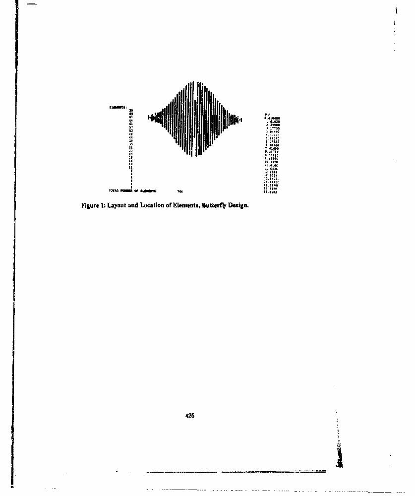
41 5.4454c'

33 4. 00340

2 I7I I 1 IIO2..

NO,,1

~ iiiiIIIi141

I LO.357

Is L1.01S41

mu 5. S4054

14. '234071,, I 3l710

S0. 31001

Figure 1: Layout and Location of Element~s, Butterfly Design.

425

Li .014

12.2.81

S. . ........ ... .................... ~ ~ L... ... .. .. . .. . . ............

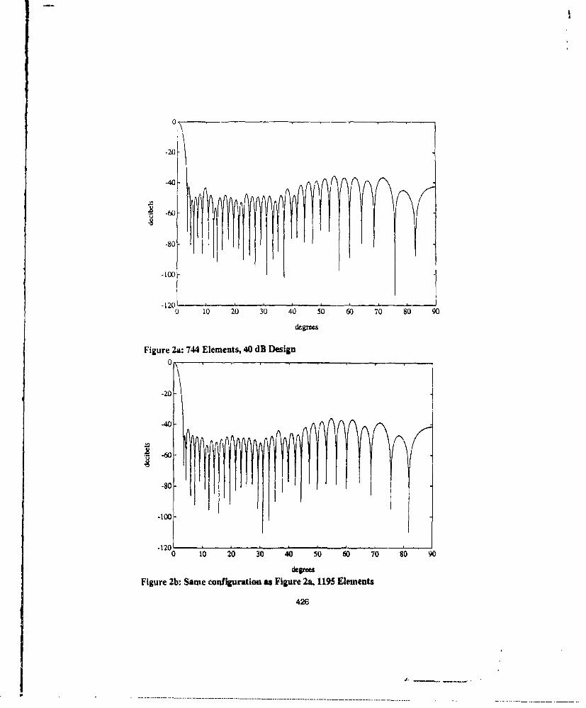
-20

-40-

-80 -i

-120

0 10 20 30 40 50 60 70 80 90

dcgrees

Figure 2a: 744 Elements, 40 dB Design

-20

-40-

".60

-100-

-120(0 10 20 30 40 50 60 70 80 90

degreesFigure 2b: Same configuration as Figure 2a, 1195 Elements

426

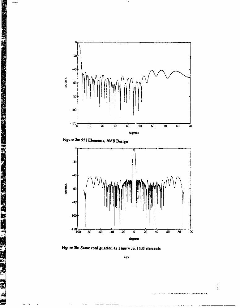
0

-80

-100-

*120 "o 10 20 30 40 50 60 70 80 90degre~es

Figure 3a: 951 Elements, 50dB Design

0

-20

-40-

.-60-

.80

.100-Jl

-100 -80 -60 -40 -20 0 20 40 60 80 100

dep~es

Figure 3b: Same configuation as Figure 3I. 1203 elements

427

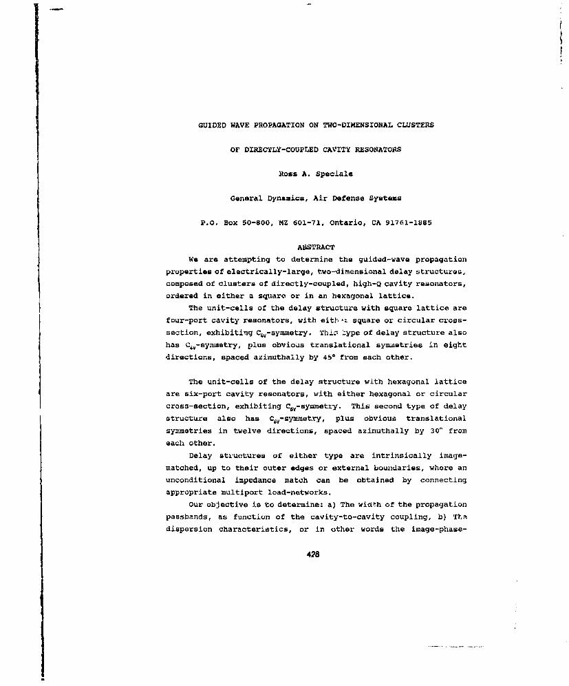
GUIDED WAVE PROPAGATION ON TWO-DIMENSIONAL CLUSTERS

OF DIRECTLY-COUPLED CAVITY RESONATORS

Ross A. Speciale

General Dynamics, Air Defense Systems

P.O. Box 50-800, MZ 601-71, Ontario, CA 91761-1885

ABSTRACTWe are attempting to determine the guided-wave propagation

properties of electrically-large, two-dimensional delay structures,composed of clusters of directly-coupled, high-Q cavity resonators,ordered in either a square or in an hexagonal lattice.

The unit-cells of the delay structure with square lattice arefour-port cavity resonators, with eith- square or circular cross-section, exhibiting C4v-symmetry. ThiL 4ype of delay structure alsohas ;v-symmetry, plus obvious translational symaetries in eightdirections, spaced azimuthally by 450 from each other.

The unit-cells of the delay structure with hexagonal latticeare six-port cavity resonators, with either hexagonal or circularcross-section, exhibiting C6v-symmetry. This second type of delaystructure also has C6.- symmetry, plus obvious translationalsymmetries in twelve directions, spaced azimuthally by 30" fromeach other.

Delay structures of either type are intrinsically image-matched, up to their outer edges or external boundaries, where anunconditional impedance match can be obtained by connectingappropriate multiport load-networks.

Our objective is to determine: a) The width of the propagationpassbands, as function of the cavity-to-cavity coupling, b) Thn

dispersion characteristics, or in other words the image-phase-

428

rotation dependence upon frequency, within any given passband andfor any given value of the cavity-to-cavity coupling, c) The extentof azimuthal anisothropy of the wave dispersion characteristics, ina continuous 3600 azimuth span through all traaslational symmetryaxes, and d) The frequency dependence of the image-impedance matrixof the clustered delay structure, defined at any planar interfacecutting edge-to-edge across the whole structure, at the discretelocation between unit cells.

The used approach considers the unit-cells as linear,reciprocal, multiport networks, exhibiting either C,,-aymmetry orC.,-symietry, consistent with either the square-lattice or thehexagonal-lattice ordering of the unit cells. This approachapplies the general theory discussed in a previcus paper [Ref. 1],but specializes the treatment to the case of unit-cells constitutedby high-Q cavity resonators, that are assumed to be characterized,analytically or experimentally, by a complex, multi-dimensionalscatterino matrix.

Because of the expected high-Q of the unit-cells, an initialanalysis has been performed, by assuming loselessness, besidesreciprocity and the appropriate type of symmetry. This combinationof constraints largely reduces the complexity of the analysis, bydrastically reducing the number of independent real parametersrequired to fully characterize a unit-cell. Indeed, already,jecause of reciprocity and symmetry alone, only three complexquantities out of the 16 entries of the 4 x 4 scattering matrix ofa four-port unit-cell have different values, and this introduces asingle degeneracy among the four eigenvalues of the scatteringmatrix, that also reduce to only three different complex values.Further, if louslessness is also assumed, the three differingeigenvalues becoms unimodular (thus falling on the unit circle), sothat the three real angular arguments of these eigenvalues may beconveniently assumed as the only free parameters of the reciprocal,symmetric, and lossleso four-port unit-cell, and of a two-dimensional delay structure with square lattice.

429

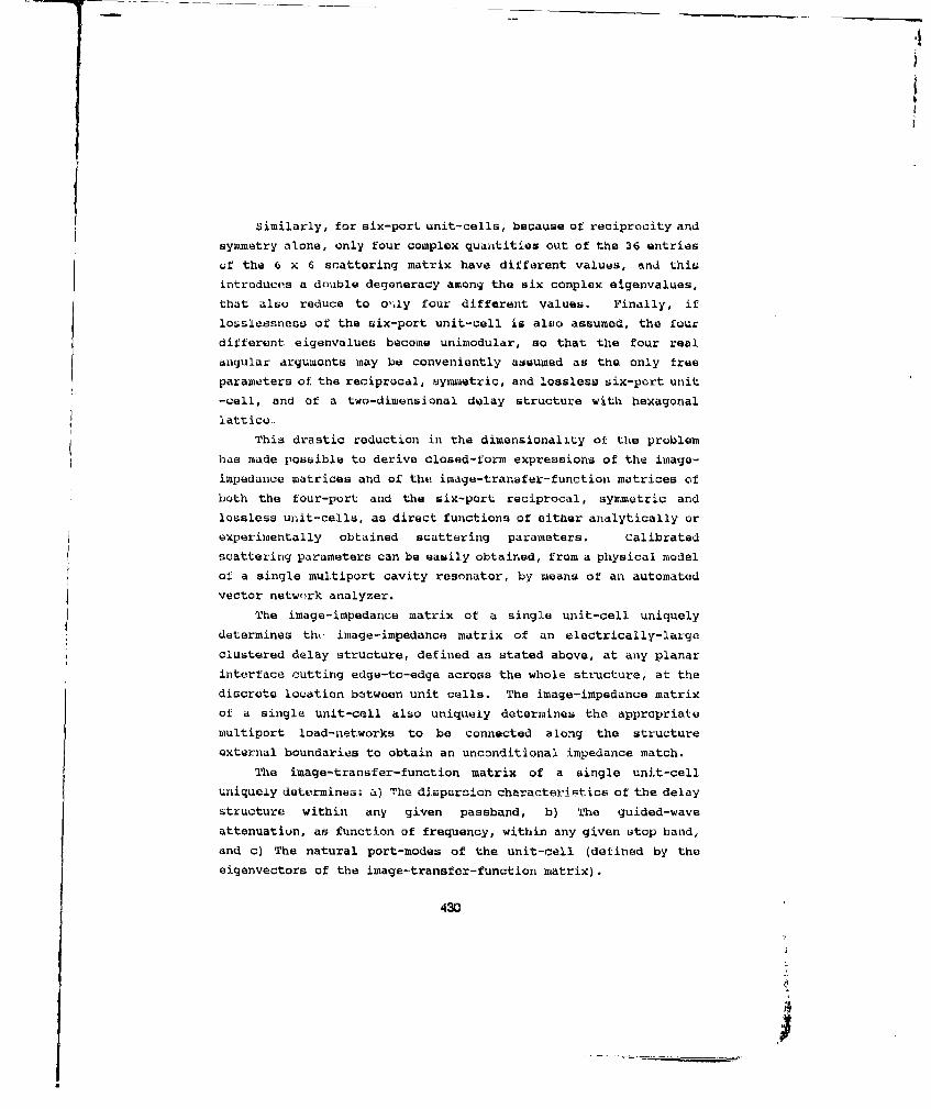
similarly, for six-port unit-cells, because of reciprocity andsymmetry alone, only four complex quantities out of the 36 entriesuo the 6 x G scattering matrix have different values, and thisintroduces a double degeneracy among the six complex eigenvalues,that also reduce to o'.Ly four different values. Finally, iflosslessness of the six-port unit-cell is also assumed, the fourdifferent eigenvalues become unimodular, so that the four realangular arguments may be conveniently assumed as the only freeparameters of the reciprocal, symmetric, and losslese six-port unit-cell, and of a two-dimensional delay structure with hexagonallattice..

This drastic reduction in the dimensionality of the problemhas made possible to derive closed-form expressions of the image-impedance matrices and of the image-transfer-function matrices ofboth the tour-port and the six-port reciprocal, symmetric andlossless unit-cells, as direct functions of either analytically orexperimentally obtained scattering parameters. calibratedscattering parameters can be easily obtained, from a physical modelof a single multiport cavity resonator, by means of an automatedvector network analyzer.

The image-impedance matrix of a single unit-cell uniquelydetermines th, image-impedance matrix of an electrically-largeclustered delay structure, defined as stated above, at any planarinterface cutting edge-to-edge across the whole structure, at thediscrete location between unit cells. The image-impedance matrixof a single unit-cell also uniquely determines the appropriatemultiport load-networks to be connected along the structureexternal boundaries to obtain an unconditional impedance match.

The image-transfer-function matrix of a single unit-celluniquely determinas: a) The disparcion characteristics of the delaystructure within any given passband, b) The guided-waveattenuation, as function of frequency, within any given stop band,and c) The natural port-modes of the unit-cell (defined by theeigenvectors of the image-transfer-function matrix).

430

'5

REFERENCES

[1] R. A. Epeciale,"Wave Propagation on Infinite, Two-DimensionalStructures," 5t Annual Review of Progress in AppliedComputational Ele';tromagnotics, Naval Postgraduate School,Mmnterey, California, March 21-23, 1989, pp. 200-244.

[2] R. A. Speociale,"Projoctive Matrix Transformations in MicrowaveNetwork Theory," IEEE 1931 Intecnacional Microwave SymposiumDigest of Technical Papers, pp. 510-512.

(3] M. G. Andreasea and R. L. Tanner,"A Wire-Grid Lens Antenna ofWide Application - Part II: Wave-Propagation Properties of aPair of Wile Grids with Square, Hexaganal or Triangular Mesh,"IXE Trans. on Antennas and Propagation, July 1962, pp. 416-429.

I

i_____ ____ ____ ____ ___

SESSION 11- "ANTENNA ANALYSIS"

Moderator: Asoke Bhattacharyya

METHOD OF MOMENTS ANALYSIS OF GAVITY-J3ACKED\\TI1R ANTFENNAS

Da~vid C..elii iNaval PUStgraduatv Scliuol

Monterey, C'A 939)13

I ugluic A ircraft Go.Fullertuii, (IA 92634

AbutractA zitet hod of Hiiiicutti sol iiLion is presented for t lie geiierdease ofjn a body

of rvol ufloll ii1he p ic prebice of ecidtell wile~s. Basis fli ctiorks are um ed ont allof the surfaices iand wires, anid coiisjvqiai~ly all oaroiiiihetoiuls to lie radlatlunfield areiLul[Clided. For flW %I)(!( iati CQOf the wire feed pul it oni the body W.,of rotat lura, only the odd azi iutilial inudes are rec ii red. 'I'lizi fact aloug Wifliisyiiinietrles betwveen tlit, positiv Vclind Regattive aiiodeb Vall beV ijaci to adlieVe-a significant reduction lin the largest inatrIx tbat inust be inverted for a givellantenna size. Calculated resultr aie bshown to hi' iii good ageenieit, with Othercalculated smud weassuced dalts. fur cavity-hacked diplmes and mpirals.

1. IntroductionA large class of imuportant practical anitennas are coniprised of two basic geometricstructures: wires and surfaces of revolution. Primiary cxamipl.,s axe cavity or groundplane backed spirals and dipoles. I iowevi-:r, ('luctrically large rotatioimally syl mii etric.reflectors fed by the above an(teiinma also fall into this category.

Iligli-frcquemicy techniques are enmimunuly used to predict the perfurinanc., oftllLse antennmas [I1,21. For example, the presence of the bottom of a cylindrical cav-ity isapproximated by a ground plane and the radiation from the wire alid itsLinage are calculated. The contribution fronm the rim is estimnated using GTD. Theprimary deficiency in this approach is that the interactionls between the wire andcavity are neglected, and these can bc significant because of the smnall electrical sizeand closeness of the structures.

The method of momrents (MM) is ideally suited for the analysis of these an-Letrima. MM sulutiosis for bodies of revolution (BO1s) and wires are well known,and a combination of the two is straightforward, InI the following mecetions the MM

432

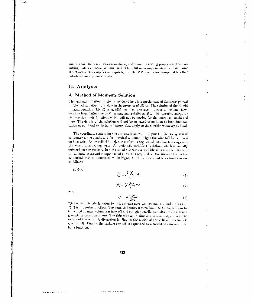
solution fur BOIlts and wires is outlined, and sonic interesting p~ropierties of tlie iiv-sulting miatrix eqtiation are discussed. Thie solution is iiiplexcicitd fur plainar wirestructures iueli as di poles anid spirals, ;aid the MM resilits iii' ii uiiiMixTrI to otilii'calculat~ed and measured data.

11. AnalysisA. Method of Moments SolutionTh'le aijteiiiii ridjitiOn rol e I)O)I1considered hecre iH iL sjietiisl Case Of tile nio1nt giiriilikprobleim of railiatioln Iroiti wiles inl the prsicetRC of 13lts. Qlli suitino(it -iliiitUgr'al equoat~ion ("ElII) Lisi ig NIMN lisa b~een Iesen ted by seVeral authors, nloWeverl the( furliiiilatioli dule to Mitschan~g anld Schlafer ill (31] app1lies directAly, excep~t fort1e jtLiii etiunl basis I'li ijetion which will nutL be needed for the( ai~uiteiiis t:onsidcr ciiI icre. 'Ihle details of thle solution will ijut bc rep~eate~d othier thau to htin trd Uf im'tatioui or poiiiit not exploitable featores that apply to thev specific gilonittry at haniid.

lThe coorliuiate systemu lotti i [tilt! i.1 issloivi ill Figure-L 1. T[le c avity axis, ofsyinunetry is the v axis, anid for practical1 antenna~k des~igni .s1 tewile Will bie niHUiTrCloin this axis. As describeicill :Ii(], Lilti surface is segziiunted into faýceted r iiis andthe wirev inlto short seguinieuis. Ani avelvi'ip,L variable i is ulelined which is radiallyoutward onlI IW siirlaiV. Inl tile camue of tint! wireC, at variable Iv' is ajiecilic(d taingeiitito Ilii axis. A second cuntponlAint of unrrciit is required oil the surface; this 41istheLaziuuiiliditl or i Col ciiiiiiiiit. shiiwin ill Figuirv . Tlie suilserl tonal u isis .fiiiiuiis area's follows:

sorfwv:e

fi= C, (2)

21ru ()'i;(t) is thei triai igle fnuerioi i (whIic un x ti'ids over tWui segi iiiuns, i Mid I 1 I1) Mid.PI'i(I) is the pul se fInn Lm ti. The aimnIid~la indeIx Us runs froml -O to ',, lint cain betruncated at snilal I valuesa of 7i (say N) aund still give excel Ilent results foir tine aut-eu usgeomietrics consitierii here. [Ilie Ii tlil- Wilr alpprox Iinationi is atHu iI Ci, and a is Goliraiuis of the wire. -A discoLssionl1 1i I u iitin ci( Cuiice- of I he'sc basis funci oins isgivenl ill [']. F'inially, Lilt, surface (uiiul-t. is expressed as a weighted s'iii of all iii('basiis fuiictioins

433

I

xti I ti~f1SBOR GBNERATIN(i Ul

CURVE

SEGIENTED WIRE

t 0 W i,

BOR FACET "

Figure .1: Cavity iuld wire geometry for tile method of momtf(lts iolution.

434

N m + Q I,4, r,., (4)/ Z z.,j,. + Y_. + * 4.Jq ' 4n.-N Lm-l P-J q-

where M, 11 and Q are the number of wire, surface t-directed and surfamce --directedbasuis functions, respectively.

Testing functions are chosen according to Galerkln's method, and tile standardMM procedure is used to reduce the EFDI, to a set of simultaneous linear equationsthat cal be written in the following block matrix form:

N - -N VN

Uzd. z•", i• ye' r,

z• z•., i• v

z-N ...Z, .... Z, zw- W ý vj

The vector I containu the current coelfcieuts, 1 the excitation elcments, and thesupCrscriptM J and w refer to surfacc and wire. The elements of tcie impedancematrix Z call be comnputed using the formulas in T'ablu 2 of [3). Lach subinatrixZ" in (,5) can in turn he wri tten in block form a

z:,' zI'+z"" z,,.1 I. (6)

It can be shown from the explicit expressions for the elemeents that

Zgn 711•-t• _ Z•,O-+ _ zI (7)

ZVr

and z,"= (z_,+' (8)

where T' signifies transpose. 'Fle 8surfacc- wire terms are of two types: Y"a' nid Z7',aid have the following symmetry

Z_. = -Z7w

Note' that. t.he preenice of the wire complicates the matrix problem; if the antennawere purely a BOR the impedance matrix would be block diagonal.

435

B. Matrix Reduction for Wire ExcitationWhIrela only tOw. wile :tructurte is xci txeit it, is possible to bareak tie, inversion irn(5) into it Sc'i's of Smalleditr im ratrix i avvrsions, and thereby reduce the courjutertilerI rovy rfqrira'niats Lor it giva'i a ivr•ia sie. 'ie sirpn ilifcation is accoaraillirledvi" Wood dbuly's itut ity ]5]

7-' = (A + aIIIV)-' -- A-' AV-'U(V 1 -t( -WA'U -IVA-' (wt)

w Ilt ( 7 is lir idtlrit-iy matrix will

A _N A A

A = Z'j' A, (11 )

A's

Z:'. 1u U 1U Z- DV = . 0 (12)

o Z'° " I ]°anid

VI/ 0 W , . ... Z °0. 1 0 ... 0• ... 0 "1[zywý ...Y T) 8 ... zx' ul 4U i .. (o1...(13)

For notatioral simplicity naw maatraiccs A, 13 ard C have beenr defiied carre.pomirrirg.to ZA, ZY aliri ZA", aloir witi a new iad-ux

,S - 1I N " 1, (14)

so thrat s4 takes oar values from I to S n7 2N 1 1. Fror (8) it is alaparent that

G. = (Is_+)". (15)The iuwvrse of A is earsily corirputed since it is block diagoral

436

m . . . . . . . . . . . . . . . . . . . . . . . . . . . . . . . . . . . . . . . . . . . . . . . . . . . . . . . . . . . . . . . .

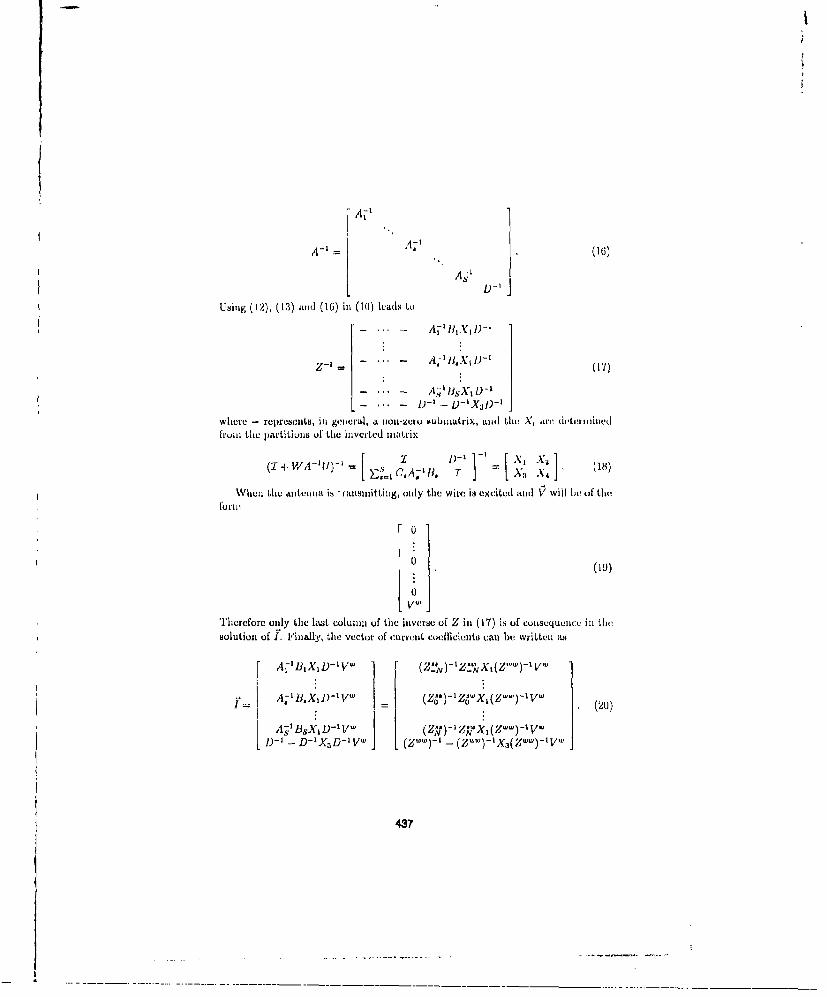
A-I L

Usitig (12), (13) and (16) ill (10) leads to

Whre rpresenits, ill ge'iiural, a lion-mv~ lsubuatrix, an d the X', all dtieturi ninedfru i eprtitions~ of) the netd nti

Whul tile ailteunlia it I aluwnlitti og, only ilewmiixiedadVwl of tile~fortel

~0

V.,,Thelirefore only the last coluimn of thu inverse of Z in (17) is of cuilsequence ill tlesolution of i. Finally, 'lie vector of current coefficients can bu writen mLr A',IB 1X 1ThlVw 1 - (Zm# Z X1-~ 1 V

As- I- BJx D- (Z""O - o x(z .. ,)l-(lVw (20

4,37

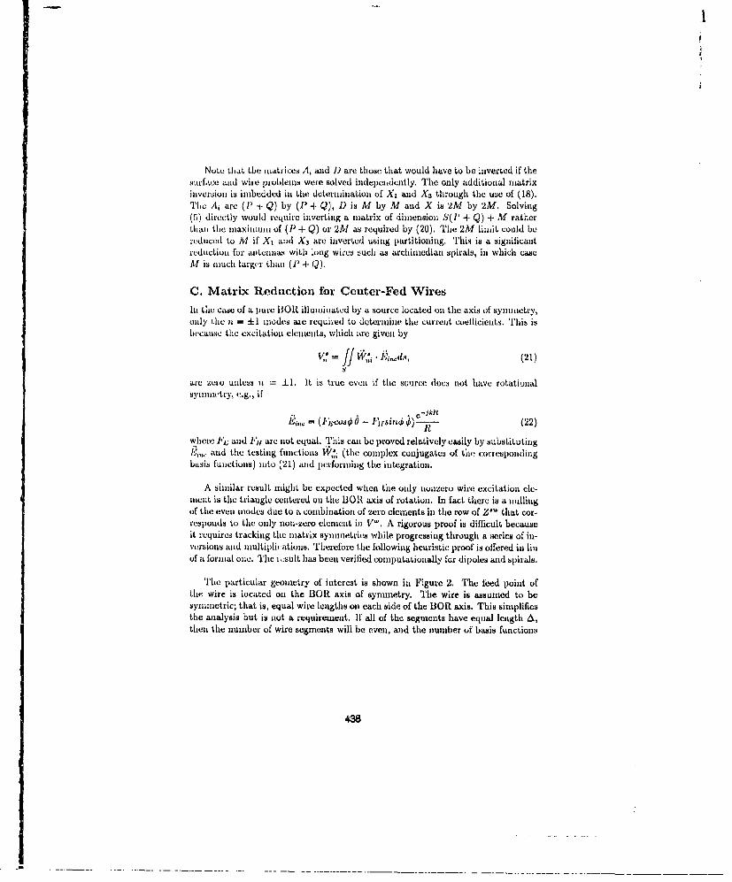
.1

Note that the matrices Ai and D are those that would have to be inverted if thesurfe•ev and wire problems were solved independently. The only additional matrixinversion is imbedded in the determination of X, and X3 through the use of (18).The A, are (P + Q) by (P + Q), D is M by M and X is 2M by 2M. Solving(5) directly would require inverting a matrix of dimension S(P + Q) + M ratherthan the maximumi of (P + Q) or 2M as required by (20). The 2M limit could bereduced to M if X, and X3 are inverted using partitioning. This is a significantreduction for avnenians with long wires such as archinmedian spirals, in which casehM is much larger thlnl (P - Q).

C. Matrix Reduction for Center-Fed WiresIn the case of a pure Bolt illuminated by a source located on the axis of symmetry,only the 2& = -1 modes are required to determine the current coefficients. This isbecause the excitation elements, which are given by

V: •j W Pi.od,, (21)

are zero unless t = ±1. It is true even if the source doce not have rotationalsymmnictry, e.g., if

F,, = (l,'r1oaO- I Y'1;i6,,) -f (22)where 1', and 1",t are not equal. This can be proved relatively easily by substituting

i',,. and the testing functions l'V.i (the complex conjugates of the correspondingbasis functions) into (21) and performing the integration.

A similar result might be expected when time only nonzero wire excitation cle-nient is the triangle centered on the 13OR axis of rotation. In fact there is a millilgof the even modes due to a combination of zero elements in the row of Z" that cor-responds to the only non-zero element in V'. A rigorous proof is difficult becauseit requires tracking the matrix symmetries while progressing through a series of in-versions and multiplirations. Therefore the following heuristic proof is offered in liiof a formal one. The i,:sult has been verified comaputationally for dipoles and spirals.

The particular geometry of interest is shown in Figure 2. The feed point ofthe wire is located on the BOR axis of symmetry. The wire is assumed to besymmetric; that is, equal wire lengths on each side of the BOR axis. This simplifiesthe analysis but is not a requirement. If all of the segments have equal length A,then the number of wire segments will be even, and the number of basis functions

438

z

/T•(w)

-w/ /+W

y

P1. ___

t constantarc on the BOR

,'igirm! 2: Symnnwtry conditions for on-axis excitation of the wire.

(Al) odd. The interaction between the excited triangle and the surface is given bythe surface-wvire imrpedace elements in (9). For the first type

j J /d dw zb[T (tf( )i - -T'(tT))] (Il)c-J"' (23)1 0 t

wheree-jk= -f- (24)

M+1 (25)2

and the primed quantities signify deriviatives. The circular curve in Figure 2 rep-reslent.s a t = constant arc. For two source points on the center triangle at +w and- w, there is a symmetry in q0 for test points on the arc

439

.- . .. . .. . . . . .. . .. . ... . . .. ... ... . . .. .. . .. . . ... . . . .. . .. . . . .. .. . ... . ... . . . .. . .. .. .. . . .. . .. . .. . . . . . . . . . ... . . . ..

R+(¢) =:- + ir) (26)

R-(¢)= R+( + ,r) (27)

I?,- w = 1 T ,,,)2 + z2 ± 2piw sin2(€/2). .8)

l'irst, (xamlne the last temi in the square brackets in (23). The integraLioln withrespect to t and its associated quantities are omitted since it will be shown thatthe integrand goes to zero for each value of t. The integration can be performed,ver a single segeniit (half o.' .he triangle) rather that two segments because of the

symil etry ill w

A oI 1f, J (10 -"" ~[ck(R')''(W) + rbI)~ i).(29)U 0

Thv !;Iuoc of the tritangle flicns at 11) = 0'1•cc) = -'A-i" (33

i d llI Isc'a . ISf( fi) ic periodic in 27r, ihi two teriis ii ,29) cancel.

I :!:vwise, lncaking oni the contributions from +w and -w for the first term inj.-J), using I,. - nc rco.sO and dropping constants gives

A 2 ,J 'lt(c,)dw J ,Ickcoa.c c-J'• [ck( R+) -I- r'(I?-)]. (31)

U sing (26) and (27) in (31)

'c(,).- , . .("" {[,,( (?+) + c,,( P- )] + t zs( 6. + 7r) f , - [" ' ( f+) + c( R -)]}

(32)whlichc ieclcccc

j T(a)d,,, J db Co.c€ Jc4[j,(R+) + Ui(R- U ([1 - (--I )1 (33)

adcl thus "a.ccishcc. 1.c 11 evvn. A similm iigucient holds for the surface- wirei ccalcce] . Ieli iecc( cI: or f-Ic" ste 'irl d cylv.

440

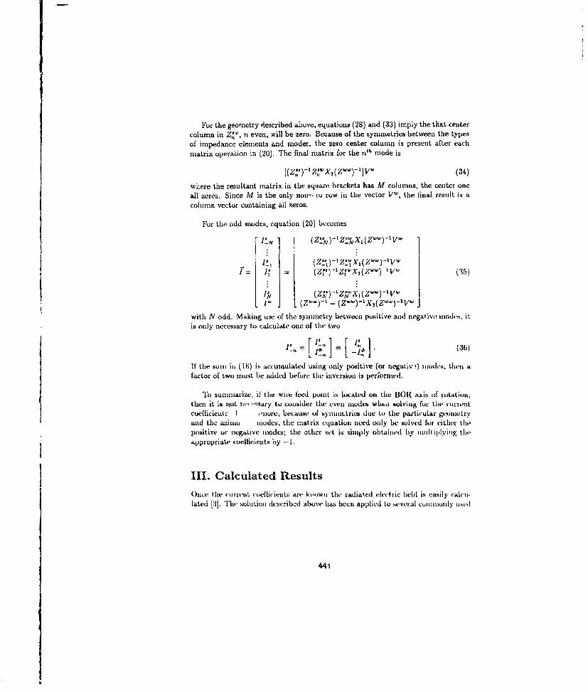
For the geometry lescribed above, equations (28) and (33) imply the that centercolumn in Z.'", n even, will be zero. Because of the symmetries between the typesof impedance elements and mode-, the zero center column is present after eachmatrix operation in (20). The final matrix for the n~'h mode is

[(Z.)-'7,'ýXl (")-l]Vw(34)where the resultant matrix in the square brackets has M columns, the center oneall zeros. Since M is the only nuill" vu row in the vector V"', the final result is acolumn vector containing all zeros.

For the odd niodes, equation (20) becomes

'N - ZN)Z N I(Z)V.

= (Zi )lZI X1(vw) IV. (35)

IW (ZU/")i' - (ZW)-lX 3 (ZWui)sVW3

with N odd. Making use of the syrninetry between positive and negal ive modes, itis only necessary to calculate one of the two

= [ ~ = [ ~(36)ff the sumn in (18) ib accumulated usinig only positive (or negativ -) imodos. tiltitj afactor of two must be added before the inversion is periornwd.

To summiarize, it' the wile feed point is located on the BOR axis of rotation,then it is niot ii e-'qsary to consider the even miodes whtes solving for the currentcoefficient,, I I ore, bsecause of byimnnucries due to the ipaxticular geurnmetrand the aZinmoL indes, the imiatrix equation neevd only be solved for either thltpositive or mnegaLive niodes; the other set is simply obtained by nnullip)lyiuy, theap~propriate coefficients by -1.

111. Calculated ResultsOnce the currenlt coellhvients are kinown the radiated electric hield is easily cahir-lated [131. 'Ill(, solution mlescribeod above has been applied to several cuninmiunly list-(

441

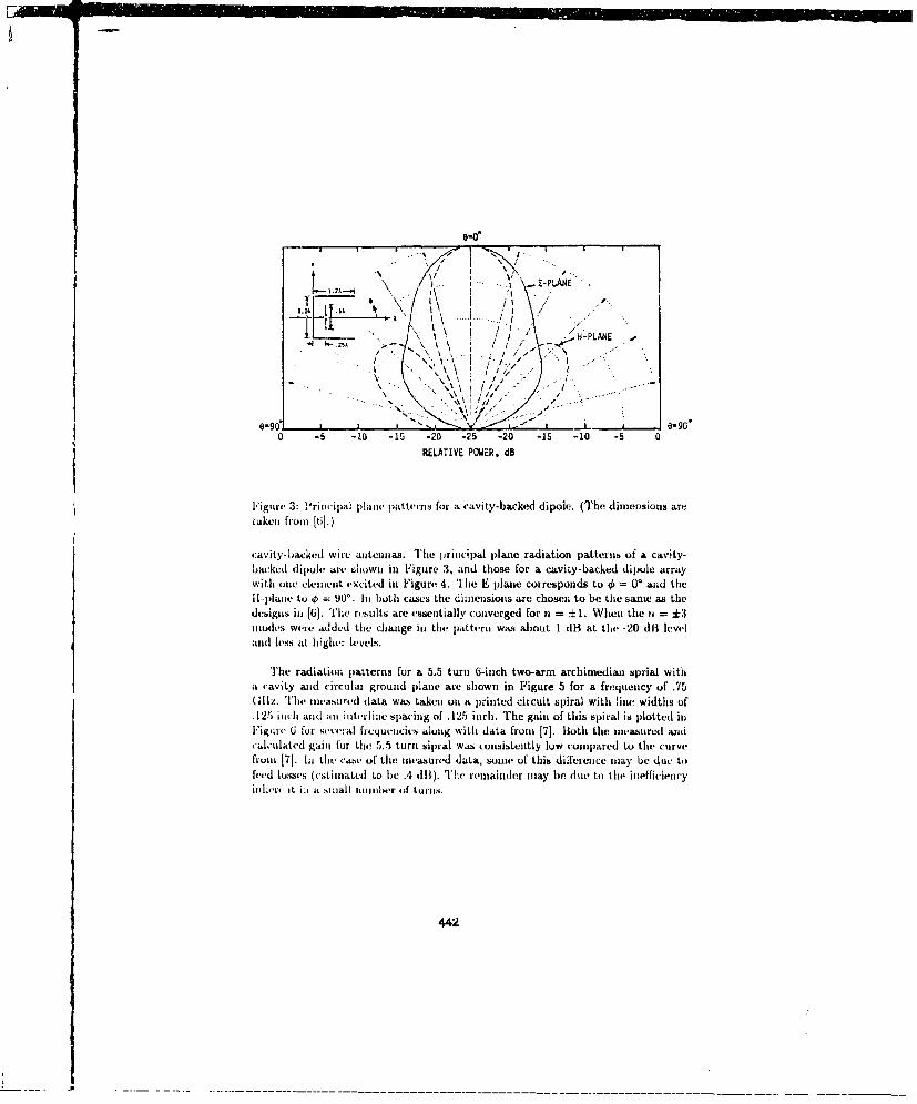
1L. ~E-PLANE

~ I -PLANE

-.9 4 a-j~ go*4/

0 -5 -10 15 20 25 20 15 10 5 0RELATIVE POWER, dB

Figure 3: Principal plane patterns for as cavity-backed dipole. (T1he dimensions arelakeii from [61.)

cavity-hacked wire antennias. 'ihe jiriiicpal plane radiation jiatterti3 of a cavity-backed dipole are eL-ikwn in Figure 3, and those for a cavity-backed dipole arraywith one elemienit excited iii Figure 4. '[ lie E-plaiie corresponds to 4A 00 and the1L-plane to 0 - 9~0' In both cases the dimensions are chosen to be the same as thedesigns in [6). The nosults are esseintially converged for n = ± 1. When the ii = :Hmiode's were added the change in the pattern was albout 1 dBi at the -20 dii level

,, less at higher levels.

The radiation piatterns for a 5.5 turn 6-inch two-arm arcItimedian sprial withit cavity and circular ground plane are shown in Figure 5 for a frequency of .75(Ill". 'lie ziiasu'ed data was taken oi a printed circuit spiral with ]in- widths of. -125 inch and ii iiit Iiiic spacing of .125 iiih. The gain of this spiral is plotted i ii

l'igilic U fur wea frequcencies along with data from [7). B~oth the mneasuired andc1.41,iilied gain for the, 5.5 turn sipral was consistently low compared to the curvefronit 7]. In the cae of the mieasured data, some of this di.ereiice may be due tofeed losses (cstiiatd to lhe .4 (lM). The remainder miay e due to the. ineffciency

inhlerc it ihi a siiiall niiiiier (if torns.

442

S __- ---------- --------- ---- ----- -- - ---------- _ - ____

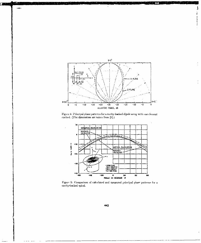
I. 2SI.- HP1/l

- ,I i E-PLANE

-0 s 10 16 -20 -25 -20 -15 -10 -5 0RELATIVE POWER, CU]

F'igure 4: P~rincipal planec pattce iz, foi a cavity-backed dipole array with one eleimentexcited. (The dimensions are taken fromj [6].)

18

jgftaI~ +P01 AZAZATI

-95A11 -fl -1 U111 58 EU

-3"3

____ I _ ____ ___ ___ ___ ___ ___--.. --- --.- ~ --. - - _ ____ __ ____ ___

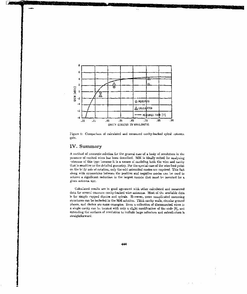
6

-2I-4

G= / MEAS111 ED

SCALCU{ ATED

SME, SURED ,*R+• 171-8

.25 .35 .45 .55 .65 .75 .85 .95CAVITY DIAMETER IN WAVELENGTHS

Figure 6: Comparison of calculated and measured cavity-backed spiral antennagain.

IV. SummaryA method of moments solution for the general case of a body of revolution in tlhepresence of excited wires has been described. MM is ideally suited for analyzing,ntenuas of this type because it is a means of modeling both the wire and cavitythat is sensitive to the detailed geometry. For the special case of the wire feed pointon the bc- dy axis of rotation, only the odd azimuthal modes are required. This factalong with symmetries between the positive and negative modes can be used toachieve a significant reduction in the largest matrix that must bn inverted for agiven antenna size.

Calculated results are in good ageement with other calculated and measureddata for several common cavity-backed wire antennas. Most of the available datais for simple cupped dipoles and spirals. However, more complicated mountingstructures can be included in the MM solution. Thick cavity walls, circular groundplanes, and chokes are some examples. Even a collection of disconnected wires ina single cavity can be Ltreated with only a sliht modification of the code 18], andextending the surfaces of revolution to include large reflectors and subrefluctors isstraightforward,

444

:1

V. References[1] A. Kuniar and H. D. Hristov, Microwave Cavity Antennas, Artech Howue, 1989.

[2] I1. Nakano, Helical and Spiral Antenna.s-A Numerical Approach, Research Stud-ies Press, 1987.

[3] J. F. Shaeffer and L. N. Medgyesi-Mitschang, 'Radiation From Wire AntennasAttached to Bodies of Revolution: The Junction Problem,' IEEE Trans. on An-tennas and Prop., vol. AP-29, no. 3, May 1981, p. 479.

[4] J. R. MauLz and R. F. Harrington, 'An Improved E-Field Solution for a Con-ducting Body of Revolution,' Syracuse University Technical Report TR-80-1.

[5] D. C. Jenn and W. V. T. Rusch, 'An E-Field Integral Equation Solution for theRadiation From Reflector Antennas With Struts,' IEEE Trans. on Antennas andProp., vol. AP-37, no. 6, June 1989, p. 683.

[6] M. Ii. Hong, et. al., 'Radiatiou Fields of Open-Cavity Radiators and a BackfireAntenna,' IEEE Trans. on Antennas and Prop., vol. 18, no. 6, November 1970, p.813.

[7] S. W. Lee, et. al., Atennla HAJidboosk, Chapter 14.

[8] D. C. Jeun, 'Application of Integral Equation Theory to Reflector AntennaAnalysis,' Ph.D. thesis, University of Southern California, December, 1987, Ch. 6.

445

i

MOMENT-METHOD MODELLING OF THE NORMAL-MODEHELICAL ANTENNA

Y I Guo and P S ExcellDepartment of Electrical Engineering, University of Bradford, West Yorkshire UK

,bstrjut

The normal-mode helical antenna is of interest as a convenient design for realizationwith high-temperature superconductors. Despite its simple structure, exact modelling ofits behaviour is far from simple since it is essentially a hybrid loop-dipole antenna, a typeknown to cause instability with some moment-method representations. An investigationof the resonant frequency performance of such an antenna, excited by a separate loop,was undertaken using the moment method, with second-order B-spline functions as basisfunctions. Stable results were obtained and it was found that. for a fixed length ofconductor, the resonant frequency of the antenna increased with the pitch and decreasedwhen the radius of the helix was increased.

Introduction

The electrically-small helical antenna is a propitious design for realization with high-temperature superconductors, since it is of simple construction, and its efficiency is poorwhen realized with conventional conductors. Provided it is operated below the 'cross-over frequency' (above which the loss in the superconductor becomes worse than that incopper), superconductor offers the possibility of greatly improved efficiency, with aconcomitant increase in Q-factor. This is, in principle, true for any electrically-smallantenna but the standard electrically-small loop and dipole antermas have to beconnected to tuning capacitors or inductors respectively, causing problems in manufac-ture from the ceramic high-temperature materials [1]. Tuning with transmission-linestubs is also possible [2] but the complete system is then no longer electrically small: itshould also be noted that electrical connections between ceramic superconductors andconventional conductors have been found to be extremely unreliable.

The normal-mode helical antenna (NMHA) is a very attractive alternative design, sinceit can be manufactured using existing processes for production of superconducting 'wire',and it can be parasitically connected to the external circuit via a copper coupling coil,thuý avoiding the need for electrical connections to the superconductor. There are threeconvenient approximate ways of viewing its behaviour: (i) as a multi-turn loop antennawithout a lumped tuning capacitor, but tuned by stray inter-turn capacitance; (ii) as ashort dipole antenna with integral central loading inductor, in which the 'arms' of thedipole have vatished, their funcdiun umiuag per'formed by the turns toward the ends of thehelix (a natural evolution of the earlier 'fat dipole' design [1]); (iii) as a coiled-up self-resonant half wavelength transmission line. The loop and dipole viewpoints areparticularly useful as they indicate that the NMHA inherently radiates in both modessimultaneously and its iadiatioa is always elliptically polarized. By appropriate choiceof the dimensions, the polarization can be made circular, or nearly linear in either the0 or 0 direction. The parasitic feed arrangement is also advantageous in that it provides

446

I

good thermal isolation between the helix and the loop and no additional matchingnetwork is required. Since the antenna operates at the first resonant mode it isparticularly imp'ortant to predict its resonant frequency precisely.

A moment-method study of multi-turn polygonal loop antennas was first proposed byRichards [3]. Later, Taylor and Harrison presented work on helical antennas [4]. Sincethey both considered antennas with only a few turns, which were not electrically small,few general rules about the relationship between the resonance and the helix parameterswere given. Besides, in their physical models the helices were directly excited at themiddle or the ends and the helices, together with the sources, formed closed structures.In the work reported here, the helix was isolated and consisted of many turns. Thecircumference of each turn was extremely small compared with the operating wavelength,so care had to be taken to ensure the validity of the moment method [5] sinceelectrically-small loops and structures combining these with highly-charged open-circuitstubs are lknown to be particular sources of instability (an attempt to model the antennawith the NEC program [6] was unsuccessful). The second-order B-spline function waschosen as a basis function, since it has better continuity than, for instance, the piecewisesinusoidal function.

Theou

The integral equation used was that given by Taylor and Harrison [4]: it is of the form:

fds'G(s,s')[d2/ds 2+k2(•.')j l(s ) -dds'l s )G(s,s')o - -j4nk/rq(E1(s)-Zjl(s)) (1)

where E' represents the impressed field, k represents the wave number, tj is the waveimpedance in the environmental medium and Z, the internal impedance per unit lengthof thc wire. The Green's function G(s,s') is given by:

G(s~s') - exp(-jkR)IR

where R is the linear distance between two points denoted by s and s'. The applicationof Eq. (1) demands that the pitch of the helix should be at lea.st four times as large asthe wire radius. Otherwise, the proximity effect must he taken into consideration [7).

Since a second-order differentiation is required ni q. (1), the following second-order B-spline function was used as the basis function to replace the piecewise sinusoidal functionadopted in [4]:

-4/3V- Wl< 1/2

f(x) - 2/3lY-2Wxt312 1/2.Ax,<3/2 (2)

0 I.3/2

447

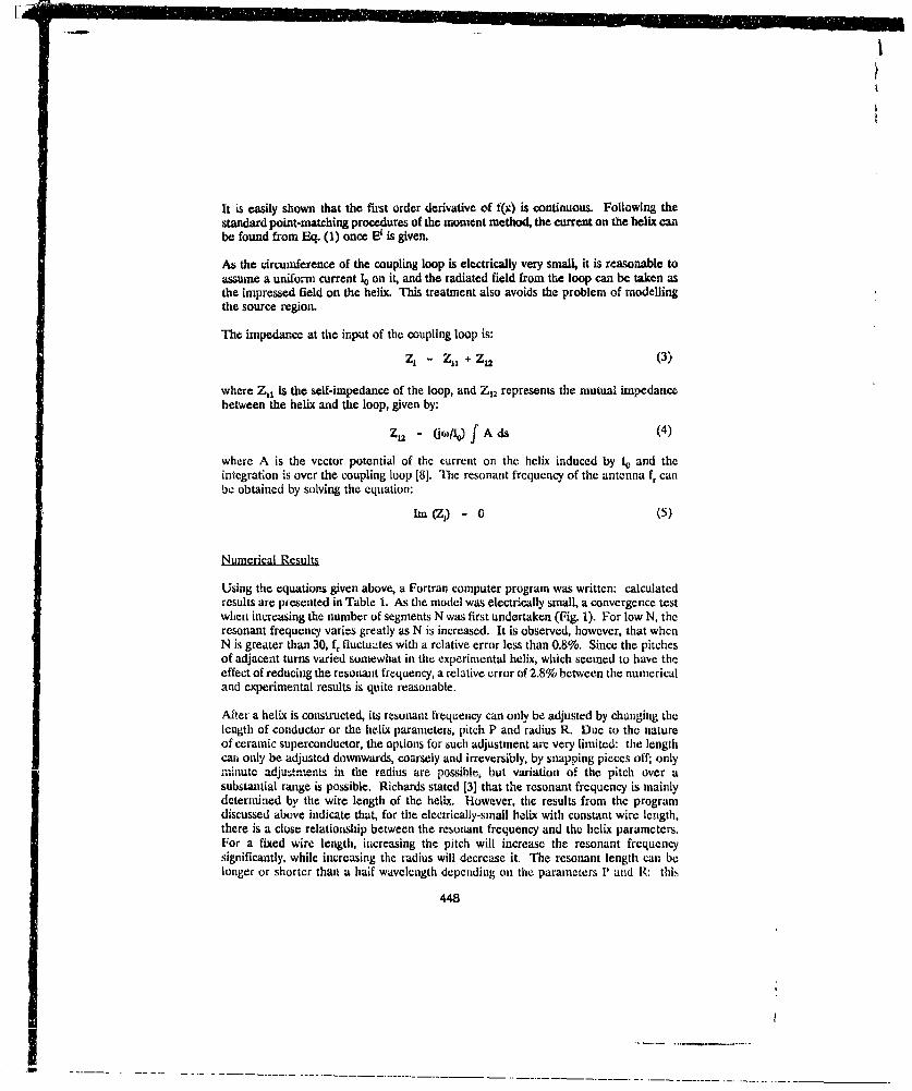
It is easily shown that the first order derivative of f(x) is continuous. Following thestandard point-matching procedures of the moment method, the current on the helix canbe found from Eq. (1) once E' is given.

As the circumference of the coupling loop is electrically very small, it is reasonable toassume a uniform current I0 on it, and the radiated field from the loop can be taken asthe impressed field on the helix. This treatment also avoids the problem of modellingthe source region.

The impedance at the input of the coupling loop is:

z, - z(1 + z2 (3)where 7., is the self-impedance of the loop, and Z12 represents the mutual impedance

between the helix and the loop, given by:

S- O6l) f A ds (4)

where A is the vector potential of the current on the helix induced by 1, and theintegration is over the coupling loop [81. The resonant frequency of the antenna fr canbe obtained by solving the equation:

Im(Z') - 0 (5)

Numerical Results

Using the equatiors given above, a Fortran computer program was written: calculatedresults are presented in Table 1. As the model was electrically small, a convergence testwhen increasing the number of segments N was first undertaken (Fig. 1). For low N, theresonant frequency varies greatly as N is increased. It is observed, however, that whcnN is greater than 30, f, fluctuates with a relative error less than 0.8%. Since the pitchesof adjacent turns varied somewhat in the experimental helix, which seemed to have theeffect of reducing the resonant frequency, a relative error of 2.8% between the numericaland experimental results is quite reasonable.

After a helix is constructed, its resonant frequency can only be adjusted by changing thelength of conductor or the helix parameters, pitch P and radius R. Due to the natureof ceramic superconductor, the options for such adjustment are very limited: the lengthcan only be adjusted downwards, coarsely and irreversibly, by snapping pieces off; only.. n'we ad,'utments in the radius are possible, but variation of the pitch over a

substantial range is possible. Richards stated [3] that the resonant frequency is mainlydetermined by the wire length of the helix. However, the results from the programdiscussed above indicate that, for the electrically-small helix with constant wire length,there is a close relationship between the resonant frequency and the helix parameters.For a fixed wire length, increasing the pitch will increase the resonant frequencysignificantly, while increasing the radius will decrease it. The resonant length can belonger or shorter than a half wavelength depending on the parameters P and R: this

448

- ----.... . . . ... ... . . ........... ... ........ ....

does not appear to have been noticed by the previous investigators.

The resonant performance of the loop-excited normal-mode helical antenna has beeninvestigated by the moment method with the second-order B-spline function as the basisfunction. Although the antennas studied were electrically very small, the programprovided convergent results which agreed well with those of an experiment. It was shownthat the resonant frequency of the antenna is closely related to the helix parameters.When the wire length is held constant, the resonant frequency increases with the pitchand decreases when the radius of the helix is increased. With a fixed helix diameter, acritical turn spacing exists which determines whether the resonant length is greater orless than one half wavelength. By adjusting the turn spacing of the helix, a specificresonant frequency can be obtained.

Computation of the radiated field and radiation resistance should be straightforwardusing a similar program, although this has not yet been attempted. Computation oflosses and the Q-factor is much more complex as it is known that there is a non-uniformcurrent distribution around the wire perimeter [71 and currents will also flow tiansverselyto the wire axis due to the inter-turn capacitance. These matters are the subject ofongoing work,

Reterece

1. Excell, P S & Alford N Mc N: 'Superconducting Electrically-Small DipoleAntenna', lEE Int. Conf, on Antennas & Propagation, York, Vol. 1, 1991.

2. Khamas, S K et al: 'High-T, Superconducting Short Dipole Antenna', EiectronicsLetters, Vol. 24, No. 8, 1988, pp. 460-461.

3. Richards, G A: 'Reaction Formulation and Numerical Results for Multitnrn LoopAntennas and Arrays', PhD Dissertation, The Ohio State University, 1970.

4. Taylor, C D & Hlarrison, C W: 'On Thin-Wire Multiturn Loop Antennas', IEEETrans. Antennas & Prop., Vol. AP-22, No. 3, 1974, p. 407-413.

5. Burke, G J: 'Enhancements and Limitations of the Code NEC for ModellingElectrically-Small Antennas', Lawrence Livermore National Laboratory, ReportNo. UCID-20970, 1987.

6. Burke, G J & Poggio, A J: 'Numerical Electromagnetics Code (NEC) - Methodof Moments', Lawrence L.ivermote National Lab., Report No. UCID- 18834, 1981.

7. Smith, G S: 'Proximity Effect in Systems of Parallel Conductors', J. Appl. Phys.,Vol. 43, No. 5, 1972, pp. 2196-2203.

8. King, R W P & Prasad, S: 'Fundamental Electromagnetic Theory and Ap-plicatms', Prentice-H1all, Englewood Cliffs, 1986.

449

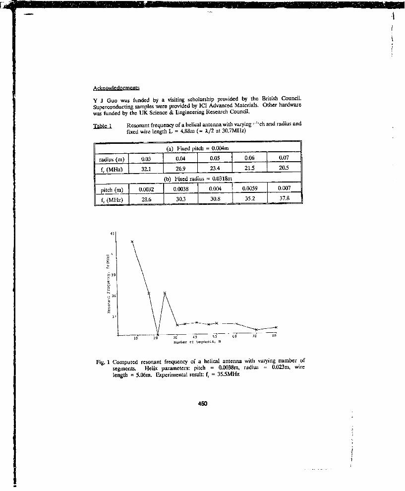
Acknowledvements

Y J Guo was funded by a visiting scholarship provided by the British Council.Superconducting samples were provided by ICI Advanced Materials. Other hardwarewas funded by the UK Science & Engineering Research Council.

Ta1l.e1. Resonant frequency of a helical antemna with varying ,"ch and radius andfixed wire length L = 4.88m (= 1/2 at 30.7MHz)

(a) Fixed pitch = 0.004m

radius (m) 0.03 0.04 0.05 0.06 0.07fr (MHz) ] 32.1 26.9 23,4 21.5 20.5

f,_(Mz)_I (b) Fixed radius - 0.0318m. _ 1___20.5

pitch (m) 0.0032 0.0038 0.004 0.0059 0.007

fr (MHz) 28.6 30.3 30.8 . 35.2 37.8

39

38

3,

10 20 30 so ¶,2 O. 70 soNumber of SOgnrnfLS, 11

Fig. I Computed resonant frequency of a helical antenna with varying number ofsegments. Helix parameters: pitch = 0.0038m, radius 0.023m, wirelength = 5.06m. Experimental result: f, = 35.5MHz

450

INTERCOMPARISON OF SEVERAL MOMENT-METHOD MODELS OF DIPOLESAND FOLDED DIPOLES

P S Excell & A F Armanious*Electrical Engineering Department, University of Bradford, West Yorkshire, UK

*now at Sultan Qaboos University, Oman

AbstrcA simple 0.47T dipole was modelled using ten different moment-method formulations: six simple versionsemploying the magnetic frill generator, and four weld-established published versions. The terminalimpedance was the main parameter examined. It was found that convergence to a stable solautiou was poorin all of the six simple formulations, which may be a consequence of the choice of geserator model. Resultsfor the rcsistancc were all similar, but reactance results showed substantial variation. Some well-establishedanalytical solutions showed substantial disagreement in both resistance and reactance, but a measurementagreed well with the mean of the moment-method predictions.

In a separate study, the impedance of folded dipoles operated below resonance were investigated. Tiepattern behaviour was similar to the electrically-small loop antenna. The impedance was found to be proneto extreme instability, including negative resistance, especially when capacitive end-loading was added.

1. Introduction

It is well known that the results hrom moment-method computer programs show variations (which may ormay not be significant) when the segmentation or the formulation are changed. An investigation of thiseffect using a very simple test object (a 0.47. dipole) was undertaken using a wide fangte of formulationsand the r"ults are presented below. Such a simple dipole is clearly a useful test object for intercomparisoaof the predictions of different approaches not least because it is amenable to analytical solutions as well.

Another potentially useful test object is the elcdrically-small folded dipole. The demands that this placeson modellirg strategies were discovered in the course of an excrcisc to compute the behaviour of suchantcenas, as they are an important canonical type for 'unintended receiving antennas', useful in EMCanalyses. The problems that were encountered in this exrcisc are outlined below.

2. Modenlin the 0.471 Dinoe

A simple 'half-wavelength' dipole was modelled using ten different moment-method formulations. The actuallength used was 0.47A, to accommodate the well-known phenomenon of resonance just below 1/2: theconductor diameter chosen was 0.011. The formulations tested were as follows:

1. Rectangular pulse basis functions and point-matching2. Piecewisc-Linear bas fanions and point-matching3. Picevise-sinusaoidal basis functions and point-matching4. Rectangular pals basis functions with Galerkin's method5. Piecewisc-linear basis functions with Galerkitn's method6. Piccewise-siniuowida basis functions with Galcrkin's method7. Rectangular pulse basis function with a modified Galerkin method: separate treatment of charge

and current (the MININEC method [1])8. Three-term atigonomrtrical-function basis functions with point-matching (the NEC method [2])9. Approsimated piecewise-linear basis functions with a modified Galerkin method (Chao and Strait's

method [31)10. Reaction integral equation solved by piccewiae-sinuaoidal basis functions with Galcrkm's method

(Richmond's method [4])

451

A magnetic frill generator was used in the first six method and delta-gap voltage generators in the othermethods.

The results of convergence tests arc shown in Table 1. The field pattern results converged to a realistic valuewith very few segments and were not considered to be an onerous test: impedince results were thusconcentrated upon.

It was found that convergence was poor in all of the first six methods, especially in the reactance results:this may be due to the use of the delta-function generator. The best results were achieved with Galcrkin'smethod and either of the picemwiso basis functions.

The version of the Chao and Strait program used became unstable before complete convergence had becaachieved. The other 'published" programs (methods 7, 8 and 10) achievd more rapid convergence thanmethods 1 to 6, possibly due to the avoidance of the magnetic frill source.

The reactance results in methods I to 6 were all in the region of 14 ohms. The results from MININEC andthe Richmond code (and also from the Chao and Strait code before it became unstable) were around 5ohms, and the result from NEC was 9 ohms. For comparison, a computer inplementation of T T Wu'sanalytical long-dipole model [5j (still claimed to be valid at a half wavelength) gave a reactance of 10 ohms,but a value of resistance (90 ohms) subsLar tially different from that predicted by the numerical models.Further analytical predictions are given in tabular form in Ref [61, together with some experimental results.Relevant results (interpolated to correspond to the dipole modelled here) are givcu in Table 2. It is ratherextraordinary to note that the expcrimental result agrees more closely with the numerical predictions(egpecially MININEC and Richmond) than with the analytical predictions. Given that an experiment exactlysimulating the conditions modelled is extremely difficult, and that analytical models still involve certainapproximations, these results beg the question of just what may be taken as the 'true' value of impedanceand they also serve to re-emphasise the criticality of reactance in ntenna modelling. This criticality isparticularly marked for a resonant antenna of this type, since the rate of change of reactance with increasingantenna length is extremely high.

3. The Electrically- l1ded Dikkl, w

In a separate study, the properties of folded dipoles operated below their resonant frequency wereinvestigated. The behaviour was found to be rather like an Lledrically-.anall loop antenna, but withadditional subtleties apparently caused by the close proximity of some of the conductors. Four moment-method codes were tried: NEC; Chao and Strait; Richmond; and TWC (a Bradford code using theMININEC solution procedure) [71. With NEC there was a curious instability in the reactanct results in that,as the number of segments was increased, the result converged to a stable value, then went unstable and thenconverged again. With the Chao-Strait code the results appeared to converge rapidly but the number ofsegments was limited by the implementation used. The Rihmasd code was vesy unstable, showing negativeresistance, TWC gave rapid convergence to realistic, able results (see Tb 3).

The object of the exercise was the modelling of shapes likely to be sigaifit in radiative electromancticcompatibility, and to this end, capacitive stuba were attached to the eunds of the folded dipole to see whetherthis could causu a reduction in the reactiaca. This caused serious int 'lilies (nqetive resistance) withNEC, aithough the problemn could be cured witl care. TfC appeAre Lo 6ve rapid wnveaaGa e W raiabl,stable results. The problems with NEC are known to be related to well-known problems with electrically-small loops 181.

452

Rernc

1. Rockway, J Wet al: 'The MININEC System: Microcomputer Analysis of Wire Antenna!.', Boston:Artech House, 1988.

2. Burke, G J & Poggio, A J: 'Numerical Electromagnctics Code (NEC)', Lawrence Livermore Nat.Lab., Report No. UCID-18834, 1981.

3. Chao, H H & Strait, B J: 'Computer Progrars for Radiation and Scattering by ArbitraryConfigurations of Bent Wires', Air Force Cambridge Research Labs., Report No. AFCRL-70-0374,1970.

4. Richmond, J H: 'Computer Program for Thin Wire Structures in a Homogeneous ConductingMedium', NASA Report No. CR.2399, 1974.

5. Wu, T T: "Theory of the Dipole Antenna and the Two-Wire Transmission Line', J. Math. Phys., Vol.I, No. 4, pp. 5501-574, 1961.

6. King, R W P: 'Tables of Antenna Characteristics', New York: IFI/Plenum, 1971.

7. Armanious, A F & Excell, P S: 'Enhancements to Moment-Method Field Computation Packages',IERE Counf. on EMC, York University, 1986, pp. 191-196.

8. Burke, G: 'LM Modeling Notes', ACES Jnl. & Newsletter, Vol, 2, No. 2, pp. 30-44, 1987.

Acknowluducmcnts

This work was funded by a studentship grant from the University of Bradford Research Committee. Somesoftware and hardware was provided by the UK Science & Engineering Research Council.

4b3

Table 1: Impedance and Convergence Rerults: 0,47X Dipole

Method Resistance Reactance No. of Segments for Convergence, NR (a) X M__

1 79 14 - 101(R) -f-10(X)2 79 14 -0(R '-90 (X)

79 14 80(Ri :80X1180(R -90X4 79 14 30R -60 -X)

5 80 15 30(R. ~60X)6 79 15 30(R 50(X)7 76 4.2 15(R) >60(X)8 78 9 25(R) >44(X)t9 75 4 20(R) 35(X)10 77 5.5

Figuresfor Knee -51 r N )all& tua relatively smalZ value: in all cases X is still increasingslowly at N=200 (maximum value tried).Values of X given axe for N =200.tNot fully converget•, but goes unstable with more segments.

Table 2: Analytical and Experimental Results: 0.471 x 0.01t Dipole

Source Impedance (a)

Wu's long-dipole treatment [51 89.7 -j10.0King & Wu tubular monopole* 16,p. Il 89.5-j10.7King & Harrison thin dipole* 16,p.41J 70.8 +jo.3Hartig monopole experiment' 16,pp.137-81 77.3+j5.1

*lnterpolated from tabulatzid resulis (monopole inipedances doubled)

454

1I

Table3 Input impedance of an electrically-small folded dipoleantenna using the NEC2 (with extended thin-wire kernel option),TWC, Chao & Strait and Richmond programs.

Codes No. of segments d* d/a** InputMajor Minor Impedance

wiros

NEC2 3 1 0.004 4 0.0052 + J87.35 1 0.004 4 0.0049 + J83.67 1 0.004 4 0.0053 + J89.011 1 0.004 4 0.0077 - j129.817 1 0.004 4 0.0053 + J86.923 2 0.002 2 0.0053 + J78.623 4 0.001 2 0.0046 + J88.2

TWG 8 2 0.002 2 0.0027 - J0.6712 2 0.002 2 0.0051 + J84.818 2 0.002 2 0.0054 + j87.124 2 0.002 2 0.0054 + j88.824 4 0.001 1 . + j89.0

Chao G 8 2 0.002 2 0.0053 + .j86,4Strait 12 2 0.002 2 0.0053 + j96.3

16 2 0.002 2 0.0053 + j816.224 2 ] 0.002 2 *AA ........24 4 ] 0.OU01 I -A ** ----.....

Richm,- 6 1 0.004 4 ).0081 A. J133.3end 8 1 0.004 4 0.00143 + j83,5

10 1 0.004 4 -0-0027 + j83.812 1 0.004 4 0.0O.20 + J84.014 1 0.004 4 0.0041 + j84.216 1 0.004 4 0.0210 + j84.618 1 0.004 4 -0.0350 + j84.9

* d is the minimum segment length in terms of wavelength.** d/a is the iatio of the minimum segment length to the

wire radius.*** Outside program limitations.

455

SIMPLIFIED HORN ANTENNA PARAMETER ES11MATIONUSING SELECTIVE CRITERIA'

Paul D. Evwing

Instrumentation and Controls DivisionOak Ridge National Laboratory,' P.O. Box 2008,

Oak Ridge, Tennessee 37831-6007

Paper to be Presented at

7th Aninual Review of Progress in AppliedComputational Electromagnetics

March 19-21, 1991Monterey California

'Reseýarch spoynsored by Department of the Navy, Naval Air Systems Command AIR-5161,under Interagency Agrceement 1501-15(11-Al with the U.S. Department of Energy.

'Managed by Martin Marietta Energy Systinns, inc., for (the U.S. Department of Energyunder Contract No. DE-AC0I5-840R21400.

456

SIMPLIFIED HORN ANTENNA PARAMETER ESTIMATIONUSING SELECTIVE CRITERIA*

fl M d e M t NO.Goy."nlflI wea• or-rt I•k. Sl-ASM AOA. l M*400 .Y. 24 U.S.Gc-,ntMm iS nuv•lroydl.-rsl hW - pAW -r t•pot

Paul D. Ewing 1h z I'A . "Vfbt- ,aWý t Ws Wo• . twe us. 0o •

Instrumentation and Controls Division voo.-Oak Ridge National Laboratory, t Oak Ridge, Tennessee

Abstract

An ap)roxixIaaLion call be used to avoid tie complex inathlejoatius and computation methodstypically required for calculating the gain and radiation pattern of the electromagnetic hornantenna. Because of the curvature of the antenna wave front, cal,;ulations using conventionaltechniques involve solving the Fresnel integrals and using computer-aided numerical integration.With this model, linear approximations give a reasonable estimate of the gain and radiationpattern using simple trigonometric functions, thereby allowing a hand calculator to replace thecomputer. Applying selected criteria, the ease of the E-plane horn antenna was used to evaluatethis technique. Results showed that the gain approximation holds for an antenna flare angle ofless than 10' for typical antenna dimensions, and the E field radiation pattern approximationholds until the antenna's phase error approaches 60', both within typical design parameters. Thistcihnique is a useful engineering tool.

INTRODUCTION

In general, the electromagnetic horn antenna is a simple aperture antenna used to providea smooth transition for a wave traveling from a waveguide into free space. The dimensions of thewaveguide are usually chosen to allow the propagation of on': dominant mode, and the hornantenna will support only that mode by acting as a filter for other modes that might be excited inthe transition. The horn antenna has the advantages of high gain, relatively wide bandwidth, andeasy construction. However, a disadvantage is that the calculations for determining gain andradiation patternm are mathematically rigorous and involve solving the Fresnel integral andperforming numerical integration that may require using a computer. To avoid the complexmathematics and computation methods, approximations for the gain and radiation pattern can beused. As with other engi. ecring approximations, values derived from the calculations are usefulonly within the limited co, traints of the approximation.

'-Research sponsored by Department of the Navy, Naval Air Systems Command AIR-5161,under Interagency Agreement 1501-1501-Al with the U.S. Department of Energy.

tManaged by Martin Marietta Energy Systems, Inc., for the U.S. Department of Energyunder Contract No. DE-AC05-84OR21400.

457

The case of the E-plane horn antenna w. -..-ed to evaluate the feasibility of tht-approximation technique. The E-plane horn anten.-' ,hown in R&. i, is fcrmed by r thewaveguide in the y-z plane, the E-plane of the antenna's aperture. The horizontal diiiens~ok ofthe aperture is the same as the width of the original waveguide, and the vertical dimen•,on ismuch greater than the height of the original waveguide.

GAIN AND RADIATION PATITERNS

Knowledge of electromagnetic horn antenna theory has been around since the 1930s, andderivations of the gain and radiation patterns of the E-planc horn antenna are welldocumented.' 3 The geometty of the E-plane horn antenna in the direction of the vertical flare isshown in Fig. 2. With the flare, the waves do not arrive at all points in the aperture at the sametime; therefore, they form a cylindrical wave front with a phase ernor.

In Fig. 2, the length of the antenna flare and the angle of the flare are represented byi9 and a, respectively. The phase error is represented by 6(Y,), since it varies along the y axis,and can be expressed as nA, (1)

"(Y))- -Y.2

where the phase constant as a function of wavelength A is expressed as

K -(2)

The aperture distribution for the E-plane horn antenna is

E•Y) - ,) .(3)

and, by substituting Eq. (1) into Eq. (3), can be expressed as

EA(Y) - , (4)

where E. is the distribution across a uniformly illuminated aperture.

Antenna gain is the ratio of the maximum pvAer density aad the average power density inan antenna; that is,

G - I.AIJ' . (5)

415%

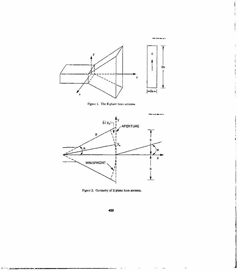
Y

H2a.-]

Figure 1. The E-plane horn antenna.

G~y.)7 y OA&.OWQ Ulz-4r*

•/~APERtTURE

Tb

Figure 2. Geometry of E-plane horn antenna.

459

The maximum power density is

P..-._ If f, E.(x.,,r dSl" (6)- l r 2 ;.2

whicc

S ý area of the aperture,dS = differential area element,

/ - intrinsic ilnpcdancu: of the medium,r = spherical coordinate indicating the distance to the point of observation.

The average power density is the total radiated power for the area of a sphere, 47rr. T-herefore,the average power density can be expressed as

ffIE,(x,,y,)2 d 7

The terIns in Eq. (5) can be replaced by Eqs. (6) and (7) so that the gain beconmes

4 ff, E,(X. , dSI12G -- -I. (8)

F:o)r the aperture distribution of the E-plane horn antenna given in Eq. (4) and the phase constantin Fq. (2), the gain is calculated to be

qI- [c 2Zs() 2(101 (9)b/A

where

and C(p) and S(Is) are Fresnel integrals.

The radiation patterns represent the radiating properties in the rar ficid of an antenna andsic a function of the direction from the antenna. They are the relative intensities of the E and 11Iields nointalized to their maxitnum intensities. The E-field in the E-plane of a rectangularaperture is

Io' the aperture distribution given in Eq. (4), Eq. (11) can be expressed as

460

S1I

Ex jE. c0 0 2, b ejM-e dY, (12)

The integral in Eq. (12) has no closed forin and must bc evaluated by numerical means. Usingnumerical integration, the integral will take thc form of

f b dY, - 2b F(Kbsin6.6) ,(13)

where F(KbsinO,6) is the relative E-Field radiation pattern for the E-plane horn antenna. Agraphical representation of F(KbsinO,6) is shown in Fig. 3.

Thc H-field in the E-plane of a rctlangular aperture is

H,- j '4ml ff E.(X,,Y,) "- d (14)

By substitutiniý the aperture distribution in Eq. (4), the H-field can he expressed as

H, j -1 E. !L- :s 2 -6 4.b C(Rs) - IS(OL cos(KasinO) (57% r 2 IL 2 2 (15))

Thus, wte relative 11-tield pattein is

F(KasinO) - ciA(KasinO) (62 (~ Ka. ýj,1)2 (6'

it

Figure 4 is a graphical representation of the relative Il-field radiation pat tern as a lu nction of thedirection fram the antenna.

GAIN APPROXIMATION

An approach to appioximating the gain can be the ratio of the power radiated by the Li-plane hoin antenna (P,~) to the power radiated by a lossless isotropic antenlna (P1 ); that is.

G'- Pý'1 (17)

with a linear approximation of the Li-plane horn antenna wave front being used to estimate I',.The ratio of P1, and PI: can be derived by letting the magnitude of thelic1-fie~ld strength traim theisotropic antenna (131) equal the magnitude of the E-field streligth from the F-plane horn antenna(4,); that is,

461

L-

s * BO~ Phase Error.64

0.6S0.41

S0.11

0.41

0,1 --

0.0 1. . S.0 4.0 .0 .0 6. 6. 109.0

Figure 3. Relative E-field radiation pattern.

1.02

IE11 - IJE, (18)

For the isotropic antenna, the power density (POI) can be used to relate P, and E, since

(19)

and

"D. (20)

By setting the power density terms equal, El can be expressed as

E . (21)4nr 2

If the intrinsic impedance is replaced by ?I = 120;r = 377 for the far field and consideration isgiven to the isotropic nature of the antenna, the magnitude of the E field strength is

iE . OP (22)r

Figure 5 shows a linear approximation of the E-plane horn antenna wave front that willdivide the wave front and the antenna into two sections, each acting as an independent hornantenna. With the linear approximation, the vertical dimension b can be replaced by

d (-3)

The phase error is zero, and the angular direction away from the antenna is approximately the

angle of the antenna flare.

With the linear approximation, the aperture distribution is

E.(X,,Y) - E. (24)

and from Eq. (11), the E-field is

"E, -2- -!--- -". feo. f:• e 'E, d . (25)Ir 2 -a Y .(5

By solving the integrals in Eq. (25), the E-field can be expressed as

463

Li

y

I Cos C

I E0',- II

d"cosox

Figure 5. Geometry of linear approximation.

E, ,2j cosA ' E d 2a d d siKdsna)] (26);.r 2 1 d2 iair I

Also, if the d term is replaced by its value in Eq. (2•3), the E-field becomes

EEj = 2,/ e- -- E. sin(K b/2tana)] (27).r 2 Cosa I K b/2 tan J

So, from the E-field in Eq. (27), its magnitude can be expressed as

4ab _,E.o, a r2 tac)] (28)Ir cuse ~ 2[K b/2 tance

However, the magnitude of El. is not expressed in terms of P:, and the power density ofone section of the antenna (PDL) will have to be used to telate EL and PE; that is,

E._ (29)

and

464

P,/2 (m)DI 2,ab/cosea

By setting the power density terms equal, E,, can be expressed as

E T| P'i2 COi (31)2ab

By substituting the intrinsic impedance ?I = 120nr = 377 and Eq. (31) into Eq. (28), themagnitude can be expressed as

4,a, 60n P S 2 CC - [sin(K bt2 tana) (32)El ).cosa iab 2 K b,2 tana

With the magnitude of the E-field front the E-plane hiorn antenna in Eq. (32) and themagnitude of the E-field from the lossless isotropic antenna in Eq. (22), the equality set forth inEq. (18) can be completed and will yield

40P oo 4ab P o a s 2 tana) (33)r Ir coa 2ab 2 [ K b112 tana

By squaring both sides of Eq. (33), manipulating the terms, and substituting the value of thephase constant K, the ratio of P, and PE and in turn the approximated gain becomes

Gf= -ý- w 16, a,/. biX co,, .•/2 [sin,• bjM .ana) (34)

Graphical representations of the actual gain and derived gain approximation result- areshown in Figs. 6 and 7, where the vertical aperturt. dimension b/I varies with the horizontalaperture dimension of a/A = 0.5 and an angie flare of a = 5' and a = 10° respectively. Usingthe criterion that the approximated values fall within 3 dB of the calculated values, the resultsshow that the gain approximation holds for an antenna flare angle of less than 100.

RADIATION PAT"ERN APPROXIMATION

As shown in Eq. (16), the H-field radiation pattern in the E-plane is rather simple tocalculate, miaking it nnnecessary to use an approximation to derive it. However, the E-fieldradiation pattern in the E-planc is more complex and requires the use of numerical integration furits cvaluation. From Eq. (13), the actual E-field radiation pattern can be expressed as

F(K•Lino.) - -L f , 'X-r,- Y , (35)

The pattern of the E-plane horn antenna is shown in Fig. 8, and the relative E-field radiationpattern, as a function of direction and phase error, has been shown in Fig. 3.

465

20

I1S

14

9 1 actualC *approximated

61N aA0.505

0.o 1.0 1. , .0 9., 8.0 8.6 4.0 4.4 ,.0 ,., 6.0Vertical Dlmenhlon b/X

Figure 6. Actual gain vs approximated gain--a/.A 0.5, a - 5', b/A , 0.5 to 6.0.

*2

v, Actual

* *ApproxImstedaIX-0.5

'I I 10*0 J

-I

0- . .0 08 ~ 0 8.5 4.0 4.8 5.0 6.4 6.0Vertloal O,,1ienhon biX

Figure 7. Actual gain vs approximated gain--a/A 0.5, a = 10, b/A = 0.5 to 6.0.

S46

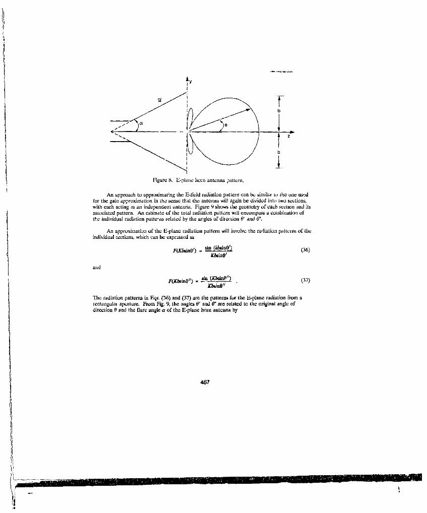
Ab-c

Figure 8. E-plaoe horn antenna pattern.

An approach to approximat-ng the E-field radiation pattern can be similar to the one use:dfor the gain approximation in the sense that the antenna wil! again be divided into two sections,with each acting as an independent antenna. Figure 9 shows the geometry of each section and itsassociated pattern. An estimate of the total radiation pattern will encompass a eombination oftnee individual radiation patterns related by the angles of ditection 0' and 0".

An approximation of the E-plane radiation pattern will involve the radiation pattcrns of theindividual sections, which can be expresscd as

F(Kbsin•') - s (kbalnOt) (36)

K6inO'

and

F(KbsinOV) sin (Kbdnfn" (37)K'inO"

"The radiation patterns in Eqs. (36) and (37) are the patterns for the E-plane radiation from arectangular aperture. From Fig. 9, the angles 0' and 0" are related to the original angle ofdirection 0 and the flare angle a of the E-planc horn antenna by

467

ly

b

Figure 9. Geometry of E-plane radiation pattern approxim•ition

±- - 0 (38)2

and

OU .0 (39)2

The E-plane radiation pattern approximation will combine Eqs. (36) and (37) and caiA beexpressed as

F'(Kbsm8O) Isin(KbsinO') +sin(KbsinOIF) ý40)2[ý Kbbinol KbsinO" I

The final expression in Eq. (40) is actually only half of the sum of the radiation puttrns of thetwo sections becausL Of the overlap between th'm.

Graphical representations of the actaul E-field radiation pattern and the approximatedradiation pattern are shown in Figs. 10 aod 11 fok maximum phase error values of W5*and 60'respectively. Using the criterion that the approximated values fall within 3 dB of the calculatedvalues, the E-field radiation pattern approximation holds until the antenna's phase c~rorapproaches f00.

I468

:l

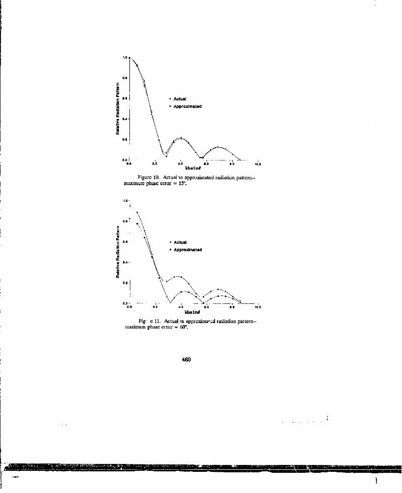
1.0 ".

0.

r* Actual*• - Appro~xmated

W

0*I

0.0 3 -. . .I

0.0 2.0 c.a 8.0 0.0 ¶0.0kbaivu

Figure 10. Actual vs approximated radiation pattern--maximum phase error = 15'.

1.0-i

E0. \v

..c O~ I oActual

* Approximated

0.0 2I.0 4.0 4.0 1.0 10.0

kbzIni

Fig. e 11. Actual vs approximat',d radiation pattern--maximum phase error 60°.

469

CONCLUSIONS

A gain and radiation pattern approximation can be used to avoid the complex mathematicsand computation methods typically involved in calculating the gain and radiation pattcrn. Ahand-held calculator can be used to solve the trigonometric terms in the approximations, while acomputer may be required to calculate the Fresnel integrals in the actual gain equation andperform numerical integration to determine the actual radiation pattern.

When the flare angle of the E-plane horn antenna is less than 10* for typical antennadimensions, the 3-dB criterion for the approximation is met. However, the correlation betweenthe actual and approximated gain falls off quickly when the angle flare is 10" or greater. Whenthe phase error is 15* or less for the antenna, the approximatiorn criterion for the radiationpanttrn is met. Except for the regions around the multiples of r, the approximated radiationpattern holds up well until the phase error is over 60f.

1. Edward A. Wolff, Antenna Analysis, Wiley, Newv York, 1966.

Warren L Stutzman, and Gary A. Thicle, Antenna Theory and Design, Wiley, New f'ork,1981.

3. Richard C. Johns•on and Henry Jasik, eds., Antenna Engineerng Handbook, 2d ed, McGrawHill9 New York, 1984.

4. Paul D. Ewing, Gain andl Eleetric Field Radiation Palter Approxintadon" for thle E-Planeflorn Antenna, ORNIJTM-10983, Oak Ridge National Laboratory, Dcceintcr 1988.

470

"-t---------

FAR-FIELD PATTERNS OF ULTRA HIGH GAIN ANTENNA ARRAYS OF FINITE SIZE

Ross A. Speciale

General Dynamics, Air Defense Systems

P.O. Box 50-800, MZ 601-71, Ontario, CA 91761-1885

ABSTRACT

We are attempting to establish, by rigorous formal andnumerical analysis, the validity of recent claims purporting thepractical feasibility of so-called 'non-diffracting' beams, atessentially any frequency across the elec.tromagnetic spectrum,including microwaves, millimeter waves, infrared and visible light[Ref. 1-4].

Our objective is to determine whether any physicallyrealizable, finite-size planar-aperture distribution can be definedthat can be proved to even only approximate, within some acceptabletolerance, the radiation characteristics of a non-diffracting beam.

Our approach has been to synthesize such a planar aperturedistribution in terms of a vectorial expansion in cylindricalmodes, while imposing the constraint of zero average radial energyflow everywhere in the half space facing the aperture. We showedin a previous paper [Ref. 5] that this condition can be met byproperly choosing the coefficients of the TE and TM components ofthe cylindrical wave spectrum with any given common azimuthal indexLi, and that for every such set of cylindrical modes optimum valuesof the radial and axial wave numbers k, and k, exist, that maximizethe average axial energy flow within any given radius from thecenter of the citcular aperture. The planar aperture distributionso synthesized is very much different from the simple plane-wave,flat-phase distribution that would be suggested by the conventionalwisdom. It is characterized by radial phase alternations,

471

superimposed upon a linear azimuthal phase evolution, and by aposition-dependent axial ratio and ellipticity across the aperture.

So far, however, our analysis has assumed an essentiallyinfinite planar aperture, and the feasibility of generating anyreasonable approximation to a non-diffracting beam has beenstrictly a matter of conjecture, based on the computed highconcentration of rAdiated axial energy flow within relatively smallradii from the aperture center, especially for cylindrical modeswith low azituthal index Z .

We are now attempting to determine the effects on the far-field pattern of truncating the circular aperture to some optimumfinite radius. Our objective is to determine whether an optimumradius exists, and whether some edge-field taper can be definedthat minimize the effects of the truncation of the circularaperture to a finite radius.

The approach followed in this attempt is to compute, bothformally and numerically, an equivalent plane-wave expansionrepresenting the radiated field in the half space facing thetruncated aperture. The main problem to be solved is thedetermination of the radiated field on the plane of the aperture,at larger radii than its physical outer radius. This fringingfield is obviously non-zero, and may depend on the particular shapeof the edge, as well as on the assumed edge-field taper. Planarwave spectra are computed numeriually through a 2D-FFT, as inplanar near-field scanning, without probe pattern correction.Planar wave spectra can also be computed analytically, by usingSommerfeld's integral representation of Bessel functions [Ref. 6).

The obtained far-field patterns are being evaluated againstcomparable Hansen's 'one parameter' circular aperture distributions(Ref. 7], that have been proposed as the best compromise betweendirectivity and sidelobe level.

472

---- ---- ---- ---- ---- ----

REFERENCES

[1] C. W. Oseen,"Die Einsteinsche Nadelstichstrahlung und dieMaxwellschen Gleichungen," Ann. Phys., Vol. 69, pp. 202-204.

(2] J. E. Durnin,"Exact Solutions for Nondiffracting Beams. - I TheScalar Theory," U. Opt. Soc, Am. A, Vol. 4, No. 4, April 1987,pp. 651 - 654.

(3] J. B. Durnin and J. H. Eberly,"Diffraction Free Arrangement,"US Patent No. 4,852,973, August 1, 1989.

14] J E. Durnin, J. J. Miceli, and J. H. Eberly,"Diffraction Free

Beams," J. Opt. Soc. Am. A, Vol. 3, March 1986, p. 128.

[5] R. A. Speciale and Paul F. Wacker,"Ultra High Gain AntennaArrays," 6'h Annual Review of Progress in Applied ComputationalBlectromagnetics, Naval Postgraduate School, Monterey,California, March 19-22, 1990, pp. 241-252.

(6] J. Stratton,"Electromagnetic Theory," McGraw-Hill, New York,1941, pp. 364-369.

(7] R. C. Hansen,"A One-Parameter Circular Aperture Distributionwith Narrow Beamwidth and Low Sidelobes," IEEE Trans. onAntenna and Propagation, July 1976, pp. 477-480.

473

SESSION 12- "NEC ANTENNA ANALYSIS"Moderator: Peter Excoll

MODELING A SHIPBOARD FAN ANTENNA

Lance KoyaniaCode 824

Naval Ocean Systems CenterSan Diego, CA 92152

Abstract

In the frequency range for which US Navy shipboard fan antennas are designed, 2-6MHz, the whole ship is hi fact the antenna. This makes for a very large and complex numericalmodeling problem. This paper describes an effort concentrated on a destroyer, the Spruance(DD-963), for which NOSC has a 1/48 scale brass model to make measurements on forcomparison with the c~leulations. The antenna characteristics used for judging thc accuracy ofthe numerical model with regardn to measured data were the feodpoint impedance and thevoltage across the insulator at the apex of the fan.

NIEC-3-VLF was used on a 719 segment model. To make a good comparison betweenmeasuied and calculated data, the code was run for 51 frequencies between 1.5 and 6.5 M-Iz.The computer used was a Convex C210 which has close to the peiformance of a single processoron the Cray X/MP-48. The code was compiled to take advantage of the vector architecture ofthe Convex and its 64 bit word size.

There was a very good match between the antenna characteristics of the numerical mod,and the measurements from the brass model, showing NEC to be a viable tool foi modeling acomplex structure with reasonable engineering effort artd use of computer resources.

Introductiou

At the NOSC Model Range, the capability exists to build both computer and physicalmodels to duplicate the electromagneic behavior of full scale ships. The models provide arelatively convenient, economical, and timely means of evaluating various antennaconfigurations. When practical, the model data is validated against measurements on board theactual ship.

Presently NEC-3-VLF is used on the NOSC Convex C210 computer for the numericalmodels. The Convex has close to the performance of a single processor on the Cray XtMP-48.The code was compiled to take advantage of the vector architecture of the Convex and its 64 bitword size.

The physical models are 1/48 scale brass models. NOSC has a model for every shipclass in the US Navy. Measurements were taken two different ways for the purposes of thisstudy: (1) in the frequency domain, using a network analyzer and (2) in the time domain, usinga pulser to get the impulse response which is subsequently converted to the frequency domain."The signal above noise ratio is about the same for the two methods. The frequency domainmeasurements have superior frequency resolution in the present NOSC equipment. The timedo,'-ain measurement airn inherently more immune to background transients but these are usuallyreadrii' recognizable in the frequency domain measurements so that data can be retaken if

474

necessary.The object of this modeling study was the fan antenna on the destroyer, USS Spruance

(DD-963), pictured in figure I below.

Figure 1 DD-963, USS Spnzance

As seen in the figure, the fan extends from the forward mast aftward. A typical configurationof a fan antenna is shown in figure 2. The fan as used on the DD-963 is shown in figure 3.This configuration is called a twin fan. There is a single feed at the top feeding two fans thatterminate down into the two apex insulators. Because of the frequency range for which thisantenna is used, 2-6 MHz, cssetiafly the whole ship becomes the radiator; making the modelingtask very large and complex.

The antenna characteristics used for judging the accuracy of the numerical model withregards to the physical miodel were the fecdpoint impedance .Ad the voltage across the insulatorat the apex of the fan. Plans arc under way to also conduct these measurements on board theactual ship.

NEC Model

As a matter of course, the brass models are constructed to very fine detail. Because ofthe complexity of a ship and computer run time and cost constraints, a numerical model cannothope to achieve the same detail. Keeping in mind the areas of the ship that would make themost electrical difference and the electrical length of all objects, an optimized model can beconstructed that would not severely tax computer time and costs.

A long term goal of this project was to hone the skills needed to create an optimizedmodel of a complex ship so that in the future, should measurement data not be so easilyavailable, the numerical modeling effort can be done with more confidence. For this project,reliable impedance data was obtained from the brass model so the object of the NFC modelconstruction was to match this data.

Although the superstructure of the ship modeled contains large amounts of plate steelconducive to modeling with patches, the topside of the ship is full of poles and wires conduciveto modeling with wires. An all-wire model approach was chosen for th," better accuracy andease of modeling.

Because of the complex topside, creating a regular grid to represent surfaces would leadto using more wires than necessary. It is more efficient to use the junctions of *wire" typestructures to surfaces as the intersection points of a grid. Additional intersection points withinthe surface can be added to make the cell sizes as desired, A disadvantage of the irregular

475

gridding is the difficulty in complying with the "diameter of wire equal to sqparation of wires'rule for representing surfaces with wires.

38 versions of the model were run in seeking to optimize the model, the later Versiorun at 51 different frequencies between 1.5 and 6.5 MHz. The final model contains 719segments and took 143 minutes of CPU time to run the 51 frequencies. Figure 4 shows themodel ard figure 5 shows two views of the fan antenna with parts of the supporting maststructure.

Some of the lessons learned in the optimization process are as follows:

* For the frequency range of interest. 1.5-6 MHz, 0.1 meter accuracy inspecifying wire length was sufficient.

* The distance between the top part of the fan (where it is fed) and the yardarmfrom which it is hung did not manm much of a difference.

4 The excitation segment joins the top part of the mast structure to the four feedwires of the fan. Its length is critical. Making it shorter made the antennaimpedance more capacitive.

a Slight changes in dte length of the apex insulators did not result in significantchanges in the fcedpoint impedance although the voltage across the insulators didchange noticeably.

a With the vertical and horizontal members of the mast structure defined, addingcross members made little difference.

* To find out what parts of the ship were most important in attaining a correctimpedance for the fan antenna, a test was run. The wire radii of the model wasreduced to about 1/50 of the actual value for each part of the ship. Then singlyand in combinations, the wire radius of various parts of the ship were increasedup to the actual value. Although the impedance of the reduced radii model wasway off the correct impedance, no single part of the ship proved to be the majorcontributor to attaining the correct impedance. Listed below is the approximatedecreasing order of impoitanct of various parts of the ship to the fan anteamimpedance.

Part of Ship Area of Smith Chart ImpedanceImproved by Correcting Wire Radius

Fan feed Highest frequenciesForward mast Lower frquenciesSuperstructure and deckhouses Lower frequenciesFan Wires Higher frequenciesAft mast Little differenceAll whips Little difference

476

Results

1. Impedance

The Smith chart comparison of the frequency domain measurement data and the NECdata are shown in figure 6. The resistances and reactances for these two data sources plus thetime domain measurement data are shown in figure 7. There is good agreement except atapproximately 3.2 and 3.6 MHz where the peaks are of different magnitude. This is the areaof first anti-resonance.

2. Apex insulator voltage

Since NEC dues not give voltage information except for the voltage across a source, thevoltage across an insulator is obtained by substituting a very high resistance for the insulator andmeasuring the current through it, then applying Ohm's law. From brass model measurements,the maximum magnitude of the impedance measured at the apex insulators is approximately4,000 ohms, so a resistance of I Gigohm was used for the insulator. This was judged highenough so as not to disturb any other electrical parameter.

The NEC calculated voltage across the insulators was highly sensitive to the length usedfor the insulators even though the feedpoint impedance showed little change. The length usedon the brass model was the equivalent of about 1 m. Three lengths were tried with NEC: 1.0m, 1.5 m, and an insulator length of 0.15 m attached to a conductive length of 0.85 m. TheNEC voltages of all three lengths are shown in figures 8 (port apex) and 9 (starboard apex).As can be seen, the voltage for an insulator length of 1.5 meters falls between that for insulatorlengths of 1 meter and 0.15 meters on the port side but the 1.5 meter data is close to the 0.15meter data for the starboard insulator.

To try to get a better feel of the effectof the insulator length on the fan antenna, atest fan was constructed, pictured in figure10 to the right. It is just a simple structureto simulate a mast (segments 1-10), afeedpoint (segment 11), a single wire *fan*(segments 12-20), and an insulator (segments21, 22). The dimensions approximate the fanunder study. The following insulator lengths .were tried:

1. 2. m insulator to ground2. 1 m insulator to ground

g. r.5 m insulator to ground3. 1 in insulator to ground4. 0.5 mn insulator to ground5. 0.5 m insulator to a 0.5 m post toground 77-6. 0.15 m insulator to a .85 m post 1 Te Modelto ground

477

_ _ _ _ _ _ _ _ _ I

The feedpoint r..sistances and reactances, and the insulator voltages are shown in figure 11.The currents for the various segments for N lious frequencies are shown in figure 12. As canbe seen, the feedpoint impedance is rather insensitive to the insulator lengths. The voltageacross the insulator is very dependent on the length but not in a very predictablt way.

The determination of the effective length of an insulator on a scale model is difficult dueto the relative size of the test leads involved in waking a voltage measurement. Thus, anarbitrary length was chosen for the NEC model and just the shapes of the frequency responseswere compared between the NEC model and the brass model. This is a reasonable method ofcomparison since in the NEC calculations for both the DD-963 model and the test model, theshape of the frequency response did not change with insulator length.

The voltages from the brass model time domain and frequency domain data, and the NECmodel data are shown in figures 13 (port apex) and 14 (starboard apex). The time domaindata, due to equipment limitations, has coarser frequency increments than the other two, andbecause of the greater amount of processing involved to present data in the frequency donuin,is more uneven. The frequency domain data though, matches quite nicely with the NECprediction except for some constant factor which could probably be attributed to differences inthe length of the insulator. What was especially gratifying though, was the similarity in shapeseven in the 3.2 to 3.6 MHz region (the anti-resonance region) where the impedance data differedgreatly between NEC and the frequency domain measurements. Apparently the voltage at theapex insulator is insensitive to the feedpoint impedance, at least in the anti-resonance region.

Conclusions

' The very complex geometry of a fan antenna on board a destroyer type ship can be accuratelyrepresented by a numedicl model with a reasonable use of computer resources.

* Comparing data with a very accurate 1/48 scale brass model, the NEC model showed a veryclose match in feedpoint impedance except for first anti-resonance.

0 Although the magnitude of the voltage across the apex insulators differed between the twomodels, the shape of tie frequency response was close.

478

r- UAICW INCTWORKE£NL.OSURC (4rpfoUl)

SH4OCK ;...ULATO (VYp)

FUDWWC (TYPI

N ~APEX INu;AMAom (TYPJ

Figure 2. Fan Antenna, Trypical Configuration

I -. • .nfealo Fire Hira r,1r'

Figure 3. Fan Antenna on the DD-963, Smtarbod and Top Views

479

L _

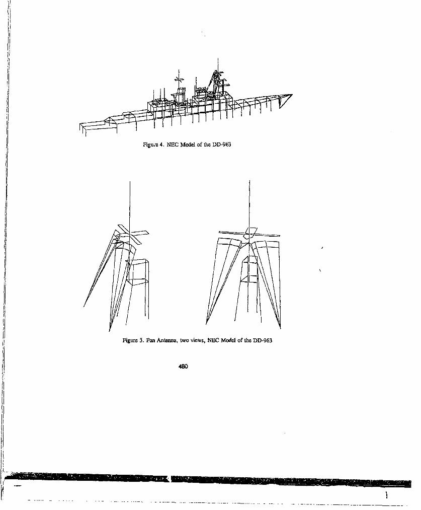
Figu,'e 4. NEC Model of the DD-963

7E:Figure 5. Fan Antenna, two views, NEC Model of the DD-963

480

S. . . .. . . .. . . .. . . . ... . .. . ... . .. . . . . .. .. . . . . .. . . . .. . . .. . . . . . . .

VU

InI

481

Resistance at Feedpoint

2.5 - r5fC oflf emcln

E' L5 00000 NEC CLO n Momumnif-xI l.c* TncDominuoMuuauswent

2.0CI

Ai

9~91I)o4Ix 1.5 -

I.0• -

7b

0.0 -

1.0 1.5 2.0 2.5 3.0 3.s 4.0 4.5 5.0 5., 6.0 6.,Frequency (MHz)

,.,5 -Reactance at Fcedpoint

1. -P

, 0.0U

S_____ FraquenVy Domain Meassuremrnt"- -- O0004 NEC CAlculation

Tit" ObnII Miasurellmint-2.0-

1.n 1.5 2.01 2.5 3,0 3.5 L.0 4.b 5.0 5.5 6.0 6.5Frequency (Pk.iz)

Figure 7. Model Impedance Summary, ResaiMance and Relctance

482

1f,

IT>.

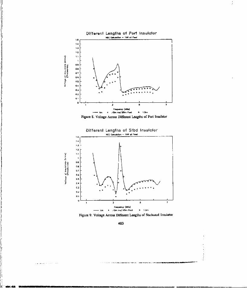
Different Lengths of Port Insulator.5. C CoicutII.. - lkW at Feed

1,5

1.4

1.2

0.9

v vi

4 0, L+ +4+0,.I.2[ + +o00.2

1 3 5 7

Freqeny (M-W- In.+ Ibr Ins/,m P..t 0 1.3,

Figure 8. Voltage Across Different Lengths of Port Insulator

Different Lengths of Stbd InsulatorNEC Cokuleion -- akW rt Fed

1.4

1.3 0

1.2

I.:0.9.,u uza

0- 0.7

o 0.7 4U5.

o 0.45

0.4 +0.3- 4 4+÷

0 1 +q•

V-eaqumy (MHz)- m -+ Ism6 1s/.r5m Po2t 0 t. rn

Figure 9. Voltage Across Different Lzngths of Starboard Insulator

483

.-0 - , -. ,..evl-uR~lf6t

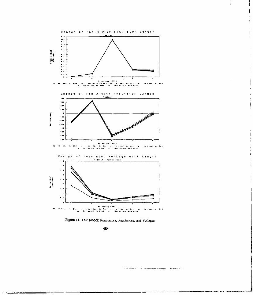
Change of Fan A wit h I nsul ator Length

a e. S* t * .. * *

Chaange of Fan X wI t h In ul ator Langth

C Ita n ye o f I S u I atoL j VI 0 1 09 w, I tL v L~'u It

tb CL.d A L UUUL.±i3Uw =,C3 Kcat 5 lCes, and Voltages

484

e - - ----- --- __ie___

Cham a 94of I it h I fit 1 *got| k 2 MdHz CChu, *f I w1th I. 18. 0la1oh - 3 MHz

Chamga of I with w.ool laIght - M MiIiz Chai4i of c i1k 1ih s.l 1glol b 5 Mli

Chang, of I ,Ith local 1aug11 h Miii

Figure 12. Test Model: Segment Cunect

485

2000- Voltage at Port Apex Insulator - I kW at Feed

Frequency Domuin Measurement- NEC Colculotion

w- Time Dornuin Meou,+urununt1500-

1000-

u~•u

A

2 3 4 5 U 7Frequency (MNlz)

Figure 13. Port Insulator Voltages: Timc Domain IRange, Frequency Domain Range, NEC

2000- Voltage at Sturbocrd Apex Insulator - I kW at Fieed

F 'requency DOumun Muosuremento.*o.- NIC Calculuhon

i- H lirilc D linuni M(;wuwbul tciiw1

1500 >i500 I

I'b

Frequency (MHz)

1486

Optimiizing Sidelobe Levels of anl Array Using NEC

Randy L. Ilampt and Christopher J1. McCormasckD~epartmesnt of Electrical Lngineering

Uzsitotl States Air Force Academny, CO 80840

Warren F. Beandow Inl82nd YIW 98 k-rS

Williamsn A11I1, AZ 85240

Abstract.This paper describes how to use NEC (Numierical Eleetroniagntetica Code) to uptiminie the

bidelube levels of anj array with Unifortiily spaiced center eleincnts and nonutniformaly spared edgeceleients.

Iultrodusctiou.Low siclelobec array 8yvithiesis genierates; a current taper through anialytical or onumerical

optimization of thme array factor. Applying the symitlesized taper (e.g. Chmebychiev, binomaial, etc.) to antaotemnua array (hoes not produce the desired result, because mnutual couplinig is not, accounted for Inl thetheory. It is possible to optimize the array pattermi by includitig miutual couplinmg at the expense ofdramatically increasing the computationi time imeded ill the sy'nthesis processa.

We set out to investigate the possibility of opt~~imizingK the vimirlobe levels of' slimahi arrays ofdipoles using NlCh (Numnerical L'lectrummmaguctict; Code) [1]. Our prhmaary imiteremit is lin partialammplltude tapering amnd partial noiumiforum spahing of the array elemments. Thisý paper describes how weuse NEC in conjunction with an optimization omethod to optimize tiie sp~acimig of thle edge clenments ofsmail arrays of colinear dipoles to obtain tile lowest posible sideiuobe levels.

Optmnxisation Using NEC on & VAX Coomputer.Our plan of nttack for syndiesizimig a low sidelolbe array is to begimi with au array of equally

spaced colinear dipoli s, timen nomuifurmmly space time outer elements, while keepinig the hinner e~lemienitsuniformly spsaced (Figure 1). Tlhe array lies alomig tie x-axlu and is symmmetric about its physicalceniter, There are 2 1' uniformily spaced elemients in the center a~d M clemments onl either edge of thearray. The goal of the opt~imizationm jrocms is to adjust time spacing of the oitter 2M elememnts toproduce the lowest possible sidelube level.

Time first step, In the problcem Is to change the constrained optimmization problem into almunconstrained problem,. Itatlici than optilnizimig onl the elemenct spacimig witll constraintsj (suchl as

x(i4-l)>x(i), anl outer eleminemt is farther from the ceniter array than an hinner element)1, the programiioptimizes aim anl unconst~ralned parameter, -t, where

= o42 ) 4 d) ]

wherex.(i), x(i-i 1) = distance of elements I and ii-l fromn the center of thme arrayd =distance between uniformly spaced elements

'Fle next stLep is to chiimem anl optimiization subroutine. We used lthe downhill simmplex andP'owell's method fromt Nunmerical iteciprm [2]. Bloth routines produced satisifactory results.

487

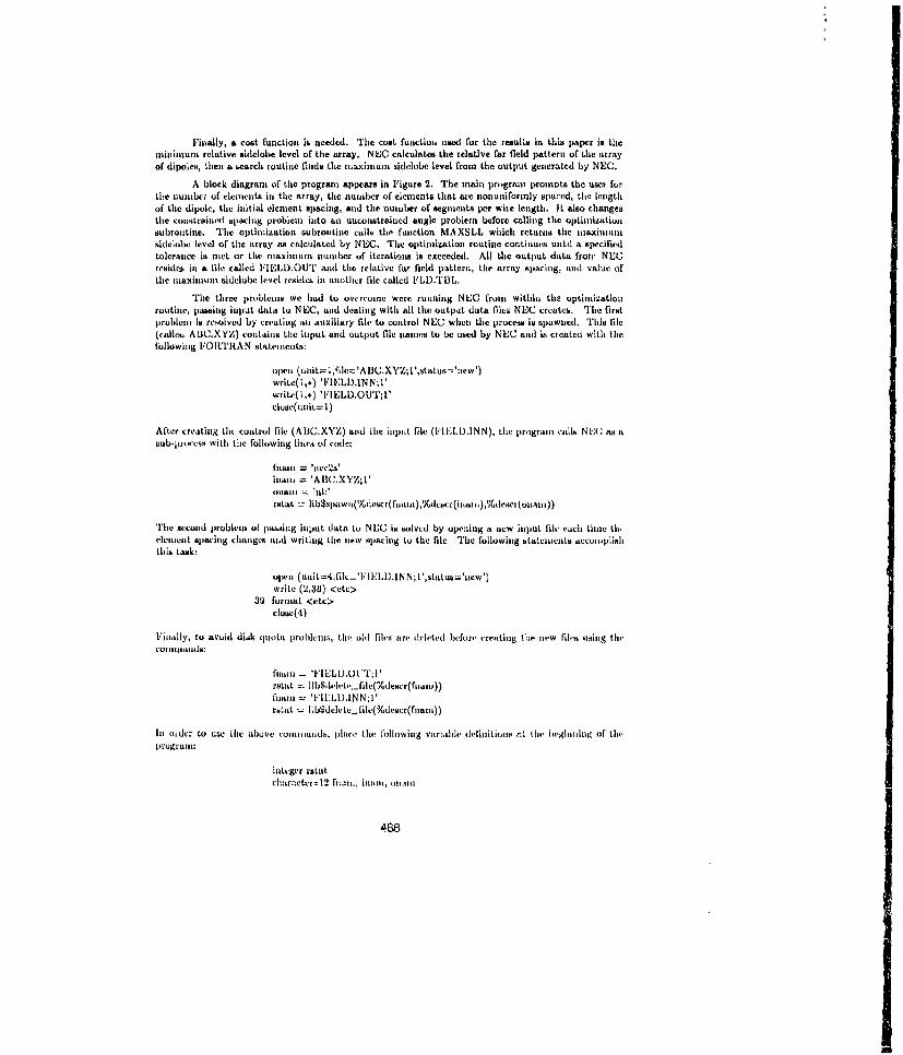
Finally, a cost function it. needed. The cost function used for the result in this paper is theminimum relative sidelobe level of the array. NEC calculates the relative far field pattern of the arrayof dipoles, then a search routine rinds the maximum sidelobe level from the output generated by NEC.

A block diagram of the program appears in Figure 2. The main program prompts the user forthle minbce of elements it, the array, the number of elements that are nonuniformly spaced, the lengthof the dipole, the initial element spacing, and the number of segments per wire length. It also changesthe constrained spacing problem into an unconstrainted angle problerm before calling the optimizationsubroutine. The optimization subroutine calls the function MAXSLL which returns the niaximunisidelobe level or the array as calculated by NEC. The optimization routine continues until a specifiedtolerance is met or the niaximuan number of iterations is exceeded. All the output data frou' NECresides hi a file called FIELD.OUT antd the relative far field pattern, the array spacing, acd value ofthe maxianum bidelube level resides in another file called FLD.TBL.

The three problems we had to overcome were running NEC froan within the optimizationroutine, passing input data to NEC, cud dealing with all the output data filex NEC creates. The firstproblenm is resolved by creating alt auxiliary file to control NEC wheat the process is spawned. Thlis file(callco ABtI.XYZ) contains the input and output file natnes to be used by NEC and in created with thefollowing FOItTItAN statemments:

ujwen (untit~= 1 ,flh:='A IIC.XYZ; t',status='mmew')write(l,s) 'FIELIOINN;I'write(I,*) 'I"IELD.OUT; l'

cluse(tmliit=l)

After creating tht control file (ABC.XYYZ) arid time input rile ("IELD.INN), tlme prograin calls NECG asub-pr4wesss wit[h the following hin's Of e'(KIe:

fninat 'itcer2s'inami = 'Alk.XYZ;l'

rsata ibgslpaWt(%deser( fntana),%dcscr(imlta;) ,%tlese'r(onatatt))

The second problem of pawsing input data to NEC Is solved by opening a new input file cacti time th,element spacing changes and writing the new spacing tu the file T'he following statemcnts accoumplishthis task:

olstt (utit.=4,filc-'eVIELU.INN; l',sLtatus='ttew')write (2,30) <etc>

39 foritat <Cetc>cloue(4)

Finally, to avoid disk qutmtaU probhlvs, tm e oldm files are ticletd lx'fmWre creating tlh.e maw fim's using it'-Commainsds:

firesma -• 'I"I ELIJO LII'; Iratat hFilmDmat1T'.file(%deacr(faan))

fmnacr ''I"I.ILINN;:1rsLat libgdclet..lailc(%descr(fmtanat))

It sider to use tie abuve ciuimmad, place th,' fulalwhig vtriabl, defimitions ., tile isgimaming, of tilt'ja mugrua II:

integer ratatclmurmactur12 fmmamtm inmtil, mnmmtlIm

488

ResuLits.

We first investigated optimizing an array factor of 8 isotropic elements with N=2 and M=2 (4uniformly spaced elements in the center and 2 nonunifornily spaced on each and of the array). Thismodel does not include mutual coupling and results in & -5.37 dB decrease In the maximum sidelobelevel with center elements op"ce .5A. apart while the two edge eloments are spacacd .69A. and .72A apart.Optimizing a NEC A./4 colinear dipole array model that do"s include mutual coupling results in a -3.9dlB decrease in the maximnum sidelobe level with center elements space .5A. apart while the two edgeelemeuts are spaced .54A. and .57A. &part. Thus, a small perturbati- to two edge elements on each endof the array results in anl almost 4 dli decrease in the sidelobe 1ev .&. The NEC results are considerablydifferent from the array factor results. Figure 3 shows tht resulting far field pattern calculated by NECfor the nonunifornily spaced array.

The next examples are for 12 elemient arrays of .474A. colinear dipoles. Figure 4 is the far fieldpattern resulting from an array with the center 10 elements spaced AA) apart and the edge elementseparated from the next elemrent by 1.11A.. The maximum relative sidelobe level is -11S.42, which Is2.32 dli less than the maximumi sideleloos level of a 12 element armsy with a spacing between elements of.6A.. Figure 5 is the far field pattern resulting from an array with the center 10 elements spaced .JAapart and the edge element separated fromn the next element by 1.21A.. The maximum relative sidelohelevel is -15.42, which in 2 65 dB3 less than the miaximnum aldelobe level of a 12 element array with aspacing between elements of In..lcreasing the uniform spacing from A6) to JA) decreases tile relativesidelube level a small amount.

Figure 6 shows the optimized far field pattern for a 12 element array of colinear .474A. dipoleswith a uniform spacing of J.7.. In this calse, N=3 and M=3. lnrem-Aing the number of nonunifornilyspaced elemrents does not necessarily help reduce the mnaximumm sidelobe level of time array.

UoC~AMIoAMS.NEC pruivides a useful tool for the hivestigation of airray opthiization. We have shown that

time sidelobes of small arrays of colinear dipoles may be lowered by nonuniforinly spacing the edgeehlements. Mutual Coupling plays all important role in determining the spaicing of the elements and thelowest possible sideluibe level.

Ildefer.acsj!] G. Jl. Bumrke anid A. J. Iloggiu, 'Numaerical Electromnagnetica Code (NEC) - Mlethod uf Munriemmts,*Lawrence Livermore Nationmal Laboratory, Domumment UCIMI,.0500.(2] W. 11. Preiss, et~A., Numrnaicial Recipes. New York: Cambridge University Press, 198t1.

489

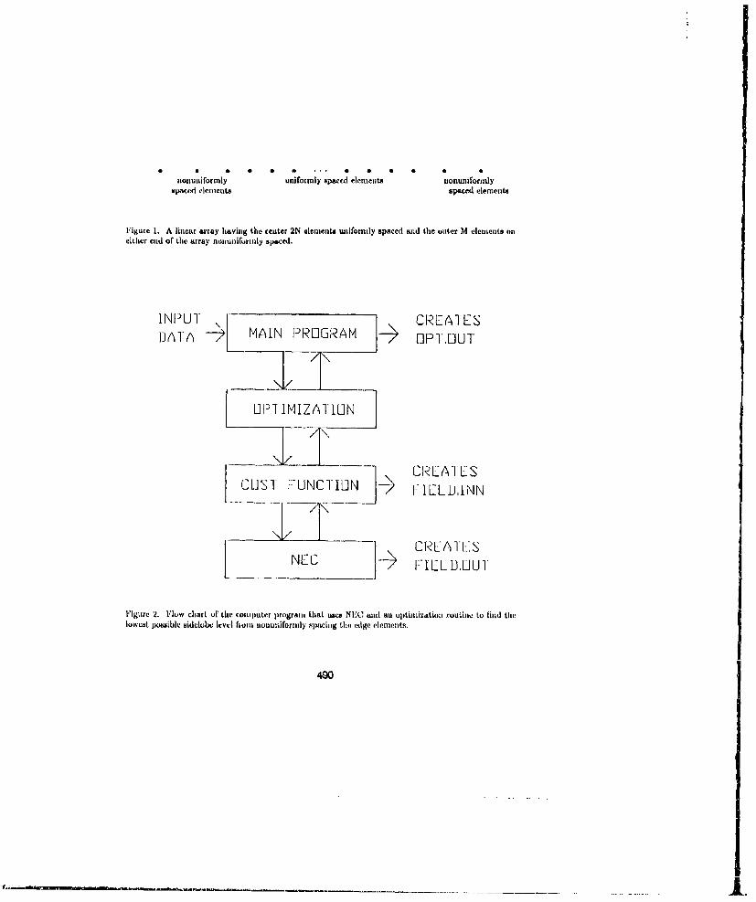
"Onalotnanfo y uniformnly spaced elements :ionuniformlyspaced elements spaced elements

Figure 1. A linear array having the center 2N elements uniformly spaced and the outer M elements oneither end of the array nununifurinly spaced.

INPUT -CRLATES

]ATfA MAIN PRUGRAM + [PI',IUT

_I L\IP1 IMIZATILIN

ZCAIIL E

CUIST FUNCTIL]N FIELD.,INN

T CR[ATLSNEC FILL1,L0UT

Figure 2. Flow chart of the computer program that uses NEM aid an optiimization routlhw to find the

lowest lxx~iblc Bideblul level Iloin 1lu-11ifo illy fpaIcig the edge elements.

490

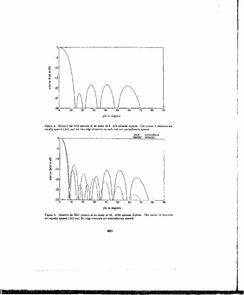
.5

w -10

.15

.25

- 10 20 30 40 50 60 70 80 90

phi in degrces

Figure 3. Relative far field patteru of an array of 8 A/4 coli3ear dipoles. The center 4 elements areequally spaced (.5A) and the twu edge elements on each end are tionuniformly spaced.

solid nonuniform0 dushed uniform

.5

3 -10

-15 \2! -20 \I

.30 - ~ ! i I0 10 20 30 40 50 60 70 80 90

phi in degrees

Figure 4. Relative far field pattern of an array of 12, .474A colinewr dipoles. The center 10 eleinentsare equally spaced (.6U,) and the edge elements are nonuniformly spaced.

491

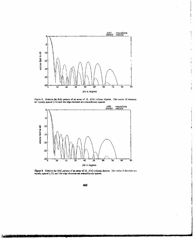
solid nonuniformdashed uniform

2-s

m -10

-3% 10 20 30 40 50 60 70 80 90

phi in degrees

Figmre 5. Relative far field pattern of an array of 12, .474A colinear dipoles. The center 10 elementsare equally spaced (.7A) and the edge element, are nonuniformly spaced.

3olid nonunifcrmdashed uniform

-5

( -10

" -20-r

.25 ' ,

-30- ...10 20 30 40 50 60 70 80 90

phi in degrecs

Figure 6. Relative far field pattern of an amay of 12, .474A coliner dipoles. The center 6 elements areequally spaced (.7A) and the edge elementa awe abamiformly spaced.

4W2

USING THE NUMERICAL ELECTROMAGNETICSCODE (NEC) TO CALCULATE MAGNETIC

FIELD STRENGTH CLOSE TO ASOMMERFELD GROUND

G.R. Haack

Microwave Radar Divisionsurveillance Research Laboratory

Defence Science andTechnology Organisation

PO Box 1650Salisbury

South Australia 5108AUSTRALIA

A H.J. Fleming

Electromagnetic Compatibility SectionTelecom Australia

Research Laboratories770 Blackbarn Road

ClaytonVictoria 3168

AUSTRALIA

ABSTRAQ

This paper presents the results of calculations using theNumerical Electromignetics Codes (NEC) for problemsinvolving horizontal dipoles near the interface betweentwo semi-infinite half spaces. The examples chosendemonstrate difficulties which may occur in thecalculation of magnetic fields in the near field region.The reasons for these difficulties are discussed andm thods for correcting them are suggested.

493

1. INTRODUCTION

In a previous paper, [1], problems in calculating the nearmagnetic fields of a horizontal dipole above a lossyground and in free space, were investigated. Threedistinct types of errors were discovered by comparingnumerical results obtained using NEC-2 and NEC-3 withexperimental results for the centre-fed dipole shown inFigure 1, operating at frequencies of 1.2, 10 and 20 MHz.These frequencies were choseg to demonstrate effectsranging from near resonance to electrically small.

The errors found for this problem were,

(1) At all frequencies NEC-3 over estimated the H-fields very close to the interface by a very largefactor, while NEC-2 gave more reasonable results;

(2) Both NEC-2 and NEC-3 gave erroneous results at1.2 MHz over the entire rangp of heights aboveground examined in that thc measured resultsvaried almost linearly with height while thecomputed results resembled an S-bend, Figure 2;

(3) NEC-3, and upon closer examination NEC-2 also,gave a 'saw-tooth' type ripple at cartain discreteheights; this effect was greatest at 10 Mi2z, whilethe results also indicated at least one singlesaw-tooth at 1.2 MHz. (see Figures 2 and 3).

The reason for the errzoneous results close to theinterface when using NEC-3 is explained in (2]. When theSommerfeld integral option is used, NEC calculates thenear-magnetic field by numerically evaluating the curl ofthe electric field by a six-point central differenceformula. The increment size used in the finite differenceevaluation is 10- 3 1A±i to each side of the specified pointfor evaluation of the field in thu upper (+) or lower (-)medium. Hence the magnetic field will generally beinaccurate within this distance from the interface sincethe vertical component of the electric field isdiscontinuous across the interface. The same method isused in NEC-2, however it has been found that thecalculated vertical component of the electric field iscontinuous across the interface and the resulting magneticfield near the interface is approximately correct. Itshould be noted that NEC-2 does not calculate the correctelectric fields below the air-ground interface. Amodified finite difference scheme which corrects theproblem when using NEC-3 will be presented elsewhere.

Accounting for error types (2) and (3) requiresexamination of both the truncation errors associated withthe 6-point finite difference (FD) scheme employed insubroutine NHFLD, and the errors, includind round-off, inboth the overall moment method calculation of the E-fieldsand the differencing of these E-fields to form the curlfrom which the H-fields are then derived.

494

I

II

____________ _________________

In principle it should be possible to reduce the errors oftype (2) by using a smaller increment size A, for the FDcalculations as outlined in (1]). The success of thisapproach will depend on the accuracy of the calculated E-fields and round-off errorrs in computing the FDcomponents. An example where this approach has been usedsuccessfully is the horizontal dipole problem in Figure 1,where an increment size of 10 4 was required to obtainaccurate i.esults at a frequency of 1.2 MHz. In other morerecent problems it has been found that even smallerincrements of the order of 10-81 must be used to obtainaccurate results. This was the case for a horizontaldipole in a medium such as sea water at very lowfrequencies where it is found that the near fields decayrapidly with height above the interface.

Rather than simply reducing A to minimize the type (2)errors, higher order FU schemes that have smallertruncation errors may also be used. Perhaps an even bettersolution would be an adaptive algorithm whichautomatically selects the appropriate increment size forany given problem by examining the convergence of the H-field solution as A and the order of the FD scheme arechanged.

Trying to understand the reasons for the saw-tooth (type(3)) errors, and additionally ways to overcome them was adifficult task which involved a detailed examination ofthe sources of errors in numerically computing H-fields byFD approximations to the curl of the E-field, andnlternative methods of formulating the li-field solution.

It will be shown in the following that for the horizontaldipole problem of Figure 1, errors due to the FD curlapproximation used in NEC are primarily due to thecomponents of the E-fields which mathematically shouldhave a zero curl component, while the numericalapproximation is non-zero.

2. CALCULATION 010 NEAR-MAGNETIC FIELDS BY rINITZ-DIFFERENCE APPROXIMATION

It is well known that in a uniform homogeneous medium themagnetic field is related to the electric field by thefollowing,

-V(1)

For problems involving wire antennas in the presence of animperfect ground, NEC calculates the Electric fields bynumerically solving the Soummerfeld integrals. However, asdiscussed above, the near magnetic fields are obtained byusing a finite-difference approximation of the curl of theelectric field. Hence the accuracy of the magnetic fieldscalculated by this method will generally be one order ofmagnitude worse than the electric field since the formerrequires differences of r-^ntitius which themselves are

495

not exact.

Under certain conditions it has been found that thecalculation of the magnetic fields by this method can bean ill-conditioned problem. ThJs is illustrated by thecase of a horizontal dipole shuwn in Figure 1. It wasfound that NEC-2 and NEC-3 gave similar, but not identicalresults. The main differences are that NEC-3 predicts amagnetic field which oscillates in magnitude as a functionof height up to about 6.0 m, whereas NFC-2 produced asmooth curve, Thic is particlarly evident in Figures 3which is for a frequency of l0MUz, although it is alsopresent in Figure 2, but not as pronounced.

When [11 was prepared, the reasons for this behaviour werenot understood, however, subsequent investigations by thepresent authors have revealed the nature of the problem.While NEC-2 and NEC-3 do not use identical methods fornumerical evaluating the electric fields via theSommerfeld integrals, [3), L4 ], comparison of thecalculated E- fields over the range of heights shown inFigures 2 and 3 show that the two codes give values whichgenerally agree to within about 3 significant figures.The differonces between the calculated H- fields howeveris obviously much greater. At some points the differencesare of the order of several dB. While in practical termserrors of this magnitude may not be significant, thepurist demands an explanation.

On closer examination of the results in Figure 2, it wasfound that if smaller increment sizes are used in thefinite-difference curl approximation with NEC-3, that thesmooth ripple at a height of approximately 2.3 m changesto a sudden step over a distance comparable to theincrement size. This effect was not noticeable using NEC-2, although for smaller increment sizes the results becomeinaccurate as demonstrated by random variations in thecomputed H-fields. (Note that both NEC-2 and NEC-3 usedhere use double prGcision as single precision was found tobe inadequate for these problems).

Closei examination of the finite-difference components ofthe H-field in the region of interest revealed that th%.contributions due to the E. and E, fields were similar inmagnitude, but the phase difference was very close to1800. Hence in this region, even though the L-fields fromNZC-2 and NEC-3 are very similar the differences in thecomputed a-fields are magnified by the near cancellationof the curl components of E, and E,. (Note that for pointsin the vertical plane containing the dipole, E is zero andits derivative is also zero as this is a plane symmetryfor E , and hence this component of the E--field does notcontribute to the H, field).

A further difficulty in the region near x - 6.0 m and z2.3 m is that the magnitudes of both E. and E, are nuar amaximum and the derivatives in the curl expression aresmall.

496

In an attempt to alleviate the numerical problem ofcancellation in the curl approximation, instead of usingfinite-differences in the x and z directions, differencesin plane rotated 450 about the y-axis were tried, however,the problem with NEC-3 is not changed significantly. Ananalysis of the Loasons for the difficulties encounteredfor this dipola problem follows.

3. IRROR ANALYSIS OF FINITE-DIFFERENCE APPROXIMATION

To understand the nature of problems which may arise inapproximating the curl function by finite differences,alternative formulations of the H- field solution ofManwell's equation are examined. One method commonly usedto obtain the electric and magnetic fields due to currentsand charges is in terms of vector and scalar potentialline A and 0 [5]. The solutions are of the form

Y= Vo--jwd (2)

jiY v,gd (3)JA JA

From the vector identity VxV%-0, [41 it is readily shownthat (3) is mathematically identical to (1). Tho successor otherwise of finite difference methods fur obtainingthe H-field from the E-field via the curl relationshipwill depend on the relative magnitudes of the two terms onthe RHS ot (2) and the magnitudes of the curl of theseterms. For example, if the magnitude of VW is much largurthan jwX or the sum of the terms Is much smaller thaneither of the two terms we might expect that finitedifference techniques would be inaccurate, particularlywhen the E-fields are not exact as in the case of NECcalculations. Indeed the latter is the situation in thevicinity of the troublesome region referred to in theprevious sectioni

While there is no simple method of separating the VO andJwA in the El-field calculated by NEC, the previousstatement can be verified by examining an alternativesolution for the fields of a horizontal dipole above aconducting ground. Bannister, (6], has given image-theoryexpressions for the quasi-static fields of infinitesimaland finite-length dipoles at or above the earth's surface.This image theory approximation is strictly valid forfield points somewhat greater than the skin depth from theordinary mirror image of the source, although in manycases the approximation is valid throughout the quasi-static range, i.e. distances much less than the wavelengthin air. In Bannister's expressions it is also assumedthat displacement currents in the giound are negligiblecompared with the conduction currents. i.e. for thegroundiFor the horizontal dipole problem considered previously,with er 1 0 , oa-.Olla/sr, at 1.2 MHz we find jo/w-i65, so

497

a ,Clio/W ( 4)

that (4) is reasonably well satisfied. Bannister'sanalytical solution for thu E- and If- fields are given interms of the Hertzian Vector Potential 7, as

i0 (5)

Using (5) it is a relatively simple matter to separate thetwo terms on the 1111s of (5), Note that the second term in(5) contributes nothing to R in (6) since V.a is ascalar, analogous to 0 in (2), and au noted previously,VxVi-o. Separating the two terms on thu RH1S of (5) andcomparing their relative magnitudes at a height near 2.3 mfor the horizontal dipole at 1.2 Wi4z, w' find that bothterms are of comparable magnitude, in the troublwsomeregion, however the stwa of these two terms is of the orderof 20 dB smaller than either term.

Comparison of the calculated E-fielde using NEC andBanniuter's image theory expressions show that theygenerally agree to within about 3 dB. This difference ismost likely due to lHannister's formula being for aninfinitesimal dipole whereas the dipole model used withNEC is finite in length and tire points at which the fieldsare evaluated are at a distance comparable to the dipolelength. We note that both methods show a maximum in themagnitudes of E. and IH, respectively near z - 2.3 m and x -6.0 111 an shown in V'igure 4. As previously noted, in thisregion the derivatives of E. and iH, in this region aresimilar in maqnitude but are almost in anti-phase in thecurl expression fur the I[-field. we also note thatBannister'u expression for the U-field does not show theanomalous behaviour predicted by NEC-3 near z - 2.3 mwhich tends tc support the argument that the latter isinaccurate.

Unfortunately, Bannister's expressions cannot be appliedto the horizontal dipole problem at 10 MWz since theinequality (4) is not satisfied and also because thedistances are becoming comparable with the frue-spacewavelength and Lho quasi-static assumption is invalid. Wecan however make the following observations. At a heightof approximately 0.71n where the first sawtooth appears in

i'igure 4, we again find that the derivatives of E' and E,'in the curl expression for the H-field are of similarmagnitudes and almost in anti-phase. Thus the saw-tootheffect is almost certainly due to loso of precision due tothe subtraction of two quantities ,f similar magnitudes.

One possible solution to the difficulties experience maybe to calculate the H-field from tho Hortzin V-ctorpotential ii as in (6), instead of (1). This wouldpresumable require considerable modifications to NEC and

498

the auxiliary program SOMNEC. In order to test thisapproach we could try using Bannister's image theoryexpression to compute the H-fiold of a horizontal dipolhby using finite difference approximations to both (1) and(6) since solutions tor iý, 9 and R are available [6].

The basic problem with calculating the 11-fields by finite-difference approximation of the curl of the E-field forhorizontal dipoles at a small heignt above ground can bebutter understood by examination of Bannister's imagetheory formulae [6]. For a dipole parallel to the x-axiswe find that the E,-field due to the first term on the RflSof (5) is of the form.

where ,1. is the distance from the dipole to the fieldpoint and Rj is the distance from an image dipole at acomplex depth below ground which depends on theconductivity of the ground M6].

The contribution of the second term on the RIS of (5) tothe U.-field is of the form.

where p is the radial distanca f •ri the dipole to thefield point, R, is the distancu from the ordinary mirror-image of the dipole to the field point, and P is aconstant depending on the wave numbers in air and in theground.

Similarly, the E,-field components due to the first andsecond terms on the RHS of (5) are of tho form

Esta Y. (d+z+h) zh(9)

and (

We see that the components of E., and U, which contribute togare varying with distance as l/R, (7) and (9), while thecomponents which do not contribute are varying as 1/R', (8)

'It should be noted that in Bannister's paper the secondterm in his equivalent to (8) here is incorrect; the "3" ismissing in the "3p2" term in the second part of thiseapres 4 ion.

4~g

7/1 !°111'' 1"8• ll~lm_____ii__l_____i_______________'__-___III ~l ••i

and (10). it is not surprising that inaccurate resultsmay be obtained when the H-fields are calculated frompartial derivatives of the E-fields and finite-differencesare used to approximate these derivatives; if themagnitudes of the derivatives of (8) and (10) are largecompared with those of (7) and (9) such difficulties maybe expected since ideally the larger derivatives shouldcancel one another, but in practice the residual error maybe comparable to the desired result.

4. CONCLUSION

We have identified three types of orror conditions inusing NEC to calculate the near magnetic fields of ahorizontal dipole close to an imperfect ground. Thu maindifficulty with using the FD curl approximation to obtaxnthe U1-fields and E-fields is that the latter may includecomponents whose curl is mathematically zero but when thisoperation is carried out numerically errors may beintroduced due to slight inaccuracies in the E-fields.

For the problem considered hare the ,rrors appear as saw-tooth discontinuities in the calculated H-field which areassociated with the curl of two orthogonal E-fieldcomponents almost cancelling one anothair.

We believe that the difficulty can be overcome by re-formulating the 11-field solution in NEC in terms of theHertzifn vector potential or an alternative vectorpotential function.

500

I,

- - A

REFERENCES

[I] I P Macfarlane, A H J Flemming, S Iskra andG R Haack "Pilgrims Progress - Learning to Use theNumerical Electromagnotics Code (NEC) to CalculateMagnetic Field Strungth Close to a SommurfeldGround" ACES Journal, Winter 1990, pp 5 8- 7 5

[2] G J Burkcv "Numerical Electromagnetics Code - Methodof Moments, User's Guidu Supplement for NEC-3 forModellitj-j Buried Wires" Lawrence LivermoreLaboratozy, Report UCI9-19918, October 1983

[3] G J Burxe, '." F Miller, J N Brittingham, D L Lager,R J Lytla and T J Okada "Computer. Modelling ofAntennas Near the Groun'." El"Lc.trowagiiuticS, Vol 1,1981, pp29-49

[4] G J Burke and E K Mile-' "Modelling Antennas Near toand Penetrating a Lossy Interface" IEEE Tranm VolAP-32, No 10, Octobaer 1984, pp1040-1049

[5] S Ramo and J R Whinn'iry "tiuldu and Waves in ModernRadio" John Wiley & Sons, Now York, 2nd Edition,1962, Chapter 4

[6] P, H Bannister "Suim..ary of Image Theory Expressionsfor the Quasi-Static Fiolds of Antennas at or Abovethe Earth's Surface" Proc IIýLL, Vol 67, No 7, July1979, ppl001- 1 0 0I3

501

14EIGHT SCAN PATHS

6O

DIPOLE

ýGENER AT OR;3m

0.15 m

DIPOLE WIRL RlADIUS Imni

1VICURE 1. GEOMETRY OF THE EXPERIMENTAL MEASUREMENTS AND OFTHE MODEL USED IN THE NEC2D AND NEC3D CALCULATIONS

502

____

FAEOUENCY 1.. MH•7- -1 ---

*... NFCZGJSOMNEC

- NEC301SOMNEC

4- --

4 . - - -J,---

3i

oo 40 50 w 70 50H-FIELD STRENGTH (dt3mVn)n'

Vi1GURJIE 2. 1.2 Mf[z

COMPARISON OF THE H-FIELD STRENGTHS CALCULATED BY NEC3DAND BY NEC2D - HORIZONTAL 3 METRE DIPOLE OVER A

SOMMEOR.VELD GROUND WITIH CONSTANTS u - 11 X 10 S/MAND er-I1)

503

iI II •iI I I IlI t I • li • I I IE IIII • I ii iiii i

FAREUENCY io AHr

..... NEC 21WSOMNtFC

6

H-FIE:LD STRENGTH (dU ILVIm)

FIGURE 3. 10 MlIz

CMW'ARI.SON 01F THE• }i-FIELD STRENGTHS CALCULATED 13Y NLC3UA-ND BY NEC2D - HIORIZONTAL 3 METE DIPOLE OVER A

SOMM4EReELD GROUND WITH CONSTANTS cJ"11 X 10-3 S/aAND r- -W /,o

504

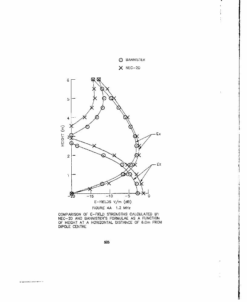
® BANNISTER

X NEC-2D

6

4.

°EE•__ Ex

3..

00

E-FIELDS V/m (dB)FIGURE 4A 1.2 MHz

COMPARISON OF E-FIELD STRENGTHS CALCULATED B1,NEC-2D AND BANNISTER'S FORMULAE AS A FUNCTIONOF HEIGHT AT A HORIZONTAL DISTANCE OF 6.Om FROMDIPOLE CENTRE

505

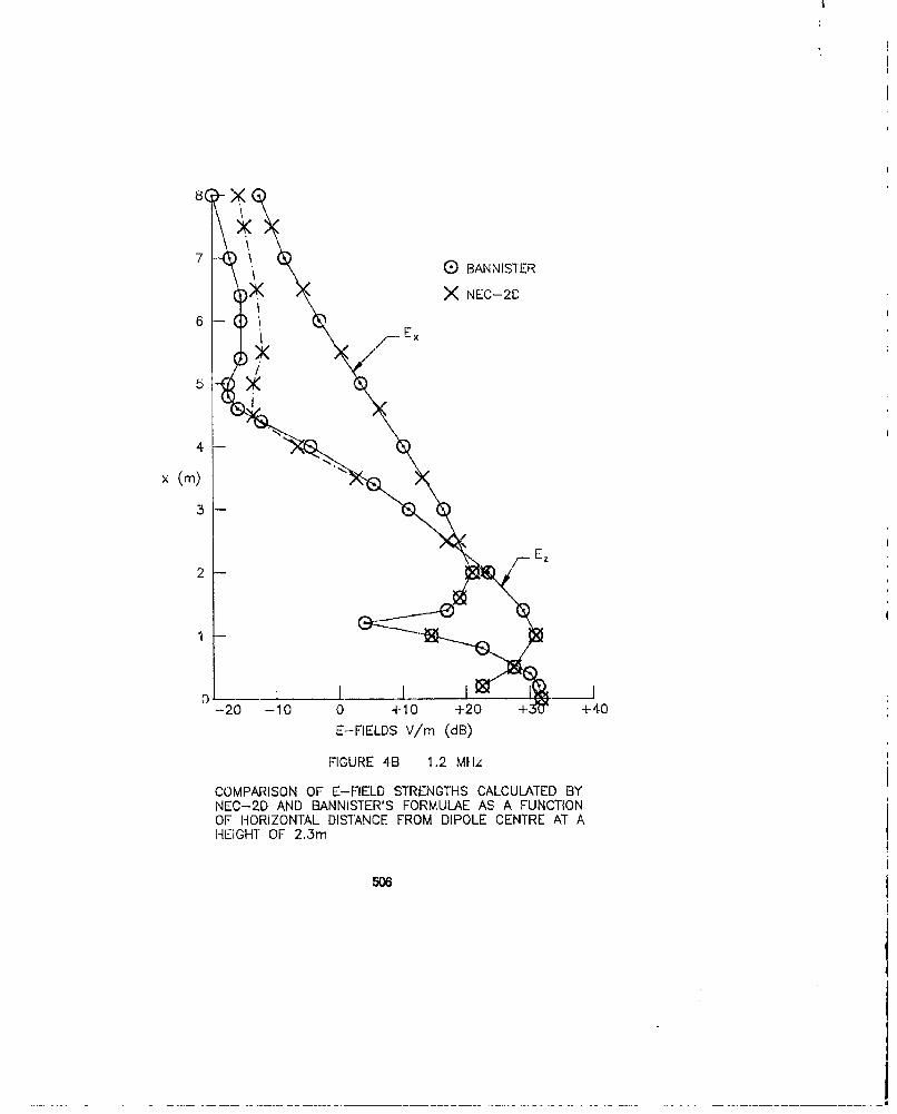
X/7 \

.\ G BANNISTER

X NEC-20

6 1

5

4-

x(m)3

E,.

2

01

-20 -10 0 +10 +20 4. +40E-FIELDS V/m (dB)

FIGURE 4B 1.2 Mtlz

COMPARISON OF E-FIELD STRENGTHS CALCULATED BYNEC-2D AND BANNISTER'S FORMULAE AS A FUNCTIONOF HORIZONTAL DISTANCE FROM DIPOLE CENTRE AT AHEIGHT OF 2.3m

506

REFINEMENT OF H" VERTICAL HALF RHOMBIC CHARACTER3ZATION

W.P. Wheless, Jr.University of Alabama Electrical Engineering Department

Tuscaloosa, Alabama 35487

M.D. FanningUDS Motorola

Huntsville, Alabama 35805

D.L. Faust and M.B. KingEyring, Inc. Communication Systems Division

Provo, Utah 84601

Abstract - Numerous radiation pattern profiles for the commercially available Barker& Williamson AC-1.8-30 antenna were presented in an earlier paper [1], Are thecomputed patterns were obtained with the code NEC2 executed on a personal computer,assuming a purely real antenna termination of 804 A. This paper improves the earlier results

use of measured complex impedance values for the antenna termination, and aen extendscomparison of computed to measured values to include patterns cakulated by the code

NECS executed on an IBM 3090 mainframe computer.

INTRODUCTION

The Barker & Williamson model AC-1.8-30 hf antenna used in this study is depictedin Figure 1. This configuration could be called a (balanced-feed, loaded) pyramid. Theanteuna of Figure I is referred to as a vertical half rhombic (VHR), however, because theVHR descriptor is more widely known and evokes an essentially accurate mentalvisualization of the geometry.

An earlier paper [1] presented graphical compaxisons of several ,easured andcomputed radiation patterns for this antenna, with the computed patterns obtained from thepersonal computer (pc) code NEC2 (specifically, NEC--1, version 2.2). In [lJ, the antennatermination was taken as 804 (1, purely resistive, over the 3-30 MHz hf spectrum.Subsequent measurements on the. termination have revealed that its value is complex anddepends significantly on frequency, as shown by the experimental data contained in Table 1."The resultant changes in computed patterns obtained from NEC2 with the refinedtermination parameters are minor, but perceptible.

The initial motivation for the work rerorted in [1] was to assess the accuracy andreliability of a pc-b)ased analysis code in the case of a typical wire antenna near zeal ground.The convenience of using a personal computer is attractive, and it appears that NEC2 isacceptable for many applications. However, because the subject antenna has two groundstakes penetrating the earth's surface in addition to a single counterpoise wire very Jose tothe surface, the potential improvement in numerical pattern predictions accuring from theutilization of the (mainframe) computer code NECS merita investigation. This paper reportsnew predicted patterns which have been computed with double-precision NEC3 code on anIBM 3090 mainfrtme. Graphical comparisons are made of the NEC2 personal computer and

P11203 ainfram reuts 41 the oril-- pattern dat a.

The pattern measurements were carried out using Bydag's Broadband Antenna TestSystem (BATS) at its Cedar Valley, Utah, test range. Details regarding the BATS

507

i

,aa

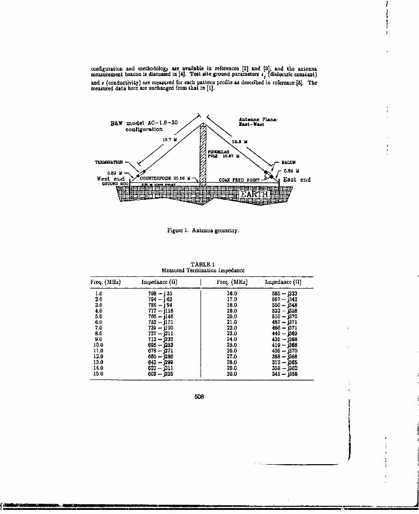
configuration and methodolog) are available in references [2] and [31, and the antennameasurement beacon is discussed in [4]. Test Bite ground parameters fr (dielectric constant)and o (conductivity) are measured for each pattern profile as described in mnference 15], Themeasured data here are unchanged from that in [1].

0• 3Antanna Plans:

B&W model AC-l.-O-3 Ant-Wu n

POIZ 10.9? Id

West e,_d COUNTERPOISE 2-66 UII-\ coCAx FEED Powr. East endGROUNDOD R ' -

Figure 1, Antenna geometry.

TABLE 1

Measured Termination Impedance

Freq. (MHz) Impedance (U) j Freq. (MHz) Impedance (fl)

1.0 798 - j 35 16.0 585 - j3332.0 794 - j 62 17.0 567 - j3.423.0 786 - j 94 18.0 550 - j3484.0 777 - j118 19.0 532 - j3585.0 766 - j146 20.0 510 - j3706.0 753 -- j171 21.0 487 - j3717.0 739 - j190 22.0 466 - j3718.0 727 - j211 23.0 449 - j3699.0 713 - j232 24.0 435 -j36810.0 695 - j253 25.0 419 - j36811.0 678 - j271 26.0 405 - j37012.0 660 - j286 27.0 388 - j36813.0 642 - j299 28.0 372 - j365

U . ,, ........... .U.15.0 603 - j325 30.0 341 - j358

508

II

COMPARISON OF COMPUTED AND MEASURED PATTERNS

Measured radiation pattern profiles were acquired at the Eyring facility at frequenciesof 3.195, 10.12, 10.0475, and 22.9015 lWHz. Corresponding NEC2 patternu were subsequentlycomputed on an IBM pc, and NEC3 patterns were computed (double precision) on an IBM3090 mainframe. BATS software, running on the pc, was used to overlay the NEC2 anddownloaded NEC3 computed patterns, compensated for efficiency, on the measured dataplots.

Figures 2--4 are gain versus elevation pattern profiles at respective frequencies of3.1925, 10.12, and 19.0475 MHz. The measured data was derived from airborne flyovevsalong a North-South cour6e (perpendicular to the axis of the antenna). The polarizationattitude was horizontal, with the measurement beacon radiator aligned parallel to the VHRaxis. Manifestations of high winds aloft are evident in the flyover patterns of figures 3 and4, which were measured four days earlier than the figure 2 pattern. While the NEC2 pcpredicted patterns exhibit satisfactory shape characteristics for figures 2-4, the pattern sizepredictions are substantially in error (i 5 dB) at 3.1025 and 19.0475 MHz. The NEC3predicted patterns emulate the measured data in all three instances.

Full-scale: 9 dill

3 d1/div

==--NEC3 COMPUTED NEC2 COMPUTED .. .MEASUREI"D

Figure 2. Gain versus elevation for" hu~rizontW pu~larization at3.1926i MHz, compass azimuth =- 0' (er -- 18.5, a =4.3 mSjm).

509

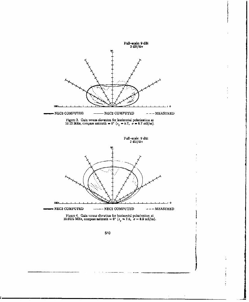
Fual--cale: 9 dBi3 dB/div

NEC3 COMPUTED - NEC2 COMPUTED - - - MEASURED

Figure 3. Cain vefsus elevation for horizontal polarization at10.12 Muz, compass azimuth 0" (r - .7, or - 8.7 mS/m).

Full-scale: 0 dbl3 d13/div

90

- NEC3 COMPUTED ... NEC2 COMPUTED .... MEASURED

1-.1ig.c 4. C-an vcu. elevation for horioznt= po1•izration at19.0475 MHz, compuas azimuth = 0 (r = 7.s, a 8.9 US/m).

510

It_ _ n _ 'iIi - n

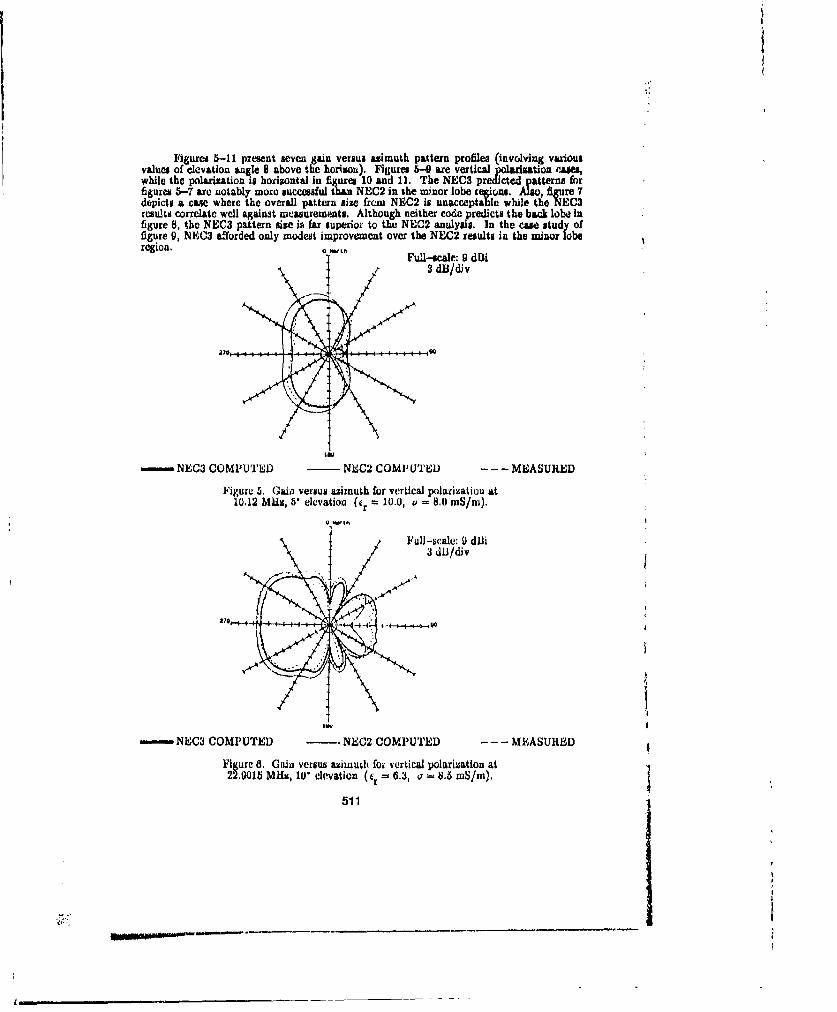
"1igurs 5-11 present seven gain versus azimuth pattern profilea (involving variousvalues of elevation "n~le 8 above the horizon). Figures 5- are vertical poli*zation r•lies,while the polarization is horizontal in figures 10 and 11. The NEC3 predicted patterns forfigures 5-7 axe notably more successful than NEC2 in the minor lobe le ions. Also, figure 7depicts a case where the overall pattern size from NEC2 is unacceptable while the NEC3results correlate well against measurements. Although neither code redicts the back lobe infigure 8, the NEC3 pattern size is far superior to the NEC2 analyY.1. In the cae study offigure 9, NEC3 afforded only modest improvement over the NEC2 results in the minor loberegion. att

Full-scale: 9 dBl3 dB/djv

- NEC3 COMPUTED NEC2 COMPUTED ..- MEASURED

Figure 5. Gain versus azimuth for vertical polarization at10.12 Mlz, 5' elevation (tr 10.0, o - 8.0 inS/ni).

Full-wcale: 0 d~li3 dUJ/div

IMP-"

=- NEC3 COMPUTED NEC2 COMPUTED - - - MEASURED

Figure 8. Gain versus azimuth for vertical polarization at22.9015 MHz, 10' elevation (r = 6.3, 8.6 mS/rn).

511

4.'.________________________________________________________________________________ _____________________________________________________

0 Nor th

/Full-scale: 9 di

illoo

- NEC3 COMPUTED NEC2 COMPUTED - - - MEASURED

Figure 7. (Gain versus azimuth for vertical polarization at3.1025 MHz, 20' elevation (er = 18.5, a = 4.3 mS/in).

FuU-wcale: 0 dIli

.- NEC3s COMPUTED - NEC2 COMPUTED - - - MEASUREDF q;,urae S. n G exn u n I-.n .uth I4=v . 6h..t- n.all.k4...n I t .

3.19202 MHz, 40' elevation (c1 - 18.5, a = 4.3 mS/m).

512

................................-..---.

Full-scale: 9 dBi3 dB\div

- NEC3 COMPUTED - NEC2 COMPUTED .... MEASURED

Figure 0, Gain veLaus azimuth for vertical polarization at19.0475 Mils, 30' elevation (fr W 8.9, a - 10.8 unS/m).

Fijures 10 and 11 show more iutricate horizontal-component patterns at 10.12 and19.0475 Mhiz, rcspectively. NEC2 and NEC3 predictions are of rompa-able quality in tlhcht

Ful--acal: 9 dBlI

- NEC3 COMPUTED - NEC2 COMPUTED .... MEASURED

,i-gurv 10. Gain versus aximuth for horizontal polarization at10.12 Mis, 30' elevation (er - 8.7, (r - 0.7 mS/mn).

513

I

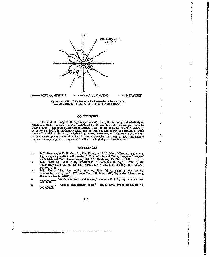
0 W~th

Full-scale: 9 dBi

SNEWC3 COMPUTEDh NEC2 COMPUTED .... MEASUREUD

ligUow 11. Gain versu6 RAimuth for horiontal po1arization at19.0475 MU; 30' elevatinn (t. = 8.9, a ' 10.8 InS/m),

CONCLUSIONSThis work has sampled, through a specific cac study, the accuracy and reliability of

NEC2 and NEC3 radiation pattern predictions for hf wire antennas in close prodximty toiinite ground. Signilfc&nt improveumnt accrued from the use of NbC3, which consistentlyoutperformed NBC2 in predictions concerning pattern size and minor lobe structuac. Once.the NEC3 model is sufficiently inclusive to give g(od agreement with the results of a modestpattern measurement series at a few discrete frequencies, patterns at new inrtomediatefrequencies inay be predicted by use of NEC3 with a high degr•ee of confidence.

RFEKRENCES

1. M.D. Fanning, W.P. Wheles, Jr., D.L, Faust, and M.1. King, "Characterization of ahigh-frequency vertical half rhombic," Proc. 61h Annual Rev. of Progreaa in AppliedCompudational Electroma•nctics, pp. 300--307, Monterey, CA, March 1990.

2. D.L. Faust and M.3. King, "Broadband HY1? antenna teating," Proc. of R1"Technoioy Expo '86, pp. 62&-431, Anaheim, CA, January 1986 (Eyring DocumentNo. 800-0168).

3. D.L. Faust, "The low profile antenna/rollout hi antenna: a new tacticalcommunication# option," HP Radio Chinic, St. Louis, MO, September 1986 (EyringDocument No. 900-0013).

4. ., "Antenna measurement beacon," January 1989, Eyfing Document No.5. - "Ground measurenent probe," March 1990, Eyrlng Document No.

514

fIBIOGRAPHY

W. Perry Whduss, Jr. (205) 348-1757University of AlabamaEI'Cctrical Engineeraing DepartmentBox 87028tTuscaloosa, AL 35487-0286Perry Wheless is an Associate Profesor of Electrical Engineering at the University ofAlabama. lie has continuous engincering experience since 1968 with rf, microwave,millimeter wave, and ionizing-radiation devices and systems.

Mike D. F nniu (201.) 430-7032UDS Motorola5000 lDradf'rd DriveHuntsville, AL 35805-1093Mike Fanning is a Design Engineer with UDI8 Motorola. He attended the University ofAlabama, where ie received both the B.S. and M.S. degrees in Electrical Engiineering, andhe is quite active in various facets of amnateur radio.

David L. )'aust (801) 376-2434Eyriny, Inc. ACommunicatioas Systems Division1455 West 820 NorthProvo, UT 84601David Faust has been associated with Elring, Inc., for twelve years. lie iii now ProgramManager and Test Engineer in Eyring's Comminunicationi Systems Division. He has extensiveexperience with hf antenna bystems and if nicasuremoeid technuiques.

Moray B. King (801) 375-2434Eyring, Inc.Communications Systems Division145b West 820 NorthProvo, UT 84001Moray King has. been with Eyring, Inc., for eleven years and he is a Systems Engineer inEyring's Communication Systems Division. His prior professional experience includes theValley Forge Research Center and the University of Pennsylvania, and the BATS softwareutilized in this study is among his many credits.

II

515

SESSION 13- "ELECTROMAGNETIC COMPATIBILITY (EMC)"Moderator: David P. Millard

_____________

___ ___ __ __ ___ __________

A Survey of Numerical Techniques for Modeling Sources ofElectromagnetic Interference

To Id HI. flubingUniversity of Missouri-Rolla

Rolla, MO 65401

Abjislic

"his paper describes the preliminary results of a study to identify ways of using numecrical3modeling techniques to analyze sources of clectromagnetic interfernce (EMI). First, two c~anonicalEMI sources were developed that represent tlic type of configurations that need to me tnodeled. *

Then a number of numerical electromagnetic modeling techniques were evaluuted todectermine theirsuitability f'or analyzing these configurations. None of the currently available techniques appcarsýto be a very practical approach, however hybrid techniques that conibinc u surface integral inethodwith a finite mecthod show considerable promise.

Manuifacturers of electronic equipment Arc taking more of an interest in the amount otfelectrontagnotie radiation that nInnates fr-ot their products. This is due to strict laws regulatingelectromagnetic intitrference: (EMI't and the potentially high cost of shields, tilttrs, and other EMIfixes required to mnake an otherwise noisy product niect these, raquircuiments. Many comipaniesemploy full-time E~Ml engineer who view every electronic system ats an cleciromingnetic radiationsource. Bly understAnding how and why diffhrent contigurations radliate, these engineers work atdeveloping designs that mevet the radiation requirementsu at the lowest possible cost.

T1raditionally, 11,Ml engineers have relied prinmarily on their nicasturimnent experiences. rules-ot-thurab, andl simiple intuitive models to guide theum in making design choices. Unfortunately, EMIrules-of-thumib that apply in somne situations umay miot apply in others. Simple rmodeling techniquessuch as circuit., transmission line, or basic antennia miodels only %ork well when the source and allrelevant currenit paths can be readily identified. Most EMIN problems today howcvcr arc not obviousenough to be predicted or aaalyzed using these simple techniques. Therefore, the only tAOolsremaining for ENI engineers in most cases are measuremnents of the systems or its components.Unfortunately. practical mieasurenments can not be umade without existinig hardware and this is nottusually available early in a product's developnicnt when critical design decisions are being made.Also, measurod reszults in the absence ofia theoretical nmodel can be mnisleadintg and do not necessarilysuggest how a designi should be moudifiedl to minimize radlated emissions.

Nunmeical modeling technique, which have revolutionized ttc fteldso oanteimnua ad microwavesystem analysis, have had relatively little impact on LMI source analysis. Sonic woik involvingthe modeling of components and cables has been dorie, but the scope of this work is limited andthose techniques ame not widely used by LIMI cngimleers. Thbe primiamy reason for this is that the typesof problems that EM enigineers would like to model cannot be aiialyzi-d by available numericaltechniques. In the following sectoun. twn configturations replm-otlng time type of problems EMIM

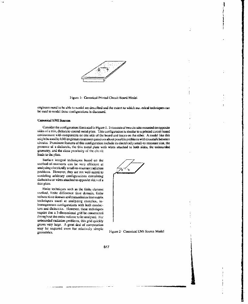
Figure 1: Canonical Printed Circuit Board Model

enginci • r neyed to be able to model air. described and the extent to which nw,erical techniques canbe used to moeXIL these cinfiguratios is dibcussd.

Ciltunical EMI Sources

Cons ider the configuration illusuawd iii Figure. 1. It consists of two cir:uits mounted on oppositesides ofa thin, dielctric-coated inctal plate. This configuration is similar to a printed circuit boaxdcnvinumnent with components on one side ol the board and traces on the other. A model like thismight be used by EMI engineers to answer questions about possible problems with crosstalk betweencircuits. Prominent fiatures of this configuration include its electrically small-to-resonant size, thepresence of a dielectric, the thin metal plate with wires attached to both sides, the unboundedgeonictry, and the close proximity of the crt titleNads to the plate.

Surface integral techniques based on theinethod-ol-mumcnts can be very efficient atanalyzing clectricaily small-to-resonant radiationproblems. However, they are not well-suitcd tomodeling arbitrary configurations containingdielectrics or wires attached to opposite sides ofathin plate.

Finite techniques such as the finite eleuentmethod, finite difference time domuin, finitevolunme time domain and transmiission line matrixtcchnicucs excel at analyZing coMplex, in-homugeneuus configurations with both conduc-tors And diclectrics. However, these techniquesrequire that a 3-dinmensional grid be c:onstructedjlhrOluwlill)t the entire volume to be Lainlyt.ed. Forunbounded radiation problems, this grid quicklygrows very large. A great deal of computationmay be required even for relatively simplegeometries. Figure 2: Canonical EMI Source Model

517

The configuration in Figure 1 is not large, but it is unbounded. It also requires a detailed gridin the vicinity of the wires because of their proximity to the plate. Because of these constraints, theauthor has not been able to locate a readily available computer code capable of analyzing this typeof configuration efficiently. I lowever finite techniques such as the finite volume time domain andfinite element methods could theoretically be applied to this problem given sufficient computerresources.

Although the configuration in Figure 1 represents an important class of EMI problems, printedcircuit cards rarely exist isolated from other sources or conductors. The configuration in Figure 2is more typical of an UMI source configuration I 11. It consists of a printed circuit board configuri-tion with a partial metal enclusune and an attached cable. Assuming that the cable is shielded, allof the currents contributing to the EMI can be assumed to flow on the outer surface and in mostcases, the cable can be modeled with a solid wire. Like the model in Figure 1, this configurationcontains dielectrics and thin plates with multiple wire attachments making surface integral techni-ques impractical, However, because of the presence of the relatively long thin wire, finite techniquesare also impractical. This is because creating a grid throughout a volume large enough to containthe card, shield, wire, and the entire near field of the source results in a problem that is unmanageablefrom a computational standpoint. Although the itndel in Figure 2 represents a relatively simpleEMI source, it cannoL be analyzed effectively by any existing numerical techniques. This illustrates 4,

why numerical modeling techniques are not commonly used to model EMI sources.

Hybrid lechniquts

Surface integral techniques such as most moment method teclniques and the boundary elementmethod are very efficient at analyzing long, thin wiles and large conductive surfaces, Finitetechniques arm best at modeling complex, inhotnogeneous regions. Therefore, it makes sense tocombine a surface integ;al technique with a finite technique in order to take advantage of the bestproperties of each. A number of hybrid methods have been proposed that combine two existingtechniques [2-01. Generally, the configuration is divided into two or inore regions. The numericaltechnique best suited to each region ih applied in that region and boundary conditions are enforcedat the interface between regions. For example, a hybrid moment method finite eement techniquemight apply -a finite clement analysis within the small volume containing the card and inside surfaceof the shield in Figur 2. A moment method tcchnique would simultaneously be applied to thesurface defined by the wire, shield, and Othe boundary with the finite element region.

So far, no one has implemented a hybrid techniquv capable of umalyzing the configuration inFigure 2 or most types of coniigurations of interest to IMi engineers. However progress continuesto be made in this area. While must numerical methods appear to have fundamnental limitations thatwill prevent thent from ever being efficiently applied to most EMI sources, hybrid techniques havethe potential to overcome these limitations.

Summary

EMI engineers have not yet benefitted significantly from the numerical techniques that haverevolutionized the antenna and microwave engineering fields. The two simple configurationspresented here illustrate some of the difficulties involved with applying numerical techniques toEMI soutce models. Hybrid techniques that combine a surface integral method with a finite method

518

II

appear to be the best long-term approach, however more development of these techniques isrequired.

Hopefully, given the rate at which progress in this area is being achieved, an algorithm capableof accurately analyzing the configurations presented here is not far off. Once such an algorithm isimplemented, it will likely become one of the most powerful tools available to EMI engineers.

Acknowledgement

This work was supported by a grant from Intel Corporation.

Refemoes

[1] T. H. Hubing and L F. Kauffman, Modeling the Electromagnetic Radiation from ElectricallySmall Table-Top Products, IEEE Transactions on Electromagnetic Conpatibiliti, vol. 31,Feb 1989, pp. 74-84.

[2] A. Taflove and K. Umashankar, "A Hybrid Moment Method/Finite-Difference Time-DomainApproach to Electromagnetic Coupling and Aperture Penetration into ComplexGeometries," IEEE Transactions on Antennas and Propagation, vol. 30, no. 4, July 1982,pp. 617-627.

[3] M. A. Morgan, C. H. (Then, S. C. Hill, and P W. Barber, "Finite Element-Boundary IntegralFormulation for Electromagnetic Scattering," Wave Motion, vol. 6. 1984, pp. 91-103.

[41 J. M. Jin and J. L. Volakis, "A Finite Elemerrt-Boundary Integral Formulation for Scatteringby Three-Dimensional Cavity-Backed Aperturcs," IEEE Transactions on Antennas andPropagation, vol. 39, no. 1, January 1991, pp. 97-104.

[5] X. C. Yuan, D. k. Lynch, and J. W. Strohbehn, Coupling of Finite Element and MomentMethods for Electromagnetic Scattering from Inhomogeneous Objects, IEEETransactions on Antennas and Propagation, vol. 38, no. 3, March 1990. pp. 386-393.

[6 X. C. Yuan, Three-Dimensional Electromagnetic Scattering from Inhomogeneous Objects bythe Hybrid Moment and Finite Element Method, IEEE Transactions on Micrewavz:Theory and Techniques, vol. 38, no. 8, August 1990, pp. 1053-1058.

519

COMPUTER AIDED ELU.C."10OMACNETIC COMPATIBILIIY ANALYSIS

D.P. Millard, J.K. Daher, R.M. Herkert, and JA WoodyElec.OMapCtic FnViro ectat Effects (E3) Laboyatoiy.

Georgia Tech Researa lirtituteGeorgia Institute of Tcchr.oloy

Atlanta, Geora 30332

ABSIW ACTElecmomragetic Compatibility (EMC) analysis is essential during all stages of system desig•i,

from aoncept to deployment. However, EMC aalyses of s'ystnm are very coamplex, requiringinputs which may not be known to the EMC analysts. Also not all of the computer aidedengineering (CAE) tools avilable to perform the analyses are appropriate for performing EMCanalyses at each stage of the design. Care must be cuercised when using these CAE tools such thatthe gar-•ge-in-guxbage-out syndrome does not prevail. What is required is a front-end CAE toolwhich will: (1) assist the EMC analysts to better defite the problem to be analyzed; (2) allow theanalyses to be performed optimally for the input data available; (3) select the appropriate analyticaltool (existing EMC CAB program); and (4) produce uniform outputs which the EMC analysts canunderstand.

An EMC CAE tool which meets these requirements is under develrý'ment at Georgia Techand is called the Georgia Tech Configuration Anralysis Program (G'I ZAP') [1-31. GTCAP is amodular EMC CAE tool with a relational database basod on a framework concept and a "les.onslearned" capability. It is menu and list directed, has a graphical user interface (GUI), and containsdefault input values based on specifications. GTCAP guides the EMC analysts through the processof performing EMC analyses at each stage in the design, acting as the EMC expert, based on theinput data available at the time. GTCAP is designed to operate on PC-based machines underseveral operating systems.

INTRODUCTION

Modern platforms (e.g., military vehicles) are designed to employ complex systems andelectronic devices which utilize much of the electromagnetic spectrum. Also, the electromagneticenvircament (EME) to which these platfo:ms will be subjected is very complex and can containemitters which generate field strengths aapable of causing adverse electromagnetic environmentaleffects (E0). Therefore, E3 analyses must be performed during each phase of the platform's lifecycle from concept to deployment. The type, degree, and reliability of the available input data forthese Es analyses varies as the platform progresses through its life-cycle phases. To perform E3

evaluations ef configured platforms in a timely, cost effective manner, a computer-based tool isrequired which utilizes the available !nput data and which allows the engineer/operator toconfigure the platform with avionics and electronic systems, including boxes, cables and antennas,

'Copyright GTRC, 1988.

520

':.4 • m m m . . .. • -I..... . . .- i. ... .. .

.1 . . • ' w -L . ...

perform an analysis (evaluation); and report the results. Also, the operator must be permitted tosave the results, to re-configure the platform's systems, and to re-do the analysis as needed.

The CAE tool which can perform this analysis in an integrated fashion is GTCAP. GTCAPis highly modular in design, menu and database driven, and contains a "lessons learned" featurewhich allows the operator (and the program) to learn during each analysis.

CONFIGURAIION ANALYSIS PROGRAM

The general structure of the GTCAP CAE software is shown in Figure 1. A modularsoftware structure is used which iacludes all required inputs and outputs for module-to-modulecommunication, and the software is programmed to DOD-STID-2167 [2]. The major modulesinclude the User Interface Module (UIM), the Platform Evaluation Module (PEM), and the variousmeasures of performance (MOP) modules.

The UIM is the program "executive" which provides the interface between the GTCAPoperator and the PEM. The logic for the UIM and GTCAP analysis process is shown in Figure2. The UIM allows the operator to (1) select the platform and the work order (WO) beingimplemented; (2) position the equipment on the platform; (3) compute and store the equipmentposition and orientation in a database; and (4) set-up the evaluation scenario by selecting the mode(baseline without interference, intersystern, or platform with external EME), the equipment andthe platform operation/mission. After the E evaluation is complete, the UIM generates theanalysis reports. It then permits the operator to reiterate the configuration/analysis process2.

The PEM is called by the UIM to perform the E3 evaluation of the platform configurationdefined in the platform configuration database. The PEM uses the electroma Petic interference(EMIl) module to compute the intra-platform coupling and perform E" i 'ayses of theconfiguration. The PEM also uses the mission module to compute the coupling UL g,'nal emittersto on-board antennas and perform electromagnetic vulnerability (EMV) predictions.

The MOP evaluation modules utilize intersystem and inter-platform E3 analysis results fromthe PEM to determine the degradation in the MOP's on the platform. Each system (FlightControl, Communications, Navigation, Electronic Warfare, Radar, Electro/Optic) has its own MOPevaluation module, EMI database and MOP database.

GTCAP utilizes large databases generated off-line. These databases include: the platformstructure descriptors, the electromagnetic MOP, platform graphics based on NASTRAN finiteelement models (FEM), equipment EMI parameters, and platform operations/mission descriptors.The equipment EMI and MOP databases, which are critical to the E3 evaluation of the platform,must be constructed from EMI and EMV test results or generated through analyses. The MOPdatabases are generated by the various system specialists in collaboration with E3 engineers. Whereactual EMI test data or analysis results are not available, MIL-STD-461 [3] emission and

: (NOTE: other analyses, e.g., weight and balance, could be performed if theappropriate modules are added).

521

Ii

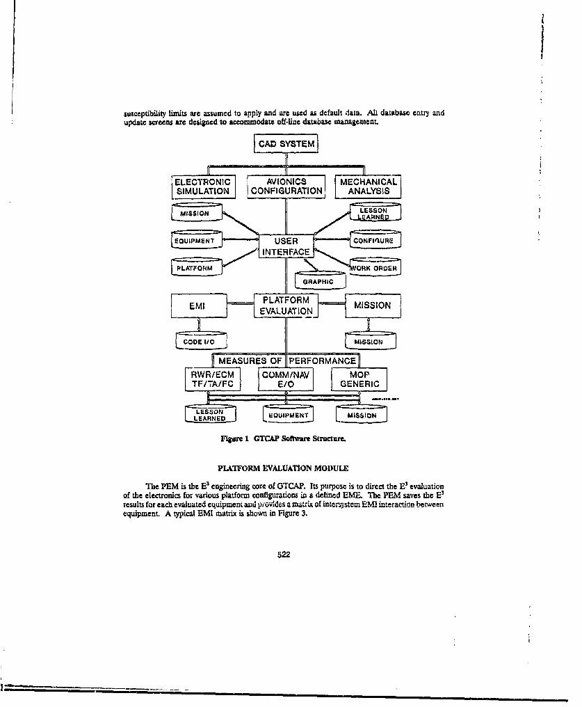
susceptibility limits are assumed to apply and are used as default data. All database entry andupdate screens are designed to accommodate off-line database management.

CAD YSE

SELECTRONIC] AINC MECHANICAL]SIMULATION COFGURA10N PAAYI

LMISSO LVLUTONMSSON

COEM V1 MISSION

ElTFR ,VALUATION MDL

Th [CMOsDeE 3 eniern=oeoUTAP t ups st irc h 3 eautoofteeetrnc vrospafomcniurtosi defne EMI.ThSSIOaNs he

resultsMASU fS eac evlae eupetan ioiEsaaRiofitRMystmEMineatobtwe

e q u i m e n t A t p i al E CM! m atri x is s h w n iOFg r e 3

-TF/T/FC /O GN522

"The PEM obtains, fromthe appropriate databases: (I) INITIALIZATIONthe platform configuration, (2)tho selected analysis mode. and(3) the created equipment list. SELECT&The ?EM uses the EMI module (1) PLATFORM Ato peixorm the EMI Analysis and (2) WORK ORDERuses the mission module todefinc the EME produced by CONFIGURE PLATFORMcxternal emitters and to ,P.determine the active equipment DEFINE EVALUATION SCENARIOlist for specific mission segments.The PEM relies on each of theequipment MOP modules todetermine the amount of PLATFORM EVALUATIONdegradation (adverse E0) causedby onuboard and externalemitters.

DISPLAY EVALUATION RESULTSEMI MODULE

The EMI Module is usedto compute the intersystem SCENARIO¶coupling. 'quick look" EMImargins, and the EMsusceptibility assessment for the CHANGEplatform. The on-board, CONFIGURAT'IONintersystem EME is defined bythe radiated and couductedemissions of the equipment on F REPORT PLATFORM EMI STATUS l]the platform. The external inter- -t --platform EME is defined by E'•IGN OFFemitters external to the platlonm. ...........The primary EMI assessmentcodes utilized in the EMImodule include: Figure 2 GTC&P Analysis Prvcess Flow Diagram.

AACIM - Aatenna-to-Atecna Coupling Interference Model (GTIX Intrasystem EMI AnalysisProgram)

GEMACS - Generalized Electromagnetic Model for the Analysis of Complex SystemsIEMCAP - Intrasystem Ele'tromagnetic Compatibility Analysis ProgramBSC - Basic Scattering CodeAAPG - Aircraft inter-Antenna Propagation with Graphics

GTCAP uses these codes, utmodified, to compute untenna-to-antenna coupling, antenna patternsof on-'board antennas, and box-toa-bo), box-to-r-ble and calcocal cpln teaLUCot

523

F

platform. In addition GTCAP utilizes AACIM for quick look antenna-to-antenna, coupling analysesand frequency culls.

SOURCE

B-=z-NO REVIEW )%,V0G-=-EMI OK CD LO C)C4C 5LR-UM-PROBLEM a-6 WLIW

AN AWCI-9/C MAN/ALQ-100 in N SAN A N-154ANAP -9 WiV , .

AN PX-72 N fl 0EAAQ-1O

S ALO-157 amALQ- 162 1A N A.RA_5 [Q_ J 1 M w10 W i luF.AN ARC-159 UANA AW27AN ARN-84 E

Figuim 3 EMI Statwu Report Matrik.

ANALYSIS APPROACH-

Equipment/system EMI paramieters tind MOP data together with EM coupling data form thebasis for E3 analyses and EM] margin e&'culations. The EIV] Moduie accesses the EM] and MAOPdatabases and calculates the EM coupling First-order approximationts of the effects of freque~ncy,pulse width, and pulse ropetitioai frtquency (PRF are assumed.

EM energy can couple to a system through oue or moro system ports of entry (POE's) [6].POE's are grouped into two separate categories: frowi-door and back door. From an analysisperspective, front-door paths are better characterized Wn terms of coupling to the POE. Front-doorcoupling is further subdivided into in-band and out-of-band cases. In-band coupling tends- to beuzurc &goadto aulyze tbnzi out-of-band coupling both in terms% of the interaction of the

524

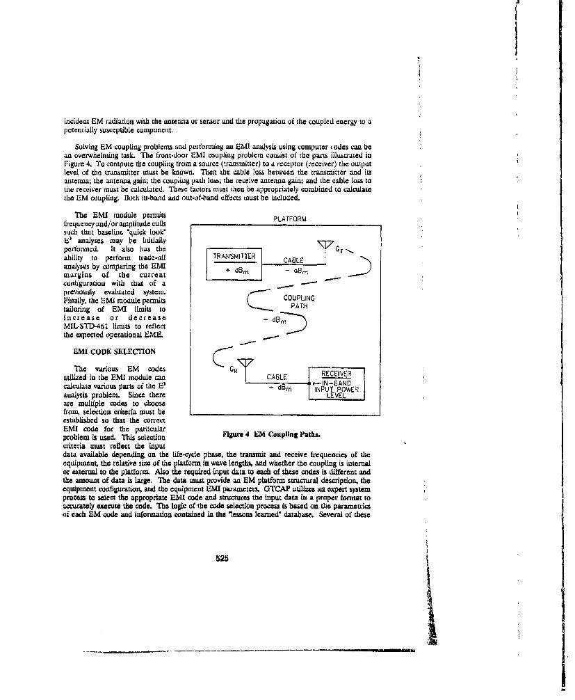
incident EM radiation with the antenna or sensor and the propagation of the couplcd energy to apotentially susceptible component.

Solving EM coupling problems and performing an EMI analysis using computer odes can bean overwhelming task. The front-door UMI coupling problem conaist of the parts illustrated inFigure 4. To compute the coupling from a source (transmitter) to a receptor (receiver) the outputlevel of the transmitter must be known. Then the cable loss between the transmitter and itsantenma; the antenna gain; the coupling path loss; the receive antenna gain; and the cable loss tothe receiver must be calculated. These factors must then be appropriately combined to calculatethe EM coupling. Both in-band and out-of-band effects must be included.

The EM1 module permits PLATFORMfrequency and/or amplitude cullssuch that baseliat "quick look"E) analyses may be initiallyperfornicd. It also has the 0Gt-.ability to perform trade-off TRANSMI1TER CABLEanalyses by comparing the EMI + dBm _ O8mmargins of the currentconfiguration with that of apreviously evaluated system.Finally, the EvI module permits COUPLINGtailoring of EMI limits to PATHincrease or decrease _dBS 'MIL-STD-461 limits to reflectthe expected operational EME.

EMI CODE SELECTION

The various EM codes Eutilized in the EMI module can CABLE - RECIVERcalculate various parts of the E- d INPUT POWERanalysis problem. Since there LEVELare multiple codes to choosefrom, selection criteria must beestablished so that the correctEMI code for the pardcularproblem Is used. This selection Figure 4 EM Coupling Paths.criteria must reflect the inputdata available depending on the life-cycle phase, the transmit and receive frequencies of theequipment, the relative size of the platform in wave lengths and whether the coupling is internalor external to the platform. Also the required input data to each of these codes is different andthe amount of data is large. The data must provide an EM platform structural description, theequipment configuration, and the equipment EMI parameters. GTCAP utilizes an expert systemprocess to seiect the appropriate EMI code and structures the input data in a proper format toaccurately execute the code. The logic of the code selection process is based on the parameru-iof each EM code and information contained in the le*ssons leaned" database,. Several of these

525

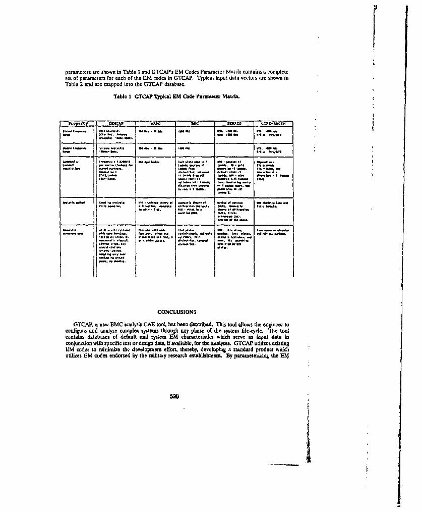
paramezers are shown in Table I and GTCAP's EM Codes Parameter Matrix contains a completeset of parameters for each of the EM codes in GTCAP. Typical input data vectors are shown inTable 2 and are mapped into thec GTCAP database.

Table 1 GTCAP Typical EM Code Parameter Matrix.

propeto a DISHAP __ AAVG "C 4aC UIUI-AACTP4

"PMod I agm. PI1 ..=Wl' lIN Me .It U. -30 Me em mem oftt 4k

loolwIll Ife-ille t. i

*ow 0 IIU.W_ l.I. "Ia.. 11 i 30fttt ina

..*W le 1 .'.9- .I"i ll a lol . 1.6 plo.W. I on - t". I.0b Iftw l..411rd.W W .1A. I.4. 0 lain olrao.l lael. III V4r. Pd 21. 1o,. 1

rca.i4LdI. b.1 I meI#-At label. m.4 I". 14441 -I atre'414111 I, . Wl of Iom..$ look& Newl, -. 5

I. .151, I. WI -l I * I514 hlmea -.. Od1,I~i uI. (S%.ba ll..

0,110 * aiom.loyI.4. Cyiff'ete. A....4 111.5 io p "tlol. (MM, 9-111 Frm, i,. faems44.4p4.1 eS'.. I .1th.41414 I'd . IAI Ay( lo~e ml. 4 4 0wl wI-d, of01t

n,.f ~ ~ ~ ~ ~~eeife $a)~,lI -*e gs.. 4.W~ . (AM)hd . VI 1..

Wt1. ori 4 .. 01. 1.4tmtvw ml." .4

p4... my50).

CONCLUSIONS

GTCAP. a ns.w EMC analysis CAE tolol hos beens described. This tool allows the engincer toconfigure and analyze complex systeto through any phase of the system life-cycle. Tbe toolcontains databases of default and system EM characteristics which serve as input data inconjunction with specific test or design data, ff available, for the analyses. GTCAP utilizes existingIEM codes to minimize thc development effort, thereby, developing a stauidard product whichutilizes )EM codes endorsed by the miltary research establishnient.1 By paracneterizinle the EM4

526

r

codes and their associated input and output vectors, GTCAP can select the optimum EM code forthe evaluation of specific EM problems. It provides an "expert system" to select the correct EMcode based on various factors such as the availability of input data. The results of the E3 analysesare compared to the MOP's and displayed, reported, and stored as lessons; learned."

Table 2 EM Cod. Typcal Input Data Vetltr.

Au wAAMz3Qz 12W __0mm J2 M VCP = AI airrf Modol de"nmt"u s DOflAS ODNTIROL AIk xI ipad bukem dmlpaimaoe DRlAWl CONTROL GROUND X3 apa•e vehicle demigmutas so" DAW.5 CONT11OL 6SPACR X4 owed "silo" ift..4e ddqs OQT.AP INPUT X X XS povad mAlice ktaldl Oearci OTCAP INPUT x x x6 poum dmninaoldtWd (Oe GTCAV INPUT * X X X7 a.1jatmr uudety mawla dB I.AMB IFLW'r XV ,w,-.toi oe•ua•t lmpedsmq l/awj DVAIM NPrIT X

10 044ie 1 1ndel ditel .AM DRM56 CONTROL FLQUIH 24I1 nm4,SthhJ•Jkm~ DM1.•1 lN~qT7 • 117 fimisel roiv lachu D0AM iNPUT ,N A13 womue tailmonm rdiva mbU 0M INP1IWF * X14 varikel wrM re.'cw4 iclus DlASri INUT * Xis ft1i-btoen cylndky 0 v 11101: 1411 li INPUTr D x16 nand •41•il•r dulallot e DRAWI CX)NMOL ROUND X17 (l•a cyinder dewlpatloe no"e DRASH CONTROL FLAT X ,is wp"u,4 dhetlo.Atio ct DASHII CONTROL WNOKT x19 buntt LIm of wing row What DHAS1 INPU" * X20 water Line oi wing rou iicnd D.ASII INPUT X21 fimelap muleo., fwo-ard toot 61:a111 DaAS. IN JrTr X22 ft41eP MNt60. aft •ot i1citVN DIAI INPUT * X23 wianaip deipatsim Nmo DOilAM CONTAOL WOWP x24 butt Limeof wiaffip ade DHAS1 iNPUTf x X2. wter Ua of win•Ip iachi DRAS INPUT x 2

26 fasateee etnLim fncward Uip 11011111 DM511 "NJr * 227 r'Mealep ,alkm, aft lip iWihes DO E INPUT * x28 eimnMa field "nqaec; del non0e DIIA31 CONI'OL UN x2P Meimn &iel h"sqeene Hti LIMIM VQ'Ur * x

ACKNOWLEDGEENWIT

The authors wishes to thank the following people for their contribudons to :his work: T.A.Torres for the initial concept and funding. ILW. Demny, RJ. Levin, D.W. Ac'ee, G.E. Beebe, M.LWheeler and Dr. JA. Mabafley for their enlightened discussions, assistance with the EM codeevaluations, and providing the EM code input vectors and ideas on the user interfac•,.

REFERENCES

1. Millard, David P, "Helicopter and Avionics Systems Electromagnetic Environmental Effects%"Digital Avionics Systems Conlerence, 16-18 October 1990, Virginia Beach, Virginia

2. Millard, David P. and Woody, Jimmy A., "System E3 Platform Evaluation," 1990 InternationalSymposium on Electromapetic Compatibility. Symposium RL 'd, Washington, D.C-, p. 607-611, 21-23 Augnst 1990.

52

527

f3. Millard, David P., "System E3 Analysis and Prediction Program." EMC EXPO 89, Washingtonl,

D.C.4. DOD-STD.2167A, "Defensive System Software Developmeot," 27 October 1987.S. MIL-STD•461C, "Electromagnetic Emission and Susceptibility Requirements for Control of

Electromagno.tic Interference," 4 August 19S6.6. Denny, H.W., Daher, J.K. and Beebe, G.E., "E3 Analysis Guidelines,"Technical Report No, 2,

Gtii Project No. A-4892 for Rome Air Dcvelopment Center, Air Force System Command,Griffiss AFB, New York, Contract No. F30602-87-C-0134, December 1990,

528

5I

SESSION 14- "LOW FREQUENCY APPLICATIONS"Moderator: Perry Wheless, Jr.

_ &

Translei. Leakage Field In Transformers

with Saturable Magnetic Core

Mlhaela [Iorega A. Alexandru.M.I.MoregaAA

Abstract

The problein of the magnetic leakage field distribution arroand windings withsaturable magnetic core is solved with a method which couples the numerical magetCLicfield calculus and the solution of the magnetic circuit, equivalent to the electric andinalinctic structure.

1. Introduc.ion.

Leakage field computation in transfornier structuics is aimed todetermine the shortcireuit parametcrs, electromagnetic forces and stry lossesin windings ard framework. The computation is usually made accordiiig to theclassical core model with infinite magnetic permncabilly, hi other words, theassumption of the windings with compensated uanpertuins i1]-[61.

Thcre arc cxpeiiliental researches 151 which evidence the IkIIUhtSC ofthc miagnetic flux values in transformer corcr in sonme particular shortcircutworking conditions, as compared to the values leached in ,tonload scivihc. Insuch conditions, the distribution of the leakage flux is influcuced us well, Thisis why this plaper presents u computaitionul nscthod for the leakage field.which Allows to consider any working conditionls of the transiformcr as well asthe influence of its iron-corc ltagntlisation curve.

In this paper, a hybrid representation of a thrce-phased trunislornier ispiopused. The magnetic core nonlincurity and the specific working couditionsarc studied on an clectro-niagnetic equivalent network; the solution of thiscircuit problemii provides for nonlhoniopcnous boundary conditions as well asthe arperturns values of the field sources. ill the magnetic; field probliet. Afinite difieren"e or finitc clement method is used to obtain the distiibution ofthe leakage field.

The nmethod is presetted with reference to a threc-phased transiomtcir,but it can be used to study any other similar devices: transhormers, inducLionfield coils, curornagncts, etc,

2. "i'lle Electro-Malinetic Circuit.

For the representation of the transfrmncr, an clectro-magnetic nctworkis proposed (fig.1), which is comlposed both of the equivalent electric circuitsof the primary and secondary windings as well as the equivalent magneticcircuit with the magnetic reluctances and the windings amperturns.

"A Dept~ul Electrical ling., Chair of Elevtrical Machines, Puly.iast of Biucharcst, ROMANIAAA^)cptiof El.".ctrical Elig.. Chair of Flcctriowclmic, Poly.tnst of Bluchuarct, ROMANIA

529

I

(U) (2) (3)A

dd Ik~w H.V." Circuit

SIlmagnefticRt2 care13 ,circuit

I' id, ~ , id )•• L V

SI I

(AL.V

Figure 7The represcnlation is bascd on the foullowing assunmptions:

I. Ihe noaniiali~sation of th~e wiuidings us prhnauy or secondary -', well us theeoonuccdon of thc iphas.e coils are arbitrarly naadc. The voltage thrce-phasesource is (Ul. 02, u3) and the load is represented through the voltage sysItem(Uki , Ul1(2, uR3). The circuits of the windhlt~s eotain: th e lcc;tnc resistances(R) and the induced voltages (wd•/dt); the "h" antd "L" indexes arc for hig~hvoltauge (iiV), respectiveiy low voltage (LV), wiudings.2. The magnetic circuit is representfd by nonlincar magnetic reluctances

LIM I1. - irThe jok, aliaind oc-fr th. wilndins)m rmr o eodr as well as lbarakthet•

II

reluctan'ecs for the leakage field domains (R). The arnperturns of thc windingsare the current sources (wi).

3. Thc reprcscntation takcs into account thc symnictry of the transformer.which simplifies the solution process, without becing a mandatory condition.

The set of equations which dcscri•b• thc transformer. with thelorrncrly specilicatiurts, for any for tinic valiation, or charge symmictry, is thefollowing:

ut(t) = Rhihl(t) + whd't 2(t)/dJ (l)

U2(.l) Rhih2(t) - whd(012(t) 4 ¢2M(t))/d (2)

13(0) = Rhih3(t) + whd¢ 3 2 (t)/dt (3)

iLl(t) -- iL2(t) + iL3(t) = ( (4)

RLiLl(t) + wLdIl(t)/dt + UK (t) RLiLZ() + wLdý2(t)/dt + UR2(t) (5)

RLiL2(t) + WLdt(0t)/dl + uR2(t) - RLiL3(t) + wLd0 3(t)/dt + uR3(t) (6)

0k(t) = fk(whihl; whih2 l Whih3; wLiL ; WLIL2; W'.LiL3) (7)

The equations (1) - (6) result by applying the Kirchhlof's laws for thecircuits "a" and "c" (fig, ); the equation (7) represents the nonlincardepe,•dences in the magnetic circuit "b". The index "k" stands for; k - 1; 2; 3; 12;23; 31.

Remarks:

* Naturally. the equivalent network could be less simple, for n belter approachto the real structure, but the improvement of the results does not justify tihecomplication of the computation.

** The values of the leakage reluctances (Re) could be determined after thefield calculus and depends on the ni. gnctisatiun level of the core as well. butthey are 2 to 3 times greater than the reluctances of the iron regions, in thesense of magnihudc order; that is why it is not necessary, for the moment, tohave more accurate values than those obtained as a result of field estimationbused on a simplified model.

It is not possible to solve the systent of nonlinear equations (1) - (7). byanalytic methods, and as such, RESEL. the well known computer code [8] wasused to simulat. the coupled circuits in fig.l.

The outputs of the simulation provides for the values of the magneticflux density in different zones of the transformer magnetic core as well as fuithe vaules of the windings aunpcrturns, at each siniulatLio time step.

531

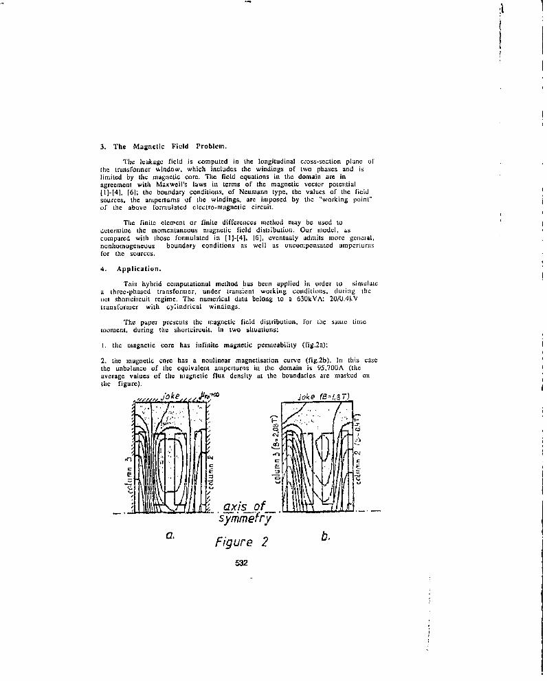
3. The Magnetic Field Problem.

The leakage field is computed in the longitudinal cross-section plane ofthe transformer window, which includes the windings of two phases and islimited by the magnetic core. The field equations in the domain are inagreement with Maxweil's laws in terms of the magnetic vector potenptial[11-[4], [6]. the boundary conditions, of Neumann type, the values of the fieldsources. the aniperturns of the windings, are imposed by the "working point"of the above formulated clcetro-magnetic circuit.

The finite clement or finite differences method may be used todetermine the momentancous magnetic field distzibution. Our model, ascompared with those formulated in [11-[4], [6], eventualy admits more general,nonhomogeneous boundary conditions as well as uncompensated amnperturnsfor the sources.

4. Application.

This hybrid computational method has been applied in order to simulatea three-phased transformer, under transient working conditions, during thenet sharteircuit regime. The numen'ical data belong to a 63OkVA: 20/0.4kVtransformer with cylindrical windings.

The paper presents the magnetic field distribution, for the same time

moment, during the shortcircuit. in two situations:

1. the magnetic core has infinite magnetic permeability (fig.2a):

2. :ihe magnetic core has a nonlinear magnetisation curve (fig,2b). In this casethe unbalance of the equivalent amperturnis in the domain is 95,700A (theaverage values of the magnetic flux density at the boundaries are marked onthe figure).

i k joke (--,87T)

0 c, I)-'4,..• -C Iz

C E3

j4 axis ofsymm-etrya. Figure 2 b,

5W2

S. Cnnricusions.

qlaThe puri,,y sof icisestearchua pprogamcwa to rsiather compedsrbuino

clecoromagnetic structures. such as transformers. under less restrictiveisaur p tionrLs.

The rLSUlls have proved tha. out hybrid model which implements.w~ihoui special difficulties the magnetIic core nonlinearity as well asuncompensated windings ..mperturns. allows a better approach to and in goodagrc.:mcr t (in nu(dclling s(nse) wid' the published experimental data [5], 171.

Its applicability to other equivalent electromagnetic devices models isnatural.

The basic concept of our model is the combined use of global (voltages,*:..'rcniS. fluxes) 9UafltiLiea (the actually measurable ones) and local (magneticv-.rtor-potenifial) quankities (obtained through field analysis) and. as such, thec.,iabined use of an electric -circuit sirmi.lator and a field-analyscr.

6. Acknaowle~dgements.

V Special thar~ks to pruf.A.Moraru and C.Fluierasu for the very usefulldi~iut;U011

Refe:e, .-e

I. Audcivcn.O.W.. - Trwsjorrner Leakage Flux Program based on the FEM - IEEETratisacticas on PAS-92, ar.2/1973.

2 ':ikvester.P.,Ko31rad.A.. - Ai-alysis of Transformer Leakage Phenomena bydlig/icr Order Finite Elements -IEEE Transactions on PAS-92

i'ulonjadoff.M.,ii~o. -TAe Dimensional Flux Calculatiors on a Three ,haseV-&sformer -IEEE Transactions Ai PD. ni.3/1986.

4. vhh.!h lieh X - VwerjcsAd Study of the Transformor Leakage Magnetic Field-iSEF, Lodz. I'oiancl. 1989.Km~aD.-Doctoral Dkrs~cr':aton - Poly.Insa.of Buebi'rst, Rums~nia. 1978,

.Marejga.M.. Kagne.:A L-raage Flux DistUwiuon In the Three PhaseTin - formers - ISEP, Lodz, Poland, 19519.7. Moci.bC~ir, IWsertation -Poly.lnst.of Bucharest. Romania. 1988.8. 1luirc;,u ., ESZ, -Ni neric Corwvutational Package for Nonlinear

Eir-usc Circicaie- Polyt.Inst.of Bucharest, Romnania. 1987.

(rev. 19V33

FINITE ELEMENT ANALYSIS OF MAGNETIC FIELD DISTRIBUTIONIN FERROMAGNETIC SHIELDS

Constantin V B-I. Ovidiu C. Craiu . Mihaela I. MoregaPolytechnic Institute of BucharestDepatment of Electrical EngineeringSplaiul Independentei 313, Buchaiest, Romania

ABSTRACTA model for the analysis of the .magnetic field distribution and the computation of eddy currentslosses in laminated ferromagnetic shields is proposed in this pape.t The magnetic field normalpenetration into the laminated shie!d, coupled with the reaction of the eddy-currents leads toa three-dimeinsional magnetic field problerm in a nonlinear medium. The numerical treatmentinvolves the FEM in conjuction with the Newton-Raphson technique.

INTRODUCTIONThe ferromagnetic and electromagnetic shields are placed in the vecinity of the electricalmachines solid parts, in order to reduce the eddy-curients losses due to the time varyingleakage fields 11.2,3,41. The computation method of the magnetic field distribution and theeddy-currents losses piesented in this paper, are applied on a three-dimensional stiucture ofa power transformer, with the tank wall piotected to the normal leakage flux penetration, bymany satutabile iron .hields (fig 1.)

Fig. I

The governing electromagnetic field equation is

curlci' Llurl I)- I - -i)

534

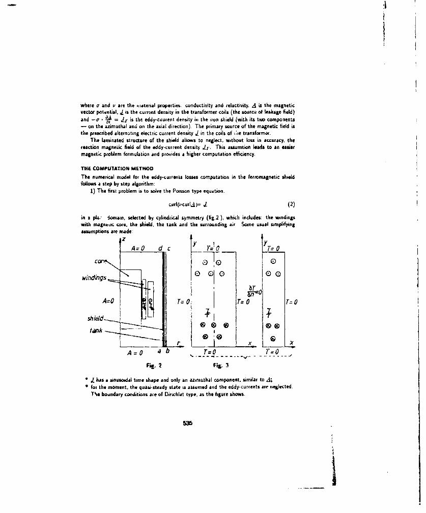
where a and v are the mjaterial properties: conductivity and reluctivity. A is the magneticvector pottntial, j is the currmnt density in the transformer coils (the source of !eakage field)and -o • = IF is the eddy-cuurent density in the iron shield (with its tw components- on the azimuthal and on the axial direction). The primary source of the magnetic field isthe prescribed alternating electric current density J in the coils of :it transformer.

The laminated structure of the shield allows to neglect, without loss in accuracy, thereaction magnezic field of the eddy-current density -L'. This assumtion leads to an easiermagnetic problem formulation and provides a higher computation efficiency.

THE COMPUTATION METHODThe numerical model for the eddy-currents losses computation in the ferromagnetic shieldfollows a step by step algorithm:

1) The first problem is to solve the Poisson type equation.

curl(Vcur1A)= J1 (2)

in a p4,. domain, selected by cylindiical symmetry (fig.2), which includes: the windingswith magneLiC core. the shield, the tank and the surrounding air Some usual simplifyingassumptions are made:

A=O d c Y = -0 T=O

ce0 0

windings I0 G 0 0 0

AA= a b T= 0 T=O

Fig? 2 RW.

"* J has a sinusoidal time shape and only an azimuthal component, similar to ,;"* for the moment, the quasi-steady state is assumed and the eddy-currents are neglected.

T1e boundary coenditions age of Dieichlat type, as the figure shows

535

:1

The solution of equation (2) is obtained by the FEM, coupled with a Newton-Raphsonttchnique if the nonlinear magnetisation curves of the shield ai. tank are considered. TheFEM formulation leads to the standard equation:

[GlI i].A} = IR- {J} (3)

and, according to the Newton-Raphson iteration procedure, the increment of the unknownvariable {6A}&+l = (A}L+, - {A}lk for the ,,k + V'-th iteration step is given by:

{6A}+ = .{ 0i OA'OA, } (4)

where the energy functional, F is expressed by:

= J4 e HI dBd - JA) d1c (5)

The discretisation mesh is not a very refined one, for exemple the depth of the shield iscovered by a single row of triangular elements. The solution of eq.(3) allows to compute thevalues of the normal flux density on the surface of the shield.

2) The values of A, obtained as the solution of the first step, are used to generate (bypolinomial interpolation) the boundary conditions for a detailed computational domain: theshield-the air space-the tank (the domain abcd in fig.2).

The problem is similar to the fiwst, only a Laplace type equation is to be solved:curl(V curl d)= 0 (6)

3) The solution of the second step allows to compute the values of the magnetic fluxdensity in the shield, especially the normal (radial) component:

at the level of each triangular element of the mesh.4) For the computation of the eddy-currents distribution, each sheet of the laminated fer-

romagnetic shield is considered with a plan-parallel symmetry (fig 3). The governing equationsare:

curl Lj -ey(8)div j1I = 0

if i irenit vect potenthd • i* introduced by the equation.

curl I L 11 (9)div I - 0

536

I

it is possible to reduce the problem at the standard FEM equation

[C(I • {T} f j }= {- (10)

where the eddy-currents field source {Js} is given L;:

{g5 } --- -o.{B} (11)at

The boundary conditions are settied by natural considerations, as fig.3 shows,5) The eddy-currents losses in every sheet could be evaluated by

IF Jl=k - r A l (12)

The sum combines the contributions of the n triangular elements of the sheet, each havinga Ak surface and JF.t current density. The sheet has the &, thickness (depth) and the c',conductivity.

Remarks:i) At this step it is possible to do a control of the above procedure. The problem fron,

the first step is comp!eted with the distribution of the eddy-currents density JF (theazimuthal component) in the sheet. With the same procedure is calculated the magneticflux density, produced both by the conduction current density (_ - through the coils)and the eddy-currents density (Js- through the sheet).The distribution of the flux density in this situation, evahl'ted on the surface of the sheet,is compared with the similar distribution, computed at the first step. If the differencesdo not exceed a prescribed error value, then the method is satisfactorily; in other case,the procedure needs a corection. However, the applications of the computational methodprooved the coherenc.. and the correcness of the algorithm.

ii) The process described above by the steps 1-5 corresponds to a value of the initial currentdensity L in the winidings. If the nonlinearity of the ferromagnetic regions is taken intoaccount, the time variation of the magnetic flux density (Ui) has another form than thecurrent density (J) and the procedure previous described must be repeted at each timestep.

NUMERICAL RESULTSFig. 4.a. shows the geometry of the model used for a numerical application of the previousalgorithm. A plan axial s.ction througL a two Wid ijig tcsa3fw er witn 1gneii k. w.Ore, in thevecinity of a ferromagnetic shield and the tank of the transformer is the computational domainfor the first step. Because of the longitudinal symmetry, only the superior half of the domain isconsidered. The geometrical dimensions and the boundary conditions are specified in fig.4.a.

537

ii

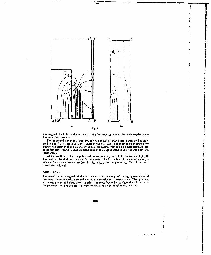
4e

1kM-

SO. 10 A aa. b.

Fig. 4

The magnetic field distribution tstimate at the first step considering the nonlinearyties of thedomain is also presented.

For the second step of the algorithm, only the doma in ABCD is considered; the boundarycondition on AD is settled with the result: of the first step. The mesh is much refined, forexemple the depth of the shield and of the tank are covered with ten time more elements thanat the first step. Fig.4.b. shows the distrbution of the magnetic field lines in the shield-air-tankregion ABCD.

At the fourth step, the computational donain is a segment of the divided shield (fig.3).The depth of the shield is composed by "-n sheets, The distribution of the current density isdifferent from a sheet to another (see fig. 5), being visible the protecting effect of the shi&Jtoward the tank wall.

CONCLUSIONSThe use of the ferromagnetic shields is a necessity in the design of the high power electricalmachines. It does not exist a general method to dimension such constructions. The algorithm,which was pvesented before, allows to select the most favourable confmgur ti F, of theh•i•d•l(its geometry and emplacement) in order to obtain minimum supplementary losses.

538

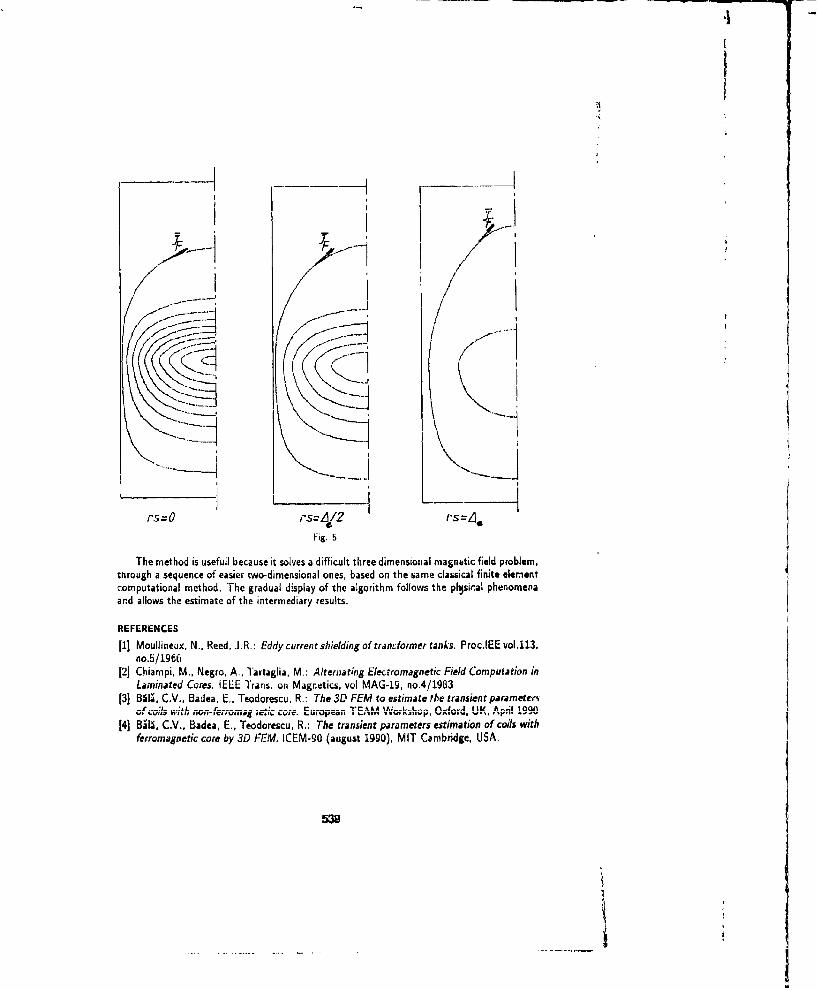
SI f- 1

- L

Fig. 5

The method is usefull because it solves a difficult three dimensionlal magnetic field problem,mlrough a sequence of easier two-dimensional ones, based on the same classical finite elementcomputational method. The gradual display of the algorithm follows the ph~sir.al phenomnepaand allows the estimate of the intermediary results.

REFERENCES[I] Moullineux, N., Reed, J.R.: Eddy current shielding of tran,'former tanks. Proc.IEE vo.1.13,

no.5/1956121 Chiampi, M., Negro, A., Tartagtia, M.: Alternating Electromagnetic Field Computation in

Laminated Cores. IEEE Trans. on Magnetics, vol MAG-19, no 4/1983[31 134i•, C.V., Badea, E., Teodorescu, R.: The 3D FEM to estimate the transient parameters

of cods• vvih non-fierrom;n8 ;zv:i- cwe. European TEA.M. MWkshop, Oxfoid, UK, April 1990141 USI, C.V.. Badea, E., Teodorescu, R.: The transient parameters estimation of coils with

ferromagnetic core by 3D -EM. ICEM-90 (august 1990), MIT Cambridge, LISA.

539

21! -

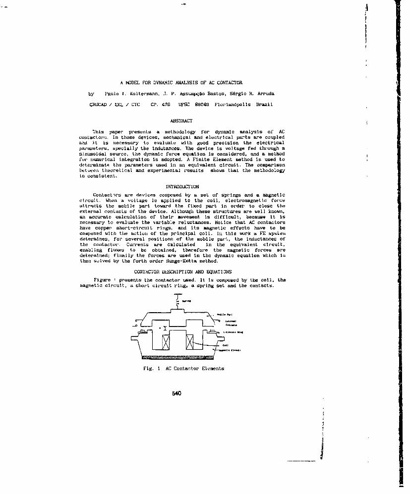
A MODEL FOR DYNAMIC ANALYSIS OF AC CONTACTOR

by Paulo I. Koltermann, J. P. Assumpq&o Bastos, S~rgio R. Arruda

GRUCAD / EEL / CTC CP. 476 UFSC 88049 Florlan•polis Brazil

ABSTRACT

This paper presents a methodology for dynamic analysis of ACcontactors. In these devices, mechanical and electrical parts are coupleda• •d Xt is necessary to evaluate with good precision the electricalpaiiiseters. specially the Indutances. The device is voltage fed through asJnusoidal source, the dynamic force equation is considered, and a methodfur numer-Ical integration Is adopted, A Finite Element method is used todetoi'minate the parameters used in an equivalent circuit, The comparisonbetween theoreLical and experimental results shows that the methodologyis consistent.

I NTR•DUCT IONContactirs are devices composed by a set of springs and a magnetic

circuit. When a voltage Is applied to the coil, electromagnetic forceattracts the mobile part toward the fixed part In order to close theexternal contacts of the device. Although these structures are well known,an accurate calculation of their movement Is difficult, because It Isnecessary to evaluate the varlable reluctances. NoLlce that AC contactorshave copper short-circuit rings, and its magnetic effects have to becomposed with the action of the principal coil. In this work a FE systesdetermines, for several positions of the mobile part, the inductances ofthe contactor. Currents are calculated In the equivalent circuit,enabling fluxes to be obtained, therefore the magnetic forces aredetermined; finally the forces are used in the dynamic equation which isthen sulved by the forth order Runge-Kutta method.

CONTACTOR DESCRIPTION AND EQUATIONSFigure I presents the contactor used. It Is composed by the coil, the

magnetic circuit, a short circult ring, a spring set and the contacts.

Fig. I AC Contactor Elements

540

I

iIThe main equation for the FE method Is:

Curl u curl A = Je (1)where A is the vector potential. Je is the external current and U is thereluctivity [I],[2],13).

Figure 2a presents the magnetic circuit, and the equivalent circuitis shown in figure 2b.

R1 Ldi

Ldsl I

ia i

Fig 2a Magnetic Circuit Fig 2b Equivalent Circuit

here Ri and R'2 are the coil and the short-circuit ring resistancesLdi, Ldni and Ld'2 are coil and ring leakage inductancesLmi is the mutual Inductance

All these inductances are found by FE method for several values ofdistance and they are refered to the primary. The equivalent circuit offig. 2b is used by both, transient and permanent regimes. During the firststep, the inductances change and they are obtained from the curvespreviously determined from FE results (and aproximated by the squareminima method). When the contactor iL. closed (permanent regime) the valuesof indutances are fixed, since there is no movement any more.The exampleunder study show no appreciable saturation. Thus the analysis by phasordiagram is possible; this diagram permits an easy visuallsation of theangles between the currents (fluxes) in the coil and in the -Ing. Thefinal result of currents and fluxes is a resultant force with a non nullvalue, avoiding an undesirable vibration.

The mechanical equation is:

M.d 2x/dt2 = Fe - K.x - B. dx/dt (2)

which is solved by time step integration. Where Fe is theelectromwagnetic force, K is the spring elasticity coefficient, " is thefriction coefficient, M Is the mass and x the displacement.

541

I

The general form of the force, given by Maxwell Tensor, Is:2F = (Bm.sinwt) .S/2.jio N/pole

where Bm is the magnetic Induction in the airgapIn pole 1 the force is Fi - sin'2wt (3)

2. M. SIThe force produced in the ring pole is:

F2 = 2 .sin2 wt + 4A,1. sil2(wt-a)2.po..SZ1 2- J4. S22

Expanding sin2 wt and assembling the terms, the expression becomes:

F2 - 0212 + 00__ 2 0212.cos2wt - 01,.cos(2wt-2a) (4)2,0o.S21 2.po522 2.o.Sai 2. 0. S22

where 021 and 01 are the fluxes In the external and internalsurfaces S21 and S22) of the ring, respectively; m is the angle betweenthe fluxes [4).

The resultant force In the ring face is made of two components whichIndividually pass through zero value, although the resultanL has non nullminimum value , The first two terms correspond to the average componentand the two last ones represent the alternate component of the force.

The resulting force (Fe) is: Fe = Fi+F2

The fluxes of equatlons (3) and (4) are obtainned from the currentsil e 12, calculated In the equiva!ent circuit. With the voltage law ofKirchoff, the following equation system Is obtainned:

V [ Ri + jw..Ld - jw.L[ ]

- jw.Lmi R'-2 + jw. Ld'2 2

where Ld = Ldi+Ld2i

Making some algebric transformations In equations (5), the stateequations of current 11 e 12 ( x1 e k2 respectively) are:

-L. ." 4 L'd 2 h 0 -R' x2 0

and:

!l rAil At?' 1 ri rBi r V1[:1 i= Aa2 ]. x'j + I (6)

where the matrix "A" is the inverse Inducances matrix multiplied bythe resistences matrix.

542

..5

:1

From the mecLanical equation (2). the state equations of displacement(U3) and speed (x4) are obtainned as:

4 - 1/.M (Fe - Fm - B.xW (7)

The mechanical force (Pa) Is given by the sum of all fo,-ces due tosprings. In order to solve the state equations, the 4th order Runge-Kuttamethod Is adopted for the numerical Integration. When the state variablesare obtainned by this method, all the others variables of the structureare easily avaluated, defining completely the devices' dynamic behaviour.

RESULTS

The methodology is applied to a test case. Figure 3b shows the flixdistribution when the ring Is current fed , in order to obtain theinductances Ldz and Lmz. Fig. 3a shows the flux distribution when thecoil is fed, and the inductances Ldi, Ld21 and Lint are evaluated. Infigure 4, the transient current is shown. Figure 5 presents the resultantforce for steady state showing without doubt that It has never a nullvalue. The experimental results have a good agreement with thetheoretical ones, as far as closing time, transient and permanent currentand finally, forces are concerned. It is interesting to note that thisprocess is an important tool, as far as design of contactors is concerned.

Fig. 3a Flux Distribution Fig. 3b Flux Distribution

543

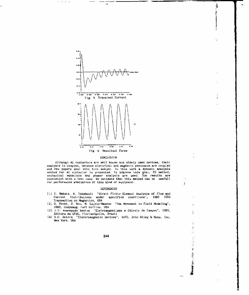
I

0.2"

S.... ns.....r

*0*.o - -.r- or• :.. ,. . .0 0V 00 0 . o 0 0 - A-0

Fig. 4 Transient Current

i •I 'Fi€otoIl u . o©00 t0, 0 0; 000.1 0

Fig. 5 Resultant Force

CONCLUSIONAlthough AC contactors are well known and widely used devices, their

analysis is complex, because electrical and magnetic phenomena are coupledand few papers deal with this subjec. In this work a dynamic analysismethod for AC contactor is presented. To achieve this goal, FE method,mechanical equations and phasor analysis are used. The results areconsistent with a test case. We estimate that this method can be usefullfor performance evaluation of this kind of equipment.

REFERENCES[1] T. Nakata. N. Takahashi "Direct Finite Element Analysis of Flux and

Current Distributions under specified conditions", 1982 IEEETransaction on Magnetics, USA

[2] B. Davat, Z. Ren, M. Lajoie-Mazenc "The Movement in Field Modeling,1985, Compumag. Fort Collins, USA

[31 J.P. Assumpqao tUastos "Eletromagnetismo a CAIculo de Campos", 1989,Editora da UFSC, Florian6polls, Brazil

[4] H.C. Roters "Electromagnetic Devices", 1970, John Wiley & Sons, Inc,New York, USA

544

1,

EDDY CURRENT ANALYSES OF THE CORE PLATEIN A LARGE POWER TRANSFORMER

Yuanren Chiu Wei Wang QIinke Zhang Guachun XiacXiaughua LiA

Electrical Englineering Dept., Wian, Shsaanxi, 710049 P.R.C.&XI'aa Trantormer & Electric Fuinace Works. XI'an,710077 PkC

ABSTRACT

ir' this Paper.- the eddy current distribution and losses in the core Plate ofiuon-magnotic steel material of a large power transformer have beeni analysed. ThisPaper also discuss how the strength of the eddy current demagnetizing effect andthe magnitude or lbs resistance of the eddy current path both Influence the eddyturrent to~ss of the non-magnetic; conductiug plate. The problem to limi, the locatoverheating caused by these Losses has been touched on. Experiments have been pei-formed on small model plates to examine the analyses,

I NTRODUCT ION

Leakage flux prubtom becomes more and more serious as the rating of powertransformer Increased. Leakage flux induces eddy current In metal strurtural,oaiponents, thus generates additional tosses. Although eddy current losses some-times are of Insignificant magnitude as compared with the total Losses, but insevere cases, It say cause excessive overheating and lead to perfurmanre failure,In this paper, eddy current loss on cure Plate due to winding leakage flux hesbeen taken Into consideretion.

Papers from different Investigators 1,234,, /are helpful in showingdifferent ways of mathematical formulation, using magnetic vector potential A orelectric vector Potential T to describe eddy current phenomena at power fre-quenry. As well known, A Is defined as a flux describing funoction, and T Is de-fined as a current describing function. As magnetic flux passes through not onlyferromagnetic part but also non-magnetic part of the space, white conductingcurrent flows onty in rondurtor. Evidently, to describe eddy current problems,T formutation has the advantage of Limited alem over A formulation and Is alsomore ronvenient to specify boundary condition In certain situation.

Fur these eddy current problems. potential functions and field quantities aretime variables, but at powet frequency and In sitnusoidgl staadý-state circua-stances, the displacement current can be Ignored, while Lime variables can beexpressed by phasors to eliminate the time factors.

lit this Paper, the distribution of winding leakage flux over tsue core plimihar. been calculated with magnetic vector potential A In the axisymmetric system,mod the eddy current distribution and loss In the core plate have been calculatedwith current vector Potential T lin the rectangular coordinates system.

WINDIND LEAKAGE FLUX DISTRIBUTION

545

A.

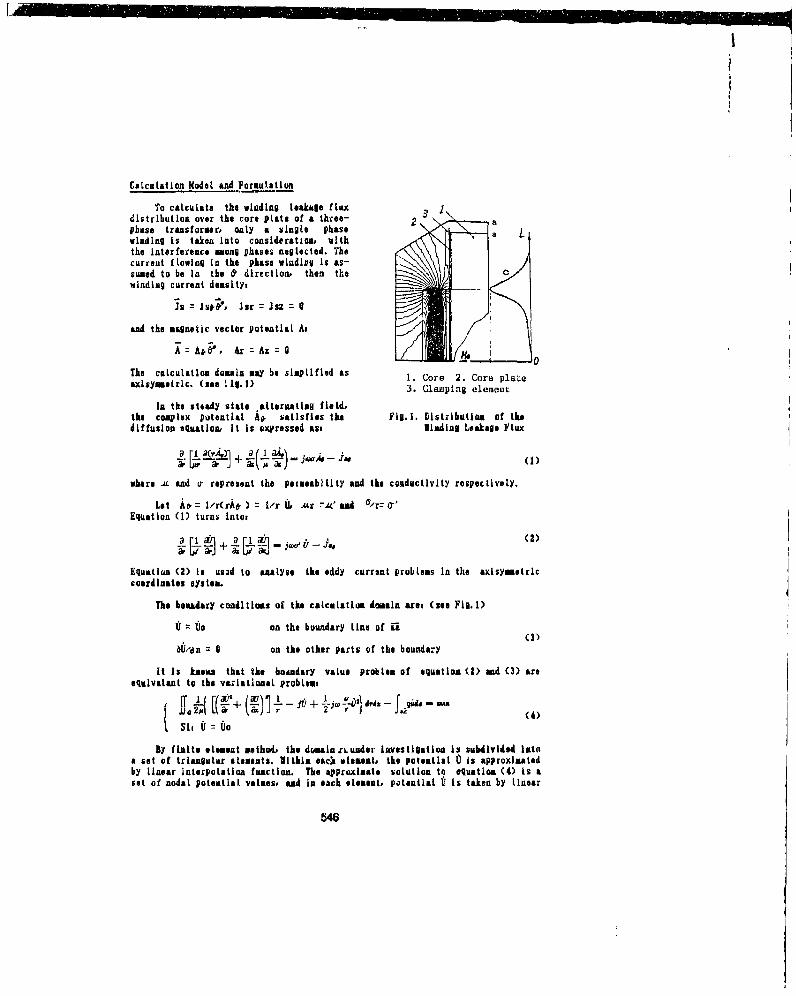
Calculation Nodel and Formulation

To calcuLate the winding leakage flux,distribution over the core plate of a three- 2phase transformer, only a single phasewinding Is taken into consideration, withthe Interference among phases neglected. Thecurrent flowing In the phase winding Is as-su-ed to be in the & direction, then the Cwinding current density,

is=Js9O, Jsr=Jsz--

an the magnetic vector potential AtC

A= A&a*, Ar = Az = a

The calculation domain may be simplified as 1. Core 2. Core plateaxisymetric. (see . 1g. 1) 3. Clamnping element

In the steady state altermatlna field,the complex potential An. satisfies the Fig.1. Distribution of thediffusion equatlon, It is expressed ass linding Leakage Flux

S(I)

where -A and o- represent the peateability and the conductivity respectively.

Let A. = i/r(rA•, ) = 1/r 6 Ar --A' a"d 6/r -'Equation (1) turns into.

+ + 2 FI ;- l (2)

Equation (2) is used to analyse the eddy current problems In the &xisymetriccoordinates system.

The bomtadary condItioss of the calcutatis doaaain area (see Fim.i)

hs on the boundary line of ii'

U/dn =0 on the other parts of the boundary

It Is known that the boandary value problem of equation (2) and (3) areequivalent to the variational problem,

+f +f 1j2-fl 2,ýOz) iri - u -~ mi.a2#air 24

by finite element methoi, the domainzn.under investigation Is subdivided Iatoa set of triangular elements. Within each element, the potential U Is approximatedby Linear InterpoLation function. The approximate solution to equation (4) is aset of nodal potential values, and in each element, p•otentlat ti is taken by linear

546

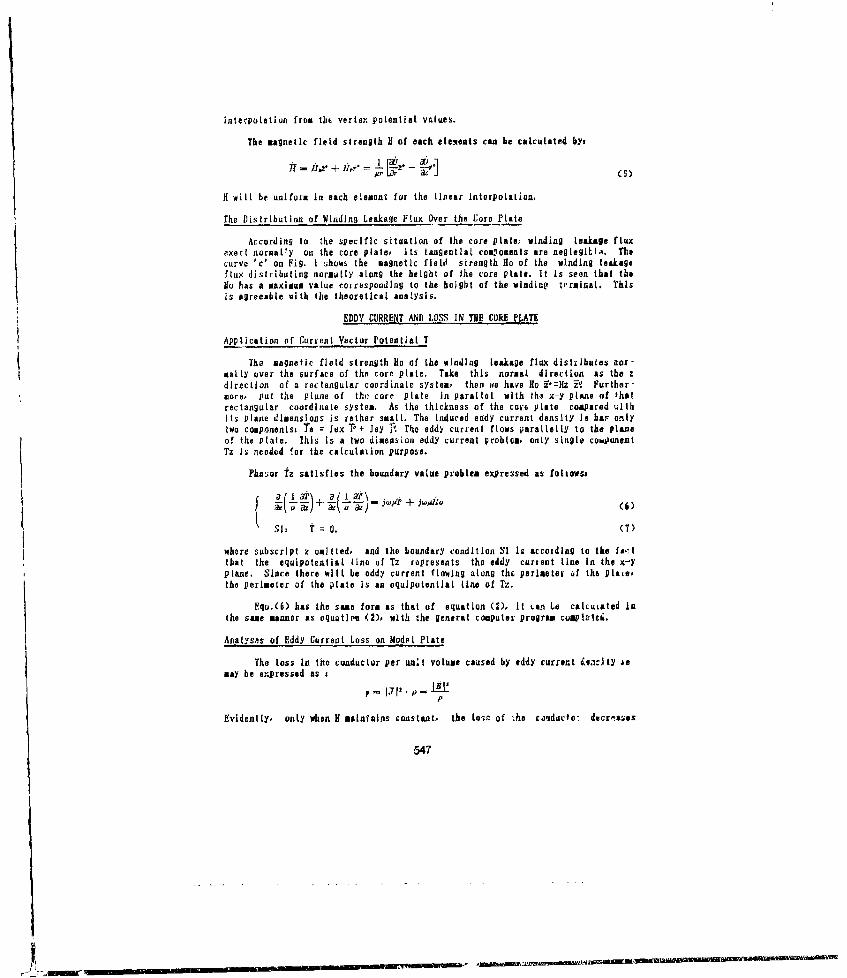
interpolation from the vertex potential values.

The magnetic field strength H of each elements can be calculated by,

if wilt be uniform In each element for the Linear interpolation.

The Distribution of Winding Leakage Flux Over the Core Plate

According to the specific situation of the core plate, winding leakage fluxexert normally on the core plate, its tangential co&,onents are neglegilj.. Thecurve 'c' on Fig. I .hows the magnetic field strength Mn of the winding leakageflux distributing normully along the height of the core plate. It is seen that thego has a maximum value corresponding to the height of the wlndlnp Irrainal. Thisis agreeable with the theoretical analysis.

EDDY CURRENT AND LOSS IN THE CORE PLATE

Application of Current Vector Potential T

The magnetic field strength Ho of the winding leakage flux distributes nor-catty over the surface of the core plate. Take this normal direction as the zdirection of a rectangular coordinate system, then ise have Nio ,--iz iof Further-more, put the plane of tho core plate in parallel wilth the x-y plane of fhatrectangular coordinate system. As the thickness of the cose plate compared ulthIts plane dimensions is rather small. The Induced eddy current density Je har. onlytwo components. Tas = Jex T- Jay 'V. The eddy current flows paratetty to the planeof the plate. Ihis is a two dimension eddy current problem, only single componentTz Is needed for the calculailont purpose.

Phau.or Tz satisfies the boundary value problem expressed as foLtowss

& "r T a i( ' I ` I j' - ) -I)e6

Sih t z . (7)

where subscript z omitted, and the boundary condition SI is according to the fm--tthat the equipotential line of Tz represents the eddy current line in the x-yplane. Since there wilt be eddy current flowing along th& perimeter uf the plaSe,the perimeter of the plate is an oquipotentlal line of Tz.

Equ.(6) has the same form as that of equation (2), It ian Le calcutated Inthe same manner as equation (2), with the general computes program complteui.

Analysas of Eddy Current Loss on Modes Plate

The loss In the conductor per unit volume caused by eddy currert 4ia:Ity jemay be expressed as s

p - 1,712, -. J-p

Evidently, only when B maintains constant, the tos. of .he coqdacfo" decr.ases

'547

with the Increase in the resistivity. But, practically, when the applied fMoldstrength Ho maintains constant, H will be changed as eddy current changes, sincethe demagnetizing effect of eddy current may counterect the applied field S~rengthto a certain extent. Thereforv, the eddy current loss In conductor Is Influencedby both the resistance of the eddy current path and the demagnetizing effect ofthe eddy current WIL," aPPLIed magnetic field strengh Hto remains stable.

For example, there are three plateconductors with the same Length of 480 on c~~ IIC~and the different width of 200, 100 anid o--4 . Or20 nz respectively. They have the same f rp _oox40operaeability of -,Ao and their resistivities -2?. lo m 4,90are varying according to the label of the -13. 20 x4a0horizontal axis, Calculation has been per-Aformed by assuming that they are under the dsame stable -td uniform magnetic field ofBo ::49 US wheich penetrating normally to- Awards those conducting plates. -__________0~~The curves of the eddy current losses 02 35 5.0 10 n, /0*7against the reskstlvities from calculationie~uLts are shown in Figue 2 . Every curvehas a maximum loss Pm &and a corresponding Fig. 2. Losses againstresistivity /1. . Each curve can be divided resistivity pInto two Parts at the Point Pa. The leftpart of the curve may be considered as the region affected mainly by dcmnigntlszingeffect of the eddy current, named 'L region'. The right purt of the cuivia may beconsidered as the region affected mainly by the resistlvitY of the eddy c~urrentpath, named 'R regiou'. These curves show that the smaller the maid ii of theplate is. the greater R regiont and the smaller L region will be,

To decrease the eddy current loss of a p late conductor , we ran make slots .)Athe Plate. As the slats 'aye longer and the distance between sltol is shortor, ItIs more possible to transfer the characteristic from L regis, to R regioen. andailso to decrease the eddy current loss.

Local Over-Healing ProblemP / 116 ______

According to the former discussIon, 2.0It is seen that we cart reduce the eddycurrent loss by making slots on theplate. At the same time we should pay2attintion to avoiding local overheating2on the plate.

1i .0BY calcuilatono we find that when 1~

slots has been made to transfer tiecharacterist~c from L region to R region,the decreasing rates of the loss are notsimultaneous with the decreasing rate ofthe maximum current density. The eddy I -*current loss and the maximuz eddy cur- 0 10 20 30 4 0 1. ("IT"11rent density against the length of theslot on a plate conductor working at R Flg.3. i----Eddy current lessregion are plotted In F19.3, In whichp Po 2 --- maximum eddy current

and IJo indic a te the eddy current loss and the maximum eddy current density,respectively, of the plate without slot. Fig.3 shows that only when the length ofthe slot is greater than 33 ma,. the maximum eddy current density will be lower thanJo. This Is the case caused by the uniform applied external field. When the ap-plied field is not uniform, the slot should be made passing through the spotwhere maximum applied field exists.

Eddy Current Distribution and Loss on the Core Plate

The non-magnetic steel core plate has thepermeability o (i).ianti the resistivityP77.2 E-711.m. The winding leakage flux d In-Oitributiun along the height( length) of the cote (a

Plate has been shown in Fig.t by curve 'c' -7--%This leakage flux causes eddy current Inducedin the core Plate. The distribution of eddycurrent over one-fourth of each plate is Is)shuini ia vig. I~ The core plate shown in Fig.4__________(a) hus two slots, (bi) has one slot and (c)without slot. The eddy current Loss of plate

(c) Is 424 w. It shows that these plates areall working !in the L region. It implies thatthere should lbe have more slots on the. plate,so as to shift the plate working friom L legion Fig. 4. Distvitiution ofto R regi,n and to reduce the eddy current eady currents Inloss effectively, core plates

MODEL EXP'ERIMENTS FOR IIJENTIFICATION

The principle diagrau of theexperiment is 5huwn in F1g.5., Thesymbol 'it' refers toi all Inslatla--tliio for producing magnetic field,Whon like vurrent Passes throughAthe winding, an uniform magneticfield wilt t,it produced In the gap. WA Plute conductor sample '6 bIs1placed Ill the gap. By thistheddy current loss of the plateconductor can be tested.

Flg.5. P'rinciple dtiagramThe Experimental and Ualculated Results fur experiment

Thlle experimentat result~s and the calculated results of the eddy currenttosses of two 4Otx"Uxii nm aluminum plates matth quite wuell as shown in Flg.b. Thepiate (a) Is without slit, and the plate (bi) Is with one slil. The loss in plate(b) decrease evidlently sinrg there'!; a slit on it. It shows that the cheracteris--tics of these Pltates are under the R region.

Another experiment has bean performed on three pieces of aluminum platewhich hbve the same dimensions of 400x44x1i ma. The first plate Is without slot.the second one withi one slut and the third one with thres slots. The Losses o,tthese thres platets a9goinst the uniform rnugnotic flux density are plotted In Fig.5.It shows the toss of the second one is greater than that of the first one, and

549

A ____ _____ . .. ____-____ _ - - __

the toss of the third one Is Less than that of the first one. It is shown that thefirst one Is under the L region, and the second one stilt wookln under L region.The characteristics of the third one have been transferred from L region to R re--glon, and the toss is reduced. The experimental results coincide with the anaLy-tical, results discussed formerly.

p (w) p (W)

30.0 x F\iwrzim.nril 200

20.0

10.0 *,• •z

I00

(1 100 600 .9 0 (0 11 0 on .50 0 TI (G>-)

F- ]

Fig. 6. a--Plate without slit Fig. 1. Eddy current tossesb--- Plate with slit in plate conductors

CONCLUSIONS

Adopting non-magaetic steel material for core plate of a large power trans-former can limit the eddy current tosses and avoid local over-heating to a groatextent.

In case of the apptlied magnetic field source remain iL hanged.When neglectingthe demagnetizIng effect of the the eddy current, tosses are inversely propor-tionat to the resistance of the current path. But through practical catculat I,the results sl ,w that even for non-magnetic steel material, the demagnetizingeffect of the ea.dy current could not be neglected. So, how the variation ofresistance Influences on the tosses should be known from calculation results.

REFERENCES

I. C.J. Carpenter, Proc. IEE. Vol.124, No.11, November 1977.2. T. Sato and Y. inui, Paper No. A 77 029-2, IEEE PES Winter Meeting, NY,

Jan. 30-Fob. 4, 1977.3. S.J. Salon and J.M. Schneider, Paper No. A 79 545-5, IEEE PEtS Summer

Meeting, Canada, July, 1979.4. T.W. Freston and A.B.J. Reece, IEEE Trans. MAil-1i, No.2, March 19102.5. L. Brown, Proc. IEE Vol. 129, Pt.A, No.1, January 1982.6. A. Konrad, IEEE Trans. MAG-2I, No.5, Sep. 1995.7. T. Tokumasa, S. Dol, K. Ito and N. Yamomoto, IEEE Trans. on PAS, vol. PAS

103, No.6, June 1984.

550

EIGIERIHG RMOLVAB1LITY OF E14HIHO I DDY MW PROBLM

Z.Cheng,S.Gao,D.ZMang,J.Wang and C.YeBaoding Transiormer Works,Baoding 071056, China

This paper proposes some ideas of engineering resolvability technique of large engi-neering 3D eddy current problems through solving a simple electrical engineering model"'for evaluation of power loss in steel. The engineering application of 'EANed (tested byIAM4) codes Will be specially emphasized.

1. ENGINEERING FIR_11B1BLIM AND ENGINFERING SOLUTION

In electrical engineering engineers often encounter various kinds of engineeringfield problems, especially, including electromagnetic field problems, the major difficultpoints of those problems are that: very large size and complex geometry of solved regionwith multi-materials. The maximum size of solved region may be more than 10 metres, butthe enetration depth is very small in steel parts of electric machinery, in general.itmay be less than 3 am, the finite elements should be enough fine, thus the application of3D electromagnetic softwares will be stemmed from too large computer storage and CPU time.

In engineering design a series of performance parameters of products will be deter-mined by aided field analysis. Unfortunately, engineers can not find out exact solutionsof complex 3D nonlinear eddy current problems.

We have proposed an idea of engineering solution of engineering problemscLU.The maincharacteristics of engineering solution may be described as follows: the confirmable aridstable error extent, the lower computing co;t, and the favorable usability.

2. ENGINER NG ANUDBENCI4 A

Recent years,TEAI workshops have proposed and solved successfully 13 benchmark prob-lemsL101, many excellent 3D) codes have been &de1-"3. All these effectively pushforward the development of 31) eddy current analysis. However, the benchmark problems arefar from large engineering eddy current problems. Authors propose an idea of engineering"TEAM for the sake of showing the differences with TIAM workshop of solving benchmark pro-blems.

As we know, the aim of benchmark TAM is to test electromagnetic analysis methods,beyond doubt, doing those tests in simple models is a best way. 'lEA~ed codes provideuseful tools, while engineering ITAM ingeniously uses those tools to solve large engi-neering problems, and dovelows various practical analysis techniques, including makingusable 3D eddy current codes, and checks their engineering usability.

In eigineering TFAM the proposed test problems will be based on typical engi-neering background, the developed resolvability techniques will be directly used in aidedanalysis of products. It will aim at the engineering application of electromagnetic ana-lysis softwares.

3. RUVIEW OF ENGINEERING RMI3SPLVIALMMIi'jl

As above,to solve a large engineering field problem, the first thing is to do thereasonable assumptions to make the problem resolvable'h', and to choose the most practi-

551

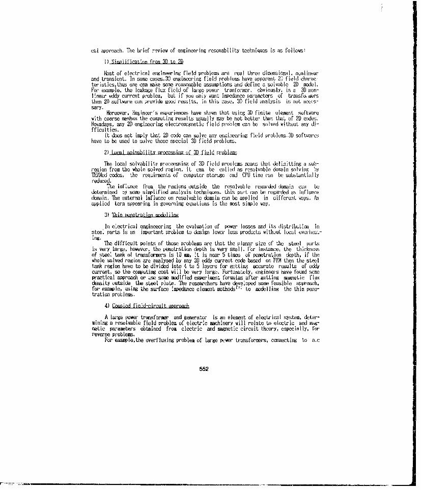
cal approach. The brief review of engineering resovability techniques is as follows:

1) Simplification from 3D to 2I

Host of electrical engineering field problems are real three dirensional, nonlinearand transient. In some cases,30 engineering field problems have apparent 21) field charac-teristics, thus one can make some reasonable assumptions and define a solvable 2D Model.For example, the leakage flux field of large power tranformer, obviously, is a 3D non-linear eddy current problem, but if you only want impedance parameters of transfoi uersthen 2D software can provide good results, in this case, 3D field analysis is not neces-sary.

lkoreover, Engineer's experiences have shown that using 3D finite element softwarewith coarse meshes the computing results usually may be not better than that of 2D codes.Nowadays, any 2D engineering electromagnetic field problem can be solved without any di-fficulties.

It does not imply that 21) code can solve any engineering field problems.3D softwarcshave to be used to solve those special 3D field problems.

2) Local solvability Processing of 3D field probleis

The local solvability proceessing of 3D field problems means that delimitting a sub-region from the whole solved region, it can be called as resolvable domain solving by

AJ)led codes, the requirments of computer storage and CPU time can be subsLantiallyreduced.

The influnce from the regions outside the resolvable regarded domain can bedetermined by some simplifie d analysis techniques, this part can be regarded as influncedomain. T'he external influnce on resolvable domain can be applied in different ways. Anapplied term appearing in governing equations is the most simple way.

3) Thin penetration medeliing

In electrical engineeering the evaluation of power losses and its disLribuLion insteel parts is an important problem to design lower loss products withuut local overheat-ing.

The difficult points of those problems are that the planar size of the steel partsis very large, however, the penetration depth is very small. For instance, the thicknessof steel tank of transformers is 10 mm, it is near 5 times of penetration depth, if thewhole solved region are analysed by any 3D eddy current code based on MEM then the steeltank region have to be divided into 4 to 5 layers for, getting accurate results of eddycurrent, so the computing cost will be very large. Fortunately, enginpers have found somepractical approach or use some modified experiment formulas after getting magnetic fluxdensity outside the steel plate. The researchers have developed some feasible approach,for example, using the surface impedance element methodsl'7 to modelling the thin pene-tration problems.

4) Cuoled field-circuit aoaroaeh

A large power transformer and generator is an element of electrical system, deter-mining a resolvable field problem of electric machinery will relate to electric and mag-netie parameters obtained from electric and maetic circuit theory, especially, forreverse problems.

For exaiple,the overfluxing problem of large power transformers, connecting to a.c

552

voltage source, is difficut to solve exactily by only field analysis because the excitingcurrent is not known beforehand.the coupled field-circuit approch shuld be used. Formore complicated enginering problems the coupled experiment-analysis methods have to beused, i.e., simulation test or product test provide necessitated data for doing furtherfield analysis.

4, fU LUDY URRENT UISS MOD

"Mhe design of the 3D eddy current model is based on typical power loss problems intransformers. It consists of two air-core coils with the same number of turns and the samedimensions in which the a.c exciting currents flow in opposite directions, the role ofexciting coils is to provide an applied field only. A steel plate of 10 mm thick is pla-ced parallelly to the coils as shown in Fig.l.

Te aim of this modelling is to calculate the distribution of 31 eddy current andeddy current losses in steel plate, to check the engineering usefulness of 3D eddy cu-rrent codes made by authors, finally, to attempt to find out practical engineering com-puting methods used in aided analysis of products, This will be demonstrated throughsolving the simple problem.

I3D eddy current analysis

his is a 3D, nonlinear, single connected eddy current problem. It can be solved byvaried kinds of Th)1&@d codes, this model provides a possibility that the distribution of3D eddy current in steel plate can be analysed in detail. The initial analysis resultsusing 3D eddy current cede based on T-Y approach with coarse meshes have been shown inFig,2(a). Fig,2(b) shows another distribution of eddy current to verify the 3D code, inthat test example the same applied magnetic fields are perpendicular to the steel plaLeanywhere.

The different schemes of the solvable mwdels have been shown in Fig.3 (a) and (b) toindicate the dealing with the external influnce in different ways. In Fig.3(a) the solvedregion includes the exciting coil, but Fig.3(b) shows that the influnce 01' exciting coilswas replaced by an applied term.

2)S1mplified 2) annlv's

In this model the regular coils and the thin steel plate placed parallelly to thecoils sho, the evident characteristics of 2D field, so it can be approximately calculatedusing 2D software,the 21) model has been shown in Fig.4.

To confirm the accuracy of field analysis in different ways authors have done 2D)analysis using beth 21) FE0 code and Image modelling program, those 2D analysis resultshave been shown in Fis.5.

3) xaperiments of flux density

The testing model has been made, the measurement of power loss in steel plate is difflcult, because, the total Power losses stored in both exciting coils and steel platc,do-termination of the losses generated only in steel plate and the local power losses shoulduse some special experiment technique which will be further developed.

The mea.urement results of magnetic flux density at specified points have been shownin Fig.6.

5. MNLW15U REIHARK

553

The engineering resolvability technique of large eddy current problem will be fur-ther developed, an idea of engineering TEAM has been proposed by authors, it is expectedthat engineering-oriented analysis technique will be effectively used in electrical en-gineering.

L. Z.Cheng,S.Gao and D.Zhang,"An electrical engineering model for Loss evaluation", sub-milted to Asian TEffi wor'kshop-Sendai,l991

L2] T.Nakata,N.Takahasii,K.Fujiwara and Y.Okata:"Improvements of T-fl method for 3-D eddycurrent analysis", IEEE Trans. on magnetics, Vol.Mag-24, (l9881,pp.94-97

L3, O.Biro and K.Preis: "Finite element analysis of 3-D eddy currents", IEEE Trans. onmagnetics,Vol.Haa-26, (1990),pp. 418- 423

[4] D.Rodger and J.F.Eastham. " A formulation for low frequency eddy current solutions",IEI- Trans. on maguetics, Vol. Hag-19,(1983),pp.2443-2446

-5] C.R.I.Emson and J..Simkin: "An optimal me!'od for 3D eddy currents", IEEE Trns. onMagnetics, Vol.Mag-19, (1983), pp.2450-2452

-6] J.Zhou: "Integrated finiteeleaent mo&elling of elec-tromagnetic fields and lea-kage field computation oflarge power transformers", VNLT

PN.D.DisserLation, March 1990 __.____,7J E.M.Deeley:"Tmproved surface - --models for 2D and 3D prob-

leo".T"' Trans.on magnetics, "Vol. l'ag-24, 11988),pp.209-211 I

[8] P.Chen,L.Yan and R.Yao: "The COL,theory and computation ofelectromagnetic fields in "electric machinery", Sciencepress-, 1986. and J.W : :".IEngineering solution of I ' 'engineering field problems- I A

in transformers", 3-D Elec- tI PLA," A

tromagnetic Field Analysis, 2Y(edited by T.Nakata). Sep. A CO-L1989, pp.151-154

[101 T.Nakata, N.Takahashi,K.Fujivaa, P.Olszewski and e.Iv-K.Huramatsu: "Analysis ofmagnetic fields of 3-D non--linear magnetostatic model(problem 13)", Proceedings ofEuropean TEM workshop and Fic. I Enrogmnor ino mod*Linterrational seminar onelectromagnetic field analy-sis, Edited by Y.Crutzan,N.J.Diserens, C.R.I.Emson,D.Rogwer, Oxford, England,23-25 April 1990

554

lI_

4 J4

(a)Engineering model Applied field by coils (b) Test m"dlFig.2 Distribution of 3 eddy current in the steel plate(The thickness of steel plate wus enlarged)

,OLTZý( PLATE-IC1RREy DIPECTION

STEEL PLATE

OIL I

4LEL PI.AT_

CRNY 0IR&ATION UL

Fiu.4 20 MODEL

WbI I REGIONPtLa- 3b ANALYSIS SCHEMES

555

F_' IF

L ... k __7/1--

S EARCM COILS

A. up NOW 7 CO ILI

(227.5)) F .* *

(162.ý5) a I 3

(460Q)6 * 6

132,) * * 7 - .

(-9 .5) 13 * I

(2275 5 *** I '

Ni. OF COLUM RJII F tUXDNST

Cý~pECIFILLO PuSlIONS FOR FLUX DLNSITY (bINEASURLORSLSO FU EST

pig.5 MCASUREMENT OF FLUX DENSITY

SteME AbURLD61,

'0

(30

pig6 COMPARISUN OF CALCULATED ANDMEASURED FLUX DENSITY

SESSION 15- "TIME DOMAIN METHODS"Moderator: Gerald Burke

F-,-._ ._m i,,' I

COMPARISON OF GTD AND MOM SCATTERING COMPUTATIONSAND TRANSFORMATION TO THE TIME DOMAIN

by

Paul G. ElliotARCO Power Technologies, Inc.

1250 24th St. NW, Suite 850Washington, DC 20037

(202) 223-8808

Ira Kohlberg, PresidentKohlberg Associates

PO Box 23077, Alexandria, VA 22304(703) 751-5637

ABSTRACT

Frequency domain scattered fields are computed using the Method ofMoments (MOM) and the Geometrical Theory of Diffraction (GTD) . Aninverse Fourier transform is used to obtain the time domain field.

The NEC code from Lawrence Livermore Labs was used for the MOMcomputation, and the Basic Scattering Code (NEC-BSC) from OhioState University was used zor the GTD computation. A comparison ofthese frequency domain results shows agreement when typicalguidelines for the use of these two approaches are met.

The radiating source is a horizontally polarized infinitesimaldipole source over ground. A fence in front of the sourcebackscatters electromagnetic energy to an observer. The fence ismodeled somewhat differently in the two models. The MOM fence mode]consists of three horizontal wires, and the GTD fence model is asingle flat plate. The models were designed for a switch from theMOM to the GTD method at a radian frequency of 0)=108, correspondingto the smallest dimensions of interest. The GTD model thus providesaccurate scattering results for frequencies higher than W=]08 whilethe MOM fence model is designed to be accurate below 01=108.

The near field options of the codes were used to computebackscattered energy reaching the observer. Both models should beaccurate close to u=108 , and in fact the magnitude plot shows thebest agreement from a-ixl0" to 1.5x10'. The phase plot shows goodagreement from about 0.8x100 to 1.8x10 8 . At low frequencies the GTDresults deteriorate and show erratic spikes.

An inverse Fourier transform is used Lo convert the wide bandwidthfrequency domain scattering transfer function into the time domainwith weighting of the frequency domain components by the incidentpulse spectrum. The resulting time domain response shows theresolution obtained using this approach.

557

LI

F-i

ME

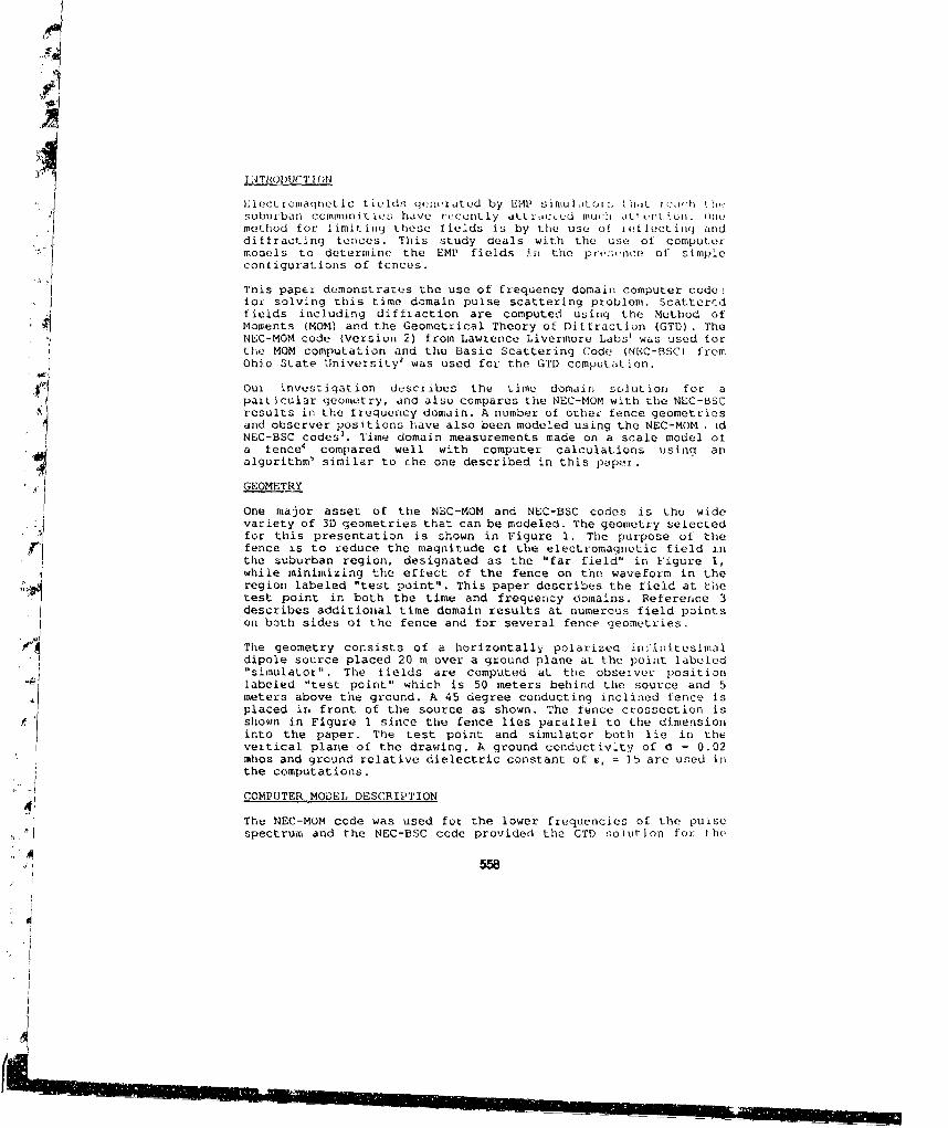
SITIeOI)UCT I ON

1 oct romagnet ic ii i! lds q•nii ated by EMLI simu •tort i h,,L Y .,trlh tIi,-:suburban communities have recently dttracuud Muc:h dl) tnt. .on.

Smethod for limiting these fields is by the use of totlectLing anddiffracting fences. This study deals with the use of computermooels to determine the EMP fields In the prosnone of simpleconligurations of fences.

This paper demonstrates the use of frequency domain computer codezfor solving this time domain pulse scattering problem. Scattertdfields including diffraction are computed using the Method ofMoments (MOM) and the Geometrical Theory of Diffracti0on (GTD) . TheNEC-MOM code (Version 2) from Lawrence Livermore Labs' was used forthe MOM computation and the Basic Scattering Code (NEC-BSC) fromOhio State University' was used for the GTD computation.

Our investigation desciibes the time domain solut ion for aparticular geometry, and also compares the NEC-MOM with the NEC-BSCresults in the frequency domain. A number of Other fence geometriesand observer positions have also been modeled using the NEC-MOM , idNEC-BSC codes 3 . Time domain measurements made on a scale model ofa fence4 compared well with computer calculations using analgorithm' similar to rhe one described in this paper.

GEOMETRY

One major asset of the NEC-MOM and NEC-BSC codes is the widevariety of 3D geometries that can be modeled. The geometry selectedfor this presentation is shown in Figure 1. The purpose of thefence is to reduce the magnitude of the electromagnetic field inthe suburban region, designated as the "far field" in Figure 1,while minimizing the effect of the fence on the waveform in theregion labeled "test point". This paper describes the field at thetest point in both the time and frequency domains. Reference 3describes additional time domain results at numerous field points

on both sides of the fence and for several fence geometries.

The geometry consists of a horizontally polarized infinitesimaldipole source placed 20 m over a ground plane at the point labeled"simulator". The fields are computed at the observer positionlabeled 'test point" which is 50 meters behind the source and 5meters above the ground. A 45 degree conducting inclined fence isplaced in. front of the source as shown. The fence crossection isshown in Figure 1 since the fence lies parallel to the dimensioninto the paper. The test point and simulator both lie in thevertical plane of the drawing. A ground conductivity of 0 = 0.02mhos and ground relative dielectric constant of c, = 15 are used inthe computations.

COMPUTER MODEL DESCRIPTION

The NEC-MOM code was used for the lower frequencies of the pulsespectrum and the NEC-BSC code provided the GTD solution for the

55

£4)4

IIU

zz

P4 0

0

E-4

TE-4

H4;,;,'

IJ559a

0 .1

01

V I I

E

0 II

00¶ 0 0.3NaJomclized Wive Spacing S/ X tknfuirfrne

Figure 2. Transmission colfficient tar parallel and perpendicular polarizationfor a grid of round wires of diameter 13 and ceniorfal-center spacing S

5W0

higher frequonrcies. Two diflferent computer models of the samegeometry were therefore used for d0 iferent frequency rangest;.

The radiating source in both computer models is a horizontallypol&rized infiniluesimal dipole source over ground. Th'_ fence ismodeled differently in the two models. The GTD fence model is asingle flat conducting plate of the height and inclination shown inFigire 1, and 600 meters long (direction into paper). Plates werenot used in the MOM model since that code requires plates to beused only for closed -urfaces. For MOM, horizontal wires are usedto model the fence. This MOM fence consists of 16 horizontal wiresof diameter 0.6 meters spaced 2.83 meters apart. Each of thesehorizontal wires is 40 meters long (direction into paper) and issegmented into 2 meter long segmtents.

An angular frequency of (=u10 is selected as the transitionfrequency from MOM to GTD for thi.j geometry, based on the physicaldimensions shown in Fiqure 1, and on computer run time,.onsidurations. Since the high fLequency GTD computer model runs350 to 600 times faster than the low frequency MOM model, it isde: '-able to use GTD for the broadest possible frequency band overwhiun it yields accurate results.

The guidelines for the use of the two codes as follows. The GTDcode is most accurate when all dimensions of the structure arelonger than approximately one wavelength. The distance from thesource to the fence should also be approximately one wavelength ormore. The distance of the source to the ground is less critical andmay be less than a wavelength. The smallest dimension of the fenceis ths_ slant length of 42 meters, and the source is 14 meters fromthe fence at the closest point. These constraints are approximateso GTDI was used to a maximum wavelength of 20 meters, whichcorresponds to frequencies of W=108 and higher. This should providegood accuracy comb'.ned with minimum computer run time.

The MOM fence model is intenoed to be accurate below about (0=10 8 .The 2 meter segments used for the MOM model are 0.1 wavelengths atWa 10'. As can be determined from Figure 26, the MOM fencedimensions given above should limit transmission through the fenceto -18 Ub of the incident field at w = 108 and to less than -18 Dbat lcrer frequencies. Thus, for all practical purposes the wiremodel of the fence provides an excellent representation of aperfectly reflecting surface for parallel polarization.

COMPARISON OF MOM AND GTD RESULTS

The near field options of the codes "ere used for a frequencydomain computation of the direct and scattered energy reaching theobservwr. Figures 3a and 3b show the magnitude and phase of the MOMand GTD results in the frequency domain. These curves arenornalized to the field that would he present at the observerposition it the same sou.rce were radiating into free space (no(ýround or fence) . Due to this normalizdtion the results shown inFigiures 3a and 3b will be referred to as the frequency domain

561

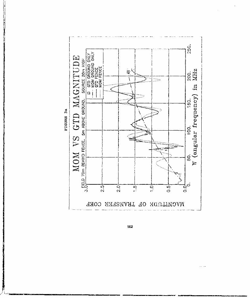
•o~o1..........

S. I ...........Tu,

7-o -

0 % iE j ...... . ......

00

00

0 LD

CLI

, ;, e ,. ..-.....LLI.

00

AdIOD ?LIANV•:,T dJO •I(Iflh1NDY}'

562

ii

a: z 0

ujLL,L woL.-

hE-

rC; 4-1

[Lio

6 6 6 6 6 6 66

JHIOD aadsmvu1I AO 3ISVHd

transfer function T(W) for the particular geometry and observerposition. Also shown in Figure 3a is the magnitude with the groundpresent but no fence, which is the same result using either of thetwo computer codes.

The MOM and GTD models should both be accurate close to W=108 asexplained above. In fact the magnitude plot shows the bestagreement from erilxl0' to l.5xlO'. The phase plot shows goodagreement from about 0.8xl08 to ] .8xl0. At low frequencies the GTDresults deteriorate and show erratic spikes.

CONVERSION TO TIME DOMAIN

The time domain response to a pulse was calculated by inverseFourier transforming the weighted frequency domain transferfunction T(OI) . T(CG) was weighted in the trequency domain by thefrequency spectrum of the incident pulse using a formula typicallyused to describe EMP pulses7 :

L(t) = E0 [axp(-0t) - exp(-at)]

where a = 4 x 10" and I = 6 x 106. 1500 values tor the frequencydomain transfer function T(Ce) shown in Figures 3a and 3b werecomputed between DC and w) = 1010. 500 oi these points were below w)- 10' and so were obtained using MOM. The remaining 1000 pointswere above j) rý 10' and so were calculated using GTD.

Curve A of Figure 4 shows the time domain field for the geomeLry of'igure 1. Curve B is the incident waveform which is thu field which

would exist in the absence of the ground or tence, and all thecurves are normalized to the peak value of this incident waveform.CuLve U is the field with no fence but with the ground. Curve Dtherefore does not show peaks and minima which are produced byreflection and diffraction from the fence. Curve C is the fieldwith the fence and ground except that only the higher frequencycomponents were used; the lower frequency (MOM) results have beenemitted from the inverse Fourier transform.

The time oi arrival of each ray reflected or diffracted from thefenice is shown by the onset of each large ripple in curve A. Thesere-sults are fi excellenit agreement with the theoretical predictionsusing ray theory. A comparison of curves A and C shows that incurve C (only high frequencies used, no MOM results) the onset oftier largu r.ipples produced by diffraction occurs befoLu the rayactually arrives at the observer. It is clear that when the fullspectrum is not used the -im(moe domain results dare not Correct.

Thi;work---wa-spj)o-rtd by the harry Diamond Labs under Contract 4DAAL.OO2-E37-C-0052 with Kohlberg Associates, inc. Mr. Elliot was aconsultanrt to Kohlberg AsUociates.

564

1.2A2 MOIA FENCE. GTD FENU

0 ,- INICIDENT WAVU-ORMI.... .. . . . C1- - l.)COM G,?ID0. GTD rP;ICE

0- .GID ONLY

0.13 13

.0.4 . . . . ... Diflraclion .. ....

-0.2 ---- ,..

-0.4 LAI Iracto n

O. 50. 100. 150. 200. 250. 300. 350. 400.Iinic (us)

Figure 4. Electrlc field for point In tost volumno 50 m from simulator at a heightof .5 m for Inward InclIned fence

565

C.

1. G.J. Burke and A.J.Poggio, "Numerical Electromagnetics Code(NEC) -- Method of Momenta", Lawrence Livermore NationalLaboratory, Report UCID-18834, January 1981.

2. R.J. Marhefka and W.D.Burnside, "Numerical Electromagnetics Cade- Basic Scattering Code, NEC-BSC (Version 2) Part 1: Users Manual,"Tachnical Report ESLT122-4214, Ohio State University ElectroscienceLaboratory, Columbus, OH, December 1982.

3. I.Kohlberg, P.Elliot, and T.Waltemyer, "Diffraction Techniquesfor Reducing the Electromagnetic Fields of EMP Simulators Beyondthe Test Volume.." presented at the 1990 IEEE InternationalConference on Nuclear and Space Raaiation Effects, Reno, NV 16-20July, 1990.

4. J. Loftus, V.Fronczak, and I. Kohlberg, "A Comparison of theDiffracted Fields as Measured and Predicted for a TotallyReflecting Fence in a Scale Model Test for and ELM Simulator,"Harry Diamond Laboratorico Report HDL-TR-2173, February 1990.

5. I. Kohlberg, "Diffraction of Far Fields Produced by E.NMPSimulators Due to a Wire Mesh Fence," Harry Diamond LaboratoriesReport I{DL-CR-90-052-2, Kohlberg Associates, Inc., ContracL UAAL02-87-C-0052, September 1990.

6. R. Johnson and Ii. Jasik, Antenna Lngineetin Handbook, McGraw-l1ll, NY, 1984. pg. 46--6.

7. Y. Lo and S. Lee, Antenna Handbook, Van Nostrand Ruinhold, NY,1985. pg.30-3.

5W6

EVALUATION OF MODIFIED LOG-PERIODIC ANTENNASFOR TRANSMISSION OF WIDE-BAND PULSES *

G. J. BurkeLawrence Livermore National Laboratory

P.O. Box 5504, L-156, Livermore, CA 94550

Abstract

Modified forms of the log-periodic dipole antenna have been proposed in the litera-ture for radiating a short pulse with minimum distortion and also for a phase responsetailored to compress a linear FM pulse. These designs are reviewed, and the antennasare evaluated by numerical modeling with the frequency domain code NEC. Responsesfor transient input signals are obtained from the NEC solution by inverse transformingand convolution. Antennas modified to obtain a linear phase characteristic are seen tobe effective in transmitting an input pulse with nxinizvn distortion. The antennas forcompressing a linear Fld pulse are somewhat effective bUt do not appear to work as wellas might be expected.

Introduction

The log-periodic dipole (LPD) antenna can operate over a very wide frequency band,limited only by mechanical constraints. However, the antenna introduces sigpnificant dis-tortion when radiating a transient signal, due to its nonlinear phase-versus--frequency re-sponse. A modified design has been proposed by Yatskevich and Fedoseniko in [1] to reducedistortion of a pulse by making the phase r,!sponse linear or, more generally, to develop afilter characteristic for compressing a signal such as a linear FM pulse. Sosne results fromnumerical modeling of these linear-phase and FM-compression antennas are presented hereto evaluate their effectiveness.

Standard LPD antennas axe constructed as an array of parallel dipoles arranged sothat their ends subtend a constant angle a, I's shown in Figure 1. The lengths of successivedipole elements farm a 6 cometric progression with scaling factor r < 1, so that

In rn do&

The dipoles are fed with a transmission liue that reverses phase between each pair ofdipoles. Another parameter often used to describe a LPD antemna is

O" - I =- cot a.v. (4 )

Thus a is the distance in wavelengths from a \/2 resonant element to the next smallerdipole in front of it. Values of a are typically in the range 0.06 to 0.22, with r in the range0.78 to 0.98. Carrel [2] detenained that the optimum gain for a given r occurs with

a • 0.22r - 0.0335. (2)* Work performed auder the auspices of the U. S. Department of Energy by the Lawrence Livermore

National Laboratory undeo CotLract W-7405-Eng-48.

587

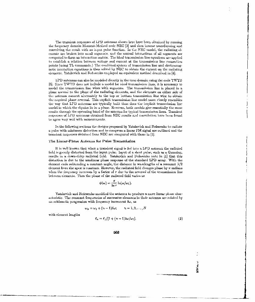
The truansient responses of LPD antennas shown here have been obtained by runningthe frequency domain Moment-Method code NEC [3] mid then inverse transforming andconvolving the result with an i•put pulse function. In the NEC model, the radiating cl-einents are broken into small segments, mad the niutual interactions of all segments areComputed to forns an interaction niatrix. The ideal transmission line equations ;irc appliedto establish a relation betweei voltage and current at the trwuisinssion line connectionpoints (using TL commands.) The combined system of transmission line and electromag-netic interaction equations is then solved by NEC to obtain the current on the radiatingelenments. Yatskevich and Fedosenko emiployed an equivalent method described in [4].

LPD antennas call also be modeled directly in the time domain using the code TWTD[5]. Since TWTD does not include a model for ideal transmission lines, it is necessary tomodel the tranlsasission line wires with sege•ncts. The transmission line is placed in aplane normnal to the plae)r of tile radiatilng ehenienlts, mad the elements on either side ofthe witenna connect alternately to the top or bottom tramnsmission line wire to obtainthe required phase reversal. This explicit traismission line model more closely resemblesthe way that LPD antennas are typically built than does the implicit transsmission linemodel in) which the dipoles lie ill a plane. However, both models give essentially the sameucresults through the operating band of the antoima for typical transmission lilies. Tt'ansicltresplonses of LPD amteinns obtained frumn NEC results mid convolution have been foundto agree very well with measuren•ents,

Ii the following sections the designs proposed by Yatskevichm aud Fedosenko to radiatea pulse with minimum distortiou wid to compress a linear FM signal are outlined and tiletrmmsient responses obtained from NEC are comparcd with those in [1].

The Limmear-Phase Antenna fbr Pulse Transnmiasion

It is well known that whenm a transient signal is fed into a LI'D autenna tie radiatedfield is greatly distorted from the input pulse. Input of a short pulse, such as a Gaussimxu,results in a down-chirp radiated field. Yatskcvicli mid 1edosexuko note in [1] that thisdistortion is due to the nodinerC phause response of tIme standard LPD array. With theelenmeit eids subtending a constanit aigle, the dist.muce in wavelengths of a resonmat A/2cleicut from tihe apex is constant. However, the radiated field douages phase by i" radianswhbeii tle frequency imicreases by a factor of r due to the reversal of the trmisiiiissiun linebetwcen eleixients. Thus the phase of the radiated iield varies as

Yatskevich and Fedosenko modified the antemma to produce a imnre linear phase Char-acteristic. The resonant frequencies of successive elem•ints ii their antemmma )re related byan m'ritinnctic progression with frequency increment 6w, as

W,3 =w 1 +(n- 1)6w; n = 1,2,. N

with elelmient lengths= d'+ (ns-16/w] 3

568

S. . . .. . ... . . . . .. .. . ... . . . . . .

Since the elements in their antenna still subtend a constant angle a, the distance of theresonant element from the apex should remain constant over the band of the antenna.Thus the phase should change by ir with a frequency increment of Sw, so that

)(0) = -me/6w.

This argument neglects the possible frequency-dependent phase velocity of the transmissionline in the antenna, but results in [1] and here show that the antenna works reasonablywell.

The linear-phase design for transmitting a pulse with minimum distortion was testedfor a 18 element antenma. A standard LPD antemna was considered first, with longestelement of length 0.88 in, and with r = 0.915, a = 0.168 and a = 7.21. This is anoptimum design according to equation (2), covering a band of about 170 to 700 MHz.A comnparable linear-phase antemna used 18 elements with the sanme largest and smallestelements, and the same a, but with element lengths determined from equation (3) withbw/wl = 0.207. The transnissiou line impedance in each case was 100 olhms. These twoantennas are shown in Figure 2. The effect of scaling the elements by equation (3) ratherthan (1) is to crowd the elements toward the small end with increased spacing for the largeelements.

The antennas were modeled at 10 MITz steps in frequency from 10 MHz to 1 GOIz,with a source of 1 volt aud a generator impedance of 50 ohms, The transfer functionobtained for radiated field was then resasnpled, inverse transformed and convolved with aGaussian input pulse with 1 us FWIIM. Comparison of the 18 element LPD and linear-phase antennma in Figures 3 and 4 shows a considerably more linear phase response forthe modified antenna. The transient response in Figure 4 is compressed, and its peakamplitude exceeds that of the standard LPD antenna in Figure 3 by a factor of nearly two.The increased spacing of the elements with the linear-phase design is secn to degrade thelow frequency performanc, however.

The degradation at low frequencies can be partially overcome by increasing the numberof radiating elements. A 30 element antenna analyzed in [il gives a cleaner impulse responsethan the 18 element antenna. NEC modeling confirmed the effectiveness of the 30-elementdesign.

Pulse Compression Antennas

Yatskevich and Fedosenko show that this concept of tailoring the phase respnsie ofthe antenna can be generalized by selecting the resonant frequencies w,, of the radiatingelements to obtain a phase response

O(W,) = ¢(w) - (n - 1)r. (4)

They apply this method to compress a linear FM signal of the form{2 2uCt) O us (oot + A ), for It !t/2,

120, for It] > tu/2,

569

where wo is the mean frequency, t4 is the duration of the signal, Aw is the bandwidth andB = twt.. The spectrum of this signal, assuming B > 1, is

e'-BT 2AVX(W) ;t Uo-AWe-J t-''••- (5)

over the frequency range wo - Aw/2 < w < wo + Aw/2.

The antenna is required to act as an optimum filter, with the conjugate phase responseto (5). Thus u(w) - -_o0) 2/2Aw 2 - coto (6)

where to is a time delay chosen to obtain a realizable antenna. Substituting (6) into (4)and solving for w,, yields

W.n=WO+ {ý-o1 - I_/ [t.to(oi -co0) -2As(w, -coo) 2 + (nr-1)7r}

Assuming co0 = w1 "+ Aw/2 as in [1], this result becomes

co = W1 I1+4-I-0.5 +7

where I = t0 /t,. Thus the element lengths scale as

t,:£/[1÷ 11 0.5+7-t- 05')-rr,-)Bl

Yatskevich and Fedosenko consider a linear FM signal with B = 407r and Aw/we = 1.Their antenna uses 30 elements with a = 40 and y = 0.705. The ratio of element radiusto length was 0.005, and the transmission line impedance was 100 ohms. The antennamodeled here was scaled for a longest element of 0.88 m, so the resonant lengths of thelargest and smallest elements were fl = 0.170 GHz and f3o = 0.511 GHz. The radiatingelements of this antenna are shown in Figure 5.

The response of the antenna, obtained from NEC, is shown in Figure 6, where theradiated field is shown for one volt input and no generator impedance. The input linearFM signal and the resulting field radiated are shown in Figure 7. The radiated pulseis compressed, but not as well as that shown by Yatskevich and Fedosenko in [1]. Oneuncertainty in this comparison is the source impedance, since a value is not stated in [1]. Inaddition to the 50 ohms used for the results in Figure 7, we also tried 100 and 1000 ohms.The high impedance was tried because reference [4] mentions fixing the input current, whichis equivalent to using a high impedance source. These variations in source impedance didnot have a significant effect on the compression of the radiated pulse, although they did

"-r its amplitude.

The result of convolving the linear FM signal with the impulse response of the optimumfilter, having the phase of equation (6) and a constant amplitude from w0 - Aw/2 to

570

wo + A!/2, is shown in Figure S. This response 18 close to that shown in [1]. The transferfunction of the antenna, computed by NEC, is compared with the ideal transfer functionin Figure 9. The magnitude of the antenna response is seen to drop off sharply aboveabout 0.34 GHz. This loss of high frequencies is also noted by Yatskevich and Fedosenko,and the gain in Figure 6b appears to be in close agreement with that shown in [1]. Thephase of the antenna response is not plotted in [1], but it is stated that the phase is within±10 degrees of the quadratic relation of (6). The phase computed by NEC is close to thatof (6) at the lower frequencies, but deviates substantially above about 0.32 Gliz. Thisdifference in phase apparently accounts for the reduced compression of the pulse. Thephase characteristic is more difficult to obtain than the smootldy varying magnitude, sincemany samples are needed to avoid aliasing. The antenna response was computed withNEC at 5 MHz increments from 160 to 570 MHz and at 10 MHz increments over the restof the band from 0 to 1 GHz. The resuits appeared to be well converged. Also, the radiatedpower, obtained by integrating the far field (computing average gain), was in balance withthe input power minus power dissipated in the terminating load. The computation of thetransfer function shown in Figure 6, from 0 to 1 GHz, required 12 hours of CPU time ona VAX 8650.

Conclusions

The concept of modifying a LPD array to produce a desired phase characteristic fortransmitting or compressing a pulse appears to have considerable merit, although thereare limitations on what can be achieved. The linear-phase modification proposed in [1] iseffective for radiating a short % ulse with minimum dispersion. However, more elements areneeded to cover a given band than with the standard LPD array.

The antenna for compression of a linear FM pulse also is effective, although theradiated pulse obtained from the NEC model is not as clean as that shown in [1]. Thereason for this discrepancy has not been determined, although it appears possible that thepulse ohown in (1] could be the response of the ideal jilter, which is then broadened by thereduced bandwidth of the antenna. Statements in [1] appear somewhat ambiguous on thispoint. Another possibility is that the result shown in [1] is for a different antenna than isdescribed.

The simple analysis used in deriving the element spacings in [1] probably does not leadto a completely optimum design. The antennas might be further optimized by adjusting theelements to correct phase errors revealed by the numerical model, although the potentialgain is not known. Also, an analysis in terms of k -)3 diagrams for propagation on thelocally-peciodic structure might lead to a better understanding of the possibilities andlimitations of these antennas.

References[1] V. A. Yatskevich and L. L. Fedosenko, "Antennas for Radiation of Very-Wide-Band

Signals," Radio Electronics and Communication Systems, Vol. 29, No. 2, pp. 62-60,1986.

571

_ _ _ _ _ _ _ _.. ....... .. .. . ...___ _ _ _ _ _ _ _j

A12] R. Carrel, "The Design of Log-Periodic Dipole Anteninas," IRR International tjonven-

tio. Record, Vol. I, pp. 61-75, 1961.

[3] G. J. Burke and A. J. Poggio, Numerical Electromagnetici Code (NEC)- Method ofMoments, Lawrence Livermore National Laboratory, Rept. UCID-18834, Jan. 1981.

[4] V. A. Yatskevich and V. M. Lapitskij, "Exact and Approximate Methods of CalculatingLog-Periodic Dipole An~enrna," Radio Electronics and Communication Systems, Vol.22, No. 5, pp. 64-67, 1979.

[5] E. K. Miller, A. J. Poggio and J. G. Burke, "An Integro-Differential Equation Techniquefor the Time-Domain Analysis of Thin Wire Structures, I. The Numerical Method,"Journal of Computational Physics, Vol. 12, No. 1, May 1973.

Fig. 1. Log-periodic dipole antenna geometry.

a)

SI I

b)

Fig. 2. Radiating elements of a) an 18 element LPD antenna with r = 0.915, o = 0.168"and a = 7.21' and b) a similar liueae-phase antenna with 6w/,w = 0.207.

572

IO

4 0I Ill I I I I__I 1 0

iI1Z.!3 I t

2.III, 1201

0 ._ ' --- -- ot '" I ' ' -- •-- - •

"0.5 - I - .

-IS ÷ -|--ISO

0 -200 0-20 80 sao 100o 0a lea@00

rr'vqN,fo (Ml.zI rrwqNu.~y 0iIHxI

10-

- a-. -se1-

-9.4,

ifi

T1.0 (.0) Ti hi)

Fig. 3. R'esponse of an• 18 element log pce- Fig. 4•. p•.espouse of all 18 element linear

riodic antenna from Fig. 2, with• T-r 0.915, phase anterma from Fig.•2. Shown are ra-

Shown wre radiated field magratude (-) diated field magnitude ( -) and phmze

and pha~se (- - -), power gainanmd transient (- - - -), power gaiu a-ad transient responseresponse to a Gaus4ian pulse 1 119 FW10M, to a jaus20i0 pulse I RS 1WHM.

V.3

I Lli IIqtlIL iHFig. 5. Radiating elenments of a thirty-element antenna for compressing a linear FMpulse, with Aw/wl = 2, B - 407r and y = 0.705.

4) b)2.5- -M .15"

111 lllj5L Ia-

,I III Illi11111 1 i ." Ll

1II - J -I -''"--se-

' lLIIII LLLL I IL I + t

Iii tLIII aneaIi ia UM lg

L III I II III111I I \ -| l i- (BSILII III i I li

l45 Ii 111 11II I I '

III 11lll11l 1 I (Q

1 4

s ia i I• '•

-40--GI-

[a 58(4 4548 so8 am4 IA134Fr-vq..lIL (Mz)

Fig. 6. Frecquency repoiwe of the thirty-elemet antenna in Figr 5 , SLhowiU. a)radiated field magnitude (- ) and phase (- - - -) on axis for one volL input, b) powergain relative to an isotropic source and c) input impedance.

574

a) i.~b) L ---

0N

- 8. 4 -4-

- .6 -

T'm (ho) thr (no)

Fig. 7. Tr~ansiem resp~oise of Lthe ptilse compression uantemia o•f Figure 5 ,shiowiiig a)linear FM input pulse withx fl,= Af --- ).3409) GHY. Did t, = 58.667 ns oald b) ratdiatedfield of the -"acimia oil axis.

0 12

6--

12 -N

7!..p (no;)

iFig. 8. iput puls wf fvolving a linear FM signan with f .= Af s0.34091 Glnzb ra dfitd 58f667 t with the optimum filter netlwic having the axba.e of equtiun (6).

575

I I *11

kl.5".5

I - 15W -I I'

Fig. 9. COnipuxiwou of the r'esponse of tile pulse coinpressiouL wiatemia in F•igur'e U)Scomputed by NEC for a 50 ohni source (--) with tile optimum-filter respOiise(...)

576

.2.8.... .... .. 1 pnlilI !m I I~ uqwl!• nl111•ij

The Pulsed Response From a Parabolic Reflector Antenna

G. & SaleBLM International. Inc.

Albuquerque, NM

INTRODUCTION source, food, and reflector. Each of these compo.The radiated pulsed response of the par- nents were modeled individually and are diB-

abolic reflector antenna system shown in figure I eussed in detail below.is presented in this paper. The emphasis of thecurrent modeling effort was to determine the The Sourcetransmitted pulse characteristics of this antenna 'The source was modeled as an idealsystem, i.e., the peak ai.hplitudm, rime time, and Gaussian voltage generator in series with a highpulse width of the transmitted pulse. It was in- pass filter. The wavefbrm produced by the gen.tially hoped that an antenna system of this type orator is given in equation 1 and plotted inwould be able to transmit high gain, short pulses fgiapre 2. With 1/a set equal to 1 ns, a pulse widthat large distances. Results from this initial of'1.7 na and a rise time of 1.2 na is produced. Inphase of analysis are very encouraging. These figure 2, to Yas set equal to 25 ns to allow forresults along with a detailed description of the easier viewing of the entire pulse0models developed will be given.

U(V 6"' (1)

S~~~~I ......-AA

F"iLure 1. Parabolic reflector antenna system.

Figure 2. Waveform produced by GauwsianMEITHODOLOGY voltage generator,

This section dIscusses the methodologyemployed during the analysis and describes the The output of the voltage generator wasmodels developed for each component of the al- fed directly into a high pasa filter to remove thetonna system. A goal of this analysis was to low frequency content of the voltage source. Thedetermine the transmitted field strength relative model developed for the pamabolic reflector (grivento the input signal level. For this reason, a com- below) is most accurate when the wavelength ispleto characterization of the antenna system small relative to the dimensions of the reflector.from the source to the radiated fields was Therefore, removal of the low frequennies (largenacoasswY. A-I shown in figure 1, there are three waveoingths), was performed to improve themajor cumponento in this antenna system - the overall accuracy of this analysis.

577

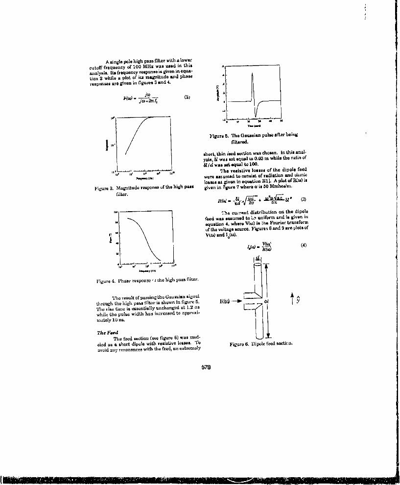
A single pole high Pass filter with a lowercutoff frequency of 100 MHz was used in thisAanalysis. its frequency response is given in equa-tion 2 while a plot of its magnitude and phaseAregponses are given in figures 3 and 4.A

.A

Figure 5. The Gaussian pulse after beingfiltered.

/ ~shoot, thin ifeed secl~on was chosen. in this anal-ysis, 81 was set equal to 0.03 m, while the ratio of

&Idwas sat equal to 100.~o * ,s.~'.The resistive losses of the dipole feed

P.Vý oh)wore as-urnsd, to consist of radiation and ohimiclosslus as given in equation 311]. A plot of RC(c) is

Fijgure 3. Magnitude response of the high pass giveni in Elgure 7 where a is So Mynhos/en.filter.

R(us -+3'

1W - "he cuireIht diatribution on the dipolefeed was assumed tolt- uniform and is given inequation 4, where V(ui) is 'he Fourier transform

C: ~of the voltage source. Figuresi 8and 9 are plots ofV~EWa and 1.(W).

IV Io, %Go top to-"-,q~ (11.)

F'igure 4. l'hasoe response -'I Lho high puss filter.

The result of puassing the Gaussian signalAthroughi the high pass filtor is shown in figure 5. 61o~ -

while the pulbu width hat; increased to apprttxi- .f Ioinately 10 ns.

The FeedLIThe food section (sue figure (1) was mod-U

eled as a short dipole with resiativn losses. To Figure 6. Dipole feed sectic n.

avuid uny rettonsmncem with the feed, anl oxtremnely

578

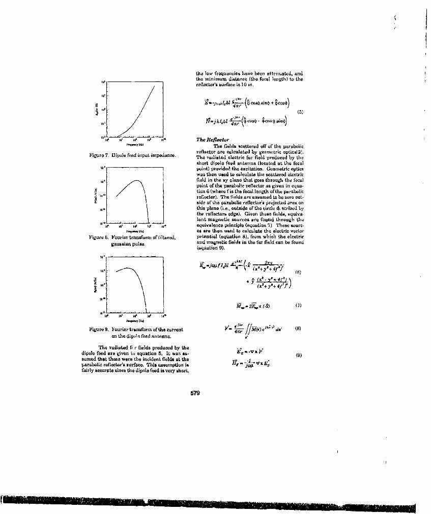
the low frequencies have been attenuated, andthe minimum distance (the focal length) to the

tx hreflector's surface is 10 .

14-p,0 S n--( COO Alin 0 + $Cs 0 )4(5)

190 to too lop to The RefleetorVq-V (iu The fields scattered off of the parabolic

reflector are calculated by geometric opticsl2l.Figure 7. Dipole feed input impedance, The radiated electric far field produced by theshort dipole feed antenna (located at the focalpoint) provided the excitation. Geometric opticswas then used to calculate the scattered electricfluid in the xy plane that goes through the focalpoint of the parabolic reflector as given in eque-tion 6 (where f is the focal length of the parabolicreflector). The fields are assumed to be zero out-side of the parabolic roflector's projected area onthis plane (i.e., outside of the circle dLscribed bythe reflectors edge), Given these fields, equiva-lent magnetic sources are found through the

le s- to- equivalence principle (equaLion 7). These sourc-Y"ou) as are then used to calculate the electric vector

Figure 8. Fourier transform of filtered, potential (equation 8), from which the electricgaussian pulse, and magnetic fields in the far field can be found

(equation 9).

El* (x1+y'+-4,".)'

IsQ.

S(1)

Figure 9. Fourier transform of the current 4n JfM(s)jA-)e '~di' (Bon the dipole feed antenna. '

The radiated fi r fields produced by thedipole feed are gvven in equation 5. It wan as- E x P(sumed that these were the incident fields at the-parabolic reflector's surface. This assumption is i jcfairly accurate since the dipole feed is very short,

579

"i "'ilt' i ', ! lf ffid l 1B

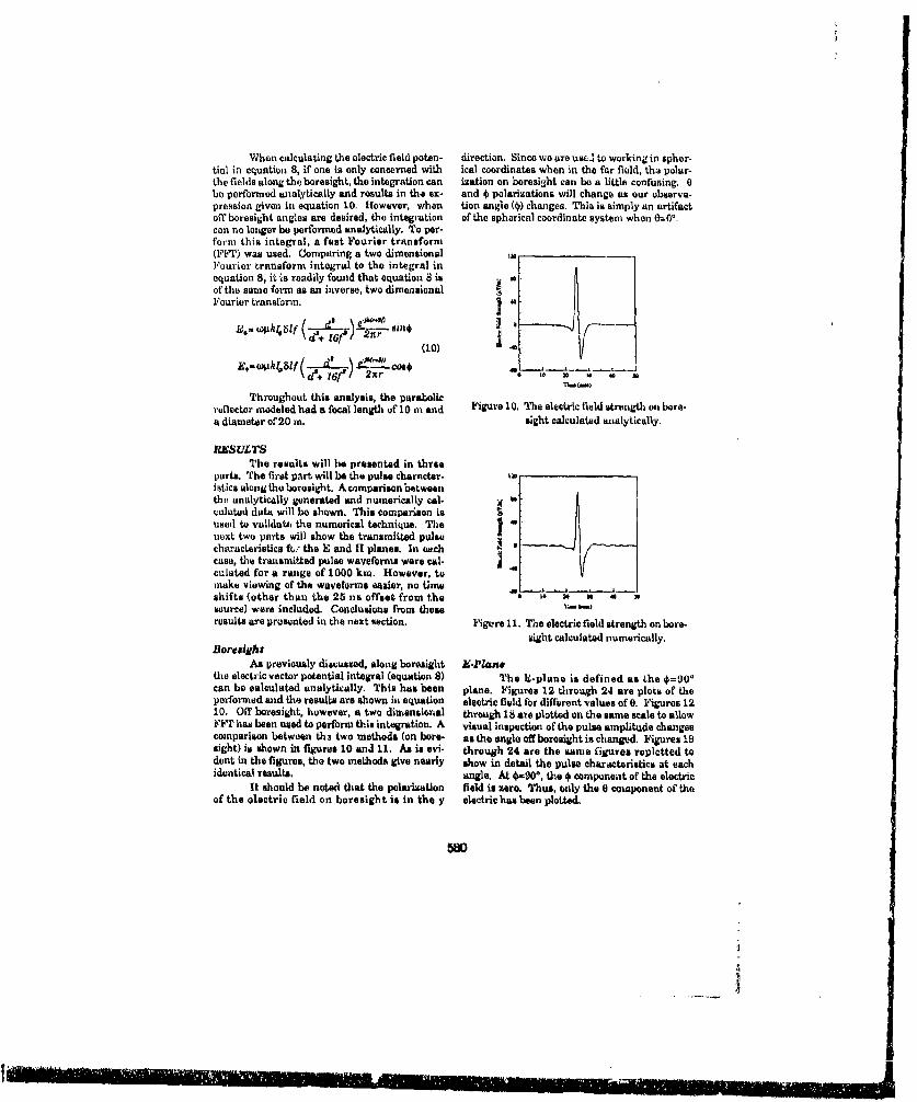
When calculating the electric field poten- direction. Since we are usE. to working in apher-tial in equation 8, if one ia only concerned with ical coordinates when in the far field, tha polar-the fields along the boresight, the integration can ization on boresight can be a little confusing. 0be performed analytically and results in the ex- and Ii polarizations will change as our observa-pression given in equation 10. However, when tion angle (ib) changes. This is simply an artifactoef boresight angles are desired, the integration of the spherical coordinate system when 0=0'.can no louger be performed analytically. To per-form this integral, a fast Fourier transform(FFT) was used. Comparing a two dimensional aFourier transform integral to the integral inequation 8, it is readily found that equation 8 isof the same form as an inverse, two dimensionalFourier transform. 'A

(10)

" 1 \,f+tl*I2xr I- 30-•o--•"'-

Throughout this analysis, the parabolicreflector modeled had a focal length of 10 m and Figure 10. T1he electric field strength on bore.a diameter oQ120 m. sight calculated analytically.

RESULTSThe results will be presented in three

parts. The first part, will be the pulse character-istics along the boresight. A cnmparison betweenthe analytically generated and numerically cal.culated data will be shown. This comparison isused to validatei the numerical technique. Thenext two parts will show the transmitted pulsecharacteristics fý-" the B and H planes. in er.chcause, the transmitted pulse waveforms were cal-culated for a range of 1000 km. However, tomake viewing of the waveforms easier, no timeshifts (other than the 26 nb offset from the • a '-psource) were included. Conclusions from these LZresults are presented in the next section. Figure 11, The electric field strength on bore-

eight calculated numerically.Boresight

As previously discussed, along boresight E.PLanthe electric vector potential integral (equation 8) The E-plane is defined as Lhe $=900can be calculated analytically. This has been plane. Figures 12 through 24 are plots of theperformed and the results are shown in equation electric field for different values of 0. Figures 1210. Off boresight, however, a two dimensional through 18 are plotted on the same scale to allowFFT' has been used to perform this integration. A visual inspection of the pulse amplitude changescomparison between th 3 two methods (on bore- as the angle offboroeight in changed. Figures 19sight) is shown in figures 10 anJ 11. As is evi. through 24 are the same figures replotted todent in the figures, the two methods give nearly show in detail the pulse characteristics at eachidenticaml results, angle. At 4w290O, the 0 component of the electric

It should be noted that the polarization field is zero. Thus, only the 0 comnponent of theof the electric field on boresight is in the y electric has been plotted.

•80

12oo

40 -

0l

Ca • a

to 30 w0 0 00 50 0 Id 0 0 00 0

Figure 12. E-plano result for 6=01. Figure 15. E-plane results for 0=5.4'.

1310

NIS

-so,

40.

Figure 13. E-plane result for 0 igure 16. H-ph)ne result for 0=7.2

1i0[ 4- - .30

IQ wS L ± 1* 2 t4

Figure 14. E-plane results Cor 0=3.6'. F~igure 17. E-phuan resulta for 0=9.00.

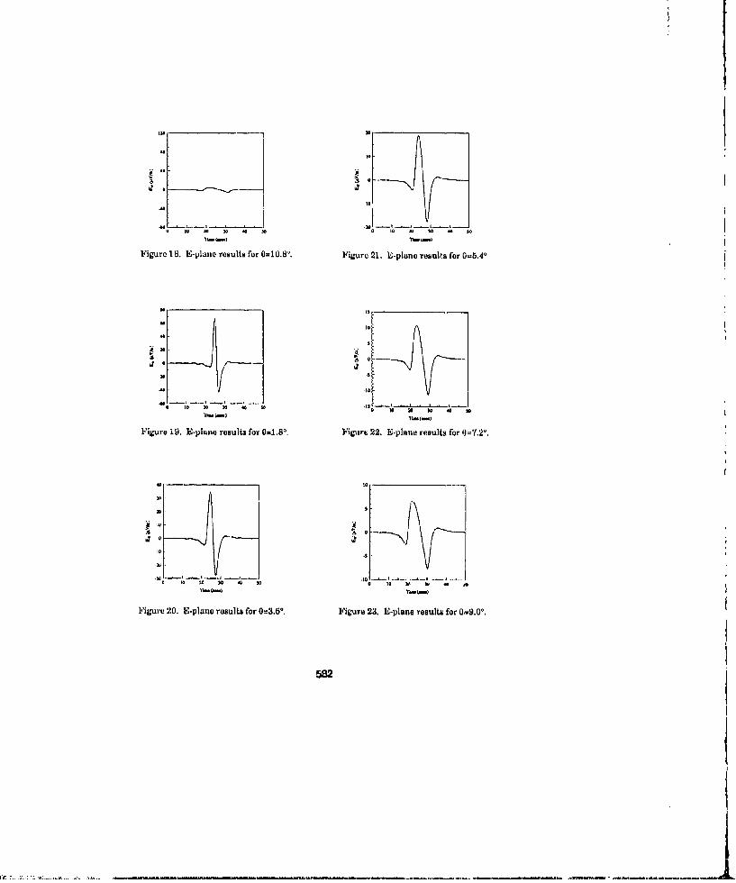
to,

Figurel8. E-plane results for 0=10.81. Figure 21. &-plune results for MA5O40

i20

"sJ • o 4o is -10 tIo 4 so..

Figure 19. E-plane resulU for 0-1i.81. Mp•i•rc. 22. E-plane results for 0--7.21,

00+

-M4I

3 "Ito 1I Ix i l~+

10 2 ; 0 I Z

Figure 20. E-plano rasults for 0=3.6*, l,'igura 23. E-plane results for 0=-9.00.

210W2

A U

Figure 24. E-plane results for 0=10.8'. Figure 26. If-plane results for 9=1.81,

ll.PlanoThe ll.plsne is defined as the O=;0 plane.

Figures 25 through 37 are plots of the electric ..

field for ditrerent values of 6. Figures 25 through31 are plotted on the same scale, while figures 32through 37 are plotted on different scales for thereasons discussed above. Since 0f0*, the 0 comn- .ponent of the electric floid is zero. Thus, only theScomponent has heen plotted.

N 10 0 0 so

Figure 27. i1-plari results for U3.6'".

44. 4

Ut

to 2 s for 00, 0 -h Wt 40 0

Figure 25. lI-piane results for 0=0O. Figure 28. lI-plane results for 0=5i.4'1.

Figure 29. H-plane results for 0-7.2'. Figure 32. H-plane results for 0=1.8°.

ta•it

INN

Figure ,30. li-plane reaults for 0=9.0*, Figure 33. 1t-plane results for 0=3.61.

In

584

-- t

s1 . 0 3 0 o 3 0 w 1 0 0I

Figure 2t). If-plane results for 0=10.8. Figure 34. 11-plano results for 0=1.80.

584

CONCLUSIONSFrom the results presented, it is easy to

understand why the parabolic reflector antennasystem looks to be very promising in its ability totransmit high gain, short pulses. Both theE andIt plane results clearly indicate that the trans-mitted pulse is maximum along boresight andattenuates rapidly with angular deviation fromboresight. At five degrees offhboresight, the peakamplitudes have decreased approximately by afactor of 5. The amplitudes continue to decrease"the further off boresight one goes, however, theassumption about the low frequency contentmade throughout this analysis begins to fail at

Figuxre 35. H-plane results for 007.2°. extreme offboresight angles. The reason for thisis simple. The parabolic roPeftor is a very highgain antenna at short wavelengths. Thus, theenergy from the high frequencies is concentratedalong boresight. However, at lower frequencies,the gain begins to broaden and the energy is dis-tributed over a wider range of angles. At largeangles off boresight, the relative content of lowfrequency versus high frequency will be greaterthan it is along boresight. Since the geometricS, •optics approximation is inaccurate at low fre-quencies. the relative energy clue to the longwavelengths must be small Compared to theshort wavelengths. Along boresight and near it.this condition is satisfied. However, at large an-

,•.. . . glee offlboresight, this condition is no longer true.Therefore, results for angles greater than 100have not been included.

Figure 36. H-plane results for 0.Gi. In addition to the pulse amplitude de-creasing, the pulse width increases with angulardeviation from boresight. Once again, this is dueto the fact that the relative contribution of lowfrequencies increases as the angle off boresightincreases.

RECOMMENDATIONSTwo enhancements could be made to im-

prove the results that have been presented here."ir The first is to improve upon the feed section. Amore realistic feed could be incorporated. This

A would complicatu the analysis considerably andis why it was not performed in this analysis.

* ., •The second enhancement would be to im-prove upon the reflector analysis. Edge effectsalong with an accurate model for low frequencies

Figure 37. H-plane results for 0=10.8°. could be developed.

REFERENCES:

(1) Warren L. Stutzman and GCay A. Thiele, Antenna Theory and Veslgrn, John Wiley and Sons. 1981

(2) Antenna Hondrbooal, Th.enrj, An plications, arid Desion, edited by Y.T. Lo mad S.W. Ler. Van Nostrandand Reinhold Company. 1988

585

NA RAY-TRACING MODEL TO PREDICT

TIME-DOMAIN RCS PERFORMA1N'1E OF A COMPACT RANGE

Norman Carey Steve Brumley Atul JainHughes Aircraft Company Denmar Incorporated Hughes Aircraft CompanyEl Segundo, California Carson City, Nevada El Segundo, California

Abstract

Characterization of time-domain High Range Resolution (HRR) scattering returns is a valuable toolin evaluating performance of RCS compact range chambers. A code, based on geometrical opticsmodeling aad empirical reflector and absorber data, is described. Results obtained using this computermodel are compared with actual downrange RCS plots measured on the Hughes Aircraft Companydual-reflector Vokurka compact range chamber in El Segundo, California. Important mechanismscontributing to thi downrange response and to measurement clutter in the sweet spot measurementzone are identified, indicating this to be a useful tool in chamber design and evaluation.

1.0 ntarol•dtlon

The quality of measurements made in an indoor compact range depends to a large extent upon thelevel of background clutter in the time vicinity of the target. The background level is due to unwantedreturns of siilar path length, and to processing sidelobes of bright peaks elsewhere in the roonm.Before mes=Lres can be taken to reduce clutter, the paths involved must be identified, and thepotential negative side effects of the design changes estimated.

Time-domain images of compact ranges show contributions from several mechanisms. Some of thesecan be deduced from the image and from knowledge of the range geometry. Certain comparativelysimple effects can be estimated accur..tely; however, detailed calculations of higher-order interactionsarc cumbersome, requiring computer assistance. While a great number of versatile RCS predictioncodes are available, they are generally unsuitable fez modeling complex, electrically large, lossycavities, such as a compact range. Specialized software exists to compute the near field of a compactrange reflector in isolation, but the absence of interactions with other objects restricts its use topredictiot. af field strength in the quiet zone; clutter in the zone, as seen in time-doma.n images,cannot be predicted. Another approach approximates profiles of the quiet zone by summation ofabsorber backscatter components, computed using empirical data for the illumination pattern andabsorber RCS 11].

A series of computer codes has explored the applicability of ray tracing to range analysis. The currentiteration, Vuku5, employs an exiended form of Geometric Optics (GO) to treat nonspecularscattering. Pure GO is quite restricted in its ability to predict calibrated background levels due to itsexclusmn of nonspucular mechanisms. In particular, the level in the quiet zone around the targetcannot be calculated, since this depends ou diffraction from the main reflector and backscaticringI ron .he..i wali.. Vuku5 provides facilities for graphical examination of specific paths in isolation

588

A

_ -_

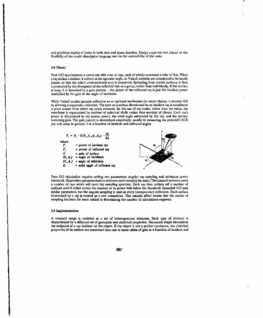
and graphical display of paths in both time and space domains. Design etphbAsis was placed on theflexibility of the model description language and on the extensibility of the "code.

2.0 Theory

Pure GO approximates a wavefront with a set of rays, each of which represents a tube of flux. Whena ray strikes a surface, it reflects at the specular angle. In VukuS, surfaces are considered to be locallyplanar, so that the tube's cross-sectional area is conserved. Spreading from curved surfaces is thcnrepresented by the divergence of the reflected rals as a group, rather than individually. If the surfaceis lossy, it is described by a gain pattern -- the power of the reflected ray is just the incident powermultiplied by the gain at the angle of incidence.

While Vuku5 retains specular reflection as an optional mechanism for metal objects, it extends GOby allowing nonspecular reflection. The spot on a surface illuminated by an incident ray is considereda point source from which ray cones emanate. By the use of ray cones, rather than ray tubes, thewavefront is repreaented by sections of spherical shells rather than ser.tions of planes. Each ray'spower is determined by the source power, the solid angle subtended by the ray, and the surfacescattering gain. The gain pattern is determined empirically, usually by measuring the material's RCSper unit area; in general, it is a function of incident and reflected angles.

P', . e , G ,,,,,, • . 0l41r

where:P, - power of ineident rayP, - power of reflected rayG - gaia of surface(6 ( - anlec of incidence(0,40,) - Angle of reflectionQ - solid angle of reflected ray y

Pure GO calculation requires setting two parameters: ar.gular ray sampling and minimum powerthreshold. (Equivalent parameterization schemes could certainly be used.) The transmit antenna emitsa number of rays which will meet the sampling specified. Each ray then reflects off a number ofsurfaces until it either strikes the receiver or its power falls below the threshold. Extended GO usessimilar parameters, but the angular sampling is used at every (nonspecular) reflection. Each surfaceilluminated by a ray is treated as a new transmitter. This cascade effect means that the choice o1"sampling becomes far more critical in determining the number of calculations required.

3.0 Implementation

A compact range is modeled as a set of heterogeneous elements. Each type of element ischaracterized by a different set of geonietric and electrical properties. Geoncttic shape determinesthe endpoint of a ray incident on the object. If the object ia not a perfect canductor, the electricalproperties of its surface arc condensed into one or more tables of gain as a function of incident and

587

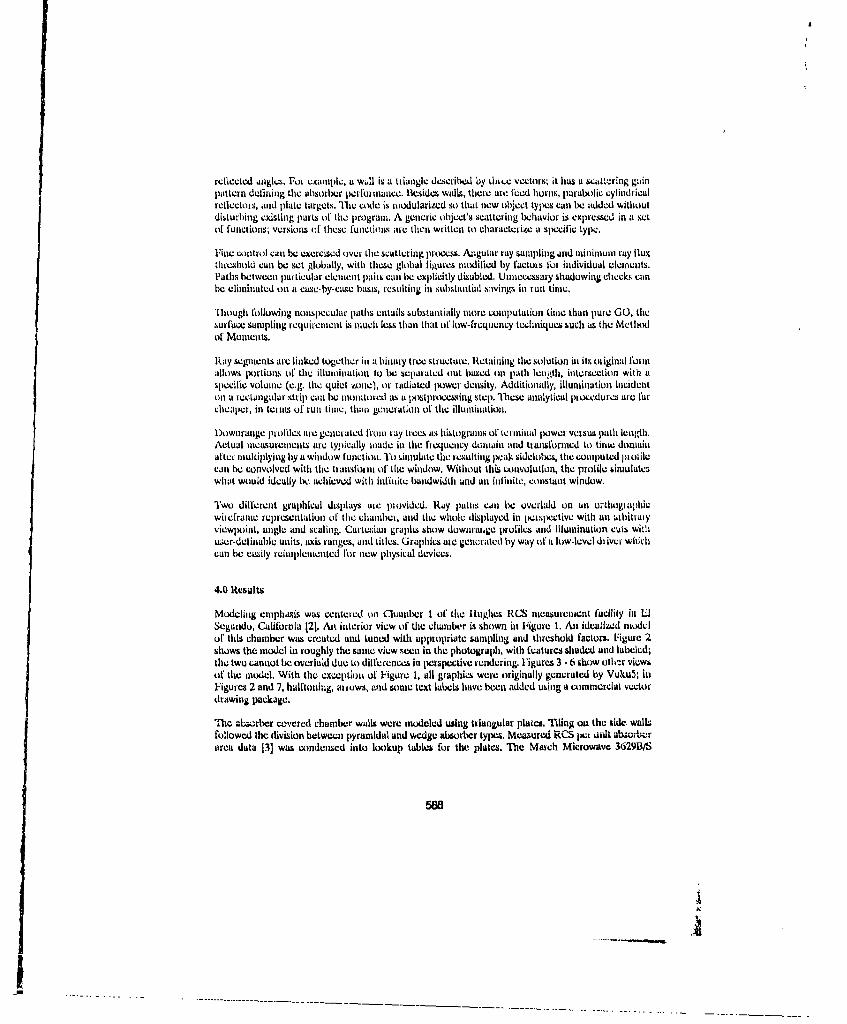
reflected wigles. Foi example, a wi~ll is a triangle de-s.'ibed by thic vectors; it hus u scii.ltý:ing gainpattern defining thle absorber perfurmnance. Ilesides walls-, there are feed horns, parabolic cylindricalreflectors, andl plate targets. Ther coide is modularized so that new object types canl be added withoutdisturbing existing parts of tli.ý program. A generic object's scattering behavior is expressed in at set(if functions; versions of these functions ate then written to characterite it specific type.

Fine control cani he exercised over the scattering proces. Angular ray sampling and minimum ray fluxthreshold can be set globally, with these global iigures modified by factors fur individual elements.Paths beltweenl pl-Licular elenment paits call he explicitly disabled. Unn ecessary shadowing checks canbe eliminated onl a case-by-case basis, resulting inl Subtanltial s:nvingN inl runl time.

I'lough foillowinig nonlspecular pathls entails substanitially wlore Computation tinie than pur4e GO, thlesurface: sampling requiremeont is much less than that of low-frequeClly techniques such as the Methodof Moments.

Ray segments arc linked together in a1 binary tree structure. Retaining thle solution in its original fulimallows. portions of the illumination to be separated out baued on path lenigth, intersection with aspecific volumei (e.g. thle quiet zone), or radiated immwer density. Additionally, illuminiation incidenton a rectangular strip canl be monitored as a imstprnscessing step. 71hese analytical piocxcdurcs are tarLlheaper, in terms Ot run timei, than( genrationl Or thle illunslinatioii.

Downrange profiles lire genetrated front lay trees as histogramls of terminital po ver wsual pathl length,Actual measurements tirc typically made inl tile frequency domain and transformed to liitte domiaiiiaftei multiplying by a window function. To simulate thre resulting peak sidelobes, the computed In ofilecanl be convolved with% thle (I anlsflbn of the Window. Without this comivulutionl, thle protile sinmlulateswhapt would ideally be. achieved with infiniite bandwidth and anr infinite, constanit window.

Two different graphical displays ate plowided. Ray patimý Canl be overlaid on an orthlogmaphikwitefrarni reprresentatiumi of the chamber, and tOe whole displayed in pcmsjxxctive with anl abitaimyviewpo)int, angle amsd scaling. Cartesian graphs bhow dowmmainge psrofiles ;And illunination cuts withuaer-deflnahle units, axis ranges, amim titles. G~raphics are generated by wily of at low-level driver whichcan be emcdly reinmpleumented tor new physical devices.

4.0 Results

Modelinig emphasis was centemed on Chamber I of thle Hughes Ila nieasuienient facility ill ESegundo, California 121. Aiix interior view or tile chanriblr is shown inl Figure 1. Ani idealized modelor this chamber was created and tuned with appropriate sampling and threshold factors. Figure 2shows the moudel in roughly the same view m.-en In the photograph, with features shaded and labeled;the two canntot be, overlaid due to dilferences in perspective renderinig. Figures 3 - 6show uhli,.r viewsor the model. With the. exception of 1-igare 1, all graphics were originally generated by Vuku5; itsFigures 2 mind 7, halftoning, arrows, and sonic text label have been added using a commercial'vectordrawing package.

"The a'~czorber covcred chamnber walls were modeled using triangular plates. Tiling onl the aide wallfollowed thle division between pyramidal and wedge abs-orber types. Measured RCS Ijxm unit absorberarea data 13] was condensed into lookup tables for the plates. The March Microwave 362913/S

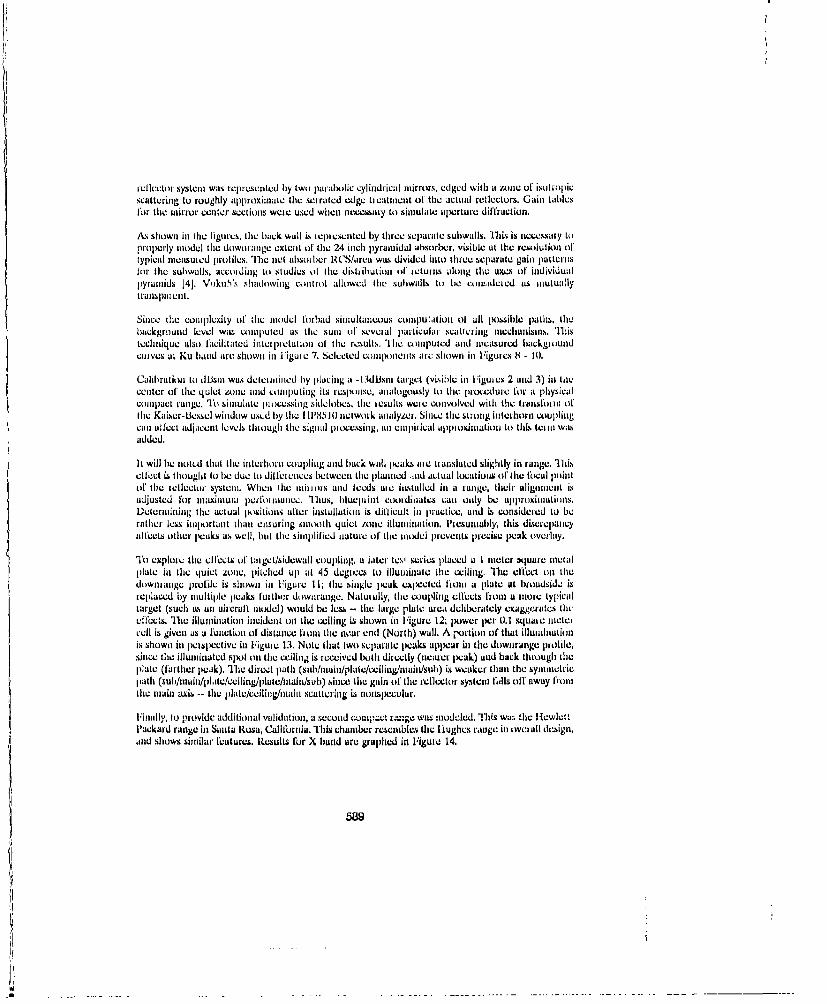
ieltector system was reipi-esented by two parabolic cylindrical mirrors, edgcd with a zotne or isotropicscattering to roughly appiroximate thle serrated edge ttL'atriicnt ol the actual reflectors. Gain tablesfor tile. mirror center sections were used when nieesary ito simulate aperture diffraction.

IV shown in tile ftgnrcs, the hack watt is repiesetited by three separate subwalls. This is tecessaiy toproperly model tile downrange cxtciit ofl thle 24 inich pyruamidal absorber, visible tit the resouluioni ortypicail melasured piot ile's. Thle nlet absoi hr RE/inVaca was divided into thll-c sep.Iarate gain patterns101t thle SUI)WUllS, miCCiding ito studies ol the distohution ofl returns along thc axes of' individuoatpmyramnids 1 41. V'ikii~i's shadowing connioio allowed tilie subwalls ito be conm~ideted us miutua~lytranlspinciii.

Since the coilitplexi ty Of ',he Model forhad simoultanteous conipatiul dtofto all lrNssible pa tils, thebiackgrountd level was5 c111ompued as thie sunt of' sevelal jiaitie~uiar %caticrinig 11neehatisins. Thistechnique 11il11 facilitated ilici tpretat ion ofl thle results. I-le computed and mieasured backgi &uniIcuiives at Ku buind are! shiown in I igu ie 7. Sclected cotmpo nenits arc shown inl liguics 8 - 11.

Calibration toi dUsmn was dutet niiiied by p ulacingitg .a.1 dllst taiget (visible inl Figui es 2 atid 3) in tilecenter of the quiet imne antd comput in g its i expi llse, ainalo goosly to the 1n-oced ule for a physicalCompatiict range. Tsimulate Ilii ceasing sidelobes, the iesut ts were convolved with the traitsfoil to ofthe Kaiser-Uesset window us-d' by thle It l'HMIt itetwork ttiialy~ci. Simte the st itlti litterhorit coupilingcanil affect adjacent levcls tht ough the sigtnal pt ocessilig, anl ettpirical apptttxiiiatirtn to thils tleiti waslidtded.

It Will ble t1intd thatl thle intritelkor couplinig atnd [latck wtall teaksL tie It anslatcd slightly in range. I'lisell -ct is thbought ito be due to diflet eices between thle plannecd ind actual locationis o1f11 the U 110 piltiof, tile tellector systetm. When tie mitit ni and feuds ate installed inl a ralige, their- alignmiien t isadjusted for ititxittluti pertlla ltuce. I'thus, bluepa at cootdiimates can uonly be alproxitiatioils.Determittting thle actual po sitiolns alter hinsallatioit is dillicult inl pracetice, and is consideied to beratthicr less iiipottatt thant ciiuliig smlooth quiet loite illtiminait ion. Il'esuittably, this discrepancyat tcts oalier peaks as we It, but tile simpnatlifed nature of the miodcl pirevertts precisse peak overliay.

To explue tilte el kets ofl tat get/sidewall coiuplitng. ta laitcr tes series placed a I mieter xjtiale metalplate itt the quiet zorit, pitched up at 45 dcgi ees to illumtinate tile ceiling. Ilie effect onl tiledowittatige plofite is shtown itt Figure 1t; ths; single peak cxleeled fioni a plate at bioadside, isieptaced by atuhtipte Ileak~s hot iteir di worange. Natut ally, tile couplinig effects from a more typicaltarget (such as. an aircraft toitiel) would be less -- tlhe huge plate areai deliberately exaggcrates tIlltlfucts. T1he itlumitination ittcidetnt oil thle ceiling is showtn in F igure 12; tlower per 0.1 &quak e vtleti

Cull is given ats a f'unetiiil of diStaitee lmit the near end (North) wall. A -ortion of that illunthuatimnis shownt inl pirlpective itt Figure 131 Note that Iwo seplarate pecaks appear iii thle dowttranige priofile,since. the illuminated spxit onil te ceiling is received both directly (nearer peak) and back through theplate (farther peak). Ilhe direct: patt(uh/nl/atfiianilu) is weaker than the symmntiteic[);itltlsh/iai/ht~eii~lt/tailu since tile gain of the reflector systeni falls ofilaway fromthle mnain axis -- teLilmtt; ciin ai scattering is itotsicpcular.

FintillY. to provide additional validiition, at Cceond euip.iei~t mange V.as., tmodeled. 1T1E. waz. tile Hfewl~ettPackard range io Santta Rosa, (2alifuriia. Thtis chamber resenibles the H ughes range ill overatl design,anid shows simtilar features. Results for X buttd aru graphed in Figure 14.

589

Tbc nwot important caveat in •-xamining thcsc rcsults is the simplidty of the reflector edgc model.

Serratcd edges arc appinximatcd here by rcetangular strips with isotropic, loss-ess reradiatiun. Th-

resulting inaccuracy is most noticeablc in the reflector backscattcr terms. Detailed, quantitative studies

of edge-telated acchanisms will require data on serration performance, either experimental or

theoretical, which was unavailable at this writing.

590

Hiurw 1: Chianlxr I Interior with Cutwalk Extcnde-d

-. USRFLECTOR -- '

,I __ _11:FE -US

Figure 2: MxdIl of Chuambr 1

591

rigurte 3: Cumpact Rarnge Model

iFiguic 4: Side ViLew Vigure 5: Top View Figure b. End View

592

Cnn

LIJ A, L

V - : -r

0(

2 ---- ---

Wý (P wý ) uin. a-

Fiur 7:TtlDoX)nc rrl

L -c3gr 8: Dixluninto of Absorbar ~~tO~

F igure 9: OIL ..lluminationbyWn RcetAboi b

HRl Chanibal- it! jjwj~Vzj, 5!ysturn

PIS_

Figure 10: Reflector Systemi

594

RJ U~- i- 61. Sq. II.f. 1'1sd.dW Lk-. 'Ek 4 I~d 1: CgI1, I II jki~wl~l 1"I.

- ijiUJ

Figurc 11: Pioiril with 45deg Plttc Figure 12: Ceiling Illumination

Figure 13: Part of Chiumber Illumination

------

.... ....

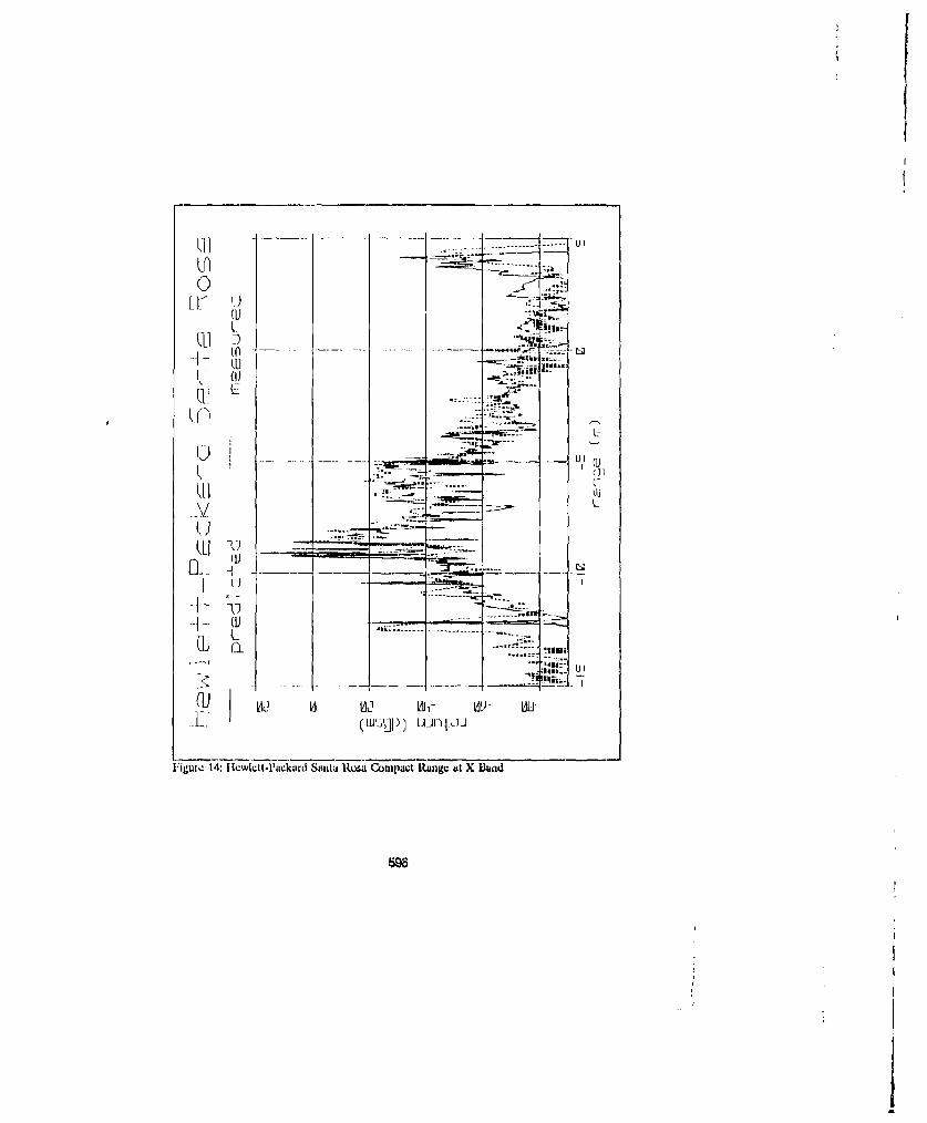
-- L

~ IJ I

0 O--- L U-

F~igurc 14: Hecwlett-Packard Santa l•,su Compact Itange at X t1land

1) IA'~1*(ii

5.0 Future Development

'he simplest improvements to Vuku5 could write, not front moditicatiuzss to the source code, butfront better modeling. Characterization or reflector edges seems to be thd bighcat priority, giveni thehigh path strength,, involved. Accurate measuremlent of edge response in a physical volaptict ranlgeis difficult, modeling the edges in isolation using ut general-purpose low-frequency RCS code wouldprobably be inure effective. Edge serrations pose a modeling challenge due to their above-resonantelectrical size. (Similar considerations would hold for other edge treatments -- rolled, absorber-loaded,Cet.) Additional histatic absotber RCS/arca data could be collected, though this h5 difficult with extantfacilities due to the aniuunt of data required and the necessary reconfiguration of monlostatic ranges.Given the relatively low gain of typical absorber, the significance of absorber/uabsorber multilouncl.scatteting is questionable. However, a study of a specific scattering mechanisnm in isolation couldmodel finer ditails thamn have becii atterupted so tar.

VukuS is written !in highly modularized, ANSI-stanidard C for maintainability and portability. Newtypes oifelemencos (or modifications of existing ones) can be added straightifurwardly; in fact, codeitubs exist to support additional targets and target mounts. Palabloluidal reflectors Could be addcdeasily. 11tv prizuai challenge Imr new elemments is nut writing code, but determining applropriamteelectrical prnlixatics; in particular, miount licrlorniance is difticult to characterize with any certainty,Graphics device dependc-lee has been enicapsulated at a low level. Suppor t is provided for X. 11,RcGIS, IIPOL, and LN03 I'luz protocols%; practice has shoWn1 that aidding suprxort for new devices isa simsple matter.

Experience with thoe plogramin has suggested 5sommie signitmcant improvemelnts that co~uld be mlade inlfutine verions. While elaidining the bask: theory, data representations co~uld be altered to beutteaccuonmminoat high resolution coinp utatiunr, I-lux density analysis wouuld be greatly stream11lned by thecapability to display two-dilmnenSiOnat imkages with contouding; or pscuudocolur techniques. Scveralmodules would need ckltensivc rewriting, but the miust lengthy and difficult part of the devellomient,validation of the scattering algorithmsh, nseed not he repeated.

Vuk-u5 now offers the unique capability to analyze multipath interactions inl a cempact tange. It callhe a valuable addition to cunventionial chamber design too~ls. As new demands arise, its functionimlitycanl be expanded.

6.0 Acknowledgemaents

Thei authors would like to gratefully acknowledge the supil)ort and eo~ntrl'ution ot: T.W. Obnstad, G.Tamtakaya, D.J. tang, and C.R. lkw:i-man, all of Hlughes.

7.0 Rererveuts

[11 S. Blrumuley, "A Modeling Technique for Predicting Anuchoit: Charrber RCS humckgiound Levels",Proceedings of the Antenna Measuremimmet Techniques Association, 1987

597

[21 A. Lamb, R. Immcll, 'Hughes Aircraft Company's New RCS Measurement Facility%, Proceedingsof thc Antenna Measurement Techniques Association, 1990

[31 S. Brumloy, R. Immcll, "Characterizing the Bistatic Performance ot Anechoic Absorbers",Proceedings of the Antenna Measurement Techniques Association, 1989

14] S. Brunmlcy, "Time-Donaain Methoxls Silence Reflections in Anechoic Chambcrs', Microwaves &RF, 'uly 1989, pp 109-113

598

SESSION 16- "TRANSMISSION LINE MATRIX (TIM)

TIME DOMAIN APPLICATIONS"Moderator: Uoyd Riggs

A TRANSMESSION LINE MATRIX (TLM) METHOD ANALYSIS OFTILE SEF.UtATED APERTURE BURIED DIELECTrIC ANOMALY

DETECTION SCHEME

Paul R. Hayes and Lloyd S. RIggsElectrical Engineering Departmer

200 Broun HallAuburn University, Alabama 36849-5201

and

Charles A. AmazeenU.S. Army Belvoir RDDE Center

_ •ATTN: STRBE-NTFt. Belvoir. Virginia 22060-5606

ABSTRACT

In this paper, a numerical time-domain technique known as thetransmission line matrix (TLM) method Is used to analyze a the separated

aprture burled dielectric anomaly (mine) detection terhnlique. This mine

detector is designed to operate in the frequency range from 600 to 1,000

MHz. As shown in Figures 1 and 2, the mine aensor consists of transmit

and receive br-adband dipole antennas. Each dipole antenna Is contained

"within an open cavity and the cavities are connected t-' a metallic

aeptum. When the detector Is over a homogeneous earth little of the

transmItted power is picked up by the receive dipole. There Is a

significant Increase in received power when the detector is over a

buried dielectric anomaly (nine). Recently, a fairly extensiveexpimental effort was carried out at Ft. Belvoir. Virginia to

characterize the performance of this mine detector. Although the"experl-nents clearly indicate how the performance of the detector changes

with mine depth, wensor height, senvor position relative to the mine,

etc., the experiments do not necessarily provide a clear undei7standing

of the electromagnetic principles underlying the mine-detection process.

The TLU analasls has been used to generate a video tape which shows how

the wave radiated by the transmit dipole interacts with the buried mine

and ecattws back into the receive cavity. This video simulation lends

cor-siderable inaoigt into the fundamental wave mechanisms which govern

the detection proces.

599

M?j..

$

INTRODUCTION

The separated aperture buried dielectric anomaly detection scheme,shown In Figures I and 2, was discovered in the IM's and studied

experimentally [I]. It was shown to have superior detection andfalse-alarm rates when compared to other mine-detection techniques. One

drawback noted was sensitivity to sensor height. A false-alarm occurredwhen the sensor septum wa" greater than approximately one-half

wavelength above the soil surface. Although the separated apertureapproach to mine detection Is simple, It has certain desirable features

that are not shared by other electromagnetic mine detection meth3id.

Electromagnetic Identification of buried mines requires a transmitter

and receiver- energy from the transmitter penetrates the earth'ssurface, interacts with the buried anomaly, and Is then coupled Into the

receiver for detection. Unfortunately, a rather large amount of energycan be directly coupled from transmitter to receiver or reflected from

the soil-air interface and coupled Into the receiver. Energy at thereceiver which interacts with the anomaly (the signal) can be quite

small in comparison with this direct and ground-refleced energy (the

clutter). The advantage of the separated aperture approach over other

electromagnetic detection techniques Is that. under proper operatingconditions. the direct and ground reflected signals are substantially

sappressed in comparison with the return from the buried anomaly. The

metal septum forms a wavegulde with the soil surface and when the

septum-surface separation Is smail, this wavegulde is below cutoff

resulting in an exponential attenuation of the direct and groundreflected signals and a vastly improved signal-to-clutter ratio. In

fact. accordig to one source, the separated aperture sensor exhibited

the best signal-to clutter ratio of any technique ever attempted [1i.

Recently, the Belvoir Countermine Technology Division of the U.S.

Army Belvoir Research, Development, and Engineering Center (BRDEC)decided to pursue an experimental and theoretical research program

dedicated toward developing a thorough understanding of the operating

characteristics of thi separated aperture mine detector. To date. fairly

extensive measurements (described in greater detaii below) have buaconducted with this detector In dry loam (a mix of sand and clay) [21,

and in moist or saturated soils 131. Belcause of Its robustness,

versatility, and utility, the transmission line matrib (TLM) method was

o00

_________________________________.. ......... .. .......... .. ........ . ... _______

"4'

chosen as the prafer.ed numerical tool with witch to carry out the

theoretical research program.

The transmission line matrix 1TLA) method (described In greater

detail in a later section) provides a very general and powerful

techniquc for the solution of wide variety or electromagnetic

interaction problems involving arbitrary material parameters and complexgeometries. The basic principle of tho TIM method is the modeliug or

space using a mesh or interconnccted tramission lines. Thistransmission line mesh Is excIted at time zero. und the voltages and

currents at the nodes in the mesh ae recorded as time Is stepped. Awell known equivalence between electromagnetic field quantities andtransmlssion line voltages and currents is used to calculate theelectric and mageiptc fields as a function of time; thus, the T'iM methodprovidea a time-domain analysis of scattering.

Twa-dimensional TLM simulations have been used to study thevariation in transmission coafficient ( I.e. S"' - ratio of the voltage

at the receive dipole to the voltage at the transmit dipole) as afunction or horizontal seso position relative to the location of theburied anomady (see Figure 3). Figure 6 shows a Thu simulation with adip-peek-dip variation in the transmission ooefficient an the sensorscans over thm buried anomaly. This result alpgee qualitatively withnmasured transmission coefficient versus poeltion data shown in Figure4. As previously mentioned, a video tape will be presented showing thetime-domaLn electromagnetic fields in the vicinity of the snmsor am thesensor scans over the buried anomaly. This particular means orpresentation lends coisiderable insight into the fundamental wavemechaalsms responsible for the dip-poek-dip response. It is interaustngto note that although th.) experimental efforts employed hare provide the"answer" (i.e. the sensor output, SZI, as a function of the variableswhich define the electromagnetic system), the experimental data alonedoes not necessarily provide any deep Insights into the electromagneticwave phetomenon responsible for the "answer". The TLU analysis on the

other band, particularly the vider generad from sequential 'anapshots" in time of the field structure throughout the analysis grid,provides a very clear picture (literally) of the mechanisms responsiblefGr the "answ•.',

801

:i

EXPERIMENTAL RLSULTS

Figure I shows a side and front view of the experimental datacollection system which consists or n motorized throe-whoeled cart.Hewlett Packard 875.3 A network analyzer, Hewlett Packard

Multi-progranuner, and separated aperture sensor head. The height of thesensor head above the soil surface Is adjusted using the hand crank and

horizontal movemeat of the sensor Is automatically controlled by a worm

gear aLtaclhed to a st¢pper motor. The test equipment Is controlled by aHlewlett Packard 9000 model 236 desktop computar via a fiber optic link.

Experlmental data collected from the network analyzer Is stored on a 3.5

Inch floppy disk, Figure 2 shows a clouse-up of the 790 Mliz sensor head

(the broadband dipoles are designed to resonate at 790 MWL) which Iscomposed of a transmit and receive broadband dipole pair separated by a

inaalliv septum. "Ach broadband dipolo resides within a cornerreflector, The crlt|ca! dimensions for this head are also shown in

Figure 2.

Ait overview of the experimental test cxnfiguratla defines the many

variables which must be exminhed in order to develop a good

understanding of' the separated aperture dielectric anomaly detection

scheme. Figure 3 Is a scale drawing of the experimental configurationshowing the 790 MHz broadband sensor parallel tu and at a twight H above

the soil surface. A dielectric anomaly, u4uilly a 1Z x 12 x 3 Inch nylonblock, I& buried at a depth D below the soil surface. For theexi,,rTmor.tanJ results presented here, the sersor head is scanned in1.5-inch increments directly over the anomaly (reeive dipole passes

over the anomaly first). As shown in Figure 3, measurements are made at27 poeltlons for a total horizontal scan of 39 in.hes. At each

hurizontal position, the notwork analyzer Is used to measure the

transmission coefficient (S24), complex ratio of voltage at the output

of the receive dipole to the voltage at the Input of the transmitdipole, at U MWz Intervals starting at 600 MHz and ending at 1,000 MHz

-- 51 frequency samples over a 400 MHz band. Sin'ce the dipoles areresonant near OO MHz. the tranonStiasi coefficient Is melaured fru, 200

Milz below resonance to 200 MHz above resonance. A 6-inch septdn was u.;ad

for all of the data taken with the 790 MHz broadband sensor.

602

_ _ I______ ________ ____

Flgurs 4 shows the aitacured transmnission coefficient (S21) as afunction of position for various sensor heights (1,3.4, land 6 Inches asindicated) an the sensor head is scanimed over a nylon block (12 nt 12 x 3in~ches) buried just under- the surface of dry loamy soil. Thetranasmasson coefficient In measured at 796 Wla. a frequaitcy which isnear the resonant frequency of the dipoles. Notice that for the threeinch he~igt, the response when the detector Is directly over the anomalyIs around 25 dD gratr than the response when the detector Is well awayfrom the anomaly (over homogeneous background)I Notice also that the2nmay eco esls "visble" as th sensoc height Imareses (wee for

direct coupling result. when the septum-eacth "wisveguide" is no longerbelow cutoff.

'TWO-DIMENSIONAL TLM SIMULATION 0OF TMlSLPARAfl1D APIERTUftE MiNE DETECTOR

The relationship between electromagnetic field quantities and thecurrents on a transmission line were first describud by Krou (41 In1%44. In 1971, Johns and Durle W5 utilized thIs relationship along withpulse propagation theory to develop a nuraerlcai method for solvingtwo-dimensional electromagnetic problems In the time domain. .loi'ns andherbe nauned this method tile transmIssion line matrix methoid, which hasbecome known as the si ansnisslon line modeling (ILu) method. Ile TLMmethod has a conceptual advantage over other methods In that it Is aphysical model (a network of' transmission lines In %pace) with rAn exactnumerical solution. Any Inaccuracies in the method are due toapproximations used In mnodeling the pvoblem being simulated and not inthe solution of' the model. Unlike other numer~cal mnethods such as themethod or momenits (MOM) 161, the algorithm used in the TLJ method doesnot have to be changed for each new problem. The TLX algorithm u~ed tocompute the data pretsented in hIls thesis Is based on the symnietricalcondensed node, developed by I'll. Johns In 1987 IP1. The computerprogram employed here was developed at Auburn University býy the firstlisted author (I'aul Hayes).

603

I7

'1

In practice. the pblem geometry i. wplfled as a serles of

boundary reflection coefflle-cts and material conutltuanta in a

cartalan mesh. An impulse Is them applied to tha mesh of nodes at se

excitatioA point. The mesh is then iterated allowing the impulses to

propagate throughout tih network of transmislon Rlos. An output point

is defined as a node at which the voltages ar saved at each time step.

This output sequence of voltages correspoods to the impulse response of

the sg otrogetic system and the sequence may be Fourier treanformed

to obtain the frequeucy-domaln tvaese or the "network" or convolved

with an arbitrary time function to obtain the time-domain response.

Figure 5 shows the 't.M problem space (reguagular boundary),

separated aperture sensor. eac-tWair interface. and burlad dielectriu

anmaly. The appropriate reflection oeff••clntl s must be applied along

tiw boerder or the mesh so that waves which are Incident on the mesh

boundary do not artificially reflect back into the problem space. The

excitation and output points a-e taken at the canter of the loft and

right rectangular cavities respectively.

Figure 6 shoav typical reailt from a ILM simulation. The seator

height to 3 inches and the avamly Is 3 inchas deep. Th7 earth was takenas loesleas end xwnnzaetlu end was modeled using a relativepermittivity of 4.UH. The nylon blok was also assumed lousleas and

noninagneti' and was modeled using s relative permittivity of 3.33. The

peak@ and dips present In the experhiental data (sm Figure 4) are

visible in the A1.M simulation am well. In the ThM model, the dips uccur

when the transmit or receive dipoles pa~s over the edge of the anomaly.

As expected, a peak occurs when the detector Is positioned directly over

the buried anomaly. The two-dimensional ThM modal produces results which

agree remarkably well with the measured data or Figure 4.

CONCLUSIONS

In this paper the fundamental operatiOe or the sepawated aperture

buried dielectric anoomly detection scheme was described. Experhments

Indicated that a" the sensor is scanned over a buried dielect•ic anomaly

the transmission L-oefricient between output and input dipoles eahlblted

a dip-peak-dip character. The treninmisslon line matrix (TLNI m.ethod of

electronmaunetIc anslysis was describnd and used to perform a

604

- -. t

two-dimensional simulation of the separated aperture zalne detector, Thetranmtiasion coefficient computed with the TLM analysis also e.vhlbLtedthis dip-peak--dip response, Furtl-ermore. it was pointed out that thedips In the TIM oomputed response occur when the transmit and receivedipoles are poeitioned over the edge of the burled aunma,. The TIManalysis has been used to generate a video tape which ahowv bow the wave 4radiated by the transmit dipole Interacts with the buried mine andecatters back into the reoeive cavity, This video simulation leon

oonaiderable inighat Into tm fuandamental wae mechauninms which &vvernthe detection procesa.

III R. V. Nolan, iI.C. i"hau-t. L. Mittianua. k. L. Urooke, F. L. Rodev,V. L. Gravette. WHAD I4 Mine IDte-tion Program: 1960-19W, Ielvoir RD&LCenter iformerly ULMACOMI, Fort Uelvolr. VA 22U00-1•6.

121 L. S. Riggs and C. A. Amnazeen. "Roe"wGh with the Wavegulds iHyondCutofrr or Separated Aperture Dielectric Anomaly Dotewtlon Scleme."Technical Report A22T-00ti. United States Army. Ilelvolr ResearchDevelopm.int & lEgineering Center, Fort Ielvoir, Virginia 22060-5606

131 L. S. Rkgg and C. A, Amezeen, Measurenumits in molat and wet soils• ,ith the wavegulde beyond cutorr or separated aperture dielectricanomaly detection incemn," Final report under contract No.DAALO3-H6-D-Oi, Delivery Order 1773. Sckentlfic Services Program.administered by Iattelle, P.O. Box 122I1, Research Tri.nigle Park. NC27709-=21.

[4) G. Kron. "•quivalent CircUit of th Field Equations or Maxwell -l,"Proc. IRE, vol. 32., pp. 289-299, 1944.

[I] P. H. Joat auid R. L ourle. "nummrical Solution of Two-DLmogenonalScattering P-oblems Using a Tr"nl'anlslon-Line Matrix." IProc. UIX vol.I1. no. 9, pp. 1203-1209, Sept. 1971.

[61 R. F. Harrhinton, .Lukio niiAtLi RX oment Ma;h9i. Macmillan.

17 1'. U. Johns, -A Symmetrical Condensed Node for the I*LM Method." IEF iTrans. Miicrowave D-viory Tech., toi. U-11-35. nu, 4, pp. -370-3-1. April

805

IUwLtVm PAC4ARD

Figure~~~FP "MO Sid ad rot ie WMfI P06CKets tat eu cnitgo

moorze tre-weeedcat Hewlett I'cksRd 73Antokaay

anAM "mt-rgrmnr eaak"e Toruessrhahadcaktcontro Migh of sesor had abie earh, an carrage withwomeafor hrizonal mnveaueht ofsenso head

(AKNA" WN DM806

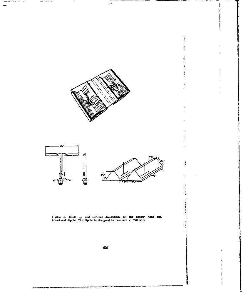
Ils

4yl,

Figure 2. Close up sad critical dimailons of the senso head madbromdbauid dipole. The dipole Is designod to resonate at 790 MHz.

607

i;

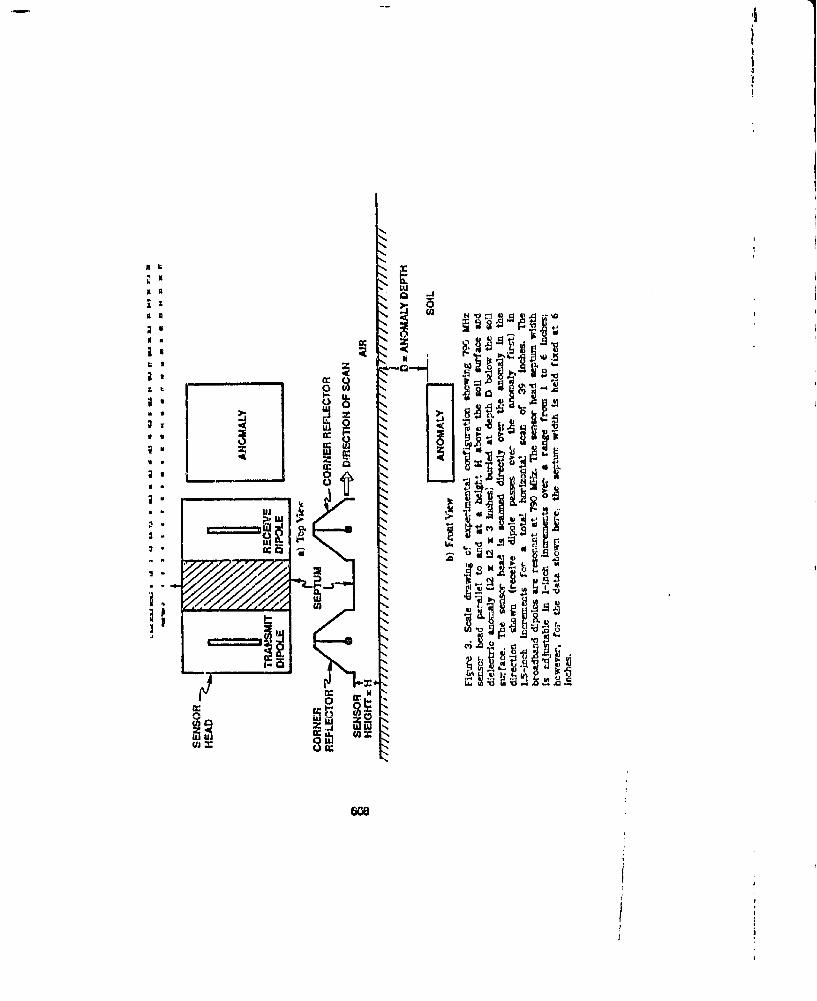
044

j~43

15 ~ ~ ~ u OZ*ir d. A WE -

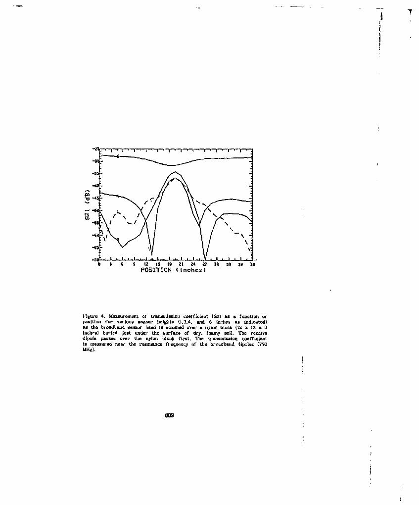
-31

4 3 6 1 12 15 19 21 24 27 30 33 39 MPOSITION (inches)

Figure 4. Measurement ot transmission coefficient (S21 as a function oiposition for various seasor helghts (1,3.4. and 6 Inches as indicated)as the broadband sensor head is scanned over a nylon block (12 x 12 x 3Inches) buried just under the surface of dry. loanmy coil. The receivedipole passes over the nylon block first. The trmunniuion coefficientis measured near the resonance frequcncy of the broimband 4lpolem (790

liMz).

609

IDI

iu1

v g:

uil

610

-W.0 'm w-w - I

mll

-70.0

-80.0U

-100.0 . ........ .... ..

0 10 20 30 40 00 0 00 7 0 100 g 10 120 130 140 16o

i"Uca (TIS model)

Vigure 6. Transmlission coefficient (SZI) as a function or positioncomputed with the two-dimensional TIM amodel. The transmissioncoefficient Is computed at 790 M1Hz and the dielectric anomaly Is buried3 inches below the earth-air Interface. (See text for further details.)

611

iS. ... . . . . .. . . . . . . ... .

THE MODELING OF LOSSY MAIERIALS WITH THE SYMMETRICALCONDENSED NODE TLM METHOD

Fred J. German, G.K. Gothard and L.S. RiggsDepartment of ElectrIcal Engineering

Auburn University, AL 36849(ZOS)R44-l864

Until recently, the symmetrical condensed node transmission line matrix

(T1M) method has not been capable of modeling lossy materials, In this

paper we present a new formulation for the symmetrical condensed TlM node

which permits the modeling of materials which exhibit both electric and

magnetic loss mechanisms. We test the validity of our formulation first by

comparing the TLM calculated results for a plane wave incident on a lossy

halr-space to the exact solution of the lossy wave equation. In addition,

we have applied the lossy node formulation to the analysis of wires coated

with radar absorbent material (RAM). The IT'., results for this problem will

be compared with results from an exact series solution.

INTRODUCTION

The transmission line matrix (TLM) method is a well known technique for

modeling physical processes with a mesh of inf.erconnected transmission

lines. A time domain impulse analysis of the transmission line mesh yields

the time history of voltages and currents In the mesh. These voltages and

currents aro then used to compute the physical quantities of Interest. For

612

electrornagnetlc applications several different verlonrc of the TLM method

haie been dcvelopei. Tbhe most efficient and accurate of these various

formulations is the symrnetrlcal condensed TLM (SCD M) me hod [I). A single

SCTLM cell is shown in Figure 1. Until recently, the SC-LM method was not

equipped to model electromagnetic interaction probLems which involved

materials that exhibited electric and/or magnetic losses. In this paper,

we reformulate the SCTLM method to include both electric and magnetic lors

mechanisms. It should be pointed out that, although arrived at

independently, the formulation that we present here 1s idtuntical to thatI. recently given by Naylor and Desai [2] for electric losses when there are

no magnetic losses present in the material being modeled. TIhic ability tomodel both electric and magnetic losses is important for many real

materials such as radar absorbent material (RAM) where both the

permittivity and permeability are complex.

FORMULATION-In order to model lossLs. six additional transmission line stubs have

been added to the symmetrical condensed node; three to model electric

losses and three to model magnetic losses. These additional stubs are

considered to be infinitely Iang (or equivalently terminated into a matchedload) so that none of tne energy that couple into these stubs is returned

- to the mesh. Thus, a loss of energy is modeled by these stubs. Since the

voltage pulses that couple into these stubs are not returned to the node,

there is no need to store them in the computer, and thus the lossy node

613

.1

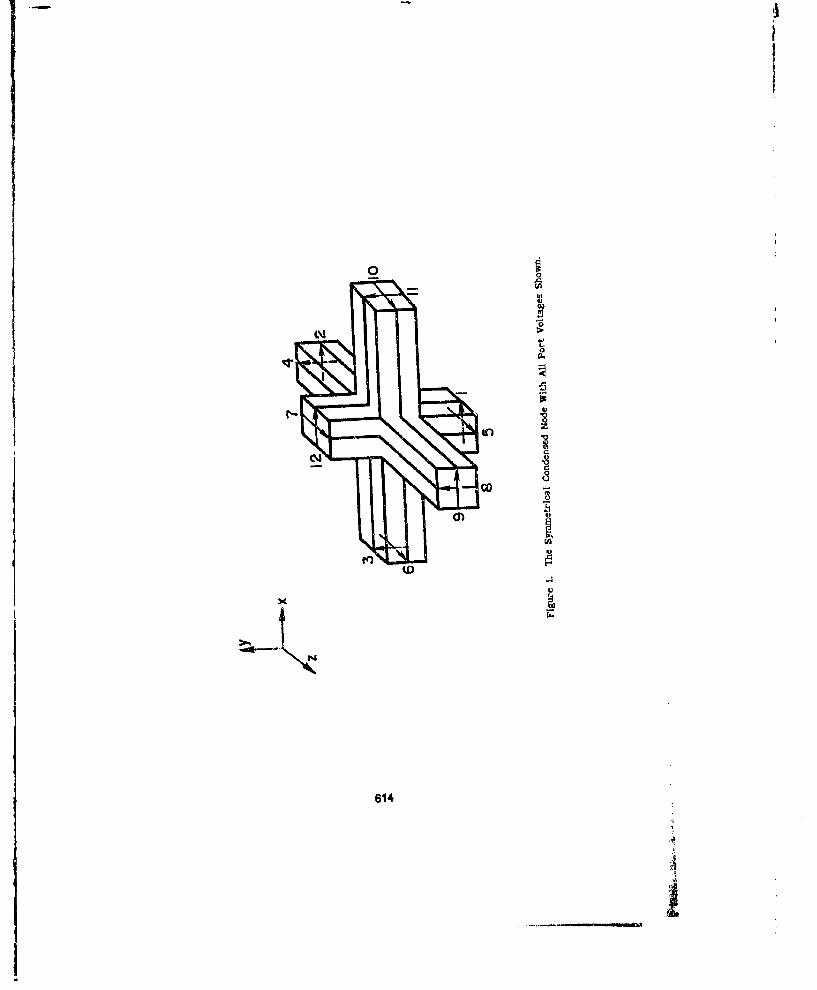
614

('-I

a..

scattering matrix requires the same computer storage space as the nude

without losses.

To begin the derivation we let three of the stubs have normalized (with

respect to 3770) characteristic admnittances GX, G an, and G. and couple only

to the Ex, E and E electric field components, respectively. Fox- magnutic

losses, three stubs with normalized characteristic impedances R , R and Ra y a

which couple only to H a, H and HZ magnetic field components, respectively,

are assumed. To obtain the scattering matrix for the lossy node, the

structure of the scattoring matrix given In III for the node with stubs is

compared to the two-dinenslonal series and uhunt TLM nodes 131. Those

nodes are the basic building blocks for the expanded node TLM mesh. The

shunt node Is equipped with an open circuited permeability stub with

normalized characteristic admittance Y and an electric loss stub of

normalized characterized admittance G.. Similarly, the series node has a

permittivity stub with normalized characteristic Impedance Z and a

magnetic loss stub with normalized characteristic impedance R . Theo

scattering matrices for these nodes are easily obtained from a simple

lumni,,i element equivalent network and are given by

-(Z+Yo+Gu) 2 2 2 ZYo

_ 2 -(2+Yo4Go) 2 2 ZY: C- 4+Y.G 2 2 -(2+Ye+ (2Y 2Y (1a)2 2 2 -(Z+Yo+Go) 2Yo2 2 2 2 (Y-Go-4)

for the shunt connected node with the loss stub and without the loss stub

Is

815

CJ

-(2+Y.) 2 2 2 2YoS2 -(Z+Yo] 2 2 2Yo

+ . )y9 2 2 -(2+Yo)- 2 MY liU}2 2 2 -(2+Y) 2Yo2 2 2 2 (Yo.-4)

For the series node vwith the ioss stub we have

(2 +Zo+Hoi 2 2 -z -zS 2 (2Zo+Ro? -2 2 22 -2 (2+Zoaeko) 2 2 (2a)

4+ZoR -2 2 2 (2+Zo+R.) -2. 2Zo 22z 2ZO -22o (44Ro-Zc)

and

(Z4.Z) 2 2 -z -a2 (2+Zo) -2 2 2a -l. 2 -2 (2Z2z) 2 2 (Zal2 2 2 (2+Zo) -2ZU Zzo 2 Zc -22 o (4+Zo)

lor the series connected node without the loss stub. It must be remembered

that, In general, the scattering matrix for the symmetrical condensed node

cannot be obtained from a )umped element equivalent circuit. However, by

comparing the scattering matrix of the symmetrical condensed node with

stubs with tho:", of tihe shunt and series nodes with stubs some useful

similarities can be obsered which lead to the scattering matrix for the

symmetrical condensed node with losses.

To begin, let us examine Johns' original scattering matrix ill In some

detail. The scattering parameters in the lossless SCTLM s.atterIng matrix

that are associated with the open circuited stub link line-to-stub

transmission coefficients (i.e., they specify the amount of coupling into

the open circuited stubs fi .,n pulses that are on the link lines connecting

616

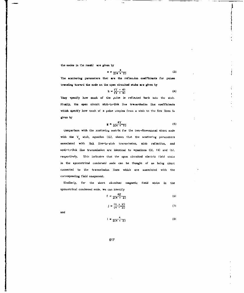
0 4

the nodes In the mesh) are given by

4 (S- -4 +-Y

The scattering parameters that are the raflecdon coefficients for pulses

traveling towmsrd the node on the open circuited stubs 'we given by

h (Y - 4)(4)

They specify how much of the pulse is reflected back Into the stub.

Fitally, the open circuit stub-to-link line transmission line coefficleats

which specify how much of a pulse couples froan a stub to tha link lines Id

given by

4Y2 (4 +- YComparison with the x'attering matrix for the two-diMnr-Aisional shunt node

with the Y stub, equation (1b), shows that the scattering parameters

associated with link line-to..stub transmission, stub reflection, end

stub-tu-link line transmission are Identical to equations (3), (4) and (5),

respcctlvely. ilils Indicates that the open circulted electric field stubs

in the symmetrical condersed node can be thought of as being shunt

connected to the transmission lines which are associated with the

corresponding field component.

Similarly, for the short circuited magnetic field stubs in the

symmetrical condensed node, we can identify

r 4 (6)

2(4 + Z)(4 + Z)-. (7)

and

1 4- (8)

617

as the entries associated with link line-to-stub coupling, stub reflection,

and stub-to-link line coupling, respectively. Comparison with the

scattering matrix for the two-dimensional series connected node with the Z

stub (Zb) uhowa that (7), (8) and (9) are identical to the corresponding

terms In (2b) suggesting that the short circuited magnetic fleld s.tubs in

the symmetrical condensed node mesh are connected in series with the link

lines that are associkted with the corresponding magnetic field component.

The correspondences between the stub coupling In the symmetrical

condensed node TLM mesh and the stub coupling In the two-dinenslonal shunt

and series node meshes which allows us to draw conclusions about the actual

physical connection of the symmetrical condensed node stubs to the lihk

lines, also allows us to easlly obtain the scattering matrix for the

symmetrical condensed node when the loss stubs are included,

Since the stubs associated with electric losses are shunt connected,

their characteristic admittance G and Y (note that G and Y take sub:;cripts

appropriate to the field value with which they are coupling) are in

parallel. Therefore. the symmetrical condensed node scattering matrix

entries Sl, I and J from 1 to 12 are identical in form as before except

that now the total stub admittance is taken to be (Y + G).

The other entries in the scattering matrix, namely, those associated with

link line-to-stub coupling, stub reflection, and stub-to-link line

transmission are obtained from the corresponding entries In the scattering

matrices for the two-dimensional shunt and series connected nodes with loss

stubs (la) and (2a). The final form for the scattering matrix of the

618

)rI

synunetrical condensed node equipped with all twelve stubs is the same as

that &iven In 111. The new expressions for the scattarlng matrix elements

for the fully equipped node are given by the following expresskonsý

(Y + G + (Z÷+ R (9a2(Y + G + 4) 2(Z + R + 4)

b 4 (9b)2(Y + G + 4)

c Y + G 3 (Z + R )(0C - -- €2(Y + G +4) 2(Z + R + 4)

d 4 (9d)2(Z + R + 4)

a b (9e)

f -4d (9f)

g Y b (9g)Y -G - 4h V - (9h)Y 4 G +4

I - d (9i0

4 +RZ +'J = (9J)

where the subscripts appropriate for G, R, Y and Z are determined from the

field component to which they couple as explained ha [W1. At this point,

relationships must be derived which rclate the luss stub Immitances, G i and

R, to the electric and magnetic conductivities, °'el and or M, respectively,

whlare I = x, y, or z, Consider a block of space with dimensions u, v, and

w in the x, y, and z coordinate direction, respectively, with a diagonal

electric conductivity tensur with entries a , vey and w' and magnetic

619

- 4

conductivities ,'M - , M and a'"

Consider as aln example care the conductivity associated with the

x-directed electric fiold, a, Uy derinition. the resistance associated

with this field component IsV

xwhere

and I Isx

I W L VW (12)

tbu,r giving

u (13)

Therefore. the characteristic admittance of the loss stub associated with

Ex, normalized to the characteristic impedance of the link linesi, Z is

a (vw)Gx - -!-'-f Zo(4iB U Q

Similarly for the other electric field loss stubs we obtainW (uw)G • Z (14b)

a. (uV)G. .~-- Z L140)

To relate the magnetic loss stub characteristic Impedance to the maguetic

loss tangent the dual of the above derivation Is used which yields the

following final results

620

I

W' (vw)R - -

U

Y u(15b)Y v

I' (uV)= mx

Often, the electric and/or magnetic loss tangent of a material Is

specified. These are related to the equivalent conductiviti•s bya'

tamn - (16a)

and

tanS - In (16b)

where tan6 *i the electric loss tangent. tan6 Is the magnetic Ioss0 01

tangent. c' is the real part of the complex permittivity and A' Is the real

part or the complex permeability.

Finally. the equations for calculating the nodal field values from the

Incident voltage pulsew require modification In ordek. to account for the

charge that couples Into the loss stubs without a etuvnlng to the node.

The'se slightly modified expressions are easily shown to be2

L.-m u-• + y 4 x (VI+ V ÷a V 9+ V 12+ Y aV 13 (17a)1N X

Ea 2 . i+VV3 +V +V IY V4 ) (17b)y" VT4-+ -+G)- v, v 1 y1y y

E . -Y -+ +V.I (17c)Y

H- 2(4 -V- - V + v - V-v (17d)

2 -(V -V V (17c)ll=~~ ~ -v---------"-+V6 10 17ty y

e21

I

I r4TL- 2 (-V + V, + V -V - V I(17f)

a It X

Thus, the symmetrical condensed node completely equipped with three

permittivlty stubs, three permeability stubs. three electric loss stubs,

axid thsee magnetic luau stubs has been comnpletely characterized.

hJUbMRIC& RESULTSIn this tiction, the lossy node formulation for the symmetrical cinndensed

node with electric and magnetic loss stubu is tested. Three examples are

presented: two which involve plane wave propagation In an inhomogeneoui

lossy tpace and one involving scattering I roen a RAM-coated cylinder,

As a first example, consider a 15 GHz plane wave to be normally Incident

on an Infinlte lossy half-space from free space. The lossy half-space has

relative complex permittivity and permeability given by Cr - 10 - J5 and jr

- 3 - J2. Figure 2 shows a plot of the electric field magnitude as a

functioh of position. 1 i' material Inter-face is located at 38ram.

comparison of the theoretical curve on the saone plot shows that the TLM

soluLion and the theoretical soi'mtion are virtually Indistinguishable.

"To examine the accuracy of the formulation for magnetic losses, we again

look at the case of a normally incident plane wave on a loasy half-space,

For this example c % 5 - J5 and IAr - 5 - J;&" where p"'' Is varied. Therr I'

reflection coerTicient from the lossy half-space is taken to be the ratio

of reflected electric field tU, incident electric field. Figure O(a) shows

the TLU calculated reflection coefficient magnitude along with the

theoretical values; again, excellent agreement is noted. Figure 3(b) plots

822

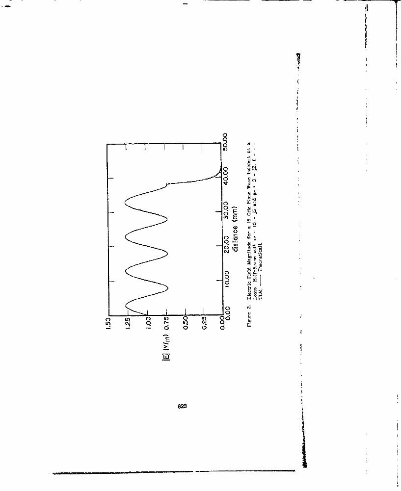
-0

623-

0.05N' ,-

0.20

.O15 -'ir

0.05

0.00 ?.oo 4.00 boo .00 0o.00

90.00-

L 0.00

-45.00--

-90.00 -

-135.O0 --IU~o.0c I I I .

-0 2.00 4.00 6.00 0.00 10.00

(b)

Flguve 3. Reflec.Lon Coorficient. (a) Magnitude (b) Plhase for cr -J5 and pr 3 -ji'

624

the TUM and theoretical reflection coefficient phas, referenced to the

material interface. with excellent agroement observed.

Finally, we present calculations for scattering from a circular PEC

cylinder coated with RAM. "ihe radius of the PEC cylinder is 2.38125 mm and

the radius of the wire and RAM coating is 4.643 nun. The material constants

for the RAM were assumed constant over the frequency range of Interest

(8-12GIIZ) and are given by r .- 15.0 - J1.0 and '1 , 0.95 - J0.25. Using the

above loss formulation we have calculated the attenuation provided by the

RAM coating on the wire. .rhe attenuation is defined as follows:

(Attenuation) d - (RcS Uncoated Cylinder) - (RtCS Coated Cylinder) d 1 (W)

In Figure 4 tha TLM results are compared to the resulLs obtained ft oam a

series solution to the problem and fair agreement is observed. It Is noted

that the results match better at the lower end of' the frequency band, and

diverge somewhat with Increasing rrequency. There are two probable causes

of this: one is that the inherent numerical dispersion of the TLM niesh

increases with increasing frequency Lnd the Inclusion of the lussy inatr'iul

makes this error more pronounced. Secondly, the error caused by the

approximation of the circul ir cylinder using a "stair-stepped" model on the

carteslan TLM mesh is known to cause serious errors at higher frequencies.

In this paper a formulation of the SCTLM method which includes both

electric and magnetic loss mechanisms is presented. Several examples have

been presented to validate the formulation.

625

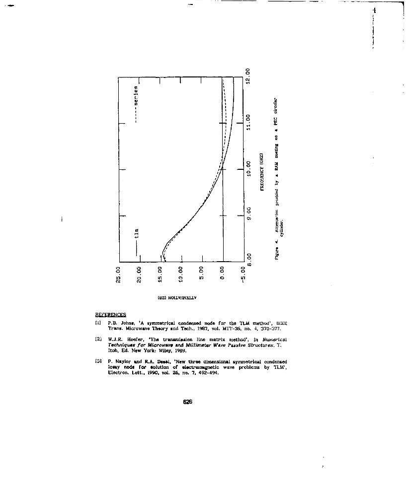
CU1

00

I44w

,4J

C.

ci IIfl I

' •0

iI 0 • I

, ,"oO

-- --•

° V

0 a 0 0 0 0 0

CU Cu .-

WaG) NOILVnN3-LV

il1 P.B. Johns, 'A symmetrical condensed node for the TLM method', IEEETrans. Microwave Theory and Tech., 1987, vol. MIT-35, no. 4, 370-377.

[21 W.J.R. Hoeler, 'The transmisilon line matrix method', In NumericalTechniqueA for MLcrowave aM Millimeter Wave PassLve Structures, T.Itoh. Ed. New York: Wiley, 1989.

[31 P. Naylor and R.A. Desal, 'New three dimensional symmetrical condensedlossy node for solution of electromagnetic wave problems by TIM',Electron. Lett.. 1990, vol. 26, no. 7. 492-494.

626

'N

"jHE ANALYSIS OF PASSIVE MICROWAVE COMPONENTSUSING THE ThM METHOD

Patrick R. Conway. F.J. German, L.S. RiggsDepartment of Electrical Engineering

Auwarn University, AL 36849(2051 844 - 1873

ABSTRACT

The Increased use of computer aided design and analysis of circuits

which transmit information ,t hIjzh frequencies has lead to a need for

reliable computer modeling of microwave frequenry circutl elements. In

this .)apui a technique is developed ushig the TLM metlhod to calculate tile

.;:X:L-.,ng matrix for a class of strip type passive microwave transmission

I.z l.. Single port and multi-port microstrip circuits with discontinuities

• tiialyzed. The technique la shown to ba a very accurate method for

using TLM in ciis type of design analysis through comparison of

rneasi rements with the rLM calculated parameters.

INTRODUCTION

0 it ,ias been shown [11] that the TLM method provides an accurate and

convenient nixh'7e'. ol slnulating mlcraoosve frequency circuits o~er a widebandwidth. l i a: .- ,:cy of the TLM method Is due to Its ability to model

irl.or.1noeneous sp,ý.ce aILL' acc.uraLeiy reproduce the frequency dependent

characteristics of sti h structures (includhlg dispersion and radiation).

ST'he convenz..,cu of the ^iLM method in due to the fact that * reformulation

is nwt niecessary for every new problem. Only a change of the Input file Is

required. Tn- TLM niethoa also produces, lI a vingle run, the ule'tric and

inagnetic i,'eld ,uc, ntities in the mod&lai space • b.-oad frequency

627

HN

range. These qualities make computer aided design a very practical

application of the TLM method.

"-his paper will take advantage of the desirable characteristics of the

TIM method to analyze several microstrip structUreS (See Fig. 0-. Five

practical microstrlp structures containing 'scontinultle will be

analyzed and four of the five circuits are multiport devices. Guidelines

for modeling the microstrlp structures will be presented. The method used

to extract the timr- domain data from the TLM mesh and the procedure used to

calculate the scattering parameters will be shown. The TLM extracted

scattering parameters are compared with the scattering parameters from

measurements. where available, and with calculated scattering parameters

from other numerical methods when measured data Is not available.

SCATVERING MARA•MMA CALCULATION

A sigle row of elements in the scattering matrix for a microwavm

component may be :alculated by taking the ratio of the voltage wave

traveling outward from ea-h port of the circuit element divided by the

voltage wave traveling inward on the input port. The inward and outward

traveling current may alhc I .d in this calculation since both voltage

and current may be considered as "normalized" power waves [2l. Both the

electric and magnetic field values are available from the TIM siatmation so

b-th current and voltage a %. svailr"le For the calculation of wide band

scattering parazmeters the traveling voltaat wave in the TIM cartesian mLesh

was used. For a given size volume and coarseiness or the mealh the lira

integral calculation of the voltage for a given point on the transmission

line would be more accurate than the c-."d line Integral around .,e

transmlssi'n lInoe for the cac.•ilatlon or current.

628

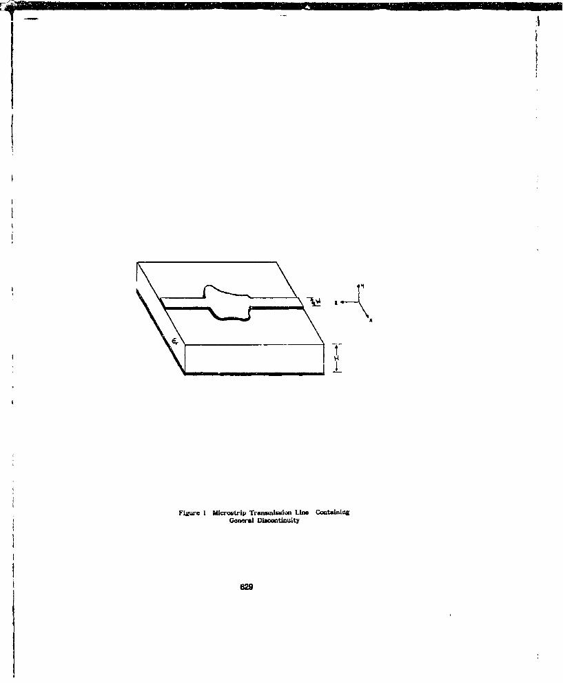
' '4

Figure 1 Ulcrostrip Transuaiuslon Line ContainingC-Oneal Discontinuity

62

I,-!

To obtain the voltage on a transmission line the impulse response

along a line at an observation point is saved as th.ý TiM simulation steps

through time. The inward and outward traveling voltages at the observation

point(s) are Fourier transformed and then the ratio of two traveling waves

is used to produce the scattering parameters as a function of frequency:

R F Vr(t) I

FE V (t) I

Where V tiW is the outward (reflected in this case) traveling voltage atr

the input port as a function of time and V I(t) is the inward traveling

voltage at the Input port.

MODELING

in order to analyze a microstrip circuit accurately using the TLLM

method, the circuit Itself and a finite volume of space surrounding the

circuit must be Included in the model. This volume, which Is Included in

the model but is not part of the circuit Itself, is a region above the

circuit and a region normal to the direction o, the propagation along the

circuit. Both of these regions are included In order to ensure that the

fields oriented in these directions have attenuated and that a TEM

condition exists at the computational domain boundaries. This is neceesary

since the boundary conditions which were enforced at the limits of the TLM

computational domain are designed to match TEl radiation. If a non-TEM

wave is present at the boundary then partial 'reflection of the fields

Incident on the boundary would result. These reflections are non-physical

and would coi rupt the circuit simulation.

63X

.4

- *1

The number of cells used to model the regions above and to the side of

each microstrip varied from circuit to cl cult because of the type of

discontinulties considered. In general though, for a straight mncrostrip

transmission line only 2 times the number of cells required to mode. the

thickness of the dielectric substrate Is required to model the region above

the transmission line. Outward from the trcnsmisslon line a region 5 times

the width of the strip was used to model this dielectric half space.

The quantity which will be used to calculate the scattering parameters

is a sum of the electric ficid values along a line from the ground plane to

the conducting strip. Because of this the TLM model should accurately

reproduce the electric field values throughout this region. The number of

cells used to model the width of a 50 n microstrip transmission line is

four, in sonic cases, to take advantage of the geometric symmetry of the

problem. This means the number of cells used to model the dielectric

region Is also four. It is possible to model the dielectric region with

only three cells beneath the strip, and this was used in cases where

symmetry was not available.

SIMULATION OU:PUT

The point used to observe the impulse response of the circuit should

be chosen such that any higher order modes which exist on the transmission

line due to the excitation and discontinultlis present In the circuit have

decayed. The decay of these modes determines the length of tran.smlsslon

lines connected to the microwave devices within the TLM model. For all of

the circuits considered in this paper the excitation was chosen to bW along

a line from the ground plane to the conducting strip. The propagating mode

did not fully develop until 20 to 30 cells away from this excit. tion. The

631

' tts&

transmission line discontinuity was therefore placed at least 30 cells down

the transmission line from the excitatiomi. Due to the various circuits

analyzed, the number of cells required to ensure that the higher modes

around the discontinuities were fully decayed varied from circuit to

circuit.

The extraction of the traveling voltage waves on the Input port of the

microwave device requires some extra attention. Both the inward and

outward (reflected) voltages will be present on this port and a method for

s*nparating the two is needed. It has been reported [3] 141 that two models

of the Input port are needed to reparate the two voltages on the input port

of a device. The method used here has only one model of the Input port.

This method models the Input poa t such that it Is long enough to allow the

Incident voltage to completely pass the observation point before the

reflected voltage can return. This method scems more efficient since

preparation and post processing time, along with computer requirements. in

most cases, are reduced since only one input file Is prepared and only one

T7.M simulation is run.

The number of time steps required for the calculation of the Fourier

transform also varies from circuit to c-rcult. An accurate method for

determining the number of time steps required is to calculate the Fourier

translorm for an Increasing number of time steps (see Fig 2). When the

traveling wave has not yet passed the observation point, the frequency

response Is seen to vary as a function of the number ii' time steps uaed in

the calculation. When the wave does completely pass the observation poInt

the frequency response remains constant as a function of time steps.

632

2.0 . .

520 iter. 540 'rter.

550 ier.560 i1e.v.

... *..... 570 "or.~80 eor.

590 ter.1.5

.. ................ ........

I.O0•

0.6 - " l , T ,

0.0 6.0 10.0 15.0 20.0 25.0

frneq (Offz)

Figure 2 Fourier Transform or Voltage ImpulseTraveling Cn a Microstrip Tranmnairwon Line

Versu; Time Steps

633

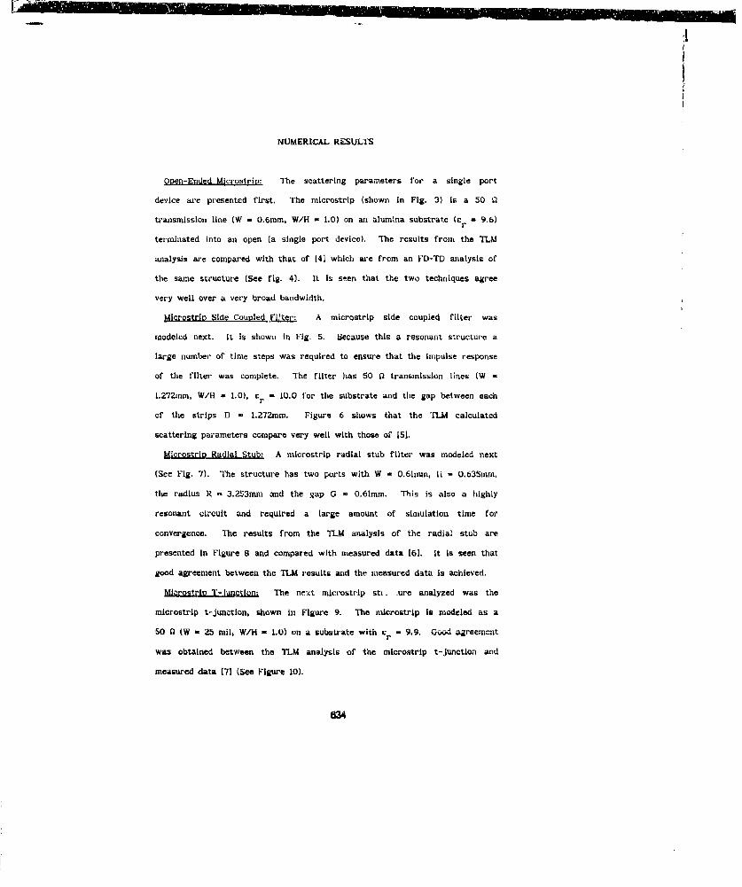
NUMERICAL RESULTS

Opien-Ended Microstrip: The scattering parameters for a single port

device are presented first, The microstrip (shown in Fig. 3) is a 50 Q

transmission line (W - 0.6mm, W/H = 1.0) on an alumina substrate (c - 9.6)r

terminated into an open (a single port device). The results front the TLM

analysis are compared with that of [41 which are from an FD-TD analysis of

the same structure (See fig. 4). It is seen that the two techniques agree

very well over a very broad bandwidth.

Microstrin Side Coupled Fl~ter: A microstrip side coupled filter was

modeled next. It is shown in Fig. 5. Because this a resonant structure a

large number of time steps was required to ensure that the impulse response

of the filter was complete. The filter has 50 0 transmission lines (W -

1.272mm, W/11 - 1.0), £r - 10.0 for the substrate and the gap between each

of the strips D - 1.272mm. Figure 6 shows that the TLM calculated

scattering parameters compare very well with those or [15.

Microstrip Radial Stub: A microstrip radial stub filter was modeled next

(See Fig. 7). The structure has two ports with W - 0.61mm, H - 0.635mm,

the radius R -= 3.253mm and the gap G - 0.61mm. This is also a highly

resonant circuit and required a large amount of simtulation time for

convergence. The results from the TLM analysis of the radial stub are

presented in Figure 8 and compared with measured data [6). It is seen that

good agreement between the TLM results and the measured data Is achieved.

Migostrji T-Ilunctlon: The next microstrip stm. ure analyzed was the

microstrip t-junction, shown in Figure 9. The microstrip is modeled as a

50 0 (W - 25 mil, W/H - 1.0) on a substrate with cr - 9.9. Good agr!.mcnt

was obtained between the 1LM analysis of the microstrip t-junctlon and

measured data (71 (See Figure 10).

634

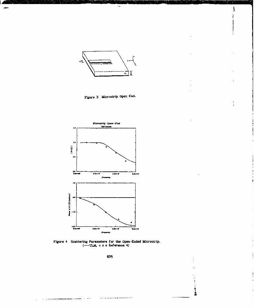
Figure 3 Microstrip Open End.

j-I

Figure 4 Scattering Parameters for the Opan-Ended microstf-ip.(--- TM. o o o Reference 4)

6315

UI

Figure S Micro-tirip Side Coupled Filter.

(--T., .- oReernc 5

-ae

-me.

-Med

-dega* 4.6 0 as I" Msd lt14.0 Me.

vvqR" (OW

Figure 6 Scattering Parameters for the Microstrip Side Coupled Filter.(--- TIM, o o o Reference 5)

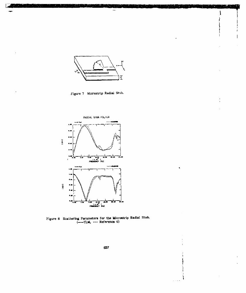
Figure 7 Microstrip Radial Stub.

RAOIAL SruS FILrLR

*. S I. . UI

7M0AICY ,i S)

(-TLM, Reernc -6

I.37

S.- I { .. I _

- II, D

Figure 8 Scattering Parameters far thle Microwtrip Radial Stub.

(--TUE.-- Reference 6)

837

Figure 9 Microstrip T -Junction.

T- Juwtis"

S IL

- ad

-LO

-'LO t eaa&

ftw-" (ON-)

Figure 10 Scattering Parameters for the Microstrip T Junction.(---TLM, o o o Reference 7)

638

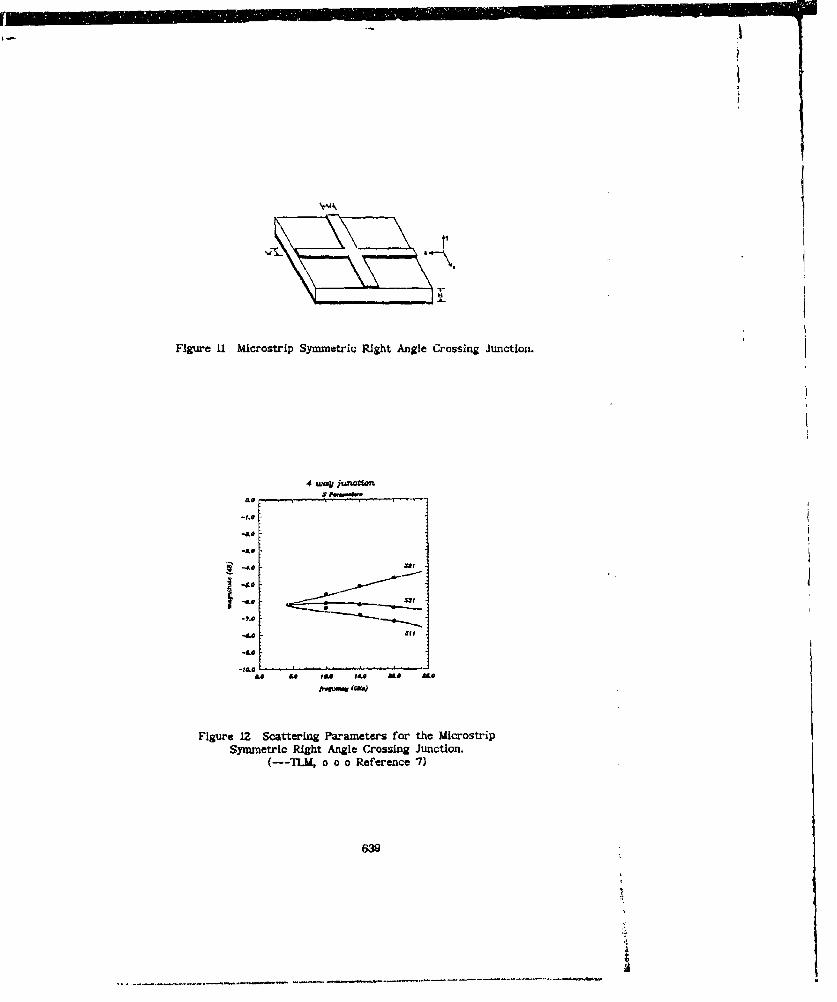
Figure 11 Microstrip Symmetric Right Angle Crossing Junction.

4 uay junction

-I @-. 0

3 -40 S81

-ALo

-"' o.. .. • . ., " ;, ' • " •,

Figure 12 Scattering Parameters for the MicrostripSymmetric Right Angle Crossing Junction.

(---TLM., o o o Reference 7)

639

I

Microgstrip Cross Junction: The next structure modeled, and shown in

Figure 11 , is the microstrfp cross junction. The TLM results are compared

in Figure 12 to a Method of Moments solution based on the EFIE 171 and

show good agreement. The microstrip Is modeled as a 50 92 transmission line

(W = 25 mil, W/H = 1.0) with c = 10.Z for the dielectric substrate.

CONCLUDING REMARKS

A method was developed which used TLM calculated data to extract

scattering parameters for single-port and multi-port naicrostrip devices.

General rules were also presented for modeling this type of mlcrbwave

transmission lines. The results of using these rules with a TLM simulation

were presented and the application of this method to resonant, as well as

nonvresonant microstrip structures was shown to produce accurate scattering

parameters over a wide frequency range.

640

REFEREN2 ES

[I1 F.J.German, H.D. Williams, L.S. Riggs, and M.E. iVaginski. "ThreeDimensional Full-Wave Analysis of Passive Microstrip Components UsingThe TLM Method", ACES Conf. Proc., 1989, 63-77.

[2] r'.A. Rizzi, The Scattering Matrix, Appendix D, Microwave EngineeringPassive CGrcutts, Prentice-Hall, Englewood Cliffs, New Jersey, 1988.

[31 J. Uher, S. Liang and W.J.R. Hoefer, "S-Parameters of MicrowaveComponents Compated With The 3D Condensed Symmetrical TLM Node", IEEEMiT Symp., 1990, 653-656.

[41 X. Zhang and K.K. Mel, "Time-Domaln Finite Difference Approach To TheCalculation of the Frequency-Dependent Cheracteristics of HicrostripDiscontinuities", IEEE Trans. Microwave Theory Tech., 1990, vol. 36,no. 12, 1775-1787.

15] T.Shibata, T.Hayashi and T. Kimura, "Analysis of Microstrip CircuitsUsing Three-Dimensional Fih-Wave Elentroinagnetic Field Analysis InThe Time Domain", IEEE Trans. Microwave Theory Tech., 1990, vol. 36,no. 6, 1064--1070.

[61 M. Wertgsn and -Z. H. 1insen, "Efficient Direct and IterativeElectrodynamic Analysis of Geometrically Complex MIC and MMICStructures", Int. J. Numerical h!)de!ling, 1989, vol. Z, 153-186.

P71 S.-C. Wu, H.-Y. Yang and N.G. Alexopoulos, "A Rigorous

Symp., 1990, 1151-1154.

841

SESSION 16- "FINITE ELEMENT AND FINITE DIFFERENCETIME DOMAIN SOLUTIOIWS"

Moderator: rFaymond Luebbers

A New Weighted Residual Finite Element Method forComputational Electromagnetics in the Time Domain

John Ambrosiano and Scott T. BrandonL-95, Box 808

Lawrence Livermore National LaboratoryLivermore, CA 94550

Rainald LmhnerCMEE School of Engineering and Applied Science

The George Washington UniversityWashington, DC 20052

Abstract

Engineers and scientists have become increasingly interested in calculating electromag-

netic effects iii the time domain. For example, the time domain is especially convenient for

studying short (wide band) pulses. For such methods to be generally useful, they must be

free of the severe geometric restrictions imposed by traditional finite difference methods.

In o- research into methods for plasma simulations in realistic geometries, we have

developed finite eleenut methods for electromagnetics in the time domain on unstructured

grids. Unstructured grids provide maximumn flexibility in fitting sample points to the prob-

lem, both on boundaries and in the interior. Finite elements provide the most convenientframiewurk fox the mathematics as well as for the implementation.

We will present a new finite element method for computational electromagnetics on

unstructured grids. The method is fast, easy to implement, and 2nd-order accurate. Al-though we use low-order elements, the method can be shown to preserve the divergence

constraints (V. B = 0, V. E = 0 in vacuum). We also present a numerical benchmark.

1. Introduction.

There has been great interejst in recent years in calculating electromagnetic fields in

the time domain. The time domain is especially convenient for modelling wide-band pulses

or for understanding transient effects.

642

To be truly useful, a good method must be geometrically flexible. This requir•ement has

motivated nmany successful research efforts using both finite elements and finite volumes1 -'.

These methods allow solutions to be computed on boundary-conforming structured meshes

or on unstructured meshes. The freedom to choose these more general meshes over thetraditional rectilinear finite difference meshes is crucial for geometric flexibilty. Wc have

concentrated exclusively on unstructured meshes of triangles. We feel this provides max-

iitaiii flexibility in fitting sample points to the problem, both on boundaries and in the

interior,

In the process of designing methods for plasma simulation, we have investigated sev

eral approaches. We have previously reported our experience with the Taylor-Galdkin

technique applied to electromagnetics3 . The Taylor-Galerkin (TG) method is a gen-

eral high-order method for hyperbolic systems that has been used sucessfully in fluid

dynamics9. Accurate computations using TG have been reported for electromagnetic scat-

tering applications'0 and we have successfully implemented a plasma particle code based

on the technique' 1 . The TG schemes are highly accurate and relatively fr,' of dispersion.

However, we have found that they are substantially more expensive than traditional finite

difference time domain (FDTD) methods. In addition, there is nothing ill the conformingGalerkin formulation to guarantee additional constraints that are often important in elcc-tromagnetics. For example, while our TG computations are globally quite accurate, they

nonetheless produce spurious local divergence errors. Although these errors are bounded

by the order of the method to relatively small dues, they are potentially troublesome for

certain applications, particularly those that seek to incorporate charged particles.

Our search for a better particle code field solver has led us to some umconventional ap-

proaches. One of the most appealing has been described by Nedelec4 who constructs specialelements appropriate to vector fields on which constraints are imposed. Nedelec's elements

have specific degrees of freedom which constrain the vector field represented by them to

conform to the special Hilbert spaces H(div, Q) or H(curl, S2). A variational formulation

643

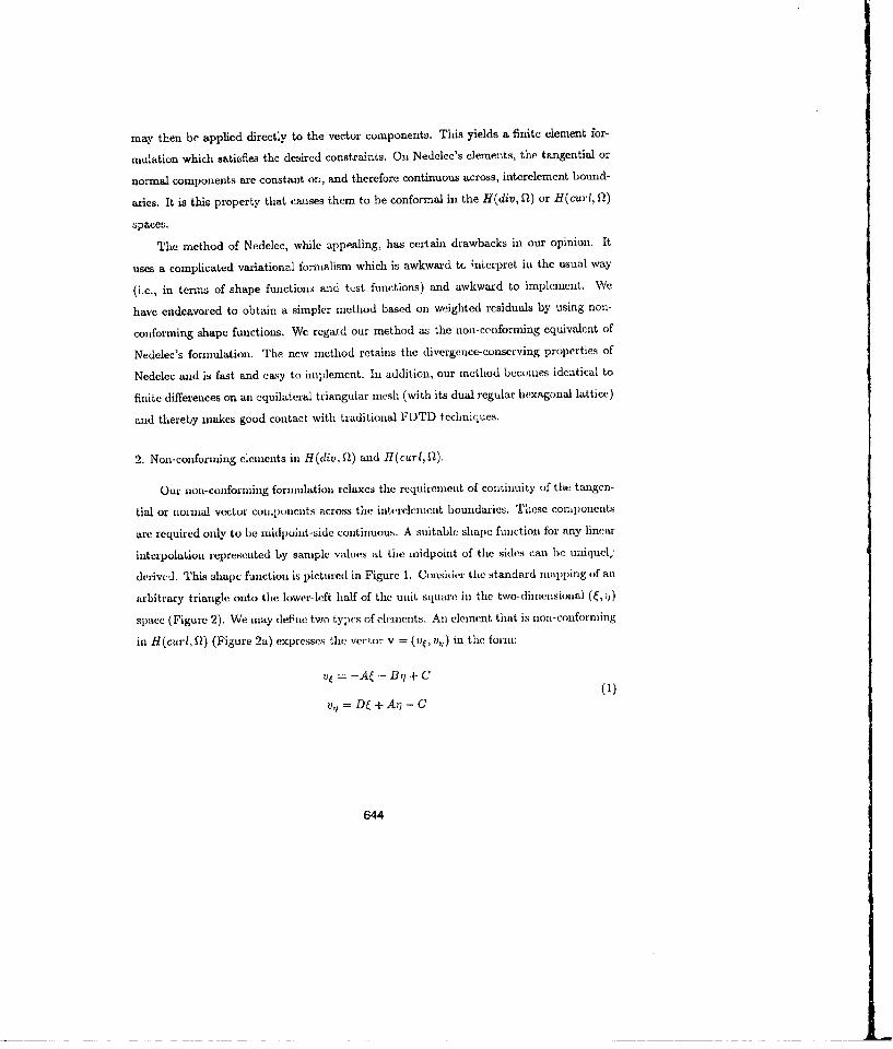
may then be applied directly to the vector components. This yields a finite eiement for-

mulation which satisfies the desired constraints. On Nedelec's elements, the tangential or

normal components are constant on, and therefore continuous across, interelement bound-

aries. It is this property that causes them to be conformal in the H(div, Q) or H(curl, Q2)

spaces.

Thle method of Nedelec, while appealing, has certain drawbacks in our opinion. It

uses a complicated variational formalism which is awkward to ;nerpret in the usual way

(i.e., in terms of shape functions and test functions) and awkward to implement. We

have endeavored to obtain a simpler method based on weightcd residuals by using non-

conforming shape functions. We regard our method as the non-conforming equivalent of

Nedelec's formulation. The new method retains the divergence-conserving properties of

Nedelec and is fast and easy to implement. In addition, our method becomes identical to

finite differences on an equilateral triangular mesh (with its dual regular hexagonal lattice)

and thereby makes good contact with traditional FDTD techniques.

2. Non-conforiming elements in H(div, Q) and H(curl, 12)

Our non-conforming formulation rclaxcs the requirement of continuity of the tangen-

tial or nuormal vector components across the intercleluent boundaries. These components

are required only to be midpoi nt-side continuous. A suitable shape function for any linear

interpolation represented by sample values at the midpoint of the sides can be uniqucl;

derive']. This shape function is pictured in Figure 1. Consider the standard mapping of an

arbitrary triangle onto the lower-left half of the unit square in the two-dimenlsional (ý', )

space (Figure 2). We may deFne two types of elements. An element that is non-conforming

in H(curl, Ql) (Figure 2a) expresses the vector v = (v4, v,) in the foriu:

v= -Aý - BrI + C (1)v= Dý + Aq - C

644

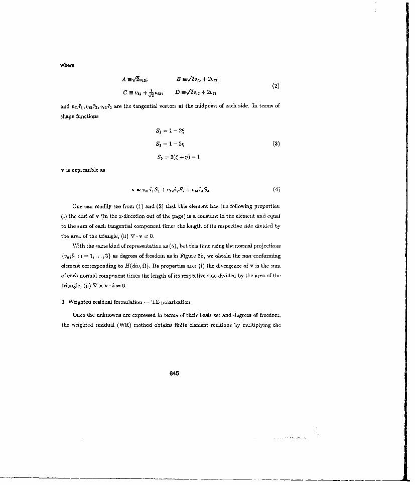
where

A =vgV23; B -=w/V1g3 + 2v,2 (2)C E Vf3 +1ut Va; D =_v'/_ + 2vt5

and vtVý, V•O2 2 ,V, 3 73 axe the tangential vectors at the midpoint of each side. In terms of

shape functions

S1 = 1- 24

S2= 1 - 2t (3)S3 =2(ý + •

v is expressible as

V V1IT SI -1 + Vf 2T2 S 2 + vg33S3 (4)

One can readily see from (I) and (2) that this element has the following properties:

(i) the curl of v (in the z-direction out of the page) is a constanit in the element and equal

to the sum of each tangential component times the length of its respective side divided by

the area of the triangle, (ii) V. v = 0.With the same kind of representation as (4), but this time using the normal projections

lvnili : i = 1, . .. 3} as degrees of freedom as in Figure 2b, we obtain the non-conforming

element corresponding to H(div, Q). Its properties are: (i) the divergence of v is the slum

of each normal component times the length of its respective side divided by the area of the

triangle, (ii) V x v. i = 0.

3. Weighted residual formulation - - TE polarization.

Once the unknowns are expressed in terms of their basis set and degrees of freedom,

the weighted residual (WR) method obtains finite element relations by multiplying the

645

residual by a "suitable" test or weighting function, setting it to zero, and integratingover the problem domain. For non-conforming representations, the loss of interelement

continuity requires that the integrals be performed elementwise.

By using a WR formulation we gain the necessary freedom to satisfy additional con-

straints. However, this freedom means that it is possible to derive a bad method by choos-ing "unsuitable" test functions. A successful Wit method is often found by serendipity or

by trial and error. Unlike variational methods or Galerkin's method, a WR. formulation

is normally justified a posteriori by examining special cases and, of course, by performing

computational benchmarks.

For the TE polarization pictured in Figure 2a, let the electric field's degrees of freedom

be its tangential projection.s at the midpoint of the sides and its basis functions be the

set of side functions {Si : i = 1.... ,K.}, where N. is the number of sides. Let B, be

constant within an element so that its basis is the set of constaat element shape functions{P,-: e = 1 ... ,NC} with A', being the number of elements. Faraday's law

OB

becomes

2eomi B.&P,.= IV ZS iEji-i) -.i EZn VS i xiyQ- (6)

To select a particular element e&' choose as our weight function Ps,. We then multiply

(6) by P•, and integrate. Clev , the only contribution is from the element c' and thesides comnected to it. Thus we obtain

Y• - -5-n,2 (7)

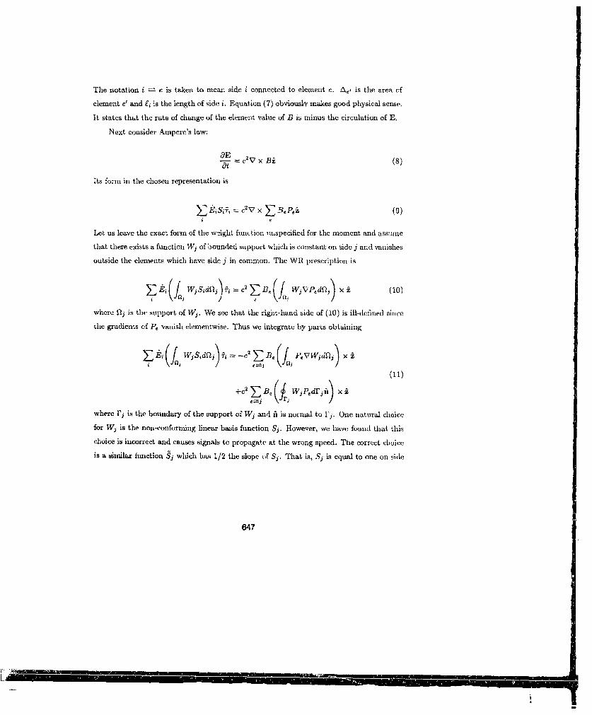
The notation i ;e is taken to mean side i connected to element e. A,, is the area cfclement e' and £i is the length of side i. Equation (7) obviously makes good physical sense.

it states that the rate of change of the element value of B is minus the circulation of E.

Next consider Ampere's law:

OE VB()•-= 2V x Bi 8

Its form in the chosen representation is

ci ex -9ePi

Let us leave the exact form of the w-ight function unspecified for the moment and assumethat there exists a function Wj of bounded support which is constant on side j and vanishes

outside the elements which have side j in common. The WR prescription is

>j4-(f wjiSd%>j c 2 ZBe ( Jw.vP~d%) X i (10)

where Sli is the support of Wj. We see that the right-hand side of (10) is ill-defined sincethe gradients of P, vanish clementwise. Thus we integrate by parts obtaining

L jW1Sid%) j -C2 Z njJ PVW~dlj) X i

+e 2 ED B( jPedrii X i

where ri is the boundary of the support of Wj and ft is normal to Ij. One natural choicefor Wj is the non-conforn-ing linear basis function Sj. However, we have found that this

choice is incorrect and causes signals to propagate at the wrong speed. The correct choice

is a ssi-ilar function Sj which has 1/2 the slope of Si. That is is equal to one on side

647

[ '7

j and goes to zero on a line joining the midpoints of the remaining two sides, while Sj is

one on side j and goes to zero at the vertex opposite side j. The left-hand-side of (11)

contains a matrix expression which may be lumped. The lumped mass contribution from

each of the two elements is A./3. Multiplying by ýj and carefully evaluating the interior

and the surface contributions yields:

= C2 (ý)B.+L -- B, (12)

Relative to side j, + (-) refers to the element in (opposite) the direction i x +y. We may

also replace the areas associated with the mass matrix with expressions in terms of the

altitude lengths hj+,hI.- obtaining:

2;=c (Bj---- Bin----- (13)= (hj+ + h1-)

In this form it is plain that if the mesh were equilateral, the update on the tangential

component of E would simply be c2 times the difference between values of B at the Voronoi

points of the two triangles common to that side.

4. Weighted residual formulation - TM polarization.

For the TM polarization pictured in Figure 2b, let the magnetic field's degrees of

freedom be its normal projections at the midpoint of the sides - again letting its basis

functions be the set {Si}. Let E, be linear within an element as interpolated from values

at the vertices so that its basis is the set of linear element shape finctions { I,, - r =

1,... ,A( } with AK, being the number of triangle vertices. Faraday's law in this polarization

OB- -V x E (14)

becomes

848

L

SB $¼ = -V x ,N (15)The appropriate test function for a side j is again the test function Si although in this

case no error occurs if Si is used instead. Integrating we obtain

A / isid%> = -ZE- (j En ivNdQ) x i (16)

In this instance the lumped mass matrix contribution to side j from each element e is

2A,/3. After taking the scalar product with Dj, we notice that, on the right-hand side,

the only vertex contributions are from those joined directly to side j. Evaluation of (16)

eventually leads to the very simple expression

= (E,+ -E) (17)

where + (-) refers to the vertex in (opposite) the direction i x ýj' Once again we have

an expression that makes good physical sense. It states that the update on the normal

component of D at the midpoint of a side is just equal to the difference between the values

of E, at each end divided by the length.

We next turn to Ampere's Law in this polarization:

Sc"[V x B].i (18)

In terms of the basis functions:

Z ENt,, -'cVx [Z cBs,] 2- (19)

We choose as our weighting function the linear vertex shape function Nm. Because our

non-conforming element representation for B has vaniehing elementwise curl, we must

integrate by parts in this case as well. Thus we have

649

L

Z~ j NmNndQn) -C 2 z i( SuVNn~~n fix ý(20)

+ E2Y , IV NSjdfnfi) X zi -where 9,, is the support of Nm and rm is the boundary. The mass matrix contributions

in this instance are the familiar lumped mass contributions associated with conforming

linear elements. That is, each element c contributes A,/3. Although somewhat tedious,

careful evaluation of (20) yields the uncomplicated expression

2 i ,, i Ai Aj-)le (21)Bi Ls 4 +' A, J/3where + or - refers to elements to the right or left respectively of side i. Using the relation

between the area of each triangle and the length of the altitude along the normal directions

v1 one may develop a straightforward interpretation (21) for an equilateral mesh. In thatcase the sum in the numerator is the sum of tie normal component Di times the distance

between the Voronoi points of the two adjacent triangles. Dividing this sum by the eiclosed

area yields a reasonable approximation to the curl about vertex m.

5. Implemention and benchmark.

Equations (7), (12), (17), and (21) constitute the new weighted residual method. Inthe spirit of traditional staggered finite difference methods, we use a leapfrog approximationto the time derivatives. Given a list linking elements with vertices and elements with

sides, the WR equations require only straightforward gather and scatter operations for

implementation. The electric fields are expressed at timelevel k and magnetic fields attimelevel k + •. Although space does not permit it here, it may be shown that theseequations have the required symmetry properties that preserve the divergences of E andB exactly (to roundoff) in the vacuum. The degrees of freedom representing the fields

650

are niatural for enforcement of boundary conditions. Specifically, boundary conditions are

enforced by setting Ei (E-tangential) and Bi (B-normal) at the midpoint of boundary faces

and by setting E. (E-tangential) at boundary nodes.

We present a numerical benchmark showing that the WI. method obtains reasonably

accurate results for a scattering problem. Figure 3a shows a portion of the mesh around

a circular obstacle. For this test a plane wave of wavenumber k is incident from the left.

Relative to the radius a of the circle, ka = 5. The observation point is one radius ahead of

the circular boundary on a line joining the center. The Courant number is 0.25. Figure 31)

compares the computation with the analytic result. We can see that tie computed solution

has sonic dispersion and a small phase error, biut is a reasonably good approximation to

the true result.

We have presented a new finite clement metiod for triangle grids that baa many useful

properties in common with traditional staggered-mesh finite diffcrence schemes, Indeed, it

reduces to a straightforward finite difference scheme on an equilateral mesh. Unlike many

methods that have been proposed, it is simple to implement and fast. It does not require

a Voronoi-Delauna) mesh or any other special mesh. Benchlnarks thus far suggest thattile method is 2nd-order accurate for smooth meshes; i.e., the same relative accuracy as

standard FDTD methods.

Acknowledgement.

We wish the thank several colleages for their suggestions and comments. We tlank

Rick DeVore, Scott Ray, Bruce Langdon, Peter Rmnbo, Dale Nielsen, Alain Adolf, antI

Bruno Schourer. This work was performed undler the auspices of the U. S. Department of

Energy by Lawrence Livermore National Laboratory under contract no. W-7405-Eng.-48.

References.1. Niel K. Madsen and R. Ziolkowski, Wave Motion, 10 (1988).2. Robert L. Lee and Niel K. Madsen, J. Comput. Phys., 88, 284 (1990)

651

_ I I J __ __ . .__. ... • • . . . . . .

3. J. Ambrosiano, S. T. Brandon, and Rainald L6hner, "Electromagnetic Propagationon an Unstructured Finite Element Grid,' Proceedings of the 6th Annu'id Review ofProgress in Computational Electromagneties, Monterey, California, January, 1990.

4. J. C. Nedelec, Numerische Mathematik, 35, 315 (1980).5. P. Degond, F. Hermeline, P. A. Raviart, and J. Segre, "A Coupled Particle-Finite El-

ement Method for the Approximation of Vlasov-Maxwell Equatiorns," (Unpublished).6. F. Hermeline, "Two Couplhd Particle-Finite Element Methods Using Delaunay-

Voronoi Meshes for the Approximation of Vljý-nv-Poisson and Vlasv-Maxwell Equa-tions," (Unpublished).

7. James Eastwood, "Virtual Particle Electromagnetic Particle-Mesh Algorithms," Cul-ham Laboratory Report CLM-P870, 1990.

8. M. E. Jones, "Elctromagnetic PIC Codes with Body-Fitted Coordinates," Proceed-in s of the 12th Conference on the Numerical Simulation of Plasmas, San FRancisco,

afornia, September, 1987.9. R. L6hner, K. Morgan, and 0. C. Zienkiewicz, lIn. J. for Num. ideth. in Fluids, 4,

1043 (1984).

10. C. R. DeVore, R. L6hner, aid J. Ambrosi no "Electromagnetic Scattering Calcula-tions Using a Finite-Element Solver for the Maxwell Equations," Proceedings of the1990 Free-Lagrange Conference, Jackbou Lake, Wyoming, June 3-7, 1990.

11. J. Ambrosiano S. T. Brandon, and R. L6hner, "Electromagnetic Particle Codes onUnstructured drids," Proceedings of the 1990 Free-Lagrange Conference, JacksonLake, Wyoming, June 3-7, 1990.

652

[

Figure 1

(0.1) (a) (0,j) (b)iio(0,0) (0,J)

Figure 2

653

V.

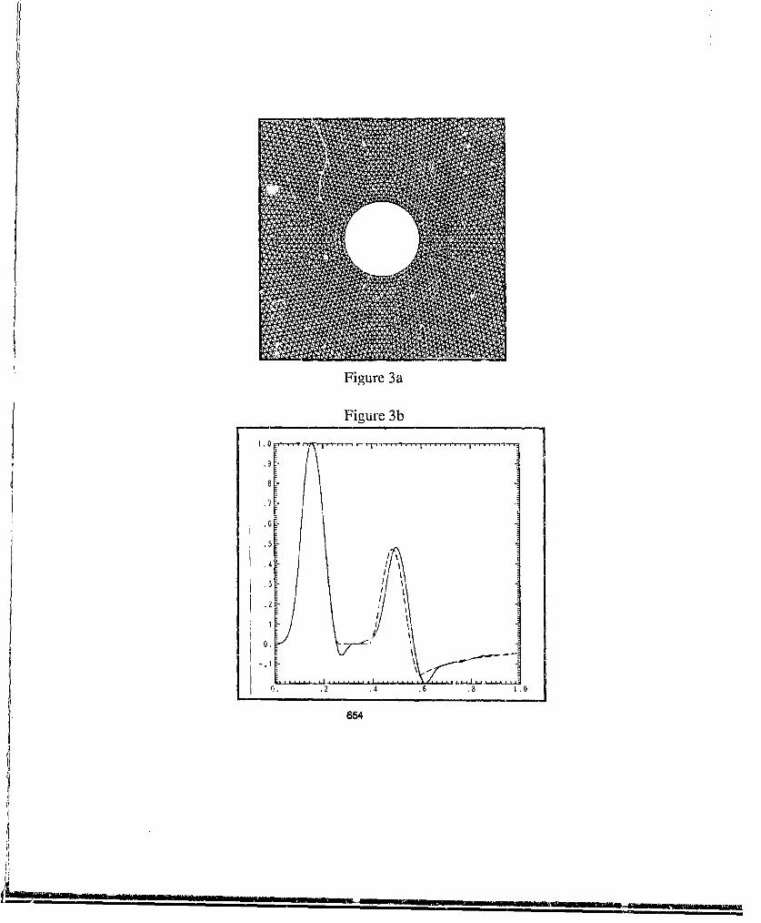
Figure 3a

Figure 3b

ki

... . 1.5 4

.1 I

.5

,~1

0. .2 .4 .6 .8

654

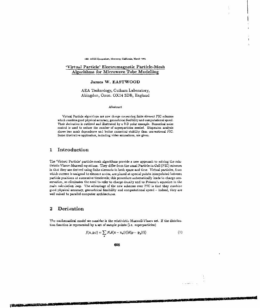
19Q1 ACES Symp-iu, MhtWay, ChaW., M-&dh 1991

'Virtual Particle' Electromagnetic Particle-MeshAlgorithms for Microwave Tube Modelling

James W. EASTWOOD

AEA Technology, Culhlam Laboratory,Abingdon, Oxon. OX14 3DB, England

Abstract

Virtual Particle algorithms are new charge conserving finite element PIC schemeswhich combine good physical accuracy, geometrical Biexibility and computational speed.Their derivation is outlined and illustrated by a 2.D polar example. Numerical noisecontrol is used to reduce the number of superparticles needed. Dispersion analysisshows less mesh dependence and better numerical stability than conventional PIC.Some illustrative application, including video animations, are given.

1 Introduction

The 'Virtual Particle' particle-mesh algorithrms provide a new approach to solving the rela-tivistic Vlasov-Maxwell equations. They differ from the usual Particle-in-Cell (PIC) schemesin that they are derived using finite elements in both space and time. Virtual particles, fromwhich current is assigned to element nodes, are placed at special points interpolated betweenparticle positions at successive timelevels; this procedure automatically leads to charge con-servation, so eliminates the need to refer to charge density and to Poisson's equation in themain calculation loop. The advantage of the new schemes over PIC is that they combinegood physical accuracy, geometrical flexibility and computational speed - indeed, they arewell suited to parallel computer architectures.

2 Derivation

The mathematical model we consider is the relativistic Maxwell-Vlasov set. If the distribu-tion function is represented by a set of sample points (i.e. superpartirles)

f(x. p,) = N.8(x - x.t)).(p - p.(t)) (1)

655

where (x., p.) gc [1, N,] are the coordinates of the N, superparticles, each of mass M =Namo and charge Q = N~q, then the Maxwell-Vlasov set may be written in terms of theaction integral

I f dr(DE-B _ 4 A) -/f) Idt (2)

where B = V x A and E = -VO - !6 Treating I a& a functional of the vector potentialA, the scalar potential 4 and particle coordinates {x,} leads to Euler-Lagrange equationswhich reduce to Maxwell's equations and the relativistic equations of motion. More extensivediscussions of this are given in references [5, 6].

The finite element approximations to the Maxwell-Vlasov equations are obtained by substi-tuting test function approximations for potentials 4, and A, and particle coordinates x, intoEq.( 2) and taking variations with respect to the unknown nodal amplitudes.

Variations art. to ý yields a discrete form oi Gauss' Law, plus a prescription for chargeassignment. Variation tart, A gives Ampere's Law and the current assignment prescription,and variations wrt. particle coordinates give discrete equations of motion and the prescriptionfor force interpolation. Explicit reference to A, 4 and charge density p can be eliminated byusing the homogeneous Maxwell equations. The result is a fast and accurate timesteppingscheme where p need not be accumulated, and charge conservation coLrections such as Poissonequation solutions for longitudinal electric field co-ec:tion [3] or "pseudocurrents" [4) are notrequired.

A whole family of virtual particle schemes may be generated by choosing appropriate elementgeometry and trial functions. If the procedure is ;orrectly followed, these schemes willautomatically have the charge conserving property.

3 A 2-D Example

We use a two dimensional polar (r, z, t) transverse magnetic (TM) model and the lowest orderconforming rectangular brick elements to illustrate the practical realisation of the methodoutlined in section 2, On a uniform net of elements, this choice leads to a numerical schemeaimilar to that using the usual interlaced TM finite difference mesh [2].

For clarity, we work with units which give length unity sides to elements and E = D, B = H.The potential and field trial functions become a mixture of piecewise linear (L) and constant(C) functions of the coordinates (r, z, t). Fields (E,, E,, Bs) are respectively (C, L, C), (L, C,C) and (C, C, L) in (r, z, t). This choice leads to node locations shown in figure 1. Variationswel. 4 and element assembly give the global discrete approximation to Gauss' Law

a,(rctE.) +,9,(ra.E,) = (3)

656

:?.-.-.- -

NW N NE

W

SW S SE

Figure 1: Location of clement node3. Values of p and 0 are stored at corners, (E., E,.) and(1., 1,.) at sides and lie at the centre.

where difference operator a, and d, (and averaging operators a, and a,) respectively act onthe indices I and in:

,9fAý = f4+1i.,,. - fh-i/2, af;.,,, = (fj-l,n + 4fl..• + f4+1m)/6 (4)

Similar expressions hold for 0, and a, on index in and 0, and a, on the time index n. In Eq.(3 ), the choice of (L, L, C) support for ý implies that q is accumulated using CIC (Cloud !nCell) in r and z, and NG11 (Nearest Grid Point) in t [1]

Variations wrt. A and assembly give the discrete approximations to the components ofAmpere's Law

0,(raE._) = (rnlBe) - I, ;,(r,.E;) - -.8.(r,,B,) - (5)

and the NGP/CIC virtual particle current assignment prescription. Faraday's Law becomes

=, Be aE. - a.E, (6)

Note that these equations for the fields differ from the usual finite difference equations onlyin the appearances of the averaging operators in Eqs,(3) and (5).

To maintain explicit forms for the equations of motion we assume that particle pot ition. areconstant over the interval from timelevel. n -. 1/2 to n + 1/2, and use a weak approximationfor the momentum. This yields the usual finite difference expression

p +1/ - pn-212 = QA E-(x-) + 9" X (+ 1 2 1.-3n-1/2 ) (7)

where V" - (v"+'/3 + v"- 1 /2)/2 and

x"+ I xn + v-t4 l/2At (8)

657

.

The fields at particle locations are the value of the finite element fields at that point. Thus,for this example, E, is the NGP in z and CIC in r interpolant of the nodal values, Br isCIC/NGP and B9 is NGP/NGP , etc.

The choice of trial functions prescribe the charge and current assignment schemes. For aunit charge at position (z, r) turt. the SW corner of a unit side clement, the charges assignedare:-

5pNS = zr 6pNw = (-z)r6S = z(1 -- r) 6 psw = (1 -- z)(1 - r) (9)

Currents assigned from a trajectory segment of length (Az, Ar) and mean position (2, •)are:-

-IN = rAz SIs = (l-r) z (10)64; = 2r 61W = (I - 2A

It can be shown that aucigninent according to Eqs. (9) and (10) identically satisfies thecharge conservation law, 01q = -49I, a,1 .J

The timestep loop for this example comprises:-(1) advance positions using Eq. (8)(2) accumulate currents using Eq, (10)(3) update fields using Eqs. (5)-(6)(4) update momenta using Eq. (7)(5) go to (1).

4 Noise Control using TCA

The algorithms derived using the variational time centred formulation arc lossless, apart fromradiation and particle fluxes through the boundaries. The small nnumber of simuiation super-particles and discontinuous current assignment enhances current fluctuations above those inthe physical counterpart. The noise radiation field depends on all past fluctuations and canrapidly inask collective phenoinena being studied. The obvious expedienti of increasing thenumber of particles and refining the current assignment are unattractive because of largercomputational costs. The transverse current adjustment (TCA) schcmeC allows computationsto be successfully undertaken with particle numbers which, in its absence, would be too siiallto keep noise levels acceptable.

The idea behind TCA is to introduce a dissipative solenoidal current, jd, which attenuatesnoise generated by particle graininess but leaves collective modes and chiarge conservationunaffected. One choice which has proved both simple and effective is

id= V X Vd X E(= -- IVd x 6,13) (11)

558

v ... .

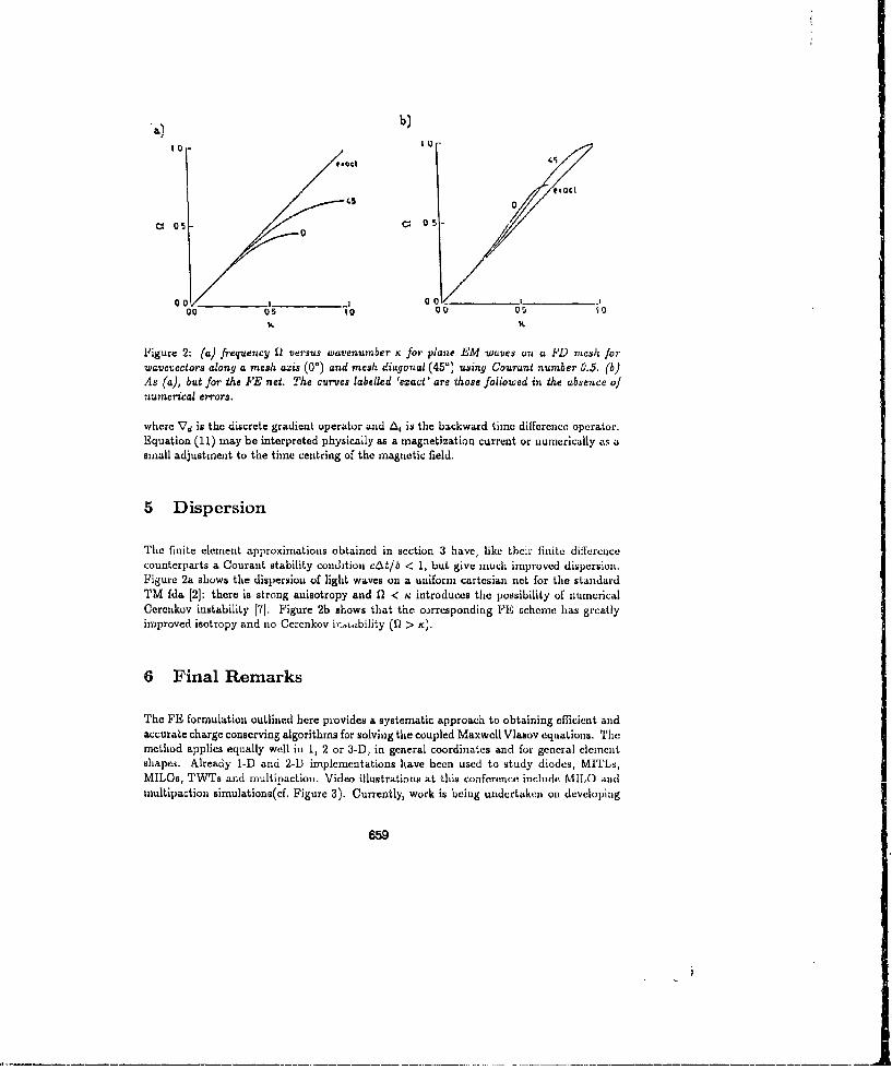
). b)10 1 U

tt~ac'

a 05 c 05-

00 05 000 05 to 1005 10

Figure 2: (a) frequency 12 versus wavenumber r for plane EMI waves on a PD r,•ct, forwavevectors alony a mesh axis (00) and mesh diagonal (45°) using Courant number 0.5. (b)As (a), but for the FE net. The curves labelled 'ezact' are those followed in the absence ofnumerical errors.

where Va is the discrete gradient operator and A, is the backward time difference operator.Equation (11) may be interpreted physically as a magnetization current or numerically as asmall adjustment to the time centring of the magnetic field.

5 Dispersion

The finite element approximations obtained in section 3 have, like their finite differencecounterpaxts a Courant stability condition cAt/6 < 1, but give much improved dispersion.Figure 2a shows the dispersion of light waves on a uniform cartesian net for the standardTM fda (2]: there is strong anisotropy and 11 < t& introduces the possibility of numericalCercnkov instability [7J. Figure 2b shows that the corresponding FE scheme has greatlyimproved isotropy and no Cercnkov ir.oLability (IQ > r).

6 Final Remarks

The FE formulation outlined here provides a systematic approach to obtaining efflicient andaccurate charge conuerving algorithms for solving the coupled Maxwell Vlasov equations. Themethod applies equally well in 1, 2 or 3-D1 in general coordinates and for general elementshapes. Already 1-1 and 2-1) implementations have been used to study diodes, MITLs,MILOs, TWTs and multipaction. Video illustrations at this conference include MILO andmultipaction simulations(cf. Figure 3). Currently, work is being undcrtaken on developing

659

a) b)

9im .00 ?%1 Time: 100 ns.~~~- . ... ...

Tinul Mg twO#il

Figure 3: (a) tlectron density scatter plots taken from the startup phase of the video ani-mations of a 6 cavity MILO device and (b) electron density and electric field vectors in amultipacting coazial transmission line.

3-D software and in studying the implementation of the VP method on parallel architecturemachines.

Reforencesi1] R. W. Hockney and J. W. Eastwood, "Computer Simulation using Particles", McGraw-

Hill (1980) (student edn. Adam-11ilger, 1988).[21 C. K. Birdsall and A. B. Langdon, "Plasma Physics via Computer Simulation", McGraw-

Hill (1985).

13) J. P. Boris, Proc. 4th conf. Num. Sire. Plasmas, (N.R.L., Washington, 1971), p3 .

{4] B. M. Marder, J. Comput. Phys. 68 (1987) 48.

[5] H. R. Lewis, Meth. Comp. Phys. 9 (1970) 0?7.

(6] H. Goldstein,"Glassical Mechanics", Addison-Wesley, (1950).

17) B. B. Godfrey, J. Comput. Phys. 15 (1974) 504.(8) J. W. Eastwood, "Virtual Particle Electromagnetic Pazticle-Mesh Algorithms", Culham

preprint CLM-P780 (1990), to appear Computer Phys. Cuai-nun.

66O

A New Magnetic Field Analysis For Dynamical ProblemInvolving Relative Displacement With Time

C. IAMAMURA. . (OKABE, T. OIIMURA and K. SATOMITSIIUBISIII ELECTRIC CO. MATERIALS & ELECTRONIC DEVICES LAB.

1-1-57, MIYASIIIMO, SAGAMIIIARA, KANAGAWA. 229 JAPAN

Oklotra__ct In order to understand the magnetic performance of therotating machines in more detail, a new analytical technique for simulatingthe device including moving parts is proposed. A concept named "supplementary region" being newly introduced allows these machines to beanalyzed by FRM taking the relative motion of a rotor into account. Thistechnique is now applied to an induction motor, and results in thatcalculated torque characteristic depends on the rotor position and that itsmean value is in good agreement with measured one. In this paper, the newconcept and the computational result are presented. The technique reportedhere is one of the promising technique to calculate the more interestingissue of the transient rotational motion of the rotor with eddy current

IntroductionThe magnetic field simulation techniques are one of the most efficient

means for understanding the detailed electromagnetic performance of manydevices. Amonp simulation techniques, a "inite element method (FHM) hasbeen widely used for the sake of its high applicability in the non-linearand the anisotropic characteristics of a magnetic material. lHowever. thereis few report on the application of the method to magnetic devices includingmoving electromagnetic parts (rotating machine, linear motor, magneticrecording system, and so forth ). because of the difficulty in generalizingthe modification of the mesh division at each time step. In the case of aninductlon motor that has a slip characteristic, the computed resultj arenot satisfied with the experimental if an analysis technique does not takethe rotor movement relative to the stator into account. Therefore, togeneralize the analysis technique based on the FEM for such a dynamicproblem is an important theme.

Several investigations on the analysis technique for the dynamicproblems have been presented In the litcrature. ` They can be roughlyclassified into a few methods. For the method using FEM, three techniquesare proposed as follows: ''" '• 7he first technique is to introduce themovement in the expression of the field equation. But it is not applied tothe rotating machines, because its reluctance is strongly dependent on theposition of the rotor, although this equation just holds in theapplications where the reluctance of the moving part does not vary duringthe movement. The second is the combined analysis technique with aboundary element method (BEM). (4' The technique can take any movement intoaccount. but it is pointed out that some problems are left to be solved interms of *the accuracy adjacent to the air gap and an increase In CPU timedue to non-symmetrical coefficient matrix. A local re-meshing is the thirdtechnique for this dynamic problem. it has the advantages uf taking a,,ymovement into consideration without 'ailing the symmetrical characteristicof the matrix. Bspecially a technique using a moving boundary is useful In

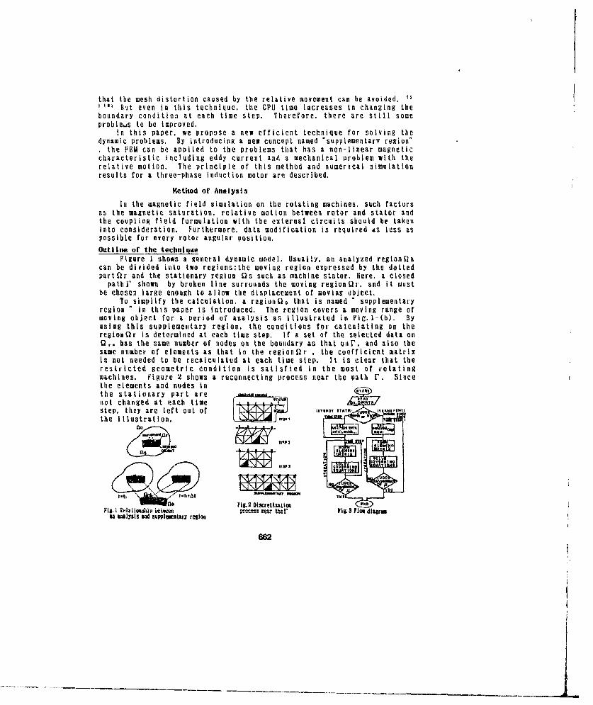
Ithat the mesh distortion caused by the relative movement can be avoided. "It" Bit even in this technique, the CPU time Increases in changing theboundary condition at each time step. Therefore, there are still someproblews to be improved.

In this paper, we propose a new efficient technique for solving thedynamic problems. By introducing a new concept named "supplementary region". the FiM can be applied to the problems that has a non-linear magneticcharacteristic including eddy current and a mechanical problem with therelative motion. The principle of this method and numerical simulationresults for a three-phase induction motor are described.

Method of Analysis

In the magnetic field simulation on the rotating machines. such factorsas the magnetic saturation, relative motion between rotor and stator andthe coupling field formulation with the external circuits should be takeninto consideration. Furthermore, data modification is required as less aspossible for every rotor angular position.Outline of the technique

Figure I shows a general dynamic model. Usually, an analyzed regionQacan be divided into two regions:the moving region expressed by the dottedpart Or and the stationary region Qs such as machine stator. Here, a closedpathr shown by broken line surrounds the moving region r, and it must

be chosen large enough to allow the displacement of moving object.To simplify the calculation, a region 0 that is named " supplementary

region " in this paper is introduced. The region covers a moving range ofmoving object for a period of analysis as illustrated in FiC.l-(b). Byusing this supplementary region, the conditions for calculating on theregionOr is determined at each time step. If a set of the selected data onQ0 . has the same number of nodes on the boundary as that onr. and also thesame number of elements as that in the region r , the coefficient matrixis not needed to be recalculated at each time step. It is clear that therestricted geometric condition Is satisfied in the most of rotatingmachines. Figure 2 shows a reconnecting process near the path F. Sincethe elements and nodes inthe stationary part arenot changed at each time *WTA

step, they are left out of 13TEADY ITAIE IVo IAHIEM

the illustration. rfilo4

P62

1 L N IMa II

an ig.2 OiuietizatioR MFig.! ileiihoanao~, btteu. p c musr~ei thel, Pit3 FIGm lacrauu awlylsi &Wd supviumItary regioni

662

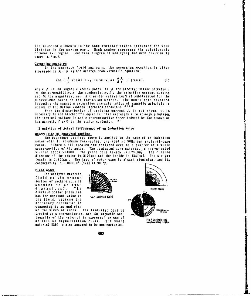
The selected elements in the supplementary region determine the meshdivision in the moving part. Each number expresses the relationshipbetween two region. The flow diagram of Modifying the mesh division isshown in Fig. 3.

Govcrning equationIn the magnetic field analysis, the governing equation is often

expressed by A- 0 method derived from Maxwell's equation.

rot ( -1-itA) - Jo 4rot M-o( a A grad@), (1)

where A is the magnetic vector potential, 0 the electric scalar potential.u the permeability, a the conductivity. Ja the exiciting current densityand M the magnetization. A time-derivative term is substituted for thediscreteme based on the variation method. The non-linear equationincluding the magnetic saturation characteristics of magnetic materials issolved by the Newton-Raphson iteration technique. '"J"'

When the distribution of exciting current J, is not known, it isnecessary to add Kirchhoff's equation, that expresses a relationship betweenthe terminal voltage Bc and electromagnetive force induced by the change ofthe magnetic fiux(D in the stator conductor. "I

Simulation of Actual Performance of an Induction MotorDescription or analyzed achine

The procedure outlined above is applied to the case of an inductionmotor with three-phase four--poles, operated at 50Hz and squirrel-cagerotor. Figure 4 illustrates the analyzed area on a quarter of a wholecross-section of the motor. The laminated core material is non-orientedsilicon steel 50A800. The gross core length is 175[mm] The outsidediameter of the stator is 210(mm] and the inside is 134[mm]. The air gaplength is 0.45[mml. The type of rotor cage is a cast aluminium, and itsconductivity is 2.88xi0' [s/mi at 20 '.

Field modelThe analyzed magnetic

field on the cross-section of machine core Isassumed to be tw o_-d im e ns ion alI. T he ,•,•URNKMelectric scalar potential h o,has the constant value in NOi4aiyze fieldthe field, because thesecondary conductor Isconnected to an end ringat the sides of rotor. The laminated core istreated as a non-conductor, and the mapnetic non- Room

Inearity of the material is expresseO by use of " ig5 Auy is anan initial magnetization curve. The shaft sppiestaryreionmaterial S35C is also assumed to be non-conductor.

663

An analyzing period Nir is the time required to be duplicate both themagnetic field and the analysis shape. If the stator has Ns slots, and theslip value and the Pole number is S and P. respectively, the followingrelationship in terms of the integral number N in the steady state issatif ied

N 2;rS 2 'y (2)P hi3-

where M is also a integral number.Motion of the rotor

In the rotating machine, either the stator or the rotor can be used asthe supplementary region. In the present model, the whole cross section ofthe rotor with the air gap are used as the supplementary region. Figure 5illustrated the regions.

Figure 1 shows the variation of magnetic flux distribution with timeand the enlarged element division near the gap on the periodic boundary lineat slip=0.05. The enlargedfigure indicates that the -mes h division of the rotorchanges in relation to therotor position at each time

uodes given the boundarycondition. The time requiredto generate the analysiscondition at every time step(18 steps) is 0.20[sec], thatincludes the time for an Fig.6 Vannic fluxdlstrlbution at Slip5%input of the initial data.( (a) wtO *bW cnt-o' (C) W -t.i12The computer used IBM 3090.)

Torque characterisletFor calculating the electromagnetic force or torque. Maxwell's stress

method are commonly used. However, it has been known that the method has adisadvantage that the calculated value often depends on the selectedsurface. '"I So in this paper. the value per unit meter T is calculated asthe change in magnetic flux 0 multiplied by the eddy current le '''

T -=le u • Ale00~ = - . (A-+ grad A)ds (3)a t 00

where 0 is a rotational angle.To find the magnetic flux difference term in eq.(3). use the formula:

a061 A 0(+ Os )-A(O- Os )00 20s

where 9s is in angle between two slots of the rotor.Figure 7 shows the computed result of the torque T at slipOU.Ub. it is

664

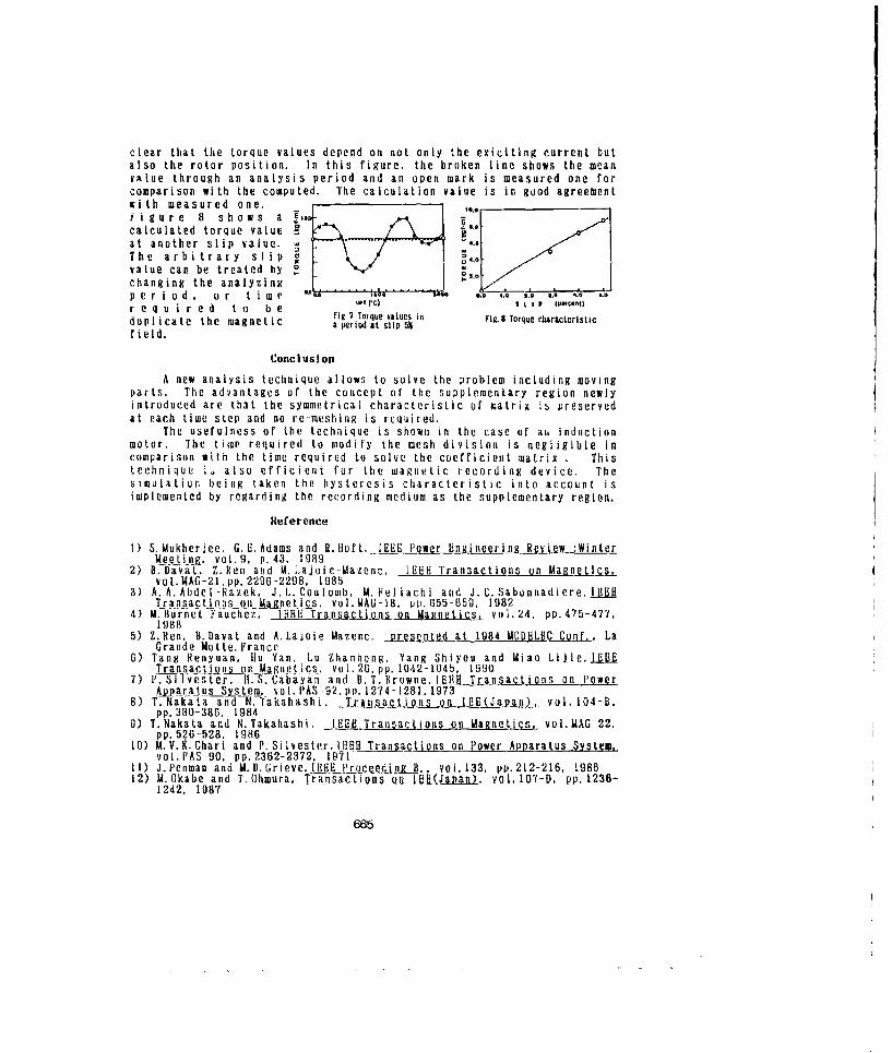
clear that the torque values depend on not only the exiciting current butalso the rotor position. In this figure, the brnken line shows the meanvalue through an analysis period and an open mark is measured one forcomparison with the computed. The calculation value is in good agreementwith measured one.F ig ur e 8 s hoaws a r1

calculated torque value Mat another slip value. -The arbitrary slip i.value can be treated by ,changing the analyzingp e r i o d. o r tim e .. , 1.,9.9, ', eA 6. 9r e qu ir ed t o b e W t c) .. 9Ucent)Fig. 7 Torque values in FI9.8 Torque elaracteristicduplicate the magnetic a period atslp5field.

Conclusion

A new analysis technique allows to solve the problem including movingparts. The advantages of the concept of the supplementary region newlyintroduced are that the symmetrical characteristic of matrix is preservedat each time step and no re-meshing is required.

The usefulness of the technique is shown in the case of am inductionmotor. The t ime required to modify the mesh division is negligible incomparison with the time required to solve the coefficient matrix . Thistechnique i. also efficient for the magnetic recording device. Thesimulation being taken the hysteresis characteristic into account isimplemented by regarding the recording medium as the supplementary region.

Reference

1) S. Mukherjee. G. E. Adams and R. lloft. IEHE Power EngineeriniRVS_ ie :WinterMeetiing. voL.9, p.43. 1989

2) B. Davat. Z.Ren and M. Lajoic-Mazenc, IEEE Transactions on MagnetL.QLvol.MAG-21,pp.2296-2298. 1085

3) A.A. Abdel-Razek, J.L..Coulomb, U.FPeliachi and J.C. Sabonnadiere.JjjTran sactins on 4"-netji&s, voI.MAG-18, pp.655- 659. 1982

4) M. Burnet 'Fauchez, I1M1 Transactions on Magnetics, vol.24, pp.475-477,1988

5) Z.Ren, B.Davat and A.Lajoie Mazenc, .pe•ented at 1984 MODBLEC Conf., LaGrande Motte, France

6) Tang Renyuan. Ilu Yan, Lu Zhanhung. Yang Shiyou and Mino Lijie.1tIEITransactions on Magnetics. vol.2b.pp. 1042-1045, 1990

7) P.Silvi ster, II.S. Cabayan and B.T. Browne. l131. Transactions on PowerAltpaLatu1 L.. tem. vol. PAS-92, Pp. 1274-1281.1973

8) T.Nakata and NN•Yakahashi, Tranjsa.j.gns on IEE(Japail vol. 104-B.pp. 380-386. 1984

0) T.Nakata and N.Takahashi, [EE8L Transactions on Magnetiq_•. vol.MAG 22,pp.526-528, 1986

10) M.V.K. Chari and P. Silvester. 1116 Transaij~ons on PoweL.Apparatus•System.vol.PAS-90, pp.2362-2372. 1171

11) J.Penman and M.D.Grieve. IEEE Proceedini . . vol.133, pp.212-216, 198612) M. Okabe and T. Ohmura. Transactions oO IJU(jjnan). vol. 107-D, pp. 1236-

1242. 1987

665

A Time Domain Approach to Calculating Radar Cross Sections

D. W. Harmony and G. R. SainBDM International, Inc.

Albuquerque, NM

The potentially large benefits of using finite difference techniques to calculate theradar cross section of complex, composite targets will be discussed. Finite differencingin the time domain will be used to calculate the near fields scattered from a perfectlyconducting cube and a solid dielectric cube. A broadband, short duration, pie tic wavepulse will be used as the excitation. The scattered near fields will be trrnsformed to thefar field and then Fourier transformed to calculate the radar cross section as a functionof frequency. Numerically generated results for the perfectly conductirng -nse will becompared to measured data. In addition, a short discussion on the nur I. benefitsand limitations of the approach will be presented.

666

A)

A 2--D Finite-Volume Time-Dowain Techniquefor ROS Evaluation

byRichard Holland, Vaughn 1'. Cable slid Louis Wilson

ABSTRACT

T1his paper describes and tests a method for computing electromagnetic scattering from 2-D metallicbodies using a generalization of the FDTD Yee algorithm, inl which a nonorthogonal piecewiselinear con-forming ineslk may be applied. Resultis for 2-1) TE and TM scattering from a shorted s-curved parallel plateregion, ank: from a 2-D circu~lar ojive are presented. In both came, solutions were obtained usin~g a structuredquadrilateral mesh. A inethod for obtaining scattering by a circular cylinder using the same basic finite--volume formulation with a fully structured mesh is also discussed. The circular cylinder, while seeminglysimple, is actually a stressing case or thle meshing algorithmn which stretches a cartesian grid to lit a curvedgeomietry.

Thc primary goal of thisu work is to model oblique or curved surfaces in the tiiiie-domaiii withoutstaircusing. Examiples arc presented for edge-on TIE illumination of an ojive which demonsitrate that 120culls/A are requircd for I 1 d .ýccuracy when staircasing is used, but only 15 cells/A are needed with conformalmeshing. The coiifornia!-misl model of the curved parallel plate regioil accurately predictb the first 1(1depth resonances and thle first 2 width resonances for 'lE illumirination directly into the aperture. Also, 'TMscattering from tike curved parallel plate model retains some fidelity with as few as 4 cells/A, while staircasediiiodela require At least 20 rcllv/A.

INTRODUCTION

Thle miajority of published work oil riiodeling curved surfaces in time domain calculations has been bydesere~tizing tile curvature into stairsteps, where each step correaiponds to a cartesian cell in tile Yee FDTDalgorithm [I]. 'Th inadequacies of this approachi have been well documented E21 &aid work toward lixingthis probileim isl progressing in a number of directions. These include; tile expression of Yee's algorithm inicurvilinear coordinates [3,41; tile selective application of Ampere aiid Faraday contour integration to "sliced"Yee cells [5); aild the generalized oblique-cell rendition of Yee's algorithnm [1S,71. Tile examples and workIdreseiited iii this, paper are anl extensloim of the latter approach; thle Yee dual1-anesh algorithmn is rewritten fora 2-dimms'nsional quadrilateral mesh with full corrections for oblique cells.

Time algorithm hasl previously beeii tested on problems of scattering by a 2-1) circular cylinrlerusingall unstructured mesh [2j. In this paper, the algorithiim is tested usling a structured mesh oii a shorted, s-shaped. pairallel place region, said a 2-1) circular ojive. All omf these objects were iiodeledi asl perfct electricalcomidmictors (l'ICC).

Thme elfectivemieas of thle meothod is denmoinitrated by the reduction inl mesh density from thle staircamedmiithmod necessary for a given accuracy. tor 'IE scattering by thle 1'EC ojive, the structured niesl required15 cells/A to achieve I dBi accuracy using time oblique cells, whereas, up to 120 cells/A were needed whenstaircasing, was used. For thle s-curved parallel plate mnodel, sonie resonancesi were predicted with as few as4 cella/A, while thme mtaircaserl model required at least 2U cells/A to achieve tile samne fidelity.

2-D FINITE VOLUME TIME -DOMAIN (FVTD) EQUATIONS

Th(- following equations are a 2-dimensional inmpleimentation of tile F1VTI) imethod iii a structuredquadrilateral iniesh. Vigure 1 illuutratemm the meshl-cotordinate relatiomntilipg waged; e.g., SP, are primary cell

liidhad hlollsmmd is &a 1625 Itunmm NI~, Albsq.akecut, NM 87106,Vamighmi, 1. Cable and 1-i.~ Wmis,,m see wi~l., Loeihesd Adaa-ce D-edopninr Company, 8.x 551, Mw~bam". CA P1520.

667

kkkkkkkkk k

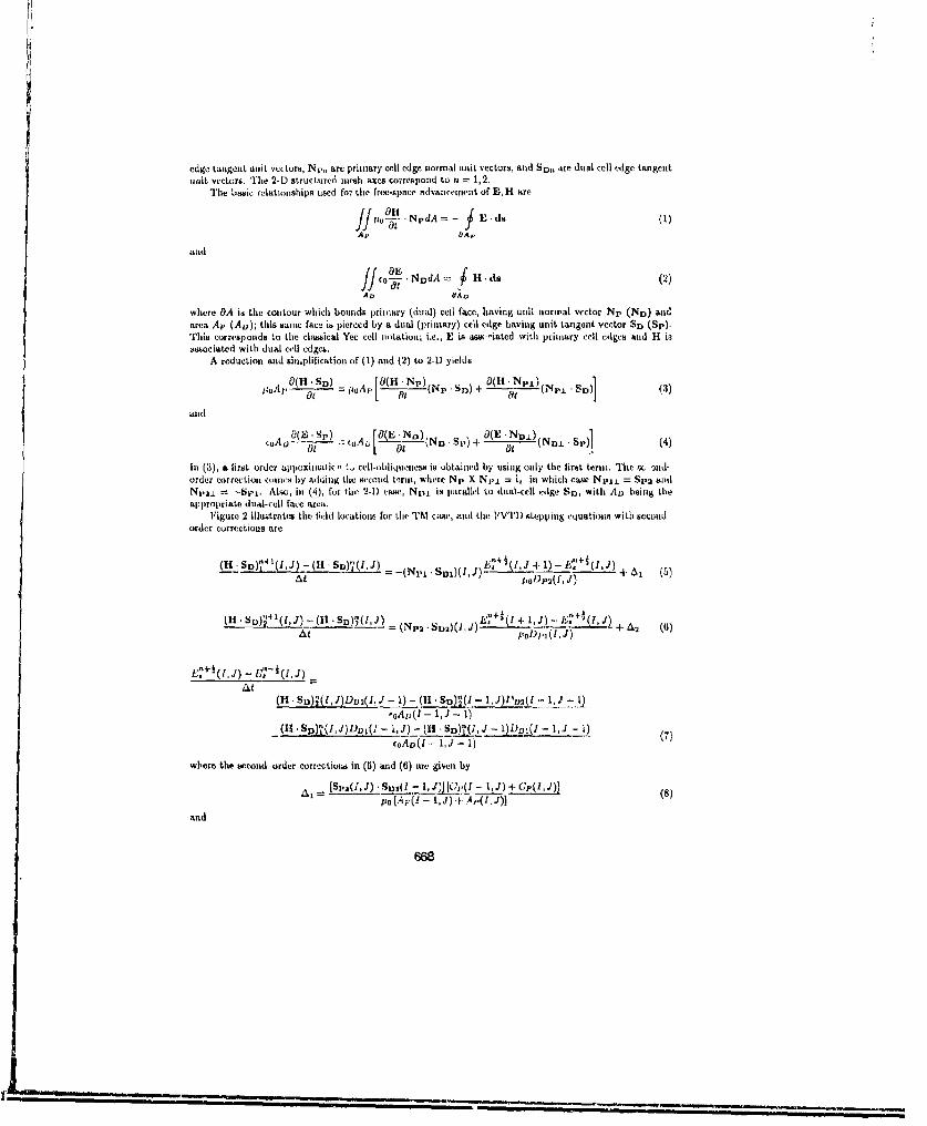
edge tangent unit vectors, Np,, are primary cell edge normal unit vectors, and SD,, are dual cell edge tangentunit vectors. The 2-D structured mesh axes correspond to n = 1,2.

"The basic relationships used for the free-space ailvancement of E, H are

Jif 110 NpdAr fE ds()A, OAp

andDE

fJ Fo -NddA -" H- d. (2)AD OAo

where OA is the contour which bounds primary (dual) cell face, having unit nornal vector Np (ND) andarea Ap (Au); this samte face is pierced by a dual (primary) cell edge having unit tangent vector SD) (Sp).This corresponds to the clamical Yee cell notatioin; i.e., E is ais-iated with primary cell Adges and H isassociated with dual cell edges.

A reduction and sinplification of (1) and (2) to 2-1) yields

oAp SD) = poA/, [(H.Np)(NI, Sr) + -Np'I'"(Np.. -SD) (3)

aild

O -- A_ ,u n (ND. St.) I "(E ND ,)n •p.l (4)(A j --- ' a) N( D L - p

In (3), a lirst order appoxiiutali, '- cll-obliquenes" is ,jbtained by using only the first term. The &C -wid-order correction cumes by adding the second term, where Np X Npj. = i, in which case Ni-I.L = Sp-2 andN .= S'= . Also, in (,4), fur the 2-1) :aw,, Nr1j is parallel to duai-cell edge SD, with Ao being theappropriate dual-cell face area.

Figure 2 illustrotes the field locations for the TM cas!e, and the IVTI) stepping equatioms with swcond-order corrections are

H-SD)"4 1 (1 jI ,,-(H SD)' (I, J) . -(NII SDI)(I,J)!- ' (l÷J + 1 (" ) -- a E6 (5)At sJDp•O(f, J)

=~~~ ~ (.p SDA)l (J) J)~ .~s(H tl 7A-(t o)(,J (N p,2 -Stu2)(J, J) 1•'"+ (I +• r (, J)-. 6+A ()

At___-(I,1J)__

At

- (_H , S D )•'j , d ) D D I , 1, J) - (H .- S )) I( I , J - 1) D D I(I - 1, d 1 ) ( 7)cOAV(I - l, J - 1)

where the second-order curiectioud in (5) and (6) are given by

A= [SpA(I, J). San(I - 1, J)] [C(](1 - 1, J) + Gp(U, )A (8)po [.Ap(! - 1. J) + A•(r, J)]

and

668

=spi(s,J). Si.(j, - 1)j[Cp(1,J - 1)+Cp(fl,J)jt lAp(l, J - 1) + Ap(l, J)]

In (8), Cp(l - 1,.J) is thie contour integral of E,(Sp2,(i,J)di + Svj(1,J)dy) on the face boundary ofprimary-cell (I- 1, J) having face area Ap(I- 1, J); Cp(I, J) is the contour integral on the face boundaryof primary-cell (1, J) having face area Ap(I, J); and Sp,3 and Sp2, are the x-y components of unit vectorSp2. The C1,(f - 1, J) contour integration is given by

C(- 1,J) =[s2.(], J)(e.(t, J) - PU(- 1. J)) + SP 2 (, J)(PY5 (, J) -- PI,(f - l, J))][E,(1,J) + ",(1- ,j)]

24- [SP2.(I. J)(P.(I, J -I- 1) - 11.(1, J)) + Sj-2V(l, J)(PY(I, J + 1) - Pe(l, Jf)]

,[E,.(I, J + + kL2

+ [SP2.(I,J)(J (I - 1,J + 1)- P (1',J + 1)) -.SP2V(I,J)(P.(t - 1,J + I)- PV(1 ', + 1))][E,(I - 1,J +.1) + Id(t,J + 1)]

2+ [Sp.(1,J)(P.(U - 1,J) - P.(t - 1,J + 1)) d- s*3(I. J)(PV(I - l, J) - PW - 1, J + t))]

{EV( - 1,.) + E.(Y- 1,J + 1)]2 '10)

and Cj,(I, J) is obtained iii a similar manner. fHere, Pf(l, J) and 11 (I, J) are the x-y coordinates of theprinmary cell corners. This is also the location where E,(I, J) is calculated. Similarly, the explicit terms in(Ui) are based on adjacent primary cells (I, J) and (I, J - 1) with conniion-edge unit vector SpI(, J) (s•eFign. 1 and 2), and Cp(l,J - 1) and Gv(I,(J) are obtained from a procedure similar to (10).

The above expressions assume the aecond -order corrections to (H • SU), and (11 , SD)2 are uniformn overAp(1 - 1, J), Ap(I, J) and Ap(!, J - 1), and that E,• varies linearly around face edges which bound areasApj(- 1, J), At (1, J) and Ap(1, J - 1). Note, primlary cell (I, J) is common to both correction calculations.

Finally, the second order TE equations are obtained in a similarly complex, but straightforward mannerI8].

2-D NUMERICAL RESULTS

In order to test the formulation documented here, calculations were mtade on a 2-D numerical spacecoasisting of approximately 6600 cells and used approxunately 2000 time steps in each case. These tinie-doinain results were then transformed into the frequency domain, and then into the far- field. In all cams, atinie-differentiated, plane wave, Gaussian pulse was used to illuminate the obstacle.

In the first application, the paiallcl-plate legion was illuminated with the TIE mode with ko along the i.direction (i.e., •b•'l" - 0). In this came, the parallel-plate region supports TEM propagation. The scatteringcros section, o(w), was comnpi•d using each of the ner.w -to-far-field integration contours of Fig. 3; theinner-loop is adjacent to the ciaved plates and the ou.,jr-loop is purposely placed outside the region ofnonorthogonal meshing. A compa iaon of the two results determnined the fidelity of electromagnetic wavespropagated across the nonorthogonal mesh. Overlaid curves of or(w) for both integration contours appear inFig. 4, and the agreement is seen to be very good, at least up to 600 MIte.

The nominal size of the mesh cells used in this case is -L meter along each edge, which at 600 MIlscorresponds to 8 cells per wavelength. We can conclude that the nonorthogonal nmesh with the second-order correction to the FVTD equations propagates electromagnetic simulation possibly even better thanmtime original orthogonal Yee scheme. This curious risult was also noticed by Madsen and Ziolkowski [9].

The resonances at which the paraltel-plate region is 4, A ... I deep are clearly visible in Fig. 4, as44 4are the very sharp resonances at which it is A and ) wide. These transverse resonances imply that cross

669

coupling lasa recured betweeln thle origiind 'EM mrode and a prarallel plate waveguide inode in tile curvedre-gion, eo. cs ti rpgtn oe

V1 i Vig. 5 compares a(w) for the TM case, as evaluated oin tile samie two integration contours. Agieemnentis again better than Idfl at virtually all frequenciesi below 0110 Mile. For the TM case, the parallel plateregion will not "mo~port 'rEM propagationi, thus thle TM results are free, of resonant behavior until thle parallelregion isat least 2ý wide, where the first TE0 . waveguide mode canl propagate. Fig. 5 clearly shows thle first

Additionally, scattering in tile TM case was coiripiited for illumndation from above (0" -90')and below (0i"' = 4-00'). Results for the inner and outer integration contours appear in Figs. 6 and 7.IthsonanCeS principally occur where the conducting plate path is -n7I around (duct is -nTi lung). Note,thle 1 F90' case involvesi electrolnnapietic piropagation across '20 cells which are 8 erina lon atwOM liz.

Calculation" for sicattering by anl ojivi-cylindee 10 meters long and 1 meter thick at the midpoint havealso becii pe'rform~ed using the second order formoulationm. Figure 8 shows thle overall conformmal meshl withinner anid outer integration contours, and Fig. 9 illustir'tes the details near tile left tip of the ojive. Resultsfor edge-oii T'I scattering appear in Fig. 10. Results from a atairrased analysis of this 'IF configuration,the dotted enrve, becomte disastrus at thle point which corresponids to 120 staireased cells/A. Conformaolcells for the Fy11.) model, are about 8 centinmeters onl a sidn (9.3 cells per wavelength at 401.1 Mile), and goodagrevimnvt is seeni using inner and outer loop near--to -far field transeformation contours at frequeocies up to250 M~lz (15 cells per wavelength) for tile TE case. The TM edge--on results in Fig. 11 deteriorate at aslightly lower frequency. Note, Fig. 11 slows considerably more amplitude (dU) resolution thas, Fig. 10.

CONCLUSIONS AND RECOMMENDATIONS

*1I'( Imurpome of thisW work is to validate thme FVTI) approach in 2-11, .and thues, to reduce thle risksi beforeproceedinig with thme truly mumnunimmtal task of developing a 3-.1) LFy'11) algorithini. Il'he results presented hierelindicate that thle l-'VTD' approach is well suited to mmodelinmg curved surfaces arid the payoff for its extensionto 3-1U is, theetfore, likely he worth the effort. As a closing note, thle FYTO approach is still imot expectedto ease the fundamental problem of turning ;% physical probmlemi space imito a successful solution mesoh, andsignmilikumt work in this area is continuing.

REFERENCES

[1) K. S. Yee, 'Nuimveiral solution of initial boundary value pIoblenis in ibotropjic miedia," IkET 11ramis.Antennas Prupagmf.,vol. AI'-14,1,1v* 302 -310, May 1060.

[23 It. Ilolland, "Tile ease agaimnst stuiressing," Conference Procee-dings, (Iti Anmual Rteview of Progress iiiApplied Comnimitatiomial Eletromnimgnetics, Monterey, CA, lip. 80 05, 1tl-22 .,arch 1U900

(31] It. Hlollanid, "IFimite-differemmce solutions of Maxwell's equations in generasli-ed nonoirtlaogonal coordi-mAtbis," IEEE' 'IThans. PNuc. Sci., vol. NS- 3U, pp. 4580-4591, Dec. 1983.

[4) M. Fumico, "Ft)TI algorithma in curvilinear coordinates," WEkE '11raim. Arite..as l'ropagmmt., vol. A P-3d8,p1'. 70 -80, Jan. 1090.

5.1 A, Talluve and K. Umnashankar, "The finite--differenee timne-donman (I'D 1'11) method fur numnereicalmudeling of electromagnetic scatterinmg," IEEEk 'llans. Magnetics, vol. M-25, pp. 3086-3000, Jul. 1981)..

[61] N. K. Madsen slnd R. W. 'Zinlluiwski, "A mnodilled finite-voluose technique for Maxwell's Equations,"Lawrence Liverninore National Laboratory, 00Kb -98405, 26. Feb. 1988

[71 It. Holland and K. S. Cho, "Itadar cross-section evaluation of arbitrary cylinders," Applied PhysicslIne., AlPI--TIK -120, Albuquerque, NM, 12 Sept. 1906.

[8) It. Holland, V. 1P. Cable, anid L. Wilson, "IICS calculation by finite-volunmoe tilimeý-dunimmimi (FV'tl))techniques', Lockheed Aeronautical Systemis Co., Itieport # LG-110E10131 , Nov 19W0.

[9) N. K. Madsen and It. W. Ziolkowski, "A 31) nmodified finite--volume technique for Mmxwell's equations,"kflcutromnagmmetics, vol. 10, pp. 147-161, Jami. 190,0

670

I:W

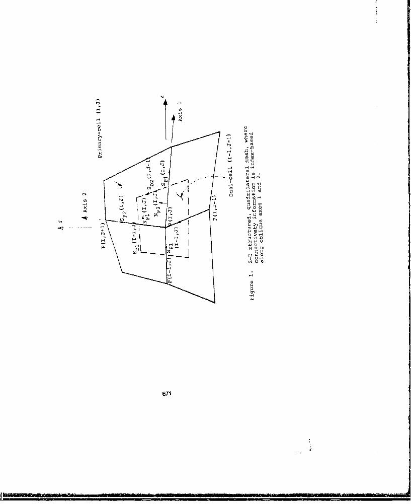
Hý

C: w

ý4iL) w a

U, C 3

C11 1 % 1 4671

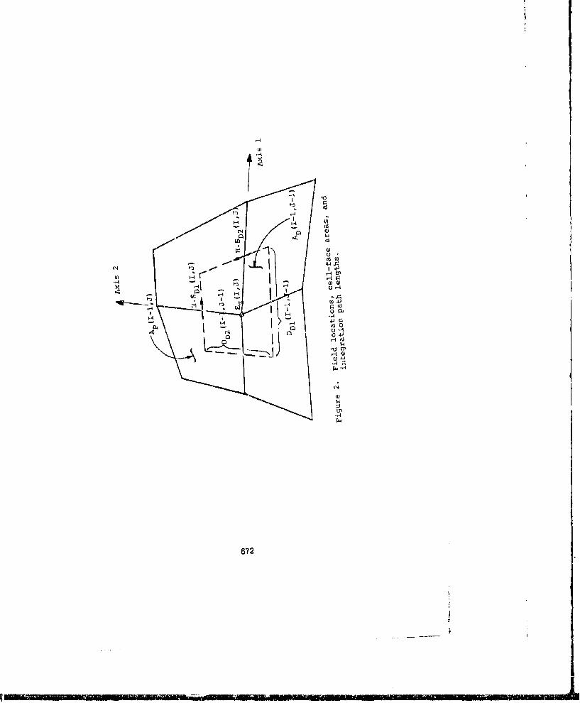
U)

410

t.

"44

0 to00

..4 A

414to

4.4to"-4

6lu2

. ~ ~ ~ I .4. . ...

V c

r0

h ~ ~~ 41J f N '1o'9(NJ~ ~~~ 14 ~

__7 0

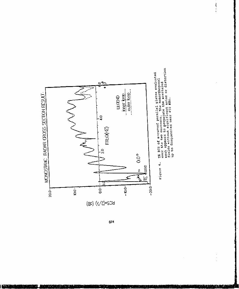
-0G~4A

~.4 0.-4 v~jU

Im o-

41 0 ()

Li- 0s-0,)0 a) 0

Cr)(a U

C)) 5-100

o oI0 (o5 0 a)

Cr))Cz 0

0w ut4>(1 )

E- 0 44.

6744

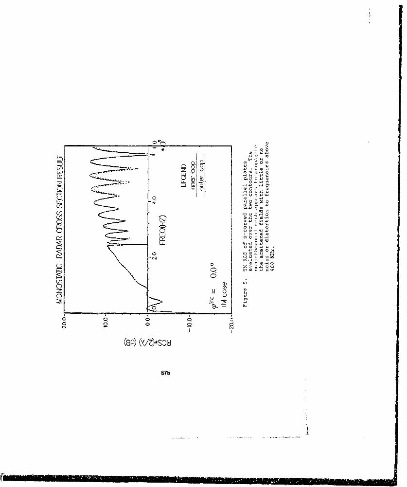
Q)

01 0~ 0

a) [- 0 (1)LU C (0 ~LA0-4 U4J 9

041 .-4 bj

r0 I4 -i 1.4

LU.4 - 0 Q0 5 0

> 4.1 a) *'A 4.1

W 44

L0 > ni . U O

z~ 2)0L 0b a)0

0q 6) 0 0P

0 6l0 l().1I

675C ) -

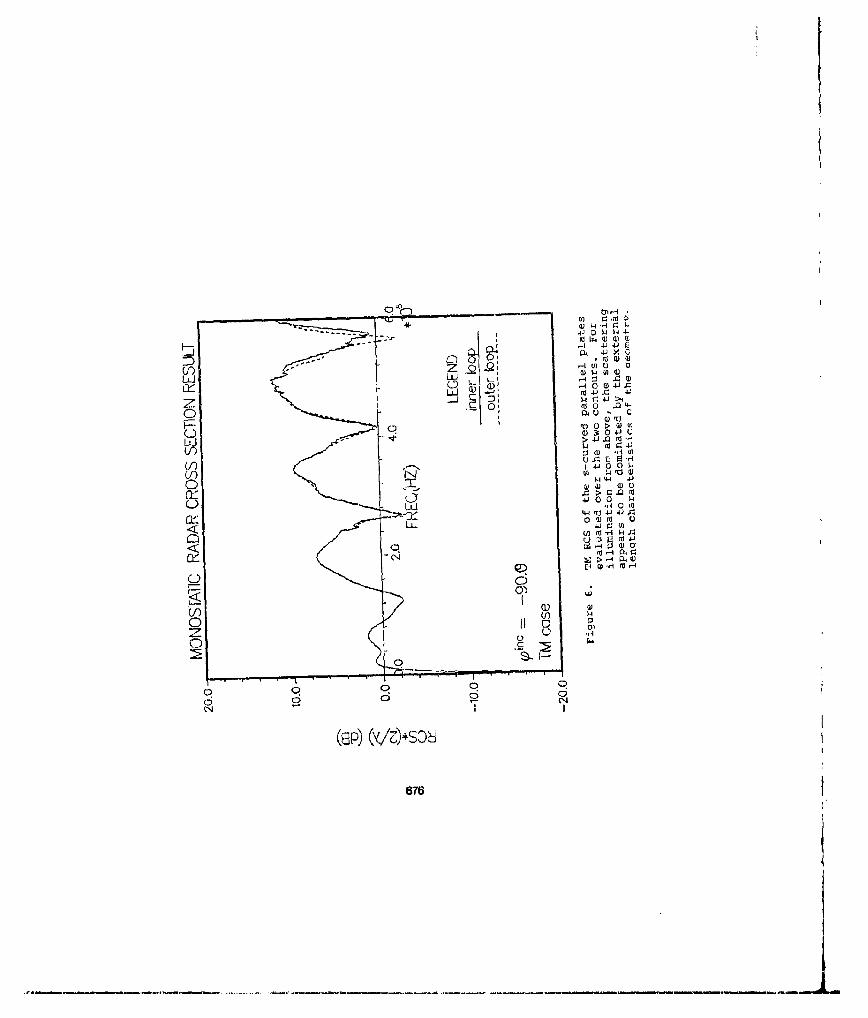
...... 4J0 P 14

- (a ( w 0i

u~r) zo24 r(U) u(U p w

0 4j C

V) a) 0> W o

'I) $ 4 i0 s *.-(I0 0

4I) N 0 ýdW

0) a) o Q

LU.) Ur

00(IE4

0J (nr4

zap "-I/)*a

676

4"J 4d r

LlI--------------- 0o) ... Jo-4 P )

00 fd. 0 tH 0

00

C)-------

94 a

(8P) (4/0)Vs 4cr- Cf (3) H 677

< LL- .0 a

.............. _ _ _ _ _ _ _ _ _ .. .. .. .. . . ...... L.... . .... ......... .. . ....

.... ... .... ... ..... 0...... ~~~ ~ ~ ~ ~ ~ .............. .. .....~ ~ ~ ~ ~ ~ ~ -- ............. . ... . .. ..

U)

- 0*

-o 7

-H04J

-cr0 LU H

LULL 0--I

LL- C

10 (d

Lij ..... I

... .. H ~440.I

711 J. Z

:T ..... ... 0'21 ý i-mm IT IT ....... M2 a f a

::1M -112 m:I TM X I IM

678

S I 0

I 0* U)

*LAD

If II )

* 670

,4

Il;" A

___ __ __0_0 -1 wS -4 >

.. CO-- --- E WnEI

•~~~~ 1 "w Z ,....:._," ' (fl... uf

rU -4 -HJ

, :..... ________-. _ °E V

--- - .. .. --- ........... 0 0 u0

0 ---. 0•

(I 0 .

_____ _____ _____ W 0

"II. 4 I ___I_____I ____7 W q) 4J

!U) oo E

-T- d afu

C o ('D (d4 0 E.

u} .......... :H ,),s V

....~~~ ...... .... .. ..... . . . . ... . . . . . . .

.0 o. .

-- -- i 40

(J :V V4(WP 0y1 a)*sod

680

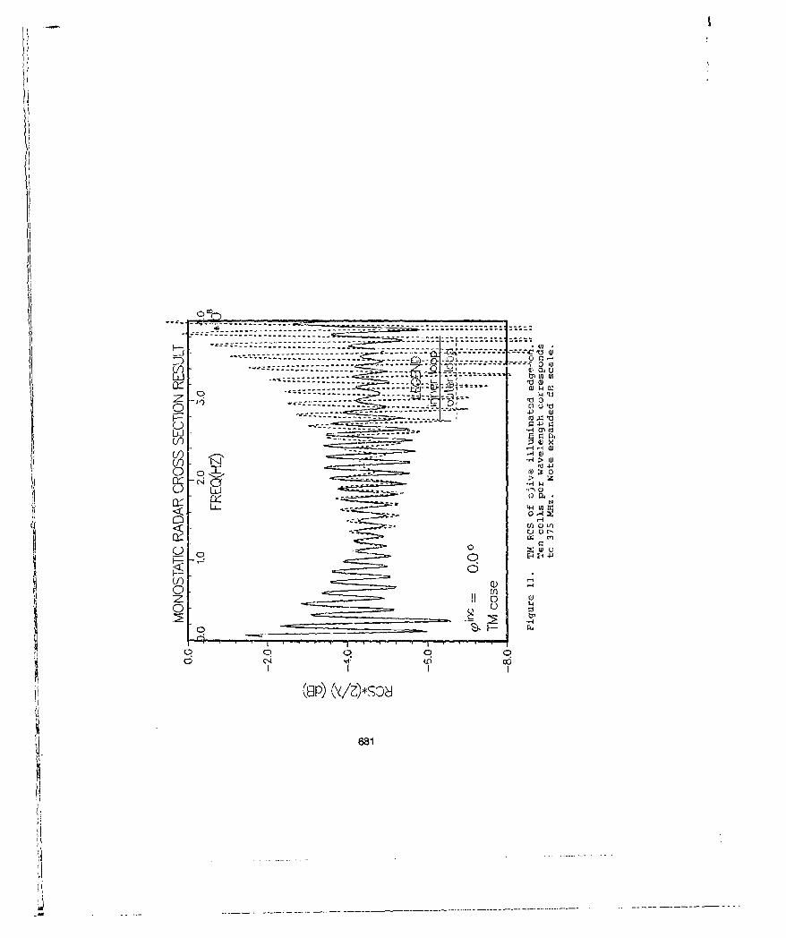
" ' -"4- , - - oi

H-. .. . . .. . . .. .- .. .•'r-.-%• --- . . . J

IH~l

S,--- --- - - - -

,•- .4-

o

-•' 0 td

o~~~ý 0 -,,6 4 14L

o r-

004-

a)) Q) H

zz0 1

0* 0IH 4

681

RCS CalcuLationfor Smooth Bodies of Revolution

using FDTD

by

R. Luebbers, D. Stelch, K. Kunz, and F. HunsbergerElectrical and Computer Engineering Dept.

The Pennsylvania State UniversityUniversity Park, PA 16802

Tel (814) 865-2362Fax (814) 865-7065

Abstract

The objective of the research reported here was to determineif FDTD, using cubical cells, could be applied successfully tocomputation of RCS for smooth bodies of revolution composed oflousy dielectric materials. The bodies considered were a sphere,an oblate spheroid, and a sphere-cone-oblate upheroid. Theseshapes were chosen to provide a challenge to the FDTD method, andalso because results computed using other methods were availablefor comparison. These shapes were modeled in three dimensionsusing cubical cells, and RCS calculations were made by Fouriertransform of the far zone timu domain scattered fields computedby VDTD.

The results were compared with the Mie series for the sphere, andwith T-matrix results for the other objects. The agreement wasquite good, indicating that, at least for the examplesconsidered, the VDTD method with cubical cells producedsatisfactory RCS results for smooth bodies of revolution.

introduction

The Finite Difference Time Domain (FDTD) method has seenincreasing application in the prediction of Radar Cross Section(RCS) of targets with a wide variety of shapes and materialcomposition. While good results have been reported for simpletargets, such as perfectly conducting flat plates [1],difficulties with targets which include smooth surfaces have beenreported, especially whsn these are modeled using cubicalcomputational cells. This "staircase" effect can be a seriousproblem in calculating low level RCS from some targets, andconsiderable effort iR currently be expended in solving thisproblem [2-4].

682

-m! ------- - - - - - - - - - - - - - - - - - - - - - - - - -- - - - - - - - -. . ... . . ..... ..... .....

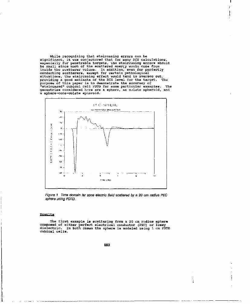
While recognizing that staircasing errors can besignificant, it was conjectured that for many RCS calculations,especially for penetrable targets, the staircasing errors shouldbe small since much of the scattered enercy woul1 come frominside the scatterer volume. In addition, even for perfectlyconducting scatterers, except for certain pathologicalsituations, the staircasing effect would tend to averaqe out,providing a good estimate of the RCS level for the target. Thupurpose of this paper is to demonstrate the accuracy of"stairoaased" cubical cell FDTD for some particular examples. Thegeometries considered hore are a sphere, an obilate spheroid, anda sphere-cone-oblate sphoroid.

1U-PUI AI K 1, ILU

1u

U -

Nt - IU

. ,,

U; b

0l d N ILI

71MA LNb)

Figure 1 Time domain !ar zone electric field scatiered by a 20 cm radius PECsphere using FDTD.

The first example is scattering from a 20 cm radius spharecomposed of either perfect electrical conductor (PE(:) or lossydielectric. In both cases the sphere is modeled using I cm FDTDcubical cells.

683

Figure I shows the FDTD computation of the far zone timedomain scattered electric field from the PEC sphere. The 1/Rdependence (where R is measured from the sphere center) of thefar zone fields is suppressed. There is an initial (negative)scattered pulse as the incident pulse strikes the front surfaceo0 the sphere, (positiva) scattered energy from tha curved spheresurface, and then a final (negative) pulse due to creeping wavestraveling around the sphere. This far zone wide bandwidth timedomain result was obtained using the approach described in (1).

P'LC 1IEECU-VULAPIZI.U UALk!AAI iLH

5U

U U 4 U1 H ~ I 4 d

I I 1JULNIJ. LWIIl

- UAII -LI

Figure 2 Back scatter cross section of 20 cm radius PEC sphere computed usingFDTrD compared with the exact soiution.

Figur4 2 shows the FDTD radar cross &naction of the sphere(determined by taking the Fourier transform of the time domainresult in Figure 1 and dividing by the Fourier transform of theincident pulse) compared with the exact solution. The agreementis excellent at low frequencies, and even at higher frequenciesitracks the exact solution reasonably well. More accurate resultscould be obtained by using mare cells to modal the sphere, or byutilizing conformal meshing techniques to reduce the stmircasingerror [2--4].

While the focus of this paper is PDTD scatteringcalculations from bodies of revolution, the next example also

6B4

__ ______

II

Lu "• L)H I lOAM

, 04 U •a , *-1* 4

Figure 3 Imagi part of complex permlttivlty of 0.25 dB fownabsorber showing actual dJisperslve variation and usual FDTDapproximation taking value a t 1.5 GI-lz.

6a IJL I)AM

Figure 4 Imaglnwy/ part 01 complex permittivity of 0.26 dBfoam absorber showing actual dispersive variation and usualFDTD approxlmatlon taking value at 1.5 GHz.

685

_- I-- - - -

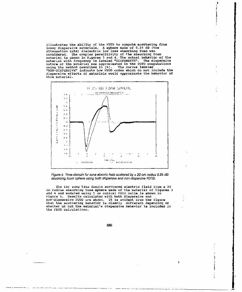
N

illustrates the ability of the FDTD to compute scattering fromloasy dispersive materials. A sphere made of 0.25 dB (theattenuation rate) dielectric low loss absorbing foam wasconsidered. The complex permittivity of the absorbing foammaterial is shown in Figures 3 and 4. The actual behavior of thematerial with frequency is labeled "DISPERSIVE". The dispersivenature of the material was approximated in the FDTD computationsusing the method described in [5). The curves labeled"NON-DISPERSIVE" indicate how FDTD codes which do not include thedispersive effects of materials would approximate the behavior ofthis material.

HI ;'., JL; I CAM tLJSPHLIHLttl U•IIA lI .L • I.. ]I [14

II

U4

1 0 . 0-

*, II h

iai, i "u I I .c b i l ' . s oII .' ,t Ii II (

Figure S Time domain far zone eiactrlc field scattered by a 20 cm r~dtus 0.25 dfiabsorbing foaim sphere using both dispersive and non-dispersive FDTD.

The far zune time domain scattered electric field from a 20cm radius absorbing roam sphere made of the material of Figures 3anld 4 and modeled using 1 cm cubical FDTD cells is shown inFigure 5. Rasults calculated with both dispersive andnon-dispersive Y,2DT are shown. It is evident from the figurethat the scattering behavior is clearly different depending onwhether or not the material's dispersive behavior is included inthe UDTO calculations.

686

A

I0.25 DO FOAM SPHEREL

CO-POLAW'.L0 3jACK5CV1TLP

0.o - -- - ---

.10-

-20

-40

-7U13

-UM4 U- W IJ - -4" -

-- 6AALI I I 'LIb I VL W) 1)*1 I ',1 'l. 1 Vi

Figure 6 Back scatter cross secton of 20 cm radius 0.26 dB low loss dielectricfoam sphere computed usng both dispersive and non-dkipersive FDID comparedwith the exact solution.

Figure 6 compares the two FDTD cross sections (obtained fromFourier transforms of the data in Figure 5) with the exactsolution (which is for the actual dispersive material).Considering the "DISPERSIVE" FDTD calculation, the improvement inaccuracy relative to the PEC data of Figure 2 can be seen. Theexplanation for this is that a significant portion the scatteredenergy is coming from the interior of the sphere, so that "staircase" errors in modeling the surface do not introduce as great anerror as for the PEC sphere where all of the currents are on thesphere surface.

Note also that the FDTD method has accurately predicted theapproximate 40 dH reduction in cross section relative to theperfectly conducting sphere (the high frequency limit of thecorresponding PEC sphere is shown by the solid line atapproximately -9 dB), illustrating the wide dynamic range of themethod.

The next geometry is an oblate spheroid. Again it ismodeled using I cm cubical VDTD cells. The major and minor azesare 0.48 and 0.288 meters. The material oomposing the oblato

687

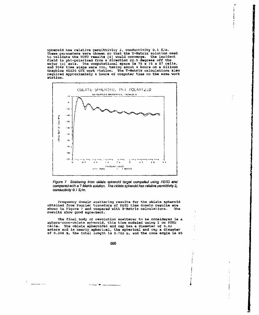
spheroid has relative permittivity 2, conductivity 0.1 S/m.These parameters were chosen so that the T-Matrix solution usedto validate the FDTD results L6) would converge. The incidentfield is phi-polarized from a direction 22.5 degrees off themajor (z) axis. The computational space is 75 x 75 x 57 cells,and 2048 time steps were run, taking about 4 hours on a siliconGraphics 4D220 GTX work ntation. The T-Matrix calculations alsorequired approximately 4 hours of computer time on the same workstation.

OULAIL SIPHLIlOIID, PHI POLAI1IZLODLU-4ULAMZ[LO MLAC~t;A I ILk. 1Pt IA c.2. 5

.5 -

It

3 -U

4U

U U 4 3 U U4 . 1 41 . 1

I L ULW 3 L .4.1

- 1.41( . I WAIIIIX

Figure 7 Scattoring from oblate spheroid target computed using FDrD andcompared with a T-Matrix solution. The oblate spheroid has relative permittivlty 2,conductivity .1 S/M.

Frequency domain acattering results for the oblate spheroidobtained from Fourier transform of FDTD time domain results areshown in Figure 7 and compared with T-Matrix calculations. Theresults chow good agreement.

The final body of revolution scatterer to be considered is asphore-cone-oblate spheroid, this time modeled using 2 cm FDTDcells. The oblate spheroidal end cap has a diameter of 0.82meters and is nearly spherical, the spherical and cap a diameterof 0.246 m, the total length is 0.702 m, and the cone angle is 85

688

iI

1i III LIL. rNID L (GDLAI L tI3PI LHC)I D, PI I I I fIC.U-IOLAIII- 7ll- Un AUST. I LII. lilt IIA--.

S - -- -- --l- -

-35

o ii '°I•

"ILNC .11 -

+.5* I

--0. 0tl i I 00I4AIIl

Figure 8 Scattering from sphere-cona-oblato spheroid computed using FDTD andcompared with a T-Matrix solution. The sphere-cone-oblate spheroid has relativepermittivlty 2, conductivity 0. 1 S/rn.

degrees. The incident field is phi-polarized from a direction22.5 degrees off the smaller end (spherical) of the major (z)axis. The material again has relative permittivity of 2,conductivity of 0.1.

In Figure 8 the frequency domain scattering cross sectioncomputed using FDTD is compared with T-Matrix results. Whilo theT-Matrix validation coda would not converge for higherfrequencies, the agreement is good over the frequency range wherecomparisons can be made.

staircasing errors due to modeling smooth surfaces with cubicalFDTD cells can be significant. The purpose of this paper is notto deny this fact, but rather to point out that, for manygeometries involving smooth surfaces, RCS results of reasonableaccuracy can be obtained using "stairoased" V'DT'D. This isespecially true for scatterers composed of electromagneticallypenetrable materials. a:esults presented in this paper showed

689

reasonable "Lcuracy over a broad bandwidth for three differentbodies of revolution, with the FDTU cell size being approximately0.. wavelength on a side at the highest frequency considered.

Improved accuracy can be obtained by using conformal meshingmethods. However, it should be kept in mind that these methodsrequire considerable more resources both in time and effort tomesh the object and in computer time needed for the finitedifferunce calculations. The results presented here wereobtained using a relatively inexpensive work station, and noadvantage of symmetry was taken to ruduce the computationalrequirements.

[1] R. Luobbers, K. Kunz, K. Schneider, F. Hunsberger, "A FiniteDifference Time Domain Near-Zone to Far-ZoneTransfui:tation", accepted for publication in IEElTanAnt. Pro.2,

[2] N. K. Madsen and R. W. Zioikowski, "Numerical solution ofMaxwell's equations in the time domain using irregularnonorthogonal grids," U, vol. 10, pp. 583.596,198B.

[3] Richard Holland at al, "RCS Evaluation and Reduction by anInteractive System," Report Number API-TR-171, AppliedPhysics, Inc., 5353 Wyoming Blvd., NE, Suite 3, Albuquerque,NM, 87109, October 1989.

[4] M. Fusco, "FDTD Algorithm in Curvilinear Coordinates," IEEETrans. Ant, Pri.LQ, vol. AP-38, pp. 76-89, Jan. 1990.

[5] R. Luebbers, F. Hunaberger, K. Kunz, R. Standler, and M.Schneider, "A frequency-dependent finite difference timedomain formulation for dispersive materials,"Eletro neti_ Coat., vol. IMC-32, pp. 222-227, Aug.1990.

[6] K. Aydin et al, "Differential radar scattering properties ofmodel hail and mixed-phase hydrometeors," Radio Science,vol. 19, pp 58-66, Jan-Feb 1984.

FUTU Waveguide Coupling Modeling and Experimental Validation

by

P. Alinikula, K. S. Kunz and R. J. LuebbersElectrical and Computer Engineering Dept.

The Pennsylvania State UniversityUniversity Park, PA 16802

Tel (814) 865-2362Fax (814) 86b-7065

Coupling of electromagnetic fields into the interior of complexaerosp.ce systems i s a problem of continuing interest aind study.At leoat three teaturms of this coupling must be successfullytreated whether the tireatment is experimiental, analytical orcomputational. The feature-s are:

- highly resonant behavior of the interior response inparticular the current response of any interior wir,'zs

- coupling between interior partitioan or cavitius inparticular via waveguids-like geometries

- effects of dense interior till in particular large cablebundles

ln an earlier effort to characterize interior couplingcomputationally with the Finite Difference Time Domain (FTUD)Technique the highly rekionant response of interior wires has beendemonstrated. In this effort the same technique is applied tocoupled waveguido geometries and the predictions compared againstexperiment to validate thin' technique's capability in this area.Toe technique does indeed accurately model coupling betweenwaveguides. The next effort will be to successfully model denseinterior fill. When this is accomplished it is expected thaLFDlTD can be used with reasonable confidence to model interiorcoupling on a real world complex aerospace system. We thereforeview validation oa coupling between waveguidew ar. - nec.ssary andimportant step in establishing confidence and credibility in theuse of the VDTD technique in interior coupling modeling.

Waveguide coupling through an aperture is a fundamentalelectromagnetic problem. it has been approximated reasonablywell with Dethe small hole theory [1], and with some more recentmodifications of it [2]. Huwevet, these analytic -olutions doliot apply to arbitrary shaped complex waveguide couplingstructures. Instead, numerical methods have tu be used.

691

Finite Difference Time Domain (FDTD) method has proven to bea very promising technique for time-domain analysis of passivemicrowave and millimeter wave structures. FDTO's strength is inits capability to model any volumetric structure with rectangularcells. No requirements for symmetry or smooth surfaces areneeded. Better modeling is of course achieved by using morecells. Additionally, the FDTD code can handle complex materials;lossy and anisotropic dielectrics as well as ferromagneticmaterials are currently included in the code and some feasibilitystudies have been conducted with nonlinear dielectrics and chiralmaterials.

Recently, FDTD has been used in modeling microstripstructures [3], [4] and in predicting aperture coupling for ashielded wire E5]. These results suggest that FOTD could besuccusutully applied to waveguide coupling problems.

The objective of this paper is to model coupled waveguidesusing VDTD. The forward and backward couplings are predicted fortwo geometries: a single circular aperture and a dual circularaperture. The single aperture coupler simulations are performedusing different mresl dimensions and different simulationdurations to observe the model's sensitivity and by that meansdetermine the setup Lor FDTLI waveguide simulations. The dualaperture geometry, however, is selected to be the same as in [2]in order to be able to compare the calculated results withmcasuremnts.

The FDTD field formalism is by now well known ([6],[7]), andwill niot be presented here. Only the introduction of the fieldinto the waveguide requires discussion. The electric wallapproach is used for the wave launching. An incident transverseelectric field is allowed to appear spatially only at atransverse plate in other end of the lower waveguide. Theamplitude of the field has u sinusoidal distribution across theplate rosulting in a wave that approximates the TEQ mode.Temporally the incident field appears in the shape of a truncatedgaussian envelope about a sinusoidally varying signal. The CWblocks the DC power and shifts the frequency band of the pulsehigher. However, a truncated pulse has always an infinitefrequency band and therefore some energy is forced inside thewaveguide at frequencies below cutoff. This energy is kept to aminimum by using a relatively long gaussian envelope.

Model of Cou9ied Wavejuj9id•

The problem space, shown in figure I consists of 4 sidesthat are defined to be perfectly conducting, i.e., the tangentialelectric field components on these planes are forced to be zero.The remaining two sides, the ends of the waveguides, are open.

692

Electric fields on these sides fulfill Mur's first orderapproximate absorption condition [8]. This condition producessome reflection for waves that are not normal to the boundary.In a waveguide problem, however, the wave is more or less normaland the first order Mur condition is sufficient.

The metal plate between the two waveguides is defined to beinfinitely thin, but effectively it has an approximate thicknessof half the cell. Circular apertures are approximated withsquare cells. Several different diameters 8, 12, 13, and 16 wereused. Naturally, the actual shape is modeled more accuratelywhen more cells are used. The distance of the aperture from thesource launcher was selected so that the whole pulse can fitinside the guide before the aperture is encountered. The testlocations of the electric field components in the backward andforward propagation directions were selected to be 1/4 of theaperture diameter away from the edges of the aperture.Transversely the test locations are in the middle of the upperwaveguide. The coupling coefficient was calculated as the ratioof electric field at the test location inside the upper waveguideand the electric field inside an undisturbed single waveguide.

Two aperture geometries that were analyzed are shown infigure 1. The first one consists of a single centered couplingaperture with circular shape and relatively large size. Thediameter of the aperture is 0.375a, where a is the broad sidedimension of the waveguide. All the waveguides have a 2:1 ratiobetween the sides. Three different mesh dimensions were used:22 x 16 x 55, 32 x 16 x 80, and 43 x 16 x 108 in 2, k, and 2directions respectively. The corresponding diameters of theapertures were 8, 12, and 16 cells. The second structure has twoparallel circular coupling apertures that are slightly smaller insize. Mesh dimensions are 42 x 26 x 108 in R, 9, and 2directions. The diameter of the apertures is 13 cells. Thisgeometry was constructed to be identical to one in [2] in orderto be able to compare the results.

Single aperture coupler simulations showed that after 8192timesteps the remaining energy in propagating waves was so smallthat truncation had negligible effect fer the fast Fouriertransformed response. The forward and backward couplingcoefficients for 32 x 16 x 80 -cell geometry with 12 cell holediameter are shown in figures 2a and b.

The model's sensitivity for mesh dimensions was conducted bycomparing responses of the single aperture geometry with threedifferent mesh dimensions. The forward and backward couplingcoefficient comparisons at a narrower frequency band are shuwii iiifigures 3a and b. The results show significant differencebetween the 22 x 16 x 55, and 32 x 16 x 80 and 32 x 16 x 80-cell geometries, whereas the responses for 43 x 16 x 108 and 32

693

jJ -

x 16 x 80 -cell geometries are very close. The results indicatethat 32 cells is sufficient for modeling the broad side of thewaveguide and 12 cello for the aperture diameter respectively.

The forward and backward coupling coefficients for a coupler"with two apertures is shown in figure 4. The experimentalforward coupling results from L2] for the same structure are also<1 shown. The forward coupling coefficient is a very close match tothe experiment. Except for the band edges, the simulationresults fall inside tha measurement accuracy range. Moreover in(2) it was observed that the directivity (forward/backwardcoupling) was larger than 3 dB. Simulations support this with aminimum of approximately 2 dB directivity.

Simple waveguide coupling problems wore successfullyanalyzed using the FDTD method. A sufficient setup for waveguidemodeling was determined. Results, that showed little sensitivityto either mesh dimensions or simulation duration, were achievedusing 32 cells for the broad side of the waveguide, 12 cells forthe aperture diameter, and 8192 timesteps. With a well modeledgeometry an accuracy inside measurement error range was achieved.Although these simple problems can be approximated reasonablywell with analytical expressions, the results show FDTD method'spotential in solving more complicated waveguide problems.Combinations of dielectric and metal screws and slabs as well aswaveguide junctir can be analyzed in the same manner and withthe bame resourc.

:• Kx•rences

(11 H. A. Bethe, "Theory of diffraction by small holes," Phvn.Boy,, vol. 66, pp. 163-182, Oct. 1944.

[2] R. Levy, "Improved single and multiaperture waveguidecoupling theory, including explanation of mutualinteractions," I fLTrans. Microwave Theory Tech., vol. MTT-28, pp. 331-338, Apr. 1980.

[3] D. M. Sheen, S. M. Ali, M. D. Abouzahra, J. A. Kong,"Application of the three-dimensional Finite-Different Time-Domain method to the analysis of planar microstripcircuits," I iTrana. Microwave Theory Tech., vol. MTT-38,pp. 849-857, July 1990.

(4] J. Moore, H. Ling, "Characterization of a 90* nicrostripbend with arbitrary miter via Time-Domain Finite Differencemethod," IEEE Trans. Microwave Theory Tech., vol. MTT-38,pp. 405-410, Apr. 1990.

-- 4

Li

[5] K. Kunz, D. Steich and R. J. Luebbers, "Low frequencyshielding characteristics of cylindrical shell with avarying size aperture," IEEE Journal of ElectromagneticCompatibility, (submitted).

[6] K. S. Yes, "Numerical solution of initial boundary valueproblems involving Maxwell's equations in isotropic media,"IEEE Trens. Antennas Prooagat., vol. AP-14, pp. 302-307, May1966.

[7] K. S. Kunz, K. M. Lee, "A three-dimensional finite-difference solution of the external response of an aircraftto a complex transient EM environment: Part I-the method andits implementation," IEEE Trans. Electromaan. ComDat., vol.EMC-20, pp. 328-333, May 1978.

[8] G. Mur, "Absorbing boundary conditions for the finite-difference approximation of the time-domain electromagnetic-field equations," _._ Electromaan. Comoat., vol.EMC-23, pp. 377-382, May 1981.

695

W!

II

FigUre Id Coupled Wavequidel, Single Aperture (16 celldiameter hole shownI)

Yx

Figure ib: Coupled Waveguides, Double Aperture Coupling (16cell diameter holes shown)

6W6

___

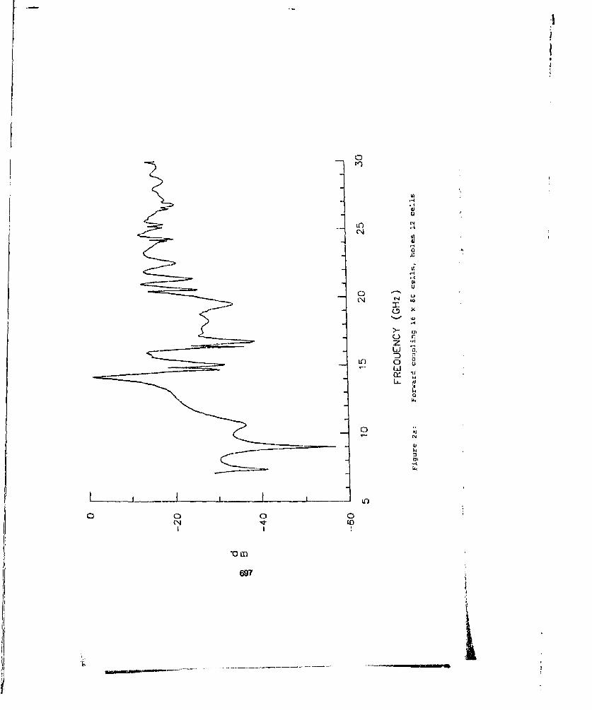
cii

LO

IN/

01

0,

N

LO

ini

697

Lr-.4

I

.4

w.4

NInH

U

U

.1

a -'N N

I0

Ii

:3- ..-4

z ')- LI k 1

Q N

3- 331

I-

LL . -__--___ _

0 a %.., 0N

0LD

III

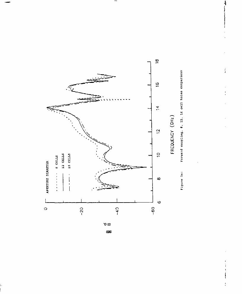
- 4

I

to

a

- aUU'

'-40

HH4'

H

* r-d -

S I H

C)C-y .,.4w ,i

'a'I4r3

a I..

'-4 -4 'a *n

4'

tog------ 0

7- I-

LLJJJ__________

0 0 0 0- to

*ocn699

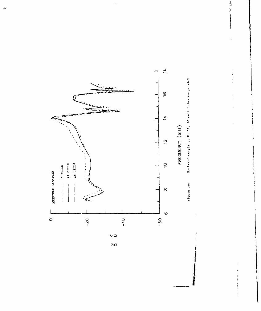
0

LIn

0

Laa

7001

0 .- 0

Ti

*700

C:1

zz

'-pp 4

7011

AUTHOR INDLX

Aulhcaa Pogo Auihaa paoge

Ago;. K.H. 520 Golad, GM. 612

Alan. B.C. 268 Quo, LI.J A

AIladkulc,P. 691 Gwel L. 218

Amoisefi. C.A. Ng9 HoocGE. A93

AntolOflO, J. 642 Hafto. S. 244

Aamataiow, A.F. 1,45 Humwmtm0, C.61

Aziudo, 6.6. 5w0 Hanock. 144 R

solo. C.V. 534 HotmorW, O.W. M66

Biall&C.A. 10 HaaI. R.&. A07

SawbS, 1.L. 432 HoWs, HA. 72

boats, G.C. 10 Haymi P.R4. o99

BuibowA.M. 190 HiwcLJ.L. 369

bolos. J.P.A. w4 Held. KS9. 235

Btwaatua.haa~y. A.K. 544 Heckert, R.M. 820

Bouarxno M. 396 HapeaJ.C. 139

Dom,. W.E. 160 HIMA. 6Y

Uaaudc. X.642 Hafrafeld. R., 203

Btoanow VA W.F. 41 ,Iwund. N. 64/

slim, a. 0/ Ilollinond. 0. k44

Blownl.lL11. 146 Iult44n.t . 816

Bawumley. S. 666 Huwel. F. 3

ucll, A.M. 159 Hwurtsge. P. 662

&Ake, 2.J. 061 lawloin, M.A. 419

"Bae, .1 69 buuct&fl. D. 74,19.0/

ka"iS, P.L. 29 woboafl E. 74

Coble, V.P. 661 flaonds, M. 37

Coley, N. 666 Joun. A, 886

Clieivy, M. 747.119 Jean D.C. 432

Clung., Z. 561 Jo~ne .CM. 94

"ChW, W.C. 216 Kojlet. 0. 320

Choi.J. 10 Kno". ~K. 254

Coffey, 111 E.1. 60M Kanawel, M. 396

Cole, R. 73 Keards, P. 4w3

C4nWy PXM 627 King.A, U.S 60

Coaieta. L.M. 190 Koltweg, l. b67

Cralu, Q.C. 534 Kofiiteararfl P.l.W

Docha(. 2.14 ow KorK. J.A. 56

DeffmalS?. 14.1. 26A i'otllpow. N. 69dOumiS? J1. 529 Kt.yafW. L.A1Ecntwood. 4.W. 655 Kitil, 0. 13

ELvct. P. 557 Ku4210, 3. 369.380

LPnWe J. 86 KWIL K. 6112.&91

Ewhng. P.D. 4a6 Loanorat, G.N.)skxcUIL. P. 1.4146,401 Lutaoalo, I.E. 86

FoarIng. M.D. 607 tetvaNol TN.H22Fowl. D.L. 507 tuuc-hlGxvv. P. 196

Faxoalaic2. 67 I..K. 36

FIWVI.R. 210 U.X. w4

Goo, 5. C61 Un% .HI. 276

106mW1. FlJ. 612,627 Wn.J.T. 94

Saka. 12. 87 10wmW, W. 642

QieoN. A.W. 265.320 Wuetben It. 682.691

Sot~ebyC 61vtnclN 04. .54

702

AUTHOR INOEX (Cant.)

Mader, T. 292 8aw, G;.H. 577.666Mahadlevan, K. 266 Sandri. G., 203Malimood. A. 184 Sota. K. 661M~crNaku. Ri. 21 Schtae"e, E. 234Motilson, A.J. 409 SoU0, A.A. 1643Mccauncack. Cj. 487 SUt .T. 1%8MCKOVM. 6491i(JW. H. 2v2

mil.J12Somuaolo, L. 14.)9MON1on, M. 86 Spwaongna. S.M. 203Mwriz. L. 139 specla' R1. 428.4/IM~lli4 D.P. 520 51atch. 0. 662Miliet, L.I. 222 Iujhr, S. 130MiONOa S.. my9 scltnI, H. 94Moxega. M.I. 629.63 Tokoudi M. U.31Uniega. A.M.L. 829 TopIc'0, A.W. 29Moyti Jr. 1. 21%A Twluall Jr. A.J. 118.130Newel, J.C. a/ 11heudoslaI G. 236NguVen. Q.H. 184l llrnm ulnw. T. 20Habls. B. 419 liumnwx CSW. 369,300Obmufo.T. 661 Wong, J. 851Okabe. M. 661 Wang. 5. 846Civucik. L. 94 Wanig. Y.M. JIGt'&j, J. ID Whelan J.. W.P. 320.80/Pagonelkl, Ui. 114 WIasback, W. 244Plrlllpp, Lb). tI M Wilbon, L. 667Prfbatch, P. 403 WOod. .t.A. ow0Putnam, J.M. 304 Ohoc. (a. 546gW.uA. 646 YeC. 861ki"ggu L.. WY4.61Z62/ Young. LU-. 1l8Hull. 8. 351 Lam. M. n2Salwar. R. 396 Zhmng. D. 851Solo. GR. 577,666 Thong. w. w4

IodlG. 203 Lheng .J 170

7W3