Calhoun: The NPS Institutional Archive

Faculty and Researcher Publications Faculty and Researcher Publications

1994-03

10th Annual Review of Progress in

Applied Computational

Electromagnetics at the Doubletree

Hotel & Convention Center,

Monterey,California, March 21-26, 1994,

Conference Proceedings Volumes I & II

Terzuoli, Andy

Monterey, California. Naval Postgraduate School

Conference Proceedings: Annual Review of Progress in Applied Computational

Electromagnetics (ACES'94) (10th) Held in Monterey, California on March 21-26, 1994. Volume

1 and 2

http://hdl.handle.net/10945/45292

ELECTE ItAPRI 01995

10th Annual Review of Progress in

AD- A286 AppliedI u|~ Computational

Electromagneticsat the

Doubletree Hotel & Convention CenterMonterey, California

March 21 - 26, 1994

CONFERENCE PROCEEDINGS

•I~t The 10to Anniversary ACES Conference

95-01330

ll l ql)&ITY Ib

IT-!

CONFERENCE PROCEEDINGS f,:•AfIbiit, ion I

VOLUME1Ii•:t.'•,,",

10th Annua Revkw of PnFWlnl

ELECTROMAGNETICS

at dieDoktbkm• How[ and Conventin Canur

Moutery, csfalniaVac 21.2A, 1994

CONFERENCE PROGRAM COMMITTEE CHAIRMAN

Andy Twao"

M Applie com"im Mwumwmi societyand VOD wd DM in with JEE, URSI, ASE.,, S"A wid ANITA

T~k C4 Conine;

1995 Co~ for Papers

1994 Comferaae Piopuin Conimuiw xii

coolleenc Chgamurnas Sit

ACES Pixdadets S ter

ACES 94 Short Couun xv

VOLUMPE I

SESSION 1: RECENT IMPACTS OF MATHEMATIC ONCOMP1ITATIONAL. ELSCIROMAONEflCIChai Adoe Nwhom

'Review o(fDTD Sen AlocrUhs for E9 'n~d Wave Prapilain inDispetsive Dielectric bMnWj bv J. Snb* 2

*Modelng Parapepti and Scatming in Dinersimn DW=Lec wthznu FD-TD" by P. Paitrxools 3

*Anslysis of Finite Element I ne Dornain Mahdwb ini Elao'tmawei Scueruigsby P. Moak. AX. Farms anc PJ. Wesson ItI

-% Shigic.Saap Mukiplek me"o for tIm Wa., Eqmmd. by Rt. COVfMB1 V. Rokhlims.ad S. Wmdm 19

"*An Optimal bwieid Plain tar Somaml Pm~ief by 0. A. Kricigmsum and L.H.C. LAak* 25

"Nowmaie Soludwof o(ha 11gi Frequmeny Asympofic Exposoio for Hypebllcc Equaiomes"by B. Ewupuia. E. PAmni, and S. Odwn 32

'A New- To'hmapa for Synthesis of OffsK Dud Rtfeca Sysmmby V. Olin mad I. Pnmo 45

-Pas and Accunf. Aigdmid for Computing the Maom Eiesat b the Unified FulA 1aveAndysis for (M)MIC A apkdý by S. Wit 53

SESSION 1~ TRANSMISSION LIN4E MEflIO tMAO 61Chirk Wadfua Hooter

-NvwRemg~w Saim Nod in 2D-IUANuewoabyQ. Zbmgu wiL. o.1w 62

'Plam-Wa.m amma Swab. diTLIM ).udodUuiagaanP lHuypmSuwe'by i.F. DmwaMiD.D. Want. SJ. Pamm aidS. Lawoma 70

"M~odeling a Resint L Cao rmiven Dipub Uskdo.si Symmbie Comcland Node (SCN)Tamaam Lim. Max (tIM) ?.4ain by M.T. 111 LS, Rhgp and K. Sbmtnmdy 73

-ILM Analysi of a O WCircla WrqAwe Ammnsby K. W. Striclist. L.S. Rigp aid M. Obabu 96

"Compuatmion of -Perwoos of Mi - i Meader Lims an C3Ams Sub... UlnilTIM M&Jmod by C. Emmetpp aid i.R. 140.1s 94

"-Cocoation Suks. or Fwmr Arkuam Laser DWyWo Vebomnen Mwemaaa?by J. Wbuau 101

,Ain** of a Cavity-lagieod Sim Awm Nomid on an Wfide Gomund Plane Using dhe 2-DTIM Mahod by Is. Erwin ad S.M. Weerwort 112

SESSION 3: MULTHILE 119

Chair Dan Reier

"Crved Line MIdmpolea for tme M P-Code" by P. Lauchumear and M. Gnce 120

"CTm b of dmie Multipob Technique with th Method of Moments"by D.D. Rams and P.A. Ryan 129

"Maktipols as Mea- s for the MEI-Method: A Testing Toolkit"by P. Lasohunmn and N. Millsr 135

SESSION 4: FINITE ELMET METHOD (1) 143Cmai Jin-Fa LA Co-Chai. Jo Volakis

"Aadyss of Dielectric-Lakas Waveguidm Us"s Cotwext Pmpcjdon Veckn Fate Elemmts"by BJL Crain and A.. Peuaa 144

"A PInS Element Formlamieon for Mulipoh Modts in Axisym Str Suctumes"by E.M. Nelson 152

"Azhmutdhlly-Deomodus Finiv Elemen Solution m ie CylimiicIal Reaonatort by R.A. Oseglua.J.H. Pierhisti, LM. Oil, A. Revie. 0J. Villalva. GJ. Dick. D.G. Santiago and R.T. Wang 159

"-O die "Mmonm il Be Meadod of Measaurd Equatioa of Inwmrio "by W. Hoag. KX. Mea, aid Y.W. Us 171

"Tlb-Dimieakonl Fmine Elemeat Tme Domuin Approach with Amomatic Mesh Generasion forMiciowve C4itos" by S. Mohem nd ). Le 1"79

"-roe Soqpping Meob,, for Tlamient Amnlysis of Magnetodyrammi Pmblems" by F. Delince,A. Nicol. F. Heorte. A. Genon ad W. Lepos 187

"-Comples Peidic Bounday Coniion fr AC Finte Elemn Models'by A. Frankel. LR. Bra', ad MA, Gockel 195

"toCmpqr CbdU for the Analysis of Plum amd Cylinmically Conformal Printed Antease"by J. Gling. LC. K pSadl, Iad JJ. Volakis 203

SESSION 5: BOUNDARY CONDITIONS 211Choir Caey Rappoor

-Ce.ompoi and Genestio of Highsr Order FDlTD Abotbing Bounaisaby D. SUsIh avd R. Ldeblmh 212

*Amiptve Aboohing cA, -Iy)Ccaditionu in FbmAs Dhlbec Timew Dotmamn Appliwationsfor EMI Simublat " by B. Awcm•aak and O.M Ramh 234

"A DIbpasve Oumi Radiodom BEctaty Conuditon fo FDTD P alculCcubio• by BJ. Zook 240

WTD Aalysis ora Curved Saw-Tooth Anechoic Ohnbr Absorbiig Boumnday Condition"by CM. iVapop and T. Gl•e! 248

"SmemipOed Magnetic PNM m Famed Convctiom Lainsa Bounday yby AM. Momga and M. Moam 256

SESSION 6: OFTIMMKI-"iO 203Chair Rk~d Gomd

Opumund. Bacmhobimlg Sidelokbs Fmu' an Army of Surip Using a Germc Algmrtkoi"by R. Hauapt and A. Ali 266

wNawmulc Ehictioomwuelcs Code Opsimizlo Design Softwore (NECOM'1by 3K. Bicalkail. J.S. Young. LiJ. Datmal, AlI. McDowell. and TA. Evilley 271

"On uth Comnlmitimu of an Otirnuized Inicifeveic Adapive Radar Sigmmi" by H. lKunschI 278

"*Optimizlion Tecniues Applied ~ lo cm us by F.M. I.Amudsafmi 290

SESSION 7: PUIYT EL~ENT~ MIETHODS (11) 299Chair. fin-Fas LA* Co-Chsait )An Volokis

"Hybrid Finite Elemrent-Modal Analysis of Jet Engine Inle Scatteing' by D.C. Ross,JiL. Voldsj mail H.T. Anqugasivi 300

lluee-Dirmazional Finute Element Analysis on a Parallel Computert by R.K.Ummlen 308

"Mu Peorlnnomc of a Partitioning Finite Eleomen Melthod an due Touchugom Delta"

by Y.S. Choi.eogas. R. Las. K. Ewo d P. Soahyqappn 316

SESSIONS8: VALIDATMO 325Chair~ Pat Faster Co-Chair Mike Hazlett

"-A Datoe of Mminaud Dmw fbr RCS Code Val@Ikmoby S R. Miska. Cl.J LoueM. Fly=n mad C.W. Tnmmun 326

-Valiudmum of Target Memistowma ns Mulupola EAvwibonnW by AJI. Saymov,K.M. Wilson mud Y.J. Sboyuiv 327

"On the Benchumark Solution of a Typica Engineeuring Lou Problin " by Z. Cheng Q. Hu,S. Goo, Z. Liui. C. Ye. and M. Wu 335

"-Evalooicm ofRedwSignature Puodlatio Using XPIA~TII by R.O. Jeeuejclc.AJ. Twz*anl.md R. ScladmM 343

-riva~mforble Scale MAceaR Mo, for doe Valhmibd o(CompotiomnslElcoaeModels m Algairium' byOD.R. Pflug and D.E. Warmu 352

-b(iu- V. lieu of Elmacnuagic CodePicti~musby S.BMacl.J. Norgmd.J. Sadint. R. Sepgand W. Pradun 360

"Val~dation of a DiffacionesI Progstan" by, P.R. Posw 366

SESSION 9- ANTENAS 375

"NE.C Mcmdefta and Testig of in Uba-Widebond Ankima for High-Peawer Operuionby B.H. Lootrmg. B.S. Polimsn, R. Pasmor', C.D. Hecisema, andm HIP. Lertming 376

"A Pnouical Applicaum osf NEC Isepodusc Calcsa~uaon by W.P, Whokrsa and D. KaMjfez 382

'NR04kWAmiyi a -(Na~vy i-AnitrMaby CA. eTmis,. S. Schukmniz,P.M. Houmsan m IC. LowpM

"Nearly Seven Years of Soces Using MININEC for Analysis and Desip or StandardB Id- Medium, Wave AM Direckual Anonmms by JLB. Haelrmd 397

-Aamlysim of Aiatuue Ammon wid, die ESP, NEC.DSC. and NEW-Air Codes'by D.V. Andermon. A. lohmommo. U. Ujdvah, and T. Lundin 408

*H-dO IHelicapes Anooum Placement Evahamijoe Experimental ad NEC-BSC Reselts'by J.M. Harris and M.L Whencr 415

"An Antemal Sifauntiui Sopemcwtur to Use OSU ESP4 Pmpmon by I.LL VusVoorties 428

-A Shady ofTwo-Disnessioasl Topered Pfvwdic Edge Tremmneuv for the Reduction of Diffraction'by R.A. Burkesco. AJ. Terteoli, E.K. EWgish and L.W. Hdermlan 436

SESSION IM FINITE D)IFFERENCE TIME DOMAIN 1 40~Chaw Jimysans Fang Co-OamrM. Bruce Archombeault

"Applicaliw of an Upweind Leap-Frog Method for Electu anetis* by B. Nguyen and P. Roe 446

'Limam Supepsjiomam of Phased Army Antenna New Field Patserns Using the FDTD Method'by CF. Roome. E.T. Thinke, A. Taflloe. MJ. Pikmt-May and AJ. Fenn 459

"Rmumimimrs d Scomriug kmr Curved Sumfum Ssuaezm with Sto-Cmr'Cu FDTD"by H.S. Lasgak mad LiJ. LAsebbera 467

lquuat Impedance. Rashmism Psam, and Rader CIUoSSctimn of Spiral Anamnnu sing FDTD"by C.W. P ey an RI. Lud'ba 468

*vlYTD Simsulinlim d an Opem-Ena ?lWliuhed Comunic Pi forb Bradbad and High-T*nspumweDieleceic P opped Nmeawunalz'by M.F. Inksod. S. BriaVgssur. and P. Gartaide 473

'FDTD Sigsuelgia of RP Drying ad Indutaions Hommeg Pmmby M.F. Madeinda P. OmUide ad. M. Whim 478

-A Goueralited FRnie-Vodae AIpridm for Solving the Maxwell Eqauione on Arbiawy Grids"by Y. Lie 487

M neyPuaralel FivoielseiffaermeTIme.Dwnain Methods ber ElocirconagiselicScattering Poblemnsa' by R.S. David mad L-T. Wille 495

iv

SESSION 11: ARRAYS 503Ch~. VRWmghC"b

"CtapKaqM of hase Anay Active nidpfa us Caapm• uami•w wim Meaana'V"by P. Ellio. P. Keen, J. Cha. R. Grad mid T. Collina 504

"TIe EfL•w " Eo medogd MechMural Design Coaains an the Peraowaue of •HLcg-Pfludic DiP*k Affys" by D.C. Baker, LT dte B aid N. Snider 516

"ModelMi of a Cylanlikcal Waveguide Slot Anry, a LoopFed Soki Annm mat an Annular SlotAru.A with the BSC and ESP Coda" by W.L Lippiacit sw J.A Bohae 524

"Multiple FSS sid Arry Analysis Peopi (MFAA)" by HA. Kwa.ki, R. Gilbea.0. Pins mid J. AIbbi 539

Raeqnucy Pnudem f Circar Ammy of Compnd Cylikmhcl Dipole Anlenby F.M. El-Hefumwi 545

"-On Effect of Phaed Qumdnm U-n Ptj Skdelobe Level in Pli Anmy Anruentby G. TDc. 0. Yatchms, mid L Immie 1533

"A Cluoed Lc Algorithm for Real PFameOnly Weighted Nulling Synthe"s i PitedArny Antennas" by 0. Te. G. Ya•clnge and F. Nengluag 560

"Tall Wave Analysis of Inrfint Phased Aray of Arbimuy Shape Ptmed Line MiaoaipAMemM" by EM. EA &M. Awya, E. Ekliwuy, and F. Elhefnawi 567

"EITsct Mummal Coupling Can.putmlin for Symmaetrical Arrys?by S. Christopher. S.D. Sane and V.V.S. Proumh 575

AUTHOR MMDEX

V

VOLUME 2

SESSION 12: PNTE DlPPERENCE TIME DOMAIN N IClbw Raymonda Luebbom C4-hair. John Begg

"MTD-T Alaridan fow seNonlinea Maismeirs iquatios witdh Applications to FftntwncaimA4*6". Possygassom' by P.M. (boorjsin, . RAM. Joseph and A. Tiflove

TFisam Ditference -Time Domain Tesu of Randoms Media Psqagauia Thensy"by L.. Nickiach and P.M. Franke 4

31) Analysi of Nonlinea Magwlc Diffusion by PWID Tocimiquei* by R. Hlolland 20

7Imiincm a Pv, for Thwa..Dimesinal Aaecloic Chamnbers using PDTD"by V. Cable. ft. Loaihom. C. Penney. S. Lailongand Jd. Sch~ai 28

*Apylictihon of the Pinke.Diffarence 71me-Domaim Me"ih, odl I SintuLniuo of DeII2-I Noiseis Ekecwms Pad~agiss" by 1. Fan, Z, Wa. Y. Chsen mod Y. Lius 30

"*AClosed Form Solutions of the bqpu !mpedec eof Two-Dimeesawsnal FDTDGrids"by Z. Wa. 1. Fass and Y. LUs 38

"D~eriving a Sycaiseoc Condocuvity To Enable Aeccmue Predictions of Losses In GoodConducau Using FDW by K. Chambahln W1n L. Gordon 46

"Cowlog PDM Modlels of Aircaf urit GWTO.FD~k 0 by C.W. Ifsemnw.SJ. Kaibsanh d B. Monier 53

'High Onr- FDT`D Mgvorisihm w Reshace Nurroiczl Dusptcsion and SlawuSMng* by T. Deveze 61

SESSION 13: GEMACS 69

Ch~ar Ken Siaakiwwi Co-Chair: Bdsady Cag~ey

"Recen Enashcemmnas toGEMACS 5.3' by E.L. Coffey 70

'Estinadon of GEI4ACS Comnpmr Revwwve Reqsiurememsa"by It. Kdshr, S.L Coffey and I.D. Leuusio 72

"Moleliwip Caivity Problems wishi GEMACS 5.3" by EJ.. Coffey 80

T-16 Suucwm Modeling Usding GEMACS 5.3" by B. Fisher. El. Coffey and TiJ. Timmermans RI

"-ft. Microwaxe and Millveve-Wawe Advwzad Ceampuatmmoil Eavirousmse Program -A Compute Bsued Design Enviromment for High Peeqisacy Eiecruuics' by R.H. Jmksim 85

"Twineri Considerations Ragailmg the Elouumagnetic Modeling and SimWslioZ-avirmumet for Sysstuw (EMSES)* by K.R. S~ieeai z 86

vi

SESSION 14: MOMENT METHODS 95Choir Pad Comasn

ItRAnl Ushrn 11f witah a New CFIE" by F.X Cannig %6

*A Now Method fir Evaluonag the Gsenealized Exponetadal lamepsh Asaociuaed witlt rainSaougt-Wise Anaum woby F.L Warne and Dtt. Warne91

"Talrwlnlma for Evaluainag die Uaniformi Currnt Varier Potential vi die Isolated Smgulanty ofalie Cylindrial Wore Kirnel- by ONH. Warner. JA, Ilulfnaaa, and FL. Weorne 106

'A Pauallel Implemmntation of a Dv~ii Wine EVM CcdC by A. Thinivwooc. A.M. Tyrrell,adS.R. Claude 113

'Mom oeIprovemao i ad. Method of Moosew Soosina af Aaeommsv onad Amyr usingPoxkhgtma' and lialWs Integrl Equations by F.M, PI-lidhawi 120

"jippadlagCanoeWin-Odd MoM tPagnby A. mad adS. Avflmh 134

U00mqn Structur Symametry an Reolucing the CMU Time for Coamputng the Moment Metho(LI Motri Elemntins" by ZO. AI-Itekait 142

-Numaraml-Aatlytical Alga iduw Bond an Dual Saitoe EqmdoasTechniquc*by)I. Ituhkka, V. Vetanvey, Y. Svisclue wAl V. Oudlka 150

"MomeP Meod Anatlysis t3Now.Cnhogoai Waveglpiae 2 'Vavegtolde Couplinig Through Slot"by S. Closborplier. AJL Slagsh and LU. Um~aye 155

A.n O(nlos2vi) leavew Method for Solving Deptae Lhae Systemsa by S. Kluachenao.P. Kobaanimkov. E. Tynyduatikov. A. Yerarn M.A. Herminsend Q. Sheikh 163

*Developing Optical and Autoavai Freqtasay Samapling in Morment-Method Solouons""y 0.1. Burke and EX Miller 165

lReflecbmonan Sonmr of the Folklore of the Momnt Metiod" by R.C. Boon 173

SESSION I5: EMI/EMP/EMC 179Chor. Frak Walker CoiCbftr. Retald Perez

'Validatio of a Numrial Finite lapatens Code to Solve flaiesso Elntoraiqaett. Acousaicaod Elasic Wave Scamring in 21) by KJ. Lanptabymg ad ftL Malkis Igo

'Comariso Deteam LEMP A NEMl? lathaed Ovenrobapa ha 33 kV Ga eiteDisribadir LinuC- by R. Mauoi. B. Koedi. B. Vahi" and M. A8s& 199

"Moampolle Nn-V~ddCouqlkag Ansly-i - ComarisonmouExdportam ad NEC Rem~tCby M1- Wheter ndRJ. Lais 201

'Develepmanti of a High Power Macowave Susceptidblity Simublaion Capability at PhillipsLtabrmoya Satelit AsseameactCenter by ML. Zywlsa 212

"Tea hidebity in Anechoi Chawnbee? by C. Courtntey and D. Van 220

"An taveatgmatr tan Ahternatve Cauwnrijon Technuiquesaam Reduce Shielded RoomRemonouie Effets" by B. Archnmbessl aid K. Cbsorawsli 228

Astuaau System ty P.1. Walker aed S.L. ledge 236

vii

"A Hybeid Apgacac-h for Canpeginalft EM Seeaoing firam. Complex Termineion, asideLarg Open Camids" by ft.'I BwrkN er. P.R. Rousso ed P.H. Po~iho 2'4

fleumwmeModding ofiJe Engine Cavitis with the C4NVEhN Cide"bv J.L. Karry wd S.D. A'-h 252

"An Is, ... e Me"ho for Comnpuaund the Scenhed -locruic Fieldes tithe Apertures of LaurgPerfectly Conducting Cavities" by D.D. Raniwer antd G A. Thiele 259

"-Hybrid Formulation fir Arbitray I-b Iodine by LN. Medgyean-Mmuclsng and I.M. Putam 267

'Hybri (MMI-tnT) Amlysi of UM Scaorniy by [age Gxine (It cu wisb Appendages"by M. Has, P.M. and H. Toon 275

"Reducig die Operation COOK in Cannpeltiaal Ekwratomneakt s ing Hyrid ModdlCby EX. Mille

"A Hythsd Tectmiqu Fir NEC (Nauatrial EkmtgeisCode)"by SA. Rounaelle and W.F. Perif 290

"An Appusis for So: eing Syueon -Levell Eieceomagnettc Coupling Problems"by E.G. PuW and MiJ. Antinone 291

"Efflelma hEMP Canpuatiie of Periodic Scrucuavae" by C. Mafmer and L.H. Boinholt 303

SESSION 17: PROPAGATION ANT) IMAGINJG 311Choir Daenni Awhe

"A Phynica Optic. Model for Scattrng of HFe Radiation by Ineguib Terrain" by G~s StaBuke 312

"Tialared Ficas Model few Taro: Xpwcb SAR Image Piedition for Groiaid Vehicles inten Dign

Chier Envwwmi au* by P.A. Ryon. R.F. Schiadet, D). Duane.r Di1. Andersh and tEK. Zelnso 320

"*Onate Use of Ray Tyating fir Comptls Torgats" by TOG. Moore, E.C. Dimand .P7. Huansterge 328

ruhlinuqmsiCalaiha te Cnas-Seco of e OpoacdeasicRads with bpule SauteofSlmocvromtkls RSS'"m by V. Oed, K. Duaouiage. S.?. Koval. A.V, Peftekowand ALE 1enitv 335

1"mekunloe tin s lerete Cwronpslon Accurwy of die Scaned Elmcuenwnedc Field an theSlmalisflso of die Ram- Doppler Size Analywr by V. Ovwd. T. WriSdi. K. Eawkhbagsld V.M. ZaljatdY 343

'Time-Doositn Elomonmeignaki Repns and Model Unonuninbs" by R. Inguva. C.ft Smish,PhL.Goap and DiJ. Asdeist 353

"EAM:LjsC An Electromagneuic Scatueing Analysis Tool fro Wicati"'by AtP. TUISoopoIIOs and Mi. Packsr VA

SESSION IS: PIE AND POST PROCESSING 371

'NBC - MoM Worktation: NMUD 3.0' by L. Russell D. Tem. J. Rockway.D. WWAWOa w Wl 1d. Eaie. 372

'AioNEC.A.MArriage of Coavuuiemor by A. NMi 330

'A Rey Tracer for the NEC Basi Scominlg Cofte by D.P. Dmv*. W. Pshys and Si. Kuhmna 398

"SOURCE.i FIELD. Whaa Happwu in Between A Now MaeiOW for Graphica Display or071) Scounring by I.A. Evra eard LL1 Coffey 396

-WMxtJW Nummiical EM~MuOMd~cs MOdeWka & Afifflydrs Uskal Cinampubr-AdiedEngineering Solwue by 5.3. Remsees. 3.5. Make md W.E. Praerw 403

"A Pi~m EM Cade Ineuacbe Sftndwd by LL. 00"le 409

-A Gel-lay Desrption Larugup for 3D Analysissa AydCodesby T. Haali",.C.Honu-Him Lunoal Jd. Drawn" 410

SESSIO 19- HIGH FREQUENCY 423Choir. biace Kaiy

"XPATCSI: A High Frequency Elactuuunmetc Scomaruug Pftdiaaos Code Usig Shooineg madBouncing Rays" by DJ. Aadersi, S.W. Lo. .. .L Dockmar. M. Omilley. It. Schaidel.M, Hateft and C.LYu 424

"A Sirmple Physical 00ac AMgorklm Pefoi tFor PEUISI Camwetiag Aauaitrcure"by W A. Imbniale mrai T. Cwik 434

'A MONISMU1 wile Apulicado L) Poomla Order Polynomial Strps'by 1.1. Morumande m E.D. Couawatinkes "2

ftoudseom Due ioa Convex Corvahere Dicaaerla~y of a Didamt Conmul Pufec Corlcfaiorby D.H. Mornahuuml .O. Olans 449

111gh Evqemay Scamwing by aCcu&Ktiqu CkcrdmrCyWbComm with a Lom" Dielectric ofNon Usibatfw Thckn--e-TE Cow'~ by S.0. Tomyor sad RG. Die 457

"Efficent Coarpa~muio Tzbeiqe fix Baclucamwag luau a Discontinuiy Along a PlecewmeContwmou Cumv on a Pla Saalte by J. Kum mod 0.3. Keeler 465

-Cmpmr Smobdonm of Diffracuom and ftomima Prosmal" ma Qimuwpwby A.V. Popov, Yu V. Kopylov. real A, V. Viougmaday 473

"Symbolic Pinagrommnif WaldSi g Expeauakm Applwiom to GipclK Weagiuiduby R.L. Geflau. A. Kim. sod A. Wousho 475

ix

SES3ION W. LOW FUEQ4UENCY 4C~Cho. t Junak COAbi Abd AMked

"A Cowmwaia of Tvmo Lovwhsqrn'sc, Pwim.2mio lb 0ws 51u FPdd g EquinusbyW. W's.A.W. Gli~monan D Kahe 4A4.Comi'vimimm 0i bu~hicod 1, d ins kiagiod Cib lapomi to Mog"wKz Fwkb"by M.A- Siincily ad W. Xi 492

wbwkxmd Cw~mwi in Owlqkd Bodies m Low I'Weqw'sy I Imug Pk F i&Impodur Makid-vi, Imipsomi SpwAWi Romewwo by W. Xm 'Sa M.A. Slc~hly 491

-rW Two.Dwaommoom Pima ipIrnigval T Cb ' *,* dmmom sqwwooI'syIro Applied io (pm PAgm' Scaew" Piobkon by GX Gohdi mmi S M Rao, 502

-A T-UMmix Soludos n for how bm Dwbuetf Cydm- by J.?. Skimw 510

SRSSION 21: EDUJCATION 521

'EMAG 210- E Im - 21) E1wuowm'c win Migbboamk Solme ai MATLAS'bFy D.P. WeLls mo . Luldmw 522

-U-4g Nwmnica Ehrnmqrnu Code (NEC) w Improve Sbnun Uninsmlirig of MmapoirAmim's WA to Drmw a Two Elamas Momaple Aty" by M. McK vghd mi md W. M. Raidell 52K

I~ DhklbuwArml~iyWb MAII.AB mdIMAP.-I I dg I~ lumawv'cnby W.P. wholw am C.S. Whim 556

SESSION ZL. MiROWAVE 545

"OpdUmmamma Mianwve Sftsomumaig a PwMelTL.M Mail,by P.M.S. Poam. and WJ.R. Mloos 546

'Swmu~lealBaomsof E'scimd Sym. aioPM Envomimwby It. lIikesi mWd R. SL. )im, $54

"A Thist-Damos Tacm fo t Ariym o Nomboom Devoms md Cwcwusby N. U.wi K. Fabowt. J. Oaime nd . Soros 569

1i'IIWeve Aniy'si of Copho Wawqol" Docatmmidss by a Puava Wave Sylinssmby R.. SaM** md P. Itto 576

SESSION 23: MA1UIUALS AND SiUALATION RM flOcS us5Cho ftbso Covalla

IMe~gkf TiSWmUs BKut~w*VN Wonin. iCo Am'movop MhIs by a SpeosuTWWsMM T.Elmq"r by J.M. Catimu and . Cavmw M86

'CCMd: CoCWNCyUsdwe Mh W o re~i Ebosa,'s~gs., Smaiw" Immi Cowmpas. TwoDdsmmuao Obpscs by A2- Ebk.hmw L- C.D. Tjykir 594

'tsm'asom of Veloc"t ad Ammomm of Sawh A~ce Waves.m LayesedPimxcectrc 11,u- by ft. Wowi U. Ras*, H. Me,. ad P. Roms (.01

'An AppikaUm' of Mim-Me's Cmi.o For LSM LSE Mod. Diimetso inFwriwl e-VI-sw LAded Wnwmvog . by E.Y. Kapikvc and TAL Riasn 608

AUTHORt INDEX

x

THE APPLIED COMPUTATIONAL ELECTROMAGNETICSSOCIETY

1.995 CALL FOR PAPERS 1995The 1 th Annual Review of Progress

in Applied Computational Electromagnetics

March 21-26 1995

Naval Postgraduate School, Monterey, CA

Share your knowledge and expertise with your colleagues

The Annual ACES Symposium is an ideal opportunity to participate in a largegathe-int of EM analysis enthusiasts. TMw purpose of dte Symposium is to brin:ganalybcs together to share information and experience about the practicalopplicatior. of EM analysis using computational methods. The Symposium features;o--, areas of interest: technical publication, demonstrations, vendor booths andshort .-oarses. Ali aspects of electromagnetic computational snalysis arerepeev . The Symposium will also include invited speakers and interactivefortanu. Contact Ray Luebbens (814) 865-2362 for details.

1"s ,TES 19S ACES 19q ACESSylp...u. Chali~m 1 AdbmletratM" C-C•airmna

Pem Sum U6ivni! Dep,-od2 ECAB EE DeL Univ of M1iAiWppi320 EE Em r~mtPuu Ad Aadin Hal Boa 41Ulmaty P PA 1102 633 D RdRo4, 437 Usmiwe'it•, MS 38677

S(914) 65-232 Mowny, CA 93943-5121 ;=( i) 232-.538Fax: (814) 00-7065 Plhae(4d0-4W111i) ftz: (601) 232-7231Emiel: LW4'sm~m pa Wod P=_(08j4.OO snag ffdoa9'vu.CC~aMhne&e*

1995 ACES SymapeasmSpmoml by. ACirS. USAJ.SA. "CCOSCC, MPS. COA N, DOWMA CECOMIn W{opew w 1ke M EEE Aaw mid fpnim Sociey, ew nEW

med~p=Cquil��i•y ¶oaey d USNCAJSI

xi

1"4 Conference Prograw Committeefor thle

10th Annual Review of Progm inApplied Computational Flectromagnetila

atl theDoubletree Hotel and Convention Center

Monterey, California

Com!... Cbamlra: Andy Terwuml oChimAir Fd"e lasnism of Ycchnoloy Jeff Fodi and lDcmis Andef

ScOlof Iqmomring WrigIKLab-uyIAARABo. x 3402 2D10 Fifth SL.. Bldg 23

lmywkOH 45401 Whi&aPomusm AJFB, OH 45433Tel (513) 255-3636 X4717MFn: 476-4055 lei (916) 643-M35/Fax: 1053

Cateuw. Advbor. Dick MheBcE Dq Code ECAflNava pMw~adum Sho133 Dym Rd.. Room 437MONOW, CA 93943Tel (406) 646-111 I/Fax: 649-0300

Cmotin=Nobdor FoemcOsur? Jodi Nix

5200 SPUS&Wh Pat.

Oh310I1.OH 45431Tel (513) 476-3550/Fax- 3577

Shor Cm,. cbmr. Robwt LAC Shurt Comna CoklCbah Jin-F& Leelbs Ohio Stom Univualty WOroanee POlytelmCW lInt.ElmaroSciam Libmakoy 100 laWNsg Rd.. EE Dept.1320 Kimem Rd. Weotrma MA 01609Calmubin. OHt 43210,1272

IMS C m I h!ý Ray LambhmPWO-Sm Univmrw320 Ekhwic Engmeesta EmUmiermaty Put, PA 16102Tel (814)1865-2362

cmfunWm - Pat Adler

A d*"m otmif Dick Adae. HNove Puft ah SchoolD-mio Awlemsb M4~W USAF, Wn& g --dioyJeff Fat. Cqmth USAF. SM.ALC/QLPM Fom.a kým mavod Ammm SymmemRkbud IL GcOw" Usim. of MbuWiwKim L&gmi. NRADRay Luther.. P.. Soo Univ.AMdY P~m.. Ooergi laidý of TeccmolWgJohn Rochway, NRADAndy Tammoli AF liniade ci TedumakogRec WALker, Soeing Defens wk! Spwe GrouPetny Whelew, Univ. of Alabona

xii

A*C*E*S 1994 APUED COMPUTA11ONAL ELECT1OMAGNEI.CS SOCIETY

TM Trith MrMn.J w of Pro.ou Ihn A•We CanWutotlur" Becflomogi.Ur

From The Con•erenc Chairman To AUAuend&S:

On behalf of the conference committee, wlckome and thank you forcmng to ACES '94. Also welcome (back) to Monery, to Califomia. And to

e avl Po adua School from which we have our rootS. If you am fromabroad, of cousE, welcome (bak) to the USA. If this is your first time bae, anetra welcome and an invitation to ask MY of us to give you vermion ofwhere W and what to do, or bow you can become in e we do need ytu!

A. Iwr=e this let., the January V94 em uartlo. L. the .Los Angeles area,and its afte shocks, are still very much in the news; as we 'lan this enjoyableweek for us all, I cabot help but think of tbose affected, posibly some of you.I find it remarkahle that destite the numerous calamities affecting A ES'

10th Annlversaay beautiful hoat state of California. an atmosphere of energetic hope always

Monterey, C fomolaO For this 10th Anniversary meeting, we have tried to make it special andMorch 21-26, 1994 memorable, and to give a disinct dusak you to Dick and Pat Adler for their yeatrs

of selfless service. We tried to centralize everything around theDoubleuteenConvention Center so a to give Dick and Pat somewhat of a breakthis year. We have coorlinated noteworthy social events, v•n&r exhibits, and

m ftwease WA shot core. Wc. deliberately tuid to extpand the short cowse and sessioos sos""'P,) that those of you at home with ACES aum reach out to other related aeas like1. 51s31.*sa,5a.7 . sMaMv Wavelets, Time Frmquency Analysis, and Measurement Valdaioo. We also felt

co, -cw- W that with research money being tight, if ACES was the oe conference you wentA." -1 G.•c A,,to this jear. you would be able to prta•lly diversify while here.

W, IAAR. By way of acknowledgments and thanks. once agin Dick and Pat Adler.t nd Pat's team of dedicated ladies who work so hard behind the scen, not only

TM F=5s~1 347sM6.4414 bere during the conference, but all year. Jodi Mit. who I'm sure you all talked toat least oae= this pat year. has been the hands and feet of ACES '94 for over ayear. She attended ACES '93, viited the Doebletre,. gave ACES publicity at

t o - numerous other co e'e- this put year, and contacted countless perspectiveati *pants in various capecities. She and her team at Veda designed oursit 614MM~I -F- 614M2zw, 7M ~ flyers, etc.. CL. Adinaftd all the mmiltegs. and even kept me. on

schedul plekase thank her evry tlne you se her!Cmtin Atobw Thanks to Jeff Futh, Dennis Anders. and the Air Force Wright

,boratories for support, advicrj, publicity, and help with evay facet of thisE5O•=_ 'ia ccnerene; to Rob Ito e In Jin Fa Lee who, as you can see. dida suner job •n

"htnP1~a~ 21 nh -'al h h cowrs ideas into a working teality. teaYTY*stMGia- *i es•ir 4 the ACE PS (deste what it .'ys ilu the January aunownscement) ConferenceEChman dida great job in helping as out this year provrding overall help and

1, -..- . V• paper review.Loas, but not kast to my friend God I simply say thank you. sir, and please

•mt ,w l don 't le the earh shake while we are here.ha:51J1•6.we * far 51347S-ir77

I~~~iBe ~ ~ ~ ~ wishes,IRe camre.me cihow"O Andy TerzuoliL Chairman.A"" ..1-0tli h 1994 ACES Confereon.P ,s buaMw.s. Daytn, Ohio

*mmv T1,,-,, TM •February, 1994t s 1wm••F€ 1,4"4

ACES PIRESIDENT`S STATEMENT

It's nice to b, here in California in March. especially considering the frigid weather weexperienced in the Midwest this pox winter.

It's especially nice, however, to be here for the tenth annual conference of ACES. It'shard o believe that nine years have gone by since Ed Miller and his colleagues xLNL convened a meeting to devtmmine if there was a need to form a society to cav:- lk-

the needs of die computational €lectromagnetics commurity. The ansv-c ,,"reaounding 'yes' then, and so it renains today.,

ACES is unique in its attitude to the profession. It hi. senior-le,''A :e.•-m ),certainly. who publish significant papers, and ye much of *e enail i ,- cv c.,s fonm=naeu radio operasni who want to use NEC in their ncti rofcs-.-iJ r . res, andrnaUlly 5ook so ACES to guv them support in their endeais, Pz l'w 4'sor ofa auedit w NEC- but ACES arted as a virtual NEC user's., priat , it's rnce to seethat we haven't lost Ow toots.

Andy Tersuoli and Jodi Nix have done a great job in orgmanz"iI ,r onference. Weowe themn a peat debt. And how about Dick and Pat Arle' .' tnoinght they werejust a couple of names who wanted your money. Now that yoc'e 24 a chance to meetthem, and their support staff, you can do the right thing and th•nk them, too.

Let me tell you how so get the most out of this conference: meet colleagues, see thewruuml, go to the banquet, have a good time. The papers will be so much better ifyou're in= good mood. That's what we want for you.

Hauold A. SabbaghACES President

xiv

ACESI 1994 SHORT COURSES

MONDAY MARflI I FULL DAY COURSE

"WAVELET EECTRcODYNAMICS'by Gefod Kilw.r Dipin at Muihenica-l Scmim UMMB-LoA'dl

MONDAY MARCH 2a FULL DAY COURSE

rIM".FREQUENCY ANALYSIS'by Leos Ciabin HisuCal egsd Godusle Ceamerof ClNY

MONDA MA~cR 21FULL DAY COURSE

"OEMAAS FROM A-Z*by Bdsdy Cafy. Advaed EM

M=6DA MARCH 21 HALF DAY COURSE

'IWDM FOR ANTENNAS AND SCATTERINGby Rey Linbben. Poe. Same Umivessity

MONDAY MARCH 21 HALF DAY COURSE

MEASMUREMENT VALIDATION FO)R COMPUITATIONAL ELECTROMAGNETICS'by Al Domiack, Obio Suam Unimmity

MONDAY MARCH 21 HALF DAY COURSE

"USEING WMODELASED PARAMETER ESTMATION TO INCREASE EFFICIENCYAND EFFECTIVENESS OF COMPlUTATIONAL. ELECTROMAGNETIcS'by Ed Miller. LAW Mumas ?omml L*

SAKIJEDAY MARCH M4 FULL DAY COURSE

'FINITE ELEMENT METHODS FOR ELECTROMAGNETICSby Jia.Fa Lee. Waromei PoLymhack Iuuitm-a. Rabat Lae, Obio Simu Urfivuny:Tom. C.1k, )a ftuaIsm I.Abmma-. end idEm Bnger, MxNmIShwendleeCayrpwom

SATURAY MACH MFULL DAY COURSE

*WIRE ANTENNA MODEUNG USIN NEC"by Rkabod AS~w, Naga Poompdaf SchL ool, iueflnal, rem Sme I Uuuvawy

end emi llbeýLawenceLavrso NooadLabHALF DAY COURSE

*VOLUME-UOTEIRAL EQUATIONS IN EDDY.CUýI NONDESTRUCTIVEEVALUATONCby HAI Sshiuagh %~~qI Asociame

5hflZBDAXMM1IM A HALF DAY COURSE

'EL.ECTROMAGNE IC CIIARACTERIZATIOM OF ELECTRONIC PACKAGES'by Andrew Cundageicm Ulvomity of Arizona

IV

SESSION 1:

RECENT IMPACTSOF

MATHEMATICSON

COMPUTATIONALELECTROMAGNETICS

Chair: Arje Nachman

Review of D-TD Based Algorithms for Electromagnetic

Wave Propagation in Dispersive Dielectric Material

I.G. Blaschak

USAF Armstrong Laboratory

Brooks AFB, TX 78235

Abstract

The radio frequency dosimetry community is actively engaged in the assessment of thebiological effects of short pulse, wide bandwidth electromagnetic sources. A key component ofthis effort is the development of robust and accurate numerical simulations for use in microwavepulse dosimetry prediction. Simulation algorithms based on the finite-difference time-domain(FD-TD) approximation to Maxwell's equations have tht poten.ial for significant contribution inthis area and are therefore of interest to bioelectromagnetics researchers at the ArmstrongLaboratory.

This study will present analysis and computational experiments designed to resolvepractical, performance questions regarding the use of FD-TD based methods to modelpropagation in dispersive dielectrics. Some questions to be considered are:

* What effect does the accumulation of phase error, inherent to the algorithm, have on thequality of the solution?

• For a sensible level of discretizauion, through what distance can the algorithm be expectedto accurately propagate waves?

- Using published guidelines for appropriate selection of time and space increments, whatcomputer resources are required to produce an expected level of accuracy?

Computed results using the FD-TD algorithm will be presented using implementations oftwo popular formulations for dispersive dielectrics. These approaches couple the constitutiverelations for the D and E fields in the material to the standard FD-TD difference scheme as eithera discrete approximation to a convolution integral, or as a discrete approximation to an ordinarydifferential equation. The FD-TD solutions will be compared to reference solutions obtainedusing in exactm Fourirr spectral approach designed to compute the penetrating fields in a simple,dispersive slab geometry.

2

Modeling Propagation and Scattering in Dispersive Dielectrics withFD-TD*

Peter G. Petropoulos,Armstrong Laboratory, AL/OES,Brooks AFB, Texas 78235-5102.

1. IntroductionThe application of ultra-short pulsed fields in the areas of radar, hyperthermia, and biolog-

ical/environmental imaging is imminent. For that reason there is a need for a thorough un-derstanding of the short-pulse response of media whose dielectric properties are described byfrequency dependent models fitted to permittivity data available for biological tissue, soils, humidatmospheres and radar absorbing materials. In addition, the planned extension of the IEEEC95.1 *igq i exoure standamrd to pulsed fields will also require qualitative and quantitativeunderstanding of this sort to be developed. The alternative to actual measurement of the responseis numerical simulation. The fact that the above mentioned problems are dispersive requires ofthe candidate numerical method to accurately propagate each fequency component present in thercmnputation. This implies that the method must be non-dissipative so that it correctly modelsany energy loss due to physical mechanisms, and it must introduce au little artificial dispersion aspossible so that the real dispersion is simulated correctly. Such nice properties are desirable fornumericrlly capturing the Brillouin (a low-frequency aspc:t of the response) and Sommerfeld (ahigh-frequency aspect of the response) premursor phenomena in dispez.ive media. Lacking sucha method one would like to characterize the spunous numerical attributes of existing approachesin order to control them or even alleviate them, Pnd to develop some ability to prescribe anacceptable error level and be certain that indeed the simulation will accumulate that error andno more. In the standard FD-TD method [11 the truncation error can be neglected since it isO(Af' + A'), where A is the typical spatial cell size and At is the timestep. Assuming propertreatment of the electromagnetic boundary conditions and of the absorbing boundary conditionusswd to truncate the computational domain one is left with the major source of error, i.e., thephase errr introduced by the finite difference scheme. This error row linearly with time. Asa result, a. given discretization will not be suitable for an arbitrary amount of computation time,and the so called Wrles of thumb' concerning the points per wavelength, N,,.-, have no meaning.The issue of how to choose N,. is central in FD-TD calculations in the absence of canonicalsolutions. In my talk I present some guidelines on how to choose the points per wavelength forFDTD in relaxing (Debye) and lossless dielectrics.

There exist a variety of useful extensions of the popular FD-TD scheme to the modeling ofpulse propagation in temporally dispersive media with complex geometry. Here I will only beconcerned withlalm'ethod [2J for Dehy ediisp~ersive materials since most materials in the microwaveare of such type. Other extensions [31 use a convolution representation of the constitutive relationand work is under way to characterize them too. I will also determine the N,_ required to controlthe phase error of the standard FD-TD in lossless dielectrics when a small Courant number, s', isused. The case Y < 1 is relevant to the discussion of FD-TD for dispersive media because thenthe timestep is very small (u we will see the scheme in [2) requires that for accuracy the smallest

'This work war supported by contract F41624-92-D-4001 with USAF Armstrong L&boratory.

3

-i-A

1.00

x 0.90

EEXACT

0.85 - h- O.-1 , 1h-0.01 ,.h•=O.O01i., -- 1 .0

0.0000

' -o 6 ..0 .... 1.600 2.00 3.00k A

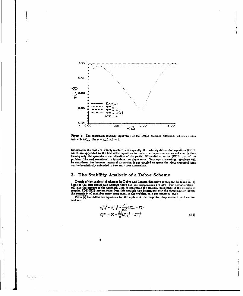
Figure 1: The maximum stability eigenvalue of the Debye medium diifference schemes versush&(= 2r/lN,.) for P = = 1.

timescale in the problem is finely resolved) consequently, the ordinary differential equations (ODE)which are appended to the Maxwell's equations to model the dispersion are solved exactly thusleaving only the space-time discratization of the partial differential equation (PDM) part of theproblem (the cudl eauations) to iatrcduce the phase error. Only one dimensional problems willbe considered but because temporal dispersion is not coupled to space the ideas presented herecan be heuristically extended to two and three dimensions.

2. The Stability AnalysiE of a Debye SchemeDetails of the "naly-is of schemes for Debye and Lorents dispersive media can be found in [4].

Some of the text herein also appears there but the explanations are new. For demon'tration IwiE give the essence of the approach used to determine the stability properties of the discretizedcoupled PDE-ODE system sirce f•om this analysis one determines how the discretization affectsthe e of each frequency component in the problem on a per timestep bajis.

Rom [2 the difference equations for the update of the magnetic, displacement, and electricfield are:

H- 'r-I- +---(E - )

D` D"+ ~(H'+ Hf'~+)A1 -, (2.1)

4

E ='+ At +2r D!' t - 21 W (-A E.Aa•+' -; j a •

where n is the discrete time index, j is the discrete spatial index, a = 2

rta._ + t.At, r is theLuedium relaxation time, E- is the infinite frequency relative permittivity, !. is the d.c. elstivepermittivity, and p, is the permeability of vacuum. An eigensolution solution of (2.1) is

Dj (2.2)In (2.2) th,. complex valued vector = (h, d, i)T is the spatial eigenvector of the difference lystemwhich is related to initial conditions, and k is the wavenumber of the harmonic wave componentwhose stability and decay is determined by ICi which is the complex time-eigenvalue we wishto find and whom magnitude will determine the stability and dissipation properties of the k-thfrequency in the difference equations. Substituting (2.2) in (2.1) and after plerty of algebra wearrive to a polynomial equation for f. The polynomial, whose solutions give ( as a function of themedium parameters, the timestep, and the quantity kA (= 27r/N,,), is at follow-

e(h + 2) - &4.. - he.4+ p'(h - 2) + Be-.. - h.s 2e_ - he,.2e_ + he. 2e,. + he. 2 =0, (2.3)

where p = 2Yssin 1, h = At/r, s, = A is the Courant number, and all permittivitie. are relativeto o4. The speed c- is the maximum wavespeed in the problem and is given by c.. = c/vli;.The speed of light in free-space is c. The product kA may be thought of as wavenumber if Ais fixed, or as inverse of points per wavelength if k is viewed as fixed. It must be emphasisedthat is and v determine the amplitude (and phase error) introduced by the discretization. Takingr = 8.1 x 10"-sec, e. = 782, and e_ = 1, we calculate numerically with IMSL routines the 3 rootsof (2.3) for a variety of h and P and examine the root of largest magnitude as a function of kAin the range 0 < kA < ir. Figure 1 shows the result for u = I and thiee levels of time resolution,Se., 10, 100, and 1000 timesteps per relaxation time. Numerical studies of the roots show the,isfference equations to be stable since it was always that mazl(I 15 I for any kA in the rangeconsidered as long as v :5 1 and h arbitrary. In such a graph the amount of artificial dissipationintroduced by the differenced ODEs is evident since it is known that the FD-TD differenced PDEsshould alwayr have mazlfl = I for all kA when. i-: 1. To determine the amplitude of the k-thmode after N timesteps one merly computes the number A x (meeI4(AA)I)N where A is the initialmode amplitude. It turned out that mazl•e > 1 (instability) whenever v > 1 regardless of themedium parameters. Thus, the well-known stability restriction of the standard FD-TD schemeis preserred by this extension to Debye media. Loo at other medium parameters and mediawhich exhibit multiple reaxation times I deduced that the amplitude error is negligible wheneverAt _< O(.0-)r- and v is at the maximum value for stability (=1). When the timestep is thuschosen the amplitude error resembles that in the case of non-dispersive FD-TD which is labeled asEXACT on Figure 1. r . is the smallest relaxation time if the medium exhibits more than onerelaxation mechanism. If P is reduced from its r, cimum possible value (in 2/3 dimensions thisis always the case) the timeitep restriction i t -- severe. Note that the incident pulse durationdoes not enter in the analysis. Thus the minim.. a relaxation time must still be finely resolved bythe timestep in this and other similar approaches even if the pulse duration is comparable to thelonger relaxations. Thus, when the problem is stiff (it is typically) the computational resourcesneeded to tackle realistic problems may be enormous. It would be helpful to be able to increase Ain a controlled fashion in order to reduce the computer storage which grows geometrically whenthe spatial cell side is reduced. Of course one will then have to execute more timesteps to compute

5

1 .00

0.80

S....... h=0.001.

0.60

0.40

0.20

CO . roo , -- =--'--.- - " .-- ,"--- ----- ' - '.--- . . . .. . . ...-

0.00 1.00 2.00 3.00

Figure 2: Phase Cror as a function of h = At/r for existing Debye medium difference schemesversus wAt for Courant number v = 1.0.

in a given physical time inttrval but the computation time increases only linearly as At is reduced.Section 3 will show Low to control the artificial dispersion (hence the phase error) for FD-TD indispersive media., and Section 4 will show how to choose the spatial cell size in cases where therequired timestep is very small, i.e. when one effectively reduces the Courant number, to thata prescribed amount of phase error is accumulated by the end of a prescribed computation timeinterval.

3. The Phase Error Analysis of a Debye SchemeNow we will determine how the discretisation affects the phaje of each frequency component

on a per tiniewtep basis for the scheme ian the previous section. Details and some of the followingtext can be found in [41 but, again, the interpretations are new. The following definition of phaseerror is employed:

*(wAt) = Ik.-(w) --k....(dA*)lIk-(w)I (3.1)

where k....(wAt) is the numerical dispersion relation and k..(w) is the dispersion relation of theDebye medium given by

•'(• = 1 .•--''C"(3.2)c is

f have set f --- f, n the -vpres__an_- _.;mpl'y. The L_, r-ge c--sder-d . .; h ,.+ vs such .t --A! T

6

. ---- Yee FO-TD t-, -- (2-4) rD•-• . -m

.'• •- theory •

":,* periment

22

I* 11 Is I 7 5

P P0) b)

Figure 3: a) The dependence of N,,, on P for an alowed phase error of 0.1 radians. For com-parison the N,,.. required by a fourth-order FD-TD at the same error level is also graphed. b)Computed phase error (stars) growth versus the number of computation time for the Yce scheme

given at. To determine the numerical dispersion relation

is substituted in the diference ,quationq (2.1). Extensive al'ebrm bives the dependence of (33on the frequency w and on the various medium and discretisation parameters u follows

2 . _2,t! sinw~t/2

c. co2 q -- .,• /. (3.4)

By inspecting (3.4) and comparing it to (3.2) a feature emerges that is solely due to the discretisa-tion of the ODE involved. The relaxation time r of the medium is now r._ = r/cos(wat/2),i.e., the medium actually modeled by the numerics is one with Age relaxation time constant.This is the source uf the artificial dissipation exhibited by the maximum root of (2.3). Suchartificial dissipation can be controlled by choosing at -so that coswAt/2 - 1 across the range offrequencies present in the short-pulse that propagates in the medium. In Figure 2 we show thedependence o" the phase error (3.1) on the number h = At/r as a function of wAt when P = 1,the maximum s for stability in ID. AgaiL we see that the timestep guideline given in the previous

7

wit

durtion is optima as for the phase error since if at !e l(xt-")... and i = I the phaoe esroris that of the non-difperhsive FD-TD in a D dielectric used with v S a, i.ll, the phase error is

orm. Experi as in w one mensdium parameters, with media exhibiting more retahationtimes and with p < I points to the optimality of this gptwvelne. If Y is reduced (typicaq in 2/3dimcentins) the timestep estimate is more sever and the error prtpertie" of the scheye can onlybe determined byI looin Lt gaho like Figures 1 and 2. In the next iection a useful estinmst,is shown for Np,,. It hold: whatever the medium in cases where one needs an extremely smalltimestep. Finally, it is to be emphasized that if" the given medium exhibits a range of relaxation

wimee then .W /s to resolve the smallest one in tie way derived here even if the incident pulseduration is comparabl he wilongar relaxation tsies. This situation occurs in simulations withrealistic pu tes a od medium mod 1.

4. Control of Phase Error in FD-TD for Small Timestep

For the Yea scheme in a one dimensionav lossless dielectric I have determined that if oneprescribes the phase error, e,, the tae points per wavelength (N st = Atf/A) required todibcretise the spatial domain is related to P, the "thctrical time," by

rePlat e tl Ao (aP)tr (4.1)

where P c ta•liul ti is the physical computation time, wu i the highest frequency in thecomputation for which we ein maccept the prescribed phase error, and ei is in radians. (4.1)wat derived fora the Courant number s t ad sad this wai done because my problems required avery small timestep and consoquently a very croat1 spatial step if I had to take 1, = eAt/A = 1-

The estimate is aese valid for t ay rg as long as where -1. It would be helpful to be able todetermine how to chose A in the case v 1 since thas ebfectively meant that, for fixed g, r hasbeen inhveasel In g5r1 derive the corresp onding relation like (4.1) for the two dimensional FD-TDwhere t als verify it with simulations of propagation in a wavegutde. Figure 3a) shows how Not is

related to P for a phase error of 0.o 1 rte ians, roughly 5.7. From (4.e1) the cell size isIf ws e Fgcalculating pub s propagation we would he the highest frequency present thus, for fixed

], the sestial cell size goes like m/v/t-.. If we are using FD-TD to march to a steady-state in orderto obtain f frequecy-dordan information then t. doer not have any meaning apart from it beingthe time interval needed to reac~h steady-state since essentially we are solving an e'lliptic problemso, for fixed so, we see that A goe" like 1/Vr4;, where ,." is the frequency of the time-harmonicwave forcdinp the problem. In this case the time ts has been lumped in the h symbol. On Figure3a) 1 ihve lsoo graphed the roresponding Nal a nequired from a fouith-order FD-TD method tbachieve a th os m memo e Yee scheme in the 4m.e amount of computation time. Notethat for long computation times the Npp, savings (nlees memory) are substantial. For the Yenscheme Fig'ure 3b) shows a comparison between the theoretical and observed phase error for a onedimensional computation whose diseretisatinn was designed with the guideline (4.1).

In 15) these concepts aure demonstrated for two d:mentinnal FD-TD methods where the cusein favor of the fourth-order. FD-TD is even stronger. We have seen in Sections 2 and 3 that theFD-TD for dispersive media require an extremely small timestep. Thus one has to look at thediscretisatinn requirements for small Courant numbers given a fixed spatial step determined bythe amount of computer memory one has. (4. 1) and [41-15] should help in such attempts. Figutre3a) and [51 indicnate that for long computation times (needed in calculations of che interaction of

pulses with dispersive media) the fourth-order FD-TD should be better. Here is another reason;The fourth-order FD.TD works 4est with a smal timestep since its truncation error is 0(AP + A'),it is second-order accurate in time, so if we choose At - A' true fourth-order accuracy is obtained

8

at a fourth of the totau computational cost of the standard FDlTD for the same ph.ose eraor level.That is, in light of the application in dispersive media, the so called (2-4) FT)TD is a natralhaoice while the standard scheme needi- - lamwe amount of computational resources since in order

to be accurate and the timestep restriction to be optimal it requires v to be chosen close to itsmaximum value possible for stability.

Ref'erences[1] K.S. Yee, 'Numerical Solution of Initial Boundary Value Problems Involving Maixwel s Equa-

tions in isotropic Media,' IEEE Trwas. Antenuss Propala., vol. 14, pp. 302-306, 1966.

121 P.M. Joseph, S.C. Hague. and A. Talhove, *Direct Time Integration of Maswell's Equationsa Linear Dispersive Media with Absorption for Scattering and Propagation of FesntosecondElectromagnetic Pulses,* Optics Lett., vol. 16, ro. 18, pp. 1412-1414, 1991.

(3) R. Luebbers, F.PL I4unsberger, K.S. Kuns, R.B. Standler and M. Schneider, "A [)requency-

Dependent Finita-Difference Time-Domain Formulation fo'r Dispersive Materials," IEEETran.d. Electimn. Compat., vol. 32, no. 3, pp. 222-227, 1990.

141 P.G. Petropoulos, "Stability and Phase Error Analysis of FD-TD Methods in DispersiveMed&i,"CEE T7rns. on Antenns Propa#at., accepted, to appear January 1994.

(51 P.G. Petropoujoo, *Phae Error Control for FD-TD Methods of Second and Fourth OrderAccuracy," IEEE Tress. on Antennas Propaiol., accepted, to appear 1924.

9

10

ANALYSIS OF FINITE ELEMENT TIME DOMAIN METHODS INELECTROMAGNETIC SCATTERING

Peter Monk' A. K. Parrott and P. J. WessonDept. of Math. Sciences Oxford University Computing Lab.Univ •sity of Delaware Parks Road

Newark, DE 19711, USA Oxford, OXI 3XD, U.K.

Abstract. Ia computing the RCS cf complex objects, or computing the interaction of microwaveswith biological tissue, one is often faied with the problem d discretizing Maxwell's equations in thepresence of exotic geometries and naterial iuhomogeneites. In these cases, the use of automaticallygenerated unstructumed tetrahedral grids is particularly attractive. Thes grids, in which some elementsmay have poor quality factors. infiuencE the choice of discrtization method. An obvious possibility isto use either standard node based continuous piecewise linear elements, or the sub-Linear edge basedfamily of Wlitnty elements This paper is devoted to an analytical and numerical comparison of thesetwu methods. We shall also discus some implematational aspects focusing on parallel computing.

1. Introduction. In this paper we shall compare, using aualytical and numerical tech-niques, two methods for discretizing th Maxwell system in Wa. In order to simplify the presen-tation and in order to focus on essential aspects of each imethod we shall only consider simplewave propagation. Other aspects, such as radiation boundary conditions, will not be consideredhere. We wish to approximate the electric field E(z, t) and magnetic field H(Z, t) that satisfythe Maxwell system.

E,-VxH=OandHt +-VxE=O in fi (1)

where (f will be either the cavity [0,2'I or the entire space R3. For the cavity fl = [0,2]3 thefieldr. are ausumed to satisfy the following boundary condition:

nxE=.- on r-s boundaryof fl, (2)

where ft is the unit outward normal to fl and y is a given tangential field. In addition, theinitial zields H(z,0) and E(z,0) must be givwm (in our case H(z,,0) = E(a,0) = 0).

We assume that ft has been covered by an unstructured tetrahedral mesh rA consisting oftetrahedra of maximum diameter h. The mesh is assumed to be regular and quasi.uniform(altliongh the latter coatraint is often ignored in practice). We shall use. the notation (u, V)fo a, v dV. With this notation, we can define the two methods under consideration.

1.1 Nidiilec's Method. Thir method was proposed by Nmdilec [131 and uses the lowest orderedge elements of Nidilec (or Whitney elements). Precisely, the approximate electric field EtC(t)is taker to satisfy the follow;ng conditions:

'Rem-h supported in pert by AFOSR.

"* Eh(t) E H(curl; n) where H(curl; 0) is the set of functionz in (L2 (fl))3 with (L2(f))3 curl.

"* On each tetrahedron K E rh, E,(t)IK = + z x bK

where ax and bgj are picawise constant vectors in space that depend on time. We denote thespace of solution functions of the above type by U,, and we. denote by U.A the space of functionswith homogeneous boundary data so that U•A -= {uh E Uitn x ut - Con r} Au advantage

of these spaces is that Ujj is easy to construct.Following NM61ec, the magnetic field is discretized using face based elements, so

"* H,(t) E il(div;fl) where H(div; n) is the space of functions in (LV(fl))3

with L2

(fl)divergence.

"a On each tetrahedron K E rh, Htp,(t)I - cx + d4-a where cK is a constant vector aad dK

a scaLar on each element.

We denote the space of functions of this type by VN.The discrete electric and magnetic fields (EA,, HA) E U,', x V'N satisfy the vuriational problem

,) - (H V x €) fII V,.h • Uk, (3a)

(HMdsA) + (V' x E.,A) = I0 VoA r Vi. (3b)

In addition, (3) is satisfied approximately by interpolating the boundary condition at the mid-point of the edges on r. This method was analyzed in [11, 9]. Advantages of this method arediscussed in [2]. Details of implementation, together with numerical RCS. absorbing boundaryconditicms and time stepping are given in [8, 7, 5]. Advantages of this method are discussedin [2]. 'We remark that the main advantages of this method are that the computed magneticfield is exactly divergence free and the electric field is discrete divergence free. In the caseof inhomogeneous media (vaciable permeability, permitivity and conductivity) this method isapplicable without modification.

Obvious disadvantages are that for s given mesh, many more unknowns are required todiscretize the problem compared to nodlal methods (but see [4] for comments on the sparsitystructure of matrices for this problem). In addition the method has a low order of convergence(as we shall see in the next section).

1.2. A Node 13ased Method. The sec-nd method we want to examine is based on continuouspiecewise linear finite elements. The d&screte electric field ER(t) satisfies:

"* Ea(t) g (e1 (f)3.

"* On each element K E rT;, Eh(t)1I E (PI? where P, is the set of linear polynomials.

We denote the space of such fields by Us (standard elements). The magnetiC field is discretizedin the same way.

Due to ambiguity in the choice of a normal vector for a polyhedral domain, we prefer to usewealdy enforzed boundary conditions so we seek (EA(t), Hk(t)) E (U,)2 such that

(Z,,I)-(Vx~h,,•)= 0 V'I,.EU,, (4a)

(l4,.A*+(Es,VxA) = <y,O,> s (4b)

Here < , v >m ,f o.- v dA. We have altio progra-mmed the use of strongly ezfarrMd boundaryconditions (see 1121). This method is similar in spirit to a method investigated in (6] in two

12

dimensions. However we do not man lump sincr- mass lumping destroys .ie superior phaieaccuracy of the method.

OWe advantage of this method is that the fields are continuous and hence available c. Anypoint in space (for example for RCS casculations or graphics). In addition, as we shall see, themethod has excellent dispersion properties. An important disadvantage is that the method doesnot generalize easily to allow for discontinuous permiability or permitivity.

1.3. 'rne Stepping. Both methods described above give rise to a aystem of differentialequations of the form

MA--CAri=0, and M"'+Cff-.0di dit

where P and 17 are vectors of electric and magnetic degrees of freedom, ME, MH and C arematrices and P and ( are data vectors. This system can be discetized conveniently by theleap-frog method [15]. Thus if At is the time step and &' m (n At) with similar definitiont forR"'+1/2 and P+1n and 0"'

ME -Cs'f~I .+/ ~At, (5a)

MI 17 '.+32_-U.+/ + _c&i•+'/ • t (5b)M At + -- S)

Note that at each time step we shall have to solve matrix problems with matrices ME and MOwhich are sparse and positive definite.

2. Analysis of the methods.2.1. Error Analysis. The N6ddlee scheme (3) was analyzed in ill, 91 where it was shown thatif I1" I denote the (L2 (fl))2 norm then II(E - Eh)(,)II + II(H - H)(t)II = O(h) provided Eand H are mmooth enough. This is an optimal estimate for the edge scheme. Using the methodsof (10], it is also possible to show the same error tstim.Ae for (4), but this estimate may notbe optimal. This first order convergence is very poor, but in R' (using a triangle based edgemethod) we find that the nodal convergence rate is O(h2 ) which is a significant improvementover the glohal estimate. In this paper we shall investigate whether such 'super convergence" isfottd i. W3 (see the sectioti on numerial results).

2.2. Dispersion Analysis. The ersor analysis above shows general global convergence. Toobtain a better understanding of the wave propagation properties of (3) and (4) we performa dispersion analysis. To do this we must use a translation invariant grid of RW. We start bydis•retizing in cube hi, = jO, h]3 using six tetrahxlra as shown in Figure I (a). Then the mesh,s• of R3 is formed by translating f0; in x, y and z. We seek discrete plane wave solutions of (3) or(4). By thi:i we meAn that Eo(z,t) = Ea(r)exp f-iwt) and Hf(z,t) = 'A(z)exp(-iw() whereEk and kh have the translation p-operty EA(r + (jh, kh, lh)) - Et(z)exp (ik (jh, kh, !h)) forinteger i, j, k. A simila, relation holds for H/A. In order for these functions to satisfy the finiteelement equations, the vector k and frequency w must satisb a dispersion relation W = w(&, h).The finite element functions and dispersion relation may be compvted by solving an eigenvalueproblem or. (.

13

(a) Subdiv~isio of the cube into 6 tetrahedra (b) Edge Dlment Method

--...........

(c) Node Basod Sceasm (d) Yee Scheme

Figure 1: J'We show contour mnape of the error in the phase velocity as a function of propagation angles9 and 41 Panel a) shows the me~h used. Panel b) shows the phase velocity error for the edge schemewith 10 grid points per wuvelegth. Shading emphasize that the error can be positive or negativedepending on propagation direction. Panel c) shows the phase velocity error for the node based schemeusing 14.7 gir cels per wavelangth (same density of unknowns; as for the edge scheme). The exror isalways negative aad much better than for the edge scheme. Panel d) shows the corresponding plot forthe Yee fiite di-ffereace scheme asing 14.7 grid cells per wavelength and the optimal Courant number(the other rictures do not include time stepping).

14

For the continuous problem (1), a plane wave solution exists if either wa - 0 or W = 4-{For a finite element problem the dispersion relation will no longer be exact, but we want anaccurate numerical dispersion relation to ensur" good phase accuracy in the numerical solution.To distinguish the finite element dispersion relation, we shall denote it by wA.

Using MAPLE, we can show that for the node based scheme (4), either wh = 0 or w, =

-1*1"I + 0(h4 ). This is a very highly accurate relation and justifies our interest in this method (forcomparison the well known Yee finite difference scherne (15] has a dispersion relation accurateto 0(h1)).

For the edge method (3), we caunot compute an analytic dispersion relation. Instead wecompare dispersion relations graphically. In Figure 1 (b) and (c) we show the error in thedispersion relation defined by

where 0 and 0 are the standard polar angles for the propagation direction and where h ischosen to correspond to 10 grid cells per wavelength for the edge method and i4.7 grid cells perwavelength for the nodal method. The choice of 10 cells per wavelength i6 at the lower end ofthe range used in practice, and h" the same density of unknowns as for the node based methodswith 14.7 cells per wavelength. For comparison, we also show the dispersion relation for the Yeefinite difference method using 14.7 grid cells per wavelength. From Figure I it is quite clear thatwe expect the edge method (3) to have a pocrer dispersion behavior than the Yee scheme, butthe nodal method (4) is far superior to either.

We should also note that the edge scheme posesases parasitic modes. Finally, the grid basedon subdividing a cube is optimal for neither the edge bx.ed or nodal methods. Using a uniformSommerville grid [3], the dispersion relations for (3) and (4) improve dramatically.

3. Implementation. In implementing the edge based method (3) it is convenient touse the Whitney. forms to represent the fields ou each element [1 81. One is left with theproblem of solving the discrete problem (5) obtained form the semi.discrete problem by leap-frog discretization.

3.1. Edge Method. In this case the matrix Ms is symmetric, positive definite and sparse(see [4] for an analysis of the sparsity pattern). We use the precoditioned conjugate gradientalgorithm to solve the asociated matrix problem using the diagonal of the matrix as the pre-conditioner (sec also [8]). To analyze the effectiveness of this approach we proceed as followsusing the anAlyis of Wathen [141 Let ME be the man matrix for element K E 7, and let DKbe the diagonal matrix formed from the main diagonal of Mf. Then the eigenvalues of the pre-conditioned matrix ME are real and lie in [XI A.] where X, = nlinoKz, AX , A., = maxKe,, A;"and . zT M~ Z z T Mfz

Xr = mn~n and ='" maxc

For the grid in Figure 1 (a) we find 6,,/,1 = 6.433 which implies that at each step of thepreconditioned conjugate gradient algorithm the error is decreased by a factor of approximately0.19.

15

Unfortunately, the conditioning of the matrix ME depends on the geometr. of the grid. Thus,k and A. must be computed for each grid used. Nevertheless, computing A., and A, does givean a priori estinmate on the number of conjugate gradient steps needed per time step. It may beworthwhile to check grids before computin& and modify poor tetrahedra to improve the conditionnumber of Mg. We note that a uniform Sommerville grid gives a condition number estimate of5 and hence a convergence factor of 0.145 per conjugate gradient step.

For the edge method the matrix My in (5) can be diagonalized so (Sb) can be solved rapidly.Numerical computations of wo show that max& w" ; 8.5 and hence the leap frog time stepping

scheme has a stability constraint of Al/h 5 0.23 where AW is the time step and A is the lengthof the sides of the cube which underlies the tetrahedralization. The actual stability bound inthe presence of boundary conditions may differ from this value.

3.2. The Node Based Method. Here both ME and Mm are symmetric, positive definite andsparse. Thus both (5a) and (5b) give rise to linear systems that must be solved by preconditionedconjugate gradients. In this case the Wathen bound on the condition number is 5 independentof the mesh. Thus the convergenoe factor per conjugate gradient step is 0.145. This indicatesthat conjugate ý'radient method converges faster for the node based scheme than the edge basedschem•, but one must do twice as many conjugate gradient problems.

Numerical computations of wA show that max&w,% = 2.77 and hence the leap frog timestepping scheme has a stability constraint of At/h S 0.72.

4. Numerical :Lesults. In order to investigate the propagation behavior of the twomethods (3) and (4) on non-uniform grids we have performed a simple computational test of themethods. We take fl = [0,213 and mesh (1 by subdividing into N x N x N cubes, then subdivideeach cube into six tetrahedra (see Figure 1 (a)). Finally the mesh is randomized by moving thecoordinates of each mesh point a random distance at most 0.1 (2/N) in the (x,y) plane. Thetime step At = h/8. The exact solution is E wEg(h - = - t) and H = Hog( - z -t) wherek = (sin(O)c-(0),sin(O)sin(O),cos(O)) and 0 9 = ir/4. Aiso ED = (sin(O),-cos(O),0) andHo - (cos(0)cos(O), ce(0)sin(O),- sin(f)). Finally the function g(t) is given by

1 -.. qm- 10)-- -i-.t) -l0) ott'erwise.

The boundary data -t is computed from be exact solution.Figure 2 shows & plot of the maximum error at the interpolation points against numbers of

degrees of freedom. The slope of the line is consistent with 0(Y) convergence with 6 = 1. Thissuggests that the error analysis mentioned earlier in the paper correctly reflects the behavior ofboth methods. A graph of the z component of the electrical field at z y = z = 1/2 is shownin Figure 3 for the case N = 16. It is clear that the phase accuracy of the nodal scheme is muchbetter than the edge scheme as is to be expected from the dispersion analysis. But the overallaccuracy is worse (for the electric field).

5. Parallel Aspects. The use of a low order tetrahedral based solver increases thecomputational burden compared to traditional finite difference schemes. For this reason it isimportant to investigate parallelization of the finite element time domain code. We have donethis for the edge based method (3). It turns out that the space VAN is nc longer convenient, so we

16

Figure 2: This figure shows a plot of the er-

•• r r :ror in the nodal values of the electric and mag-netic fields against the total number of degrees

3.. .JM6. of freedom for the method. We show results2 5L---- i ~for the edge and node based schemes and a

reference line corresponding to O(h) cunver-gence. The error is computed at t = 3 for

IN, the numerical test discussed in the text. The- - t-~-.slop, of the lines are consistent with an error

*s - - , - -proportional to O(h) for both method& which*- , ,shows that our error analysis does capture the

details of convergence. Note that, even allow.- "ing for differences in the number of degrees of

I freedom, the edge method is more accurate for

4..01 3 •.•" the electric field although the magnetic fieldis worse.

,77

Ws Nnde 1ý ItseScb~ei (h) Edge Element Scheme

Figure 3: We show the zcomponent of the exact sand computed electric field E at approximatelyX= (0.5.0.5.0.5) wile" J' = 16 ss a fuinction of time f. The nodal in:sult is for the node closest to the

desired point, while Ihr edge result is actually the component of E in the direction (0.967, -0.2-56.0.)at the point (0.523, 0.SflO,1L50). Thin is the closest edge interpolation value to the desired result. Notethe poor amplitude accuracy of the node based scheme. The integration has not been carried out fora long enough time tn show thle superior phasei Accuracy of the nodal scheme.

17

use the Space P,' of piecewise constant vector fields to discretize the magnetic field This methodgives exactly the same solution as the edge/face method mentioned before, but at the cost ofmore degrees of freedom for the magnetic field. Parallelization aspects are discussed in moredetail in [12] where we provide eficiency data using a variety ot mechanisms for parallelizationon message pasing computers.

6. Conclusion We have given a description and comparative analysis of two finite elementmethods for discretizing Maxwell's equations. Despite the superior phase accuracy of the nodebased scheme, our calculations show that the edge based finite element method is competative.For this reason we have implemented a parallel edge based finite element solver.

It would be desirable to investigate furthcr the source of error in the node based solver sinceif this source could be controlled the method could offer high phase accuracy on unstructuredgrids. We are now making anLlytical and computational investigations on this point.

References[1] A. BossAvrT, Mixed finite element, and th- eomplex of WUstney forms, in The Mathematics of

Finite Elements and Applications VI, 3. Whiteman, ed., Academic Prrw, 1988, pp. 137-144.[2] - 1, A atloai for 'edge elements' m 3-D Jields computations, IEEE Trans. Mag., 24 (1988),

pp. 74-7'9.[3] M. GOLDBEIG, Three infnite famiei of tetrehedral space-fillers, J. of Combinatorial Theory (A),

16 (1974), pp. 348-354.(4] P. KOTruGA, FEential wmihmetsc for evaltiaing three dimensional vector finite element interpo-

lasion schmese, IEEE Trans. on Magnetics, 27 (1991), pp. 5203-5210.[5] J-F. LEE, Saomlig Maswell's equstions by finile element time domain methods. Preprint, 1993.[6] N. MADSEN AND R. ZIOLKOWSKI, Numerical solution of Maxwell's equations in the time domain

wuing irgular monrthogonal grids, Wave Motion, 10 (1988), pp. 583-596.[7] K. MAHADEVAN AND R. MrrMtaA, Radar cross section computations of inhomoveneous scotterers

sing * e-6med finite element method in frequency mad time doa.ains. Preprint, 1993.

(8] K. MANADEVAN, R. MITTLA, AND P. M. VAIDYA, Use of Whitnep'a edge and face elements forefficient finte element time domain solution of Maxwell's equations. Preprint, 1993.

[9] C. MAKEIDAKIS AND P. MoNK, Time-discrete finite element schemes for Maxwell's equations.Submitted for publication.

110] F. MoNK, A mized method for apprimating Maxwell's equations, SIAM J. on Numerical Anal-ysis, 28 (1991), pp. 1610-1634.

[11] -, An analylss of Ndddikc's method for the s•asial discretization of Mazwells equations, J.Coop. Appl. Math., 47 (1993), pp. 101-121.

[12] P. MomK, A. PARaoDT, AND P. WSSON, A parallel electromagnetic scattering code. In prepa-ration, 1994.

[13] .1 NI-DU,9C, Mixed finite elements in R3, Namer. Math., 3,3 (1980), pp. 315-341.

[14] A. WATsitiN, Realistic eigenvalue nourds for the Galerkin mass matrix, IMA J. on NumericalAnalysis, 7 (1987), pp. 449-457,

1151 K. YtE, Numerical solution of initial bvundsk value problems involving Maxwell's equ•ations inisotropic media, IEEE Trans. on Antennas and Propagation, AP-16 (1966), pp. 302-307.

18

Faster Single-Stage Multipole Methodfor the Wave Equation *

Ronald CoifmanVladimir Rokhlin

Fast Mathematical Algorithms aid Hardware Corp.

Stephen WandzuraHughes Research Labs

Abstract

The fast multipole method (FMM) provides aL sparse decomposi-tion of the impedanc matrix arising from a discretization of an inte-gral equation equivalent to the wave equation with radiation boimdary"condition. Mathematically, the sparse factorizaton is made possibleby a dioal representation of translation operators for multipole ex-pansionh. Physically, this diagonal representation corresponds to thecomplete determination of fields in the source-fee region by the farfields alone.

Becaus the diagonal form of thi translation operator is not a wellbehaved function, it must be flitered in nmerical practice. (This doesnot constitute a practical limitation to the accuracy of the results oh-tamed with the method becamse of the superalgebraic convergence ofthe multipole expansions.) In the originally published version of theFMM, the filtering was accomplished by a simple truncation of the

'This research was supported by the Advanced Reweri Projecrs Avency of the De-partment of Deense and was monitored by the Air Force Office of Sdentific Researchunder Contracts No. P49620-91.C-O064 and F49620-91-C-0084. The United States Gov-ernment is authorized to ceprod'rce trd dimtibute reprints for governmental purposesrotwithamrding any coopright notation hereron.

multipole expansion of the translation operatc r. This sharp cutoffrwults in an occillatory transfer function that i non-negligible overthe entire unit sphere (i.e., in all far-field directions). Physically, thetransfer function repr*s&ats the effect a bounded source has on a well-separated obeervation region, expressed in terat of the far field of theeours. This suggets that a stutable transfer function might be non-negligib, only im the direction of the. separnticn vector. It turns outthat such & transfer function may be obtaned by applying a snoothcutoff to the multipda wxpamcn. Although such a transfer func-tion require the tabilation of far fields in a denser set of directions,the overall conputatlonal and storage requirunents for a single-stageFMM are reduced to O(N

413 ) from O(NI/2).

1 Review of FMM

The fast multipole method (FMM) for the wave equaion[l, 21 gives a pre-scription for a sparse deDomposition of the (impedance) matrix obtained bydiscretization of the integral keinel

c(x-x') - l . (3)ir Ix - 3el

Mathematically, this decomposition ensues from the diagonal form of thetranslation operator in the far-field representation[3]. For brevity, this sum-mary relies heaily on the exposition and notation of [2].

Briefly, the FMM works by deoumposing the interactions into near-fieldand far-field parts. This is done by dividing the scatterer into groups andclaslhng each pair of groups as near or far. The matrix mpreenting the near-field part is sparse by virtue of locality. The far-field part may be factoredby using

jX+dj 47rJ(:, g)

where the T iw the diagonal representation of the translation operator

LT7(r,cosf ) rE i'(21 + 1)14' )(,c)P(cos 8), (3)

20

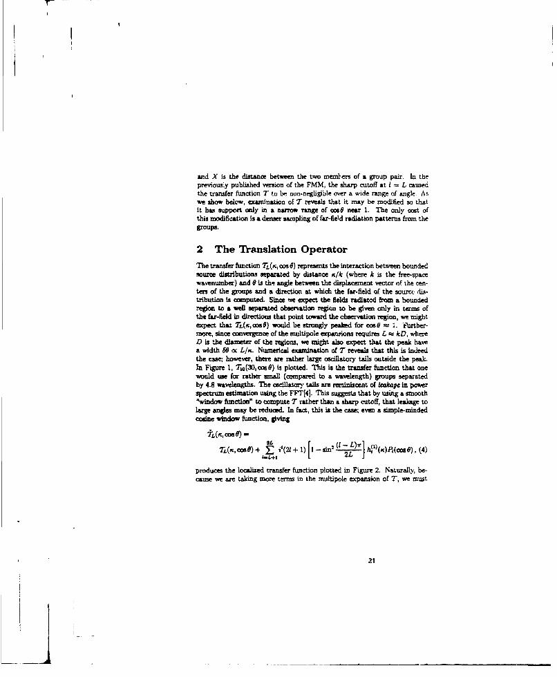
and X is the distance between the two members of a group pair. In thepreviously published version of the FMM, the sharp cutoff at I - L causedthe transfer function T to be non-negligible over a wide range of angle. Aswe show below, examination of T reveals that it may be modified so thatit has support only in a narrow range of cooa near 1. The only cost ofthis modification is a denser sampling of far-field radiation patterns from thegroups.

2 The Translation Operator

The transfer function TL(n, cos 0) represents the interaction between boundedsource distributions separated by distance r/k (where k is the free-spacewavenumber) and 8 is the angle between the displacement vector of the cen-ten of the groups and a direction at which the far-field of the sourcf. dis-tribution is computed. Since we expect the fields radiated from a bounded-egion to a well separated observation region to be given only in terms ofthe far-fied in directions that point toward the observation region, we mightexpect that TL(r,cosg) would be strongly peaked for cos0 _- 1. Furtber-more, since convergence of the multipole expanrions requires L _ kD, whereD is the diameter of the regions, we might also expect that the peak havea width M cc L/ur. Numerical examination of T reveals that this is indeedthe cam; however, there are rather large oscillatory tails outside the peak.In Figure 1, Tic(30,cos0) is plotted. This is the transfer function that onewould uae for rather small (compared to a wavelength) groups separatedby 4.8 wavelengths. The osdIlatory tails are reminiscent of leakage in powerspectrum estimation using the FFT[4]. This suggests that by using a smooth'window ftmction" to compute T rather than a sharp cutoff, that leakage tolarge angles may be reduced. In fact, this is the cawe even a simple-mindedcosine window function, giving

tl(f;,Cosa) =

produces the localized transfer function plotted in Figure 2. Naturally, be-cause we are taking more terms in the multipole expansion of T, we must

21

3

2

2

Figure 1: a d i nary parts of transfer function T of oos 6 for L = 10,- 30.

21

1.3

-1

Figure 2: Real and imaginary parts of the localized transfer function 7 ofcoe for L - 10, ic .30.

22

sample the far fields in a denser set of directions apprpriste to a quadraturerule for spherical integrations exnact for a larger set of spherical harmonics.The trigonometric window function an Eq. (4) is only ibr purposes. of illus-tration; more efficient windows should be used in practice.

3 Complexity Reduction

A detailed analysis, to be published elsewhere, reveal that the window func-tion ofI ca be csen to miatmis the support in soid angle of T. Thisanalysis confirms the intuitto, implied bove, that the solid angle of sup-port of the resulting transfer function is about ir(kD) 2/(4,C2), where D isthe diameter of the groups. In the 0 (N30) i'MM, the operation count ofthe translation operator application is ox KM2 , where M is the number ofgroups and K is the number of far-field directions tabulated. It might nowseen that W ctmt should be multiplied by a factor cK (kD)1/(4,i2) o IIM,giving a total count x (K/M)M' cx N, which is independent of M. Tl•zis incorrect, however, because it implies ahat by decresaing the size of thegroups that the number of dizectiom at which the far-field is used can bereduced without limit. Actually, since we must know the fax-field of eachgroup in at least one direction for each other group, the number of directionsmust go to a constant for very small groups. The total operation count forapplication of the translation operas is thus (bN/MU -+ c) MI , where b andc are implementation dependent constants. (Actually, a mcre caseful analysisgives a factor of In M in the b term, but it has no effect on the behavior forlarge N.) Minimizing the sum nf this with the operation count for the othersteps in the FMM (aN'/M, where a is another constant), one sees that, forlarge problems, b is inelevant, and the total operation count is minimized by

M- , (5)

so that the totw operation count is 0 (N'13). For smaller problems, wherethe c term does not dominate, the operation count varies roughly as N In N.

23

References

[1] V. Rokhlin, "Rapid solution of integral equations of scattering theoryin two dir i ," Journal of Computatoai' Physics, 86(2):414-439,1990.

[21 IL Coifman, V. Rokhlin, and S. Wandcira, The fast multipole method:A pedestrian prscmription," IEEE Antennas and Propagation Society#Magazner 35(3):7-12, June 1993.

t3] V. Rokhlin, IDiagonal form of translation operators for the Helmholtzequation in thre dimension," Applied and Computat~onal HarmonicAnal ass, l(1):82-*3, Deember 1993.

14] W. H. Press, B. P. Flannery, S. Teukolsky, and W. T. Vetterling, Numer-ial Reipes - The Art of Sdcentific Computig, Cambridge UriversityPres, Cambridge, 1986.

24

An Optimal Incident Pulse for Scattering Problems

GaEcoFY A. KRIEGSMA.NN AND JONATHAtr H. C. LUKE

Department of MathematicsCenter for A.pplied Mathematics and Statistics

New Jersey Institute of TechralogyUniversity HeightiNewark, NJ 07102

Abst.rat. Numerical computation of the field scattered from & body in t6w dimensions due to anincident plaits pressure pule is considered. Is particular, we eitamiae the proea. of inferring thescattered field due to one incident pulse given the scastered field due to another incidentt pudie. Theobjeetire is to develop an i-sdirect method that avoids the potentially expneive direct molutiun ofthe pmblem. Our approach is based on a formula expressing the scattered field as a convoluti.n ofa kernel with the incident pulse profile. The most straight forward gzneralizttion of this formula tothe discrete version of the scatter problem used in numerical romputsztions does not allow the kernelto be iferred from a single numerical esptriment-u difficulty we call the "muti.s ce probleit.preprocesing the inetlernt pulss using simple intepolatior, formulas overcomes the multi-sourctproblem giving an exctt algorithm far computing the kernel. Selection of a shsrp incident pulse(the Kronecker pulse) for the primary numerical experiment wures stability of this algorithm andpermits extremely accurate prediction of the scattered fields for secondsry incident puhles.

I. Introduction

In a recent paper [1] we presented a numerical algorithm which efficiently computes the scat-tering of plane incident pulses from a compact, impenetrable target. Assuming only that thenumerical scheme used tu solve the wave equation was linear, causal, and time invariant, wededuced an expression for the scat.tered field at a point as a ,iite convolution of the timedependent boundary dota and the scattering kernel. The later is unknown in general and rep-resents the scattering response of the target to an incident plane delta function. Our algorithmis essentially a constructive way of approximating this kernel: We sCmply run one numericalexperiament and record the response. The incident wave for this simulation is the Kroneckerpulse, which is only aonzero at one Orid point, and the response is our approximation to thekernel. We then convolve the apuroximation to the kernel with an incident pulse to determinetin scattered field.

We -elerred [11 to the Imronecker pulse as optimal because it affords us the simplest way ofapproximating the scattering kernel. Here we consider the &lgorithin from a slightly differentpoint of view; we study the response of the continuous system, K6, to this incident pulse andestimate its deviation from the scattering kernel. Specifically, we study the difference betweenthe field produced by convolving an incident pulse with K 6 and the exact scattered field.

This work was supported by the Air Force Office of Scientific Research under Grant No. AFOSR 91.02S2 andby the Office of Naval Research under Grant N000n 4-92-J-1261

25

IL The Scattering Kernel KRx. t)

For the sake of simplicity, we consider only two dimensional scattering problems for ths waveequation and assume that the target is convex and sound hard (or TM), although our analysiscan be be generalized in the obvious manner. We therefore consider the following scatteringproblem:

a2t, 8V 81vz-- -2 + , xED, t>0

(ib) v = -u,,_(t-k,*.-x), XES, t >0

(iC) V(x,0) = v,(x,0) s o1here u•,. is the incident pulse, v is the scattered pu.se. D is the scatterer and S is its boundar.;.and k,-. is the unit vector in the direction of the incident pulse. The scattered field v is alsooutgoing at on. The quantities in (1) are dimensionless; the spatial variables have been scaledwith repect to a characteristic length. L. of the target. the time with respect to Lic where cis the speed of sound (light) in D. and v and u,ne with respect to the maximum of the incidentpulse.

Taking the fourier transform of (1), denoting transformed quantities with hats., and taksnguw to be the transform variable we obtain

(2a) + Bt = , xECD

(2b) C = -E2,,d.)e'k'''. x E S

(2c) ii, + - ~ 0. r co.

The solution of (2) in principle is given by

(3a) Z =k'.

(3b) A ~ x'we'' s

where G is the peena function and ds' is the differential nrc length along S.E we take the special incident field u,- 4 = Sit - k- . -xi then 0i,. =- I and F- j is the

fourier transform of the scattered field produced an incident plane delta fanction. Its inversetransform K(x, t. kj.4 ) is the scattering kernel of the target. Applying the convolution theoremto (3) we obtain

(4) t' = Ktxt.k,.n)i(t - r)dr-

which shows that the scattered field for any incident pulse can be determined from the t~rgct'srespnnse to an incident delta function. Equation (4) is the continuous version of our discreteconvolution described in Reference 1.

26

11. The Approximate Scattering Kernel K(x,t)j

We begin by defining the triangular function u6 given by

(5a) US(t) = 0. t < -h

(5b) u(t) = (h + t)/hO, -h < t < 0

(Se) u 6(t) = (h - t)/hl, 0 < t < h

(Sd) ud(t) i O. t > -h

where h is a small positive number. The function deli ed in (5) is propo.tional to the line-s.inte' polation of the Kronecker function that we used it, our algorithm [11. In that contret hwas the mesh size and our interpolatior was h times bigger than u4.

If we take our incident pulse to be u,_, = us(t - k.,. -x) and denote by K6 the correspondingscattered field, then it follows from (4) that

(6)K6(x't) K(x r. k,.,)us(t -

Since u6 is a simple approximation to a delta function, it see"as plausible that K - K6 as h - 0.This would then suggest in light of (4) that given aay incident pulse, the produced scatteredfield is apptoximately given by

(7) Vt .C6(x, t. k,nc)"in(t -r)d.

This is the continuous version of the discrete result presented in Reference 1.Denoting by E the difference between the approximate and exact scattered fields given by

(7) and (4), msepectively, we find that

(Sa) = ui(t - r)J(r) dr

(sb) J = K(7) - K,(r)

where the dependence of the functions on x and k,,_ has been omitted for notational conve-nience. Thus, the error depends on the difference function J which according to (6) becomes

(9) J)i ' K(7) - K(p)ui(T - p) dp.

17

T ,

Since us approximates the delta function, it is clear that J -. 0 as h - 0. The question wemust the,,efore rcddresu is: how small is J fo, a fixed h?

One possible way of addressing this question goes along the following lines. Using the defini-tion of ff. the evenness of k, the convolution theorem, arid the explicit fourier transiorrm of uzwe rewrite (9) as

(10) 3(r) 3.j d -

The ability of the funutian us to approximate the delta function is mirrored in this frqumncydomain result by the bracketed term which is the difference between their fourier transforms.And if h is small enougb, thi" term is quite small for a large range of ý' For example, ifwh/2 < r/10, then the bracketed term is < 0.008.

In our numerical algorithm [Il we chose h small enough to resolve the highest frequencypresent in a class of incident functions. That is. h - /7,11Fr wheie - is this maximumfrequency. Using this ordering and the observation just made about the size of the bracketedterm, we deduce the estimate

(1 )j r l •: 1 sin ( wh/2),. 11 ý) c,. . __ -,1 ~ en(,h/2)2

Assuming that w&a 1. or equivalertly h << 1. and that A: - ý'-f'0k. we integrate (11) byparts to obtain

(12) J I K siXiwMr

wLnse .&0 is independent of w anti N is a positive integer. The existence of i'o and N followfrow greens function arguments on the helwnholtz equation and boundary conditions satisfiedby- K. Finally inseriag (12) into (Sa) we obtain

(13) E -- vict

which shows that the error - 0 as h -- 0.

IV. Numerical Examples: Time Harmonic Responses

The response of a scatterer to a time harmonic incident pulse has played a major role inscattering theory for practical and theoretical reasons. Many numerical methods have beendevised to tackle this problem, each with their strengths and limitations. A technique calledthe Fiaite Difference Time Domain Method (FDTD: is a relatively straightforward and robustw-ay of computing the time harmonic scattering response of a target (2-51. The time dependent

28

equations with a time periodic incident wave are solved using an explicit finite difference scheme.According to the limiting amplitude principle [6], the solution of the time dependent problemwill approach a time harmonic state as long as no trapped modes are present (and this iscertainly the case for compact targets). And if the explic.it finite difference scheme and non-reflecting boundary condition are carefully chosen then the numerical results will give a goodapproximation to the time harmonic response. The rate at which the solution evolves into thetime harmonic response depends upon the target shape and the polarization of the incident wave.For example, it was observed [4) that rate for sound hard (TE) targets is smaller than the ratefor a soft (TM) target. Morsover, if the target shape encouragen local energy confinemen. (e.g.,a Helmholtz Resonator), then the rate can also be quite small [5]. Thus, the FDTD method maybecome prohibitively time consuming if the target is complex and if many frequency responsesare required.

The method, presented in [I( and embodied in the discrete version of (7), may give a moreeconomical approach than the FDTD for complex targets whxere the frequency response is re-quired over a broad spectrum, 0!. Our algorithm proceeds as follows. We first use a finitedifference scheme to solve (1) for the incident pulse u#. The temporal time step h is chosen toresolve the highest frequency present in f2 and the spatial step size is chosen to satisfy the CFLcondition [7]. If the differential cross sections for different frequencies in 0 are required, thenwe save the response K6 on a large circle of radius R enclosing the compact target S. Next, wechoose our incident field to be the complex stepped sine wave

(14) u-,, = exp(-iwct)H(t)

where H(t) is the Heaviside furction and wc E f?. Then we convolve this function %ith Kaaccording to the discreete version of (7): the imaginary part of v will be the approximate response

of the target to a stepped sine wave incident pulse. Finally. we compute the convolution in (7)until v(x, t) becomes time harmonic. The amplitude of v is the differential cross section of thescatterer, A(dc,wc). This process is then continued for those frequencies of interest in thespectrum 01.

To illustrate tie process outlined above, we determine the amplitude of the surface currentson a target in the harmonic steady state from the response to an incident Kronecker pulse. Forsimplicity our tar-,et is a circle of normalized radius one. We consider several wave numbersk - 5,8,10 to illustrate that the harmonic response for many frequencies can be obtainedfrom a single computation of the response to a Kronecker pouse. The amplitude of the surfacecurreats is shown for the three wave numbers in Figure 1. The response to the Kronecker pulseis computed using the standard explicit centered difference method in polar coordinates withAr = 0.025, At - 0.0025. A& = 2,/128 t 0.0491, 2000 time steps and an absorbing boundaryat r-- 20.

Because the 'urface currents are obtained by evaluating the convolution in our method ata single large time and because computing the convolution involves only data on the surfaceof the target (rather than the fields throughout the computational domain) the computationaleffort required to obtain the surface currents from the Kronecker scattering results is many

29

orders of magnitude less than the time needed to find the harmonic response directly withFDTD. Obtaining the scattering results for the Kronecker pulse is relatively expensive, butthe computational cost is essentially equal to that of obtaining the harmonic response directlywith FDTD for a .ingle frequency. Thus. our approach gives the harmonic response for arange of frequencies for essentially the same cost as determining the harmonic response forone fiequency using FDTD directly. The surface currents shown in Figure I contain small butnoticeable errors. But these errors are no larger than then the errors suffered if FDTD is useddirectly. In fact, to machine accuracy the errors are the same. That is. our method predictsthe surfaces cmuents given by the FDTD method exactly including any error inherent in themethod.

References

[i] G. A. Kriegsman• and J. H. C. Luke. Journ. Comp. Physics. in press.[2] K. S. Yee, IEEE Trans. Ant and Prop. 14. 402-412 (1968).[3] A. Tahove and M. Brodwin. IEEE Trans. Microwave Theory 23, 888-896 (197C).[4] G. A. Kriegamana and C. S. Morawetz. SIAM Journ. Scientific and Statistical Computing

1, 371-385 (1980).[5] A. Taflove and K. Umashanhz. IEEE Trans. Electromagnetic Compatability 25. 433-440

(1983).[6] C. S. Morawetz. Comm. Pure and Applied Math. 18. 349-361 (19%2).[7] R. D. Richtmeyer and K. W. Morton, "Difference Methods for Initia" Value Problems".

Wiley Interscience, New York. 1967.

30

0

SIn

E ,;OG

0")C c,

CDC

0.

lCCDI3

Numerical Solution of the High FrequencyAsymptotic Expansion for Hyperbolic Equations

Bjorn EngquistEmad FatemiStanley Osher

Department of MathematicsUniversity of California, Los Angeles

Los Angeles, CA 90024

1 Introduction

The computation of high frequency electromagneLic waves is of paramount importance for calcula-tion of reflection of radar waves from objects and radar radiation patterns. The direct calculationof the high frequLncy waves is not practical since the wavelength of the radiation is usually quitesmall compared to the size of the ohysical objects of interest. Therefore approximate methodshave been extensively used for this type of calculations. On-. of the more successful Approximatemethjd. ii the generalized theory of diffraction. This method relies on a high frequency asymp-totic expansion of the wave equation and considers special diffracted waves from the singularitiespresent in the media and the shape of the reflecting objects. We shall r-fer to these singularitiesthat are surfaces, lines, or points as branch manifolds. Recently we have developed numericalmethods for solving the partial differential equations obtained by considering the high frequencyasymptotic expansion of the scalar wave equation. We expect these to replace ray-tracing meth-ods for many high frequency calculations and they are applicable directly for the calculation ofelectromagnetic waves.

Maxwell's equations for the electric and magnetic f£elds in an isotropic homogeneous materialcan be written as:

(cE), = cVxH -4rJ (1)

(uh'), VXE (2)

V (eE) - 4rp (3)

V. (•,H) = 0 (4)

32

where £ is the electric field. H is the isagnetic field, S is the c~urrent, p is the charge density, c is

the speed of light in the medium, and p anid are rts.,-ctively electric permittivity and magnericpe-meability. For electromagnetic waves the equations can be written as:

Ell 0 •VIE (5)

L!, !ý VI H(6)CP

These are, of course, wave equations for the E and H vectors.Special time harmonic high frequency solutions of the Maxwell's equation3 can be obtalneCý bv

arsuming solutions of thm form,

E = e(x)e'k*Xl,H = h(x)esk(X)

where t Tunction is the phase of the wave, and k is the frequency of the wave. These so) k'-correspond to a high frequency plane wave and are of important practical significance. 0"% -show that the phase satisfies an eikonal equation (81,

(V.)2 = ( (7

The eikonal equation is a first order nonlinear PDE. a Hamilton Jacobi type equation. The eikonal•,quation can be considered as the Hamilton-Jacobi equation for the variational problem based onFermat's principle [8]. The usual practice has been to solve the eikonal equation by ray.tracingmethods. Ray-tracing in this context is nothing but solving the eikonal equation using the methodof characteristics for PDE's. Our approach relies on a direct discretization of tite eikonal equationusing the recently developed numericMl me'hods for Hamilton-Jacobi equations [11.

2 Asymptotic expansion for the scalar wave equation

To develop the numerical methods we have started from the scalar wave equation in two dimen-sional space. The numerical methods developed for ihis problem are applicable to the Maxwell'sequations.

U"~ = C2 zýu= c5(x' )(U_ + iý)(8

x and y are the spatial variables, t is time. u is the amplitude oi the wave, and c(x,y) is thespeed of the wave in the medium. High frequency solutions of the scalar wave equation can beapproximated by an asymptotic expansion as introduced by Lunehurg, Kline. and Keller F9). [(0,1111. The asymptotic expansion to the wave e4, Ation is obtained by expanding the solution inpowers of w&- in an infinite series. The expansion is substituted in the wave equation and thesequence of the coefficients of w-' are collected and set to zero. This procedure produces an infinitesystem of nonlinear partial differential equations, that, together with the boundary conditions,determine the expansion. The first term and the most important term of the expansion is the

33

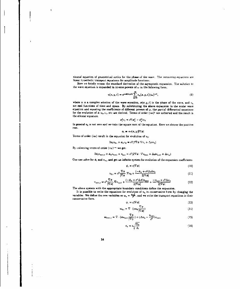
eikonal equation of geometrical optics for the phase of the wave. The remaining equations are5lnear hyperbolic transport equations for amplitude functions.

Here we briefly repeat the standard derivation of the asymptotic expansion. The solution tothe wave equation is expanded in inverse powers of w in the following form,

U(z, , t) = C"*-) r,(,vt)(w)- Y (90

where u is a complex sojution of the wave equation, 0(zyt) is the phase of the wave, and v,are real fun.:tions of time and space. By substituting the above expansion in the scalar waveequation and equating the coefficients of different powees of w, the partial differential equationsfor the evolution of 0, v0 , v1 , etc are derived. Terms of order (iw) 2

are collected and the result isthe eikonal equation.

In general vo is not zero and we take the square root of ýhe equation. Here we choose the positiveroot.

6, =f +c(-,v)lV70Terms of order (iw) rerult in the equation for evolution of v0.

2ov.., + o,,v = c2(2Vd.Vu + Aov0)

By collecting terms of order (?w)-" we get:

20,v.+,., + ,Ov,•+ + v,,, = c2(2V7• - 7v.+ + Akv,+ + AV,)

One can solve for 6, and v., and get am infinite systemn for evolution of the expansion coefficients.

0, = ClVOl (10)

= V (-6." +.•A•+)V()t j.=al"-V o+ 21v'ýj

+" (-0" + C2

A6)v,,+' -Vti + c2av, (12)

21V.pl 21Vi+

The above system with the appropriate boundary conditions define the expansion.It is possible to write the equations for evolution of v. in conservative fh)rm by changing the

variables. We define the new variables as tw, -v and we write the transport equations in theirconservative form.

0!, = ClVOI (]3)

o,, = 7 (C-0 7,0 (14)

",,Lv.+ = • (ct,,+l + tAx•', - (5

, C -- (16)

34

The above formulation of the equations seems to be natural, based on our experience with con-servation laws.

The eikonal equation for the phase is a Hamilton-Jacobi type oquation. The equations forthe variables w. form a hyperbolic system. The system is essentially decoupled, since it can betruncated at any level. The first equation, the eikonal equation, can be solved independent ofthe others. After we compute it, we use it to solve for w0. Similarly w. is solved using the oand w,_.- The equation for w. has a forcing term (Av. - t!OL) which has to be calculated fromthe previous term, w..I. If the previous term w..I is n'ot twice differentiable in space and time,the forcing term is ambiguous. From a numerical point of view, even for smooth solutions, itis important to calculate the forcing term correctly, otherwise error would spread out to higherorder terms. The ambiguity in the forcing terms could be meolved by specifying jump conditionsalong discontinuities of v.. The proper conditions depend on physical considerations as wellas rmathematical arguments and we plan to determine them for important physical applications-Continuity of the phase across branch surfaces supplies us with the necessary boundary conditionsfor multivalued solutions of the phase. The situation is more complicated for the computation ofv,•. For example the amount of reflected energy from a reflecting surface depends on the physicalcharacteristics of the surface. The situation is more complex for other kinds of branch manifoldssuch as corners and jumps in higher order derivatives. This question of the proper boundaryconditions needs to be solved for a variety of important cases, including discontinuities in theindex of refraction and singularities in the shape of objects.

3 Numerical algorithm

The traditional way of solving the eikonal equation is by the method of characteristics, which, inthis context is called ray tracing [131. We apply the modern high resolution algorithms to directlycompute the eikonal equation ind the other equations defining the terms in the expansion. Thesemodern techniques allow for accurate representation of singularities, which is essential in thisapplication. The standard viscosity solution oi the eikonal equation, [121, is not enough andan hierarchy of numerical solutions has to be generated. These new functions represent themultivalued character of the solution and are based on singularity detection.

Our numerical algorithm was developed based on the recently devised numerical methods for

Hamilton-Jacobi type equations and high order accurate, nouoscillatory methods for hyperbolicequations. We have developed numerical algorithms to solve the equations both in conservative

and nonconservative variables. We have abandoned non-conservative variables in favor of con-

servative variables. From a numerical and also theoretical point of view it is the natural way of

writing the equations. We have only considered the first three equations of the infinite system for

o. w0 , and w•, but the methods are easily applicable to an arbitrary number of terms. After the

third equation the equations are exactly the same, so even the same subroutine could be used tosolve them. The equations to be discretized are,

,= CIVOI (17)V•b

Wo= - (c0o") (18)

35

I -

(cwsj-j) - cvf-- I-,"9

W! use third order ENO interpolation and a Godunov type numerical Hasmiltonian to solve theeikonal equation (iI. For solving the transport equaticons a first order upwind scheme is used. Inprinciple, various sophisticated schemes developed for nonlinear conservation laws could be usedto solve the transport equations. At this stage a first order scheme was sufficient.

4 Numerical examples

The reflection of high frequency waves from solid objects is an important problem.In the firstexample we consider the reflection of a source off a sphere. We on!y have calculated the phasehere, but the full solution of this problem will be an essential part of our future work. Animportant problem for calculation of phase is computing multi-valued solutions to the eikonalequation. Usually the multi-valued nature of the solution is known a prsore, such as in case ofreflection and branch manifolds due to singularities in the index of refraction. Nevertheless thereare branch manifolds that are not known a prion, such as the second example that we haveconsidered here. Only after the solution to the eikonal equation is computed brarich manifoldsare found. Wz have designed a numerical procedure to do that automatically. The last examplecorresponds to propagation of a planar wave through a non-uniform media, in particular. a lens.

We consider the reflection of an incident wave off a sphere. This problem has all the featuresof reflection of high frequency waves off a convex object in a uniform medium. We consider asphere of radius one at the origin. The source of the wave is at point (0, 0, 2). We use sphericalcoordinates and exploit the symmetry of the problem tnder rotation around the z axis. Theeikonai equation in (r, 0) space is written as

= + . (20)

We solve an eikonal equation for the incident problem and an eikonal equation for the reflectedproblem. The two equations r.xe coupled only at the surface of reflection through the boundaryconditions. The physical problem is posed in all of R3 but our computational domain is (1, 3] x[-.r, r]. The computed solution is shown in figure 1. The viscosity solution of the eikonal equationc;lculates the incident and the reflected waves accurately, also it produces the phase in the shadowregion of the sphere.

In a nonuniform media, the solution of the eikonal equation in general develops singularities.These singularities are generated when two wave fronts approach each other. The solution ofthe eikonal equation in that case becomes multivalued. But the viscosity solution of the eikonalequation only chooses one branch of the solution (conjectured to be the first wave that reachesthat point). A numerical procedure was .levised to recover the multi-valued solutions. When asolution becomes multivalued a discontinuity in the giadient of the phase appears. We detect thisaiscontinuity and use the phase at that point as boundary conditions for creating the next sheet

36

ot the solution. Using the terminology from complex analysis, the discontinuities in the gradientof the phase are branch cuts. Tbe other branch cuts are the singularities in the index of refractionand the shape of the boundary. In figure two we show a generic situation where two sources arepresent ana the solution is double-valued a•ter the two waves reach other. We have superimposedthe two solutions on top of each other.

In the next example we show the conputLed phase and amplitude for a convex lens (figure 3).The lens is implemented by taking a smooth change of index of refraction in the middle of thecomputational domain. The bending of the incident planer wave creates a shock starting fromthe focal point. The amplitude of the wave is calculated. The amplitude has a singularity 31,the shock, since it has to be ronnected to the sond sheet of the solution(not done here). Theproper bour•dary conditions for the amplitude coefficients is an important question that needs tobe investigated for these applications.

5 Additional Proposed Effort

We first plan to compute problems for which the index of refraction has a known spatial disconti-nuity. This is fairly routine and amounts to solving an initial-boundary problem for a Hamilton-Jacobi equation.

Next, we plan to investigate appropriate boundary conditions at corners for the eikonal equa-tion. This is well studied. We anticipate no difficulties with the nume:ical implersentation.

An additional speculative idea involves 'cap•uring" multivilued solutions to Hamilton-Jacobiequations directly. This haa been done in one space dimension (for conservation laws. but thereis an equivalence h-.re) by Professor Yann Brenier 116]. He uses moments of the classic&l Vlasovequation in ,% original and ingenious fashion to arrive at a system o' conservation laws whichgive the different branches of the multivalued solution. An extension to multidimensions seemsdifficult, but will be investigated. This would automate the code and remove the shock detectionstep, if successful.

Another. simpler idea is to use polar coordinates in some problems and just to allow the 8dependency to be nonperiodic. This is very promising and will be explored.

After the direct algorithm matures we expect to use it " a tool for solving the inverse ?rob-lem, i.e. fi.ndig the index of refraction given a certain number of measurements. Opimisationtechniques e.g. those described in (14], (15] can be modified anuJ adapted using our fast directsolvers.

Finally, we expect to extend these results to a full Maxwell's equation situation. Numericaltechniques borrowed from the conservation law community such as space marching, the use ofbody fitted coordinates &nd artificial compression shall be incorporated in the resulting package.

References

1] S. Osher and C. W Siu. High order esseiitiall iuun-,.r•ilaly schemes fur H'amiltum-Juia iequations, SIAM J. Numer. Analysis. Vol. 28. (1991). pp. 907-927ý

37

12] Rt. N. Buchul and J. B. Keller, Boundary laver problems in diffraction theor., Communicationson Pure and Applied Mathematics. XIII (1960), 85-114.

[3] H. Hochst4xit, Asymptotic formulas for diffraction by parabolic surfaces, Communications inPurr and Applied Mathematics, X (1957), 311-329.

[4] D. Ludwig, Uniform asymptotic expansions at a caustic, Communications or. Purl and AppliedMathematics, XIX (1966), 215-250.

[5] P. D. Lax, Asymptotic solutions of oscillatory initial value problems, Duke Math J., Vol 24,(1957), pp. 627-646.

(61 C. Morawetz and D. Ludwig, An inequality -,'or the reduced wave operator and the justificationof geometrical optics. Communications on Pure and Applied Mathematics, XXI. (1968). 187-203.

[71 G. Avila and J. B. Keller, The high frequency asymptotic field of a point source in an inborno-

geneoui medium, Communications on Pure and Applied Mathematics, XVI, (1963). 363-38].

(8) M. Born and E. Wolf, Principles of Optics. Pergamon Press, sixth edition, 1989.

[91 RL Luneburg, Mathematical theory of optics, University of California press. 1964.

[10] J. B. Keller, R. Lewis, and B. Seckler, Asymptotic solution of some diffraction problems.Communications on Pure and Applied Mathematics, IX, (1965), 207-265.

"111] J. IB. FeUcr,A. Geometrical Theory of Diffraction, Caiculus o* variations and its Applications,McGraw-Hill, New York, 1958, p. 27.

[121 M. Crandtll and F. Lions, Viscosity solutions of Hamilton-Jacobi equations, Trans. Amer.

Math. Sor., 277, (1903,, pp 1-42.

[13] C 11. Chapman. Ray theory and its extensions:WKBJ and Maslov se.sinograms. Journal of

Geophysics. Vol. 58, (1985). pp. 27-43.

[14] F. Santosa and W. W. Symes, '.inear inversion of band limited reflection seismograms, SIAM

J. ;'ci. Stat. Comput., Vol. 7, (1986), pp. 1307-1330.

[151 F. Santos& and W. W. Symes, Reconstruction of blocky impedance profiles from normalincidence reflection seismograms which are band-limited and miscalibrated. Wave motion,Vol. 10, (1988), pp. 209-230.

(161 Y. Brenier, MWltivalued solutions can be captured. UCLA internal report. (1993).

38

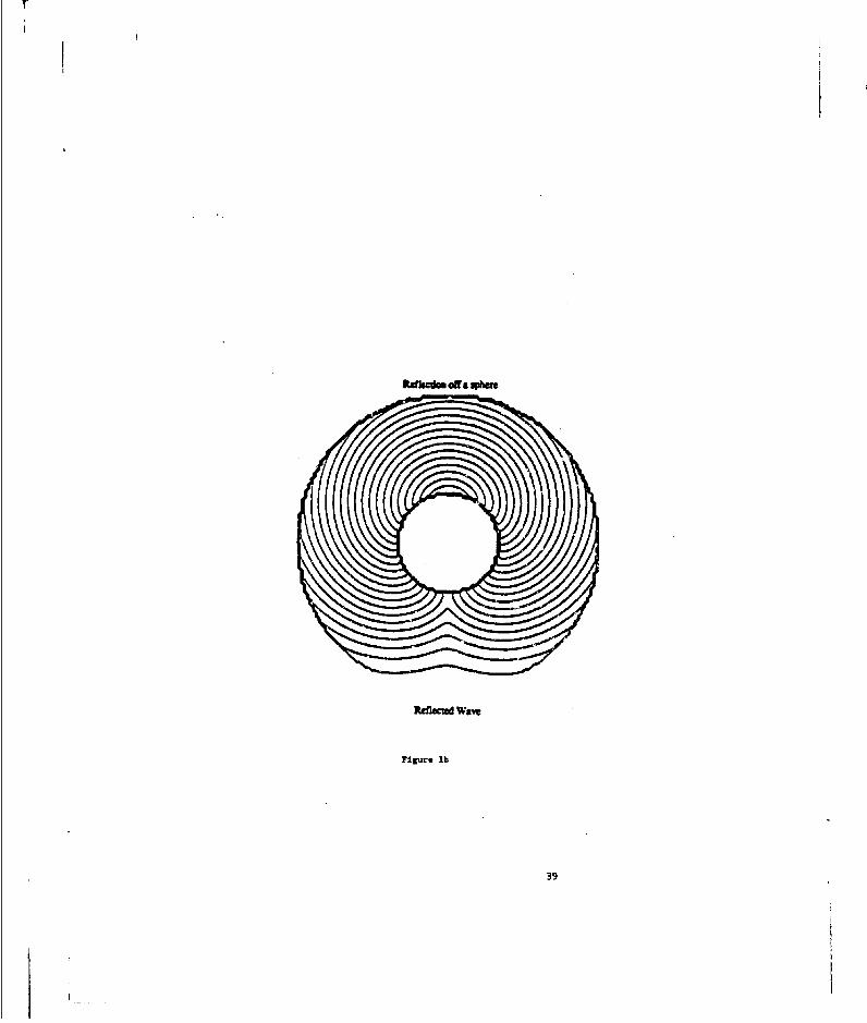
Rdlscdam off a sp

Reflacid Ways

Figure lb

39

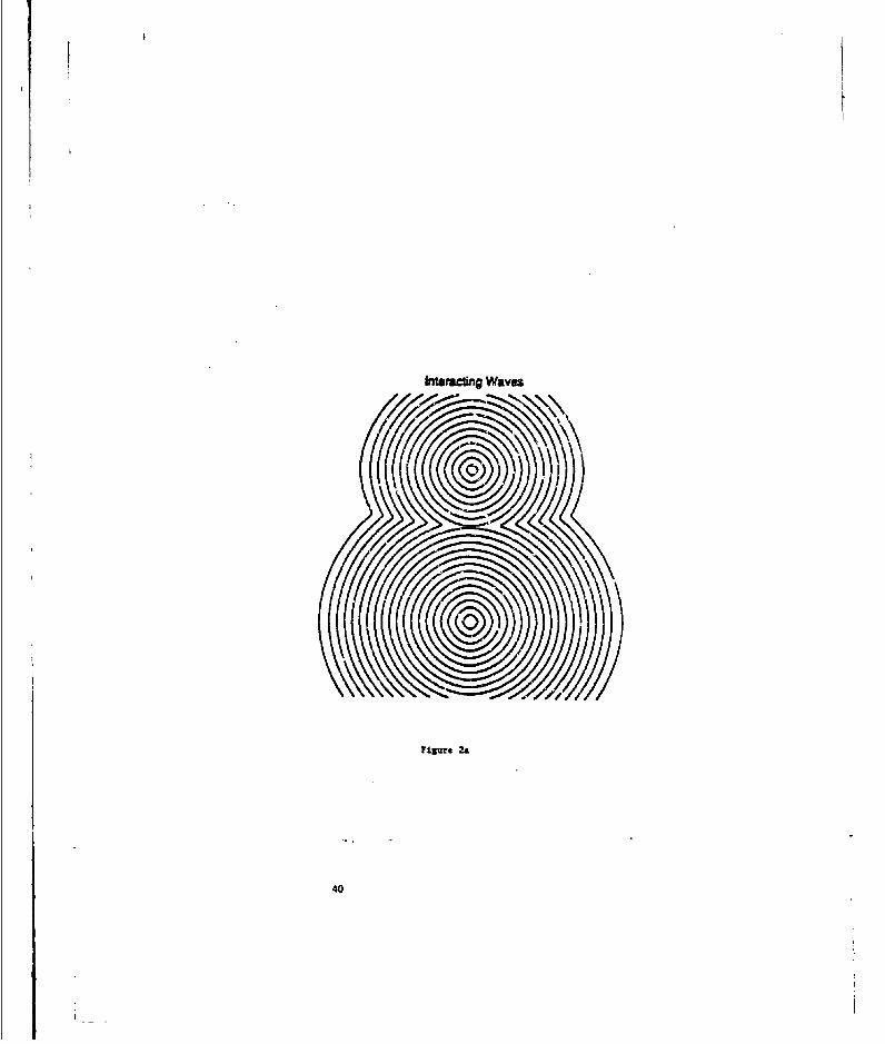
Interactina Waves

Figure 2a

40

Hidden Waves

F1guars 2b

41

PHASE

F igure 3&

42

VO AMPLITUDE

8

so60 so 80 00

40 so

20 20 40

Time= 3

rtgu4e 3b

43

44

A new technique for synthesis of offset dual reflectorsystems*

Vladimir Olikert

Department of Mathematics and Computer Science

Emory University, Atlanta, Georgia 30322

and

Laird D. Prussner

Matis, Inc., 120 Parkwood Lane, Decatur, Georgia 30030

1 Introduction

In electromagnetics the geometric optics (GO) apnroximation is used to describe offset single and dualreflector antennas when it is required to control the energy pattern and/or phase on the output apertureand at the same time minimize energy losses due to spillovers, blockage, etc. [11. Similarly, in optics, GOis used to describe systems with one. two, or more specular refletors that are required to transform aninput Gaussian laser beam into a uniform output irradiance front and at the same time optimize certasidesign parameters (2].

The differential form of the energy conservation law for such systems !eads to an equation for theJacobian determinant of the map derived by ray tracing the energy wavefront. If a quasi-potential can beassociate4 with this map then one usually arrives at an -quation of Monge-Ampore type that this quasi-potentia' must satisfy (cf. [31, [4), [5]). The same type of equation arises in a number of other applications:for example, in inverse diffraction, nondestructive evalution, allocation of resources [6[. During the last15 years there has been a surge in mathematical studies regarding theoretical solvability of equatuionsof Monge-Ampire type and their generalizations. Still, the theory is far from being complete.

The purpose of this note is to report several results on synthesis of dual reflector systems. We discusshere unly specular reflector systems with two reflectors and energy source which is a collimator. For suchsystems we present here a second order partial differentizI equation of Monge-Amplre type expressing theray tracing map and the energy conservation law. Rigorous results concerning existence and uniqursessof solutions to the resulting prmblem are established. A detailed exposition of these results is beyond thescope of this paper and will appear elsew here.

The numerical solution of the resulting equation and the generation of the surface points of the tworeflectors is done with a specially developed software package REFSYS. The algorithms are based on our

"Tha " ..n .. rpoptcI by AJOS$t uP&I -. 4tcaL f4%20-52.C-O09. T•. Uited Sit.t Go.eiawet i -aoito repeoduce and drrtibate reprints for governmental ppomee aotwitkssasdieg any copyright notssion hern.

'AlMs wish MNs. Inc.. 120 Parktwod Lne. D.atur. Georgia 30030.

45

earlier paper [7], though substantial modifications were required. Using REFSYS we can synthesize asystem with two refiettors which redirects and reshapes a plane wave front and, at the same time, thenystes, transforms the energ' pattern of the input beam into a uniform (or any other. desired) energy

distribution pattern across the frrnt of the output beam. For example, our technique allows to designa two-reflector system which will transform an arbitrary ecliptic input beam into an output beam withprespecified elliptical (rectangular. or gernsi polygonal) shape. Blockage is completely avoided. Theresulting reflectors are aspherical but convex, which is a substantial improvement over an earlier design

of Malyak [2]. In general, the reflector surfa.es are not radially syrnmetric, We illustrate the techniqueby presenting designs of two dual reflector systems converting a circular Gaussian beam into uniformcircular and elliptic beams.

As it was already mentioned, Monge-Ampore equations arise in a variety of other physical problems.and we expect that our technique will apply to such problems. Inquiries regarding concrete applicationsare we'come.

2 The synthesis equations

2.1. The configuration of the system is shown schematically on Fig.1, We denote by a the plane 0and by 0 the croes section of the incoming beam I by that plane. In order to emphasize that the shapeof the incoming beam is not requlred to be circular, on the figure, we draw 0 as an ellipse. In general,

it is allowe to be any bounded convex domain. It is assnmed that the rays of the incoming beam Iform a plane wavefront propagating in the positive direction k of the z axis. The input radiation patternis given as a nonnegative function f(X, y), (z,y) E fl. The desired characteristics of the system are as

fy - unpsa beamV V

0 - second misror T- output beam

Figure 1:

follows.

The output wa'efront III is req~ured to form a plane wave propagating IL the same direction k as

the incoming beam.

46

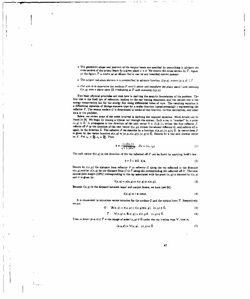
-7--

"* The geometric shape and position of the output beam are specified by prescribing in advance thecross section of the output beam by a given plane z = d. We denote this cross section by T. Again,on the figure, T is drawn a& an eUipse, but it can be any bounded convex domain.

"* The output radiation pattern is a prespecified in advance function L(p. q). where (p. q. d) T"

"* Our aim is to determine the surfaces F and G which will transform the plane wave I with intensityI(z, V) into a plane wave III irradiating at 2' with intensity L(p,q).

Two basic physical principles are used here in deriving the analytic formulation of the problem. Thefirst one is the Snail law of reflection, leading to the ray tracing equations, and the second one is theenergy conservation law for the energy flux along differential tubes of rays. The resulting equation isa differential equation of Monge-Ampere type for a scalar function (quasi-potential) z representing thereflector P. The second surface G is determined in terms of this function, its first derivatives, &ad otherda•A in the problem,

Below, we review some of the steps involved in deriving the required equation. More details can befound in [8]. We begin by tracing a typical ray through the system. Such a ray is "marked" by a point(zy) E 1). It propgaptes in the direction of the unit vector k = (0,0.1), strikes the first reflector F.reflects off F in the direction of the unit vector 4(z, V), strikes the second reflector G, and reflects off it.again, in the direction k. The reflector F we describe by a function z(z, y), (z, V) E (2. In vector form Fis given by the vector function r(z, Y) a (z, Y,z(z,y)),(zY)) E A. Denote by fi the unit normal vectoron F. Put z, - 1,z, = L. Then

(-Dz, 1)--, Liz = (zz,). (1)

The unit vector s(z, y) in the direction of the ray reflected off F can be found by applying Snell's law.

S= k- 2(k. i)n. (2)

Denote by t(z,y) the distance from reflector F to reflector G along the ray reflected in the directions)(z, is) and let s(z, y) be the distance from G to 7' along the corresponding ray reflected off G. The totaloptical path length (OPL) corresponding to the ray associated with the point (z,y) is denoted by 4(z,Y)and it is given by

'(z,') = A(X,Y) + t(ZY) + a(Zy), (3)

Because I(z, y) is the distance between input and output fronts, we have (see 19]):

I(Z.Y) = I , €onsi. (4)

It is convenient to introduce vector notation for the surface G and the output front 1. Respectively.we put

G: R(z, y) = r(z. y) + t(z, y)sz ,y). (z, y) E (5)t : V(z,y) = R(.,V) + s(z, y) (z, y)•, C {6)

Thus, a point (p.qd) E 1t is the image of some (z,y) E 11 under the ray tracing map V, that is,

47

I.

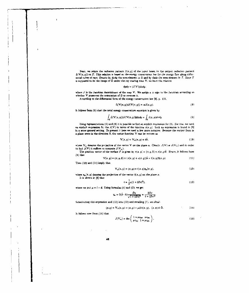
Next, we relate the radiation pattern 1(z,y) of the input beam to the output radiation patternL(V(z. y)) on T. This relation is based on the Prnorgy conservation law for the cncrgy flow along differ-entiai tubes of rays, Denote by dzdy the are" element in n and by dpdq the area element in T. Since T

is supposed to be the image of i under the ray tracing mao V, we have the relation

dpdq = I(IV)Idzdy.

where J is the Jacobian determinant of the map V. We assign a ± sign to the Jacobian according towhether V preserves the orientation of 12 or reverses it.

According to the differential form of the energy conservation law (91, p. 115,

L(V(s, y))J(V(s, y)) = ±I(z, y). (S)

It follows from (8) that the total energy conservation equation is given by

Using representations (5) and (6) it is poss~ble to find an explicit expression for (8J. For that we needan explicit eprfeWon fo: the J(V) in terms of the function t(z, y)- Such an expression is found in (8]in a more general setting. To preent it here we need a few more notation. Because the output front isa plane wave in the direction k, the vector function V can be written as

V(z, y) = Vo(z, y) k, (10)

where V. denotes the projection of the vector V on the plane a. Clearly, d(V) = 3(V 0 ) and in orderto find J(V) it suffices to compute J(Ve).

The position vector of the surface F is given by r(z, y) = (z, y, 0) + z(z, y)Ir, Hence, it follows from(6) that

V(z,V) = (Zt,,O)+ (z(x,1) + J(Zp))k + !(X, i)(zl. (1!)

Then (10) and (11) imply that

=.X'Y ~Y) + 5((Z' )s.(Xý ), (12)

where %(z. y) denotes the projection of the vector s(z, y) on the plane o,It is shown ic 181 that

I1 Ap(l + WDr[z), (13)

where we put p = I - d. Using formulas (1) and (2). we get

• Dr 2Dz

Substituting this expression and (13) into (12) and recalling (7), we obtaiur

(p,q) =V(r,1) = )(,)- QDZ(X,Y), (2, Y) El. (14)

It follows now from (14) that

J(V,)=det • Z~ l+ A Zl A

48

where z., = , and similarly z., and z,,.'laking into account (tO), (14), and suppressing the indication of dependence on the constant d in

t1he functipn L, we haveL(V) = Liz + pz.,y + uz,).

Thus, the main equation (8) assumes the following form:

L(z + OAZ., y + M')(l( + Uzr_)(1 +.UZVV) _-112,2,1 = ±-1 in f?. (1)

Dsnote by 1. the projection of the region Ton the plane a. Formula (14) shows that V0 is a map frorr.i) onto 1• and the Jacobian determinant of this map is the same as that of map V.

2.2. We perform now a transformation simplifying the equation (16). Introduce a new unknownfunction u(z, y) by setting

z,(z)=(z, ) - !(X2 + 2) + az + bz , c, (17)2

where ab,c are constants to be described in a momert. Then, in terms of function u(z. y). the map (14)assumes the form

V,(X, Y Y)(u(z, + a, u(z, ) + b) : (I - T', (18)

where u. is and u- =. •. Substituting (17) into (16), we obtain

L(u, + a,u. + b)(u.u,% - ub.) = ±1 in (1, (19)

where u, = and similarly for u. and i 1 -.Formula (18) shows that we can choose the constants a and 6 so that the map Du =- (u, u.) mapsSinto some translate 7. of t,. It is convenient to caoose these constants in ruch a way that the origin

0 of the coordinate system on a is an interior point of r.Obviously, the choice of the constant c in (17) affects neither the map (18) nor the equation (19).

That means that any function u satisfying (18) and (i9) is defined only up to a constant.2.3. The analytic formulation of the problem stated in 2.1 is now complete. We summarize it here.

"* For the given convex domain 7t determine the constants ab so that r, is a translate of T withcenter at the origin 0 of the coordinate system on the plane a (or any other translate convenientfor computations).

"* Solve the equation (19) for the function u(;,l,).

"* Assuming that M is given, and p > 0 determine the function r(z, y) from (17); the constant c canbe set equal to 0. The function z completely describes the first reflector F.

"* Using formulas (1) and (13) determine ,)r, y) and t(z,y). Then, a substitution in (5) (and alengthy calculation that we omit) gives

R(z, y)=(ue+a,uv+•6,u-zu.-yss+(l/2){[D•+A1 2tA2)), (z, 9) pE (20)

where A = (a, b). Thus, we have the parametric equations of the second reflector G.2.4. The cfitical step in the a&sove procedure is to solve the equation (19). The physically interesting

situation is the one when the + sign in the eqiations (19) is taken. We were able to investigate thisproblem completely but a full discussion is beyond the scope of this paper and will be presented elsewLere.We note only that this equation admits infinitely many solutiors leading respectively to infinitely many

49

possible designs of a two-reflector system. This feature i5 extremely useful because it allows to select asolution satisfying additionsl reuirements. Thir can be donme in a way leading to an prtimlI design Inthe test cases presented below, we construct solutions that allow to synthesize systems that convert aGaussian circular s-eamn into a uniform elliptic beam, have no blockage, and, in addition, map the centralray in the input beam into the central ray of the output beam . When the - sign is (19) is talen, theproblem can be also investigated, but by different techniques.

3 Examples

It. the examples below the inpt beam is circular with a Gaussiýn power pattern

I(r,V) = CCap(

where C is a balancing constant required to enforce the energy conservation equation (9). and a isspecified below. The crossection 0 of the input beam is given by:

fl = (z,y)Eo IaX + Y' < 9o'.

In the first example the data as the tame as in [2), Table 1, data set 1. The input beam crossection C_is a circle of radius 3a, centered at the origin (0.0), the output beam is required to have a uniform energydistribution, with circular crossection t ofrad;u' 2a,o -= .125m, and center at the point (0, 1.396m):; i"99.98050804m. The parameter p is determined from the data in 12]. The surface profile of the Y = 0cut of the first reflector F is shown on Fig. 2. Pig. 3 shows the spacial view of the first reflector, Thesurface profile of (he V = 0 cut of the second reflector G is on Fig. 4. Fig. 5 is the spacial view ofthe second reflector. It is important to note, that for the same data the design presented in [2] requireinoneonvex surface profiles with two 'humps". Our design leads to convex profiles which should be easierto manufacture.

In our second example the input beam is the Same as in the first example. The output beam is requiredto have an elliptic crossection, I, with center at (0, 1.396m), minor semiaxis 2a in the x-direction actmajor semiaxis 3a in the p-direction. The output energy distribution is required to be uniform across T.The parameter ip = 99.SO050S04m. The surface profiles and their spacial views are shown on Figures 6- 9. On all figures the measuremmnt units are meters.

a-rne o~eem.

Fig.2. First reflector. y - 0 cut. Fig.3. First reflector, side view

50

Fig.4. Second reflector, y 0 cut. Fig.5. Sccond reflector, side view.

-CfI '. w~,, , - 4.. ,a.

Fig.6. First reflector, y - 0 cut. Fig.7. •irst reflectir, side view.

FigS.. Second reflector, y - 0 cut. Fig.9, Sucond reflector, side view.

51

4 Summary

The design equations for a two-reflector system for reshaping, redirecting, and energy rediswribution ispresented. The resulting main equation is a nonlinear partial differential equation of Monge-Amperetype. Once this equation is solved, the surface data pcints of the reflectors are found by using formulaspresented here. The results of theor-tical and numerical investigation of this equation will be presentedeise shere. Using a software code REFSYS, developed by the authors, two examples of reflector syrtems.synthesized numerically, are presented. In contrast with some existing design techniques, our techniqueallows to produce noncircularly shaped output beams and uses only convex reflectors. The availabilityof convex reflectors is particv'arly importart for fabrication.

References

[1] W. V. T. Rusch. (Juasioptical antenna design (section 3.4). In A. W. Rudge. K. Milne. A. D. Olver.and P. Knight. editors, The handbook of antenna design, Volumes I and 2. Peter Peregrims Ltd..London, UK, 1986.

[21 P. H. Malyak. Two-mi•ror unobscured optical system for reshaping irradiance distribution of a laserbeam. Applied Optics, 31(22):4377-4383, August 1992.

[?) V. I. Oliker, E. J. Newman, and L. Pruasner. A formula for computing illumination intensity in amirror optical system. Journal •if te Optical Society of America A, to appear.

(4j V. I. Oliker and E. J. Newman. The energy conservation eqsation in the reflector mapping problem.Applied Matheantica Letters. 6(l):91-95, 1993.

[5] V. I Oliker. On the problem of synthesis of offset dual shaped reflector antennas. In Proceedings ofthe 1992 Antenna Applications Symposium, University of Illinois. Urbana-Champaign. 1992.

[6) Y. Brenier. Decomposition polaire et riarrangement monotone des champs de vecteurs. C.K Acad.Sci. Paris. 305(t):805-808, 1987.

17] V. . OLker and L.D. Prusaner. On the numerical solution of the equation f - (•.4),f ..udits discretizations, I. Yutrnrirche Matsh, 54:271-293, 1988.

(8] V. I Oliker. The ray tracing anrý energy ccnservation-equations for mirror sys~exo• w'th two iellectingsurfaces. Computers and M'hemanics wtoh Applications. 26(7):9-J8, 1993.

[';] M. Bor, an• E. Wolf. Prsciypies of Optics. Pergaison Press. 4 edition, 1970.

52

Fast and Accurate Algorithm far Computing che Mutrix Elements by the UnifiedFull-Wave Analysis for (M)MIC Applications

Shih-Chbang WuDepartment of Electrical and Computer Engineering

N'e% Jersey ;nstitute of Te~chnologyNewark, NJ 07102

Abstract - The unuified full-wave analysis, which yields 4 fast and accurate :~onnputi ng algo-rith~n for (M)MIC applicrtions, is introduced. This ncw analysis method combines the advan-tagess from the classical spare-domain and spertral-domain analyses in computing the matrixelements during the moment method ptocedure. A frequency-indepen~lent numerical-error con-trol algorithm is implemented to guard the jumerical accursacy. A CPW short-end discontiiuuitywa~s analy2zed and illustrated as an example of potential applications.

1. INTRODUCTION

Plecently, because of the dramatic increase. in computing power and the need from the hy-brid and monoli~hic microwave/milIlimete.-wave integrated circuiL (MIC and MMIC) industrial.full-wave analyse.- have gradually been adopted in the microwave computer- aided-design soft-ware. siecause that their formulations are directly derived from Maxwell's eq,i'stions, full-waveanalyses cai, accurately take into account tite radiation and surface weve coupling. The space-domain method 11,21 and the spectral-domain method 13-71 are the most popular full-wave meth-ods. Both of tnemn utilize the same EFIEs amsO Green's functions to formulate electromagneticproblems; hut they adopt diffeient matheinatical integration sentience in computiag the sixfoldintegral for the mutual coupling calculation among the expansion and the test functions. As aresult, the s'sake-domain r.iethod ;3 suitable for the modeliag of arbitrarily shaped geometrierrnd the circuits,a&nt..a wixh large size compared to the wavelength. The spearal-domainmetthod ctr accurately evaluates the mutual coupling between adjacent current elements; thus,it is more suitable to aualyze the circuits/antennas with the size less than a wavelength. In thispaper, the algorithm of the unified full-wave method, whi-hb combines the advantage from thespat-e-Jomnain and the spectral-domain methods, is introduced. This unified full-wave met'aodp~romises in a-ccuri-te mutual couplirg computation for the overlap) elements; while it yieldshie.~ numerical efficiency and accuracy when the elemnits are far apart.

rhe unified full-wave analysis presented in this paper is formulated to characterize themultihtyered ezplanar waveguide (CPW) cur.~guration. Similar approach can be e~xtended to

the mnrrstrip or other prin~td circuit/antenna cotifigurations. Ir. the next section, the Green'sfunction and its auzyipto'tic exprezsior for a muihilavered '2?W W~il be pnrreted. The Inlfi&,full-w3ve method will be derived. The computed reflection coefficient from a CPW 5hort-enddiscontinuity will be illustrated as an application example of the presentcd unified full-wavemethod.

53

Interface,�

N______1_ -4 --- --

0~j 0__ N - 1*N

__________ 'L 4J y(TILTU)

___________ 33 y(Ti.M)

82 2 2 Y'i73 TP yj1r.T M

)

Ti

_______yisghY¶¸> t~

I -Y-* (TIIUM)

82 •2 ~..1 T.. -- Vii -,•*

Figure 1: Multilayered substrate and its equivalent transmission line model

11. THEORY

A. Multilayered Green's Function and its Asymptotic Expression

Accurate Green's function is the essential element to solve the integral-equation formulatedelectromagnetic problems. The electric-fie.4d Green's function in a multilayered structure 'le-rived from an equivalent transmission lire model was introduced oy r. Itoh in 1980 [8]. Similarapprech has been used in the deivation of the vector potentials [9]. In this paper, the deriva-tion of the Green's function for the multilayered substrat,! follows that in 18]. In Fig.l, a layeredsubstrate and its equivalent transmission, line model are shown. The spec ral-doinain Green'sfunction is derivft by the transmission line theory and results in a recursion form als, which canbe implemented numerically. In Fig.1, fok a given (kl,kv) pair. yi.,(TL is Lhe TE/TM waveadmittance in the n"' layer. Y,.Trm ard yVi"') are the equivalent input admittances at thenW- interface by looking up and down into the equivalent transmission liue. respectively.

For a CPW configuration, the excitation source is hctizontal electric fields on the sinos.As a result, the multilayered spectral-domain Green's function at the n" interf•.c! excited bythe horizontal electric field source at the same interface is summazized as follows,

where,

""U. + y TW) (2)

54

'The a.aymptotic form of the ipectral-domici Greer.'s functicr. ii .4ived when the fol-lowing cordit!ons are met.

-C 1 (4)e-"'''< 1 5

-2

't ] (7)

where -y, -, K3 - kýe.pý,. Uad'lr these conri'inns Its..) nd Y,'T'' are expressed as

-1 (9)

And, the asymptotic expresaions for ri€rl are dztetmsed to be

yTE... = I-+-. I--- + I k, (fl

13. Unified Full-Wave Analysis

Full-Wa'e analymes, which employ the moment method to solve the electric field integralequations, were widely rpplied to characterize planar c.rcuit discontinuities and printed circuitantennas. During the m•ment method procedure, heavily numerical effort is devoted to com-puting the matrix elements, which represent mutual coupling among the testing and expansionfunctions. The calculation of the matrix elesents involves a sixfold integral M

Y, L G(z,y .r x, y.; k., k,)dk~dk~dy,d,dydx (12)

The integrand G(,v;x•,y,;k,,) contains surface-wave poles and soirce-point singularity.where special care must be taken in the numerical integration. Traditionall! the calculation ofthe matrix element was performed either by the ýpace-domaia method or by tLi. spectral-domainmethod.

The spaze-domain method [1,2J evaluated t(;e (k-., k,) in.tegrals in m.e cylindrical co-ordinates. Spectial anstuur istigration on the complex K plane was used to account for thesurface-wave contribution accurately. During the process, the precise locations of the surface-wave poles need to be pre-evaluated. In the outer space integrals, (x_,,y,,z , the source-pain

55

-10

__ - OX-OY.0.10nwn- -- .-- DXOY,0.E0mm

-25 . . .

a 100 1000 1500 2000 2500 3000

Figure 2: Comparison of the integrand behavior for two apertures of the same size but differentspacing

singularity cause" numerical inaccurmcy when the expansion function and the testing functionover!,p.

The spectral-domain method utilized the properties of the Fourier-transform pairs ofthe expansion function and the testing function to evaluate the Epae integrals, (z,. ,.- X, Y),in P close form. In the (k 5,k,) integrals, the triangultr contour [10] was used to avoid the

surface-wave poles, It yizIded very accurate mutual-coupling •omputation. However, when thetesting functior and the expansior function are electrically far apart, the highly oscillatoryintegrand needs to be computed. To illustrate, the spectral-domain integrands of two rectan-gular apertures of the same size but different spacing are plotted in Fig.2. These two aperturesare with the size of 0.05 mm x 0.05 mm and are on the dielectric substrate of (h = 0.2 mm,c, = 13.2). At 30.0 GtIl, the integrands are examined at the fixed k_, where k, = 50iA_. Thesolid line describes the integrand behavior respected to k. when two apertures are apart byDX = DY = 0.1 mm. The dotted line represents the integrand of that when DX = DY = 0.5mm. To accurately compute this highly oscillatory integrand in the spectral domain whenapertnires are electrically far apart, a large integration area and dense sampling in ýhe spectraldomain are needed. Consequently, longer computing time is required.

A solution to simultaneously improve the numerical accurcy and efficiency is to combinethe space-domain and spectral-domain schemes; and this leads t.o the unified full-wave method.With the apertures depicted in Fig.3 , the sixfold integral is (tecomposed into the summationof the low-frequency terms and the high-frequency asymptotic terms as

56

T NJDY

'h,I_______

~-DX -- I

Figure 3: Aperture dimensions and relative locations

f-l ' Y~1] S(k,; h,)S(k,; h,)T(k.; dj)T(k.; d.).

COS (k, DX) cos(k.,D Y)dk, dk,,=I Y 5 + Y2"'+YKr- Y4 " + Y,5 (

where

KF k2Ir J S(k,,; ,)S(k5; It.) cos(kDY) I{j - E [., +-zý

I fYE." k2 rM.~k2]

T(k.; dj)T(k.;d,) cos(k. DX)dk,) dk, (16)

/ S(k,; h1 )S(k,; h,) cos(k5 DY) {j L2 42- - L-,

(Z -zj.. LT(k,;dj)T(k.;d.)ccs(k~DX)dk, dk, (15)where~~ Ih fucin S In eteFuirtasomo tePSadteplefntos

repc eY.- Th costatk,;h is ielcte o s atisYfy the E,. a+mtoi codtoslse n()(

10 -k

K' is selected to be less than the lowest surface wavenumber but large enough to avoid thesingularity of the asymptotic expression at K = 0.

11" and Y2" are with double finite integrals which contain surface-wave poles. They arecomputed in the spectral domain by the triangular contour integration. The inner integral ofr can be evaluated in a close form, and the outer finite integral is directly computed in thespectral domain. During the computation of e'4, the space-domain scheme is used for the k,integral to evaluate the integratible singularity analytically; and the kv integral is performed inthe spectral domain numerically. Ys" is contributed by the asymptotic term of the integrand.A close form expression for (ks, k.) integral can be obtained by converting Ys"' into the spacedomain.

y5 D 1 4,L[ox* +t ,, [r+&,, su k, (hl - Iyj) sin k. (h, - ly - DYI)

-'"- .X -_ 1-Afl, fDJDY-4, sin k,Ah sin k-h

F(jz. - - yj)dvdydx,dx (19)

where

Flu, v) -L (2.-L+ - 2) [(u-2.5-2k.1~ ~~ + 3v(,

2-1-2-+ I.(u2 + V)-0's)

C. Numerical Example

A comparison of the computing time between the spectral-domain method and the unifiedfull-wave method was conducted. The test was performed on the single-layered CPW with thedielectric constant of 13.1 and the thickness of 0.2 mm. The dimensions of the two apertures, asshown in Fig.3, are equal and with h, = h/ = d, = di = 0.05 mm. The numerical inaccuracy forboth methods was controlled to be less than 0.001%. The numerical program was executed on a486/33 MHz PC. At 30 GHz, the computing time from each method is plotted as a function ofspacing D = DX = DY. In Fig.4, it illustrates that the computing time of the spectral-domainmethod increases linearly as the spacing increases; while that of the unified full-wave method

maintains near a constant.

An application example of this unified full-wave method is to characterize the CPWshort-end discontinuity. The aperture electric fields of the CPW short-end was expanded intoPWS and semi-infinite expansion functions as that in (71. Fig.5 shows the calculated effectivelength extension of the CPW even and odd mode incidence versus frequency. Good agreementhas been observed by comparing to the published data (I 11.

IV. CONCLUSIONS

The unified full-wave analysis, which merges the advanced schemes from the space-domainand the spectral-domain methods, was introduced. Its dynamic and accurate computational

58

380

00 300 Spectral-Domain Method

S260

200

60

0 1 2 0 4 5 6 7 8

D (mm)

Figure 4: Computing time of two ape~tures with various spacing

0.4

j 0.3

IIh*. 0.2E- 3.

* 0.1 S-0.2 nun____

U 0DD MODE

a 20 40 so a~) 100

Frequency (0Hz)

Figure 5: Effective length exten.-ion of a CPI. vshort-end.-unified full-wave method, * Dib L, Katehi IlI)

59

60

SESSION 2:

TRANSMISSION LINEMETHOD (TLM)

Chair: Wolfgang HGefer

61

New Rectangular Series Node in 2D-TLM Network

Qi Zhang and Wolfgang J.R. HooferNSERCOVMPR Teltech Rceswh Clhair in RP Engineerig

Departmient of Elececal and Computer Engineering

University of Victoria.Victoria, B C., Canada VEW 3P6

AbstractThis paper presents a ihew modification of tie tianasmissioa line Matrix method of nulniciCal

analysis in two dimensions. I'e traditional square series mesh 2D-TLM algorithm is g-neralized forrectangular moeshes of arbitrary aspect ratio. Reactive swbs are not ne-4ad in this scheme. The basictheory of the two-dimensional rectangular mesh is described in detail. A full dispersion analysis oftVie rectangular mfth is then performed for die general case, and die results are compared to the prop-erties df die traditioeril square me&h.

Introduction

The transmission line matrix (rLMN) method was proposed by P.B. Johnts for the analysis ofinxowave structures (1). The foundation of this method is the well-known concept of modelling field

space by lumped networks(2]. where these networks have been built to solve thoi wave equation.Using a distribumd paramete tranusmissioti-line network model, the propagation space is representedby a mesh of TEM umanmission lines. Electric and magnetic fields are equivalent to voltages and cur-rents on tite network. Two-dimensional propagation space can be modelled by either a shunt or aseries mauix(3]. Traditional TLM schernes are restricted to square mesh elements. This affects theefficiency of the method whenever the retsolution requirements differ considerably in different coordi-uate directions. To overcome this proolem, At-Mukhtar and Sitch proposed modifications to 'convec-tional TLM' which allow th, mizh to be graded by means of stubs[41. but the dispersion error isincreased in the mesh. and mome computer memory is required. Recently, Hoefer and Saucer haveproposed a more general 21)-TLM algorithm which removes the restriction that the cell must be

square [5]. 'The basic theory of the two-dimensional rectangular TLM shunt mezhes of arbitraryaspect ratio was described.- sod the 2D stub-kfte rectangular shunt node was introduced_

In thiib paper these concepts will he reviewed and extended to the 2D rectangular series node.The- spce end frequency dispersion charatuitiers of the rectangular series node will be derived andcompared to those of the eq'tuiient square mesh. 'The three-dimensional expanded node is presentlybeing developed which incarpornates the same ide& leading to a more efficient space discreti~zaton.

The Properties of the 2D Rectangular Series-Connected NetworkThe 2D rectangular series mesh is.-ketched in Fig.1- Fig.2 rliows the rectangular series node

and its equivalent circut. TINS node represenitt thua field components o: TM~ modes, nimmely E~, E,and H

In the rectaagular series mesh the desired fesi-tes are as folliows[5]:

62

1. Impulse Synchronism The velocities of impulsts on the dispersionfess link lines must besuwJ that the transit time 4t is the same for all lines. According to this property the line veltcity ispropotional to the line length:

where a Ax•1zx/ is the aspect ratio of the rectangular element.

Fgpte 1. Two dammsic-a- iectuui mts mesi

2. sotropic Wave Properties: In the infinitesimal limit, the plane wave netwcrk velocity vn isde same in both coordinate directions (ad in all other diections as well).

v- - v. aid k,_ k, M

We will now determine the electrical parameters of the mesh lines such that the mesh hat thesetwo propertiea. To determine the slow-wave properties of the sum mesh alog one of thedirections. it is sufficient to consider a single series cell which has its arms in the other directionshm-circuited. In z-direction the mesh'is charactarized by a tammission line of inductance L, andcapacxtance C, per unit length. The total shunt capacitance of a cell is thus:

C..-CAX ta•d the total seres uductance of this cell i

-L_ xL, (4)To get the capacitance and inductance per unit length in z direction. Eqs. 3 and 4 must be

divided by h,

C. -. C:

L. - •L, + L,

63

i. . . .

"The network velocity in z-fecUon is

I . (7)

The inducamce and capacitance of the link line in x-direcuon are L. and C, The total capaci-

unce of the cell in x.-direction is

C, - CIA m

and tft tnal inducaun in djt- is

L_ - L.Ax + LA, )

WA obtWa the coesponding values. per u•t len•th when dividing by Ax.

C,-C, and L. C am + IIa

131, 3 J4

CAL

Fpa 2. Ax uicl CA z/4i~~n C LAO

(l• (b)

F . -no unit cell of thZ 1M ma nMtw&k" (a) •ma•ui • i dno&. (b) eaqaiea hmnped el

The nework velocity in x direcou is

I I (W ")

ý- a~ta I

For isaou•ic wave p. operty the network velocities in x- and z-direction must be equal

C . -a . , (L + a L,) M l)

The phase velocities of the link iirn am

64

I Iiwd 14 -IL,C, C

From property i we ki)uw the ratio of phase velocinc.

- (Ro014)

Combining Eqs. 12 and 14 yields

1+ . 71-,

Dy solving Fq. 15. the ratio of indulcutaw can b,- obtained.

Then we can detmine the ratio of intrinsic impedances.

z2.. 1 77c

"The scamLag matix of this node is thus

[]- 21"I• sSI GC (1IS]

If the t iansison lines are approximated by lumpid inductors .nd capscit-nces as illustratedin Fig.2(b) then a pair of coupied tru•anission lim equivions can be formulamt-

t .a .31 aV i+.)I.a

with the equivaiences

H, -!, , E,.I- -V, and E. aga

C- C. - *C, and +i ,L)(LnCL 2etz531

Eqs. 19 reduce to Maxwel's equations for the TM case with

H,-M E, . and a-0 30m

"Tbus. the se•is node matrix provides a solution for the N,. E, and E, in the x-plane.

65

Th. relarionship between tetwork velocity v. and mesh line velocities v, and v. is the same inshunt-connected and series-connected networks. For a = 1. the special case of a square mesh isobtained. The square tnuh with a network r'tlocity v., is called the equivalent square mesh.

; l

(EQ 24)

A+aT

whee• ,•, is t mesh paraumetr of the equivalent square mesh.

For a 8veo leagth of transmis~sion line between nodes, it is necessary to esumate the range of

frequencies for which Ibe above pprozimase analysis is valid. The propagation prooerties of a peri-

odic 'ucaire can be analyzed by dividing the network into individual cells and assume that a currnt

wave -aves thtoigh th .,-twork as a Flo~uet mnde[6].1 . 2 2

The A! is C into the node at the node center are denoted s h., where "p" is the line number At

the center of the adjaceat nodess tse siurreon are b. we is the value of the cuseant flowing around the

cente of the series node. For thi pth braoch we have

J"- Y.V-,'•(No):

where ys is the intnsic e ldmi vtahe.

For the fouzr branches the curies can e wris.,-

4- Y.,:(T"-T)1:-TV,) and 2. Y,((r 1-T)VTV,)

7 . Ya(i t ' -- at th n dTv,) and as- .,((T w'- erV'- p i) (tn Sn e

t ce", er" t ead J 3 a are m ultspIied by -1. , and h-e rev upecovely, and J c r is aded to aiedd

a Y- (6l('TJ 102)

where T -6

Iii

Floquet's theorem is applied to 1he series node, and an eigensolution to Eq. 31 is postulated

based on the assumption that

r,- -Ie"-i - / *.~ , -Je and r.

By combining Ji. i*, J.3 and 14* the dispersion relation of the rectangular mesh is obtained:

cosrkAzr) + alcr (k..At) - (I + a2

)cog (kht)

This equation is exactly the same as the dispersion relation of the rectangular shunt node.

The dispersion for arbivuay propagation directions is i~lumied in Fig. 3. The normalized prop-

agpsion vector is plotted in a polar representation. lu Fig.3 the vc~ to k describes the unit circle forthe infinitesimal mesh case. When a coarse diacretizztion is selected fcr example (Auf!uQ.15). the

wavelength can not be considered very large compared to Az, and the velocity becomes frequen:y

dispersive and depends on the propagation direction. Tbr maiinmuin dispersion occurs in the axial

direction. In this example the parameter L- is larger than Ax; thus. the propagation vector is 33rgeralong the longer mesh, and the dispersion is higher in z-direction- Checking the dispersion relation

along the main axes, we know

S•Az - cmkz•az- -1 cm (k,-) ztekAzx

I S(EQ 34)

I Af

ee•,,A- - Okb- n tm ( 2 )and

(kz~z - ~ (kz.A-& mkA

to arcfA (GmkAz - a2 to z f) Wiokk4l

The above d ospern relations are shown in Fig. 4. Compared with the reference square mesh,the higher dispesion occurs in z-direction. It is consistent with the result presented in Fig. 3.

ConclusionIn this paper the radiubonal square serisu node TLM algorthms are generalized for recangular

cells of arbitary aspect ratio. It is shown that the anisoopic rectangular TLM networks can be cou-ceived in such a way that the propagation vector remains independent of the direction of propagation

in the infinitesimal approximation. A full dispersion analysis of the rectangular serifs mesh is then

performed for the general case, and the results are compared to that of the tradibonal square mesh.

AcknowledgmentsIhe authors thank P. So and P. Sautner for many helpful discussions and comments.

67

References[1] P.B. John @and R.L. Bewule: 'Numerical s.olution of 2-dimtzsional ýcatte:ing, problems using Ai

trammmuaiont-ine matrix', Proc IEM 1971.118, (9), pp. 1203-1208

f2] J.R. Whsnnery and S. R~amo: 'A new &pproacb to the solution of higli-ftequenr.'y ficlu pirob-lems'. PRoc. IEM1944. 32. pp. 284-288.

(3] WJ.R. Hoefer: 'The trnsmission lice matrx (TL.M) method', in Numerical Techniques furMicrowave and Millimete Wove P~assive Struccmres, T. Itoh. Ed. New York-Wiley. 1999.

[4] DA AI-Mukhtar sand JS~ Sitch: Ihamsmiusion-line mmtix method with irregularly gradedsace.e Proc. MF Vol 128. P. K. No. 6, Dec. 1981. pp.299-305.

(51 WIR. Hoefer and P. Swidw 'Characweiatics of dhe amieral rectangular 2D-11-M network'(to be published in lntemational Journal of Nurnerical Modelling Electrotuc Networks,Devices and Faieds).

[6] JS. Nielsen: 'TLM analysis of microwave and millimetex wave sn,,ctlires with embeddednon' inesr d eces' Ph. D, thesi, University of Otta-ma, 1952. Chapter 2.b.

1.2

01 .

0.2-

01

- Eukiadiet SianauManR ~: -OS. 0.I

Fa~ 3. Dispersimicf e-s paiimd tkin wcim iabitray directimisa lwzguLa serie

68

Xfl

0.5*

0.7*

Fq= 4. D~aperikzchmueo bs di &a iammited ysmpapbca vm 2 - wd x~dimm=~ for a 0.5

MN~ctnuagareu inm md - 1 (Squm MMWb.

69

Plane-Wave 'Ilumination for the TLM methodusing, a partial Huygen's surface

J.F. Dawsz~nt. D. D. Ward$. S.J. Porter I . and S. LawtouitDepartment of Electronics. UniversitV of York. Englanid

VMIRA. The Motor Industry Research Association .England

Januar: 11. 1994

A bstract

An efficient solution to the problems associated with plane %%a~e illtittinatioti of a scat-tering body in a TLM mesh. initiall *y presented in (13 is explained. Dite equivalenlce of thesolution to a partial implementation of the Hit * gen's surface 121t used fitt tie Tirne-lDoraittFin~ite Difference (TDFD) method) is outlined, Tite method allow, Tlire tr.~e of consilerably%smraller TLM meshes for scattering problems excited with a plsnw v~~sourco tlaný ' rexi-ously possible. The method uses the T LM mesh itself to generate t It, equirralenit of r i tardedsurface current., for the Huygen's surface. This gives automatric (-ompensAtion for -n * v dis-persion in the mesh. The method is therefore suitable foi prob]ý111, 11ising a, grYaed L1eShwithout further modification. New results are presented whtich detrtoi-ratra the effiicarc ofthe solution and compare its performance with other mrethtod, of plante wave illuriliiiation.,

1 IntroductionThe Transmission Line Matrix jTLM) metbloe of it irericai electronitagnttic arai shis sithe sy, mmetrical condentsed node is well known [31. It has 4eeti 1liidel utecio determinescattering front s-,ructures under plane waVe illu1iti~ ?tioti ý4l. lHo% evet rite probletrs ofobtaining ait accurate plane wave are Licot well reported, herv wec Nrill ,ddiv-e, iirest pt-olbiersand provide a simple and efficient. solution.

WIhen a plane wa'-ein excited ;in a finite TLM% mesht witht watchredt boundaries. tlre stdderttroucittion of the mesh causes a second wavefrorir to bp geiterated att earch botttdarr. Thisis due mainly to the physical truncation of the wavefront at thu botindarie.e urid to a lesserextent to the fact that the boundary does not represent a t-rte radiationi bourtdar% rontdition.

The problem of plane wave illumination is ofteni overcotme riskig problem boundarieswhich have a +1 reflectiona coefficient Iniaguetic wallsi ;t thte edge of the wave parallel tothe electric field and -1 reflecting, boundaries (electric wailk) perpenrdicular to rthe electricfield- This produces ant ideal wax-eguide itt whicht a plane wýavrc cau tropaat. However

hie reflecting walls also -wrvv TO rT itt1-it waves icattered oN ,It illtittittated objecl to titeobservation point arid tlits interferes wýith rtre observ.,ttiot of i le ClICct .ca~t 'rCr1 "fa' e-

t~~~~trn-- mr4s~tti !!es te ajiter ~,,,-,

70

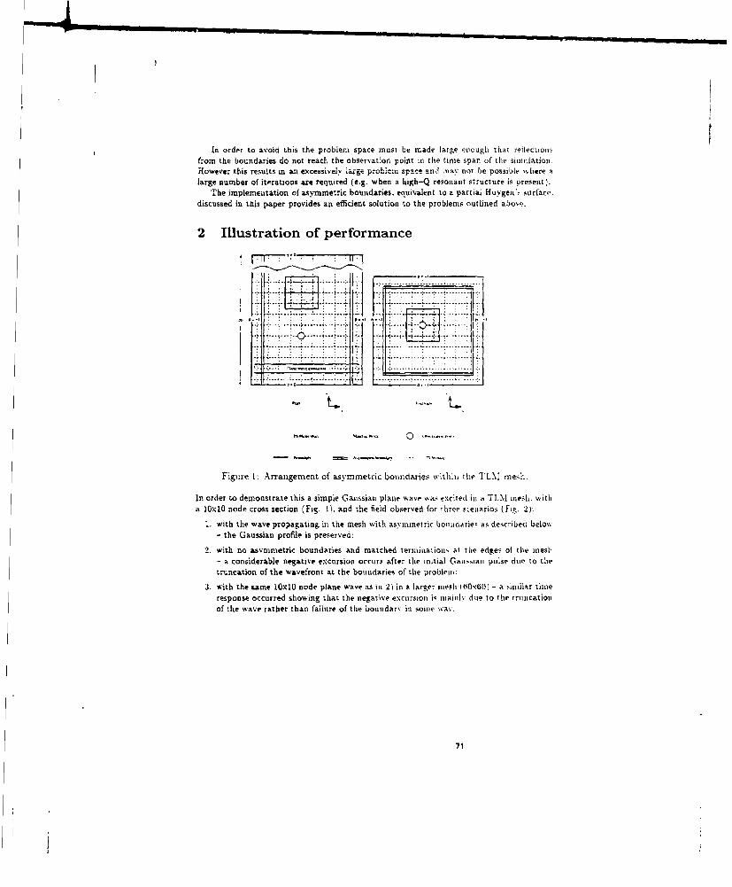
In order to avoid this the problem space must be made large enough that reflectioilsfrom the boundaries do not reach the observation point in the time span of the simulation.However this results in au excessigely 1&r.. problem spece an,3 aY. not be possible where Alarge number of iterations are required (e.g. when a high-Q resonant structure is present).

The implementation of asymmetric boundaries. equivalent to a partial Huygen'. surface.discussed in this paper provides an efficient solution to the problems outlined above.

2 Illustration of performance

7-...

I:.. .. .... ------

Figt:re [:Arrantgement of asymmetric boulndariesq within the TLM mesh•.

hn order to demonstra•te this a simple G(aussiatt plane w~ave wa,• excited in a TLM meshl, witha l0xlG node cross section (Fig. !). and the field observed for three siexlarios (Fig. •2):

1. with the wave propagating in the mesh with asymmetric boi'idarie• as described) below- the Gaussian profile is preserved:

2. with no asymmetric boundaries and matched terinitta~ion' at t.he edges• of thle mesl- a considerable negative excursion occurs after thle initial ('.uI,.iaI pulse dre to titetr'sncation of the wavefront at the bounxdaries of the problemn:

3. with the same 10xI0 node plane wave as• itt 2) in a larger tesht (60fxbh1) - s ,,inilar tuneresponse occurred showing that the negative excursion ig mainly dtt to the trttncatiott

of the wave rather than faitixre of the boundary it some way'.

71

0.4- :, '.;= : .. ...... . c......... .

711 , .,

-0.2 - -

Figure 2: Comparison of a Gaussian pulse propagation wit h asymmnetri"boundaries, with matched boundaries in ctx.C cross sectioi tesit. nd ,t1 runcated s0xe0 plane wave in C0xCO mesh (t o sc ti tl cer:'.

o . .- . .. i ;

,.,0000....

S~I

Figure 3: tonparison of Gaussian pulse plane w~e' i t le clzfwieiet tieshicsw'ith scattering object.

Fig. 3 show the time history at the observatioii point wiltth 1e i•tteritig ohjet! •Fig.l)present. It can be seen that rise use of the partial lityveen - .ti fac'e sites retlit. s•olid

line) which correspond very closely to the ideal ca-e i-- poiit, with .... boinidali u, usedwith a very large (60x20x60) mesh size but this is achieved with t .n 10x20x 0i) meshsize. The large mesh size ensures That the reflections froin itie tou d.rite do n1o: ]-acli the

72

observation point within the observed time span. j, the small mesh size +/-I boundarics

result (diamonds) in multiple r-Žflectious which distort the observation of the sc•tteied field

as does the additional wavefront if matched boundaries are used (broken line).

.....-

*revs.-,cy 'r- •

Figure 4: Comparison of the spectrumr with asymtmetric boundaries, wit h

matched boundaries in OxIf cross section mnesh. auid a ttuncat.ed 10NxO

plane wave in 60x60 mesh (impulsive excitationi).

Srx

Aqi5

Figure 5: Comparison of meamured fields in the aperlure of an exiclosuir

with TLM simulation ushig asymmetric and matched boundaries

Fig. 4 shows the spectrum of the wavefront incident at the ob.ervaz ion poisi 55 it lim-

pulsive excitation for the same scenariotis as in Fig. 2. A I u Itode piti is ais.suiwed. It

73

can be seea that the spectrum of the inicident wave is fla when it Ii partialI lHuYe it ý MitIfaceis used whilst the use of matched boundaries gives reducesd energy at low frequencies. Thetruncated (luxlU) wave in a ;Isrge (dcix6O) mesh exhibits d 1dr)l kC k.tWLpiviie.It! bal Ute-i~

has very little energy at the low frequency end o" the spectrunt.Fig. 5 compares the results obtained with asymmsetric bomitdaries and matched Lhotnd-

aries with experimental results. An enclosure (Fig,6) with ain apertuire :s placed in a semii-anechoic chamber and illunsinated with a vertically polarised wAve of constant amplitude. inthe TLM simulation a plane wavt was used, the ground plane was renresentefi b.% a - I re-flecting bolindary. and the walls of the semi-anechoic chamber were represented b% matchedor asymmetric boundaries. The field in the aperture is then plotted .III rThe TLMl simulationit can be seen that the use of asvymmetric boundaries gives a result nincli closer to experimenttha~n the use of matched boundaries. However the magnitudes of firw two resontant peaks.and the field minima czre not predicted accurately by TLM. Thi. nlsv be dire to the fact thatthe walls of the enclosure were lossless ( -1 reflection coeflicient ) "it: the TLM sintlulatiotiwhilst the reflections from the walls of the real eliclquire would not be lossless.

Fiue :Exeimetl aou o etlouy

3 ImplPmentatio

Using a set of sil-ple asymmetric bsousndaries in hie TLM mesh the distortioni of rthe wavefrouttdue to the discontinuity of the plane wave can be removed whltlt Mtill ittaintainingit a matchedboundary for the scattered field. As shown in Fig. I tl~e TLNM niesil is term-Iilactpd w~ith-1 reflection coefficient boundaries on the faces perpendicular to the electric field of thleplane wave. - I reflection boundaries parallel to tile electric: fel,. mtill itiitchied boundarieson the remanianisg two faces. Asym nmetric boundaries at(, cotnttrtictcd. as o Tube. psrsallel'o the direcsion of pnpaonxtini onite 0 olano wave, one inie~l siu Iinside Tlie TL NI niesl.

74

The reflection coefficient of the inside faces of the asymmetric boundaries is set to zero

(matched) as is the transmis5ion coefficient. This means that the problem space appears tohave matched bund-rics on all sleb for the scattered hields. Also no energy front tile inner

problem space can reach the outer region between the asymyrmtric boundaries arid the sides

of the TLM mesh. The outer faces of the asymmetric boundaries have reflection coefficientsidentical to the outer boundary which they face and a unity transmission coefficent,. Thus

a (plane) wave can propagate in the waveguide formed by the asymmetric boundaries andouter surface of the mesh undisturbed by any waves from within the problem space- However

if a plane wave is excited across the entire cross section of the TLM mesh (as in Fig. I) theparts of the wave propagating in the problem space and the outer laver are in time phaseand will remain so regardless of any dispersion in the mesh. The erergy transmitted fromthe outer layer to the problem space provides the !iecessar., continuity so that the wave in

the problem space is not truncated and thus no spurious wavefronts are genezatedTherefore. by the use of asymmetric boundaries we have achieved propagating coliditionts

for the exciting plane wave as if we had used 4/-I problem space boundaries to create a

waveguide capable of sustaining the wave, whilst for scattered fields the problem space has

matched boundaries. The method cani be shownt to be equivalent ta a partial implementationof a Huygen's surface as used in the TDFD method.

4 Theory

Let us consider the implications of using the reflection coefficient, specified oil the boundariesof the exciting surface (the asymmetric boundaries and the plane o0 initisd excitationJ. lt

particular. let us consider three points on the surface

a) a point on the surface where the plane wave starts (minithutn Y coordinate):

b) a point on the right-hand surface (maximum x coordinate):

c) a point on the top surface (maximum z coordinate).

If we consider the voltage which is im.plicitly added in when using trle appropriat-e refiec.tion coefficients on these surfaces then we get fjr each point

a) a positive z-directed voltage. V:. flowing in the positive y-direction (into tiOle interiorscattering region surrounded by the surface) azrd zero component flowing ill the negative

y-direction (into the exterior region of the surface):

b) a negative z-directed voltage. -V-12. flowing itt the positive x-directiott (out of the

scattering region) and a positive s-directed voltage. 1,/2. flowing inl thle negative x-direction (into the scattering region);

c) a positive y-directed voltage. V,/2. flowing in the positive z-direction (out of the scat-

tering region) and a pomitive v-directed voltage. "l-'v/2. flowing in tire negative z-direction

(into the scattering region).

It is possible to calculate the actual fields we are creating at thte boundaries of thescattering region. For the case of a boundary in the xz-plmie wiiit two voltages flowingoutwards along the v-dirsction. the field component., are

75

"•~~ H-- V-4 - i .I i II

nons ( 2)

where V.•() and VK(-9) are the z-directed voltage pulses travellian iii the positive andnegative y directions respectively. Similar expressions can be gi'eni for the other bouundaries,

Using equations 1 and 2 then allows us to calculate the fields created at the three boand-aries, We get

a)

E =E:=-- (3)

H =H, --- 4ZoA1 ZoAl

b)E E,£ = 0 il 5)

H =Hy j; Vo''- ( ox" 6)b)(7

c)

H=H.=0 (8)

where we have used the relation V,.- = i. say'.Using MMaxwoll's curl equations it is then possible to write down expressions for apuro-

priate electric and magnetic source current densities on the suriaces k hich wkould ti\e riseto the fields. We would need to apply the currents

a)

ZoA/

M = 1' (10)

b)J=--0 (11)

M V -(12)

c)I o'-- ' (13)

M=O (14)

If we now consider the creation of a similar plane wase using the Hutvgen,, formalismdescribed in '21 . we see that we need to apply currents to the surface given b1

M/= E" x ii (15)

3 = i x H" (16)

where fl is a unit vector perpendicular to a particular surfa:e and directed into the ,catTeringregion. Then. in ordeu to create a v-directed wave with counponest, E' = EL and H' = H:

at the ,.me three posiOis A I' earlier we net-, to t i, 0- -

76

aUT = -Hu(7)

b) J• = 0 19)

S-E h(0)

c) J - - -J (21)

M =- 0 ('22)

Fr, in examination of the Huygen's surface currents and the cuirrents actually appliedto the surface in the new method we can see that they are equivalent with

A VEh• = -- (23)

H, O--(24)

That is. exciting a plane wave of voltage. V. in the new wethod is equivalent to excitinga free space electromagnetic plane wave with fields E = V/al and H = I /Zo.I using aHuygen's surface.

5 Conclusions

A simple and efficient mitliodof implementing a partial Huygen.s boundary in the TLM meshhas been demonstrated. The method allows the use of considerably smaller TLM meshes forscattering problems excited with a plane wave source than previou.sl.y possible. The methoduses the TLM mesh itself to gen.trate the (equivalent of) retarded surface current,- for LteHuygen's surface and therefore automatic compensation for any ci,spersionl in the mesh isachieved. This also means that tie method is suitable for problems using a graded meshwithout further modification.

References'11 S.J. Porter aic. J.F. Dawson. Improved plane wave illumination for TLMi method. Elec-

tronics Letter4, pages 1663-1664. 1992.

[2] D.E. Merewether. R. Fisher. and F.W. Smith. On implementiag a runieric Huygen'ssource scheme in a finite difference program to illuminate scatlering bodies. IEEE Tmnns-action.s on Nuclear Science. pages 1829-1833. 19M0,

[31 P.B. Johns. A symmetrical condensed node for the TL.M method. IEEE Trn,.'action.son Microwave Theory and Techniques. pages 370-377. 1987.

i4' P. B. John-s -nd A. Mallik. EMP response of aircraft strucrur(- i iy aisission-linemodelling. In IEEE Intenational Symiposzium on Electrompatib (o bitzbitly. pages387-389. Zurich. Switzerland, ,5-7 March 1905.

77

Modeling a Resonant Length Center Driven Dipole Using the SymmetricCondensed Node (SCN) Transmission Line Matrix (TLM) Method

Michael T. Hendrick and Lloyd S. Riggs

Electrical Engeerin Department

Auburn University, Alabama 35849

Kelly SherbondyBelvoir Research, Development and En;neering Center

ATTN: SATBE-NTDFort Belvoir, VA 22060

Abstract

The trinsmission line matrix (TLM) method is used to amalyze the balanced bridge minedetection systam. Thoes raesuts include in examination of modeling a thir wifre in a coarseTLM mesh.

I Introduction

The TLM method of ulectromagnetic analysis is ideally suited for modeling a balanced bridge minedetection syzt.:m. This type of system requires some areas of the model to represent free spaceand other areas to represent a losry earth material. Using TLM, ;irbitrary material parameterscan be easily realized by modifying an input file. However, to use TLM to model a mine detectionsystem, an adequate method for modeling thin linear antennas in a coarse mesh must be found.

The balanced bridge mine detection system utilies a receiving antenna located between twotransmitting antennas, as shown in Figure 1. The transmitting antennas are operated 180' out ofphase to cres, a symmetric system. Due to this symmetrical property the signal at the receiveantenna is normally sao. In the presence of an anomaly, the system becomes unbalanced, and

the received signl increases.

II Theory

The Transmission Line Matrix (TLM) method i% a time domain analysis in which both spaceand time are discttit•ed. Spare i diidd nil di-.cct p-int:, nod=u, Which ere ._o_,___•_t__by a network of transmiuion lmes. The transmission line equation, are related to the Maxwellequations allowing the voltage pulses traveling along the lines to represent the propagation of fields.

78

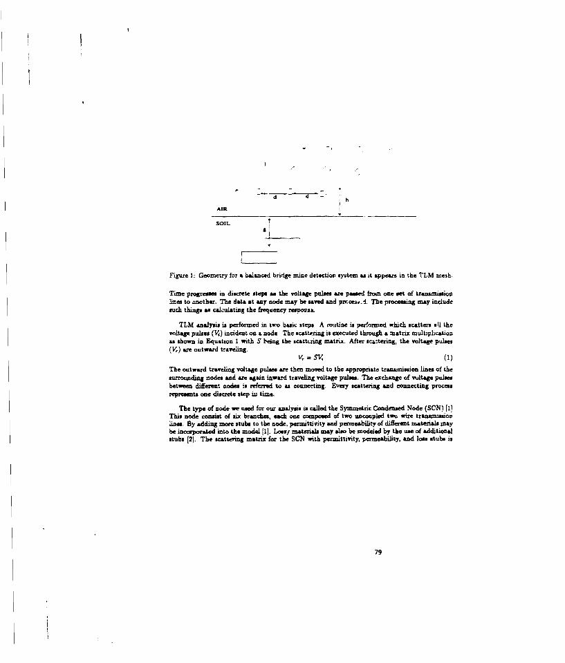
AIR

SOIL

Figure 1: Geometry for a balanced bridge mine detection system as it appears in the TLM mesh.

Time progresses in discrete steps as the voltage pulses are passed frnan one set of transmissionlines to another. The data at any node may be saved and prcor,, d. The processing may includesuch things as calculating the frequency respoosa.

TLM analysis is performed in two basit steps A routine is performed which scatters stl thevoltage pulses (Vj) incident on a node The scattering is executed through a matrix multiplicationas shown in Equation I with S being the scattring matrix. After sca•tering, the voltage pulses(V,) are outward traveling.

V, = 5,(1)

The outward traveling voltage pulses are then moved to the appropriate transmission lines of thesurrounding nodes and are again inward traveling voltage pulses. The exchwg of vultage pulsesbetween different nodes is referred to as connecting. Every scattering and connecting processrepresents one discrete step in time.

The type of node we used for our analysis is called the Symmetric Condensed Node (SCN) [1)This node consist of six branches, each one composed of two uncoupled twY wire transmissiovline. By adding momr stubs to the node, permittivity and permeability of differest materials maybe incorporated into the model [I]. Lossy materials may also be modeled by the use of additionalstubs [2). The scattering matrix for the SCN with permittivity, permeability, and loss stubs is

79

shown in Equation 2.

a b d 0 0 0 0 0 b 0 -d c 0 0 0 0 i6 a 0 b0 0 do 00 0 c d 0 b 0 0 0-i -d 0 Y 0 0 00 0 a 6 d 0 -d c 0 0 h- () ( g 0 0o o & a d o-,S 0 0 b 00 o 0e i 0 0

0 0 0 a b c -d 0 0 00 0 0 -i 0 00 d 0 0 b a b 0 -d r 0 0 0 0 g 0 i 0o o 0- C b 4 , 0 6 0 00 0 • 0 o0 0 b r-d 0 d a 0 0 b 00 g 0 -i 00

_6 C 0 0 0-d 0 0 a o 0 6 0 0 i 0 (0- - 00 c b 0 da 0 0 0 o 0 -i (2)

-d 0 _C b 6 0 0 b 0 04 a 0 g 0 0 ,C b 0 0 0 0 0 b n d a 0 0 0 -it e 0 0 0 0 0 0e 0 0 0 0 0 0 00 0 C0 0o o D 0•0 h 0 0 0 00 0 0 0 e e 00 z0 0 00 hO 0 0

I0 0 00 t 1~ 0 1f-f a0 00 0 000 0 90

0 0o 0 00000 0

The scattering is performed on every node in the system; however, the connecting cannotbe done for nodes locate- along the edge of the mesh. At these positions, only five of the sixbranches have another node with which to trade voltage pulses. 1he five branches, which haveneighboring branches, are connected using the normal process. The sixth branch, which is notabutting another branch, must be terminated so as not to disrupt the network and cause invaliddata. The termination method used in this model is based on reflection coeScients. By know.ngthe characteristics of the material surrounding the mesh, the reflection coefficient is calculated.The inward traveling voltage pulse placed on the sixth branch is the product of the outwardtraveling voltage pulse and the reflection coefficient. The disadvantage of this method is that itcannot compensate for a loay material immediately adjacent to the mesh.

Fo. the mine detection system of Figure 1, thin linear antennas need to be modeled. Thedipole, which sas a diameter much les than the incemental length (AW) of a node, ic modeledby modifying the scattering matrix to represent a node that has an infinitesimally small piece ofconductor located at the center. The scattering matrix is changed to reflect the negative of theinward traveling pulse back onto the same lines. A straight line of these "special" nodes can beused to repreant a piece of wire. As long as no voltage pulses are impressed along the adjoiningbranches of the wire, no voltage pulses will ever be reflected onto these transmission lines.

M] Results

Due to the fact that we are modeling this relatively small structure in a coarse mesh, the dipolecannot contain a center gap if the procedure outlined above is to be used. In our mesh theantenna is 1OAL, if this model were to represent the center node of the antenna with free spacethen the center gap of the dipole would comprise 10% of the entire antenna. This setup is shownin Figure 2.

Therefore, our approach to the problem was based on a concept used in the moment method

8o

1M

Figure 2: TLM mesh used for modeling the dipole. The dipole is located in the center of the meshwith its axis oriented in the s-direction. (a) Three-dimensional view of the mesh used to representa block of free space. (b) Cut away view of the x-y plane. (c) Cut away view of the x-z plane.

solution of a similar type of problem. Insnead of using two pieces of metal to represent the dipole,one continuous piece was used to model the entire dipole. Without a gap at the center, excitationand output must be obtainea without directly using the nodes located along the antenna. Theexcitation is provided by exciting a magnetic current around the dipole. Voltages across the dipoleare gathered indirectly, by finding the E-fleld around the dipole according to Equation 3

V=jE-di (3)

The characteristic admittance of the dipole is compared to that obtained by Harrington [3]using the moment method. When the re4l part of the admittance peaks or the imaginsar partis passing through zero, the system is resonant. From this data it can be seen that the resonantfrequencies occur when the length of the anteana is approximately a multiple of half a wavelength.The resonance with which we are most concerned occurs when the antenna is approximately onehalf of a wavelength. The system is to be investigated in the region surrounding this frequency.

The fields are used to obtain voltages and currents at the center oi the dipole. The voltage isobtained using Equation 3. The current is obtained in a similar manner using Ampere's law viaEquation 4.

1=fH d (4)

The admittance is defined as the raýio of current to voltage.

The dipole antenna was defined as 10Al in length with &I defined to be 0.1 meters, thusproducing an antenna with a length of 1.0 meter. The first resonance for this antenna should

81

Tr

2.343 {-- Caoducune

I/i Il

6.0 3A..47 054 . ZN .00Fn lu ncy (H-z)

Figure 3: Input admittance of a center-fed "ear antenna obtined using TLM.

theoretically occur at 110 Mls. However, the first resonAnt frequency for this antenna, as deter-mined from its input admittance shown in Figure 3, occurs at 100 MHz. This difference in thetheoretical and computed resonant frequencies can be explained through an examination of theTLM computed current distribution shown in Figure 4. The TLM computed current at locationsbetween the ends of the antenna appears to be uinusoidally distributed, but the magnitude ofthe current at the ends of the antenna is still & large percentage of the maximum current at theanterna center. A trailing current occurs beyond each end of the antenna caused by the discretenature of the TLM simulation. This trailing current continues to decrease in magnitude beyondeach end of the antenna. If the antenna is increased by 2.5AI on each end so a to include most ofthe trailing current, the effective length of the anten=a is increased from 1.0 meter to 1.5 meters.The dfective length of the antenna should therefore be used to compute the resonant frequency,which in this cae is 100 M~s. Taking the extra lergth into consideration, Figure 3 shows thecorrect response for this antenna.

This technxque of including the effects of the trailing current wa applied to antennas of variouslength, but the number of W remained the same. The length was changed by adjusting the sizeof Al, and s expected, all of these cases produead the same TLM computed current distributionwith the trailing current having a length of 5AL. When the length of the antenna was held constantbut the number of Al modeling the antenna was increased, the current distribution data showedthat the length of the trailing current was reduced. When a larger number of Al was used tomodel the antenna the data showed the current dropped to small fraction of the maximum currentin less than 5AZ beyond the ends of the antenna. This shows that the finer the discretization ofthe antenna the better the model Approximates the actual current distribution.

The TLM model was tested y running simulations of a balance bridge mine detection system

82

1 21

P.Oi.W.ofA-

0 3 0 I 5 2 0 5

Positdcn Along Antenna

Figure 4: Current distribution along the antenna, which is being modeled as one contznuous pieceof wire.

examined by Hill[41. The configuration of the mesh is shown in Figure 1. The dimensions of thesetup are as given below.

d = LOon

h=t ScI 26cm

g = 10on

frequency = 380MHz

= 3.5 - AO.05

The results obtained using TLM are very close to those obtained by Hill. Figure 5 shows

the comparison of the dat. produced by TLM and that obtained by Hill. This figure also showsthe results obtained using the two-dimensional TLM. As can be seen from the results the three-dimensional TLM code shows a closer agreement with Hill's dsata than the results produced bythe two-dimensional TLM code.

IV Conclusions

The technique presented here works well for modeling thin Iiuear antennas. However, to use this

method test need to be run to determine the amount of trailing current that must be included to

83

Z %,

ti

-0. 3 - 1 00 .I.

usn T. M nIyHl

o..d th a . ,h

Figueen: tw or desed elec t ri c enteldys , duntino tBenpsiton, Crsopouthe anodl forrin resultotained

the problem by using a lower time ste in the immediate neighborhood surrounding the conductor.Future work will investigate the applications of these methods to the mine detection problem.

References

(1) Peter P. Johns. A symmetrical condensed node fo the tim. method. IEEE Tranesactions onMicrowave Theory and Techniques, MTT-35(4):370-376, April 1987.

121 F. I. Geran, G. K. Gothard, and L. S. Riggs. Modelling of materials with electric and mag-netic Iowa with the symmetrical condensed tlrn method. Electronics Letters, 26(16):l1.07,1308,August 1990.

131 Roger F. Harringtoa. Field Computatioun &y Morment Methods. IEEE Press, 1993.

141 David A Hill. Neae-field detection of buried dielectric objects. IEEE Trrnsections oan Ge-science and Remote Sensing, 27(4):364-368, 1989.

[5] P. Naylor and C. Christopoulos. A new wire node for modeling thin wires in electromagneticfield problems solved by transmission line model[6g. IZEE !lnsactiois an Micr'ouel Theoryar.d Techiques, 38C3)-•3A-330, March 1990.

84

[6) A. J. Wfodarczyk and D. P. Johns. New wire i-iterface for graded 3-d tim. Electronics Letters,28(8):728,'1'29, April 1992.

[7] A. P. Duffy, T.M. Benson, C. Christopoulca, and J. L. H-eing. New mrahtods for &ccuratemodelling of wires using tim. Electronics Letters, 29(2):224-226, January 1993.

85

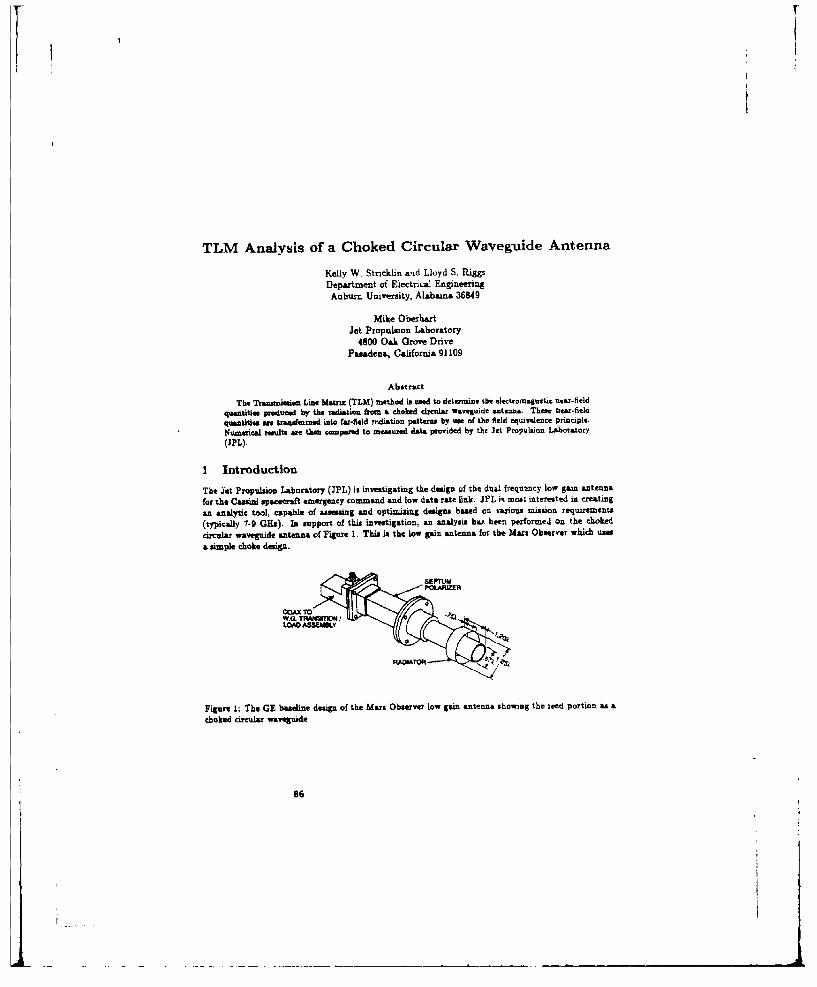
TLM Analysis of a Choked Circular Waveguide Antenna

Kelly W. Stricklin wid Lloyd S. Riggs

Department of Electrical EngineeringAuburn. University, Alabama 36849

Mike OberliartJet Propulsion Laboratory

4800 Oak Grove DrivePasa~dena, California 91109

Abstract

The Transmission Line Matrix (TLM) method is used to determine the electeomsapetic near-fieldquantities produced by the radiation from a choked circular waveguide antenna. Thefe near-fieldquantities are twasnoinaed into farsfeld rrdiation patterns by use of the field aqvalence principle.Numerical results are then compared to memured, data provided by the Jet Propulsion Laboratory(JPL).

I Introducition

The Jet Propuilsion Laboratory (JPL) is investigating the design of the dual frerlotacy low gain antenna

for the Cassini spactecrft emergency command and low data rate link. JPL i% most interested in creating

an analytic tool, capable of assessing and optin ising designs based en various mission requirements

(typically 7-9 G~s). In support of this investigation, an analysis bar been Performed on the choked

circular waveguide antenna of Figure I1. This is the low gain antenina for the Mans Observer Which US.S

a simple choke design

Figure 1: The GE baseline design of the Mars Observer low gaini antenna showing the ieed portion as achoked circular wavegude

86

Figure 2: The symmetrical condensed node showing its 12 transmission lines and voltage pulses

A numerical technique, known as the 'Transmisuion line Matrix" (TLM) method is used to mode]the propagation of waves through Ltd about the cho~ked circular waveguide antenna. After the properelectromagnetic radiation of the antenna has been produced using TLM, the electric and magnetic fieldquantities are saved over a surface surrounding the antenna. These field quantities are used to determinethe far-field radiation patterna by use of the field equivalenca principle.

2 Theoretical Foundations

2.1 3-Di TLM method and the symmetrical condensed node

In order to implement the scattering of waves through space oa a digital computer, the formulation ofthis wave model needs to be in diaawatiaed form. Therefore, both space &And time are reprasented intermes of finite, elgamentary urita, At and At. Electroinagnetin: fields are modeled with a network oftransmission lines comprising the field space. The behavior of voltage pulses traveling on this networkof transmission tines is %n&Wogous to the behavior of electromagntic: fields traveling in a homogenn-ousmed~ium. Equations associatedl with voltage pulses on transmission lines can be related to Maxwell'seqatations so that TLM can realietcally modal the propagatios. of electromagnetic fields [1).

The network of transmission lines ilatmect at nodat which represent pointsa in space separated by adistance AtL. Voltage pr1ses launched on the network scatter from point to point in space in a fixed time-stsp At. One of the more recently developed node models is the symmetrical condensed node createdby Johns 121. Ria symmetrical condensed node for modelina free space is depicted in Figure 2. Two-wiretransmission line connect the ports of the node on 'the aides of square ducts made of insulating material.In all six dirertions of propagation, two polairisatenus are carried on two pains of transmission lines whic-hare completely separated throughout the network of transmission lines.

Each transmission line has a characteristic impedance equal to the characteristic impedance of freespace, i*. Thesee transmission lines link the mesh of nodes together in Cartesian fashion. Twelve voltagepulses incident upon the twelve pai" of transmission lines produce scattering into twelve reflected pulses.These incident and rejlected voltage pulses appear on the terminals of the transmission lines at each ofthe twelve ports on the node. The voltage pulses are numbered and directed according to the arrows onFigure 2 [2].

The scattering at each node is defined by

V, Sv'()

87

where S is a 12x12 scattering matrix in the cam with no stubs. VN is the column vector of reflectedpulses, and V' is the oolumn vector of incident pulses on each node A voltage pulke V' of unit amplitudeincident upon port 1 of the node in Figure 2 proceeds toward the center with field quantities E. and H,.Likewise, the other.ulevet ports have field quantities associated with them' By applying thý ron' p'nrtmof current, voltage, and energy to the symmetrical condensed node of Figure 2, the scattering matrixbecomes

0 1 1 0 0 0 0 0 1 0 -1 01 0 0 0 0 1 0 a 0 -1 0 11 0 0 1 0 0 0 1 0 0 0 -10 0 1 0 1 0 -1 0 0 0 1 00 0 0 1 0 1 0 -1 0 1 0 0

S 0 1 0 0 1 0 1 0 -1 o 02 0 0 0-1 0 1 0 1 0 1 0 0 (2)

0 0 1 0 -1 0 1 0 0 0 1 01 0 0 0 0 -1 0 0 0 1 0 10 -1 Q 0 1 0 1 0 1 0 0 0

-1 0 0 1 0 0 0 1 0 0 0 10 1 -1 0 0 0 0 0 1 0 1 0

which provides the bua for scattering in TLM progamming 12].After the scattering process has been carried out on eieory node in the transmission line mesh, a

connection process must take place. This connection process takes all twelve output voltage pulses oneach node, and transfers them to the corresponding ports oa adjacenst nodes. At the same time a nodeoutputs its twelve voltage pubm=, it receives twelf. input voltage pulses from the six neighboring nodes,assuming the node is not on the boundary of the transmission line mesh.

The six field quantities can be calculated at any node from the following equations [2]:

= ~(V+V+P.v1 ,)E. = !(V,

E. = 1 +v,+r+vii)1E. = (VSC+ PO+ -W7+ ,)

if. = (V.- -n'-V.,+ I0)

H.= V? + V - I + V1. (3)

To implemnent boundauies aad surfaces, output voltage pulses incident upon a boundary ar multipliedby the proper riection coefcient, r, and injected back into the same node as input voltage pulses. Inthe following analysis, three typos of reflection coefficients awe used. For the can of a perfect electricconductor like the surface of in antenna, r = -1. At the edges of the TLM network, r = 0 so thatthe fields are completely ehborbed. For the third case, an infiitely N.ng waveguide is modeled using afrequency dependent reflection coefficient. An expression for this reflection coeffirient is derived by usingthe waveguide impedenre at the termination; the individual transmission lines have an impedance equalto the impedance of free space.

88

2.2 Near- to far-field t.ransformaetionss

For many anteimins cor'.iguritions, such as aperture antennas, it is possible to t&ale this field quantities nearthe antenna and transform them into at far-field radiiation pattern. One such technique is a mathematicaltchiq~ue beaad on the ficid equivalencer prifrme (.3

The field equivalence principle allows actual sources, such a., an antenna, to be replaced by equivalentsources. The fictitious sources are said to be eqiunlent within a region because they produce the Sarnrfields 'vithin that region 131L

The fields outside an imaginary closed surface ane obtained by placing over the closed surface suitableelectric and magnetic: curret densities which satisy the boundary conditions. Ptoper Current densitiesare selected so that the fields inside the closed surface are ear sad outside they are equal to the radiationproduced by the actual source. If the fmieds outside of the closed surface are rerpriasented by El and H Iand the fields kniside are madle to be sero, then the surface currenit densities become*

1. fi H (4)Ni. -i xL (5)

where Ai is the outward normal of S. T.hese current densities are then ised to determine the true fieldsradiated outside the closed sursfacf' by the sources within it 131.

After the current densities on S have bee determined, the electric and magnetic vector potentials,A and F, respectively, can be calculated from

A = ' J Jj !:j....d' (6)

]F .1 MefJL ide (7)

where ks= (A is the wavelength), and A is the distance from the source point (r.'z)to theobservation point (z, y, s). The totaLI fields are then given by

E = IA 1 1 LV( A (8)

H = IF-jLV( IP)+ VXA 9

However, theee formulations are complex, imd the integrals are dificult to evaluate. Therefore, someiipproxlznations which are valid for far-laild observations will be introduced [31.

Referring to Figure 3, for jev-field obseevematu, R can be -.%ppressimated by

Rr -r'cosO 10

for phase variations, andI(R1

for an~plitude iexiationz 131In Equation 10, -P is the anzgle between the vectors r and r'. The primed coordinates(z,')

indicate the space occupied by the sources J. and Mi., over which integration must be performed. Theimprimed coordinates (z, y.a) represent thie e'Newrvation point 131.

89

Fig`ue 3: Coordinate systen for aperture antenna analyusi

Equations 6 end 7 cn now be written as

A [ e'! - ' = - ! (12)

N6 = [ ,÷' dt (13)

M. =- ds (14)

L = fjM~e+*""eedJ. (5

Equations 13 and 15 can be simplifed by separating them into their z, V, and z components and thenusing a rectangular-to-spherical component transfonrmtion, to give f3l

N(16)•,= fL(-JX, .+ 3o,)+'•" (1

S= Jj(-u'=-i4,+Mveo.ql).+'•" J'* (19)

Where"Co# xsin~coS#+v'siD*sin#4+ ecoee. (20)

After substituting Equations 16-19 into Zquations 8 snd 9, and sepsratiat the fields into sphericalcomponents, the total E- and H-fields c be written an 131

Fr (21)

(22)- ( - ,yN*) (23)

90

H. U (24)

N(25)

4-- (26)

To implement thee formulations in a computer progpam, discrete v taons of these equations areused. After the TLM algorithm has run for several thousand iterations, the Founer.transformed fieldquantities aen savd ou a virtual surface jut inside the oute boundary of the TLM network. This virtualsurface is the surface to which the equIvalemce principle is appl.Wd. An algorithm incorporatiýn the aboveformulations, in discee form, is used to cainsite the rad&ated &. ead -f.eldcs.

2.3 Obtaining circuLar polarization pittern.

The measured data provided fo.v the Mars Oberver low Sam antenna was obtained for cirrult polarisation. Therefore, it was necessary to convert the linearly polarized far.eld data produced by TLM tocircularly polarised patterns.

In order to coupute circular polarization, it is convenient to della. A aew pair of unt rectors,

A. = - 4 (27)

A. *+ J14 (28)

Thee vectors correspond to time-varying unit i'ctors rotating in the rlih-handed and left-Landed senses,respectively, where the thumb points in the direction of propagation [41. Thue, any wave field can bewritten in one of the two following forms:

E = ,aEi. -E, (29)

orE = Eitil + aL.A (30)

F•om thee two equations it can be shown tbat

=l . (~jE 3 (31)2

EL = I(E.-E) (32)

Crcvu"ar polarization, cau be thought of as a superposition of two spaciajly orthogonal linear polJrisa.tion separated by a Wr phase difereace. Therefore, in circular coordmate., E, becomes Ed of the firstpolarization. Likewise, E, becomes N of the issomi. polarszaton whicL is e. of the first polarization.After making these subetitutions, Equatiots 31-32 become

Et = !(E.- E.) (33)EL= 1,,= •(E. .. ) (34)

iu spherica, coordinates.

91

3 Numerical reults

A caue wee run to determine the radiationi characteristics of the Manz Observer antenna design of Fignre 1A croee-eectsag ofthe TIM miodal for this design is shown in Fiure 4. Each nodein theTLMnetwrk is1 sam a4 eah side- The diamete of the wavaguide in22 am. At freuqency of 9. 13 G~l:, this diameteris 0 '4 A Vh choke bee a d:urnetr of 42 mm=, a dapti of(25 mm, and the mousth of the choke is re-cessed15 ma back from the aparetus of the wavagaida. A TLM unetwck of 100 mm on each side sisxrourdsthis earsoenat. The domke..ut T35, amade was milowod to w.opegate down the waveguide end w&N esradleted bnoow the reandbag TLM autwish inodaiing free epL=. Aftsw 15,000 iterelums, the tungentuelisetric em0 megaetic: A"d -,v eaved *a a vaeal sairlieo 90 nodes as eah side. The usew- to faz-fial,'tsumloeaute isahgnets produued lPgt S. Ideesied dat for dctarlar poLarisation was provided byJ1PL hir comperlena. This igere shams the nsmeated pattern for circular polaisation plotted from -90'to W, %he J4 mad Se, peanasa, "~ the nogt- mad Wifthasd circela polazisation plots.

4 Limitations and conclusions

Thai particular case was run es the cray sapercompater to take advantage of tht cray's memory and tospeed ar res-time. Noome v, e-mv the cray has a limit on the &ine of TLM networks it can handle- Thislimit su~nes to be on the eider of 101 media. Therefore, the vivo end resolution of the structure beingmodeled n ewes mine mlt. Uhmsub, the amount of spew nirseszuning the antesnna is limited. EnoughEmsam as hame of tke aetaina should h -i Io I so that an accurate-reprenaeninon of the near-fieldquesstiti &a the vizteal surface cun be Sheweted. Fut the lian Obeervera antenna, deepg with a simplecholse,1 x 101 media w=4 and in the TIM enalysis. Anteana designs with large chokes can he analysedmialg TLU. No-me, for '-igas w-4 vary larg dchke, so- , 1 Ation may need to be sacrificed.

Anassallipsiof.caq. - aeguide eateemawrit a ample Choke hass bee made using a TLM elgorithmnmadu a ane,- to hzr-ald transhewatnk mipsithai. Initial rune produced radiatbon patterns that agreequite favorably with meansied dhAa. Iletter reaclutson by usiag larger -LM network sizes will increasethe accuracy of the mehiaticas tbaractersetics astallysts

Refvemnces

II ll fdtmg J. IL Ia~ mad Pomai P.11. So. 71e Shmfarem edistc Wave Ssndaiteir. John Wiley endSUS, 1331.

121 %ane S3 Johns. A "xwiitsicnl ecidmesd aede 1r the TIM usethod. IEEE Tiwecswes.m onlts-csem 2 smrp d Tadmainsgi. MIT-11R4)-.370-3T7, Ape!' 198T7

13) Ceewaatesit A. Deallei. Assinasu Thrbm Af wel- and Desips. Harper and kow, 198.

14] Idward C. Joeda ari Kith G. lalinais. Beebwumenuec W~ es md Redisiebu Spleme. Prentice-

man, Ise., I333.

92

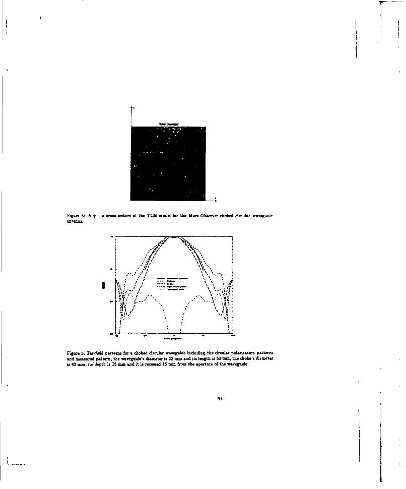
,Ouw amum~

Figure 4: A y - z crose..ection of the TLM model for the Mar Obe -ver choked drcalar waveguidoantemnn

I, • •, J

Figurel 5: Pa-field patterns for a choked circular wavegude including the circular Poblariztion patternsand mesue pattern, the waveuide's diamete is 22 mm and its length is 50 mm, the choke's diameteri 42 mam, its'depth is A mzn and it is recessd 15 m= from the apeture of the wr.veguide

93

COMPUTATION OF S-PARAMETERS OF A MICROSTRIP

M1EANDER LINE ON GaAs SUBSTRATE USING TLM METHOD

Chiannabaaappa Eswmnappa and Wolfgang J. R. Hoefer

NS=CVU' Tedmch RWXseCactir in RE EWi'nh. OqmxVm of Ekinncui odCoqnwEimtsi . Uzivusky ofVgmis. VIxisEZL D.C. CANADA VEW 3P6

ABSTRACTr

In ids papat. a fil)d bawd tkree-dinteaaional time domain Transmission Line Matinx CflM)

method has been applied to analyze a microstnip mcwnde Line configuration on GaAs substrate.

Both zegular and variable Thd nmeshes have been employed. The scattering parameters obtained

have been compared with thone of Sonnet em software and measuremnents (available data). Theresults agree well indicating that the ThMA method, which is a fuliwave electromagnetic solver,can properly account for die strong inzatereon between various purts of the meander line.

i. W(TRODUCTION

The Thnamission Line W=i (TI-NI method 6s a numerical technique in which both space andtime are discretized [1]. The simulation of propagation of electromagnetic waves is done through

scanneing of minptilaa in a 3-13 meshed network of transmisaan Lone. This powerful anod versatiletechique is auiable for microwave and millimeter-wavecircuit simulationespeciallywhen th

circuit geometry is highly irregular. Also since it is a fullwave electromagnetic solver, it can

acountm for electromeagnc nunscacn between various pusts of the circuitL

The mande lione (2] ame ued in monolithic microwave integrated circuits (MMICs) as delay

Lines as well as plana miductors. As a meane Uim consists of a uniform transmission line laid out

in a such a way at; to minimise" the qpace requiredt, this' will be strong electrmanaetic interaction

between various partv of the transmission line. It will be very difficult to take care of such interac-

amn using analytical methods. The TUA method is ideal for analysis of such atructures. Also, die

time domain Iepns obtained from the TI-N method are very useful when using them as delaylines. In the fiollowing, we reportsa detailed analysis of a microataip meander line configuration onGaus aubsisie

There are sonme difficulties associated with the TLM analysis of such large structures. The regular

uniform meah TLM leads to large computer memuory and large coarseness and diiperston esTors.

We have applied a variable mesh schemne based on AI-Mukhtar's and Sitclis [3] approach to

94

)p

reduce these rron. Also, the variable mesh allows feting of the exact dimn-sions of the structure

into the TLM mesh. Excitation of the circuit with a Gausman pulse (containing narrow band fre-

quency components) faciliates reaching the steady state faster.

This paper also compares the scattering parameters obtained from the TLM method with those

obtained using Sonnet emr software and measurements.

2. THEORY

The symmetrical co•d•,Aed TLM node [4] (shown in Fig.1) has been .' ed far our n, q.W

advantages of t node when compared to the expanded TLM node are mc• folJwrn,: i-,,•e i vydesaciption a easier, all six field components can be defined at single po, ao ipe, •/. tt.,. tsno dispersion in axial directions. It has six branches, each branch consi-,i" ,! r coupledtwo-wire trPnsmission linea. The 12 transmission lines linking the Cmakzf a: t ýh"nodestogether have the char•a-•ci.t impedance of free tpine. To compute the s•c•irr •,2m rneters of

meander lines, we need. the incident and reflacted flelds at the input port, ane d -: 'Amanittd fieldat the output port To compute the incide.i field, we discrex a length of unuaorm mncrosm- p line

with asorbing bomdaries placed an all sides of the coaputstional domain. Then, we include themeander line in the computational domain, and compute the transmiuted field at the output portand the total field at the inpim port. The reflected field is obtained by subtracting the incident held

12 f.-7 2

3

6 10

y-

Fig. 1: The Symme-r-ai Condensed Node

95

from the total field. The scattering paramets are then determined by Fourie transforming thesetiue domain wavdor•is. Good quality absorbing boundaries must be used for accurate extractionof scattering parameters. We have used the secad-order one-way equation absorbing boundaries[5] in the main propagation direction of the microstrip. A voltage impulse reflected from theabsorbing boundary can be computed from the knowledge of impulses in the cells in front of theboundary using the following equation:

V'(a~j~k) . (n 1 4.e2)V'(m,j.k)-e•o.,r-(uu~j,k) 4 (•l~ I)Vi(w•.- l.A.)

" (il ÷.?2-C1 P2 -P1 a) V"÷*(m- l~j. k) - (o172T•÷aI) V" 2 (m- 1/,jk)

(I)

The interpolation coefficients art:

(2)(a-g,(l-b)) (a- 1 " ,b) a(--bg,)

(a-1-~(I-b~s~p~ (a--g~l-) - (a-' -g,(l-b) -s-Al

where coefficaenh a Lnd b are weighted time and space averages of the spce &Ad time diferences,respectvely. E, and 2 are damping factors. The parameter gi for the uniform mesh is

g.- 2J[,-,(f,) (3)

while for the variable mesh, it can be wrntn as

2. - .2

, q ,) O; I; (4)

wher At- is the unit length of the mesh. Thia is deter••ned after scanning the cntire variablemeah so that no stub impedances or admitances are negatve. 1-' is the space resolution at theabsorbing bou•daies. Th absorbing boundaries on the aides and top of the meander line structuream implemented ty means of a ample zero reflection cofficient.

3. NUMERICAL RESULTS

The meande line configurvaon is shown in FIg. 2. This line has been studied earlier by W, Prib-ble using Sonnet es software aid measurements (6,7]. The microstrip line width and substratethickness ae 50 and 75 psm respectvely. The dielectric conamnt of the substrate is 12.9. First, the

96

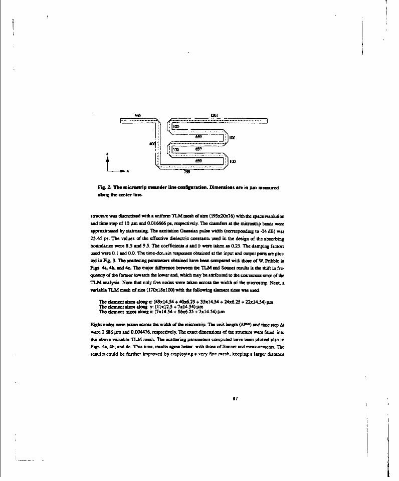
545 1201

.... .... ..75910

Fig. 2: The micruatrip meander fine configuration. Dimensions ame in pmn measuredalong the center line.

structure was thsaueized with.a uniform TLJM mesh of size (I9520x76) with the space resolutionand time step of 10 Iimn and 0.016666 ps, respectively. The chamrfers at the microstrip benids wereapproximated by staircasuig. The excitation Graussian pulse width (corresponding to -34 dB) was25.45 ps. T1he values of the effective dielectric constsnu used in the design of the absorbingboundaries were 8.5 and 9.5. The coefficiene a and b were taken as OM,5 The damping factorsused were 0. 1 and 0.0 T-he time-dc,~ sin responses obtained at the input and output ports are plot-ted inFig.3. The seattring parameters obtained have been comnpared with those Of W Pribbln inFigs. 4a, 4b. and 4c. The major difference between the 1124 and Soonet results is the shift in fre-quency of the former towards the lower end, which mauy be anttibuted to the coarseness erro of theT.M analysis. Note that only five nodes were taken across the width of the miucrastrip. Next, avariable 71M mesh of size (170x18zl00) with the following element sizes was used.

Thw element sizes along x: (49x14.54 + 40x6.25 + 35x14354 + 24x6.25 + 22x14.54) ILmThe elemntaizes along y, (11412_5+7414.54) jamThe element sizes along z: (7x 1434 + 86x6.25 + Ux14.54) Jim

Eight nodes were taken across the width of the nicroamrp. The unit length (Aý) and time step Atwere 2.616 pam And 0.004476. respectively. The exac dimensions of the structure were fitted intothe above varriable TLM mesh. The scattering parameters comnputed have been plotted also inFigs. 4a, 4b, and 4r. This time, results agree better with those of Soonet and measurements. Theresults could be further improved by employing a very fine mesh, keeping a larger distance

97

between t.e excitation and sampling points (at the ijput port), and pla-cing absorbing boundaries

(on the sides and top of the rsncre) at larger distances from the stip. IBM RISC Systerm/6000-

model 350 and HP 9000-model 755 computers have .'e.n used for computation. The computa-

tional time for the uniform TLM algorithmn was about twelve hours.

4. CONCLUSIONS

A . c1) '•i,)rrrsi d n -• lc . ioni... n has been 1udid using the 3D-TLM method. The r s.

seem to awr well with fhe available data except for a shift in fr-equency. Application of the van-able meash (based on Al-Mukhtar's and Sitrh's approach) leads to better results, but it takes more

computasional tune. The coarsenea eror, which is due to imperfect resolution of fields in the

vicimty of sharp edges, has been the major source of eatu in the TLM analysis. This could not be

reduced considerAbly for the meand-z line smtuctie because of as large size. and limited computer

resources.

REFERENCES

(1] W. J. R Hoefer. -he Thnaninion Line Marix (.,M) Method", in T Itoh: Naumerical Tech-

niques for Microwave and Millimeter Wave Passive Structures, John Wiley & Sons, New York

(1989).

(2] L J. Bahl, "MIC Simulation Column" in Inernational Journal of Microwave and Millimeter-

Wave Compider-Aided Engineering, vol. 3, no. 2. pp. 156-157, 1993.

(3] D. A. AI-Mukhtar and J. E. SiWtLchnmnititioa-line matrix method with irreguiarly graded3pace," lEE Proc., part H. Microwaves, Optics and Antennas, vol. 128, pp. 299-305, Dec. 1981.

[4] P. B. Johns, "Symmetrical condensed node for the TLM method", IEEE Trans. Microwave

Theory Tech. voL UrT-35. no. 4. pp. 3 70 -377, April 1987.

[51 C. Eswuappa and WJ.'-. Hoefer, -One-Way Equatin Absorbing Boundary Conditons for 3-

D TLM Analysis of PlLr and Quasi-planar Structores". to be published in IEEE Trans. Micro-wave Theory Techniques.

(6] W'liain Pribble, 'WC Simulation Columu" in international Journal of Microwave and Milli.

miter-Wave Computer-Aided Engineering, vol.3, 3o.4. pp. 4

60 -461. 1993

(7] Wrlliam Pribble, rlT-GTC, USA, private communcaons.

98

1-

1 .4*-- Incident 3aussman Pulse

,---w-Transmied wave at output port

0.61

_o _

02, Reflected aeat put port

-0 2 400 00am 12000 14M I daOO li00

Time StepFig. 3: Tame respone for meander line

S21 ......uw

016

M7-- TL.M (uniform mesh)

-- =M(Yariable mesh)OL - 0 Sote em software

UIJ •4-0.5

Si'0.1 & .

0.1 0000 00

5 10 is 20o2Frequency (GuI)

Fig. 4a: Magnitude of S-parameters for meander line

99

MGo

To0 - (unffriim mash)

at Sow° -CMUf[r-.

1 3 02

Frequency ((;HZ)

i4: Phan of S-0aramors for meader ine

0000

*a .1 4 ( U ff o m m esh)ao Sonone CM Softwar

* Measurements

S2D tO 10S 20 25

Frequency (GHz)Fig. 4c: Phase of S-peruneters for meander hine

1008

CCWUIT.ATflONAL $fl~nws OF FACTORS AFFECTING

LASER DOPPLER VELOCIMETER MEASUREMENTS

Dr. Joseph E. Whalen3115 E Navaho Street

Sierra Viat, Arizona 856335

This Pape discusses a Lase Dopplr Velocrrieter (WV) Simulation (LDVSIM). Rtepresentativs results includehmne histoie of photocurrenta. distribution of polotcirntnsh'fowing their Gaussian behavior, effects of varyingscatterer sirn, effects of velocity vurlations withidn the meosurarniat vaiune (my), mid trit alfaffa of fluin reanflow through too. my. Emphasi is on the fluid chaeracturistcs as opposed to hardware charactensitics.

11.0 lintruduoflan

LDVB am devices for deterwniseg velocities of solid olifects said fluids contininng pertbiclateas. Fluid applicatonsinvoves several physialS phenormen that ae of interot e.g., convieatve flow, Brownien motion. Browniannmbo nbits the ability of the LOVe to meamuw low velocities. LDVSIM wes designed to be simple and Providesan alternative to more sophisiicated moes Desiepis simplipcity, LD/SIM hes provided significant insight IntoLDV behravior Also, LOVSM provides a mee" of validating; mom complicatd models. Simpl icy n modelingas achieved by conslsieng the problem as en electromagnetic scattering problem. E~ac scatterer an the my asconsidered to be a source of a shrical wave tha as rehete from the aclittres onto the photo detector. Thetota field at the &Aedtor is the smin of thisfelds from the Individual scatterers. Obviously, if one needs to modelthe aSilns of volitioenal typically encountered, the LDt/SIN approach is imipiucical from a computationalperspective; however, as is ~r later. as few as 32 scatterems we sufficient to obtain the Geussiein behaviorfor phoftoinurnts that is ezapected in the laiait of i large numnber of urcetterers.

2.0 Lee ',oppler Veloclrietarar (LDV) Operating Principles

Bemause of thes Doppler~ef d the frequncy of light scattere fnom a moving objpct isshifted with esec tothe bindent Wigt [1,21. Since fth velocit of the scitterers of intoe is considerablyi less then the speed of lightthe Doppler fl~uquncy shift is only a -ml fract~i of the optical frequencvy. Since measurements at opticalfrequencies -m impe, *down nooiban to lowe frequencies. is employe to translate to a mneasurablefruquencyrnga. A aoto appiroec to frequency shifting is tatreld in F1ur 1. The lase boemn is spiltinto two compoinents: thes sltumnc beomanead the Inadmn been,. The refereno bean as shifted in frequencyby Bragg ream.s The incident bea is r11oa tram ectrr " in the fluid mnediumi end maturae -s fth scafttredbelan. Both sc 1ee enid reference beI we directed to a photo detector. For stationary scatterers, thephotcuaent frmn lie photo detector ail oscilt at the frequency difference betwee the scattered andrefersixs beats,. A shaft In frequenicy of the sterdbeamn caused by scattere motion wilt appearas a shiftin frequency cf the photocurrent power spectra.

The output of the photo detecto is amrpliffied, filtered to remove Ae outside the frequencj band of interest,and demnodulted. The shift in the spectrum of the demodulatiec . otmrurrent is proportional to bth velocity ofthe, scattereme. In typical laboratory appliatibons. provision is made to extrac the photocurrent timre histories ina complex envelope ropuusentation. One way of achwieig this is ilasted by the ellectronic componentsappearing in Figure 1. Otheir LOV configurations are presented an References [3.4],

101

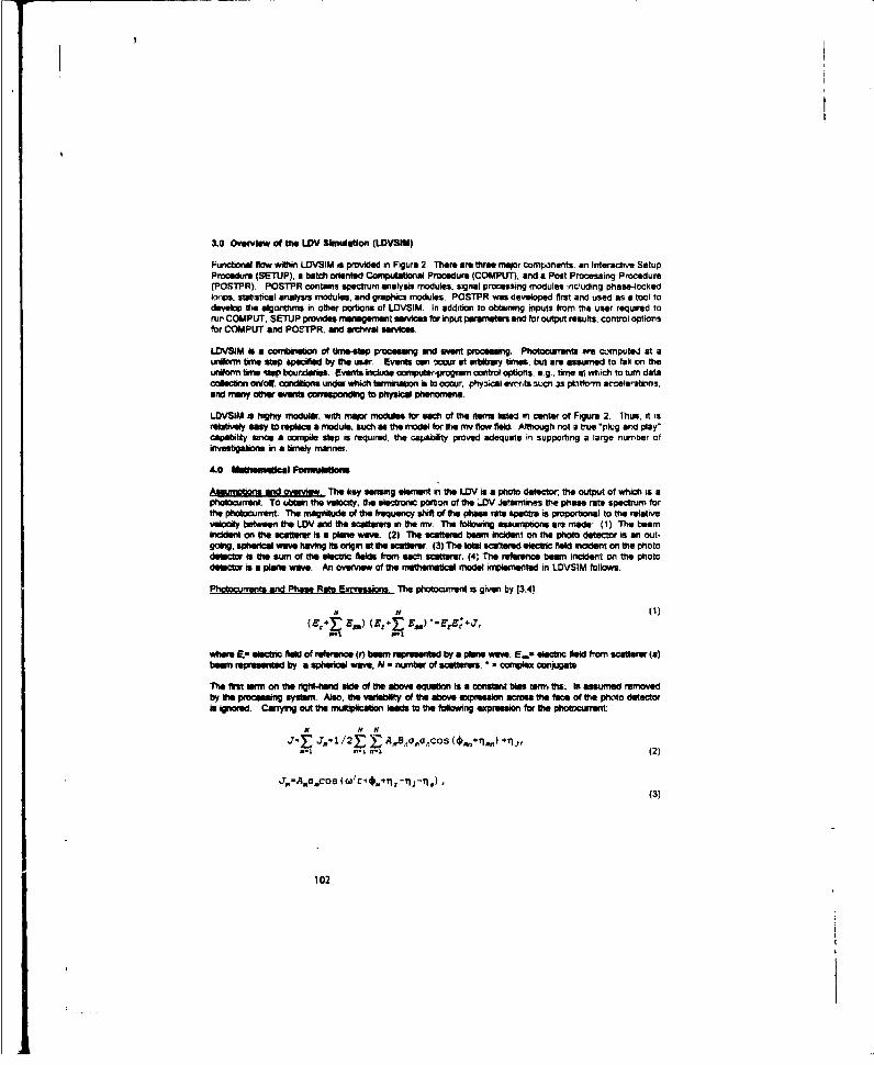
3.0 Overvlew of the LWV Snituatalon (LDVSM)

Functional flo wiMtin LDVSIM is provided in Figure 2 There are three major components. an Interactive SetupProedure (SETUP), a batch oriented Computational Procedure (COMPUT), and a Post Processing Procedure(POSTPR). POSTPR cortains spectrum analysis modules, signal processing modules including phase-lockedIlps. statistical analysis modules, and graphics modules. POSTPR was developed first and used as a tool todevelop the algorithms in other portions of LDVSIM. In addition to obtaining inputs from the user required torun COMPUT. SETUP provides management eiviies for input p1rameters and for outp results, control optionsfor COMPUT and POSTPR. and anrhival services.

LDVSIM is a coonbaflton. of tetp aocessig 0nd event procesaing. Photocurnta are c4'mputeJ at auwlfcvm tine step specified by the usar. Events nm "a=sr at arbitrary to , bit are assumed to tall on theuniform time -tap bourndies. Events iiniue wnrputer€progren• control options, e.g., ime at which to turn data

'oec " orVo# condl ions underuti nisaton im to occur, p. ynl eveits si as pltform accelerabons.and many otheir evenr corresponding to physical phenomena.

LDVSIM is high" modular, wi mtamorm ules for each of the itans ate in center of Figune 2. Thus, it isrelavely easy to r a module, su as model for the mv flow field. Although not a true "plug and play"capability orce a compile step is requnred, the capability proved adequate in supporting a large number afinvestigtiors in aa timely manner.

4,0 Muomwelcal FoMrnltmae

Asauntions and ov•aview The key eamrig element in te LDV is a photo dtactoc. the output of which is apholocumenr To AtaIn the velocity, th electronc portion of the LDV JetfmiineS the phise rate spectrum forthe pot-o s-st. The magnitude of the frequency s"il of the phase raf spectra is proportional to the relativevelocily between tie LDV ard the scatterers in the mv The following assmptons are made: (1) The beamincident on the scatt iis a pl•ine wave. (2) The scattered beamfincidet on the photo detector is an out-going, sphical wave having ft origin et the scatterer. (3) The total scfteard electric field incident on the photodetector is the sum of theelec 0hi fields from each scatteer. (4, The rfene beam incident on the photodelactorm a plane wave. An overview of the rathematical model niplemented in LDVSIM follows.

Photocurreta and Phase Rte E .ressions The photocurrent is given by 13,41i

it N (1)

where .. ctrc field of referie (r)lem b upee eand by a plane an, E.._" eienc fied from acattarer (s)beam reprie te. by a spherical wave, N - number of catterers, * complx conjuga

"The first fom onthe Ongt-hwd aide of th abo equaion is a consteant bia term ft, is assumed removedby te pn-oeIg system. Aleo, tie variabelity of the above wexeealon ores the face of the phoo detectoris Ignored. Carrying out the Wnulteptatlon feads to the folwing exproeson for the photocurnent:

Nv NH

-,-a a-n (2)

Ja-Aaoicos (Qw'c *.4*, -l1 q1 -,),(3)

102

where at - difference frequency between reference beem and the incdefnt boem; A., S. - terms containingwave number, laser intensity. aid geometrical parameters a,, - scatnng cross secOtm for the mth scatterer,o ý various noise sources, e.g., shot noise (J). rfmence (I. incident (0). scattered (S) beam noise.

The complex envelope representa•tio for J. is grven by,

7. -. z, i Q., (4)

where the I and C arm refered to as the "inphaee" and "quadratunr" concgnts• To obtain expressions forI. and Q., J. a mixed with Coa(e't) and sin(w•t) terms. The inphaae component is giwen by,

T- (1/2) Ao.a(cos (2•w'c+40.+tj,ij) +cos (4+". n)) +N

A.•',,Coa (wit:) F. AnOrCO"(ci+s .).n-I

A srIir expes is obWied for the quadrinatu component; however, cosine tan. am replaced by sineWtMs ad .1e second sine Nm M eUhive.

The required phase rate from filch velocities can be detebKined is obtained by difftrentatAng Me arc tangentof the ratio of quadrature to inphaee components:

'0- ( I•- h / (I' +Q') • (6)

Aftr taking ma time derivative of appropriate teins, a messy job. an expresso for the time rate of change ofphase can be obtained in terms of the tim rates of change of geometncal fecors, scatterer velocities,piroagation redria chaIcltnbcs, sattIrer mass. and noise siources.

Scaerer Postions and Velocities The simulatn'i computes the value for the phase rate at time intervalsspecified by the user. At any perticular ltre, the parties wi hawe a vecrity caused by Brownian effects andby the fRid velocity. The Yelocity distlibution assocated with Brownian motion is given by,

P u U, 0 "( in )1/22nkT(1-exp (-2yTC) )

exp ( -m ( u-u~exp (-y 0 ) ) 2 /2kT( 1-exp ( -2y •))), (7)

where u. i velocity amt ( 0: j - mlnItareous veoct of a scatterer. I - trne; in = scatterir mass,; k

Boltmarnn's conutait; T - temperature: y 6 n v r / in; v viscosity. kgl(ac-m); r r scalterer radius.

The abov exprensioni GaIGnm with stndaid deatim on ad mea given by:

o- (kT (I-txp (-2y C) I/m) 12 ,

u-uoexp ( -y )

Module BROWN computes Brownila velocities using a Gaussian dietribution using the above parameters

Betwee times at which tie photocurrent and phase rafte m computed, the scatterers are subject to colisionswith surrounding molecules. As a result the scatteren diffuse in end out of the nm. To capture these effects.new positions are computed for each time step using the ditribubon for particle diffusion [5]:

103

I

P,(x 0.x, C) u(rry 3/27tkT(2yt-3.4exp(-yc) -exp(-2yt) )111

(2kT(2yc-3+4exp(-yt)-exp(-2yr)) , 8

where x., - iritial particle position. x - particle position at timet

The above form is Gaussian woth standard deviation and. mew given by:

o,- (kT(2y C-3 +4exp (-yeC) -exp (-2ytC) (MI /O) 112,

0X X+.11 -exp ( -Yt0))/Y

Module BROWN conmputes changes in position caused by Brownian effects using a Gaussian disttitiitioi' huavingthe above parameters. These change ns ar4ade to position changes associated with other fluid-flow elements.

APw,~pr ate roojeis for other relooty effects can he incorporatedc into LDVSIM by replacing the particle velocitymodule (VEUNTi o#u n appropriate velocity fild moduel. One model u&6,1 for this paper rep~asý_. U fuid t,.'win a convection tWI (a). The requiried , aterr velocities we obtainerd by a two dimensional interpolation within

mesred velocity fielids. LDVSNoU has on option to euperimposee a liriear flow field on the my so that bransitbrostening effects can be investigaed. One othleirvelocity componen Ithfat istmodeled is WDV Platform motions.

6.0 Repsesenfatlve AMalt

Results are presente in thq fIgureis that follow thes test.

Photocurront Time Histon Cheractenstbcs. Figure 3 contains unphasa amd quadrature time sannes for Brownieanmotion In adelbon to rapid fluctuations, the datsa ehibit low firequen cy behavior caused by Brownuan diffusionof particles in anid out of the my. The average number of sactterenr is 32.

Phol~cuturi~t" MI~hracenstcs.in many analytic derivations the number of particles is assumed large.Typo*.ty a niv contain Itnusiands of scaltetrs, often miions. Simnulation tuna involving large number ofparicles Icr Iig pe"d of smuleAd tie ae pofbtrebecaaeof bigoniputetioal time. Thus, it sworthdetemnifiwg how meny setterier need tobe included in the autnuflion to obtain reasonable statistical agreementlwift ffumny-scatteercas. HItgwo -. of the inptuase compuienat of photocurreuit for a single scatterer(ties)411s1 conipered with a32-scatterr se(ahoeadportio) hi Figure 4l. The 32-scatterarcase poesa trueKohgorov-Sot i ioff wt for Gausalanilty at tWu 95% confidenice level.

PhoflixrrentPowerSonsra If acattuer erialeoffects we ignored the power spectra of fth photocairentsfor Brownian ;mCin. will be L6.oruenb . As meit efecs- aintroduced, the spectiewl "huave lower value.A comparison of the output from the ainwilaton whc contains maertial effectsi (See Eqs. 7 and! 8) wvith the corre-aponding Lorenflo profte is prevenfted mn Figure 6. Note that the Vaeid a as axpetd

flfnanMgL n. For these runs all effctssept Btownian motlioln were turned off. Five different simulationswere conducted corresponding to five differet scttrr massers. As; mess ncrueases the Brownian-velocitydifstribution p Aiak at lower velocitiesi. Thus, power at hugh fiequencies will decrease as scatteer massincseasee. Theae efetsae iluistiated in Figure 6. which contains a powler spectra for the photorurrents.Ultintsely, the velocity of thes fluid is datanrminad by thes shi in the power spectra of fth photocurrent phsse rate.Power specr ,fr pluttoannent phassnoeas for live diffrent patil sizes ame iustratled in Figure 7 The noosfloor for me 1 mitcron sa=ttere- is aignificot.

104

Velociy Vansbatv within the my. Velocity diversityr a *ect. we invvestigtd bY, introdwiEng a convecti., flowpattern consistinig oftw 11 a. Th eddinoes aaumd gerierted by placing a tmperauegradient crosia tx2xl cm Call coritaeirei the etlluecd mv with its kirng wai at a 1o-1fi degree angl with reepect to "h Ux2cmn tace Fluid flow is up in the coo tar of the my arid down at e9the end P"ain scatterer, in two groups al"th ernda of the m eMulits in a veloit cornponent toward the detector for one group and away "rm th deectorfor trime other group. 'noe ~hs spectrum has two peaks corresponding to the two groups of s-attiors asAluatree in Figure 8. As time peases the wscattre, miegrate throughout the mv because of the convect -a flowAfter several riarsitee the reauftVi spectnrum a aAmI -I rlo in Figure 9 Note the broad nature of ith spectrumnThe hic of pwr oukide of 250 H2,elet the manlluRTi etcn e in tMe call for Wie thermal gradient appliedThe nariow bledpeel at the lef miy reipoasatrapped! pIbl however this heasnt beew ngoi uglycofme&d

A comrparkson of~ rle ate apach fo tiree diferwit Oernt gslns crstlie convection Oak is OAJatlutin Fogur 10. As toe temiperatur vciwese. exianvectve peinsm xelplamlehed &nd Vie tcattarara velocitiesrer

no longer Uero hiciewg Ie tempertur Provides a greser oncenmtration of high speed scatterer., ulirclincreame the spectrail sprsead g

Tras rfiWM Transit bluadenin effct wer iesaigtd by introducing a rmom flow in the my Twocases wer simulated corresponding to two diferent velocities These raults am provided in Figure 11 Thedrite line represents.O thefgher spe The higher speed case. line (b), is significaritly broader

6.0 Couctsinoue

The basic elarnienits of Lawe Doppler Velocimetn (LDV) opearabit a aapple to fluid veloit measunrement,hame been discussed idre-nocd with computaisonial remift.. The LWV aspects ju tee in this paperrepresent only a wriel ftshm of gothea problu . Additional phenorrona tha may be of interst for futureirestilgation " uIoid u~erea shape. scoteriar optic* l retc soe dv esho nt. scattere intesrnal dynamics.platorm vibrobones. turbiulence at fte vv"st of Owe platflorm, arid a"p processing refuisiametts.

Developing moel aria li veftiglbitg LOV aysle provided a conivenient means to investigate fundarrentalphysiacl phenogrea. suchias Ukrswiti motipon, vevep pI gss ftrough rindom mfedia, Optical eystem. fluidflow thenriiul dynm=cearid elec conc sysems. E " I g LDV eapeifairisyet at acade ,micssbftit for tiepurpose of anveedgethi WUV systemis w m recm ended a basic research endeavor anid as a teachigot toI.,t modern apspcts of laer system sia well as fiundiernantel pilyw phenomeWN A

1. BrnM_ ridWaf, E. 1019,Pnr~n (Opim.Pergernon Press. New York. New York.2. .iadton David J.. 196WJh jma VA" d Sane Im~. New York. New Yolt.3. Adian Ronald J.. 1963. -Lse Vebai oonay,* Chapte 5, Fudhsh=MtlM dtdbRidied J Goidistim, m t mivephe Pullwig ConporeWr. Washigt~or, 0 C.4 Oaorna, W. K. and Lrviley. J. L., 1973. "The Loas-Dopplar Veloicnisliar and nos Application to theMeasuverement of Turbtiulwi,* JLFn ho Val 4, p 1220.5 14M=o MoLt, m edto, elact Papers on oIse aid Sklobliatc Piosea Dover Publicetions, p 99.6 Bueat. F. H., 1967. -On the Stability, of Taip.Dirmensionat Convection in a Layer Hastled from Below."J athied Physiaii, Vol. 46. p 140

105

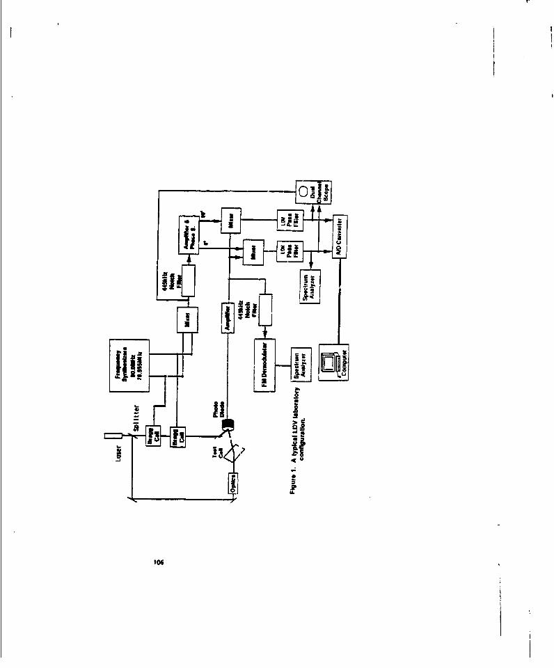
ow

W 6

106

-yr-i-.= ZvwK!) -i K) ~ L)

U.

%02-I

0 ~107

TI

.. .. .. . U. ....... . ... ...... ...... .. .......... .........

.. ... .. .. . . .. . .

......... .... ....... .. ! ....... ..... ...... ... ........... ........... .............. ....

20 50

:F LREQUEINC PROFIL

15 ~~TM -- 1SoEC)AIO

Figure 4. IPhataum adistuart~os iure .ompnew rrwnanroison.o iuas

sdition@n

108

0-5 5

0 .1000 5 10 is 20 0 10 20 30 40 5

Class ThimousnlFREQUENCY (HZ)

Figure 4. Photocurrent dixtributions. Figure S. Comparison of simulatedphotocurrent witht tihuorehcai Pre-dictin.

108

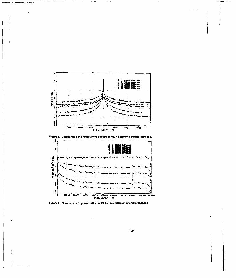
00

-7100 -5;00 -6500 0 20 0 70

FREQUENCY (liz)

Figure6. Comparison of photocu~'~ spoecb for five differeni sCatterer masses.

0 NAM VCI

a IO ME

a 25000 5,0000 750000 00400 32i000 350000 -1)0 200000 22;400 200000FREQUENCY (HZ)

Figure 7. Comparison of phase rat spectra for five different scafterar maases.

109

I(

-1250 -1000 -7w0 -500 -25 0 25) 0 7;0 1Q00 12500

FREQUENCY (HZ)

Figure S. Photocurrnt spectra for non-uniform distribution of scaftrer location atthe beginning of the simulution run.

.. .... .. .. .. .

150- -1;00 -450 -__ -io _ 2;0 5o 7-"So 1000o .250

FREQUENCY (HZ)

Figure 9. phaour, nt spectr aftr scatares have disrbuted themmselves

110

NI

z1C~2C

c'JJ

TUVIRllfl DIFFERENCE 0 DEGRIESSTWTWJfIlM DIFFERENCE 1.6 ofiRE(TWEIVEATIME DIFFERENCE 4.8 DEGREES

-1000 -750 -500 450 0 250 5i0 75'0 1000FREQUENCY (HZ)

Figure, 102. Photocumne specti. for convectlos-ceII myv at diree different temperature,gradients resulting in thre. leveft of convective flow.

.. .. .. . .... .. .. . .... . .. ...

...... . .........

0O~O0-00OO40O0-300O2fl0-I0000 10000 20000 3000 40000 80000 60000 7MO0.FREQUENCY (HZ)

Figure 11 Photocurrent spectia at two differenit mean flows.(a) Mean flow m10 cm/sec. (bi Mean flow -15 cm/atc

Analysis of a Cavity-Backed Slot AntennaMounted on an Infinite Ground Plane Using

the 2-D TLM MethodJohn B. Erwin and Smart M. Wentworth

Dept. of Electical Engineviing200 Broun Hall

Auburn University, AL 36849

Introduction

The trnssmission line matrix (TLM) method is a very powerful technique for solvingelectromagnetic problems. A single computer algorithm can be used to analyze a wide variety ofelectromagnetic inteactimn problems since arbiuay media parameters and boundary conditions cmn bechanged simply by modif-, ing an input file. The model simulates waves propagating in the time domrinwithin a space that has been discretized into transmission line sections, called TIM 'nodes'. Voltagesand currents on these nodes correspond to electric and magnetic field quantities. Two dimensionslspace is discretized into four-port nodes and thre dimensional space may be discrtnzed into 12-portsymetrical condensed nodes [1]. A pulse entering one port of a node is scattered to the other posbased upon a scattering matrix which can be derived for either the 2D or the 3D node and can includethe effects of material parameters such as permitivity, permeability, and conductive losses. Thescattered or reflece pulse leaving one port of a node becomes an incident pulse on the appropriate portof an adjacent node. The TLM method is then a two-step iterative procedure that first involvesscattering of inciden pulses at every node followed by a connection step to pass the reflected pulses toadjacent nodes. Repeated application of this scattering-connection process results in an output functionat some observation point (output node) which consists of a train of pulses in time which may beFourier eransformed to obtain a frequency response or convolved with an arbiuary time domain inputsequence to get a corresponding output.

The TLM method can be wsed to calculate the fields scattered from arbiu-r'y bodies. By exciting aparticular group of nodes (a line of nodes in the 2-D model or a plane of nodes in the 3-D model), aplane wave will begin propagating through the mesh. If the Witic RCS is desired, the scattered fieldsresulting fom this plane wave encountering the body are determined along a virtual surface

simnndi t th foy7n a t aclt hs fed st ban h rtlfed with the scatterer in

~.lcad bo icden filswt h ctee eoe.Tesatrdfed r iply the differencethe total and the incident fields. The resultig fields are thema used to determine the far-field

pattern (2,3].

One of the difficulties in ob.tining RCS through numerical modeling is that the incident planewave must appear infinite. This reluirment is often me by making the mesh very large along thewavefnt Howev, a large mesh conVtining many nodes will requir a lengthy computation time.One way to simulate an infinite p~ae wave with a more manageable mesh size is to implement"magnetic walls" that guide the plamt wave. These magnetc walls at perfectly reflecting bounzloies ofinfinite impedance. This approach is r !equate for obtaining the incident fields (since there is noscattertr), but the magnetic walls would interfere with waves reflected off the scatterer. Ideally,scanerd fields see only absorbing boundaries, which in the 2-D TLM model can be realized by using areflection coefficient of -0.1716.

An approach to this problem is to nan a total fields case, which includes the scattem along withabsorbing boundaries, concurrently with the incident fields case, which omits the scarterer and hasmagnetic boundaries to make the plane wave appear infinite. During each iteration, a scaled portion ofthe pulses reflected at the magnetic houndpries for the incident fields case are injeted into theboundaries for the total fields case. The details of this approach are described in a previous work [4].

112

. f -

Fig. 1: 3-Dl depiction and side view of a cavity-backed slot antenna mounted arn aninfinite ground plane.

T7he situation is mote complicated when the satrerm consists of an element mounted on aninfinite pround plane. When a plane wave is incident upon an infinite ground plane. it is reflected (orscattered) as a plane wave. For a normally incident plane wave, the inicident fields and those scattered

frmteground p~lane may be maintained along the boundary by using magnetic walls with reflectionffce +1However, there would als be ciantering from an element mounted in the pround plane

whic' o-ould require an absorbing boundary to prevent ft-scattering. Thus, the problem ofsimultarieously maintaining the incident plane wave, and the two scattered fields (front the ground planeand from the mounted element) arises. This paper will disc-ass a solution to this problem using aca,-, -backed slot antenna mounted on the infinite ground plane in a 2-D TLM mresh, as shown in Fig.

xamrple. These antnnas are coammnoly used in aircraft and spac applications because of theirAunding abilities 15].

ALF ch

Determinatison of the scattered fields from a cavity-backed slot antenna. mounted on an infiniteground plane requires an adequate model of die infinite ground plane in only a finite TLM mesh. Onemethod i .o truncate the ground plane, but allw it to remain excessively large compared to themotmWd ment. This method raises several questions: How much larger thin the mounted elementdoes the ground plane need to be.? Is the size of the grond plane dependent upon the number ofitem'- -un? In addition, how lengthy a run timne can be toleraed for a large mesh? A secondmethoL, - one we will describe in this paper, is to employ a pulse injection technique to handle thereflected plane wave. This approach is similar to one taken in modeling an incident plane wave [4].This approach, a plane wave injection technique for the incident plane wave, will be treviewed. Thienwe will show how a similar methiod can be used to model the plane wave reflected off of an infiniteground plane. Figure 2 shows the actual ThM model of a cavity mounted insa ground plane. This is anapproximtiaon of the cavity-backed sloc antenna case where now the slot dimensions ate actually equalto the coss-section of the cavity.

113

I

Absorbing boundary. F--O.1716

P"•

x

Fig. 2: A representation of" the 2D model for the cavity mounted on an infinite appearingground plane. The plane wave would be normally incident from the top, and the fieldpints am determined at the indicated nodes 1-8.

Pulse Injledlon

Ofpeoble requireo simulation of both an inciden t plane wavea a a plane wave maflected wornan infplie d plan while by1tany ateorng the field scamed frot the cavity. An accxrateand tone-efficient method to model an incident plane wave is to maintain the absorbing boundaries

while injecting pulses previously calculated [4m These injections maninta the integrity of the planewave by allowing it to appear to be non-aztenuating. Since the absorbing walls cannOt distinguishbetwe incident and scattered waves in the total fields case, -0.1716 tims the incident field is alsoreflected at the boundary. Therefore., the incident field pulse at a port next to the magnetic wall ismultiplied by 1.1716 and then added to the total field p~ulse at the corresponding port next to theabsorbig wall. The pulses to be injected may' be determined by rnnming a one-dimensional stung of

nodes, as shown in Fig. 3a. For example, during ach iteration, the pulse at port p in Fig. 3a is scaledand injected into port p in Fig. 2. This technique works well for normally incident plane waves andmay be modified for oblique incidence cases uiing a tined pulse injection technique for both the irtiaiaexcitation and thE maintenance of the plane wave i6.

114

rr-0.1716

r.=÷ l -+ I

["=+1

17-0. 1716 ''" _ "-

(a) (b)

Fi;. 3: One dimensional plane wave injection models. In both cases, the waves areguided by PMC walls. (a) For the incident wiywo case, the wave terminates in anabsorbing boundary. (b) For the reflected wave case, the wave is reflected by a PEC.

Fcr our pioblem, we must incotporate a unique scatter, the infinite pound plane, to which thecavity is ,inintd. The technique discussed above works well for maintaining the incident plane wavewhile absorbing the scaned field fromt the cavity, but some rt action must be taken o account forthe scattered field from the ground plane. The field smatered from the ground plane would be a planewave except for the presence of the cavity. It thertfore should not be allowed to attenuate whenpropagating through the mesh. Since the absorbing btIsndaries used to absorb the fields scattre fromthe cavity would give rise to attenuation of the plane wave, an approach similar to the one used tomaintain the incident plane wave may be taken to main ain the reflected plane wave.

Similar to the incident case, pulses me pr-calautked and injected mto the mesh every iterationto maintain the scancred plane wave from the pound plane. The pulu-s we calculated by using a one-dimenmiooal s of nodes, as shown in Fig. 3b. Note that the left and right boundaries an PMC and thebottom boundary is a PEC, representing the ground plane. Because of the normally incident field'ssyminy, this accurstely represents the infinite gorLnd plane without the cavity. When the pulse isinjected at the top of Fig. 3b (as shown by the arromt), a one dimensional wave. representing a planewave, propagates through the mesh. During each iteration, the voltage pulses on the ports next to themagnetic boundaries are increased by 17.16% and injected into their otrresponding ports of the 2-Dmesh. In Fig. 3b. once the wave reflects from the I'EC, the total fields become present in the mesh."Therefore, the reflected pulses along the PMCs r-prcunit both the incident wave and the scattered wave.Consquently, the pulses injected from Fig. 3b into Fig. 2 simultaneously maintain the integrity of boththe incident plane wave and the scattered plane wave from the infinite ground plane.

1'15

Verification

The electic field calculated at selected points using our injection technique was compared to thefield using a very large ground plane. Tixe large ground plane extended 1249 nides on each side of a 2x 2 node cavity, and the mesh reached 10 nodes above this ground planet The injection technique wasused to simulate the incident plane wave, but no injettion was used to simulate the TcfleCtcd plane wave.The extrwem size of this mesh was sufficient to calculate the field in the vicinity of the cavity as thoughit were mounted on an infinite ground plane. Using 1500 iterations, an accurate 1-field distributionwas calculated over a line of 8 nodes parallel to the ground plane. These nodes wcre selected 2 nodesdirectly above the cavity and were synmnecncal to the cavity's center (the node location relative te thecavity is shown in Fig. 2).

In the mesh includinig tie injection technique for the reflected wave, the ground plane extendedonly 5 nodesan either side of the 2 x 2 node cavity. Again, the mesh reached 10 nodes above theround plane, the field was calculated over the 8 nodes indicated in Fig. 2, and 1500 ,terations were

run. As shown in Fig. 4. we achieved very close ageement with the large mesh case. The maximumdeviation was less than 0.4%. A comparison of the phase showed similar agreement. For an additionalcomparison. Fig. 4 also shows the field obtained when the smaller mesh was run without the injectiontechnique for the reflected wave (injection was still used to simulate an incident plane wave). This casedeviates from the large ground plane case by as much as 16%.

Theme is a limit to how close the siuc walls can be brought in using our technique. With thewalls moved to within one node of .- caviry, the field deviated from the very large ground plane case(the maximum deviation was 4.01). However, with the walls only 2 nodes from the cavity, themaximum deviation dropped to 2 M%.

1.81

1.6 "

B1.4

1.2

1.0 •0 I 2 3 4 5 6 7 8 9

Node

Fig. 4: Comparison among calculated electniL. fields for three cases:(i) (M) a large mesh, 1500 nodes in length, used without the injection

techn•qe(ii) (0) a small mesh, 12 nodes in length, incorporating the injection

thnique(dii) (A) a small mesh, 1? nodes in length, without the injection technique

116

Conclusions

By injecting pulses at the boundaries, our 2-Dl TLM network can simulate a plane wavenormally incident on a cavity which hab been mounted on an infinite pround plane. Since a relativelysmall ground plane in the mesh can be made to appear infinite, a significant savings in memory and runtirre is realized over the large mesh approach. We am. now developing a rimed pulse injection techniqueto accurately model plane waves obliquely~ incident on an infinite ground plane. Further, thesetechniques will be adapted for the 3-D ThM network.

Acknowledgments

This work hos been supported by %he Atntennas Laboratory of Texas Instruments, Inc.,McKinney, Texas.

Refa~renees

I . P. B. Johns, "A symmetrical condensed node for the TLM method." IEEE Trans. MicrowaveTheory Tech.. Vol. MTT-35, No. 4. pp. 370-377, 1987.

2. IC Omissaankar and A. Taflove. "A Novel Method to Analyze Electromnagnetic Scattering ofComplex Objects." IEEE Trams. on Electromagnetic Compatibility, EMS.24, No. 4, pp. 397-405, 1982.

3. F. J. German. G. KC. Gothard. L S. Riggs. and P. M. Cloggans, 'The Calculation of RadarCross-Section (RCS) Using the TLM Metnod," International Journtal of Nuinerical Modelling:Electronr& Networks, Devices and Fields. Vol. 2. pp. 267-278,1989.

4. 1. B. Erwin and S. M. Wentwortht, "Plane Wave Injection Technique to Calculate RCS in a 2-DTLM Network," Electronics Letters, Vol. 29, No. 14, pp. 1241-1243, 8th July 1993.

5. S. Hashemi-Yeganeh and C. Birtcher, "Teorrical and Experimental Studies of Cavity-BackedSlot Antenna Excited by a Narrow Strip," IEEE Trans. Antennas Prop., Vol. 41, No. 2, pp. 236.241. Feb. 1993.

6. F. J. Cerman. Personal communication, Texas Instruments, Inc.. December 1993.

117

l1e

SESSION 3:

MULTIPOLE

Chair: Dan Reuster

it,

Curved Line Multipolesfor the MMP-Code

P. Leuchtmann and M. GnosLab. of El-mag. Fteldsi and M~crvwave Electronics. ETH Z--rch

CR-8092 Zurich. Sctstzerlund

Abstract

The s.Vneon of the itlctromasratw field used an MMP (Mult.ipl .IMultipole Program) may be simplified

m particalar •o•s.. Depending on te set of eananoio functions a signiuicant reduction of the number of

unr~nson is seslik. The paper dueribes a new set of etzpesion functions (fthe 'curved line multipoles'which mil he flessr•y adapted to nly curved long strtieurre inchlding edges. Curved line rnulttpoes have

two n4epenmdmnt Parameters (orader N and idgm M) to pradefine the mnaxmum possible varntion ofthe field to he expmnded N steerm the vearitiom along a curved line of finite length while M sfeer" thefield tanation saround this line. The oaskslation of the line multipolej is discussed and the application to

,-attciao r ,cstertmrg problems shows their adrentage versus the conventional multtpoles.

1. lateodmtiom

This papir dals with a particular subset of expansion functions for the MNMP-code. the line multipoles.

First let us bridy describe the basic ideas of UIIP (Multiple hultipole Program) it, order ,o see what

the lane maltipoles are good for.The basic problem is finding an unknown electromagnetic field functior. f w'here f = (E. H has

six compoients. the components of the electric field t and the components of the magnetic field 17.

In a domain D (with boundary OD) f has to satisfy MaaxweUs equations in the stationary case (-e-'): curl£ w swid and curl

1 -fi -iwi where ;: angular frequency. p.e: constant (complex)

permeability.permattivity in D. i; imaginary unit, t: time. On 8D. f must satisfy some boundarycoeditiow MMP starts with the saees expansion

J

wbe each expaafioe ancti m f fulfils Ma-xwell's equations. but not necessarily the boundary conditions.

The unknownr coeffi.ents u are used to satisfy the latter in a least squmes sense. Obviously. the choiceof the expansion functions fj has signiicnnt influence on the convergence of the expansion (1). If thesolution has a particular behavior - e.g.. f is the scattered field and radiates energy away from thsscatterer - it -ak- saft to use OUly expansion functions fJ with the same behavior. On the other hand

the get of expansion functions huld span a wide variety of possible solutions. Let us consider a specialcase; scattering at an ideally coaducting spire (ae fig. 1). The optimum set of expansion functions

for modeling the scattered field is a series of multipole functions. Assume that the sphere is electrically

arge and the incident field is a uneazly polarized plane wave traveling in z.direction. In this particular

case. N most be large. but M a I is sufficient. Since & full multipole expansion has N2

- I parameterswhile the adaasted set (all orders but only terms of first degree) has only N parameter., the number ofunknowns is sigaifi:antly reduced without any lack of accuracy. This example shows how an intelligent

choice of the expansion functions may dramatically reduce both the amount of calculation .N) and

120

incddent

wave

Figr For any incident field, the scattered field I may be written as a sum of multipole functions.starting with a dipole and ending up with functions of higher order and degree. With the setof all multipoles up to the maximum order N any variation of f along 0 E [0. -] describableby an N-th order polynomial in cstA may be represented exactly. Similarly, with the set of allmultipoles up to the maximum degree M any variation of allong 0 E [0,2rj describable byan M-th degree Fourier sens in o may be rep asented exactly. Note that M and N mry bechosen independently. but it is always At S N- For N,. -. on the functions form a maxhe-matically complete set of expansion functions.

the amount of computer memory (- N2

). The line multipoles to be discussed in this paper offer a similarpossibility for reducing the total number of unknowns not only for spheres but for any 'long structures'.

2. Curved Line Ma.tipolesa Qualitative Description

The set of expansion functions to be presented in this paper may be looked as distributed multipolesalong an arbitrrry curved line L of finite length L. We define a longitudinal coordinate z along L and anazimuthal coordinate . around the line L (see fig. 2). The field of the curved line multipoles is singularon the finite line L and fulfils Maxwell's equations anywhere else. The strength of the singularity variesalong L in a polynomial way. i.e., line multipoles up to order N model any variation along z E [0, LVdescribable by an N-th order polynomial in z. For a given s-variation of a curved hue muhtipole functionthere are various n-variations available. ramely any trigonometric function in Ii. More precisely: LinemulhipoLts up to M-th degree model any variation along 4 E [0,21r describable by an M-th degreeFoiie.- sern in o. Note that M and IV may be chosen independently from each other. For S, M -3the resulting set forms a complete set of expansion functions in the space outside the line L.

Physically. the zero degree term is the field of a line current I(s) along L. Very dose to L this fielddoes no, depend on 4. However, for a curved L the n-independency ie lost away from the line. This isdue to the fact that v- and z-values are not uniqutly defined 'or such points. Nevertheless, the curvedline multipole function gives eartly the correct field.

Curved line multipoles are useful not only for modeling the field arund long thin structures likewires but also for edges. The important point is that the user m~y predefine the maximum variationalong - and 6 independently from each other just by specifying maximum order N and maximum degreeA'. Note that this is exactly what is requestcd in practice: E.g.. the field along an edge varies most oftenmuch less than around the edge-

121

Eiry Curved Line multipole ar singular en a line L of fnite length, vary t"nusoidally along o andlike a polynomnal along x. This behavior is strictly true only close to L since the coordinamesand 0 are not unique away from the curved line L.

3. The Computation of the Curved Line Multipole FieldsIt is sell known that the electromagnetic field of a thin straight linsi current I(z) (nonzero only on thefinite length) may be given in *woed form if 1(z) = 1, com kz+1. sin hz, where k is the wave number of thesurrounding medium and I,!, are constant [1J. Based on this formula the field of an equally segmentedlong straight wire with n free parameters (the currents at the segment joints) has been given [2]. Sineand cosine shaped currents on each segment were combined in such a way that the current is continuousalong the whole wire. For segment lengths Al < A = (27)/k (A = wave length) we have cos kz = Iand sin kz :a kz on the whole segment and the mentioned combination results es.entially in a polygonialapproximation of an arbitrary current distribution 1(z).

In order to reduce the number of Iree parameters on a long wire the values at the segment jointsmay be given, e.g. equal to a polynomial p,(z) of degree n. A series Zý0 a,p, allows the representationof any cutrt distribution I(z). Note that the field of one segment has tr be calculated orly once butit is part of the contribution of all p,. The main advantage of such a procedure is that the number ofsegments may be chosen independently from the number of unknowns [4].

A generalization of the single segment current field has been described in [3J. While a line current hasan electromagnetic field with rotational symmetry the mentioned generalization (called 'line multipoles')yields an azimuthal field behavior (along c) proportional to sin mn or oe sm6 respectively. For rs = 0 itis equal to the common wire current. Since the rs-th degree line multipole is built up using 2rm singlecurrents

1, there are line multipoles of the same degree both with sin kz and with we kz behavior. Thus

it it posibhie to consider a segmented hie and to combine the field functions of each degree to a iongmultipole in the same way as it has been done for the long wire in [2] and, as a next step. as in i4]. Thisis essentially what has been done for this paper.

Other than ixt the previous versions the line may be curved and segmented in an arbitrary way. Thetser must epecify a number of points (Lie segment joints) and - due to the lack of rotational symmetry- for each segment an additional vector specifying the zero-e drectson of this particular segment. Thisinformation is stored in an extra file. The graphical MMP preprocesor Lmmptool' (or =Mptool') (5]allc-s the efficient generation of the data.

Two different types of curved line multipoles are available. The diffence betweet the two lies in thetreatment of the longitudinal behavior of the fields. The first version is essentially analogous to MMP'sthin wire feature 1], Since au N-segment wire has N + 1 joints (including the end points) there are N ý- 1parameters. If M is the maximum degree, there are 2M + 1 functions with different 0-depecdency foreach single segment functioa. Thus, the total number of parameters is Pts = (,V + 1)(2M + 1). In thesecond version the number of segrnmts is decoupled from the number of parameters in a similar way asin MM Ps long wire expansions [4]. The longitudinal behavior is modeled using Legendre poiynomials

SThe actual Calculation a isrcuuwe with respect to m and includes a limit (shifting all currents together on the sameplace) M crdr in hbas a suinile with amnla li6t. 'aloes [31.

122

of order n and the maximum order IV may be specified. Thus, the total number of parameters becomesagain Pot, = (N + 1)(2M+ 1), but N is now the maximum order of the longitudinal polynomial expansionrather than the ntmber of segments. Of course the latter should be larger.

A second set of field functions may be obtained using non physical magnetic currents rather thanelectric currents. For a single segment the electric curren, fields are TM with respect to z while themagnetic current fields are TE. For simplidty's sake we call the respective curved multipole fields alsoTE and T.M respectively. in spite of the fact thaz the longitudinal direction varies from segment tosegment. A 'complete curved line multipole' has now Pi,*8 = 2(N, + 1)(2M + 1) free parameters. Notethat the calculation of the dual field is very easy and cheap: only the final field values have to be'dtalised', i.e., interchanging f and A and multiplying by the (negative) wave impedance.

Another set of PJ* field functions may be obtained using the ingaing Greens function rather thanoutwards radiating Greens functions for the calculation of the field of a single current segment. Thisgives non physical fields in free space. Nevertheless, in bounded domains such functions Are usef-d.

The following table gives the exact MMP data needed for all possible variants of curved line multipol.expansions. Remember: an MMP expansion has 6 integer parameters (IEI-IKE) among other paramererswhich are not used for curved line mnultipolms.

1EI; 131... 134 (versiont 1) or 141...144 (version 2)IE2: 3 (outgoing waves) or 4 (ingoing waves)I.3: minimum 4-egree or maximum degree (2)IE4: maximum o-degreeIE.: maximum (longitudin.) order (only version 2)

IMe: 1pp or w

The paamneter IMl is 131/141. if both TE- and TM-fields are requested. In this case. all o-degreesfrom 0 to 1E3 are computed. If LIl is 132/142, only &-degrees from IEW to 1E4 are computed. Finally,IEI = 133/143, only TM-fields are computed and for I"E = 134/144, only TE-fields are computed. inboth cases only 6-degrees from IK3 to IE4. The parameter IE1 is used for specifying the file %kith thegeometric data of the Line. It it named p.1yy .zxz where pp is the (two digit) number of the line andxxx is the (three digit) number of the problem to be solved. The zero order term of the TE-fields (a singlemagnetic current) is only computed if 1E6 > 99. For the Ill = 131 ... 134, Ptot = P•,• is proportionalto the number of segment joints (J, + 1) while for IZE = 141 ... 144, the longitudinal behavior is modeledusing Legendre polynomials up to order IE.

4. ExamplesIn order to show the advantage of the curved line multipoles compared to the conventional mulhipoles.we calculate problems where the line multipoles seem to be useful. In a first example the scatteringat a banana shaped object is investigated. The geometrical situatiou is shown in fig. 3 giving also thetime mean wiue of the power flux (Poysting vector), while in fig. 4, some details of the near field arerepresented.

The same situation has been modeled in different manners using either line multipoles or conventionalmultipoles. Further on, the number of psramreses (i.e., the orders and degrees of the multipoles) hasbeen varied as well as the number of matching points. Finally. the field has been computed at twodifferent frequencies resulting in a overall 'banana' length of half a wave length A (low frequency) and3A (high frequency). Field plots of the different computations look almost identical. This is due to thefact that the errors are very small: all versions deliver good results but at very different amounts of bothcalculation time and computer memory.

123

Figur The banana shaped object (id4a conductor in ir, half a wavelength (A) long and 0.027Athick. bent along a quarter of a full circle) is illuminated by an a-polarized plane wave trav.eing in a-direction. The picture shows the time man value of the Povnting vector of the to-tal nar field. There is a shadow region S with low field values and a :standing wave area' Fwhere the fields are high but only th time man value of the power flux is low. See also fig, 4for more details of the field in the rectangle R.

The geom.try of the situation is symmetrical with respect to two planes- This symmetry maybe used to simplify the expansion. Due to the fact that the line muitipoles may be curved in a threedimensional way ther is no built it symmetry for these functions while conventional multipoles havebuilt in symmetry. This has the consequence that the models are different for the two cases: Usingline multipolas one half of the 'banana' has to be modeled while using conventional multipoles only aquarter of the 'banana' must be modeled. On the other hand, more matching points per unit surface arenecessary for the conventional multipolea. The following geometrical models are used:

1: Rough model for conventional multipoles. 686 matching pointsEI: Fine model for conventional multipoles, 1295 matching points

IIl: Thick model for line multipoks, 854 matching pointsIV: Thin model for line multipoles. 840 matching points (3)

Note that model IV is a three times thinner 'banana' of the same length (diameter = 0.009A). Thefollowing expansions have been used for the same geometrical model where all line multipoles are alongthe axis of the 'bananf" and have 28 (internal) segments of equal length for a half of the 'banana'. Inmost cases an additional (point-)muhtipole has been used for modeling the field at the end cap. Table

124

Annel A more detailed view of the instantaneous value of the electric field (I4t) and of the magneticfield (right) respectively within the rectangle ft (see fig. 3). Arrows and octagons (for vectorsperpendicular to the drawing plane) show the direction of the field while the underlaid contourlione give the magnitude of the field atrmngth.

(4) gives the integer parameters IEI and ZES of the line mtzltlpole. its related number of parameters NL,the nomber of conventional multipoles Ns.. and its related number of parameters NM as well as the totanumber of parameters N, = Nt + n..--- NM for the different expans-ion models. For the line multipoleit is Ifl 3 (outgoing waves), 1E3 - 0, III = 2 (6-degree) and 116 < 100 (no magnetic current).

model: a Is c d e f g Is i k I uIEI: 142 142 142 142 142 142 132 142 142 142 - -

XIS: 3 3 5 5 8 12 - 5 8 12 - -

NtL: $4 36 54 54 81 117 26135A 81 117 -Tf ; - 1 1 1 1 1 1 1 1 1 19 19

-V 66 66 96 66 66 86 56 36 36 ±18 k42Mewt: $4 102 120 150 147 183 327 110 137 173 342 802 (4)

The loa z-axes rcf the Conventional multipoles are oriented along the 'bianana' axis and its degrees are 2,i.e.. equal to the i-degree of the line multipoles. The multipoles in models l and sm are found automaticallyusing [5]. The number of parameters varies slightly from multipole to multipole. Note that the modelsusing conventional multipoles are symmetry adapted. An '3D curved banana' would require both twiceas many matching points and twice an many parameters for the conventional muitipoles but the samenumbers for the line multipole model.

Combining the geometrical models 1-VI with the expansion models a-rn and runnitig the computerat low and high frequency, different results are obtained. We list the mean percentage error (meanmaismatchiing divided by mean value of kied values on the matching points tirres 100%) and the cpu time(in sends) for computing the parameters and the errors on a Sun SPARC 2 machine.

model MIaUHIbliMclldIMeIMgfMc EleIlel~fIVh MiIVkl1 Urn fl Urnfrequency low low low low low low high high high low low low low low high higherror r%] 16.9 0.4 0.1 0.1 0.1 0.1 0.6 0.4 0.5 0.4 0.1 0.1 2.9 0.1 0.8 0.3CPU (par) 98 122 149 181 193 447 150 195 262 13'1 179 243 361 3404 361 3404cpu (err) 88 86 97 101 117 84 99 118 143 94 114 139 49 193 48 195 (5)

figure 5 shows the distribution of the errors for somse particular Lases.

125

X10

hI m

low high high

Fiuan 5 The error vans along the surface or the scatterer. The 'hedgehog' pietures give the distribu-tion of the errom for three low frequency calculatiors (left) and two high frequency calcula-tions (right). Note that the scaling of the e-rors is the same for all caes except in case 1lc:The actual errors sm more than ten times larger in this cas. The 'reference" at the very righthas not ssnigficantly smaller errors, in spite of the fact that almost ten times more parametersare used. This shows the power of the curved line multipols.

In fig. 6, a more complicated example is shown: the scattering at a four turn helix. The helix is halfa wavelength A high, the total length of the wire is almost 2A and its thickness is A/20. It is modeledusing 3472 matching points (each rectangle on the surface in fig. 6 is one matching point).

The scattered field is modeled using four line multipoles (one for each turn) of longitudinal order 12and a 6-degree of four (-884 Parameters). Additionally, two conventional multipoles have been used tomodel the field at the wire ends (-132 parameters). Hence the field model has 1016 degrees of freedom.The computer (a Sparc 2 workstation) needs about 6 hours to solve the problem end ends up with anaverage error of 2.2%. The maximum error occur% at the end of the wire and is only 26.3% (see fig. 6left).

Note that this example brought the computer to its limit if it would be calculated using onlyconventional multipoles. It had to be discretized with at least 7000 matching points and 60 multipoleswith 36 parameters each. This results into approximately 2200 parameters resulting in about 50 MBytesof computer memory and 11 hours cpu time on a Sparc 2 machine. The given numbers refer to the roughmodel of the 'banana' in our previous example. A finer model would have to double both the numbet ofmatching points and the number of parameters - and came (with 200 MBytes required memory and 88hours cpu time on a Sparc 2 without speaking about numerical problems) definitely out of the scope ofýnormal' computers.

126

S...ee .e.e .... . 0oo0

£. .eGoo

0s eoeo• s 00000

*~~~~~ * e* * ee**0000 .

S• 0 a GOO®

max ~ ~ q,.. r0 0OO e -••e • (

* * oeOte@ ®eo .* *. ino Q inc. wve I

Figu~J Left: The helix (ideal conductor in &ir, height: A/2) is illuminated by a pLar. wave comingfrom left. The pictule shows the inatanstantaneous value of the k-field in the Hl-plkne (theincident H is vertica while the incident i-field is perpendicular to the drawing plane). I!heundies on the surface of the scatterer represent the loc4a mismatching, i.e., thr *angential elec-tric field ý ,id the normal magnetic field in this cuse. Mien error: 2.2%.Right: The same field on a helical surface (white). Note that the electric feld is alway- per-pendicu"lar to the scatterer's surfasc. The direction of the incident wave is indicated. See alsofig. 7 for the power flux of the same field.

Summary

The curved line multipole !'ow the exact calculation of the near (and far) field of thin structures.Compared to convention. Jtipoles the number of parameters ib - at comparable errors - reducedby a fW-tor .5 ... 10 (a: l•ta!), whee the reductuon is increased when the wires become thinner. Thescope of MMP calcui.blz siuWations i signacantly enlarged. The curved line multipoles are useful totakte into accout a priori knowledges, since the maxium field variations in two directions (along andaround the line) may be chosen independently from each other.

127

Figur This picture shows the instantaneous value (lft) and the time mea value (right) of thePoynting vactor S I x & of the emin situation as in fig. 6. The contour lines at the leftrepreAnt the absolute value of S. Note the 'ecreaning effect' of the helix Some of the vectorsat the left poin, below the white helical surface and wxe not visible for this reason. The localtime mean aesor flux is always along the wire and makv have different directions insde andoutside the helix. N.B.: The eiae effect occurs with the 'banana' example (see fig. 3).

References(11 G. J. Burke and A. J. PolWo, "Numerical electromapetics code (NEC) - Method of Moments-,

NOSC Technical Document 116, Vol. 1, Lawrence Livermore Laboratory, Livermore, CA, Januazy1981.

[2] P. Leucktmann and L. Bomholt, "Thin wire feature for the MMP-code,"in 6th Annual Review ofPragress in Applied Computational Electroingnettis (ACES), Conference Proceedings, (Monterey).Mar. 1990.

[3] P. Leuchtmann. "New expansion functions for long structures in the MMP-code,' in 7th AnnualReview of Progress in Applied Computational Elreclromagnetics (ACES), Conference Proceedings.(Monterey), Ma. J 91.

[4. P. Leuchtmann and M. Gnos. "New thin wire expansions for long wires in the M[MP-code,' in9th AnneW. Review of Progress in Applied Computational Electromagnetics (ACES), ConferenceProceedings. (Monterey), Mar. 1993.

[5] P. Regli, 'mmptool', public domain program. available through ftp anonymous onsirius.ethz.ch (129.132.41.1), directory momp, ZUrich, N6v. 1993.

128

COMPARISON OF THE MULTIPOLE TECHNIQUEWITH THE METHOD OF MOMENTS

Daniel D. Reuster"Department of Electractl Engineering

University of DaytonDayton, Oi145469-0227

Patricia A. RyanGeorgia Tec:. Research Institute

Atlanta, GA 30332-0800

Abstract

This paper presents a comparison of the multipole technique with the method of momcn,as applied to the problem of electromagneoc scattering by perfectly corducting cylirxkrs.Comparisons are made on the performances of the two techniques with respect to variatiovs ofthe cylinder's cross section. Theoretical development is given for both techniques, along withcomments regarding the uniqueness of each technique. ComparLwons are made with respect torun time, number of special function calls, matrix sizes required for convergence, and numericalstability. Bisatic sataering patterns are presented for perfectly conducting cylinders of variouscross sections. Conclusions and general rules of thumb are given for the ute of each technique.

1. bfroductdm

The method of moments (MoM) has been used for numerous years to solve variouselcomagei scaritg and propagation problems where the object under study is on the orderof the wavelength of ierest. The method is well documented [I.2] and shown to producereliable results for a lare clm of problems. However, in recent yva inerest has grown inthe use of the multipole technique (MPrT [3,4J as an altwrive method for so!ving many of theclasswial MoM problems. In response to questions regarding the efficiently and reliability of thenewer MnT, two Fortran based computer codes were developed (one MoM and the other MPT)to run a direct comparison between the two techniques. The two codes both use the samesubroutine (CROUT reduction) to invert their respective reaction matrices and both codes usestandard IMSL libraries for all of their special function calls. Thus, the two computer codesallow for a direct comparison of the two methods and provide insight into the ab~lities of thenewer MPT with respect to the traditional used MoM technique.

129

2. Matheinatlcai Development

Figttre 1 shows the cross section of three infinitely long perfectly conducting cylinders(PEC), with their axi aong the z direction. The region surrounding; the c'ylinder is free spacewith permeability ;% anid permittsv'ty eo. It will be assumed that the cylinder is illuminated by

a transverse magnetic (TM) plane wave, of unit amplitude, propagating in the x-y plane.

DjPaxiodic Rectangle E1llipse

z-0.61~ A-0.21 w-0.31 h-0.6A x=O.6A y-O.3A

Figrm I Sicattering Test Bodlie.

A) Multlpolu Technique

Let the scattered electric field at an obsservations point extierimi to the PEC cylinder beI en by :

where. k,0 and H."' am., respectively, the waveuzinber of fice space and the Hankel function

of the second kind of order n.Frons the PEC boundary condition, the tangentia components of the electric field must

vanish along the contour of the cylinder. This leads to the following equation relating theincident electric field to the scattered electric field:

130

where p - R(¢) is the parametric contour of the cylinder.

Approximating the above series by the first 2N+ . terms and enforcing the resultingequations at 2N+ I matching points on the contour results in the following matrix equation:

(Z-1[o-['o (3)

Solving equation (3) provides the series expansion coefficients for the scattered fields outside thecylinder.

B) Meod of Momem

Let the scattered electric field at an observation point external to the PEC cylinder begiven by:

-2l~ )H(ý(!pp:)d1' (4)

where, s and J(p') are, respectively, the intrinsic impedance of free space and the surface

curn along the contour of the cylinder.From the PEC boundary condition, the tangential components of the electric field must

vanish along the contour of the cylinder. This leads to the following equation relating theincident electric field to the surface currents along the contour of the body:

where p = R(40) is the parmeC contour of the cylinder.

Approximating the surface current by N pulse basis functions and choosing N matchingpoints along the conmour of the cylinder, allows equation 5 to be approximated by the followingmatrix equation:

[z.,] [J.] (EI.,j (6)Solving equation 6 provides the surface currents al3rg the contour of the body which in

turn can then be integrated to produce the desired scatered fields.

3. Compar-isb

Table I presents the n taune and matrix sae required to produce converged bistaticradar cross section (RCS) plots for each of the scattering bodies excited by a TM incident planewave. All test cases were run on an HP 9000 model 730 using double precision arithmetic,CROUT reduction, and IMSL special function calls. Figure 2 shows the converged RCSpatterns of the two methods for each of the test bodies.

Comparing the performance of the two techniques, with regards to the periodicallydeformned cylinder, shows that while both techniques produce the identical RCS plots and require

131

approximately the same size reaction matix, the MoM is approxinately five tu-nes faster thanthe MoM. This considerable speed difference is a direct result of the larger number of specialfunction calls required to generate the MoM rer tion matrix. Similar results are obtained forthe rectangular cylinder, with the MPT appearing to be slightly faster, However, a closecomparison of the two RCS plots shows that the RCS plot produced by the MPT is slightly off.This error iF attributed to the known problets of trying to expand a step type function with aFourier series. The short coming of the Mfl is illustrated by its converged RCS plot for theelliptical cylinder which is in error with the RCS plot produced by the MoM. The MPT islimited by the numerical problems associated with the Hankel function used in the seriesexpansion. If dte number of matching points greatly exceeds the minimum electrical dimensionof the body, usmerical problems associated with she behavior of the Hantel lu-cctions used inthe series expansion caue the matrix wo become ill-conditioned, If the desired answer bat notbeen reached at this limit, no improvement in the answer can be obtained by using an increasednumber of expansion functions.

4. Coancluien

Comparison of the MPFT and the MoM shows a trade off between speed and versatility Theprimary diffcrme between the two codes is the generation of their corresponding reactionmatrices. The MPT's reaction mauix is developed using a cylindrical basis function approach,while the MoM's reaction matrix is developed using the traditional integral equation approach.For targets nar circular, the MPT requires smaller matrix sizes than the MoM; howevcr, as thetarget's cross section becomes less circular, the matrix size quickly increases. Limits on themaximum allowable matrix size for the MPT are directly related to the minimurm electricaldimension of the body, While the MoM does not suffer from an upper bound on the numberof matching points allowed, it is, in general, slower than the MPT. This is, in part, due to thelarger nmter of basis functions and special function calls required to accurately approximatethe needed surface current. Thus, the principle factor when choosing between the twotechniques is the general shape of the body under analysis.

REFERENCES

[1] R. F. Harrington, Field Computation by Moment MAfhodt. Macmillan, New York, 1968.

[21 J. Moore and R. Pizer Moment Methods in Elearomagnerics, Research Studies Press.LeAchwotth. England. 1984.

[3] E. Yamashitm and K. Atsuki.The Point Matching Method," in Analysis Methods forElectromagnetc Wave Problems, E. Yamashita, Ed. Norwood, MA: Artech House,1990, ch.3.

[4] C. Hafner, The Generalized Multipole Technique for Computational Elecrromagnetics,Norwood, MA: Artech House, 1990.

132

Table I

Method of Moments

Cylinder cross section Periodic Rectangle Ellipse

Matrix size 24 26 42

for convergence

Run time in 0.333 0.637 1.243

seconds

Number of Special 576 676 176;

function calls I

Table 1!

Muidpole Technique

Cylinder cross section Periodic Rectangle Ellipse

Matrix size 25 19 23

for convergence

Run time in 0.164 0.119 0.131seconds

Number of Special lIuO 76 92

funtdon cals

133

Method of Mowm Mutinpole Technique

RADIU - a. 6 U WOL 6.2 "OXUS -4.4 VGTA -.

. .. .1

* -5

-4 -

U 2 40 44144 1 044620 640 14411244 a 30 40 so 84, IGO 120 140 I00 In4

Oln- 0.4 I3000 * 0.3 117GT *0.0 lIMO * 0.3

U.30 - -I4

$ ~ ~ i .A32'

:1-2 -223.17

11-1

.2

-) 4.0 344044 GOme1" U120 0144 1" o 20 40 60 0 100220 140 140&no"1!0. 8osm LAMVA2M1 ANCIA Z0

13 4 -0. 4 00 000 .

Multipoles as Metrons for the

MEI-Method: A Testing Toolkit

P. Leuchtmann and N. PilferLa& of El.-mag. Fields and Microwave Electronics. ETH Zurich

CH-8092 Zurich, Switzerland

Abstract

The mea.ured equations of intariance (MEI), proposed by K.K. Mei et at. [1] is compared with traditionalfinite difference (FD) techniquw,. MEI starts with the choice of the metrons which Wrill determine the gridoperator. We investigate h.r influence of the metro•s on the operator itself, on the local errors bothin inner grid points and in boundary points and the influence on the final result. As a general rulewe can say that the ME] result tends to be similar to the metrimis. This is both an advantage and adrotoback: A good choice of the metrons yields ezeellent results but a bad choice turns out in real rubbish.A new M'EI progvam has been written for this investigation. It is highly flexible. accepts input from MMPpreprocessors and produces MMP compalible output files.

1. Introduction

In Ahis paper we discuss some special details of the MEI-method (Measured Equations of Invariance) [1.21.Since MEl is si-;]- to the conventional FD (Flinite Difference) technique we give a short description ofboth methods. Fig. I shows what t"pe of problems we are dealing with.

iircident wave(TE or TMd) ]

. tangential

D (A + -k2)f 0 mnD (1)

TM f- f0

=006. L,.,f: cattred TE (r7. x grad(f+ fO)] .ii =1) on 8D (2)

B I ABC on B (3)

Ftoyn I A cylindrical ideally conducting structure S is embedded in a linear isotropic and homogeneousmecdiurn and Ls illuminated by a (time harmonic) incident plane wave f•. The unknown seca.tered wive f has to satisfy both the Helmholtz equation (1) in the whole surrounding space Dand the bovndary condition (2) on the boundary OD of D. Note that f iz equal to tP. i7. (TM-case) or ff - l.. ITE-case), and k is the wave number of the surrounding medium. The ABC(=absorbing boundary condition) on the outer boundary B (3) is necssuiry if the field dornainD must be restricted.

135

For both. FD and MEL an almost arbitrarily shaped grid is laid on D. The field value on the 1-thgrid point is denoted by f(1). Each grid point is related to a set of St neighbor points with numbcrs 1 .12 .... IN, (see fig. 2). For grid points on 8D, the field values are given through equation (2) in fig. 2 whutthe values of all the other grid points are unknown. A f.eld operator L, gives a relation among the fieildvalue f(l) and the values on the neighbor points:

N,Lif := csf(1) + Tcfl 4

jtI

The (complex) numbers c,, fully describe the field operator Lt.

+ 4- 4. 4.+ 4. + + -

+ +\ + + 4- ±24. + + + + + +

£im Part of a general grid (left) k , a regular quadratic grid with gid cons'ant d (righO1 .

FD and MEI differ in the way how the field operators L, are obtained. In PD. the operators areessentially first order approximations of the Helmholtz operator (A + V). E.g.. in a regular quadraticgrid (see fig. 2, right) we have (after multiplication with d')

CIO = (kd)2

-4. C11 "-. I, C12 = I, cI5 = 1, Cre = 1. (5)

For non regular grids the coefficients cl, depend on the relative positions of the grid points.In general. each inner point contributes one equation to a large (but sparse) system of equations.

The I-th equation contains only NV + I unknown field values.Points on the outer boundary B require a special treatment since tht isotropy of the field operator is

lost on B. So culled absorbing boundary conditions (ABC) takc into account some a priori knowledge onthe field, e.g. the fact that the scattered wave is traveling outwards. Hence, eca point on B contributesan equation to the system - and the number of unknowns is equal to the number of equations. Thus,the system may be solved. This is essentially what we refer to as FD.

Rather than approximating the Helmholtz operator, MEI finds the coefficients eq by using fieldsolutions rr.i. The mettons ni satisfy the field equation (1) in D. but not necessarily the boundaryconditions (2). The i-th metonu delivers the equation

Lif := EADm,(f + E d 1mQ(l) 0. (6)

In this equ.tico, the cofficients ;:1 are the unknowns. They may be computed if at least N"t differentmetrons are chosen. If the number of metrons is larger than N, a least squares solution may be obtained.Note that points on the outer boundary B require no special treatment, Once the coefficients ei, aredetermined for all grid points, the field is computed in the same way ts in FD.

It is the purpoee of this paper to show how different choices of metrons do (or do not) influence thefinal solution.

136

2. How Do the Metrons Influence the Field Operator?

In a first step we choose plane waves as metrons and consider a regular quadratic grid (see fig. 2, right).In this case, the FD field operator is given by (5). We normalize the %El field operator in such a waythat Zo =o -= (Ad)

2 - 4 and investig&te the deviation of the other

4tj frmm clr = I for j = I ... 4. The

result is given in fig. 3. As a main result we find that the phase of the coefficients decreases in the maiz,

direction of the propagatioa of the metrons.

fjgg.r. A quadratic grid (paints 0.2A spart) is used to show the influencie of the metrons on the MEldeld operator. The direction of the metron waves are given in the top. while at the bottomthe resulting MEl coefficients are indicated. The shading is d4rker for lower phase and thetriangles an narrower, if the corresponding value of ct, I is smaller. Cames 1-3 are syirmet-rical, i.e., all four va•lues of crr are equal. We have (here. the firt.a index I denotes the cae)ci = 1.048, c-2, = 1.088 and cs, = 1.068. In case 3, eight metrons have been used (-+leastsquares for computing the coeficients ej). All these values are very 4ines to the FD values.For cess 4 and 8 symmetry is lost since all four metrons propagaie maminly is ne direction. Ifthe second index j varies from 1 to 4 in correspondance to fig. 2 right. the values of the coeffi.cients are cm- = 1.084--31S, c 4• -- 4 = 0.210',

0s = 1.08L31' and c,: = C42 = 0.93--8.6.

== . &= 0.93/=8.61.

The influence of the propagaition direction decreases with a finer grid. Figure 4 gives an exampleusing TM-multipoles as metrons. These intatipole functions radiate energy originating from the centerof the picture towards all directions. In spite of this behavior the MEI operators are almost symmetrical

as long a- the grid constant d is small compared with the wave length ).For ingoing multipoles, i.e., the energy propagates from.r far away cowards the singtsaxity, the coef.

ficients become conjugate complex to that of outgoing waves. (See fig. 5)

137

MIAT II

Esmr .1 Tbe m ftour TM-multipoks (monopole, dipole@ etc.) placed in the ce•.er of the picture aneused a motro. At the left the wave length is ten times larger than at the right - A/d = 40

and A/d = 4 reepectively. As in fig. 3 a mmlat graphical reprsentation of the coefficients

using &rrows rather than trangles is used bean.

4.

_________ fFF X±figur The first four TF-multipoies (monopole. dipoles etc) placed in the center of the picture are

used as metroas. Outgoing waves (lef.) are compared to ingoing waves (right). (Ai/d. 5)

3. The Local Error of ME1 Field Operators

We defbe the following local error of the ME1 field operator: Given az analytical sohition f of the

138

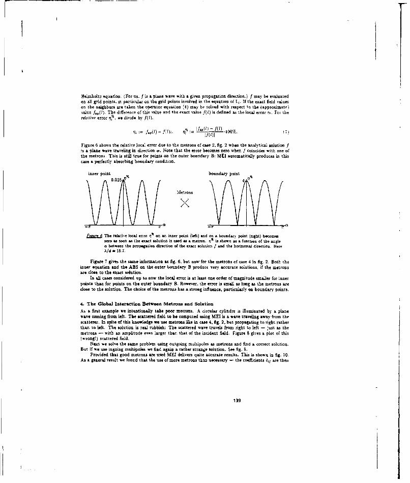
Helmholtz equation. (For us. f is a plane wave with a given propagation direction.) f may be evaluatedon all grid points, in particular on the grid points involved in the equation of L1. If the exact field valueson the neighbors are taken the ooerator equation (4) may be solved with respect to the (approximate)value f.,(1). The difference of this value and the evazt value f(l) is defined as the local error ??,. For therelative error 79. we divide by f(l).

77, := if ,PM l - f (0 1l. 7?.7 := I f J , (I 7./lM. - 1 0 % fW01(~ - 10C frfi

Figure 6 shows the relative local error due to the metrons of case 2, fig. 2 when the analytical solution f;s a plane wave traveling in direction a. Note that the error becomes zero when f coincides with one ofthe metrons. This is still true for points on the outer boundary B: MEI automatically produces in thiscase a perfectly absorbing boundary condition.

inner point boundary point

Metrons

EgaiM The relative local erot rv79 on an. inner point (left) and on a boundary point (right) becomeszero as soon as the exact solution is used as a metron. r7t6 is shown as a function of the anglea between the propagation direction of the exact solution I and the horizontal direction. HereA/d = 15.7.

Figure 7 gives the same information as fig. 6, but now for the metrons of case 4 in fig. 2. Both theinner equation and the ABS on the outer boundary. B produce very accurate solutions, if the matronsare close to the exact solution.

In aU cases considered up to now the local error is at least one order of magnitude smaller for innerpoints than for points on the outer boundary B. However, the error is small as long as the metrons aredose to the solution. The choice of the metrous has a strong influence, particularly on boundary points.

4. The Global Interaction Between Metrons and Solution

As a first example we intentionally take poor metrons. A circular cylindre is illuminated by a planewave coming from left- The scattered field to be computed using MEI is a wave traveling away from thescatterer. In spite of this knowledge we use matrons like in case 4, fig. 2, but propagating to right ratherthan to left. The solution is real rubbish: The scattered wave travels from right to left - just as themetrons - with an amplitude even larger than that of the incident field. Figure 8 gives a plot of this(wrong!) scattered field.

Next we solve the same problem using outgoing mulhipoles as metrons and find a correct solution.But if we use ingoing multipoles we find again a rather strange solution. See fig. 9.

Provided that good matrons are used MEI delivers quite accurate results. This is shown in fig. 10.As a general result we found that the use of mort Metrons th=n necessary - the coefficients c4. are then

139

inner point - boundary point

Metrons

10-4' r 0-0327

fi- 7 The relative local error ni6 betomes very small, if the metons and the exa•:t slution are close

together. On the other hand the error is increased as soon as the metrons ire really differentfrom the exact solution. Note that boundary points produce higher errors han inner points.Here k/d= 15.7.

obtained by solving an overdetermined system of equations using least squares tcichdnques - turns outin better results, particularly in the near field.

The fact that the choice of the metrons has am inguence onto the result mai" be seen either as anadvantage or as a drawback. It is pmeaible to take into account a priori knowledge about the solutionby an 'intelligent' choice of the metrons. E.g., K. K. Mei et al. [1] has used a specific type of metrons(outwards radiating fields of arbitrary (non physical) current distributions on the scatterer) and foundreasonable ABC's from these metrons.

S. The Proguass

A 2D electromagnetic TE- or TM-scattering code has been wrhten. It uses the nmptool [34] for thedata input us well as for the representation of the results. This is advantageous at preprocessing in thesense that almost arbitrarily complex shapes of scatterers "ay be constructed in very short time, anyregula or sonregular grid may be used and any MMP expansion function may b. declared as a metion.The advantage at output time is that afl "estures of field representation - E., R. and 9 field plotsincluding animation. densitity plots etc. are possible.

The only new written part is a MET module performing the calculation of the MEI coefficient! andthe setup of the MEI matrix. A Linpack solver is used for the solution of the (spaise) MEl matrix. Data"exchange between MET and M1MP g= through files which have appropriate IMMP formats. Fina•ly ahigh level -manager program' has been written to handle the data exchange between MMP and the MEImodule. This manager program includes 'macro features' (to shorten several steps to a single one) and

140

"scatterer

ffui The scatterer is illuminated from left (TM-c-ase). The plot shows the (wrong!, instantaneousvalue of the total electromagnetic field energy obtusned by ME] with a poor set of metrouns.Note that the Patches are trAveling from right to left, just - the motrons. Here A•d = 30,

diameter of the sttering cylindre: A/2.

hamS The use of different matrons for the m eatn scattering problem gives very different results. Bnthpictures show the time mean value of the total Po.uting field. Crtgointg multipoles as metronsyield a correct solution (left) while injoing multipoles ma metrooa yield a totally wrong powerflux looking as if it came from the oppoeite side than the incident field but the power flux as

from left to right in both came. Here Ald = 30. diameter of the scattering cylindre: A/2.

automatic file generation and file naming. The program runs on Sun workstations (UNIX). It is available

141

!I

Eimsm I Compsnismo of MEI (left) and MMP (right). The time mean value of the Poynting vector (to-tal field) is shown in the neawdile The accuracy of the MMP mslution is better than 1% andmay be taken as a rfarence. For the MEl 9 institu (outgoing multipoles) have been usea(--lseet squares for computt•g the codeffientst ej). Note "hat the M.MP solution has no prob-lems at the outer boundary. Dimension of the whole picture: 6A x 4A. A/d = I.

from the authors.

8. Summary

We have shown that the quality of MEI solutions does depend 01; the choice of the metrons. In generalthe solution tends to become similar to the metrons. This may" be seen as an advantage since a prioriknowledge about the solution may be brought in by a particular choice of the metrons. Using moremetrons than necessary and computing the grid operator by !east squares techniques yields better resultsparticularly in the near field. This is at least true for the example in fig. 10. Lowever, poor metronsdeliver rubbish rather than results. The presented program allows it to play with different choices ofmecrons and to represent the results in many different ways.

References

[1] K. K. Mai. L Pons, Z. Chen and Y. W. Liu, "Measured equation of invariance - a lean a.ndfast method for field computation." in Proceedings jo the 1992 URSI Int. Symp. on electromagnetictheory, (Sydney) Aug. 1992,

[2] D. B Wright and A. C. Cangelaris. "Performance evaluation of MEI-based mhes truncation condi-tiuns for finite element modelling of electromagnetic scattering by penetrable bodies." in 9th AnnualReview of Progress in Applied Computational blectromagnetics (ACES), Conference Proceedings.(Monterey), Mar. 1993.

[3] L. Bomholt, P. Regli, Ch. Harrer, and P. Leuchtmann, "NMMP-3D: A package for computation of3D electromagnetic felsls on PC's and workstations," in 6th Annual Review of Progress in AppliedComputational ElectronAgnetrcs (ACES), Conference Proceedings, (Monterey), Har. 1990,

[4] P. Regh, 'm=ptool', putlic domaip program, available through ftp anonymous on sirius.ethz.ch(129.132.41.1), directory rmp, Zirich. Nov. 1993.

142

SESSION 4:

FLNITE ELEMENT METHOD (I)

Chair: Jin-Fa LeeCo-Chair: John Volakis

143

Analysis of Dielectric-Loaded Waveguides Using Covariant ProjectionVector Finite Elements

Bruce R. Ci, in and Andrew F. PetersonSchool of Electrical and Computer Engineenrng

Georgia Institute of TechnologyAtlanta, GA 30332-0250

Over the years, a large number of procedures have been proposed for the analysis ofdielectric-loaded waveguiding structures. Most of these approaches are unreliable because of theappearance of spurious modes. Recent research demonstrates that mixed-order covariant projectionfinite elements eliminate difficulties with spurious modes in vector waveguide formulations [1)Furthermore, the fimctions introduced in (1] can be extended to higher polynomial orders and allowparametric mappings to cells with curved sides.

This presentation describes approaches fbr finite element analysis of open and closeddielectric-loaded waveguiding structures using mixed-order covariant nrojection finite elements.Details of the element matrix calculations will be presented. Efficient sparse eigensolvers hased oniterative methods will be described which can handle both non-linear as well as linear eigenvaiueequations. The treatment of open geometries using local absorbing boundary conditions will bediscussed. Analysis results will be preweted that demonstrate the ability of the formulations to solvefor the propagating modes of boxed and oven microstrip lines, without the aopearance of spuriousmodes,

troducinThe finite element method is a ust •ul technique for analyzing propagating .nodes in wavegaiding

structures. A scalar formulation in terms of the longitudinal component of either the electric ormagnetic field is normally used when analyzang homogeneous structures loaded with isotropic material.However, the scalar formulation is inadequate (except as an approximation) for analyzing waveguideswith inhomogeneous cross section or asisotropic materials [2],

To analyze waveguides inhomogeneously loaded with dielectric material, the fitite ulementformulation must consider at least 2 vector field components. Most vector formulations are plagued bythe occurrence of spurious solutions mixed in with the true ones. Mhny techniques have been proposedto deal with the prolemn of spurious solutions (1-5].

One approach that effectively eliminates spurious solutions uses mixeI--' r covariantprojection finite elements in a standard prob:em formulation [I]. This preset. sclsses theapplication of these elements to the solution of dielectric loaded waveguiding structures.

The waveguiding structure under consideration is assumed to be uniform along the longitudinalaxid (,) and, in general, non-uniform across the transverse plane (i -5). The structure is assumed to befilled with a source-free, inhomogeneous, isotropic, losslcss dielectric material, with permiti',ity

144

t(x.y) = e,(xy) eo and permeability p4(xy) - p,(x,yIA. (typically p,(xy) I). The time-dependent

electromagnetic fields in the waveguide at the frequency w are assumed to have the form

.(x,y, z, t) =Re (l(xy) exp A(o - Oz)) (i)

-(x,y, x, t) =Re (E(x,,y) exp j(W - fU)) (2)

where 0 is the propagation constant in the 2 direction.

Mixed-Order Covarlant Proiecd qn Finite lc]MenMixed-order covarian projection finite elements were proposed by Crowley in [I]. These finite

elements have been demonstrated to not allow spurious solutions in standard vector formnulations-These elements faill into the general category of "edge" or 'tangential" elements. In the global mesh,continauity of tangential fields be~een elements is maintained but normal continuity is not.

A general curvilinear quadniateral element in the i-4 plane is mapped into the standardquadrilateral element in the ý - . plane as shown in Figure I. In the standard element, the six 4directed basis functions vary lineary with 4 and quadratically with "q (hence the term "mixed-order").Likewise, the six ý1 directed basis functions vary linearly with Tl and quadratically with F. These twelvefunctions represent the transver field ,omponents As suggested by [6-7], the longitudinal (i)components are represented by nine Lagrangian basis functions with quadratic dependence in bothand ii. In total, there are 12 transverse and 9 longitudinal basis functions per element.

it It~T if

Figure ISlandard Element

Derivation of Finite Element Eitenvalue EauntionsThe finite element formulation is based on the vector Helmholtz equation:

where k1. = a) I z. (4)

Assuming the general form of (1), the transverse components can be separated from thelongitudinal components according to:

y A , . )- l-) (5)

145

It follows from (5) that the vector Helmholtz equation can be separated into two parts, a vector

equation that is entirely transverse to 1 :

V, x {LV, . k,) - , ,.-0k =g-- 0ý p., J(6)

and a scalar equation that has only . components:

-V, . J&(,H: 4JPH,) } ký AH (7)

At this point, one can proceed to derive an eigenvalue equation with either k. or 1 as theunkmown eigenvalue. The derivation that follows considers k. to be the eigenvalue, with A' given.

For convenience, the following scaling is introduced (6]:

,' = 0 if, (S)h. = -j (9)

Using (g) and (9), equations (6) and (7) can be rewritten as:

Coupled weak equations are constructed by "testings" the vector equation (10) with a transversevector testing function T(x,y) and testing the scalar equation (11) with a scalar testing function T(x,y).After using some vector identities and manipulating, the following equations are obtained:

{V TV Xh, + 027h+02 TVh: k .2 ji~h h .Th V .i (12)

fuI {VT -Vh + VT -r =k. Thý Tj -0.+ Th h 1 (13)

where ar is the outer boundary of the region r and h is the outward normal on 1r.Employing the covariant projection elements for the field and testing functions produces the

following matrix eigenvalue equation:

,•h•:A A=.-l'v• ~ • h: o B= h:where: A lV x,. -V xB + 02 h. ) }+J ..hhVxB, (1)

or

A = IJ• ,.VB. (16)A =jJ~vT..•.B- [Tm.;B. (17)

A. = vT..VT . - I . -8)ar

-.. = 4., (19)B= fif T,". B. (20)

146

Ifthe problem is formulated to solve for 32 as the eigenvalue, with kP given, a similar derivationleads to the following global matrix eigenvalue equation

A" A'_ I D ,, 00 h

where AL .=fJ {•(Vs ..vx ) - b,.1 - jr. (h.)

-- (24)

n- V.- + T. h

In the case of a perfect electric conductor (PEC) or perfect magnetic conductor (PMC)boundary condition, it can be shown that al; line inteeg•ls along X go to zero For open regionproblem special treatment of the boundary integrals must be considered One such approach isaddressed in the discussion of the open microstrip problem.

The PEC boundary condition is the natural boundary condition for the H formulation. ThePMC boundary condition is an essential boundary condition which is imposed by enforcing that themagnetic fields tangential to the boundary are equal to zero.

Iterative Solver MethodThe matrix eigenvalue equations ot'(14) and (21) can be written in the general form:

[A] F = X [B] i (27)

Because there are 21 unknowns per element, the global matrices (A] and [B) are large and verysparse. It has been observed by various researchers (e.g. [71) that in edge element formulations usingklas the eierenvalue. there are as many zero eigenvalues calculated as there are free longitudinalcomponents. It has been observed by the authors that in the present formulation using DI as theegenvalue, there Are as many eigenvalues that approach infinity as there are free longitudinalcomponents.

In order not to waste computational resources on calculation of zero or infinite eigervalum, andto allow analysis of medium sized problems (-500 unknowns) on a personal computer, the authors havedeveloped an iterative solver using spar matrix storage techniques. This solver is btsed on the shiftedinver power method which converges to the eigenvalue closest to a selecmed input parameter.

Choosing an arbitrary parameter p, the generalized eigenvalue equation of (27) can bemanipulated as follows:

[[A] - [B1] - = (X. - p) [B] Fr (28)

i [[A] - p~45]j-' (B] R (29)

When equation (29) is iteratively solved, X and i will converge to the eigenvalue and eigenvectorcorresponding to the eigenvalue closest to p, provided that the initial 'seed" vector i does not closelyresemrible .....ih . ... ion eie-iWc"to. .

147

In mdler to avoid puriorning an explicit matrix inversion, the algorithm actually iterates usingthe following varanto, of equation (29)

[[Al -,'8B]] r' = [B] i (30)where i"' is the unknown vector, i' is the value of the unknown vector calculated in the previousiteration, and II- represents the Euclidean norm After each iteration, rrP I is computed and comparedto its valie in the previoub itnrittion When IV' I converges to a stable value, the eigenvalue k is foundfirom

t=!riI sgn({k''4 (31)

what spin) is the Signum funcaiw. The initial seed vector i is created using a raidom numbergenerafor in an attaupt to avoid possible resembleice to a parula•mlr eigenvector and ersure that thealgorisu converges to the eigenivalue closest to X.

In the solver implemented by the auth•ors, the shifted inverse power method is extended tocalculate tM set of einvalues (X) that are closest to p. This is -ccomolished by working with a setof eigenvectors (i,) which are orthogonalized after each solver iteratica using a Gram-Schmidtonhonormaiization procedure Ex, -rimensal trias show that the resulting set of eigenvalues andagaewetorn .oerespod to the md of e~genvalues closes to the input parameter p.

The solver is based on a sparse matrix storage scheme and uses the YI2M subrcutine library tosove the set t-f linear tquatkua repreared by (30) [8]. The user can vary the desired number ofesswqvales The required nunmbr of iterations ncreases with both the dissance between V and thetarget engenvaluest nd the um"ber of desired 'igtaivalues. Fot a selection of I or 2 eigenvalues, thesolvr typcaly cverges to aty dilpts of accuracy within 10-40 iterations The practical maximummier of egenvallues chit can be solved at a time is about 4. Beyond this point, the accuracy of the

outer eageuvalues suffers and the convergence rate stagnates

Annieasmu to I1uxad, Mjg~erA faute ellaneut aialysis tool, basie on equation (21) and the previously discussed eigensolver,

bas been writte in FORTRAN 77 This tool can analyze geometries bounded by either PEC or PMC,A tn-Ul application of sti. tool is to analyze the propagating modes in boxed anicostrip. The covaniantp .q.l.. vector finte .elauuts have bee recommended for this type of problem because edge

caan better handle the smgularaiLs that occur at the trip edges [7]

The gwmiety of the problem is shown in Figure 2. Because of the svmnuery in the p obler,only the right ha plane of the geomeuy ws analyzed. A PMC was ued as a boundary condition inthe plane of wvnm.euy, Thrt sm elemenu we-e used, and after imposition of essential boundarycrt~iuoes, 463 u.awwn s rensaime Usai an HP/Apollo 720 RISC workstation. construction of therS natmucus required about 100 seconds, and the solve, iteration time was around 005 swconds per¶ ienvwkuc itetrjuov:

The iesults of the analysis are in close igreemert with those of [7] 'obtaintd using an aternatecovenatm projection finite element formulation) and [91 (obtained using a formulation based on anintegral equrtion method wih the microstrip currents a. she unknown functions). No spurious modeswere observed Figure 3 shows a comparisor between the first six modes calculated using this methodnd that of[()

148

3.4

i l li

11.43mm 1.27m PIk. I., 1 Picn

1.27nmm

12.7Tam 0.0

Filguas2 0 A 8 12 16 20 24 28 12 M 40 44 43

Bozed MKcrostrnp OCeoetr'Figure 3

Companson of Results for BoxW Microstnp

Aaolliathin to Onen Mic •strjLo 9blemnIn order to analyze open problems, a boundary condition that mimics infinite space must be

imposed along the outer boundary. In general, this type of boundary condition is a non-linear functionofthe eigenvalue and complicates the eigensolution procedure.

To analyze the problem of open microstrip line, an approach adapted from [10] was used. Thisapproach differs from [10 and other similar methods in that the desired field behavior is enforced usingan "absorbing boundary condition' rather than some type of"infinite element".

Along the boundary to the open region of the problem, it is assumed that the magnetic fieldsexhibit exponential decay in the open region according to:

H(x.y 4,z:) =T(x.,yo) exp {--(r - x.) - z,(y -y.o)) (32)

where: a. = a (h. i) (33)a,> = c. (h .J) (34)

t= PO -,, k.1 (35)

and where A is outward normal to the boundary, and x. and y are points along the boundary X. Theparameter ja is in effect the propagation constant of the transverse wave in the A direction. The fieldwill exhibit exponential decay in the open region (e.g a is real positive) as long as 02 is greater than

e, k2. By selecting the geometry of the finite element mesh so that all h of the boundaries to the openregion are directed approximately radially outward, the fields at these boundaries can be forced toexhibit exponential radial decay. This effectively creates a type of absorbing boundary condition. Thedesired field behavior is embedded in the global meshes via the boundary line integrals using the basisfunctions modified as shown in equation (32) The resulting eigenvalue problem, however, is non-lineara&d special solution techniques must be used.

The finite element code used to analyze the boxed microstrip problem was modified to performanalysis of open boundary problems with fields exhibiting exponential decay in the open region. The

itcrative nature of the existing solver allowed solution of the non-linear eigenvalue problem with onlyminor modification of the algorithm The solver was modified such that for each iteration, the boundary

149

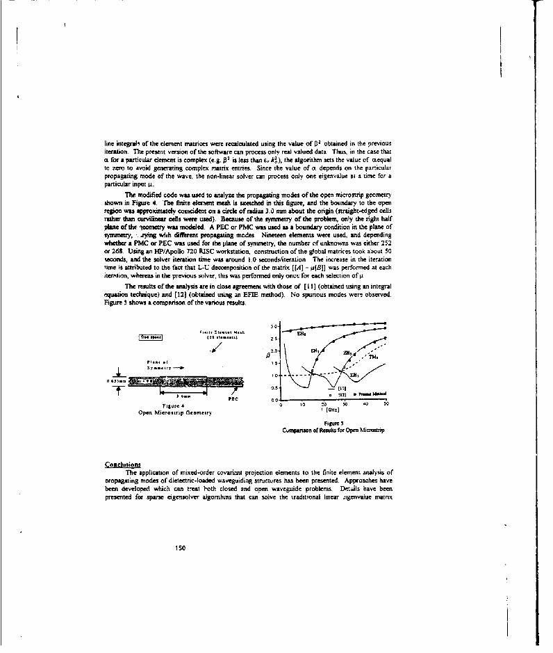
line integrah of the element matrices were recalculated using the value of 12 obtained in the previousiteration. The present version of the software can process only real valued data Thus, in the case thata for a particular element is complex (e.g. 02 is less than c, k2), the algorithm sets the value of coequalto ze•o to avoid generating complex matrix entries. Since the value of aE depends on the particularpropagating mode of the wave, the non-linear solver can process only one eigenvalue at a time for aparticular input 4t.

The modified code was used to analyze the propagating modes of the open nicrostrip geometryshown in Figure 4. The finite elerent mesh is sketched in this figure, and the boundary to the openregion was approximately councident on a circle of radius 3.0 mm about the origin (straight-edged cellsrather than curvilinear cells were used). Because of the symmetry of the problem, on!y the right halfplane of the 4eometry was modeled. A PEC or PMC was used as a boundary condition in the plane ofsymmetry, . Ay•zg wiih different propagating modes. Nineteen elements were used, and dependingwhether a PMC or PEC was used for the plane of symmetry, the number of unknowns was either 252or 268. Using an HP/Apollo 720 RISC workstation, construction of the global matrices took about 50seconds, and the solver iteration time was around 1.0 seconds/iteration The increase in the iterationrime is attributed to the fact that L-U decomposition ofrthe matrix [[A] - p(BB] was performed at eachiter'.tion, whereas in the previous solver, this was performed only onct for each selection of A

The results of the analysis are in close agreement with those of [11] (obtained using an integrallquasion technique) and [12] (obtained using an EFIE method). No spurious modes wer- observed.

Figure 5 shows a comparison of the various results.

• / •2.j I,

S.. -~I---------

pl C 0 0

Figure 4 0 1t 20 30 '0 50Open Microstrip Gfeoery [GHZ]

Figure 5Cumpano• n of RPalts for Open kiclosinp

ConclusionsThe application of mixed-order covari•nt projection elements to the finite element analysis of

propagating modes of dielectric-loaded waveguiding strictures has been presented. Approaches havebeen developed which can treat both closed and open waveguide problems. DIeils have beenpresented for sparse eigensolver algofihisns that can solve the traditional linear .igenvalue matrix

150

equation as well as the non-linear eigenvalue equation that results during the analysis of the open regionproblem. The formulations avoid the calculation of spurious modes and sample results show goodagreement with other published data.

[1] C. W. Crowley, "Mixed Order Covariant Projection Finite Elements for Vector Fields." Ph.D.Dissertation, McGill University, Cnawa, 1988.

(2] B. M. A. Rahmmna, F. A. Fermandez and J. B. Davies, "Review of Finite Element Methods forMicrowave and Optical Waveguides," Procteeings of the IEEE, vol. 79, no. 10, pp. 1442-1448,Oct. 1991.

(3] M. Koshiba, K. Hayata and M. Suzuki, Finite-Element Method Analysis of Microwave andOptical Waveguides - Trends in Countermeasures to Spurious Solutions," Elect. and Comm.Japan, part 2, vol. 70, no. 9, pp. 96.107, 1987.

[4] A. Konrad, "A Direct Three-Dimensional Finite Element Method for the Solution ofElectromagnetic Fields in Cavities," IEEE Trans. AMagn., vol. 21, no 6, pp. 2276-2279. Nov.1995.

[5] E. T. Moyer Jr. and E. A. Schroeder. "Finite Element Formulations of Maxwell's Equations -Advantages and Comparisons Between Available Approaches," IEEE Trans. Magn., vol. 27, no.5, pp. 4217-4220, Sept. 1991.

[6] 1. F. Lee, D. K. Sun and Z. J. Cendes, "Full-Wave Analysis of Dielectric Waveguides UsingTangential Vector Finite Elements," IEEE Trans. Microwave Theory Tech., vol. 39. no 8, pp1262-1271, Aug. 1991.

(7] R. Miniowitz and I P Webb, "Covariant.Projection Quadrilateral Elements for the Analysis ofWaveguides with Sharp Edges,' IEEE Trans. Microwave Theory Tech.. vol. 39. no. 3, pp.501-505, March 1991.

[8] Z. Zlatev, J. Wasniewski and K Schaumburg, Y12M, Springer-Verlag, New York, 1981,

[9] C. J. Railton and T. Rozw, "Complex Modes in Boxed Micros'ip," IEEE Trans. MicrowaveTheory Tech, vol. 36, -to. 5, pp. 865-874, May 1988.

(10] K Haysta, M. Eguchi and M. Koshiba, "Self-Consistent Finite/Infinite Element Scheme forUnbounded Guided Wave Problems," IEEE Trans. Microwave Theory Tech., vol. 36, no. 3, pp.614-616, March 1988.

[11 K A Michalski and D. Zheng, "Rigorous Analysis of Open Microstrip Lines of Arbitrary CrossSection in Bound and Leaky Regimes," IEEE Trans. Microwave Theory Tech., vol. 37, no. 12,pp. 2005-2010, Dec. 1989.

[12] C.H. Lee and J S. Bagby, "The Analysis of Coupled Microstrip Transmission Lines with EFIEI~ethod." in Dig. URSI Radio Sci. Meeting (Syracuse, NY), June 1988, p. 318.

151

A Finite Element Formulation for MutitpolveModes In AxIsymmati-ic Structures'

E. M.' NelsonStanford Uinear Accelerator Center

Stanford Uninverity, Stanford, CA 94309

Abftrxacfinite element Boeld solver for multipole modes in &xisymmetric structures has been written and tested. The

ohwr is based on a weak version of the cudi-curl formulatiin of Maxwell's equations in cylludrical coordinates. Acombination of mixed-order (edge) and ILgrange-tyie basis functions axe used to avoid spurious modes. Second-order trianguilar elements are employed to obtain very accurate mode frequencies. Elements which touch the axisuse speciial bais functions.

Tomt on analytically soluble structures demonstrate the accuracy of thc computed mode frequencies and theavoidance of spurious modes. A disk-looded waveguide example demonstrates not only the accuracy of the solverbut also boundary conditions for periodic and/or symmetric structures. The solver has been applied to the designof detuand accelerator structures for the nam generation of linear colliders. A precise distribution of dipole modesis required to minimixe the 3,fect of wakefields. An overmoded 90* waveguide bend example demonstrates thespplicabflty Of the solver to curved wuveguide.

Finite Element Formulation

Consider an adsymmetri- structure represented by the two-dimensional region 5 Land various types of bound-&rie ihe &Is-p plane. The boundary l'aon is a perfectly conducting metal boundary and Isym,.") and rar-jmawe symmetry planes of the irtructure with electric and magnetic boundary conditions, respectively. For periodicstructures, fl is one cell bounded by rv,ý and r.& as shown in figure I(&), ind for symmetric periodic structures,

Sis a hal cull bounded by rw-1 0f and rs-. as shown in figure I1(b).Wiriting the probirm is c'linddical coordinates z, P and 0 with fidd components Z,, E# and E., the solutions

can be decomposed into multipole modes with -azimtha dependence e-. A weak formulation of Maxwell'sequsations toe~ this problem to the gausian "ymti of units ir~ given the region A', its material properties c and 14,an asimuthial symmetry number mn, and possibly a phase advance 0 (for periodic structures), find the cigenmodefields 8 eUas and the corresponding elgenvaltes w/c2 such tiint for all teat functions F EU.

., ((VsrF-).-p1 (VsrE) - 7 V -cE) 2spdpds 0 (Ut)

where the space as of test and trial functions iscis -(3 e 7f 1 5 ,(j

i~xE-=0 on r,-and r,.4-0 41 ,fixj#- -&xEI~, e v x e ri,, (lb)

%Nm~fiE) =0 onnro...f an(:%iM 012 17.,} -0Uo

andWork arippot zed by Department of Energy, contract DE-AC03-76SFOOSIS

152

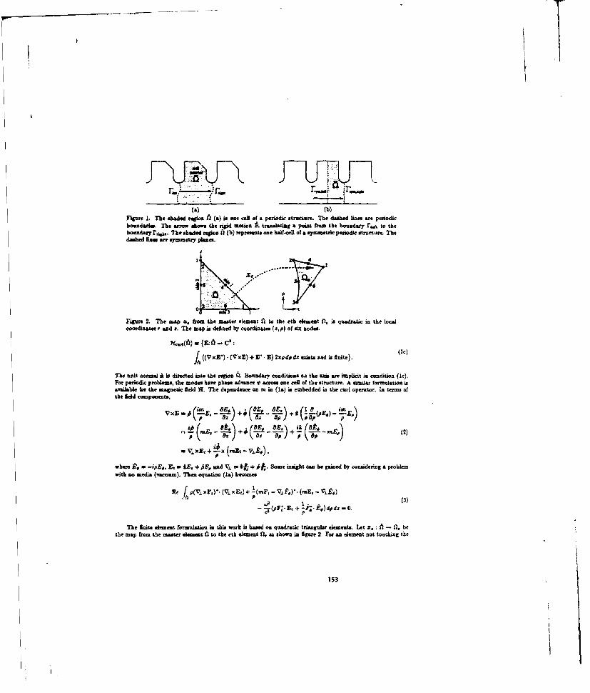
S(a) (b)Figure 1. The shaded region • (a) is one call of a periodic structure. The duhed lines are periodicbondarim. The wow shows the r motion A traa-st.ing a poit from the bondary rien to theboundary r.04. The shaded region (b) represents cue half-cel of a symuetric periodic structure, Thedashed aes are symmetry plane.

#2

IS 4%

Piu re2. The map z. fm the muter element to the eth element P, is quadratic in the local

coordinates r and a. The map is defned by coordinates (z, p) of six modes.

((VxZ*) • (VxE) + V1. E) 2epdpiz exists and is finitel. (Ic)

The unit normal is is directed into the region CL Boundary conditions ou the A4s as implicit in condition (ic).For periodic problems, the modes have phase advance 0 asross one ceal of the structure. A similar formulation isavailable for the -an etic Aded H. The dependence on mr in (•a) is embedded in the curl operator. In terms ofthe field components.

i'4 + 4± ( !~--V. !Z-.) +i.(L 2

where to - -apBo, Ef- UE. +,5Fpand VL - i ,+ . Some insight can bepgined by considering aproblemnwith so media (vwcuum). Then equatiou (I&) becomes

we /p(% x.) . (V.LxEa) + !(in 1- F,) (r-E, - l#

W2 .(pF*. E, + 1,Pz. ,t)dpd. - 0. (3)

The Auite element formulation is this work is baned an quadratic triangular elements. Let z. : f) - 11, bethe map from the master element f) to the eth element fl, ah shown in figure 2. For an element not touching the

153

ýct3

LlNT No N14Figure &~ E-sapla of local basis functions. i., is a vector field normal to sides 2 and 3. This field couldbe a badis function far. a"ea edge element. NII, No and N14 am quadratic basis functions for the vectorfield It. constructed frum Li. M7 and No have -ona-zero tangential field on side 1. The size and directionof the triangles indicate the umagntede and direction of the vector basis function

axis, the scalair field ta, is modelled by aecond-osrIer lagrange-type basis functions No

N, wr(2 - 1) N2 =e(2# -l) N3 =t(2 -1) (4N' aire Ns -4u1 No .4rt,()

where t wI- r - a. No Ee that the map ze is a llow combination of the Ni listed above:

*.(r~s) = _cJN.(r,&), (5)

where e, ame the (z,p) coordinates of the ith node of the eth element.The bm"i funictions belnow for the vector field E, were inspired by the cov~riant projection element31lj-[5j of

Crowley and the work of Nedelec[fij. They ane similar to the basis functions described in [7] Lod 181, Starting withvector fields V; tangential to side i and directed counterclockwise,

VI =-(V2 +VS), V2 =---- and V3 (6)

construct reciprocal vectoar fields A, normal to side i and directed inward,

*(--R R) 2 OVsx ndRs- )V (7)

The reciprocal vectors can also he written as

which states that the reciprocal vactors are derivatives of <I the invers of the elevrart transformation. Nowconstruct voctor fuaetoss Li which satisfy L1 V1 an 6q, on aide j of the element:

Ll nerR3 - *R,, In uRi- SR. and L3 -tR - rRl. (9)

The vector fields La ams suitable basis fuinctions for a linelar edge element. Rollever, quadratic basin functions areemployed in this woeo

NT - rL, NIO =11M2 Ni2 3 -243sNo = Al1 Nil = tL3 N14 - -Mtl. (0No. A, M3sN = rL3

The first six vector basis functions, N7 to NM, have con-zero tangential field en one side of the element. This fieldmusto match the tangential field of the adjacet elemelit. if there is one, in order to construct Valid global basisfiunctions. The last two v-uwo basis functions. N 1 &And N14, bave No~ tangent'ia fivid on the element nides. Eachof the local vector hexis functions N 13 and Ni. by themselves constitute valid global basis functions, thus they useinternal depeen of frteýdom for the element. Figure 3 shows some of thene local basis functions.

154

Elements which touch tbe aids Sze restricted so that the globa badis functions satisfy condition (1c). Theimportant terms ane those weighted by 11p, hen"e

t.o a and mE,- Vj. - 0

is required of each basis function. This is accomplished by using l"ear combinatius of the basis fuuctious above_First consider the int # 0 case. For an element with an edge (edge 3) on sail there are 6 local 4asis functious.Written as (E,,to) they are:

NJ - (O0'.) NJ (-Rs, at) No - (.I,,O)

N,..-(L~Rs~) N. (LO No - (-2sLs,0). (2

An element witi, uiactly one node (node 2) on Lids baa 11 local basis functions:

NJ (0, r(2r - 1) + r) NS - (!LsNJ = (0, f(25- 1) + at) mNo = (rL3,O)

NJ - (O,4rt) No (rL1, 0) Nic = (-243,,0) (13)

N4=(-=L,ro) NT - (ML,0) NI, - (-25L,O).N n No = (tI,,0)

For the special canm - 0the feldsZ, and t#an uncoupled and canbeseparatedif desired. A quadratic elementwith edge 3 on axi has one basis function,

N a2,,(4

for to,. and all 8 basis functions, N2 through No, for Es. A quadratic element with only node 2oan aids has threebasis functions,

N. - r(2r -1) +a Ps 2-t(2t -1) +st and N = 4rt, (15)for4t, and a~lS basis functions, N4 through NJ I, for E,.

Tarets

The formulation has been tested on some analytically soluble problems: an annnlar ring (L~e., a length ofcoania cable shorted a± the two ends), a pillbox and a sphere. For the annular ring the elgenuTlue error is 0(k

4)

whetn k is the min of the elements. For the pillbox and the sphere the eigeuvalue errr is O(V'9). Examples ofmeshes fur a sphere are shown in figure 4 and the error of the computed elgeuwallue for the 10 lowest mn -1I modiŽas the mesh is reined is shown in figure 5(a). The formulation converge smoothly to the exact eigenvoloe &A themesh is refined, which allows extrapolation of the computed *ieunealues to an infinitely refined mesh to obtaina better estimatte of the exact eigenvalnm. In figure 5(b) the error of the computed eigeaealues, in a pillbox isshown as a foacties of mn. The relative aerrr of the computed elgeumalue increases slowly as it ncreases beyondmn =2. Hence, the Sormoulation is sulitable for lm agen. In addition to integer mn, taut on an annular ring show theformulation works well for noa-integer en as well. Flor mote details of these uits" me 91

)deasurementsoll~ of the dissensions and resonant frequencies of a stack of six cell of disk-loaded warreguidewere used t& further test this formulation. The stack consists of five coell with a shorted half-cell at each end.A mash in shown in figure 7(a). The ouerasud dimensions am. cell diameter 2.159cm, disk aperture diameter0.8574 cm, disk thickness 0.1404 cm end period 0.8751 cm. The dispersion diagram for this strcture is shown infigure 7(b). The measured frequencis in the nascend hand agree with the computed frequencies to better than0.1%. The estimated error of the, computed frequencies is lass than 0.01%, anthe di~srepancies axe probably dueto farication and measurement errol' of the six cell stawk.

Applications

The motivation for this work was the design of detuned accelerator structuresilll. A precise distributionof dipole modes is required to miaimine the effect of wakealelds. This solver was used to compute the dipole

155

0 1

Figure 4. A course mesh (on. element) and two refined meshes for the sphere problem. Each meshcovers the shaded region M The dashed line is a symmetry plans

IQ0-4

10

"OTH3 2

IQ VR35 3 -

I o ! ~4 -E4Tii

AT

M141

15H

0 Th1 0

0.02 0.05 5.1 0.2 O-. 10 0 2 4 6 8 10

Node spang Azimuthal symmetry number m(a) (b)

Figure S. Ralsl' errort of the computed agenvalue vs (a) mesh refinement and (b) m. In (a) the electricfied is coumpted for the va= I modes of a sphere with radius 1. In (b) the electric field is computed ona 312 element mesh fo a piPbox with length I and radius 1.

egg... .. aae -WU Coas:-wl...

Figure 6. Field plots of the two lowest m ,,I mode; of a sphere based on the 256 element mesh infigure 4. The trianls represent the magnitude and direction of the fields E. and Hi, The size of thecirles represent the magnitude of the (imaginary) fields E, and H#. A crossed circle indicates the fieldis w"PLt15

156

/2

0 30 40 90 120 l'50 1SOphase advance *(deg)

(a) (b))

igure 7. A coae.. mash (a) and a fine mesh (b) for one hali-cell of disk-loaded wavegutide. The leftand right edges ame .ymetry plane.i. The bottom edge is the amis. The dispersion diagram (c) for thisstructure wus generated from calculations at seven phase advances.

oz.2- t*lSA 15.6 13.4 15.2 15.0 14.8 14.6 14.4 14.2

0.8 0.9 1.0dish aperture diameter 2a (cm)

Figure S. The lowest synudizonous dipole mode Erequency f, (in G~z) for periodic disk-loaded wavesuide.The* call dimaeter 2b i determneiad front the syndixunism condition for the 11.424 GHz accelerating soode:phas" vakodtq o .e c at phase advance * . 2U/3. The open dirces awe the dimensions at which ft wascomputed. The dots wxe the 206 cells of the detunad accelerator structure.

4

2 ~2

Figure 9. Dispersion diagram of a curved guide with radus of curvature A, The dashed live is the drivefrequency, and the dotted line corresponds to the speed of light along the center of the guide.

157

mode tkequovndes synchronous with the beamt iý periodic disk-loaded waveguide, as sbcws. in figure a. Then cellpamameters of an a cale afar etructus, wem ub-sae to obtasin the ,iesired diptole mode distribution.

Another application of this solver was the desgn of a 90' overmoded wavreguide btnd[121. It is useful toconsider modes propagating along 0 in the curved guide with phaa.L factor e'-. This is analagoui to wodespropagating along x with phase factor ei" in straight guide. Since the bend is only over 90*, cot a full circle,there is no condition that vm be an integer. This solver was used to compute dispersion diagrams for the curvedguide. An example is shown in figure 9. Note that the curves; awe not parallel as one would expect in straighthomogmnouso guide.

Conclusion

The Anit. element formnlation described above computee modes in periodic structures with excellent accuracy.

befstrences

(11 C. W. Crowley, P. P. Silvester sad H. Hurwitz Jr., 410ovariant Projections Elements for 3D Vector FieldProbhlem," IEEE Trans. Msgneejcs, vol. MAG-24. pp. 397-40W, Jan. 1988.

[2] A. &. Piucbuk, C. W. Crowley and P. P. Silveeter, 'Spurious Solutions to Vector Diffusion and Wave FieldProblems.* IEEE Trans. Magnetics, vol. MAG-24, pp. 158-61, Jan. 1988.

[31 J. P. Webb and Ruth Miniowits, 6Analysis of 3-1) Microwave Resonatnrs using Covariant-Projection Ele.metsu,' MEE Trans. Microwave Theory Tech., vol. M'1"-39, pp. 1895-1899, Nov. 1991.

[41 Ruth IMiniowita and J. P. Webb, 0Coaraiant-Projscticn Quaduilateral Elements for the Analysis of Waveguideswith Sharp Edge, MEEE Thsas. Microwave Theory Tech.. vol. ldI1.39, pp. 501-605. Mar. 1991.

[5] C. W. Crowley, 'Mixe Order Covauiant Projection Finite Elements for Vector Fields," Ph.D. dissertation,McGill University, Mountral, PQ, C-anda, 1968

[6] J. C. Nedolec, *Mixed Finite Elements in ',* Nam. Mfath., vol. 35, pp. 315-341, 1980.[7] Jin-Fa Lee, Din-Kow Sun and Zoltan J1. Ceades, "Full-Wave Analysis of Dielectric Waveguides Using Tangential

Vector Flunite Elements," 13=E Trsns. Microwave Theory Tech., vol. MTI'-39, pp. 1262-1271, Aug. 1991.[8] Jiu-Fa Lee, Gregory X VIWilkins and Raj %Mittrs, *Finite.Eleznent Analysis of Azisynmetric Cavity Resonator

Using a Hybrid Edge Element Technique," IEEE Trans Microwave Theory Tech., vol. MTT-41, pp. 1981-1987,Nov. 1993.

(9] E. Mt. Nelson, 'High Accuracyr Electromagnetic Field Solvem rr.r Cylindrical Waveguides and AxisymmotricStructures Using the Finitet Element Method," Ph.D. dissertation, Stanford University, Stanford, CA, 1993;also SLAC-431.

110] H. Dernyter -f ad. Hoag, private ontmnlcation.111] J. W. Wang and P.Mh. Nelson, "Desig of the Detrined Accelerator Structure," Proc. i 199 EE Particie

Accelerator Conf, pp. I08-10688 also SLAC-PUB46142.[12] C. ltantists., N.M. Kroll and E. M. Nelson, 'Design of a 90' Overmoded Wavegude Bend," in Proc. 199.3

IEVE PArticle, Accelerator Cos&L,. pp. 983-U85; also SLAC-PUB4141.

158

AZIMUTHALLY-DEPENDEN r FINITE ELEMENT SOLUTION TOTHE CYLINDRICAL RESONATOR'

Roberto A. Osegueda, Joseph H. Pierluissi, Luis M. Gil,Arturo Revilla and Gustavo J. Villalva

The University of Texas at El PasoCollege of Engineering

El Paso, TX 79958

and

G. John Dick, David G. Santiago end Rabi T. WangJet Propulsion Laboratory

Calitornia Instizute of TechnologyPasadena, CA 91009

Abstract: The cylindr~cal cavity resonator loaded with an anisotropic dielectric isanalyzed as a two-dimensional problem using a finite element approach that assumessinusoidal dependence in azimuth. This methodology allows the first finite elementtreatment of the technically important case of a resonator containing a sapphire elementwith a cylindrically aligned c axis. Second order trial functions together with quadrilateral

elements are adopted in the calculations. The method was validated through comparisonswith the analytical solutions tor the hollow metal cavity and a coaxial cavity, as well asthrough measurements on a snielded sapphire resonator.

I. Introducdon

Although the analytical determination of resonant modes and frequencies of themetallic cylindrical cavity has a well established history, a solution for "the cavity partiallyfi'led with an anisotropic dielectric generally requires computatijnally complex, three-dimensional numerical analyses. Approximate analytical means of analyzing the dielcc;tric

resonator have been proposed throughout the years [1, 21, and with some degreit of

accuracy the theoretic3l ettimates have agreed well with experimental results. However,

becausc of the inherent shortcomings of the approximate analytical modols, numeaicalmethods have continued to receive a great deal of attention during the past years [3, 41.

Recently. so called "whispering gallery" resonators consisting of a sapphire dielectric

element in a metallic container have made possible new capebilities for microwave

oscillator phase noise and frequency stability (5,6]. With high azimuthal mode numlners,

* This work was sponsored by and carried out in part at Jet Propulsion Laboratory, California Irtilrte of

Tecnnoiogy. undo . t -.4 ftt2%;Qr l Aconi sUtICS 2M -Spce Adrntiniitrti~n.

159

these ranOnatorS isolate radio-frequency energy to the dielectric, ement and away fromthe metallic container, thus providing extraordinary low losses a d high quality factors(O's). However, these widely disparate field magnitudes pos a challenge for anymethodology to accurately calculate (e.g.) conductive losses due to small evanescent fieldsat the wall of the containing can. In particular, a three-dimensional finite element methO•allowing full treatment of sapphire's anisotropic dielectric constant, would require such alarge number of nodes as to become impractical. Analytical rrathuds are unattractive, withnew approaches required for every geometrical configuration change. A xwo-dimensionalfinite element approach, however, would allow easy treatment of any cylindricallysymmetric resonator geometry.

Because the dielectric constant for sapphire shows cylindrical symmetry, a twodimensional treatment is allowed for the important case where its crystal c axis is alignedwith a physical axis nt exisymmetry. In terms of the field intensities. the problem isgoverned by the three-compoiient vector Helmholtz equation which can be treated as anaxisymmetric problem only for rmodes with no azimuthal (or 0) dependence. Such zero-arder modes can be o'btained from a two-dimensional approach tu the cavity in the r-zplane using a variety of techniques which yield reasonable accuracy. Higher order solutionfor isotropic dielectrics are still obtainab!e in two dimensions ;f the azimuthal dependenceof the modes is assumed a proml [7]. In the work presented here, the authors reduce thefinite element analysis of the anisotropic dielectric resonitor to two dimensions byassuming an exponential O-dependence, and limiting the permittivity tensor to posseslongitudinal and transverse components only. While ruling out most anisotropic dielectricconfigurations, this approach makss possible the first two-dimensional finite elementtreatment for sapphire "wh~spering gallery' resonatcrs.

I1. Fundamental Equations

In terms of the mv!netic field intensity H, the vector Helmholtz equation with thepenalty term included is given by 181

V xik]" VxH-aV(V-H) -k* 2 H - 0 (1)

in which [k] is the tensor dielectric constam, a is an empirical coefficient of the penaltyterm 1 (7-H-, ond k. is the free-space propagation constant. The variational energyfunctional associated with (1) is given by 18]

F{ H) - I{ (VxH) -([k]"- VxH) - k3

o H°.H + aoV.H)*.(V./} dO (2)

where 0 is the volume of the resontator. In a finite element solution, H is normally choseninstead of E because of the discontinuity of the latter at dielectric interfaces.

160

At the interface between a perfect conductor and a lossless dielectric with a unitnormal vector a, the use of (2) imnlies that

a, '[kj-' (VxH) - 0 (3)

as a naturally satisfied condition, while the condition

a. - H - 0 , (4)

needs to be enforced, There is no axis of axisymmetry for the higher order modes (n >0)and, hence, no perfect magnetic conductor with its associated boundary condition needsto be invoked along the z axis.

Ill. Finite Element Analysis

Inside the volume of the cylindrical resonator the magnetic field vector may bedescribed as

H.(r,O,zl{ H (r,O,z) }. Hor,0,z( 0 - (H (r,zl ) e' ) e)

H,(r,.,z)

where

{ H (r,z)T - L H,(r,z) I H,(rz) H,(r,z) J (6)

and H,(r,z). H,(rz) and H,(r,z) are functions describing the variations of the components ofthe field vectors in the r-z plane. The n in (5) denotes the azimuthal mode number (1, 2,3_. .) while j is used to establish the comoonent H, to be in phase quadrature with thetransverse components H, and H,. In this manner, H,(rzl. Hi(r.z) and H,(r~z) are realfunctions.

This finite element formulation considers the use of general ring elements to solvefor the magnetic field vectors. These elements are defined in the r-z plane and have mnodes. Within each finite element, H(rz) is approximated in terms o' the standard shapefunction matrix JAI as

{ Hlr,oz) } - [N(r,z)]r { H ). e0'1 , (7)

in which

{ N(r,z) }r L N, 1r.z) N2(rzi .... N,(r,z) J , (9)

161

{)z) { {N(rz) { (0) 1L (0) (0) { N(r,z)}J

and

(H)T- LUH: {H.): I.,}J (10)

Here. •1*, is a rI.Olecticrn matrix of order 3m by 1 containing the unknown nodal

values of the fielo arranged as in (10), and NV.z) is the shape function associated with the

io node o. the .s;..ront. 'l',a speci:ication of the azimuthal dependence in 17) allows for

a triviani 8raytZiCb! integratian of tht; functional in (2) from m-0 to 0=2" when the

die'ectric properties 3re. i-i-dependent.

The substitutidO of the field approximation in (71 into trhe functional expression (2)

leac;s to ihe element Mnux equation

F. H) [ [SI. -LI., - k.2 IT.]{,] . (11)

where

LS]. [ I [A ' [ -" [AI dr n 112)

[UR, - IC) [Clr d , (13)

171. (PA' [NIT dO . (14)

(0) Fe} -.i (vrl

[A] - e•"' -j ( -E {0} , L-7[A] (.L(N 0) 1W (151

r.2.(N) -{---} fa)

'62

4'-

ind

(C] - er' -2(N) (16)

The integrations of (12), (131 and (141 over the azimuthol direction are doneanalytically, requiring that the dielectric properties [(] in (12) be 0-independent. This issatisfied when (K) has zero value off diagonal coefficients, and when the radial permittivityis equal to the azimuthal permittivity. The integrations of (12), (13) and (14) over theelement area in the r-z plane are evaluated numerically using the standard Gauss-quadraturetechnique generally used for isoparametric elements with non-rectangular and curvedshapes [9).

The global form of the functional in (11) may be expressed symbolically as

F={ Hlr[[SI . IU]-ko2 (T] ]{IH , (17)

where [S), IUL and 11T are global matrices resulting from the superposition of thecorresponding element matrices, and {(M contains all the unknown nodal values of themagnetic field vector.

Applying the Rayleigh-Ritz criterion, 117) yields the eigenvalue equation

( I SI I - U I I( H} -k.2

[ T I{H) -0 , (18)

which needs to be solved for the resonant frequencies w, = ck, and for the' nodal valuesof the corresponding mode intensities {'h. The parameter c is the velocity of light in freespace.

IV. Comparison to Analytical Solution

The proposed method was tested by solving for the resonant frequencies and modesof a metallic hollow, cylindrical cavity resonator with a radius of 3.8 cm and a height of 4.5cm since the exact analytical solution is well-known. The resonator was modeled usingrectangular ring elements with four corner nodes and bilinear shape functions. Solutionswere obtained using 16, 36, 64 and 100 elements. A penalty factor of a = I wasassumed in (1) throughout the calculations. The identification of the modes and theremoval of spurious modes was assisted by computations of the cosine of the angle ftbetween the eigenvectors frnm Tlhe finit_ element sn!ution and the exact eiganvactors.The cosine of this angle is given by [81 as:

163

cos - { IL} {Hr }19)IT-- { )TEU O H.} U

where (H} is the eigenvector solution of (18), (H.) are the nodal values calculated from theexact analytical expressions, and the factors in the denominator are Euclidian norms. If thevalue of cos f in (19) is close to one or minus one, then the field vectors (H} and {H.) arethe same. Equation 119) was evaluated using each {H,} and all {H) vectors to find thecorrespondence between each aralytical vector and the numerical eigenvector.

Figure 1 shows convergence curves for w, obtained from the finite element solutionfor the transverse magnetic TMew series modes, where the subscripts reps esent the nuttberof oscillations in 0, r, and z, respectively. The abscissa corresponds to tho order of modeextraction in the finite element so;jtion. For 100 elements the resonant frequerciesconverged to about 0.12% frorm tne exact values for both the TE iu, TM moJes. Fig. 2shows a sample of the rn-sufts obtair~ed through the use of the cosine of the angla betweenvectors in (19) for mode identification. The true TE0,. modes are shown on the top of thefigure, with a cosine close to one, while the sp'irir)us modes have values much lower thanone. Fig. 3 shows the frequencies of various families of TiE and TM modes of the cavityresonator as functions of the azimuthal ndex.

-4 ICMEMENT5

f 16

(GHz)

14

1 2 3 £ 5 6

OFFR OF MODE B 'TACTION

Figure 1. Convergence curves of the finite element frequencies fnr the first six modes ofthe hollow cavity with r .- 6.

164

1-l0

1 0 0

0 0 0 0 CJ 0 00.90

Cos P

080

0.70

0.60 I

5 11 14 17

f (GHz)

Figure 2. Finite element frequencies of modes obtained for the hollow cavity. The modeswith cosines close to unity are physical, while those with smaller values are spurious.

TEMIf mn2O I-- mj:;ýTWO~1

oA - TM,1O

T&22 TEW~ 2

14f TEW 11

(6 10

6

2 I I I I I I I I

0 1 2 3 4 5 6 7 8 9 10

AIIMUTHAL M0DE NUMBER (n)

Figure 3. Sample fa, nilies of modes obtained from the finite element analysis of the hollowcavity with 100 quadrilateral elements.

165

I

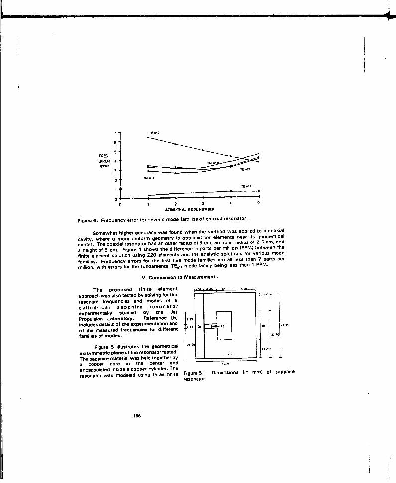
7 Tni 2

6

FRRCR ATM n

IP 3 6. . ~ ~2 TM

TiiI

TE"11

0 1 2 3 4

AZMUTHAL. MODE NUMS

Figure 4. Frequency error for several mode familios of coaxial resonator.

Somewhat higher accuracy was found when the method was applied to a coaxial

cavity, where a more uniform geometry is obtained for elements near its geometrical

center. The coaxial resonator had an outer radius of 5 cm, an inner radius of 2.5 cm, and

a height of 5 cm. Figure 4 shows the difference in parts per million (PPM) between the

finite element solution using 220 elements and the analytic solutions for various mode

families. Frequency errors for the first five mode families are all less than 7 parts per

million, with errors for the fundamental TE,, mode family being less than 1 PPM.

V. Comparison to Measurements

The proposed finite element ,

approach was also tested by solving for the ' :,

resonant frequencies and modes of acylindrical sapphire resonator

experimental:y studied by the Jet 7IPropulsion Laboratory. Reference 15] ,

includes details of the experimentation and ,

of the measured frequencies for different C.1 20

families of modes. 132.70

Figure 5 illustrates the geometrical ,

axisymmetric plane of the resonator tested. 73-

The sapphire material was held together by ,

a copper core in the center and

encapsulated irnsde a copper cylinder. The

resonator was modeled using three finite Figure 5. Dimensions lin mm) of sapphire

resonator.

166

element meshes comprising of eight-node elements of sapphire and air materials. Th.edielectric properties of the sapphire material were taken from Ref. (21 as ir, =- f - 9.407and E. = 11.62. The coarse mesh consisted of 62 nodes fnd 15 elements, the mediumme.-h of 193 nodes and 54 elements, and the finest mesh has 709 nodes and 216elements. The perfect electric conductor boundary condition reflected in (4) was enforcedat all metal boundaries of the finite element meshes. The eigenvalue solution of (18) wasobtained for azimuthal order values ranging from 3 to 12. Each solution yielded a set ofresonant frequencies with associated eigenvectors. The lowest frequency solutioncorresponded to the fundamental mode for that ne azimuthal order.

Figure 6 shows the resonant frequencies of the fundamental family of modes WGI-,,for the three meshes with n values ranging from 3 to 12, Illustrating convergence of thesolutions as the finite element wash was refined. The mode lassification shown is basedon the notation of Jiao, et al. [6) for whispering-gallery modes. A finer mesh was notconsidered feasible due to computer memory limitations.

10 10 ~16 ELE=MENTS

f(GHz) 7

6

5

43 4 5 6 7 8 9 10 11 12

AZIMUTHAL NODE MUMBER (n)

Figure 6. Convergence curves of the finite element frequency for the fundamental WGH,,tfamily in the sapphire resonator using different mesh sizes.

Figure 7 shows the frequencies of the families of modes that were identified and thatmatched with the frequency measurements made at the Jet Propulsion Laboratory [5]. Thesolid lines of the figure correspo.,d to the finite element results and the dots are themeasured values. From this figure it is ooserved that the finite element results agree wellwith the measurements. The errors in the resonant frequencies of fundamental fami:yWGHl- I modes, obtained from the three meshes, with respect to the measurements arelisted in Table 1. Errors of the resonant frequencies of the rest of the families shown inFig. 7, including uncertainties in e, were all les,- than one percent.

167

-F. 9. CALCULATIONS9 T JPL MEASUR•IENT5

fr WGG 122)7 1

6

3 4 5 6 7 8 9 10AZIMUTHAL MODE NUMBE (n)

FPgure 7. Comparisun of resonant froquerncies obtained from finite element analyses withmeasurements made on a cylindrical sapphire iesonator.

Tab!o 1. Error of Resonant Frequency of Fundamental Family WGH•,1 withRespect to Experimental Measurements

Azimuthal Error (%)Number n Coarse Mesh Medium Mesh Fine Mesh

6 11.0 1.9 0.15

7 12.0 2.3 0.16

8 13.1 2.7 0.22

9 14.0 3.1 0.26

10 14.9 3.6 0.28

11 15.7 4.1 0.55

168

VI. Conclusions

A finite element method has been presented for troating a cylindrical resonatorpqrcially filled with an anisotropic dielectric as a two-dimensional finite elemert problemassuming harmonic osrillation for the field dependence in azimuth. T',is technique allowsthe first treatment of the technically interesting case of an anisotropic but axisymmetricdielectric mounted in a cylindrical conducting container. The method was first validatedwith a hollow, metallic, cylindrical resonator and with a coaxial cavity by comparing thenumerically-obtained results with the exact analytical expressions. The method was thentested with a cylindrical sapphire resonator for which there are no exact solutions available.The numerical results obtained fromrn the method were grouped by tami;ies of modes andine frequencies compared to experimental values obtained at the Jet Propulsion Laboratory.Excellent agreement was found fo; all the cases, thus indicating that the method is valid.

Acknowledgements

The authors wish to acknowledge the technical comments and discussions providedby Alfred R. Paiz and Lute Maleki frnm the Jet Propulsion Laboratory during the course ofthis research.

REFERENCES

11], Kajfez, D. and P. Gillon, Eds., itric Rsonators, Artech House, Bcston, 19865.

121. Tobar, M.E. and A.G. Main, Resonant Frequencies of Higher-Order Modes inCylindrical Anisotropic Dielectric Resonators, IEEE MTT-S International MicrowaveSymposium Digest, pp. 495-490, 1991.

13]. Konrad, A., Vector Variational Formulation of Electiomagnetic Fields in AnisotropicMedia, IEEE Trans. Microwave Theory and Techniques, Vol, MTT-24, No 9, pp.553-559, 1976.

14]. Wang, J.S. and N. Ida, Eigenvalue Analysis in Anisotropically LoadedElectromagnetic Cavities Using 'Edge" Finite Elements, IEEE Trans. on Magnetics,Vol. 28,, No. 2, pp. 1438-1441, 1992.

[5]. Dick, G.J. and J. Saunders, Measurements and Analysis of a Microweve OscillatorStabilized by a Sapphire Dielectric Resonator for Ultra-Low Noise, IEEE Trans. onUltrasonics, Ferroelectrics, and Frequency Control, Vol. 37, No. 5. pp.339-Z46,1990.

16). Jiao, X., P. Guillon, and L.S. Bermudez, Resonant Frequencies of Whispering-GalleryDielectric Resonator Modes, IEEE Proceedings, Vol. 134, Pt. H. No. 6, pp 497-501,1987.

169

171. Davies, J..., F.A. Fernandez, and G.Y, Phileppou, Finite Element Analysis of AllModes in Cavities with Circular Symmetry, IEEE Trans. Microwave Theory &Techniques, Vol. MTT-30, No. 11, pp. 1975-1980, 1982.

[8). Kushiba, M., K. Hayata. and M. Suzuki, Improved Finite Element Formul,-tion inTerms of the Magnetic Field Vector for Dielectric Waveguides, IEEE Trans. onMicrowave Theory and Techniques, Vol. MTT-33, No. 3, pp. 227-233, 19W5.

[9]. Zienkiewicz, D.C. and Taylor, R.L., The Finite Element Method, 4•' Ed.. Vol. 1 BasicFormulation and Linear Problems, McGraw-Hill, London, 1989.

[10]. Conte, S.D. and C. Do Boor, Elementary Numerical Analvuisl: anI Aorithnm Anroach,3rd. Ed., McGraw-Hill, NY, 1950.

170

ON THE "METRON" IN THE METHOD OFMEASURED EQUATION OF INVARIANCE

Wei HongDept. of Radio Eng., Southeast University

Nanjing 210018, P.L China

Kenneth K. Mei and Yao W. LiuDept. of Electricai Engine•ring and Computer Science

University of Calfornia, Berkeley, CA94720

ABSTRACT: The measured equation of invariance (MEI) is a new concept for electromag-netic field computation, and the "metron" is an important concept in the method of MEl,but people still have different opinions on the meaning of metrons up to now. Many peoplethink metrons to be basis functions just like ones in the method of moments (MoM). In fact,metromi are quite different from the basis functions. The coefficients in MEI are determinedby metrons based on the postulate: 'The MEI is invariant to the field of excitation", and thecurrent distribution or scattered field etc. are determined by the final field values at nodesother than the metrons. Previously, the metrons are usually choosed ac global functions whichtie defined on the whole object surface. For some problems, especiaLly for 3-D problems, thedefinition and calculation of global metron functions are very dfficult. Therefore, in this paperwe proposed several kinds of piecewise metron functions which are flexible for fitting arbitrarilyshaped objects and no more computation time increased. Many numerical results are presentedfor comparing the different kinds of metrons.

I. Introduction

The measured equation of invariance (MEI) is a simple technique used to derive finite differ-ence type local equation at mesh boundaries, where the conventional finite difference approachfalls [1]. Conves.tionally, finite difference or finite element meshes span from boundary toboundary, or to any surface where an abhorbing boundary condition can be simulated. It isdemonstrated that the MEI technique can be used to terminate meshes very close to the objectboundary and still strictly preserves the sparsity of the finite difference equations. It results indra&mic savings in computing time and memory needs.

In the first paper of MEI [11, this new method successfully applied to the scattering problemsof general boundary geometries including both convex and concave metal surfaces. Lately, theauthors extended this technique to the scattering problems involving penetrable medium [2J andanisotropic medium L31, where the electric metrons and the magnetic metrons are succesfullydeoupnd Iby & nove ,anc•pt. 1a thj P.'-.t-, _- gen----zed FD --..- tin r i!nh ofnlo-n~ f,

anisotropic ferrite medium is derived, taen the method of MEI is first extended to the scattenngproblems of azisotropic medium cylinders.

171

The coefficients in MEI are determined by metrons based on the postulate: "The MEI4i in-ariant to the field of excitation". Previously, the metrons are usually choosed as global

functions which e'w defined an the whole object surface. For some problems, especially for 3-D

problems, the defiaitircn and calculation of giobal metron functions are very difficult Therefore,

in this paper we proposed several kinds of piecewise metron functions which are flexible for

fitting arbitraxily shaped objects and no more computation time increased. Many numerical

results are presented for comparing the different kinds of metrons.

Ii. The PrincIple ol MEI

Let's ccnaider the electromagnetic scattering problem of a conducting cylinder with arbi-

trarily shaped roas-,sction as shown in Fig.i, where several layers meshes are drawed around

the surface of the cylinder.

Fig.l 2D scattering problem and the meshes

terminated boundary

2 3

Fig.2 Nodes at terminated boundary for MEI

In the earlier paper [1], Mel potulated that the finite difference/element equations at the

mesh boundary may be represented by a local linear equation of the type

Cii -o (1)

where the node configuration is shown in Fig.2, and the coefficients C's are (i) location depen-

172

dent, (ii) Keometry specific, (iii) invariant to the field of excitation.

It is known that the scattered fields at MEI nodes shown in Fig.2 can be determined by thecurrent on the surface of the conducting cylinder as

{frJ(t')G(A,t')dl' for TM or E-wave) = fr M(t')-iiG(Cirf)dl' for TM or F-wave (2)

where G(f, F) is the 2D Green's function of free space, n stands for the outward normal directionof the cylinder surface, the superscript' denotes source point, J(F) and M(1') are electrical andmagnetic currents on the cylinder surface respectively, I is the distance measured along thecircumference of the cylinder and L is the total circumferential dimension of the cylinder.

If the current J(l) or M(1) are given, the scattered field values at the four MEI nodes are thendetermini-d by Eq.(2). However, the currents on the surface of the cylinder are unknown whichare also what we want to calculate. On the other hand, the MI Eq.(1) should be independentof the incident wave, that means the MEl should be independent of the current distributionon the surface of the cylinder for different excitation produces different current. Therefore, ourMEI musm be valid for various kinds of current distribution on the cylinder surface other thansome special one. In other words, we should find a set of MEI coefficients C,, i = Tq which aresuitable for all kinds of currents distribution on the surface of the cylinder.

Assuming that {4V,, n = 1,2, ..... ) is a complete set of functions defined on the surface ofthe cylinder, then any current distribution on it can be expanded with the functions SL as

.14() M a•Ln.,,() (3)

M(1) = 2 b-4(l) (4)

If the MEI Eq.(1) is valid for each expansion function 0,., it can be obviously seen fromEq..(3)(4) that the MEI is valid for any current distribution on the surface of the cylindar,this alit means the MEI is independent uf the excitation. For this reason, we can determinethe MEI coefficients C,,i = T14 by forcing the MEI to be valid for each expansion function &,That results in the following linear algebraic equations

±Ci fr p.n(l')GQr, )dr = 0, n = 1,21---, for E-wave (5)

,C, ,() G(f',i)d' = 0, n = 1,2,.-., for H-wave (6)

Subtituua•gi t ichi valu-co at b .u-da.y nub e--' 0, ito tho ME, Eq.(!),a linear algebraic equation (5) or (6) with respect to the MEI coefficients Ci,: = -1I is thenfollowed. This process just like measuring the MEI by function fO., so we call 0. 'nietronu.

173

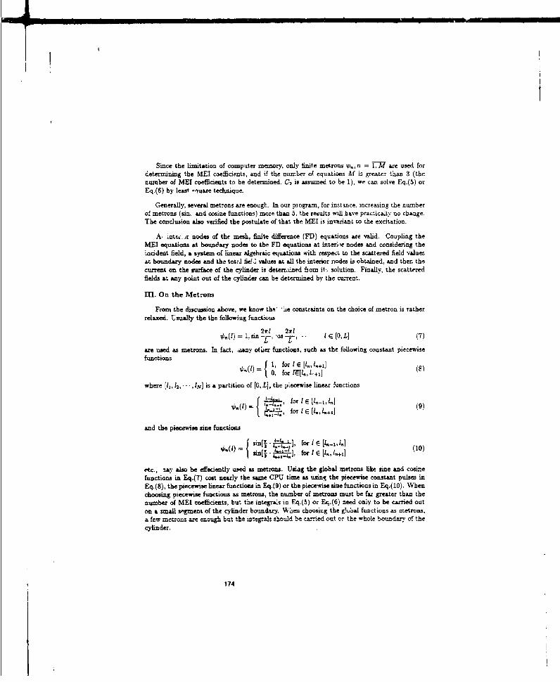
Since the limitation of computer memory, only finite metrons Ob,,n = are used fordetermining the MEI coefficients, and if the number of equations M is greater than 3 (thenumber of MEl coefficients to be determined, C2 is assumed to be 1), we can solve Fq.(5) orEq.(6) by least -luare technique.

Generally, several metrons are enough. In our program, for instance, increasing the numberof metrons (sin, and cosine functions) more than 5, the results will have practically uo change.The conclusion also verified the postulate of that the MEI is invariant to the excitation.

A. 'ntc .•)r nodes of the mesh, finite differeace (FD) equations are valid. Coupling theMEl equations at boundary nodes to the FD equations at intes.r nodes and considering theincident field, a system of linear 4gebraic equations with respect to the scattered field valuesat boundary nodes and the tot:J fie!,U values at all the interior nodes is obtained, and then thecurrent on the surface of the cylinder is detertined from itP solution. Finally, the scatteredfields at any point out of the cylinder can be determined by the current.

M. On the Metrons

From the discussion above, we know thAe b he constraints on the choice of metron is ratherrelaxed. Usually the the following functious

2rI 2xlI't(I na-f- z-os , . IE[0,L] (7)

are used as metrons. In fact, iiany otier functions, such as the following constant piecewisefunctions

1, for IE [l,,ln+s] (8)0,for fl, i

where [11,, , IN] is a partition of [G,L], the piecewise linear functions

-''Ifor!I E 1.1,nI(90.0t) -- - -'(91)

= t5 ,for I1E [I.,1I.+.

and the piecewise sine functions

{) j " n ,2 for E [1.-,,+] (10)s,()• in(!. t,.'- • for I E [I,., I.+,]

etc., aay also be effeciently used as metrons. Usiag the global metrons like sine and cosinefunctions in Eq.(7) cost nearly the same CPu time as using the piecewise constant pulses inEq.(8), the piecewise linear functions in Eq.(9) or the piecewise sine functions in Eq.(10). Whenchoosing piecewise functions as metrons, the number of metrons must be far greater than thenumber of MEI coefficients, but the integrals in Fq.(5) or Eq.(6) need only to be carried outon a small vgMent of the cylinder boundary. When choosing the g!ubal functions as metrons,a few mc:rons arc enough but the integ-r-as s•zuld b car-ied out or the wh.le boundary, of thecylinder.

174

Fig.3 thows the RCS results of an elliptic dielectric cylinder with E-wave incidence, wherethe permittl'ity er = 4, permeability M, = 1, the incident angle M" = 450, the lengths of theprincipal semiaxis of the ellipse are a = 1A(wavelength), b = O.SA, the mesh steps h. = h, =0.025A. and global sine and cojine functions are chooee! as metrons. It can be seen the resultsobtained by MEI are in good agreement with that obtained by MoM, and when the numberof metruns is equal to or greater than 3, the results sxe almost the same, Besides, in Fig.3the incident angle is 45', if we change the incident -angle, the coefficients of ME1 not change,that means the MEI is independent of the excitation. For this problem, any linear combinationof the three metrons is great different from the real currents. Therefore, the metron is fullydifferent from the basis functions in MoM.

A 4:1 aspect ratio rectangular cylinder of 20A circumferential dimension is shown in Fig.4.The surface current distributions with H-wave incidence and constant piecewise metrons areshown in Fig.5, and that with pieciwise linear metrons are shown in Fig.6, where the meshstep h = 0.04A or 25 nodes per wavelength. The integrals in Eq.(4) or Eq.(5) are calculatedby an approximate mid-point formular when constant piecewise fjections a3 metrons, whichis equivalent to using many point sources on the surface of the cylinder to measuring theMEL. It can be seen that both piecewse constant and linear metron; can get good results,but the piecewise linear metrons seem something better. For this problem and piecewise linearmatrons, enough accurate rnulks can be obtained with 30 or more metrcns. It is known that,10 segments per wavelength are basically requirement in MoM. For this problem, therefore, atleast 200 piecewise basis functions am necessary for guarsateing the acct-acy of the solution.Thus, it also shows the difference between metrons and basis functions.

The RCS of a 4:1 rectangular conducting cylinder with H-nave incidence and 12.5 circum-ferentiel dimension is shown in Fig.7, where piecewise sine functions are chosen as metrons.It can be seen that piecewise sine nietrons can also get very good resuhs. On our experience.piecewise sine metrons is a little better than piecewise metrons.

REFERENCES

[11 K.K. Mei, It Po-s, Z.Q. Chen and Y.W. Liu: "The measured equation of invariance: Anew concept in field computation", IEEE AP-S, Digest pp.

204 7

-20

5 0, Chicago, July, 1992.

[2] Wei Hong. Y.W. Liu and K.K. Me: "Application of the measured equation of invariance tosolve scattering problems involving penetrable medium", Submitted to Radio Science.

[3] Wei Hong, K.K. Mei: "Application of the metod of MEI to the scattering problems ofanssotropic medium c3ylinders", Submitted to IEEE AP-S, 1994.

175

in:D--

.100-

4.00-

4:2.0

*802 -

N V-1 3.00- -20 -LC 00 .0 i

-14.0C?

Fi. RSo aepicdeecrc0-ne

Fig.4 AI: bw etnva odcigcae

1l-

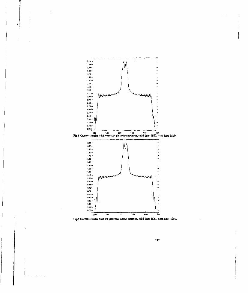
1f0i

2.L0 -

:.20 ---

1G00---

1.70 -0.0

-

o "00--

0.40--

0,10 -i -

0.01 0 lO .O 30 ,•

aoD 100 2'00 3.W 4.0 310Fig.5 Current results 'iAh Cox.Stant pioewise metrons, solid line: MM dash line: MoM

2.10 -

1.9D -

"amI. .

--

IJ.O --

1.00-

0.90-

,0- •l

0.10 .0. 20 • .

O.w t) L O •. ,.0 5 0

i •"ig.6 Current O',SSl•t with 50 piecewise linear m20r~n5, solid line: M•l da• line: MoM0 m .00

177

,ISO

2.10-

1.70 -

I1O

0.90-

0.80- _

0.70 e- I _

060- -

0.40- -

020-

0.10-

0400 :.00 2.00 3.00 -"00 1.00

Fig.7 Current results with 30 piecewise sine metrons, solid line: ME., daub line: MoM

178

THREE-DIMENSIONAL FINITEELEMENT TIME DOMAIN APPROACH

WITH AUTOMATIC MESHGENERATION FOR MICROWAVE

CAVITIES

Surender Mohan and Jin-Fa LeeECE Dept.

Worcester Polytechnic Institute100 Institute Rd.

Worcester, MA 01609

January 28, 1994

Abstract

The finite difference time domain (FDTD) [1] algorithm has been used widely insolving the transent responses of electromagnetic problems, However, it is diffcultto model complex EM problems with curved surfaces uing the FDTD method in itsoriginal form. Many varants have been proposed in the past with the aim to drcum-vent %his difficulty with varying degres of success. Almost all of thee approaches arebased upon, one form or the other, the use of finite difference approximation in bothspatial and temporal domains. It is the purpose of this paper to show a finite elementtime domain formulation, which uses Whitney l.forms in the spatial domain and thefint•e difference in the time domain, respectively, for solving Maxwell's equations. Inthis way, the proposed WETD method can be used on a tetrahedral nlte elementmesh generated by an automatic mesh generation program, TETLA.

1 Automatic Mesh Generation

Due to recent improvements in computer technology, in particular the massively parallelmachines, the size of engineering problems which it is practical to analyze using finiteelement method is dramatically larger than before. This makes it increasingly importantto automate the mesh generation process, so that creation of a mesh does not become abottleneck in the analysis of a product design. Furthermore, if mesh generation can be fully

179

automated, then it becomes feasible to embed the entire finite element analysis (includingthe mesh generation) in a feedback loop in which the mesh can be selectively refined toensure acturate numerical solutions.

The current implementation for meshing multiple objects, based upon the use of De-launay tessellation 12! algorithm, comprises of three major modules. These three majormodules are: surface meshing, initial Delaunay tessellation, and mesh refinements and qua:-ity improvements. The major tasks involved in each module are outlined in Fig. 1.

TEM PROJECT

M. S Iwkb Surface WrkV4US u,5 1..440*IfkemDan-Wpi if•,dg circkiWu • q•q•.

E Spw"* '"l~~l " r -

-pt --. k

Figure 1: Three modules in current Delaunkay mesh generation.

1.1 Three-Dimensional Delaunay Mesh Generation

In the Delaunay mesh generation, originally all the mesh points are generated via the surfacetriangulation. Except in the case of adding points to preserve the surfaces of the solidobjects, no additional points should be generated.

Watson AlgorithmOne method of forming Delaunay tessellation of a given set of points P is the Watson's

algorithm. The basic approach as shown in Fig. 2 for a two-dimensional case, is based uponthe incremental point insertion into a pre-existing mesh.

The extension of the algorithm to three dimensions can be briefly described as follows:

"* Start with an initi-l tetrahedral mesh Do containing all the points to be added; newinternal tetrabodra are formed as the points are entered one at a time.

"* At any typical stage of the process, a new point is teasted to determine which circum-sphere of the existing tetrahedra contains the point. The associated tetrahedra areremoved, leaving an insertion polyhedron containing the new point.

"* Edges connecting the new point to all triangular faces of surface of the insertion poly-hedron are created, defining tetrahedra that fill the insertion polyhedron. Combining

180

Q) d1Jsh MW Nab

Figure 2: Watson's algorithm

these with the tetrahedra outside the insertion polyhedron produces a new Delaunaytriangulation that contains the newly added point.

Watson's algorithm, although conceptually straightforward, suffers from three major dif-ficulties in practical application. First, improper resolution in dealing with the degeneratecases can yield an invalid mesh; Secondly, due to the finite-precision calculation, the appli-cation of Watson's algorithm may result in structural inconsistencies and ultimately fail toconstruct a valid nmsh; and, Thirdly, for real-life problems with high degrees of complexity,the algorithm will take prohibitive computation time. Therefore, methods implementingWatson's algorithm need to resolve the degenerate problems, enforce strict point convexitycondition, and provide a vehicle to localize the use of Watson's algorithm.

Localize the ActionIn its original form, the Watson's algorithm requires a scan through all the tetrahedra,consequently, it is inefficient and undesirable. A modification in the Watson's algorithmwhich localizes the action and provides & significant speed-up is proposed herein. The ideais to employ a multi-zone search method: First divide the bounding box into M. x M. x Ml.zones, and for each zone construct a directed tree with tetrahedra whose centroids are withinthe zone. Furt.e-more, by noticing that once the tetrahedron which contains the new pointis located, the creation of the insertion polyhedron may not go beyond two layers of it.H. ace, it is possible to form a localized action region centered at the tetrahedron with thenew point inside it.

Finally, the modified Watson's algorithm in the present implementation works as follows:

1. First find the zone, Z., to which the new point belongs. Consequently, find thetetrahedron, T., which contains the new point. This tetrahedron should be found in27 zones centered at Z., if not check all the zones (this case happens only in the earlystages of the process when the number of tetrahedra is few).

181

2. Form a localized action region which is centered at T. and extend no more than a fewlayers (we choose 3 in our program). Also, mark all the tetrahedra inside this actionregion.

3. Perform the circumsphere checking for all the tetrahedra inside the action region andform the insertion polyhedron.

4. Perform the point convenxity checking and construct the final insertion polyhedron.

5. Connect the new point to the faces of the insertion polyhedron,

After step S has been completed, the new point has been successfully d44.; to the set oftetrahedra and the process is complete.

2 FINITE ELEMENT TIME DOMAIN METHODS

2.1 FAEDO-GALERKIN FORMULATION

Let us consider the following vector wave equation for the electric field, E, which is derivedfrom Maxwell's equations:

V X 1VX +e-. . - in Q

iix-=O on r.axvx£t O on r()

where r,,r& are electric and magnetic walls, respectively. The weak form, or the Galerkinform, of Eq. (1) is just

0' C2-2 + V'. V X 1VX fd) " -L(8 ap 1A- fi, f (2)

where U is a test vector function. To achieve a greater symmetry between trial and testvector functions, we apply vector identities to result in (aasUming either PEC or PMCcondition on the boundary r)

To make this formulation operational, we use the Whitney 1-forms as the bases for the trialspace S"1 and expand the trial and test vector functions as

f1f92 t) =k(-) ei( (4)

182

where e', W, are the drculation of the electric field and the vector basis function asoci-ated with edge i, respectively. Also, in Eq.(4) we have used the Einstein notation for thesummation over index i.

Finally, the optimal weights e are determined by the Galerkin principletlv .;" t-V.) df ,o-+I - f W'-.!x W'.*V xiVj)dQ e=~ Olt ~dn (5)

for all j

Now we put the Galerkin eqtwion into vector notation, with £ s the coefficient vector, theresult is an ordinary differential equation (ODE) as:

l !L + C2 (S] r

2.2 FINITE DIFFERENCES IN TIME

A. Central DifferenceBy applying the central difference to the time derivative in Eq. (6), we obtain:

[71 1 (C*' - 2r +r"-') + j 151 C- - 0 7

The above equation can be rearranged to result in a matrix equation which can be used toupdate the coefficient vector, e, as

[Tj -- +' = - [T] "- + (2•[T] - c2t6 [S]) r" (8)

As evidenced in Eq. (8), the updating of the electric field, for each time step, requiressolving a matrix equation of the form

IT]X - Y (9)

However, since the matrix (T] is positive-definite, equation (9) can be solved efficiently by,for example, the Pre-Conditioned Conjugate Gradient (PCCG) method [3].

From Eq. (8), it can be shown that it will be stable if and only if the following conditionholds

p ({2 [TI - -bt' [S]}2) : 4p ([T]2) (10)

where p(A) is the spectral radius of the matrix A. Finally, with algebraic operations, thefinal stability condition can be deduced as

Ct 5 2()

183

where AT.,. and Al. are the minimum and the naximum eigenvulues of matrices [T) andM.5, respectively.B. Forwar DiffrenceApplying the forward diffemmce to tbe ODE in Eq. (6) results in the following procedureto update the E field in time:

r+'- -_E-' + 2f' -Et* r,_ (12)IT]

However, it can be shown that the numerical scheme proposed in Eq. (12) is unstableregardless of the time step 6t that is used in the computation.C. Backard DfePreceWhen the O.D.E. (6) is approximated by backward difference, the following equation isobtained

([71 + c26t2 [S]) ÷' = 2 [T])C" - [T] f-' (13)

The nice feature of Eq. (13) is that it is unconditionally stable, via. it is stable regardlessof the time stop it. The bad feature is that the numerical solution will always decay evenfor loesless problems.D. Mird DuffenceAs evidenced irom abee discusslons that both forward and backward differences sufferserious drawbacks: in the forward difference scheme, the numerical solution always grows;whereas, in thM backward difference case, it always decays. Consequently, in their originalforms, neither oe of them is practical. To eliminate these numexical artifacts, we proposehere a mixed difference scheme. Namely,

1 1bcwrd(4mixed difference - -forward difference + -backward difference (14)

2 2

Applying this mixed difference to the ODE in Eq. (6) results in

r+,1 - _"- + (2 [T] 4[T ] (15)(2I]+ 02 60t8]

It can be shown that equation (15) is not only unconditionally stable but also the energy ofthe numerical solution remains a constant, as is required for lossless problems.

3 NUMNERICAL RESULTS

A. RectangWar Caot'tA rectangular cavity with dimensions 2m x 3m x 4m has been analyzed by using the threeWETD methods described in this paper. The cavity is first discretized into tetrahedra withthe average element size h m 0.378m, furthermore the constant a for the excitation is chosenas a - 1/(wif) and f = 500MHz. The CPU time, number of iterations, and the computedresonant frequencies are summarized in Table 1. We note that WETD1 provides the best

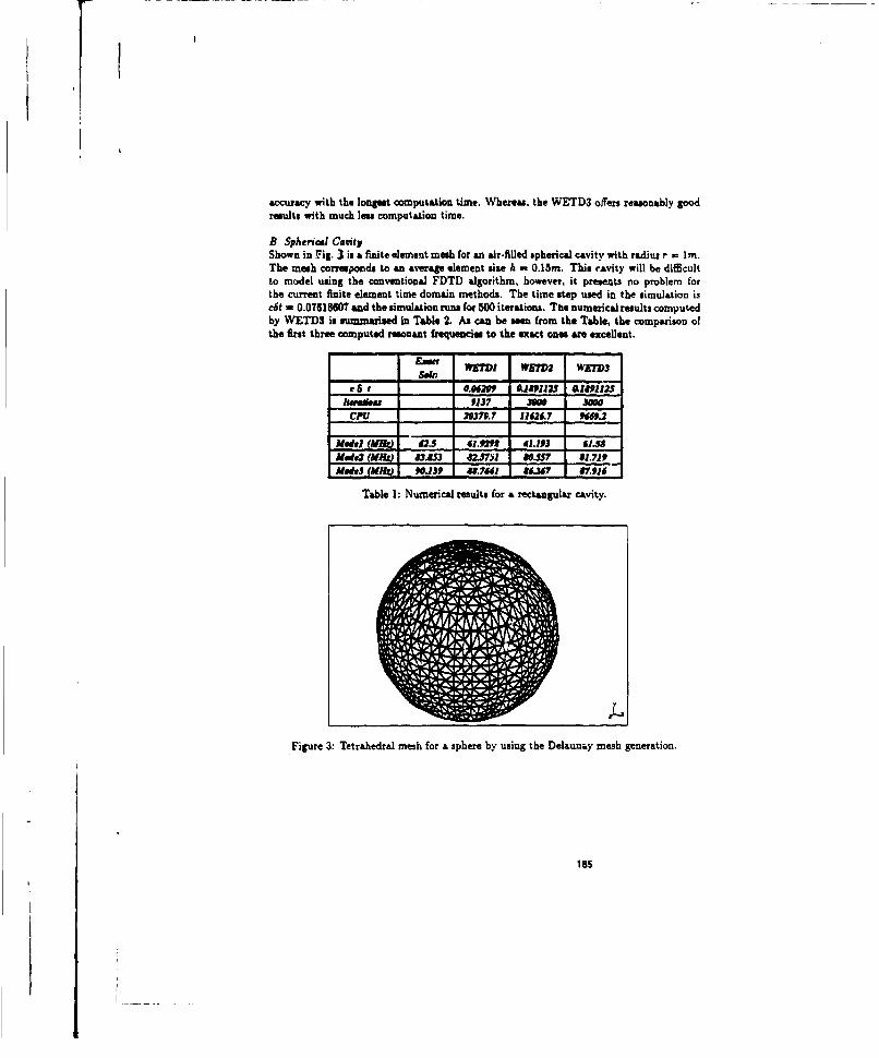
accuracy with the longst computation time. Whereas, the WETD3 offers reasonably goodresults with much less computation time.

B. Sphericeal CavityShown in Fig. 3 is a finite element mesh for art air-filled spherical cavity with radius r = lm.The mesh corresponds to an average element size h - 0.13m. This cavity will be difficultto model using the conventional FDTD algorithm, however, it presents no problem forthe current finite element time domain methods. The time step used in the simulation isc6t - 0.0T618607 and the simulation runs for 500 iterations. The numerical results computedby WETD3 is summsaised in Table 2. As can be seen from the Table, the comparison ofthe first three computed resonant frequencies to the exact ones ar excellent.

Ejt WETI WE/D3 WETD3

ltu.sm 9137 300J 30CPU - 2e7.7 1192&7 OW..

Mdel (MAW 92.. 41329 41.103 61.5Med*2 (MAW< £185.831 ZSIV3 A&W5 81.719MOeW (MHQ1 9..139 1 7W I 86,347 870i6

Table 1: Numerical results for a rectangular cavity.

Figure 3: Tetrahedral mesh for a sphere by using the Delaunay mesh generation.

185

~I-i

h a=LJ c 8, 0dO7615107

&Wt Compsted (WETD 3) amr

(MHZ j MHz) (V131.016 130.745 0.207

184.7789 184.81 0.107

2J4.5279 215.345 0.382

Table 2: Numerical meuts for a sphere cavity.

References

[1] K. S. Yee, *Numerical solution of initial boundary value problems involving Maxwell'sequations in isotropic media," IEEE Trans. Antennas Prop., vol. AP-14, pp. 302-307,1966.

[2] A. Bowyer, 'Computing Dirichlet tessellations," The Computer Journal, vol. 24, no. 2,pp 162-166, 1981.

[3) G. H. Golub and C. F. Van Loan, 'Matrix computations," ieftJnd edition, Baltimore.MD: The Johns Hopkins Pres, 1991.

186

Time stennin. methods fgr tau~lam~maa nntdn

F. Dsiiac. A. kxIsii. F." 3.m. A. GumumW. LgmUmive ryoflh~w-biaIk Maafu SrtU~ fhm 32

sk .32-41-562910ftc +2-41-MIOkb

17 mbw is a ?4ummc Aewtia do ft fhmimm *. Ow 8dmi~ haaMirF,~ Nor ~ e~ N-C* red d sd-pr wrmip Pgo 4fe u.00Nimoy 146Ai &dm

Sim. MwAth"i N O 05w. SCMIWj P@&Y PrewgFdi. "3 mi.~ rf**%060y Ar m * by du now

TO M 11 1a w modo ammi a odvo&NW am 11111 u sUCMA-HI.MP (CTE) Pmd f

So mshommu dum*M~4 aw!is aepl IN an~ NNW a&i a mama m~d Ow mwo p"r ab ami"uq.u U bmf *1 hafe f 080 k Noy mM* a umil mum apbomil bo .IN d w. as 04 on"my bom. inwh. Amd I" pam k an -am emsb bm&W 5dw e wi ilm mud ow to~ I

As npan pom s w do MW doo aimm.ammU @f 0 boba US U IM Of OPIP1111fII~~ *Qwd do amam be man nica~y No7u~ #4d quomm (11. Thsy m aoI$Ysum& La. wil Uh vaed..k soft or S. Afw mu mqdm. awl am dy be wmmai by mqflism e#AdCMMMM md"an m I A hwdiMsannm bmdm do iwM Rw-ige lemime*& a *A wmd bind Nh

A *Ai a~S.,.Um ammd am ~i =mViu caffinim. ambymmmi.

The giqUfx s U u.m i is(

Immnl 0*do2 am~penitmbm hmam. L" Ows low. doimm of awCmbm im toS , by 0606"(2) nd wwwi seM do iidwmity Ik M

Jog. 4 t-

Tim coniem b ei,tfi by bm dwoad sorndowb and U Nu to Wtimoa a do man wo~ f doinmbimar (pw w* of kmk) Ts Od amm brmidwie is Imida Uw sawdww GOMM aUmU Wui~mamwaS (3) fcw do ammi a of bounmUm r ma aanmi.s w is a wg fAmesk (awet m mm

lb fiwm .(w) m . r 40dm w Sm i nimnVi.Fr)U~ .

137

in doe astarn fsepthe gap-tuarn 10 elecuomaoetic, quantma u isgiven up man the SoacmJ systemn of

A j'(t)+5 y(t)-b(t) (4)- low A and 3s aft coal&i~m owaniat b is the sight hand smember vocto, y uisthe tmheown vector. t is the film and the

dot bdi dm ma rnivaw.Noss tha A and 5l may d~odon yin die can ofa ame linear/w cyineg. 8 depends onym jutmeosl' fused ivia one ham beW70).The arna h olo ofea 3 (3) 1mca a dma "mIeI A oyiss scheme isgiven by (5);

-~ Zi2L~la~u(y., +%1-a)y.)-u.l 1 .(I-a)b (5AtIonkwma an oo uh4 tao o qzwodo at do ra an 61 . h+At supewly. Vmarius dsahaa of the ponuneer a iesd woi~houlo Methds (64. is implivit O wsrd) Eo. tw a expika (forard) aBuh. u..lf a O~ha-Nacowsn Crs2/3lbGdksh).71r, .t;m VM/h s. 6; in bovelya in *0 malsi of Syse (5). One obeioa ceadiaim Is thit amust be investible Le.amn 'SlIb. The sof of DAZ sloas soch a.() 1 alm Us *A m~aou A *X~ 3 of uhices A sod 3 where X. isan abistuYI s J1.31. It own be regula La. det(A + X. 3) asri;notm d idsntically. If it is not the cam, it isbrg.-I~k4 to r..At hasd on a scdoA/At + 02 is pol Alega aned Use sr is meneiqs. one fthea oherindifA + X 3 s a g I poil, mawaesF, F at uh dot

A' E A F dlbgJ)()

uwhosdaladmaosesa .e M unoussed Will sh gupoa ws mafio Plian an its iasm.J I wnue mimAsiofs *A .swtaleonsi W lb a iogsar miws str. andJ lb a allpostIerunI block movii % At blacks of the farm-

4 1 &;eo fvoobocks is a, the nislWU orf~@La the syma- (noe mrpsioeacy of a anowen j mayobrabmuduy be defra dui~e minksosch*u 0ms and-0nedr* 0).Vfh y, - 'y andV - E. b. the DAE symsn (4)

i +Wu::q wuu Yr.(w) ".. rlJ* + f- kv) (q)

'Themin~l eh~~oa DAB nyrn depneb mwoelhoo mailptay. On doom bod& iMtse alomay lb pmetaow. dx rose is very d~ls = ~ and m mW ashs uos o In &a&d One d r cdwho. if dus na~aa; is

*V so ow (J lb t~dcally sqim s aiso). Ow sysau is souk wor so=h adsned dassemosi masods low ODE may

In doasoof bs 6 rasso ft swohadeofte'qd mobsam a TM fes kind we dos ao~scnmnI nde luado bdooof oat *(e1~dmde do "nqo~ Mid valis atdo; voter pmoed gwass a MoMe amu amO disosa eof eA. Sach eq~aft de aM idnecs lbs A=l.y of Msesyms. Tic soadoo Ulad as lbs eq -d, Nto msof belonging only w s condom" regions Tbowtspowcasn do onIm -aV '4iy dibm mnow doy to eseuly alpiphuc and dow al- os the wout A mar null line.They ob ounly hod so a syssne a( aillaicy L. Thereby. clooiuii mansbod mob as the amAus (5) wy be used.Noermdolso. V do exlic Ba-- method lb "ead do:d * -- A/,& i nvlb anh d do sobludwis lb hqhuhle. Inpoural. p* asp apck sofamm-y -u be WNW 0 vo ba (4) heaue doy beevW sojouha matiesmaud impoois

woust - o notm Scomeofshw olbnueods o epromi i do bfiewlC sscdoo

i - Ry-t0 (10)To soleas gby a IwuddifilopecelomAWR(VF)mosod (4)ld ~the'lmlan a

135

j-0

f-+ i !jf.I-j (12)J-0

Indim i refer ia uiinm amiss e.&gyj - y~j d (yijj.ag de i ntes zbeng od by a consoim me stpAtTeslbatimna be"s kiw" up l w lins , die Wclisdo at sm 1ý is umapume by molheg for y.. the sysumc

ob~ined by daiag Me meqahomna (11) mad (32) in (10). A i Iu method a dubudby givgp~l weffkicena a4 usq41 coedelemi &. Ta~e I An am cl~aI uical xf Adu hms Manhsd Ow auhd*6 appw as Whighr ordur

implicit Ealer 1 1 -3 1

Cmk Nicalaa, I 1 .1 1 3 /1dn kdo 1- .13 2 5112 812 -1112

MOMO 2 3, j 4L*.J. - .L....... - -

T*kIa : Da ~wjd cfmm uuab

In them can fte DAS sync (4). wis do fadcwing mun

Y. jaj Y041-j (13)

B -) Djoi ).~. (14)j-0

bp - oi b.I-j(15)

the coomfswion of dw am time r~p Is Lhe nasitum of die symcf (16):

atL(~y (16)for yvs,whuudspndemoemo(3asyhbemaminexplicin

The gmand dffuemmsy3 . (10) is coniwdered spin. An qupenutimsio of iw xsobaujom dao h values y. of thesoito&I* as thew~yl due ac a0 be obsand try 1dvmg dus fallonwug relainims 15]:

Yi-y.+Aipij f(Yj.&,,+ci6s) i-L..s

a-I (17)

189

1Wf~LW

Tb wsimof boch foms, any be sba-w, by ranmkring kthat -ki aIt(Y, I. Lm+ ai A). A s-utep method iscomnby dig CoMmflmi Q+ DU~ and given in is Rmtge.Xaumgbkme or 9huberdiawun

02 2 .

with a ~jj-1

The Rap Yo K m inbods any be 0060w ~ of dm* dlqagm. Mws chmak expicit natihad am theIM boibhuth PN-Ofovjki ZL U0condiineuisno ftafhln(sfV*O forj,ýi). tbemef weca~lllth hatimjlid

R-0g Kums wef (3M. Spech cuu of K~ ame die gmmly uimpheklRm KieKm (DmK) umhos (if A. 0 for0. i a sub cmWy of wbich m te singly dlsgmully hinplicis Puuge Kau (S DIRK) maethd, (if 04 m 0 for j >ý i aMd if

Ai.- P (m soi).The 3KX methods may be qiplie au fth DAE mym (4). Nevatelgat.s only form 2 may be used becat= form I woukdinowA.lve theivem of A irn aitslm amp. Tb. eabpenon of forms 2 to die DAB sy~mm gives the followintg twtauiois (6]:

Aki b~. cat) - (y. +Zj k)Y (Y,. + B for i-I... s

I- i., 3 )

uL. 8(a.a) a(m.) symhsa esolved to fbo fth k. Nevutenha.wt in do cae of DMIR. k, depwA's only ony.. k2 oly ony* ua kt. er-m..d bsilnom m (1) Im to a mofs s ni yswnmosiunxinLn

Hemam me exodj5) fMY

Ia icmofi Il di~in. **io vadmo so wdii (5) mohnd f th idomdm am b wiudi is diuimml a

X 0

1112 1/2

ofa Wa2 0 0112 Ia112-a 0t-*/2 CI 1-2a a12

I a1-2aL a

190

with W-V m 3aNofted tht isi wmbtod is rympliced i~e. for Hamilsoani sys 1. it conservs the symptertie two form. The weakerg g m of vokmeami i vadmin pne = me(Lieuvile's theu) wd of consere loonotegywe a conieqtewe ofthi4 symttVeCttness~ Unform*sd the ;~~ conskidand in this paper are mo IHamilmnasw PM' Jhib schemne does nor

- -U.Th fflw g lorutla masy be mad .o imra ls the DIRI behd to aolvo (4) and k, kaq) -,A !j. of the non [inner

ssnto he solvedu doo powbh to the am involved in doe othe mebotod:

For i- I so -I

To fiad K6 solve tho sy

(A + M Ap+ j& - Y

b§6

Comp- y.jyajA ki

7We principle of exaupimol methodis 0 toPefa orm piminwms with a basi sedma for a *qmo of d Lrd im aempad so eampai s ro ame de mp (ftiehind's hefard 1ts~ t die howk 19.7Tins is mom by considering dac

arympoddeveloeameo or Whe arrorof the bade athenie a powersof "the a* and by a ilirig the - - ' e in=.Doe following alge 11ho bee and for die eompuibon piniond ni dot papmc The ehom bauic sehema a theimplidt Euler method. Aihoogh the Crank ?4icalsn meto is marn mcorms. mall acileltiamt due to ins weakersiability j I "dimte , , , of the msspalaolm pmm. The inp~iek Ealer Aethed is vM sM eanimd Its aerrdei-lopms includes au the poises of the do. es W hu the fki ... The ami devc&pmetie of Oti Aiclades the sanewins aeted ahe 91m cder e. The following teasegom al qi am a"aam ed (9t:

[AL. A112. W54, At/6. he/S. &112..... We ..4. ) ,aq2%n.2 lbrO,4W

Suaihig atimek t., wbmithsslion y.. a soled., T

il atdea t,.+& is obzimed by olon*qm~ Ia sset of implicit Eulermeidid with the ame wmi ht. The 101owding seqwsme ofmoonauwiuakuIt"

IT11. T21. T31. T41. SIt. T41. 771. ... Tit ...} (2

7Ue bigher order qtpprxiownr an obtomod by theemi dalIdhwiag iagm

T21 Tn~T

T3 TT2T3

The fit. columnn is give, by (21) and the odher oes wte comptuted using 6ci foilowing reeteresce formula (polynomnial

191

Ti,k Ti*,k-I + (-I-T3)-a

in practice.aedaima msmm ieb ieb oatip ng a new lj aid performing Ube eximapolatioms. 'Me PfttSSis stopped whena Tit am T~il a up to tie aqId acciracy. The rational ensuapoLazzon may alaso give good results and isadvisd by - Madam (9). It amphm onlY the Me 0(24) Wiuaadof(23):

fi-k+t TU-4-in Practi. huh 6 am a me buoome a i h e s choen. In nmimical iam. ft polynomia extrapoLationsams to bemse coverge.

As an aplicalbmt. the m ibwe of a ~sino a smnur ItLC acircut is cumsidered. whim thle inductive effects amcompesed by the IIAme elemet method 1101. 71s is a liee oscillation problem, which is mome sensitive to timeMMisgtio m0e11od than finned amellaia onets. FMrsthe LiweN eas (ufar I OW) is conidiered in order to study diebehasiaer Ot the V-- xhum. The -Iu , adttiine ite ;"ms ,*Athe Craka-mhNialso methiod and wuith a veryAMM VApeie b 4.104 sr- Tim - ;paigC the ime maWKde a comma gmie ofIt . 4.10,3 me is considered.

.hd 'A eqne I I M uiM y lo 20 mdnIn n pwio. tn fig=u 1. the mulstep madiods we oompred. It Wbee be finileeEulw m~odha.o -a ftm pfe ffwL MWl k-Ninc 1 hwi. is nuy accsre (dhe energyof the sy is qipuoimaly coamavud).but a mesh hequmeay cme is bzodaied. The mor , cs bunb e is abeAdaM Pbeom. one,.o eif b.~em ub after ad lerw puiodI Fimly, twosee pOem is not of gatintcemst beeMasAuq-1ncy a0i01se well inca WAVthg e -ffect ame puemat. It mus be noticed dot a&l thase methods we similar incompuo tthe. Hllair order methods (such as two maep Clar sad Adams Widti=~) onily tuquire the storage of

mlo p .eu athodsame poaee a g.2 tq s*b yalci uLmto weU as bhe emupoissionniddgive uexlle m la.i A C-Yup ofdi th -ziaokal proce.s s gta-aey amtedrii 3 mabdivisions Of die

sapeb h s "a mm dont this method a wmi espensklve to Crank-Niiolsm aa . Lurge upi have beentateid.For bhe larges spaphm (4h). bie eumw un IIIpr,,1oeseavuag after 4 tobdlvW=e The solmion s as il excellent. buit

lmedmidom. This ese explim why dom Cok-Nicoims method is prefaind or howv problemn.

4M - eeuc

-400.V

Fig=s I r'M eveldaion (a) of capacitor voliag (V) - MUWLtsap methods.

192

400~gd DA

20:0e va-,()ocaniwY1Uu()Ot mpmto.

Asa h C, he pule wtha yma wus ~nliee. s ~nsatq~eyatth alu. it

Ap~n.o f a h am eMWUK, died mudse (problem 4iba). -P Itc dcworetis . i. ... saciwu o fq yO the Sileea fIKmnolution tenbaane s &*&I obliit *ce~ni g s"L i ovre niqtsai

enryaddI- i s ol n ytacbme h omdna= ~ fa"mngv h o

12.

10.

a.

2. -I

0.05 0.1 0.15 0.2 0.25 0.3 0.35 0.4Figure 3: Tuim evoistior (s) of tan meuuies (J) c~snputkd with Cizttk.NicoIm rhote

193

I--- ----

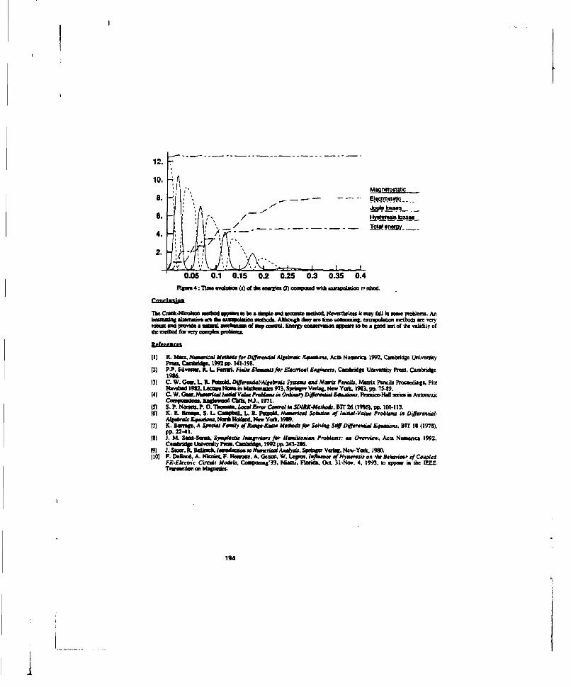
122.

10.

a.

Th6.c-iommdo pust b m n ehdNvrhls at ma W ifrt fsIos pobems.A

2.s '-/4idgc IMp. 4-1

13 . .Gear 4L TIt. e't'oW Dift(Ontathe mnmum (3)u dusatd Mwitz Penc~ilst Mari idriad. rce~ Pl

THe v~ 19n-M 2Ln mecthre 1m~ inMa plens 973d awb~ metod. New York.~c a 19a3 pai. 758.eprt.n(4) i. g 0awk murye eta d Vhe aalmbimethodn OPAltogvhy DWuua Spudw omm renag zticual =ntods ine Avery

row id pumonsdEna ~maidl. aht NJ 9 1a. ngyaevannpusobagodnttdevldiyo

M1 IL ?.-z. Am~. Spethods y fo D40t-VJAI Aokwh f- Soh-Se, Acm Niatia 1992. CaBri InTv1e(978)22-41.Cmid.19p.111

(2] .PP. Succ-Scre. L phectcl Fniaiw rentn for Hacndkal~ Eagi"s., CanOvervidew Actsnu Pwfrei, Cambidg

19194

COMPLEX PERIODIC SOUNDARY CONDITONS FORAC FINITE ELEMENT MODELS

A- F,::nkeI J. R. Braver an'd W-. A (3okelRAFAEL T7he MacaNeai-Schwendler CorporationP.O.Box 2250 4300 W Brown Deer RoadHaifa, ISRAEL Milwaukee, WI 53223 USA

E;mail: Lbrauer@mraescb-com

Absi~o'Ilimpaper describes for the firt time nwencwriclicrpeiadi boundary conditons that enable efficient fiite elementmodeling of periodic alternating current elmcroaigapetc dgvims Thes boundairy conditiors are shown to bW aspecial form ofmultipoustoonstraint. Applications are made to iow frequencyectraical machinery and to higit fre-quency phased array antennass. Computed results ate verifieid IY their agreement with those of muchi larger models

INTRODUCflONPeriodic boundaycondit ar commony ued to reduce the siz of finite element models to only one portionof an entire devivce [1J. Conventional periodic boundary auoditions constrain the potentials and fields on onebounidary to be eqlual or ;1pndt- to those on a boundary one Period away. Thus in alternatingo Wticelectromas-now optoblemas. these periodic boundary conditions Wasdy a phase "hf that ia an integer multiple of 180 degrees.Mha paper describes and appliesa new conspler phasor periodic boundary conditions that enable smaller phase shiftsand therefor smaller ac mtodesh to be used. While smarbounidary omiditioin have recently been mentioned fora hybrid suethod 12J. this paper is the first to describe the theory of comples:boundary conditions for finite elements.The fizzt application of the new boundary conditoious is to low frequency 6;pparatuL IResults obtained for a one -third pole moodel of an induction motor with the new boudtar, eandmiti m ar compared to those of an entire polemodel using conventional boundary conditions.The secotnd appiicatio of the nwa boundary conditioaslato high frequenicy antennass. An infinitely periodic phasedarMa is. analyzed with the new boundary conditions for comparison with results obtained by a much lage finiteelement model having conventional boundary condmitios. The new complex periodic boundary conditions are alsoused for anterns. can angles that cannot be analyzed uising conventional boundary conditionz.

COMPLEX MULTIPOINI'CONSTRARMT71he finite element analysis sofware used here. MSCIEM.AS"'(3J. based upon the potential vemor 10s made upof magnetic vector potential X and time-integrated electric scaler Potential v., has three matrices mae"n up itsequatioCL

lMlNu} + [18101 + IKI~u) - (P)()

where [MI is prxportional to permittivlt. [3] is proportional to conductivty, and [K] Is proportior to reluctivitY.fP1 isathe exitation &nd is asasmed known. In this paperwe =asme simsuodal aic exceation so that u is a complexpliasor, and so are its fims and second time derinvatvs Thus for an aingular frequency w -2 x f, (1) becomes:

[-w'(a% ur+Iw q+ 90)- [~fIu}={ p) (2)

Boundary conditions that relate a potential u on oue boundary in to those on another boundary n ran be expressedas a nudom oxssrt'ehtr Thim consitraint obeys a matrix relation between nodal values:

(us..) - (0G14.){u (3)

One way of enforcing such a constraintni the Lageaen~uthipIler wutiip (LbM). It can be expressed as:

195

where the vector Palrtiton qj. contanS the Lagrange multipliers and wheresFindicates the adjoint.

Another way of enforcing the constraint of (3) is the consrrninl tenabl elimmanon tehmique (CVET). It can beexpressed as:

[FJ~u) - P.')(5)

where

[F.]- CF.] + [FwjO..] + [01JIFL1 + f0jk]G.1(6)

(P.') - 1P.) + [.3J(P.) (7)

If [M is a real symmetric matrix, then [F'] !s Hermlianm otherwise [F'] is a complex unsymmetric matrix. Openboundaries [4],[5) might produce an unsymmatric (F) matrix.

The two cousmist rsdrniquea are compared asfollows. The LhMT enlarges the aize of the matrix, but make. it moreue.The CVET reduces the size of th matrix, and waes chosen for the computations of this paper.

APPIJICAflONO 10 WW FREQUENCY APPARATUS

Thtiow freqencyl deice- to besanalyd iaO 60)hpophas AC induction motor that has two poles. Figurel1showsstew geometry of the induction motor, including the staor windings of phaaes A. 3. and C. There are 24 stator slotsand teeth and 36 r otor bers &nd teeth. These numbers of saoor and rowo teeth are quite common for inductioninctors Becaue of the three- phases amtcr indln. the nwmber of statw slots is usually a multiple of 3 times thenumber of polese and hencee 24 stator slots ane often used. 7lb minimise torque variation aod acoustic noise. thenumbe of rotor teeth.i usually significantly greater than the number of stator teeth. and hence 36 aluminum rotorbar are ofte used [6].

The mirnt mumodel size with eonventloald real periodlic boundary conditions is one pole pitch, or 180 degrees.Figure 2 sabase the IMD degree fiite eltament model developed for the mo- of Figure 1. The model consists of444 two-dimensional quadrilateral finite elemets and 414 bangular fiite elements. There are 697 grid points(nodes). subh with only owe deg=e of h -ed, -. the componeut of mantiact vector potential A that is in the x direc-do nornal to thes 2D finite elemenats. The boundary consditions consist of setting A to secr at the inner and out,diameteer plus periodic1 boundary conditinns. The perimlic bounidary, conditions ame (11:

A (r, 110) -(-I) A(r, 00 ) (8)

which mu enfoeced at the grid points of rathus r between the inner and outer motor radii Beeua-e (8) involves acoeffiden that is a real number. most biite element codes ane abe to enfttee it.

The so magoetic field can be computed for the 1800 model of figures 2 at various slip frequencies. Figre 2showsthe composed magnetic flux lines at a typical 6-ntat and! a typical slip frequency of 3 Hz (5% of 60 Hiz). The conm-puted values of stored energy end indrwat power for the 1800 model are listed in lhble 1.

Figure 3 shows a new 60 model of the motor of Figure I. It has owe third the number of finite elements of the 1800model, and has only 241 grid points. Figure 4 requires the complex periodic boundary comditionsz

A (r. 609 ) -(cos WO +j sin 60* ) A(r. 0*) (9)

which mu enforced at the grid points of radluss r between the inne and outer motor radli.

196

Flgue 1. Indiacho moatws umtwdic~p of pbmmA.3wWndC.

rgem 2. One-pole (18b) fiite element model of FW=m 1, comamputed iuatnasfidns

197

Fix, 3 ONe-thd Pak (WeC) MOWu of Figure 1. showing computed moszantaneoua fledioe&

Thee muess fild e. engete Smthe 600 model of Fiqze, 3 at variou sulip freqluessies. Figuare 3 thws thecosputumepehe Ms. unseat a typicl isitanttat slip requency of 3 Hzz thefux ins " b ge with those of the IW0Uodel ciFigure 3. Ihecmpusd cou andpom rfr*0'modela ~us td in¶Ibkle, and ae sen to be ectyoae thir thee. of the IWO0 modal. I I== the eampa penoic boundaryconditionsame obtaiwS the correct an-pmm. Decau the complex conmitia redone she =odel me, the overall CPU unse is reduced trom 60.7 secondsto 40.9 stecnds on en HP 9=0 wadwaim. This rseduao is mpseced tohbe even moms dramatic for larger modelssucheas3D moduiL. In addikkes to CPU rediactom., disk estoage said memory requirements are also greatly reducedbthe cmaplex p 1, , II -Ih)ad ndidoes.ibbl 1. CbOkWITED WEROY & POWER IN DIDUCTON MOTOR MODELS

Mapeti aWu (joul) 2.04543-2 6.915143E-3Powe (awet) 72V?40E-2 2.409915-2

AFPUCAn TIOIr PHASED ARRAY ANTENNASThe big h q, adsA 2 to be anlmcluis a5 phwtd any micawave arn==& Figure 4 &hows tW finite elemeatmodel adhwanums a the phased arny. whith an fed by recangaglar metal wwiavuuie operating m the funds-wood IW10 made wfth sheca ic fid the wy 71w~ tefrequency la 3 Oft TMw waveguide width in the xidirecio b 5.714 cm sad its legt Is the a i ~Ia s 12 em. Now; that a radome of ralailve pezuittisity 3.0625

Theb hexoe acallms of Pigien 4 ar. aninaod to he membsers of en minbite arry of eometruically identimai cellsplacd sling the x We. The ilaniuil wavquguish ame Wl aused to have emtatlous of identical amplitude, butwaitpbe eagle.tatbuare gepordonal to thei poslioss aloing the xaula. There ame also identical wavygulde -atins-Munimey in thu y direction, but the I I , I ,mapisthad andi ph... ame myauianh in the y direction. By varyingthe pbaee shit in thu a diestwo. the salem beem mas be camd" (pointed) at various angles in the itplane.Hern this phued army awma can be aaslynd uoit two-dimesudocal finite elemnent. is the raplane. Tb absotrb

*the powe leaWing hafe sbusset model at the m~admuz bomusuay of Figue 4. qweda plansuave ABCs (Ab-u Bou n daruuy Coodifoso) wee smed at that bowadary (I

198

_____ZIx

FLgm Fiit elemshent model of bw sotanten atils of. pa Oed way aloug the x uAL

In the an. of a jibass shi par adl that hn a WwW dl bwm a of IID IgIs- a model df the Inlabite azua can bemde& w tog reel tipoint comuenuaiw Tbm comashoamu be placd an a model tbuzea cantain anas.w Foc

ale she finite element no" loiF~lm 4 wM f am ancom bb. rhas m sidpoint atwusuim for 180 degreetota -hu ehL or 45 dolnsp.. abitt per cl. Figure 5 Ahmn the Pytngvem.cotmjuted by NWS/EMAS

forhemoe~oF~ws4, hointhath aepadirectedszasemeqleat"24 dere Thbobepthie eli-

z

.X . .... f l..

- - -- - - -- - ---- - - -a -

FW=~~~ea S.-qtdPytn atnfrteIwc =d fPm4 o b & 84 eo

199 --

$a. Os' )43 d) (10)

WWee)~I Xithe wawl~th d d is the mwidth. wchlhIs .714em In thecuesPIPMr 4 lba.. s the A ~M ft" a~ CM OW f the (Out modeVO The pbs.. fr hiew the wene antgle as thePoanUah VOMBof IPNgw S. that hs6 1206 dspi..

Ix

Cci e ltocikt coorlveaw eabe audio the d anist anwo. maywith a mde" Oof aey =teo[ its an-tem.Far %a~pb PFWM? le slica , th " VsMM CO d by lASCtASW wfth a ams c*ul model with

acImpliamoisam pbsa sibik6 dega, The reidl NFIe Iff th00sof the kwr cal movd of Figiie 5. amethAvg the masher of AWN elou idse b adwdby abow of lo.Aprge 7b hacs lds ph..wo eagleeolet. ric field comipsd lor theacm cell mod*L Twhe pbs.boats ae hSem ON a Pip"e 6, tht is. 12.6 Iegu Theeoqiz pe",i b-iny uwifisasus pamptolyinmpostga pbase dlarem of 45 dorm. Sonsom b - icks) of do. moda tothM oppoth." of. cth nodeAmodokay advasagepC h o qih pImi M ah lethal the cm .1model E Pps.7 canbe ed to&a- nmwpm- MairAW-'INAdqO Figuase cam the ompatedpayusveh "M~ IW==a21 degee..dFpv 1, Cl OMW phueases . Ifats thatpinthe p- Ms I e _~m mdM Mn obe,4 nd that the was rkb Imcoott iPlgusbse9eethsmqiudushbrephmdacE7oda1eev NOW sifMPps Pa tathescas as&l isbinmemedaumodoglo (10). FWW %When thet bSo bondwycomdicos COO0 duegre ph.. shift eam osyad.The abasepboed myasm hi.benm=odeedwithtwo-den.Iomd la bIt -im and with onl oem co-PcueatOf mapedevae -mrp ew~ X. wathe - sceloeys thebenawkfied. Tb. rebictio se tscorn.pUztd by bSCIUMA wI be conmpaned wit those of the method of womeents M7 in a humus paper[51

elemen omoehs. In e ssachGn p t~eo mzsCOMOE fX a vuan nDWpm ot~amw1, we au Oen phaeCamosits Plant ama" that MDIm two Ndke1 9s reqobe threet dinano bifte lement Models wit nich

mtiti-dapm--bsdomeompl ml~Mmiss.ti

200

- Z a).

Ix

-a--

----PW7OMUdl(WWOW Ub M~hO4d@pmW

ap ~~I I-I si

IfI 11am IF[il I a I a iult

Fipa.6 Cera~d emlah brwmgl =odd widt pbm 00 ahdmoftu.a~wg~aft b). pb-gwO*d-*IkW 3lq Us~ plruM in).t

201

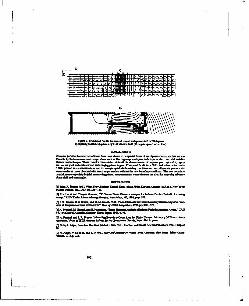
z

Ix LLLL

b).

F 9. Cmpad m~miw h ma mU mauwthphina ct t70 daaua)Je~mwiog~ 401b00&*8. aqi a ftuiearlc M o(20 spaa rewwfnec o).

CO3NCLUSIONS

£k90" by AriM abubime Saad aPerados SA SO the Lasam mairiphir teChnique or the r munint variablei1umatiauchmqu.Tboea. cImmodusscobeafhe sloom mod aanly am p mcmitomMw.900 ME A" af each COW awhd WOl mwy Phase ans Cuomused Adda Ow a OD0Ht iad-&. no and a

kmacd Dithe. brc. 1393. pp. LU-141.

121 Daic LUau and MWOM. FbMW -M %eM F* lM6040 Am*=i fhr Infs.f Doubty Periodic RadiatingArI710 ZC?SUJ'& wa AJbs4hwAb. Am AbrW, bG. 199&. pals 193.r.) L bI Amm . -said bt bL Mnic *,UC F Mbss lia~mr Open bvefy Elooinpeti Prab-Won at aeqowamd bum DC io O. Am. afACJ*Srm 1993M. pp. W-0-37.141 A. PimahL.X064Si P. M"000.L Na FWWm Mommal A aalr of fI P FW Aamm.AITrm URSI

VM~ GmwwdImm*.4A~w. gfu*)ý quw& I p99.949.(5I A. Peahe and I.3R. Draw. Wxrbo - 1 3 ComdL~s For Fjmin Eksmt Modeliag Of Ptased ArrayAvwmtui.A~c. qfZ IUAmaau & h* Soa SjmqlL~vbm Seanha. Jin 1994, in peam(61"FiiL Aomlokiam-, w(2'4edj, New VesGanbomdbuethSaesminPuaha~mn.97C, Chaptr10.rM N. Amily. O.ekdo, and C. P. Wk. Thowy mau m~ k of ~AMWaA~sW. N*wV Miley -Iter.mis.... IM7 p. 23&

202

COMPUTER CODES FOR THE ANALYSIS OF PLANAR ANDCYLINDRICALLY CONFORMAL PRINTED ANTENNAS

Jian Gong, Leo C. Kempel and John L. VolakiaRadiation Laboratory

Department of Electrical Engineering and Computer ScienceUniversity of Michigan

1301 Bead Ave.Ann Arbor, MI 48109-2122

Introduction

The hybrid finite elemeut.boundasy integral (FE-BI) method has been found par.ticuladly attractive for simulating patch antennas/arrays, printed spirals and non.planar cavity-backed antennas. The analysis of such a diverse collection of antennasand arrays can be readily analyzed using a single computer code while taking intoconsideration feeding lines and antenna geometry substructure. Because the exactboundary integral is used for terminating the finite element mesh on the aperturesurface, there is no compromise in accuracy and furthermore use of the Fast FourierTransform (FFT) in evaluating the boundary integral contribution leads to a min-imal O(N) memory requirement and a substantial increase in the efficiency of thesolution method.

After a brief overview of the formulation, in this paper we will describe thecharacteristics and capabilities of a new computer code which uses tetrahedral ele-ments for dlscrotizing antenna cavity and triangular patches for zoning the aperture.The geometricw interface of the code will be addressed. The accuracy of this FE-BI code will also be described in comparison to other finite element formulationswhich employ absorbing boundary conditions or artificial absorbers for terminatingthe mesh. Several calculation examples involving different antenna geometrift willbe presented. Radar cress section (RCS) and radiation patterns as well as inputimpedance computations will be compared to measured or reference data.

A second code for cylindrically conformal patch antennas will also be described.This code employs shell elements for meshing the antenna cavity. Since these ele-meats are analogous to bricks, the code incorporates its own mesh generation algo-rithm for rapid geometry specification. Attention will be focused on the validationof this code for wraparound patch antennas and accurate feed modeling using mea-sured or reference data. In addition, antenna performance results will be presentedas a function of radius for a typical configuration.

Formulation

The FE-BI system for cavities embedded in a metallic surface (planar or cylindrical)may be written as a matrix equation

+ 1 ) 101 1 j IE ' {fr )1{E;} 1 [o =1

203

where the entries of A4] are due to the finite elenent portion of the formulation and[91 is attributed to the boundary integral. The coefficients Ej and E,"' denoteunknowns associated with the aperture and interior fields, respectively, whereasff" is the excitation function due to exterior sources, such as a plane wave, andfj` is the excitation function due to interior sources. In this paper the source is aninfinitesimally thin probe feed normal to the patch and cavity base. This formulationmay be readily modified to include the effect of lumped impedance posts, 3hortingpins or resistive cards as reported by Jim and Volakis [1].

Solution Methodology

For both planar and cylindrical geometries, the unknown electric fields are foundby solving (1) using a Biconjugate Gradient-Fast Fourier Transform (BiCG-FFT)salver. Since the system Is symmetric, only one matrix-vector product is requiredfor each iteration of the BiCG algorithm. This product comprises the oulk of thecomputational effort in the solution and it is therefore advantageous to minimize itsexecution time. In our implementation, substantial CPU reduction time is achievedby using a sparse matrix-vector product for the finite element matrix term [A] anda discrete convolution product for the boundary integral term (G). The resultingproduct imposes both low computational and memory load.

Having determined the electric fields within the cavity and on its aperture,engineering quantities such as RCS, radiation pattern and input impedance may bedetermined. Both the RCS and antenna pattern are computed using the aperturefields while the input impedance calculation requires the interior fields near theprobe feed.

Planar Code

Consider the printed conformal antenna configuration shown in figure 1 where acavity is recessed in a perfectly conducting ground plane. Printed on the cavity'saperture is a radiation element of arbitrary shape. In order to simulate the geo-metrical irregularities as well as the dielectric inhomogeneities of these antennas,we choose tetrahedral elements for the FE volume discretization because of theirgeometr2cal adaptability. The expansion of the unknown electric field in this imple-mentation is then carried out by using linear edge-based shape functions [2] sincethese elements are well suited for vector field representation. The boundary inte-gral portion of the system is formulated on the basis of the equivalence principlewhich requires an integral equation in terms of the free space Green's function anda magnetic current over the aperture surface which relates the magnetic field R' tothe tangential component of the electric field E. Thic leads to an exact boundary.ondition for the FE volume termination as opposed to other truncation schemessuch as absorbing boundary conditions or artificial absorbers. The tetrahedral ele-ments in the cavity reduce to triangle patches on the aperture surface which resultsin triangular zoning. Linear edge-based shape functions associated with a pair oftriangular patches are introduced for the electric field expansion. Again, the sur-face basis functions just like their volume counterparts are divergence free and wellsuited for the vector field representation.

Since a geometry of arbitrary composition is to be analyzed, a commercial mesh-ing package such as SDRC 1-DEAS is employed for preprocessing so that a tedious

20'i

geometric dAta input is avoided. An interface between the main program and themesh generator is provided as the second stage of preprocess. To reduce the mere-ory requirement, only nonzero elemonts for the FE system are stored and the BICGsolver is utilized. If the geometry of the radiating elements is regular and uniformzoning on the aperture is physically accessible, then the boundary integral systembecomes a discrete convolution (provided the unknown edges are appropriately or-dered) and the efficient BICG-FFT solver is used.

Since tetrahedral/triangular elements are chosen for the cavity/aperture dis-cretization, a particular feature of this program is its capability to simulare planar/non-planar antennas, dielectric substrate inhomogenieties and diverse feeding schemes.Several numerical examples are shown to illustrate the code's capability. Figure 2(a)

displays a aquare Archlmedsan spiral. A square rat.er than a circular spiral wasselected because it allowed comparisons with reference data. The complementarysquare spiral consists of strip arms, each of width 0.09375 cm, plac-ed (free-standing)on the aperture of a square air-filled cavity which measures 2.812 cm per side and0.9375 cm deep. Figure 2(b) illstrates the 0 = 45" plane at* and a## bistaticpatterns for this structure where the plaen wave was incident from 30M off nor-mal. The C. pattern compares well with corresponding data based on the finitedifference-time domain (FD-TD) method [4]. No FD-TD data were available for thea## pattern but as expected, the a## return is much lower and vanishes at grazing.

Figure 3(a) illustrates a circular patch residing on the surface of a 0.406 cm thicksubstrate having a relative dielectric xoustant of t, = 2.9. The patch's diameter is2.6 cm and the substrate is enclosed in a circular caiity 6.292 cm wide. This cavitywas recessed in a low cress section test body for measurements. A comparison of themeasured and calculated input impedance is displayed in figure 3(b). For brevity,the excellent RCS data comparison is not shown. The feed in this case was placed0.8 cm from the patch's center and it is ain seen that the measurements and cal-culations are in good agreement. We considered next the modeling of a one-armconical spiral to demorstrate the geometrical versatility of the tetrahedral code. Aconfiguration of the spiral radiator and surface mesh is illustrated in figure 4(a) froma side view. The top and bottom edges of the strip forming the spiral follow the linesp = 0.0503Aexp(0.221(0 ± 2.66)), z = a exp(0.22l0), where (p.,,:) denote thestandard cylindrical coordinates, a* are equal to 0.032,A and 0.0257A, respectively,and 0 < 0 < 2r. This spiral arm resides on an inverted cone (9.24 cm tall) whosebottom cross section has a diameter of 1.68 cm and the top cross section has adiametetr of 21.78 cm. For our calculation.s A = 30 cm and the spiral was situated ina circular cavity 10.01 cm deep. The computed EO radiation pattern, using a probefeed at the cavity base, is given in figure 4(b). It is sen that the E, principal planepattern is ir, good agreement with the data given in [5]. However, the E0 patterndiffers from the measured data primarily because of the circular cavity included inthe analytical model. The latter was not part of the measurement configuration

which consisted of the spiral antenna on a large circular plate.

Cylindrical Code

The cylindrical code differs from the tetrahedral code primarily in terms of its ele-

ments and dyadic Green's function. The elements are circular shell elements such asthe one shown in figure 5. These elements, like their tetrahedral rounterparts, are

205

divergence f~'es in accordance with the requirem~ents of the vector wave equation andhence no penalty function ii requie. They atre als edge-based elements and arctherefore well maited for uflectromapuetics applications since they avoid specificationof a field at gnometry corners whese a singularity might exist. The cylindrical shelleement shown in figure ,5 is most clsey related to the brick element and is in facta member of the general class of curvilinear brick elements. The dyadic Green'sfunction used in this code eliminates the presence of the magnetic field on the meshboundary aud requires a magnetic current with support only over the aperture.Thus, the unknowns are associated with the electric field within the cavity and onthe aperture. Although use of such a Green's function is typically associated witha lag compuUtatonal burden for large radius cylinders, we have found that by em-ploying a high frequmeny asymptotic evaluation, we can maintain a highly efficientcode.

The cylindrical code currently allows the calcuintion of the IRCS. the ii. '.napatte-n sad the input impedance for cylindrical-rectangular and wraparound an-tenna elements, Of principal concern are the radiation and scattering propertiesof wraparound antenna arrays. Two types of arrays may be constructed: discretecylindrlcal-rectrngular cavities and cylindrical-rectangular patches printed a.top acontinuous substrate ring. These two types of wraparound arrays are illustrated infigure 6. The scattering and radiation behavior of each of these arrays are of inter-a t to a low obeervable antenna designer and ar the subject of a series of papersj6,7]. Evidenty,y continuous wraparound cavities support substrate modes whichdramatically aff'ect the back lobe RCS and radiation patterns.

An Interesting application of this code is to investigate the effect of curvatureon the reson~ance behavior of p~rinted antennas. The resonance characteristics of anaxially polarized 3.6 cm x 3.5 cm patch antenna which is placed within a 14 crmx 14 cm x 0.3175 cm cavity filled with a dielectric substrate (, - 2417) is shownin figure 7. The input impedance is also strongly affected by curvature for axiallypolarized elements as shown in figure 8-

This code can currently model continuous and discrete wraparound arrays, two-dimensional arrays on a cylinder face, planar arrays r•d elements which containlumped impedance/shorting poets. In the near future, resistive card overlays willbe added to the code for RCS vs. gain trade-ofl" studies involving curvature.

References

1.J-M 3in and J.L. Volakis, 'A hybrid finiteelmet method for scatteiing and radiationby micrsrip patch antennas and arrays residing in a cavity," IEE£ Trens. Aateuas/hPVpege, Vol. 39, pp. 1,598-1604, Nov. 1991.

2. M.L. Dituone nd LI. Cendee, ANew vector finite elements for three dimensionalmagnetic field coinputationa," J. Appi. PA;.. Vol 61. pp 3919-3921. 1987.

:i. C.W. Penney and LIJ. Lnebbrrs, "Radiation and sca~ttent form a square Archimedeanspiral antenna using FD-TD." E'Irctrwmagsegara. 1994 (to appear).

4. D.W. Smith and p.E. Maya, 'Numerical and experimental analysis of' circularlypolarized radtiating line antennas." Elkctroanegetie lLab Rezpel NVO, 90-4, Universityof Illinois, 19110.

206

d 2.6aci

(a) (6)

Figure 3: Circular patch antenna: (a) geometry; (b) inpuit impedance.

A1 -10.

.30.F F-1

490 -60. -30, 0. 30. 60. w0.

.50.

(ab)

Figure 4: Spiral rtntenna: (a) geometry; (b) principal plane antenna patterns.

207

Figure 5: Cylindrical shell element.

Figure 6: Illustration of two types of arrays: (a) wraparound array; (b) discretecavity array

208

5. L.C. Xempel and J.L. Volaki. "Scatternog by cavity-backW antennas an a circularcylinadn using the FE-fl method," 1994 IEEE Antensa, sad Prop..gal. Sac. mlI.5rap.

6. L.C. Kempel and J.L. Volaskis, 'Radiation by patch antennas on~ a circular cylinderusing the FE-Bl methmod,* 1994 IEEE Astenads and Prep"gat. Sac. Ivl. Sjmpý

Paich Grw p-r

Figure 1: Arbitrary cavity-back-ed antenna element recessed in a ground plane.

0.

.... .. ...

I 31~ 1M404 + - 0M

0. 10. M±0 n O 0 D

Figure 2: Archimedean spiral: (a) geometry; (b) bistatic patterns.

209

it

S. L.C. Kemp and I.L. Volakmi, -Scatterin by covity,-bacled antennO on a ctrcularcylioder using the FE-01 method,' 1994 IEEE Aatenwu 49ni Propj~ta. Scw. lat.

6, .. C. Kempel and J.L. Vlakiti, "Wim.ion by patch atannu on a circular cylinderusing, the FE-*1 method, 1994 IEEE Awlessaa aud PropapceI Soc. lat, Syrmp.

Powh Qmuj plant

Figure 1: Arbitrary cavity-backed antenna element recessed in a ground plane.

10. ,

.0

0.. to 0. A 4 % i. l . go 9,eui

(a) (b)

Figure 2: Archimedean spiral: (a) geometry; (b) bistatic patterns.

210

Ir

SESSIONS5:

BOUNDARY CONDITIONS

Chair: Carey Rappaport

211

COMPARISON AND GENERATION

OF

HIGHER ORDER FDTD ABSORBING BOUNDARIES

David Steich and Raymond Luebbers*Department of Electrical EngineeringThe Pennsylvania State University

University Park, PA 16802

ABSTRACT

For application to radiation and scattering problems the Finite Difference Time Domain (FDTD)method requires the limits of the computation space to approximate unbounded free space.Poor performance of this absorbing boundary limits th accuracy which can be obtained byFDTD, and may be a source of instability. When making an FDTD calculation an importantdecision is the number of cells to use In the boundary layer. In this paper convergence testsmade by varying the size of this boundary will be reported for popular outer boundaryconditions. Further, a new approach for expressing these and other boundary conditions andfor obtaining higher order boundary conditions from lower order ones will be presented,

I. INTRODUCTICN

When the Finite Difference Time Domain (FDTD) method os proposed by Yee [1I is appliedto scattering and radiation problem, the surfaces formed by the truncation of the FDTD cellspace must absorb the scattered or radiated fields for accurate results. This absorption is notperfect, and the fields refiecteo back Into the FDTD space introduce errurs. Better absorptionreduces these errors. Absorbing boundary conditions in common us" provide better absorptionas they are moved farther from the scatterer or radiator since the fields impinging on the outerboundary more closely approximate plane waves incident at angles nearer to the surfacenormal. In addition, the fields reflected back to the radiator or scatterer will be of loweramplitude due to the spatial spreading of the waves. As a practical matter, any of the popularabsorbing boundary conditions will provide accurate results if the outer boundaries are movedfar enough away from the radiator or scatterer. But this requires relatively more computermemory and time.

Many absorbing boundaries have been proposed in the literature. The most popularones are based on the one-way wave equation. This assumes a wave incident on the outerboundary surface, then attempts to predict values of this wave just outside the FDTD spacebased on present and past values of the wave at various locations near the outer boundary.

212

A survey of various boundary conditions is given in [2]. A more mrent companison of boundaryconditions is contained In [31.

In (41 the Mur condition is compared with other boundary conditions relative to thedistance from the source to the outer boundary. In (Sl it is shown tMat increasing tne order ofthe absorbing boundary, while Improving performance for a surface at infinity, may actuallydegrade performance when the absorbing surface is close to the scatterer. But the resultsgiven In [4,51 of absorption error relative to distance again am difflcult to relate to actual FDTDperformance, since no correspondence is given between the boundary reflections and theireffect on quantilles of actual interest, ucI as s Icttering crss section or antenna currents.

Them has been discussion of the relative stability of different boundary conditions. Mostof then have been for two-dimensional geometries, mn have used an analytical approach.In [61 It was shown that sonm boundary conditions am inherently unstable. In [71 it wasanalytically shown that some boundary conditions may be unstable even if the Courantcondition Is satisfied. A more complete discussion of stability was given In 180. In (8] it wasdemonstrated that the choice of discratzation has a strong effect on stability.

Hero we have chosen to evaluate several representative outer boundary conditionsusing methods that relate directly to practical applications in electromagnetics. Four popularFDTD absorbing boundary conditions wil be compared for representUtive geometries in bothtwo and thme dimensions. The comparison will be made by observing convergence of FDTDresults while increasing the distance from the scattereor radiator to the outer boundary. Thismethod provides information on the most important criteri in comparing absorbing boundaries,that is, how far must the boundary be removed from the geometry in order to obtain accurateresults.

The four boundary conditions to be compared are second order Mur (9],Superabeo'ption [101 (sometimes here referred to as "Super") applied to first order Mur, thesecond order Lieao 111 absorbing boundary modified for increased stability 112], and secondorder Higdon (13, 14] modified for increased stability. Applying Superabsorption to first orderMur results In a second order boundary. The stabilized forms of Liao and Higdon were usedsince It was found that the unstabilized forms were likely to become unstable before typicalFDTD radiation or scattering calculations were completed. All results labeled Limo and Higdonare computed with stabilized forms.

Higher order Liao and Higdon boundary conditions are generated by forming productsof lower order conditions. In this paper we show how to express the boundary conditions Ina coefficient matrix. The coefficient matrix dearly shows which field values am being used toestimate the boundary field. The coefficient matrices for lower order outer boundaries maythen be combined to form higher order outer boundary conditions. The combination operationis straightforward and simple to implement ft allows lower order boundiry conditionsoptimized for different incidence angles or with different stabilizing loss terms to be combined.Even different boundary conditions of different order may be combined. For example, orderP Higdon could be combined with order 0 Liao to produce a combined outer bourdarycondition of order P+Q. Another advantage of the coefficient matrix notation is that theanalytical plane wave reflection coefficients are easily obtained using the same procedureregardless of the particular boundary condition being considered.

The notation of Yee is used, with E"(I,J,K) corresponding to the electric field at locationx=tAx, y=J&y, z=KAz at time tznAt, The absorbing boundary equations are for a z componentof electric field on the x-O plane, that is. an En(I=O,J,K) component Is understood to be E, at

213

xinO. If the J anid K indices ame unchanged in any given equation they may be omitted forclarity. AN three-dimensionsi calculations uae Axw~ym~zf1 cm cubic FDTD cells with time stepAtuO.01926 ns which lsast the Courant limit. All two-dimensional calculations use ~Axmy=O.5cm with time step 0.0236 no, also at the Courant limit.

The far zone fields and scattering crosa sections used in acme Of the convergence testswere obtained from the near zone fields using the methods dearibisd in (15,161. The FDTDequations were Implemented in single preocsion, while all absorbing boundary calculations wereperformed lIn doubles precision, No difference, betwen single and double precision calculationof the boundaries was noted. For scattering calculations with an inddent plane wave, thescatterd fiel formiulation of FDTD was used (17, 181, and only scatte~red fiedds were incidenton the ou'ter boundaries for absorption. However, for radiation calculations, total fields wervito be absorbed.

11 MUR BOUNDARY

The second order Mur absorbing condition at the boundary x=0 used in these comparisons isgiven in (18) of (9]. Since this absorbing boundary utilizes electric field values at different y andz (J and K) locations, It cannot be uaeo for field values at locations adjacent to the atfiar outersurfaces. At these locations first order Mur as given In (15) of [91, is used.

111. SUPERABSORPTION

For theme comparisons Superobsoirption as described in (101 is applied to first order Murso that a direct comparison between It and second order Mur can be made. Superebsorptiorican be applied to other boundary conditions, so that the results of its application to first orderMur presented here should not be taken, and is not presented, as a general evaluation of themethod.

IV. LIAO BOUNDARY

Since we will be modifying Owi Liao boundary to increase stability, it will be discussed in moredetail. The Nth order Liao absoirbing boundary condition for an electiricflield component locatedon the x-l~x0 surface is given by (111

J-1 *-A

where the first order (Nxt) Tik oefficients are given by

T1(- s)(1-s) (2)2

with

214

~z9 (4)

aeAt - I cAt 5

whore a Is a awnsnt.n To Include affect, of diffarenit inodeic's angles for waives sMiking mheouter boundary a may be tuaken as theinmproa of the moines of fte Incidenrci angle 8,, where0, is the Incidence angle on the outer bou~idary (9.0O for normal incidence). For uniformity inthe comparisons, and to limit the number of plote, awl Is used for all calculations in this paper

For higher order implementations the additional Ti, cefficlients can be obtained fromthe recursion relation

The form of the Liao boundary given here is slightly diffeent VlSIin (11). anidis ainplerto implement. An excellent discussion of the Liao absorbing boundary Isgiven in (191. Thereis no difficulty at eidges and in corners slince the JK values wre unchangd for ast erms

The major diffculty, with applying the Uao absorbing boundary as given above is thatit tends to be unstable in many situations. Conditions Meat may cause Wwftabtiy includelocating the outer boundary close to tie geomney, calcisting manry time steps. and includingdielectric or magneti materials in the geometry. For Othi meason a modifctebn to Vie originalLiao absorbing bound"ar has been proposed (121. In this modiflicatlion equation (2) becomess

2where increasing d from zero corresponds to Inh oduoti enrmy los in the calcumlation. Largevalues of d provide increased stability, but at the expense of increasing reflections from theboundary. For all calculations in this paper a value of dwm00075 wase used. This value wasobtained empiricayllyfom calculations for a vartet of differen geomelflee and toteltime stepsThes indicate that for calculations involving relativelly few len steps, or with the outerboundary relatively far from the obped, d can be decreesed wllhcut losing stabiltyýConversely, calculations with large number of time steps or with the outer boundary close tothe objgect tend to require larger values of d for stability.

215

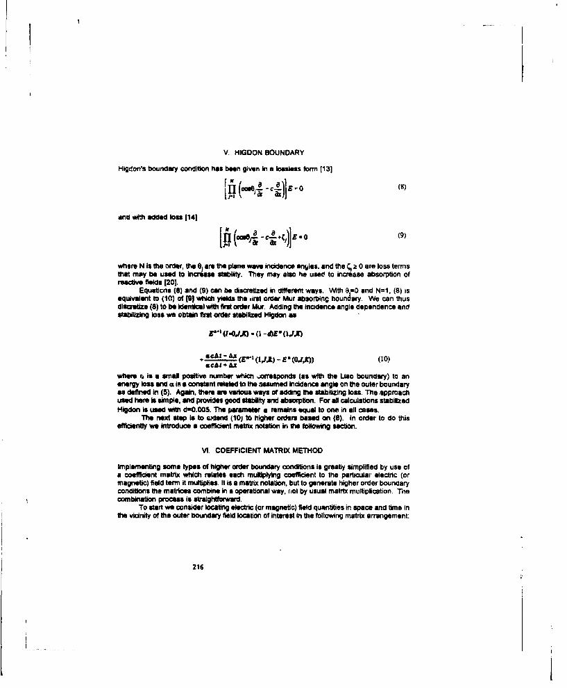
V. HIGDON BOUNDARY

Hlgeon's boundary condition has been given In a loasless form 1131

arnd with added IOUs 114)

[I h(o'sqa-C0 c..)E -0 (9)

whore IN is the order, fthe are the plane wave inicidence angles, and the a: 0 are loss termisthat may be used to increase stability. They may also Ne used to increase absorption ofreactive fields 120].

Equsticris (8) and (9) can be discrelized in different ways. With 8 =0 and N=1, (8) isequivalent to (10) of (9) which yields thes virst order Mur absorbing boundary. We can thusdlacretiza (8) to be Identical with first order Mur. Adding the incidence angle dependence andstabilizing loss we obtain flin order stabilized Hilgdon as

&cS -Ax b(EN*1(I.JL) E E(O4J,)) (SCAt + AX

where a is a emall positive number whichi -wresponds (as with the Liao boundary) to anenergy los and ot is a constant relatled to the assumed incidence angle on the outer boundaryas defined in (5). Again. there ame vwariu ways or' adding the stabilizing loss. The approachused here is simple, and provides good stability and absorption. For all calculations stabilizedHigdon is used with d*O.005. The parametler a remains equal to one in all cases.

The next Asep Is to axtmnd (10i to higher orders based on (8). In order to do thisefficently we introiduce a coeffiient matrix notation in the foollowinig section.

VI. COEFFICIENT MATRIX METHOD

Implementing some types of higher order boundary conditins is greatly simplified by use ofa coefficient matrix which relates; each multiplying coefficient to the particular' electnic (ormagnetic) field termniIt multiples. It is a matrix notation, but to generate higher order boundaryconditions the matrices combine in a operational way, niot by usual matrix multiplication. Thecombination process is straightforward.

To start we consider locatin electric (or magnetic) field quantities in space and time inthe vidnity of the outer boundary field location of interest in the following matri arrangement:

216

II

E' (0JK) E•' (I.JtL) EftJ WK).

The electric (or magnetic) fields are arranged in position horizontally, and in time vertically.An analogy exists with a system of linear equations, but instead of the unknown linear

equation variables, we have the known values of electric fields plus the one unknownboundary field in the upper left corner of the matrix. The matrix will be large enough to containall the electric field terms included in a given boundary condition, which will depend on theparticular bour Amry condition and Its order. For example, for first order Mur only the four termsin the uppsr left comer are included in the matrix, since first order Mur does not involve anyother electric fields.

Any absorbing boundary condition that operates on field terms with the same J.Kpositional locations can be put in this form very easily. This includes all the boundaryconditions considered hem excapt for second order Mur. Forms such as second order Murwhich operate on mu'iple spatial dimensions can also be put in cefficint matrix notation, butthe coefficient matrix will have additional dimensions corresponding to transverse fieldvanations. This can be quite simply accommodated in calculations by declaring an array withsufficient dimensions for each spatial variation plus one for the time variation.

First order Liao has a coefficient matrix given by

T,, T1 T. O )-0 (12)

The stabilized form of first order Liao is obtained merely by substituting To, for T1 .

First order stabilized Higdon has a coefficient matrix

-I b , ( E)-• • 0 (13)

where b, - -!LA- and d1 It the stabilizing factor. With o1=1 and dl=O first order HigdonS'C~t+hAz

as implemented here is identical with first order Mur.One aantage of this cefficiaent matrix notation is that the terms being used to

estimate the oute- boundary electric fieWl am cMarly shown. For example, both first order Mur

217

and first order Higdon operate on the current time electric field one position into the spice,plus past time electric flo.ds at the bouneary and at one position in, First order Liao operatesonly an past values of~ eleclie lo eld, but Soso one field lor~etion further into the FOTO space.

Whilo useful in Oils way, the real advantage of ths coefficient matrix notation is ingenerating higher order boundary conditions from lower order ones. This is most clearly soonfrom considering the product notation equations (8) and (9). These equations clearly state thatnigher order .bsoibing 1oundary condftion; are to be obtained by forming products of lowerorder ones. The combination procesu involves multilying and shifing. A general deflhrton ofthis operation process on the coefficienit matrices can be given as follows. Consider twodifferent coefficient matricas for two diffent outer bIrundary conditions. The first is given by

4p.•,.q,) - (14)

-o., - -p

and a corresponding mtrIx A2(p 2.q,) is defined similarly. Each by itself dlefines an cuterboundary conditioni. We wish to obtain Mte combined higher order boundary condition. Let theresulting coefficient matrix be defined 8s A(pq). The combination process will yield terms inA(pq)with indices p=O,1,2,...(PI+P 2 ) and q=0,1,2,...(Q,+Q 2 ). Each term in this coefficient matrix isgiven by

A(p4q) - - rj E ,,_,6.e A 1(p141) 2(p2.q2) (5A-

0 4 #,-a0 6,0

where the Kronecker delta is defined as0. U0,,.

Equation (15) provides the shift combinations necessary to generate each term of thecomrtined coefficient matrix. This process corrosponds to the product combinations given inequations (8) and (0).

For example, consider generating second order Higdon from two first order Higdoncoefficient matices as given in (13). Each of the first order Higdon coefficient matrices couldhave different a and d terms, which is allowed for by having subscripts 1 and 2. Applying (15),the coefficient matrix for second order Higdon is

218

(b-b -1-db+ 1.1p)2 bj -bj1-db2(IdJ(7

-b~b2 b2(i -4,) 'b,(l -dZ) -0 -d~XI -d,) ,

Third order Higdon can be generated by applying (15) to combine (17) with first arder MI,.donof (13). The pgocess can be repeated to generate Higdon boundary conditions of arbitraryorder.

While. not explicitly clear fronitesttne the th ia oud rycnition, higher orderLiao boundary conditions can also be geinerated using this &approachi. For example, byapplying (15) with bothi coefficient matrice A., and A. given by (12), the coefficent matrix for

scnd order Liao Is obtained as

( - +71 T a + T o'3 I 0 a0

While different In appearance, this result is exactly equivalent to the Liao boundary conditionexpressions given in Section iV for N=2. Note that equation (6) is not needed to generatehigher onder Liao boundary conditios v'hen using the coefficient matrix appronch. First orderLiao Is directly extend~ed to second ordeur Liao, and toen to tnird or higher order by combiningcoefficient matrices,

The resul given in (18) assumes that both first order Unso coefficient matrices urse thesime values of ct (end d If the stabilized form is used). But the coefficient matrix com.binationoperaftion used to obtain (18a) wiflworft just as wall If the TP4terms fbr the deiffrent first orderUsc coefficient frnatricea use different values of a andfor d. So that designing higher orderabsorting boundary condlitions with different contribulting orders optimized for differentincidence angles used to compute fth a piarameiter end with differet loest factors d is quitesimple using this approach.

Furthermore, Use and Hilgdon (or any other boundkry condition that can be expressedin coefficient matrix notation) can be combine together. For example, coefficient matrices forfirst order ULie and first order Hlgdon could be combined to grve a second order boundaryconditfion that would combine the features of both. If transverse directions are Included in thecoefficient matrix by adding additional dimensions, thisi procedure sallws boundary coriditonsinvolving transverse directions to be combined. For example, a second cxder Mur boundarycould be combined with en order P Liao boundary to create a (P+2) order Misr-Liao boundarycondition.

VII. THREE-DIMENSIONAL CONVERGENCE

In this section an example comparison between the boundary conditions is mede for three-dimensional calculations. This example is wide band scattering frcm a fiat conducting plate.

219

Kt

The plate is 40 x 40 cm, and is centered in the FOTD space and perpendicular to the zcoordinate axis, The incidonce angle is 0=45, #=O, which puts the back and forward scatterinto an edge of the FDTD space, but not into a corner. Results are shown in Figures 1-4. Murhas not converged even with a 40 cell border, Super has converged with a 30 cell border andalmost conerged with 20 calls, and Liao and Higdon have very nearty converged with a 20cell border.

This three dimenaliona! example is chosen as a representabve set from a large collectionof limlar calculations. They Indicate that for three dimensions the Super, Liao end Higdonboundaries performT much better than Mur, with Liao and Hiqdon perhaps slightly better thanSuper for dose boundaries, and with Uio and Hiqdon providing almost identical convergenceresults. Mile not Induded here, all boundary conditions converged to identrcal resulis for alltest cases If the outer boa aday was located at a sufficent distance from the geometry. Murwie the only exception, and only for geometries where convergence still had not been obtainedfor boundary distances at the limit of available computer memory. We now proceed to acomparison in two dimensions.

Vill. TWO-DIMENSIONAL CONVERGENCE

WMile two-dimensional FDTD calculations have somewhat limited application, they may beu'eful In certaIn situations. We therefore Indude one two-dimensional compariscn, a perfectlyconducting circular cylinder. For this catcubla',n the cylinder has a 0.25 m radius, so that with0.5 cm square FDTD cells the cyinder diameter is 100 cells. Staircase errors are not a factorIn the comparison, swi they will be the same for all four boundary conditions. The excitationis a pulsed plane *wa incident from 4=45 degrees.

Figures 5-8 show the far zorm beciacafter for the four boundary conditions for variousborders between the cylinder and outer boundary. The advantages of Super. Liao and Higdonover Mur we even more sot"tdn en for the three dimensional calculabtonS considered in theprevious section. This may be due to the necessity of using first order Mur in corners, butthere may aO be more fundamentae shortcomings with Mur in two dimensions. While Super,Liao and Higdon have converged reasonably well with a 30 cell border, the Mur results havenot converged even with a 250 cell border. The Uio and Higdon results for small borders aresightly better than Super, especially at low frequencies.

IX. ANALYTICAL REFLECTION COEFFICIENTS

Additional Insight Into tie performance of these outer boundary conditions may be gained byconsideration of analytically-determined reflection refic•lcents. Following the approach of [22],it is very simple to determine the analytical reflection coefficients using the coefficient matricespresented in Selaun VI. For simplicity we assume that the boundary condition can bespealmd using a lwo-0imensional coefficient matrix operating on time and one spatialdimension. Fof a general coefficient matrix A•4 ) with indices p=0,1,2,...P and q=0,1,2,...,we can express the operation of this matrix on the electric field quantities of (11) explicitly as

220

Af 4)~'~(-qJ,) -0(19)JP4 q-0

Equation (19) specifies aparticular absorbing outer boundary as determined by the czoefficiantsOf tha A(p~q) Matrix. If different J or K values of electric fields are used in the boundarycondlitions, as in second order Mur for example, this can be Included by adding additionaldimensions to the A4~,q) Mabx and adding more summations.

Following the approach In [221 we can then obtain the reflection coefficient R as

1. -3, (20)

where

S, E 1: 4qP')eAwPA LO0 * (21)

andP Q

P40 q'0

and where in (21) and (22) the termi corresponding to p and q simultaneously equal 0 is notincluded. Once the coefficient matrix for a particular absorbing boundary is determined, theplane wave reflection coefflloent can bo obtained easily. Additional summations can be addedto (21) and (22) to Include ele"cti field values with different J or K indices.

Using this result, calculations of ainaiytcai reflection coefficients for the boundaryco'nditions considered in the previous comparisons have been made. These calculations aremade for the same outer boundary parameters used in the convergence comparisons. Theincidence patrameter x =11. and the loss term renames do0 0075 for stabIlized Liao and d=0.005for uabibilized Higdon. The calculationr are for a threeM-dimnensinal FDTO space. Exampleresults are shown In Figure 9 for FOTD cells size corresponding to 10 per wavelength. Thebehavior of the stabilized and unstabilized Liao and Hligdon boundaries are quite slrndar. Thedeep null in the unstabilized versons is softened with stabilization. Both Liao and Higdoni aresignificantly bette thwn Mur and Super at incidence angles near normal, Other calculationsof analytcal reflection coefficients Indicate that they are a reasonable indication of performanceat high frequencies, where Moere are many calls per wavelength. But at lower frequencies,where the outer boundaries are near the target (as measured in wavelengths) are areinteracting with reactive fields, the analytical reflection coefficients do not provide a reliableindication of absorbing boundary performance.

221

X. SUMMARY AND CONCLUSIONS

Four absorbing outer boundary conditions popular among FDTD users have been compared.The four boundary conditions are second order Mur, Superabsorption applied to first order Mur(which is then of second order), and stabilized forms of the second order Liao and Higdonboundary condition. The three-dimensional comparisons indicate that Superabsorption,stabilized Lisao and stabilized Higdon provided significant improvement over the Mur condition.In mos thrae-dimensional comparisons stabilized aiao and Higdon performed nearly identically,with both of these converging somewhat faster than Superabsorptlon. The two-dimensionalcomparison indicate that Superabeorption, stabilized Uao and stabilized Higdon provide evenmore of an improvement over the Mur condition than for three dimensions, again with Liao andHigdon pmviding slightly Iefttr performance.

Analytical calculations of plane wave reflection coefficients for the outer boundaryconditions, ilnciuang stabilization loss, were presented. These showed the effects of addingstabilizing loss to Liao and Higdon boundary conditions.

These results ae presented to provide informa tion for FDTD users faced with choosingan outer bounorlry condilion and determining the size of the free space border region. Theyare not an exhaustive evaluation of the Superabsorption method or of the stabilized Liao andHigdon conditions. Superabsorption may be applied to many different boundary conditions,and our results are specific to its application to first order Mur as described. These resultsstrongly indicate that the Superabsorptlon method is valuable, since applying Superabsorptionto first order Mur provided much more absorption than second order Mur.

Similarly, Liao and Higdon may be stabilized using different values of the stabilizingfector or using different values of a. However, unless extreme stability is required forcalculatirta which include unusually large numbers of time steps (hundreds of thousands ormore) the second order Mur absorbing boundary is not the optimum choice. It requiressignificantly more border space in three dimensions than other boundary conditions, andperforms viery poorly In two-dimienslonal applications.

To aid in the generation of higher order boundary conditions, a coefficient matrixnotation was Introduced. The coefficent matrix notation also allows a general implementationof absorbing boundaries, so that changing from Liao to Higdon, for example, requireo onlychanging the firat order coefficient mabtx eitries. The analytical reflection coefficients are alsoobtained in a simple and straightorward way from the coefficient matnx.

XlI ACKNOWLEDGEMENT

The second author would like to acilmowledge helpful discussions with Dr. Richard Holland whohas long been awaru of the shortcomings of the Mur boundary condition in two dimensions.Discussions with Dr. Brian Zook have also been very helpful to the second author indeveloping an underatanding the operation of the Higdon boundary condition.

222

XIII REFERENCES

1. K S. Yes, *Numencal solution of initial boundary ViAIUe problems involvng Maxwell'sequations in isotropic media," IEEE Trans, Antennas and Prouoagil, vol. AP-1 4. pp302-307, May 1966

2. T. G. Moore, J. Bleachak, A. Tafiove, and G. Krigsnismn, "Theory and applications ofradiation boundary operators," IEEE Trans. Antennas and Proopaat. vol. AP-36, No.12, pp 1797-1812, December 198a

3. P. Tlrkas, C. Balani.", and R. Renautk "Higlher Order Absorbing Boundary Conditions forOne inille-Difference Time-Domain Method," IEEE Trmas. Antennas and Propacat. vol.AP-40, No. 10, pp, 1215-1222, October 1992.

4. F. X. Canning, "On mhe Application of Some Radiation Boundary Conditions,"Trans, Antennaseand Prooaoat, vol. AP-38, pp 740-745, May 1990.

5. F. X. Canning, "Are Higher Order Radiation Boundary Conditions More Accurate?".Proceedings of the IEEE AP-S International Symposium (Dallas, TX), pp 1364-1367,1990.

6. L. H. Howell and L. N. Trefethan. "Ill-posedness of absorbing boundary conditions formigration." ~Geophysics vol. 53, pp 5934603, May 1985.

7. R. A. Renaut and J. Petersen. "Stability of wide-angle absorbing boundary conditionsfor the wave equation.* Geophysics vol. 54, pp 1153-11G3, Sep. 1969.

8. R. A. Renaut, "Absorbing Boundary Conrlitions, DIfference Operators, Stability," Joraof Computational Physics vol 102. pp ý.36-251. 1992.

9. G. Mur, "Absorbing boundary conditions for finite-difference approximation of the time-domain electromagnetic-field equations," IEEE Trans. Electromaon. Comoat., vol. EMC-23, pp 1073-1077, Nov. 1981.

10. K. K. Mei and J. Fang, "Superabsorplion-A Method to Improve Absorbing BoundaryConditions", IEEE Trans. Antennas and Prooagat., vol. AP.40, pp 1001-1010, Sep.1992.

11. Z. P. Liao, H. L. Wong, G. P. Yang, and Y. F. Yuan, "A transmitting boundary fortransient wave analysis," ScDientia Snics, vol. 28, no. 10, pp 1063-1076, Oct. 1984.

12. M. Moghaddam and W. C. Chew. "Stabilizing Liao's Absorbing Boundary Conditionsusing Single Precision Arithmetic," Proceedings of the IEEE AP-S InternationalSymposium (London, Ontario), pp 430-433, 1991.

13. R. L. Higdon, "Absorbing Boundary Conditions for DWference Approximations to theMulti-Dimensional Wave Equation," Mathemnaticsl of Computation, vol. 47, No. 176, lpp437-459, October 1986.

14. R. L. Higdon, "Nunerical Absorbing Boundary Conditions for the Wave Equation,"Mathematics of Computation, vol. 49, No. 179, pop 65-91, July 1987.

15. R. Luebbers, K. Kunz, M. Schneider, F. Hunsaerger, "A Finite DIfference Time DomainNear-Zone to Far-Zone Transformation", IEEE Tr-ansactions on Antennas and

'qjtiion, vol 39, no 4, pp 429-433, April 1991.le uebbers, D. Ryan, J. Beggs, "A Two-Dimensional rime Domain Near Zone to Fnr

Zone Transformation," IEEE Transactions on Antennas and Propqgatign, voll 40, no 7,pp 848-851, July 1992.

17. R. Holland, L. Simpson, and K. Kunz, "Finite difference analysis of EMP coupling tolossy dielectric structures," IEEE Trans, EEMC vol. EMC-22, pp 203-209, Aug. 1980.

223

18. K. Kunz, R. Luebbers, The Finite Difference Time DoMain Method for Electromagnetics,CRC Press, 1993.

19. W. C. Chew, Wve.O and Fields in lnhomogensous MediaVan Nostrand Reinhold, 1990.20. J. Fang, "Absorbing Boundary Treatments in the Simulation of Wave Propagation in

Microwave Integrated Circuits,"Conforence Proceedings of the 9th Annual Review ofProgress in Applied Computational Electromagnetics, Naval Postgraduate School.Monterey, CA, pp 322-329, March 22-26, 1993,

21. R. Luebbers, K. Kunz, 'Finite Difference Time Domain Calculations of Antenna MutualCoupling', IEEE Trensactioris on Elactromsonatlo Compatibility, voll 34, no 3, pp 357-360, August 1992.

22. S. Ray. "Characierization of Radiation Boundary Conditions used in thie Finite-DtffprenceTime-Domain Method," Procedings of the IEEE AP-S International Symposium, SanJose, California. June 26-30, 11969.

224

V

I

I I I .-

L L 0

4- 0�Ila

II�

N L�0

I�t�.4 Ig.� 0

I::: .4.I. I� *� 0

.� .� .� '0a

5- '0

00

0

U

a

I I -

0 0 It� 0 U- - U

I I S 5 '0

�wI&p � za;�v�n�pve

225

* 0

2262

0

LM.4)

Q Q -u U

II C.,

gu,/p so mmI

I22

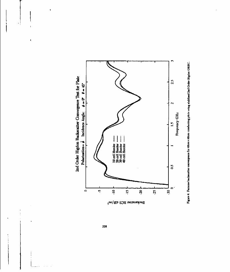
t

00

I 0

"-II IC.'

b-

0� a

- a*0a.11 1K!

uu.�IJ -.� .u '� *�

0

aI'.�

II I I

li.� mJ'� C �I.

* . I .q.aU

U'

229

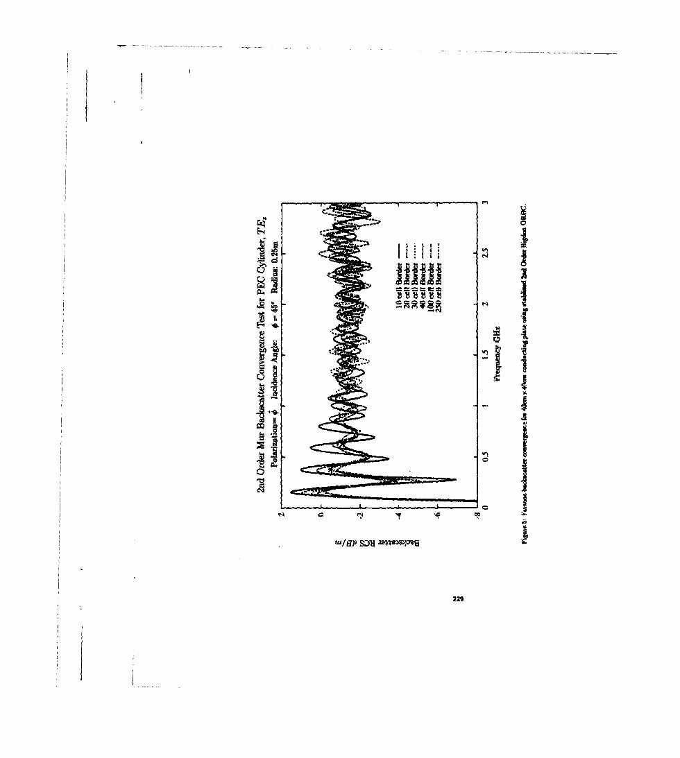
'4 C

'b 16

229

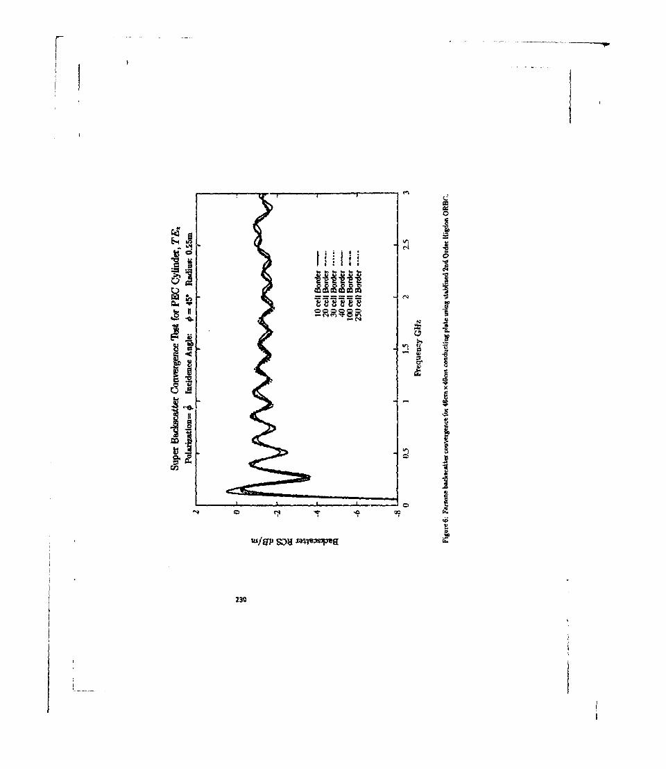
I

______________- C

0

0if *0

4H fI 0

-�

C) �'-I d

* ---.---

w'I 0 ifII -N� WI-N II

if

-

WI �.,V -

- U)

0p U

b4 B0

U, I

V

141/ap s�11 JW�3U�

230

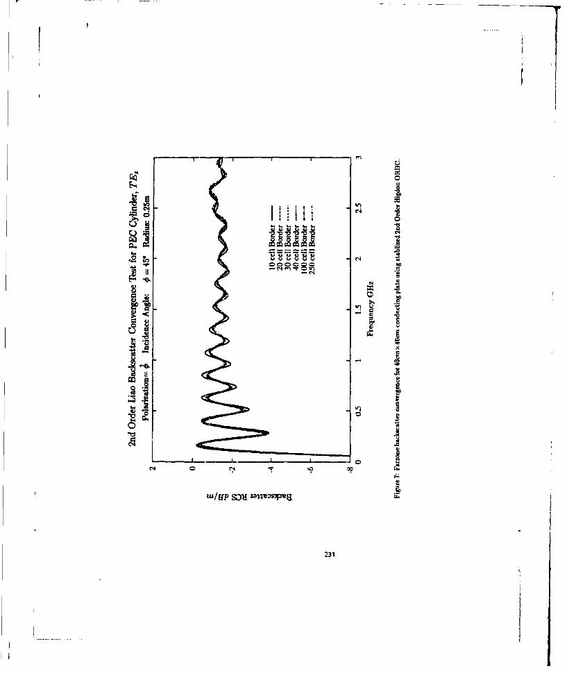
t

I I

0'I, e-a

iIt) UI..., 'IIHIH -U

00 -aa

'.4

* uuuui d�uc�uu�ooo 0

-!4e�Vq 0 It) a-0.

�

�

-4) -�

4)� U U� C

4) *.I4)

LI x

-� 4. -U.-I, U

a8

0 C

aI-' U 8

0 U

Q UU

I)

a0

0 '0 �J..

4)a

wftjp s3��i £�t�ee

231

iI

~~°.'

.:3

I.-' - '

V M

I Ii I

_la 106lofi

I i233:.• •,r ',& .[ -

•.•, • .s. .••,S- C

3, \ ,-

• • "• C

.y -.. = ,,,4...-._. •• •o

0 -,+ # • 0 l

:- . • - II. .

233

Adaptive Absorbing Boundaiy Conditionsin Finite Difference Time Domain Applications

for EMI Simulations

Bruce Archunbeaslt and Omar Mv. RarnhiDignadEqu~curntCoporanion

MaynardMA 01754

ABSTACT1

Abmnibiag bufidary conaditions (AB) awe typically constructed to annihilate waves kim-pinging, en the mesh truncating boundary 8t4 or clane to, normal incleence. Trhese ABCs givesufracient accuracy provided that the truncation boundary is chosen far frown the source or

cterr asking the comiputatioan (auaig finte element or finite differencp moethods) very ex-pemlve. p~apper presents urn aktemntlve foeumlation to ABCs by optbmzinig the boundarycondition at each boundary call for the 1igho likely direction of incidence. The adaptation ofthe new ABC to the Finite DOfereone rume Domain (FPTD) solution is simple and effective.

DMTODUCMlNAbsorbing Boundary Conditions (ABCs) have btum widely uscd in Finite Difference Time Do-

ruian (FT=) and Finne H~ement (FE) modxeling of open region scattering problemns anid microwavtcrctums. Several papers hav eloen published explaining and comnparing the performance of auarbrof difterent ABC&. The basic operation of these absorbing boundary conditions is to simulate fiveaspace, that is, absorb ali electromnagnetic waves as if there was art infintaie smount of free space inplace of the ABC. Theve boundary conditions we enforced along thte boundary of the cocnputationaldomain that is used to truncate the &=is dillirence grid and ame usually deriveol wit the assurptionthat wves impinge mn the boundary as angles .qiil to or close to normal ,soci-e r.

To constrct the perfect absorbing boundary condition, two major considerations we in order(1) The boundary condition has to absorb wave itnpirngirig on the boundary tam~ all direconrs simul-taneously, and (2) The bomndary operaor must absorb wave ds t ant both tvtenescent stad traveling atthe sacm im-. (evanescen wave typically exist i the acar field.) To conastruct: a bonmAday operatorthat addanesas (1) is thecoretically possible but wriuid requac extensive computer memory and calciala-notis to be performed it echb boundary call. amr to mention the possibility of unstable solutions. Thecontstruction of boundary operators to accommnodate (2) is possible but comes at a considerable costarnd complexity in code development time and code execution tune. To the kniowledge of thc authois.the indmina absorbing boundary condition [1! is the only ABC that has the potential of effectivelydealing with evanescent and raveling waves, but involves considerable %;ompurational comnplexity andcan be very expctisvc to implaemem.

234

For an nuportucans ss of electromagnetic radiation ptablernts such -s those arising in Electro-ianewti lutealerence (EMI) applications, a large dynamc range is critical to allow accutraie predic.amc of nadatou fromt shia;ded structure. Typical ABCs can produce reflections on the order of -60dB relative to the incident pulse mniplinade. This level of accuracy in the boundary conditions is usu-ally sufficient for clasr"-Al scattering applicatiomr. However, for ENI applications higher accuracy isneeded. It is zmprrat o note dwthis d lintitarion on die accuracy cannot be lifted even if the outer

atindarwy is receded further by increasing dhe comaputational domain, sinc waves still imipinge on theboundary at unges that deviat appreciably frurm normal incdene

In this work, we made, use of the flexibility inherent in die IDT method to Minimize die re-Siection arising firom due use of die ABC. This wa possible by adapting the ABC to the wave's mostblkey direction of mincidec at each of the boundary cells. For die pecialclassof radiatiotsproblemssudh as in EMI, the source is typically localized whinch allows a good prediction of the angles the mci-dent waves make with the boundary. Since the ABC is adapted to a tinge wave (at echd boundarycell.) one can get optimal results by using us esacr boundary condition. or more accurately, anm adap-tive absorbing boundary cmndition (AABC).

FORM~LLATION

There ane seveail ways in whicdh one can constucti an adaptive absorbing boundary condition.In this work, the formnuLaion is bated on the Liao's absorbing bouindary condition (2] which has theadvantage that firs, it is readily adaptable to the FDTD grid, and, second, it guarantee stability for awide range of incident angles.

The Liao's Nd' absorbing boundary condition can he written as [3]

O(z,t+ At) O (l~C (x- jcdt I- Qj- l)ds)

where

4o is the field value and Atr is the limne step used in the FDTD solution. Notice "a the field valuesinvolved in the absorbing boundary condition are not necessarily evaluated at the FDTD grid. To ex-press the botundary conditior in te-ms of field values availble at the FDTD grid, quadratic intespola-tion is used. For btstuuce, (x -cALt)is expressed in ten.uof the field atthe botundary point xas

O(x- CA:,t) 0,-r ) +Ir ,(2-s02'(.)-+ ) 1+ s(2-s)3(zz

where

e = *-(I-)dx.j- (mn- 1$t]

235

The IAs's ABC a givt above is opumized for nord incidence, a the sense that rays hitingthe boundary a normal incidence would be completely absorbed. To optimize the Liao's ABC foreach cell lying an the ltice ouucion boundary, we will make the assumption thd only one ray hasthe boundary. Define 0 to be the angle the assumed incident ray makes with the: normal directons aparticnIar boundary cell. To optimize the boundary condition for ech boundary cell, the wave speedis modified by the assumed aigle of mcidence ea

The absorbing bounday condition applied at each boundary cell will then be

t (Xoz + At) , t•_(- lr'c - j#XJ A,4it- (j- 1)d)

It is imnp•rtant to keep in mind that the full strngth of die adaptive absorbing boundary cordi-amn is realized wen thie source is localized in space which ives rise to a single ray hittng eachboundary cell (-asuing the tuncaticn boundary is outside the nei field region.) In EMI problemnsinvolving rdiation drough a single slot, the slot width or area is typically small compared to dhe sizeof the comptriital boundary and to the dc from the slot to the lattice runcation boundauy. Insuch prob te most appropriate choice for the tsenr of the localized source, for the purpose ofenforcing the adaptive absorbing boundary condition, will be the geomtric center of the slot. Forproblems where unltiple slots of equal or similar widths/aa exist, it was found, as can be seen fromthe atumeuical reuhts presented below, that if the center of the localized source was taken as the geo-metric cam of dte poits definin the centr of the slots, then the AABC still gives a appreciablei over ABC. Finally. for cases where s slots are larger in size than thers, it is rec-ommended that the choice for the nencr of the localized source should be made such tha it will biasthe slots with larger mi.

NUMEIhCAL RESULTS

Two representatie examapla wee studied to show the effectiveness of using the adptave ab-sotbing boundary oanditiasa in FDTD soluiont In the first examqp, we considered the two-dimenimonal proln of radiatin though an O.Olm wide apertare in an infiie perfectly conductingp'rnd saen. The gomrny of tde problem is shown in Fig. 1. The utne sep used in ft FDTDsohlsat is At = 2.36 ps and the grid sin used was Ax = Ly w O.O01m. The source exitation fu-ctionis the derivative of a Gaussian pulse of width 32 A& Sine= the inueast lies in finding the radiationlevels outside the source region, the opmal choice for the localized source for the purpose of apply-ing the AABC, is chosen to be the oruer of the aperture as shown in Fig. 1. The electric field (Ez) atthe observation point is shown in Fig. 2 as caiculated using the FDTD method for both cases using theABC and AABC. Since the field conrihut•on a the observation point is coming from two ray-likewaves, the first coming through a direct path from the localized source, and the second is the reflec-

235

non from the side trwation boundaries. The results shown in Fig. 2 clearly demonstste that theAABC has significantly reduced the effect of the second ray.

The second exarnile employed the geouwny and F3TD pztxmee used above, but two aper-tures were added, Each of the tree apertures has a width of 0.01m. and the separation between themis O.Olm, as shown in Fig. 3. In this case, the field contribution at the observation point is expecLed tocome from several my-like waves emanating from the three apertures, thus resulting in an effectivesource which is morn distributed over the conducting screen than what was erperienced in the firstexampl (me Fig. 1.) The optimal choice for dte localized source will be again x the center of thethee aperuirs as shown in Fig. 3. Nummical results using the FDTD method are shown in Fig. 4,which, despite the exi of a distributed source, Le., the three huygens' sources a the three sper-tures, the AADC performed appreciably better than the ABC.

CONCLUSION

This work presented an alternative lomsulation to ABCs for certain class of radiation problemshaving localized sources or sources distributed over a small region. By optimizing the boundary con-dition at each boundary cell for the highet likely direction of incidence, spurious reflections can bereduced significatly resulting in more accurate solumiom. The nw nurnercal fonnulation, or theadaptive absorbing boundary condition is especially well-suited for imple5 muttion into the FDTDmethod.

REFERENCES

[1] E, L Iindrimuan "Free space boundary conditions for the drne dependent wave equatim" J.Camp. Phys., No. 18, pp. 66-78, 1975.

[2] Z. P. Liao, H. L. Wang, B. P. Yang and Y. F. Yuan. "A uinsmimiig boundary for transientwave analysis," Scievina Siuca (seie A.), No. 27(10), pp 1063-1076,1984.

(3] W. C. Chew, Waves and Field in Inhomogeneous Media. New York: Van Nosurmd Reinhold,1990.

237

I 0.25.

a-"

-12400 9~kbdm

2.30a 4. 2. < 0.

Mg. 2. 1.=FcM(t atmm hWziauan og fixu~ thge qat -p a~m w bmed =mg teAUurmebi withAB ad 0.01..

aoooo. ~ 238

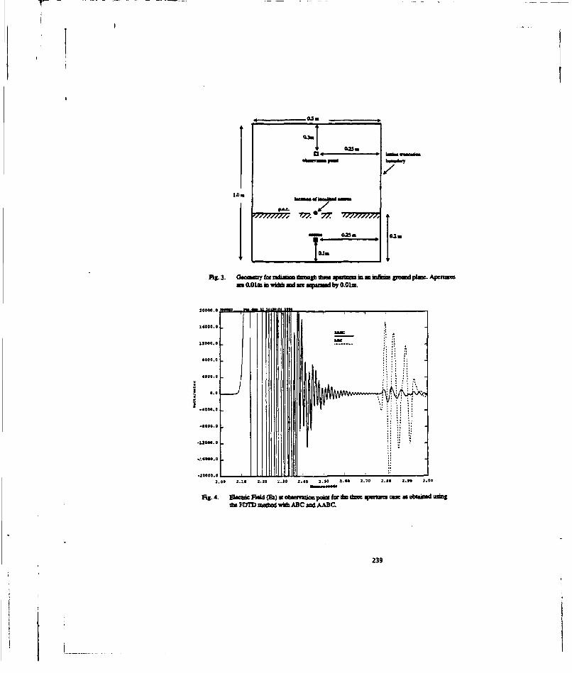
7. 77 77,7,7=

0Sým

I1"G 0~MS. 4. GeM~i ddyZ at riobovd poih fo te fmtea WK- i Cam hU OUid pUe.ASomuu

tko 0.01M Me w~h AB Meapud by .Oin

20002.9

A Dqism~ve 0.1s Radation Boundary Conodition for FDTD Calculationsi

Brian J, ZookSouthwest Rjtmerh Institute

P.O. Drawer 21510San Antonio, TX 77228-0510

Outer radiation bosmdga7 condition (ORBCs) in the Flnite-Difftenrec Time-Domatin (FDTD) m&ethd ameusually applied to fle-spane, computational bouendauies. T1his is satisfatory for Radar Cross Section andSUimil probles when tde modeled Object ks suspended in five space. Miene anea number of applications,however, whine, the computational boundaries we located in dissipative media which may or may not bedispersive. Examples of such media include soil mad plss'ia. In these cases. a free-space ORBC resultsin unacceptable reflections, motivating due development of a dispersive ORBC.

Higlidous Outer Radialiont Boundary Condition

Higdloni' ORBC has doe flexibility to be adapted for use in dispersive media IlI]. Not only is it able tohandle different wave velocities. but Fang astutely obmevedoth method is able to absorb evanescenit wavesby including atteuaation terms hir the OROC [21. Higdon originally introduced small avenuatiorn terms tostabilize the ORBC. We wish to emphasize that the attenuation tarm sue even mnoe general and can beused to accoumt for other formn of attenuation, in partiultar, to abseorb a wave propagating through adissipative me~dium. For a wavefleld u(x~t) approaching due boundary x = 0 from x > 0. the Nth-orderORBC can be written as

IA(1 ,- I =,Ot 0. 1

Each tn.m of this ORBC annihilates plane waves traveling at velocity Y, impinging at an incidence angleof Ok through a meliums wriathtenuation coefficient %~.

Higdon discretima this diffrenia operator by introducing a m~iing parasnemr h. used to mix time andsitme derivatives. This parameter affects both stability and accuracy. Me discrete form of dhe ORflC canthen be writtenat

b Iu(0.t*AI) -0 (2)

240

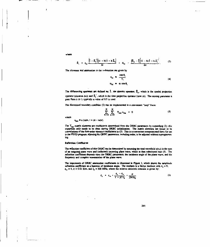
where

h) h a) [0 - h) h (3)at Ax

The slowness and attenstutiont in the x-directian awe given by

S51 a -olGVI (4)

TIe differencing operenrs ae defined ft: t. the ideandy opeint t,, which is tde spaial projection

opesator (distance Ax); and k'. which is the time projection operator (time &t). The mixing parameter hgoes from 0 to 1; typically a value of 0.5 is used.

The discretizisd boundary condition (2) can be implemented in a uonvenient "loop" form:N N

E T. u. - 0 (5)nm.O rn.O

whereum au(nx.t + A-mA).

The Tom mormx elements we coefficients determined from die OR]C parameters by expaiding (2). tiusexpasSion only needs to be done durng ORWC inializatmion. The mnMix elements we found to beconvolutions of dte firm-order opeautir coefficient$ in (3), This is a convenient comptational form for usein the FDTD program. allowing thz ORBC panrmeei. including order, to be adjusted without reprograms-isig.

Reflectimn Coetlcrut

The reflection coefficient of this ORBC can be detemined by assuming the toul wavefield u(xz) is the sumof an outgoing plane wave and (reflected) incoming plane wave, which is thin substituted into (5). Thereflection coefficient depends upon the ORBC pairametets. the incidence angle of the plane wave, and thefrequency and complex wavnumber of the plma wave.

nit impornasce of OR.C aenuaotion coefficiets is illustrated in Figure 1. which shows die amplitudereflection coefficient as a function of incidence angle. The medium is a Debye msedium with ; =9.e,. = 4.0 = 0.01 S/sn. aind fo = 500 M&z. where dte relative dicloctric constant is given by;

s+ - f- * " (6)

241

no3 figure shows the magnitude of the reflection coefficient for 500 NMz plane waves. If no attenuationis tincw-ine the ORIC. the retlection is uinacceptably large. Including attenuation in the ORBC reducestie reflection significaretly.

Figur 2 shows the reflection coefficient as a fianction of freqtuency. for plane waves at normal incidence.Again. ORBC atteuation reduces the reflection coefficient significantly. The figure shows that thereflection coefficient goes to tinily at zro-frequency; dii. con alo be shown uiatlycuiy. This suggeststhat taucet sigal. such as ani incident pulse, should not ocoruain significani miergym very low frequencies.

1he low-frequency reflection phewne'ueum Is pastiwularly problenmatic when the computaional domain ismeastly filled with a dissipative or dispersive nudi--, In susd media low frequencies experience muchleas attnuation than high frequencies. This mum my low-frequency energy sla toj reflected fromnthdeORD C is able to tritel larg disanmces in dhie simulation resulting in a low-frequency "ringig" effect, whichwe have observed. Foadasurnoe. shoe high-fteqtaecy energy may be lusi~y Watteuated by die mediumbeFore- reaching die bouidary. the high-frequency reflection coefficient is riot as important. This mean theORBC design should be skewed mucli dio a small low-frequentcy coefficient is favored.

We would like to have in ORBC that ha a small reflection coefficient over a broad range of bothfrequency aid incident inigle. A uhnpl choice of ORBC peametuas would be to choose velocities anodsnmanntio cstefflcianst dim correapond to di e ndium at frequencies within the tange of the sourcespeosma. But as we hav smes. a small low-frequentcy coefc imn needs to be favored. Also. ORBCstability. discussed below, as another considerattion. We find it usefual to examine die reflection coefficientas a iniction of both frequency and mngle by using a contour plot. rich as in Figure 3.

Stability of the ORSC

Material and ORtBC p~a salso affect die atablit Mprpres of the ORBC. The anaytic diffesentiaORBC (1) is muntable unless tie ORBC atenuatiAn s laqwg din the attmauatson of die rnediuzn. We havederived a stability cumotes for this ORBC. It as bissed on requiring tie roots of the Z-trisforn to lieinside die unit circle [31. The stability can be analysed for each order separately. The root for the ith-orderis found to be:

-nx 'I pab 1j,.cl (7)

where

AX

b, aýAx cos O 1- ReI K -1)*i ImIK-11

di cos O 1 .&,ReIK -lIl

K C~' i.aixie k-j) A mi8

242

The Z-transform root gives usr a stability cniterion:

ci 2 (2a - pi) - bi (2d1 - b, pi) C 0 (i

This expression shows therm are two main ways to increse. stability: 1) reduce the miLXing parometr h, or2) increase thse ORBC attenuation coeffieest Bacon of die asensiivity of die sufleeson coefficientfrequency response to the ORBC attenuation. we find it convenienst to adjuint the mixing parameter.

Figure 4 shows a stabihlzd reflectioss coefficiesat crosed by adjuustig the ORBC pamsetnm for figws 3.The reflection coefficient is now bot lavradsod. which reerteo be characteristics of diestabilization process.

FDTD Zmplemenula~o.

We have implemented this ORBC ins as FDTL# code. Instied of applying tse ORBC to doe E-field. Wt isusually done, we apply it to the H-field. allowing fte adjacent E-fields to be updated with thle usual interiordispersive update equations. For the interior calculations, we amn using the recursive convolution methoddeveloped by Luelbeats 14).

As -n example of the ORBC implemnentation. we show the smolts of TE polarization calculations. Theconfiguration is shown in Figursm . Two calculations in done - one on dhe small domain CII and one onthe Luge domain Ck2. Both calculations asm stopped before refluesions frm 02 can reach 01. Thus. anydifferences between the two suns at all field points inside £lI are only affected by reflectionts from 01.Samples ame taken at die two indicated points, ju~st inside 015. The sosurce is an inlinizesirnal H-field soucelocated at dhe camte of the domains.

Figure 6 shows such a nut. Notice die pulse is dispersed bust decays nicely to zeo showing no instability.The reflections firom the edge and the corner were approximately -55 dB; and -30 dB. respectively. Thesource fusnction used was a pulse that has a master frequency near 500 Mr. with energy ranging from70-210D MHz (60 dB points).

Figure 7 shows a run with a source function that produces more low-firequency energy. T1he reflectionsfrom the edge and the corner were about -50 d3 and -40 dB. respectively. When comparisns are donebetween the two domain calculations, a low-firequency difference is see tha is slowly dissipated.

Cenelusiau

We have shown how Hlgdon's ORC cani be adapted for use in dissipative and dispersive media. Astbility criterion and contour plots (firequency vs. angle) of the plane wave reflection coefficies i can beused to design an optimal ORBC. Results show a complex relationship between ORBC paraneters.material properties. reflection coefficient, andl stability. Yet. properly applied. this ORBC allowscalculations inside an infinite dispersive medium.

243

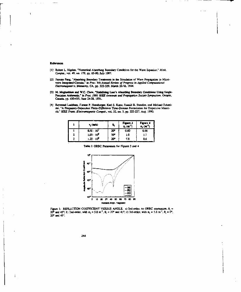
(1) Robert L Higda. "Numerical Absorbing Boundary Conditimn for the Wave Equation." Mahci.Campus.. voL 49. no. 179. pp. 65-90. July 1937.

121J .iaytan Fang. "Absorbing Bomaidary Treammusi in dhe Simulation of Wave Propagation in Micro-wave Imegrued-Circuiss." in Phk-. 9rit Anand a Revfew of Progress in Applied ConpufarionalEkacm~eatmsgesi Mlouammy, CA, pp. 322-329. March 22-M., 1994.

[3) M. Moshulddrn and W.C~ Cbww "Seahillu Liao's Abmeiag Dommday Conditmios Using Single-Precision Aighmae" in Proc. 1991 IEEE Aoeaaw and Pwoagadron Sodaey Symposhum. Ononjo,Cvanad. pp. 430-433. ftme 24-28. 1991.

(4j Rkmvmoud Luebmea. Fmz P. Haunsuerger Karl S. Ku= mz Lnal B. Starmdics. umd Midmal Sdunei-der. "A Pmtqueacy-Depeiuent Futiire.Dlf~ene rine-Donmain Pornmilanosa for Dispersive Maeri-AILa" IEEE Tras. Electrmpeiqc Compo.. vol. 32. no. 3, pp. =2-227. Aug. 199.

I 1 (Is Fgm 3 Fginaed461 WI 0 (0

BI Sn 101 W0 0.60 0.66

3i 1.23-109 20 7.8 8.6

Table 1: ORBC Paraneen for Figures 3 and 4

Figure 1: REFU.ZJ7ON COEFFICIENT VERSUS ANGLE, a) 2nd-order, no ORBC azzenuanion. a,00and 450: b, 2nd-order. with nt.j 5.8 mn". 9,i 20* and 43*; c) 3rd-order, with a, 5.8 m-'1. 9, 0.,

200 and 4S'.

2"

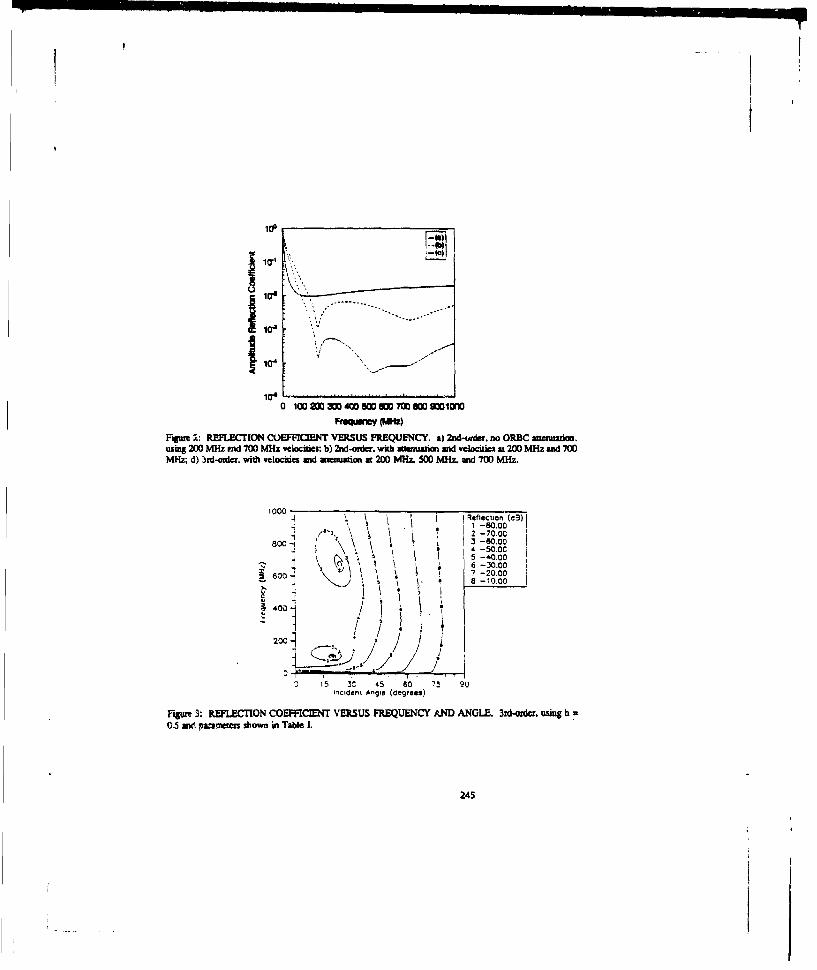
......104

104 '

0 10 2= =040W 0WlM)==800g0l=~

r-mq=W (Kf)

Figp =: REFLECHION COEFFICENT VERSUS FREQUENCY. a) 2nd-4jme, no ORBC anumuato.using 200 MHz end 700 MHz velocimes: b) 2nd-order. with Maemiuaion amd vekxci&e at 200 MHz and 700MHz; d) 3rd-order. with velocites md atenuation at 200 MHz. 500 MHz. xWd 700 MHz.

t 000 1000 \ jReflection (c3)t ' \ 1.-80.00

' 2 -70.OCBoo -1 3-_60.00

5 -40.006 -30.00

26001 7 -20.00

~4001 -00

200 .

\•'i \' . -oo

3C5 " 45 60 75 90incident fAngle (degrees)

Fitpv 3: REFLECTION COEFCIENT VERSUS FREQUENCY AND ANGLE, 3rd-order. using h =0.5 mu pusLammem shown in Table 1.

245

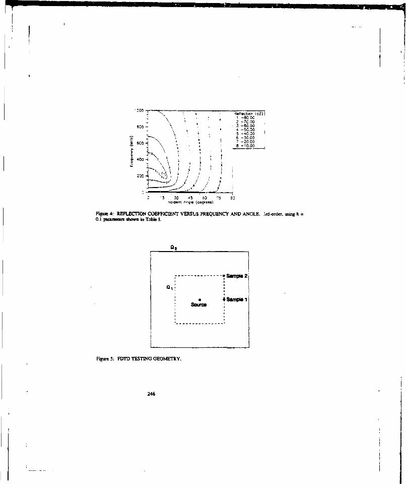
R eflection. (c9)1 -a•.O02 -7C.00

800- 3-60.00& -50.00"5 -40.00" -30.00

600i 7-20.00a -10.00

400 *

- 5 30 5 60 75 ýC*cOfm •rg;it (cegrees)

Fipwe 4: REFLECTION COEFFICIENT VERSIUS FREQUENCY AND ANGLE. 3rd-order. using h =0.1 pu2mw shown in Table I.

I I01,

Figure 5: FDTD TESTING GEOMETRY.

246

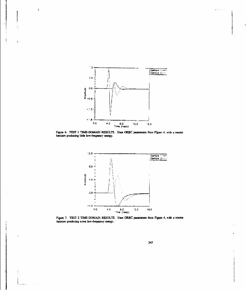
06-.

S1 i0.0

CI.-0.6

C.0 4.0 8.0 12.0 "6.0Time (rlsec)

Figure 6: TEST I TIME-DOMAIN RESULTS. Uses ORBC pawnetrs from Figure 4, with a sourcfunction producing litle Iow-fwqueucy eampey.

12.0 , ' Sonwe i -- ,- ,Samee 2

8.0 -'

C.-0-

0.0

0,0 40 8C 2.0 16.0"me (nsic)

Figure 7: TEST 2 TIME-DOMAD; RESULTS. Uses ORBC paramee from FguRe 4, with a souzefunction producing 3omc low-frequency eer=y,

247

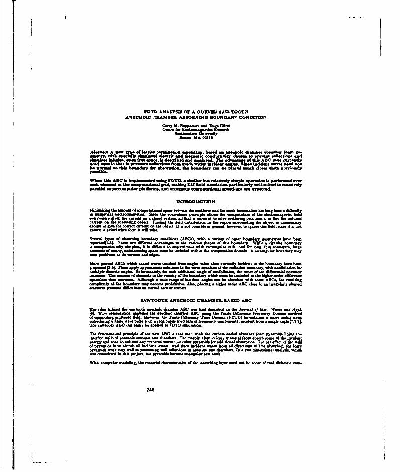
3DTm ANALYSIS OF A CURVV) SlAW-TOOTHIA!4ZCCUOIC, ,NAMBER ABSORPI14G BOUNDARY CONDITON

Came M. Rappepvzt and Tolga G"re

Boston, MA 02115

Aheseei A -m t ofe d lewasti o ulustion, allgookhm., basedoas amedbolic chamber tbsober town ga.vmty wait specialy wboleted deletric ad ocudj~ita dhs to re.'eat resections anad

u tla.indialter aopem Qse. opie. in desalcrib~ n nlsd h da f" AC vscreneedines La that kn p~~ ~leisfo ac ides Iuaidsvt a" Sxm sie waves need notbe anumel to this bounarey be, abrarptinal. do boundary Se he plinmel enack slower than prev4owely

When this ABC is e dmnand using MDTV, a sheiae buat relatively =lphwaetion is perforated over-wul slaso in the aoput-A-lme grad maskIng EM Gold sinmmlatiou n e l welU-siated to mnassivelyPerele su~ervotairub Platiowem, and anomsout ocomputationaol speed-usap we pemrtedl.

IN4TRODUCTION

Minammags the anowv s'omattoa pace hetwona the eceotrer end the toeeb teartuatioa hen long been a di~caltyio --m-&ca elecotwoinapetcs. Saum the eqeivovalune pnuacple allows the canoputatiom of thefileverywher pvc the Ieeto closed surface, adl that is mnabad to solve sottering proboma lia to fin Ithe isdueedcornet as the aatteuiag ~obet. Feniowg the fied disrlostrbuo in the agi nmud'n the objec - 'a~ ya to tgive the cormect cvvinw an the object, Iti . poso ibhle inesal however, to ignor thu ield, ac =iit.

anw praor what form it will tabe.

Svel tps ofaherbag ounar oaeditions, (ABCs), with a warlety of onmer boundary geomettive have beenrqpoctedl.q. There are diffrent advantage to the vwarw shapes ef this boendary. While a circular boundaryis cmputiue.ally, ssuaplam.it is diflicult to aojaaoxinAae with rectsangaar colla, and for long, thin ocatterewe, larg

a easOf sny anael~pace cout he included raiti the oneupatatire domnain. A rectangular boundary maypostrb t t one da

Momw Senal ABCs or"icovaed waver incident fromt angles aothe then annunally incident to toe boundary have benpcodtmd &14]s Thisas. ap apgeutuset. forsish adthdai eutiona ats thn radiation boundary, with annihillation (w~~~m~~~~sry~~~~~~~~e~ anlI Upotntl.frst diielageo niiein ee I the differential oeaoimasson. The number of elements is the wianir of the bovadlaey whicb man be included in the highe-r-cder dfeecopatnija duthe encrae. Although a wide rnoe of incidsoot angle cai ha aheorbed with thst ABCs, the caaul~

eseegihatiy awte on ary heocuon.pt ibt Also, placing a highe order ABC cl. to o en ltysadsenitew ipument digfclteeno en carad wam or answes.

SAWTOOTH ANECHOIC CNAMBER.DASED ABC

The idwo lohind the esworotia anethic hellcber ABC was fizat doesaibed in the Journal of She. WewAe and AppI.Zo Te presentateion, analysaed &bhe aneckec dwc*er ABC ealag *ATheuFnit Diffeasece Ikequmncy Doomas nethodt

VorM'Apsag ecotteved faied. Noweva, thA Finite rl~lleeenc limet Domasin (FDTD) foeMulatMo mciso Metal whencooridaeing a finte waet' PONs with eContinauou spectrums Q vo awrquny enenpflenta, imnadent from a singia angle 1,,]The mawinotho ABC tan esandy be applied to FDTD smnaainio.

The fradeanatal penac~le of the new ABC aw that. asoii writh thoe carben-looded absorer 65am pyreanid lining themntxjri walb if ansehooc antomw at e cbsoembee. The tseeply emote Wary vastetial Lacer abeceb some of the incidentemap wsd 1ed to rediret Sany ýdw~sd warow iu~o other pyramidsa for add lionl absorption. Tate set effect af the wellof pyramids as to ah-oeb all inlaciet avwn And Race, incdent wavew front all directions will be absorbed, The hayipyramido wamI Very woll at Preventing: WWlI afolectios in Sasinaa lot dheembeen, Ins two dienemoio"a sanaysnawhcwe considered in this peojec, tOe pyranads, bettms truangamla sew teetho.

With corenpter m=dlW%, the masterial characteristics or the absorbing layer need not h,2 those of real dielectrie corn-

248

pounds. Instead, sbe material can ha moddeld as bein lousy tb= bwad eoh lectric and magaietic cosduetevity a', WK.end .T"' vawlam of Permnittivity cand Pmrmeebility # seleted & megct matich at the vaecond bounce or One moemallyisasou wer. ft' h Van ta Von" m ofOhms tninlm we equltr, ,the aaaj the rasected toy makhm with the Secondtrianfls wee it ir (V lotalmd s angle). Thu loos"mw in eshoae in Figmie 1.

As long aseplo w oeu/s = po/to (Which corerspoud. to imaitang coasant firequency dowansw wave impedance saersethe boundary'), there will be no reflectioes for normal incideace to a taimagl far"

This rsqoiramant is Adlictult to attain with ,ssl materials, but quite easy to specify by cmputer. It is important tomake the conductivities Wlea = #e s that the wav quickly decays asit pbopague ato h bsre medium, butnot so lImp thw the decayinig Reda laadsquatly sampled anA tke U .

FAgure 1. Ray paths for wase Normally incddent Figure 2.Geometryfo the cireular .awtoothABsad imoidwal at angl a asequilateral nclosing perfecly Cooedecio square (totrisagula, al-nbing houndar, alb-s 6 tdo IS) and shlowing the circular cylia-melipis booasm anto medium. dricel pulse moaximum level at 9 = 0.

POWD 51114ATION

Twu duarewmoaI FDTD simulstion of this equilateral triangle saw-tooth shsorbNgl layer is ezamined using amen aztatompulse whih simolates a cylindrical wave, em batig r. a point soun. Uatoritwaately, there is no closed form solutiona,w the time-dolasm, to the cylindrical waeeuto.The stanadrd Bauket function solutionse caly work in the hasqwMcydomain. T'healeis, the my peotic =t'n with 1 a dslgussis. nelp and a modulatiag carrier is wed:

For lapre rdii, this form approximwats the wvev equation well. Flor Inne rai, however, a small but mouticable iWaa4-propagating wave is generated. To eliminate sputum.s dctw of th" artifact, a smallm dis aftmatcd, lous ABC mediaa Wasrtad at She center or the cylindrical move. Being small enouagh to "o Willowes with the oat-going wave, this

dsisbptie Oce eatW the artifact is uadsosi to jesigailouant hasmi, sand then teeown,. The s'inve sqilats isdieWseat by using i4 I ~ - jA, 9 - ea&. The oomuthiae doWmai is chsM as A 11111191tasgurid Of points1

The magletic field cnmposeens, which folow directly fborn Faraday's law, have the exat snum @pate sad urs dspen-deme, hat ancehgoa to sand am reduced in maniud by the cosauaal impedance vp e 32701.

The ultimate see of the sawtooth ABC is in the Stemo at contour, melou ibgte scatterer Figure 2 ahows this gisimetry,with -n off-esater square scateme. The soamrcenater as a t j ~rtm- (M7, 3M) - 30 by 30 glid points away from themetier of the computationa domain. The pulse hall-width, = I .

To sawe cOqmutataa time, and reduce the otkmgly oblique incident pulse interaction wita the ALBC, the total A" edeucalculated only in a reducsd squal.re togn immediately surrounding the diamood-ehapod scattererfloj. 5cattered RAidwer calculated outside tbe total add region. The houndary Ibec-m- the two kild tegior is specifed in terms of thetotal Sold minus the calculated incident Reiad fortOhs nera (scattered kIed) calculaltion, sand in teorm of the scatteredRamd plus the same calculated incident Raid lot the itra(oalkdclcaio.With thsprocedure, the incidentRAdd saver encounters the ABC, so so sever o~bmiqsageW iatnocu.

249

andl the hall-with, W or tabegma neo Taie conductivity i spcfe la m of the dielectric reltzatiomln.r=l. Thus, hrawveSeecye a fator of a in 20 lime ama, = 0 Also, lb. Courant condition, which

th elative usam of lme and spa"e skep In lbs FDTD algoithm/Az is chomave ob 16.0, implying that

GRAPHMcAL DATA P~aMENTATION

lr~r FDTD oesdhtioa In -mhm soodalmatd isioldel A" ansimulatled, a great deal odata4 maust he calculated and~a~uL~hma~e concern; ofea the fimited dynamic mem sumary nded far eam tUses Wesa"~li seep, andstam neo d thet rensul at lb. aqav intervals. The most deiilgaspect of

ooupheated FDTl) sisdlmalt analyseis m, ho eviss the b acsarsts, graphdwa dimptay of the compule em

The momt descriptve means of praenting; fieldl data inby using tbrem-dlmossianel and metoer plot lpapihic. There= she aheftwem pecim"e &wailale, but none can iateliligibly =lo the complete beha tior of.a wave which

I t.= th eomseCan~ ea a." m . -h p -be omta dis4playig el the da"a reaulting in an4=hy emgd wit d0 yICcamn ai.Teoeasnam ot& dc.s usually dealt with by sander-eanaplin;.Thefied dta beannple esry12 peints to yield a 50 by 50 point graphica 3-1) suaicea (as is prmsented in this

me Agon 3..)b. = Mb phase ane quit readable, hut becaused athlb undezunanpliag; of lbe moodulation, lb.

A saleehle elliruativeweas developed to illaustitote lSgome behavior of the scattered S"d without rvasotig to cagnthe scale or roueelmlo atte doplots. The akeraistve a to sumeuricnlly low-pat. filter the field data. Mhile a tesmwalI-adshbaehed telbnriqnei smmmn need a AM radio eignal deniodulatiom. I the current application, the wave spa[told data to aved ptallel padsrahe than as a feactia. of tuses, sothlb smoothing totmolves low-pass epetiallfltseslag.

Reth than usinag a formal Passive Usualnesos or cassuot=a to filte the spatial d"ta the eavelope cam be amplydtected byr aIn&% the absolute vitJew of the modulation, peak., and thu. connecting thin valuas with straigt lare~ene~hogssth mdultin fat nogh t ha th eea. em peaks are osmall reaieto th pa"duumew ansetraasght Jm b eesdn scot meoduo much earsr That, are about 3 pueak within, the full

0 ismal.Te liosgamesw foe"d in both a n pdicectioeyielding

O000 ath itorbe paele s fsa d lbse hten' modiateaample ponsanl eal y to Eind using Wh hi-lhnear interpolation. Tb.reault of smothieng new aeQaaaatin th, data or Figura hat ob. nr Fi gure U. Notw that the wave in now circular,comiutaoss, mad *!Mir*l pomlave. Tim'O lo ot dswamdpict the modulation at all, bet abows the overall envehnpe shape.Used ba costianctics with Figure U raW data gut. coodderable Wnorst.W. alout his highly modulated

aa snely itcaly *os Wave.

COMPUITATIONAL RZSULMS

MMI ranlt, have been ehtaiaed for the cylindrical - lm tlgsuoesater b ec iue) hog6, th Am r anthe ap = the actual data values, the owed sheen the smoothedl bulk fiel behavior. These

Inthe presnce of the square perfectly aonducig scastier shows an figure 2. TheAC thestondana circle with radaus No0 grid ushte 100 multe in free en& a ta thelb doain.

Fi1453. ~Siv the total Meld at 150 Otimeosep, whetins dros Bstcataterig from the squar e isvisble, ha the middle ofas bhello. part o( th. plot. The smocote plot (FIgure 3b) obecuza the stattsera by interpolating right amr it. It isfor saaLket elects, each w this meantervi., that the &acta data pilot (Figure 3&% is meta.Figurze 4 gives lb. palser att= 250AS, whkieealonwt tecrclreatohAB7mvabeExmnn the upper fight cocoa, as the

point on the ABC choeat to the pake. cote,. the amphu* bsiot decrease. Tb. smoothed plot, Fiagure 4b shows"hi elfect of the wave penetruting the ABC most dlearly. At 4061 ime stPAM Figu 5 hdescnvoateat that almost all lbeincident paine han eatered the upper right ,e. and baem attenuatd. Some o= lbscand t pulse. isAM Preveat in do.lowre, aLt cmor, %at having cmpletlsy reached lhe ADO Vet. Tb. Bnal pktt in the ancident wave aeqauace, Failixe 6,occtsh I=SC,

The aheorLion of tbe incdeant peit is cearly visible in thin sequaene. Alan, the scattering firom the siluars dominatotthe A"d Lan the center of the computation.] domain. The epecujar reliection fircom the sacatteur and itA shadow are

250

clal imn Figue 5 Fiur 6 inictage t"a only lb. scattered tlid smnains at so0 time.maps, rud, . GwletwamatteIniat .aeta h BC cdas.

CONCLUSIONS

An unsproved *bombieng ondaay aeodlSitom band -n aaoni dcainanb asorber $nsu prervmos. rdctas. froma wad.map f wawics awss eamd lissr oud he aitkuos very alan so Mutamgetstterers. 7u redudctio Of

.mauportaat aanpolt-aaa Spain leands to eavlap of computer mansod CP= tIne La tam c~ase considered,the Novel ABC aboaneh ld~an all of she ad&Ma lAdd, Mr~pdluss of Uhe damisami fauquan maanpassaand mou*460anglus of the satteread 'ware, BSwed on Ate anulte peasetud Ahj novel ABC is waftfiv at amudmlastg selat tomes.

O~~ne atiuaradvasat rof "sesul ssen oth ABWmin It dpraDshoss" very a~ciestly. Whkie ciher higher-cearoperator ABC&l reupen~ra a al handling abof nar g=alt p %6 h

m-tohACcan be Usk"~~h ju t HimUeno ofi do thsm tapsusna -. , Tbe only dl&,mnoaw w"d cacsarmin shioan ABC layer is She -aso and agneti onmducivity. Since the nam operatos aft gu u ian"d" h

lau seutada the mode is particularly Aim*l and a.isi ine MMD copatenn5 and laws wrat-peoon, a onvantianallcomputers. Nusolaaiaao aieyprle ueopam. laica.ta" a aympFT mllcSOY.atth. utah e tace sputaenlCUtimeov. ua srklta =-&e Zemuary ocefcima.s In the thin-rd-ede Liao ABCat *Ae gpid purcirner. )e a. 4000 by 4000 point psi. she aft ageibout aoaiethoasead timnan as many pcnt. a Sn he interim0 am the permatkma, yet the hulk oft the malculation wan spant an the ABC.

Ftwrthmam, the ABC cam. be cosaely positimaas around a. emsatte of any ehape, by meralyafan the boundarylocation M~ar ABC methoda may only woek cc planes panalle to grid "a or on = = we. adna. The a..asympaof %rant the aawtoathi ABC ou a picwmVr wt~litcla pid teammnaseou coul1d be coosidevible.

WREFRNCES

1. 1mylies A. Gussinurger, *., mad Tahkell, E., "Boundary Cond tkwn for She Numerical Solution of Elliptic Equationsin -Z.~ -tO suAm J..r.. of AWWie Maikawcetia, do. .2,196M, pp. 430-451.

2. Layquiet B., and Majia, A., 'Abeorbing Boundary Condtion, for th6 Numerical Simeulation of Waves,' Meathessdt-Cam Crstation, vol. 31,19IM, pp. 629-451.

3. 1,a@ 5., Si, IL, Kong J., and UcCartin, B.I., -Absorbing Bounidary Conditions -u Circ ulaan Elliptic Bound-sina, IES SeeasswsP we goap, July7 IM6, pp. 317-416.

4. 1.indiA-- E. 'Fuea-Spaon Boundary Conditicee fix thes Time Depmnidant Wave Equation., Journal of Compuat~ionalPhptir.. vol. 16, 1975. pp. 66.78.

5. Kigan. Rt.. 'Numerical Abeorbing Bnmadar11y CanditiAM for the Wors Equation,- Mgat. Comp., vol. 49. 1967.pp.65-DO.

S. Rappaport, C. and Bahnnmu, L. ,An Abmaibing Boundary Conditin nasud am Aneuohic Abearbefor c EM Scat-Skiag GamputaiZe! iefkn-s~aem Waste ena Applicelira, vo.16, no.12, Dec. 1M9, pp. 1621-1634.

7. Yea, K.S., %NumeialW Solution at Initial Banninaay, Va" Prooblem lavolving Maxwell's EquatLkan in lisotrapitMed", 15.32 70wasedalesa on Ankennaisa.d Prepatzhir, vol. AP.14, 1966, pp. 302.30T.

6. Tag.... A.. Veusslusaaar, K., -Mb lit.ien TkiansDowslo (FMT) Method for Elactroamgostic Scatteringand Interaection Psablems,' Pemal *f Liat~aeputbe~c We... and Apphostuesin. vol. 1. 1IM, pp. 243-267.

9 Rappaport. C.. 'Preliminsary FMT limutAi form the Aneoboice Absober A~bsring Boundary Coadiioe," MR9IEEE AP-S Srepeapemc Dipeul, July 199, pp. 5444547.

10. Mur, G., 'Absorbn Boundary Coodltianafouthe FuicaDfsne Apumi azioooth.ionofth-DscomansnElectroau~cField Equations, 1ESS Trona~cho"a em Ekdvit~eapgruc Cesipeflsihiap, vol. EMC-23, ano. 4, Nov. 1966, pp.37-2

251

.. na

o~ea a

Figurwe 3as Acbl computedi data fr totW field dum to cyB~drical Vaor t ,= 150.

]Pig=* 3b: Smootled data at t w IM0

252

Figut, 4a ActWs computed data for toWa field due to cylindnc.1 pulas t 2,580.

lIgum 4b: SmootAsd data ea t -280.

253

I t

-S. etl

Irxgw Sm Aztva1 amputed daot for total fi*W due to cyizddiml pule t ,400.

Figu Six R-oothed data at t 400.

254

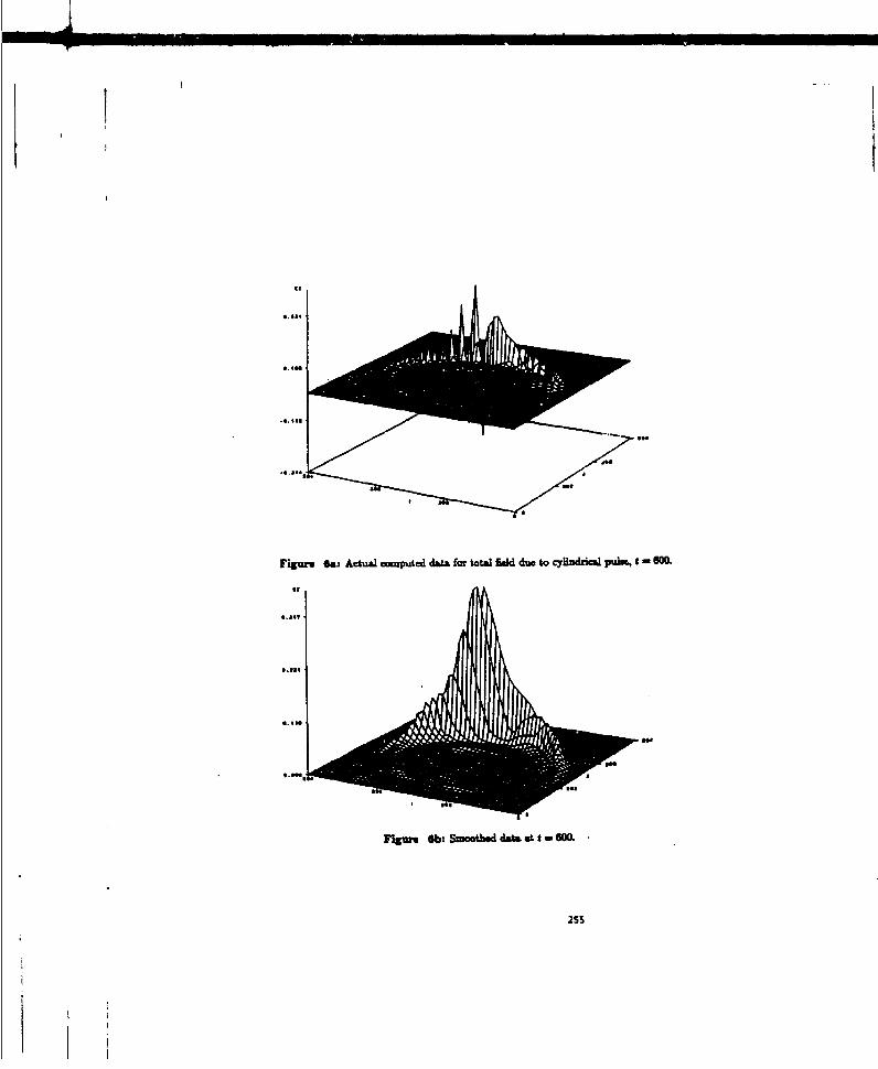
SUPERIMPOSED MAGNETIC FIELD IN

FORCED CONVECTON LAMINAR BOUNDARY lAYER

byNmsisouu Xi Mompeanad Miboola Moreg

Duoheuat ROMANIA

ABSTRACr. Toe Blasius problem for the laminar boundary layer is reformulated forthe came of n aletraooeaductive fluid. The impact of an external magnetic field isobserved through the similitude (Blsaits) functioe fji). Furtber moe the assoasieddtheiial (Polibausen) problem is solved for this clss of flows and the tunperatureprofile is obtained. Flinally, the usie path af convection as well as the effect of theemnt" magnetic field ane found to be better witnessed by the hoaajlascfton, a novelphysical qomty.

L Inbredeboo

Electrooamductive fluids convecting in external (imposed) magnetic fields are the siege ofaupplemey (tharmal, meaucal, tetc. phnme' When the incident magnetic field is steady

(ti. Wnependula) and the flow is s:o '(mZ). mmad.e free arn. velocity or natural convection)the main effect is an increasee of the drag form prodaucd throughi elecoodynamic (Lcorz) forces.

If the electioaenductive fluid is a beat caries as well, as it is the can of forced convection

promuthehem nas=Wetm sinfluencedwto.In ay ialo urw~k leuaaii.mgnoyro dyuamics etc.) this is a side

ofect and it is ieaena tkniow in what seasa It SM- unpiOviag owrbayt the prcess vne control.dksaruskba 1 T==ie&th malifilmtiaa -ad the stability of the flowpnmo a fluid widrthe

isfiseu of a magnetic fiekld Oreasr W2,1 amlynad ths qec in a crysa o~w ih mn convectioncontaxt whil Morega "45 showed doe eeeespoeuah ma Blitobli of the thera structure of theeppuas. Thm hydrodynmaic toolys 'tlly developed interal flows (Hagen - Poisenille) in a

Lam ~a thedwagee~e n f 1bord convection boundar L~yra (theslender transtional region. in the fl11d. I gtesolid wall bathed by the flow) and pcfnlyiConflcton with t hebeat - Th 710~ n featues of aukaninteeratcacn e be investigated

droso s b asicon moedls. Therefor. we fon u o est transfer problem of a steady. Wainafored onactonbounay layer flow - the Uleaies and Polilionasa problems. 7Ue viscous flow

undr study Ismas a thesmally comue (asthesl soli fla wall. The objective of our work is toevalut the effects ofAll impse magnetic field trwverse an the flow dIirection. it Wil in seen dialfor the specific magnetic field amamemd, the mm features of the convecting flow are preserved - thevelocity and temperaue proilhes am stil gaE - similar. Purthe to completing the classical (Blasius)

mode byincudig m somout fo th manetc feldconibutkan and solving the combinedflow andutmperature problems, we use the hea~1meon - a novel physical quantity - to &how themiodification which occurs in the true p"1 of convection bye presence of the magnetic field.intoduced or decade sqo by Dejou (6]. fth heduam imp osed f it betrbansfer cofimiinity,at least mna powedl visual mountsin convection poess(.,01.

256

2. Furnsasfinataf the problem aid uinly

Tle eqtiatons Yht ome the mass, momatus and energy in the constaut property forcedconvection lumm bounaylayer flow of Fig. I wte [111:

ax ay

ft an a2 g -u+ n-u . (2)

PCP( j+ J (3)

Hlee v is the kinematic viscosity, a is the electric conductivity, p is the mass density, Cp is the heagcapacity, k is the thertual Codctivity and T is the aseolute thermodynamic Weaspwartur. It is asumedthat the external (imposed) maguetic field is time-In~.hpendeat and oriented in the h-direction (oz axis).its presence (and, hence. influence) is limited to a slender region intigl the boundary layer. Further tothe scale umayss (6) the (Oy) piviertiou of the m mizaequation, ab Iomee to the (Ox) mn, is abalance between secomd-oxder (small) terms and. thus, amt relevant.

The specific form of the magnuetic flux density is coesidened to be hepuincipal part (firs order)

of a Laurent expansion for a more general field B8- B(y)-= BOL (L is a characteristic length,oytpcfy the length of the plate in the flow diresom).n This deflinition for B satisfiee lbs divarene2!ree --mnz and pmsery. the similarity featuies, of Blamsiu Pobihausa velocity sand tempeaurn

boundary layers. The difficulty that this qualtity diverges for y - 0 is all~eviae~d tbroqit theobservation that the flow is assaiad viacous and, hance, on the plate:a a 0 nd v a0. The(electnrconducdive) fluid is then motionless sod the quantity oB2u (Lorsuaz force) vaishes in this

Further more, the reaction of the induced electric field upon the incident magnatic field is

In generil (3-D). the steady stat forta of the enall equatiocn o be written as

div (w T - gad T)- 0, (4)

where a -kI1(pCp) isthe thermal diffusivity and wisthe t-D velocity field. tis possible tointroduce a vactor potential, F~x'y'2) through its corlt

acltH=wT-cV T.- (5)

This quantity, labeled hbeaaftmciou" was introduced by Bejan (6] for the 2-D flows in ClartesianCoordinates and used thereafter to evidence the bean transfer peoes in Convective media. When w = 0(i.e. pane conduction) H reduces to the classical heat flux. The hescfunction, as a visual aid, isrecognized to be superior to the isohema representation in convection hea a wet M8,9. 103.

From the point of view of die fiandiameatai Iiiiorsn of vemirfikldr M in 2-D proUams H iscompletely defined througb (5) sne(one can easily check) div BHw . In the special case of the 2-Dboundary layer (eqz. 1-3), eq. (5) reduces to;

257

AN Cpu(T-T�j (6)

AN ATp C�4T�TIJ-k- (7)

For cor�isene� a we ahall present wily the cold isothermal plate (T0) washed by a warm fluid whoseties meam teinper�une is T.. (warm). The reference T��j Is set to T0 . the lowest zemperarure in theboauluy layer. All odiar existing minalarity thermal boundary lrryers (imposed heal flux, etc. [121)cmbe u�d analogotuly.

Fodowing the elassicid (similarity) Elmius salution [11]:

uuU.,f. (8)

(9)

where, F = df/ d� U1 . is the tre1. �m veloaty of the fluid. Un is the true steesm velocity and

V (tO)

A.'trr saw ininpulaikus. en's. (I) and (2) prodwie the ordizusy differential equmion:

- �tt =f"'--L�.H4. (11)'1

where HDL:J B 0 L� Hmma�nis the number [7]. Eq. (11) differs fivm the classical Blasius

eq�ou through the second tn�rw in the riht hand side. The bon&iy Conditions for this (Cauchy)

f(O)=O, f'(O)�O, (12)

(13)

It is wath aaaa� that s�. (II) reserves the e pmperty of invariance to the han�ormanous

as the initial (Blmius) equation (61 which pestly reduces the bial-and-error shoobag procedure offladiag t(O) -the misung boinL.dasy condition.

Following Po�lhauaens (sinibeky) azalysis, the n monal Inuperatne �rj) = (T -TS(Tm -T0 )intlaflea 1111:

(15)

where Pr = via is the Prandzl poup, sul$ectto the boundary Condibons

8(O)=oe (�j,�=1 . (16)

258

-A

For the siilarity boundary layer, [131 an analytic solution for Hi is availale:

i(g,y)I~j,(.),(7

is the nondinreasional hea function and

8 01 = f00 0(14 + -- 0'00.(19)

~The VMpor ftepoblemn eqs.(11). (12). (13) was written as an autoennomou systemof ODEs and aolved ming a 41h, / 5 order adaptive iT-aie Range Knau algorithm with error controlperhl-step (tolaceaeWro 10'6). A first ranwascarriedoak with t(O)= (asumed value)and asecond (final) ran with f'(0) = fltwf3 /2. baned on the invariance property of eq. (11) mentionedbefore Since CINically. flar> 5 we set rW = 20 (a asic limit) and kept it throughout the analysis.

The second part of thre problem, the tempesature field, was then solved. Agiai, the Range Knif aalgorithms and the trial-and-error scheme was used to integrate esqL (15) and (16), written as anaumnomous system of ODEs and to pin point the appropriate initial condition. O(0). The needed f(TI)futntios was obtained through a locally parabolic integpolation scheme of the tabulated outpu for theflow phase. At this stage Ri (t y. ) can be computed using f(YI), 0(1q), W'(') (locally parabolicinanp"ourus) and the analytic fomnalla (17).

Figure 2 shows the influence of the mhlgnetic field on the conivection system via f'bj) (the u-comptonent of the velocity) for Ha =0.; 0-5; 1.; 1.5; 2.

Fclrafluadsuchmasilicon withp= 2330kgm-3 .vn4.3.1046in2s-1, modU.= lcms-1 ,L=I cml this would meal Ba = 0; 3; 10-.15; 20 mT. Figure 3 shows the corresponding 0(n) profies when

Nraaselt number, defuned [6] through Nu = -A (fFr/y)y. / (To- To.) wnd plotted in Fig. 4.evidences a clewr reduction in the head -hombed by the cold wall. One can speculate that in the limitwhen B0 - ** there will be only a conduction region in the boundary layer and, hece the Nu number(ratio convection I conduction) will match an asymptotic value - this trend is apparent int Fig. 4 too.

Figor 5 and 6 sahw 9(Z y)mund R (t ) for the Ha= 0and 2ca m i dertvestigationTheI s tmetwe otour plots indicate an increasingly cold boundary layer region for incrasingvalues of the 14* nmsber. No other trend is edadily distinguishabe firom these plots (Figs. 5b and fib)while the contour plots for the beatfuraction offer some more subtle insighits in the tre path ofconvection. FiM~ tney an orthngoeal to the wall indficating thet at this surfmce the begt Munsser is 0512]tlrtugh conduction. For inrreasing Ha numubers. this orthogonality is extended to a large domain -condutmion is predominant over the ftansport consmernet in the energy equation. The headines densityis decreasing with the H& number bndcating a colder boundary layer, as the cosant temperature linessuggest too. The effect of the imposition of a magnetic field is, for short, equivalent to a shift(decease) in the Pr number for the flind - an apparent increasing of die conduction part in thre overall

259

4. Caudmoiem

to this study we mnporte thec modified Bladsi ono to include the presence of a specific(fast decaying) externial magnetic 3Wed. The insulting-t~e (velocity and temperature) maintain theself inskihiyprety

AlthoMOMi ti work we addrrssod only the cold isothemal wall (Folilbause problem), it isclear that thsapoc saplicable to all other thermal cases (based on Blasius flow solutions)knlown to pesrethis prnwty - boaflux wAlls, etc. [12].

ThdIp. . of =eun fromt the velocity ad temperaturre master profiles (no magnetic field)am he montored through the variation of the Ha (Hartetn) group. Qualitatively, a soeod kneeappears when Ha is0 in the velocity profile, while th* ta I - proffil keeps the same shiape.

The hatdiaea prove tv be moore sextsitive than the isotherm,; to the changes in the flowstructurs. Tb. org niftf to the intsohmal plt is conisistet with the hypothesis of viscous flow(adhainst to the wall). This @bows thet the hegt transier is only throm diffusion (no temnperatureconvection) at the plate leveL. When; Ha > 0 the hiss lines oarthiogonahityP isapaent insa larger zoeeand their density decreases - it is a stem that the magnetic drag of the low reduces also the

taprteconvection. 71e dI'MsI. counterpart in the overall hoat transfer is larger in the presenceof te anei field. This featnurs ar not easily distinguishable in the classical isothermal charts.

The decrease in the overall howt trandsf procss is confirmed through the. decay experienced bythe No (Nusselt) peevp too. The offect a an external magnetic field can be sought as; an artificial&carm at the Pr (ftanti m her of the fluid.

1. Chandmusekhar. S.. Hj'dju =ks uhdrawwgnesic nmbilhry, Clarendon (1962).2I Ozuper. G. K. sai? 11d-O SzkiJ'h fiect of an externally impoaed magnetic field on buoyancy

driven flow ist a - tn~gular cavity', £, .Cmy..ls go h. 6, pp. 505- 515 (1983).3. Oreper, G., M. and Szekoy, J.. ' The effect of a magnetic field on transport phenomena in

Biga-SWocbwg- crystal powthI r r-awt~lmh. 0i, pp. 405-419 (1984).4. ltorega, Al, K., Mapietic field influeacie on the convective beat transfer in the solidification

procesaW, Purt. 1, UvP .S T4n mg33. 1. pp. 33-39 (1968).S. Mworual& Al, M., Magnetic field influenice. on the conavective hea buzsfer in the sowiiication

p macses' Part 11, Rev- URniza. Sim Tach MJe-5 Pi'v 33.2. pp. 155 -166 (1968.6. BejmAn,A Ccawecti-i how bwile~, Johe Viley said Sam, New Yo&L 1984.7. Moacmu. C., I., Etero'ouasivcjlcd Awy. 2nd edition. Bd. Didacticasa Pedagogmst, Buchrest

(1992).&. Lkki"fed D. anid Dad,ý P., flboyant luaduer coavectios ina vertcal cylindrical anul.?*, L

Ro a@L 14, 98.14- 21 (1966)9. Agasawsi, S., ILand ahe ,A., *Use of headins" for usndstay bonyracy-driven flow in acyl i Whka aidalsmoauu. L :zm I-armo ll. pp. 5% -578 (19 ).

10. Ho, C., J. said Us. Y., H., "Natural convection of aid wam in a vertical aminla with constantheat flits on th is= wall. L11sidzTdio IM2 pp. 117 - 123 (1990).

11. 1- mqý P., saidDo Witt. M. P.. Fliidlsasanak of hexar ad mm~ awufer 3rd edition. John

12. SparrwE., M.bu.H.S. onaylyr wt rsoe et flux - application toinshamousconecton d aiadn',tntI fasmMas T~nd~ 3.pp. 437 - 449 (1965).

13. Moga. AL, M.,Opsimslgemuamfisof elecrokpackagercoo~edbyfibaced comvecom, Ph. D.Thesis. Dukce Universiy (1993).

260

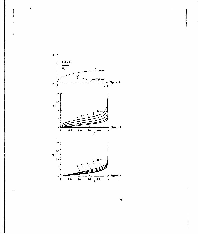
T.(6O 1)

U.

* L L

20

'IsE

10j

0 0.2 0.4 0.6 C., 1

S 0.2 0.4 0.2 0.861S

261

0.4

as

00.2 L. . .

I.~~~~~~~ ~~~ _______________________________________

4~ i3-

262

4.3

02 0.15 0.6 .

* 0.2 6.4 0.6 0.8

Sx

25

264

SESSION 6:

OPTIMIZATION

Chair: Richard Gordon

265

OPTIMIZED BACKSCATTERING SIDELOBES FROM AN ARRAY OFSTRIP USING A GENETIC ALGORITHM

Randy Haupt and Am Ali"D atment of Electrical Enineering

2354 Faurchild Dr Suite 2F6United States Air Force Academy, CO 90840

Abstract - A uniform army of closely spaced perfectly conducting thin strips has a backcatteringpattern with a maximum relative sidelobe level of about -13 dB. We present a method of using agenetic algorithm to strategically remove some of the strips in this arry to yield the lowestbackcaftering sidelobe level possible.

INTRODUCTION

A closely spaced grid of thin strips has a backcattering pattern very similar to that of aperfectly conducting plate of the sam size. Increasing the spacing between the srtips increases theresistivity of this structure as sa by the incident wave, Consequently, the peak scattering return isreduced but the relative sidelobe levels remain fairy constant. Once the spacing between the stripsgets too big, the backscattering pattern no longer resembles that of a flat plate.

One possible method of reducing the backscatterin sidelobe levels is to nonunifnbraly spacethe strips in the grid. Tbe namniform spacing spatially tapers the currat distribution across the grid.If the distribution of grips is most dene in the center and gradually thins towards the edges, thencertain strip geomenea may lower the backcattering sidelohes.

This paper investigates options to lower the sidelobes of an army of thin srips by thinning thepouplaton, in other words by removing some of the strips in a uniform grid. Thinning is used inanuma arrays to lower the sidelobe levels in the far fieWl pattern of the army. Usually, however,a statistical method is usd to thin the army. Hem, we apply a genetic optimiation algorithm (I] toamive at an idtally thimed distributon of tips that results in the lowest backscatering sidelobe level.

FORMULATION

Consider an army of uiformly speced strips as shown in Fi&'Ire I. The srips are infinitelyion in the z-ftectoo and have a center-of-strip to cemer-of-strip separation of d and inch strip has

a width of 2w. Only bkeisatering is con ,leved. so the direction of the incident wave and thedirect of scatering am given by #. The incident plane wave has an electric field poinrize in thez-disactios and has a maetic field normalized to one. The currents induced on the trips ae foud

266

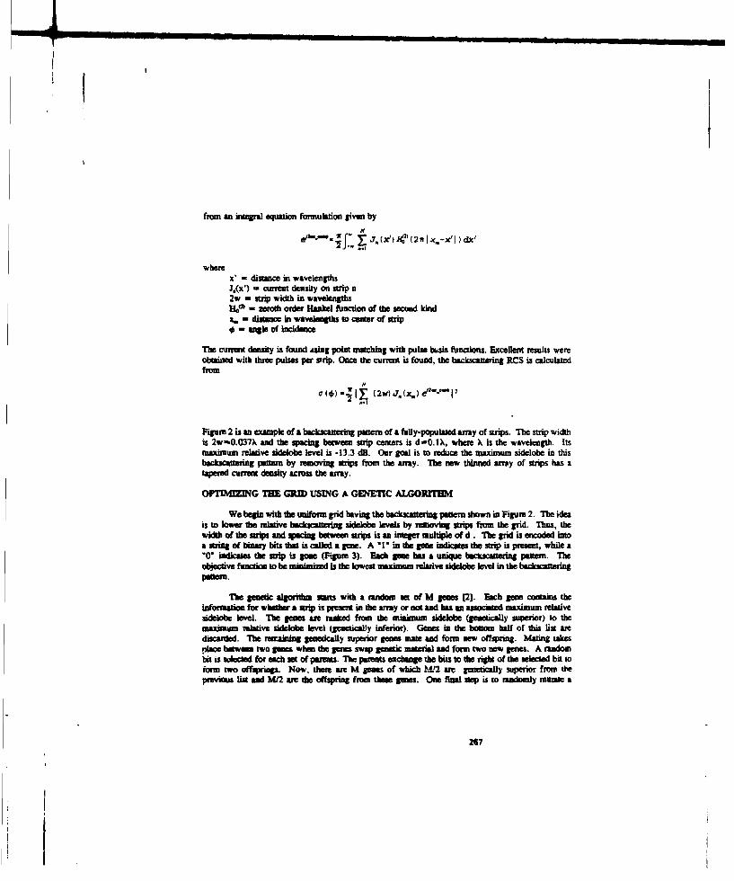
from an integral equation fornulation given by

".7 - e 2ax -I x

wherex'- distance in wavelengths

Ji(x') - ctzrrent density on strip n2w - strip width in wavelengthsH602 - wroth order Hankel function of fte second kindX,. -distanc in Wavelengths tOD cete Of Strip0 agle of Incidence

The current density is found Asing point matching with pulse bmusi functions. Excellent resuilts wereob~tained with three pubses per strip. Once the current is found, the backscawteing RCS is calculatedfrom

Figure 2 is an example of a backscaucring pattern of a fully-populated amy of Strips. The strip widthis 2w-rO.037k and die spacing betwees strip center is d-OAX), where X~ is the wavelength. Itsinaximum relative sideolme level is -13.3 dB. Our goal is to reduce the maximum sidelobe in thisbackscaussing pattern, by removing strips from this sray. The new thinned any of strips has atapered current density across the armay.

OPrTEWEIZUG THE GRID USING A GENiETIC ALGORITHM

We begin with the uniforn grid having the bck~acae g pattern shiown tn Figure 2. The ideais to loewe the relative backacattering sidelob leves by removing strips from the grid Thus, thewidth of the Strips and spacing between strips is an intege multiple of d . The grid is encoded intoa suringof biaybitsth intis calledag iSe. A "I indtlegenelnicats theSstrip ispresent, whilesa*0O inidicates the strip is gonse (Figure 3). Each Vis has a unique buckscastering patten. Theobjective function to be minimized is the lovest naximum. relatve sidelobe level in the bwAckacaeringJieWDf.

The genetic &*grid= sawm with a oudsne of M gienes 12]. Each gene contains theinformation for whethe a Strip is piessit in the array or six and has an associate nmaximumn relativesidelobc level. The gene are tunked from the mtinlimfuml Sideloi (genetically su~perior) to thmaxismum relative sidelobe level (genetically inferior). Genes in the botto ha alf of this list amediscarded. The renmaiing genetically Superior gene mate and formn new offsprnog. Mating takesplace between two gne when the gene swap genetic material sand form two new gene. A randombit is solecled for inch Se of parents. The parents exchange the bits to the righa of the selecied bit toform two offspings. Now, these amn M gens of which M12 ate genetically susperio from' th~e

pe ios ls and M12 are the offspring from thnew genes. One final rAp is to randomly mutate a

267

small peroeap of the bits. A mutation just changes a "!A to a "0" or a "0* to a "I". This mutationis an importnt stop in the algorithm, because it helps the algorithm Lvoid local minima.

Genetic algorithms are slow. On the other hand, they search for a global minimum ano canhandle a large number of unknowns. In addition, they are well suited to optimizing problems withdiscme panmeters.

OPTIMUM GRID OF STRIPS

The geomic algoithm is applied so the unifom aray of 40 strips. Starting with 80 genes andoptimizing over 8 gemerations produces a geneticay superior gene given by (1 000011 1 0 101 01 0 011 1 0 1 0 1 01011 110 000 1]. Tetheinned array epesntd by thisgene now consists of only 24 strips but has a relative sidelobe level of -17.1 dM. Figi.re4 sbows thetckscaaetlng pwanrn of the optimized army. Note that the peak RCS is also reduced, because 40%of the strips were removed from doe gd.

REFERENCES

1. J.H. Holland, Gotic algorithms', Scientific American, July, 1992. pp. 66-72.2. Ooldberg, EDavid 3. Gaeke Algrithms. Addison-Wesley, New York: 1939.

268

E

- l4- 2w d

Figure I Diagram of an array of perfectly conducting thin strips.

20

1.5

S.Eo-I

C

.10-11. [1 0.2 Ol U.4 0.5 .7 O.A 0.9

Figure 2 Backsh:tering paot-m of a ully-popl• aed array of 40 strips withd,,I )X and 2w-0.037). The mIaisum relative aidelobe level is -13.3 dB.

269

1 0 1 0 1 1 1 1 1 1 0 1• 0 1 x

Figure 3 Gene assoclated with an array or uniformly spaced strips. A "1"indiates the strip is preseat, and a "0" indicates a strip is absent.

at

t10-Is

.1

S 0

I) 0.1 0.2 03 0.4 0- ).6 0. OA 0.9

Figure 4 Backscrtering pate of a thinned array of 40 strips with d--O.lV.and 2w=03f.0 There are 24 strips praeunt and 16 removed. The relativesideiblevel is -37.1 dB.

270

NU!URZCAL ELRCTROMAGN=TZCS CODI OPTIMIZATION DESZGN OOFTWARZ(NECOPT)

James K. Breakall, Joel S. Young,Robert J. Bauerle, Athena I. McDowellDepartment of Electrical Engineering

The Pennsylvania State UniversityUniversity Park, PA 16802

Todd A. ErdleyParagon Technology, Inc.

200 Innovation Blvd.. Suite 240State College, PA 1680:

This paper discusses a new antenna optimization software packagedeveloped for personal computer based workstations. The NumericalElectromagnetics Code OPTimization design software package (NECOPT) isa new and innovative approach for designing antennas. Most previousantenna modeling software has been only concerned with the analysis ofantennas where the user could test or determine the performancechdracterisaics. For designing antennas, one still needed to eithertest different designs by trial and error. ,r apply "handbook"approaches. The computer is an extremely powerful tool which isutilized to dramatically accelerate the optlmizetion process in NECOFT.

Circuit analysis codes use the same methods that we now apply toantenna analysis software to produce a package that can optimize thedesign of antennas. The circuit analysis tools have been very usefulover the traditional methods of circuit design and have made a majorimpact in analog,digital and microwave c.rcuit design. We haveincorporated the powerful techniques used in circuit design codes andhave produced antenna design software which works with the well testedNEC antenna analysis package. Using this package, the user can providedesign goals for the antenna and the computer will perform an iterativeadjustment of user selected parameters on the antenna to achieve thefinal results.

The implementation of this package has been achieved using highlyaccurate, fast and flexible optimization techniques which act as adriver for the NEC analysis software. The user creates a data .nputfilt very similar to the standard NEC data file and indicates whichparts of the file are to be considered the variables for the computerto iteratively adjust in order to achieve a desired performance goal.The user can set limits for the variables in order to maintain"realism" for the final design. After the desired performancecharacteristics have been established, the coy.,u:er wi-l begir aniterative adjustment of the parameters until the goals are realized.

271

DESCRIPTION

The NECOPT software package consists of a quasi-Newton opt~mizerintegrated with a double precision version of NEC2 and the requiredinterfaces to provide the necessary communication between the twosections. Both constrained and unconstrained optimization is providedby the optimizer. User input is provided by a series of command linessimilar to standard NEC input which are appended to a standard NECinput file. The input section defines all the desired design goals,variables, and optimization parameters. In addition to optimizationthe NECOPT package has the ability to sequence any variable defined inthe NEC input file over a specified range of values. This may beuseful for developing design curves or performing a worst caseanalysis. The intermediate values of the variables and goals may beoutput to a plot file for further processing or graphical analysis.

GOALS

Goals in the NECOPT system define what parameters the user isinterested in optimizing or examining. Four different NEC output typesmay be sampled and processed with the NECOPT package, far-fieldpatterns, near-field patterns, source impedance, and segment currents.For each goal there are many options which select specific parts of thedesired NEC output data or define the processing to be performed on it.The many options provide a generic and versatile interface to nearlyevery type of NEC output data. High level characteristics such asgain, partern beamwidth, VSNR, front-to-back ratio, and many others maybe chosen for optimization and output processing.

Multiple goals may be specified for the same run of the NECOPTpackage. Each goal may be separately weighted to allow the user tobalance the signS ficance of each goal to meet the specific needs of theproblem at haad.

VAZZAALS

Variables identify which parameters of toe NEC input file are tobe optimized or changed. Three types of variables are available to theuser, optimization variables, function variables, and step variables.Variables may spec4ify any non-integer quantity in a NEC input file.items such as geometry position and length, loading, excitation, andfrequency, may be defined by variables.

Optimization variables are controlled by the optimizer and areautomatically adjusted to meet the defined goals. The range ofoptimizer variables may be limited by user input bounds.

Function variables are used to define one variable in terms ofother previously defined variables. They are not part of theoptimization process. They only serve as an aid in defining the user'sinput structure. Function variables are particularly useful forvarying the size of symmetric input structures, or other structureswhere relative proportions must be maintained. They allow non-physicalparameters to be optimized or scanned.

272

Step variables are simply sequenced from an initial value to anend value by the optimizer. They are useful for sweeping a parameterand observing the corresponding output. When combined with anappropriate output selection they may be used to determine worst/bestcase performance over a given range of one or more parameters.

IXAMPLZ

This example demonstrates the use of the NECOPT package in thedesign of an optimum 3-element Yagi antenna. The only design goal wasto maximize the front-to-back ratio by changing the lengths of thedirector and reflector elements. The element spacing was fixed as wasthe length of the driven element. The elament radius was fixed at1.0E-4 wavelengths. Table I contains a summary of the Yagi parameters,and Figure i contains a diagram of the structure.

Figure 2 contains a surface plot of the problem space. Stepvariables in the NECOPT package were used to step the reflector anddirector lengths over the complete matrix of values. Reflector lengthis shown on the Y-axis; director length is shown on the X-axis; and thefront-to-back ratio is shown as the surface value or the Z-axis. Theoptimum front-to-back ratio of 22.4 dB is obtained with a refleccorlength of 0.499X and a director length of 0.457X. From the figure itin apparent that there are several other local maximum points on thesurface.

The optimizer was used to find the optimum location from severaldifferent starting points. Because there is more than one localmaximum in the problem space, the optimizer will find differentsolutions depending on the choice of starting point. Figure 2 showsthe optimization paths taken when the variables were constrainedbetween the specified bounds. The paths shown in Figure 2 start witha circle and terminate with an X. The paths are overlaid on a contourmap of the surface shown in Figure 1. The optimizer is very wellbehaved in this mode. When the optimizer reaches a local maximum pointon a boundary it terminates without wasting computation time searchingfor solutions which are not decired.

Figure 4 shows the optimization paths when the variables are notconstrained. For the unconstrained cis*, depending on the initialstarting point, the optimizer may waste valuable computation timesearching for undesired solutions which are out of bounds. Thissituation will depend on the initial starting point.

CcULUSIONs

This software package represents a major breakthrough as comparedto the antenna design methods currently available. The NECOPT packagebrings the proven analysis power of NEC together with optimization tocreate a powerful new design tool for antenna engineering. The NECOPTpackage significantly expands the users ability to develop an optimumantenna design in a timely fashion.

273

Table I

3-Element YAGI parameters

Eleme'.t Length (G) Spacing (X)

Refl,actor 0.4 - 0.6 0.182

Driven O.S NA

Dir.,tor 0.4 - 0.6 0.182

Director -0.182

K -0.5 >0.182

< Reflector -,

Figure I 3-Element Yag. C dimensions in wavelengths ,

274

riguze 2 Front-to-back ratio of 3-element Yagi.

275

I -

!3

Figure 3 Constri&ned optimizat.ion of 3-element Yagi.

276

j~ %I

IV

(10) t44Bu6 JoPOPH

Pigur* 4 Unconstrained optimization ot 3-element Yagi.

277

On the Computataion of anOptlanised Interferernce Adaptive

Radar Signal

byHeiner Kuschel

FGAN-FHk'Forsehungslsurtat tr HIKochfrequertapbysilt

Neusnabrer Sir. 205343Wachthberg.Werthlioven

ljIntraductiua

One of the reasearch projects of FGAN-FHP is an experimental VHF-radar which is used to studyspecific problema of low firequency radar. Since the VHF-band is umainly used for radio commnmttications.the problem of miutua interference of radio services and radars has to be solved if the benefits of lowf~requency radar are to toe exploited. Here, a method has been developed to avoid mutusl interference b)spectrally shaping the basic radar signal waveformn in cirder not to uransmiut radar energy at frequencyranges, within the radar ignad bandwidth, where a narrow band radio transmuission has been detced.The bodic radar sipsal is a hie- frequency modulated pulse (chirp) of 2 &Oftz bandwidth.The basic chirp -ul m spectrally shaped so that spectral notchies occur at ~requencies of radio services.Thus, by oucsving the radar sigpsl echo with a matched filar, shaped in the samue manner, neither theradar is affected by radio tranminsdows, nor radio services softe from radar interferences.The detection properties of the radar. however, wee strongly affected by this pulse shaping. Unwantedsidelobes occur and can mask weakter targets. To counter this effect, further shaping of the signalspectrum is applied.

2. Spectral Signal Shaping

The basic radar signal is a line fequency modulated pulse (chirp) of 2 M&z bandwidth and a durationof 16.4 lisec, yielding a pulse compression factor of 32. The radar pulse is samnpled at 3.9 MMzresulting in 64 samplas per pulse. la the frequenicy domain, the spectumsi of the sampled signal consitersof 64 frequiency sanylas. The 2 M&z bandwidth of the pulse is reptesented by 32 frequency saMpleswith a spectral resolution of 60 kHz.To adapt fth radar psiga to the present interference, situation, a spectral analysis of the electrormagneticenivironmeat is condce~d using a thaa Fourier transform (FFT algorithmn This spectuem is compared toa Oven threshold. rsuulting in a weighting vector w(f) which is set to =er at those spectral samiples,where the inthrfemce exceeds the threshold and which is set one elsewhere. The vec-or w(f) ismultiplid with the signal spectrum, producing spectral notches at die firequencies of interference. Fig- Ishows the low puss repesenatiou of an interfuence spectrum (a) and the shaped spectrum of the basicchirp pulse (b), adapted to the interference situation. In the firre domain, the spectral shaping can beregarded as an amplitude and phase modulation of the radar pulse. Fig 2 shows a block diagram of thespectral shaping procss

278

xtt3.*'tMO~ reeve ransmfi~tted

FFT F T1

I' adaptive____________________________________threshold

-1 0 -1 -t/MHZweighting

b)signit signal

Fig.I a) interference spectrum, Fig. 2 block diagram of spectralb) shapted signal spectrum shaping process.

3. Distortion by Shaping

The choice of the radar wavieform is subject to several requirenents, one the mnost vital is a point targetresponse with narrow a peakc and low sidelobes after compression. Here, the Doppler tolerant chirpwaveforni was chosen as a starting point. The signal properties. like a narrow main peak,. low sidelobesand Doppler tolerance can be displayed in the so called ambiguity function. It is defined at /I/

A(td fd ) -=X k ,d~fd) I

where X0 is the cross-coufellatioo functions of the radar signal and its dopplefshifted version, td denotingthe time delay and fid denoting the Doppler shift frequerncy. Fig 3 shows the uambiguity function of achirp signal of 5 Whll bandwidth and 10 &asec duration for different Doppler shifts Id, as an example ifan initerference situaiaon is assumed and the radar signal ns spectrally shaped to avoid transmission indisombed areas, the ambiguity function is subject to changes. too. Depending on the spectral locationand bandwidth of the interferences wifthn the radar signal bajidwidthi, the Doppler tolerance of the radarsignal is affected, as well as the tine sidelobe structure of the ambiguity function. Since at VHF.radarfrequencies Doppler fr-equency shifts are small, even for fast targts all interesting Doppler frequenciesare within the mainiobe of the arnbiguity function. Fig 4 shows a sarll section of the amrbiguitly functionfor a spectrally shaped radar signal with +i- 3kHz Doppler shift region, indicating a negligible distortionof the main peak due to spectral shaping,

279

P. IIs _ Lis

.Inse---- --- -- - . -

p~T0 fp*1*.a

Ii L,

Flg Ambiltvity f~mctlan of the basic chirp signal for differentDoppler ,shift with respect to the signall bandwidth fd/Af.

- a. ,

"- .1 W . -

.i !

-c a

Flig. 4 Main peak section of the shaped chirp sional.

i i t g

To.. I~ * cc

4 I I

"0

L

L -30.,00•

_j,--------------,

0.e 20.e 4ee 0.0 e ee.e ee ¶.et ,Lme sampI es -> t/260 nsec

FIg. 5 a) Autocorriatlou %w .on of oiginal chrp slgnali with Umllent.

---1 . - : :,0

L -

t tme aampias -> L/250 neac

Fil S b) Autocorren'4on functlon of shaped "birp signal.Interferences.: 0-3-0.4, 0.6"0.7,1.0-1.1, 1.4-1.S MHz

281

r!

MexkmtsatL~n of me tt-to-*idelobe rat LotILerfero•eo. .30- .40; .6e- .70:1.00-1.10;1,40- 150', Hz

Au •.@,VghLtLn

ohLrpsLgnml wLtlh Lrenstent

-- 20.00

CD

CO 0.0L -A Il0.00 10.00 20.00 30.00 40.ee 50.0e 60.00

froquen cy -> f/62,5 kHz

FEu 5 c) Spcrmofth apesinl

Serious radar peaformnne degradation., however. can be expected from increaed sidelobes of thecop d pisu In fRpm I the ati ocoruelaton funmtion of dhe original chrp agnal (a) is comparedto that of a sigal spectally shped to avoid inference (b). Since in the discussed system, ther is mwitched with evpulse, the transient of the uanamiuer has the effect of a weightsNction an dhe sga smoothing te leading and trailing edges of the pulse. The adaptation to four

inseting sources covering 20 % of the signal bandwidth causes an unacceptably high sidelobe level.Figure 5.c gives the spectrum of the shaped siVnal, showing 4 notches. The sidelobes would ma':weaker tarpts in tdo adjacent range cels. Hence, the radar sipal has to be modified in a way thm thesidelobes of the autocoaelation function are reduced to a reasonable level without loosing its specualnotch structure.

LSlgnal Opthastion

The probler of optimal shaping of the radar signal under the constraints of inteufrence avoidance and areduced sidelobe level could not be solved amlytically, yet. Though a reasonable approach to solve theproblem is the so calIed random walk nthod which is known from evolution.

The method is based on the random mutation of one of the 32 CoIplex spectral samples, representingthe w.pd bandwidth. at a time, For the mumtion, first a maximum mutation stepwidth 6 is set and acomplex number cm is gameuaed. The real and the imaina-y pan of cm are randomly discributedbetween -&82 and .&2. A•nther .1 of the random generator yields ihe random position of the sampleto be mataed under the constraint that a mutation within the prmdlefined notches is rejected and a newtrial is conducted. The chonen spectral sample S(fn) is added to the mutaton step m, formng the newsample S(fn). To check the new signal waveform s(O. a 64 step PPT (Fast Fourier Transform) isapplied to the specunim S(f).

282

I ...

The autocorrelation function X0(td) is calculated as the integral

XO(td)~ f S -(1)SO)e)2XNdf

using the equivalent sum

64

XO(td) j 1: IS(f)! 2 ep~std

U -44

The meoulting autocornelation fanction XO(n)(td) is then compared to the autocorrelationfunwton Xo(fld)(td) prior to doe muftesen, occording to tediease. opfingsaljon c~terion. Mlutations.leading to deteriorations are neglected. thost leading to imnprovemns are retamed. After an improvingmutation. the sequence starts aver egain with the new spectrum S(f) as tht basic stgnal Dunng theopoantiason runs, no FIFT is used for tie eaculasa. of the new h4Wa waveforma instead it Ls sufficientto replace only that team of the sum XO(td) containing the mutated sample S(fn). After the finalmutation step, the signal waveform ys calculated again, using an M.T algorithm. it is then used as thepresent radar pulse, adapted to the uaserfmnsce ekuabmon aid apunised for reduced sidelobes. Theoptimisastioc criterion that a used wsthmn the rundom walk sequenoce is dependent on the desiredproperties of the autocorrellatioss function.

3. Optitnleatl criteria

Three opidmrisation criteria have bee exwnied for dhe reduction of the sidelabes of the autocorrelationfunction of a spectrally shaped radar pulse.

1. Maximization of moits-to-asdelobe-ratir2. Maximum simhilarity with a sample functon3. Maximum similarity with as ida" aIc model function.

For eli or the optimsaalon criteria the optinvisadon is conducted under die constesint of not affectingthe tuma~qn phase of the pulse. Tim craitein of mmxna~~ms of the men-isst-sidelolbe-ratio", funt ofa&, erequire a defiraido. of dhe exwmio of the wmilobe. Has, the mnuinh as defihed to strech fromthe center of the maxumin to the center of the fire: loal zausmu. sym~moucly to the center of thezhexsmum. All ssampk of the autooralwas Non acto beyond the first local mimirin we regarded assidelobes. Since.a general effact with the redoction of sulelobes is dhe broadening of the mwailobe, themainlobe area has to be updated with every improving muat~ion. The second and thited optimisationcriteria an based on a differen principle. Tba "Illaic between the -nm Wassllto function of themutated signal aid dwm of the 'ode fiactw is scmalusadend =0dbidnustons of the difference after amutation we regarded as improvemns Deiiai shapes of the imenlobee of the two comparedfunctions normally yield larga diffierence or error values than a Lack of similarity in the sidelobes.Hence. since reduced sudelobes ame desired property. the errors in the sidelobes are assessed higher

283

dm dwe m th di tnaalbe. The unqie function choven for the opumitr ion was the autocurrelitionfDAMaN of an mithampe cbrp pulse wh tramnmot, having low sidelobes. In the cae of using a genericmod falmc an &a M comrzfraon ftnction repd--m$g a Dm-c impulse was pplied for comparison,

6. Pazr ta

kubdom walk muIads af. in gneral, sensitive to the choke of pi•raoete le starting value and stepwidt. Th7 ane of im'maoria is of ls imporance. itnough there is a t-•eshold. depending on tV'ýchoe of dhe other wanrnuuzn ha ing the cost effectivenrs of fulther tmprovemn•s. Uttle influencecan be mognized i--n the choic of differeastartiag values, too- It is uritdficant. which of lt*oft% aso ka mies dmW fri The f1• sew swp width, however, has a deciing factor for the,eeevu of the UMdM walk U" opminsaom. It m hadly predictable, if the imng position - beforedo Am SPAfim - a a *6. vicrv of the g1l mmnxium or a local one. Hence, the mutation 4,1.wmft has to be hilb mouih so dia die vicaisty of a local aminim can be left and it should, or theete ML. be ow saewah to avoi mppag from one local nmma wn au to the next with every-00fta. U to mty in the viehty of tde SLual IMmaumnn ocam "i mar is reached. Stveral mutation

p wdWhs have be• OP& a wall as diffevent amgia to alter the sample which is to te mutated.

CBL +,l Od LitO Sideich.b r.~leleO 1.61 di

.31 .4;.0

°"': .1

I -7•A~¢'' , ,

i..ef. foto . 2..

0

Ut

"•'• • •• •• • m . -m •'' • .9.00 20. 49 4.B 66.6 . 106.00 12.ee

t Lme Bamp.es -> L/260 nrsac

6a A•se.iaruridale Aheis oif %bap digal adte IOM Iteratlom 65 25.

2S4

MaxITILsotion of rtsLr- to-% Ldelkob ra .tlo

a ar nei 30- 0;.o- 70 1 ' 0i 1e 0 1-SM4

-~1 e

opt - 1--oa- tvo d ---069443L~

;Z 1.~ !eC e 2.0 4.0 6.0 80 6.0 100

L ~ m ope - ,5 ie

F 0.6bAaoobis ucico hpdsga fe I'0ieaos8 10

wjd~~ ~~ Livme 9 aemiaydenine vpalu as _>ve to be 0 a godc wie sic e a

Smsmutation steps. en s;l hiniiavbent rejeted. are post ihe as welas siai vAmong frm aw loere h

approach of a nmxizmiun, The pd prinii irluence of the mutation step ividth is deraoo atred in figure 6for the two values 61 = 25 and t" = 100, when tat criterion of maximum main-to-sidelobc ratio isapplied. With 0.5 61 being equal to du111 mraxirnum tpectal samuple of the unweighzed pulse, the mautationsteps ste in the order of magalmde of the real and iznaighity pan of the spectral samples. wbile 82~allows mutation steps larger than the spectral signal amplitude which requiries morm flexibiliy in thesignal generation. Figure 6& shows the autocorrelation function (a"i oi the shaped signal after 10000iterations; with 8 - 25 (solid line) compared to the ak! without signal olamisation (dashed line). Fiurm6b shows the alif before (dashed) and after (solid) optimis Mion for 8 =100. The larger mintation stepwidth achieves a better sidelobe suppression at tba expense of a broader tnainlobe and higher signalamplitudes.

28S

7. ReuI iaad CoudIMIons

Numerous simulatious have bee= made with different interference scemnrios. Here, one typical scenariowith 4 int•rfeences. covering 20% of the signal bandwidth, shall be regarded to compare the differentoptimisation criteria. In figure 7, the result of the optimisation after 10000 iterations with 6 = 100 is

displayed for the cu that the deviaion of the akf of the shaped signal from the akf of an unshapedchirp with ransient is rinimised Figure 8 shows the result of the mlnirnisa•on of the deviation from anideal, Dirac-like ai. The reference functions are reprTented by the dashed lines. These criteria may besuccessfully applied. if a narrow mainlobe is the most important demand. The maximisation of the main-

Mtn tMm .,rer wtt, hr.peot to forenco. "fun CILeo.Lnt~o Pforoncee .30- .40; .60- .70;1.0e-1.10;1.40-1.S(r'z"no .~ t Lh"ta

oh t•rP Lgnos I LLh t,. La L enL.Lt.rat 'Loao: IO fecto, : 100.0

optimtofod It•IS eLdolbe rSLLo 13.03 db

0

01 I Al-° IL 30.00- io _Ao

0. a 0r•.. .ttme samples -> t./250 nsec

& 7 Auioeerralae ftustie of sbaped signal aftar 0IGM tala.Cuharlaa.: Mlujm,-a-- of dalastln frm rdm m fimeturu

tb-sidelobe ratio always ansis to lowe= the sidelobes at the expense of a broadened mainlobe. as shown

in fig= 6. Using the latt, criterion, after 5M0 iteratios, a sidelo•e lvel of -24.63 db compared to-22 db for the unshaped pulse with transient be reached. The signal shape has usigficantly changed,both in the spctral and time domain but the notch ruenre is still uintaiat& as shown in figure 9.Thewidth of the mainlobe has increased by a factor of 3, reducing the range resolution of the radar by 1/3.This is shown in figier 10. In table 1. thre stepwidths 8 25, 50 and 100 are compared for iterations

ranging from I to 50000.

256

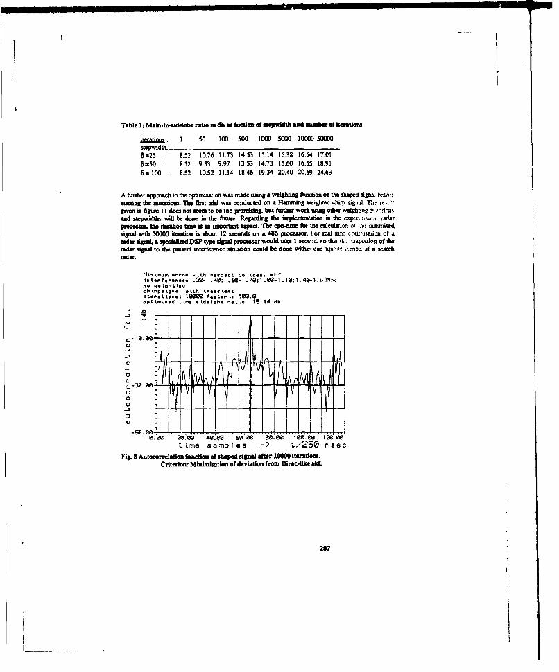
"Table 1: Main-to-sidelobe ratio in db as fuction of stepwidth and number of iterations

az•ni. 1 50 100 500 1000 5000 10000 50000stepwid th.6f=25 8.52 10.76 11.73 14.53 15.14 16.38 16.64 17.01

6=50 8.52 9.33 9.97 13.53 14.73 15.60 16.55 18.91

B=100 . 8.52 10.52 11.14 18.46 19.34 20.40 20.69 24.63

A futher appma to the optimisation was made using a weighting fhiction on the shaped signal b'h.fristarting the mumattons. The irm trial was conducted on a Hamming weighted chirp signal. The ?, A

given in fijure 11 does not seem to be too promising but further work using other weightiny 14.;, •insand stepwidrh will be done in the future. Regarding the implementation in the expcv?,,LA; ridarprocessor, the. iteraton time is an i,-oportant asec. The cpu-ido fix the Calculaton 0, Inr' ,outunsed

signal with 5000 iteration is about 12 seconds on a 486 processor. For real ditt opitIPadon of aradar signal, a specialized DSP type signal processor would uiks I secm A, •o tht, tvi. tuwion of theradar signal to the present interference situation could be done within one upd1 ý,riod of a searchradar.

Mt m.,n .ro- .e tIth onesp~eL ato Ldoa ;@ f

,o " LghtIngchLrptg ol with LrenstenLIt.oe ot.n: 180M fec!01 .: 100.0

opttmLeed tmoe stdolbolo eotia 15.14 db

I 4 -

L i A iCI

D

e.ee 2ie0 40,00 60.00 e .•e 1e .08 12.L!ne SOmple -> L/250 nsec

Fig. 8 Autocorrelation function of shaped signal after 10000 Iterations.Criterion: MinimIsation of deviation from Dirac-like akf.

287

t. .34- .0: .63

ChLVP. LO, I I.tLh t- . t. Lk to.nL Ln:, 5066 f.. L., 1 ee.eoL~nL. t . .LdoIobe r.Li.. 24.63 db

S. e~e

" . rfrnc .0-.0

no2 .0.0h6 :

Fig Sgnl etn ane; eeope afoter : 00.00 trtos61

epttaxtood Ltfn. eldelob. n.LLo 24.63 do

0

- LL0

20.0 40.Oi 0) S~oe 100.00 120.00

t Lmo sampIeG a ) L/2o0 neec

Fig.10 Autocorrelation functon of shaped slgnai after 50000 Iterations S lo10.

288

-- -I ... ! .... o /. n[I - lO - .., L .t. .d I b . . . .. .. . ... _-

ehrpd~gfiel .tLh tr*.*L*nL

oLt led t.m. r.ObLb f~e O 15,42 db

S00C A0

t Lme s"ip IS as t/2so ngeac

FIg.11 AutowrreltlrontAufto n for Iiaueag weighted chirp after 10000 iteratio•S 8 = 100.

8. References

111D.K.Balnon Modem Radar System Analysis, Atech House

/2/ S.Davidovici, 1:E.G.vaaerakis Nsxrow Band Interference Rejection Using Real-

Time Fourier Transforms-

STrans. on Comm. Vol 37, N-o. 7. 1959

fu LE.GZV.h, H.V.poot Na'rowband Interferene Suppression in ImpulsiveChapels, MM Trans. AES Vol. 28, No. 1 1992

/4/ Y.S.Iq Murty. A..Sa',apyi Rm o Design of Waveform Agge Radar Systems1COMM-90, New D-Jhi 1990

I/1 B. Hona'y, M. Damnell, T. Ng, G. Markarian Specu•l Shaping Codes for Co-ChanmelIntarfirenceSuppesion. 5th Inc. Conf. on BY-Radio, Edinburj;,lUK No. 339 1991

289

Optimization Techniques Applied to Electromagnetics

F. M. LandstorferInstitut fur Hochfrequenztechnik,University of Stuttgart, Germany

1 Introduction

The history of electrical engineering is strongly connected with the discovery of the basic lawsof electramagnetic field theory by Ampkr and Faraday. This development found its climax andpreliminary end by the contributions of J.C. Maxwell and H. Hertz at the end of the 19th century.

While the theory of electromagnetic fields and waves has been well understood since this time,its application to enginearing problems remains a challenge. Contrary to the ambitions of naturalsciences such a physics, it is synthesis rather than analysis that is required for solving typicalengineering problems. Out of many possible solutions we are looking for the op.imum, either byapplying our professional experience or by using mathematical optimization techniques or - mostlikely to succeed - by a combination of bothIn the following, some examples will be tiven to demonstrate the potential of mathematicaloptimization methods for solving electromagnetic problems in an - at least partially - new way.

2 Mathematical Optimization RoutinesThe overwhelming majority of electromagnetic engineering problems can be characterized by a

number of parameters, which can be arranged in a vector

X2,23, ... X.) (I)

and have to be chosen in such a way that a certain function

which depends on these parameters and acts as a quality criterion, will become a global minimumor maximum depending on the situation given. Generally this optimization process will have tobe performed under consideration of certain side constraints. It should be noted that there ispresently no method available to yield a global extremnum with any certainty and that only when

290

arriving at the same solution from different starting points some confidence can be placed intoits global nature.

If Z has only two parameters z, and zi, F(Z) can be represented in a 3-D-plot as given in Fig. 1and the optimization process consists in findiag those values of x3 and z2 for which F(l) becomesa minimum. With the majority of examples to follow, a conjugate gradient method with linesearch was used as it sh'owed faster convergence compared to other methods such as conventionalgradient techniques or the Simplex- method.

F - -1. Linesearch

2. Linessarch

Figure 1: Minimizing a function of two variable with the conjugate gradient method

3 Coaxial Resonator Shaped for Maximum Unloaded Q

Conventional coaxial line resonators as shown in Fig. 2a have constant i.aner and outer diametersand a length of A/2. By properly shaping the inner conductor while the outer conductor and theresonance frequency remain constant (Fig. 2b), it should be possible to obtain a higher value ofthe unloaded Q. For the analysis of this problem a variational technique is utilized 11]. For anycoaxial line resonator with rotational symmetry the resonant wave number can be given by

+( (, f. (p•(H)) ] pdpd(" .H,,, ,p ,p dx 2

Equation (2) contains the magnetic fieldstressgth H. only. L is the amea in the longitudinalsection of the resonator between inner and outer conductor. As k at resonance corresponds toan eigenvalue, equation (2) is stationary and H. can be found by means of the Rayleigh-Ritzvariational teahnique. For a given shape of the longitudinal section of the inner conductor (theouter conductor remains unchanged) H, can be approximated by

2(3

291

Figure 2: a) Conventional resonator b) Resonuor shaped for maximum Q

where 11 denotes 1 different basis functions and q4 N different unknown constants. For basisfunctions monoms of the conveniently standardized coordinates 9' and z' are chosen. Insertingesuation (3) into (2) and setting the partial derivatives of this expression with respect to cj equalto zero, a set of linear equations is obtained whose solutions give the unknown constants cj andconsequently the magnetic field from which the unloaded quality factor Q of the resonator canbe computed.

For the optimization process the shape of the iunnj conductor is approximated by straight-linedsegments whose boundary coordinates form the parameter vector i to be varied for maximum Q.In order to simultaneously fulfil the side constraint of constant resonance frequency, the lengthof the resonator is considered a variable as well.

The final resonator as given in Fig. 2b offers an almost 10 % increase in unloaded Q as comparedto a conventional one.

4 Shaped Dipole Reflector Antenna

Shaping wire antonasi for optimum performance has been dealt with in [2]. Here, as an examplefor broadband problems, optimization of the UHF reflector-atenna as shown in Fig. Ua will bediscussed. Its E- and H- plane radiation patterns ae given in Fig. 4a. By a proper shapingof reector mad dipole of this antenna it should be possible to reduce the considerable frequencysensitivity particularly in the H-plane. For this purpose the refjector is modelled by a wire gridLad the computations ae done with NEC [41. For the numerical optimization, a quality criterionha to be defined, which helps to decide wether an actual antenna shape is better or worst thananother. The squared deviation of the radiation pattern C from a desired pattern Ce defines errorfunctions FS and FP for the E- and H-planes.

F,-PS SEe s~~fs] (4)

292

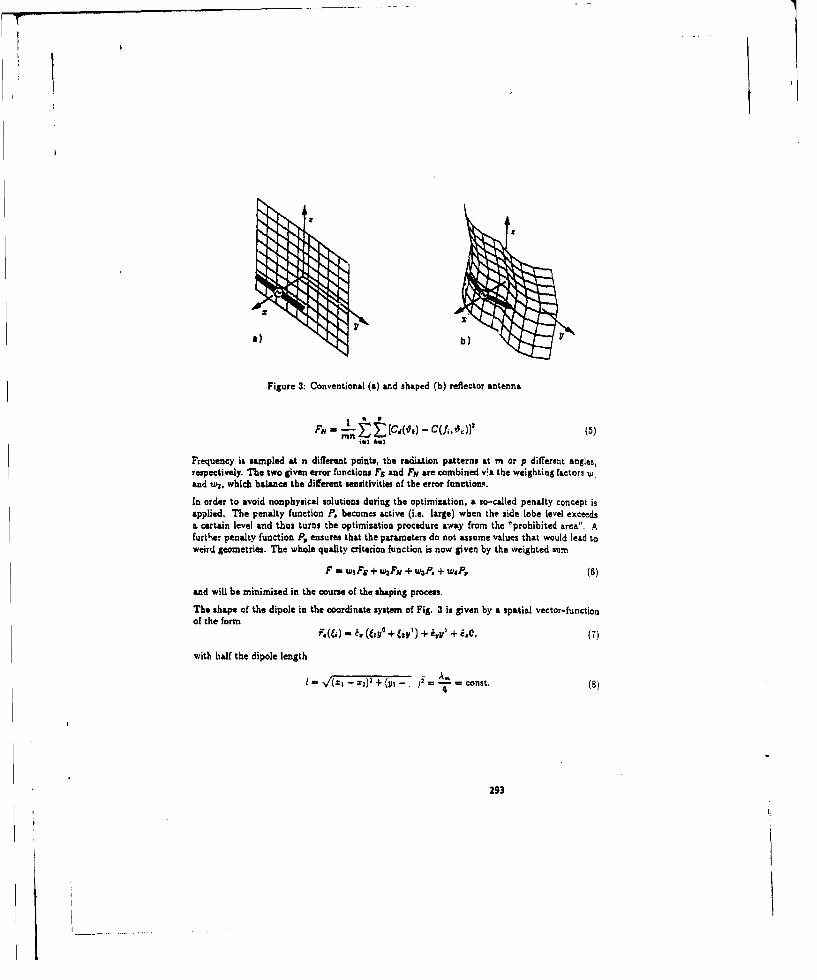
z

a) b1

Figure 3: Conventional (a) and shaped (b) reflector antenna

F, .- t t [C'(l') - Cu,] (5)m s &-I

Frequency is sampled at n different points, the radiation patterns at m or p different angles,respectively. The two given error functions FS and FH are combined via the weighting factors W,and w2 , which balance the different sensitivities of the error functions.

In order to avoid nonphysical solutions during the optimization, a so-called penalty concept isapplied. The penalty function P. becomes active (i.e. large) when the side lobe level exceedsa certain level and thus turns the optimisation procedure away from the "prohibited area". Afurther penalty function P. ensures that the parameters do not assume values that would lead to

weird geometries. The whole quality criterion function is now given by the weighted sum

F -wiFs+ w2FR+ wSP. + w4P.

and will be minimized in the course of the shaping process.The shape of the dipole in the coordinate system of Fig. 3 is given by a spatial vector-function

of the form

F - ((O + iy,') + iY' + i.c, (7)

with half the dipole length

V'i-v T7 X -+(y- , const, (894

293

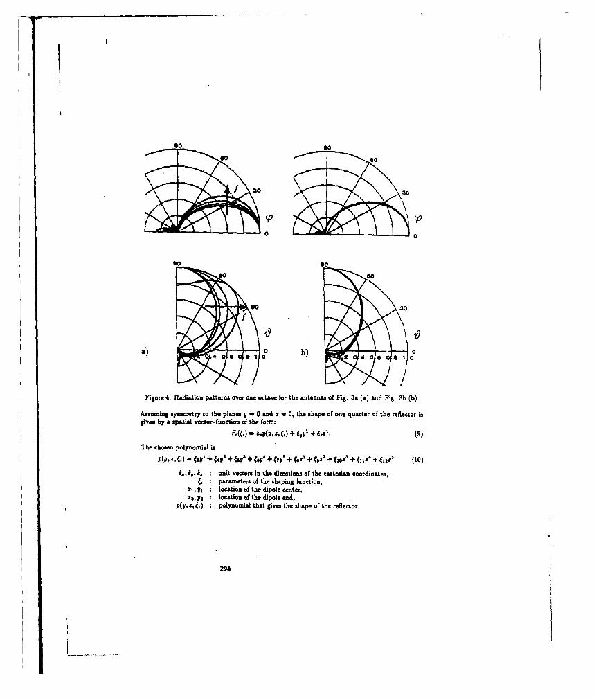
90

0o

f 30 30to so

so so

so 30

a) 0 05 0 b) .204 600 a0o

Figure 4: Radiation patterns over one octave for the antennas of Fig. 3a (a) and Fig. 3b (b)

Assuming symmetry to the planes y w 0 and z u 0, the shape of one quarter of the reflector isgiven by a spatial vector-function of the form:

F,(M) - 4•(y.,ZE.) + y ' + 4ZI. (9)

The chosen polynomial is

p(y,2,(6) _ y +(4M 2 +e5113 +C5114 +fT11 5+(S +(4Sl +(102 +ýIZ4 +412r, (10)

,,4,, : unit vectors in the directions of the cartesian coordinates,parameters of the shaping function,

zi, VI :location of the dipole center,x2, Y2 : location of the dipole end,

p(y, z, 4i) : polynomial that gives the shape of the reflector.

294

The result of the optimzzation process is shown in Fig. 3b and Fig. 4b. It is possible toobtain nearly frequency-independent radiation patterns over a one octave bandwidth with theoptimized shape of dipole and reflector. This holds not only W, the E- and H-plane but also inthree dimensional space.

5 Omnidirectional Array

Antennas consisting of dipoles in front of a refecting screen ane often arranged in arrays arounda central mast in order to provide omnidirectional radiation for FM- and TV-stations (Fig. 5).On the assumption of proper individual radiation chsractelistics, the overall radiation patternof the array would be omnaidirectional, only if the phase centers of the different array elementsware located in the center of the mast. As this is not possible with this type of antennas, theradiations of the difetrent elements of the array superimpose in a frequency-dependent way. Theresulting deviation from the ideal oamnidirectional pattern is the "ripple", which is measured indE. For an antenna of the type shown in Fig. 5, which consists of a flat straight broadband dipole

Figure 8: Array of 4 reflector antennas with flat V-dipoles arranged round a central mast

in front of a reflecting screen with a central ridge, the maximum ripple over an octave bandwidthis around S dB with a mast diameter in the order of 2A at center frequency. As this antennais already in practical use, only small variations of its geometry, such U a tilt between the twohalves of the dipole and a change of the distance dipol&-reflector couWd be contemplated in orderto optimize the omnidirectional pattern. The analysis was carried out using a computer programdeveloped by Jakobus 161, based on the method of moments [3), modelling dipole and reflectorwith triangular patches as shown in Fig. 5 and using basis functions for the surface currentsaccording to Rao et al. [51.Fig. 6 shows that by proper choice of tilt or bend angle and distance of the flat dipole to thereflecting screen, the maximum ripple within an octave bandwidth can be reduced by a factorgreater than two.

295

•00

, 1 0~Fmo d

In n

Figure 6: Ripple of omnidirectional pattern over dipole bend angle and distance from reflector

6 ILS-Glidepath

Fig. 7 shows the 3D-modelling by triangular patches of the approach are& of an airport withinstrument landing system (ILS). Greatly simplified, the interference between an antenna arrayinstalled abeam the intended touchdown son. and its mirror image with respect to the groundproduces & null of the electrical fieldstmngth, which acts m a guiding line (instrument glide path)for landing aircraft. With uneven terrain in the sppronsh area the mirror image becomes blurredand the glidepeth will show deviations from the ideal straight line, which until now could only becompensated by changes in antenna position and phue after lengthy trial and error procedures.With a new optimixation technique 17] based on an extended UTD, all antenna param eters cannow be determined in advance and intermediate calibration flights have become dispersable.

References

E1] N. Y. Zhu and F. M. Landstorfer, "Quality factor optimisation of coaxial resonators,' M1ec-tronics Leatters, vol. 24, pp. 862-483, 1988.

296

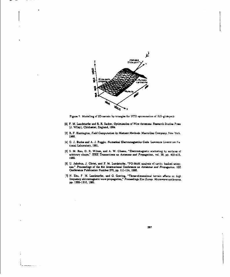
Figure 7: Modelling of 3D-terrain by tri~agles tor UTD optimization of ILS-glidepath

121 F. M. Lmandutorfer and ft. f. Sacher, Optmirnation of Wire Antennas. Rceee.rch Studies Press(1. Wiley), Chichester, EnILand, 1984.

[3] R. F. Haringtou, Field Computation by Moment Methods. Macmi~lan Company, New York.1968.

(4) 0. J. Durke and A. J. Pogglo, Numerical Fletromapetica Code. Lawrence Livermire Na-tional Laboratory, 1981.

(5] S. M. Rao, e . R. Wilton, and A. W. Glison, Electromagnoetic scattering by surfaces ofa rbitra, y shapea IEEE KTranacton s oW Antenas end Propgation. vol.c30, pp. 409-418.1982.

S] U. JRakobu,. J. Christ, and F. W. Ladtorfe, 'P0-MoM mnalysis sf cavity backed santen

nas," Proceedings of the 8th lnternational Conference on Antennas and Propagation, IEEConference Publication Number 370, pp. 111-114, 1993.

[71 N. Zhu, F M. Landstorfer, and G. Graving, "Threse imensional terrain effects on highfrequency elctromagnetic wave propagation,' Proceedings 21st Europ. Microwave conference,pp. 1205-1210, 1991.

297

298

SESSION 7:

FINITE ELEMENT METHODS (HI)

Chair: Jin-Fa LeeCo-Chair: John Volakis

299

Hybrid Finite Element-Modal Analysis of Jet Engine InletScattering

Daniel C. Ross, Johrn L. Volakis and Hrijrtos T. Anastassiut

Radiation LaoaoyUniversity of Michigan

Aim Arbor Ml 43109-2122

1aboe - Accturate numerical simulation of rafar actering from jet engine inlets is of vital iniPor-wee for target identificationa. High frequency techniques fail due to the complexity of the engine

face. A hybrid finite elarment-modal ateithd It presented. Only the region of the inlet directly adja-cent to fth engine face is considered fav the Arthe element portion of the solution, which is assunmedto have a circular cross; section. The finite element method is used to find a generalized scatteringmatrix for an N-port representaition of the engine face. where N is the number of traveling cylindri-cal waveguide modes in the inlet. Important implementation issues ame addressed including: the useof an optimized, fictitious, material absorber to tuincate the FEM mesh, and an examnination of thesuitability of node-based or edge-based elements. Results am shown for some benchmark corifigura-tions.

1.0 Introduction

The simtulation of radar scattering fronm jet engine inlets is an important step towards the character-ztwice of aircraft structures. While high frequency techniques can accurately simiulate many scatter-

ing mechanisms on a typical aircraft, there techniques ame not suitable for resonant or guidingstructures such as antenastradomes and jet engine inlets. The engine face is an intricate target. pos-sessing complex geometrical features at the wavelength level or less and is therefore inappropriateior high frequency analysis. By comparison, the finite element method (FEM) (11121 is well suitedfor the analysis of geometrically complex, inhontogeneous volumteeric targets such as the engineface. However, in spite of its inherent 0(n) storage demand, the FEM analysis would still requireprohibitive compautational resources were it to be also used for. mdling the volume enclosed by theinlet leading to the engine. By coupling the finite element method (applied at the engine face). to ahigh frequency ry ornmodal technique (o propagate the fields in and out of the inlet), an efficientmethod is developed for analyzing the inlet and engine configuration.

Of importance in this analysis is the interface between the ray/modal and FEM methods, and thetruncation of the finite clement mesh. Given that the inlet ctoss section near and at the engine loca-tion is circular. and our desire to propose an efficient and flexible coupling scheme, the coupling ofthe FEM and my fields in this paper is accomplishd via the generalized modal scattering marnax,'rhat is, the FEMA analysis generates the modal scattering natrix which can then be interfaced withany high frequency technique for computing the engine scattered fields without referenice to thegeometry of the jet engine. Regrading t1A truncation of the FEM mesh, several schemes are consid-ered including absorbing boundary conditions, the unkmomeni method and a new artificial broad-ban absorber, with the later found most effective for this *pplication. T1he suitability of edge-basedand node-based elemnents for this application is also presented.

300

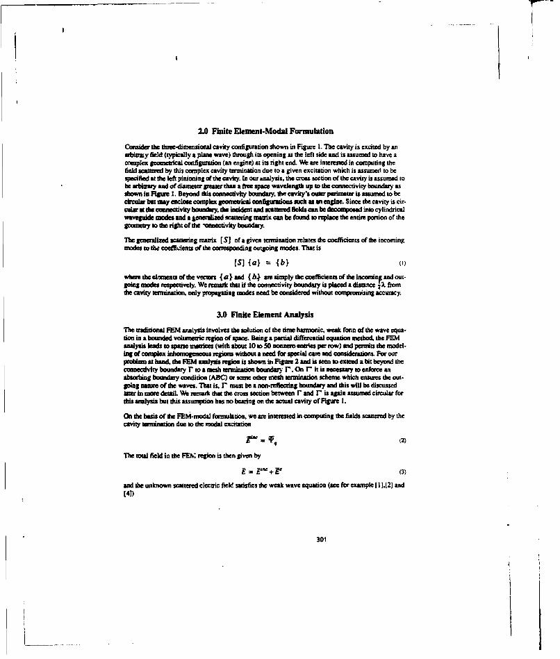
2.0 Finite Element-Modal Formulation

Consider die three-dimensional cavity configuration shown in Figure 1. The cavity is excitd by anarbiraiy field (typically a plante wave) through its opening at the left side andi is assumed to have acomspku geomnetrical configuration (an engine) at its right end. We we interested in computing thefield scattered by this complex cavity term ination due to a given excitation which is assumed to bespecified at the lef pinianing of the cavity. En our analysis, the cros section of the cavity is assumed tobe arbinarry and of diameter Steine than a free space wavelength up to the connectivity boundary asshown in Figure 1. Beyond this cennectivity boundary. thet cavity's oqater perimeter is assumed to becircular bat tmay enclose comples geometrical configurations suchbaa an engine. Since the cavity is cir-culair at the connectivity boundaury, the incdet and acattered fields can be decompiosed into cylinducalwrAvguWd modes and a 1generalized scattering matrix can be found oo replace the entire pardion of thegoonmeby to the right of the -annectivity boundary.

The generalized scattering mratrix CSI of a given termination relates the coefficients or the incomingmdsto the coefflients of the corresponding outgoing modes. That is

[S] {al = f b} I

where the elomenta of the vecaaars a}I andl { b.) ame simply the coefficients of the incominF and out-going mdsrespectively. We remark that if the connectivity boundary is placed a distance ZX fromthe cavity terminationi, only propagating modes need be considered without compromising accuracy.

3.0 Finite Element Analysis

Thbe traditional P514 analysis involves the solution of the time hairmontic, weak Cann of the wave equa-tion in a bouinded volumetric region of space. Being a partial diflerential equation method, the FEManalysis leads to sparse matnice:3 (with about 10 to 50 nonzer envries per row) and permits the model-ing of compkix inhoniaogencous regionts without a need for special canmiad considerations. For ourproblem at hando theMP1 analysis region is shown, in Figure 2 sand is see to einend a bit beyoqd theconnectivity boundary r to a mesh termnination boundary r. on rl it is necessary to enforce anabsorbing boundary condition (ABC) or some other mesh termination scheme which ensures the out-going natue. of the waves. That is. r must be a non-reflecting boundary ward this will be discussedlater in more detail. We temark that the crom section between r and r is again assutred circular forthis analysis but this assumption has no bearing on the actual cavity of Figure 1.

On the basis of die FEM-modal formulation, we are interested in computing the fields scated by thecavity termination due to the modial excitation

r- . iF (2)

The total field in the FEN' r~egion is then given by

+ (3)

and the unknown scattered electric field satisfies the weak wave equation (see for example 111,12) and[41)

301

-L~j.(VxE'.VxT) -T'kor!di 1 .~kO1*(Xr)S

J~J{!L(V.Es) (V.T)}dv= (4)

r' (Adx (Vx rinc))}d1sýj-{±T. (fx (VxE~fC))}dS

in which rd represetits the surface over dielectric boundary discontinuities between regions ofdiffererit Viagnetic permeability. Note that Ad points from p P2 to gIand only materialdiscontinuities within the scatterer, not the fictitious absorber contrbwe to the boundary integral onr.. Also, the thir ter ison the left hand side of (4) is the usual penalty term which ensures that thedivarec condition be .disfied in the Galeriti least squares sense.

4.0 Implementation of the FEM Solution

Creating user-oriented and efficienit software to implement the above FEM formulation requiresthat&a nuniberof issues be addressed. Firstthe mss appropriate shape and elements must be cho-sea. Also, sinice the: problems will be large, efficient pre-;procesing softwar musn be created toettac (ficen a given mesh) information needed to enforce the boundary conditions. This includesfihnding mretal surfaces and edges. comrues, normals, material discontinuities andl the elements ontt heconnectivity boundary. It is alW crucial io develop preprocessing algorithms that run in O(n) timefor a general mesh. Tlo this end, an efficient preprocessor has bee created for extracting relevanttinfinusatioin tran an arbitrary three-dimenisional tetrahedral mesh 13].

IEkoMaeub . AFISEZpdaissiou

Mhere we two clasies uf field expansions that could be used with tembaedral elements: node basedand edge base expansions. Edge-based elements am a bettu chokce thant node-based elements forthe eigsgmalue problem becase standard node-based elements caninot accurately represenit theeagenwictors (fields) that correpond to oe eigenvalues. All of the eigenvalues that should be zero(one fbr each internal degree of frecdoma) have some snall non-aeo value when using standardnode-based elements. This large wcale degeneracy cause considerable numerical problems whencomputing the elgenvalues especia'y for large systems. When using edge-basied elements, thecigenvulues we cleanly split into =eo wnd non-zero groups thus alleviating rmuch of the numericslproblems [5]. MTat is. the zero eigenvalues are identically zero.)

Although edge-based elements are indeed better for eigenvalur problems, the best choice ofelements for three-dimensional scattering analysis is not clear. Both classes of elements wereconsidered (node-based and edge-based) for this problem.

Node-hesedekwa~set

302

When using linear node based elements, the scatered field is given by3

44

O .! + Ney +y N'r

2

where

IV ley = Al2 =N(x,Y, Z)

am the standard scalar shape functions [1)3w Eand,Ea and Ea- are the components of the vectordPSe gr of freedom associated with each of the fou

By numerical experimentaton was found that boundary conditions for these elements must beimplemented carefully to avoid deterioration the system condition. For a node lying on a conductor,two tangent vectors can be defined from the surface normal, such that

i* E P = El1- in,

? FS= -12' . inc

wheo 1, 2 denote the orthonormal unit vectors tangent to dhe metallic surface. Them ate many pos-sible ways of coupling the global equations to enferce the boundary conditions (5). but there isalways a bena way which preserves the system's condition. If the boundary conditions am enforcedarbitrarily, it is ,ossible to completely destroy the condition of the system and to geuerte wrongresults. The following procedure will guarantee a well conditioned final system:

Given the metal surface normal A at the node, find the two tangent vectors 1t and 12 as follows

*if ljxMl> 0.l5 then set .• = A19xx

-.. xA Ii• xA---s xA

*r i~t x AM-Given the dw- global equations for , and at the node

- find the largest component of 1 (x, y or z) and replace the corresponding global equa-tion with I1 - = -- . 4c

- find the largest component of 12 (z, y or z) and replace the corresponding global equa-tion with i2 =-.

Edge,-w4 •d aseasa

303

te first order, vector, edge based, tetrahedral elenjurts Siven in Fipgre 5 expand the unknown fieldas

where a is the vector shape functdon associated with the ath edge. The sca"ar degres of freedomE refer to di compoantz of the steied field diected along the a'th edge.

s element win en hIemenowd for the inl tmidnadtion scatteing problem and were found tobeak down when the scatte l field was parey TE (no zoomponet of the scattered electnic field).This bmrkdown is highly msh depeadans and is mdiftsed in a poorly conditioned global system.Cleriy. if a veaor field a the =star of a given edge of an element is orthogonal to that edge, edge-based elemrets cannot represent that field and yield a singular system. When a large volume isfilled with ftee atrahedral mesh and the solution is purely TB, apparently a nearly singular systemmay result,

Since it is the job of the FEM to find the modal coupling, and since this coupling may in some casesbe pure TB, the eleantmums be able o accorately rp Pet a pue TE field while at the same timerepresent other types offields. Because of the above difficulties for edge-based elements in model.

ing pure TE fields, we resorted to the node.based elements for this application.

MeIhT rmladoe Schrmes

At the open end of the mesh, the fields radiate into an infinite, cylindrical waveguide. The boundarycondition at this open end must absorb all uatveling modes in the guide. The most obvious choice isto expand the seamed field as a sum of all raveling modes and couple this expansion directly tothe FEM equations.

Let the tangential electric field at the open end be :iven by

I - .r. (6)-- I

where b. ar •SL-ovn coefficients and 'l is a cylindrical wavegpide mode. Substitution of thisexpansion into dte second term of (4) yields

With the introduction of the new coefficients b., to solve the system, resulting form (4). it is neces-sary to construct additional equabion. These ar given by

'(x, y, z 0 ) * (x, y, z o) (s

(04, y, zo) (x, Y, ze)

304

and couple eachs unknown coefficient b. to the fild associated with nodes on r. This leads to aspasrse, square (FMN system coupled a admue, rectnguar (modIal expansion) system. While thisscheme worked for shiorted inlets, it was found to be unslabli for the stub termilnated inlet.

The design ofta fictitious material absorber to absorb all tiAvelng modes is complicated because theimpedance and propagation constants of these modes vary greatly. 1The eight traveling. mes in aguide of radius .W6~wer used to design an optimized absorber. Clearly, if the absor bet wereallowed to be very long, a nearly perfect absorber could be constructed. However. since theasherter will be pert of the PEN mesh, as a design constraint, it should be no more than about ahalf of a fme spe wavelmogt long to be praetical.

A Monte Carlo opdstimiaton scefme based on (61 was used that has the desizable pr oper ty of find-ing not only the bent performing but als fth most sambie design. A five section, metal backedabsorber was used as a starting point with 1. and Prset to unity in each section. The length ofeachsection was setinitiallyto .lk. The 15 patuneter (material constants andI lengths of each sec-don) were varied randomsly. independent of one another. Thasmiasion UiNe theory was used to cal-culate the reflection coefficient for esh mcje (see FRgiz 3). and the algebraic sum or reflectioncoefficients (the sum of absolute values) was used as the global optimization parameter. A pass/failcriterion on the global F ,nte was set to give about a 50% yield. For each random design, a passor fall was noted for each IP Pmee and after a number of designs have been sampled, a patternbegins to -merg. Sorm pisnuneters "dcate a tightening up is in order since most of the 'good'designs were centeed about a certain value. Other parameters indicate a don't care condition as allvalues worked equally well. A new met of initial values and ranges is chosen and the process isrestarted. Again, the global paramnesr threshold is chosen to give about a 50% yield. This globalthreshold continues a, drop each iteration until a stable design is found. The final design and its per-fonmance is shown in Figure 4. Note that the. rfeton coefficient for all modes is less than.!I (- 104BD).

Example: Ckcwier ftub UndowS..

A circular stub terminated inlet was analyzed because this jeontrny also possesses a referencemodetnutching solutonmM.1The absorberwassplated 0.33%. from the stub and the scatteringmatrix was cr'mputed at a distance of 0.25 X in front of the stub. FigreS5 shows a cut of the vol.ume mesh for this configuration and the co-polatrized backsasteter patterns are given in Figure 6.

It was found that the paoper handling of the boundaty conditions at tho inner edge (the rim of thestub) was critical. If the total field were set to zer at this inn= edge, the results were sLuite wrong.

Yweve, if only the comiponent tangential to the edge (E#) was set to zeo. whereas Ewas.,owed to float, the results were much improved and this as shown in Figure 6.

%ble the shown results atein good agreemnct for horimzntal polarnsationi, theme is sorm discrep-ancy in the vertical polaiziation. Finer sampling around t'-e rim does improve the comparisonslightly but with,.ery slow conrverjqence. The result shownt wese obtained using a global element sizeof atndan elemnent size of w.aoutnd thenrm

305

engine face

nSoun L Hybewie inst. Mist wwwL~a

connectivity boundary (r) finite element mesh

mesh tefmination boundary (r)

FIGURX .RjE t severbmnji u.b~e Gakueint agAay*m applied

33 33 ~34~~s

nau~ Taim~l~elb mde . 21bain Za.qnd baa

"gift

0.1 - - - - -- - - - - - - - - - - - - - - - --

(r. DueOAS

T%%, ML TE!, TE3, TM-, TA rrj, TU4,S0.

95-jt.22

- I 33-J 1.

C ,- 1.043 A ( Ir a I ft AU 6e06i0

FIGURS. l - o te URE 4. Oplifn ofm hm va g udaorr.

(horiGUES paoa • stu) Mgmatdc RmS

aM,•, ,.-. (~~~db) ' . . . . . ." "

• a," "m

ftb*Wdt A* HI e s I , e

FIGUU Oft•,•- 1 aws frm gobSeyj~ilried cavity (14 ofr Uao Poutr is Ir- ) * RGCURE 6. Refts for a stub wmmimaked inlet

References[ lP. P. Silv em and R. L Fenrri, Fake E/lmnmn for Elecirs/F•l E neers, Cambridge, 1986.

[211. L. Volais, A. COtaajee and L C. Kempel, -A review of the finite element method for three-dimessionaj elecntromgnec eaztming."J. Opi. Soc. An.-A. April 1994 (to appear)(31D. C. Ross, "Same Finifte-Elrent Preprocessing Algorithms for Electomagnetic Scattering",IWEE Amem as n d PrqpqadoR Mqaw, Vol. 35. No. 3, pp. 68-72Z iune 1993.

143r, D. Paulsen, D. R. Lynch and J. W. SwdhbeKhn. "rhsee-dinaional finite, boundary andhybrid element solutinm of the Maxwell equations for lossy dielectric media," IEEE Trans. Micro-wave Tieory Tech., vol. 36. no. 4, pp 682-693, Apr. 1988.

[5],. I. Cndo, "Vector Finite Eements for Electuomag•etic Field Computation". IEEE Trans. onMagnenes, Vol. 27. No. 5, pp. 3953-3966, Sept 1991.[6]A. B. MacFauland. "Namee Centering and Tolemncing". Master's IThesis. Electrical Engi-neering Graduate School, Univ. of Idaho, Aug. 86.

[7]H. T. Araaaa.su and J. L Vobakis. "T'he Mode Matching Technique for Electomagnetic Scat-tering by Inlets with Complex Teminations", Technical Report 030395-3-T, The University ofMichigan. EECS Radiatin Laboratmoy, Ann Arbor MI. October 1993.

307

Thee-Dimensional Finite Element Analysis on a Parallel Computer

Richard K. GordonDepartnant of Electrical Engineering

University of MississippiUniversity, MS 38677

L b* o tmIn the recent past, a number of researchers have investigated the use of parallel computers for

the solution of problems in computational electromagnetics. For instance, in [1], Calalo, Cwik,Imbuale, Jacobi, Liewer, Lockf L. Lyzengs, and Patterson discuss the implementation of an FDTDcode and the NEC code on the Mark M Hypercube. Barkeshli and Volakis present the parallelizationof the CGFFI algorithm in 1. In [31, Bedrosian, D'Angelo, and deBlois review the implementationof the T-mawbE method and an integral equation technique on parallel computers. And Chatedrje,Volakia, and Wiadelise discuss the paralellaation of a finite element algorithm !n [4).

In the p•esent paper, a three-dimensional finite element algoithrm that employs edge elementsis used in the analysis of complex cavities. The cavities may have arbitrary shape and loading. Athree-dimensional finite element formulation [5] is used to determine the cutoff frequencies of thecavity. Edge elements are used in order to eliminate the poasibility of spurious modes.

Becamuse the number of unknowns needed to model a three-dimensional region grows sorapidly as the size or complexity of the region increases, there is a strong motivation to ty toimplement the numerical analysis of such regions on parallel computers. The use of a parallelcomputer permits the analysis of significantly larger cavities than those that could be convenientlystudied using most sequential computs. Furthenmo, in some cases it can also result in a significantspeedup in the numerical solution process.

In this paper. the parallelization of the three-dimensional finite element algorithm is discussedin detail. Results obtained on the 400 node Para-gon parallel computer at the San Diego

Supercompotr Cenw are compared to those generated on the Cray X-MP21216 at the University ofMississippi. Computatioa times ar presented and the advantages and disadvantages of using eitherkind of computer am discussed.

I. Finite Ijemet FormnalationA three-dimensional finite element aIlorithm is employed in this analysis. The derivation of

the equation that is implemented in the numerical procedure begins with MaxweU's equations for asource-free region:

V X -jaqdi (I)

308

and

Vוjaoe.. (2)

If each side of (2) is multiplied by the curl of each side of the resulting equation is taken.

and (1) is used to eliminate the cud of * on the right hand side, the resulting equation is:

V x (IVx •)u= (3)C

It is the weak form of this equation that is implemented in the numerical procedure. The nextstep in the derivation of this weak form is to multiply each side of (3) by a testing function T7 and then

to use the vector.identity V.(Z X 6) - 6 • V X d- d. V x & to obtain:

In the method used he•, the region of interest is divided into a number of parallelepipeds.With each edge of a parallelepiped there are an associated vector basis function and vector testingfunction. , is the vector tesing function associated with edge Oi. If we integmre (4) over AV, theregion occupied by a single parallelepiped, and use the divergence theosem on the right hand side. weobtain:

where a(AV) is the surface botuming AV.If (2) is used on the right hand side, the resulting equation is:

j V X h)._(V X f) _ 24~A}L =§J4 ~.} (6)

This equation is valid over the region AV enclosed by a single parallelepiped. The goal is tofind the equation that is appropriate for the entire meshed region r, the boundary of which is a!-.This is done by summing the equations (6) that result from all of the parallelepipeds. When thissummation is done on the left hand side, it is clear that the result is simply an integral of exactly thesame form over the entire region r. To dewrmine what happens on the right hand side, consider a

309

face shared by two adjacent parallelepipeds. We note that since no source is present, the tangentialcomponent of I is continuous eamr this face and that the normal vector pointing out of one of theparallelepipeds will be the negative of the normal vector pointing out of the other. So, thecontributions from the right hand sides of the equations (6) of these two adjacent parallelepipeds willexactly cancel. Since no sources am present in the cavity. this same cancellation will occur along anyinterior face in the meask So, when dOe contributions from all of the parallelepipeds ar added, theresult on the right hand side is an integral of exactly the same form over dT, the surface of the entire

ntshed miom Thu& the eNd weak form f (3) can be writen as:

Iff[ V xR)- V x Wez ' - 0[~itur, -i' .(f x 4S. (7)

In this work, tdo goal is to determine the cutoff frequencies of a cavity that is enclosed byeither pmc or pee walls. If the wl are proc, the value of the tangential component of R ailorg thewalls is known, thus. for any edge i that lies along the wall, there is no need for the use of a testing

function; T, can be taWmn to be wro. Thus, if the walls are pmc, the right hand side of this equation is

aeo. If. on the other bad, dte walls am pec, then Ix is zero along the wall. So, again, the righthand side of (7) vanishes. So, for eidher pnc of pec walls, we have:

;JJ[±c(v X A). (V X:t,) _ a)A }i. -i0. (8)

As was mentioned above, with each edge of a paralelepiped there are an associated vectorbasis function and vector testing function. T7e vector basis function at edge j is A. In the finite

element procedume, H is expressed in terms of these basis functions ac:

where N is the total number of edges in the mesh. If t expression is substituted into (S). we obtain:

(v x J .(v x 0,. (10)

This is one equation in the N unknowns ht through h/v. If we now let i vary from I to N. i.e.,we test over each edge, we obtain a system of N equations in N unknowns that can be written in marixform a:

310

Thi..0 1I)

where

Al,-JJJ(xi.V-oMiEV (12)

11e only way that (11) can be saisWe for amo-tivlal iA.Ie. the only way them will be non-trivial souoo-free solutions, is for the determinant of 17 to be sam. lIs observation leads us to thetechntique that is need to damemine the cutoff fuequanels of doe cavity.

ilL Proeduan lfor lNuding Cutoff Freq uenI

We note from (12) that the entries of V depend on the frequency, f . where f =The

technique for determining the cutoff Frequencies begina with a choice of an initial frequency, f., andfrequency increment. Vf- Once the initial frequency, f., is chosen. all the termes in the matri anedetermined and the determinant of the matrix can be eajeculaied. This is done and then dhe frequency is

incremented by the amount hf. The determinant is the calculated split. This process of calcuatingthe detenrminant as the freiquency is scanned continues until the determinant changes sign, thterebyindicating that a cutoff f~requenicy has Just been passed. At this point. it is known that a cutofffrequency lie between the last two firequencies considered; a mome precise value for this frequency canbe obtained either by interpolation or by choosing a smaller frequency increment and scanningbetween the lest two frequencles considered

IV. PWasalantl. at the Tedob"iuThis algorithm was paualielized in three respects. Parallellzation was incorporated into the

assembly and soramp of the matrix, the evaluationi of the determinant, and the frequency acanning.The idea is as follows. After the finiat element .. hl has ben enerated for the geometry of interest.the siz of the system matrix is known. In order to sae memory. this matrix is stored in bandedstorage mode. Still. litli generally too large to fit on oam node. So. the minimum number of nodes thatwill accommodate this matrix is next calculated; this number is called xainf. The next step is tochoose the number of nodes over which the matrix is distribute for a single calculation of thedefteinant, keeping in mind that this number must be grsate thime or equal to nasht. This number iscalled nopersr. 71he next step is to decide the total number of nodes that will be used. This totalnumber is divided by nopergr to obtain the number groops. The idea is that all of the nodes amedivided into a number of groups of nodes, Each group has nopergr node,. The tota number of groupsis groups. Since each group is capable of accommodating the matrix. it can work independently of allthe other groups. So. frequency scanning is achieved by assigning different frequencies to differentgroups. Within each group. the filling of the matrix and the evaluation of the determinant is

311

dilatboand ove all aaprgr nodes in thes group. Thas. the assembfing and storage of the matrix, theevAluntao of she deemnsiaus. and the sanning of the fmquency have all been purallelized.

V. Numerd Rad~t;Although th" technique is suitable fur die determination or tie cuteff ftaaquencies of ani

arbitarly shasped! and arbitraily filled camity, in order to be able to obtain a companson withanalytical valur for te usFf fe cIes I m empty cavity having the shape of a parallelepiped wasCheasm for do sisft Unowerlsal mslams. Tkia cavity M4~ lengt in do x. y. and z directions of 5 cm..7 cm.. and I I on., tespecdvisly. The walls wene pec. The technique described above wasisuploasused om da 40P aids Pa5gm compoer at San Diego Supercomputer Cente (SDSC). For thesbak of oompaalaa. tde uapmrellasd veraion of this algorithm was implemented on die CrayX-MP2rAI6 at Ban Mlfityi Causer fin Saparconsputin Raumrla (MCSR). A frequency vange of2.3-5.4 GlIz sad fkaquenacy inceuaenat of 0.1 O~s wer chosen and a finite element mesh with 5divisions in the a-diresloa, 7 dkvlalam in dhe y-direction, and I I divisions in the z-direcuion was used.The WWoeal sher of edges in the meob was 1.512. The numerically deternmined values for the cutofff~requencies woe the son os both computers; these valnca ame shown in AtL right hand column ofTable 1. Mots that two of Ba firs us umuoN 0 qumcie wer not desected. The masont for this is thateach of doss two frupaulesi is the cutooff firequency for two modes. Thus. am determinant goes toume at this frequsency but dosam n ho p c ui sp, so. the cuoff frequency cannot be detected using the

I Ice- P describe sh a e. For the other canoE fzquhsncls. the apeement between the numerical andanalytial values is quits goed.

The date mqulze4 to ran this program on the Cray X-MP2/216 was 97.044 a. The timeORqb doa B Paugon deedean the muber of nodes used as shown in T able 2 and Fig. 1. In this

cast. he goal was io determinme the effect of dhe frequency scanning. So. the calculation of theI e ,rIluant at a singkc frequency was asigned to a single node; that L, wspergr was chosen to be I

and tro was equal I* Ba total -ember of nodes employed. As can be seen from Fig. 1. there wtsessentially lies. speed-fV ov terB entire mage. Me teson for this is that the frequenacy scanning isembanausizgly paialel; Bae calulawins of the detimianam at diffesams frequencies ame completelyindependemit ofer.A other.

The next goa was to investigat the effect of the paratkeiiation of the calculation of thedesratlams. So. a sigle freuqeuscy was chonsn. The daemminant at this frequency was calculatedwing 1.,2.44.I16 lmd 32 nodes. The ==Isamlu shown in Table 3and Fig. 2. The speed-upiu noteveaiclose v Haw in *klsea. Theseis some beainetu vsan 2.4. 8, or 16 nodes rather han just 1;in fact Ba ben choice of those &mod is 4 nodes. Nowe that if 32 nodes we used the elapsed time islonger than ifsa single node is emplotyed. The reason for this and for the failure to achieve linearspeed-up inthBa case is thus when Bae cmain is distributed over severa nodes. a considerable amountof inser wode communicataio is necessary in tae calculation of the determinant: tbis communicationslow& down Bae mehitique.

312

VL ConcusionsA thre-dimcusional finite element algoridthm that employs edge elements in the detennination

of the cutoff frequencies of an arbitrarily shaped and arbitrarily filled cavity has been discussed. A

method for parallelizing this technique has also ben presented. This method includes parallelization

of both dte frequency scanning and the calculation of the determinant uf the fuinte element matrix. It

was found that the frequency scanning was an embarrassingly parallel procedure; essentially linear

speed-up was obtained for this part of the parallelization. On the other hand, if the matrix is

distributed over several nodes, the calculation of thc detrminxni requiwm considerable communication

between these nodes; thus, the speed-up obtained fo' this part of the paralldlization fell considerably

short of being linear.The coteputadion time on the Cray X-MP24216 was less than tar any of the cases aatempted on

the Paragon. Furthermote, the development of the code for the Cray X-MP2/216 required less effort

than did the development of the code for the Paragon. But it is important to recall the simplicity of the

cavity that was under investigation. For a cavity of more complicated shape and/or filling, the

discretiza*ion process can easily lead to a mesh Mhat will be too large for convenient analysis on the

Cray X-MP2f216; this is the Ui of case for which the technique described is suitable.

AcknowledgMentsThe author would like to express his sincert appreciation to the National Science Foundation

for affording him tae opponrauty to participate in the Metacenter Computational Science Institute in

Paiallel Computing, the Sa. Diego Supercomputer Cenrer for the use of their Paragon computer and

tMeir expert advice, and the Mississippi Center for Supercomputing Research for their expert help and

the use of the Cray X-MP22 16.

REFEENCES

[1] R. H. Calalo. T. A. Cwik, W. A. Imbriale, N. Iscobi, P. C. Liewer, T. G. osdr-art. G. A.

Ly-nga, and J. E. Patterson, "Hypercube parallel architecture applied to electromagnetic

scatte.,g analysis." IEEE Trantectots on Magnetics, voL 25. nun. 4. pp. 2898-2900, July

1919.

[2] K. ]atkeshil and 1. L Volakis, "A vector-concrunnt application of a conjugate gradient FFF

algortha to elevtromagnetic radiation and scattering pioblems,* IEEE Transactions on

Me4,1reds, voL 25, aum. 4, pp. 2892-2894, July 1989.

(3] G. Bedrosian, J. D'Angelo. and A. de~loia, "Parallel compining for RF scattering calculations,"

IEEE Traunactions on Magnedc-. vol. 25. num. 4, pp. 2884-2889, July 1989.

[4) A. Chltettree, J. L. Volakis, and D. Wizdheiser, "Paaflel computation of 3D electromagnetic

scattering using finite elments,* submitted to Internaonal Journal of Nuaerical Modelng.

[51 K.. Iv, K. Inoue, and M. Koshiba, "Three-dimensional finite-olement mt-thod with edge

elements for electrotaagnetic waveguide discontinuitis," IEEE Tra dcnots on Micrewave

Theory and Techniques, voL 39, num. 8,pp. 1289-1295, August 1991.

313

Anrlytical Value for Cutoff Frequency (GHz) Numerical Value for Cutoff Frequency (GHz)

2.54 2.503.29 3-303.47 3.503.69 3.703.93 not detected4.05 4.104.50 4.604.59 not dateaard4.62 4.705.23 5-30

Table 1. Comparison of analytical and numerical values for cutoff frequencies

Totdl Number of Nodes Fapse.d TIme (s)1 12.953.8472 6.631.9904 3.212.8698 1,626.15216 834.42132 432.927

Table 2. Elapsed time for calculation of determinant at 32 frequencies

Total Number of Nodes Elapsed Time (s)1 421.8122 270.1784 199.1488 222.54616 351.27932 693.090

Table 3. Elapsed time for calculation of determinant at 1 frequency

314

25--

20 -

I I

A 0 . I I .!I

02 - i- i I I0 5 10 15 20 25 30 35

Total Numiber of NoOesFgure .Speed-up for scanning of fiequenows

25 -

1 15-0 10

0 5 10 15 20 25 30 35Total Number of Nodes

Figure 2. Speed-up for calculation of deerminant

315

THE PERFORMANCE OF APARTITIONING FINITE ELEMENT METHOD

ON THE TOUCHSTONE DELTA

Yung Shirley Choi-Grogan and Robert Lee Klalluri Eswar and P. SadayappanElectroScience Laboratory Dept of Computer and Info. ScienceDept. of Electrical Engineering The Ohio State UniversityThe Ohio State University 2036 Neil Ave.1320 Kinnear Rd, Columbus, OH 43210Columbus, OH 43212

I. Introduction

The finite elment modeling of electrically larpe structures has always been a difficult problemin electrosnuagetlcs because the number of unknowns increases dramatically as the electrical sizeof the structure increafse. One of the ways to increase the efficiency of the finite element methodIs to uoe a "divide and conquer" stratey. This idea has been applied to integral equation methodsin which the computation domain is partitioned into many smaller sections. The solution is thengenerated in each section independent of the other sections. The coupling between the sections isthen performed in either an iterative manner [I] or by employing a more rigorous and computa-tionally expeslive procedure [2,31. The concept of partitioning has also been used for the finiteelement method [4,51. However, in all these methods except [2), the partitioning has only beenperformed along one dimension. In this paper, we consider an extension of [4] for two-dimensional(2-D) geometries, where the computation domain is partitioned along both dimensions. In [41,the problem of electromagnetic scatterin from a 2-D cylinder is considered where the bymomentmethod (60 is sed for the boundary truncation. The byrnoment method requires the solution ofmultiple finite element problems with known Neumann boundary conditions. Since the purposeof this paper is to consider the improvement in efficiency of the finite element solution, we willonly consider finite element problems with known Neumann boundary conditions. Another majoradvantage of the partitioning method is its inherent adaptablity to massively parallel multiproces-mrs. Since much of the calculations for each section are done independent of the other sections.

each processor can perform the operations associated with its own sections without communicat-ing with the other other processons. The performance of the method on a MIMIJ (multiple inputmultiple data) architecture is shown here.

I. Formulation

The 2-D problem considered bere is as infinitely long cylinder of arbitrary shape and arbitrarymaterial properties in free space. In this paper, only the TM. polarization is described. Let usconsider a partitioning of a representative cylinder (Figure 1) A known Neumann boundary con-dition is applied to the outer boundary which is represented by hl. The inter-section boundariesae denoted by $S..

The Neumann boundary condition can be defined in terms of the tangential magnetic fieldalong the boundaries of each section. Although the Neumann boundary condition is given on 611,it is not known a priori on 6S.. However, we can approximate the values on each inter-sectionboundary in terms of a sum of known basis functions multiplied by unknown coefficients. TheNeumann boundary condition on the inter-section boundary is defined to be:

18E (I61 = 6it,(t), t E 60,d] (1)

316

where t represents the points on the inter-section boundary 6S. which has a length of d. Thevariable aj represents a set of the unknown coefficient to be determined. The functin *j(i) is aset of linearly independent basis functions, In the numerica Implementation of ( I), the infinitesum is truncated tn I.

VX

mx

FIgure 1: The partitioned solution domain

Let us consider the interior n"' section (not touching $0) with the Neumann boundary condi-tions applied on each of the four inter-section boundaries. Based on the property of linearity, thetotal electric field solution on the n'u interior section can be determined from the superpositionof the four boundary value problems. The total solution on the section is expressed as a sum offour boundary value solutions:

E "L(z, y) = E.O(=, y) + E,(z, 1) + E(z, y) + E.z,,y) (2)

where the four field solutions are defined to be,

I 0

! !

•(z,.,) = . , E s,,p).= , , (3)

The subscripts i,'n refer to the i term in the sum and the n" section respectively. The su-perscripts, L (let), D (down), R (right), and U (up), refer to the Wde of the section on whichthe Neumann boundary condition is applied, with Its corresponding unknown coefficient vec-tors (N, q., r., and &,). The finite element solution Ai,.(z, y) is obtained from the use of thecorresponding basis function ti(t) as the Neumann boundary condition.

To evaluate the unknown coefficients on each inter-section boundary, the finite element so-lutions of each setion are coupled to the adjacent sections by enforcing the continuity of thetangential electric and magnetic fields on the inter-section boundayq. The continuity of the tan-gential magnetic field is enforced explicitly. However, the continuity of the t"ssgenial electricfield is enforced in an integral sense. The application of field continuity results in a sparse matrixequation, which we call the coupVng Fratriz. A general sparse Cholesky LU factorization and

317

Table 1: Time comn s-leon for solving the entire body vs the aprtitioned bodytraditional method partition technique

domain time(sec) subregion tim.(sec)banded sparse

4A sq 5.10 1.01 .5A•sq 1.21IA s5 1.71

8A' sq 106.89 5.77 .3A sq 5.651, sq 7.97

12A sq 16.27 .5. sq 14.18

solve algorithm [71 is used to solve the coupling matrix. In order to minimize the fill-ins duringthe LU factorization, a nested dissection reordering of the matrix is done. It is expected that thecomputation time will be proportional to N'4 and the storage will be proportional to N whereN represents the size of the coupling matrix.

III. Performance for the Sequential Partitioning Technique

To demonstrate the efficiency of the partitioning technique, we study the results of the methodon a plane wave incident on a rectangular region of free space of varying sizes. The main reasonthat we consider free space is that the boundary conditions are known for this case. The efficiencyshould be the same for more complex geometries, The three problems considered here are freespace square regions with sides of length 4A, $A, mad 12,A. Eight-node quadrilateral elements areused to discretion the commutation domain. For the traditional method, the number of nodes inthe three computation domains is 4,961 (4.%), 19,521 (8A), and 43,681 (12A). Each geometry ispartitioned into either 0.5A square sections or IA square sections. Triangular subdomain basisfunctions have been used for 9i in (1). For the cams presented below, the solutions from thepartitioning method and the traditional method have ben compared to verify that they have thesame degree of accuracy.

A. Time PcerfnsomnoTable I shows the computation time for the traditional method sad the partitioning technique

on a Cray YMP. The Airst two time columns in Table I represent the time required to soave thecorresponding problems with the traditional finite element method by the use of either the abanded solwvr algorithm or a general spaunr solver algorithm. The latter algorithm has a smallernumber of non-zeros and thus requires a smaller operation count to factorize the matrix.

The data for the 40' geometry show that the partitioning technique Is more computatiodaily"exensive than the traditiomal method. This difference in time is due to the overhead timerequired in coupling the partitioned sectieon ad in calculating and solving the coupling matrix.The geometry is not large enough to talme advantage of the partitioning techaique with the givensizes of the partitioned sections. However, as the size of the solution domain increases (and thepartitioned sections re of a relatively smaller size), the computation time becomes smaller thanthat required for the traditional method. As the size of the computation domain increases, weexpect the diff'erence in efficiency between the partitioning method and the traditional method toincrease. Unfortunately, a larger Sze could not be tested because the mumory requirements forthe traditional method exceeded the available memory on the Cray.

318

Table 2:Memory cm 'afr ovn the entire body vs partitioned body

solution 1-tradiiona metho partition techniquedo-main )Rwmory(htword) sbeiojn I lemory(Mwod)]

4 banded sparse j______4 0.63 0.56 SsqT 0.06

IA sq 0.03SA sq 4.90 2.81 .5A sq T 0.39

IA__ . sq 1 0.1512A sq 15.99 T.07 5A sq 1.12

1. IAsq 0.54

H. Memsormj RquvirmntsnThe reduction in memory requirements is one of the major advantages of the partitioning

technique over the traditional method. Table 2 shows the memory requirements for both thetraditional and the partitioning technique on the same solution domain& as discussed in Table 1.The first two "memory" columns in Table 2 represent the memory requirements for the tradtionalmethod with either a banded solvesr algorithm or a general sparse solver algorithm. For the sparsesolver algorithm only the nonzero values of the matrix under consideration need to be stored,whereas, the banded solver stores all the terms within the entire half bandwidth. The last columnis for tua. memory requirements of the partitioning technique.

TV. Parakl lel plementatian of the Partitioning Technique

Tbe MIMD architecture of the 1-7tel machines allows each processor to execute different in-structions; on different d"t. It is noted that concurrency of operations is grediy utilized beforegenerating and solving the coupling iu %trix; no communication is required for solving the finiteelement sulutions for the appropriate sections. Commusnication between processors starts duringthe calculation of the coupling matrix.

A. Mapping tlhe Coupling MatricThe sparse Gaussian eliminatioa akgorithm operates on units of the matrix that we will Call

raw-columns. The- in, as many row-columns as there are unknowns in the coupling system.Row-column i tou. . of the following matrix elemets: (i) the diagonal element in row/columni (Ci.), (ii) the upper triangular elements in row i(QiJ, > ij, (iii) the right hand side elementin row i (Cj,N+.), and (iv) the lower triangular elements in column i(Ci.jJ> i). The forwardelimination phase of the sparse Gaussian elimination consists of two kinds of operations: (i)nocludiw. the scaling of the upper triangular and right hand side elements of a row-column byits diagonal element, and (ii) updaW. the modification of the elements of a row-column iusingthe elements of a row-column k, where i > k and Cai is a nonzero. The time required for theback substitution phase is much smaller than that the fo~rward elimination phase. The mappingalgorithm therefore concentrates on making the forward elimination process efficient.

The mapping of the row-columns to processors should he done so as to simultaneously have lowcommunication and good dynamic load balancing. A simple data structure, called the eliminationfree helps in achieving this. This tree has N nodes, osse for each of the row-columns of the matrix.and the parent of. v Kod' .d by par-est(i) - ins(j :ji> iand CjIsa nonzero ).It can be sl.' ;_ ruw,-. 2 dates only a subset of its ancestors in the elimination treeand in turn is updated only vy a subset of its descendants. In general, therefore, if a mapping

319

is chosen so that nodes which ae in the same ubtree are mapped onto the same processor oramong a small subeet of the processors, reduction in communication can be expected.

A heuristic algorithm, called rsesprue partitiosmng [8), which takes the &Mount of Work at eachnode of the elimination tree Into consideration to produce a load-balanced mapping, is used. Theamount of work at each node is considered to be the sum of the number of update operations ontothe row-column corresponding to the node and the number of normalization operations for therow-column corresponding to the mode. The algorithm performs a breadth-first traversal of theelimination tree assigning nodes is wrap fashion to all processors. This continues until two setsof subtrues having approximately equal total work ae found. At this point, the set of processorsis split into two subsets, each of them assigned one subset of subtree, and the algorithm isrecursively applied to each of them.

a. Mq*g LS ee""The mapping of sections to procesors is performed by using a simple heuristic algorithm.

The results of the FEM computations on a section am needed to determine the values in therow-columns whose unknowns are represented by the expansion terms on the boundaries of thesection. Call these row-columns the relevuen row-columns of the section. Therefore, each section ismapped onto one of ihe set of processors that have at least one of its relevant row-columns mappedonto them. The processor chosen out of this set is the one that has the maximum number of therelevant row-columns mapped onto it. If there are ties, the section remains unmapped at thatpoint. After attempting to map all sections using the above method, all remaining sections aremapped to processors using a greedy algorithm as foows. Each unmapped sections is consideredin turn and mapped onto the processo: that has the least number of sections mapped onto it atthat p'int.

C. Solving the Coupling Systemi in ParulleiThe oeralwae elgorithm used :)r the computationally dominant forward elimination phase maps

the update and normalise computations as follows. The updating operation of a row-column i (thetarget row-column) using a row-column k (the source row-column) can be considered to happenin two stages. The first is a set of multiplications to form the contribution of row-column k torow-column i. The second is the subtraction of the contribution to the corresponding elements inrow-column . The multiplication operations are mapped onto the processor that owns the sourcerow-column. If the processor owns other source row-columns that update the same target row-column, a•l their contributions ue added together on the processor. This combined contributionis th•n seat to the procesor that owns the target row-column, where it is subtracted from thetarget row-column's etemats. The normalizing operations for a row-column am mapped onto thep..oVt.or that owns it.

-The next issue to consider after deciding on the computation mapping is the order in whicheach processor carries out Ita computations. One approach is for each processor to consider eachtarget row-column in turn. The combined contribution for this target (using the source row-columns that the processor owns) is formed and then sent to the processor owning the target,if It is a different procemor, or subtracted iocally if it is the same processor. If a row-columnis owned, the processor also waits for all combined contributions destined for it to arrive fromother processors. Thee combined contributions are subracted from the row-column, and it isthen normalized. By considering the targets in iUcreusing order of their index in the matrix, allthe locally owned sources that update it are guaranteed to have been normaiWzed by the time thetarget is con.idered. This approach is based on the fan-in algorithm for parallel sparen Choleskyfactorization [9]. The primary adnvatage of this approach over the one to be considered next isthat the working storage required on eah processor consists mainly of the storage required for one

320

combined fcctrlbutlon. This storage, which need be only u larg as the largest row-column, isreused for each target row-column. The primary drawback of the oapproacb is the problem of i(1 %processors due to the far•t that updates onto subsequent target row-columns are not performedby a processor until all combined contributions are received for earlier owned row-co!usndu, eventhough the source row-columns that update the later target have been normaliz-. and ready tobe used.

Another approach to the ordering of the computations on each processor is based on thekii-agg-sup algorithm (101. In this approach, a normalized source row-column can be used toupdate any of Its targt row-columns. These updates are aided together to form a combinedcontribution as before. Inrtead of considering the target row-columns In turn, this approachmaintains a queue of normalized locally owned sources, and considers sources from this queue asthey become available. If the queue is empty, the processor waits for combined contributions toarive from other processors. This approach has been found, in the Cholesky factorisation case,to have better dynamic load balancing than the fan-ia approach. It also has the advantage ofmaking better use of the data cache, If one exists, on each processor. However, its main drawbackis the amount of working storage required on each processor. There will be many partially formedcombined contributions existing on each processor at any instant. Therefore, wo~kiing storageis required on each processor that could potentially be as large as the sum of the sizes of thetarget row-columns for which combined contributions originate from the processow. This is quiteunsatisfactory, especially for large problems. The approach presented next, which is the one usedhere, addresse this problem.

Each procesor participating in a forward elimination computation based on row-columnsneeds space for the row-columns that it owns. In addition, spac *.A needed for keeping the nonzerostructure of the matrix (in compressed form, and thus usually ts.es; up considerably less spacethan the matrix), and for some auxiliary information such as row-column-to-processor mappinginý,rmation. The new approach usm all the remaining memory on each processor for storingcombined contributions formed on that processor. The parallel algorithm can thus adapt to theamount of available memory. Updates to any target row-column are done whenever possible.

The computation on each processor is driven by a queue of locally owned source row-columnsthat have been completely updated. When this queue is empty, the processors waits for messagesfrom other processors containing combined contributions to be applied to its owned row-columns.A source that is deleted from the queue is normalized and then used to update its targets insuccession. If a target is owned, it is directly updated in tahe matrix structure. if this is thelast update onto the target, it is added to the queue. If a target is not owned, then a combinedcontribution for the target needs to be updated. If this is the first update onto that target, spacefor its combined contribution is allocated from the available memory. In say case, if this is thelast owned source to update this target, the combined contribution is pent to the target's owner,and the space used by it Is freed. If memory is unavailable for the combined contribution of atarget that is being updated for the first time, it is added to a queue of pending targets. Thesource which attempted to update the target is placed on a list of failed sources associated withthat target. When apace is freed, a target from the pending queut is allocated space, and it isupdated by the sources that had been placed on its list.

V. Results for the Parallel Partitioning Technique

in this section, we will show the benefits of pararelinstion of the partitioning technique forfurther reducing the computation time. The parallel computers used for collecting the data is the547-node 2D mesh architecture Intel Touchstone Delta machine. The problems considered here

321

are the SA and 12A cams from the sequential results. A square region with sides of length 20A(120,801 unknowns) is also coneidered.

The total execution time consists of four dominant components: pnerating the boundaryconditions for each partitioned sections, solving the finite element solutions on the sections for eachbouLdary condition, generating the coupling matrix, and finally, solving the unknown coefficieutsfrom the coupling matrix. The finite element solutions are calculated for various sections ondiff•rent proceesors concurrently. From the "bdry" and "FEM" columns in Table 3, we can seethat the time reduction in generating the boundary conditiona siad solving the finite eiementsoutions Is approximately a linear function with respect to the number of processors used. Asthe number of processors Icreases, the section mapping algorithm will distribute all sections tobalance the work load on each proceso.

Message passing starts when the finite element solutions are used to generate the couplingmatrix. The "set coup" column in Table 3 represents the time spent in sending and receivingthe ,nite element solutions and to generate the coupling matrix. There is a decrease in thetime required for generating the coupling matrix at the number of processors increases. Thisis due to the fact that fewer row/column pairs ae owned by one processor as the matrix isdistributed among more processors. However, the time spent on passing messages is dependenton the coupling and the section mapping algorithms. It also depends on the volume of themessages and the number of initiated communications.

The final sta•e of the parallalised partitioning technique is the solution of a coupling matrixby the use of a parallel Gaussian elimination algorithm. The column "solver" in Table 3 showsthe time required in solving the coupling matrix. The total computation time in Table 3 showsa significant reduction in the time required for solving the electrically large solution domain by

entire # # ect. # I toutald ry "FEM set solver]a m. rs size procs. time - matixcoup._

A8 256 2880 .5 A sq 4 934.76 10.59 0.43 4.00 9.638 18.93 5.34 525 -- _6_T4

- - - 1 "1W 275 .69 .74- 4.30S16 10.59 IT 6974

- - 32 636 1.44 1.31 .38 3.1464 4.28 0.66 0.61 .21 2.70

12 Asq 144 2904 1 A sq 4 133.0 37.18 67.36 7.90 19.778 71.36 18.18 34.11 4.03 14.24

-i-1 40.45-T931 17.28 2.18 10.8832 .96 4.86 8.96 0.90 7.4464 13.79 2.11 4.75 .512 T.1

12 Asq 576 6624 .5A sq -16 -- 29.52 6.34 8.86 2.40 14.232 16.3 3.07 2.94 083~ 9.3

- 64 10.97 1.58 1.57 0.67 7.04- - 128 8.27 0.88 .871 0.58 5.83

256 1 6.98 0.9 .486 0.51 5.38F20 _As 400 8360 IA sq 32 80.08 12.42 23.46 ]2.91 40.50]

64 51.89 6.26 12.32 2.46 30.05- 128 34.16 3.22 6.63 1.86 21.65

256 2 7.39 1.61 3.31 01 20. 86]

322

using the ?artitioning finite element techrique. In Table 3, we see that a speed-up factor ofapproximately 1.85 is achieved when 8 processors are used instead of 4. The speed-up factor isapproximately 5.73 as we increase the number of processors from 4 to 32. The latter two cuesrepresent two larger problems which require more processors for the field solution. The smellervalue of the speed-up factor for the larger problems is due to the larger number of processors usedand the dominance of the the Gaussian elimination algorithm as the size of the coupling matrixincreases.

VI. Summary

The two major concerns for the efficiency in wolving an electrically large electromagneticproblem ae the computation time and memory requirements. The partitioning technique wasdi~cssed and the numerical results summarised to show the benefits of the pmritioning techniqueover the traditional finite element method. The fact that the partitioned sections can be solvedindependently Is ideal for a parallel implem-ntatiou of the method. Algorithms such as nesteddissection ordering and parallel Ganuian elimination were carefully implemented to reduce theoperation counts and the communication time on sech processor.

VII. R•ferences

[1] K. R. Umashankar and A. Tafiove, 'Numerical analysis of electromagnetic scattering fromelectrically large objects using spatial decomposition techniques," IEEE Truns. Antennoasend Pepge., AP-40,pp. 867-877,August,1992.

[21 W. C. Chew and C. C. Lu, *NEPAL-An N-s5 algorithm for solving volume integral equations,'IEEE Antennas and Prupasat. Soc. Int. Sym. Dig,, vol. 1,pp. 184-187, July, 1992.

[3] T. M. Wang and H. Livg, 'Electromagnetic Scattering from three-dimensional cavities via aconnection scheme," IEEE Trana. Antennas and Propaget., AP-39,pp. 1505-1513, Oct.,1991.

[4] R. Lee and V. Chupongstimun, "A partitioning technique for the finite element solution ofelectromagnetic scattering from electrically large dielectric cylinders," to appear in IEEE

euns,. Antennas and Propgeaf.

[3] C. T. Spring and A. C. Cangellaris. "A Partitioning Approach to the Electromagnetic Char-acterization of Large Two and Three Dimensional Structures," 1992 URS) Radio ScienceMeeting Digest, p. 230.

[6] A, C. CanugUa&is and L Lee, "The hymoment mathod for two-dimensional electromagneticscattering, IEEE Trans. Antennas en Pnd aSpat., AP-8,pp. 1429-1437,Sept.,1990

[7] A. George and J. W. Liu, Compnuter Solution of Large Sparee Positive Definite Systems,Prentice-Hall, Englewood Cliffs, NJ, 1981.

[a] K. Eawar, P. Sadayappan, and V. Visvsanathan, 'Parallel direct solution of sparse linearsystems," in Parallel Computig on Distributed Memory Multiiprcesso, F. Oagiiner andF. Ertal (eds.), Springer Verlag, Berlin Heidelberg New York, 1993.

[9] C. Ashcraft, S. Eisenstat, and J. W.-H. Liu, "A f&a-in algorithm for distributed sparse nu-merical factorisation," SIAM J. Sci. Statist. Comput., Vol. 11, pp. 593.599, 1990.

[10] K. Eswar, P. Sadayappan, C.-H. Huang, V. Visvanathan, "Supernodul sparse Cholesky fac-torization on distributed-memory multiprocessors," Proceedings of the Twenty-second In.lernationsl Conference on Parallel Processing, St. Charles, IL, Vol. III, pp. 18-22, 1993.

323

324

SESSION 8:

VALIDATION

Chair: Patricia FosterCo-Chair: Mike Hazlett

325

A DATA BASE OF MEASURED DATA FOR RCS CODE VALIDATION

S. R. Mishra. C. L. Larose, M. Flynn C. W. TruemanDavid Florida Laboratory Concordia UniversityCanadian Space Agency Montreal, CanadaOttawa, Canada

SUMMARY

The Canadian Space Agency's David Florida Laboratory (DR.) has measured the radarem. section (RCS) of a large number of targets over the past few years. The objectiv.- of this

.easurement program war to create a database of measured data expressly for the purpose ofvalidating and developing modeling guidelines for various computational codes. Tergetsteasur-d vary in their complexity from simple geometrical shapes such as cubes, cyiinders,pyramtds, cones, rods, and mom complicated objects like models of generic aircraft and ships.T6e RCS database program was conceived to help organize this large collection of RCSmeasurements. It was the intention of the progrom developers to enhance the accessibility of theRCS data and provide some simple cools For plotting and viewing the measurements. Thedatabase program and some of the measured data will be made available for public distribution.

Although developed for distributing RCS data the software is suitable for use with anyinformation that can be stored in discrete data files. The program employs a hierarchicalorganizational system. Each experiment (or data file) is categorized by a series of labels that arearranged in a 'tree'. This is similar to the MS-DOS hierarchical system of directories andsubdirectories. Foreramlpc the path

Simiglt'A'.Iwhutrlcrtiit tst'ltk',•{'c ioVVlxdl/Stlpt 23. 19•).could represent a single angle RCS measurement of a K(kcm dielectric cube, vertical transmit.vertical receive polarization (VV). This path would be associated with a corresponding data file,say "CUBE.RPL" stored somewhere on a connected mass storage system. This methodology issufficiently generalized so that any kind of data files can be organized using the database.

Once entered into the database, the data files can be manipulated in several ways. There areoptions for moving, compressing and decompressing, editing, viewing, and plotting data files.Compression and eecompression is accomplished using Gnu's freely distributable GnuZIPcompression code. It typically compressed files at a ratio of 5 to I saving !arge amounts of diskspace. Although the database has its own algorithms for plotting multipie data files on the samegraph (in a Window), the program is bundled with RPLOT software developed at Concordia

niversity. RPLOT is a complete plotting package providing opt;ons like zooming and axes-scaling.

One of the themes for database development is easy access. For this reason, the databasehas been written under the Microsoft Windows 3.1 OS. This facilitates the implementation of afriendly point-and- click interface, and allows for a wide distribution of the database software andmeasured data.

The DFL's RCS database file currently contains nearly 1100 experiments representing 32nmegabytes (uncompressed) of single angle RCS measurements. Once the fuil-anglemeasurements are included, the database will represent several hundred megabytes of measureddata. However. only part of this data is released for public distribution. This includes allpublished data and data indeperdently verified by comparison with computational codes.

326

VALIDATION OF TARGET MEASUREMENTS IN MULTIPATH ENVIRONMENT

A. J. Stoyanov, K. M. Wilson and Y. J. Stoyanov

Carderock Division. Naval Surface Warfare CenterBethesda, MD 20084-5000

Abstract

Computer models provide the flexibility and insight into the relationship among the basicpmrmneters that may be difficult to obtain from measured data. Improvements in the computationaltechniques permit exploring wider ranges of natural phenomena influencing radar signature. In thispaper we present comparison of calculated and experimental results of radar backscattering from atrihedral conrn reflector at different altitudes above the sea surface. The presencer of the sea surface maysubstantially influence target radar cross section (RCS) since the electromagnetic wave propagation isdominated by two-path coherent interference between direct and surface-reflected waves. The targetR(M may vary considerably as a function of radar and target height above the sea surface due todifferent propagation path lengths. Rclative variations in the RCS of the comer reflector are calculatedfor different radar and target heights above the sea surface at different ranges and validated usingmeasured data. Influence of the multipath lobing on the RCS measurements of radar targets in themarine environment is also considered.

Introduction

The growing interest in the radar cross-section of Navy targets calls for accurate modeling ofnatu'al phenomena. In many cases the radar signature of 4 marine target includes effects of clutter,mutipath and target motion. Analysis of the target RCS requires acccatme detneminauion of all the effectsinfluencing radar returns. The two basic methods of determining radar reflecdvity of full scale targetsare static and dynamic measurements. The static measurements when correctly implemented areinherently accurate and repeatable, but limited to target sizes which can be handled conveniently. Forthose cases where the target cannot be positiontd for static measurements, dynamic measurements amused. The major advantage of the dynamic RCS measurements is that "real world" data are obtained.While dynamic RCS data are very practical, one must be careful about concluding that the measured datainclude all major scattering centers of the target. Environmental influence and limitations on the viewingangles and ranges at which good measurements can be made encourage repetitious measurements which.however, can easily produce high costs. Analytic techniques become valuable for analysis of differentconditions and trade-offs that may influence radar scattering from a target&

Considerable research has been conducted on low-elevation angle RCS measurements of marinetargets.1l

2 Since the target is located on the sea surface, part of the transmintted signal from the radar and

the return signals from the individual scatterers on the target are reflected off the sea surface. Thesurface reflected signal and the desired signal from the target form a composite signal that enters themain beam of the radar and may serioualy degrade its perfomanc. I-The direct path and mulidpath se•mnsignals sum constructively or destructively so that energy illuminating the target may increase ordcrease ts compared with free space measurements.

It was shown earlier that the lobing structure due to the interference of the direct and reflectedsignals creates problems for radars operating at low elevation angles because severe fading anddistortions in measured RCS can occurI. To quantify fading and distortions in measured RCS. a seriesof experiments was conducted at Santa Cruz Radar Imaging Facility (SCRIF). Measurmnents weremade of radar returns from a trihedral corner reflector of known free space radar echoing area. Ahelicopter with the mounted trihedral descended from high altitude to the ocean surface and thenascended at the same range to determine the sea influence on a scatterer along the vertical direction.Measurements of the multipath effects have been performed at different ranges. A computer model was

327

used in predicting RCS returns from the tihedral at various elevations above the sea surface. Results ofthe measuremrnts and conmuser calculations are presented below.

2. Multipath Measurements

To investigate the multipath penomenon under controlled concitions, a series of measurementswere conducted at Santa Cruz Island located west of Los Angeles in October 1992. The SCRIFantennas are positioned at two different sites located at the edge of a high cliff above the Pacific Ocean.The high elevation site antennas are mounted 1550 ft. above sea level. The low elevation site antenna ismounted further down the cliff only 110 ft above the sea surface. The low-elevation site antenna isconnecied to the hih site using optical fiber cables. The RF signals am converted to light signals andshipped beck and lirth to the low site on a single mode fiber optic cable. Two fiber optic tasmit-receve links ae used.

Calibration of the high-elevauion site radar is performed using a 24- by 24 in. dihedral comerreflecitor mounted on a cliff some 1500 ft from the antenna. The RCS of the dihedral corner reflector at10 GHz is 35.8 dBas. For the low site a 35.875 in. trihzsLa comer reflector is used some 2500 feetfrom the antenna. The RCS of the trihedral corner reflector at 10 GHz is 35.1 dBsm. A completecalibration of the radar system is pefformed immediately before and after the test. Periodic systemchecks art performed during the test

All RCS measurements were taken using a step-chirp waveform. Each burst consists of a seriesof pulsed sinusoids the frequencies of which increase in equal increments from some minimum value toa mariunum -Adue over the duration of the burst The base frequency of 9 GHz is increased in 256 stepsso that the total band-width is 256 MHlz. The radar return from an illuminated patch at a specificdownrange location is measured by me'ls of range gating. The down-range dimension is one-half thepulse length expressed in units of length, or one-half the pulse-width times the speed of light. Rangeresolution of 0.59 m is achieved. Both vertical and horizontal polarizations are available.

Figure 1 shows the calculated RCS of the triangular trihedral corner reflector versus elevationangle at two different azimuth angles when one of the triangular faces is horizontal. The RCS of acorner reflector provides strong and relatively steady signal return over a wide range of aspect angles.The RCS of a triangular comer reflector as a function of spherical angles 0 (elevation) and (p (azimuth)is3:

,- [a4[cose + sina(sinv+ cosp) - 2[COSe + sinO(sinrp + cosPrl]2 (I)

where a is the dimensiora of the orthogonal edge of the mangular corner reflector. Note that the RCSof the trihedral corner reflector cnanges only 0.5 dB from its maximum value within 8 degrees inelevation and 10 degrees in azimuth. Such stability over a wide range of aspect angles is more thansufficient for the 'ihedral to be mounted in the helicopter.

The first measurement run was executed with the thedril mounted in a helicopter making a 360degree turn at about 800 ft above the sea surface to avoid any multipath effects. Figure 2 shows targetaltitude and the RCS returns for H-polarization from the helicopter and the trihedral that indicate aconsistently higher RCS when the rade.r is looking directly into the t'ihedral than the return from thehelicope. Relative returns from the thedral corner reflector and the helicopter were measured from thehigh site some 3 nmi away. Measured median RCS values for H-polarization are about 32.0 dBsm thatcorresponds to the predicted maximum RCS of the trihedral. It is interesting to note that the maximumRCS of the helicopter does not exceed 25 dBsm except for a few bursts. The median return from thehelicopter is about 14.2 d~sm for H-polarization. The median RCS of the trihedral is greater than theradar return ft= the helicopter by more than 10 dB. Clearly, median RCS contributions from thehelicopter am an order of magnitude smaller than the median RCS of the tihedral.

328

The RCS measurements of the trihedral comer reflector in the helicopter were performed fromthe high- and low-elevation radar sites at three different ranges. Each run consisted of measuring RCSreturns from the trihedral when the helicopter was descending fom some 300 ft above the sea surface aslow as possible and then ascending again to the initial altitude.

Position of the scatterer relative to the sea surface was obtained using a digital altimeter. Thealtimeter provides digital output and interfaces directly to data acquisition. The altimtier is calibrated andhas a dual-diaphragm pressure sensor which has extremely low sensitivity to shock, vibration.acceleration, and changes in orientation or temperature. Calibration data are stored in ROM memory.and groups of readings can be averaged before stnring on a hard disk. According to manufacturerspe-ifications, the accuracy of the altimeter is :t 8 ft and the altitude resolution is one foot. Altitude isrecorded every second.

To ensure the maximum radar scattering from the trihedral comer reflector, a television camerawas installed to guide the pilot in orienting the helicopter so that the trihedral always faced the radarantenna. Figure 3 shows the altitude and the RCS data measured at the high site as a function of burstnumber (alternatively, burst number can be translated into time) for the horizontal polarization. Figure 4shows the altitude and the RCS data measured at the low site. Note the differences in the measured RCSlobing stucture when the measurements are performed from the high site versus the low radar site.

Figures 5 and 6 show a portion of the measurement run with the helicopter ascending from thesurface to 150 ft. at 5 nmi range for high and low radar sites, respectively. The 150 ft altitude wasarbitrarily chosen to represent the highest position of a scauterer on a ship. Large fluctuations in the RCSof the trihedral corner reflector are observed for measurements performed from the low site. Note thatthe RCS of the reflector stabilizes when the helicopter is hovering at the same altitude. The RCS valuesstrongly depend on the height of the scatterer relative to the sea surface and may vary as much as 20 dBwhen measured from the low radar site. The median RCS of the scatterer, however, varies only a fewdB when all RCS mrasurements ame included from the sea surface up to 150 ft. The following tableshows median RCS values of the scatterer measured from the high and the low radar sites for both theascending (a) and descending (d) helicopter.

Median RCS of scatterer measurements above the sea surface.

-Hih Ra Antena Si•t . Radar Antenna SitePotarbuina Median REV. nm, MedimIRCSv,,d3sm MedianRaize.nini .MedianRCSAdBsuH-,-.l . 2,9 32.76 2.90 3.09

2.. W.32• 2.90 32.1.H-M. (0 5.;9 .339•9 5.06 32.83H-c.). 7 5. 34.01 _ -01 35,30H.- . (d) .67 8.14 29.61H-01.a 8.a)1 38.04 ' , .13 32.75

The median RCS values presented are averaged (average RCS return is calculated for all 256frequencies in the burst) and again medianized for all butrss during the target descent from 150 ft to thesea surface or for the target ascent from the sea surface to an altitude of 150 ft. Median values arechosen to avoid target RCS dependence on the number of bursts. The median RCS measured at the highsite shows stable returns for the two polarizations and are almost the same for descending or ascendingperiods at a given range. Differences. however, are present between the median RCS of the scanerermeasured at the low radar site for the descending or ascending periods. The differences in the medianRCS become progressively larger as the range increases. Such instability is due to strong muldpathinfluence on measured RCS values of the target at low radar sites.

Figures 7 and 8 show relative variations in the RCS of the target measured at !ow- and high-radar sites as a function of target height at the 5- and 8 nmd range, respectively. Relative variiors in theRCS of the trihedral comner reflector measured at the high and low radar sites can be calculated directlyfrom the given height of the transmitting antenna, the target, and the distance between them.

329

The Multipath Phenomena.

Multipath effects occur since the sea surface can act as a good radar reflector, especially when thesurface is smooth. The direct path electromagnetic wave combines with the wave reflected from the seasurface so that the target is illuminated by complex wave front. The reflection properties of the seasurface are not subject to control and depend on the roughness of the surface. If we examine the phasesof the iidividual waves arriving at the target from the sea surface, we will generally find that a tracoonof these phases will be randomly distributed (diffuse scattering) and the remainder will be stronglycorrelated in phase (coherent scattering). The diffuse scattering can be neglected in the firstapproximation for small grazing angles because the phases in the diffuse scantering signal produce a fieldstregth that is •rmall compared with the coherently mflected field.' The result of the intorference effectsamong the various paths between radar and target is

5:

or . a(6)1F12 (I)

where os0() is the RCS of a scantnw in free space The factor F is the function of many parameters:

F - A + 2 gtB + g 2 C (2)

in which A. B, and C represent individual patterns and are functions of antenna pattern, elevation angleand fequency6

. Each tern can be traced to one of the interaction effects between the radar, target andeam surface. The first to.. represents the pattern that would be measured had the sea not been present

and therefore. represents the free space pattern of an isolated target. The second term includes twoconmbutions which ae identcal and represent the interaction of the target with the sea surface. Thesetwo single-bounce paths are identical, because of the reciprocity, hence the multiplicative factor 2 ispresent in Eq. (2). A multiplicative factor ;L represents a single bounce mechanism and denotes acomplex reflection coefficient for the sea surface. The third term in Eq. 2 represents the pattern of theimage of the target in the sea except for the double bounce factor I&

2. Thus. the cumulative effect of the

three scattering components (direct, single bounce and double bounce) is present in the radar echoresponse.

A simple theoreticall model has been developed to calculate the specular reflection coefficient A,of rough surface4

. The root-mean-square (RMS) value of the specular reflection coefficient is:

(l)OMs - (PS)R.MS G (3)where ps is the specular scattering coefficient &d G is the reflection coefficient for a smooth sea surface.For a Gatssian-model rough surface:

<Ps'2&avune - expi- (4•t Ah sin\/vAý2 ) (4)

where Al is the root-mean-squared deviation in surface height. V is the razing angle, and X. is the radarwave length. The quantity in the parenthesis is just the phase difference between two rays that reflectfrom tie rough surface: one ray reflecting from the mean surface level and other from a crest of heightAh on the surface. This simple theoretical model agrees fairly well with actual measurements over arange of grazing angleO. The propagation measurements with which the model can be compared permitonly relitively crude estimates of Ah, and it does not aplear useful to consider more elaborate modelsuntil more complete and accurate data with quantitative ground truth are obtained. A sea statedescription, however, can be related to the room-mean-square wave height and grazing angles. For sea

330

states and grazing angles exceeding about twice the critical angle, the specular component becomesinsignificant, and reflection coefficient will depend upon the diffuse scattering ractor

7.

Figures 9 and 10 show calculated RCS of the t'ihedral corner reflector for 9.2 GHz at low, andhigh radar sites for 5- and 8 nmi ranges, respectively. The range and positions of the reflector relative tothe sea surface are measured values during each experimental run. The similarity between the calculated(Figures 9 and 10) and measured (Figures 7 and 8) RCS values for different target altitudes isremarkable considering model simplifications. The differences in the lobing smtctures can be atributedto a number of environmental factors among which sea swells may play important role. The agreementof the calculated and observed RCS can further be improved by considering relative changes in theanteann and target positions during the experiment.

Conclusions

It has been demonstrated that a theoretical model is capable of describing RCS measurneents inthe multipath environment. Differences in RCS values for a given target measured at low and high radarsites ame clarly identified and explained using straightforward approach. Future work on the multipathphenomena will be aimed at extending the range of sea conditions, target geometries and radarparameters.

Acknowledgments: The authors wish to thank all personnel in the Measurement TechnologyDepartment of the CDNSWC Signatures Directorate associated with the measurements for theircontributions to the collection and processing of the data. The authors are grateful for the supportby the Office of Naval Research, Surface Ship Technology Program.

References:

1. Stoyanov, A. J. et al.. "Multipath Effects on Radar Cross Section Me.asurements", AntennaMeasurement Techniques Association, 12th Annual Meeting and Symposium, Philadelphia, PA,1990.

2. Li, M.-C.. "Concurren RCS Measurements." Antenna Measurement Techniques Association 13th

Annual Meeting and Symposium, Bolder, CO, 1991.

3. Ruck, G. T., editor, "Radar Cross Section Handbook," Plenum Press 1970.

4. Beckmann, P., and A. Spizzichino, "The Scattering of Electromagnetic Waves form RoughSurfaces," Oxford, Pergammon Press, Ltd. 1963.

5. Skolnik, M. I., editor. "Radar Handbook," McGraw-Hill, 1990.

6. Kerr, D. E., editor, "Propagation of Short Radio Waves," McGraw-Hill, 1951.

7. Barton, D. K. and H. R. Ward, "Handbook of Radar Measurements," Artech House, 1984.

331

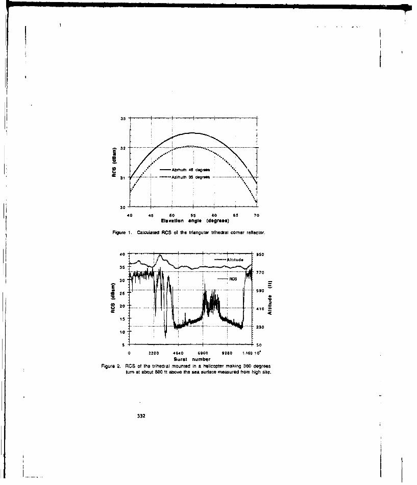
!I-33 - , I - . . .

I N3 2 .. .. . . . . . . ... .... .

30I I40 45 50 55 60 65 70

Elevation angle (degrees)

Figure 1. Calculated RCS of the Iriangular trihedral comer reflector.

40 9 50

/... Altitude35

30 RCSS. ... . . . . ..... . . . ..... . ....... o

S256

15T

o 2320 4640 6960 9280 1.160 1o

Burst number

Figure 2. RCS of the trihedlral mounted in a helicopter making 360 degreesturn at about 800 ft above the sea surface measured from high site.

332

40 (i0

i 35 -. 25

2502 20

25 2

20 W*A1Ig

0 3400 600 is le0 1*010 moleID 0 3600 1200 AO 1. 4410 1 .~ 0' 13omitBoos msour Bust "bon

Fort3. AI00devW RCS 0 m sauemeaot6 Fga t A douAMSof t~it 1 ~manmm

45 15C 45 15-I ' -$ ' ' s-~ -lliuRs- ~ Altdude

40. .... 40 .. .... . . ..... ..5- 12012

1'9 toI

4 to

til O 25 ~ ...... ... ..0' ...0.

20 ........ ....... 3 r 3Fyn~20

05ii~bw~dgu ~~~

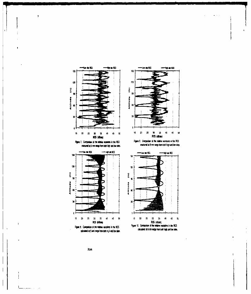
30 3

15 20 2630 M A 15 i : 1 20 5 I c 4 s

ISO

314is 2 s 30 35 4 5 5ss0s 20 2 0 35 4 5 s

adw f1 mia ;.nbm L. a N334

ON THlE EE(IMR BOU7TIIP OF A TTPICAL DINEERI33

Reding Irustemser seeks. eedling Wines. Chios

Tkia paper istrodaceso a benchmrk model closed to a typical loas problem in electricalsaghneeriag. proesets the testing results of eddy currents, magnetic flux densities aidpowr losses with respect to the model, further verifies the available comuter codes.

1. WmxuMIi CACGROiW

?he total stray-fielid lose of large poin transformers ceased is windings and structuralperteill can he obtained by loi-lues test, howver, it is difficult to exactly determinethe distrihution of total loess ehier by experiment or by analysis, moreover, the comutingresults of so large engineer ing field problem to set be sttrictly ver if ied.

It is really necessary to establieh a reduced prehlum-oriented modal which enable us tohave th inetrested data ia detail, for ample. the 3-D mignptic flun densities and eddycurreata nloulding their weveforms, tie distribitiss of the stray- field Ioases thehysteresis and shielding effert&setc., mid various available computer codas can be furthervatlf led through this hecasebk model.

Twin stray-fielad looe models (A & 9 13-4 hive been msde a isBeding Transformer Works.laodleg. China. Fit~ I shoes the eagfinter lag hukeahed of the model.

2. E~MIU am

2. 1 Dusacript io of the modelI (A AMoedl B consists of two air-core exciting coils and a steel plate with no hole is set

near the ceilLa the exciting curretsilt flowing in differant coilsa ue in the oppositedireCtims.

Tie Moeal A has the am exciting coils an Meda I and two setol plates being nearby thecells. In the cutter Of 46e Steel Plate Of Mode A tharat is A hole.2.3 Inpuat parameters

The dimmasloos or the steel platas and the cells wire ilm in fig. 2. the otherparomters are aI follows:

3.2.1 litesi plate(s) B-H carve was shen in Fig, 3(hI Conductivity 18l0: &S75iolir at 20 IC

2.2.2 Ieciting coil(a) Turn Ratber of each coil: 300 turns.(hI Kxciting current (ALr, 50 Hz): 11 0W (row).(c) Disensios and conductivity of copper wire,

335

3. 0 eve thickness aid 6,.7 ev ksi~bt for bate wire.The not saetiosal area of the wir , its .0I 4 agsaCcudertivitY 0/0 1 &7148910' at so tC

2. 3 Quest ities ato be eaciuted and nmeauredL.&.1 Magnetic flax densities at specified positions, se. fig 4 and Table 1;3. &. 2 Punt lesses caused it the steel plates, eve Table 2;2.3& 3 Total astigmtic flux laterlialted vith steel plate at specified positions, see Pit. 5

and Table %;L.3.4 Total magnetic fln laterliabod ulth the exalting rolls, ase Fig. 6 and Table 4;23.5 Eddy cntrrents at specifiled positions a the atrface of eteel plates, eve Fig 7 and

Table 6:L.L.6 Iddy current lesses caused is the excitlag coils with and without steel plate, see

T"abl s.

3. TESTING RMmS

The 3-D ediy current codes humid a the T- 0 11-21, the At-V-Ar 121 and the cinhinat ion ofthe T- * and the At-V-Ar IS] developed by sauthottre maised to analyze the models In both thetuehan aramic mad the transient ea114s. The brich elemenmt with S modia aid the PIOD solverlars "dopted.

The mirror- impsemethod was ased to calculate the msagntic field and eddy current lossesof exciting coils for "ode I The I-D ?A3 cede chow, a 2-D distribution of magnetic fieldan the Sjtric pAlane Of the models

The Guavomter imds by P. w.hBa) was vied to macasre the magnetic flut densities atspecified positivesa octead& steel plate. while the ' isterlished coils' wers ased forwasur lemgneotIc flux deasities inside steel plate, as shion in fig. M3 The waveforms ofthe flu deneities were obtained by a I emspater- aided- test' systemr developed by authors, ofvell an the waireform of the eddy currants at specified positiosas the surface of steelplaces.

Bizet total stray-field losasas wre distributed in both steel plates and exciting roils,to split themm a comimid method of experiment and analysis u we ued, L e., the total stray--field lessee ware meunanrd vhile both the losesa of the coils and the losses of steelplate Tors calculated

Sies watured and compted results of magnetic flux densities, eddy currents and passsrlusts were shown in FIg. 8-14 and Table 1-6.

4. OMEMICE

The henclawk model described here Is quits closed to the stray-field lose problem inpint transforMers Tie detailed testiag of the probleso-or lasted model to ve~rify variouspossible analysis mesthods is acressary beforc solving smrs general pta. ats problem.The presented results of magnetic flux doasities, eddy currents and power losease withrespect to the mOde sem to he satiafactory.

Acknowledgement

336

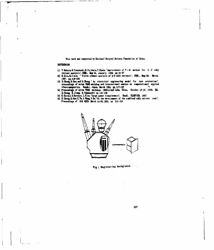
?hJi work we supported by Natioal Natural ScieRce Foundation of CIliA.

II] T.)Nahtm.XTakihashi.KFmjlivra.Y.Okade. ']mpravcentm of T- method for 3- D eddyenrreat "slyais', JaI, iMag--4, January, 198L. pp. 94-97

WI] O.3ire.LFreis, ' Visite lemat analysis of 1-D eddy currents', 1B , Mieg-20, march.I119, pp.418-435

13] L am&l.Ga@ .ad i.LZhae' An electrical eaglineriag model for loss evaluation',procludings of Aslin TINA rkusklp and iatessatismal laminar so eomptatioonl appliedeleetrioggetism, 8"e1d, JapaL liarck 1)l, pp. 117-113

14] Prseeidings of Ailmt 1AM werkshop, lO0lulsad Lake, Cias. October 18-19, 1992, (Ed.LCIhig, LJinu& KTnakaichi) pp. 131-13

151 LKratmi,iD.Keramyl, Kl Kim'Larp pemr treaformsts', (Book), EhViC . 1987I61 &CMog, & Gas CTo.J.lungP.Ah, 'On the developent of the combined eddy current code',

Proceedings of 8tk AS MArch 16-30, 1192, pp. 314-330

I //

Pig., jiglneering background

337

I __ _

f9. 1 40 RodtdI A

fig.3.-I'.) V4# ,I I ho T-(ATI .3N.0

S61141-4 cum" aallY

I ab.oonow

ma uleam 1 ' 61

0 CGIL2gof~h..

1113 Imadt'eel~.. * L A

338

1 MODEL A ibý MODELasPitt Spit ld wUiling fe gum art""

pi .(eeof ta P AUSM

Pig 4 reirku Peehimta. 90.tic v .

t SL 30K3ml

I.a~. 10. - ... ~

a) PL 7L T-tLON Position 1.. s it 4-Oi

Fig sp~ire pultifm fee touta fin 5

tateril" ek $lk plate4Ph .herm d..hLu. mpAWtIh

-" .1. offs Will) J-0..3 122. of (AIM)

J--3303 704 (7))

bea. ~14Su11. 10. .

W, y-in 16?"we1.3 a) Point V for 10440 A. am Fig. 7

*. DaisI(AMU)

.' t# AIN P\IN

.6 044 A/U) J...1471.A4 (Ai11)

ad =16 0I1 a1/4 regio wa MuIYW &*I2Pasca: 7ow o * r~ vlt hI. a a s

Of wapplied Va194g.* 141 fo kr-T-A*1 dill T. 10 1, Pa~int S for moeal L. go* Fig. 7

CSbW 13 Ur* aIwag SC 1 d

.21.3044 (AIN')

.7. 60.. m

rig0 ~ia4,istatirm at 6 mI. C daofMI I c) point P for moeal A amet Fig.?7

1. +if (A lto) I1Gm )4

100. 0 0(0O

1- .8414 (AW)0 1. 24.

304 P W0 16.1000.6-.96. 01. Itse Fig., U)

in, r~vluet ofl (hsdisity: 57.0IGOtoo.$ooa

.7.46 $34 (AY

/N4 1`11 M 76. 0. 0.97.0 5) sae F o. 4(bM

i4app\1e a 000.4 roem vales of flzz density: 31-01G

4D point L for Metld IL Iq Peg 00. 11*l. 260+6 UlmN')

-L4(0.70.a 200. 0 F4 see fig. 4 Wb2(J.....,236I 2".0 (AW1 ) 000 ms Talte of [tl dosslty: 11,708

52. 04 *1 (A/U(Z Ot1.0 3.0 1(0 0*

In P$0Z. 76,0.0.0. 0). s. Fig. IlL)IV 3 V - ram valet of rise density; 152. SGs

-7. $44 M ,..6611(1

200.4

ag .0 0.0.1 .,a 81cr aie .cm ~. -100.0

*. 044 (AJIM' -060.6o

'j:2 -4n d- 42 (Ge) P66 4 0400), See Fig. 4 (M

IN,/) 30. too 'alum tt 01 density: 126. lGs

Al A.4111116.

1.0 3.0

\1 -00 0:§

.1. 60 +1 M 0) (AW) Fig s3simform of swti flue densitiesCS - a It pmesoribed .titimIL

\-J \alm P oats

medel 0. Fig.

P

at puueorsbed poseeiewsM fig?7

341

&h.43 80,)rlsedtoa

P91.0fil et: 1080. 40. t-0I

0INTCULIUCDUCO110 .

31.834.2Gs) PositisaL so* Fit.& eot

1. \la 3 4.0 t Oi .11

X Position C.689 rog.6

40' rus valve o istoIrlinked total

a) MO~DE A b) NOCEL S U 3F7(71.5.0, 1eS. ml. Ie j1.12

?Ite isle efstw ofer~ee rmB fv .#ri%

el. e 1 lu stee plate$e atesitlae "Iiglulsi Fig Sh.A (m, 6 Cke Wmee liv wreeeo

itl,16 totuale fslux imstwiwm witha steel pit

1113. 9s ed Vale I of i.,h ed iskedl ax

4342

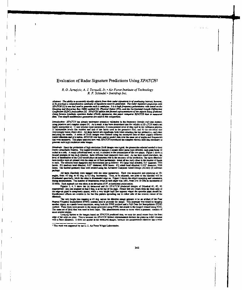
Evaluation of Radar Signature Predictions Using XPATCH1

R. 0. Jernewjdc, A. 1. TerztuoU. Jr. * Air Force Institute of TechnologyR. F. Schindel -Sverdrup Inc.

Abonso MabisUVAP -- aut ww i Hemqec.tsfmodn. t ai ~ rgm awIefwinagievs hews.',

XPATCH I) ax-. S o~omeL edi z. aut a ealhin Ilia a hih jlmquiwey ~lpWiigmic ceik batdem theSh loru OaW Bemacug A"7 (SBR) mailed Ill, Physicle 09*5 (O), -md ie IucveWdm L-sgt DofwilanCeaffatat'(LDC) fm*W -j~ia 31 XPATCH .aig.' , fma d ,p~wm-es f the aWfbjr dqpvddekMauiag1 e., Syn~ahab Aparw And- (MRA) stg -s Ahps p--'mp-X PATCffd-*9in wad

Ass Two aiWle wmalihuwe Seemoim me assi inad emalwmpf.

Iab'ndeedea XPArCH1 has already unadenone extmave vallislailo in Mhe frequency doma n rd time dooma,hingh piinretive trioe 1) in.' saelete n4ut As reul. 2) nasbeendtzerminaeofda'td tha the validat fX-THrsulo s p teohiughl prmiu ta 1) wer shleced (4.np u lIt haamtes. 2) deasuementero d at the i the validityo ofX-.TH uti wes3) facechasloo levels (the atmber and szea of Whe faces used in dhe geometry file), and 4) the electrical size(wavelmos venous object sma). ADl these (samt am sgilalltn. both when selecing the rest geometries. and whenanalzing the meain. A series of ISAR images wet Meaimed using the measured data of three slightly differenloade dihedrals and of a opbs. )LPATOI was thn used w predict da over the ame sot of angles and frqeqtmcesthat were scaiwaed. 'This poper only= how well ".AIM repunhm the complex dectric field datanecessay togeneat um ni high molnudon radar images.

Dihedraufi' Siame Me production of high reokstion ISM himages was a Zo@L. the geomerie selected waeded to havereadly identifiable ctmeam. ' luaded dihedal is boxially a sq- Wied metl right dibedral. meac plink being 12inches ta a side. A metal cyllisdricai bond, or rod. is =ahd" io she inlsersctime of die two pline. Figure I shows afatsdas of 0 oft meb dihedral; three dilftereti bud dihues; wn used. As hat beern noted elsewhere. thelevel of liceuion of the CAD model plays -n heinmeo role in she waccray of the prediction. The threee dihethnlsfamemodtla wer all anesd widh dhe muot wo~fattrmn ets; beaall wenirty cleat inthe smabof facetsin ek The M dihedil h dimein ad famrsmes nee aas fllws: #1) large bead dhedraL 0.5' damewe, 7954

(se; #2) maium head dihedral. 0.2' diseser, 6M5 beats; #3) small badihdral. .123' damter. 509faces., 11e faOWpmed m y fles wierae*5n the Advanced Computer Aided Design (ACA)) [51 softwareI ' .

All tkf dibedrals -et baged with doe am parmeters. Each was measured and predicted at 181miles. from .45 deg. mo 45 deg. in 035 deg. incremenra. Thrus, atOo asimath. one plane of use dibedral will beiflusiamaid qseinlmly. while the o*5 ia illuimunawd edge am. Pilgm 2 shos ft he bect aistinnsg and oeimassiondorsalg mmument. The amaber of freummies swept ma each anglle was, 160L. from 2 aso 18 Glu a marnem of20MLis Eahch w cot a m enas devadmo of 0. aibxoerml pomizudo

ftwes 3.,4.5 show the, (a) measued and (b) XPATrCH predicted images of Dihedral 01, #2, #3respectkely' theywe orMeso sbu 00g. it aate up of the pg. Poc dot any om n frm the houe edge ofthe edge-ce Plante is complemly abenot, while a very bigMhtard line -~w whnese the specula plane should be.Mbltiboance effecta we evW=idnts the fan Nota pee spreading out to either side of the iolncini counm of the(11111110111

The very bright line riumig FAt45 deg. acrss fth dihedra impapepeuar to he an alliact of ate PoorNewrest Neighbor latnpolation (PNNI) scheme used IDto gusme the image. This pmsiltwm was asiod by Imagnmother objectsit a much lower resolotion, using both die FNNI method and a rail Data Set Interpolation, (FDSI)todid. Thene lines wa present in the image processed using RNNI. btu absen in the imaged created! using l'1)SLThe same set of el thean was med a both came. Thais phenomeneon seems to cetwhent a gemaetu consists ofacute 'intro angLes

Looking further at the images based ono XPATCH predlicted data, we not she =All return from the frontedge of the edge-on plate. This us because the XPATCH fetdrepireenombon models the plaite$ as solid Voluzuewith a finite tbitlesis. It does not appear in th measured images. because the measurement chabrrie has a noise

This wait was suportedl by the U. S. Air Forem Wright Laborasneies.

343

fioer such that signals dow toorn below this value ar masked by clsmer boise; of Comte XPATCH has no Richrestriction. Ntices Also the ghost line tming isoewhat diagonally behind the dihedral image, which Weabsent in the smosaed kDp. The ar e somewhat less noticale in fth XPATCH preedicted umage of dihedra #2(Figure 4(b)). and we completely ashame for dihedral #3 (17ignee S(b)). Thus it could be due to the bead runningalong the inside of the coer, Au the bead gets smale, the lDnes disappear. Notice also that the RF1NI diagonalstreak is nearly invisible so Figure 5(b).

Figum 6 shows eanapanded image of dihedral 03. Notice how fin away the multlboumce signal extendsfioes the object MAlo note the Not astoe Ingle FNNI Indnced line smunng through the cotmer of the dibedral'simage which exiuas out to* Unl~its of the smage frmame, with al Sp of dIminishing. For a very' complexgeomety. tim pbsminm could cim thin image 0 o So Makes it tmeCOplzthle.

Topkat 1Ue teploo codt 01 a 0.5 - Msn by 0.5 mitw diameter metal cylide with a 135 meermacttcicualr metal ploo anced u one tad. Mwh gpommy Is showns In fatmed form in Figure 7. Th1s objec was

md sure!ad predicted at 701 ingle. from -5 dog. to 105 des. in inermenesa 01 0.15 deg.. The number offremencie sw~ep at eac angle war 1601, fran 20Hz ato 10Hz to lomemua of 20 Mfz. Faich aimntb cut was

mnsat me dev~satino 5.5 doga b- - ] peolparization. The slightly postiive elevation cut was chosen to beingout mote of the cote edge of the brim of she arphas Had it bee imaged at 0 deg. elevation, the brim would haewbeea simpl a maighlint.Hs aimilw to the broaside plows an the dihe-1ral mae. Figure & shows the motunting andorienaton of the topo a it war mearwed

Becans of the size and weighst 01 the tophat it was necessay to mount it permanently on a counter-weiglnd. clse hem. ibis was dos afl had to a eas" pale that attachd to the pylon rotato. The top"a ACADmodel dad see include the channl beeam. FPgm 9 shows the measured lohat image. It at much casier to see theVVINK in thin imale, dos it wa to methe dihedral - thei respecthivae si The him is well dellned, as is theImolor edge w~hare th cybderarms the brim. In this Image. doe radar was swept acros the tpper right quadrantattb Otae o st 3 dog o aW o eticalB0 m 10 dog. panthe rigkht adedge of thae brm ecamreof this, weme mer detail on Oe right Aft Waig spoolhermum from the right side of the cylinder. On the right side, notedhe multiamee speeading at the pam where fth cylinder and hinst meet. We can also see a small amount of edgedifftaceoo ha omi the left side of the end of the cylinder (Imbeled Poin A).

The WAmY high rem, --i fromt the M&c side of the ugihat is the result of the channel beam bolted tothe back of do e (inuaui by Faist 8). Beans is was puaumently mounted to fth topbat. vector subtractsonCousld not he used to elimiate hto mumr. Inusted electrie Rader Absorbing Material (FLAW.4 was wrapped smundthe fixtur, the woghs med No coma-bala th U m and. th U nsumg pole affixed to the pedestal rotator. Inaddibus the bb& masoro of me himn war coaled with mAgei RAM. to pe.ent traveling waves acrots the back ofdth brim. While this did sact copletey mask the mambuig bean u did geadly reduce its noten.

Neut we leok at the ISAR soup as predicted by XPATCH. In 9S=e 10. we immediately onotce the welldefined bhim of the sophat. Also apparent is the high setam from, the intersecton of the cyline and hrim,particualy an Utghe t aide. We can ses the chtmristo Bnoting (or Whobmg etigonaLLy from this point. As withth diliedcuis. fth is posdely a manfestaton of the multiboessee effiecs. It Is aIprtin the measured image as well.though 00 a letter exaent Again this lsAtey the smtst 01 the fUnm vim flowt io the meoratemni range. We alsome a nsml fromu fronmt iefed 01U cylinder. jousta in die smeareed Wmage (lOWA Am FIgX= 9).

The m m~ lin shae inthe pend ranfrmthe rightlside ofthe cylinder. This was causedinthe meameedt kop. by a bu ie~ illa aloo of diecylinder. atm sacident wsuth of(90 deg.. WhileXPATCHfdoes not ptsdt eumma tWes of scanning phtnomenoe such as tip dilmcdo n d oavellagiereping waves. none01 thse would, he dominn t Us pariular musith. Fmamizasso is am Histy, lemon for Els anomaly. In hisarticle on the effects of hoomso level on XPATCH pmedctsons Mille (6] saote tha sbout 10,000 faesa weregenerally needed an amos mý emud, fora dmthly curved object sch as the almond. It is possible that at thispaesircu elevami at 05.3 deg., ther am too kw facet on th sides of thes cylinder dthe is perpendicular to theineiem wave.

Tarting this hypothesis. mother set 01 predictsd dat Was genOsed. Wish a 100 meg. sperture coweed inincreens of 0.15 deg. and the ftuquicy swept Froms 2 so 18 0Hz in 25 WhsIaonps. The image maessed frout thisdams is shown in Figure 11. T1his diffuemo ase of angles and frequonmie would insuie that a differont set o( sayssturoi the object, wish a dftmt may density and set of incidence angles. As ame can see, the cylinder edge mkIssnto the previusn image is now there. So it couldi he the result of fouzations asses, or an artifact of the inamagnproces. Except for dthi ame moosumsiscy. theXPATCR1 mage apeasma to he a good woatch with the seastered.

Cancleaivit: This set of simple objects was =se to evsluate XPATCH'S ability to produe. high resolution ISARounges. Of pasictul ismesest was Uh ect= of multiple bounoces of the incident wave on the image. These testshighlightled the codes caprhAlifies and laaiimcons, as wsell as factors and parmeters that could significantly effect

344

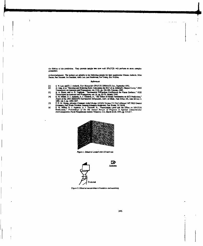
the fidelity of Whe pradiction. They provide iesight haa bow wall XPATCH will perforns ont mome oiplexgieoieffV

Ackheuiedguau&Th lbauthOr are Fateul to the oldlOwing peoplec for their Inglakms: Dennis Andersh. MikeHazier. Paul Sk-i-,a Joe Sacchlizi Andy I&-- Lee Headerson. 3m Yom&g, Eric Walton.

AOI-

[I] S. W. Lee. and D. J. Anadmh, User Moamaorfc'PAIOI, DEMACO. Inc.. September 1993.121 Ii. Ling. at. &"Shooting sod Doutchag Rays: Caklatlain the RCS of -n Arbtraruily Shaped Cavity,' IEEE

TrasctiowuoAxw an nu d Aryngarkm. vol. 37(2). pp. lId-205. Fdnwy 1989.[3] IL A. Shore and A. D. Yaghissi. laaowmssectl DiffZaetim Coefficints for Plana Smfaocs,' IEEE

Troasamcr rot Antwdsa ad PmMpqeon. vol. K6 pp. 55-70, Januay 1988.[41 E. M. MIllor, D. 7. Anderah. A. J. To=* Jr, 'The Effect of Moda Facedudonf ons RCS ftedilimma"

rnea of the 1993 IEELAPS Istanatwnnonl Sywr'osums. Univ. of Mcb. Aso Attan, NM. June 2S-iuly 2II9M, vol.3. Mp 1406-1407.

151 P. D. M. Gtotep6 Adanice Compsier Aidrd Design (ACAD) Version 7.2 Vier's Nzanl . W 2635 GeneualDyniscica Fort Worth Dhvsm Umersi Dynaic Doutermi, Fort Worth, 'TX 76 101

(6] E. M. MUilr. D. J. Abdersb. A. J. Terrnoli, Jr.. 'Fsacauao Level and the Effect on XPATCHPreclictions,. Proceeingsr of the 9th Anauwal Review of Pro~pess in Applied ComaputationalElectrUaIVrimcs. Naval Postpubitase School, Monsc.ey, CA. Match 22-26.1993. pp. 610-617.

Figure1. Dihedra Loodled with 0/ buch rod

Aa

Rl .destal

Figure 2Z Dihedral measurem'ent oflenunstoc and mounting,

345

F89-3. DiOW&L 01. lar bet H -pot 2-18 Gift in 20 MHz nApt. -4S at, 4Sdrg. in as deg. iaps.

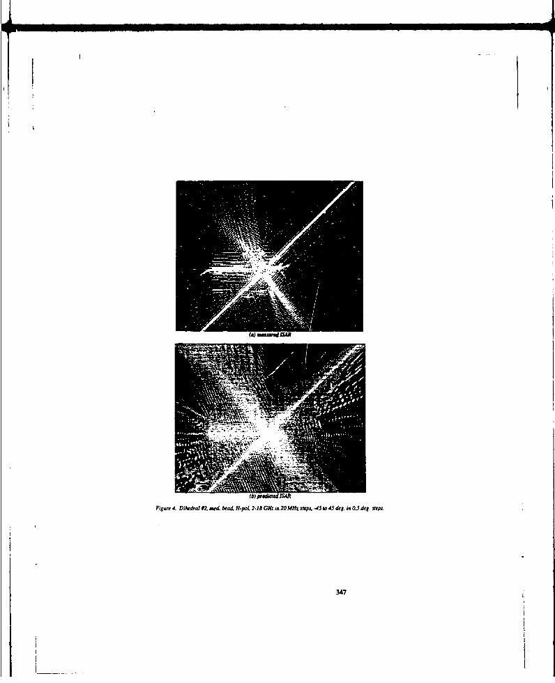
Figuire 4. Dihedral #2, metL bead, If po 2-18 G~z ift 20 MMz sieps. -45wt 45 deg. in 0.5 deg, xrepst

347

Fa~ww 5. Dike" 03. w" nnlbw H-po4 2-18 G~z in20 MI~z zaPS, -45 045 *f.- imOS deg, ttePs.

348

Figured. DUWhed m r-Ujsl beeH-paL 2-18Gl in 2M~h mpsý .45 w45 dug. inf65dag. aepa apmdedaedj& of view,

Figure 7. Fracted wreseneaflon afof sca ks 5.566facel.

349

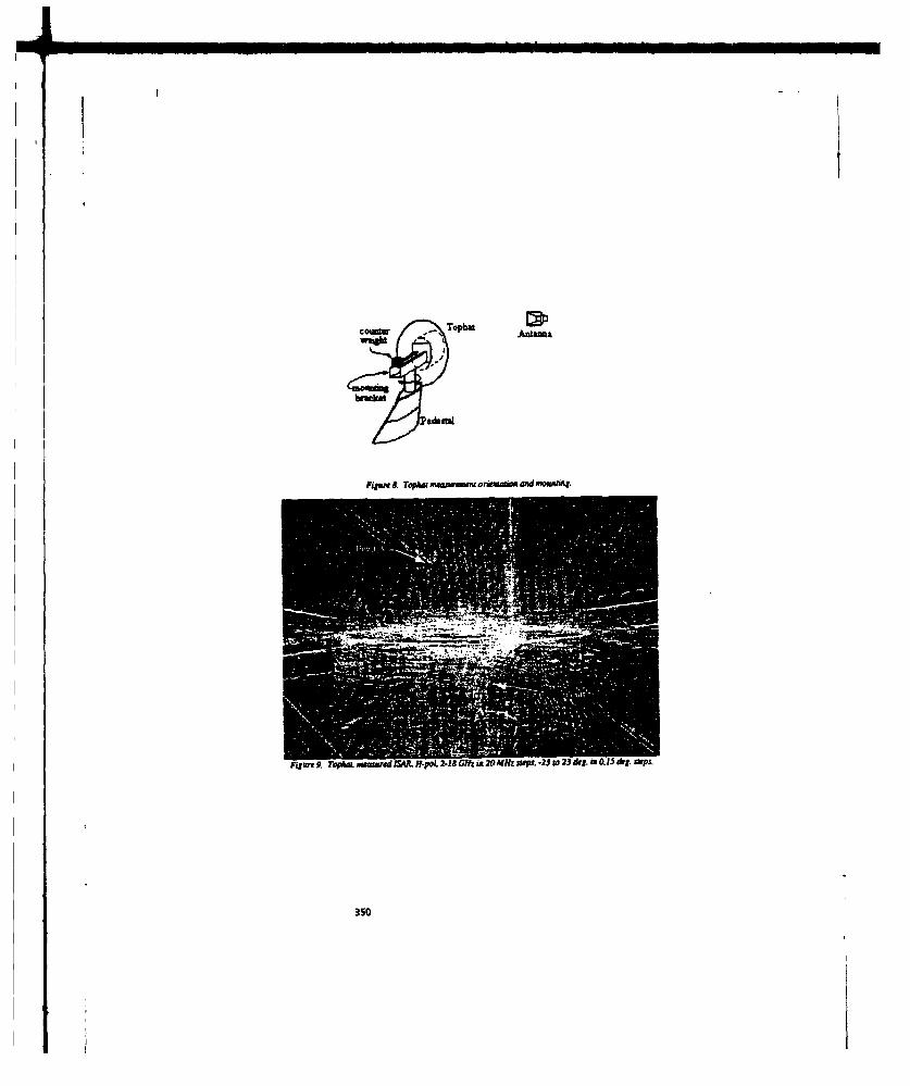
-Tophat

bedassa

350

Fg.11. WATCH prt aM15hZw=n lofreq wnms sd 6$6&vans 1N-04

351

Transformable Scale kircraft-Likoe Model or the Validation of

Computational Sleatzamagnotic Models and Algorithms

by

Donald R. Pflug and Daniel R. WarrenRome Laboratory525 broOa* Road

Griffiss Ara, MY 13441-4505

A novel technique which utilizes measurements on a Transformable ScaleAircraft-Like Model (TSAR) to validate computational electr•omagnetics(MM) computer codes is described. Good agreament between measured andsimulated data is necessary in order to validate algorithms and modelsresiding within large computational electrceagnetics (CU) codes. Ifcomputation and measurement errors are sufficiently small or are known,the remaining differences between simulated and measured data can beat~tributed to algorithm and modeling limitations within the code. Thecombination of these errors (simulation error) often can be estimatedbut not the individual errors. The novelty in the technique is to makemeasurements on a scale aircraft-like modal that is a duplicate, inboth form and substance, of the model in the code. Differences betweenmeasured and simulated data then can be attributed to algorithm errorsince measured and simulated aircraft models coincide, From knowledgeof both algorithm and simulation errors, modeling error now can beestimatod. Xodeling and simulation errors Can be adjusted separatelyas required to minimize simulation and measurement differences.Measuremants as a validation tool now become more useful and helpful.Initially TSAR will be fabricated using conducting canonic shapes andsimple radiation sources. over time it is expected that the TSAN willbe modified by installing new components that correspond to n•ew CUsimulation capabilities. Measurements on the transformed TSAM then willbe used to validate the improved simulation. Advanced TSAM componentsare expected to include nonmetallic materials, doubly curved surfaces,realistic aircraft shapes and more sophisticated radiation sourcas.

During the last twenty years a large number of computationalelectromagnetics (CUK) codes have been developed by numerousindividuals a7.i organizations. These codes range from large, multi-purpose, widely dimtributed, well maintained and validated simulationsemploying established numerical techniques individually or in hybridcombinations to perform system level CEU analysis to smaller,specialized codes developed by individual researchers using state-of-the-art methods to attack very specialized or specific sets ofproblems.

352

A very important aspect in the development of any CZ4 code isvalidation. The problems associated with code validation areparticularly acute for large codes involving numerous modules andprogram paths. One validation method is to compare results fromdifferent codes. The code under test analyzes standard or benchmarkproblems whose answers are known very accurately. Such an approach,while very useful, may provide only limited validation because a smallor special part of the code may be tested and the solutions may be ofpractical use only over a limited frequency range. Another method,comeonly used for codes distributed in the C community, is to enalyzea wide variety of CEN problems over time which collectively test allcode modules. Guch analysis cmonly is performed during codedevelopmemt but also can be provided as feedback by the user communityto the coda developer. This method can be used repeatedly over the lifecycle of the code and provides "lessons learnedO data as well asvalidation. As new problem are analysed over time, code maintenance,modification and enhancements are performed and validation isaccomplished by comparison to other simulation results or measurementsas the code evolves and matures. Unfortunately, different simulationsdo not analyze a problem identically even if both use the same analysistechniques, implement the same algorithms and modelig scheames, or usethe same coding practices. Also, it is usually difficult or impossibleto relate the differences observed between the CEN code output andvalidation data to specific limitations within, the code quantitativelyor even qualitatively. Hopefully, trends in the results will beconsistent and the collective numerical data reasonably close tomeasurements and other simulated data.

The best CEK code validation is good agreement between aimulatedreaults and carefully controlled measured data. Unfortunately, thedifferences observed between simulation and measurement are difficultto explain and are analogous to and are as difficult to quantify as thedifferences between simulation and simulation. A further complicationis that "good agreeamentO depends on the sophistication of both themodeling and algorithms implemented in the code and externalmeasurements performed for validation.

These difficulties in interpretation that are encountered whencomparing simulations and measurements form a common thread runningthrough CE( validat4on. In this paper, a novel tajt article, theTransformable Scale Aircraft.Like Model (TIAM), is described. Thespecial configuration of the TSAM is designed to mirror the modelingcapabilities of a given CEM code exactly and, as a consequence, appearsto hold great prorise for allowing alyoritham and modeling errors withina CR6 code to be assessed qualitatively and quantitatively usingmeasurements on the TSAM as a quide. Both errors then can be adjustedas necessary to achieve a given level of code simulation accuracy. TheCEI code to be used initially for simulation is the GeneralElectromagnetic Model for the Analysis of Complex Systems (GCDACS) [1]but the TSAN validation methodology is applicable to CED codes ingeneral, The TSAM appears to open the door to using measurements tovalidate CEM codes in a more informative and useful way.

353

C= code jAliQaj•j &ad the =M Const

when the results of 3imulation are compared to measurement, differencesare always present %nd ultimately place a limit on the accuracy towhich CEN codes can be validated by measurements. Figure 1 shows acomparison between measured and simulated (GE(ACS) radiation patternsfro an aircraft antenna. There is general agreement overall but thereare apparent difference* in lucation of pattern maxima and minima aswell as in pattern shape and power levels. These differences are dueprincipally to the following factors: limitations within the code onmodeling of the goometry and physics of the problem (modeling error);limitations in Loth the equations used by the code to describe therelevant alectromagnetic pheomena and in their specific implementationwit.in the code (a.gorithm error); limitations in the computationalapeklities of the computer platform hostinxj the code (computation

error), and limitations in miasurement accuracy (measurement error).'-he combination of these errors (simulation error) can be estimatedcoempr.nq the results from the code against measurements for arepresentativa set of CE4 problams. The individual errors typically arenot known and may be mutually dependent. In this paper, it will beassumed that both computation error (typically computer round-offerror) and measurement error either are known or are sufficiently smallso as to be unimpcrtant. Simulation error in this case then reduces tomodeling and algorithm error.

The novelty in the technique is to make measurements on a scaleaircraft-like model that is a duplicate, in both form and substance,of the model developed for use by the code. Differences betweenmeasured �..d simulaed data then can be attributed only to algorithmerror sines measured and simulated aircraft models coincide. Fromknowledge of algorithm error and simulation error, modeling error canbe estimatod and mdjxsted if necessary. Differences between measurementand simulatior now point to specific causes. TSAM will be composed ofreplaceable parts coeanw to coincide with the current modelingcepahilities of the code. As the CME code evolves and matures, the TSAMparts and configuration will evolve and mature to match the simulation.Detail will be added incrementally to the TSAM to match incrementaladvances in code simulation capability. Measurements will be performedto validate code modificrtiorz at every step.

TSAM initially will be aircraft-like in the sense that canonic shapessuch as cylinders and flat plates will be configured to resemble a wideb-oied airceft. The TAN zimensions were chosen to representapproximately a 1/20 scaliLng in frequency. All measurements

-ot elated to date will be done in an Lnechoic chamber facility atRxome Laboratory.

?BAN TaltitAl CofiOLTAtiom

The first TSAM dasiqn has been chosen to conform roughly to the generalsha.pe of a wide bodied airborne platform. Thi3 initial TSAM testarticle will be a metallic st-ructure fabricated from highly conductingmaterials, such as aluminum ond copper, and composed of several canonic

354

shapes to represent wings, fuselage, stabilizers, engine nacelles andengine pylons. Each canonic shape can be modeled exactly in principleusing the GMACS code.

The design and dimensions of the TSAM (1/20 scale model) are shown inFigure 2. This initial configuration incorporates a hollow ellipticalcylinder capped at both ends as a fuselage, two thin flat plates aswings, three thin plates as the horizonal and vertical stabilizers,four uncapped circular cylinders as engine nacelles and four thinplates for pylons. The elliptical cylinder is capped in front to form"a blunt model for the nose section and is capped in the rear to form"a tapered tail section. All components are hinged and individuallyremovable. The geometry of each component can be modeled exactly inprinciple by GDNCS and the complete metallic structure is assumedperfectly conducting. Since the wings of a wide bodied aircraft flexconsiderably in flight, both thin plates serving as wings will behinged in order to vary the wing cant. Fuselage rigidity is maintainedby an I-beam positioned Lnside the hollow elliptical cylinder as shownin Figure 3. This I-beam also serves to position and support a scalemodel antenna on the TSAM. The complete TSAM test article is shown inFigure 4.

YSSN XIitial Nzeitation

The TSAM will be excited by one or more antennas mounted directly onthe structure. Initially, antennas will be either thin wires or conesthat serve as monopoles, the cone antennas providing a wider bandwidth.The antenna to be excited will be connected to a 50 Ohm cable threadedthrough the antenna mounting structure to the antenna under test.Pattern measurements will be done for all antennas, both in the absenceand presence of the test article, in an anechoic chamber using standardmeasurement techniques. It is anticipated that coupling measuresentsbetween pairs of antennas on TSAM also will be performed using anetwork analyzer which will sweep over the relevant range offrequencies.

The ability of GUIACS to analyze large, system level electromagneticproblems and the presence within GEMACS of a variety of analysistechniques and solution algorithms sake it a logical first choice foruse with the TSAM. GD4ACS was developed to analyze system-levelelectromagnetic interactions between sources and general materialbodies having a complex geometry. The analysis is performed in thefrequency domain using modem numerical techniques such as the methodof moments (MO), uniform theory of diffraction (UTD), and finitedifferences (FD) either individually or in hybrid combination. Thevarious regions of external problems are treated using an appropriatecombination of MOM and GTD techniques while internal problems aretreated using finite differences. Coupling between exterior andinterior regions is achieved by matching exterior and interiorsolutions at apertures using appropriate boundary conditions.

355

A number of solution techniques exist within GDIACS to efficientlysolve for the unknowns in the problem under study. Matrix techniquesinclude a full-matrix lower-upper decomposition (LUD) algorithm, abanded-matrix iteration (BMI) algorithm and algorithms for handlingrotational or planar symmetry. A model order reduction (MOR) algorithmfor reducing matrix size is also is available whenever FD is used.Electromagnetic sources include incident fields, excitations on antennastructure, and specific antenna and radiator patterns. GEKACS outputthat is particularly useful includes radiation patterns from sourceson the structure that include the distortions of the structure.

A novel and promising validation methodology has been described inwhich measurements on a specialized test article, the TSAR, are usedto determine the quality of the modeling and analysis techniquesresiding in advanced Cal simulation programs. The use of the TSAM makesit possible to distinguish COE. modeling error from algorithm error.Deficiencies in CEa simulations are identified more specifically andmeasurements are better understood and thus become m,)re useful andhelpful as a validation tool. The configuration chosen for the TSARmust mirror the simulation capabilities of the CDI code being studied.Initially, the TSAJ configuration will be chosen to match thecapabilities of GWDACS which approximates system-level complexgeometries with a set of canonic shapes (wires, cylinders and flatplates).

Because aircraft wings are a major source of multipath and the GEMACSfuselage model is rather crude, the evolution of canonic models for theTSAR will focus initially on them. The next TSAM wing design will mostlikely have a triangular cross section followed by a similar wing witha rounded leading edge and camber. Finally a scale model of an actualwing design will be used. The rear stabilizers will undergo a similarevolution. The current GEIACS fuselage is either a blunt truncatedcapped cylinder or is constiuct*ed from a series of connected platestapered at different angles :o form a nose. both models will evolvetowards an actual fuselage in several steps where geometry becomesprogressively smoother and more realistic. Sources, it is hoped, canevolve to small flush mounted elements or arrays. Finally, it isplanned that the TSAR will contain nonmetallic materials.

1.Z. L. Coffey UII and D. L. Kadlee, General Electromagnetic Model forthe Analysis of Complex Systems (GWMACS), Version 5.0, AdvancedElectromagnetica, RADC-TR-90-360, Volumes 1,II,111, December 1990.

356

0g

Figuare 1. Antenna Pattern Measured and Simulated Data

357

7AO

6 6 ,• 66 N ' - /--TlG-" z7;l -. , - SA

Fiqur. 2. TSAN Desiqn and Dimensions (Inches)

358

2igUrS 3. TSAR Internal Layout

rip are 4. TSAR Complete StruCture

359

INFRARED VERIFICATION of ELECTROMAGNETIC CODE PREDICTIONS

Sydney Blocher, John Norgard, Joseph Sadler,Ronald Sega", William Prather

Microwave Research GroupUSAF Phillips Laboratory (PLMWSR)

3550 Aberdeen Avenue SEKirtlend AFB. NIl 87117-5776

ABSTRACT

An infrared (IR) imaging technique has been developed to map two-dimensional electric field distributions near an emitter or a scattering body.This technique is applied to verify the time domain results of the TSAR codefor the problem of scattering from and coupling into a cylinder. The cylinderhas a circular cross-section and contains a long thin rectangular slot aperturecentered in its side and oriented in the axial direction. The cylinder isirradiatad with a pulse normally incident on the cylinder. The polarization ofthe incident pulse is perpendicular to the axis of the cylinder. A Fast FourierTransform (FFT) of the pulse data is used to predict the frequency domain(Ca), effects at various resonant frequencies associated with the lengths ofthe cylinder and the slot.

Experimentally measured IR thermograms (field images) are compared withthe theoretically predicted CW results in the interior of the cylinder in a planecentered on the aperture. The field near the aperture slot is of specialinterest and is also mapped with the IR imaging technkiue.

This example illustrates the use of the IR technique to correlate theoreticaldata with experimental observations and to experimentally validate numericalcodes which predict electric field distributions inside complicated objects.

Also with the University of Colorfdo at Colorado Springs"Also with NASA/JSC Houston

360

1. Introduction

A non-destructive, minimally perturbing infrared (IR) measurement technique [1-6]has been developed to observe electric fields. This measurement technique produces atwo-dimensional IR thermogram (image) of the electric field being measured, i.e. a two-dimensional Isothermal contour map or a gray scale of the Intensity of the electric field.

This IR imaging technique is applied to determine the modal distributions of theelectric fields Induced inside a cylindrical cavity when excited through a thin slot aperture.The mode structure was measured in the cross. sectional plans at the center of the slot.

Numerical computations of the fields coupled Into the cylinder also were determinedusing the Temporal Scattering And Response (TSAR) code fromn Lawrence UvermoreNational Laboratory (LLNL). The mode structure was determined in the same cross-sectional plane at the center of the slot.

Comparisons between the theoretical predictions and the measured IR results aremade to verify the accuracy of the experimental technique and the numerical code.

The experimental setup for the IR imaging of the cavity modes and the numericalaspects of the TSAR model of the cylinder are discussed next.

2. IR Measurement Technique

The IR measurement involves the observation of microwave energy deposited in anelectrically lossy detection screen placed in the plane over which the electric field is to bemeasured. Joule heating of the de*ector material results in IR emissions which can bedetected by an IR imaging system. The detection screen material is calibrated such thata given temperature rise (above the ambient temperature of the material) corresponds toa particular electric field intensity level.

2.1. IR Experimental Setup

A thin, planar sheet of lossy carbon loaded paper is used to map electric fields.The carbon sheet is placed in the plane over which the electric field is to be measured.Trae absorbed heat energy is converted into conducted and convected heat energy and Intore-radiated EM energy. The radiated EM energy is concentrated in the IR band. This"black body' energy is detected with an IR (Scanning) Array or with an IR (Starring) FocalPlane Array (FPA). The camera can detect temperature differences of approximately 0.009"K, and has a relative accuracy of plus or minus 10% when detecting electric fields.

2.2. IR Thermograms (Images)

The measured two-dimensional temperature distribution is digitized and stored in thememory of the IR camera. The electric field can be visualized by presenting the two-dimensional temperature profile as a false color image, w'-.re cool colors (for example

361

shades of blue) r-present weak areas of EM energy and hot colors (for example shadesof red) represent strong areas of EM energy. The resulting two-dimensional false colorimage is called an IR thermogram, is. an iso-temperature contour map, and is arepresentation of the electric field distribution passing through the screen material

Therefore, It is possible to correlate local surface temperature variations to electricfield intensities. The stored IR thermogram data represents the temperature distributionover the extent of the detector screen and 's a map of the intensity of the electric fielddistribution absorbed In the screen.

3. Cylindrical Experiment

As an example of the IR measurement of electric fields, a right circular cylinder,containing a long, thin slot aporture In Its side, was irradiated with microwave energy froma hom antenna. The experimental setup is shown in figure 1.

The experimental cyiinder was one meter in length and had an inner diameter ofapproximately 10 centimeters. The rectangular slot aperture was 0.64 millimeters in widthand was 10 centimeters in length. The slot was located in the middle of the cylinder andwas oriented parallel to the axis of the cylinder. The cylinder was irradiated with microwaveenergy at 2 GHz (15 centimeter wavelength) from a pyramidal horn antenna, polarized inthe circumferential direction of the cylinder. Cylindrical TE modes were predominantlyexcited by the wave polarization inside the cavity.

The arrangement of the IR camera and the detector screen for images of the slotaperture coupling into the cylindrical waveguide cavity is also shown is figure 1. Tomeasure the interior cylindrical waveguide cavity modes, the IR camera was positioned onthe axis of the cylinder and looked through a wire mesh screen which simulated amicrowave shield.

4. Theory/Experiment

Measurements on a finite length cylinder and theoretical predictions for the cross-sectional electric field modes are now presented and correlated.

4.1 Measurements (IR Thermograms)

A small circular disk of carbon paper was positioned in the radial plane thatintersected the middle of the slot aperture.IR thermograms were made of the cylindrical modes excited inside the cavity in this plane.The brightness of each color in the image corresponds to the intensity of the EM field.

Thermog,'ams of the induced modes coupled Into the cylindrical waveguioe cavityare shown in figure 2. The long, thin, horizontal slot aper.ure is centered on the left-handside of the IR thermograms. Note the reflection in the waveguide walls. Figure 2a is animage of the electrical field coupled through the aperture for a frequency 10% below the

362

cutoff frequency of the cylindrical waveguide and shows the excitation of an evanescentmode. The EM energy coupled through the aperture is visible in this thermogram and, aspredicted by Bathe Hole coupling models, has the radiation pattern at an electric dipole.The dominant TE,, waveguide modal pattern is partially developed in the center of thewaveguide. Figure 2b is an image of the electrical field coupled through the aperture fora frequency 10% above the cutoff frequency of the cylindrical waveguide and shows theexcitation of the dominant TE, cylindrical wavegulde mode.

Figure 3 is an Image of the electrical field coupled through the aperture at afrequency of 2 GHz and shows the excitatlon of the dominant TE, cylindrical waveguidemode. The dominant TE11 waveguide modal pattern Is now fully developed in the centerof the wavegulde.

The modal patterns of the induced cylindrical cavity modes are dearty indicated in

these figures.

4.2 Theory (TSAR Code)

The numerical computations on the cylinder were performed using the TSAR codefrom LLNL. This code utilizes the Finite Difference Time Domain (FDTD) method tocalculate the electric and magnetic fields from the Maxwell curl equations[7,8].

First, the object was modeled using the MGED package from the BRL-CADpackage. Then, an FDTD mesh was made using the Ana package, on which the TSARcode was run. Due to the physically small width of the axial slot, the hybrid thin slotalgorithm (HTSA) in the TSAR code was used to couple the incident field into thecylinder[O].

The object was excited by a time domain gaussian function with a sinusoidalmodulation of 2 GHz. This modulation was chosen since it was very dose to the resonantfrequency of the slot. The gaussian envelope was seventy time steps wide with its peakat 40 time steps. Second order Mur boundary conditions located eight 'pad* cells from thecylinder enclosed the computational problem space. The code was run for a total of 2048time steps to allow the excitation of the experimentally determined TE, mode.

The mode structuro was determined by arranging a series of point sensors acrossthe tranbiverse axes (y and z axes in the TSAR code) of the cylinder at the center of theslot. The total time domain electric field was calculated and a FFT was performed at eachpoint. By plotting the resonant field values as a lunction of positior, the familiar plot for thismode was produced and verified (figure 4).

5. Results

Comparisons between the theoretical predictions in Figure 4 and the measured IRthermograms in Figure 3 show that good correlations exist between theory and experiment.Each pair of figures show the theoretical contour plot and the experimental gray scale plot

363

at the frequency corresponding to the electrically equivalent theoretical issult.

6. Conclusion

The IR measurement technique is a viable method to aid in the determination of EMenergy coupled Into complex cavity structures. This method is of particular importance inthe study of coupling into complic3ted geometrical shapes, whose patterns of electric fieldmodal distributions may not be found easily using theoretical methods.

The IR method allows for rapid observation of EM field activity and interference,resulting in an In-depth understanding of the EM scattering and coupling phenomena.Qualitative and quantitative comparisons can be made between the fields measured usingthe thermal radiation experimental approach and the fields predicted using a

theoretical/numerical approach. Experimental and theoretical data, therefore, can be easilycorrelated with this technique.

Top View

1 Cornon

Fig. 1. - Experimental Arrangement of IR Camera and Detector Screen

364

REFERENCES

[1] D.W. Metzger, J.D. Norgard and R.M. Saga, "Near-Fields Patterns from PyramidalHorn Antennas: Numerical Calculation & Experimental Verification' IEEE-EMCTransactions, Vol. 33, No. 3, August 1991, pp. 188-196.

[2] R.M. Sega and J.D. Norgard, "Infrared Measurement of Scattering andElectron inetic Penetrations through Apertures," IEEE-NS Transactions, Vol. NS-33, No.L, Oecember 1986, pp. 1658-1661.

[3] J.D. Norgard, R.M. Sega, K.J. lanacone, M.G. Harrison, A.T. Pests and M.A. Seifert,"Scattering Effects of Electric and Magnetic Field Probes," IEEE-NS Transactions,Vol. NS-36, No. 6, December 1989, pp. 2050-2057.

[4] R.M. Sega and J.D. Norgard, "An Infrared Measurement Technique for theAssessment of Electromagnetic Coupling,' IEEE-NS Transactions, Vol. 32, No. 6,December 1985. pp. 4330-4332.

[5] R.M. Sega, J.D. Norgard and G.J. Genello, "Measured Internal CoupledElectromagnetic Fields Related to Cav~ty and Aperture Resonance." IEEE-NSTransactions, Vol. NS-34, No. 6, December 1987, pp. 1502-1507.

[6] J.D. Norgard, D.C Fromme and R.M. Sega, "Correlation of Infrared MeasurementResults of Coupled Fields in Long Cylinders with a Dual Series Solution," IEEE-NSTransactions, Vol. NS-37, No. 6, December 1990, pp. 2138-2143.

[7 K.S. Yee, "Numerical Solution of Initial Boundary Value Problems InvolvingMaxwell's Equations in Isotropic Media," IEEE-AP Transactions, Vol. AP-14, No. 3,1966.

[8] R.R. McLeod. "Temporal Scattering and Response Software User's Manual, Version2.3. LLNL Report, June 1992.

[9] D.J. Riley and C.D. Turner, 'Hybrid Thin-Slot Algorithm for the Analysis of NarrowApertures in Finite-Difference Time-Domain Calculations," IEEE-AP Transactions,Vol. AP-38, No. 12, 1990.

36S

ti

VALIDATION OF A DIFFRACTION PROGRAM

P R Foster

Microwave and Ananna Systems, Malvern, UK

INTRODUCTION

The problem of validation and acuracy of a difflaction progrun is addressed, The program (ALDAS)deals with the radistion patterns of low directivity anteinas on conducting stuctures such as aircra••,ships, spacecraft, masts for cellular radio, The program is based on the division of a conducting structureinto elementary canonical shapes such as plates, elliptical cylinder, cones and ellipsoids [I] Validationrequires careful assessment of the progra output against radiation pztterns generated by other meanswhich have included:-

" measured patmen" pattmr generatsd by other computer techniques - mainiy Method of Moments

" paens generated by analytical techmques.

Validaion provides a check on gr errors in the algorthms and allows an estimate of the errors in theradiation pastes Vaious teclhniques have been invesigated for assessing the accuracy and the twomost uneful techniques have ben found to be:-

"* RMS arrom basal on point by point differences. These are obtained by taking thedifferemoc in gain level between the ALDAS computed results and the comparison sultsat exactly the one swle and then computing the RMS erro in various gain bins (those ofthe ALDAS reoults).

"* N WiVe dgeuplo The p uage, P, of the nal number of angles which havesm gis r than G(d~i) is comput and•P% plonted as a faction of 0.

The a~ucy isaepndu•n onste aia of dte saicwe eitmems in wnns of wav•eliph since difmcondteory. beilg based an my tracing, is less accurate when the eleamnt dimentions me Iess than two wave-lengths. The accuracy is also dependent on the compliecty of the s•ruct're.

The validation ereins was approached by consdering the stuctures in increasing order of complexityas

I) Single isolated elementa

2) Simple stcres consisting of three or four sucture elements

3, Comple structures such as aircaft

366

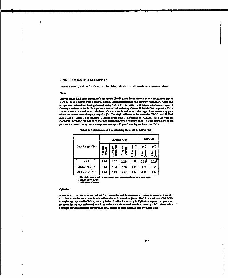
SINGLE ISOLATED ELEMENTS

Isolated elements such as flat plates, circular plates, cylinders and ellipsoids have been considered.

Platse

Many measured radiation patlerna of a monopole (See Figure I for an etample) on a conducting groundplane [2] or of a dipole over a ground plane [3] have been used in the progran validaton. Additionalcompaiaoa matzeal has been generated using NEC.3 (4], an example of which is shown in Figure 2.Convorpee tests on the MoM input dama was carred out using incraung numbers of segnmms. Theseare particularly required around the base of the monopole and arund the edle of the conducdng platewhere do currents are changig vaey fiast [5]. The slight differences between the NEC-3 and ALDASresults can be amtibuted to igodng a second order double diffimection in ALDAS (ray path from themonopole, diffracted off one edge and then diffracted off the opposite edge). As the dimensions of theplate are increased, the agreement improves (compare Figure I and Figure 2 and see Table !)

Me 1: Antem above a conducting place: RMS Ermr (diB)

sMONOPOLE DIPOLE

Gain ~ Range (di Ij I ? ý V

>0.0 0.67 1.37 2.201 0.71 0.832 1.223

-10.0 < G < 0.0 1.84 3.,O 5.50 1.98 2.61 1.63

-20.0 < G < -!0.0 0.67 5.081 7.92 2.39 4.96 3.99

I. TiM MOM riadu haM• Contergled. More aqasars should have bean usd.2.,-•W-pi E otf pok3. la H-j•ieofdpeteo

Cylsdair

A similar exerose has been carned out for monopoles and dipoles over cylinders of circular erass-sec-tion. Few exasnpies; am available wher the cylinder his a radius greate than I or 2 wavelengths Someexamples we tabulated in Table 2 for a cyli tder of radius I wavelength. Cylinders require that geodesicare found for the rays diffracted round the surface but, siace a cylinder is a 'developable' surface, this isa straight-forward exercise. However, the my tracing is more difficult than for a flat plate.

367

Mhb 2: Anuma above a cyUlder (Radus 1 I): RMS Error (dB)

Gain Range (dBi) MONOPOLE DIPOLE

Modal Matching[61 Mementsh4] Modal Matching [3]

SG>0.0 0.36 0.71 0.43

-I0.0<G<0.0 1.12 1.98 0.49

-20.0<G <-10.0 1.37 2.39 1.55

Sph- ad Elipesids

Spheres and ellipsoids ae doubly curved surfaces and require that the geodesics are found for each raydifE- 'ooa dte surface [7]. The problem is more difficult than that ofan antenna over a cylinder.Radiatieomntam ta umm ole tead onph• ofdffe radii have been published in Russian[8] and the Method of Momeus has been used to model a monopole and a dipole over an ellipsoid. Thersuts provided by Oyelh'na and Welnstein (usng an anaytical method) have redii varying from 0.477to 15.9 )L As the radius increases ao does the aem between ALDAS and these results. Figure 3shows the radiaion pans•m for a mnoopole on a sphere of radius 1.5915 X for ALDAS and Byelkinaand Figure 4 shows the results for # sphere of radius 15.9 X. Measured cmu-polarsation results of amaonoole on an ellipsod at 8 Ghz alms agreed well with compuled results [9], Table 3 shows the increasein agremenm as the dimensions increase in wavelengths.

T, 3: Aamen aoe •pbem and elp dst RMS Error (dB)

Meoopole Dipole

GainReanp(dla) ~ ~ ~ -

0 > 0.0 1.70 2.6 1.7 2.02 1.22 0.31 0.12 0.05 0.81

-10.0 < G < 0.0 3.31 2.51 2.00 2.75 1.37 1.47 0.37 0.35 1.62

-20.0 < (3 <. 10.0 3.70 4.30 4.20 1.85 0.33 0.91 0.36 1.07 4.63

Refemace MoM MoM [8] MoM [8J 18) 181 (8] MoM

I. !Egh " we specifled by faor psm .s +X Y, 7. -X

368

STRUCTURES

Simple Stuctures

The results fir simple smuctures such as boxes or a cylinder with attached plates, will be less than w.mci-than isolated single elements. There mfew uch examples mailable in the iktwmre to use as

checks. The general trnd is that the RMS err is about 1.5 times dud for a single isolated element.

Cemphs Structure

Strucusre are 'complex' who they conis of many srucral eemena Examples am civil and miliutayaircealsipspt space-crA gromd vehicles and so on. Extensive data is svtilable for several aircraft atfrequencies ranging from 500 Mlhl to 10 GHz in which the model may contain up to 70 stuntl ele-ment. Details of some examples are given in Table 4. The acoxacy is iflueaced by the choice of thestrucmturs elments which are used to mak up the strcture. If the geomety is varieu end the range ofradiation pattems obtained is eusnined, the most obvious features are

I) the mesa gin level does not vary vae, much (+/- 0.5 dB)

2) the poitioma of the mulls does vay by seveal degmes.

Since the RMS errors are baed on diffesences bhween the gein levels at the sane angle, any skewingof the null posiions will make the mmerically derved atiors appear much worse than they seen to theeye. An ulteruave presentation is thePercentage Coverage Plot'. An example is shown in Figure 5 forthe results ofa monopole on a BOEING 747. The corresponding radiation patterns are shown in Figure6 and Figure 7. For the systems engineer, the Percentag Coveaje Plot is more approptsate because itgives a measure of the sysem perfoumance. Such plot have an acounacy of +1- 0.5 dB down to -20.0 dBieven on the moat complex strucares.

Table 4: Anteamu an complex struleus: RWMS Err• (dB)

Gain Range (dBi)Frequency

SuVCsM (GM) 0>0.0 -10.0<0-cC.0 -20.0'CG-10.0

KC-135monopoh over win [101 1.4 2.15 5.17 5.62

KC-135:mnonopo fwd of wi•gs IA 1.43 3.2C 8.76[10]

BOEING 747: monopole on fuse- 1.0 2.08 3.77 7.63lae:(O = 0.0,90.0 degs) [I I

BOEING 747: monopole on fuse- 1.0 2.56 4.70 8.76lage:(0= 60 - 120 degs) [I l

Helicopter Spirals on nose 2.0-8.0 025 0.50(e-- 60-120 degs) [121

369

K _

CONCLUSIONS

The radiation patterns presented in the prnious sections have shown that smple canonical strctre arewell modelled but that complex stscres are not so accurate. This is due to the difficulty of describinga complex asactum such as an aircraft in terms of the canonical shapes ellowed in ALDAS. The assump-lion has been made in this document that all mor are due to ALDAS since it is not possible todisentangle the vriousa error sourcs. However, it is clea that the errors in ALDAS will be less thanthe quoted.

I) For single elemnsts, the accuacy improves as the sixe of dhe element in wsvalengths increasesabove 2ot3 .k This is ot suprising siice diffraction tbemy theoreically bresks down for dimen-

an kut than I )L iwb of • his companion work was couied out using MoM or other analyticalteclniqucs which am likely to be more accurate than masuanents. Convergence tests on MOMmodls awe 'sAlul.

2) When complex strctuna ae studied measurementt must be relied upon and often no details ofthe mnwsuremen techiques are given. Personal experience has shown that meamantrig a low ganastemana an antacture reqmnres a chamber which has a eactivity of less than -400 dB and amo /mmsing/r on sysem which does not introduce spurious reflections. A reflectivity of--45.0 dBtrnlate into a gain error of 1.0 dB at a gain level of -20.0 dBi when the peak gin is 5.0 dli,

3) When a comple structure such asan aircraft is mrodeled usian ALDAS, various other sources oferr come in.

"* the asocture of the aircraft will not be totally conducting. There will be transparentse•tions suct as cockpits, radornes at camee

"* an actual airraft is not accusidy modelled using flat plates and die simple curved shapesprovided by ALDAS for the fuselage

"* the mesmnmemts am likly to be in aicr thettelves"* far accuante mo6deling, it is possible that the matured radiation patterns of the antenna in

ifee space should be used rather than $0001k pattenL These re not generally aailable.4) The use fthe pearentea cr-arp plot does smm useful as it gives an acutate indication of the

gin coYWrd5 which is usel for sysm purpose The accuracy of ALDAS appears much bettbeamss the masll rottiona. eftam weemoved.

Table 5 sucmiirises the RM errors an point by paint basis. The percentage coverage plots indicate atnaccuracy of bhar then -04- :.0 dB down to a gain level of -20.0 dBi.

370

Tole 5 CamI Level of Accurviey in ALDAS. EMS Error Oil)

GainRang (M) Single Element Simple xtf

< 21 >>21 Stracwtin icrf

G 0.0 0.7 0.4 1.0 2.0-10.0<0<~0.0 1.4 0.8 2.0 5.0

-20.0<0<~-10.0 2.5 1.2 4.0 7'

REFERENCES

I PR It astr, 'Analymsiof Low Dinecovity Antansmw on Strucure'. 6th ACES Symposnom. 1990. p362.3692 Fee P R mid Miller T. Redintou Pmouns of a Quertarwawe Moaupole on a Finite Gounid Plaes'. ICAPBI. p451 .

455. YOCK.'M3 P K Poiahk. 'Teniuques for Hfigh-heqy Problmns', Chapter 4.i *Amntan Huidhaik'. edited by' Y T Loa md S W

Les. Van 14jarnd. 19384 0 18orke =dA I Pago.loo'urnericaletm lz Code- Medsod of Masents'. ecksuijal Doc 116. NOSC, 1977

5 C Silmene. prwivae m ii~6 W Bun-d. Analysis of Onosirtrat Anusuesa Poiemos, Ph D TWAs. Ohio Suft Univerity. 19727 P R Faster 'Acrc mid Conplamity in Electromaspate Cods Applied to a GTD/UTI) Propamn. CEM-91, Lon-

dam 1991.pw04-4IM MG Syeckinand~ L A Wmas.sas 'Radiation Patncas of Spbarical Surface Antmasw'. in 'Diffactiom of Eleefomo-naew Wavas by Some Bodiesof Ravoleuum. Soviet Radio. Moscow 1965 (in Russian)

9 PR Foam, Unpubbidied isesw at~ Monopole anim oUqipand. 199210 W DBunaside t aý. A**dyof KC.135s sciacrfiampmnwo,'. Trans MEE. AP-23. 1o ,10.975, p309-31611 14C Albenwemi md l JossesPaerter Wuioe for L-.oo miewsas on an. %TICRA Report S-77.03.1,Novemuber

197712 Result of onmi U skl model

371

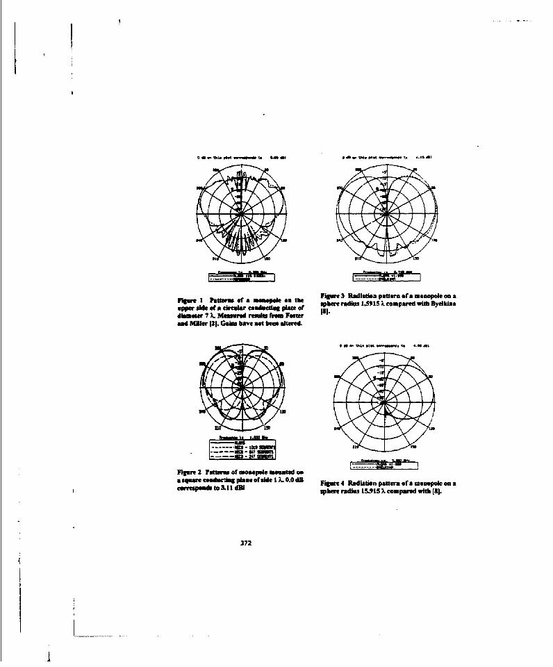
II

lPlre I hires of a monopole on the Figure 3 Radiation pattern fea monopole an auppre side of a ire r conducting plate ort sphere radius 1 X915 •. compared with Bydlkina

diamerw 7 L. Measured results freom Faster Is

and M]ler 12]. Gan hove not bees altered.

Finure 2 Patterns of monepole mounted ona square coductig plane of side I L 0.0 4B Fipre 4 Radiation pattern oea memonopoe on acorrespmds to 3.11 dil sphere radius IM.915 X compared with [81.

372

b1

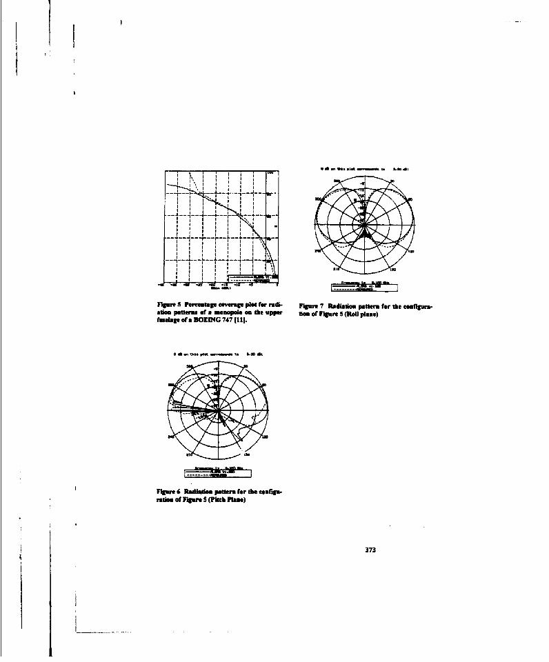
T Ilar 5 ecnaeIvrppo o ai rpr aito atr o h mfp

___________________ potea of a. moopl on the upe lnoa~m5(olp

foslapof BO IN 74 111

Fi I 6 Ist mpteefo h ofq*

rao of-v PthPae

I 373

374

SESSION 9:

ANTENNAS

Chair: Gary Theile

375

NEC Modeling and trsting of an

Ultra-Wideband Antenna for 1-igh-Power Operation

Eli. Lensing. Dr, B.S. Perlman, R. Pastate, US Army Rese-arch Laboratury,BPSD Ft. Monmouth, N.J.

Dr. C.D. Hachusian, lLF. Lenzing,Stevens Institute of Techinology. Hobokran, N J.

In an antenna design proposed for high power, wideband operation , a tapered TEM horn' istenrmnatad with a conical spiral mansena so that the small featureaon associated wkt ate hi uecoperation is replaced by a structure capable of handling hi"he power, while maintaini~tng simalireflections thua producing a hybrid antenna structure capable of supprtng high pwrover a widefrequeny pcom.The mannna can be driven with a high speed Laser con'o.e solid-state switchor other hi =*Us cy geneator.

Thspapr dscses the design bfeture ard the modeling and testing of this prototype conicalspsrall'M hor hybrid antenna. issues concerning the NEC wire modeling of surfaces andprolemns arisingifromn it will be discuissed.

Inun1ducuion

Mew categoy of antennas generally referred to as "wldeband antennas" consists of plana andcon~ical spirals [li, log-eriodic: arrays [21. Vivaldi tapers [31, bowtie horns, etc. T'here have beenrecent Aattmpts to combiue two wideband antenna types in order to realize ultra-widebarid operation(4,5]. In the antenna presented herein, a bowtie-horn antenna is ten.ninated with a conical spiralmannna, thus extending the low-frequency cutoff of the structure, conriptually resulting in an ultra-wideband radiator. The intent of the present deign is to drive the antenna with a high-speed, laser-controlled solid-ustat switch situated across the qusaa-parallel bowiie ham conductors.

Antenna Design and Modeling

'T1w smallest dimensin of the bow&s horn determines the upper-frequency limit of thestructure, andIalso determines; its power-handlirlljcapability. The lower-frequenicy limit of thestructre is detertnlned by the Irgest diamezr of the conical spiral. To mintinize reflections at thebowtie horn to co.'sal , lspira tsuans~ron, the conductors Must follow a smooth and continuous path,matching the tangential derivative allalong the transition. To accomplish this, a novel swwutur which is actually a seccion of a Cmrnu spiralwas modeled and. also fabricated in the labloratroy.

Aap rersntaive structure (figure 1) was modeled and analysed using the NumericalElectrorapeetics Code (NEC)[16]. Figure 2 is a closer view of fth bowtie horn stuncture. In order tobe compatible with NEC., ibe sansctum was modeled with wires. 'The wire makng up the arms of thespiral run only in the direction of the spiral curve. This has been shown to be a valid a. pmiinatiorby Aria and Mei ink their integral equaoon formnulation of conical spiral antennas ('7]. This also wastested by simulating the antenna with and without crosshatching wires. The two different casesshowed little difference in current dlissibuimoa or radiation pattern. A fuirther consideraition formodeling tbe antenna surfaces with wires is the wine radius. The generally arcepted nile for wirediameter is that the set of wires representing a square grid must have a total surface ama of twice thesquare grid area being modeled (I1. Using this rule, the wire diameters in the spiral portion of theantenna mutt increase eixponentially. To further test this method of coiducting surface simulaton

376

small microusupprs ermdlduin E n nte oua MOM microsamp modelingpa ,g ald Sont(0.Tepthswr lofabictd n saedad opa with dhe

iuiunda.The wire diuametrs used in the NEC imnulat,.on were dmscldiuithe simulatsiomatched the measurements. This wciling was then used in tie antenna model.

Modeling and Testing Results

Computasion of input resistance from 2 t 190Gib Is shown in figure 3. In the lower ptIonof the bwan the input resistanc varies around 130 olmssathe thectratcal input resistance of a concaspiral of thaea dimbnsions predticed, by Dyson [1I3. At die uspper pottion of the band. the inputresistance climbs toward 377 ohms but dhan begins to decreazse slowly above 17 GHs. ThaL nay beexplained by leakage fran the prllel pLate waveguldd region.

Repesetative modele radiation patterns am shown in figure 4. Note that die polarization isset'quzE dependent: at the higher frequencies where the bowtie horn is the predominant nsidistor,

poaiainis ellipticallnear linear. In the lower firequency, conical spiral regime, polarization iselliptical Anea circular.

The modeled antnena structure was fabricaeod In the laboratory, wan the return loss wasmemasued using an HP85 IOC network analyzer. The return lots results are shown in figure 5. Aphotogrph of the antenna structure is shown in figure &. It should be noted that this design was notintended so be driven by at constant or swept somrce, rashe bye laser controlled or other switch. Workwill have so be done in order to transfonn the pmllelW plase balanced mode to a coaxial unbalanemode Ibr connection puhpcoes. Preliminary stuffiss we tuderway to explore the use of ultra-widebandbaluns (9]. It must be mmsd that dhe fabricated antenna was only for CAD model validation to keepus on track with dhe modeling.

A oes of die psn3OYPe asntermat power capability was concucted at the EPSD pulse powercenter. A 250 amep 2kv pulse across a one hundied ohm load was applied to thm antenna with nowarver osr heating High-power patten nmeasuremnents ane not available but e-field probes were placedat various points inthe lab and the risesimes of the detected field showed widebond operation, Work isunderway to produce a proper method of testing the transient response of the antenna.

Refterences

[1) JD. Dyson. "The characteristics and design of the conical spiral antena" MUE Trans. onAntennas and Propagation,vol. 13, July 1965,pp 488-499.(2) RH. DuHaniel and D.CI. Isbell, "Btoscdband lotanthmiaally periodic antenna stucucnre."MRNat. COnv.Rec.,pan 1,1957,pp 119-128(3) P.J. Oibson,"The Vivaldi scrial."Proc. 9th Europ. Mic. Conf.,1979.pp.101-105.[41 A.LY. LaiA.L-Sinopoli~snd W.V. Burns We.'A novel antenna for ultra-wideband

a~lcations."IM Trams. on Antennas and Propagatdorivol. 40.n. 7. July 1 992.pp. 755-760.[jA. Marvin andl 5.3. Poster," 30 Mbz to I Chzt in one sweep-the bilog,'EMC Tesm and Design

Magazine-Atzg. 1993. . 28-30.[6) (UJ. Burker!AAJ Pofggio,"Numerlcal eletrotnagictics; code (NEC)-method ofnioannts."Naval Oceasm Syst. Center. San DiegoCA.NOSC TERCH Doc.l I6Win. 198 1.[71 A.I. Atia and KLK Mei."Analysis of niultiple-asin conical log-rpiral antennas,ITEEE Trans.on Antennas and Propagaton~vol. 19.no.3,May 197 1.(81 A.C. Ludwig."Wirt grid modelin of surface."EEE Trans on Antennas and Propagauion'Vol.35.no.9.Sept. 1987.

377

flg.3 Wife E.~U ofpU do bybdd mww

nZ3. Expno view ONVOWu~ bM~ NOW

37.

I: zL->�. 'p14j::, j7+ -4- -

I--i I�ii�irY -�

- -- - - *- -I-iiy L� 1 _

-

fig 3. � *. m�. � qumcy

�:"

IA,. I�

I /�ju * -.

* I .YW. I *ii.I . C*I....y UI *1ta� - - '.1

,�.. I s�(.M �. t"', **M I �

Ag.4 Slini f.�a plow fw 3450 ud I2�22S Gb

37�

4. D -.. aft18.0.0vL,~I --

7w Y dom~ L

fit. 6 PhIbW fct ~ pvwoe typc.

380

fig. 7 Meumwedafiam p~u j 12jCbz

381

-31

A Practical Application of NECImpedance Calculations*W. Pery Whteless. Jr., Unir'erity of Alabama

Darko Kajfez, Uniwersity of MssauiOppi

.....~ ......... ....a ..... ..... .......S

~mmminSaS~ V.. - ddmWl~ - a.. (30) em~Nowes

Wm'sm Neeis. 0 s0 m =tworkV ES oft a. Sm womms Whmkmai we ~M4ui1 10

"b LMO.a as aw 1::s:N ma beim Na.Apu Impwem * mqmh .4 I d&G A" W . madk bT fl..immemiae &W.maumys Wmeedwasee a",M.4 b

1. IWMI~DuCTIOW rig. 1. Practical wire antenna equivalent.

FiIMotae that th thoeialwr appzoadi. it is believed that the transformnationtenam eed:Ilmint inmedance ZA.. is chanced to appliam equally wall to other typos of practical wirnactually observed icaedane Z... by th., feeding anens

network assoctd" with the antenna. The lwac The procedwue of determining the transforma-networl; shown in Fig. 1 may izhAnde imeakto tiwo wefficents at togs3 has becomme known as de-.ad ilapPorktranei ha Owtim & b~u& emheddag 121(3]. The technique in (31 includesItunped~eden components of an antenn tum- .eputation of tbe standard deviations for theing unit, and stray reactanmm, with l;ieaity the three transform co~affcnts directly from the sma-only gaguptio ner-Y for the network It has mird da"a Notabl tesgths of the methodologbeen shown (11 that the theoretical imopedance Of & inckLude only one inversion of a complex 3 x 3 ma-delte-gsp cylindrical dipole -a be related on-tO- t= in all mas. and the ordern of data pointsove to the actua! nsmared impedance Lthough a is nomhportant. in many applications, the num-bilinear transformation at a givu singl frequenCY. be of dat point ey uvceed 3, in which coThe transfarnmrtom is an avhenderngsd get of equatioes is solved in a

G*AZ + at West squares am While Cmi isapedance transior-4- GA - II miano associated with prac"ia ant-na is One

wheres~,e andlosei of probism amemable to treatment with thewhee a, s, ndas a coomplex codldenta and fracional linear tmasfrato the farnoulatlan

7-, Z, ame shortened names for Z-. and Zggmi, actually relates the (comsplex) input to output fixrespectively. to [11, the independent varw&iae s lHOea two-porte in general.dirtance d of a hodeontal dipole above a perfect Wire anteona wre nowadays analyzed reliably.ground plane the ideal impedances Z~ associated even in the prosimaity of lossy esarth, by nun-mnlawith the various distances of interest. at a fixed mathods. Moat notable anurm Ile availble wirefrequemcy wereabtamined fromlan intepal equatio nten codes are MEC-2 and KC.3 (41[51, which

___________ane both based on the mormat method. INEC-2 is*lheehein4e~ s~h 55 a= m- -.N. available to the public. and is a powerful tool fat

^mh al.NM. e~=-IA PA =E as _ 531.U ,W~ the analysis of wire antennas residing in the air

382

half-space. NEC.3 is required to analyze anten- measurement and NEC computatior! give Z4, andfnas involving air-to-earth 'ground stakes' or un- Z,.,, respectively, and Eq. 2~ beollymderground (buried) wires, but the distribution ofNEC-3 is restricted. NEC-4 exists but is generally taZ..+ U2 7_' ,,, (3)unavailable because its distribution is strongiy re-stricted. so NEC-4 is Pat considered here. When Withbjust thtft d4A 0:11iý W whsxethreeequa-properly applied (that is, the known inherent liur in- whicalo Pt ýý x~ ~initicfl for C1.07, anditations of the codas ane observed) to a borad class 4s. An overdec.-ano! system results from ot-al

of wise antesnna types, NEC-2 amn NEC-S can cal. data point! N > it which caue a least square

culate food-point, impedances which are aecuratc solutio nu (U~? .baitied: it is usually more re-and reliable to tae point that they canbhetaken liable to 3 a 4;1taroverd.3ernined system of

As ideal theocetical values. Similarly, network atn- equatic, i ¾,auie it reduces the iniftuence of ran-

alYUMr ame now widespread so that reflection cod. dtfl¾ a~ r-,j in the rzaasuriezots.ficienta, or uaPedanoms may be mesue rediy 1'0 e4 ~ matrix equation suitable for corn.

The main objective of this paper is to demon- P4iM'1Vi ir,'emrnftat1n. in nccord with [61. the co-strate application of the fractional linear trans-. i ~ of

tat. 4, and a, from the left hand side

formation relationship to the new situation where Of L~q 3 am loaded respectively. into

the variable is frequency and the geomnetry is fixed.as compared to the original formulation for fixedI

It is shown hemethat the approach can be valid [cs(4

ovreq iuecyand bandwria th, geovetn dihen tetasi .)1Jformation ooDdffi ts are (complex) constants.oe a infcn aditee hntetAmZNtrailing-wire HF antenna. deployed from & fixed.wing aircraft, is usd as a specific example wo ii-

trnfrainwe rqet loe ti.I~ttethe basic characterisths of the impedance I02)- (5)

II. PROCEDURE FOR IUPEDA14CE DATA andANtALYsIS ZiI l 1

For ronenifut references. essetial points of the Ie,) - - -

computer-based proeisur for ciptermination of the (22

impedance tramlermation cosExients and other -ZZ,

paramters of intaret are summarized below. Ad- with the right hand side values packaged into theditional dletals and considerations are in [1) and fourth vector131 where it is noted. that the basic v.cwo cascrip-tiou which yield the curve-fitting procedure forthe fractional linar transformatin follows from (7)161. [1(T

Re-writing Eq. 1 in implicit form gives Z?

2iZ. + 42 - 43Z'Z.. - Z.. - 0 (2) so that Eq. 3 can be written compactly as

for a single ideal impedance Z. and a single corre- - 3)-~ ie

sponding measured impedance 2._ When multi- ie)()

pie points are involved, a second subscript is addedto denote the rnumber of the independent variable- The distanes het we If) aid its expansion is minn-sample. That is, at the n' -th data frequency, imized wh~et constantsa, are found from solving

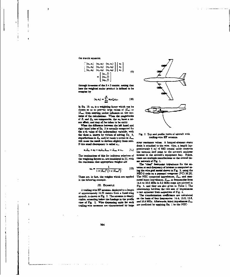
the matrix equation

f(at'i at) 47.9 (t 3,ti,,r i(91,92) (C2,92) (e3'es) :"

(41,93) (C2,93) (e3,43) 43 (9)

through in rem of the 3 x 3 inaiix. noting thathem the weighted scaiar product is defined to becompl- by

(44,e, E Wk 'jk (10)

In Eq. 10. w.,is a Weighting factor which can bechamso -"a to prow-nt Large values of JZ,., orIZ-; from craning undue influence on the out-come of the caklsalaim. Whia the magnitudesof Z and Z4 asn comparable, the wi, have a mi-nam dect, and may all he take to be unity.

V/boa the diffuence between the left hand andright hand'wides of Eq. 3 is actually computed forthe n-tb value of the independent vauiahk withthe thre s, blown by virtare of solving Eq. 9, Fig. 2. Top and profile views of aircraft withimperfections in Z.. and/or random etro us in 2...tril g-wite HF antenna.will calmn the tookt to deviate slightly'- fro Zeroacevla lme-lmetsai

If tis salldisapanc iscalld ~drain is att-ache to the wire. Also, a length (ap-

GA.+ 6 -t~lZ- Z-- I- ý1)promiawely 6 n) -71f 3W( coaida cable coonectsa~L~eeZ... 2.. ~ ~ the antouna iced poant to the network analyzer

The umplications of this for judicious selection of located in the ahwcaft's equipment bay. Halce.the weightiag factors wj ane considered in (1], with there me multiple contributions to the overall Un-the conclusion, that appropriate woights am a network of Fig. 1.

I The 'ideal' feed-point impedance for the an.Wa(12) tofln""Soeach -3eusy ( ntermsi s computed us-

- 1+ ILIj (1 + z..I ing the wire grid madd shown in Fig. 3. using theNEC-2 code os a personal computer (PC) [41 (51,

These are. in fact, the svights which are applied The NEC computed inpodsance, 2._. and mea-in the fOltoWing exampla. s-re input kmW'Anc. 2..- at frequtencies how

14A to 16.6 M31z in 0.2 M~z steps ame plotted inIll. ExAmPLE Fig. 4. and they ame also given in Table 1. The

A trailing-wire HF anteunna deployed to a lengt relationship between the two sets of inpedascesof approximately 16.75 meters from a fixed-wing is not apparent from inspection of Fig. 4.

aircraft. is shown in Fig. 2. The anennna is clearly Th tralnformation cooffizients are calculatedvisible. extending below the fuselae an the profile -a the basi of b-fureum-cr: 14.4, 15.2 15.8,view of Fig. 2. Wirle dispensing units for suchi and 16.6 MHz. Aftewasrds, input impedances Z_.trailing-wire anetnnas ane chlaracterized by large ptedicted by appling Eq. 1 to the NEC-

3.4

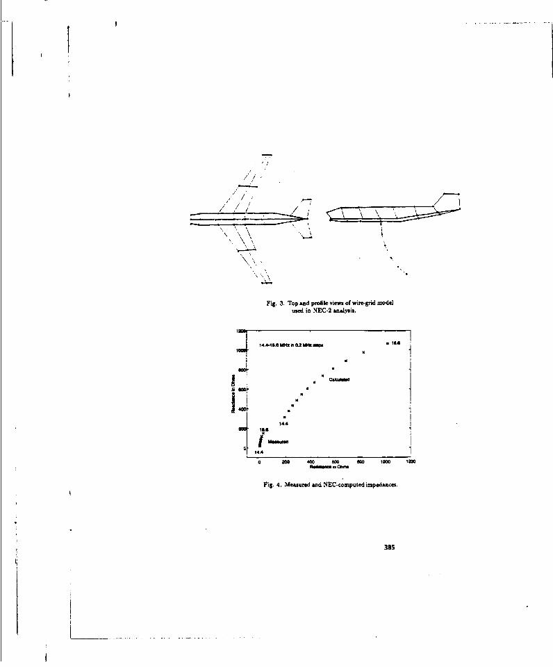
Fig. 3. Top and profile views of wire-grid modelused in NEC-2 analysis.

stM *. -

, I

14 4 A

"Fig. 4. Measured and NEC-computed impe.ances.

385

I ______________________ ~ -

Tause 1

Ir~ 10 C.me4 beamed~n ?wfcei E~..a ~ ~ i~.(fl) 111,141,114 (0 OIP311af" in) t

I. 4. 12..~31.4 .6 160 .5j16.0 0.02 14. 'C5 27. ... 2. .j2. .M: 14,2.. 481.7 41.6. .j2. .4 18:. M.O. 4467.5 4.1. 84.2 4.2.- S4.6 1.,

3W NS.A 26..64. .6. 40.7 4.11- 40.6 0.1

"7 48.6 S6.. 001.2 6.. "6. 6.6. U6.4 0.6a 18.6. 46.. 726. vA.4 67.1 s.. 66.4 1.0

1 6.0 561.7. M.2 I.e., We. 10.4. ?9.7 1.8i0 16.2 M6.4* 641.1 13.S. 10.2 13.6. 64.0 1.12 16.4 M.a. 676.9 it:**1la. 1. 117.6? 0.:12 18.6. 1038*6l 106T.0 26.. 160.3 L6.2.:264 Z.0

Avmqga tarro a 13

LeIjAlOCIY tafla IF - 0.0012 (ab..14 be It". thea X.0)

as . 0.06"m1 j 0.01"n9 (h 0.002m2)

S3.- 1.O876 1 7 .68035 (6 0. TIM1)

*3 oOO ~000 32 0.00012 (0-000M1)

14~ 4AJ

144.11 A -6 OhM6

38

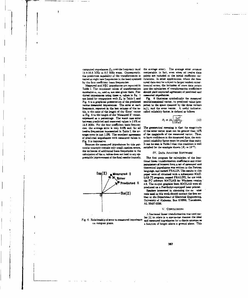
computed impedances Z,. over the frequency band the average error). The average error re-mains14L4-16.6 NlHz in 0.2 MHz steps. Consequently, comparable. in fact, even when all twelve datathe prediction capability of the transformation is points are included in the initial coefficient cal-tested at eight new frequencies in the band spanned culations. In other applications. where the mea-by the four coefficient basis frequencies. sured data may be subject to larger random exper-

Measured and NEC impedances are reported in imental errors, the inclusion of more data pointsTable 1. The ctlculated values of transformation into the calculation of transformation coefficientsconstants aI, a2, and as ar• also given there. Pre- should yield improved agreement of predicted anddicted impedances using these at values in Eq. I measured impedances.are fisted for comparison with Z. in Table I. and Fig. 6 illustrates symbolically the measuredFig. 5 is a graphical presentation of the predicted multidimensional vector. its predicted value (pro-versus measured impedances. The error at each jected to the space spanned by the three vectorsfrequency, reported in the last column of the ta- lei)), and the error vector. A useful indicator.hie, is the ratio of the length of the *Error' vector called reliability factor, is defined as followsin Fig. 6 to the length of the 'Measured Z' vector.expressed as a percentage. The worst case error R1 . l0 l13between predicted and measured values is 3.6% at F 0 i4k§(1314.6 MHz. For the four coefficient basis frequen-cies. the average error is only 0.6% and, for all The geometrical meaning is that the magnitudetwelve frequencies reprsented in Table I, the av- of the error vector must not be greater than 10%erage error is just 1.2%. The excellent agreement of the magnitude of the tneasured vector. Thus,of predicted impedones with measured values in to have confidence in the measured dAta, the com-Fig. 5 is impressive. puted reliability factor must be smaller than unity.

Because the measured impedances for this par. It can be seen in Table I that this condition is wellticular example contain only small random erors, satisfied for the example shown (R = 10`).the inclusion of additional basis frequencies in thecalculation of the at values does not lead to any ap- IV. DATA ANALYSIS SOFTWARE

preciable improvement of the final results (namely, The first piogram for calculation of the frac-tional linear transforrmaion coefficients and otherparameters of interest from a set of measured andtheoretical impedances was written in the Fortranlanguage, and named FRALIN. The results in this

[m(t) UO&SIIU.Od Z pape were all obtained with a subsequent MAT-rror LAD (71 program named FRAL!N2, for uje with

the PC software MATLAB for Windows version"Predicted Z 4.0. The output graphics from MATLAB were all

produced on a PostScript-equipped laser printer.Readers interested in obtaining the ow -uter

eZ) code used in this work should cntact the first as-thor at the Departme•t of Electrical Engineering,University of Alabama, Box 870286, Tuscaloosa,AL 35487-0286.

V. CONCLUSIONS

A fractional linear transformation was used ear-lier I1) to relate in a one-to-one manner the ideal

Fig. 6. Relationship of error to measured impedance and measured impedances for a dipole antenna anon compiex plane. a function of height above a ground plane. This

387

work provides additional evidence that other prac-

tical wire antenna types also may be modeled re-lably by the same procedure. Also. the results inthis paper show that the transformation may beapplied over limited bandwidths. even for coWe-cient values which am restricted to be constants.

One possible application of this impedance trans-formation model is to predict the input impedanceof a wire antmejn at new frequencies of interestwithin a band spann by a few (but > 3) samplefrequencies on which acullation of the transfor-mation coefficients is based.

The transorm relationship between the idealantuena impedance one obtains from NEC andactual mote feed-point impedance for practicalwire antennas should be of particular interest tousers of HF/VHF wire antennas.

Future work will attempt to extend the tran-formation to become frequency dependent so thatwider frequency ranges, includiq rmonant andanui-resoant Tegions, can be modeled with oneset of coefficiets.

Acknowledgment

The provision of masured impedance data byMr. Neil Hurst is gratefully acknowledged.

RgvzazIVCzS

11l D. KWW i4 O•A Mim . . i" D*& s..

131 *3. 5 d P = V k. 0e. d~ .iW5Mm..m" SC• 7 M4ý 7k•." 7.k.. -L. WMT2.,

W- 3 Uw Min I74.(, 0. x.ho -Nmt e Ve u= m e .1 " e."

I'm .ond w ab• ISA" lSs .TO•- .•m.

.d .L D~f pp. 4.11CI. M 4.N IO mm TLK4 O.J. 'wm Wid AJ. Pq.N 'N....Wi SW-P-c.d. (-SC). - Aft" .1 f - Lý Uwumw.. Mm

=mU&10$-• Oavb. t9GL.• LM ..armp. Rwetm' 1,'.101 ion.. , hsma. m

a Lm 101-La - L4-, As4".Stmim hr A. 1., ba Tm~ a -N d Wi As.

.d M Wmea44 Monk. 0. N.. Y..i h~mwmin P.S

SMATLAR .Tb. MmhWf. be.. C.,,P6. 24 Phem Pirk W.*.. N..4•" MA G17CC.

388

NEC4 Analysis of a Navy VLF Antenna

C. A. Danars, J. H. Schuhantl. P. M. Hanson, J. C. LopanNaval Command, Cash, and Ocean Surveillance Center

RDTSE DivisionSan ,•oge, CA 021-2.-04

ABSMACT

?EC4 is useed to evoluf proposemdilnuaena So a Pbiy %&F top-food nwooopoie.Chargp dnoafte -m oonpuded and use to cobleuti Oe mnaflinn top-dod gradient lbrIo wi ,a,. Alomuighi m sto n aCwdaA suMa elaw mand' of segnevits isnede to olah I -'eg desired reWAowl hinO SeW dusp . G-uafln vaous derived #wnOw N0C4 dOsa - a•fmt to be in doa asm m a *M Os fl0~ Porn meaunmddva 7he gurseti valus allow Out Ow proposed corfnowaon Wees not nieet flumawnun grad~sy desin hlt b' anis s ern.

lMTRODUCHO

Electrcaly shoat, topload monopolas am commonly used by the U.S. Navy for Vay LowFrquency (V.F) communication. Although eesdkloa sunall. the opaiting frequancy range fllcelly 12kM ft O0 kit) re hI pP ya large antennae requireg sgnficant maintenanc One such antannais me Cutler VLF Antenna System located at U.S. Naval Radio Station, Wahiongon County, Maine. Theane Is a dual ary, a each aay meaing over 07 in height and 6000d in diameter Thismwain atutllure Is curranty sa duled for eutensive wik replacnem . An economical way to evaluatethe proposed changes I necessary, and ualng aie modelin is one solutlon. This paper presentsa •c••pter-elkid analysis of the Cutler antenma main the Numerical Electromagnefs Code, Version 4(NEC4) Ill. Previous wirk has demomftrad the app~lctay of NEC-Gs (NEC-Ground Semen) tosimeir VLF aswses P2]. Her, the objective is to ume NEC4 to denle the mas•inion surfao electricfiled, or gradient, on the antenna top-.at. Krwing t•he nad-l provides a means otf oansesn theImnp1ct of the p poe wire replacernt on anten poifornus

ANTENNA COhlhRIPTION

The CUle antenna iConsi of IWO Ideulcal away. an shoWn in FIg 1. Each anmy isseNtlaky a bee-fSd. top-oae moopole. The top-ha of ewan away coI of six dimownd shaped

pinuls arranged symethioally arou•n a colntr tomr. The pan-s are supported by one center tow.'rO), al inner town. and six omur towers. The towrs range hi heilt ftm O00W at the outer ring to Justunr10o00•at iente Eachtlowerlssuppoae by asyem ofguywires. All towerandguywireswe grounded, aid an Me panes era Inaulated from ti toLers a, est other. EBac rknel is fetd uWavera down lad wen e•d lndhg fron a conneclon neartde ceont toW Insulator, tM a helix huu.a V4mhe ane where th em ted together.

A plan view Iustrtion , a single top-hat poal is Soam in Figure 2. Each panel in the array isappro mately 3 long, an ha eight wies running fron To to the outer tlowse. The four Inner wirsof each panel are V diamerer sold core cables. The four ouler wims of each ponel conis of V solidcore cables connected to 1.5r diamoter ho•low core cables. Hollow cor cablls were onginally used tosave on veight. The 1.3" d1amnter Is necessary to avoid corona on tMe antenna at lower operatingfroence.

389

ME

I" T

lam4.

Plgws1 Gwa • Iaaut of the Cutler afltflha 1RI.

- .r dm. O

Figur 2. Plan view of a skiW top-hat panel of the Cutler anteOna.

390

CcOM11 is a disciarge of electrical etiery that Wa omcu near I sharp point oft& coniductorreledto a high potenftil. Enery 15 ded"aWWe when the eleatt field striength an the conductor

e Oned t reat~kdowni voltage of the suxroundinig sit. Since the energy is dissipated Into the air. itrepeents a power lose in the systemn. Therefore. it Is rinportent to avoid tiron to maintain systemeffidency.

Currently, the Cutler anternna operates at 24.0 kttz. It's maxim'um input power is one megawattfor single awrayt operation, anid two megawafta for dual array operaltio. At 24.0 kllz, corona Is not aprokie. linthe 1.01 wiles. 1 owever, it is deirafble to o-e-at at 17.8 kHz. and at this freuenicy, the il.5wio eanes eded. Unfortur-ately. theals wire ame due for repiacemnto and Met hollow cor ae it s noWWpe evaltabte. it was necessary tmmhereore to study differen conffiguratlona to landean allemnalve to the1.65asile. Modefsgt~heantenna using NEC4 provide a ooflwenlent way lo do this.

T11* NC4 MOOSL

A NE04 model of the Cutler antenna was constructed for the computer-Ided anialysis. Althoughthe anttenna, co Ia- of two sways, it is often operalWa using "nl a single away. Therefore, single army"oprtON was assurned to Mirpll this walnalist Two anten confliguration were modeled.Contfiguration I moesthe mmanain 5, preeet state, usin Woh V arid 1.$" diameter top-hat wires.Configuration 2 consatta entiel of I* top-hat wires. Taow 1 beowe gives model dimensions for both

cofgpto.Inner pane wires refer to the peael aedilors from TO to the Inner towers. Outer panelraeer 0 o the W mono.hnt the lamer towes to the oute towers.

Antenna Corsttgurstller 1: 11"amd tWWits Confligurowt~o : I"Witea Only_________ fft DW~ti (IN) Langls PIL) Diaeneselr (in.)

Cner Tower 979,15 72.0 070.3 72.0Inner Towers 675.8 72.0 675.6 72.0

OU Turne 799.0 7.0 790.0 72.0owlada 550.11 1.0 550.1 11.0

Itime Pane WIresWW"I & a4 1352 1.0 1575 1.0

__________ 223.3 1.5--Wkue2&7 1218 1.0 1441 1.0

224.9 1.6 - -

Panel wiresWre 146 W00.0 1.0 1575 1.0

________ 774.7 1.5 - -

W=a24T 774.2 1.0 1l4g 1.0MY______ 7. 1.5 1 - I -

Table 1. Dimension. of the NECA Cufler uintelllr model.

Since the antenna Is rater complex, several approamatlns were made in onstructinig thecomiputer models. To begfin with, the top- ha emnefts were modele as flt wires with no coton"l. Alltowr guy whoe are neghweded and a perfect grouwnd was assumned. Since the towers mu raul sed fromthe panels in the antenna, they were. moee has fe standing Itonopoles in the model. On the actualantenna, severa veianl fee wire fan but from the source at the bae% to each paenl. On thes computterModelet oh pane Swa fMed usin a singl veat"a lead exsandln from the source. Furthefrmore, since

the ositte tower is not fed, the fee stnaicure had to be made slightl~y asymmeutrc to acorm~odate thetowwa' poellon. That Is. the distance fromn the surce to each paneal variee sliggtly front penal to poanl.This asynunetry can dearly be seen if, the center of Figure 3, which shows a view of the NEC4 wife

391

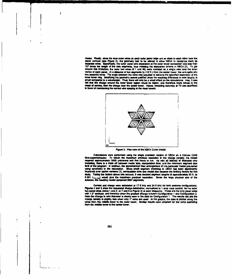
mol ily, " at uasl oater wires on ew outer U NOl eg areso doee to each other roara"Mea vefilce (eM Pfgme ") h geometry tie to be n~ee to efuw NECA to macuniae themn asa wNe. Gpecitfu . t outer an wir aet"r at the inner tower connecton was lees thanIr Wm a W t of wo r a a ftIwa., thus vleikimg t *eperetion outiefl in NEC4 Ill. To getWound 06l EmItellan. lthe aster two wire (II I and N) were moefled -s a qaini wire near the InnerVaeste of eac Panel. As a distaince of two agnIet (a 112 ft.) from the cnentertower, the wire spats intotwo 01 per 1 e w fte 01`e1angle betee thle wi'swf a djssete to achieve the apeafid separation at thesuner ler rng. I t g eryeers justifed slm their.sulti diffrence In wirae l ieit is

Oed to a wevelan . Thus, the we only be a aa ~e on ahe calaa•tons. Am, It weeleivst em chrg arms aot htIsser ten reg@o woul be hifler, arnd therefore moicre crtital to aeOseW of iaie. Owent a ov c oha te owa a cnter I l ence, moodeli ngacouracy a TOewas sey t.icedIn levr o melstalnhg111 aM ca0e a6 ep ag ta d isser towet

PI'ews3. Piont viw* of ae MICA Cutter model.

Caimletla, e were peualme using the usge p e veraln of NE0C on a Convex 240Mnlmumetcopar. To omi3Mft a " m ...cI resolution In ag charg density, th r.seq-id ec ppraWdise 34W un(•itows a• id five hours to run. As wid aI Metho of Momenlt wiremo .elt •there is a tere off betwiee mo a , cmpato tlim. ai o na minimum aepsen elinebys* or a1 pivpusmr. in edemasn, at aeymmsslcel loew arrne men wxof tMA passiia mde preveNte-e hes w eby in t oanciison. U mss - agme mo dI-"ng Wi c1C4 has been significatloy

amroe veerW11 9M se wee pjOM M . compaon *t &W a 011 m ONe s e a ati th VWan 0Mai for Ofttidly. Talsin aw fadim above kfo amcoshAwas Ie dcie aegsoen i 6sit. at appoinirrnslely SS ft. (is0.001 X,, ,j aoid giv at mamumn precel seevoluln Given the larg physical size of ahana,, M•e mannamodel"ied 2egM

Current andl chege were calmaleted at 17.3 koz OMe 24.0 k~tz for both siennam canltalnam.FOgRMS 4 IRdd 5aho the Calmalate charge d~drbftlon, ncrssietlzed to I amp input Current, for fles ottertwo penal as (as I and 2. or?7 aid ISin Figure 2) a each frequency. Them amath only penal wireswAir* 4i, ao. ancitiftet sho at graest change bwen Configuration I and Conflousatian 2.Note aw duang in air diameter Is clearly -m In the data for Corfluretlon 1. The results lfl&ate aicharge dwelty is vlighilyeas when Gaily 1-airs we ueed. tn ah graphs. at ata Is platted a lonmVa lrn ago dale t to UOe outer tower. sisler ressi were obtained for aw wies sanding

leas isseta towsto acser tower

392

Wi "O~(n) (VOWIA (ihmn) Q lChmA) R_ kYAIW)Oandto - 23b10'o 0.9" 2.1$x¶O' 0.016

I- (A) 2," 20 IS

TOM 2.M&Wmm ptO diflW oGSWd "Mki NEC4.

MISFiue ClIuSe Isae dnits o 0-gue m w n 2 40 240 w it

TWIN OTAM NAMM OWTW ow393.

OPDW CALCUATKW

The mirfiba: I fldicIeld. or grudiert. on a coaduor deftennines whethier or not Coron willGoum. Fertile -erno. Al 16 en Wmot peauiestam to PoPulde when wdagt with highi voltage antennasIke CuLOW. In Oti~ ue. U, gidlw con be umed to uaue the bilpeo of replacing the I.5 wirs with Vwies. AccaootIkIg O141. themazimnur-m -lee- gradlien to avoid coaroa for the Culler antennai to.6WVMw. Therefore, if fte mI~axium gradient on the V Mrepacement wire exceeds this limit they will not

MMg the design mVqAmremft

For a cylindrical oxoduor, the gradent can be calculated from,

Eu .S (1)

whee qj to the law carAge dewulty in couondon porinier, to i the pemaIttivty of free space, and r Isdieradium. EIxabWl of FIgures 4 m~d5 owe gththemaxim dum caredetuly per amp ocousonthe outer wire (01 cr91) at toe inner tOwe conuietion. Multipying these chrgme values by the maximum

inp~utbi cunreat and lahelitmion ini (1) yIelds the maxinum grudent. The maximurt antennahue C~trma I.. for Single anray operation are 247? A at 17.8 klz. and 2030 A at 24 kHz (33. Usingthe011 cun'oats, the maximumn top~hat gradients for each configuration are calculated and shown In Table2.

The validm of thet NE04 data was checked by -omparing the resmt with gradients calculatedfrun mesaimnemmit. The memamunmeits were taken during a model study of the anitenna using a 1001a=W mode 141. The model data Incluides ftcirema~n ditatubutoim on the outler panel wires, which can be..~d with (1) to calcuO the gradient

To calclat One g, dei from the measurrnients, the charge density must be derived from thecurrent dINt-lb~i I. From the continuity equaioni. the linear charge density along a wire is related to theMlope oOWcurrent "dixitatfon by.

OTAW 9=-L(2)

2 - = -(3)

where 0,wi On UMe char ge on the vdra Ieyond a given polKint s the rainfrequency. s&M QL is thelines chaump density at lie poke. SubinMbu (3) Int (1) gives,

Es a 1 a (4)

hellen E. 19 Die enIe -0 eleaulo field (Loe.. Vie gradlient) on fte wire. Equation (4) isa maimumntn when theeOpe of the curnard dlinbsiin a a nmuuiunt. From (4], the maxim-um Mlope of the measured currentdebbtiton to O.&US anAlr per Amp of Input curent. Therefore. subetitution into (4) gives an equationfor Ma mnuMM Surface gradliit n au hitmon the auitaa bue current 1,

EO.02g,6jO-31*,Eu go (5)Y

394

Seared input marens for vanw confggureta, of the atWma Fmoda are found In P131wiauaig meanm urniois for I Jr and Ir wires at several frequenoe Subslbdhig the currents ilto(S) resulted In the curves shWn in Figur 5. The graph compares the measured data with the NEC4r=ad. The agement between tie two is wery good, with the NEC4 values falling within 10% of thernemurements. Mole teat botihtWa NGC4 data and the measured data Indicxte 1.r wires on the outerpeanl -n unacceptable for operation at 17.8 kllz. east.e gradient in this case cexces the 0.8 kV/mrndesign limit.

12 1 ..... . .... e........ .

WALS I.~ ~ ~ ~ ~ ~ sa ... is..... .W............... .

. .............. .. ...... .....

Zic r

I- 24 2 9 3i.'-hm~ ") cc

Figre0.Meaurd nd alultedmaxi um o-o rdetfrteCle mnjSUMMARYThe rsultsof ths wok hooclemOSWO S.. blt ocmlme:teatnadsg

FRIWENCYES;

F11Gure. Meaured -uand~ caclaed axpimum ta-htordien forC- Mthed Cute an~tennad1

TMresl of t.Chis wCmorkhlp eonsrt of~t shECGy to comleen th aitnn design cre o L coo.I

pram 1 Cn K.e patcua mae. LIt waspel slnd 8.G canbeused o, evialuateprpo sed changff esrtormthetav stsCutlert VLF tanteloade oU.So. Chvalrgei dtataifom lEGsh o - ousedto, calcne, the

madniwi 'ktoo.h71E. for the antnna h opd resulIC.. agre very wel h eauedmoe

daa.Boh at stskiime o raiet n o r irs xced te extnm esgnliitnede5t

141 W. 8. Aflw ft. E AntsmW. Val.. 'U.S. Nava radio stman Ctdlwa. Maine nmwflnfiddmdalsys~en ~agn DECO ftapmt No. 13-s4, Oavaloprnstal Enginammig

Cmwrwlon. Aim. n,. 1987.

396

NEARLY SEVE YEARS OF SUCCES USING M[ININEC FORANALYSI AND DESIGN OF STANDARD BROADCAST MEDIUM WAVE

AM DIRECTIONAL ANTENNAS

JAMES K HAWIND, Pa.HATIELD & DAWJSONI CONSULTING ENGINEERS

INTRODUCLION

In die nineteent &Ixtes, Robert Silhinan was one of the first consulting radio engineers to usecomputer point m'tching techniques based on Hallens integral equations to analyze broadcastantenna behavior. la succeeding decades Camt Bingenian, Jerry Westberg. Stan Kubinia, G.LRoyer. Dane Plinion &nd others applied various moment method programs to the analysis of AMstandard broadcast directional antennas. By the end of the nineteen eighties NEC, MINNECand a program from Ohio State University were in common use for AM antenna analysis.

Consulting engineer such as ths writer, Ron Rackley and Karl Lahm (now at VOA) have usedMININEC since the mid nneteen -ighties for the analysis and adjustment ("tune up") of AMdirectional antennas. Advantages thm. MNINEC offers for modeling medium wave monopolesover radia wire pround screens are ea~ie of me, the centering of current pulses an segmentJunctions, and preater accuracy handlin& abrupt radiu transitions. Good agreement withmeasured and FCC computed far field paiterna is achieved with MININEC using just sevensegments per radiator. Experience impedansce .=ves can be duplicated with a reasonable marginof error tifthe base region of the tower is modelec' in detail and an impedance correction is addedto the computed results. Near electric and nsgnev:, fiel human exposure from AM towers canals be computed using MININEC if the modeling is performed carefully RF shock hazardestimates for workers on de-energized power lines and coftmaie loading cranes near AM stationshawe been computed using MININEC. Conversely the ezfte' of power lines anl cranes uponAM directional anteama patterns and Federal Commuicaion rominminain (F C) mandatedmonitor points have been computed using the nesar field provisions oi MINIEC.

ADJUSTING AM DIRECTIONAL ANTENNAS

FCC directional antenna pattern computatios, arc based upon point sources and parallel raygeometry (See Figutre One). The design specifications used to devtimine pattern shape !ncludethe relative contribution to the -far field of each radiator in terms of the field ratio and phase cthe radiation from each point source. Since the horizontal planie far field of each radia~c.-, inatilliVolts per meter at one Kilometer, is 120ir/1 times the total current moment of the radiatorthe relative contribution oi each radiator to the hor field is found by taking the ratios of the totalcurrent moments of the radiators. The NMNUEC drive voltages for a given set of FCC designparameters can be found by inverting a matrix whose constanrts, derived from MININECcomputations, relate the drive voltages to the har fields. The FCC requires that directional

397

antenna performae be monitored. This is accomplished by measura•ng the relative magnitudeand phase of the tower currents, usually at the base. The matri inversion proce&% produces thevoltage drives that can be used to compute the bas cm rnts and phases for a given set of fieldratios and phases.

The computed base current values are used to adjust directional antennas. After the adjustmentshave been made ground level measurements arc performed along radials eatending 30 Kilometersfrom the center of the array. These measurements are used to prove that the directional patternia within the lmit proescbed for It by the F .

Over the yea we have adjusted or assisted others in adjusting nearly 100 directional antennasusing the MINMC / matrix inversion teclhnique. In all but two of the adjustments themeAremets verified the accuracy of the procedur In both of the exeeptions the horimontalplane field was perturbed by nearby scattererm In one case there was re.radiation from nearbyoffice buildings and in the other cse there were terrain irregularities In those situations it wasless expemv and time consuming to adjust the array by trial and error than it was to modelcomplex objects in the environment in order to account for their effects.

Most AM directional antennas are used to control skywave radiation at night at some angle abovethe horizon. The adjustment of arrays so that horiwntai plane measurements can be made in thepresence of re-radiating or scattering objects to show the proper pattern can have a deleteriouseffect upon the performance of the antena array at a vertical angie. Les interference wouldtherefore be caused by simply adjusting the array to base current parameters based upon methodof moments computations and not woring about making accurate horizontal planemeasurements. Stch a proposal is now before the FCC.

DE.TUNING AM TOWERS

If one sets the field ratio of a tower to zero and then follows the procedure outined above, thecomputed drive voltage for that tower will result in current moments that sum to zero for thattower, or at least to a value five or six orders of magnitude below the reference tower. Thecomputed c.rrents for the array and the de-tuned tower will show an active bae impedance witha resistive component that is usually a few pereent of the reactive component. This means thatthe conjugate of the remactance can be applied to the base of the tower for de-tuning purposes.This impedance should be trimmed by measuring the cement minimum at the height where thephase reversal in the computed current distribution occurs. The bae reactance is then adjustedfor a minimum reading

Sim the de-tuning process reduces the field in the horiontal plane where field strengthmeasurements are made the radiation at vertical angles increases. For nighttime operation thehorizontal plane pattern is therefore within limits while the vertical angle rdiation increasespotentially creating greater skywave interference (See Figure Two). For this reason de-tuningunwed towers in a nighttime array is not necessarily a good idea.

398

MITIGATING RADIO TOWER / POWER LINE INTERACTIONS

It sonetimes happens that power lines are constructed near edting AM directional arrays. Ifthe power poles or towers are 30 metem er more tall their re-radiation and mutual couplingeffects can distort the far field pattern of the station. Additional problems are created when thereis a "skywire" or "shield" wire running along the tops of the poles for lightning protection andelectrically connected to the poles. The poles and towers used for power transetssion usuallyprovide a conducdive path to groand. The F current flowi in the loops thus created causesdirectional antema pattern distortio. The matern aed to measure the AM station fields employshiebled loop =team to meaure the magnetic fld component of te tramnmitted wave. Sincethe electric fetld Is the desired measuremen parameter, the magnetic field mnaitude ismultiplied by the impedance of free space and depicted on the meter face in term of electricfield. When measurements are made within the near ield of the RF currents circulating in theloop created by the power line erroneou readings result This effect can be predicted using thenear magnetic field computation of MIN4EC Re-adjustme of the army can then be madebased upon MININEC computations so that the FCC monitoring points near the power lWne arebrought into tolerance while arrangements are being made to either de-tune the power poles orfloat the "skywire".

When electric power transmission lines are in cose proximity to AM radio towers serious RFshock hazard to electric utility linecrews can result. In one imnstnce two AM towers were locatednear a 150 K'V line. One of the towers was only 23 meters from the line. Several instances ofRF burns were reported to the utility safety officer. The work crane, power line, and power poleswere modeled in a simplified schematic fashion. Computations of the RF current that flowsthrough an equivalent human impedance at the aane work platform at various locations weremade to determine the potential shock hazard.

AM TOWER BASE IMPEDANCE

The measurements and computation of R.W.P. King and other academic workers are usuallyused to benchmark antenna impedances computed by moment method programs. The centerconductor of a coadial cable poked through a sheet of copper, used by King and others as amodel for computation and measurements of a monopole over a ground plane, is not the sameas a base inulated tower fed by a horizontal half inch pipe. When the base capacitante and theradius disjunction between the base and the feed ie are carefully modelled (See Fqgue Three)the base impedance given by MINNEC is much closer to the measured impedance of the typicalAM tower. The match between the computed values and the cunves showing the measured baseimpedance for toes of various heights is improved when one adds a correction of 5 + j43 Ohmsto all computed values (See Figure Four).

COMPUTING BANDWIDTH

Progrms such as WCAP (a specialized program similar to SPICE written for the anmysis ofdhectional antennas and their feed circuitry) can be used for dynamic modeling of the

399

combination of thne dietacdeed antenna anc its feed system. The frequency response of thetransmitted signal can be determnined in this manner. NMIMEC can be used to compute the selfand mutual admsittances for the antenna array over a specified rang of frequencies. This as usefulfor determining why a station's sound quality varies in different directions in a directional Pattern.

RF HAZARD COMPUTA7IONS

The FCC requires a showing from liesees that the provisions of ANSI C95.l-196 Sl~IaK

met. UMMM~C cans be wed for this purpose, but its accazac decreases as one approaches thetowe. The electric and mapnti near &Mel computations provided by MUNINC are useful ifone is careful to checi for coragmec. Seven segments per wire gives a lumpy and unrealisticresult. Fifty segment; show a computed fiel that varies smoothl with distance and is areasonzable appiumnmtias of measured values. Figure Five shows the computed near fields witha measured data point for comaparison Figur Thve also shows the efec of insufficielirsegmentation upon accuracy. Ric Tell Bob Clevlan of the FCC, and Ed Mazttiply of the EPi 'Llave esplored this iesse in several papers.

NIGGH~MAE INTRFERENCE,

The method that has been used for FCC purposes since the nineteen thirtiles to compute verticalangl radiation from AM towers utilize simple trigonoimetric functions to represent tower currentdistributions. The impact of mutual coupling between towers upon the current distrbution Is*wnred in these wi~'culations. Nighttime interference can be affected by inaccurate computationsof the antenna crenti distribufions since the vertical angle radiation, computed from the currentdistributitan, Contributes to the =cuaWe coveage a station provides at nigt due to skywirvepropagatIon The Vertical angl fields computed wwig the more realistic MDM4ECcurtdistzrUtiom provides a -e accurate picture of potential skywirve inefeec (Se Fi~ Si)

NFAR FIELD C0OMPUTAMIONS AND MEASUREMENIS OF ARRAY PERFORMANCE

In order to provide ;perorInnee verification infceuusion ffr an arra that is located at theshoreline of a tropical island, Ron Rackley and Den Dawson used the neafield comptuttionfeature of MDIIEC to calculte mge~tic fieM values for speciid location vMY close to thearray. Measurements were masde at these locations using a cotventional magnetic field intensitymeter desesaitized by shotrting the loop antennas shield. The meter, with the shield shorty, wasthen calibrated in a inown field. The same MININEC moftl that was used for arra patterncurrent distribution. *W impedance calculations predicted near magnetic fields that speed withmeasured values to better than 2% accuracy. The data Provided by fth technique was used todemonstrate proper operation of the antenina system despite the fact that complete far fieldineagurezinents wer virtually impossible due to open ocean on one side of the array, and denseroadless tropicsl jungle on the other.

400

CONCLUSION

Programs like NEC and NNNEC have enabled the practicing radio engineer to analyzeantennas in new ways to solve problems for which there was previously no exact solution. ForAM medium wave directional antennas this means that the effects of coupling between antennaelements upon the antenna current distnibution can be included in the design and analysisprocess and precise relatioships between antenrna crents and radiated fields can be computed.Directional antenna adjustnen and pattern verification based upon NEC and MINITECcomputations has been successfully performed for hundret of AM arrays all over the world bya cadre of iternatdi radio engineers. These pnorams have also been helpful for the analystsof the interactions of radio towers with games and power lnes and the human exposure toelectromagnetic fields. New versions of NEC and MININEC, such a NEC4, VLF+, andMININEC Professional ave the potential to help engineers analyze finer structures in greaterdetail with higher accuracy.

The FCC is curmently investigating whether its Rules & Regulations regarding AM patternverification should be updated to include numerical electromagnetic modeling techniques. Theburden and expense o detailed measurement and data analysis could be replaced in the futureby rmi requirements for an•t• na current or voltage monitoring and compuations using NEC,MININEC or other moment method computer programs.

We have finally reached the point where simplified directional AM antenna pattern analysis basedupon trigonometric functions i about to be replaced by more exact moment method techniques.A further benefit of this change will be the ability for the AM radio engineer to &nalyze complexelectromagnetic environments wing a deak top computer. The responsibility incurred through useof these programs will be to always check for stability and convergence in the computed resultsand to verify that the results agree with measured data.

401

E K~r.IPFlZ s cosc... -4) + P2) FAR FIELD

TO FAR FIELDO6SERVATIOM

i tPOINT

MIL I A T O01 TWlIWI Tl

**AZImUTH FROM4 1141F NOM 11iOF OBSERVER .

- AZI', 0•m TOWER 02FROM TRUE NORTH T ,T12

S * SPACIWG BETWEEN TOWERS

K PATIIRI SIZE CONSTANT

HATFIELD & DAWSON FIGURE I

HORIZONTAL PLANE FAR FIELD

CONSULTING ENGINERS CALCULATED FROM POINT SOURCES

402

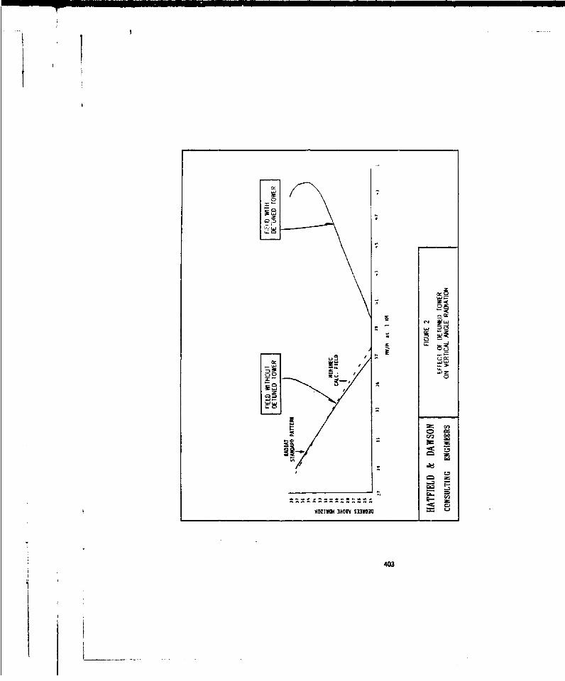
403

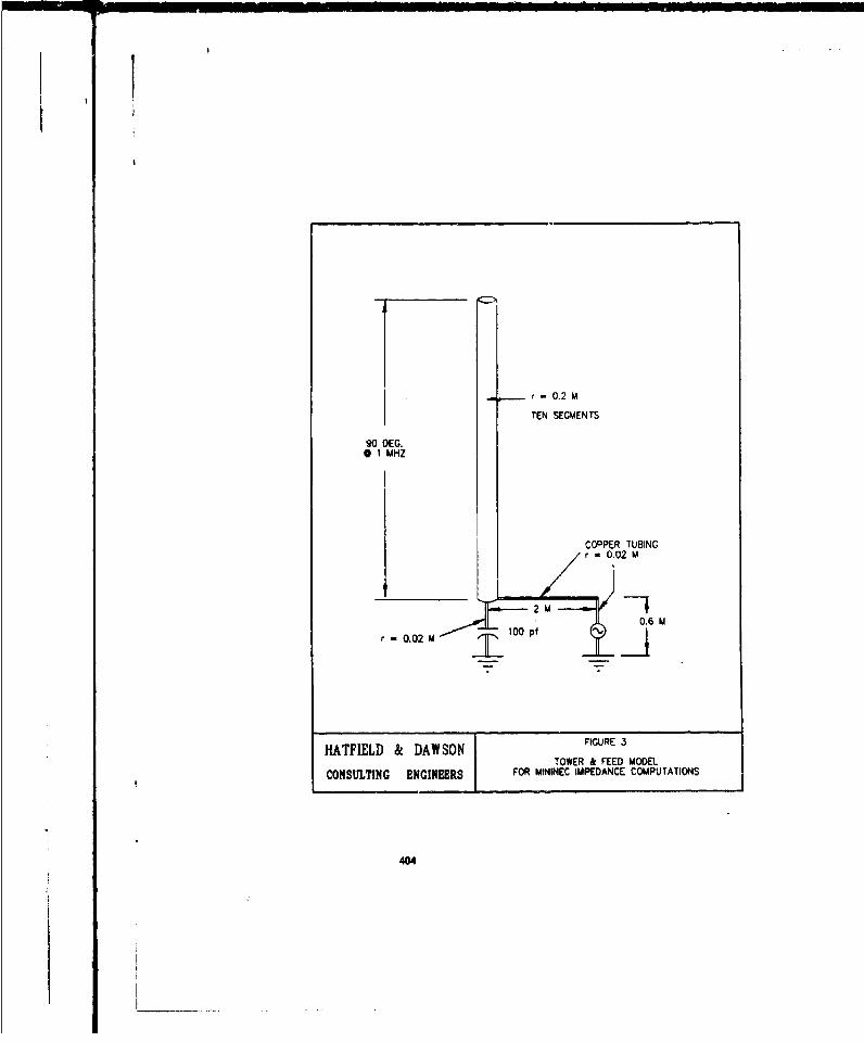
!T

- 0.2 M

TEN SEGMENTS

90 DEG.* 1 MHZ

COPPER TUBING[ / r -0.02 M

0.6 M

HATFIELD & DAWSON FIGURE 3

TOWER & FEED MODELCONSULTING ENGINEERS FOR MININEC IMPEDANCE COMPUTATIONS

404

200--

100

200

10

1.36 54 72 90 108 125 144 162 180 198PH4YSICAL HEIGH4T IN ELECTRICAL DEGREES

HAFEL, DWO SEFIPDNE0 OOOEOE A. .IE RON

1O0CE00 00G8$ OCOPTDUPDNE

I -I LII

200E YMIWC(E F~R N

CONULI8 ENGINEERS CO&~JE0DT POI2T PI44TE ON2 EI 8CA CUVEFO

[ ECRONCS"AC.Z N ARTICLE IR!15 g13

500

,

$I

-,. 54 72 90 108 126 144 162 Igo 198

P14YSCAL. HEIGHT IN ELECTRICAL DEGKES;

H A T F IE L D & D A W S O N S EL F IMPEDA C E O r MO NO PO LE OV ER A R ADIL IM E RO NSCR~rEN MODELED BY MWNMEC (SEE FIGURE ,) AND0

CORRECTED BY ADDING 5 +J43 TO COMPUTE"D IMPEDANCE.

CO NSU LT I NG EN G INEER S CO MPUT ED DA TA POITS PLOTTE O N EMPIRIC AL CURVES FRO MELECTRONICS M•AA ARTCLE ("F 192 pg.143)

405

I-J I

cla

'°i , -- -- -......

Jc i .--- - A

-- --------

-~i __ III-:mOw

4M- -

I III

I 4O' •UTA

0 O0 30 n 4 w a 70 s0liUmmu1 Im wm'1

HATFIELD & DAWSON FIURE 6

COMPARISON OF VERTICAL ANGLE AM FIELDCONSULTING ENGINERS FROM A 0.6 WAVELENGTH TOWER AS COMPLTED

BY FCC METHODS AND MININEC

407

ANALYSIS OF AIRBORNE ANTENNAS

WITH THE ESP, NTC-BSC, AND NEW-AIR CODES

B V Anderson, A Joha.ssn, U Uidvail, T LundinCon=mmuica CEC AB

PO Box 1310, S-17125 SolnaSweden

1 Abstract

R*Adr and coMatn antr.Az s , on an AEW-aircraft have beenanalysed with the use of the ESP, ;FC-W, and NEW-AIR computerwagrum~

•An coveg e and antenna to ante-n coupling have beenMthe complex environment of the antennas into accountCa=czatsd antuia pattetn have been compared to measured data

2 Introduction

On modern airborne early warning (AEW) platforms it is important to haveradar andma kmm =kati antma functions with the require-d patterncoverae, suldslobe charcteristics, and antenna to antemna isolation. Severalyzw with simultaneous a necessao en order to fufil the

AW- .G a uber of art a ve to be integrated onthe aircrft ý ýyS teAN'W-d.

It is importan to have the capability to anls n cesteprformanceof aMu and co atioms of antemna systems, including their

qonkA eRramenwxt, in early devhlopLunt phases, during systemSand inast phaes of a proec to acctplish a balanceddeagis with th bet oprl p m T cpbty to analyse

.tantwnas in their true environment makes it posle to evaluate theirizilusme on system psfarmance and to inviatemodifications and

For this adwqute ionalw tools are required. Such tools are thecomputer code ESP, 1EC-USC, and NEW-AMR developed at The OhioStam Utv"ty, EectrScence Laboratm . ES based on the method ofwatinits D&oM, can be used for the lo frqe~y problems and NEC-

IBSC and NEW-AIR based on ray mnethodzs (11), can be used for the highfrquny -naysThis paper presents results from the analysis of radar and communicationantennas on an AEW-airraft usin these codes. Antenna patterns andantnna to antenna coupling havee coputed.

406

Iy

3 Analysis of a radar antenna on an AEW-aircraft

3.1 Model

Alternative antenn a n form an AEWSstem, fig. 1, have beenstudied. The influe of fi.t wrier ai (SAAB 0, FairchildMETRO C26 ) on the performance of a dorsal radar antenna have beeninvestigated with the NEC-BSC code. One of the two side looking arrayantennas is modelled as an array aperture. •The aircraft model is built withPEC ellipsoids, cones, cylinders, and flat plates as shown in fig. 2.

Fig.! AEW-airat (SAAB 340) wft dors.! udm updtmad cmmumWoon anuemm- , A,-A' b/m

Fig. 2 NEC-BSC madd ofan AEW-ai.rcmft (Faird'ud ME7RO (26) foa Nheank-is of thedormd•atar ndm

409

3.2 Computed radiation pattern

The radiation function for one side Iooldng array antenna has beencalculated with NEC-USC at S-baind. Anazimut radiation pte,4below the horizontal plant, for an ideal array aperture is shown in fig.The main strucua (air-dilid METRO C26) scattering contributions to Dside lobe levels emanate from~ the wing, the engine, and the propellerbladows

.. . . . .. . . . . . . . . . .. .. . . . . . .. . . . .

.~ ~ .. ... ... ...... ........ ...... ...........

-a0 -70 X, LO E 0 70 90

Nome A~ziuth Tail

Fig. 3 CAlwl1- =,nmA mdiWim pttp, 4- bdow the korilo, with NEC-BSC fortlui~m fvul enmdawwu tS~und Cnwairmft Fat kli MOTRO C26

4 Analysis of commnunication antennas on an AEW-aircraft

4.1 Model

The AEW-alcraaft of fig. 1 is modelled with PEC plates as shown 1 ft4 forthe calculation of commtzunication antenna patterns with the G =S Thmodel of fig. 4 has also been used for the calculation of the coupbetween three antenna pairs. The coirmunication antennas arepmodelled asmonopoles on a ground plane

4.2 Computed radiation patterns

The izadiation function for an antenna at position A2 in fig. I has beencomputed with ESP at 130 MHz. Fig. 5 shows a calculated azimuth pattern

410

Fig.r e= as untiodu -eut and elevationz forp theh A3fr~mud~ antanna

A2 at 130 Mhz. No dorin radar unit n the wamer ahrafft.CakLMAtW- Mgmvui

411

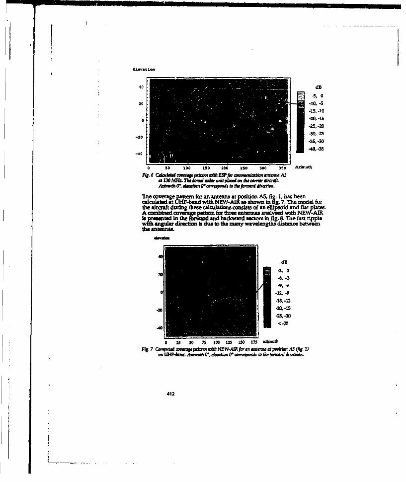
40 dB

20 -10, -5-15, -10

02,1

-25, -20

-20 -30, -25-35, -30

-40 -40, -35

0 so 10; 150 200 250 300 350 A~i-ath

Fi. 6 CkIadWiisd cME~tn t IPfvrawmnudwmtcmwztmuA3at DO30 L Thrz 27vrM nadwi unit pbW o Ae v1 tk aberafrTt.

The covme patten for an antenna at position A5, fig. 1, has beencakulatud at UHF-band with NEWI-AIR as sh~owni in fig. 7. The model forthe aircraft during thes colculations ccmsisb of an ellipsoid and flat plate.A conibied cvawmepte threfue antennAs al'sdwith NW -A2is pented in the fradndbadcward sectors =in g. 8. The fast ripple

v~hangular directon Is due tD the many wavelengths distance between

40

X ~-3, 0-6,-3-9, -6

0 -12,-9-15,12

-201 -2Q, 15-25,20

.401 2

0 25 50 75 100 125 150 175 azdmuthFig. 7 Computa oemgper, Um ~h NE W-AIR fian dmwtmaatpcsW=oiA5 (fig.!1)

on ZTD-knd. Azmugz 0',clumtion 0 cewupnds to heforuwd directimi

412

e~syauioaalmdatonFig .. . . _ . .... ..

...e *oajvte heim aa tpU~ mAl S11ds

63-6,-30-

•~~

-3, 0

-

-20, -15

Aznad, h O w', deeo O coupnd to tem f wwd,, d forgto.

4.3 Computed antenna coupling

boup .ing between antentnas. at po9shom A at, A 6, A 7, a AS fg. 1) ha

been cacutlded with ESP ove te 4efreq, cy band 100-250 M•z as shownin fig. 9. The coupling has also been cdc'lated for the same antenna pairs

..-.0 .........

-40-

30D 400050006m

Fig. 9 Computed mazimon coupng bet ion three antennaa jun wth ESP in the band100-250 MHz ma with NEW-AIM in the band 250-6W MHzAnt pm A4 to A6 nt pos A4 to A7 - --,m pos A4 to AB-.-.-

413

and frequiewms 250450 MHz with NFW-AmR (fig. 9). The aree.mentbetweei the results for the ESP and the NEW-AIR computations at thetransition frequency 250 Mhz is very Sood.

5 Condusions

Airborne radar and communication antennas have been analysed using theESP, NEC-BSC, and NEW-AIR computer codes. Antenna radation patternsand antmna to antenna coupling have been calculated.

These computer programs have been shown to be useful tools in all phasesof development o6f communicatio and radar systems. The performance ofantenna systems induding the influence of their complex environL-ent canbe calcuWted. The comtputer codes have prqv.= to be useful when manysystems ar integrated on one platform and the goal is to achieve abalanced design with the best over all performance.

414

I

2-40 HEalcopter DItense Placement DswluationtEampeinestal and 330-DEC Results

J. M. Harris end K. L. Wheeler

Georgia Tech Research instituteGeorgia Institute of Technology

Sensors and Zlectromagnetics Applications LaboratoryAtlanta, Georgia 30332

This paper presents the details of an antenna placement evaluationthat was performed for th HH/H-6-OG PAVE HANK helicopter. The antennasystem is part of the AN/ARS-6 Lightweight Airborne Recovery System(LARS) and consists of two blade antennas mounted on the underside ofthe helicopter fuselage. The antenna outputs are supplied to a'combiner network that produces the sun (Z) and difference (A) patternsused by the LARS for direction finding. The antenna E pattern isdetermined for two available locations on the underside of the fuselageusing two methods: scale model antenna mear,'rements, and computermodeling. The physical model of the predominant features of thehelicopter underside and rose was constructed at 1/4 scale. Thecomsputer model was conatructed using the Numerical gl-ctrouaqneticsCode - basic Scatterin4 Code (NBC-BBC) with source distributionsderived from the Numerical Xlectromagnotics Code - Method of Moments(IRC-NON). To overcome NEC-BSC limitations, several analytical modelswere constructed and the results waer combined to form compositeantenn• natterns to compare to the measurements on the physical model.The posit. and measured patterns compared very well vwth theanVtw.s located further than one wavelength from any scatteringstructure. However, the patterns were significantly different with theantennas located within one wavelength of a scattering structure.

The placement of antennas for a new system on an aircraft can bea difficult task. The antennas must be placed in an area where theywill provide maximzue performance for the system while minimizingperformance degradation to and from existing mystems. often, existingstructures or antennas limit the number of suitable locations formounting the new antennas. These limitations can degrade theperforw.'nce - 'he new antennas and their associated system.TI-va, ý,, th, em.nt of new antennas on an aircraft requires trade-v t. opt' Y uystan performance.

415

F

The RH/NI-GOG PAVE HAWK helicopter is equipped with variouscomiunication, navigation, and defense systems that utiliaz antennasmounted on the fuselage. In addition, the exterior of the aircrattcontains lights, sensors, access door&, and other structures that limitthe available locations for a new antenna system. The installation ofthe AN/AMW-0 Lightweight Airborne Recovery System (LARS) on the PAVElAWK requires that two blade antennas be mounted on the underside ofthe fuselage. Th• LAM is a MN? Radio system, operating in the 225-300-a frequency bend, used to locate and direct the aircrew to downedaviators equipped with band-held IRS transponders. The outputs of thetwo aircraft-scunted antennas ar provided to a combiner network thatproduue the sUm and difference patterns used by the LAM to performdirection finding. Por optimm performnance the two antennas aremounted 15 inaces apart on a line orthogonal to the longitudinal axisof the aircraft. The two antennas must be mounted as far forward aspossible to min:&mze fuselage shading in the forward direction.

Figure 1 shows the tunderside of the PAVE HAWK. The space forlocating the LADS antennas on the underside of the aircraft is limited.Por this reason and because of the requirement to minimizeelectrczagnetic interference (=II) to other existing aircraft systems,the possible locatiois for mounting the XADS antennas were reduced tothe two shown in Figure 2. The forward location is labeled FWD and therear location is labeled AFT.

Two methods were utilized to evaluate the performance of the LARSantennas at ý.ot FWD and ArT locations. First, a 1/4 scale model of theforward underside of the PAVE HAWK helicopter was constructed. Thismodel was simplified to include only the scaled radius of curvature ofthe aircraft fuselage and a scaled version of the AN/AAQ-16 ForwardLooking Infrared (FLIR) turret. Other aircraft features, such aslights and flush-mount antennas, were not included because they werenot expected (based engineering judgement and experience) to have asignificant effect on the antenna performance. This simplificationallowed the model to be constructed and tested quickly while producingaccurate antenna performanoe data. Secondly, a computer modelequivalent to the sizplified physical model was constructed using theNumerical Electromagnetic Code - basic Scattering Cod* (mEc-BSC) [1].Several variations of the computer model were evaluated to identify theone that provided the best prediction or antenna performance relativeto the scaled model measuraments.

Figure 1. 1E/00-600 PN AMWK Underside

416

For both the physical and computer model evaluations, only theantenna elevation pattervn along the helicopter roll axis wasconsidered. This approach was chosen because, first, the LARS isdesigned as a hosing system to direct the aircrew to the survivor.Therefore, the primary direction of arrival of the signal from thesurvivor radio is toward the nose of the aircraft. Secondly, theaircraft will f3y at various altitudes depending on the threatenvironment and ether factors. Along with the aircraft's none do@,nattitude in forward flight and typical range limitations, thesealtitudes oozTespond to elevation "agles from a few degrees belowhorizon to a few degrees above horizon. Therefore, tne performance ofthe LA•R antenna system in the elevation plane is most important.

acaa on•. znsmm 115n5 im&Uftnmum

The 1/4 scale model of the forward underside of the PAVE H(AWKincluded the single dimension radius of curvature and P•.''AKQ-16 FLIRturret shown in Figure 2. The scale factor vas cL;•,, primar..,because of the availability of higher frequency blade ,t,,-la4si•ilalin oonstructicn to the LAM blade antennas and the -v,. Atem * malimltations of the anecho.4 chamber in which the anutknw patte7.nmeasurements were made. Szaainq the aircraft to 1/4 requi.4vgs t1at theLARS operating frequency be scaled upward by a factoz of four.Therefore, the LARS aid-band frequency of 265 MHz was multiplied byfour to obtain the 1060 MHz teat frequency.

W-V PLIVE Vw

DFee300 ~ ~ U A -*.*'-.- Is= ~7 A

o "T D

4AM. can A, T

*22 0LME VIE

Plum0 A

Figure a. 1/4 scale model

417

The fuselage portion of the model waa constructed of a singlesheet of aluminum formed on a wood frame. A mingle curvature wasoonsidered suff icent for evaluating the elevation plane performance ofthe LAR antennas. The FMR turret model was constructed of acardboard cylinder and frame covered with adhesive-backed aluminumfoil. The FWD and AFT positions for the antennas shown in Figure 2oureapond to the 1ind and AT posaitins on the aircraft shown in Figure

1. The Z antenna pattern was formed by combining the two antennaoutputs in phase. The Z elevation pattern (in the X-Z Plane) wasmeamured in an anebeoic chamber. Absolute antenna gain measurements,in 41a, we"e obtained using the substitution method of normalizing thepattern data to that of a standard gain antenna located at the phaseaenter of the antennas at the FlD and AFT positions.

Figure 3 is a plot of the X-Z Plane (elevation) antenna patternsfor both antenna locations. (It should be noted that the model ismunted with the fuselage underside facing upward to simplify themeasurements.) Theta (5) is the angle measured from the positive Z(vertical) Axis. Therefore, 6-go0 is equivalent to the horizon withvalues of 0>90 being above horizon on the actual aircraft. The primaryobservation from reviewing the test data is that the FLip turretsignificantly decreases the LRA antenna gain when the antennas aremounted in the FID location. This is not a surprising result due tothe lsse of the turret and its close proximity to the antenna* in theFWD position. Included on Figure 3 are lines shoving the peak envelopeof the two patterns. Theme envelopes are used later when comparing themeasured data to the predicted data.

15

10 . . . .

5

.4

-10

50 60 10 00 00 100 110 120 130Thm• (doges)

Figure S. Xatama Pattezus Meesured, on 1/4 scale model

418

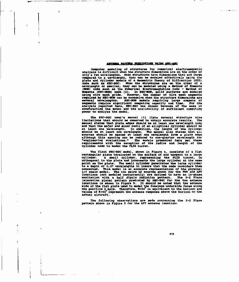
nim'ms imaem. imiaImz us•ll curse Imin-mac

Computer modeling of structures for numerical electromagneticanalysis is difficult when the structure dimensions are on the order ofonly a few wavelengths. When structures have dimensions that are largecompared to a wavelength, they can be modeled effectively using theplate and cylinder models of a Geoaetric Theory of Diffraction (GTD)code such am NZC-2EC. When the structures are on the order of awavelength or smaller, they can be modeled using a Method of Moments(NMM) code such as the Numerical Zleatromagnetios Code - Method ofNoments (KRC-No) code (2]. Zn NXC-NOI, solid surfaces are modeledusing vire nmsh grids. However, the number of wire mash segmentsrequired by I•C-gI can be excessive when the structure dimensions areseveral wavelengths. NBC-NO z models requiring large numbers ofsegients require significant computing capacity and time. n or theanalysis reported here, NRC-3SC was chosen because of the ease ofconstructing the model and the availability of sufficient computingpower to analyze the model.

The NRC-BSC user's manual (l1 lists several structure sizelimitations that should be observed to obtain accurate results. Themanual states that plate edges should be at least one wavelength longand that the major and minor radii of an elliptical cylinder should beat least one wavelength. In addition, the length of the cylindershould be at least one wavelength. The manual also states that allsources should be spaced at least one wavelength from a plate edgealthough this spacing can be reduced to one-quarter wavelength for"engineering evaluations." The models presented here met theserequirements with the exception of the radius and length of thecylinder used to model the FLZR turret.

The first NRC-SEC model, shown in Figure 4, consists of a flatrectangular plate terminated on the surface of and tangent to a largecylinder. A small cylinder, representing the FUiR turret, isorthogonal to the plate and intersects the large cylinder at the samepoint as the plate. The sweil cylinder penetrates the large cylinderto a depth of 0.07 wavelengths to insure that the code considers themconnected. This model is an accurate representation of the physical1/4 scale model. The two pairs of sources shown for the PUD and AFnlocations (not modeled concurrently) are defined to have an in-phaseexcitation with a half dipole radiation pattern. The X-Z Plane(elevation plane) pattern predicted by NRC-DEC for the two antennalocations is shown in Figure S. It should be noted that the antennaside of the flat plate used to model Vw fuselage underside faces alongthe positive Z Axis. Therefore, 0-90 ic equivalent to the horizon andvalues of 8>90' represent the antenna response above the horizon on theactual aircraft.

The following observations are made concerning the X-Z Planepattern shown in Figure 5 for the AFT antenna location:

419

II

IL - -USAr

4 l

I./0

-10

II

I11

yhaw (

llgur. S USCU . ne-U le, Wet atlsa and Plate4 modeflat .

420

(1) The discontinuity at 6-786 in due to the inclusion ofrefltctions and diffractions frow the turret cylinder at0>78 For O-S7. thet pattern is primarily the direct signalfrom the sources.

(2) The discontinuity at 90' is due to the exclusic" of thedirect signals and diffmaotional/efleat"ons from the turretcyUnder. The pattern for g4"d11 3 is dominated bydiffration from the large cylinder.

(3) For e'li2, the pettr i. dcminated .y diffractions free theflat plate edge opposite the large cylinder.

The following observations are ade concerning the X-9 Plane patternshown in Figure 5 for the PMD antnna locations

(1) The pattern tfr S5S9<9Oc is a combination of direct rays fromthe sources and reflectionamdiffractions from the turretcylinder.

(2) NBC-SaC predicts no pattern responAe for 90*44113*. However,if the sources are moved along the flat plate away from theturret cylinder to a location outside of the radius of thelarge cylinder, N3C-SaC will calculate the pattern. Anexplanation for this anomaly cannot be given without furtherinvestigation.

(3) For 6)413%? the pattern is dominated by diffractions from theflat plate edge opposite the large cylinder.

In order to confirm the pattern responses for 0<90o for the FWD andAFT locations, another model consisting of a large rectangular flatplate intersected by a small cylinder representing the 71.R turret wasconstructed. As seen in Figure 6, the location of the sources and theturret relative to the aft edge of the large plate are identical tothose for the model shown in Figure 4. The long front portion of theflat plate effectively prevents front edge diffractions from distortingthe pattern for 6<90. The turret cylinder is imbedded i17 the flatplate to a sufficient depth to insure that the code considers themconnected. Figure 7 shows the X-Z Plane antesba patterns predicted byPlC-UsC for this model. The patterns for (050 are almost identical tothose shown in Figure.5 thereby adding confidence to the predictions.The patterns for S>90 shown in Figure 7 should be ignored due to themodel limitations.

In order to confirm the AFT location antenna pattern response anddetermine the FM location aistunna pattern response for 9:-90, a thirdmodel was constructed. This model, shown in Figure 6, consists of alarge cylinder intersected by a small cylinder reptesonting the FLUturret. The turret cylinder penetrates the large cylinder to asufficient depth to insure that the code considers then connected. Thesources, modeled as point sources with dipole radiation patterns, arelocated on a plane tangent to the large cylinder at the point where theturret cylinder intersects it. The long flat plate extending from thebottom of the large cylinder is used as a baffle to prevent signalsfrom diffracting around the bottom of the large cylinder and distorting

421

0;m h -1 3Iast P.- .7

UtMT--

~O

cr- owm %~~ ago fm m Pm

s~e. x. eC-US Large viate sad cylinder Model

-10

-1550 60 70 80 90 ¶00 110 120 130

Thft (d.Fm)

pigure 7. * 33-38 2-5 11ame Pattern for Large Plate/Cylinder Model

422

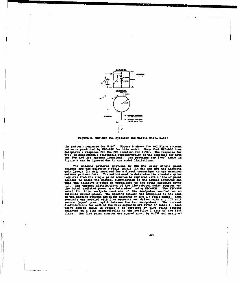
"'N

m.

II

Figure 0. EC-Boc TWO CylizAer &ad efftle Plate o•del

the pattern response for 8>90". Figure 9 shows the X-Z Plane antennapatterns predicted by NEC-BSC for this model. Note that NEC-BSC doescalculate a response for the IWO location for 6>900. The response for0>900 is considered a reasonable representation of the response for boththe FWD and AFT antenna locations. The patterns for 6<90- shown inFigure 9 can be ignored due to the model limitations.

The antenna patterns produced by WWC-BSC using single pointsources are the relative 3-Field levels (in dB) and not the absolutegain levels (in dai) required for a direct comparison to the measuredantenna pattern data. The method used to determine the absolute gainsrequires that the single point sources be replaced with a line of point,sources to model the spatial distribution of the actual antennas andthat the relative Z-Field be normalized to the total radiated power[1]. The current distributions of the distributed point sources andthe total radiated power are determined using NEC-WMO. The XZC-HOKmodal for this analysis consists of two monopoles mounted on aninfinite ground-plane. The spacing between the monopoles is the sameas the spacing between the blade antennas on the 1/4 scale model. Eachmonopole was modeled vith five selment* and driven with a 0.707 voltsource (equal power split between the two monopoles). The currentdistributions for each of the five segments are given in Table 1. Eachpoint source shown in Figure 4 is replaced by five point sourcesoriented o.s a line perpendicular to the positive Z side of the flatplate. The five point sources are spaced apart by 0.051 and assigned

423

715

10

.5

90 W0 70 9D 90 100 110 1D 130Thef (€WMe)

Figure 9. 330-20C X-I Plame Patternfr ot ato Cyliader/saftle Model

Table ;o. N1-UM Source Distributions

current DistributionReight above Flat Plate. mejumtUd Pase

0.0251 0.013623 -3.636

0.0751 0.012466 -6.227

0.1251 0.010124 -8.422

0.175). 0.00o 15s -. o0.142

0.2251 0.002718 -21.809

the current weightings given in Table 1. The relative ]-Fieldcalculated using NIC-BSC with these distributed sources applied to themodel shown in Figure 4 is then nornalazed by the total radiated powerthat was computed With NEC-MN. going this method, a maximum absolutegain of 6.9 dBi was calculated at 0-58 for the AFT antenna location and-0.8 dfi at 0-63" for the FWD antenna location.

424

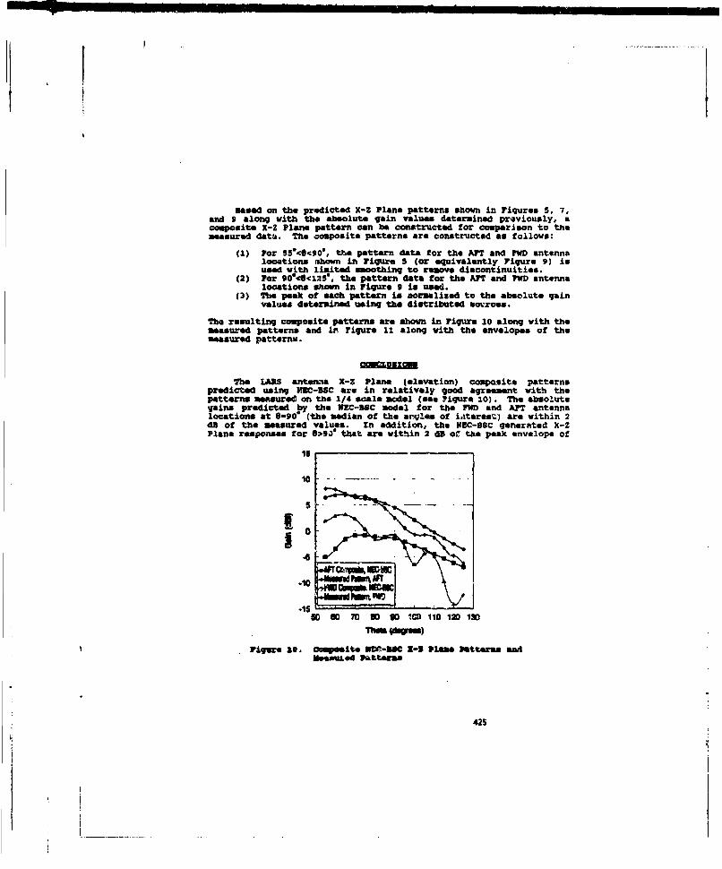
Based on the predicted X-Z Plane patterns shown in Figures 5, 7,and 9 along with the absolute gain values determined previously, acomposite X-Z Plane pattern can be constructed for comparison to themeasured datu. The composite patterns are constructed as follows:

(1) For 55040<909, the pattern data for the AFT and PWD antennalocations mhown in Figure 5 (or equivalently Figure 9) isused with limited smoothing to remove discontinuities.

(2) For 904<S<llS%, the pattern data for the AFT and IWD antennalocations shown in Figure g is usd.

(3) The pak of each pattern is normalized to the absolute gainvalue. determined using the distributed somrces.

The resulting composite patterns are shown in Figure 10 along with themeasured patterns and in Figure 11 along vith the envelopes of themeasured patterns.

The LARS anternia X-3 Plane (elevation) composit6e patternspredicted using MC-SSC are in relatively good agreement with thepatterns measured on the 1/4 scale modal (see Pigure 10). The absolutegains predicted by the NEC-BSC model for the FWD and AFT antennalocations at 0-90e (the median of the aorges of i.teresý-) are within 2dB of the measured values. In addition, the NEC-S8C generated X-ZPlane responses for 0:90* that are within 2 do of the peak envelope of

10

-10

.15 .50 60 70 W0 OD W 110 120 130

Them (Om)

Figure it. Composite U=-N@C • -• - lame Patterns a&4Mws~dPatteras

425

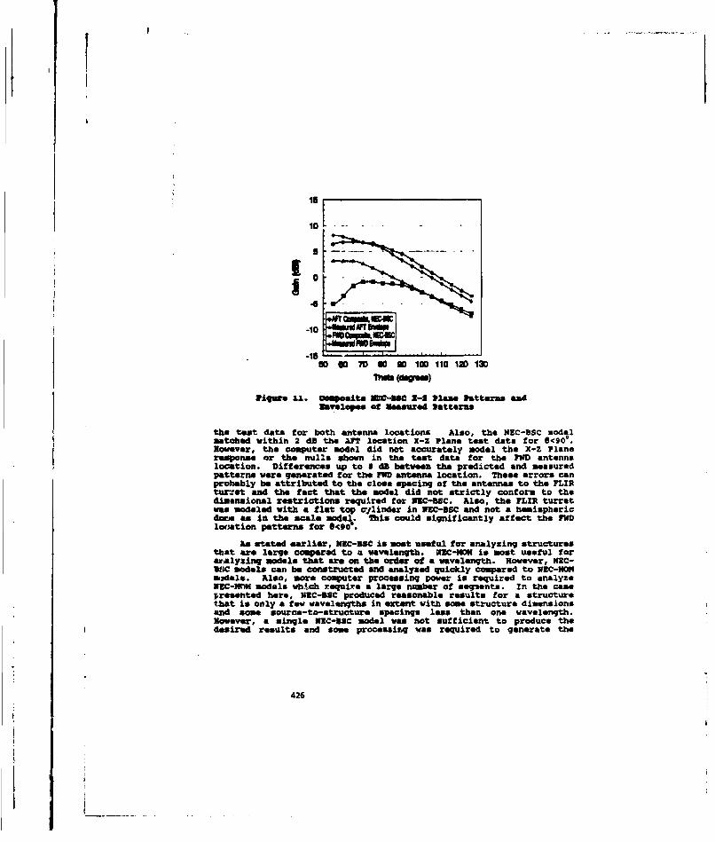
15............................__

108

'0-10 . .

4

-1580 60 70 90 10 100 110 120 130

Thef Pe~m)

ligWue I1. COsPsite UWO-MC Z-2 Plane Patterns andgavelo.pe of Measured Patteors

the test data for both antenna locations Also, the NEC-BSC modelMatched Within 2 dlB the An1 location X-Z Plans test data for 0<900.However, the Computer model did not accurately model the X-Z Planeresponse or the nulls shown in the test data for the FWD antennalocation. Differences up to A dB between the predicted and measuredpatterns were generated for the FWD antenna location. These errors canprobably be attributed to the close spacing of the antennas to the FURtur•,et and the fact that the model did not strictly conform to thediamensional restrictions required for NEC-5SC. Also, the FLIR turretwas modeled with a flat top wflinder in NEC-BSC and not a hemisphericdosie as in the scale modek. This could significantly affect the FWDlocation pattarns for 8<90.

As stated earlier, NRC-5SC is most useful for analyzing structuresthat are large c€mparad to a wavelength. OWC-IWM is moat useful foraralyzing models that are on the order of a vavelength. However, NEC-W*C models can be constructed and analysed quickly compared to NEC-NOAmidels. Also, more computer processing power is required to analyzeNEC-3rm models which require a large number of segments. In the case

resaented here, NEC-USC produced reasonable results for a structurethat is only a few wavelengths in ertent with some structure dimensionsand so*me source-to-structure alecings less than one wavelength.However, a single NMC-UC model was not sufficient to produce thedesired results and some procassing was required to generate the

426

r

composite patterns. The availability of test data prior to the NEC-5SCanalysis assisted in determining the model manipulations required toproduce reasonable results. Unfortunately, test data is not usuallyavailable prior to a NBC-BBC analysis. Therefore, NEC-aSC should beused with caution when analyzing relatively small structures. Amethod-of-moments code, such as NZC-NOH, should be used for cases suchas the one presented hare if sufficient time to construct the model andcomputing power is available.

Based on the Computer model and test data presented here, arecommendation was made to locate the LARS antennas at the APT locationan the PAVE BANK. measurements of the on-aircraft LARS antennaperformance for the selected location ware not possible due thedifficulty and expense of executing a full scale aircraft antenna test.However, flight testing of the HI/MH-600 PAVE HANK confirmed that theLARS met its range versus altitude requirements indicating adequateantenna performance.

The work presented here was performed under U. S. Air ForceContract No. F09603-91-G-0094-0010 out of the Warner Robins AirLogistics Center at Robins Afb, Georgia.

(1] ONear Zone - Basic Scattering Code User's Manual with SpaceStation Applications, Version 3," N. J. Marhefka and J. W.Silvestro, Ohio State University Electroscienced Laboratory, March1989.

(2] "Numerical Electromagnatica Code (NEC) - Method of Moments,Version NEC-2,0 G. 3. Burke and A. 3. Poggio, Lawrence LivermoreNational Laboratory, January 1961.

427

4;J

An Antenna Simulation Superstructure to the OSU. ESP4 ProgramKurt L VanVoorhies

West Virginie University

IntroduatIonTlb wanaerl eleevomaginestl silmulatikun al udeacribed heresn was one ai several tooils developed as amome toamga lvdly invosilpat ambnau s ta ca pmioahe wire woundl biffsi nauo.tsw nd toroidal helical antena [11. Theoveral bvesigatigao bapmuaioed lea man~iaudaheud eatpenmenel tedemiran, both of whibcheanplimented ame another.The pebelp1 Hity of fte uilmliint was in paredicting boih af ulectric commint diasnlbuuotris ok Uth conmstituent wifeetoa.s and do rilab pautms whode imaean was oqwavid tithe ft 5u tun~ ad ban dfp alg leqaiek&

Thiis damladitIDOL M ervlainafte referTS as FSP4K. was developed with stusdenra genararuty to facilita zte st.-udy of awide variety Of relaa notioa geometreis. lte ESP4K but is a squuneraure to the Eleotlnmmageetic: Strace MutchVentice IV proisua beretndmter referred as ESP4, developed by Ohio State Univensiez (OSU) 12). ESP4K coapn'.aacolieSan o(proeapua. written i both C and FORTRAN tar operation in Unix eaivirmemen - and related dataurincun ad aasystmfiordia mamnflemenL The £SP4 ra'jtui was selected as te kernel tor FSP4X becausseotl)1itsSilly0 Smulat geI esw with both vanes aidi oPMilnespn, 2) its ready, availability in acetrce code form fmin OSU. mand3) iarns cano by 060. lb £5P41 oo saiditats fte flP4 junges with 1) an Impioved msraste reemace ler b"lpoea-manis and posillimcannalg m.t 2) alilismnal functionality. bainciing calculintion of racetance and banidwviddi, aNd3) th craion, of live gam=liunl pesarameerzd geomeris. While the ESP4X tool was specifically talk wedl to Uth ESP4progrlfS,manty cfiia comanitama pocedwar eam o general utility. aWd would! be appicable sto any simoulation prngrman.

The paame of this pape isn todesribse the philoaophly and makwthalloy of LSP4X and to discuss t stirmc e aste litonito la SP4,peeps; coniciderhing the overall tinput and outputs, the added iunctmialtuy and geometries. the "tnoicAdiowa10 te £SP4 htrens, Sid some flmimatim of die £¶P4 kernel that w=ere discovered by this invesegaion. lTh reader L'refurmel to D I isr the Slawh of due ESP4X constituent procedmres. An EP4XuowesmanualbIsm ntyet been written.

Overview of OSUs*ESPd Program£SP4 is a FORTRAN pnigruin eCemrwifig a tinge: MAIN procedure (oave 1510D liens at code). 511 ubroutnes. and 7funcin. ESP4 salves dbat Electrc Faie Integral Equtaieon (WFit) using the Moment Miedita. ami is apiplicable to bt haradiatioin ad sawntiling pinibeisa ioe germetukie. aitetaining wires midAir plates, the later having either opten (it cloedsurfin.o The giaps is aontrolled with a squential list inputt tile ateilaning strictly eouteric data. The inu mnid otetputf"im ista will pee-detfined logiestUm sIts Wheich the misermust assigns ostepemindg physical thins riles. Severa at theEFP eutp flila we formanted for Saps to a GICS graphics pouwJ processor for plotting: 1) Uth problem geometry andvonwiaid aonini male dis~tributsio ou plates. 2) ank elevation crows-seeton radiatsioatetcseang pne.arnd 3) Man sattnsdaacm-sAwei radoraliancaicnfg pattern. The problem geometiry, is apecifial either astat lirmated list of male coovdittaeraand minuvmocutkm. ex via a asrtfmelFURTRAN suleeamatm.

The ESP4 MAIN procedure comprises three levels as defined by twit neal macsi loops which ruccessively define thepaubIs The asSla Moment Method sianuatiesi is pefosmal as the lowtest levet. These liarc levels atm designated is mile

si olkuws: 1) MAIN proendmre. 2) NRIJNS: plat gemsetr loopi. and 3) NWOS: wil geotnetrytt'ad loop. Pinramiercomcmi in all sm atns t sak nth locautimof d'iee field "aut amid Ut neausos-section plumes; and the simulationtteqmesep(s). we defined -n The MAIN level. Tbe plate geometry is then specified at the NRUNS level. and finaly the wiregnmety. wietateM sattamhents. total imnpedancsn, soil fed voltages am specifid at the NWOS level. !a a givei run ofUte ESP program. each -~ geometry speimfie in the NRUNS looip iv simulated using alt wire geometries specified madie NWNGS "oo. The EAP4 simnulatian is perftrated at discrete sscir-defined trefuetteties. bid the sy.-aina inpedance tmatrixmy he either calculated at eafi frequency: or for a sweep of frequencies, calculated a cOars frequency intervalh atudminampokatal a line firetfuency intervals

428

£8 P4K Philosophy and MethodologyThe development of the F.SP4K tool was; motivated by the desire ti reliably peatorri a harge number ot simlawtuions oa1 avariely of parametrically defined geometries. and to j~resent the results in a readily utilinsat foarim. The. related procedureswere designed to improveftboervall efficiencyaOWre-lrinbiiity of I) deibuttg the paoblem, 2) aunming the simlaltion. satd 3)maccssiug die results witiin a conistraent fralteworl:: enabling die uiter it) focus on the enigineerting and physics ot theptfIce to he solved. The ESP'K procedures achieve dhis dijetive by using hierarchical. self-docsxenting. wti-defiiatited.aeratedtables as the nsa for both Input Ked output, both by die ever - via eff-athe shelf qeandalshbsIiest programs -mist by the £5P4K amaiianuitt proceuhre; -via a collection of cianni wuiscen utility subroutines.

Pruraip lapulsevera ways to 1 - er, the efficiency and iellabil"i~ af a simulation program am 1) by reducing the Amount of Inpu thatmant he -n 1by tha stal n 2) by habeling dhe inputs thetca. it mat be mitered by die user. and providing delitulavalues fot opticatl inputat. This is achieved in the ESP4If tool with a series of Wienrtchl. self-documenting. tab.dntinv.macue Input tiles which am teadiy crate with a quemia-sheet propram sac as Mienwsut# East: ecah rowofta give able tq ah a diMiterst data teii.ad, each column of be while squusmsiaug a diflierent dau fkied A saubetof the fields - normally, one aed by default the fiust - cattest keys. am used as, designate die records. All of the fields axeowned. aned dvmt nssets - woaiaist in the first recant of the taile. The L$P4K proceduins locale a pnaticutar hem in thetables by "h field nam adc key value. so the fields and records co be in any torder without affecting the operaim of theprongami. Aadhitkirwl fils and recotds mn, also he aklaIn wiiiv table witlsaut affecting acets tit the paint table cowt'tt.it

The amounit of ruiupisd meti intput for a given simulation may be reduced by structuring the input tattls to pauip suintlatquinititties. -I the oaf a all qentitiex being generally required at the sam paitt in the proigramt - tiigetttet as recards of

,as tables. In general these tables11 can he linked togaeither wiie rtrioalty or i.enurcblidly. dqt. ndi'g upon fthfsuture of thec date. A relatiotanl linkage is establishedi when muhtiple tables slime the sam key Value, A hierarchicalrelation is estatblished whom the field cornsent - 44t a field tnnmed deter the ciueupori~lng child tattle - o4 the parent tablecontain hey values of the child table. T1his, hierarch-ast scheme enablets a single recant ofia child taile in Ie used for litaydifferet stalnattlons without having to re-citer the istoramation of' the chitld tabe fur each sanoulatlitti; i.e. this enable,.either a amy to onec. or may to few relationship to be established between, the patatn tabtle and its Children. This alsoentebe the infoemation in the child tattle to he acccssed via recognizable labels. For example. may simulations maiy

niecify alas we or copper conductors. The simulation programs rneuires a numerical value for the conihnlcviay of themsaterial. Ratther then having to stpecify this value is its piupae units far every simuliatrion, us; is reqaired by £SP4pnreag Onth ESP4X procedures ie a chikl table or matenat chxac.cuistics whose key values ar the mefacs nmtim. andwhos filaw value is the conductivity in the appuipuiate units. With ESP4X. the ater need only specify the name of themattril. i~e. *coppiert. in the field of the aaresiqmndinl zaent taile. The value of conductivity is then found automanacallytitan die Child table by Ike £SP4K preprocessing; putaedure, These parent-chkl relationships will he evidment in the siecificups t emdailltuW Ae491*d isle.

In addItion lb to providing a sf-hc etiag ranspareialty espxidabtitte inpot mechanism. 2) to providing a meanus forrabdagsf do amt input aequwaeaias and3) to cablin easily rmemetfýre ehuace suring key Valus to he subsmtitted ford~ifficai o remember mnanirical vaitiest. these briemairdicaly structiurd aIpu tables providle a natural eatd auuiarstlc way tifdisaiansing anctri wi of situnlatiosc for archlivial purpawes.

File & Data MatwlnaenantSlinulations, or experimneuts bagin with the rpciicatiiami of 'he conditions under which abete at. caaluctml - the design atexperines. The smalt of be: sinultaion or experiment is a corneasaoning sea of oautput dWAa or eieVAtsfenint& Since theonipu doeis a Oly geanigfl in the context 49 tdse conditioais under which it was genraicrad. an aumnat mechannism firaidmlaffilisg this linkage can Improtve the relitbility ait the sinsulistin an mtist Imrve die use's efticiency mn analyzing theresitlts All dmertiss generale by the ESPv4K pactedtures arc autotnaticatly tzanied in a manneir that maintains fullunmaccailitty hack it) the cturospamding input tattles. Each exceution of the &SP4K procedhes is desaiglnsit by a uniqiuethree digit simtulation number. T1heti. within :i given siinaatiom. fth mitilion level at echb ot the MAIN priuceil~srprimtry neste Control loopsa - akezasly dusaassed fir the ES14 ltngaani. i~e. the NRUNS loop, and die NWCvS loop asdesignated by a iaflspxonding letter, beginning with "A" anal sequentially tmcremented with each, pass through the toorp.Thie ESP4K wtoo uses an adlditional freqiuency tntiaukms~io loop, feaned P1FQS, nested below the NWC3S loop, and thisloaqi is also diigised by a corresponding letter. Alt datasel for a gives simtulatirts are uniquely named using thesedesignationi. The various dtlaaitets are distionguished friveran e another by a two or dhre latter symbolic 'tofk, i.e. EL forelevtion crass-seciot. ar JM lor creune andnse distribution and associated wiut geomietry. The simnlation number andthese dhesignmatrs amu alsi~o ecfied as fields an Ithe progrm input tables, establishing d-c direct correspondeatce hetween

429

input comaidmltma and output result.'. The automatifc naming ot altlmoutput daunseit elimianics any confus3ion as toI theconditions under which a given net of data wias gvreraed. which in tmorajmmnt to maintaining controt Anti integrity of the

dta when paanrliung a barge muntie or simulaktion under a wide wilety, of otaditions.

Program. OutputMiat output tMle gatermted by the ESP4K pmocedures are alto formtatted as vetl-dacttmenuing. tab-detrmilem ltablet, whichcan be presed to a aeroahidut ental pogram forei ther risplay, printing. or suhtequsaint procesring oatudilysis The ES P4Kmodcsl daes a poipestrigpcedure with teals the collecdorm oif audic output tiles fromt a specllled aimulalicm and, egt- a setalndy Mn of data tdabb - conttaining unity essential data -mid a correapoading grapomecs conurrerid Wie oroanfle 11os1 by the Tailetrin. Inc. Airamn PC taisd plkting and aualyxas progrant. AtLmuR alters a wale varietyof plot tylae, ailt type, anwl anaysis capdultiStlaesinluding 2-D. 3-D, Smith char and polfrploc. Mhet ESP4X piot;amcodedl by coffer smysbol shapec aid linee typ aid inchude labeled numerical dtea. all desi-gwod to mnarutne the asrtumilatfion ofbioeafc by dom.

aser Imnerfame MeehanlaumSiam the ECMX ,ea-saho rely rpon mab-deinrlteru tUfas for booh input nod output, the pernctple user-Interlace can hroff-the-shelf eemlalsbeec proprmt. which an capablde of mrleing and writing such files. There progrestia provide aconsiderable advantge of 1) beig alreadly tealily available and fallir ito moat uerem. 2) providing rtewerfut display.ralleg. c bi R yaatlag fin ldc. 3) Pwevimhm4 addinndlloal rcesslng csitabihides VStats sorting. seconddry calcumlations,aand piotl nf.d 4) beang s iepalydthcumianeed maintained, and enhanoed. The ES$04K mmvil utilized the Micrmnsol'1Exul~clpop a the primary their intersimt lot Creating hittgu dMt. aid the Ttialfieri. Inc. Arnant pma r-a as the prinotrjtUna WAU%= 1101 jtltIttg MXU rLTeinput da l ablshes ca be realily outsed by copying anl dust modifying recort:. frmmpreviouss sainaulatiax. Multiplei abten can be aiutaumseouly displayed in a WindrmwsO or Macintrarb envioronmeta40*68g the =nto ahoultaawsmntiy view all Input cranidhlaini.

Adaptabilitylbe self-diucnasieng lesarn- of the inpum and ouqart tubista enable; almSr tabl to rmetain tranasraun, to the evolution of thepnmSgaw. Modlifmicaiuas or amdtitioan hr) the E5P4k progratas retquifitig amldimirsal input variables can be readilyxxianammneed - without disrupting ezititagm data ur the asnimeited pirogsrirms which acces that data - by simply aiddingClmani to exiating table..

Aeenanamadmtlon at Ohjsectlv FunctionsIn fummimig the £SP4K tool, the ESP MAIN pmocedture: was reformtulated inuto 30 separate, structured procedures. Thegh*S vfl neud by tman fimnsisenia welre WaiWe amongst 32 spano COMMON bloks. Thes4e step were taken 1)to umove clatrIty. 2) to eidssaistredhundrncices. 3) to add opicific fumsctiona4y to the coide iscluding the satomaticcalculations of ,eces frequency antI Indwidh and4) ts prupare for autmatnic opi sato i nenona dtesign. The thAttwo has require the riefinhiram of an objectivIciacti. which for third item was either the reactive impedance or thediferenc ben u is operatiag arn! utargt VSWR lyeves. Thim wan added by modifying the SSPit program to male thespecificatio. of Awlefoscy. !intpeet of the calculationutil ados:olutiont of the impiedance masrie so that. an indfeparleaktroot aclvanooid nod die rentot aild anedge frwmsfisn. Other actve aos abe mea~y added o the 4Kproceures fot example: as praon a gectuirally aunsted iystialla Of siensna design fitnmetets to Maximize thetaloni glace o bLhemkIwi

TheC110k peocithwrens cct an inconsistency in ise qreclrkalhmi of valines lot the orevent mathematical and physicalcans. Nod angt the varwious ESP4 ausutmlines. Tahha 1 thows the variotus values (or theme crinmarant- definedis both LEN4 Wa LEP4r. The LENA4 procedure% define rudly three wamnots trumeriwlly: pt. the speed of tight, aidEaler' cosaft: other crainstalt ate dibm delundrs! inares of then thee varialeis. The turitttricat derunnlomis arm made inis MAIN jrtiaduf and Owiaed; -A ih all othe penhao. via a COMMON data b~k.&

Paramnetarlsod Geummarrylbe specific wire gnesicriam simuLmted by fthe LESP4 otool a described later. Each is definted in a generlizted form intemas Of its relvan geoumetric ',e-uneicts. wbks %2a1 hespecilial either in anbsoluime osuernaoenrt units. ire rantalimal withrspecitt a sspecfled tlati~gn freqitetwy. The value,; lt the pratteters, am spetcified in the: resptective input tabiles, enablingise um perform paraetric thaga studis" dtrectly. With the sddriiion t(o at oponiieer and the definition of arm .mbixivefunction. hec values of threm warisacema coulti dm alhe otumiad alrmtanicaly.

430

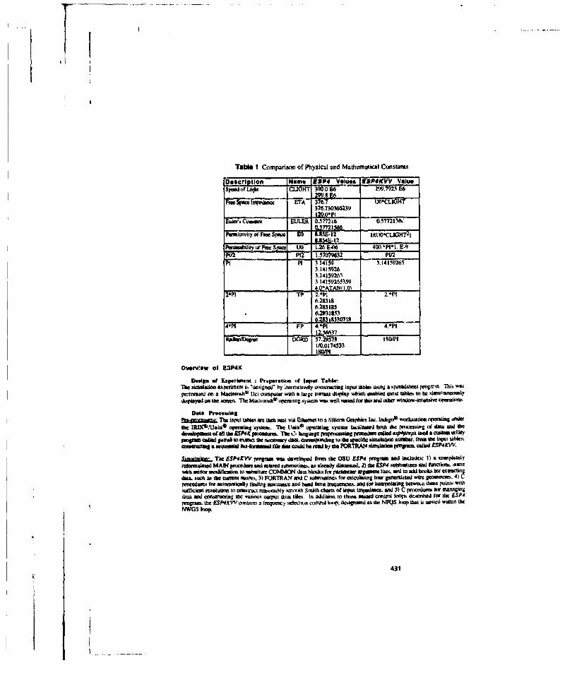
Table 1 Comparison of Physical and Mathemnatical CoatIS!hIte

De.scription Name E8P4 Values rSP4KVV Valuesfow rLtiguht Cl-lTin WoE 299.7923 E6

2991 E6 ______

Fma Spama laqashete 316. - tOItCLIC.HT376,7303662394

Ealer Mw=san EULERi 0.577216 0-.37721 -%&

hostfivity of Free Spei El 11.11E.12 lt1-LCH2S U.8~~~1154E.12 _______

Pistrhlikty tit Pee Sju LX 1.21, E-06 401t.*P1 I. E-9

P112 P12 I I.7CM162 PUPi PI 11.141S9 3,141.59265

3,141."263-14150)2653.14159265359

2*121-TP .*P12.*Pl6.293186.2931856.2831853

4-PI FP 4-'P1 .PI

RwWOenlqwe DGRD 57.29578 I WillI

Overv~ew of E3P4K

DNsigm of Expembnant :Preprsatitm of Input Tah~W,11W simutlation eaperuacra is "designed" by ýNtenieively ..omstauiinS inpuit tibiss usting a speAWMlee prWogM. This wa%rwetraW nke) a Macifflowh0 116 comiriwee with a larse Itmeat duinfiay which sasblteU mosst tales,ý to be sinutttlurnalyihrplyed tin the Mxeef The Meattinib'tai peauing tystentam welli:1 staw) fur this aal tither whitlow-intanstW tttaskxm.

Data PractuifaaJa The:lo nptabl"e am thet taIn via Etherne to a Silloina GOphics Inc. Iridigti wotrhttiwnti orsipatg owlet

the 131X',Uuax* ,ipe-aing system. The UuixO oftsraing syxtem Inciliutid. both Lith pKKSairss' Ot daLU Wan theolerselitipat of AMl the ESP4K ismobumtl ,s The rd" t uiue piepratuahig pvucdma call. elptpe useed a cesim utilityloopft W8#Vaedg~~ t b1U0 th% muuWWaa.aaqau the heseel uheiiinumber. from the ittwu tables;constucting a wamunial lmaaitiostal filked than aits he ! taut do FORTRAN Aswitalmt pmV=e. calld £¶P4XVV

SimlllE". The ESP4XVV prailigrul was develtipd Ittan the OSU E.SP4 "Mlirin and Includes 1) a LmpctniteYirorauulated MAIN prucxiir and itale'ate tshrostlnesK. axslimely 411-arned, 2) the ES P4 sobruutaes and Iterciasts.ilaiewith mdnwtrfire mmW1kIt to uitienbue COMMON data hkastc let pentaieter veianost lists. antI tn &W hnuks tor extracitingthea such ast the ceetant smtaes. 3) FORTRAN4 ant C suhnvetines for calculating tair geneazlized wire gwetnmame. 4) Cistrnceadtes far = twas ically, tinduitg remuneas atI hanai limit trw4tiances. XI) for iMkenpglait betVAa aUMM Points withtufricicnt aestlutitin itn eemstrtit evamtitbly sminsith Smitth charts of input lptpedance. anW 5) C procedureh 14W manginsitiU=t and cohmsisnt~tg the varwixs uaipu (kink Hile. In atduriokm to thusne nixtetl ctrnet kett" described for the ESP4

ravirami the ES P4K Vt emaints~ a tregitncy sred iti comit'nl 14mop. designatetl &% the NFQS kKti that 6 netd Withinl theNWOS looip.

431

buwI;nu~::W The ma~pa filies atomn the E.SP4KV slimulation, andi the ctwrespcmding input tables, are autommilcallyreedl by the C-langpuage prephn rgm "u. which corasinan; batch p~icessing Lommmanti lites lot connrol tit the PC-based.TdriteiiL Inc. AnemG plotting peovat. Ajwm* can ptn-ear speemadheet-fonnarted dtaer IlflieIn a batch itrsie tiat iscoatenlbtid by the above desaribimi cotmmand flie. Known to Azure) asa hristory Ilke All of the plats sre stokmi in templateinitim in a mate file. ant these tanrpires ame titen mulilleti to incorporate data frmn the spjecific tests to tr plotted. Theprepiti progtam Cm rmewt multiple atmalaritat. and a DOS batch file is mirautotsaucsly conwiucret wviith the proper Calls

The hitiny, film.. data fibs. anti the DOS batc fb Me samttarmeferrd vra !FAhemt to a PC1396 tunning the DOS op~erruingsysma The -ka - gmatl ina £bckpcuud mntie wsh~ the uample execion of the MOS bestc coonanid file. Thehil sojtllmumt of -Oft k each sidelmiras unjielnas five pages, each page having ftsar plots.Inpu fablesaaT"n 2 fees ao strutur of the £5P4K hilcrasecall input sables. Five toot level. relaWtioa abbes ae tertned. the

towi of tracts beIanln With ao asubs 'SD&- antiech having n key Raleik called "SlM-0 which contitrt the tirrea sdigitsimsulation atwater. This titree digit simulation tumitaler *t pavsed intotte de npprrpx ruograin a% an argument nuponissoemmlikn. and is hin tunand ta o find the coeeespssndlnp records In each of these mtn levwl tables, The Sl?.l~tain table istrod III md lW mar sand only onte envy- lot oji sltnmulatitta. The fields NRUNS. NWCtS. and NPmQS specily the stutmberofA tteguiotw in the respective nested ciastrit loops in thre MAIN peogtmntt. and alsto indicate the itiuttber oi :orreponditafrecord in the 30.4 tn.., SIN wires tand Sltsfireq tables respectively. whereby at tew rectsts is read Inao Ute SlMrusrtntable with each iteatlinr of the NRUINS loop, a ew* remird as read fmen the SIM-.wires table with echrt iteration of theNWOS harp, end a new tecora is real foIns the SIM.Srq table wim each iteratiton tif thre NFQS loop. The grannetersNRUIN. NWO. and HNQ in thSet Wiles. the goIdntifirsna nrct e file amarmgemenat as discussed abotve. Nitmally lor eachAnnotation that. me liste cquminially, A Z. The SItsz table is used for taving; sallor rmuevingl a system unpedatteearkatri. All of the ESP4 ltqtu eainbes hae taken onriTi over to thet £SP4XW prenceure without any drangv in sname ortnmoing, soý nmany of she fieklsits sh e t3P4K input tattles- will he recognizable to ESP4 un%.

____________ Table 2 £¶VP4KW lIn TaleSrscturepjvsno lSlMe8 Das. AM NPRtNT NRUlS NWOS NK)QS MW IW27mZ INWR MOUM IFILiNflBI E"

urnFF PHIW3 THPIPS PHINPS 3WWPA PHFE WA SCIPA ISE flEE ISA THSA THN PHIN

34t0 (in WIT INT INTO)Riald (VieW AFjar NRF RFjrlmn AFjrus SIF~jcde R~nennRAAPAT (id IPFE rNOPE IPPA IEFSA lASOG)ucPAr (id IPSE P11098 1PMA P1CSA IESOA IASGE:)

g1111nirna (SIMS11 N"I MmmW jl Wan PlSLe m)gMinarial (id CIWM Flrnaratlvey(emn Note.)"WFmuud (id A USAdiajr MAOSM)Plafteelgn (id Re#q S.AhMEflILATIED)

MSIM-ieS (SIM_* P50 Wkrm.DagloWhvepmlpt (id Freq 5M fl3 WFlID Shape taida N~wstitaMiter &eW IFDTYPO tfICNNT

WOWE (WIRIEW A VL2 WORt N2 OMN NPI.D OFFSET)HELIX (WAEV in ru NO tNP 54. INORM N2 IPSNSI IPSN52 ROFF 150FF Ala NTtatns NSe!p

NPAD OFFSET)OLOOP (WIREID id 14.2 NOD tNOfW Se16,12 PN1P51 P313 5FF Alao Ntflte WaNng NF1.D OFFSET

NO DZ FWidetst OR N2 KWNat N5,- "1.0 OFFSET)Peedi (Feed rmxk aml-r fljnug Vjneg V-ptraae-g It

UMjre (SIMite NPO FUIr FM(2 ER~b Amonm IFOR IF05 tFQV VSWA IFOPAT)P505WNI (hi NCakrZ NTrptaZ INor OFZt! OFF IPFO)RecA , , (in ZIRZ ZOZR5ZT8 tiD SMIN OSMAX OVSWJR NFFjmnm)

(SIN) fiM MIUN NWG WO IROZM L-Wine IWMU)

432

SIM-m.nain :Geneiral Simulation ParametugrsThe SIM-main famble has hair child tables,: INTORK. Field. RADPAT. and SCPAT. which are csxrespqamdingly unamed asfiels in the parent inable. The IN1YRS table contains, salt for die Sinpsont's rule integration pframxeters. The Fieldtable contains paramtetrs defining the distuicelsl itl the: tieal rotAts) to the center of the antennat wherein the E.VP4KVVtwoput ca calculate the faeidi at a multiplicity 0i such di~sttlices ini L~tiilrtslwishtheda &5P4 program~ for which only ontiradial dimatce couald be specified. The RADPAT sand SCPAT tables, speetly the psaritersc for the rstdlaftinv teal scatteingpeattern. These tahles cointain new parameters enabiling the field patients ito he calculated at a %urfxe-detanni;ng msh ofpoints. extending the L1P4 progranns limitationmtof single elmevtiton sald fsidth erssisseclfls. A single record in each Stthe above Whim AM used fir moat,01 simuatiosn. deionstnsnng smtemomomy of tist hieaurchical input table meibrellology -frequently fixd informiation need only be iearned omr%. ml the rume level tahmls ae.l thNo cie ftestnaal

SiMbrnaw; Material Proeprties, Wine Slam, & Plate Deal 3nThek SIMseas table coamitis infirainnttt about material ptspenllea and plade smign. and rifertences the foalloiwing tables:~tirahl, Wlrejaid. and Platt-Design. Material naimes are used as bcy YW=t. in the Material table, and Wire gaugenumbersaSm wedi as bey valuies in the Whujial table, The PilaiamDesain table i5htcatjwith two key ield, ThePLA713TYPE Ami swims to the ntie of a thabl condacaisng plate slenp puimflsa. while the PLATLID field relexs to thekey value of the cixgtda eodin this table. Uses may easily add their own parmeterized plate design subenuilnesso the tSP4rA' ursiram that specify anal conastruct the ctwrexqsstding input tables-, and finally modlify the prsprricessaing;jaocahm to read ald lr'ea& these utiles.

SIM-wires t Wire GeometeryThe SlIt-wwle Wile qiecfies; she wire geomretry. The Wlre-Desaig lies desiguacd a record in the corresitttmiingWhu..DaPtlsables which rersqvns a specific physical emnhoidinaent. 'Me Wire. Desigi. table in turn rtmrencests theguramesm fura specific wire geometry via twit key fwfs., WIRETYPE and WIREID. The WIRETYPE fleld spectilesa thewmet *( aable, while the WIREID field specifies the specific recortd within that table. The key values for allo theseeahims we typically dkema 4to be meaningful names sti character toinge. PStir different WIRErYPE tables aim pressentlydefined: DIPOLE, HELIX. DILGOOP. and RINGiBAR. Each sif thema tables rietitie af cenut-r-ed delement which is nestaedalong a line. 'the DIPOLE table qniLifes the usual linear dipole eleimel. The HELIX t-ti specifics a helical eleitentt or

a cnmaoun hlicl eemet.The DI)OPutbile specfles avspcialrzed tepwestsonaiinat cm elix, or cinsnswtvnd heix.Ceomprising a smks of open rap elements.ý normntd to and sameentric with the antam axia which are iotcmvtenected by aserie of collinmar elemnents which am ilneallel tos the axis aif the anlecnos. The RINGIIAR table specifies a ring-bar.epresetasin sita csamerawstens linea helix. alter the wcvk sir Riohli and Everhar (3]. These WIREFYE tables speedtydie goetattic peralefts in tennit of either absolute sir wavellength nswnud'zed malts. Thte physical siam of a noranalizedMariaa isern by the slesig frequaency firom the Reqf field saf the WizeDesign table. The genralized linear eletneats definedin the WIRETYPE tables c- be srnaasfarmstd hinto either a circle, semicircle, or polygon hy specifyrigl such in she Shapefield orf th Wlre..Desin Waile. The iniqegr pruianeser NSiile specfies% hallf abe nusilw of sides in the prilygci. Forclecuheor a polygonal shopes the ICNNCT Amiedspecifies wbhethr the wife dcunea is closed or opena The NContrapuwneter qtecifes wheither the HELIX sirDILOOP anttveas we bifilsi contrawound. sir monofllIa. while the Feed field"sgaifellft shkey value in the Feed table which defines fth volitage read isperdance at the feed punant(s). Each of thegatuallmd linea elMent Q111 he septiemed and 10ed pstt ONi he koante At theOPNF sp l hrualarha.

Assa illetitaisntof sth slimgeerality, o~f tha getuatenesuand tie aimplcisy of dthir specification, sine recod in the DIPOLEsable, together with various cstebinatines of insamnelis in the Wire,.Dmaign table, can he used to specify either aconventional lines dipol~e. a amaetuiteuaal dipole. a pislygonsl apposiniiation son acircular to", oran rewn-ia-sed prilygeesal~oep The Inst configuratios ma be either tran cvr chased Wd may he fed asl eibler a single point. As wishba shusvensicataldipol or ltiss. oar at makeiple poants. e.g. such ass at hair espit-spocd points in a Smith tl'avesleeC atenrai. This statiegeneaulity also applties sto hells. dikaip. and aiig-I'sr aintritirins.

SIM-frog t Simlaetiton Freqeqaney antlfair l'rmqamney SweepThe 5SIN-fiesil table specifies; the friequentcy ort frequency tanage at sor over which the sinitakioiin is pextritined. Whensimulating over a range sit treqaeicaces. the lisequaticis inaty either be specified at fixed tsetluency stuervats, - its itt thesmaginal LVTP4 Ieagsamn - or fthsimulation may be usecd itosauntmioiocatly fuel rescinatit hsland edge frqesee.uingaspe14citiesl VSWR ass the Criteria te li setaisig tIle sraprating; bandidakth. 7be litirace appecaich as speciftol by the Itable onaredFTIQSWP which has the staaaalavd L 4 vtarathles. Rtaleisis peenrts cani be calculated iii these tiseu, frequency rsisao Thelatte qipprsatm is. spsecified by the tal teemed Rtestuiece. Rjnuizexm pateria can he etalcealeil FA reinnaice KWs hantd edgeireqaecies. The program riads. the roams tald head edge frequenc.ies using the ZDRENT algoradatt laros 141.awd then -sto as, to prosduem data tor sanmih Smith ('hauls - slccessavety splits the resultings frequenc~y intervals ustil the getistrnlizeidistance: betwee adiacent trequency pssnls in the ounpr.ies Smith platte is less sleen a table-Maciettedar:iurstni

433t

Output Data FiliesThe outratp file psoalucd by the L1PK potcealires awe lintedl in Table). Reference I II list, the dletailed ninectuse ofthaesenfiles, Tlhe data film are written in three difleRnti foratstaL. The ESPat tuisntt dalgnueus [lha £SP4 progriasiltinsatiret fileswhichS we delenilud in 121. lbs ESP4KfrV foratana designates tilest which rseaut froma pfle-procensing die input tables andiwhice ame used an direct Input ito the ESPKVV pttaeaiun. The Tat' format alexagnates sell-aiocwnrentsag Lnh-delantteel tilewb ine emedaeralrcture: baa already bun described. The daitaeto namring aeatnenriem -an integrtal pealt tt the t5P4K "limanagenisa aysem - coawerrsex a two tX three chare acteac(tueionml Isefla. followed by an alpleanraneric simulatinoeIsbaifying auffix etmpottsl trn. the fotllowing valmenens a) SIMJ. abe iiesulatlien number hI NRUN. tile character

Iqrmata I 1 thde NOUNS kxVeiop nnw, 0) lWD, the character represetanakat oft the NWC'S loop counter. d) fNF. thechastncer irpyrertAloa of the NFUS lesep conanme stat 0) 10. the charmer preteeentntlttn of the renooaice numtber. Thesufixes wedl lit Tublita 3mar tlelined s i tlomwe

PitAblE (SIMS1p4RUN](W~i(N ~l1GKUME- (SWaL#JINUUNINWOJ

tENAblEu (SIM-SINRUNIINWGJNPUR~ZI.Output Plot.TlIs preplot treagrmi nelectively reain the ESPAK output tables and casnwucis tAlen (it plot ctitmaaets an the Azurntlplotting: language nalthtbe fairnuttilsqasett bonch proc~essing. Tahble 4 lines £5P4K' f ull viattingetet of 2U p~nts stiinonan

g ares utilizing a vaitty ref sAxes tyres, and annoMtet with Wilmt'ain numerical data fer the usr et) - in mnostt caes-fullycoanpriheriti the itiunlaaee embondiienet wiahetue, having to rely upon other output data. The wire gtoeirsey in shaown inboth 3-D (Plot 1) .inI in a geeraglized hasn (Plea 2) - the greneralivera variables, being the auimuthtal and polaidu angles tor ataroaifill getaesty whom ta~t axis hn z-oresini. The teced locatitinma wae sow with nytntesli. seal the coteespiondlingvoltage laid ptlaert b laittaata. ELINK sugpta sumemanries with both one and two wites. anl the current elistribuiticitsfor issch Visa AMe ah"oweslor and snyubri-ol'caat salt restaaincie end crespondineg honded mge retqueaetiex n emseparate pKNtfer each wire (Roitax 3 sand 4). The fereuency responne of impedance I% ahowva n soPlats anal6 at both full st.le. eand at aflner salne not atcsidln; +I- 1IOM0 which sedtence line- delineating the restonticie anal hatal edge trequencies. Polo 7shows tho iampetance in Smnith chart banns,. with aeastepial lines cotnexpatewing to netemalizations with reepect lta each ret thle

te t lmetpmmcits. Pleeq A jans the VSWRt. eepnnately normtalized few mch resnotance. ploted against thecinontiatat letiefqaacy. fleas plots - nastuatetl with lists of the notutallized atioteatt sanl banal edge frequeancies. the

asreimomltin tasmi lnegtehaecel; sald eanafsitalze bandidths. The ralalisgapin eald pleme are shown, ie Plet$ 9 and 10.rmteVlifly. AN ak k fa Uat.o erqtencMy few beetlh gats1iliizaaie ala the ngtecific fil poi-nt apeci'el an liar SIN-main tattle.

PiM I I shos various enutm for the mannia veloceity facter which is the taeka of the wavelength etf the guiclea wane it)tha of free qatel. Ploet 12. ueseftul for unniaw with multsple teed points. shown a notrmealized uimpedance as a function offd Point. 'The pleats etin e iNwo pages eAte* the rialtatiem gala an a fuanction of elevatatat (Pleas 13-16) oil azimuth angle(Pots 17-20). -eta-ectvely. acti boh theta vaiacl sald phi Ctamieeratli aiumionstn both unset anal poelar axes. Thepain is plotted at each reenauaz arid coreasaponding heald edge treapteacy with canting by catbor. symboel. .sh line type.ESP4 AnomalyThe P474KW gimngs s iad the LIP4 isolutian ietnlal xogoy withoate clangs other than the flaweveselecibul wtt ofstainms values tar the phy*Wa anti mathenmsiasaleasauats. '11w veoitcy inctew of hel"al d cnatleatrawetunel helical antentea

smat w" of larticslf inesuiteatoi the inveehigaeaaae de~lenuied in11). lbesnimualated velocity faetor of enallattfilar heliaelelemuesa wus atuaneen with exitpenenineatmeasutrements. however the simltneada velocity factor of bIfllae contsawoaaldhellcal anewtrst witanti-smntszeriic cureartl stale duitrilbtain- othierwise similar in patch. rahanier. anal length -wa afacio of ahoste rena in three Aiee faster elan that aentually meatiread, Thin will be eepew'.ed in greater detail in a later

summuearylIM LIFER stienalatimn tool is -n enaaceataoeu cat the W7517 ETF programa. The bierarchlmal, neniactarial Input an4 outputeables providle a ceetimaluet awd easty he) a*n Inaterla which tinelitales thesinadtulnicaeof a hrad see of paratntencieal siregeoetresni. User ianputex uam tas aisle m1inisw anad am twlt'elttuaztnaing. The procehure and tablet; we inherettly upsetcodedl and flexibtile. senabing othe parameerizes getnseuries or he reaily elelinel sal sistaeatetl within tilt suns ltnnnewfeclc.The LIFER teen pileseetly rnuts. in a ctiahatasa Unoit'h anwl DOS muvirteement. the beer being required air the plottingiwwugman A Mrea ate of aaaeactalsd plots wae suauaeiniaaally genseoat late each lunuhitaint. enanhitig ehe titer itat quticklytavhmitnise riny measuen ti the sitlatealm satuesn enitaeelemenfn nbuuurmat: Th rundelyiog; LSIP4K VVl Pomtn canautomtneically cablcinte rcsnxa Itian limqaerae and VSWR baalndwidth~. and in structured eto acilitute the de inuelkn iat aaffoter"itaetve tsacteo mald the sajinttair ttsn ofl separate otptimitzaeitntapoweateres

434

Table 3 List of ESP4KVV Output FilesDatas.: Name Format DescriptionORPRF M ESP4 )Symaea lmpmbmw: MauiftPIISIMJ'I E,¶P4XVV Cop of EvPEKVV list InputZLI AMEJ Thh iw;!eaic cateatiwam IngMWFN Tab ~Vtwwkm RathwlaimutePhnn

T? M Ij TO NMw PAN RadialePuse I .a Ain Coh~____

FV(GMME) elatin PnqueaemuM _ A VSWR: All DewTqaF~wJ Ta Rafstion Fr~rt Imaw. kmnfAma & Bandwalt: 0"a

Sg(-RZI4AMEI Tab R&~.= LgWmla wiit Romawum M-1u~clONJJr Tab £Iprmei: Raeii Fnlmpacma

R.Z- AMZ- f lý; PObIiitmllaumFpxe Re~ite simwiil Frevutwsa(ONA~tEJ Toh $atn umy ae e e

QISIM..SJ PES £SP4 Foimacy ReplamDeataIw;Z~ l Esp4LKVV o T4Vlimp7Win. Cannary

wUWwsdat l j W* ,uJM[FN I ~Tab Wauuaa CuilMusCthua

M-OSIWj] MAT- 7~ ClauwnyDue

Table 4 ZSP4K Output Plot-; _____

P60e pict -Descriptionit I WieC

2 eCisalud M2 Csuumwy-. 4- Cutrt 50Pa Datw - Wire 1.2

11 3.6 I, iec unRauw-Full Scale.Fune Scale7 Smith OwnI Vswptin 9 I Raiatimkn Caan/Pbum. vy.. Fmoac (Thew & Phi FZ;Ginlo)It Veltwityr-amir

12 IReative impohr.viuett uullipe tslpwnti.14 Ehnia..nuvSgcw TMAIM~h PttlwhlaiitA LOOMg SCRM

Ill!N! Aza!a CMtui.eacIm. fhlullhi Puaiazwazi Plan Sal

'9.0 AilmlliCn~Secunm. Tbeujftl PthAlwistm. 1-mar Scale

References1.VaVojAtii KLL.. The Segmented &flarn Ca~ramannwd Twimeala Neticiii Amlatn., Ph.D. Dissnathiva. West VirginiaUnuvesiuty, Dec.. 19193. (To K- pulisheil hy University Micrnlltmi. Ineauiaenal).

2. Nowutma. E~ll., A Users Aonsloare th Ie Elgewimovpgwsc Saurjte Patch Code: ESP Version IV. NASA AdaninrnkiunsComm,. Lmgley Rucarh Center, Huriouipn, VA. 19M.

3 Biniwuul. C.K.*: Evterart, TE.. 'MixfjiW OiutCav-Wiwad liefi Circuits for Nigh-Po)wcr Traveling Wave Tubeio" IRETuat suawitse on Elercrut Okvttf, ED-.I. Ocet. 1956,14)(1-204.

4. Press, W.H.; Flannery,. UP.: Teukotrky. S.A,: Vetiealing, W.T.. Numecrical Recipes in C (The Art efScientificComnpu~ting). Camhnajge lOluvemey Pms,~ New Yiwk. 1998.

435

A Study of Two-Dimensional Tapered Periodic EdgeTreatments for the Reduction of Diffraction I

R. A. Burleson, A. A1 Terzuoli. Jr. - Air Force Institute of TechnologyE En~lish - Mission Research Corp.

L W. Henderson - Ohio State University

inuv~dcm Ilip$ r iwm the results of a study using tapered periodic edge treamentswo , , P wide bindp =l difrcirm n a knife edge for the lauization parallel to the plane

oficd e.The tapersw= deige using the Periodic ?Mlet Method (PMM) and theFlaw DdrawTimeDomin FDTD. ad ten epenmeataly verified.

The designs described herein use the capacitive properties of thin strips for parallelpoalmo.Other designs were built and tested for the orthogonal polarization using their

inueie Plope=e but the results were not very promising. Since the tapers were to beulumaely mend mn anas, the tapers were designed and emaed at near grazing incidence; the

meaurene... we utenedto approximat a two dimensional (2D) knife edge with plane waveincidence and ik far Enied observation point.

T7W Deingur. The upsim were designed using the PMM Version 3.0 [11 for doubly-inrtiniestructiea bouset an a 33 M& 486DX. To use this co-Ic, local periodicity was assumed for thetaper design Dy taking v~alues along the taper and assuming local periodicity, the reflectioncoexident was found w: a anction of positio a o the taper. Due to the 8:1 length to width ratiorequired by PMM. the =elcto cooeffiicients netar free space could not be calculated for the

-aaitv taper.For the capacitive taper, the gr=n plane edge was the most difficult, since the challenge

was to drveoa dreip that had larg capacitance (low impedance) over a bandwidth of 2-18GHz. The rfcton coefficient for the ground plane side should be very close to unity (0 dB)over the bandwidth

Trhe tapers were phot etched on a 10 uir. dielectric suaistrate with a 5 mil minimum linewidth. The dielehzcm substriae hod a dielectric constant of 4.5 over 2-18 0Hzx. The capacitivetape design had a constant center to center spacing design with varying strip widths. Toincreae the capactutance, this design had a second array of thin strips on the bottom of~ thedielectric -1bam Th Me bonozn array was the sine as the top array except that it was offset byhalf of a cesswro-censr spaing, as shown in Figure 1. The widest strip that had a 5 mil gapand a imLragefectiott : =ffeIa1 over the atunbandwidth was 330 meils wide, as shown inFgRem 2. The strip widths were linearly tapere frm 330 to 5 mils. with the center-to-centerspacing for the Ciparitive design being 335 mils. Two tapers were built, 15 and 30 cm long.

The taper prodiaad resonances that occurred at approximately the same position on the"taer The lower frquencies Approached the reonne . and have a mom gradual taper, asshown in Figwz 3. At the resnwainc the impedac approaches - and the ground plane isaxacty mawibed to free space. On the ground plane side of the resonance, the reflectioncoefficient (i-i SB) decreaaed from 0 to large negative values. On the free space side of theresonance, the reflection coefW~cieat increased to"'ard the free space edge. Thie reflectioncoefficient wits still fairly low at the end of the tapeir over most of the frequency range. Theground plane interface was still a scattering source for low and highi frequencies, due. to lowreflection coefficients and a second resonance, respectively. This taper displayed the bestreflection and impedmice characteristics of all of the designs over the frequency range.

IThis wrok was supported by the U. S. Air Force Wright and Phillips Labotoraroes.

436

rt

Mwurn,mnu: Since the goal of this study was to develop better tapering mechnisms forante•nas, the tapers neee to be effective at near graing incidence. To "y the effectivenetsof the a= designs. a platform was designed to siiulate an semi-infinite thin ground plane. Tominimize edge diffraction from the sides of the ground plane, the AEL horn was mounted at theapex of a triangular plate. The triangular plate wu then mounted on a 2 inch Styrofoamsubstrate for stabilit). The source antevna was then mounted by a wocden bracket to the apex ofthe triangle. Since the distance frosi the antenna to the edge is mote than 5 wavelengths, theplane wave incidence approximation on the edge is valid. Figure 4 shows the setup of theantna p-WOM

The total field was measured for a variety of angles and freluencies. The angles recordedwere bimatic. because the aure was fixed for all measurements abot 4.7 deg. from grazing off

ie triangular ground plae. The so•rce born was rotated to have the E-field orthogonal to thelong edge. The horn was mouned on the apex of the ground plane by a small wooden bracket.The antenna was rotated to the proper polarization and then hed into the wooden bracket. Thetaper was attached to the Styrofoam substrate with masking tape. To reduce scattering, coppertape was applied to the interu between taper and the poud pa-ne.

The Laper showed a marked improvement over a bare edge. Firs the hard edge diffractionfrom the platform with no taper was compared to the UTD prediction of a knife edge withincident angle = 4.7 deg. from the ground plane. Figure 5 shows the comparison with additionalscatterinS in the measured data over the UTD prediction of the data kWife edge, in the region lessthan 300 into dhe shadowed regiot. Matle improvmnet dplayed in the rgi greater than300 into the shadow region for both the long and ahort tapers. Figures 7. 8, and 9 give the'frequency scans of the capacitive design at the observation angles 90 deg., 120 deg., and 150deg. respectively. The de"sgn seemed to work well over the frequency range 5-15 GHz, whichagreed with the results from Figue 3. The taper did not seem to be effective in the region lessthan 30 deg. into the shadow region, possibly due to the additional scattering sources.

FDTD Modzi: A 2D TE(z) FDTD code [2, 3], hosted on a Silicon Graphics workstation, wasused to calculate the capacitive Wtper. To ensure that the dielectric slab of 10 mils thick could bemodeled by the code, the cell size was set to 0.4244 mm by 0.4244 mm which gave time steps ofI psec. The dielectric constant for the Styrofoam was set to 1.02 and the dielectric constant forthe photo etch substrate was set to 4.5. The entire grid size for the FDTD rn was 4300 by 700.The rims for this model required over 50 MB of RAM and several hous The obervwton anglesmeasured were 90, 60. 30, 0. -30, -60, and -90 deg.- The time domain results were then FouiierTansfotmed to echo width using a companion program; ae Figure 10.

FDTD supported the measurments since no noticeable reduction was made in diffractionuntil the observation was greaer than 30 deft into the shadow region in both the FDTD modeland the measurements. TMe FDTD •ets showed improvement for the long over the short taperonly at fteqaencies less than 6 HL. This result agreed with the measurements. Th type oftaper used (linear, binomial. triangular. etc.) should only be significant when the taper iseleesically shorter. The FDTD results suggested that the capacitive taper was effective in theranlle of 2-13 GHz. This resul tended to support the experimental data" whae the capacitivetaper was effecve in reducing deep shadow fields in the frequency range of 6-16 GHz.

Further, the FDTD results showed additioral scatterng for the no taper design in the sallowshadow region. FDTD was then used to isolate the sources of additional scattering. First, slopediffraction was considered, but since the source was a simple source, no slope diffraction couldoccur. Second, the scattering from the 2 inch thick Styrofoam was considered; FDTD was usedto determine the scattering as a function of the dielectric cotistat from the 2 inch thickStyrofom alone, withou, the pround plane or taper design. The FDTD results from the dielectricsubstrate alone showed considerable scatnering in the region less than 30 deg. into the shadowregion. Therefore, at least part of &t additional scattering was due to scattering from theStyrofoam substrate.

437

Coxclmaio.u The tape was highly effiective over a &Mooeuny range of 6-16 GHz. The taper didhave resonances which would produce dispersion for a signal in the tirie doinun. Thiu piroperty.while unwanted for time domain applications. is tolerable for continuous frequency applimti~ons.

One improvement to the taper would be to change fronm constant center-to-center spacing toconstant pap size iLe. the length of the gap between strips. This charge would provide a morecontinuous tape design and increas the bandwidth of the taper. Another improvement ta thefirst taer would be to load the flue space edge of the taper. This would niduce the scatteringfrom the free space end of the taper. Another tapr improvement would be to try differentperiodic geometries than create capacitive impedance. Discrete capacitive elements would beIe'm . foe bandwidth and continuous tapers; however, these discrete elements would resonate,and degrade time domasin applicatiom. Therefore, depending upon the application, the tapercould he improved in a variety of ways.

Mhe mmasurements in this study were bistatic measurements. Monostatic or backacattermeasurements would lilso be of inuna especially for RCS reduction. Monostatic measurementswould be much earne to perfomi and wol not reuire sucih a large structure for measurements.Also monostatic measurements woul not require mhe asstumptions that were needed in a bistaticstudy. If a similar antenn platform was to be used in a future study, the dielectric constant ofthe Styrcfoam must he measured for proper modeling. For a dielectric constant to close to unity,a cavity rescrmotc method of measuring the dielectric constant would be needed instead of thewaveguidit method. Other fumur work would be to attach the tapers directly to antennas, muchlIge edge cards. Another major amu of study for these periodic tapers would be the reduction in:edge scatiering from a finite size radome. For better modeling of the tapers, singly-periodicPMM codes could be used instead of Henderson's PMM code. This would allow the tapers to be

designed without having to assume local periodicity. To improve the modeling of the platformusing FDTD, the entire stnarurve, including the source antenna. should be modeled using a 3D)total field PDTD code. This would eliminate the plane wave incidence and the 21)approximations. By modeling the entire stutcture. the addtional sources of scattering would beeasier to determine.

Acknowledgment The authors we grateful to the foflowiag people for their suggestions: CsrlBaum. Jerty Buchenaur. Raley Marek, Dave Scbdriner. Paul Skinner, Joe Sacehini, Bill Baker.Leco Felsen Carey Rappaport, Larry Carin. Ray Luebbers Jon Young, Eric Walton, JimMaloney- Allen Taflove.

Rtefaview

(I] L W. Henderson, Intrroducuion sp PMM. Technical Report 715582-5. The Ohio StateUniversity ElectroScience Laboratory. Department of Electrical Engincerin ; - paeunder Contract F33615-13-C-1013 for Avionics Laboraory (APWALJAAWP-'3). AirForce Wright Aero.natical Systemts Command. Wright-Patterson Air Force Base, OH.Feb. 1986.

(2) J. Beggat, L. Luebbers, and I. Langdon. User's Manual for TEC: PSV FDTD CodeVersion ClvforTwo-Dimensional Transv'erse Electric (IT) Transient Scattering fromFrequency-Independrnt Dielectric and Magnetic Matre.ials, University Park. PA, June1993.

[3] K. S. Kunz, R. J. Luebbers. The Finite Difference Time Domain Method forEkctrvinagetics. CRC Press, 1993.

438

Grun (spncuig 335 milm)

Width CnW to Ce

PEC Maumial Dieectric Si~a~tc

Figitr 1. Taper dnsigta for parallel polarizfiuio, wish consiamr center w center spacmng,

Rf bctlon Coefflcent vs Frequitny (Capacitlv. DoWsgn #2)

1 2 3 4 5 a 7 6 9 10 11 1IT 13 14 1S 16 17 13 190.

"I " stop Wk1h = 330 n

.4

figwe2. Refteeton Coefficient vs. Fre*quencyfor Ground Plane FA~ge of Taper. Thidefign was for aw~ thin strp arrays of constons cerner-to-cerner spacing of 335 mils, with

strip width of1330 niues

439

Refliectiofi Coefficient vs Length of Toper (Capacitive Design #2)Ground Plarm Free Space

-20.

-40

Figm 3. Reflec~so Coefflcie~w vs. length of Taper. Note that this taer is well behavedever most of the frequency range.

Top View

91.44cm 30~m

AEL Antenna

91.4 40Z

Totl Field vs Avmuth Angle (Hard Polarization)

-90 - .0 -70 -40 -3 -20 -10

I* M•w DmN Adubl cuwm 10i4" -• "•'- "' -0-'

Fm-umi0 - 40 GHz - 3 2 -

I.

Anmft Angle (- )

Figre 5. CoAimut on of o and MeaDes d Rat U rJIE showin g ie moe thana~dmgioal werin$ w 3en the observation was les than 300 int the shadowed region.

Tatel Reid va Azimuth Aigle (Capwl, Des4gn #2)

-90 -80 .70 -60 -60 ,40 -30 -20 -10 .

30° io th shaow rgion

Fmu4y-10 40

Total Field vs Frequency (Capacitive Design #2)

2 3 4 5 6 1 89g 0 1112 1314 15 16170.

-10.. Azkrdh Angle.90

-20. -NO TMPW

460470

Fisam 7. Frequmeny Swesp for Capacifive Design at 900 into the Shadow Region,shoning a 10 d6 reductiiu oer for 6-16 GHz at 9W into the shadow region.

Total ield vs Frequency (Capacitive Deeign #2)

2 3 4 5 6 1 8 9 10 11 12 13 14 15 16 17

0.-

440

Total Flied vs Firequency (Capacitive Deal- ~2 3 4 56 6 6 9 10 11 12 1 14 15 16 17

-0.

-40

Ftmquaswy (GH"

FIgurre. Frequency Sweep for Capaciaw Detign at 1500 into the Shadowi'Region,

showi~ng no iyrownient for the enare frequency range at 1500 into the shadow region.

FDTD Scaftered Field vs Freqmecy

0 . t I I I

5 6 2 4 6 a 10 12 14 16 18 20

0-

-40-

Filurr ZO. Comparison of FDTD Resulusfor Taper, showing improvement for thecapacitiv taper design up to 13 GHz. The incident field wa~s at 1700 and the farfield

obsermnton angle was W.90

"43

444

SESSION 10:

FINITE DIFFERENCE TIME DOMAIN I

Chair: Jiayuan FangCo-Chair: Bruce Archambeault

445

Application of an Upwind Leap-frog Method forElectromagnetics

Brian Nguyen and Philip RoeDepartment of Aerospace Engineering

University of Mfichigan

1 Introduction

Advances in the ocomputational:science, of the past decades; have increased the feasibility of timedomain solutions of Maxwell's equations. In the last few years, many studies and applicationsof finite difference time-domain (FD)TD) method have been published. [3, 1, 5, 6, 8]. FDTDsolutions can overcome the limits of older methods such as geometrical optics, physical optics andfrequency domain method~i These limits am in particular, non-lineur material response, ultrs..highfrequencies, continuous excitatrios and wide-band excitations. Recsently proposed technologiessuch as electro-optical and ail-optical devices demand solutions that cannot be given by the oldermethods (3]. Hence the time domain methods are required.

Three common fumilies of FD)TD methods are the leapfrog method [16], finite volume methodsusing Riemann solutions 110, 91, and finite element methods [4]. AUl three methods axe currentlyreceiving interest and gaining improvements. In this work, we apply a rseently developed variationof the leapfrog family of methods to obtaiaing FDTD solutions of Maxwell's equations.

The upwind leapfrog (UL) method was developed originally to improve time domain solutionsin computational aeroscoustics [14]. It addresse the issue of propagating a disturbance accuratelyand efficiently, that is, withoal; numerical dissipation, very little numerical dispersion and on acoarat grid (with respect to the spatial wavelength of the disturbance).

The UL scheme works equally well for Maxwell's equations in 2D, where the equations aredual to the 2D acoustic equations. In 3D), its practical implementation in a computer program isslightly different.

2 Upwind Leapfrog Scheme

The various versions of the leapfrog scheme used by Yee [16] and Taflove and Gooriian 113,12,2,S]all used a central differece (or symmetric) spatia stencil (although variations in grid staggeringwere employed). Works in fluid dynamics have shown the importance of treating hyperbolic Partial

LA6

I

n+1

no

j +1 1 j+l

Figure 1: Upwind lapflrog stencils in I dimension

differential equations in an *upwind" manner (as opposed to symmetrically in space) when solvingthem with finite-difereace methods [15, 7]. Accordingly, the stencil of Figure 1 is proposed for aID (in space) system. The first stencil is used for a right ping wave, the second for a left goingwave. The leapfrog scheme owes its dissipation-free characteristic to the fact that it is reversiblein time. In Figure 1, the stencils are clearly reversible. Using this stencil, a ID Maxwell's equationis written, in finite difference form as

U7÷+ =*--;: - (2y - I)fu. -,] (1)

where u is any carusian component of the charcteristic vadiable vector GQ - D :F "/fR, and v isthe Courant numbe:, constrained by stability to be la than 1. This scheme has no numericaldissipation. It's numerical dispersion error is a function of the frequency and the Courant number.A complete discussion of the UL scheme can be found in reference [14].

In two spatial dimensions, the situation is more complicated because the direction of the wavepropagation, a decidfing factor in upwinding, can vary continuously in (0, 2r], wheeas we must belimited to a finite number of discrete equations. One solution is to discretize the bich-acteristicequation along each grid direction using the stencil in Figure 2. In this manner, the characteristicvariables are required on the cell interfaces (faces), thus all unknowns are kept on the faces. Theresulting bicharacteristic equations for a transverse magnetic (TM) polarization are obtained bytaking combinations of Maxwell's equations:

:ki. & *cy (1,. :F ) + =;; 0 (2)

a (D. E- ) _~ (D. _ 0 (3)

Upon applying the stencils of Figure 2 to these equations, we obtain the difference equations

Q!-+'= Q! - (Q'÷ - Q'-1) - 2P(Qr - O'+,) - 2AI ay (5)

"447

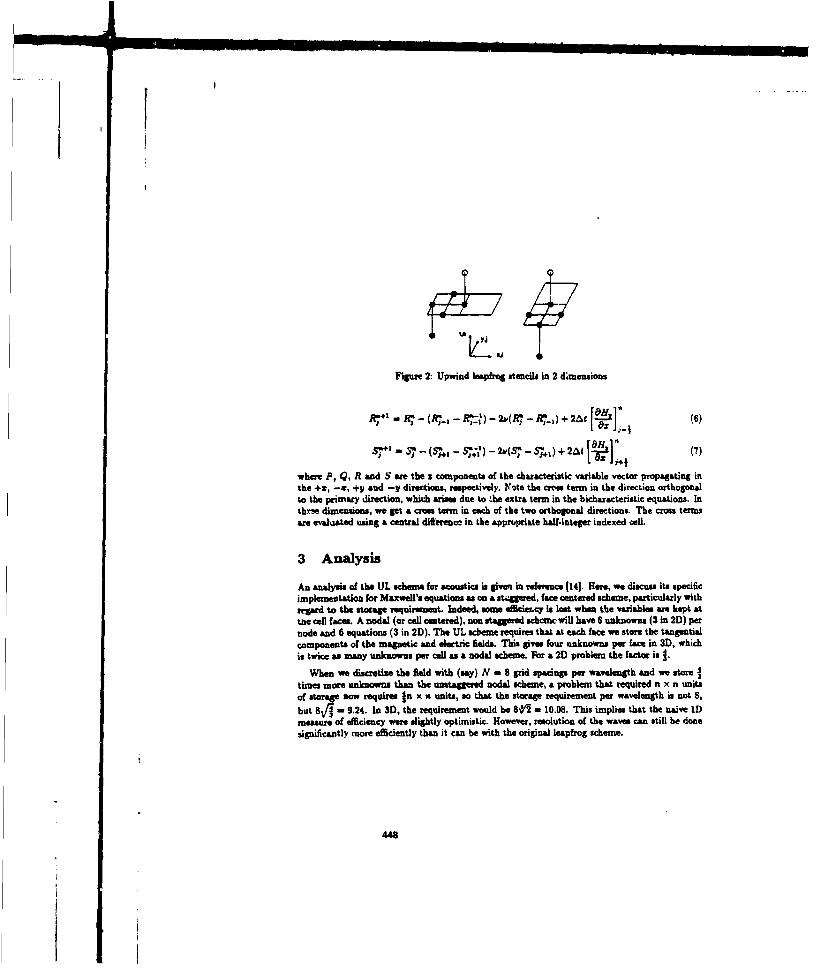
Figure 2: Upwind le6phog stencils In 2 dCmensions

,sT+. - + - (Pj++ - P,;,) - 2,,(Pj -"++,) + 2A, I -118H-11 1 (7)

where P, Q, R and S are the z components of the characteristic variable vector propagating inthe +a, -a, +y and -y directions, respectively. K~ote the cres term in the direction orthogonalto the primary direction, which arises due to *he extra term in the bichearcteristic equations. Inthree dimensions, we get a crs term in each of the two orthogonal directions. The cos termsare evaluated using a central difference in the apprupriate half.integer indexed cell.

3 Analysis

An analysis of the UL scheme for acoustics is given in reference (14]. Her, we discuss its specificimplementation for Maxwell's equations as on a saggered, face centered scheme, particularly withreard to the swapr requirement. Indeed, some affcircy is last when the variables we kept atthe cell faces. A nodal (or cell centered), non staggered achcme will have 6 unknowns (3 in 2D) pernode and 6 equations (3 in 2D). The UL scheme requires that at each face we store the tangentialcomponents of the magnetic and electric fields. This gives four unknowns per face in 3D, whichis twice &a many unknowns per cell as a nodal smheme. For a 2D problem the factor is I.

When we discretias the field with (say) N = 8 grid spacings per wavelength and we storetimes more unknowns than the unstaggered nodal scheme, a problem that required n x n unitsof storage now requires In xw, units, so that the storage requirement per wavelength is not 8,

but 8V4 a 9.24. In 3D, the requirement would be 8/'2 = 10.08. This implies that the naive IDmeasure of efficiency were slightly optimistic. However, resolution of the waves can still be donesignificantly more efficiently than it can be with the original leapfrog scheme.

448

4 Boundary Condition

4.1 Image Grid Elements

To implement certain boundary conditions in an upwind scheme, it is useful to set the field justoutside the computational domain and let the upwind scheme separate what information is al!nwedto propagate inward and what information is ignored. This method simplifies the incidence and,in some cases, the exit boundary conditions. It also allows the boundary face to he includedin moat loops without special treatments. We refer to the first fvce outside the computationaldomain as the image fans. Likewise the first cell and the first point are the image call and theimage point.

4.2 Perfect Electric Conductor

At a perfect electric conductor (pec) surface, any wave hitting the surfe is cornmotely reflected.We think of this as having the wave penetrate the surface while another emerges such that theresulting electric field on the surface is sero. The two waves are shown in Figure 3 where the G"wave is the fomer and the G" wave is the latter. Denoting the conditions outside the pec withsuperscript '"i and the condition inside the pec with superscript "r", we have by definition

G -- D'+ n-x Hi

G+ D' - n H (9)C

The electric displacement on the surface, obtained from these characteristic variables are

D - G+ + G- (10)

Thus the zero electric tangential electric field amounts to requiring

Gt w -GT (1)

where the subscript 't* denotes the components tangential to the boundary. This completelyspecifies the imaginary (or reflected) wave at the boundary of a pec.

This method applies to the total (incidence and scattered Wd). When the scattered fieldequations are solved, the solution is converted to the total field befose applying this boundarycondition.

4.3 Outer Boundary Condition

A very simple method for treating the outer boundary faces so that waves exiting the domain

are not reflected is to set the image faces to a zero field. This method works very well when the

"449

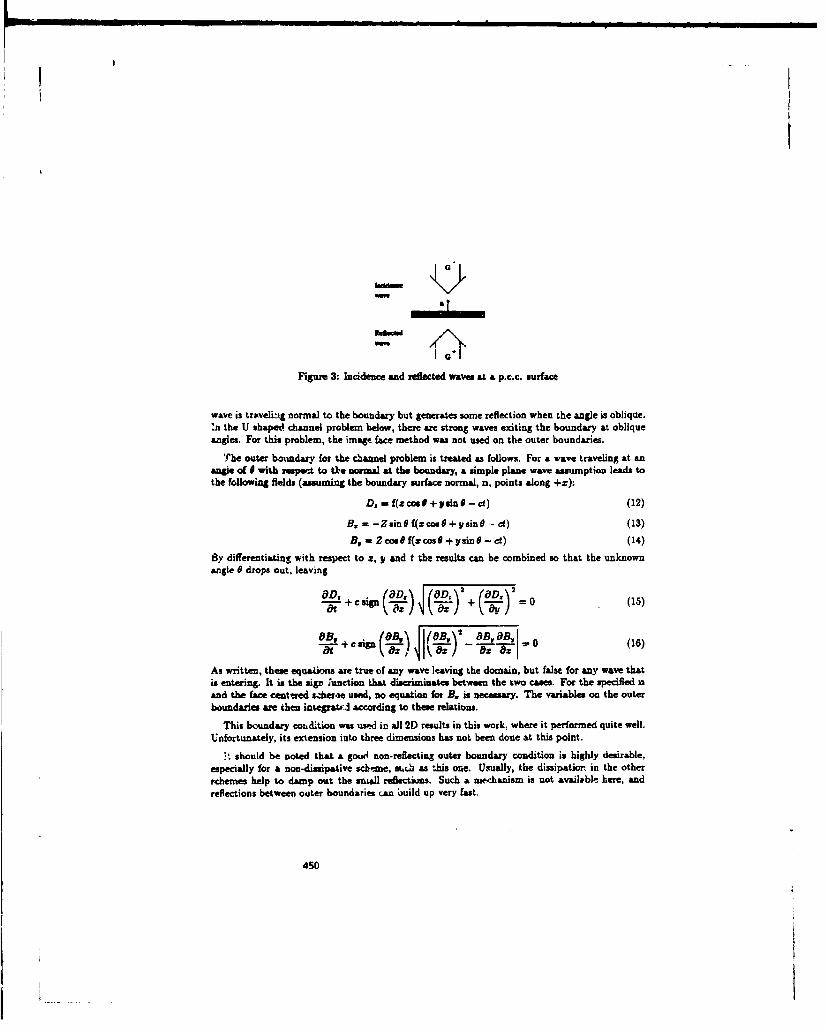
-©t

Figure 3: Incidence and reflected waves at a p.c.c. surface

wave is traveli-g normal to the boundary but generates some reflection when the angle is oblique.in the U shaped channel problem below, there are strong waves exiting the boundary at obliqueangles. For this problem, the imago face method was not used on the outer boundaries.

The outer boundary for the channel problem is treated as follows. For a wave traveling at anangle of 0 with respeqt to tlOe normal at the boundary, a simple plane wave asumption leads tothe following fields (assuming the boundary surface normal, n, points along +x):

D, = f(zco + ysin 0-ct) (12)

B. = -Zainf f(zcosS + ysinO -- d) (13)

B,= ZCoe f(Xce + ysine - d) (14)

By differentiating with respect to z, y and t the results can be combined so that the unknownangle e drops out, leaving

+8 c sip (D.' (0D:5 \2 (2D. ) 2 =0 (15)

ATB' 1.9). DB8yI 0(

.0,9 Or, tk(B,) aB eaBI(as, kw - Ia -

As written, these equations are true of any wave leaving the domain, but false for any wave thatis entering. It is the sign lunction that discriminates between the two cames. For the specified nand the face cetered &dih4e used, no equation for B. is necessary. The variables on the outerboundaries are then integrat*:J according to these relations.

This boundary coud;tion was used in all 2D results in this work, where it performed quite well.

Unfortunately, its extension into three dimensions has not been done at this point.

"I should be noted that a goon non-reflecting outer boundary condition is highly desirable,especially for a non-dissipative schb~ne, such as this one. Usually, the dissipatior in the other-chemes help to damp out the smaall relctions. Such a niec-anism is not available here, andreflections between outer boundaries can build up very fast.

450

Figure 4: Geometry and grid of U shaped channel

4.4 Incidence Boundary Condition

All incidence boundary conditions in this work are treated by setting the image faces to theinciden field. The upwind scheme then allows the incident waves in but simultaneously allowsthe interior waves to exit (to a certain degrw, as noted in Section 4.3). For the solutions of 2Dand 3D beams in Sections 5.2 and 5.3, this allows the surface of the boundary on the side of theincidence wave, but outside the beam, to act as far field boundaries. As noted in Section 4.3,waves approaching the boundary at an oblique angle do experience significant refiections withthis treatment, but for the problems of Sections 5.2 and 5.3, the waves doing this have very lowstrengths.

5 Results

5.1 U Shaped Channel

The two d&-nensional result of a harmonic plane TM wave incident on a perfectly conductingU shaped channel is considered. The geometry of the problem is shown in Figure 4. The gridspacing was h = I for the geometry, and the wavelength A = 10. The channel's outer dimensionsare 42 x 12 and its wall thickness is 2. The grid saie was 127 x 97 leaving about 42 cells betweenthe body and the outer boundary. The wavelength 3f the incident field was 10. The incidentplane wave was inclined at a = 30" with respect to the z axis. The scattered feld equations weresolved.

The problem was integrated forward with v = .3125 (although the stability limit in two dimen-siona is t, - .5) in o~der to have one wavelength passing each point in exactly 32 time steps. Thiswas done only to have the right sampling rate for conversion into a frequency domain solution viaa fast Fourier transform (FFT).

The frequency domain solution was used to compute the radar cross section (RCS) of thechannel, using the definition of the RCS, and the farfield solution can be obtained from thenearfield numerical solution using the Stratton-Chu integral 1111 -uAd equivalence principles.

4S1

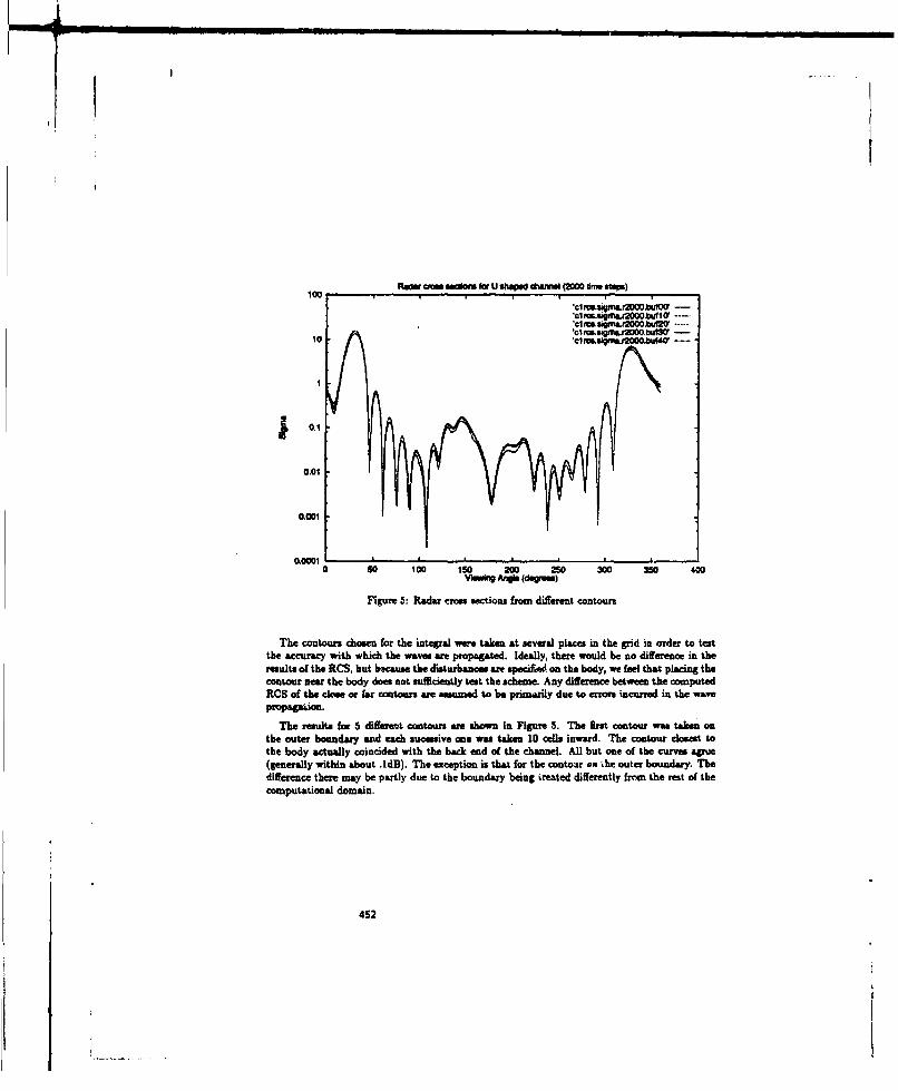
Radar soaf v W U shaped sha•wui (00O Ore Mp)c1re aigmaJ2,0,tf,

c10 mar2000.bu7 -cilms.sigms~r2OOO.buf20'-

0.1

0.01

0.00010 5o 100 150 20 250 0 30 350 400

V~f NV1@ (degree)

Figure 5: Radar • e ctions from different contours

The coutours chosen for the integral were taken at several places in the grid in order to testthe accuracy with which the waves are propagated. Ideally, there would be no difference in theresults of the RCS, but because the disturbances ame specified on the body, we feel that placing thecontour near the body does not sufficiently test the scheme. Any difference between the computedRCS of the ckl or far contours are amumed to be primarily due to errors incurred in the wave

The result. for 5 different contours ass shown in Figure 5. The first contour was taken onthe outer boundary and each sucessive one was taken 10 cells inward. The contour closest tothe body actually coincided with the back end of the channel. All but one of the curves agrue(generaly within about .1dB). The exception is that for the contour om ',he outer boundary. Thedifference there may be partly due to the boundary being .reated differently from the rest of thecomputational domain.

452

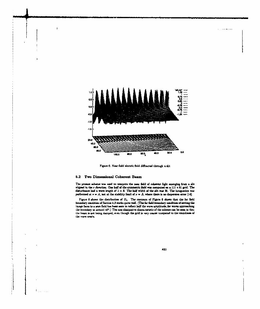
0.5 ~ -OC u.~ 00 a~ 0.0

-1.0

-is0

40.0

40.0

Figure 6: Near field electric feid difracted through a slit

5.2 Two Dimensional Coherent Beam

The preamt shere was used to compute the nar field of coberest ight emerging fhm a alitaligned in the s dwaction. One half of the symmetric ed was computd an a IIIl 91 spid. The"durbance bad a wave legth of A -8 . The hlf width of the slit was 20. The integration waperformed at a, w .4, not at the stability limit of& r .5, where ther is no dis o earot 114).

Figure 6 show: the distribution of D,. The contours of Figure 6 shows that the far feldboundary condition of Sectin 4.3 works quite wall. (The far field boundary cmdition af setting theimage faces to a mero field has bean men to reflect hal the wave amplitude, for wavu approachingthe boundary at around 4W.) The no-dissipative ch.a,.ieristic of the scheme can be ý in thastthe beam is not being damped, even though the grid is very coa compawed to the rmndnem ofthe wave cr•ts.

453

Figure 7. Round aperture problem

5.3 Three Dimensionali Coherent Beam

The three dimmnsional scheme was used to compute the near field of a uniform coherent beam ofcircular - -- seciom (Figure 7). Due to symmetry, it is only necessary to simulate a quarter ofthe beam. For this problem, the grid spacing was h = 1; the. wave length was A =8; and theradius of the beam (befor diffracting) wees2A. The grid sise was 32 x 48 x48. The soaution wasintegrated at bo - .4.

For all the boundaries, the conditions on the image faces were set. The incidence field boundarycondition of Section 4.4 was used for the boundary at m nizoum x. For the boundaries at minimumpr and minimum s, the images were set to the the conditions immrediately inside the domain tosimulate the symmetric half of the beam on the other side. AUl other boundaries awe outerboundaries, &and there, the image faces were set to the zero field. Although, as noted in Section4.3. this typ of outer boundary did not work well when there was a strong wave citing thedomain at an oblique angle, that is not the case here The strong pert of the field is in the core,which is exiting at the matinal an*l. Nevertheless, due to the unavailability of a reliable far fieldboundary condition at this pown, only 100 iterations were taken to avoid reflected waves haompossibly building up inside the domnain. After 100 iterations, there are no visible reflections.

The magnitudes of D, B and E x Han shown in Figures 8, 9 and 10. It should he noted that,for the purposet of plotting the data, all faew centered quantities have been averaged to the cell,where then all cesapoesiots of D and B could be mae& available.

Figures 10 and 11 shows that the strongest wavs are in the core and exiting the boundary atreasonably normal angles. Outside the core, the strengths of the waves am negligible, in regardsto producing recognizable reieectmons. Thus, from this at least, the tar field boundary does notappear to be introducing significant errors.

454

FigureS8: D vector magnitude

Figure 9: B vector magnitude

455

Fig'". 10 Poyntiag vector mapaitude

Figure U: Poyntang vectmc

416

6 Summnary and Conclusions

The upwind leapfrog method, a non-dissipative, low dispersion error scheme was applied toMaxwell's equation in 2D and 3D. The scheme performed well, however, at this point, few quan-titative comparisons was made.

It was found that due to the lack of dissipation, waves reflected back from far field boundariescan cause problems as they build up inside the domain. A far field boundary condition basedon the assumption of a single exiting wave was tested and performed quite well in 2D, but a3D extenaion is not yet available. However, simpler far field boundary conditions make workablesubstituta if the conditions for stmng refiections from far field boundaries are not present.

In the future, we plan to develop lain reflective boundary conditions for use in 3D and tocompare the reults of this scheme to other analytical and numerical solutions.

Acknowledgement: This work has been supported through a fellowship granted by the Depart-ment of Energ,.

References

[1] David G. Bishop and Dale A. Anderson. A Comparison of Finite-Volume Timn-DomainSchema for the Maxwell Equations. Technical Report 92-0456, AIAA, January 1992.

12] Peter Goorjian and Allen Talove. Computational Modeling of Nonlinear ElectromagneticPhenomena. Technical Report 92-045T, AIAA, January 1992.

131 Peter M. Goorjian. Computational Modeling of Femtosecoad Optical Solitons from Maxwell'sEquations. IEEE Journal o. Quantum Electronics, 28(10), October 1992.

14] Nathan Ida and Joao P. A. Bastos. Electmfaasyetic aned Calcultion of Fies. Springer-Verlag. New York, NY, 1992.

[5) Ralph Noack and Dale A. Anderson. Time Domain Solution of Maxwell's Equations UsingA Finite-Volume Formulation. Technical Report 92-4151, AIAA, January 1992.

16] Benoit PetitJean and Rainald Lohner. Finite Element Sol'ver for Radar Crow-Sectiom (RCS)Calculations. Technical Report 92-0455, AIAA, January 1992.

[7] Philip L. Roe. Approximate Riemann Solvers, Parameter Vectors and Difereice Schemes.Journal of Compu*aional Physics, 43:357-3762, 1981.

[8] Vijay& Shankar. A Gigaflop Performance Algorithm for Solving Maxwell's Equations ofElectromaetics. Technical Repogt 91-1578, AIAA, 1•91.

457

[9] Vijay& Shankar, William Hall, and Aliresa Mohm amadian. A CFD-Based Finite-Volume Pro-cedure for Computational Electromanetics- Interdisciplinary Applications of CFD Methods.Technical Report 89-1987, AIAA, 1989.

[101 Vijaya, Shaaklr, Alireza Moharnmadian, William Hall, and Roy Erickson, CFD Spinoff -Computational Electromagnetics for Radar Crom Section (RCS) Studies. Technical Report90-30,55, AIAA, 1990.

111] .ulius Adams Stratton. ElecFronmapetic Theory. McGraw-Hill, London, first edition, 1941.

(121 Allen Tadove and Morris Brodwin. Numerical Solution of Steady-State ElectromagneticScattering Problem Using the Time-Dependent Maxwell's Equations. IEEE Transaetionaon Microsve Theory and Teehniqmea, MTT.23(8),'623-63, August 1975.

[131 Allen Taove and Korada R. Umashankar. Review of FD-TD Numerical Modeling of Elec-tromantic Wave Scattering and Radar Crm Section. Proc. IEEE, 77(5):682-699, May1989.

114] Jefr-y P. Thomas and Philip L. Rae. Development of Non-Dissipative Numerical Schemesfor Computational Aeroacoustice. Technical Report 93-3282, AIAA, 1993.

(151 Brain van Leer, James L. Thomas, and Philip L. Roe. A Comparison of Numerical filuxFormulas for the Euler and Navier-Stokes Equations. Technical Report 87-1104, AIAA,1987.

1161 Kane S. Yee. Numerical Solution of Initial Boundary Value Problems Involving Maxwell'sEquations in Isotropic Media. IEEE Transactions en Antennas and Propagation, AP-14(3):302-307, May 1966.

454

Linear Superposition of Phased Array AntennaNear Field Pattern

Using the FD-TD Method

C. E. Reuwe. £E. T. Thiele. A. TafloveDquarunemt of Elecwica Eoginerin man Comwe SciencNorthwesmez Universiy. McCormicic Schol of Engiueernog

Fvanstoiu, Ilinois 4(0206

Mi. J. PIket-May*Departmen of Electrical and Computer Engbaerin

University of ColoradoBoulder, Colorado 80309

A. 1. F=rnLireola Laboratory

MassaCINaUS InsdiUte Of TechnIoloyLcxington. Msaclacheus 02173

1 lofdocion

This pape r ealies the oowW of hnam aqpeposiudon from circuit amery to 3-D FD-TDwholmin to Maxwell's equatr=. The Inear superposition phrisple ms applied to M MTDsUl~aamd raditio panrerm of iWo speifi phase Wray aSM used ur eiec=aagneikpertletnik. The firs. Is the DSD SigmA40 arnada phased way desined to beat canocr4 isaam= dee withn fti body. The secood is an experimental pratoype device in use at LincolnLaboratory. It is a non-invasive mnonpol ptasd HMa dAiN d to beat cancerous umors nartthe a,~ of the ski. ft is believed that the lmar awnapoeosr technkiqu has broad applicatonin FD-TD-besed panemrtn sytsi, adaptive mAfin, a&d desim of phased array Syamms.

2 Umin -uepdiBecause Mxwrell's equations are liner. the resultant field distribto of any aunte MAY -Rthall anry elernesn radiating in a linea medium can be eliougi of as fte linear superposition of mthefield diasrbmo duoe to each etua radiatng ijilviduisaly. The demotuamio Of d&esuperpoasu psiple has = be=ntriorousy repote m the linerature for isamncal siulatiston

45S9

or the fulal 3-D vector Maxwell's equations. Sullivan [11 qualitatively describes a superpositionprocedure in the context of FD-TD simulationsi. However, given the date of his paper (May1991). it is clear that be did not employ resistive sources in his r'l-TD model (which weredeveloped approxtimately 2 years Later (21). Therefore. Sullivan's superposition treatment does nothave the rigorous flavor of the work reported he~re

now basic proced1u1e consists of' exciting one array element using & recently-developedresistive sourc food repiraesitaslo [2). The remaining elements ame unexcited, but loaded with theortailsl gemswrat source iayedais . Nwa-fled data are stored for this run. Tis procedure isrepeated for eawlh array elmmnat. Tints, -n array with 8 elements would require 8 separate FD-TDrum. A subsequent post-paocessing saep, noe requiring a Cray FD-TD run, would merely scaleeach ase of stored datm by an arbitrary magnitudiephase distribution, and then transform to the farfield (if desired) for the radiated pattern. In this maimer, literally hundreds of amplitude/phasetsprs across the phased array couild be quickely examinsd. Or, a synthesis procedure involvingadaptive nulling techniques [31 could be used to optimrally provide the ma", tude/phase taper. It isbelieved that this linea supeposition approach employing resistive sources is novel relative to PD-TD modeing.

3 S ae -PaRpeees

Two different source represenarioss were investigated with regards to the Itiieser superposition-ehnique. Thes awe described below.

The initial source considered is the "hard source." This source forces a specified fieldcomponent that excises an iamsana n eme, to have a desired sitassoidal or imspulsive time

at~ee any tm step, regardless of anythin~g else bappetslng in the FD-TD grid, The bar,!source is analogous to the Weal voltage sourc. That is, it has a zer sourct impedance and cansWrc sunlmisd powe ragastileas of the load that is placed on it.

The ascaud source considend ks the resistive source. This simulates a true physical sourcehaving afingite sourc inlsdaec. It CUMo sUVply U~inlinsl power, and its output voltae is

deneton the load. The following i0dile PD-TD electri field update expressions were usedfor the ectic field components g a y-directed resistive source F(2]. Here, Vs is thesourc voltage verm or toe blakrig functon:

,- C.(m)EL+

460

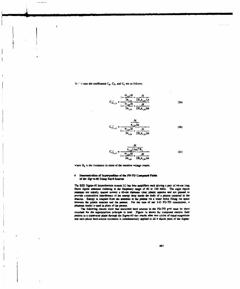
In is case the coefficiellZs Ca, Cb, arnd rC are as follows:

2 s,,k 2R,e1c,AX

At

61At At (2b)2 1:L~k 2R,zLjkAx

- (2c)

+ e 2R,s1,kAX

where R. is fth res's-c in ohmas of the restitive voliq ageros.

4 Demoinutsadm of Stipmpoiitlm of the FD-TD Cuun~odhieldsof the Slgna4OIU Ha r Md S

The BSD Sigina40 by'paitimnia syasi [I] bas four auisilifler eac driving a pair of 44-cm longflaswd dipole maamau rodumamg in the frequany tmop of 60 to 120 MMz. The eiglit dipolesmaas are equally spaa aroundi a 60-cin dAze clea pluzic ma-hu and are phasm 10ptirvide c~onsmaaaive usarfur=c of doeemg deV 4 M W inidhde body of a pauim cminted in thevamuus. EneWg is compled froeu die aneeams to the patim via a wam bolua filin the spacbet*e the plastic armaslu and the patnat. For the caoe of owr 3-D FD-TD) soubasaio, apluses modelI is umd in place of Ome pastie.

The following reisuls sbow that uneacld herd soumes in fth FD-TD grid must be shloCctiatevd for dn superposition principle to bold. Figmr I& shows the comzpumld electri f=elpwamn usm a uaivem planec fthogh the S~mga60 dat reslts aher two cycles of eqtmal-nm ragidesand zero-phase lurd-souros excimion is siciulmamousy appiied to all 4 dipole Vairn of the Sigma-

x Im ftaiU% (u 1 tme I'

&LI gp~est" -ied-(b)Additive superposition,.

(a) P~l aJ~kaora na~i~d. bu st unscittd Op~licatOrsofn~circuitid-

puwf 1 VD-TD =10014 4kc Wmd 4ft&,o in da amuva plm Of fth Sipga 0.

C.".a fth Bafta for %U1 qPicinul eSzCwd (a) wtdz addhiae uaaOV kiP i of t1

fmift du w IW1i'itha 8PIPZvfl 'itd am at a ANN =d the tMaiaW pmsiwe (b. c).

60. (rhis is tio' at the sinuasoidal steady state; however, it is sufficient to demronstrate thesuperposition principle using dhe FD-TD method.) Figure lb shows die results for the sumnitionof the PD-TI) computed electric fied patterns of 4 runs, where each run represens= the fielddistribution after 2 sloutaoidal cycles of excitation of an individual dipole pair while the threunexcited dipole pairs are left open-circulted. Figure Ic shows the computed electric field patterncorresponding to the case of Figure lb, with the exception that the dipole pairs have their canter-gaps short circuited. It is clear that Figs. Is and Ic are very similar. In fact, detailed analysis ofthe darn indicates point-by-point agreement of the field of Fip. I a and I c to 3 decimal places.

5 Demomtsration of S~aperpualoem of the MDTD Composed Fieldsof the Mlonopole Phumed Array Using Ruseive Sources

Here, the goal of our sirmulations is to provide theoretical support for the experiments performed at~itatoln Laboratory in phased-arry tachawlogy for EM hyperthermina. ':hewe experiments; are

designed to focus a monopole phased army (UFA) to a point 2.5 cin deep in a muscle phantom.The 915-M&z monopole phased array is shown in Figure 2. It conseists of a semlicimcwar

metal disk hollowed out to form a cavity for 8 active monopole elements. The disk bas an outerradius of 10.59 cm And an inner radius of 9.32 Cm giving a wall thicknous of 1.27 cm. The cavitycan be viewed as a parallel-plate waveguide region (top sand boa=o plates of the disk) with aconducting back wall for the purpose of focuing the energy from the radiating ele menP towardsthe aperture. of the applicator. Thei conduicting beck wall has a consex arc radius of 9.32 cm.The aperture: is 2.54 cmt wide by 18.64 cm long. The 8 actve Ilmet, each 1.27 am long,penetrate through holes in one of the purallel plates, are positioned on an arc, or radius of 8.66 cmncentered at the cePnotr of die housing disk.

The cavity regihin of Uth housing of the monopole army applicator ia filled with low-lossdeionized or distilled water to provide inmpedance matching for the active arrmy, elements. Theapplicator is sealed with a solid dkielctric cover. The amocle, tkantorn is shown aclematically inFigure Zh. It Is a 15 x 36 x 13 cm box containing a saline solutio having relative dielectricoonstant er - 50 and electrical coonductivity a - 1.3 S/rn.

Teflt flowing resiult for Uth MPA show the validity of the linear superposition concpt forPD-TI) siasalasiom with resistive soures. Figure 3 shows FD-TD conqamated electric: fields alongsan H-plate cut paralle to the aperture of die IEPA and 2.54 cm deep within the phateaom. Thesqluares dcp=t fields for the phase-focusved run wiantein all elements are excited with a phasedistribution selecaed to obtainm atexinan heating at the 2.54-cm depth. The circles depict thecorresponingi dat pouts for dth linearauy suaperimposed results of 9 runs, where each rnnsimulaed the excitation of only one element at a tim. leaving the 7 other elements unexcited but

tennrdin S0 D1. There is excellent agreement of the two results even at the depths of the -30dB nulls,

"43

Garlan m-sI-.I_1auucIoa wa~l.*IMO mOWM ALL-"'---4--%

Top

I•- --' -- -- ', -

Fa TauPOa view

I.-\ T-,m . mum m

I (a) I' I ~ ' *~

. 3u. MU

IN

PointC `1ý ;r

Point a Phantm 3

Poit A .. h

i,.

(b)

Figire 2 Scltihac represacaon of t. moanopole phased amy applicator shaowmg t locationsof the 8 active any eleawnts (a). Schematic representation showing the dnimesions ofthe umiac phantom material inside the plexiglas contair with the monopole phasedarray applicatr postiond below (b).

4b-4

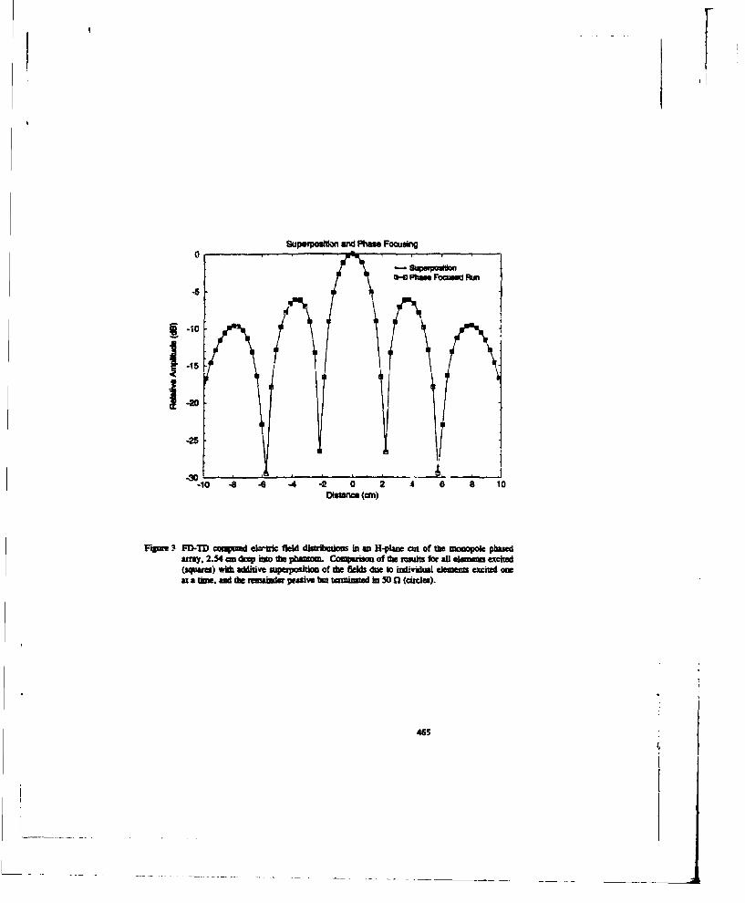
Superpoafti~ and Phaft Focusing0

M-13 Phae Focused Flun

-5

-25

" .8o 4 4, -2 0 2 4 6 a 1oDs•Mc (cm)

Figue 3 FD-TD comqped cemi f&M hdmbuisoas m an H-pae cut of the minooole phsedrmy, 2.54 cm d*V imo the pbaom . Comparison of the remA for all Wmemn excikW

(squares) with additve uperposition of the fields due to individual ekiea excited oneat a time. and ft remainer p•sive but mimtd in 50 0 (circles).

465

6 Cmadmhem

This work showed that the concept of linear superpoition can be generalized from circuit theory to3-D PD-TD simulations of phased array antennas, The presence of generator source resistance isaccounted in a suaightorward w . It is believed that the linear superposition technique hasbroad applicadosm in PD-TD-hased paitn synthesis, adaptive nulling. and design of phased amy

synms. Ibis procedure will be applied to a linear anly antenna consisting of 8 crossed-pair

Vivaldi flarld born amman eleuwnts in the near fAture.

This work was sptported in pant by Cray Research Inc., ONR contract number N00014-93-0133,and the Departmen of the Air Force consct snmber F19628-90-C-4OX12.

a Refermns

(11 D.IM. Sullivan. Mathenmtical methods for reatnent planning in deep regionalhyperthejmia," MEE Tron. Microwwve Theory Tech.. vol. 39, pp. 864-872, 1991.

(2] M. J, Piket-May, A. Taflove and I. Baron, "FD-TD modeling of digital signal propagation in

3-D circuits with passive ad active loads." IEE Tress. Microwave 7teory Tech., in press.

[31 A. J. Fen, "Evaluaion of adaptive pbased-rray antenna far-field nulling performance in thenear-field region,' IEEE Trts. Awcaos flopagat., vol. 38, pp. 173-185, 1990.

466

Radiation and Scattering from Curved SurfaceScatterers with Stair-Cased FDTD

H. Scott Langdon* and Raymond J. LuebbersThe Peunsylvanias State University

University Park, PA 16802

Results for FDTD lculions of radiation and scattering for some 2 and 3-dimensional canoni-acl scatterers, with curved surfaces, will be presented. The objects are meshed using stair stepped,cubical PDTI)D cells. The FDTD results ,re compared with accepted values.

The authors hope to show that with care in meshing, the standard, s4mple, cubical FDTDmesh can yield good results for many shapes which include curved surfaces, at relatively lowresolution, 20-S cull/kA.

An examination of cylindrical and spherical objects meshed with diferent diameters showsmarked changes in accuracy with a resolution change of only a few celLs/A. Comparative resultswith a 2-dimmeional cylinder clearly show this change in accuricy.

It is possible to help account for the effects of partial filling of a cell volume by a dielecticscatterer by setting the constituitive parameters for that call to a value between the values for theobject and free space. A simple linear interpolation of the censtituitive parameters is shown toimprove the results. Some exarAples of curved and tilted surfaces are given which demonstrate thisimprovement. More accurate determinatiun of the conatituitive parameters, based on boundaryconditions for the E and H-fields give better results.

Most of these techniques are simple and straightforward to use with a typical FDTD code.Computer time savings over more complicated methods, due to fewer computations per cell andto fewer cells needed for a giwen object may allow more intricate geometries to be modeled on agiven computer.

467

Input Impedance, Radiation Paittern, and Radar Cross-Section ofSpiral Antennas using FDTD

Christopher W. Penney' end Ra~ymond J. LueboersDepartmient of Electrical Engieerng

The Pennsylvania State UniversityUniversity Park, PA 16802

AbstractA Finite-Difference, Time-Domain (FDTD) analysis of several spiral antetnnAs was perfoiMed

to calculate input imperlance, antenna gain and scatering patterns. Broadband input impedancecalculataios were performied on an equiangular spiral slat antenna and compared to measuredresults (1]. Data from Finite Element calculations 12, 3, 41 of a square Arclhimedean spiral with acavity backirg was used for comparison to FDTD radiation gan pattern and RCS versus incidenceangle computations.

IntroductionFDTD input impedance calculations were performed using a computer code developed at the

Pennsylvania State University (PSTJ). This code uses a total field formulation and approximatesthe feed of the antenna by applying an electric field between two input terminals, The inputelectric field and resulting loop of magnetic fields are saved by the FDTD program and the inputimpedance is found 'by Fouirier Transforming these values and dividing them. This gives the input;impedance over a broad frequency range, necessary when dealing with spiral antennas.

The equ;=ngular spiral slot antenna used for the input impedance calculations has an armlengt of 42.3 cm and a rate of expansion of 30.3 cm/radian. The feodpoint separation is 0.5 cm.and the ratio of the inner to outer radii of the arms is 0.75. The FDTD approximation of thisantenna uses cubical cells measuring 01 centimeters on a side for a resolution at them maimufrequency of 40 cells/wavetlength. The input impedance for the anteuna has been measured to beapproxdimately 80 + jO 0 over a frequency range of 0.73 to 2.5 Glix [1]. A modulated Gaussianpulse was used as the input waveform for the FDTD simulation so that the spectrum of inputfrequencies would span the entire operating range of the antenna without introducing frequenciesbelow the low frequency ecutoff. This was necessary to avoid energy being trapped on the antennaand cawsing unwanted resonances.

The antenna used for the FDTD radiation and scattering computations was a 2.8125 cma squareArchimedean spiral antenna mounted in a large conducting ground plane above a, cavity. Thecavity was both air-filled (0.9375 cm deep) and absorber-filled (2.7375 cm deep with a 0.9375 cmseparation iayer below the antenna and three 0.6 em thick layers of absorber). Further calculationswere performed on the absorber-filled cavity configuration with 1.0 fl/square and 5.0 fl/squareresistive sheets covering the aperture of the antenna.. The PDTD approximation of this antenna

468

used cubical cells measuring 0.09375 cm on a aide for a minimum resolution of 70 cells/wavelength.A timentep of 1.8 pa (also the Courant limit) was used for all FDTD calculations on this antenna.

ResultsThe FDTD feedpoint current calculated on the equiangular spiral antenna used for the impedance

results was completely converged after 1300 timesteps with the timestep size at the Courant limitof 1.93 pa (Figure 1). The resulting impedance plots varied slightly from the measured values(appmaimately 180 + JO), but did display the broadband behavior desired (Figure 2). The FDTDradiation pattern calculations used the same total field formulation of the input impedance, butthe far-soes radiation patterns were calculated by saving the complete time record of the tangen-tial electric fields in the aperture. These aperture electric fields are then Fourier transformed togive the complex tangential magnetic currents in the aperture. These currents can then be usedto compute the radiation gain pattern at any frequency in any plane above the ground plane ofthe antenna (5]. Figure 3 displays FDTD results for the radiation patterns in the 0 = 45 plane(diagonal of the square) of the air-filled cavity backed anlcnna at 4.5 GHz. Vert good agreementis shown between FDTD and the Finite Element-Boundary Integral [4] computations for thisantmanna.

Scattering was performed using an FDTD code modified for apertures above large groundplanes [6]. The complete time records of the tangential aperture electric fields are saved andconverted to the far-zone in the same manner used for radiation. Figure 4 shows a comparisonof the FDTD and FE-BI (4] computations of RCS versus incidence angle for the air-filled cavitybacked antenna in the o - 45 plane at 4.5 GHz with a e-polarized Gaussian incident plane wave.Good agreement was found for all cae tested with better agreement in the calculations withresistive sheets covering the aperture.

ConclusionsThis paper has shown that FDTD can be used for computing broadband antenna impedance,

radiation patterns and radar cross-section. The results shown are for spiral antennas but can beextended to other types of antennas.

AcknowledgementThe anthors would like to thank Dr. John Volakis of The University of Michigan for his

assistance during this study. His results for the square spiral antenna, and Lis suggestions andcomments, were extremely helpful in providing verification of the FDTD scattering and radiationresults presented here.

References

(1] J. D. Dyson, "The equiangular spiral antenna," IRE Trans. Antenna Propagat., vol. 7, pp.181-187, April 1959.

[2] J. M. Jin and I. L. Volakis, "A hybrid Finite Element method for scattering and radiation bymicroetrip patch antennas and arrays residing in a cavity," IEEE Trans. Antennas Prapagat.,vol. 39, pp.1598-1804, Nov. 1991.

469

(3) 1. M. An, I. L. Volakis, C. L. Yu and A. C. Woo, 'Modeling of resistive sheets in FiniteElesmnt solutions," IEEE Trans. Antenea Proapag., vol. 40, pp. 727-731, June 1992.

141 3. L. Voluhd., 3. Gong and A. Alexanian, "Electromagnetic scattering frum m icrostrip patchantennas and spirals residing in a cavity," Accepted for publication in Electromagnetics.

[6] C. A. Basles, Adweued E*%ss ring Eliramagrelics, Wiley, 1900.

[6] RX I. Luebbea and C. W. Penney, ¶Scsttering from apertures in infinite ground planes wsingFrDTD,* IEEE Tre•u. Antennee Propejte., accepted for publication.

470

2

Timtes" (timstep s -. 1.93 ps)

Figure 1: FDTD input voltage and current rwonse for equianular spiral slot antena.

Inotmosy -

150

1 2 3 4 5 6 7Frequency (Gl~z)

YFigur 2: FDTD input impedenoe for equiangular spiral slot an~tenna. Measured value at approx-itey80 + jO fl fmom 0.'75 to 2.5 GHz.

471

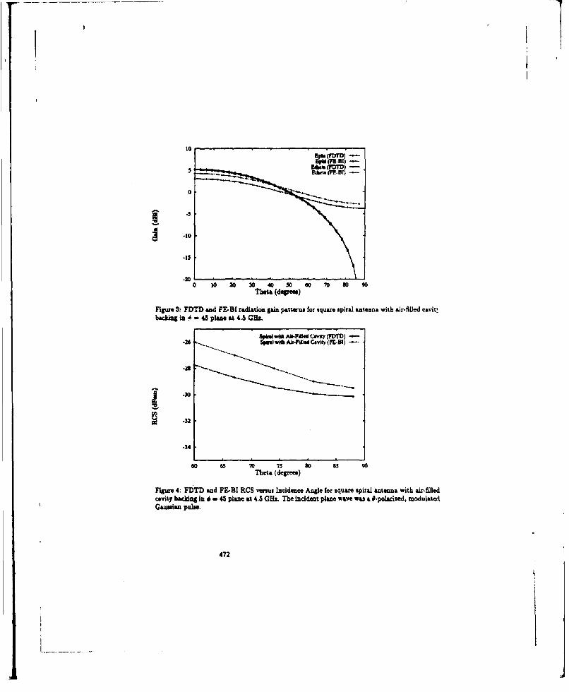
10

0

o10

-15

*2010 20 30 40 M0 00 70 so 90

Thata (dwpe)

Figure 3: FDTD and FE-BI radiation gain pa•terus for iquare spiral antenna with air-filled cavit.backing in 4 w4 plane at 4.5 GHs.

•~w Ai-ue .•.ay WllD) ---

-26 S= I wid Air-Fdiwed Cavity (F•-B) - •

-32

-32

60 65 70 75 00 85 90Theta (deree)

Figure 4: FDTD and FE-BI RCS versus Incidence Angle for square spiral antenna with air-filledcavity backing In 0 - 45 plane at 4.5 GHs. The incident plane wave was a 9-polarized, modulatedGaussian pulse.

472

FDTD SIMULATION OF AN OPEN-ENDED METALLIZEDCERAMIC PROBE FOR BROADBAND HIGH-TEMPERATURE

DIELECTRIC PROPERTIES MEASUREMENTS

Magdy F. Isitander, Shane Bhtnghurst, and Paul OusiudeElstrcml Engineering Depanrtment

S1alt LAWe City, UT 14112

A861TRACT

Open-ended co~ixlo p-obes have, bean conveniently used for broadband dielectric propei tiswoassitaeinns for several roots. A commercial probe and associated calibration and nrasnetmentmofware are now available front Howlett-PoArkad Cotipanty. Several mathematical models forcalculating the dielectric properties of mameials fawn nreasured input impedance values ame alsoavailable. In conjunction with our ongoing researrb taivides in the am of -,rwaep.csIng ofmaterials and in puilcu:ar, in the microwave sintorlng of ermics, we fetdI necessary to makcdillctric piopues s meastamrms at taposanues as bigh as 1000C. Available high-tera ture

prcdrsbaned o. cavityplutto mothodsarsrelativelynarow band and mealc -exapoeareno "SWial ft these igh-tempueratie nasrsmmTi sto only bocause of dhe differentalthuitl exason of the r antmd nou eonsducus in coaxial metallic probes. which meke caurryingout the prbcain rto difficult, also because metallic probes tequila iorjR cooling sections tominimizebeatuto torsto mossmmnuent equipumen (e~g.. Metoog analysue,).

We have developed a new rmetallized ceramic coaxial probe for broadband, blgh-w-tenp"awdielecuOc properies msa e . To help optimize the deuign of the probe and, in particular, to:

deveopa;! i that would iomma the pmenetation of fields in samples undler veat, improve the probesesitivity to variation lin properties of a largerlam of matulials, and help determilne the required

;lir-u thicimesses of various sa~ples for obtaining accuatem rsults. we nodeled and simuilated theprobe performac using the Finlme-Diffmerece Time-Domain (PDTD) method. A TEM mode was

exctedin o caxal feud, and one ead, of the probe was terminated by an absorbing boundary. Thesample under teat was placed at the other end of the probe.

Nunwrical and graphical esuaua illustrating fth obtained FDTD results will be described and someof the Identifted guidelines regarding suitable probe deeip sand sample dimensions will be discussed.Experimental results of broadband and hlgh-temporatre dielectric properties menw-mrueats will alsobe prosomed.

LTFTRODUCTION

broadbanddielecuic--- prpry es tun artm genenally important in characterizing the atomicand molecular strcture of maeil.In the new and emerging tochnolo ,of microyave processing ofmaterials (including sinteuing of coermics, curing of polymers and =eeito of hazadou wast), itis also impotmant that these measurements be made assa function of temperature that somtim reachesas high a value as 1OO(?C. Data obtained from these messutwunents are used to support the numericalmodeling and simulation activities as well as to characterize the asourption characteristics of ceramicpolymers and glass materials during heating. Isome such as smuplti~nsulation coptbility andparameters involved in optimizsing the besting process, may also benefit from the resultso'tes

473

measurements. In perca. tedleti hvi osapsmapay ak role in controlling theheana proess amd thepoeibe Wrvelln fprblM1 suh-1 =atedimlrunaway.

High tempazum dileectric prepetls h owever, we only knowni for a limited number ofmatediab and tere am serious frequency gape in the available dielecric database. It istherefore crucial to davelop hiaqussa devocs and testing procedures that M =cilaemaking thesemeasuremmnts accurately and an a routine basis1-21. Bemmass of diethmue expension problems oftenencountered in -kin Isgli-Uqmpeure dllcucpe na msaaremets using metal probes, wehave deeoe imetllized weuie cos-a ad cxial pebe fhe making broadband dielectricpsopusy rn-md for Viam e po -100MC OlWMtrck PrePMee ftme OaieMent SM made

L sedielewi In Smcma with the apes end of she coaxial dielectric probe. The

To help us desaign, Od adbefukily use the developed dielectric probe, we irmuatead thepo~e pribmane eag DID aPsesmr subh as mfienium thickneaa of a sumple, optantm probe

thes probe can be bum understoed wing result from the FTD~a ,in'ais Intis paer, we willdeacribe the probe dieep and operation, andgraphically show amom of the PDTD results thatdewoesnatethe probe f

T%@eu Ime t desgnd m u is ofe jwpoposed open-emnde coaxial probe include:=oa =labn Iedne :::PC I~ng eAtsuction -onecor and am ability to carry out accurate and

rerdcbecalibeaulon IrocduAe over a reasonably broad frequency bead, and for -nopertures ash1ig h as 100C. Thuerefame, issued of designing a special conneeser that flu dhe desired dimensions ofo ur probe, we testd several comenuisslaly available connectors that may be easy to modify to fit the

dw dh dmimsl of the probe. To facillisass routine -M entiaon procedures and to minimiseposealbe excesi~ve heatIng ofd thersr a coaxial probe with the ftmsasshw nFg I was

C@uM9DftO.std ID.9016*

W~~~ WIG u0V4

Fig. 1. Dimzensions of the ope. eniod coaxial probe design for broadband dielectric measurements(500 MHz to 30OHz) for., smicrattea up to I00rC.

A GR..so-N type corsmeeor was selected to comenect the designed probe to the standard accesgoriesof a network analysis syswLm Ilse broadband perforanceu of the OR-to-N type connecto was testedusing tinss-omain gating rid hooequecy to ime-domairn anaysis capab~lte Of the HPIOB 108 etwork

474

Analyser. 71e inner end ouste conductor of the OR half of the comeesaw weuyreovd and a newadapte was machined to facilitate connecting the center and outer coaduciors or titz probe so the Nconnecnt

The metallized probe waes fabricasted of a stardsar aittadna WM-99) tube and center conductor rod.The alumnau coaxial probe was machined to die desiln. qwecficadonsa. 7he dianuter of the caviter andouste conductors wra 6. san sd I I mm, res ctivt y rThe ptobs was that aellised at Wesgo Inc.The nevalflzadoe was socouplabtle by p5 I g ermie with a vaoly. 1 ! 4 paint and then"flts them at high swoersmw in ,o n -I (eg.... .onkyo ). The moly.unuilme. - aal "is abosm I and thW and a passow laow of mscha pletug with a Adcimesa ofabat0. diz wa as added.

Usngdae etllsis u~en. it was -mdb to bea h w Po pupi 00 a00c in aItagmabuutwta au opeL. Obtlaied kwaded~uamcesof he probe, fora shon. atMSIad 1000T we ashow vs. Ouqeelscy in Pig. 2. Pium doee obtained fasults. it is clew that a

'ueslt w-etatidon pwoondur hat beew achieved end the desiged probe is adequate for comnplexpwmitdsal. memanasueats in don frequecy range from 50D Wha to 3 Os and ii .eparntes up tolE00(c

5>475

FVDh SMIULATIKON OF -R PKRORMANCK

As lathowsd euer FDTD siahtion of dw PMe mrfer~a tsowea~ optimize thedesig @f an proe ifa SO"I51Ift SbU" It wIllae epbte di a suitable simpletidk"M lor ja sie ,* =.7~ mhs the vld~ity ri dhe, assumpton of an infinitely

tmletusmie aqwuidy the effect of sames, c oly aounsered experimentalroo Gom w dothe mple.

Th PDTD iguhose was sipl ahee by no= an PDTD cof availble in card11tm M *(&lTE. apaeee ea~f~ n an exclusion which is located- -be~m lmn "U aesgh eteepnedc. us eetholereth ndiwas uminaterd

by aft 1"es~ bim l absa meimd y ommthkci A to wnr dihedan *s-e&i; c c('t &-A TRWwa4vetern lmb ado avis mo -~a fielM distriuams he the osala pecom andm aie mp~i

v4usaelosehed aft A~ ws~a Yet x P ,rssia h a Fives doealesasd fields, both the cusment ck the

eammresCMeeein(f A -d - 1) and onu pasmesia -Wm boewes inhe o W o nxa ductors (I t d! -V) nooe lO a~ d ban humus ase soetedspt h d5UIII5 7 hIudISOdprobe. Th input impedance

cil~ed po iss som siwithdo w na adittnc when pisced in directcosumo with a dimbscmic smple. (3).

FUvD RIUL1I

Pillem3 thwa m if the chimegdd PDTDnsWem atthe field distribudion in the coaxial probleesad ~smowrmoiest. Thel fiue shows the FDTD resuls for four different samples includinSrsl~us. 61lamihi ae. =&"mo. ad NVoe. lPvom Pig. 3 it is estdwenaud that the fields do not

pemm emplamly deemab the won a methanol imsples, thtis satisying the infinite sampletmaus.im. thed sbqmP, - pVs. the fieds psoams very well in the that coqule of -o and then

winmes ID 0011 y twaa dwth whole ampe. In the mdlm a. mu . the fitds asily penearne$I heW . f s (Vený)d hi hus miususpusie te wd ithe ample Tlmaufare, it ta

atae nthe almoem ails shooim he atpnut 17-18 mor to sols) dre infinite smplwe criteia andthe R rale shamed be abaft 20Gmm *A&i These results were ealculamed at 143 GHL.

That s welln isA say ether FMT ad xxer'sauel roeslts, will be IeaR it is Bacmulyhellew On we hense ' Iee a muaeetemesilused probe design, hi the FDTD simoulato hasipifeim*' soadmnh emr Aft to makem hd optirmin the probe pefmufcemaina givr

bu *oy da hi a teyicl elmsa deectricmull

1 . 0. A. Aethuis. Ki F. liener. and - uagu. Brnis High Temperswue BHosdbend DielectricPilepuis Memeamn T-. k ss is Afm~crqw Aumwmak;eMamals I//, X L Batty, W.IL Steam hi K6 F. lians.! ad! s. Uuells- Resserel Society Symposium Proceedings 269,1"2.ppW 37-52G.

2Z 5. Drieghmrz. 0. A. Amdrade. hi NL F. lakandr. lligh-Tamperawor Dielectric PRopertiesMammn" of Ceehics,* is Atlcvasaw Procussla* of Atamiela Ill. R. L Baity, W. H.Steen hi M. F. Isizeder. ads. Mssials Baumck Society Sympositm Proedings 269, M92,pp. 561-SU.

1. Fl. Levins hi C. H. P-~ss Tlbeory of the L'irculm Diff~ction Antennaa JoWarno of AppliedPkuia. voL 22. No. 31

(a) (b)

(e) (d)

Fig. 3. Electric field distribution in the high-frequency coaxial pobe and the sample. The .rults wereobtained using FDTD calculations at f 2.45 GIL. (a) Alumina sample; (b) deionized water(c) methanol; (d) teflon.

477

FDTD SIMULATION OF RF DRYING ANDINDUCTION HEATING PROCESSES

Magdy F. Iskander. Paul Gautside. Mikel White

Salt Lake City, LIT 84112

and

christpber 3. MaukeyComning, Inc.

Ceipro Development - El 114Corning, NY 14831

ABSTRACT

Rediohequency (RF) d=n wad induction heating have been in industrial use for over 20 years.Relatively smaple electrode caldcl designs provided satisfactory resullts in many manufacatinegfacilities. As omna prouct continue: to invade new mnawkets and continue to be used in ni-w hi-tehapplications, mare dE;iat dryin and fihing placessw are ften required. Business economics often

demad dyin atf Frats.which malles achieving dhe required uniformit of The drying process at= :naicll v" awvery challenging. More spIsticated tidesgnsobte heatig rsystes 1-c

rqieand lnqwoed amuolw of ZZin yuem ar becomis CUia'L

.In tipae. we use the Flnite-Difference Time-Dimn-in (FDTD) method to smaulate RE dryingandindctin hazig ssasa.The IMT code was uaed to model realistic electrode designs and to

ihtC~tptepr~edues or u~I~vmg te unifority, speed, and efficiency of betin; relatively large-sized produocts. T oe thcode routshaoe t"p of masesial, and location and orientation betweendie electrodes Crf anP d -C" ~ simla14d,0an effonsw us M uo wayt provide pidelines towardsincreasiing the efiinyand hetn n~f ity in existinig dryers. A variety of options in feeding theREI head g electrodes *wasas - iule and i parpdmance evaluated.

Similar simulations ware made to help Investigat ways and means; for improving theperformance: of die Induction heating procss. In, addition to die role of die geometrical and type ofmaterial fwacen die theati@ng rP --. the FDTD simlationi was extended to include the optimizationof the cotil design and die operating frequvency to increase die RMee and hMpnwe the uniformity of dieinduction besting process. -rThD smulation is also intended to examine the effectiveness of theinduction beating process in drying moe-magnetic mterials.

Results of dime MMT simulation eftn will he shown and described, and saeguidelines thatmay help improve die palfortance and increase die efficiency of RP drying and induction heatingsystems will be discussed.

478

INYhODUCTION

Coptrmodeling and asimulationt of microwave processing systems provide significantadvanags ha are expected to play an important role in the develop aet, scale-up, and effective

utiizaio ofraiolrequency heating technology. 'These advantages include the following:

I1, Understanding of the physical aspects of RE [11 inteaction with materials. Radiofrequency henir!is a complex process, and cputer modeling may help identify the soile of materials piuýn.s , t.dimensions, input power, heating rates, etc. on the effibow use of RF heating procedures.

2. Design, characterizaion, a&d optimsizaton of the varions RF drying and prmri~sirniý systerni.Several RIF processing syt= - including RP dryers and indow~ion headng -ystir is -- arepresenlyavalab~e, and esetection mnd/or the design of the most suittabe or, !,A 4 pecific

applcado I @a oe of the challenges. Fsuthermoma. chwworacter iron are ~. tgrlustxts of theperformance of a specific design am erurial in pmerbmlisg cowtrolkdal nd ve od ~ Seating.

3. Develptent ofeffective training and continued educabtto in this highly v~ tvt-d !l&plinvry are. Itis roalyaccptd tatvianallzaion and animations based on computer s"n itlai'r:s are imiportant in

providing effective usinaing proced-xs

It may be noted diat for accurat and, in particular, experimentally relevant computer simu~lation,not only ame adequate comrputer model and simulation analysis capabilities required, but also

knweg fthe thermophysical proyperties of materials (including deectsic properties) and theirvariation with tenperarure and freuency is needed. With the availability of hiSlh-perfonnan!cecomptars and three-dinsonsinntal modeling software however, required materials properties should bemeasured, and rnore efforts need to be focused on the simutlation, design, and optimizatio of RIFProcessing system.

This paper desmrbes the use of FDTD simulation in modeling various aspects of RE heating ofmaterial&. Examples ilustrating results ftoa simnulation of various heating systems. including RIF-rer and Induction heating system, will be presented.

FINI M-DIFFERENCE TIME-DOMAIN METHOD AND EXAMPLES

Several analytical and numterical solutions at availabiz and can be used to model RE proceisi'igsystems (2-61. Our efforts a: the University of Utah, however, ame focused as using the finite-difference time-domain (PDTD) mthod. An iterative soluton of Maxwefll' curl equations in both timeand spote PDTD emn be used to detaumsin both die dynamic behavior of the heating process and alsothe steady-stat values of the electrew mp ti depositio, pattern in the sample and in thesurrounding insulation. FDTD has also been sow provide a suitable. accurate proc-3dure formodeling initsmoagaeom.s and electrically large objects of cope emtis171. Thes features arecertainly imotatin P-mulating realistic heating exeieta. Tefloigwill describe examplesof applying PDTD to the modeling of somne RE heating systems.

FDTD Simulations of RIF Drying Proem

For this simulation, we used several Models of electrode: dryers including the one shown in Fig. 1.A coaxial line is used to feed the RIF energy, and the end topers an used to limit the leakage of the RIFradiation. The drying zone is basically beneath the central electode fed by the coaxial line. CeramicWare is placed on dilctr= trays and carried through the dryer on a conveyer belL The EDTD solutionprocedure involves placing an excitation plane along die coaxial feed, a first-oeder absorbing boundary

479

Fig. 1. Schemnatic: diagram of an RF drying system.

at one end, and the shIngeectrodoe ornime atte other end. The FD7D is then used to determine

d=es=ed-tt RF fil itiuin nidy~ h lcso'prmtr usas the smle shape,sie.~esie.location, oen atoand amet opf plaemet o mutipe smpi o ofdzyng nd n teroauleffcey of te yg p=cesam then examnined tigare 2 showsexml

reut o and e ftre ifrn shapes. Fro this figr t my seen that the mostunorhearing may be abwchi d when elliptical ware iusda nplcdercay parallel to the electric field.All presen mtersut ane at 25 MH. Figues 3 shu dowth field diastribution along the conveyer belt when

thWleto esrie s rtdb two dfent dsaes12- and 15". In this figue the dielectrcprprisoffthecrai wr w varid longth cnvYe belt to simulat wet=wr at one end and

dry ware a the other end. Figur 4 shows the field dimtibution around the stub (coil) rein Figure 5shows the FDTD field distribuiion in the coaxial feed and electrode amea Thvese stubsarofeusdi

praciceto mprve feldunionsiry lon th drsr.These as well as other results illustrating thechrctrsics ofvaiou d Wer a = Wrceue o mr uniformity and efficiency of the dryingproes will be shown atidd actbd

FDTD Slums~im of ludmdiato Hiesting

Although it my semthat the induction heating Proces has been well understood for manyye.teapplication of this procedure In the del-c drying process of non-metallic and non-magneticaeeanis challenging. Parameteursuch as the coil piwah and its efec an the magnitude of the axial

E-fieldd dintiben that sisgsificandy contribute to unifeentity of drying in the coil need -.o be eamnined.Also, the role of frequency on uniformity of resulting heating patterns as well as an optimumn"satplki diamewe ratio that *zeeds to be used to improve the uniformity of heating need to be

We used FDTD simulation to study various important aspects of induction heating. The solutionprocedure in this case involves placing an excitation voltage at the two termirals of the coil andemploying the Yee cell to calculate doe various components of the electric: and magnetic fields

thogotthe computaton domain. Abssxbig boundaries were placed outside the colto limit theco aurun domain. Example results are shown in Figs. 6-8. While Fig. 6 shows marked

480

(a) (b)

(C)

Fig. 2. 2 DrD result illusm g the e field dizu'd on in ciamin c we ofdiffemrigmeries.(a) Spherical wai (b) ellipical war placed vertically, (c) adpacal ware placed horiotally.

improvement in the unifou•mty of heating when a frequency around 25 MOU is used, Fig. 7 hows thatincreasing the coil pitch from 2" to 4" helps improve the uniformity of heating in the sample. Figure 8shows results of employing multiple samples, where it is expected that separation distance betweensamples plays an imlportnt role in improving the drying pattern.

481

4(

I!I

(a) (b)

Fig. 3. Field distributio• along the axis of the dryar for two separation distances between theelecutrdes. Dielectric proper•s were varied from e' - 25, a = 0.04 (wet ware) to Z' = 5,a =0.00 (dry wmr) alongethe dryer. (a) Ecodw a upz..tso. 12"; (b) ,Aemode separatiov 15".

(a) (b)

Fig. 4. Field distrbution around the electrodes and the stubs (coils) for two differett separationdistmac. Stubs are often used to improve field distribution along elecaodes. (a) Electrodesepration 12"; (b) elecuele separation 15".

482

(a) (b)

Fig. 5. Field distribution around &he feed coaxial line and the electrodes. (a) 12" separation; (b) IF"'seprtion.

Thewe as well as many other results illustrating characteristics of induction heating systems, wIlbe showvn and described.

CONCLUSIONS

PDTD modeling and numerical simulation provide valuable tools for addressin various aspectsof Fprocessingafof aterials. They help in understanding the physical aspects of interaction withmaterials. in eaingissues involved in the dynamic heating procms and in heating multiplesamples, and in siuatn, evaluating, and controlling the performance of different RF processingsystems. Examles presented hemn have ilustrated thes application of FDTD in simulating heatingsystems for =RP ryr and induction heating. FDYID results als am being usead in conjunction with a3-D finite-different buat transfer code to develop a dynamic model for calculating temperature

ACKNOWLEDCMENTS

This work is* compilation of efforts by manay individuals and is supported by two sponsors: HalKimrey of Oak Ridge National Laboratory and Chris Malarkey of Corning, Inc. The authors areindebted to them for their technical contributions and the financial support of their institutions.Graduate students working on this project include Tom R~eed, Dan Ropr, Shane Bringhurst, andZhenlong Huang. Undergrduat Engineering Clinic students wosrkin; an teproject supported by OakRidge National Laboraitory also contributed to this work. This work is supported by Corming, Inc. andthe Oak Ridge National Laboratory, (Metis and Ceramic Division) under the auspices of the AdvancedIndustrial Concepts Program.

483

Eliil

(a) (b)

(C)

Fig. 6. lFDrD rul ti iumdnII the role of ftlqeacy on improving the uniformity of M&eing using

i.duction coils. (a) 300 ktz (b) 2 ML (c) 2MHL

484

L If

(a) (b)

Fig.7. •)T resldts illustrang the fact that changng the coil pitch from 2" to 4" helped improve theuniformiy of healing. Results ae shown at 2 MHz. (a) Results for 2" pitch; (b) results for 4"pitch.

Fig. S. FDTD results when multiple nw.ples ae placed -de the heating coil. The coil diameter is10" mrd tf operatng freqUoncy is 2 MHz. The ",nple/coil diamnter ratio is 1/3.

485

REF•RIENCES

1. M. F. Iskander, 0. Andmde, A. Virkar. and H. Kiumy, "Microwave Procesing of C 3nuiics St theUlnlvesity of Utah - Description of Activities and Summary of Proges," in Mlcrowaws: Theoryand Applgtsion in MareriaLs Procusing, D. E. Clark. F. D. Gac, and W. H. Sutton, eds. AmercanCeramic Society, Ceramic Transactions Vol. 21, 1991, pp. 35-48.

2. P. Chaussecouns, J. F. LImaudiere, and B. Maestrahl, "Electomagnet•c Field Modeling of aSdMkrowave Cavity," in Micr•wave Procesng of Matrria Ill, R. L Beatty, W. H. Sutton,andM. F. iskandar, Wda Materials Research Society Symposium Proceedings 269, 1992. pp. 69-74.

3. C • Lauso and C. Olehisaulh, *Nume&ic] Mlethods for the Modelling of Microwave Melds," inMicrswwea: Thory and Applicaion In Materials Processing. D. E. Clark, F. D. Gac. and W. HSutton, eds. American Cernutc Society, Ceramic Tmunsaicons Vol. 21. 1991, pp. 193-200.

4. B. Manring and 1. Asmussen Jr., MElecuomagneuc Modeling of Sinrle-Mode Excited Material

L4" A iP t ,axs" in Microwave: Theory and Application in Marirals Processing, D. E.Clark, F. D. G, and W. K. Sutton. eds. Aneiewn Ceramic Society. Ceramic Transactio.s Vol.21, 1991, pp. 159-166.

5. M Barmatz and EL W. Jackson, "Steady Stat Temperatne Profile in a phere Heated byMicrowavm" in Microwave Processing of Mauerials U!,R. LL Beany, W. H. Sutton, and M. F.Iskaader, eds. Muerlals Resarch Society Symposium Proceedings 269 1992. pp. 97-103.

6. M. F. Iskander, "Computer Modeling and Numerical Techniques for Quantifying MicrowaveInteractions with Mateda" in Microwave Procssing of Materials If. W. B. Snyder Jr., W. H.Sutton, M. F. Iskander, and D. L. Johnson, eds. Materials Rescarch Society SymposiumProceedings 139,1991, pp. 149-171.

7. P. C. C. ry and M. F. Ianri , "IDTD Analysis of Power Deposition Patterns of an Array ofInterttidal Antenns for Use In Microwave Hypenera." IEEE Transactions on MicrowaveTheory and Techniques, Vol. 40, Augs 1992, pp. 1692-1700.

486

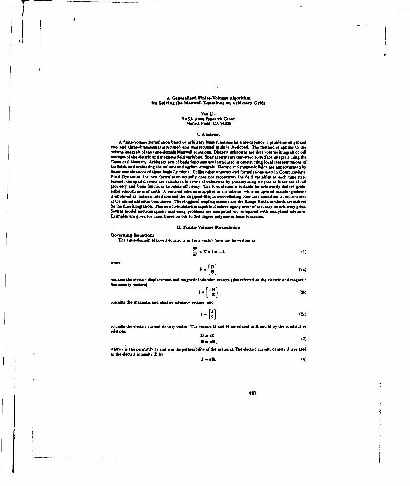
A Qewarltead IfInite-Volume Algouithmnfor Solving the Maxwell Squations on Arbitrary Grids

Yen LiuNASA Armes Research Center

Mo~et Filid, CA 94035

.L Abstract

A fintevolwme formulation based on arbitrary buasi functions for time-dependent problems on generaltwo-. and threv.immnslonal structured and uostructurwd grids is devealopedl. The method is applied to thevolume integash of the Umewdamala Maxwell equ~atls. Discesat unirowas are thus volume iategrals, or cellaveragasofthe electric and magdeticfield variables. Spatial termaart converted to surface Integrals using theGause eld theorsem. Arbitrary sets of heasis functwaose san introduiced In constructing local representations ofthe fle1s and evaluating tht volume and suracac untegrals. Electric and magnetic fleids ane approximated bylmase onmbiataetson of these basis 'unctions. Vln&i other umnsrctured formulations used in ComputationalFluid Dynamics, the saw formulation actually dose not reconstruct the fkied variables at each time step.Instead, the spatial teems ane calculated in terms of unknowns, by precomputing weights as functions of tellgeunotry and breis functions to retaina eiciency. The formulation is suitable roe arbitrarily defined grids.either smooth or unanwoth. A centered scheme is applied in e,.- interior, while an upwind matching schemeis employed at material intearfaces and the Enaquist-Maida non-reflecting boundary condition is implementedat ths numerical outer boundaries. The itrguered leapfrog scheme and thre R~unge-Kutlts Methods aWe Utilizedfoe thetime integration. This new formulatiou is capab" of achieving any order of accuracy on arbitrsry grids.Several model electromnagnetcl scattering problems are computed anO compared with analytical solutions.Examples awe given for cases band on 0th to 3rd degree polynomial basis functions.

M. riplite-voluss Formulation

Governing EquationsThe time-domain Maxwell equations in their vector form can be written as

OF

where

contains the electric displacmemnt and magnetic induction vectors (lalo referred as the electric and magneticflux density vectors),

coetaints the magnetic and electric intensity vectors, mand

contains the electric current de'ity vector. The vectors D and H are related to Z and B by the constitutiverelations

D0- cE()8 -pHt,(3

where f is the permittivity and pe is the Permeability of the materiel. The electric current density J is relatedto the electric intensity Zby

3 o.t, (4)

487

where.# is the aeletric condu~tviVty of the material. Hie" we asaerm the problem is linear and all theprprisane nat flsactionsal the Wsen.

Goessul Properties of GridsThe Maxwell equations can be solved numerically based on the integral form of Eqs. (I)L ()no first

generates a geld which consists a met of diacrete points and a so of lines or curves connecting the points.Thts connecting lines. or curves muat he chosen in a way that divides th. region into a set of contiguous,non-overlapping, space Rilling cells, The discrete point. am then CAlle Cell vertices (or nodes), and thecomnnecting lines or curves ane called cell edges. The suirfaces common to' two neighboring cells are calledcell tame. Eaeh eall insDisclosed by a combination of face. The bounding curv or each face in farmed by acomblnetlom of edges, and esuch edge enaneacts two vertices. Every call, face, edge, and vertex to assigned anInedx to id=%Wtifyltelf. To complete the gesmatrit description of a grid, ane must alon specify the shoapes ofthe edges and faces..

A grid cas be stractttred at %matracturved based aen the ordering of cells, faem, edges, and vertices. Fatstructiated gilds, the indices fat thes geomsetric eI ist are ordered, given one index, the others can bedetermined imsplicitly. Far unstructured gilds, such as order does not exsta, sad scen information must begivens implicitly. A spime way is to -ts the indice or the vertices and the two neighboring ('left" and'right) culls fat each faew. All other iafarmation, wclb as indices or faes and vertices for eachs cell, can

thea be determinsed fraom It. A special cm of structured grids, which ms called a regular grid, is that allcells have exactly the seane shape and volume. There ame a few regular thremtdirmensionall shapes knownto crytukllogralihers which a"e space-filling. Thoes inJude the her~ahedron, tetradecahiedron (truncatedoctahedron), hexagonal prism, rL. uobic doilecahedmoa, and elongated rhombic dodecahiedron (1]. The moat

astrcured gild is one that is topological equivalent to a gmenealized curvilinear coordinate system, whichtoarnst of oredred sarras of hexahedta. An example or a commonly uised unstructured grid is one consistingof nn-ddtetrahedira.

lnatgrali.j Eqs (1) over each and every cell dellnes a geserallsed finite volume method. Retalling thatfit Guess curl t#eorem convents a volume integral oae a cell V, to a closed surface integral aver its faces8

j,i oise thus obtains.IFdV + fdS Xi I . JdV. 1

Here the subscript j dlenotes a generic index frat cell and the suhecript i denotes a generic index for a face.,f oortinatto are deflod by some analytical, diffmaetiahle transformation, then thene shapes could be takent* he p.ortions of thes exact cooedinate lines and coordinate surfaces. However, this procedure generally doesMCA is*es the accuracy of interior schiemest but oaly complicate the process in evaluating the volume andsurface integrals. Since Eqr (5) we valid fat any call shapes, it is therefore preferable to construct simplerAspes foe the surfaces and cells that could facilitate integitioms ivrralting those elements. T~iv only pwssbleexception would he for the edges and face involving grid noints on a prescribed, curved, solid bat dacaryat material interface. In oeder to obtain hig accuracy in the msoluion on such a boundary, ottis , ay bewilling to camr out the more cusnberina integrations involving the curved elements, particularly %incespecial procedures have to be involved to m"t6f the boundar sad interface conditions. Line. triangle, andtetrahedron ar the momt Fundamental shape of edge, face, and cell, respectively. Integrations over thesefundamenatal shapes afe relatively simple and for some cues can be eact. We notice that general polyhedron,polygon, end edge is a union of tetlrahdra, triangles, and lines, respectively. Any volume integral over apollyhedra. it equal to the suimsatioin of the volume integrals ave each individual tetrahedron, any surfaceintegral ame a polygon is equa to the summation or thre surface integrals over asci individual trisangle, andany hone integral aOve a edg is equal to the summation of the line integral ever each line element. In thispaper we sthall Sormulai* our method on arbitrary grids. hut emphasis will be. giern4 to geaeral polyhedralgrids. Mle formnulation is suitable for either smrooth at unemooth grids. Except for the bookkeeping ofindlices, whether the grid is structured or unstructured is irrelevant to our formulation.

Unknown Variables aned Piecewlise Loca Repraeeatntiaces'To olve Eq. (1)num*ericaly,mwa.. W ke ele the discrete unknown variables which are to be advanced in

time. One thten obtais a set of equations to solve foe the discrete unknowns by converting the spatial termsin tierm of the unknowns. There are two metheds of defining the unknown variables -either as values at

lireue nodal points at as discrete volume Wauhailm (or voism. aveuages). In the Amt mewthod, use dofies the.skmewa vwi&hle at veslces. Far high order lonnatlatsuss, unkinowns meet also We defined at extra poitsmont the rsfaes nod/or inside 0he cells. The volumv u tted,,ft intkepsk eis evaluated by quadratures usingqusirditm at them model points. Unfortunastely. this procedure coupleb the model unknowns. Therefore, vethsoicitd timer isfepntions are electively Implicit, For a tlmswdependeset problem, this can be very ineffcieut.In this paper we diori. the volumes intefras, Idenoted by the symbiol -,

F,.L )Fr ru ~f,,D(:) dVI*[ (6)

as the saktownm variaiias. In order to evaluate the volumns mad suefase integrals in Eq, (5) consistently, weIntroduce on arbitrary set of husi tummictOm 4(r) mod immmes* that h Wed variable can be #%prmed bya plecei'me local espumewwnloa is to.e of lmass combisatmia of thuse husi lactiotes

V) (r) - :a..)

The type and iumn.,tu of heels feectiona chosen depend as the deeleod accuracy The Most common farm forEqfs. (7) iseM a spastiall polynomnial in which the #..(r) aft tNsor products of the position vector, Dependingon the natures of problems, odbesi datese of functions, such a* splines, wriveleti. trlgtnomaTIttrl. exponential, orother specvial fuiction, "a elm be mod as a bowt aet. Our forminusticeis will be given in wrmes of arbitrarybaesh licttions, but awserimnJ mpin will he restricted to the polynomiail repreeeatation. We shall. leavethe ASOd a(other types Of repecstetiia"n to ftutosreseteb.

fnsomeauetrim" imid In"OPOLatlMOnce the basis fuact~ioam have besoewa the wellietias dim ied bm in Eqs. (7) can then be

determined Wn temms of the distoet mnknowns in the nsbuhahothed of the cell i. This process is Normallyrefiteda to an rrcoetruciica (2,31. The neighborhood of a cell is dellnof an am munble of ite seighboritngcalls. The first hierarchical neighborhood of the call ,p is itself. The seon hierauchiacl neighborhiood consiststhe call j an all its immediete neighbors An Immediate ieegbbor of a cell can be a commono-face nieghbor.which satemi a comman face with the cell, or a conaon-irdlie or commont-node neighbors, which sharesone or mor edges or modes with the cel~l, res pectively, The third hierarchical misiglbothood includes the

seod maghbothood and thimeanudiate neighbores of eli cells in the emend neighborhood Higher leveeof neighborhood wte built recumveily. The lWs of the neighborhood con he - Ie by the distance buw.,enthe cerp*oido or the paenot sad neighboring celb, The stoered for remnmetiutoi Wi then selected froin theni~ghborhood. The selectima cas be synmmetricaly around the ~ssa callj, us con be directionally hiasedIn uam of the inseeluals or soelonk Weds. Own. eeula avoid choosling a stencil that it ncross a materialimlntusirs, usesm oein Aeld compowaiss sad derivativeany hW e diorminimous &t the Interface,

Ihe "mPudgiy, hbea we man one componen is Eqs. (7) to ill"Winsca the recoritrucslon. Let IA(r) be acoponentl of Pj() j(r) OW C) 6 sadEM at.. I copoen The local representation can be written

f, (r) a Z:ci..4#.(F) a 47(r*c (S)

wbeae and O(r) sad c wee the row vector of*.4r) and the column vector of Ci, repectvey. Let M,Aenote the list of indims or th reoeiuto stni oetecl j ierting Eq. J11) eve all the cels in9,, ane formsi a linen, system of squmationes for the catllj. If the number of recoustruction calls present inAfi, C, is equal to the number of basis functions 0. the cvisflcieoss ejv. can be determined from a standardlinen, systam solvet For general unstructuated gInds. it is more likely that those numbet awe not the sums.If NC > 111, one than so-Ives an o~e~e tnedmamiuaitiou Problem with respect to susi chosen normn. Ifthe 12 nrWM usWed. this me eqeivllentL to aIist equanes prI e

Ae~f.()

483

wAne A is a reetagulew wwM~ of Was NC a *whth lma

MsaI is a eakaumO " oefi clam K wth e.t

See the eaambepi k = A(,(*)i do nthe h mebein the noxaccati~so. etencil for the cell and the sy-mbol= dwane a law slaeqa problem. Tadmiqeam 1oe solving a lam selvar problemn ane well known and canbe iihed anoiledmd esaboehe (a. g. ". 4-6)ý gone aene the nehod of singular value deccmpmsition,and the soltion far the cwndmew can be wlt= ia

c aA~f, (12)

whierte I yM ol +epeI the peaud icasee of a rectangular matrix. T1hus, the field can be reatn-.gtruaed by a piecewise u~Alytc function

11(r) - *V(r)A~f. (13)

NOOVw that Ow panda does am~ alwaga Sive a correct nswim if the rank of A is less than 113. Itis swiem as she pemeat tLow what kind of aeeus shouldl be sainiathed for this type of under-determ~inedspanm. Tegeheve. mour aud, we chuem the -an--ructac etancil eand that the rank of A is alwaysprater than at equal to the auwber of beds fancias used. It isaho possible to build soetn constrains inthe sanaaso I -- . Thewo mancomme am Ie the preshrvatiorn of the volurne integral. i. e.. the volunbeintegral of SI.. maltiag meuwasectium 9q. (13) matchas ?,. Procedures tnr solving eonatrerne-I least squames1 11 aa do SAn ia Aie. 4-4. Once the I=a densty voeceer D, (t) and 81 (r) have been reconstructed.the fladiasa of the astimity mad tureat densty vectore can than be eapseasd as

(04

Jj(ir) - !Dj(r)

As we mai above, the tecakeustruci peoms involves eolivng an ow'-detaesnatio lirnear systernof e!uetrL- feeach "Ao, whichis a my tio-me~caumia procadan. This pet baa been employedim mas -- w Uerdmpatalia mai polyaweamiaha featians for auaetaictured Srida 1*,$.. 6-7). However.. rua the reontructiorn was mled out at every tises ma, them cemspame~oo ame very inedlicient andbeseme iupradieal for thoem-danedosl 1eo-e-e. Rae we would like to emupham thaL thr reconsassaction,one"~ a4 t sibooginsg and the wed ofeinpusa~ioa, is actually ausacsseery during the timse integration if thenm~arsebs usainil se vachempdi What really Anarelned us the ompuatetmos aft act the reconstructedaaalyticl .pm~esautiAm. but their fuacticeal valuin each as point values of &6 reptementatmcns or theirdesi~vn sas cat s posits m Welisal valwas of the reprnsentations ver somne regma. Thwe- funcuioal valuescan be clmneed to the pioducta of mwesgilte sad the unkanowns. lhisi procemsis known as interpclstmoo.In Do knohemlaiet as we Ahi&M1a in she as

m* aection. the epaWtialitegrala, can be ex;rme as

f

tad

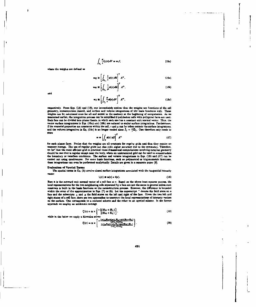
fU

where the weights awe defined as

wEj IF . 14(r)d A+.(1b

and

wj [I, !.{4,rv]A+, (15c)

respectively. From Eqs. (16) and (10), one immediately notcee that the weight; awe functions of the cellgeometry, reconstruction stencil, and wurface and volume integrations of the basia functions oaiy. Thoseweights can be calculated once foe all and stored in the memory at the beginning of computation. As wementioned earlier, the integration protosa can be simplilled if polyhedral cells with polygonal faces are used.Each face cant be divided into planar facets, in which ser one has a constant unit normal vector. Thus, Lhevector surface integrations in E.v. (1

5a) and (16b) amre educed to scalar surface integration$. Furthermore,if the material properties are constsants within the cell, t and pa can be taken outside the surface integrations,and the volume integration in Eq. (15c) is no longer needed since Jj = f~. One thserefore only needs to

Mregelar

we fser that the most slficient, grid in practical three-dimsosional computations involving complex geometryshould beone thtis regular except nearth body, whr nusiatrdgrid cnb sdt comdtthe boundary or interface conditions, The surface a&d volume integrations in Eqs. (16) end (17) can becarrie out using quadratures. For smne basis functiones, such as polynmoial or trigonomnetric functions,these integrations can eve be performnod anallytically. Detaisare given in a&separate paper f 81.

Evaluattion of Spatial TonsThe spatial terms in Eq. (8) involve closed surface integrations anociated with the tangential intensity

vector"l(W) ae a(?) x l(r). (18)

Bere a is the outward unit notmn" vector of a cell face at r. Based on the above least squares proceem. thelocal uepeesentatiocts for the two neighmboring cells separated by a face are not the same in general unless such

'osrain is built in the basis functions or the reconstrusction proem. However, the differnice is boundedwithin the error of the approximation in Eqs. (7) or (8). Let the superscript -denote the field state on aface and the subscripts L and p the field stat. on the left and tight of the face Given the two left andigtk tates of a cell face, there are two approaches to construct the locall representations or inteunsty vectors

on the surface, One Col.poad to a centered schemne sand the other to an upwind scheme. In the formerapproach we employ an arithmetic average

while in the latter we apply a Rirmnnn solver

Ha-Nt; n (20)

491

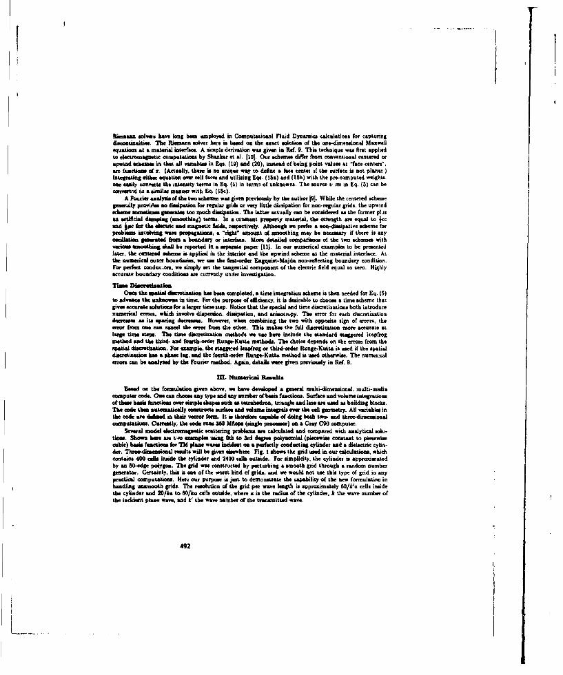
Rissnano solvers have long baes employed in Computaticeni Fluid Dlynamnics calculations for capturingdisoostinuities. The Riemann solver hore is based on the exact solutmo of the one-dimensional Maxwellequations at a material interface. A sumpis derivation was given in Ref. 9. This technique was first appliedto electromagnetic computations by Sbankor et &L. (101. Our schemes differ from conventional centered orupwin schemes in that all variables in Eqs. (19) and (20), instead of being point values at "face centers"are functions ofir. (Actually, thene is no unique way to define a face center if the surface is not planar.)Integrating either equation over cell faces and utitaing Eqs. (15ia) and (15bh) with the pre-computed weights.one easily converts the intensity terms in Eq. (5) in ternt3 of unknowns. The source L' :11 in Eq. (5) can hecosaveetd in a similar mannier with Eq. (I6c).

A Fourtier analysis ofthe two schaemes was given previously by the author [9]. While the centered schemnegimarully provirise so dissipation for regular grids or very little dissipation for non-regular grids, the upwindscheme somnetimes goneraese too much dissipation. The latter actually can be considered it the former pl isano artificial damping (smoothing) terms. In a tonsteant property material, the strength are equal to (Ccand 4pc for the electric mad magnetic fild, respectively. Although we prefer a nont-dissipative scheme forproblems insvolving wave propagations, a "riht amount of smoothing may be necessary if there is anyoscillation, generatedf frcoi a boundary or interface. Moss detailed comparisonasof the two schimes withvarious smoot~hing shall be reported in a separate pape (11). In our mnuerical examples to be presentedlater, the centered schme is applied in the inteiore and the upwind schemc at the material interface. ALthe numerical outer boundaries, we ase the fars-order Engquist-Majda non-reflecting boundary condition.For perfect coudu~ces.r we simply set the tangential component of the electric field equal to zero. Highlyaccurate boundary conditions are currently under investigation.

Time DlacrwelsaftiortOnce the spatial discretisatfion has been completed, a time integration schteme is then needed for Eq. (5)

to advance the unknowns in time. For the purpose of efficiency, it is desirable to choose a time scheme thatgives accurate solutions foe a larger time ste. Notice that the spatial end time discretizations both introducenumericel errors, which involve dispersion, dissipation, and anisotrupy. The error for each discretizationdecreases as its spacing dec-e---s. However, when combining the two with opposite sign of errors, theerror fronm ore can cased the error from the other. This makes the full discretiwaion more accurate atlarge, times steps. The tizae discretisation methods we use hers include the standard staggered lcspfrogmethod and the third- and fourth-order Runge-Knuta methods. The choice depends on the errors from thespatial discrtlationu. For example, the staggered leapfrog or third-order ltunge-Kutta is used if the spatialdiscretzation has a phase lag, sad the fourth-ceder Runge-Kutte method is used otherwise. The mnueresalerrara can be analysed by the Fourier method. Again, details were given previously in Ref. 9.

13L Nuernsical Rteaults

Based on the foermulation given socve, we have developed a general niulti-dimenaconal, multi-mediacomputer cods. One can cheese any type and soy number of bas functions. Surface and volume integrationsof there basis functions oave simple shap such as tetrahsedron, triangle and line are used as buildipg blocks.The cods then automatlically constructs surface and volume integrals over the cell geometry. All variabl.s inthe code ain definad in their vector form. It is thaerefoes capable of doing both two. and three-diusensionalcomnputations. Canvetily, the code tars 360 Mflope (single pruemaor) on a Cray COO computer.

Several model electromagnetic wscatering prbenmen are calculated and compared with analytical solu-tions. Shown huer ams t~o examples using 0th to 3rd degree polynomial. (piecewise constanrt to piecewisecubic) basis fanctions for TM plane waves incident on a perfectly conducting cylinder and a dielectric cylin-der. Three-dimensional results will be given elsewhere Fig. I shows the grid used in our calculations, whichcontains 400 cel1a inside the cylinder and 2400 celia outside. For simplicity, the cylinder is approximatedby an 80-edge polygon. The grid was constructed by pertarbing a smooth grid through a random numbergenerrator. Certainly, this is one of the worst kind of grids, aud we would not use this type of grid in anypractical computations. Hem,. our purpose is just to demonstrate the capability of the view formulation inihandling unirnooth grids. The resolution of the grid pet wave length is approximately 60/k'o cells insidethe cylinder and 20/ks to 80/ho cells outside, whens a is the radius of the cylinder. k the wave number ofthe incident plane wave, and k' the wave number of the transmitted wave.

492

In the perfectly conducting cylinder cue, the incident wave has a value of ka 3 propagating from left totight. The analytical solution consists of an inflnito series of Hassel fuactions of the first and second kinds[12]. Shown in Fig. 2a are the contour line or the otal electric field of the exact solution in the vicinity of&he cylinder. Plotcedl in Fig. 2b through 2@ are the same field from the numerical solutions using 0th to 3rddegree polynomial basis functions, respectively. With the Oth degree reconstruction the field is asumed tobe panonwis. consaant and the solution therefore resets th* unsmoothsme of the grid (Fig. 2b). However,the general feautues ae well captured. By using 1st degree polynomial basis functions, the grid-scale noise iseliminated (Fig. 2c). With the next two higher order reconstrructions, the solutions (Figs. 2d-2e) are hardlydiatinguishahbe from the exact solution. The magnitudes of these solutions at the entroids of cells along thenegative x aid ae compared in Fig. 2f. Thom remlts with 2nd and 3rd degree polynomial basis functionsclosely reproduce the exact solution.

In the dieleetric eylinder case, the incident wave has a value of ka 1. The permittivity ratio of thedielectric to the fhre space is set to 4, therefore, k's a2. The analytical milutio. again consists of an infinite

serin of Bessd functioons [12]. The sane Kh to 3rd degree polynomial basis functions am used for computingthe numerical solutions. Features of the comparisons among then results and the exact solution are similarto those in the previous ca. Only the exact and the 0th and let de•gre solutions are given in Fig. 3.

Referva,•ces

'I] 3 V. Smith. Geomnetrical and Structural Crystallogr "Wile New York, 1982). p. 77.2 B. van Leer, "Towards the Ultimate Conervative Diference heme. .. V. A Second Order Sequel to

Godunov'e Methods," J Cesp. Phjr. 54, 101 (1979).(31 A. Haten and S. 6besh, 'Uniformly Hilgh.Otdar Accurate Non-Oscillatory Schemes, I.," SIAM J.

Num.Anal. 24, 711 (1987).[41 CL.L.• son and LI. Banum, Solving Lenas Squae Problem, sPrntice-Hall,, Eng od Cliffs, 1974).

G.M. Golub and C.F van Loa•, Matrix Comnputaions, 2nd ditione, (The 3ohns Hopkins UniversityPress, Baltimore, 1989).

(61 TJ. Barth and P.O. Frederickon, "Higher Order Solution of the Euler Equaions on Unstructured GridsUsing Quadratic Recoenstrction," AIAA pper 90-0013. (1990).

[ S.I Chakravartby, K.Y. Ssema and C.L. Chen, "A UNIVERSE-Sriae Code for Inviscid CFD withSpae Shuttle Applicathons Using Unstructured Grids," AIAA paper 91-3340, (1991)..

[81 Y. Liu, "Exact Integrations of Polynomial and Trigonometric Functions over Arbitrary PolyhedralCells," in preparation, (1994).

[9] Y. Liu, 'Fourier Analysis of Numerical Algorithms for the Maxwell Equations," AIAA paper 93-0368,(19930).[10] V. Shenker, W.F. Hall, and A.B. Moliammadlan. "A CFD-Baned Finite-Volume Procedure for Com-

pmtational Electogom ngeics - Interdisciplinary Applications for CFD Methods," AIAA paper 89-1987,(1%2).[11( Y. Liu, "A Comparion of Centered and Upwind Schemes for Solving the Maxwell Equations,' in

preparation, (1994).(12] R.F. Harrington, Time-Harmonaic Electromagnetic Fields, (McGraw-Hill. New York, 1961), Chap 6.

FiG. I An unsmooth grid for &,cylinder

493

(a) ecadt (b) piecelee constant (c) pie•-Tise linear

(d) pie-wims quadmeaac (e) pietewise cubic (f) E, along negative z axis

FiG. 2 Comparisao of electric field for a plane wave incident on a perfectly conducting cylinder

() ec (b) piewi constant (C) piecewise linear

Pip. 3 C•mpeaison of electric field for a plane wave incident on a dielectric cylinder

494

MassIvey PW2Wi 6izduCAMfainc U03640=10n nuetOdS for ekcuVRedc Wanmg probmLe.

R. S. David and L T. Wec Department of Physics. Florida Adant~c University. Boca Raton, FL33431, USA.

Ahiaw&ct We disoms the develo~eet of thme~faaedu-omain aigoddmaso fix massivelywith a ngleInsuction utehipie-dmt hun Variou astraleg we unsuiatedadsting seqenia code. which Is relatvely simple ye f dfflcient colpkmy to

Oslt or me ~1fatlYof puie itoIssues adciosiesrauons. We give nimmeicalval" fr = r anse of problem diam and numbers of proccesoms Finally, we

c~dally sanlyre theme rembiaind uibe peromise they hald for the lminio of ame compkme problem

Thn-damain ele-ctra-msgnetc prohiente include a wide variety of phenomena of pma pratiscciinterst rimnging from the ctri ric Ipulse prouaced in nuclear sisposions to radir mtare

enilsiaand whole-body, to mention justafew. Only in very mae camse usuallywith high rimmuyat lpife gceaies. Isas naynalsolun feasibeand form sanstaosaccourdn an typimi ppladoes a compuatosanal m icamo m.Thdretaunofic

I I Vy be bedan Maxwells eqatosi iThered fomuaison leonS vofisutee~sorfnb difamcecalulaioa 1 r itmay untio I nua equtioen approach, lading

so the moothod of miomnu 23 Oa l ofsi&M s=be=e and hybrid mdmnlaiqe have also beenFormd e~no an acoon aswlla hg spatial resolution these methods

deadn n mm dofa time mod, m a leserexieni siosge. Trum, esearehers inc -uuti l cuhovutnanics. just like thei colleagues in umny other fields, have been mnuting

ozm r luZf:=ff~ coinpowa. Including vector sand par"le macblue (see the eveww

PuAllelim is no pansoea however, and. different techniques may be bever suterd for differenttypes of wehicectores.'r Theubod oftooments, leads to a Uff i equanaon which is well-suited farpser" conputedio (4-71 aetomy vendors have emuflsei.toefcetIqlouinoveem a tu'odmalopac antjsirprocts. diffa (FDTD) nothods;dw slu ento a symmhm of Homr equations that tateds wo be solved for the field as a function of space and fte.Pwfasliniden x possible at the level of the eatambos, but con mst be taken because fte matrices inqiakein e u sparse, or it nkay be paI mn -mhd at doe physica level by assigning owe (or amo) spaim!

lom=Weach uoceaaoin a assillel meebbue. Pum UlllP M codes haef bumee 9ep1rt1 by a mnmberof hoeao [41. Simmila zmmustegi y be e"loye upuzallellae flubs dam=& codes [41, for which the"seulahy of the mild becommes, an =an la10 dugl which type of tnuchine to use. A very pmndadlimad on these and othe technkques with a large bIbligeh (up to 1985) can be found in

Iee [3PIS. In thepmeent paper thomawn emphasis, is an the method fl-the orisintal fmaoulatiof Yes 93antItediuso wilbl belforpaflklismdlon' q, co as with asaig6AoIsteuctitonmahiple-dam -__tene 2Welh pcamneampis being Oeven fat the Maoft bm ofy nchiumdns

mpe vmmc thbis paais tmuefokk in be a ge Ia introducntion paraWel coMyatinl. o he atutorial -an -how ID- pas iezta existing sequential Fortzsn-code. and to illustrate the kind of

pefomac da may be realistically expected for FM spocations. In the , i I of this paper wedsasteparilliata of FDTD elgorifths an the Mutclass of coipuxers although mass of the

.mt a .4eua.y well krt~ohe type of ardabecusres In section 2 we give a brio overview ofvarnios types of parallel comu-e awrchiecstures, discoss; software issues, and describe the MasPar

hn* f OMPU an 6mrelation to other parallel tuschiet with related ardtchimeus Scotio3outlies th FWIDmetb d mA com era vaiout appfoaches used to parallelize an exasun FThD

495

code, Section 4 presents end analyzes the tuning rsults, while section 5 concludes the powc with asumostry and a discussion of fatenwork.

2. Imssea is peskis Comnpeting.

Cevetonal single-CPU computers based on the so-calledl van Neumann architecture arerapidly shpwigf z Iphysical limitation poe by the finitenes of te spe of light: and the

5 wlowerlmisp uto n t iaa n i adov by quanitum me h n ca r ct. us; the only way to, maintain theexetd i.eas in cnpmrspeed with doas is so get several composers; so coopaus on a sigetask.

'= tmplay sme form of=asls [101. Of caurse, even omseun tl ~ir lme ansOfpenflldism han ee used, cmvnby havig bit-pmrllel sruumcc by allowing for instructio!phulnn.but the smornt of op - t ha obue ine n this way is rather rsicd. Cmue

uelususamy be classified veyaor vaesy in turnss of a ta oyfirst: proposed by lyain1972, basad on ah notieex ofan instuction wstem and a dramssr Inl this wheme traditional single-poaceasormachines wea cledW SJSD (single instruction mingl data), since theme is a single instauctonstran and etch instructioin opellawe on a single daotum at a dues. On the other hand, moat paraillemachines in curate-use either camploy, "h SDAED (singl instruction multiple data) or Milifi (multiple

intuctia multiple data.) paradigmn In th fist case a single instruction sn=a broadst by a singlecontrol askis axacusld by many pocesviing eianents (P's .an _n dif- n data elmns sus simaned in samt regular f5ashion such as a mesh, hyparcuhe. noe, etc. sand operate in a synchronous!!y. SMisvery well suited for ma=vel parallel piogroumang. with manery thouslands of PE's

coopratielyWd or 11 a ighdegrees of granularity and inherent parallelism.I.UDWpslds is a man genera homework in which prvsaeu s may be simultaneously executngdifteent instrucions an diffeent dom in essentially on ane m um mner, no centrallzed or global

aynheoonutehansa hetpresent.UmlyN2G4DM co .ue contain a rlatively lm~ll nWmbea oesr (Ilens tohumbedsand they atconsidered to he ber suited 1br coarse grained or

Z-w rIobiems. Although by their verny design they usmo fleltible. MoMD malchines are quiteefficienloy and great care needs t be takeon that WWpe La balsocing is aWhievd

inc tatthenu ae of ide imoessurs is kept toea minmurn. In bohprle udguit is alsoinqmpotnt that the amont of inuqxaeessor dama ex-tallge is relatively smal siA coiication isgonallyaslwer pruocessinpm ado land &.i omunicaron channsel usually has a smnall

banwith an dos ot lo sautaao cmosan dr bewe all si hmso erwmis is alsocouscnrsetohain mexcoshmanisu orwwht e = ti1011opology Plays

anlmpneasrle. Hlgher-dimenmionma networksanu to be paefiesre for their short inmpiuceasodisancshutned nmny move links; tha loWer-di~meaki onesa mking Lbhem hard.r to design and

bOUid Mlat medalna provade some fas comuicaiona mchalosm between nearby processors and asloergloalm~muiad o mchanins (a rosr)hwiiay twol -,uesae Anotherissue in

Whc Wscts d~iher Is the mosoly organizaton: in shod memory syteMos. all iancsmsarilblmemosy in a Utighly coupled or loosely coupled fashion a&W infiormation exchuange happens

im irily 1 8 central memory, while in distributed memory system, eaci. ;rocessom has its ownpececsC "oopratie ocount throug ma sa M passing. T'. a:lluy shubsd umameyt~o

afe.or. wmerotpossibicdeisninIs very us ed num us uom sypsamebeen built atresearc isiuot.While the0 1 o 0 cesomucuafly available Machines also continues to increase

Rmtm the softwalre point of ----w th -eeoue aan efticem Parallel algorithat is not an easytask which ideally should not ama flaw porting a sruuetta code. but rahe from a Modhinking of theentlire approach. =an problems and solution stralegipespasces a high degree of inherent parallelismwhich is often obscured when the solution is satnymad by' a sequential algouithmn. A useful , ae ofthe perfaunanos of a psullel -rga is the .pedo saltied which is defined as the dine neessasry toCosom the algorithmn on a Iingeproeso ivddby the fise, this takes on N processarst. There wesomet problem with this defniusout sinc Ros no lwhw toobtain the time -ecessa m) for execution ona single processor and ofteni same appouxrsmdoe is used or the scaling behavior over a range of

4961

auesrmiey sizes is measured. Also. AlthMuh It Might naivelypp dhat the maximumti possibleEd L N --ean - would be N (a Hw speeupt w been a vocal debat in the

timpossibillsy ~ ~ ~ ~ ~ 00 o'ualcrpedu(1.whhwy win - tin sarch probitamwith random elements. However, this isune need not concern us here since we am considered withdeaerministic Or cujaica.. In rme cases the problem breaks up into N independent, identical pie=e,leading to so-called 'embarrassingly parallel' code. The speed-up in such case is N &ince theme is nto

oveod aseoltd with comanlcation or scrial portlons of the code. Tbis may happen when anIdentica calculation needs to be dome for a range, oremea or initial ondidions, flar eanspi. tocdeajelt avaerges. Suach cosupuraticual approaches have been called replication algorlithm (13].

Hoee m problems do nam fall in *WIS cassda more#ial on'nM d to aind an effiasmtI onteproblem, so the ougat parall o IMIpule. INmo VappOaches include gemtian dA-, p lItchm 1131. In the JIM st doe thepyca space in which the sysiem to be

twavedgIed raukdes ii Itwok up lino cels ech ceH usocisud wihapoesr while in die Inner caseit is th69 lllmi the nuthemedeal, formulatlio ofdie =ahe that is explolied. Other techniquesinclude mvd~mlcnp er thods in which die wski4 sabdivided hin - uu-l hI- in and results arnpoedfrntthe; leaves to the parnts. Clearly mos. of these approaches. except data parallelism, are

wsiefa !MIM computas. since the ranks allocated to each processor are not necessarilyAticaL

The emergence of parallel computing has also necessim-At the devaelomat of new computerlanguages or extensions so old ocas, to allo parllel constructs. Origin ly there was a considerableIsl: ofstndardiuation with each macine having its own iauraamn lagab uttacentlymor andmne ellen is being mde to establish some usifile akywc-Onapebility. particular, the Fomencommuity has adapted a powerful new standard, Fectean 90, which commais several features of

prmr inaest for parallel, programmming [14,15). Of psauiar relvace~ we the powerfu sarmyopasons uppodbythisalanguage. Fae exayle. the am, C, of two arays. A and 3, of the sam

namy he accomplished smaply by the staeet C - A. +3, rather than by the standard netdlooprunuing ver all cemets Liwbwlae die satement C - AOB ams sig the do tn The value Aaf Dlj.

NowK&z is nam the matrix prouct.o The WHER statmat may be use =o values to onlythose array elements wheom a certin logical expression evaltuafte so one. For example, the followingstamuet fill each element of the array A with the inverse oldie -or - .on In -eo t in arrmy Baslong r, Inne is rAD-zeo: WHERE (3W60) A - 1.013. A similar lnmco sF4RALL. which was

;aI rtcinsl Foxa SK draft, but was not retained for ibt Fori 90 standard, although it is beingnu.'- mber of manufactaters as an cuunsloa. It allows the conditional assignmet of array

clem. ased on a conedtiw that itself may congda explicit subscript expressions. Many moreirnovit '-am we present in the Language, but the ones discussed areof specialmrlevenmio othediwst s, athis ;papr A new standard sta mrnuyuntudrde opumut by the IHigh Performance:Fartamirum

In the jswmk ther min eoom isa thed Masar MW-l and MP-2 (DECmpp 1200W) cia. ofmusively prasittl cocapaners (10.11,16.17]. In belef tie -- chi-e in this clan at based on due SMhDnearadisamd ams uist atlE PB-warrayniuged inac two-dimensoesl mesh with wraidal wraps-aoundbudary uxt. Aunts. Tbey wanmde outof 1, 2,4. 8. or16 processor boards, ecub of which holds1,04 Ps and their sassocived mery (16 kbyte or 64 kbyz In Dynmanic RAM as well as forty 32-bit

Ott sinlT~isoldone by dbeAnty Control Uit (ACU).This is aregister-ba.. gxsouden 12.WPS scalar: rcso which ftches and decodes the machinematwuron asisdlex arlea and acalar cmUsanouas, monult the stats of the PE array, and

br~stacoeul ignls oiLIn addition it contais 128 kbyte ci data m'.-nnr and 1Mbyte of codleSee. The combinauloo 01 the Marray, dicccommuication mbcanien. and fte ACU is called the Data-parallel Unit (DPU). Itrscescomniao betwaen neates-acghbcT PE's is possible throughthe s-challd X-Me hc ik each FF. to its eight nares neighbors and pi'..ides a fastnuimiopath with a bandwidth bitween I and 20 Clbyre~s depending on -he mocecl. Data interchange betweena ciuwy~ FE's is prowitll by a gloa oW based on aemold-stage it m~ b e~xroasber swiath. At waon1.02$ asimuarswos linki am possible and die sysMM is AMCe to cwuse at an aggregate bandwidth of 1.5Obytes/i. Thke global zster is also responsible fcce data tdanse woh di ;,,-spacd J/0 subsystem.

497

Clerly weneerpossible, rosete communicationa shooki be avoided since they awe slower than X-octa-,mnwd nceiaze hgs8atidontthePB-may aemn m idle.Teconqrnweri tntendd by

a woirnksation with assandd ]V) whbich evdhs Ufa se interace and newtwok cotowusucaoa,Only wfen there is need for massively leaýe excton is the DPU invoked, all other sequential

-- m-don is ft an Thefnu n hour doa acm as the host for the MasParPopitgEaiomet MIo)wfidudebugging and code development &Ad as wonl as the lnag

~rs. mreny tw lanisg.am a ponoted h MP a Version of Kermtighan and Rnch'e Cwuau .and' W version of Foctran,90 with esmeniui (including:FORALL). In MFL

th ou'arciehlcturs baccessible so the uer aim has averd the location, where dant willtoe ith& th peinblils w addcosa Individua PEa. In MPW on doe other band the array zin and PEcoeer u hldnhm i= 11 themo. Tif buathe sdiviatqe finrewag codevirtablilsbetweentmodels

elputdogti Urns so s h mi hait du theondwopile m dom. especilaly Ira in the demius format.(Asmilw Ah A , an available a mud in haibks ML Te recently anounced -2 urhinesamu binarycometbl with the P-i, butare abou 5ties howae.

In ternof itee"nue the MasPw , -a am very Amdlaran the Dlsmrbumed Array Frooesscw(DAP) for which a good deal ofexpertize bsaa been macoslaued 1181 as well as a awthf f 7ompt=rthat were mainly used is acaemc or Isemla ishmuoy environments (Illia IV, MP. etc.). Niaspsthe beat-knoswn clams of SSWD compmnpwisi the Connection Machine CM-2 famtily. Thewe machines arebased an a hyptcbe architecture. single-bit procesm are connected in a twelve-dimensionalhypereube :;V bof whicht my have ep t 16 pocass. They ame not ,n be confued with the .nsucens CM-S fisally which an a mixed SIDADMIPAD paredigmo (sometimes called SAMD:Sylciumnona/Aaysichrnon Muoltiple Dan[=121. It - that algorithms developed for a mesh

m'would nor be masily ~edforothe bet ortumasely it twoe out that mony of thecoOODcatVity mS y be embedded into oth1 [191, so that an aLgonebs for one may be ported

f"*d xv o antberone. In particular, the two-dimensional mesh can be embedded quiteOwl b~d Ia die beod~n alzboUN impl~meite on the MasPar

cm ,pterehavemoia - ..

3. Massively parale FDTD methdsi.

To illintaftm the pmllu of ean existing sequentia oode, we decided o mtae a programaUsed in adL [2](papa 1. -23 bhihivolve the penetratinof ta pla wave Int a loiales: diedetisphore Althug isn t by no meassu a very coqlctdor uine-onaning calculation, it is ofsuificiont goienezfe and '~exe Z n motex cedabo fflm a pso lel it e03clently and it alsoaflowe usanlllkoun som of tdhe 'yp ~ica migithat gay beusdtaony isthis. As eantionedbeforeIsis me awaysbu n n-rji anport an mistigsquential code so =a puIll machine, &proassaptly described as trjuvooodog aen1 a code by Lo et at. (M. In the fam pLace, .te is noguaaause. that the mes m Uiie sl ultb is also the best sequeta alpwIffman Also, it is nordwnvusy an dirsten Ur eabselig porallebus lea particuargel dome th nhmadomial

laelcbme thepuemfpusleleaetina.Even If ineigalsoion ispule in nature anda I eeudaode exim ts, thIicsyncrads of the conympoe lagaend may sender pa allltion of

tisode 'low dum alvidl coeunvuem such as W-atmoment and 070s in Frmneed to be replacedby TOALL' or 'WHERE' insauctiom in FIum -~e hsm ea daumntin and ___ - -- I--lntask. Deaflow an, and ftom mntmmmue is amother isme tha needs an be handled carefolly: CM Oblocks in pwrtcula am often a source of eimi, leading may programocts anpass all argumentsexplicidvam the msokodne call. U fkac, COMMON blocks am cosidered obsoleein Parmun 90, alongwith =o~ GOTO soneme, the CON-MUS statement, and others. Als in oider an accomplish anefficien upigc heds.my oo th pcswray oft needs an undierstand the way this is doneby due couier Q lit i -uom an mt so =m the number of active lcesoon and so it way besocssay ans-,inorange Udo order of 6he mbwip kinsaan may rder a ompisNtis

498

It Will be massmed that the Weader is familiar with the geaeral Ideas behind the Thh omethod:~finbdo details may be found in the arroial =5 Yee (9)3or the review by Taflove and Umabna120], as well us the wtxt by Sadku (2 si time method week dituciy from Maxwell's time-dependent cudi equationa and uses aecoad-arder eenul-diffeeace approximadoes for the spatial andtemporal deri'vatives of the electric and magnetic fields. Thus. it is a relatively simnple. yet fast andaccurste, gnediod oi appiazoinis"l determine tie waves psige in physical space by a timle-stepiNg

psodr nadlaaute pid. In Iee U -1lginal notadram teid . points are denoted by integers i, j, and k

(ij~k) -(inx jAy, ktz). Iwhere "x Ay, wan Az are the lattice incremnsts in the x, y, and z direcslos. The grid spacing hs typicallythake to be night or sxencells per wavelangth. Ukewise any functionm of space and time will bedencee as.

F(,j.k) - F(i"x j~y, kAzAndt). (2)whens n is an tontger and At is the time increment chasen to ensure stability of the time-stepping

alota.Sinmom time p msca d ini nvolved is unally unbounded. some form of bowndury condozmsnued anbe mpoed.Here we: only conskier the most widetly used frm. the absorbing boundary

cosiides-e-e- Jd by Taflove and collaboratims (20].l~iDF eqan osat inrmigmd poitsate all quise similar to eac other and caz& be found

in the references umendoned earlier M29.20]. Fur the sake of discussion we just list one of theseequations. which gives the x opoet of the magnetic fied,. Hz. at time a inte-i of Fix at thepinl-ustimewn and thy ad zeooxmp nasof the iemet~fiekt.]Ey mdEzat psevios m atepw s an

mebygild punn (equations (3.16) in (2]):H13(i~j.k) - Ham-I(ij~k) + EyDm- kl~~~.) - E,,D-'(QJk)

- E211-04+14 + E1 51 (i~jk). (3)Clearly these equations are well sudici for parallel cisnaputation since only datz fromn previous am saipsand ftom tinmrst-mmelglbor geld points ate needed. lie absorbing boundary conditionms (equations (3.32)in [2]) use similar except that all fields sane calculated in ierma of quantities two time ste" prior (forpropagaton in flee space) and spadial inteasctio is with grid points that differ by I from the ciurrnt onein one or two dkwctm-s for eausnple:

Hy(O~k~a(H94 ij~kl) _ Hyfr(j~k) + H *,(lj~k+l))/3.()As can be seen this czmipeson is tllwell suite for parallei~tion as it involves short-rangecoaimumcadons. In the particular code that was pargillezzd the inital field consists of a staple-

frequecy incident plane wave, The ~prori sum by putting all field componen t deS pitequal to zo. while the plan e w saince a activated us th mf__ se adlf anfrth du rido ~ofthe calculationm. This problemn iofoocane exactly solvable and nmerial oualts obtained werscmete

The parllelmiatieof he FU cde proceeded in a nmbner of stages. First thme original Foru.77 code was compiled wihm MW umd excsdt salish a baseline fix future comarison. Sinc onlyFores 90 cousutrai actually runm on the DNU so paleltonwas obtianed at this level. Next all DOlooipswere converseduilFuwmn 90 by eliutimating CONTWNU staements. At the same dime simpleloop amdpmnent47 eauon were coversied. For example. initalization of lbs fields is perfunmed by asinle stsmn Dtefri Y - 0. which inddales. in sue all elements of the four-dimensiosal wnay

EY"(-JMA+I. -JMAX+I. O-KM.X+1, 0-NMAX). The compier dizective CeIFF ONDPU EYintrousifa thme cosepileropt this aray an thme P1-array. Thme elefaumt assignment on the MOSParis that diefirst index goes along texdreo ~f the aild, the secnd one along the y-diecton, and furtherindices am put in PE-meniosy. At all stages it was checktet that the numerical results still agreedt withthose producd by the sequential coe.- Next a numberofine compex loops were parallelised by using

the sus r;p Iplt notation whic allows one to refer to a range of subismip values within an amesdelmie by a lower bound. an upper bound, and an iwneriuien Far example, .i double loop over I andK to handl the boundary condition onEX neaw J I iswritten in MPF as follos: EC (O)-DIAX. 0,

499

0dMLA NCUR) - EX (0.IMAX, 1. 0 AX NPR2). Her the intern separased by colons am putof th•r iplet (the drud eglmt in the nipl, the iemcment, is I in this case PMd may thuefore beominc). In odww ,o asim lcImsdlmas/y the ffects of pm1alldndt the umi2 loop over L J, and K indom asqtu al oode wa brokm up in sveral maller loops sod each lop individually utcked. In thisway the loop fr the inueior vrid points could be completely pa/allelied and the same was possible for= of the absorting bounday conditions. However, for a number of bounday conditios it was

obe e limiat one of the loops, but not the other becamse of the way Ioop variables were"gaip ed. For dune cises, ratial pma1-ullzlion is obin Led . a numbe" of PEr d iin the towmworooiun will be active siulsatam ly but mam will be idle. 'It ip;em to be no easy way to avoiddhi 8tm oocuring sd these loops (wt will be inchuled In the maqumial inip so be presened) apmut pox a lmi o the smouK at thiau c be obained. F•nally. the cotaputadon of theminm Of do abolte valhs ti OeM p which Ib a oumbiseion oft loop and if-tm inthe seaqumedl coe can be pefome quite dlepuly bya WHERE con suction in the panUll code.

4. RMults.

We now umn to a diacusuion of rome of the performmuce results of the parallel code. Alcalati waeo perVAN1 nad on a 4 (10-nodo WP-1 ee Florddt Atlantic Uniuvsity and a 8,192-node NV-I at MasPar besdqur'•n in Suayvale (CA). The ftrmr m'bit has 16 kbyte of-niemory for each PF,whtile doh suer has 64 kbyte of P-mmory.

100 40"tinmw (s) Urnu (a~u.)60'8'1 03

30

20-40

10"20.

uSt X 10^4) *Proc. (k)

0 10 20 30 0 2 4 6 8"

Rg 1 t Ehcudas dr, (In ae S) as a Fig. 2I Eacudon dn of fully punalklized- ,osube ash (number ofghid loop for I - er rid points on venous ma-

* parallel portion of chine sizes. Thm is masurad in abitaycode ope cicies qsicali- potion of units the numobe of processca is in awl-

code. uples cf 1,024.

Fig. 1 shows the executio din for 10 tim steps on the 8,192-&ode IP-I of the parallel andse=%uAl pons of the oode as a function of problem due (imsumd as the toul number of pidponu). Based on a oma ison with squmetial rius we esadum that the code Fusnly is about 95%pma all A s can be s e a the ex M oa me m for m oderately i ed problem s is esse tially do inoe d by O k _

500

3% of the codle that is sequential. Mhis is 10 ilustration of AutisM's law (121. which studs. that thepossWl tpe-pb using peralleIbm is limteid simc evment as~ mali but no-elgilsquent"a

p of the cede will 4~mkm d the .2sm atimu e mad a thus pltd gis satiened by doa parallel parts.an W b ni saqUSeia pnedosa U Dses ads line~ally With probI lseM A a im s la be expcte

udsay limits snaliftse speed-up. WI shows that the parallel portion of the codehas a uacknildar lacm with -eoi-a sins. Inn flact It exhibtsir plateus (only one of whichis shown)since the execuwtimn d ~ar of,prli - will remain consaga with incresingproblemn sin au longaus no anl Pa's aie busy. y whom the any den taaed a imultiple of thes P1-sray size does wrap-aroundoccc and th sciindn time Ofthspsllels UMMI -im -o e discontmeaaly.

For may ynam Andhl's law was consideIII'mB*ohbmste towwads explo~tngpaaelmuxni hsw vean n = ha tineo hidu& saepia in isk rvaini that the p~emmuge of sqetal codermilns coast" as the nis fpoesusIuan.hwas argued by (Imaus mtad n- beawdthat is lame sensible to sesek Up ls~obom sien with the wofposatheykeindeucaitload per processo constant. sathis lrnds to the Ostuwboo-Imlas; law which is much moptizWn& a Its 3eiao ofpsil speed-up (now calledaosled speed-up' ) [12J. While we have nomyet performed measumemen of scaled speed-up, Mg 2 dows thes effec of immmd.;n the number of

I . fkar fixed problem dien. To clearly display this we have only timed doe paralle~lizd loop oveinterior brin :rHM. (3) shove). The calculation was pab:et fbe the 19x39x19 gId also used inthe Original coeic in Sadilm [2]. This problem sin dosnt i very well amn the PE-array sAme(32O 2andmusltiples of i) and, thus tie speed-u iso la r Hawn mightb he expectdaince thenumber of

lol I's idcoseqemuwCalls var --- I machtm inesa . In particular the time differenc ingoing from 1,024 to 2A04 rauce=sr is very small. B=yu that however, the speedup is close Wo 2when pang from 2,043 so 09 aund approximately 33 when gans ftom 2.048 to I,19 procesaors.Preliminaycalculations show that If grid-sizes am multiple of th-atmay alas a mor linear trend isobtakned but we feel that it is ofm moreiteet a show whao as possible with neslstic pid-tizes

S. Coudluslons.

Stummarizing. we have shwn that for a rulatively simple case of the PDTD electomgntisculgalglurthm. maijor speed impstwements an possible an a1 ralle mmta. This is mil

bcueof the -tuiz formlation of the underlying equatios and t~iita ny values on nearbygrinp !itsaendd enLD- -t updat Ate fld a in.etin rId Point. The MMai loop Of the calCUlaionk at

ismior ~ ~ ~ ~ ~ Wv~ possioospul alhral parlle~lfam but Vism con is needed to, handle theshablngbadayoodiiea.Because theresfine mxlar sculaticessm repeated ins

eglr balshio this approach is well invd, Oftor S Thexunn of work invlved ispaaleiing tse akwas not neglWgble ut it was very satiusfy so wnse what could be attalned with

Lou the - Idr tink that SlI pmrallelmn is the con so all MWalt is also important en paoint otusam=n of its thontoomalap for FlYD calculations. oeary, the approasch is not well stilard for irregular

reieor ob* amensnnes Outwayhave to use MIhM computers PIn those cases;althoughhensb. difficult.so contral. In zre t n acoordinates

the maepping in a mash (of hypecubeM) is sarni~ and mta~ta WuLbtin mte oormnt Systemsdui may not be the case. Also, as Flp.lI shows, Amdsbl's rw mill ap"plies in that the seqenMa part ofthe coda eventualily bec: nsP doamnating hact Go. C u thMs~aft we wereT Hemtn * sines thancoulhe handledbay the h-= anoYdP-mw an ldlrnanansMpl n ie hine.The uwAnfer of the mu"asvemount of diew suoend on a parialle machine to W/ devices is often abottleneck and has; a detrimental efec on code performance if swapping Occtir. Clearly, tmaychallenge rsmarin. both algorithmic and architectural in nature. It is to he expected, however, that

sast y P-M~d comPuations wall only Pin in imposrtance for corrvusadonal elea ougnatics over thenex few years..

Acinowledgesumaws Robert S. David is the recipient of a Motorola Partnerhips in Research Grant.

501

References.

(1) K A. (ad.), O& R~nloem elan m laismDifaemucu Methods in Rlscvomapnetic Scatteing',mmier. owstO (1990)

[21M. N. 0. SaIt" 'Numeical Teehaiqms in EkcwotnagrtecsX CRC Press, Boca RaOM (1992).Fl L F. Hmihsm. 'Fish ComputatimmbyMacmml Mlethods'. Moamullan. New York 1196I).41 IL D. Tanise andti. hCI . TiWUmTrns Magnsc. 25.2901(1989).5) D. S. Dsvldmaau -M Amass Pu gup Mgt.26(9)

161 D. B. Davidecs. I=Ainea Pcgs ec Magaos 34.9 9(199)17 Y "A.0.Moamd. 0). Pa, L P. Halh gme in TPeallel Processing for ScientificCom~ag' MLL F. Shocm~e, D. L. Keys. X. R. Lea.6 L L. Pea, sd. &W3. A. Reed. SIAM,

[8) 1. B Cage ad~ IL . WAgi 'Squdam of Partial Diffandatal Equsuoms a. Vactot mand Parallel'.SIAM. ibilsmpwa (I95)

S. Ym, M TM Am mpAP.14. 302 (1966).I%1LHwSUE'AdIvancdCoCGta Aavhitcw Paraolleim. Scalebility, Progrsuummblllty'.

mchwEl New York (19W).

VAWW(0&.'hs Pnmt.Parallel - A stmne of AvJila. Paralle Computing(11J.R Swt ' -1 D signan Analyds of Parel Algorittms'. Oxford Uuiversity Press Oxfor

(13] D3. W. IHasmams ed A. N. Dbs.k 'Par"S Algorithm in Computatonal Scionm'. Springer-

P14LW. S.S" ealled.l C. IL Goldibee. end J. C. Adams, 'Programmer's Guide to For 90'.ac~wuuwJL New York (1990).(15] hL Macalf a#A J. Reid, Fcsumn90 ined . Oxford Ung Press. Oxford (1990).(161 T1. Blank, In Plo adlags f due Sping 990.35th CompseSocit Itm adomlMectIng, 20 (190).(17)1'. X. NIckolls In moda of-- ComnpCa. Spring 1990, 35th IME Computer Societylabsudal Maeting. 25 (1990)13I D3. Pakldama and J. UUin (ds). 'Massively Pail Computing with the DAP'. Pasmn. Loodm

(191 F. T. LWomatn. 'Izeoduacdmz so pnwalgorithms ant aurcitimet arrays * otras ,bwarubcs',mawa San mam (a 199[20] A. Taflov and K. R. Umasbanitar, to 'Finite Elasaent snd Plaite Difference Methods in

EhecnocScaterSaing', ad. hi. A. Moqan. Elsevier. New York (1990).

502

SESSION 11:

ARRAYS

Chair: Vaughn Cable

503

Cemputatlom of Pbsbed Array Active JImpedances and Comparisonwith Measurements

PAW EI&N' POWi NOgn'. imws CI.' Rkdiad GroG', an Thomas Cofling

'ARCO Pawe ToUoslog,. AppWte PAmEVI LabmmY Cooler br Elactoic Designi:X) 246 St NW Sa 010 The Pawylroa Sat~ Umve"MY Cindacub & COUi~

&W&POC 30037 Hank Adwon STbn Pnewylvasaf Stai mvst3M. Collae, PA 16103 Uhivuty Pnk. VIA 16102

~mad ~ ~ .aphmd.~a rnwww cym~dThe caJcada, were, davew wring fhe

mow ,ofm do eflonaw ot~mmnw. it ~jae ef dkffmnt, A'EC argwutaoo, mak~d,. dad uuvecz sfefor arv alsoitmmoloulim n~uwam ef~ni ~ 0Mz i walk tzuigof4e ewenEe~ whincha P0w o __nant of@ Aw #np.,* #Mwmina be had Each turn. conwaa oaft, stcarbdbd b boand cmwsd grad-lsn Tbrhe . a~r wuaaaadged&** is *Wow ie mwerpaeaen of di /reqemwy bond mad &r zamaliercro;Wa

pid4"d u ased* the hW-igb w #--.ni Ia~eca -e --aerd -ud ceaeileard stp--Jyf hi ech dipole (tad~hiapwchn'~Aeg~~ Orvdan?.m, i# god& aeam u hbeteen itwme movwed cjkalard tasulta.

Vi~nrge am 7z7 acw mpoalaw , hein bowuaam owe At hivp~qa'nc han sha dw hgh band,

* yraA 1120 awnpbu umy anemso cawul wii calculatsms wMa the NumwicAlEkamompu Cade - NEC-a' The NEC dowpw inWda -e ,o an SUN SPARCasation 10, 'DEC Apha madd otberSevepoamaU~ool,0, ,aff an. fAnW a folx I. 23L2 mad 7x7 iaty wit ma a Im.lamtc we sbowa The

Agn aq anq was I. 56 bOt to 2W010W wv6 army yinag a(4 Amo bemvncludmiAL ailbaut the daiLsplimmi aI2x lai S 22.10 i 0) U murmud ama 1120 sup soale model. FoLlowig6e, b m Seas. 2 dra*. iow &5-pafumums an eat n ~ ae wK copmcd. Secao 3 compwc ibe-uwayof '~am NEC umudib bi amill Kmra IS1 4 Amodinc mu *e MHl 7%7 art maguencaa with NEC

naldim madl *wAm ~ h*aephg- a Sa dm@a UN7x7 zrt Somc of NEC midebea moa~are dmascsda SecveS. falomaW by .lar~om an Sema. &

F,~.I= mad 2 v wo NECK~dm sgE.maeurs -Thai. NC elonmat n svh c u=iwithvancus nbenb-of omas and maof mmem. an cak~alam a oit e pound plemibe eksma camims of mwa gacku

'Wink p.aui w oact C NO14-92-C-0210 wih UNOEace cNavulUaimita.

- Eloms. daimpad mAUN ARCO Fowam 7eichwhsss R&D haft&. po appbcaum has bma flot

Aobowlepmma Theadaurs w to adoowledge Di. Laon Sumani of ARCO Power Technolegies. Di.Waow Kel at ANEO Inc. Sauces FL. aid W, Ed Kmedy amd Dr. Adrian Eley oftthe Naval Re"-chd Labormaory,Wasmo DC for Ohm mgomesi. mad Wr Ron Bell mid W. Astlioy Mad of' Anataa Products Corp.. MMdIeaWells. TX Im ince ý flakmaima of UNatm

C ftAAWh7 lF4A9UVE WPO

S04

bt~ oine psdqielesThe Ingo. upper cressed grid dipole is used over the lower portion of the hecqsency, band (2.8to 7 M94z in the phis), and the smaller crossed ped dipole is used for the Wither ftequencies (7 to 10 Wh4 to the plots).

2. Comuputations of S-Parametelmu and Active Impedances

roe uehdtseda io rmpub S-paranctem and active impedances are dwaibed in this secio. S-parsmteersw~eremeasutedat the dipole feed points by calibrating out the baluss and bed lines. NEC however does not compute S'pitraieters directly,bu the S-peranseters for th- asay cmn be deivwed fiven the NEC ouqiutcurraens and the loath; and voltagest placed im the NECinu file as described below'. Measured or calculated S-paraseters am thee sumed to obtain aetive inspedusees,

2.1 Computiatimof S-Paramirter fixim NEC Outpu Curet

S.Pommater = widely uaed atRIF *ai to the em adt securiy with whaic they can be meastured. To ealculate theis froutMEC rnks, the NEC model was run with cue dipole in fte array wicitad uig a voltagle *amce V. The other )Ws e

ended bri "he veuoad id a I opfm a asse kin the dipole Re (50 ohom wan used). Fi gie 3 a and 3b showthe NEC model fed cc.With the drivmn dhipole disignamd usng the .suacript 1, and the other dipoles by subscript n, thevoltge directly acos h dipoles an:

V. - I. R,

Thetsxs Lee the midriven dipoles am gencrtoed by coupiling troam dipole 1. V, (the voltage acoss the excited dipole) ae*oto 6cwas MC aemhane voltage Vs de w die voltage drep arfo kr All voltages ad currents msedg for dipole #I

en heanoraliedtiag t aqueroot of R,:

V., V.I -

The forword anid reverse avvelmng waves we then dofesed as

a. -(*+

ad the S-Psamters eoupling been~ ports n sed Itis:

S'- b. Is,

2.2 Active Input Impedances

ihe ~ ~ i ina . used throughout lo riefr ihmanu rlecaicou tioedientso itentm lead impedance iWall theApiivnaw readisfing Theaee u lkots I ~ e " -- enqoinlss of the sivsdialS.Ptwn with eah S-pauisrerVoushd by t uamphde andplse of the forwad trnvelitg wave% a, hrastsmaoowandose sig the S-paurwem fommNEC and using the mecastred S-parmocers to ya iedte NEC ad eIre mactiveimpedncesa reopeetively. AII mnteird'swit inshpedee shw ntu qrw hreoeanaly oibtsi ~by sm dg the adtamallya~,asured -pauetsThis poodute is highly acewane ad widel used si momma measuremet for obtaiing sanw. aray imspedanees'.

Thie a6 (ocusplex ferward vokltae &Wpltud soad phases) are selected to provide the desired illunrmanotitn fectiess polarizationandim stgic. 1aThivwe Impb nd actie reflitecton oodeseiern we therefore: Waoswitat diffeteit for differevt tapers, scanangles and polaistusotms. All the plots ashown are frt uniform ampltud .Ilnvwmio and either b4Al or Right Hand CireudaPolarization (LHCP or RMtCP). Tapered tlltanmsinton fiinetices would produce slightly d4ffa'rett active inpiipeanes; than theunsiform case show.Len I olarizationsa also differ a hole but aot much frca the circularly polssized imipedances shownt.

CAMlARP7WAO \ALWAC~ACIMPAP.WIM

505

For the, a. so bedermed the pemwd 6~me dixecdon for the dipole exitsosmatiw be know&t In NEC the sure thepoit .e ..... dirooonem kirirents ani ike wune sepuam. which am deteutnised by dhe NEC input file and shown in tkeNEC outliu. hin the meuenmenis ai may be taken as the dipole kailt which is connected to the catler pino Vthe feed coax onthe lee side of the balsa (the other half dipole is e xnu-ieci-e0 to dime oam outer conuictor).

3. Companionaz of NEC Spegmtalatom Models

F~gures I and 2 showed two NEC models uned and Fillure 3 shows a closeup top view of die feed egina and tower of Figure1.The hdrpn otissic fed wyes istheir emme penstons end metahe support inumiene dike vicinity of the dipole feed

poid. These NEC aement modells were used with verwow nie of segments sued numbers of elements. and run moe aninfinite Vowted plme.Iqedoe were measured sod calidied seimlelay hor seach dipo (twoe per element). Unless

Iwu spa"d is the fierses, mIne ) -NoW, not lialsd, by a Cuve am Amn NEC, whereas ell continuouss curves with orherserae~ Caree and coerdipole reutsnk = mcblded. The side dipoles we not plotted Lawe they have

nauedeemethime uuuiiabati tem d e.TheNEC die isashown ma0.6 MHz meeet while Ike'ddo isslve hin =5 Wkb umnaimss. TI. i t uwer scusally taken at 20 time the flrequmuiny piotted and

at 0.5 Ibft tenermens sithe fikeicated imel is hiseded a a Wi20 scale model.

Sxi I ad Wx actifve isupedane remI we Irsne fers to illusnet the effect of different NEC models and seltmentabon.Figuire S shows tohe hia bnd lI selWf tupdI . The model with towe sand feed details (300 tcgienetskietieinet) is iewe toprovide ansie betsr sysmoo with mesuemnt, especaslly at the higer kreuencies, than the 130 segmientieinneut modelwbich has no towa or feed details.

Fipluead6esd 7 eomere "ig bad W calculations Ibr diirn NEC models. end Spiure 8 shows the -soe:impeade ne mad.. ofnImmr poeur maipitud reselutaicit but with on phas ~om ustim The eme nusenmred date is shomwn miii threefipmAs. fu rd k all ive scowimeducces n this paper. to Noith.Soudih dipole: with Righ Hatnd Circulair Pouiaritimot (RHCP)has the me sispde is theoty an broadu" as fth East-West Diole with Lef Hand Cuteulau Polardinuno (LH4CP). to theNEC point apply to both, enid ft two meatre inunv am anely identica.

AD the NEC -ot in Fill= 6 tsed lic enise stella abo i the radiating portions; of 11w clement, the only differace is in thesower sadihadiumodel,. Skadiwly. all the NEC - u Fsigus 7 eaddime saigegetmo for the inditing portoins of theelme. The 130 adl 174 selmweielmm models do ut include my tower or feed repon detasils, with the 174 sepient modelbeing -e fiely Ielete or the redas pattions of th element. Simislaly. the 300 end end 342 sepienit NEC modelstand W-1 sowes ed had region modelLjsit the semepmtion ofdth ruleidig portionts is ddfereni. Anscond 342 segmenat-mai dd l t as r sted diemsmseodd doke iid"leeet whereac all the other NEC ciam in thij paper

need the sfighily diireni as deigme dueiosm.. The 254 supomimd is Amaisosi to the 300 sellment mode esecept itkm no tower bee k dotes inlue disme haed regin

Not astr y ike 342 umomentodelt A t him i sha sss w is muewtsms for the high frequency esclment especiallythe .342 as hale mosdel. The 254 setmenw model composed with the 300 sepoom Ioe shows duat the tow n essthecapacitance slgd* hor dih hg baend active hupdae iligbte puu ihms e.A oonpeartonof the130 end 254 sepriee moidells simdeoa thatd effect of the feed region is alt to increase cepactuimne end to reduice inputresniumone as well, both of imyove accuacyl hr the ighbend eemen Theconenperisonibetwee the 174 and 342septift modelsupports the Above conclusies.

Fag=u 9 blhough 12 show eopaseisms for the low had itel ad Ws. The towe enod feed regio, wh"c inmproved souaywhen slte tododmk highi bend NEC models. actually scourse c iany dite low bend NEC models. Ailinagh both models inFigs 9 we quite ,cre die 114 segment model wWhicsk no towe or flied region is more accumae than the 300 mellinen-AA itchbas owa sd fed deai Siotilsly inFigures l0 asd I11 (which show differnat polinvAions). the 342 aegimit-nahW model.i maom orate the the 300 sellen model at resonance. hut neithe is as accurateu asthe 114 segsmen awdel.This difficulty with the low bend NEC tower said feed region mode lu notw bean explained as yet.

However for ortheogona dipolein shoiwing very low coqpiag the NEC model ZAl feed detasis t more aiccurate due to a

c:WAAtPMv/iRDSCAIEAPCIAWAP WPD

peculuessy is shelsWdrepois, Thi nouta sihowsin. Fipre 12 which is the arne S, due asin Fispire 9 using the 300 sepsoutNEC model, but plmoid irs Oi iapathade format, isad Figure 12 alsto shows the SI coupling term to the orthogonal dipob: itis am thast the S,, c4plmg berateesthe orthepoal Irsr dipola is masureod a~d ualciaslo by the 300Yaepscst model tDbe ahrw -40dBl. The 114 aepseattmodel mhwlal. abouit -130 dR (ami af rage), scithe model tech towemindlfordwasimuchi

claudis int.TIedk*h -40db mihghse adgos dipoles is probably due to a sltgi asymmetry M the scaitmodel foed amp which was bthzfisly nmorparased into the NEC 300 Mepa end otherMOsdelswhichmtcude towls' and feedregcodeA-Ils: as down an Filmr 4 ecrA dipislo half us dzivess at-is a corner of the square tiwer isisrged of against the middleof the tower farim.~ rso ent ahge oaii ewe oial rhgnldpla This feed asyrrismecy willwu be prau as the ful amtr relumt dampg.

hi wraibeesiipui etweem NEC mill-, mnempainassa is quite cose, the mam discrepancy bmwa that the measmiedcurve kd to dAm a dqb1y highe resom. For may result below abou -40 dB the ageistwith meassuresents is not

wryels do t th reatiel lage1e5 oftnot..andother nmseror atm glow siPa levels.

for the NEC results shown SI the rats of this paper, sianls vited otherwise the smaller a~rras (3s3 osr smaller) used the 300umpie er eknevt model with tower smid fted repor- The Wx usisi 6e smler NEC modls without tower or feed regionwhich ame the 114 se~for thn, low 'Did asid 130 sepisest for the high band. This congiroususe in the Larger NEC modelswere doot dueso lthe lsoll compumtwo rms rqsred for saprp arays. wipecisally ass odd niumbe of aray rows and colauns suchas a Wx.

4. 707 Arrmy Raisins

tls ass s NEC islve Mipeftwe .6 -1a ersalioang cm pareu d below for the 7x7 array. These are agoilicarit becausethe #esme mingedausce is the lmam load soiedate whest the arriay a stinder operation.

4.1 Low Band 7x7

FiFgusms 13.14 and IS show siact low bod lheipdne for the full'mu assay. lBoth dipoles inhe orer and caruerdlemsest ame shown, eachs for both Left maid Right Hod Ciaselr Polariztir (LHCP assd IHCP) broadside tillumsnsoast Tbrcomer dro~oae setsk, dnoIc asow-- depadesmeass polarizsec but she madoss not on Wroadside: due to cancellation of

-igica orthogossal dipole coqsping-

Stwpruntigly, the sgrement with NEC does nest aea to he adversetly affiected for the eorarne element derpite the nearbytmuloatitictsi fhe pase momn mesos NEC modeled an vinisme &v Syosowy was esed to obalins the 70t low band activeimpisdatienso not all S-pearsinow wei socaaed directy. mmr ware ddatsanr d by 1 0 e to be idaesicl in theory tosynxntially placd deens The -elmalal ~assie 1- irclde ositrihboosts fro the whole wsay, but the cortuer707 nmasied cti~ve Inpd e only, achadess owip" terms up so3 demeris away. More diustat elsisesis were neglected

frhsaxmw - Yone 16 omua inped~fx te w ifs wesma oia aa eae a 0dpeofaazads.(booilse) am erd 360 azircthaged The agmarow wsh nmeaurirct is seen to be of abouc the imprcsoas for broadside.

4.2 HighfBandU7ac

Fx the high bond 7%7 results, which begin with Figure 17, sy stmetsy was =not sqiied to ,buais. all the S-paramecters for theonMWdeseru achy hred simmne all 5-psaimeates were ineamsed. but 5ymmz was used fx the earner elaement Also.as for the low bave- 70. the otaseir classict actsive iscpedatice aincudes aosshrbticee fromi dth whole array but the creutsmuand co ime ps.)srie orly sicluhad nagifrinoa up to 3 eleneassi away. Figur 21 comipares impedasices for the mssvyifit were smaing a consical pasta. at a coastant these off of zenith (beoeside) over all 360 aziintsh angles, with theta equlal' n30 depoes at 7 M&t and 10 de, ee at 10 WI4. Agroenenet is aibout the amas %wr brodaide.

lTh hog band agmeno for do mW pat is noa good assfar the low bend, hut the same: stecred ev sid: ent hter agrementfor small arays dim bei assays., bowr sgememas for S,, coupling term shies for the S,, self uspednese for the most pms and

C TAAfM vrljiu~SAZV/~A.P

507

bette apreement icc S1, betwo thpoWe a the sume row, or colunw tibst between dipoles on the diagonaL very poor or no~ufor ooupling below aibout .40 dB due to wise.

4.3 Coupling as a Function of Distztce

F~ae 22 through 25 show the 7x7 etiaRM coupling (S 1 2) term from the corme dipoles to ether dipoles along the side anidan the diagonasl for both the low sinaItohig boos. The reduction in coupling with ditasnce is sufficient to ensure the cossvergeneeMisth mwiieme watsawt m g m ie It also providles the justification for not includirig elemnents moredmth rws awa an the active mnipedsme vsinsaisos for the cmane dipoles, The calculaled results in these four figures weacuiallyfitim eii"NC a? odlwWX o uni amount cC error when compatred to the 70l measunmd armay. Thebeeeum bawe WEC and 60 mina isms aus M for dhe dipole allong she side. Th enaipliig so the cioseselenicttonth. dkoalla elmocsualy, Iu I The two cmu placed (aide pea"e sad diagonal orthuou,.r) are the beet end wontcam nses mamm of egremut betwam NEC nod momw~sw Sailsier plots for tie colmeeir dipoles along the side and thepsa"l dipoles on the di~amynl am intermedisie wn vec.zac.

S. Dbcusuiou olMaddiag Esron

Estrum betwe e , tdoserasd tend calculated remtilft =e gmersll smnall considering the sumber and consplexit 'Y of celements.The wowa mtyialocufo eacieipeie of the limrgesiary. the hgh frequency band Possible sources of

EC modeligim a ca e hated below and discussied in more detal in the parsaphs that follow One or more of these errorsounme workoig aimulumeously. plussmeaesensrertrmots, are the liely came of the sinsil discrepisisete between NEC andftmeaxwommes Wit aseral wan souree oewaisg simuisltmusissly it heroines more difficuilt to pinlipint the effect of each

isamsdim- the NEC mode

NEC Model Sources of Error

Limitationsis(NEC al oit ell: psustisc et%

Aaftm feed region moI

arounod 9=0e mesh sad trnsion

Mochuts"ia tolemom sod ailivinsin

Use of Syammy for ActriteI sIpde Sum

Tuimadncof Snonisti lb, 7.7 Acts.n Impedances

TIlorlmost linoro fda MEC a i atemi nwosimi be aeged into a faiste ntumber of matcb points Thumatchpoints aft locaftd at tde amer of eaths wie aagment Ctm.re as onthe smme =e solved enly at fth match points. Thisdixcretizatwio of the crstrus on *A-he -, m a saiths asmem "crice of bocuracy. vith pase aasricv wben u*jog moresegmens. The tetalnumber ofuSegu ts" "s -issby the cmowiue resoutrcesavilble (RAM. disk Size, anid CPU S!ec)Anot her imatioi of NEC is thAt only mia on.o =e ecomuted on each wire: cmurctresitiail curremasts we neglected. For

a ulerdieame te ECaloriht hese der usoatdto the NEC min.

The niodereg ctthe sind tos of the smaem is critical for soeeral mm: The =nput itpedance sod miuttiail coupling ternis@ma eoqsad 1110116 NEC .MeAa~~sr SlWIVugal di feed poent Vse Segisents so111ky e1ct there mushdirectly ine onuSin the milsedmiam and S-w u.The cs at e alsorgeat new the lised regsio so it is critical tat tiesea be accurately

..dled Unflsetamtely. te eor is she lisd region is also dhe moastmsrseate mud difficult to reproduce in NEC due to thelorge eisimer oinaJLl srregsilory slsapzd very thin or very wide condutors. susch as prtitted cirm ncui. metalatio for the scalemodel. Tim reied region of the scale model fbcd include a fibecrglas printed ciruit bead which cannot be inchided in NEC.The eseac teriminatSimgkpetalse of the fted (looking tack from the dipol foo ponts thrzoughs the baltas) is asssumsed to be

501

a"~I So ohms, for the NEC oowvuip~on. but that is onily' apti wed in thie actual mscl model by the coax feed and baluntand by -imb wah tolerances -- kinig a friction fit into A plated trogh hole in the pe bond. The tower is difficult to modelwacasely itt NEC because it it much wJ&dT thm the conductors orjrxtced to it, hot L'I resulting splrtumnauioes in the tower

model als affect the placement of other NEC coodutors in the vicituty of the feedý

The obie paectlo oodsedag psutid sceten use in %he NEC model is -n approtronalion neceastuy bt'caust of the ctxmestvcnumber of wire segments that woula be required to model the actual mesh used fhzx~cse model gr3und screen was notcoampWely planar sinc it isagged in places and also had slightly elevated plaimoett at the bite of each tower, which may havecontrbuted rcnm-hat to aaim in die comparisno to NEC. The conductvity of the sctedcos esapew to havebeenaggaumemsoaazr dig the 6ecomciivitydfthe givand plane in NEC did act wakte mueh diffaumm i the inputaupedancem. The Wx is the onyaray sie thee approiachaded thie mweedledge of te aem. Niceofthe evidence itdicamrthat ther idi-it scream used in NEC was nta significantsc mof am lo when isunpared to doe umeated rmewii which useda 1a-em d scram For the low bond 7x7 Li coer el whic are closedt to the truncals edg actually shovoed beattespeme with NEC nactive Inqede than the caer elemntsa alahuigh this wa "o the cae for qhe high band. Howeiver.th self sunpdome sod active inipalanes did show inreurasi errme sith the anuber of elsenas, which may hayw been doeto the edge emeahatai %a,~ ca laW~ array would poneide a coupling path for enrg ta reach the edg of the screen,. whereasa smaller artay at die center of the screem might Wa lees affected by the edge.

The cabbrateic of the Dnetork analyze removes the effect of the ballm and feed up to the feed point of the dipoles. Howeverthe measurement systemi is not completely etra-free. Typical measurement uncertainties ranged fronm froni +/- I dB and 4

dgesphase for the low haul S:. lo 1-W-33 d and 1,5 degrees phase for the high bead S,, Much of this is due wo mechanicaltolerancet and akiipmnet of the dipales: for uexeaple the dipole tips were ofis ahout 2 inche off frum their desired positiondew,~ rotation afthe dipole arms.

The active impedances are obtained by smmnaing the S-parameters as cstlsined carliea. Symmnetry in the srry gotietebyIenje . hliooSpaaa ti .uw~ .ed euigtemne fmaceinarqm Howevrmthismay have intaducd someiarm i=9 the mesavred active impedances since a a n o wc maenassured S-pmta wotrid herepeatedly included in the surimaoiato -eam' of being averaged out by different aerrrs in other S-paransttetas The UK- ofsyviretry as a sourc,, of erter is nsupicned by the 7x7 data shown. ame the low band ocnuf active inpedanre was momaca thm an low bW. onlat (which made momue iin01msnchy), and the high band corner was less accurate than the highb~eadiwN~twhvistadle n imewrymety) The atimsmtiofthie scir lntAdale ilummalton beyond 3 elainewis may havealso coamtboae to the erect, for the 701 army.

di. COsscstausa

Overall theein i Kagreemenpt between the measured and calcuilated resuts" including far the 70 wactve impedances. Thepagrement is hectc over the low band than the high band. Meataenit and mechanical tolerances limit the measurementaccray to aboat -SC adi. Miadctplhsg is tuafly mo smwaely predicted by NEC thani the S,, self impedanice or the active- 5usD Smalsa-i imow bawlinuiS thn- acrreys even when diffavences in N'SC segmentation is accoumse

fo Fr die lWge ar-rays Ate NEC element moedl wa simplfie, which realted mn scene additional calculated erran for thehigh baud 7x7. The arn% c.-r for all the NEC scale model vs measuements appear to hem tle vicinity of 15%.

7. Rdergceg

1. 'Numariaal Elactrm~apotic Code - NEC-4 Method of h=nts. Gerald Ileske, .Aweuice Livermore, NationalLoaboraty Report #VCISI.-MA- 109338, Jennaamy 19"2. Refe requests to Cinentander. US Army Information SysuemsFzigiiiecriisg Commnn~d, Attn: ASQB-OSE-TP. Fort Himbuca. AZ 9561 14-300.

2 Collin, RE., 'Fountions for Microwave Engineering'. McGraw-Hill, New York, 1966. p. 171

3 Hansen, RE.. ,Mierowavc Scunnin Asuteoas'. vol. 11. Peninsula publishing, Los Altos, CA. 1985. p.2 13.

C-VASAJ~Z CLACC A.P

509

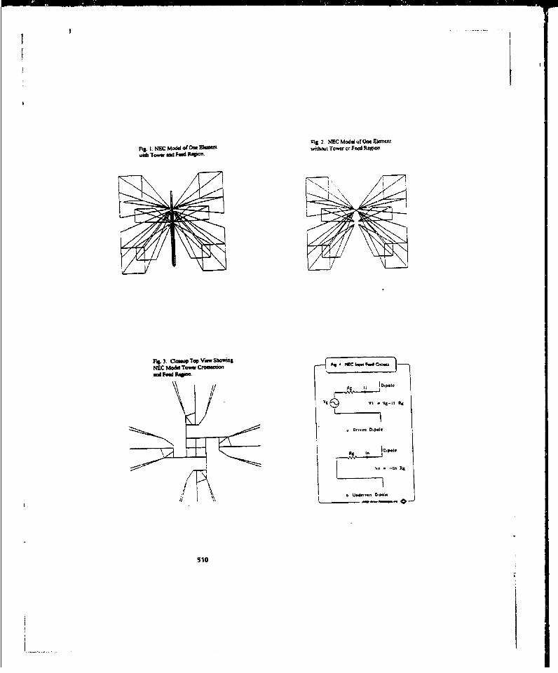
Fis. 2. NEC P.odd of One Element11 1i. NEC M!dil of One I1 Iit imt Tower or Foi d Repoinwith Tomwermd Feed R40qfe

1--

Fig. 3. OcMAp Top V'eShowict f ,C ,

Rod Food MqoonNEC ae tom

vg vI V C-il R i

Ie

E:: -i. Re

pi

F4 .U2g NO. A,. "mU C..p..g NEC. fi Mftlh

F., . 1.1 woM0 C- dD.wSI 3 1 .t m

I

-

<

RS 7 bl NO BW A .- C~..P MWC BWh MNh 54 ,22Iq .4 .00 ~ d

~51

F,$ io 2.2 a~L-A.WAýL.iW IS 7$-MH.

P.3 1A& L12 I.1 L- 2SA- C-MJ

512

I .

Rs 13. 7z7 IA. rNi Ace" 1oM fr c~.. D...h 21 7 7MMz___________________Fit. K4 7a1 to. B..g A,,-. 1W I. C.ý OW" 2,1 7 We9

/ l. 1& 7, D p A f pW C VW

Arm-

* ~ s.. 513

17,I 7%7 P40 SWg Ag. C- MO .Wý 7 10 Mra

*' HM B* Aft' , N~ r, N..,.1.,7 M 1

dl.

0. 71 .

-ac

514

, .---

:- "

•* -] -.-' ' :

" IiI

I ! i-

fat- " i

a _ _ _ _ _I _ _ _ _ _

S.. . . . .. .. . aL . I •! -.•?

U

U S aS

T`he Efiects of Eaceeding Mechanical Design Constraints on thePerforsmance of HF Log.Perlodic Dipole Arrays.

Doncan Q. Bakh&, J. Tobsias de Bleer' and Nrieen Stander2

'Department of Electrical and ElOCITroIC EnganrbIng2Departmet of Mechanical Eagneesting,University or Pretoria, On=2 Preomna, South Affin.

C-muail? dtmcaa bskwert-eUp~acLsa

4317 Rd C1 mvescloesdprcticerevpuras "h felfsaidy w i mechucal xodewsar be adhivwd to so Mhe desig amdnm 4cnr 4If? Jo pft d M dk Od Ap - (LPDA) -e*sna Do. dt ofetsng chasW -a ramew Amgh and

4afg' elonerser a" At die WA whd e~ exama ese for' two RF LPD.4' Ips ym~ed in harmimad and zk~opM plentrPrvbmLsqan redsuf badici dAN in Imcdc" he nsechandcui dir Knm id~can be tdueid considwerbly withmss~'ecxing time dchwmafftwu'csof shLPDA s Murathersa* is ,n~naed it xould qipear tht the troreascescoul We Melad by a factor of af howe A or iem more, ,Mdtow ut axesvet de~dlngO aiewa psilopmance in Practice.

I VnWRDUlCTION

This brial'study of the eftecte of exceeding the deepn comraits recommended by Smith 111 for HIF log-periodic dipoleaarst" (LPDA!&), wa prompted by probhlems caused by wind-induced vibentions - LPDA's designed and hwsalled to

cfo to these recommendations [21. Whin solutions for the problem of extree vibration. were sought, it was byno means cortain what the effect of relaxsta the recommended toleramnce foe element length, height above pound(sag or spacing along the feedline would beu onain, take-off angles or input imspedances of the LPDAis Simplemechaoicai vibration dampers; were found to be an effective inwero solution to the problem [21.

Ina order to provide guidelines for fNewe mechanical designs of LPDA's, the effects of exeseding the recommendedtolerances of ±2?.5% of element halflengh for height abofe pround (sag), z0.5% for the element length itself sadt0.1% for tbe spacing between elements, were investigated mini NE(C [31. This exercise also offered an opponwtunyfor Ratther comparion ofpma predictions obtained using the antimat desig ,omsne fromt HFhUFES4 [4) with thosefrom NE(7. The sabromeuie hrow HFMUFFS4 have the advatage of beig eamy to implement an a Personalcomputer, and several cedes of maniatude faster to run than NEC2. The basi design of the antessi is the s-am sthat msed in 14 The deinpraeeso the 4.30 1,0h L m (a) rerceotttl egh*41m (b)celsuot length rxedctio. factr - 057, (c) ange Iet -I oet tips ed fselie - IS I'egs,- and (d) numberof elements - 20. Unless otherwise stated all computations Vare mae& at 11HzIcrmet in the HF band.

In order to investigate the effects of sag of the LPDA stuctures, ame was mad& of doe progr'so TOWEROPTdeveloped by ams of the anthors (NS) for the desig of medansica strocturts. The program uses Suite elementstmncctiwa modelling for sacmlisea saanyai of an arbererily she*a guyed am or cable sntrotwe. Allowanc ma madem the progrss for arbitrary groquing of ntrucure umba's a desig dpgoups. Assmed masses per metrewere 117In and 275 gsa for the cooductors ad catesay/stay wirsmrespeclvel. Appropriate loading allow&nc for mechanicalconnection compoeents wan mande. The astomuom breaking strain of the catenarics and staywre wan about 20Kl~oNewtoo,

Two caue were selected for this study. The first caue is for an L.PDA intended for use over a long distnces. and theseodfor shorter dshtances of sbout 1200km.

516

I UTIC OF &AGGING ON THE PERFORM.AN4CE Of TWO DIVVEUNI1Y DEPLOYD LPhA'S

2.1 CASE I - LONG RANGE LPIDA IN A HORIZONTAL PLANE

Flurt, I Wiutrates the s~tatstcl distnbludw of arrivalangles of HT Asigal vsed in ioonagherc cominimaioaamr dlstamo frow tiuvral hundreds of kin to 4000 knolate 61. F1ev. 2a and 3b ihow the pin costouri, in dbl,*k '

predlied timing N1W and HFMUPES4 respetaively, as a 3 \\ \functon of take-off angle and frequency for -n LPDA t d\which hoa hesawmebakdcdapaathat wed in SI. The *

mrdsl enu for a LDA dopkloed Ane aheslustal plane ,*

m wlint a smeooth leel peend wkth coadnaivlty of

OM~ Slmias and rdedv ifielowl conmman of 15,

ceeios l toe avasap phown. Tnedwtal e'' 1.S ad.diauoofnwlnlgt

*noapwkcaA' pmpmgmWs HF saina lafter el)

ft R Gain CON- WOW 5 t 4 M

NW (b) WAK4MLS fo PtdvWih* dWAWW Ula%20" &Mothe 9.pwsd.

Nogrms 3(a), (b) mad W(o) iturase the effcat of nisia6 and Inset the place of the LVFDA by 2im, air io% of hmevan the inaldm= pbN the olike-off 8009 for .awdowi gpin end the =M imnpedainc nespediv*l. rte ondissedchamptel is intsou perfortmncoam usmot eupected to be signidicant in prause.

A real urucama wil of couae sag undeir be amn weig, as Mfusraked in. Figure 4. The propuam, TOwERoFT uiwsed to analyse the effects a three cases of stroctwal sag as the usana" thamacetiilc These mmse amt- (a) anCilrema -m fmsu a where the LPDA is considered to have bass deployed on the round wit so prests'in ay of the sq lwets or catenauies aad raisd into the deup ponido2M abase the - -sad (b) moderateprestress" such a could readily be achrievd in pruacice. sad (c) high prvtressing with the catennesm prestresited toto a cootdkmisa n which the gramis the real pontimo wa aboutt 79% of the breaking stun of the cazeaary materiaL

517

.... .... .. .

ftma. a bftm Of amulgng~, ft h~v offtfa*ds~yd VW~ by +/- 21m on (a)

ffvm i* , M)~ zake-o angf. & m~wmw~ gumn,

MR 2alvw Wound (reference htwght)

I * -... 2- MlI bOW Wounid

rwon~) 1I) ();u ;s; i a. Scheaffaic ftwofti sag lof hoquonwIhy*3 =lf pmru p ufiNEC mine devbyod LPD4& A# ku, caunehe and srnwire"WAR= we if h& uhb so prueume rnftm we s~ownV~ 4.3om at, Aumen aeavh, *a &a ub-f 68 *wma~ TU Wo* of fth s~aEmh e'gm k

t/~. ~ -

I- - SIB

__________________ Figur I PeI~ ituvme pwftvamen forhorlznvally depbyoyd LPDA Icr vadusoa caditons ofsbaii M W*potdnig owwrienes &-7d soswfva.ý

A-V~ A ideal caue no 3agging

I owienal sagging, final stILO - 79%j ... - Of breakng stawn

n.-. m*odat nnggtno, Mnal strain - 40%* of brnndhift*Wn__oumsamm magowo, flw Strain - 8%,.2 VV'VV V.f dbmnhhgav

24.14.. thus the sal in about 18% of the total element lempth. In teams of perogutap the moatormu mg was about29% of the total ehuent length at the louwt element. Fcc this structure a decrease oU 0.8B was prediteed in them-inom pin at 10 MHz, uilb an ameap decrease of about 0.5 aR betm 5 and W0MHz. The predicted take-offan*l at maidmua gpin inramsed by a mwamfun value of about 6 depug at about 5 to 6 MHz. No sipifcant changeswere predkWitean the intenna imqedanc. In prnacice it is expecte that it will be relatively eay to reduce the sag tothe order of 1-2m ur 5-10% of he*Mighn this mauple. without placing aesesalve echagnicealsrain as the catenariesmd/or staywiree.

2.2 CASM 2 - SLOPING LFIIA FOR USE OVER A DISTANCE Or 120 KILOAMEIES.

Frqnr 6 shme the cieced range of take-off angles for ___________

diatanzz of 400 to a0m km for -Singl hop, x-icpherpropeadton vi the E. sad F-repoes, for nil frequencies,ties, of day and semooe, mad for low to Wog solar activ4t.The li~ure m boed on remlis froem HFMUFES4 fortemperate latitudes At 12W0 km the taka-off angit tin I

be &e bowt 19 and 32 degues, measued frau she I

b--me The boghe= probable frequenc preaiced ore

edemot x a haillit of i.5 mand an aray slope of 33.8

degrees as measured froom the honeoutaL n-3= -F~ea 7(a) sad (b) show the pus cootourn an dML. as a

fetiou ~ ~ ~ ~ ~ ~ ~ t 6-tk. qeadfeuac sotie s Co-oasc OfO - 4eoad ake angles forN= and I(PMUFZS4 respectively Te rensults an ý Uýf~l hop &Wphatl prepageon preicted WVn

reoeabe peme only at the low frequency and sad at s~ fS &V taM quencosea ofmas c( daey, sessomalower take-off angles Thec predicted gun coutomi differ Ndsw ~wiomrasim* at highe take-off angles mn the frequencyimem- a. diflream are belived tobe due to tke, simpified approacli med in HFMUFES4 to estnnnt the effectof Vvind r -flectimeo an mtennas whc are ground arrayed. The vertict radiatio patrern is compmie by summn~gthe coutibutslioan for the direct and pound rEatcted rays usnig t'.t appropraste reflection coiefficient for borlizotalpolarimaitkot. As far as can be determined from 17b. which predates and Sies a detailed de=Vitic of the approachiused in 141 th" methocd doe nm appear to take into woo= fully the. orientatio of the plan of the LFIDA relativeto the pouind. Thifs aspect requires hwiber investgationIt i's fortutidow that the measuired results and those predicted

wing~ HFMUFES4 and NEC2 for a frequer~cy of 5.27 MHz as reported in [51 were im reAooable, agement. From

519

70 NM -:_1-:

ROiM Gain COMOMMa PrW- 4 (.1) NEC2,

a practical ra dP viewi is AW a fortale tha and is 0() HFMUFES4 for ,*Vaph LPDA'fenowle aveeme at the lowe taha-off anglas Badu for _________ _ _ _

HeCMUkaicnoa betee rnks -MCe Min NMC*md *EFhCUPVS.

FVvue 0 Mlusmaes the MsiW LPDA o~efarmw~io th acmdkfte(if sever $law& Anl atme elements,eutesmus. sppoo wir. mod saya we sboin As wkhCme I *be -stam wa s=AW i a kebnul Plane antkw Vmmd with Af OWneWO6 catomares md badk ~Ars maa ....ic of mro ewminuss or mre and thei riakzd intothe findi puloski igresr 9(n)L (b) and (c) cma.pare the

ina the LPD)A chmaradensics for the ideal cnas,

. Micha asn *mW1 be eas*l aekievd in practice,cand ie prawtessm each Ust the gsramn of the ROMU & Schanakn ditA-T&tin -g )br *42p1g

-esm m he final pmbm ios about 8% of the bmasktag dooe LPC& A# wvvs. osuna,1 andi shrWestrai. of dthce m =ain ws unr mseaL For the case aios.of extrase svspý the greaest effct is swerally obserwd

I M .

* .-521

I- II Nnl____illlROM 9. PiuditI iAM minn .I w ti nra for I RIigLPDA Iff vowi camond os orf n in =*Pwfn

Ic c-wo - gw

Mkm Ughg oal z•,ma - 8

] . d W,- o r W n g , fi-a/.V an - 4 5 %I . -,of Jrkkle saw

n'mdmasmagin, firma srain - 86%\r~AJVof brvakkswauin

at fthghur ' end. Fat the c tho oocd at the thid element where a samg of 33% of totalele.m kzlb ts pr..,iatd. TIh LIDA pirf'mance predictos for moderate peatressm,& such as could be aduievedm pncty,-A smhw vmey 5ik1.l dilfermot siuspared to the dW cs.

3 TIM EFFECTS OW CHANGING ELEMENT LENGTH

in red=, to =mo the efcs of c..go Ce d elen t cimh tiengt of, the th.tec.sh Clement, with legh 15AMMwas chapd by plan ad winus &M5 or balf of the t3% by which smmuain elements are propreaiwly shortened.Ekimat ,IU one is the Am= element at % length of 190m. The rea, for ths somewhat drastic change indmrnm length is becme little sigmifieant changes we predicted for len&t chamge at the order of 2.5%, or about

liv tme te ee~imeaded to'eac of05.Spificast effects wer noted for the largr lengih variatiat for the

usia''--C,

e im .pedance, but the gain performanc .e iM Con _=nsor of pr.dksc kWbetween 5 •ad 10 Mz for btsh the o'ýnM and hemlozaltuy Arpderca for ./- GAP% ciano in th ng& ofdeployd LP1tA. These resub are shown us F•. 10(a) ahwr 13, (a) &Aophi LPDA W hodmim4tr yand (b) rapecty for the slopig LPDA and the LFDA in deploy LPOAthe hoirizontal plas.. Ba1sisin and Nkeng [81 base shown

eimrkenvay that aa0maztrical sharpY rsonan mode - Ia casean oce due so tmamusi-- tim remonnces. In crJlr to +6.. + ,5%imeigle this aspect, the predictions of inp" impedance: .... 5. 1

521

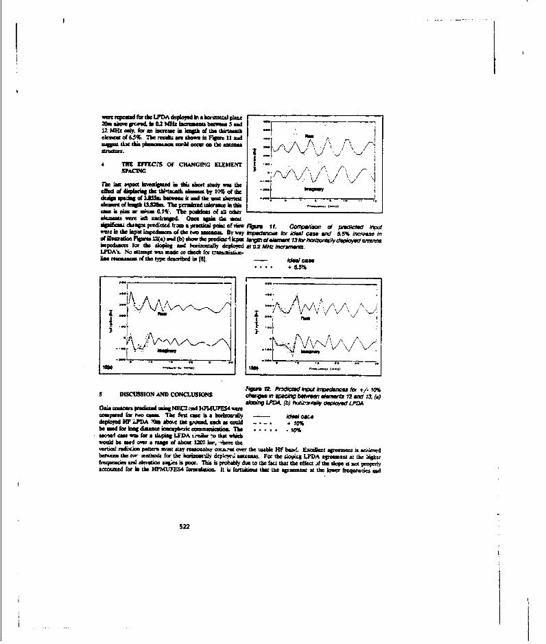
wart repelatd for the LPDA dupipad in a horizoatal paim2mabo'u pct"ud in 0.2 ?,Gi wetemetsa betwees 5 and

1.2 bOft a*l, for an ioesse in 1mh of the thlsteenthelement of 63%. 7he rushk ame lsown a Vmpr 11 mid -. /I ,

4 THE EFIEMYS OF CHANGl?.G ELEMENT /. 7 "ISPACING /~ / / .

The lu aipect mwveueo.i this abort study was theefeta of ",spgacnI the tbi~tacash Wassa by 10% of the -dulp spacin of 1215a Ibweow it sod the am sb~ehotmsknit f awjmp 13- The P~cittd tolerance a tbsh .

cae is Oum or whow 0j1%. Tba positious of all otheredemeat were aft unclitiegd. Once apa Qth meesip1lcmaw &-amp preditued from a practical point of View Mpau 11. Conpaoin of pr~W~i inpv*we, inhe input impedaama of dothwo~ morma. By way ftisdancosa for id"a can a&W 6.5% inclease in?fIlltadmatig P lAaa a) m (bý shwtowte pdiaa4w*p lnpof.~~lfmsum lywi~wtnXnpedaca for the dloping and iNotortmaly depsloyed at 0.2 Aft hn)MMO-0.LPDA's. No attemp was mafe :o chesh for 'azativusa~-has masmcansa vt the tje descibied in [1. - keAw caw

+ &5%

AA

j ~ ~ ~ : MW

'faw 12. Prjdictod hAr knpednca flow+/ 10%5 DISCWSSION AND CONCLUSIONS dwqig in kW~Ach buuW~ i&iniata 12 aSW 13, (a)

Skp4g LOA, (b) huvLj#aWl dapioyd LPDAGam cntows predictad mung N=eCnd HFMUPS vat

comard for tdo cum. The Fmceit aw l botbo'ally -w leJC"kdeployed H? IJIDA IW abov like goad. msod as could --. + 10%be used for kong dig icealmsph-tic amemmicasm. The . . . . 0secAul cms urn for a tkping LFDA imauihear thatL w"icwould be used over a rane of about M~I khw, "'ere the.veniri radixaom pattern must stay remoesahy coms.'nat oye the usab" HF baod. Excelent apeemear a a'cis-dbetween the tMa metboda for the Iori *t~~ depki4 aswemnas For the SboptLs IPDA aveeent at the ugkarferequenes and leva~tioa ang~e is poor. This is probabl due to the fac that the etawcif the skope is not properlyacwmei for in the HPMUFES4 foemulatioo. It it fertuitiosas tbat the apinm at the hrmez frequmcads aid

522

elewatln angles between NEM and HFMUFES4 pecdieti'n ts acceptable for practical HF wmiummm

Resnls predicted unng NEC2 for rwas mn widch the arrays are allowed to w&g or the element length or spnanpo areallowed to vary by mome than the recominended tolerances, suggt that these tolerancias could be reLmdAsustabntialy.Utili fv the studies are msade it is suete that a Uacor of 6ie Feaster than the values Oven in ~11 wotld not leadto exauve and imacceptable degradatmc of antenna perfocutance. From a praCtial POWn Of VIeW it is easier tosmastain relatively high tolerances sa the cunt of element length and spacing. In the cue of sasuel of the antennagrutnowee an effor to a&&er to the stict spedfiCatioe of (11 ull lead to ~hi stresses in cateenies and staywies forHF antennas. Failure could resalt from m3Wa fatigue nduce by wind driven mechasiaw resoeances on the stucture.

It isumggsed dhud the strong coupft betwe the various elementa accun for the slow degradation in perfomanoceni the anennas. Iloswere, the possibility of maym~ietrit resnoance effect of the type decractd in (8b resulting fromthe reirataon of the design tolerances, need to be inestiatd further.

6 REIFER"CE

[1] SndNh C.L, 'Lg Periodic Aw-an Design Handbook', First Edition, Smith Electronics lInc, Cleveland. Ohio,"U141, 1966.

12] Belmk, Dr-. 'Mechanical damping of vibration of staywirea on antenna -Mas%' ACES Newsleter Vol. 7, No.1, ppL4l-2, 1992.

P1 3arkm, Gj. and AJ. Pa Ne, eriWe Eedrmsýnt Code (lC)-Method of Moments', NOSCTochmW Docuiment TD 1W6 NaOa Ocea SYeeMU Center, San Dirge C&UAkiona 1981.

[4] User, LF-I.,L UPAy G.W. Unpiwe and 0±. Lacm. 'Estimatin the performance of teleammuicmatinsystem& oung the vouoeplieric trnmmmsao channel', NTIA Report 83.127. US Department of Comsmerce,Dibonder, Colorado, 1993

151 Balm~. DrC.'A inked comparisna of predicted and measmurd rawks for an HF pround-arrayed log periodicdipole array, ACES Jomnas, VoL 5, No. L, ppZ--38, Summer, 1990.

[6) Sfnrh, A.. 'RotaabLe log-periodic dipole watennas fore5 to 30 MHz', News fromn Robde and Schwamr No. 63.P. I&=~ No Year gien

B1 ayie &.W, WL Ldffi and L. Noike, Predictin the performan- of We &wp-quee sky-ate unesmatioea systmas', OT Report 76-102, US Department of Coumawce, Boulder, Colorado, 1976.

taUsonla LGM and IN.M assu. 'Arymtmetry phenomenon of log-perodic dipole -antena, IEEE Trans.Anumen and Propsagne, Vol. AP-24, pp. 402-10,19I6.

323

Modeling of a Cylindrical Waveguide Slot Array, a Loop-Fed SlotAntenna and an Annular Slot Antenna with the BSC and ESP Codes

Wendy L Lippincott Dr. Joseph A. BoharNaval Research Laboratory Antenna Corporation of AmericaWashington, D.C. 20375 Harleysville, PA, 19438

Abstrflt

Experimental data and modeling results from the Ohio State BSCI (BasicScattering Code) and the Ohio State ESP 2 (Electromagnetic Surface Patch) codewere compared for three antennas: a cylindrical waveguide slot array, a loop-fed cylindrical slot antenna, and an annular slot antenna. The BSC code gavegood results for the antennas alone on a small ground plane. It tended tomispredict by a few dB the ripple in the azimuth pattern caused by a largescatterer placed a few wavelengths away. The ESP code modeling for the loop-fed slot antenna gave good results for both the antenna alone and in thepresence of a large scatterer.

1. Introduction

The cylindrical wavegulde slot array, loop-fed cylindrical slot antenna,and annular slot antenna are omul-directional antennas that can be placed oncomplex platforms where considerable effort must be made to ensure thesurrounding structures do not unduly affect the radiation patterns. Decisionsregarding antenna placement can be made through anechoic chamber studiesor computer EM (electromagnetic) Ulimulations. This study was designed tovalidate the use of the BSC and ESP codes in modeling these antennas and theirsurroundings. The BSC code is based on the Uniform Geometrical Theory ofDiffraction (UTD) and is a HF (high frequency) ray tracing/diffraction code.The ESP code uses the method of moments. In general, the BSC code is bettersuited for structures many wavelengths in dimension. The ESP code providesmore exact modeling, but becomes computationally impractical for largestructures.

524

2. Cylindrical Wwveguide Slot Array

The cylindrical wavegulde slot array can have either horizontal orvertical polarizaton depending on the slot orientation. Both polarizations weremodeled. This antenna was only modeled with the BSC code. Modeling withthe ESP code would require a complex mesh, and it is doubtful whether itwould model the internal waveguide cavity appropriately. This antenna has arelatively high frequency compared to the surrounding structures, so theadded complexity and computational burden of using the ESP code was notwarranted.

2.1 Horizontally PolarizedCyUlndrical Slot Array

Fig. 1 shows a horizontallypolarized slot array. The array isfed at the bottom by a short stubinside the tube. Machined onto thehollow tube are 8 columns of slotsand 14 rows. The slots are tiltedboth as an aid in packin and also tocontrol the amount of radiation ofeach slot. The amount of tiltincreases vertically to offset thedecreasing EM energy in the tube.The tilt Is designed so that theamplitude out of the column of slotsfollows a truncated cosine Fig. 1. Horizontally polarizeddistribution. The average slot tilt cylindrical slot arrayangle is 12.80, so some crosspolarization does exist.

The slot length is X/2 and the distance between the rows is 0.54 L Thetube outer radius is 0.52 X. The array is relatively ground plane independentbecause little of the radiation pattern intercepts the ground plane. The phasesin the individual slots for the array are calculated knowing the cutofffrequenct of the TMOI mode in a circular wavagulde. These values and thetruncated cosine amplitude distribution are then used as Input data for the BSCcode.

525

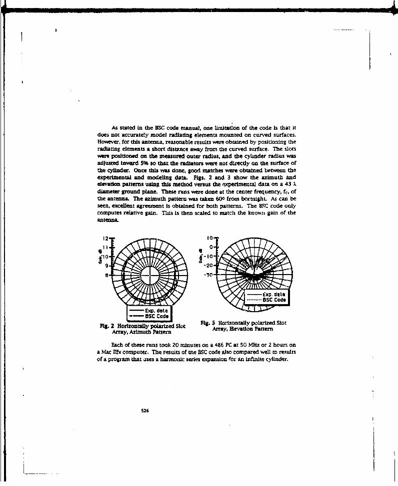
As stated in the BSC code manual, one limitation of the code is that itdoes not accurately model radiating elements mounted on curved surfaces.However, for this antenna, reasonable results were obtained by positioning theradiating elements a short distance away from the curved surface. The slotswere positioned on the measured outer radius, and the cyhnder radius wasadjusted inward 5% so that the radiators were not directly on the surface ofthe cylinder. Once this was done, good matches were obtained between theexperimental and modeling data. Figs. 2 and 3 show the azimuth andelevation patterns using this method versus the experimental dam on a 43 ).diameter ground plane. These runs were done at the center frequency, fo, ofthe antenna. The azimuth pattern was taken 600 from boresight. As can beseen, excellent agreement is obtained for both patterns. The BSC code onlycomputes relative gain. This is then scaled to match the knowu gain of theantenna.

12= O-

g= -20-

Si • Exp. data

S......... BSC Code

-Ep. data

-•BSC Code

Fig. 2 Horizontally polarized Slot Arr a, H rlzonally plarized SlotArray, Azimuth Pattern Array, Ee-/atlon Pattern

Each of these runs took 20 minutes on a 486 PC at 50 MHz or 2 hours ona Mac Ifx computer. The resuits of me BSC code also compared well to resultsof a prognam that uses a harmonic series expansion for an infinite cylinder.

S26

This antenna was also modeled as an eight-sided cylinder, with the slotsmounted directly on the plates. The size of tile plates was first adjusted sothat the perimeter matched the circumference of the actual cylinder. Slightvariations of the plate sizes were then made to better match the experimentaldata. For modeling on a 43 X diameter ground plane, the elevation patternsmatcbed the experimental data well. The computed azimuth pattern at 600from borealght had 2 dB of ripple. When the array was modeled with 16 sidesInstead of 8, the ripple in the azimuth pattern increased. This increase in erroris believed to be due to the edges of the plates being too near to the center ofthe slots. For accurate modeling, plate dimensions in the BSC code should be noless than one wavelength.

2.2 Vertically Polarized CylindricalSlot Army

The vertically polarized slot array Issimilar to the horizontally polarized slotarray except that its slots are orientedhorizontally. Fig. 4 shows this antenna.This slot array has 6 columns of 18 slotseach. The Jlot length is 0.35X and thespacing between the rows is 0.39X. Thetube inside and outside radii are 0.418).and 0.462). respectively.

Fig. 4 Verticallypolarized cylindrical slot

array

The phases In the individual slots for the array are calculated knowingthe effective cutoff frequency of the TM0I mode in a circular waveguide. Forthis antenna, an additional phase shift is introduced by the slots, effectivelychanging the cutoff frequency of the waveguide. Once this effective cutofffrequency is determined empirically, the phases are then calculated and usedas input to the BSC code. The amplitude of the slots along the axis of the tubeis known to follow a truncated cosine distribution.

This antenna was modeled vth the BSC code using both a cylindricalcenter and flat plates. For the cylindrical center modeling, good results wereobtained by modeling the antenna as slots placed a short distance from a

527

cylinder. The slots were positioned on the measured radius, and the cylinderradius was adjusted inward 2.5% so that the radiating elements were notmounted cirectly on the cylinder surface. Once this was done, good matcheswere obtained between the experimental and modeling data. Figs. 5 and 6show the elevation and azimuth patterns compared to experimental data. Theazimuth pattern was taken 600 from boresight. There is a strong central lobeon the modeling data not seen experimentally. The actual antenna has a chokering on top of It to suppress radiation along the tube. In the modeling, a smallplate on top of the antenna was used to model the choke, but this did Dot havemuch .ffect in suppressiug the central lobe. With vertical polarization, theground plane has more of an effect on the far-field pattern than for horizontalpolarization.

11-T 10"

. y l ig V c p rS20l-30

U Ep. date- Eg,. dat ......... BSC Code

--- BSC Code

5. Vertically polarized Slot Fig. 6 Vertically polarized Slot

Array, Azimuth Pattern Array, Elevation Pattern

This antenna was also modeled with slots mounted on six flat plates. Thecomputed elevation patterns for the vertically polarized antenna matched theexperimental data well. For the azimuth pattern at an angle of 600 fromboresight, the computed ripple was 2.5 dB compared ro 1.1 dB determinedexperimentally. This error is due to the interaction of the s ,-° Uatlon withthe edges of the plates. With vertical polarization, the diffraction off the sideplate edges is much more pronounced than for the horizontal polarization caseand causes a poor match to the experimental data. The antenna was alsomodeled with 12 sides instead of 6. This did not change the resultssubstantially.

528

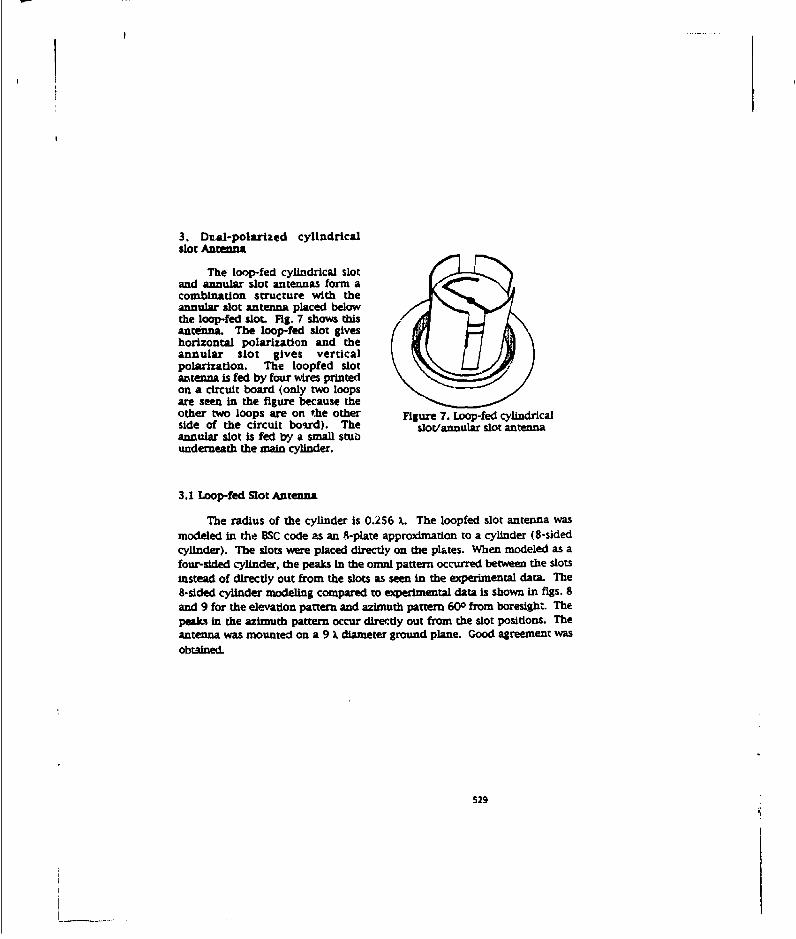
3. Dual-polarlzed cylindricalslot Antenna

The loop-fed cylindrical slotand annular slot antennas form acombination structure with theannular slot antenna placed belowthe loop-fed slot. Fig. 7 shows thisantenna. The loop-fed slot giveshorizontal polarization and theannular slot gives verticalpolarization. The loopfed slotantenna is fed by four wires printedon a circuit board (only two loopsare seen in the figure because theother two loops are on the other Figure 7. Loop-fed cylindricalside of the circuit boird). The slot/annular slot antennaannular slot Is fed by a small stubunderneath the main cylinder.

3.1 Loop-fed Slot Antenna

The radius of the cylinder is 0.256 X. The loopfed slot antenna was

modeled in the BSC code as an 8-plate approximation to a cylinder (8-sidedcylinder). The slots were placed directly on the plates. When modeled as a

four-sided cylinder, the peaks in the onmui pattern occurred between the slotsinstead of directly out from the slots as seen in the experimental data. The8-sided cylinder modeling compared to experimental data is shown in figs. 8

and 9 for the elevation pattern and azimuth pattern 600 from boresight. The

peaks in the azimuth pattern occur dirertly out from the slot positions. Theantenna was mounted on a 9 X. diameter ground plane. Good agreement wasobtained.

529

7II

7" 10-

1"5 -0-

4- -20-

3" -30

-Exp. dataBSC Coe

~4 odeCo

d Fig. 9 Horizontally polarizedFig. 8 Horizontally polarized Loop-fed Slot, Elevation Pattern

Loop-fed Slot, Azimuth Pattern

Modeling this antenna with a cylindrical center was also tried. Thismethod did not work well for this antenna. Large notches occurred in theazimuth pattern.

Results were also obtained with a large scatterer on the ground plane.As shown in Fig. 10, a large 2.3 .x 1.9 X width plate was placed near the edgeof the ground plane, directly out from a slot.

FIg. 10 Loop-fed.'Annular Slot Antenna on 9 wavelength diameter groundwith large plate scatterer

Figs. 11 and 12 shows comparisons of experimental and modeling datafor 2 frequencies for the azimuth pattern at 600 from boresite. The BSC codeWn general predicts less ripple than the experimental data.

530

!a

0', j _'',,6 da 8

-- Exp. d- dat-- SC CodeI J ---- E. 'ý:Iotga'S-- OSC Code

Fig. 11 Horizontally polarized Fig. 12 Horizontally polarizedLoop-ted Slot, at fc Loop-fed Slot, at 0.9 fc

with large plate scatterer with large plate scatterer

A smaller 1.16 ). by 0.93 X. plate was also used In place of the larger2.3 . x 1.9 . plate. For this case, the BSC code matched the data better, with amaximum error In the azimuth patterns of I dB.

The loopfed slot autenna wasalso modeled with the ESP MOMcode. Fig. 13 shows the antenna asit was modeled with flat plates andwires,

The ESP code has a built-inmesh generator. For the meshgenerator to work efficiently, it isnecessary to break up the structureInto plates that are close torectangular. Otherwise, too manymodes are used to mesh the surface.Wedge-shaped plates areparticularly bad. A maximum of6800 modes could be modeled on Fig. 13 ESP Code Plate and Wirethe a CRAY YMP with 0.5 GBytes of Model of Loop-Fed/Annular SlotRAM, Antenna

5?i

Figs. ]4 and 15 show the results of the experimental and ESP codemodelinig data for the loop fed slot antenna mounted on an 9 wavelengthdiameter ground plane alone. The peaks in the azimuth pattern occur directlyout from the slot positions. The ESP code predicts more power towardsboresight. as seea In the elevation plot. When a top plate was placed on theantenma to try and suppress some of ihe radiation towards boresight, poorreWuz wmn obtained.

2" -30--

•Exp. dataSEp•Jt ESP Code

4 1 -ESP Codee

Fig. 14 Loop-fed Sloz, 1.0 fc Fig. 15 Loop-fed Slot, 1.0 fcon 9 wavelength dla. ground alone, on 9 wavelength dia. ground alone,

600 azimuth pattern elpvatLon pattern

Figs. 16 and 17 compare experimental and modeling data when a large2.3 ). x 1.9 X WIdth plate was added near the edge of the ground plane. Theeievadon pattern for this case is the cut through the plate scatterer. Figs. 18and 19 show the resufth for a lower frequency, 0.9 fc. Figs. 20 and 21 showthe resuls for a higher frequncy, 1.13 fc. Good agreement was ottained forall these cases. For all these figures, the actual calculated gain is plotted,uniike the BSC code results, which were normalized.

For runs an the 9 wavel•ngth diameter ground plane, the code was set tomesh the plates for 0.2 modes/L. With fewer modes/l, the code would bombwith a floating point exception during the run. For the 113 fc runs,7900 modes were needed. This rn needed -63 MWords and 10 hours on aCray C90. For the 0.9 fc runs, 5054 modes were needed. This run needed.45 MWords and 28 hours on a Cray YMP.

Another opuon when using the ESP code is to approximate the finiteground plane with an inflnite ground. For this case, the method of images is

532

used and the ground plane does not need to be meshed. This saves both in thenumber of modes to be solved for and also In the complexity of specifying theground plates.

o10 10"

2" -20-

0 - , - 3 0 -

-Exp. data

Exp. data ......... ESP Code

Fig. 16 Horizontally polarized Fig. 17 Horizontally polarizedLoop-fed Slot, 1.0 fc Loop-fed Slot, 1.0 fc

with large plate scatterer, with large plate scatterer ,elevation600 azimuth pattern pattern

I0-

0-

S4" e-10"2" 0_20.

0- - -30

\ -Exp. dataUExp. data ......... ESP cods

S...... SP Code

Fig. 18 Horizontally polarized Fig. 19 Horizontally polarized

Loop-fed Slot, 0.9 fc Loop-fed Slot, 0.9 fcwith large plate scatte,-er, 600 with large plate scatterer ,elevation

azimuth pattern pattern

533

0k0J 4"i!- oo2"" -20-

- Exp. date - Exp. data......... E de ......... ESP Code

FI;. 20 Horizontally volarized Fig. 21 Horizontally polarizedLoop-fed Slot, 143 fc Loop-fed Slot, 1-.3 fc

vIth large plate scatterer, 600 with large plate scatterer ,elevationazimuth pattern pattern

3.2 Annular Slot

The annular slot antenna is part of the dual polarization antenna shownin Fig. 7. The annular slot is fed by a small stub underneath the main cyUnder.The slot aperture circles around the main cylinder of the loop-fed slot antenna.For the BSC code annular slot modeling, a cylinder is placed on top of a ground

plate. To simulate the annular ring, a set of 64 slots are placed flat on theground plane surrounding the cylinder, with their short dimension aligned

radially. Fewer than 64 slots caused the azimuth pattern to have too muchripple. This antenna could be modeled accurately with as few as 8 slots (or as

an annular ring source) when the cylindrical center was omitted. However, thecylindrical center could interact with other scatterers in a complex setting, andso it was thought best to include It. The annular ring source provided in the

BSC code gave zero output when a cylinder was placed in the center of it,presumably because the model approximates the annular ring as a pointsource at its center.

534

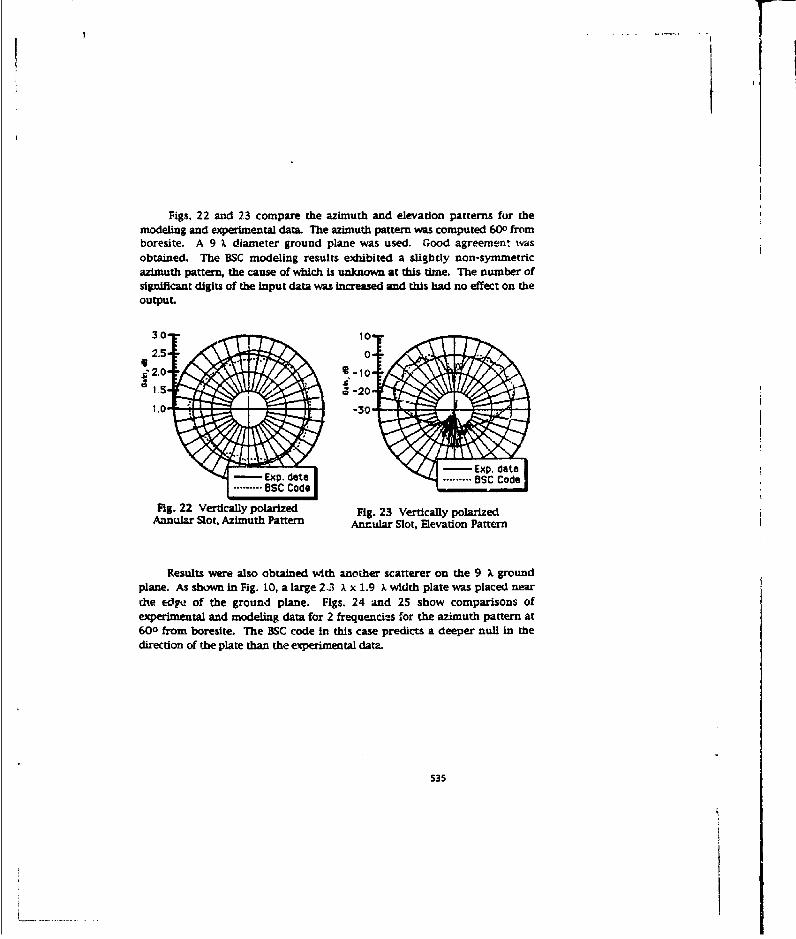
Figs. 22 and 23 compare the azimuth and elevation patterns for themodeling and experimental data. The azimuth pattern was computed 600 fromboresite. A 9 X diameter ground plane was used. Good agreement ! wsobtained. The BSC modeling results exhibited a slightly non-symmetricazimuth pattern, the cause of which is unknown at this time. The number ofsignificant digits of the input data was increased and this had no effect on theoutput.

2.5- O-

1.5- Z •-20-

1.0-- 0 -

- Exp. date ......... OSC CodeS........ BSC Code

Fig. 22 Vertically polarized Fig. 23 Vertically polarizedAnnular Slot, Azimuth Pattern Annular Slot, Elevation Pattern

Results were also obtained with another scatterer on the 9 X groundplane. As shown in Fig. 10, a large 2.3 X. x 1.9 X. width plate was placed nearthe -O•e of the ground plane. Figs. 24 and 25 show comparisons ofexperimental and modeling data for 2 frequencies for the azimuth pattern at600 from boresite. The BSC code in this case predicts a deeper null in thedirection of the plate than the experimental date.

535

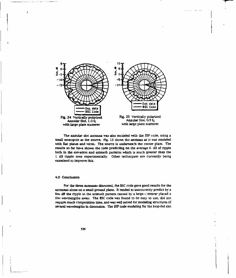
5" 10"

-15- !- -

!- - ---- E Ex p. dotea-Exp. date 8 OSC Code

- BSC Code

Fig. 24 Vertically polarized Fig. 25 Vertically polarizedAnnular Slot, L0 fc Annujar Slot, 0.9 fc

with large plate scatterer with large plate scatterer

The annular slot antenna was also modeled with the ESP code, using asmall monopole as the source. Fig. 13 shows the antenna as it was modeledwith flat plates and wires. The source is underneaih the center plate. Theresults so far have shown the code predicting on the average 6 dB of rippleboth in the elevation and azimuth patterns which is much greater than theI dB ripple seen experimentally. Other techniques are currently beingexamined to improve this.

4.0 Conclusion

For the three antennas discussed, the BSC code gave good results for theantennas alone on a small ground plane. It tended to inaccurately predict by afew dB the ripple in the azimuth pattern caused by a large s-atterer placed afew wavelengths away. The BSC code was found to be easy to use, did notrequire much computation time, and was well suited for modeling structures ofseveral wavelengths in dimension. The ESP code modeling for the loop-fed slot

536

antenna gave good results for both the antenna alone and in the presence of 1large scatterer. This code requires more time to implement, since the structuremust be broken down into plates and wires. It is computationally intensive,but with our current maximum resource of a CRAY C90 with 96 MWords ofmemory, could model a structure - 15 Xx 15 X in size.

5.0 References

[1] R. J. Marbefka, J. W. Silvestro, Near Zone - Bas.c Scattering Code, User's Manuiwith Space Station Applications, Version 3.2, Ohio State University, Report No.716199-13, Performed under Grant No. NSG 1498, March 1989.

(2] E. H. Newman, A User's Manual for the Electromagnetic Surface Patch Code:ESP Version IV, Technical Report 716199-11 (Grant No. NSG 1498), August 1988.

ACKNOWLEDGMENT

The authors are grateful to Bruce Folk and Jim Barnes of the NavalResearch Laboratory for many helpful discussions regarding the antennas andfor taking the uperimental anechoic chamber data presented here.

This work was sponsored by Art Boland of SRDO. It was supported inpart by a grant of HPC time from the DoD HPC Shared Resource Center (CEWESCray C90, NRL Cray YMP).

537

Muiule FSS mid Amty AnalysisPruiwa (MPAA)'

HOMY A. KIrawd and Roland ilmienL~ocidwd Sanders. Loc.

Gerald Plaimg dad Jack AbbasiNaval Air Wafwa Conr AtczA Divisimi (NA WC-ADWAR)

The bFAA;~ is a user-cramex ed"m o code for Ohe elec~ovemianesc (MW analysis of plana Layeredcoqa. temiuawhicbmicomprimod ofall or a emehedI o dileourie layess thin Crequency selective surfaces

(PBS's). a pwfduey poudnd Plene law. and imawmar iamy layer. Tie code calculates the EM field scaliesedby. or cominuted thesgh doe ,hw for an rncadeet.arbtemi polaise (ME & TM) plane wave, The code can alsoPHIS Mhe eadillign wean of an almn ebaai As Part of the comtputaton. dhe code computes die wave niunbers fora Iomird md mante plie wan &M the fieweue of twhe bas functones reprueang d cur m~ms on "she wemai.The PBS Md anyr Magam- a Usalu aoo wad adst linluismdmally shin. pmwfeclly conductialg ractugula atipor ciond ad ach 8Mb and mawa mry layer is comiddeted in be an hsmitelv Wpg planaer wary of time pripe orcmwas. The umamiel lyase which mais dupd co.imsamitm am lawless and isotmoic dielectric subisutres. To

oalpaime a finn -ac-n- one caselect a subat of doWte aoit armay. The assumption is made that all almentens havthe -m mutua counilg No= the ed* effect of side eleenmts in a phyincal stay ae riot represented.

The wi&dsaw a Ploepu bauamtc model ewsam at do th ~u m ed flelde from each layer of the Iinfiite periodicbare1 solve for IM tem ameadow Sald. The G"ld am matched at each uumbusc except where die H-fleld we

disceoniutes by asý an do ulpsr. The muliumi nisebler of Ploquems modes can be mutiied by the code isasiamwisd to 361. any ram of which ca be sim -A-da mode. Ina psamaL dhe tolusicit convease with fewer emode=.

7be cuncou which wm excited on the MS and mrssy mera m demmised trouh a (lalerkmt method ofsMUrnm VPMoneb udiln Up 10 9 MeIKSOf fal o e MP WAMUM baissW mcining fisteomie The comber Of buasi fuscteicinnot wead in do compwo Is selected by the eam at dsthert of the poIani Obviously, comipiatioo time ncreamsediiawly widt addedlso of bales factison In lmmi cas. am or two was aall thin is needed lot convergece to a

The &UFAA code was wsinm laY(MTA?) as a PC basd wimlysistsynzhesl too but co also be used or,mehilamm copuer if uempldwith minor damn to the IV Portions.

The mulyss memo the ana is Imp,~ thomforc. minbit wriy theory a uwed an expand fth EM rield axswsmiteo of Fkqarn space haomaic modia. Thas g g ecI wasd eba primaiwly because it inlierenly includes mutualcoup', heewee the thOle eemeers. Altlioupl a method of moment aprah could be useed (foe xreasonable acrtsray,doe spaneavcien ot the conductsor muss be im the order of one tenth of a wavelefgth); it requires tihe inverimon ofextemely Wpg matrices to prvide a soluion for even a small way of elements.

This wosk was ofpmtg by dhe Naval Air Warfare Cqnser (NAWC) under contract No. N62269-90-C-058

538

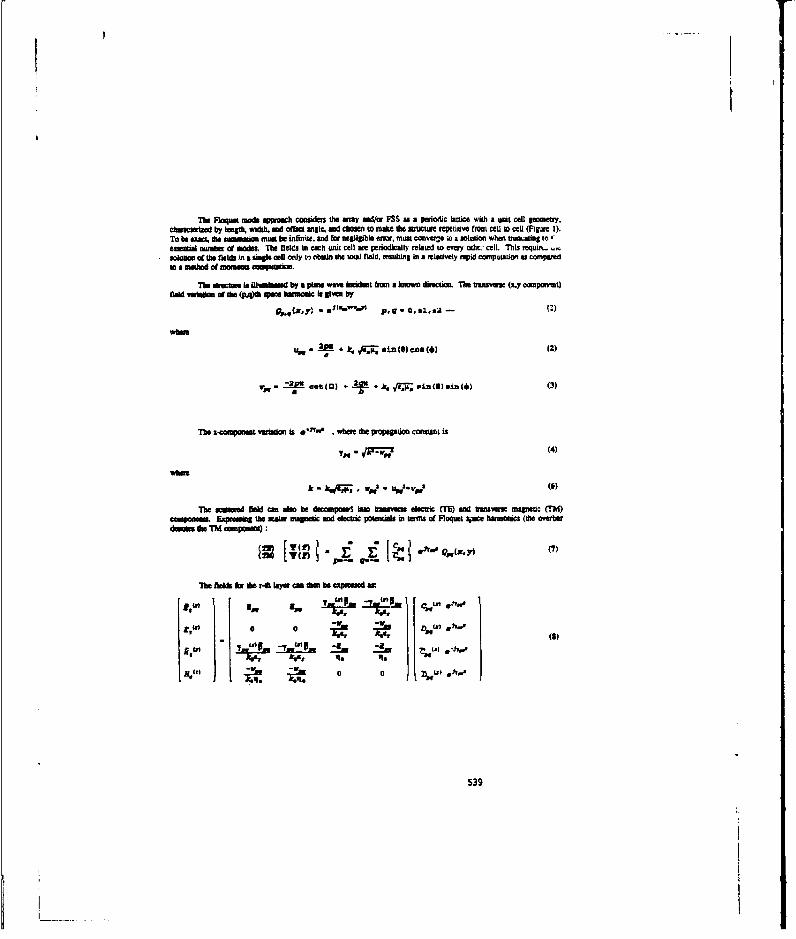
Tbe Flcqim mods aipeodlc camede Me army ma/rn FSS isar pariordc lWum with & unit coll geomyo.Clmcaie by lmgs, w"dh mad ciba angle. mndcit t matde IMuCImCn repetitive fromt cell W CCU (Figure I).To be exact die smunmeio made be jnfinime Wn for negligable mmn mumi convere io a soluione when trusin~rnm ioemsial number of modes. The fiels in each urns cell wte periodically ralated wo every otbc2 Cell. This tequliL.-molads. of do flele in a &in&l cell otly ti chumn the IOW field. resulting in a relatively rapid crnipugtanon ma comparedto x wethod of mamas eeioamins~.

The - ,na Is filmind hby a plans wm nc ident trum a kmmow directiaiL The uwvemu (n~y compoast)Odd 0(nao ofwh (P4th Mme hummluc if gies by

'ptY~ pq. O 22,u

whore

UMq.IL sin 18~~a l) coo(* (2)

V.M(Q a - k, 'e.x. P.n(q)miin() (3)

7We zecqa le voroxioa U**r'' . where fte proapgation comiact is

1M ,~Vff(4)

k kq-P- WWI " %W+p)

The sx dm fl Can alon be daIn m I mlam uavuwo electric (Th) and amnasnueme apic (MidCimaaa. Faema tdo maaLr amgnette and elcti pwotimbl mn etaer of Ficquet spect bansanacs (ftil overbdoom die lid ooupMas

TMe fie fo die r-O Ibw cam thm be expemed m

Ntgar a" I tjr, 48 mumt *."no

1t Yp -'L -.74 .1-11

att * ~0 0

539

The prkim tha becmas ofe@ dou~maung th mikowit field coafleienae Cm and D,. The dominant spacehomic. with p - 0,4= .0 isOWam thf primary WUMa Ifte. it is sUDCiald with fth Man beaM propageting modewhile ft oghi hurmoosars U, iad so pallig obesMa nhexmt step in the anialysis isino calate Owe B"d in Mach layerby mmuf tM mipinl 111de (E uavi M) a thA invefae.. Th lsimepiedeeomleeci basdarin lead to

uins~anacticev of Ohe tm. (forTE vo z

IN H (10)

ad simiarly IN T4 to Z.

Inbe ebadmed a astip ls~u isc wisivity 01 Mangeetia Eifimid

Aboudt condtion that mutt bet saisfid ie that the taimenal coniponent of dhe electric-field mtmt be amn

arys awaned ao be ocoia.izve strpsdiwecmr nt& meepecalive unit calls Applying thn zerotangeenatfieldrwconcidos Yiceld an onloaade nips:.

41" Z' . a. -0(12)

(nam *4 am te 0115 )To elks fo bb n do strips, the u elwJ fied an do sary iarp saisfiues

Ar Cz, y. 0.) - 5l,-X,l.f(x. y) - E 260 (z) 4.116 o (x-dZ) .5...* 6 1x-d2) 1 (13)

whets 6(x) is doa Dowc dabs ~~e7M ae Loin the Ier model = sueed tbe pina reldw. pase blod. The le= boundary condlition to be

saddled in the cmicaiy of eOSMI )11lieid an do alp.

Ire *.ry, a.) _N4, Ca.y. 0_.) _ -2Ek4 Ze.f CX.y) (14)

I. ie fhe curent mwxmm end 7, is the fian space empedeece EvAc equation is tested with an sinner product defined as

when xppliod so equation (11)

540dv (,A 7

when applied to sqI.Onz (12,13) f

when applied to equation (14)

"TMe csmu bow fooedm f (1,y) Is slecd much tha

Tih sqimian for a sile basis function art, simplifled by intioducing a rotation ,nd translation of the wordimataxes to align wirth e "nip comrn is donnld by:

N 2

(19)

whom 1.,1,L 1.. 1,. me the tumbsows cunat uagiu'ldes in the x wandy direction of the * symnulric and asymuneamcmodal kim hfcst . A notmalumon cosarnu mm be denved frm the ingrl over the =p am of the ft productado •o ksa fimctia (19) with iaelf.

TIU ;F bea r product ((13), (16), (17)) we then appbd to the bhs functio get (19). Once tbe ilner1onuas awe r md the qWuams are masuipulaed wnb subaumosi of the appoop eaitma saeoaamiu(lO). a im of eqaslom emkt:

C.,,,4Als4 ~Cu1) AMU CSOASw) DMOUU-Aau)

-T alt ~ i-~ ~,-,..~ i 1 L (21)

541

~ ~ -(22)

~ q IJ.~0..U)-gsU a)~~uI} -- 2o i* (23)

W- ,,A.A-D -jA (14)

Whit". upto fm~ h" ban for

2

2 (26

VWk1f. wA Bd 2m dieUsw icixa mamix coeftl*"~ mid the supermIpt denotes the incienwane. A method of - ainauqmcb 1 db UN und to molve for the unknown coniTU nfuaniwdns by Usmtg according to

Oamon diod

?hk Mobiks WO ma of ataft .qanbuas

whict m be asmdm:.,.p 4w,&b cw.fbl r13 1 A?

I) I*(28)

for die HlM" us. wih* a imib form fir On E-field m~aqums. Itie solnutios for the unknowns 1.Ke dten found by-ai *Nnasme

542

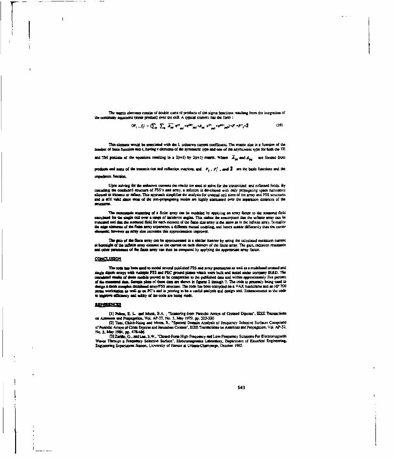
The manrut *lemses coausin ofdouble sumsi of products of the sigms functions resulting from die integratio oftie cantinuity equadous (bume product) over dhe cell. A typical elementL has the forin:

(W, , f,) - (L, L ;F 0 P11 -00F.P 1 .l (29)

This elemnten would hes associated wishth* d11l unlunown currents coelrasent. The inuar sze is a Funcijon of theatunipa of herim fluseskan an r, having r elements of dhe symmunic type and otne of the asynuneuk type for boshthed TE

ad TM pastims; of th equaionues resuling in a 2(r+l) by 2(r+]) matixs. Whet A,~ dme Ae fomead fuir

I , 1, and -un of the uranmluioe and mileetian matrices, and F, air d , ou 2 a the hesis fiunctions and the

Upon solving for doe unikeuwe camus the resuls are used to wilve for the tramniutsd and Mimead fields. bycascadling the combinied structure of FSSas and arry, a solutioni is developed with only ptopsapting space harmn~iicsalowed to usoinsa or reflect. Ilbsm approci sisnptirmthsde analysis for unequal cell Sime of the arry and FSS stuictusresad sa etll valid gome mos of doe noo111proptgan modes ae highly sagosaled oveOn rh eparaotio dissanes of the

The monornon =waft~ of a Monte array can he modeled by applying an arry bat= to the scattered fieldaiculiaid for the, sge& =0l owe a eanage of incidence angles. This makes; the assumptitoni the iesinfinite arry can hetntmaid and dua the stend faied for each elementi of the Dataiia arre ay is the ans. as in die infinite way. In mealityth edge elemeuts of the flaa way expersence a difernm mutual coupling, and hence scootr differendy d~un the centerolamess however as arry Size increases this approuinadon inproves.

Ilia pin of The fde arry ano be approsdaumad us a sanllu manner by using die calculated excitation currnestat baeteiht of doe mflaise asay alemest. as the eurraft oneah elanewnt of the finite way. he gaitn. radiation resistanecead adiN Iame ato the Amit am ay n thee he computed by aplying the appropriate a&my factor.

The cadai ha busi end so model several published FSS and any geometries as well as a multibend crosaed andsungla dipsole ameys with uaeldpilet FSS and PEC gratrad planes which wae besi and testd under company IPAD. lbealcribeed analis of *8 suodebk pved so he comspareble to the publishied dria and within approximately rive Percntof doe usessd dwi. Sample piom oC these data mre shown at rtgntes 2 though 7. The code is presently being used todeepag osa oom plat niitlursu oeFfSS mscrues. l1b code has beet comspiled en a VAX mitmstrasfs mid an HP 700seeres wa tma an wall as co PC' sad is ;aoving so he a useful analysis mad design tool. Enhanciniesu to the codeso isapove eflionby and atlity of doe odle am. beng nade.

[I) Palar 3. L and Munk. BAi. . *Scasteing from Palio*i Arrys of Crossed Dipolese. MEE Transactiisesan Anuans and Propeaption, Vol. AP-27. No. 3. May 197". pp. 323-330

[21 Tun,. Chich-Hving and Mats.a. IL, Spacual Domain Analysis of Frequency Selectuvo Surfaces Comprisedof Peslodl Amyp of Qoft Dipoles and Jeruasalem Crosesm". MEEE Tramsacisosson Antennas and Propagation,. Vol. AP-32.No. 5, May 1964. pp. 478-486

(31 Zarillo. 0.. ad Les. S.W, tilosed-Foem High-Feequency sad Low-Frequency Solutions For Electromagnetic:Wrave Throughs a Fretlquacy Selective Surf"ce Electreesagneuls Laboratoy. Department or Electrical Engineerintg.Engineeringa Experimento Satin. Uciwamay of tIlinoes At UrbnassCharnnapu, October 1982.

543

-- -+- - - - -

--.4 4.-

Figlure 4 Commn amplitad. vs "Vequemy

- -- - --------- for 1.2 Ght wirip dipole

Fillors3 Omby of ts~ee~dfld MM WWaI d~odo 0um t LI ad 1. Gin

A, V

92-,AMC~rý1-1 Figure S -C"mn Malaupl1 .Itude frqmuyfr1.7 Gbzsti dipole

FjP"e 7 141Me Fligue 3-plumepetaru at 17 On pefters at 1.2Gbz

544

FREOUNCY PERT", ATION FOR CIR-CULARARRAY OF COUPLED CYLINDRICAL DIPOLE.F A ENNAS

OR FATNIA H. EL-HEFNAVIELECTRONIC3 RESEARCH INSTITUTE

flKI / CAIF4 / EGYPT

1. INTODUCTION :This paper presents a pi'edurte fcr calculating efficiently the frequency

perturbation of a circular coupled cylindrical dipole. This is commonly donethrough subsequent application of the algorithm at different values of

frequency. A novel technique is developed to avoid such repeated coeputation.hence saving computer time, storage and effort. This is done by solving the

coupled integral equation at a single frequency and then extending thesolution to cover a band of frequencies, by implementing Taylor series

expansion for the current distributions on the different antenna elements as afunction of frequency. The derivatives needed for Taylor vxpansions are

cAlculated using the same impedance matrix calculated far the solution at asingle frequency.

Convergance of Taylor series expanrion is guaranteed by two

transformation&. The first onm requirwe a knowledge of pole location. toextract the singularity out, then applying Taylor meriec On the analytic part

only is straight forward. The second am utilizes the fact that the poles of afunction are the zeros of its Inverse, hence. Taylor series is a"plied on the

Inverse of the current distribution. Both transformations do not requirerepoeted coaputation of the impedance matrix or its Inverse.

Coupled inpr.,ved Pocklington integral equation is suggested for thesolution using the method of momnts El. Kernel singularity is ovarcome using

extended boundary condition (2] resulting in a nregular kernel. Currentexpansion basis is chosen to be of the entire-domain type to save computerstorage and time [3],(4]. The increase in the expected time to carry out suchintegration numerically is fairly red&K-ed by a seie-analy-tic technique similar

to that used by Duncan and Hinchey [5] with some modificrtions. This is done

by expanding the kernel in Fourier serie . Infinite Fourier Series (IFS) ischosen for the self lenal. whila Finite Fourier 3eries (FF3) is use for the

mjtaal kernel. The beavior of the kernel is behind the choice of IFS or FF3.The method of feeding suggested is such that it is in the operator range

(6] which represant the electric field distribution In the aper.ure of a

coaxial fed monopole over a ground plane [7].

2. COUPLED INTEGRAL EQUATION IN CIRCULAR ARRAY:Consider n symmetrically identical antennas of a circular array of

dipoles equally miueed as shown in fig.(1). Eich antenna has a half length hand radius a, relative to the wave length. The antennas are ausued to be thinsuch that a<<O , h/a >)X. Asume p is the radius of the circular array. theset of coupled Pocklington has the following form:

! tb - J44kE, 1 (z,k)I _1 1. (z',k)X. (z,z.'.k) dz' - , -1,2,._..N(1)D1 /h 3

where. I- is the current distriwution on the s" antenna. Kl--,.-' is the

Kernel between the ih and the m antenna respe;tively and is given by:

Kin (Z,Z.' ,k) (k2

+ _4 ) akXn (2)

545

ned A' is the distrane Oet.4tn the, ano then" 'i atenna. ;lso. C-"- istile i-soacmnt of f~ if.dfftieid cei the &.is of antenna itrstjitinc fiothet method by C.111 j3$ AIxCil is. *C.Al to

n ~ jk~t a -jk

The keetin eq~aticdn (1) oujfietrs ftro uing~lai t, -hein 1,oth theeservatio.n and thet sca.rca paoiiiTs cxaxitil. Th~is Sýt o.trcome using extend~ed1irm type boundar~y condition .&ýifv ute a"O the faet t."et the electreic fieldvanishee an the axis of tre diprila and within tne dibole surface.- Thus theobervation point CAn A tee'a,* oil the dipole axis. While the source point istaken --o the antenna surf,-ce, hence, tnae distaweA Rcan be writttan as:

z*a ýz') *b2 I#f(6

B ( )

The set of cc.4ml Ad integral equation ()is s iv sin; the omCind ofbZ'50t5 in thL full lowing sac~ticat.

3. CUMIW" C!3TfltTIUQ4 aM C!EIJLPA MAWAYThq sat of caonirrtegrC equatinm (1) is aoloed using tne method of

sent* (Z]. The kernel 15, espended usin.; Fourier series making use of thetact that z.z' enter cu1 ý 46 ttin squre. ter%, 0 their difference. Since hnz-hand toz')-h. Then let ! z- ' Zn ne>J 2h>!-2h. Thus the Kernel caa beemancareed in lourier **rid at f~r.-Ad 4ha giving

vhere 2r-- f

and 201-1 are the total numer a? points. Mhile Do'* in equation (9) arecalculasted using the ls#st ~quarea for mutuial kernal. For the salt kernel,nin~itde Fouiter marias eape'wlw is used with the sam period giving:

veereD -r -~k~(k)i a=~,- d( 2

tsar; a oroceoure simil~ar to flat aepliad xMforc by Ducen-Hiincy (5] gives:

(I _, sig' C -3R) q-~ K (13)

2x 2h- 2_ .-- (2-k) ev .(c..t 2)fl q (17)

lrýfor2-- Xo54ha

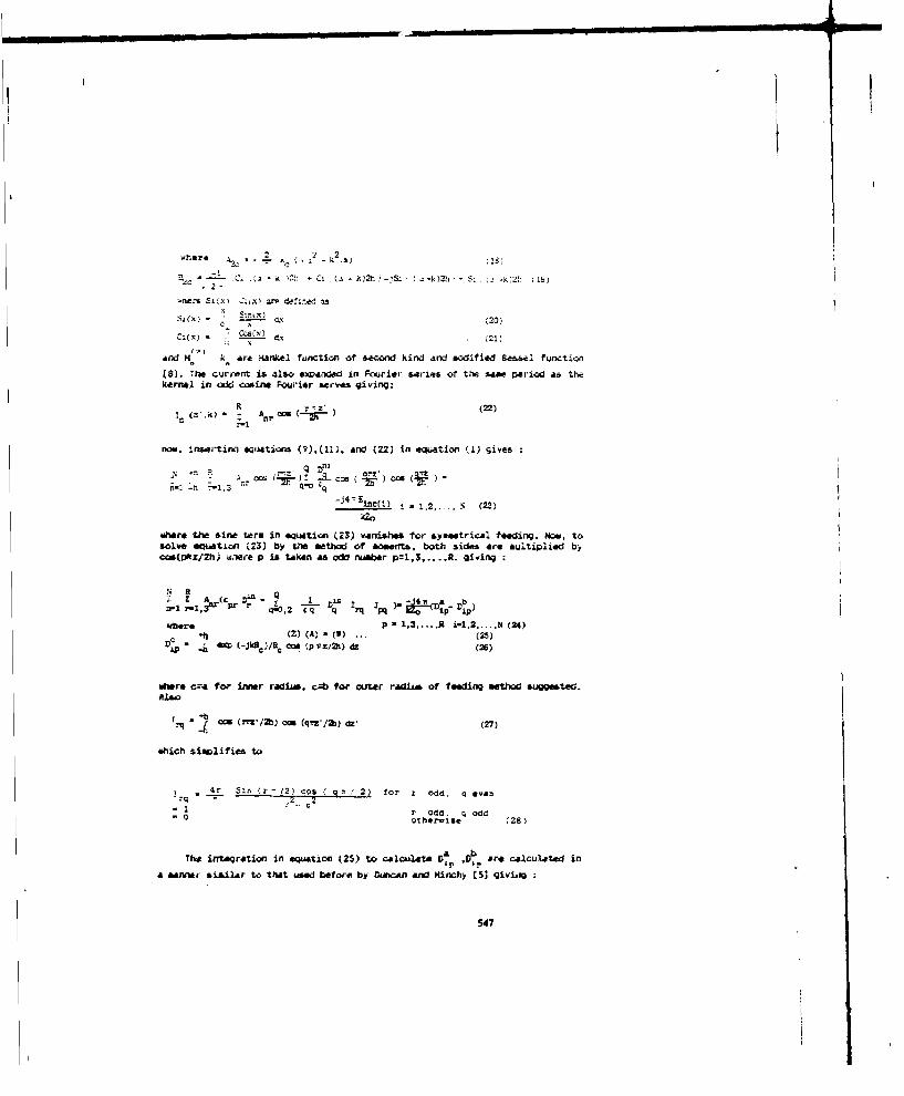
where k2.

"B .,; -I C k h: -k-:S - " )2h - ;:S - -k;iC• 1LI), 2-

.nere Sled. seMx are defi!'ed 2s

S(x) ' -20)

CeC<) - C&X (21;

and H k are Mankel function of second kind and modified Besal function

[83. The current is also expanded in Fourier series of the saae Period as thekernel in odd cosine Fourier serves giving:

K -,z (22)

now. irnerting cquAtions ( a),(1}, end (22) in equation (I) gives

n-i -I r1,2 q-c-.44.. inc(..).......... (23)

Where the sine taer in equation (23) vanishes for symmetrical feeding. Nos, tosolve equation (23) by the method of momentrs, both sides are multiplied byco•(01z/2h) Wflere p is taken as odd nuber p=l.3_.. R. giving

A(C * ( Di- 4. 4 wn r 1. rt prrD D )_D

n-I 3- r ir2 cq q rq 'PQ 4-1 ip P)

where P 1,3 ..... t i-1,2...N (24)D - (Z) (A) - (W) ... (25)

DI -b ý(-3kl )/ "c (ptIzj2) az (2l)

Where c-e for inner radiua, czb for outer radius of feeding method suggested.

. 4 c, (iz'/2T) com (q,/2i) a (27)

which simplifies to

4r S:n (r - /2) cos ( ga, 2) for r odd, q evenq •2 q2

- "r Odd., q odd"o herwime (28)

The integration in eation (25) to calculate G&p P t are calculated in

a •r•er similar to that used before by Ounc.n and Klnchy [53 givi ag

547

- D2 - . (2) 22ip L ~ 4 H0 2 - a)--U0 (k 2a)-Hý, C

for " < 29)where - p / 2h and,) t: k -k,2a, - 2_ k 2 b 30:

a.d fP - "I n (W/e) .31;

Thus equation (24) can be solved making use of syaeetries in circulararroy, where the resultant matrix is circulant. Aolying the prcaedure used bySinnot E7]. am can easily get the current distribution of the circ'flar arra•.

4. CALCULATING3 OF CURRENT DERIVATIVES :

Differentiating equation (I) with respect to kv times gies

l" -h Zk•) k 1 (z'z ) . Z'k)' 1 -k v,-z' CV-v'k) v'3

Where lv)(z~k; is the vh derivativ- with respec% to k of the right hand side

of equation (1) n is the derivative of the current on the nth element arnd

k in v derivative of kernel between the ith and the nt elementrespectively.

Equation (32) can be applied for increasing values of r from r=l tohigher walis ýcto get current derivatives. It is to be noxed that the kernel inequation (32) is the saes as the kernel of equation (I). Hence employing the"ea procedure awplied in section 3 by e3pending the kernels ani the carrcntderivatives in Frur:ar series yields the same matrix (Z. obtained in equation(25). but with different right hand side. Heo", it is only tmed tocalculate for each derivative value v a new right hand side of equation (32).Applying the procedure described in sction 3 on equation (32) yields

N R +bI I A (C Din, I t I t" kmr (q ,r . r. q rtq P -b (z

cos(z/h)dz- (v-v) (v)

DiQ 1 nv', r1,3 Ar (pr Dr -

4,2 "q P 3 - 1,2 ...... . (N;

"here rnr is the rth harmonic of the vth derivative or, the th elemeort and

0Dn is the q harmonic of the v '" derivative of the kernel bstnen elements

(lin) and is calculated using least square. Also fi (z.k) is e*sndedinfinite Fourier series

548

I--

share F 's are calculated us),4 ýCCat 1~-~.T2J nat (533 reduces to• :z. . z -35:

ea P fn - V - ( v -V ') T6v : - 1 .3 > r

4-0

pa 13,11..., I:4,, N (6

S. FRQUENCY PERTURBATIONSTaylor series representation of the currert on each antenna eleaent is

Duilt Lp as function of K gives:

10 (z'k() * I( " .) (k-k.) . 2) - (- i )(Z,.)

• ' Ar. k"° -- " * -k

S n =m L,-,.. (37)

The value of (z',k) at kko is calculated at iW,:tion 3, WhileI ( ,k) ,.... are calculated in section 4. thus the curreht on #Ac•

elerent of the circular array Is directly obtained. Due to the existenc of

pole location in the complex freq•ency plane, divergence occurs In equation(37) which is owrcome y buildi, up enother layljr series of the inverse ofthe current, provided it is analytic at that poirrt. Ebpenaicn of lIn(z' .k) isbuilt Us where :

zn(z'k) - I a ("k)I (k,)I 4/' (2',k)1 - (" )' ,.Z (a(z'K)1

+.. 1 ...... (38)

making use at Ze (Zk) - 1/13 (zEX (38)

or Z. (zalb) . 1 (z'k) - 1 (40)

differentiation equation (40) v time with respect to k gives

(vv-V) (v')z l(Vv,' 0= (z',)

which cau be written as

,. (V-V') (v

"e, , -c . 42:

Hnece equation (42) can be applied for n=1.2,. . N to get the inverse of the

549

- Gil Using 1,11,!l0 ~ Term*OIZ S.'iOll

We ..

t~~~~~u.S& ~ ~ ~ ~ ~ ~ I 31*fee i .~.a~j. r..£am*~

pit-.li

350

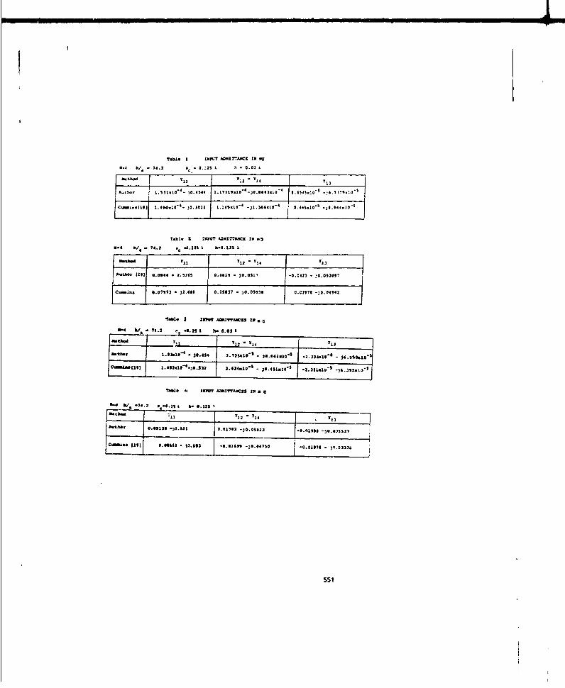
T-bl. 2phr ADr.AMll~Z 1:4 .

341 3/ *74.2 k 22 *02

Oft &0d Y- V1 I

j C...o.119f 1 490 10'.,01,2 1.14S.10- -2l.3g4,o441~ .4s0 2.4.

* /i-74.2 .0.1251 13.0.125

A0usC i10 o .. * 2.51fi5 0.0419 -~ o -0.017.242) 3O).052407,

4.07973 - J2,489 0.05437 3 0.050)80056 ~.44

*W jl 01,DMTAN9 T

I eI-.i .0 0

ACft J8.43 3.725.10 -2 J4.643.10 -. 2 4 1 k-~4S~j

T6131 4433 .1 o~TAmsAMoS10l

3.4 mlg 34/i 24.7 P JS21 0.332 3212-

~1III - via

0.00139 .32.2.0 0.0179a -JO.05022 -451043.@20517

ai M 639 0. 0 ) 2 .402 -0.014 69 -;0.047$0 -0.01102 - 20.03376

5s1

c urrenlt derivatioes for v:1.2.3 ..... N. Th4s . euatiOn (38) can be calulatedfor all antenna elesents. Nertc its invrse gives the currant dist, ibutlxc oleach alea-nt of the circular array.

6. NUMERICAL RESULTS AND CWNCLUSIC:The methods presented infrequency perturbation give the solution at a

band of frequencies without repeated calculation of Lhe ifo-dace &at- :,.its elements. the second method which uses Taylor series of the i,•ee of thecurrent gives better results when coepared with eAperiwantal and othe,published numerical results as shown in tables i-tand figure (1)

REFEflENCES:[I] RtF.laringtan Field co•putation by aoment methods N.Y.. raciillan.1968.[2] K.A.Al-Sadaaihy and Z.L.Yen ,* Extonded bonary corndition integralequation for perfectly conducting and dielectric bodies : forulation anduniOuenss -, IEEE AP-23 . No 4 , pp 546-551, July 1971.(3] R.E.Collin .- Equivatent line current for cylindrical dipole antennas andIt's asymptotic behavior . IEEE AP-32 *No 2 ,pp 200-204 , Feb.1984 .[41 E.K.Miller .- A selective survey of computational el•,trcagnetics , IEEEAP-36 , No 9 *) 1281-1305 , Sept. 198U .(S) R.H.Burunan and F.A.Hinchey "Cylindrical antenna theory ". J.Res N83,Sec.D (Radio Propagation ) , Vol. 64 ,pp 569-534 , 3apt./Oct. 1960.(6] T.J.Sarkar ."A study of the various methods for coemputing electromagneticfield utilizing thin wire integral equation - Radio 3ciera . Vol. 18 , 6V28-38 , 1983 .[7] 0.C.Chang .- On the electrically thick mopol : Part I theoreticalsolution ,- IEEE *9F-16 , No I , pp 58-"4 . Jan. 1Q68.(0] D.N.Sirrot .- Anhlysis and design of circular ar-ray by matrix method"Ph.D. dissertation electrical enineering dapertent , Syracuse UniversityN.Y. , Jan. 192.

552

On Effect of Phase Quantization Upon Peak

Sidelobe Level in Phased Array Antennas

GAO Tie GUO Yanchang LI Ian.'xinNanjing Research Institute of Electronics Tectmology

P.O.Box: 1315-403, Nanjing, 210013, P.R.Cina

ABSTRACr

In this paper, the peak sidelobe level degradation due to the phase quantization in scan-ning phased array antenna is described. The several computation formulas which estimate thepeak sidelobe level degradation and the some simulated computation results are given. It isshown that the theoretical analysis are in good agreement with the simulated computation re-sults.

I. INTRODUCTION

Beam steering for phased arrays normally employs electrouically switchable digitaishifters in a few microseconds. Most of the phase shifters in use are digital, the digital phaseshifter consist of P uxed phase sl.ifters whose volues are individually equal to 2x / 2, 2x / 22,--.,27r / 2p, P is called the bit number of the phase shifter. In order to steer the beam to a givendirection, we must set up the phases computed according to the steering direction in the phaseshifters. Rut all the values cannot be exactly phased in the digital phase shifter. Therefore, thephase should be set up in the element must be quantized, it introduces parasitic sidelobes dueto the phase quantization, ernd the peak sidelobe of the array will be degradated.

In the early phased array research, many techniques are proposed to analysis the effect ofthe phase quanuftion on the peak sidelobe level. It is well known that. when the rounding offis used, the parasitic sidelobe is -6? (dB). when the random phase shift teehaique is used, theFarasitic sidelobe is -12P (dB). In fact, these results are effective for a large array, when thearray is not large, the above conclusions are not accurate.

In this paper, using the principle of the probability and the statistics, the peak sidelobedegradation due to thk phase quantization in scanning phased array antenna is described. Theseveral compitttion formulas ( for rounding off, rounding up, rounding to the nearest bitsand random phase quantization ) which estimate the peak sidelobe level degradation amgiven. It is shown that the sidelobe level degradation is the function of ideal designed sidelobe.array aperture efficiency, the elements number of an array antenna and the bit number of thephase shifter. Some simulated computation results ire given and Qey confirm the theoreticalanalysis.

553

I1. THEORMICAL ANALYSIS

For simlolicity, suppose that there is a linesr array antenna with N isotropic elementsspaced at distp-nce d, the field pattern can be written as

E- Z . - (I)M.I

Viherr a u-k ,4U"I ), ud- ,(sineo), 1 is the amplitude at the n-tb element,k-, 2A / A, ). and 9O a-e the wave length ind scanning angle respectively. In general, the phasequantization function of array antenna can be expressed as

-no6,, - In (n) (2)where, 6. is the quantized phase at the n--th element, A- 2n /, 2 P, P and Int( * ) stand for thebit number of phase shifter and intetralization respectively, 0o is the accurate phase shift.

For rounding off, rounding up and rounding the to the nearest bits, the phasequantization function is

f', (n) .- ¢, 0 !- C¢ -1 (3)

C -0, for reunding o[ffC - 1, for rounding up (4)

C .- 0.5, for rounding 1o *he ntares. bitsFor random phae quantization, the phase quantization function is

In equ.(5), the C. is the random number uniformly distributed in region (0,1). Due to tk'ephase quantization, the array pattern can be written as

N

X-1where wo is the accmrate phase shift, 6r. is phase error due to phase quantization.

Using the pnnciple of probability and statistic theory, it is known that, for rounding off.rounding up and roundint to the nearest bits, the phase error 0. in equm() is random numberunifocmly in region -x / 2•', 7 / 2'. So

N< - X" > <1e4 > a'-' ) (7)

M-1

< > stands for mean value, it is obvious

~ 2 PAccording to the definition of variance

N

D(E•"(u))- < '(u)E' (u)> - < E(u)> <E'" (u)> I • DU) (9ga)

554

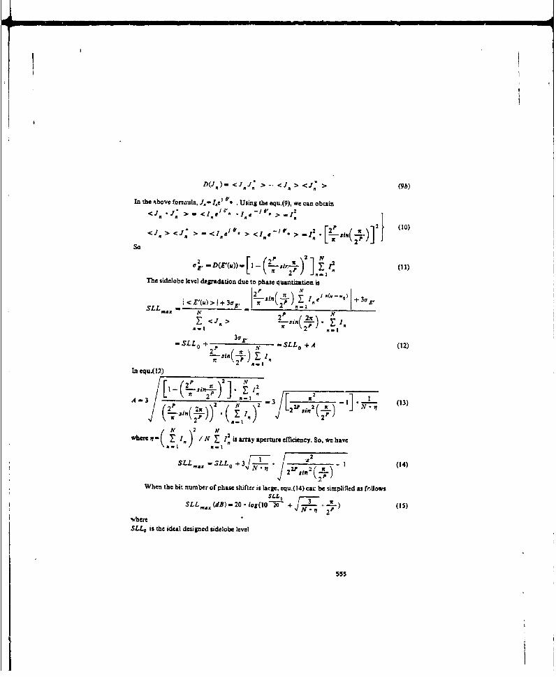
D ( , ) .< .J, , ,J . > - - < J , > < J ,' > ( 9 b )

In the Above fornula, J.- I4e' a' Using the equ.(9), we can obtain< J . "J . > .< l. d -J 1 ' . > 12 ]

< J -> <,: >- <,1 .. > <I.&- > -1 / ( 10n()so

2 2)2So ~ C D•-z(.'(u))= 2 x \2"J

The zidelobe level degradation due to phase quantization is

S< E'(u) > + k%, + 3ar=SLLx N S<-". > "7-R.L " )" .E .,

"-SLL-O 3+ , ,SLL0 +A (12)

PIn equ.(17)

• -3/ L -," 2'J " " /" , . • (32 22P.2 Na()(3

ALL,3, 3LL +3 :. . 1 - (1)27./.n 2 (_ .) l(4

,7

When the bit number of phase shifter is large, equ.(14) caL be simplified as followsSLL

-3SLL ,,,. (dB) - 20 -iot'(1O0T + • • ,2J(5

whereSLL0 is the ideal designed sidelobe level

555

N is the total number of the array element,I is the array aperture efficiencyP is the bit number of the phase sbifter

It can be seen that, from equs.(14) and (15), the sidelobe level degradation due to thephase quantization is the function of anay aperttsre efficiency , the number of array element,the ideal designed sidelobe level and the bit numbe. of phase shifter. According to equ.(l 5), wecan estimate the effect or phase quntization on the sidelobe level degradation for roundingoff, rounding up and rounding to the ncarest bits. Similarly, based on the above method, forthe cams of planar array, suppose that M x N elements are arranged along the X and Y axeswith oquai spacing d, and d. the formula of sidelobe level degradation due to the phasequantization can be writoen as

SLL,•, Z--..LL 0 + 3Vi 2 -I (16)

Af N 2 ArN

where- if Y. I.. / MN 1. Z I is the aperture efficiency of a planar array\m-n- 10 -'lm I --

antenna. When the bit number of phase shifter is large, equ.(l 6) can be simplified as followsSLLo

SLL.,,, (dB) - 20./ og(lO•0 M N'i2i (17)M*- 2 P

When the random phase is used, for a linear array, the formula estimated for the sidelobelevel dcrnadaaon is

2SLL SLLo +3 [-: -1 (18)/"'"22F-2 in, I z ( (IS)-N''i"2

when the iit number of phase shifter is large, 9qu.(l 8) can be simplified asSLLS. 2x

SLL.ex(dB)-20.1o 1T7.( .- . -+ (19)

For the planar array anterna, the formula estimated for sidclobe level d-gradation can beexpressed as

SLLA",.L -i LLo + M N +- 3 F -Zs-- -- l (20)

When the bit number of phase shifter is large, we have

SLL* 3 2zSLLJ 2 - 2O.Iog(O• 20 + ' ) (21)

556

M. SIMULATED COMPUTATION

In the followi, some typical examples are given. The total number N of linear array el-ements is 32, the ideal pattern is -30(dB) taylor, the array aperture efficiency is -= 0.8488 andthe bit number of phase shifter P - 5. When the array is scanning from 0 * 60 , the peaksidelobe level is calculated using the FFT, the results are shown in Fig.] (a) (b) - Fig4 (a) (b),where, from Fig.2 - Fig.4, the rounding to the nearest bits, rounding off, rounding up andrandom phase quantization are used respectively. In these Figures, (a) is the peak sidelobe 1ev-d distribution in region 0 ' - 60 * , (b) is the probability of PSLLs less than the specifiedsidelobe, From Fig.1 to Fig.3, we can see that the peak sidelobe level is -24.3(dB) in region 0" -560 ' , the sidelobe level degradation estimated by equ.(15) is -23.84(dB), the simulated

values differ from the prediction by no more than a few percent in analysis of PSLLs degrada-tion. The Fig.5 - Fig.6 are typical quantization pattern in which the array is scanning to 35*when the rounding to nearest bits and the random phase quantization are tsed respectively. Itcan be seen that, from Fig.5 - Fig.6, the effect of phase quandzation on peak sidelobe levelcannot be neglected.

IV. CONCLUSION

In this paper, the effect of phase quantization on the sidelobe level for phased array an-tennas are described, some formulas of estimating sidelobe level degradation due to phasequantization and some typical simulated computation results are given. It can be seen that thesidelobe level degradation due to the phase quantization is the function of arrmy aperture effi-ciency qt, the bit number of phase shifter P, the ideal designed sidelobe SLL4 and the totalnumber N of array elements, the simulated computation results are in good agreement withthe theoretical analysis. It is effective and practical for designing phased array antennas.

REFERENCES

I Guo, Y.C., et al. Principles of phased array and frequency scanning antennas. Chinese De-fence Press, 1978, 48- 141

2 Guo. Y.C., et al. Sidelooe reduction for phased array antena using digital shifters. IEEProc., Pt.H, 1983, 130(5): 343-351

3 Quo, Y.C., et al. Sidelobe reduction for phased array antenna using digital shifters. lEEProc., PtH, 1983, 130(5): 351- 357

4 Smith, M.S. and Guo, Y.C. A comparison of methods for randomizing phasedquantization errors in phased arrays. IEEE Trans. Antennas Propagat., Vol. AP-31, 821-828. Nov. 1983

557

O 60 (Dogree) Sc-iv PS.L - -60 (Des.) Scanzsg Pro.-22 - .

S-23-_ _ _ _

S-24~S-26-

S -26- i-27 IN1 ,0 '

D. -10 20 30040 50 •0 - 1-;0 -29-28 -' -2e-2 _2'0 - 60 (Degree) SU (M.)

(a) (b)Fig.] For rounding to the nearest bits, (a) PSLL distribution in region 0 60 (b) proba-bility curve or PSLL

o - 00 (Delrme) Scanning PSLu. 0-60 (Dei.) Scan•ning Pro.-2 1 0.+

-24 F 7'25", O's

02

T j0.4

S-2a+r 0.2 -

So 20 30 40 50 6o -31-30-29-28-27-26-25_-240 - 60 (Degree) Sl. (di)

(a) (b)FiZI For rounmnig off, (a) PSLL distribution in region 0 - 60 (b) probability curve ofPSLL

-220 0 (Dogret) Scanning PSLL 0-60 (Dei.) Sci i Prc.

0.8q -24l J )I• -• - 0,6,

-30 0.0

D 10 20 3C 40 So 60 -31 -30 -29 -28 -2-7 -26 -25 -240 - 60 (Coctee) SLL fdB)

(a) (b)Fig.3 For rounding up, (a) PSLL distribution in region 0 - 60 , (b) probability curve ofPSLL

558

0 60 (Degree) Scanng PSa o-6o (Do&.; Sca..g Pro.

S- 20 .v

2-3-- 0.4 - - 1-2-H

o 2t 0o 30 40 50 60 -60-3o-2-a-2-2e-5-24-2-20 - 6o (Doere) SU. (do)

(a) (b)Fig.4 For random phase quantization, (a) PSLL distribution in region 0 - 60 (b) proba-bility curve of PSLI

-7(-4-•

-50--7

-00 , ....... .. . .,. .-90 -45 .

Fig.5 The pattern of scaning to 35 ° when the rounding to the nearest bits is used.

-iO

-24

-30

-40

-90

-BC -4 45 90

•IBO,

Fig.6 The pattern of scanning to 35 when the random phase quantization is used.

559

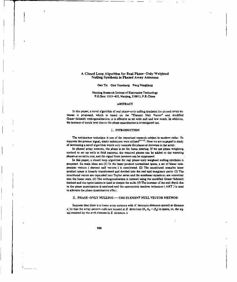
A Closed Loop Algorithm for Real Phase-Only WeightedNulling Synthesis in Phased Array Antennas

Gao Tic Guo Yanchang Fang Nenghang

Nanjing Research Intitute of Electronics TechnologyP.O.Box: 1315-403, Nanjing, 210013, P.R.China

ABSTRACT

In this paper, a novel algorithm of real phase-only nulling synthesis for phased array an-tennas is proposed, which is based on the 'Element Null Vector' and modifiedGram-Schmidt orthogonalization, it is effective to set wide null and low notch. In addition,the increase of notch level due to the phase quantization is investigated too.

I. INTRODUCTION

The Rntijammer technique is one of the important research subject in modern radar. Tosuppress the jammer signal, many techniques were utilizedi-11" 1 .Now we are ergaged in studyof developing a novel algorithm which only controls the phases at elements in the array.

In phased array antenna, the phase is set for beam steering. If we use phase weightingmethod to set up nulls in field patterns, the required phases can be added to the scanningphases at no extra cost, and the signal from jammers can be suppressed.

In this paper, a closed loop algorithm for real phase-only weighted nulling synthesis isproposed. Its main ideas are (I) In the inner product normalized &pace, a set of linear inde-pendent vectors ( element null vectors ) is constituted. (2) The coustituted complex innerproduct space is linearly transformed and divided into the real and imaginary parts. (3) Theoonstituted vector are expaaded into Taylor series and the nonlinear equationt are convertedinto the linear ones. (4) The orthogonalization is iterated using the modified Gram-Schmidtmethod and the optirrization is used to deepen the nulls. (5) The increase of the null depth dueto the phase quzntization is analysed and the appropriate random technique ( ART ) is usedto alleviate the phase quantization effect.

11. PHASE-ONLY NULLING-THE ELEMENT NULL VECTOR METHOD

Suppose that there is a linear array antenna with N isotropic elements spaced at distanced, let that the array pattern nulls are located at K directions (81, 02, ... Ox) in space, so, the sig-nal received by the n-th element in K direction is

560

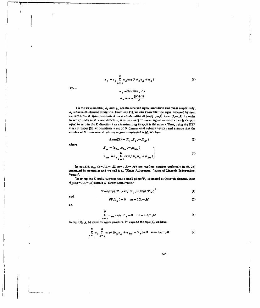
xn. a. akexp(J b.Uk +Pk) (1)k-I

where

~' 2

A is the wave number, a, and q'* are the received signal amplitude and phase respectively,

a. is the n-th element excitation. From equ.(l), we can know that the signal received by eachdement from K space direction is linear combination of {expj (nuk)) (k- 1,2,---,E). In orderto set up nulls in K space direction, it is necessary to make signal received at each elementequal to zero in the K direction ( as a transmitting array, it is the same ). Thus, using the DBFideas in paper [9J, we constitute a set of N dimensional column vectors and assume that thenumber of N dimensional column vectors constituted is M. We have

Span{X} - (XI ,X' ,"ZXM) (2)

where

-c K pj~~~ 1 (3)kr IBn• XTJbn qk

In equ.(3), op - (k-1.2,...,K., m-1.-2.M) are -an,' m number uniformly in (0, 2a)generated by computer and we call it as rPhase Adjustsntnu •actor of iunearly IndependentVector'.

To set up the K nulls, suppose that a small phase IF. is created at the n-th element, theseT.'s (n 1.2.,,•.) form a N dimensional vector

S -(expi IP I ,exp/i T 2 ,..,xp IF M ) r (4)

and •v'x. ). 0 m ,- 1,2,-.- (5)

i.e,

A-1In equ.(5), (a, b) stand for inner product. To expand the equ.(6), we have

N KZ an Z expj [b.nuk +0Pk. + 'FRI0 ml,2,o..,M" (7)

R-1 k-1

561

Now we take out the real component and imaginary ones from equ.(7), we have

N KI: a., : co:[bnuk +111km + ,T. 0

,-1 k-I m-1,2,.- (8)N K

a 2. .uin[b.uk + qk3 + 1P. 0-I k-I

We assume that •. and T, are anzi-symmetric to the centre of the array antenna.

Therefore, equ.(8) can be simplified as follows

M KX a X cos[b uk +4U, + IF]-0 (9)

R.1 .k-I

Equ.(9) is nonlinear problem, since Y.'S are the small phases, equ.(9) arm expanded into

Taylor series and the nonlinear equations are converted into the linear ones, and two term are

kept. We obtain

N K Nr K1: a,. E coa[bl uA +OkmJ-- 2: an X

7A51M[bflt +oIk.]- (10)

M-1 k-i "-I k- I

which constitutes a linear problem, it can be solved by using the modified Gram-Schmidt

orthogonalization12 1

. Beiause of equ.(5) or (10), T' is orthogonal to all X,,s, from equ.(3), itcan be seen that X. is a linear combination of the K element nulls vectors, i.e

V1 -(eXp/ blu1 ,expi b 2 u,..-,expj bNul)

V 2 -- (expi b, u 2 ,ircpi b2 u 2 ,.",expj bNu )(

VK -(expi b'uKexpj b 2 UXl,.",expi bMMuK)

Then we have

(',Vk) - 0 k = 1,2,---,K (12)

It nmeans that if we use the weighting phases TI., the received signal at array antenna are

zcro in K direction and the object of setting up nulls is achieved. In addition, in equ.(3), by

neans of the basic criteria of optimal weights 5- S , we select the number M of initial

constructional veecors.

562

Mi. THE EFFECT OF PHASE QUANTIZATION ON NULL DEPTH

Because the phase-only nulling synthesis is employed, most of the phase shifters aredigital. The digital phase shifter consist of P fixed phase shifters whose values are individuallyequal to 21 / 2, 2n / 22,..-,2= / 2', P is called the bit number of the phase shifter. Thus, all thevalues cannot be exactly phased in the digital phase shifter. Therefore, the phase should be setup in the element must be quantized. In this section, the effect of phase quantization on thenull depth is analysied.

In general, the phase quantization function of array antenna can be expressed as

"V. -,nt( +a+b. R). A (13)

where, A 2 / 2", Int(* ) stand for integralization, T. is the accurate phase shift, T• is thequantized phase, A is the random number unifoimly in region (0, 1), a and b are Lnknownconstant. When a-0 and b-0, the phase quantization is rounding off. When a =0.5 andb-0, the phase quantization is rounding to the nearest bits. When aI -and b-0. the phasequantization is rounding up. When a-0 and b- 1, the phase quantization is random phasequantization. A vast amount of computation results show that, when a-0.25 and b0.5, theeffect of phase: quantization on null depth is smallest, this method is called as AppropriateRandom Tecanique (ART).

Due to the phase quantization, the array pattern can be written as

N

E(u). a EaAY ,ib.u+Y*) (14)N I

where, AY. is phase error due to phase quantization, when a0.25 and b-0.5, using theprinciple of peobability and statistics, the phase error is random number uniformly in region-3s / 22, 3x / 2P2. So

N< - oa <> *- >a.(b<e+>.) (15)

it is obvious

3n 2 2, P<, = > 2 ." Ž--. (6)

according to the definition of variance

563

D(E(u)) < E(u)E * (u)> < Ecu) > <.E " (u) > = .D(J,,)} (17)

D(.F,)- <J, < < >-

we have

2 /2P+2 3. )2a. J[ D(~) x i; (18)

therefore, the increase of null depth due to phase quantization is

SL K 2 2E +1 4~ 2 2 sin 2(~ -1 195 fY < J. > 22+M 2P+2,+

where q ( a) /N(X a, Z isarrayapertureefficiency

When the bit number of phase shifter is larger, equ.(19) can be simplified as follows

SLL(dB) - 2.673 - 10Iog(Ntn) - 6P (20)

IV. SIMULATED COMPUTATION

In the following, some typical examples are given. In Fig.l, the total number N of lineararray elements is 20, (a) shows the quiescent pattern, its distribution is -30 (dB) Taylor ones,#-0.8488, (b) is the pattern with 3 nulls which are located at =-33.37 , 34.03 * and-44.43* , (c) is the pattern with 4 close nulls which are located from -33.36 to -37.58 *.Itis obvious that null depth to suppress interferences is about -80 (d0). The effect of phasequantization on nail depth are shown in Fig.2. (a) (b) (c) which are the patterns of Fig.l (c)with 6, 8 and 10 bit phase quantization respectively. Because N- 20 and q - 0.8488, equ.(20)can be expressed as

SLL(dB) -9.625 - 6P (21)

When Jhe P = 6, 9 and 10, the SLL are -45.625 dB, -57.625 dB and -69.625 dB. FromFig.2, it can be seen that the theoretical prediction are in good agreement with simulated com-putation results.

564

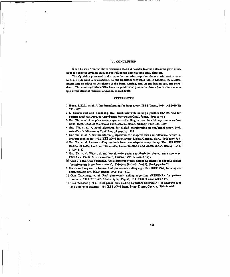
V. CONCLUSION

It can be seen from the above discussion that it is possible to creat nulls in the given direc-tions to suppress jammers through controlling the phase at each array elements.

The algorithm presented in this paper has an advantage that the real arithmetic opera-tions are only used in computation. So this algorithm converges fast. In addition, the resultedphases can be added to the phases of the beam steering, and the production cost can be re-duced. The simulated values differ from the prediction by no more than a few percents in a-a-lysis of the effect of phase quantization on null depth.

REFERENCES

I Hung. E.K.L., et al. A fast beamforming for large array. IEEE Trans., 1984, AES-19(4):598-607

2 Li Jianxin and Guo Yanchang. Real amplitude-only nulling algorithm (RAMONA) forpattern synthesis. Proc. of Asia-Pacific Microwave Conf., Japan, 1990: 81--84

3 Gao Tie, et al. A amplitude-only synthesis of nulling pattern for arbitrary convex surfacearray. Inter. Conf. of Microwave and Communication, Nanjing, 1992: 344-439.

4 Gao Tie, et al. A novel algorithm for digital beamforming in confnrnal array. 5-thAsia-Pacific Microwave Conf. Proc., Australia, 1992

5 Gao Tie, et al. A fast beamforming algorithm for adaptive sum and difference pattern inconformal antennas. 1992 IEEE AP-S Inter. Symp. Digest, Chicago, USA, 1992:450-453

6 Gao Tie, et al. Pattern nulling synthesis based on adaptive array theory. The 1993 IEEERegion 10 Liter. Conf. on 'Computer, Communication and Automation', Beijing, 1993:1142-1145

7 Gao Tie, et al. Wide null and low sidelobe pattern synthesis for phased array antennas1993 Asia-Pacific Microwave Conf., Taiwan, 1993: Session Arrays.

[8] Gao Tie and Guo Yanchang, 'Real amplitude-only weight algorithm for adaptive digitalbeamforming in conformal array', 4Moderm RadarD , Vol.13, No.6, pp.43-52.

9 Guo Yanchang and Li Jianxin. Real phase-only nulling algorithm (REPONA) for adaptivebeamforming.1990 ICSP. Beijing, 1990:661-662

10 Guo Yanchang, et al. Real phase-only nulling algorithm (REPONA) for patternsynthesis, 1990 IEEE AP-S Inter. Symp. Digest, USA, 1990: Session ARRAYS

11 Guo Yanchang, et al. Real phase-only nulling algorithm (REPONA) for adaptive sumand difference patterns. 1991 IEEE AP-S Inter. Symp. Digest, Canada, 1991: 94- 97

565

5 P

* ia 4q.. *(a) (a)

_ -l

go .-. 0

*,/ l ! -_,0 -! 0• .5

":"'\ (• f0. . .• .. 5S o ....

(c) (c)

F~ig.l Pattern for 20 array elemeoc.• with phase-on- Fi$.2 The effect Of phase quanusztion on field

ly weisht. (a) qwiescent pattrn, (b) (c) pattern pattern of glel. (c), here, the bit number of phase

with nulls, shifter are 6, S and 10 resp~ectively.

566

_ ,

A W .. ....... ..

FULL VAVE ANALYSIS OF INFINITE PHASED ARRAY

OF ARBITRARY SHAPE PRINTED LIME MICAOSTRIP ANTENMAS

Prof. Elhilaly H. Eld , Ahmed N. Attlya , Essam EldiwanyFatma Elhbfnawi

ELECTRONICS RESEARCH INSTITUTEELTAHREER ST. \ DOKKI \ CAIRO \ EGYPT

ABSTRACI'

This paper presents full wavw analysis of infinite array of arbitrary

shape microstrip line antenna based on moment method. The active elementparameters are found using the current distribution on the radiating element.

Comparison is made between the parameters for difTerent Infinite arrays when

the array element is a linear microstrip dipole and when It is of arbitraryshape line such as circular loop, zigzag, spiraland meander for the samesubstrate parameters.

I INTRODUCTION

Microstrip antenna structures are suitable as radiating elements fcr

phased array due to their light weight, compact structure and low cost,

compared with other types of radiatlnU elements. Another important feature ofmicrosLrip antenna structures is the ability of integrating different devicts

such as phase shifters end amplifiers on the antenna substrate,Some forms of microstrip antenna structures; such as rectangular patch,

circular patch and linear dipole; were studied as a single element and as anarray structure. H.Nankano et al 11,21 and H.A.PRagheb et &1 [3] studiedarbitrary shaped printed line microstrip single element antennas. They showthe properties cf single radiating element for several configurations such as

circular loop,meander ,zigzagand spiral. D.M.Pozar et al studied the array

structure of linear microstrip dipole [4,5] and the array structure of

rectangular patch W6].The studies in [41 and [5) are concerned with finite and

infinite array structures of a linear dipole respectively. Comparing the

results of [4] and [5] it can be concluded that for almost all practical

finite microstrip array structures the properties of the infinite array

structure can represent to a good degree of approximation those of each of

most of the finite array elements except those elements near the edge of the

finite array.On the other hand. solving for an infinite array requires solvingfor only one element In a periodic structure which takes implicitly the

coupling among the elements, while solving for the finite array requires

solving for all the elements in addition to solving for the coupling amongthem. This means the increase of the order of the moment method matrix by a

factor equals the number of the array elements The situation becomes worsewhen solving radiating elements structures chat need large number of basis

functions to describe their current distributions such as the case ofarbitrary shape radiating eiemen:s.

This paper presents the moment method solution of an Infinite array

composed of arbitrary shape printed radiating elements. The solution• is based

on the technique of Poisson's sum formula [51.It is assumed that the radiatingelament Is excited by a delta function generator placed at arbitrary point

along its 'ength. The current distribution on the radiating element is found bysolving the moment method matrix. Then.one can determine the active inputimp*d ¢a. and the active radiation pattern , which represent the radiating

element parameters in the presence of the array structure The variation of the

567

Input impedance with scanning angle Is studied also. Results ire presented forsome special cases where the array element is a circular loop, a zigzag, a

spiral, or a meander.

II THEORY & ANALYSIS

Fig. (1) shows the geometry of the Infinite planar arraý of identicalarbitrary shape microstrip antenna elements. The radififng ^lamonts are

assumed to lie In a rectangular grtd with spacing a&b in x&y directions,respectively.

For scaninS angle ( e0. ); as shown in fig. (1): the current on thean "radiating element Is phased as

•jko(mau~nbv) 1)

where ko Is the free space wave number (ko-2-'w/Ao Ao is the free apace wavelength ) and u&v are defined as:

u-sin(G)cos(#) (2-a)v-sin(6)%ln(#) (2-b)

The electric field at any observation point L xy ) on trie surface of the

substrate is given by :

m-+- n..- a, eJko(mau+nbv)

•(x.y)" =- J , ' xoyo) (5)

where 0mis the dyadic Green's function for the mnthelement- Applying theboundary condition that the total tangential electric field is zero along anyradiating element except at the feeding point, the above electric fieldintegral equation ia solved for the unknown current distribution

where (xo,yo) represents the location of the excitation point-or such planar structure the solution requires only four elements of the

dyadic Green's fuiction Gp. which represent the electric field in each of the(p - x or y) direction due to elements in each of the (q-x or y ) direction.

The elements of the dyadic Green's functions are given in reference [61 .The Green's function for the field at (x,y) on the substrate due to an

infinite array of infinitesimal dipole on the substrate phased at (a.) isgiven by :

-JZe m=% n-u eJko(mau nbvlf k jkx(x-xo-°a) eJky(y-yo°nb)Gpq- -pq(kxky)

koab mr-- n-- -I dkx dky (4)

where Qpq(kx.iky) is the dyadic Green's function for single element inspectral domain representation (6). Using Poisson's sum formula [5] equation(4) can be rewritten as' follows ;

-JZo m-+u n-+ ejkx(xxxo) jky/y-yo) (9)

pq~r------ r E Opq(kx,ky) (5)koab mr--u n-u

where kx and ky in equation (5) are given by21t m 21t n

kx--- .kou ky-- + kov (6)

The moment method can now be applied to Q single radiating elementstrvcture In a shaile unit cell, and then by periodicity the effects of allthe radiating elements in the infinite array are taken into account (5].Thelength of the radiating element is divided into small equal linear segments asshown in fig.(2).The position of each segment is defined by its x&ycoordinates and Its angle a with respect to the x axis. The Iangential

568

*le1.tilt 1;crent on ths antenna it 9xpandtd Into a 20t of overlAppingpiecewise sinusoidal expansion functions in the form :

J(I,W}-f II Ji(1) f(W) (7-a)

Ii is the unknown amplitude of the basis function and JI(l) is given bysin ce(a-Il-liI)

Ji(l) - Sir, ke; for Ii-1i Is 5 (7-b)

where s is the length of each segment and ke is the wave number of the

expansion function which is taken here to be ko,/(er-i)/2 . The feeding point

should lie at the center of one of the expansion functions. The dependence ofthe current on the radiating element across its width satisfies the edgebehavior which is given by :

f[W)- I for -Wo/22 W a Wo/2 (81

' W9 - M2

where Wo is the width of the radiating element and W is the location across

the width of the radiating element w.r-.t its center The testing functions aretaken to be the same as the expansion functions in both directions; the lengthand the width of the antenna element. The aovantage of this choice is to makeu*e of every symmetry to redu-e the computational time as much as possible,The feeding is taken to be a Dirac delta function.

By integration w. r. t. I over the "e" source segment and integrationw.r.t. V over the "f" observation segment, it can be shown that the generalterm Zef of the moment method impedance matrix is liven by the followingequations ý

JZo li-! Jnz , ;Ue oso I I ue.i-fJ (9)

1-0 J-O

ma.. na.- IUeAi,f.j- Z E Ca-,f-j Af Aej If le 3

e m.-a n=- f sin2koa

AJkxlxe~i - xf÷J) 0Jiky(ye*i-yf+J) (10)

Cs,- cosar coses Qxx(kx,ky) * sin(mr~as) Qxy(kx, ky)

*sinar sinas Qyy(Ckx,ky) (11)

,-J(kx cosareky sinarLs

ArOk2 -(kx cosma*ky sinEr) (-J(kx cosar~ky sinar)-ke Coskee +

eI(kx €osar~ky sinirc& ke ) (12)

Ari i -(kx cosar~k• sinar)2 (J(kx cosar~ky sinir)slnkQed-ke coskea*c-J(kx cosar+ky sinar)a ke ) (13)

Ir-Jo([kx sminr-iy coaer]Wo/2) (14)

where kx & ky are given by equation (6), The elements for the excitationvector [V] are zero ;since the electric field on the surface of strip antennais ere; except at the feeding point where it equals unity.

Now solving the matrix equation

the current distribution and consequently the input impedance can becalculated .

Studying equations (6,9-14) it can be concluded that the moment method

matrix is not symmetrIz except at the broadside direction (scanning angle=OC.and O., ). However, Crs equals Cs. for all scanning angles so that

569

equation (10) can be used effectively for calculating Zef and Zfe by changing

the conjugate operation during summation process. Toeplitz property whichholds for moment -,ethod matrix of linear dipole[S] is not valid for the case

of arbitrary shape printed antenna, ror the broadside dlrectiln. similar pairsof elements which have the same spacing between each other and the sameorientation with respect to each other; as shown in fig(.); have equalimpedante element. For any direction other than the broadside, all the momentmethod natrix should be calcui&l"d,

Variation of the impedance and consequently the reflectlon coaffitiant ofthe radiating element with scannig ang le is studied. The worst case for thephased array occurs when the reflection coofficient approaches unity. Thisrepresents what is called scan blindness. In an infinite phased array scanblindness is due to excitation of surface wave along the array structure.Microstrip structure supports at least one surface wave because the dominantmode Tho has zero cutoff frequency. Scan blindness is therefore an expectedbehavior for an infinite phased array of microstrip radiating elements. Atscan blindness the radiating elements are highly reactive with zero resistive

Impedance part since all the incident power is captured as surface wave and noradiation exists. It can be explained matheratically due to the rr.ots of theTe and Tm functions which appear in the denominator of the Green's function[equations (5-7)]. If one of the terms of the series in equation (20) haskxky satisfying the root of Te or Tm it causes an infinite increase in theimaginary part of the impedance elements which causes the highly reactivebehavior of the radiating element. An exception exists ýthen there is a zero inthe numerator of this term that can cancel this root. Physically, thecancellation means that the polarization of the array is such that it Isorthogonal to the excited surface wave [5).

The active radiation pattern of a single radiating element in an Infinitearray structure is actually the radiation pattern of a single elemeat with thecurrent distribution derived from an infinite array analysis. The total antennaradiation pattern for practical cases is given by multiplication f activeradiation pattern of the radiating elements by the array factor for the actualarray size. The method used for calculating the active radiation pattern forunit cell is the Tame as that described in (1-31.

III RESULTS AND DISCUSSION

The above theory is Implemented in a computer code for calculating the

active input impedance and the active current distribution of several shapesof radiating elements. The active current distribution is used by another

computer code for calculating and plotting the active radiation pattern.Results for different configurations are presented throughout this section.For the sake of simplicity of comparison the substrate parameters . thelattice dimensions and the width of the radiating elements are kept constantfor all cases studied. Hence for all the cases, the dielectric constant4r-2.5S, the dielectric thickness d..14Ao, the lattice dimensions a-b-.5Ao andthe width of the radiating elements Wo.,002Xco. For these substrate parametersthere is only one surface wave pole corresponding to the TMe mode. For theabove lattice dimensions and substrate dimensions .this surface wave pole isexcited for e scan angle equals 56.203 at the two principal planes

(o- 0"xz plane" and o=90 "yz plane").The cases studied here are :

I- linear dipole of length .35Ao (fig. 4-a).2- Circular loop of radius .135.Xo . (fig. 5-a),3- Zigzag of total length 1.

2 9ho and 3 Zigzag sections. The angle between any

two adjacent elements of the studied zigzag Is 4S" . (fIg6-a).4- Rampart~two sections meander)of total length l.dOAo and 5 equal sections,

570

(fig 7-a)5- Spiral of totsi length 1 9l1o The straight part at its center Is 04064hoThe spiral function Is p-A •5 where A Is the spiral constant and os Is theSpiral winding angle. A - 0077616 Ao/rad , (fig B-a)

varlation of the active Impedance of the array element with scan anglesIs presented as the reflection coefficient w r t the broadside itmpedancýSo that

Z16.,¢; -Zk.6

?0e,€-= (t.CIwhere R(9,0) & ZIe.,) are the reflection coefficient and the input impedancerespectively for scanning angile (0,0) •

The five figures 4b:gb Draesnt the reflection coefficient versus scanangle for the two principal planes for the above five casea. by comparison It

can be seen that the reflection coefficients for the circular loop, therampart and the spiral do not reach unity In the two principal planes at theangle corresponding to excitation of surface wave and at which scan blindnessis supposed to take place. But for the linear dipole and the zigzag the:eflectlon coefficient reaches unity at scan blindness for the plane 0-90

The explanation for this behavior of the reflection coefficient Is thatthe current distributior. along the radiating element tends to rotate alcng theelement in the direction ortholor.al to the surface wave polarization If thepositions of the segments of the radiating elements allow this rotation. Thisproperty Is obvious by studying the current distribution and the activeradiation pattern presented here for the case of the spiral at the broad side

direction and at the angIe corresponding to the excitation of surface we,,e(figs 8-c:f). Due to this property the real part of the current at thefeeding point does not reach zero and consequently the real part of theimpedance does no, reach zero either Fot the zigzag and the linear dipole,the property of rotation of the currant dose not exist because all thesegments of the radiating elements are not orthogonal to the surface wavepolarization at the yz-plane

By studying Figures 17-o 6 S-b) other peaks in the reflectioncoefficients are shown not to conclde with the angle corresponding to theexcitation of the surface wave and these peaks are lower than the peakscorresponding to the surface wave in the other scanning plane. These peaks aredue to a leaky wave excited along the array structure M7. The differencebetween the peak reflection due to leaky wave and the peak reflection due tosurface wave is that for the former the real pert of the active impedanceincreases rapidly w - t the broadside one while for the later the imaginarypart increases rapidly w.r.t the broadside one. Fign (6 B-h) show the currentdistribution and the active radiation pattern for the spiral at the anglecorresponding to the leaky wave.

IV CONCLUSIONl

Full wave analysis of infinite phased array of arbitrary shape printedantenna Is presented based on solving the Integral equation for the currentdistribution using moment method. PRsu:ts are obtained for special cases wherethe radiating element is a circular a looprampart (two sections meander), azigzag or a spiral Comparison is maoe betý.een the results obtained for theseconfigurations and the linear dipole with the same substrate parameters andthe same lpttice dimensions. It is found that the Infinite array of arbitraryshape configuration tends to rotate the real part of the current distributionalong Its 2ength to be orthogonal to the surface wave polarization tf therotation Is possible for the element configuration. This results In reducingthe reflection ceffrcirnt -es*s tan unity at the scanning angles

corresponding to the excitation of the surface wave,

571

REFERENES:[I] HXSAflATSU NAKAN O t Al. "The ?tonnt Nethod Solution for Printed WireAntenna of Arbitrary Configuration,- EEE Trans.Antennsa Propagat. .vol. AP-36,pp.1467-1673. Dec. 1788.E2] HISAHATSU NAKAN4O Pt Al. HNumoricAi Analyses of Printed Lima Antannaa,'lEEProc. .VolA136 , Pt. Hi. DP.9A-l04. Aor. l989.1351 HASOAN A.RAOCHES and LOTFrOLLAN 3HAFAI "Analleis of Arbitrarvy shane PrintedLine Nicicatric. Antennas . ',FEE Trans- Antennas Prepaget.. Vol. AP-36, rc.269-274, Feb. 1990.(4) D.1$.PUZAR .- Analysis of Finite Phased Arrays of Pirinted 31L oleS .IE

Trans. Antennas Propagat- Vol. AP-33 , pp 1043-1053. 0Oct. 1M8.[Si O..M.PGZAR and 0.H.3CNAUBERT "Scan Blindness in infinite Phased; Arrays of,Peintcd Div*!"e "IEEE 7rans. Antennas Pi-cpegat., Vcol. AP-32 , W~ 602-610.June 116A.[4] D.hI.POZAR and O.H.SHAUBERT 7p1ssof an Int3aniti Array ot RactangularIlicrostrip PatcMes with Idealized Probe Feeds .- AEE Trans. AntennasPrc~ngat. Vol. A;'-42 . PC l101-1107 .Oc't 1784.[7) C.L.iu *A.M*S~l and j.flmoys .*Ferformance of proc-fad microetrio-ga4tchelement phased deraws . EEE Trans. Antennas Procegat.. Vol. AP-36.pp 1a..l1..07 14Q,. 1968.

Fig.(1) G*OstiY yOf the infinite arinay riad2iGom trofeintraleyshareof arbitrary shape pi inted antenna prne raatgeest

q Y

49*ila par

N. Fig-ti orientetlO') Ofssiapirof 6eqeents

v ~For Broadside ScAnning angle4A if P_=nPri*21 IS

- rPI %zjl then Z_=;

572

LLIJ& - nnir4q ANA*~ LA...-~ CjdciaL.l.

F~~6~, Sf~.~~o1Cco~fficient V.S Scan Argles Of total, lenQ'h i.55"A

'0

I4(-0 efetion Coefficient V.S. 3cafl Angles Ofg 7-a)i 13A-e

of tota! length 1-ýfor all t,4 .abovae cocligul'atic*,nS azbz.5x*Aý .,~Q2~ ~3

573

4., 4 PA

Zen. 0,04OMA.

L 4

L .131!IA.

0 9 3eanning Angle 90Fig("-b) Reflection Coefficient V.$. Fig(B-aj) Sciral Of total length L.9g'-

3can angles For the! abov* configurations azb=.Sk-,d:.lA).. :.O02) & E'=Z.55

FIg(") Current Distribution along thd Fig(8-c) active Radiation Pattern in the. raditing element for the sWanning angle yz plane fow- A 6ingle radiating element.

Ao #: 0) The scariv•ng angle is (0-0 , #O)

Fig(S-f) Currenft Distribution along Fig(g-*) Active PRadiation Pattern in therediting~th tieen forr Ut paefor a single radiating element.

eThe scanu!ng angle is (9=56.2 =*90)(OmS6.2 .10290) which is& corresponding to 3.W. exci~tationl.

Real,.+ I. ElO

Imag. I td

"Fig(B-9) bctive RAdiation Pattern in the

Fig(B-h) Currenlt Distribution along the yZ Plane for 4 single radiating elemn .raditinq lement for the acanning angle The Plane ir angle is ( atin0 . #=m0)

1A:C , *+0) which is zorres-podiryl to L.W. excitation.

574

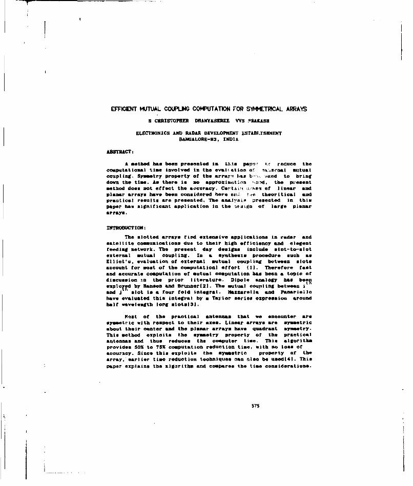
EFFICIENT MUTUAL COUPLING COMPUTATION FOR SYIMETRICAL ARRAY

S CERISTOPHER D&KNYASHREE VYS PRALASH

ELECTRONICS AND RADAR DEVELOPMENT 1ESTABLISfHENTBANGALORE-93, INDIA

ABSTRACT:

A method has been presented in ttl~s pavy.- t, reduce the

computational time involved in the evalluation a' 'w.senal mutualcoupling, Symmetry property at the arrarx has U, t•acd to bringdown the time. As there is no approxiuvition ,zrvd. the presentmethod does not effect the aocuracy. CertLci %3sfea of linear andplanar arrays have been considereda here mn; ýae theoritical andpractical results are presented. The analyzei presented in thispaper has significant application in the Aeign of large planararrays.

INTRODUCTION:

The slotted arrays find extensive applications in rader andsatellite communications due to their high efficiency and olegentfeeding network. The present day designs include slot-to-slotexternal mutual coupling. In a synthesis procedure such as

Elliot's, evaluation of external mutual coupling between slot*account for most of the computationl effort (Il. Therefore fastand accurate computation of mutual computation has been a topic of

discussion in the prior literature. Dipole analogy has be aemployrd by Hanson and Brunner[21. The mutual coupling between i

and j slot is a four told integral. Nazzarella and Panariello

have evaluated this integral by a Taylor series expression aroundhalf wavelength lorg slots[31.

Most of the practical antennas that we encounter aresymmetric with respect to their axes. Linear arrays are symmetricabout their center and the planar arrays have quadrant symmetry.

This method exploits the symmetry property of the practicalantennas and thus reduces the computer time. This algorithmprovides 50% to 75% computation reduction time, with no loss ofaccuracy. Since this exploits the symmetric property of thearray, earlier time reduction techniques oan also be used(41. This

paper explains the algorithm and compares the time considerations.

575

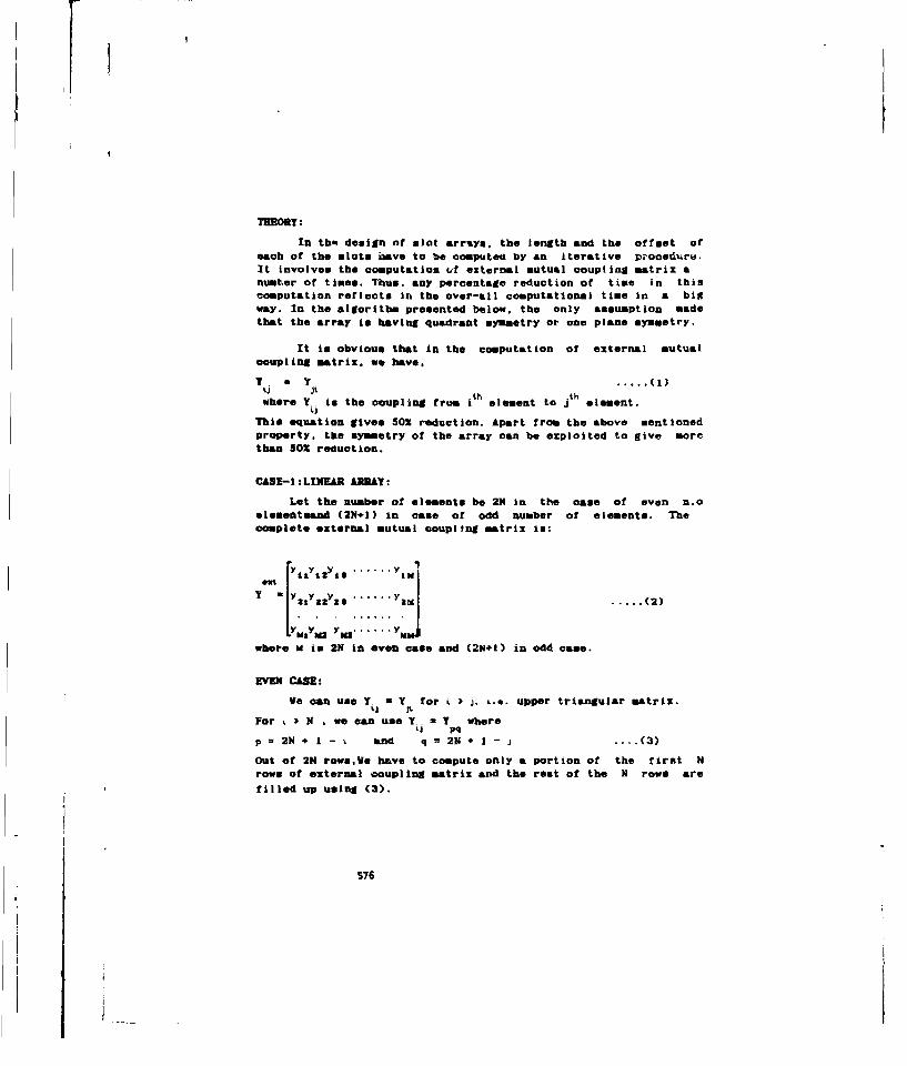
THEORY:

In th" design of slot arrsys, the length and the offset ofeach of the sotse cave to be computed by an iterative p0oeZrw.

t involves the computation ,f external mutual coupling matrix anumter of times. Thus. any percentage reduction of time in thiscomputation reflects in the over-all computational time in a bigway. In the algorithm presented below, the only assumption madethat the array is having quadrant symmetry or one plane symmetry.

It is obvious that In the computation of external mutualcoupling matrix, we have.

T _ . ....... (1)

where Y.. Is the coupling from I element to j element.Li

This equation gives 50% reduction. Apart from the above mentionedproperty, the symmetry of the array can be exploited to give morethan 50% reduction.

CASE-I :LINEAR ARRAY:

Let the number of elements be 2N in the case of even n.oelementmand (2N+I) in case of odd number of elements. Thecomplete external mutual coupling matrix is:

Y11 Y L.Ia...

ext y . . . M1

Y21YX|22 ...... Y %. .(2)

LYMtYM2 YNA ...... Y UN"

where m is 2N in even case and (2K+0) in odd came.

EVEN CAS:

Ve can use Y. = Y.. for . ) j. i.e. upper triangular matrix.

Fork 3)N , wecanusieY,•Y whereUJ pqp = 2N + I -, and q = 2N + I - j .... (3)

Out of 2N rowsae have to compute only a portion of the first Nrows of external coupling matrix and the rest of the N rows are

filled up using (3).

576

ODD CASE:

We can use Y Y , fort j.'a JL

For L. - (N+1)Sad j >(N-.2) and for i 1 (N4I)andl5j _(2N+÷)

We use. Y Y ¥ where p = 2N+ 2- and q z 2N + 2 -j.

(4)

CASE-2- PLANAR ARRAY:

EVEN CASE:

Lot the number of elements be N1. The complete coupling

matrix will be of (NZ.N) size. We have,

tj pq

For 1 -< j - N2 .

if (N.K 4 N/2) < ý < N(K+1); for K 0,2......(N-1)

then p = (N.K+l) + (N.K * N) -

q = (N+1) + 2(L - O)N - j

for (L.N*I-N) -5 j < L.N for L = 1.2.3. .. N

else

if (N2/2 + K.N) • L :5 (NZ1/2+N(+1)) for I - 0,1.2 .... ,(N/2-1)

then p = i - 2.K.N - N

q - 2.N.L + N(N+i) ..... (5)

Those elements not covered by (5) are to be computed. The

numbering of the elements 1 done from left to right and too to

bottom as shown in Fig.le. For a typical case of. 16 element planar

array, the elements for which mutual coupling integral has to be

evaluated is shown in Fig.Ic. Even for theme elements, only a

portion of the row elements have to be computed.The equations for

Odd number of elements and one plane symmetry are not presented

here an they are simple extension of the above mentioned cases.

Even though the equations appear to be complex, they are quite

easy to program.

577

RESULTS-:

For a Linear slot array of N elements, the Time ReductionCode (TRC) is implemented by using an array 1ck-ek(NN) of integertype. If Icbek(ij) a I then that particular element of couplingmatrix has to be Computed and if lohek(i.j) a 0, it need not beocaputmd The percentage saving in computatic time for evennumber of elements, computed using E.(.3) is ua in Fig.2, Acomparision in made between tueoritical data , the practicaldata which considers the time taken to run the time reductioncode. In Fig.3, for the case of odd number f elements.the timereduction (S) is presented as a function of .,umber of elements ofthe lir~ear arzay. To compute the mutual coupling between elements.the equations derived in 141 have been used. In the case of Planararray, the time reduction is presented In Fig.4. The Quadrantsymmetry as well an lif-plane symmetry have been shown. For atrivial came of 4 element planar array, quadrant symmetry andRalf-plane symmetry are one and same. The practical results takeninto consideration the finite run Lime of TRC are presented. Eventhough, the run time of TRC is significant, the over-all timereduction is considerable as can be visualized. All the programs

are written in Fortran and run on 386 machine.

CONCLUSION:

A method has been presented to design slot arrays with rapidcomputation of mutual coupling in the linear and planar cases. Asthere are no assumptions made on the element properties Itself.there is no loss of accuracy. It is found that the computationaltime is dependent on how efficiently the equations are programed.

The difference between the theoritical complitational time and thetime taken practically is attributed to the run time of theequations given in this paper.

REERNCS:

(11 R.S.Elliot.'An Improved Design Procedure for small Arrays ofShunt Slots,. IEEE TransAntenna Propagat., vol.3l.Jan.1983,pp.48-53.

(21 R.C.hansen and G.Brunner.'Dipole Mutual Impedance for Design

of Slot Arrays', Microwave Journal.vol.22, Dec.1979. pp.54-56.131 4azzarella and G.Panariello."Fast computation of Mutual

coupling in Slot Arrays.'Nicrowave Journal,vol.31.June 1988,pp.102-196.

141 S.R.Rengarajan and E.Gabrelian, :Efficient and Accurate

Evaluation of External mutual Coupling Betveen Compound Broad

Wall Slots.' IEEE Tran. Antenna Propagat.,vol. 40.June

1992, pp.733-737.

578

1 2 3 4 5 0 7 9

x x X x 0 a 0 0

Fig.(Ia) Symetric Linear Array with Even Number of Elements,

0 1,2 1,3 L,4 o 1,2 1.2 1.4

0 o Zal %,4 0 0 2.3 0

0 0 a 3,4 0 0 0 0

0 0 0 o 0 0 0 0

Using % 2 yV only. Using presen method,

FiS.(lb) Compariuion between Coupling Matrices using present

method and Uprer Triangular matrix for 4 eloment Linear Array.

a 2 2 4

-- Laamenta L.obe cowP&td.x x 0 0

9 10 t1 i 2 0 - RIOYnts not tob. computed.

0 0 0 0

Is 14 15 t1

0 0 0 0

Fig.(lc) Quadrant Symmetric Planar Array with 16 Elements.

579

oes

oE

W

0 LUG

a0 E

E I-S 0

0 0 0 0Z 0 0

0 0 0 0 0 0 0

awlij UOI;D~ndwoo ui 6U!ADS %

les

0.2

*- E

00uv~~U 0 Pz ,

n

I-a..

0 0 0 0 0 0 0 0 9oi 6 6 i A 0 m 0

r- r-. CD (0 LO LSW~uj !ouo!joifldWuo: Ul BUlArDS z

E E.

0 v

I C

E ~0 c

I E <C:

> 0tw I--a-

'awil IOU010OfLdWO U, 6U!ADS 19

583

VP . Vcbrnm P

Aflal, .J VI-W ~ Cotimen, A. VP-1S Frads, P.M. VPI-2Abedl, M. VIP-IS111 Col~lni, T. VP-SN Fro"t, .X VP-lAl-NlculI, tO. V11-142 Catonflokitnle E.D. VPI-AA Gellowa, AL. V1'-475Mimpach, S.D. ViI-252 Courit"e, C. V~i-220 Goo, &. V-m

Anflamehu, M.T.. VP-SO0 CAin, BA.R VI-144 GOwSmd, P. VI-473, 478Andarmh, 04J. VN-Si.S8S,4i4 Owk, T. VIP-45 Genes,.1. VII-56Andarsuan. t.V. VI-400" iatsR. VI-41E1 Ga1 , & A Vt-IS?Aanuwm. RdJ. fl-iS OWls. O.P. V11111111S G0. LOA Vt-ISOArchouflaA, S. V14a, Vu1-1121 Cmont JFA VI-70 WhetL It vt-sMAfyin, A.M VP-SO?1 dokOt, J.T. VI-SIS1 Whe. k VIP-ANAvorbust. S. VIP-IS4 0.1k..e, F. VP-IS?11 Gbow , A.W. ViP-d"AM. A. Vt-lOS CwAno, C. Vt-SW Gonc. M. Vt-I20Bodge, ILL VIP-016 Deans, T. VI-IS?1, VA-Si Godial, M.A, VP-lO5B".e D.C. VI-51S Ohenymflve VI-S75 Gogglns. P.M. VIP-353ianaidiag. K. VIP-SSS 243 Dckl, Gd. Vt-I SO Gong, J. VI-203aHenna, Ad.' VP-2t Ciloaw, 0. VIP-Si0 GoolWe. P.M. VII-iSadiner, F.L VIP-4i4 Dreulil J. %IP-410. 417 Gordon. L VIP-AS

tlr, A. VIP-ISI Dudka. V. VIP-1SO Gordlon, AK. VP-SOSBkic it, J. VP-2 Ealb. J. VU1-S7 GOctod, .K. VIP-SOSslodiar. S. vt-no Eil, E.M. VP-K? Granl. A. Vt-BOABohar, .A. VP-Bid Eiulwmbni, A.Z. VIP-S94 OurSi, T. VP-24SBonhot. LM. VIP-303 El-Motel. FMA Vt-S5, Miner, C. VIP-SOSean, ftC. VN-173 VII-120 ueman. P.M. VI-SOSRerglia. 0. viP-SOS EklerV. E. VP-SO7 Herb, J.M. VP"15BraimJ.f VP-1t Ellmona.. F. Vt-SO? Hadcmw. .B. VP-SO?are". J. vI-271 Eblot P. VP-SOS Maap, R. Vt-rn6ShlNghra. S. VI-473 English. E. Vt-AS eutiall, M. V11-d2dSflul, 0.4. Vtl-1OS, 312 Engquist,. B 3 VtSHedmierno. C.D. VI-3?6tarktuoldmr, RJ-. VIP-244 Erdlay, T. Vt-271 PHideo n. L VI-4SSSiuemen, Rh. VP-AG Erwin, JAt VPIA 12 1 menil M. VP-7lStart S.C. VIP-32S Emw Ie C. Vt-ed Mmevoolm F. VP-IS?Calma. V. VPP-SO1 Ems., K VI-31G Mmmi.. M.A. VIP-I6SConnin, F.K VSl-96 Evena. J.A. VIP-SO Nooelor W.J.R. VP-82t94.Ceuckone d.K. VN-SO Fog, J. VIP-SO SO VIP-54OCavaPlint, F. VIIaO Fur, F-G VIP-SOS No~eS. At. VIP-SOUSACiell 4. Vt-SOS Farta, S. VP-S Hong, W. VP-171Citwntedin. K. V04-S,228 Fedoinve. TX. VIP-SO Hseu, M. VIP-77UChtes, Y. VIP-S Foem. hA.J Vt-ASS Ho. Q Vt-SM5Cheng. Z. VP-SM Fbumr, S. VA-fl, SI H~oing. T. V4P-110,417Coil-Orgon, Y.& VP-SI Fly. Kt VP-SN Holmes JA. VA-106Clupliephr, a. Vt-fl, VIP-lBS Fobblelma K. VIP-SO Hosnbtlger. FP. VIP-32SClouds, S. VP-1S3 Foemu. PAR. Vt-SW Irntdisi W.A. VII-43ACollar- E.L VPP-?O.?S,0O.S1,

396.409g

AUTH4OR irnX (Cwt)

Whgw,~a N. VN-SIS Uay*. K.U. VA 156 Paer. MJ, VII-364Woiwsdv. M.F, VI.473. 473 Lipp~mt, W.L VS 524 Psknys, R. VA-SIPPmiwsav, A.E. VII-335 Liu,. Y. Vt-447, VII-300. 31 Pam.t1 A.K VSI-1

Joduim. R.M, VN4U Uu. Y.W. VSI-7I Pmuc, Ft. VI-376Jsmlc. R.O. Vt443 Lu. Z. Vt-MS PuI~i*. P.M. V11.2"4, 275JAwI~d, L VS-Big L"W'. J.C. VS-3M Peow*Ve. C. VIt-20

Ahinmngn &. VS-dO LUAam R. J. VI-2ll.467,4M. Powaye. CV-. V"86UJoempi, N.M. VA-i Vmoo Pw.acmS. A.V, VII-336Ksau. 0. VS-3M VA-did Lid. J. VS- P"iW, W.F. VA-ISO.403Kopbwrvic. LV. VMWBO LUmir', T. V140O Patm~, &S. VI-371Koly. J.L V"-l SMW-I -, C.J. V"747 P.eb@4n. &.F. VI-144Kamis. H. VS-&W VtAsusm. N.J. VO-4dl Ptarpcoi4Oa. P. Vt-3KmA uS. LC. VI-lW Win. N. VII-MS P"u, 0, A, VI-352Ke"~, O.L ViS-dI M0,11 . N. VA-1SO PWartaa. J.H. VI-I50Khwahe*ka 8. VA-I3 osm1u, a.S. VA-403 Phat-May. .J. VH.459Kim. J. VS-40 mwaqow,~ M. VA-as P.5W, N. VI.135Kulr, P. VS-B04 Modipel-bftsd'an. LN. VW-N? Pb"m. 0. VI-ISSKOWer'nIAV. P. V6A-143 Mmt, K.K VS-17t Pop.. ANV. VII-471Kapplia. Y.V. V"4-d3 mola. H. VA-Uti Porte, S.J wS-7OKwd. W VIS-In Moo@&. S. VN-53 Prmkah. WVS VI-575KwWu. S.T. VW=SI MUin, .K. VN-t58Ifl Potutt, W. Vt-SIKs"mgwmu, 0. A, VI-U6 MaWhL S. N. VS-WI Piarjser, LO. VS-45Ks~u- 34J VU-BS. M hmi & Vt-I?, Put'~. J.M, VHS-2N7VA~i. A. VI"-7l Maim. N. VN-l0 RMauiw. TA V11405Kum"tia. H. VS-hA Siaf. P. Vt-1I Rawnat. O.M. VI-234Lowmtfmt. F.M. VS2IS Mma uIN. D.H. VtS-4'S RaidaSS. W.M. VIS-52BLUngiau.M.B. Vt-de7 Mm1- T.G. VA-SOS Ram S.M. VII-502Lu~gm. s. VSS-U -, rap A.M. VS-256 NRa or, C.kI. VS-241Lm~ptme . K.J. ViS-ISO Manag. M. Vt-29I Nmurn. 0. VI-12,.VIS.25gLUsu, C.L W=SI Nolm , E.M. WS152 Ra"de, C.E. V"-4Linq,. S. Vt-lO Nw.mVrgh. F. VI-ASO Rule. A. VS-ISOLoebmt. J5. VtS-5 iSluoe . L Vt4de Rigp, LS. VS-7l, N5

Le". J. Vt-179 111d,11 mU. VA-I Roca -', J. VII-372LftoN. VS-SIB la'-' . VS-IS? Rme. P. Vt-ddLe. &W. VA-di No""a. J. Vw=S NukhSon. V. Vt-ISLooma. W. VS-IP7 Nlkmt A. VHS-IS Raew. U. VSS4OLmubhg, Em. VH-M7 Owt~u. m. Vt- RAeW 0 C. Vt-SOLoefteM. J.0. VNS-72 0Smmr V. Vt-45 Rwmie. P.R. VW264Lmumd* . P. VS-1I0.136 Obeen. N.G. VtS-ddS 457 Noumeele. S.R. VIS-NO. 4W3

Leein. N.J. VA-NO Oseegua N.A VS-lBS RunW.d L VN-alLWNIdvS U. Vt-40 Oilhr. a. VS-S Rinse. P. VIS-571. 501LW", C.H. VA-dC, 417 Ovod. V. VIS-356, 343 Rym,. P. VS-129. 0i-=O

AUTlHOR WdEX (COKII

8adayappmi. P. VU-316 Vilwy, O.J. VI-ISOSadler. V VI-SU V~iogradov. AN. VII-473Sanhlago. D.G. VI-It9 Valelkis J.L VI.203, 300Schindel. R. VI-Wi, VII-320.424 yoa., D. VII-220Schffhdh. R. VII-576 Walker, F.E. 1'11-238Schukantz. J.H. VI-389 Wandzura, S. M VI-1gSchimb". J1. VIA-25 Waing, R.T. VI-159Sega. R. VL38O Wond. 0.0. VI-7Shelth. . Vl1U3 Warren. D.E. VW-352Shmbandy, K. VI-79 WOWal H. V11.601Slodrlmi KFA VU-86 Wealshaar. A. VII-75Bk'mg, AKL VII.165 Wo. D.P. VII-62Sldinn,w J.P. Vhl-SIO Wentwodi, 0. Vfl.372Smfhlli C.Rt VlI-914W Ww~antun, S.M. VyB-hZSo. P.P.M VWS-46 Werner. 0.H. V11428. 106St. John, R. ViI 554 Warnr. P.L Vl-96, 106Swen~er, N. VI-316 Wesson, PA1 VIAI

Sloyansov. &J. V1,327 Wheeler, .L. VB-415. Vll-200SkoyAnv. Y.J. Vl.32 Whole"a, C.S. VII-536Sbidftb, K W. VW- Whielege W.P. Vl-392, VII-536Slluchly . M. Vfl-492. 495 Wh~e. M. YB-478

vichov. Y. VII-ISO Wift, LT. VI-496Tallow.. A. VO-45g. VIB-2 Wilson, K.U. VI-327Tarn, D. V!1-372 Wriedt. T. VII-M4Tertyor.Ga. VII-457 Wu. M. VI-33STaylor, C.D. Vll4Q24 Wu. S, VlISSTeizuahl. A.J. VP-34S, 436 Wu. W. VII-494Thiele, E.T. VI-459 Wu, Z VIP-30, 38Thiele. G.A. V"-.25 Xl, W. VU-492, 495Tie, G VI-552, w4j Yanchan. G. Vl.553, SW0TiorJr-o. cld A. VWd-113 Ye. C. VI-335Trusim-n, C.W. VI-326. VII-53 Yermmi, A. VII-163Teeng, H. VlP-27 Young, J. Vl-271Tokhcpouloa. AP. VNd-34 Yu, C.L. VIP-24TuchknM, Y. VIP-150 Zalolo. EX. VWP320Tyrun, AM. VII-113 Zen4.wlny, V.M. Vll-343Tyflyahvilam. E. VII-193 zhong. 0. V142Vali, a. VI-laso Zook. BLi. VI-240VaiVoowtime, B(L VI-426 Zywlen, M.L VA-212Viewto, V. VBII-50