Computational Physics - Get support
563
Morten Hjorth-Jensen Computational Physics Lecture Notes Fall 2015 August 2015 Department of Physics, University of Oslo
-
Upload
khangminh22 -
Category
Documents
-
view
0 -
download
0
Transcript of Computational Physics - Get support

Morten Hjorth-Jensen
Computational Physics
Lecture Notes Fall 2015
August 2015
Department of Physics, University of Oslo


Preface
So, ultimately, in order to understand nature it may be necessary to have a deeper understandingof mathematical relationships. But the real reason is that the subject is enjoyable, and although wehumans cut nature up in different ways, and we have different courses in different departments, suchcompartmentalization is really artificial, and we should take our intellectual pleasures where we findthem. Richard Feynman, The Laws of Thermodynamics.
Why a preface you may ask? Isn’t that just a mere exposition of a raison d’etre of anauthor’s choice of material, preferences, biases, teaching philosophy etc.? To a large extent Ican answer in the affirmative to that. A preface ought to be personal. Indeed, what you willsee in the various chapters of these notes represents how I perceive computational physicsshould be taught.
This set of lecture notes serves the scope of presenting to you and train you in an algorith-mic approach to problems in the sciences, represented here by the unity of three disciplines,physics, mathematics and informatics. This trinity outlines the emerging field of computa-tional physics.
Our insight in a physical system, combined with numerical mathematics gives us the rulesfor setting up an algorithm, viz. a set of rules for solving a particular problem. Our under-standing of the physical system under study is obviously gauged by the natural laws at play,the initial conditions, boundary conditions and other external constraints which influence thegiven system. Having spelled out the physics, for example in the form of a set of coupledpartial differential equations, we need efficient numerical methods in order to set up the finalalgorithm. This algorithm is in turn coded into a computer program and executed on availablecomputing facilities. To develop such an algorithmic approach, you will be exposed to severalphysics cases, spanning from the classical pendulum to quantummechanical systems. We willalso present some of the most popular algorithms from numerical mathematics used to solvea plethora of problems in the sciences. Finally we will codify these algorithms using some ofthe most widely used programming languages, presently C, C++ and Fortran and its mostrecent standard Fortran 20081. However, a high-level and fully object-oriented language likePython is now emerging as a good alternative although C++ and Fortran still outperformPython when it comes to computational speed. In this text we offer an approach where onecan write all programs in C/C++ or Fortran. We will also show you how to develop largeprograms in Python interfacing C++ and/or Fortran functions for those parts of the programwhich are CPU intensive. Such an approach allows you to structure the flow of data in a high-level language like Python while tasks of a mere repetitive and CPU intensive nature are leftto low-level languages like C++ or Fortran. Python allows you also to smoothly interface yourprogram with other software, such as plotting programs or operating system instructions.
1 Throughout this text we refer to Fortran 2008 as Fortran, implying the latest standard.
v

vi Preface
A typical Python program you may end up writing contains everything from compiling andrunning your codes to preparing the body of a file for writing up your report.
Computer simulations are nowadays an integral part of contemporary basic and applied re-search in the sciences. Computation is becoming as important as theory and experiment. Inphysics, computational physics, theoretical physics and experimental physics are all equallyimportant in our daily research and studies of physical systems. Physics is the unity of theory,experiment and computation2. Moreover, the ability "to compute" forms part of the essen-tial repertoire of research scientists. Several new fields within computational science haveemerged and strengthened their positions in the last years, such as computational materialsscience, bioinformatics, computational mathematics and mechanics, computational chemistryand physics and so forth, just to mention a few. These fields underscore the importance of sim-ulations as a means to gain novel insights into physical systems, especially for those caseswhere no analytical solutions can be found or an experiment is too complicated or expensiveto carry out. To be able to simulate large quantal systems with many degrees of freedomsuch as strongly interacting electrons in a quantum dot will be of great importance for futuredirections in novel fields like nano-techonology. This ability often combines knowledge frommany different subjects, in our case essentially from the physical sciences, numerical math-ematics, computing languages, topics from high-performace computing and some knowledgeof computers.
In 1999, when I started this course at the department of physics in Oslo, computationalphysics and computational science in general were still perceived by the majority of physi-cists and scientists as topics dealing with just mere tools and number crunching, and not assubjects of their own. The computational background of most students enlisting for the courseon computational physics could span from dedicated hackers and computer freaks to peoplewho basically had never used a PC. The majority of undergraduate and graduate studentshad a very rudimentary knowledge of computational techniques and methods. Questions like’do you know of better methods for numerical integration than the trapezoidal rule’ were notuncommon. I do happen to know of colleagues who applied for time at a supercomputingcentre because they needed to invert matrices of the size of 104× 104 since they were usingthe trapezoidal rule to compute integrals. With Gaussian quadrature this dimensionality waseasily reduced to matrix problems of the size of 102× 102, with much better precision.
More than a decade later most students have now been exposed to a fairly uniform intro-duction to computers, basic programming skills and use of numerical exercises. Practicallyevery undergraduate student in physics has now made a Matlab or Maple simulation of forexample the pendulum, with or without chaotic motion. Nowadays most of you are famil-iar, through various undergraduate courses in physics and mathematics, with interpretedlanguages such as Maple, Matlab and/or Mathematica. In addition, the interest in scriptinglanguages such as Python or Perl has increased considerably in recent years. The modern pro-grammer would typically combine several tools, computing environments and programminglanguages. A typical example is the following. Suppose you are working on a project which de-mands extensive visualizations of the results. To obtain these results, that is to solve a physicsproblems like obtaining the density profile of a Bose-Einstein condensate, you need howevera program which is fairly fast when computational speed matters. In this case you would most
2 We mentioned previously the trinity of physics, mathematics and informatics. Viewing physics as the trinityof theory, experiment and simulations is yet another example. It is obviously tempting to go beyond thesciences. History shows that triunes, trinities and for example triple deities permeate the Indo-Europeancultures (and probably all human cultures), from the ancient Celts and Hindus to modern days. The ancientCelts revered many such trinues, their world was divided into earth, sea and air, nature was divided in animal,vegetable and mineral and the cardinal colours were red, yellow and blue, just to mention a few. As a curiousdigression, it was a Gaulish Celt, Hilary, philosopher and bishop of Poitiers (AD 315-367) in his work DeTrinitate who formulated the Holy Trinity concept of Christianity, perhaps in order to accomodate millenia ofhuman divination practice.

Preface vii
likely write a high-performance computing program using Monte Carlo methods in languageswhich are tailored for that. These are represented by programming languages like Fortranand C++. However, to visualize the results you would find interpreted languages like Matlabor scripting languages like Python extremely suitable for your tasks. You will therefore end upwriting for example a script in Matlab which calls a Fortran or C++ program where the num-ber crunching is done and then visualize the results of say a wave equation solver via Matlab’slarge library of visualization tools. Alternatively, you could organize everything into a Pythonor Perl script which does everything for you, calls the Fortran and/or C++ programs andperforms the visualization in Matlab or Python. Used correctly, these tools, spanning fromscripting languages to high-performance computing languages and vizualization programs,speed up your capability to solve complicated problems. Being multilingual is thus an advan-tage which not only applies to our globalized modern society but to computing environmentsas well. This text shows you how to use C++ and Fortran as programming languages.
There is however more to the picture than meets the eye. Although interpreted languageslike Matlab, Mathematica and Maple allow you nowadays to solve very complicated problems,and high-level languages like Python can be used to solve computational problems, compu-tational speed and the capability to write an efficient code are topics which still do matter.To this end, the majority of scientists still use languages like C++ and Fortran to solve sci-entific problems. When you embark on a master or PhD thesis, you will most likely meetthese high-performance computing languages. This course emphasizes thus the use of pro-gramming languages like Fortran, Python and C++ instead of interpreted ones like Matlabor Maple. You should however note that there are still large differences in computer time be-tween for example numerical Python and a corresponding C++ program for many numericalapplications in the physical sciences, with a code in C++ or Fortran being the fastest.
Computational speed is not the only reason for this choice of programming languages. An-other important reason is that we feel that at a certain stage one needs to have some insightsinto the algorithm used, its stability conditions, possible pitfalls like loss of precision, rangesof applicability, the possibility to improve the algorithm and taylor it to special purposes etcetc. One of our major aims here is to present to you what we would dub ’the algorithmicapproach’, a set of rules for doing mathematics or a precise description of how to solve aproblem. To device an algorithm and thereafter write a code for solving physics problemsis a marvelous way of gaining insight into complicated physical systems. The algorithm youend up writing reflects in essentially all cases your own understanding of the physics andthe mathematics (the way you express yourself) of the problem. We do therefore devote quitesome space to the algorithms behind various functions presented in the text. Especially, in-sight into how errors propagate and how to avoid them is a topic we would like you to payspecial attention to. Only then can you avoid problems like underflow, overflow and loss ofprecision. Such a control is not always achievable with interpreted languages and cannedfunctions where the underlying algorithm and/or code is not easily accesible. Although wewill at various stages recommend the use of library routines for say linear algebra3, ourbelief is that one should understand what the given function does, at least to have a mereidea. With such a starting point, we strongly believe that it can be easier to develope morecomplicated programs on your own using Fortran, C++ or Python.
We have several other aims as well, namely:
• We would like to give you an opportunity to gain a deeper understanding of the physicsyou have learned in other courses. In most courses one is normally confronted with simplesystems which provide exact solutions and mimic to a certain extent the realistic cases.Many are however the comments like ’why can’t we do something else than the particle in
3 Such library functions are often taylored to a given machine’s architecture and should accordingly run fasterthan user provided ones.

viii Preface
a box potential?’. In several of the projects we hope to present some more ’realistic’ casesto solve by various numerical methods. This also means that we wish to give examples ofhow physics can be applied in a much broader context than it is discussed in the traditionalphysics undergraduate curriculum.
• To encourage you to "discover" physics in a way similar to how researchers learn in thecontext of research.
• Hopefully also to introduce numerical methods and new areas of physics that can be stud-ied with the methods discussed.
• To teach structured programming in the context of doing science.• The projects we propose are meant to mimic to a certain extent the situation encountered
during a thesis or project work. You will tipically have at your disposal 2-3 weeks to solvenumerically a given project. In so doing you may need to do a literature study as well.Finally, we would like you to write a report for every project.
Our overall goal is to encourage you to learn about science through experience and by askingquestions. Our objective is always understanding and the purpose of computing is furtherinsight, not mere numbers! Simulations can often be considered as experiments. Rerunninga simulation need not be as costly as rerunning an experiment.
Needless to say, these lecture notes are upgraded continuously, from typos to new in-put. And we do always benefit from your comments, suggestions and ideas for making thesenotes better. It’s through the scientific discourse and critics we advance. Moreover, I havebenefitted immensely from many discussions with fellow colleagues and students. In partic-ular I must mention Hans Petter Langtangen, Anders Malthe-Sørenssen, Knut Mørken andØyvind Ryan, whose input during the last fifteen years has considerably improved theselecture notes. Furthermore, the time we have spent and keep spending together on theComputing in Science Education project at the University, is just marvelous. Thanks somuch. Concerning the Computing in Science Education initiative, you can read more athttp://www.mn.uio.no/english/about/collaboration/cse/.
Finally, I would like to add a petit note on referencing. These notes have evolved overmany years and the idea is that they should end up in the format of a web-based learningenvironment for doing computational science. It will be fully free and hopefully represent amuch more efficient way of conveying teaching material than traditional textbooks. I have notyet settled on a specific format, so any input is welcome. At present however, it is very easyfor me to upgrade and improve the material on say a yearly basis, from simple typos to addingnew material. When accessing the web page of the course, you will have noticed that you canobtain all source files for the programs discussed in the text. Many people have thus writtento me about how they should properly reference this material and whether they can freelyuse it. My answer is rather simple. You are encouraged to use these codes, modify them,include them in publications, thesis work, your lectures etc. As long as your use is part of thedialectics of science you can use this material freely. However, since many weekends haveelapsed in writing several of these programs, testing them, sweating over bugs, swearing infront of a f*@?%g code which didn’t compile properly ten minutes before monday morning’seight o’clock lecture etc etc, I would dearly appreciate in case you find these codes of anyuse, to reference them properly. That can be done in a simple way, refer to M. Hjorth-Jensen,Computational Physics, University of Oslo (2013). The weblink to the course should also beincluded. Hope it is not too much to ask for. Enjoy!

Contents
Part I Introduction to programming and numerical methods
1 Introduction . . . . . . . . . . . . . . . . . . . . . . . . . . . . . . . . . . . . . . . . . . . . . . . . . . . . . . . . . . . . . . . 31.1 Choice of programming language . . . . . . . . . . . . . . . . . . . . . . . . . . . . . . . . . . . . . . . . . 51.2 Designing programs . . . . . . . . . . . . . . . . . . . . . . . . . . . . . . . . . . . . . . . . . . . . . . . . . . . . . 6
2 Introduction to C++ and Fortran . . . . . . . . . . . . . . . . . . . . . . . . . . . . . . . . . . . . . . . . . . . 92.1 Getting Started . . . . . . . . . . . . . . . . . . . . . . . . . . . . . . . . . . . . . . . . . . . . . . . . . . . . . . . . . 9
2.1.1 Scientific hello world . . . . . . . . . . . . . . . . . . . . . . . . . . . . . . . . . . . . . . . . . . . . . . 102.2 Representation of Integer Numbers . . . . . . . . . . . . . . . . . . . . . . . . . . . . . . . . . . . . . . . 15
2.2.1 Fortran codes . . . . . . . . . . . . . . . . . . . . . . . . . . . . . . . . . . . . . . . . . . . . . . . . . . . . . 182.3 Real Numbers and Numerical Precision . . . . . . . . . . . . . . . . . . . . . . . . . . . . . . . . . . . 19
2.3.1 Representation of real numbers . . . . . . . . . . . . . . . . . . . . . . . . . . . . . . . . . . . . . 202.3.2 Machine numbers . . . . . . . . . . . . . . . . . . . . . . . . . . . . . . . . . . . . . . . . . . . . . . . . . 22
2.4 Programming Examples on Loss of Precision and Round-off Errors . . . . . . . . . . . 242.4.1 Algorithms for e−x . . . . . . . . . . . . . . . . . . . . . . . . . . . . . . . . . . . . . . . . . . . . . . . . . 242.4.2 Fortran codes . . . . . . . . . . . . . . . . . . . . . . . . . . . . . . . . . . . . . . . . . . . . . . . . . . . . . 272.4.3 Further examples . . . . . . . . . . . . . . . . . . . . . . . . . . . . . . . . . . . . . . . . . . . . . . . . . 30
2.5 Additional Features of C++ and Fortran . . . . . . . . . . . . . . . . . . . . . . . . . . . . . . . . . . 322.5.1 Operators in C++ . . . . . . . . . . . . . . . . . . . . . . . . . . . . . . . . . . . . . . . . . . . . . . . . . 322.5.2 Pointers and arrays in C++. . . . . . . . . . . . . . . . . . . . . . . . . . . . . . . . . . . . . . . . . 342.5.3 Macros in C++ . . . . . . . . . . . . . . . . . . . . . . . . . . . . . . . . . . . . . . . . . . . . . . . . . . . 362.5.4 Structures in C++ and TYPE in Fortran . . . . . . . . . . . . . . . . . . . . . . . . . . . . . 37
2.6 Exercises . . . . . . . . . . . . . . . . . . . . . . . . . . . . . . . . . . . . . . . . . . . . . . . . . . . . . . . . . . . . . . . 39
3 Numerical differentiation and interpolation . . . . . . . . . . . . . . . . . . . . . . . . . . . . . . . . 453.1 Numerical Differentiation . . . . . . . . . . . . . . . . . . . . . . . . . . . . . . . . . . . . . . . . . . . . . . . . 45
3.1.1 The second derivative of exp(x) . . . . . . . . . . . . . . . . . . . . . . . . . . . . . . . . . . . . . 493.1.2 Error analysis . . . . . . . . . . . . . . . . . . . . . . . . . . . . . . . . . . . . . . . . . . . . . . . . . . . . 58
3.2 Numerical Interpolation and Extrapolation . . . . . . . . . . . . . . . . . . . . . . . . . . . . . . . . . 603.2.1 Interpolation . . . . . . . . . . . . . . . . . . . . . . . . . . . . . . . . . . . . . . . . . . . . . . . . . . . . . 613.2.2 Richardson’s deferred extrapolation method . . . . . . . . . . . . . . . . . . . . . . . . . 64
3.3 Classes in C++ . . . . . . . . . . . . . . . . . . . . . . . . . . . . . . . . . . . . . . . . . . . . . . . . . . . . . . . . . 653.3.1 The Complex class . . . . . . . . . . . . . . . . . . . . . . . . . . . . . . . . . . . . . . . . . . . . . . . . 673.3.2 The vector class . . . . . . . . . . . . . . . . . . . . . . . . . . . . . . . . . . . . . . . . . . . . . . . . . . . 72
3.4 Modules in Fortran . . . . . . . . . . . . . . . . . . . . . . . . . . . . . . . . . . . . . . . . . . . . . . . . . . . . . . 863.5 How to make Figures with Gnuplot . . . . . . . . . . . . . . . . . . . . . . . . . . . . . . . . . . . . . . . . 903.6 Exercises . . . . . . . . . . . . . . . . . . . . . . . . . . . . . . . . . . . . . . . . . . . . . . . . . . . . . . . . . . . . . . . 92
ix

x Contents
4 Non-linear Equations . . . . . . . . . . . . . . . . . . . . . . . . . . . . . . . . . . . . . . . . . . . . . . . . . . . . . . 954.1 Particle in a Box Potential . . . . . . . . . . . . . . . . . . . . . . . . . . . . . . . . . . . . . . . . . . . . . . . . 954.2 Iterative Methods . . . . . . . . . . . . . . . . . . . . . . . . . . . . . . . . . . . . . . . . . . . . . . . . . . . . . . . 964.3 Bisection . . . . . . . . . . . . . . . . . . . . . . . . . . . . . . . . . . . . . . . . . . . . . . . . . . . . . . . . . . . . . . . 984.4 Newton-Raphson’s Method . . . . . . . . . . . . . . . . . . . . . . . . . . . . . . . . . . . . . . . . . . . . . . . 994.5 The Secant Method . . . . . . . . . . . . . . . . . . . . . . . . . . . . . . . . . . . . . . . . . . . . . . . . . . . . . . 103
4.5.1 Broyden’s Method . . . . . . . . . . . . . . . . . . . . . . . . . . . . . . . . . . . . . . . . . . . . . . . . . 1054.6 Exercises . . . . . . . . . . . . . . . . . . . . . . . . . . . . . . . . . . . . . . . . . . . . . . . . . . . . . . . . . . . . . . . 106
5 Numerical Integration . . . . . . . . . . . . . . . . . . . . . . . . . . . . . . . . . . . . . . . . . . . . . . . . . . . . . 1095.1 Newton-Cotes Quadrature . . . . . . . . . . . . . . . . . . . . . . . . . . . . . . . . . . . . . . . . . . . . . . . 1095.2 Adaptive Integration. . . . . . . . . . . . . . . . . . . . . . . . . . . . . . . . . . . . . . . . . . . . . . . . . . . . . 1155.3 Gaussian Quadrature . . . . . . . . . . . . . . . . . . . . . . . . . . . . . . . . . . . . . . . . . . . . . . . . . . . . 116
5.3.1 Orthogonal polynomials, Legendre . . . . . . . . . . . . . . . . . . . . . . . . . . . . . . . . . . 1195.3.2 Integration points and weights with orthogonal polynomials . . . . . . . . . . . 1215.3.3 Application to the case N = 2 . . . . . . . . . . . . . . . . . . . . . . . . . . . . . . . . . . . . . . . 1235.3.4 General integration intervals for Gauss-Legendre . . . . . . . . . . . . . . . . . . . . . 1245.3.5 Other orthogonal polynomials . . . . . . . . . . . . . . . . . . . . . . . . . . . . . . . . . . . . . . 1255.3.6 Applications to selected integrals . . . . . . . . . . . . . . . . . . . . . . . . . . . . . . . . . . . 126
5.4 Treatment of Singular Integrals . . . . . . . . . . . . . . . . . . . . . . . . . . . . . . . . . . . . . . . . . . . 1285.5 Parallel Computing . . . . . . . . . . . . . . . . . . . . . . . . . . . . . . . . . . . . . . . . . . . . . . . . . . . . . . 130
5.5.1 Brief survey of supercomputing concepts and terminologies . . . . . . . . . . . 1315.5.2 Parallelism . . . . . . . . . . . . . . . . . . . . . . . . . . . . . . . . . . . . . . . . . . . . . . . . . . . . . . . 1325.5.3 MPI with simple examples . . . . . . . . . . . . . . . . . . . . . . . . . . . . . . . . . . . . . . . . . 1345.5.4 Numerical integration with MPI . . . . . . . . . . . . . . . . . . . . . . . . . . . . . . . . . . . . 139
5.6 An Integration Class . . . . . . . . . . . . . . . . . . . . . . . . . . . . . . . . . . . . . . . . . . . . . . . . . . . . . 1435.7 Exercises . . . . . . . . . . . . . . . . . . . . . . . . . . . . . . . . . . . . . . . . . . . . . . . . . . . . . . . . . . . . . . . 147
Part II Linear Algebra and Eigenvalues
6 Linear Algebra . . . . . . . . . . . . . . . . . . . . . . . . . . . . . . . . . . . . . . . . . . . . . . . . . . . . . . . . . . . . . 1536.1 Introduction . . . . . . . . . . . . . . . . . . . . . . . . . . . . . . . . . . . . . . . . . . . . . . . . . . . . . . . . . . . . 1536.2 Mathematical Intermezzo . . . . . . . . . . . . . . . . . . . . . . . . . . . . . . . . . . . . . . . . . . . . . . . . 1546.3 Programming Details . . . . . . . . . . . . . . . . . . . . . . . . . . . . . . . . . . . . . . . . . . . . . . . . . . . . 157
6.3.1 Declaration of fixed-sized vectors and matrices . . . . . . . . . . . . . . . . . . . . . . . 1586.3.2 Runtime Declarations of Vectors and Matrices in C++. . . . . . . . . . . . . . . . . 1606.3.3 Matrix Operations and C++ and Fortran Features of Matrix handling . . . 162
6.4 Linear Systems . . . . . . . . . . . . . . . . . . . . . . . . . . . . . . . . . . . . . . . . . . . . . . . . . . . . . . . . . 1686.4.1 Gaussian Elimination . . . . . . . . . . . . . . . . . . . . . . . . . . . . . . . . . . . . . . . . . . . . . . 1706.4.2 LU Decomposition of a Matrix . . . . . . . . . . . . . . . . . . . . . . . . . . . . . . . . . . . . . . 1736.4.3 Solution of Linear Systems of Equations . . . . . . . . . . . . . . . . . . . . . . . . . . . . . 1776.4.4 Inverse of a Matrix and the Determinant . . . . . . . . . . . . . . . . . . . . . . . . . . . . . 1786.4.5 Tridiagonal Systems of Linear Equations . . . . . . . . . . . . . . . . . . . . . . . . . . . . . 185
6.5 Spline Interpolation . . . . . . . . . . . . . . . . . . . . . . . . . . . . . . . . . . . . . . . . . . . . . . . . . . . . . 1876.6 Iterative Methods . . . . . . . . . . . . . . . . . . . . . . . . . . . . . . . . . . . . . . . . . . . . . . . . . . . . . . . 189
6.6.1 Jacobi’s method . . . . . . . . . . . . . . . . . . . . . . . . . . . . . . . . . . . . . . . . . . . . . . . . . . . 1896.6.2 Gauss-Seidel . . . . . . . . . . . . . . . . . . . . . . . . . . . . . . . . . . . . . . . . . . . . . . . . . . . . . . 1906.6.3 Successive over-relaxation . . . . . . . . . . . . . . . . . . . . . . . . . . . . . . . . . . . . . . . . . 1916.6.4 Conjugate Gradient Method . . . . . . . . . . . . . . . . . . . . . . . . . . . . . . . . . . . . . . . . 192
6.7 A vector and matrix class . . . . . . . . . . . . . . . . . . . . . . . . . . . . . . . . . . . . . . . . . . . . . . . . 1946.7.1 How to construct your own matrix-vector class . . . . . . . . . . . . . . . . . . . . . . . 196
6.8 Exercises . . . . . . . . . . . . . . . . . . . . . . . . . . . . . . . . . . . . . . . . . . . . . . . . . . . . . . . . . . . . . . . 205

Contents xi
6.8.1 Solution . . . . . . . . . . . . . . . . . . . . . . . . . . . . . . . . . . . . . . . . . . . . . . . . . . . . . . . . . . 209
7 Eigensystems . . . . . . . . . . . . . . . . . . . . . . . . . . . . . . . . . . . . . . . . . . . . . . . . . . . . . . . . . . . . . . 2137.1 Introduction . . . . . . . . . . . . . . . . . . . . . . . . . . . . . . . . . . . . . . . . . . . . . . . . . . . . . . . . . . . . 2137.2 Eigenvalue problems . . . . . . . . . . . . . . . . . . . . . . . . . . . . . . . . . . . . . . . . . . . . . . . . . . . . 2137.3 Similarity transformations . . . . . . . . . . . . . . . . . . . . . . . . . . . . . . . . . . . . . . . . . . . . . . . 2147.4 Jacobi’s method . . . . . . . . . . . . . . . . . . . . . . . . . . . . . . . . . . . . . . . . . . . . . . . . . . . . . . . . . 2157.5 Similarity Transformations with Householder’s method . . . . . . . . . . . . . . . . . . . . . . 220
7.5.1 The Householder’s method for tridiagonalization . . . . . . . . . . . . . . . . . . . . . 2207.5.2 Diagonalization of a Tridiagonal Matrix via Francis’ Algorithm . . . . . . . . . 224
7.6 Power Methods . . . . . . . . . . . . . . . . . . . . . . . . . . . . . . . . . . . . . . . . . . . . . . . . . . . . . . . . . 2257.7 Iterative methods: Lanczos’ algorithm . . . . . . . . . . . . . . . . . . . . . . . . . . . . . . . . . . . . . 2267.8 Schrödinger’s Equation Through Diagonalization . . . . . . . . . . . . . . . . . . . . . . . . . . . 227
7.8.1 Numerical solution of the Schrödinger equation by diagonalization . . . . . 2307.8.2 Program example and results for the one-dimensional harmonic oscillator230
7.9 Exercises . . . . . . . . . . . . . . . . . . . . . . . . . . . . . . . . . . . . . . . . . . . . . . . . . . . . . . . . . . . . . . . 235
Part III Differential Equations
8 Differential equations . . . . . . . . . . . . . . . . . . . . . . . . . . . . . . . . . . . . . . . . . . . . . . . . . . . . . . 2438.1 Introduction . . . . . . . . . . . . . . . . . . . . . . . . . . . . . . . . . . . . . . . . . . . . . . . . . . . . . . . . . . . . 2438.2 Ordinary differential equations . . . . . . . . . . . . . . . . . . . . . . . . . . . . . . . . . . . . . . . . . . . 2448.3 Finite difference methods . . . . . . . . . . . . . . . . . . . . . . . . . . . . . . . . . . . . . . . . . . . . . . . . 245
8.3.1 Improvements of Euler’s algorithm, higher-order methods . . . . . . . . . . . . . 2478.3.2 Verlet and Leapfrog algorithms . . . . . . . . . . . . . . . . . . . . . . . . . . . . . . . . . . . . . 2488.3.3 Predictor-Corrector methods . . . . . . . . . . . . . . . . . . . . . . . . . . . . . . . . . . . . . . . 249
8.4 More on finite difference methods, Runge-Kutta methods . . . . . . . . . . . . . . . . . . . . 2508.5 Adaptive Runge-Kutta and multistep methods . . . . . . . . . . . . . . . . . . . . . . . . . . . . . . 2538.6 Physics examples . . . . . . . . . . . . . . . . . . . . . . . . . . . . . . . . . . . . . . . . . . . . . . . . . . . . . . . 255
8.6.1 Ideal harmonic oscillations . . . . . . . . . . . . . . . . . . . . . . . . . . . . . . . . . . . . . . . . . 2558.6.2 Damping of harmonic oscillations and external forces . . . . . . . . . . . . . . . . . 2608.6.3 The pendulum, a nonlinear differential equation . . . . . . . . . . . . . . . . . . . . . . 261
8.7 Physics Project: the pendulum . . . . . . . . . . . . . . . . . . . . . . . . . . . . . . . . . . . . . . . . . . . . 2638.7.1 Analytic results for the pendulum . . . . . . . . . . . . . . . . . . . . . . . . . . . . . . . . . . . 2638.7.2 The pendulum code . . . . . . . . . . . . . . . . . . . . . . . . . . . . . . . . . . . . . . . . . . . . . . . 265
8.8 Exercises . . . . . . . . . . . . . . . . . . . . . . . . . . . . . . . . . . . . . . . . . . . . . . . . . . . . . . . . . . . . . . . 270
9 Two point boundary value problems . . . . . . . . . . . . . . . . . . . . . . . . . . . . . . . . . . . . . . . . 2839.1 Introduction . . . . . . . . . . . . . . . . . . . . . . . . . . . . . . . . . . . . . . . . . . . . . . . . . . . . . . . . . . . . 2839.2 Shooting methods . . . . . . . . . . . . . . . . . . . . . . . . . . . . . . . . . . . . . . . . . . . . . . . . . . . . . . . 284
9.2.1 Improved approximation to the second derivative, Numerov’s method. . . 2849.2.2 Wave equation with constant acceleration. . . . . . . . . . . . . . . . . . . . . . . . . . . . 2869.2.3 Schrödinger equation for spherical potentials . . . . . . . . . . . . . . . . . . . . . . . . 289
9.3 Numerical procedure, shooting and matching . . . . . . . . . . . . . . . . . . . . . . . . . . . . . . 2919.3.1 Algorithm for solving Schrödinger’s equation. . . . . . . . . . . . . . . . . . . . . . . . . 292
9.4 Green’s function approach . . . . . . . . . . . . . . . . . . . . . . . . . . . . . . . . . . . . . . . . . . . . . . . 2949.5 Exercises . . . . . . . . . . . . . . . . . . . . . . . . . . . . . . . . . . . . . . . . . . . . . . . . . . . . . . . . . . . . . . . 297

xii Contents
10 Partial Differential Equations . . . . . . . . . . . . . . . . . . . . . . . . . . . . . . . . . . . . . . . . . . . . . . 30110.1 Introduction . . . . . . . . . . . . . . . . . . . . . . . . . . . . . . . . . . . . . . . . . . . . . . . . . . . . . . . . . . . . 30110.2 Diffusion equation . . . . . . . . . . . . . . . . . . . . . . . . . . . . . . . . . . . . . . . . . . . . . . . . . . . . . . . 303
10.2.1Explicit Scheme . . . . . . . . . . . . . . . . . . . . . . . . . . . . . . . . . . . . . . . . . . . . . . . . . . . 30410.2.2 Implicit Scheme. . . . . . . . . . . . . . . . . . . . . . . . . . . . . . . . . . . . . . . . . . . . . . . . . . . 30810.2.3Crank-Nicolson scheme . . . . . . . . . . . . . . . . . . . . . . . . . . . . . . . . . . . . . . . . . . . . 31010.2.4Solution for the One-dimensional Diffusion Equation . . . . . . . . . . . . . . . . . . 31310.2.5Explict scheme for the diffusion equation in two dimensions . . . . . . . . . . . 315
10.3 Laplace’s and Poisson’s Equations . . . . . . . . . . . . . . . . . . . . . . . . . . . . . . . . . . . . . . . . 31510.3.1Scheme for solving Laplace’s (Poisson’s) equation . . . . . . . . . . . . . . . . . . . . 31610.3.2 Jacobi Algorithm for solving Laplace’s Equation . . . . . . . . . . . . . . . . . . . . . . 31910.3.3 Jacobi’s algorithm extended to the diffusion equation in two dimensions . 321
10.4 Wave Equation in two Dimensions . . . . . . . . . . . . . . . . . . . . . . . . . . . . . . . . . . . . . . . . . 32210.4.1Closed-form Solution . . . . . . . . . . . . . . . . . . . . . . . . . . . . . . . . . . . . . . . . . . . . . . 324
10.5 Exercises . . . . . . . . . . . . . . . . . . . . . . . . . . . . . . . . . . . . . . . . . . . . . . . . . . . . . . . . . . . . . . . 325
Part IV Monte Carlo Methods
11 Outline of the Monte Carlo Strategy . . . . . . . . . . . . . . . . . . . . . . . . . . . . . . . . . . . . . . . . 33711.1 Introduction . . . . . . . . . . . . . . . . . . . . . . . . . . . . . . . . . . . . . . . . . . . . . . . . . . . . . . . . . . . . 337
11.1.1Definitions . . . . . . . . . . . . . . . . . . . . . . . . . . . . . . . . . . . . . . . . . . . . . . . . . . . . . . . 33911.1.2First Illustration of the Use of Monte-Carlo Methods . . . . . . . . . . . . . . . . . . 34211.1.3Second Illustration, Particles in a Box . . . . . . . . . . . . . . . . . . . . . . . . . . . . . . . 34611.1.4Radioactive Decay . . . . . . . . . . . . . . . . . . . . . . . . . . . . . . . . . . . . . . . . . . . . . . . . 34911.1.5Program Example for Radioactive Decay . . . . . . . . . . . . . . . . . . . . . . . . . . . . . 34911.1.6Brief Summary . . . . . . . . . . . . . . . . . . . . . . . . . . . . . . . . . . . . . . . . . . . . . . . . . . . . 351
11.2 Probability Distribution Functions . . . . . . . . . . . . . . . . . . . . . . . . . . . . . . . . . . . . . . . . . 35111.2.1Multivariable Expectation Values . . . . . . . . . . . . . . . . . . . . . . . . . . . . . . . . . . . 35411.2.2The Central Limit Theorem . . . . . . . . . . . . . . . . . . . . . . . . . . . . . . . . . . . . . . . . . 35611.2.3Definition of Correlation Functions and Standard Deviation . . . . . . . . . . . . 358
11.3 Random Numbers . . . . . . . . . . . . . . . . . . . . . . . . . . . . . . . . . . . . . . . . . . . . . . . . . . . . . . . 35911.3.1Properties of Selected Random Number Generators . . . . . . . . . . . . . . . . . . . 362
11.4 Improved Monte Carlo Integration . . . . . . . . . . . . . . . . . . . . . . . . . . . . . . . . . . . . . . . . 36411.4.1Change of Variables . . . . . . . . . . . . . . . . . . . . . . . . . . . . . . . . . . . . . . . . . . . . . . . 36511.4.2 Importance Sampling . . . . . . . . . . . . . . . . . . . . . . . . . . . . . . . . . . . . . . . . . . . . . . 36911.4.3Acceptance-Rejection Method . . . . . . . . . . . . . . . . . . . . . . . . . . . . . . . . . . . . . . 370
11.5 Monte Carlo Integration of Multidimensional Integrals . . . . . . . . . . . . . . . . . . . . . . 37111.5.1Brute Force Integration . . . . . . . . . . . . . . . . . . . . . . . . . . . . . . . . . . . . . . . . . . . . 37211.5.2 Importance Sampling . . . . . . . . . . . . . . . . . . . . . . . . . . . . . . . . . . . . . . . . . . . . . . 373
11.6 Classes for Random Number Generators . . . . . . . . . . . . . . . . . . . . . . . . . . . . . . . . . . . 37511.7 Exercises . . . . . . . . . . . . . . . . . . . . . . . . . . . . . . . . . . . . . . . . . . . . . . . . . . . . . . . . . . . . . . . 376
12 Random walks and the Metropolis algorithm . . . . . . . . . . . . . . . . . . . . . . . . . . . . . . . 38112.1 Motivation . . . . . . . . . . . . . . . . . . . . . . . . . . . . . . . . . . . . . . . . . . . . . . . . . . . . . . . . . . . . . 38112.2 Diffusion Equation and Random Walks . . . . . . . . . . . . . . . . . . . . . . . . . . . . . . . . . . . . . 382
12.2.1Diffusion Equation . . . . . . . . . . . . . . . . . . . . . . . . . . . . . . . . . . . . . . . . . . . . . . . . 38212.2.2Random Walks . . . . . . . . . . . . . . . . . . . . . . . . . . . . . . . . . . . . . . . . . . . . . . . . . . . . 385
12.3 Microscopic Derivation of the Diffusion Equation . . . . . . . . . . . . . . . . . . . . . . . . . . . 38712.3.1Discretized Diffusion Equation and Markov Chains . . . . . . . . . . . . . . . . . . . . 38912.3.2Continuous Equations . . . . . . . . . . . . . . . . . . . . . . . . . . . . . . . . . . . . . . . . . . . . . 39412.3.3Numerical Simulation . . . . . . . . . . . . . . . . . . . . . . . . . . . . . . . . . . . . . . . . . . . . . 395
12.4 Entropy and Equilibrium Features . . . . . . . . . . . . . . . . . . . . . . . . . . . . . . . . . . . . . . . . 397

Contents xiii
12.5 The Metropolis Algorithm and Detailed Balance . . . . . . . . . . . . . . . . . . . . . . . . . . . . 40012.5.1Brief Summary . . . . . . . . . . . . . . . . . . . . . . . . . . . . . . . . . . . . . . . . . . . . . . . . . . . . 404
12.6 Langevin and Fokker-Planck Equations . . . . . . . . . . . . . . . . . . . . . . . . . . . . . . . . . . . . 40512.6.1Fokker-Planck Equation . . . . . . . . . . . . . . . . . . . . . . . . . . . . . . . . . . . . . . . . . . . . 40512.6.2 Langevin Equation . . . . . . . . . . . . . . . . . . . . . . . . . . . . . . . . . . . . . . . . . . . . . . . . 408
12.7 Exercises . . . . . . . . . . . . . . . . . . . . . . . . . . . . . . . . . . . . . . . . . . . . . . . . . . . . . . . . . . . . . . . 410
13 Monte Carlo Methods in Statistical Physics . . . . . . . . . . . . . . . . . . . . . . . . . . . . . . . . . 41513.1 Introduction and Motivation . . . . . . . . . . . . . . . . . . . . . . . . . . . . . . . . . . . . . . . . . . . . . . 41513.2 Review of Statistical Physics . . . . . . . . . . . . . . . . . . . . . . . . . . . . . . . . . . . . . . . . . . . . . 417
13.2.1Microcanonical Ensemble . . . . . . . . . . . . . . . . . . . . . . . . . . . . . . . . . . . . . . . . . . 41813.2.2Canonical Ensemble . . . . . . . . . . . . . . . . . . . . . . . . . . . . . . . . . . . . . . . . . . . . . . . 41913.2.3Grand Canonical and Pressure Canonical . . . . . . . . . . . . . . . . . . . . . . . . . . . . 420
13.3 Ising Model and Phase Transitions in Magnetic Systems . . . . . . . . . . . . . . . . . . . . . 42113.3.1Theoretical Background . . . . . . . . . . . . . . . . . . . . . . . . . . . . . . . . . . . . . . . . . . . 421
13.4 Phase Transitions and Critical Phenomena . . . . . . . . . . . . . . . . . . . . . . . . . . . . . . . . . 42913.4.1The Ising Model and Phase Transitions . . . . . . . . . . . . . . . . . . . . . . . . . . . . . . 43013.4.2Critical Exponents and Phase Transitions from Mean-field Models . . . . . . 432
13.5 The Metropolis Algorithm and the Two-dimensional Ising Model . . . . . . . . . . . . . . 43413.5.1Parallelization of the Ising Model . . . . . . . . . . . . . . . . . . . . . . . . . . . . . . . . . . . 440
13.6 Selected Results for the Ising Model . . . . . . . . . . . . . . . . . . . . . . . . . . . . . . . . . . . . . . 44213.7 Correlation Functions and Further Analysis of the Ising Model . . . . . . . . . . . . . . . 445
13.7.1Thermalization . . . . . . . . . . . . . . . . . . . . . . . . . . . . . . . . . . . . . . . . . . . . . . . . . . . . 44513.7.2Time-correlation Function . . . . . . . . . . . . . . . . . . . . . . . . . . . . . . . . . . . . . . . . . . 448
13.8 The Potts’ model . . . . . . . . . . . . . . . . . . . . . . . . . . . . . . . . . . . . . . . . . . . . . . . . . . . . . . . . 45113.9 Exercises . . . . . . . . . . . . . . . . . . . . . . . . . . . . . . . . . . . . . . . . . . . . . . . . . . . . . . . . . . . . . . . 452
14 Quantum Monte Carlo Methods . . . . . . . . . . . . . . . . . . . . . . . . . . . . . . . . . . . . . . . . . . . . 45714.1 Introduction . . . . . . . . . . . . . . . . . . . . . . . . . . . . . . . . . . . . . . . . . . . . . . . . . . . . . . . . . . . . 45714.2 Postulates of Quantum Mechanics. . . . . . . . . . . . . . . . . . . . . . . . . . . . . . . . . . . . . . . . . 458
14.2.1Mathematical Properties of the Wave Functions . . . . . . . . . . . . . . . . . . . . . . 45814.2.2 Important Postulates . . . . . . . . . . . . . . . . . . . . . . . . . . . . . . . . . . . . . . . . . . . . . . 459
14.3 First Encounter with the Variational Monte Carlo Method . . . . . . . . . . . . . . . . . . . 46014.4 Variational Monte Carlo for Quantum Mechanical Systems . . . . . . . . . . . . . . . . . . . 462
14.4.1First illustration of Variational Monte Carlo Methods . . . . . . . . . . . . . . . . . . 46414.5 Variational Monte Carlo for atoms . . . . . . . . . . . . . . . . . . . . . . . . . . . . . . . . . . . . . . . . 466
14.5.1The Born-Oppenheimer Approximation . . . . . . . . . . . . . . . . . . . . . . . . . . . . . . 46714.5.2The Hydrogen Atom . . . . . . . . . . . . . . . . . . . . . . . . . . . . . . . . . . . . . . . . . . . . . . . 46814.5.3Metropolis sampling for the hydrogen atom and the harmonic oscillator . 47214.5.4The Helium Atom . . . . . . . . . . . . . . . . . . . . . . . . . . . . . . . . . . . . . . . . . . . . . . . . . 47514.5.5Program Example for Atomic Systems . . . . . . . . . . . . . . . . . . . . . . . . . . . . . . . 48014.5.6 Importance sampling . . . . . . . . . . . . . . . . . . . . . . . . . . . . . . . . . . . . . . . . . . . . . . 486
14.6 Exercises . . . . . . . . . . . . . . . . . . . . . . . . . . . . . . . . . . . . . . . . . . . . . . . . . . . . . . . . . . . . . . . 488
Part V Advanced topics
15 Many-body approaches to studies of electronic systems: Hartree-Fock theory and Density Functional
15.1 Introduction . . . . . . . . . . . . . . . . . . . . . . . . . . . . . . . . . . . . . . . . . . . . . . . . . . . . . . . . . . . . 49515.2 Hartree-Fock theory . . . . . . . . . . . . . . . . . . . . . . . . . . . . . . . . . . . . . . . . . . . . . . . . . . . . . 49715.3 Expectation value of the Hamiltonian with a given Slater determinant . . . . . . . . 50015.4 Derivation of the Hartree-Fock equations . . . . . . . . . . . . . . . . . . . . . . . . . . . . . . . . . . 502
15.4.1Reminder on calculus of variations . . . . . . . . . . . . . . . . . . . . . . . . . . . . . . . . . . 502

xiv Contents
15.4.2Varying the single-particle wave functions . . . . . . . . . . . . . . . . . . . . . . . . . . . 50515.4.3Detailed solution of the Hartree-Fock equations . . . . . . . . . . . . . . . . . . . . . . 50615.4.4Hartree-Fock by variation of basis function coefficients . . . . . . . . . . . . . . . . 509
15.5 Density Functional Theory . . . . . . . . . . . . . . . . . . . . . . . . . . . . . . . . . . . . . . . . . . . . . . . 51215.5.1Hohenberg-Kohn Theorem . . . . . . . . . . . . . . . . . . . . . . . . . . . . . . . . . . . . . . . . . 51415.5.2Derivation of the Kohn-Sham Equations. . . . . . . . . . . . . . . . . . . . . . . . . . . . . . 51415.5.3The Local Density Approximation and the Electron Gas . . . . . . . . . . . . . . . . 51415.5.4Applications and Code Examples . . . . . . . . . . . . . . . . . . . . . . . . . . . . . . . . . . . . 514
15.6 Exercises . . . . . . . . . . . . . . . . . . . . . . . . . . . . . . . . . . . . . . . . . . . . . . . . . . . . . . . . . . . . . . . 514
16 Improved Monte Carlo Approaches to Systems of Fermions . . . . . . . . . . . . . . . . . 51916.1 Introduction . . . . . . . . . . . . . . . . . . . . . . . . . . . . . . . . . . . . . . . . . . . . . . . . . . . . . . . . . . . . 51916.2 Splitting the Slater Determinant . . . . . . . . . . . . . . . . . . . . . . . . . . . . . . . . . . . . . . . . . . 51916.3 Computational Optimization of the Metropolis/Hasting Ratio . . . . . . . . . . . . . . . . . 520
16.3.1Evaluating the Determinant-determinant Ratio . . . . . . . . . . . . . . . . . . . . . . . 52016.4 Optimizing the ∇ΨT/ΨT Ratio . . . . . . . . . . . . . . . . . . . . . . . . . . . . . . . . . . . . . . . . . . . . . 522
16.4.1Evaluating the Gradient-determinant-to-determinant Ratio . . . . . . . . . . . . 52216.5 Optimizing the ∇2ΨT/ΨT Ratio . . . . . . . . . . . . . . . . . . . . . . . . . . . . . . . . . . . . . . . . . . . . 52316.6 Updating the Inverse of the Slater Matrix . . . . . . . . . . . . . . . . . . . . . . . . . . . . . . . . . . 52416.7 Reducing the Computational Cost of the Correlation Form . . . . . . . . . . . . . . . . . . . 52416.8 Computing the Correlation-to-correlation Ratio . . . . . . . . . . . . . . . . . . . . . . . . . . . . . 52516.9 Evaluating the ∇ΨC/ΨC Ratio . . . . . . . . . . . . . . . . . . . . . . . . . . . . . . . . . . . . . . . . . . . . . 525
16.9.1Special Case: Correlation Functions Depending on the Relative Distance 52616.10Computing the ∇2ΨC/ΨC Ratio . . . . . . . . . . . . . . . . . . . . . . . . . . . . . . . . . . . . . . . . . . . . 52716.11Efficient Optimization of the Trial Wave Function . . . . . . . . . . . . . . . . . . . . . . . . . . . 52916.12Exercises . . . . . . . . . . . . . . . . . . . . . . . . . . . . . . . . . . . . . . . . . . . . . . . . . . . . . . . . . . . . . . . 530
17 Bose-Einstein condensation and Diffusion Monte Carlo . . . . . . . . . . . . . . . . . . . . . 53717.1 Diffusion Monte Carlo . . . . . . . . . . . . . . . . . . . . . . . . . . . . . . . . . . . . . . . . . . . . . . . . . . . 537
17.1.1 Importance Sampling . . . . . . . . . . . . . . . . . . . . . . . . . . . . . . . . . . . . . . . . . . . . . . 54117.2 Bose-Einstein Condensation in Atoms. . . . . . . . . . . . . . . . . . . . . . . . . . . . . . . . . . . . . . 54317.3 Exercises . . . . . . . . . . . . . . . . . . . . . . . . . . . . . . . . . . . . . . . . . . . . . . . . . . . . . . . . . . . . . . . 544References. . . . . . . . . . . . . . . . . . . . . . . . . . . . . . . . . . . . . . . . . . . . . . . . . . . . . . . . . . . . . . . . . . 548

Part I
Introduction to programming and numerical
methods

The first part of this text aims at giving an introduction to basic C++ and Fortran pro-gramming, including numerical methods for computing integrals, finding roots of functionsand numerical interpolation and extrapolation. It serves also the aim of introducing the firstexamples on parallelization of codes for numerical integration.

Chapter 1
Introduction
In the physical sciences we often encounter problems of evaluating various properties of agiven function f (x). Typical operations are differentiation, integration and finding the roots off (x). In most cases we do not have an analytical expression for the function f (x) and we cannotderive explicit formulae for derivatives etc. Even if an analytical expression is available, theevaluation of certain operations on f (x) are so difficult that we need to resort to a numericalevaluation. More frequently, f (x) is the result of complicated numerical operations and isthus known only at a set of discrete points and needs to be approximated by some numericalmethods in order to obtain derivatives, etc etc.
The aim of these lecture notes is to give you an introduction to selected numerical methodswhich are encountered in the physical sciences. Several examples, with varying degrees ofcomplexity, will be used in order to illustrate the application of these methods.
The text gives a survey over some of the most used methods in computational physicsand each chapter ends with one or more applications to realistic systems, from the structureof a neutron star to the description of quantum mechanical systems through Monte-Carlomethods. Among the algorithms we discuss, are some of the top algorithms in computationalscience. In recent surveys by Dongarra and Sullivan [1] and Cipra [2], the list over the tentop algorithms of the 20th century include
1. The Monte Carlo method or Metropolis algorithm, devised by John von Neumann, Stanis-law Ulam, and Nicholas Metropolis, discussed in chapters 11-14.
2. The simplex method of linear programming, developed by George Dantzig.3. Krylov Subspace Iteration method for large eigenvalue problems in particular, developed
by Magnus Hestenes, Eduard Stiefel, and Cornelius Lanczos, discussed in chapter 7.4. The Householder matrix decomposition, developed by Alston Householder and discussed
in chapter 7.5. The Fortran compiler, developed by a team lead by John Backus, codes used throughout
this text.6. The QR algorithm for eigenvalue calculation, developed by Joe Francis, discussed in chap-
ter 77. The Quicksort algorithm, developed by Anthony Hoare.8. Fast Fourier Transform, developed by James Cooley and John Tukey.9. The Integer Relation Detection Algorithm, developed by Helaman Ferguson and Rodney
10. The fast Multipole algorithm, developed by Leslie Greengard and Vladimir Rokhlin; (tocalculate gravitational forces in an N-body problem normally requires N2 calculations. Thefast multipole method uses order N calculations, by approximating the effects of groups ofdistant particles using multipole expansions)
The topics we cover start with an introduction to C++ and Fortran programming (withdigressions to Python as well) combining it with a discussion on numerical precision, a point
3
4 1 Introduction
we feel is often neglected in computational science. This chapter serves also as input toour discussion on numerical derivation in chapter 3. In that chapter we introduce severalprogramming concepts such as dynamical memory allocation and call by reference and value.Several program examples are presented in this chapter. For those who choose to program inC++ we give also an introduction to how to program classes and the auxiliary library Blitz++,which contains several useful classes for numerical operations on vectors and matrices. Thischapter contains also sections on numerical interpolation and extrapolation. Chapter 4 dealswith the solution of non-linear equations and the finding of roots of polynomials. The linkto Blitz++, matrices and selected algorithms for linear algebra problems are dealt with inchapter 6.
Therafter we switch to numerical integration for integrals with few dimensions, typicallyless than three, in chapter 5. The numerical integration chapter serves also to justify theintroduction of Monte-Carlo methods discussed in chapters 11 and 12. There, a variety ofapplications are presented, from integration of multidimensional integrals to problems instatistical physics such as random walks and the derivation of the diffusion equation fromBrownian motion. Chapter 13 continues this discussion by extending to studies of phase tran-sitions in statistical physics. Chapter 14 deals with Monte-Carlo studies of quantal systems,with an emphasis on variational Monte Carlo methods and diffusion Monte Carlo methods.In chapter 7 we deal with eigensystems and applications to e.g., the Schrödinger equationrewritten as a matrix diagonalization problem. Problems from scattering theory are also dis-cussed, together with the most used solution methods for systems of linear equations. Finally,we discuss various methods for solving differential equations and partial differential equa-tions in chapters 8-10 with examples ranging from harmonic oscillations, equations for heatconduction and the time dependent Schrödinger equation. The emphasis is on various finitedifference methods.
We assume that you have taken an introductory course in programming and have somefamiliarity with high-level or low-level and modern languages such as Java, Python, C++,Fortran 77/90/95, etc. Fortran1 and C++ are examples of compiled low-level languages, incontrast to interpreted ones like Maple or Matlab. In such compiled languages the computertranslates an entire subprogram into basic machine instructions all at one time. In an in-terpreted language the translation is done one statement at a time. This clearly increasesthe computational time expenditure. More detailed aspects of the above two programminglanguages will be discussed in the lab classes and various chapters of this text.
There are several texts on computational physics on the market, see for example Refs. [3–10], ranging from introductory ones to more advanced ones. Most of these texts treat howeverin a rather cavalier way the mathematics behind the various numerical methods. We’ve alsosuccumbed to this approach, mainly due to the following reasons: several of the methodsdiscussed are rather involved, and would thus require at least a one-semester course for anintroduction. In so doing, little time would be left for problems and computation. This courseis a compromise between three disciplines, numerical methods, problems from the physicalsciences and computation. To achieve such a synthesis, we will have to relax our presentationin order to avoid lengthy and gory mathematical expositions. You should also keep in mindthat computational physics and science in more general terms consist of the combination ofseveral fields and crafts with the aim of finding solution strategies for complicated problems.However, where we do indulge in presenting more formalism, we have borrowed heavily fromseveral texts on mathematical analysis.
1 With Fortran we will consistently mean Fortran 2008. There are no programming examples in Fortran 77 inthis text.

1.1 Choice of programming language 5
1.1 Choice of programming language
As programming language we have ended up with preferring C++, but all examples discussedin the text have their corresponding Fortran and Python programs on the webpage of this text.
Fortran (FORmula TRANslation) was introduced in 1957 and remains in many scientificcomputing environments the language of choice. The latest standard, see Refs. [11–14], in-cludes extensions that are familiar to users of C++. Some of the most important features ofFortran include recursive subroutines, dynamic storage allocation and pointers, user defineddata structures, modules, and the ability to manipulate entire arrays. However, there are sev-eral good reasons for choosing C++ as programming language for scientific and engineeringproblems. Here are some:
• C++ is now the dominating language in Unix and Windows environments. It is widelyavailable and is the language of choice for system programmers. It is very widespread fordevelopments of non-numerical software
• The C++ syntax has inspired lots of popular languages, such as Perl, Python and Java.• It is an extremely portable language, all Linux and Unix operated machines have a C++
compiler.• In the last years there has been an enormous effort towards developing numerical libraries
for C++. Numerous tools (numerical libraries such as MPI [15–17]) are written in C++ andinterfacing them requires knowledge of C++. Most C++ and Fortran compilers comparefairly well when it comes to speed and numerical efficiency. Although Fortran 77 and C areregarded as slightly faster than C++ or Fortran, compiler improvements during the lastfew years have diminshed such differences. The Java numerics project has lost some of itssteam recently, and Java is therefore normally slower than C++ or Fortran.
• Complex variables, one of Fortran’s strongholds, can also be defined in the new ANSI C++standard.
• C++ is a language which catches most of the errors as early as possible, typically at compi-lation time. Fortran has some of these features if one omits implicit variable declarations.
• C++ is also an object-oriented language, to be contrasted with C and Fortran. This meansthat it supports three fundamental ideas, namely objects, class hierarchies and polymor-phism. Fortran has, through the MODULE declaration the capability of defining classes, butlacks inheritance, although polymorphism is possible. Fortran is then considered as anobject-based programming language, to be contrasted with C++ which has the capabilityof relating classes to each other in a hierarchical way.
An important aspect of C++ is its richness with more than 60 keywords allowing for agood balance between object orientation and numerical efficiency. Furthermore, careful pro-gramming can results in an efficiency close to Fortran 77. The language is well-suited forlarge projects and has presently good standard libraries suitable for computational scienceprojects, although many of these still lag behind the large body of libraries for numericsavailable to Fortran programmers. However, it is not difficult to interface libraries written inFortran with C++ codes, if care is exercised. Other weak sides are the fact that it can be easyto write inefficient code and that there are many ways of writing the same things, adding tothe confusion for beginners and professionals as well. The language is also under continuousdevelopment, which often causes portability problems.
C++ is also a difficult language to learn. Grasping the basics is rather straightforward,but takes time to master. A specific problem which often causes unwanted or odd errors isdynamic memory management.
The efficiency of C++ codes are close to those provided by Fortran. This means often thata code written in Fortran 77 can be faster, however for large numerical projects C++ and

6 1 Introduction
Fortran are to be preferred. If speed is an issue, one could port critical parts of the code toFortran 77.
1.1.0.1 Future plans
Since our undergraduate curriculum has changed considerably from the beginning of the fallsemester of 2007, with the introduction of Python as programming language, the content ofthis course will change accordingly from the fall semester 2009. C++ and Fortran will thencoexist with Python and students can choose between these three programming languages.The emphasis in the text will be on C++ programming, but how to interface C++ or Fortranprograms with Python codes will also be discussed. Tools like Cython (or SWIG) are highlyrecommended, see for example the Cython link at http://cython.org.
1.2 Designing programs
Before we proceed with a discussion of numerical methods, we would like to remind you ofsome aspects of program writing.
In writing a program for a specific algorithm (a set of rules for doing mathematics or aprecise description of how to solve a problem), it is obvious that different programmers willapply different styles, ranging from barely readable 2 (even for the programmer) to well doc-umented codes which can be used and extended upon by others in e.g., a project. The lack ofreadability of a program leads in many cases to credibility problems, difficulty in letting oth-ers extend the codes or remembering oneself what a certain statement means, problems inspotting errors, not always easy to implement on other machines, and so forth. Although youshould feel free to follow your own rules, we would like to focus certain suggestions whichmay improve a program. What follows here is a list of our recommendations (or biases/preju-dices).
First about designing a program.
• Before writing a single line, have the algorithm clarified and understood. It is crucial tohave a logical structure of e.g., the flow and organization of data before one starts writing.
• Always try to choose the simplest algorithm. Computational speed can be improved uponlater.
• Try to write a as clear program as possible. Such programs are easier to debug, and al-though it may take more time, in the long run it may save you time. If you collaborate withother people, it reduces spending time on debugging and trying to understand what thecodes do. A clear program will also allow you to remember better what the program reallydoes!
• Implement a working code with emphasis on design for extensions, maintenance etc. Focuson the design of your code in the beginning and don’t think too much about efficiencybefore you have a thoroughly debugged and verified program. A rule of thumb is the so-called 80−20 rule, 80 % of the CPU time is spent in 20 % of the code and you will experiencethat typically only a small part of your code is responsible for most of the CPU expenditure.Therefore, spend most of your time in devising a good algorithm.
• The planning of the program should be from top down to bottom, trying to keep the flow aslinear as possible. Avoid jumping back and forth in the program. First you need to arrange
2 As an example, a bad habit is to use variables with no specific meaning, like x1, x2 etc, or names forsubprograms which go like routine1, routine2 etc.

1.2 Designing programs 7
the major tasks to be achieved. Then try to break the major tasks into subtasks. These canbe represented by functions or subprograms. They should accomplish limited tasks andas far as possible be independent of each other. That will allow you to use them in otherprograms as well.
• Try always to find some cases where an analytical solution exists or where simple testcases can be applied. If possible, devise different algorithms for solving the same problem.If you get the same answers, you may have coded things correctly or made the same errortwice.
• When you have a working code, you should start thinking of the efficiency. Analyze theefficiency with a tool (profiler) to predict the CPU-intensive parts. Attack then the CPU-intensive parts after the program reproduces benchmark results.
However, although we stress that you should post-pone a discussion of the efficiency ofyour code to the stage when you are sure that it runs correctly, there are some simple guide-lines to follow when you design the algorithm.
• Avoid lists, sets etc., when arrays can be used without too much waste of memory. Avoidalso calls to functions in the innermost loop since that produces an overhead in the call.
• Heavy computation with small objects might be inefficient, e.g., vector of class complexobjects
• Avoid small virtual functions (unless they end up in more than (say) 5 multiplications)• Save object-oriented constructs for the top level of your code.• Use taylored library functions for various operations, if possible.• Reduce pointer-to-pointer-to....-pointer links inside loops.• Avoid implicit type conversion, use rather the explicit keyword when declaring construc-
tors in C++.• Never return (copy) of an object from a function, since this normally implies a hidden
allocation.
Finally, here are some of our favorite approaches to code writing.
• Use always the standard ANSI version of the programming language. Avoid local dialectsif you wish to port your code to other machines.
• Add always comments to describe what a program or subprogram does. Comment lineshelp you remember what you did e.g., one month ago.
• Declare all variables. Avoid totally the IMPLICIT statement in Fortran. The program willbe more readable and help you find errors when compiling.
• Do not use GOTO structures in Fortran. Although all varieties of spaghetti are great culi-naric temptations, spaghetti-like Fortran with many GOTO statements is to be avoided.Extensive amounts of time may be wasted on decoding other authors’ programs.
• When you name variables, use easily understandable names. Avoid v1 when you canuse speed_of_light . Associatives names make it easier to understand what a specificsubprogram does.
• Use compiler options to test program details and if possible also different compilers. Theymake errors too.
• Writing codes in C++ and Fortran may often lead to segmentation faults. This means inmost cases that we are trying to access elements of an array which are not available.When developing a code it is then useful to compile with debugging options. The use ofdebuggers and profiling tools is something we highly recommend during the developmentof a program.


Chapter 2
Introduction to C++ and Fortran
Abstract This chapters aims at catching two birds with a stone; to introduce to you essentialfeatures of the programming languages C++ and Fortran with a brief reminder on Pythonspecific topics, and to stress problems like overflow, underflow, round off errors and even-tually loss of precision due to the finite amount of numbers a computer can represent. Theprograms we discuss are tailored to these aims.
2.1 Getting Started
In programming languages1 we encounter data entities such as constants, variables, re-sults of evaluations of functions etc. Common to these objects is that they can be rep-resented through the type concept. There are intrinsic types and derived types. Intrinsictypes are provided by the programming language whereas derived types are provided bythe programmer. If one specifies the type to be for example INTEGER (KIND=2) for Fortran2 or short int/int in C++, the programmer selects a particular date type with 2 bytes(16 bits) for every item of the class INTEGER (KIND=2) or int. Intrinsic types come in twoclasses, numerical (like integer, real or complex) and non-numeric (as logical and charac-ter). The general form for declaring variables is data type name of variable and Table2.1 lists the standard variable declarations of C++ and Fortran (note well that there be maycompiler and machine differences from the table below). An important aspect when declar-ing variables is their region of validity. Inside a function we define a a variable through theexpression int var or INTEGER :: var . The question is whether this variable is availablein other functions as well, moreover where is var initialized and finally, if we call the functionwhere it is declared, is the value conserved from one call to the other?
Both C++ and Fortran operate with several types of variables and the answers to thesequestions depend on how we have defined for example an integer via the statement int var.Python on the other hand does not use variable or function types (they are not explicitelywritten), allowing thereby for a better potential for reuse of the code.
1 For more detailed texts on C++ programming in engineering and science are the books by Flowers [18]and Barton and Nackman [19]. The classic text on C++ programming is the book of Bjarne Stoustrup [20].The Fortran 95 standard is well documented in Refs. [11–13] while the new details of Fortran 2003 can befound in Ref. [14]. The reader should note that this is not a text on C++ or Fortran. It is therefore importantthan one tries to find additional literature on these programming languages. Good Python texts on scientificcomputing are [21,22].2 Our favoured display mode for Fortran statements will be capital letters for language statements and lowkey letters for user-defined statements. Note that Fortran does not distinguish between capital and low keyletters while C++ does.
9

10 2 Introduction to C++ and Fortran
Table 2.1 Examples of variable declarations for C++ and Fortran . We reserve capital letters for Fortrandeclaration statements throughout this text, although Fortran is not sensitive to upper or lowercase letters.Note that there are machines which allow for more than 64 bits for doubles. The ranges listed here maytherefore vary.
type in C++ and Fortran bits range
int/INTEGER (2) 16 −32768 to 32767unsigned int 16 0 to 65535signed int 16 −32768 to 32767short int 16 −32768 to 32767unsigned short int 16 0 to 65535signed short int 16 −32768 to 32767int/long int/INTEGER(4) 32 −2147483648 to 2147483647signed long int 32 −2147483648 to 2147483647float/REAL(4) 32 10−44 to 10+38
double/REAL(8) 64 10−322 to 10e+308
The following list may help in clarifying the above points:
type of variable validity
local variables defined within a function, only available within thescope of the function.
formal parameter If it is defined within a function it is only available withinthat specific function.
global variables Defined outside a given function, available for all func-tions from the point where it is defined.
In Table 2.1 we show a list of some of the most used language statements in Fortran andC++.
In addition, both C++ and Fortran allow for complex variables. In Fortran we would declarea complex variable as COMPLEX (KIND=16):: x, y which refers to a double with word lengthof 16 bytes. In C++ we would need to include a complex library through the statements
#include <complex>
complex<double> x, y;
We will discuss the above declaration complex<double> x,y; in more detail in chapter 3.
2.1.1 Scientific hello world
Our first programming encounter is the ’classical’ one, found in almost every textbook oncomputer languages, the ’hello world’ code, here in a scientific disguise. We present first theC version.
http://folk.uio.no/mhjensen/compphys/programs/chapter02/cpp/program1.cpp
/* comments in C begin like this and end with */
#include <stdlib.h> /* atof function */
#include <math.h> /* sine function */
#include <stdio.h> /* printf function */
int main (int argc, char* argv[])

2.1 Getting Started 11
Fortran C++
Program structure
PROGRAM something main ()FUNCTION something(input) double (int) something(input)SUBROUTINE something(inout)
Data type declarations
REAL (4) x, y float x, y;REAL(8) :: x, y double x, y;INTEGER :: x, y int x,y;CHARACTER :: name char name;REAL(8), DIMENSION(dim1,dim2) :: x double x[dim1][dim2];INTEGER, DIMENSION(dim1,dim2) :: x int x[dim1][dim2];LOGICAL :: xTYPE name struct name declarations declarations;END TYPE name POINTER :: a double (int) *a;ALLOCATE new;DEALLOCATE delete;
Logical statements and control structure
IF ( a == b) THEN if ( a == b)b=0 b=0;ENDIF DO WHILE (logical statement) while (logical statement)do something do somethingENDDO IF ( a>= b ) THEN if ( a >= b)b=0 b=0;ELSE elsea=0 a=0; ENDIFSELECT CASE (variable) switch(variable)CASE (variable=value1) do something case 1:CASE (. . .) variable=value1;. . . do something;
break;END SELECT case 2:
do something; break; . . .
DO i=0, end, 1 for( i=0; i<= end; i++)do something do something ;ENDDO
Table 2.2 Elements of programming syntax.
double r, s; /* declare variables */
r = atof(argv[1]); /* convert the text argv[1] to double */
s = sin(r);
printf("Hello, World! sin(%g)=%g\n", r, s);
return 0; /* success execution of the program */
The compiler must see a declaration of a function before you can call it (the compilerchecks the argument and return types). The declaration of library functions appears in so-called header files that must be included in the program, for example #include <stdlib.h.
We call three functions atof, sin, printf and these are declared in three differentheader files. The main program is a function called main with a return value set to an integer,

12 2 Introduction to C++ and Fortran
returning 0 if success. The operating system stores the return value, and other programs/u-tilities can check whether the execution was successful or not. The command-line argumentsare transferred to the main function through the statement
int main (int argc, char* argv[])
The integer argc stands for the number of command-line arguments, set to one in our case,while argv is a vector of strings containing the command-line arguments with argv[0]
containing the name of the program and argv[1], argv[2], ... are the command-line args,i.e., the number of lines of input to the program.
This means that we would run the programs as mhjensen@compphys:./myprogram.exe 0.3.The name of the program enters argv[0] while the text string 0.2 enters argv[1]. Here wedefine a floating point variable, see also below, through the keywords float for single pre-cision real numbers and double for double precision. The function atof transforms a text(argv[1]) to a float. The sine function is declared in math.h, a library which is not automat-
ically included and needs to be linked when computing an executable file.With the command printf we obtain a formatted printout. The printf syntax is used for
formatting output in many C-inspired languages (Perl, Python, awk, partly C++).In C++ this program can be written as
// A comment line begins like this in C++ programs
using namespace std;
#include <iostream>
#include <cstdlib>
#include <cmath>
int main (int argc, char* argv[])
// convert the text argv[1] to double using atof:
double r = atof(argv[1]);
double s = sin(r);
cout << "Hello, World! sin(" << r << ")=" << s << endl;
// success
return 0;
We have replaced the call to printf with the standard C++ function cout. The headerfile iostream is then needed. In addition, we don’t need to declare variables like r and s
at the beginning of the program. I personally prefer however to declare all variables at thebeginning of a function, as this gives me a feeling of greater readability. Note that we haveused the declaration using namespace std;. Namespace is a way to collect all functionsdefined in C++ libraries. If we omit this declaration on top of the program we would have toadd the declaration std in front of cout or cin. Our program would then read
// Hello world code without using namespace std
#include <iostream>
#include <cstdlib>
#include <cmath>
int main (int argc, char* argv[])
// convert the text argv[1] to double using atof:
double r = atof(argv[1]);
double s = sin(r);
std::cout << "Hello, World! sin(" << r << ")=" << s << endl;
// success
return 0;

2.1 Getting Started 13
Another feature which is worth noting is that we have skipped exception handlings here.In chapter 3 we discuss examples that test our input from the command line. But it is easy toadd such a feature, as shown in our modified hello world program
// Hello world code with exception handling
using namespace std;
#include <cstdlib>
#include <cmath>
#include <iostream>
int main (int argc, char* argv[])
// Read in output file, abort if there are too few command-line arguments
if( argc <= 1 )
cout << "Bad Usage: " << argv[0] <<
" read also a number on the same line, e.g., prog.exe 0.2" << endl;
exit(1); // here the program stops.
// convert the text argv[1] to double using atof:
double r = atof(argv[1]);
double s = sin(r);
cout << "Hello, World! sin(" << r << ")=" << s << endl;
// success
return 0;
Here we test that we have more than one argument. If not, the program stops and writes toscreen an error message. Observe also that we have included the mathematics library via the#include <cmath> declaration.To run these programs, you need first to compile and link them in order to obtain an
executable file under operating systems like e.g., UNIX or Linux. Before we proceed we givetherefore examples on how to obtain an executable file under Linux/Unix.
In order to obtain an executable file for a C++ program, the following instructions underLinux/Unix can be used
c++ -c -Wall myprogram.c
c++ -o myprogram myprogram.o
where the compiler is called through the command c++. The compiler option -Wall meansthat a warning is issued in case of non-standard language. The executable file is in this casemyprogram. The option -c is for compilation only, where the program is translated into ma-chine code, while the -o option links the produced object file myprogram.o and produces theexecutable myprogram .
The corresponding Fortran code is
http://folk.uio.no/mhjensen/compphys/programs/chapter02/Fortran/program1.f90
PROGRAM shw
IMPLICIT NONE
REAL (KIND =8) :: r ! Input number
REAL (KIND=8) :: s ! Result
! Get a number from user
WRITE(*,*) 'Input a number: '
READ(*,*) r
! Calculate the sine of the number
s = SIN(r)
! Write result to screen

14 2 Introduction to C++ and Fortran
WRITE(*,*) 'Hello World! SINE of ', r, ' =', s
END PROGRAM shw
The first statement must be a program statement; the last statement must have a corre-sponding end program statement. Integer numerical variables and floating point numericalvariables are distinguished. The names of all variables must be between 1 and 31 alphanu-meric characters of which the first must be a letter and the last must not be an underscore.Comments begin with a ! and can be included anywhere in the program. Statements are writ-ten on lines which may contain up to 132 characters. The asterisks (*,*) following WRITErepresent the default format for output, i.e., the output is e.g., written on the screen. Sim-ilarly, the READ(*,*) statement means that the program is expecting a line input. Note alsothe IMPLICIT NONE statement which we strongly recommend the use of. In many Fortran 77programs one can find statements like IMPLICIT REAL*8(a-h,o-z), meaning that all variablesbeginning with any of the above letters are by default floating numbers. However, such ausage makes it hard to spot eventual errors due to misspelling of variable names. With IM-PLICIT NONE you have to declare all variables and therefore detect possible errors alreadywhile compiling. I recommend strongly that you declare all variables when using Fortran.
We call the Fortran compiler (using free format) through
f90 -c -free myprogram.f90
f90 -o myprogram.x myprogram.o
Under Linux/Unix it is often convenient to create a so-called makefile, which is a scriptwhich includes possible compiling commands, in order to avoid retyping the above lines everyonce and then we have made modifcations to our program. A typical makefile for the abovecc compiling options is listed below
# General makefile for c - choose PROG = name of given program
# Here we define compiler option, libraries and the target
CC= c++ -Wall
PROG= myprogram
# Here we make the executable file
$PROG : $PROG.o
$CC $PROG.o -o $PROG
# whereas here we create the object file
$PROG.o : $PROG.cpp
$CC -c $PROG.cpp
If you name your file for ’makefile’, simply type the command make and Linux/Unix ex-ecutes all of the statements in the above makefile. Note that C++ files have the extension.cpp
For Fortran, a similar makefile is

2.2 Representation of Integer Numbers 15
# General makefile for F90 - choose PROG = name of given program
# Here we define compiler options, libraries and the target
F90= f90
PROG= myprogram
# Here we make the executable file
$PROG : $PROG.o
$F90 $PROG.o -o $PROG
# whereas here we create the object file
$PROG.o : $PROG.f90
$F90 -c $PROG.f
Finally, for the sake of completeness, we list the corresponding Python code
http://folk.uio.no/mhjensen/compphys/programs/chapter02/python/program1.py
#!/usr/bin/env python
import sys, math
# Read in a string a convert it to a float
r = float(sys.argv[1])
s = math.sin(r)
print "Hello, World! sin(%g)=%12.6e" % (r,s)
where we have used a formatted printout with scientific notation. In Python we do not needto declare variables. Mathematical functions like the sin function are imported from the mathmodule. For further references to Python and its syntax, we recommend the text of HansPetter Langtangen [22]. The corresponding codes in Python are available at the webpage ofthe course. All programs are listed as a directory tree beginning with programs/chapterxx.Each chapter has in turn three directories, one for C++, one for Fortran and finally one forPython codes. The Fortran codes in this chapter can be found in the directory programs/chap-ter02/Fortran.
2.2 Representation of Integer Numbers
In Fortran a keyword for declaration of an integer is INTEGER (KIND=n) , n = 2 reserves 2bytes (16 bits) of memory to store the integer variable wheras n = 4 reserves 4 bytes (32 bits).In Fortran, although it may be compiler dependent, just declaring a variable as INTEGER ,reserves 4 bytes in memory as default.
In C++ keywords areshort int, int, long int, long long int. The byte-length iscompiler dependent within some limits. The GNU C++-compilers (called by gcc or g++)assign 4 bytes (32 bits) to variables declared by int and long int. Typical byte-lengthsare 2, 4, 4 and 8 bytes, for the types given above. To see how many bytes are reserved for aspecific variable, C++ has a library function called sizeof(type) which returns the numberof bytes for type .
An example of a program declaration is
Fortran: INTEGER (KIND=2) :: age_of_participant

16 2 Introduction to C++ and Fortran
C++: short int age_of_participant;
Note that the (KIND=2) can be written as (2). Normally however, we will for Fortran pro-grams just use the 4 bytes default assignment INTEGER .
In the above examples one bit is used to store the sign of the variable age_of_participantand the other 15 bits are used to store the number, which then may range from zero to215− 1 = 32767. This should definitely suffice for human lifespans. On the other hand, if wewere to classify known fossiles by age we may need
Fortran: INTEGER (4) :: age_of_fossileC++: int age_of_fossile;
Again one bit is used to store the sign of the variable age_of_fossile and the other 31 bits areused to store the number which then may range from zero to 231− 1 = 2.147.483.647. In orderto give you a feeling how integer numbers are represented in the computer, think first of thedecimal representation of the number 417
417 = 4× 10²+ 1× 101+ 7× 100,
which in binary representation becomes
417 = an2n + an−12n−1 + an−22n−2 + · · ·+ a020,
where the coefficients ak with k = 0, . . . ,n are zero or one. They can be calculated throughsuccessive division by 2 and using the remainder in each division to determine the numbersan to a0. A given integer in binary notation is then written as
an2n + an−12n−1 + an−22n−2 + · · ·+ a020.
In binary notation we have thus
(417)10 = (110100001)2,
since we have
(110100001)2 = 1× 28+ 1× 27+ 0× 26+ 1× 25+ 0× 24+ 0× 23+ 0× 22+ 0× 22+ 0× 21+ 1× 20.
To see this, we have performed the following divisions by 2
417/2=208 remainder 1 coefficient of 20 is 1208/2=104 remainder 0 coefficient of 21 is 0104/2=52 remainder 0 coefficient of 22 is 052/2=26 remainder 0 coefficient of 23 is 026/2=13 remainder 0 coefficient of 24 is 013/2= 6 remainder 1 coefficient of 25 is 16/2= 3 remainder 0 coefficient of 26 is 03/2= 1 remainder 1 coefficient of 27 is 11/2= 0 remainder 1 coefficient of 28 is 1
We see that nine bits are sufficient to represent 417. Normally we end up using 32 bits asdefault for integers, meaning that our number reads
(417)10 = (00000000000000000000000110100001)2,
A simple program which performs these operations is listed below. Here we employ themodulus operation (with division by 2), which in C++ is given by the a%2 operator. In Fortranwe would call the function MOD(a,2) in order to obtain the remainder of a division by 2.

2.2 Representation of Integer Numbers 17
http://folk.uio.no/mhjensen/compphys/programs/chapter02/cpp/program2.cpp
using namespace std;
#include <iostream>
int main (int argc, char* argv[])
int i;
int terms[32]; // storage of a0, a1, etc, up to 32 bits
int number = atoi(argv[1]);
// initialise the term a0, a1 etc
for (i=0; i < 32 ; i++) terms[i] = 0;
for (i=0; i < 32 ; i++)
terms[i] = number%2;
number /= 2;
// write out results
cout << `` Number of bytes used= '' << sizeof(number) << endl;
for (i=0; i < 32 ; i++)
cout << `` Term nr: `` << i << ``Value= `` << terms[i];
cout << endl;
return 0;
The C++ function sizeof yields the number of bytes reserved for a specific variable. Notealso the for construct. We have reserved a fixed array which contains the values of ai being0 or 1, the remainder of a division by two. We have enforced the integer to be represented by32 bits, or four bytes, which is the default integer representation.
Note that for 417 we need 9 bits in order to represent it in a binary notation, while anumber like the number 3 is given in an 32 bits word as
(3)10 = (00000000000000000000000000000011)2.
For this number 2 significant bits would be enough.With these prerequesites in mind, it is rather obvious that if a given integer variable is
beyond the range assigned by the declaration statement we may encounter problems.If we multiply two large integers n1×n2 and the product is too large for the bit size allocated
for that specific integer assignement, we run into an overflow problem. The most significantbits are lost and the least significant kept. Using 4 bytes for integer variables the resultbecomes
220× 220 = 0.
However, there are compilers or compiler options that preprocess the program in such a waythat an error message like ’integer overflow’ is produced when running the program. Hereis a small program which may cause overflow problems when running (try to test your owncompiler in order to be sure how such problems need to be handled).
http://folk.uio.no/mhjensen/compphys/programs/chapter02/cpp/program3.cpp
// Program to calculate 2**n
using namespace std;
#include <iostream>
int main()
int int1, int2, int3;
// print to screen
cout << "Read in the exponential N for 2^N =\n";
// read from screen

18 2 Introduction to C++ and Fortran
cin >> int2;
int1 = (int) pow(2., (double) int2);
cout << " 2^N * 2^N = " << int1*int1 << "\n";
int3 = int1 - 1;
cout << " 2^N*(2^N - 1) = " << int1 * int3 << "\n";
cout << " 2^N- 1 = " << int3 << "\n";
return 0;
// End: program main()
If we run this code with an exponent N = 32, we obtain the following output
2^N * 2^N = 0
2^N*(2^N - 1) = -2147483648
2^N- 1 = 2147483647
We notice that 264 exceeds the limit for integer numbers with 32 bits. The program returns0. This can be dangerous, since the results from the operation 2N(2N− 1) is obviously wrong.One possibility to avoid such cases is to add compilation options which flag if an overflow orunderflow is reached.
2.2.1 Fortran codes
The corresponding Fortran code is
http://folk.uio.no/mhjensen/compphys/programs/chapter02/Fortran/program2.f90
PROGRAM binary_integer
IMPLICIT NONE
INTEGER i, number, terms(0:31) ! storage of a0, a1, etc, up to 32 bits,
! note array length running from 0:31. Fortran allows negative indexes as well.
WRITE(*,*) 'Give a number to transform to binary notation'
READ(*,*) number
! Initialise the terms a0, a1 etc
terms = 0
! Fortran takes only integer loop variables
DO i=0, 31
terms(i) = MOD(number,2) ! Modulus function in Fortran
number = number/2
ENDDO
! write out results
WRITE(*,*) 'Binary representation '
DO i=0, 31
WRITE(*,*)' Term nr and value', i, terms(i)
ENDDO
END PROGRAM binary_integer
and
http://folk.uio.no/mhjensen/compphys/programs/chapter02/Fortran/program3.f90
PROGRAM integer_exp
IMPLICIT NONE
INTEGER :: int1, int2, int3
! This is the begin of a comment line in Fortran 90

2.3 Real Numbers and Numerical Precision 19
! Now we read from screen the variable int2
WRITE(*,*) 'Read in the number to be exponentiated'
READ(*,*) int2
int1=2**int2
WRITE(*,*) '2^N*2^N', int1*int1
int3=int1-1
WRITE(*,*) '2^N*(2^N-1)', int1*int3
WRITE(*,*) '2^N-1', int3
END PROGRAM integer_exp
In Fortran the modulus division is performed by the intrinsic function MOD(number,2) in caseof a division by 2. The exponentation of a number is given by for example 2**N instead of thecall to the pow function in C++.
2.3 Real Numbers and Numerical Precision
An important aspect of computational physics is the numerical precision involved. To design agood algorithm, one needs to have a basic understanding of propagation of inaccuracies anderrors involved in calculations. There is no magic recipe for dealing with underflow, overflow,accumulation of errors and loss of precision, and only a careful analysis of the functionsinvolved can save one from serious problems.
Since we are interested in the precision of the numerical calculus, we need to understandhow computers represent real and integer numbers. Most computers deal with real numbersin the binary system, or octal and hexadecimal, in contrast to the decimal system that wehumans prefer to use. The binary system uses 2 as the base, in much the same way that thedecimal system uses 10. Since the typical computer communicates with us in the decimal sys-tem, but works internally in e.g., the binary system, conversion procedures must be executedby the computer, and these conversions involve hopefully only small roundoff errors
Computers are also not able to operate using real numbers expressed with more than afixed number of digits, and the set of values possible is only a subset of the mathematicalintegers or real numbers. The so-called word length we reserve for a given number places arestriction on the precision with which a given number is represented. This means in turn,that for example floating numbers are always rounded to a machine dependent precision,typically with 6-15 leading digits to the right of the decimal point. Furthermore, each suchset of values has a processor-dependent smallest negative and a largest positive value.
Why do we at all care about rounding and machine precision? The best way is to considera simple example first. In the following example we assume that we can represent a floatingnumber with a precision of 5 digits only to the right of the decimal point. This is nothing buta mere choice of ours, but mimicks the way numbers are represented in the machine.
Suppose we wish to evaluate the function
f (x) =1− cos(x)
sin (x),
for small values of x. If we multiply the denominator and numerator with 1+ cos(x) we obtainthe equivalent expression
f (x) =sin (x)
1+ cos(x).
If we now choose x = 0.006 (in radians) our choice of precision results in
sin(0.007)≈ 0.59999× 10⁻²,

20 2 Introduction to C++ and Fortran
andcos(0.007)≈ 0.99998.
The first expression for f (x) results in
f (x) =1− 0.99998
0.59999× 10−2=
0.2× 10⁻⁴
0.59999× 10−2= 0.33334× 10⁻²,
while the second expression results in
f (x) =0.59999× 10⁻²
1+ 0.99998=
0.59999× 10⁻²
1.99998= 0.30000× 10⁻²,
which is also the exact result. In the first expression, due to our choice of precision, wehave only one relevant digit in the numerator, after the subtraction. This leads to a loss ofprecision and a wrong result due to a cancellation of two nearly equal numbers. If we hadchosen a precision of six leading digits, both expressions yield the same answer. If we wereto evaluate x∼ π , then the second expression for f (x) can lead to potential losses of precisiondue to cancellations of nearly equal numbers.
This simple example demonstrates the loss of numerical precision due to roundoff errors,where the number of leading digits is lost in a subtraction of two near equal numbers. Thelesson to be drawn is that we cannot blindly compute a function. We will always need tocarefully analyze our algorithm in the search for potential pitfalls. There is no magic recipehowever, the only guideline is an understanding of the fact that a machine cannot representcorrectly all numbers.
2.3.1 Representation of real numbers
Real numbers are stored with a decimal precision (or mantissa) and the decimal exponentrange. The mantissa contains the significant figures of the number (and thereby the precisionof the number). A number like (9.90625)10 in the decimal representation is given in a binaryrepresentation by
(1001.11101)2 = 1× 23+ 0× 22+ 0× 21+ 1× 20+ 1× 2−1+ 1× 2−2+ 1× 2−3+ 0× 2−4+ 1× 2−5,
and it has an exact machine number representation since we need a finite number of bits torepresent this number. This representation is however not very practical. Rather, we preferto use a scientific notation. In the decimal system we would write a number like 9.90625 inwhat is called the normalized scientific notation. This means simply that the decimal point isshifted and appropriate powers of 10 are supplied. Our number could then be written as
9.90625= 0.990625× 101,
and a real non-zero number could be generalized as
x =±r× 10n,
with a r a number in the range 1/10≤ r < 1. In a similar way we can represent a binary numberin scientific notation as
x =±q× 2m,
with a q a number in the range 1/2≤ q < 1. This means that the mantissa of a binary numberwould be represented by the general formula

2.3 Real Numbers and Numerical Precision 21
(0.a−1a−2 . . .a−n)2 = a−1× 2−1+ a−2× 2−2 + · · ·+ a−n× 2−n.
In a typical computer, floating-point numbers are represented in the way described above, butwith certain restrictions on q and m imposed by the available word length. In the machine,our number x is represented as
x = (−1)s×mantissa× 2exponent,
where s is the sign bit, and the exponent gives the available range. With a single-precisionword, 32 bits, 8 bits would typically be reserved for the exponent, 1 bit for the sign and 23for the mantissa. This means that if we define a variable as
Fortran: REAL (4) :: size_of_fossileC++: float size_of_fossile;
we are reserving 4 bytes in memory, with 8 bits for the exponent, 1 for the sign and and 23bits for the mantissa, implying a numerical precision to the sixth or seventh digit, since theleast significant digit is given by 1/223 ≈ 10−7. The range of the exponent goes from 2−128 =
2.9× 10−39 to 2127 = 3.4× 1038, where 128 stems from the fact that 8 bits are reserved for theexponent.
A modification of the scientific notation for binary numbers is to require that the leadingbinary digit 1 appears to the left of the binary point. In this case the representation of themantissa q would be (1. f )2 and 1 ≤ q < 2. This form is rather useful when storing binarynumbers in a computer word, since we can always assume that the leading bit 1 is there.One bit of space can then be saved meaning that a 23 bits mantissa has actually 24 bits. Thismeans explicitely that a binary number with 23 bits for the mantissa reads
(1.a−1a−2 . . .a−23)2 = 1× 20+ a−1× 2−1 + a−2× 2−2 + · · ·+ a−n× 2−23.
As an example, consider the 32 bits binary number
(10111110111101000000000000000000)2,
where the first bit is reserved for the sign, 1 in this case yielding a negative sign. The exponentm is given by the next 8 binary numbers 01111101 resulting in 125 in the decimal system.However, since the exponent has eight bits, this means it has 28− 1 = 255 possible numbersin the interval −128≤ m≤ 127, our final exponent is 125−127=−2 resulting in 2−2. Insertingthe sign and the mantissa yields the final number in the decimal representation as
−2−2(
1× 20+ 1× 2−1+ 1× 2−2+ 1× 2−3+ 0× 2−4+ 1× 2−5)= (−0.4765625)10.
In this case we have an exact machine representation with 32 bits (actually, we need less than23 bits for the mantissa).
If our number x can be exactly represented in the machine, we call x a machine num-ber. Unfortunately, most numbers cannot and are thereby only approximated in the machine.When such a number occurs as the result of reading some input data or of a computation, aninevitable error will arise in representing it as accurately as possible by a machine number.
A floating number x, labelled f l(x) will therefore always be represented as
f l(x) = x(1± εx), (2.1)
with x the exact number and the error |εx| ≤ |εM |, where εM is the precision assigned. A num-ber like 1/10 has no exact binary representation with single or double precision. Since themantissa

22 2 Introduction to C++ and Fortran
1.(a−1a−2 . . .a−n)2
is always truncated at some stage n due to its limited number of bits, there is only a limitednumber of real binary numbers. The spacing between every real binary number is given bythe chosen machine precision. For a 32 bit words this number is approximately εM ∼ 10−7 andfor double precision (64 bits) we have εM ∼ 10−16, or in terms of a binary base as 2−23 and 2−52
for single and double precision, respectively.
2.3.2 Machine numbers
To understand that a given floating point number can be written as in Eq. (2.1), we assumefor the sake of simplicity that we work with real numbers with words of length 32 bits, or fourbytes. Then a given number x in the binary representation can be represented as
x = (1.a−1a−2 . . .a−23a−24a−25 . . .)2× 2n,
or in a more compact formx = r× 2n,
with 1≤ r < 2 and −126≤ n≤ 127 since our exponent is defined by eight bits.In most cases there will not be an exact machine representation of the number x. Our
number will be placed between two exact 32 bits machine numbers x− and x+. Following thediscussion of Kincaid and Cheney [23] these numbers are given by
x− = (1.a−1a−2 . . .a−23)2× 2n,
andx+ =
((1.a−1a−2 . . .a−23))2 + 2−23
)× 2n.
If we assume that our number x is closer to x− we have that the absolute error is constrainedby the relation
|x− x−| ≤1
2|x+− x−|=
1
2× 2n−23 = 2n−24.
A similar expression can be obtained if x is closer to x+. The absolute error conveys onetype of information. However, we may have cases where two equal absolute errors arise fromrather different numbers. Consider for example the decimal numbers a = 2 and a = 2.001. Theabsolute error between these two numbers is 0.001. In a similar way, the two decimal numbersb = 2000 and b = 2000.001 give exactly the same absolute error. We note here that b = 2000.001
has more leading digits than b.If we compare the relative errors
|a− a||a| = 1.0× 10⁻³,
|b− b||b| = 1.0× 10⁻⁶,
we see that the relative error in b is much smaller than the relative error in a. We will seebelow that the relative error is intimately connected with the number of leading digits in theway we approximate a real number. The relative error is therefore the quantity of interest inscientific work. Information about the absolute error is normally of little use in the absenceof the magnitude of the quantity being measured.
We define then the relative error for x as
|x− x−||x| ≤ 2n−24
r× 2n=
1
q× 2−24 ≤ 2−24.

2.3 Real Numbers and Numerical Precision 23
Instead of using x− and x+ as the machine numbers closest to x, we introduce the relativeerror
|x− x||x| ≤ 2n−24,
with x being the machine number closest to x. Defining
εx =x− x
x,
we can write the previous inequality
f l(x) = x(1+ εx)
where |εx| ≤ εM = 2−24 for variables of length 32 bits. The notation f l(x) stands for the machineapproximation of the number x. The number εM is given by the specified machine precision,approximately 10−7 for single and 10−16 for double precision, respectively.
There are several mathematical operations where an eventual loss of precision may ap-pear. A subraction, especially important in the definition of numerical derivatives discussedin chapter 3 is one important operation. In the computation of derivatives we end up sub-tracting two nearly equal quantities. In case of such a subtraction a = b− c, we have
f l(a) = f l(b)− f l(c) = a(1+ εa),
orf l(a) = b(1+ εb)− c(1+ εc),
meaning that
f l(a)/a = 1+ εb
b
a− εc
c
a,
and if b≈ c we see that there is a potential for an increased error in the machine representa-tion of f l(a). This is because we are subtracting two numbers of equal size and what remainsis only the least significant part of these numbers. This part is prone to roundoff errors and ifa is small we see that (with b≈ c)
εa ≈b
a(εb− εc),
can become very large. The latter equation represents the relative error of this calculation.To see this, we define first the absolute error as
| f l(a)− a|,
whereas the relative error is| f l(a)− a|
a≤ εa.
The above subraction is thus
| f l(a)− a|a
=| f l(b)− f (c)− (b− c)|
a,
yielding| f l(a)− a|
a=|bεb− cεc|
a.
An interesting question is then how many significant binary bits are lost in a subtractiona = b− c when we have b ≈ c. The loss of precision theorem for a subtraction a = b− c statesthat [23]: if b and c are positive normalized floating-point binary machine numbers with b > c
and
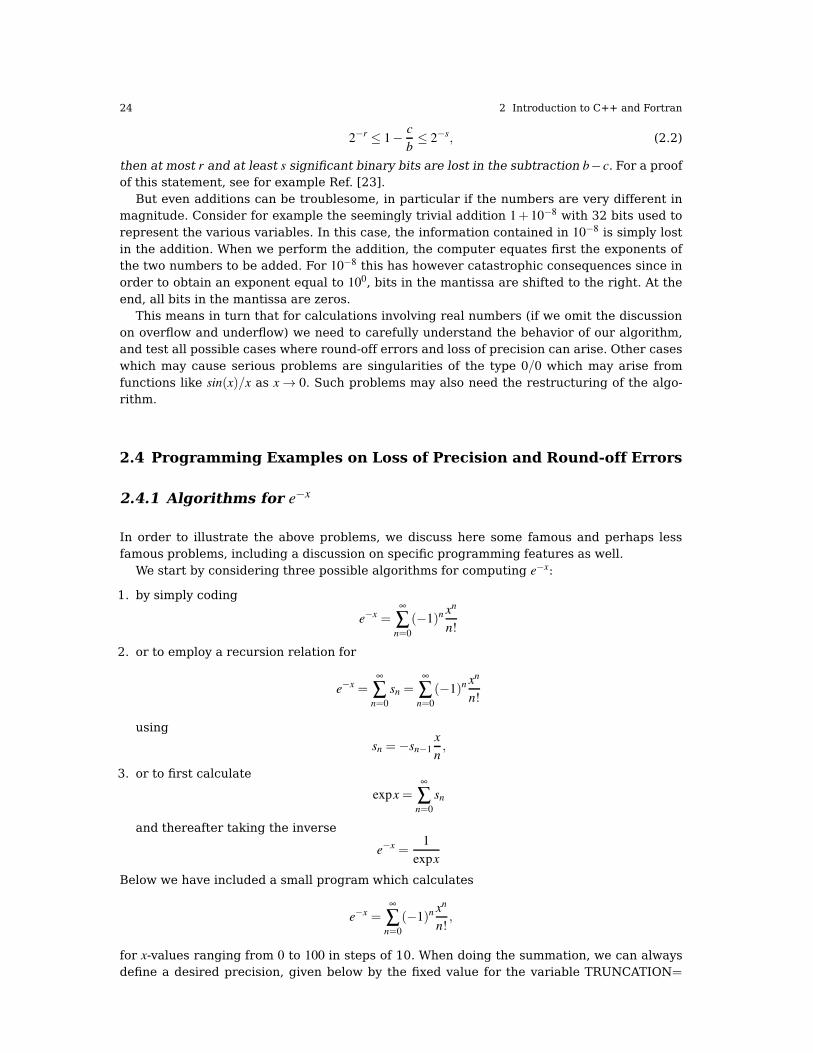
24 2 Introduction to C++ and Fortran
2−r ≤ 1− c
b≤ 2−s, (2.2)
then at most r and at least s significant binary bits are lost in the subtraction b−c. For a proofof this statement, see for example Ref. [23].
But even additions can be troublesome, in particular if the numbers are very different inmagnitude. Consider for example the seemingly trivial addition 1+ 10−8 with 32 bits used torepresent the various variables. In this case, the information contained in 10−8 is simply lostin the addition. When we perform the addition, the computer equates first the exponents ofthe two numbers to be added. For 10−8 this has however catastrophic consequences since inorder to obtain an exponent equal to 100, bits in the mantissa are shifted to the right. At theend, all bits in the mantissa are zeros.
This means in turn that for calculations involving real numbers (if we omit the discussionon overflow and underflow) we need to carefully understand the behavior of our algorithm,and test all possible cases where round-off errors and loss of precision can arise. Other caseswhich may cause serious problems are singularities of the type 0/0 which may arise fromfunctions like sin(x)/x as x→ 0. Such problems may also need the restructuring of the algo-rithm.
2.4 Programming Examples on Loss of Precision and Round-off Errors
2.4.1 Algorithms for e−x
In order to illustrate the above problems, we discuss here some famous and perhaps lessfamous problems, including a discussion on specific programming features as well.
We start by considering three possible algorithms for computing e−x:
1. by simply coding
e−x =∞
∑n=0
(−1)n xn
n!
2. or to employ a recursion relation for
e−x =∞
∑n=0
sn =∞
∑n=0
(−1)n xn
n!
using
sn =−sn−1x
n,
3. or to first calculate
expx =∞
∑n=0
sn
and thereafter taking the inverse
e−x =1
expx
Below we have included a small program which calculates
e−x =∞
∑n=0
(−1)n xn
n!,
for x-values ranging from 0 to 100 in steps of 10. When doing the summation, we can alwaysdefine a desired precision, given below by the fixed value for the variable TRUNCATION=

2.4 Programming Examples on Loss of Precision and Round-off Errors 25
1.0E− 10, so that for a certain value of x > 0, there is always a value of n = N for which theloss of precision in terminating the series at n = N is always smaller than the next term in theseries xN
N!. The latter is implemented through the while. . . statement.
http://folk.uio.no/mhjensen/compphys/programs/chapter02/cpp/program4.cpp
// Program to calculate function exp(-x)
// using straightforward summation with differing precision
using namespace std;
#include <iostream>
// type float: 32 bits precision
// type double: 64 bits precision
#define TYPE double
#define PHASE(a) (1 - 2 * (abs(a) % 2))
#define TRUNCATION 1.0E-10
// function declaration
TYPE factorial(int);
int main()
int n;
TYPE x, term, sum;
for(x = 0.0; x < 100.0; x += 10.0)
sum = 0.0; //initialization
n = 0;
term = 1;
while(fabs(term) > TRUNCATION)
term = PHASE(n) * (TYPE) pow((TYPE) x,(TYPE) n) / factorial(n);
sum += term;
n++;
// end of while() loop
cout << `` x ='' << x << `` exp = `` << exp(-x) << `` series = `` << sum;
cout << `` number of terms = " << n << endl;
// end of for() loop
return 0;
// End: function main()
// The function factorial()
// calculates and returns n!
TYPE factorial(int n)
int loop;
TYPE fac;
for(loop = 1, fac = 1.0; loop <= n; loop++)
fac *= loop;
return fac;
// End: function factorial()
There are several features to be noted3. First, for low values of x, the agreement is good,however for larger x values, we see a significant loss of precision. Secondly, for x = 70 wehave an overflow problem, represented (from this specific compiler) by NaN (not a number).The latter is easy to understand, since the calculation of a factorial of the size 171! is beyondthe limit set for the double precision variable factorial. The message NaN appears since thecomputer sets the factorial of 171 equal to zero and we end up having a division by zero inour expression for e−x.
3 Note that different compilers may give different messages and deal with overflow problems in differentways.

26 2 Introduction to C++ and Fortran
x exp(−x) Series Number of terms in series0.0 0.100000E+01 0.100000E+01 1
10.0 0.453999E-04 0.453999E-04 4420.0 0.206115E-08 0.487460E-08 7230.0 0.935762E-13 -0.342134E-04 10040.0 0.424835E-17 -0.221033E+01 12750.0 0.192875E-21 -0.833851E+05 15560.0 0.875651E-26 -0.850381E+09 17170.0 0.397545E-30 NaN 17180.0 0.180485E-34 NaN 17190.0 0.819401E-39 NaN 171
100.0 0.372008E-43 NaN 171
Table 2.3 Result from the brute force algorithm for exp (−x).
The overflow problem can be dealt with via a recurrence formula4 for the terms in the sum,so that we avoid calculating factorials. A simple recurrence formula for our equation
exp(−x) =∞
∑n=0
sn =∞
∑n=0
(−1)n xn
n!,
is to note thatsn =−sn−1
x
n,
so that instead of computing factorials, we need only to compute products. This is exemplifiedthrough the next program.
http://folk.uio.no/mhjensen/compphys/programs/chapter02/cpp/program5.cpp
// program to compute exp(-x) without factorials
using namespace std;
#include <iostream>
#define TRUNCATION 1.0E-10
int main()
int loop, n;
double x, term, sum;
for(loop = 0; loop <= 100; loop += 10)
x = (double) loop; // initialization
sum = 1.0;
term = 1;
n = 1;
while(fabs(term) > TRUNCATION)
term *= -x/((double) n);
sum += term;
n++;
// end while loop
cout << ``x ='' << x << ``exp = `` << exp(-x) << ``series = `` << sum;
cout << ``number of terms = " << n << endl;
// end of for loop
// End: function main()
4 Recurrence formulae, in various disguises, either as ways to represent series or continued fractions, areamong the most commonly used forms for function approximation. Examples are Bessel functions, Hermiteand Laguerre polynomials, discussed for example in chapter 5.

2.4 Programming Examples on Loss of Precision and Round-off Errors 27
x exp (−x) Series Number of terms in series0.000000 0.10000000E+01 0.10000000E+01 1
10.000000 0.45399900E-04 0.45399900E-04 4420.000000 0.20611536E-08 0.56385075E-08 7230.000000 0.93576230E-13 -0.30668111E-04 10040.000000 0.42483543E-17 -0.31657319E+01 12750.000000 0.19287498E-21 0.11072933E+05 15560.000000 0.87565108E-26 -0.33516811E+09 18270.000000 0.39754497E-30 -0.32979605E+14 20980.000000 0.18048514E-34 0.91805682E+17 23790.000000 0.81940126E-39 -0.50516254E+22 264
100.000000 0.37200760E-43 -0.29137556E+26 291
Table 2.4 Result from the improved algorithm for exp (−x).
In this case, we do not get the overflow problem, as can be seen from the large number ofterms. Our results do however not make much sense for larger values of x. Decreasing thetruncation test will not help! (try it). This is a much more serious problem.
In order better to understand this problem, let us consider the case of x = 20, which alreadydiffers largely from the exact result. Writing out each term in the summation, we obtain thelargest term in the sum appears at n = 19, with a value that equals −43099804. However, forn= 20 we have almost the same value, but with an interchanged sign. It means that we have anerror relative to the largest term in the summation of the order of 43099804×10−10≈ 4×10⁻².This is much larger than the exact value of 0.21× 10⁻⁸. The large contributions which mayappear at a given order in the sum, lead to strong roundoff errors, which in turn is reflectedin the loss of precision. We can rephrase the above in the following way: Since exp(−20) isa very small number and each term in the series can be rather large (of the order of 108,it is clear that other terms as large as 108, but negative, must cancel the figures in front ofthe decimal point and some behind as well. Since a computer can only hold a fixed numberof significant figures, all those in front of the decimal point are not only useless, they arecrowding out needed figures at the right end of the number. Unless we are very carefulwe will find ourselves adding up series that finally consists entirely of roundoff errors! Ananalysis of the contribution to the sum from various terms shows that the relative error madecan be huge. This results in an unstable computation, since small errors made at one stageare magnified in subsequent stages.
To this specific case there is a simple cure. Noting that exp(x) is the reciprocal of exp(−x),we may use the series for exp(x) in dealing with the problem of alternating signs, and simplytake the inverse. One has however to beware of the fact that exp(x) may quickly exceed therange of a double variable.
2.4.2 Fortran codes
The Fortran programs are rather similar in structure to the C++ program.In Fortran Real numbers are written as 2.0 rather than 2 and declared as REAL (KIND=8)
or REAL (KIND=4) for double or single precision, respectively. In general we discorauge theuse of single precision in scientific computing, the achieved precision is in general not goodenough. Fortran uses a do construct to have the computer execute the same statements morethan once. Note also that Fortran does not allow floating numbers as loop variables. In theexample below we use both a do construct for the loop over x and a DO WHILE constructionfor the truncation test, as in the C++ program. One could altrenatively use the EXIT state-

28 2 Introduction to C++ and Fortran
ment inside a do loop. Fortran has also if statements as in C++. The IF construct allows theexecution of a sequence of statements (a block) to depend on a condition. The if constructis a compound statement and begins with IF ... THEN and ends with ENDIF. Examples ofmore general IF constructs using ELSE and ELSEIF statements are given in other programexamples. Another feature to observe is the CYCLE command, which allows a loop variableto start at a new value.
Subprograms are called from the main program or other subprograms. In the C++ codeswe declared a function TYPE factorial(int);. Subprograms are always called functionsin C++. If we declare it with void is has the same meaning as subroutines in Fortran,. Sub-routines are used if we have more than one return value. In the example below we computethe factorials using the function factorial . This function receives a dummy argument n.INTENT(IN) means that the dummy argument cannot be changed within the subprogram.INTENT(OUT) means that the dummy argument cannot be used within the subprogram un-til it is given a value with the intent of passing a value back to the calling program. Thestatement INTENT(INOUT) means that the dummy argument has an initial value which ischanged and passed back to the calling program. We recommend that you use these optionswhen calling subprograms. This allows better control when transfering variables from onefunction to another. In chapter 3 we discuss call by value and by reference in C++. Call byvalue does not allow a called function to change the value of a given variable in the callingfunction. This is important in order to avoid unintentional changes of variables when trans-fering data from one function to another. The INTENT construct in Fortran allows such acontrol. Furthermore, it increases the readability of the program.
http://folk.uio.no/mhjensen/compphys/programs/chapter02/Fortran/program4.f90
! In this module you can define for example global constants
MODULE constants
! definition of variables for double precisions and complex variables
INTEGER, PARAMETER :: dp = KIND(1.0D0)
INTEGER, PARAMETER :: dpc = KIND((1.0D0,1.0D0))
! Global Truncation parameter
REAL(DP), PARAMETER, PUBLIC :: truncation=1.0E-10
END MODULE constants
! Here you can include specific functions which can be used by
! many subroutines or functions
MODULE functions
CONTAINS
REAL(DP) FUNCTION factorial(n)
USE CONSTANTS
INTEGER, INTENT(IN) :: n
INTEGER :: loop
factorial = 1.0_dp
IF ( n > 1 ) THEN
DO loop = 2, n
factorial=factorial*loop
ENDDO
ENDIF
END FUNCTION factorial
END MODULE functions
! Main program starts here
PROGRAM exp_prog
USE constants
USE functions

2.4 Programming Examples on Loss of Precision and Round-off Errors 29
IMPLICIT NONE
REAL (DP) :: x, term, final_sum
INTEGER :: n, loop_over_x
! loop over x-values
DO loop_over_x=0, 100, 10
x=loop_over_x
! initialize the EXP sum
final_sum= 0.0_dp; term = 1.0_dp; n = 0
DO WHILE ( ABS(term) > truncation)
term = ((-1.0_dp)**n)*(x**n)/ factorial(n)
final_sum=final_sum+term
n=n+1
ENDDO
! write the argument x, the exact value, the computed value and n
WRITE(*,*) x ,EXP(-x), final_sum, n
ENDDO
END PROGRAM exp_prog
The MODULE declaration in Fortran allows one to place functions like the one which calculatesthe factorials. Note also the usage of the module constants where we define double andcomplex variables. If one wishes to switch to another precision, one just needs to changethe declaration in one part of the program only. This hinders possible errors which arise ifone has to change variable declarations in every function and subroutine. In addition wehave defined a global variable truncation which is accessible to all functions which have theUSE constants declaration. These declarations have to come before any variable declara-
tions and IMPLICIT NONE statement.
http://folk.uio.no/mhjensen/compphys/programs/chapter02/Fortran/program5.f90
! In this module you can define for example global constants
MODULE constants
! definition of variables for double precisions and complex variables
INTEGER, PARAMETER :: dp = KIND(1.0D0)
INTEGER, PARAMETER :: dpc = KIND((1.0D0,1.0D0))
! Global Truncation parameter
REAL(DP), PARAMETER, PUBLIC :: truncation=1.0E-10
END MODULE constants
PROGRAM improved_exp
USE constants
IMPLICIT NONE
REAL (dp) :: x, term, final_sum
INTEGER :: n, loop_over_x
! loop over x-values, no floats as loop variables
DO loop_over_x=0, 100, 10
x=loop_over_x
! initialize the EXP sum
final_sum=1.0 ; term=1.0 ; n = 1
DO WHILE ( ABS(term) > truncation)
term = -term*x/FLOAT(n)
final_sum=final_sum+term
n=n+1
ENDDO
! write the argument x, the exact value, the computed value and n
WRITE(*,*) x ,EXP(-x), final_sum, n
ENDDO
END PROGRAM improved_exp

30 2 Introduction to C++ and Fortran
2.4.3 Further examples
2.4.3.1 Summing 1/n
Let us look at another roundoff example which may surprise you more. Consider the series
s1 =N
∑n=1
1
n,
which is finite when N is finite. Then consider the alternative way of writing this sum
s2 =1
∑n=N
1
n,
which when summed analytically should give s2 = s1. Because of roundoff errors, numericallywe will get s2 6= s1! Computing these sums with single precision for N = 1.000.000 results in s1 =
14.35736 while s2 = 14.39265! Note that these numbers are machine and compiler dependent.With double precision, the results agree exactly, however, for larger values of N, differencesmay appear even for double precision. If we choose N = 108 and employ double precision, weget s1 = 18.9978964829915355 while s2 = 18.9978964794618506, and one notes a difference evenwith double precision.
This example demonstrates two important topics. First we notice that the chosen precisionis important, and we will always recommend that you employ double precision in all calcu-lations with real numbers. Secondly, the choice of an appropriate algorithm, as also seen fore−x, can be of paramount importance for the outcome.
2.4.3.2 The standard algorithm for the standard deviation
Yet another example is the calculation of the standard deviation σ when σ is small comparedto the average value x. Below we illustrate how one of the most frequently used algorithmscan go wrong when single precision is employed.
However, before we proceed, let us define σ and x. Suppose we have a set of N data points,represented by the one-dimensional array x(i), for i = 1,N. The average value is then
x =∑N
i=1 x(i)
N,
while
σ =
√∑i x(i)2− x∑i x(i)
N− 1.
Let us now assume thatx(i) = i+ 105,
and that N = 127, just as a mere example which illustrates the kind of problems which canarise when the standard deviation is small compared with the mean value x.
The standard algorithm computes the two contributions to σ separately, that is we sum
∑i x(i)2 and subtract thereafter x∑i x(i). Since these two numbers can become nearly equaland large, we may end up in a situation with potential loss of precision as an outcome.
The second algorithm on the other hand computes first x(i)− x and then squares it whensumming up. With this recipe we may avoid having nearly equal numbers which cancel.

2.4 Programming Examples on Loss of Precision and Round-off Errors 31
Using single precision results in a standard deviation of σ = 40.05720139 for the first andmost used algorithm, while the exact answer is σ = 36.80579758, a number which also resultsfrom the above second algorithm. With double precision, the two algorithms result in thesame answer.
The reason for such a difference resides in the fact that the first algorithm includes thesubtraction of two large numbers which are squared. Since the average value for this exam-ple is x = 100063.00, it is easy to see that computing ∑i x(i)2− x∑i x(i) can give rise to verylarge numbers with possible loss of precision when we perform the subtraction. To see this,consider the case where i = 64. Then we have
x264− xx64 = 100352,
while the exact answer isx2
64− xx64 = 100064!
You can even check this by calculating it by hand.The second algorithm computes first the difference between x(i) and the average value.
The difference gets thereafter squared. For the second algorithm we have for i = 64
x64− x = 1,
and we have no potential for loss of precision.The standard text book algorithm is expressed through the following program, where we
have also added the second algorithm
http://folk.uio.no/mhjensen/compphys/programs/chapter02/cpp/program6.cpp
// program to calculate the mean and standard deviation of
// a user created data set stored in array x[]
using namespace std;
#include <iostream>
int main()
int i;
float sum, sumsq2, xbar, sigma1, sigma2;
// array declaration with fixed dimension
float x[127];
// initialise the data set
for ( i=0; i < 127 ; i++)
x[i] = i + 100000.;
// The variable sum is just the sum over all elements
// The variable sumsq2 is the sum over x^2
sum=0.;
sumsq2=0.;
// Now we use the text book algorithm
for ( i=0; i < 127; i++)
sum += x[i];
sumsq2 += pow((double) x[i],2.);
// calculate the average and sigma
xbar=sum/127.;
sigma1=sqrt((sumsq2-sum*xbar)/126.);
/*
** Here comes the second algorithm where we evaluate
** separately first the average and thereafter the
** sum which defines the standard deviation. The average
** has already been evaluated through xbar
*/

32 2 Introduction to C++ and Fortran
sumsq2=0.;
for ( i=0; i < 127; i++)
sumsq2 += pow( (double) (x[i]-xbar),2.);
sigma2=sqrt(sumsq2/126.);
cout << "xbar = `` << xbar << ``sigma1 = `` << sigma1 << ``sigma2 = `` << sigma2;
cout << endl;
return 0;
// End: function main()
The corresponding Fortran program is given below.
http://folk.uio.no/mhjensen/compphys/programs/chapter02/Fortran/program6.f90
PROGRAM standard_deviation
IMPLICIT NONE
REAL (KIND = 4) :: sum, sumsq2, xbar
REAL (KIND = 4) :: sigma1, sigma2
REAL (KIND = 4), DIMENSION (127) :: x
INTEGER :: i
x=0;
DO i=1, 127
x(i) = i + 100000.
ENDDO
sum=0.; sumsq2=0.
! standard deviation calculated with the first algorithm
DO i=1, 127
sum = sum +x(i)
sumsq2 = sumsq2+x(i)**2
ENDDO
! average
xbar=sum/127.
sigma1=SQRT((sumsq2-sum*xbar)/126.)
! second algorithm to evaluate the standard deviation
sumsq2=0.
DO i=1, 127
sumsq2=sumsq2+(x(i)-xbar)**2
ENDDO
sigma2=SQRT(sumsq2/126.)
WRITE(*,*) xbar, sigma1, sigma2
END PROGRAM standard_deviation
2.5 Additional Features of C++ and Fortran
2.5.1 Operators in C++
In the previous program examples we have seen several types of operators. In the tablesbelow we summarize the most important ones. Note that the modulus in C++ is representedby the operator % whereas in Fortran we employ the intrinsic function MOD. Note also thatthe increment operator ++ and the decrement operator -- is not available in Fortran . InC++ these operators have the following meaning
++x; or x++; has the same meaning as x = x + 1;
--x; or x--; has the same meaning as x = x - 1;

2.5 Additional Features of C++ and Fortran 33
Table 2.5 lists several relational and arithmetic operators. Logical operators in C++ and
arithmetic operators relation operatorsoperator effect operator effect− Subtraction > Greater than+ Addition >= Greater or equal∗ Multiplication < Less than/ Division <= Less or equal
% or MOD Modulus division == Equal−− Decrement ! = Not equal++ Increment
Table 2.5 Relational and arithmetic operators. The relation operators act between two operands. Note thatthe increment and decrement operators ++ and −− are not available in Fortran .
Fortran are listed in 2.6. while Table 2.7 shows bitwise operations.
Logical operatorsC++ Effect Fortran0 False value .FALSE.1 True value .TRUE.!x Logical negation .NOT.x
x&& y Logical AND x.AND.yx||y Logical inclusive OR x.OR.y
Table 2.6 List of logical operators in C++ and Fortran .
Bitwise operationsC++ Effect Fortran~i Bitwise complement NOT(j)i&j Bitwise and IAND(i,j)i^j Bitwise exclusive or IEOR(i,j)i|j Bitwise inclusive or IOR(i,j)i<<j Bitwise shift left ISHFT(i,j)i>>n Bitwise shift right ISHFT(i,-j)
Table 2.7 List of bitwise operations.
C++ offers also interesting possibilities for combined operators. These are collected inTable 2.8.
Expression meaning expression meaninga += b; a = a + b; a -= b; a = a - b;
a *= b; a = a * b; a /= b; a = a / b;
a %= b; a = a % b; a «= b; a = a « b;
a »= b; a = a » b; a &= b; a = a & b;
a |= b; a = a | b; a ∧= b; a = a ∧ b;
Table 2.8 C++ specific expressions.
Finally, we show some special operators pertinent to C++ only. The first one is the ? oper-ator. Its action can be described through the following example

34 2 Introduction to C++ and Fortran
A = expression1 ? expression2 : expression3;
Here expression1 is computed first. If this is "true" (6= 0), then expression2 is computed andassigned A. If expression1 is "false", then expression3 is computed and assigned A.
2.5.2 Pointers and arrays in C++.
In addition to constants and variables C++ contain important types such as pointers andarrays (vectors and matrices). These are widely used in most C++ program. C++ allows alsofor pointer algebra, a feature not included in Fortran . Pointers and arrays are importantelements in C++. To shed light on these types, consider the following setup
int name defines an integer variable called name. It is given an address inmemory where we can store an integer number.
&name is the address of a specific place in memory where the integername is stored. Placing the operator & in front of a variable yieldsits address in memory.
int *pointer defines an integer pointer and reserves a location in memory forthis specific variable The content of this location is viewed as theaddress of another place in memory where we have stored aninteger.
Note that in C++ it is common to write int* pointer while in C one usually writesint *pointer. Here are some examples of legal C++ expressions.
name = 0x56; /* name gets the hexadecimal value hex 56. */pointer = &name; /* pointer points to name. */printf("Address of name = %p",pointer); /* writes out the address of name. */printf("Value of name= %d",*pointer); /* writes out the value of name. */
Here’s a program which illustrates some of these topics.
http://folk.uio.no/mhjensen/compphys/programs/chapter02/cpp/program7.cpp
1 using namespace std;
2 main()
3
4 int var;
5 int *pointer;
6
7 pointer = &var;
8 var = 421;
9 printf("Address of the integer variable var : %p\n",&var);
10 printf("Value of var : %d\n", var);
11 printf("Value of the integer pointer variable: %p\n",pointer);
12 printf("Value which pointer is pointing at : %d\n",*pointer);
13 printf("Address of the pointer variable : %p\n",&pointer);
14

2.5 Additional Features of C++ and Fortran 35
Line Comments
4 • Defines an integer variable var.5 • Define an integer pointer – reserves space in memory.7 • The content of the adddress of pointer is the address of var.8 • The value of var is 421.9 • Writes the address of var in hexadecimal notation for pointers %p.10 • Writes the value of var in decimal notation%d.
The ouput of this program, compiled with g++, reads
Address of the integer variable var : 0xbfffeb74
Value of var: 421
Value of integer pointer variable : 0xbfffeb74
The value which pointer is pointing at : 421
Address of the pointer variable : 0xbfffeb70
In the next example we consider the link between arrays and pointers.
int matr[2] defines a matrix with two integer members – matr[0] og matr[1].
matr is a pointer to matr[0].
(matr + 1) is a pointer to matr[1].
http://folk.uio.no/mhjensen/compphys/programs/chapter02/cpp/program8.cpp
1 using namespace std;
2 #included <iostream>
3 int main()
4
5 int matr[2];
6 int *pointer;
7 pointer = &matr[0];
8 matr[0] = 321;
9 matr[1] = 322;
10 printf("\nAddress of the matrix element matr[1]: %p",&matr[0]);
11 printf("\nValue of the matrix element matr[1]; %d",matr[0]);
12 printf("\nAddress of the matrix element matr[2]: %p",&matr[1]);
13 printf("\nValue of the matrix element matr[2]: %d\n", matr[1]);
14 printf("\nValue of the pointer : %p",pointer);
15 printf("\nValue which pointer points at : %d",*pointer);
16 printf("\nValue which (pointer+1) points at: %d\n",*(pointer+1));
17 printf("\nAddress of the pointer variable: %p\n",&pointer);
18
You should especially pay attention to the following
Line
5 • Declaration of an integer array matr with two elements6 • Declaration of an integer pointer7 • The pointer is initialized to point at the first element of the array matr.8–9 • Values are assigned to the array matr.
The ouput of this example, compiled again with g++, is

36 2 Introduction to C++ and Fortran
Address of the matrix element matr[1]: 0xbfffef70
Value of the matrix element matr[1]; 321
Address of the matrix element matr[2]: 0xbfffef74
Value of the matrix element matr[2]: 322
Value of the pointer: 0xbfffef70
The value pointer points at: 321
The value that (pointer+1) points at: 322
Address of the pointer variable : 0xbfffef6c
2.5.3 Macros in C++
In C we can define macros, typically global constants or functions through the define state-ments shown in the simple C-example below for
1. #define ONE 1
2. #define TWO ONE + ONE
3. #define THREE ONE + TWO
4.
5. main()
6.
7. printf("ONE=%d, TWO=%d, THREE=%d",ONE,TWO,THREE);
8.
In C++ the usage of macros is discouraged and you should rather use the declarationfor constant variables. You would then replace a statement like #define ONE 1 withconst int ONE = 1;. There is typically much less use of macros in C++ than in C. C++
allows also the definition of our own types based on other existing data types. We can do thisusing the keyword typedef, whose format is: typedef existing_type new_type_name ;,where existing_type is a C++ fundamental or compound type and new_type_name is thename for the new type we are defining. For example:
typedef char new_name;
typedef unsigned int word ;
typedef char * test;
typedef char field [50];
In this case we have defined four data types: new_name, word, test and field as char, unsignedint, char* and char[50] respectively, that we could perfectly use in declarations later as anyother valid type
new_name mychar, anotherchar, *ptc1;
word myword;
test ptc2;
field name;
The use of typedef does not create different types. It only creates synonyms of existing types.That means that the type of myword can be considered to be either word or unsigned int,since both are in fact the same type. Using typedef allows to define an alias for a type that isfrequently used within a program. It is also useful to define types when it is possible that wewill need to change the type in later versions of our program, or if a type you want to use hasa name that is too long or confusing.
In C we could define macros for functions as well, as seen below.

2.5 Additional Features of C++ and Fortran 37
1. #define MIN(a,b) ( ((a) < (b)) ? (a) : (b) )
2. #define MAX(a,b) ( ((a) > (b)) ? (a) : (b) )
3. #define ABS(a) ( ((a) < 0) ? -(a) : (a) )
4. #define EVEN(a) ( (a) %2 == 0 ? 1 : 0 )
5. #define TOASCII(a) ( (a) & 0x7f )
In C++ we would replace such function definition by employing so-called inline functions.The above functions could then read
inline double MIN(double a,double b) (return (((a)<(b)) ? (a):(b));)
inline double MAX(double a,double b)(return (((a)>(b)) ? (a):(b));)
inline double ABS(double a) (return (((a)<0) ? -(a):(a));)
where we have defined the transferred variables to be of type double. The functions alsoreturn a double type. These functions could easily be generalized through the use of classesand templates, see chapter 6, to return whather types of real, complex or integer variables.
Inline functions are very useful, especially if the overhead for calling a function implies asignificant fraction of the total function call cost. When such function call overhead is sig-nificant, a function definition can be preceded by the keyword inline. When this function iscalled, we expect the compiler to generate inline code without function call overhead. How-ever, although inline functions eliminate function call overhead, they can introduce otheroverheads. When a function is inlined, its code is duplicated for each call. Excessive use ofinline may thus generate large programs. Large programs can cause excessive paging invirtual memory systems. Too many inline functions can also lengthen compile and link times,on the other hand not inlining small functions like the above that do small computations,can make programs bigger and slower. However, most modern compilers know better thanprogrammer which functions to inline or not. When doing this, you should also test variouscompiler options. With the compiler option −O3 inlining is done automatically by basically allmodern compilers.
A good strategy, recommended in many C++ textbooks, is to write a code without inlinefunctions first. As we also suggested in the introductory chapter, you should first write a assimple and clear as possible program, without a strong emphasis on computational speed.Thereafter, when profiling the program one can spot small functions which are called manytimes. These functions can then be candidates for inlining. If the overall time comsumption isreduced due to inlining specific functions, we can proceed to other sections of the programwhich could be speeded up.
Another problem with inlined functions is that on some systems debugging an inline func-tion is difficult because the function does not exist at runtime.
2.5.4 Structures in C++ and TYPE in Fortran
A very important part of a program is the way we organize our data and the flow of datawhen running the code. This is often a neglected aspect especially during the developmentof an algorithm. A clear understanding of how data are represented makes the programmore readable and easier to maintain and extend upon by other users. Till now we havestudied elementary variable declarations through keywords like int or INTEGER, double orREAL(KIND(8) and char or its Fortran equivalent CHARACTER. These declarations could alsobe extended to general multi-dimensional arrays.
However, C++ and Fortran offer other ways as well by which we can organize our data ina more transparent and reusable way. One of these options is through the struct declaration

38 2 Introduction to C++ and Fortran
of C++, or the correspondingly similar TYPE in Fortran. The latter data type will also bediscussed in chapter 6.
The following example illustrates how we could make a general variable which can bereused in defining other variables as well.
Suppose you would like to make a general programwhich treats quantummechanical prob-lems from both atomic physics and nuclear physics. In atomic and nuclear physics the single-particle degrees are represented by quantum numbers such orbital angular momentum, totalangular momentum, spin and energy. An independent particle model is often assumed as thestarting point for building up more complicated many-body correlations in systems with manyinteracting particles. In atomic physics the effective degrees of freedom are often reduced toelectrons interacting with each other, while in nuclear physics the system is described by neu-trons and protons. The structure single_particle_descript contains a list over differentquantum numbers through various pointers which are initialized by a calling function.
struct single_particle_descript
int total_states;
int* n;
int* lorb;
int* m_l;
int* jang;
int* spin;
double* energy;
char* orbit_status
;
To describe an atom like Neon we would need three single-particle orbits to describe theground state wave function if we use a single-particle picture, i.e., the 1s, 2s and 2p single-particle orbits. These orbits have a degeneray of 2(2l + 1), where the first number stemsfrom the possible spin projections and the second from the possible projections of the orbitalmomentum. Note that we reserve the naming orbit for the generic labelling 1s, 2s and 2p
while we use the naming states when we include all possible quantum numbers. In totalthere are 10 possible single-particle states when we account for spin and orbital momentumprojections. In this case we would thus need to allocate memory for arrays containing 10elements.
The above structure is written in a generic way and it can be used to define other variablesas well. For electrons we could write struct single_particle_descript electrons; andis a new variable with the name electrons containing all the elements of this structure.
The following program segment illustrates how we access these elements To access theseelements we could for example read from a given device the various quantum numbers:
for ( int i = 0; i < electrons.total_states; i++)
cout << `` Read in the quantum numbers for electron i: `` << i << endl;
cin >> electrons.n[i];
cin > electrons.lorb[i];
cin >> electrons.m_l[i];
cin >> electrons.jang[i];
cin >> electrons.spin[i];
The structure single_particle_descript can also be used for defining quantum num-bers of other particles as well, such as neutrons and protons throughthe new variablesstruct single_particle_descript protons and struct single_particle_descript neutrons.The corresponding declaration in Fortran is given by the TYPE construct, seen in the fol-
lowing example.
TYPE, PUBLIC :: single_particle_descript

2.6 Exercises 39
INTEGER :: total_states
INTEGER, DIMENSION(:), POINTER :: n, lorb, jang, spin, m_l
CHARACTER (LEN=10), DIMENSION(:), POINTER :: orbit_status
REAL(8), DIMENSION(:), POINTER :: energy
END TYPE single_particle_descript
This structure can again be used to define variables like electrons, protons and neutrons
through the statement TYPE (single_particle_descript) :: electrons, protons, neutrons.More detailed examples on the use of these variable declarations, classes and templates willbe given in subsequent chapters.
2.6 Exercises
2.1. Set up an algorithm which converts a floating number given in the decimal representa-tion to the binary representation. You may or may not use a scientific representation. Writethereafter a program which implements this algorithm.
2.2. Make a program which sums
1.
sup =N
∑n=1
1
n,
and
sdown =n=1
∑n=N
1
n.
The program should read N from screen and write the final output to screen.2. Compare sup og sdown for different N using both single and double precision for N up to
N = 1010. Which of the above formula is the most realiable one? Try to give an explanationof possible differences. One possibility for guiding the eye is for example to make a log-logplot of the relative difference as a function of N in steps of 10n with n = 1,2, . . . ,10. Thismeans you need to compute log10(|(sup(N)− sdown(N))/sdown(N)|) as function of log10(N).
2.3. Write a program which computes
f (x) = x− sinx,
for a wide range of values of x. Make a careful analysis of this function for values of x nearzero. For x≈ 0 you may consider to write out the series expansions of sinx
sinx = x− x3
3!+
x5
5!− x7
7!+ . . .
Use the loss of precision theorem of Eq. (2.2) to show that the loss of bits can be limited to atmost one bit by restricting x so that
1− sinx
x≥ 1
2.
One finds then that x must at least be 1.9, implying that for |x| < 1.9 we need to carefullyconsider the series expansion. For |x| ≥ 1.9 we can use directly the expression x− sinx.
For |x| < 1.9 you should device a recurrence relation for the terms in the series expansionin order to avoid having to compute very large factorials.
2.4. Assume that you do not have access to the intrinsic function for expx. Write your ownalgorithm for exp(−x) for all possible values of x, with special care on how to avoid the loss of

40 2 Introduction to C++ and Fortran
precision problems discussed in the text. Write thereafter a program which implements thisalgorithm.
2.5. The classical quadratic equation ax2 + bx+ c = with solution
x =(−b±
√b2− 4ac
)/2a,
needs particular attention when 4ac is small relative to b2. Find an algorithm which yieldsstable results for all possible values of a, b and c. Write thereafter a program and test theresults of your computations.
2.6. Write a Fortran program which reads a real number x and computes the precision in bits(using the function DIGIT(x))for single and double precision, the smallest positive number(using TINY(x)), the largets positive number (using the function HUGE(x)) and the number ofleading digits (using the function PRECISION(x)). Try thereafter to find similar functionalitiesin C++ and Python.
2.7. Write an algorithm and programwhich reads in a real number x and finds the two nearestmachine numbers x− and x+, the corresponding relative errors and absolute errors.
2.8. Recurrence relations are extremely useful in representing functions, and form expedientways of representing important classes of functions used in the Sciences. We will see two suchexamples in the discussion below. One example of recurrence relations appears in studies ofFourier series, which enter studies of wave mechanics, be it either in classical systems orquantum mechanical ones. We may need to calculate in an efficient way sums like
F(x) =N
∑n=0
ancos(nx), (2.3)
where the coefficients an are known numbers and x is the argument of the function F(). If wewant to solve this problem right on, we could write a simple repetitive loop that multiplieseach of the cosines with its respective coefficient an like
for ( n=0; n < N; n++)
f += an*cos(n*x)
Even though this seems rather straightforward, it may actually yield a waste of computertime if N is large. The interesting point here is that through the three-term recurrence relation
cos(n− 1)x− 2cos(x)cos(nx)+ cos(n+1)x= 0, (2.4)
we can express the entire finite Fourier series in terms of cos(x) and two constants. Theessential device is to define a new sequence of coefficients bn recursively by
bn = (2cos(x))bn−1− bn+2+ an n = 0, . . .N− 1,N, (2.5)
defining bN+1 = bN+2 + .. · · ·= 0 for all n > N, the upper limit. We can then determine all the bn
coefficients from an and one evaluation of 2cos(x). If we replace an with bn in the sum for F(x)
in Eq. (2.3) we obtain
F(x) = bN [cos(Nx)− 2cos((N− 1)x)cos(x)+ cos((N− 2)x)]+
bN−1 [cos((N− 1)x)− 2cos((N− 2)x)cos(x)+ cos((N− 3)x)]+ . . .
b2
[cos(2x)− 2cos2(x)+ 1
]+ b1 [cos(x)− 2cos(x)]+ b0. (2.6)
2.6 Exercises 41
Using Eq. (2.4) we obtain the final result
F(x) = b0− b1cos(x), (2.7)
and b0 and b1 are determined from Eq. (2.3). The latter relation is after Chensaw. This methodof evaluating finite series of orthogonal functions that are connected by a linear recurrenceis a technique generally available for all standard special functions in mathematical physics,like Legendre polynomials, Bessel functions etc. They all involve two or three terms in therecurrence relations. The general relation can then be written as
Fn+1(x) = αn(x)Fn(x)+βn(x)Fn−1(x).
Evaluate the function F(x) = ∑Nn=0 ancos(nx) in two ways: first by computing the series of
Eq. (reffour-1) and then using the equation given in Eq. (2.5). Assume that an = (n+2)/(n+1),set e.g., N = 1000 and try with different x-values as input.
2.9. Often, especially when one encounters singular behaviors, one may need to rewrite thefunction to be evaluated in terms of a taylor expansion. Another possibility is to used so-calledcontinued fractions, which may be viewed as generalizations of a Taylor expansion. Whendealing with continued fractions, one possible approach is that of successive substitutions.Let us illustrate this by a simple example, namely the solution of a second order equation
x2− 4x− 1 = 0, (2.8)
which we rewrite as
x =1
4+ x,
which in turn could be represented through an iterative substitution process
xn+1 =1
4+ xn
,
with x0 = 0. This means that we have
x1 =1
4,
x2 =1
4+ 14
,
x3 =1
4+ 1
4+ 14
,
and so forth. This is often rewritten in a compact way as
xn = x0 +a1
x1 +a2
x2+a3
x3+a4
x4+...
,
or as
xn = x0 +a1
x1+
a2
x2+
a3
x3+. . .
Write a program which implements this continued fraction algorithm and solve iterativelyEq. (2.8). The exact solution is x = 0.23607 while already after three iterations you shouldobtain x3 = 0.236111.

42 2 Introduction to C++ and Fortran
2.10. Many physics problems have spherical harmonics as solutions, such as the angularpart of the Schrödinger equation for the hydrogen atom or the angular part of the three-dimensional wave equation or Poisson’s equation.
The spherical harmonics for a given orbital momentum L, its projection M for −L ≤M ≤ L
and angles θ ∈ [0,π ] and φ ∈ [0,2π ] are given by
Y ML (θ ,φ) =
√(2L+ 1)(L−M)!
4π(L+M)!PM
L (cos(θ ))exp(iMφ),
The functions PML (cos(θ ) are the so-called associated Legendre functions. They are normally
determined via the usage of recurrence relations. Recurrence relations are unfortunatelyoften unstable, but the following relation is stable (with x = cos(θ ))
(L−M)PML (x) = x(2L− 1)PM
L−1(x)− (L+M− 1)PML−2(x),
and with the analytic (on closed form) expressions
PMM (x) = (−1)M(2M− 1)!!(1− x2)M/2,
andPM
M+1(x) = x(2M+ 1)PMM (x),
we have the starting values and the equations necessary for generating the associated Leg-endre functions for a general value of L.
1. Make first a function which computes the associated Legendre functions for different val-ues of L and M. Compare with the closed-form results listed in chapter 5.
2. Make thereafter a program which calculates the real part of the spherical harmonics3. Make plots for various L = M as functions of θ (set φ = 0) and study the behavior as L is
increased. Try to explain why the functions become more and more narrow as L increases.In order to make these plots you can use for example gnuplot, as discussed in appendix3.5.
4. Study also the behavior of the spherical harmonics when θ is close to 0 and when it ap-proaches 180 degrees. Try to extract a simple explanation for what you see.
2.11. Other well-known polynomials are the Laguerre and the Hermite polynomials, bothbeing solutions to famous differential equations. The Laguerre polynomials arise from thesolution of the differential equation
(d2
dx2− d
dx+
λ
x− l(l + 1)
x2
)L (x) = 0,
where l is an integer l≥ 0 and λ a constant. This equation arises for example from the solutionof the radial Schrödinger equation with a centrally symmetric potential such as the Coulombpotential. The first polynomials are
L0(x) = 1,
L1(x) = 1− x,
L2(x) = 2− 4x+ x2,
L3(x) = 6− 18x+ 9x2− x3,
andL4(x) = x4− 16x3 + 72x2− 96x+ 24.
They fulfil the orthogonality relation

2.6 Exercises 43
∫ ∞
−∞e−x
Ln(x)2dx = 1,
and the recursion relation
(n+ 1)Ln+1(x) = (2n+ 1− x)Ln(x)− nLn−1(x).
Similalry, the Hermite polynomials are solutions of the differential equation
d2H(x)
dx2− 2x
dH(x)
dx+(λ − 1)H(x) = 0,
which arises for example by solving Schrödinger’s equation for a particle confined to move ina harmonic oscillator potential. The first few polynomials are
H0(x) = 1,
H1(x) = 2x,
H2(x) = 4x2− 2,
H3(x) = 8x3− 12,
andH4(x) = 16x4− 48x2 + 12.
They fulfil the orthogonality relation
∫ ∞
−∞e−x2
Hn(x)2dx = 2nn!
√π,
and the recursion relationHn+1(x) = 2xHn(x)− 2nHn−1(x).
Write a program which computes the above Laguerre and Hermite polynomials for differentvalues of n using the pertinent recursion relations. Check your results agains some selectedclosed-form expressions.


Chapter 3
Numerical differentiation and interpolation
Abstract Numerical integration and differentiation are some of the most frequently neededmethods in computational physics. Quite often we are confronted with the need of evaluat-ing either the derivative f ′ or an integral
∫f (x)dx. The aim of this chapter is to introduce
some of these methods with a critical eye on numerical accuracy, following the discussionin the previous chapter. The next section deals essentially with topics from numerical dif-ferentiation. There we present also the most commonly used formulae for computing firstand second derivatives, formulae which in turn find their most important applications in thenumerical solution of ordinary and partial differential equations. We discuss also selectedmethods for numerical interpolation. This chapter serves also the scope of introducing somemore advanced C++ programming concepts, such as call by reference and value, readingand writing to a file and the use of dynamic memory allocation. We will also discuss severalobject-oriented features of C++, ending the chapter with an analogous discussion of Fortranfeatures.
3.1 Numerical Differentiation
The mathematical definition of the derivative of a function f (x) is
d f (x)
dx= lim
h→0
f (x+ h)− f (x)
h
where h is the step size. If we use a Taylor expansion for f (x) we can write
f (x+ h) = f (x)+ h f ′(x)+h2 f ′′(x)
2+ . . .
We can then obtain an expression for the first derivative as
f ′(x) =f (x+ h)− f (x)
h.+O(h),
Assume now that we will employ two points to represent the function f by way of a straightline between x and x+ h. Fig. 3.1 illustrates this subdivision.
This means that we can represent the derivative with
f ′2(x) =f (x+ h)− f (x)
h+O(h),
45

46 3 Numerical differentiation and interpolation
where the suffix 2 refers to the fact that we are using two points to define the derivative andthe dominating error goes like O(h). This is the forward derivative formula. Alternatively, wecould use the backward derivative formula
f ′2(x) =f (x)− f (x− h)
h+O(h).
If the second derivative is close to zero, this simple two point formula can be used to ap-proximate the derivative. If we however have a function like f (x) = a+ bx2, we see that theapproximated derivative becomes
f ′2(x) = 2bx+ bh,
while the exact answer is 2bx. Unless h is made very small, and b is not too large, we couldapproach the exact answer by choosing smaller and smaller values for h. However, in thiscase, the subtraction in the numerator, f (x+ h)− f (x) can give rise to roundoff errors andeventually a loss of precision.
A better approach in case of a quadratic expression for f (x) is to use a 3-step formula wherewe evaluate the derivative on both sides of a chosen point x0 using the above forward andbackward two-step formulae and taking the average afterward. We perform again a Taylorexpansion but now around x0± h, namely
f (x = x0± h) = f (x0)± h f ′+h2 f ′′
2± h3 f ′′′
6+O(h4), (3.1)
which we rewrite as
f±h = f0± h f ′+h2 f ′′
2± h3 f ′′′
6+O(h4).
Calculating both f±h and subtracting we obtain that
f ′3 =fh− f−h
2h− h2 f ′′′
6+O(h3),
and we see now that the dominating error goes like h2 if we truncate at the second derivative.We call the term h2 f ′′′/6 the truncation error. It is the error that arises because at some stagein the derivation, a Taylor series has been truncated. As we will see below, truncation errorsand roundoff errors play an important role in the numerical determination of derivatives.
For our expression with a quadratic function f (x) = a+ bx2 we see that the three-pointformula f ′3 for the derivative gives the exact answer 2bx. Thus, if our function has a quadraticbehavior in x in a certain region of space, the three-point formula will result in reliable firstderivatives in the interval [−h,h]. Using the relation
fh− 2 f0 + f−h = h2 f ′′+O(h4),
we can define the second derivative as
f ′′ =fh− 2 f0 + f−h
h2+O(h2).
We could also define five-points formulae by expanding to two steps on each side of x0.Using a Taylor expansion around x0 in a region [−2h,2h] we have
f±2h = f0± 2h f ′+ 2h2 f ′′± 4h3 f ′′′
3+O(h4). (3.2)
Using Eqs. (3.1) and (3.2), multiplying fh and f−h by a factor of 8 and subtracting (8 fh− f2h)−(8 f−h− f−2h) we arrive at a first derivative given by

3.1 Numerical Differentiation 47
f (x)
x
x0−2h x0−h x0 x0 +h x0 +2h
Fig. 3.1 Demonstration of the subdivision of the x-axis into small steps h. Each point corresponds to a set ofvalues x, f (x). The value of x is incremented by the step length h. If we use the points x0 and x0 +h we can drawa straight line and use the slope at this point to determine an approximation to the first derivative. See textfor further discussion.
f ′5c =f−2h− 8 f−h + 8 fh− f2h
12h+O(h4),
with a dominating error of the order of h4 at the price of only two additional function eval-uations. This formula can be useful in case our function is represented by a fourth-orderpolynomial in x in the region [−2h,2h]. Note however that this function includes two addi-tional function evaluations, implying a more time-consuming algorithm. Furthermore, thetwo additional subtraction can lead to a larger risk of loss of numerical precision when h be-comes small. Solving for example a differential equation which involves the first derivative,one needs always to strike a balance between numerical accurary and the time needed toachieve a given result.
It is possible to show that the widely used formulae for the first and second derivatives ofa function can be written as
fh− f−h
2h= f ′0 +
∞
∑j=1
f(2 j+1)0
(2 j+ 1)!h2 j, (3.3)
andfh− 2 f0 + f−h
h2= f ′′0 + 2
∞
∑j=1
f(2 j+2)0
(2 j+ 2)!h2 j, (3.4)
and we note that in both cases the error goes like O(h2 j). These expressions will also be usedwhen we evaluate integrals.

48 3 Numerical differentiation and interpolation
To show this for the first and second derivatives starting with the three points f−h = f (x0−h), f0 = f (x0) and fh = f (x0 + h), we have that the Taylor expansion around x = x0 gives
a−h f−h + a0 f0 + ah fh = a−h
∞
∑j=0
f( j)0
j!(−h) j + a0 f0 + ah
∞
∑j=0
f( j)0
j!(h) j, (3.5)
where a−h, a0 and ah are unknown constants to be chosen so that a−h f−h + a0 f0 + ah fh is thebest possible approximation for f ′0 and f ′′0 . Eq. (3.5) can be rewritten as
a−h f−h + a0 f0 + ah fh = [a−h + a0 + ah] f0
+[ah− a−h]h f ′0 +[a−h + ah]h2 f ′′0
2+
∞
∑j=3
f( j)0
j!(h) j
[(−1) ja−h + ah
].
To determine f ′0, we require in the last equation that
a−h + a0 + ah = 0,
−a−h + ah =1
h,
anda−h + ah = 0.
These equations have the solution
a−h =−ah =−1
2h,
anda0 = 0,
yielding
fh− f−h
2h= f ′0 +
∞
∑j=1
f(2 j+1)0
(2 j+ 1)!h2 j.
To determine f ′′0 , we require in the last equation that
a−h + a0 + ah = 0,
−a−h + ah = 0,
and
a−h + ah =2
h2.
These equations have the solution
a−h =−ah =−1
h2,
and
a0 =−2
h2,
yielding
fh− 2 f0 + f−h
h2= f ′′0 + 2
∞
∑j=1
f(2 j+2)0
(2 j+ 2)!h2 j.

3.1 Numerical Differentiation 49
3.1.1 The second derivative of exp(x)
As an example, let us calculate the second derivatives of exp(x) for various values of x. Fur-thermore, we will use this section to introduce three important C++-programming features,namely reading and writing to a file, call by reference and call by value, and dynamic memoryallocation. We are also going to split the tasks performed by the program into subtasks. Wedefine one function which reads in the input data, one which calculates the second derivativeand a final function which writes the results to file.
Let us look at a simple case first, the use of printf and scanf. If we wish to print a variabledefined as double speed_of_sound; we could for example write
double speed_of_sound;
.....
printf(``speed_of_sound = %lf\n'', speed_of_sound);
In this case we say that we transfer the value of this specific variable to the functionprintf. The function printf can however not change the value of this variable (there is noneed to do so in this case). Such a call of a specific function is called call by value. The crucialaspect to keep in mind is that the value of this specific variable does not change in the calledfunction.
When do we use call by value? And why care at all? We do actually care, because if a calledfunction has the possibility to change the value of a variable when this is not desired, callinganother function with this variable may lead to totally wrong results. In the worst cases youmay even not be able to spot where the program goes wrong.
We do however use call by value when a called function simply receives the value of thegiven variable without changing it.
If we however wish to update the value of say an array in a called function, we refer to thiscall as call by reference. What is transferred then is the address of the first element of thearray, and the called function has now access to where that specific variable ’lives’ and canthereafter change its value.
The function scanf is then an example of a function which receives the address of a vari-able and is allowed to modify it. Afterall, when calling scanf we are expecting a new valuefor a variable. A typical call could be scanf(‘‘%lf\n’’, &speed_of_sound);.
Consider now the following program
1 using namespace std;
2 # include <iostream>
3 // begin main function
4 int main(int argc, char argv[])
5 int a;
6 int *b;
7 a = 10;
8 b = new int[10];
9 for( int i = 0; i < 10; i++)
10 b[i] = i;
11
12 func(a,b);
13 return 0;
14 // end of main function
15 // definition of the function func
16 void func(int x, int *y)
17
18 x += 7;
19 *y += 10;
20 y[6] += 10;

50 3 Numerical differentiation and interpolation
21 return;
22 // end function func
There are several features to be noted.
• Lines 5 and 6: Declaration of two variables a and b. The compiler reserves two locationsin memory. The size of the location depends on the type of variable. Two properties areimportant for these locations – the address in memory and the content in the
• Line 7: The value of a is now 10.• Line 8: Memory to store 10 integers is reserved. The address to the first location is stored
in b. The address of element number 6 is given by the expression (b + 6).• Line 10: All 10 elements of b are given values: b[0] = 0, b[1] = 1, ....., b[9] = 9;• Line 12: The main() function calls the function func() and the program counter transfers
to the first statement in func(). With respect to data the following happens. The contentof a (= 10) and the content of b (a memory address) are copied to a stack (new memorylocation) associated with the function func()
• Line 16: The variable x and y are local variables in func(). They have the values – x = 10, y= address of the first element in b in the main() program.
• Line 18: The local variable x stored in the stack memory is changed to 17. Nothing happenswith the value a in main().
• Line 19: The value of y is an address and the symbol *y stands for the position in memorywhich has this address. The value in this location is now increased by 10. This means thatthe value of b[0] in the main program is equal to 10. Thus func() has modified a value inmain().
• Line 20: This statement has the same effect as line 9 except that it modifies element b[6]in main() by adding a value of 10 to what was there originally, namely 6.
• Line 21: The program counter returns to main(), the next expression after func(a,b);. Alldata on the stack associated with func() are destroyed.
• The value of a is transferred to func() and stored in a new memory location called x. Anymodification of x in func() does not affect in any way the value of a in main(). This is calledtransfer of data by value. On the other hand the next argument in func() is an addresswhich is transferred to func(). This address can be used to modify the corresponding valuein main(). In the programming language C it is expressed as a modification of the valuewhich y points to, namely the first element of b. This is called transfer of data by refer-
ence and is a method to transfer data back to the calling function, in this case main().
C++ allows however the programmer to use solely call by reference (note that call by ref-erence is implemented as pointers). To see the difference between C and C++, consider thefollowing simple examples. In C we would write
int n; n =8;
func(&n); /* &n is a pointer to n */
....
void func(int *i)
*i = 10; /* n is changed to 10 */
....
whereas in C++ we would write
int n; n =8;
func(n); // just transfer n itself
....
void func(int& i)

3.1 Numerical Differentiation 51
i = 10; // n is changed to 10
....
Note well that the way we have defined the input to the function func(int& i) or func(int *i)
decides how we transfer variables to a specific function. The reason why we emphasize thedifference between call by value and call by reference is that it allows the programmer toavoid pitfalls like unwanted changes of variables. However, many people feel that this re-duces the readability of the code. It is more or less common in C++ to use call by reference,since it gives a much cleaner code. Recall also that behind the curtain references are usuallyimplemented as pointers. When we transfer large objects such a matrices and vectors oneshould always use call by reference. Copying such objects to a called function slows downconsiderably the execution. If you need to keep the value of a call by reference object, youshould use the const declaration.
In programming languages like Fortran one uses only call by reference, but you can flagwhether a called function or subroutine is allowed or not to change the value by declaring forexample an integer value as INTEGER, INTENT(IN) :: i. The local function cannot changethe value of i. Declaring a transferred values as INTEGER, INTENT(OUT) :: i. allows thelocal function to change the variable i.
3.1.1.1 Initializations and main program
In every program we have to define the functions employed. The style chosen here is todeclare these functions at the beginning, followed thereafter by the main program and thedetailed tasks performed by each function. Another possibility is to include these functionsand their statements before the main program, meaning that the main program appears atthe very end. I find this programming style less readable however since I prefer to read acode from top to bottom. A further option, specially in connection with larger projects, isto include these function definitions in a user defined header file. The following programshows also (although it is rather unnecessary in this case due to few tasks) how one can splitdifferent tasks into specialized functions. Such a division is very useful for larger projects andprograms.
In the first version of this program we use a more C-like style for writing and reading tofile. At the end of this section we include also the corresponding C++ and Fortran files.
http://folk.uio.no/mhjensen/compphys/programs/chapter03/cpp/program1.cpp
/*
** Program to compute the second derivative of exp(x).
** Three calling functions are included
** in this version. In one function we read in the data from screen,
** the next function computes the second derivative
** while the last function prints out data to screen.
*/
using namespace std;
# include <iostream>
void initialize (double *, double *, int *);
void second_derivative( int, double, double, double *, double *);
void output( double *, double *, double, int);
int main()
// declarations of variables
int number_of_steps;

52 3 Numerical differentiation and interpolation
double x, initial_step;
double *h_step, *computed_derivative;
// read in input data from screen
initialize (&initial_step, &x, &number_of_steps);
// allocate space in memory for the one-dimensional arrays
// h_step and computed_derivative
h_step = new double[number_of_steps];
computed_derivative = new double[number_of_steps];
// compute the second derivative of exp(x)
second_derivative( number_of_steps, x, initial_step, h_step,
computed_derivative);
// Then we print the results to file
output(h_step, computed_derivative, x, number_of_steps );
// free memory
delete [] h_step;
delete [] computed_derivative;
return 0;
// end main program
We have defined three additional functions, one which reads in from screen the value of x, theinitial step length h and the number of divisions by 2 of h. This function is called initialize.To calculate the second derivatives we define the function second_derivative. Finally, wehave a function which writes our results together with a comparison with the exact value toa given file. The results are stored in two arrays, one which contains the given step length h
and another one which contains the computed derivative.These arrays are defined as pointers through the statement
double *h_step, *computed_derivative;
A call in the main function to the function second_derivative looks then like this
second_derivative( number_of_steps, x, intial_step, h_step, computed_derivative);
while the called function is declared in the following way
void second_derivative(int number_of_steps, double x, double *h_step,double
*computed_derivative);
indicating that double *h_step, double *computed_derivative; are pointers and thatwe transfer the address of the first elements. The other variables int number_of_steps, double x;
are transferred by value and are not changed in the called function.Another aspect to observe is the possibility of dynamical allocation of memory through the
new function. In the included program we reserve space in memory for these three arrays inthe following way
h_step = new double[number_of_steps];
computed_derivative = new double[number_of_steps];
When we no longer need the space occupied by these arrays, we free memory through thedeclarations
delete [] h_step;
delete [] computed_derivative;
3.1.1.2 The function initialize

3.1 Numerical Differentiation 53
// Read in from screen the initial step, the number of steps
// and the value of x
void initialize (double *initial_step, double *x, int *number_of_steps)
printf("Read in from screen initial step, x and number of steps\n");
scanf("%lf %lf %d",initial_step, x, number_of_steps);
return;
// end of function initialize
This function receives the addresses of the three variables
void initialize (double *initial_step, double *x, int *number_of_steps)
and returns updated values by reading from screen.
3.1.1.3 The function second_derivative
// This function computes the second derivative
void second_derivative( int number_of_steps, double x,
double initial_step, double *h_step,
double *computed_derivative)
int counter;
double h;
// calculate the step size
// initialize the derivative, y and x (in minutes)
// and iteration counter
h = initial_step;
// start computing for different step sizes
for (counter=0; counter < number_of_steps; counter++ )
// setup arrays with derivatives and step sizes
h_step[counter] = h;
computed_derivative[counter] =
(exp(x+h)-2.*exp(x)+exp(x-h))/(h*h);
h = h*0.5;
// end of do loop
return;
// end of function second derivative
The loop over the number of steps serves to compute the second derivative for differentvalues of h. In this function the step is halved for every iteration (you could obviously changethis to larger or smaller step variations). The step values and the derivatives are stored in thearrays h_step and double computed_derivative.
3.1.1.4 The output function
This function computes the relative error and writes the results to a chosen file.The last function here illustrates how to open a file, write and read possible data and then
close it. In this case we have fixed the name of the file. Another possibility is obviously to readthe name of this file together with other input parameters. The way the program is presentedhere is slightly unpractical since we need to recompile the program if we wish to change thename of the output file.

54 3 Numerical differentiation and interpolation
An alternative is represented by the following C++ program. This program reads fromscreen the names of the input and output files.
http://folk.uio.no/mhjensen/compphys/programs/chapter03/cpp/program2.cpp
1 #include <stdio.h>
2 #include <stdlib.h>
3 int col:
4
5 int main(int argc, char *argv[])
6
7 FILE *inn, *out;
8 int c;
9 if( argc < 3)
10 printf("You have to read in :\n");
11 printf("in_file and out_file \n");
12 exit(1);
13 inn = fopen( argv[1], "r"); // returns pointer to the in_file
14 if( inn == NULL ) // can't find in_file
15 printf("Can't find the input file %s\n", argv[1]);
16 exit(1);
17
18 out = fopen( argv[2], "w"); // returns a pointer to the out_file
19 if( out == NULL ) // can't find out_file
20 printf("Can't find the output file %s\n", argv[2]);
21 exit(1);
22
... program statements
23 fclose(inn);
24 fclose(out);
25 return 0;
This program has several interesting features.
Line Program comments
5 • The function main() takes three arguments, given by argc. The vari-able argv points to the following: the name of the program, the first andsecond arguments, in this case the file names to be read from screen.
7 • C++ has a data type called FILE. The pointers inn and ?out?point tospecific files. They must be of the type FILE.
10 • The command line has to contain 2 filenames as parameters.13–17 • The input file has to exit, else the pointer returns NULL. It has only read
permission.18–22 • This applies for the output file as well, but now with write permission
only.23–24 • Both files are closed before the main program ends.
The above represents a standard procedure in C for reading file names. C++ has its ownclass for such operations.
http://folk.uio.no/mhjensen/compphys/programs/chapter03/cpp/program3.cpp
/*
** Program to compute the second derivative of exp(x).
** In this version we use C++ options for reading and
** writing files and data. The rest of the code is as in
** programs/chapter3/program1.cpp
** Three calling functions are included
** in this version. In one function we read in the data from screen,
** the next function computes the second derivative
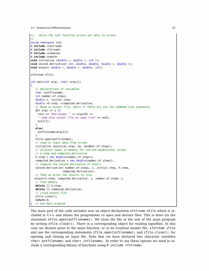
3.1 Numerical Differentiation 55
** while the last function prints out data to screen.
*/
using namespace std;
# include <iostream>
# include <fstream>
# include <iomanip>
# include <cmath>
void initialize (double *, double *, int *);
void second_derivative( int, double, double, double *, double *);
void output( double *, double *, double, int);
ofstream ofile;
int main(int argc, char* argv[])
// declarations of variables
char *outfilename;
int number_of_steps;
double x, initial_step;
double *h_step, *computed_derivative;
// Read in output file, abort if there are too few command-line arguments
if( argc <= 1 )
cout << "Bad Usage: " << argv[0] <<
" read also output file on same line" << endl;
exit(1);
else
outfilename=argv[1];
ofile.open(outfilename);
// read in input data from screen
initialize (&initial_step, &x, &number_of_steps);
// allocate space in memory for the one-dimensional arrays
// h_step and computed_derivative
h_step = new double[number_of_steps];
computed_derivative = new double[number_of_steps];
// compute the second derivative of exp(x)
second_derivative( number_of_steps, x, initial_step, h_step,
computed_derivative);
// Then we print the results to file
output(h_step, computed_derivative, x, number_of_steps );
// free memory
delete [] h_step;
delete [] computed_derivative;
// close output file
ofile.close();
return 0;
// end main program
The main part of the code includes now an object declaration ofstream ofile which is in-cluded in C++ and allows the programmer to open and declare files. This is done via thestatement ofile.open(outfilename);. We close the file at the end of the main programby writing ofile.close();. There is a corresponding object for reading inputfiles. In thiscase we declare prior to the main function, or in an evantual header file, ifstream ifile
and use the corresponding statements ifile.open(infilename); and ifile.close(); foropening and closing an input file. Note that we have declared two character variableschar* outfilename; and char* infilename;. In order to use these options we need to in-clude a corresponding library of functions using # include <fstream>.

56 3 Numerical differentiation and interpolation
One of the problems with C++ is that formatted output is not as easy to use as the printfand scanf functions in C. The output function using the C++ style is included below.
// function to write out the final results
void output(double *h_step, double *computed_derivative, double x,
int number_of_steps )
int i;
ofile << "RESULTS:" << endl;
ofile << setiosflags(ios::showpoint | ios::uppercase);
for( i=0; i < number_of_steps; i++)
ofile << setw(15) << setprecision(8) << log10(h_step[i]);
ofile << setw(15) << setprecision(8) <<
log10(fabs(computed_derivative[i]-exp(x))/exp(x))) << endl;
// end of function output
The function setw(15) reserves an output of 15 spaces for a given variable while setprecision(8)yields eight leading digits. To use these options you have to use the declaration # include <iomanip>.
Before we discuss the results of our calculations we list here the corresponding Fortranprogram. The corresponding Fortran example is
http://folk.uio.no/mhjensen/compphys/programs/chapter03/Fortran/program1.f90
! Program to compute the second derivative of exp(x).
! Only one calling function is included.
! It computes the second derivative and is included in the
! MODULE functions as a separate method
! The variable h is the step size. We also fix the total number
! of divisions by 2 of h. The total number of steps is read from
! screen
MODULE constants
! definition of variables for double precisions and complex variables
INTEGER, PARAMETER :: dp = KIND(1.0D0)
INTEGER, PARAMETER :: dpc = KIND((1.0D0,1.0D0))
END MODULE constants
! Here you can include specific functions which can be used by
! many subroutines or functions
MODULE functions
USE constants
IMPLICIT NONE
CONTAINS
SUBROUTINE derivative(number_of_steps, x, initial_step, h_step, &
computed_derivative)
USE constants
INTEGER, INTENT(IN) :: number_of_steps
INTEGER :: loop
REAL(DP), DIMENSION(number_of_steps), INTENT(INOUT) :: &
computed_derivative, h_step
REAL(DP), INTENT(IN) :: initial_step, x
REAL(DP) :: h
! calculate the step size
! initialize the derivative, y and x (in minutes)
! and iteration counter
h = initial_step
! start computing for different step sizes
DO loop=1, number_of_steps
! setup arrays with derivatives and step sizes
h_step(loop) = h

3.1 Numerical Differentiation 57
computed_derivative(loop) = (EXP(x+h)-2.*EXP(x)+EXP(x-h))/(h*h)
h = h*0.5
ENDDO
END SUBROUTINE derivative
END MODULE functions
PROGRAM second_derivative
USE constants
USE functions
IMPLICIT NONE
! declarations of variables
INTEGER :: number_of_steps, loop
REAL(DP) :: x, initial_step
REAL(DP), ALLOCATABLE, DIMENSION(:) :: h_step, computed_derivative
! read in input data from screen
WRITE(*,*) 'Read in initial step, x value and number of steps'
READ(*,*) initial_step, x, number_of_steps
! open file to write results on
OPEN(UNIT=7,FILE='out.dat')
! allocate space in memory for the one-dimensional arrays
! h_step and computed_derivative
ALLOCATE(h_step(number_of_steps),computed_derivative(number_of_steps))
! compute the second derivative of exp(x)
! initialize the arrays
h_step = 0.0_dp; computed_derivative = 0.0_dp
CALL derivative(number_of_steps,x,initial_step,h_step,computed_derivative)
! Then we print the results to file
DO loop=1, number_of_steps
WRITE(7,'(E16.10,2X,E16.10)') LOG10(h_step(loop)),&
LOG10 ( ABS ( (computed_derivative(loop)-EXP(x))/EXP(x)))
ENDDO
! free memory
DEALLOCATE( h_step, computed_derivative)
! close the output file
CLOSE(7)
END PROGRAM second_derivative
The MODULE declaration in Fortran allows one to place functions like the one which calcu-lates second derivatives in a module. Since this is a general method, one could extend itsfunctionality by simply transfering the name of the function to differentiate. In our case weuse explicitely the exponential function, but there is nothing which hinders us from defin-ing other functions. Note the usage of the module constants where we define double andcomplex variables. If one wishes to switch to another precision, one needs to change the dec-laration in one part of the program only. This hinders possible errors which arise if one has tochange variable declarations in every function and subroutine. Finally, dynamic memory allo-cation and deallocation is in Fortran done with the keywords ALLOCATE( array(size)) andDEALLOCATE(array). Although most compilers deallocate and thereby free space in memorywhen leaving a function, you should always deallocate an array when it is no longer needed.In case your arrays are very large, this may block unnecessarily large fractions of the memory.Furthermore, you should always initialize arrays. In the example above, we note that Fortranallows us to simply write h_step = 0.0_dp; computed_derivative = 0.0_dp, which meansthat all elements of these two arrays are set to zero. Coding arrays in this manner brings usmuch closer to the way we deal with mathematics. In Fortran it is irrelevant whether thisis a one-dimensional or multi-dimensional array. In chapter 6, where we deal with allocationof matrices, we will introduce the numerical libraries Armadillo and Blitz++ which allow for

58 3 Numerical differentiation and interpolation
similar treatments of arrays in C++. By default however, these features are not included inthe ANSI C++ standard.
3.1.1.5 Results
In Table 3.1 we present the results of a numerical evaluation for various step sizes for thesecond derivative of exp(x) using the approximation f ′′0 =
fh−2 f0+ f−h
h2 . The results are comparedwith the exact ones for various x values. Note well that as the step is decreased we get
x h = 0.1 h = 0.01 h = 0.001 h = 0.0001 h = 0.0000001 Exact0.0 1.000834 1.000008 1.000000 1.000000 1.010303 1.0000001.0 2.720548 2.718304 2.718282 2.718282 2.753353 2.7182822.0 7.395216 7.389118 7.389057 7.389056 7.283063 7.3890563.0 20.102280 20.085704 20.085539 20.085537 20.250467 20.0855374.0 54.643664 54.598605 54.598155 54.598151 54.711789 54.5981505.0 148.536878 148.414396 148.413172 148.413161 150.635056 148.413159
Table 3.1 Result for numerically calculated second derivatives of exp(x) as functions of the chosen step sizeh. A comparison is made with the exact value.
closer to the exact value. However, if it is further decreased, we run into problems of loss ofprecision. This is clearly seen for h = 0.0000001. This means that even though we could let thecomputer run with smaller and smaller values of the step, there is a limit for how small thestep can be made before we loose precision.
3.1.2 Error analysis
Let us analyze these results in order to see whether we can find a minimal step length whichdoes not lead to loss of precision. Furthermore In Fig. 3.2 we have plotted
ε = log10
(∣∣∣∣∣f ′′computed− f ′′exact
f ′′exact
∣∣∣∣∣
),
as function of log10(h). We used an intial step length of h = 0.01 and fixed x = 10. For largevalues of h, that is −4 < log10(h) < −2 we see a straight line with a slope close to 2. Close tolog10(h)≈−4 the relative error starts increasing and our computed derivative with a step sizelog10(h)<−4, may no longer be reliable.
Can we understand this behavior in terms of the discussion from the previous chapter? Inchapter 2 we assumed that the total error could be approximated with one term arising fromthe loss of numerical precision and another due to the truncation or approximation made,that is
εtot = εapprox + εro.
For the computed second derivative, Eq. (3.4), we have
f ′′0 =fh− 2 f0 + f−h
h2− 2
∞
∑j=1
f(2 j+2)0
(2 j+ 2)!h2 j,
and the truncation or approximation error goes like

3.1 Numerical Differentiation 59
Relative error
log10(h)
ε
0-2-4-6-8-10-12-14
6
4
2
0
-2
-4
-6
-8
-10
Fig. 3.2 Log-log plot of the relative error of the second derivative of exp(x) as function of decreasing steplengths h. The second derivative was computed for x = 10 in the program discussed above. See text for furtherdetails
εapprox ≈f(4)0
12h2.
If we were not to worry about loss of precision, we could in principle make h as small aspossible. However, due to the computed expression in the above program example
f ′′0 =fh− 2 f0 + f−h
h2=
( fh− f0)+ ( f−h− f0)
h2,
we reach fairly quickly a limit for where loss of precision due to the subtraction of two nearlyequal numbers becomes crucial. If ( f±h− f0) are very close, we have ( f±h− f0) ≈ εM, where|εM| ≤ 10−7 for single and |εM | ≤ 10−15 for double precision, respectively.
We have then ∣∣ f ′′0∣∣=∣∣∣∣( fh− f0)+ ( f−h− f0)
h2
∣∣∣∣≤2εM
h2.
Our total error becomes
|εtot| ≤2εM
h2+
f(4)0
12h2. (3.6)
It is then natural to ask which value of h yields the smallest total error. Taking the derivativeof |εtot| with respect to h results in
h =
(24εM
f(4)0
)1/4
.
With double precision and x = 10 we obtain
h≈ 10−4.
Beyond this value, it is essentially the loss of numerical precision which takes over. We notealso that the above qualitative argument agrees seemingly well with the results plotted in Fig.3.2 and Table 3.1. The turning point for the relative error at approximately h ≈ 10−4 reflects

60 3 Numerical differentiation and interpolation
most likely the point where roundoff errors take over. If we had used single precision, wewould get h ≈ 10−2. Due to the subtractive cancellation in the expression for f ′′ there is apronounced detoriation in accuracy as h is made smaller and smaller.
It is instructive in this analysis to rewrite the numerator of the computed derivative as
( fh− f0)+ ( f−h− f0) = (exp(x+ h)− expx)+ (exp(x− h)− expx),
as( fh− f0)+ ( f−h− f0) = exp(x)(exp(h)+ exp(−h)− 2),
since it is the difference (exp(h)+exp(−h)−2) which causes the loss of precision. The results,still for x = 10 are shown in the Table 3.2. We note from this table that at h≈ ×10−8 we have
h exp (h)+ exp(−h) exp (h)+ exp(−h)−2
10−1 2.0100083361116070 1.0008336111607230×10⁻²
10−2 2.0001000008333358 1.0000083333605581×10⁻⁴
10−3 2.0000010000000836 1.0000000834065048×10⁻⁶
10−4 2.0000000099999999 1.0000000050247593×10⁻⁸
10−5 2.0000000001000000 9.9999897251734637×10⁻¹¹
10−6 2.0000000000010001 9.9997787827987850×10⁻¹³
10−7 2.0000000000000098 9.9920072216264089×10⁻¹⁵
10−8 2.0000000000000000 0.0000000000000000×100
10−9 2.0000000000000000 1.1102230246251565×10⁻¹⁶
10−10 2.0000000000000000 0.0000000000000000×100
Table 3.2 Result for the numerically calculated numerator of the second derivative as function of the stepsize h. The calculations have been made with double precision.
essentially lost all leading digits.From Fig. 3.2 we can read off the slope of the curve and thereby determine empirically
how truncation errors and roundoff errors propagate. We saw that for −4 < log10(h) < −2,we could extract a slope close to 2, in agreement with the mathematical expression for thetruncation error.
We can repeat this for−10< log10(h)<−4 and extract a slope which is approximately equalto −2. This agrees again with our simple expression in Eq. (3.6).
3.2 Numerical Interpolation and Extrapolation
Numerical interpolation and extrapolation are frequently used tools in numerical applicationsto physics. The often encountered situation is that of a function f at a set of points x1 . . .xn
where an analytic form is missing. The function f may represent some data points from ex-periment or the result of a lengthy large-scale computation of some physical quantity thatcannot be cast into a simple analytical form.
We may then need to evaluate the function f at some point x within the data set x1 . . .xn,but where x differs from the tabulated values. In this case we are dealing with interpolation.If x is outside we are left with the more troublesome problem of numerical extrapolation.Below we will concentrate on two methods for interpolation and extrapolation, namely poly-nomial interpolation and extrapolation. The cubic spline interpolation approach is discussedin chapter 6.

3.2 Numerical Interpolation and Extrapolation 61
3.2.1 Interpolation
Let us assume that we have a set of N + 1 points y0 = f (x0),y1 = f (x1), . . . ,yN = f (xN) wherenone of the xi values are equal. We wish to determine a polynomial of degree n so that
PN(xi) = f (xi) = yi, i = 0,1, . . . ,N (3.7)
for our data points. If we then write PN on the form
PN(x) = a0 + a1(x− x0)+ a2(x− x0)(x− x1)+ · · ·+ aN(x− x0) . . . (x− xN−1), (3.8)
then Eq. (3.7) results in a triangular system of equations
a0 = f (x0)
a0+ a1(x1− x0) = f (x1)
a0+ a1(x2− x0)+ a2(x2− x0)(x2− x1) = f (x2)
. . . . . . . . . . . .
.
The coefficients a0, . . . ,aN are then determined in a recursive way, starting with a0,a1, . . . .The classic of interpolation formulae was created by Lagrange and is given by
PN(x) =N
∑i=0
∏k 6=i
x− xk
xi− xk
yi. (3.9)
If we have just two points (a straight line) we get
P1(x) =x− x0
x1− x0
y1 +x− x1
x0− x1
y0,
and with three points (a parabolic approximation) we have
P3(x) =(x− x0)(x− x1)
(x2− x0)(x2− x1)y2 +
(x− x0)(x− x2)
(x1− x0)(x1− x2)y1 +
(x− x1)(x− x2)
(x0− x1)(x0− x2)y0
and so forth. It is easy to see from the above equations that when x = xi we have that f (x) =
f (xi) It is also possible to show that the approximation error (or rest term) is given by thesecond term on the right hand side of
f (x) = PN(x)+ωN+1(x) f (N+1)(ξ )
(N + 1)!. (3.10)
The function ωN+1(x) is given by
ωN+1(x) = aN(x− x0) . . . (x− xN),
and ξ = ξ (x) is a point in the smallest interval containing all interpolation points x j and x.The program we provide below is however based on divided differences. The recipe is quitesimple. If we take x = x0 in Eq. (3.8), we then have obviously that a0 = f (x0) = y0. Moving a0
over to the left-hand side and dividing by x− x0 we have
f (x)− f (x0)
x− x0
= a1 + a2(x− x1)+ · · ·+ aN(x− x1)(x− x2) . . . (x− xN−1),
where we hereafter omit the rest term

62 3 Numerical differentiation and interpolation
f (N+1)(ξ )
(N + 1)!(x− x1)(x− x2) . . . (x− xN).
The quantity
f0x =f (x)− f (x0)
x− x0
,
is a divided difference of first order. If we then take x = x1, we have that a1 = f01. Moving a1
to the left again and dividing by x− x1 we obtain
f0x− f01
x− x1
= a2 + · · ·+ aN(x− x2) . . . (x− xN−1).
and the quantity
f01x =f0x− f01
x− x1
,
is a divided difference of second order. We note that the coefficient
a1 = f01,
is determined from f0x by setting x= x1. We can continue along this line and define the divideddifference of order k+ 1 as
f01...kx =f01...(k−1)x− f01...(k−1)k
x− xk
, (3.11)
meaning that the corresponding coefficient ak is given by
ak = f01...(k−1)k.
With these definitions we see that Eq. (3.10) can be rewritten as
f (x) = a0 + ∑k=1
N f01...k(x− x0) . . . (x− xk−1)+ωN+1(x) f (N+1)(ξ )
(N + 1)!.
If we replace x0,x1, . . . ,xk in Eq. (3.11) with xi+1,xi+2, . . . ,xk, that is we count from i+ 1 to k
instead of counting from 0 to k and replace x with xi, we can then construct the followingrecursive algorithm for the calculation of divided differences
fxixi+1...xk=
fxi+1...xk− fxixi+1...xk−1
xk− xi
.
Assuming that we have a table with function values (x j, f (x j) = y j) and need to construct thecoefficients for the polynomial PN(x). We can then view the last equation by constructing thefollowing table for the case where N = 3.
x0 y0
fx0x1
x1 y1 fx0x1x2
fx1x2fx0x1x2x3
x2 y2 fx1x2x3
fx2x3
x3 y3
.
The coefficients we are searching for will then be the elements along the main diagonal.We can understand this algorithm by considering the following. First we construct the uniquepolynomial of order zero which passes through the point x0,y0. This is just a0 discussed above.

3.2 Numerical Interpolation and Extrapolation 63
Therafter we construct the unique polynomial of order one which passes through both x0y0
and x1y1. This corresponds to the coefficient a1 and the tabulated value fx0x1and together with
a0 results in the polynomial for a straight line. Likewise we define polynomial coefficients forall other couples of points such as fx1x2
and fx2x3. Furthermore, a coefficient like a2 = fx0x1x2
spans now three points, and adding together fx0x1we obtain a polynomial which represents
three points, a parabola. In this fashion we can continue till we have all coefficients. Thefunction we provide below included is based on an extension of this algorithm, knowns asNeville’s algorithm. The error provided by Neville’s algorithm is based on the truncationerror in Eq. (3.10).
http://folk.uio.no/mhjensen/compphys/programs/chapter03/cpp/program4.cpp
/*
** The function
** polint()
** takes as input xa[0,..,n-1] and ya[0,..,n-1] together with a given value
** of x and returns a value y and an error estimate dy. If P(x) is a polynomial
** of degree N - 1 such that P(xa_i) = ya_i, i = 0,..,n-1, then the returned
** value is y = P(x).
*/
void polint(double xa[], double ya[], int n, double x, double *y, double *dy)
int i, m, ns = 1;
double den,dif,dift,ho,hp,w;
double *c,*d;
dif = fabs(x - xa[0]);
c = new double [n];
d = new double [n];
for(i = 0; i < n; i++)
if((dift = fabs(x - xa[i])) < dif)
ns = i;
dif = dift;
c[i] = ya[i];
d[i] = ya[i];
*y = ya[ns--];
for(m = 0; m < (n - 1); m++)
for(i = 0; i < n - m; i++)
ho = xa[i] - x;
hp = xa[i + m] - x;
w = c[i + 1] - d[i];
if((den = ho - hp) < ZERO)
printf("\n\n Error in function polint(): ");
printf("\nden = ho - hp = %4.1E -- too small\n",den);
exit(1);
den = w/den;
d[i] = hp * den;
c[i] = ho * den;
*y += (*dy = (2 * ns < (n - m) ? c[ns + 1] : d[ns--]));
delete [] d;
delete [] c;
// End: function polint()
When using this function, you need obviously to declare the function itself.

64 3 Numerical differentiation and interpolation
3.2.2 Richardson’s deferred extrapolation method
Here we present an elegant method to improve the precision of our mathematical truncation,without too many additional function evaluations. We will again study the evaluation of thefirst and second derivatives of exp(x) at a given point x = ξ . In Eqs. (3.3) and (3.4) for the firstand second derivatives, we noted that the truncation error goes like O(h2 j).
Employing the mid-point approximation to the derivative, the various derivatives D of agiven function f (x) can then be written as
D(h) = D(0)+ a1h2 + a2h4 + a3h6 + . . . ,
where D(h) is the calculated derivative, D(0) the exact value in the limit h→ 0 and ai areindependent of h. By choosing smaller and smaller values for h, we should in principle beable to approach the exact value. However, since the derivatives involve differences, we mayeasily loose numerical precision as shown in the previous sections. A possible cure is to applyRichardson’s deferred approach, i.e., we perform calculations with several values of the steph and extrapolate to h = 0. The philososphy is to combine different values of h so that theterms in the above equation involve only large exponents for h. To see this, assume that wemount a calculation for two values of the step h, one with h and the other with h/2. Then wehave
D(h) = D(0)+ a1h2 + a2h4 + a3h6 + . . . ,
and
D(h/2) = D(0)+a1h2
4+
a2h4
16+
a3h6
64+ . . . ,
and we can eliminate the term with a1 by combining
D(h/2)+D(h/2)−D(h)
3= D(0)− a2h4
4− 5a3h6
16. (3.12)
We see that this approximation to D(0) is better than the two previous ones since the errornow goes like O(h4). As an example, let us evaluate the first derivative of a function f using astep with lengths h and h/2. We have then
fh− f−h
2h= f ′0 +O(h2),
fh/2− f−h/2
h= f ′0 +O(h2/4),
which can be combined, using Eq. (3.12) to yield
− fh + 8 fh/2− 8 f−h/2 + f−h
6h= f ′0−
h4
480f (5).
In practice, what happens is that our approximations to D(0) goes through a series of steps
D(0)0
D(1)0 D
(0)1
D(2)0 D
(1)1 D
(0)2
D(3)0 D
(2)1 D
(1)2 D
(0)3
. . . . . . . . . . . .
,
where the elements in the first column represent the given approximations

3.3 Classes in C++ 65
D(k)0 = D(h/2k).
This means that D(0)1 in the second column and row is the result of the extrapolation based on
D(0)0 and D
(1)0 . An element D
(k)m in the table is then given by
D(k)m = D
(k)m−1 +
D(k+1)m−1 −D
(k)m−1
4m− 1(3.13)
with m > 0.In Table 3.1 we presented the results for various step sizes for the second derivative of
exp(x) using f ′′0 =fh−2 f0+ f−h
h2 . The results were compared with the exact ones for various x
values. Note well that as the step is decreased we get closer to the exact value. However,if it is further increased, we run into problems of loss of precision. This is clearly seen forh = 0.000001. This means that even though we could let the computer run with smaller andsmaller values of the step, there is a limit for how small the step can be made before we looseprecision. Consider now the results in Table 3.3 where we choose to employ Richardson’sextrapolation scheme. In this calculation we have computed our function with only threepossible values for the step size, namely h, h/2 and h/4 with h = 0.1. The agreement withthe exact value is amazing! The extrapolated result is based upon the use of Eq. (3.13). An
x h = 0.1 h = 0.05 h = 0.025 Extrapolat Error0.0 1.00083361 1.00020835 1.00005208 1.00000000 0.000000001.0 2.72054782 2.71884818 2.71842341 2.71828183 0.000000012.0 7.39521570 7.39059561 7.38944095 7.38905610 0.000000033.0 20.10228045 20.08972176 20.08658307 20.08553692 0.000000094.0 54.64366366 54.60952560 54.60099375 54.59815003 0.000000245.0 148.53687797 148.44408109 148.42088912 148.41315910 0.00000064
Table 3.3 Result for numerically calculated second derivatives of exp (x) using extrapolation. The first threevalues are those calculated with three different step sizes, h, h/2 and h/4 with h = 0.1. The extrapolated resultto h = 0 should then be compared with the exact ones from Table 3.1.
alternative recipe is to use our function for the polynomial extrapolation discussed in theprevious subsection and calculate the derivatives for several values of h and then extrapolateto h = 0. We will use this method to obtain improved eigenvalues in chapter 7.
Other methods to interpolate a function f (x) such as spline methods will be discussed inchapter 6.
3.3 Classes in C++
In Fortran a vector (this applies to matrices as well) starts with 1, but it is easy to changethe declaration of vector so that it starts with zero or even a negative number. If we have adouble precision Fortran vector which starts at −10 and ends at 10, we could declare it asREAL(KIND=8) :: vector(-10:10). Similarly, if we want to start at zero and end at 10 wecould write REAL(KIND=8) :: vector(0:10). Fortran allows us to write a vector additiona = b+ c as a = b + c. This means that we have overloaded the addition operator in order totranslate this operation into two loops and an addition of two vector elements ai = bi + ci.
The way the vector addition is written is very close to the way we express this relationmathematically. The benefit for the programmer is that our code is easier to read. Further-more, such a way of coding makes it more likely to spot eventual errors as well.

66 3 Numerical differentiation and interpolation
In Ansi C and C++ arrays start by default from i = 0. Moreover, if we wish to add twovectors we need to explicitely write out a loop as
for(i=0 ; i < n ; i++)
a[i]=b[i]+c[i]
However, the strength of C++ over programming languages like C and Fortran 77 is thepossibility to define new data types, tailored to some particular problem. Via new data typesand overloading of operations such as addition and subtraction, we can easily define sets ofoperations and data types which allow us to write a vector or matrix addition in exactly thesame way as we would do in Fortran. We could also change the way we declare a C++ vector(or matrix) element ai, from a[i] to say a(i), as we would do in Fortran. Similarly, we could alsochange the default range from 0 : n− 1 to 1 : n.
To achieve this we need to introduce two important entities in C++ programming, classesand templates.
The function and class declarations are fundamental concepts within C++. Functions areabstractions which encapsulate an algorithm or parts of it and perform specific tasks in aprogram. We have already met several examples on how to use functions. Classes can bedefined as abstractions which encapsulate data and operations on these data. The data canbe very complex data structures and the class can contain particular functions which operateon these data. Classes allow therefore for a higher level of abstraction in computing. Theelements (or components) of the data type are the class data members, and the proceduresare the class member functions.
Classes are user-defined tools used to create multi-purpose software which can be reusedby other classes or functions. These user-defined data types contain data (variables) andfunctions operating on the data.
A simple example is that of a point in two dimensions. The data could be the x and y
coordinates of a given point. The functions we define could be simple read and write functionsor the possibility to compute the distance between two points.
The two examples we elaborate on below demonstrate most of the features of classes.We develop first a class called Complex which allows us to perform various operations oncomplex variables. We extend thereafter our discussion of classes to define a class Vector
which allows us to perform various operations on a user-specified one-dimesional array, fromdeclarations of a vector to mathematical operations such as additions of vectors. Later, in ourdiscussion on linear algebra, we will also present our final matrix and vector class.
The classes we define are easy to use in other codes and/or other classes and many of thedetails which would be present in C (or Fortran 77) codes are hidden inside the class. Thereuse of a well-written and functional class is normally rather simple. However, to write agiven class is often complicated, especially if we deal with complicated matrix operations. Inthis text we will rely on ready-made classes in C++ for dealing with matrix operations. Wehave chosen to use the libraries like Armadillo or Blitz++, discussed in our linear algebrachapter. These libraries hide many low-level operations with matrices and vectors, such asmatrix-vector multiplications or allocation and deallocation of memory. Such libraries makeit then easier to build our own high-level classes out of well-tested lower-level classes.
The way we use classes in this text is close to the MODULE data type in Fortran and weprovide some simple demonstrations at the end of this section.

3.3 Classes in C++ 67
3.3.1 The Complex class
As remarked in chapter 2, C++ has a class complex in its standard template library (STL).The standard usage in a given function could then look like
// Program to calculate addition and multiplication of two complex numbers
using namespace std;
#include <iostream>
#include <cmath>
#include <complex>
int main()
complex<double> x(6.1,8.2), y(0.5,1.3);
// write out x+y
cout << x + y << x*y << endl;
return 0;
where we add and multiply two complex numbers x = 6.1+ ı8.2 and y = 0.5+ ı1.3 with theobvious results z = x+ y = 6.6+ ı9.5 and z = x · y = −7.61+ ı12.03. In Fortran we would declarethe above variables as COMPLEX(DPC) :: x(6.1,8.2), y(0.5,1.3).
The libraries Armadillo and Blitz++ include an extension of the complex class to opera-tions on vectors, matrices and higher-dimensional arrays. We recommend the usage of suchlibraries when you develop your own codes. However, writing a complex class yourself is agood pedagogical exercise.
We proceed by splitting our task in three files.
• We define first a header file complex.h which contains the declarations of the class. Theheader file contains the class declaration (data and functions), declaration of stand-alonefunctions, and all inlined functions, starting as follows
#ifndef Complex_H
#define Complex_H
// various include statements and definitions
#include <iostream> // Standard ANSI-C++ include files
#include <new>
#include ....
class Complex
...
definition of variables and their character
;
// declarations of various functions used by the class
...
#endif
• Next we provide a file complex.cpp where the code and algorithms of different functions(except inlined functions) declared within the class are written. The files complex.h andcomplex.cpp are normally placed in a directory with other classes and libraries we havedefined.
• Finally,we discuss here an example of a main program which uses this particular class.An example of a program which uses our complex class is given below. In particular wewould like our class to perform tasks like declaring complex variables, writing out the realand imaginary part and performing algebraic operations such as adding or multiplying twocomplex numbers.
#include "Complex.h"
... other include and declarations

68 3 Numerical differentiation and interpolation
int main ()
Complex a(0.1,1.3); // we declare a complex variable a
Complex b(3.0), c(5.0,-2.3); // we declare complex variables b and c
Complex d = b; // we declare a new complex variable d
cout << "d=" << d << ", a=" << a << ", b=" << b << endl;
d = a*c + b/a; // we add, multiply and divide two complex numbers
cout << "Re(d)=" << d.Re() << ", Im(d)=" << d.Im() << endl; // write out of the real
and imaginary parts
We include the header file complex.h and define four different complex variables. Theseare a = 0.1+ ı1.3, b = 3.0+ ı0 (note that if you don’t define a value for the imaginary partthis is set to zero), c = 5.0− ı2.3 and d = b. Thereafter we have defined standard algebraicoperations and the member functions of the class which allows us to print out the real andimaginary part of a given variable.
To achieve these features, let us see how we define the complex class. In C++ we coulddefine a complex class as follows
class Complex
private:
double re, im; // real and imaginary part
public:
Complex (); // Complex c;
Complex (double re, double im = 0.0); // Definition of a complex variable;
Complex (const Complex& c); // Usage: Complex c(a); // equate two complex variables
Complex& operator= (const Complex& c); // c = a; // equate two complex variables, same
as previous
~Complex () // destructor
double Re () const; // double real_part = a.Re();
double Im () const; // double imag_part = a.Im();
double abs () const; // double m = a.abs(); // modulus
friend Complex operator+ (const Complex& a, const Complex& b);
friend Complex operator- (const Complex& a, const Complex& b);
friend Complex operator* (const Complex& a, const Complex& b);
friend Complex operator/ (const Complex& a, const Complex& b);
;
The class is defined via the statement class Complex. We must first use the key wordclass, which in turn is followed by the user-defined variable name Complex. The body of theclass, data and functions, is encapsulated within the parentheses ...;.
Data and specific functions can be private, which means that they cannot be accessed fromoutside the class. This means also that access cannot be inherited by other functions outsidethe class. If we use protected instead of private, then data and functions can be inheritedoutside the class. The key word public means that data and functions can be accessed fromoutside the class. Here we have defined several functions which can be accessed by functionsoutside the class. The declaration friend means that stand-alone functions can work on pri-vately declared variables of the type (re, im). Data members of a class should be declaredas private variables.
The first public function we encounter is a so-called constructor, which tells how we de-clare a variable of type Complex and how this variable is initialized. We have chosen threepossibilities in the example above:
1. A declaration like Complex c; calls the member function Complex() which can have thefollowing implementation
Complex:: Complex () re = im = 0.0;

3.3 Classes in C++ 69
meaning that it sets the real and imaginary parts to zero. Note the way a member functionis defined. The constructor is the first function that is called when an object is instantiated.
2. Another possibility is
Complex:: Complex ()
which means that there is no initialization of the real and imaginary parts. The drawbackis that a given compiler can then assign random values to a given variable.
3. A call like Complex a(0.1,1.3); means that we could call the member function as
Complex:: Complex (double re_a, double im_a)
re = re_a; im = im_a;
The simplest member function are those we defined to extract the real and imaginary partof a variable. Here you have to recall that these are private data, that is they are invisible forusers of the class. We obtain a copy of these variables by defining the functions
double Complex:: Re () const return re; // getting the real part
double Complex:: Im () const return im; // and the imaginary part
\endlstlistingline
Note that we have introduced the declaration \verb?const. What does it mean?
This declaration means that a variable cannot be changed within a called function.
If we define a variable as
\verb?const double p = 3;? and then try to change its value, we will get an error when we
compile our program. This means that constant arguments in functions cannot be changed.
\beginlstlisting
// const arguments (in functions) cannot be changed:
void myfunc (const Complex& c)
c.re = 0.2; /* ILLEGAL!! compiler error... */
If we declare the function and try to change the value to 0.2, the compiler will complain bysending an error message. If we define a function to compute the absolute value of complexvariable like
double Complex:: abs () return sqrt(re*re + im*im);
without the constant declaration and define thereafter a function myabs as
double myabs (const Complex& c)
return c.abs(); // Not ok because c.abs() is not a const func.
the compiler would not allow the c.abs() call in myabs since Complex::abs is not a constantmember function. Constant functions cannot change the object’s state. To avoid this we de-clare the function abs as
double Complex:: abs () const return sqrt(re*re + im*im);
3.3.1.1 Overloading operators
C++ (and Fortran) allows for overloading of operators. That means we can define algebraicoperations on for example vectors or any arbitrary object. As an example, a vector additionof the type c = a+ b means that we need to write a small part of code with a for-loop overthe dimension of the array. We would rather like to write this statement as c = a+b; as thismakes the code much more readable and close to eventual equations we want to code. Toachieve this we need to extend the definition of operators.
Let us study the declarations in our complex class. In our main function we have a state-ment like d = b;, which means that we call d.operator= (b) and we have defined a so-calledassignment operator as a part of the class defined as

70 3 Numerical differentiation and interpolation
Complex& Complex:: operator= (const Complex& c)
re = c.re;
im = c.im;
return *this;
With this function, statements like Complex d = b; or Complex d(b); make a new object d,which becomes a copy of b. We can make simple implementations in terms of the assignment
Complex:: Complex (const Complex& c)
*this = c;
which is a pointer to "this object", *this is the present object, so *this = c; means settingthe present object equal to c, that is this->operator= (c);.
The meaning of the addition operator + for complex objects is defined in the function
Complex operator+ (const Complex& a, const Complex& b);
The compiler translates c = a + b; into c = operator+ (a, b);. Since this implies the callto a function, it brings in an additional overhead. If speed is crucial and this function call isperformed inside a loop, then it is more difficult for a given compiler to perform optimizationsof a loop. The solution to this is to inline functions. We discussed inlining in chapter 2. Inliningmeans that the function body is copied directly into the calling code, thus avoiding calling thefunction. Inlining is enabled by the inline keyword
inline Complex operator+ (const Complex& a, const Complex& b)
return Complex (a.re + b.re, a.im + b.im);
Inline functions, with complete bodies must be written in the header file complex.h. Considerthe case c = a + b; that is, c.operator= (operator+ (a,b)); If operator+, operator= andthe constructor Complex(r,i) all are inline functions, this transforms to
c.re = a.re + b.re;
c.im = a.im + b.im;
by the compiler, i.e., no function callsThe stand-alone function operator+ is a friend of the Complex class
class Complex
...
friend Complex operator+ (const Complex& a, const Complex& b);
...
;
so it can read (and manipulate) the private data parts re and im via
inline Complex operator+ (const Complex& a, const Complex& b)
return Complex (a.re + b.re, a.im + b.im);
Since we do not need to alter the re and im variables, we can get the values by Re() and Im(),and there is no need to be a friend function
inline Complex operator+ (const Complex& a, const Complex& b)
return Complex (a.Re() + b.Re(), a.Im() + b.Im());
The multiplication functionality can now be extended to imaginary numbers by the follow-ing code
3.3 Classes in C++ 71
inline Complex operator* (const Complex& a, const Complex& b)
return Complex(a.re*b.re - a.im*b.im, a.im*b.re + a.re*b.im);
It will be convenient to inline all functions used by this operator. To inline the completeexpression a*b;, the constructors and operator= must also be inlined. This can be achievedvia the following piece of code
inline Complex:: Complex () re = im = 0.0;
inline Complex:: Complex (double re_, double im_)
...
inline Complex:: Complex (const Complex& c)
...
inline Complex:: operator= (const Complex& c)
...
// e, c, d are complex
e = c*d;
// first compiler translation:
e.operator= (operator* (c,d));
// result of nested inline functions
// operator=, operator*, Complex(double,double=0):
e.re = c.re*d.re - c.im*d.im;
e.im = c.im*d.re + c.re*d.im;
The definitions operator- and operator/ follow the same setup.Finally, if we wish to write to file or another device a complex number using the simple
syntax cout << c;, we obtain this by defining the effect of << for a Complex object as
ostream& operator<< (ostream& o, const Complex& c)
o << "(" << c.Re() << "," << c.Im() << ") "; return o;
3.3.1.2 Templates
The reader may have noted that all variables and some of the functions defined in our classare declared as doubles. What if we wanted to make a class which takes integers or floatingpoint numbers with single precision? A simple way to achieve this is copy and paste our classand replace double with for example int.
C++ allows us to do this automatically via the usage of templates, which are the C++constructs for parameterizing parts of classes. Class templates is a template for producingclasses. The declaration consists of the keyword template followed by a list of template ar-guments enclosed in brackets. We can therefore make a more general class by rewriting ouroriginal example as
template<class T>
class Complex
private:
T re, im; // real and imaginary part
public:
Complex (); // Complex c;
Complex (T re, T im = 0); // Definition of a complex variable;
Complex (const Complex& c); // Usage: Complex c(a); // equate two complex variables
Complex& operator= (const Complex& c); // c = a; // equate two complex variables, same
as previous
~Complex () // destructor

72 3 Numerical differentiation and interpolation
T Re () const; // T real_part = a.Re();
T Im () const; // T imag_part = a.Im();
T abs () const; // T m = a.abs(); // modulus
friend Complex operator+ (const Complex& a, const Complex& b);
friend Complex operator- (const Complex& a, const Complex& b);
friend Complex operator* (const Complex& a, const Complex& b);
friend Complex operator/ (const Complex& a, const Complex& b);
;
What it says is that Complex is a parameterized type with T as a parameter and T has to be atype such as double or float. The class complex is now a class template and we would definevariables in a code as
Complex<double> a(10.0,5.1);
Complex<int> b(1,0);
Member functions of our class are defined by preceding the name of the function with thetemplate keyword. Consider the function we defined as
Complex:: Complex (double re_a, double im_a)
We could rewrite this function as
template<class T>
Complex<T>:: Complex (T re_a, T im_a)
re = re_a; im = im_a;
The member functions are otherwise defined following ordinary member function definitions.To write a class like the above is rather straightforward. The class for handling one-
dimensional arrays, presented in the next subsection shows some of the additional possibili-ties which C++ offers. However, it can be rather difficult to write good classes for handlingmatrices or more complex objects. For such applications we recommend therefore the usageof ready-made libraries like Blitz++ or Armadillo.
Blitz++ http://www.oonumerics.org/blitz/ is a C++ library whose two main goals areto improve the numerical efficiency of C++ and to extend the conventional dense array modelto incorporate new and useful features. Some examples of such extensions are flexible stor-age formats, tensor notation and index placeholders. It allows you also to write several op-erations involving vectors and matrices in a simple and clear (from a mathematical pointof view) way. The way you would code the addition of two matrices looks very similar tothe way it is done in Fortran. From a computational point of view, a library like Armadillohttp://arma.sourceforge.net/, which contains much of the array functionality included inBlitz++, is preferred. Armadillo is a C++ linear algebra library that aims towards a good bal-ance between speed and ease of use. It includes optional integration possibilities with popularlinear algebra packages like LAPACK and BLAS, see chapter 6 for further discussions.
3.3.2 The vector class
Our next next example is a very simple class to handle one-dimensional arrays. It demon-strates again many aspects of C++ programming. However, most likely you will end upusing a ready-made array class from libraries like Blitz++ or Armadillo discussed above.Furthermore, as was the case for the complex class, C++ contains also its own class for one-dimensional arrays, that is a vector class. At the end however, we recommend that you uselibraries like Armadillo.

3.3 Classes in C++ 73
Our class Vector has as data a plain one-dimensional array. We define several functionswhich operate on these data, from subscripting, change of the length of the array, assignmentto another vector, inner product with another vector etc etc. To be more specific, we define thefollowing usage of our class,that is the way the class is used in another part of the program:
• Create vectors of a specified length defining a vector as Vector\ v(n); Via this statementwe allocate space in memory for a vector with n elements.
• Create a vector with zero length by writing the statement Vector v;
• Change the dimension of a vector v to a given length n by declaring v.redim(n);. Notehere the way we use a function defined within a class. The function here is redim.
• Create a vector as a copy of another vector by simply writing Vector v(w);
• To extract the length of the vector by writing const int n = v.size();
• To find particular value of the vector double e = v(i);
• or assign a number to an entry via v(j) = e;
• We would also like to set two vectors equal to each other by simply writing w = v;
• or take the inner product of two vectors as double a = w.inner(v); or alternativelya = inner(w,v);
• To write out the content of a vector could be done by via v.print(cout);
This list can be made longer by adding features like vector algebra, operator overloading etc.We present now the declaration of the class, with our comments on the various declara-
tions.
class Vector
private:
double* A; // vector entries
int length; // the length ofthe vector
void allocate (int n); // allocate memory, length=n
void deallocate(); // free memory
public:
Vector (); // Constructor, use as Vector v;
Vector (int n); // use as Vector v(n);
Vector (const Vector& w); // us as Vector v(w);
~Vector (); // destructor to clean up dynamic memory
bool redim (int n); // change length, us as v.redim(m);
Vector& operator= (const Vector& w);// set two vectors equal v = w;
double operator() (int i) const; // a = v(i);
double& operator() (int i); // v(i) = a;
void print (std::ostream& o) const; // v.print(cout);
double inner (const Vector& w) const; // a = v.inner(w);
int size () const return length; // n = v.size();
;
The class is defined via the statement class Vector. We must first use the key word class,which in turn is followed by the user-defined variable name. The body of the class, data andfunctions, is encapsulated within the parentheses ...;.
Data and specific functions can be private, which means that they cannot be accessed fromoutside the class. This means also that access cannot be inherited by other functions outsidethe class. If we use protected instead of private, then data and functions can be inheritedoutside the class. The key word public means that data and functions can be accessed fromoutside the class. Here we have defined several functions which can be accessed by functionsoutside the class.
The first public function we encounter is a so-called constructor, which tells how we declarea variable of type Vector and how this variable is initialized
74 3 Numerical differentiation and interpolation
Vector v; // declare a vector of length 0
// this actually means calling the function
Vector::Vector ()
A = NULL; length = 0;
The constructor is the first function that is called when an object is instantiated. The variableA is the vector entry which defined as a private entity. Here the length is set to zero. Notealso the way we define a method within the class by writing Vector::Vector (). The generalform is < return type> name of class :: name of method(<list of arguments>.
To give our vector v a dimensionality n we would write
Vector v(n); // declare a vector of length n
// means calling the function
Vector::Vector (int n)
allocate(n);
void Vector::allocate (int n)
length = n;
A = new double[n]; // create n doubles in memory
Note that we defined a Fortran-like function for allocating memory. This is one of nice featuresof C++ for Fortran programmers, one can always define a Fortran-like world if one wishes.Moreover,the private function allocate operates on the private variables length and A. AVector object is created (dynamically) at run time, but must also be destroyed when it is nolonger in use. The destructor specifies how to destroy the object via the tilde symbol shownhere
Vector::~Vector ()
deallocate();
// free dynamic memory:
void Vector::deallocate ()
delete [] A;
Again we have define a deallocation statement which mimicks the Fortran way of removingan object from memory. The observant reader may also have discovered that we have sneakedin the word ’object’. What do we mean by that? A clarification is needed. We will always referto a class as user defined and declared variable which encapsulates various data (of a giventype) and operations on these data. An object on the other hand is an instance of a variableof a given type. We refer to every variable we create and use as an object of a given type. Thevariable A above is an object of type int.
The function where we set two vectors to have the same length and have the same valuescan be written as
// v and w are Vector objects
v = w;
// means calling
Vector& Vector::operator= (const Vector& w)
// for setting v = w;
redim (w.size()); // make v as long as w

3.3 Classes in C++ 75
int i;
for (i = 0; i < length; i++) // (C++ arrays start at 0)
A[i] = w.A[i]; // fill in teh vector w
return *this;
// return of *this, i.e. a Vector&, allows nested operations
u = v = u_vec = v_vec;
where we have used the redim function
v.redim(n); // make a vector v of length n
bool Vector::redim (int n)
if (length == n)
return false; // no need to allocate anything
else
if (A != NULL)
// "this" object has already allocated memory
deallocate();
allocate(n);
return true; // the length was changed
and the copy action is defined as
Vector v(w); // take a copy of w
Vector::Vector (const Vector& w)
allocate (w.size()); // "this" object gets w's length
*this = w; // call operator =
Here we have defined this to be a pointer to the current (“this”) object, in other words thisis the object itself.
void Vector::print (std::ostream& o) const
int i;
for (i = 1; i <= length; i++)
o << "(" << i << ")=" << (*this)(i) << '\n';
double a = v.inner(w);
double Vector::inner (const Vector& w) const
int i; double sum = 0;
for (i = 0; i < length; i++)
sum += A[i]*w.A[i];
// alternative:
// for (i = 1; i <= length; i++) sum += (*this)(i)*w(i);
return sum;
// Vector v
cout << v;

76 3 Numerical differentiation and interpolation
ostream& operator<< (ostream& o, const Vector& v)
v.print(o); return o;
// must return ostream& for nested output operators:
cout << "some text..." << w;
// this is realized by these calls:
operator<< (cout, "some text...");
operator<< (cout, w);
We can redefine the multiplication operator to mean the inner product of two vectors:
double a = v*w; // example on attractive syntax
class Vector
...
// compute (*this) * w
double operator* (const Vector& w) const;
...
;
double Vector::operator* (const Vector& w) const
return inner(w);
// have some Vector u, v, w; double a;
u = v + a*w;
// global function operator+
Vector operator+ (const Vector& a, const Vector& b)
Vector tmp(a.size());
for (int i=1; i<=a.size(); i++)
tmp(i) = a(i) + b(i);
return tmp;
// global function operator*Vector operator* (const Vector& a, double r)
Vector tmp(a.size());
for (int i=1; i<=a.size(); i++)
tmp(i) = a(i)*r;
return tmp;
// symmetric operator: r*a
Vector operator* (double r, const Vector& a)
return operator*(a,r);
3.3.2.1 Classes and templates in C++
We can again use templates to generalize our class to accept other types than just doubles.To achieve that we use templates, which are the native C++ constructs for parameterizingparts of classes, using statements like
template<class T>
class Vector

3.3 Classes in C++ 77
T* A;
int length;
public:
...
T& operator() (int i) return A[i-1];
...
;
In a code which uses this class we could declare various vectors as Declarations in user code:
Vector<double> a(10);
Vector<int> i(5);
where the first variable is double vector with ten elements while the second is an integervector with five elements.
Summarizing, it is easy to use the class Vector and we can hide in the class many detailswhich are visible in C and Fortran 77 codes. However, as you may have noted it is not easyto write class Vector. One ends often up with using ready-made classes in C++ librariessuch as Blitz++ or Armadillo unless you really need to develop your own code. Furthermore,our vector class has served mainly a pedagogical scope, since C++ has a Standard TemplateLibrary (STL) with vector types, including a vector for doing numerics that can be declaredas
std::valarray<double> x(n); // vector with n entries
However, there is no STL for a matrix type. We end therefore with recommending the useof ready-made libraries like Blitz++ or Armadillo or the matrix class discussed in the linearalgebra chapter, see chapter 6.
We end this section by listing the final vector class, with both header file and the definitionsof the various functions. The major part of the listing below is obvious and is not commented.The usage of the class could be as follows:
Vector v1;
// Redimension the vector to have length n:
int n1 = 3;
v1.redim(n1);
cout << "v1.getlength: " << v1.getLength() << endl;
// Extract the length of the vector:
const int length = v1.getLength();
// Create a vector of a specific length:
int n2 = 5;
Vector v2(n2);
cout << "v2.getlength: " << v2.getLength() << endl;
// Create a vector from an existing array:
int n3 = 3;
double* array = new double[n3];
Vector v4(n3, array);
cout << "v4.getlength: " << v4.getLength() << endl;
// Create a vector as a copy of another one:
Vector v5(v1);
cout << "v5.getlength: " << v5.getLength() << endl;
// Assign the entries in a vector:
v5(0) = 3.0; // or alternatively v5[0] = 3.0;

78 3 Numerical differentiation and interpolation
v5(1) = 2.5; // or alternatively v5[1] = 2.5;
v5(2) = 1.0; // or alternatively v5[2] = 1.0;
// Extract the ith component of a vector:
int i = 2;
double value = v5(1);
cout << "value: " << value << endl;
// Set a vector equal another one:
Vector v6 = v5;
cout << "try redim.v6: " << v6.redim(1) << endl;
cout << "v6.getLength: " << v6.getLength() << endl;
// Take the inner product between two vectors:
double dot = v6.inner(v5); // alternatively: double dot = inner(v6,v5);
cout << "dot(v6,v5): " << dot << endl;
// Get the euclidean norm to a vector:
double norm = v6.l2norm();
cout << "norm of v6: " << norm << endl;
// Normalize a vector:
v5.normalize();
// Dump a vector to the screen:
v5.print(std::cout << "v5: " << endl);
// Arithmetic operations with vectors using a
// syntax close to the mathematical language
Vector w = v1 + a*v2;
We list here the header file first.
http://folk.uio.no/mhjensen/compphys/programs/chapter03/cpp/Vector.h
#ifndef VECTOR_H
#define VECTOR_H
#include <cmath>
#include <iostream>
/*****************************************************************************/
/* VECTOR CLASS */
/*****************************************************************************/
/**
* @file Vector.h
* @class Vector
* @brief Class used for manipulating one-dimensional arrays.
*
* Contains user-defined operators to do computations with arrays in a style
* close to mathematical equations.
*
**/
class Vector
private:
int length; // Number of entries.
double *vec; // Entries.
public:

3.3 Classes in C++ 79
/**
* @brief Constructor. Creates a vector initializing its elements to zero
* @param int _length. The number of entries in the array.
**/
// Default constructor
Vector();
/**
* @brief Constructor. Creates a vector initializing its elements to zero
* @param int length. The number of entries in the array.
**/
// Constructor
Vector(int _length);
/**
* Constructor. Creates a vector to hold a given array.
* @param int _length. Number of entreis in the array.
* @param const double* a. Constant pointer to a double array.
**/
// Constructor
Vector(int _length, const double *array);
/**
* Copy constructor.
*
**/
// copy constructor
Vector(const Vector&);
/**
* Destructor.
**/
// Destructor
~Vector();
/** Get the number of elements in an array.
* @return the length of the array.
**/
// Get the length of the array.
int getLength() const;
// Return pointers to the data: Useful for sending data
// to Fortran and C
const double* getPtr() const;
double* getPtr();
double inner(const Vector&) const;
//Normalize a vector, i.e., create an unit vector
// Normalize a vector
void normalize();
void print(std::ostream&) const;
/**
* Change the length of a vector
**/

80 3 Numerical differentiation and interpolation
bool redim(int n1);
/****************************************************/
/* (USER-DEFINED) OVERLOADED OPERATORS */
/****************************************************/
// Member arithmetic operators (unary operators)
// Vector quantities: u, v, w. Scalar: a
// Copy-assignment (assignment by copy) operator
Vector& operator =(const Vector&); // v = w
// Add-assignment (assigment by addition) operator
Vector& operator+=(const Vector&); // v += w
// Substraction-assignment (assignment by substraction) operator
Vector& operator-=(const Vector&); // v -= w
// Multiplication-assignment (assignment by multiplication) operator
Vector& operator*=(double); // v *= a
// Division-assignment (assignment by division) operator
Vector& operator/=(double); // v /= a
const double& operator[](int i) const;
double& operator[](int i);
const double& operator()(int i) const;
double& operator()(int i);
bool indexOk(int i) const;
// Get the euclidian norm (l2norm)
double l2norm() const;
// Unary operator +
friend Vector operator+(const Vector&); // u = + v
// Unary operator -
friend Vector operator-(const Vector&); // u = - v
/**
* Addition of two vectors:
**/
friend Vector operator+(const Vector&, const Vector&); // u = v + w
/**
* Substraction of two vectors:
**/
friend Vector operator-(const Vector&, const Vector&); // u = v - w
/**
* Product between two vectors:
**/
friend Vector operator*(const Vector&, const Vector&); // u = v * w
/**
* Premultiplication by a floating point number:
**/
friend Vector operator*(double, const Vector&); // u = a*v
/**
* Postmultiplication by a floating point number:
**/
friend Vector operator*(const Vector&, double); // u = v*a
/**
* Matrix-vector product:
**/
friend Vector operator*(const Matrix&, const Vector&); // u = A*v

3.3 Classes in C++ 81
/**
* Division of the entries of a vector by a scalar.
**/
friend Vector operator/(const Vector&, double); // u = v/a
// dot product
friend double inner(const Vector&, const Vector&);
/**
* print the entries of a vector to screen
**/
friend std::ostream& operator<<(std::ostream&, const Vector&); // cout << v
// Note: This function does not need access to the data
// member. Therefore, it could have been declared as a not friend.
;
/*******************************************************************/
/* INLINE FUNCTIONS */
/*******************************************************************/
// Destructor
inline Vector::~Vector()delete[] vec;
// Get the number of entries in a vector
inline int Vector::getLength() const return length;
/**
* @return a constant pointer to the array of data.
* This function can be used to interface C++ with Fortran/C.
**/
inline const double* Vector::getPtr() const return vec;
/**
* @return a pointer to the array of data.
* This function can be used to interface C++ with Fortran/C.
**/
inline double* Vector::getPtr()return vec;
// Subscript. If v is an object of type Vector, the ith
// component of v can be accessed as v[i] closer to the
// ordinary mathematical notation instead of v.vec[i].
// The return value "const double&" is equivalent to
// "double", with the difference that the first approach
// is preferible when the returned object is big.
inline const double& Vector::operator[](int i) const
#ifdef CHECKBOUNDS_ON
indexOk(i);
#endif
return vec[i];
// read-only the ith component of the vector.
// const at the end of the function declaration means
// that the caller code can just read, not modify
// Subscript. (DANGEROUS)
inline double& Vector::operator[](int i)
#ifdef CHECKBOUNDS_ON
indexOk(i);
#endif
return vec[i];
// read-write the ith coordinate

82 3 Numerical differentiation and interpolation
// Alternative to operator[]
inline const double& Vector::operator()(int i) const
#ifdef CHECKBOUNDS_ON
indexOk(i);
#endif
return vec[i];
// read-only the ith component of vec
// Subscript (DANGEROUS). If v is an object of type Vector, the ith
// component of v can be accessed as v(i) closer to the
// ordinary mathematical notation instead of v.vec(i).
inline double& Vector::operator()(int i)
#ifdef CHECKBOUNDS_ON
indexOk(i);
#endif
return vec[i];
// read-write the ith component of vec
/******************************************************************/
/* (Arithmetic) Unary operators */
/******************************************************************/
// Unary operator +
inline Vector operator+(const Vector& v) // u = + v
return v;
// Unary operator -
inline Vector operator-(const Vector& v) // u = - v
return Vector(v.length) -v;
#endif
Finally, we list the source codes not included in the header file (all function which are notinlined)
http://folk.uio.no/mhjensen/compphys/programs/chapter03/cpp/Vector.cpp
#include "Vector.h"
/**
* @file Vector.cpp
* @class Vector
* @brief Implementation of class used for manipulating one-dimensional arrays.
**/
// default constructor
Vector::Vector()
length = 0;
vec = NULL;
// constructor
Vector::Vector(int _length)
length = _length;
vec = new double[_length];
for(int i=0; i<_length; i++)
vec[i] = 0.0;
// Declare the array to be constant because it is passed
// as a pointer. Hence, it could be modified by the calling code.

3.3 Classes in C++ 83
Vector::Vector(int _length, // length of the array
const double *array) // one-dimensioal array
length = _length;
vec = new double[length];
for(int i=0; i<length; i++)
vec[i] = array[i];
// copy constructor
Vector::Vector(const Vector& w)
vec = new double[length = w.length];
for(int i=0; i<length; i++)
vec[i] = w[i]; // This possible because we have overloaded the operator[]
// A more straigforward way of implementing this constructor is:
// vec = new double[length=w.length];
// *this = w; // Here we use the assignment operator=
// normalize a vector
void Vector::normalize()
double tmp = 1.0/l2norm();
for(int i=0;i<length; i++)
vec[i] = vec[i]*tmp;
void Vector::print(std::ostream& os) const
int i;
for(i=0; i<length; i++)
os << "(" << i << ") = " << vec[i] << "\n";
// change the length of a vector
bool Vector::redim(int _length)
if(length == _length)
return false;
else
if(vec != NULL)
delete[] vec;
length = _length;
vec = new double[length];
return true;
bool Vector::indexOk(int i) const
if(i<0 || i>=length)
std::cerr << "vector index check; index i=" << i
<< " out of bounds 0:" << length-1
<< std::endl;
return false;
else
return true; // valid index!
/**********************************************************/
/* DEFINITION OF OPERATORS */
/**********************************************************/
84 3 Numerical differentiation and interpolation
Vector& Vector::operator=(const Vector& w) // v = w
if(this != &w) // beware of self-assignment v=v
if(length != w.length)
std::cout << "Bad vector sizes" << std::endl;
for(int i=0; i<length; i++)
vec[i] = w[i]; // closer to the mathematical notation than w.vec[i]
return *this;
// assignment operator
Vector& Vector::operator+=(const Vector& w) // v += w
if(length != w.length) std::cout << "Bad vector sizes" << std::endl;
for(int i=0; i<length; i++)
vec[i] += w[i]; // This is possible because we have overloaded the operator[]
return *this;
// add a vector to the current one
Vector& Vector::operator-=(const Vector& w) // v -= w
if(length != w.length) std::cout << "Bad vector sizes" << std::endl;
for(int i=0; i<length; i++)
vec[i] -= w[i];// This possible because we have overloaded the operator[]
return *this;
Vector& Vector::operator*=(double scalar) // v *= a
for(int i=0; i<length; i++)
vec[i] *= scalar;
return *this;
Vector& Vector::operator/=(double scalar) // v /= a
for(int i=0; i<length; i++)
vec[i] /= scalar;
return *this;
/******************************************************************/
/* (Arithmetic) Binary operators */
/******************************************************************/
// Sum of two vectors
Vector operator+(const Vector& v, const Vector& w) // u = v + w
// The copy constructor checks the lengths
return Vector(v) += w;
// vector plus vector
// Substraction of two vectors
Vector operator-(const Vector& v, const Vector& w) // u = v - w
// The copy constructor checks the lengths
return Vector(v) -= w;
// vector minus vector
// Multiplication between two vectors
Vector operator*(const Vector& v, const Vector& w) // u = v * w
if(v.length != w.length) std::cout << "Bad vector sizes!" << std::endl;
int n = v.length;
Vector tmp(n);
for(int i=0; i<n; i++)
tmp[i] = v[i]*w[i];
return tmp;
// vector times vector

3.3 Classes in C++ 85
// Postmultiplication operator
Vector operator*(const Vector& v, double scalar) // u = v*a
return Vector(v) *= scalar;
// Premultiplication operator.
Vector operator*(double scalar, const Vector& v) // u = a*v
return v*scalar; // Note the call to postmultiplication operator defined above
// Multiplication (product) operator: Matrix times vector
Vector operator*(const Matrix& A, const Vector& v) // u = A*v
int m = A.getRows();
int n = A.getColumns();
if(A.getColumns() != v.getLength())
std::cerr << "Bad sizes in: Vector operator*(const Matrix& A, const Vector& v)";
Vector u(m);
for(int i=0; i<m; i++)
for(int j=0; j<n; j++)
u[i] += A[i][j]*v[j];
return u;
// Division of the entries in a vector by a scalar
Vector operator/(const Vector& v, double scalar)
if(!scalar) std::cout << "Division by zero!" << std::endl;
return (1.0/scalar)*v;
// compute the dot product between two vectors
double inner(const Vector& u, const Vector& v) // dot product
if(u.length != v.length)
std::cout << "Bad vector sizes in: double inner(const Vector& u, const Vector& v)" <<
std::endl;
double sum = 0.0;
for(int i=0; i<u.length; i++)
sum += u[i]*v[i];
return sum;
double Vector::inner(const Vector& v) const // dot product double a = u.inner(v)
if(length != v.length)
std::cout << "Bad vector sizes in: double Vector::inner(const Vector& v) const" <<
std::endl;
double sum = 0.0;
for(int i=0; i<v.length; i++)
sum += vec[i]*v.vec[i];
return sum;
// compute the eucledian norm
double Vector::l2norm() const
double norm = fabs(vec[0]);
for(int i=1; i<length; i++)

86 3 Numerical differentiation and interpolation
double vi = fabs(vec[i]);
if(norm < 100 && vi < 100)
norm = sqrt(norm*norm + vi*vi);
else if(norm > vi)
norm *= sqrt(1.0 + pow(vi/norm,2));
else
norm = vi*sqrt(1.0 + pow(norm/vi,2));
return norm;
// dump the components of a vector to screen
std::ostream& operator<<(std::ostream& s, const Vector& v) // output operator
v.print(s);
return s;
3.4 Modules in Fortran
In the previous section we discussed classes and templates in C++. Classes offer severaladvantages, such as
• Allows us to place classes into structures• Pass arguments to methods• Allocate storage for objects• Implement associations• Encapsulate internal details into classes• Implement inheritance in data structures
Classes contain a new data type and the procedures that can be performed by the class. Theelements (or components) of the data type are the class data members, and the proceduresare the class member functions. In Fortran a class is defined as a MODULE which contains anabstract data TYPE definition. The example we elaborate on here is a Fortran class for definingoperations on single-particle quantum numbers such as the total angular momentum, theorbital momentum, the energy, spin etc.
We present the MODULE single_particle_orbits here and discuss several of its featurewith links to C++ programming.
! Definition of single particle data
MODULE single_particle_orbits
TYPE, PUBLIC :: single_particle_descript
INTEGER :: total_orbits
INTEGER, DIMENSION(:), POINTER :: nn, ll, jj, spin
CHARACTER*10, DIMENSION(:), POINTER :: orbit_status, &
model_space
REAL(KIND=8), DIMENSION(:), POINTER :: e
END TYPE single_particle_descript
TYPE (single_particle_descript), PUBLIC :: all_orbit, &
neutron_data, proton_data
CONTAINS
! various member functions here

3.4 Modules in Fortran 87
SUBROUTINE allocate_sp_array(this_array,n)
TYPE (single_particle_descript), INTENT(INOUT) :: this_array
INTEGER , INTENT(IN) :: n
IF (ASSOCIATED (this_array%nn) ) &
DEALLOCATE(this_array%nn)
ALLOCATE(this_array%nn(n))
IF (ASSOCIATED (this_array%ll) ) &
DEALLOCATE(this_array%ll)
ALLOCATE(this_array%ll(n))
IF (ASSOCIATED (this_array%jj) ) &
DEALLOCATE(this_array%jj)
ALLOCATE(this_array%jj(n))
IF (ASSOCIATED (this_array%spin) ) &
DEALLOCATE(this_array%spin)
ALLOCATE(this_array%spin(n))
IF (ASSOCIATED (this_array%e) ) &
DEALLOCATE(this_array%e)
ALLOCATE(this_array%e(n))
IF (ASSOCIATED (this_array%orbit_status) ) &
DEALLOCATE(this_array%orbit_status)
ALLOCATE(this_array%orbit_status(n))
IF (ASSOCIATED (this_array%model_space) ) &
DEALLOCATE(this_array%model_space)
ALLOCATE(this_array%model_space(n))
! blank all characters and zero all other values
DO i= 1, n
this_array%model_space(i)= ' '
this_array%orbit_status(i)= ' '
this_array%e(i)=0.
this_array%nn(i)=0
this_array%ll(i)=0
this_array%jj(i)=0
this_array%nshell(i)=0
this_array%itzp(i)=0
ENDDO
SUBROUTINE deallocate_sp_array(this_array)
TYPE (single_particle_descript), INTENT(INOUT) :: this_array
DEALLOCATE(this_array%nn)
DEALLOCATE(this_array%ll)
DEALLOCATE(this_array%jj)
DEALLOCATE(this_array%spin)
DEALLOCATE(this_array%e)
DEALLOCATE(this_array%orbit_status); &
DEALLOCATE(this_array%model_space)
END SUBROUTINE deallocate_sp_array
!
! Read in all relevant single-particle data
!
SUBROUTINE single_particle_data
IMPLICIT NONE
CHARACTER*100 :: particle_species
READ(5,*) particle_species
WRITE(6,*) ' Particle species: '
WRITE(6,*) particle_species
SELECT CASE (particle_species)
CASE ('electron')
CALL read_electron_sp_data

88 3 Numerical differentiation and interpolation
CASE ('proton&neutron')
CALL read_nuclear_sp_data
END SELECT
END SUBROUTINE single_particle_data
END MODULE single_particle_orbits
The module ends with the END MODULE single_particle_orbits statement. We have defineda public variable TYPE, PUBLIC :: single_particle_descript which plays the same roleas the struct type in C++. In addition we have defined several member functions whichoperate on various arrays and variables.
An example of a function which uses this module is given below and the module is accessedvia the USE single_particle_orbits statement.
!
PROGRAM main
....
USE single_particle_orbits
IMPLICIT NONE
INTEGER :: i
READ(5,*) all_orbit%total_orbits
IF( all_orbit%total_orbits <= 0 ) THEN
WRITE(6,*) 'WARNING, NO ELECTRON ORBITALS' ; STOP
ENDIF
! Setup all possible orbit information
! Allocate space in heap for all single-particle data
CALL allocate_sp_array(all_orbit,all_orbit%total_orbits)
! Read electron single-particle data
DO i=1, all_orbit%total_orbits
READ(5,*) all_orbit%nn(i),all_orbit%ll, &
all_orbit%jj(i),all_orbit%spin(i), &
all_orbit%orbit_status(i), &
all_orbit%model_space(i), all_orbit%e(i)
ENDDO
! further instructions
.......
! deallocate all arrays
CALL deallocate_sp_array(all_orbit)
END PROGRAM main
Inheritance allows one to create a hierarchy of classes in which the base class contains thecommon properties of the hierarchy and the derived classes can modify and specialize theseproperties. Specifically, a derived class contains all the class member functions of the baseclass and can add new ones. Further, a derived class contains all the class member functionsof the base class and can modify them or add new ones. The value in using inheritance is toavoid duplicating code when creating classes which are similar to one another. Fortran doesnot support inheritance, but several features can be faked in Fortran! Consider the followingdeclarations:
TYPE proton_sp_orbit
TYPE (single_particle_orbits), PUBLIC :: &

3.4 Modules in Fortran 89
proton_particle_descript
INTEGER, DIMENSION(:), POINTER, PUBLIC :: itzp
END TYPE proton_sp_orbit
To initialize the proton_sp_orbit TYPE, we could now define a new function
SUBROUTINE allocate_proton_array(this_array,n)
TYPE (single_particle_descript), INTENT(INOUT) :: this_array
INTEGER , INTENT(IN) :: n
IF (ASSOCIATED (this_array%itzp) ) &
DEALLOCATE(this_array%itzp)
CALL allocate_sp_array(this_array,n)
this_array%itzp(i)=0
END SUBROUTINE allocate_proton_array
and
SUBROUTINE dellocate_proton_array(this_array)
TYPE (single_particle_descript), INTENT(INOUT) :: this_array
DEALLOCATE(this_array%itzp)
CALL deallocate_sp_array(this_array)
END SUBROUTINE deallocate_proton_array
and we could define a MODULE
MODULE proton_class
USE single_particle_orbits
TYPE proton_sp_orbit
TYPE (single_particle_orbits), PUBLIC :: &
proton_particle_descript
INTEGER, DIMENSION(:), POINTER, PUBLIC :: itzp
END TYPE proton_sp_orbit
INTERFACE allocate_proton
MODULE PROCEDURE allocate_proton_array, read_proton_array
END INTERFACE
INTERFACE deallocate_proton
MODULE PROCEDURE deallocate_proton_array
END INTERFACE
.....
CONTAINS
....
! various procedure
END MODULE proton_class
PROGRAM with_just_protons
USE proton_class
....
TYPE (proton_sp_orbit ) :: proton_data
CALL allocate_proton(proton_data)
....
CALL deallocate_proton_array(prton_data)
We have a written a new class which contains the data of the base class and all the pro-cedures of the base class have been extended to work with the new derived class. Interfacestatements have to be used to give the procedure uniform names.
We can now derive further classes for other particle types such as neutrons, hyperons etcetc.

90 3 Numerical differentiation and interpolation
3.5 How to make Figures with Gnuplot
We end this chapter with a practical guide on making figures to be included in an eventualreport file. Gnuplot is a simple plotting program which follows the Linux/Unix operatingsystem. It is easy to use and allows also to generate figure files which can be included in aLATEX document. Here we show how to make simple plots online and how to make postscriptversions of the plot or even a figure file which can be included in a LATEX document. Thereare other plotting programs such as xmgrace as well which follow Linux or Unix as operatingsystems. An excellent alternative which many of you are familiar with is to use Matlab to readin the data of a calculation and vizualize the results.
In order to check if gnuplot is present type
which gnuplot
If gnuplot is available, simply write
gnuplot
to start the program. You will then see the following prompt
gnuplot>
and type help for a list of various commands and help options. Suppose you wish to plot datapoints stored in the file mydata.dat. This file contains two columns of data points, wherethe first column refers to the argument x while the second one refers to a computed functionvalue f (x).
If we wish to plot these sets of points with gnuplot we just need to write
gnuplot>plot ’mydata.dat’ using 1:2 w l
or
gnuplot>plot ’mydata.dat’ w l
since gnuplot assigns as default the first column as the x-axis. The abbreviations w l stand for’with lines’. If you prefer to plot the data points only, write
gnuplot>plot ’mydata.dat’ w p
For more plotting options, how to make axis labels etc, type help and choose plot as topic.Gnuplot will typically display a graph on the screen. If we wish to save this graph as a
postscript file, we can proceed as follows
gnuplot>set terminal postscript
gnuplot>set output ’mydata.ps’
gnuplot>plot ’mydata.dat’ w l
and you will be the owner of a postscript file called mydata.ps, which you can display withghostview through the call
gv mydata.ps
The other alternative is to generate a figure file for the document handling program LATEX.The advantage here is that the text of your figure now has the same fonts as the remainingLATEX document. Fig. 3.2 was generated following the steps below. You need to edit a filewhich ends with .gnu. The file used to generate Fig. 3.2 is called derivative.gnu and containsthe following statements, which are a mix of LATEX and Gnuplot statements. It generates afile derivative.tex which can be included in a LATEX document. Writing the following

3.5 How to make Figures with Gnuplot 91
set terminal pslatex
set output "derivative.tex"
set xrange [-15:0]
set yrange [-10:8]
set xlabel "log$_10(h)$"
set ylabel "$\epsilon$"
plot "out.dat" title "Relative error" w l
generates a LATEX file derivative.tex. Alternatively, you could write the above commands ina file derivative.gnu and use Gnuplot as follows
gnuplot>load ’derivative.gnu’
You can then include this file in a LATEX document as shown here
\beginfigure
\begincenter
\inputderivative
\endcenter
\captionLog-log plot of the relative error of the second
derivative of $e^x$ as function of decreasing step
lengths $h$. The second derivative was computed for
$x=10$ in the program discussed above. See text for
further details\labelfig:lossofprecision
\endfigure
Most figures included in this text have been generated using gnuplot.Many of the above commands can all be baked in a Python code. The following example
reads a file from screen with x and y data, and plots these data and saves the result as apostscript figure.
#!/usr/bin/env python
import sys
from Numeric import *import Gnuplot
g = Gnuplot.Gnuplot(persist=1)
try:
infilename = sys.argv[1]
except:
print "Usage of this script", sys.argv[0], "infile", sys.argv[1]; sys.exit(1)
# Read file with data
ifile = open(infilename, 'r')
# Fill in x and y
x = [] ; y = []
for line in ifile:
pair = line.split()
x = float(pair[0]); y = float(pair[1])
ifile.close()
# convert to a form that the gnuplot interface can deal with
d = Gnuplot.Data(x, y, title='data from output file', with='lp')
g.xlabel('log10(h)') # make x label
g.ylabel('log10(|Exact-Computed|)/|Exact|')
g.plot(d) # plot the data
g.hardcopy(filename="relerror.ps",terminal="postscript", enhanced=1, color=1)
92 3 Numerical differentiation and interpolation
3.6 Exercises
3.1. We want you to compute the first derivative of
f (x) = tan−1(x)
for x =√
2 with step lengths h. The exact answer is 1/3. We want you to code the derivativeusing the following two formulae
f ′2c(x) =f (x+ h)− f (x)
h+O(h), (3.14)
and
f ′3c =fh− f−h
2h+O(h2), (3.15)
with f±h = f (x± h).
1. Find mathematical expressions for the total error due to loss of precision and due to the nu-merical approximation made. Find the step length which gives the smallest value. Performthe analysis with both double and single precision.
2. Make thereafter a program which computes the first derivative using Eqs. (3.14) and (3.15)as function of various step lengths h and let h→ 0. Compare with the exact answer.Your program should contain the following elements:
• A vector (array) which contains the step lengths. Use dynamic memory allocation.• Vectors for the computed derivatives of Eqs. (3.14) and (3.15) for both single and double
precision.• A function which computes the derivative and contains call by value and reference (for
C++ users only).• Add a function which writes the results to file.
3. Compute thereafter
ε = log10
(∣∣∣∣∣f ′computed− f ′exact
f ′exact
∣∣∣∣∣
),
as function of log10(h) for Eqs. (3.14) and (3.15) for both single and double precision. Plotthe results and see if you can determine empirically the behavior of the total error asfunction of h.
3.2. Modify your program from the previous exercise in order to include both Richardson’sdeferred extrapolation algorithm from Eq. (3.13) and Neville’s interpolation algorithm dis-cussed in program4.cpp in this chapter. You will need to write a program for Richardson’salgorithm. Discuss and comment your results.
3.3. Use the results from your program for the calculation of derivatives to make a tableof the derivatives as a function of the step length h. Write thereafter a program which readsthese results and performs a numerical interpolation using Lagrange’s formula from Eq. (3.9)up to a polynomial of degree five. Compare the tabulated values with those obtained usingLagrange’s formula. Compare also these results with those obtained using Neville’s algorithmand comment your results.
3.4. Write your own C++ class which allows for operations on complex variables, such asaddition, subtraction, multiplication and division.
3.5. Write a C++ class which allows for treating one-dimensional arrays for integer, realand complex variables. Use your complex class from the previous exercise. Use this class toperform simple vector addition and vector multiplication operations.

3.6 Exercises 93
3.6. Write a C++ class which sets up various approximations to the derivatives and repeatexercise 3.1 using this class.
3.7. Write a C++ class which sets up the position for a given particle in arbitrary dimensions.Write thereafter a program which uses this class in order to set up the electron coordinatesfor the ten electrons in the neutral neon atom. This is a three-dimensional system. Calculate
also the distance |ri|=√
x2i + y2
i + z2i (modulus of the position from the mass center, where the
mass center is defined as the the atomic nucleus) of a given electron i to the atomic nucleus.Extend the class so that it can be used to calculate the modulus of the relative distancebetween two electrons
|ri− r j|=√(xi− x j)2 +(yi− y j)2 +(zi− z j)2.
3.8. Use the class from the previous exercise to write a program which reads in the positionof all planets in the solar system, using the sun as the center of mass of the system. Let thisprogram calculate the distance from the sun to all planets, and the relative distance betweenall planets.
3.9. Use and extend the vector class discussed in this chapter to compute the 1 and 2 vectornorms given by
||x||1 = |x1|+ |x2|+ · · ·+ |xn|,
||x||2 = (|x1|2 + |x2|2 + · · ·+ |xn|2)12 = (xT x)
12 .
Add to the vector class the possibility to calculate an arbitrary norm p
||x||p = (|x1|p + |x2|p + · · ·+ |xn|p)1p ,
where p≥ 1.Write thereafter a program which checks numerically the the so-called Cauchy-Schwartz.
For any x and y being real-valued or complex-valued quantities, the inner product spacesatisfies
|xT y| ≤ ||x||2||y||2,and the equality is obeyed only if x and y are linearly dependent. Your program should be ableto read from file two tabulated vectors, or, alternatively let the program set them up.


Chapter 4
Non-linear Equations
Abstract In physics we often encounter the problem of determining the root of a functionf (x). Especially, we may need to solve non-linear equations of one variable. Such equationsare usually divided into two classes, algebraic equations involving roots of polynomials andtranscendental equations. When there is only one independent variable, the problem is one-dimensional, namely to find the root or roots of a function. Except in linear problems, rootfinding invariably proceeds by iteration, and this is equally true in one or in many dimensions.This means that we cannot solve exactly the equations at hand. Rather, we start with someapproximate trial solution. The chosen algorithm will in turn improve the solution until somepredetermined convergence criterion is satisfied. The algoritms we discuss below attempt toimplement this strategy. We will deal mainly with one-dimensional problems.
In chapter 6 we will discuss methods to find for example zeros and roots of equations. Inparticular, we will discuss the conjugate gradient method.
4.1 Particle in a Box Potential
You may have encountered examples of so-called transcendental equations when solving theSchrödinger equation (SE) for a particle in a box potential. The one-dimensional SE for aparticle with mass m is
− h2
2m
d2u
dx2+V(x)u(x) = Eu(x), (4.1)
and our potential is defined as
V (r) =
−V0 0≤ x < a
0 x > a(4.2)
Bound states correspond to negative energy E and scattering states are given by positiveenergies. The SE takes the form (without specifying the sign of E)
d2u(x)
dx2+
2m
h2(V0 +E)u(x) = 0 x < a, (4.3)
andd2u(x)
dx2+
2m
h2Eu(x) = 0 x > a. (4.4)
If we specialize to bound states E < 0 and implement the boundary conditions on the wavefunction we obtain
u(r) = Asin(√
2m(V0−|E|)r/h) r < a, (4.5)
95
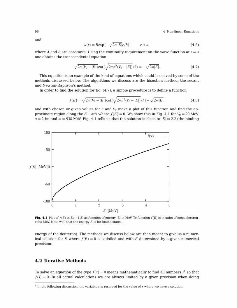
96 4 Non-linear Equations
andu(r) = Bexp(−
√2m|E|r/h) r > a, (4.6)
where A and B are constants. Using the continuity requirement on the wave function at r = a
one obtains the transcendental equation
√2m(V0−|E|)cot(
√2ma2(V0−|E|)/h) =−
√2m|E|. (4.7)
This equation is an example of the kind of equations which could be solved by some of themethods discussed below. The algorithms we discuss are the bisection method, the secantand Newton-Raphson’s method.
In order to find the solution for Eq. (4.7), a simple procedure is to define a function
f (E) =√
2m(V0−|E|)cot(√
2ma2(V0−|E|)/h)+√
2m|E|. (4.8)
and with chosen or given values for a and V0 make a plot of this function and find the ap-proximate region along the E− axis where f (E) = 0. We show this in Fig. 4.1 for V0 = 20 MeV,a = 2 fm and m = 938 MeV. Fig. 4.1 tells us that the solution is close to |E| ≈ 2.2 (the binding
-100
-50
0
50
100
0 1 2 3 4 5
f (E) [MeV]
|E| [MeV]
f(x)
Fig. 4.1 Plot of f (E) in Eq. (4.8) as function of energy |E| in MeV. Te function f (E) is in units of megaelectron-volts MeV. Note well that the energy E is for bound states.
energy of the deuteron). The methods we discuss below are then meant to give us a numer-ical solution for E where f (E) = 0 is satisfied and with E determined by a given numericalprecision.
4.2 Iterative Methods
To solve an equation of the type f (x) = 0 means mathematically to find all numbers s1 so thatf (s) = 0. In all actual calculations we are always limited by a given precision when doing
1 In the following discussion, the variable s is reserved for the value of x where we have a solution.

4.2 Iterative Methods 97
numerics. Through an iterative search of the solution, the hope is that we can approach,within a given tolerance ε, a value x0 which is a solution to f (s) = 0 if
|x0− s|< ε, (4.9)
and f (s) = 0. We could use other criteria as well like
∣∣∣∣x0− s
s
∣∣∣∣< ε, (4.10)
and | f (x0)| < ε or a combination of these. However, it is not given that the iterative processwill converge and we would like to have some conditions on f which ensures a solution. Thiscondition is provided by the so-called Lipschitz criterion. If the function f , defined on theinterval [a,b] satisfies for all x1 and x2 in the chosen interval the following condition
| f (x1)− f (x2)| ≤ k |x1− x2| , (4.11)
with k a constant, then f is continuous in the interval [a,b]. If f is continuous in the interval[a,b], then the secant condition gives
f (x1)− f (x2) = f ′(ξ )(x1− x2), (4.12)
with x1,x2 within [a,b] and ξ within [x1,x2]. We have then
| f (x1)− f (x2)| ≤ | f ′(ξ )| |x1− x2| . (4.13)
The derivative can be used as the constant k. We can now formulate the sufficient conditionsfor the convergence of the iterative search for solutions to f (s) = 0.
1. We assume that f is defined in the interval [a,b].2. f satisfies the Lipschitz condition with k < 1.
With these conditions, the equation f (x) = 0 has only one solution in the interval [a,b] and itconverges after n iterations towards the solution s irrespective of choice for x0 in the interval[a,b]. If we let xn be the value of x after n iterations, we have the condition
|s− xn| ≤k
1− k|x1− x2| . (4.14)
The proof can be found in the text of Bulirsch and Stoer. Since it is difficult numerically tofind exactly the point where f (s) = 0, in the actual numerical solution one implements threetests of the type
1.|xn− s|< ε, (4.15)
and2.
| f (s)| < δ , (4.16)
3. and a maximum number of iterations Nmaxiter in actual calculations.

98 4 Non-linear Equations
4.3 Bisection
This is an extremely simple method to code. The philosophy can best be explained by choosinga region in e.g., Fig. 4.1 which is close to where f (E) = 0. In our case |E| ≈ 2.2. Choose a region[a,b] so that a = 1.5 and b = 3. This should encompass the point where f = 0. Define then thepoint
c =a+ b
2, (4.17)
and calculate f (c). If f (a) f (c) < 0, the solution lies in the region [a,c] = [a,(a+ b)/2]. Changethen b← c and calculate a new value for c. If f (a) f (c) > 0, the new interval is in [c,b] =
[(a+ b)/2,b]. Now you need to change a← c and evaluate then a new value for c. We cancontinue to halve the interval till we have reached a value for c which fulfills f (c) = 0 to agiven numerical precision. The algorithm can be simply expressed in the following program
......
fa = f(a);
fb = f(b);
// check if your interval is correct, if not return to main
if ( fa*fb > 0)
cout << ``\n Error, root not in interval'' << endl;
return;
for (j=1; j <= iter_max; j++)
c=(a+b)/2;
fc=f(c)
// if this test is satisfied, we have the root c
if ( (abs(a-b) < epsilon ) || fc < delta ); return to main
if ( fa*fc < 0)
b=c ; fb=fc;
else
a=c ; fa=fc;
......
Note that one needs to define the values of δ , ε and iter_max when calling this function.The bisection method is an almost foolproof method, although it may converge slowly to-
wards the solution due to the fact that it halves the intervals. After n divisions by 2 we have apossible solution in the interval with length
1
2n|b− a| , (4.18)
and if we set x0 = (a+ b)/2 and let xn be the midpoints in the intervals we obtain after n
iterations that Eq. (4.14) results in
|s− xn| ≤1
2n+1|b− a| , (4.19)
since the nth interval has length |b−a|/2n. Note that this convergence criterion is independentof the actual function f (x) as long as this function fulfils the conditions discussed in theconditions discussed in the previous subsection.
As an example, suppose we wish to find how many iteration steps are needed in order toobtain a relative precision of 10−12 for xn in the interval [50,63], that is

4.4 Newton-Raphson’s Method 99
|s− xn||s| ≤ 10−12. (4.20)
It suffices in our case to study s≥ 50, which results in
|s− xn|50
≤ 10−12, (4.21)
and with Eq. (4.19) we obtain13
2n+150≤ 10−12, (4.22)
meaning n≥ 37. The code for the bisection method can look like this
/*
** This function
** calculates a root between x1 and x2 of a function
** pointed to by (*func) using the method of bisection
** The root is returned with an accuracy of +- xacc.
*/
double bisection(double (*func)(double), double x1, double x2, double xacc)
int j;
double dx, f, fmid, xmid, rtb;
f = (*func)(x1);
fmid = (*func)(x2);
if(f*fmid >= 0.0)
cout << "\n\nError in function bisection():" << endl;
cout << "\nroot in function must be within" << endl;
cout << "x1 ='' << x1 << ``and x2 `` << x2 << endl;
exit(1);
rtb = f < 0.0 ? (dx = x2 - x1, x1) : (dx = x1 - x2, x2);
for(j = 0; j < max_iterations; j++)
fmid = (*func)(xmid = rtb + (dx *= 0.5));
if (fmid <= 0.0) rtb=xmid;
if(fabs(dx) < xacc || fmid == 0.0) return rtb;
cout << "Error in the bisection:" << endl; // should never reach this point
cout "Too many iterations!" << endl;
// End: function bisection
In this function we transfer the lower and upper limit of the interval where we seek thesolution, [x1,x2]. The variable xacc is the precision we opt for. Note that in this function the testf (s)< δ is not implemented. Rather, the test is done through f (s) = 0, which is not necessarilya good option.
Note also that this function transfer a pointer to the name of the given function throughdouble(*func)(double).
4.4 Newton-Raphson’s Method
Perhaps the most celebrated of all one-dimensional root-finding routines is Newton’s method,also called the Newton-Raphson method. This method is distinguished from the previouslydiscussed methods by the fact that it requires the evaluation of both the function f and itsderivative f ′ at arbitrary points. In this sense, it is taylored to cases with e.g., transcendental

100 4 Non-linear Equations
equations of the type shown in Eq. (4.8) where it is rather easy to evaluate the derivative. Ifyou can only calculate the derivative numerically and/or your function is not of the smoothtype, we discourage the use of this method.
The Newton-Raphson formula consists geometrically of extending the tangent line at acurrent point until it crosses zero, then setting the next guess to the abscissa of that zero-crossing. The mathematics behind this method is rather simple. Employing a Taylor expansionfor x sufficiently close to the solution s, we have
f (s) = 0 = f (x)+ (s− x) f ′(x)+(s− x)2
2f ′′(x)+ . . . . (4.23)
For small enough values of the function and for well-behaved functions, the terms beyondlinear are unimportant, hence we obtain
f (x)+ (s− x) f ′(x)≈ 0, (4.24)
yielding
s≈ x− f (x)
f ′(x). (4.25)
Having in mind an iterative procedure, it is natural to start iterating with
xn+1 = xn−f (xn)
f ′(xn). (4.26)
This is Newton-Raphson’s method. It has a simple geometric interpretation, namely xn+1 isthe point where the tangent from (xn, f (xn)) crosses the x−axis. Close to the solution, Newton-Raphson converges fast to the desired result. However, if we are far from a root, where thehigher-order terms in the series are important, the Newton-Raphson formula can give grosslyinaccurate results. For instance, the initial guess for the root might be so far from the trueroot as to let the search interval include a local maximum or minimum of the function. If aniteration places a trial guess near such a local extremum, so that the first derivative nearlyvanishes, then Newton-Raphson may fail totally. An example is shown in Fig. 4.2
It is also possible to extract the convergence behavior of this method. Assume that thefunction f has a continuous second derivative around the solution s. If we define
en+1 = xn+1− s = xn−f (xn)
f ′(xn)− s, (4.27)
and using Eq. (4.23) we have
en+1 = en +−en f ′(xn)+ e2
n/2 f ′′(ξ )f ′(xn)
=e2
n/2 f ′′(ξ )f ′(xn)
. (4.28)
This gives|en+1||en|2
=1
2
| f ′′(ξ )|| f ′(xn)|2
=1
2
| f ′′(s)|| f ′(s)|2 (4.29)
when xn→ s. Our error constant k is then proportional to | f ′′(s)|/| f ′(s)|2 if the second derivativeis different from zero. Clearly, if the first derivative is small, the convergence is slower. Ingeneral, if we are able to start the iterative procedure near a root and we can easily evaluatethe derivative, this is the method of choice. In cases where we may need to evaluate thederivative numerically, the previously described methods are easier and most likely safer toimplement with respect to loss of numerical precision. Recall that the numerical evaluationof derivatives involves differences between function values at different xn.
We can rewrite the last equation as

4.4 Newton-Raphson’s Method 101
-5
0
5
10
15
20
0 2 4 6 8 10
f (x)
x
f (x) = x−2cos(x)c = x1
c = x2
Fig. 4.2 Example of a case where Newton-Raphson’s method does not converge. For the function f (x) =x− 2cos(x), we see that if we start at x = 7, the first iteration gives us that the first point where we cross thex−axis is given by x1. However, using x1 as a starting point for the next iteration results in a point x2 whichis close to a local minimum. The tangent here is close to zero and we will never approach the point wheref (x) = 0.
|en+1|=C|en|2, (4.30)
with C a constant. If we assume that C ∼ 1 and let en ∼ 10−8, this results in en+1 ∼ 10−16, anddemonstrates clearly why Newton-Raphson’s method may converge faster than the bisectionmethod.
Summarizing, this method has a solution when f ′′ is continuous and s is a simple zero of f .Then there is a neighborhood of s and a constant C such that if Newton-Raphson’s method isstarted in that neighborhood, the successive points become steadily closer to s and satisfy
|s− xn+1| ≤C|s− xn|2,
with n≥ 0. In some situations, the method guarantees to converge to a desired solution froman arbitrary starting point. In order for this to take place, the function f has to belong toC2(R), be increasing, convex and having a zero. Then this zero is unique and Newton’s methodconverges to it from any starting point.
As a mere curiosity, suppose we wish to compute the square root of a number R, i.e.,√
R.Let R > 0 and define a function
f (x) = x2−R.
The variable x is a root if f (x) = 0. Newton-Raphson’s method yields then the following itera-tive approach to the root
xn+1 =1
2
(xn +
R
xn
), (4.31)
a formula credited to Heron, a Greek engineer and architect who lived sometime between100 B.C. and A.D. 100.
Suppose we wish to compute√
13= 3.6055513 and start with x0 = 5. The first iteration givesx1 = 3.8, x2 = 3.6105263, x3 = 3.6055547 and x4 = 3.6055513. With just four iterations and a nottoo optimal choice of x0 we obtain the exact root to a precision of 8 digits. The above equation,

102 4 Non-linear Equations
together with range reduction , is used in the intrisic computational function which computessquare roots.
Newton’s method can be generalized to systems of several non-linear equations and vari-ables. Consider the case with two equations
f1(x1,x2) = 0
f2(x1,x2) = 0, (4.32)
which we Taylor expand to obtain
0 = f1(x1 + h1,x2 + h2) = f1(x1,x2)+ h1∂ f1/∂x1 + h2∂ f1/∂x2 + . . .
0 = f2(x1 + h1,x2 + h2) = f2(x1,x2)+ h1∂ f2/∂x1 + h2∂ f2/∂x2 + . . .. (4.33)
Defining the Jacobian matrix J we have
J =
(∂ f1/∂x1 ∂ f1/∂x2
∂ f2/∂x1 ∂ f2/∂x2
), (4.34)
we can rephrase Newton’s method as
(xn+1
1
xn+12
)=
(xn
1
xn2
)+
(hn
1
hn2
), (4.35)
where we have defined (hn
1
hn2
)=−J−1
(f1(x
n1,x
n2)
f2(xn1,x
n2)
). (4.36)
We need thus to compute the inverse of the Jacobian matrix and it is to understand thatdifficulties may arise in case J is nearly singular.
It is rather straightforward to extend the above scheme to systems of more than two non-linear equations.
The code for Newton-Raphson’s method can look like this
/*
** This function
** calculates a root between x1 and x2 of a function pointed to
** by (*funcd) using the Newton-Raphson method. The user-defined
** function funcd() returns both the function value and its first
** derivative at the point x,
** The root is returned with an accuracy of +- xacc.
*/
double newtonraphson(void (*funcd)(double, double *, double *), double x1, double x2,
double xacc)
int j;
double df, dx, f, rtn;
rtn = 0.5 * (x1 + x2); // initial guess
for(j = 0; j < max_iterations; j++)
(*funcd)(rtn, &f, &df);
dx = f/df;
rtn -= dx;
if((x1 - rtn) * (rtn - x2) < 0.0)
cout << "\n\nError in function newtonraphson:" << endl ;
cout << "Jump out of interval bracket" << endl;
if (fabs(dx) < xacc) return rtn;

4.5 The Secant Method 103
cout << "Error in function newtonraphson:" << endl;
cout << "Too many iterations!" << endl;
// End: function newtonraphson
We transfer again the lower and upper limit of the interval where we seek the solution, [x1,x2]
and the variable xacc. Firthermore, it transfers a pointer to the name of the given functionthrough double(*func)(double).
4.5 The Secant Method
For functions that are smooth near a root, the methods known respectively as false position(or regula falsi) and secant method generally converge faster than bisection but slower thanNewton-Raphson. In both of these methods the function is assumed to be approximately linearin the local region of interest, and the next improvement in the root is taken as the pointwhere the approximating line crosses the axis.
The algorithm for obtaining the solution for the secant method is rather simple. We startwith the definition of the derivative
f ′(xn) =f (xn)− f (xn−1)
xn− xn−1
and combine it with the iterative expression of Newton-Raphson’s
xn+1 = xn−f (xn)
f ′(xn),
to obtain
xn+1 = xn− f (xn)
(xn− xn−1
f (xn)− f (xn−1)
), (4.37)
which we rewrite to
xn+1 =f (xn)xn−1− f (xn−1)xn
f (xn)− f (xn−1). (4.38)
This is the secant formula, implying that we are drawing a straight line from the point(xn−1, f (xn−1)) to (xn, f (xn)). Where it crosses the x− axis we have the new point xn+1. Thisis illustrated in Fig. 4.3.
In the numerical implementation found in the program library, the quantities xn−1,xn,xn+1
are changed to a, b and c respectively, i.e., we determine c by the point where a straight linefrom the point (a, f (a)) to (b, f (b)) crosses the x− axis, that is
c =f (b)a− f (a)b
f (b)− f (a). (4.39)
We then see clearly the difference between the bisection method and the secant method. Theconvergence criterion for the secant method is
|en+1| ≈ A|en|α , (4.40)
with α ≈ 1.62. The convergence is better than linear, but not as good as Newton-Raphson’smethod which converges quadratically.
While the secant method formally converges faster than bisection, one finds in practicepathological functions for which bisection converges more rapidly. These can be choppy, dis-continuous functions, or even smooth functions if the second derivative changes sharply near

104 4 Non-linear Equations
-100
-50
0
50
100
0 1 2 3 4 5
f (E) [MeV]
|E| [MeV]
f (E)Eq. ()
Fig. 4.3 Plot of f (E) Eq. (4.8) as function of energy |E|. The point c is determined by where the straight linefrom (a, f (a)) to (b, f (b)) crosses the x−axis.
the root. Bisection always halves the interval, while the secant method can sometimes spendmany cycles slowly pulling distant bounds closer to a root. We illustrate the weakness of thismethod in Fig. 4.4 where we show the results of the first three iterations, i.e., the first pointis c = x1, the next iteration gives c = x2 while the third iterations ends with c = x3. We mayrisk that one of the endpoints is kept fixed while the other one only slowly converges to thedesired solution.
-20
0
20
40
60
80
100
120
140
0 0.2 0.4 0.6 0.8 1 1.2 1.4
f (x)
x
f (x) = 25x4− x2/2−2c = x1
c = x2
c = x3
Fig. 4.4 Plot of f (x) = 25x4− x2/2−2. The various straight lines correspond to the determination of the pointc after each iteration. c is determined by where the straight line from (a, f (a)) to (b, f (b)) crosses the x−axis.Here we have chosen three values for c, x1, x2 and x3 which refer to the first, second and third iterationsrespectively.

4.5 The Secant Method 105
The search for the solution s proceeds in much of the same fashion as for the bisectionmethod, namely after each iteration one of the previous boundary points is discarded in favorof the latest estimate of the root. A variation of the secant method is the so-called falseposition method (regula falsi from Latin) where the interval [a,b] is chosen so that f (a) f (b)<
0, else there is no solution. This is rather similar to the bisection method. Another possibilityis to determine the starting point for the iterative search using three points (a, f (a)), (b, f (b))
and (c, f (c)). One can thenuse Lagrange’s interpolation formula for a polynomial, see thediscussion in the previous chapter.
4.5.1 Broyden’s Method
Broyden’s method is a quasi-Newton method for the numerical solution of nonlinear equationsin k variables.
Newton’s method for solving the equation f (x) = 0 uses the Jacobian matrix and deter-minant J, at every iteration. However, computing the Jacobian is a difficult and expensiveoperation. The idea behind Broyden’s method is to compute the whole Jacobian only at thefirst iteration, and to do a so-called rank-one update at the other iterations.
The method is a generalization of the secant method to multiple dimensions. The secantmethod replaces the first derivative f ′(xn) with the finite difference approximation
f ′(xn)≃f (xn)− f (xn−1)
xn− xn−1
,
and proceeds using Newton’s method
xn+1 = xn−1
f ′(xn)f (xn).
Broyden gives a generalization of this formula to a system of equations F(x) = 0, replacingthe derivative f ′ with the Jacobian J. The Jacobian is determined using the secant equation(using the finite difference approximation):
Jn · (xn− xn−1)≃ F(xn)−F(xn−1).
However this equation is underdetermined in more than one dimension. Broyden suggestedusing the current estimate of the Jacobian Jn−1 and improving upon it by taking the solution tothe secant equation that is a minimal modification to Jn−1 (minimal in the sense of minimizingthe Frobenius norm ‖Jn− Jn−1‖F))
Jn = Jn−1 +∆Fn− Jn−1∆xn
‖∆xn‖2∆xT
n ,
and then apply Newton’s method
xn+1 = xn− J−1n F(xn).
In the formula above xn = (x1[n], ...,xk[n]) and Fn(x) = ( f1(x1[n], ...,xk[n]), ..., fk(x1[n], ...,xk[n])) arevector-columns with k elements for a system with k dimensions. We obtain then
∆xn =
x1[n]− x1[n− 1]
...
xk[n]− xk[n− 1]
and ∆Fn =
f1(x1[n], ...,xk[n])− f1(x1[n− 1], ...,xk[n− 1])
...
fk(x1[n], ...,xk[n])− fk(x1[n− 1], ...,xk[n− 1])
.
106 4 Non-linear Equations
Broyden also suggested using the Sherman-Morrison formula to update directly the inverseof the Jacobian
J−1n = J−1
n−1 +∆xn− J−1
n−1∆Fn
∆xTn J−1
n−1∆Fn
(∆xTn J−1
n−1)
This method is commonly known as the "good Broyden’s method". Many other quasi-Newtonschemes have been suggested in optimization, where one seeks a maximum or minimum byfinding the root of the first derivative (gradient in multi dimensions). The Jacobian of thegradient is called Hessian and is symmetric, adding further constraints to its upgrade.
4.6 Exercises
4.1. Write a code which implements the bisection method, Newton-Raphson’s method andthe secant method.
Find the positive roots ofx2− 4xsinx+(2sinx)2 = 0,
using these three methods and compare the achieved accuracy number of iterations neededto find the solution. Give a critical discussion of the methods.
4.2. Make thereafter a class which includes the above three methods and test this classagainst selected problems.
4.3. We are going to study the solution of the Schrödinger equation (SE) for a system with aneutron and proton (the deuteron) moving in a simple box potential.
We begin our discussion of the SE with the neutron-proton (deuteron) system with a boxpotential V (r). We define the radial part of the wave function R(r) and introduce the definitionu(r) = rR(R) The radial part of the SE for two particles in their center-of-mass system and withorbital momentum l = 0 is then
− h2
m
d2u(r)
dr2+V (r)u(r) = Eu(r),
withm = 2
mpmn
mp +mn
,
where mp and mn are the masses of the proton and neutron, respectively. We use here m = 938
MeV. Our potential is defined as
V (r) =
−V0 0≤ r < a
0 r > a
Bound states correspond to negative energy E and scattering states are given by positiveenergies. The SE takes the form (without specifying the sign of E)
d2u(r)
dr2+
m
h2(V0 +E)u(r) = 0 r < a,
andd2u(r)
dr2+
m
h2Eu(r) = 0 r > a.
We are now going to search for eventual bound states, i.e., E < 0. The deuteron has only onebound state at energy E =−2.223 MeV. Discuss the boundary conditions on the wave functionand use these to show that the solution to the SE is
4.6 Exercises 107
u(r) = Asin(kr) r < a,
andu(r) = Bexp(−β r) r > a,
where A and B are constants. We have also defined
k =√
m(V0−|E|)/h,
andβ =
√m|E|/h.
Show then, using the continuity requirement on the wave function that at r = a you obtain thetranscendental equation
kcot(ka) =−β . (4.41)
Insert values of V0 = 60 MeV and a = 1.45 fm (1 fm = 10−15 m) and make a plot plottingprograms) of Eq. (4.41) as function of energy E in order to find eventual eigenvalues. See ifthese values result in a bound state for E.
When you have localized on your plot the point(s) where Eq. (4.41) is satisfied, obtain anumerical value for E using the class you programmed in the previous exercise, including theNewton-Raphson’s method, the bisection method and the secant method. Make an analysisof these three methods and discuss how many iterations are needed to find a stable solution.
What is smallest possible value of V0 which gives a bound state?


Chapter 5
Numerical Integration
Abstract In this chapter we discuss some of the classical methods for integrating a func-tion. The methods we discuss are the trapezoidal, rectangular and Simpson’s rule for equallyspaced abscissas and integration approaches based on Gaussian quadrature. The latter aremore suitable for the case where the abscissas are not equally spaced. The emphasis is onmethods for evaluating few-dimensional (typically up to four dimensions) integrals. In chapter11 we show how Monte Carlo methods can be used to compute multi-dimensional integrals.We discuss also how to compute singular integrals. We end this chapter with an extensive dis-cussion on MPI and parallel computing. The examples focus on parallelization of algorithmsfor computing integrals.
5.1 Newton-Cotes Quadrature
The integral
I =∫ b
af (x)dx (5.1)
has a very simple meaning. If we consider Fig. 5.1 the integral I simply represents the areaenscribed by the function f (x) starting from x = a and ending at x = b. Two main methods willbe discussed below, the first one being based on equal (or allowing for slight modifications)steps and the other on more adaptive steps, namely so-called Gaussian quadrature methods.Both main methods encompass a plethora of approximations and only some of them will bediscussed here.
In considering equal step methods, our basic approach is that of approximating a functionf (x) with a polynomial of at most degree N− 1, given N integration points. If our polynomialis of degree 1, the function will be approximated with f (x)≈ a0 +a1x. The algorithm for theseintegration methods is rather simple, and the number of approximations perhaps unlimited!
• Choose a step size
h =b− a
N
where N is the number of steps and a and b the lower and upper limits of integration.• With a given step length we rewrite the integral as
∫ b
af (x)dx =
∫ a+h
af (x)dx+
∫ a+2h
a+hf (x)dx+ . . .
∫ b
b−hf (x)dx.
109

110 5 Numerical Integration
f (x)
x
a a+h a+2h a+3h b
Fig. 5.1 The area enscribed by the function f (x) starting from x = a to x = b. It is subdivided in several smallerareas whose evaluation is to be approximated by the techniques discussed in the text. The areas under thecurve can for example be approximated by rectangular boxes or trapezoids.
• The strategy then is to find a reliable polynomial approximation for f (x) in the variousintervals. Choosing a given approximation for f (x), we obtain a specific approximation tothe integral.
• With this approximation to f (x) we perform the integration by computing the integrals overall subintervals.
Such a small measure may seemingly allow for the derivation of various integrals. To see this,we rewrite the integral as
∫ b
af (x)dx =
∫ a+2h
af (x)dx+
∫ a+4h
a+2hf (x)dx+ . . .
∫ b
b−2hf (x)dx.
One possible strategy then is to find a reliable polynomial expansion for f (x) in the smallersubintervals. Consider for example evaluating
∫ a+2h
af (x)dx,
which we rewrite as ∫ a+2h
af (x)dx =
∫ x0+h
x0−hf (x)dx. (5.2)
We have chosen a midpoint x0 and have defined x0 = a+ h. Using Lagrange’s interpolationformula from Eq. (3.9), an equation we restate here,

5.1 Newton-Cotes Quadrature 111
PN(x) =N
∑i=0
∏k 6=i
x− xk
xi− xk
yi,
we could attempt to approximate the function f (x) with a first-order polynomial in x in thetwo sub-intervals x ∈ [x0− h,x0] and x ∈ [x0,x0 + h]. A first order polynomial means simply thatwe have for say the interval x ∈ [x0,x0 + h]
f (x) ≈ P1(x) =x− x0
(x0 + h)− x0f (x0 + h)+
x− (x0 + h)
x0− (x0 + h)f (x0),
and for the interval x ∈ [x0− h,x0]
f (x) ≈ P1(x) =x− (x0− h)
x0− (x0− h)f (x0)+
x− x0
(x0− h)− x0
f (x0− h).
Having performed this subdivision and polynomial approximation, one from x0− h to x0 andthe other from x0 to x0 + h,
∫ a+2h
af (x)dx =
∫ x0
x0−hf (x)dx+
∫ x0+h
x0
f (x)dx,
we can easily calculate for example the second integral as
∫ x0+h
x0
f (x)dx ≈∫ x0+h
x0
(x− x0
(x0 + h)− x0f (x0 + h)+
x− (x0 + h)
x0− (x0 + h)f (x0)
)dx,
which can be simplified to
∫ x0+h
x0
f (x)dx≈∫ x0+h
x0
(x− x0
hf (x0 + h)− x− (x0 + h)
hf (x0)
)dx,
resulting in ∫ x0+h
x0
f (x)dx =h
2( f (x0 + h)+ f (x0))+O(h3).
Here we added the error made in approximating our integral with a polynomial of degree 1.The other integral gives
∫ x0
x0−hf (x)dx =
h
2( f (x0)+ f (x0− h))+O(h3),
and adding up we obtain
∫ x0+h
x0−hf (x)dx =
h
2( f (x0 + h)+ 2 f (x0)+ f (x0− h))+O(h3), (5.3)
which is the well-known trapezoidal rule. Concerning the error in the approximation made,O(h3) = O((b− a)3/N3), you should note the following. This is the local error! Since we aresplitting the integral from a to b in N pieces, we will have to perform approximately N suchoperations. This means that the global error goes like ≈ O(h2). To see that, we use the trape-zoidal rule to compute the integral of Eq. (5.1),
I =∫ b
af (x)dx = h( f (a)/2+ f (a+ h)+ f (a+ 2h)+ · · ·+ f (b− h)+ fb/2) , (5.4)
with a global error which goes like O(h2).

112 5 Numerical Integration
Hereafter we use the shorthand notations f−h = f (x0− h), f0 = f (x0) and fh = f (x0 + h). Thecorrect mathematical expression for the local error for the trapezoidal rule is
∫ b
af (x)dx− b− a
2[ f (a)+ f (b)] =− h3
12f (2)(ξ ),
and the global error reads
∫ b
af (x)dx−Th( f ) =−b− a
12h2 f (2)(ξ ),
where Th is the trapezoidal result and ξ ∈ [a,b].The trapezoidal rule is easy to implement numerically through the following simple algo-
rithm
• Choose the number of mesh points and fix the step.• calculate f (a) and f (b) and multiply with h/2
• Perform a loop over n = 1 to n− 1 ( f (a) and f (b) are known) and sum up the termsf (a+ h)+ f (a+ 2h)+ f (a+ 3h)+ · · ·+ f (b− h). Each step in the loop corresponds to agiven value a+ nh.
• Multiply the final result by h and add h f (a)/2 and h f (b)/2.
A simple function which implements this algorithm is as follows
http://folk.uio.no/mhjensen/compphys/programs/chapter05/cpp/trapezoidal.cpp
double trapezoidal_rule(double a, double b, int n, double (*func)(double))
double trapez_sum;
double fa, fb, x, step;
int j;
step=(b-a)/((double) n);
fa=(*func)(a)/2. ;
fb=(*func)(b)/2. ;
TrapezSum=0.;
for (j=1; j <= n-1; j++)
x=j*step+a;
trapez_sum+=(*func)(x);
trapez_sum=(trapez_um+fb+fa)*step;
return trapez_sum;
// end trapezoidal_rule
The function returns a new value for the specific integral through the variable trapez_sum.There is one new feature to note here, namely the transfer of a user defined function calledfunc in the definition
void trapezoidal_rule(double a, double b, int n, double *trapez_sum,
double (*func)(double) )
What happens here is that we are transferring a pointer to the name of a user defined func-tion, which has as input a double precision variable and returns a double precision number.The function trapezoidal_rule is called as
trapezoidal_rule(a, b, n, &MyFunction )

5.1 Newton-Cotes Quadrature 113
in the calling function. We note that a, b and n are called by value, while trapez_sum andthe user defined function MyFunction are called by reference.
The name trapezoidal rule follows from the simple fact that it has a simple geometricalinterpretation, it corresponds namely to summing up a series of trapezoids, which are theapproximations to the area below the curve f (x).
Another very simple approach is the so-called midpoint or rectangle method. In this casethe integration area is split in a given number of rectangles with length h and height givenby the mid-point value of the function. This gives the following simple rule for approximatingan integral
I =∫ b
af (x)dx ≈ h
N
∑i=1
f (xi−1/2), (5.5)
where f (xi−1/2) is the midpoint value of f for a given rectangle. We will discuss its truncationerror below. It is easy to implement this algorithm, as shown here
http://folk.uio.no/mhjensen/compphys/programs/chapter05/cpp/rectangle.cpp
double rectangle_rule(double a, double b, int n, double (*func)(double))
double rectangle_sum;
double fa, fb, x, step;
int j;
step=(b-a)/((double) n);
rectangle_sum=0.;
for (j = 0; j <= n; j++)
x = (j+0.5)*step+; // midpoint of a given rectangle
rectangle_sum+=(*func)(x); // add value of function.
rectangle_sum *= step; // multiply with step length.
return rectangle_sum;
// end rectangle_rule
The correct mathematical expression for the local error for the rectangular rule Ri(h) forelement i is ∫ h
−hf (x)dx−Ri(h) =−
h3
24f (2)(ξ ),
and the global error reads
∫ b
af (x)dx−Rh( f ) =−b− a
24h2 f (2)(ξ ),
where Rh is the result obtained with rectangular rule and ξ ∈ [a,b].Instead of using the above first-order polynomials approximations for f , we attempt at
using a second-order polynomials. In this case we need three points in order to define asecond-order polynomial approximation
f (x) ≈ P2(x) = a0 + a1x+ a2x2.
Using again Lagrange’s interpolation formula we have
P2(x) =(x− x0)(x− x1)
(x2− x0)(x2− x1)y2 +
(x− x0)(x− x2)
(x1− x0)(x1− x2)y1 +
(x− x1)(x− x2)
(x0− x1)(x0− x2)y0.
Inserting this formula in the integral of Eq. (5.2) we obtain
∫ +h
−hf (x)dx =
h
3( fh + 4 f0 + f−h)+O(h5),

114 5 Numerical Integration
which is Simpson’s rule. Note that the improved accuracy in the evaluation of the deriva-tives gives a better error approximation, O(h5) vs. O(h3) . But this is again the local errorapproximation. Using Simpson’s rule we can easily compute the integral of Eq. (5.1) to be
I =∫ b
af (x)dx =
h
3( f (a)+ 4 f (a+ h)+ 2 f (a+ 2h)+ · · ·+ 4 f (b− h)+ fb) , (5.6)
with a global error which goes like O(h4). More formal expressions for the local and globalerrors are for the local error
∫ b
af (x)dx− b− a
6[ f (a)+ 4 f ((a+ b)/2)+ f (b)] =− h5
90f (4)(ξ ),
and for the global error ∫ b
af (x)dx− Sh( f ) =−b− a
180h4 f (4)(ξ ).
with ξ ∈ [a,b] and Sh the results obtained with Simpson’s method. The method can easily beimplemented numerically through the following simple algorithm
• Choose the number of mesh points and fix the step.• calculate f (a) and f (b)
• Perform a loop over n = 1 to n− 1 ( f (a) and f (b) are known) and sum up the terms4 f (a+ h)+ 2 f (a+ 2h)+ 4 f (a+ 3h)+ · · ·+ 4 f (b− h). Each step in the loop correspondsto a given value a+ nh. Odd values of n give 4 as factor while even values yield 2 asfactor.
• Multiply the final result by h3.
In more general terms, what we have done here is to approximate a given function f (x) witha polynomial of a certain degree. One can show that given n+1 distinct points x0, . . . ,xn ∈ [a,b]
and n+ 1 values y0, . . . ,yn there exists a unique polynomial Pn(x) with the property
Pn(x j) = y j j = 0, . . . ,n
In the Lagrange representation discussed in chapter 3, this interpolating polynomial is givenby
Pn =n
∑k=0
lkyk,
with the Lagrange factors
lk(x) =n
∏i = 0
i 6= k
x− xi
xk− xi
k = 0, . . . ,n,
see for example the text of Kress [24] or Burlich and Stoer [25] for details. If we for exampleset n = 1, we obtain
P1(x) = y0x− x1
x0− x1
+ y1x− x0
x1− x0
=y1− y0
x1− x0
x− y1x0 + y0x1
x1− x0
,
which we recognize as the equation for a straight line.
5.2 Adaptive Integration 115
The polynomial interpolatory quadrature of order n with equidistant quadrature pointsxk = a+ kh and step h = (b− a)/n is called the Newton-Cotes quadrature formula of order n.General expressions can be found in for example Refs. [24,25].
5.2 Adaptive Integration
Before we proceed with more advanced methods like Gaussian quadrature, we mentionbreefly how an adaptive integration method can be implemented.
The above methods are all based on a defined step length, normally provided by the user,dividing the integration domain with a fixed number of subintervals. This is rather simpleto implement may be inefficient, in particular if the integrand varies considerably in certainareas of the integration domain. In these areas the number of fixed integration points maynot be adequate. In other regions, the integrand may vary slowly and fewer integration pointsmay be needed.
In order to account for such features, it may be convenient to first study the propertiesof integrand, via for example a plot of the function to integrate. If this function oscillateslargely in some specific domain we may then opt for adding more integration points to thatparticular domain. However, this procedure needs to be repeated for every new integrandand lacks obviously the advantages of a more generic code.
The algorithm we present here is based on a recursive procedure and allows us to automatean adaptive domain. The procedure is very simple to implement.
Assume that we want to compute an integral using say the trapezoidal rule. We limit our-selves to a one-dimensional integral. Our integration domain is defined by x ∈ [a,b]. The algo-rithm goes as follows
• We compute our first approximation by computing the integral for the full domain. We labelthis as I(0). It is obtained by calling our previously discussed function trapezoidal_rule as
I0 = trapezoidal_rule(a, b, n, function);
• In the next step we split the integration in two, with c = (a+b)/2. We compute then the twointegrals I(1L) and I(1R)
I1L = trapezoidal_rule(a, c, n, function);
and
I1R = trapezoidal_rule(c, b, n, function);
With a given defined tolerance, being a small number provided by us, we estimate thedifference |I(1L) + I(1R)− I(0)| < tolerance. If this test is satisfied, our first approximation issatisfactory.
• If not, we can set up a recursive procedure where the integral is split into subsequentsubintervals until our tolerance is satisfied.
This recursive procedure can be easily implemented via the following function
// Simple recursive function that implements the
// adaptive integration using the trapezoidal rule
// It is convenient to define as global variables
// the tolerance and the number of recursive steps
const int maxrecursions = 50;
const double tolerance = 1.0E-10;
// Takes as input the integration limits, number of points, function to integrate
// and the number of steps
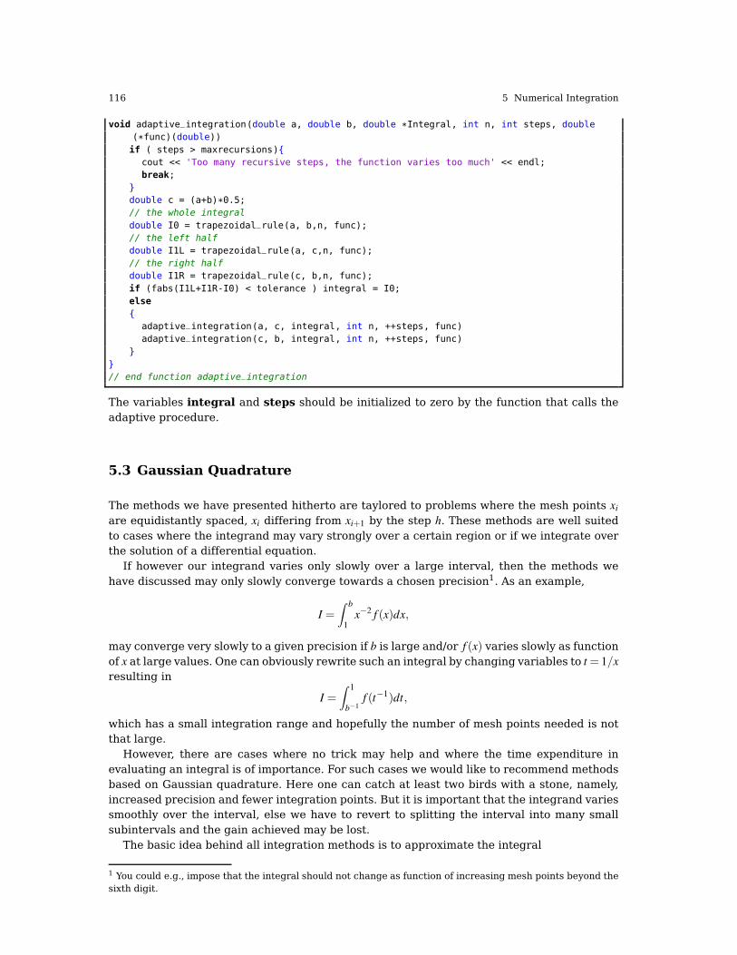
116 5 Numerical Integration
void adaptive_integration(double a, double b, double *Integral, int n, int steps, double
(*func)(double))
if ( steps > maxrecursions)
cout << 'Too many recursive steps, the function varies too much' << endl;
break;
double c = (a+b)*0.5;
// the whole integral
double I0 = trapezoidal_rule(a, b,n, func);
// the left half
double I1L = trapezoidal_rule(a, c,n, func);
// the right half
double I1R = trapezoidal_rule(c, b,n, func);
if (fabs(I1L+I1R-I0) < tolerance ) integral = I0;
else
adaptive_integration(a, c, integral, int n, ++steps, func)
adaptive_integration(c, b, integral, int n, ++steps, func)
// end function adaptive_integration
The variables integral and steps should be initialized to zero by the function that calls theadaptive procedure.
5.3 Gaussian Quadrature
The methods we have presented hitherto are taylored to problems where the mesh points xi
are equidistantly spaced, xi differing from xi+1 by the step h. These methods are well suitedto cases where the integrand may vary strongly over a certain region or if we integrate overthe solution of a differential equation.
If however our integrand varies only slowly over a large interval, then the methods wehave discussed may only slowly converge towards a chosen precision1. As an example,
I =∫ b
1x−2 f (x)dx,
may converge very slowly to a given precision if b is large and/or f (x) varies slowly as functionof x at large values. One can obviously rewrite such an integral by changing variables to t = 1/x
resulting in
I =
∫ 1
b−1f (t−1)dt,
which has a small integration range and hopefully the number of mesh points needed is notthat large.
However, there are cases where no trick may help and where the time expenditure inevaluating an integral is of importance. For such cases we would like to recommend methodsbased on Gaussian quadrature. Here one can catch at least two birds with a stone, namely,increased precision and fewer integration points. But it is important that the integrand variessmoothly over the interval, else we have to revert to splitting the interval into many smallsubintervals and the gain achieved may be lost.
The basic idea behind all integration methods is to approximate the integral
1 You could e.g., impose that the integral should not change as function of increasing mesh points beyond thesixth digit.

5.3 Gaussian Quadrature 117
I =
∫ b
af (x)dx≈
N
∑i=1
ωi f (xi),
where ω and x are the weights and the chosen mesh points, respectively. In our previousdiscussion, these mesh points were fixed at the beginning, by choosing a given number ofpoints N. The weigths ω resulted then from the integration method we applied. Simpson’srule, see Eq. (5.6) would give
ω : h/3,4h/3,2h/3,4h/3, . . .,4h/3,h/3,
for the weights, while the trapezoidal rule resulted in
ω : h/2,h,h, . . . ,h,h/2 .
In general, an integration formula which is based on a Taylor series using N points, willintegrate exactly a polynomial P of degree N− 1. That is, the N weights ωn can be chosen tosatisfy N linear equations, see chapter 3 of Ref. [3]. A greater precision for a given amountof numerical work can be achieved if we are willing to give up the requirement of equallyspaced integration points. In Gaussian quadrature (hereafter GQ), both the mesh points andthe weights are to be determined. The points will not be equally spaced2. The theory behindGQ is to obtain an arbitrary weight ω through the use of so-called orthogonal polynomials.These polynomials are orthogonal in some interval say e.g., [-1,1]. Our points xi are chosen insome optimal sense subject only to the constraint that they should lie in this interval. Togetherwith the weights we have then 2N (N the number of points) parameters at our disposal.
Even though the integrand is not smooth, we could render it smooth by extracting from itthe weight function of an orthogonal polynomial, i.e., we are rewriting
I =
∫ b
af (x)dx =
∫ b
aW (x)g(x)dx≈
N
∑i=1
ωig(xi), (5.7)
where g is smooth and W is the weight function, which is to be associated with a givenorthogonal polynomial. Note that with a given weight function we end up evaluating theintegrand for the function g(xi).
The weight function W is non-negative in the integration interval x ∈ [a,b] such that forany n≥ 0, the integral
∫ ba |x|nW (x)dx is integrable. The naming weight function arises from the
fact that it may be used to give more emphasis to one part of the interval than another. Aquadrature formula
∫ b
aW (x) f (x)dx ≈
N
∑i=1
ωi f (xi), (5.8)
with N distinct quadrature points (mesh points) is a called a Gaussian quadrature formula ifit integrates all polynomials p ∈ P2N−1 exactly, that is
∫ b
aW (x)p(x)dx =
N
∑i=1
ωi p(xi), (5.9)
It is assumed that W (x) is continuous and positive and that the integral
∫ b
aW (x)dx
2 Typically, most points will be located near the origin, while few points are needed for large x values sincethe integrand is supposed to vary smoothly there. See below for an example.

118 5 Numerical Integration
exists. Note that the replacement of f →Wg is normally a better approximation due to thefact that we may isolate possible singularities of W and its derivatives at the endpoints of theinterval.
The quadrature weights or just weights (not to be confused with the weight function) arepositive and the sequence of Gaussian quadrature formulae is convergent if the sequence QN
of quadrature formulae
QN( f )→Q( f ) =
∫ b
af (x)dx,
in the limit N→ ∞. Then we say that the sequence
QN( f ) =N
∑i=1
ω(N)i f (x
(N)i ),
is convergent for all polynomials p, that is
QN(p) = Q(p)
if there exits a constant C such thatN
∑i=1
|ω(N)i | ≤C,
for all N which are natural numbers.The error for the Gaussian quadrature formulae of order N is given by
∫ b
aW (x) f (x)dx−
N
∑k=1
wk f (xk) =f 2N(ξ )
(2N)!
∫ b
aW (x)[qN(x)]
2dx
where qN is the chosen orthogonal polynomial and ξ is a number in the interval [a,b]. Wehave assumed that f ∈ C2N [a,b], viz. the space of all real or complex 2N times continuouslydifferentiable functions.
In science there are several important orthogonal polynomials which arise from the solu-tion of differential equations. Well-known examples are the Legendre, Hermite, Laguerre andChebyshev polynomials. They have the following weight functions
Weight function Interval Polynomial
W (x) = 1 x ∈ [−1,1] Legendre
W (x) = e−x2 −∞≤ x≤ ∞ HermiteW (x) = xα e−x 0≤ x≤ ∞ Laguerre
W (x) = 1/(√
1− x2) −1≤ x≤ 1 Chebyshev
The importance of the use of orthogonal polynomials in the evaluation of integrals can besummarized as follows.
• As stated above, methods based on Taylor series using N points will integrate exactly apolynomial P of degree N− 1. If a function f (x) can be approximated with a polynomial ofdegree N− 1
f (x) ≈ PN−1(x),
with N mesh points we should be able to integrate exactly the polynomial PN−1.• Gaussian quadrature methods promise more than this. We can get a better polynomial
approximation with order greater than N to f (x) and still get away with only N mesh points.More precisely, we approximate
f (x)≈ P2N−1(x),
and with only N mesh points these methods promise that

5.3 Gaussian Quadrature 119
∫f (x)dx ≈
∫P2N−1(x)dx =
N−1
∑i=0
P2N−1(xi)ωi,
The reason why we can represent a function f (x) with a polynomial of degree 2N−1 is dueto the fact that we have 2N equations, N for the mesh points and N for the weights.
The mesh points are the zeros of the chosen orthogonal polynomial of order N, and theweights are determined from the inverse of a matrix. An orthogonal polynomials of degree N
defined in an interval [a,b] has precisely N distinct zeros on the open interval (a,b).Before we detail how to obtain mesh points and weights with orthogonal polynomials, let
us revisit some features of orthogonal polynomials by specializing to Legendre polynomials.In the text below, we reserve hereafter the labelling LN for a Legendre polynomial of order N,while PN is an arbitrary polynomial of order N. These polynomials form then the basis for theGauss-Legendre method.
5.3.1 Orthogonal polynomials, Legendre
The Legendre polynomials are the solutions of an important differential equation in Science,namely
C(1− x2)P−m2l P+(1− x2)
d
dx
((1− x2)
dP
dx
)= 0.
Here C is a constant. For ml = 0 we obtain the Legendre polynomials as solutions, whereasml 6= 0 yields the so-called associated Legendre polynomials. This differential equation arisesin for example the solution of the angular dependence of Schrödinger’s equation with spher-ically symmetric potentials such as the Coulomb potential.
The corresponding polynomials P are
Lk(x) =1
2kk!
dk
dxk(x2− 1)k k = 0,1,2, . . . ,
which, up to a factor, are the Legendre polynomials Lk. The latter fulfil the orthogonalityrelation ∫ 1
−1Li(x)L j(x)dx =
2
2i+ 1δi j , (5.10)
and the recursion relation
( j+ 1)L j+1(x)+ jL j−1(x)− (2 j+ 1)xL j(x) = 0. (5.11)
It is common to choose the normalization condition
LN(1) = 1.
With these equations we can determine a Legendre polynomial of arbitrary order with inputpolynomials of order N− 1 and N− 2.
As an example, consider the determination of L0, L1 and L2. We have that
L0(x) = c,
with c a constant. Using the normalization equation L0(1) = 1 we get that
L0(x) = 1.

120 5 Numerical Integration
For L1(x) we have the general expression
L1(x) = a+ bx,
and using the orthogonality relation
∫ 1
−1L0(x)L1(x)dx = 0,
we obtain a = 0 and with the condition L1(1) = 1, we obtain b = 1, yielding
L1(x) = x.
We can proceed in a similar fashion in order to determine the coefficients of L2
L2(x) = a+ bx+ cx2,
using the orthogonality relations
∫ 1
−1L0(x)L2(x)dx = 0,
and ∫ 1
−1L1(x)L2(x)dx = 0,
and the condition L2(1) = 1 we would get
L2(x) =1
2
(3x2− 1
). (5.12)
We note that we have three equations to determine the three coefficients a, b and c.Alternatively, we could have employed the recursion relation of Eq. (5.11), resulting in
2L2(x) = 3xL1(x)−L0,
which leads to Eq. (5.12).The orthogonality relation above is important in our discussion on how to obtain the
weights and mesh points. Suppose we have an arbitrary polynomial QN−1 of order N−1 and aLegendre polynomial LN(x) of order N. We could represent QN−1 by the Legendre polynomialsthrough
QN−1(x) =N−1
∑k=0
αkLk(x), (5.13)
where αk’s are constants.Using the orthogonality relation of Eq. (5.10) we see that
∫ 1
−1LN(x)QN−1(x)dx =
N−1
∑k=0
∫ 1
−1LN(x)αkLk(x)dx = 0. (5.14)
We will use this result in our construction of mesh points and weights in the next subsection.In summary, the first few Legendre polynomials are
L0(x) = 1,
L1(x) = x,
L2(x) = (3x2− 1)/2,

5.3 Gaussian Quadrature 121
L3(x) = (5x3− 3x)/2,
andL4(x) = (35x4− 30x2+ 3)/8.
The following simple function implements the above recursion relation of Eq. (5.11). for com-puting Legendre polynomials of order N.
// This function computes the Legendre polynomial of degree N
double Legendre( int n, double x)
double r, s, t;
int m;
r = 0; s = 1.;
// Use recursion relation to generate p1 and p2
for (m=0; m < n; m++ )
t = r; r = s;
s = (2*m+1)*x*r - m*t;
s /= (m+1);
// end of do loop
return s;
// end of function Legendre
The variable s represents L j+1(x), while r holds L j(x) and t the value L j−1(x).
5.3.2 Integration points and weights with orthogonal polynomials
To understand how the weights and the mesh points are generated, we define first a polyno-mial of degree 2N−1 (since we have 2N variables at hand, the mesh points and weights for N
points). This polynomial can be represented through polynomial division by
P2N−1(x) = LN(x)PN−1(x)+QN−1(x),
where PN−1(x) and QN−1(x) are some polynomials of degree N− 1 or less. The function LN(x)
is a Legendre polynomial of order N.Recall that we wanted to approximate an arbitrary function f (x) with a polynomial P2N−1 in
order to evaluate ∫ 1
−1f (x)dx≈
∫ 1
−1P2N−1(x)dx.
We can use Eq. (5.14) to rewrite the above integral as
∫ 1
−1P2N−1(x)dx =
∫ 1
−1(LN(x)PN−1(x)+QN−1(x))dx =
∫ 1
−1QN−1(x)dx,
due to the orthogonality properties of the Legendre polynomials. We see that it suffices toevaluate the integral over
∫ 1−1 QN−1(x)dx in order to evaluate
∫ 1−1 P2N−1(x)dx. In addition, at the
points xk where LN is zero, we have
P2N−1(xk) = QN−1(xk) k = 0,1, . . . ,N− 1,
and we see that through these N points we can fully define QN−1(x) and thereby the integral.Note that we have chosen to let the numbering of the points run from 0 to N− 1. The reasonfor this choice is that we wish to have the same numbering as the order of a polynomial of
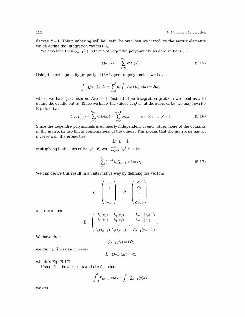
122 5 Numerical Integration
degree N− 1. This numbering will be useful below when we introduce the matrix elementswhich define the integration weights wi.
We develope then QN−1(x) in terms of Legendre polynomials, as done in Eq. (5.13),
QN−1(x) =N−1
∑i=0
αiLi(x). (5.15)
Using the orthogonality property of the Legendre polynomials we have
∫ 1
−1QN−1(x)dx =
N−1
∑i=0
αi
∫ 1
−1L0(x)Li(x)dx = 2α0,
where we have just inserted L0(x) = 1! Instead of an integration problem we need now todefine the coefficient α0. Since we know the values of QN−1 at the zeros of LN , we may rewriteEq. (5.15) as
QN−1(xk) =N−1
∑i=0
αiLi(xk) =N−1
∑i=0
αiLik k = 0,1, . . . ,N− 1. (5.16)
Since the Legendre polynomials are linearly independent of each other, none of the columnsin the matrix Lik are linear combinations of the others. This means that the matrix Lik has aninverse with the properties
L−1L = I.
Multiplying both sides of Eq. (5.16) with ∑N−1j=0 L−1
ji results in
N−1
∑i=0
(L−1)kiQN−1(xi) = αk. (5.17)
We can derive this result in an alternative way by defining the vectors
xk =
x0
x1
.
.
xN−1
α =
α0
α1
.
.
αN−1
,
and the matrix
L =
L0(x0) L1(x0) . . . LN−1(x0)
L0(x1) L1(x1) . . . LN−1(x1)
. . . . . . . . . . . .
L0(xN−1) L1(xN−1) . . . LN−1(xN−1)
.
We have thenQN−1(xk) = Lα,
yielding (if L has an inverse)L−1QN−1(xk) = α,
which is Eq. (5.17).Using the above results and the fact that
∫ 1
−1P2N−1(x)dx =
∫ 1
−1QN−1(x)dx,
we get

5.3 Gaussian Quadrature 123
∫ 1
−1P2N−1(x)dx =
∫ 1
−1QN−1(x)dx = 2α0 = 2
N−1
∑i=0
(L−1)0iP2N−1(xi).
If we identify the weights with 2(L−1)0i, where the points xi are the zeros of LN , we have anintegration formula of the type
∫ 1
−1P2N−1(x)dx =
N−1
∑i=0
ωiP2N−1(xi)
and if our function f (x) can be approximated by a polynomial P of degree 2N− 1, we havefinally that
∫ 1
−1f (x)dx ≈
∫ 1
−1P2N−1(x)dx =
N−1
∑i=0
ωiP2N−1(xi).
In summary, the mesh points xi are defined by the zeros of an orthogonal polynomial of degreeN, that is LN , while the weights are given by 2(L−1)0i.
5.3.3 Application to the case N = 2
Let us apply the above formal results to the case N = 2. This means that we can approximatea function f (x) with a polynomial P3(x) of order 2N− 1 = 3.
The mesh points are the zeros of L2(x) = 1/2(3x2− 1). These points are x0 = −1/√
3 andx1 = 1/
√3.
Specializing Eq. (5.16)
QN−1(xk) =N−1
∑i=0
αiLi(xk) k = 0,1, . . . ,N− 1.
to N = 2 yields
Q1(x0) = α0−α11√3,
and
Q1(x1) = α0 +α11√3,
since L0(x =±1/√
3) = 1 and L1(x =±1/√
3) =±1/√
3.The matrix Lik defined in Eq. (5.16) is then
L =
(1 − 1√
3
1 1√3
),
with an inverse given by
L−1 =
√3
2
(1√3
1√3
−1 1
).
The weights are given by the matrix elements 2(L0k)−1. We have thence ω0 = 1 and ω1 = 1.
Obviously, there is no problem in changing the numbering of the matrix elements i,k =
0,1,2, . . . ,N− 1 to i,k = 1,2, . . . ,N. We have chosen to start from zero, since we deal with poly-nomials of degree N− 1.
Summarizing, for Legendre polynomials with N = 2 we have weights
ω : 1,1 ,

124 5 Numerical Integration
and mesh points
x :
− 1√
3,
1√3
.
If we wish to integrate ∫ 1
−1f (x)dx,
with f (x) = x2, we approximate
I =
∫ 1
−1x2dx≈
N−1
∑i=0
ωix2i .
The exact answer is 2/3. Using N = 2 with the above two weights and mesh points we get
I =
∫ 1
−1x2dx =
1
∑i=0
ωix2i =
1
3+
1
3=
2
3,
the exact answer!If we were to emply the trapezoidal rule we would get
I =
∫ 1
−1x2dx =
b− a
2
((a)2 +(b)2
)/2 =
1− (−1)
2
((−1)2 +(1)2
)/2 = 1!
With just two points we can calculate exactly the integral for a second-order polynomial sinceour methods approximates the exact function with higher order polynomial. How many pointsdo you need with the trapezoidal rule in order to achieve a similar accuracy?
5.3.4 General integration intervals for Gauss-Legendre
Note that the Gauss-Legendre method is not limited to an interval [-1,1], since we can alwaysthrough a change of variable
t =b− a
2x+
b+ a
2,
rewrite the integral for an interval [a,b]
∫ b
af (t)dt =
b− a
2
∫ 1
−1f
((b− a)x
2+
b+ a
2
)dx.
If we have an integral on the form ∫ ∞
0f (t)dt,
we can choose new mesh points and weights by using the mapping
xi = tan
π
4(1+ xi)
,
andωi =
π
4
ωi
cos2(
π4(1+ xi)
) ,
where xi and ωi are the original mesh points and weights in the interval [−1,1], while xi andωi are the new mesh points and weights for the interval [0,∞).
To see that this is correct by inserting the the value of xi =−1 (the lower end of the interval[−1,1]) into the expression for xi. That gives xi = 0, the lower end of the interval [0,∞). Forxi = 1, we obtain xi = ∞. To check that the new weights are correct, recall that the weights

5.3 Gaussian Quadrature 125
should correspond to the derivative of the mesh points. Try to convince yourself that theabove expression fulfills this condition.
5.3.5 Other orthogonal polynomials
5.3.5.1 Laguerre polynomials
If we are able to rewrite our integral of Eq. (5.7) with a weight function W (x) = xα e−x withintegration limits [0,∞), we could then use the Laguerre polynomials. The polynomials formthen the basis for the Gauss-Laguerre method which can be applied to integrals of the form
I =
∫ ∞
0f (x)dx =
∫ ∞
0xα e−xg(x)dx.
These polynomials arise from the solution of the differential equation
(d2
dx2− d
dx+
λ
x− l(l + 1)
x2
)L (x) = 0,
where l is an integer l≥ 0 and λ a constant. This equation arises for example from the solutionof the radial Schrödinger equation with a centrally symmetric potential such as the Coulombpotential. The first few polynomials are
L0(x) = 1,
L1(x) = 1− x,
L2(x) = 2− 4x+ x2,
L3(x) = 6− 18x+ 9x2− x3,
andL4(x) = x4− 16x3 + 72x2− 96x+ 24.
They fulfil the orthogonality relation
∫ ∞
0e−x
Ln(x)2dx = 1,
and the recursion relation
(n+ 1)Ln+1(x) = (2n+ 1− x)Ln(x)− nLn−1(x).
5.3.5.2 Hermite polynomials
In a similar way, for an integral which goes like
I =
∫ ∞
−∞f (x)dx =
∫ ∞
−∞e−x2
g(x)dx.
we could use the Hermite polynomials in order to extract weights and mesh points. TheHermite polynomials are the solutions of the following differential equation
d2H(x)
dx2− 2x
dH(x)
dx+(λ − 1)H(x) = 0.
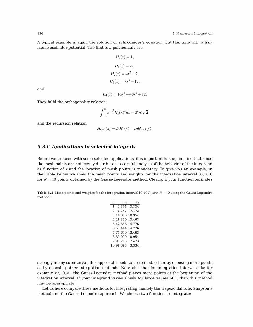
126 5 Numerical Integration
A typical example is again the solution of Schrödinger’s equation, but this time with a har-monic oscillator potential. The first few polynomials are
H0(x) = 1,
H1(x) = 2x,
H2(x) = 4x2− 2,
H3(x) = 8x3− 12,
andH4(x) = 16x4− 48x2 + 12.
They fulfil the orthogonality relation
∫ ∞
−∞e−x2
Hn(x)2dx = 2nn!
√π,
and the recursion relationHn+1(x) = 2xHn(x)− 2nHn−1(x).
5.3.6 Applications to selected integrals
Before we proceed with some selected applications, it is important to keep in mind that sincethe mesh points are not evenly distributed, a careful analysis of the behavior of the integrandas function of x and the location of mesh points is mandatory. To give you an example, inthe Table below we show the mesh points and weights for the integration interval [0,100]for N = 10 points obtained by the Gauss-Legendre method. Clearly, if your function oscillates
Table 5.1 Mesh points and weights for the integration interval [0,100] with N = 10 using the Gauss-Legendremethod.
i xi ωi
1 1.305 3.3342 6.747 7.4733 16.030 10.9544 28.330 13.4635 42.556 14.7766 57.444 14.7767 71.670 13.4638 83.970 10.9549 93.253 7.473
10 98.695 3.334
strongly in any subinterval, this approach needs to be refined, either by choosing more pointsor by choosing other integration methods. Note also that for integration intervals like forexample x ∈ [0,∞], the Gauss-Legendre method places more points at the beginning of theintegration interval. If your integrand varies slowly for large values of x, then this methodmay be appropriate.
Let us here compare three methods for integrating, namely the trapezoidal rule, Simpson’smethod and the Gauss-Legendre approach. We choose two functions to integrate:
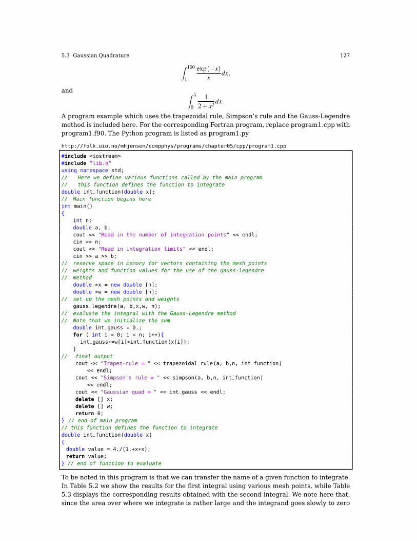
5.3 Gaussian Quadrature 127
∫ 100
1
exp(−x)
xdx,
and ∫ 3
0
1
2+ x2dx.
A program example which uses the trapezoidal rule, Simpson’s rule and the Gauss-Legendremethod is included here. For the corresponding Fortran program, replace program1.cpp withprogram1.f90. The Python program is listed as program1.py.
http://folk.uio.no/mhjensen/compphys/programs/chapter05/cpp/program1.cpp
#include <iostream>
#include "lib.h"
using namespace std;
// Here we define various functions called by the main program
// this function defines the function to integrate
double int_function(double x);
// Main function begins here
int main()
int n;
double a, b;
cout << "Read in the number of integration points" << endl;
cin >> n;
cout << "Read in integration limits" << endl;
cin >> a >> b;
// reserve space in memory for vectors containing the mesh points
// weights and function values for the use of the gauss-legendre
// method
double *x = new double [n];
double *w = new double [n];
// set up the mesh points and weights
gauss_legendre(a, b,x,w, n);
// evaluate the integral with the Gauss-Legendre method
// Note that we initialize the sum
double int_gauss = 0.;
for ( int i = 0; i < n; i++)
int_gauss+=w[i]*int_function(x[i]);
// final output
cout << "Trapez-rule = " << trapezoidal_rule(a, b,n, int_function)
<< endl;
cout << "Simpson's rule = " << simpson(a, b,n, int_function)
<< endl;
cout << "Gaussian quad = " << int_gauss << endl;
delete [] x;
delete [] w;
return 0;
// end of main program
// this function defines the function to integrate
double int_function(double x)
double value = 4./(1.+x*x);
return value;
// end of function to evaluate
To be noted in this program is that we can transfer the name of a given function to integrate.In Table 5.2 we show the results for the first integral using various mesh points, while Table5.3 displays the corresponding results obtained with the second integral. We note here that,since the area over where we integrate is rather large and the integrand goes slowly to zero

128 5 Numerical Integration
Table 5.2 Results for∫ 100
1 exp (−x)/xdx using three different methods as functions of the number of meshpoints N.
N Trapez Simpson Gauss-Legendre10 1.821020 1.214025 0.146044820 0.912678 0.609897 0.217809140 0.478456 0.333714 0.2193834
100 0.273724 0.231290 0.21938391000 0.219984 0.219387 0.2193839
for large values of x, both the trapezoidal rule and Simpson’s method need quite many pointsin order to approach the Gauss-Legendre method. This integrand demonstrates clearly thestrength of the Gauss-Legendre method (and other GQ methods as well), viz., few points areneeded in order to achieve a very high precision.
The second table however shows that for smaller integration intervals, both the trapezoidalrule and Simpson’s method compare well with the results obtained with the Gauss-Legendreapproach.
Table 5.3 Results for∫ 3
0 1/(2+x2)dx using three different methods as functions of the number of mesh pointsN.
N Trapez Simpson Gauss-Legendre10 0.798861 0.799231 0.79923320 0.799140 0.799233 0.79923340 0.799209 0.799233 0.799233
100 0.799229 0.799233 0.7992331000 0.799233 0.799233 0.799233
5.4 Treatment of Singular Integrals
So-called principal value (PV) integrals are often employed in physics, from Green’s functionsfor scattering to dispersion relations. Dispersion relations are often related to measurablequantities and provide important consistency checks in atomic, nuclear and particle physics.A PV integral is defined as
I(x) = P
∫ b
adt
f (t)
t− x= lim
ε→0+
[∫ x−ε
adt
f (t)
t− x+
∫ b
x+εdt
f (t)
t− x
],
and arises in applications of Cauchy’s residue theorem when the pole x lies on the real axiswithin the interval of integration [a,b]. Here P stands for the principal value. An importantassumption is that the function f (t) is continuous on the interval of integration.
In case f (t) is a closed form expression or it has an analytic continuation in the complexplane, it may be possible to obtain an expression on closed form for the above integral.
However, the situation which we are often confronted with is that f (t) is only known atsome points ti with corresponding values f (ti). In order to obtain I(x) we need to resort to anumerical evaluation.
To evaluate such an integral, let us first rewrite it as
P
∫ b
adt
f (t)
t− x=
∫ x−∆
adt
f (t)
t− x+
∫ b
x+∆dt
f (t)
t− x+P
∫ x+∆
x−∆dt
f (t)
t− x,

5.4 Treatment of Singular Integrals 129
where we have isolated the principal value part in the last integral.Defining a new variable u = t− x, we can rewrite the principal value integral as
I∆ (x) = P
∫ +∆
−∆du
f (u+ x)
u. (5.18)
One possibility is to Taylor expand f (u+x) around u = 0, and compute derivatives to a certainorder as we did for the Trapezoidal rule or Simpson’s rule. Since all terms with even powersof u in the Taylor expansion dissapear, we have that
I∆ (x)≈Nmax
∑n=0
f (2n+1)(x)∆ 2n+1
(2n+ 1)(2n+ 1)!.
To evaluate higher-order derivatives may be both time consuming and delicate from anumerical point of view, since there is always the risk of loosing precision when calculatingderivatives numerically. Unless we have an analytic expression for f (u+ x) and can evaluatethe derivatives in a closed form, the above approach is not the preferred one.
Rather, we show here how to use the Gauss-Legendre method to compute Eq. (5.18). Letus first introduce a new variable s = u/∆ and rewrite Eq. (5.18) as
I∆ (x) = P
∫ +1
−1ds
f (∆s+ x)
s. (5.19)
The integration limits are now from −1 to 1, as for the Legendre polynomials. The principalvalue in Eq. (5.19) is however rather tricky to evaluate numerically, mainly since computershave limited precision. We will here use a subtraction trick often used when dealing withsingular integrals in numerical calculations. We introduce first the calculus relation
∫ +1
−1
ds
s= 0.
It means that the curve 1/(s) has equal and opposite areas on both sides of the singular points = 0.
If we then note that f (x) is just a constant, we have also
f (x)
∫ +1
−1
ds
s=
∫ +1
−1f (x)
ds
s= 0.
Subtracting this equation from Eq. (5.19) yields
I∆ (x) = P
∫ +1
−1ds
f (∆s+ x)
s=∫ +1
−1ds
f (∆s+ x)− f (x)
s, (5.20)
and the integrand is no longer singular since we have that lims→0( f (s+ x)− f (x)) = 0 and forthe particular case s = 0 the integrand is now finite.
Eq. (5.20) is now rewritten using the Gauss-Legendre method resulting in
∫ +1
−1ds
f (∆s+ x)− f (x)
s=
N
∑i=1
ωif (∆si + x)− f (x)
si
, (5.21)
where si are the mesh points (N in total) and ωi are the weights.In the selection of mesh points for a PV integral, it is important to use an even number of
points, since an odd number of mesh points always picks si = 0 as one of the mesh points. Thesum in Eq. (5.21) will then diverge.
Let us apply this method to the integral

130 5 Numerical Integration
I(x) = P
∫ +1
−1dt
et
t. (5.22)
The integrand diverges at x = t = 0. We rewrite it using Eq. (5.20) as
P
∫ +1
−1dt
et
t=
∫ +1
−1
et − 1
t, (5.23)
since ex = e0 = 1. With Eq. (5.21) we have then
∫ +1
−1
et − 1
t≈
N
∑i=1
ωi
eti − 1
ti. (5.24)
The exact results is 2.11450175075.....With just two mesh points we recall from the previoussubsection that ω1 =ω2 = 1 and that the mesh points are the zeros of L2(x), namely x1 =−1/
√3
and x2 = 1/√
3. Setting N = 2 and inserting these values in the last equation gives
I2(x = 0) =√
3(
e1/√
3− e−1/√
3)= 2.1129772845.
With six mesh points we get even the exact result to the tenth digit
I6(x = 0) = 2.11450175075!
We can repeat the above subtraction trick for more complicated integrands. First we mod-ify the integration limits to ±∞ and use the fact that
∫ ∞
−∞
dk
k− k0
=∫ 0
−∞
dk
k− k0
+∫ ∞
0
dk
k− k0
= 0.
A change of variable u =−k in the integral with limits from −∞ to 0 gives
∫ ∞
−∞
dk
k− k0
=
∫ 0
∞
−du
−u− k0
+
∫ ∞
0
dk
k− k0
=
∫ ∞
0
dk
−k− k0
+
∫ ∞
0
dk
k− k0
= 0.
It means that the curve 1/(k− k0) has equal and opposite areas on both sides of the singularpoint k0. If we break the integral into one over positive k and one over negative k, a change ofvariable k→−k allows us to rewrite the last equation as
∫ ∞
0
dk
k2− k20
= 0.
We can use this to express a principal values integral as
P
∫ ∞
0
f (k)dk
k2− k20
=
∫ ∞
0
( f (k)− f (k0))dk
k2− k20
, (5.25)
where the right-hand side is no longer singular at k = k0, it is proportional to the derivatived f/dk, and can be evaluated numerically as any other integral.
Such a trick is often used when evaluating integral equations, as discussed in the nextsection.

5.5 Parallel Computing 131
5.5 Parallel Computing
We end this chapter by discussing modern supercomputing concepts like parallel computing.In particular, we will introduce you to the usage of the Message Passing Interface (MPI) li-brary. MPI is a library, not a programming language. It specifies the names, calling sequencesand results of functions or subroutines to be called from C++ or Fortran programs, and theclasses and methods that make up the MPI C++ library. The programs that users write inFortran or C++ are compiled with ordinary compilers and linked with the MPI library. MPIprograms should be able to run on all possible machines and run all MPI implementetationswithout change. An excellent reference is the text by Karniadakis and Kirby II [17].
5.5.1 Brief survey of supercomputing concepts and terminologies
Since many discoveries in science are nowadays obtained via large-scale simulations, thereis an ever-lasting wish and need to do larger simulations using shorter computer time. Thedevelopment of the capacity for single-processor computers (even with increased processorspeed and memory) can hardly keep up with the pace of scientific computing. The solution tothe needs of the scientific computing and high-performance computing (HPC) communitieshas therefore been parallel computing.
The basic ideas of parallel computing is that multiple processors are involved to solve aglobal problem. The essence is to divide the entire computation evenly among collaborativeprocessors.
Today’s supercomputers are parallel machines and can achieve peak performances almostup to 1015 floating point operations per second, so-called peta-scale computers, see for ex-ample the list over the world’s top 500 supercomputers at www.top500.org. This list getsupdated twice per year and sets up the ranking according to a given supercomputer’s perfor-mance on a benchmark code from the LINPACK library. The benchmark solves a set of linearequations using the best software for a given platform.
To understand the basic philosophy, it is useful to have a rough picture of how to clas-sify different hardware models. We distinguish betwen three major groups, (i) conventionalsingle-processor computers, normally called SISD (single-instruction-single-data) machines,(ii) so-called SIMD machines (single-instruction-multiple-data), which incorporate the idea ofparallel processing using a large number of processing units to execute the same instruc-tion on different data and finally (iii) modern parallel computers, so-called MIMD (multiple-instruction- multiple-data) machines that can execute different instruction streams in parallelon different data. On a MIMD machine the different parallel processing units perform op-erations independently of each others, only subject to synchronization via a given messagepassing interface at specified time intervals. MIMDmachines are the dominating ones amongpresent supercomputers, and we distinguish between two types of MIMD computers, namelyshared memory machines and distributed memory machines. In shared memory systems thecentral processing units (CPU) share the same address space. Any CPU can access any data inthe global memory. In distributed memory systems each CPU has its own memory. The CPUsare connected by some network and may exchange messages. A recent trend are so-calledccNUMA (cache-coherent-non-uniform-memory- access) systems which are clusters of SMP(symmetric multi-processing) machines and have a virtual shared memory.
Distributed memory machines, in particular those based on PC clusters, are nowadays themost widely used and cost-effective, although farms of PC clusters require large infrastuc-tures and yield additional expenses for cooling. PC clusters with Linux as operating systemsare easy to setup and offer several advantages, since they are built from standard commodity

132 5 Numerical Integration
hardware with the open source software (Linux) infrastructure. The designer can improveperformance proportionally with added machines. The commodity hardware can be any ofa number of mass-market, stand-alone compute nodes as simple as two networked comput-ers each running Linux and sharing a file system or as complex as thousands of nodes witha high-speed, low-latency network. In addition to the increased speed of present individualprocessors (and most machines come today with dual cores or four cores, so-called quad-cores) the position of such commodity supercomputers has been strenghtened by the factthat a library like MPI has made parallel computing portable and easy. Although there areseveral implementations, they share the same core commands. Message-passing is a matureprogramming paradigm and widely accepted. It often provides an efficient match to the hard-ware.
5.5.2 Parallelism
When we discuss parallelism, it is common to subdivide different algorithms in three majorgroups.
• Task parallelism:the work of a global problem can be divided into a number of inde-pendent tasks, which rarely need to synchronize. Monte Carlo simulations and numericalintegration are examples of possible applications. Since there is more or less no commu-nication between different processors, task parallelism results in almost a perfect mathe-matical parallelism and is commonly dubbed embarassingly parallel (EP). The examples inthis chapter fall under that category. The use of the MPI library is then limited to some fewfunction calls and the programming is normally very simple.
• Data parallelism: use of multiple threads (e.g., one thread per processor) to dissect loopsover arrays etc. This paradigm requires a single memory address space. Communicationand synchronization between the processors are often hidden, and it is thus easy to pro-gram. However, the user surrenders much control to a specialized compiler. An example ofdata parallelism is compiler-based parallelization.
• Message-passing: all involved processors have an independent memory address space.The user is responsible for partitioning the data/work of a global problem and distribut-ing the subproblems to the processors. Collaboration between processors is achieved byexplicit message passing, which is used for data transfer plus synchronization.This paradigm is the most general one where the user has full control. Better parallelefficiency is usually achieved by explicit message passing. However, message-passing pro-gramming is more difficult. We will meet examples of this in connection with the solutioneigenvalue problems in chapter 7 and of partial differential equations in chapter 10.
Before we proceed, let us look at two simple examples. We will also use these simpleexamples to define the speedup factor of a parallel computation. The first case is that of theadditions of two vectors of dimension n,
z = αx+β y,
where α and β are two real or complex numbers and z,x,y ∈ Rn or ∈ Cn. For every elementwe have thus
zi = αxi +β yi.
For every element zi we have three floating point operations, two multiplications and oneaddition. If we assume that these operations take the same time ∆ t, then the total time spentby one processor is

5.5 Parallel Computing 133
T1 = 3n∆ t.
Suppose now that we have access to a parallel supercomputer with P processors. Assumealso that P≤ n. We split then these addition and multiplication operations on every processorso that every processor performs 3n/P operations in total, resulting in a time TP = 3n∆ t/P
for every single processor. We also assume that the time needed to gather together thesesubsums is neglible
If we have perfect parallelism, our speedup should be P, the number of processors avail-able. We see that this is the case by computing the relation between the time used in caseof only one processor and the time used if we can access P processors. The speedup SP isdefined as
SP =T1
TP
=3n∆ t
3n∆ t/P= P,
a perfect speedup. As mentioned above, we call calculations that yield a perfect speedup forembarassingly parallel. The efficiency is defined as
η(P) =S(P)
P.
Our next example is that of the inner product of two vectors defined in Eq. (6.5),
c =n
∑j=1
x jy j.
We assume again that P≤ n and define I = n/P. Each processor is assigned with its own subsetof local multiplications cP = ∑p xpyp, where p runs over all possible terms for processor P. Asan example, assume that we have four processors. Then we have
c1 =n/4
∑j=1
x jy j, c2 =n/2
∑j=n/4+1
x jy j,
c3 =3n/4
∑j=n/2+1
x jy j, c4 =n
∑j=3n/4+1
x jy j.
We assume again that the time for every operation is ∆ t. If we have only one processor, thetotal time is T1 = (2n− 1)∆ t. For four processors, we must now add the time needed to addc1 + c2 + c3 + c4, which is 3∆ t (three additions) and the time needed to communicate the localresult cP to all other processors. This takes roughly (P− 1)∆ tc, where ∆ tc need not equal ∆ t.
The speedup for four processors becomes now
S4 =T1
T4
=(2n− 1)∆ t
(n/2− 1)∆ t+ 3∆ t + 3∆ tc=
4n− 2
10+ n,
if ∆ t = ∆ tc. For n = 100, the speedup is S4 = 3.62< 4. For P processors the inner products yieldsa speedup
SP =(2n− 1)
(2I+P− 2))+ (P− 1)γ,
with γ = ∆ tc/∆ t. Even with γ = 0, we see that the speedup is less than P.The communication time ∆ tc can reduce significantly the speedup. However, even if it is
small, there are other factors as well which may reduce the efficiency ηp. For example, wemay have an uneven load balance, meaning that not all the processors can perform usefulwork at all time, or that the number of processors doesn’t match properly the size of the

134 5 Numerical Integration
problem, or memory problems, or that a so-called startup time penalty known as latency mayslow down the transfer of data. Crucial here is the rate at which messages are transferred
5.5.3 MPI with simple examples
When we want to parallelize a sequential algorithm, there are at least two aspects we needto consider, namely
• Identify the part(s) of a sequential algorithm that can be executed in parallel. This can bedifficult.
• Distribute the global work and data among P processors. Stated differently, here you needto understand how you can get computers to run in parallel. From a practical point of viewit means to implement parallel programming tools.
In this chapter we focus mainly on the last point. MPI is then a tool for writing programsto run in parallel, without needing to know much (in most cases nothing) about a given ma-chine’s architecture. MPI programs work on both shared memory and distributed memorymachines. Furthermore, MPI is a very rich and complicated library. But it is not necessary touse all the features. The basic and most used functions have been optimized for most machinearchitectures
Before we proceed, we need to clarify some concepts, in particular the usage of the wordsprocess and processor. We refer to process as a logical unit which executes its own code,in an MIMD style. The processor is a physical device on which one or several processes areexecuted. The MPI standard uses the concept process consistently throughout its documen-tation. However, since we only consider situations where one processor is responsible for oneprocess, we therefore use the two terms interchangeably in the discussion below, hopefullywithout creating ambiguities.
The six most important MPI functions are
• MPI_ Init - initiate an MPI computation• MPI_Finalize - terminate the MPI computation and clean up• MPI_Comm_size - how many processes participate in a given MPI computation.• MPI_Comm_rank - which rank does a given process have. The rank is a number between 0
and size-1, the latter representing the total number of processes.• MPI_Send - send a message to a particular process within an MPI computation• MPI_Recv - receive a message from a particular process within an MPI computation.
The first MPI C++ program is a rewriting of our ’hello world’ program (without the com-putation of the sine function) from chapter 2. We let every process write "Hello world" on thestandard output.
http://folk.uio.no/mhjensen/compphys/programs/chapter05/program2.cpp
// First C++ example of MPI Hello world
using namespace std;
#include <mpi.h>
#include <iostream>
int main (int nargs, char* args[])
int numprocs, my_rank;
// MPI initializations
MPI_Init (&nargs, &args);
MPI_Comm_size (MPI_COMM_WORLD, &numprocs);
MPI_Comm_rank (MPI_COMM_WORLD, &my_rank);

5.5 Parallel Computing 135
cout << "Hello world, I have rank " << my_rank << " out of " << numprocs << endl;
// End MPI
MPI_Finalize ();
return 0;
The corresponding Fortran program reads
PROGRAM hello
INCLUDE "mpif.h"
INTEGER:: numprocs, my_rank, ierr
CALL MPI_INIT(ierr)
CALL MPI_COMM_SIZE(MPI_COMM_WORLD, numprocs, ierr)
CALL MPI_COMM_RANK(MPI_COMM_WORLD, my_rank, ierr)
WRITE(*,*)"Hello world, I've rank ",my_rank," out of ",numprocs
CALL MPI_FINALIZE(ierr)
END PROGRAM hello
MPI is a message-passing library where all the routines have a corresponding C++-bindings3
MPI_Command_name or Fortran-bindings (function names are by convention in uppercase, but canalso be in lower case) MPI_COMMAND_NAME
To use the MPI library you must include header files which contain definitions and decla-rations that are needed by the MPI library routines. The following line must appear at the topof any source code file that will make an MPI call. For Fortran you must put in the beginningof your program the declaration
INCLUDE 'mpif.h'
while for C++ you need to include the statement
#include "mpi.h"
These header files contain the declarations of functions, variabels etc. needed by the MPIlibrary.
The first MPI call must be MPI_INIT, which initializes the message passing routines, asdefined in for example
INTEGER :: ierr
CALL MPI_INIT(ierr)
for the Fortran example. The variable ierr is an integer which holds an error code whenthe call returns. The value of ierr is however of little use since, by default, MPI aborts theprogram when it encounters an error. However, ierr must be included when MPI starts. Forthe C++ code we have the call to the function
MPI_Init(int *argc, char *argv)
where argc and argv are arguments passed to main. MPI does not use these arguments in anyway, however, and in MPI-2 implementations, NULL may be passed instead. When you havefinished you must call the function MPI_Finalize. In Fortran you use the statement
CALL MPI_FINALIZE(ierr)
3 The C++ bindings used in practice are the same as the C bindings, although reading older texts like [15–17]one finds extensive discussions on the difference between C and C++ bindings. Throughout this text we willuse the C bindings.

136 5 Numerical Integration
while for C++ we use the function MPI_Finalize().In addition to these calls, we have also included calls to so-called inquiry functions. There
are two MPI calls that are usually made soon after initialization. They are for C++,
MPI_COMM_SIZE((MPI_COMM_WORLD, &numprocs)
and
CALL MPI_COMM_SIZE(MPI_COMM_WORLD, numprocs, ierr)
for Fortran. The function MPI_COMM_SIZE returns the number of tasks in a specified MPI com-municator (comm when we refer to it in generic function calls below).
In MPI you can divide your total number of tasks into groups, called communicators. Whatdoes that mean? All MPI communication is associated with what one calls a communicatorthat describes a group of MPI processes with a name (context). The communicator desig-nates a collection of processes which can communicate with each other. Every process isthen identified by its rank. The rank is only meaningful within a particular communicator. Acommunicator is thus used as a mechanism to identify subsets of processes. MPI has the flex-ibility to allow you to define different types of communicators, see for example [16]. However,here we have used the communicator MPI_COMM_WORLD that contains all the MPI processes thatare initiated when we run the program.
The variable numprocs refers to the number of processes we have at our disposal. The func-tion MPI_COMM_RANK returns the rank (the name or identifier) of the tasks running the code. Eachtask (or processor) in a communicator is assigned a number my_rank from 0 to numprocs− 1.
We are now ready to perform our first MPI calculations.
5.5.3.1 Running codes with MPI
To compile and load the above C++ code (after having understood how to use a local cluster),we can use the command
mpicxx -O2 -o program2.x program2.cpp
and try to run with ten nodes using the command
mpiexec -np 10 ./program2.x
If we wish to use the Fortran version we need to replace the C++ compiler statement mpiccwith mpif90 or equivalent compilers. The name of the compiler is obviously system dependent.The command mpirunmay be used instead of mpiexec. Here you need to check your own system.
When we run MPI all processes use the same binary executable version of the code andall processes are running exactly the same code. The question is then how can we tell thedifference between our parallel code running on a given number of processes and a serialcode? There are two major distinctions you should keep in mind: (i) MPI lets each processhave a particular rank to determine which instructions are run on a particular process and (ii)the processes communicate with each other in order to finalize a task. Even if all processesreceive the same set of instructions, they will normally not execute the same instructions.Wewill discuss this point in connection with our integration example below.
The above example produces the following output

5.5 Parallel Computing 137
Hello world, I’ve rank 0 out of 10 procs.
Hello world, I’ve rank 1 out of 10 procs.
Hello world, I’ve rank 4 out of 10 procs.
Hello world, I’ve rank 3 out of 10 procs.
Hello world, I’ve rank 9 out of 10 procs.
Hello world, I’ve rank 8 out of 10 procs.
Hello world, I’ve rank 2 out of 10 procs.
Hello world, I’ve rank 5 out of 10 procs.
Hello world, I’ve rank 7 out of 10 procs.
Hello world, I’ve rank 6 out of 10 procs.
The output to screen is not ordered since all processes are trying to write to screen simul-taneously. It is then the operating system which opts for an ordering. If we wish to have anorganized output, starting from the first process, we may rewrite our program as follows
http://folk.uio.no/mhjensen/compphys/programs/chapter05/program3.cpp
// Second C++ example of MPI Hello world
using namespace std;
#include <mpi.h>
#include <iostream>
int main (int nargs, char* args[])
int numprocs, my_rank, i;
// MPI initializations
MPI_Init (&nargs, &args);
MPI_Comm_size (MPI_COMM_WORLD, &numprocs);
MPI_Comm_rank (MPI_COMM_WORLD, &my_rank);
for (i = 0; i < numprocs; i++)
MPI_Barrier (MPI_COMM_WORLD);
if (i == my_rank)
cout << "Hello world, I have rank " << my_rank << " out of " << numprocs << endl;
fflush (stdout);
// End MPI
MPI_Finalize ();
return 0;
Here we have used the MPI_Barrier function to ensure that every process has completed its setof instructions in a particular order. A barrier is a special collective operation that does notallow the processes to continue until all processes in the communicator (here MPI_COMM_WORLD)have called MPI_Barrier. The output is now
Hello world, I’ve rank 0 out of 10 procs.
Hello world, I’ve rank 1 out of 10 procs.
Hello world, I’ve rank 2 out of 10 procs.
Hello world, I’ve rank 3 out of 10 procs.
Hello world, I’ve rank 4 out of 10 procs.
Hello world, I’ve rank 5 out of 10 procs.
Hello world, I’ve rank 6 out of 10 procs.

138 5 Numerical Integration
Hello world, I’ve rank 7 out of 10 procs.
Hello world, I’ve rank 8 out of 10 procs.
Hello world, I’ve rank 9 out of 10 procs.
The barriers make sure that all processes have reached the same point in the code. Manyof the collective operations like MPI_ALLREDUCE to be discussed later, have the same property;viz. no process can exit the operation until all processes have started. However, this is slightlymore time-consuming since the processes synchronize between themselves as many times asthere are processes. In the next Hello world example we use the send and receive functionsin order to a have a synchronized action.
http://folk.uio.no/mhjensen/compphys/programs/chapter05/program4.cpp
// Third C++ example of MPI Hello world
using namespace std;
#include <mpi.h>
#include <iostream>
int main (int nargs, char* args[])
int numprocs, my_rank, flag;
// MPI initializations
MPI_Status status;
MPI_Init (&nargs, &args);
MPI_Comm_size (MPI_COMM_WORLD, &numprocs);
MPI_Comm_rank (MPI_COMM_WORLD, &my_rank);
// Send and Receive example
if (my_rank > 0)
MPI_Recv (&flag, 1, MPI_INT, my_rank-1, 100, MPI_COMM_WORLD, &status);
cout << "Hello world, I have rank " << my_rank << " out of " << numprocs << endl;
if (my_rank < numprocs-1)
MPI_Send (&my_rank, 1, MPI_INT, my_rank+1, 100, MPI_COMM_WORLD);
// End MPI
MPI_Finalize ();
return 0;
The basic sending of messages is given by the function MPI_SEND, which in C++ is defined as
MPI_Send(void *buf, int count, MPI_Datatype datatype, int dest, int tag, MPI_Comm comm)
while in Fortran we would call this function with the following parameters
CALL MPI_SEND(buf, count, MPI_TYPE, dest, tag, comm, ierr).
This single command allows the passing of any kind of variable, even a large array, to anygroup of tasks. The variable buf is the variable we wish to send while count is the number ofvariables we are passing. If we are passing only a single value, this should be 1. If we transferan array, it is the overall size of the array. For example, if we want to send a 10 by 10 array,count would be 10× 10= 100 since we are actually passing 100 values.
We define the type of variable using MPI_TYPE in order to let MPI function know what toexpect. The destination of the send is declared via the variable dest, which gives the IDnumber of the task we are sending the message to. The variable tag is a way for the receiverto verify that it is getting the message it expects. The message tag is an integer numberthat we can assign any value, normally a large number (larger than the expected number ofprocesses). The communicator comm is the group ID of tasks that the message is going to. Forcomplex programs, tasks may be divided into groups to speed up connections and transfers.In small programs, this will more than likely be in MPI_COMM_WORLD.

5.5 Parallel Computing 139
Furthermore, when an MPI routine is called, the Fortran or C++ data type which is passedmust match the corresponding MPI integer constant. An integer is defined as MPI_INT in C++and MPI_INTEGER in Fortran. A double precision real is MPI_DOUBLE in C++ and MPI_DOUBLE_PRECISION
in Fortran and single precision real is MPI_FLOAT in C++ and MPI_REAL in Fortran. For furtherdefinitions of data types see chapter five of Ref. [16].
Once you have sent a message, you must receive it on another task. The function MPI_RECV
is similar to the send call. In C++ we would define this as
MPI_Recv( void *buf, int count, MPI_Datatype datatype, int source, int tag, MPI_Comm comm,
MPI_Status *status )
while in Fortran we would use the call
CALL MPI_RECV(buf, count, MPI_TYPE, source, tag, comm, status, ierr).
The arguments that are different from those in MPI_SEND are buf which is the name of thevariable where you will be storing the received data, source which replaces the destination inthe send command. This is the return ID of the sender.
Finally, we have used MPI_Status~status;where one can check if the receive was completed.The source or tag of a received message may not be known if wildcard values are used in thereceive function. In C++, MPI Status is a structure that contains further information. Onecan obtain this information using
MPI_Get_count (MPI_Status *status, MPI_Datatype datatype, int *count)
The output of this code is the same as the previous example, but now process 0 sends amessage to process 1, which forwards it further to process 2, and so forth.
Armed with this wisdom, performed all hello world greetings, we are now ready for seriouswork.
5.5.4 Numerical integration with MPI
To integrate numerically with MPI we need to define how to send and receive data types. Thismeans also that we need to specify which data types to send to MPI functions.
The program listed here integrates
π =
∫ 1
0dx
4
1+ x2
by simply adding up areas of rectangles according to the algorithm discussed in Eq. (5.5),rewritten here
I =∫ b
af (x)dx ≈ h
N
∑i=1
f (xi−1/2),
where f (x) = 4/(1+ x2). This is a brute force way of obtaining an integral but suffices todemonstrate our first application of MPI to mathematical problems. What we do is to subdi-vide the integration range x ∈ [0,1] into n rectangles. Increasing n should obviously increasethe precision of the result, as discussed in the beginning of this chapter. The parallel partproceeds by letting every process collect a part of the sum of the rectangles. At the end ofthe computation all the sums from the processes are summed up to give the final global sum.The program below serves thus as a simple example on how to integrate in parallel. We willrefine it in the next examples and we will also add a simple example on how to implement thetrapezoidal rule.

140 5 Numerical Integration
http://folk.uio.no/mhjensen/compphys/programs/chapter05/program5.cpp
1 // Reactangle rule and numerical integration using MPI send and Receive
2 using namespace std;
3 #include <mpi.h>
4 #include <iostream>
5 int main (int nargs, char* args[])
6
7 int numprocs, my_rank, i, n = 1000;
8 double local_sum, rectangle_sum, x, h;
9 // MPI initializations
10 MPI_Init (&nargs, &args);
11 MPI_Comm_size (MPI_COMM_WORLD, &numprocs);
12 MPI_Comm_rank (MPI_COMM_WORLD, &my_rank);
13 // Read from screen a possible new vaue of n
14 if (my_rank == 0 && nargs > 1)
15 n = atoi(args[1]);
16
17 h = 1.0/n;
18 // Broadcast n and h to all processes
19 MPI_Bcast (&n, 1, MPI_INT, 0, MPI_COMM_WORLD);
20 MPI_Bcast (&h, 1, MPI_DOUBLE, 0, MPI_COMM_WORLD);
21 // Every process sets up its contribution to the integral
22 local_sum = 0.;
23 for (i = my_rank; i < n; i += numprocs)
24 x = (i+0.5)*h;
25 local_sum += 4.0/(1.0+x*x);
26
27 local_sum *= h;
28 if (my_rank == 0)
29 MPI_Status status;
30 rectangle_sum = local_sum;
31 for (i=1; i < numprocs; i++)
32 MPI_Recv(&local_sum,1,MPI_DOUBLE,MPI_ANY_SOURCE,500,MPI_COMM_WORLD,&status);
33 rectangle_sum += local_sum;
34
35 cout << "Result: " << rectangle_sum << endl;
36 else
37 MPI_Send(&local_sum,1,MPI_DOUBLE,0,500,MPI_COMM_WORLD);
38 // End MPI
39 MPI_Finalize ();
40 return 0;
41
After the standard initializations with MPI such as
MPI_Init, MPI_Comm_size, MPI_Comm_rank,
MPI_COMM_WORLD contains now the number of processes defined by using for example
mpirun -np 10 ./prog.x
In line 14 we check if we have read in from screen the number of mesh points n. Note that inline 7 we fix n= 1000, however we have the possibility to run the code with a different numberof mesh points as well. If my_rank equals zero, which correponds to the master node, then weread a new value of n if the number of arguments is larger than two. This can be done asfollows when we run the code
mpiexec -np 10 ./prog.x 10000

5.5 Parallel Computing 141
In line 17 we define also the step length h. In lines 19 and 20 we use the broadcast functionMPI_Bcast. We use this particular function because we want data on one processor (our masternode) to be shared with all other processors. The broadcast function sends data to a group ofprocesses. The MPI routine MPI_Bcast transfers data from one task to a group of others. Theformat for the call is in C++ given by the parameters of
MPI_Bcast (&n, 1, MPI_INT, 0, MPI_COMM_WORLD);.
In case we have a floating point variable we need to declare
MPI_Bcast (&h, 1, MPI_DOUBLE, 0, MPI_COMM_WORLD);
The general structure of this function is
MPI_Bcast( void *buf, int count, MPI_Datatype datatype, int root, MPI_Comm comm)
All processes call this function, both the process sending the data (with rank zero) and allthe other processes in MPI_COMM_WORLD. Every process has now copies of n and h, the numberof mesh points and the step length, respectively.
We transfer the addresses of n and h. The second argument represents the number ofdata sent. In case of a one-dimensional array, one needs to transfer the number of arrayelements. If you have an n×m matrix, you must transfer n×m. We need also to specify whetherthe variable type we transfer is a non-numerical such as a logical or character variable ornumerical of the integer, real or complex type.
We transfer also an integer variable int root. This variable specifies the process whichhas the original copy of the data. Since we fix this value to zero in the call in lines 19 and 20,it means that it is the master process which keeps this information. For Fortran, this functionis called via the statement
CALL MPI_BCAST(buff, count, MPI_TYPE, root, comm, ierr).
In lines 23-27, every process sums its own part of the final sum used by the rectangle rule.The receive statement collects the sums from all other processes in case my_rank==0, else anMPI send is performed.
The above function is not very elegant. Furthermore, the MPI instructions can be simplifiedby using the functions MPI_Reduce or MPI_Allreduce. The first function takes information from allprocesses and sends the result of the MPI operation to one process only, typically the masternode. If we use MPI_Allreduce, the result is sent back to all processes, a feature which is usefulwhen all nodes need the value of a joint operation. We limit ourselves to MPI_Reduce since it isonly one process which will print out the final number of our calculation, The arguments toMPI_Allreduce are the same.
The MPI_Reduce function is defined as follows
MPI_Reduce( void *senddata, void* resultdata, int count, MPI_Datatype datatype, MPI_Op, int
root, MPI_Comm comm)
The two variables senddata and resultdata are obvious, besides the fact that one sends theaddress of the variable or the first element of an array. If they are arrays they need to have thesame size. The variable count represents the total dimensionality, 1 in case of just one variable,while MPI_Datatype defines the type of variable which is sent and received. The new feature isMPI_Op. MPI_Op defines the type of operation we want to do. There are many options, see againRefs. [15–17] for full list. In our case, since we are summing the rectangle contributions fromevery process we define MPI_Op=MPI_SUM. If we have an array or matrix we can search for thelargest og smallest element by sending either MPI_MAX or MPI_MIN. If we want the location aswell (which array element) we simply transfer MPI_MAXLOC or MPI_MINOC. If we want the productwe write MPI_PROD. MPI_Allreduce is defined as

142 5 Numerical Integration
MPI_Allreduce( void *senddata, void* resultdata, int count, MPI_Datatype datatype, MPI_Op,
MPI_Comm comm)
The function we list in the next example is the MPI extension of program1.cpp. The dif-ference is that we employ only the trapezoidal rule. It is easy to extend this code to includegaussian quadrature or other methods.
It is also worth noting that every process has now its own starting and ending point. Weread in the number of integration points n and the integration limits a and b. These are calleda and b. They serve to define the local integration limits used by every process. The localintegration limits are defined as
local_a = a + my_rank *(b-a)/numprocs
local_b = a + (my_rank-1) *(b-a)/numprocs.
These two variables are transfered to the method for the trapezoidal rule. These two methodsreturn the local sum variable local_sum. MPI_Reduce collects all the local sums and returns thetotal sum, which is written out by the master node. The program below implements this. Wehave also added the possibility to measure the total time used by the code via the calls toMPI_Wtime.
http://folk.uio.no/mhjensen/compphys/programs/chapter05/program6.cpp
// Trapezoidal rule and numerical integration using MPI with MPI_Reduce
using namespace std;
#include <mpi.h>
#include <iostream>
// Here we define various functions called by the main program
double int_function(double );
double trapezoidal_rule(double , double , int , double (*)(double));
// Main function begins here
int main (int nargs, char* args[])
int n, local_n, numprocs, my_rank;
double a, b, h, local_a, local_b, total_sum, local_sum;
double time_start, time_end, total_time;
// MPI initializations
MPI_Init (&nargs, &args);
MPI_Comm_size (MPI_COMM_WORLD, &numprocs);
MPI_Comm_rank (MPI_COMM_WORLD, &my_rank);
time_start = MPI_Wtime();
// Fixed values for a, b and n
a = 0.0 ; b = 1.0; n = 1000;
h = (b-a)/n; // h is the same for all processes
local_n = n/numprocs; // make sure n > numprocs, else integer division gives zero
// Length of each process' interval of
// integration = local_n*h.
local_a = a + my_rank*local_n*h;
local_b = local_a + local_n*h;
total_sum = 0.0;
local_sum = trapezoidal_rule(local_a, local_b, local_n, &int_function);
MPI_Reduce(&local_sum, &total_sum, 1, MPI_DOUBLE, MPI_SUM, 0, MPI_COMM_WORLD);
time_end = MPI_Wtime();
total_time = time_end-time_start;
if ( my_rank == 0)
cout << "Trapezoidal rule = " << total_sum << endl;
cout << "Time = " << total_time << " on number of processors: " << numprocs << endl;

5.6 An Integration Class 143
// End MPI
MPI_Finalize ();
return 0;
// end of main program
// this function defines the function to integrate
double int_function(double x)
double value = 4./(1.+x*x);
return value;
// end of function to evaluate
// this function defines the trapezoidal rule
double trapezoidal_rule(double a, double b, int n, double (*func)(double))
double trapez_sum;
double fa, fb, x, step;
int j;
step=(b-a)/((double) n);
fa=(*func)(a)/2. ;
fb=(*func)(b)/2. ;
trapez_sum=0.;
for (j=1; j <= n-1; j++)
x=j*step+a;
trapez_sum+=(*func)(x);
trapez_sum=(trapez_sum+fb+fa)*step;
return trapez_sum;
// end trapezoidal_rule
An obvious extension of this code is to read from file or screen the integration variables. Onecould also use the program library to call a particular integration method.
5.6 An Integration Class
We end this chapter by presenting the usage of the integral class defined in the programlibrary. Here we have defined two header files, the Function.h and the Integral.h files. Theprogram below uses the classes defined in these header files to compute the integral
∫ 1
0exp(x)cos(x).
#include <cmath>
#include <iostream>
#include "Function.h"
#include "Integral.h"
using namespace std;
class ExpCos: public Function
public:
// Default constructor
ExpCos()
// Overloaded function operator().
// Override the function operator() of the parent class.
double operator()(double x)

144 5 Numerical Integration
return exp(x)*cos(x);
;
int main()
// Declare first an object of the function to be integrated
ExpCos f;
// Set integration bounds
double a = 0.0; // Lower bound
double b = 1.0; // Upper bound
int npts = 100; // Number of integration points
// Declared (lhs) and instantiate an integral object of type Trapezoidal
Integral *trapez = new Trapezoidal(a, b, npts, f);
Integral *midpt = new MidPoint(a, b, npts, f);
Integral *gl = new Gauss_Legendre(a,b,npts, f);
// Evaluate the integral of the function ExpCos and assign its
// value to the variable result;
double resultTP = trapez->evaluate();
double resultMP = midpt->evaluate();
double resultGL = gl->evaluate();
// Print the result to screen
cout << "Result with trapezoidal : " << resultTP << endl;
cout << "Result with mid-point : " << resultMP << endl;
cout << "Result with Gauss-Legendre: " << resultGL << endl;
The header file Function.h is defined as
http://folk.uio.no/mhjensen/compphys/programs/chapter05/cpp/Function.h
/**
* @file Function.h
* Interface for mathematical functions with one or more independent variables.
* The subclasses are implemented as functors, i.e., objects behaving as functions.
* They overload the function operator().
*
* Example Usage:
// 1. Declare a functor, i.e., an object which
// overloads the function operator().
class Squared: public Function
public:
// Overload function operator()
double operator()(double x=0.0)
return x*x;
;
int main()
// Instance an object Functor
Squared f;
// Use the instance of the object as a normal function
cout << f(3.0) << endl;
@endcode
*
**/

5.6 An Integration Class 145
#ifndef FUNCTION_H
#define FUNCTION_H
#include "Array.h"
class Function
public:
//! Destructor
virtual ~Function(); // Not needed here.
/**
* @brief Overload the function operator().
*
* Used for evaluating functions with one independent variable.
*
**/
virtual double operator()(double x)
/**
* @brief Overload the function operator().
*
* Used for evaluating functions with more than one independent variable.
**/
virtual double operator()(const Array<double>& x)
;
#endif
The header file Integral.h contains, with an example on how to use it, the following state-ments
http://folk.uio.no/mhjensen/compphys/programs/chapter05/cpp/Integral.h
#ifndef INTEGRAL_H
#define INTEGRAL_H
#include "Array.h"
#include "Function.h"
#include <cmath>
class Integral
protected: // Access in the subclasses.
double a; // Lower limit of integration.
double b; // Upper limit of integration.
int npts; // Number of integration points.
Function &f; // Function to be integrated.
public:
/**
* @brief Constructor.
*
* @param lower_. Lower limit of integration.
* @param upper_. Upper limit of integration.
* @param npts_. Number of points of integration.
* @param f_. Reference to a functor representing the function to be integrated.
**/
Integral(double lower_, double upper_, int npts_, Function &f_);
//! Destructor
virtual ~Integral()

146 5 Numerical Integration
/**
* @brief Evaluate the integral.
* @return The value of the integral in double precision.
**/
virtual double evaluate()=0;
// virtual forloop
; // End class Integral
class Trapezoidal: public Integral
private:
double h; // Step size.
public:
/**
* @brief Constructor.
*
* @param lower_. Lower limit of integration.
* @param upper_. Upper limit of integration.
* @param npts_. Number of points of integration.
* @param f_. Reference to a functor representing the function to be integrated.
**/
Trapezoidal(double lower_, double upper_, int npts_, Function &f_);
//! Destructor
~Trapezoidal()
/**
* Evaluate the integral of a function f using the trapezoidal rule.
* @return The value of the integral in double precision.
**/
double evaluate();
; // End class Trapezoidal
class MidPoint: public Integral
private:
double h; // Step size.
public:
/**
* @brief Constructor.
*
* @param lower_. Lower limit of integration.
* @param upper_. Upper limit of integration.
* @param npts_. Number of points of integration.
* @param f_. Reference to a functor representing the function to be integrated.
**/
MidPoint(double lower_, double upper_, int npts_, Function &f_);
//! Destructor
~MidPoint()
/**
* Evaluate the integral of a function f using the midpoint approximation.
*
* @return The value of the integral in double precision.
**/
double evaluate();
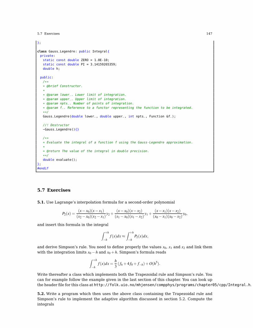
5.7 Exercises 147
;
class Gauss_Legendre: public Integral
private:
static const double ZERO = 1.0E-10;
static const double PI = 3.14159265359;
double h;
public:
/**
* @brief Constructor.
*
* @param lower_. Lower limit of integration.
* @param upper_. Upper limit of integration.
* @param npts_. Number of points of integration.
* @param f_. Reference to a functor representing the function to be integrated.
**/
Gauss_Legendre(double lower_, double upper_, int npts_, Function &f_);
//! Destructor
~Gauss_Legendre()
/**
* Evaluate the integral of a function f using the Gauss-Legendre approximation.
*
* @return The value of the integral in double precision.
**/
double evaluate();
;
#endif
5.7 Exercises
5.1. Use Lagrange’s interpolation formula for a second-order polynomial
P2(x) =(x− x0)(x− x1)
(x2− x0)(x2− x1)y2 +
(x− x0)(x− x2)
(x1− x0)(x1− x2)y1 +
(x− x1)(x− x2)
(x0− x1)(x0− x2)y0,
and insert this formula in the integral
∫ +h
−hf (x)dx ≈
∫ +h
−hP2(x)dx,
and derive Simpson’s rule. You need to define properly the values x0, x1 and x2 and link themwith the integration limits x0− h and x0 + h. Simpson’s formula reads
∫ +h
−hf (x)dx =
h
3( fh + 4 f0 + f−h)+O(h5).
Write thereafter a class which implements both the Trapezoidal rule and Simpson’s rule. Youcan for example follow the example given in the last section of this chapter. You can look upthe header file for this class at http://folk.uio.no/mhjensen/compphys/programs/chapter05/cpp/Integral.h.
5.2. Write a program which then uses the above class containing the Trapezoidal rule andSimpson’s rule to implement the adaptive algorithm discussed in section 5.2. Compute theintegrals

148 5 Numerical Integration
I =∫ 1
0
4
1+ x2= π ,
and
I =
∫ ∞
0xexp(−x)sinx =
1
2.
Discuss strategies for choosing the integration limits using these methods
5.3. Add now to your integration class the possibility for extrapolating h→ 0 using Richard-son’s deferred extrapolation technique, see Eq. (3.13) and exercise 3.2 in chapter 3.
5.4. Write a class which includes your own functions for Gaussian quadrature using Legen-dre, Hermite and Laguerre polynomials. You can write your own functions for these methodsor use those included with the programs of this book. For the latter see for example theprograms in the directory programs/chapter05. The functions are called gausslegendre.cpp,gausshermite.cpp and gausslaguerre.cpp.
Use the Legendre and Laguerre polynomials to evaluate again
I =
∫ ∞
0xexp(−x)sinx =
1
2.
5.5. The task here is to integrate a six-dimensional integral which is used to determine theground state correlation energy between two electrons in a helium atom. The integral appearsin many quantum mechanical applications. However, if you are not too familiar with quantummechanics, you can simply look at the mathematical details. We will employ both Gauss-Legendre and Gauss-Laguerre quadrature. Furthermore, you will need to parallelize yourcode. You can use your class from the previous problem.
We assume that the wave function of each electron can be modelled like the single-particlewave function of an electron in the hydrogen atom. The single-particle wave function for anelectron i in the 1s state is given in terms of a dimensionless variable (the wave function isnot properly normalized)
ri = xiex + yiey + ziez,
asψ1s(ri) = e−αri ,
where α is a parameter and
ri =√
x2i + y2
i + z2i .
We will fix α = 2, which should correspond to the charge of the helium atom Z = 2.The ansatz for the wave function for two electrons is then given by the product of two
so-called 1s wave functions asΨ(r1,r2) = e−α(r1+r2).
Note that it is not possible to find a closed-form solution to Schrödinger’s equation for twointeracting electrons in the helium atom.
The integral we need to solve is the quantum mechanical expectation value of the correla-tion energy between two electrons which repel each other via the classical Coulomb interac-tion, namely
〈 1
|r1− r2|〉=
∫ ∞
−∞dr1dr2e−2α(r1+r2)
1
|r1− r2|.
Note that our wave function is not normalized. There is a normalization factor missing, butfor this project we don’t need to worry about that.
This integral can be solved in closed form and the answer is 5π2/162. Can you derive thisvalue?

5.7 Exercises 149
1. Use Gauss-Legendre quadrature and compute the integral by integrating for each variablex1,y1,z1,x2,y2,z2 from −∞ to ∞. How many mesh points do you need before the results con-verges at the level of the third leading digit? Hint: the single-particle wave function e−αri ismore or less zero at ri ≈? (find the appropriate limit). You can therefore replace the integra-tion limits −∞ and ∞ with −? and ?, respectively. You need to check that this approximationis satisfactory, that is, make a plot of the function and check if the abovementioned limitsare appropriate. You need also to account for the potential problems which may arise when|r1− r2|= 0.
2. The Legendre polynomials are defined for x ∈ [−1,1]. The previous exercise gave a veryunsatisfactory ad hoc procedure. We wish to improve our results. It can therefore be usefulto change to another coordinate frame and employ the Laguerre polynomials. The Laguerrepolynomials are defined for x ∈ [0,∞) and if we change to spherical coordinates
dr1dr2 = r21dr1r2
2dr2dcos(θ1)dcos(θ2)dφ1dφ2,
with1
r12
=1√
r21 + r2
2− 2r1r2cos(β )
andcos(β ) = cos(θ1)cos(θ2)+ sin(θ1)sin(θ2)cos(φ1−φ2))
we can rewrite the above integral with different integration limits. Find these limits andreplace the Gauss-Legendre approach in a) with Laguerre polynomials. Do your resultsimprove? Compare with the results from a).
3. Make a detailed analysis of the time used by both methods and compare your results.Parallelize your codes and check that you have an optimal speed up.


Part II
Linear Algebra and Eigenvalues

This part of the text aims at giving an overview over several methods to solve linear al-gebra and eigenvalue problems. These methods span from standard Gaussian elimination toiterative eigenvalue solvers for large eigenvalue problems. Furthermore, several technicali-ties which pertain to handling arrays, their memory allocation and deallocation, classes forhandling arrays and links to professional software packages such as LAPACK and BLAS willalso be discussed. Parallelization of both eigenvalue solvers and linear algebra problems arealso discussed.

Chapter 6
Linear Algebra
Abstract This chapter introduces several matrix related topics, from the solution of linearequations, computing determinants, conjugate-gradient methods, spline interpolation to effi-cient handling of matrices
6.1 Introduction
In this chapter we deal with basic matrix operations, such as the solution of linear equations,calculate the inverse of a matrix, its determinant etc. The solution of linear equations is animportant part of numerical mathematics and arises in many applications in the sciences.Here we focus in particular on so-called direct or elimination methods, which are in principledetermined through a finite number of arithmetic operations. Iterative methods will also bediscussed.
This chapter serves also the purpose of introducing important programming details suchas handling memory allocation for matrices and the usage of the libraries which follow theselectures.
The algorithms we describe and their original source codes are taken from the widely usedsoftware package LAPACK [26], which follows two other popular packages developed in the1970s, namely EISPACK and LINPACK. The latter was developed for linear equations andleast square problems while the former was developed for solving symmetric, unsymmetricand generalized eigenvalue problems. From LAPACK’s website http://www.netlib.org it ispossible to download for free all source codes from this library. Both C++ and Fortran ver-sions are available. Another important library is BLAS [27], which stands for Basic LinearAlgebra Subprogram. It contains efficient codes for algebraic operations on vectors, matricesand vectors and matrices. Basically all modern supercomputer include this library, with effi-cient algorithms. Else, Matlab offers a very efficient programming environment for dealingwith matrices. The classic text from where we have taken most of the formalism exposed hereis the book on matrix computations by Golub and Van Loan [28]. Good recent introductorytexts are Kincaid and Cheney [23] and Datta [29]. For more advanced ones see Trefethen andBau III [30], Kress [24] and Demmel [31]. Ref. [28] contains an extensive list of textbookson eigenvalue problems and linear algebra. LAPACK [26] contains also extensive listings tothe research literature on matrix computations. For the introduction of the auxiliary libraryBlitz++ [32], which allows for a very efficient way of handling arrays in C++ we refer to theonline manual at http://www.oonumerics.org. A library we highly recommend is Armadillo,see http://arma.sourceforge.org. Armadillo is an open-source C++ linear algebra libraryaiming towards a good balance between speed and ease of use. Integer, floating point andcomplex numbers are supported, as well as a subset of trigonometric and statistics functions.
153

154 6 Linear Algebra
Various matrix and vector operations are provided through optional integration with BLASand LAPACK.
6.2 Mathematical Intermezzo
The matrices we will deal with are primarily square real symmetric or hermitian ones, assum-ing thereby that an n×n matrix A∈Rn×n for a real matrix1 and A ∈Cn×n for a complex matrix.For the sake of simplicity, we take a matrix A ∈R4×4 and a corresponding identity matrix I
A =
a11 a12 a13 a14
a21 a22 a23 a24
a31 a32 a33 a34
a41 a42 a43 a44
I =
1 0 0 0
0 1 0 0
0 0 1 0
0 0 0 1
, (6.1)
where ai j ∈ R. The inverse of a matrix, if it exists, is defined by
A−1 ·A = I.
In the following discussion, matrices are always two-dimensional arrays while vectors areone-dimensional arrays. In our nomenclature we will restrict boldfaced capitals letters suchas A to represent a general matrix, which is a two-dimensional array, while ai j refers to amatrix element with row number i and column number j. Similarly, a vector being a one-dimensional array, is labelled x and represented as (for a real vector)
x ∈ Rn ⇐⇒
x1
x2
x3
x4
,
with pertinent vector elements xi ∈ R. Note that this notation implies xi ∈ R4×1 and that themembers of x are column vectors. The elements of xi ∈R1×4 are row vectors.
Table 6.2 lists some essential features of various types of matrices one may encounter.Some of the matrices we will encounter are listed here
Table 6.1 Matrix properties
Relations Name matrix elementsA = AT symmetric ai j = a ji
A =(AT)−1
real orthogonal ∑k aika jk = ∑k akiak j = δi j
A = A∗ real matrix ai j = a∗i j
A = A† hermitian ai j = a∗jiA =
(A†)−1
unitary ∑k aika∗jk = ∑k a∗kiak j = δi j
1. Diagonal if ai j = 0 for i 6= j,
1 A reminder on mathematical symbols may be appropriate here. The symbol R is the set of real numbers.Correspondingly,N, Z and C represent the set of natural, integer and complex numbers, respectively. A symbollike R
n stands for an n-dimensional real Euclidean space, while C[a,b] is the space of real or complex-valuedcontinuous functions on the interval [a,b], where the latter is a closed interval. Similalry, Cm[a,b] is the spaceof m-times continuously differentiable functions on the interval [a,b]. For more symbols and notations, see themain text.

6.2 Mathematical Intermezzo 155
2. Upper triangular if ai j = 0 for i > j, which for a 4× 4 matrix is of the form
a11 a12 a13 a14
0 a22 a23 a24
0 0 a33 a34
0 0 0 ann
3. Lower triangular if ai j = 0 for i < j
a11 0 0 0
a21 a22 0 0
a31 a32 a33 0
a41 a42 a43 a44
4. Upper Hessenberg if ai j = 0 for i > j+ 1, which is similar to a upper triangular except thatit has non-zero elements for the first subdiagonal row
a11 a12 a13 a14
a21 a22 a23 a24
0 a32 a33 a34
0 0 a43 a44
5. Lower Hessenberg if ai j = 0 for i < j+ 1
a11 a12 0 0
a21 a22 a23 0
a31 a32 a33 a34
a41 a42 a43 a44
6. Tridiagonal if ai j = 0 for |i− j|> 1
a11 a12 0 0
a21 a22 a23 0
0 a32 a33 a34
0 0 a43 a44
There are many more examples, such as lower banded with bandwidth p for ai j = 0 for i> j+ p,upper banded with bandwidth p for ai j = 0 for i < j + p, block upper triangular, block lowertriangular etc.
For a real n× n matrix A the following properties are all equivalent
1. If the inverse of A exists, A is nonsingular.2. The equation Ax = 0 implies x = 0.3. The rows of A form a basis of Rn.4. The columns of A form a basis of Rn.5. A is a product of elementary matrices.6. 0 is not an eigenvalue of A.
The basic matrix operations that we will deal with are addition and subtraction
A = B±C =⇒ ai j = bi j± ci j, (6.2)
scalar-matrix multiplicationA = γB =⇒ ai j = γbi j,
vector-matrix multiplication

156 6 Linear Algebra
y = Ax =⇒ yi =n
∑j=1
ai jx j, (6.3)
matrix-matrix multiplication
A = BC =⇒ ai j =n
∑k=1
bikck j, (6.4)
transpositionA = BT =⇒ ai j = b ji,
and if A ∈ Cn×n, conjugation results in
A = BT=⇒ ai j = b ji,
where a variable z = x− ıy denotes the complex conjugate of z = x+ ıy. In a similar way wehave the following basic vector operations, namely addition and subtraction
x = y± z =⇒ xi = yi± zi,
scalar-vector multiplicationx = γy =⇒ xi = γyi,
vector-vector multiplication (called Hadamard multiplication)
x = yz =⇒ xi = yizi,
the inner or so-called dot product
c = yT z =⇒ c =n
∑j=1
y jz j, (6.5)
with c a constant and the outer product, which yields a matrix,
A = yzT =⇒ ai j = yiz j, (6.6)
Other important operations are vector and matrix norms. A class of vector norms are theso-called p-norms
||x||p = (|x1|p + |x2|p + · · ·+ |xn|p)1p ,
where p≥ 1. The most important are the 1, 2 and ∞ norms given by
||x||1 = |x1|+ |x2|+ · · ·+ |xn|,
||x||2 = (|x1|2 + |x2|2 + · · ·+ |xn|2)12 = (xT x)
12 ,
and||x||∞ = max |xi|,
for 1≤ i≤ n. From these definitions, one can derive several important relations, of which theso-called Cauchy-Schwartz inequality is of great importance for many algorithms. For any x
and y being real-valued or complex-valued quantities, the inner product space satisfies
|xT y| ≤ ||x||2||y||2,
and the equality is obeyed only if x and y are linearly dependent. An important relation whichfollows from the Cauchy-Schwartz relation is the famous triangle relation, which states thatfor any x and y in a real or complex, the inner product space satisfies

6.3 Programming Details 157
||x+ y||2 ≤ ||x||2 + ||y||2.
Proofs can be found in for example Ref. [28]. As discussed in chapter 2, the analysis of therelative error is important in our studies of loss of numerical precision. Using a vector normwe can define the relative error for the machine representation of a vector x. We assume thatf l(x) ∈ Rn is the machine representation of a vector x ∈ Rn. If x 6= 0, we define the relativeerror as
ε =|| f l(x)− x||||x|| .
Using the ∞-norm one can define a relative error that can be translated into a statement onthe correct significant digits of f l(x),
|| f l(x)− x||∞||x||∞
≈ 10−l,
where the largest component of f l(x) has roughly l correct significant digits.We can define similar matrix norms as well. The most frequently used are the Frobenius
norm
||A||F =
√m
∑i=1
n
∑j=1
|ai j|2,
and the p-norms
||A||p =||Ax||p||x||p
,
assuming that x 6= 0. We refer the reader to the text of Golub and Van Loan [28] for a furtherdiscussion of these norms.
The way we implement these operations will be discussed below, as it depends on theprogramming language we opt for.
6.3 Programming Details
Many programming problems arise from improper treatment of arrays. In this section wewill discuss some important points such as array declaration, memory allocation and arraytransfer between functions. We distinguish between two cases: (a) array declarations wherethe array size is given at compilation time, and (b) where the array size is determined dur-ing the execution of the program, so-called dymanic memory allocation. Useful references onC++ programming details, in particular on the use of pointers and memory allocation, areReek’s text [33] on pointers in C, Berryhill’s monograph [34] on scientific programming inC++ and finally Franek’s text [35] on memory as a programming concept in C and C++.Good allround texts on C++ programming in engineering and science are the books byFlowers [18] and Barton and Nackman [19]. See also the online lecture notes on C++ athttp://heim.ifi.uio.no/~hpl/INF-VERK4830. For Fortran we recommend the online lec-tures at http://folk.uio.no/gunnarw/INF-VERK4820. These web pages contain extensivereferences to other C++ and Fortran resources. Both web pages contain enough material,lecture notes and exercises, in order to serve as material for own studies.

158 6 Linear Algebra
Fig. 6.1 Segmentation fault, again and again! Alas, this is a situation you will most likely end up in, unlessyou initialize, access, allocate and deallocate properly your arrays. Many program development environmentssuch as Dev C++ at www.bloodshed.net provide debugging possibilities. Beware however that there may besegmentation errors which occur due to errors in libraries of the operating system. (Drawing: courtesy byVictoria Popsueva 2003.)
6.3.1 Declaration of fixed-sized vectors and matrices
In the program below we discuss some essential features of vector and matrix handling wherethe dimensions are declared in the program code.
In line awe have a standard C++ declaration of a vector. The compiler reserves memory tostore five integers. The elements are vec[0], vec[1],....,vec[4]. Note that the numberingof elements starts with zero. Declarations of other data types are similar, including structuredata.
The symbol vec is an element in memory containing the address to the first element vec[0]and is a pointer to a vector of five integer elements.
In line b we have a standard fixed-size C++ declaration of a matrix. Again the elementsstart with zero, matr[0][0], matr[0][1], ....., matr[0][4], matr[1][0],.... This se-quence of elements also shows how data are stored in memory. For example, the elementmatr[1][0] follows matr[0][4]. This is important in order to produce an efficient code andavoid memory stride.
There is one further important point concerning matrix declaration. In a similar way as forthe symbol vec,matr is an element in memory which contains an address to a vector of threeelements, but now these elements are not integers. Each element is a vector of five integers.This is the correct way to understand the declaration in line b. With respect to pointers thismeans that matr is pointer-to-a-pointer-to-an-integer which we can write ∗∗matr. Furthermore∗matr is a-pointer-to-a-pointer of five integers. This interpretation is important when we wantto transfer vectors and matrices to a function.
In line c we transfer vec[] and matr[][] to the function sub_1(). To be specific, we trans-fer the addresses of vec[] and matr[][] to sub_1().

6.3 Programming Details 159
In line d we have the function definition of subfunction(). The int vec[] is a pointer to aninteger. Alternatively we could write int ∗vec. The first version is better. It shows that it is avector of several integers, but not how many. The second version could equally well be usedto transfer the address to a single integer element. Such a declaration does not distinguishbetween the two cases.
The next definition is int matr[][5]. This is a pointer to a vector of five elements and thecompiler must be told that each vector element contains five integers. Here an alternativeversion could be int (∗matr)[5] which clearly specifies that matr is a pointer to a vector of fiveintegers.
int main()
int k,m, row = 3, col = 5;
int vec[5]; // line a
int matr[3][5]; // line b
// Fill in vector vec
for (k = 0; k < col; k++) vec[k] = k;
// fill in matr
for (m = 0; m < row; m++)
for (k = 0; k < col ; k++) matr[m][k] = m + 10*k;
// write out the vector
cout << `` Content of vector vec:'' << endl;
for (k = 0; k < col; k++)
cout << vec[k] << endl;
// Then write out the matrix
cout << `` Content of matrix matr:'' << endl;
for (m = 0; m < row; m++)
for (k = 0; k < col ; k++)
cout << matr[m][k] << endl;
subfunction(row, col, vec, matr); // line c
return 0;
// end main function
void subfunction(int row, int col, int vec[], int matr[][5]); // line d
int k, m;
// write out the vector
cout << `` Content of vector vec in subfunction:'' << endl;
for (k = 0; k < col; k++)
cout << vec[k] << endl;
// Then write out the matrix
cout << `` Content of matrix matr in subfunction:'' << endl;
for (m = 0; m < row; m++)
for (k = 0; k < col ; k++)
cout << matr[m][k] << endl;
// end of function subfunction
There is at least one drawback with such a matrix declaration. If we want to change thedimension of the matrix and replace 5 by something else we have to do the same change inall functions where this matrix occurs.
There is another point to note regarding the declaration of variables in a function whichincludes vectors and matrices. When the execution of a function terminates, the memory re-

160 6 Linear Algebra
quired for the variables is released. In the present case memory for all variables in main() arereserved during the whole program execution, but variables which are declared in subfunc-tion() are released when the execution returns to main().
6.3.2 Runtime Declarations of Vectors and Matrices in C++
We change thereafter our program in order to include dynamic allocation of arrays. As men-tioned in the previous subsection a fixed size declaration of vectors and matrices beforecompilation is in many cases bad. You may not know beforehand the actually needed sizes ofvectors and matrices. In large projects where memory is a limited factor it could be importantto reduce memory requirement for matrices which are not used any more. In C an C++ it ispossible and common to postpone size declarations of arrays untill you really know what youneed and also release memory reservations when it is not needed any more. The followingprogram shows how we could change the previous one with static declarations to dynamicallocation of arrays.
int main()
int k,m, row = 3, col = 5;
int vec[5]; // line a
int matr[3][5]; // line b
cout << `` Read in number of rows'' << endl; // line c
cin >> row;
cout << `` Read in number of columns'' << endl;
cin >> col;
vec = new int[col]; // line d
matr = (int **)matrix(row,col,sizeof(int)); // line e
// Fill in vector vec
for (k = 0; k < col; k++) vec[k] = k;
// fill in matr
for (m = 0; m < row; m++)
for (k = 0; k < col ; k++) matr[m][k] = m + 10*k;
// write out the vector
cout << `` Content of vector vec:'' << endl;
for (k = 0; k < col; k++)
cout << vec[k] << endl;
// Then write out the matrix
cout << `` Content of matrix matr:'' << endl;
for (m = 0; m < row; m++)
for (k = 0; k < col ; k++)
cout << matr[m][k] << endl;
subfunction(row, col, vec, matr); // line f
free_matrix((void **) matr); // line g
delete vec[];
return 0;
// end main function
void subfunction(int row, int col, int vec[], int matr[][5]); // line h
int k, m;
// write out the vector

6.3 Programming Details 161
cout << `` Content of vector vec in subfunction:'' << endl;
for (k = 0; k < col; k++)
cout << vec[k] << endl;
// Then write out the matrix
cout << `` Content of matrix matr in subfunction:'' << endl;
for (m = 0; m < row; m++)
for (k = 0; k < col ; k++)
cout << matr[m][k] << endl;
// end of function subfunction
In line a we declare a pointer to an integer which later will be used to store an address to thefirst element of a vector. Similarily, line b declares a pointer-to-a-pointer which will containthe address to a pointer of row vectors, each with col integers. This will then become a matrixwith dimensionality [col][col]
In line c we read in the size of vec[] and matr[][] through the numbers row and col.Next we reserve memory for the vector in line d. In line e we use a user-defined function
to reserve necessary memory for matrix[row][col] and again matr contains the address to thereserved memory location.
The remaining part of the function main() are as in the previous case down to line f. Herewe have a call to a user-defined function which releases the reserved memory of the matrix.In this case this is not done automatically.
In line g the same procedure is performed for vec[]. In this case the standard C++ libraryhas the necessary function.
Next, in line h an important difference from the previous case occurs. First, the vectordeclaration is the same, but the matr declaration is quite different. The corresponding pa-rameter in the call to sub_1[] in line g is a double pointer. Consequently, matr in line h mustbe a double pointer.
Except for this difference sub_1() is the same as before. The new feature in the programbelow is the call to the user-defined functions matrix and free_matrix. These functions aredefined in the library file lib.cpp. The code for the dynamic memory allocation is given below.
http://folk.uio.no/compphys/programs/FYS3150/cpp/cpluspluslibrary/lib.cpp
/*
* The function
* void **matrix()
* reserves dynamic memory for a two-dimensional matrix
* using the C++ command new . No initialization of the elements.
* Input data:
* int row - number of rows
* int col - number of columns
* int num_bytes- number of bytes for each
* element
* Returns a void **pointer to the reserved memory location.
*/
void **matrix(int row, int col, int num_bytes)
int i, num;
char **pointer, *ptr;
pointer = new(nothrow) char* [row];
if(!pointer)
cout << "Exception handling: Memory allocation failed";
cout << " for "<< row << "row addresses !" << endl;
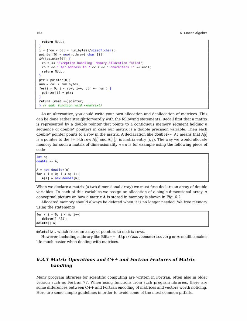
162 6 Linear Algebra
return NULL;
i = (row * col * num_bytes)/sizeof(char);
pointer[0] = new(nothrow) char [i];
if(!pointer[0])
cout << "Exception handling: Memory allocation failed";
cout << " for address to " << i << " characters !" << endl;
return NULL;
ptr = pointer[0];
num = col * num_bytes;
for(i = 0; i < row; i++, ptr += num )
pointer[i] = ptr;
return (void **)pointer;
// end: function void **matrix()
As an alternative, you could write your own allocation and deallocation of matrices. Thiscan be done rather straightforwardly with the following statements. Recall first that a matrixis represented by a double pointer that points to a contiguous memory segment holding asequence of double* pointers in case our matrix is a double precision variable. Then eachdouble* pointer points to a row in the matrix. A declaration like double** A; means that A[i]is a pointer to the i+ 1-th row A[i] and A[i][ j] is matrix entry (i, j). The way we would allocatememory for such a matrix of dimensionality n× n is for example using the following piece ofcode
int n;
double ** A;
A = new double*[n]
for ( i = 0; i < n; i++)
A[i] = new double[N];
When we declare a matrix (a two-dimensional array) we must first declare an array of doublevariables. To each of this variables we assign an allocation of a single-dimensional array. Aconceptual picture on how a matrix A is stored in memory is shown in Fig. 6.2.
Allocated memory should always be deleted when it is no longer needed. We free memoryusing the statements
for ( i = 0; i < n; i++)
delete[] A[i];
delete[] A;
delete[]A;, which frees an array of pointers to matrix rows.However, including a library like Blitz++ http://www.oonumerics.org or Armadillo makes
life much easier when dealing with matrices.
6.3.3 Matrix Operations and C++ and Fortran Features of Matrix
handling
Many program libraries for scientific computing are written in Fortran, often also in olderversion such as Fortran 77. When using functions from such program libraries, there aresome differences between C++ and Fortran encoding of matrices and vectors worth noticing.Here are some simple guidelines in order to avoid some of the most common pitfalls.

6.3 Programming Details 163
double∗∗A =⇒ double∗A[0 . . .3]
A[0][0] A[0][1] A[0][2] A[0][3]
A[1][0] A[1][1] A[1][2] A[1][3]
A[2][0] A[2][1] A[2][2] A[2][3]
A[3][0] A[3][1] A[3][2] A[3][3]
A[0]
A[1]
A[2]
A[3]
Fig. 6.2 Conceptual representation of the allocation of a matrix in C++.
First of all, when we think of an n× n matrix in Fortran and C++, we typically wouldhave a mental picture of a two-dimensional block of stored numbers. The computer storesthem however as sequential strings of numbers. The latter could be stored as row-majororder or column-major order. What do we mean by that? Recalling that for our matrix el-ements ai j, i refers to rows and j to columns, we could store a matrix in the sequencea11a12 . . .a1na21a22 . . .a2n . . .ann if it is row-major order (we go along a given row i and pick up allcolumn elements j) or it could be stored in column-major order a11a21 . . .an1a12a22 . . .an2 . . .ann.
Fortran stores matrices in the latter way, i.e., by column-major, while C++ stores themby row-major. It is crucial to keep this in mind when we are dealing with matrices, becauseif we were to organize the matrix elements in the wrong way, important properties like thetranspose of a real matrix or the inverse can be wrong, and obviously yield wrong physics.Fortran subscripts begin typically with 1, although it is no problem in starting with zero, whileC++ starts with 0 for the first element. This means that A(1,1) in Fortran is equivalent toA[0][0] in C++. Moreover, since the sequential storage in memory means that nearby matrixelements are close to each other in the memory locations (and thereby easier to fetch) ,operations involving e.g., additions of matrices may take more time if we do not respect thegiven ordering.
To see this, consider the following coding of matrix addition in C++ and Fortran. We haven× n matrices A, B and C and we wish to evaluate A = B+C according to Eq. (6.2). In C++this would be coded like
for(i=0 ; i < n ; i++)
for(j=0 ; j < n ; j++)
a[i][j]=b[i][j]+c[i][j]

164 6 Linear Algebra
while in Fortran we would have
DO j=1, n
DO i=1, n
a(i,j)=b(i,j)+c(i,j)
ENDDO
ENDDO
Fig. 6.3 shows how a 3× 3 matrix A is stored in both row-major and column-major ways.
a11 a12 a13
a21 a22 a23
a31 a32 a33
=⇒⇐=
a11
a12
a13
a21
a22
a23
a31
a32
a33
a11
a21
a31
a12
a22
a32
a13
a23
a33
Fig. 6.3 Row-major storage of a matrix to the left (C++ way) and column-major to the right (Fortran way).
Interchanging the order of i and j can lead to a considerable enhancement in processtime. In Fortran we write the above statements in a much simpler way a=b+c. However, theaddition still involves ∼ n2 operations. Matrix multiplication or taking the inverse requires∼ n3 operations. The matrix multiplication of Eq. (6.4) of two matrices A = BC could then takethe following form in C++
for(i=0 ; i < n ; i++)
for(j=0 ; j < n ; j++)

6.3 Programming Details 165
for(k=0 ; k < n ; k++)
a[i][j]+=b[i][k]*c[k][j]
and in Fortran we have
DO j=1, n
DO i=1, n
DO k = 1, n
a(i,j)=a(i,j)+b(i,k)*c(k,j)
ENDDO
ENDDO
ENDDO
However, Fortran has an intrisic function called MATMUL, and the above three loops canbe coded in a single statement a=MATMUL(b,c). Fortran contains several array manipulationstatements, such as dot product of vectors, the transpose of a matrix etc etc. The outerproduct of two vectors is however not included in Fortran. The coding of Eq. (6.6) takes thenthe following form in C++
for(i=0 ; i < n ; i++)
for(j=0 ; j < n ; j++)
a[i][j]+=x[i]*y[j]
and in Fortran we have
DO j=1, n
DO i=1, n
a(i,j)=a(i,j)+x(j)*y(i)
ENDDO
ENDDO
A matrix-matrix multiplication of a general n× n matrix with
a(i, j) = a(i, j)+ b(i,k)∗ c(k, j),
in its inner loops requires a multiplication and an addition. We define now a flop (floatingpoint operation) as one of the following floating point arithmetic operations, viz addition,subtraction, multiplication and division. The above two floating point operations (flops) aredone n3 times meaning that a general matrix multiplication requires 2n3 flops if we havea square matrix. If we assume that our computer performs 109 flops per second, then toperform a matrix multiplication of a 1000× 1000 case should take two seconds. This can bereduced if we multiply two matrices which are upper triangular such as
A =
a11 a12 a13 a14
0 a22 a23 a24
0 0 a33 a34
0 0 0 a44
.
The multiplication of two upper triangular matrices BC yields another upper triangular matrixA, resulting in the following C++ code
for(i=0 ; i < n ; i++)
for(j=i ; j < n ; j++)
for(k=i ; k < j ; k++)

166 6 Linear Algebra
a[i][j]+=b[i][k]*c[k][j]
The fact that we have the constraint i≤ j leads to the requirement for the computation of ai j
of 2( j− i+ 1) flops. The total number of flops is then
n
∑i=1
n
∑j=1
2( j− i+ 1) =n
∑i=1
n−i+1
∑j=1
2 j ≈n
∑i=1
2(n− i+ 1)2
2,
where we used that ∑nj=1 j = n(n+1)/2≈ n2/2 for large n values. Using in addition that ∑n
j=1 j2≈n3/3 for large n values, we end up with approximately n3/3 flops for the multiplication of twoupper triangular matrices. This means that if we deal with matrix multiplication of uppertriangular matrices, we reduce the number of flops by a factor six if we code our matrixmultiplication in an efficient way.
It is also important to keep in mind that computers are finite, we can thus not store in-finitely large matrices. To calculate the space needed in memory for an n×n matrix with dou-ble precision, 64 bits or 8 bytes for every matrix element, one needs simply compute n×n×8
bytes . Thus, if n = 10000, we will need close to 1GB of storage. Decreasing the precision tosingle precision, only halves our needs.
A further point we would like to stress, is that one should in general avoid fixed (at com-pilation time) dimensions of matrices. That is, one could always specify that a given matrix A
should have size A[100][100], while in the actual execution one may use only A[10][10]. If onehas several such matrices, one may run out of memory, while the actual processing of theprogram does not imply that. Thus, we will always recommend that you use dynamic memoryallocation, and deallocation of arrays when they are no longer needed. In Fortran one usesthe intrisic functions ALLOCATE and DEALLOCATE, while C++ employs the functions newand delete.
6.3.3.1 Strassen’s algorithm
As we have seen, the straightforward algorithm for matrix-matrix multiplication will require p
multiplications and p−1 additions for each of the m×n elements. The total number of floating-point operations is then mn(2p− 1)∼ O(mnp). When the matrices A and B can be divided intofour equally sized blocks, [
C11 C12
C21 C22
]=
[A11 A12
A21 A22
][B11 B12
B21 B22
], (6.7)
we get eight multiplications of smaller blocks,
[C11 C12
C21 C22
]=
[A11B11 +A12B21 A11B12 +A12B22
A21B11 +A22B21 A21B12 +A22B22
]. (6.8)
Strassen discovered in 1968 how the number of multiplications could be reduced fromeight to seven [28]. Following Strassen’s approach we define some intermediates,
S1 = A21 +A22, T1 = B12−B11,
S2 = S1−A11, T2 = B22−T1,
S3 = A11−A21, T3 = B22−B12,
S4 = A12− S2, T4 = B21−T2,
(6.9)
and need seven multiplications,

6.3 Programming Details 167
P1 = A11B11, U1 = P1 +P2,
P2 = A12B21, U2 = P1 +P4,
P3 = S1T1, U3 =U2 +P5,
P4 = S2T2, U4 =U3 +P7,
P5 = S3T3, U5 =U3 +P3,
P6 = S4B22, U6 =U2 +P3,
P7 = A22T4, U7 =U6 +P6,
(6.10)
to find the resulting C matrix as [C11 C12
C21 C22
]=
[U1 U7
U4 U5
]. (6.11)
In spite of the seemingly additional work, we have reduced the number of multiplicationsfrom eight to seven. Since the multiplications are the computational bottleneck compared toaddition and subtraction, the number of flops are reduced.
In the case of square n× n matrices with n equal to a power of two, n = 2m, the dividedblocks will have n
2= 2m−1. Letting f (m) be the number of flops needed for the full matrix and
applying Strassen recursively we find the total number of flops to be
f (m) = 7 f (m− 1) = 72 f (m− 2) = · · ·= 7m f (0), (6.12)
where f (0) is the one floating-point operation needed for multiplication of two numbers (two20× 20 matrices). For large matrices this can prove efficient, yielding a much better scaling,
O (7m) = O
(2log2 7m
)= O
(2m log2 7
)= O
(nlog2 7
)≈ O
(n2.807
), (6.13)
effectively saving 7/8 = 12.5% each time it is applied.
6.3.3.2 Fortran Allocate Statement and Mathematical Operations on Arrays
An array is declared in the declaration section of a program, module, or procedure using thedimension attribute. Examples include
REAL, DIMENSION (10) :: x,y
REAL, DIMENSION (1:10) :: x,y
INTEGER, DIMENSION (-10:10) :: prob
INTEGER, DIMENSION (10,10) :: spin
The default value of the lower bound of an array is 1. For this reason the first two state-ments are equivalent to the first. The lower bound of an array can be negative. The last twostatements are examples of two-dimensional arrays.
Rather than assigning each array element explicitly, we can use an array constructor togive an array a set of values. An array constructor is a one-dimensional list of values, sepa-rated by commas, and delimited by "(/" and "/)". An example is
a(1:3) = (/ 2.0, -3.0, -4.0 /)
is equivalent to the separate assignments
a(1) = 2.0
a(2) = -3.0
a(3) = -4.0

168 6 Linear Algebra
One of the better features of Fortran is dynamic storage allocation. That is, the size of anarray can be changed during the execution of the program. To see how the dynamic allocationworks in Fortran, consider the following simple example where we set up a 4×4 unity matrix.
......
IMPLICIT NONE
! The definition of the matrix, using dynamic allocation
REAL, ALLOCATABLE, DIMENSION(:,:) :: unity
! The size of the matrix
INTEGER :: n
! Here we set the dim n=4
n=4
! Allocate now place in memory for the matrix
ALLOCATE ( unity(n,n) )
! all elements are set equal zero
unity=0.
! setup identity matrix
DO i=1,n
unity(i,i)=1.
ENDDO
DEALLOCATE ( unity)
.......
We always recommend to use the deallocation statement, since this frees space in memory.If the matrix is transferred to a function from a calling program, one can transfer the dimen-sionality n of that matrix with the call. Another possibility is to determine the dimensionalitywith the SIZE function. Writing a statement like n=SIZE(unity,DIM=1) gives the number of rows,while using DIM=2 gives the number of columns. Note however that this involves an extracall to a function. If speed matters, one should avoid such calls.
6.4 Linear Systems
In this section we outline some of the most used algorithms to solve sets of linear equations.These algorithms are based on Gaussian elimination [24,28] and will allow us to catch severalbirds with a stone. We will show how to rewrite a matrix A in terms of an upper and a lowertriangular matrix, from which we easily can solve linear equation, compute the inverse of A
and obtain the determinant. We start with Gaussian elimination, move to the more efficientLU-algorithm, which forms the basis for many linear algebra applications, and end the discus-sion with special cases such as the Cholesky decomposition and linear system of equationswith a tridiagonal matrix.
We begin however with an example which demonstrates the importance of being able tosolve linear equations. Suppose we want to solve the following boundary value equation
−d2u(x)
dx2= f (x,u(x)),
with x ∈ (a,b) and with boundary conditions u(a) = u(b) = 0. We assume that f is a continuousfunction in the domain x ∈ (a,b). Since, except the few cases where it is possible to find ana-lytic solutions, we will seek approximate solutions, we choose to represent the approximationto the second derivative from the previous chapter
f ′′ =fh− 2 f0 + f−h
h2+O(h2).

6.4 Linear Systems 169
We subdivide our interval x∈ (a,b) into n subintervals by setting xi = a+ ih, with i= 0,1, . . . ,n+1.The step size is then given by h = (b− a)/(n+ 1) with n ∈ N. For the internal grid pointsi = 1,2, . . .n we replace the differential operator with the above formula resulting in
u′′(xi)≈u(xi + h)− 2u(xi)+ u(xi− h)
h2,
which we rewrite as
u′′i ≈
ui+1− 2ui+ ui−i
h2.
We can rewrite our original differential equation in terms of a discretized equation with ap-proximations to the derivatives as
−ui+1− 2ui+ ui−i
h2= f (xi,u(xi)),
with i = 1,2, . . . ,n. We need to add to this system the two boundary conditions u(a) = u0 andu(b) = un+1. If we define a matrix
A =1
h2
2 −1
−1 2 −1
−1 2 −1
. . . . . . . . . . . . . . .
−1 2 −1
−1 2
and the corresponding vectors u = (u1,u2, . . . ,un)T and f(u) = f (x1,x2, . . . ,xn,u1,u2, . . . ,un)
T wecan rewrite the differential equation including the boundary conditions as a system of linearequations with a large number of unknowns
Au = f(u). (6.14)
We assume that the solution u exists and is unique for the exact differential equation, viz thatthe boundary value problem has a solution. But the discretization of the above differentialequation leads to several questions, such as how well does the approximate solution resemblethe exact one as h→ 0, or does a given small value of h allow us to establish existence anduniqueness of the solution.
Here we specialize to two particular cases. Assume first that the function f does not dependon u(x). Then our linear equation reduces to
Au = f, (6.15)
which is nothing but a simple linear equation with a tridiagonal matrix A. We will solve sucha system of equations in subsection 6.4.3.
If we assume that our boundary value problem is that of a quantum mechanical particleconfined by a harmonic oscillator potential, then our function f takes the form (assumingthat all constants m = h = ω = 1) f (xi,u(xi)) = −x2
i u(xi)+ 2λ u(xi) with λ being the eigenvalue.Inserting this into our equation, we define first a new matrix A as

170 6 Linear Algebra
A =
2h2 + x2
1 − 1h2
− 1h2
2h2 + x2
2 − 1h2
− 1h2
2h2 + x2
3 − 1h2
. . . . . . . . . . . . . . .
− 1h2
2h2 + x2
n−1 − 1h2
− 1h2
2h2 + x2
n
, (6.16)
which leads to the following eigenvalue problem
2h2 + x2
1 − 1h2
− 1h2
2h2 + x2
2 − 1h2
− 1h2
2h2 + x2
3 − 1h2
. . . . . . . . . . . . . . .
− 1h2
2h2 + x2
n−1 − 1h2
− 1h2
2h2 + x2
n
u1
u2
un
= 2λ
u1
u2
un
.
We will solve this type of equations in chapter 7. These lecture notes contain however severalother examples of rewriting mathematical expressions into matrix problems. In chapter 5 weshow how a set of linear integral equation when discretized can be transformed into a simplematrix inversion problem. The specific example we study in that chapter is the rewritingof Schrödinger’s equation for scattering problems. Other examples of linear equations willappear in our discussion of ordinary and partial differential equations.
6.4.1 Gaussian Elimination
Any discussion on the solution of linear equations should start with Gaussian elimination. Thistext is no exception. We start with the linear set of equations
Ax = w.
We assume also that the matrix A is non-singular and that the matrix elements along thediagonal satisfy aii 6= 0. We discuss later how to handle such cases. In the discussion we limitourselves again to a matrix A ∈ R4×4, resulting in a set of linear equations of the form
a11 a12 a13 a14
a21 a22 a23 a24
a31 a32 a33 a34
a41 a42 a43 a44
x1
x2
x3
x4
=
w1
w2
w3
w4
.
or
a11x1 + a12x2 + a13x3 + a14x4 = w1
a21x1 + a22x2 + a23x3 + a24x4 = w2
a31x1 + a32x2 + a33x3 + a34x4 = w3
a41x1 + a42x2 + a43x3 + a44x4 = w4.
The basic idea of Gaussian elimination is to use the first equation to eliminate the first un-known x1 from the remaining n− 1 equations. Then we use the new second equation to elimi-nate the second unknown x2 from the remaining n− 2 equations. With n− 1 such eliminationswe obtain a so-called upper triangular set of equations of the form

6.4 Linear Systems 171
b11x1 + b12x2 + b13x3 + b14x4 = y1
b22x2 + b23x3 + b24x4 = y2
b33x3 + b34x4 = y3
b44x4 = y4.
We can solve this system of equations recursively starting from xn (in our case x4) and proceedwith what is called a backward substitution. This process can be expressed mathematicallyas
xm =1
bmm
(ym−
n
∑k=m+1
bmkxk
)m = n− 1,n− 2, . . .,1.
To arrive at such an upper triangular system of equations, we start by eliminating the un-known x1 for j = 2,n. We achieve this by multiplying the first equation by a j1/a11 and thensubtract the result from the jth equation. We assume obviously that a11 6= 0 and that A is notsingular. We will come back to this problem below.
Our actual 4× 4 example reads after the first operation
a11 a12 a13 a14
0 (a22− a21a12a11
) (a23− a21a13a11
) (a24− a21a14a11
)
0 (a32− a31a12a11
) (a33− a31a13a11
) (a34− a31a14a11
)
0 (a42− a41a12a11
) (a43− a41a13a11
) (a44− a41a14a11
)
x1
x2
x3
x4
=
y1
w(2)2
w(2)3
w(2)4
.
or
b11x1 + b12x2 + b13x3 + b14x4 = y1
a(2)22 x2 + a
(2)23 x3 + a
(2)24 x4 = w
(2)2
a(2)32 x2 + a
(2)33 x3 + a
(2)34 x4 = w
(2)3
a(2)42 x2 + a
(2)43 x3 + a
(2)44 x4 = w
(2)4 ,
(6.17)
with the new coefficientsb1k = a
(1)1k k = 1, . . . ,n,
where each a(1)1k is equal to the original a1k element. The other coefficients are
a(2)jk = a
(1)jk −
a(1)j1 a
(1)1k
a(1)11
j,k = 2, . . . ,n,
with a new right-hand side given by
y1 = w(1)1 , w
(2)j = w
(1)j −
a(1)j1 w
(1)1
a(1)11
j = 2, . . . ,n.
We have also set w(1)1 = w1, the original vector element. We see that the system of unknowns
x1, . . . ,xn is transformed into an (n− 1)× (n− 1) problem.This step is called forward substitution. Proceeding with these substitutions, we obtain the
general expressions for the new coefficients
a(m+1)jk = a
(m)jk −
a(m)jm a
(m)mk
a(m)mm
j,k = m+ 1, . . . ,n,

172 6 Linear Algebra
with m = 1, . . . ,n− 1 and a right-hand side given by
w(m+1)j = w
(m)j −
a(m)jm w
(m)m
a(m)mm
j = m+ 1, . . . ,n.
This set of n− 1 elimations leads us to Eq. (6.17), which is solved by back substitution. If thearithmetics is exact and the matrix A is not singular, then the computed answer will be exact.However, as discussed in the two preceeding chapters, computer arithmetics is not exact. Wewill always have to cope with truncations and possible losses of precision. Even though thematrix elements along the diagonal are not zero, numerically small numbers may appear andsubsequent divisions may lead to large numbers, which, if added to a small number may yieldlosses of precision. Suppose for example that our first division in (a22− a21a12/a11) results in−107, that is a21a12/a11. Assume also that a22 is one. We are then adding 107 + 1. With singleprecision this results in 107. Already at this stage we see the potential for producing wrongresults.
The solution to this set of problems is called pivoting, and we distinguish between partialand full pivoting. Pivoting means that if small values (especially zeros) do appear on thediagonal we remove them by rearranging the matrix and vectors by permuting rows andcolumns. As a simple example, let us assume that at some stage during a calculation we havethe following set of linear equations
1 3 4 6
0 10−8 198 19
0 −91 51 9
0 7 76 541
x1
x2
x3
x4
=
y1
y2
y3
y4
.
The element at row i = 2 and column 2 is 10−8 and may cause problems for us in the nextforward substitution. The element i = 2, j = 3 is the largest in the second row and the elementi = 3, j = 2 is the largest in the third row. The small element can be removed by rearrangingthe rows and/or columns to bring a larger value into the i = 2, j = 2 element.
In partial or column pivoting, we rearrange the rows of the matrix and the right-handside to bring the numerically largest value in the column onto the diagonal. For our examplematrix the largest value of column two is in element i = 3, j = 2 and we interchange rows 2and 3 to give
1 3 4 6
0 −91 51 9
0 10−8 198 19
0 7 76 541
x1
x2
x3
x4
=
y1
y3
y2
y4
.
Note that our unknown variables xi remain in the same order which simplifies the implemen-tation of this procedure. The right-hand side vector, however, has been rearranged. Partialpivoting may be implemented for every step of the solution process, or only when the diago-nal values are sufficiently small as to potentially cause a problem. Pivoting for every step willlead to smaller errors being introduced through numerical inaccuracies, but the continualreordering will slow down the calculation.
The philosophy behind full pivoting is much the same as that behind partial pivoting. Themain difference is that the numerically largest value in the column or row containing the valueto be replaced. In our example above the magnitude of element i = 2, j = 3 is the greatest inrow 2 or column 2. We could rearrange the columns in order to bring this element onto thediagonal. This will also entail a rearrangement of the solution vector x. The rearranged systembecomes, interchanging columns two and three,

6.4 Linear Systems 173
1 6 3 4
0 198 10−8 19
0 51 −91 9
0 76 7 541
x1
x3
x2
x4
=
y1
y2
y3
y4
.
The ultimate degree of accuracy can be provided by rearranging both rows and columnsso that the numerically largest value in the submatrix not yet processed is brought ontothe diagonal. This process may be undertaken for every step, or only when the value onthe diagonal is considered too small relative to the other values in the matrix. In our case,the matrix element at i = 4, j = 4 is the largest. We could here interchange rows two andfour and then columns two and four to bring this matrix element at the diagonal positioni= 2, j = 2. When interchanging columns and rows, one needs to keep track of all permutationsperformed. Partial and full pivoting are discussed in most texts on numerical linear algebra.For an in-depth discussion we recommend again the text of Golub and Van Loan [28], inparticular chapter three. See also the discussion of chapter two in Ref. [36]. The libraryfunctions you end up using, be it via Matlab, the library included with this text or other ones,do all include pivoting.
If it is not possible to rearrange the columns or rows to remove a zero from the diagonal,then the matrix A is singular and no solution exists.
Gaussian elimination requires however many floating point operations. An n× n matrixrequires for the simultaneous solution of a set of r different right-hand sides, a total of n3/3+
rn2− n/3 multiplications. Adding the cost of additions, we end up with 2n3/3+O(n2) floatingpoint operations, see Kress [24] for a proof. An n×n matrix of dimensionalty n = 103 requires,on a modern PC with a processor that allows for something like 109 floating point operationsper second (flops), approximately one second. If you increase the size of the matrix to n = 104
you need 1000 seconds, or roughly 16 minutes.Although the direct Gaussian elmination algorithm allows you to compute the determinant
of A via the product of the diagonal matrix elements of the triangular matrix, it is seldomlyused in normal applications. The more practical elimination is provided by what is calledlower and upper decomposition. Once decomposed, one can use this matrix to solve manyother linear systems which use the same matrix A, viz with different right-hand sides. Withan LU decomposed matrix, the number of floating point operations for solving a set of linearequations scales as O(n2). One should however note that to obtain the LU decompsed ma-trix requires roughly O(n3) floating point operations. Finally, LU decomposition allows for anefficient computation of the inverse of A.
6.4.2 LU Decomposition of a Matrix
A frequently used form of Gaussian elimination is L(ower)U(pper) factorization also knownas LU Decomposition or Crout or Dolittle factorisation. In this section we describe how onecan decompose a matrix A in terms of a matrix L with elements only below the diagonal(and thereby the naming lower) and a matrix U which contains both the diagonal and matrixelements above the diagonal (leading to the labelling upper). Consider again the matrix A
given in Eq. (6.1). The LU decomposition method means that we can rewrite this matrix asthe product of two matrices L and U where
A = LU =
a11 a12 a13 a14
a21 a22 a23 a24
a31 a32 a33 a34
a41 a42 a43 a44
=
1 0 0 0
l21 1 0 0
l31 l32 1 0
l41 l42 l43 1
u11 u12 u13 u14
0 u22 u23 u24
0 0 u33 u34
0 0 0 u44
. (6.18)

174 6 Linear Algebra
LU decomposition forms the backbone of other algorithms in linear algebra, such as thesolution of linear equations given by
a11x1 + a12x2 + a13x3 + a14x4 = w1
a21x1 + a22x2 + a23x3 + a24x4 = w2
a31x1 + a32x2 + a33x3 + a34x4 = w3
a41x1 + a42x2 + a43x3 + a44x4 = w4.
The above set of equations is conveniently solved by using LU decomposition as an interme-diate step, see the next subsection for more details on how to solve linear equations with anLU decomposed matrix.
The matrix A ∈ Rn×n has an LU factorization if the determinant is different from zero. If
the LU factorization exists and A is non-singular, then the LU factorization is unique and thedeterminant is given by
detA= u11u22 . . .unn.
For a proof of this statement, see chapter 3.2 of Ref. [28].The algorithm for obtaining L and U is actually quite simple. We start always with the first
column. In our simple (4×4) case we obtain then the following equations for the first column
a11 = u11
a21 = l21u11
a31 = l31u11
a41 = l41u11,
which determine the elements u11, l21, l31 and l41 in L and U. Writing out the equations for thesecond column we get
a12 = u12
a22 = l21u12 + u22
a32 = l31u12 + l32u22
a42 = l41u12 + l42u22.
Here the unknowns are u12, u22, l32 and l42 which can all be evaluated by means of theresults from the first column and the elements of A. Note an important feature. When goingfrom the first to the second column we do not need any further information from the matrixelements ai1. This is a general property throughout the whole algorithm. Thus the memorylocations for the matrix A can be used to store the calculated matrix elements of L and U.This saves memory.
We can generalize this procedure into three equations
i < j : li1u1 j + li2u2 j + · · ·+ liiui j = ai j
i = j : li1u1 j + li2u2 j + · · ·+ liiu j j = ai j
i > j : li1u1 j + li2u2 j + · · ·+ li ju j j = ai j
which gives the following algorithm:Calculate the elements in L and U columnwise starting with column one. For each column( j):
• Compute the first element u1 j byu1 j = a1 j.
• Next, we calculate all elements ui j, i = 2, . . . , j− 1

6.4 Linear Systems 175
ui j = ai j−i−1
∑k=1
likuk j.
• Then calculate the diagonal element u j j
u j j = a j j−j−1
∑k=1
l jkuk j. (6.19)
• Finally, calculate the elements li j, i > j
li j =1
u j j
(ai j−
i−1
∑k=1
likuk j
), (6.20)
The algorithm is known as Doolittle’s algorithm since the diagonal matrix elements of L are 1.For the case where the diagonal elements of U are 1, we have what is called Crout’s algorithm.For the case where U = LT so that uii = lii for 1≤ i≤ n we can use what is called the Choleskyfactorization algorithm. In this case the matrix A has to fulfill several features; namely, itshould be real, symmetric and positive definite. A matrix is positive definite if the quadraticform xT Ax > 0. Establishing this feature is not easy since it implies the use of an arbitraryvector x 6= 0. If the matrix is positive definite and symmetric, its eigenvalues are always realand positive. We discuss the Cholesky factorization below.
A crucial point in the LU decomposition is obviously the case where u j j is close to or equalszero, a case which can lead to serious problems. Consider the following simple 2×2 exampletaken from Ref. [30]
A =
(0 1
1 1
).
The algorithm discussed above fails immediately, the first step simple states that u11 = 0. Wecould change slightly the above matrix by replacing 0 with 10−20 resulting in
A =
(10−20 1
1 1
),
yieldingu11 = 10−20
l21 = 1020
and u12 = 1 andu22 = a11− l21 = 1− 1020,
we obtain
L =
(1 0
1020 1
),
and
U =
(10−20 1
0 1− 1020
),
With the change from 0 to a small number like 10−20 we see that the LU decomposition is nowstable, but it is not backward stable. What do we mean by that? First we note that the matrixU has an element u22 = 1− 1020. Numerically, since we do have a limited precision, which fordouble precision is approximately εM ∼ 10−16 it means that this number is approximated inthe machine as u22 ∼−1020 resulting in a machine representation of the matrix as
U =
(10−20 1
0 −1020
).

176 6 Linear Algebra
If we multiply the matrices LU we have
(1 0
1020 1
)(10−20 1
0 −1020
)=
(10−20 1
1 0
)6= A.
We do not get back the original matrix A!The solution is pivoting (interchanging rows in this case) around the largest element in a
column j. Then we are actually decomposing a rowwise permutation of the original matrix A.The key point to notice is that Eqs. (6.19) and (6.20) are equal except for the case that wedivide by u j j in the latter one. The upper limits are always the same k = j− 1(= i− 1). Thismeans that we do not have to choose the diagonal element u j j as the one which happens tofall along the diagonal in the first instance. Rather, we could promote one of the undividedli j’s in the column i = j+ 1, . . .N to become the diagonal of U . The partial pivoting in Crout’sor Doolittle’s methods means then that we choose the largest value for u j j (the pivot element)and then do the divisions by that element. Then we need to keep track of all permutationsperformed. For the above matrix A it would have sufficed to interchange the two rows andstart the LU decomposition with
A =
(1 1
0 1
).
The error which is done in the LU decomposition of an n× n matrix if no zero pivots areencountered is given by, see chapter 3.3 of Ref. [28],
LU = A+H,
with|H| ≤ 3(n− 1)u(|A|+ |L||U|)+O(u2),
with |H| being the absolute value of a matrix and u is the error done in representing thematrix elements of the matrix A as floating points in a machine with a given precision εM,viz. every matrix element of u is
| f l(ai j)− ai j| ≤ ui j,
with |ui j| ≤ εM resulting in| f l(A)−A| ≤ u|A|.
The programs which perform the above described LU decomposition are called as follows
C++: ludcmp(double ∗∗a, int n, int ∗indx, double ∗d)Fortran: CALL lu_decompose(a, n, indx, d)
Both the C++ and Fortran 90/95 programs receive as input the matrix to be LU decom-posed. In C++ this is given by the double pointer **a. Further, both functions need thesize of the matrix n. It returns the variable d, which is ±1 depending on whether we havean even or odd number of row interchanges, a pointer indx that records the row permu-tation which has been effected and the LU decomposed matrix. Note that the originalmatrix is destroyed.
6.4.2.1 Cholesky’s Factorization
If the matrix A is real, symmetric and positive definite, then it has a unique factorization(called Cholesky factorization)
A = LU = LLT

6.4 Linear Systems 177
where LT is the upper matrix, implying that
LTi j = L ji.
The algorithm for the Cholesky decomposition is a special case of the general LU-decompositionalgorithm. The algorithm of this decomposition is as follows
• Calculate the diagonal element Lii by setting up a loop for i = 0 to i = n− 1 (C++ indexingof matrices and vectors)
Lii =
(Aii−
i−1
∑k=0
L2ik
)1/2
.
• within the loop over i, introduce a new loop which goes from j = i+1 to n−1 and calculate
L ji =1
Lii
(Ai j−
i−1
∑k=0
Likl jk
).
For the Cholesky algorithm we have always that Lii > 0 and the problem with exceedinglylarge matrix elements does not appear and hence there is no need for pivoting.
To decide whether a matrix is positive definite or not needs some careful analysis. To findcriteria for positive definiteness, one needs two statements from matrix theory, see Goluband Van Loan [28] for examples. First, the leading principal submatrices of a positive definitematrix are positive definite and non-singular and secondly a matrix is positive definite if andonly if it has an LDLT factorization with positive diagonal elements only in the diagonal matrixD. A positive definite matrix has to be symmetric and have only positive eigenvalues.
The easiest way therefore to test whether a matrix is positive definite or not is to solve theeigenvalue problem Ax = λ x and check that all eigenvalues are positive.
6.4.3 Solution of Linear Systems of Equations
With the LU decomposition it is rather simple to solve a system of linear equations
a11x1 + a12x2 + a13x3 + a14x4 = w1
a21x1 + a22x2 + a23x3 + a24x4 = w2
a31x1 + a32x2 + a33x3 + a34x4 = w3
a41x1 + a42x2 + a43x3 + a44x4 = w4.
This can be written in matrix form asAx = w.
where A and w are known and we have to solve for x. Using the LU dcomposition we write
Ax≡ LUx = w. (6.21)
This equation can be calculated in two steps
Ly = w; Ux = y. (6.22)
To show that this is correct we use to the LU decomposition to rewrite our system of linearequations as
LUx = w,

178 6 Linear Algebra
and since the determinat of L is equal to 1 (by construction since the diagonals of L equal 1)we can use the inverse of L to obtain
Ux = L−1w = y,
which yields the intermediate stepL−1w = y
and multiplying with L on both sides we reobtain Eq. (6.22). As soon as we have y we canobtain x through Ux = y.
For our four-dimentional example this takes the form
y1 = w1
l21y1 + y2 = w2
l31y1 + l32y2 + y3 = w3
l41y1 + l42y2 + l43y3 + y4 = w4.
and
u11x1 + u12x2 + u13x3 + u14x4 = y1
u22x2 + u23x3 + u24x4 = y2
u33x3 + u34x4 = y3
u44x4 = y4
This example shows the basis for the algorithm needed to solve the set of n linear equations.The algorithm goes as follows
• Set up the matrix A and the vector w with their correct dimensions. This determinesthe dimensionality of the unknown vector x.
• Then LU decompose the matrix A through a call to the function
C++: ludcmp(double a, int n, int indx, double &d)Fortran: CALL lu_decompose(a, n, indx, d)
This functions returns the LU decomposed matrix A, its determinant and the vectorindx which keeps track of the number of interchanges of rows. If the determinant iszero, the solution is malconditioned.
• Thereafter you call the function
C++: lubksb(double a, int n, int indx, double w)Fortran: CALL lu_linear_equation(a, n, indx, w)
which uses the LU decomposed matrix A and the vector w and returns x in the sameplace as w. Upon exit the original content in w is destroyed. If you wish to keep thisinformation, you should make a backup of it in your calling function.
6.4.4 Inverse of a Matrix and the Determinant
The basic definition of the determinant of A is

6.4 Linear Systems 179
detA= ∑p
(−1)pa1p1·a2p2
· · ·anpn ,
where the sum runs over all permutations p of the indices 1,2, . . . ,n, altogether n! terms. Tocalculate the inverse of A is a formidable task. Here we have to calculate the complementarycofactor ai j of each element ai j which is the (n− 1)determinant obtained by striking out therow i and column j in which the element ai j appears. The inverse of A is then constructedas the transpose of a matrix with the elements (−)i+ jai j. This involves a calculation of n2
determinants using the formula above. A simplified method is highly needed.With the LU decomposed matrix A in Eq. (6.18) it is rather easy to find the determinant
detA= detL× detU= detU,
since the diagonal elements of L equal 1. Thus the determinant can be written
detA=N
∏k=1
ukk.
The inverse is slightly more difficult. However, with an LU decomposed matrix this reducesto solving a set of linear equations. To see this, we recall that if the inverse exists then
A−1A = I,
the identity matrix. With an LU decomposed matrix we can rewrite the last equation as
LUA−1 = I.
If we assume that the first column (that is column 1) of the inverse matrix can be written asa vector with unknown entries
A−11 =
a−111
a−121
. . .
a−1n1
,
then we have a linear set of equations
LU
a−111
a−121
. . .
a−1n1
=
1
0
. . .
0
.
In a similar way we can compute the unknow entries of the second column,
LU
a−112
a−122
. . .
a−1n2
=
0
1
. . .
0
,
and continue till we have solved all n sets of linear equations.A calculation of the inverse of a matrix could then be implemented in the following way:
• Set up the matrix to be inverted.• Call the LU decomposition function.

180 6 Linear Algebra
• Check whether the determinant is zero or not.• Then solve column by column the sets of linear equations.
The following codes compute the inverse of a matrix using either C++ or Fortran as pro-gramming languages. They are both included in the library packages, but we include themexplicitely here as well as two distinct programs which use these functions. We list first theC++ code.
http://folk.uio.no/compphys/programs/chapter06/cpp/program1.cpp
/* The function
** inverse()
** perform a mtx inversion of the input matrix a[][] with
** dimension n.
*/
void inverse(double **a, int n)
int i,j, *indx;
double d, *col, **y;
// allocate space in memory
indx = new int[n];
col = new double[n];
y = (double **) matrix(n, n, sizeof(double));
// first we need to LU decompose the matrix
ludcmp(a, n, indx, &d);
// find inverse of a[][] by columns
for(j = 0; j < n; j++)
// initialize right-side of linear equations
for(i = 0; i < n; i++) col[i] = 0.0;
col[j] = 1.0;
lubksb(a, n, indx, col);
// save result in y[][]
for(i = 0; i < n; i++) y[i][j] = col[i];
// return the inverse matrix in a[][]
for(i = 0; i < n; i++)
for(j = 0; j < n; j++) a[i][j] = y[i][j];
free_matrix((void **) y); // release local memory
delete [] col;
delete []indx;
// End: function inverse()
We first need to LU decompose the matrix. Thereafter we solve linear equations by using theback substitution method calling the function lubksb and obtain finally the inverse matrix.
An example of a C++ function which calls this function is also given in the following pro-gram and reads
http://folk.uio.no/compphys/programs/chapter06/cpp/program1.cpp
// Simple matrix inversion example
#include <iostream>
#include <new>
#include <cstdio>
#include <cstdlib>
#include <cmath>
#include <cstring>

6.4 Linear Systems 181
#include "lib.h"
using namespace std;
/* function declarations */
void inverse(double **, int);
/*
** This program sets up a simple 3x3 symmetric matrix
** and finds its determinant and inverse
*/
int main()
int i, j, k, result, n = 3;
double **matr, sum,
a[3][3] = 1.0, 3.0, 4.0,
3.0, 4.0, 6.0,
4.0, 6.0, 8.0;
// memory for inverse matrix
matr = (double **) matrix(n, n, sizeof(double));
// various print statements in the original code are omitted
inverse(matr, n); // calculate and return inverse matrix
....
return 0;
// End: function main()
In order to use the program library you need to include the lib.h file using the #include "lib.h"
statement. This function utilizes the library function matrix and free_matrix to allocate andfree memory during execution. The matrix a[3][3] is set at compilation time. Alternatively, youcould have used either Blitz++ or Armadillo.
The corresponding Fortran program for the inverse of a matrix reads
http://folk.uio.no/compphys/programs/FYS3150/f90library/f90lib.f90
!
! Routines to do mtx inversion, from Numerical
! Recipes, Teukolsky et al. Routines included
! below are MATINV, LUDCMP and LUBKSB. See chap 2
! of Numerical Recipes for further details
!
SUBROUTINE matinv(a,n, indx, d)
IMPLICIT NONE
INTEGER, INTENT(IN) :: n
INTEGER :: i, j
REAL(DP), DIMENSION(n,n), INTENT(INOUT) :: a
REAL(DP), ALLOCATABLE :: y(:,:)
REAL(DP) :: d
INTEGER, , INTENT(INOUT) :: indx(n)
ALLOCATE (y( n, n))
y=0.
! setup identity matrix
DO i=1,n
y(i,i)=1.
ENDDO
! LU decompose the matrix just once
CALL lu_decompose(a,n,indx,d)
! Find inverse by columns

182 6 Linear Algebra
DO j=1,n
CALL lu_linear_equation(a,n,indx,y(:,j))
ENDDO
! The original matrix a was destroyed, now we equate it with the inverse y
a=y
DEALLOCATE ( y )
END SUBROUTINE matinv
The Fortran program matinv receives as input the same variables as the C++ program andcalls the function for LU decomposition lu_decompose and the function to solve sets of linearequations lu_linear_equation. The program listed under programs/chapter4/program1.f90performs the same action as the C++ listed above. In order to compile and link these pro-grams it is convenient to use a so-called makefile. Examples of these are found under thesame catalogue as the above programs.
6.4.4.1 Scattering Equation and Principal Value Integrals via Matrix Inversion
In quantum mechanics, it is often common to rewrite Schrödinger’s equation in momentumspace, after having made a so-called partial wave expansion of the interaction. We will not gointo the details of these expressions but limit ourselves to study the equivalent problem for so-called scattering states, meaning that the total energy of two particles which collide is largerthan or equal zero. The benefit of rewriting the equation in momentum space, after havingperformed a Fourier transformation, is that the coordinate space equation, being an integro-differantial equation, is transformed into an integral equation. The latter can be solved bystandard matrix inversion techniques. Furthermore, the results of solving these equation canbe related directly to experimental observables like the scattering phase shifts. The latter tellus how much the incoming two-particle wave function is modified by a collision. Here we takea more technical stand and consider the technical aspects of solving an integral equation witha principal value.
For scattering states, E > 0, the corresponding equation to solve is the so-called Lippman-Schwinger equation. This is an integral equation where we have to deal with the amplitudeR(k,k′) (reaction matrix) defined through the integral equation
Rl(k,k′) =Vl(k,k
′)+2
πP
∫ ∞
0dqq2Vl(k,q)
1
E− q2/mRl(q,k
′), (6.23)
where the total kinetic energy of the two incoming particles in the center-of-mass system is
E =k2
0
m. (6.24)
The symbol P indicates that Cauchy’s principal-value prescription is used in order to avoidthe singularity arising from the zero of the denominator. We will discuss below how to solvethis problem. Equation (6.23) represents then the problem you will have to solve numerically.The interaction between the two particles is given by a partial-wave decomposed versionVl(k,k
′), where l stands for a quantum number like the orbital momentum. We have assumedthat interaction does not coupled to partial waves with different orbital momenta. The vari-ables k and k′ are the outgoing and incoming relative momenta of the two interacting parti-cles.
The matrix Rl(k,k′) relates to the experimental the phase shifts δl through its diagonal
elements as
Rl(k0,k0) =−tanδl
mk0
, (6.25)
6.4 Linear Systems 183
where m is the reduced mass of the interacting particles. Furthemore, the interaction betweenthe particles, V , carries
In order to solve the Lippman-Schwinger equation in momentum space, we need first towrite a function which sets up the integration points. We need to do that since we are goingto approximate the integral through
∫ b
af (x)dx≈
N
∑i=1
wi f (xi),
where we have fixed N integration points through the corresponding weights wi and pointsxi. These points can for example be determined using Gaussian quadrature.
The principal value in Eq. (6.23) is rather tricky to evaluate numerically, mainly since com-puters have limited precision. We will here use a subtraction trick often used when dealingwith singular integrals in numerical calculations. We use the calculus relation from the pre-vious section ∫ ∞
−∞
dk
k− k0
= 0,
or ∫ ∞
0
dk
k2− k20
= 0.
We can use this to express a principal values integral as
P
∫ ∞
0
f (k)dk
k2− k20
=∫ ∞
0
( f (k)− f (k0))dk
k2− k20
, (6.26)
where the right-hand side is no longer singular at k = k0, it is proportional to the derivatived f/dk, and can be evaluated numerically as any other integral.
We can then use the trick in Eq. (6.26) to rewrite Eq. (6.23) as
R(k,k′) =V (k,k′)+2
π
∫ ∞
0dq
q2V (k,q)R(q,k′)− k20V (k,k0)R(k0,k
′)
(k20− q2)/m
. (6.27)
We are interested in obtaining R(k0,k0), since this is the quantity we want to relate to experi-mental data like the phase shifts.
How do we proceed in order to solve Eq. (6.27)?
1. Using the mesh points k j and the weights ω j, we can rewrite Eq. (6.27) as
R(k,k′) =V (k,k′)+2
π
N
∑j=1
ω jk2jV (k,k j)R(k j,k
′)
(k20− k2
j )/m− 2
πk2
0V (k,k0)R(k0,k′)
N
∑n=1
ωn
(k20− k2
n)/m. (6.28)
This equation contains now the unknowns R(ki,k j) (with dimension N×N) and R(k0,k0).2. We can turn Eq. (6.28) into an equation with dimension (N+1)×(N+1) with an integration
domain which contains the original mesh points k j for j = 1,N and the point which cor-responds to the energy k0. Consider the latter as the ’observable’ point. The mesh pointsbecome then k j for j = 1,n and kN+1 = k0.
3. With these new mesh points we define the matrix
Ai, j = δi, j−V(ki,k j)u j, (6.29)
where δ is the Kronecker δ and
u j =2
π
ω jk2j
(k20− k2
j)/mj = 1,N (6.30)

184 6 Linear Algebra
and
uN+1 =−2
π
N
∑j=1
k20ω j
(k20− k2
j)/m. (6.31)
The first task is then to set up the matrix A for a given k0. This is an (N+1)× (N+1)matrix.It can be convenient to have an outer loop which runs over the chosen observable valuesfor the energy k2
0/m. Note that all mesh points k j for j = 1,N must be different from k0. Notealso that V (ki,k j) is an (N + 1)× (N+ 1) matrix.
4. With the matrix A we can rewrite Eq. (6.28) as a matrix problem of dimension (N + 1)×(N + 1). All matrices R, A and V have this dimension and we get
Ai,lRl, j =Vi, j, (6.32)
or justAR =V. (6.33)
5. Since we already have defined A and V (these are stored as (N + 1)× (N + 1) matrices) Eq.(6.33) involves only the unknown R. We obtain it by matrix inversion, i.e.,
R = A−1V. (6.34)
Thus, to obtain R, we need to set up the matrices A and V and invert the matrix A. With theinverse A−1 we perform a matrix multiplication with V and obtain R.
With R we can in turn evaluate the phase shifts by noting that
R(kN+1,kN+1) = R(k0,k0), (6.35)
and we are done.
6.4.4.2 Inverse of the Vandermonde Matrix
In chapter 3 we discussed how to interpolate a function f which is known only at n+1 pointsx0,x1,x2, . . . ,xn with corresponding values f (x0), f (x1), f (x2), . . . , f (xn). The latter is often a typi-cal outcome of a large scale computation or from an experiment. In most cases in the scienceswe do not have a closed-form expression for a function f . The function is only known at spe-cific points.
We seek a functional form for a function f which passes through the above pairs of values
(x0, f (x0)),(x1, f (x1)),(x2, f (x2)), . . . ,(xn, f (xn)).
This is normally achieved by expanding the function f (x) in terms of well-known polynomialsφi(x), such as Legendre, Chebyshev, Laguerre etc. The function is then approximated by apolynomial of degree n pn(x)
f (x) ≈ pn(x) =n
∑i=0
aiφi(x),
where ai are unknown coefficients and φi(x) are a priori well-known functions. The simplestpossible case is to assume that φi(x) = xi, resulting in an approximation
f (x)≈ a0 + a1x+ a2x2 + · · ·+ anxn.
Our function is known at the points n+ 1 points x0,x1,x2, . . . ,xn, leading to n+ 1 equations ofthe type

6.4 Linear Systems 185
f (xi)≈ a0 + a1xi + a2x2i + · · ·+ anxn
i .
We can then obtain the unknown coefficients by rewriting our problem as
1 x0 x20 . . . . . . xn
0
1 x1 x21 . . . . . . xn
1
1 x2 x22 . . . . . . xn
2
1 x3 x23 . . . . . . xn
3
. . . . . . . . . . . . . . . . . .
1 xn x2n . . . . . . xn
n
a0
a1
a2
a3
. . .
an
=
f (x0)
f (x1)
f (x2)
f (x3)
. . .
f (xn)
,
an expression which can be rewritten in a more compact form as
Xa = f,
with
X =
1 x0 x20 . . . . . . xn
0
1 x1 x21 . . . . . . xn
1
1 x2 x22 . . . . . . xn
2
1 x3 x23 . . . . . . xn
3
. . . . . . . . . . . . . . . . . .
1 xn x2n . . . . . . xn
n
.
This matrix is called a Vandermonde matrix and is by definition non-singular since all pointsxi are different. The inverse exists and we can obtain the unknown coefficients by invertingX, resulting in
a = X−1f.
Although this algorithm for obtaining an interpolating polynomial which approximates ourdata set looks very simple, it is an inefficient algorithm since the computation of the inverserequires O(n3) flops. The methods we discussed in chapter 3, together with spline interpola-tion discussed in the next section, are much more effective from a numerical point of view.There is also another subtle point. Although we have a data set with n+ 1 points, this doesnot necessarily mean that our function f (x) is well represented by a polynomial of degree n.On the contrary, our function f (x) may be a parabola (second-order in n), meaning that wehave a large excess of data points. In such cases a least-square fit or a spline interpolationmay be better approaches to represent the function. Spline interpolation will be discussed inthe next section.
6.4.5 Tridiagonal Systems of Linear Equations
We start with the linear set of equations from Eq. (6.15), viz
Au = f,
where A is a tridiagonal matrix which we rewrite as
A =
b1 c1 0 . . . . . . . . .
a2 b2 c2 . . . . . . . . .
a3 b3 c3 . . . . . .
. . . . . . . . . . . . . . .
an−2 bn−1 cn−1
an−1 bn

186 6 Linear Algebra
where a,b,c are one-dimensional arrays of length 1 : n. In the example of Eq. (6.15) the arraysa and c are equal, namely ai = ci =−1/h2. We can rewrite Eq. (6.15) as
Au =
b1 c1 0 . . . . . . . . .
a2 b2 c2 . . . . . . . . .
a3 b3 c3 . . . . . .
. . . . . . . . . . . . . . .
an−2 bn−1 cn−1
an−1 bn
u1
u2
. . .
. . .
. . .
un
=
f1
f2
. . .
. . .
. . .
fn
.
A tridiagonal matrix is a special form of banded matrix where all the elements are zero exceptfor those on and immediately above and below the leading diagonal. The above tridiagonalsystem can be written as
aiui−1 + biui + ciui+1 = fi,
for i = 1,2, . . . ,n. We see that u−1 and un+1 are not required and we can set a1 = cn = 0. In manyapplications the matrix is symmetric and we have ai = ci. The algorithm for solving this set ofequations is rather simple and requires two steps only, a forward substitution and a backwardsubstitution. These steps are also common to the algorithms based on Gaussian eliminationthat we discussed previously. However, due to its simplicity, the number of floating pointoperations is in this case proportional with O(n) while Gaussian elimination requires 2n3/3+
O(n2) floating point operations. In case your system of equations leads to a tridiagonal matrix,it is clearly an overkill to employ Gaussian elimination or the standard LU decomposition. Youwill encounter several applications involving tridiagonal matrices in our discussion of partialdifferential equations in chapter 10.
Our algorithm starts with forward substitution with a loop over of the elements i and can beexpressed via the following piece of code taken from the Numerical Recipe text of Teukolskyet al [36]
btemp = b[1];
u[1] = f[1]/btemp;
for(i=2 ; i <= n ; i++)
temp[i] = c[i-1]/btemp;
btemp = b[i]-a[i]*temp[i];
u[i] = (f[i] - a[i]*u[i-1])/btemp;
Note that you should avoid cases with b1 = 0. If that is the case, you should rewrite theequations as a set of order n− 1 with u2 eliminated. Finally we perform the backsubstitutionleading to the following code
for(i=n-1 ; i >= 1 ; i--)
u[i] -= temp[i+1]*u[i+1];
Note that our sums start with i = 1 and that one should avoid cases with b1 = 0. If that is thecase, you should rewrite the equations as a set of order n− 1 with u2 eliminated. However, atridiagonal matrix problem is not a guarantee that we can find a solution. The matrix A whichrephrases a second derivative in a discretized form
A =
2 −1 0 0 0 0
−1 2 −1 0 0 0
0 −1 2 −1 0 0
0 . . . . . . . . . . . . . . .
0 0 0 −1 2 −1
0 0 0 0 −1 2
,
6.5 Spline Interpolation 187
fulfills the condition of a weak dominance of the diagonal, with |b1| > |c1|, |bn| > |an| and|bk| ≥ |ak|+ |ck| for k = 2,3, . . . ,n−1. This is a relevant but not sufficient condition to guaranteethat the matrix A yields a solution to a linear equation problem. The matrix needs also tobe irreducible. A tridiagonal irreducible matrix means that all the elements ai and ci arenon-zero. If these two conditions are present, then A is nonsingular and has a unique LUdecomposition.
We can obviously extend our boundary value problem to include a first derivative as well
−d2u(x)
dx2+ g(x)
du(x)
dx+ h(x)u(x) = f (x),
with x ∈ [a,b] and with boundary conditions u(a) = u(b) = 0. We assume that f , g and h arecontinuous functions in the domain x ∈ [a,b] and that h(x)≥ 0. Then the differential equationhas a unique solution. We subdivide our interval x ∈ [a,b] into n subintervals by setting xi =
a+ ih, with i = 0,1, . . . ,n+ 1. The step size is then given by h = (b− a)/(n+ 1) with n ∈ N. Forthe internal grid points i = 1,2, . . .n we replace the differential operators with
u′′i ≈
ui+1− 2ui+ ui−i
h2.
for the second derivative while the first derivative is given by
u′i ≈
ui+1− ui−i
2h.
We rewrite our original differential equation in terms of a discretized equation as
−ui+1− 2ui+ ui−i
h2+ gi
ui+1− ui−i
2h+ hiui = fi,
with i = 1,2, . . . ,n. We need to add to this system the two boundary conditions u(a) = u0 andu(b) = un+1. This equation can again be rewritten as a tridiagonal matrix problem. We leave itas an exercise to the reader to find the matrix elements, find the conditions for having weaklydominant diagonal elements and that the matrix is irreducible.
6.5 Spline Interpolation
Cubic spline interpolation is among one of the most used methods for interpolating betweendata points where the arguments are organized as ascending series. In the library programwe supply such a function, based on the so-called cubic spline method to be described below.The linear equation solver we developed in the previous section for tridiagonal matrices canbe reused for spline interpolation.
A spline function consists of polynomial pieces defined on subintervals. The different subin-tervals are connected via various continuity relations.
Assume we have at our disposal n+ 1 points x0,x1, . . .xn arranged so that x0 < x1 < x2 <
.. .xn−1 < xn (such points are called knots). A spline function s of degree k with n+ 1 knots isdefined as follows
• On every subinterval [xi−1,xi) s is a polynomial of degree ≤ k.• s has k− 1 continuous derivatives in the whole interval [x0,xn].
As an example, consider a spline function of degree k = 1 defined as follows
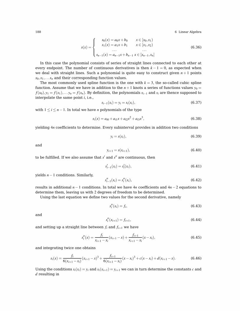
188 6 Linear Algebra
s(x) =
s0(x) = a0x+ b0 x ∈ [x0,x1)
s1(x) = a1x+ b1 x ∈ [x1,x2)
. . . . . .
sn−1(x) = an−1x+ bn−1 x ∈ [xn−1,xn]
(6.36)
In this case the polynomial consists of series of straight lines connected to each other atevery endpoint. The number of continuous derivatives is then k− 1 = 0, as expected whenwe deal with straight lines. Such a polynomial is quite easy to construct given n+ 1 pointsx0,x1, . . .xn and their corresponding function values.
The most commonly used spline function is the one with k = 3, the so-called cubic splinefunction. Assume that we have in addition to the n+ 1 knots a series of functions values y0 =
f (x0),y1 = f (x1), . . .yn = f (xn). By definition, the polynomials si−1 and si are thence supposed tointerpolate the same point i, i.e.,
si−1(xi) = yi = si(xi), (6.37)
with 1≤ i≤ n− 1. In total we have n polynomials of the type
si(x) = ai0 + ai1x+ ai2x2 + ai3x3, (6.38)
yielding 4n coefficients to determine. Every subinterval provides in addition two conditions
yi = s(xi), (6.39)
andyi+1 = s(xi+1), (6.40)
to be fulfilled. If we also assume that s′ and s′′ are continuous, then
s′i−1(xi) = s′i(xi), (6.41)
yields n− 1 conditions. Similarly,s′′i−1(xi) = s′′i (xi), (6.42)
results in additional n− 1 conditions. In total we have 4n coefficients and 4n− 2 equations todetermine them, leaving us with 2 degrees of freedom to be determined.
Using the last equation we define two values for the second derivative, namely
s′′i (xi) = fi, (6.43)
ands′′i (xi+1) = fi+1, (6.44)
and setting up a straight line between fi and fi+1 we have
s′′i (x) =fi
xi+1− xi
(xi+1− x)+fi+1
xi+1− xi
(x− xi), (6.45)
and integrating twice one obtains
si(x) =fi
6(xi+1− xi)(xi+1− x)3 +
fi+1
6(xi+1− xi)(x− xi)
3 + c(x− xi)+ d(xi+1− x). (6.46)
Using the conditions si(xi) = yi and si(xi+1) = yi+1 we can in turn determine the constants c andd resulting in

6.6 Iterative Methods 189
si(x) =fi
6(xi+1−xi)(xi+1− x)3 +
fi+1
6(xi+1−xi)(x− xi)
3
+ (yi+1
xi+1−xi− fi+1(xi+1−xi)
6)(x− xi)+ ( yi
xi+1−xi− fi(xi+1−xi)
6)(xi+1− x). (6.47)
How to determine the values of the second derivatives fi and fi+1? We use the continuityassumption of the first derivatives
s′i−1(xi) = s′i(xi), (6.48)
and set x = xi. Defining hi = xi+1− xi we obtain finally the following expression
hi−1 fi−1 + 2(hi+ hi−1) fi + hi fi+1 =6
hi
(yi+1− yi)−6
hi−1
(yi− yi−1), (6.49)
and introducing the shorthands ui = 2(hi + hi−1), vi =6hi(yi+1− yi)− 6
hi−1(yi− yi−1), we can refor-
mulate the problem as a set of linear equations to be solved through e.g., Gaussian elemina-tion, namely
u1 h1 0 . . .
h1 u2 h2 0 . . .
0 h2 u3 h3 0 . . .
. . . . . . . . . . . . . . . . . .
. . . 0 hn−3 un−2 hn−2
0 hn−2 un−1
f1
f2
f3
. . .
fn−2
fn−1
=
v1
v2
v3
. . .
vn−2
vn−1
. (6.50)
Note that this is a set of tridiagonal equations and can be solved through only O(n) operations.It is easy to write your own program for the cubic spline method when you have written
a slover for tridiagonal equations. We split the program into two tasks, one which finds thepolynomial approximation and one which uses the polynomials approximation to find an in-terpolated value for a function. These functions are included in the programs of this chapter,see the codes cubicpsline.cpp and cubicsinterpol.cpp. Alternatively, you can solve exercise6.4!
6.6 Iterative Methods
Till now we have dealt with so-called direct solvers such as Gaussian elimination and LU de-composition. Iterative solvers offer another strategy and are much used in partial differentialequations. We start with a guess for the solution and then iterate till the solution does notchange anymore.
6.6.1 Jacobi’s method
It is a simple method for solvingAx = b,
where A is a matrix and x and b are vectors. The vector x is the unknown.It is an iterative scheme where we start with a guess for the unknown, and after k + 1
iterations we havex(k+1) = D−1(b− (L+U)x(k)),
with A = D+U + L and D being a diagonal matrix, U an upper triangular matrix and L a lowertriangular matrix.

190 6 Linear Algebra
If the matrix A is positive definite or diagonally dominant, one can show that this methodwill always converge to the exact solution.
We can demonstrate Jacobi’s method by a 4×4 matrix problem. We assume a guess for the
initial vector elements, labeled x(0)i . This guess represents our first iteration. The new values
are obtained by substitution
x(1)1 = (b1− a12x
(0)2 − a13x
(0)3 − a14x
(0)4 )/a11
x(1)2 = (b2− a21x
(0)1 − a23x
(0)3 − a24x
(0)4 )/a22
x(1)3 = (b3− a31x
(0)1 − a32x
(0)2 − a34x
(0)4 )/a33
x(1)4 = (b4− a41x
(0)1 − a42x
(0)2 − a43x
(0)3 )/a44,
which after k+ 1 iterations result in
x(k+1)1 = (b1− a12x
(k)2 − a13x
(k)3 − a14x
(k)4 )/a11
x(k+1)2 = (b2− a21x
(k)1 − a23x
(k)3 − a24x
(k)4 )/a22
x(k+1)3 = (b3− a31x
(k)1 − a32x
(k)2 − a34x
(k)4 )/a33
x(k+1)4 = (b4− a41x
(k)1 − a42x
(k)2 − a43x
(k)3 )/a44,
We can generalize the above equations to
x(k+1)i = (bi−
n
∑j=1, j 6=i
ai jx(k)j )/aii
or in an even more compact form as
x(k+1) = D−1(b− (L+U)x(k)),
with A = D+U + L and D being a diagonal matrix, U an upper triangular matrix and L a lowertriangular matrix.
6.6.2 Gauss-Seidel
Our 4× 4 matrix problem
x(k+1)1 = (b1− a12x
(k)2 − a13x
(k)3 − a14x
(k)4 )/a11
x(k+1)2 = (b2− a21x
(k)1 − a23x
(k)3 − a24x
(k)4 )/a22
x(k+1)3 = (b3− a31x
(k)1 − a32x
(k)2 − a34x
(k)4 )/a33
x(k+1)4 = (b4− a41x
(k)1 − a42x
(k)2 − a43x
(k)3 )/a44,
can be rewritten as
x(k+1)1 = (b1− a12x
(k)2 − a13x
(k)3 − a14x
(k)4 )/a11
x(k+1)2 = (b2− a21x
(k+1)1 − a23x
(k)3 − a24x
(k)4 )/a22
x(k+1)3 = (b3− a31x
(k+1)1 − a32x
(k+1)2 − a34x
(k)4 )/a33
x(k+1)4 = (b4− a41x
(k+1)1 − a42x
(k+1)2 − a43x
(k+1)3 )/a44,

6.6 Iterative Methods 191
which allows us to utilize the preceding solution (forward substitution). This improves nor-mally the convergence behavior and leads to the Gauss-Seidel method!
We can generalize these equations to the following form
x(k+1)i =
1
aii
(bi−∑
j>i
ai jx(k)j −∑
j<i
ai jx(k+1)j
), i = 1,2, . . . ,n.
The procedure is generally continued until the changes made by an iteration are below sometolerance.
The convergence properties of the Jacobi method and the Gauss-Seidel method depend onthe matrix A. These methods converge when the matrix is symmetric positive-definite, or isstrictly or irreducibly diagonally dominant. Both methods sometimes converge even if theseconditions are not satisfied.
6.6.3 Successive over-relaxation
We can rewrite the above in a slightly more formal way and extend the methods to what iscalled successive over-relaxation. Given a square system of n linear equations with unknownx:
Ax = b
where:
A =
a11 a12 · · · a1n
a21 a22 · · · a2n
......
. . ....
an1 an2 · · · ann
, x =
x1
x2
...xn
, b =
b1
b2
...bn
.
Then A can be decomposed into a diagonal component D, and strictly lower and upper trian-gular components L and U:
A = D+ L+U ,
where
D =
a11 0 · · · 0
0 a22 · · · 0...
.... . .
...0 0 · · · ann
, L =
0 0 · · · 0
a21 0 · · · 0...
.... . .
...an1 an2 · · · 0
, U =
0 a12 · · · a1n
0 0 · · · a2n
......
. . ....
0 0 · · · 0
.
The system of linear equations may be rewritten as:
(D+ωL)x = ωb− [ωU +(ω− 1)D]x
for a constant ω > 1. The method of successive over-relaxation is an iterative technique thatsolves the left hand side of this expression for x, using previous value for x on the right handside. Analytically, this may be written as:
x(k+1) = (D+ωL)−1(ωb− [ωU +(ω− 1)D]x(k)
).
However, by taking advantage of the triangular form of (D+ωL), the elements of x(k+1) canbe computed sequentially using forward substitution:
x(k+1)i = (1−ω)x
(k)i +
ω
aii
(bi−∑
j>i
ai jx(k)j −∑
j<i
ai jx(k+1)j
), i = 1,2, . . . ,n.

192 6 Linear Algebra
The choice of relaxation factor is not necessarily easy, and depends upon the properties of thecoefficient matrix. For symmetric, positive-definite matrices it can be proven that 0 < ω < 2
will lead to convergence, but we are generally interested in faster convergence rather thanjust convergence.
6.6.4 Conjugate Gradient Method
The success of the Conjugate Gradient method for finding solutions of non-linear problems isbased on the theory for of conjugate gradients for linear systems of equations. It belongs tothe class of iterative methods for solving problems from linear algebra of the type
Ax = b.
In the iterative process we end up with a problem like
r = b− Ax,
where r is the so-called residual or error in the iterative process.The residual is zero when we reach the minimum of the quadratic equation
P(x) =1
2xT Ax− xT b,
with the constraint that the matrix A is positive definite and symmetric. If we search for aminimum of the quantummechanical variance, then the matrix A, which is called the Hessian,is given by the second-derivative of the variance. This quantity is always positive definite. Ifwe vary the energy, the Hessian may not always be positive definite.
In the Conjugate Gradient method we define so-called conjugate directions and two vectorss and t are said to be conjugate if
sT At = 0.
The philosophy of the Conjugate Gradient method is to perform searches in various conjugatedirections of our vectors xi obeying the above criterion, namely
xTi Ax j = 0.
Two vectors are conjugate if they are orthogonal with respect to this inner product. Beingconjugate is a symmetric relation: if s is conjugate to t, then t is conjugate to s.
An example is given by the eigenvectors of the matrix
vTi Av j = λ vT
i v j,
which is zero unless i = j.Assume now that we have a symmetric positive-definite matrix A of size n× n. At each
iteration i+ 1 we obtain the conjugate direction of a vector
xi+1 = xi +αipi.
We assume that pi is a sequence of n mutually conjugate directions. Then the pi form a basisof Rn and we can expand the solution Ax = b in this basis, namely
x =n
∑i=1
αipi.

6.6 Iterative Methods 193
The coefficients are given by
Ax =n
∑i=1
αiApi = b.
Multiplying with pTk from the left gives
pTk Ax =
n
∑i=1
αipTk Api = pT
k b,
and we can define the coefficients αk as
αk =pT
k b
pTk Apk
If we choose the conjugate vectors pk carefully, then we may not need all of them to obtaina good approximation to the solution x. So, we want to regard the conjugate gradient methodas an iterative method. This also allows us to solve systems where n is so large that the directmethod would take too much time.
We denote the initial guess for x as x0. We can assume without loss of generality that
x0 = 0,
or consider the systemAz = b− Ax0,
instead.One can show that the solution x is also the unique minimizer of the quadratic form
f (x) =1
2xT Ax− xT x, x ∈ Rn.
This suggests taking the first basis vector p1 to be the gradient of f at x = x0, which equals
Ax0− b,
and x0 = 0 it is equal −b. The other vectors in the basis will be conjugate to the gradient,hence the name conjugate gradient method.
Let rk be the residual at the k-th step:
rk = b− Axk.
Note that rk is the negative gradient of f at x = xk, so the gradient descent method wouldbe to move in the direction rk. Here, we insist that the directions pk are conjugate to eachother, so we take the direction closest to the gradient rk under the conjugacy constraint. Thisgives the following expression
pk+1 = rk−pT
k Ark
pTk Apk
pk.
We can also compute the residual iteratively as
rk+1 = b− Axk+1,
which equalsb− A(xk +αkpk),
or

194 6 Linear Algebra
(b− Axk)−αkApk,
which givesrk+1 = rk− Apk,
If we consider finding the minimum of a function f using Newton’s method, that implies asearch for a zero of the gradient of a function. Near a point xi we have to second order
f (x) = f (xi)+ (x− xi)∇ f (xi)1
2(x− xi)A(x− xi)
giving∇ f (x) = ∇ f (xi)+ A(x− xi).
In Newton’s method we set ∇ f = 0 and we can thus compute the next iteration point
x− xi = A−1∇ f (xi).
Subtracting this equation from that of xi+1 we have
xi+1− xi = A−1(∇ f (xi+1)−∇ f (xi)).
6.7 A vector and matrix class
We end this chapter by presenting a class which allows to manipulate one- and two-dimensional arrays. However, before we proceed, we would like to come with some generalrecommendations. Although it is useful to write your own classes, like the one included here,in general these classes may not be very efficient from a computational point of view. Thereare several libraries which include many interesting array features that allow us to writemore compact code. The latter has the advantage that the code is lost likely easier to debugin case of errors (obviously assuming that the library is functioning correctly). Furthermore,if the proper functionalities are included, the final code may closely resemble the mathemat-ical operations we wish to perform, increasing considerably the readability of our program.And finally, the code is in almost all casesmuch faster than the one we wrote!
In particular, we would like to recommend the C++ linear algebra library Armadillo, seehttp://arma.sourceforgenet. For those of you who are familiar with compiled programslike Matlab, the syntax is deliberately similar. Integer, floating point and complex numbersare supported, as well as a subset of trigonometric and statistics functions. Various matrixdecompositions are provided through optional integration with LAPACK, or one of its highperformance drop-in replacements (such as the multi-threaded MKL or ACML libraries). Theselected examples included here show some examples on how to declare arrays and rearrangearrays or perform mathematical operations on say vectors or matrices. The first examplehere defines two random matrices of dimensionality 10× 10 and performs a matrix-matrixmultiplication using the dgemm function of the library BLAS.
Simple matrix-matrix multiplication of two random matrices
#include <iostream>
#include <armadillo>
using namespace std;
using namespace arma;
int main(int argc, char** argv)

6.7 A vector and matrix class 195
mat A = randu<mat>(10,10);
mat B = randu<mat>(10,10);
// Matrix-matrix multiplication
cout << A*B << endl;
return 0;
In the next example we compute the determinant of a 5× 5 matrix, its inverse and performthereafter several operations on various matrices.
Determinant and inverse of a matrix
#include <iostream>
#include "armadillo"
using namespace arma;
using namespace std;
int main(int argc, char** argv)
cout << "Armadillo version: " << arma_version::as_string() << endl;
mat A;
// Hard coding of the matrix
// endr indicates "end of row"
A << 0.165300 << 0.454037 << 0.995795 << 0.124098 << 0.047084 << endr
<< 0.688782 << 0.036549 << 0.552848 << 0.937664 << 0.866401 << endr
<< 0.348740 << 0.479388 << 0.506228 << 0.145673 << 0.491547 << endr
<< 0.148678 << 0.682258 << 0.571154 << 0.874724 << 0.444632 << endr
<< 0.245726 << 0.595218 << 0.409327 << 0.367827 << 0.385736 << endr;
// .n_rows = number of rows
// .n_cols = number of columns
cout << "A.n_rows = " << A.n_rows << endl;
cout << "A.n_cols = " << A.n_cols << endl;
// Print the matrix A
A.print("A =");
// Computation of the determinant
cout << "det(A) = " << det(A) << endl;
// inverse
cout << "inv(A) = " << endl << inv(A) << endl;
// save to disk
A.save("MatrixA.txt", raw_ascii);
// Define a new matrix B which reads A from file
mat B;
B.load("MatrixA.txt");
B += 5.0*A;
B.print("The matrix B:");
// generate the identity matrix
mat C = eye<mat>(4,4);
// transpose of B
cout << "trans(B) =" << endl;
// maximum from each column (traverse along rows)
cout << "max(B) =" << endl;
cout << max(B) << endl;
// sum of all elements B
cout << "sum(sum(B)) = " << sum(sum(B)) << endl;
cout << "accu(B) = " << accu(B) << endl;
// trace = sum along diagonal
cout << "trace(B) = " << trace(B) << endl;
// random matrix -- values are uniformly distributed in the [0,1] interval
mat D = randu<mat>(4,4);
D.print("Matrix D:");
// sum of four matrices (no temporary matrices are created)
mat E = A+B + C + D;

196 6 Linear Algebra
F.print("F:");
return 0;
For more examples, please consult the online manual, see http://arma.sourceforgenet.
6.7.1 How to construct your own matrix-vector class
The rest of this section shows how one can build a matrix-vector class. We first give an exam-ple of a function which use the header file Array.h.
#include "Array.h"
#include <iostream>
using namespace std;
int main()
// Create an array with (default) nrows = 1, ncols = 1:
Array<double> v1;
// Redimension the array to have length n:
int n1 = 3;
v1.redim(n1);
// Extract the length of the array:
const int length = v1.getLength();
// Create a narray of specific length:
int n2 = 5;
Array<double> v2(n2);
// Create an array as a copy of another one:
Array<double> v5(v1);
// Assign the entries in an array:
v5(0) = 3.0;
v5(1) = 2.5;
v5(2) = 1.0;
for(int i=0; i<3; i++)
cout << v5(i) << endl;
// Extract the ith component of an array:
int i = 2;
double value = v5(1);
cout << "value: " << value << endl;
// Set an array equal another one:
Array<double> v6 = v5;
for(int i=0; i<3; i++)
v1(i) = 1.0;
v2(i) = 2.0;
// Create a two-dimensional array (matrix):
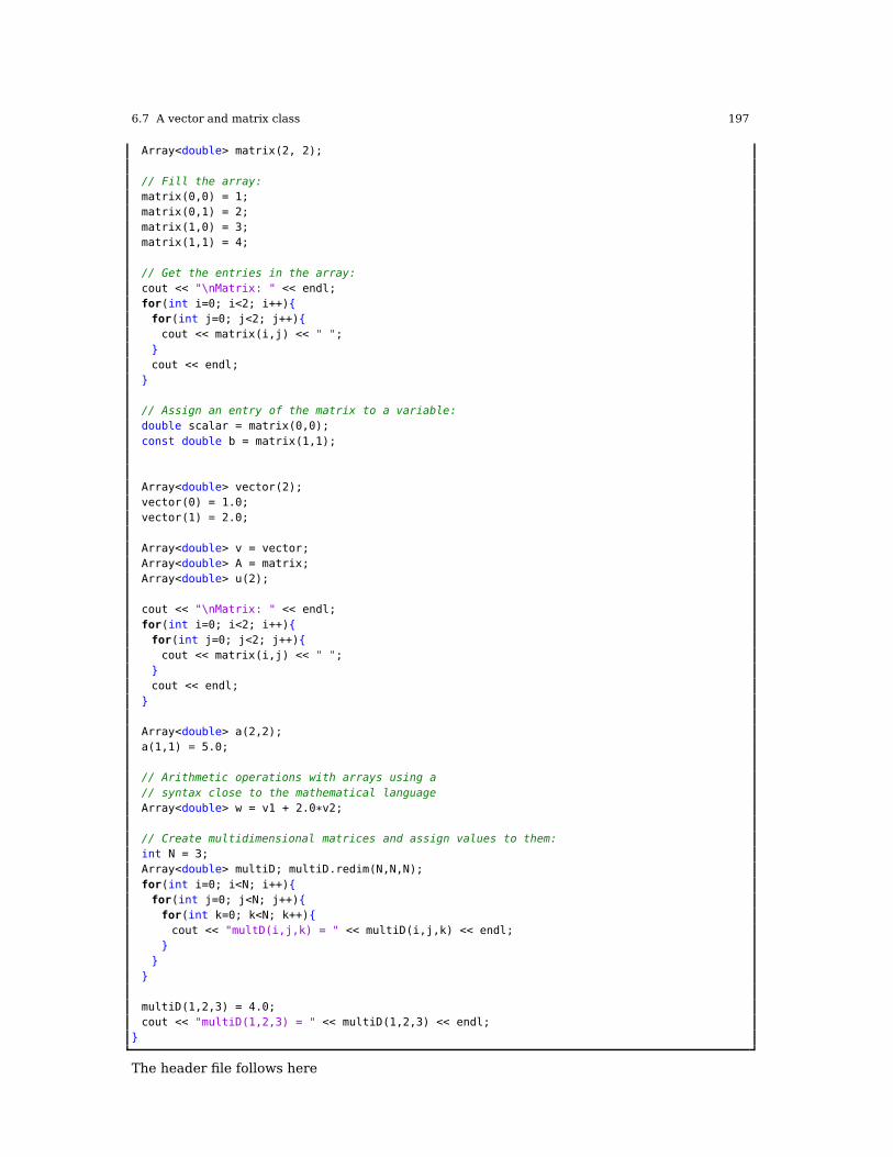
6.7 A vector and matrix class 197
Array<double> matrix(2, 2);
// Fill the array:
matrix(0,0) = 1;
matrix(0,1) = 2;
matrix(1,0) = 3;
matrix(1,1) = 4;
// Get the entries in the array:
cout << "\nMatrix: " << endl;
for(int i=0; i<2; i++)
for(int j=0; j<2; j++)
cout << matrix(i,j) << " ";
cout << endl;
// Assign an entry of the matrix to a variable:
double scalar = matrix(0,0);
const double b = matrix(1,1);
Array<double> vector(2);
vector(0) = 1.0;
vector(1) = 2.0;
Array<double> v = vector;
Array<double> A = matrix;
Array<double> u(2);
cout << "\nMatrix: " << endl;
for(int i=0; i<2; i++)
for(int j=0; j<2; j++)
cout << matrix(i,j) << " ";
cout << endl;
Array<double> a(2,2);
a(1,1) = 5.0;
// Arithmetic operations with arrays using a
// syntax close to the mathematical language
Array<double> w = v1 + 2.0*v2;
// Create multidimensional matrices and assign values to them:
int N = 3;
Array<double> multiD; multiD.redim(N,N,N);
for(int i=0; i<N; i++)
for(int j=0; j<N; j++)
for(int k=0; k<N; k++)
cout << "multD(i,j,k) = " << multiD(i,j,k) << endl;
multiD(1,2,3) = 4.0;
cout << "multiD(1,2,3) = " << multiD(1,2,3) << endl;
The header file follows here

198 6 Linear Algebra
#ifndef ARRAY_H
#define ARRAY_H
#include <iostream>
#include <sstream>
#include <iomanip>
#include <cstdlib>
using namespace std;
template<class T>
class Array
private:
static const int MAXDIM = 6;
T *data ; /**> One-dimensional array of data.*/
int size[MAXDIM]; /**> Size of each dimension.*/
int ndim; /**> Number of dimensions occupied. */
int length; /**> Total number of entries.*/
int dx1, dx2, dx3, dx4, dx5;
void allocate(int ni=0, int nj=0, int nk=0, int nl=0, int nm=0, int nn=0)
ndim = MAXDIM;
// Set the number of entries in each dimension.
size[0]=ni;
size[1]=nj;
size[2]=nk;
size[3]=nl;
size[4]=nm;
size[5]=nn;
// Set the number of dimensions used.
if(size[5] == 0)
ndim--;
if(size[4] == 0)
ndim--;
if(size[3] == 0)
ndim--;
if(size[2] == 0)
ndim--;
if(size[1] == 0)
ndim--;
if(size[0] == 0)
ndim = 0;
length = 0;
data = NULL;
else
try
int i;
// Set the length (total number of entries) of the one-dimensional array.
length = 1;
for(i=0; i<ndim; i++)
length *= size[i];
data = new T[length];
dx1 = size[0];

6.7 A vector and matrix class 199
dx2 = dx1*size[1];
dx3 = dx2*size[2];
dx4 = dx3*size[3];
dx5 = dx4*size[4];
catch(std::bad_alloc&)
std::cerr << "Array::allocate -- unable to allocate array of length " << length <<
std::endl;
exit(1);
public:
/**
* @brief Constructor with default arguments.
*
* Creates an array with one or two-dimensions.
*
* @param int nrows. Number of rows in the array.
* @param int ncolsd. Number of columns in the array.
**/
Array(int ni=0, int nj=0, int nk=0, int nl=0, int nm=0, int nn=0)
// Allocate memory
allocate(ni,nj,nk,nl,nm,nn);
// end constructor
//! Constructor
Array(T* array, int ndim_, int size_[])
ndim = ndim_;
length = 1;
int i;
for(i=0; i<ndim; i++)
size[i] = size_[i]; // Copy only the ndim entries. The rest is zero by default.
length *= size[i];
// Now when we known the length, we should not forget to allocate memory!!!!
data = new T[length];
// Copy the entries from array to data:
for(i=0; i<length; i++)
data[i] = array[i];
// End constructor.
//! Copy constructor
Array(const Array<T>& array);
//! Destructor
~Array();

200 6 Linear Algebra
/**
* @brief Checks the validity of the indexing.
* @param i, an integer for indexing the rows.
* @param j, an integer for indexing the columns.
**/
bool indexOk(int i, int j=0) const;
/**
* @brief Change the dimensions of an array.
* @param ni number of entries in the first dimension.
* @param nj number of entries in the second dimension.
* @param nk number of entries in the third dimension.
* @param nl number of entries in the fourth dimension.
* @param nm number of entries in the fifth dimension.
* @param nn number of entries in the sixth dimension.
**/
bool redim(int ni, int nj=0, int nk=0, int nl=0, int nm=0, int nn=0);
/**
* @return The total number of entries in the array, i.e., the sum of the entries in all
the dimensions.
**/
int getLength()constreturn length;
/**
* @return The number of rows in a matrix.
**/
int getRows() const return size[0];
/**
* @return Returns the number of columns in a matrix.
**/
int getColumns() const return size[1];
/** @brief Gives the number of entries in a dimension.
*
* @param i An integer from 0 to 5 indicating the dimension we want to explore.
* @return size[i] An integer for the number of elements in the dimension number i.
**/
int dimension(int i) constreturn size[i];
/**
* The number of dimensions in the array.
**/
int getNDIM()constreturn ndim;
/**
* @return A constant pointer to the array of data.
* This function can be used to interface C++ with Python/Fortran/C.
**/
const T* getPtr() const;
/**
* @return A pointer to the array of data.
* This function can be used to interface C++ with Python/Fortran/C.

6.7 A vector and matrix class 201
**/
T* getPtr();
/**
* @return A pointer to an array with information on the length of each dimension.
**/
int* getPtrSize();
/************************************************************/
/* OPERATORS */
/************************************************************/
//! Assignment operator
Array<T>& operator=(const Array<T>& array);
//! Sum operator
Array<T> operator+(const Array<T>& array);
//! Substraction operator
Array<T> operator-(const Array<T>& array)const; /// w=u-v;
//! Multiplication operator
//Array<T> operator*(const Array<T>& array);
//! Assigment by addition operator
Array<T>& operator+=(const Array<T>& w);
//! Assignment by substraction operator
Array<T>& operator-=(const Array<T>& w);
//! Assignment by scalar product operator
Array<T>& operator*=(double scalar);
//! Assignment by division operator
Array<T>& operator/=(double scalar);
//! Index operators
const T& operator()(int i)const;
const T& operator()(int i, int j)const;
const T& operator()(int i, int j, int k)const;
const T& operator()(int i, int j, int k, int l)const;
const T& operator()(int i, int j, int k, int l, int m)const;
const T& operator()(int i, int j, int k, int l, int m, int n)const;
T& operator()(int i);
T& operator()(int i, int j);
T& operator()(int i, int j, int k);
T& operator()(int i, int j, int k, int l);
T& operator()(int i, int j, int k, int l, int m);
T& operator()(int i, int j, int k, int l, int m, int n);

202 6 Linear Algebra
/**************************************************************/
/* FRIEND FUNCTIONS */
/**************************************************************/
//! Unary operator +
template <class T2>
friend Array<T> operator+ (const Array<T>&); // u = + v
//! Unary operator -
template <class T2>
friend Array<T> operator-(const Array<T>&); // u = - v
/**
* Premultiplication by a floating point number:
* \f$\mathbfu = a \mathbfv\f$,
* where \f$a\f$ is a scalar and \f$\mathbfv\f$ is a array.
**/
template <class T2>
friend Array<T> operator*(double, const Array<T>&); // u = a*v
/**
* Postmultiplication by a floating point number:
* \f$\mathbfu = \mathbfv a\f$,
* where \f$a\f$ is a scalar and \f$\mathbfv\f$ is a array.
**/
template <class T2>
friend Array<T> operator*(const Array<T>&, double); // u = v*a
/**
* Division of the entries of a array by a scalar.
**/
template <class T2>
friend Array<T> operator/(const Array<T>&, double); // u = v/a
;
#include "Array.cpp"
// Destructor
template <class T>
inline Array<T>::~Array()delete[] data;
// Index operators
template <class T>
inline const T& Array<T>::operator()(int i)const
#if CHECKBOUNDS_ON
indexOk(i);
#endif
return data[i];

6.7 A vector and matrix class 203
template <class T>
inline const T& Array<T>::operator()(int i, int j)const
#if CHECKBOUNDS_ON
indexOk(i,j);
#endif
return data[i + j*dx1];
template <class T>
inline const T& Array<T>::operator()(int i, int j, int k)const
#if CHECKBOUNDS_ON
indexOk(i,j,k);
#endif
return data[i + j*dx1 + k*dx2];
template <class T>
inline const T& Array<T>::operator()(int i, int j, int k, int l)const
#if CHECKBOUNDS_ON
indexOk(i,j,k,l);
#endif
return data[i + j*dx1 + k*dx2 + l*dx3];
template <class T>
inline const T& Array<T>::operator()(int i, int j, int k, int l, int m)const
#if CHECKBOUNDS_ON
indexOk(i,j,k,l, m);
#endif
return data[i + j*dx1 + k*dx2 + l*dx3 + m*dx4];
template <class T>
inline const T& Array<T>::operator()(int i, int j, int k, int l, int m, int n)const
#if CHECKBOUNDS_ON
indexOk(i,j,k,l,m,n);
#endif
return data[i + j*dx1 + k*dx2 + l*dx3 + m*dx4 + n*dx5];
template <class T>
inline T& Array<T>::operator()(int i)
#if CHECKBOUNDS_ON
indexOk(i);
#endif
return data[i];
template <class T>
inline T& Array<T>::operator()(int i, int j)
#if CHECKBOUNDS_ON
indexOk(i,j);

204 6 Linear Algebra
#endif
return data[i + j*dx1];
template <class T>
inline T& Array<T>::operator()(int i, int j, int k)
#if CHECKBOUNDS_ON
indexOk(i,j,k);
#endif
return data[i + j*dx1 + k*dx2];
template <class T>
inline T& Array<T>::operator()(int i, int j, int k, int l)
#if CHECKBOUNDS_ON
indexOk(i,j,k,l);
#endif
return data[i + j*dx1 + k*dx2 + l*dx3];
template <class T>
inline T& Array<T>::operator()(int i, int j, int k, int l, int m)
#if CHECKBOUNDS_ON
indexOk(i,j,k,l,m);
#endif
return data[i + j*dx1 + k*dx2 + l*dx3 + m*dx4];
template <class T>
inline T& Array<T>::operator()(int i, int j, int k, int l, int m, int n)
#if CHECKBOUNDS_ON
indexOk(i,j,k,l,m,n);
#endif
return data[i + j*dx1 + k*dx2 + l*dx3 + m*dx4 + n*dx5];
template <class T>
inline const T* Array<T>::getPtr() const return data;
template <class T>
inline T* Array<T>::getPtr()return data;
template <class T>
inline int* Array<T>::getPtrSize()return size;
// template <class T>

6.8 Exercises 205
// inline int Array<T>::dim()constreturn ndim;
/******************************************************************/
/* IMPLEMENTATION OF FRIEND FUNCTIONS */
/******************************************************************/
/******************************************************************/
/* (Arithmetic) Unary operators */
/******************************************************************/
//! Unary operator +
template <class T>
inline Array<T> operator+(const Array<T>& v) // u = + v
return v;
//! Unary operator -
template <class T>
inline Array<T> operator-(const Array<T>& v) // u = - v
return Array<T>(v.size[0],v.size[1]) -v;
//! Postmultiplication operator
template <class T>
inline Array<T> operator*(const Array<T>& v, double scalar) // u = v*a
return Array<T>(v) *= scalar;
//! Premultiplication operator.
template <class T>
inline Array<T> operator*(double scalar, const Array<T>& v) // u = a*v
return v*scalar; // Note the call to postmultiplication operator defined above
//! Division of the entries in a array by a scalar
template <class T>
inline Array<T> operator/(const Array<T>& v, double scalar)
if(!scalar) std::cout << "Division by zero!" << std::endl;
return (1.0/scalar)*v;
#endif
6.8 Exercises
6.1. The aim of this exercise is to write your own Gaussian elimination code.
1. Consider the linear system of equations
a11x1 + a12x2 + a13x3 = w1
a21x1 + a22x2 + a23x3 = w2
a31x1 + a32x2 + a33x3 = w3.

206 6 Linear Algebra
This can be written in matrix form asAx = w.
We specialize here to the following case
−x1 + x2− 4x3 = 0
2x1 + 2x2 = 1
3x1 + 3x2 + 2x3 =12.
Obtain the solution (by hand) of this system of equations by doing Gaussian elimination.2. Write therafter a program which implements Gaussian elimination (with pivoting) and
solve the above system of linear equations. How many floating point operations are in-volved in the solution via Gaussian elimination without pivoting? Can you estimate thenumber of floating point operations with pivoting?
6.2. If the matrix A is real, symmetric and positive definite, then it has a unique factorization(called Cholesky factorization)
A = LU = LLT
where LT is the upper matrix, implying that
LTi j = L ji.
The algorithm for the Cholesky decomposition is a special case of the general LU-decompositionalgorithm. The algorithm of this decomposition is as follows
• Calculate the diagonal element Lii by setting up a loop for i = 0 to i = n− 1 (C++ indexingof matrices and vectors)
Lii =
(Aii−
i−1
∑k=0
L2ik
)1/2
. (6.51)
• within the loop over i, introduce a new loop which goes from j = i+1 to n−1 and calculate
L ji =1
Lii
(Ai j−
i−1
∑k=0
Likl jk
). (6.52)
For the Cholesky algorithmwe have always that Lii > 0 and the problemwith exceedingly largematrix elements does not appear and hence there is no need for pivoting. Write a functionwhich performs the Cholesky decomposition. Test your program against the standard LUdecomposition by using the matrix
A =
6 3 2
3 2 1
2 1 1
(6.53)
Finally, use the Cholesky method to solve
0.05x1 + 0.07x2+ 0.06x3+ 0.05x4 = 0.23
0.07x1 + 0.10x2+ 0.08x3+ 0.07x4 = 0.32
0.06x1 + 0.08x2+ 0.10x3+ 0.09x4 = 0.33
0.05x1 + 0.07x2+ 0.09x3+ 0.10x4 = 0.31
You can also use the LU codes for linear equations to check the results.
6.3. In this exercise we are going to solve the one-dimensional Poisson equation in terms oflinear equations.

6.8 Exercises 207
1. We are going to solve the one-dimensional Poisson equation with Dirichlet boundary con-ditions by rewriting it as a set of linear equations.The three-dimensional Poisson equation is a partial differential equation,
∂ 2φ
∂x2+
∂ 2φ
∂y2+
∂ 2φ
∂ z2=−ρ(x,y,z)
ε0
,
whose solution we will discuss in chapter 10. The function ρ(x,y,z) is the charge densityand φ is the electrostatic potential. In this project we consider the one-dimensional casesince there are a few situations, possessing a high degree of symmetry, where it is possibleto find analytic solutions. Let us discuss some of these solutions.Suppose, first of all, that there is no variation of the various quantities in the y- and z-directions. In this case, Poisson’s equation reduces to an ordinary differential equation inx, the solution of which is relatively straightforward. Consider for example a vacuum diode,in which electrons are emitted from a hot cathode and accelerated towards an anode. Theanode is held at a large positive potential V0 with respect to the cathode. We can think ofthis as an essentially one-dimensional problem. Suppose that the cathode is at x = 0 andthe anode at x = d. Poisson’s equation takes the form
d2φ
dx2=−ρ(x)
ε0
,
where φ(x) satisfies the boundary conditions φ(0) = 0 and φ(d) = V0. By energy conserva-tion, an electron emitted from rest at the cathode has an x-velocity v(x) which satisfies
1
2mev2(x)− eφ(x) = 0.
Furthermore, we assume that the current I is independent of x between the anode andcathode, otherwise, charge will build up at some points. From electromagnetism one canthen show that the current I is given by I =−ρ(x)v(x)A, where A is the cross-sectional areaof the diode. The previous equations can be combined to give
d2φ
dx2=
I
ε0A
(me
2e
)1/2
φ−1/2.
The solution of the above equation which satisfies the boundary conditions is
φ =V0
( x
d
)4/3
,
with
I =4
9
ε0A
d2
(2e
me
)1/2
V3/20 .
This relationship between the current and the voltage in a vacuum diode is called theChild-Langmuir law.Another physics example in one dimension is the famous Thomas-Fermi model, widelyused as a mean-field model in simulations of quantum mechanical systems [37, 38], seeLieb for a newer and updated discussion [39]. Thomas and Fermi assumed the existenceof an energy functional, and derived an expression for the kinetic energy based on thedensity of electrons, ρ(r) in an infinite potential well. For a large atom or molecule witha large number of electrons. Schrödinger’s equation, which would give the exact densityand energy, cannot be easily handled for large numbers of interacting particles. Sincethe Poisson equation connects the electrostatic potential with the charge density, one can

208 6 Linear Algebra
derive the following equation for potential V
d2V
dx2=
V 3/2
√x,
with V (0) = 1.In our case we will rewrite Poisson’s equation in terms of dimensionless variables. We canthen rewrite the equation as
−u′′(x) = f (x), x ∈ (0,1), u(0) = u(1) = 0.
and we define the discretized approximation to u as vi with grid points xi = ih in the intervalfrom x0 = 0 to xn+1 = 1. The step length or spacing is defined as h = 1/(n+1). We have thenthe boundary conditions v0 = vn+1 = 0. We approximate the second derivative of u with
−vi+1 + vi−1− 2vi
h2= fi for i = 1, . . . ,n,
where fi = f (xi). Show that you can rewrite this equation as a linear set of equations of theform
Av = b,
where A is an n× n tridiagonal matrix which we rewrite as
A =
2 −1 0 . . . . . . 0
−1 2 −1 0 . . . . . .
0 −1 2 −1 0 . . .
. . . . . . . . . . . . . . .
0 . . . −1 2 −1
0 . . . 0 −1 2
and bi = h2 fi.In our case we will assume that f (x) = (3x+x2)ex, and keep the same interval and boundaryconditions. Then the above differential equation has an analytic solution given by u(x) =
x(1− x)ex (convince yourself that this is correct by inserting the solution in the Poissonequation). We will compare our numerical solution with this analytic result in the nextexercise.
2. We can rewrite our matrix A in terms of one-dimensional vectors a,b,c of length 1 : n. Ourlinear equation reads
A =
b1 c1 0 . . . . . . . . .
a2 b2 c2 . . . . . . . . .
a3 b3 c3 . . . . . .
. . . . . . . . . . . . . . .
an−2 bn−1 cn−1
an bn
v1
v2
. . .
. . .
. . .
vn
=
b1
b2
. . .
. . .
. . .
bn
.
A tridiagonal matrix is a special form of banded matrix where all the elements are zeroexcept for those on and immediately above and below the leading diagonal. The abovetridiagonal system can be written as
aivi−1 + bivi + civi+1 = bi,

6.8 Exercises 209
for i = 1,2, . . . ,n. The algorithm for solving this set of equations is rather simple and re-quires two steps only, a decomposition and forward substitution and finally a backwardsubstitution.Your first task is to set up the algorithm for solving this set of linear equations. Find alsothe number of operations needed to solve the above equations. Show that they behavelike O(n) with n the dimensionality of the problem. Compare this with standard Gaussianelimination.Then you should code the above algorithm and solve the problem for matrices of the size10× 10, 100× 100 and 1000× 1000. That means that you choose n = 10, n = 100 and n = 1000
grid points.Compare your results (make plots) with the analytic results for the different number of gridpoints in the interval x ∈ (0,1). The different number of grid points corresponds to differentstep lengths h.Compute also the maximal relative error in the data set i = 1, . . . ,n,by setting up
εi = log10
(∣∣∣∣vi− ui
ui
∣∣∣∣),
as function of log10(h) for the function values ui and vi. For each step length extract themax value of the relative error. Try to increase n to n = 10000 and n = 105. Comment yourresults.
3. Compare your results with those from the LU decomposition codes for the matrix of size1000×1000. Use for example the unix function time when you run your codes and comparethe time usage between LU decomposition and your tridiagonal solver. Can you run thestandard LU decomposition for a matrix of the size 105× 105? Comment your results.
6.8.1 Solution
The program listed below encodes a possible solution to part b) of the above project. Notethat we have employed Blitz++ as library and that the range of the various vectors are nowshifted from their default ranges (0 : n−1) to (1 : n) and that we access vector elements as a(i)
instead of the standard C++ declaration a[i].The program reads from screen the name of the ouput file and the dimension of the prob-
lem, which in our case corresponds to the number of mesh points as well, in addition to thetwo endpoints. The function f (x) = (3x+ x2)exp(x) is included explicitely in the code. An ob-vious change is to define a separate function, allowing thereby for a generalization to otherfunction f (x).
/*Program to solve the one-dimensional Poisson equation
-u''(x) = f(x) rewritten as a set of linear equations
A u = f where A is an n x n matrix, and u and f are 1 x n vectors
In this problem f(x) = (3x+x*x)exp(x) with solution u(x) = x(1-x)exp(x)
The program reads from screen the name of the output file.
Blitz++ is used here, with arrays starting from 1 to n
*/
#include <iomanip>
#include <fstream>
#include <blitz/array.h>
#include <iostream>
using namespace std;
using namespace blitz;

210 6 Linear Algebra
ofstream ofile;
// Main program only, no other functions
int main(int argc, char* argv[])
char *outfilename;
int i, j, n;
double h, btemp;
// Read in output file, abort if there are too few command-line arguments
if( argc <= 1 )
cout << "Bad Usage: " << argv[0] <<
" read also output file on same line" << endl;
exit(1);
else
outfilename=argv[1];
ofile.open(outfilename);
cout << "Read in number of mesh points" << endl;
cin >> n;
h = 1.0/( (double) n+1);
// Use Blitz to allocate arrays
// Use range to change default arrays from 0:n-1 to 1:n
Range r(1,n);
Array<double,1> a(r), b(r), c(r), y(r), f(r), temp(r);
// set up the matrix defined by three arrays, diagonal, upper and lower diagonal band
b = 2.0; a = -1.0 ; c = -1.0;
// Then define the value of the right hand side f (multiplied by h*h)
for(i=1; i <= n; i++)
// Explicit expression for f, could code as separate function
f(i) = h*h*(i*h*3.0+(i*h)*(i*h))*exp(i*h);
// solve the tridiagonal system, first forward substitution
btemp = b(1);
for(i = 2; i <= n; i++)
temp(i) = c(i-1) / btemp;
btemp = b(i) - a(i) * temp(i);
y(i) = (f(i) - a(i) * y(i-1)) / btemp;
// then backward substitution, the solution is in y()
for(i = n-1; i >= 1; i--)
y(i) -= temp(i+1) * y(i+1);
// write results to the output file
for(i = 1; i <= n; i++)
ofile << setiosflags(ios::showpoint | ios::uppercase);
ofile << setw(15) << setprecision(8) << i*h;
ofile << setw(15) << setprecision(8) << y(i);
ofile << setw(15) << setprecision(8) << i*h*(1.0-i*h)*exp(i*h) <<endl;
ofile.close();
The program writes also the exact solution to file. In Fig. 6.4 we show the results obtainedwith n = 10. Even with so few points, the numerical solution is very close to the analyticanswer. With n = 100 it is almost impossible to distinguish the numerical solution from theanalytical one, as shown in Fig. 6.5. It is therefore instructive to study the relative error,which we display in Table 6.2 as function of the step length h = 1/(n+ 1).
The mathematical truncation we made when computing the second derivative goes likeO(h2). Our results for n from n = 10 to somewhere between n = 104 and n = 105 result in aslope which is almost exactly equal 2,in good agreement with the mathematical truncation

6.8 Exercises 211
0
0.2
0.4
0.6
0.8
1
0 0.2 0.4 0.6 0.8 1
u(x)
x
Numerical solutionAnalytical solution
Fig. 6.4 Numerical solution obtained with n = 10 compared with the analytical solution.
0
0.2
0.4
0.6
0.8
1
0 0.2 0.4 0.6 0.8 1
u(x)
x
Numerical solutionAnalytical solution
Fig. 6.5 Numerical solution obtained with n = 10 compared with the analytical solution.
Table 6.2 log10 values for the relative error and the step length h computed at x = 0.5.
n log10(h) εi = log10 (|(vi−ui)/ui|)10 -1.04 -2.29
100 -2.00 -4.191000 -3.00 -6.18
104 -4.00 -8.18105 -5.00 -9.19106 -6.00 -6.08

212 6 Linear Algebra
made. Beyond n = 105 the relative error becomes bigger, telling us that there is no point inincreasing n. For most practical application a relative error between 10−6 and 10−8 is morethan sufficient, meaning that n = 104 may be an acceptable number of mesh points. Beyondn = 105, numerical round off errors take over, as discussed in the previous chapter as well.
6.4. Write your own code for performing the cubic spline interpolation using either Blitz++or Armadillo. Alternatively you can use the vector-matrix class included in this text.
6.5. Write your own code for the LU decomposition using the same libraries as in the previousexercise. Find also the number of floating point operations.
6.6. Solve exercise 6.3 by writing a code which implements both the iterative Jacobi methodand the Gauss-Seidel method. Study carefully the number of iterations needed to achieve theexact result.
6.7. Extend thereafter your code for the iterative Jacobi method to a parallel version andcompare with the results from the previous exercise.
6.8. Write your own code for the Conjugate gradient method.
6.9. Write your own code for matrix-matrix multiplications using Strassen’s algorithm dis-cussed in subsection 6.3.3.1 and compare the speed of your program with the matrix-matrixmultiplication provided by the Armadillo library.

Chapter 7
Eigensystems
Abstract We present here two methods for solving directly eigenvalue problems using sim-ilarity transformations. One is the familiar Jacobi rotation method while the second methodis based on transforming the matrix to tridiagonal form using Householder’s algorithm. Wediscuss also so-called power methods and conclude with a discussion of iterative algorithms.These are particularly interesting for eigenvalue problems of large dimnesionality.
7.1 Introduction
Together with linear equations and least squares, the third major problem in matrix com-putations deals with the algebraic eigenvalue problem. Here we limit our attention to thesymmetric case. We focus in particular on two similarity transformations, the Jacobi method,the famous QR algoritm with Householder’s method for obtaining a triangular matrix andFrancis’ algorithm for the final eigenvalues. Our presentation follows closely that of Goluband Van Loan, see Ref. [28].
7.2 Eigenvalue problems
Let us consider the matrix A of dimension n. The eigenvalues of A are defined through thematrix equation
Ax(ν) = λ (ν)x(ν), (7.1)
where λ (ν) are the eigenvalues and x(ν) the corresponding eigenvectors. Unless otherwisestated, when we use the wording eigenvector we mean the right eigenvector. The left eigen-vector is defined as
x(ν)LA = λ (ν)x(ν)L
The above right eigenvector problem is equivalent to a set of n equations with n unknowns xi
a11x1 + a12x2 + · · ·+ a1nxn = λ x1
a21x1 + a22x2 + · · ·+ a2nxn = λ x2
. . . . . .
an1x1 + an2x2 + · · ·+ annxn = λ xn.
We can rewrite Eq. (7.1) as
213
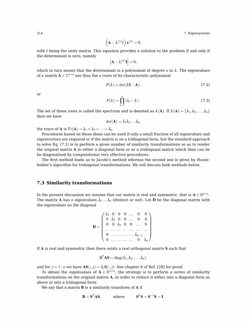
214 7 Eigensystems
(A−λ (ν)I
)x(ν) = 0,
with I being the unity matrix. This equation provides a solution to the problem if and only ifthe determinant is zero, namely ∣∣∣A−λ (ν)I
∣∣∣= 0,
which in turn means that the determinant is a polynomial of degree n in λ . The eigenvaluesof a matrix A ∈ C
n×n are thus the n roots of its characteristic polynomial
P(λ ) = det(λ I−A), (7.2)
or
P(λ ) =n
∏i=1
(λi−λ ) . (7.3)
The set of these roots is called the spectrum and is denoted as λ (A). If λ (A) = λ1,λ2, . . . ,λnthen we have
det(A) = λ1λ2 . . .λn,
the trace of A is Tr(A) = λ1 +λ2 + · · ·+λn.Procedures based on these ideas can be used if only a small fraction of all eigenvalues and
eigenvectors are required or if the matrix is on a tridiagonal form, but the standard approachto solve Eq. (7.1) is to perform a given number of similarity transformations so as to renderthe original matrix A in either a diagonal form or as a tridiagonal matrix which then can bebe diagonalized by computational very effective procedures.
The first method leads us to Jacobi’s method whereas the second one is given by House-holder’s algorithm for tridiagonal transformations. We will discuss both methods below.
7.3 Similarity transformations
In the present discussion we assume that our matrix is real and symmetric, that is A ∈ Rn×n.The matrix A has n eigenvalues λ1 . . .λn (distinct or not). Let D be the diagonal matrix withthe eigenvalues on the diagonal
D =
λ1 0 0 0 . . . 0 0
0 λ2 0 0 . . . 0 0
0 0 λ3 0 0 . . . 0
. . . . . . . . . . . . . . . . . . . . .
0 . . . . . . . . . . . . λn−1
0 . . . . . . . . . . . . 0 λn
.
If A is real and symmetric then there exists a real orthogonal matrix S such that
ST AS = diag(λ1,λ2, . . . ,λn),
and for j = 1 : n we have AS(:, j) = λ jS(:, j). See chapter 8 of Ref. [28] for proof.To obtain the eigenvalues of A ∈ R
n×n, the strategy is to perform a series of similaritytransformations on the original matrix A, in order to reduce it either into a diagonal form asabove or into a tridiagonal form.
We say that a matrix B is a similarity transform of A if
B = ST AS, where ST S = S−1S = I.

7.4 Jacobi’s method 215
The importance of a similarity transformation lies in the fact that the resulting matrix has thesame eigenvalues, but the eigenvectors are in general different. To prove this we start withthe eigenvalue problem and a similarity transformed matrix B.
Ax = λ x and B = ST AS.
We multiply the first equation on the left by ST and insert ST S = I between A and x. Then weget
(STAS)(STx) = λ STx, (7.4)
which is the same asB(STx
)= λ
(STx
).
The variable λ is an eigenvalue of B as well, but with eigenvector STx.The basic philosophy is to
• either apply subsequent similarity transformations so that
STN . . .ST
1 AS1 . . .SN = D, (7.5)
• or apply subsequent similarity transformations so that A becomes tridiagonal. Thereafter,techniques for obtaining eigenvalues from tridiagonal matrices can be used.
Let us look at the first method, better known as Jacobi’s method or Given’s rotations.
7.4 Jacobi’s method
Consider an (n× n) orthogonal transformation matrix
S =
1 0 . . . 0 0 . . . 0 0
0 1 . . . 0 0 . . . 0 0
. . . . . . . . . . . . . . . . . . 0 . . .
0 0 . . . cosθ 0 . . . 0 sinθ
0 0 . . . 0 1 . . . 0 0
. . . . . . . . . . . . . . . . . . 0 . . .
0 0 . . . 0 0 . . . 1 0
0 0 . . . −sinθ . . . . . . 0 cosθ
with property ST = S−1. It performs a plane rotation around an angle θ in the Euclideann−dimensional space. It means that the matrix elements that differ from zero are given by
skk = sll = cosθ ,skl =−slk =−sinθ ,sii =−sii = 1 i 6= k i 6= l,
A similarity transformationB = ST AS,
results in
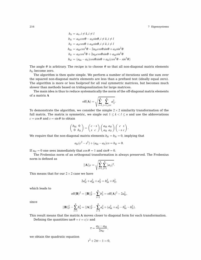
216 7 Eigensystems
bii = aii, i 6= k, i 6= l
bik = aikcosθ − ailsinθ , i 6= k, i 6= l
bil = ailcosθ + aiksinθ , i 6= k, i 6= l
bkk = akkcos2θ − 2aklcosθ sinθ + allsin2θ
bll = allcos2θ + 2aklcosθ sinθ + akksin2θ
bkl = (akk− all)cosθ sinθ + akl(cos2θ − sin2θ )
The angle θ is arbitrary. The recipe is to choose θ so that all non-diagonal matrix elementsbkl become zero.
The algorithm is then quite simple. We perform a number of iterations until the sum overthe squared non-diagonal matrix elements are less than a prefixed test (ideally equal zero).The algorithm is more or less foolproof for all real symmetric matrices, but becomes muchslower than methods based on tridiagonalization for large matrices.
The main idea is thus to reduce systematically the norm of the off-diagonal matrix elementsof a matrix A
off(A) =
√n
∑i=1
n
∑j=1, j 6=i
a2i j.
To demonstrate the algorithm, we consider the simple 2× 2 similarity transformation of thefull matrix. The matrix is symmetric, we single out 1 ≤ k < l ≤ n and use the abbreviationsc = cosθ and s = sinθ to obtain
(bkk 0
0 bll
)=
(c −s
s c
)(akk akl
alk all
)(c s
−s c
).
We require that the non-diagonal matrix elements bkl = blk = 0, implying that
akl(c2− s2)+ (akk− all)cs = bkl = 0.
If akl = 0 one sees immediately that cosθ = 1 and sinθ = 0.The Frobenius norm of an orthogonal transformation is always preserved. The Frobenius
norm is defined as
||A||F =
√n
∑i=1
n
∑j=1
|ai j|2.
This means that for our 2× 2 case we have
2a2kl + a2
kk + a2ll = b2
kk + b2ll,
which leads to
off(B)2 = ||B||2F −n
∑i=1
b2ii = off(A)2− 2a2
kl,
since
||B||2F −n
∑i=1
b2ii = ||A||2F −
n
∑i=1
a2ii +(a2
kk + a2ll− b2
kk− b2ll).
This result means that the matrix A moves closer to diagonal form for each transformation.Defining the quantities tanθ = t = s/c and
τ =all− akk
2akl
,
we obtain the quadratic equationt2 + 2τt− 1 = 0,

7.4 Jacobi’s method 217
resulting in
t =−τ±√
1+ τ2,
and c and s are easily obtained via
c =1√
1+ t2,
and s = tc. Choosing t to be the smaller of the roots ensures that |θ | ≤ π/4 and has the effectof minimizing the difference between the matrices B and A since
||B−A||2F = 4(1− c)n
∑i=1,i6=k,l
(a2ik + a2
il)+2a2
kl
c2.
The main idea is thus to reduce systematically the norm of the off-diagonal matrix elementsof a matrix A
off(A) =
√n
∑i=1
n
∑j=1, j 6=i
a2i j.
To implement the Jacobi algorithm we can proceed as follows
• Choose a tolerance ε, making it a small number, typically 10−8 or smaller.• Setup a while-test where one compares the norm of the newly computed off-diagonal
matrix elements
off(A) =
√n
∑i=1
n
∑j=1, j 6=i
a2i j > ε.
This is however a very time-comsuming test which can be replaced by the simplertest
max(a2i j)> ε.
• Now choose the matrix elements akl so that we have those with largest value, that is|akl |= maxi6= j|ai j|.
• Compute thereafter τ = (all− akk)/2akl, tanθ , cosθ and sinθ .• Compute thereafter the similarity transformation for this set of values (k, l), obtaining
the new matrix B = S(k, l,θ )T AS(k, l,θ ).• Continue till
max(a2i j)≤ ε.
The convergence rate of the Jacobi method is however poor, one needs typically 3n2−5n2 ro-tations and each rotation requires 4n operations, resulting in a total of 12n3−20n3 operationsin order to zero out non-diagonal matrix elements. Although the classical Jacobi algorithmperforms badly compared with methods based on tridiagonalization, it is easy to parallelize.
The slow convergence is related to the fact that when a new rotation is performed, matrixelements which were previously zero, may change to non-zero values in the next rotation. Tosee this, consider the following simple example.
We specialize to a symmetric 3×3 matrix A. We start the process as follows (assuming thata23 = a32 is the largest non-diagonal matrix element) with c = cosθ and s = sinθ
B =
1 0 0
0 c −s
0 s c
a11 a12 a13
a21 a22 a23
a31 a32 a33
1 0 0
0 c s
0 −s c
.

218 7 Eigensystems
We will choose the angle θ in order to have b23 = b32 = 0. We get the new symmetric matrix
B =
a11 a12c− a13s a12s+ a13c
a12c− a13s a22c2 + a33s2− 2a23sc (a22− a33)sc+ a23(c2− s2)
a12s+ a13c (a22− a33)sc+ a23(c2− s2) a22s2 + a33c2 + 2a23sc
.
Note that a11 is unchanged! As it should.We have then
b11 = a11
b12 = a12cosθ − a13sinθ ,1 6= 2,1 6= 3
b13 = a13cosθ + a12sinθ ,1 6= 2,1 6= 3
b22 = a22cos2θ − 2a23cosθ sinθ + a33sin2θ
b33 = a33cos2θ + 2a23cosθ sinθ + a22sin2θ
b23 = (a22− a33)cosθ sinθ + a23(cos2θ − sin2θ )
We will fix the angle θ so that b23 = 0.We get then a new matrix
B =
b11 b12 b13
b12 b22 0
b13 0 a33
.
We repeat assuming that b12 is the largest non-diagonal matrix element and get a new matrix
C =
c −s 0
s c 0
0 0 1
b11 b12 b13
b12 b22 0
b13 0 b33
c s 0
−s c 0
0 0 1
.
We continue this process till all non-diagonal matrix elements are zero. It is easy to con-vince oneself that when performing the above operations, the matrix element b23 which waspreviously set to zero may become different from zero. This is one of the problems whichslows down the Jacobi procedure. We leave this experience to the reader in form of a largenumerical project at the end of this chapter.
An implementation of the above algorithm, normally referred to as the classical Jacobialgorithm, is exposed partially in the code here.
http://folk.uio.no/compphys/programs/chapter07/cpp/jacobi.cpp
/*Jacobi's method for finding eigenvalues
eigenvectors of the symetric matrix A.
The eigenvalues of A will be on the diagonal
of A, with eigenvalue i being A[i][i].
The j-th component of the i-th eigenvector
is stored in R[i][j].
A: input matrix (n x n)
R: empty matrix for eigenvectors (n x n)
n: dimention of matrices
*/
#include <iostream>
#include <cmath>
#include "jacobi.h"
void jacobi_method ( double ** A, double ** R, int n )

7.4 Jacobi’s method 219
// Setting up the eigenvector matrix
for ( int i = 0; i < n; i++ )
for ( int j = 0; j < n; j++ )
if ( i == j )
R[i][j] = 1.0;
else
R[i][j] = 0.0;
int k, l;
double epsilon = 1.0e-8;
double max_number_terations = (double) n * (double) n * (double) n;
int iterations = 0;
double max_offdiag = maxoffdiag ( A, &k, &l, n );
while ( fabs(max_offdiag) > epsilon && (double) iterations < max_number_iterations )
max:offdiag = maxoffdiag ( A, &k, &l, n );
rotate ( A, R, k, l, n );
iterations++;
std::cout << "Number of iterations: " << iterations << "\n";
return;
// Function to find the maximum matrix element. Can you figure out a more
// elegant algorithm?
double maxoffdiag ( double ** A, int * k, int * l, int n )
double max = 0.0;
for ( int i = 0; i < n; i++ )
for ( int j = i + 1; j < n; j++ )
if ( fabs(A[i][j]) > max )
max = fabs(A[i][j]);
*l = i;
*k = j;
return max;
// Function to find the values of cos and sin
void rotate ( double ** A, double ** R, int k, int l, int n )
double s, c;
if ( A[k][l] != 0.0 )
double t, tau;
tau = (A[l][l] - A[k][k])/(2*A[k][l]);
if ( tau > 0 )
t = 1.0/(tau + sqrt(1.0 + tau*tau);
else
t = -1.0/( -tau + sqrt(1.0 + tau*tau);
c = 1/sqrt(1+t*t);
s = c*t;
else
c = 1.0;
s = 0.0;

220 7 Eigensystems
double a_kk, a_ll, a_ik, a_il, r_ik, r_il;
a_kk = A[k][k];
a_ll = A[l][l];
// changing the matrix elements with indices k and l
A[k][k] = c*c*a_kk - 2.0*c*s*A[k][l] + s*s*a_ll;
A[l][l] = s*s*a_kk + 2.0*c*s*A[k][l] + c*c*a_ll;
A[k][l] = 0.0; // hard-coding of the zeros
A[l][k] = 0.0;
// and then we change the remaining elements
for ( int i = 0; i < n; i++ )
if ( i != k && i != l )
a_ik = A[i][k];
a_il = A[i][l];
A[i][k] = c*a_ik - s*a_il;
A[k][i] = A[i][k];
A[i][l] = c*a_il + s*a_ik;
A[l][i] = A[i][l];
// Finally, we compute the new eigenvectors
r_ik = R[i][k];
r_il = R[i][l];
R[i][k] = c*r_ik - s*r_il;
R[i][l] = c*r_il + s*r_ik;
return;
7.5 Similarity Transformations with Householder’s method
In this case the diagonalization is performed in two steps: First, the matrix is transformedinto tridiagonal form by the Householder similarity transformation. Secondly, the tridiago-nal matrix is then diagonalized. The reason for this two-step process is that diagonalizing atridiagonal matrix is computational much faster than the corresponding diagonalization of ageneral symmetric matrix. Let us discuss the two steps in more detail.
7.5.1 The Householder’s method for tridiagonalization
The first step consists in finding an orthogonal matrix S which is the product of (n−2) orthog-onal matrices
S = S1S2 . . .Sn−2,
each of which successively transforms one row and one column of A into the required tridi-agonal form. Only n−2 transformations are required, since the last two elements are alreadyin tridiagonal form. In order to determine each Si let us see what happens after the firstmultiplication, namely,
ST1 AS1 =
a11 e1 0 0 . . . 0 0
e1 a′22 a′23 . . . . . . . . . a′2n
0 a′32 a′33 . . . . . . . . . a′3n
0 . . . . . . . . . . . . . . .
0 a′n2 a′n3 . . . . . . . . . a′nn

7.5 Similarity Transformations with Householder’s method 221
where the primed quantities represent a matrix A′ of dimension n−1 which will subsequentelybe transformed by S2. The factor e1 is a possibly non-vanishing element. The next transforma-tion produced by S2 has the same effect as S1 but now on the submatirx A
′only
(S1S2)T
AS1S2 =
a11 e1 0 0 . . . 0 0
e1 a′22 e2 0 . . . . . . 0
0 e2 a′′33 . . . . . . . . . a′′3n
0 . . . . . . . . . . . . . . .
0 0 a′′n3 . . . . . . . . . a′′nn
Note that the effective size of the matrix on which we apply the transformation reduces forevery new step. In the previous Jacobi method each similarity transformation is in principleperformed on the full size of the original matrix.
After a series of such transformations, we end with a set of diagonal matrix elements
a11,a′22,a
′′33 . . .a
n−1nn ,
and off-diagonal matrix elementse1,e2,e3, . . . ,en−1.
The resulting matrix reads
ST AS =
a11 e1 0 0 . . . 0 0
e1 a′22 e2 0 . . . 0 0
0 e2 a′′33 e3 0 . . . 0
. . . . . . . . . . . . . . . . . . . . .
0 . . . . . . . . . . . . a(n−1)n−1n−1 en−1
0 . . . . . . . . . . . . en−1 a(n−1)nn
.
It remains to find a recipe for determining the transformation Sn. We illustrate the methodfor S1 which we assume takes the form
S1 =
(1 0T
0 P
),
with 0T being a zero row vector, 0T = 0,0, · · · of dimension (n−1). The matrix P is symmetricwith dimension ((n− 1)× (n− 1)) satisfying P2 = I and PT = P. A possible choice which fulfillsthe latter two requirements is
P = I− 2uuT ,
where I is the (n− 1) unity matrix and u is an n− 1 column vector with norm uT u = 1, that isits inner product.
Note that uuT is an outer product giving a dimension ((n−1)×(n−1)). Each matrix elementof P then reads
Pi j = δi j− 2uiu j,
where i and j range from 1 to n− 1. Applying the transformation S1 results in
ST1 AS1 =
(a11 (Pv)T
Pv A′
),
where vT = a21,a31, · · · ,an1 and P must satisfy (Pv)T = k,0,0, · · ·. Then
Pv = v− 2u(uT v) = ke, (7.6)

222 7 Eigensystems
with eT = 1,0,0, . . .0. Solving the latter equation gives us u and thus the needed transforma-tion P. We do first however need to compute the scalar k by taking the scalar product of thelast equation with its transpose and using the fact that P2 = I. We get then
(Pv)T Pv = k2 = vT v = |v|2 =n
∑i=2
a2i1,
which determines the constant k =±v. Now we can rewrite Eq. (7.6) as
v− ke = 2u(uT v),
and taking the scalar product of this equation with itself and obtain
2(uT v)2 = (v2± a21v), (7.7)
which finally determines
u =v− ke
2(uT v).
In solving Eq. (7.7) great care has to be exercised so as to choose those values which makethe right-hand largest in order to avoid loss of numerical precision. The above steps are thenrepeated for every transformations till we have a tridiagonal matrix suitable for obtaining theeigenvalues. It is not so difficult to implement Householder’s algorithm, as demonstrated bythe following code.
http://folk.uio.no/compphys/programs/chapter07/cpp/householder.cpp
/*
** The function
** householder()
** perform a Housholder reduction of a real symmetric matrix
** a[][]. On output a[][] is replaced by the orthogonal matrix
** effecting the transformation. d[] returns the diagonal elements
** of the tri-diagonal matrix, and e[] the off-diagonal elements,
** with e[0] = 0.
*/
void householder(double **a, int n, double *d, double *e)
register int l,k,j,i;
double scale,hh,h,g,f;
for(i = n - 1; i > 0; i--)
l = i-1;
h = scale= 0.0;
if(l > 0)
for(k = 0; k <= l; k++)
scale += fabs(a[i][k]);
if(scale == 0.0) // skip transformation
e[i] = a[i][l];
else
for(k = 0; k <= l; k++)
a[i][k] /= scale; // used scaled a's for transformation
h += a[i][k]*a[i][k];
f = a[i][l];
g = (f >= 0.0 ? -sqrt(h) : sqrt(h));
e[i] = scale*g;
h -= f * g;
a[i][l] = f - g;
f = 0.0;

7.5 Similarity Transformations with Householder’s method 223
for(j = 0;j <= l;j++)
a[j][i] = a[i][j]/h; // can be omitted if eigenvector not wanted
g = 0.0;
for(k = 0; k <= j; k++)
g += a[j][k]*a[i][k];
for(k = j+1; k <= l; k++)
g += a[k][j]*a[i][k];
e[j]=g/h;
f += e[j]*a[i][j];
hh=f/(h+h);
for(j = 0; j <= l;j++)
f = a[i][j];
e[j]=g=e[j]-hh*f;
for(k = 0; k <= j; k++)
a[j][k] -= (f*e[k]+g*a[i][k]);
// end k-loop
// end if-loop for l > 1
else
e[i]=a[i][l];
d[i]=h;
// end i-loop
d[0] = 0.0;
e[0] = 0.0;
/* Contents of this loop can be omitted if eigenvectors not
** wanted except for statement d[i]=a[i][i];
*/
for(i = 0; i < n; i++)
l = i-1;
if(d[i])
for(j = 0; j <= l; j++)
g= 0.0;
for(k = 0; k <= l; k++)
g += a[i][k] * a[k][j];
for (k = 0; k <= l; k++)
a[k][j] -= g * a[k][i];
d[i] = a[i][i];
a[i][i] = 1.0;
for(j = 0; j <= l; j++)
a[j][i]=a[i][j] = 0.0;
// End: function householder()

224 7 Eigensystems
7.5.2 Diagonalization of a Tridiagonal Matrix via Francis’ Algorithm
The matrix is now transformed into tridiagonal form and the last step is to transform it into adiagonal matrix giving the eigenvalues on the diagonal1.
Before we discuss the algorithms, we note that the eigenvalues of a tridiagonal matrix canbe obtained using the characteristic polynomial
P(λ ) = det(λ I−A) =n
∏i=1
(λi−λ ) ,
with the matrix
A−λ I =
det
d1−λ e1 0 0 . . . 0 0
e1 d2−λ e2 0 . . . 0 0
0 e2 d3−λ e3 0 . . . 0
. . . . . . . . . . . . . . . . . . . . .
0 . . . . . . . . . . . . dNstep−2−λ eNstep−1
0 . . . . . . . . . . . . eNstep−1 dNstep−1−λ
We can solve this equation in a recursive manner. We let Pk(λ ) be the value of k subde-terminant of the above matrix of dimension n× n. The polynomial Pk(λ ) is clearly a poly-nomial of degree k. Starting with P1(λ ) we have P1(λ ) = d1− λ . The next polynomial readsP2(λ ) = (d2−λ )P1(λ )− e2
1. By expanding the determinant for Pk(λ ) in terms of the minors ofthe nth column we arrive at the recursion relation
Pk(λ ) = (dk−λ )Pk−1(λ )− e2k−1Pk−2(λ ).
Together with the starting values P1(λ ) and P2(λ ) and good root searching methods we ar-rive at an efficient computational scheme for finding the roots of Pn(λ ). However, for largematrices this algorithm is rather inefficient and time-consuming.
The programswhich performs these transformations are matrix A−→ tridiagonal matrix−→diagonal matrix
C: void householder(double ∗∗a, int n, double d[], double e[])void francis(double d[], double[], int n, double ∗∗z)
Fortran: CALL householder(a, n, d, e)CALL francis(d, e, n, z)
The last step through the function francis() involves several technical details. Let us de-scribe the basic idea in terms of a four-dimensional example. For more details, see Ref. [28],in particular chapters seven and eight.
The current tridiagonal matrix takes the form
A =
d1 e1 0 0
e1 d2 e2 0
0 e2 d3 e3
0 0 e3 d4
.
As a first observation, if any of the elements ei are zero the matrix can be separated intosmaller pieces before diagonalization. Specifically, if e1 = 0 then d1 is an eigenvalue. Thus, let
1 This section is not complete it will be finished end of fall 2009.

7.6 Power Methods 225
us introduce a transformation S1
S1 =
cosθ 0 0 sin θ
0 0 0 0
0 0 0 0
−sinθ 0 0 cosθ
Then the similarity transformation
ST1 AS1 = A′ =
d′1 e′1 0 0
e′1 d2 e2 0
0 e2 d3 e′30 0 e′3 d′4
produces a matrix where the primed elements in A′ have been changed by the transformationwhereas the unprimed elements are unchanged. If we now choose θ to give the elementa′21 = e
′= 0 then we have the first eigenvalue = a
′11 = d
′1.
This procedure can be continued on the remaining three-dimensional submatrix for thenext eigenvalue. Thus after four transformations we have the wanted diagonal form.
7.6 Power Methods
We assume A can be diagonalized. Let λ1, λ2, . . . , λn be the n eigenvalues (counted withmultiplicity) of A and let v1, v2, . . . , vn be the corresponding eigenvectors. We assume that λ1
is the dominant eigenvalue, so that |λ1|> |λ j| for j > 1.The initial vector b0 can be written:
b0 = c1v1 + c2v2 + · · ·+ cmvm.
If b0 is chosen randomly (with uniform probability), then c1 âL’a 0 with probability 1. Now,
Akb0 = c1Akv1 + c2Akv2 + · · ·+ cmAkvm
= c1λ k1 v1 + c2λ k
2 v2 + · · ·+ cmλ kmvm
= c1λ k1
(v1 +
c2c1
(λ2λ1
)k
v2 + · · ·+ cm
c1
(λm
λ1
)k
vm
).
The expression within parentheses converges to v1 because |λ j/λ1|< 1 for j > 1. On the otherhand, we have
bk =Akb0
‖Akb0‖.
Therefore, bk converges to (a multiple of) the eigenvector v1. The convergence is geometric,with ratio ∣∣∣∣
λ2
λ1
∣∣∣∣ ,
where λ2 denotes the second dominant eigenvalue. Thus, the method converges slowly ifthere is an eigenvalue close in magnitude to the dominant eigenvalue.
Under the assumptions:
• A has an eigenvalue that is strictly greater in magnitude than its other eigenvalues• The starting vector b0 has a nonzero component in the direction of an eigenvector associ-
ated with the dominant eigenvalue.

226 7 Eigensystems
then:
• A subsequence of (bk) converges to an eigenvector associated with the dominant eigen-value
Note that the sequence (bk) does not necessarily converge. It can be shown that bk = eiφk v1 +
rk where: v1 is an eigenvector associated with the dominant eigenvalue, and ‖rk‖ → 0. Thepresence of the term eiφk implies that (bk) does not converge unless eiφk = 1. Under the two
assumptions listed above, the sequence (µk) defined by µk =b∗kAbk
b∗kbk
converges to the dominant
eigenvalue.Power iteration is not used very much because it can find only the dominant eigenvalue.The algorithm is however very useful in some specific case. For instance, Google uses it
to calculate the page rank of documents in their search engine. For matrices that are well-conditioned and as sparse as the web matrix, the power iterationmethod can be more efficientthan other methods of finding the dominant eigenvector.
Some of the more advanced eigenvalue algorithms can be understood as variations ofthe power iteration. For instance, the inverse iteration method applies power iteration tothe matrix A−1. Other algorithms look at the whole subspace generated by the vectors bk.This subspace is known as the Krylov subspace. It can be computed by Arnoldi iteration orLanczos iteration. The latter is method of choice for diagonalizing symmetric matrices withhuge dimensionalities. We discuss the Lanczos algorithm in the next section.
7.7 Iterative methods: Lanczos’ algorithm
The Lanczos algorithm is applied to symmetric eigenvalue problems. The basic features witha real symmetric matrix (and normally huge n > 106 and sparse) A of dimension n× n are
• The Lanczos’ algorithm generates a sequence of real tridiagonal matrices Tk of dimensionk× k with k ≤ n, with the property that the extremal eigenvalues of Tk are progressivelybetter estimates of A’ extremal eigenvalues.
• The method converges to the extremal eigenvalues.• The similarity transformation is
T = QT AQ,
with the first vector Qe1 = q1.
We are going to solve iterativelyT = QT AQ,
with the first vector Qe1 = q1. We can then write out the matrix Q in terms of its columnvectors
Q = [q1q2 . . . qn] .
The matrixT = QT AQ,
can be written as
T =
α1 β1 0 . . . . . . 0
β1 α2 β2 0 . . . 0
0 β2 α3 β3 . . . 0
. . . . . . . . . . . . . . . 0
. . . βn−2 αn−1 βn−1
0 . . . . . . 0 βn−1 αn

7.8 Schrödinger’s Equation Through Diagonalization 227
Using the fact that QQT = I, we can rewrite
T = QT AQ,
asQT = AQ,
and if we equate columns (recall from the previous slide)
T =
α1 β1 0 . . . . . . 0
β1 α2 β2 0 . . . 0
0 β2 α3 β3 . . . 0
. . . . . . . . . . . . . . . 0
. . . βn−2 αn−1 βn−1
0 . . . . . . 0 βn−1 αn
we obtainAqk = βk−1qk−1 +αkqk +βkqk+1.
We have thusAqk = βk−1qk−1 +αkqk +βkqk+1,
with β0q0 = 0 for k = 1 : n−1. Remember that the vectors qk are orthornormal and this implies
αk = qTk Aqk,
and these vectors are called Lanczos vectors. We have thus
Aqk = βk−1qk−1 +αkqk +βkqk+1,
with β0q0 = 0 for k = 1 : n− 1 andαk = qT
k Aqk.
Ifrk = (A−αkI)qk−βk−1qk−1,
is non-zero, thenqk+1 = rk/βk,
with βk =±||rk||2. These steps can then be written in terms of the following simple algorithm:
r_0 = q_1; beta_0=1; q_0=0; int k = 0;
while (beta_k != 0)
q_k+1 = r_k/beta_k
k = k+1
alpha_k = q_k^T A q_k
r_k = (A-alpha_k I) q_k -beta_k-1q_k-1
beta_k = || r_k||_2
end while
7.8 Schrödinger’s Equation Through Diagonalization
Instead of solving the Schrödinger equation as a differential equation, we will solve it throughdiagonalization of a large matrix. However, in both cases we need to deal with a problem withboundary conditions, viz., the wave function goes to zero at the endpoints.

228 7 Eigensystems
To solve the Schrödinger equation as a matrix diagonalization problem, let us study theradial part of the Schrödinger equation. The radial part of the wave function, R(r), is a solutionto
− h2
2m
(1
r2
d
drr2 d
dr− l(l + 1)
r2
)R(r)+V(r)R(r) = ER(r).
Then we substitute R(r) = (1/r)u(r) and obtain
− h2
2m
d2
dr2u(r)+
(V (r)+
l(l + 1)
r2
h2
2m
)u(r) = Eu(r).
We introduce a dimensionless variable ρ =(1/α)r where α is a constant with dimension lengthand get
− h2
2mα2
d2
dρ2u(r)+
(V (ρ)+
l(l + 1)
ρ2
h2
2mα2
)u(ρ) = Eu(ρ).
In the example below, we will replace the latter equation with that for the one-dimensionalharmonic oscillator. Note however that the procedure which we give below applies equallywell to the case of e.g., the hydrogen atom. We replace ρ with x, take away the centrifugalbarrier term and set the potential equal to
V (x) =1
2kx2,
with k being a constant. In our solution we will use units so that k = h = m = α = 1 and theSchrödinger equation for the one-dimensional harmonic oscillator becomes
− d2
dx2u(x)+ x2u(x) = 2Eu(x).
Let us now see how we can rewrite this equation as a matrix eigenvalue problem. First weneed to compute the second derivative. We use here the following expression for the secondderivative of a function f
f ′′ =f (x+ h)− 2 f (x)+ f (x− h)
h2+O(h2),
where h is our step. Next we define minimum and maximum values for the variable x, Rmin
and Rmax, respectively. With a given number of steps, Nstep, we then define the step h as
h =Rmax−Rmin
Nstep.
If we now define an arbitrary value of x as
xi = Rmin + ih i = 1,2, . . . ,Nstep− 1
we can rewrite the Schrödinger equation for xi as
−u(xk + h)− 2u(xk)+ u(xk− h)
h2+ x2
ku(xk) = 2Eu(xk),
or in a more compact way
−uk+1− 2uk + uk−1
h2+ x2
kuk =−uk+1− 2uk + uk−1
h2+Vkuk = 2Euk,
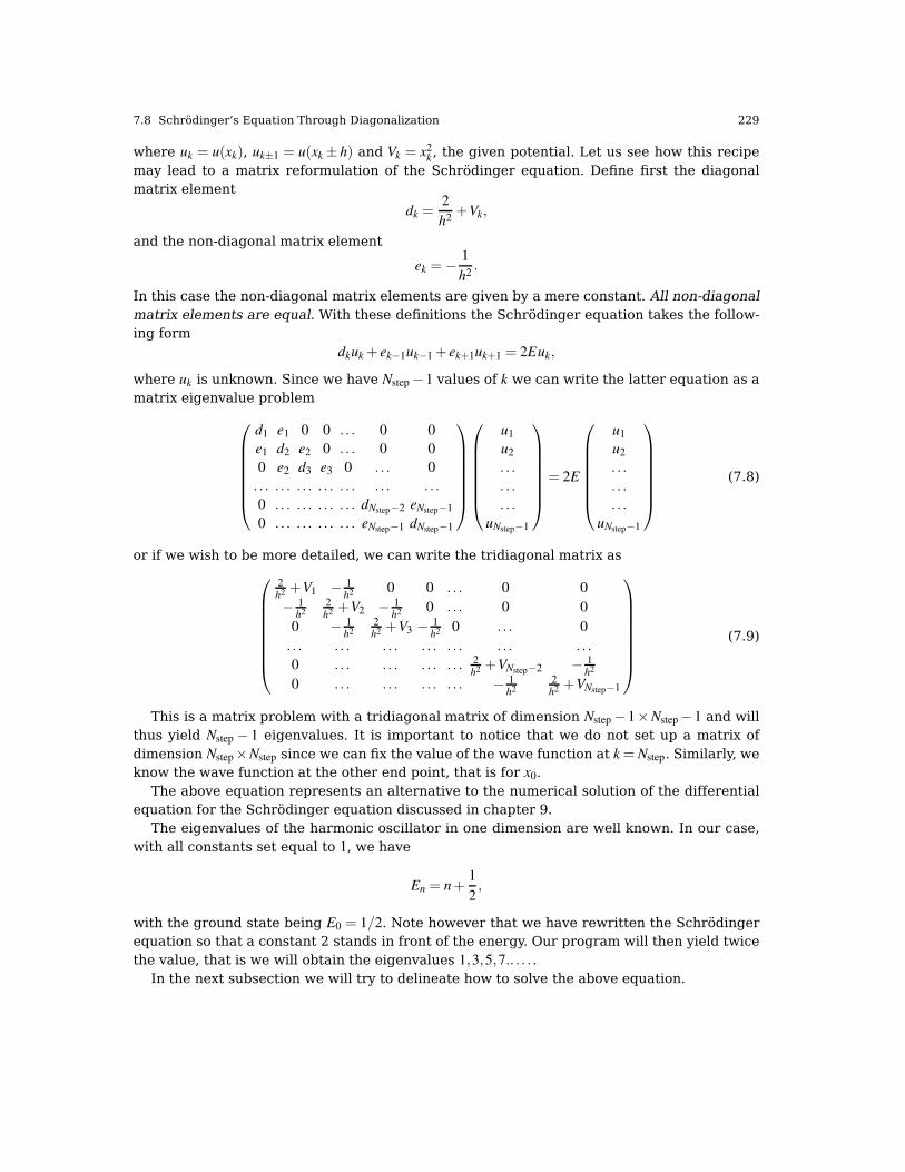
7.8 Schrödinger’s Equation Through Diagonalization 229
where uk = u(xk), uk±1 = u(xk± h) and Vk = x2k , the given potential. Let us see how this recipe
may lead to a matrix reformulation of the Schrödinger equation. Define first the diagonalmatrix element
dk =2
h2+Vk,
and the non-diagonal matrix element
ek =−1
h2.
In this case the non-diagonal matrix elements are given by a mere constant. All non-diagonalmatrix elements are equal. With these definitions the Schrödinger equation takes the follow-ing form
dkuk + ek−1uk−1 + ek+1uk+1 = 2Euk,
where uk is unknown. Since we have Nstep−1 values of k we can write the latter equation as amatrix eigenvalue problem
d1 e1 0 0 . . . 0 0
e1 d2 e2 0 . . . 0 0
0 e2 d3 e3 0 . . . 0
. . . . . . . . . . . . . . . . . . . . .
0 . . . . . . . . . . . . dNstep−2 eNstep−1
0 . . . . . . . . . . . . eNstep−1 dNstep−1
u1
u2
. . .
. . .
. . .
uNstep−1
= 2E
u1
u2
. . .
. . .
. . .
uNstep−1
(7.8)
or if we wish to be more detailed, we can write the tridiagonal matrix as
2h2 +V1 − 1
h2 0 0 . . . 0 0
− 1h2
2h2 +V2 − 1
h2 0 . . . 0 0
0 − 1h2
2h2 +V3 − 1
h2 0 . . . 0
. . . . . . . . . . . . . . . . . . . . .
0 . . . . . . . . . . . . 2h2 +VNstep−2 − 1
h2
0 . . . . . . . . . . . . − 1h2
2h2 +VNstep−1
(7.9)
This is a matrix problem with a tridiagonal matrix of dimension Nstep− 1×Nstep− 1 and willthus yield Nstep− 1 eigenvalues. It is important to notice that we do not set up a matrix ofdimension Nstep×Nstep since we can fix the value of the wave function at k = Nstep. Similarly, weknow the wave function at the other end point, that is for x0.
The above equation represents an alternative to the numerical solution of the differentialequation for the Schrödinger equation discussed in chapter 9.
The eigenvalues of the harmonic oscillator in one dimension are well known. In our case,with all constants set equal to 1, we have
En = n+1
2,
with the ground state being E0 = 1/2. Note however that we have rewritten the Schrödingerequation so that a constant 2 stands in front of the energy. Our program will then yield twicethe value, that is we will obtain the eigenvalues 1,3,5,7.. . . . .
In the next subsection we will try to delineate how to solve the above equation.

230 7 Eigensystems
7.8.1 Numerical solution of the Schrödinger equation by
diagonalization
The algorithm for solving Eq. (7.8) may take the following form
• Define values for Nstep, Rmin and Rmax. These values define in turn the step size h. Typicalvalues for Rmax and Rmin could be 10 and −10 respectively for the lowest-lying states. Thenumber of mesh points Nstep could be in the range 100 to some thousands. You can checkthe stability of the results as functions of Nstep − 1 and Rmax and Rmin against the exactsolutions.
• Construct then two one-dimensional arrays which contain all values of xk and the potentialVk. For the latter it can be convenient to write a small function which sets up the poten-tial as function of xk. For the three-dimensional case you may also need to include thecentrifugal potential. The dimension of these two arrays should go from 0 up to Nstep.
• Construct thereafter the one-dimensional vectors d and e, where d stands for the diagonalmatrix elements and e the non-diagonal ones. Note that the dimension of these two arraysruns from 1 up to Nstep− 1, since we know the wave function u at both ends of the chosengrid.
• We are now ready to obtain the eigenvalues by calling the function tqli which can be foundon the web page of the course. Calling tqli, you have to transfer the matrices d and e, theirdimension n = Nstep− 1 and a matrix z of dimension Nstep− 1×Nstep− 1 which returns theeigenfunctions. On return, the array d contains the eigenvalues. If z is given as the unitymatrix on input, it returns the eigenvectors. For a given eigenvalue k, the eigenvector isgiven by the column k in z, that is z[][k] in C, or z(:,k) in Fortran.
• TQLI does however not return an ordered sequence of eigenvalues. You may then needto sort them as e.g., an ascending series of numbers. The program we provide includes asorting function as well.
• Finally, you may perhaps need to plot the eigenfunctions as well, or calculate some otherexpectation values. Or, you would like to compare the eigenfunctions with the analyticalanswers for the harmonic oscillator or the hydrogen atom. We provide a function plotwhich has as input one eigenvalue chosen from the output of tqli. This function gives youa normalized wave function u where the norm is calculated as
∫ Rmax
Rmin
|u(x)|2 dx→ h
Nstep
∑i=0
u2i = 1,
and we have used the trapezoidal rule for integration discussed in chapter 5.
7.8.2 Program example and results for the one-dimensional harmonic
oscillator
We present here a program example which encodes the above algorithm.
http://folk.uio.no/compphys/programs/chapter07/cpp/program1.cpp
/*Solves the one-particle Schrodinger equation
for a potential specified in function
potential(). This example is for the harmonic oscillator
*/
#include <cmath>
#include <iostream>

7.8 Schrödinger’s Equation Through Diagonalization 231
#include <fstream>
#include <iomanip>
#include "lib.h"
using namespace std;
// output file as global variable
ofstream ofile;
// function declarations
void initialise(double&, double&, int&, int&) ;
double potential(double);
int comp(const double *, const double *);
void output(double, double, int, double *);
int main(int argc, char* argv[])
int i, j, max_step, orb_l;
double r_min, r_max, step, const_1, const_2, orb_factor,
*e, *d, *w, *r, **z;
char *outfilename;
// Read in output file, abort if there are too few command-line arguments
if( argc <= 1 )
cout << "Bad Usage: " << argv[0] <<
" read also output file on same line" << endl;
exit(1);
else
outfilename=argv[1];
ofile.open(outfilename);
// Read in data
initialise(r_min, r_max, orb_l, max_step);
// initialise constants
step = (r_max - r_min) / max_step;
const_2 = -1.0 / (step * step);
const_1 = - 2.0 * const_2;
orb_factor = orb_l * (orb_l + 1);
// local memory for r and the potential w[r]
r = new double[max_step + 1];
w = new double[max_step + 1];
for(i = 0; i <= max_step; i++)
r[i] = r_min + i * step;
w[i] = potential(r[i]) + orb_factor / (r[i] * r[i]);
// local memory for the diagonalization process
d = new double[max_step]; // diagonal elements
e = new double[max_step]; // tridiagonal off-diagonal elements
z = (double **) matrix(max_step, max_step, sizeof(double));
for(i = 0; i < max_step; i++)
d[i] = const_1 + w[i + 1];
e[i] = const_2;
z[i][i] = 1.0;
for(j = i + 1; j < max_step; j++)
z[i][j] = 0.0;
// diagonalize and obtain eigenvalues
tqli(d, e, max_step - 1, z);
// Sort eigenvalues as an ascending series
qsort(d,(UL) max_step - 1,sizeof(double),

232 7 Eigensystems
(int(*)(const void *,const void *))comp);
// send results to ouput file
output(r_min , r_max, max_step, d);
delete [] r; delete [] w; delete [] e; delete [] d;
free_matrix((void **) z); // free memory
ofile.close(); // close output file
return 0;
// End: function main()
/*The function potential()
calculates and return the value of the
potential for a given argument x.
The potential here is for the 1-dim harmonic oscillator
*/
double potential(double x)
return x*x;
// End: function potential()
/*The function int comp()
is a utility function for the library function qsort()
to sort double numbers after increasing values.
*/
int comp(const double *val_1, const double *val_2)
if((*val_1) <= (*val_2)) return -1;
else if((*val_1) > (*val_2)) return +1;
else return 0;
// End: function comp()
// read in min and max radius, number of mesh points and l
void initialise(double& r_min, double& r_max, int& orb_l, int& max_step)
cout << "Min vakues of R = ";
cin >> r_min;
cout << "Max value of R = ";
cin >> r_max;
cout << "Orbital momentum = ";
cin >> orb_l;
cout << "Number of steps = ";
cin >> max_step;
// end of function initialise
// output of results
void output(double r_min , double r_max, int max_step, double *d)
int i;
ofile << "RESULTS:" << endl;
ofile << setiosflags(ios::showpoint | ios::uppercase);
ofile <<"R_min = " << setw(15) << setprecision(8) << r_min << endl;
ofile <<"R_max = " << setw(15) << setprecision(8) << r_max << endl;
ofile <<"Number of steps = " << setw(15) << max_step << endl;
ofile << "Five lowest eigenvalues:" << endl;
for(i = 0; i < 5; i++)
ofile << setw(15) << setprecision(8) << d[i] << endl;
// end of function output

7.8 Schrödinger’s Equation Through Diagonalization 233
There are several features to be noted in this program.The main program calls the function initialise, which reads in the minimum and maximum
values of r, the number of steps and the orbital angular momentum l. Thereafter we allocateplace for the vectors containing r and the potential, given by the variables r[i] and w[i], respec-tively. We also set up the vectors d[i] and e[i] containing the diagonal and non-diagonal matrixelements. Calling the function tqli we obtain in turn the unsorted eigenvalues. The latter aresorted by the intrinsic C-function qsort.
The calculaton of the wave function for the lowest eigenvalue is done in the function plot,while all output of the calculations is directed to the fuction out put.
The included table exhibits the precision achieved as function of the number of mesh pointsN. The exact values are 1,3,5,7,9.
Table 7.1 Five lowest eigenvalues as functions of the number of mesh points N with rmin =−10 and rmax = 10.
N E0 E1 E2 E3 E4
50 9.898985E-01 2.949052E+00 4.866223E+00 6.739916E+00 8.568442E+00100 9.974893E-01 2.987442E+00 4.967277E+00 6.936913E+00 8.896282E+00200 9.993715E-01 2.996864E+00 4.991877E+00 6.984335E+00 8.974301E+00400 9.998464E-01 2.999219E+00 4.997976E+00 6.996094E+00 8.993599E+00
1000 1.000053E+00 2.999917E+00 4.999723E+00 6.999353E+00 8.999016E+00
The agreement with the exact solution improves with increasing numbers of mesh points.However, the agreement for the excited states is by no means impressive. Moreover, as thedimensionality increases, the time consumption increases dramatically. Matrix diagonaliza-tion scales typically as ≈ N3. In addition, there is a maximum size of a matrix which can bestored in RAM.
The obvious question which then arises is whether this scheme is nothing but a mereexample of matrix diagonalization, with few practical applications of interest. In chapter 3,where we dealt with interpolation and extrapolation, we discussed also called Richardson’sdeferred extrapolation scheme. Applied to this particualr case, the philosophy of this schemewould be to diagonalize the above matrix for a set of values of N and thereby the step lengthh. Thereafter, an extrapolation is made to h→ 0. The obtained eigenvalues agree then with aremarkable precision with the exact solution. The algorithm is then as follows
• Perform a series of diagonalizations of the matrix in Eq. (7.9 ) for different values ofthe step size h. We obtain then a series of eigenvalues E(h/2k) with k = 0,1,2, . . . .That will give us an array of ’x-values’ h,h/2,h/4, . . . and an array of ’y-values’E(h),E(h/2),E(h/4), . . . . Note that you will have such a set for each eigenvalue.
• Use these values to perform an extrapolation calling e.g., the function POLINT withthe point where we wish to extrapolate to given by h = 0.
• End the iteration over k when the error returned by POLINT is smaller than a fixedtest.
The results for the 10 lowest-lying eigenstates for the one-dimensional harmonic oscilla-tor are listed below after just 3 iterations, i.e., the step size has been reduced to h/8 only.The exact results are 1,3,5, . . . ,19 and we see that the agreement is just excellent for theextrapolated results. The results after diagonalization differ already at the fourth-fifth digit.
Parts of a Fortran program which includes Richardson’s extrapolation scheme is includedhere. It performs five diagonalizations and establishes results for various step lengths andinterpolates using the function POLINT.

234 7 Eigensystems
Table 7.2 Result for numerically calculated eigenvalues of the one-dimensional harmonic oscillator afterthree iterations starting with a matrix of size 100×100 and ending with a matrix of dimension 800×800. Thesefour values are then used to extrapolate the 10 lowest-lying eigenvalues to h = 0.. The values of x span from−10 to 10, that means that the starting step was h = 20/100 = 0.2. We list here only the results after threeiterations. The error test was set equal 10−6.
Extrapolation Diagonalization Error0.100000D+01 0.999931D+00 0.206825D-100.300000D+01 0.299965D+01 0.312617D-090.500000D+01 0.499910D+01 0.174602D-080.700000D+01 0.699826D+01 0.605671D-080.900000D+01 0.899715D+01 0.159170D-070.110000D+02 0.109958D+02 0.349902D-070.130000D+02 0.129941D+02 0.679884D-070.150000D+02 0.149921D+02 0.120735D-060.170000D+02 0.169899D+02 0.200229D-060.190000D+02 0.189874D+02 0.314718D-06
! start loop over interpolations, here we set max interpolations to 5
DO interpol=1, 5
IF ( interpol == 1) THEN
max_step=start_step
ELSE
max_step=(interpol-1)*2*start_step
ENDIF
n=max_step-1
ALLOCATE ( e(n) , d(n) )
ALLOCATE ( w(0:max_step), r(0:max_step))
d=0. ; e =0.
! define the step size
step=(rmax-rmin)/FLOAT(max_step)
hh(interpol)=step*step
! define constants for the matrix to be diagonalized
const1=2./(step*step)
const2=-1./(step*step)
! set up r, the distance from the nucleus and the function w for energy =0
! w corresponds then to the potential
! values at
DO i=0, max_step
r(i) = rmin+i*step
w(i) = potential(r(i))
ENDDO
! setup the diagonal d and the non-diagonal part e of
! the tridiagonal matrix matrix to be diagonalized
d(1:n)=const1+w(1:n) ; e(1:n)=const2
! allocate space for eigenvector info
ALLOCATE ( z(n,n) )
! obtain the eigenvalues
CALL tqli(d,e,n,z)
! sort eigenvalues as an ascending series
CALL eigenvalue_sort(d,n)
DEALLOCATE (z)
err1=0.
! the interpolation part starts here
DO l=1,20
err2=0.
value(interpol,l)=d(l)
inp=d(l)

7.9 Exercises 235
IF ( interpol > 1 ) THEN
CALL polint(hh,value(:,l),interpol,0.d0 ,inp,err2)
err1=MAX(err1,err2)
WRITE(6,'(D12.6,2X,D12.6,2X,D12.6)') inp, d(l), err1
ELSE
WRITE(6,'(D12.6,2X,D12.6,2X,D12.6)') d(l), d(l), err1
ENDIF
ENDDO
DEALLOCATE ( w, r, d, e)
ENDDO
7.9 Exercises
7.1. The aim of this problem is to solve Schrödinger’s equation for two electrons in a three-dimensional harmonic oscillator well with and without a repulsive Coulomb interaction. Yourtask is to solve this equation by reformulating it in a discretized form as an eigenvalue equa-tion to be solved with Jacobi’s method. To achieve this you will have to write your own codewhich implements Jacobi’s method.
Electrons confined in small areas in semiconductors, so-called quantum dots, form a hotresearch area in modern solid-state physics, with applications spanning from such diversefields as quantum nano-medicine to the contruction of quantum gates.
Here we will assume that these electrons move in a three-dimensional harmonic oscillatorpotential (they are confined by for example quadrupole fields) and repel each other via thestatic Colulomb interaction. We assume spherical symmetry.
We are first interested in the solution of the radial part of Schrödinger’s equation for oneelectron. This equation reads
− h2
2m
(1
r2
d
drr2 d
dr− l(l + 1)
r2
)R(r)+V(r)R(r) = ER(r).
In our case V (r) is the harmonic oscillator potential (1/2)kr2 with k = mω2 and E is the energyof the harmonic oscillator in three dimensions. The oscillator frequency is ω and the energiesare
Enl = hω
(2n+ l+
3
2
),
with n = 0,1,2, . . . and l = 0,1,2, . . . .Since we have made a transformation to spherical coordinates it means that r ∈ [0,∞).
The quantum number l is the orbital momentum of the electron. Then we substitute R(r) =
(1/r)u(r) and obtain
− h2
2m
d2
dr2u(r)+
(V (r)+
l(l + 1)
r2
h2
2m
)u(r) = Eu(r).
The boundary conditions are u(0) = 0 and u(∞) = 0.We introduce a dimensionless variable ρ = (1/α)r where α is a constant with dimension
length and get
− h2
2mα2
d2
dρ2u(ρ)+
(V (ρ)+
l(l + 1)
ρ2
h2
2mα2
)u(ρ) = Eu(ρ).
We will set in this project l = 0. Inserting V (ρ) = (1/2)kα2ρ2 we end up with
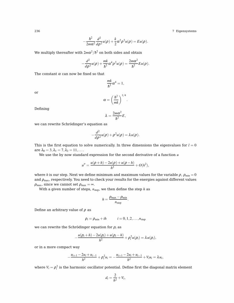
236 7 Eigensystems
− h2
2mα2
d2
dρ2u(ρ)+
k
2α2ρ2u(ρ) = Eu(ρ).
We multiply thereafter with 2mα2/h2 on both sides and obtain
− d2
dρ2u(ρ)+
mk
h2α4ρ2u(ρ) =
2mα2
h2Eu(ρ).
The constant α can now be fixed so that
mk
h2α4 = 1,
or
α =
(h2
mk
)1/4
.
Defining
λ =2mα2
h2E,
we can rewrite Schrödinger’s equation as
− d2
dρ2u(ρ)+ρ2u(ρ) = λ u(ρ).
This is the first equation to solve numerically. In three dimensions the eigenvalues for l = 0
are λ0 = 3,λ1 = 7,λ2 = 11, . . . .
We use the by now standard expression for the second derivative of a function u
u′′ =u(ρ + h)− 2u(ρ)+ u(ρ− h)
h2+O(h2),
where h is our step. Next we define minimum and maximum values for the variable ρ , ρmin = 0
and ρmax, respectively. You need to check your results for the energies against different valuesρmax, since we cannot set ρmax = ∞.
With a given number of steps, nstep, we then define the step h as
h =ρmax−ρmin
nstep.
Define an arbitrary value of ρ as
ρi = ρmin + ih i = 0,1,2, . . . ,nstep
we can rewrite the Schrödinger equation for ρi as
−u(ρi + h)− 2u(ρi)+ u(ρi− h)
h2+ρ2
i u(ρi) = λ u(ρi),
or in a more compact way
−ui+1− 2ui+ ui−1
h2+ρ2
i ui =−ui+1− 2ui+ ui−1
h2+Viui = λ ui,
where Vi = ρ2i is the harmonic oscillator potential. Define first the diagonal matrix element
di =2
h2+Vi,

7.9 Exercises 237
and the non-diagonal matrix element
ei =−1
h2.
In this case the non-diagonal matrix elements are given by a mere constant. All non-diagonalmatrix elements are equal. With these definitions the Schrödinger equation takes the follow-ing form
diui + ei−1ui−1 + ei+1ui+1 = λ ui,
where ui is unknown. We can write the latter equation as a matrix eigenvalue problem
d1 e1 0 0 . . . 0 0
e1 d2 e2 0 . . . 0 0
0 e2 d3 e3 0 . . . 0
. . . . . . . . . . . . . . . . . . . . .
0 . . . . . . . . . . . . dnstep−2 enstep−1
0 . . . . . . . . . . . . enstep−1 dnstep
u1
u2
. . .
. . .
. . .
unstep−1
= λ
u1
u2
. . .
. . .
. . .
unstep−1
(7.10)
or if we wish to be more detailed, we can write the tridiagonal matrix as
2h2 +V1 − 1
h2 0 0 . . . 0 0
− 1h2
2h2 +V2 − 1
h2 0 . . . 0 0
0 − 1h2
2h2 +V3 − 1
h2 0 . . . 0
. . . . . . . . . . . . . . . . . . . . .
0 . . . . . . . . . . . . 2h2 +Vnstep−2 − 1
h2
0 . . . . . . . . . . . . − 1h2
2h2 +Vnstep−1
(7.11)
Recall that the solutions are known via the boundary conditions at i = nstep and at the otherend point, that is for ρ0. The solution is zero in both cases.
a) Your task here is to write a function which implements Jacobi’s rotation algorithm in orderto solve Eq. (7.10).We Define the quantities tanθ = t = s/c, with s = sinθ and c = cosθ and
cot2θ = τ =all− akk
2akl
.
We can then define the angle θ so that the non-diagonal matrix elements of the transformedmatrix akl become non-zero and we obtain the quadratic equation (using cot2θ = 1/2(cotθ−tanθ )
t2 + 2τt− 1 = 0,
resulting in
t =−τ±√
1+ τ2,
and c and s are easily obtained via
c =1√
1+ t2,
and s = tc. Explain why we should choose t to be the smaller of the roots. Show that thesechoice ensures that |θ | ≤ π/4) and has the effect of minimizing the difference between thematrices B and A since
||B−A||2F = 4(1− c)n
∑i=1,i6=k,l
(a2ik + a2
il)+2a2
kl
c2.

238 7 Eigensystems
b) How many points nstep do you need in order to get the lowest three eigenvalues with fourleading digits? Remember to check the eigenvalues for the dependency on the choice ofρmax.How many similarity transformations are needed before you reach a result where all non-diagonal matrix elements are essentially zero? Try to estimate the number of transforma-tions and extract a behavior as function of the dimensionality of the matrix.You can check your results against the code based on Householder’s algorithm, tqli in thefile lib.cpp.Comment your results (here you could for example compute the time needed for bothalgorithms for a given dimensionality of the matrix).
c) We will now study two electrons in a harmonic oscillator well which also interact via arepulsive Coulomb interaction. Let us start with the single-electron equation written as
− h2
2m
d2
dr2u(r)+
1
2kr2u(r) = E(1)u(r),
where E(1) stands for the energy with one electron only. For two electrons with no repulsiveCoulomb interaction, we have the following Schrödinger equation
(− h2
2m
d2
dr21
− h2
2m
d2
dr22
+1
2kr2
1 +1
2kr2
2
)u(r1,r2) = E(2)u(r1,r2).
Note that we deal with a two-electron wave function u(r1,r2) and two-electron energy E(2).With no interaction this can be written out as the product of two single-electron wavefunctions, that is we have a solution on closed form.We introduce the relative coordinate r = r1− r2 and the center-of-mass coordinate R =
1/2(r1 + r2). With these new coordinates, the radial Schrödinger equation reads
(− h2
m
d2
dr2− h2
4m
d2
dR2+
1
4kr2 + kR2
)u(r,R) = E(2)u(r,R).
The equations for r and R can be separated via the ansatz for the wave function u(r,R) =
ψ(r)φ(R) and the energy is given by the sum of the relative energy Er and the center-of-mass energy ER, that is
E(2) = Er +ER.
We add then the repulsive Coulomb interaction between two electrons, namely a term
V (r1,r2) =β e2
|r1− r2|=
β e2
r,
with β e2 = 1.44 eVnm.Adding this term, the r-dependent Schrödinger equation becomes
(− h2
m
d2
dr2+
1
4kr2 +
β e2
r
)ψ(r) = Erψ(r).
This equation is similar to the one we had previously in (a) and we introduce again adimensionless variable ρ = r/α. Repeating the same steps as in (a), we arrive at
− d2
dρ2ψ(ρ)+
mk
h2α4ρ2ψ(ρ)+
mαβ e2
ρ h2ψ(ρ) =
mα2
h2Erψ(ρ).

7.9 Exercises 239
We want to manipulate this equation further to make it as similar to that in (a) as possible.We define kr = 1/4k The constant α is then again fixed so that
mkr
h2α4 = 1,
or
α =
(h2
mkr
)1/4
.
Defining
λ =mα2
h2E,
we can rewrite Schrödinger’s equation as
− d2
dρ2ψ(ρ)+ρ2ψ(ρ)+
γ
ρ= λ ψ(ρ),
with
γ =mαβ e2
h2.
We treat γ as a parameter which reflects the strength of the oscillator potential.Here we will study the cases γ = 0, γ = 0.5, γ = 1, γ = 2 and γ = 4. for the ground state only,that is the lowest-lying state.For γ = 0 you should get a result which corresponds to the relative energy of a non-interacting system. The way we have written the equations means you get the same asin (a) for γ = 0. Make sure your results are stable as functions of ρmax and the number ofsteps.We are only interested in the ground state with l = 0. We omit the center-of-mass energy.You can reuse the code you wrote for (a), but you need to change the potential from ρ2 toρ2 + γ/ρ .Comment the results for the lowest state (ground state) as function of varying strengths ofγ.For specific oscillator frequencies, the above equation has analytic answers, see the articleby M. Taut, Phys. Rev. A 48, 3561 - 3566 (1993). The article can be retrieved from thefollowing web address http://prola.aps.org/abstract/PRA/v48/i5/p3561_1.
d) In this exercise we want to plot the wave function for two electrons as functions of the rel-ative coordinate r and different values of γ. For γ = 0 your wave function should correspondto that of a harmonic oscillator. Varying γ, the shape of the wave function will change.We are only interested in the wave function for the ground state with l = 0 and omit againthe center-of-mass motion.You can choose between two approaches; the first is to use the existing tqli function. Herethe eigenvectors are obtained from the matrix z[i][ j], where the index j refers to eigenvaluej. The index i points to the value of the wave function in position ρ j. That is, u(λ j)(ρi) = z[i][ j].The eigenvectors are normalized. Plot then the normalized wave functions for differentvalues of γ and comment the results.The other alternative is to add a piece to your Jacobi routine which also returns the eigen-vectors. This is the more difficult part. You will need to normalize the eigenvectors.


Part III
Differential Equations

Here we discuss both ordinary differential equations and partial differential equations,with a focus on finite difference schemes. We specialize also in a dedicated chapter on nu-merical solutions of the time-dependent Schrödinger equation.

Chapter 8
Differential equations
If God has made the world a perfect mechanism, he has at least conceded so much to our imperfectintellect that in order to predict little parts of it, we need not solve innumerable differential equations,but can use dice with fair success.Max Born, quoted in H. R. Pagels, The Cosmic Code [40]
Abstract This chapter aims at giving an overview on some of the most used methods tosolve ordinary differential equations. Several examples of applications to physical systemsare discussed, from the classical pendulum to the physics of Neutron stars.
8.1 Introduction
We may trace the origin of differential equations back to Newton in 16871 and his treatise onthe gravitational force and what is known to us as Newton’s second law in dynamics.
Needless to say, differential equations pervade the sciences and are to us the tools by whichwe attempt to express in a concise mathematical language the laws of motion of nature. Weuncover these laws via the dialectics between theories, simulations and experiments, and weuse them on a daily basis which spans from applications in engineering or financial engineer-ing to basic research in for example biology, chemistry, mechanics, physics, ecological modelsor medicine.
We have already met the differential equation for radioactive decay in nuclear physics.Other famous differential equations are Newton’s law of cooling in thermodynamics. thewave equation, Maxwell’s equations in electromagnetism, the heat equation in thermody-namic, Laplace’s equation and Poisson’s equation, Einstein’s field equation in general relativ-ity, Schrödinger equation in quantum mechanics, the Navier-Stokes equations in fluid dynam-ics, the Lotka-Volterra equation in population dynamics, the Cauchy-Riemann equations incomplex analysis and the Black-Scholes equation in finance, just to mention a few. Excellenttexts on differential equations and computations are the texts of Eriksson, Estep, Hansbo andJohnson [41], Butcher [42] and Hairer, Nørsett and Wanner [43].
There are five main types of differential equations,
• ordinary differential equations (ODEs), discussed in this chapter for initial value problemsonly. They contain functions of one independent variable, and derivatives in that variable.The next chapter deals with ODEs and boundary value problems.
• Partial differential equations with functions of multiple independent variables and theirpartial derivatives, covered in chapter 10.
1 Newton had most of the relations for his laws ready 22 years earlier, when according to legend he wascontemplating falling apples. However, it took more than two decades before he published his theories, chieflybecause he was lacking an essential mathematical tool, differential calculus.
243

244 8 Differential equations
• So-called delay differential equations that involve functions of one dependent variable,derivatives in that variable, and depend on previous states of the dependent variables.
• Stochastic differential equations (SDEs) are differential equations in which one or more ofthe terms is a stochastic process, thus resulting in a solution which is itself a stochasticprocess.
• Finally we have so-called differential algebraic equations (DAEs). These are differentialequation comprising differential and algebraic terms, given in implicit form.
In this chapter we restrict the attention to ordinary differential equations. We focus oninitial value problems and present some of the more commonly used methods for solving suchproblems numerically. The physical systems which are discussed range from the classicalpendulum with non-linear terms to the physics of a neutron star or a white dwarf.
8.2 Ordinary differential equations
In this section we will mainly deal with ordinary differential equations and numerical methodssuitable for dealing with them. However, before we proceed, a brief remainder on differentialequations may be appropriate.
• The order of the ODE refers to the order of the derivative on the left-hand side in theequation
dy
dt= f (t,y).
This equation is of first order and f is an arbitrary function. A second-order equation goestypically like
d2y
dt2= f (t,
dy
dt,y).
A well-known second-order equation is Newton’s second law
md2x
dt2=−kx, (8.1)
where k is the force constant. ODE depend only on one variable, whereas• partial differential equations like the time-dependent Schrödinger equation
ih∂ψ(x, t)
∂ t=
h2
2m
(∂ 2ψ(r, t)
∂x2+
∂ 2ψ(r, t)
∂y2+
∂ 2ψ(r, t)
∂ z2
)+V(x)ψ(x, t),
may depend on several variables. In certain cases, like the above equation, the wave func-tion can be factorized in functions of the separate variables, so that the Schrödinger equa-tion can be rewritten in terms of sets of ordinary differential equations.
• We distinguish also between linear and non-linear differential equation where e.g.,
dy
dt= g3(t)y(t),
is an example of a linear equation, while
dy
dt= g3(t)y(t)− g(t)y2(t),
is a non-linear ODE. Another concept which dictates the numerical method chosen forsolving an ODE, is that of initial and boundary conditions. To give an example, in our study

8.3 Finite difference methods 245
of neutron stars below, we will need to solve two coupled first-order differential equations,one for the total mass m and one for the pressure P as functions of ρ
dm
dr= 4πr2ρ(r)/c2,
anddP
dr=−Gm(r)
r2ρ(r)/c2.
where ρ is the mass-energy density. The initial conditions are dictated by the mass beingzero at the center of the star, i.e., when r = 0, yielding m(r = 0) = 0. The other condition isthat the pressure vanishes at the surface of the star. This means that at the point wherewe have P = 0 in the solution of the integral equations, we have the total radius R of thestar and the total mass m(r = R). These two conditions dictate the solution of the equations.Since the differential equations are solved by stepping the radius from r = 0 to r = R, so-called one-step methods (see the next section) or Runge-Kutta methods may yield stablesolutions.In the solution of the Schrödinger equation for a particle in a potential, we may need toapply boundary conditions as well, such as demanding continuity of the wave function andits derivative.
• In many cases it is possible to rewrite a second-order differential equation in terms of twofirst-order differential equations. Consider again the case of Newton’s second law in Eq.(8.1). If we define the position x(t) = y(1)(t) and the velocity v(t) = y(2)(t) as its derivative
dy(1)(t)
dt=
dx(t)
dt= y(2)(t),
we can rewrite Newton’s second law as two coupled first-order differential equations
mdy(2)(t)
dt=−kx(t) =−ky(1)(t), (8.2)
anddy(1)(t)
dt= y(2)(t). (8.3)
8.3 Finite difference methods
These methods fall under the general class of one-step methods. The algoritm is rather sim-ple. Suppose we have an initial value for the function y(t) given by
y0 = y(t = t0).
We are interested in solving a differential equation in a region in space [a,b]. We define a steph by splitting the interval in N sub intervals, so that we have
h =b− a
N.
With this step and the derivative of y we can construct the next value of the function y at
y1 = y(t1 = t0 + h),

246 8 Differential equations
and so forth. If the function is rather well-behaved in the domain [a,b], we can use a fixed stepsize. If not, adaptive steps may be needed. Here we concentrate on fixed-step methods only.Let us try to generalize the above procedure by writing the step yi+1 in terms of the previousstep yi
yi+1 = y(t = ti + h) = y(ti)+ h∆(ti,yi(ti))+O(hp+1),
where O(hp+1) represents the truncation error. To determine ∆ , we Taylor expand our functiony
yi+1 = y(t = ti + h) = y(ti)+ h
(y′(ti)+ · · ·+ y(p)(ti)
hp−1
p!
)+O(hp+1), (8.4)
where we will associate the derivatives in the parenthesis with
∆(ti,yi(ti)) = (y′(ti)+ · · ·+ y(p)(ti)hp−1
p!). (8.5)
We definey′(ti) = f (ti,yi)
and if we truncate ∆ at the first derivative, we have
yi+1 = y(ti)+ h f (ti,yi)+O(h2), (8.6)
which when complemented with ti+1 = ti + h forms the algorithm for the well-known Eulermethod. Note that at every step we make an approximation error of the order of O(h2), how-ever the total error is the sum over all steps N = (b− a)/h, yielding thus a global error whichgoes like NO(h2) ≈ O(h). To make Euler’s method more precise we can obviously decrease h
(increase N). However, if we are computing the derivative f numerically by e.g., the two-stepsformula
f ′2c(x) =f (x+ h)− f (x)
h+O(h),
we can enter into roundoff error problems when we subtract two almost equal numbers f (x+
h)− f (x) ≈ 0. Euler’s method is not recommended for precision calculation, although it ishandy to use in order to get a first view how a solution may look like. As an example, considerNewton’s equation rewritten in Eqs. (8.2) and (8.3). We define y0 = y(1)(t = 0) an v0 = y(2)(t = 0).The first steps in Newton’s equations are then
y(1)1 = y0 + hv0 +O(h2)
andy(2)1 = v0− hy0k/m+O(h2).
The Euler method is asymmetric in time, since it uses information about the derivative at
the beginning of the time interval. This means that we evaluate the position at y(1)1 using the
velocity at y(2)0 = v0. A simple variation is to determine y
(1)n+1 using the velocity at y
(2)n+1, that is
(in a slightly more generalized form)
y(1)n+1 = y
(1)n + hy
(2)n+1+O(h2)
andy(2)n+1 = y
(2)n + han +O(h2).
The acceleration an is a function of an(y(1)n ,y
(2)n , t) and needs to be evaluated as well. This is the
Euler-Cromer method.Let us then include the second derivative in our Taylor expansion. We have then

8.3 Finite difference methods 247
∆(ti,yi(ti)) = f (ti)+h
2
d f (ti,yi)
dt+O(h3).
The second derivative can be rewritten as
y′′ = f ′ =d f
dt=
∂ f
∂ t+
∂ f
∂y
∂y
∂ t=
∂ f
∂ t+
∂ f
∂yf
and we can rewrite Eq. (8.4) as
yi+1 = y(t = ti + h) = y(ti)+ h f (ti)+h2
2
(∂ f
∂ t+
∂ f
∂yf
)+O(h3),
which has a local approximation error O(h3) and a global error O(h2). These approximationscan be generalized by using the derivative f to arbitrary order so that we have
yi+1 = y(t = ti + h) = y(ti)+ h( f (ti,yi)+ . . . f (p−1)(ti,yi)hp−1
p!)+O(hp+1).
These methods, based on higher-order derivatives, are in general not used in numerical com-putation, since they rely on evaluating derivatives several times. Unless one has analyticalexpressions for these, the risk of roundoff errors is large.
8.3.1 Improvements of Euler’s algorithm, higher-order methods
The most obvious improvements to Euler’s and Euler-Cromer’s algorithms, avoiding in addi-tion the need for computing a second derivative, is the so-called midpoint method. We havethen
y(1)n+1 = y
(1)n +
h
2
(y(2)n+1 + y
(2)n
)+O(h2)
andy(2)n+1 = y
(2)n + han +O(h2),
yielding
y(1)n+1 = y
(1)n + hy
(2)n +
h2
2an +O(h3)
implying that the local truncation error in the position is now O(h3), whereas Euler’s or Euler-Cromer’s methods have a local error of O(h2). Thus, the midpoint method yields a global errorwith second-order accuracy for the position and first-order accuracy for the velocity. However,although these methods yield exact results for constant accelerations, the error increases ingeneral with each time step.
One method that avoids this is the so-called half-step method. Here we define
y(2)n+1/2
= y(2)n−1/2
+ han+O(h2),
andy(1)n+1 = y
(1)n + hy
(2)n+1/2
+O(h2).
Note that this method needs the calculation of y(2)1/2
. This is done using for example Euler’smethod
y(2)1/2
= y(2)0 +
h
2a0 +O(h2).

248 8 Differential equations
As this method is numerically stable, it is often used instead of Euler’s method. Anothermethod which one may encounter is the Euler-Richardson method with
y(2)n+1 = y
(2)n + han+1/2+O(h2), (8.7)
andy(1)n+1 = y
(1)n + hy
(2)n+1/2
+O(h2). (8.8)
8.3.2 Verlet and Leapfrog algorithms
Another set of popular algorithms, which are both numerically stable and easy to implementare the Verlet and Leapfrog algorithms. These algorithms are much used in so-called Molec-ular Dynamics applications, see for example Refs. [44, 45]. Consider again a second-orderdifferential equation like Newton’s second law, whose one-dimensional version reads
md2x
dt2= F(x, t),
which we rewrite in terms of two coupled differential equations
dx
dt= v(x, t) and
dv
dt= F(x, t)/m = a(x, t).
If we now perform a Taylor expansion
x(t + h) = x(t)+ hx(1)(t)+h2
2x(2)(t)+O(h3).
In our case the second derivative is know via Newton’s second law, namely x(2)(t) = a(x, t).If we add to the above equation the corresponding Taylor expansion for x(t− h), we obtain,using the discretized expressions
x(ti± h) = xi±1 and xi = x(ti),
xi+1 = 2xi− xi−1 + h2x(2)i +O(h4).
We note that the truncation error goes like O(h4) since all the odd terms cancel when weadd the two Taylor expansions. We see also that the velocity is not directly included in theequation since the function x(2) = a(x, t) is supposed to be known. If we need the velocityhowever, we can compute it using the well-known formula
x(1)i =
xi+1− xi−1
2h+O(h2).
We note that the velocity has a truncation error which goes like O(h2). In for example so-calledMolecular dynamics calculations, since the acceleration is normally known via Newton’s sec-ond law, there is seldomly a need for computing the velocity. The above sets of equations forthe position x(t) and the velocity defines the Verlet formula. The Leapfrog algorithm is alsoeasily derived.
We can rewrite the above Taylor expansion for x(t + h) as
x(t + h) = x(t)+ h
(x(1)(t)+
h
2x(2)(t)
)+O(h3).

8.3 Finite difference methods 249
Noting that
x(1)(t + h/2) =
(x(1)(t)+
h
2x(2)(t)
)+O(h2),
we obtainx(t + h) = x(t)+ h+ x(1)(t + h/2)+O(h3),
which needs to be combined with
x(1)(t + h/2) = x(1)(t− h/2)+ hx(2)(t)+O(h2).
Again, there is a lower truncation error in h for the velocity. Furthermore, the positions andthe velocities are evaluated at different time steps. If one needs x(1)(t), this can be computedusing
x(1)(t) =
(x(1)(t∓ h/2)± h
2x(2)(t)
)+O(h2).
The initial conditions can be handled in similar ways and the inaccuracy which arises betweenx(1)(0) and x(1)(h/2) is normally ignored. Summarizing, the popular Leapfrog algorithm impliesthe evaluation of position and velocity at different time steps. The final algorithm is given bythe following steps
x(1)(t + h/2) = x(1)(t− h/2)+ hx(2)(t)+O(h2),
which is used inx(t + h) = x(t)+ h+ x(1)(t + h/2)+O(h3),
and finally
x(1)(t + h) = x(1)(t + h/2)+h
2x(2)(t + h)+O(h2),
8.3.3 Predictor-Corrector methods
Consider again the first-order differential equation
dy
dt= f (t,y),
which solved with Euler’s algorithm results in the following algorithm
yi+1 ≈ y(ti)+ h f (ti,yi)
with ti+1 = ti+h. This means geometrically that we compute the slope at yi and use it to predictyi+1 at a later time ti+1. We introduce k1 = f (ti,yi) and rewrite our prediction for yi+1 as
yi+1 ≈ y(ti)+ hk1.
We can then use the prediction yi+1 to compute a new slope at ti+1 by defining k2 = f (ti+1,yi+1).We define the new value of yi+1 by taking the average of the two slopes, resulting in
yi+1 ≈ y(ti)+h
2(k1 + k2).
The algorithm is very simple,namely

250 8 Differential equations
1. Compute the slope at ti, that is define the quantity k1 = f (ti,yi).2. Make a predicition for the solution by computing yi+1 ≈ y(ti)+ hk1 by Euler’s method.3. Use the predicition yi+1 to compute a new slope at ti+1 defining the quantity k2 =
f (ti+1,yi+1).4. Correct the value of yi+1 by taking the average of the two slopes yielding yi+1 ≈ y(ti)+
h2(k1 + k2).
It can be shown [24] that this procedure results in a mathematical truncation which goeslike O(h2), to be contrasted with Euler’s method which runs as O(h). One additional functionevaluation yields a better error estimate.
This simple algorithm conveys the philosophy of a large class of methods called predictor-corrector methods, see chapter 15 of Ref. [36] for additional algorithms. A simple extensionis obviously to use Simpson’s method to approximate the integral
yi+1 = yi +
∫ ti+1
ti
f (t,y)dt,
when we solve the differential equation by successive integrations. The next section dealswith a particular class of efficient methods for solving ordinary differential equations, namelyvarious Runge-Kutta methods.
8.4 More on finite difference methods, Runge-Kutta methods
Runge-Kutta (RK) methods are based on Taylor expansion formulae, but yield in general bet-ter algorithms for solutions of an ODE. The basic philosophy is that it provides an intermedi-ate step in the computation of yi+1.
To see this, consider first the following definitions
dy
dt= f (t,y),
and
y(t) =
∫f (t,y)dt,
and
yi+1 = yi +∫ ti+1
ti
f (t,y)dt.
To demonstrate the philosophy behind RK methods, let us consider the second-order RKmethod, RK2. The first approximation consists in Taylor expanding f (t,y) around the cen-ter of the integration interval ti to ti+1, i.e., at ti + h/2, h being the step. Using the midpointformula for an integral, defining y(ti + h/2) = yi+1/2 and ti + h/2 = ti+1/2, we obtain
∫ ti+1
ti
f (t,y)dt ≈ h f (ti+1/2,yi+1/2)+O(h3).
This means in turn that we have
yi+1 = yi + h f (ti+1/2,yi+1/2)+O(h3).

8.4 More on finite difference methods, Runge-Kutta methods 251
However, we do not know the value of yi+1/2. Here comes thus the next approximation, namely,we use Euler’s method to approximate yi+1/2. We have then
y(i+1/2) = yi +h
2
dy
dt= y(ti)+
h
2f (ti,yi).
This means that we can define the following algorithm for the second-order Runge-Kuttamethod, RK2.
k1 = h f (ti,yi),
k2 = h f (ti+1/2,yi + k1/2),
with the final valueyi+1 ≈ yi + k2 +O(h3).
The difference between the previous one-step methods is that we now need an intermedi-ate step in our evaluation, namely ti + h/2 = t(i+1/2) where we evaluate the derivative f . Thisinvolves more operations, but the gain is a better stability in the solution. The fourth-orderRunge-Kutta, RK4, which we will employ in the solution of various differential equations be-low, is easily derived. The steps are as follows. We start again with the equation
yi+1 = yi +∫ ti+1
ti
f (t,y)dt,
but instead of approximating the integral with the midpoint rule, we use now Simpson’s ruleat ti+h/2, h being the step. Using Simpson’s formula for an integral, defining y(ti+h/2)= yi+1/2
and ti + h/2 = ti+1/2, we obtain
∫ ti+1
ti
f (t,y)dt ≈ h
6
[f (ti,yi)+ 4 f (ti+1/2,yi+1/2)+ f (ti+1,yi+1)
]+O(h5).
This means in turn that we have
yi+1 = yi +h
6
[f (ti,yi)+ 4 f (ti+1/2,yi+1/2)+ f (ti+1,yi+1)
]+O(h5).
However, we do not know the values of yi+1/2 and yi+1. The fourth-order Runge-Kutta methodsplits the midpoint evaluations in two steps, that is we have
yi+1 ≈ yi +h
6
[f (ti,yi)+ 2 f (ti+1/2,yi+1/2)+ 2 f (ti+1/2,yi+1/2)+ f (ti+1,yi+1)
],
since we want to approximate the slope at yi+1/2 in two steps. The first two function evalua-tions are as for the second order Runge-Kutta method. The algorithm is as follows
1. We compute firstk1 = h f (ti,yi), (8.9)
which is nothing but the slope at ti.If we stop here we have Euler’s method.2. Then we compute the slope at the midpoint using Euler’s method to predict yi+1/2, as
in the second-order Runge-Kutta method. This leads to the computation of
k2 = h f (ti + h/2,yi+ k1/2). (8.10)
3. The improved slope at the midpoint is used to further improve the slope of yi+1/2 bycomputing

252 8 Differential equations
k3 = h f (ti + h/2,yi+ k2/2). (8.11)
4. With the latter slope we can in turn predict the value of yi+1 via the computation of
k4 = h f (ti + h,yi+ k3). (8.12)
5. The final algorithm becomes then
yi+1 = yi +1
6(k1 + 2k2+ 2k3 + k4) . (8.13)
Thus, the algorithm consists in first calculating k1 with ti, y1 and f as inputs. Thereafter, weincrease the step size by h/2 and calculate k2, then k3 and finally k4. With this caveat, we canthen obtain the new value for the variable y. It results in four function evaluations, but theaccuracy is increased by two orders compared with the second-order Runge-Kutta method.The fourth order Runge-Kutta method has a global truncation error which goes like O(h4).Fig. 8.1 gives a geometrical interpretation of the fourth-order Runge-Kutta method.
y
t
ti
yi and k1
yi+1 and k4
yi+1/2 and k2
yi+1/2 and k3
ti +h/2 ti +h
Fig. 8.1 Geometrical interpretation of the fourth-order Runge-Kutta method. The derivative is evaluated atfour points, once at the intial point, twice at the trial midpoint and once at the trial endpoint. These fourderivatives constitute one Runge-Kutta step resulting in the final value for yi+1 = yi +1/6(k1 +2k2 +2k3 + k4).

8.5 Adaptive Runge-Kutta and multistep methods 253
8.5 Adaptive Runge-Kutta and multistep methods
In case the function to integrate varies slowly or fast in different integration domains, adap-tive methods are normally used. One strategy is always to decrease the step size. As we haveseen earlier, this leads to more computations and may eventually even lead to the loss ofnumerical precision. An alternative is to use higher-order Runge-Kutta methods for example.However, this leads again to more cycles, furthermore, there is no guarantee that higher-order leads to an improved error, see for example the discussions in Ref. [42]
Assume the exact result is y and that we are using a Runge-Kutta method of order M.Suppose we run two calculations, one with a step length h (which we will label y1) and onewith step length h/2 (labelled y2). The exact solution in terms of y1 is
y = y1 +ChM+1 +O(hM+2),
where C is some constant and
y = y2 + 2C(h/2)M+1+O(hM+2).
Note that we need to perform two calculations in the last equation, one for each intervaldefined by h/2.calculate two halves in the last equation. The difference between the twosolutions is then
|y1− y2|=ChM+1(1− 1
2M),
from which we can define the constant C as
C =|y1− y2|
(1− 2−M)hM+1. (8.14)
We rewrite then the exact solution in terms of a quantity ε
y = y2 + ε +O((h)M+2),
with
ε =|y1− y2|2M− 1
.
If we employ our fourth-order Runge-Kutta scheme, we have
y = y2 + ε +O(h6),
with
ε =|y1− y2|
15.
The estimate is one order higher than the original Runge-Kutta method to fourth order. Butthis method is normally rather inefficient since it requires a lot of computations. We solvetypically the equation three times at each time step. However, we can compare the estimateε with some by us given accuracy ξ say for example ξ = 10−8. We can then ask the followingquestion: what is, with a given y j and t j, the largest possible step size h that leads to an errorbelow ξ? We want
ChM+1 ≤ ξ ,
which leads to, using Eq. (8.14),
(h
h
)M+1 |y1− y2|(1− 2−M)
≤ ξ ,

254 8 Differential equations
meaning that we can define this optimal step length as
h = h
(ξ
ε
)1/(M+1)
.
Using this equation, we can design the following algorithm:
• If the two answers are close, use the current value for the step length h.• If ε > ξ we need to decrease the step size in the next time step.• If ε < ξ we need to increase the step size in the next time step.
At each step, two different approximations for the solution are made and compared. If thetwo answers are in close agreement, the approximation is accepted. If the two answers donot agree to a specified accuracy, the step size is reduced. If the answers agree to moresignificant digits than required, the step size is increased. Even though this algorithm israther simple to implement, it requires unnecessarily many computations.
It is possible to reduce the number of operations by combining Runge-Kutta algorithmsof different orders. A much used algorithm is the so-called Runge-Kutta-Fehlberg algorithmwhich uses a combination of fourth and fifth order Runge-Kutta methods, normally abbrevi-ated to RKF45. Without going into much details, the philosophy of such methods consists inevaluating the function f such that the function values can be used for both the fourth orderand the fifth order method, avoiding thereby additional computations. The RKF45 methodrequires at each step the computations of the following six values
k1 = h f (tk,yk),
k2 = h f (tk +1
4h,yk +
1
4k1),
k3 = h f (tk +3
8h,yk +
3
32k1 +
9
32k2),
k4 = h f (tk +12
13h,yk +
1932
2197k1 +
7200
2197k2 +
7296
2197k3),
k5 = h f (tk + h,yk +439
216k1− 8k2 +
3680
513k3 +
845
4104k4),
and
k6 = h f (tk +1
2h,yk−
8
27k1 + 2k2−
3544
2565k2 +
1859
4104k4−+
11
40k5).
Then an approximation to the solution of the ordinary differential equation is made usinga Runge-Kutta method of order four:
yk+1 = yk +25
216k1 +
1408
2565k3 +
2197
4101k4−
1
5k5,
where the four function values k1 , k3 , k4 , and k5 are used. Notice that k2 is not used here.A better value for the solution is determined using a Runge-Kutta method of order five asfollows
zk+1 = yk +16
135k1 +
6656
12825k3 +
28561
56430k4−
9
50k5 +
2
55k6.
The optimal time step αh is then determined by
α =
(ξ h
2|zk+1− yk+1|
)1/4
,

8.6 Physics examples 255
with ξ our defined tolerance. For more details behind the derivation of this method, see forexample Ref. [42].
8.6 Physics examples
8.6.1 Ideal harmonic oscillations
Our first example is the classical case of simple harmonic oscillations, namely a block slidingon a horizontal frictionless surface. The block is tied to a wall with a spring, portrayed in e.g.,Fig. 8.2. If the spring is not compressed or stretched too far, the force on the block at a givenposition x is
F =−kx.
x
km v
Fig. 8.2 Block tied to a wall with a spring tension acting on it.
The negative sign means that the force acts to restore the object to an equilibrium position.Newton’s equation of motion for this idealized system is then
md2x
dt2=−kx,
or we could rephrase it asd2x
dt2=− k
mx =−ω2
0 x, (8.15)
with the angular frequency ω20 = k/m.
The above differential equation has the advantage that it can be solved analytically withsolutions on the form
x(t) = Acos(ω0t +ν),
where A is the amplitude and ν the phase constant. This provides in turn an important test forthe numerical solution and the development of a program for more complicated cases whichcannot be solved analytically.

256 8 Differential equations
As mentioned earlier, in certain cases it is possible to rewrite a second-order differentialequation as two coupled first-order differential equations. With the position x(t) and the ve-locity v(t) = dx/dt we can reformulate Newton’s equation in the following way
dx(t)
dt= v(t),
anddv(t)
dt=−ω2
0 x(t).
We are now going to solve these equations using the Runge-Kutta method to fourth orderdiscussed previously. Before proceeding however, it is important to note that in addition tothe exact solution, we have at least two further tests which can be used to check our solution.
Since functions like cos are periodic with a period 2π , then the solution x(t) has also to beperiodic. This means that
x(t +T ) = x(t),
with T the period defined as
T =2π
ω0
=2π√k/m
.
Observe that T depends only on k/m and not on the amplitude of the solution or the con-stant ν.
In addition to the periodicity test, the total energy has also to be conserved.Suppose we choose the initial conditions
x(t = 0) = 1 m v(t = 0) = 0 m/s,
meaning that block is at rest at t = 0 but with a potential energy
E0 =1
2kx(t = 0)2 =
1
2k.
The total energy at any time t has however to be conserved, meaning that our solution has tofulfill the condition
E0 =1
2kx(t)2 +
1
2mv(t)2.
An algorithm which implements these equations is included below.
1. Choose the initial position and speed, with the most common choice v(t = 0) = 0 andsome fixed value for the position. Since we are going to test our results against theperiodicity requirement, it is convenient to set the final time equal t f = 2π , where wechoose k/m = 1. The initial time is set equal to ti = 0. You could alternatively read inthe ratio k/m.
2. Choose the method you wish to employ in solving the problem. In the enclosed pro-gram we have chosen the fourth-order Runge-Kutta method. Subdivide the time in-terval [ti, t f ] into a grid with step size
h =t f − ti
N,
where N is the number of mesh points.3. Calculate now the total energy given by

8.6 Physics examples 257
E0 =1
2kx(t = 0)2 =
1
2k.
and use this when checking the numerically calculated energy from the Runge-Kuttaiterations.
4. The Runge-Kutta method is used to obtain xi+1 and vi+1 starting from the previousvalues xi and vi..
5. When we have computed x(v)i+1 we upgrade ti+1 = ti + h.6. This iterative process continues till we reach the maximum time t f = 2π .7. The results are checked against the exact solution. Furthermore, one has to check
the stability of the numerical solution against the chosen number of mesh points N.
8.6.1.1 Program to solve the differential equations for a sliding block
The program which implements the above algorithm is presented here, with a corresponding
http://folk.uio.no/mhjensen/compphys/programs/chapter08/cpp/program1.cpp
/* This program solves Newton's equation for a block sliding on a
horizontal frictionless surface. The block is tied to a wall with a
spring, and Newton's equation takes the form m d^2x/dt^2 =-kx with
k the spring tension and m the mass of the block. The angular
frequency is omega^2 = k/m and we set it equal 1 in this example
program.
Newton's equation is rewritten as two coupled differential
equations, one for the position x and one for the velocity v
dx/dt = v and dv/dt = -x when we set k/m=1
We use therefore a two-dimensional array to represent x and v
as functions of t y[0] == x y[1] == v dy[0]/dt = v dy[1]/dt =
-x
The derivatives are calculated by the user defined function
derivatives.
The user has to specify the initial velocity (usually v_0=0)
the number of steps and the initial position. In the
programme below we fix the time interval [a,b] to [0,2*pi].
*/ #include <cmath> #include <iostream> #include <fstream> #include
<iomanip> #include "lib.h" using namespace std; // output file as
global variable ofstream ofile; // function declarations void
derivatives(double, double *, double *); void initialise ( double&,
double&, int&); void output( double, double *, double); void
runge_kutta_4(double *, double *, int, double, double, double *,
void (*)(double, double *, double *));
int main(int argc, char* argv[]) // declarations of variables
double *y, *dydt, *yout, t, h, tmax, E0; double initial_x,
initial_v; int i, number_of_steps, n; char *outfilename; // Read
in output file, abort if there are too few command-line arguments
if( argc <= 1 ) cout << "Bad Usage: " << argv[0] << " read also
output file on same line" << endl; exit(1); else
outfilename=argv[1]; ofile.open(outfilename); // this is the
number of differential equations n = 2; // allocate space in

258 8 Differential equations
memory for the arrays containing the derivatives dydt = new
double[n]; y = new double[n]; yout = new double[n]; // read in
the initial position, velocity and number of steps initialise
(initial_x, initial_v, number_of_steps); // setting initial
values, step size and max time tmax h = 4.*acos(-1.)/( (double)
number_of_steps); // the step size tmax = h*number_of_steps; //
the final time y[0] = initial_x; // initial position y[1] =
initial_v; // initial velocity t=0.; // initial time E0 =
0.5*y[0]*y[0]+0.5*y[1]*y[1]; // the initial total energy // now
we start solving the differential equations using the RK4 method
while (t <= tmax) derivatives(t, y, dydt); // initial
derivatives runge_kutta_4(y, dydt, n, t, h, yout, derivatives);
for (i = 0; i < n; i++) y[i] = yout[i]; t += h; output(t,
y, E0); // write to file delete [] y; delete [] dydt; delete
[] yout; ofile.close(); // close output file return 0; // End
of main function
// Read in from screen the number of steps, // initial position and
initial speed void initialise (double& initial_x, double&
initial_v, int& number_of_steps) cout << "Initial position = ";
cin >> initial_x; cout << "Initial speed = "; cin >> initial_v;
cout << "Number of steps = "; cin >> number_of_steps; // end of
function initialise
// this function sets up the derivatives for this special case void
derivatives(double t, double *y, double *dydt) dydt[0]=y[1]; //
derivative of x dydt[1]=-y[0]; // derivative of v // end of
function derivatives
// function to write out the final results void output(double t,
double *y, double E0) ofile << setiosflags(ios::showpoint |
ios::uppercase); ofile << setw(15) << setprecision(8) << t; ofile
<< setw(15) << setprecision(8) << y[0]; ofile << setw(15) <<
setprecision(8) << y[1]; ofile << setw(15) << setprecision(8) <<
cos(t); ofile << setw(15) << setprecision(8) <<
0.5*y[0]*y[0]+0.5*y[1]*y[1]-E0 << endl; // end of function
output
/* This function upgrades a function y (input as a pointer) and
returns the result yout, also as a pointer. Note that these
variables are declared as arrays. It also receives as input the
starting value for the derivatives in the pointer dydx. It receives
also the variable n which represents the number of differential
equations, the step size h and the initial value of x. It receives
also the name of the function *derivs where the given derivative is
computed */ void runge_kutta_4(double *y, double *dydx, int n,
double x, double h, double *yout, void (*derivs)(double, double *,
double *)) int i; double xh,hh,h6; double *dym, *dyt, *yt; //
allocate space for local vectors dym = new double [n]; dyt = new
double [n]; yt = new double [n]; hh = h*0.5; h6 = h/6.; xh =
x+hh; for (i = 0; i < n; i++) yt[i] = y[i]+hh*dydx[i];
(*derivs)(xh,yt,dyt); // computation of k2, eq. 3.60 for (i = 0;
i < n; i++) yt[i] = y[i]+hh*dyt[i]; (*derivs)(xh,yt,dym); //
computation of k3, eq. 3.61 for (i=0; i < n; i++) yt[i] =
y[i]+h*dym[i]; dym[i] += dyt[i]; (*derivs)(x+h,yt,dyt); //
computation of k4, eq. 3.62 // now we upgrade y in the array yout
for (i = 0; i < n; i++) yout[i] =
y[i]+h6*(dydx[i]+dyt[i]+2.0*dym[i]); delete []dym; delete []
dyt; delete [] yt; // end of function Runge-kutta 4

8.6 Physics examples 259
In Fig. 8.3 we exhibit the development of the difference between the calculated energy andthe exact energy at t = 0 after two periods and with N = 1000 and N = 10000 mesh points. Thisfigure demonstrates clearly the need of developing tests for checking the algorithm used. Wesee that even for N = 1000 there is an increasing difference between the computed energyand the exact energy after only two periods.
-3e-11
-2.5e-11
-2e-11
-1.5e-11
-1e-11
-5e-12
0
0 2 4 6 8 10 12 14
∆E(t)
T
N = 1000
-3e-15
-2.5e-15
-2e-15
-1.5e-15
-1e-15
-5e-16
0
5e-16
0 2 4 6 8 10 12 14
∆E(t)
T
N = 10000
Fig. 8.3 Plot of ∆E(t) = E0 −Ecomputed for N = 1000 and N = 10000 time steps up to two periods. The initialposition x0 = 1 m and initial velocity v0 = 0 m/s. The mass and spring tension are set to k = m = 1.

260 8 Differential equations
8.6.2 Damping of harmonic oscillations and external forces
Most oscillatory motion in nature does decrease until the displacement becomes zero. We callsuch a motion for damped and the system is said to be dissipative rather than conservative.Considering again the simple block sliding on a plane, we could try to implement such adissipative behavior through a drag force which is proportional to the first derivative of x,i.e., the velocity. We can then expand Eq. (8.15) to
d2x
dt2=−ω2
0 x−νdx
dt, (8.16)
where ν is the damping coefficient, being a measure of the magnitude of the drag term.We could however counteract the dissipative mechanism by applying e.g., a periodic exter-
nal forceF(t) = Bcos(ωt),
and we rewrite Eq. (8.16) asd2x
dt2=−ω2
0 x−νdx
dt+F(t). (8.17)
Although we have specialized to a block sliding on a surface, the above equations arerather general for quite many physical systems.
If we replace x by the charge Q, ν with the resistance R, the velocity with the current I,the inductance L with the mass m, the spring constant with the inverse capacitanceC and theforce F with the voltage drop V , we rewrite Eq. (8.17) as
Ld2Q
dt2+
Q
C+R
dQ
dt=V (t). (8.18)
The circuit is shown in Fig. 8.4.
V
L
C
R
Fig. 8.4 Simple RLC circuit with a voltage source V .
How did we get there? We have defined an electric circuit which consists of a resistance R
with voltage drop IR, a capacitor with voltage drop Q/C and an inductor L with voltage dropLdI/dt. The circuit is powered by an alternating voltage source and using Kirchhoff’s law,which is a consequence of energy conservation, we have
V (t) = IR+LdI/dt+Q/C,
and using

8.6 Physics examples 261
I =dQ
dt,
we arrive at Eq. (8.18).This section was meant to give you a feeling of the wide range of applicability of the
methods we have discussed. However, before leaving this topic entirely, we’ll dwelve into theproblems of the pendulum, from almost harmonic oscillations to chaotic motion!
8.6.3 The pendulum, a nonlinear differential equation
Consider a pendulum with mass m at the end of a rigid rod of length l attached to say a fixedfrictionless pivot which allows the pendulum to move freely under gravity in the vertical planeas illustrated in Fig. 8.5.
mg
mass m
length l
pivot
θ
Fig. 8.5 A simple pendulum.
The angular equation of motion of the pendulum is again given by Newton’s equation, butnow as a nonlinear differential equation
mld2θ
dt2+mgsin(θ ) = 0,
with an angular velocity and acceleration given by
v = ldθ
dt,
and
a = ld2θ
dt2.
For small angles, we can use the approximation

262 8 Differential equations
sin(θ )≈ θ .
and rewrite the above differential equation as
d2θ
dt2=−g
lθ ,
which is exactly of the same form as Eq. (8.15). We can thus check our solutions for smallvalues of θ against an analytical solution. The period is now
T =2π√l/g
.
We do however expect that the motion will gradually come to an end due a viscous dragtorque acting on the pendulum. In the presence of the drag, the above equation becomes
mld2θ
dt2+ν
dθ
dt+mgsin(θ ) = 0,
where ν is now a positive constant parameterizing the viscosity of the medium in question.In order to maintain the motion against viscosity, it is necessary to add some external drivingforce. We choose here, in analogy with the discussion about the electric circuit, a periodicdriving force. The last equation becomes then
mld2θ
dt2+ν
dθ
dt+mgsin(θ ) = Acos(ωt), (8.19)
with A and ω two constants representing the amplitude and the angular frequency respec-tively. The latter is called the driving frequency.
If we now define the natural frequency
ω0 =√
g/l,
the so-called natural frequency and the new dimensionless quantities
t = ω0t,
with the dimensionless driving frequency
ω =ω
ω0
,
and introducing the quantity Q, called the quality factor,
Q =mg
ω0ν,
and the dimensionless amplitude
A =A
mg
we can rewrite Eq. (8.19) as
d2θ
dt2+
1
Q
dθ
dt+ sin(θ ) = Acos(ω t).
This equation can in turn be recast in terms of two coupled first-order differential equationsas follows

8.7 Physics Project: the pendulum 263
dθ
dt= v,
anddv
dt=− v
Q− sin(θ )+ Acos(ω t).
These are the equations to be solved. The factor Q represents the number of oscillationsof the undriven system that must occur before its energy is significantly reduced due to theviscous drag. The amplitude A is measured in units of the maximum possible gravitationaltorque while ω is the angular frequency of the external torque measured in units of thependulum’s natural frequency.
8.7 Physics Project: the pendulum
8.7.1 Analytic results for the pendulum
Although the solution to the equations for the pendulum can only be obtained through nu-merical efforts, it is always useful to check our numerical code against analytic solutions. Forsmall angles θ , we have sin(θ )≈ θ and our equations become
dθ
dt= v,
anddv
dt=− v
Q−θ + Acos(ω t).
These equations are linear in the angle θ and are similar to those of the sliding block or theRLC circuit. With given initial conditions v0 and θ0 they can be solved analytically to yield
θ (t) =[θ0− A(1−ω2)
(1−ω2)2+ω2/Q2
]e−τ/2Qcos(
√1− 1
4Q2 τ)
+[v0 +
θ02Q− A(1−3ω2)/2Q
(1−ω2)2+ω2/Q2
]e−τ/2Qsin(
√1− 1
4Q2 τ)+A(1−ω2)cos(ωτ)+ ω
Q sin(ωτ)
(1−ω2)2+ω2/Q2 ,
and
v(t) =[v0− Aω2/Q
(1−ω2)2+ω2/Q2
]e−τ/2Qcos(
√1− 1
4Q2 τ)
−[θ0 +
v02Q− A[(1−ω2)−ω2/Q2]
(1−ω2)2+ω2/Q2
]e−τ/2Qsin(
√1− 1
4Q2 τ)+ωA[−(1−ω2)sin(ωτ)+ ω
Q cos(ωτ)]
(1−ω2)2+ω2/Q2 ,
with Q > 1/2. The first two terms depend on the initial conditions and decay exponentiallyin time. If we wait long enough for these terms to vanish, the solutions become independentof the initial conditions and the motion of the pendulum settles down to the following simpleorbit in phase space
θ (t) =A(1− ω2)cos(ωτ)+ ω
Qsin(ωτ)
(1− ω2)2 + ω2/Q2,
and
v(t) =ωA[−(1− ω2)sin(ωτ)+ ω
Qcos(ωτ)]
(1− ω2)2 + ω2/Q2,
tracing the closed phase-space curve

264 8 Differential equations
(θ
A
)2
+
(v
ωA
)2
= 1
with
A =A√
(1− ω2)2 + ω2/Q2.
This curve forms an ellipse whose principal axes are θ and v. This curve is closed, as we willsee from the examples below, implying that the motion is periodic in time, the solution repeatsitself exactly after each period T = 2π/ω. Before we discuss results for various frequencies,quality factors and amplitudes, it is instructive to compare different numerical methods. InFig. 8.6 we show the angle θ as function of time τ for the case with Q = 2, ω = 2/3 andA = 0.5. The length is set equal to 1 m and mass of the pendulum is set equal to 1 kg. Theinital velocity is v0 = 0 and θ0 = 0.01. Four different methods have been used to solve theequations, Euler’s method from Eq. (8.6), Euler-Richardson’s method in Eqs. (8.7)-(8.8) andfinally the fourth-order Runge-Kutta scheme RK4. We note that after few time steps, we obtainthe classical harmonic motion. We would have obtained a similar picture if we were to switchoff the external force, A = 0 and set the frictional damping to zero, i.e., Q = 0. Then, thequalitative picture is that of an idealized harmonic oscillation without damping. However, wesee that Euler’s method performs poorly and after a few steps its algorithmic simplicity leadsto results which deviate considerably from the other methods. In the discussion hereafter
-3
-2
-1
0
1
2
3
0 5 10 15 20 25 30 35
θ
t/2π
RK4Euler
HalfstepEuler-Richardson
Fig. 8.6 Plot of θ as function of time τ with Q = 2, ω = 2/3 and A = 0.5. The mass and length of the pendulumare set equal to 1. The initial velocity is v0 = 0 and θ0 = 0.01. Four different methods have been used to solvethe equations, Euler’s method from Eq. (8.6), the half-step method, Euler-Richardson’s method in Eqs. (8.7)-(8.8) and finally the fourth-order Runge-Kutta scheme RK4. Only N = 100 integration points have been usedfor a time interval t ∈ [0,10π ].
we will thus limit ourselves to present results obtained with the fourth-order Runge-Kuttamethod.
The corresponding phase space plot is shown in Fig. 8.7, for the same parameters asin Fig. 8.6. We observe here that the plot moves towards an ellipse with periodic motion.This stable phase-space curve is called a periodic attractor. It is called attractor because,irrespective of the initial conditions, the trajectory in phase-space tends asymptotically to

8.7 Physics Project: the pendulum 265
such a curve in the limit τ → ∞. It is called periodic, since it exhibits periodic motion intime, as seen from Fig. 8.6. In addition, we should note that this periodic motion showswhat we call resonant behavior since the the driving frequency of the force approaches thenatural frequency of oscillation of the pendulum. This is essentially due to the fact that weare studying a linear system, yielding the well-known periodic motion. The non-linear systemexhibits a much richer set of solutions and these can only be studied numerically.
-1
-0.5
0
0.5
1
-1 -0.5 0 0.5 1
v
θ
Fig. 8.7 Phase-space curve of a linear damped pendulum with Q = 2, ω = 2/3 and A = 0.5. The inital velocityis v0 = 0 and θ0 = 0.01.
In order to go beyond the well-known linear approximation we change the initial conditionsto say θ0 = 0.3 but keep the other parameters equal to the previous case. The curve for θ
is shown in Fig. 8.8. The corresponding phase-space curve is shown in Fig. 8.9. This curvedemonstrates that with the above given sets of parameters, after a certain number of periods,the phase-space curve stabilizes to the same curve as in the previous case, irrespective ofinitial conditions. However, it takes more time for the pendulum to establish a periodic motionand when a stable orbit in phase-space is reached the pendulum moves in accordance withthe driving frequency of the force. The qualitative picture is much the same as previously.The phase-space curve displays again a final periodic attractor.
If we now change the strength of the amplitude to A = 1.35 we see in Fig. 8.10 that θ asfunction of time exhibits a rather different behavior from Fig. 8.8, even though the initialconditions and all other parameters except A are the same. The phase-space curve is shownin Fig. 8.11.
We will explore these topics in more detail in Exercise 8.2 below, where we extend ourdiscussion to the phenomena of period doubling and its link to chaotic motion.
8.7.2 The pendulum code
The program used to obtain the results discussed above is presented here. The enclosed codesolves the pendulum equations for any angle θ with an external force Acos(ωt). It employes

266 8 Differential equations
-1
-0.5
0
0.5
1
0 10 20 30 40 50
θ
t
Fig. 8.8 Plot of θ as function of time τ with Q = 2, ω = 2/3 and A = 0.5. The mass of the pendulum is set equalto 1 kg and its length to 1 m. The inital velocity is v0 = 0 and θ0 = 0.3.
-1
-0.5
0
0.5
1
-1 -0.5 0 0.5 1
v
θ
Fig. 8.9 Phase-space curve with Q = 2, ω = 2/3 and A = 0.5. The mass of the pendulum is set equal to 1 kgand its length l = 1 m.. The inital velocity is v0 = 0 and θ0 = 0.3.

8.7 Physics Project: the pendulum 267
-4
-3
-2
-1
0
1
2
3
4
0 20 40 60 80 100
θ
t
Fig. 8.10 Plot of θ as function of time τ with Q = 2, ω = 2/3 and A = 1.35. The mass of the pendulum is setequal to 1 kg and its length to 1 m. The inital velocity is v0 = 0 and θ0 = 0.3. Every time θ passes the value ±πwe reset its value to swing between θ ∈ [−π , pi]. This gives the vertical jumps in amplitude.
-2
-1.5
-1
-0.5
0
0.5
1
1.5
-20 -15 -10 -5 0 5
v
θ
Fig. 8.11 Phase-space curve after 10 periods with Q = 2, ω = 2/3 and A = 1.35. The mass of the pendulum isset equal to 1 kg and its length l = 1 m. The inital velocity is v0 = 0 and θ0 = 0.3.

268 8 Differential equations
several methods for solving the two coupled differential equations, from Euler’s method toadaptive size methods coupled with fourth-order Runge-Kutta. It is straightforward to applythis program to other systems which exhibit harmonic oscillations or change the functionalform of the external force.
We have also introduced a class where we define various methods for solving ordinary andcoupled first order differential equations. This is done via the . classpendulum. This methodsaccess variables which belong only to this particular class via the private declaration. Assuch, the methods we list here can easily be reused by other types of ordinary differentialequations. In the code below, we list only the fourth order Runge Kutta method, which wasused to generate the above figures. For the full code see programs/chapter08/program2.cpp.
http://folk.uio.no/mhjensen/compphys/programs/chapter08/cpp/program2.cpp
#include <stdio.h> include <iostream.h> include <math.h> include
#<fstream.h> /* Different methods for solving ODEs are presented We
#are solving the following eqation:
m*l*(phi)'' + viscosity*(phi)' + m*g*sin(phi) = A*cos(omega*t)
If you want to solve similar equations with other values you have
to rewrite the methods 'derivatives' and 'initialise' and change
the variables in the private part of the class Pendulum
At first we rewrite the equation using the following definitions:
omega_0 = sqrt(g*l) t_roof = omega_0*t omega_roof = omega/omega_0 Q
= (m*g)/(omega_0*reib) A_roof = A/(m*g)
and we get a dimensionless equation
(phi)'' + 1/Q*(phi)' + sin(phi) = A_roof*cos(omega_roof*t_roof)
This equation can be written as two equations of first order:
(phi)' = v (v)' = -v/Q - sin(phi) +A_roof*cos(omega_roof*t_roof)
All numerical methods are applied to the last two equations. The
algorithms are taken from the book "An introduction to computer
simulation methods" */
class pendelum private: double Q, A_roof, omega_0, omega_roof,g;
// double y[2]; //for the initial-values of phi and v int n; //
how many steps double delta_t,delta_t_roof; // Definition of
methods to solve ODEs public: void
derivatives(double,double*,double*); void initialise(); void
euler(); void euler_cromer(); void midpoint(); void
euler_richardson(); void half_step(); void rk2();
//runge-kutta-second-order void
rk4_step(double,double*,double*,double); // we need it in
function rk4() and asc() void rk4(); //runge-kutta-fourth-order
void asc(); //runge-kutta-fourth-order with adaptive stepsize
control ;
// This function defines the particular coupled first order ODEs void
pendelum::derivatives(double t, double* in, double* out) /* Here we
are calculating the derivatives at (dimensionless) time t 'in' are
the values of phi and v, which are used for the calculation The
results are given to 'out' */
out[0]=in[1]; //out[0] = (phi)' = v if(Q)

8.7 Physics Project: the pendulum 269
out[1]=-in[1]/((double)Q)-sin(in[0])+A_roof*cos(omega_roof*t);
//out[1] = (phi)'' else
out[1]=-sin(in[0])+A_roof*cos(omega_roof*t); //out[1] = (phi)''
// Here we define all input parameters. void pendelum::initialise()
double m,l,omega,A,viscosity,phi_0,v_0,t_end; cout<<"Solving the
differential eqation of the pendulum!\n"; cout<<"We have a pendulum
with mass m, length l. Then we have a periodic force with amplitude
A and omega\n"; cout<<"Furthermore there is a viscous drag
coefficient.\n"; cout<<"The initial conditions at t=0 are phi_0 and
v_0\n"; cout<<"Mass m: "; cin>>m; cout<<"length l: "; cin>>l;
cout<<"omega of the force: "; cin>>omega; cout<<"amplitude of the
force: "; cin>>A; cout<<"The value of the viscous drag constant
(viscosity): "; cin>>viscosity; cout<<"phi_0: "; cin>>y[0];
cout<<"v_0: "; cin>>y[1]; cout<<"Number of time steps or
integration steps:"; cin>>n; cout<<"Final time steps as multiplum
of pi:"; cin>>t_end; t_end *= acos(-1.); g=9.81; // We need the
following values: omega_0=sqrt(g/((double)l)); // omega of the
pendulum if (viscosity) Q= m*g/((double)omega_0*viscosity); else
Q=0; //calculating Q A_roof=A/((double)m*g);
omega_roof=omega/((double)omega_0);
delta_t_roof=omega_0*t_end/((double)n); //delta_t without dimension
delta_t=t_end/((double)n); // fourth order Run void
pendelum::rk4_step(double t,double *yin,double *yout,double delta_t)
/* The function calculates one step of
fourth-order-runge-kutta-method We will need it for the normal
fourth-order-Runge-Kutta-method and for RK-method with adaptive
stepsize control
The function calculates the value of y(t + delta_t) using
fourth-order-RK-method Input: time t and the stepsize delta_t,
yin (values of phi and v at time t) Output: yout (values of phi
and v at time t+delta_t)
*/ double k1[2],k2[2],k3[2],k4[2],y_k[2]; // Calculation of k1
derivatives(t,yin,yout); k1[1]=yout[1]*delta_t;
k1[0]=yout[0]*delta_t; y_k[0]=yin[0]+k1[0]*0.5;
y_k[1]=yin[1]+k1[1]*0.5; /*Calculation of k2 */
derivatives(t+delta_t*0.5,y_k,yout); k2[1]=yout[1]*delta_t;
k2[0]=yout[0]*delta_t; y_k[0]=yin[0]+k2[0]*0.5;
y_k[1]=yin[1]+k2[1]*0.5; /* Calculation of k3 */
derivatives(t+delta_t*0.5,y_k,yout); k3[1]=yout[1]*delta_t;
k3[0]=yout[0]*delta_t; y_k[0]=yin[0]+k3[0]; y_k[1]=yin[1]+k3[1];
/*Calculation of k4 */ derivatives(t+delta_t,y_k,yout);
k4[1]=yout[1]*delta_t; k4[0]=yout[0]*delta_t; /*Calculation of
new values of phi and v */
yout[0]=yin[0]+1.0/6.0*(k1[0]+2*k2[0]+2*k3[0]+k4[0]);
yout[1]=yin[1]+1.0/6.0*(k1[1]+2*k2[1]+2*k3[1]+k4[1]);
void pendelum::rk4() /*We are using the
fourth-order-Runge-Kutta-algorithm We have to calculate the
parameters k1, k2, k3, k4 for v and phi, so we use to arrays
k1[2] and k2[2] for this k1[0], k2[0] are the parameters for phi,
k1[1], k2[1] are the parameters for v */
int i; double t_h; double yout[2],y_h[2];
//k1[2],k2[2],k3[2],k4[2],y_k[2];
t_h=0; y_h[0]=y[0]; //phi y_h[1]=y[1]; //v ofstream
fout("rk4.out"); fout.setf(ios::scientific); fout.precision(20);
for(i=1; i<=n; i++) rk4_step(t_h,y_h,yout,delta_t_roof);
fout<<i*delta_t<<"\t\t"<<yout[0]<<"\t\t"<<yout[1]<<"\n";

270 8 Differential equations
t_h+=delta_t_roof; y_h[0]=yout[0]; y_h[1]=yout[1];
fout.close;
int main() pendelum testcase; testcase.initialise();
testcase.rk4(); return 0; // end of main function
8.8 Exercises
8.1. In the pendulum example we rewrote the equations as two differential equations in termsof so-called dimensionless variables. One should always do that. There are at least two goodreasons for doing this.
• By rewriting the equations as dimensionless ones, the program will most likely be easier toread, with hopefully a better possibility of spotting eventual errors. In addtion, the variousconstants which are pulled out of the equations in the process of rendering the equationsdimensionless, are reintroduced at the end of the calculation. If one of these constants isnot correctly defined, it is easier to spot an eventual error.
• In many physics applications, variables which enter a differential equation, may differby orders of magnitude. If we were to insist on not using dimensionless quantities, suchdifferences can cause serious problems with respect to loss of numerical precision.
An example which demonstrates these features is the set of equations for gravitationalequilibrium of a neutron star. We will not solve these equations numerically here, rather, wewill limit ourselves to merely rewriting these equations in a dimensionless form.
The equations for a neutron star
The discovery of the neutron by Chadwick in 1932 prompted Landau to predict the existenceof neutron stars. The birth of such stars in supernovae explosions was suggested by Baadeand Zwicky 1934. First theoretical neutron star calculations were performed by Tolman, Op-penheimer and Volkoff in 1939 and Wheeler around 1960. Bell and Hewish were the first todiscover a neutron star in 1967 as a radio pulsar. The discovery of the rapidly rotating Crabpulsar ( rapidly rotating neutron star) in the remnant of the Crab supernova observed by thechinese in 1054 A.D. confirmed the link to supernovae. Radio pulsars are rapidly rotating withperiods in the range 0.033 s ≤ P≤ 4.0 s. They are believed to be powered by rotational energyloss and are rapidly spinning down with period derivatives of order P ∼ 10−12− 10−16. Theirhigh magnetic field B leads to dipole magnetic braking radiation proportional to the magneticfield squared. One estimates magnetic fields of the order of B∼ 1011− 1013 G. The total num-ber of pulsars discovered so far has just exceeded 1000 before the turn of the millenium andthe number is increasing rapidly.
The physics of compact objects like neutron stars offers an intriguing interplay betweennuclear processes and astrophysical observables, see Refs. [46–48] for further informationand references on the physics of neutron stars. Neutron stars exhibit conditions far fromthose encountered on earth; typically, expected densities ρ of a neutron star interior are ofthe order of 103 or more times the density ρd ≈ 4 ·1011 g/cm3 at ’neutron drip’, the density atwhich nuclei begin to dissolve and merge together. Thus, the determination of an equationof state (EoS) for dense matter is essential to calculations of neutron star properties. TheEoS determines properties such as the mass range, the mass-radius relationship, the crustthickness and the cooling rate. The same EoS is also crucial in calculating the energy releasedin a supernova explosion.
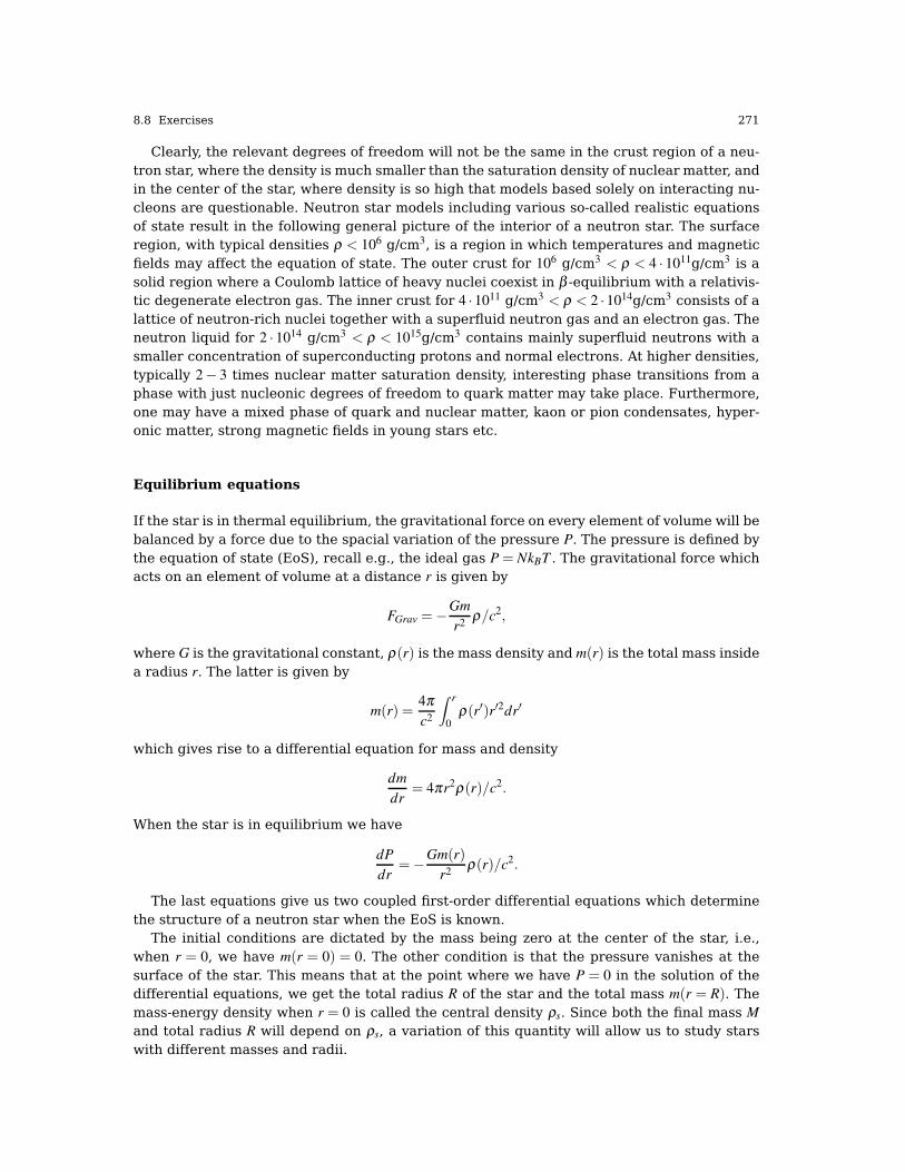
8.8 Exercises 271
Clearly, the relevant degrees of freedom will not be the same in the crust region of a neu-tron star, where the density is much smaller than the saturation density of nuclear matter, andin the center of the star, where density is so high that models based solely on interacting nu-cleons are questionable. Neutron star models including various so-called realistic equationsof state result in the following general picture of the interior of a neutron star. The surfaceregion, with typical densities ρ < 106 g/cm3, is a region in which temperatures and magneticfields may affect the equation of state. The outer crust for 106 g/cm3 < ρ < 4 · 1011g/cm3 is asolid region where a Coulomb lattice of heavy nuclei coexist in β -equilibrium with a relativis-tic degenerate electron gas. The inner crust for 4 ·1011 g/cm3 < ρ < 2 ·1014g/cm3 consists of alattice of neutron-rich nuclei together with a superfluid neutron gas and an electron gas. Theneutron liquid for 2 · 1014 g/cm3 < ρ < 1015g/cm3 contains mainly superfluid neutrons with asmaller concentration of superconducting protons and normal electrons. At higher densities,typically 2− 3 times nuclear matter saturation density, interesting phase transitions from aphase with just nucleonic degrees of freedom to quark matter may take place. Furthermore,one may have a mixed phase of quark and nuclear matter, kaon or pion condensates, hyper-onic matter, strong magnetic fields in young stars etc.
Equilibrium equations
If the star is in thermal equilibrium, the gravitational force on every element of volume will bebalanced by a force due to the spacial variation of the pressure P. The pressure is defined bythe equation of state (EoS), recall e.g., the ideal gas P = NkBT . The gravitational force whichacts on an element of volume at a distance r is given by
FGrav =−Gm
r2ρ/c2,
where G is the gravitational constant, ρ(r) is the mass density and m(r) is the total mass insidea radius r. The latter is given by
m(r) =4π
c2
∫ r
0ρ(r′)r′2dr′
which gives rise to a differential equation for mass and density
dm
dr= 4πr2ρ(r)/c2.
When the star is in equilibrium we have
dP
dr=−Gm(r)
r2ρ(r)/c2.
The last equations give us two coupled first-order differential equations which determinethe structure of a neutron star when the EoS is known.
The initial conditions are dictated by the mass being zero at the center of the star, i.e.,when r = 0, we have m(r = 0) = 0. The other condition is that the pressure vanishes at thesurface of the star. This means that at the point where we have P = 0 in the solution of thedifferential equations, we get the total radius R of the star and the total mass m(r = R). Themass-energy density when r = 0 is called the central density ρs. Since both the final mass M
and total radius R will depend on ρs, a variation of this quantity will allow us to study starswith different masses and radii.

272 8 Differential equations
Dimensionless equations
When we now attempt the numerical solution, we need however to rescale the equations sothat we deal with dimensionless quantities only. To understand why, consider the value of thegravitational constant G and the possible final mass m(r = R) = MR. The latter is normally ofthe order of some solar masses M⊙, with M⊙= 1.989×1030 Kg. If we wish to translate the latterinto units of MeV/c2, we will have that MR ∼ 1060 MeV/c2. The gravitational constant is in unitsof G = 6.67×10−45× hc (MeV/c2)−2. It is then easy to see that including the relevant values forthese quantities in our equations will most likely yield large numerical roundoff errors whenwe add a huge number dP
drto a smaller number P in order to obtain the new pressure. We list
here the units of the various quantities and in case of physical constants, also their values. Abracketed symbol like [P] stands for the unit of the quantity inside the brackets.
Quantity Units
[P] MeVfm−3
[ρ ] MeVfm−3
[n] fm−3
[m] MeVc−2
M⊙ 1.989×1030 Kg= 1.1157467×1060 MeVc−2
1 Kg = 1030/1.78266270D0 MeVc−2
[r] mG hc6.67259×10−45 MeV−2c−4
hc 197.327 MeVfm
r = r/R0, mass-energy density ρ = ρ/ρs, pressure P = P/ρs and mass m = m/M0.The constants M0 and R0 can be determined from the requirements that the equations for
dmdr
and dPdr
should be dimensionless. This gives
dM0m
dR0r= 4πR2
0r2ρsρ ,
yieldingdm
dr= 4πR3
0r2ρsρ/M0.
If these equations should be dimensionless we must demand that
4πR30ρs/M0 = 1.
Correspondingly, we have for the pressure equation
dρsP
dR0r=−GM0
mρsρ
R20r2
and since this equation should also be dimensionless, we will have
GM0/R0 = 1.
This means that the constants R0 and M0 which will render the equations dimensionless aregiven by
R0 =1√
ρsG4π,

8.8 Exercises 273
and
M0 =4πρs
(√
ρsG4π)3.
However, since we would like to have the radius expressed in units of 10 km, we shouldmultiply R0 by 10−19, since 1 fm = 10−15 m. Similarly, M0 will come in units of MeV/c2, and itis convenient therefore to divide it by the mass of the sun and express the total mass in termsof solar masses M⊙.
The differential equations read then
dP
dr=− mρ
r2,
dm
dr= r2ρ .
In the solution of our problem, we will assume that the mass-energy density is given bya simple parametrization from Bethe and Johnson [49]. This parametrization gives ρ as afunction of the number density n = N/V , with N the total number of baryons in a volume V . Itreads
ρ(n) = 236× n2.54+ nmn, (8.20)
where mn = 938.926MeV/c2, the mass of the neutron (averaged). This means that since[n] =fm−3, we have that the dimension of ρ is [ρ ] =MeV/c2fm−3. Through the thermodynamicrelation
P =−∂E
∂V, (8.21)
where E is the energy in units of MeV/c2 we have
P(n) = n∂ρ(n)
∂n−ρ(n) = 363.44× n2.54.
We see that the dimension of pressure is the same as that of the mass-energy density, i.e.,[P] =MeV/c2fm−3.
Here comes an important point you should observe when solving the two coupled first-order differential equations. When you obtain the new pressure given by
Pnew =dP
dr+Pold,
this comes as a function of r. However, having obtained the new pressure, you will need touse Eq. (8.1) in order to find the number density n. This will in turn allow you to find the newvalue of the mass-energy density ρ(n) at the relevant value of r.
In solving the differential equations for neutron star equilibrium, you should proceed asfollows
1. Make first a dimensional analysis in order to be sure that all equations are really dimen-sionless.
2. Define the constants R0 and M0 in units of 10 km and solar mass M⊙. Find their values.Explain why it is convenient to insert these constants in the final results and not at eachintermediate step.
3. Set up the algorithm for solving these equations and write a main program where thevarious variables are defined.
4. Write thereafter a small function which uses the expressions for pressure and mass-energydensity from Eqs. (8.1) and (8.20).
5. Write then a function which sets up the derivatives
− mρ
r2, r2ρ.

274 8 Differential equations
6. Employ now the fourth order Runge-Kutta algorithm to obtain new values for the pressureand the mass. Play around with different values for the step size and compare the resultsfor mass and radius.
7. Replace the fourth order Runge-Kutta method with the simple Euler method and comparethe results.
8. Replace the non-relativistic expression for the derivative of the pressure with that fromGeneral Relativity (GR), the so-called Tolman-Oppenheimer-Volkov equation
dP
dr=− (P+ ρ)(r3P+ m)
r2− 2mr,
and solve again the two differential equations.9. Compare the non-relatistic and the GR results by plotting mass and radius as functions of
the central density.
8.2.
mld2θ
dt2+mgsin(θ ) = 0,
with an angular velocity and acceleration given by
v = ldθ
dt,
and
a = ld2θ
dt2.
We do however expect that the motion will gradually come to an end due a viscous dragtorque acting on the pendulum. In the presence of the drag, the above equation becomes
mld2θ
dt2+ν
dθ
dt+mgsin(θ ) = 0, (8.22)
where ν is now a positive constant parameterizing the viscosity of the medium in question.In order to maintain the motion against viscosity, it is necessary to add some external drivingforce. We choose here a periodic driving force. The last equation becomes then
mld2θ
dt2+ν
dθ
dt+mgsin(θ ) = Asin(ωt), (8.23)
with A and ω two constants representing the amplitude and the angular frequency respec-tively. The latter is called the driving frequency.
1. Rewrite Eqs. (8.22) and (8.23) as dimensionless equations.2. Write then a code which solves Eq. (8.22) using the fourth-order Runge Kutta method.
Perform calculations for at least ten periods with N = 100, N = 1000 and N = 10000 meshpoints and values of ν = 1, ν = 5 and ν = 10. Set l = 1.0 m, g= 1 m/s2 and m = 1 kg. Choose asinitial conditions θ (0) = 0.2 (radians) and v(0) = 0 (radians/s). Make plots of θ (in radians)as function of time and phase space plots of θ versus the velocity v. Check the stability ofyour results as functions of time and number of mesh points. Which case corresponds todamped, underdamped and overdamped oscillatory motion? Comment your results.
3. Now we switch to Eq. (8.23) for the rest of the project. Add an external driving force andset l = g = 1, m = 1, ν = 1/2 and ω = 2/3. Choose as initial conditions θ (0) = 0.2 and v(0) = 0
and A = 0.5 and A = 1.2. Make plots of θ (in radians) as function of time for at least 300periods and phase space plots of θ versus the velocity v. Choose an appropriate time step.Comment and explain the results for the different values of A.

8.8 Exercises 275
4. Keep now the constants from the previous exercise fixed but set now A = 1.35, A = 1.44 andA = 1.465. Plot θ (in radians) as function of time for at least 300 periods for these values ofA and comment your results.
5. We want to analyse further these results by making phase space plots of θ versus thevelocity v using only the points where we have ωt = 2nπ where n is an integer. These arenormally called the drive periods. This is an example of what is called a Poincare sectionand is a very useful way to plot and analyze the behavior of a dynamical system. Commentyour results.
8.3. We assume that the orbit of Earth around the Sun is co-planar, and we take this to be thexy-plane. Using Newton’s second law of motion we get the following equations
d2x
dt2=
FG,x
MEarth
,
andd2y
dt2=
FG,y
MEarth
,
where FG,x and FG,y are the x and y components of the gravitational force.
a) Rewrite the above second-order ordinary differential equations as a set of coupled first or-der differential equations. Write also these equations in terms of dimensionless variables.As an alternative to the usage of dimensionless variables, you could also use so-calledastronomical units (AU as abbreviation). If you choose the latter set of units, one astro-nomical unit of length, known as 1 AU, is the average distance between the Sun and Earth,that is 1 AU = 1.5× 10¹¹ m. It can also be convenient to use years instead of secondssince years match better the solar system. The mass of the Sun is Msun = M⊙ = 2× 1030
kg. The mass of Earth is MEarth = 6× 1024 kg. The mass of other planets like Jupiter isMJupiter = 1.9× 1027 kg and its distance to the Sun is 5.20 AU. Similar numbers for Mars areMMars = 6.6× 10²³ kg and 1.52 AU, for Venus MVenus = 4.9× 1024 kg and 0.72 AU, for Saturnare MSaturn = 5.5× 1026 kg and 9.54 AU, for Mercury are MMercury = 2.4× 10²³ kg and 0.39AU, for Uranus are MUranus = 8.8×1025 kg and 19.19 AU, for Neptun are MNeptun = 1.03×1026
kg and 30.06 AU and for Pluto are MPluto = 1.31× 10²² kg and 39.53 AU. Pluto is no longerconsidered a planet, but we add it here for historical reasons.Finally, mass units can be obtained by using the fact that Earth’s orbit is almost circu-lar around the Sun. For circular motion we know that the force must obey the followingrelation
FG =MEarthv2
r=
GM⊙MEarth
r2,
where v is the velocity of Earth. The latter equation can be used to show that
v2r = GM⊙ = 4π2AU3/yr2.
Discretize the above differential equations and set up an algorithm for solving these equa-tions using the so-called Euler-Cromer.
b) Write then a program which solves the above differential equations for the Earth-Sun sys-tem using the Euler-Cromer method. Find out which initial value for the velocity that givesa circular orbit and test the stability of your algorithm as function of different time steps∆ t. Find a possible maximum value ∆ t for which the Euler-Cromer method does not yieldstable results. Make a plot of the results you obtain for the position of Earth (plot the x andy values) orbiting the Sun.

276 8 Differential equations
Check also for the case of a circular orbit that both the kinetic and the potential energiesare constants. Check also that the angular momentum is a constant. Explain why thesequantities are conserved.
c) Modify your code by implementing the fourth-order Runge-Kutta method and compare thestability of your results by repeating the steps in b). Compare the stability of the twomethods, in particular as functions of the needed step length ∆ t. Comment your results.
d) Kepler’s second law states that the line joining a planet to the Sun sweeps out equal areasin equal times. Modify your code so that you can verify Kepler’s second law for the case ofan elliptical orbit. Compare both the Runge-Kutta method and the Euler-Cromer methodand check that the total energy and angular momentum are conserved. Why are thesequantities conserved? A convenient choice of starting values are an initial position of 1 AUand an initial velocity of 5 AU/yr.
e) Consider then a planet which begins at a distance of 1 AU from the sun. Find out by trialand error what the initial velocity must be in order for the planet to escape from the sun.Can you find an exact answer?
f) We will now study the three-body problem, still with the Sun kept fixed at the centerbut including Jupiter (the most massive planet in the solar system, having a mass thatis approximately 1000 times smaller than that of the Sun) together with Earth. This leadsus to a three-body problem. Without Jupiter, Earth’s motion is stable and unchanging withtime. The aim here is to find out how much Jupiter alters Earth’s motion.The program you have developed can easily be modified by simply adding the magnitudeof the force betweem Earth and Jupiter.This force is given again by
FEarth−Jupiter =GMJupiterMEarth
r2Earth−Jupiter
,
where MJupiter is the mass of the sun and MEarth is the mass of Earth. The gravitationalconstant is G and rEarth−Jupiter is the distance between Earth and Jupiter.We assume again that the orbits of the two planets are co-planar, and we take this to bethe xy-plane. Modify your first-order differential equations in order to accomodate both themotion of Earth and Jupiter by taking into account the distance in x and y between Earthand Jupiter. Set up the algorithm and plot the positions of Earth and Jupiter using thefourth-order Runge-Kutta method. Include an adaptive solver to your Runge-Kutta method,using for example the adaptive scheme proposed by Fehlberg.Discuss the stability of the solutions using the standard Runge-Kutta4 solver and the adap-tive scheme.Repeat the calculations by increasing the mass of Jupiter by a factor of 10 and 1000 andplot the position of Earth. Study again the stability of the standard and the adaptive Runge-Kutta solvers.
g) Finally, using your optimal Runge-Kutta solver, we carry out a real three-body calculationwhere all three systems, Earth, Jupiter and the Sun are in motion. To do this, choose thecenter-of-mass position of the three-body system as the origin rather than the position ofthe sun. Give the sun an initial velocity which makes the total momentum of the system ex-actly zero (the center-of-mass will remain fixed). Compare these results with those from theprevious exercise and comment your results. Extend your program to include all planetsin the solar system (if you have time, you can also include the various moons, but it is notrequired) and discuss your results. Try to find data for the initial positions and velocitiesfor all planets.
h) The perihelion precession of Mercury. This part is optional but gives you an additional 30%on the final score!An important test of the general theory of relativity was comparing its prediction for theperihelion precession of Mercury to the observed value. The observed value of the peri-

8.8 Exercises 277
helion precession, when all classical effects (such as the perturbation of the orbit due togravitational attraction from the other planets) are subtracted, is 43′′ (43 arc seconds) percentury.Closed elliptical orbits are a special feature of the Newtonian 1/r2 force. In general, anycorrection to the pure 1/r2 behaviour will lead to an orbit which is not closed, i.e. afterone complete orbit around the Sun, the planet will not be at exactly the same position as itstarted. If the correction is small, then each orbit around the Sun will be almost the sameas the classical ellipse, and the orbit can be thought of as an ellipse whose orientation inspace slowly rotates. In other words, the perihelion of the ellipse slowly precesses aroundthe Sun.You will now study the orbit of Mercury around the Sun, adding a general relativisticcorrection to the Newtonian gravitational force, so that the force becomes
FG =GMSunMMercury
r2
[1+
3l2
r2c2
]
where MMercury is the mass of Mercury, r is the distance between Mercury and the Sun,l = |r× v| is the magnitude of Mercury’s orbital angular momentum per unit mass, and c isthe speed of light in vacuum. Run a simulation over one century of Mercury’s orbit aroundthe Sun with no other planets present, starting with Mercury at perihelion on the x axis.Check then the value of the perihelion angle θp, using
tanθp =yp
xp
where xp (yp) is the x (y) position of Mercury at perihelion, i.e. at the point where Mercury isat its closest to the Sun. You may use that the speed of Mercury at perihelion is 12.44AU/yr,and that the distance to the Sun at perihelion is 0.3075AU. You need to make sure that thetime resolution used in your simulation is sufficient, for example by checking that theperihelion precession you get with a pure Newtonian force is at least a few orders ofmagnitude smaller than the observed perihelion precession of Mercury. Can the observedperihelion precession of Mercury be explained by the general theory of relativity?
8.4. In this exercise we will implement a molecular dynamics (MD) code to model the be-havior of a system of Argon atoms, and use this model to study statistical properties of thesystem. In all calculations, we will use so-called MD units. These assume that all the particlesin a simulation are identical, so the masses and LJ parameters can be factored out of theequations. You will need to insert A = AA0 for every variable quantity A in equations 8.25-8.30above. For example, for velocity, v = v
L0t0. The time step ∆ t must also be treated this way.
Quantity Conversion factor ValueLength L0 = σ 3.405 Å
Time t0 = σ√
m/ε 2.1569 ·103 fsForce F0 = mσ/t2
0 = ε/σ 3.0303 ·10−1 eV/ÅEnergy E0 = ε 1.0318 ·10−2 eV
Temperature T0 = ε/kB 119.74 K
Table 8.1 Conversion factors A0 from MD units for variable quantities.
In case you want to convert between your internal MD units and other units during inputand output, the actual values of the conversion factors are listed in table 8.1. These arecalculated using the argon mass, lattice constant and LJ parameters: m= 39.948 amu, a= 5.260

278 8 Differential equations
Å (solid argon), σ = 3.405 Å, ε = 1.0318 ·10−2 eV. Another common practice is putting E0 = 4ε,affecting the conversion factors F0, T0 and t0.
Normally distributed random numbers are obtained by performing a Box-Muller transformon uniformly distributed numbers. Let u and v be uniform numbers in the interval (−1,1).These numbers will only be accepted for the transformation if s = u2 + v2 is in the interval(0,1). In that case, we obtain two normally distributed numbers n1 and n2 by multiplying u
and v with a constant,
n1 = Su, n2 = Sv, S =
√− lns
s. (8.24)
n1 and n2 will have standard deviations of 1, but multiplying all generated numbers with aconstant will give a distribution with that constant as the standard deviation.
a) Write a program that generates an Nc×Nc×Nc unit cell face centered cubic lattice of argonatoms. If you use an object oriented programming language, each atom and/or the entirelattice should be objects of a class.For easy testing of the lattice arranger and the later MD implementation, you should al-ready visualize your atoms. VMD is a visualization program with a simple output formatand pretty graphics. It can be downloaded and run from your home area, and a descriptionof its output format can be found in the appendix.
b) Consider first free particles with initial independent Maxwell-Boltzmann distributed veloc-ities. These correspond to normally distributed values with standard deviation
√kBT/m for
the desired temperature T . In a system of N atoms, all 3N velocity components v are setusing
v =√
kBT/mξ (8.25)
where ξ is a normally distributed number with mean 0 and standard deviation 1. Removeany initial total linear momentum from the system.Integrate the dynamical equation (N2L) using the symplectic and numerically stable veloc-ity Verlet algorithm. For each particle i, the steps are as follows (currently setting Ui = 0):
vi(t +∆ t/2) = vi(t)+Fi(t)
2m∆ t (8.26)
ri(t +∆ t) = ri(t)+ vi(t +∆ t/2)∆ t (8.27)
Fi(t +∆ t) =−∇iUi(r(t +∆ t)) (8.28)
vi(t +∆ t) = vi(t +∆ t/2)+Fi(t +∆ t)
2m∆ t (8.29)
The particles will now spread out into space. We are only interested in bulk atoms in amaterial, so the next step is implementing periodic boundary conditions. Every time theposition of a particle is updated, the program must check if it has gone though one of thesides.
c) Create a function for calculating the force between all particles. Use the Lennard-Jonespotential, which has the following form:
Ui j(ri j) = 4ε
[(σ
ri j
)12
−(
σ
ri j
)6]
(8.30)
where ri j = ri− r j. Differentiate the expression analytically for finding the force. Summingup the potential energy between all particles can also be useful.Use the minimum image convention when calculating the distance between particles. E.g.the distance between atoms/atom replicae i and j in the x direction becomes minδ (xi− x j + δL)
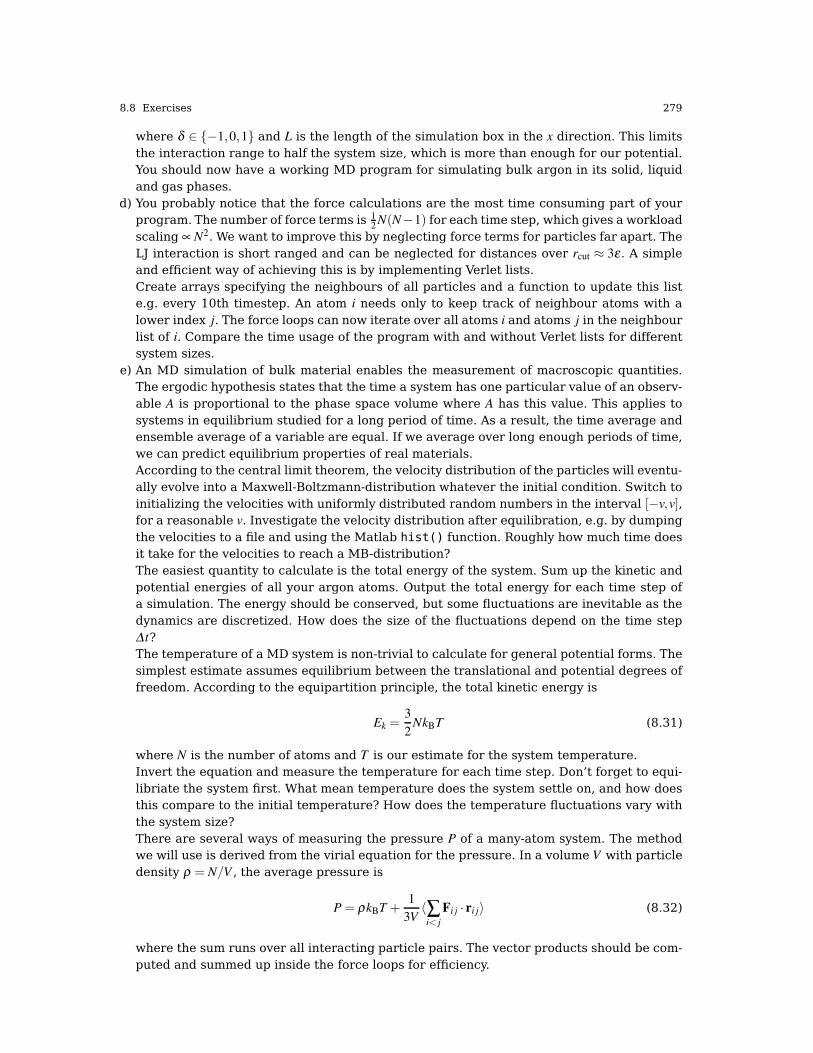
8.8 Exercises 279
where δ ∈ −1,0,1 and L is the length of the simulation box in the x direction. This limitsthe interaction range to half the system size, which is more than enough for our potential.You should now have a working MD program for simulating bulk argon in its solid, liquidand gas phases.
d) You probably notice that the force calculations are the most time consuming part of yourprogram. The number of force terms is 1
2N(N−1) for each time step, which gives a workload
scaling ∝ N2. We want to improve this by neglecting force terms for particles far apart. TheLJ interaction is short ranged and can be neglected for distances over rcut ≈ 3ε. A simpleand efficient way of achieving this is by implementing Verlet lists.Create arrays specifying the neighbours of all particles and a function to update this liste.g. every 10th timestep. An atom i needs only to keep track of neighbour atoms with alower index j. The force loops can now iterate over all atoms i and atoms j in the neighbourlist of i. Compare the time usage of the program with and without Verlet lists for differentsystem sizes.
e) An MD simulation of bulk material enables the measurement of macroscopic quantities.The ergodic hypothesis states that the time a system has one particular value of an observ-able A is proportional to the phase space volume where A has this value. This applies tosystems in equilibrium studied for a long period of time. As a result, the time average andensemble average of a variable are equal. If we average over long enough periods of time,we can predict equilibrium properties of real materials.According to the central limit theorem, the velocity distribution of the particles will eventu-ally evolve into a Maxwell-Boltzmann-distribution whatever the initial condition. Switch toinitializing the velocities with uniformly distributed random numbers in the interval [−v,v],for a reasonable v. Investigate the velocity distribution after equilibration, e.g. by dumpingthe velocities to a file and using the Matlab hist() function. Roughly how much time doesit take for the velocities to reach a MB-distribution?The easiest quantity to calculate is the total energy of the system. Sum up the kinetic andpotential energies of all your argon atoms. Output the total energy for each time step ofa simulation. The energy should be conserved, but some fluctuations are inevitable as thedynamics are discretized. How does the size of the fluctuations depend on the time step∆ t?The temperature of a MD system is non-trivial to calculate for general potential forms. Thesimplest estimate assumes equilibrium between the translational and potential degrees offreedom. According to the equipartition principle, the total kinetic energy is
Ek =3
2NkBT (8.31)
where N is the number of atoms and T is our estimate for the system temperature.Invert the equation and measure the temperature for each time step. Don’t forget to equi-libriate the system first. What mean temperature does the system settle on, and how doesthis compare to the initial temperature? How does the temperature fluctuations vary withthe system size?There are several ways of measuring the pressure P of a many-atom system. The methodwe will use is derived from the virial equation for the pressure. In a volume V with particledensity ρ = N/V , the average pressure is
P = ρkBT +1
3V〈∑
i< j
Fi j · ri j〉 (8.32)
where the sum runs over all interacting particle pairs. The vector products should be com-puted and summed up inside the force loops for efficiency.
280 8 Differential equations
f) In order to simulate the canonical ensemble, interactions with an external heat bath mustbe taken into account. Many methods have been suggested in order to achieve this, allwith their pros and cons. Requirements for a good thermostat are:
• Keeping the system temperature around the heat bath temperature• Sampling the phase space corresponding to the canonical ensemble• Tunability• Preservation of dynamics
The method closest to fullfilling these requirements which is in widespread use is the Nosé-Hoover thermostat, which is somewhat complicated to implement. We will focus on simplermethods. They will require negligble CPU time and should be applied for each time step.Many thermostats work by rescaling the velocities of all atoms by multiplying them with afactor γ. The Berendsen thermostat uses
γ =
√1+
∆ t
τ
(Tbath
T− 1
)(8.33)
with τ as the relaxation time, tuning the coupling to the heat bath. Though it satisfiesFouriers law of heat transfer (the transfered heat between two bodies is proportional totheir temperature difference) it does a poor job at sampling the canonical ensemble.Implement the Berendsen thermostat as a function in your code. τ = ∆ t will keep the (esti-mated) temperature exactly constant. It should be put to 10-20 times this value.The Andersen thermostat simulates (hard) collisions between atoms inside the system andin the heat bath. Atoms which collide will gain a new normally distributed velocity withstandard deviation
√kBTbath/m. For all atoms, a random uniformly distributed number in
the interval [0,1] is generated. If this number is less than ∆ tτ , the atom is assigned a new
velocity. In this case, τ is treated as a collision time, and should have about the samevalue as the τ in the Berendsen thermostat. The Andersen thermostat is very useful whenequilibrating systems, but disturbs the dynamics of e.g. lattice vibrations.Implement the Andersen thermostat, and compare T (t) graphs for simulations using thedifferent methods. Again, be aware that our T is just an approximation to the real temper-ature. Differences can also be seen in the dynamics.
g) In a volume with PBC and atoms consituting a fluid, self-diffusion can be simulated. We areto measure the self-diffusion constant D for liquid argon. This is achieved by finding themean square displacement of all atoms after a given time,
〈r2(t)〉= 1
N
N
∑i=1
(r(t)− rinitial). (8.34)
From diffusion theory, we know that 〈r2(t)〉 = 6Dt for a random walk in three dimensions,which is a good approximation to the motion of an atom in a fluid. Plot the mean squaredisplacement as a function of time and extract the diffusion constant. Investigate the effectof temperature by finding D for some temperatures in the liquid phase of argon. Rememberthat you are measuring the total distance travelled by the atoms, which must be continouswhen an atom is displaced though a PBC boundary.
h) A radial distribution function g(r), also called a pair correlation function, is a tool for char-acterizing the microscopic structure of a fluid. It is interpreted as the radial probability forfinding another atom a distance r from an arbitrary atom, or equivalently, the atomic den-sity in a spherical shell of radius r around an atom. It is commonly normalized by dividingit with the average particle density so that limr→∞ g(r) = 1.

8.8 Exercises 281
Estimate g(r) for r ∈ (0, L2] in your argon system. The easiest way is to divide the distance
interval into bins, loop over all pairs of particles and count how many distances belong ineach bin. Time-averaging the function gives a better description of the system’s generalbehaviour. Plot g(r) for temperatures where the system is in solid and liquid phases. Doesit appear as expected? How would the exact g(r) look for a perfect crystal?


Chapter 9
Two point boundary value problems
Abstract When differential equations are required to satisfy boundary conditions at morethan one value of the independent variable, the resulting problem is called a boundary valueproblem. The most common case by far is when boundary conditions are supposed to be satis-fied at two points - usually the starting and ending values of the integration. The Schrödingerequation is an important example of such a case. Here the eigenfunctions are typically re-stricted to be finite everywhere (in particular at r = 0) and for bound states the functionsmust go to zero at infinity.
9.1 Introduction
In the previous chapter we discussed the solution of differential equations determined byconditions imposed at one point only, the so-called initial condition. Here we move on todifferential equations where the solution is required to satisfy conditions at more than onepoint. Typically these are the endpoints of the interval under consideration. When discussingdifferential equations with boundary conditions, there are three main groups of numericalmethods, shooting methods, finite difference and finite element methods. In this chapter wefocus on the so-called shooting method, whereas chapters 7 and 10 focus on finite differencemethods. Chapter 7 solves the finite difference problem as an eigenvalue problem for a onevariable differential equation while in chapter 10 we present the simplest finite differencemethods for solving partial differential equations with more than one variable. The finiteelement method is not discussed in this text, see for example Ref. [50] for a computationalpresentation of the finite element method.
In the discussion here we will limit ourselves to the simplest possible case, that of a lin-ear second-order differential equation whose solution is specified at two distinct points, formore complicated systems and equations see for example Refs. [51, 52]. The reader shouldalso note that the techniques discussed in this chapter are restricted to ordinary differen-tial equations only, while finite difference and finite element methods can also be appliedto boundary value problems for partial differential equations. The discussion in this chapterand chapter 7 serves therefore as an intermediate step and model to the chapter on par-tial differential equations. Partial differential equations involve both boundary conditions anddifferential equations with functions depending on more than one variable.
In this chapter we will discuss in particular the solution of the one-particle Schödingerequation and apply the method to hydrogen-atom like problems. We start however with afamiliar problem from mechanics, namely that of a tightly stretched and flexible string orrope, fixed at the endpoints. This problem has an analytic solution which allows us to defineour numerical algorithms based on the shooting methods.
283

284 9 Two point boundary value problems
9.2 Shooting methods
In many physics applications we encounter differential equations like
d2y
dx2+ k2(x)y = F(x); a≤ x≤ b, (9.1)
with boundary conditionsy(a) = α, y(b) = β . (9.2)
We can interpret F(x) as an inhomogenous driving force while k(x) is a real function. If it ispositive the solutions y(x) will be oscillatory functions, and if negative they are exponention-ally growing or decaying functions.
To solve this equation we could start with for example the Runge-Kutta method or variousimprovements to Euler’s method, as discussed in the previous chapter. Then we would need totransform this equation to a set of coupled first-order equations. We could however start withthe discretized version for the second derivative. We discretise our equation and introducea step length h = (b− a)/N, with N being the number of equally spaced mesh points. Ourdiscretised second derivative reads at a step xi = a+ ih with i = 0,1, . . .
y′′i =yi+1 + yi−1− 2yi
h2+O(h2),
leading to a discretised differential equation
yi+1 + yi−1− 2yi
h2+O(h2)+ k2
i yi = Fi.
Recall that the fourth-order Runge-Kutta method has a local error of O(h4).Since we want to integrate our equation from x0 = a to xN = b, we rewrite it as
yi+1 ≈−yi−1 + yi
(2− h2k2
i + h2Fi
). (9.3)
Starting at i = 1 we have after one step
y2 ≈−y0 + y1
(2− h2k2
1 + h2F1
).
Irrespective of method to approximate the second derivative, this equation uncovers our firstproblem. While y0 = y(a) = 0, our function value y1 is unknown, unless we have an analyticexpression for y(x) at x = 0. Knowing y1 is equivalent to knowing y′ at x = 0 since the firstderivative is given by
y′i ≈yi+1− yi
h.
This means that we have y1 ≈ y0 + hy′0.
9.2.1 Improved approximation to the second derivative, Numerov’s
method
Before we proceed, we mention how to improve the local truncation error from O(h2) to O(h6)
without too many additional function evaluations.Our equation is a second order differential equation without any first order derivatives.
Let us also for the sake of simplicity assume that F(x) = 0. Numerov’s method is designed tosolve such an equation numerically, achieving a local truncation error O(h6).

9.2 Shooting methods 285
We start with the Taylor expansion of the desired solution
y(x+ h) = y(x)+ hy(1)(x)+h2
2!y(2)(x)+
h3
3!y(3)(x)+
h4
4!y(4)(x)+ · · ·
Here y(n)(x) is a shorthand notation for the nth derivative dny/dxn. Because the correspond-ing Taylor expansion of y(x− h) has odd powers of h appearing with negative signs, all oddpowers cancel when we add y(x+ h) and y(x− h)
y(x+ h)+ y(x− h)= 2y(x)+ h2y(2)(x)+h4
12y(4)(x)+O(h6).
We obtain
y(2)(x) =y(x+ h)+ y(x− h)− 2y(x)
h2− h2
12y(4)(x)+O(h6).
To eliminate the fourth-derivative term we apply the operator (1+ h2
12d2
dx2 ) on the differentialequation
y(2)(x)+h2
12y(4)(x)+ k2(x)y(x)+
h2
12
d2
dx2
(k2(x)y(x)
)≈ 0.
In this expression the y(4) terms cancel. To treat the general x dependence of k2(x) weapproximate the second derivative of (k2(x)y(x) by
d2(k2y(x))
dx2≈(k2(x+ h)y(x+ h)+ k2(x)y(x)
)+(k2(x− h)y(x− h)+ k2(x)y(x)
)
h2.
We replace then y(x+ h) with the shorthand yi+1 (and similarly for the other variables) andobtain a final discretised algorithm for obtaining yi+1
yi+1 =2(1− 5
12h2k2
i
)yi−
(1+ 1
12h2k2
i−1
)yi−1
1+ h2
12k2
i+1
+O(h6),
where xi = ih, ki = k(xi = ih) and yi = y(xi = ih) etc.It is easy to add the term Fi since we need only to take the second derivative. The final
algorithm reads then
yi+1 =2(1− 5
12h2k2
i
)yi−
(1+ 1
12h2k2
i−1
)yi−1
1+ h2
12k2
i+1
+h2
12(Fi+1 +Fi−1− 2Fi)+O(h6).
Starting at i = 1 results in, using the boundary condition y0 = 0,
y2 =2(1− 5
12h2k1y1
)−(1+ 1
12h2k2
0y0
)
1+ h2
12k2
2
+h2
12(F2 +F0− 2F1)+O(h6).
This equation carries a local truncation error proportional to h6. This is an order better thanthe fourth-order Runge-Kutta method which has a local error proportional to h5. The globalfor the fourth-order Runge-Kutta is proportional to h4 while Numerov’s method has an errorproportional to h5. With few additional function evulations, we have achieved an increasedaccuracy.
But even with an improved accuracy we end up with one unknown on the right hand side,namely y1. The value of y1 can again be determined from the derivative at y0, or by a goodguess on its value. We need therefore an additional constraint on our set of equations beforewe start. We could then add to the boundary conditions

286 9 Two point boundary value problems
y(a) = α, y(b) = β ,
the requirement y′(a) = δ , where δ could be an arbitrary constant. In quantum mechani-cal applications with homogenous differential equations the normalization of the solution isnormally not known. The choice of the constant δ can therefore reflect specific symmetryrequirements of the solution.
9.2.2 Wave equation with constant acceleration
We start with a well-known problem from mechanics, that of a whirling string or rope fixed atboth ends. We could think of this as an idealization of a jumping rope and ask questions aboutits shape as it spins. Obviously, in deriving the equations we will make several assumptionsin order to obtain an analytic solution. However, the general differential equation it leads to,with added complications not allowing an analytic solution, can be solved numerically. Wediscuss the shooting methods as one possible numerical approach in the next section.
Our aim is to arrive at a differential equation which takes the following form
y′′+λ y = 0; y(0) = 0, y(L) = 0,
where L is the length of the string and λ a constant or function of the variable x to be definedbelow.
We derive an equation for y(x) using Newton’s second law F = ma acting on a piece of thestring with mass ρ∆x, where ρ is the mass density per unit length and ∆x is small displace-ment in the interval x,x+∆x. The change ∆x is our step length.
We assume that the only force acting on this string element is a constant tension T actingon both ends. The net vertical force in the positive y-direction is
F = T sin(θ +∆θ )−Tsin(θ ) = Tsin(θi+1)−Tsin(θi).
For the angles we employ a finite difference approximation
sin(θi+1) =yi+1− yi
∆x+O(∆x2).
Using Newton’s second law F = ma, with m = ρ∆x = ρh and a constant angular velocity ω
which relates to the acceleration as a =−ω2y we arrive at
Tyi+1 + yi−1− 2yi
∆x2≈−ρω2y,
and taking the limit ∆x→ 0 we can rewrite the last equation as
Ty′′+ρω2y = 0,
and defining λ = ρω2/T and imposing the condition that the ends of the string are fixed wearrive at our final second-order differential equation with boundary conditions
y′′+λ y = 0; y(0) = 0, y(L) = 0.
The reader should note that we have assumed a constant acceleration. Replacing the constantacceleration with the second derivative of y as function of both position and time, we arriveat the well-known wave equation for y(x, t) in 1+ 1 dimension, namely

9.2 Shooting methods 287
∂ 2y
∂ t2= λ
∂ 2y
∂x2.
We discuss the solution of this equation in chapter 10.If λ > 0 the above wave equation has a solution of the form
y(x) = Acos(αx)+Bsin(αx),
and imposing the boundary conditions results in an infinite sequence of solutions of the form
yn(x) = sin(nπx
L), n = 1,2,3, . . .
with eigenvalues
λn =n2π2
L2, n = 1,2,3, . . .
For λ = 0 we havey(x) = Ax+B,
and due to the boundary conditions we have y(x) = 0, the trivial solution, which is not aneigenvalue of the problem. The classical problem has no negative eigenvalues, viz we cannotfind a solution for λ < 0. The trivial solution means that the string remains in its equilibriumposition with no deflection.
If we relate the constant angular speed ω to the eigenvalues λn we have
ωn =
√λnT
ρ=
nπ
L
√T
ρ, n = 1,2,3, . . . ,
resulting in a series of discretised critical speeds of angular rotation. Only at these criticalspeeds can the string change from its equilibrium position.
There is one important observation to made here, since later we will discuss Schrödinger’sequation. We observe that the eigenvalues and solutions exist only for certain discretisedvalues λn,yn(x). This is a consequence of the fact that we have imposed boundary conditions.Thus, the boundary conditions, which are a consequence of the physical case we wish toexplore, yield only a set of possible solutions. In quantum physics, we would say that theeigenvalues λn are quantized, which is just another word for discretised eigenvalues.
We have then an analytic solution
yn(x) = sin(nπx
L),
from
y′′+n2π2
L2y = 0; y(0) = 0, y(1) = 0.
Choosing n = 4 and L = 1, we have y(x) = sin(4πx) as our solution. The derivative is obviously4πcos(πx). We can start to integrate our equation using the exact expression for the derivativeat y1. This yields
y2 ≈−y0 + y1
(2− h2k2
1 + h)= 4hπcos(4πx0)
(2− 16h2π2
)= 4π
(2− 16h2π2
).
If we split our interval x∈ [0,1] into 10 equally spaced points we arrive at the results displayedin Table 9.1. We note that the error at the endpoint is much larger than the chosen mathemat-ical approximation O(h2), resulting in an error of approximately 0.01. We would have expecteda smaller error. We can obviously get better precision by increasing the number of integra-tion points, but it would not cure the increasing discrepancy we see towards the endpoints.

288 9 Two point boundary value problems
Table 9.1 Integrated and exact solution of the differential equation y′′ + λ y = 0 with boundary conditionsy(0) = 0 and y(1) = 0.
xi = ih sin(πxi) y(xi)
0.000000E+00 0.000000E+00 0.000000E+000.100000E+00 0.951057E+00 0.125664E+010.200000E+00 0.587785E+00 0.528872E+000.300000E+00 -.587785E+00 -.103405E+010.400000E+00 -.951056E+00 -.964068E+000.500000E+00 0.268472E-06 0.628314E+000.600000E+00 0.951057E+00 0.122850E+010.700000E+00 0.587785E+00 -.111283E+000.800000E+00 -.587786E+00 -.127534E+010.900000E+00 -.951056E+00 -.425460E+000.100000E+01 0.000000E+00 0.109628E+01
With N = 100, we have 0.829944E−02 at x = 1.0, while the error is ∼ 10−4 with 100 integrationpoints.
It is also important to notice that in general we do not know the eigenvalue and the eigen-functions, except some of their limiting behaviors close to the boundaries. One method forsearching for these eigenvalues is to set up an iterative process. We guess a trial eigenvalueand generate a solution by integrating the differential equation as an initial value problem,as we did above except that we have here the exact solution. If the resulting solution does notsatisfy the boundary conditions, we change the trial eigenvalue and integrate again. We re-peat this process until a trial eigenvalue satisfies the boundary conditions to within a chosennumerical error. This approach is what constitutes the so-called shooting method.
Upon integrating to our other boundary, x = 1 in the above example, we obtain normally anon-vanishing value for y(1), since the trial eigenvalue is normally not the correct one. We canthen readjust the guess for the eigenvalue and integrate and repeat this process till we obtaina value for y(1) which agrees to within the precision we have chosen. As we will show in thenext section, this results in a root-finding problem, which can be solved with for example thebisection or Newton methods discussed in chapter 4.
The example we studied here hides however an important problem. Our two solutions arerather similar, they are either represented by a sin(x) form or a cos(x) solution. This meansthat the solutions do not differ dramatically in behavior at the boundaries. Furthermore,the wave function is zero beyond the boundaries. For a quantum mechanical system, wewould get the same solutions if a particle is trapped in an infinitely high potential well. Thenthe wave function cannot exist outside the potential. However, for a finite potential well,there is always a quantum mechanical probability that the particle can be found outside theclassical region. The classical region defines the so-called turning points, viz points fromwhere a classical solution cannot exist. These turning points are useful when we want tosolve quantum mechanical problems.
Let us however perform our brute force integration for another differential equation aswell, namely that of the quantum mechanical harmonic oscillator.
The situation worsens dramatically now. We have then a one-dimensional differentialequation of the type, see Eq. (14.6), (all physical costants are set equal to one, that ism = c = h = k = 1)
−1
2
d2y
dx2+
1
2x2y = εy; −∞ < x < ∞,
with boundary conditions y(−∞)= y(∞)= 0. For the lowest lying state, the eigenvalue is ε = 1/2
and the eigenfunction is

9.2 Shooting methods 289
Table 9.2 Integrated and exact solution of the differential equation −y′′+ x2y = 2εy with boundary conditionsy(−∞) = 0 and y(∞) = 0.
xi = ih exp (−x2/2) y(xi)
-.100000E+02 0.192875E-21 0.192875E-21-.800000E+01 0.126642E-13 0.137620E-13-.600000E+01 0.152300E-07 0.157352E-07-.400000E+01 0.335462E-03 0.331824E-03-.200000E+01 0.135335E+00 0.128549E+000.000000E-00 0.100000E+01 0.912665E+000.200000E+01 0.135335E+00 0.118573E+000.400000E+01 0.335463E-03 -.165045E-010.600000E+01 0.152300E-07 -.250865E+030.800000E+01 0.126642E-13 -.231385E+090.900000E+01 0.257677E-17 -.101904E+13
y(x) =
(1
π
)1/4
exp(−x2/2).
The reader should observe that this solution is imposed by the boundary conditions, whichagain follow from the quantum mechanical properties we require for the solution. We repeatthe integration exercise which we did for the previous example, starting from a large negativenumber (x0 = −10, which gives a value for the eigenfunction close to zero) and choose thelowest energy and its corresponding eigenfunction. We obtain for y2
y2 ≈−y0 + y1
(2+ h2x2− h2
),
and using the exact eigenfunction we can replace y1 with the derivative at x0. We use nowN = 1000 and integrate our equation from x0 =−10 to xN = 10. The results are shown in Table9.2 for selected values of xi. In the beginning of our integrational interval, we obtain anintegrated quantity which resembles the analytic solution, but then our integrated solutionsimply explodes and diverges. What is happening? We started with the exact solution for boththe eigenvalue and the eigenfunction!
The problem is due to the fact that our differential equation has two possible solution foreigenvalues which are very close (−1/2 and +1/2), either
y(x)∼ exp(−x2/2),
ory(x)∼ exp(x2/2).
The boundary conditions, imposed by our physics requirements, rule out the last possibility.However, our algorithm, which is nothing but an approximation to the differential equationwe have chosen, picks up democratically both solutions. Thus, although we start with thecorrect solution, when integrating we pick up the undesired solution. In the next subsectionswe discuss how to cure this problem.
9.2.3 Schrödinger equation for spherical potentials
We discuss the numerical solution of the Schrödinger equation for the case of a particle withmass m moving in a spherical symmetric potential.
The initial eigenvalue equation reads

290 9 Two point boundary value problems
Hψ(r) = (T+ V)ψ(r) = Eψ(r). (9.4)
In detail this gives (− h2
2m∇2 +V(r)
)ψ(r) = Eψ(r). (9.5)
The eigenfunction in spherical coordinates takes the form
ψ(r) = R(r)Y ml (θ ,φ), (9.6)
and the radial part R(r) is a solution to
− h2
2m
(1
r2
d
drr2 d
dr− l(l + 1)
r2
)R(r)+V(r)R(r) = ER(r). (9.7)
Then we substitute R(r) = (1/r)u(r) and obtain
− h2
2m
d2
dr2u(r)+
(V (r)+
l(l + 1)
r2
h2
2m
)u(r) = Eu(r). (9.8)
We introduce a dimensionless variable ρ =(1/α)r where α is a constant with dimension lengthand get
− h2
2mα2
d2
dρ2u(ρ)+
(V (ρ)+
l(l + 1)
ρ2
h2
2mα2
)u(ρ) = Eu(ρ). (9.9)
In our case we are interested in attractive potentials
V (r) =−V0 f (r), (9.10)
where V0 > 0 and analyze bound states where E < 0. The final equation can be written as
d2
dρ2u(ρ)+ k(ρ)u(ρ) = 0, (9.11)
where
k(ρ) = γ
(f (ρ)− 1
γ
l(l + 1)
ρ2− ε
)
γ =2mα2V0
h2
ε =|E|V0
(9.12)
9.2.3.1 Schrödinger equation for a spherical box potential
Let us now specify the spherical symmetric potential to
f (r) =
1
−0for
r ≤ a
r > a(9.13)
and choose α = a. Then
k(ρ) = γ
1− ε− 1
γl(l+1)
ρ2
−ε−− 1γ
l(l+1)ρ2
forr ≤ a
r > a(9.14)

9.3 Numerical procedure, shooting and matching 291
The eigenfunctions in Eq. (9.5) are subject to conditions which limit the possible solutions.Of importance for the present example is that u(r) must be finite everywhere and
∫ |u(r)|2dτ
must be finite. The last condition means that rR(r) −→ 0 for r −→ ∞. These conditions implythat u(r) must be finite at r = 0 and u(r)−→ 0 for r −→ ∞.
9.2.3.2 Analysis of u(ρ) at ρ = 0
For small ρ Eq. (9.11) reduces to
d2
dρ2u(ρ)− l(l + 1)
ρ2u(ρ) = 0, (9.15)
with solutions u(ρ) = ρ l+1 or u(ρ) = ρ−l. Since the final solution must be finite everywhere weget the condition for our numerical solution
u(ρ) = ρ l+1 for small ρ (9.16)
9.2.3.3 Analysis of u(ρ) for ρ −→ ∞
For large ρ Eq. (9.11) reduces to
d2
dρ2u(ρ)− γεu(ρ) = 0 γ > 0, (9.17)
with solutions u(ρ) = exp(±γερ) and the condition for large ρ means that our numerical solu-tion must satisfy
u(ρ) = e−γερ for large ρ (9.18)
As for the harmonic oscillator, we have two solutions at the boundaries which are verydifferent and can easily lead to totally worng and even diverging solutions if we just integratefrom one endpoint to the other. In the next section we discuss how to solve such problems.
9.3 Numerical procedure, shooting and matching
The eigenvalue problem in Eq. (9.11) can be solved by the so-called shooting methods. Inorder to find a bound state we start integrating, with a trial negative value for the energy,from small values of the variable ρ , usually zero, and up to some large value of ρ . As longas the potential is significantly different from zero the function oscillates. Outside the rangeof the potential the function will approach an exponential form. If we have chosen a correcteigenvalue the function decreases exponentially as u(ρ) = e−γερ . However, due to numericalinaccuracy the solution will contain small admixtures of the undesireable exponential growingfunction u(ρ) = e+γερ . The final solution will then become unstable. Therefore, it is better togenerate two solutions, with one starting from small values of ρ and integrate outwards tosome matching point ρ = ρm. We call that function u<(ρ). The next solution u>(ρ) is thenobtained by integrating from some large value ρ where the potential is of no importance,and inwards to the same matching point ρm. Due to the quantum mechanical requirementsthe logarithmic derivative at the matching point ρm should be well defined. We obtain thefollowing condition

292 9 Two point boundary value problems
ddρ u<(ρ)
u<(ρ)=
ddρ u>(ρ)
u>(ρ)at ρ = ρm. (9.19)
We can modify this expression by normalizing the function u<u<(ρm) = Cu>u>(ρm). ThenEq. (9.19) becomes
d
dρu<(ρ) =
d
dρu>(ρ) at ρ = ρm (9.20)
For an arbitary value of the eigenvalue Eq. (9.19) will not be satisfied. Thus the numericalprocedure will be to iterate for different eigenvalues until Eq. (9.20) is satisfied.
We can calculate the first order derivatives by
d
dρu<(ρm)≈
u<(ρm)− u<(ρm− h)
h
d
dρu>(ρm)≈
u>(ρm)− u>(ρm + h)
h(9.21)
Thus the criterium for a proper eigenfunction will be
f = u>(ρm + h)− u<(ρm− h) = 0. (9.22)
9.3.1 Algorithm for solving Schrödinger’s equation
Here we outline the solution of Schrödinger’s equation as a common differential equation butwith boundary conditions. The method combines shooting and matching. The shooting partinvolves a guess on the exact eigenvalue. This trial value is then combined with a standardmethod for root searching, e.g., the secant or bisection methods discussed in chapter 4.
The algorithm could then take the following form
• Initialise the problem by choosing minimum and maximum values for the energy, Emin andEmax, the maximum number of iterations max_iter and the desired numerical precision.
• Search then for the roots of the function f , where the root(s) is(are) in the interval E ∈[Emin,Emax] using for example the bisection method. Newton’s method, also discussed inchapter 4 requires an analytic expression for f . A possible approach is to use the standardbisection method for localizing the eigenvalue and then use the secant method to obtain abetter estimate.The pseudocode for such an approach can be written as
do
i++;
e = (e_min+e_max)/2.; /* bisection */
if ( f(e)*f(e_max) > 0 )
e_max = e; /* change search interval */
else
e_min = e;
while ( (fabs(f(e) > convergence_test) !! (i <= max_iterations))
The use of a root-searching method forms the shooting part of the algorithm. We havehowever not yet specified the matching part.
• The matching part is given by the function f (e) which receives as argument the presentvalue of E. This function forms the core of the method and is based on an integrationof Schrödinger’s equation from ρ = 0 and ρ = ∞. If our choice of E satisfies Eq. (9.22)

9.3 Numerical procedure, shooting and matching 293
we have a solution. The matching code is given below. To choose the matching point itis convenient to start integrating inwards, that is from the large r-values. When the wavefunction turns, we use that point to define the matching point. The reason for this is that westart integrating from a region which corresponds normally to classically forbidden ones,and integrating into such regions leads normally to inaccurate solutions and the pick up ofthe undesired solutions. The consequence is that the solution diverges. We can thereforedefine as a matching point the classical turning point and start to integrate from larger-values. In the absence of such a point, we can use the point where the wave functionturns.
The function f (E) above receives as input a guess for the energy. In the version imple-mented below, we use the standard three-point formula for the second derivative, namely
f ′′0 ≈fh− 2 f0 + f−h
h2.
We leave it as an exercise to the reader to implement Numerov’s algorithm.
//
// The function
// f()
// calculates the wave function at fixed energy eigenvalue.
//
double f(double step, int max_step, double energy, double *w, double *wf)
int loop, loop_1,match;
double const sqrt_pi = 1.77245385091;
double fac, wwf, norm;
// adding the energy guess to the array containing the potential
for(loop = 0; loop <= max_step; loop ++)
w[loop] = (w[loop] - energy) * step * step + 2;
// integrating from large r-values
wf[max_step] = 0.0;
wf[max_step - 1] = 0.5 * step * step;
// search for matching point
for(loop = max_step - 2; loop > 0; loop--)
wf[loop] = wf[loop + 1] * w[loop + 1] - wf[loop + 2];
if(wf[loop] <= wf[loop + 1]) break;
match = loop + 1;
wwf = wf[match];
// start integrating up to matching point from r =0
wf[0] = 0.0;
wf[1] = 0.5 * step * step;
for(loop = 2; loop <= match; loop++)
wf[loop] = wf[loop -1] * w[loop - 1] - wf[loop - 2];
if(fabs(wf[loop]) > INFINITY)
for(loop_1 = 0; loop_1 <= loop; loop_1++)
wf[loop_1] /= INFINITY;
// now implement the test of Eq. (10.25)
return (wf[match-1]-wf[match+1]);
// End: funtion plot()
The approach we have described here suffers from the fact that the matching point is notproperly defined. Using a Green’s function approach we can easily determine the matching

294 9 Two point boundary value problems
point as the midpoint of the integration interval and compute safely the solution. This is thetopic of the next section.
9.4 Green’s function approach
A slightly different approach, which however still keeps the matching procedure discussedabove, is based on the computation of the Green’s function and its relation to the solution ofa differential equation with boundary values.
Consider the differential equation
− u(x)′′ = f (x), x ∈ (0,1), u(0) = u(1) = 0, (9.23)
and using the fundamental theorem of calculus, there is a constant c1 such that
u(x) = c1 +
∫ x
0u′(y)dy,
and a constant c2
u′(y) = c2 +
∫ y
0u′′(z)dz.
This is true for any twice continuously differentiable function u
If u satisfies the above differential equation we have then
u′(y) = c2−∫ y
0f (z)dz.
which inserted into the equation for u gives
u(x) = c1 + c2x−∫ x
0
(∫ y
0f (z)dz
)dy,
and defining
F(y) =
∫ y
0f (z)dz,
and performing an integration by parts we obtain
∫ x
0F(y)dy =
∫ x
0
(∫ y
0f (z)dz
)dy =
∫ x
0(x− y) f (y)dy.
This gives us
u(x) = c1 + c2x−∫ x
0(x− y) f (y)dy.
The boundary condition u(0) = 0 yields c1 = 0 and u(1) = 0, resulting in
c2 =
∫ 1
0(1− y) f (y)dy,
meaning that we can write the solution as
u(x) = x
∫ 1
0(1− y) f (y)dy−
∫ x
0(x− y) f (y)dy
The solution to our differential equation can be represented in a compact way using theso-called Green’s functions, which are also solutions to our differential equation with f (x) = 0.

9.4 Green’s function approach 295
If we then define the Green’s function as
G(x,y) =
y(1− x) if 0≤ y≤ x
x(1− y) if x≤ y≤ 1
we can write the solution as
u(x) =∫ 1
0G(x,y) f (y)dy,
The Green’s function, see for example Refs. [52,53] is
1. continuous2. it is symmetric in the sense that G(x,y) = G(y,x)
3. it has the properties G(0,y) = G(1,y) = G(x,0) = G(x,1) = 0
4. it is a piecewise linear function of x for fixed y and vice versa. G′ is discontinuos aty = x.
5. G(x,y)≥ 0 for all x,y ∈ [0,1]
6. it is the solution of the differential equation
d2
dx2G(x,y) =−δ (x− y).
The Green’s function can now be used to define the solution before and after a specificmatching point in the domain.
The Green’s function satisfies the homogeneous equation for y 6= x and its derivative isdiscontinuous at x = y. We can see this if we integrate the differential equation
d2
dx2G(x,y) =−δ (x− y)
from x = y− ε to x = y+ ε, with ε as an infinitesmally small number. We obtain then
dG
dx|x=y+ε −
dG
dx|x=y−ε = 1.
The problem is obvioulsy to find G.We can obtain this by considering two solutions of the homogenous equation. We choose a
general domain x ∈ [a,b] with a boundary condition on the general solution u(a) = u(b) = 0.One solution is obtained by integrating from a to b (called u<) and one by integrating
inward from b to a, labelled u>.Using the continuity requirement on the function and its derivative we can compute the
Wronskian [52,53]
W =du>
dxu<−
du<
dxu>,
and usingdG
dx|x=y+ε −
dG
dx|x=y−ε = 1,
and one can then show that the Green’s function reads
G(x,y) = u<(x<)u>(x>), (9.24)
where x< is defined for x = y− ε and x> = y+ ε. Using the definition of the Green’s function inEq. (9.24) we can now solve Eq. (9.23) for x ∈ [a,b] using
296 9 Two point boundary value problems
u(x) = u>(x)
∫ x
au<(x′) f (x′)dx′+ u<(x)
∫ b
xu>(x′) f (x′)dr′ (9.25)
The algorithm for solving Eq. (9.23) proceed now as follows: Your task is to choose a match-ing point, say the midpoint, and then compute the Greens’ function after you have used Nu-merov’s algo to find u (inward and outward integration for all points). Find u integrating withthe Green’s function.
A possible algorithm could be phrased as follows:
• Compute the solution of the homogeneous part of Eq. (9.23) using Numerov’s method.You should then have both the inward and the outward solutions.
• Compute the Wronskian at the matching point using
du
dx≈ u(x+ h)− u(x+ h)
2h,
for the first derivative and choose the matching point as the midpoint. You should trythe stability of the solution by choosing other matching points as well.
• Compute then the outward integral of the Green’s function approach, including theinhomogeneous term. For the integration one can employ for example Simpson’s rulediscussed in chapter 5.
• Compute thereafter the inward integral of the Green’s function approach. Addingthese two integrals gives the resulting wave function of Eq. (9.25).
An example of a code which performs all these steps is listed here
void wfn(Array<double,2> &k, Array<double,2> &ubasis, Array<double,1> &r, Array<double,2>
&F,Array<double,1> &uin, Array<double,1> &uout)
int loop, loop_1, midpoint, j;
double norm, wronskian, sum, term;
ubasis=0;uin=0;uout=0;
// Compute inwards homogenous solution
for(j=0;j<mat_size;j++)
uin(max_step) = 0.0;
uin(max_step-1) = 1.0E-10;
for(loop = max_step-2; loop >= 0; loop--)
uin(loop) = (2.0*(1.0-5.0*k(loop+1,j)/12.0)* uin(loop+1)- (1.0+k(loop+2,j)/12.0)*uin(loop+2))/(1.0+k(loop,j)/12.0);
// Compute outwards homogenous solution
uout(0) = 0.0;
uout(1) = 1.0E-10;
for(loop = 2; loop <= max_step; loop++)
uout(loop) = (2.0*(1.0-5.0*k(loop-1,j)/12.0)* uout(loop-1)-
(1.0+k(loop-2,j)/12.0)*uout(loop-2))/(1.0+k(loop,j)/12.0);

9.5 Exercises 297
// Compute Wronskian at matching mid-point
midpoint = (max_step)/2;
// first part of Wronskian
wronskian = (uin(midpoint+1)-uin(midpoint-1))* uout(midpoint)/(2*step);
// second part
wronskian -= (uout(midpoint+1)-uout(midpoint-1))* uin(midpoint)/(2*step);
// Outward integral of Greens function
sum = 0.0;
for(loop = 0; loop <= max_step; loop++)
term = uout(loop)*F(loop,j);
sum += term;
ubasis(loop,j) = uin(loop)*sum*step;
// Inward integral of Greens function
sum = 0.0;
for(loop = max_step; loop >= 0; loop--)
term = uin(loop)*F(loop,j);
sum += term;
ubasis(loop,j) = (ubasis(loop,j)+uout(loop)*sum*step)/wronskian;
// Compute the norm
for(loop = 0, norm = 0.0; loop <= max_step; loop++)
norm += ubasis(loop,j)*ubasis(loop,j) * step;//wf[loop] * step;//fabs(wf[loop] *step);//wf[loop]* wf[loop] * step;
if(fabs(norm) < 1.0e-15)
printf("\n\nError in norm in function wfn(): ");
//exit(1);
norm = 1./sqrt(norm); //
for(loop = 0; loop <= max_step; loop++)
ubasis(loop,j) *= norm;
// End: funtion wfn()
9.5 Exercises
9.1. In this project we will solve the one-dimensional Poissson equation
−u′′(x) = f (x), x ∈ (0,1), u(0) = u(1) = 0.
with the inhomogeneous given by f (x) = 100e−10x. This equation has u(x) = 1−(1−e−10)x−e−10x
as analytic solution.Write a code which solves the above differential equation using Numerov’s algorithm and
the Green’s function method. Can you find an analytic expression for the Green’s function?

298 9 Two point boundary value problems
Compare these results with those obtained by solving the above differential equation as aset of linear equations, as done in chapter 6. Which method would you prefer?
9.2. We are going to study the solution of the Schrödinger equation for a system with aneutron and a proton (the deuteron) for a simple box potential. This potential will later bereplaced with a realistic one fitted to experimental phase shifts.
We begin our discussion of the Schrödinger equation with the neutron-proton (deuteron)system with a box potential V (r). We define the radial part of the wave function R(r) andintroduce the definition u(r) = rR(R) The radial part of the SE for two particles in their center-of-mass system and with orbital momentum l = 0 is then
− h2
2m
d2u(r)
dr2+V (r)u(r) = Eu(r), (9.26)
withm = 2
mpmn
mp +mn
, (9.27)
where mp and mn are the masses of the proton and neutron, respectively. We use here m = 938
MeV. Our potential is defined as
V (r) =
0 r > a
−V0 0 < r ≤ a
∞ r ≤ 0
, (9.28)
displayed in Fig 9.1.
x
0 a
−V0
V (x)
Fig. 9.1 Example of a finite box potential with value −V0 in 0 < x ≤ a, infinitely large for x ≤ 0 and zero else.
Bound states correspond to negative energy E and scattering states are given by positiveenergies. The SE takes the form (without specifying the sign of E)

9.5 Exercises 299
d2u(r)
dr2+
m
h2(V0 +E)u(r) = 0 r < a, (9.29)
andd2u(r)
dr2+
m
h2Eu(r) = 0 r > a. (9.30)
1. We are now going to search for eventual bound states, i.e., E < 0. The deuteron has onlyone bound state at energy E = −2.223 MeV. Discuss the boundary conditions on the wavefunction and use these to show that the solution to the SE is
u(r) = Asin(kr) r < a, (9.31)
andu(r) = Bexp(−β r) r > a, (9.32)
where A and B are constants. We have also defined
k =√
m(V0−|E|)/h, (9.33)
andβ =
√m|E|/h. (9.34)
Show then, using the continuity requirement on the wave function that at r = a you obtainthe transcendental equation
kcot(ka) =−β . (9.35)
2. Insert values of V0 = 60 MeV and a = 1.45 fm (1 fm = 10−15 m) and make a plot of Eq. (9.35)as function of energy E in order to find eventual eigenvalues. See if these values result ina bound state for E.When you have localized on your plot the point(s) where Eq. (9.35) is satisfied, obtain anumerical value for E using for example Newton-Raphson’s method or similar methods,see chapter 4. To use these functions you need to provide the function kcot(ka)+β and itsderivative as function of E.What is smallest possible value of V0 which gives one bound state only?
3. Write a program which implements the Green’s function method using Numerov’s methodfor this potential and find the lowest eigenvalue for the case that V0 supports only onebound state. Use the results from b) to guide your choice of trial eigenvalues. Plot thewave function and discuss your results.
4. We turn now to a fitted interaction which reproduces the low-lying phase shifts for scat-tering between a proton and neutron. The parametrized version of this potential fits theexperimental phase-shifts. It is given by
V (r) =Vae−ax
x+Vb
e−bx
x+Vc
e−cx
x(9.36)
with x = µr, µ = 0.7 fm−1 (the inverse of the pion mass), Va = −10.463 MeV and a = 1,Vb =−1650.6 MeV and b = 4 and Vc = 6484.3 MeV and c = 7. Replace the box potential frompoint c) and find the wave function and possible eigenvalues for this potential as well.Discuss your results.


Chapter 10
Partial Differential Equations
Abstract Partial differential equations play an important role in our modelling of physicalprocesses, from diffusion of heat to our understanding of Tsunamis. In this chapter we presentsome of the basic methods using finite difference methods.
10.1 Introduction
In the Natural Sciences we often encounter problems with many variables constrained byboundary conditions and initial values. Many of these problems can be modelled as partialdifferential equations. One case which arises in many situations is the so-called wave equationwhose one-dimensional form reads
∂ 2u
∂x2= A
∂ 2u
∂ t2, (10.1)
where A is a constant. The solution u depends on both spatial and temporal variables, viz. u =
u(x, t). In two dimension we have u = u(x,y, t). We will, unless otherwise stated, simply use u
in our discussion below. Familiar situations which this equation can model are waves on astring, pressure waves, waves on the surface of a fjord or a lake, electromagnetic waves andsound waves to mention a few. For e.g., electromagnetic waves we have the constant A = c2,with c the speed of light. It is rather straightforward to extend this equation to two or threedimension. In two dimensions we have
∂ 2u
∂x2+
∂ 2u
∂y2= A
∂ 2u
∂ t2,
In Chapter 12 we will see another case of a partial differential equation widely used in theNatural Sciences, namely the diffusion equation whose one-dimensional version we derivedfrom a Markovian random walk. It reads
∂ 2u
∂x2= A
∂u
∂ t, (10.2)
and A is in this case called the diffusion constant. It can be used to model a wide selection ofdiffusion processes, from molecules to the diffusion of heat in a given material.
Another familiar equation from electrostatics is Laplace’s equation, which looks similar tothe wave equation in Eq. (10.1) except that we have set A = 0
∂ 2u
∂x2+
∂ 2u
∂y2= 0, (10.3)
301

302 10 Partial Differential Equations
or if we have a finite electric charge represented by a charge density ρ(x)we have the familiarPoisson equation
∂ 2u
∂x2+
∂ 2u
∂y2=−4πρ(x). (10.4)
Other famous partial differential equations are the Helmholtz (or eigenvalue) equation,here specialized to two dimensions only
− ∂ 2u
∂x2− ∂ 2u
∂y2= λ u, (10.5)
the linear transport equation (in 2+ 1 dimensions) familiar from Brownian motion as well
∂u
∂x+
∂u
∂x+
∂u
∂y= 0, (10.6)
and Schrödinger’s equation
−∂ 2u
∂x2− ∂ 2u
∂y2+ f (x,y)u = ı
∂u
∂ t.
Important systems of linear partial differential equations are the famous Maxwell equations
∂E
∂ t= curlB; −curlE = B; divE = divB = 0.
Similarly, famous systems of non-linear partial differential equations are for example Euler’sequations for incompressible, inviscid flow
∂u
∂ t+u∇u =−Dp; divu = 0,
with p being the pressure and
∇ =∂
∂xex +
∂
∂yey,
in the two dimensions. The unit vectors are ex and ey. Another example is the set of Navier-Stokes equations for incompressible, viscous flow
∂u
∂ t+u∇u−∆u =−Dp; divu = 0.
Ref. [54] contains a long list of interesting partial differential equations.In this chapter we focus on so-called finite difference schemes and explicit and implicit
methods. The more advanced topic of finite element methods are not treated in this text. Fortexts with several numerical examples, see for example Refs. [50,55].
As in the previous chapters we will focus mainly on widely used algorithms for solutionsof partial differential equations. A text like Evans’ [54] is highly recommended if one wishesto study the mathematical foundations for partial differential equations, in particular howto determine the uniqueness and existence of a solution. We assume that our problems arewell-posed, strictly meaning that the problem has a solution, this solution is unique and thesolution depends continuously on the data given by the problem. While Evans’ text providesa rigorous mathematical exposition, the texts of Langtangen, Ramdas-Mohan, Winther andTveito and Evans et al. contain a more practical algorithmic approach see Refs. [50,52,55,56].
A general partial differential equation with two given dimensions reads
A(x,y)∂ 2u
∂x2+B(x,y)
∂ 2u
∂x∂y+C(x,y)
∂ 2u
∂y2= F(x,y,u,
∂u
∂x,
∂u
∂y),

10.2 Diffusion equation 303
and if we setB =C = 0,
we recover the 1 + 1-dimensional diffusion equation which is an example of a so-calledparabolic partial differential equation. With
B = 0, AC < 0
we get the 2+ 1-dim wave equation which is an example of a so-called elliptic PDE, wheremore generally we have B2 > AC. For B2 < AC we obtain a so-called hyperbolic PDE, with theLaplace equation in Eq. (10.3) as one of the classical examples. These equations can all beeasily extended to non-linear partial differential equations and 3+ 1 dimensional cases.
The aim of this chapter is to present some of the more familiar difference methods andtheir possible implementations.
10.2 Diffusion equation
The diffusion equation describes in typical applications the evolution in time of the densityu of a quantity like the particle density, energy density, temperature gradient, chemical con-centrations etc.
The basis is the assumption that the flux density ρ obeys the Gauss-Green theorem
∫
Vdivρdx =
∫
∂VρndS,
where n is the unit outer normal field and V is a smooth region with the space where we seeka solution. The Gauss-Green theorem leads to
divρ = 0.
Assuming that the flux is proportional to the gradient ∇u but pointing in the opposite directionsince the flow is from regions of high concetration to lower concentrations, we obtain
ρ =−D∇u,
resulting indiv∇u = D∆u = 0,
which is Laplace’s equation, an equation whose one-dimensional version we met in chapter 6.The constant D can be coupled with various physical constants, such as the diffusion constantor the specific heat and thermal conductivity discussed below. We will discuss the solution ofthe Laplace equation later in this chapter.
If we let u denote the concetration of a particle species, this results in Fick’s law of dif-fusion, see Ref. [57]. If it denotes the temperature gradient, we have Fourier’slaw of heatconduction and if it refers to the electrostatic potential we have Ohm’s law of electrical con-duction.
Coupling the rate of change (temporal dependence) of u with the flux density we have
∂u
∂ t=−divρ ,
which results in∂u
∂ t= Ddiv∇u = D∆u,

304 10 Partial Differential Equations
the diffusion equation, or heat equation.If we specialize to the heat equation, we assume that the diffusion of heat through some
material is proportional with the temperature gradient T (x, t) and using conservation of en-ergy we arrive at the diffusion equation
κ
Cρ∇2T (x, t) =
∂T (x, t)
∂ t
where C is the specific heat and ρ the density of the material. Here we let the density be rep-resented by a constant, but there is no problem introducing an explicit spatial dependence,viz.,
κ
Cρ(x, t)∇2T (x, t) =
∂T (x, t)
∂ t.
Setting all constants equal to the diffusion constant D, i.e.,
D =Cρ
κ,
we arrive at
∇2T (x, t) = D∂T (x, t)
∂ t.
Specializing to the 1+ 1-dimensional case we have
∂ 2T (x, t)
∂x2= D
∂T (x, t)
∂ t.
We note that the dimension of D is time/length2. Introducing the dimensionless variablesα x = x we get
∂ 2T (x, t)
α2∂ x2= D
∂T (x, t)
∂ t,
and since α is just a constant we could define α2D = 1 or use the last expression to define adimensionless time-variable t. This yields a simplified diffusion equation
∂ 2T (x, t)
∂ x2=
∂T (x, t)
∂ t.
It is now a partial differential equation in terms of dimensionless variables. In the discussionbelow, we will however, for the sake of notational simplicity replace x→ x and t→ t. Moreover,the solution to the 1+1-dimensional partial differential equation is replaced by T (x, t)→ u(x, t).
10.2.1 Explicit Scheme
In one dimension we have the following equation
∇2u(x, t) =∂u(x, t)
∂ t,
oruxx = ut ,
with initial conditions, i.e., the conditions at t = 0,
u(x,0) = g(x) 0 < x < L

10.2 Diffusion equation 305
with L = 1 the length of the x-region of interest. The boundary conditions are
u(0, t) = a(t) t ≥ 0,
andu(L, t) = b(t) t ≥ 0,
where a(t) and b(t) are two functions which depend on time only, while g(x) depends only onthe position x. Our next step is to find a numerical algorithm for solving this equation. Herewe recur to our familiar equal-step methods discussed in Chapter 3 and introduce differentstep lengths for the space-variable x and time t through the step length for x
∆x =1
n+ 1
and the time step length ∆ t. The position after i steps and time at time-step j are now givenby
t j = j∆ t j ≥ 0
xi = i∆x 0≤ i≤ n+ 1
If we then use standard approximations for the derivatives we obtain
ut ≈u(x, t +∆ t)− u(x, t)
∆ t=
u(xi, t j +∆ t)− u(xi, t j)
∆ t
with a local approximation error O(∆ t) and
uxx ≈u(x+∆x, t)− 2u(x, t)+ u(x−∆x, t)
∆x2,
or
uxx ≈u(xi +∆x, t j)− 2u(xi, t j)+ u(xi−∆x, t j)
∆x2,
with a local approximation error O(∆x2). Our approximation is to higher order in coordinatespace. This can be justified since in most cases it is the spatial dependence which causesnumerical problems. These equations can be further simplified as
ut ≈ui, j+1− ui, j
∆ t,
and
uxx ≈ui+1, j− 2ui, j + ui−1, j
∆x2.
The one-dimensional diffusion equation can then be rewritten in its discretized version as
ui, j+1− ui, j
∆ t=
ui+1, j− 2ui, j + ui−1, j
∆x2.
Defining α = ∆ t/∆x2 results in the explicit scheme
ui, j+1 = αui−1, j +(1− 2α)ui, j+αui+1, j. (10.7)
Since all the discretized initial values
ui,0 = g(xi),

306 10 Partial Differential Equations
a(t)
t
g(x)
b(t)
x
ui−1, j ui, j
ui, j+1
ui+1, j
Fig. 10.1 Discretization of the integration area used in the solution of the 1+ 1-dimensional diffusion equa-tion. This discretization is often called calculational molecule.
are known, then after one time-step the only unknown quantity is ui,1 which is given by
ui,1 = αui−1,0 +(1− 2α)ui,0+αui+1,0 = αg(xi−1)+ (1− 2α)g(xi)+αg(xi+1).
We can then obtain ui,2 using the previously calculated values ui,1 and the boundary conditionsa(t) and b(t). This algorithm results in a so-called explicit scheme, since the next functionsui, j+1 are explicitely given by Eq. (10.7). The procedure is depicted in Fig. 10.1.
We specialize to the case a(t) = b(t) = 0 which results in u0, j = un+1, j = 0. We can thenreformulate our partial differential equation through the vector V j at the time t j = j∆ t
V j =
u1, j
u2, j
. . .
un, j
.
This results in a matrix-vector multiplication
V j+1 = AV j
with the matrix A given by
A =
1− 2α α 0 0 . . .
α 1− 2α α 0 . . .
. . . . . . . . . . . .
0 . . . 0 . . . α 1− 2α
which means we can rewrite the original partial differential equation as a set of matrix-vectormultiplications
V j+1 = AV j = · · ·= A j+1V0,

10.2 Diffusion equation 307
where V0 is the initial vector at time t = 0 defined by the initial value g(x). In the numericalimplementation one should avoid to treat this problem as a matrix vector multiplication sincethe matrix is triangular and at most three elements in each row are different from zero.
It is rather easy to implement this matrix-vector multiplication as seen in the followingpiece of code
// First we set initialise the new and old vectors
// Here we have chosen the boundary conditions to be zero.
// n+1 is the number of mesh points in x
// Armadillo notation for vectors
u(0) = unew(0) = u(n) = unew(n) = 0.0;
for (int i = 1; i < n; i++)
x = i*step;
// initial condition
u(i) = func(x);
// intitialise the new vector
unew(i) = 0;
// Time integration
for (int t = 1; t <= tsteps; t++)
for (int i = 1; i < n; i++)
// Discretized diff eq
unew(i) = alpha * u(i-1) + (1 - 2*alpha) * u(i) + alpha * u(i+1);
// note that the boundaries are not changed.
However, although the explicit scheme is easy to implement, it has a very weak stabilitycondition, given by
∆ t/∆x2 ≤ 1/2.
This means that if ∆x = 0.01 (a rather frequent choice), then ∆ t = 5×10⁻⁵. This has obviouslybad consequences if our time interval is large. In order to derive this relation we need someresults from studies of iterative schemes. If we require that our solution approaches a definitevalue after a certain amount of time steps we need to require that the so-called spectral radiusρ(A) of our matrix A satisfies the condition
ρ(A)< 1, (10.8)
see for example chapter 10 of Ref. [28] or chapter 4 of [23] for proofs. The spectral radius isdefined as
ρ(A) = max|λ | : det(A−λ I) = 0
,
which is interpreted as the smallest number such that a circle with radius centered at zero inthe complex plane contains all eigenvalues of A. If the matrix is positive definite, the conditionin Eq. (10.8) is always satisfied.
We can obtain closed-form expressions for the eigenvalues of A. To achieve this it is conve-nient to rewrite the matrix as
A = I−αB,
with
B =
2 −1 0 0 . . .
−1 2 −1 0 . . .
. . . . . . . . . . . . −1
0 0 . . . −1 2
.
The eigenvalues of A are λi = 1−αµi, with µi being the eigenvalues of B. To find µi we notethat the matrix elements of B are

308 10 Partial Differential Equations
bi j = 2δi j− δi+1 j− δi−1 j,
meaning that we have the following set of eigenequations for component i
(Bx)i = µixi,
resulting in
(Bx)i =n
∑j=1
(2δi j− δi+1 j− δi−1 j
)x j = 2xi− xi+1− xi−1 = µixi.
If we assume that x can be expanded in a basis of x = (sin(θ ),sin(2θ ), . . . ,sin(nθ )) with θ =
lπ/n+ 1, where we have the endpoints given by x0 = 0 and xn+1 = 0, we can rewrite the lastequation as
2sin(iθ )− sin((i+ 1)θ )− sin((i− 1)θ ) = µi sin(iθ ),
or2(1− cos(θ ))sin(iθ ) = µi sin(iθ ),
which is nothing but2(1− cos(θ ))xi = µixi,
with eigenvalues µi = 2− 2cos(θ ).Our requirement in Eq. (10.8) results in
−1 < 1−α2(1− cos(θ ))< 1,
which is satisfied only if α < (1− cos(θ ))−1 resulting in α ≤ 1/2 or ∆ t/∆x2 ≤ 1/2.A more general tridiagonal matrix
A =
a b 0 0 . . .
c a b 0 . . .
. . . . . . . . . . . . b
0 0 . . . c a
,
has eigenvalues µi = a+ s√
bccos(iπ/n+ 1)with i = 1 : n, see for example Ref. [56] for a deriva-tion using a finite difference scheme.
10.2.2 Implicit Scheme
In deriving the equations for the explicit scheme we started with the so-called forward for-mula for the first derivative, i.e., we used the discrete approximation
ut ≈u(xi, t j +∆ t)− u(xi, t j)
∆ t.
However, there is nothing which hinders us from using the backward formula
ut ≈u(xi, t j)− u(xi, t j−∆ t)
∆ t,
still with a truncation error which goes like O(∆ t). We could also have used a midpoint ap-proximation for the first derivative, resulting in
ut ≈u(xi, t j +∆ t)− u(xi, t j−∆ t)
2∆ t,

10.2 Diffusion equation 309
with a truncation error O(∆ t2). Here we will stick to the backward formula and come back tothe latter below. For the second derivative we use however
uxx ≈u(xi +∆x, t j)− 2u(xi, t j)+ u(xi−∆x, t j)
∆x2,
and define again α = ∆ t/∆x2. We obtain now
ui, j−1 =−αui−1, j +(1− 2α)ui, j−αui+1, j.
Here ui, j−1 is the only unknown quantity. Defining the matrix A
A =
1+ 2α −α 0 0 . . .
−α 1+ 2α −α 0 . . .
. . . . . . . . . . . . . . .
. . . . . . . . . . . . −α
0 0 . . . −α 1+ 2α
,
we can reformulate again the problem as a matrix-vector multiplication
AV j =V j−1
meaning that we can rewrite the problem as
V j = A−1V j−1 = A−1(A−1V j−2
)= · · ·= A− jV0.
This is an implicit scheme since it relies on determining the vector ui, j−1 instead of ui, j+1. If α
does not depend on time t, we need to invert a matrix only once. Alternatively we can solvethis system of equations using our methods from linear algebra discussed in chapter 6. Theseare however very cumbersome ways of solving since they involve ∼ O(N3) operations for aN ×N matrix. It is much faster to solve these linear equations using methods for tridiago-nal matrices, since these involve only ∼ O(N) operations. The function tridag of Ref. [36] issuitbale for these tasks.
The implicit scheme is always stable since the spectral radius satisfies ρ(A)< 1. We couldhave inferred this by noting that the matrix is positive definite, viz. all eigenvalues are largerthan zero. We see this from the fact that A = I +αB has eigenvalues λi = 1+α(2− 2cos(θ ))
which satisfy λi > 1. Since it is the inverse which stands to the right of our iterative equa-tion, we have ρ(A−1) < 1 and the method is stable for all combinations of ∆ t and ∆x. Thecalculational molecule for the implicit scheme is shown in Fig. 10.2.
10.2.2.1 Program Example for Implicit Equation
We show here parts of a simple example of how to solve the one-dimensional diffusion equa-tion using the implicit scheme discussed above. The program uses the function to solve linearequations with a tridiagonal matrix discussed in chapter 6.
// parts of the function for backward Euler
void backward_euler(int n, int tsteps, double delta_x, double alpha)
double a, b, c;
vec u(n+1); // This is u of Au = y
vec y(n+1); // Right side of matrix equation Au=y, the solution at a previous step
// Initial conditions
for (int i = 1; i < n; i++)

310 10 Partial Differential Equations
y(i) = u(i) = func(delta_x*i);
// Boundary conditions (zero here)
y(n) = u(n) = u(0) = y(0);
// Matrix A, only constants
a = c = - alpha;
b = 1 + 2*alpha;
// Time iteration
for (int t = 1; t <= tsteps; t++)
// here we solve the tridiagonal linear set of equations,
// see chapter 6
tridag(a, b, c, y, u, n+1);
// boundary conditions
u(0) = 0;
u(n) = 0;
// replace previous time solution with new
for (int i = 0; i <= n; i++)
y(i) = u(i);
// You may consider printing the solution at regular time intervals
.... // print statements
// end time iteration
...
10.2.3 Crank-Nicolson scheme
It is possible to combine the implicit and explicit methods in a slightly more general approach.Introducing a parameter θ (the so-called θ -rule) we can set up an equation
a(t)
t
g(x)
b(t)
x
ui−1, j+1 ui, j+1 ui+1, j+1
ui, j
Fig. 10.2 Calculational molecule for the implicit scheme.

10.2 Diffusion equation 311
θ
∆x2
(ui−1, j− 2ui, j + ui+1, j
)+
1−θ
∆x2
(ui+1, j−1− 2ui, j−1+ ui−1, j−1
)=
1
∆ t
(ui, j− ui, j−1
), (10.9)
which for θ = 0 yields the forward formula for the first derivative and the explicit scheme,while θ = 1 yields the backward formula and the implicit scheme. These two schemes arecalled the backward and forward Euler schemes, respectively. For θ = 1/2 we obtain a newscheme after its inventors, Crank and Nicolson. This scheme yields a truncation in time whichgoes like O(∆ t2) and it is stable for all possible combinations of ∆ t and ∆x.
To derive the Crank-Nicolson equation, we start with the forward Euler scheme and Taylorexpand u(x, t +∆ t), u(x+∆x, t) and u(x−∆x, t)
u(x+∆x, t) = u(x, t)+ ∂u(x,t)∂x
∆x+ ∂ 2u(x,t)
2∂x2 ∆x2 +O(∆x3), (10.10)
u(x−∆x, t) = u(x, t)− ∂u(x,t)∂x
∆x+ ∂ 2u(x,t)2∂x2 ∆x2 +O(∆x3),
u(x, t +∆ t) = u(x, t)+ ∂u(x,t)∂ t
∆ t +O(∆ t2).
With these Taylor expansions the approximations for the derivatives takes the form
[∂u(x,t)
∂ t
]approx
= ∂u(x,t)∂ t
+O(∆ t), (10.11)[
∂ 2u(x,t)
∂x2
]approx
= ∂ 2u(x,t)
∂x2 +O(∆x2).
It is easy to convince oneself that the backward Euler method must have the same truncationerrors as the forward Euler scheme.
For the Crank-Nicolson scheme we also need to Taylor expand u(x+∆x, t +∆ t) and u(x−∆x, t +∆ t) around t ′ = t +∆ t/2.
u(x+∆x, t +∆ t) = u(x, t ′)+ ∂u(x,t′)∂x
∆x+ ∂u(x,t′)∂ t
∆ t2+ ∂ 2u(x,t′)
2∂x2 ∆x2 + ∂ 2u(x,t′)2∂ t2
∆ t2
4+
∂ 2u(x,t′)∂x∂ t
∆ t2
∆x+O(∆ t3)
u(x−∆x, t +∆ t) = u(x, t ′)− ∂u(x,t′)∂x
∆x+ ∂u(x,t′)∂ t
∆ t2+ ∂ 2u(x,t′)
2∂x2 ∆x2 + ∂ 2u(x,t′)2∂ t2
∆ t2
4−
∂ 2u(x,t′)∂x∂ t
∆ t2
∆x+O(∆ t3)
u(x+∆x, t) = u(x, t ′)+ ∂u(x,t′)∂x
∆x− ∂u(x,t′)∂ t
∆ t2+ ∂ 2u(x,t′)
2∂x2 ∆x2 + ∂ 2u(x,t′)2∂ t2
∆ t2
4−
∂ 2u(x,t′)∂x∂ t
∆ t2
∆x+O(∆ t3)
u(x−∆x, t) = u(x, t ′)− ∂u(x,t′)∂x
∆x− ∂u(x,t′)∂ t
∆ t2+ ∂ 2u(x,t′)
2∂x2 ∆x2 + ∂ 2u(x,t′)2∂ t2
∆ t2
4+
∂ 2u(x,t′)∂x∂ t
∆ t2
∆x+O(∆ t3)
u(x, t +∆ t) = u(x, t ′)+ ∂u(x,t′)∂ t
∆t2+ ∂ 2u(x,t′)
2∂ t2 ∆ t2 +O(∆ t3)
u(x, t) = u(x, t ′)− ∂u(x,t′)∂ t
∆ t2+ ∂ 2u(x,t′)
2∂ t2 ∆ t2 +O(∆ t3)
We now insert these expansions in the approximations for the derivatives to find
[∂u(x,t′)
∂ t
]approx
=∂u(x,t′)
∂ t+O(∆ t2), (10.12)
[∂ 2u(x,t′)
∂x2
]approx
=∂ 2u(x,t′)
∂x2 +O(∆x2).
Bringing all these equations together results in Eq. (10.9) with θ = 1/2.The following table summarizes the three methods.Using our previous definition of α = ∆ t/∆x2 we can rewrite Eq. (10.9) as

312 10 Partial Differential Equations
Scheme: Truncation Error: Stability requirements:
Crank-Nicolson O(∆x2) and O(∆t2) Stable for all ∆t and ∆x.Backward Euler O(∆x2) and O(∆t) Stable for all ∆t and ∆x.
Forward Euler O(∆x2) and O(∆t) ∆t ≤ 12
∆x2
Table 10.1 Comparison of the different schemes.
−αui−1, j +(2+ 2α)ui, j−αui+1, j = αui−1, j−1 +(2− 2α)ui, j−1 +αui+1, j−1,
or in matrix-vector form as (2I+αB
)V j =
(2I−αB
)V j−1,
where the vector V j is the same as defined in the implicit case while the matrix B is
B =
2 −1 0 0 . . .
−1 2 −1 0 . . .
. . . . . . . . . . . . . . .
. . . . . . . . . . . . −1
0 0 . . . −1 2
.
We can rewrite the Crank-Nicolson scheme as follows
V j =(2I+αB
)−1 (2I−αB
)V j−1.
We have already obtained the eigenvalues for the two matrices(2I+αB
)and
(2I−αB
). This
means that the spectral function has to satisfy
ρ((2I+αB
)−1 (2I−αB
))< 1,
meaning that ∣∣∣((2+αµi)−1 (2−αµi)
∣∣∣< 1,
and since µi = 2−2cos(θ )we have 0< µi < 4. A little algebra shows that the algorithm is stablefor all possible values of ∆ t and ∆x.
The calculational molecule for the Crank-Nicolson scheme is shown in Fig. 10.3.
10.2.3.1 Parts of Code for the Crank-Nicolson Scheme
We can code in an efficient way the Crank-Nicolson algortihm by first multplying the matrix
V j−1 =(2I−αB
)V j−1,
with our previous vector V j−1 using the matrix-vector multiplication algorithm for a tridiago-nal matrix, as done in the forward-Euler scheme. Thereafter we can solve the equation
(2I+αB
)V j = V j−1,
using our method for systems of linear equations with a tridiagonal matrix, as done for thebackward Euler scheme.
We illustrate this in the following part of our program.
void crank_nicolson(int n, int tsteps, double delta_x, double alpha)
double a, b, c;

10.2 Diffusion equation 313
vec u(n+1); // This is u in Au = r
vec r(n+1); // Right side of matrix equation Au=r
....
// setting up the matrix
a = c = - alpha;
b = 2 + 2*alpha;
// Time iteration
for (int t = 1; t <= tsteps; t++)
// Calculate r for use in tridag, right hand side of the Crank Nicolson method
for (int i = 1; i < n; i++)
r(i) = alpha*u(i-1) + (2 - 2*alpha)*u(i) + alpha*u(i+1);
r(0) = 0;
r(n) = 0;
// Then solve the tridiagonal matrix
tridag(a, b, c, r, u, xsteps+1);
u(0) = 0;
u(n) = 0;
// Eventual print statements etc
....
10.2.4 Solution for the One-dimensional Diffusion Equation
It cannot be repeated enough, it is always useful to find cases where one can compare thenumerical results and the developed algorithms and codes with closed-form solutions. Theabove case is also particularly simple. We have the following partial differential equation
a(t)
t
g(x)
b(t)
x
ui−1, j+1 ui, j+1 ui+1, j+1
ui−1, j ui+1, jui, j
Fig. 10.3 Calculational molecule for the Crank-Nicolson scheme.

314 10 Partial Differential Equations
∇2u(x, t) =∂u(x, t)
∂ t,
with initial conditionsu(x,0) = g(x) 0 < x < L.
The boundary conditions are
u(0, t) = 0 t ≥ 0, u(L, t) = 0 t ≥ 0,
We assume that we have solutions of the form (separation of variable)
u(x, t) = F(x)G(t).
which inserted in the partial differential equation results in
F ′′
F=
G′
G,
where the derivative is with respect to x on the left hand side and with respect to t on righthand side. This equation should hold for all x and t. We must require the rhs and lhs to beequal to a constant. We call this constant −λ 2. This gives us the two differential equations,
F ′′+λ 2F = 0; G′ =−λ 2G,
with general solutions
F(x) = Asin(λ x)+Bcos(λ x); G(t) =Ce−λ 2t .
To satisfy the boundary conditions we require B = 0 and λ = nπ/L. One solution is thereforefound to be
u(x, t) = An sin(nπx/L)e−n2π2t/L2
.
But there are infinitely many possible n values (infinite number of solutions). Moreover, thediffusion equation is linear and because of this we know that a superposition of solutions willalso be a solution of the equation. We may therefore write
u(x, t) =∞
∑n=1
An sin(nπx/L)e−n2π2t/L2.
The coefficient An is in turn determined from the initial condition. We require
u(x,0) = g(x) =∞
∑n=1
An sin(nπx/L).
The coefficient An is the Fourier coefficients for the function g(x). Because of this, An is givenby (from the theory on Fourier series)
An =2
L
∫ L
0g(x)sin(nπx/L)dx.
Different g(x) functions will obviously result in different results for An. A good discussion onFourier series and their links with partial differential equations can be found in Ref. [52].

10.3 Laplace’s and Poisson’s Equations 315
10.2.5 Explict scheme for the diffusion equation in two dimensions
We end this section by setting up an explicit scheme for the diffusion equation in two spatialcoordinates. Here we assume that we are dealing with dimensionless quantities. The implictscheme is discussed in section 10.3. The 2+ 1-dimensional diffusion equation, with the diffu-sion constant D = 1, is given by
∂u
∂ t=
(∂ 2u
∂x2+
∂ 2u
∂y2
),
where we have u = u(x,y, t). We assume that we have a square lattice of length L with equallymany mesh points in the x and y directions.
We discretize again position and time using now
uxx ≈u(x+ h,y, t)− 2u(x,y, t)+ u(x− h,y, t)
h2,
which we rewrite as, in its discretized version,
uxx ≈ul
i+1, j− 2uli, j + ul
i−1, j
h2,
where xi = x0 + ih, y j = y0 + jh and tl = t0 + l∆ t, with h = L/(n+1) and ∆ t the time step. We havedefined our domain to start x(y) = 0 and end at X(y) = L. The second derivative with respectto y reads
uyy ≈ul
i, j+1− 2uli, j + ul
i, j−1
h2.
We use again the so-called forward-going Euler formula for the first derivative in time. In itsdiscretized form we have
ut ≈ul+1
i, j − uli, j
∆ t,
resulting in
ul+1i, j = ul
i, j +α[ul
i+1, j + uli−1, j + ul
i, j+1 + uli, j−1− 4ul
i, j
],
where the left hand side, with the solution at the new time step, is the only unknown term,since starting with t = t0, the right hand side is entirely determined by the boundary and initialconditions. We have α = ∆ t/h2. This scheme can be implemented using essentially the sameapproach as we used in Eq. (10.7). To find the constraints on ∆ t and h is left as an exercise.
10.3 Laplace’s and Poisson’s Equations
Laplace’s equation reads∇2u(x) = uxx + uyy = 0.
with possible boundary conditions u(x,y) = g(x,y) on the border δΩ . There is no time-dependence. We seek a solution in the region Ω and we choose a quadratic mesh with equallymany steps in both directions. We could choose the grid to be rectangular or following polarcoordinates r,θ as well. Here we choose equal steps lengths in the x and the y directions. Weset
h = ∆x = ∆y =L
n+ 1,
where L is the length of the sides and we have n+ 1 points in both directions.The discretized version reads

316 10 Partial Differential Equations
uxx ≈u(x+ h,y)− 2u(x,y)+ u(x− h,y)
h2,
and
uyy ≈u(x,y+ h)− 2u(x,y)+ u(x,y− h)
h2,
which we rewrite as
uxx ≈ui+1, j− 2ui, j + ui−1, j
h2,
and
uyy ≈ui, j+1− 2ui, j + ui, j−1
h2,
which gives when inserted in Laplace’s equation
ui, j =1
4
[ui, j+1 + ui, j−1 + ui+1, j + ui−1, j
]. (10.13)
This is our final numerical scheme for solving Laplace’s equation. Poisson’s equation addsonly a minor complication to the above equation since in this case we have
uxx + uyy =−ρ(x,y),
and we need only to add a discretized version of ρ(x) resulting in
ui, j =1
4
[ui, j+1 + ui, j−1 + ui+1, j + ui−1, j
]+
h2
4ρi, j. (10.14)
The boundary condtions readui,0 = gi,0 0≤ i≤ n+ 1,
ui,L = gi,0 0≤ i≤ n+ 1,
u0, j = g0, j 0≤ j ≤ n+ 1,
anduL, j = gL, j 0≤ j ≤ n+ 1.
The calculational molecule for the Laplace operator of Eq. (10.13) is shown in Fig. 10.4.With n+ 1 mesh points the equations for u result in a system of (n+ 1)2 linear equations in
the (n+ 1)2 unknown ui, j. One can show that there exist unique solutions for the Laplace andPoisson problems, see for example Ref. [52] for proofs. However, solving these equations us-ing for example the LU decomposition techniques discussed in chapter 6 becomes inefficientsince the matrices are sparse. The relaxation techniques discussed below are more efficient.
10.3.1 Scheme for solving Laplace’s (Poisson’s) equation
We rewrite Eq. (10.14
4ui, j =[ui, j+1 + ui, j−1+ ui+1, j + ui−1, j
]− h2ρi, j = ∆i j− ρi j, (10.15)
where we have defined∆i j =
[ui, j+1 + ui, j−1 + ui+1, j + ui−1, j
],
andρi j = h2ρi, j.

10.3 Laplace’s and Poisson’s Equations 317
In order to illustrate how we can transform the last equations into a linear algebra problemof the type Ax = w, with A a matrix and x and w unknown and known vectors respectively, letus also for the sake of simplicity assume that the number of points n = 3. We assume also thatu(x,y) = g(x,y) on the border δΩ . Our calculational molecule becomes then We can now spellout the four equations which define the four unknown values of the function arising from thefour inner points, using the labeling of Fig. 10.5.
The inner values of the function u are then given by
4u11− u21− u01− u12− u10 = −ρ11
4u12− u02− u22− u13− u11 = −ρ12
4u21− u11− u31− u22− u20 = −ρ21
4u22− u12− u32− u23− u21 = −ρ22.
If we isolate on the left-hand side the unknown quantities u11, u12, u21 and u22, that is the innerpoints not constrained by the boundary conditions, we can rewrite the above equations as amatrix A times an unknown vector x, that is
Ax = b,
or in more detail
4 −1 −1 0
−1 4 0 −1
−1 0 4 −1
0 −1 −1 4
u11
u12
u21
u22
=
u01 + u10− ρ11
u13 + u02− ρ12
u31 + u20− ρ21
u32 + u23− ρ22
.
The right hand side is constrained by the values at the boundary plus the known functionρ. For a two-dimensional equation it is easy to convince oneself that for larger sets of meshpoints, we will not have more than five function values for every row of the above matrix. Fora problem with n+1 mesh points, our matrix A∈R(n+1)×(n+1) leads to (n−1)× (n−1) unknown
g(x,y)
y
g(x,y)
g(x,y)
x
ui, j+1
ui−1, j ui+1, jui, j
ui, j−1
Fig. 10.4 Five-point calculational molecule for the Laplace operator of Eq. (10.13). The border δ Ω definesthe boundary condition u(x,y) = g(x,y).

318 10 Partial Differential Equations
function values ui j. This means that, if we fix the endpoints for the two-dimensional case (witha square lattice) at i( j) = 0 and i( j) = n+ 1, we have to solve the equations for 1≥ i( j)len.
Since the matrix is rather sparse but is not on a tridiagonal form, elimination methodslike the LU decomposition discussed in chapter 6, are not very practical. Rather, iterativeschemes like Jacobi’s method or the Gauss-Seidel method discussed in the same chapter, arepreferred. The above matrix is also always diagonally dominant, a necessary condition forthese iterative solvers to converge.
In setting up for example Jacobi’s method, it is useful to rewrite the matrix A as
A = D+U+L,
with D being a diagonal matrix with 4 as the only value, U¯is an upper triangular matrix and
L a lower triangular matrix. In our case we have
D =
4 0 0 0
0 4 0 0
0 0 4 0
0 0 0 4
,
and
L =
0 0 0 0
−1 0 0 0
−1 0 0 0
0 −1 −1 0
U =
0 −1 −1 0
0 0 0 −1
0 0 0 −1
0 0 0 0
.
We assume now that we have an estimate for the unknown functions u11, u12, u21 and u22. Wewill call this the zeroth value and label it as u
(0)11 , u
(0)12 , u
(0)21 and u
(0)22 . We can then set up an
iterative scheme where the next solution is defined in terms of the previous one as
u(1)11 = 1
4(b1− u
(0)12 − u
(0)21 )
u(1)12 = 1
4(b2− u
(0)11 − u
(0)22 )
u(1)21 = 1
4(b3− u
(0)11 − u
(0)22 )
u(1)22 = 1
4(b4− u
(0)12 − u
(0)21 ),
y
x
u00
u01
u02
u03
u10
u11
u12
u13
u20
u21
u22
u23u2,3
u30
u31
u32
u33
Fig. 10.5 Explicit molecule for n = 3. The border δ Ω defines the boundary condition u(x,y) = g(x,y).

10.3 Laplace’s and Poisson’s Equations 319
where we have defined the vector
b =
u01 + u10− ρ11
u13 + u02− ρ12
u31 + u20− ρ21
u32 + u23− ρ22
.
We can rewrite the equations in a more compact form in terms of the matrices D, L and U as,after r+ 1 iterations,
x(r+1) = D−1(
b− (L+U)x(r)), (10.16)
where the unknown functions are now defined in terms of
x =
u11
u12
u21
u22
.
If we wish to implement Gauss-Seidel’s algorithm, see our discussion in chapter 6, the set ofequations to solve are then given by
x(r+1) =−(D+L)−1(
b−Ux(r)), (10.17)
or alternatively as
x(r+1) = D−1(
b−Lx(r+1)−Ux(r)).
In the next subsection we discuss an actual implementation of the Jacobi algorithm.
10.3.2 Jacobi Algorithm for solving Laplace’s Equation
It is thus fairly straightforward to extend this equation to the three-dimensional case.Whether we solve Eq. (10.13) or Eq. (10.14), the solution strategy remains the same. Weknow the values of u at i = 0 or i = n+ 1 and at j = 0 or j = n+ 1 but we cannot start at one ofthe boundaries and work our way into and across the system since Eq. (10.13) requires theknowledge of u at all of the neighbouring points in order to calculate u at any given point.
The way we solve these equations is based on an iterative scheme based on the Jacobimethod or the Gauss-Seidel method or the relaxation methods discussed in chapter 6.
Implementing Jacobi’s method is rather simple. We start with an initial guess for u(0)i, j where
all values are known. To obtain a new solution we solve Eq. (10.13) or Eq. (10.14) in order
to obtain a new solution u(1)i, j . Most likely this solution will not be a solution to Eq. (10.13).
This solution is in turn used to obtain a new and improved u(2)i, j . We continue this process
till we obtain a result which satisfies some specific convergence criterion. Summarized, thisalgorithm reads
1. Make an initial guess for ui, j at all interior points (i, j) for all i = 1 : n and j = 1 : n
2. Use Eq. (10.13) to compute um at all interior points (i, j). The index m stands foriteration number m.
3. Stop if prescribed convergence threshold is reached, otherwise continue to the nextstep.

320 10 Partial Differential Equations
4. Update the new value of u for the given iteration5. Go to step 2
A simple example may help in understanding this method. We consider a condensatorwith parallel plates separated at a distance L resulting in for example the voltage differencesu(x,0) = 200sin(2πx/L) and u(x,1) =−200sin(2πx/L). These are our boundary conditions and weask what is the voltage u between the plates? To solve this problem numerically we providebelow a C++ program which solves iteratively Eq. (10.13) using Jacobi’s method. Only thepart which computes Eq. (10.13) is included here.
....
// We define the step size for a square lattice with n+1 points
double h = (xmax-xmin)/(n+1);
double L = xmax-xmin; // The length of the lattice
// We allocate space for the vector u and the temporary vector to
// be upgraded in every iteration
mat u( n+1, n+1); // using Armadillo to define matrices
mat u_temp( n+1, n+1); // This is the temporary value
u = 0. // This is also our initial guess for all unknown values
// We need to set up the boundary conditions. Specify for various cases
.....
// The iteration algorithm starts here
iterations = 0;
while( (iterations <= max_iter) && ( diff > 0.00001) )
u_temp = u; diff = 0.;
for (j = 1; j<= n,j++)
for(l = 1; l <= n; l++)
u(j,l) = 0.25*(u_temp(j+1,l)+u_temp(j-1,l)+ &
u_temp(j,l+1)+u_temp(j,l-1));
diff += fabs(u_temp(i,j)-u(i,j));
iterations++;
diff /= pow((n),2.0);
// end while loop
The important part of the algorithm is applied in the function which sets up the two-dimensional Laplace equation. There we have a while statement which tests the differencebetween the temporary vector and the solution ui, j. Moreover, we have fixed the number ofiterations to a given maximum. We need also to provide a convergence tolerance. In the aboveprogram example we have fixed this to be 0.00001. Depending on the type of applications onemay have to change both the number of maximum iterations and the tolerance.
While the Jacobi iteration scheme is very simple and parallelizable, it has a slow conver-gence rate, which often renders it impractical for any "real world" applications. However, thealgorithm is easy to parallelize.
One way to speed up the convergent rate would be to "over predict" the new solution bylinear extrapolation. This leads to the Successive Over Relaxation scheme, see chapter 19.5on relaxation methods for boundary value problems of Ref. [36].
10.3 Laplace’s and Poisson’s Equations 321
10.3.3 Jacobi’s algorithm extended to the diffusion equation in two
dimensions
In our previous section we discussed the extension of the diffusion equation to two dimen-sions, using an explicit scheme. Let us know implememt the implicit scheme and show howwe can extend the previous algorithm for solving Laplace’s or Poisson’s equations to the dif-fusion equation as well. As the reader will notice, this simply implies a slight redefinition ofthe vector b defined in Eq. (10.16).
To see this, let us first set up the diffusion in two spatial dimensions, with boundary and ini-tial conditions. The 2+1-dimensional diffusion equation (with dimensionless variables) readsfor a function u = u(x,y, t)
∂u
∂ t= D
(∂ 2u
∂x2+
∂ 2u
∂y2
).
We assume that we have a square lattice of length L with equally many mesh points in thex and y directions. Setting the diffusion constant D = 1 and using the shorthand notationuxx = ∂ 2u/∂x2 etc for the second derivatives and ut = ∂u/∂ t for the time derivative, we have,with a given set of boundary and initial conditions,
ut = uxx + uyy x ∈ (0,L), t > 0
u(x,0) = g(x) x ∈ (0,L)
u(0,y, t) = u(L,y, t) = u(x,0, t) = u(x,L, t)0 t > 0
We discretize again position and time, and use the following approximation for the secondderivatives
uxx ≈u(x+ h,y, t)− 2u(x,y, t)+ u(x− h,y, t)
h2,
which we rewrite as, in its discretized version,
uxx ≈ul
i+1, j− 2uli, j + ul
i−1, j
h2,
where xi = x0 + ih, y j = y0 + jh and tl = t0 + l∆ t, with h = L/(n+ 1) and ∆ t the time step. Thesecond derivative with respect to y reads
uyy ≈ul
i, j+1− 2uli, j + ul
i, j−1
h2.
We use now the so-called backward going Euler formula for the first derivative in time. In itsdiscretized form we have
ut ≈ul
i, j− ul−1i, j
∆ t,
resulting in
uli, j + 4αul
i, j−α[ul
i+1, j + uli−1, j + ul
i, j+1+ uli, j−1
]= ul−1
i, j ,
where the right hand side is the only known term, since starting with t = t0, the right hand sideis entirely determined by the boundary and initial conditions. We have α = ∆ t/h2. For futuretime steps, only the boundary values are determined and we need to solve the equationsfor the interior part in an iterative way similar to what was done for Laplace’s or Poisson’sequations. To see this, we rewrite the previous equation as
uli, j =
1
1+ 4α
[α(ul
i+1, j + uli−1, j + ul
i, j+1+ uli, j−1)+ ul−1
i, j
],

322 10 Partial Differential Equations
or in a more compact form as
uli, j =
1
1+ 4α
[α∆ l
i j + ul−1i, j
], (10.18)
with ∆ li j =
[ul
i, j+1 + uli, j−1 + ul
i+1, j + uli−1, j
]. This equation has essentially the same structure as
Eq. (10.15), except that the function ρi j is replaced by the solution at a previous time stepl− 1. Furthermore, the diagonal matrix elements are now given by 1+ 4α, while the non-zero non-diagonal matrix elements equal α. This matrix is also positive definite, meaning inturn that iterative schemes like the Jacobi or the Gauss-Seidel methods will converge to thedesired solution after a given number of iterations.
We leave it as an exercise to implement the Jacobi and Gauss-Seidel algorithms forEq. (10.18).
10.4 Wave Equation in two Dimensions
The 1+ 1-dimensional wave equation reads
∂ 2u
∂x2=
∂ 2u
∂ t2,
with u = u(x, t) and we have assumed that we operate with dimensionless variables. Possibleboundary and initial conditions with L = 1 are
uxx = utt x ∈ (0,1), t > 0
u(x,0) = g(x) x ∈ (0,1)
u(0, t) = u(1, t) = 0 t > 0
∂u/∂ t|t=0 = 0 x ∈ (0,1)
.
We discretize again time and position,
uxx ≈u(x+∆x, t)− 2u(x, t)+ u(x−∆x, t)
∆x2,
and
utt ≈u(x, t +∆ t)− 2u(x, t)+ u(x, t−∆ t)
∆ t2,
which we rewrite as
uxx ≈ui+1, j− 2ui, j + ui−1, j
∆x2,
and
utt ≈ui, j+1− 2ui, j + ui, j−1
∆ t2,
resulting in
ui, j+1 = 2ui, j− ui, j−1+∆ t2
∆x2
(ui+1, j− 2ui, j + ui−1, j
). (10.19)
If we assume that all values at times t = j and t = j−1 are known, the only unknown variableis ui, j+1 and the last equation yields thus an explicit scheme for updating this quantity. Wehave thus an explicit finite difference scheme for computing the wave function u. The onlyadditional complication in our case is the initial condition given by the first derivative in time,namely ∂u/∂ t|t=0 = 0. The discretized version of this first derivative is given by
ut ≈u(xi, t j +∆ t)− u(xi, t j−∆ t)
2∆ t,

10.4 Wave Equation in two Dimensions 323
and at t = 0 it reduces to
ut ≈ui,+1− ui,−1
2∆ t= 0,
implying that ui,+1 = ui,−1. If we insert this condition in Eq. (10.19) we arrive at a specialformula for the first time step
ui,1 = ui,0 +∆ t2
2∆x2(ui+1,0− 2ui,0+ ui−1,0) . (10.20)
We need seemingly two different equations, one for the first time step given by Eq. (10.20)and one for all other time-steps given by Eq. (10.19). However, it suffices to use Eq. (10.19)for all times as long as we provide u(i,−1) using
ui,−1 = ui,0 +∆ t2
2∆x2(ui+1,0− 2ui,0+ ui−1,0) ,
in our setup of the initial conditions.The situation is rather similar for the 2+ 1-dimensional case, except that we now need to
discretize the spatial y-coordinate as well. Our equations will now depend on three variableswhose discretized versions are now
tl = l∆ t l ≥ 0
xi = i∆x 0≤ i≤ nx
y j = j∆y 0≤ j ≤ ny
,
and we will let ∆x = ∆y = h and nx = ny for the sake of simplicity. The equation with initial andboundary conditions reads now
uxx + uyy = utt x,y ∈ (0,1), t > 0
u(x,y,0) = g(x,y) x,y ∈ (0,1)
u(0,0, t) = u(1,1, t) = 0 t > 0
∂u/∂ t|t=0 = 0 x,y ∈ (0,1)
.
We have now the following discretized partial derivatives
uxx ≈ul
i+1, j− 2uli, j + ul
i−1, j
h2,
and
uyy ≈ul
i, j+1− 2uli, j + ul
i, j−1
h2,
and
utt ≈ul+1
i, j − 2uli, j + ul−1
i, j
∆ t2,
which we merge into the discretized 2+ 1-dimensional wave equation as
ul+1i, j = 2ul
i, j− ul−1i, j +
∆ t2
h2
(ul
i+1, j− 4uli, j + ul
i−1, j + uli, j+1 + ul
i, j−1
), (10.21)
where again we have an explicit scheme with ul+1i, j as the only unknown quantity. It is easy to
account for different step lengths for x and y. The partial derivative is treated in much thesame way as for the one-dimensional case, except that we now have an additional index dueto the extra spatial dimension, viz., we need to compute u−1
i, j through
u−1i, j = u0
i, j +∆ t
2h2
(u0
i+1, j− 4u0i, j + u0
i−1, j + u0i, j+1 + u0
i, j−1
),

324 10 Partial Differential Equations
in our setup of the initial conditions.
10.4.1 Closed-form Solution
We develop here the closed-form solution for the 2+ 1 dimensional wave equation with thefollowing boundary and initial conditions
c2(uxx + uyy) = utt x,y ∈ (0,L), t > 0
u(x,y,0) = f (x,y) x,y ∈ (0,L)
u(0,0, t) = u(L,L, t) = 0 t > 0
∂u/∂ t|t=0 = g(x,y) x,y ∈ (0,L)
.
Our first step is to make the ansatz
u(x,y, t) = F(x,y)G(t),
resulting in the equationFGtt = c2(FxxG+FyyG),
orGtt
c2G=
1
F(Fxx +Fyy) =−ν2.
The lhs and rhs are independent of each other and we obtain two differential equations
Fxx +Fyy +Fν2 = 0,
andGtt +Gc2ν2 = Gtt +Gλ 2 = 0,
with λ = cν. We can in turn make the following ansatz for the x and y dependent part
F(x,y) = H(x)Q(y),
which results in1
HHxx =−
1
Q(Qyy +Qν2) =−κ2.
Since the lhs and rhs are again independent of each other, we can separate the latter equationinto two independent equations, one for x and one for y, namely
Hxx +κ2H = 0,
andQyy +ρ2Q = 0,
with ρ2 = ν2−κ2.The second step is to solve these differential equations, which all have trigonometric func-
tions as solutions, viz.H(x) = Acos(κx)+Bsin(κx),
andQ(y) =C cos(ρy)+Dsin(ρy).
The boundary conditions require that F(x,y) = H(x)Q(y) are zero at the boundaries, meaningthat H(0) = H(L) = Q(0) = Q(L) = 0. This yields the solutions

10.5 Exercises 325
Hm(x) = sin(mπx
L) Qn(y) = sin(
nπy
L),
orFmn(x,y) = sin(
mπx
L)sin(
nπy
L).
With ρ2 = ν2−κ2 and λ = cν we have an eigenspectrum λ = c√
κ2 +ρ2 or λmn = cπ/L√
m2 + n2.The solution for G is
Gmn(t) = Bmn cos(λmnt)+Dmn sin(λmnt),
with the general solution of the form
u(x,y, t) =∞
∑mn=1
umn(x,y, t) =∞
∑mn=1
Fmn(x,y)Gmn(t).
The final step is to determine the coefficients Bmn and Dmn from the Fourier coefficients. Theequations for these are determined by the initial conditions u(x,y,0) = f (x,y) and ∂u/∂ t|t=0 =
g(x,y). The final expressions are
Bmn =2
L
∫ L
0
∫ L
0dxdy f (x,y)sin(
mπx
L)sin(
nπy
L),
and
Dmn =2
L
∫ L
0
∫ L
0dxdyg(x,y)sin(
mπx
L)sin(
nπy
L).
Inserting the particular functional forms of f (x,y) and g(x,y) one obtains the final closed-formexpressions.
10.5 Exercises
10.1. Consider the two-dimensional wave equation for a vibrating membrane given by thefollowing initial and boundary conditions
uxx + uyy = utt x,y ∈ (0,1), t > 0
u(x,y,0) = sin(x)cos(y) x,y ∈ (0,1)
u(0,0, t) = u(1,1, t) = 0 t > 0
∂u/∂ t|t=0 = 0 x,y ∈ (0,1)
.
1. Find the closed-form solution for this equation using the technique of separation of vari-ables.
2. Write down the algorithm for solving this equation and set up a program to solve thediscretized wave equation. Compare your results with the closed-form solution. Use aquadratic grid.
3. Consider thereafter a 2+ 1 dimensional wave equation with variable velocity, given by
∂ 2u
∂ t2= ∇(λ (x,y)∇u).
If λ is constant, we obtain the standard wave equation discussed in the two previous points.The solution u(x,y, t) could represent a model for water waves. It represents then the sur-face elevation from still water. The function λ simulates the water depth using for examplemeasurements of still water depths in say a fjord or the north sea. The boundary conditionsare then determined by the coast lines. You can discretize

326 10 Partial Differential Equations
∇(λ (x,y)∇u) =∂
∂x
(λ (x,y)
∂u
∂x
)+
∂
∂y
(λ (x,y)
∂u
∂y
),
as follows using again a quadratic domain for x and y:
∂
∂x
(λ (x,y)
∂u
∂x
)≈ 1
∆x
(λi+1/2, j
[ul
i+1, j− uli, j
∆x
]−λi−1/2, j
[ul
i, j− uli−1, j
∆x
]),
and∂
∂y
(λ (x,y)
∂u
∂y
)≈ 1
∆y
(λi, j+1/2
[ul
i, j+1− uli, j
∆y
]−λi, j−1/2
[ul
i, j− uli, j−1
∆y
]).
Convince yourself that this equation has the same truncation error as the expressions usedin a) and b) and that they result in the same equations when λ is a constant.
4. Develop an algorithm for solving the new wave equation and write a program which imple-ments it.
10.2. In this project will first study the simple two-dimensional wave equation and compareour numerical solution with closed-form results. Thereafter we introduce a simple model fora tsunami.
Consider first the two-dimensional wave equation for a vibrating square membrane givenby the following initial and boundary conditions
λ(
∂ 2u∂x2 +
∂ 2u∂y2
)= ∂ 2u
∂ t2 x,y ∈ [0,1], t ≥ 0
u(x,y,0) = sin(πx)sin(2πy) x,y ∈ (0,1)
u = 0 boundary t ≥ 0
∂u/∂ t|t=0 = 0 x,y ∈ (0,1)
.
The boundary is defined by x = 0, x = 1, y = 0 and y = 1.
• Find the closed-form solution for this equation using the technique of separation of vari-ables.
• Write down the algorithm for the explicit method for solving this equation and set upa program to solve the discretized wave equation. Describe in particular how you treatthe boundary conditions and initial conditions. Compare your results with the closed-formsolution. Use a quadratic grid.Check your results as function of the number of mesh points and in particular against thestability condition
∆ t ≤ 1√λ
(1
∆x2+
1
∆y2
)−1/2
where ∆ t, ∆x and ∆y are the chosen step lengths. In our case ∆x = ∆y. It can be useful tomake animations of the results.An example of a simple code which solves this problem using the explicit scheme is listedhere.
int main ( int argc, char * argv[] )
.....
// Various declarations, not all are included
.....
// n is the number of mesh points for x and y (square lattice)
// m is the number of integration points in time
int n, m
double tstep = (tfinal-tinitial)/m;
double h = 1.0/(n+ 1.0);

10.5 Exercises 327
double alpha = tstep*tstep/(h*h)
// We define the solution u at an explicit time step l
// using Armadillo to define matrices
mat u( n+1, n+1), u_last( n+1, n+1), u_next( n+1, n+1);
// We declare also vectors that hold the position in the x and y directions
vec x(n+1), y(n+1);
for ( int i = 0; i < n+1 ; i++ )
x(i) = i*h;
y(i) = x(i);
u_last = 0.0;
// initializing the function (using the initial conditions)
for ( int i = 1; i < n; i++ ) // setting initial step
for ( int j = 1; j < n; j++ )
u_last(i,j) = sin(PI*x(i))*sin(2*PI*y(j));
u = 0.0; u_next =0.0; // includes also the boundary, set for all times
for ( int i = 1; i < n; i++ ) // setting first step using the initial derivative
for ( int j = 1; j < n; j++ )
u(i,j) = u_last(i,j) - alpha*0.5*(4*u_last(i,j) - u_last(i+1,j) - u_last(i-1,j) - u_last(i,j+1) - u_last(i,j-1));
// iterating in time
double t = tinitial;
while ( t < tfinal )
t = t + tstep;
for ( int i = 1; i < n; i++ ) // computing next step
for ( int j = 1; j < n ; j++ )
u_next(i,j) = 2*u(i,j) - u_last(i,j) -
alpha*(4*u(i,j) - u(i+1,j) - u(i-1,j) - u(i,j+1) - u(i,j-1));
// Update then the new function value
for ( int i = 1; i < n; i++ )
for ( int j = 1; j < n; j++ )
u_last(i,j) = u(i,j);
u(i,j) = u_next(i,j);
// One may consider to print to file the results after a given # of time steps
.... print statements
return 0;
We modify now the wave equation in order to consider a 2+ 1 dimensional wave equationwith a position dependent velocity, given by
∂ 2u
∂ t2= ∇ · (λ (x,y)∇u).
If λ is constant, we obtain the standard wave equation discussed in the two previous points.The solution u(x,y, t) could represent a model for water waves. It represents then the surfaceelevation from still water. We will model λ as
λ = gH(x,y),
with g being the acceleration of gravity and H(x,y) is the still water depth.

328 10 Partial Differential Equations
The function H(x,y) simulates the water depth using for example measurements of stillwater depths in say a fjord or the north sea. The boundary conditions are then determinedby the coast lines as discussed in point d) below. We have assumed that the vertical motion isnegligible and that we deal with long wavelenghts λ compared with the depth of the sea H,that is λ/H≫ 1. We will also neglect Coriolis effects.
You can discretize
∇ · (λ (x,y)∇u) =∂
∂x
(λ (x,y)
∂u
∂x
)+
∂
∂y
(λ (x,y)
∂u
∂y
),
as follows using again a quadratic domain for x and y:
∂
∂x
(λ (x,y)
∂u
∂x
)≈ 1
∆x
(λi+1/2, j
[ul
i+1, j− uli, j
∆x
]−λi−1/2, j
[ul
i, j− uli−1, j
∆x
]),
and∂
∂y
(λ (x,y)
∂u
∂y
)≈ 1
∆y
(λi, j+1/2
[ul
i, j+1− uli, j
∆y
]−λi, j−1/2
[ul
i, j− uli, j−1
∆y
]).
• Show that this equation has the same truncation error as the expressions used in a) and b)and that they result in the same equations when λ is a constant.
We assume that we can approximate the coastline with a quadratic grid. As boundarycondition at the coastline we will employ
∂u
∂n= ∇u ·n = 0,
where ∂u/∂n is the derivative in the direction normal to the boundary.We are going to model the impact of an earthquake on sea water. This is normally modelled
via an elevation of the sea bottom. We will assume that the movement of the sea bottomis very rapid compared with the period of the propagating waves. This means that we canapproximate the bottom elevation with an initial surface elevation. The initial conditions arethen given by (with L the length of the grid)
u(x,y,0) = f (x,y) x,y ∈ (0,L),
and∂u/∂ t|t=0 = 0 x,y ∈ (0,L).
We will approximate the initial elevation with the function
f (x,y) = A0 exp
(−[
x− xc
σx
]2
−[
y− yc
σy
]2),
where A0 is the elevation of the surface and is typically 1−2 m. The variables σx and σy repre-sent the extensions of the surface elevation. In this project we will let σx = 80 km and σy = 200
km. The 2004 tsunami had extensions of approximately 200 and 1000 km, respectively.The variables xc and yc represent the epicentre of the earthquake.We need also to model the sea bottom and the function λ (x,y) = gH(x,y). We assume that
we can model the sea bottom with a water depth of 5000 m and a surface elevation of 2 m.The sea bottom towards one of the coastlines has a shape with an inclination of θ = 1 degreeand depth where the earthquake takes place of 5000 m. This gives the following model forλ (x,y) = gH(x,y) = gH(x) with H0 = 5000 m
for ( int i = 0; i < (2*n+1); i++ )

10.5 Exercises 329
if ( (i-1)*(h/2.0) < X_0 )
lambda[i] = G*H_0; // lambda depends only on x
else
lambda[i] = G*(H_0 - ((i-1)*(h/2.0)-X_0)*0.0174550649282176);
Here X0 is the point where the sea bed changes (with respect to shore). Your tasks are asfollows:
• Develop an algorithm for solving the new wave equation and write a program which imple-ments it. Pay in particular attention to the implementation of the boundary conditions andthe initial conditions. Figure out how to deal with the fictitious values in time and spacefor the discretized functions. You need also to find the functional form of H(x,y) = H(x).Be careful to scale the equations properly. With the depth of 5000 m, extensions σx = 80
km and σy = 200 km you need to figure out the proper dimensions of the grid L×L. Scalethe equations so that you can use dimensionless quantities.With the above parameters, initial values and boundary conditions, study the temporalevolution of the wave towards the coastline. Comment your results. It can be useful tomake animations of the results (a simple recipe with gnuplot and python for this is availableunder the project link for project 4 at the webpage).It also important that you keep in mind the stability condition
∆ t ≤ 1√maxλ (x,y)
(1
∆x2+
1
∆y2
)−1/2
• We keep now the same shape of the sea bottom and the same parameters as in d), but weshift the center of the earthquake to the right with 40 km. Which one of the two earth-quakes will produce the largest impact (wave elevation) at the coastline? Comment yourresults.
10.3. Consider a condensator with parallel plates separated at a distance L resulting in thevoltage differences u(x,0) = 100sin(2πx/L) and u(x,1) = −100sin(2πx/L). These are our bound-ary conditions. Write a program which obtains the voltage u between the plates using both theJacobi method and the Gauss-Seidel method. Parallelize your program as detailed in chapter6 and study the stability of your solutions as functions of the number of mesh points. Howdoes your parallel code scale?
10.4. The dominant way of transporting signals between neurons (nerve cells) in the brainis by means of diffusion of particular signal molecules called neurotransmitters across thesynaptic cleft separating the cell membranes of the two cells. A drawing of a synapse is givenin Fig. 10.6.
Following the arrival of an action potential in the axon terminal a process is initiated inwhich (i) vesicles inside the axon terminal (filled with neurotransmitter molecules) mergewith the presynaptic (axon) membrane and (ii) release neurotransmitters into the synapticcleft. These neurotransmitters diffuse across the synaptic cleft to receptors on the postsy-naptic side which “receives” the signal. A schematic illustration of this process is shown inFig. 10.7(left). Since the transport process in the synaptic cleft is governed by diffusion, wecan describe it mathematically by
∂u
∂ t= D∇2u, (10.22)
where u ais the concentration of the particular neurotransmitter, and D is the diffusion coeffi-cient of the neurotransmitter in this particular environment (solvent in synaptic cleft).

330 10 Partial Differential Equations
Fig. 10.6 Drawing of a synapse. The axon terminal is the knoblike structure and the spine of the receivingneuron is the bottom one. The synaptic cleft is the small space between the presynaptic (axon) and postsy-naptic (dendritic spine) membrane. (From Thompson: “The Brain”, Worth Publ., 2000)
Fig. 10.7 Left: Schematic drawing of the process of vesicle release from the axon terminal and releaseof transmitter molecules into the synaptic cleft. (From Thompson: “The Brain”, Worth Publ., 2000). Right:Molecular structure of the two important neurotransmitters glutamate and GABA.
If we assume (i) that the neurotransmitter is released roughly equally on the “presynaptic”side of the synaptic cleft, and (ii) that the synaptic cleft is roughly equally wide across thewhole synaptic terminal, we can, given the large area of the synaptic cleft compared to itswidth, assume that the neurotransmitter concentration only varies in the direction acrossthe synaptic cleft (from presynaptic to postsynaptic side). We choose this direction to be thex-direction (see Fig. 10.8). In this case u(r) = u(x), the diffusion equation reduces to
∂u
∂ t= D
∂ 2u
∂x2. (10.23)
Immediately after the release of a neurotransmitter into the synaptic cleft (t = 0) the concen-tration profile in the x-direction is given by

10.5 Exercises 331
u(x, t = 0) = N δ (x), (10.24)
where N is the number of particle released into the synaptic cleft per area of membrane.To get an idea over the time-dependence of the neurotransmitter concentration at the
postsynaptic side (x= d), we can look at the solution of a “free” randomwalk (i.e., no obstaclesor particle absorbers in either direction). The solution of Eq. (10.23) with the initial conditionin Eq. (10.24) is given by (see Nelson: Biological Physics, p. 143 or Lectures notes chapter12.3)
u(x, t) =N√
4πDte−x2/4Dt . (10.25)
The concentration at the postsynaptic side u(d, t) approaches 0 in the limit t→ 0 aand t → ∞.The above assumption regarding the neurotransmitter molecules undergoing a “free” ran-
dom walk, is obviously a simplification. In the true diffusion process in the synaptic cleft theneurotransmitter molecules will, for example, occasionally bump into the presynaptic mem-brane they came from. Also at the postsynaptic side the neurotransmitters are absorbed byreceptors located on the postsynaptic cell membrane and are thus (temporally) removed fromthe solution.
To approach this situation in our mathematical model we can impose the following bound-ary and initial conditions with x ∈ [0,d]
u(x = 0, t > 0) = u0, u(x = d,all t) = 0, u(0 < x < d, t < 0) = 0 . (10.26)
Hereafter we set d = 1. This corresponds to that (i) for t < 0 there are no neurotransmittersin the synaptic cleft, (ii) for t > 0 the concentration of neurotransmitters at the presynapticboundary of the synaptic cleft (x = 0) is kept fixed a at u = u0 = 1 in our case, and (iii) thatthe postsynaptic receptors immediately absorb nearby neurotransmitters so that u = 0 on thepostsynaptic side of the cleft (x = d = 1).
The full solution of the diffusion equation with boundary/initial conditions in Eq. (10.26)can be found in a closed form. We will use this solution to test our numerical calculations.
We are thus looking at a one-dimensional problem
∂ 2u(x, t)
∂x2=
∂u(x, t)
∂ t, t > 0,x ∈ [0,d]
oruxx = ut ,
with initial conditions, i.e., the conditions at t = 0,
u(x,0) = 0 0 < x < d
with d = 1 the length of the x-region of interest. The boundary conditions are
x=d
x=0
x
dendrite (postsynaptic)
axon (presynaptic)
synaptic cleft
Fig. 10.8 Schematic drawing of the synaptic cleft in our model. The black dots represent neurotransmittermolecules, and the situation shown corresponds to the situation immediately after neurotransmitter releaseinto the synaptic cleft.

332 10 Partial Differential Equations
u(0, t) = 1 t > 0,
andu(d, t) = 0 t > 0.
In this project we want to study the numerical stability of three methods for partial differ-ential equations (PDEs). These methods are
1. The explicit forward Euler algorithm with discretized versions of time given by a forwardformula and a centered difference in space resulting in
ut ≈u(x, t +∆ t)− u(x, t)
∆ t=
u(xi, t j +∆ t)− u(xi, t j)
∆ t
and
uxx ≈u(x+∆x, t)− 2u(x, t)+ u(x−∆x, t)
∆x2,
or
uxx ≈u(xi +∆x, t j)− 2u(xi, t j)+ u(xi−∆x, t j)
∆x2.
2. The implicit Backward Euler with
ut ≈u(x, t)− u(x, t−∆ t)
∆ t=
u(xi, t j)− u(xi, t j−∆ t)
∆ t
and
uxx ≈u(x+∆x, t)− 2u(x, t)+ u(x−∆x, t)
∆x2,
or
uxx ≈u(xi +∆x, t j)− 2u(xi, t j)+ u(xi−∆x, t j)
∆x2,
3. Finally we use the implicit Crank-Nicolson scheme with a time-centered scheme at (x, t +∆ t/2)
ut ≈u(x, t +∆ t)− u(x, t)
∆ t=
u(xi, t j +∆ t)− u(xi, t j)
∆ t.
The corresponding spatial second-order derivative reads
uxx ≈1
2
(u(xi +∆x, t j)− 2u(xi, t j)+ u(xi−∆x, t j)
∆x2+
u(xi +∆x, t j +∆ t)− 2u(xi, t j +∆ t)+ u(xi−∆x, t j +∆ t)
∆x2
).
Note well that we are using a time-centered scheme wih t +∆ t/2 as center.
a) Find the closed form solution to this problem. You will need this in order to study thenumerical accuracy of your results. To find the closed-form solution, we will need the sta-tionary solution (steady-state solution). The solution to the steady-state problem is on theform u(x) = Ax+ b. The solution for the steady-state case us that obeys the above boundaryconditions is
us(x) = 1− x.
You can use this solution to define a new function v(x) = u(x)− us(x) with boundary condi-tions v(0) = v(d) = 0. The latter is easier to solve both numerically and on a closed form.
b) Write down the algorithms for these three methods and the equations you need to imple-ment. For the implicit schemes show that the equations lead to a tridiagonal matrix systemfor the new values.

10.5 Exercises 333
c) Find the truncation errors of these three schemes and investigate their stability properties.d) Implement the three algorithms in the same code and perform tests of the solution for
these three approaches for ∆x = 1/10, h = 1/100 using ∆ t as dictated by the stability limitof the explicit scheme. Study the solutions at two time points t1 and t2 where u(x, t1) issmooth but still significantly curved and u(x, t2) is almost linear, close to the stationarystate. Remember that for solving the tridiagonal equations you can use your code fromproject 1.
e) Compare the solutions at t1 and t2 with the closed form result for the continuous problem.Which of the schemes would you classify as the best?
f) The above problem can be solved using Monte Carlo methods and random walks. We followhere Farnell and Gibson in Journal of Computational Physics, volume 208, pages 253-265(2005). Choose a constant step length l0 =
√2D∆ t and equal probability for jumping left
and right. Set up the algorithm for solving the above diffusion problem and write a code todo it. Compare your results with those from the partial differential equation solution andcomment the results.
g) Change the above stepsize by using a Gaussian distribution with mean value 1 and stan-dard deviation 0. The step length of the random walker is now l0 =
√2D∆ tξ , where ξ is
random number chosen from the above Gaussian distribution. Implement this stepsize tothe program from f) and compare the results and comment.
10.5. In this exercise the aim is to derive both an explicit and an implicit scheme for thetwo-dimensional diffusion equation.
Our differential equation is
∂ 2u(x,y, t)
∂x2+
∂ 2u(x,y, t)
∂y2=
∂u(x,y, t)
∂ t, t > 0,x,y ∈ [0,1],
where we now have made a model with a square lattice for x and y. Here we will assume thatthe initial conditions are
u(x,y,0) = (1− y)exp(x) 0≤ x,y≤ 1.
The boundary conditions (so-called Dirichlet conditions) are
u(0,y, t) = (1− y)exp(t) t ≥ 0 0≤ y≤ 1,
u(1,y, t) = (1− y)exp(1+ t) t ≥ 0 0≤ y≤ 1,
u(x,0, t) = exp(x+ t) t ≥ 0 0≤ x≤ 1,
andu(x,1, t) = 0 t ≥ 0 0≤ x≤ 1,
This equation has a closed form solution of the type u(x,y, t) = (1− y)exp(x+ t). It is easy tocheck this by insertion. In this exercise you are asked to set up an explicit and an implicitscheme for solving the above equation. You should also discuss convergence criteria and thenumerical stability of the scheme(s) you have chosen. Outline the algorithms for solving thetwo-dimensional diffusion equation and implement these schemes as functions of ∆x (assum-ing ∆x = ∆y). Solve the equations numerically and give a critical discussion of your results.Compare your results with the closed form answer.


Part IV
Monte Carlo Methods

We start with an introduction to the basic Monte Carlo philosophy in the first chapter.Thereafter we discuss Markov chains and Brownian motion, we present the famous Metropo-lis algorithm and discuss several applications of this algorithm to many problems in Science,from the simulation of phase transitions in materials, via studies quantum mechanical sys-tems to the simulation of stock markets and genomic data.

Chapter 11
Outline of the Monte Carlo Strategy
’Iacta Alea est’, the die is cast, is what Julius Caesar is reported by Suetonius to have said on January 10,49 BC as he led his army across the River Rubicon in Northern Italy. (Twelve Ceasars) Gaius Suetonius
AbstractWe present here the basic philosophy behind stochastic Monte Carlo methods, withan emphasis on numerical integration. Random number generators and properties of proba-bility density functions are also discussed.
11.1 Introduction
Monte Carlo methods are widely used in Science, from the integration of multi-dimensionalintegrals to solving ab initio problems in chemistry, physics, medicine, biology, or even Dow-Jones forecasting. Computational finance is one of the novel fields where Monte Carlo meth-ods have found a new field of applications, with financial engineering as an emerging field,see for example Refs. [58, 59]. Emerging fields like econophysics [60–62] are new examplesof applications of Monte Carlo methods.
Numerical methods that are known as Monte Carlo methods can be loosely described asstatistical simulation methods, where statistical simulation is defined in quite general termsto be any method that utilizes sequences of random numbers to perform the simulation. Asmentioned in the introduction to this text, a central algorithm in Monte Carlo methods is theMetropolis algorithm, ranked as one of the top ten algorithms in the last century. We discussthis algorithm in the next chapter.
Statistical simulation methods may be contrasted to conventional numerical discretizationmethods, which are typically applied to ordinary or partial differential equations that describesome underlying physical or mathematical system. In many applications of Monte Carlo, thephysical process is simulated directly, and there is no need to even write down the differentialequations that describe the behavior of the system. The only requirement is that the physical(or mathematical) system be described by probability distribution functions (PDF’s). Oncethe PDF’s are known, the Monte Carlo simulation can proceed by random sampling fromthe PDF’s. Many simulations are then performed (multiple “trials” or “histories”) and thedesired result is taken as an average over the number of observations (which may be a singleobservation or perhaps millions of observations). In many practical applications, one canpredict the statistical error (the “variance”) in this average result, and hence an estimateof the number of Monte Carlo trials that are needed to achieve a given error. If we assumethat the physical system can be described by a given probability density function, then theMonte Carlo simulation can proceed by sampling from these PDF’s, which necessitates a fastand effective way to generate random numbers uniformly distributed on the interval [0,1].
337

338 11 Outline of the Monte Carlo Strategy
The outcomes of these random samplings, or trials, must be accumulated or tallied in anappropriate manner to produce the desired result, but the essential characteristic of MonteCarlo is the use of random sampling techniques (and perhaps other algebra to manipulatethe outcomes) to arrive at a solution of the physical problem. In contrast, a conventionalnumerical solution approach would start with the mathematical model of the physical system,discretizing the differential equations and then solving a set of algebraic equations for theunknown state of the system. It should be kept in mind that this general description of MonteCarlo methods may not directly apply to some applications. It is natural to think that MonteCarlo methods are used to simulate random, or stochastic, processes, since these can bedescribed by PDF’s. However, this coupling is actually too restrictive because many MonteCarlo applications have no apparent stochastic content, such as the evaluation of a definiteintegral or the inversion of a system of linear equations. However, in these cases and others,one can pose the desired solution in terms of PDF’s, and while this transformation may seemartificial, this step allows the system to be treated as a stochastic process for the purpose ofsimulation and hence Monte Carlo methods can be applied to simulate the system.
There are at least four ingredients which are crucial in order to understand the basicMonte-Carlo strategy. These are
1. Random variables,2. probability distribution functions (PDF),3. moments of a PDF4. and its pertinent variance σ2.
All these topics will be discussed at length below. We feel however that a brief explanationmay be appropriate in order to convey the strategy behind a Monte-Carlo calculation. Let usfirst demystify the somewhat obscure concept of a random variable. The example we chooseis the classic one, the tossing of two dice, its outcome and the corresponding probability. Inprinciple, we could imagine being able to determine exactly the motion of the two dice, andwith given initial conditions determine the outcome of the tossing. Alas, we are not capableof pursuing this ideal scheme. However, it does not mean that we do not have a certainknowledge of the outcome. This partial knowledge is given by the probablity of obtaining acertain number when tossing the dice. To be more precise, the tossing of the dice yields thefollowing possible values
2,3,4,5,6,7,8,9,10,11,12.These values are called the domain. To this domain we have the corresponding probabilities
1/36,2/36/3/36,4/36,5/36,6/36,5/36,4/36,3/36,2/36,1/36.
The numbers in the domain are the outcomes of the physical process tossing the dice. Wecannot tell beforehand whether the outcome is 3 or 5 or any other number in this domain.This defines the randomness of the outcome, or unexpectedness or any other synonimousword which encompasses the uncertitude of the final outcome. The only thing we can tellbeforehand is that say the outcome 2 has a certain probability. If our favorite hobby is tospend an hour every evening throwing dice and registering the sequence of outcomes, wewill note that the numbers in the above domain
2,3,4,5,6,7,8,9,10,11,12,
appear in a random order. After 11 throws the results may look like
10,8,6,3,6,9,11,8,12,4,5.

11.1 Introduction 339
Eleven new attempts may results in a totally different sequence of numbers and so forth.Repeating this exercise the next evening, will most likely never give you the same sequences.Thus, we say that the outcome of this hobby of ours is truly random.
Random variables are hence characterized by a domain which contains all possible valuesthat the random value may take. This domain has a corresponding PDF.
To give you another example of possible random number spare time activities, considerthe radioactive decay of an α-particle from a certain nucleus. Assume that you have at yourdisposal a Geiger-counter which registers every 10 ms whether an α-particle reaches thecounter or not. If we record a hit as 1 and no observation as zero, and repeat this experimentfor a long time, the outcome of the experiment is also truly random. We cannot form a specificpattern from the above observations. The only possibility to say something about the outcomeis given by the PDF, which in this case is the well-known exponential function
λ exp−(λ x),
with λ being proportional to the half-life of the given nucleus which decays.If you wish to read more about the more formal aspects of Monte Carlo methods, see for
example Refs. [63–65].
11.1.1 Definitions
Random numbers as we use them here are numerical approximations to the statistical con-cept of stochastic variables, sometimes just called random variables. To understand thebehavior of pseudo random numbers we must first establish the theoretical framework ofstochastic variables. Although this is typical textbook material, the nomenclature may differfrom one textbook to another depending on the level of difficulty of the book. We would there-fore like to establish a nomenclature suitable for our purpose, one that we are going to useconsequently throughout this text.
A stochastic variable can be either continuous or discrete. In any case, we will denotestochastic variables by capital letters X ,Y, . . .
There are two main concepts associated with a stochastic variable. The domain is the setD = x of all accessible values the variable can assume, so that X ∈ D. An example of adiscrete domain is the set of six different numbers that we may get by throwing of a dice,x ∈ 1, 2, 3, 4, 5, 6.
The probability distribution function (PDF) is a function p(x) on the domain which, in thediscrete case, gives us the probability or relative frequency with which these values of X
occurp(x) = Prob(X = x)
In the continuous case, the PDF does not directly depict the actual probability. Instead wedefine the probability for the stochastic variable to assume any value on an infinitesimalinterval around x to be p(x)dx. The continuous function p(x) then gives us the density ofthe probability rather than the probability itself. The probability for a stochastic variable toassume any value on a non-infinitesimal interval [a, b] is then just the integral
Prob(a ≤ X ≤ b) =
∫ b
ap(x)dx
Qualitatively speaking, a stochastic variable represents the values of numbers chosen as ifby chance from some specified PDF so that the selection of a large set of these numbersreproduces this PDF.

340 11 Outline of the Monte Carlo Strategy
Also of interest to us is the cumulative probability distribution function (CDF), P(x), whichis just the probability for a stochastic variable X to assume any value less than x
P(x) = Prob(X ≤ x) =
∫ x
−∞p(x′)dx′
The relation between a CDF and its corresponding PDF is then
p(x) =d
dxP(x)
There are two properties that all PDFs must satisfy. The first one is positivity (assumingthat the PDF is normalized)
0≤ p(x)≤ 1
Naturally, it would be nonsensical for any of the values of the domain to occur with a proba-bility greater than 1 or less than 0. Also, the PDF must be normalized. That is, all the proba-bilities must add up to unity. The probability of “anything” to happen is always unity. For bothdiscrete and continuous PDFs, this condition is
∑xi∈D
p(xi) = 1
∫
x∈Dp(x)dx = 1
In addition to the exponential distribution discussed above, there are two other continuousPDFs that are especially important. The first one is the most basic PDF; namely the uniformdistribution
p(x) =1
b− aθ (x− a)θ (b− x) (11.1)
with:θ (x) = 0 x < 0
θ (x) = 1 x≥ 0
The second one is the Gaussian Distribution, often called the normal distribution
p(x) =1
σ√
2πexp(− (x− µ)2
2σ2)
Let h(x) be an arbitrary function on the domain of the stochastic variable X whose PDF isp(x). We define the expectation value of h with respect to p as follows
〈h〉X ≡∫
h(x)p(x)dx (11.2)
Whenever the PDF is known implicitly, like in this case, we will drop the index X for clarity.A particularly useful class of special expectation values are the moments. The n-th moment
of the PDF p is defined as follows
〈xn〉 ≡∫
xn p(x)dx
The zero-th moment 〈1〉 is just the normalization condition of p. The first moment, 〈x〉, is calledthe mean of p and often denoted by the letter µ
〈x〉= µ ≡∫
xp(x)dx

11.1 Introduction 341
Qualitatively it represents the centroid or the average value of the PDF and is therefore oftensimply called the expectation value of p.1 A PDF can in principle be expanded in the set of itsmoments [66]. For two PDFs to be equal, each of their moments must be equal.
A special version of the moments is the set of central moments, the n-th central momentdefined as
〈(x−〈x〉)n〉 ≡∫(x−〈x〉)n p(x)dx
The zero-th and first central moments are both trivial, equal 1 and 0, respectively. But the sec-ond central moment, known as the variance of p, is of particular interest. For the stochasticvariable X , the variance is denoted as σ2
X or Var(X)
σ2X = Var(X) = 〈(x−〈x〉)2〉=
∫(x−〈x〉)2 p(x)dx
=
∫ (x2− 2x〈x〉 + 〈x〉2
)p(x)dx
= 〈x2〉− 2〈x〉〈x〉+ 〈x〉2
= 〈x2〉− 〈x〉2
The square root of the variance, σ =√〈(x−〈x〉)2〉 is called the standard deviation of p. It
is clearly just the RMS (root-mean-square) value of the deviation of the PDF from its meanvalue, interpreted qualitatively as the “spread” of p around its mean.
We will also be interested in finding the PDF of a function of a stochastic variable. Letthe stochastic variable X have the PDF pX(x), and let Y = h(X) be a function of X . What wewant to find is the PDF of Y , pY (y). We will have to restrict ourselves to the case whereh(X) is invertible, so that it has to be strictly monotonous. First we construct the cumulativedistribution of Y , considering only the case where h increases
PY (y) = Prob(Y ≤ y) = Prob(h(X)≤ y) = Prob(X ≤ h−1(y)) = PX (h−1(y))
where h−1 is the inverse function of h, meaning that if y = h(x) then x = h−1(y). This gives thePDF of Y
pY (y) =d
dyPY (y) =
d
dyPX (h−1(y))
Considering in a similar manner the other case of a decreasing h we arrive at
pY (y) = pX (h−1(y))
∣∣∣∣d
dyh−1(y)
∣∣∣∣ (11.3)
This formula will become useful when transforming simple pseudo random number genera-tors to more general ones.
All the PDFs above have been written as functions of only one stochastic variable. SuchPDFs are called univariate. A PDF may well consist of any number of variables, in which casewe call it multivariate. A general multivariate expectation value is defined similarly as for theunivariate case, but all stochastic variables are taken into account at once. Let P(x1, . . . ,xn)
be the multivariate PDF for the set Xi of n stochastic variables and let H(x1, . . . ,xn) be anarbitrary function over the joint domain of all Xi. The expectation value of H with respect toP is defined as follows
1 We should now formulate 11.2 in a more rigorous manner. It is mathematically more correct to speak of h
as a function transforming the stochastic variable X to the stochastic variable Y , Y = h(X). Let pX (x) be theknown PDF of X, and pY (y) be the unknown PDF of Y . It can then be shown [66] that the expectation value ofY , namely 〈y〉Y =
∫ypY (y)dy, must equal what we have defined as the expectation value of h(x) with respect to
pX , namely 〈h〉X =∫
h(x)pX (x)dx.

342 11 Outline of the Monte Carlo Strategy
〈H〉X1...Xn =
∫· · ·∫
H(x1, . . . ,xn)P(x1, . . . ,xn)dx1 . . .dxn
If we want to find the expectation value of an arbitrary function h(xi) on the domain of justone stochastic variable Xi, we must still use the joint PDF P and remember to integrate overthe total domain of all Xi
〈h〉X1...Xn =
∫· · ·∫
h(xi)P(x1, . . . ,xn)dx1 . . .dxn (11.4)
We will now define the property of correlation, of great importance for our study of randomnumbers. Let us continue with the same set of n stochastic variables Xi as above. Thevariables are uncorrelated (or independent) if P may be factorized in the following form
P(x1,x2, . . . ,xn) =n
∏i=1
pi(xi)
where pi(xi) is the univariate PDF of Xi. Notice, that if all Xi are uncorrelated, then the aboveequation for the expectation value of the univariate function h, eq. (11.4) reduces, nicely tothe familiar simple univariate form of eq. (11.2).
To understand the definition of independence qualitatively, consider a process of n se-quential events determined by the stochastic variables Xi ∀ i ∈ 1,2, . . . ,n. The PDF pi(xi)
determines the probability density that the i-th event (governed by Xi) will have the outcomexi. If the individual events are to be independent, then the joint probability density shouldintuitively be just the product of the individual densities. The events receive no informationabout each other. The probability to get some particular outcome of an event is independentof whether other events are happening at all or not.
11.1.2 First Illustration of the Use of Monte-Carlo Methods
With this definition of a random variable and its associated PDF, we attempt now a clarifica-tion of the Monte-Carlo strategy by using the evaluation of an integral as our example.
In chapter 5 we discussed standard methods for evaluating an integral like
I =
∫ 1
0f (x)dx≈
N
∑i=1
ωi f (xi),
where ωi are the weights determined by the specific integration method (like Simpson’s orTaylor’s methods) with xi the given mesh points. To give you a feeling of how we are to eval-uate the above integral using Monte-Carlo, we employ here the crudest possible approach.Later on we will present slightly more refined approaches. This crude approach consists insetting all weights equal 1, ωi = 1. That corresponds to the rectangle method presented inEq. (5.5), displayed again here
I =
∫ b
af (x)dx ≈ h
N
∑i=1
f (xi−1/2),
where f (xi−1/2) is the midpoint value of f for a given value xi−1/2. Setting h = (b− a)/N whereb = 1, a = 0, we can then rewrite the above integral as
I =
∫ 1
0f (x)dx ≈ 1
N
N
∑i=1
f (xi−1/2),

11.1 Introduction 343
where xi−1/2 are the midpoint values of x. Introducing the concept of the average of thefunction f for a given PDF p(x) as
〈 f 〉= 1
N
N
∑i=1
f (xi)p(xi),
and identify p(x) with the uniform distribution, viz p(x) = 1 when x∈ [0,1] and zero for all othervalues of x. The integral is is then the average of f over the interval x ∈ [0,1]
I =
∫ 1
0f (x)dx ≈ 〈 f 〉.
In addition to the average value 〈 f 〉 the other important quantity in a Monte-Carlo calculationis the variance σ2 and the standard deviation σ . We define first the variance of the integralwith f for a uniform distribution in the interval x ∈ [0,1] to be
σ2f =
1
N
N
∑i=1
( f (xi)−〈 f 〉)2 p(xi),
and inserting the uniform distribution this yields
σ2f =
1
N
N
∑i=1
f (xi)2−(
1
N
N
∑i=1
f (xi)
)2
,
orσ2
f =(〈 f 2〉− 〈 f 〉2
).
which is nothing but a measure of the extent to which f deviates from its average over the re-gion of integration. The standard deviation is defined as the square root of the variance. If weconsider the above results for a fixed value of N as a measurement, we could recalculate theabove average and variance for a series of different measurements. If each such measumer-ent produces a set of averages for the integral I denoted 〈 f 〉l , we have for M measurementsthat the integral is given by
〈I〉M =1
M
M
∑l=1
〈 f 〉l .
We show in section 11.3 that if we can consider the probability of correlated events to bezero, we can rewrite the variance of these series of measurements as (equating M = N)
σ2N ≈
1
N
(〈 f 2〉− 〈 f 〉2
)=
σ2f
N. (11.5)
We note that the standard deviation is proportional to the inverse square root of the numberof measurements
σN ∼1√N.
The aim of Monte Carlo calculations is to have σN as small as possible after N samples. Theresults from one sample represents, since we are using concepts from statistics, a ’measure-ment’.
The scaling in the previous equation is clearly unfavorable compared even with the trape-zoidal rule. In chapter 5 we saw that the trapezoidal rule carries a truncation error O(h2), withh the step length. In general, methods based on a Taylor expansion such as the trapezoidalrule or Simpson’s rule have a truncation error which goes like ∼ O(hk), with k ≥ 1. Recallingthat the step size is defined as h = (b− a)/N, we have an error which goes like ∼ N−k.

344 11 Outline of the Monte Carlo Strategy
However, Monte Carlo integration is more efficient in higher dimensions. To see this, letus assume that our integration volume is a hypercube with side L and dimension d. This cubecontains hence N = (L/h)d points and therefore the error in the result scales as N−k/d for thetraditional methods. The error in the Monte carlo integration is however independent of d andscales as σ ∼ 1/
√N, always! Comparing this error with that of the traditional methods, shows
that Monte Carlo integration is more efficient than an algorithm with error in powers of k
when d > 2k. In order to expose this, consider the definition of the quantummechanical energyof a system consisting of 10 particles in three dimensions. The energy is the expectation valueof the Hamiltonian H and reads
E =
∫dR1dR2 . . .dRNΨ∗(R1,R2, . . . ,RN)H(R1,R2, . . . ,RN)Ψ(R1,R2, . . . ,RN)∫
dR1dR2 . . .dRNΨ∗(R1,R2, . . . ,RN)Ψ(R1,R2, . . . ,RN),
where Ψ is the wave function of the system and Ri are the coordinates of each particle. If wewant to compute the above integral using for example Gaussian quadrature and use for exam-ple ten mesh points for the ten particles, we need to compute a ten-dimensional integral witha total of 1030 mesh points. As an amusing exercise, assume that you have access to today’sfastest computer with a theoretical peak capacity of more than one Petaflops, that is 1015
floating point operations per second. Assume also that every mesh point corresponds to onefloating operation per second. Estimate then the time needed to compute this integral witha traditional method like Gaussian quadrature and compare this number with the estimatedlifetime of the universe, T ≈ 4.7× 10¹⁷s. Do you have the patience to wait?
We end this first part with a discussion of a brute force Monte Carlo program which inte-grates ∫ 1
0dx
4
1+ x2= π ,
where the input is the desired number of Monte Carlo samples. The program is listed below.What we are doing is to employ a random number generator to obtain numbers xi in the
interval [0,1] through a call to one of the library functions ran0, ran1, ran2 or ran3 whichgenerate random numbers in the interval x ∈ [0,1]. These functions will be discussed in thenext section. Here we simply employ these functions in order to generate a random variable.All random number generators produce pseudo-random numbers in the interval [0,1] usingthe so-called uniform probability distribution p(x) defined as
p(x) =1
b− aΘ(x− a)Θ(b− x),
with a= 0 og b= 1 and whereΘ is the standard Heaviside function or simply the step function.If we have a general interval [a,b], we can still use these random number generators througha change of variables
z = a+(b− a)x,
with x in the interval [0,1].The present approach to the above integral is often called ’crude’ or ’Brute-Force’ Monte-
Carlo. Later on in this chapter we will study refinements to this simple approach. The reasonis that a random generator produces points that are distributed in a homogenous way in theinterval [0,1]. If our function is peaked around certain values of x, we may end up samplingfunction values where f (x) is small or near zero. Better schemes which reflect the propertiesof the function to be integrated are thence needed.
The algorithm is as follows

11.1 Introduction 345
• Choose the number of Monte Carlo samples N.• Perform a loop over N and for each step generate a a random number xi in the interval
[0,1] through a call to a random number generator.• Use this number to evaluate f (xi).• Evaluate the contributions to the mean value and the standard deviation for each
loop.• After N samples calculate the final mean value and the standard deviation.
The following C/C++ program2 implements the above algorithm using the library functionran0 to compute π . Note again the inclusion of the lib.h file which has the random numbergenerator function ran0.
http://folk.uio.no/mhjensen/compphys/programs/chapter11/cpp/program1.cpp
#include <iostream>
#include "lib.h"
using namespace std;
// Here we define various functions called by the main program
// this function defines the function to integrate
double func(double x);
// Main function begins here
int main()
int i, n;
long idum;
double crude_mc, x, sum_sigma, fx, variance;
cout << "Read in the number of Monte-Carlo samples" << endl;
cin >> n;
crude_mc = sum_sigma=0. ; idum=-1 ;
// evaluate the integral with the a crude Monte-Carlo method
for ( i = 1; i <= n; i++)
x=ran0(&idum);
fx=func(x);
crude_mc += fx;
sum_sigma += fx*fx;
crude_mc = crude_mc/((double) n );
sum_sigma = sum_sigma/((double) n );
variance=sum_sigma-crude_mc*crude_mc;
// final output
cout << " variance= " << variance << " Integral = "
<< crude_mc << " Exact= " << M_PI << endl;
// end of main program
// this function defines the function to integrate
double func(double x)
double value;
value = 4/(1.+x*x);
return value;
// end of function to evaluate
2 The Fortran 90/95 programs are not listed in the main text, they are found under the corresponding chapteras programs/chapter8/programn.f90.

346 11 Outline of the Monte Carlo Strategy
Note that we transfer the variable idum in order to initialize the random number generatorfrom the function ran0. The variable idum gets changed for every sampling. This variable iscalled the seed. The results of our computations are listed in Table 11.1. We note that asN increases, the integral itself never reaches more than an agreement to the fourth or fifthdigit. The variance also oscillates around its exact value 4.13581E− 01. Note well that thevariance need not be zero but one can, with appropriate redefinitions of the integral be madesmaller. A smaller variance yields also a smaller standard deviation. Improvements to thiscrude Monte Carlo approach will be discussed in the coming sections.
As an alternative, we could have used the random number generator provided by theC/C++ compiler through the functions srand and rand. In this case we initialise it via thefunction srand. The random number generator is called via the function rand, which returnsan integer from 0 to its maximum value, defined by the variable RAND_MAX as demonstrated inthe next few lines of code.
invers_period = 1./RAND_MAX;
// initialise the random number generator
srand(time(NULL));
// obtain a floating number x in [0,1]
x = double(rand())*invers_period;
Table 11.1 Results for I = π = 4∫ 1
0 dx/(1 + x2) as function of number of Monte Carlo samples N. The exactanswer is 3.14159E +00 for the integral and 4.13581E−01 for the variance with six leading digits.
N I σN
10 3.10263E+00 3.98802E-01100 3.02933E+00 4.04822E-01
1000 3.13395E+00 4.22881E-0110000 3.14195E+00 4.11195E-01
100000 3.14003E+00 4.14114E-011000000 3.14213E+00 4.13838E-01
10000000 3.14177E+00 4.13523E-01109 3.14162E+00 4.13581E-01
11.1.3 Second Illustration, Particles in a Box
We give here an example of how a system evolves towards a well defined equilibrium state.Consider a box divided into two equal halves separated by a wall. At the beginning, time
t = 0, there are N particles on the left side. A small hole in the wall is then opened and oneparticle can pass through the hole per unit time.
After some time the system reaches its equilibrium state with equally many particles inboth halves, N/2. Instead of determining complicated initial conditions for a system of N par-ticles, we model the system by a simple statistical model. In order to simulate this system,which may consist of N≫ 1 particles, we assume that all particles in the left half have equalprobabilities of going to the right half. We introduce the label nl to denote the number ofparticles at every time on the left side, and nr = N− nl for those on the right side. The proba-bility for a move to the right during a time step ∆ t is nl/N. The algorithm for simulating thisproblem may then look like this

11.1 Introduction 347
• Choose the number of particles N.• Make a loop over time, where the maximum time (or maximum number of steps)
should be larger than the number of particles N.• For every time step ∆ t there is a probability nl/N for a move to the right. Compare
this probability with a random number x.• If x ≤ nl/N, decrease the number of particles in the left half by one, i.e., nl = nl − 1.
Else, move a particle from the right half to the left, i.e., nl = nl + 1.• Increase the time by one unit (the external loop).
In this case, a Monte Carlo sample corresponds to one time unit ∆ t.The following simple C/C++-program illustrates this model.
http://folk.uio.no/mhjensen/compphys/programs/chapter11/cpp/program2.cpp
// Particles in a box
#include <iostream>
#include <fstream>
#include <iomanip>
#include "lib.h"
using namespace std;
ofstream ofile;
int main(int argc, char* argv[])
char *outfilename;
int initial_n_particles, max_time, time, random_n, nleft;
long idum;
// Read in output file, abort if there are too few command-line arguments
if( argc <= 1 )
cout << "Bad Usage: " << argv[0] <<
" read also output file on same line" << endl;
exit(1);
else
outfilename=argv[1];
ofile.open(outfilename);
// Read in data
cout << "Initial number of particles = " << endl ;
cin >> initial_n_particles;
// setup of initial conditions
nleft = initial_n_particles;
max_time = 10*initial_n_particles;
idum = -1;
// sampling over number of particles
for( time=0; time <= max_time; time++)
random_n = ((int) initial_n_particles*ran0(&idum));
if ( random_n <= nleft)
nleft -= 1;
else
nleft += 1;
ofile << setiosflags(ios::showpoint | ios::uppercase);
ofile << setw(15) << time;
ofile << setw(15) << nleft << endl;

348 11 Outline of the Monte Carlo Strategy
return 0;
// end main function
Figure 11.1 shows the development of this system as function of time steps. We note thatfor N = 1000 after roughly 2000 time steps, the system has reached the equilibrium state.There are however noteworthy fluctuations around equilibrium.
If we denote 〈nl〉 as the number of particles in the left half as a time average after equilib-rium is reached, we can define the standard deviation as
σ =√〈n2
l 〉− 〈nl〉2. (11.6)
This problem has also an analytic solution to which we can compare our numerical simula-tion. If nl(t) is the number of particles in the left half after t moves, the change in nl(t) in thetime interval ∆ t is
∆n =
(N− nl(t)
N− nl(t)
N
)∆ t,
and assuming that nl and t are continuous variables we arrive at
dnl(t)
dt= 1− 2nl(t)
N,
whose solution is
nl(t) =N
2
(1+ e−2t/N
),
with the initial condition nl(t = 0) = N. Note that we have assumed n to be a continuousvariable. Obviously, particles are discrete objects.
300
400
500
600
700
800
900
1000
0 500 1000 1500 2000 2500 3000 3500 4000
nl(∆t)
∆t
MC simulation with N=1000Exact result
Fig. 11.1 Number of particles in the left half of the container as function of the number of time steps. Thesolution is compared with the analytic expression. N = 1000.

11.1 Introduction 349
11.1.4 Radioactive Decay
Radioactive decay is among one of the classical examples of Monte-Carlo simulations. Assumethat at the time t = 0 we have N(0) nuclei of type X which can decay radioactively. At atime t > 0 we are left with N(t) nuclei. With a transition probability ω, which expresses theprobability that the system will make a transition to another state during a time step of onesecond, we have the following first-order differential equation
dN(t) =−ωN(t)dt,
whose solution isN(t) = N(0)e−ωt ,
where we have defined the mean lifetime τ of X as
τ =1
ω.
If a nucleus X decays to a daugther nucleus Y which also can decay, we get the followingcoupled equations
dNX (t)
dt=−ωX NX (t),
anddNY (t)
dt=−ωY NY (t)+ωXNX (t).
The program example in the next subsection illustrates how we can simulate such the decayprocess of one type of nuclei through a Monte Carlo sampling procedure.
11.1.5 Program Example for Radioactive Decay
The program is split in four tasks, a main program with various declarations,
http://folk.uio.no/mhjensen/compphys/programs/chapter11/cpp/program3.cpp
// Radioactive decay of nuclei
#include <iostream>
#include <fstream>
#include <iomanip>
#include "lib.h"
using namespace std;
ofstream ofile;
// Function to read in data from screen
void initialise(int&, int&, int&, double& ) ;
// The Mc sampling for nuclear decay
void mc_sampling(int, int, int, double, int*);
// prints to screen the results of the calculations
void output(int, int, int *);
int main(int argc, char* argv[])
char *outfilename;
int initial_n_particles, max_time, number_cycles;
double decay_probability;
int *ncumulative;
// Read in output file, abort if there are too few command-line arguments
if( argc <= 1 )
cout << "Bad Usage: " << argv[0] <<

350 11 Outline of the Monte Carlo Strategy
" read also output file on same line" << endl;
exit(1);
else
outfilename=argv[1];
ofile.open(outfilename);
// Read in data
initialise(initial_n_particles, max_time, number_cycles,
decay_probability) ;
ncumulative = new int [max_time+1];
// Do the mc sampling
mc_sampling(initial_n_particles, max_time, number_cycles,
decay_probability, ncumulative);
// Print out results
output(max_time, number_cycles, ncumulative);
delete [] ncumulative;
return 0;
// end of main function
followed by a part which performs the Monte Carlo sampling
void mc_sampling(int initial_n_particles, int max_time,
int number_cycles, double decay_probability,
int *ncumulative)
int cycles, time, np, n_unstable, particle_limit;
long idum;
idum=-1; // initialise random number generator
// loop over monte carlo cycles
// One monte carlo loop is one sample
for (cycles = 1; cycles <= number_cycles; cycles++)
n_unstable = initial_n_particles;
// accumulate the number of particles per time step per trial
ncumulative[0] += initial_n_particles;
// loop over each time step
for (time=1; time <= max_time; time++)
// for each time step, we check each particle
particle_limit = n_unstable;
for ( np = 1; np <= particle_limit; np++)
if( ran0(&idum) <= decay_probability)
n_unstable=n_unstable-1;
// end of loop over particles
ncumulative[time] += n_unstable;
// end of loop over time steps
// end of loop over MC trials
// end mc_sampling function
and finally functions for reading input and writing output data. The latter are not listed herebut contained in the full listing available at the webpage. The input variables are the numberof Monte Carlo cycles, the maximum number of time steps, the initial number of particlesand the decay probability. The output consists of the number of remaining nuclei at each timestep.

11.2 Probability Distribution Functions 351
11.1.6 Brief Summary
In essence the Monte Carlo method contains the following ingredients
• A PDF which characterizes the system• Random numbers which are generated so as to cover in an as uniform as possible
way on the unity interval [0,1].• A sampling rule• An error estimation• Techniques for improving the errors
In the next section we discuss various PDF’s which may be of relevance here, thereafterwe discuss how to compute random numbers. Section 11.4 discusses Monte Carlo integrationin general, how to choose the correct weighting function and how to evaluate integrals withdimensions d > 1.
11.2 Probability Distribution Functions
Hitherto, we have tacitly used properties of probability distribution functions in our computa-tion of expectation values. Here and there we have referred to the uniform PDF. It is now timeto present some general features of PDFs which we may encounter when doing physics andhow we define various expectation values. In addition, we derive the central limit theoremand discuss its meaning in the light of properties of various PDFs.
The following table collects properties of probability distribution functions. In our notationwe reserve the label p(x) for the probability of a certain event, while P(x) is the cumulativeprobability.
Table 11.2 Important properties of PDFs.
Discrete PDF Continuous PDFDomain x1,x2,x3, . . . ,xN [a,b]Probability p(xi) p(x)dx
Cumulative Pi = ∑il=1 p(xl ) P(x) =
∫ xa p(t)dt
Positivity 0≤ p(xi)≤ 1 p(x) ≥ 0
Positivity 0≤ Pi ≤ 1 0≤ P(x) ≤ 1
Monotonic Pi ≥ Pj if xi ≥ x j P(xi)≥ P(x j) if xi ≥ x j
Normalization PN = 1 P(b) = 1
With a PDF we can compute expectation values of selected quantities such as
〈xk〉= 1
N
N
∑i=1
xki p(xi),
if we have a discrete PDF or
〈xk〉=∫ b
axk p(x)dx,
in the case of a continuous PDF. We have already defined the mean value µ and the varianceσ2.

352 11 Outline of the Monte Carlo Strategy
The expectation value of a quantity f (x) is then given by for example
〈 f 〉 =∫ b
af (x)p(x)dx.
We have already seen the use of the last equation when we applied the crude Monte Carloapproach to the evaluation of an integral.
There are at least three PDFs which one may encounter. These are the
1. uniform distribution
p(x) =1
b− aΘ(x− a)Θ(b− x),
yielding probabilities different from zero in the interval [a,b]. The mean value and thevariance for this distribution are discussed in section 11.3.
2. The exponential distributionp(x) = α exp(−αx),
yielding probabilities different from zero in the interval [0,∞) and with mean value
µ =
∫ ∞
0xp(x)dx =
∫ ∞
0xα exp(−αx)dx =
1
α
and variance
σ2 =
∫ ∞
0x2 p(x)dx− µ2 =
1
α2.
3. Finally, we have the so-called univariate normal distribution, or just the normal distribu-tion
p(x) =1
b√
2πexp
(− (x− a)2
2b2
)
with probabilities different from zero in the interval (−∞,∞). The integral∫ ∞−∞ exp
(−(x2
)dx
appears in many calculations, its value is√
π, a result we will need when we compute themean value and the variance. The mean value is
µ =∫ ∞
0xp(x)dx =
1
b√
2π
∫ ∞
−∞xexp
(− (x− a)2
2b2
)dx,
which becomes with a suitable change of variables
µ =1
b√
2π
∫ ∞
−∞b√
2(a+ b√
2y)exp−y2dy = a.
Similarly, the variance becomes
σ2 =1
b√
2π
∫ ∞
−∞(x− µ)2 exp
(− (x− a)2
2b2
)dx,
and inserting the mean value and performing a variable change we obtain
σ2 =1
b√
2π
∫ ∞
−∞b√
2(b√
2y)2 exp(−y2
)dy =
2b2
√π
∫ ∞
−∞y2 exp
(−y2
)dy,
and performing a final integration by parts we obtain the well-known result σ2 = b2. It isuseful to introduce the standard normal distribution as well, defined by µ = a = 0, viz. adistribution centered around zero and with a variance σ2 = 1, leading to
p(x) =1√2π
exp
(−x2
2
). (11.7)

11.2 Probability Distribution Functions 353
The exponential and uniform distributions have simple cumulative functions, whereas thenormal distribution does not, being proportional to the so-called error function er f (x), givenby
P(x) =1√2π
∫ x
−∞exp
(− t2
2
)dt,
which is difficult to evaluate in a quick way. Later in this chapter we will present an algorithmby Box and Mueller which allows us to compute the cumulative distribution using randomvariables sampled from the uniform distribution.
Some other PDFs which one encounters often in the natural sciences are the binomialdistribution
p(x) =
(n
x
)yx(1− y)n−x x = 0,1, . . . ,n,
where y is the probability for a specific event, such as the tossing of a coin or moving left orright in case of a random walker. Note that x is a discrete stochastic variable.
The sequence of binomial trials is characterized by the following definitions
• Every experiment is thought to consist of N independent trials.• In every independent trial one registers if a specific situation happens or not, such as
the jump to the left or right of a random walker.• The probability for every outcome in a single trial has the same value, for example
the outcome of tossing (either heads or tails) a coin is always 1/2.
In the next chapter we will show that the probability distribution for a random walkerapproaches the binomial distribution.
In order to compute the mean and variance we need to recall Newton’s binomial formula
(a+ b)m =m
∑n=0
(m
n
)anbm−n,
which can be used to show that
n
∑x=0
(n
x
)yx(1− y)n−x = (y+ 1− y)n = 1,
the PDF is normalized to one. The mean value is
µ =n
∑x=0
x
(n
x
)yx(1− y)n−x =
n
∑x=0
xn!
x!(n− x)!yx(1− y)n−x,
resulting in
µ =n
∑x=0
x(n− 1)!
(x− 1)!(n− 1− (x−1))!yx−1(1− y)n−1−(x−1),
which we rewrite as
µ = nyn
∑ν=0
(n− 1
ν
)yν(1− y)n−1−ν = ny(y+ 1− y)n−1 = ny.
The variance is slightly trickier to get. It reads σ2 = ny(1− y).Another important distribution with discrete stochastic variables x is the Poisson model,
which resembles the exponential distribution and reads

354 11 Outline of the Monte Carlo Strategy
p(x) =λ x
x!e−λ x = 0,1, . . . , ;λ > 0.
In this case both the mean value and the variance are easier to calculate,
µ =∞
∑x=0
xλ x
x!e−λ = λ e−λ
∞
∑x=1
λ x−1
(x− 1)!= λ ,
and the variance is σ2 = λ . An example of applications of the Poisson distribution could be thecounting of the number of α-particles emitted from a radioactive source in a given time inter-val. In the limit of n→ ∞ and for small probabilities y, the binomial distribution approachesthe Poisson distribution. Setting λ = ny, with y the probability for an event in the binomialdistribution we can show that
limn→∞
(n
x
)yx(1− y)n−xe−λ =
∞
∑x=1
λ x
x!e−λ ,
see for example Refs. [63,64] for a proof.
11.2.1 Multivariable Expectation Values
An important quantity is the so called covariance, a variant of the variance. Consider theset Xi of n stochastic variables (not necessarily uncorrelated) with the multivariate PDFP(x1, . . . ,xn). The covariance of two of the stochastic variables, Xi and X j, is defined as follows
Cov(Xi, X j) ≡⟨(xi−〈xi〉)(x j−〈x j〉)
⟩
=∫· · ·∫(xi−〈xi〉)(x j−〈x j〉)P(x1, . . . ,xn)dx1 . . .dxn (11.8)
with
〈xi〉=∫· · ·∫
xi P(x1, . . . ,xn)dx1 . . .dxn
If we consider the above covariance as a matrix Ci j = Cov(Xi, X j), then the diagonal elementsare just the familiar variances, Cii = Cov(Xi, Xi) = Var(Xi). It turns out that all the off-diagonalelements are zero if the stochastic variables are uncorrelated. This is easy to show, keeping inmind the linearity of the expectation value. Consider the stochastic variables Xi and X j, (i 6= j)
Cov(Xi, X j) =⟨(xi−〈xi〉)(x j−〈x j〉)
⟩
= 〈xix j− xi〈x j〉− 〈xi〉x j + 〈xi〉〈x j〉〉= 〈xix j〉− 〈xi〈x j〉〉− 〈〈xi〉x j〉+ 〈〈xi〉〈x j〉〉= 〈xix j〉− 〈xi〉〈x j〉− 〈xi〉〈x j〉+ 〈xi〉〈x j〉= 〈xix j〉− 〈xi〉〈x j〉
If Xi and X j are independent, we get 〈xix j〉= 〈xi〉〈x j〉, resulting in Cov(Xi,X j) = 0 (i 6= j).Also useful for us is the covariance of linear combinations of stochastic variables. Let Xi
and Yi be two sets of stochastic variables. Let also ai and bi be two sets of scalars.Consider the linear combination
U = ∑i
aiXi V = ∑j
b jYj

11.2 Probability Distribution Functions 355
By the linearity of the expectation value, it can be shown [66] that
Cov(U,V ) = ∑i, j
aib jCov(Xi,Yj)
Now, since the variance is just Var(Xi) = Cov(Xi,Xi), we get the variance of the linear combi-nation U = ∑i aiXi
Var(U) = ∑i, j
aia jCov(Xi,X j) (11.9)
And in the special case when the stochastic variables are uncorrelated, the off-diagonal ele-ments of the covariance are as we know zero, resulting in
Var(U) = ∑i
a2i Cov(Xi,Xi) =∑
i
a2i Var(Xi)
Var(∑i
aiXi) = ∑i
a2i Var(Xi)
which will become very useful in our study of the error in the mean value of a set of measure-ments.
Now that we have constructed an idealized mathematical framework, let us try to applyit to empirical observations. Examples of relevant physical phenomena may be spontaneousdecays of nuclei, or a purely mathematical set of numbers produced by some deterministicmechanism. It is the latter we will deal with, using so-called pseudo-random number gener-ators. In general our observations will contain only a limited set of observables. We remindthe reader that a stochastic process is a process that produces sequentially a chain of values
x1,x2, . . . xk, . . ..
We will call these values our measurements and the entire set as our measured sample. Theaction of measuring all the elements of a sample we will call a stochastic experiment (since,operationally, they are often associated with results of empirical observation of some physi-cal or mathematical phenomena; precisely an experiment). We assume that these values aredistributed according to some PDF pX(x), where X is just the formal symbol for the stochasticvariable whose PDF is pX (x). Instead of trying to determine the full distribution p we are oftenonly interested in finding the few lowest moments, like the mean µX and the variance σX .
In practical situations however, a sample is always of finite size. Let that size be n. Theexpectation value of a sample α, the sample mean, is then defined as follows
〈xα〉 ≡1
n
n
∑k=1
xα ,k.
The sample variance is:
Var(x)≡ 1
n
n
∑k=1
(xα ,k−〈xα〉)2,
with its square root being the standard deviation of the sample.You can think of the above observables as a set of quantities which define a given experi-
ment. This experiment is then repeated several times, say m times. The total average is then
〈Xm〉=1
m
m
∑α=1
xα =1
mn∑α ,k
xα ,k, (11.10)
where the last sums end at m and n. The total variance is

356 11 Outline of the Monte Carlo Strategy
σ2m =
1
mn2
m
∑α=1
(〈xα〉− 〈Xm〉)2,
which we rewrite as
σ2m =
1
m
m
∑α=1
n
∑kl=1
(xα ,k−〈Xm〉)(xα ,l −〈Xm〉). (11.11)
We define also the sample variance σ2 of all mn individual experiments as
σ2 =1
mn
m
∑α=1
n
∑k=1
(xα ,k−〈Xm〉)2. (11.12)
These quantities, being known experimental values or the results from our calculations,may differ, in some cases significantly, from the similarly named exact values for the meanvalue µX , the variance Var(X) and the covariance Cov(X ,Y ).
The law of large numbers (see for example [66] and the next subsection) states that as thesize of our sample grows to infinity, the sample mean approaches the true mean µX of thechosen PDF:
limn→∞〈xα〉= µX
The sample mean xn works therefore as an estimate of the true mean µX .What we need to find out is how good an approximation xn is to µX . In any stochastic
measurement, an estimated mean is of no use to us without a measure of its error. A quantitythat tells us how well we can reproduce it in another experiment. We are therefore interestedin the PDF of the sample mean itself. Its standard deviation will be a measure of the spread ofsample means, and we will simply call it the error of the sample mean, or just sample error,and denote it by errX . In practice, we will only be able to produce an estimate of the sampleerror since the exact value would require the knowledge of the true PDFs behind, which weusually do not have.
The straight forward brute force way of estimating the sample error is simply by producinga number of samples, and treating the mean of each as a measurement. The standard devi-ation of these means will then be an estimate of the original sample error. If we are unableto produce more than one sample, we can split it up sequentially into smaller ones, treatingeach in the same way as above. This procedure is known as blocking and will be given moreattention in later chapters. At this point it is worth while exploring more indirect methods ofestimation that will help us understand some important underlying principles of correlationeffects.
Let us first take a look at what happens to the sample error as the size of the sample grows.We derive here the central limit theorem first.
11.2.2 The Central Limit Theorem
Suppose we have a PDF p(x) from which we generate a series N of averages 〈xi〉. Each meanvalue 〈xi〉 is viewed as the average of a specific measurement, e.g., throwing dice 100 timesand then taking the average value, or producing a certain amount of random numbers. Fornotational ease, we set 〈xi〉= xi in the discussion which follows.
If we compute the mean z of m such mean values xi
z =x1 + x2 + · · ·+ xm
m,
the question we pose is which is the PDF of the new variable z.

11.2 Probability Distribution Functions 357
The probability of obtaining an average value z is the product of the probabilities of obtain-ing arbitrary individual mean values xi, but with the constraint that the average is z. We canexpress this through the following expression
p(z) =∫
dx1 p(x1)∫
dx2 p(x2) . . .∫
dxm p(xm)δ (z−x1 + x2 + · · ·+ xm
m),
where the δ -function enbodies the constraint that the mean is z. All measurements that lead toeach individual xi are expected to be independent, which in turn means that we can express p
as the product of individual p(xi). The independence assumption is important in the derivationof the central limit theorem.
If we use the integral expression for the δ -function
δ (z− x1 + x2 + · · ·+ xm
m) =
1
2π
∫ ∞
−∞dqexp
(iq(z− x1 + x2 + · · ·+ xm
m)
),
and inserting eiµq−iµq where µ is the mean value we arrive at
p(z) =1
2π
∫ ∞
−∞dqexp(iq(z− µ))
[∫ ∞
−∞dxp(x)exp(iq(µ− x)/m)
]m
,
with the integral over x resulting in
∫ ∞
−∞dxp(x)exp(iq(µ− x)/m) =
∫ ∞
−∞dxp(x)
[1+
iq(µ− x)
m− q2(µ− x)2
2m2+ . . .
].
The second term on the rhs disappears since this is just the mean and employing the definitionof σ2 we have ∫ ∞
−∞dxp(x)e(iq(µ−x)/m) = 1− q2σ2
2m2+ . . . ,
resulting in [∫ ∞
−∞dxp(x)exp(iq(µ− x)/m)
]m
≈[
1− q2σ2
2m2+ . . .
]m
,
and in the limit m→ ∞ we obtain
p(z) =1√
2π(σ/√
m)exp
(− (z− µ)2
2(σ/√
m)2
),
which is the normal distribution with variance σ2m = σ2/m, where σ is the variance of the PDF
p(x) and µ is also the mean of the PDF p(x).Thus, the central limit theorem states that the PDF p(z) of the average of m random values
corresponding to a PDF p(x) is a normal distribution whose mean is the mean value of thePDF p(x) and whose variance is the variance of the PDF p(x) divided by m, the number ofvalues used to compute z.
The theorem is satisfied by a large class of PDFs. Note however that for a finite m, it is notalways possible to find a closed expression for p(x). The central limit theorem leads then tothe well-known expression for the standard deviation, given by
σm =σ√m.
The latter is true only if the average value is known exactly. This is obtained in the limit m→∞
only. Because the mean and the variance are measured quantities we obtain the familiarexpression in statistics

358 11 Outline of the Monte Carlo Strategy
σm ≈σ√
m− 1,
see for example Ref. [66] for further discussions.In many cases however the above estimate for the standard deviation, in particular if cor-
relations are strong, may be too simplistic. We need therefore a more precise defintion of theerror and the variance in our results.
11.2.3 Definition of Correlation Functions and Standard Deviation
Let us now return to the definition of the variance and standard deviation of our measure-ments. Our estimate of the true average µX is then the sample mean 〈Xm〉
µX ≈ Xm =1
mn
m
∑α=1
n
∑k=1
xα ,k.
We can then use Eq. (11.11)
σ2m =
1
mn2
m
∑α=1
n
∑kl=1
(xα ,k−〈Xm〉)(xα ,l−〈Xm〉),
and rewrite it as
σ2m =
σ2
n+
2
mn2
m
∑α=1
n
∑k<l
(xα ,k−〈Xm〉)(xα ,l−〈Xm〉),
where the first term is the sample variance of all mn experiments divided by n and the lastterm is nothing but the covariance which arises when k 6= l. If the observables are uncorre-lated, then the covariance is zero and we obtain a total variance which agrees with the centrallimit theorem. Correlations may often be present in our data set, resulting in a non-zero co-variance. The first term is normally called the uncorrelated contribution. Computationally theuncorrelated first term is much easier to treat efficiently than the second. We just accumu-late separately the values x2 and x for every measurement x we receive. The correlation term,though, has to be calculated at the end of the experiment since we need all the measurementsto calculate the cross terms. Therefore, all measurements have to be stored throughout theexperiment.
Let us analyze the problem by splitting up the correlation term into partial sums of theform
fd =1
nm
m
∑α=1
n−d
∑k=1
(xα ,k−〈Xm〉)(xα ,k+d−〈Xm〉),
The correlation term of the total variance can now be rewritten in terms of fd
2
mn2
m
∑α=1
n
∑k<l
(xα ,k−〈Xm〉)(xα ,l−〈Xm〉) =2
n
n−1
∑d=1
fd
The value of fd reflects the correlation between measurements separated by the distance d
in the samples. Notice that for d = 0, f is just the sample variance, σ2. If we divide fd by σ2,we arrive at the so called autocorrelation function
κd =fd
σ2(11.13)
which gives us a useful measure of the correlation pair correlation starting always at 1 ford = 0.

11.3 Random Numbers 359
The sample variance of the mn experiments can now be written in terms of the autocorre-lation function
σ2m =
σ2
n+
2
n·σ2
n−1
∑d=1
fd
σ2=
(1+ 2
n−1
∑d=1
κd
)1
nσ2 =
τ
n·σ2 (11.14)
and we see that σm can be expressed in terms of the uncorrelated sample variance times acorrection factor τ which accounts for the correlation between measurements. We call thiscorrection factor the autocorrelation time
τ = 1+ 2n−1
∑d=1
κd (11.15)
For a correlation free experiment, τ equals 1. From the point of view of Eq. (11.14) we caninterpret a sequential correlation as an effective reduction of the number of measurementsby a factor τ. The effective number of measurements becomes
neff =n
τ
To neglect the autocorrelation time τ will always cause our simple uncorrelated estimateof σ2
m ≈ σ2/n to be less than the true sample error. The estimate of the error will be too“good”. On the other hand, the calculation of the full autocorrelation time poses an efficiencyproblem if the set of measurements is very large. The solution to this problem is given bymore practically oriented methods like the blocking technique, see for example Ref. [67] formore details. This method is discussed in more detail in chapter 15.
11.3 Random Numbers
Uniform deviates are just random numbers that lie within a specified range (typically 0 to 1),with any one number in the range just as likely as any other. They are, in other words, whatyou probably think random numbers are. However, we want to distinguish uniform deviatesfrom other sorts of random numbers, for example numbers drawn from a normal (Gaussian)distribution of specified mean and standard deviation. These other sorts of deviates are al-most always generated by performing appropriate operations on one or more uniform devi-ates, as we will see in subsequent sections. So, a reliable source of random uniform deviates,the subject of this section, is an essential building block for any sort of stochastic modeling orMonte Carlo computer work. A disclaimer is however appropriate. It should be fairly obviousthat something as deterministic as a computer cannot generate purely random numbers.
Numbers generated by any of the standard algorithms are in reality pseudo random num-bers, hopefully abiding to the following criteria:
1. they produce a uniform distribution in the interval [0,1].2. correlations between random numbers are negligible3. the period before the same sequence of random numbers is repeated is as large as possi-
ble and finally4. the algorithm should be fast.
That correlations, see below for more details, should be as small as possible resides in thefact that every event should be independent of the other ones. As an example, a particularsimple system that exhibits a seemingly random behavior can be obtained from the iterativeprocess
xi+1 = cxi(1− xi),
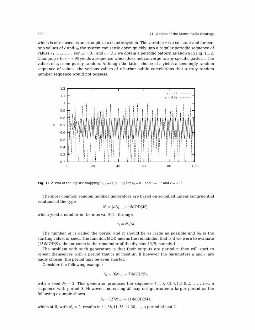
360 11 Outline of the Monte Carlo Strategy
which is often used as an example of a chaotic system. The variable c is a constant and for cer-tain values of c and x0 the system can settle down quickly into a regular periodic sequence ofvalues x1,x2,x3, . . . . For x0 = 0.1 and c = 3.2 we obtain a periodic pattern as shown in Fig. 11.2.Changing c to c = 3.98 yields a sequence which does not converge to any specific pattern. Thevalues of xi seem purely random. Although the latter choice of c yields a seemingly randomsequence of values, the various values of x harbor subtle correlations that a truly randomnumber sequence would not possess.
c = 3.98
c = 3.2
i
x
100806040200
1.2
1.1
1
0.9
0.8
0.7
0.6
0.5
0.4
0.3
0.2
Fig. 11.2 Plot of the logistic mapping xi+1 = cxi(1− xi) for x0 = 0.1 and c = 3.2 and c = 3.98.
The most common random number generators are based on so-called Linear congruentialrelations of the type
Ni = (aNi−1 + c)MOD(M),
which yield a number in the interval [0,1] through
xi = Ni/M
The number M is called the period and it should be as large as possible and N0 is thestarting value, or seed. The function MOD means the remainder, that is if we were to evaluate(13)MOD(9), the outcome is the remainder of the division 13/9, namely 4.
The problem with such generators is that their outputs are periodic; they will start torepeat themselves with a period that is at most M. If however the parameters a and c arebadly chosen, the period may be even shorter.
Consider the following example
Ni = (6Ni−1 + 7)MOD(5),
with a seed N0 = 2. This generator produces the sequence 4,1,3,0,2,4,1,3,0,2, ... . . ., i.e., asequence with period 5. However, increasing M may not guarantee a larger period as thefollowing example shows
Ni = (27Ni−1 + 11)MOD(54),
which still, with N0 = 2, results in 11,38,11,38,11,38, . . ., a period of just 2.
11.3 Random Numbers 361
Typical periods for the random generators provided in the program library are of the orderof ∼ 109 or larger. Other random number generators which have become increasingly popularare so-called shift-register generators. In these generators each successive number dependson many preceding values (rather than the last values as in the linear congruential generator).For example, you could make a shift register generator whose lth number is the sum of thel− ith and l− jth values with modulo M,
Nl = (aNl−i + cNl− j)MOD(M).
Such a generator again produces a sequence of pseudorandom numbers but this time witha period much larger than M. It is also possible to construct more elaborate algorithms byincluding more than two past terms in the sum of each iteration. One example is the generatorof Marsaglia and Zaman [68] which consists of two congruential relations
Nl = (Nl−3−Nl−1)MOD(231− 69), (11.16)
followed byNl = (69069Nl−1+ 1013904243)MOD(232), (11.17)
which according to the authors has a period larger than 294.Moreover, rather than using modular addition, we could use the bitwise exclusive-OR (⊕)
operation so thatNl = (Nl−i)⊕ (Nl− j)
where the bitwise action of ⊕ means that if Nl−i = Nl− j the result is 0 whereas if Nl−i 6= Nl− j
the result is 1. As an example, consider the case where Nl−i = 6 and Nl− j = 11. The first onehas a bit representation (using 4 bits only) which reads 0110 whereas the second number is1011. Employing the ⊕ operator yields 1101, or 23 + 22 + 20 = 13.
In Fortran90, the bitwise ⊕ operation is coded through the intrinsic function IEOR(m,n)
where m and n are the input numbers, while in C it is given by m∧n. The program below (fromNumerical Recipes, chapter 7.1) shows how the function ran0 implements
Ni = (aNi−1)MOD(M).
However, since a and Ni−1 are integers and their multiplication could become greater thanthe standard 32 bit integer, there is a trick via Schrage’s algorithm which approximates themultiplication of large integers through the factorization
M = aq+ r,
where we have definedq = [M/a],
andr = M MOD a.
where the brackets denote integer division. In the code below the numbers q and r are chosenso that r < q. To see how this works we note first that
(aNi−1)MOD(M) = (aNi−1− [Ni−1/q]M)MOD(M), (11.18)
since we can add or subtract any integer multiple of M from aNi−1. The last term [Ni−1/q]MMOD(M)
is zero since the integer division [Ni−1/q] just yields a constant which is multiplied with M. Wecan now rewrite Eq. (11.18) as

362 11 Outline of the Monte Carlo Strategy
(aNi−1)MOD(M) = (aNi−1− [Ni−1/q](aq+ r))MOD(M), (11.19)
which results in
(aNi−1)MOD(M) = (a(Ni−1− [Ni−1/q]q)− [Ni−1/q]r))MOD(M), (11.20)
yielding(aNi−1)MOD(M) = (a(Ni−1MOD(q))− [Ni−1/q]r))MOD(M). (11.21)
The term [Ni−1/q]r is always smaller or equal Ni−1(r/q) and with r < q we obtain always a num-ber smaller than Ni−1, which is smaller than M. And since the number Ni−1MOD(q) is betweenzero and q− 1 then a(Ni−1MOD(q)) < aq. Combined with our definition of q = [M/a] ensuresthat this term is also smaller than M meaning that both terms fit into a 32-bit signed integer.None of these two terms can be negative, but their difference could. The algorithm belowadds M if their difference is negative. Note that the program uses the bitwise ⊕ operator togenerate the starting point for each generation of a random number. The period of ran0 is∼ 2.1×10⁹. A special feature of this algorithm is that is should never be called with the initialseed set to 0.
/*
** The function
** ran0()
** is an "Minimal" random number generator of Park and Miller
** Set or reset the input value
** idum to any integer value (except the unlikely value MASK)
** to initialize the sequence; idum must not be altered between
** calls for sucessive deviates in a sequence.
** The function returns a uniform deviate between 0.0 and 1.0.
*/
double ran0(long &idum)
const int a = 16807, m = 2147483647, q = 127773;
const int r = 2836, MASK = 123459876;
const double am = 1./m;
long k;
double ans;
idum ^= MASK;
k = (*idum)/q;
idum = a*(idum - k*q) - r*k;
// add m if negative difference
if(idum < 0) idum += m;
ans=am*(idum);
idum ^= MASK;
return ans;
// End: function ran0()
The other random number generators ran1, ran2 and ran3 are described in detail in Ref. [36].Here we limit ourselves to study selected properties of these generators.
11.3.1 Properties of Selected Random Number Generators
As mentioned previously, the underlying PDF for the generation of random numbers is theuniform distribution, meaning that the probability for finding a number x in the interval [0,1]is p(x) = 1.
A random number generator should produce numbers which uniformly distributed in thisinterval. Table 11.3 shows the distribution of N = 10000 random numbers generated by the
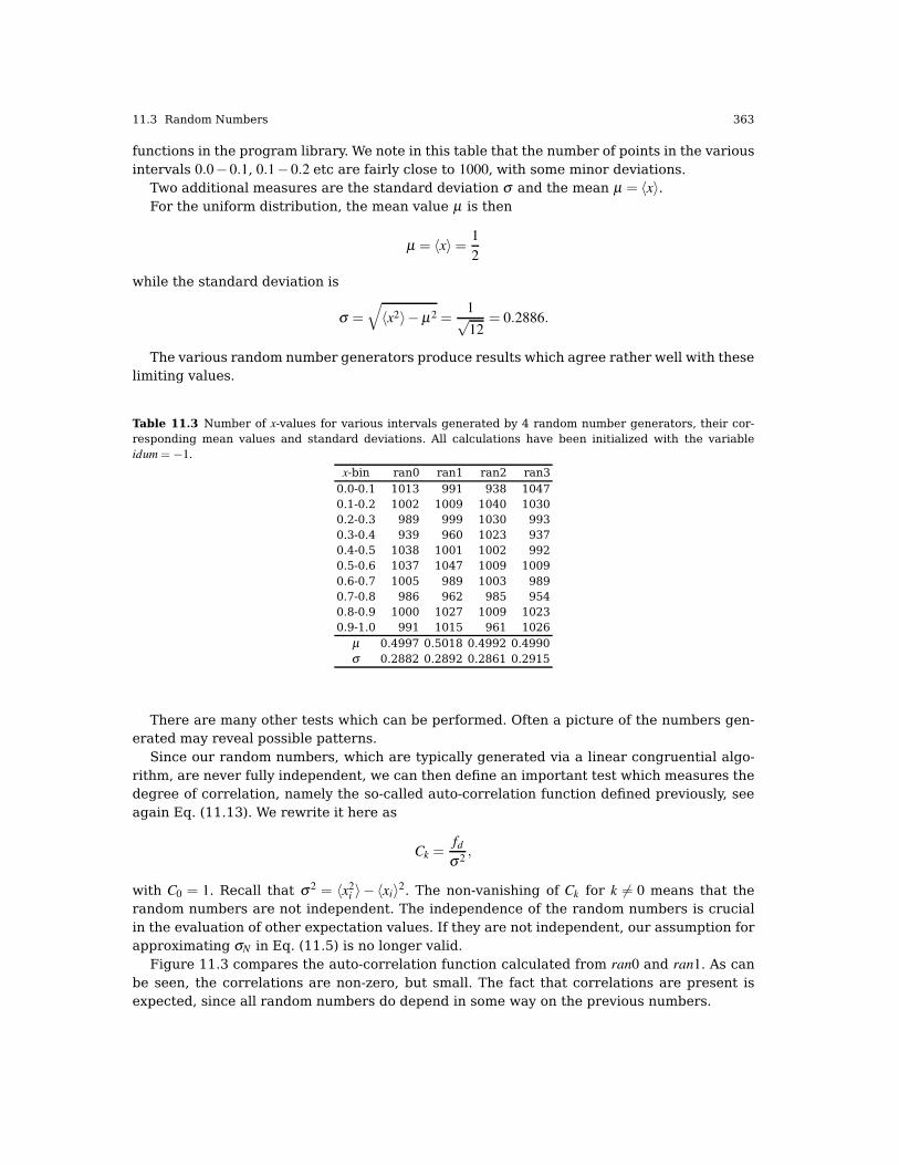
11.3 Random Numbers 363
functions in the program library. We note in this table that the number of points in the variousintervals 0.0− 0.1, 0.1− 0.2 etc are fairly close to 1000, with some minor deviations.
Two additional measures are the standard deviation σ and the mean µ = 〈x〉.For the uniform distribution, the mean value µ is then
µ = 〈x〉= 1
2
while the standard deviation is
σ =√〈x2〉− µ2 =
1√12
= 0.2886.
The various random number generators produce results which agree rather well with theselimiting values.
Table 11.3 Number of x-values for various intervals generated by 4 random number generators, their cor-responding mean values and standard deviations. All calculations have been initialized with the variableidum =−1.
x-bin ran0 ran1 ran2 ran30.0-0.1 1013 991 938 10470.1-0.2 1002 1009 1040 10300.2-0.3 989 999 1030 9930.3-0.4 939 960 1023 9370.4-0.5 1038 1001 1002 9920.5-0.6 1037 1047 1009 10090.6-0.7 1005 989 1003 9890.7-0.8 986 962 985 9540.8-0.9 1000 1027 1009 10230.9-1.0 991 1015 961 1026
µ 0.4997 0.5018 0.4992 0.4990σ 0.2882 0.2892 0.2861 0.2915
There are many other tests which can be performed. Often a picture of the numbers gen-erated may reveal possible patterns.
Since our random numbers, which are typically generated via a linear congruential algo-rithm, are never fully independent, we can then define an important test which measures thedegree of correlation, namely the so-called auto-correlation function defined previously, seeagain Eq. (11.13). We rewrite it here as
Ck =fd
σ2,
with C0 = 1. Recall that σ2 = 〈x2i 〉 − 〈xi〉2. The non-vanishing of Ck for k 6= 0 means that the
random numbers are not independent. The independence of the random numbers is crucialin the evaluation of other expectation values. If they are not independent, our assumption forapproximating σN in Eq. (11.5) is no longer valid.
Figure 11.3 compares the auto-correlation function calculated from ran0 and ran1. As canbe seen, the correlations are non-zero, but small. The fact that correlations are present isexpected, since all random numbers do depend in some way on the previous numbers.

364 11 Outline of the Monte Carlo Strategy
Ck with ran1Ck with ran0
k
Ck
30002500200015001000500
0.1
0.05
0
-0.05
-0.1
Fig. 11.3 Plot of the auto-correlation function Ck for various k-values for N = 10000 using the random numbergenerators ran0 and ran1.
11.4 Improved Monte Carlo Integration
In section 11.1 we presented a simple brute force approach to integration with the MonteCarlo method. There we sampled over a given number of points distributed uniformly in theinterval [0,1]
I =∫ 1
0f (x)dx = 〈 f 〉.
Here we introduce two important topics which in most cases improve upon the abovesimple brute force approach with the uniform distribution p(x) = 1 for x ∈ [0,1]. With improve-ments we think of a smaller variance and the need for fewer Monte Carlo samples, althougheach new Monte Carlo sample will most likely be more times consuming than correspondingones of the brute force method.
• The first topic deals with change of variables, and is linked to the cumulative functionP(x) of a PDF p(x). Obviously, not all integration limits go from x = 0 to x = 1, rather, inphysics we are often confronted with integration domains like x ∈ [0,∞) or x ∈ (−∞,∞)
etc. Since all random number generators give numbers in the interval x ∈ [0,1], weneed a mapping from this integration interval to the explicit one under consideration.
• The next topic deals with the shape of the integrand itself. Let us for the sake ofsimplicity just assume that the integration domain is again from x = 0 to x = 1. If thefunction to be integrated f (x) has sharp peaks and is zero or small for many values ofx ∈ [0,1], most samples of f (x) give contributions to the integral I which are negligibleor zero. As a consequence we need many N samples to have a sufficient accuracy inthe region where f (x) is peaked. What do we do then? We try to find a new PDF p(x)
chosen so as to match f (x) in order to render the integrand smooth. The new PDFp(x) has in turn an x domain which most likely has to be mapped from the domain ofthe uniform distribution.

11.4 Improved Monte Carlo Integration 365
Why care at all and not be content with just a change of variables in cases where thatis needed? Below we show several examples of how to improve a Monte Carlo integrationthrough smarter choices of PDFs which render the integrand smoother. However one classicexample from quantum mechanics illustrates the need for a good sampling function.
In quantum mechanics, the probability distribution function is given by p(x) =Ψ(x)∗Ψ (x),where Ψ (x) is the eigenfunction arising from the solution of e.g., the time-independentSchrödinger equation. If Ψ(x) is an eigenfunction, the corresponding energy eigenvalue isgiven by
H(x)Ψ (x) = EΨ(x),
where H(x) is the hamiltonian under consideration. The expectation value of H, assuming thatthe quantum mechanical PDF is normalized, is given by
〈H〉=∫
dxΨ (x)∗H(x)Ψ(x).
We could insert Ψ(x)/Ψ(x) right to the left of H and rewrite the last equation as
〈H〉=∫
dxΨ(x)∗Ψ(x)H(x)
Ψ (x)Ψ (x), (11.22)
or
〈H〉=∫
dxp(x)H(x),
which is on the form of an expectation value with
H(x) =H(x)
Ψ(x)Ψ (x).
The crucial point to note is that if Ψ(x) is the exact eigenfunction itself with eigenvalue E,then H(x) reduces just to the constant E and we have
〈H〉=∫
dxp(x)E = E,
since p(x) is normalized.However, in most cases of interest we do not have the exact Ψ . But if we have made a
clever choice for Ψ(x), the expression H(x) exhibits a smooth behavior in the neighbourhoodof the exact solution. The above example encompasses the main essence of the Monte Carlophilosophy. It is a trial approach, where intelligent guesses lead to hopefully better results.
11.4.1 Change of Variables
The starting point is always the uniform distribution
p(x)dx =
dx 0≤ x≤ 1
0 else
with p(x) = 1 and satisfying ∫ ∞
−∞p(x)dx = 1.
All random number generators provided in the program library generate numbers in thisdomain.

366 11 Outline of the Monte Carlo Strategy
When we attempt a transformation to a new variable x→ y we have to conserve the proba-bility
p(y)dy = p(x)dx,
which for the uniform distribution implies
p(y)dy = dx.
Let us assume that p(y) is a PDF different from the uniform PDF p(x) = 1 with x ∈ [0,1]. If weintegrate the last expression we arrive at
x(y) =
∫ y
0p(y′)dy′,
which is nothing but the cumulative distribution of p(y), i.e.,
x(y) = P(y) =
∫ y
0p(y′)dy′.
This is an important result which has consequences for eventual improvements over thebrute force Monte Carlo.
To illustrate this approach, let us look at some examples.
11.4.1.1 Transformed Uniform Distribution
Suppose we have the general uniform distribution
p(y)dy =
dy
b−aa≤ y≤ b
0 else
If we wish to relate this distribution to the one in the interval x ∈ [0,1] we have
p(y)dy =dy
b− a= dx,
and integrating we obtain the cumulative function
x(y) =
∫ y
a
dy′
b− a,
yieldingy = a+(b− a)x,
a well-known result!
11.4.1.2 Exponential Distribution
Assume thatp(y) = exp(−y),
which is the exponential distribution, important for the analysis of e.g., radioactive decay.Again, p(x) is given by the uniform distribution with x ∈ [0,1], and with the assumption thatthe probability is conserved we have
p(y)dy = exp(−y)dy = dx,

11.4 Improved Monte Carlo Integration 367
which yields after integration
x(y) = P(y) =∫ y
0exp(−y′)dy′ = 1− exp(−y),
ory(x) =− ln(1− x).
This gives us the new random variable y in the domain y ∈ [0,∞) determined through therandom variable x ∈ [0,1] generated by functions like ran0.
This means that if we can factor out exp(−y) from an integrand we may have
I =
∫ ∞
0F(y)dy =
∫ ∞
0exp(−y)G(y)dy
which we rewrite as
∫ ∞
0exp(−y)G(y)dy =
∫ 1
0G(y(x))dx≈ 1
N
N
∑i=1
G(y(xi)),
where xi is a random number in the interval [0,1]. We have changed the integration limitsin the second integral, since we have performed a change of variables. Since we have usedthe uniform distribution defined for x ∈ [0,1], the integration limits change to 0 and 1. Thevariable y is now a function of x. Note also that in practical implementations, our randomnumber generators for the uniform distribution never return exactly 0 or 1, but we may comevery close.
The algorithm for the last example is rather simple. In the function which sets up theintegral, we simply need to call one of the random number generators like ran0, ran1, ran2 orran3 in order to obtain numbers in the interval [0,1]. We obtain y by the taking the logarithmof (1− x). Our calling function which sets up the new random variable y may then includestatements like
.....
idum=-1;
x=ran0(&idum);
y=-log(1.-x);
.....
11.4.1.3 Another Example
Another function which provides an example for a PDF is
p(y)dy =dy
(a+ by)n,
with n > 1. It is normalizable, positive definite, analytically integrable and the integral isinvertible, allowing thereby the expression of a new variable in terms of the old one. Theintegral ∫ ∞
0
dy
(a+ by)n=
1
(n− 1)ban−1,
gives
p(y)dy =(n− 1)ban−1
(a+ by)ndy,
which in turn gives the cumulative function

368 11 Outline of the Monte Carlo Strategy
x(y) = P(y) =
∫ y
0
(n− 1)ban−1
(a+ bx)ndy′,
resulting in
x(y) = 1− 1
(1+ b/ay)n−1,
ory =
a
b
((1− x)−1/(n−1)− 1
).
With the random variable x ∈ [0,1] generated by functions like ran0, we have again the appro-priate random variable y for a new PDF.
11.4.1.4 Normal Distribution
For the normal distribution, expressed here as
g(x,y) = exp(−(x2 + y2)/2)dxdy.
it is rather difficult to find an inverse since the cumulative distribution is given by the errorfunction er f (x)
erf(x) =2√π
∫ x
0e−t2
dt.
We obviously would like to avoid computing an integral everytime we need a random variable.If we however switch to polar coordinates, we have for x and y
r =(x2 + y2
)1/2θ = tan−1 x
y,
resulting ing(r,θ ) = r exp(−r2/2)drdθ ,
where the angle θ could be given by a uniform distribution in the region [0,2π ]. Followingexample 1 above, this implies simply multiplying random numbers x∈ [0,1] by 2π . The variabler, defined for r ∈ [0,∞) needs to be related to to random numbers x′ ∈ [0,1]. To achieve that,we introduce a new variable
u =1
2r2,
and define a PDFexp(−u)du,
with u ∈ [0,∞). Using the results from example 2 for the exponential distribution, we have
u =− ln(1− x′),
where x′ is a random number generated for x′ ∈ [0,1]. With
x = r cos(θ ) =√
2ucos(θ ),
andy = r sin(θ ) =
√2usin(θ ),
we can obtain new random numbers x,y through
x =√−2ln(1− x′)cos(θ ),

11.4 Improved Monte Carlo Integration 369
andy =
√−2ln(1− x′)sin(θ ),
with x′ ∈ [0,1] and θ ∈ 2π [0,1].A function which yields such random numbers for the normal distribution would include
statements like
.....
idum=-1;
radius=sqrt(-2*ln(1.-ran0(idum)));
theta=2*pi*ran0(idum);
x=radius*cos(theta);
y=radius*sin(theta);
.....
11.4.2 Importance Sampling
With the aid of the above variable transformations we address now one of the most widelyused approaches to Monte Carlo integration, namely importance sampling.
Let us assume that p(y) is a PDF whose behavior resembles that of a function F defined ina certain interval [a,b]. The normalization condition is
∫ b
ap(y)dy = 1.
We can rewrite our integral as
I =
∫ b
aF(y)dy =
∫ b
ap(y)
F(y)
p(y)dy.
This integral resembles our discussion on the evaluation of the energy for a quantum me-chanical system in Eq. (11.22).
Since random numbers are generated for the uniform distribution p(x) with x ∈ [0,1], weneed to perform a change of variables x→ y through
x(y) =∫ y
ap(y′)dy′,
where we usedp(x)dx = dx = p(y)dy.
If we can invert x(y), we find y(x) as well.With this change of variables we can express the integral of Eq. (11.4.2) as
I =
∫ b
ap(y)
F(y)
p(y)dy =
∫ b
a
F(y(x))
p(y(x))dx,
meaning that a Monte Carlo evaluation of the above integral gives
∫ b
a
F(y(x))
p(y(x))dx =
1
N
N
∑i=1
F(y(xi))
p(y(xi)).
Note the well the change in integration limits from a and b to a and b. The advantage of sucha change of variables in case p(y) follows closely F is that the integrand becomes smooth and

370 11 Outline of the Monte Carlo Strategy
we can sample over relevant values for the integrand. It is however not trivial to find such afunction p. The conditions on p which allow us to perform these transformations are
1. p is normalizable and positive definite,2. it is analytically integrable and3. the integral is invertible, allowing us thereby to express a new variable in terms of the
old one.
The variance is now with the definition
F =F(y(x))
p(y(x)),
given by
σ2 =1
N
N
∑i=1
(F)2−
(1
N
N
∑i=1
F
)2
.
The algorithm for this procedure is
• Use the uniform distribution to find the random variable y in the interval [0,1]. Thefunction p(x) is a user provided PDF.
• Evaluate thereafter
I =∫ b
aF(x)dx =
∫ b
ap(x)
F(x)
p(x)dx,
by rewriting ∫ b
ap(x)
F(x)
p(x)dx =
∫ b
a
F(x(y))
p(x(y))dy,
sincedy
dx= p(x).
• Perform then a Monte Carlo sampling for
∫ b
a
F(x(y))
p(x(y))dy,≈ 1
N
N
∑i=1
F(x(yi))
p(x(yi)),
with yi ∈ [0,1],• and evaluate the variance as well according to Eq. (11.4.2).
11.4.3 Acceptance-Rejection Method
This is a rather simple and appealing method after von Neumann. Assume that we are lookingat an interval x ∈ [a,b], this being the domain of the PDF p(x). Suppose also that the largestvalue our distribution function takes in this interval is M, that is
p(x)≤M x ∈ [a,b].
Then we generate a random number x from the uniform distribution for x ∈ [a,b] and a corre-sponding number s for the uniform distribution between [0,M]. If
p(x)≥ s,

11.5 Monte Carlo Integration of Multidimensional Integrals 371
we accept the new value of x, else we generate again two new random numbers x and s andperform the test in the latter equation again.
As an example, consider the evaluation of the integral
I =
∫ 3
0exp(x)dx.
Obviously to derive a closed-form expression is much easier, however the integrand couldpose some more difficult challenges. The aim here is simply to show how to implent theacceptance-rejection algorithm. The integral is the area below the curve f (x) = exp(x). If weuniformly fill the rectangle spanned by x∈ [0,3] and y∈ [0,exp(3)], the fraction below the curveobtained from a uniform distribution, and multiplied by the area of the rectangle, shouldapproximate the chosen integral. It is rather easy to implement this numerically, as shown inthe following code.
Acceptance-Rejection algorithm
// Loop over Monte Carlo trials n
integral =0.;
for ( int i = 1; i <= n; i++)
// Finds a random value for x in the interval [0,3]
x = 3*ran0(&idum);
// Finds y-value between [0,exp(3)]
y = exp(3.0)*ran0(&idum);
// if the value of y at exp(x) is below the curve, we accept
if ( y < exp(x)) s = s+ 1.0;
// The integral is area enclosed below the line f(x)=exp(x)
// Then we multiply with the area of the rectangle and divide by the number of cycles
Integral = 3.*exp(3.)*s/n
11.5 Monte Carlo Integration of Multidimensional Integrals
When we deal with multidimensional integrals of the form
I =
∫ b1
a1
dx1
∫ b2
a2
dx2 . . .
∫ bd
ad
dxdg(x1, . . . ,xd),
with xi defined in the interval [ai,bi] we would typically need a transformation of variables ofthe form
xi = ai +(bi− ai)ti,
if we were to use the uniform distribution on the interval [0,1]. In this case, we need a Jacobideterminant
d
∏i=1
(bi− ai),
and to convert the function g(x1, . . . ,xd) to
g(x1, . . . ,xd)→ g(a1 +(b1− a1)t1, . . . ,ad +(bd− ad)td).
As an example, consider the following six-dimensional integral
∫ ∞
−∞dxdyg(x,y),

372 11 Outline of the Monte Carlo Strategy
whereg(x,y) = exp(−x2− y2)(x− y)2
with d = 6.We can solve this integral by employing our brute force scheme, or using importance sam-
pling and random variables distributed according to a gaussian PDF. For the latter, if we setthe mean value µ = 0 and the standard deviation σ = 1/
√2, we have
1√π
exp(−x2),
and using this normal distribution we rewrite our integral as
π3
∫ 6
∏i=1
(1√π
exp(−x2i )
)(x− y)2dx1. . . .dx6,
which is rewritten in a more compact form as
∫f (x1, . . . ,xd)F(x1, . . . ,xd)
6
∏i=1
dxi,
where f is the above normal distribution and
F(x1, . . . ,x6) = F(x,y) = (x− y)2,
Below we list two codes, one for the brute force integration and the other employing im-portance sampling with a gaussian distribution.
11.5.1 Brute Force Integration
http://folk.uio.no/mhjensen/compphys/programs/chapter11/cpp/program4.cpp
#include <iostream>
#include <fstream>
#include <iomanip>
#include "lib.h"
using namespace std;
double brute_force_MC(double *);
// Main function begins here
int main()
int n;
double x[6], y, fx;
double int_mc = 0.; double variance = 0.;
double sum_sigma= 0. ; long idum=-1 ;
double length = 5.; // we fix the max size of the box to L=5
double jacobidet = pow((2*length),6);
cout << "Read in the number of Monte-Carlo samples" << endl;
cin >> n;
// evaluate the integral with importance sampling
for ( int i = 1; i <= n; i++)
// x[] contains the random numbers for all dimensions
for (int j = 0; j< 6; j++)
x[j]=-length+2*length*ran0(&idum);

11.5 Monte Carlo Integration of Multidimensional Integrals 373
fx=brute_force_MC(x);
int_mc += fx;
sum_sigma += fx*fx;
int_mc = int_mc/((double) n );
sum_sigma = sum_sigma/((double) n );
variance=sum_sigma-int_mc*int_mc;
// final output
cout << setiosflags(ios::showpoint | ios::uppercase);
cout << " Monte carlo result= " << setw(10) << setprecision(8) << jacobidet*int_mc;
cout << " Sigma= " << setw(10) << setprecision(8) << volume*sqrt(variance/((double) n
)) << endl;
return 0;
// end of main program
// this function defines the integrand to integrate
double brute_force_MC(double *x)
// evaluate the different terms of the exponential
double xx=x[0]*x[0]+x[1]*x[1]+x[2]*x[2];
double yy=x[3]*x[3]+x[4]*x[4]+x[5]*x[5];
double xy=pow((x[0]-x[3]),2)+pow((x[1]-x[4]),2)+pow((x[2]-x[5]),2);
return exp(-xx-yy)*xy;
// end function for the integrand
11.5.2 Importance Sampling
This code includes a call to the function normal_random, which produces random numbersfrom a gaussian distribution.
http://folk.uio.no/mhjensen/compphys/programs/chapter11/cpp/program5.cpp
// importance sampling with gaussian deviates
#include <iostream>
#include <fstream>
#include <iomanip>
#include "lib.h"
using namespace std;
double gaussian_MC(double *);
double gaussian_deviate(long *);
// Main function begins here
int main()
int n;
double x[6], y, fx;
cout << "Read in the number of Monte-Carlo samples" << endl;
cin >> n;
double int_mc = 0.; double variance = 0.;
double sum_sigma= 0. ; long idum=-1 ;
double jacobidet = pow(acos(-1.),3.);
double sqrt2 = 1./sqrt(2.);
// evaluate the integral with importance sampling
for ( int i = 1; i <= n; i++)
// x[] contains the random numbers for all dimensions
for (int j = 0; j < 6; j++)
x[j] = gaussian_deviate(&idum)*sqrt2;

374 11 Outline of the Monte Carlo Strategy
fx=gaussian_MC(x);
int_mc += fx;
sum_sigma += fx*fx;
int_mc = int_mc/((double) n );
sum_sigma = sum_sigma/((double) n );
variance=sum_sigma-int_mc*int_mc;
// final output
cout << setiosflags(ios::showpoint | ios::uppercase);
cout << " Monte carlo result= " << setw(10) << setprecision(8) << jacobidet*int_mc;
cout << " Sigma= " << setw(10) << setprecision(8) << volume*sqrt(variance/((double) n
)) << endl;
return 0;
// end of main program
// this function defines the integrand to integrate
double gaussian_MC(double *x)
// evaluate the different terms of the exponential
double xy=pow((x[0]-x[3]),2)+pow((x[1]-x[4]),2)+pow((x[2]-x[5]),2);
return xy;
// end function for the integrand
// random numbers with gaussian distribution
double gaussian_deviate(long * idum)
static int iset = 0;
static double gset;
double fac, rsq, v1, v2;
if ( idum < 0) iset =0;
if (iset == 0)
do
v1 = 2.*ran0(idum) -1.0;
v2 = 2.*ran0(idum) -1.0;
rsq = v1*v1+v2*v2;
while (rsq >= 1.0 || rsq == 0.);
fac = sqrt(-2.*log(rsq)/rsq);
gset = v1*fac;
iset = 1;
return v2*fac;
else
iset =0;
return gset;
// end function for gaussian deviates
The following table lists the results from the above two programs as function of the number ofMonte Carlo samples. The suffix cr stands for the brute force approach while gd stands for theuse of a Gaussian distribution function. One sees clearly that the approachwith a Gaussiandistribution function yields a much improved numerical result, with fewer samples.

11.6 Classes for Random Number Generators 375
Table 11.4 Results as function of number of Monte Carlo samples N. The exact answer is I ≈ 93.020 for theintegral. The suffix cr stands for the brute force approach while is stands for the importance sampling results.All calculations use ran0 as function to generate the uniform distribution.
N Icr Igd
10000 9.92072E+01 9.33225E+01100000 8.75039E+01 9.30042E+01
1000000 9.56759E+01 9.29988E+0110000000 9.15446E+01 9.30203E+01
11.6 Classes for Random Number Generators
We end this chapter with presenting a possible class for using random number genrerators.The class consists of five files, one which defines the random number generators, random.hand four separate files Ran0.h, Ran1.h, Ran2.h and Ran3.h discussed in the text. We list hereonly the definitions contained in random.h. The file is well commented and all information iscontained within the file itself.
The file random.h
/**
* @file Random.h
* @class Random
*
* Interface for random number generators (RNG). The particular RNG are
* implemented in the various subclasses.
*
**/
#ifndef RANDOM_H
#define RANDOM_H
class Random
protected:
long seed;
public:
/**
* @brief Constructor.
*
* @param seed_ A negative long integer. If none is given, seed takes the default value
-1.
**/
Random(long seed_=-1): seed(seed_)
//! Destructor
virtual ~Random();
/**
* This function is useful in cases where it is necessary to take care of the seed in
order
* to reproduce experiments with the same sequences.
*
* @return The seed used during the initialization of the Random Number Generator.
**/
long getSeed()constreturn seed;
//! Modify the seed.
virtual reseed(long seed_)seed = seed_;

376 11 Outline of the Monte Carlo Strategy
/**
* @return A random number from a particular Random Number Generator
* implemented in the subclasses.
**/
virtual double sample()=0;
;
#inline Random::~Random()
#endif
11.7 Exercises
11.1. Calculate the cumulative functions P(x) for the binomial and the Poisson distributionsand their variances.
11.2. Make a program which computes random numbers according to the algorithm ofMarsaglia and Zaman, Eqs. (11.16) and (11.17). Compute the correlation function Ck andcompare with the auto-correlation function from the function ran0.
11.3. Make a function normal_random which computes random numbers for the normal distri-bution based on random numbers generated from the function ran0.
11.4. Make a function exp_random which computes random numbers for the exponential dis-tribution p(y) = e−αy based on random numbers generated from the function ran0.
11.5.1. Calculate the integral
I =∫ 1
0e−x2
dx,
using brute force Monte Carlo with p(x) = 1 and importance sampling with p(x) = ae−x wherea is a constant.
2. Calculate the integral
I =
∫ π
0
1
x2 + cos2(x)dx,
with p(x) = ae−x where a is a constant. Determine the value of a which minimizes the variance.
11.6. In this exercise we are going to simulate the radioactive decay of these nuclei usingsampling through random numbers. We assume that at t = 0 we have NX (0) nuclei of thetype X which can decay radioactively. At a given time t we are left with NX(t) nuclei. With atransition rate ωX , which is the probability that the system will make a transition to anotherstate during a time step of one second, we get the following differential equation
dNX(t) =−ωX NX (t)dt,
whose solution isNX (t) = NX (0)e
−ωX t ,
and where the mean lifetime of the nucleus X is
τ =1
ωX
.
If the nucleus X decays to Y , which can also decay, we get the following coupled equations
dNX (t)
dt=−ωX NX (t),

11.7 Exercises 377
anddNY (t)
dt=−ωY NY (t)+ωXNX (t).
We assume that at t = 0 we have NY (0) = 0. In the beginning we will have an increase of NY
nuclei, however, they will decay thereafter. In this project we let the nucleus 210Bi representX . It decays through β -decay to 210Po, which is the Y nucleus in our case. The latter decaysthrough emision of an α-particle to 206Pb, which is a stable nucleus. 210Bi has a mean lifetimeof 7.2 days while 210Po has a mean lifetime of 200 days.
1. Find closed form solutions for the above equations assuming continuous variables and settingthe number of 210Po nuclei equal zero at t = 0.
2. Make a program which solves the above equations. What is a reasonable choice of timestep∆ t? You could use the program on radioactive decay from the web-page of the course asan example and make your own for the decay of two nuclei. Compare the results from yourprogram with the exact answer as function of NX (0) = 10, 100 and 1000. Make plots of yourresults.
3. When 210Po decays it produces an α particle. At what time does the production of α particlesreach its maximum? Compare your results with the closed form solutions for NX (0) = 10, 100
and 1000.
11.7. The task here is to integrate in a brute force manner a six-dimensional integral whichis used to determine the ground state correlation energy between two electrons in a heliumatom. Furthermore, you will need to parallelize your code for the Monte-Carlo integration.
We assume that the wave function of each electron can be modelled like the single-particlewave function of an electron in the hydrogen atom. The single-particle wave function for anelectron i in the 1s state is given in terms of a dimensionless variable (the wave function isnot properly normalized)
ri = xiex + yiey + ziez,
asψ1s(ri) = e−αri ,
where α is a parameter and
ri =√
x2i + y2
i + z2i .
We will fix α = 2, which should correspond to the charge of the helium atom Z = 2.The ansatz for the wave function for two electrons is then given by the product of two 1s
wave functions asΨ(r1,r2) = e−α(r1+r2).
Note that it is not possible to find a closed form solution to Schrödinger’s equation for twointeracting electrons in the helium atom.
The integral we need to solve is the quantum mechanical expectation value of the correla-tion energy between two electrons, namely
〈 1
|r1− r2|〉=
∫ ∞
−∞dr1dr2e−2α(r1+r2)
1
|r1− r2|. (11.23)
Note that our wave function is not normalized. There is a normalization factor missing, butfor this project we don’t need to worry about that.
1. Set up a program which performs a Monte Carlo integration of the above integral, but with-out using importance sampling. That is, use only the uniform distribution. An example of aprogram which implements this can be written as

378 11 Outline of the Monte Carlo Strategy
double int_mc = 0.; double variance = 0.;
double sum_sigma= 0. ; long idum=-1 ;
double length=1.5; // we fix the max size of the box to L=3
double jacobidet=pow((2*length),6.);
// evaluate the integral with importance sampling
for ( int i = 1; i <= n; i++)
// x[] contains the random numbers for all dimensions
for (int j = 0; j< 6; j++)
// Maps U[0,1] to U[-L,L]
x[j]=-length+2*length*ran0(&idum);
fx=brute_force_MC(x);
int_mc += fx;
sum_sigma += fx*fx;
int_mc = jacobidet*int_mc/((double) n );
sum_sigma = jacobidet*sum_sigma/((double) n );
variance=sum_sigma-int_mc*int_mc;
....
We include also an example of a function which sets up the function to integrate
double brute_force_MC(double *x)
double alpha = 2.;
// evaluate the different terms of the exponential
double exp1=-2*alpha*sqrt(x[0]*x[0]+x[1]*x[1]+x[2]*x[2]);
double exp2=-2*alpha*sqrt(x[3]*x[3]+x[4]*x[4]+x[5]*x[5]);
double deno=sqrt(pow((x[0]-x[3]),2)
+pow((x[1]-x[4]),2)+pow((x[2]-x[5]),2));
double value=exp(exp1+exp2)/deno;
return value;
// end function for the integrand
2. Improve your brute force Monte Carlo calculation by using importance sampling. Hint: usethe exponential distribution. Does the variance decrease? Does the CPU time used comparedwith the brute force Monte Carlo decrease in order to achieve the same accuracy? Commentyour results. An extract from a code which performs the importance sampling is includedhere.
double int_mc = 0.; double variance = 0.;
double sum_sigma= 0. ; long idum=-1 ;
// The 'volume' contains 4 jacobideterminants(pi,pi,2pi,2pi)
// and a scaling factor 1/16
double jacobidet=4*pow(acos(-1.),4.)*1./16;
// evaluate the integral with importance sampling
for ( int i = 1; i <= n; i++)
for (int j = 0; j < 2; j++)
y=ran0(&idum);
x[j]=-0.25*log(1.-y);
for (int j = 2; j < 4; j++)
x[j] = 2*acos(-1.)*ran0(&idum);
for (int j = 4; j < 6; j++)
x[j] = acos(-1.)*ran0(&idum);
fx=integrand_MC(x);
....

11.7 Exercises 379
The importance sampling improves considerably the results, as we noted in the example withthe normal distribution. Typical results are
Table 11.5 Results obtained with the uniform distribution only and importance sampling. The suffix ud standsfor the approach with the uniform distribution while is stands for the use of importance sampling.
N Iud σud time(s) Iis σis time(s)1E6 0.19238 3.85124E-4 0.6 0.19176 1.01515E-4 1.4
10E6 0.18607 1.18053E-4 6 0.192254 1.22430E-4 14100E6 0.18846 4.37163E-4 57 0.192720 1.03346E-4 138
1000E6 0.18843 1.35879E-4 581 0.192789 3.28795E-5 1372
3. Parallelize your code from the previous point and compare the CPU time needed with thatfrom the first point above. Do you achieve a good speedup?
4. The integral of Eq. (11.23) has a closed form solution. Can you find it?


Chapter 12
Random walks and the Metropolis algorithm
The way that can be spoken of is not the constant way. (Tao Te Ching, Book I, I.1) Lao Tzu
Abstract We present the theory of random walks, Markov chains and present the Metropolisalgorithm.
12.1 Motivation
In the previous chapter we discussed technical aspects of Monte Carlo integration such asalgorithms for generating random numbers and integration of multidimensional integrals.The latter topic served to illustrate two key topics in Monte Carlo simulations, namely aproper selection of variables and importance sampling. An intelligent selection of variables,good sampling techniques and guiding functions can be crucial for the outcome of our MonteCarlo simulations. Examples of this will be demonstrated in the chapters on statistical andquantum physics applications. Here we make a detour from this main area of applications.The focus is on diffusion and random walks. Furthermore, we will use these topics to derivethe famous Metropolis algorithm.
The rationale for this is that the tricky part of an actual Monte Carlo simulation resides inthe appropriate selection of random states, and thereby numbers, according to the probabilitydistribution (PDF) at hand.
Suppose our PDF is given by the well-known normal distribution. Think of for example thevelocity distribution of an ideal gas in a container. In our simulations we could then accept orreject new moves with a probability proportional to the normal distribution. This would par-allel our example on the sixth dimensional integral in the previous chapter. However, in thiscase we would end up rejecting basically all moves since the probabilities are exponentiallysmall in most cases. The result would be that we barely moved from the initial position. Ourstatistical averages would then be significantly biased and most likely not very reliable.
Instead, all Monte Carlo schemes used are based on Markov processes in order to generatenew random states. A Markov process is a random walk with a selected probability for makinga move. The new move is independent of the previous history of the system. The Markovprocess is used repeatedly in Monte Carlo simulations in order to generate new randomstates. The reason for choosing a Markov process is that when it is run for a long enough timestarting with a random state, we will eventually reach the most likely state of the system. Inthermodynamics, this means that after a certain number of Markov processes we reach anequilibrium distribution. This mimicks the way a real system reaches its most likely state ata given temperature of the surroundings.
381

382 12 Random walks and the Metropolis algorithm
To reach this distribution, the Markov process needs to obey two important conditions, thatof ergodicity and detailed balance. These conditions impose constraints on our algorithms foraccepting or rejecting new random states. The Metropolis algorithm discussed here abidesto both these constraints and is discussed in more detail in Section 12.5. The Metropolisalgorithm is widely used in Monte Carlo simulations of physical systems and the understand-ing of it rests within the interpretation of random walks and Markov processes. However,before we do that we discuss the intimate link between random walks, Markov processesand the diffusion equation. In section 12.3 we show that a Markov process is nothing butthe discretized version of the diffusion equation. Diffusion and random walks are discussedfrom a more experimental point of view in the next section. There we show also a simplealgorithm for random walks and discuss eventual physical implications. We end this chapterwith a discussion of one of the most used algorithms for generating new steps, namely theMetropolis algorithm. This algorithm, which is based on Markovian random walks satisfiesboth the ergodicity and detailed balance requirements and is widely in applications of MonteCarlo simulations in the natural sciences. The Metropolis algorithm is used in our studies ofphase transitions in statistical physics and the simulations of quantum mechanical systems.
12.2 Diffusion Equation and Random Walks
Physical systems subject to random influences from the ambient have a long history, datingback to the famous experiments by the British Botanist R. Brown on pollen of different plantsdispersed in water. This lead to the famous concept of Brownian motion. In general, smallfractions of any system exhibit the same behavior when exposed to random fluctuations of themedium. Although apparently non-deterministic, the rules obeyed by such Brownian systemsare laid out within the framework of diffusion and Markov chains. The fundamental works onBrownian motion were developed by A. Einstein at the turn of the last century.
Diffusion and the diffusion equation are central topics in both Physics and Mathematics,and their ranges of applicability span from stellar dynamics to the diffusion of particles gov-erned by Schrödinger’s equation. The latter is, for a free particle, nothing but the diffusionequation in complex time!
Let us consider the one-dimensional diffusion equation. We study a large ensemble of par-ticles performing Brownian motion along the x-axis. There is no interaction between the par-ticles.
We define w(x, t)dx as the probability of finding a given number of particles in an intervalof length dx in x ∈ [x,x+ dx] at a time t. This quantity is our probability distribution function(PDF). The quantum physics equivalent of w(x, t) is the wave function itself. This diffusioninterpretation of Schrödinger’s equation forms the starting point for diffusion Monte Carlotechniques in quantum physics.
Good overview texts are the books of Robert and Casella and Karatsas, see Refs. [63,69].
12.2.1 Diffusion Equation
From experiment there are strong indications that the flux of particles j(x, t), viz., the numberof particles passing x at a time t is proportional to the gradient of w(x, t). This proportionalityis expressed mathematically through
j(x, t) =−D∂w(x, t)
∂x,

12.2 Diffusion Equation and Random Walks 383
where D is the so-called diffusion constant, with dimensionality length2 per time. If the num-ber of particles is conserved, we have the continuity equation
∂ j(x, t)
∂x=−∂w(x, t)
∂ t,
which leads to∂w(x, t)
∂ t= D
∂ 2w(x, t)
∂x2, (12.1)
which is the diffusion equation in one dimension.With the probability distribution function w(x, t)dx we can use the results from the previous
chapter to compute expectation values such as the mean distance
〈x(t)〉=∫ ∞
−∞xw(x, t)dx,
or
〈x2(t)〉=∫ ∞
−∞x2w(x, t)dx,
which allows for the computation of the variance σ2 = 〈x2(t)〉− 〈x(t)〉2. Note well that theseexpectation values are time-dependent. In a similar way we can also define expectation valuesof functions f (x, t) as
〈 f (x, t)〉=∫ ∞
−∞f (x, t)w(x, t)dx.
Since w(x, t) is now treated as a PDF, it needs to obey the same criteria as discussed in theprevious chapter. However, the normalization condition
∫ ∞
−∞w(x, t)dx = 1
imposes significant constraints on w(x, t). These are
w(x =±∞, t) = 0∂ nw(x, t)
∂xn|x=±∞ = 0,
implying that when we study the time-derivative ∂ 〈x(t)〉/∂ t, we obtain after integration byparts and using Eq. (12.1)
∂ 〈x〉∂ t
=∫ ∞
−∞x
∂w(x, t)
∂ tdx = D
∫ ∞
−∞x
∂ 2w(x, t)
∂x2dx,
leading to∂ 〈x〉∂ t
= Dx∂w(x, t)
∂x|x=±∞−D
∫ ∞
−∞
∂w(x, t)
∂xdx,
implying that∂ 〈x〉∂ t
= 0.
This means in turn that 〈x〉 is independent of time. If we choose the initial position x(t = 0) = 0,the average displacement 〈x〉= 0. If we link this discussion to a random walk in one dimensionwith equal probability of jumping to the left or right and with an initial position x = 0, thenour probability distribution remains centered around 〈x〉= 0 as function of time. However, thevariance is not necessarily 0. Consider first
∂ 〈x2〉∂ t
= Dx2 ∂w(x, t)
∂x|x=±∞− 2D
∫ ∞
−∞x
∂w(x, t)
∂xdx,

384 12 Random walks and the Metropolis algorithm
where we have performed an integration by parts as we did for ∂ 〈x〉∂ t
. A further integration byparts results in
∂ 〈x2〉∂ t
=−Dxw(x, t)|x=±∞ + 2D
∫ ∞
−∞w(x, t)dx = 2D,
leading to〈x2〉= 2Dt,
and the variance as〈x2〉− 〈x〉2 = 2Dt. (12.2)
The root mean square displacement after a time t is then
√〈x2〉− 〈x〉2 =
√2Dt.
This should be contrasted to the displacement of a free particle with initial velocity v0. In thatcase the distance from the initial position after a time t is x(t) = vt whereas for a diffusionprocess the root mean square value is
√〈x2〉− 〈x〉2 ∝
√t. Since diffusion is strongly linked
with random walks, we could say that a random walker escapes much more slowly from thestarting point than would a free particle. We can vizualize the above in the following figure.In Fig. 12.1 we have assumed that our distribution is given by a normal distribution withvariance σ2 = 2Dt, centered at x = 0. The distribution reads
w(x, t)dx =1√
4πDtexp(− x2
4Dt)dx.
At a time t = 2s the new variance is σ2 = 4Ds, implying that the root mean square valueis√〈x2〉− 〈x〉2 = 2
√D. At a further time t = 8 we have
√〈x2〉− 〈x〉2 = 4
√D. While time has
elapsed by a factor of 4, the root mean square has only changed by a factor of 2. Fig. 12.1demonstrates the spreadout of the distribution as time elapses. A typical example can be thediffusion of gas molecules in a container or the distribution of cream in a cup of coffee. In bothcases we can assume that the the initial distribution is represented by a normal distribution.
0
0.02
0.04
0.06
0.08
0.1
0.12
0.14
0.16
0.18
0.2
-10 -5 0 5 10
w(x, t)dx
x
Fig. 12.1 Time development of a normal distribution with variance σ 2 = 2Dt and with D = 1m2/s. The solidline represents the distribution at t = 2s while the dotted line stands for t = 8s.

12.2 Diffusion Equation and Random Walks 385
12.2.2 Random Walks
Consider now a random walker in one dimension, with probability R of moving to the rightand L for moving to the left. At t = 0 we place the walker at x= 0, as indicated in Fig. 12.2. Thewalker can then jump, with the above probabilities, either to the left or to the right for eachtime step. Note that in principle we could also have the possibility that the walker remainsin the same position. This is not implemented in this example. Every step has length ∆x = l.Time is discretized and we have a jump either to the left or to the right at every time step.Let us now assume that we have equal probabilities for jumping to the left or to the right, i.e.,
• • • • • • • •.. −3l −2 −l x = 0 l 2l 3l ..
Fig. 12.2 One-dimensional walker which can jump either to the left or to the right. Every step has length∆x = l.
L = R = 1/2. The average displacement after n time steps is
〈x(n)〉=n
∑i
∆xi = 0 ∆xi =±l,
since we have an equal probability of jumping either to the left or to right. The value of 〈x(n)2〉is
〈x(n)2〉=(
n
∑i
∆xi
)(n
∑j
∆x j
)=
n
∑i
∆x2i +
n
∑i6= j
∆xi∆x j = l2n.
For many enough steps the non-diagonal contribution is
N
∑i6= j
∆xi∆x j = 0,
since ∆xi, j =±l. The variance is then
〈x(n)2〉− 〈x(n)〉2 = l2n. (12.3)
It is also rather straightforward to compute the variance for L 6= R. The result is
〈x(n)2〉− 〈x(n)〉2 = 4LRl2n.
In Eq. (12.3) the variable n represents the number of time steps. If we define n = t/∆ t, we canthen couple the variance result from a random walk in one dimension with the variance fromthe diffusion equation of Eq. (12.2) by defining the diffusion constant as
D =l2
∆ t.
In the next section we show in detail that this is the case.

386 12 Random walks and the Metropolis algorithm
The program below demonstrates the simplicity of the one-dimensional random walk al-gorithm. It is straightforward to extend this program to two or three dimensions as well.The input is the number of time steps, the probability for a move to the left or to the rightand the total number of Monte Carlo samples. It computes the average displacement and thevariance for one random walker for a given number of Monte Carlo samples. Each sample isthus to be considered as one experiment with a given number of walks. The interesting partof the algorithm is described in the function mc_sampling. The other functions read or writethe results from screen or file and are similar in structure to programs discussed previously.The main program reads the name of the output file from screen and sets up the arrays con-taining the walker’s position after a given number of steps. The corresponding program fora two-dimensional random walk (not listed in the main text) is found under programs/chap-ter12/program2.cpp
http://folk.uio.no/mhjensen/compphys/programs/chapter12/cpp/program1.cpp
/*1-dim random walk program.
A walker makes several trials steps with
a given number of walks per trial
*/
#include <iostream>
#include <fstream>
#include <iomanip>
#include "lib.h"
using namespace std;
// Function to read in data from screen, note call by reference
void initialise(int&, int&, double&) ;
// The Mc sampling for random walks
void mc_sampling(int, int, double, int *, int *);
// prints to screen the results of the calculations
void output(int, int, int *, int *);
int main()
int max_trials, number_walks;
double move_probability;
// Read in data
initialise(max_trials, number_walks, move_probability) ;
int *walk_cumulative = new int [number_walks+1];
int *walk2_cumulative = new int [number_walks+1];
for (int walks = 1; walks <= number_walks; walks++)
walk_cumulative[walks] = walk2_cumulative[walks] = 0;
// end initialization of vectors
// Do the mc sampling
mc_sampling(max_trials, number_walks, move_probability,
walk_cumulative, walk2_cumulative);
// Print out results
output(max_trials, number_walks, walk_cumulative,
walk2_cumulative);
delete [] walk_cumulative; // free memory
delete [] walk2_cumulative;
return 0;
// end main function
The input and output functions are
void initialise(int& max_trials, int& number_walks, double& move_probability)
cout << "Number of Monte Carlo trials =";

12.3 Microscopic Derivation of the Diffusion Equation 387
cin >> max_trials;
cout << "Number of attempted walks=";
cin >> number_walks;
cout << "Move probability=";
cin >> move_probability;
// end of function initialise
void output(int max_trials, int number_walks,
int *walk_cumulative, int *walk2_cumulative)
ofstream ofile("testwalkers.dat");
for( int i = 1; i <= number_walks; i++)
double xaverage = walk_cumulative[i]/((double) max_trials);
double x2average = walk2_cumulative[i]/((double) max_trials);
double variance = x2average - xaverage*xaverage;
ofile << setiosflags(ios::showpoint | ios::uppercase);
ofile << setw(6) << i;
ofile << setw(15) << setprecision(8) << xaverage;
ofile << setw(15) << setprecision(8) << variance << endl;
ofile.close();
// end of function output
The algorithm is in the function mc_sampling and tests the probability of moving to the left orto the right by generating a random number.
void mc_sampling(int max_trials, int number_walks,
double move_probability, int *walk_cumulative,
int *walk2_cumulative)
long idum;
idum=-1; // initialise random number generator
for (int trial=1; trial <= max_trials; trial++)
int position = 0;
for (int walks = 1; walks <= number_walks; walks++)
if (ran0(&idum) <= move_probability)
position += 1;
else
position -= 1;
walk_cumulative[walks] += position;
walk2_cumulative[walks] += position*position;
// end of loop over walks
// end of loop over trials
// end mc_sampling function
Fig. 12.3 shows that the variance increases linearly as function of the number of time steps, asexpected from the closed-form results. Similarly, the mean displacement in Fig. 12.4 oscillatesaround zero.
12.3 Microscopic Derivation of the Diffusion Equation
When solving partial differential equations such as the diffusion equation numerically, thederivatives are always discretized. Recalling our discussions from Chapter 3, we can rewritethe time derivative as

388 12 Random walks and the Metropolis algorithm
0
20
40
60
80
100
0 20 40 60 80 100
σ 2
Time steps t
Fig. 12.3 Time development of σ 2 for a random walker. 100000 Monte Carlo samples were used with thefunction ran1 and a seed set to −1.
-0.04
-0.02
0
0.02
0.04
0 20 40 60 80 100
〈x(t)〉
Time steps t
Fig. 12.4 Time development of 〈x(t)〉 for a random walker. 100000 Monte Carlo samples were used with thefunction ran1 and a seed set to −1.
∂w(x, t)
∂ t≈ w(i,n+ 1)−w(i,n)
∆ t,
whereas the gradient is approximated as
D∂ 2w(x, t)
∂x2≈ D
w(i+ 1,n)+w(i− 1,n)− 2w(i,n)
(∆x)2,
resulting in the discretized diffusion equation

12.3 Microscopic Derivation of the Diffusion Equation 389
w(i,n+ 1)−w(i,n)
∆ t= D
w(i+ 1,n)+w(i− 1,n)− 2w(i,n)
(∆x)2,
where n represents a given time step and i a step in the x-direction. The solution of such equa-tions is discussed in our chapter on partial differential equations, see Chapter 10. The aimhere is to show that we can derive the discretized diffusion equation from a Markov processand thereby demonstrate the close connection between the important physical process diffu-sion and random walks. Random walks allow for an intuitive way of picturing the process ofdiffusion. In addition, as demonstrated in the previous section, it is easy to simulate a randomwalk.
12.3.1 Discretized Diffusion Equation and Markov Chains
A Markov process allows in principle for a microscopic description of Brownian motion. Aswith the random walk studied in the previous section, we consider a particle which movesalong the x-axis in the form of a series of jumps with step length ∆x = l. Time and spaceare discretized and the subsequent moves are statistically independent, i.e., the new movedepends only on the previous step and not on the results from earlier trials. We start at aposition x = jl = j∆x and move to a new position x = i∆x during a step ∆ t = ε, where i≥ 0 andj≥ 0 are integers. The original probability distribution function (PDF) of the particles is givenby wi(t = 0) where i refers to a specific position on the grid in Fig. 12.2, with i = 0 represent-ing x = 0. The function wi(t = 0) is now the discretized version of w(x, t). We can regard thediscretized PDF as a vector. For the Markov process we have a transition probability from aposition x = jl to a position x = il given by
Wi j(ε) =W (il− jl,ε) =
12|i− j|= 1
0 else,
where Wi j is normally called the transition probability and we can represent it, see below, asa matrix. Note that this matrix is not a stochastic matrix as long as it is a finite matrix. Ournew PDF wi(t = ε) is now related to the PDF at t = 0 through the relation
wi(t = ε) = ∑j
W ( j→ i)w j(t = 0).
This equation represents the discretized time-development of an original PDF. It is a micro-scopic way of representing the process shown in Fig. 12.1. Since both W and w representprobabilities, they have to be normalized, i.e., we require that at each time step we have
∑i
wi(t) = 1,
and
∑j
W ( j→ i) = 1,
which applies for all j-values. The further constraints are 0≤Wi j ≤ 1 and 0≤w j ≤ 1. Note thatthe probability for remaining at the same place is in general not necessarily equal zero. Inour Markov process we allow only for jumps to the left or to the right.
The time development of our initial PDF can now be represented through the action ofthe transition probability matrix applied n times. At a time tn = nε our initial distribution hasdeveloped into
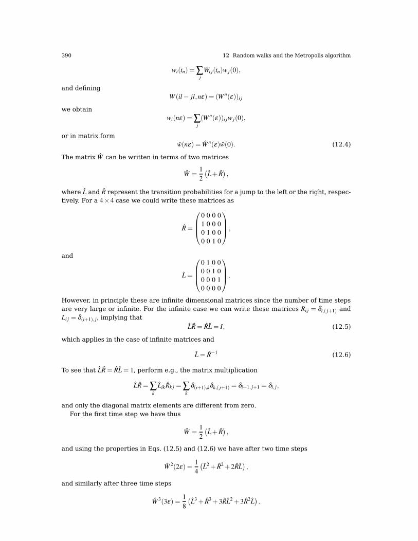
390 12 Random walks and the Metropolis algorithm
wi(tn) = ∑j
Wi j(tn)w j(0),
and definingW (il− jl,nε) = (W n(ε))i j
we obtainwi(nε) = ∑
j
(W n(ε))i jw j(0),
or in matrix formw(nε) = W n(ε)w(0). (12.4)
The matrix W can be written in terms of two matrices
W =1
2
(L+ R
),
where L and R represent the transition probabilities for a jump to the left or the right, respec-tively. For a 4× 4 case we could write these matrices as
R =
0 0 0 0
1 0 0 0
0 1 0 0
0 0 1 0
,
and
L =
0 1 0 0
0 0 1 0
0 0 0 1
0 0 0 0
.
However, in principle these are infinite dimensional matrices since the number of time stepsare very large or infinite. For the infinite case we can write these matrices Ri j = δi,( j+1) andLi j = δ(i+1), j, implying that
LR = RL = I, (12.5)
which applies in the case of infinite matrices and
L = R−1 (12.6)
To see that LR = RL = 1, perform e.g., the matrix multiplication
LR = ∑k
LikRk j = ∑k
δ(i+1),kδk,( j+1) = δi+1, j+1 = δi, j,
and only the diagonal matrix elements are different from zero.For the first time step we have thus
W =1
2
(L+ R
),
and using the properties in Eqs. (12.5) and (12.6) we have after two time steps
W 2(2ε) =1
4
(L2 + R2 + 2RL
),
and similarly after three time steps
W 3(3ε) =1
8
(L3 + R3 + 3RL2 + 3R2L
).
12.3 Microscopic Derivation of the Diffusion Equation 391
Using the binomial formulan
∑k=0
(n
k
)akbn−k = (a+ b)n,
ee we have that the transition matrix after n time steps can be written as
W n(nε)) =1
2n
n
∑k=0
(n
k
)RkLn−k,
or
W n(nε)) =1
2n
n
∑k=0
(n
k
)Ln−2k =
1
2n
n
∑k=0
(n
k
)R2k−n,
and using Rmi j = δi,( j+m) and Lm
i j = δ(i+m), j we arrive at
W (il− jl,nε) =
12n
(n
12(n+ i− j)
)|i− j| ≤ n
0 else
, (12.7)
and n+ i− j has to be an even number. We note that the transition matrix for a Markov processhas three important properties:
• It depends only on the difference in space i− j, it is thus homogenous in space.• It is also isotropic in space since it is unchanged when we go from (i, j) to (−i,− j).• It is homogenous in time since it depends only the difference between the initial time
and final time.
If we place the walker at x = 0 at t = 0 we can represent the initial PDF with wi(0) = δi,0.Using Eq. (12.4) we have
wi(nε) = ∑j
(W n(ε))i jw j(0) = ∑j
1
2n
(n
12(n+ i− j)
)δ j,0,
resulting in
wi(nε) =1
2n
(n
12(n+ i)
)|i| ≤ n.
We can then use the recursion relation for the binomials(
n+ 112(n+ 1+ i)
)=
(n
12(n+ i+ 1)
)+
(n
12(n+ i− 1)
)(12.8)
to obtain the discretized diffusion equation. In order to achieve this, we define x = il, where l
and i are integers, and t = nε. We can then rewrite the probability distribution as
w(x, t) = w(il,nε) = wi(nε) =1
2n
(n
12(n+ i)
)|i| ≤ n,
and rewrite Eq. (12.8) as
w(x, t + ε) =1
2w(x+ l, t)+
1
2w(x− l, t).
Adding and subtracting w(x, t) and multiplying both sides with l2/ε we have

392 12 Random walks and the Metropolis algorithm
w(x, t + ε)−w(x, t)
ε=
l2
2ε
w(x+ l, t)− 2w(x, t)+w(x− l, t)
l2.
If we identify D = l2/2ε and l = ∆x and ε = ∆ t we see that this is nothing but the discretizedversion of the diffusion equation. Taking the limits ∆x→ 0 and ∆ t → 0 we recover
∂w(x, t)
∂ t= D
∂ 2w(x, t)
∂x2,
the diffusion equation.
12.3.1.1 An Illustrative Example
The following simple example may help in understanding the meaning of the transition matrixW and the vector w. Consider the 4× 4 matrix W
W =
1/4 1/9 3/8 1/3
2/4 2/9 0 1/3
0 1/9 3/8 0
1/4 5/9 2/8 1/3
,
and we choose our initial state as
w(t = 0) =
1
0
0
0
.
We note that both the vector and the matrix are properly normalized. Summing the vector el-ements gives one and summing over columns for the matrix results also in one. Furthermore,the largest eigenvalue is one. We act then on w with W . The first iteration is
w(t = ε) = W w(t = 0),
resulting in
w(t = ε) =
1/4
1/2
0.0
1/4
.
The next iteration results inw(t = 2ε) = W w(t = ε),
resulting in
w(t = 2ε) =
0.201389
0.319444
0.055556
0.423611
.
Note that the vector w is always normalized to 1. We find the steady state of the system bysolving the linear set of equations
w(t = ∞) = Ww(t = ∞).
This linear set of equations reads

12.3 Microscopic Derivation of the Diffusion Equation 393
W11w1(t = ∞)+W12w2(t = ∞)+W13w3(t = ∞)+W14w4(t = ∞) = w1(t = ∞)
W21w1(t = ∞)+W22w2(t = ∞)+W23w3(t = ∞)+W24w4(t = ∞) = w2(t = ∞)
W31w1(t = ∞)+W32w2(t = ∞)+W33w3(t = ∞)+W34w4(t = ∞) = w3(t = ∞)
W41w1(t = ∞)+W42w2(t = ∞)+W43w3(t = ∞)+W44w4(t = ∞) = w4(t = ∞)
(12.9)
with the constraint that
∑i
wi(t = ∞) = 1,
yielding as solution
w(t = ∞) =
0.244318
0.319602
0.056818
0.379261
.
Table 12.1 demonstrates the convergence as a function of the number of iterations or timesteps. After twelve iterations we have reached the exact value with six leading digits.
Table 12.1 Convergence to the steady state as function of number of iterations.
Iteration w1 w2 w3 w4
0 1.000000 0.000000 0.000000 0.0000001 0.250000 0.500000 0.000000 0.2500002 0.201389 0.319444 0.055556 0.4236113 0.247878 0.312886 0.056327 0.3829094 0.245494 0.321106 0.055888 0.3775135 0.243847 0.319941 0.056636 0.3795756 0.244274 0.319547 0.056788 0.3793917 0.244333 0.319611 0.056801 0.3792558 0.244314 0.319610 0.056813 0.3792649 0.244317 0.319603 0.056817 0.379264
10 0.244318 0.319602 0.056818 0.37926211 0.244318 0.319602 0.056818 0.37926112 0.244318 0.319602 0.056818 0.379261
w(t = ∞) 0.244318 0.319602 0.056818 0.379261
We have after t-stepsw(t) = Wtw(0),
with w(0) the distribution at t = 0 and W representing the transition probability matrix. Wecan always expand w(0) in terms of the right eigenvectors v of W as
w(0) = ∑i
αivi,
resulting inw(t) = Wtw(0) = Wt ∑
i
αivi = ∑i
λ ti αivi,
with λi the ith eigenvalue corresponding to the eigenvector vi.If we assume that λ0 is the largest eigenvector we see that in the limit t→∞, w(t) becomes
proportional to the corresponding eigenvector v0. This is our steady state or final distribution.

394 12 Random walks and the Metropolis algorithm
12.3.2 Continuous Equations
Hitherto we have considered discretized versions of all equations. Our initial probability dis-tribution function was then given by
wi(0) = δi,0,
and its time-development after a given time step ∆ t = ε is
wi(t) = ∑j
W ( j→ i)w j(t = 0).
The continuous analog to wi(0) isw(x)→ δ (x), (12.10)
where we now have generalized the one-dimensional position x to a generic-dimensional vec-tor x. The Kroenecker δ function is replaced by the δ distribution function δ (x) at t = 0.
The transition from a state j to a state i is now replaced by a transition to a state withposition y from a state with position x. The discrete sum of transition probabilities can thenbe replaced by an integral and we obtain the new distribution at a time t +∆ t as
w(y, t +∆ t) =
∫W (y,x,∆ t)w(x, t)dx,
and after m time steps we have
w(y, t +m∆ t) =
∫W (y,x,m∆ t)w(x, t)dx.
When equilibrium is reached we have
w(y) =∫
W (y,x, t)w(x)dx.
We can solve the equation for w(y, t) by making a Fourier transform to momentum space. ThePDF w(x, t) is related to its Fourier transform w(k, t) through
w(x, t) =
∫ ∞
−∞dkexp(ikx)w(k, t), (12.11)
and using the definition of the δ -function
δ (x) =1
2π
∫ ∞
−∞dkexp(ikx),
we see thatw(k,0) = 1/2π .
We can then use the Fourier-transformed diffusion equation
∂ w(k, t)
∂ t=−Dk2w(k, t), (12.12)
with the obvious solution
w(k, t) = w(k,0)exp[−(Dk2t)
)=
1
2πexp[−(Dk2t)
].
Using Eq. (12.11) we obtain

12.3 Microscopic Derivation of the Diffusion Equation 395
w(x, t) =
∫ ∞
−∞dkexp [ikx]
1
2πexp[−(Dk2t)
]=
1√4πDt
exp[−(x2/4Dt)
], (12.13)
with the normalization condition ∫ ∞
−∞w(x, t)dx = 1.
It is rather easy to verify by insertion that Eq. (12.13) is a solution of the diffusion equation.The solution represents the probability of finding our random walker at position x at time t ifthe initial distribution was placed at x = 0 at t = 0.
There is another interesting feature worth observing. The discrete transition probabilityW itself is given by a binomial distribution, see Eq. (12.7). The results from the central limittheorem, see Sect. 11.2.2, state that transition probability in the limit n→ ∞ converges to thenormal distribution. It is then possible to show that
W (il− jl,nε)→W (y,x,∆ t) =1√
4πD∆ texp[−((y− x)2/4D∆ t)
],
and that it satisfies the normalization condition and is itself a solution to the diffusion equa-tion.
12.3.3 Numerical Simulation
In the two previous subsections we have given evidence that a Markov process actually yieldsin the limit of infinitely many steps the diffusion equation. It links therefore in a physical in-tuitive way the fundamental process of diffusion with random walks. It could therefore be ofinterest to visualize this connection through a numerical experiment. We saw in the previoussubsection that one possible solution to the diffusion equation is given by a normal distribu-tion. In addition, the transition rate for a given number of steps develops from a binomialdistribution into a normal distribution in the limit of infinitely many steps. To achieve thiswe construct in addition a histogram which contains the number of times the walker wasin a particular position x. This is given by the variable probability, which is normalized inthe output function. We have omitted the initialization function, since this identical to pro-gram1.cpp or program2.cpp of this chapter. The array probability extends from -number_walks
to +number_walks
http://folk.uio.no/mhjensen/compphys/programs/chapter12/cpp/program2.cpp
/*1-dim random walk program.
A walker makes several trials steps with
a given number of walks per trial
*/
#include <iostream>
#include <fstream>
#include <iomanip>
#include "lib.h"
using namespace std;
// Function to read in data from screen, note call by reference
void initialise(int&, int&, double&) ;
// The Mc sampling for random walks
void mc_sampling(int, int, double, int *, int *, int *);
// prints to screen the results of the calculations
void output(int, int, int *, int *, int *);

396 12 Random walks and the Metropolis algorithm
int main()
int max_trials, number_walks;
double move_probability;
// Read in data
initialise(max_trials, number_walks, move_probability) ;
int *walk_cumulative = new int [number_walks+1];
int *walk2_cumulative = new int [number_walks+1];
int *probability = new int [2*(number_walks+1)];
for (int walks = 1; walks <= number_walks; walks++)
walk_cumulative[walks] = walk2_cumulative[walks] = 0;
for (int walks = 0; walks <= 2*number_walks; walks++)
probability[walks] = 0;
// end initialization of vectors
// Do the mc sampling
mc_sampling(max_trials, number_walks, move_probability,
walk_cumulative, walk2_cumulative, probability);
// Print out results
output(max_trials, number_walks, walk_cumulative,
walk2_cumulative, probability);
delete [] walk_cumulative; // free memory
delete [] walk2_cumulative; delete [] probability;
return 0;
// end main function
The output function contains now the normalization of the probability as well and writes thisto its own file.
void output(int max_trials, int number_walks,
int *walk_cumulative, int *walk2_cumulative, int * probability)
ofstream ofile("testwalkers.dat");
ofstream probfile("probability.dat");
for( int i = 1; i <= number_walks; i++)
double xaverage = walk_cumulative[i]/((double) max_trials);
double x2average = walk2_cumulative[i]/((double) max_trials);
double variance = x2average - xaverage*xaverage;
ofile << setiosflags(ios::showpoint | ios::uppercase);
ofile << setw(6) << i;
ofile << setw(15) << setprecision(8) << xaverage;
ofile << setw(15) << setprecision(8) << variance << endl;
ofile.close();
// find norm of probability
double norm = 0.;
for( int i = -number_walks; i <= number_walks; i++)
norm += (double) probability[i+number_walks];
// write probability
for( int i = -number_walks; i <= number_walks; i++)
double histogram = probability[i+number_walks]/norm;
probfile << setiosflags(ios::showpoint | ios::uppercase);
probfile << setw(6) << i;
probfile << setw(15) << setprecision(8) << histogram << endl;
probfile.close();
// end of function output
The sampling part is still done in the same function, but contains now the setup of a histogramcontaining the number of times the walker visited a given position x.

12.4 Entropy and Equilibrium Features 397
void mc_sampling(int max_trials, int number_walks,
double move_probability, int *walk_cumulative,
int *walk2_cumulative, int *probability)
long idum;
idum=-1; // initialise random number generator
for (int trial=1; trial <= max_trials; trial++)
int position = 0;
for (int walks = 1; walks <= number_walks; walks++)
if (ran0(&idum) <= move_probability)
position += 1;
else
position -= 1;
walk_cumulative[walks] += position;
walk2_cumulative[walks] += position*position;
probability[position+number_walks] += 1;
// end of loop over walks
// end of loop over trials
// end mc_sampling function
Fig. 12.5 shows the resulting probability distribution after n steps In Fig. 12.5 we have plottedthe probability distribution function after a given number of time steps. Do you recognize theshape of the probabiliy distributions?
12.4 Entropy and Equilibrium Features
We use this section to motivate, in a physically intuitive way, the importance of the ergodichypothesis via a discussion of how a Markovian process reaches an equilibrium situationafter a given number of random walks. It serves then purpose of bridging the gap between aMarkovian process and our discussion of the Metropolis algorithm in the next section.
To achieve this, we will use the program from the previous section, see programs/chap-ter12/program3.cpp and introduce the concept of entropy S. We discuss the thermodynamicalmeaning of the entropy and its link with the second law of thermodynamics in the next chap-ter. Here it will suffice to state that the entropy is a measure of the disorder of the system,thus a system which is fully ordered and stays in its fundamental state (ground state) haszero entropy, while a disordered system has a large and nonzero entropy.
The definition of the entropy S (as a dimensionless quantity here) is
S =−∑i
wiln(wi),
where wi is the probability of finding our system in a state i. For our one-dimensional randomwalk case discussed in the previous sections it represents the probability for being at positioni = i∆x after a given number of time steps. In order to test this, we start with the previousprogram but assume now that we have N random walkers at i = 0 and t = 0 and let theserandomwalkers diffuse as function of time. This means simply an additional loop. We computethen, as in the previous program example, the probability distribution for N walkers after agiven number of steps i along x and time steps j. We can then compute an entropy S j for agiven number of time steps by summing over all probabilities i. We show this in Fig. 12.6.The code used to compute these results is in programs/chapter12/program4.cpp. Here wehave used 100 walkers on a lattice of length from L = −50 to L = 50 employing periodic

398 12 Random walks and the Metropolis algorithm
0
0.02
0.04
0.06
0.08
0.1
0.12
0.14
0.16
0.18
-20 -15 -10 -5 0 5 10 15 20
w(x, t)
steps x
10 steps
0
0.01
0.02
0.03
0.04
0.05
0.06
0.07
0.08
-40 -20 0 20 40
w(x, t)
steps x
100 steps
0
0.005
0.01
0.015
0.02
0.025
-40 -20 0 20 40
w(x, t)
steps x
1000 steps
Fig. 12.5 Probability distribution for one walker after 10, 100 and 1000 steps.
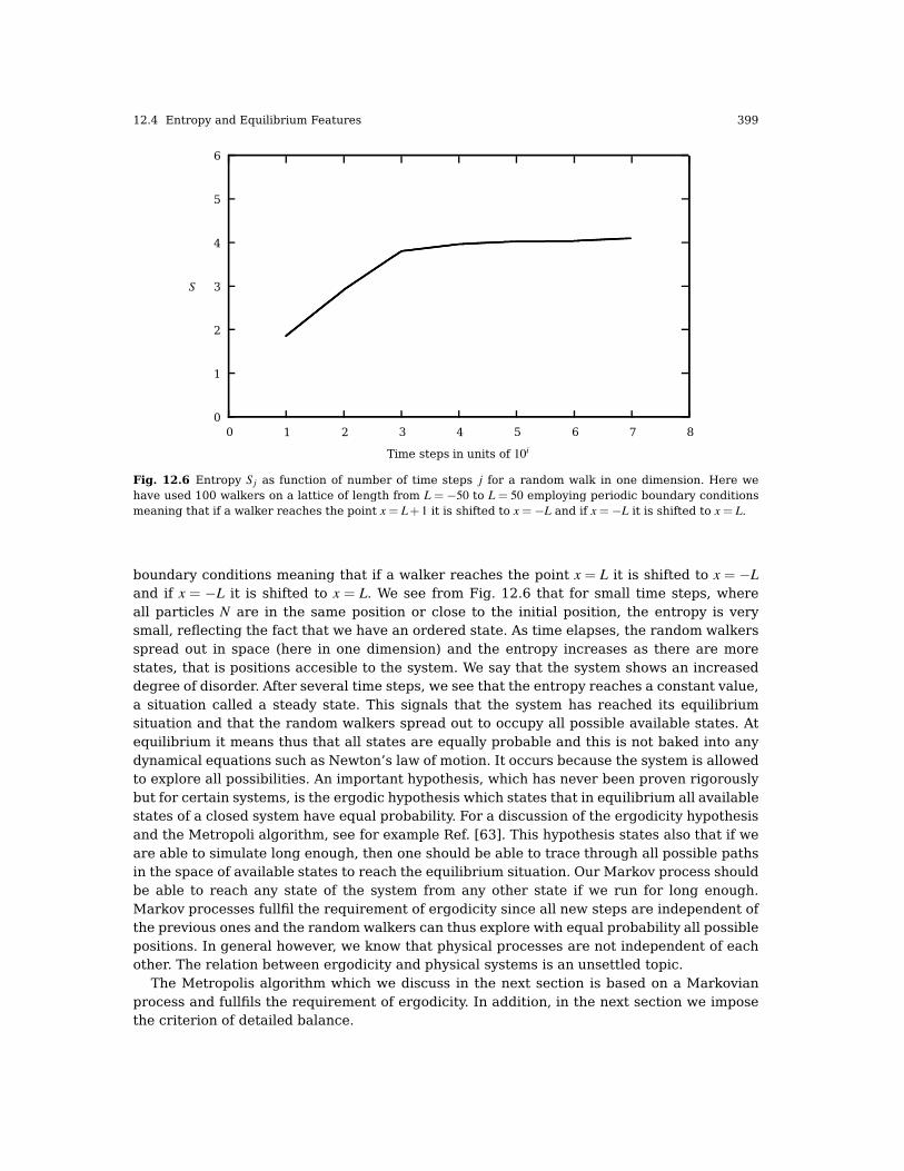
12.4 Entropy and Equilibrium Features 399
0
1
2
3
4
5
6
0 1 2 3 4 5 6 7 8
S
Time steps in units of 10i
Fig. 12.6 Entropy S j as function of number of time steps j for a random walk in one dimension. Here wehave used 100 walkers on a lattice of length from L = −50 to L = 50 employing periodic boundary conditionsmeaning that if a walker reaches the point x = L+1 it is shifted to x =−L and if x =−L it is shifted to x = L.
boundary conditions meaning that if a walker reaches the point x = L it is shifted to x = −L
and if x = −L it is shifted to x = L. We see from Fig. 12.6 that for small time steps, whereall particles N are in the same position or close to the initial position, the entropy is verysmall, reflecting the fact that we have an ordered state. As time elapses, the random walkersspread out in space (here in one dimension) and the entropy increases as there are morestates, that is positions accesible to the system. We say that the system shows an increaseddegree of disorder. After several time steps, we see that the entropy reaches a constant value,a situation called a steady state. This signals that the system has reached its equilibriumsituation and that the random walkers spread out to occupy all possible available states. Atequilibrium it means thus that all states are equally probable and this is not baked into anydynamical equations such as Newton’s law of motion. It occurs because the system is allowedto explore all possibilities. An important hypothesis, which has never been proven rigorouslybut for certain systems, is the ergodic hypothesis which states that in equilibrium all availablestates of a closed system have equal probability. For a discussion of the ergodicity hypothesisand the Metropoli algorithm, see for example Ref. [63]. This hypothesis states also that if weare able to simulate long enough, then one should be able to trace through all possible pathsin the space of available states to reach the equilibrium situation. Our Markov process shouldbe able to reach any state of the system from any other state if we run for long enough.Markov processes fullfil the requirement of ergodicity since all new steps are independent ofthe previous ones and the random walkers can thus explore with equal probability all possiblepositions. In general however, we know that physical processes are not independent of eachother. The relation between ergodicity and physical systems is an unsettled topic.
The Metropolis algorithm which we discuss in the next section is based on a Markovianprocess and fullfils the requirement of ergodicity. In addition, in the next section we imposethe criterion of detailed balance.

400 12 Random walks and the Metropolis algorithm
12.5 The Metropolis Algorithm and Detailed Balance
Let us recapitulate some of our results about Markov chains and random walks.
• The time development of our PDF w(t), after one time-step from t = 0 is given by
wi(t = ε) =W ( j→ i)w j(t = 0).
This equation represents the discretized time-development of an original PDF. We canrewrite this as a
wi(t = ε) =Wi jw j(t = 0).
with the transition matrix W for a random walk given by
Wi j(ε) =W (il− jl,ε) =
12|i− j|= 1
0 else
We call Wi j for the transition probability and we represent it as a matrix.• Both W and w represent probabilities and they have to be normalized, meaning that at
each time step we have
∑i
wi(t) = 1,
and
∑j
W ( j→ i) = 1.
Here we have written the previous matrix Wi j = W ( j → i). The further constraints are0≤Wi j ≤ 1 and 0≤ w j ≤ 1.
• We can thus write the action of W as
wi(t + 1) = ∑j
Wi jw j(t),
or as vector-matrix relationw(t + 1) = Ww(t),
and if we have that ||w(t+1)−w(t)|| → 0, we say that we have reached the most likely stateof the system, the so-called steady state or equilibrium state. Another way of phrasing thisis
w(t = ∞) = Ww(t = ∞). (12.14)
In most situations, the transition probability Wi j =W ( j→ i) is not known1. It can representa complicated set of chemical reactions which we are not capable of modeling or, we are ableto write down and account for all the boundary and the initial conditions needed to describeW ( j → i). A Markov chain is a process where this probability is in general unknown. Thequestion then is how can we model anything under such a severe lack of knowledge? TheMetropolis algorithm comes to our rescue here. Since W ( j→ i) is unknown, we model it asthe product of two probabilities, a probability for accepting the proposed move from the statej to the state j, and a probability for making the transition to the state i being in the state j.We label these probabilities A( j→ i) and T ( j→ i), respectively. Our total transition probabilityis then
W ( j→ i) = T ( j→ i)A( j→ i).
1 Note that the discrete equations here can easily be replaced by continuous ones.

12.5 The Metropolis Algorithm and Detailed Balance 401
The algorithm can then be expressed as
• We make a suggested move to the new state i with some transition or moving probabilityTj→i.
• We accept this move to the new state with an acceptance probability A j→i. The new state i
is in turn used as our new starting point for the next move. We reject this proposed movedwith a 1−A j→i and the original state j is used again as a sample.
We wish to derive the required properties of the probabilities T and A such that w(t→∞)i → wi,
starting from any distribution, will lead us to the correct distribution.We can now derive the dynamical process towards equilibrium. To obtain this equation we
note that after t time steps the probability for being in a state i is related to the probability ofbeing in a state j and performing a transition to the new state together with the probabilityof actually being in the state i and making a move to any of the possible states j from theprevious time step. We can express this as, assuming that T and A are time-independent,
wi(t + 1) = ∑j
[w j(t)Tj→iA j→i +wi(t)Ti→ j (1−Ai→ j)] .
All probabilities are normalized, meaning that ∑ j Ti→ j = 1. Using the latter, we can rewrite theprevious equation as
wi(t + 1) = wi(t)+∑j
[w j(t)Tj→iA j→i−wi(t)Ti→ jAi→ j] ,
which can be rewritten as
wi(t + 1)−wi(t) = ∑j
[w j(t)Tj→iA j→i−wi(t)Ti→ jAi→ j] .
This equation is very similar to the so-called Master equation, which relates the temporaldependence of a PDF wi(t) to various transition rates. The equation can be derived fromthe so-called Chapman-Einstein-Enskog-Kolmogorov equation, see for example Ref. [70]. Theequation is given as
dwi(t)
dt= ∑
j
[W ( j→ i)w j−W(i→ j)wi] , (12.15)
which simply states that the rate at which the systems moves from a state j to a final statei (the first term on the right-hand side of the last equation) is balanced by the rate at whichthe system undergoes transitions from the state i to a state j (the second term). If we havereached the so-called steady state, then the temporal development is zero since we are nowsatisfying Eq. (12.5). This means that in equilibrium we have
dwi(t)
dt= 0.
In the limit t → ∞ we require that the two distributions wi(t + 1) = wi and wi(t) = wi and wehave
∑j
w jTj→iA j→i = ∑j
wiTi→ jAi→ j,
which is the condition for balance when the most likely state (or steady state) has beenreached. We see also that the right-hand side can be rewritten as
∑j
wiTi→ jAi→ j = ∑j
wiWi→ j,
and using the property that ∑ j Wi→ j = 1, we can rewrite our equation as

402 12 Random walks and the Metropolis algorithm
wi = ∑j
w jTj→iA j→i = ∑j
w jWj→i,
which is nothing but the standard equation for a Markov chain when the steady state hasbeen reached.
However, the condition that the rates should equal each other is in general not sufficientto guarantee that we, after many simulations, generate the correct distribution. We may riskto end up with so-called cyclic solutions. To avoid this we therefore introduce an additionalcondition, namely that of detailed balance
W ( j→ i)w j =W (i→ j)wi.
These equations were derived by Lars Onsager when studying irreversible processes, seeRef. [71]. At equilibrium detailed balance gives thus
W ( j→ i)
W (i→ j)=
wi
w j
.
Rewriting the last equation in terms of our transition probabilities T and acceptance probobal-ities A we obtain
w j(t)Tj→iA j→i = wi(t)Ti→ jAi→ j.
Since we normally have an expression for the probability distribution functions wi, we canrewrite the last equation as
Tj→iA j→i
Ti→ jAi→ j
=wi
w j
.
In statistical physics this condition ensures that it is e.g., the Boltzmann distribution which isgenerated when equilibrium is reached.
We introduce now the Boltzmann distribution
wi =exp(−β (Ei))
Z,
which states that the probability of finding the system in a state i with energy Ei at an inversetemperature β = 1/kBT is wi ∝ exp(−β (Ei)). The denominator Z is a normalization constantwhich ensures that the sum of all probabilities is normalized to one. It is defined as the sumof probabilities over all microstates j of the system
Z = ∑j
exp(−β (Ei)).
From the partition function we can in principle generate all interesting quantities for a givensystem in equilibrium with its surroundings at a temperature T . This is demonstrated in thenext chapter.
With the probability distribution given by the Boltzmann distribution we are now in a posi-tion where we can generate expectation values for a given variable A through the definition
〈A〉=∑j
A jw j =∑ j A j exp(−β (E j)
Z.
In general, most systems have an infinity of microstates making thereby the computationof Z practically impossible and a brute force Monte Carlo calculation over a given number ofrandomly selected microstates may therefore not yield those microstates which are importantat equilibrium. To select the most important contributions we need to use the condition fordetailed balance. Since this is just given by the ratios of probabilities, we never need to

12.5 The Metropolis Algorithm and Detailed Balance 403
evaluate the partition function Z. For the Boltzmann distribution, detailed balance results in
wi
w j
= exp(−β (Ei−E j)).
Let us now specialize to a system whose energy is defined by the orientation of singlespins. Consider the state i, with given energy Ei represented by the following N spins
↑ ↑ ↑ . . . ↑ ↓ ↑ . . . ↑ ↓1 2 3 . . . k− 1 k k+ 1 . . . N− 1 N
We are interested in the transition with one single spinflip to a new state j with energy E j
↑ ↑ ↑ . . . ↑ ↑ ↑ . . . ↑ ↓1 2 3 . . . k− 1 k k+ 1 . . . N− 1 N
This change from one microstate i (or spin configuration) to another microstate j is the con-figuration space analogue to a random walk on a lattice. Instead of jumping from one placeto another in space, we ’jump’ from one microstate to another.
However, the selection of states has to generate a final distribution which is the Boltzmanndistribution. This is again the same we saw for a random walker, for the discrete case we hadalways a binomial distribution, whereas for the continuous case we had a normal distribu-tion. The way we sample configurations should result, when equilibrium is established, in theBoltzmann distribution. Else, our algorithm for selecting microstates is wrong.
As stated above, we do in general not know the closed-form expression of the transitionrate and we are free to model it asW (i→ j) = T (i→ j)A(i→ j). Our ratio between probabilitiesgives us
A j→i
Ai→ j
=wiTi→ j
w jTj→i
.
The simplest form of the Metropolis algorithm (sometimes called for brute force Metropolis)assumes that the transition probability T (i→ j) is symmetric, implying that T (i→ j) = T ( j→ i).We obtain then (using the Boltzmann distribution)
A( j→ i)
A(i→ j)= exp(−β (Ei−E j)).
We are in this case interested in a new state E j whose energy is lower than Ei, viz., ∆E =
E j − Ei ≤ 0. A simple test would then be to accept only those microstates which lower theenergy. Suppose we have ten microstates with energy E0≤ E1≤ E2≤ E3≤ ·· · ≤ E9. Our desiredenergy is E0. At a given temperature T we start our simulation by randomly choosing state E9.Flipping spins we may then find a path from E9→ E8→ E7 · · · → E1→ E0. This would howeverlead to biased statistical averages since it would violate the ergodic hypothesis discussed inthe previous section. This principle states that it should be possible for any Markov process toreach every possible state of the system from any starting point if the simulations is carriedout for a long enough time.
Any state in a Boltzmann distribution has a probability different from zero and if such astate cannot be reached from a given starting point, then the system is not ergodic. Thismeans that another possible path to E0 could be E9→ E7→ E8 · · · → E9→ E5→ E0 and so forth.Even though such a path could have a negligible probability it is still a possibility, and if wesimulate long enough it should be included in our computation of an expectation value.
Thus, we require that our algorithm should satisfy the principle of detailed balance and beergodic. The problem with our ratio

404 12 Random walks and the Metropolis algorithm
A( j→ i)
A(i→ j)= exp(−β (Ei−E j)),
is that we do not know the acceptance probability. This equation only specifies the ratio ofpairs of probabilities. Normally we want an algorithm which is as efficient as possible andmaximizes the number of accepted moves. Moreover, we know that the acceptance proba-bility has 0 as its smallest value and 1 as its largest. If we assume that the largest possibleacceptance probability is 1, we adjust thereafter the other acceptance probability to this con-straint.
To understand this better, assume that we have two energies, Ei and E j, with Ei < E j. Thismeans that the largest acceptance value must be A( j→ i) since we move to a state with lowerenergy. It follows from also from the fact that the probability wi is larger than w j. The trickthen is to fix this value to A( j→ i) = 1. It means that the other acceptance probability has tobe
A(i→ j) = exp(−β (E j−Ei)).
One possible way to encode this equation reads
A( j→ i) =
exp(−β (Ei−E j)) Ei−E j > 0
1 else,
implying that if we move to a state with a lower energy, we always accept this move withacceptance probability A( j→ i) = 1. If the energy is higher, we need to check this acceptanceprobability with the ratio between the probabilities from our PDF. From a practical point ofview, the above ratio is compared with a random number. If the ratio is smaller than a givenrandom number we accept the move to a higher energy, else we stay in the same state.
Nothing hinders us obviously in choosing another acceptance ratio, like a weighting of thetwo energies via
A( j→ i) = exp(−1
2β (Ei−E j)).
However, it is easy to see that such an acceptance ratio woud result in fewer accepted moves.
12.5.1 Brief Summary
The Monte Carlo approach, combined with the theory for Markov chains can be summarizedas follows: A Markov chain Monte Carlo method for the simulation of a distribution w is anymethod producing an ergodic Markov chain of events x whose stationary distribution is w.The Metropolis algorithm can be phrased as
• Generate an initial value x(i).• Generate a trial value yt with probability T (yt |x(i)). The latter quantity represents the
probability of generating yt given x(i).• Take a new value
x(i+1) =
yt with probability = A(x(i)→ yt)
x(i) with probability= 1−A(x(i)→ yt)
• We have defined the transition (acceptance) probability as
A(x→ y) = min
w(y)T (x|y)w(x)T (y|x) ,1
.

12.6 Langevin and Fokker-Planck Equations 405
The distribution f is often called the instrumental (we will relate it to the jumpingof a walker) or proposal distribution while A is the Metropolis-Hastings acceptanceprobability. When T (y|x) is symmetric it is just called the Metropolis algorithm.
Using the Metropolis algorithm we can in turn set up the general calculational scheme asshown in Fig. 12.7.
The dynamical equation can be written as
wi(t + 1) = ∑j
Mi jw j(t) (12.16)
with the matrix M given by
Mi j = δi j
[1−∑
k
Ti→kAi→k
]+Tj→iA j→i . (12.17)
Summing over i shows that ∑i Mi j = 1, and since ∑k Ti→k = 1, and Ai→k ≤ 1, the elements of thematrix satisfy Mi j ≥ 0. The matrix M is therefore a stochastic matrix.
The Metropolis method is simply the power method for computing the right eigenvector ofM with the largest magnitude eigenvalue. By construction, the correct probability distributionis a right eigenvector with eigenvalue 1. Therefore, for the Metropolis method to converge tothis result, one has to show that M has only one eigenvalue with this magnitude, and all othereigenvalues are smaller.
12.6 Langevin and Fokker-Planck Equations
We end this chapter with a discussion and derivation of the Fokker-Planck and Langevinequations. These equations will in turn be used in our discussion on advanced Monte Carlomethods for quantum mechanical systems, see chapter for example chapter 16.
12.6.1 Fokker-Planck Equation
For many physical systems initial distributions of a stochastic variable y tend to an equilibriumdistribution wequilibrium(y), that is w(y, t)→wequilibrium(y) as t→∞. In equilibrium, detailed balanceconstrains the transition rates
W (y→ y′)w(y) =W (y′→ y)wequilibrium(y),
where W (y′ → y) is the probability per unit time that the system changes from a state |y〉 ,characterized by the value y for the stochastic variable Y , to a state |y′〉.
Note that for a system in equilibrium the transition rateW (y′→ y) and the reverse W (y→ y′)may be very different.
Let us now assume that we have three probability distribution functions for times t0 < t ′< t,that is w(x0, t0), w(x′, t ′) and w(x, t). We have then
w(x, t) =
∫ ∞
−∞W (x.t|x′.t ′)w(x′, t ′)dx′,

406 12 Random walks and the Metropolis algorithm
Initialize:Establish aninitial state,for examplea position x(i)
Suggesta move yt
Compute ac-ceptance ratio
A(x(i) → yt)
Generate auniformlydistributedvariable r
IsA(x(i)→yt)≥ r?
Reject move:x(i+1) = x(i)
Accept move:x(i) = yt = x(i+1)
Lastmove?
Get localexpecta-
tion values
LastMCstep?
Collectsamples
End
yes
no
yes
yes
no
Fig. 12.7 Chart flow for the Metropolis algorithm.

12.6 Langevin and Fokker-Planck Equations 407
and
w(x, t) =
∫ ∞
−∞W (x.t|x0.t0)w(x0, t0)dx0,
and
w(x′, t ′) =∫ ∞
−∞W (x′.t ′|x0, t0)w(x0, t0)dx0.
We can combine these equations and arrive at the famous Einstein-Smoluchenski-Kolmogorov-Chapman (ESKC) relation
W (xt|x0t0) =
∫ ∞
−∞W (x, t|x′, t ′)W (x′, t ′|x0, t0)dx′.
We can replace the spatial dependence with a dependence upon say the velocity (or momen-tum), that is we have
W (v, t|v0, t0) =∫ ∞
−∞W (v, t|v′, t ′)W (v′, t ′|v0, t0)dx′.
We will now derive the Fokker-Planck equation. We start from the ESKC equation
W (x, t|x0, t0) =
∫ ∞
−∞W (x, t|x′, t ′)W (x′, t ′|x0, t0)dx′.
We define s = t ′− t0, τ = t− t ′ and t− t0 = s+ τ. We have then
W (x,s+ τ|x0) =
∫ ∞
−∞W (x,τ|x′)W (x′,s|x0)dx′.
Assume now that τ is very small so that we can make an expansion in terms of a small stepxi, with x′ = x− ξ , that is
W (x,s|x0)+∂W
∂ sτ +O(τ2) =
∫ ∞
−∞W (x,τ|x− ξ )W(x− ξ ,s|x0)dx′.
We assume that W (x,τ|x− ξ ) takes non-negligible values only when ξ is small. This is justanother way of stating the Master equation!
We say thus that x changes only by a small amount in the time interval τ. This means thatwe can make a Taylor expansion in terms of ξ , that is we expand
W (x,τ|x− ξ )W(x− ξ ,s|x0) =∞
∑n=0
(−ξ )n
n!
∂ n
∂xn[W (x+ ξ ,τ|x)W(x,s|x0)] .
We can then rewrite the ESKC equation as
∂W
∂ sτ =−W (x,s|x0)+
∞
∑n=0
(−ξ )n
n!
∂ n
∂xn
[W (x,s|x0)
∫ ∞
−∞ξ nW (x+ ξ ,τ|x)dξ
].
We have neglected higher powers of τ and have used that for n = 0 we get simply W (x,s|x0)
due to normalization.We say thus that x changes only by a small amount in the time interval τ. This means that
we can make a Taylor expansion in terms of ξ , that is we expand
W (x,τ|x− ξ )W(x− ξ ,s|x0) =∞
∑n=0
(−ξ )n
n!
∂ n
∂xn[W (x+ ξ ,τ|x)W(x,s|x0)] .
We simplify the above by introducing the moments

408 12 Random walks and the Metropolis algorithm
Mn =1
τ
∫ ∞
−∞ξ nW (x+ ξ ,τ|x)dξ =
〈[∆x(τ)]n〉τ
,
resulting in∂W (x,s|x0)
∂ s=
∞
∑n=1
(−ξ )n
n!
∂ n
∂xn[W (x,s|x0)Mn] .
When τ → 0 we assume that 〈[∆x(τ)]n〉 → 0 more rapidly than τ itself if n > 2. When τ ismuch larger than the standard correlation time of system then Mn for n > 2 can normally beneglected. This means that fluctuations become negligible at large time scales.
If we neglect such terms we can rewrite the ESKC equation as
∂W (x,s|x0)
∂ s=−∂M1W (x,s|x0)
∂x+
1
2
∂ 2M2W (x,s|x0)
∂x2.
In a more compact form we have
∂W
∂ s=−∂M1W
∂x+
1
2
∂ 2M2W
∂x2,
which is the Fokker-Planck equation. It is trivial to replace position with velocity (momentum).The solution to this equation is a Gaussian distribution and can be used to constrain pro-
posed transitions moves, that one can model the transition probabilities T from our discussionof the Metropolis algorithm.
12.6.2 Langevin Equation
Consider a particle suspended in a liquid. On its path through the liquid it will continuouslycollide with the liquid molecules. Because on average the particle will collide more often onthe front side than on the back side, it will experience a systematic force proportional with itsvelocity, and directed opposite to its velocity. Besides this systematic force the particle willexperience a stochastic force F(t). The equations of motion then read
dr
dt= v,
dv
dt=−ξ v+F,
The last equation is the Langevin equation. The original Langevin equation was meant todescribe Brownian motion. It is a stochastic differential equation used to describe the timeevolution of collective (normally macroscopic) variables that change only slowly with respectto the microscopic ones. The latter are responsible for the stochastic nature of the Langevinequation. We can say that we model our ignorance about the microscopic physics in a stochas-tic term. From the Langevin equation we can in turn derive for example the fluctuation dissi-pation theorem discussed below. To see, we need some information about the friction constantfrom hydrodynamics. From hydrodynamics we know that the friction constant ξ is given by
ξ = 6πηa/m
where η is the viscosity of the solvent and a is the radius of the particle.Solving the Langevin equation we get
v(t) = v0e−ξ t +
∫ t
0dτe−ξ (t−τ)F(τ).

12.6 Langevin and Fokker-Planck Equations 409
If we want to get some useful information out of this, we have to average over all possiblerealizations of F(t), with the initial velocity as a condition. A useful quantity is then
〈v(t) · v(t)〉v0= v−ξ 2t0 + 2
∫ t
0dτe−ξ (2t−τ)v0 · 〈F(τ)〉v0
+
∫ t
0dτ ′
∫ t
0dτe−ξ (2t−τ−τ ′)〈F(τ) ·F(τ ′)〉v0
.
In order to continue we have to make some assumptions about the conditional averages ofthe stochastic forces. In view of the chaotic character of the stochastic forces the followingassumptions seem to be appropriate. We assume that
〈F(t)〉= 0,
and〈F(t) ·F(t ′)〉v0
=Cv0δ (t− t ′).
We omit the subscript v0 when the quantity of interest turns out to be independent of v0. Usingthe last three equations we get
〈v(t) · v(t)〉v0= v2
0e−2ξ t +Cv0
2ξ(1− e−2ξ t).
For large t this should be equal to the well-known result 3kT/m, from which it follows that
〈F(t) ·F(t ′)〉= 6kT
mξ δ (t− t ′).
This result is called the fluctuation-dissipation theorem.Integrating
v(t) = v0e−ξ t +∫ t
0dτe−ξ (t−τ)F(τ),
we get
r(t) = r0 + v0
1
ξ(1− e−ξ t)+
∫ t
0dτ
∫ τ
0τ ′e−ξ (τ−τ ′)F(τ ′),
from which we calculate the mean square displacement
〈(r(t)− r0)2〉v0
=v2
0
ξ(1− e−ξ t)2 +
3kT
mξ 2(2ξ t− 3+ 4e−ξ t− e−2ξ t).
For very large t this becomes
〈(r(t)− r0)2〉= 6kT
mξt
from which we get the Einstein relation
D =kT
mξ
where we have used 〈(r(t)− r0)2〉= 6Dt.
The standard approach in for example quantum mechanical diffusion Monte Carlo calcula-tions, is to use the Langevin equation to propose new moves (for examples new velocities orpositions) since they will depend on the given probability distributions. These new proposedstates or values are then used to compute the transition probability T , where the latter is thesolution of for example the Fokker-Planck equation.
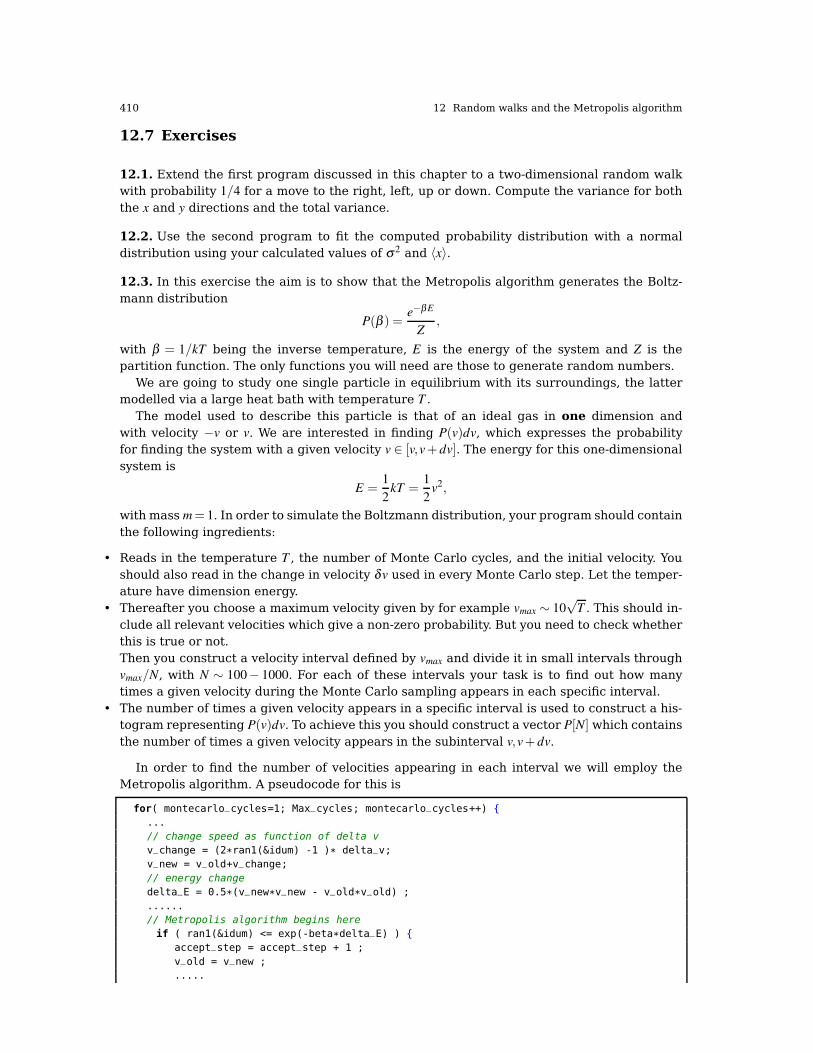
410 12 Random walks and the Metropolis algorithm
12.7 Exercises
12.1. Extend the first program discussed in this chapter to a two-dimensional random walkwith probability 1/4 for a move to the right, left, up or down. Compute the variance for boththe x and y directions and the total variance.
12.2. Use the second program to fit the computed probability distribution with a normaldistribution using your calculated values of σ2 and 〈x〉.
12.3. In this exercise the aim is to show that the Metropolis algorithm generates the Boltz-mann distribution
P(β ) =e−β E
Z,
with β = 1/kT being the inverse temperature, E is the energy of the system and Z is thepartition function. The only functions you will need are those to generate random numbers.
We are going to study one single particle in equilibrium with its surroundings, the lattermodelled via a large heat bath with temperature T .
The model used to describe this particle is that of an ideal gas in one dimension andwith velocity −v or v. We are interested in finding P(v)dv, which expresses the probabilityfor finding the system with a given velocity v ∈ [v,v+ dv]. The energy for this one-dimensionalsystem is
E =1
2kT =
1
2v2,
with mass m= 1. In order to simulate the Boltzmann distribution, your program should containthe following ingredients:
• Reads in the temperature T , the number of Monte Carlo cycles, and the initial velocity. Youshould also read in the change in velocity δv used in every Monte Carlo step. Let the temper-ature have dimension energy.
• Thereafter you choose a maximum velocity given by for example vmax ∼ 10√
T . This should in-clude all relevant velocities which give a non-zero probability. But you need to check whetherthis is true or not.Then you construct a velocity interval defined by vmax and divide it in small intervals throughvmax/N, with N ∼ 100− 1000. For each of these intervals your task is to find out how manytimes a given velocity during the Monte Carlo sampling appears in each specific interval.
• The number of times a given velocity appears in a specific interval is used to construct a his-togram representing P(v)dv. To achieve this you should construct a vector P[N] which containsthe number of times a given velocity appears in the subinterval v,v+ dv.
In order to find the number of velocities appearing in each interval we will employ theMetropolis algorithm. A pseudocode for this is
for( montecarlo_cycles=1; Max_cycles; montecarlo_cycles++)
...
// change speed as function of delta v
v_change = (2*ran1(&idum) -1 )* delta_v;
v_new = v_old+v_change;
// energy change
delta_E = 0.5*(v_new*v_new - v_old*v_old) ;
......
// Metropolis algorithm begins here
if ( ran1(&idum) <= exp(-beta*delta_E) )
accept_step = accept_step + 1 ;
v_old = v_new ;
.....
12.7 Exercises 411
// thereafter we must fill in P[N] as a function of
// the new speed
P[?] = ...
// upgrade mean velocity, energy and variance
...
1. Make your own algorithm which sets up the histogram P(v)dv, find mean velocity, energy 〈E〉,energy variance Var(E) and the number of accepted steps for a given temperature. Study thechange of the number of accepted moves as a function of δv. Compare the final energy withthe closed form result 〈E〉= kT/2 for one dimension. Find also the closed-form expressions forthe energy variance and the mean velocity and compare your calculations with these results.Use T = 4 and set the intial velocity to zero, i.e., v0 = 0. Try different values of δv. Check thefinal result for the energy as a function of the number of Monte Carlo cycles.
2. Repeat the calculation in the previous exercise but using now a normal distribution. Doesthat improve your results compared with the exact expressions?
3. Make thereafter a plot of log(P(v)) as function of E and see if you get a straight line. Commentthe result.
4. In our analysis under [1) we have not discussed how the system reaches the most likely state,that is whether equilibrium has been reached or not. Make a plot of the mean velocity, energy,energy variance and the number of accepted steps for a given temperature as function of thenumber of Monte Carlo samples. Perform these calculations for several temperatures, namelyT = 0.5, T = 1, T = 2 and T = 10 and comment your results. Can you find a rough measure forwhen the most likely state has been reached?
5. The analysis in point [4) is rather rough and obviously user dependent, in the sense that it isvery much up to the user to define when an equilibrium situation has been reached or not. Toimprove upon this, compute the so-called time autocorrelation function defined here as
φ(t) =1
tmax− t
tmax−t
∑t′=0
E(t ′)E(t ′+ t)− 1
tmax− t
tmax−t
∑t′=0
E(t ′)× 1
tmax− t
tmax−t
∑t′=0
E(t ′+ t)
for the mean energy E (t) and plot it as function of the number of Monte Carlo steps for thetemperatures in [c). The time t corresponds to a given number of Monte Carlo cycles. Canyou extract an equilibration measure? How does the correlation time behave as function oftemperature? Comment your results. Be careful in choosing values of t, they should not betoo close to tmax. Compute the autocorrelation function for all temperatures listed in [d) andcompare your results with those in [d). Comment your results.
6. In the previous analysis we computed the time autocorrelation function. This quantity can berelated to the covariance of our measurements. To achieve this you need to store the resultsof all contributions to the measurements of the mean energy and its variance σ2
E given by
σ2E =
1
n2
n
∑k=1
(Ek− E)2 +2
n2 ∑k<l
(Ek− E)(El− E)
Here we assume that n corresponds to the number of Monte Carlo samples in one experi-ment and that we repeat these experiments a given time. We can assume here that we repeatthese experiments m = n times. The value E is the mean energy while Ek,l represent indi-vidual measurements. The first term is the same as the error in the uncorrelated case. Thismeans that the second term accounts for the error correction due to correlation between themeasurements. For uncorrelated measurements this second term is zero.

412 12 Random walks and the Metropolis algorithm
Computationally the uncorrelated first term is much easier to treat efficiently than the sec-ond.
Var(E) =1
n
n
∑k=1
(Ek−〈E〉)2 =
(1
n
n
∑k=1
E2k
)−〈E〉2
We just accumulate separately the values E2k and Ek for every measurement Ek we receive.
The correlation term, though, has to be calculated at the end of the experiment since we needall the measurements to calculate the cross terms. Therefore, all measurements have to bestored throughout the experiment.Let us analyze the problem by splitting up the correlation term into partial sums of the form:
fd =1
n
n−d
∑k=1
(Ek−〈E〉)(Ek+d−〈E〉)
The correlation term of the error can now be rewritten in terms of fd:
2
n∑k<l
(Ek−〈E〉)(El−〈E〉) = 2n−1
∑d=1
fd
The value of fd reflects the correlation between measurements separated by the distance d
in the samples. Notice that for d = 0, f is just the sample variance, Var(E). If we divide fd byVar(E), we arrive at the so called autocorrelation function:
κd =fd
Var(E)
which gives us a useful measure of the correlation pair correlation starting always at 1 ford = 0.The sample variance can now be written in terms of the autocorrelation function:
σ2E =
1
nVar(E)+
2
n·Var(E)
n−1
∑d=1
fd
Var(E)
=
(1+ 2
n−1
∑d=1
κd
)1
nVar(E)
=τ
n·Var(E) (12.18)
and we see that σ2E can be expressed in terms the uncorrelated sample variance times a
correction factor τ which accounts for the correlation between measurements. We call thiscorrection factor the autocorrelation time:
τ = 1+ 2n−1
∑d=1
κd
For a correlation free experiment, τ equals 1. From the point of view of Eq. (12.18) we caninterpret a sequential correlation as an effective reduction of the number of measurementsby a factor τ. The effective number of measurements becomes
neff =n
τ
From the previous exercise you needed to store all experiments Ek in order to compute thetime autocorrelation function. You can reuse these data in this exercise and compute the full

12.7 Exercises 413
variance σ2E , the covariance, the autocorrelation time τ and the effective number of measure-
ments neff. It is sufficient to choose only one of the temperatures. Comment your results. Canyou relate the correlation time τ to what you found [5)? What about the covariance and thetime autocorrelation function?
12.4. The aim of this exercise is to simulate financial transactions among financial agentsusing Monte Carlo methods. The final goal is to extract a distribution of income as functionof the income m. From Pareto’s work (V. Pareto, 1897) it is known from empirical studies thatthe higher end of the distribution of money follows a distribution
wm ∝ m−1−α ,
with α ∈ [1,2]. We will here follow the analysis made by Patriarca et al [72].Here we will study numerically the relation between the microdynamical relations among
financial agents and the resulting macroscopic money distribution.We assume we have N agents that exchange money in pairs (i, j). We assume also that all
agents start with the same amount of money m0 > 0. At a given ’time step’, we choose ran-domly a pair of agents (i, j) and let a transaction take place. This means that agent i’s moneymi changes to m′i and similarly we have m j → m′j. Money is conserved during a transaction,meaning that
mi +m j = m′i +m′j. (12.19)
The change is done via a random reassignement (a random number) ε, meaning that
m′i = ε(mi +m j),
leading tom′j = (1− ε)(mi+m j).
The number ε is extracted from a uniform distribution. In this simple model, no agents are leftwith a debt, that is m≥ 0. Due to the conservation law above, one can show that the systemrelaxes toward an equilibrium state given by a Gibbs distribution
wm = β exp(−β m),
with
β =1
〈m〉 ,
and 〈m〉= ∑i mi/N = m0, the average money. It means that after equilibrium has been reachedthat the majority of agents is left with a small number of money, while the number of richestagents, those with m larger than a specific value m′, exponentially decreases with m′.
We assume that we have N = 500 agents. In each simulation, we need a sufficiently largenumber of transactions, say 107. Our aim is find the final equilibrium distribution wm. Inorder to do that we would need several runs of the above simulations, at least 103− 104 runs(experiments).
a) Your task is to first set up an algorithm which simulates the above transactions with an initialamount m0. The challenge here is to figure out a Monte Carlo simulation based on the aboveequations. You will in particular need to make an algorithm which sets up a histogram asfunction of m. This histogram contains the number of times a value m is registered and rep-resents wm∆m. You will need to set up a value for the interval ∆m (typically 0.01− 0.05). Thatmeans you need to account for the number of times you register an income in the intervalm,m+∆m. The number of times you register this income, represents the value that enters thehistogram. You will also need to find a criterion for when the equilibrium situation has beenreached.

414 12 Random walks and the Metropolis algorithm
b) Make thereafter a plot of log(wm) as function of m and see if you get a straight line. Commentthe result.
c) We can then change our model to allow for a saving criterion, meaning that the agents savea fraction λ of the money they have before the transaction is made. The final distribution willthen no longer be given by Gibbs distribution. It could also include a taxation on financialtransactions.The conservation law of Eq. (12.19) holds, but the money to be shared in a transaction be-tween agent i and agent j is now (1−λ )(mi+m j). This means that we have
m′i = λ mi + ε(1−λ )(mi+m j),
andm′j = λ m j +(1− ε)(1−λ )(mi+m j),
which can be written asm′i = mi + δm
andm′j = m j− δm,
withδm = (1−λ )(εm j− (1− ε)mi),
showing how money is conserved during a transaction. Select values of λ = 0.25,0.5 andλ = 0.9 and try to extract the corresponding equilibrium distributions and compare thesewith the Gibbs distribution. Comment your results. If you have time, see if you can extract aparametrization of the above curves (see Patriarca et al [72])

Chapter 13
Monte Carlo Methods in Statistical Physics
When you are solving a problem, don’t worry. Now, after you have solved the problem, then that’s thetime to worry. Richard Feynman
Abstract The aim of this chapter is to present examples from the physical sciences whereMonte Carlo methods are widely applied. Here we focus on examples from statistical physicsand discuss two of the most studied models, the Ising model and the Potts model for theinteraction among classical spins. These models have been widely used for studies of phasetransitions.
13.1 Introduction and Motivation
Fluctuations play a central role in our understanding of phase transitions. Their behaviornear critical points convey important information about the underlying many-particle inter-actions. In this chapter we will focus on two widely studied models in statistical physics, theIsing model and the Potts model for interacting spins. The main focus is on the Ising model.Both models can exhibit first and second order phase transitions and are perhaps among themost studied systems in statistical physics with respect to simulations of phase transitions.The Norwegian-born chemist Lars Onsager developed in 1944 an ingenious mathematicaldescription of the Ising model [73] meant to simulate a two-dimensional model of a magnetcomposed of many small atomic magnets. This work proved later useful in analyzing othercomplex systems, such as gases sticking to solid surfaces, and hemoglobin molecules thatabsorb oxygen. He got the Nobel prize in chemistry in 1968 for his studies of non-equilibriumthermodynamics. Many people argue he should have received the Nobel prize in physics aswell for his work on the Ising model. Another model we discuss at the end of this chapter is theso-called class of Potts models, which exhibits both first and second order type of phase tran-sitions. Both the Ising model and the Potts model have been used to model phase transitionsin solid state physics, with a particular emphasis on ferromagnetism and antiferromagnetism.
Metals like iron, nickel, cobalt and some of the rare earths (gadolinium, dysprosium) ex-hibit a unique magnetic behavior which is called ferromagnetism because iron (ferrum inLatin) is the most common and most dramatic example. Ferromagnetic materials exhibit along-range ordering phenomenon at the atomic level which causes the unpaired electronspins to line up parallel with each other in a region called a domain. The long range orderwhich creates magnetic domains in ferromagnetic materials arises from a quantum mechani-cal interaction at the atomic level. This interaction is remarkable in that it locks the magneticmoments of neighboring atoms into a rigid parallel order over a large number of atoms inspite of the thermal agitation which tends to randomize any atomic-level order. Sizes of do-
415

416 13 Monte Carlo Methods in Statistical Physics
Fig. 13.1 Example of a cubic lattice with atoms at each corner. Each atom has a finite magnetic momentwhich points in a particular direction..
mains range from a 0.1 mm to a few mm. When an external magnetic field is applied, thedomains already aligned in the direction of this grow at the expense of their neighbors. For agiven ferromagnetic material the long range order abruptly disappears at a certain temper-ature which is called the Curie temperature for the material. The Curie temperature of ironis about 1043 K while metals like cobalt and nickel have a Curie temperature of 1388 K and627 K, respectively, and some of the rare earth metals like gadolinium and dysprosium have293 K and 85 K, respectively. We could think of an actual metal as composed of for example acubic lattice with atoms at each corner with a resulting magnetic moment pointing in a par-ticular direction, as portrayed in Fig. 13.1. In many respects, these atomic magnets are likeordinary magnets and can be thought of in terms of little magnet vectors pointing from southto north poles. The Ising model provides a simple way of describing how a magnetic materialresponds to thermal energy and an external magnetic field. In this model, each domain hasa corresponding spin of north or south. The spins can be thought of as the poles of a barmagnet. The model assigns a value of +1 or -1 to the spins north and south respectively. Thedirection of the spins influences the total potential energy of the system.
Another physical case where the application of the Ising model enjoys considerable successis the description of antiferromagnetism. This is a type of magnetism where adjacent ionsspontaneously align themselves at relatively low temperatures into opposite, or antiparallel,arrangements throughout the material so that it exhibits almost no gross external magnetism.In antiferromagnetic materials, which include certain metals and alloys in addition to someionic solids, the magnetism from magnetic atoms or ions oriented in one direction is canceledout by the set of magnetic atoms or ions that are aligned in the reverse direction.
This spontaneous antiparallel coupling of atomic magnets is disrupted by heating and dis-appears entirely above a certain temperature, called the Néel temperature, characteristicof each antiferromagnetic material. (The Néel temperature is named for Louis Néel, French

13.2 Review of Statistical Physics 417
physicist, who in 1936 gave one of the first explanations of antiferromagnetism.) Some anti-ferromagnetic materials have Néel temperatures at, or even several hundred degrees above,room temperature, but usually these temperatures are lower. The Néel temperature for man-ganese oxide, for example, is 122 K.
Antiferromagnetic solids exhibit special behaviour in an applied magnetic field dependingupon the temperature. At very low temperatures, the solid exhibits no response to the exter-nal field, because the antiparallel ordering of atomic magnets is rigidly maintained. At highertemperatures, some atoms break free of the orderly arrangement and align with the exter-nal field. This alignment and the weak magnetism it produces in the solid reach their peakat the Néel temperature. Above this temperature, thermal agitation progressively preventsalignment of the atoms with the magnetic field, so that the weak magnetism produced in thesolid by the alignment of its atoms continuously decreases as temperature is increased. Forfurther discussion of magnetic properties and solid state physics, see for example the text ofAshcroft and Mermin [74].
As mentioned above, spin models like the Ising and Potts models can be used to modelother systems as well, such as gases sticking to solid surfaces, and hemoglobin moleculesthat absorb oxygen. We sketch such an application in Fig. 13.2.
Fig. 13.2 The open (white) circles at each lattice point can represent a vacant site, while the black circlescan represent the absorption of an atom on a metal surface..
However, before we present the Ising model, we feel it is appropriate to refresh someimportant quantities in statistical physics, such as various definitions of statistical ensembles,their partition functions and relevant variables.
13.2 Review of Statistical Physics
In statistical physics the concept of an ensemble is one of the cornerstones in the definition ofthermodynamical quantities. An ensemble is a collection of microphysics systems from whichwe derive expectations values and thermodynamical properties related to experiment. As anexample, the specific heat (which is a measurable quantity in the laboratory) of a systemof infinitely many particles, can be derived from the basic interactions between the micro-scopic constituents. The latter can span from electrons to atoms and molecules or a systemof classical spins. All these microscopic constituents interact via a well-defined interaction.We say therefore that statistical physics bridges the gap between the microscopic world andthe macroscopic world. Thermodynamical quantities such as the specific heat or net magne-tization of a system can all be derived from a microscopic theory.
There are several types of ensembles, with their pertinent expectaction values and poten-tials. Table 13.1 lists the most used ensembles in statistical physics together with frequently

418 13 Monte Carlo Methods in Statistical Physics
arising extensive (depend on the size of the systems such as the number of particles) andintensive variables (apply to all components of a system), in addition to associated potentials.
Table 13.1 Overview of the most common ensembles and their variables. Here we have define M - to be themagnetization, D - the electric dipole moment, H - the magnetic field and E - to be the electric field. The lasttwo replace the pressure as an intensive variable, while the magnetisation and the dipole moment play thesame role as volume, viz they are extensive variables. The invers temperatur β regulates the mean energywhile the chemical potential µ regulates the mean number of particles.
Microcanonical Canonical Grand canonical Pressure canonical
Exchange of heat no yes yes yeswith the environment
Exchange of particles no no yes nowith the environemt
Thermodynamical V,M ,D V,M ,D V,M ,D P,H ,Eparameters E T T T
N N µ N
Potential Entropy Helmholtz PV Gibbs
Energy Internal Internal Internal Enthalpy
13.2.1 Microcanonical Ensemble
The microcanonical ensemble represents an hypothetically isolated system such as a nucleuswhich does not exchange energy or particles via the environment. The thermodynamicalquantity of interest is the entropy S which is related to the logarithm of the number of pos-sible microscopic states Ω(E) at a given energy E that the system can access. The relationis
S = kBlnΩ .
When the system is in its ground state the entropy is zero since there is only one possibleground state. For excited states, we can have a higher degeneracy than one and thus anentropy which is larger than zero. We may therefore loosely state that the entropy measuresthe degree of order in a system. At low energies, we expect that we have only few stateswhich are accessible and that the system prefers a specific ordering. At higher energies, morestates become accessible and the entropy increases. The entropy can be used to computeobservables such as the temperature
1
kBT=
(∂ logΩ
∂E
)
N,V
,
the pressure

13.2 Review of Statistical Physics 419
p
kBT=
(∂ logΩ
∂V
)
N,E
,
or the chemical potential.µ
kBT=−
(∂ logΩ
∂N
)
V,E
.
It is very difficult to compute the density of states Ω(E) and thereby the partition functionin the microcanonical ensemble at a given energy E, since this requires the knowledge of allpossible microstates at a given energy. This means that calculations are seldomly done in themicrocanonical ensemble. In addition, since the microcanonical ensemble is an isolated sys-tem, it is hard to give a physical meaning to a quantity like the microcanonical temperature.
13.2.2 Canonical Ensemble
One of the most used ensembles is the canonical one, which is related to the microcanoni-cal ensemble via a Legendre transformation. The temperature is an intensive variable in thisensemble whereas the energy follows as an expectation value. In order to calculate expec-tation values such as the mean energy 〈E〉 at a given temperature, we need a probabilitydistribution. It is given by the Boltzmann distribution
Pi(β ) =e−β Ei
Z
with β = 1/kBT being the inverse temperature, kB is the Boltzmann constant, Ei is the energyof a microstate i while Z is the partition function for the canonical ensemble defined as
Z =M
∑i=1
e−β Ei ,
where the sum extends over all microstates M. The potential of interest in this case isHelmholtz’ free energy. It relates the expectation value of the energy at a given temperaturT to the entropy at the same temperature via
F =−kBTlnZ = 〈E〉−TS.
Helmholtz’ free energy expresses the struggle between two important principles in physics,namely the strive towards an energy minimum and the drive towards higher entropy as thetemperature increases. A higher entropy may be interpreted as a larger degree of disorder.When equilibrium is reached at a given temperature, we have a balance between these twoprinciples. The numerical expression is Helmholtz’ free energy. The creation of a macroscopicmagnetic field from a bunch of atom-sized mini-magnets, as shown in Fig. 13.1 results froma careful balance between these two somewhat opposing principles in physics, order vs. dis-order.
In the canonical ensemble the entropy is given by
S = kBlnZ+ kBT
(∂ lnZ
∂T
)
N,V
,
and the pressure by
p = kBT
(∂ lnZ
∂V
)
N,T
.

420 13 Monte Carlo Methods in Statistical Physics
Similarly we can compute the chemical potential as
µ =−kBT
(∂ lnZ
∂N
)
V,T
.
For a system described by the canonical ensemble, the energy is an expectation value sincewe allow energy to be exchanged with the surroundings (a heat bath with temperature T ).
This expectation value, the mean energy, can be calculated using
〈E〉= kBT 2
(∂ lnZ
∂T
)
V,N
or using the probability distribution Pi as
〈E〉=M
∑i=1
EiPi(β ) =1
Z
M
∑i=1
Eie−β Ei.
The energy is proportional to the first derivative of the potential, Helmholtz’ free energy. Thecorresponding variance is defined as
σ2E = 〈E2〉− 〈E〉2 = 1
Z
M
∑i=1
E2i e−β Ei−
(1
Z
M
∑i=1
Eie−β Ei
)2
.
If we divide the latter quantity with kT 2 we obtain the specific heat at constant volume
CV =1
kBT 2
(〈E2〉− 〈E〉2
),
which again can be related to the second derivative of Helmholtz’ free energy. Using the sameprescription, we can also evaluate the mean magnetization through
〈M 〉=M
∑i
MiPi(β ) =1
Z
M
∑i
Mie−β Ei ,
and the corresponding variance
σ2M = 〈M 2〉− 〈M 〉2 = 1
Z
M
∑i=1
M2i e−β Ei−
(1
Z
M
∑i=1
Mie−β Ei
)2
.
This quantity defines also the susceptibility χ
χ =1
kBT
(〈M 2〉− 〈M 〉2
).
13.2.3 Grand Canonical and Pressure Canonical
Two other ensembles which are much used in statistical physics and thermodynamics arethe grand canonical and pressure canonical ensembles. In the first we allow the system (incontact with a large heat bath) to exchange both heat and particles with the environment.The potential is, with a partition function Ξ(V,T,µ) with variables V,T and µ ,
pV = kBT lnΞ ,

13.3 Ising Model and Phase Transitions in Magnetic Systems 421
and the entropy is given by
S = kBlnΞ + kBT
(∂ lnΞ
∂T
)
V,µ
,
while the mean number of particles is
〈N〉= kBT
(∂ lnΞ
∂ µ
)
V,T
.
The pressure is determined as
p = kBT
(∂ lnΞ
∂V
)
µ,T
.
In the pressure canonical ensemble we employ with Gibbs’ free energy as the potential. Itis related to Helmholtz’ free energy via G = F + pV . The partition function is ∆(N, p,T ), withtemperature, pressure and the number of particles as variables. The pressure and volumeterm can be replaced by other external potentials, such as an external magnetic field (or agravitational field) which performs work on the system. Gibbs’ free energy reads
G =−kBT ln∆ ,
and the entropy is given by
S = kBln∆ + kBT
(∂ ln∆
∂T
)
p,N
.
We can compute the volume as
V =−kBT
(∂ ln∆
∂ p
)
N,T
,
and finally the chemical potential
µ =−kBT
(∂ ln∆
∂N
)
p,T
.
In this chapter we work with the canonical ensemble only.
13.3 Ising Model and Phase Transitions in Magnetic Systems
13.3.1 Theoretical Background
The model we will employ in our studies of phase transitions at finite temperature for mag-netic systems is the so-called Ising model. In its simplest form the energy is expressed as
E =−JN
∑<kl>
sksl−B
N
∑k
sk,
with sk =±1, N is the total number of spins, J is a coupling constant expressing the strengthof the interaction between neighboring spins and B is an external magnetic field interactingwith the magnetic moment set up by the spins. The symbol < kl > indicates that we sum overnearest neighbors only. Notice that for J > 0 it is energetically favorable for neighboring spinsto be aligned. This feature leads to, at low enough temperatures, a cooperative phenomenoncalled spontaneous magnetization. That is, through interactions between nearest neighbors,a given magnetic moment can influence the alignment of spins that are separated from the

422 13 Monte Carlo Methods in Statistical Physics
given spin by a macroscopic distance. These long range correlations between spins are asso-ciated with a long-range order in which the lattice has a net magnetization in the absence ofa magnetic field. In our further studies of the Ising model, we will mostly limit the attentionto cases with B = 0 only.
In order to calculate expectation values such as the mean energy 〈E〉 or magnetization 〈M 〉in statistical physics at a given temperature, we need a probability distribution
Pi(β ) =e−β Ei
Z
with β = 1/kT being the inverse temperature, k the Boltzmann constant, Ei is the energy of astate i while Z is the partition function for the canonical ensemble defined as
Z =M
∑i=1
e−β Ei ,
where the sum extends over all microstates M. Pi expresses the probability of finding thesystem in a given configuration i.
The energy for a specific configuration i is given by
Ei =−JN
∑<kl>
sksl .
To better understand what is meant with a configuration, consider first the case of the one-dimensional Ising model with B = 0. In general, a given configuration of N spins in one di-mension may look like
↑ ↑ ↑ . . . ↑ ↓ ↑ . . . ↑ ↓1 2 3 . . . i− 1 i i+ 1 . . . N− 1 N
In order to illustrate these features let us further specialize to just two spins.With two spins, since each spin takes two values only, we have 22 = 4 possible arrangements
of the two spins. These four possibilities are
1 =↑↑ 2 =↑↓ 3 =↓↑ 4 =↓↓
What is the energy of each of these configurations?For small systems, the way we treat the ends matters. Two cases are often used.
1. In the first case we employ what is called free ends. This means that there is no contri-bution from points to the right or left of the endpoints. For the one-dimensional case, theenergy is then written as a sum over a single index
Ei =−JN−1
∑j=1
s js j+1,
If we label the first spin as s1 and the second as s2 we obtain the following expression forthe energy
E =−Js1s2.
The calculation of the energy for the one-dimensional lattice with free ends for one spe-cific spin-configuration can easily be implemented in the following lines
for ( j=1; j < N; j++)
energy += spin[j]*spin[j+1];

13.3 Ising Model and Phase Transitions in Magnetic Systems 423
where the vector spin[] contains the spin value sk = ±1. For the specific state E1, we havechosen all spins up. The energy of this configuration becomes then
E1 = E↑↑ =−J.
The other configurations giveE2 = E↑↓ =+J,
E3 = E↓↑ =+J,
andE4 = E↓↓ =−J.
2. We can also choose so-called periodic boundary conditions. This means that the neighbourto the right of sN is assumed to take the value of s1. Similarly, the neighbour to the left ofs1 takes the value sN . In this case the energy for the one-dimensional lattice reads
Ei =−JN
∑j=1
s js j+1,
and we obtain the following expression for the two-spin case
E =−J(s1s2 + s2s1).
In this case the energy for E1 is different, we obtain namely
E1 = E↑↑ =−2J.
The other cases do also differ and we have
E2 = E↑↓ =+2J,
E3 = E↓↑ =+2J,
andE4 = E↓↓ =−2J.
If we choose to use periodic boundary conditions we can code the above expression as
jm=N;
for ( j=1; j <=N ; j++)
energy += spin[j]*spin[jm];
jm = j ;
The magnetization is however the same, defined as
Mi =N
∑j=1
s j,
where we sum over all spins for a given configuration i.Table 13.2 lists the energy and magnetization for both free ends and periodic boundary
conditions.We can reorganize Table 13.2 according to the number of spins pointing up, as shown
in Table 13.3. It is worth noting that for small dimensions of the lattice, the energy differsdepending on whether we use periodic boundary conditions or free ends. This means alsothat the partition functions will be different, as discussed below. In the thermodynamic limit

424 13 Monte Carlo Methods in Statistical Physics
Table 13.2 Energy and magnetization for the one-dimensional Ising model with N = 2 spins with free ends(FE) and periodic boundary conditions (PBC).
State Energy (FE) Energy (PBC) Magnetization1 =↑↑ −J −2J 22 =↑↓ J 2J 03 =↓↑ J 2J 04 =↓↓ −J −2J -2
Table 13.3 Degeneracy, energy and magnetization for the one-dimensional Ising model with N = 2 spins withfree ends (FE) and periodic boundary conditions (PBC).
Number spins up Degeneracy Energy (FE) Energy (PBC) Magnetization2 1 −J −2J 21 2 J 2J 00 1 −J −2J -2
we have N → ∞, and the final results do not depend on the kind of boundary conditions wechoose.
For a one-dimensional lattice with periodic boundary conditions, each spin sees two neigh-bors. For a two-dimensional lattice each spin sees four neighboring spins. How many neigh-bors does a spin see in three dimensions?
In a similar way, we could enumerate the number of states for a two-dimensional systemconsisting of two spins, i.e., a 2× 2 Ising model on a square lattice with periodic boundaryconditions. In this case we have a total of 24 = 16 states. Some examples of configurationswith their respective energies are listed here
E =−8J↑ ↑↑ ↑ E = 0
↑ ↑↑ ↓ E = 0
↓ ↓↑ ↓ E =−8J
↓ ↓↓ ↓
In the Table 13.4 we group these configurations according to their total energy and mag-netization.
Table 13.4 Energy and magnetization for the two-dimensional Ising model with N = 2×2 spins with periodicboundary conditions.
Number spins up Degeneracy Energy Magnetization4 1 −8J 43 4 0 22 4 0 02 2 8J 01 4 0 -20 1 −8J -4
For the one-dimensional Ising model we can compute rather easily the exact partitionfunction for a system of N spins. Let us consider first the case with free ends. The energyreads
E =−JN−1
∑j=1
s js j+1.

13.3 Ising Model and Phase Transitions in Magnetic Systems 425
The partition function for N spins is given by
ZN = ∑s1=±1
. . . ∑sN=±1
exp(β JN−1
∑j=1
s js j+1),
and since the last spin occurs only once in the last sum in the exponential, we can single outthe last spin as follows
∑sN=±1
exp(β JsN−1sN) = 2cosh(β J).
The partition function consists then of a part from the last spin and one from the remainingspins resulting in
ZN = ZN−12cosh(β J).
We can repeat this process and obtain
ZN = (2cosh(β J))N−2Z2,
with Z2 given byZ2 = ∑
s1=±1∑
s2=±1
exp(β Js1s2) = 4cosh(β J),
resulting inZN = 2(2cosh(β J))N−1.
In the thermodynamical limit where we let N→∞, the way we treat the ends does not matter.However, since our computations will always be carried out with a limited value of N, weneed to consider other boundary conditions as well. Here we limit the attention to periodicboundary conditions.
If we use periodic boundary conditions, the partition function is given by
ZN = ∑s1=±1
. . . ∑sN=±1
exp(β JN
∑j=1
s js j+1),
where the sum in the exponential runs from 1 to N since the energy is defined as
E =−JN
∑j=1
s js j+1.
We can then rewrite the partition function as
ZN = ∑si=±1
N
∏i=1
exp(β Jsisi+1),
where the first sum is meant to represent all lattice sites. Introducing the matrix T (the so-called transfer matrix)
T =
(eβ J e−β J
e−β J eβ J
),
with matrix elements t11 = eβ J, t1−1 = e−β J, t−11 = eβ J and t−1−1 = eβ J we can rewrite the parti-tion function as
ZN = ∑si=±1
Ts1s2Ts2s3
. . . TsNs1= TrTN .
The 2× 2 matrix T is easily diagonalized with eigenvalues λ1 = 2cosh(β J) and λ2 = 2sinh(β J).Similarly, the matrix TN has eigenvalues λ N
1 and λ N2 and the trace of TN is just the sum over

426 13 Monte Carlo Methods in Statistical Physics
eigenvalues resulting in a partition function
ZN = λ N1 +λ N
2 = 2N([cosh(β J)]N +[sinh(β J)]N
).
In the limit N→∞ the two partition functions with free ends and periodic boundary conditionsagree, see below for a demonstration.
In the development phase of an algorithm and its pertinent code it is always useful to testthe numerics against closed-form results. It is therefore instructive to compute propertieslike the internal energy and the specific heat for these two cases and test the results againstthose produced by our code. We can then calculate the mean energy with free ends from theabove formula for the partition function using
〈E〉=−∂ lnZ
∂β=−(N− 1)Jtanh(β J).
Helmholtz’s free energy is given by
F =−kBT lnZN =−NkBT ln(2cosh(β J)) .
If we take our simple system with just two spins in one-dimension, we see immediately thatthe above expression for the partition function is correct. Using the definition of the partitionfunction we have
Z2 =2
∑i=1
e−β Ei = 2e−β J + 2eβ J = 4cosh(β J)
If we take the limit T → 0 (β → ∞) and set N = 2, we obtain
limβ→∞〈E〉=−J
eJβ − e−Jβ
eJβ + e−Jβ=−J,
which is the energy where all spins point in the same direction. At low T , the system tendstowards a state with the highest possible degree of order.
The specific heat in one-dimension with free ends is
CV =1
kT 2
∂ 2
∂β 2lnZN = (N− 1)k
(β J
cosh(β J)
)2
.
Note well that this expression for the specific heat from the one-dimensional Ising model doesnot diverge or exhibit discontinuities, as can be seen from Fig. 13.3.
In one dimension we do not have a second order phase transition, although this is predictedby mean field models [57].
We can repeat this exercise for the case with periodic boundary conditions as well.Helmholtz’s free energy is in this case
F =−kBT ln(λ N1 +λ N
2 ) =−kBT
Nln(λ1)+ ln
(1+(
λ2
λ1
)N
),
which in the limit N → ∞ results in F = −kBTNln(λ1) as in the case with free ends. Sinceother thermodynamical quantities are related to derivatives of the free energy, all observablesbecome identical in the thermodynamic limit.
Hitherto we have limited ourselves to studies of systems with zero external magnetic field,viz B = 0. We will mostly study systems which exhibit a spontaneous magnitization. It ishowever instructive to extend the one-dimensional Ising model to B 6= 0, yielding a partition

13.3 Ising Model and Phase Transitions in Magnetic Systems 427
0
0.05
0.1
0.15
0.2
0.25
0.3
0.35
0.4
0.45
0 1 2 3 4 5 6 7
CV
Inverse Temperature β J
Fig. 13.3 Heat capacity per spin (CV /(N−1)kB as function of inverse temperature β for the one-dimensionalIsing model.
function (with periodic boundary conditions)
ZN = ∑s1=±1
. . . ∑sN=±1
exp(βN
∑j=1
(Js js j+1 +B
2(s j + s j+1)),
which yields a new transfer matrix with matrix elements t11 = eβ (J+B), t1−1 = e−β J, t−11 = eβ J
and t−1−1 = eβ (J−B) with eigenvalues
λ1 = eβ Jcosh(β J)+ (e2β Jsinh2(βB)+ e−2β J)1/2,
andλ1 = eβ Jcosh(β J)− (e2β Jsinh2(βB)+ e−2β J)1/2.
The partition function is given by ZN = λ N1 +λ N
2 and in the thermodynamic limit we obtain thefollowing free energy
F =−NkBT ln(
eβ Jcosh(β J)+ (e2β Jsinh2(βB)+ e−2β J)1/2).
It is now useful to compute the expectation value of the magnetisation per spin
〈M /N〉= 1
NZ
M
∑i
Mie−β Ei =− 1
N
∂F
∂B,
resulting in
〈M /N〉= sinh(βB)(sinh2(βB)+ e−2β J)1/2
) .
We see that for B = 0 the magnetisation is zero. This means that for a one-dimensional Isingmodel we cannot have a spontaneous magnetization. For the two-dimensional model however,see the discussion below, the Ising model exhibits both a spontaneous magnetisation and aspecific heat and susceptibility which are discontinuous or even diverge. However, except forthe simplest case such as 2× 2 lattice of spins, with the following partition function

428 13 Monte Carlo Methods in Statistical Physics
Z = 2e−8Jβ + 2e8Jβ + 12,
and resulting mean energy
〈E〉=− J
Z
(16e8Jβ − 16e−8Jβ
),
it is a highly non-trivial task to find the closed-form expression for ZN in the thermodynamiclimit. The closed-form expression for the Ising model in two dimensions was obtained via amathematical tour de force in 1944 by the Norwegian chemist Lars Onsager [73]. The exactpartition function for N spins in two dimensions and with zero magnetic field B is given by
ZN =[2cosh(β J)eI
]N,
with
I =1
2π
∫ π
0dφ ln
[1
2
(1+(1−κ2sin2φ)1/2
)],
andκ = 2sinh(2β J)/cosh2(2β J).
The resulting energy is given by
〈E〉=−Jcoth(2β J)
[1+
2
π(2tanh2(2β J)− 1)K1(q)
],
with q = 2sinh(2β J)/cosh2(2β J) and the complete elliptic integral of the first kind
K1(q) =
∫ π/2
0
dφ√1− q2sin2φ
.
Differentiating once more with respect to temperature we obtain the specific heat given by
CV =4kB
π(β Jcoth(2β J))2
K1(q)−K2(q)− (1− tanh2(2β J))
[π
2+(2tanh2(2β J)− 1)K1(q)
],
(13.1)where
K2(q) =
∫ π/2
0dφ√
1− q2sin2φ , (13.2)
is the complete elliptic integral of the second kind. Near the critical temperature TC thespecific heat behaves as
CV ≈−2
π
(2J
kBTC
)2
ln
∣∣∣∣1−T
TC
∣∣∣∣+ const. (13.3)
In theories of critical phenomena one ca show that for temperatures T below a criticaltemperature TC, the heat capacity scales as [75]
CV ∼∣∣∣∣1−
T
TC
∣∣∣∣−α
,
and Onsager’s result is a special case of this power law behavior. The limiting form of thefunction
limα→01
α(Y−α − 1) =−lnY,
can be used to infer that the closed-form result is a special case of the power law singularitywith α = 0.
Similar relations applies to other expectation values. An example is the the spontaneousmagnetisation per spin. This quantity is also highly non-trivial to compute. Here we simply

13.4 Phase Transitions and Critical Phenomena 429
limit ourselves to list Onsager’s result
〈M (T )/N〉=[
1− (1− tanh2(β J))4
16tanh4(β J)
]1/8
,
for T < TC. For T > TC the magnetization is zero. From theories of critical phenomena one canshow that the magnetization behaves as T → TC from below
〈M (T )/N〉 ∼ (TC−T)1/8.
The susceptibility behaves asχ(T )∼ |TC−T |−7/4.
Before we proceed, we need to say some words about phase transitions and critical phe-nomena.
13.4 Phase Transitions and Critical Phenomena
A phase transition is marked by abrupt macroscopic changes as external parameters arechanged, such as an increase of temperature. The point where a phase transition takes placeis called a critical point.
We distinguish normally between two types of phase transitions; first-order transitions andsecond-order transitions. An important quantity in studies of phase transitions is the so-calledcorrelation length ξ and various correlations functions like spin-spin correlations. For theIsing model we shall show below that the correlation length is related to the spin-correlationfunction, which again defines the magnetic susceptibility. The spin-correlation function isnothing but the covariance and expresses the degree of correlation between spins.
The correlation length defines the length scale at which the overall properties of a materialstart to differ from its bulk properties. It is the distance over which the fluctuations of the mi-croscopic degrees of freedom (for example the position of atoms) are significantly correlatedwith each other. Usually it is of the order of few interatomic spacings for a solid. The correla-tion length ξ depends however on external conditions such as pressure and temperature.
First order/discontinuous phase transitions are characterized by two or more states oneither side of the critical point that can coexist at the critical point. As we pass throughthe critical point we observe a discontinuous behavior of thermodynamical functions. Thecorrelation length is normally finite at the critical point. Phenomena such as hysteris occur,viz. there is a continuation of state below the critical point into one above the critical point.This continuation is metastable so that the system may take a macroscopically long time toreadjust. A classical example is the melting of ice. It takes a specific amount of time beforeall the ice has melted. The temperature remains constant and water and ice can coexist fora macroscopic time. The energy shows a discontinuity at the critical point, reflecting the factthat a certain amount of heat is needed in order to melt all the ice
Second order or continuous transitions are different and in general much difficult to un-derstand and model. The correlation length diverges at the critical point, fluctuations arecorrelated over all distance scales, which forces the system to be in a unique critical phase.The two phases on either side of the critical point become identical. The disappearance of aspontaneous magnetization is a classical example of a second-order phase transitions. Struc-tural transitions in solids are other types of second-order phase transitions. Strong correla-tions make a perturbative treatment impossible. From a theoretical point of view, the way

430 13 Monte Carlo Methods in Statistical Physics
out is renormalization group theory [75–81]. Table 13.5 lists some typical system with theirpertinent order parameters.
Table 13.5 Examples of various phase transitions with respective order parameters.
System Transition Order Parameter
Liquid-gas Condensation/evaporation Density difference ∆ρ = ρliquid−ρgas
Binary liquid mixture/Unmixing Composition differenceQuantum liquid Normal fluid/superfluid < φ >, ψ = wavefunctionLiquid-solid Melting/crystallisation Reciprocal lattice vector
Magnetic solid Ferromagnetic Spontaneous magnetisation M
Antiferromagnetic Sublattice magnetisation M
Dielectric solid Ferroelectric Polarization P
Antiferroelectric Sublattice polarisation P
Using Ehrenfest’s definition of the order of a phase transition we can relate the behavioraround the critical point to various derivatives of the thermodynamical potential. In thecanonical ensemble we are using, the thermodynamical potential is Helmholtz’ free energy
F = 〈E〉−TS =−kT lnZ
meaning lnZ =−F/kT =−Fβ . The energy is given as the first derivative of F
〈E〉=−∂ lnZ
∂β=
∂ (β F)
∂β.
and the specific heat is defined via the second derivative of F
CV =− 1
kT 2
∂ 2(β F)
∂β 2.
We can relate observables to various derivatives of the partition function and the free energy.When a given derivative of the free energy or the partition function is discontinuous or di-verges (logarithmic divergence for the heat capacity from the Ising model) we talk of a phasetransition of order of the derivative. A first-order phase transition is recognized in a discon-tinuity of the energy, or the first derivative of F . The Ising model exhibits a second-orderphase transition since the heat capacity diverges. The susceptibility is given by the secondderivative of F with respect to external magnetic field. Both these quantities diverge.
13.4.1 The Ising Model and Phase Transitions
The Ising model in two dimensions with B = 0 undergoes a phase transition of second order.What it actually means is that below a given critical temperature TC, the Ising model exhibitsa spontaneous magnetization with 〈M 〉 6= 0. Above TC the average magnetization is zero.The mean magnetization approaches zero at TC with an infinite slope. Such a behavior is anexample of what are called critical phenomena [78,80,82]. A critical phenomenon is normally

13.4 Phase Transitions and Critical Phenomena 431
marked by one or more thermodynamical variables which vanish above a critical point. In ourcase this is the mean magnetization 〈M 〉 6= 0. Such a parameter is normally called the orderparameter.
Critical phenomena have been extensively studied in physics. One major reason is thatwe still do not have a satisfactory understanding of the properties of a system close to acritical point. Even for the simplest three-dimensional systems we cannot predict exactly thevalues of various thermodynamical variables. Simplified theoretical approaches like mean-field models discussed below, can even predict the wrong physics. Mean-field theory resultsin a second-order phase transition for the one-dimensional Ising model, whereas we saw inthe previous section that the one-dimensional Ising model does not predict any spontaneousmagnetization at any finite temperature. The physical reason for this can be understood fromthe following simple consideration. Assume that the ground state for an N-spin system in onedimension is characterized by the following configuration
↑ ↑ ↑ . . . ↑ ↑ ↑ . . . ↑ ↑1 2 3 . . . i− 1 i i+ 1 . . . N− 1 N
which has a total energy −NJ and magnetization N, where we used periodic boundary condi-tions. If we flip half of the spins we obtain a possible configuration where the first half of thespins point upwards and the last half points downwards we arrive at the configuration
↑ ↑ ↑ . . . ↑ ↑ ↓ . . . ↓ ↓1 2 3 . . . N/2− 1 N/2 N/2+ 1 . . . N− 1 N
with energy (−N + 4)J and net magnetization zero. This state is an example of a possibledisordered state with net magnetization zero. The change in energy is however too small tostabilize the disordered state. There are many other such states with net magnetization zerowith energies slightly larger than the above case. But it serves to demonstrate our point, wecan namely build states at low energies compared with the ordered state with net magne-tization zero. And the energy difference between the ground state is too small to stabilizethe system. In two dimensions however the excitation energy to a disordered state is muchhigher, and this difference can be sufficient to stabilize the system. In fact, the Ising modelexhibits a phase transition to a disordered phase both in two and three dimensions.
For the two-dimensional case, we move from a phase with finite magnetization 〈M 〉 6= 0 toa paramagnetic phase with 〈M 〉= 0 at a critical temperature TC. At the critical temperature,quantities like the heat capacity CV and the susceptibility χ are discontinuous or diverge atthe critical point in the thermodynamic limit, i.e., with an infinitely large lattice. This meansthat the variance in energy and magnetization are discontinuous or diverge. For a finite latticehowever, the variance will always scale as∼ 1/
√M, M being e.g., the number of configurations
which in our case is proportional with L, the number of spins in a the x and y directions. Thetotal number of spins is N = L×L resulting in a total of M = 2N microstates. Since our latticeswill always be of a finite dimensions, the calculated CV or χ will not exhibit a divergingbehavior. We will however notice a broad maximum in e.g., CV near TC. This maximum, asdiscussed below, becomes sharper and sharper as L is increased.
Near TC we can characterize the behavior of many physical quantities by a power lawbehavior (below we will illustrate this in a qualitative way using mean-field theory).
We showed in the previous section that the mean magnetization is given by (for tempera-ture below TC)
〈M (T )〉 ∼ (T −TC)β ,
where β = 1/8 is a so-called critical exponent. A similar relation applies to the heat capacity
CV (T )∼ |TC−T |−α ,

432 13 Monte Carlo Methods in Statistical Physics
and the susceptibilityχ(T )∼ |TC−T |−γ ,
with α = 0 and γ = −7/4. Another important quantity is the correlation length, which is ex-pected to be of the order of the lattice spacing for T is close to TC. Because the spins becomemore and more correlated as T approaches TC, the correlation length increases as we getcloser to the critical temperature. The discontinuous behavior of the correlation ξ near TC is
ξ (T )∼ |TC−T |−ν . (13.4)
A second-order phase transition is characterized by a correlation length which spans thewhole system. The correlation length is typically of the order of some few interatomic dis-tances. The fact that a system like the Ising model, whose energy is described by the inter-action between neighboring spins only, can yield correlation lengths of macroscopic size at acritical point is still a feature which is not properly understood. Stated differently, how canthe spins propagate their correlations so extensively when we approach the critical point, inparticular since the interaction acts only between nearest spins? Below we will compute thecorrelation length via the spin-sin correlation function for the one-dimensional Ising model.
In our actual calculations of the two-dimensional Ising model, we are however always lim-ited to a finite lattice and ξ will be proportional with the size of the lattice at the critical point.Through finite size scaling relations [75, 78–80] it is possible to relate the behavior at finitelattices with the results for an infinitely large lattice. The critical temperature scales then as
TC(L)−TC(L = ∞) ∝ aL−1/ν , (13.5)
with a a constant and ν defined in Eq. (13.4). The correlation length for a finite lattice sizecan then be shown to be proportional to
ξ (T ) ∝ L∼ |TC−T |−ν .
and if we set T = TC one can obtain the following relations for the magnetization, energy andsusceptibility for T ≤ TC
〈M (T )〉 ∼ (T −TC)β ∝ L−β/ν ,
CV (T )∼ |TC−T |−γ ∝ Lα/ν ,
andχ(T )∼ |TC−T |−α ∝ Lγ/ν .
13.4.2 Critical Exponents and Phase Transitions from Mean-field
Models
In order to understand the above critical exponents, we will derive some of the above relationsusing what is called mean-field theory.
In studies of phase transitions we are interested in minimizing the free energy by varyingthe average magnetisation, which is the order parameter for the Ising model. The magnetiza-tion disappears at TC.
Here we use mean field theory to model the free energy F. In mean field theory the localmagnetisation is a treated as a constant and all effects from fluctuations are neglected. Stateddifferently, we reduce a complicated system of many interacting spins to a set of equationsfor each spin. Each spin sees now a mean field which is set up by the surrounding spins. Weneglect therefore the role of spin-spin correlations. A way to achieve this is to rewrite the

13.4 Phase Transitions and Critical Phenomena 433
interaction between two spins at sites i and j, respectively, by adding and subtracting themean value of the spin 〈S〉, that is
SiS j = (Si−〈S〉+ 〈S〉)(Si−〈S〉+ 〈S〉)≈ 〈S〉2 + 〈S〉(Si−〈S〉)+ 〈S〉(S j−〈S〉),
where we have ignored terms of the order (Si−〈S〉)(Si−〈S〉). These are the terms which leadto correlations between neighbouring spins. In mean field theory we ignore correlations.
This means that we can rewrite the Hamiltonian
E =−JN
∑<i j>
SkSl−BN
∑i
Si,
asE =−J ∑
<i j>
〈S〉2 + 〈S〉(Si−〈S〉)+ 〈S〉(S j−〈S〉)−B∑i
Si,
resulting inE =−(B+ zJ〈S〉)∑
i
Si + zJ〈S〉2,
with z the number of nearest neighbours for a given site i. We have included the externalmagnetic field B for completeness.
We can then define an effective field which all spins see, namely
Beff = (B+ zJ〈S〉).
To obtain the vaue of 〈S〉) we employ again our results from the canonical ensemble. Thepartition function reads in this case
Z = e−NzJ〈S〉2/kT (2cosh(Beff/kT ))N ,
with a free energy
F =−kT lnZ =−NkTln(2)+NzJ〈S〉2−NkTln(cosh(Beff/kT ))
and minimizing F with respect to 〈S〉 we arrive at
〈S〉= tanh(2cosh(Beff/kT )) .
Close to the phase transition we expect 〈S〉 to become small and eventually vanish. We canthen expand F in powers of 〈S〉 as
F =−NkT ln(2)+NzJ〈s〉2−NkT −BN〈s〉+NkT
(1
2〈s〉2 + 1
12〈s〉4 + . . .
),
and using 〈M〉 = N〈S〉 we can rewrite Helmholtz free energy as
F = F0−B〈M〉+ 1
2a〈M〉2 + 1
4b〈M〉4 + . . .
Let 〈M〉 = m and
F = F0 +1
2am2 +
1
4bm4 +
1
6cm6
F has a minimum at equilibrium F ′(m) = 0 and F ′′(m)> 0
F ′(m) = 0 = m(a+ bm2+ cm4),

434 13 Monte Carlo Methods in Statistical Physics
and if we assume that m is real we have two solutions
m = 0,
or
m2 =b
2c
(−1±
√1− 4ac/b2
).
This relation can be used to describe both first and second-order phase transitions. Herewe consider the second case. We assume that b > 0 and let a≪ 1 since we want to study aperturbation around m = 0. We reach the critical point when a = 0, that is
m2 =b
2c
(−1±
√1− 4ac/b2
)≈−a/b.
We define the temperature dependent function
a(T ) = α(T −TC),
with α > 0 and TC being the critical temperature where the magnetization vanishes. If a isnegative we have two solutions
m =±√−a/b =±
√α(TC−T )
b,
meaning that m evolves continuously to the critical temperature where F = 0 for T ≤ TC
We can now compute the entropy as follows
S =−(
∂F
∂T
).
For T ≥ TC we have m = 0 and
S =−(
∂F0
∂T
),
and for T ≤ TC
S =−(
∂F0
∂T
)−α2(TC−T)/2b,
and we see that there is a smooth crossover at TC.In theories of critical phenomena one has that
CV ∼∣∣∣∣1−
T
TC
∣∣∣∣−α
,
and Onsager’s result is a special case of this power law behavior. The limiting form of thefunction
limα→0
1
α(Y−α − 1) =− log(Y ),
meaning that the closed-form result is a special case of the power law singularity with α = 0.
13.5 The Metropolis Algorithm and the Two-dimensional Ising Model
We switch now back to the Ising model in two dimensions and explore how to write a pro-gram that will allow us to compute various thermodynamical quantities. The algorithm of

13.5 The Metropolis Algorithm and the Two-dimensional Ising Model 435
choice for solving the Ising model is the approach proposed by Metropolis et al. [83] in 1953.As discussed in chapter 12, new configurations are generated from a previous one using atransition probability which depends on the energy difference between the initial and finalstates.
In our case we have as the Monte Carlo sampling function the probability for finding thesystem in a state s given by
Ps =e−(β Es)
Z,
with energy Es, β = 1/kT and Z is a normalization constant which defines the partition functionin the canonical ensemble. As discussed above
Z(β ) = ∑s
e−(β Es)
is difficult to compute since we need all states. In a calculation of the Ising model in twodimensions, the number of configurations is given by 2N with N = L×L the number of spinsfor a lattice of length L. Fortunately, the Metropolis algorithm considers only ratios betweenprobabilities and we do not need to compute the partition function at all. The algorithm goesas follows
1. Establish an initial state with energy Eb by positioning yourself at a random configu-ration in the lattice
2. Change the initial configuration by flipping e.g., one spin only. Compute the energyof this trial state Et .
3. Calculate ∆E = Et −Eb. The number of values ∆E is limited to five for the Ising modelin two dimensions, see the discussion below.
4. If ∆E ≤ 0 we accept the new configuration, meaning that the energy is lowered andwe are hopefully moving towards the energy minimum at a given temperature. Go tostep 7.
5. If ∆E > 0, calculate w = e−(β ∆E).6. Compare w with a random number r. If
r ≤ w,
then accept the new configuration, else we keep the old configuration.7. The next step is to update various expectations values.8. The steps (2)-(7) are then repeated in order to obtain a sufficently good representation
of states.9. Each time you sweep through the lattice, i.e., when you have summed over all spins,
constitutes what is called a Monte Carlo cycle. You could think of one such cycle as ameasurement. At the end, you should divide the various expectation values with thetotal number of cycles. You can choose whether you wish to divide by the number ofspins or not. If you divide with the number of spins as well, your result for e.g., theenergy is now the energy per spin.
The crucial step is the calculation of the energy difference and the change in magneti-zation. This part needs to be coded in an as efficient as possible way since the change inenergy is computed many times. In the calculation of the energy difference from one spinconfiguration to the other, we will limit the change to the flipping of one spin only. For theIsing model in two dimensions it means that there will only be a limited set of values for ∆E.

436 13 Monte Carlo Methods in Statistical Physics
Actually, there are only five possible values. To see this, select first a random spin positionx,y and assume that this spin and its nearest neighbors are all pointing up. The energy forthis configuration is E = −4J. Now we flip this spin as shown below. The energy of the newconfiguration is E = 4J, yielding ∆E = 8J.
E =−4J
↑↑ ↑ ↑↑
=⇒ E = 4J
↑↑ ↓ ↑↑
The four other possibilities are as follows
E =−2J
↑↓ ↑ ↑↑
=⇒ E = 2J
↑↓ ↓ ↑↑
with ∆E = 4J,
E = 0
↑↓ ↑ ↑↓
=⇒ E = 0
↑↓ ↓ ↑↓
with ∆E = 0,
E = 2J
↓↓ ↑ ↑↓
=⇒ E =−2J
↓↓ ↓ ↑↓
with ∆E =−4J and finally
E = 4J
↓↓ ↑ ↓↓
=⇒ E =−4J
↓↓ ↓ ↓↓
with ∆E =−8J. This means in turn that we could construct an array which contains all valuesof eβ ∆E before doing the Metropolis sampling. Else, we would have to evaluate the exponen-tial at each Monte Carlo sampling. For the two-dimensional Ising model there are only fivepossible values. It is rather easy to convice oneself that for the one-dimensional Ising modelwe have only three possible values. The main part of the Ising model program is shown here(there is also a corresponding Fortran program).
http://folk.uio.no/mhjensen/compphys/programs/chapter13/cpp/ising_2dim.cpp
/*Program to solve the two-dimensional Ising model
The coupling constant J = 1
Boltzmann's constant = 1, temperature has thus dimension energy
Metropolis sampling is used. Periodic boundary conditions.
*/
#include <iostream>
#include <fstream>
#include <iomanip>
#include "lib.h"
using namespace std;
ofstream ofile;
// inline function for periodic boundary conditions
inline int periodic(int i, int limit, int add)
return (i+limit+add) % (limit);
// Function to read in data from screen
void read_input(int&, int&, double&, double&, double&);
// Function to initialise energy and magnetization

13.5 The Metropolis Algorithm and the Two-dimensional Ising Model 437
void initialize(int, double, int **, double&, double&);
// The metropolis algorithm
void Metropolis(int, long&, int **, double&, double&, double *);
// prints to file the results of the calculations
void output(int, int, double, double *);
// main program
int main(int argc, char* argv[])
char *outfilename;
long idum;
int **spin_matrix, n_spins, mcs;
double w[17], average[5], initial_temp, final_temp, E, M, temp_step;
// Read in output file, abort if there are too few command-line arguments
if( argc <= 1 )
cout << "Bad Usage: " << argv[0] <<
" read also output file on same line" << endl;
exit(1);
else
outfilename=argv[1];
ofile.open(outfilename);
// Read in initial values such as size of lattice, temp and cycles
read_input(n_spins, mcs, initial_temp, final_temp, temp_step);
spin_matrix = (int**) matrix(n_spins, n_spins, sizeof(int));
idum = -1; // random starting point
for ( double temp = initial_temp; temp <= final_temp; temp+=temp_step)
// initialise energy and magnetization
E = M = 0.;
// setup array for possible energy changes
for( int de =-8; de <= 8; de++) w[de+8] = 0;
for( int de =-8; de <= 8; de+=4) w[de+8] = exp(-de/temp);
// initialise array for expectation values
for( int i = 0; i < 5; i++) average[i] = 0.;
initialize(n_spins, double temp, spin_matrix, E, M);
// start Monte Carlo computation
for (int cycles = 1; cycles <= mcs; cycles++)
Metropolis(n_spins, idum, spin_matrix, E, M, w);
// update expectation values
average[0] += E; average[1] += E*E;
average[2] += M; average[3] += M*M; average[4] += fabs(M);
// print results
output(n_spins, mcs, temp, average);
free_matrix((void **) spin_matrix); // free memory
ofile.close(); // close output file
return 0;
The array w[17] contains values of ∆E spanning from −8J to 8J and it is precalculated in themain part for every new temperature. The program takes as input the initial temperature,final temperature, a temperature step, the number of spins in one direction (we force thelattice to be a square lattice, meaning that we have the same number of spins in the x andthe y directions) and the number of Monte Carlo cycles. For every Monte Carlo cycle werun through all spins in the lattice in the function metropolis and flip one spin at the timeand perform the Metropolis test. However, every time we flip a spin we need to compute theactual energy difference ∆E in order to access the right element of the array which stores

438 13 Monte Carlo Methods in Statistical Physics
eβ ∆E . This is easily done in the Ising model since we can exploit the fact that only one spinis flipped, meaning in turn that all the remaining spins keep their values fixed. The energydifference between a state E1 and a state E2 with zero external magnetic field is
∆E = E2−E1 = JN
∑<kl>
s1ks1
l − JN
∑<kl>
s2ks2
l ,
which we can rewrite as
∆E =−JN
∑<kl>
s2k(s
2l − s1
l ),
where the sum now runs only over the nearest neighbors k of the spin Since the spin to beflipped takes only two values, s1
l =±1 and s2l =±1, it means that if s1
l = 1, then s2l = −1 and if
s1l =−1, then s2
l = 1. The other spins keep their values, meaning that s1k = s2
k . If s1l = 1 we must
have s1l − s2
l = 2, and if s1l =−1 we must have s1
l − s2l = −2. From these results we see that the
energy difference can be coded efficiently as
∆E = 2Js1l
N
∑<k>
sk, (13.6)
where the sum runs only over the nearest neighbors k of spin l. We can compute the changein magnetisation by flipping one spin as well. Since only spin l is flipped, all the surround-ing spins remain unchanged. The difference in magnetisation is therefore only given by thedifference s1
l − s2l =±2, or in a more compact way as
M2 = M1 + 2s2l , (13.7)
where M1 and M2 are the magnetizations before and after the spin flip, respectively. Eqs. (13.6)and (13.7) are implemented in the function metropolis shown here
void Metropolis(int n_spins, long& idum, int **spin_matrix, double& E, double&M, double *w)
// loop over all spins
for(int y =0; y < n_spins; y++)
for (int x= 0; x < n_spins; x++)
// Find random position
int ix = (int) (ran1(&idum)*(double)n_spins);
int iy = (int) (ran1(&idum)*(double)n_spins);
int deltaE = 2*spin_matrix[iy][ix]*(spin_matrix[iy][periodic(ix,n_spins,-1)]+
spin_matrix[periodic(iy,n_spins,-1)][ix] +
spin_matrix[iy][periodic(ix,n_spins,1)] +
spin_matrix[periodic(iy,n_spins,1)][ix]);
// Here we perform the Metropolis test
if ( ran1(&idum) <= w[deltaE+8] )
spin_matrix[iy][ix] *= -1; // flip one spin and accept new spin config
// update energy and magnetization
M += (double) 2*spin_matrix[iy][ix];
E += (double) deltaE;
// end of Metropolis sampling over spins
Note that we loop over all spins but that we choose the lattice positions x and y randomly.If the move is accepted after performing the Metropolis test, we update the energy and the
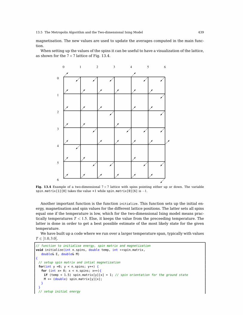
13.5 The Metropolis Algorithm and the Two-dimensional Ising Model 439
magnetisation. The new values are used to update the averages computed in the main func-tion.
When setting up the values of the spins it can be useful to have a visualization of the lattice,as shown for the 7× 7 lattice of Fig. 13.4.
0 1 2 3 4 5 6
0
1
2
3
4
5
6
Fig. 13.4 Example of a two-dimensional 7× 7 lattice with spins pointing either up or down. The variablespin_matrix[1][0] takes the value +1 while spin_matrix[0][6] is −1.
Another important function is the function initialize. This function sets up the initial en-ergy, magnetisation and spin values for the different lattice positions. The latter sets all spinsequal one if the temperature is low, which for the two-dimensional Ising model means prac-tically temperatures T < 1.5. Else, it keeps the value from the preceeding temperature. Thelatter is done in order to get a best possible estimate of the most likely state for the giventemperature.
We have built up a code where we run over a larger temperature span, typically with valuesT ∈ [1.0,3.0].
// function to initialise energy, spin matrix and magnetization
void initialize(int n_spins, double temp, int **spin_matrix,
double& E, double& M)
// setup spin matrix and intial magnetization
for(int y =0; y < n_spins; y++)
for (int x= 0; x < n_spins; x++)
if (temp < 1.5) spin_matrix[y][x] = 1; // spin orientation for the ground state
M += (double) spin_matrix[y][x];
// setup initial energy

440 13 Monte Carlo Methods in Statistical Physics
for(int y =0; y < n_spins; y++)
for (int x= 0; x < n_spins; x++)
E -= (double) spin_matrix[y][x]*(spin_matrix[periodic(y,n_spins,-1)][x] +
spin_matrix[y][periodic(x,n_spins,-1)]);
// end function initialise
In the function output we print the final results, spanning from the mean energy to the sus-ceptibility. Note that we divide by all spins. All the thermodynamical variables we computeare so-called extensive ones meaning that they depend linearly on the number of spins. Sinceour results will depend on the size of the lattice, we need to divide by the total number ofspins in order to see whether quantities like the energy or the heat capacity stabilise or notas functions of increasing lattice size. This is
void output(int n_spins, int mcs, double temperature, double *average)
double norm = 1/((double) (mcs)); // divided by total number of cycles
double Eaverage = average[0]*norm;
double E2average = average[1]*norm;
double Maverage = average[2]*norm;
double M2average = average[3]*norm;
double Mabsaverage = average[4]*norm;
// all expectation values are per spin, divide by 1/n_spins/n_spins
double Evariance = (E2average- Eaverage*Eaverage)/n_spins/n_spins;
double Mvariance = (M2average - Maverage*Maverage)/n_spins/n_spins;
double M2variance = (M2average - Mabsaverage*Mabsaverage)/n_spins/n_spins;
double Mvariance = (M2average - Mabsaverage*Mabsaverage)/n_spins/n_spins;
ofile << setiosflags(ios::showpoint | ios::uppercase);
ofile << setw(15) << setprecision(8) << temperature;
ofile << setw(15) << setprecision(8) << Eaverage/n_spins/n_spins;
ofile << setw(15) << setprecision(8) << Evariance/temperature/temperature;
// ofile << setw(15) << setprecision(8) << Maverage/n_spins/n_spins;
ofile << setw(15) << setprecision(8) << M2variance/temperature;
ofile << setw(15) << setprecision(8) << Mabsaverage/n_spins/n_spins << endl;
// end output function
13.5.1 Parallelization of the Ising Model
To parallelize the Ising model, or many Monte Carlo procedures is in general rather simple.Here we show an example of a modified main program where we let different nodes performa given set of Monte Carlo samples. We have fixed the size of the grid to a 40×40 lattice, butthe reading of these variables can easily be done by the master node, either by reading thevariables from the command line or via a user-defined file.
Note that every node has its own seed for the random number generators.
/*Program to solve the two-dimensional Ising model
with zero external field using MPI
The coupling constant J = 1
Boltzmann's constant = 1, temperature has thus dimension energy
Metropolis sampling is used. Periodic boundary conditions.
The code needs an output file on the command line.
*/
#include "mpi.h"

13.5 The Metropolis Algorithm and the Two-dimensional Ising Model 441
#include <cmath>
#include <iostream>
#include <fstream>
#include <iomanip>
#include "lib.h"
using namespace std;
// output file
ofstream ofile;
// inline function for periodic boundary conditions
inline int periodic(int i, int limit, int add)
return (i+limit+add) % (limit);
// Function to initialise energy and magnetization
void initialize(int, int **, double&, double&);
// The metropolis algorithm
void Metropolis(int, long&, int **, double&, double&, double *);
// prints to file the results of the calculations
void output(int, int, double, double *);
// Main program begins here
int main(int argc, char* argv[])
char *outfilename;
long idum;
int **spin_matrix, n_spins, mcs, my_rank, numprocs;
double w[17], average[5], total_average[5],
initial_temp, final_temp, E, M, temp_step;
// MPI initializations
MPI_Init (&argc, &argv);
MPI_Comm_size (MPI_COMM_WORLD, &numprocs);
MPI_Comm_rank (MPI_COMM_WORLD, &my_rank);
if (my_rank == 0 && argc <= 1)
cout << "Bad Usage: " << argv[0] <<
" read output file" << endl;
exit(1);
if (my_rank == 0 && argc > 1)
outfilename=argv[1];
ofile.open(outfilename);
n_spins = 40; mcs = 1000000; initial_temp = 2.4; final_temp = 2.7; temp_step =0.1;
/*Determine number of intervall which are used by all processes
myloop_begin gives the starting point on process my_rank
myloop_end gives the end point for summation on process my_rank
*/
int no_intervalls = mcs/numprocs;
int myloop_begin = my_rank*no_intervalls + 1;
int myloop_end = (my_rank+1)*no_intervalls;
if ( (my_rank == numprocs-1) &&( myloop_end < mcs) ) myloop_end = mcs;
// broadcast to all nodes common variables
MPI_Bcast (&n_spins, 1, MPI_INT, 0, MPI_COMM_WORLD);
MPI_Bcast (&initial_temp, 1, MPI_DOUBLE, 0, MPI_COMM_WORLD);
MPI_Bcast (&final_temp, 1, MPI_DOUBLE, 0, MPI_COMM_WORLD);
MPI_Bcast (&temp_step, 1, MPI_DOUBLE, 0, MPI_COMM_WORLD);

442 13 Monte Carlo Methods in Statistical Physics
// Allocate memory for spin matrix
spin_matrix = (int**) matrix(n_spins, n_spins, sizeof(int));
// every node has its own seed for the random numbers, this is important else
// if one starts with the same seed, one ends with the same random numbers
idum = -1-my_rank; // random starting point
// Start Monte Carlo sampling by looping over T first
for ( double temperature = initial_temp; temperature <= final_temp;
temperature+=temp_step)
// initialise energy and magnetization
E = M = 0.;
// initialise array for expectation values
initialize(n_spins, spin_matrix, E, M);
// setup array for possible energy changes
for( int de =-8; de <= 8; de++) w[de+8] = 0;
for( int de =-8; de <= 8; de+=4) w[de+8] = exp(-de/temperature);
for( int i = 0; i < 5; i++) average[i] = 0.;
for( int i = 0; i < 5; i++) total_average[i] = 0.;
// start Monte Carlo computation
for (int cycles = myloop_begin; cycles <= myloop_end; cycles++)
Metropolis(n_spins, idum, spin_matrix, E, M, w);
// update expectation values for local node
average[0] += E; average[1] += E*E;
average[2] += M; average[3] += M*M; average[4] += fabs(M);
// Find total average
for( int i =0; i < 5; i++)
MPI_Reduce(&average[i], &total_average[i], 1, MPI_DOUBLE, MPI_SUM, 0, MPI_COMM_WORLD);
// print results
if ( my_rank == 0)
output(n_spins, mcs, temperature, total_average);
free_matrix((void **) spin_matrix); // free memory
ofile.close(); // close output file
// End MPI
MPI_Finalize ();
return 0;
13.6 Selected Results for the Ising Model
In Figs. 13.5-13.8 we display selected results from the program discussed in the previous sec-tion. The results have all been obtained with one million Monte Carlo cycles and the Metropo-lis algorithm for different two-dimensional lattices. A temperature step of ∆T = 0.1 was usedfor all lattices except the 100×100 results. For the latter we single out a smaller temperatureregion close to the critical temperature and used ∆T = 0.05. Fig. 13.5 shows the energy tostabilize as function of lattice size. We note that the numerics indicates a smooth and continu-ous curve for the energy, although there is a larger increase close to the critical temperatureTC ≈ 2.269.
We mentioned previously that the two-dimensional Ising model with zero external magneticfield exhibits a second-order phase transition and a spontaneous magnetization below TC.Fig. 13.6 shows the absolute value of the magnetisation as function of the number of spins.

13.6 Selected Results for the Ising Model 443
"100×100""80×80""40×40""10×10"
kBT
E/J
2.62.42.221.81.6
0
-0.5
-1
-1.5
-2
-2.5
Fig. 13.5 Average energy per spin as function of the lattice size for the two-dimensional Ising model.
We note that with increasing lattice size we approach a steeper line and the transition froma smaller magnetisation to a larger one becomes sharper. This is a possible sign of a phasetransition, where we move from a state where all spins (or most of them) align in a specificdirection (high degree of order) to a phase where both spin directions are equally probable(high degree of disorder) and result in zero net magnetisation. The ordered phase at lowtemperatures is called a ferromagnetic phase while the disordered phase is called the param-agnetic phase, with zero net magnetisation. Since we are plotting the absolute value, our netmagnetisation will always be above zero since we are taking the average of a number whichis never negative.
"100×100""80×80""40×40""10×10"
kBT
〈|M|〉
32.82.62.42.221.81.6
1.4
1.2
1
0.8
0.6
0.4
0.2
0
Fig. 13.6 Absolute value of the average magnetization per spin as function of the lattice size for the two-dimensional Ising model.

444 13 Monte Carlo Methods in Statistical Physics
The reason we choose to plot the average absolute value instead of the net magnetisationis that slightly below TC, the net magnetisation may oscillate between negative and positivevalues since the system, as function of the number of Monte Carlo cycles is likely to have itsspins pointing up or down. This means that after a given number of cycles, the net spin maybe slightly positive but could then occasionaly jump to a negative value and stay there fora given number of Monte Carlo cycles. Above the phase transition the net magnetisation isalways zero.
The fact that the system exhibits a spontaneous magnetization (no external field applied)below TC leads to the definition of the magnetisation as an order parameter. The order param-eter is a quantity which is zero on one side of a critical temperature and non-zero on the otherside. Since the magnetisation is a continuous quantity at TC, with the closed-form results
[1− (1− tanh2(β J))4
16tanh4(β J)
]1/8
,
for T < TC and 0 for T > TC, our transition is defined as a continuous one or as a second orderphase transition. From Ehrenftest’s definition of a phase transition we have that a secondorder or continuous phase transition exhibits second derivatives of Helmholtz’ free energy(the potential in this case) with respect to e.g., temperature that are discontinuous or divergeat TC. The specific heat for the two-dimensional Ising model exhibits a power-law behavioraround TC with a logarithmic divergence. In Fig. 13.7 we show the corresponding specificheat.
"100×100""80×80""40×40""10×10"
kBT
CV/J
k B
2.62.42.221.81.6
4
3.5
3
2.5
2
1.5
1
0.5
0
Fig. 13.7 Heat capacity per spin as function of the lattice size for the two-dimensional Ising model.
We see from this figure that as the size of the lattice is increased, the specific heat developsa sharper and shaper peak centered around the critical temperature. A similar behavior isseen for the susceptibility as well, with an even sharper peak, as can be seen from Fig. 13.8.

13.7 Correlation Functions and Further Analysis of the Ising Model 445
"100×100""80×80""40×40""10×10"
kBT
χ
2.62.52.42.32.22.12
250
200
150
100
50
0
Fig. 13.8 Susceptibility per spin as function of the lattice size for the two-dimensional Ising model. Note thatwe have computed the susceptibility as ξ = (〈M2〉−〈|M|〉2)/kbT .
The Metropolis algorithm is not very efficient close to the critical temperature. Other algo-rihms such as the heat bath algorithm, the Wolff algorithm and other clustering algorithms,the Swendsen-Wang algorithm, or the multi-histogram method [84, 85] are much more effi-cient in simulating properties near the critical temperature. For spin models like the classof higher-order Potts models discussed in section 13.8, the efficiency of the Metropolis algo-rithm is simply inadequate. These topics are discussed in depth in the textbooks of Newmanand Barkema [79] and Landau and Binder [80].
13.7 Correlation Functions and Further Analysis of the Ising Model
13.7.1 Thermalization
In the code discussed above we have assumed that one performs a calculation starting withlow temperatures, typically well below TC. For the Ising model this means to start with anordered configuration. The final set of configurations that define the established equilibriumat a given T , will then be dominated by those configurations where most spins are alignedin one specific direction. For a calculation starting at low T , it makes sense to start with aninitial configuration where all spins have the same value, whereas if we were to perform acalculation at high T , for example well above TC, it would most likely be more meaningfulto have a randomly assigned value for the spins. In our code example we use the final spinconfiguration from a lower temperature to define the initial spin configuration for the nexttemperature.
In many other cases we may have a limited knowledge on the suitable initial configurationsat a given T . This means in turn that if we guess wrongly, we may need a certain number ofMonte Carlo cycles before we reach the most likely equilibrium configurations. When equilib-rium is established, various observable such as the mean energy and magnetization oscillatearound their mean values. A parallel is the particle in the box example discussed in chap-

446 13 Monte Carlo Methods in Statistical Physics
ter 11. There we considered a box divided into two equal halves separated by a wall. At thebeginning, time t = 0, there are N particles on the left side. A small hole in the wall is thenopened and one particle can pass through the hole per unit time. After some time the systemreaches its equilibrium state with equally many particles in both halves, N/2. Thereafter, themean number of particles oscillates around N/2.
The number of Monte Carlo cycles needed to reach this equilibrium position is referred toas the thermalization time, or equilibration time teq. We should then discard the contributionsto various expectation values till we have reached equilibrium. How to determine the ther-malization time can be done in a brute force way, as demonstrated in Figs. 13.9 and 13.10.In Fig. 13.9 the calculations have been performed with a 40× 40 lattice for a temperaturekBT/J = 2.4, which corresponds to a case close to a disordered system. We compute the abso-lute value of the magnetization after each sweep over the lattice. Two starting configurationswere used, one with a random orientation of the spins and one with an ordered orienta-tion, the latter corresponding to the ground state of the system. As expected, a disorderedconfiguration as start configuration brings us closer to the average value at the given temper-ature, while more cycles are needed to reach the steady state with an ordered configuration.Guided by the eye, we could obviously make such plots and discard a given number of sam-ples. However, such a rough guide hides several interesting features. Before we switch to amore detailed analysis, let us also study a case where we start with the ’correct’ configurationfor the relevant temperature.
Random start configurationGround state as start
t
|M|
500040003000200010000
1
0.8
0.6
0.4
0.2
0
Fig. 13.9 Absolute value of the mean magnetisation as function of time t. Time is represented by the numberof Monte Carlo cycles. The calculations have been performed with a 40×40 lattice for a temperature kBT/J =2.4. Two start configurations were used, one with a random orientation of the spins and one with an orderedorientation, which corresponds to the ground state of the system.
Fig. 13.10 displays the absolute value of the mean magnetisation as function of time t for a100× 100 lattice for temperatures kBT/J = 1.5 and kBT/J = 2.4. For the lowest temperature,an ordered start configuration was chosen, while for the temperature close to the criticaltemperature, a disordered configuration was used. We notice that for the low temperaturecase the system reaches rather quickly the expected value, while for

13.7 Correlation Functions and Further Analysis of the Ising Model 447
kBT/J = 2.4kBT/J = 1.5
t
|M|
8007006005004003002001000
1.2
1
0.8
0.6
0.4
0.2
0
-0.2
Fig. 13.10 Absolute value of the mean magnetisation as function of time t. Time is represented by the numberof Monte Carlo cycles. The calculations were performed with a 100× 100 lattice for temperatures kBT/J =1.5 and kBT/J = 2.4. For the lowest temperature, an ordered start configuration was chosen, while for thetemperature close to TC, a disordered configuration was used.
the temperature close to kBTC/J ≈ 2.269 it takes more time to reach the actual steady state.It seems thus that the time needed to reach a steady state is longer for temperatures close
to the critical temperature than for temperatures away. In the next subsection we will definemore rigorously the equilibration time teq in terms of the so-called correlation time τ. Thecorrelation time represents the typical time by which the correlation function discussed inthe next subsection falls off. There are a number of ways to estimate the correlation time τ. Itis normal to set the equilibration time τ = teq. The correlation time is a measure of how long ittakes the system to get from one state to another one that is significantly different from thefirst. Normally the equilibration time is longer than the correlation time, mainly because twostates close to the steady state are more similar in structure than a state far from the steadystate.
Here we mention also that one can show, using scaling relations [79], that at the criticaltemperature the correlation time τ relates to the lattice size L as
τ ∼ Ld+z,
with d the dimensionality of the system. For the Metropolis algorithm based on a single spin-flip process, Nightingale and Blöte obtained z = 2.1665± 0.0012 [86]. This is a rather highvalue, meaning that our algorithm is not the best choice when studying properties of theIsing model near TC.
We can understand this behavior by studying the development of the two-dimensional Isingmodel as function of temperature. The first figure to the left shows the start of a simulationof a 40× 40 lattice at a high temperature. Black dots stand for spin down or −1 while whitedots represent spin up (+1). As the system cools down, we see in the picture to the right thatit starts developing domains with several spins pointing in one particular direction.figure=figures/pict4.ps,width=height=6cm figure=figures/pict2.ps,width=height=6cm

448 13 Monte Carlo Methods in Statistical Physics
Cooling the system further we observe clusters pervading larger areas of the lattice, asseen in the next two pictures. The rightmost picture is the one with T close to the criti-cal temperature. The reason for the large correlation time (and the parameter z) for thesingle-spin flip Metropolis algorithm is the development of these large domains or clusterswith all spins pointing in one direction. It is quite difficult for the algorithm to flip overone of these large domains because it has to do it spin by spin, with each move havinga high probability of being rejected due to the ferromagnetic interaction between spins.figure=figures/pict1.ps,width=height=6cm figure=figures/pict6.ps,width=height=6cm
Since all spins point in the same direction, the chance of performing the flip
E =−4J
↑↑ ↑ ↑↑
=⇒ E = 4J
↑↑ ↓ ↑↑
leads to an energy difference of ∆E = 8J. Using the exact critical temperature kBTC/J ≈ 2.269,we obtain a probability exp−(8/2.269) = 0.029429 which is rather small. The increase in largecorrelation times due to increasing lattices can be diminished by using so-called cluster al-gorithms, such as that introduced by Ulli Wolff in 1989 [87] and the Swendsen-Wang [88]algorithm from 1987. The two-dimensional Ising model with the Wolff or Swendsen-Wangalgorithms exhibits a much smaller correlation time, with the variable z = 0.25± 001. Here,instead of flipping a single spin, one flips an entire cluster of spins pointing in the samedirection.
13.7.2 Time-correlation Function
The so-called time-displacement autocorrelation φ(t) for the magnetization is given by1
φ(t) =
∫dt ′[M (t ′)−〈M 〉
][M (t ′+ t)−〈M 〉
],
which can be rewritten as
φ(t) =
∫dt ′[M (t ′)M (t ′+ t)−〈M 〉2
],
where 〈M 〉 is the average value of the magnetization and M (t) its instantaneous value. Wecan discretize this function as follows, where we used our set of computed values M (t) for aset of discretized times (our Monte Carlo cycles corresponding to a sweep over the lattice)
φ(t) =1
tmax− t
tmax−t
∑t′=0
M (t ′)M (t ′+ t)− 1
tmax− t
tmax−t
∑t′=0
M (t ′)× 1
tmax− t
tmax−t
∑t′=0
M (t ′+ t). (13.8)
One should be careful with times close to tmax, the upper limit of the sums becomes small andwe end up integrating over a rather small time interval. This means that the statistical errorin φ(t) due to the random nature of the fluctuations in M (t) can become large. Note also thatwe could replace the magnetization with the mean energy, or any other expectation values ofinterest.
The time-correlation function for the magnetization gives a measure of the correlation be-tween the magnetization at a time t ′ and a time t ′+ t. If we multiply the magnetizations atthese two different times, we will get a positive contribution if the magnetizations are fluc-
1 We follow closely chapter 3 of Ref. [79].

13.7 Correlation Functions and Further Analysis of the Ising Model 449
tuating in the same direction, or a negative value if they fluctuate in the opposite direction.If we then integrate over time, or use the discretized version of Eq. (13.8), the time corre-lation function φ(t) should take a non-zero value if the fluctuations are correlated, else itshould gradually go to zero. For times a long way apart the magnetizations are most likelyuncorrelated and φ(t) should be zero. Fig. 13.11 exhibits the time-correlation function for themagnetization for the same lattice and temperatures discussed in Fig. 13.10.
kBT/J = 2.4kBT/J = 1.5
t
φ(t)
8007006005004003002001000
1.2
1
0.8
0.6
0.4
0.2
0
-0.2
Fig. 13.11 Time-autocorrelation function with time t as number of Monte Carlo cycles. It has been normalizedwith φ (0). The calculations have been performed for a 100×100 lattice at kBT/J = 2.4 with a disordered stateas starting point and at kBT/J = 1.5 with an ordered state as starting point.
We notice that the time needed before φ(t) reaches zero is t ∼ 300 for a temperaturekBT/J = 2.4. This time is close to the result we found in Fig. 13.10. Similarly, for kBT/J = 1.5
the correlation function reaches zero quickly, in good agreement again with the results ofFig. 13.10. The time-scale, if we can define one, for which the correlation function falls offshould in principle give us a measure of the correlation time τ of the simulation.
We can derive the correlation time by observing that our Metropolis algorithm is based ona random walk in the space of all possible spin configurations. We recall from chapter 12 thatour probability distribution function w(t) after a given number of time steps t could be writtenas
w(t) = Wtw(0),
with w(0) the distribution at t = 0 and W representing the transition probability matrix. Wecan always expand w(0) in terms of the right eigenvectors of v of W as
w(0) = ∑i
αivi,
resulting inw(t) = Wtw(0) = Wt ∑
i
αivi = ∑i
λ ti αivi,

450 13 Monte Carlo Methods in Statistical Physics
with λi the ith eigenvalue corresponding to the eigenvector vi. If we assume that λ0 is thelargest eigenvector we see that in the limit t → ∞, w(t) becomes proportional to the corre-sponding eigenvector v0. This is our steady state or final distribution.
We can relate this property to an observable like the mean magnetization. With the prob-abilty w(t) (which in our case is the Boltzmann distribution) we can write the mean magneti-zation as
〈M (t)〉= ∑µ
w(t)µMµ ,
or as the scalar of a vector product
〈M (t)〉= w(t)m,
with m being the vector whose elements are the values of Mµ in its various microstates µ .We rewrite this relation as
〈M (t)〉= w(t)m = ∑i
λ ti αivimi.
If we define mi = vimi as the expectation value of M in the ith eigenstate we can rewrite thelast equation as
〈M (t)〉=∑i
λ ti αimi.
Since we have that in the limit t→∞ the mean magnetization is dominated by the the largesteigenvalue λ0, we can rewrite the last equation as
〈M (t)〉= 〈M (∞)〉+∑i6=0
λ ti αimi.
We define the quantity
τi =−1
logλi
,
and rewrite the last expectation value as
〈M (t)〉= 〈M (∞)〉+∑i6=0
αimie−t/τi . (13.9)
The quantities τi are the correlation times for the system. They control also the auto-correlation function discussed above. The longest correlation time is obviously given by thesecond largest eigenvalue τ1, which normally defines the correlation time discussed above.For large times, this is the only correlation time that survives. If higher eigenvalues of thetransition matrix are well separated from λ1 and we simulate long enough, τ1 may well definethe correlation time. In other cases we may not be able to extract a reliable result for τ1.Coming back to the time correlation function φ(t) we can present a more general definition interms of the mean magnetizations 〈M (t)〉. Recalling that the mean value is equal to 〈M (∞)〉we arrive at the expectation values
φ(t) = 〈M (0)−M (∞)〉〈M (t)−M (∞)〉,
and using Eq. (13.9) we arrive at
φ(t) = ∑i, j 6=0
miαim jα je−t/τi ,
which is appropriate for all times.

13.8 The Potts’ model 451
13.8 The Potts’ model
The Potts model has been, in addition to the Ising model, widely used in studies of phasetransitions in statistical physics. The so-called two-dimensional q-state Potts model has anenergy given by
E =−JN
∑<kl>
δsl ,sk,
where the spin sk at lattice position k can take the values 1,2, . . . ,q. The Kronecker deltafunction δsl ,sk
equals unity if the spins are equal and is zero otherwise. The variable N is thetotal number of spins.
For q = 2 the Potts model corresponds to the Ising model. To see that we can rewrite thelast equation as
E =−J
2
N
∑<kl>
2(δsl ,sk− 1
2)−
N
∑<kl>
J
2.
Now, 2(δsl ,sk− 1
2) is +1 when sl = sk and −1 when they are different. This model is thus equiv-
alent to the Ising model except a trivial difference in the energy minimum given by a anadditional constant and a factor J→ J/2. One of the many applications of the Potts model isto helium absorbed on the surface of graphite.
For references on the Potts Models see Refs. [89–92]Compared with the two-dimensional Ising model, the Potts model can take only four possi-
ble values for ∆E, as shown in the following part of code
void Energy(double T,double *Boltzmann)
Boltzmann[0] = exp(-J/T) ;
Boltzmann[1] = exp(-2*J/T);
Boltzmann[2] = exp(-3*J/T);
Boltzmann[3] = exp(-4*J/T);
//Energy
However, when we run the Potts model we must choose the new value of q randomly. Thefollowing functions encodes the Metropolis algorithm for the Potts model.
void Metropolis(int q,double *Boltzmann,int **Spin,long& seed,double& E)
int SpinFlip, LocalEnergy0, LocalEnergy, x, y, dE;
for(int i = 0; i < N; i++)
for(int j = 0; j < N; j++)
x = (int) (ran1(&seed)*N);
y = (int) (ran1(&seed)*N);
LocalEnergy0 = 0;
LocalEnergy = 0;
dE = 0;
if(Spin[x][y] == Spin[x][periodic(y,N,-1)])
LocalEnergy0 --;
if(Spin[x][y] == Spin[periodic(x,N,-1)][y])
LocalEnergy0 --;
if(Spin[x][y] == Spin[x][periodic(y,N,1)])
LocalEnergy0 --;
if(Spin[x][y] == Spin[periodic(x,N,1)][y])
LocalEnergy0 --;
do
SpinFlip = (int)(ran1(&seed)*(q)+1);
while(SpinFlip == Spin[x][y]);
if(SpinFlip == Spin[x][periodic(y,N,-1)])

452 13 Monte Carlo Methods in Statistical Physics
LocalEnergy --;
if(SpinFlip == Spin[periodic(x,N,-1)][y])
LocalEnergy --;
if(SpinFlip == Spin[x][periodic(y,N,1)])
LocalEnergy --;
if(SpinFlip == Spin[periodic(x,N,1)][y])
LocalEnergy --;
dE = LocalEnergy - LocalEnergy0;
if(dE<=0)
Spin[x][y] = SpinFlip;
E += J*dE;
else if(ran1(&seed)<Boltzmann[dE-1])
Spin[x][y] = SpinFlip;
E += J*dE;
In the calculation of the energy difference from one spin configuration to the other, wehave for the q = 2 Potts two possible values only. When we change one of the values such asflipping a spin we start with an energy E = −4J. Now we flip this spin as shown below. Theenergy of the new configuration is E = 0J, yielding ∆E = 4J.
E =−4J
↑↑ ↑ ↑↑
=⇒ E = 4J
↑↑ ↓ ↑↑
However, when q becomes large the standard Metropolis algorithm becomes inefficient.Assume that q = 100. At high T the acceptance probability is close to 1 and our algorithm isefficient.
When we cool down the system T → TC, more and more ’spins’ will take the same valueand we build up cluster/domains with equally valued ’spins’. If the spins are aligned with itsneigbours it has lower energy and thereby larger weight e−β E .
The problem comes when q is large. If our value is one of the other 96 values, we need onaverage 100/4 = 25 steps to find a desired state. This can result in a very long time to findstate with lower energy.
If we start at low temperatures, there is an extra cost to excite, leading to smaller accep-tance probability. We can easily end up in situation where we have almost 96 out 100 movesrejected. This means that we need a better algorithm. Such improvements are discussed inthe chapter on advanced statistical physics problems (not available in this version).
13.9 Exercises
13.1. Convince yourself that the values listed in Table 13.4 are correct.
13.2. Calculate the internal energy and heat capacity of the one-dimensional Ising modelusing periodic boundary conditions and compare the results with those for free ends in thelimit N→ ∞.
13.3. In this project we will use the Metropolis algorithm to generate states according to theBoltzmann distribution. Each new configuration is given by the change of only one spin at thetime, that is sk→−sk. Use periodic boundary conditions and set the magnetic field B = 0.
1. Write a program which simulates the one-dimensional Ising model. Choose J > 0, the numberof spins N = 20, temperature T = 3 and the number of Monte Carlo samples mcs = 100. Let

13.9 Exercises 453
the initial configuration consist of all spins pointing up, i.e., sk = 1. Compute the mean energyand magnetization for each cycle and find the number of cycles needed where the fluctuationof these variables is negligible. What kind of criterium would you use in order to determinewhen the fluctuations are negligible?Change thereafter the initial condition by letting the spins take random values, either −1 or1. Compute again the mean energy and magnetization for each cycle and find the number ofcycles needed where the fluctuation of these variables is negligible.Explain your results.
2. Let mcs≥ 1000 and compute 〈E〉, 〈E2〉 and CV as functions of T for 0.1≤ T ≤ 5. Plot the resultsand compare with the exact ones for periodic boundary conditions.
3. Using the Metropolis sampling method you should now find the number of accepted config-urations as function of the total number of Monte Carlo samplings. How does the number ofaccepted configurations behave as function of temperature T? Explain the results.
4. Compute thereafter the probability P(E) for a system with N = 50 at T = 1. Choose mcs≥ 1000
and plot P(E) as function of E. Count the number of times a specific energy appears and buildthereafter up a histogram. What does the histogram mean?
13.4. Here we will simulate the two-dimensional Ising model.
1. Assume that the number of spins in the x and y directions are two, viz L = 2. Find the closed-form expression for the partition function and the corresponding mean values for E, M , thecapacity CV and the suceptibility χ as function of T using periodic boundary conditions.
2. Write your own code for the two-dimensional Ising model with periodic boundary conditionsand zero external field B. Set L = 2 and compare your numerical results with the closed-formones from the previous exercise. using T = 0.5 and T = 2.5. How many Monte Carlo cyclesdo you need before you reach the exact values with an unceertainty less than 1%? What aremost likely starting configurations for the spins. Try both an ordered arrangement of thespins and a randomly assigned orientations for both temperature. Analyse the mean energyand magnetisation as functions of the number of Monte Carlo cycles and estimate how manythermalization cycles are needed.
3. We will now study the behavior of the Ising model in two dimensions close to the criticaltemperature as a function of the lattice size L× L, with L the number of spins in the x andy directions. Calculate the expectation values for 〈E〉 and 〈M 〉, the specific heat CV and thesusceptibility χ as functions of T for L = 10, L = 20, L = 40 and L = 80 for T ∈ [2.0,2.4] witha step in temperature ∆T = 0.05. Plot 〈E〉, 〈M 〉, CV and χ as functions of T . Can you see anindication of a phase transition?
4. Use Eq. (13.5) and the exact result ν = 1 in order to estimate TC in the thermodynamic limitL→ ∞ using your simulations with L = 10, L = 20, L = 40 and L = 80.
5. In the remaining part we will use the exact result kTC/J = 2/ln(1+√
2) ≈ 2.269 and ν = 1.Determine the numerical values of CV , χ and M at the exact value T = TC for L = 10, L = 20,L = 40 and L = 80. Plot log10 M and χ som funksjon av log10 L and use the scaling relations inorder to determine the constants β and γ. Are your log-log plots close to straight lines? Theexact values are β = 1/8 and γ = 7/4.
6. Make a log-log plot using the results for CV as function of L for your computations at theexact critical temperature. The specific heat exhibits a logarithmic divergence with α = 0,see Eqs. (13.1) and (13.3). Do your results agree with this behavior? Make also a plot of thespecific heat computed at the critical temperature for the given lattice.The exact specific heats behaves as
CV ≈−2
π
(2J
kBTC
)2
ln
∣∣∣∣1−T
TC
∣∣∣∣+ const.
Comment your results.
454 13 Monte Carlo Methods in Statistical Physics
13.5. The Potts model has been, in addition to the Ising model, widely used in studies ofphase transitions in statistical physics. The so-called two-dimensional q-state Potts model hasan energy given by
E =−JN
∑<kl>
δsl ,sk,
where the spin sk at lattice position k can take the values 1,2, . . . ,q. The Kroneckr delta func-tion δsl ,sk
equals unity if the spins are equal and is zero otherwise. N is the total number ofspins. For q = 2 the Potts model corresponds to the Ising model. To see that we can rewritethe last equation as
E =−J
2
N
∑<kl>
2(δsl ,sk− 1
2)−
N
∑<kl>
J
2.
Now, 2(δsl ,sk− 1
2) is +1 when sl = sk and −1 when they are different. This model is thus equiv-
alent to the Ising model except a trivial difference in the energy minimum given by a anadditional constant and a factor J→ J/2. One of the many applications of the Potts model isto helium absorbed on the surface of graphite.
The Potts model exhibits a second order phase transition for low values of q and a first ordertransition for larger values of q. Using Eherenfest’s definition of a phase transition, a secondorder phase transition has second derivatives of the free energy that are discontinuous ordiverge (the heat capacity and susceptibility in our case) while a first order transition has firstderivatives like the mean energy that are discontinuous or diverge. Since the calculations aredone with a finite lattice it is always difficult to find the order of the phase transitions. Inthis project we will limit ourselves to find the temperature region where a phase transitionoccurs and see if the numerics allows us to extract enough information about the order of thetransition.
1. Write a program which simulates the q = 2 Potts model for two-dimensional lattices with10×10, 40×40 and 80×80 spins and compute the average energy and specific heat. Establishan appropriate temperature range for where you see a sudden change in the heat capacityand susceptibility. Make the analysis first for few Monte Carlo cycles and smaller latticesin order to narrow down the region of interest. To get appropriate statistics afterwards youshould allow for at least 105 Monte Carlo cycles. In setting up this code you need to find anefficient way to simulate the energy differences between different microstates. In doing thisyou need also to find all possible values of ∆E.
2. Compare these results with those obtained with the two-dimensional Ising model. The exactcritical temperature for the Ising model is TC = 2.269. Here you can eventually use the above-mentioned program from the lectures or write your own code for the Ising model. Tip whencomparing results with the Ising model: remove the constant term. The first step is thus tocheck that your algorithm for the Potts model gives the same results as the ising model. Notethat critical temperature for the q = 2 Potts model is half of that for the Ising model.
3. Extend the calculations to the Potts model with q= 3,6 and q= 10. Make a table of the possiblevalues of ∆E for each value of q. Establish first the location of the peak in the specific heatand study the behavior of the mean energy and magnetization as functions of q. Do you see anoteworthy change in behavior from the q = 2 case? For larger q values you may need latticesof at least 50× 50 in size.For q = 3 and higher you can then proceed as follows:
• Do a calculation with a small lattice first over a large temperature region. Use typicaltemperature steps of 0.1.
• Establish a small region where you see the heat capacity and the susceptibility start toincrease.

13.9 Exercises 455
• Decrease the temperature step in this region and perform calculations for larger latticesas well.
For q = 6 and q = 10 we have a first order phase transition, the energy shows a discontinuityat the critical temperature.
To compute the magnetisation in this case can lead to some preliminary conceptual prob-lems. For the q = 2 case we can always assign the values of −1 and +1 to the spins. We wouldthen get the same magnetisation as we had with the two-dimensional Ising model. However,we could also assign the value of 0 and 1 to the spins. A simulation could then start with allspins equal 0 at low temperatures. This is then the ordered state. Increasing the tempera-ture and crossing the region where we have the phase transition, both spins value should beequally possible. This means half of the spins take the value 0 and the other half take thevalue 1, yielding a final magnetisation per spin of 1/2. The important point is that we seethe change in magnetisation when we cross the critical temperature. For higher q values, forexample q = 3 we could choose something similar to the Ising model. The spins could takethe values −1,0,1. We would again start with an ordered state and let temperature increase.Above TC all values are equally possible resulting again in a magnetisation equal zero. Forthe values 0,1,2 the situation would be different. Above TC, one third has value 0, anotherthird takes the value 1 and the last third is 2, resulting in a net magnetisation per spin equal0× 1/3+ 1×1/3+2×1/3= 1.


Chapter 14
Quantum Monte Carlo Methods
If, in some cataclysm, all scientific knowledge were to be destroyed, and only one sentence passed onto the next generation of creatures, what statement would contain the most information in the fewestwords? I believe it is the atomic hypothesis (or atomic fact, or whatever you wish to call it) that allthings are made of atoms, little particles that move around in perpetual motion, attracting each otherwhen they are a little distance apart, but repelling upon being squeezed into one another. In that onesentence you will see an enormous amount of information about the world, if just a little imaginationand thinking are applied. Richard Feynman, The Laws of Thermodynamics.
Abstract The aim of this chapter is to present examples of applications of Monte Carlo meth-ods in studies of simple quantummechanical systems. We study systems such as the harmonicoscillator, the hydrogen atom, the hydrogen molecule and the helium atom. Systems withmany interacting fermions and bosons such as liquid 4He and Bose Einstein condensation ofatoms are discussed in chapters 16 and 17.
14.1 Introduction
Most quantum mechanical problems of interest in for example atomic, molecular, nuclear andsolid state physics consist of a large number of interacting electrons and ions or nucleons.The total number of particles N is usually sufficiently large that an exact solution cannot befound. In quantum mechanics we can express the expectation value of a given operator O fora system of N particles as
〈O〉=∫
dR1dR2 . . .dRNΨ∗(R1,R2, . . . ,RN)O(R1,R2, . . . ,RN)Ψ(R1,R2, . . . ,RN)∫dR1dR2 . . .dRNΨ ∗(R1,R2, . . . ,RN)Ψ (R1,R2, . . . ,RN)
, (14.1)
where Ψ(R1,R2, . . . ,RN) is the wave function describing a many-body system. Although wehave omitted the time dependence in this equation, it is an in general intractable problem.As an example from the nuclear many-body problem, we can write Schrödinger’s equation asa differential equation with the energy operator H (the so-called Hamiltonian) acting on thewave function as
HΨ (r1, ..,rA,α1, ..,αA) = EΨ(r1, ..,rA,α1, ..,αA)
wherer1, ..,rA,
are the coordinates andα1, ..,αA,
457

458 14 Quantum Monte Carlo Methods
are sets of relevant quantum numbers such as spin and isospin for a system of A nucleons(A = N +Z, N being the number of neutrons and Z the number of protons). There are
2A×(
A
Z
)
coupled second-order differential equations in 3A dimensions. For a nucleus like 16O, witheight protons and eight neutrons this number is 8.4× 10⁸. This is a truely challenging many-body problem.
Equation (14.1) is a multidimensional integral. As such, Monte Carlo methods are idealfor obtaining expectation values of quantum mechanical operators. Our problem is that wedo not know the exact wavefunction Ψ (r1, ..,rA,α1, ..,αN). We can circumvent this problemby introducing a function which depends on selected variational parameters. This functionshould capture essential features of the system under consideration. With such a trial wavefunction we can then attempt to perform a variational calculation of various observables,using Monte Carlo methods for solving Eq. (14.1).
The present chapter aims therefore at giving you an overview of the variational MonteCarlo approach to quantum mechanics. We limit the attention to the simple Metropolis al-gorithm, without the inclusion of importance sampling. Importance sampling and diffusionMonte Carlo methods are discussed in chapters 16 and 17.
However, before we proceed we need to recapitulate some of the postulates of quantummechanics. This is done in the next section. The remaining sections deal with mathemati-cal and computational aspects of the variational Monte Carlo methods, with examples andapplications from electronic systems with few electrons.
14.2 Postulates of Quantum Mechanics
14.2.1 Mathematical Properties of the Wave Functions
Schrödinger’s equation for a one-dimensional onebody problem reads
− h2
2m∇2Ψ (x, t)+V(x, t)Ψ(x, t) = ıh
∂Ψ(x, t)
∂ t,
where V (x, t) is a potential acting on the particle. The first term is the kinetic energy. The so-lution to this partial differential equation is the wave functionΨ(x, t). The wave function itselfis not an observable (or physical quantity) but it serves to define the quantum mechanicalprobability, which in turn can be used to compute expectation values of selected operators,such as the kinetic energy or the total energy itself. The quantum mechanical probabilityP(x, t)dx is defined as1
P(x, t)dx =Ψ(x, t)∗Ψ(x, t)dx,
representing the probability of finding the system in a region between x and x+ dx. It is, asopposed to the wave function, always real, which can be seen from the following definition ofthe wave function, which has real and imaginary parts,
Ψ (x, t) = R(x, t)+ ıI(x, t),
1 This is Max Born’s postulate on how to interpret the wave function resulting from the solution ofSchrödinger’s equation. It is also the commonly accepted and operational interpretation.

14.2 Postulates of Quantum Mechanics 459
yieldingΨ(x, t)∗Ψ (x, t) = (R− ıI)(R+ ıI) = R2 + I2.
The variational Monte Carlo approach uses actually this definition of the probability, allowingus thereby to deal with real quantities only. As a small digression, if we perform a rotationof time into the complex plane, using τ = it/h, the time-dependent Schrödinger equation be-comes
∂Ψ(x,τ)
∂τ=
h2
2m
∂ 2Ψ(x,τ)
∂x2−V(x,τ)Ψ (x,τ).
With V = 0 we have a diffusion equation in complex time with diffusion constant
D =h2
2m.
This is the starting point for the DiffusionMonte Carlo method discussed in chapter 17. In thatcase it is the wave function itself, given by the distribution of random walkers, that definesthe probability. The latter leads to conceptual problems when we have anti-symmetric wavefunctions, as is the case for particles with spin being a multiplum of 1/2. Examples of suchparticles are various leptons such as electrons, muons and various neutrinos, baryons likeprotons and neutrons and quarks such as the up and down quarks.
The Born interpretation constrains the wave function to belong to the class of functions inL2. Some of the selected conditions which Ψ has to satisfy are
1. Normalization ∫ ∞
−∞P(x, t)dx =
∫ ∞
−∞Ψ(x, t)∗Ψ(x, t)dx = 1,
meaning that ∫ ∞
−∞Ψ(x, t)∗Ψ (x, t)dx < ∞.
2. Ψ(x, t) and ∂Ψ(x, t)/∂x must be finite3. Ψ(x, t) and ∂Ψ(x, t)/∂x must be continuous.4. Ψ(x, t) and ∂Ψ(x, t)/∂x must be single valued.
14.2.2 Important Postulates
We list here some of the postulates that we will use in our discussion, see for example [93]for further discussions.
14.2.2.1 Postulate I
Any physical quantity A(r, p) which depends on position r and momentum p has a correspond-ing quantum mechanical operator by replacing p −ih, yielding the quantum mechanicaloperator
A = A(r,−ih).
Quantity Classical definition Quantum mechanical operatorPosition r r = r
Momentum p p =−ihOrbital momentum L = r× p L = r× (−ih)
Kinetic energy T = (p)2/2m T =−(h2/2m)()2
Total energy H = (p2/2m)+V(r) H =−(h2/2m)()2 +V(r)

460 14 Quantum Monte Carlo Methods
14.2.2.2 Postulate II
The only possible outcome of an ideal measurement of the physical quantity A are the eigen-values of the corresponding quantum mechanical operator A,
Aψν = aνψν ,
resulting in the eigenvalues a1,a2,a3, · · · as the only outcomes of a measurement. The corre-sponding eigenstates ψ1,ψ2,ψ3 · · · contain all relevant information about the system.
14.2.2.3 Postulate III
Assume Φ is a linear combination of the eigenfunctions ψν for A,
Φ = c1ψ1 + c2ψ2 + · · ·= ∑ν
cνψν .
The eigenfunctions are orthogonal and we get
cν =
∫(Φ)∗ψν dτ.
From this we can formulate the third postulate:
When the eigenfunction is Φ, the probability of obtaining the value aν as the outcome of ameasurement of the physical quantity A is given by |cν |2 and ψν is an eigenfunction of A witheigenvalue aν .
As a consequence one can show that when a quantal system is in the state Φ, the meanvalue or expectation value of a physical quantity A(r, p) is given by
〈A〉=∫(Φ)∗A(r,−ih)Φdτ.
We have assumed that Φ has been normalized, viz.,∫(Φ)∗Φdτ = 1. Else
〈A〉=∫(Φ)∗AΦdτ∫(Φ)∗Φdτ
.
14.2.2.4 Postulate IV
The time development of a quantal system is given by
ih∂Ψ
∂ t= HΨ ,
with H the quantal Hamiltonian operator for the system.
14.3 First Encounter with the Variational Monte Carlo Method
The required Monte Carlo techniques for variational Monte Carlo are conceptually simple,but the practical application may turn out to be rather tedious and complex, relying on agood starting point for the variational wave functions. These wave functions should include

14.3 First Encounter with the Variational Monte Carlo Method 461
as much as possible of the pertinent physics since they form the starting point for a variationalcalculation of the expectation value of the Hamiltonian H. Given a Hamiltonian H and a trialwave function ΨT , the variational principle states that the expectation value of 〈H〉
〈H〉=∫
dRΨ∗T (R)H(R)ΨT (R)∫dRΨ∗T (R)ΨT (R)
, (14.2)
is an upper bound to the true ground state energy E0 of the Hamiltonian H, that is
E0 ≤ 〈H〉.
To show this, we note first that the trial wave function can be expanded in the eigenstatesof the Hamiltonian since they form a complete set, see again Postulate III,
ΨT (R) = ∑i
aiΨi(R),
and assuming the set of eigenfunctions to be normalized, insertion of the latter equation inEq. (14.2) results in
〈H〉= ∑mn a∗man
∫dRΨ∗m(R)H(R)Ψn(R)
∑mn a∗man
∫dRΨ∗m(R)Ψn(R)
=∑mn a∗man
∫dRΨ∗m(R)En(R)Ψn(R)
∑n a2n
,
which can be rewritten as∑n a2
nEn
∑n a2n
≥ E0.
In general, the integrals involved in the calculation of various expectation values are multi-dimensional ones. Traditional integration methods like Gaussian-quadrature discussed inchapter 5 will not be adequate for say the computation of the energy of a many-body sys-tem.
We could briefly summarize the above variational procedure in the following three steps:
1. Construct first a trial wave function ψT (R;α), for say a many-body system consistingof N particles located at positions R = (R1, . . . ,RN). The trial wave function dependson α variational parameters α = (α1, . . . ,αm).
2. Then we evaluate the expectation value of the Hamiltonian H
〈H〉=∫
dRΨ∗T (R;α)H(R)ΨT (R;α)∫dRΨ∗T (R;α)ΨT (R;α)
.
3. Thereafter we vary α according to some minimization algorithm and return to thefirst step.
The above loop stops when we reach the minimum of the energy according to some speci-fied criterion. In most cases, a wave function has only small values in large parts of configu-ration space, and a straightforward procedure which uses homogenously distributed randompoints in configuration space will most likely lead to poor results. This may suggest that somekind of importance sampling combined with e.g., the Metropolis algorithm may be a moreefficient way of obtaining the ground state energy. The hope is then that those regions ofconfigurations space where the wave function assumes appreciable values are sampled moreefficiently.

462 14 Quantum Monte Carlo Methods
The tedious part in a variational Monte Carlo calculation is the search for the variationalminimum. A good knowledge of the system is required in order to carry out reasonable vari-ational Monte Carlo calculations. This is not always the case, and often variational MonteCarlo calculations serve rather as the starting point for so-called diffusion Monte Carlo cal-culations. Diffusion Monte Carlo allows for an in principle exact solution to the many-bodySchrödinger equation. A good guess on the binding energy and its wave function is howevernecessary. A carefully performed variational Monte Carlo calculation can aid in this context.Diffusion Monte Carlo is discussed in depth in chapter 17.
14.4 Variational Monte Carlo for Quantum Mechanical Systems
The variational quantum Monte Carlo has been widely applied to studies of quantal systems.Here we expose its philosophy and present applications and critical discussions.
The recipe, as discussed in chapter 11 as well, consists in choosing a trial wave functionψT (R) which we assume to be as realistic as possible. The variable R stands for the spatialcoordinates, in total 3N if we have N particles present. The trial wave function defines thequantum-mechanical probability distribution
P(R;α) =|ψT (R;α)|2
∫ |ψT (R;α)|2 dR.
This is our new probability distribution function.The expectation value of the Hamiltonian is given by
〈H〉=∫
dRΨ∗(R)H(R)Ψ(R)∫dRΨ∗(R)Ψ(R)
,
where Ψ is the exact eigenfunction. Using our trial wave function we define a new operator,the so-called local energy
EL(R;α) =1
ψT (R;α)HψT (R;α), (14.3)
which, together with our trial probability distribution function allows us to compute the ex-pectation value of the local energy
〈EL(α)〉=∫
P(R;α)EL(R;α)dR. (14.4)
This equation expresses the variational Monte Carlo approach. We compute this integral fora set of values of α and possible trial wave functions and search for the minimum of thefunction EL(α). If the trial wave function is close to the exact wave function, then 〈EL(α)〉should approach 〈H〉. Equation (14.4) is solved using techniques from Monte Carlo integra-tion, see the discussion below. For most Hamiltonians, H is a sum of kinetic energy, involvinga second derivative, and a momentum independent and spatial dependent potential. The con-tribution from the potential term is hence just the numerical value of the potential. A typicalHamiltonian reads thus
H =− h2
2m
N
∑i=1
∇2i +
N
∑i=1
Vonebody(ri)+N
∑i< j
Vint(| ri− r j |). (14.5)
where the sum runs over all particles N. We have included both a onebody potentialVonebody(ri)
which acts on one particle at the time and a twobody interaction Vint(| ri− r j |) which acts be-

14.4 Variational Monte Carlo for Quantum Mechanical Systems 463
tween two particles at the time. We can obviously extend this to more complicated three-bodyand/or many-body forces as well. The main contributions to the energy of physical systems islargely dominated by one- and two-body forces. We will therefore limit our attention to suchinteractions only.
Our local energy operator becomes then
EL(R;α) =1
ψT (R;α)
(− h2
2m
N
∑i=1
∇2i +
N
∑i=1
Vonebody(ri)+N
∑i< j
Vint(| ri− r j |))
ψT (R;α),
resulting in
EL(R;α) =1
ψT (R;α)
(− h2
2m
N
∑i=1
∇2i
)ψT (R;α)+
N
∑i=1
Vonebody(ri)+N
∑i< j
Vint(| ri− r j |).
The numerically time-consuming part in the variational Monte Carlo calculation is the evalu-ation of the kinetic energy term. The potential energy, as long as it has a spatial dependenceonly, adds a simple term to the local energy operator.
In our discussion below, we base our numerical Monte Carlo solution on the Metropolisalgorithm. The implementation is rather similar to the one discussed in connection with theIsing model, the main difference resides in the form of the probability distribution function. The main test to be performed by the Metropolis algorithm is a ratio of probabilities, asdiscussed in chapter 12. Suppose we are attempting to move from position R to a new positionR′. We need to perform the following two tests:
1. IfP(R′;α)
P(R;α)> 1,
where R′ is the new position, the new step is accepted, or2.
r ≤ P(R′;α)
P(R;α),
where r is random number generated with uniform probability distribution function suchthat r ∈ [0,1], the step is also accepted.
In the Ising model we were flipping one spin at the time. Here we change the position of saya given particle to a trial position R′, and then evaluate the ratio between two probabilities.We note again that we do not need to evaluate the norm2 ∫ |ψT (R;α)|2 dR (an in generalimpossible task), since we are only computing ratios between probabilities.
When writing a variational Monte Carlo program, one should always prepare in advancethe required formulae for the local energy EL in Eq. (14.4) and the wave function neededin order to compute the ratios of probabilities in the Metropolis algorithm. These two func-tions are almost called as often as a random number generator, and care should therefore beexercised in order to prepare an efficient code.
If we now focus on the Metropolis algorithm and the Monte Carlo evaluation of Eq. (14.4),a more detailed algorithm is as follows
• Initialisation: Fix the number of Monte Carlo steps and thermalization steps. Choosean initial R and variational parameters α and calculate |ψT (R;α)|2. Define also thevalue of the stepsize to be used when moving from one value of R to a new one.
2 This corresponds to the partition function Z in statistical physics.

464 14 Quantum Monte Carlo Methods
• Initialise the energy and the variance.• Start the Monte Carlo calculation with a loop over a given number of Monte Carlo
cycles
1. Calculate a trial position Rp = R+ r ∗∆R where r is a random variable r ∈ [0,1] and∆R a user-chosen step length.
2. Use then the Metropolis algorithm to accept or reject this move by calculating theratio
w = P(Rp)/P(R).
If w≥ s, where s is a random number s ∈ [0,1], the new position is accepted, else westay at the same place.
3. If the step is accepted, then we set R = Rp.4. Update the local energy and the variance.
• When the Monte Carlo sampling is finished, we calculate the mean energy and thestandard deviation. Finally, we may print our results to a specified file.
Note well that the way we choose the next step Rp = R+ r ∗∆R is not determined by thewave function. The wave function enters only the determination of the ratio of probabilities,similar to the way we simulated systems in statistical physics. This means in turn that oursampling of points may not be very efficient. We will return to an efficient sampling of in-tegration points in our discussion of diffusion Monte Carlo in chapter 17 and importancesampling later in this chapter. Here we note that the above algorithm will depend on the cho-sen value of ∆R. Normally, ∆R is chosen in order to accept approximately 50% of the proposedmoves. One refers often to this algorithm as the brute force Metropolis algorithm.
14.4.1 First illustration of Variational Monte Carlo Methods
The harmonic oscillator in one dimension lends itself nicely for illustrative purposes. TheHamiltonian is
H =− h2
2m
d2
dx2+
1
2kx2, (14.6)
where m is the mass of the particle and k is the force constant, e.g., the spring tension for aclassical oscillator. In this example we will make life simple and choose m = h = k = 1. We canrewrite the above equation as
H =− d2
dx2+ x2,
The energy of the ground state is then E0 = 1. The exact wave function for the ground state is
Ψ0(x) =1
π1/4e−x2/2,
but since we wish to illustrate the use of Monte Carlo methods, we choose the trial function
ΨT (x) =
√α
π1/4e−x2α2/2.
Inserting this function in the expression for the local energy in Eq. (14.3), we obtain thefollowing expression for the local energy

14.4 Variational Monte Carlo for Quantum Mechanical Systems 465
EL(x) = α2 + x2(1−α4),
with the expectation value for the Hamiltonian of Eq. (14.4) given by
〈EL〉=∫ ∞
−∞|ψT (x)|2 EL(x)dx,
which reads with the above trial wave function
〈EL〉=∫ ∞−∞ dxe−x2α2
α2 + x2(1−α4)∫ ∞−∞ dxe−x2α2
.
Using the fact that ∫ ∞
−∞dxe−x2α2
=
√π
α2,
we obtain
〈EL〉=α2
2+
1
2α2.
and the variance
σ2 =(α4− 1)2
2α4. (14.7)
In solving this problem we can choose whether we wish to use the Metropolis algorithm andsample over relevant configurations, or just use random numbers generated from a normaldistribution, since the harmonic oscillator wave functions follow closely such a distribution.The latter approach is easily implemented, as seen in this listing
... initialisations, declarations of variables
... mcs = number of Monte Carlo samplings
// loop over Monte Carlo samples
for ( i=0; i < mcs; i++)
// generate random variables from gaussian distribution
x = normal_random(&idum)/sqrt2/alpha;
local_energy = alpha*alpha + x*x*(1-pow(alpha,4));
energy += local_energy;
energy2 += local_energy*local_energy;
// end of sampling
// write out the mean energy and the standard deviation
cout << energy/mcs << sqrt((energy2/mcs-(energy/mcs)**2)/mcs));
This variational Monte Carlo calculation is rather simple, we just generate a large numberN of random numbers corresponding to a gaussian probability distribution function (whichresembles the ansatz for our trial wave function ∼ |ΨT |2) and for each random number wecompute the local energy according to the approximation
〈EL〉=∫
P(R)EL(R)dR≈ 1
N
N
∑i=1
EL(xi),
and the energy squared through
〈E2L〉=
∫P(R)E2
L(R)dR≈ 1
N
N
∑i=1
E2L(xi).
In a certain sense, this is nothing but the importance Monte Carlo sampling discussed inchapter 11. Before we proceed however, there is an important aside which is worth keepingin mind when computing the local energy. We could think of splitting the computation of the

466 14 Quantum Monte Carlo Methods
expectation value of the local energy into a kinetic energy part and a potential energy part.The expectation value of the kinetic energy is
−∫
dRΨ∗T (R)∇2ΨT (R)∫dRΨ∗T (R)ΨT (R)
, (14.8)
and we could be tempted to compute, if the wave function obeys spherical symmetry, just thesecond derivative with respect to one coordinate axis and then multiply by three. This willmost likely increase the variance, and should be avoided, even if the final expectation valuesare similar. For quantum mechanical systems, as discussed below, the exact wave functionleads to a variance which is exactly zero.
Another shortcut we could think of is to transform the numerator in the latter equation to∫
dRΨ∗T (R)∇2ΨT (R) =−∫
dR(∇Ψ ∗T (R))(∇ΨT (R)), (14.9)
using integration by parts and the relation∫
dR∇(Ψ∗T (R)∇ΨT (R)) = 0,
where we have used the fact that the wave function is zero at R = ±∞. This relation can inturn be rewritten through integration by parts to
∫dR(∇Ψ∗T (R))(∇ΨT (R))+
∫dRΨ∗T (R)∇2ΨT (R)) = 0.
The right-hand side of Eq. (14.9) involves only first derivatives. However, in case the wavefunction is the exact one, or rather close to the exact one, the left-hand side yields just aconstant times the wave function squared, implying zero variance. The rhs does not and maytherefore increase the variance.
If we use integration by parts for the harmonic oscillator case, the new local energy is
EL(x) = x2(1+α4),
and the variance
σ2 =(α4 + 1)2
2α4,
which is larger than the variance of Eq. (14.7).
14.5 Variational Monte Carlo for atoms
The Hamiltonian for an N-electron atomic system consists of two terms
H(R) = T (R)+ V(R), (14.10)
the kinetic and the potential energy operator. Here R = r1,r2, . . .rN represents the spatialand spin degrees of freedom associated with the different particles. The classical kineticenergy
T =P2
2M+
N
∑j=1
p2j
2m,
is transformed to the quantum mechanical kinetic energy operator by operator substitutionof the momentum (pk→−ih∂/∂xk)

14.5 Variational Monte Carlo for atoms 467
T (R) =− h2
2M∇2
0−N
∑i=1
h2
2m∇2
i . (14.11)
Here the first term is the kinetic energy operator of the nucleus, the second term is the kineticenergy operator of the electrons, M is the mass of the nucleus and m is the electron mass.The potential energy operator is given by
V (R) =−N
∑i=1
Ze2
(4πε0)ri
+N
∑i=1,i< j
e2
(4πε0)ri j
, (14.12)
where the ri’s are the electron-nucleus distances and the ri j’s are the inter-electronic dis-tances.
We seek to find controlled and well understood approximations in order to reduce thecomplexity of the above equations. The Born-Oppenheimer approximation is a commonly usedapproximation. In this approximation, the motion of the nucleus is disregarded.
14.5.1 The Born-Oppenheimer Approximation
In a system of interacting electrons and a nucleus there will usually be little momentumtransfer between the two types of particles due to their differing masses. The forces betweenthe particles are of similar magnitude due to their similar charge. If one assumes that themomenta of the particles are also similar, the nucleus must have a much smaller velocitythan the electrons due to its far greater mass. On the time-scale of nuclear motion, onecan therefore consider the electrons to relax to a ground-state given by the Hamiltonian ofEqs. (14.10), (14.11) and (14.12) with the nucleus at a fixed location. This separation of theelectronic and nuclear degrees of freedom is known as the Born-Oppenheimer approximation.
In the center of mass system the kinetic energy operator reads
T (R) =− h2
2(M+Nm)∇2
CM−h2
2µ
N
∑i=1
∇2i −
h2
M
N
∑i> j
∇i ·∇ j, (14.13)
while the potential energy operator remains unchanged. Note that the Laplace operators ∇2i
now are in the center of mass reference system.The first term of Eq. (14.13) represents the kinetic energy operator of the center of mass.
The second term represents the sum of the kinetic energy operators of the N electrons, eachof them having their mass m replaced by the reduced mass µ = mM/(m+M) because of themotion of the nucleus. The nuclear motion is also responsible for the third term, or the masspolarization term.
The nucleus consists of protons and neutrons. The proton-electron mass ratio is about1/1836 and the neutron-electron mass ratio is about 1/1839. We can therefore approximatethe nucleus as stationary with respect to the electrons. Taking the limit M→∞ in Eq. (14.13),the kinetic energy operator reduces to
T =−N
∑i=1
h2
2m∇2
i
The Born-Oppenheimer approximation thus disregards both the kinetic energy of the cen-ter of mass as well as the mass polarization term. The effects of the Born-Oppenheimer ap-proximation are quite small and they are also well accounted for. However, this simplifiedelectronic Hamiltonian remains very difficult to solve, and closed-form solutions do not exist
468 14 Quantum Monte Carlo Methods
for general systems with more than one electron. We use the Born-Oppenheimer approxima-tion in our discussion of atomic and molecular systems.
The first term of Eq. (14.12) is the nucleus-electron potential and the second term isthe electron-electron potential. The inter-electronic potential is the main problem in atomicphysics. Because of this term, the Hamiltonian cannot be separated into one-particle parts,and the problem must be solved as a whole. A common approximation is to regard the ef-fects of the electron-electron interactions either as averaged over the domain or by means ofintroducing a density functional. Popular methods in this direction are Hartree-Fock theoryand Density Functional theory. These approaches are actually very efficient, and about 99%
or more of the electronic energies are obtained for most Hartree-Fock calculations. Other ob-servables are usually obtained to an accuracy of about 90− 95% (ref. [94]). We discuss thesemethods in chapter 15, where also systems with more than two electrons are discussed inmore detail. Here we limit ourselves to systems with at most two electrons. Relevant systemsare neutral helium with two electrons, the hydrogen molecule or two electrons confined in atwo-dimensional harmonic oscillator trap.
14.5.2 The Hydrogen Atom
The spatial Schrödinger equation for the three-dimensional hydrogen atom can be solved ina closed form, see for example Ref. [93] for details. To achieve this, we rewrite the equationin terms of spherical coordinates using
x = r sin θ cosφ ,
y = r sin θ sinφ ,
andz = r cosθ .
The reason we introduce spherical coordinates is due to the spherical symmetry of theCoulomb potential
e2
4πε0r=
e2
4πε0
√x2 + y2 + z2
,
where we have used r =√
x2 + y2 + z2. It is not possible to find a separable solution of the type
ψ(x,y,z) = ψ(x)ψ(y)ψ(z).
as we can with the harmonic oscillator in three dimensions. However, with spherical coordi-nates we can find a solution of the form
ψ(r,θ ,φ) = R(r)P(θ )F(φ) = RPF.
These three coordinates yield in turn three quantum numbers which determine the energy ofthe system. We obtain three sets of ordinary second-order differential equations [93],
1
F
∂ 2F
∂φ2=−C2
φ ,
Cr sin2 (θ )P+ sin(θ )∂
∂θ(sin (θ )
∂P
∂θ) =C2
φ P,
and
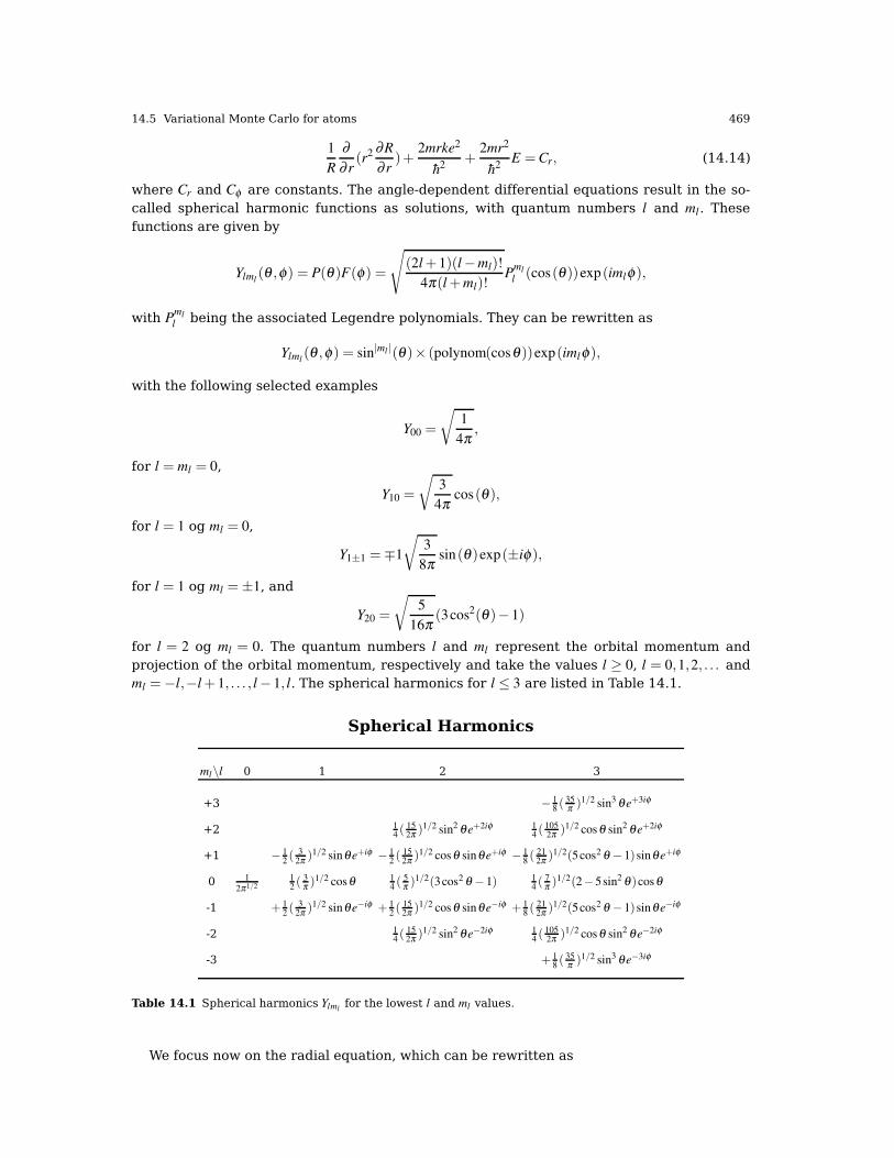
14.5 Variational Monte Carlo for atoms 469
1
R
∂
∂ r(r2 ∂R
∂ r)+
2mrke2
h2+
2mr2
h2E =Cr, (14.14)
where Cr and Cφ are constants. The angle-dependent differential equations result in the so-called spherical harmonic functions as solutions, with quantum numbers l and ml. Thesefunctions are given by
Ylml(θ ,φ) = P(θ )F(φ) =
√(2l+ 1)(l−ml)!
4π(l+ml)!P
ml
l (cos(θ ))exp(imlφ),
with Pml
l being the associated Legendre polynomials. They can be rewritten as
Ylml(θ ,φ) = sin|ml |(θ )× (polynom(cosθ ))exp(imlφ),
with the following selected examples
Y00 =
√1
4π,
for l = ml = 0,
Y10 =
√3
4πcos(θ ),
for l = 1 og ml = 0,
Y1±1 =∓1
√3
8πsin(θ )exp(±iφ),
for l = 1 og ml =±1, and
Y20 =
√5
16π(3cos2(θ )− 1)
for l = 2 og ml = 0. The quantum numbers l and ml represent the orbital momentum andprojection of the orbital momentum, respectively and take the values l ≥ 0, l = 0,1,2, . . . andml =−l,−l+ 1, . . . , l− 1, l. The spherical harmonics for l ≤ 3 are listed in Table 14.1.
Spherical Harmonics
ml\l 0 1 2 3
+3 − 18( 35
π )1/2 sin3 θe+3iφ
+2 14( 15
2π )1/2 sin2 θe+2iφ 1
4( 105
2π )1/2 cosθ sin2 θe+2iφ
+1 − 12( 3
2π )1/2 sinθe+iφ − 1
2( 15
2π )1/2 cosθ sinθe+iφ − 1
8( 21
2π )1/2(5cos2 θ −1)sinθe+iφ
0 1
2π1/212( 3
π )1/2 cosθ 1
4( 5
π )1/2(3cos2 θ −1) 1
4( 7
π )1/2(2−5sin2 θ )cosθ
-1 + 12( 3
2π )1/2 sinθe−iφ + 1
2( 15
2π )1/2 cosθ sinθe−iφ + 1
8( 21
2π )1/2(5cos2 θ −1)sinθe−iφ
-2 14( 15
2π )1/2 sin2 θe−2iφ 1
4( 105
2π )1/2 cosθ sin2 θe−2iφ
-3 + 18( 35
π )1/2 sin3 θe−3iφ
Table 14.1 Spherical harmonics Ylmlfor the lowest l and ml values.
We focus now on the radial equation, which can be rewritten as

470 14 Quantum Monte Carlo Methods
− h2r2
2m
(∂
∂ r(r2 ∂R(r)
∂ r)
)− ke2
rR(r)+
h2l(l + 1)
2mr2R(r) = ER(r).
Introducing the function u(r) = rR(r), we can rewrite the last equation as
− h2
2m
∂ 2u(r)
∂ r2−(
ke2
r− h2l(l + 1)
2mr2
)u(r) = Eu(r), (14.15)
where m is the mass of the electron, l its orbital momentum taking values l = 0,1,2, . . . , andthe term ke2/r is the Coulomb potential. The first terms is the kinetic energy. The full wavefunction will also depend on the other variables θ and φ as well. The energy, with no externalmagnetic field is however determined by the above equation . We can then think of the radialSchrödinger equation to be equivalent to a one-dimensional movement conditioned by aneffective potential
Veff(r) =−ke2
r+
h2l(l + 1)
2mr2.
The radial equation yield closed form solutions resulting in the quantum number n, inaddition to lml . The solution Rnl to the radial equation is given by the Laguerre polynomials[93]. The closed-form solutions are given by
ψnlml(r,θ ,φ) = ψnlml
= Rnl(r)Ylml(θ ,φ) = RnlYlml
The ground state is defined by n = 1 and l = ml = 0 and reads
ψ100 =1
a3/20
√π
exp(−r/a0),
where we have defined the Bohr radius a0
a0 =h2
mke2,
with length a0 = 0.05 nm. The first excited state with l = 0 is
ψ200 =1
4a3/2
0
√2π
(2− r
a0
)exp(−r/2a0).
For states with with l = 1 and n = 2, we can have the following combinations with ml = 0
ψ210 =1
4a3/2
0
√2π
(r
a0
)exp(−r/2a0)cos(θ ),
and ml =±1
ψ21±1 =1
8a3/2
0
√π
(r
a0
)exp(−r/2a0)sin(θ )exp(±iφ).
The exact energy is independent of l and ml, since the potential is spherically symmetric.The first few non-normalized radial solutions of equation are listed in Table 14.2.When solving equations numerically, it is often convenient to rewrite the equation in terms
of dimensionless variables. This leads to an equation in dimensionless form which is easierto code, sparing one for eventual errors. In order to do so, we introduce first the dimension-less variable ρ = r/β , where β is a constant we can choose. Schrödinger’s equation is thenrewritten as
− 1
2
∂ 2u(ρ)
∂ρ2− mke2β
h2ρu(ρ)+
l(l + 1)
2ρ2u(ρ) =
mβ 2
h2Eu(ρ). (14.16)

14.5 Variational Monte Carlo for atoms 471
Hydrogen-like atomic radial functions
l\n 1 2 3
0 exp (−Zr) (2− r)exp (−Zr/2) (27−18r+2r2)exp (−Zr/3)
1 rexp (−Zr/2) r(6− r)exp (−Zr/3)
2 r2 exp (−Zr/3)
Table 14.2 The first few radial functions of the hydrogen-like atoms.
We can determine β by simply requiring3
mke2β
h2= 1 (14.17)
With this choice, the constant β becomes the famous Bohr radius a0 = 0.05 nm a0 = β =
h2/mke2. We list here the standard units used in atomic physics and molecular physics calcu-lations. It is common to scale atomic units by setting m = e = h = 4πε0 = 1, see Table 14.3. We
Atomic Units
Quantity SI Atomic unit
Electron mass, m 9.109 ·10−31 kg 1Charge, e 1.602 ·10−19 C 1Planck’s reduced constant, h 1.055 ·10−34 Js 1Permittivity, 4πε0 1.113 ·10−10 C2 J−1 m−1 1
Energy, e2
4πε0a027.211 eV 1
Length, a0 =4πε0h2
me2 0.529 ·10−10 m 1
Table 14.3 Scaling from SI units to atomic units.
introduce thereafter the variable λ
λ =mβ 2
h2E,
and inserting β and the exact energy E = E0/n2, with E0 = 13.6 eV, we have that
λ =− 1
2n2,
n being the principal quantum number. The equation we are then going to solve numericallyis now
− 1
2
∂ 2u(ρ)
∂ρ2− u(ρ)
ρ+
l(l + 1)
2ρ2u(ρ)−λ u(ρ) = 0, (14.18)
with the Hamiltonian
H =−1
2
∂ 2
∂ρ2− 1
ρ+
l(l + 1)
2ρ2.
3 Remember that we are free to choose β .

472 14 Quantum Monte Carlo Methods
The ground state of the hydrogen atom has the energy λ =−1/2, or E =−13.6 eV. The exactwave function obtained from Eq. (14.18) is
u(ρ) = ρe−ρ ,
which yields the energy λ =−1/2. Sticking to our variational philosophy, we could now intro-duce a variational parameter α resulting in a trial wave function
uαT (ρ) = αρe−αρ . (14.19)
Inserting this wave function into the expression for the local energy EL of Eq. (14.3) yields
EL(ρ) =−1
ρ− α
2
(α− 2
ρ
). (14.20)
For the hydrogen atom we could perform the variational calculation along the same lines aswe did for the harmonic oscillator. The only difference is that Eq. (14.4) now reads
〈H〉=∫
P(R)EL(R)dR =
∫ ∞
0α2ρ2e−2αρEL(ρ)ρ
2dρ ,
since ρ ∈ [0,∞). In this case we would use the exponential distribution instead of the normaldistrubution, and our code could contain the following program statements
... initialisations, declarations of variables
... mcs = number of Monte Carlo samplings
// loop over Monte Carlo samples
for ( i=0; i < mcs; i++)
// generate random variables from the exponential
// distribution using ran1 and transforming to
// to an exponential mapping y = -ln(1-x)
x=ran1(&idum);
y=-log(1.-x);
// in our case y = rho*alpha*2
rho = y/alpha/2;
local_energy = -1/rho -0.5*alpha*(alpha-2/rho);
energy += (local_energy);
energy2 += local_energy*local_energy;
// end of sampling
// write out the mean energy and the standard deviation
cout << energy/mcs << sqrt((energy2/mcs-(energy/mcs)**2)/mcs));
As for the harmonic oscillator case, we need to generate a large number N of random numberscorresponding to the exponential probability distribution function α2ρ2e−2αρ and for eachrandom number we compute the local energy and variance.
14.5.3 Metropolis sampling for the hydrogen atom and the harmonic
oscillator
We present in this subsection results for the ground states of the hydrogen atom and harmonicoscillator using a variational Monte Carlo procedure. For the hydrogen atom, the trial wavefunction
uαT (ρ) = αρe−αρ ,

14.5 Variational Monte Carlo for atoms 473
depends only on the dimensionless radius ρ . It is the solution of a one-dimensional differentialequation, as is the case for the harmonic oscillator as well. The latter has the trial wavefunction
ΨT (x) =
√α
π1/4e−x2α2/2.
However, for the hydrogen atom we have ρ ∈ [0,∞), while for the harmonic oscillator we havex∈ (−∞,∞). In the calculations below we have used a uniform distribution to generate the vari-ous positions. This means that we employ a shifted uniform distribution where the integrationregions beyond a given value of ρ and x are omitted. This is obviously an approximation andtechniques like importance sampling discussed in chapter 11 should be used. Using a uni-form distribution is normally refered to as brute force Monte Carlo or brute force Metropolissampling. From a practical point of view, this means that the random variables are multipliedby a given step length λ . To better understand this, consider the above dimensionless radiusρ ∈ [0,∞).
The new position can then be modelled as
ρnew = ρold +λ × r,
with r being a random number drawn from the uniform distribution in a region r ∈ [0,Λ ],with Λ < ∞, a cutoff large enough in order to have a contribution to the integrand close tozero. The step length λ is chosen to give approximately an acceptance ratio of 50% for allproposed moves. This is nothing but a simple rule of thumb. In this chapter we will stay withthis brute force Metropolis algorithm. All results discussed here have been obtained with thisapproach. Importance sampling and further improvements will be discussed in chapter 15.In Figs. 14.1 and 14.2 we plot the ground state energies for the one-dimensional harmonic
0
1
2
3
4
5
0.2 0.4 0.6 0.8 1 1.2 1.4
E0
α
MC simulation with N=100000Exact result
Fig. 14.1 Result for ground state energy of the harmonic oscillator as function of the variational parameterα . The exact result is for α = 1 with an energy E = 1. See text for further details.
oscillator and the hydrogen atom, respectively, as functions of the variational parameter α.These results are also displayed in Tables 14.4 and 14.5. In these tables we list the varianceand the standard deviation as well. We note that at α = 1 for the hydrogen atom, we obtain
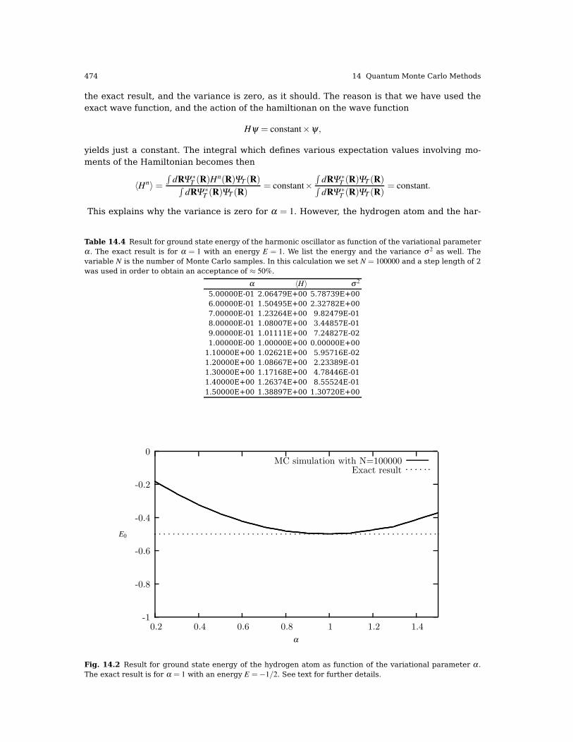
474 14 Quantum Monte Carlo Methods
the exact result, and the variance is zero, as it should. The reason is that we have used theexact wave function, and the action of the hamiltionan on the wave function
Hψ = constant×ψ ,
yields just a constant. The integral which defines various expectation values involving mo-ments of the Hamiltonian becomes then
〈Hn〉=∫
dRΨ∗T (R)Hn(R)ΨT (R)∫dRΨ∗T (R)ΨT (R)
= constant×∫
dRΨ∗T (R)ΨT (R)∫dRΨ∗T (R)ΨT (R)
= constant.
This explains why the variance is zero for α = 1. However, the hydrogen atom and the har-
Table 14.4 Result for ground state energy of the harmonic oscillator as function of the variational parameterα . The exact result is for α = 1 with an energy E = 1. We list the energy and the variance σ 2 as well. Thevariable N is the number of Monte Carlo samples. In this calculation we set N = 100000 and a step length of 2was used in order to obtain an acceptance of ≈ 50%.
α 〈H〉 σ 2
5.00000E-01 2.06479E+00 5.78739E+006.00000E-01 1.50495E+00 2.32782E+007.00000E-01 1.23264E+00 9.82479E-018.00000E-01 1.08007E+00 3.44857E-019.00000E-01 1.01111E+00 7.24827E-021.00000E-00 1.00000E+00 0.00000E+001.10000E+00 1.02621E+00 5.95716E-021.20000E+00 1.08667E+00 2.23389E-011.30000E+00 1.17168E+00 4.78446E-011.40000E+00 1.26374E+00 8.55524E-011.50000E+00 1.38897E+00 1.30720E+00
-1
-0.8
-0.6
-0.4
-0.2
0
0.2 0.4 0.6 0.8 1 1.2 1.4
E0
α
MC simulation with N=100000Exact result
Fig. 14.2 Result for ground state energy of the hydrogen atom as function of the variational parameter α .The exact result is for α = 1 with an energy E =−1/2. See text for further details.
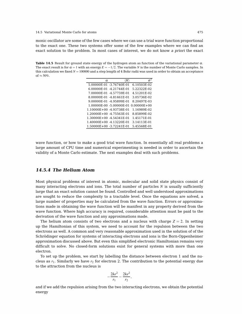
14.5 Variational Monte Carlo for atoms 475
monic oscillator are some of the few cases where we can use a trial wave function proportionalto the exact one. These two systems offer some of the few examples where we can find anexact solution to the problem. In most cases of interest, we do not know a priori the exact
Table 14.5 Result for ground state energy of the hydrogen atom as function of the variational parameter α .The exact result is for α = 1 with an energy E =−1/2. The variable N is the number of Monte Carlo samples. Inthis calculation we fixed N = 100000 and a step length of 4 Bohr radii was used in order to obtain an acceptanceof ≈ 50%.
α 〈H〉 σ 2
5.00000E-01 -3.76740E-01 6.10503E-026.00000E-01 -4.21744E-01 5.22322E-027.00000E-01 -4.57759E-01 4.51201E-028.00000E-01 -4.81461E-01 3.05736E-029.00000E-01 -4.95899E-01 8.20497E-031.00000E-00 -5.00000E-01 0.00000E+001.10000E+00 -4.93738E-01 1.16989E-021.20000E+00 -4.75563E-01 8.85899E-021.30000E+00 -4.54341E-01 1.45171E-011.40000E+00 -4.13220E-01 3.14113E-011.50000E+00 -3.72241E-01 5.45568E-01
wave function, or how to make a good trial wave function. In essentially all real problems alarge amount of CPU time and numerical experimenting is needed in order to ascertain thevalidity of a Monte Carlo estimate. The next examples deal with such problems.
14.5.4 The Helium Atom
Most physical problems of interest in atomic, molecular and solid state physics consist ofmany interacting electrons and ions. The total number of particles N is usually sufficientlylarge that an exact solution cannot be found. Controlled and well understood approximationsare sought to reduce the complexity to a tractable level. Once the equations are solved, alarge number of properties may be calculated from the wave function. Errors or approxima-tions made in obtaining the wave function will be manifest in any property derived from thewave function. Where high accuracy is required, considerable attention must be paid to thederivation of the wave function and any approximations made.
The helium atom consists of two electrons and a nucleus with charge Z = 2. In settingup the Hamiltonian of this system, we need to account for the repulsion between the twoelectrons as well. A common and very reasonable approximation used in the solution of of theSchrödinger equation for systems of interacting electrons and ions is the Born-Oppenheimerapproximation discussed above. But even this simplified electronic Hamiltonian remains verydifficult to solve. No closed-form solutions exist for general systems with more than oneelectron.
To set up the problem, we start by labelling the distance between electron 1 and the nu-cleus as r1. Similarly we have r2 for electron 2. The contribution to the potential energy dueto the attraction from the nucleus is
−2ke2
r1
− 2ke2
r2
,
and if we add the repulsion arising from the two interacting electrons, we obtain the potentialenergy
476 14 Quantum Monte Carlo Methods
V (r1,r2) =−2ke2
r1
− 2ke2
r2
+ke2
r12
,
with the electrons separated at a distance r12 = |r1− r2|. The Hamiltonian becomes then
H =− h2∇21
2m− h2∇2
2
2m− 2ke2
r1
− 2ke2
r2
+ke2
r12
,
and Schrödingers equation readsHψ = Eψ .
Note that this equation has been written in atomic units (a.u.) which are more convenientfor quantum mechanical problems. This means that the final energy has to be multiplied by a2×E0, where E0 = 13.6 eV, the binding energy of the hydrogen atom.
A very simple first approximation to this system is to omit the repulsion between the twoelectrons. The potential energy becomes then
V (r1,r2)≈−Zke2
r1
− Zke2
r2
.
The advantage of this approximation is that each electron can be treated as being indepen-dent of each other, implying that each electron sees just a central symmetric potential, orcentral field.
To see whether this gives a meaningful result, we set Z = 2 and neglect totally the repulsionbetween the two electrons. Electron 1 has the following Hamiltonian
h1 =−h2∇2
1
2m− 2ke2
r1
,
with pertinent wave function and eigenvalue Ea
h1ψa = Eaψa,
where a = nalamla are the relevant quantum numbers needed to describe the system. Weassume here that we can use the hydrogen-like solutions, but with Z not necessarily equal toone. The energy Ea is
Ea =−Z2E0
n2a
.
In a similar way, we obtain for electron 2
h2 =−h2∇2
2
2m− 2ke2
r2
,
with wave function ψb, b = nblbmlb and energy
Eb =Z2E0
n2b
.
Since the electrons do not interact, the ground state wave function of the helium atom isgiven by
ψ = ψaψb,
resulting in the following approximation to Schrödinger’s equation
(h1 + h2
)ψ =
(h1 + h2
)ψa(r1)ψb(r2) = Eabψa(r1)ψb(r2).
14.5 Variational Monte Carlo for atoms 477
The energy becomes then
(h1ψa(r1)
)ψb(r2)+
(h2ψb(r2)
)ψa(r1) = (Ea +Eb)ψa(r1)ψb(r2),
yielding
Eab = Z2E0
(1
n2a
+1
n2b
).
If we insert Z = 2 and assume that the ground state is determined by two electrons in thelowest-lying hydrogen orbit with na = nb = 1, the energy becomes
Eab = 8E0 =−108.8 eV,
while the experimental value is −78.8 eV. Clearly, this discrepancy is essentially due to ouromission of the repulsion arising from the interaction of two electrons.
14.5.4.1 Choice of trial wave function
The choice of trial wave function is critical in variational Monte Carlo calculations. How tochoose it is however a highly non-trivial task. All observables are evaluated with respect tothe probability distribution
P(R) =|ψT (R)|2
∫ |ψT (R)|2 dR.
generated by the trial wave function. The trial wave function must approximate an exacteigenstate in order that accurate results are to be obtained. Improved trial wave functionsalso improve the importance sampling, reducing the cost of obtaining a certain statisticalaccuracy.
Quantum Monte Carlo methods are able to exploit trial wave functions of arbitrary forms.Any wave function that is physical and for which the value, the gradient and the laplacian ofthe wave function may be efficiently computed can be used. The power of Quantum MonteCarlo methods lies in the flexibility of the form of the trial wave function.
It is important that the trial wave function satisfies as many known properties of the exactwave function as possible. A good trial wave function should exhibit much of the same fea-tures as does the exact wave function. Especially, it should be well-defined at the origin, thatis Ψ (|R| = 0) 6= 0, and its derivative at the origin should also be well-defined . One possibleguideline in choosing the trial wave function is the use of constraints about the behavior ofthe wave function when the distance between one electron and the nucleus or two electronsapproaches zero. These constraints are the so-called “cusp conditions” and are related to thederivatives of the wave function.
To see this, let us single out one of the electrons in the helium atom and assume that thiselectron is close to the nucleus, i.e., r1 → 0. We assume also that the two electrons are farfrom each other and that r2 6= 0. The local energy can then be written as
EL(R) =1
ψT (R)HψT (R) =
1
ψT (R)
(−1
2∇2
1−Z
r1
)ψT (R)+finite terms.
Writing out the kinetic energy term in the spherical coordinates of electron 1, we arrive atthe following expression for the local energy
EL(R) =1
RT (r1)
(−1
2
d2
dr21
− 1
r1
d
dr1
− Z
r1
)RT (r1)+finite terms,
478 14 Quantum Monte Carlo Methods
where RT (r1) is the radial part of the wave function for electron 1. We have also used that theorbital momentum of electron 1 is l = 0. For small values of r1, the terms which dominate are
limr1→0
EL(R) =1
RT (r1)
(− 1
r1
d
dr1
− Z
r1
)RT (r1),
since the second derivative does not diverge due to the finiteness ofΨ at the origin. The latterimplies that in order for the kinetic energy term to balance the divergence in the potentialterm, we must have
1
RT (r1)
dRT (r1)
dr1
=−Z,
implying thatRT (r1) ∝ e−Zr1 .
A similar condition applies to electron 2 as well. For orbital momenta l > 0 it is rather straight-forward to show that
1
RT (r)
dRT (r)
dr=− Z
l + 1.
Another constraint on the wave function is found when the two electrons are approachingeach other. In this case it is the dependence on the separation r12 between the two electronswhich has to reflect the correct behavior in the limit r12 → 0. The resulting radial equationfor the r12 dependence is the same for the electron-nucleus case, except that the attractiveCoulomb interaction between the nucleus and the electron is replaced by a repulsive interac-tion and the kinetic energy term is twice as large.
To find an ansatz for the correlated part of the wave function, it is useful to rewrite thetwo-particle local energy in terms of the relative and center-of-mass motion. Let us denotethe distance between the two electrons as r12. We omit the center-of-mass motion since weare only interested in the case when r12→ 0. The contribution from the center-of-mass (CoM)variable RCoM gives only a finite contribution. We focus only on the terms that are relevantfor r12. The relevant local energy becomes then
limr12→0
EL(R) =1
RT (r12)
(2
d2
dr2i j
+4
ri j
d
dri j
+2
ri j
− l(l + 1)
r2i j
+ 2E
)RT (r12) = 0,
where l is now equal 0 if the spins of the two electrons are anti-parallel and 1 if they areparallel. Repeating the argument for the electron-nucleus cusp with the factorization of theleading r-dependency, we get the similar cusp condition:
dRT (r12)
dr12
=− 1
2(l+ 1)RT (r12) r12→ 0
resulting in
RT ∝
exp(ri j/2) for anti-parallel spins, l = 0
exp(ri j/4) for parallel spins, l = 1
.
This is so-called cusp condition for the relative motion, resulting in a minimal requirementfor the correlation part of the wave fuction. For general systems containing more than twoelectrons, we have this condition for each electron pair i j.
Based on these consideration, a possible trial wave function which ignores the ’cusp’-condition between the two electrons is
ψT (R) = e−α(r1+r2), (14.21)

14.5 Variational Monte Carlo for atoms 479
where r1,2 are dimensionless radii and α is a variational parameter which is to be interpretedas an effective charge.
A possible trial wave function which also reflects the ’cusp’-condition between the twoelectrons is
ψT (R) = e−α(r1+r2)er12/2. (14.22)
The last equation can be generalized to
ψT (R) = φ(r1)φ(r2) . . .φ(rN)∏i< j
f (ri j),
for a system with N electrons or particles. The wave function φ(ri) is the single-particle wavefunction for particle i, while f (ri j) account for more complicated two-body correlations. Forthe helium atom, we placed both electrons in the hydrogenic orbit 1s. We know that theground state for the helium atom has a symmetric spatial part, while the spin wave functionis anti-symmetric in order to obey the Pauli principle. In the present case we need not to dealwith spin degrees of freedom, since we are mainly trying to reproduce the ground state ofthe system. However, adopting such a single-particle representation for the individual elec-trons means that for atoms beyond the ground state of helium, we cannot continue to placeelectrons in the lowest hydrogenic orbit. This is a consenquence of the Pauli principle, whichstates that the total wave function for a system of identical particles such as fermions, has tobe anti-symmetric. One way to account for this is by introducing the so-called Slater deter-minant (to be discussed in more detail in chapter 15). This determinant is written in terms ofthe various single-particle wave functions.
If we consider the helium atom with two electrons in the 1s state, we can write the totalSlater determinant as
Φ(r1,r2,α,β ) =1√2
∣∣∣∣ψα(r1) ψα(r2)
ψβ (r1) ψβ (r2)
∣∣∣∣ ,
with α = nlmlsms = (1001/21/2) and β = nlmlsms = (1001/2− 1/2) or using ms = 1/2 =↑ andms = −1/2 =↓ as α = nlmlsms = (1001/2 ↑) and β = nlmlsms = (1001/2 ↓). It is normal to skipthe two quantum numbers sms of the one-electron spin. We introduce therefore the shorthandnlml ↑ or nlml ↓) for a particular state where an arrow pointing upward represents ms = 1/2
and a downward arrow stands for ms =−1/2. Writing out the Slater determinant
Φ(r1,r2,α,β ) =1√2
[ψα(r1)ψβ (r2)−ψβ (r1)ψγ (r2)
],
we see that the Slater determinant is antisymmetric with respect to the permutation of twoparticles, that is
Φ(r1,r2,α,β ) =−Φ(r2,r1,α,β ).
The Slater determinant obeys the cusp condition for the two electrons and combined withthe correlation part we could write the ansatz for the wave function as
ψT (R) =1√2
[ψα(r1)ψβ (r2)−ψβ (r1)ψγ(r2)
]f (r12),
Several forms of the correlation function f (ri j) exist in the literature and we will mentiononly a selected few to give the general idea of how they are constructed. A form given byHylleraas that had great success for the helium atom was the series expansion
f (ri j) = exp(εs)∑k
ckrlk smk tnk
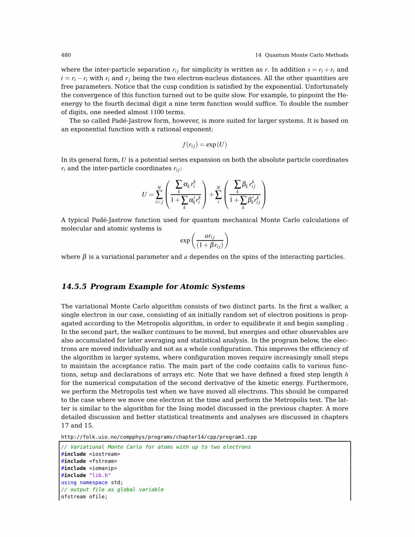
480 14 Quantum Monte Carlo Methods
where the inter-particle separation ri j for simplicity is written as r. In addition s = ri + ri andt = ri− ri with ri and r j being the two electron-nucleus distances. All the other quantities arefree parameters. Notice that the cusp condition is satisfied by the exponential. Unfortunatelythe convergence of this function turned out to be quite slow. For example, to pinpoint the He-energy to the fourth decimal digit a nine term function would suffice. To double the numberof digits, one needed almost 1100 terms.
The so called Padé-Jastrow form, however, is more suited for larger systems. It is based onan exponential function with a rational exponent:
f (ri j) = exp(U)
In its general form,U is a potential series expansion on both the absolute particle coordinatesri and the inter-particle coordinates ri j:
U =N
∑i< j
∑k
αk rki
1+∑k
α ′krki
+
N
∑i
∑k
βk rki j
1+∑k
β ′krki j
A typical Padé-Jastrow function used for quantum mechanical Monte Carlo calculations ofmolecular and atomic systems is
exp
(ari j
(1+β ri j)
)
where β is a variational parameter and a dependes on the spins of the interacting particles.
14.5.5 Program Example for Atomic Systems
The variational Monte Carlo algorithm consists of two distinct parts. In the first a walker, asingle electron in our case, consisting of an initially random set of electron positions is prop-agated according to the Metropolis algorithm, in order to equilibrate it and begin sampling .In the second part, the walker continues to be moved, but energies and other observables arealso accumulated for later averaging and statistical analysis. In the program below, the elec-trons are moved individually and not as a whole configuration. This improves the efficiency ofthe algorithm in larger systems, where configuration moves require increasingly small stepsto maintain the acceptance ratio. The main part of the code contains calls to various func-tions, setup and declarations of arrays etc. Note that we have defined a fixed step length h
for the numerical computation of the second derivative of the kinetic energy. Furthermore,we perform the Metropolis test when we have moved all electrons. This should be comparedto the case where we move one electron at the time and perform the Metropolis test. The lat-ter is similar to the algorithm for the Ising model discussed in the previous chapter. A moredetailed discussion and better statistical treatments and analyses are discussed in chapters17 and 15.
http://folk.uio.no/compphys/programs/chapter14/cpp/program1.cpp
// Variational Monte Carlo for atoms with up to two electrons
#include <iostream>
#include <fstream>
#include <iomanip>
#include "lib.h"
using namespace std;
// output file as global variable
ofstream ofile;

14.5 Variational Monte Carlo for atoms 481
Initialize:Set rold, α
and ΨT−α(rold)
Suggesta move
Computeacceptanceratio R
Generate auniformlydistributedvariable r
IsR≥ r?
Reject move:rnew = rold
Accept move:rold = rnew
Lastmove?
Get localenergy EL
LastMCstep?
Collectsamples
End
yes
no
yes
yes
no
Fig. 14.3 Chart flow for the Quantum Varitional Monte Carlo algorithm.

482 14 Quantum Monte Carlo Methods
// the step length and its squared inverse for the second derivative
#define h 0.001
#define h2 1000000
// declaraton of functions
// Function to read in data from screen, note call by reference
void initialise(int&, int&, int&, int&, int&, int&, double&) ;
// The Mc sampling for the variational Monte Carlo
void mc_sampling(int, int, int, int, int, int, double, double *, double *);
// The variational wave function
double wave_function(double **, double, int, int);
// The local energy
double local_energy(double **, double, double, int, int, int);
// prints to screen the results of the calculations
void output(int, int, int, double *, double *);
// Begin of main program
//int main()
int main(int argc, char* argv[])
char *outfilename;
int number_cycles, max_variations, thermalization, charge;
int dimension, number_particles;
double step_length;
double *cumulative_e, *cumulative_e2;
// Read in output file, abort if there are too few command-line arguments
if( argc <= 1 )
cout << "Bad Usage: " << argv[0] <<
" read also output file on same line" << endl;
exit(1);
else
outfilename=argv[1];
ofile.open(outfilename);
// Read in data
initialise(dimension, number_particles, charge,
max_variations, number_cycles,
thermalization, step_length) ;
cumulative_e = new double[max_variations+1];
cumulative_e2 = new double[max_variations+1];
// Do the mc sampling
mc_sampling(dimension, number_particles, charge,
max_variations, thermalization,
number_cycles, step_length, cumulative_e, cumulative_e2);
// Print out results
output(max_variations, number_cycles, charge, cumulative_e, cumulative_e2);
delete [] cumulative_e; delete [] cumulative_e;
ofile.close(); // close output file
return 0;

14.5 Variational Monte Carlo for atoms 483
The implementation of the brute force Metropolis algorithm is shown in the next function.Here we have a loop over the variational variables α. It calls two functions, one to computethe wave function and one to update the local energy.
// Monte Carlo sampling with the Metropolis algorithm
void mc_sampling(int dimension, int number_particles, int charge,
int max_variations,
int thermalization, int number_cycles, double step_length,
double *cumulative_e, double *cumulative_e2)
int cycles, variate, accept, dim, i, j;
long idum;
double wfnew, wfold, alpha, energy, energy2, delta_e;
double **r_old, **r_new;
alpha = 0.5*charge;
idum=-1;
// allocate matrices which contain the position of the particles
r_old = (double **) matrix( number_particles, dimension, sizeof(double));
r_new = (double **) matrix( number_particles, dimension, sizeof(double));
for (i = 0; i < number_particles; i++)
for ( j=0; j < dimension; j++)
r_old[i][j] = r_new[i][j] = 0;
// loop over variational parameters
for (variate=1; variate <= max_variations; variate++)
// initialisations of variational parameters and energies
alpha += 0.1;
energy = energy2 = 0; accept =0; delta_e=0;
// initial trial position, note calling with alpha
// and in three dimensions
for (i = 0; i < number_particles; i++)
for ( j=0; j < dimension; j++)
r_old[i][j] = step_length*(ran1(&idum)-0.5);
wfold = wave_function(r_old, alpha, dimension, number_particles);
// loop over monte carlo cycles
for (cycles = 1; cycles <= number_cycles+thermalization; cycles++)
// new position
for (i = 0; i < number_particles; i++)
for ( j=0; j < dimension; j++)
r_new[i][j] = r_old[i][j]+step_length*(ran1(&idum)-0.5);
wfnew = wave_function(r_new, alpha, dimension, number_particles);
// Metropolis test
if(ran1(&idum) <= wfnew*wfnew/wfold/wfold )
for (i = 0; i < number_particles; i++)
for ( j=0; j < dimension; j++)
r_old[i][j]=r_new[i][j];
wfold = wfnew;
accept = accept+1;
// compute local energy
if ( cycles > thermalization )
delta_e = local_energy(r_old, alpha, wfold, dimension,
number_particles, charge);

484 14 Quantum Monte Carlo Methods
// update energies
energy += delta_e;
energy2 += delta_e*delta_e;
// end of loop over MC trials
cout << "variational parameter= " << alpha
<< " accepted steps= " << accept << endl;
// update the energy average and its squared
cumulative_e[variate] = energy/number_cycles;
cumulative_e2[variate] = energy2/number_cycles;
// end of loop over variational steps
free_matrix((void **) r_old); // free memory
free_matrix((void **) r_new); // free memory
// end mc_sampling function
The wave function is in turn defined in the next function. Here we limit ourselves to a functionwhich consists only of the product of single-particle wave functions.
// Function to compute the squared wave function, simplest form
double wave_function(double **r, double alpha,int dimension, int number_particles)
int i, j, k;
double wf, argument, r_single_particle, r_12;
argument = wf = 0;
for (i = 0; i < number_particles; i++)
r_single_particle = 0;
for (j = 0; j < dimension; j++)
r_single_particle += r[i][j]*r[i][j];
argument += sqrt(r_single_particle);
wf = exp(-argument*alpha) ;
return wf;
Finally, the local energy is computed using a numerical derivation for the kinetic energy. Weuse the familiar expression derived in Eq. (3.4), that is
f ′′0 =fh− 2 f0 + f−h
h2,
in order to compute
− 1
2ψT (R)∇2ψT (R). (14.23)
The variable h is a chosen step length. For helium, since it is rather easy to evaluate thelocal energy, the above is an unnecessary complication. However, for many-electron or othermany-particle systems, the derivation of a closed-form expression for the kinetic energy canbe quite involved, and the numerical evaluation of the kinetic energy using Eq. (3.4) mayresult in a simpler code and/or even a faster one.
// Function to calculate the local energy with num derivative
double local_energy(double **r, double alpha, double wfold, int dimension,
int number_particles, int charge)
int i, j , k;
double e_local, wfminus, wfplus, e_kinetic, e_potential, r_12,

14.5 Variational Monte Carlo for atoms 485
r_single_particle;
double **r_plus, **r_minus;
// allocate matrices which contain the position of the particles
// the function matrix is defined in the progam library
r_plus = (double **) matrix( number_particles, dimension, sizeof(double));
r_minus = (double **) matrix( number_particles, dimension, sizeof(double));
for (i = 0; i < number_particles; i++)
for ( j=0; j < dimension; j++)
r_plus[i][j] = r_minus[i][j] = r[i][j];
// compute the kinetic energy
e_kinetic = 0;
for (i = 0; i < number_particles; i++)
for (j = 0; j < dimension; j++)
r_plus[i][j] = r[i][j]+h;
r_minus[i][j] = r[i][j]-h;
wfminus = wave_function(r_minus, alpha, dimension, number_particles);
wfplus = wave_function(r_plus, alpha, dimension, number_particles);
e_kinetic -= (wfminus+wfplus-2*wfold);
r_plus[i][j] = r[i][j];
r_minus[i][j] = r[i][j];
// include electron mass and hbar squared and divide by wave function
e_kinetic = 0.5*h2*e_kinetic/wfold;
// compute the potential energy
e_potential = 0;
// contribution from electron-proton potential
for (i = 0; i < number_particles; i++)
r_single_particle = 0;
for (j = 0; j < dimension; j++)
r_single_particle += r[i][j]*r[i][j];
e_potential -= charge/sqrt(r_single_particle);
// contribution from electron-electron potential
for (i = 0; i < number_particles-1; i++)
for (j = i+1; j < number_particles; j++)
r_12 = 0;
for (k = 0; k < dimension; k++)
r_12 += (r[i][k]-r[j][k])*(r[i][k]-r[j][k]);
e_potential += 1/sqrt(r_12);
free_matrix((void **) r_plus); // free memory
free_matrix((void **) r_minus);
e_local = e_potential+e_kinetic;
return e_local;
The remaining part of the program consists of the output and initialize functions and is notlisted here.
The way we have rewritten Schrödinger’s equation results in energies given in atomicunits. If we wish to convert these energies into more familiar units like electronvolt (eV), wehave to multiply our reults with 2E0 where E0 = 13.6 eV, the binding energy of the hydrogenatom. Using Eq. (14.21) for the trial wave function, we obtain an energy minimum at α =

486 14 Quantum Monte Carlo Methods
1.68754. The ground state is E = −2.85 in atomic units or E = −77.5 eV. The experimentalvalue is −78.8 eV. Obviously, improvements to the wave function such as including the ’cusp’-condition for the two electrons as well, see Eq. (14.22), could improve our agreement withexperiment.
We note that the effective charge is less than the charge of the nucleus. We can interpretthis reduction as an effective way of incorporating the repulsive electron-electron interaction.Finally, since we do not have the exact wave function, we see from Fig. 14.4 that the varianceis not zero at the energy minimum. Techniques such as importance sampling, to be contrasted
-3
-2.9
-2.8
-2.7
-2.6
-2.5
-2.4
1 1.2 1.4 1.6 1.8 2
E0
α
MC simulation with N=107
Exact result
Fig. 14.4 Result for ground state energy of the helium atom using Eq. (14.21) for the trial wave function.A total of 107 Monte Carlo moves were used with a step length of 1 Bohr radius. Approximately 50% of allproposed moves were accepted. The variance at the minimum is 1.026, reflecting the fact that we do not havethe exact wave function. The variance has a minimum at value of α different from the energy minimum. Thenumerical results are compared with the exact result E[Z] = Z2−4Z + 5
8Z.
to the brute force Metropolis sampling used here, and various optimization techniques of thevariance and the energy, will be discussed in the next section and in chapter 17.
14.5.6 Importance sampling
As mentioned in connection with the generation of random numbers, sequential correlationsmust be given thorough attention as it may lead to bad error estimates of our numericalresults.
There are several things we need to keep in mind in order to keep the correlation low. Firstof all, the transition acceptance must be kept as high as possible. Otherwise, a walker willdwell at the same spot in state space for several iterations at a time, which will clearly leadto high correlation between nearby succeeding measurements.
4 With hydrogen like wave functions for the 1s state one can easily calculate the energy of the ground statefor the helium atom as function of the charge Z. The results is E[Z] = Z2− 4Z + 5
8Z, and taking the derivative
with respect to Z to find the minumum we get Z = 2− 516
= 1.6875. This number represents an optimal effectivecharge.

14.5 Variational Monte Carlo for atoms 487
Secondly, when using the simple symmetric form of ω(rold, rnew), one has to keep in mindthe random walk nature of the algorithm. Transitions will be made between points that arerelatively close to each other in state space, which also clearly contributes to increase corre-lation. The seemingly obvious way to deal with this would be just to increase the step size, al-lowing the walkers to cover more of the state space in fewer steps (thus requiring fewer stepsto reach ergodicity). But unfortunately, long before the step length becomes desirably large,the algorithm breaks down. When proposing moves symmetrically and uniformly around rold,the step acceptance becomes directly dependent on the step length in such a way that a toolarge step length reduces the acceptance. The reason for this is very simple. As the steplength increases, a walker will more likely be given a move proposition to areas of very lowprobability, particularly if the governing trial wave function describes a localized system. Ineffect, the effective movement of the walkers again becomes too small, resulting in largecorrelation. For optimal results we therefore have to balance the step length with the accep-tance.
With a transition suggestion rule ω as simple as the uniform symmetrical one emphasizedso far, the usual rule of thumb is to keep the acceptance around 0.5. But the optimal intervalvaries a lot from case to case. We therefore have to treat each numerical experiment withcare.
By choosing a better ω, we can still improve the efficiency of the step length versus accep-tance. Recall that ω may be chosen arbitrarily as long as it fulfills ergodicity, meaning that ithas to allow the walker to reach any point of the state space in a finite number of steps. Whatwe basically want is an ω that pushes the ratio towards unity, increasing the acceptance. Thetheoretical situation of ω exactly equal to p itself:
ω(rnew, rold) = ω(rnew) = p(rnew)
would give the maximal acceptance of 1. But then we would already have solved the prob-lem of producing points distributed according to p. One typically settles on modifying thesymmetrical ω so that the walkers move more towards areas of the state space where thedistribution is large. One such procedure is the Fokker-Planck formalism where the walkersare moved according to the gradient of the distribution. The formalism “pushes” the walkersin a “desirable” direction. The idea is to propose moves similarly to an isotropic diffusionprocess with a drift. A new position xnew is calculated from the old one, xold, as follows:
rnew = rold+ χ +DF(rold)δ t (14.24)
Here χ is a Gaussian pseudo-random number with mean equal zero and variance equal 2Dδ t.It accounts for the diffusion part of the transition. The third term on the left hand side ac-counts for the drift. F is a drift velocity dependent on the position of the walker and is derivedfrom the quantum mechanical wave function ψ. The constant D, being the diffusion constantof χ , also adjusts the size of the drift. δ t is a time step parameter whose presence will beclarified shortly.
It can be shown that the ω corresponding to the move proposition rule in Eq. (14.24)becomes (in non-normalized form):
ω(rold, rnew) = exp
(− (rnew− rold−Dδ tF(rold))
2
4Dδ t
)(14.25)
which, as expected, is a Gaussian with variance 2Dδ t centered slightly off rold due to the driftterm DF(rold)δ t.
What is the optimal choice for the drift term? From statistical mechanics we know that asimple isotropic drift diffusion process obeys a Fokker-Planck equation of the form:

488 14 Quantum Monte Carlo Methods
∂ f
∂ t= ∑
i
D∂
∂xi
(∂
∂xi
−Fi(F)
)f (14.26)
where f is the continuous distribution of walkers. Equation (14.24) is a discretized realizationof such a process where δ t is the discretized time step. In order for the solution f to convergeto the desired distribution p, it can be shown that the drift velocity has to be chosen as follows:
F =1
f∇ f
where the operator ∇ is the vector of first derivatives of all spatial coordinates. Convergencefor such a diffusion process is only guaranteed when the time step approaches zero. But in theMetropolis algorithm, where drift diffusion is used just as a transition proposition rule, thisbias is corrected automatically by the rejection mechanism. In our application, the desiredprobability distribution function being the square absolute of the wave function, f = |ψ |2, thedrift velocity becomes:
F = 21
ψ∇ψ (14.27)
As expected, the walker is “pushed” along the gradient of the wave function.When dealing with many-particle systems, we should also consider whether to move only
one particle at a time at each transition or all at once. The former method may often be moreefficient. A movement of only one particle will restrict the accessible space a walker can moveto in a single transition even more, thus introducing correlation. But on the other hand, theacceptance is increased so that each particle can be moved further than it could in a standardall-particle move. It is also computationally far more efficient to do one-particle transitionsparticularly when dealing with complicated distributions governing many-dimensional anti-symmetrical fermionic systems.
Alternatively, we can treat the sequence of all one-particle transitions as one total transi-tion of all particles. This gives a larger effective step length thus reducing the correlation.From a computational point of view, we may not gain any speed by summing up the individualone-particle transitions as opposed to doing an all-particle transition. But the reduced corre-lation increases the total efficiency. We are able to do fewer calculations in order to reach thesame numerical accuracy.
Another way to acquire some control over the correlation is to do a so called blockingprocedure on our set of numerical measurements. This is discussed in chapter 16.
14.6 Exercises
14.1. The aim of this problem is to test the variational Monte Carlo apppled to light atoms.We will test different trial wave function ΨT . The systems we study are atoms consisting oftwo electrons only, such as the helium atom, LiII and BeIII . The atom LiII has two electronsand Z = 3 while BeIII has Z = 4 but still two electrons only. A general ansatz for the trial wavefunction is
ψT (R) = φ(r1)φ(r2) f (r12). (14.28)
For all systems we assume that the one-electron wave functions φ(ri) are described by the anelecron in the lowest hydrogen orbital 1s.
The specific trial functions we study are
ψT 1(r1,r2,r12) = exp(−α(r1 + r2)), (14.29)

14.6 Exercises 489
where α is the variational parameter,
ψT 2(r1,r2,r12) = exp(−α(r1 + r2))(1+β r12), (14.30)
with β as a new variational parameter and
ψT 3(r1,r2,r12) = exp(−α(r1 + r2))exp
(r12
2(1+β r12)
). (14.31)
a) Find the closed-form expressions for the local energy for the above trial wave function for thehelium atom. Study the behavior of the local energy with these functions in the limits r1→ 0,r2→ 0 and r12→ 0.
b) Compute
〈H〉=∫
dRΨ∗T (R)H(R)ΨT (R)∫dRΨ∗T (R)ΨT (R)
, (14.32)
for the helium atom using the variational Monte Carlo method employing the Metropolisalgorithm to sample the different states using the trial wave function ψT 1(r1,r2,r12). Compareyour results with the closed-form expression
〈H〉= h2
me
α2− 27
32
e2
πε0
α. (14.33)
c) Use the optimal value of α from the previous point to compute the ground state of the heliumatom using the other two trial wave functions ψT 2(r1,r2,r12) and ψT 3(r1,r2,r12). In this caseyou have to vary both α and β . Explain briefly which function ψT 1(r1,r2,r12), ψT 2(r1,r2,r12)
and ψT 3(r1,r2,r12) is the best.d) Use the optimal value for all parameters and all wave functions to compute the expectation
value of the mean distance 〈r12〉 between the two electrons. Comment your results.e) We will now repeat point 1c), but we replace the helium atom with the ions LiII and BeIII .
Perform first a variational calculation using the first ansatz for the trial wave functionψT 1(r1,r2,r12) in order to find an optimal value for α. Use then this value to start the varia-tional calculation of the energy for the wave functions ψT 2(r1,r2,r12) and ψT 3(r1,r2,r12). Com-ment your results.
14.2. The H+2 molecule consists of two protons and one electron, with binding energy EB =
−2.8 eV and an equilibrium position r0 = 0.106 nm between the two protons.We define our system through the following variables. The electron is at a distance r from
a chosen origo, one of the protons is at the distance −R/2 while the other one is placed atR/2 from origo, resulting in a distance to the electron of r−R/2 and r+R/2, respectively.
In our solution of Schrödinger’s equation for this system we are going to neglect the kineticenergies of the protons, since they are 2000 times heavier than the electron. We assumethus that their velocities are negligible compared to the velocity of the electron. In additionwe omit contributions from nuclear forces, since they act at distances of several orders ofmagnitude smaller than the equilibrium position.
We can then write Schrödinger’s equation as follows
− h2∇2
r
2me
− ke2
|r−R/2| −ke2
|r+R/2|+ke2
R
ψ(r,R) = Eψ(r,R), (14.34)
where the first term is the kinetic energy of the electron, the second term is the potentialenergy the electron feels from the proton at −R/2 while the third term arises from the po-tential energy contribution from the proton at R/2. The last term arises due to the repulsionbetween the two protons.

490 14 Quantum Monte Carlo Methods
Since the potential is symmetric with respect to the interchange of R→−R and r→−r
it means that the probability for the electron to move from one proton to the other must beequal in both directions. We can say that the electron shares it’s time between both protons.
With this caveat, we can now construct a model for simulating this molecule. Since we haveonly one elctron, we could assume that in the limit R→ ∞, i.e., when the distance betweenthe two protons is large, the electron is essentially bound to only one of the protons. Thisshould correspond to a hydrogen atom. As a trial wave function, we could therefore use theelectronic wave function for the ground state of hydrogen, namely
ψ100(r) =
(1
πa30
)1/2
e−r/a0 . (14.35)
Since we do not know exactly where the electron is, we have to allow for the possibility thatthe electron can be coupled to one of the two protons. This form includes the ’cusp’-conditiondiscussed in the previous section. We define thence two hydrogen wave functions
ψ1(r,R) =
(1
πa30
)1/2
e−|r−R/2|/a0 , (14.36)
and
ψ2(r,R) =
(1
πa30
)1/2
e−|r+R/2|/a0 . (14.37)
Based on these two wave functions, which represent where the electron can be, we attemptat the following linear combination
ψ±(r,R) =C± (ψ1(r,R)±ψ2(r,R)) , (14.38)
with C± a constant. Based on this discussion, we add a second electron in order to simulatethe H2 molecule. That is the topic for project 14.3.
14.3. The H2 molecule consists of two protons and two electrons with a ground state energyE =−1.17460 a.u. and equilibrium distance between the two hydrogen atoms of r0 = 1.40 Bohrradii. We define our systems using the following variables. Origo is chosen to be halfwaybetween the two protons. The distance from proton 1 is defined as −R/2 whereas proton 2has a distance R/2. Calculations are performed for fixed distances R between the two protons.
Electron 1 has a distance r1 from the chose origo, while electron 2 has a distance r2. Thekinetic energy operator becomes then
− ∇21
2− ∇2
2
2. (14.39)
The distance between the two electrons is r12 = |r1− r2|. The repulsion between the two elec-trons results in a potential energy term given by
+1
r12
. (14.40)
In a similar way we obtain a repulsive contribution from the interaction between the twoprotons given by
+1
|R| , (14.41)
where R is the distance between the two protons. To obtain the final potential energy weneed to include the attraction the electrons feel from the protons. To model this, we needto define the distance between the electrons and the two protons. If we model this along a

14.6 Exercises 491
chosen z-akse with electron 1 placed at a distance r1 from a chose origo, one proton at −R/2
and the other at R/2, the distance from proton 1 to electron 1 becomes
r1p1 = r1 +R/2, (14.42)
andr1p2 = r1−R/2, (14.43)
from proton 2. Similarly, for electron 2 we obtain
r2p1 = r2 +R/2, (14.44)
andr2p2 = r2−R/2. (14.45)
These four distances define the attractive contributions to the potential energy
− 1
r1p1
− 1
r1p2
− 1
r2p1
− 1
r2p2
. (14.46)
We can then write the total Hamiltonian as
H =−∇21
2− ∇2
2
2− 1
r1p1
− 1
r1p2
− 1
r2p1
− 1
r2p2
+1
r12
+1
|R| , (14.47)
and if we choose R = 0 we obtain the helium atom.In this project we will use a trial wave function of the form
ψT (r1,r2,R) = ψ(r1,R)ψ(r2,R)exp
(r12
2(1+β r12)
), (14.48)
with the following trial wave function
ψ(r1,R) = (exp(−αr1p1)+ exp(−αr1p2)) , (14.49)
for electron 1 andψ(r2,R) = (exp(−αr2p1)+ exp(−αr2p2)) . (14.50)
The variational parameters are α and β .One can show that in the limit where all distances approach zero that
α = 1+ exp(−R/α), (14.51)
resulting in β kas the only variational parameter. The last equation is a non-linear equationwhich we can solve with for example Newton’s method discussed in chapter 4.
1. Find the local energy as function of R.2. Set up and algorithm and write a program which computes the expectation value of 〈H〉
using the variational Monte Carlo method with a brute force Metropolis sampling. For eachinter-proton distance R you must find the parameter β which minimizes the energy. Plot thecorresponding energy as function of the distance R between the protons.
3. Use thereafter the optimal parameter sets to compute the average distance 〈r12〉 between theelectrons where the energy as function of R exhibits its minimum. Comment your results.
4. We modify now the approximation for the wave functions of electrons 1 and 2 by subtractingthe two terms instead of adding up, viz
ψ(r1,R) = (exp(−αr1p1)− exp(−αr1p2)) , (14.52)

492 14 Quantum Monte Carlo Methods
for electron 1ψ(r2,R) = (exp(−αr2p1)− exp(−αr2p2)) , (14.53)
for electron 2. Mathematically, this approach is equally viable as the previous one. Repeatyour calculations from point b) and see if you can obtain an energy minimum as function ofR. Comment your results.

Part V
Advanced topics

The last part of this book contains several project oriented advanced topics. Each of thesetopics can serve as a regular one-semester course based on the solution of the pertinentprojects. We present several topics, mainly within applications to quantum mechanical sys-tems and statistical mechanics. We discuss Hartree-Fock and density-functional theory cal-culations for electronic systems, variational and diffusion Monte Carlo calculations of many-particle systems (atoms, quantum dots and Bose-Einstein condensation), large molecular-dynamics calculations of solids, percolation and critical phenomena and advanced simulationsof phase transitions.

Chapter 15
Many-body approaches to studies of electronic
systems: Hartree-Fock theory and Density
Functional Theory
Abstract This chapter presents the Hartree-Fock method with an emphasis on computing theenergies of selected closed-shell atoms.
15.1 Introduction
A theoretical understanding of the behavior of quantum mechanical systems with many in-teracting particles, normally called many-body systems, is a great challenge and providesfundamental insights into systems governed by quantum mechanics, as well as offering po-tential areas of industrial applications, from semi-conductor physics to the construction ofquantum gates. The capability to simulate quantum mechanical systems with many interact-ing particles is crucial for advances in such rapidly developing fields like materials science.
However, most quantum mechanical systems of interest in physics consist of a large num-ber of interacting particles. The total number of particles N is usually sufficiently large that anexact solution (viz., in closed form) cannot be found. One needs therefore reliable numericalmethods for studying quantum mechanical systems with many particles.
Studies of many-body systems span from our understanding of the strong force with quarksand gluons as degrees of freedom, the spectacular macroscopic manifestations of quantalphenomena such as Bose-Einstein condensation with millions of atoms forming a coherentstate, to properties of new materials, with electrons as effective degrees of freedom. Thelength scales range from few micrometers and nanometers, typical scales met in materialsscience, to 10−15− 10−18 m, a relevant length scale for the strong interaction. Energies canspan from few meV to GeV or even TeV. In some cases the basic interaction between the in-teracting particles is well-known. A good example is the Coulomb force, familiar from studiesof atoms, molecules and condensed matter physics. In other cases, such as for the strong in-teraction between neutrons and protons (commonly dubbed as nucleons) or dense quantumliquids one has to resort to parameterizations of the underlying interparticle interactions. Butthe system can also span over much larger dimensions as well, with neutron stars as one ofthe classical objects. This star is the endpoint of massive stars which have used up their fuel.A neutron star, as its name suggests, is composed mainly of neutrons, with a small fractionof protons and probably quarks in its inner parts. The star is extremely dense and compact,with a radius of approximately 10 km and a mass which is roughly 1.5 times that of our sun.The quantum mechanical pressure which is set up by the interacting particles counteractsthe gravitational forces, hindering thus a gravitational collapse. To describe a neutron starone needs to solve Schrödinger’s equation for approximately 1054 interacting particles!
With a given interparticle potential and the kinetic energy of the system, one can in turndefine the so-called many-particle Hamiltonian H which enters the solution of Schrödinger’s
495

49615 Many-body approaches to studies of electronic systems: Hartree-Fock theory and Density Functional Theory
equation or Dirac’s equation in case relativistic effects need to be included. For many parti-cles, Schrödinger’s equation is an integro-differential equation whose complexity increasesexponentially with increasing numbers of particles and states that the system can access.Unfortunately, apart from some few analytically solvable problems and one and two-particlesystems that can be treated numerically exactly via the solution of sets of partial differen-tial equations, the typical absence of an exactly solvable (on closed form) contribution to themany-particle Hamiltonianmeans that we need reliable numerical many-body methods. Thesemethods should allow for controlled approximations and provide a computational schemewhich accounts for successive many-body corrections in a systematic way.
Typical examples of popular many-body methods are coupled-cluster methods [95–99], var-ious types of Monte Carlo methods [100–102], perturbative many-body methods [103–105],Green’s function methods [106, 107], the density-matrix renormalization group [108, 109],density functional theory [110] and ab initio density functional theory [111–113], and large-scale diagonalization methods [114–116], just to mention a few. The physics of the systemhints at which many-body methods to use. For systems with strong correlations among theconstituents, methods based on mean-field theory such as Hartree-Fock theory and densityfunctional theory are normally ruled out. This applies also to perturbative methods, unlessone can renormalize the parts of the interaction which cause problems.
The aim of this and the next three chapters is to present to you many-body methods whichcan be used to study properties of atoms, molecules, systems in the solid state and nuclearphysics. We limit the attention to non-relativistic quantum mechanics.
In this chapter we limit ourselves to studies of electronic systems such atoms, moleculesand quantum dots, as discussed partly in chapter 14 as well. Using the Born-Oppenheimerapproximation we rewrote Schrödinger’s equation for N electrons as
[−
N
∑i=1
1
2∇2
i −N
∑i=1
Z
ri
+N
∑i< j
1
ri j
]Ψ(R) = EΨ(R),
where we let R represent the positions which the N electrons can take, that is R= r1,r2, . . . ,rN.With more than one electron present we cannot find an solution on a closed form and mustresort to numerical efforts. In this chapter we will examine Hartree-Fock theory applied tothe atomic problem. However, the machinery we expose can easily be extended to studies ofmolecules or two-dimensional systems like quantum dots.
For atoms and molecules, the electron-electron interaction is rather weak compared withthe attraction from the nucleus. An independent particle picture is therefore a viable first steptowards the solution of Schrödinger’s equation. We assume therefore that each electrons seesan effective field set up by the other electrons. This leads to an integro-differential equationand methods like Hartree-Fock theory discussed in this chapter.
In practical terms, for the Hartree-Fock method we end up solving a one-particle equation,as is the case for the hydrogen atom but modified due to the screening from the other elec-trons. This modified single-particle equation reads (see Eq. (14.15 for the hydrogen case) inatomic units
−1
2
d2
dr2unl(r)+
(l(l + 1)
2r2− Z
r+Φ(r)+Fnl
)unl(r) = enlunl(r).
The function unl is the solution of the radial part of the Schrödinger equation and the functionsΦ(r) and Fnl are the corrections due to the screening from the other electrons. We will derivethese equations in the next section.
The total one-particle wave function, see chapter 14 is
ψnlml sms= φnlml
(r)ξms(s)
15.2 Hartree-Fock theory 497
with s is the spin (1/2 for electrons), ms is the spin projection ms =±1/2, and the spatial partis
φnlml(r) = Rnl(r)Ylml
(r)
with Y the spherical harmonics discussed in chapter 14 and unl = rRnl. The other quantumnumbers are the orbital momentum l and its projection ml = −l,−l + 1, . . . , l − 1, l and theprincipal quantum number n = nr+ l+1, with nr the number of nodes of a given single-particlewave function. All results are in atomic units, meaning that the energy is given by enl =
−Z2/2n2 and the radius is dimensionless.We obtain then a modified single-particle eigenfunction which in turn can be used as an
input in a variational Monte Carlo calculation of the ground state of a specific atom. Thisis the aim of the next chapter. Since Hartree-Fock theory does not treat correctly the roleof many-body correlations, the hope is that performing a Monte Carlo calculation we mayimprove our results by obtaining a better agreement with experiment.
In the next chapter we focus on the variational Monte Carlo method as a way to improveupon the Hartree-Fock results. Although the variational Monte Carlo approach will improveour agreement with experiment compared with the Hartree-Fock results, there are still fur-ther possibilities for improvement. This is provided by Green’s function Monte Carlo meth-ods, which allow for an in principle exact calculation. The diffusion Monte Carlo method isdiscussed in chapter 17, with an application to studies of Bose-Einstein condensation. Othermany-body methods such as large-scale diagonalization and coupled-cluster theories are dis-cussed in Ref. [117].
15.2 Hartree-Fock theory
Hartree-Fock theory [97, 118] is one of the simplest approximate theories for solving themany-body Hamiltonian. It is based on a simple approximation to the true many-body wave-function; that the wave-function is given by a single Slater determinant of N orthonormalsingle-particle wave functions1
ψnlml sms= φnlml
(r)ξms(s).
We use hereafter the shorthand ψnlmlsms(r) = ψα(r), where α now contains all the quantum
numbers needed to specify a particular single-particle orbital.The Slater determinant can then be written as
Φ(r1,r2, . . . ,rN ,α,β , . . . ,ν) =1√N!
∣∣∣∣∣∣∣∣∣∣∣
ψα(r1) ψα(r2) . . . ψα(rN)
ψβ (r1) ψβ (r2) . . . ψβ (rN)
......
. . ....
ψν (r1) ψβ (r2) . . . ψβ (rN)
∣∣∣∣∣∣∣∣∣∣∣
. (15.1)
Here the variables ri include the coordinates of spin and space of particle i. The quantumnumbers α,β , . . . ,ν encompass all possible quantum numbers needed to specify a particularsystem. As an example, consider the Neon atom, with ten electrons which can fill the 1s, 2s and2p single-particle orbitals. Due to the spin projections ms and orbital momentum projectionsml, the 1s and 2s states have a degeneracy of 2(2l+1)= 2 while the 2p orbital has a degeneracy
1 We limit ourselves to a restricted Hartree-Fock approach and assume that all the lowest-lying orbits arefilled. This constitutes an approach suitable for systems with filled shells. The theory we outline is thereforeapplicable to systems which exhibit so-called magic numbers like the noble gases, closed-shell nuclei like 16Oand 40Ca and quantum dots with magic number fillings.

49815 Many-body approaches to studies of electronic systems: Hartree-Fock theory and Density Functional Theory
of 2(2l + 1)2(2 ·1+ 1) = 6. This leads to ten possible values for α,β , . . . ,ν. Fig. 15.1 shows thepossible quantum numbers which the ten first elements can have.
s p
K
L
H
s p s p
K
L
He Li
s p s p s p s p
n = 1
n = 2
Be B C N
s p s p s p
n = 1
n = 2
O F Ne
Fig. 15.1 The electronic configurations for the ten first elements. We let an arrow which points upward torepresent a state with ms = 1/2 while an arrow which points downwards has ms =−1/2.
If we consider the helium atom with two electrons in the 1s state, we can write the totalSlater determinant as
Φ(r1,r2,α,β ) =1√2
∣∣∣∣ψα(r1) ψα(r2)
ψβ (r1) ψβ (r2)
∣∣∣∣ , (15.2)
with α = nlmlsms = (1001/21/2) and β = nlmlsms = (1001/2− 1/2) or using ms = 1/2 =↑ andms = −1/2 =↓ as α = nlmlsms = (1001/2 ↑) and β = nlmlsms = (1001/2 ↓). It is normal to skipthe quantum number of the one-electron spin. We introduce therefore the shorthand nlml ↑ ornlml ↓) for a particular state. Writing out the Slater determinant
Φ(r1,r2,α,β ) =1√2
[ψα(r1)ψβ (r2)−ψβ (r1)ψγ (r2)
], (15.3)
we see that the Slater determinant is antisymmetric with respect to the permutation of twoparticles, that is
Φ(r1,r2,α,β ) =−Φ(r2,r1,α,β ),
For three electrons we have the general expression
Φ(r1,r2,r3,α,β ,γ) =1√3!
∣∣∣∣∣∣
ψα(r1) ψα(r2) ψα(r3)
ψβ (r1) ψβ (r2) ψβ (r3)
ψγ(r1) ψγ(r2) ψγ(r3)
∣∣∣∣∣∣. (15.4)
Computing the determinant gives
Φ(r1,r2,r3,α,β ,γ) = 1√3!
[ψα(r1)ψβ (r2)ψγ(r3)+ψβ (r1)ψγ(r2)ψα(r3)+ψγ(r1)ψα (r2)ψβ (r3)−
ψγ (r1)ψβ (r2)ψα(r3)−ψβ (r1)ψα (r2)ψγ(r3)−ψα(r1)ψγ (r2)ψβ (r3)]. (15.5)
We note again that the wave-function is antisymmetric with respect to an interchange of anytwo electrons, as required by the Pauli principle. For an N-body Slater determinant we havethus (omitting the quantum numbers α,β , . . . ,ν)

15.2 Hartree-Fock theory 499
Φ(r1,r2, . . . ,ri, . . . ,r j, . . .rN) =−Φ(r1,r2, . . . ,r j, . . . ,ri, . . .rN).
As another example, consider the Slater determinant for the ground state of beryllium.This system is made up of four electrons and we assume that these electrons fill the 1s and 2s
hydrogen-like orbits. The radial part of the single-particle could also be represented by othersingle-particle wave functions such as those given by the harmonic oscillator.
The ansatz for the Slater determinant can then be written as
Φ(r1,r2, ,r3,r4,α,β ,γ,δ ) =1√4!
∣∣∣∣∣∣∣∣
ψ100↑(r1) ψ100↑(r2) ψ100↑(r3) ψ100↑(r4)
ψ100↓(r1) ψ100↓(r2) ψ100↓(r3) ψ100↓(r4)
ψ200↑(r1) ψ200↑(r2) ψ200↑(r3) ψ200↑(r4)
ψ200↓(r1) ψ200↓(r2) ψ200↓(r3) ψ200↓(r4)
∣∣∣∣∣∣∣∣.
We choose an ordering where columns represent the spatial positions of various electronswhile rows refer to specific quantum numbers.
Note that the Slater determinant as written is zero since the spatial wave functions for thespin up and spin down states are equal. However, we can rewrite it as the product of twoSlater determinants, one for spin up and one for spin down. In general we can rewrite it as
Φ(r1,r2, ,r3,r4,α,β ,γ,δ ) = Det ↑ (1,2)Det ↓ (3,4)−Det ↑ (1,3)Det ↓ (2,4)
−Det ↑ (1,4)Det ↓ (3,2)+Det ↑ (2,3)Det ↓ (1,4)−Det ↑ (2,4)Det ↓ (1,3)+Det ↑ (3,4)Det ↓ (1,2),
where we have defined
Det ↑ (1,2) =∣∣∣∣
1√2
ψ100↑(r1) ψ100↑(r2)
ψ200↑(r1) ψ200↑(r2)
∣∣∣∣ ,
and
Det ↓ (3,4) =∣∣∣∣
1√2
ψ100↓(r3) ψ100↓(r4)
ψ200↓(r3) ψ200↓(r4)
∣∣∣∣ .
The total determinant is still zero! In our variational Monte Carlo calculations this will obvi-ously cause problems.
We want to avoid to sum over spin variables, in particular when the interaction does notdepend on spin. It can be shown, see for example Moskowitz et al [119, 120], that for thevariational energy we can approximate the Slater determinant as the product of a spin upand a spin down Slater determinant
Φ(r1,r2, ,r3,r4,α,β ,γ,δ ) ∝ Det ↑ (1,2)Det ↓ (3,4),
or more generally asΦ(r1,r2, . . .rN) ∝ Det ↑ Det ↓,
where we have the Slater determinant as the product of a spin up part involving the number ofelectrons with spin up only (two in beryllium and five in neon) and a spin down part involvingthe electrons with spin down.
This ansatz is not antisymmetric under the exchange of electrons with opposite spins butit can be shown that it gives the same expectation value for the energy as the full Slaterdeterminant as long as the Hamiltonian is spin independent. It is left as an exercise to thereader to show this. However, before we can prove this need to set up the expectation valueof a given two-particle Hamiltonian using a Slater determinant.

50015 Many-body approaches to studies of electronic systems: Hartree-Fock theory and Density Functional Theory
15.3 Expectation value of the Hamiltonian with a given Slater
determinant
We rewrite our Hamiltonian
H =−N
∑i=1
1
2∇2
i −N
∑i=1
Z
ri
+N
∑i< j
1
ri j
,
as
H = H0 + HI =N
∑i=1
hi +N
∑i< j=1
1
ri j
, (15.6)
where
hi =−1
2∇2
i −Z
ri
. (15.7)
The first term of Eq. (15.6), H1, is the sum of the N identical one-body Hamiltonians hi. Eachindividual Hamiltonian hi contains the kinetic energy operator of an electron and its potentialenergy due to the attraction of the nucleus. The second term, H2, is the sum of the N(N−1)/2
two-body interactions between each pair of electrons. Let us denote the ground state energyby E0. According to the variational principle we have
E0 ≤ E[Φ] =
∫Φ∗HΦdτ (15.8)
where Φ is a trial function which we assume to be normalized∫
Φ∗Φdτ = 1, (15.9)
where we have used the shorthand dτ = dr1dr2 . . .drN. In the Hartree-Fock method the trialfunction is the Slater determinant of Eq. (15.1) which can be rewritten as
Ψ(r1,r2, . . . ,rN ,α,β , . . . ,ν) =1√N!
∑P
(−)PPψα(r1)ψβ (r2) . . .ψν(rN) =√
N!A ΦH , (15.10)
where we have introduced the anti-symmetrization operator A defined by the summationover all possible permutations of two eletrons. It is defined as
A =1
N!∑P
(−)PP, (15.11)
with the the Hartree-function given by the simple product of all possible single-particle func-tion (two for helium, four for beryllium and ten for neon)
ΦH(r1,r2, . . . ,rN ,α,β , . . . ,ν) = ψα(r1)ψβ (r2) . . .ψν (rN). (15.12)
Both H0 and HI are invariant under electron permutations, and hence commute with A
[H0,A ] = [HI,A ] = 0. (15.13)
Furthermore, A satisfiesA
2 = A , (15.14)
since every permutation of the Slater determinant reproduces it. The expectation value of H0
∫Φ∗H0Φdτ = N!
∫Φ∗HA H0A ΦHdτ

15.3 Expectation value of the Hamiltonian with a given Slater determinant 501
is readily reduced to ∫Φ∗H0Φdτ = N!
∫Φ∗HH0A ΦHdτ,
where we have used eqs. (15.13) and (15.14). The next step is to replace the anti-symmetryoperator by its definition eq. (15.10) and to replace H0 with the sum of one-body operators
∫Φ∗H0Φdτ =
N
∑i=1
∑P
(−)P
∫Φ∗H hiPΦHdτ. (15.15)
The integral vanishes if two or more electrons are permuted in only one of the Hartree-functions ΦH because the individual orbitals are orthogonal. We obtain then
∫Φ∗H0Φdτ =
N
∑i=1
∫Φ∗H hiΦHdτ. (15.16)
Orthogonality allows us to further simplify the integral, and we arrive at the following expres-sion for the expectation values of the sum of one-body Hamiltonians
∫Φ∗H0Φdτ =
N
∑µ=1
∫ψ∗µ(ri)hiψµ(ri)dri. (15.17)
The expectation value of the two-body Hamiltonian is obtained in a similar manner. Wehave ∫
Φ∗HIΦdτ = N!
∫Φ∗HA HIA ΦHdτ, (15.18)
which reduces to ∫Φ∗HIΦdτ =
N
∑i≤ j=1
∑P
(−)P
∫Φ∗H
1
ri j
PΦHdτ, (15.19)
by following the same arguments as for the one-body Hamiltonian. Because of the dependenceon the inter-electronic distance 1/ri j, permutations of two electrons no longer vanish, and weget
∫Φ∗HIΦdτ =
N
∑i< j=1
∫Φ∗H
1
ri j
(1−Pi j)ΦHdτ. (15.20)
where Pi j is the permutation operator that interchanges electrons i and j. Again we use theassumption that the orbitals are orthogonal, and obtain
∫Φ∗HIΦdτ =
1
2
N
∑µ=1
N
∑ν=1
[∫ψ∗µ(ri)ψ
∗ν (r j)
1
ri j
ψµ(ri)ψν (r j)dxidxj −∫
ψ∗µ(ri)ψ∗ν (r j)
1
ri j
ψν(ri)ψµ(ri)dxidxj
].
(15.21)The first term is the so-called direct term or Hartree term, while the second is due to thePauli principle and is called the exchange term or the Fock term. The factor 1/2 is introducedbecause we now run over all pairs twice.
Combining Eqs. (15.17) and (15.21) we obtain the functional
E[Φ] =N
∑µ=1
∫ψ∗µ(ri)hiψµ(ri)dri +
1
2
N
∑µ=1
N
∑ν=1
[∫ψ∗µ(ri)ψ
∗ν (r j)
1
ri j
ψµ(ri)ψν (r j)dridr j− (15.22)
−∫
ψ∗µ(ri)ψ∗ν (r j)
1
ri j
ψν(ri)ψµ(r j)dridr j
].
50215 Many-body approaches to studies of electronic systems: Hartree-Fock theory and Density Functional Theory
15.4 Derivation of the Hartree-Fock equations
Having obtained the functional E[Φ], we now proceed to the second step of the calculation.With the given functional, we can embark on at least two types of variational strategies:
• We can vary the Slater determinant by changing the spatial part of the single-particlewave functions themselves.
• We can expand the single-particle functions in a known basis and vary the coefficients,that is, the new single-particle wave function |a〉 is written as a linear expansion in termsof a fixed chosen orthogonal basis (for the example harmonic oscillator, or Laguerre poly-nomials etc)
ψa = ∑λ
Caλ ψλ .
In this case we vary the coefficients Caλ .
We will derive the pertinent Hartree-Fock equations and discuss the pros and cons of the twomethods. Both cases lead to a new Slater determinant which is related to the previous onevia a unitary transformation.
Before we proceed we need however to repeat some aspects of the calculus of variations.For more details see for example the text of Arfken [53].
We have already met the variational principle in chapter 14. We give here a brief reminderon the calculus of variations.
15.4.1 Reminder on calculus of variations
The calculus of variations involves problems where the quantity to be minimized or maximizedis an integral.
In the general case we have an integral of the type
E[Φ] =∫ b
af (Φ(x),
∂Φ
∂r,r)dr,
where E is the quantity which is sought minimized or maximized. The problem is that althoughf is a function of the variables Φ, ∂Φ/∂r and r, the exact dependence of Φ on r is not known.This means again that even though the integral has fixed limits a and b, the path of integrationis not known. In our case the unknown quantities are the single-particle wave functions andwe wish to choose an integration path which makes the functional E[Φ] stationary. This meansthat we want to find minima, or maxima or saddle points. In physics we search normally forminima.
Our task is therefore to find the minimum of E[Φ] so that its variation δE is zero subjectto specific constraints. In our case the constraints appear as the integral which expressesthe orthogonality of the single-particle wave functions. The constraints can be treated viathe technique of Lagrangian multipliers. We assume the existence of an optimum path, thatis a path for which E[Φ] is stationary. There are infinitely many such paths. The differencebetween two paths δΦ is called the variation of Φ.
The condition for a stationary value is given by a partial differential equation, which wehere write in terms of one variable x
∂ f
∂Φ− d
dx
∂ f
∂Φx
= 0,

15.4 Derivation of the Hartree-Fock equations 503
This equation is better better known as Euler’s equation and it can easily be generalized tomore variables.
As an example consider a function of three independent variables f (x,y,z) . For the functionf to be an extreme we have
d f = 0.
A necessary and sufficient condition is
∂ f
∂x=
∂ f
∂y=
∂ f
∂ z= 0,
due to
d f =∂ f
∂xdx+
∂ f
∂ydy+
∂ f
∂ zdz.
In physical problems the variables x,y,z are often subject to constraints (in our case Φ andthe orthogonality constraint) so that they are no longer all independent. It is possible at leastin principle to use each constraint to eliminate one variable and to proceed with a new andsmaller set of independent varables.
The use of so-called Lagrangian multipliers is an alternative technique when the elimi-nation of of variables is incovenient or undesirable. Assume that we have an equation ofconstraint on the variables x,y,z
φ(x,y,z) = 0,
resulting in
dφ =∂φ
∂xdx+
∂φ
∂ydy+
∂φ
∂ zdz = 0.
Now we cannot set anymore∂ f
∂x=
∂ f
∂y=
∂ f
∂ z= 0,
if d f = 0 is wanted because there are now only two independent variables. Assume x and y
are the independent variables. Then dz is no longer arbitrary. However, we can add to
d f =∂ f
∂xdx+
∂ f
∂ydy+
∂ f
∂ zdz,
a multiplum of dφ , viz. λ dφ , resulting in
d f +λ dφ = (∂ f
∂ z+λ
∂φ
∂x)dx+(
∂ f
∂y+λ
∂φ
∂y)dy+(
∂ f
∂ z+λ
∂φ
∂ z)dz = 0,
where our multiplier is chosen so that
∂ f
∂ z+λ
∂φ
∂ z= 0.
However, since we took dx and dy to be arbitrary we must have
∂ f
∂x+λ
∂φ
∂x= 0,
and∂ f
∂y+λ
∂φ
∂y= 0.
When all these equations are satisfied, d f = 0. We have four unknowns, x,y,z and λ . Actuallywe want only x,y,z, there is no need to determine λ . It is therefore often called Lagrange’sundetermined multiplier. If we have a set of constraints φk we have the equations

50415 Many-body approaches to studies of electronic systems: Hartree-Fock theory and Density Functional Theory
∂ f
∂xi
+∑k
λk
∂φk
∂xi
= 0.
Let us specialize to the expectation value of the energy for one particle in three-dimensions.This expectation value reads
E =
∫dxdydzψ∗(x,y,z)Hψ(x,y,z),
with the constraint ∫dxdydzψ∗(x,y,z)ψ(x,y,z) = 1,
and a Hamiltonian
H =−1
2∇2 +V (x,y,z).
The integral involving the kinetic energy can be written as, if we assume periodic boundaryconditions or that the function ψ vanishes strongly for large values of x,y,z,
∫dxdydzψ∗
(−1
2∇2
)ψdxdydz = ψ∗∇ψ |+
∫dxdydz
1
2∇ψ∗∇ψ .
Inserting this expression into the expectation value for the energy and taking the variationalminimum (using V (x,y,z) =V ) we obtain
δE = δ
∫dxdydz
(1
2∇ψ∗∇ψ +Vψ∗ψ
)= 0.
The requirement that the wave functions should be orthogonal gives
∫dxdydzψ∗ψ = constant,
and multiplying it with a Lagrangian multiplier λ and taking the variational minimum weobtain the final variational equation
δ
∫dxdydz
(1
2∇ψ∗∇ψ +Vψ∗ψ−λ ψ∗ψ
)= 0.
We introduce the function f
f =1
2∇ψ∗∇ψ +Vψ∗ψ−λ ψ∗ψ =
1
2(ψ∗x ψx +ψ∗y ψy +ψ∗z ψz)+Vψ∗ψ−λ ψ∗ψ .
In our notation here we have dropped the dependence on x,y,z and introduced the shorthandψx, ψy and ψz for the various first derivatives.
For ψ∗ the Euler equation results in
∂ f
∂ψ∗− ∂
∂x
∂ f
∂ψ∗x− ∂
∂y
∂ f
∂ψ∗y− ∂
∂ z
∂ f
∂ψ∗z= 0,
which yields
−1
2(ψxx +ψyy +ψzz)+Vψ = λ ψ .
We can then identify the Lagrangian multiplier as the energy of the system. The last equationis nothing but the standard Schrödinger equation and the variational approach discussedhere provides a powerful method for obtaining approximate solutions of the wave function.

15.4 Derivation of the Hartree-Fock equations 505
15.4.2 Varying the single-particle wave functions
If we generalize the Euler-Lagrange equations to more variables and introduce N2 Lagrangemultipliers which we denote by εµν , we can write the variational equation for the functionalof Eq. (15.23) as
δE−N
∑µ=1
N
∑ν=1
εµν δ
∫ψ∗µψν = 0. (15.23)
For the orthogonal wave functions ψµ this reduces to
δE−N
∑µ=1
εµδ∫
ψ∗µ ψµ = 0. (15.24)
Variation with respect to the single-particle wave functions ψµ yields then
N
∑µ=1
∫δψ∗µ hiψµdxi +
1
2
N
∑µ=1
N
∑ν=1
[∫δψ∗µψ∗ν
1
ri j
ψµψν d(xixj)−∫
δψ∗µ ψ∗ν1
ri j
ψνψµdridr j
]
+N
∑µ=1
∫ψ∗µ hiδψµdri +
1
2
N
∑µ=1
N
∑ν=1
[∫ψ∗µ ψ∗ν
1
ri j
δψµψνdridr j−∫
ψ∗µψ∗ν1
ri j
ψν δψµdridr j
]
−N
∑µ=1
Eµ
∫δψ∗µψµdxi−
N
∑µ=1
Eµ
∫ψ∗µδψµdri = 0.
(15.25)
Although the variations δψ and δψ∗ are not independent, they may in fact be treated assuch, so that the terms dependent on either δψ and δψ∗ individually may be set equal tozero. To see this, simply replace the arbitrary variation δψ by iδψ, so that δψ∗ is replaced by−iδψ∗, and combine the two equations. We thus arrive at the Hartree-Fock equations
[−1
2∇2
i −Z
ri
+N
∑ν=1
∫ψ∗ν (r j)
1
ri j
ψν(r j)dr j
]ψµ(xi)
−[
N
∑ν=1
∫ψ∗ν (r j)
1
ri j
ψµ(r j)dr j
]ψν(ri) = εµ ψµ(ri).
(15.26)
Notice that the integration∫
dr j implies an integration over the spatial coordinates rj anda summation over the spin-coordinate of electron j.
The two first terms are the one-body kinetic energy and the electron-nucleus potential.The third or direct term is the averaged electronic repulsion of the other electrons. Thisterm includes the ’self-interaction’ of electrons when i = j. The self-interaction is cancelled inthe fourth term, or the exchange term. The exchange term results from our inclusion of thePauli principle and the assumed determinantal form of the wave-function. The effect of theexchange is for electrons of like-spin to avoid each other. A theoretically convenient form ofthe Hartree-Fock equation is to regard the direct and exchange operator defined through thefollowing operators
V dµ (ri) =
∫ψ∗µ(r j)
1
ri j
ψµ(r j)dr j (15.27)
and
V exµ (ri)g(ri) =
(∫ψ∗µ(r j)
1
ri j
g(r j)dr j
)ψµ(ri), (15.28)

50615 Many-body approaches to studies of electronic systems: Hartree-Fock theory and Density Functional Theory
respectively. The function g(ri) is an arbitrary function, and by the substitution g(ri) = ψν(ri)
we get
V exµ (ri)ψν(ri) =
(∫ψ∗µ(r j)
1
ri j
ψν(r j)dr j
)ψµ(ri). (15.29)
We may then rewrite the Hartree-Fock equations as
HHFi ψν (ri) = εν ψν(ri), (15.30)
with
HHFi = hi +
N
∑µ=1
V dµ (ri)−
N
∑µ=1
V exµ (ri), (15.31)
and where hi is defined by equation (15.7).
15.4.3 Detailed solution of the Hartree-Fock equations
We show here the explicit form of the Hartree-Fock for helium and berylliumLet us introduce
ψnlml sms= φnlml
(r)ξms(s)
with s is the spin (1/2 for electrons), ms is the spin projection ms =±1/2, and the spatial partis
φnlml(r) = Rnl(r)Ylml
(r)
with Y the spherical harmonics and unl = rRnl. We have for helium
Φ(r1,r2,α,β ) =1√2
φ100(r1)φ100(r2)[ξ↑(1)ξ↓(2)− ξ↑(2)ξ↓(1)
],
The direct term acts on1√2
φ100(r1)φ100(r2)ξ↑(1)ξ↓(2)
while the exchange term acts on
− 1√2
φ100(r1)φ100(r2)ξ↑(2)ξ↓(1).
How do these terms get translated into the Hartree and the Fock terms?The Hartree term
V dµ (ri) =
∫ψ∗µ(r j)
1
ri j
ψµ(r j)dr j,
acts on ψλ (ri) = φnlml(ri)ξms(si), that is it results in
V dµ (ri)ψλ (ri) =
(∫ψ∗µ(r j)
1
ri j
ψµ(r j)dr j
)ψλ (ri),
and accounting for spins we have
V dnlml↑(ri)ψλ (ri) =
(∫ψ∗nlml↑(r j)
1
ri j
ψnlml↑(r j)dr j
)ψλ (ri),
and
V dnlml↓(ri)ψλ (ri) =
(∫ψ∗nlml↓(r j)
1
ri j
ψnlml↓(r j)dr j
)ψλ (ri),

15.4 Derivation of the Hartree-Fock equations 507
If the state we act on has spin up, we obtain two terms from the Hartree part,
N
∑µ=1
V dµ (ri),
and since the interaction does not depend on spin we end up with a total contribution forhelium
N
∑µ=1
V dµ (ri)ψλ (ri) =
(2
∫φ∗100(r j)
1
ri j
φ100(r j)dr j
)ψλ (ri),
one from spin up and one from spin down. Since the energy for spin up or spin down is thesame we can then write the action of the Hartree term as
N
∑µ=1
V dµ (ri)ψλ (ri) =
(2
∫φ∗100(r j)
1
ri j
φ100(r j)dr j
)ψ100↑(ri).
(the spin in ψ100↑ is irrelevant)What we need to code for helium is then
Φ(ri)u10 = 2V d10(ri)u10(ri) = 2
∫ ∞
0|u10(r j)|2
1
r>dr j)u10(ri).
with r> = max(ri,r j). What about the exchange or Fock term
V exµ (ri)ψλ (ri) =
(∫ψ∗µ(r j)
1
ri j
ψλ (r j)dr j
)ψµ(ri)?
We must be careful here with
V exµ (ri)ψλ (ri) =
(∫ψ∗µ(r j)
1
ri j
ψλ (r j)dr j
)ψµ(ri),
because the spins of µ and λ have to be the same due to the constraint
〈sµ mµs |sλ mλ
s 〉= δm
µs ,mλ
s.
This means that if mµs =↑ then mλ
s =↑ and if mµs =↓ then mλ
s =↓. That is
V exµ (ri)ψλ (ri) = δ
mµs ,mλ
s
(∫ψ∗µ(r j)
1
ri j
ψλ (r j)dr j
)ψµ(ri),
The consequence is that for the 1s ↑ (and the same for 1s ↓) state we get only one contribu-tion from the Fock term, namely
N
∑µ=1
V exµ (ri)ψ100↑(ri) = δ
mµs ,↑
(∫ψ∗µ(r j)
1
ri j
ψ100↑(r j)dr j
)ψµ(ri),
resulting inN
∑µ=1
V exµ (ri)ψ100↑(ri) =
(∫ψ∗100↑(r j)
1
ri j
ψ100↑(r j)dr j
)ψ100↑(ri).
The final Fock term for helium is then
N
∑µ=1
V exµ (ri)ψ100↑(ri) =
(∫ψ∗100↑(r j)
1
ri j
ψ100↑(r j)dr j
)ψ100↑(ri),
50815 Many-body approaches to studies of electronic systems: Hartree-Fock theory and Density Functional Theory
which is exactly the same as the Hartree term except for a factor of 2. Else the integral is thesame. We can then write the differential equation
(−1
2
d2
dr2+
l(l + 1)
2r2− 2
r+Φnl(r)−Fnl(r)
)unl(r) = enlunl(r).
as (−1
2
d2
dr2+
l(l + 1)
2r2− 2
r+ 2Vd
10(r)
)u10(r)−V ex
10(r) = e10u10(r),
or (−1
2
d2
dr2− 2
r+V d
10(r)
)u10(r) = e10u10(r),
since l = 0. The shorthand V ex10 (r) contains the 1s wave function.
The expression we have obtained are independent of the spin projections and we haveskipped them in the equations.
For beryllium the Slater determinant takes the form
Φ(r1,r2, ,r3,r4,α,β ,γ,δ ) =1√4!
∣∣∣∣∣∣∣∣
ψ100↑(r1) ψ100↑(r2) ψ100↑(r3) ψ100↑(r4)
ψ100↓(r1) ψ100↓(r2) ψ100↓(r3) ψ100↓(r4)
ψ200↑(r1) ψ200↑(r2) ψ200↑(r3) ψ200↑(r4)
ψ200↓(r1) ψ200↓(r2) ψ200↓(r3) ψ200↓(r4)
∣∣∣∣∣∣∣∣,
When we now spell out the Hartree-Fock equations we get two coupled differential equa-tions, one for u10 and one for u20.
The 1s wave function has the same Hartree-Fock contribution as in helium for the 1s state,but the 2s state gives two times the Hartree term and one time the Fock term. We get
N
∑µ=1
V dµ (ri)ψ100↑(ri) = 2
∫ ∞
0dr j
(φ∗100(r j)
1
ri j
φ100(r j)+φ∗200(r j)1
ri j
φ200(r j)
)ψ100↑(ri)
= (2V d10(ri)+ 2Vd
20(ri))ψ100↑(ri)
for the Hartree part.For the Fock term we get (we fix the spin)
N
∑µ=1
V exµ (ri)ψ100↑(ri) =
∫ ∞
0dr jφ
∗100(r j)
1
ri j
φ100(r j)ψ100↑(ri)+
∫ ∞
0dr jφ
∗200(r j)
1
ri j
φ100(r j)ψ200↑(ri) =V ex10(ri)+V ex
20(ri).
The first term is the same as we have for the Hartree term with 1s except the factor of two.The final differential equation is
(−1
2
d2
dr2− 4
r+V d
10(r)+ 2V d20(r)
)u10(r)−V ex
20(r) = e10u10(r).
Note again that the V ex20(r) contains the 1s function in the integral, that is
V ex20 (r) =
∫ ∞
0dr jφ
∗200(r j)
1
r− r j
φ100(r j)ψ200↑(r).
The 2s wave function obtains the following Hartree term (recall that the interaction has nospin dependence)

15.4 Derivation of the Hartree-Fock equations 509
N
∑µ=1
V dµ (ri)ψ200↑(ri) = 2
∫ ∞
0dr j
(φ∗100(r j)
1
ri j
φ100(r j)+φ∗200(r j)1
ri j
φ200(r j)
)ψ200↑(ri) =
(2V d10(ri)+ 2V d
20(ri))ψ200↑(ri)
For the Fock term we get
N
∑µ=1
V exµ (ri)ψ200↑(ri) =
∫ ∞
0dr jφ
∗100(r j)
1
ri j
φ200(r j)ψ100↑(ri)+
∫ ∞
0dr jφ
∗200(r j)
1
ri j
φ200(r j)ψ200↑(ri) =V ex10 (ri)+V ex
20(ri)
The second term is the same as we have for the Hartree term with 2s. The final differentialequation is (
−1
2
d2
dr2− 4
r+ 2Vd
10(r)+V d20(r)
)u20(r)−V ex
10(r) = e20u20(r).
Note again that V ex10(r) contains the 2s function in the integral, that is
V ex10 (r) =
∫ ∞
0dr jφ
∗100(r j)
1
r− r j
φ200(r j)ψ100↑(r).
We have two coupled differential equations
(−1
2
d2
dr2− 4
r+V d
10(r)+ 2V d20(r)
)u10(r)−V ex
20(r) = e10u10(r),
and (−1
2
d2
dr2− 4
r+ 2Vd
10(r)+V d20(r)
)u20(r)−V ex
10(r) = e20u20(r).
Recall again that the interaction does not depend on spin. This means that the single-particleenergies and single-particle function u do not depend on spin.
15.4.4 Hartree-Fock by variation of basis function coefficients
Another possibility is to expand the single-particle functions in a known basis and vary thecoefficients, that is, the new single-particle wave function is written as a linear expansion interms of a fixed chosen orthogonal basis (for example harmonic oscillator, Laguerre polyno-mials etc)
ψa = ∑λ
Caλ ψλ . (15.32)
In this case we vary the coefficients Caλ .The single-particle wave functions ψλ (r), defined by the quantum numbers λ and r are
defined as the overlapψα(r) = 〈r|α〉.
We will omit the radial dependence of the wave functions and introduce first the followingshorthands for the Hartree and Fock integrals
〈µν|V |µν〉=∫
ψ∗µ(ri)ψ∗ν (r j)V (ri j)ψµ(ri)ψν (r j)drir j,
and
51015 Many-body approaches to studies of electronic systems: Hartree-Fock theory and Density Functional Theory
〈µν|V |νµ〉=∫
ψ∗µ(ri)ψ∗ν (r j)V (ri j)ψν(ri)ψµ(ri)drir j.
Since the interaction is invariant under the interchange of two particles it means for examplethat we have
〈µν|V |µν〉= 〈νµ |V |νµ〉,or in the more general case
〈µν|V |στ〉= 〈νµ |V |τσ〉.The direct and exchange matrix elements can be brought together if we define the anti-
symmetrized matrix element
〈µν|V |µν〉AS = 〈µν|V |µν〉− 〈µν|V |νµ〉,
or for a general matrix element
〈µν|V |στ〉AS = 〈µν|V |στ〉− 〈µν|V |τσ〉.
It has the symmetry property
〈µν|V |στ〉AS =−〈µν|V |τσ〉AS =−〈νµ |V |στ〉AS.
The antisymmetric matrix element is also hermitian, implying
〈µν|V |στ〉AS = 〈στ|V |µν〉AS.
With these notations we rewrite Eq. (15.21) as
∫Φ∗H0Φdτ =
1
2
A
∑µ=1
A
∑ν=1
〈µν|V |µν〉AS. (15.33)
Combining Eqs. (15.17) and (15.33) we obtain the energy functional
E[Φ] =N
∑µ=1
〈µ |h|µ〉+ 1
2
N
∑µ=1
N
∑ν=1
〈µν|V |µν〉AS. (15.34)
which we will use as our starting point for the Hartree-Fock calculations.If we vary the above energy functional with respect to the basis functions |µ〉, this corre-
sponds to what was done in the previous subsection. We are however interested in defininga new basis defined in terms of a chosen basis as defined in Eq. (15.32). We can then rewritethe energy functional as
E[Ψ ] =N
∑a=1
〈a|h|a〉+ 1
2
N
∑ab
〈ab|V |ab〉AS, (15.35)
where Ψ is the new Slater determinant defined by the new basis of Eq. (15.32). UsingEq. (15.32) we can rewrite Eq. (15.35) as
E[Ψ ] =N
∑a=1
∑αβ
C∗aαCaβ 〈α|h|β 〉+1
2∑ab
∑αβ γδ
C∗aαC∗bβCaγCbδ 〈αβ |V |γδ 〉AS. (15.36)
We wish now to minimize the above functional. We introduce again a set of Lagrange multi-pliers, noting that since 〈a|b〉= δa,b and 〈α|β 〉= δα ,β , the coefficients Caγ obey the relation
〈a|b〉= δa,b = ∑αβ
C∗aαCaβ 〈α|β 〉= ∑α
C∗aαCaα ,

15.4 Derivation of the Hartree-Fock equations 511
which allows us to define a functional to be minimized that reads
E[Ψ ]−∑a
εa ∑α
C∗aαCaα . (15.37)
Minimizing with respect to C∗kα , remembering that C∗kα and Ckα are independent, we obtain
d
dC∗kα
[E[Ψ ]−∑
a
εa ∑α
C∗aαCaα
]= 0, (15.38)
which yields for every single-particle state k the following Hartree-Fock equations
∑γ
Ckγ 〈α|h|γ〉+1
2∑a
∑β γδ
C∗aβCaδCkγ 〈αβ |V |γδ 〉AS = εkCkα . (15.39)
We can rewrite this equation as
N
∑γ=1
〈α|h|γ〉+ 1
2
N
∑a
N
∑β δ
C∗aβCaδ 〈αβ |V |γδ 〉AS
Ckγ = εkCkα . (15.40)
Defining
hHFαγ = 〈α|h|γ〉+ 1
2
N
∑a
N
∑β δ
C∗aβCaδ 〈αβ |V |γδ 〉AS,
we can rewrite the new equations as
N
∑γ=1
hHFαγ Ckγ = εkCkα . (15.41)
The advantage of this approach is that we can calculate and tabulate the matrix elementsα|h|γ〉 and 〈αβ |V |γδ 〉AS once and for all. If the basis |α〉 is chosen properly, then the matrixelements can also serve as a good starting point for a Hartree-Fock calculation. Eq. (15.41)is nothing but an eigenvalue problem. The eigenvectors are defined by the coefficients Ckγ .
The size of the matrices to diagonalize are seldomly larger than 1000× 1000 and can besolved by the standard eigenvalue methods that we discussed in chapter 7.
For closed shell atoms it is natural to consider the spin-orbitals as paired. For example,two 1s orbitals with different spin have the same spatial wave-function, but orthogonal spinfunctions. For open-shell atoms two procedures are commonly used; the restricted Hartree-Fock (RHF) and unrestricted Hartree-Fock (UHF). In RHF all the electrons except thoseoccupying open-shell orbitals are forced to occupy doubly occupied spatial orbitals, while inUHF all orbitals are treated independently. The UHF, of course, yields a lower variationalenergy than the RHF formalism. One disadvantage of the UHF over the RHF, is that whereasthe RHF wave function is an eigenfunction of S2, the UHF function is not; that is, the totalspin angular momentum is not a well-defined quantity for a UHL wave-function. Here we limitour attention to closed shell RHF’s, and show how the coupled HF equations may be turnedinto a matrix problem by expressing the spin-orbitals using known sets of basis functions.
In principle, a complete set of basis functions must be used to represent spin-orbitalsexactly, but this is not computationally feasible. A given finite set of basis functions is, due tothe incompleteness of the basis set, associated with a basis-set truncation error. The limitingHF energy, with truncation error equal to zero, will be referred to as the Hartree-Fock limit.
The computational time depends on the number of basis-functions and of the difficulty incomputing the integrals of both the Fock matrix and the overlap matrix. Therefore we wish tokeep the number of basis functions as low as possible and choose the basis-functions cleverly.

51215 Many-body approaches to studies of electronic systems: Hartree-Fock theory and Density Functional Theory
By cleverly we mean that the truncation error should be kept as low as possible, and that thecomputation of the matrix elements of both the overlap and the Fock matrices should not betoo time consuming.
One choice of basis functions are the so-called Slater type orbitals (STO), see for exampleRef. [121]). They are defined as
Ψnlml(r,θ ,φ) = N r
ne f f−1
e
Ze f f
ρ
ne f f Ylml
(θ ,φ). (15.42)
Here N is a normalization constant that for the purpose of basis set expansion may be putinto the unknown ciµ ’s, Ylml
is a spherical harmonic and ρ = r/a0.The normalization constant of the spherical harmonics may of course also be put into the
expansion coefficients ciµ . The effective principal quantum number ne f f
is related to the trueprincipal quantum number N by the following mapping (ref. [121])
n→ ne f f
: 1→ 1 2→ 2 3→ 3 4→ 3.7 5→ 4.0 6→ 4.2.
The effective atomic number Ze f f
for the ground state orbitals of some neutral ground-stateatoms are listed in table 15.1. The values in table 15.1 have been constructed by fitting STOsto numerically computed wave-functions [122].
Effective Atomic Number
H He1s 1 1.6875
Li Be B C N O F Ne1s 2.6906 3.6848 4.6795 5.6727 6.6651 7.6579 8.6501 9.64212s 1.2792 1.9120 2.5762 3.2166 3.8474 4.4916 5.1276 5.75842p 2.4214 3.1358 3.8340 4.4532 5.1000 5.7584
Na Mg Al Si P S Cl Ar1s 10.6259 11.6089 12.5910 13.5754 14.5578 15.5409 16.5239 17.50752s 6.5714 7.3920 8.2136 9.0200 9.8250 10.6288 11.4304 12.23042p 6.8018 7.8258 8.9634 9.9450 10.9612 11.9770 12.9932 14.00823s 2.5074 3.3075 4.1172 4.9032 5.6418 6.3669 7.0683 7.75683p 4.0656 4.2852 4.8864 5.4819 6.1161 6.7641
Table 15.1 Values of Ze f f
for neutral ground-state atoms [122].
15.5 Density Functional Theory
Hohenberg and Kohn [123] proved that the total energy of a system including that of themany-body effects of electrons (exchange and correlation) in the presence of static externalpotential (for example, the atomic nuclei) is a unique functional of the charge density. Theminimum value of the total energy functional is the ground state energy of the system. Theelectronic charge density which yields this minimum is then the exact single particle groundstate energy.
It was then shown by Kohn and Sham that it is possible to replace the many electronproblem by an exactly equivalent set of self consistent one electron equations. The totalenergy functional can be written as a sum of several terms:

15.5 Density Functional Theory 513
for a fixed set of atomic nuclei. The first two terms are the classical Coulomb interactionbetween the electrons and ions and between electrons and other electrons respectively, bothof which are simply functions of the electronic charge density. This equation is analogous tothe Hartree method, but the term contains the effects of exchange and correlation and alsothe single particle kinetic energy. In the different HF methods one works with large basis sets.This poses a problem for large systems. An alternative to the HF methods is density functionaltheory (DFT) [123, 124], see also Refs. [3, 110, 125–127]. DFT takes into account electroncorrelations but is less demanding computationally than for example full diagonalization oormany-body perturbation theory.
The electronic energy E is said to be a functional of the electronic density, E[ρ ], in thesense that for a given function ρ(r), there is a single corresponding energy. The Hohenberg-Kohn theorem [123] confirms that such a functional exists, but does not tell us the form of thefunctional. As shown by Kohn and Sham, the exact ground-state energy E of an N-electronsystem can be written as
E[ρ ] =−1
2
N
∑i=1
∫Ψ∗i (r1)∇
21Ψi(r1)dr1−
∫Z
r1
ρ(r1)dr1 +1
2
∫ρ(r1)ρ(r2)
r12
dr1dr2 +EEXC[ρ ]
with Ψi the Kohn-Sham (KS) orbitals. The ground-state charge density is given by
ρ(r) =N
∑i=1
|Ψi(r)|2,
where the sum is over the occupied Kohn-Sham orbitals. The last term, EEXC[ρ ], is theexchange-correlation energy which in theory takes into account all non-classical electron-electron interaction. However, we do not know how to obtain this term exactly, and are forcedto approximate it. The KS orbitals are found by solving the Kohn-Sham equations, which canbe found by applying a variational principle to the electronic energy E[ρ ]. This approach issimilar to the one used for obtaining the HF equation in the previous section. The KS equa-tions read
−1
2∇2
1−Z
r1
+
∫ρ(r2)
r12
dr2 +VEXC(r1)
Ψi(r1) = εiΨi(r1) (15.43)
where εi are the KS orbital energies, and where the exchange-correlation potential is givenby
VEXC[ρ ] =δEEXC[ρ ]
δρ. (15.44)
The KS equations are solved in a self-consistent fashion. A variety of basis set functionscan be used, and the experience gained in Hartree-Fock calculations are often useful. Thecomputational time needed for a Density function theory calculation formally scales as thethird power of the number of basis functions.
The main source of error in DFT usually arises from the approximate nature of EXC. In thelocal density approximation (LDA) it is approximated as
EEXC =∫
ρ(r)εEXC[ρ(r)]dr, (15.45)
where εEXC [ρ(r)] is the exchange-correlation energy per electron in a homogeneous electrongas of constant density. The LDA approach is clearly an approximation as the charge is notcontinuously distributed. To account for the inhomogeneity of the electron density, a nonlocalcorrection involving the gradient of ρ is often added to the exchange-correlation energy.

51415 Many-body approaches to studies of electronic systems: Hartree-Fock theory and Density Functional Theory
15.5.1 Hohenberg-Kohn Theorem
15.5.2 Derivation of the Kohn-Sham Equations
15.5.3 The Local Density Approximation and the Electron Gas
15.5.4 Applications and Code Examples
15.6 Exercises
15.1. The aim of this problem is to perform Hartree-Fock calculations in order to obtain anoptimal basis for the single-particle wave functions Beryllium.
The Hartree-Fock functional is written as
E[Φ] =N
∑µ=1
∫ψ∗µ(ri)hiψµ(ri)dri +
1
2
N
∑µ=1
N
∑ν=1
[∫ψ∗µ(ri)ψ
∗ν (r j)
1
ri j
ψµ(ri)ψν(r j)drir j
−∫
ψ∗µ(ri)ψ∗ν (r j)
1
ri j
ψν(ri)ψµ(ri)drir j
].
The more compact version is
E[Φ] =N
∑µ=1
〈µ |h|µ〉+ 1
2
N
∑µ=1
N
∑ν=1
[〈µν| 1
ri j
|µν〉− 〈µν| 1
ri j
|νµ〉].
With the given functional, we can perform at least two types of variational strategies.
• Vary the Slater determinant by changing the spatial part of the single-particle wave functionsthemselves.
• Expand the single-particle functions in a known basis and vary the coefficients, that is, thenew function single-particle wave function |a〉 is written as a linear expansion in terms of afixed basis φ (harmonic oscillator, Laguerre polynomials etc)
ψa = ∑λ
Caλ φλ ,
Both cases lead to a new Slater determinant which is related to the previous via a unitarytransformation. The second one is the one we will use in this project.
1. Consider a Slater determinant built up of single-particle orbitals ψλ , with λ = 1,2, . . . ,N.The unitary transformation
ψa = ∑λ
Caλ φλ ,
brings us into the new basis. Show that the new basis is orthonormal. Show that the newSlater determinant constructed from the new single-particle wave functions can be writtenas the determinant based on the previous basis and the determinant of the matrix C. Showthat the old and the new Slater determinants are equal up to a complex constant with absolutevalue unity. (Hint, C is a unitary matrix).
2. Minimizing with respect to C∗kα , remembering that C∗kα and Ckα are independent and defining
hHFαγ = 〈α|h|γ〉+
N
∑a=1
∑β δ
C∗aβCaδ 〈αβ |V |γδ 〉AS,

15.6 Exercises 515
show that you can write the Hartree-Fock equations as
∑γ
hHFαγ Ckγ = εkCkα .
Explain the meaning of the different terms.Set up the Hartree-Fock equations for the ground state beryllium with the electrons occupy-ing the respective ’hydrogen-like’ orbitals 1s and 2s. There is no spin-orbit part in the two-bodyHamiltonian.
3. As basis functions for our calculations we will use hydrogen-like single-particle functions. Inthe computations you will need to program the Coulomb interaction with matrix elementsinvolving single-particle wave functions with l = 0 only, so-called s-waves. We need only theradial part since the spherical harmonics for the s-waves are rather simple. Our radial wavefunctions are
Rn0(r) =
(2Z
n
)3/2√
(n− 1)!
2n× n!L1
n−1(2Zr
n)exp(−Zr
n),
with energies −Z2/2n2. A function for computing the generalized Laguerre polynomialsL1
n−1(2Zr
n) is provided at the webpage of the course under the link of project 2. We will use
these functions to solve the Hartree-Fock problem for beryllium.Show that you can simplify the direct term developed during the lectures
∫r2
1dr1
∫r2
2dr2R∗nα 0(r1)R∗nβ 0(r2)
1
(r>)Rnγ 0(r1)Rnδ 0(r2)
∫ ∞
0r2
1dr1R∗nα 0(r1)Rnγ 0(r1)
[1
(r1)
∫ r1
0r2
2dr2R∗nβ 0(r2)Rnδ 0(r2)+∫ ∞
r1
r2dr2R∗nβ 0(r2)Rnδ 0(r2)
].
Find the corresponding expression for the exchange term.4. With the above ingredients we are now ready to solve the Hartree-Fock equations for the
beryllium atom. Write a program which solves the Hartree-Fock equations for beryllium.You will need methods to find eigenvalues (see chapter 7) and gaussian quadrature (chap-ter 5) to compute the integrals of the Coulomb interaction. Use as input for the first iterationthe hydrogen-like single-particle wave function. Compare the results (make a plot of the 1s
and the 2s functions) when self-consistency has been achieved with those obtained using thehydrogen-like wave functions only (first iteration). Parameterize thereafter your results interms of the following Slater-type orbitals (STO)
RSTO10 (r) = N10 exp(−α10r)
andRSTO
20 (r) = N20r exp(−α20r/2)
Find the coefficients α10 and α20 which reproduce best the Hartree-Fock solutions. Thesefunctions can then be used in a variational Monte Carlo calculation of the beryllium atom.
15.2. In this problem we will attempt to perform so-called density functional calculations.
1. The first step is to perform a Hartree-Fock calculation using the code developed in the previ-ous exercise but omitting the exchange (Fock) term. Solve the Hartree equation for berylliumand find the total density determined in terms of the single-particle wave functions ψi as
ρH(r) =N
∑i=1
|ψi(r)|2,

51615 Many-body approaches to studies of electronic systems: Hartree-Fock theory and Density Functional Theory
where the single-particle functions ψi are the solutions of the Hartree equations and the indexH refers to the density obtained by solving the Hartree equations. Check that the density isnormalised to ∫
d3rρH(r) = N.
Compare this density with the corresponding density ρHF(r) you get by solving the fullHartree-Fock equations. Compare both the Hartree and Hartree-Fock densities with thoseresulting from your best VMC calculations. Discuss your results.
2. A popular approximation to the exchange potential in the density functional is to approximatethe contribution to this term by the corresponding result from the infinite electron gas model.The exchange term reads then
Vx(r) =−(
3
π
)1/3
ρH(r).
Use the Hartree results to compute the total ground state energy of beryllium with the aboveapproximation to the exchange potential. Compare the resulting energy with the resultingHartree-Fock energy.
15.3. We consider a system of electrons confined in a pure two-dimensional isotropic har-monic oscillator potential, with an idealized total Hamiltonian given by
H =N
∑i=1
(−1
2∇2
i +1
2ω2r2
i
)+∑
i< j
1
ri j
,
where natural units (h = c = e = me = 1) are used and all energies are in so-called atomic unitsa.u. We will study systems of many electrons N as functions of the oscillator frequency ω
using the above Hamiltonian. The Hamiltonian includes a standard harmonic oscillator part
H0 =N
∑i=1
(−1
2∇2
i +1
2ω2r2
i
),
and the repulsive interaction between two electrons given by
H1 = ∑i< j
1
ri j
,
with the distance between electrons given by ri j =√
r1− r2. We define the modulus of the po-
sitions of the electrons (for a given electron i) as ri =√
r2ix+ r2
iy. We limit ourselves to quantum
dots with N = 2 and N = 6 electrons only.
1. The first step is to develop a code that solves the Kohn-Sham equations for N = 2 and N = 6
quantum dot systems with frequencies ω = 0.01, ω = 0.28 and ω = 1.0 ignoring the exchangecontribution. This corresponds to solving the Hartree equations. Solve the Kohn-Sham equa-tions with this approximation for these quantum dot systems and find the total density deter-mined in terms of the single-particle wave functions ψi as
ρH(r) =N
∑i=1
|ψi(r)|2,
where the single-particle functions ψi are the solutions of the approximated Kohn-Sham equa-tions. Check that the density is normalised to
∫d3rρH(r) = N.

15.6 Exercises 517
Compare this density with the corresponding density you get by solving the VMC calculations.Discuss your results.
2. A popular approximation to the exchange potential in the density functional is to approxi-mate the contribution to this term by the corresponding result from the infinite electron gasmodel in two dimensions. For the exchange interaction Vx(r) we will use the local-density ap-proximation of Rajagopal and Kimball, see Phys. Rev. B 15, 2819 (1977). Use the Kohn-Shamequations to compute the total ground state energy of the same ground states as in 2a) withthe above approximation to the exchange potential. Compare the resulting energy with thatobtained by performing a Hartree-Fock calculation of these quantum dot systems..


Chapter 16
Improved Monte Carlo Approaches to Systems of
Fermions
Abstract This chapter develops the equations and formalism that are necessary to studymany-particle systems of fermions. The crucial part of any variational or diffusion MonteCarlo code for many particles is the Metropolis evaluation of the ratios between wave func-tions and the computation of the local energy. In particular, we develop efficient ways ofcomputing the ratios between Slater determinants
16.1 Introduction
For fermions we need to pay particular attention to the way we treat the Slater determinant.The trial wave function, as discussed in chapter 14, consists of separate factors that incorpo-rate different mathematical properties of the total wave function. There are three types thatwill be of concern to us: The Slater determinant, the product state, and the correlation factor.The two first are direct functions of the spatial coordinates of the particles, while the last onetypically depends on the relative distance between particles.
The trial wave function plays a central role in quantum variational Monte Carlo simula-tions. Its importance lies in the fact that all the observables are computed with respect to theprobability distribution function defined from the trial wave function. Moreover, it is neededin the Metropolis algorithm and in the evaluation of the quantum force term when impor-tance sampling is applied. Computing a determinant of an N×N matrix by standard Gaussianelimination is of the order of O(N3) calculations. As there are N · d independent coordinateswe need to evaluate Nd Slater determinants for the gradient (quantum force) and N ·d for theLaplacian (kinetic energy). Therefore, it is imperative to find alternative ways of computatingquantities related to the trial wave function such that the computational perfomance can beimproved.
16.2 Splitting the Slater Determinant
Following for example Ref. [128], assume that we wish to compute the expectation value ofa spin-independent quantum mechanical operator O(r) using the spin-dependent state Ψ(x),where x = (r,σ) represents the space-spin coordinate par. Then,
〈O〉= 〈Ψ(x)|O(r)|Ψ(x)〉〈Ψ (x)|Ψ(x)〉 .
519

520 16 Improved Monte Carlo Approaches to Systems of Fermions
If for each spin configuration σ = (σ1, . . . ,σN) we replace the total antisymmetric wave func-tion by a version with permuted arguments arranged such that the first N↑ arguments arespin up and the rest N↓ = N−N↑ are spin down we get
Ψ(x1, . . . ,xN)→Ψ(xi1, . . . ,xiN)
= Ψ(ri1,↑, . . . ,riN↑ ,↑,riN↑+1,↓, . . . ,riN,↓)
= Ψ(r1,↑, . . . ,rN↑ ,↑,r1N↑+1,↓, . . . ,rN,↓).
Because the operator O is symmetric with respect to the exchange of labels in a pair ofparticles, each spin configuration gives an identical contribution to the expectation value.Hence,
〈O〉= 〈Ψ(r)|O(r)|Ψ (r)〉〈Ψ (r)|Ψ(r)〉
The new state is antisymmetric with respect to exchange of spatial coordinates of pairs ofspin-up or spin-down electrons. Therefore, for spin-independent Hamiltonians, the Slater de-terminant can be splitted in a product of Slater determinants obtained from single particleorbitals with different spins. For electronic systems we get then
ΨD = D↑D↓,
where
D↑ = |D(r1,r2, . . . ,rN/2)|↑ =
∣∣∣∣∣∣∣∣∣
φ1(r1) φ2(r1) · · · φN/2(r1)
φ1(r2) φ2(r2) · · · φN/2(r2)...
.... . .
...φ1(rN/2) φ2(rN/2) · · · φN/2(rN/2)
∣∣∣∣∣∣∣∣∣↑
. (16.1)
In a similar way, D↓ = |D(rN/2+1,rN/2+2, . . . ,rN)|↓. The normalization factor has been removed,since it cancels in the ratios needed by the variational Monte Carlo algorithm, as shownlater. The new state ΨD(r) gives in this case the same expectation value as Ψ (x), but is moreconvenient in terms of computational cost.The Slater determinant can now be factorized as
ΨT (x) = D↑D↓ΨC. (16.2)
16.3 Computational Optimization of the Metropolis/Hasting Ratio
In the Metropolis/Hasting algorithm, the acceptance ratio determines the probability for aparticle to be accepted at a new position. The ratio of the trial wave functions evaluated atthe new and current positions is given by
R≡ ΨnewT
Ψ curT
=|D|new↑
|D|cur↑
|D|new↓
|D|cur↓︸ ︷︷ ︸
RSD
Ψ newC
Ψ curC︸ ︷︷ ︸RC
. (16.3)
16.3.1 Evaluating the Determinant-determinant Ratio
Evaluating the determinant of an N×N matrix by Gaussian elimination takes of the order ofO(N3) operations, which is rather expensive for a many-particle quantum system. An alter-

16.3 Computational Optimization of the Metropolis/Hasting Ratio 521
native algorithm not requiring the separated evaluation of the determinants will be derivedin the following. We start by defining a Slater matrix D with its corresponding (i, j)−entriesgiven by
Di j ≡ φ j(ri), (16.4)
where φ j(ri) is the jth single particle wave function evaluated for the particle at position ri.
The inverse of a (Slater) matrix is related to its adjoint (transpose matrix of cofactors) and itsdeterminant by
D−1 =ad jD
|D| ⇒ |D|=ad jD
D−1, (16.5)
or
|D|=N
∑j=1
C ji
D−1i j
=N
∑j=1
Di jC ji, (16.6)
i.e., the determinant of a matrix equals the scalar product of any column(row) of the matrixwith the same column(row) of the matrix of cofactors.
In the particular case when only one particle is moved at the time (say particle at position ri),this changes only one row (or column)1 of the Slater matrix. An efficient way of evaluatingthat ratio is as follows [94,129].
We define the ratio of the new to the old determinants in terms of Eq. (16.6) such that
RSD ≡|D(xnew)||D(xcur)| =
∑Nj=1 Di j(x
new)C ji(xnew)
∑Nj=1 Di j(xcur)C ji(xcur)
.
When the particle at position ri is moved, the ith−row of the matrix of cofactors remainsunchanged, i.e., the row number i of the cofactor matrix are independent of the entries in therows of its corresponding matrix D. Therefore,
Ci j(xnew) =Ci j(x
cur),
and
RSD =∑N
j=1 Di j(xnew)C ji(x
cur)
∑Nj=1 Di j(xcur)C ji(xcur)
=∑N
j=1 Di j(xnew)D−1
ji (xcur)|D|(xcur)
∑Nj=1 Di j(xcur)D−1
ji (xcur)|D|(xcur)
. (16.7)
The invertibility of D implies thatN
∑k
DikD−1k j = δi j. (16.8)
Hence, the denominator in Eq. (16.7) is equal to unity. Then,
RSD =N
∑j=1
Di j(xnew)D−1
ji (xcur).
Substituting Eq. (16.4) we arrive at
RSD =N
∑j=1
φ j(xnewi )D−1
ji (xcur) (16.9)
1 Some authors prefer to express the Slater matrix by placing the orbitals in a row wise order and the positionof the particles in a column wise one.

522 16 Improved Monte Carlo Approaches to Systems of Fermions
which means that determining RSD when only particle i has been moved, requires only theevaluation of the dot product between a vector containing orbitals (evaluated at the newposition) and all the entries in the ith column of the inverse Slater matrix (evaluated at thecurrent position). This requires approximately O(N) operations.
Further optimizations can be done by noting that when only one particle is moved at thetime, one of the two determinants in the numerator and denominator of Eq. (16.3) is unaf-fected, cancelling each other. This allows us to carry out calculations with only half of the totalnumber of particles every time a move occurs, requiring only (N/2)d operations, where d isthe number of spatial components of the problem, in systems with equal number of electronswith spin up and down. The total number of operations for a problem in three dimensionsbecomes (N/2)3 = N3/8, i.e., the total calculations are reduced up to by a factor of eight.
16.4 Optimizing the ∇ΨT/ΨT Ratio
Setting ΨD = |D|↑|D|↓ in Eq. (16.2) we get,
∇Ψ
Ψ=
∇(ΨDΨC)
ΨDΨC
=ΨC∇ΨD +ΨD∇ΨC
ΨDΨC
=∇ΨD
ΨD
+∇ΨC
ΨC
=∇(|D|↑|D|↓)|D|↑|D|↓
+∇ΨC
ΨC
,
or
∇Ψ
Ψ=
∇(|D|↑)|D|↑
+∇(|D|↓)|D|↓
+∇ΨC
ΨC
. (16.10)
16.4.1 Evaluating the Gradient-determinant-to-determinant Ratio
The evaluation of Eq. (16.10) requires differentiating the N entries of the Slater matrix withrespect to all the d spatial components. Since the evaluation of the Slater determinant scalesas O(N3) this would involve of the order of N · d ·O(N3) ≈ O(N4) floating point operations. Acheaper algorithm can be derived by noting that when only one particle is moved at the time,only one row in the Slater matrix needs to be evaluated again. Thus, only the derivatives ofthat row with respect to the coordinates of the particle moved need to be updated. Obtainingthe gradient-determinant ratio required in Eq. (16.10) becomes straigforward. It is analogousto the procedure used in deriving Eq. (16.3). From Eq. (16.9) and Eq. (16.3) we see that
∇i|D(x)||D(x)| =
N
∑j=1
∇iDi j(x)D−1ji (x) =
N
∑j=1
∇iφ j(xi)D−1ji (x), (16.11)
which means that when one particle is moved at the time, the gradient-determinant ratio isgiven by the dot product between the gradient of the single-particle wave functions evaluatedfor the particle at position ri and the inverse Slater matrix. A small modification has to be donewhen computing the gradient to determinant ratio after a move has been accepted. Denotingby y the vector containing the new spatial coordinates, by definition we get,

16.5 Optimizing the ∇2ΨT /ΨT Ratio 523
∇i|D(y)||D(y)| =
N
∑j=1
∇iDi j(y)D−1ji (y) =
N
∑j=1
∇iφ j(yi)D−1ji (y),
which can be expressed in terms of the transpose and inverse of the Slater matrix evaluatedat the old positions [94] to get
∇i|D(y)||D(y)| =
1
R
N
∑j=1
∇iφ j(yi)D−1ji (x). (16.12)
Computing a single derivative is an O(N) operation. Since there are dN derivatives, the totaltime scaling becomes O(dN2).
16.5 Optimizing the ∇2ΨT/ΨT Ratio
From the single-particle kinetic energy operator, the expectation value of the kinetic energyexpressed in atomic units for electron i is
〈Ki〉=−1
2
〈Ψ |∇2i |Ψ〉
〈Ψ |Ψ 〉 , (16.13)
which is obtained by using Monte Carlo integration. The energy of each space configurationis cummulated after each Monte Carlo cycle. For each electron we evaluate
Ki =−1
2
∇2i Ψ
Ψ. (16.14)
Following a procedure similar to that of section 16.4, the term for the kinetic energy is ob-tained by
∇2Ψ
Ψ=
∇2(ΨDΨC)
ΨDΨC
=∇·[∇(ΨDΨC)]
ΨDΨC
=∇·[ΨC∇ΨD +ΨD∇ΨC]
ΨDΨC
=∇ΨC ·∇ΨD +ΨC∇2ΨD +∇ΨD ·∇ΨC +ΨD∇2ΨC
ΨDΨC
(16.15)
∇2Ψ
Ψ=
∇2ΨD
ΨD
+∇2ΨC
ΨC
+ 2∇ΨD
ΨD
· ∇ΨC
ΨC
=∇2(|D|↑|D|↓)(|D|↑|D|↓)
+∇2ΨC
ΨC
+ 2∇(|D|↑|D|↓)(|D|↑|D|↓)
· ∇ΨC
ΨC
,
or
∇2Ψ
Ψ=
∇2|D|↑|D|↑
+∇2|D|↓|D|↓
+∇2ΨC
ΨC
+ 2
[∇|D|↑|D|↑
+∇|D|↓|D|↓
]· ∇ΨC
ΨC
, (16.16)
where the laplace-determinant-to-determinant ratio is given by
∇2i |D(x)||D(x)| =
N
∑j=1
∇2i Di j(x)D
−1ji (x) =
N
∑j=1
∇2i φ j(xi)D
−1ji (x) (16.17)

524 16 Improved Monte Carlo Approaches to Systems of Fermions
for particle at xi as deduced from Eq. (16.9) and Eq. (16.3). The comments given in section16.4 on performance yields applies also to this case. Moreover, Eq. (16.17) is computed withthe trial move only if it is accepted.
16.6 Updating the Inverse of the Slater Matrix
Computing the ratios in Eqs. (16.9), (16.11), (16.12) and (16.17) requires that we maintainthe inverse of the Slater matrix evaluated at the current position. Each time a trial positionis accepted, the row number i of the Slater matrix changes and updating its inverse has to becarried out. Getting the inverse of an N×N matrix by Gaussian elimination has a complexityof order of O(N3) operations, a luxury that we cannot afford for each time a particle moveis accepted. An alternative way of updating the inverse of a matrix when only a row/columnis changed was suggested by Sherman and Morris. It has a time scaling of the order ofO(N2) [94,128,129] and is given by
D−1k j (x
new) =
D−1k j (x
cur)− D−1ki
(xcur)
R ∑Nl=1 Dil(x
new)D−1l j (x
cur) if j 6= i
D−1ki
(xcur)
R ∑Nl=1 Dil(x
cur)D−1l j (x
cur) if j = i
(16.18)
The evaluation of the determinant of an N ×N matrix by standard Gaussian eliminationrequires O(N3) calculations. As there are Nd independent coordinates we need to evaluateNd Slater determinants for the gradient (quantum force) and Nd for the Laplacian (kineticenergy). With the updating algorithm we need only to invert the Slater determinant matrixonce. This can be done by the LU decomposition discussed in chapter 6.
Table 16.1 summarizes the computational cost associated with the Slater determinant part ofthe trial wave function.
Operation No optimization With optimization
Evaluation of R O(N2) O
(N2
2
)
Updating inverse O(N3) O
(N3
4
)
Transition of one particle O(N2)+O(N3) O
(N2
2
)+O
(N3
4
)
Table 16.1 Comparison of the computational cost involved in the computation of the Slater determinant withand without optimization.
16.7 Reducing the Computational Cost of the Correlation Form
The total number of different relative distances ri j is N(N− 1)/2. In a matrix storage format,the set forms a strictly upper triangular matrix2
2 In the implementation, however, we do not store the entries lying on the diagonal.

16.9 Evaluating the ∇ΨC/ΨC Ratio 525
r≡
0 r1,2 r1,3 · · · r1,N
... 0 r2,3 · · · r2,N
...... 0
. . ....
......
.... . . rN−1,N
0 0 0 · · · 0
. (16.19)
This applies to g = g(ri j) as well.
16.8 Computing the Correlation-to-correlation Ratio
For the case where all particles are moved simlutaneously, all the gi j have to be reevaluated.The number of operations for getting RC scales as O(N2). When moving only one particleat a time, say the kth, only N − 1 of the distances ri j having k as one of their indices arechanged. It means that the rest of the factors in the numerator of the Jastrow ratio has asimilar counterpart in the denominator and cancel each other. Therefore, only N− 1 factorsof Ψ new
C and Ψ curC avoid cancellation and
RC =Ψ new
C
Ψ curC
=k−1
∏i=1
gnewik
gcurik
N
∏i=k+1
gnewki
gcurki
. (16.20)
For the Padé-Jastrow form
RC =Ψnew
C
Ψ curC
=eUnew
eUcur= e∆U , (16.21)
where
∆U =k−1
∑i=1
(f newik − f cur
ik
)+
N
∑i=k+1
(f newki − f cur
ki
)(16.22)
One needs to develop a special algorithm that iterates only through the elements of theupper triangular matrix g that have k as an index.
16.9 Evaluating the ∇ΨC/ΨC Ratio
The expression to be derived in the following is of interest when computing the quantumforce and the kinetic energy. It has the form
∇iΨC
ΨC
=1
ΨC
∂ΨC
∂xi
,
for all dimensions and with i running over all particles. From the discussion in section 16.8,for the first derivative only N − 1 terms survive the ratio because the g-terms that are notdifferentiated cancel with their corresponding ones in the denominator. Then,
1
ΨC
∂ΨC
∂xk
=k−1
∑i=1
1
gik
∂gik
∂xk
+N
∑i=k+1
1
gki
∂gki
∂xk
. (16.23)

526 16 Improved Monte Carlo Approaches to Systems of Fermions
An equivalent equation is obtained for the exponential form after replacing gi j by exp(gi j),yielding:
1
ΨC
∂ΨC
∂xk
=k−1
∑i=1
∂gik
∂xk
+N
∑i=k+1
∂gki
∂xk
, (16.24)
with both expressions scaling as O(N).
Later, using the identity∂
∂xi
gi j =−∂
∂x j
gi j (16.25)
on the right hand side terms of Eq. (16.23) and Eq. (16.24), we get expressions where all thederivatives act on the particle are represented by the second index of g:
1
ΨC
∂ΨC
∂xk
=k−1
∑i=1
1
gik
∂gik
∂xk
−N
∑i=k+1
1
gki
∂gki
∂xi
, (16.26)
and for the exponential case:
1
ΨC
∂ΨC
∂xk
=k−1
∑i=1
∂gik
∂xk
−N
∑i=k+1
∂gki
∂xi
. (16.27)
16.9.1 Special Case: Correlation Functions Depending on the Relative
Distance
For correlation forms depending only on the scalar distances ri j, we note that
∂gi j
∂x j
=∂gi j
∂ ri j
∂ ri j
∂x j
=x j− xi
ri j
∂gi j
∂ ri j
, (16.28)
after substitution in Eq. (16.26) and Eq. (16.27) we arrive at
1
ΨC
∂ΨC
∂xk
=k−1
∑i=1
1
gik
rik
rik
∂gik
∂ rik
−N
∑i=k+1
1
gki
rki
rki
∂gki
∂ rki
. (16.29)
Note that for the Padé-Jastrow form we can set gi j ≡ g(ri j) = e f (ri j) = e fi j and
∂gi j
∂ ri j
= gi j
∂ fi j
∂ ri j
. (16.30)
Therefore,
1
ΨPJ
∂ΨPJ
∂xk
=k−1
∑i=1
rik
rik
∂ fik
∂ rik
−N
∑i=k+1
rki
rki
∂ fki
∂ rki
, (16.31)
whereri j = |r j− ri|= (x j− xi)e1 +(y j− yi)e2 +(z j− zi)e3 (16.32)
is the vectorial distance. When the correlation function is the linear Padé-Jastrow, we set
fi j =ai jri j
(1+βi jri j), (16.33)

16.10 Computing the ∇2ΨC/ΨC Ratio 527
which yields the closed-form expression
∂ fi j
∂ ri j
=ai j
(1+βi jri j)2. (16.34)
16.10 Computing the ∇2ΨC/ΨC Ratio
For deriving this expression we note first that Eq. (16.29) can be written as
∇kΨC =k−1
∑i=1
1
gik
∇kgik +N
∑i=k+1
1
gki
∇kgki.
After multiplying by ΨC and taking the gradient on both sides we get,
∇2kΨC = ∇kΨC ·
(k−1
∑i=1
1
gik
∇kgik +N
∑i=k+1
1
gki
∇kgki
)
+ΨC∇k ·(
N
∑i=k+1
1
gki
∇kgki +N
∑i=k+1
1
gki
∇kgki
)
=ΨC
(∇kΨC
ΨC
)2
+ΨC∇k ·(
N
∑i=k+1
1
gki
∇kgki +N
∑i=k+1
1
gki
∇kgki
). (16.35)
Now,
∇k ·(
1
gik
∇kgik
)= ∇k
(1
gik
)·∇kgik +
1
gik
∇k ·∇kgik
=− 1
g2ik
∇kgik ·∇kgik +1
gik
∇k ·(
rik
rik
∂gik
∂ rik
)
=− 1
g2ik
(∇kgik)2
+1
gik
[∇k
(1
rik
∂gik
∂ rik
)· rik +
(1
rik
∂gik
∂ rik
)∇k · rik
]
=− 1
g2ik
(rik
rik
∂gik
∂ rik
)2
+1
gik
[∇k
(1
rik
∂gik
∂ rik
)· rik +
(1
rik
∂gik
∂ rik
)d
]
=− 1
g2ik
(∂gik
∂ rik
)2
+1
gik
[∇k
(1
rik
∂gik
∂ rik
)· rik +
(1
rik
∂gik
∂ rik
)d
], (16.36)
with d being the number of spatial dimensions.Moreover,
∇k
(1
rik
∂gik
∂ rik
)=
rik
rik
∂
∂ rik
(1
rik
∂gik
∂ rik
)
=rik
rik
(− 1
r2ik
∂gik
∂ rik
+1
rik
∂ 2gik
∂ r2ik
).

528 16 Improved Monte Carlo Approaches to Systems of Fermions
The substitution of the last result in Eq. (16.36) gives
∇k ·(
1
gik
∇kgik
)=− 1
g2ik
(∂gik
∂ rik
)2
+1
gik
[(d− 1
rik
)∂gik
∂ rik
+∂ 2gik
∂ r2ik
].
Inserting the last expression in Eq. (16.35) and after division by ΨC we get,
∇2kΨC
ΨC
=
(∇kΨC
ΨC
)2
+k−1
∑i=1
− 1
g2ik
(∂gik
∂ rik
)2
+1
gik
[(d− 1
rik
)∂gik
∂ rik
+∂ 2gik
∂ r2ik
]
+N
∑i=k+1
− 1
g2ki
(∂gki
∂ rki
)2
+1
gki
[(d− 1
rki
)∂gki
∂ rki
+∂ 2gki
∂ r2ki
]. (16.37)
For the exponential case we have
∇2kΨPJ
ΨPJ
=
(∇kΨPJ
ΨPJ
)2
+k−1
∑i=1
− 1
g2ik
(gik
∂ fik
∂ rik
)2
+1
gik
[(d− 1
rik
)gik
∂ fik
∂ rik
+∂
∂ rik
(gik
∂ fik
∂ rik
)]
+N
∑i=k+1
− 1
g2ki
(gik
∂ fki
∂ rki
)2
+1
gki
[(d− 1
rki
)gki
∂ fki
∂ rki
+∂
∂ rki
(gki
∂ fki
∂ rki
)].
Using
∂
∂ rik
(gik
∂ fik
∂ rik
)=
∂gik
∂ rik
∂ fik
∂ rik
+ gik
∂ 2 fik
∂ r2ik
= gik
∂ fik
∂ rik
∂ fik
∂ rik
+ gik
∂ 2 fik
∂ r2ik
= gik
(∂ fik
∂ rik
)2
+ gik
∂ 2 fik
∂ r2ik
and substituting this result into the equation above gives rise to the final expression,
∇2kΨPJ
ΨPJ
=
(∇kΨPJ
ΨPJ
)2
+k−1
∑i=1
[(d− 1
rik
)∂ fik
∂ rik
+∂ 2 fik
∂ r2ik
]+
N
∑i=k+1
[(d− 1
rki
)∂ fki
∂ rki
+∂ 2 fki
∂ r2ki
]. (16.38)
Again, for the linear Padé-Jastrow, we get in this case the closed-form result
∂ 2 fi j
∂ r2i j
=− 2ai jβi j
(1+βi jri j)3. (16.39)

16.11 Efficient Optimization of the Trial Wave Function 529
16.11 Efficient Optimization of the Trial Wave Function
Energy minimization requires the evaluation of the derivative of the trial wave function withrespect to the variational parameters. The computational cost of this operation depends, ofcourse, on the algorithm selected. In practice, evaluating the derivatives of the trial wavefunction with respect to the variational parameters analitically is possible only for small sys-tems (two to four electrons). On the other hand, the numerical solution needs the repeteadevaluation of the trial wave function (the product of a Slater determinant by a Jastrow func-tion) with respect to each variational parameter. As an example, consider using a centraldifference scheme to evaluate the derivative of the Slater determinant part with respect to aparameter α,
dΨSD
dα=
ΨSD(α +∆α)−ΨSD(α−∆α)
2∆α+O(∆α2).
The reader should note that for the Slater determinant part we need to compute the expres-sion above two times per Monte Carlo cycle per variational parameter. Computing a deter-minant is a highly costly operation. Moreover, the numerical accuracy in the solution willdepend on the choice of the step size ∆α.
In the following we suggest a method to efficiently compute the derivative of the energywith respect to the variational parameters. It derives from the fact that the energy derivativeis equivalent to
∂E
∂cm
= 2
[⟨EL
∂ lnΨTcm
∂cm
⟩−E
⟨∂ lnΨTcm
∂cm
⟩],
or more precisicely,
∂E
∂cm
=2
1
N
N
∑i=1
[(EL[cm])i
(∂ lnΨTc
∂cm
)
i
]− 1
N2
N
∑i=1
(EL[cm])i
N
∑j=1
(∂ lnΨTc
∂cm
)
j
, (16.40)
and because ΨTcm=ΨSDcm
ΨJcm, we get that
lnΨTcm= ln(ΨSDcm
ΨJcm) = ln(ΨSDcm
)+ ln(ΨJcm)
= ln(ΨSDcm↑ΨSDcm↓)+ ln(ΨJcm)
= ln(ΨSDcm↑)+ ln(ΨSDcm↓)+ ln(ΨJcm).
Then,
∂ lnΨTcm
∂cm
=∂ ln(ΨSDcm↑)
∂cm
+∂ ln(ΨSDcm↓)
∂cm
+∂ ln(ΨJcm
)
∂cm
, (16.41)
which is a convenient expression in terms of implementation in an object oriented fashionbecause we can compute the contribution to the expression above in two separated classesindependently, namely the Slater determinant and Jastrow classes.
Note also that for each of the derivatives of concerning the determinants above we have,in general, that
∂ ln(ΨSDcm)
∂cm
=
∂ΨSDcm
∂cm
ΨSDcm↑
For the derivative of the Slater determinant yields that if A is an invertible matrix whichdepends on a real parameter t, and if dA
dtexists, then

530 16 Improved Monte Carlo Approaches to Systems of Fermions
d
dt(||A) = (||A)tr
(A−1 dA
dt
).
d
dtln ||A(t) = tr
(A−1 dA
dt
)=
N
∑i=1
N
∑j=1
A−1i j A ji , (16.42)
where N is the number of entries in a row. What we have here is the expression for com-puting the derivative of each of the determinants appearing in Eq. (16.41). Furthemore, notethat the specialization of this expression to the current problem implies that the term A−1
appearing on the right hand side is the inverse of the Slater matrix, already available afterfinishing each Monte Carlo cycle as deduced from the algorithms discussed in the previoussections. It means that the only thing we have to do is to take the derivative of each singlewave function in the Slater matrix with respect to its variational parameter and taking thetrace of ΨSD(α)−1 ˙ΨSD(α). The implementation of this expression and its computation usinganalytical derivatives for the single state wave functions is straighforward. The flow chart forthe Quantum Variational Monte Carlo method with optimization of the trial wave function isshown in figure 16.1.
16.12 Exercises
16.1. The aim of this project is to use the Variational Monte Carlo (VMC) method and evaluatethe ground state energy of the atoms helium, beryllium and neon.
We label r1 the distance from electron 1 to the nucleus and similarly r2 the distance be-tween electron 2 and the nucleus. The contribution to the potential energy from the interac-tions between the electrons and the nucleus is
− 2
r1
− 2
r2
, (16.43)
and if we add the electron-electron repulsion with r12 = |r1− r2|, the total potential energyV (r1,r2) is
V (r1,r2) =−2
r1
− 2
r2
+1
r12
, (16.44)
yielding the total Hamiltonian
H =−∇21
2− ∇2
2
2− 2
r1
− 2
r2
+1
r12
, (16.45)
and Schrödinger’s equation readsHψ = Eψ . (16.46)
All equations are in so-called atomic units. The distances ri and r12 are dimensionless. To haveenergies in electronvolt you need to multiply all results with 2×E0, where E0 = 13.6 eV. Theexperimental binding energy for helium in atomic units a.u. is EHe =−2.9037 a.u..
1. Set up the Hartree-Fock equations for the ground state of the helium atom with two electronsoccupying the hydrogen-like orbitals with quantum numbers n = 1, s = 1/2 and l = 0. There isno spin-orbit part in the two-body Hamiltonian.Make sure to write these equations using
atomic units.2. Write a program which solves the Hartree-Fock equations for the helium atom. Use as input
for the first iteration the hydrogen-like single-particle wave function, with analytical shape∼ exp(−αri) where ri represents the coordinates of electron i. The details of all equations

16.12 Exercises 531
Initialize R,set α andΨT−α(R)
Suggesta move
Compute ac-ceptance ratio
Generate auniformlydistributedvariable r
IsR≥ r?
Reject move:xnew
i = xoldi
Accept move:xold
i = xnewi
Lastmove?
Get localenergy EL
LastMCstep?
Collectsamples
Is〈E〉min?
End
yes
no
yes
yes
no
yes
no
Fig. 16.1 Optimization of the trial wave function Ψtrial(α) and minimization of the energy with respect to thevariational parameters.

532 16 Improved Monte Carlo Approaches to Systems of Fermions
which you need to program will be discussed during the lectures. Compare the results withthose obtained using the hydrogen-like wave functions only.
3. Our next step is to perform a Variational Monte Carlo calculation of the ground state of thehelium atom. In our first attempt we will use a brute force Metropolis sampling with a trialwave function which has the following form
ψT (r1,r2,r12) = exp(−α(r1 + r2))exp
(r12
2(1+β r12)
), (16.47)
with α and β as variational parameters.Your task is to perform a Variational Monte Carlo calculation using the Metropolis algorithmto compute the integral
〈E〉=∫
dr1dr2ψ∗T (r1,r2,r12)H(r1,r2,r12)ψT (r1,r2,r12)∫dr1dr2ψ∗T (r1,r2,r12)ψT (r1,r2,r12)
. (16.48)
In performing the Monte Carlo analysis you should use blocking as a technique to make thestatistical analysis of the numerical data. The code has to run in parallel. A code for doing aVMC calculation for the helium atom can be found on the webpage of the course, see underprograms.
4. Repeat the last step but use now importance sampling. Study the dependence of the resultsas function of the time step δ t.
5. Our final step is to replace the hydrogen-like orbits in Eq. (16.47) with those obtained fromb) by solving the Hartree-Fock equations. This leads us to only one variational parameter, β .The calculations should include parallelization, blocking and importance sampling. There isno need to do brute force Metropolis sampling.Compare the results with those from c) and the Hartree-Fock results from b). How importantis the correlation part?Here we will focus on the neon and beryllium atoms. It is convenient to make modules orclasses of trial wave functions, both many-body wave functions and single-particle wave func-tions and the quantum numbers involved,such as spin, orbital momentum and principal quan-tum numbers.The new item you need to pay attention to is the calculation of the Slater Determinant. Thisis an additional complication to your VMC calculations. If we stick to hydrogen-like wavefunctions, the trial wave function for beryllium can be written as
ψT (r1,r2,r3,r4) = Det (φ1(r1),φ2(r2),φ3(r3),φ4(r4))4
∏i< j
exp
(ri j
2(1+β ri j)
), (16.49)
where the Det is a Slater determinant and the single-particle wave functions are the hydrogenwave functions for the 1s and 2s orbitals. Their form within the variational ansatz are givenby
φ1s(ri) = e−αri , (16.50)
andφ2s(ri) = (1−αri/2)e−αri/2. (16.51)
For neon , the trial wave function can take the form
ψT (r1,r2, . . . ,r10) = Det (φ1(r1),φ2(r2), . . . ,φ10(r10))10
∏i< j
exp
(ri j
2(1+β ri j)
), (16.52)
In this case you need to include the 2p wave function as well. It is given as

16.12 Exercises 533
φ2p(ri) = αrie−αri/2. (16.53)
Observe that ri =√
r2ix+ r2
iy+ r2
iz.
6. Set up the Hartree-Fock equations for the ground state of the beryllium and neon atoms withfour and ten electrons, respectively, occupying the respective hydrogen-like orbitals. Thereis no spin-orbit part in the two-body Hamiltonian. Find also the experimental ground stateenergies using atomic units.
7. Solve the Hartree-Fock equations for the beryllium and neon atoms. Use again as input forthe first iteration the hydrogen-like single-particle wave function. Compare the results withthose obtained using the hydrogen-like wave functions only (first iteration).
8. Write a function which sets up the Slater determinant for beryllium and neon. Use theHartree-Fock single-particle wave functions to set up the Slater determinant. You have onlyone variational parameter, β . Compute the ground state energies of neon and beryllium. Thecalculations should include parallelization, blocking and importance sampling. Compare theresults with the Hartree-Fock results. How important is the correlation part? Is there a dif-ference compared with helium? Comment your results.
16.2. The aim of this project is to use the Variational Monte Carlo (VMC) method to evaluatethe ground state energy, onebody densities, expectation values of the kinetic and potentialenergies and single-particle energies of quantum dots with N = 2, N = 6 and N = 12 electrons,so-called closed shell systems.
We consider a system of electrons confined in a pure two-dimensional isotropic harmonicoscillator potential, with an idealized total Hamiltonian given by
H =N
∑i=1
(−1
2∇2
i +1
2ω2r2
i
)+∑
i< j
1
ri j
, (16.54)
where natural units (h = c = e = me = 1) are used and all energies are in so-called atomic unitsa.u. We will study systems of many electrons N as functions of the oscillator frequency ω
using the above Hamiltonian. The Hamiltonian includes a standard harmonic oscillator part
H0 =N
∑i=1
(−1
2∇2
i +1
2ω2r2
i
),
and the repulsive interaction between two electrons given by
H1 = ∑i< j
1
ri j
,
with the distance between electrons given by ri j =√
r1− r2. We define the modulus of the
positions of the electrons (for a given electron i) as ri =√
r2ix+ r2
iy.
1a) In exercises 1a-1e we will deal only with a system of two electrons in a quantum dot with afrequency of hω = 1. The reason for this is that we have exact closed form expressions for theground state energy from Taut’s work for selected values of ω, see M. Taut, Phys. Rev. A 48,3561 (1993). The energy is given by 3 a.u. (atomic units) when the interaction between theelectrons is included. If only the harmonic oscillator part of the Hamiltonian, the so-calledunperturbed part,
H0 =N
∑i=1
(−1
2∇2
i +1
2ω2r2
i
),
the energy is 2 a.u. The wave function for one electron in an oscillator potential in two dimen-sions is

534 16 Improved Monte Carlo Approaches to Systems of Fermions
φnx,ny(x,y) = AHnx(√
ωx)Hny(√
ωy)exp(−ω(x2 + y2)/2.
The functions Hnx(√
ωx) are so-called Hermite polynomials, discussed in appendix while A
is a normalization constant. For the lowest-lying state we have nx = ny = 0 and an energyεnx,ny = ω(nx + ny+ 1) = ω. Convince yourself that the lowest-lying energy for the two-electronsystem is simply 2ω.The unperturbed wave function for the ground state of the two-electron system is given by
Φ(r1,r2) =C exp(−ω(r2
1 + r22)/2
),
with C being a normalization constant and ri =√
r2ix+ r2
iy. Note that the vector ri refers to
the x and y position for a given particle. What is the total spin of this wave function? Findarguments for why the ground state should have this specific total spin.
1b) We want to perform a Variational Monte Carlo calculation of the ground state of two electronsin a quantum dot well with different oscillator energies, assuming total spin S = 0 using theHamiltonian of Eq. (16.54). In our first attempt we will use a brute force Metropolis samplingwith a trial wave function which has the following form
ψT (r1,r2) =C exp(−αω(r2
1 + r22)/2
)exp
(ar12
(1+β r12)
), (16.55)
where a is equal to one when the two electrons have anti-parallel spins and 1/3 when thespins are parallel. Finally, α and β are our variational parameters.Your task is to perform a Variational Monte Carlo calculation using the Metropolis algorithmto compute the integral
〈E〉=∫
dr1dr2ψ∗T (r1,r2)H(r1,r2)ψT (r1,r2)∫dr1dr2ψ∗T (r1,r2)ψT (r1,r2)
. (16.56)
You should parallelize your program. As an optional possibility, to program GPUs can be usedinstead of standard parallelization with MPI throughout the project.Find the energy minimum and compute also the mean distance r12 =
√r1− r2 (with ri =√
r2ix+ r2
iy) between the two electrons for the optimal set of the variational parameters. A
code for doing a VMC calculation for a two-electron system (the three-dimensional heliumatom) can be found on the webpage of the course, see under programs.You should also find a closed-form expression for the local energy. Compare the results of thiscalculation (in terms of CPU time) compared with a calculation which performs a brute forcenumerical derivation.
1c) Introduce now importance sampling and study the dependence of the results as a function ofthe time step δ t. Compare the results with those obtained under 1a) and comment eventualdifferences. In performing the Monte Carlo analysis you should use blocking as a techniqueto make the statistical analysis of the numerical data. The code has to run in parallel.
1d) With the optimal parameters for the ground state wave function, compute the onebody den-sity. Discuss your results and compare the results with those obtained with a pure harmonicoscillator wave functions. Run a Monte Carlo calculations without the Jastrow factor as welland compute the same quantities. How important are the correlations induced by the Jastrowfactor? Compute also the expectation value of the kinetic energy and potential energy usingω = 0.01, ω = 0.28 and ω = 1.0. Comment your results.
1e) Repeat step 1c) by varying the energy using the conjugate gradient method to obtain the bestpossible set of parameters α and β . Discuss the results.
The previous exercises have prepared you for extending your calculational machinery to othersystems. Here we will focus on quantum dots with N = 6 and N = 12 electrons. It is convenient

16.12 Exercises 535
to make modules or classes of trial wave functions, both many-body wave functions and single-particle wave functions and the quantum numbers involved, such as spin, value of nx and ny
quantum numbers.The new item you need to pay attention to is the calculation of the Slater Determinant. This
is an additional complication to your VMC calculations. If we stick to harmonic oscillator likewave functions, the trial wave function for say an N = 6 electron quantum dot can be writtenas
ψT (r1,r2, . . . ,r6) = Det (φ1(r1),φ2(r2), . . . ,φ6(r6))6
∏i< j
exp
(ari j
(1+β ri j)
), (16.57)
where Det is a Slater determinant and the single-particle wave functions are the harmonicoscillator wave functions for the nx = 0,1 and ny = 0,1 orbitals. For the N = 12 quantum dot,the trial wave function can take the form
ψT (r1,r2, . . . ,r12) = Det (φ1(r1),φ2(r2), . . . ,φ12(r12))12
∏i< j
exp
(ari j
2(1+β ri j)
), (16.58)
In this case you need to include the nx = 2 and ny = 2 wave functions as well. Observe that
ri =√
r2ix+ r2
iy. Use the Hermite polynomials defined in the appendix.
(1f) Write a function which sets up the Slater determinant handle larger systems as well. Findthe Hermite polynomials which are needed for nx = 0,1,2 and obviously ny as well. Computethe ground state energies of quantum dots for N = 6 and N = 12 electrons, following thesame set up as in exercise 1e) for ω = 0.01, ω = 0.28 and ω = 1.0. The calculations shouldinclude parallelization, blocking, importance sampling and energy minimization using theconjugate gradient approach. To test your Slater determinant code, you should reproducethe unperturbed single-particle energies when the electron-electron repulsion is switchedoff. Convince yourself that the unperturbed ground state energies for N = 6 is 10ω and forN = 12 we obtain 28ω. What is the expected total spin of the ground states?
1g) With the optimal parameters for the ground state wave function, compute again the onebodydensity. Discuss your results and compare the results with those obtained with a pure har-monic oscillator wave functions. Run a Monte Carlo calculations without the Jastrow factoras well and compute the same quantities. How important are the correlations induced by theJastrow factor? Compute also the expectation value of the kinetic energy and potential energyusing ω = 0.01, ω = 0.28 and ω = 1.0. Comment your results.
Additional material on Hermite polynomials
The Hermite polynomials are the solutions of the following differential equation
d2H(x)
dx2− 2x
dH(x)
dx+(λ − 1)H(x) = 0. (16.59)
The first few polynomials areH0(x) = 1,
H1(x) = 2x,
H2(x) = 4x2− 2,
H3(x) = 8x3− 12x,
and

536 16 Improved Monte Carlo Approaches to Systems of Fermions
H4(x) = 16x4− 48x2 + 12.
They fulfil the orthogonality relation
∫ ∞
−∞e−x2
Hn(x)2dx = 2nn!
√π,
and the recursion relationHn+1(x) = 2xHn(x)− 2nHn−1(x).

Chapter 17
Bose-Einstein condensation and Diffusion Monte
Carlo
AbstractWe discuss how to perform diffusion Monte Carlo calculations for systems of bosons
17.1 Diffusion Monte Carlo
The DMC method belongs to a larger class of methods often called projector Monte Carlo. Asthe name indicates, this is a general class of methods based on taking projections in Hilbertspace.
Consider a system governed by a Hamiltonian H. Its stationary eigenfunctions are thengiven by
Hφi = εiφi
DMC is a method of projecting out the φi from Ψ with the lowest energy. Most often, and inour case particularly, we are interested in the ground state. But just as with the variationalprinciple used by VMC, if we let Ψ fulfill a certain mathematical symmetry, the projected φk
will be the state of lowest energy with that given symmetry.In contrast to VMC, which relies on the variational principle, DMC does not directly depend
on any a priori choice of wave function that ultimately restricts the quality of the result.Thus, DMC can in principle produce the exact ground state of our system, at least within thestatistical limits of the algorithm.
The procedure of projecting out the component state of Ψ with the lowest energy is basedon operating on Ψ with the special evolution operator exp(−Ht)
e(−Ht)Ψ(x) = ∑i
ci exp(−εit)φi(x)
This is just the formal solution of the special equation:
− ∂
∂ tΨ(x, t) = HΨ(x, t) (17.1)
which resembles the time dependent Schrödinger equation as if it were transformed to imag-inary time it→ t. Recall that the formal solution of the time dependent Schrödinger equationis just
Ψ (x, t) = e−ih
Ht Ψ(x) = ∑i
cie− i
hεit φi(x)
As we let t→∞, the exponential makes all the eigenstates with negative energy blow up whilethe ones with positive energy vanish. To control this effect we introduce a constant energyshift ET, called a trial energy, to the potential term of H. This shift does, of course, not change
537

538 17 Bose-Einstein condensation and Diffusion Monte Carlo
any relevant physical properties of our system since it is generally independent of the choiceof the zero point of the energy. The effect on the projection operation becomes
Ψ(x, t) = e−(H−ET)tΨ(x) = ∑i
cie−(εi−ET)tφi(x) (17.2)
Consider the ideal situation of letting ET equal exactly ε0, resulting in
Ψ(x, t) = e−(H−ET)tΨ(x) = c0φ0 +∑i>0
ciφi(x)e−(εi−ε0)t
Since εi > ε0 for i 6= 0, all the remaining exponents become negative. In the limit t → ∞, thecontributions from excited states must obviously vanish, so that propagating Ψ according toEq. (17.1) gives
limt→∞
e−(H−ε0)tΨ(x) = c0φ0
thus projecting out the ground state.Without even considering how to do the time propagation in practice, the formulas already
indicate to us that approaching the problem first with VMC can help produce an initial Ψ
close to φ0 and, more importantly, a trial energy ET being an upper bound to the true groundstate energy ε0. Hopefully ET is close enough to ε0 to be smaller than the first excited energy.Inserting such a ET into Eq. (17.2) while letting t → ∞ will make all the excited states col-lapse while the ground state blows up and dominates because of the positive exponent in thecoefficient.
From this consideration we also see that the evolution operator is not unitary. The norm ofΨ is not necessarily conserved with time. Depending on the value of ET it may grow withoutlimit or go to zero. Only in the case of ET = ε0 the state tends to a constant. This proposesa method of determining the ground state energy by adjusting ET dynamically during timepropagation so that the state stays constant.
Writing out the imaginary time Schrödinger equation, Eq. (17.1), including the energyoffset ET, we get
∂
∂ tΨ(x, t) = −KΨ(x, t)− (V(x)−ET)Ψ (x, t)
=h2
2m∇2Ψ(x, t)− (V(x)−ET)Ψ (x, t) (17.3)
where K and V is the kinetic and potential energy operator, respectively. We see that this isof the form of an extended diffusion equation. We can therefore consider the wave functionΨ as a probability distribution evolving according to this equation. This greatly contrasts theusual quantum mechanical interpretation of |Ψ |2 being the actual probability density function(PDF). We will see that the approach poses some potentially serious problems when the wavefunctionΨ we seek has nodes and is partially negative and possibly complex. But to illustratethe main mechanisms of the method we will at the moment focus on the simple cases ofbosonic ground states which usually are strictly positive and real.
In simple terms, the job consists of representing the initial state Ψ by a collection of walk-ers, much the same way as in VMC, and letting them evolve in time as a controlled diffusionprocess governed by Eq. (17.3). Interpreting the rhs. terms of Eq. (17.3), we see that the firstterm is a standard diffusion term with a diffusion constant of
D≡ h2
2m(17.4)

17.1 Diffusion Monte Carlo 539
The second term is called a branching term. When positive, it induces a growth of the numberof walkers and a decay if it is negative.
Before we expand on how to carry out DMC in practice, it may be helpful to consider ananalytically exact approach by focusing on the Green’s function corresponding to the timeevolution of the wave function. The approach is called Green’s function Monte Carlo (GFMC)and shares its main ideas with the DMC method. Using Dirac’s bracket notation, we startover by substituting the initial wave function Ψ(x) with its corresponding state ket |Ψ 〉 andlet the special evolution operator work on |Ψ〉
|Ψ〉t = e−(H−ET)t |Ψ〉,
Now we switch to position representation:
Ψ(x, t) = 〈x|Ψ〉t = 〈x|e−(H−ET)t |Ψ〉=∫〈x|e−(H−ET)t |x′〉〈x′|Ψ 〉dx′
where we have just inserted a completeness relation, 1 =∫|x′〉〈x′|dx′. Defining the Green’s
function for this case
G(x,x′, t)≡ 〈x|e−(H−ET)t |x′〉= 〈x|e−(K+V−ET)t |x′〉
we get:
Ψ(x, t) =
∫G(x,x′, t)Ψ (x′)dx′ (17.5)
Calculating the Green’s function G would be greatly simplified if we could split it into separatefactors for each of the terms K and (V − ET) of the Hamiltonian H, as with the followingfactorization
eA+B = eA eB
However, such a factorization requires that the operators A and B commute, [A,B] = 0. Un-fortunately, this is not the case for the terms K and V of the Hamiltonian. But, by expandingthe exponential of each part, using a descendent of the so called Baker-Campbell-Hausdorffformula
eAeB = eA+Be12 [A,B]
we get that:
e−(H−ET)t = e−(K+V−ET)t = e−Kte−(V−ET)t +O(t2)
It is also possible to make approximations to higher orders of t, but we will here keep to thesimple first order case. As t → 0, the error term disappears and the simple factorized formbecomes exact. Thus, an approximation of the form
e−(H−ET)t ≈ e−Kte−(V−ET)t
is only good for small t and is readily called a short time approximation. The Green’s functioncan by this be approximated as follows
G(x,x′, t) = 〈x|e−(H−ET)t |x′〉= 〈x|e−Kt e−(V−ET)t |x′〉+O(t2)
=
∫〈x|e−Kt |x′′〉〈x′′|e−(V−ET)t |x′〉dx′′+O(t2)
=
∫GK(x,x
′′, t)GV (x′′,x′, t)dx′′+O(t2)
For the kinetic energy part, GK , we get
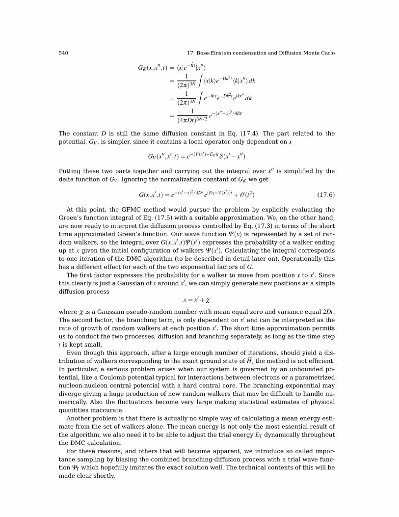
540 17 Bose-Einstein condensation and Diffusion Monte Carlo
GK(x,x′′, t) = 〈x|e−Kt |x′′〉
=1
(2π)3N
∫〈x|k〉e−Dk2t〈k|x′′〉dk
=1
(2π)3N
∫e−ikxe−Dk2teikx′′ dk
=1
(4πDt)3N/2e−(x
′′−x)2/4Dt
The constant D is still the same diffusion constant in Eq. (17.4). The part related to thepotential, GV , is simpler, since it contains a local operator only dependent on x
GV (x′′,x′, t) = e−(V (x′)−ET)tδ (x′− x′′)
Putting these two parts together and carrying out the integral over x′′ is simplified by thedelta function of GV . Ignoring the normalization constant of GK we get
G(x,x′, t) = e−(x′−x)2/4Dt e(ET−V (x′))t +O(t2) (17.6)
At this point, the GFMC method would pursue the problem by explicitly evaluating theGreen’s function integral of Eq. (17.5) with a suitable approximation. We, on the other hand,are now ready to interpret the diffusion process controlled by Eq. (17.3) in terms of the shorttime approximated Green’s function. Our wave function Ψ (x) is represented by a set of ran-dom walkers, so the integral over G(x,x′, t)Ψ(x′) expresses the probability of a walker endingup at x given the initial configuration of walkers Ψ(x′). Calculating the integral correspondsto one iteration of the DMC algorithm (to be described in detail later on). Operationally thishas a different effect for each of the two exponential factors of G.
The first factor expresses the probability for a walker to move from position x to x′. Sincethis clearly is just a Gaussian of x around x′, we can simply generate new positions as a simplediffusion process
x = x′+ χ
where χ is a Gaussian pseudo-random number with mean equal zero and variance equal 2Dt.The second factor, the branching term, is only dependent on x′ and can be interpreted as therate of growth of random walkers at each position x′. The short time approximation permitsus to conduct the two processes, diffusion and branching separately, as long as the time stept is kept small.
Even though this approach, after a large enough number of iterations, should yield a dis-tribution of walkers corresponding to the exact ground state of H, the method is not efficient.In particular, a serious problem arises when our system is governed by an unbounded po-tential, like a Coulomb potential typical for interactions between electrons or a parametrizednucleon-nucleon central potential with a hard central core. The branching exponential maydiverge giving a huge production of new random walkers that may be difficult to handle nu-merically. Also the fluctuations become very large making statistical estimates of physicalquantities inaccurate.
Another problem is that there is actually no simple way of calculating a mean energy esti-mate from the set of walkers alone. The mean energy is not only the most essential result ofthe algorithm, we also need it to be able to adjust the trial energy ET dynamically throughoutthe DMC calculation.
For these reasons, and others that will become apparent, we introduce so called impor-tance sampling by biasing the combined branching-diffusion process with a trial wave func-tion ΨT which hopefully imitates the exact solution well. The technical contents of this will bemade clear shortly.
17.1 Diffusion Monte Carlo 541
17.1.1 Importance Sampling
Let us introduce a time independent trial wave function ΨT(x). We define the new quantity
f (x, t)≡ΨT(x)Ψ (x, t)
Now by inserting Ψ = f/ΨT into Eq. (17.3) we get a slightly more complicated equation interms of f (x, t)
∂ f (x, t)
∂ t= D∇2 f (x, t)−D∇(F(x) f (x, t))− (EL(x)−ET) f (x, t) (17.7)
with the constant D defined as in Eq. (17.4). Notice that the rhs. consists of three terms. Bythe same line of thought as before we now recognize the first term as the familiar diffusionterm, acting on f instead ofΨ . The last term, similar in form to the potential term, is our newbranching term, also acting on f . The quantity EL(x) is just the local energy with respect toΨT, defined in the same manner as in the variational Monte Carlo procedure
EL ≡1
ΨT
HΨT
The vector quantity F(x) in the unfamiliar middle term is the drift velocity as we know it fromthe Fokker-Planck formalism we used to improve the Metropolis algorithm
F(x)≡ 2
ΨT
∇ΨT (17.8)
Actually, the two first terms on the rhs. of Eq. (17.7) can equivalently be expressed as thefamiliar Fokker-Planck drift-diffusion on the rhs. of Eq. (14.26).
Eq. (17.7) motivates us to let the set of random walkers represent f instead ofΨ . A typicalfirst order short time approximation of the corresponding Green’s function is
G(x,x′, t) =1
(4πDt)3N/2e−(x−x′−DtF(x′))2/4Dt e−((EL(x)+EL(x
′))/2−ET)t
+ O(t2) (17.9)
We see that the Green’s function above consists of two factors. The first one is similar to theGaussian in Eq. (17.6). But now we have in addition a drift term displacing the mean of theGaussian by DtF(x′). Notice that this factor of the Green’s function is practically identicalto the transition proposition rule introduced by the Fokker-Planck formalism to improve theMetropolis algorithm (see Eq. (14.25)). We can therefore use the same drift-diffusion formal-ism for the first factor in the above Green’s function. Recall that if a walker is initially atposition x′, the new position x is calculated as follows (see Eq. (14.24))
x = x′+ χ +DF(x′)t (17.10)
where χ is again a Gaussian pseudo-random number with mean equal zero and variance equal2Dt while DF(x′)t gives a drift in the direction that ΨT increases. The size of the time step t
biased the final outcome of the Fokker-Planck algorithm of the drifted diffusion. A desirablediffusion was reached only as t→ 0 for each iteration. Also in the present application to DMC,this bias must be taken into account. In the Metropolis algorithm, the rejection mechanismtook care of it. So we may use the same approach here. After calculating a new position withEq. (17.10), we accept it according to the acceptance matrix

542 17 Bose-Einstein condensation and Diffusion Monte Carlo
A(x, x′, t) =min
[1,
GK(x′,x)
GK(x,x′)|ΨT(x)|2|ΨT(x′)|2
](17.11)
where GK is the kinetic part of the Green’s function, the part related to the diffusion pro-cess. If we do not wish to do such a Metropolis test, we may alternatively conduct separatecalculations for a set of different time steps t and extrapolate the results to t = 0.
The second factor of Eq. (17.9) plays the same role as the branching term of Eq. (17.6).But the potential V is replaced by an expression dependent on the local energy,
EL(x)+EL(x′)
2−ET
The new branching term gives a greatly reduced branching effect compared to the one inEq. (17.6). Particularly, in the limit ofΨT = φ0 and ET = ε0 (exactly equal the ground state of H),the local energy is constant, giving equal branching everywhere, or in effect, no branching atall. Thus we can in general expect the number of walkers to fluctuate less and we certainlyavoid uncontrollable growth. In addition, the branching favors the areas of the configurationspace that give the lowest local energy, i.e. the local energy closest to the true ground stateenergy. Furthermore, the drifted diffusion pushes the walkers towards the desirable areas.Thus the whole DMC process is conducted more efficiently.
Finally, the introduction of the trial wave function ΨT makes it possible to evaluate anestimate of the mean energy given the distribution of the walkers. Instead of calculating thetypical mean energy ∫
Ψ∗HΨdx∫Ψ∗Ψdx
we calculate the so called mixed estimator
〈E〉mixed =
∫ΨTHΨdx∫ΨTΨdx
(17.12)
As the DMC method approaches the exact result Ψ = φ0, the mixed estimator becomes
〈E〉mixed =
∫ΨT ε0Ψdx∫
ΨTΨdx=
ε0
∫ΨTΨdx∫
ΨTΨdx= ε0
so that the estimate indeed becomes correct. Because of the hermiticity of H we can rewritethe mixed estimator of Eq. (17.12) as follows
〈E〉mixed =
∫Ψ HΨTdx∫ΨTΨdx
=
∫ΨTΨ 1
ΨTHΨT dx
∫ΨTΨdx
=
∫EL f (x)dx∫
f (x)dx(17.13)
Since the walkers represent f we just need to average the local energy EL over the set ofwalkers.
This energy estimator allows us to calculate relatively easily the mean energy on the dis-tribution of walkers so that we can update the trial energy ET dynamically as the algorithmproceeds. As the trial energy gets better and better, the algorithm will hopefully stabilize onthe exact result within the limits of statistical fluctuations imposed by the local energy andour choice of ΨT.
As we know, a good choice of ΨT reduces the fluctuations of the local energy EL. Now wesee that this also makes the estimation of the mean energy in Eq. (17.13) more efficient sincethe same number of points (walkers) gives a smaller variance, thus pinpointing the energymore exactly.

17.2 Bose-Einstein Condensation in Atoms 543
Importance sampling makes it also to some extent easier to deal with wave functions thatare not positive definite, like fermionic states whose wave function have nodes. What hap-pens is that the nodes of the function f are tied by the nodes of the trial wave function ΨT.Therefore it is necessary for ΨT to have a node configuration that best reproduces the phys-ical properties of the exact wave function. Operationally, the node surfaces of ΨT becomeimpenetrable walls to the walkers in the sense that the drift velocity F in the vicinity of sucha surface increases in a direction away from it pushing any walker away, preventing it fromcrossing the nodal surfaces of ΨT. The approach is called a fixed node approximation.
From all these deliberations on importance sampling we should by now understand theimportance of the trial wave function being as close to the exact solution as possible. Wetherefore rely heavily on simpler methods like VMC that do not necessarily solve the prob-lem exactly, but are easier to handle computationally and are much less sensitive to initialconditions.
17.2 Bose-Einstein Condensation in Atoms
The spectacular demonstration of Bose-Einstein condensation (BEC) in gases of alkali atoms87Rb, 23Na, 7Li confined in magnetic traps [130–132] has led to an explosion of interest inconfined Bose systems. Of interest is the fraction of condensed atoms, the nature of thecondensate, the excitations above the condensate, the atomic density in the trap as a functionof Temperature and the critical temperature of BEC, Tc. The extensive progress made up toearly 1999 is reviewed by Dalfovo et al. [133].
A key feature of the trapped alkali and atomic hydrogen systems is that they are dilute.
The characteristic dimensions of a typical trap for 87Rb is ah0 = (h/mω⊥)12 = 1− 2× 10⁴ Å
(Ref. [130]). The interaction between 87Rb atoms can be well represented by its s-wave scat-tering length, aRb. This scattering length lies in the range 85 < aRb < 140a0 where a0 = 0.5292
Å is the Bohr radius. The definite value aRb = 100a0 is usually selected and for calculations thedefinite ratio of atom size to trap size aRb/ah0 = 4.33× 10⁻³ is usually chosen [133]. A typical87Rb atom density in the trap is n≃ 1012−1014 atoms/cm3 giving an inter-atom spacing ℓ≃ 104
Å. Thus the effective atom size is small compared to both the trap size and the inter-atomspacing, the condition for diluteness (na3
Rb ≃ 10−6 where n = N/V is the number density). Inthis limit, although the interaction is important, dilute gas approximations such as the Bo-goliubov theory [134], valid for small na3 and large condensate fraction n0 = N0/N, describethe system well. Also, since most of the atoms are in the condensate (except near Tc), theGross-Pitaevskii equation [135,136] for the condensate describes the whole gas well. Effectsof atoms excited above the condensate have been incorporated within the Popov approxima-tion [137].
Most theoretical studies of Bose-Einstein condensates (BEC) in gases of alkali atoms con-fined in magnetic or optical traps have been conducted in the framework of the Gross-Pitaevskii (GP) equation [135, 136]. The key point for the validity of this description is thedilute condition of these systems, i.e., the average distance between the atoms is much largerthan the range of the inter-atomic interaction. In this situation the physics is dominated bytwo-body collisions, well described in terms of the s-wave scattering length a. The crucialparameter defining the condition for diluteness is the gas parameter x(r) = n(r)a3, where n(r)
is the local density of the system. For low values of the average gas parameter xav ≤ 10−3,the mean field Gross-Pitaevskii equation does an excellent job (see for example Ref. [133]for a review). However, in recent experiments, the local gas parameter may well exceed thisvalue due to the possibility of tuning the scattering length in the presence of a Feshbachresonance [138].
544 17 Bose-Einstein condensation and Diffusion Monte Carlo
Under such circumstances it is unavoidable to test the accuracy of the GP equation byperforming microscopic calculations. If we consider cases where the gas parameter has beendriven to a region were one can still have a universal regime, i.e., that the specific shape ofthe potential is unimportant, we may attempt to describe the system as dilute hard sphereswhose diameter coincides with the scattering length. However, the value of x is such thatthe calculation of the energy of the uniform hard-sphere Bose gas would require to take intoaccount the second term in the low-density expansion [139] of the energy density
E
V=
2πn2ah2
m
[1+
128
15
(na3
π
)1/2
+ · · ·], (17.14)
where m is the mass of the atoms treated as hard spheres. For the case of uniform systems,the validity of this expansion has been carefully studied using Diffusion Monte Carlo [140]and Hyper-Netted-Chain techniques [141].
The energy functional associated with the GP theory is obtained within the frameworkof the local-density approximation (LDA) by keeping only the first term in the low-densityexpansion of Eq. (17.14)
EGP[Ψ ] =∫
dr
[h2
2m| ∇Ψ(r) |2 +Vtrap(r) |Ψ |2 +
2π h2a
m|Ψ |4
], (17.15)
where
Vtrap(r) =1
2m(ω2
⊥x2 +ω2⊥y2 +ω2
z z2) (17.16)
is the confining potential defined by the two angular frequencies ω⊥ and ωz. The condensatewave function Ψ is normalized to the total number of particles.
By performing a functional variation of EGP[Ψ ] with respect toΨ∗ one finds the correspond-ing Euler-Lagrange equation, known as the Gross-Pitaevskii (GP) equation
[− h2
2m∇2 +Vtrap(r)+
4π h2a
m|Ψ |2
]Ψ = µΨ , (17.17)
where µ is the chemical potential, which accounts for the conservation of the number ofparticles. Within the LDA framework, the next step is to include into the energy functional ofEq. (17.15) the next term of the low density expansion of Eq. (17.14). The functional variationgives then rise to the so-called modified GP equation (MGP) [142]
[− h2
2m∇2 +Vtrap(r)+
4π h2a
m|Ψ |2
(1+
32a3/2
3π1/2|Ψ |
)]Ψ = µΨ . (17.18)
The MGP corrections have been estimated in Ref. [142] in a cylindrical condensate inthe range of the scattering lengths and trap parameters from the first JILA experimentswith Feshbach resonances. These experiments took advantage of the presence of a Fesh-bach resonance in the collision of two 85Rb atoms to tune their scattering length [138]. Fullymicroscopic calculations using a hard-spheres interaction have also been performed in theframework of Variational and Diffusion Monte Carlo methods [143–146].

17.3 Exercises 545
17.3 Exercises
17.1. The aim of this project is to use the Variational Monte Carlo (VMC) method and evaluatethe ground state energy of a trapped, hard sphere Bose gas for different numbers of particleswith a specific trial wave function. See Ref. [94] for a discussion of VMC.
This wave function is used to study the sensitivity of condensate and non-condensate prop-erties to the hard sphere radius and the number of particles. The trap we will use is a spher-ical (S) or an elliptical (E) harmonic trap in three dimensions given by
Vext(r) =
12mω2
hor2 (S)12m[ω2
ho(x2 + y2)+ω2
z z2] (E)(17.19)
where (S) stands for symmetric and
H =N
∑i
(−h2
2m2
i +Vext(ri)
)+
N
∑i< j
Vint(ri,r j), (17.20)
as the two-body Hamiltonian of the system. Here ω2ho defines the trap potential strength. In
the case of the elliptical trap, Vext(x,y,z), ωho = ω⊥ is the trap frequency in the perpendicularor xy plane and ωz the frequency in the z direction. The mean square vibrational amplitude
of a single boson at T = 0K in the trap (17.19) is < x2 >= (h/2mωho) so that aho ≡ (h/mωho)12
defines the characteristic length of the trap. The ratio of the frequencies is denoted λ =ωz/ω⊥leading to a ratio of the trap lengths (a⊥/az) = (ωz/ω⊥)
12 =√
λ .We represent the inter boson interaction by a pairwise, hard core potential
Vint(|ri− r j|) =
∞ |ri− r j| ≤ a
0 |ri− r j|> a(17.21)
where a is the hard core diameter of the bosons. Clearly, Vint(|ri− r j|) is zero if the bosons areseparated by a distance |ri− r j| greater than a but infinite if they attempt to come within adistance |ri− r j| ≤ a.
Our trial wave function for the ground state with N atoms is given by
ΨT (R) =ΨT (r1,r2, . . .rN ,α,β ) = ∏i
g(α,β ,ri)∏i< j
f (a, |ri− r j|), (17.22)
where α and β are variational parameters. The single-particle wave function is proportionalto the harmonic oscillator function for the ground state, i.e.,
g(α,β ,ri) = exp [−α(x2i + y2
i +β z2i )]. (17.23)
For spherical traps we have β = 1 and for non-interacting bosons (a = 0) we have α = 1/2a2ho.
The correlation wave function is
f (a, |ri− r j|) =
0 |ri− r j| ≤ a
(1− a|ri−r j | ) |ri− r j|> a.
(17.24)
a) Find analytic expressions for the local energy
EL(R) =1
ΨT (R)HΨT (R), (17.25)

546 17 Bose-Einstein condensation and Diffusion Monte Carlo
for the above trial wave function of Eq. (17.22). Compute also the analytic expression for thedrift force to be used in importance sampling
F =2∇ΨT
ΨT
. (17.26)
The tricky part is to find an analytic expressions for the derivative of the trial wave function
1
ΨT (R)
N
∑i
∇2i ΨT (R),
for the above trial wave function of Eq. (17.22). We rewrite
ΨT (R) =ΨT (r1,r2, . . .rN ,α,β ) = ∏i
g(α,β ,ri)∏i< j
f (a, |ri− r j|),
asΨT (R) = ∏
i
g(α,β ,ri)e∑i< j u(ri j)
where we have defined ri j = |ri− r j| and
f (ri j) = e∑i< j u(ri j),
and in our caseg(α,β ,ri) = e−α(x2
i +y2i +z2
i ) = φ(ri).
The first derivative becomes
∇kΨT (R) = ∇kφ(rk)
[
∏i6=k
φ(ri)
]e∑i< j u(ri j)+∏
i
φ(ri)e∑i< j u(ri j) ∑
j 6=k
∇ku(ri j)
We leave it as an exercise for the reader to find the expression for the sceond derivative. Thefinal expression is
1
ΨT (R)∇2
kΨT (R) =∇2
kφ(rk)
φ(rk)+
∇kφ(rk)
φ(rk)
(
∑j 6=k
rk
rk
u′(ri j)
)+
∑i j 6=k
(rk− ri)(rk− r j)
rkirk j
u′(rki)u′(rk j)+ ∑
j 6=k
(u′′(rk j)+
2
rk j
u′(rk j)
)
You need to get the analytic expression for this expression using the harmonic oscillator wavefunctions and the correlation term defined in the project.
b) Write a Variational Monte Carlo program which uses standard Metropolis sampling and com-pute the ground state energy of a spherical harmonic oscillator (β = 1) with no interaction.Use natural units and make an analysis of your calculations using both the analytic expres-sion for the local energy and a numerical calculation of the kinetic energy using numericalderivation. Compare the CPU time difference. You should also parallelize your code. The onlyvariational parameter is α. Perform these calculations for N = 10, 100 and 500 atoms. Compareyour results with the exact answer.
c) We turn now to the elliptic trap with a hard core interaction. We fix, as in Refs. [143, 147]a/aho = 0.0043. Introduce lengths in units of aho, r→ r/aho and energy in units of hωho. Showthen that the original Hamiltonian can be rewritten as
H =N
∑i=1
1
2
(−∇2
i + x2i + y2
i + γ2z2i
)+∑
i< j
Vint(|ri− r j|). (17.27)

17.3 Exercises 547
What is the expression for γ? Choose the initial value for β = γ = 2.82843 and set up a VMC pro-gram which computes the ground state energy using the trial wave function of Eq. (17.22).using only α as variational parameter. Use standard Metropolis sampling and vary the pa-rameter α in order to find a minimum. Perform the calculations for N = 10,50 and N = 100
and compare your results to those from the ideal case in the previous exercise. In actualcalculations employing e.g., the Metropolis algorithm, all moves are recast into the chosensimulation cell with periodic boundary conditions. To carry out consistently the Metropolismoves, it has to be assumed that the correlation function has a range shorter than L/2. Then,to decide if a move of a single particle is accepted or not, only the set of particles containedin a sphere of radius L/2 centered at the referred particle have to be considered.
d) We repeat exercise c), but now we replace the brute force Metropolis algorithm with im-portance sampling based on the Fokker-Planck and the Langevin equations. Discuss yourresults and comment on eventual differences between importance sampling and brute forcesampling.Your code should reproduce the results of Refs. [143,147].

548 17 Bose-Einstein condensation and Diffusion Monte Carlo
References
1. J. Dongarra, F. Sullivan, Computing in Science and Engineering 2, 22 (2000)2. B. Cipra, SIAM News 33, 1 (2000)3. J. Thijssen, Computational Physics (Cambridge, 1999)4. S. Koonin, D. Meredith, Computational Physics (Addison Wesley, 1990)5. J. Gibbs, Computational Physics (World Scientific, 1994)6. B. Giordano, H. Nakanishi, Computational Physics (Preston, 2005)7. R. Landau, M. Paez, Computational Physics (Wiley, 1997)8. R. Guardiola, E. Higon, J. Ros, Metodes Numèrics per a la Física (Universitat de Valencia, 1997)9. E. Schmid, G. Spitz, W. Lösch, Theoretische Physik mit dem Personal Computer (Springer Verlag, 1987)
10. H. Gould, J. Tobochnik, An Introduction to Computer Simulation Methods: Applications to Physical Sys-tems (Addison-Wesley, 1996)
11. B. Smith, J. Adams, W. Brainerd, J. Wagener, Fortran 95 Handbook (MIT press, 1997)12. M. Metcalf, J. Reid, The F90 Programming Language (Oxford University Press, 1996)13. A. Marshall, Fortran 90 Programming (University of Liverpool, 1995)14. J. Reid, The new features of fortran 2003. Tech. rep., ISO working group on Fortran (2007). URL
http://www.iso.org/iso/home.htm
15. W. Gropp, E. Lusk, A. Skjellum, Using MPI (The MIT Press, 1999)16. M. Snir, S. Otto, S. Huss-Ledermann, D. Walker, J. Dongarra, MPI, the Complete Reference, Vols I and II
(The MIT Press, 1998)17. G.E. Karniadakis, R.M. Kirby II, Parallel scientific computing in C++ and MPI (Cambridge, 2005)18. B. Flowers, An Introduction to Numerical Methods in C++ (Oxford University Press, 2000)19. J. Barton, L. Nackman, Scientific and Engineering C++ (Addison Wesley, 1994)20. B. Stoustrup, The C++ Programming Language (Pearson, 1997)21. H. Langtangen, Python Scripting for Computational Science (Springer, 2006)22. H. Langtangen, Introduction to Computer Programming; A Python-based approach for Computational
Science (Springer Verlag, 2009)23. D. Kincaid, W. Cheney, Numerical Analysis (Brooks/Gole Publishing Company, 1996)24. R. Kress, Numerical Analysis (Springer, 1998)25. J. Stoer, R. Bulirsch, Introduction to Numerical Analysis (Springer Verlag, 1983)26. LAPACK – Linear Algebra PACKage (http://www.netlib.org/lapack/)27. C.L. Lawson, R.J. Hanson, D. Kincaid, F.T. Krogh, ACM Trans. Math. Soft. 5, 308 (1979)28. G. Golub, C. Van Loan, Matrix Computations (John Hopkins University Press, 1996)29. B. Datta, Numerical Linear Algebra and Applications (Brooks/Cole Publishing Company, 1995)30. L. Trefethen, D. Bau III, Numerical Linear Algebra (SIAM Publications, 1997)31. J. Demmel, Numerical Linear Algebra (SIAM Publications, 1996)32. T. Veldhuizen, Blitz++ User’s Guide (http://www.oonumerics.org/blitz/ , 2003)33. K. Reek, Pointers on C (Addison Wesley, 1998)34. J. Berryhill, C++ Scientific Programming (Wiley-Interscience, 2001)35. F. Franek, Memory as a Programming Concept in C and C++ (Cambridge University Press, 2004)36. W. Press, B. Flannery, S. Teukolsky, W. Vetterling, Numerical Recipes in C++, The art of scientific Com-
puting (Cambridge University Press, 1999)37. L.H. Thomas, Proc. Camb. Phil. Soc. 23, 542 (1927)38. E. Fermi, Rend. Accad. Naz. Lincei 6, 602 (1927)39. E.H. Lieb, Rev. Mod. Phys. 53(4), 603 (1981). DOI 10.1103/RevModPhys.53.60340. H.R. Pagels, Cosmic Code: Quantum Physics as the Law of Nature (Simon and Schuster, 1982)41. K. Eriksson, D. Estep, P. Hansbo, C. Johnson, Computational Differential Equations (Cambridge Univer-
sity Press, 1996)42. J. Butcher, Numerical Methods for Ordinary Differential equations (Wiley, 2008)43. E. Hairer, S. NÃÿrsett, G. Wanner, Solving Ordinary Differential Equations I (Springer Verlag, Berlin,
1987)44. D.C. Rapaport, The Art of Molecular Dynamics Simulation (Cambridge University Press, 2007)45. D. Marx, J. Hutter, Ab Initio Molecular Dynamics (Cambridge University Press, 2010)46. S.L. Shapiro, S.A. Teukolsky, Black holes, white dwarfs, and neutron stars: the physics of compact objects
(Wiley, 1983)47. H. Heiselberg, M. Hjorth-Jensen, Phys. Rep. 328, 237 (2000). DOI doi:10.1016/S0370-1573(99)00110-648. N.K. Glendenning, Compact Stars (Springer, 2000)49. H. Bethe, M. Johnson, Nucl. Phys. A 230, 1 (1974)50. H. Langtangen, Computational Partial Differential Equations: Numerical Methods and Diffpack Pro-
gramming (Springer, 1999)

References 549
51. J. Ortega, W. Poole, An Introduction to Numerical Methods for Differential Equations (Pitman, 1981)52. A. Tveito, R. Winther, Introduction to Partial Differential Equations (Springer, 2002)53. G. Arfken, Mathematical Methods for Physicists (Academic Press, 1985)54. L. Evans, Partial differential equations, Graduate Studies in Mathematics, vol. 19 (American Mathemat-
ical Society, 2002)55. L. Ramdas Ram-Mohan, Finite Element and Boundary Element Applications in Quantm Mechanics (Ox-
ford University Press, 2002)56. G. Evans, J. Blackledge, P. Yardley, Numerical methods for partial differential equations (Springer, 1999)57. M. Pliscke, B. Bergersen, Equilibrium Statistical Physics (Prentice-Hall, 1989)58. P. Glasserman, Monte Carlo Methods in Financial Engineering (Springer Verlag, 2004)59. P. Jackel, Monte Carlo Methods in Finance (John Wiley and Sons, LTD, 2002)60. J. Voit, The Statistical Mechanics of Financial Markets (Springer Verlag, 2005)61. J.L. McCauley, Dynamics of Markets, Econophysics and Finance (Cambridge University Press, 2004)62. D. Sornette,Why Stock Markets Crash (Princeton University Press, 2002)63. C. Robert, G. Casella, Monte Carlo Statistical Methods (Springer Verlag, 2004)64. J. Johnson, Probability and Statistics for Computer Science (Wiley-Interscience, 2003)65. G. Fishman, Monte Carlo, Concepts, Algorithms and Applications (Springer, 1996)66. J.A. Rice, Mathematical Statistics and Data Analysis (Duxbury Advanced, 1994)67. H. Flyvbjerg, H.G. Petersen, The Journal of Chemical Physics 91(1), 461 (1989). DOI 10.1063/1.457480.
URL http://link.aip.org/link/?JCP/91/461/1
68. H. Marzaglia, B. Zaman, Computers in Physics 8, 117 (1994)69. I. Karatsas, S. Shreve, Brownian Motion and Stochastic Calculus (Springer, 1988)70. M. Chaichian, A. Demichev, Path Integrals in Physics, Volume 1 (Institute of Physics Publishing, 2001)71. L. Onsager, Phys. Rev. 31, 405 (1931)72. M. Patriarca, A. Chakraborti, K. Kaski, Physica A 340, 334 (2004). DOI doi:10.1016/j.physa.2004.04.02473. L. Onsager, Phys. Rev. 65(3-4), 117 (1944). DOI 10.1103/PhysRev.65.11774. N. Ashcroft, N. Mermin, Solid State Physics (Holt-Saunders, 1976)75. J. Cardy, Scaling and Renormalization in Statistical Physics (Cambridge University Press, 1996)76. K.G. Wilson, Rev. Mod. Phys. 47, 773 (1975). DOI 10.1103/RevModPhys.47.77377. K.G. Wilson, Rev. Mod. Phys. 55, 583 (1983). DOI 10.1103/RevModPhys.55.58378. H.E. Stanley, Rev. Mod. Phys. 71(2), S358 (1999). DOI 10.1103/RevModPhys.71.S35879. M. Newman, G. Barkema, Monte Carlo Methods in Statistical Physics (Clarendon Press, 1999)80. D. Landau, K. Binder, A Guide to Monte Carlo Simulations in Statistical Physics (Cambridge University
Press, 2000)81. R. Shankar, Rev. Mod. Phys. 66(1), 129 (1994). DOI 10.1103/RevModPhys.66.12982. H. Stanley, Introduction to Phase Transitions and Critical Phenomena (Oxford University Press, 1971)83. N. Metropolis, A.W. Rosenbluth, M.N. Rosenbluth, A.H. Teller, E. Teller, The Journal of Chemical Physics
21(6), 1087 (1953). URL http://link.aip.org/link/?JCP/21/1087/1
84. A.M. Ferrenberg, R.H. Swendsen, Phys. Rev. Lett. 61, 2635 (1988). DOI 10.1103/PhysRevLett.61.263585. A.M. Ferrenberg, R.H. Swendsen, Phys. Rev. Lett. 63, 1195 (1989). DOI 10.1103/PhysRevLett.63.119586. M.P. Nightingale, H.W.J. Blöte, Phys. Rev. Lett. 76(24), 4548 (1996). DOI 10.1103/PhysRevLett.76.454887. U. Wolff, Phys. Rev. Lett. 62(4), 361 (1989). DOI 10.1103/PhysRevLett.62.36188. R.H. Swendsen, J.S. Wang, Phys. Rev. Lett. 58, 86 (1987). DOI 10.1103/PhysRevLett.58.8689. J.L. Monroe, Phys. Rev. E 66(6), 066129 (2002). DOI 10.1103/PhysRevE.66.06612990. M.S.S. Challa, D.P. Landau, K. Binder, Phys. Rev. B 34(3), 1841 (1986). DOI 10.1103/PhysRevB.34.184191. F.Y. Wu, Rev. Mod. Phys. 54(1), 235 (1982). DOI 10.1103/RevModPhys.54.23592. K. Binder, Reports on Progress in Physics 50(7), 783 (1987). URL
http://stacks.iop.org/0034-4885/50/783
93. R. Liboff, Introductory Quantum Mechanics (Addison Wesley, 2003)94. B.L. Hammond, W.A. Lester, P. Reynolds, Monte Carlo Methods in ab Initio Quantum Chemistry (World
Scientific, 1994)95. H. Kümmel, K.H. Luhrmann, J.G. Zabolitzky, Phys. Rep. 36, 1 (1978, and references therein)96. R.J. Bartlett, M. Musiał, Reviews of Modern Physics 79(1), 291 (2007). DOI 10.1103/RevModPhys.79.
291. URL http://link.aps.org/abstract/RMP/v79/p291
97. T. Helgaker, P. Jørgensen, J. Olsen, Molecular Electronic Structure Theory. Energy and Wave Functions(Wiley, Chichester, 2000)
98. D.J. Dean, M. Hjorth-Jensen, Physical Review C 69, 054320 (2004). URLhttp://link.aps.org/abstract/PRC/v69/e054320
99. K. Kowalski, D.J. Dean, M. Hjorth-Jensen, T. Papenbrock, P. Piecuch, Phys.Rev. Lett. 92, 132501 (2004). DOI 10.1103/PhysRevLett.92.132501. URLhttp://link.aps.org/doi/10.1103/PhysRevLett.92.132501

550 17 Bose-Einstein condensation and Diffusion Monte Carlo
100. B.S. Pudliner, V.R. Pandharipande, J. Carlson, S.C. Pieper, R.B. Wiringa, Phys. Rev. C 56, 1720 (1997).DOI 10.1103/PhysRevC.56.1720
101. S. Koonin, D. Dean, K. Langanke, Phys. Rep. 278, 1 (1997). DOI doi:10.1016/S0370-1573(96)00017-8102. D.M. Ceperley, Rev. Mod. Phys. 67, 279 (1995). URL http://link.aps.org/abstract/RMP/v67/p279
103. P.J. Ellis, E. Osnes, Rev. Mod. Phys. 49, 777 (1977). URL http://link.aps.org/abstract/RMP/v49/p777104. I. Lindgren, J. Morrison, Atomic Many-Body Theory (Springer, Berlin, 1985)105. M. Hjorth-Jensen, T.T.S. Kuo, E. Osnes, Phys. Rep. 261, 125 (1995). DOI doi:10.1016/0370-1573(95)
00012-6106. W.H. Dickhoff, D.V. Neck,Many-Body Theory exposed! (World Scientific, 2005)107. J.P. Blaizot, G. Ripka, Quantum theory of finite systems (MIT press, Cambridge, USA, 1986)108. S.R. White, Phys. Rev. Lett. 69, 2863 (1992). DOI 10.1103/PhysRevLett.69.2863. URL
http://link.aps.org/abstract/PRL/v69/p2863
109. U. Schollwock, Rev. Mod. Phys. 77, 259 (2005). URL http://link.aps.org/abstract/RMP/v77/p259
110. R.O. Jones, O. Gunnarsson, Rev. Mod. Phys. 61(3), 689 (1989). DOI 10.1103/RevModPhys.61.689111. R.J. Bartlett, V.F. Lotrich, I.V. Schweigert, J. Chem. Phys. 123, 062205 (2005). URL
http://link.aip.org/link/?JCP/123/062205/1
112. K. Peirs, D.V. Neck, M. Waroquier, Physical Review A (Atomic, Molecular, and Optical Physics) 67,012505 (2003). URL http://link.aps.org/abstract/PRA/v67/e012505
113. D.V. Neck, S. Verdonck, G. Bonny, P.W. Ayers, M. Waroquier, Physical Review A (Atomic, Molecular, andOptical Physics) 74, 042501 (2006). URL http://link.aps.org/abstract/PRA/v74/e042501
114. R.R. Whitehead, A. Watt, B.J. Cole, I. Morrison, Adv.Nucl.Phys. 9, 123 (1977)115. E. Caurier, G. Martinez-Pinedo, F. Nowacki, A. Poves, A.P. Zuker, Rev. Mod. Phys. 77, 427 (2005). URL
http://link.aps.org/abstract/RMP/v77/p427
116. M. Horoi, B.A. Brown, T. Otsuka, M. Honma, T. Mizusaki, Phys. Rev. C 73, 061305 (2006). URLhttp://link.aps.org/abstract/PRC/v73/e061305
117. D.J. Dean, M. Hjorth-Jensen, Computational Quantum Mechanics for Nuclear Physics (Chapman & Hal-l/CRC, 2009)
118. B.H. Bransden, C.J. Joachain, Physics of Atoms and Molecules (Longman, 1983)119. J.W. Moskowitz, M.H. Kalos, Int. J. Quantum Chem. 20, 1107 (1981)120. J.W. Moskowitz, K.E. Schmidt, M.A. Lee, M.H. Kalos, The Journal of Chemical Physics 76(2), 1064 (1982).
DOI 10.1063/1.443098. URL http://link.aip.org/link/?JCP/76/1064/1
121. P.W. Atkins, R.S. Freidman, Molecular Quantum Mechanics (Oxford Univerity Press, 2003)122. E. Clementi, D.L. Raimondi, J. Chem. Phys. 38, 2686 (1963)123. P. Hohenberg, W. Kohn, Phys. Rev. 136(3B), B864 (1964). DOI 10.1103/PhysRev.136.B864124. W. Kohn, L.J. Sham, Phys. Rev. 140(4A), A1133 (1965). DOI 10.1103/PhysRev.140.A1133125. J.P. Perdew, A. Zunger, Phys. Rev. B 23(10), 5048 (1981). DOI 10.1103/PhysRevB.23.5048126. J.P. Perdew, Y. Wang, Phys. Rev. B 45(23), 13244 (1992). DOI 10.1103/PhysRevB.45.13244127. J.P. Perdew, J.A. Chevary, S.H. Vosko, K.A. Jackson, M.R. Pederson, D.J. Singh, C. Fiolhais, Phys. Rev. B
46(11), 6671 (1992). DOI 10.1103/PhysRevB.46.6671128. A.J. Williamson, S.D. Kenny, G. Rajagopal, A.J. James, R.J. Needs, L.M. Fraser, W.M.C. Foulkes, P. Maccul-
lum, Phys. Rev. B 53(15), 9640 (1996). DOI 10.1103/PhysRevB.53.9640129. D. Ceperley, G.V. Chester, M.H. Kalos, Phys. Rev. B 16(7), 3081 (1977). DOI 10.1103/PhysRevB.16.3081130. M.H. Anderson, J.R. Ensher, M.R. Matthews, C.E. Wieman, E.A. Cornell, Science 269, 198 (1995)131. K.B. Davis, M.O. Mewes, M.R. Andrews, N.J. van Druten, D.S. Durfee, D.M. Kurn, W. Ketterle, Phys. Rev.
Lett. 75(22), 3969 (1995). DOI 10.1103/PhysRevLett.75.3969132. C.C. Bradley, C.A. Sackett, J.J. Tollett, R.G. Hulet, Phys. Rev. Lett. 75(9), 1687 (1995). DOI 10.1103/
PhysRevLett.75.1687133. F. Dalfovo, S. Giorgini, L.P. Pitaevskii, S. Stringari, Rev. Mod. Phys. 71, 463 (1999). DOI 10.1103/
RevModPhys.71.463134. N. Bogolyubov, Dolk. Akad. Nauk SSSR 119, 244 (1959)135. E. Gross, Nuovo Cimento 20, 454 (1961)136. L. Pitaevskii, Zh.EKSP.Teor.Fiz. 40, 646 (1961)137. D.A.W. Hutchinson, E. Zaremba, A. Griffin, Phys. Rev. Lett. 78(10), 1842 (1997). DOI 10.1103/
PhysRevLett.78.1842138. S.L. Cornish, N.R. Claussen, J.L. Roberts, E.A. Cornell, C.E. Wieman, Phys. Rev. Lett. 85(9), 1795 (2000).
DOI 10.1103/PhysRevLett.85.1795139. A.L. Fetter, J.D. Walecka, Quantum Theory of Many-Particle Systems (McGraw-Hill, 1971)140. S. Giorgini, J. Boronat, J. Casulleras, Phys. Rev. A 60(6), 5129 (1999). DOI 10.1103/PhysRevA.60.5129141. F. Mazzanti, A. Polls, A. Fabrocini, Phys. Rev. A 67(6), 063615 (2003). DOI 10.1103/PhysRevA.67.063615142. A. Fabrocini, A. Polls, Phys. Rev. A 60(3), 2319 (1999). DOI 10.1103/PhysRevA.60.2319143. J.L. DuBois, H.R. Glyde, Phys. Rev. A 63(2), 023602 (2001). DOI 10.1103/PhysRevA.63.023602

References 551
144. A.R. Sakhel, J.L. DuBois, H.R. Glyde, Phys. Rev. A 66(6), 063610 (2002). DOI 10.1103/PhysRevA.66.063610
145. J.L. DuBois, H.R. Glyde, Phys. Rev. A 68(3), 033602 (2003). DOI 10.1103/PhysRevA.68.033602146. D. Blume, C.H. Greene, Phys. Rev. A 63(6), 063601 (2001). DOI 10.1103/PhysRevA.63.063601147. J.K. Nilsen, J. Mur-Petit, M. Guilleumas, M. Hjorth-Jensen, A. Polls, Physical Review A (Atomic, Molecular,
and Optical Physics) 71, 053610 (2005). URL http://link.aps.org/abstract/PRA/v71/e053610