Computational Physics : FORTRAN Version - Booksfree
656
-
Upload
khangminh22 -
Category
Documents
-
view
0 -
download
0
Transcript of Computational Physics : FORTRAN Version - Booksfree

COM IONAL PHYSICS Fortran V&on

This page intentionally left blank
COMPUTAT L S Version
Professor of Theoretical Physics Calvomzia institute of Rchmlogy
Dawn C. Meredith Assistant Professor of Physics Univmsity of New Ham-pshire
' A Member of the I'erseus Books Group

This book was tmtsset by Elkabeth K, Wmd ushg the 'Q@ &xt-processing syskm running on a Bigibl Equipment Gomodion n 2@m cornpuk~ Camera-read~ f i i d COPY
ww produced on an Appb WerWrikr.
FoElswing is a list ofbadernsks used in tke book: V M , VMsMion, W S , W axe &&emaks af Bi@M Equipment Copoaion.
UES, HCFJIS*** CA-DISSPM is a &&emmk of Computer boci-s In&rn&iond, E nc. W= is a bdernmk ofAT&T. XBM-PC is a. W e m m k of Xnteraliond Bushess Mitchhes, MackWsh is a Wademmk of Apple Compukr, Inc, %Won& 4010 iisl a &demwk of%k&anix Enc. GO-235 is a mdentak af Graphon Copomtion. WDS3200 is a trdemwk of Humizn Dwiped Sys&ms. %X is a trMemwk of the Ame~cm Mahernaied Society. PST is a Wemask sf Mme Computers, Enc. Kermit Is a Mexnwk af Wdt Bisnq &oduc:tiox1s, S;m is a r e g b k ~ d of SW Mcrasp&ms,Inc.
Koonin, Skven E. version) I SWen E. Koonb, Dawn Nereditk.
p. cm. Includes index.
physie+D@ processing, 2. Physic+Computer pragms, 3. puter program lmguage) 4. Nume~cal malysis. I, Meredith, Dawn, IE. Title, Q620.XE4K66 1M 530.1 "W02855133-d~L9 90- 129 ISBN 0-201 -X 2774-2 ( h ~ d ~ ~ e r ) ISBN 0-201 -38623-2 [pperback)
Copyight 8 199l)byWestviecv Press, a member of the Per~eus Books Group
All rim& resemed. No part of this text publiatjon may be reproduced, stored in a reeied system, or kansmitbd, in my fom or by my me=, ekc&anic, mechicat, phoacopyhg, recordhg, or o themh , wigbout the prior Wtten permimion of the publisher. Prinkb in the Unikd S b k s ofbefica. Prxblhfied simulkneously in CmiltZa, 1 0 9 8 ' 7 6 5 4
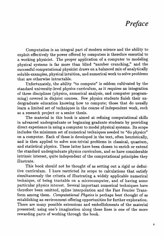
Preface
Computation is an integral part of modern science and the ability to exploit effectively the power offered by computers is therefore essential to a working physicist. The proper application of a computer to modeling physical systems is far more than blind "number crunching," and the successful computational physicist draws on a bdanced mix of analytically soluble examples, physicd intuition, and numerical work to solve problems that x e otherwige intractable.
Unfortunately, the ability "to computen is seldom cultivated by the stmdard zrniwrsity-level physics crtrri culum, as it requires an inteaation of three disciplines (physics, numerical analysis, and computer program- ming) covered in disjoint courses. Few physics students finish their un- dergraduate education knowing how to compute; those that do usually leara a L i ~ t e d get of techniques in the coufse of independent work, such as a research projed or a senior thesis.
The materid in. this book is ~ m e d r e f i~ng eomputationd sEns in advanced undergraduate ar be@nning graduate students by providixrg
experimce in using a computer to model physical systems. Its s q e includes the minimam set of numerical techaiques needed to '"do physics" on a mmputer. Each of these is developed In the text, often hmristicdy, and is then applied to solve non-trivial problems in classical, qnantum, and statisticd physics, The= latter have been chosen to enrich or a t end the standard undergraduate physics curriculum, and so haw considerable intrinsic interest, quite independent of the comput ationd principles they illustrate,
This book should not be thought of as setting out a rigid or defini- tive curriculum. I have restricted its scope to calculations that satisfy simultaneously the criteria of illustrating a widely applicable numerical technique, of being tractable on a microcomputer, and of having some parhicalm physics interest. Several import ant numeric& techniques have therefore been o ~ t t e d , spEae iaterpdatim asld the F a t Fburier Trans- form among them. Computational Physics is perhaps best thought of as establishing m environment rer ring opportunities for further eqloration. There are =my possible extensions and embelEshmerrts of the materid prescjnted; using mevs iana&nation dong these liaw is one of the mom rewwding parts of working through the book.
C"omp.utat%'onal Pltysz'cb? is primwily a physics text, For xnknrum benefit, the student should have taken, or be taking, undergrad- uate courses in dwsical meclzanic~, quantum mechanics, stat;jstical me- chmics, and advanced cafculus m the mathematical methods of physics. Tbis is slot a text on aurnerical analysis, as there hahs been no attempt at rigor or completeness in any of the expositions of numerical techniques. However, a prior course in that subject is probabb not essential; the dis- cussions of numerical techniques should be accessible to a student with the physics background outlined above, perhaps with gome reference to any one of the excellent texts on numerical andysis (for example, [AC~O], [Bu81], or [Sh84]). This is dso not a text on computer programming. AI- though I have tried to follow the principles of good programming through- out (see Appendix B), there has been no attempt to teach programming per se. Indeed, techniques for organizing and writing code are somewhat peripheral to the main gods of the book. Some familiarity with program- ming, at least to the extent of a one-semester introductory course in any of the standard high-level languages (BASIC, FORTRAN, PASCAL, C), is therefore essentid.
The choice of language invariably invokes strong feelings among sci- entists who use computers. Any language is, after d, only a mews of expressing the concqts underlying a program. The contents of this book are therefore rdevant no m&ter what lanpae;e one vvorfis in. However, some laneage had to be elrosen to implement the programs, and I have selected the Microsoft dialect of BASIC standard on the IBM PC/XT/AT computers for this purpose. The BASIC language has many well-known deficiencies, foremost among them being a lack of local subroutine vari- ables and an awkwardness in expressing structured code. Nevertheless, I believe that these are more than balanced by the simplicity of the language and the widespread ftuency in it, BASIC'S almost universal avdability on the microcomputers most likely to be used with this book, the exis- tence of both BASIC interpreters convenient for writing and debugging programs and of compilers for producing rapidly executing finished pro- grams, and the powerful graphics and I/O statements in this language. I expect that readers familiar with some other high-level language can learn enough BASIC "on the Ay'' to be able to use this book. A synopsis of the language is contained in Appendix A to help in this regard, and further information can be found in readily available manuds. The reader may, of course, elect to write the programs suggested in the text in any convenient 1anguag;e.
This book arose out of the Advanced Computational Physics Lab- oratory taught to third- and fourth-year undergraduate Physics majors

at Csiltech during the Winter m d Spring of 1984, The content ilnd pre- sentation have benefitted grea;t.ly fram the many inspired suggestims af M,-C. Chtt, V. PGnisc11, R. WiUiarns, md D. Meredith. Mrs. Mereditb wads also af great wsistance in producing the find fom of the mannscript and programs. I. also wish to thank my wife, Laarie, ibr her extraordinary galienct;, anderstanang, and support during my twa-year involvemeat in this project.

This page intentionally left blank
Preface to the FOR Edition
At the request of the readers of the BASIC edition of Computational Physics we offer this FORTRAN version. Although we stand by our original choice of BASIC for the reasons cited in the preface to the BASIC edition it is dear that many of our readers strongly prefer FORTRAN, and so we gladly oblige. The text of the book is essentially unchanged, but ofthe codes haw been trmslated into standard FQRTRAN-7had will run (with some modification) on a variety of machines. Although the programs will run significmtly faster on mainframe computers than on PC%$ we have not increased the mope or complegty af the calculations. Resdts, therefore, are still produced in "red time'" and the codes r e m ~ n . suitable for interactive use,
Another development since the BASIC edition is the publication of an excellent new text on numerical analysis (Nclmerical Recipes [Pr86]) which providecs detajled discussions md code for state-of-th-at dgorithms. We highly recommend it as a compaaion to this text.
The FORTRAN versions of the code were written with the help of T. Berke (who designed the menu), G . Buzzell, and J. Parley. We have also profited from the suggestions of many colleagues who have generously tested the new codes or pointed out errors in the BASIC edition, VVe gratefully acknowledge a grant from the University of New Hampshire DIS Covery Computer Aided Instruction Program which provided the initial impetus for the translation. Lastly, our thanks go to E. Wood for typesetting the text in T&jX.
Stevetn E Koonz'n Pasadeaa, CA August, 1989
Dawn C. 1Medith Durham, NE

This page intentionally left blank
How to Use This Book
This book is organized into chapters, each containing a text section, an example, and a project. Each text section is a brief discussion of one or several related numerical techniques, often illustrated with simple mathematical examples. Throughout the text are a number of exercises, in which the student's understanding of the material is solidified or ex- tended by an andyticd derivation or through the writing and rnnning of a simple program. These exercises are indicated by the symbol m.
Also located throughout the text are tables of numerical errors. Note that the values listed in t hae tables w r e taken from runs udng BASIC code on an IBM-PC. When the machine precision dominates the error, your values obtained with FORTRAN code may diger.
The example and project in each chqter are applications of the nu- mericd techniques to particular physical problems. Each includes a brid expmition of Ihe physics, f~llowed by a discussim of how the numericd techniques are "c be applied, The examples and projects diRer mly in that the student is expected to use (and perhaps modify) the program that is @ven for the forxner in Appendix B, while the book provides &uid- anee in writing progrms to treizt the latter through a series of steps, dso indicated by the symbol m. However, programs for the projiects have dso b e n included in Appendk C; these can swve as models far the student's o m p r o g r a or as a means of investigating the physics without having to write a major progrm "from ~cratch", A number of susetated studies &c- company each example and project; these guide the student in exploiting the programs and understanding the physical principles and numerical techniques invdved.
The progFrams for b d h the examples and projects are avdfable either sver the Internet network or on diskedtes. Appendix E: describes how to obtain files over the network; &ernativdy, there is aa order form in the back of the book .far IBM-PC or Macintosh formatted diskettes. The codes are suitable for running on any computer that h a a FORTRAM- 77 standard compiler. (The IBM BASIC versions of the code are also available over the network.) Detailed instructions for revising and running the codes are @ven in Appendix A.
A "laboratory" format has proved to be one effective mode of pre- senting this material in a university setting. Students are quite able to

zi i Rout to U@e mis Book
m k throagh the text on their w n , with the instmctor being avd1de for consultation and to monitor prosess t;Broup;h brief personat interviews on each chapter. Three chaptens in teen weeks (60 hours) af instruction has proved to be a reasonal>le pace, with students typicdy writing two of the p r o j ~ t s during this time, and usiag the "cmned" codes t s work through the physics of the remaining project a~nd the examples. The dgkrt chapters in this book should therefore be more than sufficient for a one-semester course. Alterrr;n;tively, this book em be nsed ta provide supplementary material far the usud mrses in cla@icat, quantum, and statisticd mechanics. Many of the examples and proJects are vivid ill=- tratims of basic concepts in these subjects and are therefore suitable for clasgroom dennonstratims os independeIll study.
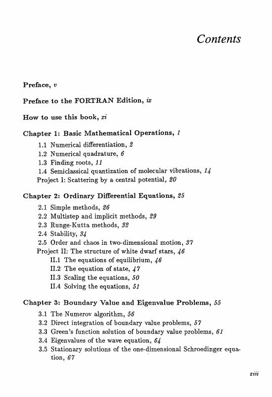
Contents
Preface, u
Preface Lia the FORTRAN Editiaa, iz
Haw to use this baak, zi
Chapter 1: Basic Mathematical Operations, 1
2 -1 Numerical diEerentiatioa, 2 1.2 Nnnterieal quadratwe, 6 1.3 Finding roots, 11 1.4 Sernidz~ssicd quantiz-atioa of molecular vibrations, 14 Project I: Scattering by a central potential, &O
Chapter 2: Ordinary DiEerential Equations, 25
2.1 Simple methods, 26 2.2 Multistep and impEcit method@, 89 2.3 Range-Kutta methods, $2 2.4 StabiEdy, $4 2.5 Order and chaos in. two-disniensiand zndion, $7 Project 11: The stmcture of white dwmf s tas , 46
11.1 The equations of eqailibrium, 46 11.2 The equation of state, 4 7 11.3 S e d i ~ g the equations, 50 B.4 Solving the equalians, 51
Chapter 3: Boundary Value and Eigenvalue Prablems, 55
3*1 The Numerov dgorithm, 56 3.2 Direct intepatian of boundav value problems, 57 3.3 Green" function solution of boundary value problems, 61 3.4 Eigenvalues of the wave equ;t;tion, 64 3.5 St ittioaary solutions of the one-dimensional Schroedinger equ*
tion, 67

ziu Contends
Project 111: Atomic structure in the Martree-Fa& approximation, Y23 f 11.1. Basis af the Hartre@- Fock approximation, 72 IfI,2 The tw-electron problem, 75 112.3 Many-electron systems, 78 If 1.4 S~Iving the equations, 80
Chapter 4: Special Functions and Gausshn Quadrature, 85
4.1 Specid funcZlion~, 85 4.2 Gaussian quadrature, 9b 4.3 Born and eiXcond qproSrnadions ta quantum scattering, 96 Project IV: Partial wave solution of quantum scattering, 108
IV.1 Partial wave decomposition of the wave function, 109 IV.2 Finding the phase shifes, 104 IV.3 Sdving the equations, 1135
Chapter 5: Matrix Operations, 109
5.1 M;xtrix inversion, 109 5.2 Eigenvalues of a tri-diagonal matrix, 11 2 5.3 &duction to tri-diagond fom, f L5 5.4 Determining nudear charge densities, Id0 Project V: A schematic shell model, 188
V.1 Definition of the model, 184 KZ The exact dgenstates, 196 V.3 Approximat;e eigenstates, 158 V.4 Solving the model, 149
Chapter 6: Elliptic Partial Differential Equations, 145
6.1 Disercdizatian and the varizttiond principle, 24 7 6.2 An idesstiw method for boundav value problems, 151 6.3 More on, discretizatio~, 1155 6.4 Elliptic equations in two dimensions, 157 Project VI: S teady-state hydrodynamics in two dimensions, 158
VI.l The equations and their diseretization, 159 VI.2 Boundary conditions, f 68 VI.3 Solving the equations, 166
Chapter 7: Pwrabofie Partial DiEerenlial Eqaatiarzs, 169
7.1 Naive discretiz;ztion and instabilities, l69 7.2 Impfici t schemes m d the inversion of tri-diagond matrices, 174 "7.3 DiRusion and boundary value problems in tw dimensians, 179 7.4 Iterative methods for eigenvdue problems, 181 7.5 he time-dependent Schroedinger equation, 186 Prdect VXI: Self-osganizaeion in chemical. rextions, 189
V11.1 Descriptiolz of the model, I89 V"11.2 Lillear st abi2ity andysis, 191 VE.3 Nun2erirzd solution of the model, r"$d
Chapter 8: Monte Carto Methods, 197 8.1 The basic Mmte Carlo strategy, 198 8.2 Generating random. variables with a spedfied &&ribation, 205 8.3 The algorithm of Metropolis et al., 210 8.4 The Isiag model in two dimensions, 215 Project VIIZ: Quantum Mm& Cado for the H2 mdecule, 221
VIII.1 S t&ement of the problem, 231 VIII.2 Variational Monte Carlo and the trial wave function, 288 VIII.3 Monte Carlo evaluation of the exact energy, $85 VXII.4 Solving the problem, 229
Appendix A: How to use the programs, 231 AI Insfaflation, 231 A.2 Files, $32 A.3 CompiZatian, 233 A.4 Execution, 635 A5 Graphics, L97 A.6 P r w ~ a m Structure, $88 A.7 Menu Structure, 259 A.8 Default Value Revision, 241
Appendix B: Programs for the Examples, 849
B,l Example 1, 243 B.2 Exanlplc 2, 256 B.3 Exa~nple 3, $73 B.$ Exampks 4, 295 B.5 Exan113le 5, 316 B.6 Exan3ple G, $89
B.7 Example 7, 370 B.8 Example 8, 991
Appendix C: Programs far the Projects, C.1 Project I, 409 6.2 Project If, 421 C.3 Project XII, 4914 C.4 Project W , 454 6.5 Project V, $W C.6 Project, VX, 494 C.7 Project VII, 580 C.8 Project VIfI, @S
Appendix D: Cornman UGilif;y Code@, 567 D.1 Standardization Code, 567 D.2 Hardware and Compiler Specific Code, 570 D.3 General Input/oatpu% Codes, 574 D.4 Graphics Codes, 598
Appendix E: NeLwork Fife =ans&r, 681
Index, 631"
The problem with computers is that they only give answers -attributed do P. Picasso
Chapter I
Basic Mathematics
Operations
Three numerical operations -- differentiation, quadrature, and the finding of roots - are central to mhst computer modeling of physical sys- tems. Suppose that we have the ability to calculate the value of a function, f (s), at any value of the independent variable z. In digerentiation, we seek one of the derivatives of f at a given value of x. Quadrature, roughly the inverse of differentiation, requires us to calculate the definite integral off between two specified limits (we reserve the term "integration" for the process of solving ordinary differential equations, as discussed in Chap- ter 21, while in root finding we seek the d u e s of s (there may be several) at which f vanishes,
If f is knourn mafyticatly, it is almost always possible, with ensue fortitude, to derive expEcit formulas for the defivatives of f , aad it is aften possible t s do so for its degnite integal as well. However, it is often the ease that an m d y t i d method cannot be used, even though pife cm evaluate f (S) itself. This might be either because some very complicated numerid procedure is rquired to e d u a t e f and we have no suitable analytical formula upon which to apply the rules of digerentiation and quadraturn, or, even worse, because the wily we can. generate f provides ns with its values at only a set; of discrete abseissm, In these situations, we must employ qpro&m&e form&% expressing the derjvatives and integrd in terms of the values of f we can compnte. Moreover, the root8 of 41 but the simplest functions cannot be found anatyticdly, and nuzrrericd methods are therefore essentialt.
This chapter dealfs d t h the computer redigation of these three ba- sic operations. The centrd technique is to appradmate f by a simple function (such as first- or second-degree polynomial) upon which these
2 2. Basic Mathematical Qpervrdians
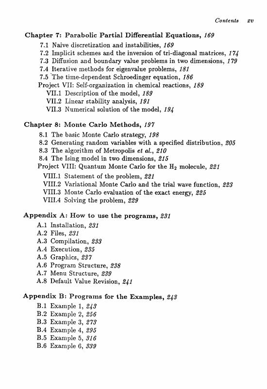
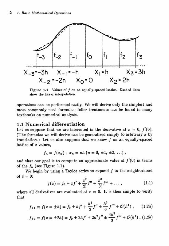
Figure 3.1 Wues of f on an equdEy-spud ladtice. Dmhed lines how the hear interpslalion.
operaLioas caa be performed easily, We will derive only the Simpleet and mo& commonly used fomdas; fufbr treatments can be h n d in many textbooks an nmericd andysis.
1 .l Numerical diEerentiatiolz Let us suppose that we we interested in the derivative at z = 0, f '(0). (The formulas we will derive can be generalized simply to arbitrary z by translation.) Let us also suppose that we know f on an equally-spaced lattice of z vdnes,
and that our god is to compute an approximate value of fE(0) in terms of the f, (see Figure 1.1).
We begin by using a Taylor series to expand f in the neighborhood
whem all derimtives are evduated at z = 0. It is then simple to verify that
where O(h4) means terms of order h4 or higher. To estimate the size of such terns, we cm assume that J and its derivatives are aJ1 of the same order of magnitude, as is the case for many functions of physical rdemnee.
Upon subtracting from fi as given by (1.2a), we find, after a sEght rcjarrangea;lc?n%,
' The term involving f f N vanishes as h becomes small and is the dominant error associat;ecl with the finige dfference q p r o ~ m i t t i m that Tetijtin~ mly the f i r~ t term:
This "%point" formula would be exact if f were a second-deetje poly~o- mid in the 3-point interval [-h, +h], because the third- and all higher- order derivatives would then vanish. Hence, the essence of Eq. (1.3b) is the assannptian that a quadratic p o l y n o ~ d inticrrpolatiofi of f throu& the thrw points z = &h, O i s v&d.
Equation (1.3b) is a very naturd result, reminiscent of the formulas used to define the derivative in elementary calculus. The error term (of order h2) can, in principle, be made as small as is desired by using smder and smder d u e s of h. Note also that the 8ynmetric difirence about z = O is used, as it is more aecurate (by one order in h) than the forward or badward CliRerenm form~las:
These "2-pointw formulas are based on the assumption that f i s well agproSma2ed by a fineas fanctian over the intervds between z = O and z = &h*
As a concrete example, consider evaluating ff(z = 1) when f (g) = sin 2. The exact answer is, of course, cos 1 = 0.540302. The following FORTRAN program evaluates Eq. (1.3b) in this case for the value of h input:
4 1. Basic Mathemalical Operations
10 FRIlT * , %HT= VALUE OF ft C. LE, O TO STOP) READ *, WI IF (B .LE, 0) STOP F P R ~ E = ( S X W (x+E>-SXN(X-B] > / ( 2 * ~ >
DIW=EXACT-FPRIME PRTMT 28,W,BIFF
20 FOMAT(~=',Elb.$,5X,%MOR=~,E1668) GOT15 10 ElD
(If you are a beginner in FORTRAN, note the way the value of H is requested from the keyboard, the fact that the code will stop if a non- positive d u e of R is entered, the natural way in whi& variable names are chosen and the mathematical formula (1.3b) is transcribed using the SIN function in the sixth line, the way in which the number of significant digits is specified when the result is to be output to the screen in line 20, and the jump in program control at the end of the program.)
Result8 generated urlth this progrm, as W& as with s i d a r ones evaluating the forward and backward difference formulas Eqs. (1.4a,b), are shown in Table 1.1. (AU. of the tables of errors presented in the text wre generilted f f ~ m BASIC progras; the numbers may vary from those obtdned from FQRTRATJ code, especidy when numerical roundoff dominates.) Note that the result improves as we decrease h, but only up to a point;, after which it becomes worse, This is because arithmetic in the computer i s performed with only a limited precision (5-6 decimai digits for a single precision BASIC variable), so that when the difference in the numentor of f;he appro~mafsions is formed, i t is subject to large "round- off" erfors if h is smdl and fi and diger very little. For example, if h = 10-7 then
f 2 = sin (1.000001) = 0.841472 ; f-l = sin (0.999999) = 0.841470 , so that fi -lml = 0.000002 to six significant digits. When substituted
into (1.3b) we find f t m 1.000000, a very poor result. However, if we do the arithmetic with 10 significant digits, then
which gives a respectable f' rr: 0.540300 in Eq. (1.3b). In this sense, nu- merical differe~ltiation is an intrinsically unstable process (no well-defined limit as h --+ 01, aud so must be carried out with caution.
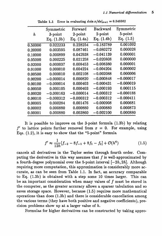
Table 3.1 Error in cvduating d;sin t / d ~ l ~ = ~ = 0.5403@
S ~ e ( ; r i e Forward B s c k w d Symmetric h $point %point 2-point &point
Eq. (1.3b) Eq. (1.4a) Eq. (1.4b) Eq. (1.5) 0,50000 0.022233 0.228254 -0,183789 0,001092 0,20000 01003595 0,087461 -0.080272 0.000028 0,10000 0,000899 0.042938 -0,041139 0.000001 0,05000 0.000225 0,021258 -0.020808 0,000000 0.02000 0.000037 0.008453 -0.008380 0.000001 0.01000 01000010 0,004224 -0,004204 0.000002 0,00500 0,0000X0 0,002108 -0,002088 0.000006 0.00200 -0,000014 0,000820 -0.000848 -0,000017 0,00100 -0,000014 0,000403 -.0.000431 -O.O00019 0,00050 0,000105 0,000403 -0.000193 0.000115 0,00020 -0,000163 -0.000014 -0.000312 -0,000188 0,00010 -0.000312 --0.000312 --0,000312 -0.000411 0.00005 0.000284 0.001476 -0.00090Zf 0.000681 0.00002 0,000880 0,000880 0.000880 0.000873 0,00001 01000880 0.003860 -0,002100 0,000880
It is poasible to improve on the Spoint formula (1.3b) by rdating f to lattice points fnrther removed from z = 0. For example, using Eqs. (1.2), it is easy to show that the U5point" f o d a
caneels dl derivatives in the Taylm series through fourth order. Com- puting the derivative in this way amumee that f is well-appdmated by a fonrth-degree polynomial over the &point !interval [-21r,2h]. Although reqniring more computation, this approximation is considerably more ae- curate, as can be e e n from Tabfe 1.1. In fact, an curacy earnparable to Eq. (1.3b) is obtained with a step some 10 times larger. This ean be an important eonsideration when many d u e s of f must be stored in the computer, as the greater accnracy dows a sparser tabnlatibn and so saves storage space. However, because (1.5) requires more mathematical operations than does (1.3b) and there is considerable urncellation among the varions terns (they have both positive and negative coefficients), pre- cision p m b l ~ m ~ show up at a larger value of he
Forrndit8 for higher derivatives can be conatnrcted by taking appro-
6 l. Basic Mathematical Ogrzrations
Table f .2 4- and S-pint BiRerence: formulas for de~vativw
priate combinations of Eqs. (1.2). For example, i t is easy to see that
so that an appraximation to the second derivative accurate to order h2 is
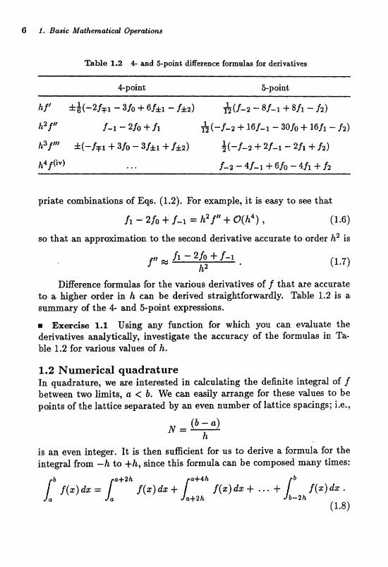
DiEerence formulm for the various derivative^ of f th& are accurate to a higher order in h can be derived straightforwardly. Table 1.2 is a summary of the 4 &ad 5-pdnt ewressiaas.
Exercise 1.1 Using any function for which you can evduate the derivatives analytically, investigate the accuracy of the formulas in Ta- ble 1.2 for various vdues af h.
1.2 Numerical quadrature In quadrature, we are interested in calculating the definite integral of f between two limits, a < b. We can easily arrange for these values to be points of the lattice separated by an even number of lattice spacings; i.e.,
is an even integer. It is then sufident for us to derive a formula for the integral from -h to +h, since this formula can be composed many times:
b a+2h a+4h f (s) dz = f (4 + f(.)dz + * * * + f (4 62% *
(1.8)
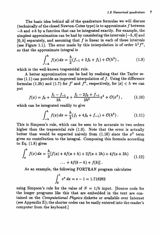
The basic idea &hind all of the quadrature formulas we wilI discuss (technically of the closed Newton-Cotes type) is to approximate f between -h and +h by a function that can be integrated exactly. For example, the simplest approximation can be had by considering the intervals [-h, 01 and [O, h] separately, and assuming that f is linear in each of these intervals (see Figure 1.1). The enor made by this interpolation is of order h2 f ", so that the approximale iate& is
which is the weU-known trapezoidaf rule. A better approximation can be had by realizing that the Taylor se-
ries (1.1) can provide an improved interpolation of f. Using the difference formulas (1.3b) and (1.7) for f' and f ", respectively, for 1s put
which can be intepated readily ta give
This is Sinnpsonk rule, wEch em be seen to be accurate to two orders higher than the trapezoidd rule (1.9). Note that the error i s actually better than would be expected naively from (1.10) since the x3 term gives no contribution to the integral. Composing this formula according to Eq. (1.8) gives
As an example, the following FORTRAN program calculates 1
e"dz = e - I = 1.718282
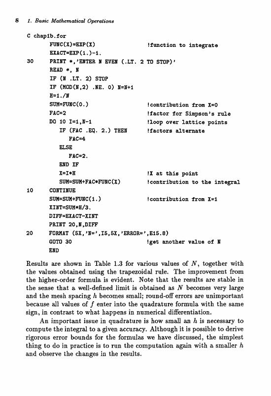
using Simpson's rule for the value of N = l l h input. [Source code for the lmger program like this that are embedded in the text are con- t;ained m tbe Gmplubats'oncrl Phgaics diskette or avdlabIe over Xaterne~, (see Appendix E); the shorter codes can be easily entered into the reader's computer from the keyboard.]
8 I , Basic Mathematical QpraEdons
C chaplb.rS"or m C ( X ) =EP(X) ! Sact;ion to ia%epat e E X A ~ = E ~ ( I . 1-2,
30 PRZRT * , "ETER I EVm ( ,LT, 2 'B3 STIZP) @
Rm*, 1 ZP (1 .LT. 2) SmP IF (NOD(1,2) .HE. 0 ) I=@+$ E=%. /#l
SW=mC (0 . ) !contribation from X=O FAC=2 !factor for Siapson% rule DO 10 X = l , W - I !loop over Xattice paints
f F (FAC .Eq, 2.) T H D ?factors altemage FAG4
ELSE: FAC=2.
m IF X=S*LI !X at thfe point SW=Sm+FAG*mC (X) icontribution t o the fntegsa2
10 COrnICrnE S W = S ~ + ~ C ( 1 , ) ?contribatioa fron X=% XXBfT=Srn*H/3. L ) I ~ = ~ A C * I " - X Z I I T PRIBT 20,I,DIW
20 FO~AT(6X,i#=i,XS,6X,8~WR=\ElEi.Ef) 60TQ 30 !get motker v a u a oQ I EED
Resdts are shown in Table 1.3 for variaus d m s of N , together Prith the v d w s obtained nsine; the trapezoidd rule. The improvement from the kigber-order famda i s evident. Note that the resdts are skabltj in the sense that a wdI-dehed limit is obt~xred as N becomes very lztrge and ths! mesh spacing h becams @m&; round-aff arms me unimportant because dl vdue8 of f enter irzte, the quadratare formda Pvith the same s i p , in corrtrast to what happens in numerical diRert?ntiation,
An important issue in quadraturn is how s a d an h is necessary to compute the integral to a Egiwn accuracy, Although it is passible to derive rigorous error bounds for the formulas we have discussed, the simplest thing to do in practice is to run the computation again with a smaller h and ob~erve the chmges in the results.
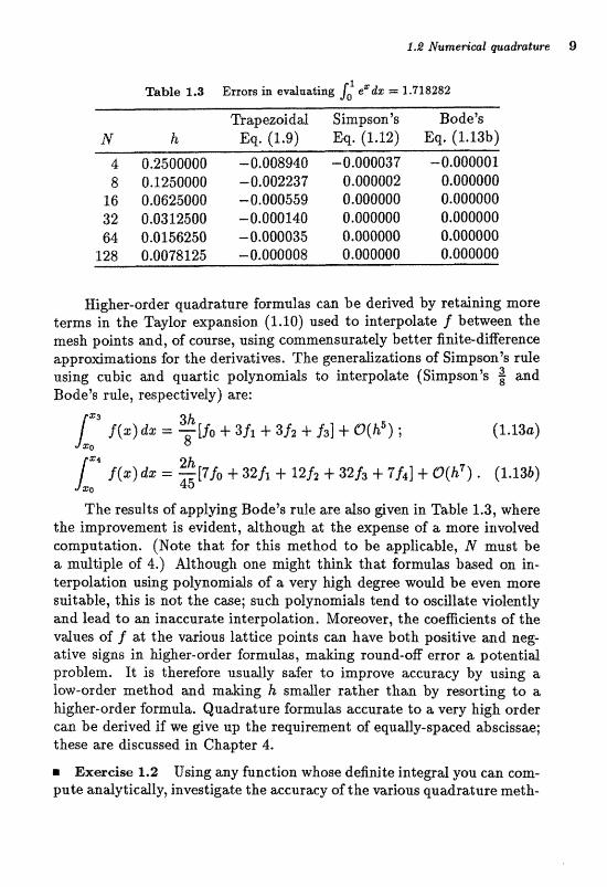
1 Table 1.3 Errors in evaluating eZdz = 1.718282
W, ~ ~
Trapezoidal Simpson's Bode's N h Eq. (1.9) Eq. (1.12) Eq. (1.13b)
4 0.2500000 -0,008940 --0.000037 -0.00QO01 8 0.1250000 -0,002237 0.000002 0.000000
16 0.0625000 --0.000559 0.000000 0.000000 32 0.0312500 -0.000146 0.000000 0.000000 64 0,0156250 -0.000035 0,000000 0.000000
Higher-order quadrature formulas can be derived by retaining more terms in the Taylor expansion (1.10) used to interpolate f between the mesh points and, of course, using commensurately better finite-difference approximations for the derivatives. The generalizations of Simpson's rule using cubic and quartic polynomials to interpolate (Simpson's $ and Bode's rule, respectiveb) are:
The! results olE applying Bode's rule are &so @ven in Table 1.3, where the improvement is evident, afthough a;t the expense of a more involvt3d computation. (Note that for this method to be applicable, N must be a multiple of 4.) Although one might think that formulas based on in- terpolation using polynomials of a very high degree would be even m r e suitable, this is not the cme; s;u& pdpornids tend to osciUate vidently and lead go an inaccurate interpolation, Moreover, the coefFicients of the vailues of f at the vaious lattice paints em have both positive aad neg- a i v e signs in higher-order farxnulas, maEng rouad-oE error a potentid problem. It is therefore usually safer to improve accuracy by using a low-order method and making h smder rather than by resorting to a higher-order formula. Quadr ature formulas accurate to a very high order cm be derived if we give up the requirement of equdlycspaeed abscissae; these are discussed irr Chapter 4.
m Exercise 1.2 Using any function whose definite in tepd you can com- pate anitlytically, investigate the acuracy of the mrious guadrat;ure nreth-
10 d . Ba@ie IkPh&ematieol Operations
ads discussed above far aBerent vdaes of h,
Same care and G on sense must be! exerciwd in the wpfication of the numericat quadrature formulas discussed above. For example, an integral in which the upper limit is very large is best handled by a change in vaiable. Thus, the Simpsonk s l e eduat ion of
with g(z) constant at large z, would result in a (finite) sum converging very slowly as b becomes large for fixed h (and taking a very long time to compute!). However, changing variables to t = r -l gives
whi& can then be evdualed by any of tlne formulas ure hwe discnssed. Integrable sinmlar4tiies, vvhich caase the naive Ibrmdas "co give non-
sense, can dso be hmdled in a simple way. For example,
has an integrable singularity at = 1 (if g is regular there) and is a finite number. However, since f ( z = 1) = m, the quadrature fomdas &scussed above @v@ an infinite result, An accurae result can bc? obtained by changing variables to t = (1 - z)'i2 to obtain
which is then approdmated vvith no trou'ble. Integrable singularities can also be handled by deriving quadrature
formulas especidy adapted to tl~em, Sunpose we me intefested in
where f (2) b e h m s as Cs-'I2 near 5 = O , with C a. constan%. The integral from h to 1 is regular and can be handled easily, while the integral from O to h can be approximated as 2ch'I2 = 2h f (h).
IN Exweise 1.3 M"fite a program to calculate
%sing one of the quadraturn formula8 diswssed above and investigate its accuracy for various values of h. (Hint: Split the range of integration into tvm parts and make a agerent dhange of variable h each integral ta handle the siagufafities.)
1.3 Finding roots The find deznentary operation that is commmly mqnired is to find a root of a function f that we can compute for arbitrary z. One sure- fire method, when the appraxim;bte location of a root (say at I = %@)
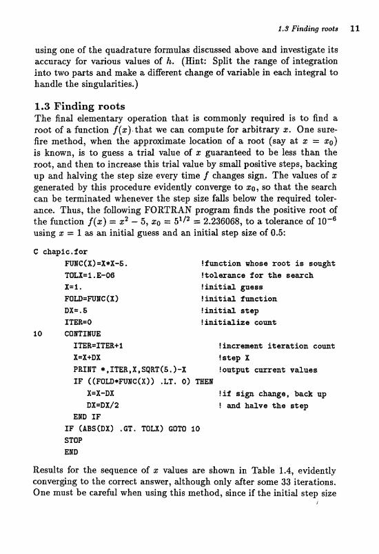
is known, i s to guess a trial value of z guaranteed to be less than the root, and then to inerease this trM d u e by smdl positive steps, backing up and halving the step size every time f changes sign. The values of x generated by this procedure evidently converge to $0, so that the search can be terminated whenever the step size falls helm the mqnired talef- ance, Thus, the fanowing FORTRAN proe;rano finds the positive root of the function f (g) = z2 - 5, 50 = = 2.236068, to a. tolerance of 1 0 ~ ~ using z = f as an initid guess and m initid step size of 0.5:
C ch&plc.for FWCCX) =X*X-5, !fmction wkosa root i s sought TOLX=1,E-OB !toleruce fox %hie sewch X=%. !inf.lsia guess FOD=WBC(X) l initf a i l i m c f i o n DX= . fr ? i n i t i d step ITER=@ ! i n i t i a i z s come
10 COaTSME
XmR=SITm+I !increfaen* iteration, corn$ X=X+E)X !step, X PRIIT *,XTER,X,SQET(&,)-X !ou.lspat cummt values IF ((FQm+FWC(X)) .LT. 0) TZfEg
X=X-DX ! f f sign change, back up xlX=DX/Z ! arrd havet the attap
EID SF IF (ABSCDX) . GT. TOLX) GOTO 10 STOP EHD
Results far the sequence of z d u e s me shown in Table 1,4, evidently convergiatg to the correct answer, dthough orrly after some 33 iterattions. One must be careful when using this method, since if the initid step size
I
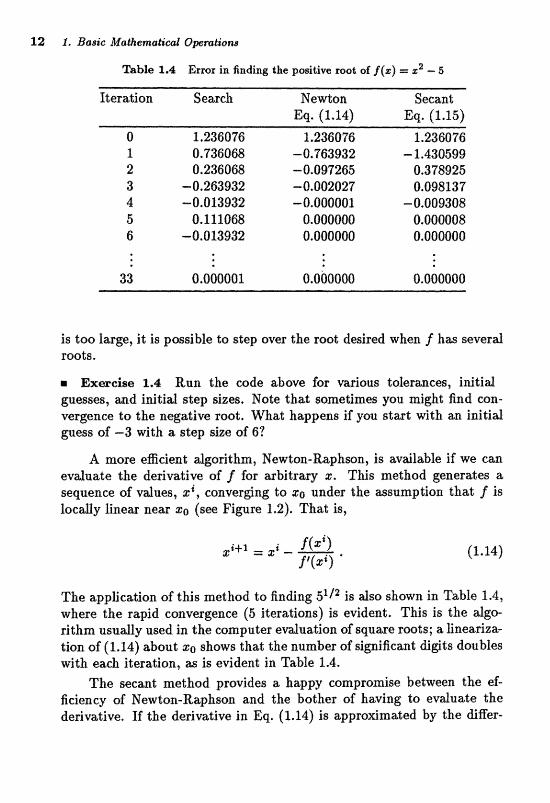
Table 2.4 Error in finding the pwitivr: root off (z) = z2 -- 5
Iteration Sear& Hewton Secant Eq. (1.14) Eq. (1.15)
if3 too large, it is possible ta step over the root desimd when f has several. roots,
r Exercise 1-4 &an the code above far vmious t~lermces, irr;itid guesses, and ini.t;id ~ t e p sizeis. Note that sometimes you might find con- vergence to the negative root. What happens if you start with an initial gGess of -3 with a step ~ i z e olt 6?
A more efficient algorithm, Newton-Raphson, is available if we can evaltuate the derivative of f for ubitrary a. Tfiis method generates a sequence of values, g', eonverljng to zo under the assumption that f is locally linear near $0 (see Figure 1.2). That is,
f (g') l f '(S') '
The application of this method to finding is also shown in Table 1.4, where the rapid convergence (5 iterations) is evident. This is the algo- rithm usually used in the computer evaluation of square roots; a lineariza- tion of (1.14) about shows that the number of significant digits doubles tvith ea& itmation, as is evident in Table 1.4.
The secant method provides a happy compromise between the eg ficiency of Newton-Raphson and the bother of having to evduate the de~vative. If the derivative in Eq. (1.14) is approximated by the differ-
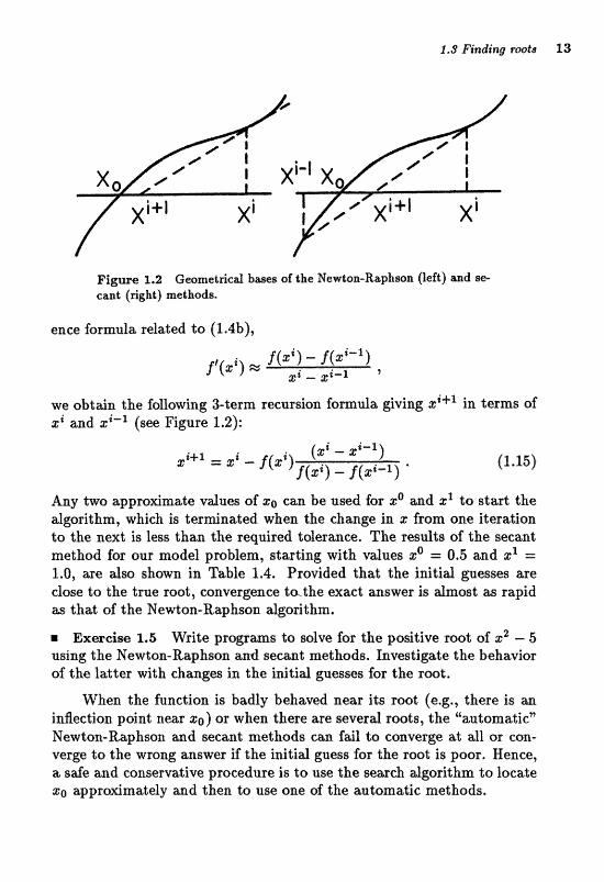
F i v e 1.2 Geometrical bases of tbe Newton-Rrtphm (left) and se- cant (fight) methods.
ence formula related to (1.4b),
we obtain the following 3-term recursion formula giving S'+' in terms of I' and zi-l (see Figure 1.2):
Any two approximate values of $0 can be used for +@ and s' to start the algorithm, which is terminated when the change in z from one iteration to the next is less than the required tolerance. The results of the secmt method for our model problem, starting with values z0 = 0.5 and z' = 1.0, m also s h w a in Table 1.4, Prcrvided that the initid gue8s;aes ase dose to the true root, convergenm to- the exact answer is dmast as rapid as that of the Newton-Rapksan dgorithm,
D Exercise 1.5 Write programs to solve for the positive root of sZ - 5 using the Newton-Raphsan a d secant methods. Invwtigate the behavisr of the latter vvith changes in the initial guesse~ for the rmt.
When the function is badly behaved near its root (e.g., there i s m inflection point near so) or when there are several roots, the "automatic" ME?wt;on-Raphson afld secant methodts can fail to converge at dl m con- verge to the wrong mswer if the initid guess for the root is poox. Henee, a safe and conservative procedure is to use the seaeh dgorithm to loe&e $0 app~o~mate ly and then to uae one of the wtomatic meehods.
14 1. Basic Mathernatiurl Qperatians
Exercise 1.6 The function f ( s ) = tanh z has a root at + = 0. Write a p r q r m to show that the Newton-Rqhson method does not co~verge for an iaStid gueshi of z X l. Cm you understand what's going wrong by considering a graph of tanh I? From the explicit form of (1.14) for this problem, desive the critical value of the initid guess abave which coavergence will not occur, Try to solve the problem using the secant method. m a t happens for vmious initial guesses if you try to find the z == O mot of tan z usiw either method?
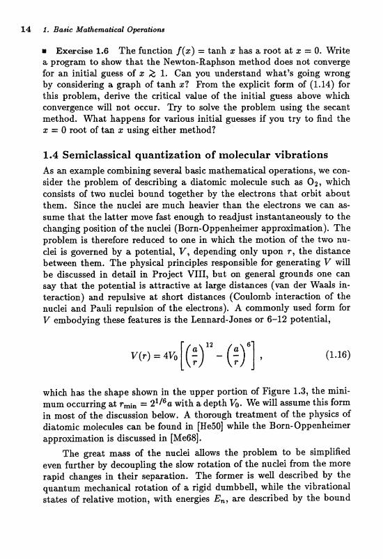
1.4 Semiclassical quantization of molecular vibrations As an =ample combining several basic mathematicall operations, we con- sider the problem of describing a diatomic molecule such as 02, which wnsists of two nuclei bound together by the electroas that; orbit about them. Sinm the nnclei are much heavier than the electrons we czm as- sume that the latter move fat enough to readjust inst;arrtmeously to the changing position of the nudei (Born-Oppenheimer approximation). The problem is therefore reduced to one in which the motion of the two nu- dei is governed by a potential, V, depending only upon r , the distance between them. The physical principh mspmsibb for generating V will be discussed in detair in Project VIII, but on generd grounds one c m say that the potential is attractive at large distances (van der W d s in- teraction) and repulsive at short distances (Coulomb interaction of the nuclei and Pauli repulsion of the electrons). A commonly used form for V embodying these features is the Lennard-Jones or 6-12 potential,
which has the shape shown in the upper portion of Figure 1.3, the mini- mum occurring at rmim = 2'j6a with a depth %. We will assume this form in most of the discussion below. A thorough treatment of the physics of diatomic molecules can be found in [He501 while the Born-Oppenheimer approximation is discussed in [Me68].
The great mass of the nudei allows the problem to be simplified even further by dewupling the slow rotation of the nuclei from the more rapid changes in their separation. The former is well described by the quantum mechanical rotation of a rigid dumbbell, while the vibrational states of relative motion, with energies E,, are described by the bound
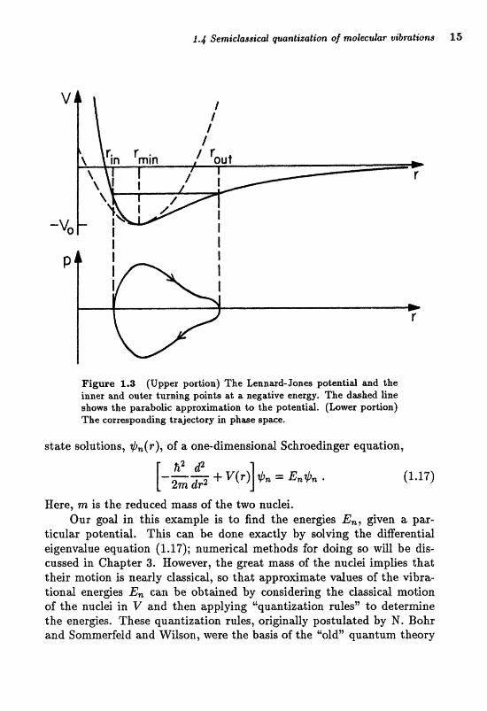
Fignre 1.3 (Upper portion) The Leaamd-Janes potentrid and the inner and outer turning point8 kLt, a neg&ive energy. The &;take& tine show8 Ch~f p~rabolic approxhation to the potential, (Lawer parlion) The corresponding trajectory in ghatcie spwe.
state solutions, +%(F), of a one-dimension$ Schroedinger equation,
Here, m i s the r f ~ d ~ ~ e d mws of the two nucfei, Our ~ a l in. this exampb i s to find tht! enerdes E,, given a par-
ticular potential. This can be done wwtly by salving the &Rerentid eigenvdue equation (1.17); numerical methods for doing so will be dis- cussed in Clrapter 3. Hawever, the great mass of the audei. implies that their motion i s neafly dasical, so that approdmate values of the vibra- tiond ener@es cE, can be obtaliwd by conrjidering the clmsieal motion of the nuclei in V and then applying '"quantization ruks" to d e t e r ~ n e the energies, These quantizatio~ rdes, origindly postulatd by N. Bobr and Sornrnerfeld and Wilson, were the bwis of the "old" quantum tbwry
I6 1. Basic XkialFhematiml Operations
from which the modern formulation of quantum mechanics arose. How- ever, they can also be obtained by considering the WKB appraximation to the wave equation (1.17). (See [Me681 for details.)
Confined dassical motion of the internudear separation in the poten- tial V(7) can occur for energies -Vo < E < 0. The distance between the nuclei osdllates periodically (but not necessarily harmonically) between inner and outer turning points, q, and rout, as shown in Figure 1.3. Dur- ing these oscillations, energy is exchanged between the kinetic energy of relative motion and the potential energy such that the total energy,
is a constant (p is the relative momentum of the nuclei). We can therefore think of the oscillations at any (jven energy as defining a dosed trajectory in phase space (coordinates r and p) along which Eq. (1.18) is satisfied, ab; s h m in the lower portion of Figzlre 1.3, An explieit eqnaLim for this trajectory can be obtained by solving (1.18) for p:
The classid motion desaibed above occurs at any enerw between. -6 a;nd 0. To qnmtize the motion, and hence obtain approximations to the eigenvdues E, appearing in (1 .IT), we consider the dimensionless action at a, @ven energy,
where k(r ) = h-lp(r) is the local de Braglie wave number and the integral is over one complete cyde of oscillation. This action is just the area (in units of h) enclosed by the phase space trajectory. The quantization rules state that, a t the allowed energies E,, the action is a hdf-integral multiple of 2a. Thus, upon using (1.19) and recalling that the oscillation passes through each value of r twice (once with positive p and once with negative p), we have
where n is a nonnegative integer. At the limits of this integral, the turning points Q, and rout, the integrand vanishes.
To specialize the quantization condition to the Lennard-Jones poten- tial (l.16), we define the dimensionless quantities
so that (1.21) becomes
is the scded potentid. The quantity 7 is a dimensionless measure of the quantum nature of
the problem. In the dassical limit (a small or m large), 7 becomes large. By knowing the moment of inertia of the moleeule (from the energies of its rotational motion) and the dissociation energy (energy reqnired to separate the molecule into i t s two constituent atoms), it is possible to determine from observation the parameters a and 'Vo and hence the quantity 7. For the H2 molecule, 7 = 21.7, while for the HD molecule, 7 = 24.8 (only m, but not h, changes when one of the protona is replaced by a deuteron), and for the much heavier O2 molecule made of two lBO nuclei, 7 = 150. These rather I q e vdues indicate that a s e ~ c l u s i c d appro~xnation is a valid dwcription of the vibratianal motion.
The FORTUN program for Exmple 1, whose source code is can- tained in Appendix B asld in the file EXMPLI.FOR, findg, for the d u e of y input, the values of the E, for which Eq. (1.22) is satisfied. After all of the ener@es have been h n d , the corresponding phase pace trajwt* ries we dram. (Befora attempting to gun this code on yovr camputer syaern, you should review the m&t3rid on the progrms in ""How to use this book" and in Appendix A.)
The following exercises are aimed at increasing yovr undemtmding of the physical principles and numerical. methods demonstrawd in this example.
m Exwcise l.'? One of the most important aspects of using ie computer ;as a tool to do pbysics is knovving when to have confidence that the pro- gram is giving the correct answers. In this regard, an egsential teat ia the d e t ~ l e d quantitative comparison of results urith what is known in =a- 'lytieaffy soluble situations. Modify the code! to use a pasabotic potential
18 1. Basic Malhematic-al Operations
(in subroutine POT, taking care to heed the instructions given there), for which the Bohr-Sommerfeld quantization gives the exact eigenvdues of the Schroedinger equation: a series of equdly-spaced energes, with the lowest being one-half of the level spaeing above the minimum of the potentid. Far sever& vdues of 7, compare the numerical resalts .for this case with what you obtain by solving Eq. (1.22) a n e t i c d y . Are the phase spwe trajectosies what you eqect?
B Exercise L8 Another important test of a- working code i s to compare its results with what is expected on the basis of physical intuition. Re- store the code to use the Lemard-Jones potential and run it for 7 = 50. Note that, as in the case of the purely pmabolic potentid discussed in the previous exerdse, the first excited state is roughly three times as high above the bottom of the well as is the ground state and that the spacing8 between the few lowest states are rougllly constant. This is because the Lennard-Jones potentid is roughly parabolic about its minimum (see Fig- ure 1.3). By calculating the second derivative of V at the minimum, find the ""spriag conatat" and show that the fi.equency of small-amplitude motion is expected ta be:
Verify that this is wnslstent with the numerical resuks and explore tbis agreement for different values of y. Can you understand why the higher energies are more densely spaced than the lower ones by comparing the Lennard-Jones potential with its parabolic approximation?
= Exwcisos %.Q bvwiance of results under changes in the numerical algorithms or their parameters can give additional confidence in a calcu- lation. Change the tolerances for the turning point and energy searches or the number of Simpson's rule points (this 'be done at mn-time by choosing menu option 2) and observe the effects on the results. Note that because of the way in which the expected number of bound states is calculated (see the end of subroutine PARAM) this quantity can change if the energy toferance is vwied.
B Exareise 1.10 Replace the searches for the inner and outer turning points by the Newton-Raphson method or the secant method. (When ILEVELZ 0, the turning points for ILEVEL - l are excellent starting values.) Replace the Simpson's rule quadratare for s by a higher-order formula [Eqs. (l.13a) or (1.13b)I and observe the improvement.
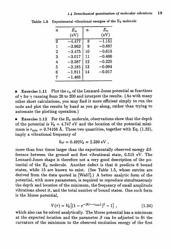
Table 1.5 Experiment& vvibraLional energi~ af the E2 molecule
r Exercise 1.1% Plot the E , of the Lennard-Jones potential as functions of 7 for 7 running from 20 to 200 and interpret the results. (As with many other short calculations, you may find it more efficient simply to run the code and plot the results by hand as you go along, rather than trying to automate the plotting operation.)
Exercise 1. 12 Fbr the Hlz mofecufe, observations show &at the depth of the potedial is 6 == 4.747 elf and the location of the pdentid mini- mum is Tmjn = 0.74166 A. These two quantities, together with Eq. (1.23), imply a vibrationd frequency of
mare t h m four times lager t h m the experiraentdly absemed energy dif- ference between the ground and first vibrationd state, 0.525 eV. The Zennard-Jones shillpe is therefore not a very good description of the po- tentid sf the Hz molecnk. Another defect is that it predicts 6 h a n d states, while 15 are known to exist. (See Table 1.5, whose entries are derived from the data quoted in [Wa67].) A better andytic form of the potentid, with more parametws, is required to repmduce gimdtaneou6ly the depth and location of the minimum, the frequency of smaU amplitude vibratians about it, and the total number of bound states. One such fom i~ the Morse potentid,
which &so C= be ~olved analyticrzlly. The Marse potentid has a minimum a;t the expected locat;ian a d the parameter P can be a u s t e d to ht the curvature of the miaiI-nurn to the observed excitatioa enerw of the first
2Q l. Basic Mathematical Qperatians
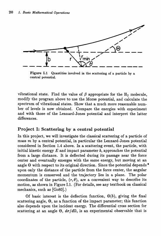
Figure X,% Quantitim involved h the krcatte~i~g of a particle by a,
central patentid.
vibrational state. Find the value of P appropriate for the Hz molecule, modify the pf~gram above to use the Morm potent;iaI, and cdcdate the spectmm of vibrational statas. Show that st much more reasonable nu=- ber of levels is now obtained. Compare the energies with experiment and with those of the Lennard-Jones potential and interpret the latter digererrces.
Project I: Scattering by a central potential
h this, project, urt; uriU investigate the dassical scattering of a particle of mms nz by a centrd poteatid, in particula the Lennad-$ones potentid c0nsiderci.d in Section 1.4 above, h a scattePing event, the partide, with. initial kinetic t?nergy E z~nd impact parameter b, approaches the potential from a large distance, It is deflected during its pasage n e a e h force center and eveatudy emergee with the same enera, but moving at an. angle O with respect to its original direction. Since the potentid depends ' upon an& the distance of the partide fronn the force center, the aagular momentum is conserved and the trajedory Lies in a plane. Thcr pdar coordinates of the partide, (P,@), are a convenient way to describe its motion, as shown in Figure 1.1. (For details, see any textbook on dasdcal mechanics, such M [Go80].)
Of basic interest is the deflection function, O(b), giving the final scattering angle, 0, as a function of the impact parameter; this function also depends upon the inddent energy. The differential cross section for scattering at an angle 0, do/dQ, is an experimental observable that is
related to the defiection function by
Thus, if dOldb = (dbldO)- l can be computed, then the cross section is known..
Expressions for the deflection function c m be found analytically for only a very few potentials, so that numerical methods usually must be employed. One way to solve the problem would be to integfate the equa- tions of motion in time (i.e., Newton's law relating the acceleration to the force) to find the trajectories corresponding to various impact parameters and then to tabulate the final directions of the motion (scattering angles). Tbis would involve integrating four coupled first-order differential equa tions Eos two coordinates and t h i r velocities in the scattering plane, discussed in Section 2.5 bebw. However, since anpla r rxramerrtum is con- served, the evdution of B is related dire6tly to the radial motion, and the probhrn can be reduced to a one-dimensiond one, wEch can be s d v d by quadratare. This fatter approach, which i s simpler and more accurate, is the one we will, pursae here.
To d e ~ v e an clbppropriaGe expression for 8, we begin vvjth the conser- vation of arrgular momentum, which implie8 &hat
is a constant o-f the motion. Here, dB/& is the augtrlas velocity and v is the asymptotic velocity, related to the bombarding energy by E = imv2. The radid motion owurs in an eRective potentid th& is the sum of V and the centrifugal potential, so that energy conservation implies
If we use F as the independent variable in (1.21, rather than the time, we can write
and salving (1.3) for d ~ / o t t thrtn yields
22 2 . Basic Mathematical Ofterations
Recalling that 0 = n when r = oo on the incoming branch of the tra- jectory and that B is always decreasing, this equation can be integrated immediately to give the scattering ande,
where r,i. is the distance of closest approach (the turning point, deter- mined by the outermost zero of the argument of the square root) and the factor of 2 in front of the integral accounts for the incoming and out- going branches of the trajectory, which give equal contributions to the scatterixlg angle.
One find transformation is useful before beginning a numerical cal- culation. Suppose th& there exist8 a distmce rr,,, beyond which vve can safely nedect V. In this case, the integrand in (1.6) mishes as T - ~ for large r , so that numericd quadrature could be very ineRcient. In fact, since the p o t e ~ t i d hap aa eEect for r > rm,, , we would just be "wasting time" "describing stra;igJRt-line nrotisn, To hanae this situation &cientXy, note that since 63 = O when V = 0, Eq. (1.6) implies that
which, when substituted into (I.6), results in
The integrals here extend only to rm,, since the integands becme equd when T >
Our goal will be to study scattering by the Lennard-Jones poten- tial (1.16), which we can s a f e set to zero beyond P,,, = 3a if we are not interested in eneees smaller than about
The study is best done in the hlloMring sequence of steps:
Step 1 Before beginning any numerical computation, it i s important to have some idea of what the results should look Like. Sketch what you think the deflection function is at relatively low energies, E 6 where the peripheral collisions at large b 5 F,,, will take place in a predominantly at tractive potential and the more central collisions will LLbounce" against the repulsive core. What happens at much higher energies, E > Vo, where
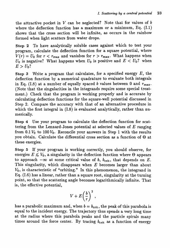
1. Scattering by( a cent& potential 23
the attractive pocket in V can be neglected? Note that for values of b where the deflection function has a maximum or a minimum, Eq. (1.1) shows that the cross section will be infinite, as occurs in the r&nbow formed when light scatters from water drops.
Step 2 To have analytically soluble cases against which to test your program, calculate the deflection function for a square potential, where V ( r ) = U. for r < Fmax and vanishes for r > r,,,. What happens when U. is negative? What happens when U. is positive and E < Uo? when E > U@? Step 3 Write a program that calculates, for a specified energy E, the deflection function by a numerical quadrature to evaluate both integrals in Eq. (1.8) at a number of equally spaced b values between O and F,,.
(Note that the singularities in the integrands require some special treat- ment .) Check that the program is working properly and is accurate by cafculating deflection functions for the square-well potentid discussed in Step 2. Campwe the accuracy with that of asl dterndive procedure in which the first intepal in (1.8) is evdaated andytiea;lly5 rather than m- meri cdy.
Step 4 Use your propam to cdc.ulilLee the degection function far scat- tering from the Lennard-Jones potential at selected values of E ranging from 0.1 to 100h . Reconcile your answrs in Step I with the result8 you obtGn. Calcu1;at;e the diflerentid cross section as a function of @ at these energies.
Step 5 E your progrm is working comectly, ycru &odd observe, for ener@w E K t a siqulmity in the deflection function whese O appeaas to apprawh -m at some critical vdue of b, brit, that depends on E. This singularity, which disappears when E becomes larger than about V@, is characteristic of Uorbiting." In this phenomenon, the integrmd in Eq. (1.6) has a linear, rather than a square root, singularity at the turning poiat, 80 thitt the scattering aggle becomes logiurithrnically iagnite. That is, the eEective pohential,
has a parabolic maximum and, when 6 = bcrit, the peak of this parabola is equal to the incident energy. The trajectory thus spends a very long time at the radius where this parabola peaks and the particle spirals many times around the force center. By tracing bcrit as a function of energy
24 1. Basic Mathematical Operations
and by plotting a few of the effective potential8 involved, convince yourself that this is indeyed what's happening. Determine the xn~muan e n e r ~ far vvbich the Lennard-Jones potenkid exhibits orbiting, either by a d u t i o n of an agprcfpriate set of equatons invalviag Y and its derivatiw~ ar by a systematic numerical investiwtion of the deflection function. If you pufsue the latter approach, ysu Iulight have to reemider the treatment of the aingdafities in %he numerical. quadratures.
Chapter 2
Ordinary Differentia
Equations
Many of the laws of physics are most conveniently formulated in terms of differential equations. It is therefore not surprising that the nurnericd sdution af differentid equations is one of the mast common tasks in modeling physicd systems. The most general form of an ordinary differentid equation is a set of M coupled first-order equations
where is the independent variablt? and y is a set of M dependent vari- ables (f is thus an M-component vector). Differentid equations of higher order can be written in this first-order form by introducing auxiliary func- tions. For example, the one-dimensional motion of a partide of mws m under a force field F ( z ) is described by the second-order equation
If we define the morne~rtum
then (2.2) becomes the two coupled first-order (Hamilton's) equations
0% P ~~~ . * = F(z ) , dt nz "dt
which are in the h r m of (22). It is therefore suficient ta ccznsjdes in detGl anly nnetlrods for firs t-order equations, Since the matrix structure
of coupled differential equations is ofthe most natural form, our discussion of the case where there is only one independent variable can be generalized readily. Thus, we need be concerned only with solving
for a single dependent variable y (g). In this chapter, we will discuss several methods for solving ordinary
differentid equations, with emphasis on the initial vdue problem. That is, find g(%) given the vdue of y at some initial point, say y(z = 0) = yo. T h i ~ kind of problem occurs, for example, when we are given the initial position and momentum of a particle and we wish to find its subsequent motion using Eqs. (2.3). In Chapter 3, we will discuss the equally important boundary vdue and eigenmlue problems.
2.1 Simple methods To repeat the basic probjem, we me interested in the solution of the differential equation (2.4) with the initial condition y(z = 0) = go. More specificitlly, W are usudy interested in the d u e of y at a particular value of I, say z = 1. The general strategy is to divide the interval [O, 11 inLo a large number, N, of equdlg spaced subintmds of length h = 1IN and then to develop a recursion formula relating y, to y,-l, . . .l, where y, is our approximation to g(+, = nh). Such a recursion relation will then dew a step-by-step integatioa of the digeratid equation earn a : = Q t o 1 = 1 ,
One of the simplest algorithms is Euler" smethod, in whi& we con- sider Eq. (2.4) at the point x, and replace the derivative on the left-hand side by its forward difference approximation (1.4a). Thus,
so that the recursion relation expressing in terms of y, is
This formula has a local error (that made in taking the single step from g, to that is O(h2) since the emor in (1.4a) is 6(h) . The LLglobal" error made in finding y(l) by taking N such steps in integrating from I = O to r = 1 is then NO(^^) a Q(&). This error decreases only
linearly with decreasing step size so that half as large an h (and thus twice as many steps) is required to halve the inaccuracy in the final an- swer. The numerical work for each of these steps is essentially a single evaluation af f .
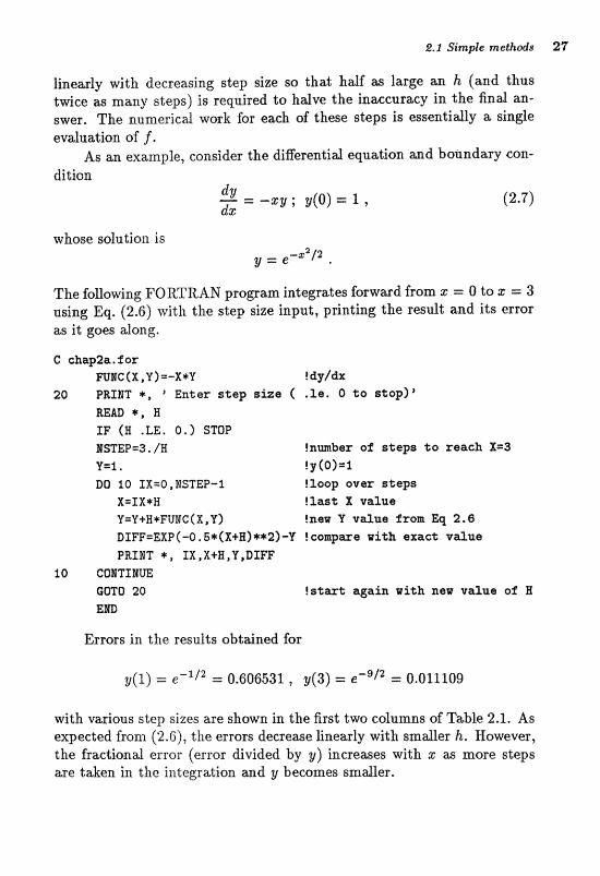
As an example, consider the differentid equation and boundary con- di tion
-- = -zy ; y(0) = 1 , dz
(2.7)
whose solutioiz is y = e - g 2 / 2 .
The following FORTRAN program integrates forward from s = O to I = 3 using Eq. (2.6) with the step size input, printing the result and its error zls it goes along.
G chap2a.for mIG(X,Y)=-X*U f dy/&
20 PRIlT *, "ntar step size ( .l@. O to stop)' REm *, H IF' (H .LE. 0,) STOP MSTEP=3. /W !nmbsr of steps to reach. X=3
V=l, !y(O)=I DO 50 IX=O,WSTEP-5 !loop over steps
X = I X + H !last X value Y=Y+H*FUBG(X,Y) !new Y ~2~3.~4 fram Eq 2.Q DTFF=EXP f -Q. S* (X+H) **2] -Y ! compme with axaet v a u a PRIBT *, IX,X+B,P,DIW
10 COIQTINUE GOTO 20 i a t a ~ again with new v a u a o f H Em
Errors in the results obtained for
with various step sizes are ghown in the first two cdunms of Tabh 2.1. As expected fmm ( & G ) , the errors decrease linearly with smaller h. However, the fractional error (error divided by y) increases with I as more steps me taken in the ilttegratlon asrd y beeernes smajtler.
28 1, Ordinary Diflemntial Equatrions
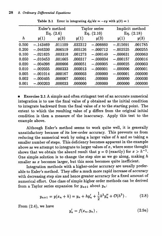
Table 2.2 Error in integrating dy/cbz z: -zy with gf 0) 1.
E d e r ? ~ method Taylor series ImpEcit method Eq. (2.6) Eq. (2.10) Eg, (2.18)
k @(l) ~ ( 3 ) ~ ( 1 ) ~ ( 3 ) ~ (1 ) ~ ( 3 )
m Exaeise 2.1 A simple aad aftm stringent test of an =cur&@ nmericd integration is to use the find vdue of y abtained as the initid condition to integrat;e bacbwxd fram the find vdue of a: to the starting poia_t. The extentt to which the resulling vdw of y differs from the origind initial condlition is then a measure of the i n a c e u r ~ y Apply this test to the e x a p l e above.
Although Euler's method seems to work quite wen, it is generally unsatisfactory because of its low-order accuracy. This prevents us from reducing the numerical work by using a larger value of h and so taking a smaller number of steps. This deficiency becomes apparent in the example above as we attempt to integrate to larger values of z, where some thought shows that we obtain the absurd result that y = 0 (exactly) for z > h-'. One simple ~olution is to change the step size as we go along, making h smaller as s becomes larger, but this soon becomes quite inefficient.
Integration methods with a higher-order accuracy are usually prefer- able to Euler's method. They offer a much more rapid increase of accuracy with decreasing step size and hence greater accuracy for a fixed amount of numericd effort. One dass of simple higher order methods can be derived from a Taylor series expansion for y,+l about y,:
From (2.4), we have r
Y, = f ( z m , v a ) 3
which, when substituted into (2.8), results in
where f and its derivittives are to be evaluated at (g,, g,). This recursion relation has a local emor O(h3) and hence a global error 6(h2) , one order more accurate than Euler's method (2.6). It is most useful when f is known analytically and is simple enough to differentiate. If we apply Eq. (2.10) to the example (2.7), we obtain the results shown in the middle t m columns of Table 2.1; the improvement over Eder" method is dear. Algorithms with an even greater accuracy can be obtained by retaining more terms in the Taylor expansion (2.8), but the algebra soon becomes prohibitive in a31 but the simplest czases.
2.2 Multist ep and implicit met hods Another way of ~ E e v i n g higher accuracy is to use recursion relations that relate y,+z not just to yn, but also to poiats funther "h the past;,n say yn-1, h - 2 l . . .. To derive such fcrrmulas, we can intef3rate one step of the differential equation (2.4) eznctly to obtain
The problem, of CaQrse, is that we d d t know j owr the intmval of integration. However, we can use the values of y at I, and z,-l to provide a linear extrapolation of f over the requirc?d inlervd:
where f i E f (z i ,y i ) . Inserting this into (2.11) and doing the s integral then results in the Adms-Bashforth two-&ep method,
Related higher-order methods can be derived by extrapolating with 6igher- &gee polynomials, For example, if f is extrapdated by a cubic pdyns- '
mid fitted to f,, fnml, fnm2, and fnmst the Adams-Bashforth four-Step method results:
I
Note that because the recursion relations (2.13) and (2.14) involve several previous steps, the value of y~ alone is not sufficient information to get them started, and so the vdues of ly at the first few lattiee points must be obtained from some other procedure, such as the Taylur series (2.8) or the Range-Kutta metbads discussed below.
R Exc3rcise 2.2 Apply the Adas-Bashforth two- and four-step dgo- rithms to the example defined by Eq. (2.7) using Euler's method (2.6) to generate the vdues of y needed to start the recursian relation. In- vestigate the accuracy of g(%) for vaious values of h by comparing with the walfytied resdts a d by appfyj,ng the reversibiEty teat described in Exercise 2.1.
The methods we have discussed so far me ""expfidt" in inhat the gn+l is given directly in terns of the drezldy known value of y,. '"2nnplicit" methods, in wKcb m equation must be solved ta determine %+l t oEer yet another means of achieving higher accuracy. Suppose wre conaidclr Eq. (2.4) at a point r,+l/l (n f #)h mid-way between two lattice points:
= f (%,+l/l 9 ~ R + 1 / 2 ) *
If we then use the symmetric difference approfinnatian for the derivative (the analog of (1.3b) with h -+ $h) and replace by the average of its values at the two adjacent lattice points [the error in this replacement is O(h2)], we can write
wkich eorrespands to the recursioa, rel;ation
2.2 MulEli~teqp and inapilielib metfaads 31
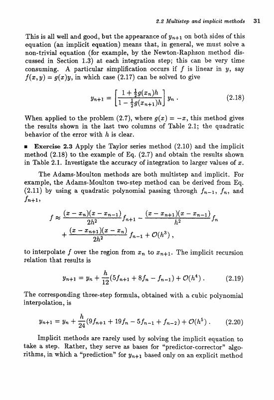
This is iill well and p o d , but the appearmce of g,+$ on both sides of this equation (an implicit equation) means that, in general, we must solve a non-trivial equation (for example, by the Newton-Raphson method dis- cussed in Section 1.3) at each integration step; this can be very time eoctszlming. A particulas ~implification. occurs if f is linear in y, say f (gF 3) = g(z)y, in which case (2.17) can be solved to give
When applied to the problem (2.7), where g(%) = --g, this method gives the results shown in the last tvvo columns of Tabfe 2.2; the quadratic behavior of the error with h is clear.
m Exercise 2.3 Apply the Taylor series method (2.10) and the implidt method (2.18) to the example of Eq. (2.7) and obtain the results shown in Table 2.1. Investigate the accuracy of integration to larger vdzles of z,
The Adas-Moulton. methods are bath mdtistep and implicit. For example, the Adams-Modton two-step method can be deriwd from m, (2.11) by using a quadratic polynomid passing through Awl, f,, asld &+l 3
to interpolate f over the region from I, to r,+l. The implicit recursion relation that resdts is
The corresponding three-step formula, obtained with a cubic polynomial interpolation, is
Implidt methods are rarely used by solving the implicit equation to take a step. Rather, they serve as bases for Upredictor-corrector" algo- rithms, in which a "prediction" for y,+l based only on an explicit method
is then 'korrected" to give a better value by using this prediction in an. implicit method. Such dgorithxns have the advantage of atlawing a e m - tinuous monitoring of the accuracy of the integration, for exmpXe by making sure that the corre&ion is small. A commonly used predictor- corrector algorithm with local error O(h5) is obtained by using the ex- plicit Adams-Bashforth four-step met hod (2.14) to make the prediction, and then caleul&ing the correction with the Adams-Maulton three-step method (2.201, using the predicted value of y,+l to evaluate f,+l on the right-hand Elide.
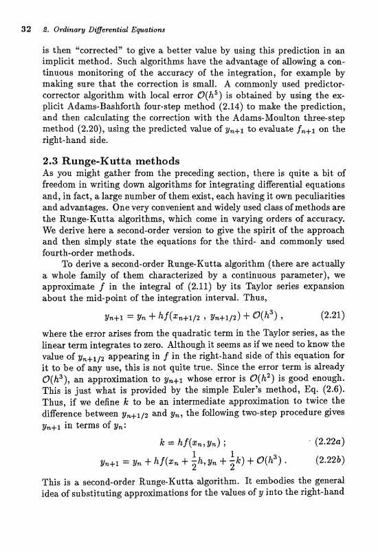
2.3 Runge-Kutta methods As you might gather Erom the preceding section, there is quite a bit 05 freedom. in writing down dgorithnrs for integating differentid equations and, in fact, a large number of them exist, each having it atvn pecdiarlties and advmtages, One very convenie~t and widely used cla9.s of methods are the Range-Kutta dgorithms, whielt come in varyiag orders of accuracy, We derive here a second-order mrsion to @ve the spirit of the appromh and then simply state the equations for the third- and carnmoxliy used fourth-order methods,
To derive a second-order Runge-Kut ta algorithm (there are actually a whde fmily of t b m chmacterized by a continuous parmetef), we approximate f in the integral of (2.11) by its Taylor series expansion about the mid-polnt of the intepation intervat. Thus,
where the error arises from the quadratic term in the Taylor series, as the linear term integrates to zero. Although it seems as if we need to know the vdue of g,+, appearing in f in the right-hand side of this equation for it to be of any use, this is not quite true. Since the error term is already O(h3), an approximation to y,+l whose error is O(h2) is good enough. This is just what is provided by the simple Euler's method, Eq. (2.6). Thus, if we define k to be an intermediate approximation to twice the difference between g,+,/, and y,, the following two-step procedure gives y,+l in terms af g%:
This is a second-order Runge-Kutta algorithm. It embodies the general idea of substituting approximations for the values of y into the right-hand
side of implicit expressions involving f . It is as accurate as the Taylor series or implicit methods (2.10) or (2.171, respectively, but places no special constraints on f , such as easy differentiability or linearity in y. It also uses the value of y at only one previous point, in contrast to the multipoint methods discussed above. However, (2.22) does require the evafuatGion of f twietj for each step dong the lattice.
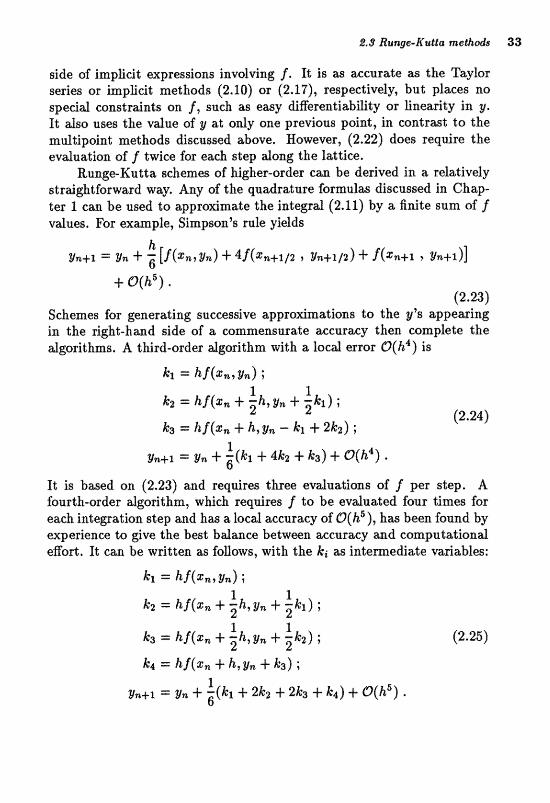
Range-Kutta schemes of higher-order can be derived in a relatively straightforward way. Any of the quadratare formulas discussed in Chap- ter 1 can be used to approximate the integral (2.11) by a finite sum of f d u e s , For example, Sirnipson's mle yields
Schemes for generating successive approximations to the g's appewiing in the right-hmd side of a commensurate accuracy then complete the algorithms. A third-order algorithm with a local error O(h4) is
It is based on (2.23) and requires three evaluations of f per step. A fourth-order algorltbm, whieb r e q ~ r e s f to be evaluated four times for each integration step and has a local accuracy of O(hS), has been found by experience to give the beat balance betwmn accurwy and computational egort. Id can be written as fouows, with the ki as intemediate va~iabXes:

W Exercise 2.4 Try out the second-, third-, and fourth-order Runge- Kutta methods discussed above on the problem defined by Eq. (2.7). Compare the camput ationd eEor t for a given accuracy with that of other methods.
r Exercise 2.5 The two coupled first-o&r equatims
define simple harmonic motion with period 1. By generdizing one of the single-variable formulas given above to this two-variable case, integrate thege equations with any particular initid conditions you choose and in- vestigate the aceurwy with whi& the system returns to its initial state at integrd valum of t.
2.4 Stability A major consideration in integating &Rerentid equations is the Burner- icd stability of the dgorithm used; i.e., the extent to whick rouad-off or other errors in the namericd computation em be ampfified, in many cases enough ifar this "noise" to dominate the resuks, To illustrate the problenr, let us attempt to improve; the accuracy of Euler's method and approximate the derivative in (2 '4) directly by the symmetric difference approximation (1.3b). We thereby obtain the three- term recursion rela- tion
g%+% = 3,-2 4- 2hf(gn,gn) 4- 0 ( h 3 ) 9 (2.27)
which superficidb looks about as useful as either of the third-order formu- las (2.10) or (2.18). However, consider what happens when this method is applied to the problem
whose solution is y = em". To start the recursion relation (2.271, we need the vdue of y, as well as go = 1. This can be obtained by using (2.10) to
(This is just the Taylor series for emh .) The following FORTRAN program then uses the method (2.27) to find y for vdues of r up to 6 using the vdue of h input:
8.4 Stability 35
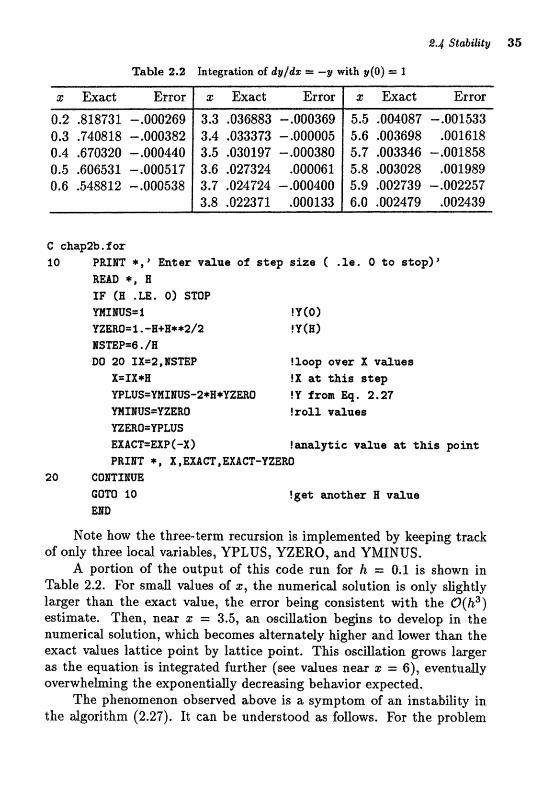
Table 2.2 Integration of dg ldz = --g with g(@) -- X
C: chap=lb.for IQ PRIHT *,"n%er vdue of step size ( .Is, O to step)"
8 U D *, E XF (H .LE. O) STOP P;lutIrnS= rzi !V(O) YZEM=i.-EI+H+*2/2 I P (B) ISmP=6. /B BQ 20 ZX=2,15TEP tZsop over X vdtles
X=IX*H !X at this step WLUS=YPUIIWS-IZ+B+TZE !Y frem Eq. 2.27 mImS=TZEEO Iro23, vaXaarzr Y-ZIERQ=YPLVS EXACT=EXP(-X) lg t i c valas at this poht PRINT *, X,EXAm,EXAm-YZEW
20 COITXmE;
Note how the three-term recursion is implemented by keeping track of only three local variables, YPLUS, YZERO, and YMINUS.
A portion of the output oS tkjs code run for h -. 6.1 is shown in Table 2.2. For s m d values of I, the numerical solution is only slightly larger than the exact value, the error being consistent with the O(h3) estimate. Then, near z = 3.5, an oscillation begins to develop in the numerical solution, which becomes dternately higher and lower than the exact values lattice point by lattice point. This oscillation grows larger as the equation is integrated further (see values near z = 6) , eventually overwhelming the exponentially decreasing behavior expected.
The phenomenon observed above is a symptom of an instability in the algorithm (2.27). It can be understood as follows. For the problem
(2.28), the recursion relation (2.27) reads
We can solve this equation by assuming an exponential solution of the form g, = AT" where A and r are constants. Substituting into (2.29) then results in an equatim for F,
the constant A being unimportant since the recursion relation is lines. The salations of tbis equatlon are
nrhere we have indicated approxinraeions valid for h < I, The positive root is sEgHtly less than m e and eone8po1lds to the expomutidy de- creasing solution we are after. However, the negative root is slightly less thaa --X, and so corresponds to a spurious solution
whose m-itude increases with n and which oscillates ffom fat;tfce point to lattice point,
The general solution to the linear difference equation (2.27) is a linear combination of these two exponentid solutions, Even though we m'tght carefully arrrtnge the initial vdues ya and yl so that only the decre~ing sdution is present Tor smalt s, numericd round-off during the recursion relation [Eq. (2.29) shows that two pasitive quantities are subtracted to obtain a smaller one] will introduce a amall admixture of the "bad" so- lution that will ewntualfy @W to domin&e the results, This instability is dearly wsociated with the thme-tern nature of tbe recursion rdation (2.29). A good rule of thumb is that instabilities and round-off prob- lems should be watched for whenever integrating a sdutim that decreases strongly as the iteration proceeds; such a situation should therefore be avoided, if possible. We will see the s m e sort of instability phenomenon ag&n in our discussion of second-order diRerentid equatians in Chanter 3.
B Exweise 2.6 Investigate the stability of sever& other integralion meth- ods discussed in this chapter by apphing them to the problem (2.28). Can you give analytical arguments to explain the results you obtain?

g.5 Order and chaos in two-dimensional motion 37
2.5 Order and chaos in two-dimensional mation A fundamental, advantage of. udng computers in physics is the ability to treat systems that caxlnot be sdved astdyticdly, In the usual situation, the numerical resdts gmeraited agree qu&tatively with the intnition W
h a t developed by studfirtg soluble models and it is the quantitaive val- ues that are of real interest. However9 in a few cases computer results defy our intuition (and thereby reshape it) and numerical work is then essentiat for a p rve r understanding. Surprisindy, such cases include the dynmics of simple classic& systems, where the generic behavior diEers quala'tcatively from that Qf the models covered in a traditiond Mechanics course. In this example, we will study mme of this surprising behavior by intepat;ing numerically the trajectories of a partide moving in two dimensions. General discussions of these systems can be found in [Hego], [Ri80], and [Ab78].
WC? consider a particle of unit mass moving in a potentid, V, in two dimensions and a4sunte that V is such that the particle remains confined for all times if its energy is low enough, E the momenta can,jug&e to the two coordinates (s, g ) are (p,, p,), then the Hamiltonian takes the form
Given any particular initid vdue~ of the coordinates and nromenta, the particle's trajectory is spedfied by their time evolution, which is governed by four coupled first-order differentid equations (Hamilton's equations):
For any V, these equations conserve the energy, E, so that the constraint
restrict S the trajectory to lie in a thre-dirnensiond manifold embedded in the four-dimensional phase space. Apart from this, there are very few other geaerd statements that caa be made about the evolution of the system.
One impart ant class of two-dimensional Hamiltonians for which ad- ditiond statements about the trajectories can be made are those that ape
38 2. Oranary Biflemnitlial Equations
intwrabke. Far these potentids, there is a semnd function 06 the coor- dinates and momenta, apart from the energy, that is a constant of the motion; the trajectory is thus canstsrtined to a two-dimensionat ma6fold of the phase space. Two familiar kinds of integrable systems are separable an& wntral potentids. h the separable c a ~ ,
where the V,*, are two independent functions, so that the Hamiltonian separates into t w pards, each involving mly one wordinate and its con- jugate momentum,
The mations in a: and g therefm deeouplt, from each other and each of the Hamiltonians ESPY is separately a constant of the motion. (Equivalently, H, - E, is the second quantity conserved in addition to E = H, + h.) In the ease of a centrd poteatid,
so that the angular momentum, p8 = %p, - yp,, is the second constant of the motion and the Hmiftonian can be written m
Pthwe p, is the zraolnenturn conjug& to r. The aCt&tiorrd constraint on the trajectory present in integrable systems allows the equations of motion to be "solved" by reducing the problem to one of evaluating certain integrals, much as we did for one-dimensional motion in Chapter 1. All of the familiar analytically soluble problems of classical mechanics are those that are integable,
Although the dynamics of integrable systems are simple, it is often not at aI1 easy to make this simplidty apparent. There is no general ana- lytical method for deciding if there is a second constmt of the motion in an arbitrary potential or for finding it if there is one. Numerical calcu- lations are not obviously any better, as these supply only the trajectory for given initial conditions and this trajectory can be quite complicated
liar cases, as can be seen by recdling the Lissajous patterns
h.5 Ondc?r and chaos in two-dimensional motion 39
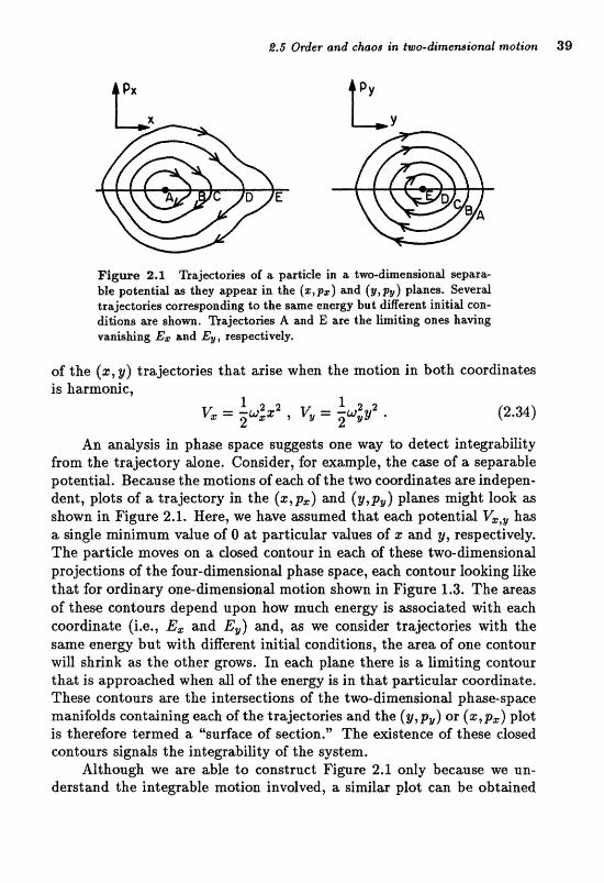
Figme 2.3 Ikajectode~ of a particge in a two-dimens;iana;l separa- ble potentid as they appear in the ~ n d (g,py) planes, Several trajectorim corrmpa~&rrg to the s m e energy but di@erent initid con- diljone me shorn. najectories A and E are the gmiting ones h a ~ n g vanlshina; .Eg and E@, rmpwtively.
of the (2, g) trajectories that arise when the motion in both coordinates
An analyds in phase space sugests one way to detect integrability from the trajeetary done. Consider, for exmple, the caae of a sepafable potent;id. Be~ause the motions of each of the two coordinates are indepea- dent, plots of a trajectory in the ($,p,) and ($,py) planes might look as shown in Figure 2.1. Here, we have assumed that each potential V = , hrzs a single &Rjmum vdue of 0 at particular vdues of z a d g, respectively, The particle move8 on a closed contaur in each of these two-dimensional projections of the four-dirnensiond phase space, each contour looking like that for ordinay one-dirnensimd motion shown in Figure 1.3. The aseas of these contours depend upon how much energy is associated with each coordinate (i.e., E, and E,) and, as we consider trajectories with the s m e energy but with diEerent initid condlitions, the area of one coatour will sMnk as the other grouls. In each plwe t h m is a lidtine; contoar that is appraxhed when all of the energy is in that particular coordinate. These cantoars axe the intersections of the twedimensiand phasa-spaee manifolds containing each of the trajectories and the (y,py) or (z, p,) plot is therefare termed a "surfxe of seetiori." The efistence of them crlosed contours signds the integrability of t htr. sys-tem.
Althon& we are able to construct F i e r e 2.1 only because WC? un- derstand the integrable motion involved, a similar plot can Be abtained
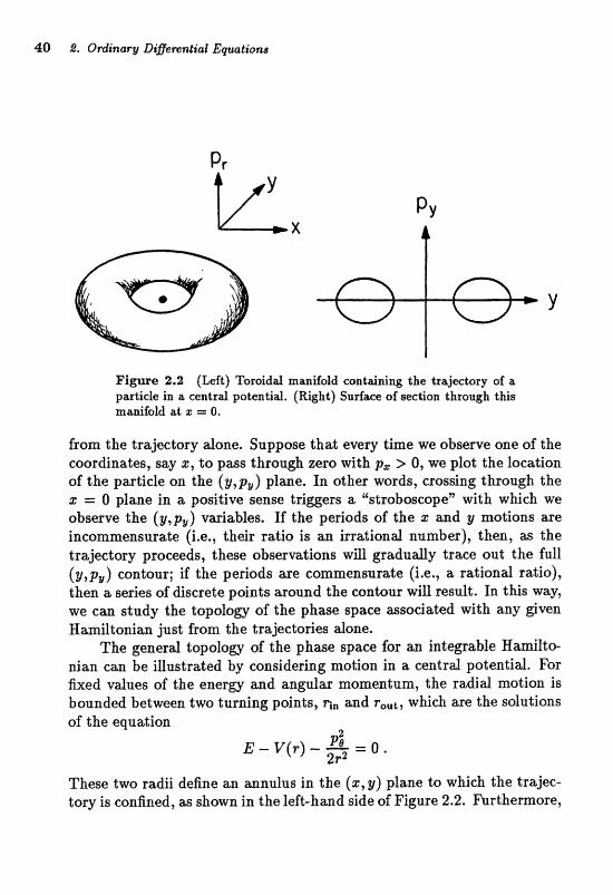
Figwe 2.2 (Left) Toraid& mmgold coatalniag Ghe trajectory of a,
pslrticle in a centrd potentid. (Right) Surface of ~ s t j o n through this mhfold ad 21 r=: 0.
;Eron %he f rgectory done, Suppoae that every t h e W &smm m e of the coordinates, say 2, to pass throuejh zero with pz > Q , W plot the locaf;ion of the partide on the (g, p,) plane. In other words, crossing through the z = 0 plane in a positive sense triaers a Ustroboscopen with which art! observe the (y,p,) variables. If the periods of the 2 and y motions are incommensurate (i.e., their ratio is an irrational number), then, as the trajectory proceeds, these observations will gradudy trace out the full (g, p,) contour; if the periods are commensurate (i.e., a rational ratio), then a series of discrete points around the contour will result. In this way, we can study the topology of the phase space associated with any given
tonian just from the trajectories alone. The general topology of the phase space for an integrable Hamilto-
nian can be iUustrated by considering motion in a central potential. For fixed vdues of the energy and angular momentum, the radial motion i s bounded between two turning points, pin and rout, which are the solutions of the equation n
These two radii define an annulus in the (E, y) plane to which the trajec- tory is confined, as shown in the left-hand side of Figure 2.2. Furthemore,
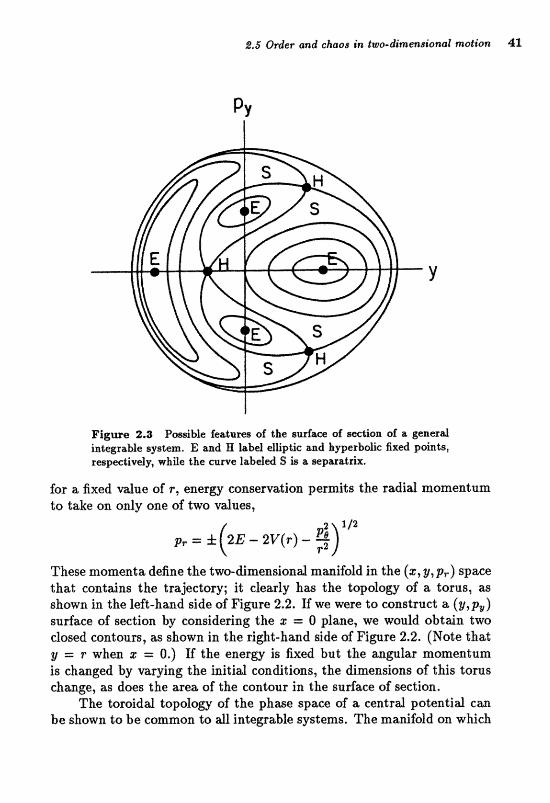
h.6 Qrdttr and chaos in tzoa-dimensiond mot-l"on 4%
Figme 2,8 Pmible batuxez~ of the sudwe mtion af a general integrable system. E a ~ d H label elliptic md hyperbdic fixed points, respectively, wjhife the curve labded S is a sepaszttrix,
for a fixed value of r , energy conservation permits the radial momentum to take on ody one of twa dues ,
These momenta define the two-dimensional manifold in the (I, y,p,) space that contains the trajecdosy; it charly has the tapdogy of a torus, as shown in the left-hand side of Figure 2.2. If we were to construct a (gypy) sudace of section by emsidering the z = 0 plane, are would obtain two dosed contours, as shown in the right-hand side of Figure 2.2. (Note that y = r when I = 0.) If the energy is fixed but the angular momentum is changed by vi~rybg the initial conditions, the dimensions of this torus change, as does the m a of the contour in the sudace of section,
The toroidal topoloa of the phase space of a central potential cian be shown to be common to all i n t e ~ a b b systems. The manifold on which
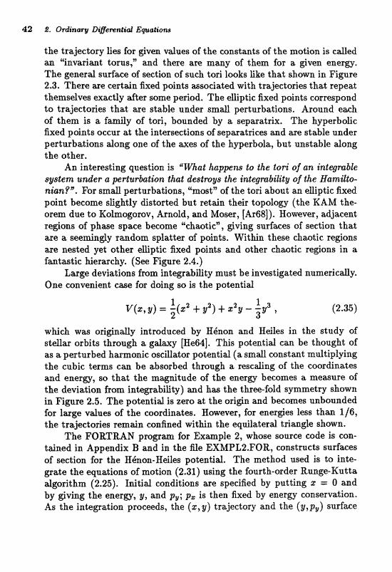
the trajectory lies for @ven vdaes of the consta~ts of the motion is cded an u"imrimt toms," and these a ~ t m a y of them for a gven mergy. The general surface of section of such tori looks like that shmn in Figure 2.3. There me cefiajrr k e d points asodated with trajectories that repeat themselves exactly after same pefiod, The elliptic fixed points correspond to trajectories thafr are stable under smafl perturbations. Around e x h of them is a family of tori, bounded by a sepasatrix. The hyperboEc fixed pdnts occur at the Intersectioas of sepruratdces and me stabb under perturbations dong one of the wes of the hyperbda, but unstabb dmg the ather *
An interesting guestion, is @What happens to the lori of an infqmblr: &@em under a perturbatha that destmys the integprtbihty cif the Hamitto- nian B", For sma31 perturbatiom, 'host" of the tori about an eBiptic fixed point become slightly distorted but retain their topology (the KAM the- orem due to Kolmogorov, Arnold, and Maser, [Ar68]). However, adjacent reg;ions of phase spwe become "chmtic", dving sudwes of section that are a seemingty random splatter af points. Within these chaotic regions =CS nested yet other &ptk fixed point;s and other chaatic regions in a fantastic hierarchy. (See Figure 2.4.)
Large deviations from integrability must be invegtigated numerically. One convenient case for doing so is the potentid
which was originally introduced by HQnon and IIeiles in the study of stellar orbits thro~gh a gilrlaxy [He64]. This potential can be thought of as a perturbed harmonic osciuator potential (a small constant multiplying the cubic terms can be absorbed through a rescaling of the coordinates and energy, so that the magnitude of the energy becomes a measure of the deviation from integrability) and has the three-fold symmetry shown in Figure 2.5. The potential is zero at the origin and becomes unbounded for lasge values of the coordinates. However, for energies less than 116, the trajectories remain confined within the equilateral triangle shown.
The FORTRAN program for Example 2, whose source code is con- tained in Appendix B and in the file EXMPL2.FOR, constructs surfaces of section for the B6non-WcliXles poteatid, The method used is to inte- grate the equations of motion (2.31) using the fourth-order Runge-Kutta algorithm (2.25). Initial conditions are spedfied by putting s = O and by giving the energy, g, and p,; p, is then fixed by energy conservation. As the integration proceeds, the (s, g) trajectory and the ( y, p,) surface
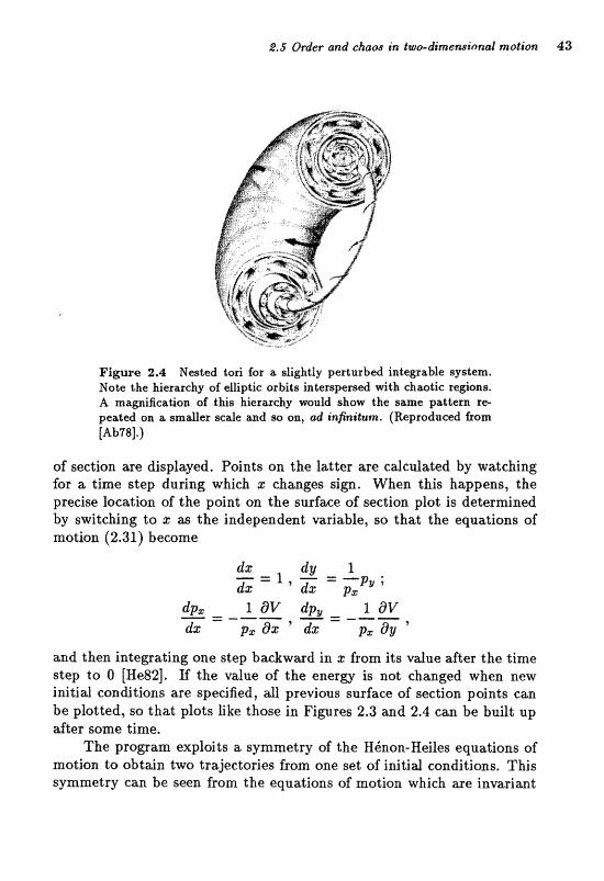
i9.5 Qder and chaos in two-drimensional motion 43
Figure 2.4 Nested tori for a. slljightly perturbed integrable system, Note the hierarchy of eltliptk orbits inlerspersed with chwtic regions. A magnification af this hierarchy would show the same pattern re- peat& on a smdler scale and so on, ad trrfiitum. (Reproduced &am [Ab78],)
of section u e displayed. Pointis on. the latter are calculated by w;tt;ching for a time step duPing which a: changes sign. When this happms, the precise l~cli t t i~n of the point an the surface of section plot i s determined by switching to 2 a~ the independent variable, so that the equations of motion (2.31) beeorne
and then integating one step bwkwasd in a: from its vdue after the time step to 0 [He82]. If the value of the energy is not changed when new initial conditions are specified, all previous surface of sectisn pdnts c m be plotted, so that plots like those in Figures 2.3 and 2.4 can be built up after some time.
The p r o g m exploits a symmetry of the Henon-X-feiles equations af motion to obtain two trajectories &om one set of initid conditio~s, This symmetry can be seen from the equations of motion which me invariant
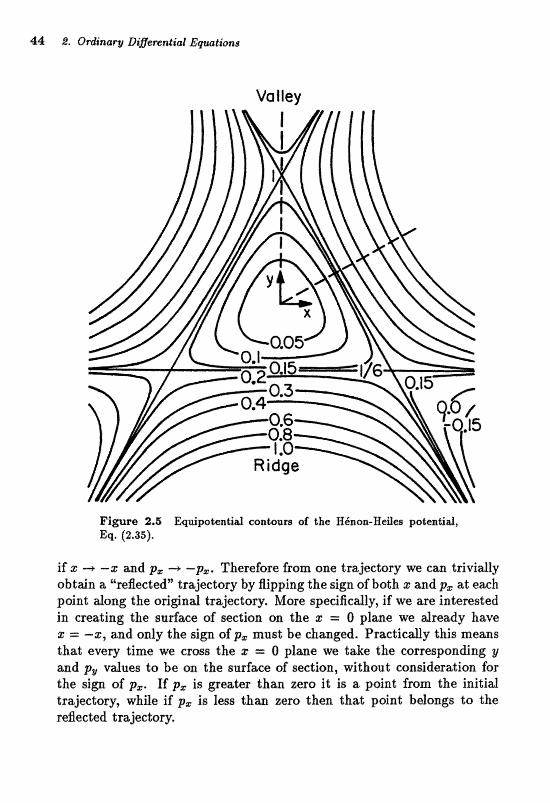
Valley
Figure 2.8 muipolentiait eont;ours of the IXknani-XXe3es potentid, Eq, (2.35).
if + -+ -I and p, -+ -p,. Therefore from one trajectory we can trivially obtain a "reflected" trajectory by flipping the sign of both I and p, at each point along the original trajectory. More specifically, if we are interested in creating the surface of section on the z = 0 plane we $ready have z = -g, and only the sign of p, must be changed. Practically this means that every time we cross the I = 0 plane we take the comesponding y and p, values to be on the surface of section, without consideration for the sign of p,. If p, is greater than zero it is a point from the initial trajectory, while if p, is less than zero then that point belongs to the reBected trajectory.
2.5 Oder and chaoe in two-9mensitrnal motion 45
The following exercises are aimed at improving your understanding of the physical principles and numerical methods demonstrated in this example,
Exercise 2.7 One necessary (but not suffident) cheek of the aecuracy of the integration in Hamiltonian systems is the conservation of energy. Change the time step used and observe how this affects the accuracy. Replace the integration method by one of the other dgorithms discussed in this chapter and observe the change in accurrccy and eficiency, Note that we require an algorithm that is both accurate and eficient because of the very long integration times that must be considered.
U kxercise 2.8 Change the potential to a central one (function subrou- tine V) and observe the character of the (z, y) trajectories and surfaces of section for va~ons initial conditions. Compwe the resub with Figure 2.2. and verify that the quatative hatares don't change if you use a diEerent centrd patentid. Nde that yaa wi11 have to adjust the energy and scale of the potential M, that the (r, y) trajectory does not go beyond the equilateral triangle of the HQnon-Heiles potential (Figure 2.5) or else the grapEcs subroutine will fail,
m Exercise 2.9 If the sign of the y3 term in the Henon-Heiles potential (2.35) is reversed, the Hamiltonian becomes integrable. Verify andyticdy that this is so 'by making a canonicd trmsformation to the variables z r f : y and showing that the potentid is sepasabl~ in these variables. MafEe the corresponding chmge in sign in the GO& and &save the character of the sadaces of metion that result for various injtid conditions at a given energy. (You should keep the energy below 1/12 to avoid having the trajectory become unbounded.) Verify that there are no qualitative differences if you use a different separable potential, say the harmonic one of Eq. (2.34).
U Exereiw 2.10 Use the code to construct surface8 of section for the Hhnon-Heiles potentid (2.35) at ener@es ranging from 0.025 to 0.15 in steps of 0.025. For each enera, consider various initid conditions and integrate each trajectory long enough in time (some will require going to t m 1100) to map out the surface-of-section adequateb. For each energy, see if you can find the elliptic fixed points, the tori (and tori of tori) around them, and the chaotic regions of phaee space and observe how the relative proportions of each change with increasing energy. With some patience and practice, you should be able to generate a plot that resembles the schematic representation of Figure 2.4 around each elliptic trajectory.
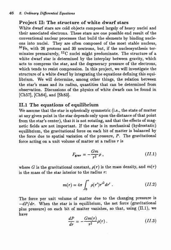
46 h. Ordinary Diflemntial Equations
Project 11: The structure of white dwarf stars White dwarf stars are cold Objects eomiposed largely of heavy nudel and thdr associated electrons. These stms me one possible end result of the conventiond nuclear proces8es that build the elements by binding rrrrcfe- ons into nuclei. They are often composed of the most stable nudeus, '@Fe, with 26 protons and 30 neutrons, but, if the nucleosynthesis ter- minates prematurely, C nudei might predominate. The structure of a w&te dwad star is detemined by the interplay between pavity, wEch acts to cornpress the star, and the degeneracy pressure of the electrons, vvhicb tends to resist eompressim. fn this project, we will investjgate the structure of a white dwasf by integrating the equations dtefiniq this eqrti- Xibfiurn. VCTe W% determine, among other things, the rdation between the stark rnahts a d its radius, quasltiLies that can be deterxnined ffsm observation. Discussions of the p2rysics of wkite d w d s can be found in [Ch57], [Ch84], and [Sh83].
11.1 The equations o f equilibrium We assume that the star is sphericalk symmetric (i.e., the state of matter at any given point in the star depends only upon the distance of that point from the star's center), that it is not rotating, and that the effects of mag- netic fields are not important. If the star is in mechanical (hydrostatic) equilibrium, the gravitational force on each bit of matter is balanced by the force due to spatial variation of the pressure, P. The gravitational force acting on a unit volume of matter at a radius r is
Cm F,., = -- ,z P ?
where G is the gravitational constant, p(r) is the mass density, and m(r) is the mass of the star interior to the radius r :
The force per unit volume of matter due to the changing pressure is -dP/dr. When the star is in equilibrium, the net force (gravitational plus pressure) on each bit of matter vanishes, so that, using (II.1), we
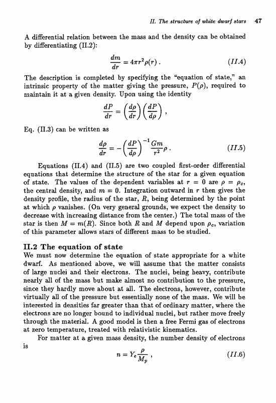
11. The st;ruckre of white dwarf star8 47
A digereatid relation betwen the anss and the density can be obtained by differentiating (11.2):
The description is completed by specifying the "equation of state," an intrinsic property of the matter giving the pressure, P(p), required to maintain it at a given density. Upon using the identity
Eq. (11.3) can be written as
Equations (11.4) and (11.5) are two coupled first-order differential equat;ims that determine the structure of the star for a given equation of state, The v d u a of the depeadent variables at r = O a e p = p,, the central density, and m = 0. 1ntegr;hlim outward in r then giws the density profie, the radius of the star, R, being detemined By the point at which p vanishes. (On very general grounds, we expect the density to decrease with increasing distance from the center.) The total mass of the star is then M = m(&). Since both R and M depend upon p,, variation of this parameter d a w s stass of rligerent masa; to be studied,
11.2 The equation of state We must now deternine the equatioxl of sh t e appropri&e fctr a white dvvad. As ment:ioned above, we will assume that the matter consists of large nuclei aad th&r electrons, The nuclei, be iq heavy, cont;ribute nearly atl of the mass but make almost; no contribuLim to the pressure, since they hardly move about at. d. The dectmns, hwever, contribute virtudly abl of the pressure but essenlidy none of the mass, VVe will be intexsted in densities fas ge&er than that of ordinmy mat;ter, where the electrons am no longer bound to individuitl nuclei, but mther move fredy thmufi the naakrid. A good model is then a free F e r ~ gas af electrons at zero tamperiature, treated with relativistic Xcfnematics.
h r matter at; a. @ven mass densi.2,~~ the numb= density of electrons

where M, is the proton mass (we neglect the small difference between the neutron and proton masses) and Y, is the number of electrons per nucleon. If the nudei are all $@Fe, then
while Ye = 4 if the nuclei are I2C; electrical neutraiity of the matter requires one electron for every protoll.
The free Femi gas is studied by considering a large volume If con- taining N electrons that occupy the lowest energy plane-wave states with momentum p < pt. Remembering the two-fold spin degeneracy of each plarie wave, we have
where n = N/V. (We put h = e = 1 unless indicated explidtb.) The totat energy density sf thege electrons i s
whicfi can be integitted to @vet
%(l+ 2z2)(1 f I ~ ) ~ / ~ - log
The variaMe z chasacberizes the electron density in terms of
the density at which the Fermi momentum is equal to the electron mass, m,*
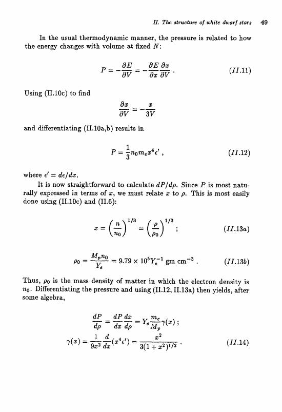
11. The &tmrchins, aJ" white dwarf stars 49
In the usual thermodyn G mmner, the pressure is related to how the eneru chwges with volume at k e d N :
Using (11.10~) to find
and differentiating (II.lOa,b) results in
where c' = de / dz. It is now straightforward to calculate dP/dp. Since P is most natu-
rally expressed in terms of I, we must relate I to p. This i s most easily done using (11.10~) and (11.6):
Thus, p0 is the mass density of matter in which the electron density is no. Differentiating the pressure and using (11.12, II.13a) then yields, after some algebra,
11.3 Scaling the equations It is often usefd to xd-btee equations desellibing a physicd system to di- mensiodess form, both for physical. insiglice and for xturnesicd convenience (i.e., to avoid dealing with very lage or very s m d nwnbers in the com- puter), To do this for the equations of white dwasf &metare, we introdwe dimensiodess radius, density, and milss vwiables:
with the ra&us and mass scdes, & and Ma, to be deternzined for con- venience. Substituting into Eqs. (IIe4,11.5) and using (11.14) yields, after some reanangement ,
If we now choose MO and & so that the coeEeients in pmerrtheses in these two equ&ions are unity, we find
a ~ d t he dimensiadess diEerential equations me
These equations axe compkted by rec g that 7 i s given by Eq. (11.14) with r = p'/3.
The scaling quantities (II.13b) and (II.17) tell us how to relate the structures of stars with digerent Ye and hence reduce the nnnnericd work to be done. Spedfiedy, if we have the solution for Ye = 1 at some value of pc = p,/po, then the solution at any other Ye is obtained by scaling the density as Y;', the radius as Ye, and the mass as Y:.
J% The structurcl? of while dwarf stars 51
To give some feeling for the scales (11. IT), recall that the solar radius and mms axe
while the density at the center of the sun is m 1150 gm cmw3. We therefore expect white dwarf stars to have masses comparable to a solar mass, but their radii will be considerably smaller and their densities will be much higher.
11.4 Solving the equations We are now in a position to solve the equations and determine the prop- erties of a white d w d . This cm be done in the folladng sequence af steps.
Step 1 Verify the steps in the derivations given above. Determine the leading behavior of E and 7 in the extreme non-relativistic (z &: 1) and relativistic ( x > 1) limits and verify that these are what you expect from simple arguments. Andyze Eqs. (II.IBa,b) when ifs and F are finite and p is smdl to shsw thztO j? vanishes at a finite ra&us; the star therefore has a well-defined surface. Determine the function4 form with whieh p vmishes near the surf=@.
Step 2 Write a program to integrate Eqs. (11.18) outward from F = O for Ye = f , Calculate the density p rdes , total masses, and. radii of stars with selected d u e s of the dinaeasimbss centrd density p, ranging from 10-' to 1Q6. By changing the radial step and the integration algorithm, verify that your s~lutions we accurate, Show that the totd kinetic and rest enera of the electrans in the star is
where E/V is the energy density given by (11.10) and that the total grav- itatimal energy of the star can be written as
Use the scaling discussed above to cast these integrals in dimensionless form and calculate these energies for the solutions you've generated. Try to understand all of the trends you observe through simple physicat rea- soning.
r Step 3 A commady tl~ed de~clLiptim of stellar slrructuse involves a pdytropic equation of state,
where PO, p0 , and l? are constants, the latter being the adiabatic index. By suitably scaling Eqs. (II.4,5), show that a star with a polytropic equation of state obeys Eqs. (11.18) with
The degenerate electron gas therefore corresponds to F = 413 in the extreme relativistic (high-density) h i t and I? = 513 in the extreme non- relativistic (low- density) limit.
Patropic equations of state provide a simple way to dudy the ef- fects of varying the equation of state (by changing l?) and also give, for two spedd vdnes of r", andytieal solutions wainst whieh numericill so- lutions c a ~ be checked, For this latter palpose, if is most convenient to recast Eqs. (11.18) as a single second-order differential equation for p by solving (II.18a) for and then differentiating with respect to f and using (II.18b). Show that the differential equation that results (the Lane- Emden equation, [Ch57]) is
and that far ]E' == 2 the mlutian i s
sin r" p ' pc- F *
while for I? = 615 the solution is
Use these analytical solutions to check the code you wrote in Step 2. Then study the structure of stars with different adiabatic indexes I? and interpret the results,
I ' The struct-UFY? of ullaile &a$ stars 53
N Step 4 If things are working correctly, you should find that, as the central density of a white dwarf increases, its mass approaches a limiting value, (the Chandrasekhar mass, MCh) and the star becomes very small. To understand tkis aad to get an estimat;e of Mch, we cm faurn the steps in an argument originally given by Landau in 1932. The total energy of the star is composed of the gravitational energy (W < 0) and the internd energy of the matter (U > 0). Assume that a star of a given total mass has a constant density profile. (This is not a very good assumption for quantitative purposes, but it is valid enough to be useful in understanding the situation.) The radius is therefore related simply to the total mass and the eonstmt density, Calculate U and W h r this density profile, assuming that the density is high enough so that the electrons can be treated in the relativistic limit. Show that both energies scale as 1/R and that W dodrriltes Zf when the totd mass exceeds a cert%in criticd vdue. It then becomes energetically favorable for the star to collapse (shrink its radius to zero). Estimate the Chandrasekbar mass in this way and compare it to the =salt of your numeric& calculation, Also verify the correcgness of this rtrgumexlt by showing th& U and W for your solutions found in Step 2 become equal and opposite as the star .approaches the finriting mass,
m Seep F; Scde the mass-radius rdation you found in Step 1 to the cases corresponding to and I2C nuclei. Three white dwarf stars, Sirius B, 40 Eri B, and Stein 2051, have masses and radii (in units of the solar values) determined from observation to be (1.053 f 0.028,0.0074& 0.0006), (0.48 it 0.02, 0.0124 0.0005), and (0.50 k 0.05 or 0.72 f. 0.08, 0.0115 f 0.00 121, respectively [Sh83]. Verify that these values axe consistent wit h the model we hwe developed. What can you say abbot the compositions of thege stws?

This page intentionally left blank
Chapter 3
Bound
Many of the important differentid equations of physics can be cast in the Earm of a linear, second-order equalim:
where S i s an inhomogeneous ("drivingn) term and k2 is a real function. When kZ is positive, the solutions of the homogeneous equation (i.e., S = 0) are oscillatory with local wavenumber k, while when k2 is negative, the solutions grow or decay exponentidly at a local rate (- kZ)* . For example, consider trying to find the dectrostatic poteratiaf, @, generated by a localized charge distribution, p(r). Poisson's equation is
which, far a spbericdly symmetric p and Qtr, simplifies to
The standard substitution
then results in
which is of the form (3.1) with kZ = 0 and S = -4rrrp. In a similar manner, the quantum m e c h ~ e a l wave fanetion, for a partide of mass m
56 S. Boundarq, Value and Eigenvalue Problems
and energy E moving in a central potential V(?) can be written as
where YAM is a sghericd harmonic and the radid wave function R satisfies
This is also of the form (3.11, with S = 0. The equations discussed above appeas unremarkable and readily
treated by the methods discussed in Chapter 2, except for two points. First, the boundary conditions imposed by the physics often appear as constrdnts on the deptjndent vdablr, at t m sepmfe points of tke inde- pendent variable, so that solution as an initial d u e problem is not obvi- ously possible. Moreover, the S ehroedinger equation (3.5) is an eigenvdue equatim in which we m u ~ t jsad the energies that had to physicdy ac- ceptable solutions satisfying the appropriate boundary eonditiws. This chapter is concerned with methods for treating such problems. We begin by deriving aa integration atgorithm parlieulaxly well suited to equal;ims of the form (3.1), and then discuss boundary value and eigenvalue prob- lems in turn.
3.1 The Numerov algorithm There is a particuldy simple an& eficient method for integating second- order differential equations having the form of (3.1). To derive this method, cammonly c d e d the Numerov or Cowling's method, we begin by approximating the second derivative in (3.1) by the three-point difference formula (1.7),
where we have written out explicitly the 6 ( h 2 ) "error" term, which i s derived easily from the Taylor expansion (1.1, 1.2a). From the differentid equation itself, we hitve
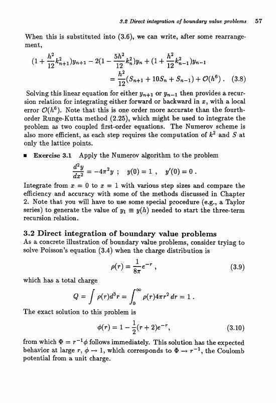
3.8 Birst integmtfiorz of boundarg value pr~bbms 57
When this i s substituted into (3.6), we can write, after some rearrange- ment,
Solving this finear equation for either gn+1 or gn-l then. provides a recur- sion relation. for integrating &ther forwxd or bukward in s, with a. bcal error O(hs). Note that this is one order more accurate than the fourth- order Runge-Kutta method (2.25), which might be used to integrate the problem as; two coupbd first-order equations. The Nunrerw seheme is also more efficient, as each step requires the computation of k2 and S at only the lattice points,
Exercise 3.1 Apply the Numerov dgorithm to the pmblem
Iategrate from s = 0 to a: = 1 with vwious ~ t e p ~ i z e ~ and the eaciency a~ ld xcuracy with some of the methods discussed in Chapter 2. Note that yon will have to use some h;pedd prowdure (e.g., a Taylor series) to generate the value of yl E y(h) needed to start the three- term recursion relation.
3.2 Direct integration of boundary value problems As a concrete illustration of boundmy value problems, consider trying to solve Poisson's equation (3.4) when the charge distribution i s
wEch has a told charge
The e x x t solution to this problem is
b +(F) = I - -(v + 2)e-', 2 (3.10)
from which @ = r-'# follows immediately. This solution has the expected behavior at large r , 4 4 1, which corresponds to 4! -+ v-', the Coulomb potential frm a unit charge.
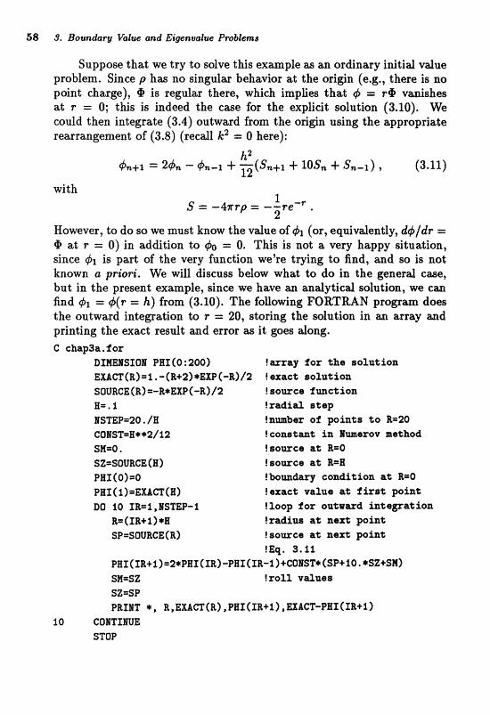
58 9; Boundary Vhlue and Eigenvalue Problems
Suppose that we try to solve this example as ;an ordinmy initial vdue problem. Since p has no singular behavior at the origin (e.g., there is no point charge), @ is regular there, which implies that 4 = rQ vanishes at r = 0; this is indeed the case for the explicit solution (3.10). We could then integrate (3.4) outward from the origin using the appropriate rearrangement of (3.8) (recall k2 = 0 here):
However, to do so we must know the value of (or, equivalently, d+/dr = O at r = 0) in addition to q ! ~ = 0. This is not a very happy situation, s ine gSil is part of the very function we're tr~ring to find, and go is not knovvn a pva'ori. We will discuss below what to 1Co in the generd c m , but in the pre~ent exmpk, &nee we have asl mdytical golutim, m cm find = $(P = h) from (3.10). The following FORTRAN program does the antward integration to r = 20, storing the sxrlution in m &gray and printing the exact r e d t and efror as it gws along. G cbp3a.for
BIEmSTOM PHI (0 : 200) !=ray for %he solm%fun EXACT (R) = 1 I. - (E+2) *EXP (-B)/2 ? exact solm%iorr SOUME (R) S-R*EXP (-R) 12 ! sowce i w e t ion H=.$ !xa&ia step ISmP=20./eE !nmber o f p i n t a to R=20 C01ST=8*+2/12 ! ~ o m t a t in E-erov method SMI=O. !arouce; a$ R=O SZ=SOURCE (E ) Iso-ca at MB[ PHX (a)=o i b ~ m d w ~ ~ ~ d i t i ~ n at R=O PHI ( l)=EXkGI"(B) ! exact value a% Sfrst poiat ao 10 XB=I,IS~P-I rloop ior O U ~ W W ~ i x t e ~ a t i o n
R=(IB+l)*B ?radius a% next point. SX"=SOUECECR) !sowee a% next poh%
!Eq. 3.11 PH~(xR+~)~~+PHI(TR)-PEX(TR-I)+C:OIST*~SP+~~~ *SZ+SX] SM=SZ !roll vanss SZ=SP PRXIS *, R,EXA~(R),P~I(IR+~),EXACT-FHI(IR;+II
10 CORTIrnE STOP
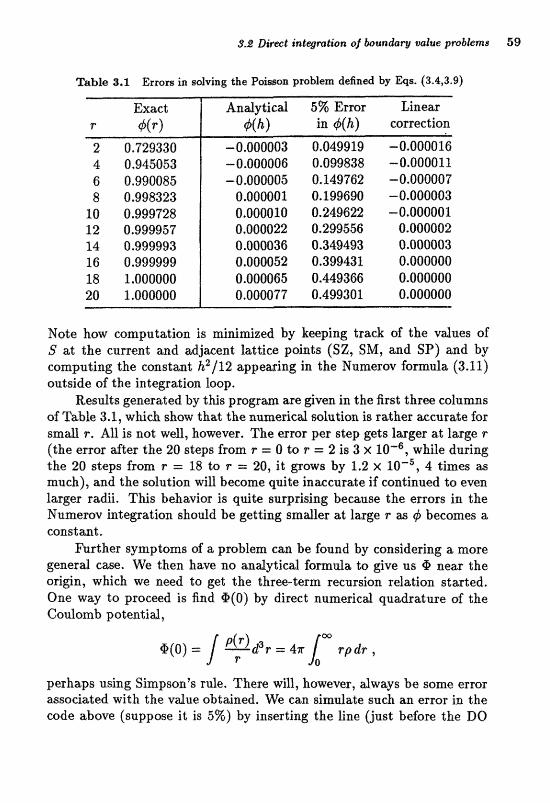
$3 Dimt intclgration of baundary value problems 59
Table 8.1 Errors in salving the Paisan pfablem defined by %a, (3.4,3.9)
Note haw computation is minimized by kwping track of the vdues of S at the current and adjacent lattice points (SZ, SM, and SP) and by computing the constant h2/12 appeaing in the Numerov formula (3.11) &side of the ixltegration loop,
Results genwated by this progrm axe giwn in the first three columns of Table 3.1, which show that the ~umericd so1af;ion is rather accurate for small v, All is ~ o t well, however. Tbe error per step gets larger at large r (the error after the 20 steps from T = 0 to r = 2 is 3 X 10-', while during the 20 steps from r = 18 to r = 20, it grows by 1.2 X IQ-', 4 times as much), and the solution afiB beeorne quite inaccurate if continued to even larger radii. This behavim is quitre surp~ging because the error6 in, the Numerov ietegration should be get.t;ing smdler at large r as gi becomes a constant.
f irther symptoms of a problem em be found by considePing a mare general caM. Mlt3 then h m RO andytical farmda to give us @ near the origin, which we need to get the three-term recursion relation started. One way to proceed is find @(0) by direct numerical quadratare of the Coulomb potentid,
perhaps using Simpson's rule. There will, however, dways be some error wsoeiated with the vdue obtajxled. We c m simulate such an, ermr in, the code above (suppose it is 5%) by inserting the line (just before the DO
fSO S. Boundarg Value and Eigenualua Prablenas
The code then gives the ersors listed in the fourth cafumn of Table 3.1, Evidently disaster has struck, for a 5% &ange in the initial conditions has induced a 50% error in the solution at large r.
Xt is simple to understand what hsts happened. Solutions to the homogeneous version of (3.4),
can be added to any particular solution of (3.4) to give yet another solu- tion, There are tvvo linearly indepenhnt Iromogeneous solutions,
and q5 W constant ; @ F-' .
The general solution to (3.4) in the asymptotic region (where p vanishes and the equation i s homogeneous) can be written as a linear combina- tion of these two functions, but the latter, sub-donainant soIution is the physical one, since we know the potentid at large r is given by @ -, l lr. hprecision in the gnecification of rP at the origin or any numericd round- off e m in ehe inteeation process c m idroduce a, small admixtare of the q5 p soXutim:, which eventudy do~xlale-s at, large r.
The cure fbr this diBeul"cy is &raightforward: subtrwt a multiple of the "'bad," anphysical solugion, to the homogeneaus ewatioll from the numerical result to guarantw the physical behavior in the wymptotie region. It is easy to see that the 'bad" results shown in the fourth column
linearly with r for large r. The following lines of code (which can be inserted just before the n a p statement) then fit the last 10 points of the numericd solution to the form
(and subtract mr from the numerical results to guarantee the angropriab large- r behavior .
9.8 Gmen'g finctisn golution of boundlsry value problem# 61
The errors in 4 so obtdned are shown in the final column of Table 3.1; the solution is emn more accur&e at large r than the uncorrected one found when the exact value of PHI(1) is used to start the integration.
In this simple example, the instabilities we not too severe; satisfm- tory rwults for moderate d u e s of r are obtained with outwasd integration when the exact (or reasonably accurate apprauimate) value of PHI(1) is used, Alternatively, it is also feasible to integate inwasd, otarting at lasge r 6 t h qi = Q, independent of r. This results in, a sdution that often sat- isfies aiecur&ely the boundasy mndition at r = 0 and avoids having to
a quadrat are to determine the (approximate) stmting value of PHI(1).
m Exercise 3.2 Solve the problem defined by Eqs. (3.4,3.9) by Numerov integation inward from large r using the known wymptotie behavior of tiJ fof the starting values. IIow welI do& your solution satisfy the boundary condition 4(r = 0) z= 01
3.3 Green's function solution of boundary value proble When thc? twa salations to the homogeneous equation have very diger- ent behaviors, some extra precautions must be taken. For example, in describing the potential from a charge distribution of a multipole order l > 0, the monopole equation (3.4) is modified to
which has the two homogeneous solutions
For large r , the first of these solutions is much larger than the second, so that ensuring the correct asymptotic behavior by subtracting a multiple of this dominant homogeneous solution from a particular solution we have found by outward integration is subject to large round-off errors. Inward integration is also unsatisfactory, in that the unphysical r-' solution is fikely to dominate at @malt r .
One possible way to generate an accurate solution is by combining the two methods. Inward integration em be used to obtain the potentid for r greater than some intermediate radius, r,, and outward integration can be used for the potential when T < +m. As long as r , is chosen so that
162 3. Bsundarg Value and BigenuaZue Problems
neither homogeneous solutim is d o ~ a m t , the outer and inner patenlids obtained respectively from these two integrations will match at F, and, together, descrjlbe the a t i r e sdution. Of course, if the inner and outer potmtids don't quite match, a mult;iple of the hamqeneous golution cm be added to the former to comect for m y hficiencies in aur knowledge of Qr(r = 0).
Sometimes the two homogenmns solutions have sach &Eere& behw- iars that it is impossible to find a d u e af r, that permits sartisfactory integration of the inner and outer potentids. Such cases can be solved by the Green's function of tlre homogeneous eqluatim. To illustrate, let us consider Eq. (3.1) with the boundary condition 4(x = 0) = #(r = m) = 0. Since the problem is linear, W can w~ite the sdution as
whert; G is a Green's suction sati~fying
It is clear that G satisfies the homogeneous equation far z f si. However, the derivative of G is discontinuous at I = z', as can be seen by integrating (3.14) from s = r f - E to z = zi f E, where E is an infinitesimal:
The problem, of course, is to find G. This can be done by eoxlsjderinig two solutions to the homogeneous problem, arnd (6>, ~.tltiSfSring tbe boundary conditions at rt: -- O and z = so, respective?ly, md nomaiized so that their Wrmslrian,
is unity. (It is easy to use the homogeneous equation to show that W is independent of 2). Then the Green's function is given by
where r , and z> are the smaller and larger of r and z', respectively. It is evident: Ghat this expression for G satisfies the h o m ~ e n e m s eguatim and the discontinuity condition (3.15). From (3.13), we then have the explidt
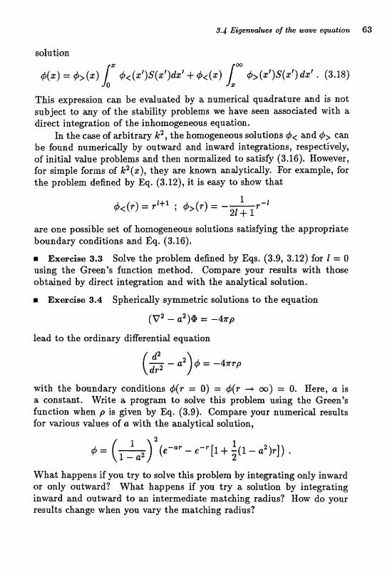
3.4 Eigenvaluedr of the wave egeralz'on 63
This expression can be evaluated by a numerical quadrature and is not subject to any of the stability problem we have seen associated with a direct integration of the inhomogeneous equation.
In the case of arbitrary kZ , the homogeneous solutions and gi> can be found numericdly by ouward and inward integr&ions;, respectively, of initial value problems and then normalized to satisfy (3.16). However, for simple forms of k2(x) , they are known analytically. For example, for the problem defined by Eq. (3.12), it is easy to show that
are one possible sel of hornqeneaus solutions satisfying the approplliatte boundary conditions and Eq. (3.16).
m Exercise 3.3 Solve the problem definedby Eqs. (3.9, 3.12) for I = O using the Green's function method. Compare your resdts with those obtajned by direct integration and with the andyticd solution.
r Exercise 3.4 Sphel.iedly sy etric solvtioas to the equa;t;ian
l e d to the ordinary diRerenlia1 equation
with the boundary conditions 4(r = 0) = +(P -r W) = 0. Here, a is a constaat. Write a program %o solve this problem using the Green's function when p is given by Eq. (3.9). Compare your numerical results fir varims; v d u e ~ Of a with the andytical golution,
What happens if you try to solve this problem by integrating only inward or only outward? What happens if you try a solution by integrating inwmd and outward to an intermediate zn&ching radius? Bow do your results change when you v a y the rnalching radius?
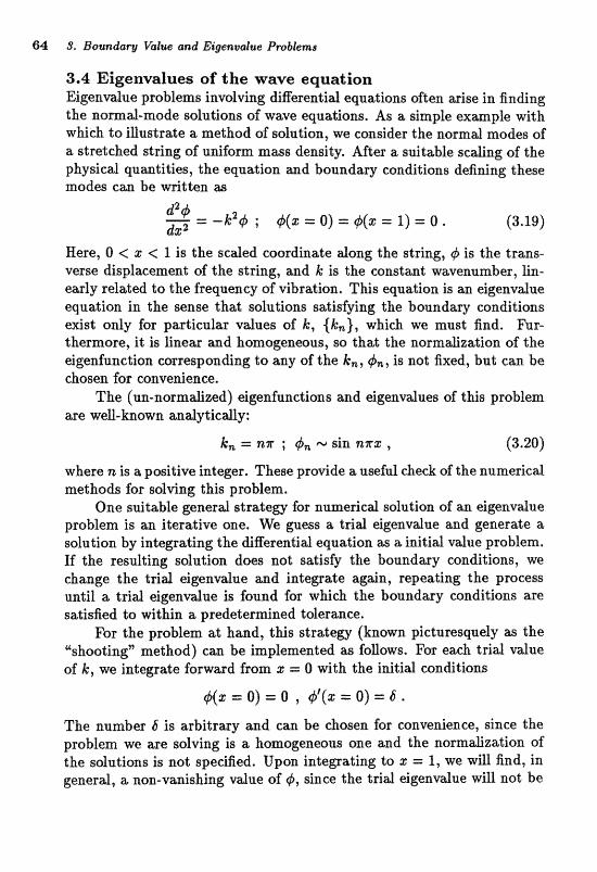
84 3. Boundarg Vialwe and Eigenvalue Problem8
3.4 Eigenvalues of the wave equation Eigenvalue problems involving differential equations often arise in finding the normal-mode solutions of wave equations. As a simple example with wEch to iuustrate a method of solution, we consider the normal modes of a stretched string of uniform mass dendty. After a suitable scaling of the physical quantities, the equation a d boundary conditions defining these modes cm be mitten zw
Here, Q < 5 < I is the aeded coordinate dong the string, 4 is the trans- verse displxement of the string, and k: is the constant wavenumber, lin- e d y related to the frequency of vibration. This v a t i o n is an eiwnvdw equationi in the sense th%t solutions satisfying the boundary conditions exist only for particular values of k, {k,), which we must find. Fur- thermme, it is linear md homogeneous, so th& the normdzation of the dgenfunction comesponding to any ol the k,, +,, is not fixed, bat can be &osen for convenience.
The (un-normalized) eigenfunctions and eigenvalues of this problem are weU-known analyticdly ;
km = nn ; g5n sin nz3: , (3.20)
where n is a positive integer. Them provide a useful Gbe& of the nurnericd methods for solving thiz; problem.
One suitable general strategy for numeric& solution of an eigenvdue problem is an itersltive oon. VVe? mesa a trial eigenva9ue and gemrate a solution by integrating the differential equation as a initial d u e problem. If the resulting solution does not satis@ the boundary conditions, we change the trial eigenvalue and integrate again, repeating the process until a trial eigenvalue is found for which the boundary conditions are s&sfied to within a predetermined tderanec;.
For the problem at hand, this strategy (known picturesquely as the "shootingn method) can be implemented as follows. For emh tr id value of k, we integrate forward from z = O with the initial conditions
The number 6 i s arbitra~y and can be &osen for convenience, since the problem we are solving is a homogeneous one and the normalization of the solutions is not specified. Upon integrating to s = 1, we will find, in general, a non-vanishing value of 4, since the trial eigenvalue will not be
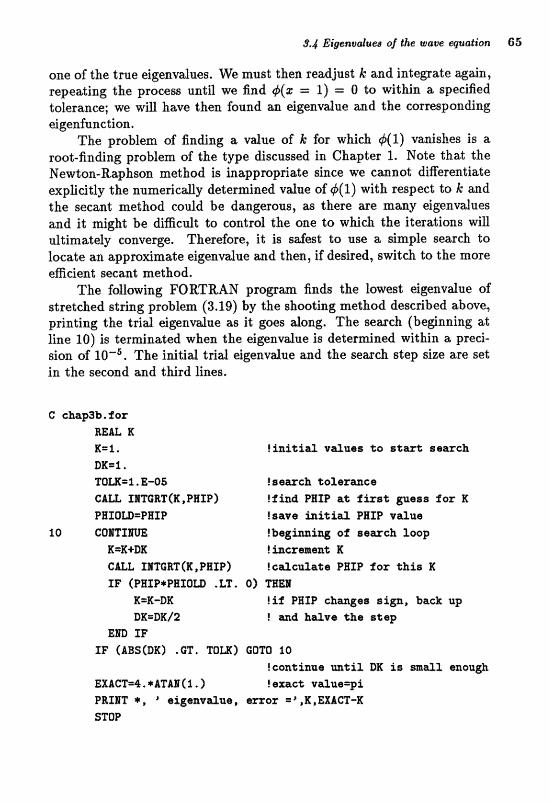
3.4 Bigemvalues of the wave equation 65
one of the true eigenvdues. We must then readjust k and integrate ~ a i n , repeating the process until we find ~z = 1) = 0 to within a specified tolerance; we will have then found an eigenvalue and the corresponding eigenfunction.
The problem of finding a value of k for which &(l) vanishes is a root-finding problem of the type discussed in Chapter 1. Note that the Newton-Raphson method i s inappropriate since we cannot differentiate explicitly the numerically determined value of #(l) with respect to k and the secant method could be dangerous, as there are many eigenvdues and it might be difficult to control the one to which the iterations will ultimately converge. Therefore, it is safest to use a simple search to locate an approximate eigenvdue and then, if desired, switdt to the more efidemtt secant methed.
The following FORTRAN program finds the lowest eigenvalue of stretched string problem (3.19) by the shooting method described above, printing the trial eigenvdue as it goes along. The search (beginning at line 10) is terminated when the eigenvalue is determined within a preci- sion of 1 0 ~ ~ . The initial trial eigenvalue and the seareh step size are set in the second ~ n d third lines.
C chp3b.for RrnL K K=1. ! i n i t i a v a n s s to stwt search BK=Z, IfOU=S. E 4 5 iasmch to lermts CA= IITGRT(K, PHXP) !fi& FEIP a t f i r s t p e s a fox X: PHIClW=tPHIP !save i n i t i a l PEIP value
10 COmIWE ing of search loop K=K+DE Iiacreatalz2; II CALL ImGRT (K, PHGP) ! c a ~ u l a t e PEIXP for this X: IF (PHIP*PBTOm .LT. 0) THEB
X=K-DX ! i f PBSP chagea sign, ba& up DK=DK/~ ! and Wve3 t h e aeap
Em IF IF (ABS(BK) .m, mu) ~om $0
Ican$inue mtil fIK i s s m d 1 enough EXACT=$.*ATAI(I.) ! exartt v d m e ~ i PRIIT *, p eigenvaae, error =\,EE,EXIm-g STGP
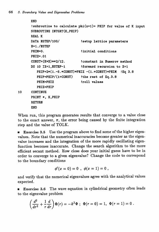
643 S. Bouradarg Value and Eo'genvalue Pwblems
Ern !sabzoatina t o c d c d a % a phi(s=l)= FEZP for value of R hpat SmWWIIE IITGRT (K, PIXIPI ItML K DATA I S ~ P / 2001 !8etap li9t;lice pmaeLers B=%. CBSmP PHIR=O. ! i n i t i d canditians PHXZ=. 0% CI)IST= (K*B) *+2/%2, !can;9tm% in Imszov meLhod, DQ IQ SX-2,NSmF-2 !forwad recmsian eo X=f
FHTP=2* ( 5 . -5. *CQm'5T] *PBX Z -( Z l tCQBST) +PETPI ! Eq 3.8 PEEP=PBIFI(%+CBIST) !the real of Eq,3.8 PHIM=PHIZ !rol l valnes PBXZ=PIXIP
10 COmXmB PRflT *, ZI,BEIP RErnEE EBB
When run, this program generates results that converge to a value close to the exact answer, a, the error being caused by the finite integration. step and the vdue of TOZK.
Exercise 3.5 Use the program above to find some of the higher eigen- d u e s . Note that the numaicd inzcuracies became greater as the eigen- vdue increases and the integration of the more rapidly oscillating eigen- function becomes inaccurate. Change the search algorithm to the more eBcient secaxlt method, How close does p r initial guess have to be in order to converge to a given eigenvdue? Change the code to correspond to the boundary eonditians
and verify that the numerical eigenvalues agree with the analytical values expected,
m Exercise 3.6 The wave equation in cylindrical geometry often leads to the eigenvalue problem
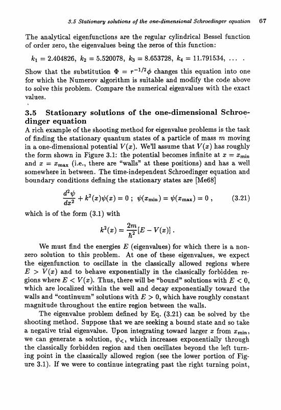
9.5 StaEt'onarg solutions of lfre one-dimensional Schroeditager equation fir
The andytical eigenfuactims are the re&= cylindricat Bessd funetian c->f order zero, the eigenvdues bdng the zeros of this function:
Show that the substitution 9 = r-'f2# changes this equation into one for which the Mumerov dgarithaa is suitable and modify the code &m to solve this problem. Compare the numerical eigenvalues with the exact vdues.
3.5 Stationary solutions of the one-dimensional Schroe- dinger equation A. rich e x a p l e of the shooting method far .eigenvdue problems is the task of finding the stationary quantum states of a particle of mass m moving in a one-dimensional potential V(%). Well assume that V(%) has roughly the form shown in Figure 3.1: the potential beeome-s irtfinite at, r = and s = g,., (i.e., there are 'walls" at these positions) and has a weEl somewhere in between. The timeindependent Schroedinger equation md boundary conditions defining the stationary states are [MeGB]
which is of the form (3.1) with
We must find the energies E (eigenvatues) for which there is a non- zero solution to this probXem. At one c>f these eigeavdues, W q e c t the eigenfunction to oscillate in the dassically dowed regions where E > V(+) and to behave exponentidly in the classically forbidden re- gions where E < v(%). Thus, there will be '4bound" solutions with E < 0, W&& are localized vvithin the well and decay exponenZ;idy toward the walls and gcontinuum" solutions with E > 0, which have roughly constant magnitude throughout the entire region between the walls,
The eigenvalue problem defined by Eq. (3.21) can be solved by the shooting method. Supphse that we are seeking a bound state and so take a negative tdal eigenvalue. Upon integrating toward larger z from i m i n ,
we can generate a solution, +<, which increases exponentially through the clasicauy forbidden redon and then oscillates beyond .the left tura- ing pojnt in the classically allowed region (see the lower portion of Fig- ure 3.1). If we were to continue integrating past the right turning point,
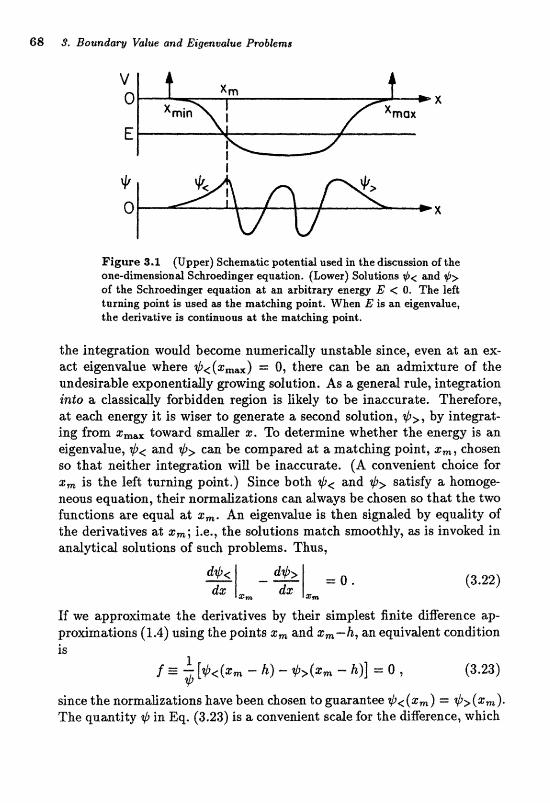
68 S. Boundary Value and Eligenvalzre Pmblczms
Figwe 9,1 (Upper) Schematic patentid used in the dbcnmion of the one-~mensionat Sclzrrzedinger equation, (hwer) Solutions $P< wd +> aP the Schraedinger eqnation at an arbitrary energ E < Q, The lef% turning point, is used m the matching point. When 6 is m eigeavalue, the de~vative is continuous at the matching paint,
the integation, wodd become numericdly unstable since, even, at an ex- act eigenvalue where $<(z,,,) = 0, there can be an admixture of the undesira;ble exponenliay gowing ~ ~ I u t i o a . As a general rule, integration into a classicay forbidden region is fikefy to be inaceurat;e, Thmefort;, aYt each mergy it is wiser to epenerata a second solu.t;ian, $>, by inlegat- ing from g,,, toward smaer g. To determine whether the enegy is an E?igenvalue, and $> carr be compared a;t a msatehing point, s,, cho~en so that neither integration will be inaccurate. (A convenient choice for s, is the left turning pcrint .) Since both and y5> satisfy a, homage- nems equation, thdr nomalizations can dwaya be chosen so that the two functions are equal at r,. An eigenvalue is then signaled by equality of the desivatives at z,; i.e., the sdutions naatGh smoothly; as is invoked in analyticd sQlvtions of such prablenns. Thus,
If we wpro~ma;t;e the derivatives by thdr simplest finite diEerence ap- proximations (1.4) using the points s, and $,-h, an equivalent condition is
since the nomalizations have been chosen to guarantee +< (s, ) = +> (1,). The quantity + in Eq. (3.23) is a convenient scale for the difference, which
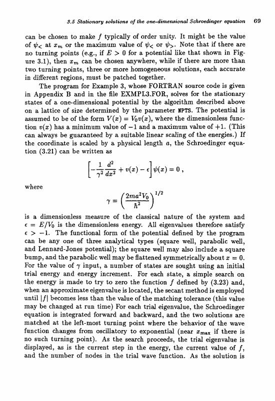
9.5 Stationary solutions of t-he one-dimensional Schrwdi~ger quodian 69
can be chosen to make f Vpicdy of order unity. l t might be the value of at x, or the maximum value of t$, or $>. Note that if there are no turning points (e.g., if E > 0 for a potential like that shown in Fig- ure 3.1), then s, can be chosen anywhere, while if there are more than two turning points, three or more homogeneous solutions, each accurate in different regions, must be patched together.
The program for Example 3, whose FORTRAN source code is given in Appendix B and in the R h EXMPE3,FOR, solves fof the seationmy states of a one-dimensional potential by the algorithm described above on a lattice of size determined by the parmeter EFTS. The potentid is assumed to be of the form V(z) = &v(z), where the dimensionless func- tion v(s) has a minimum value of -1 and a maximum value of +l. (This can always be guaranteed by a suitable linear scaling of the energies.) If the coordinat;e is scded by a physied length a, the Shrwdinger equa- tion (3.21) can be written as
where
is a dimensionless memure of the clmsicd nature of the system and 6 = E/% is the dimensionless energy. All eigenvalues therefore satisfy e > - 1. The function4 form of the patentid defined by the grogram can be any one of three analytical types (square well, parabolic well, and Lennard-Jones potential); the square well may also include a square bump, and the parabolic well may be flattened symmetrically about z = 0. For the value of 7 input, a number of states are sought using an initial trial energy and energy increment. For each state, a simple search on the energ i s made to try to zero the function f defined by (3.23) and, when an approximate eigenvalue is located, the secant method is employed
becomes less than the value of the matching tolerance (this value may be changed at run time) For each trid eigenvalue, the Schroedinger equation is integrated forward and bxkward, and the two salations are matched at the left-most turning point where the behwior of the wave function changes from oscillatory to exponential (near I,., if there is no such turning point). As the search proceeds, the trial eigenvdue i s displayed, as is the current step in the energy, the current value of f , a ~ d the number of nodes in, the trial wave function. As the solution is
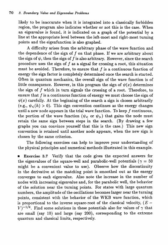
78 9. Bopmdarg Value and Bigenvalue Problems
likely to be inaccurate when it is integrated into a dassicalfy forbidden region, the program also indicates whether or not this is the case. When an eigenvalue is found, it is indicat;ed on a gaph of the potentid by a line at the appropriate level between the left-most and right-most turning points and the eigenfanction is dso gaphed.
A dificulty arises fram the ibrbitrary phase of the wave function and the dependence of the sign of f cm that phase. If we are arbitrary &oat; the sign of $, then the sign off is also arbitrary. However, since the search procedure uses the sign of f as a sign4 for crossing a root, this situation must be avoided. Therefore, to ensure that f is a continuous function of enero the sign hctor is completdy determined once the seaseh is started, Often in quantum mechanics, the averd sign of the wave function i s of little consequence. However, in this program the sign of +(S) determines the sign of f which in turn signats the crossing of a root. Therefore, to ensure that f is a continuous function of energy we must choose the sign of +(z) carefully. At the beginning of the search a sign is chosen arbitrarily (e.g., $<(h) > 0). This sign convention continues as the energy changes until a new node appears in the trid wave function, To keep f continuous, the portion of the wave function (+< or th& gains the node mast retajn the s m e sign betvveen steps in the search, (By drawing a few graphs you can convince yoursdf that this is the case.) This new s i p convention is retained until another node q p e m , when the new sigxl is chosen by the s m e criterion,
The following exercises can help to improve your understmdi~g of the physicd principles and nunrericd methods illustrated in this example.
Exercise 3*7 Verify that the code gives the expected mswers for the eigenvalues of the square-well and parabolic-well patentids (y = 50 mjght be a mnvenient mlue to use), Observe how the dismtinuity in the derivative at the matching point is smoothed out as the energy converges to each eigenvalue. Also note the increase in the number of nodes with increasing eigenvalue and, for the parabolic well, the behavior of the solution. near the turning gdnts. For states with l q e quantum numbers, the amplitude of the aftcillations becomes larger new the turning points, consistent with the behavior of the WKB wave function, which i s proportional to the inverse square-root of the classical velocity, (E - v ) - ' / ~ . Find some solutions in these potentids also for values of y that are small (say 10) and large (say 2001, corresponding to the extreme quantum and daf;ical limits, respectively;

3.6 IS;tat:onary solutions of the one-dimensional Sckrodinger wuation 7%
r Exmciw 3*8 For the mdyt icdy salable square and pafaboGc welh, investigat;e the eEects of &angin% the integration method from the Nu- merw dgoaithm to the '"nsve" one obldned by appra~mating the see- ond derivative by just the three-point formula (1.7); that is, neglecting the 6(h2 ) term in (3.6).
r 16xweist3 3.9 Change the progam so that the eigenvdues me found by integrating only forward and demanding that the wave fanceian vanish at g,,,. Qbserw the problems that arise in trying to integrate an ex- ponerttidy dying sdution into a classicadly forbiddea regon, (It is wise to keep 7 relatively small fiere so that the instabilities don't become tas large.)
Exercise 3.10 When the potential. is reflection symmetric about z = 0, the eigenfunctions will have a definite parity (symmetric or anti-symme- tric about I = 0) and that parity will alternate as the quantum number (energy) increases. Verify that this is the case for the numerical solutions generated by the code. Can you think of a way in which the parity can be exploited to halve the numerical effort involved in finding the eigenvalues of a symmetric potentid? ff so, modify the code to try it oat.
r Exercise 3.11 If we consider a situation where v(%) = O for r < I,,. and I > S,,, (i.e., we remove the walls), then the zero boundary condi- tions at $he ends of the lattice are inappropriate for weaMy bound ~ ta t e s (E 6 0) since the wave function decays very slowly as 11 More appropriate boundary conditions at and g,,, are therefore
Change the code to implement these boundary conditions and observe the eEeet on thc? wave functions afld energies of the states n e a zero energy. Note that if we were to normaEze the wave functiaa in the conventional way, the contributions from these exponential tails would have to be included. Can you derive, in the style of the Numerov algorithm, a numerical redzation of these boundary conditions accurate to a high order in DX?
B Exercige 3.22 Check nzrmericdly that, for a given golentid, two eigenfunctions, $E and +h, corresponding to different eigenvdues E and E', am orthogond,
+~(2)$k(2)dg= 0 ,
72 S. Boundary Value and Eigetavalue Problemor
as iis m q ~ r e d by the general principle8 of quantum mechanics,
m Exercise 3.13 For small, intermediate, and large values of 7, compare the exact eigenvdues of the Lennard-Jones potential with the semidassicd energies generated by the code for Example 1.
m Exercise 3.14 Investigate the eigenfunctions and eigenvalues for po- tential~ you might have encountered in learning elementary quantum me- chanics: the Cfunetion potential, a finite square-well, double-well poten- tials, periodic potentials, etc. This may be done by dtering the potentid in subroutine POTNTL. Interpret the wave fundions and eigenvdues you find. (Note that the code will sometimes have trouble finding two eigen- values that are nearly degenerate.)
Project III: Atomic structure in the Hartree-Fock approx- imation The self consistent field approximation (Hartree-Fock) is known to be an aemrate descfipti~n of many of the properties of multi-eledron atorns and ions. In this appraxirnatim, each electron is described by a separate single-partide wave funetion (as distinct from the many-electron wave function) that solves a Schroedinger-like equation. The potential appear- ing in this equatioa is that generded by the average motion of & of the other electrons, and so depends on their sinde-particle wave fiaelions. The resdt is a set of an-fine= eigenvdue equalions, wEch c m be solved by the methods introdumd in this chapter. In this project, we vviU solve the seIf-consistent field equations to deternine the pound-st&e ~itrac- ture of small atomic systems (e.g., the atoms aod ions of the elements in the periodic table from Hydrogen through Mean). The totd energies cdculated em be compmed direct& with experimental values. The brief derivation we give here cm be supplemented with the maLerid found in [Be68], [Me68], and [We80].
111.1 Basis of the Hartree-Fock approximation ltonian for N dectroas moving about a heavy nucleus of ehar~;ge
Z located at the ori@a can be writtea as
Here, the {ri) are the locations of the electrons, m and -e are the electron mass and charge, and rij E ri - rj is the separation between
electrons i and j. The three sums in (111.1) embody the electron kinetic energy, the electron-nucleus at traction, and the inter-electron repulsion. As is appropriate to the level of accuracy of the self-consistent field approximation, we have neglected much smaller terms, such as those assodated with the spin-orbit int;eraction, hypefine interactions, recoil motion of the nucleus, and relativity.
A proper quantum meehanicd description requires that we specify the spin state of each electron, in addition to its location. This can be done by giving its spin projection on some fixed quantization axis, = f 1/2. For convenience, we will use the notation (E$, oi) to denote all of the coordinates (space and spin) of electron i.
The seE-consistent field method8 ase based on the Rayleigh-Ritz vmiationalt principle, which states that the ground &ibCe eigenfanctim of the Hamiltonian, @(gl, $2, . . . , zN) , is that wave function that minimizes the eqectation value, of H,
subject to the constraints that !B obey the Pauli principle (i.e., that it be anti-symmetric under the interchange of any two of the z's) and that it be norrvlrilized to unity:
(The notation d N z means integration over all of the spatial coordinates ation over all of the spin coordinates of the N electrons.)
Furthermore, this minimum value of E is the ground state energy. A calculation of (111.2) for any normalized and anti-symmetric trial function P therefore furnishes an upper bound to the ground state energy.
The fifartree-Fock qproSmatioa is based on restl.icting the trial wave function to be a Slater detex~nant:
Here, the $,(I) are a set of N orthonormd single-particle wave functions; they are functims of the coor&nates of only a siagle electron. The determinant is that of the M x N matrk formed as a and zi each take on their N possible values, while the factor ( N ! ) - ' / ~ ensures that $P is normalized according to (111.3). The physical interpretation of this wave function is that each of the dectrons moves independently in orbitd
under the average inguence of all the ather electrons. This turns out; to be a good apprainrdion to the t m wave function of an atom because
4 9. Boundary Value and Eigenvalue Pmblern9
the smooth Coulomb interaction between the electrons averages out many of the det&ls of their motion.
Uairrg the properties of determinants, it is easy to see that @ has the required anti-symmetry under interchange of any two electrons (a deter- minant changes sign whenever any two of its columns are interchanged) and that i s properly normalized according to Eq. (111.3) if the single- particle wave fmctiorrs are orthonormd:
Since the Hamiltonian (111.1) does not involve the electron spin variables, the spins decouple from the space degrees of fredom, so th& it is ua;efd to writGe each sinde-pmticle wave functioa as a, product of spme and spin functions:
(111.6)
where o, = f 1/2 i s the spin projection of the orbit4 a. The orthonor- mality constraint (111.5) then takes the form
630 that orbitals c m be orthogond by dther their spin or spac~e depen- dence,
The computation of the energy (111.2) using the wave function defined by (IB.4-6) is straightforward but tedious. After some algebra, we have
In this expression, the one-body matrix elements of the kinetic energy are
the electron density i s the sum of" the sinde-paftiele densitirss,
the electrostatic potential generated by the electrons is
(Ill.1 l a )
so that V ~ P , = -4aezp(r) , ( I l l . l l b)
and the exchange matrix elements of the inter-electron repulsion are
The interpretation of the various terms in (111.8) is straightforward. The kinetic energy is the sum of the kinetic energies of the single parti- cle orbitals, while the electron-nucleus attraction and direct inter-electron repulsion are just what would be expected from a total charge of -Ne distributed in space with density p(r). The final term in (111.8) is the exchange energy, which arises from the anti-symmetry of the trial wave function (111.4). It is a sum over all pairs of orbitals with the same spin projection; pairs of orbitals with different spin projections are 'distin- guishable" and therefore do not contribute to this term.
The s t ra tea of the self-consistent field approaeh should now be clear. The variational wave function (111.4) depends on a set of "parameters": the values of the single-particle wave functions at each p&nt in s p w , Variation of these parameters M, as to minimize the energy (111.8) while respecting the constraints (111.7) results in a set of Euler-Lagrange equa- tions (the Eartree-Fock equations) that define the "best" determinental wave fanctim afld @ve m optinad bauad on the tot& enerw. Because these equations are somewhat compficated in detail, we conaider first the tw-dectrm problem, and then turn La situations with thrw or more electronis.
111.2 The two-electron problem For two electrons that don't interact with ewh other, the ground ~tit te of their motion around a nudeus is the %a2 configuration; i.e., both electrons are in the same real, spherically symmetric spatid state, but have opposite spin pro jeetions, It is therefore naturd to take it trial wave function for the interacting system that redizes this same configarsttion; the corresponding two single-pastick wave functions me
76 9. Boundary ltalue and Eigenvalere Pwbkens
so that the many-body wave function (111.4) is
This trial wave function i s anti-sy etdc under the interchange of the electron q i z s bat is symmetric r the interchmp of th coordinates. It respects the Pas phdple , since it is antis under the interchange of all variables describing the two electrons. The normalization condition (111.5) becomes
while the energy (111.8) becomes a
(111.16) with (IIL10) reducing to
1 p(.) = 2 x -R' ( r )
4nr2
and (IIl.11 b) becoming
Note that the a&ange energy i s attractive and has a magnitude of one- half of that of the direct inter-electron repulsion [resulting in a net factor of 114 in the find term of (III.16)] and that various factors of two have entered from the mm over the two spin projections.
A common variational treatment of the two-elec tron system ("poor man's Hartree-Fock") takes R to be a hydrogenic 1s orbital parametrized by an effective charge, Z':
where a is the Bohr radius. The energy (EL16) is then minimized as a func%iian of Z" to find m approximation to the wave function and energy. This procedure, which i s detailed in many textbooks (see, for example,
111. Atomic 9tructum in &c: Narlrm-FNX: appro%imaEion TT
[Me68]), results in
In carrying out this minimization, it is amusing to note that the kinetic energy scales as while all of the potential energies scale as E*, so that, at the optimal Z', the kinetic energy is - 112 of the potential. This is a specific case of a more general virid theorem pertaining to the Hartree- Fock approximation (see Step 1 below).
The full Hatree-Fock app ation jfQr the tweelectron problem is very much in this same variational spirit, but the most general class of normalized singlepartide wave functions is considered. That is, we consider E in Eq. (111.16) to be a functional of R md require that it be stat;ianary with respect to all possible norm-conserving vdations of the single-particle wave function. If the normalization constraint (111.15) is enforced by the method of fiagrane aadtipEers, for an afbiitrav vsiatim of 6R(r) we require
where E is a Lagange rnultipXier $0 be de te r~ned aft= variation so that the solution is pmperly nomalized. The standard techniques of vmiatio~d cdcdas then lead to
which is satisfied if R solves the Schroedinger-like equation
Choosing E (the "single-partide energy") to be an eigenvalue of the single- particle Hamiltonim appearing in (111.23) ensures that R is nomalizable. Equations (III.18,23) are the two coupled non-linear differential equations in one dimension that form the Hartree-Fock approximation to the origi- nal six-dimensional Schroedinger equation. Note that only one-half of @ appears in (111.23) since each electron interxts only with the other and not "with itself"; inclusion of the exchange tern in the energy (III.16) is necesswy to get this bookk~pine; right.
78 S. ET-oundargr Vixlue and EigenvaZue Probbms
The assmption of spherical symmetry is m enomous simpEfication in. the two-dectron pro'filem, as it dowed us to reduce the aigenvdue prob- lem for the sin$e-partide wave function aad the Poisson equation folc the potentid from three-&measion4 partid diEerrtntial equations to ordinary differentid equations. For the two-electron problem, it is plausible (and true) that a spherical& sy etric solution has the lowest energy* How- ever, for most many-eleetmn systems, spheric& symmetry of the density m d potential axe by no metbns gailranteed, In principle, non-spherical solutions should be considered, and such "&famedB wave functian~ are in fact -the optimal ones for describing the structure of certain nuclei.
To undwstand what the probhrn is, let us assume that the po- tentid 4t is spbericdy symmetric, The solutions to the single--partide Schroe&nger equation in such s potential me orga~zed into "sheas," each characte~zed by an arbitd angular momentum, I, a ~ d a r d i d quantum number, n. Within each shell, all 2(2l f 1) orbitals associated with the vasious vdues of a, a;nd tbe projection of the orbltd mefar momentum, m, are degenerate. The orbitds have the form
However, we must decide which of these orbitals to use in constructing the Hartrw-Pock determinant* Unless the number of electrons is such thak all of the 2(2I + 1) substates of a given shell are filled, the density as given by (111.10) will not be spherically symmetric. This, in turn, leads to a non- symmetric potential and a much more &%cult single-particle eigenvdue equation; the general problem is therefore intrinsically three-dimensiond.
A slight modification of the rigorous Hartree-Foch method (the filling or central-field approximation) is useful in generating a spherically sym- metric approximation to such "open-shell" systems. The basic idea is to spread the vdence electrons uniformly over the last occupied shell. For example, in discussing the neutral Carbon atom, there would be 2 elec- trons in the i s shell, 2 electrons in the 29 shell, and 2 electrons spread out over the 6 orbitals of the 2p shell. (Note that we don't put 4 electrons in the 2p shell and none in the 29 shell since the single-partide energy of the latter is expected to be more negative.) Thus, we introduce the number of electrons in each shell, Nnl, which can take on integer values between 0 and 2(21+ l), and, using the wave functions (III.24), write the
density (111.10) as
In writing this expression, we have used the identity
In the same spirit, the energy functional (111.8) can be generalized to open-shell situations as
with the exchange enera being
1 13-1"
E,, = -- C N,rNalp C nlnt18 A=if- l * \
Ia. this expression, I is the intepd
(111.27) where r< and r> are the smaller and larger of r and r' and the 3 - j symbol v ~ s f i e s when l + l'+ A Xis odd and otherwise has tfio vdue
( - l + l[ + A)! (l - l' + A)! ( l + lt - A)! ( I + l'+ X + l)!
P! X - l')! (JJ - l f ) ! @ - X)!
where p = 5 ( l + l' + A). In deriving these expressions, we have used the multipole decomposition of the Coulomb intesitedion and the standard techniques of angular momentum algebra (Br68].
The Hartree-Fa& equations defining the optimal radial wave func- tioans aovv foUow from the calculus of varialioas, as in the two-electran
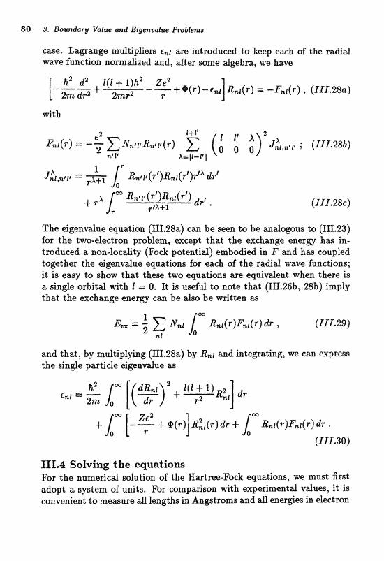
80 S. Boundary Value and Eigenudue Problems
case. Lagrange multipliers Ear are introduced to keep each of the radial wave function normalized and, after some algebra, we have
The eigenvalue equation (III.28a) can be seen to be analogous to (111.23) for the two-electron problem, except that the exchange energy has in- troduced a non-loc&ty (Fock potential) embodied in F and has coupled together the eigenvalue equations for each of the radial wave functions; it is eagy to show that these two eqvations are equivalent when tbere is a single orbital with l = 0. It is useful to note that (III.26b, 28b) imply that the exchmge energy can be also be writ.tt3lt as
and that, by multiplying (III.28a) by R,r and integrating, we can express the single pastilcle eigenvdue as
111.4 Solving the equations For the numeric4 solution of the Eartree-Pock equa;tisats, we must, jimt adopt a system of units. Far comparison with experimental vdues, it, i s convenient ta merrsure all lea@hs in Angstroms m d 41 energies in dectraa
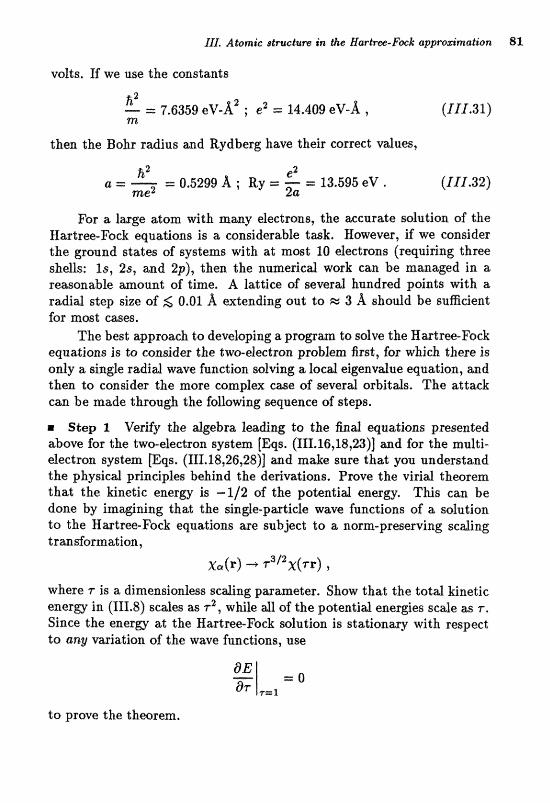
volts. If we use the constants
then the Bahr radius and wdberg have their correct vdues,
For a lmge atom with many electrons, the accurate solution of the Hatree-Fock equsttions is a considerable tmk. Rawever, if we consider the ground states of systems with at most 10 electrons (requiring three shells: 18, 29, and 2p), then the numerical work can be managed in a reasoxlable mount of time. A lattice of several hundred points with a radid step size of 0.01 A extending out to B 3 A should be sufficient for most cases.
The best appmach to developing a progrm t;o tistve the Bartree-Fsck equations is to consider the two~eleetra~ problem fir~t, for which t h e is only a sinde radial wave function solving a locd eigenvdue equation, and then to consider the more complex case af several, orbit&. The attwk can be made through the following sequence of steps.
r Step 1 Verify the dgebslz leading to the find equations presaged above for the two-electron system [Eqs. (III.16,18,23)] and for the multi- electron system [Eqs. (III.18,26,28)] and make sure that you understand the phygi~d yincipfes behind the defivations. Prove the virial theorem that the kinetic energy is - 112 of the potential energy. This can be done by imagining that the single-particle wave functions of a solution to the Hwtree-Pock equations are subject to a nam-preserving scaling trmdormation,
~a ( r) + X ( ~ P ) , where r is a dimensionless scaling parameter. Show that the total kinetic energy in (111.8) scales as rZ , while 4 of the potential energies scale as r. Since the energy at the Hartree-Fock solution is stationary with respect to any variation of the wave functions, use
to prove the theorem.
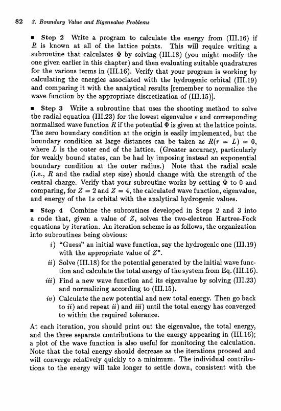
82 3. Boundary k l u e and Bigenualucr Problr?ms
R Step 2 Write a program to calculate the energy from (III.16) if R is known at all of the lattice points. This wil l require writing a subroutine that calculates @ by solving (111.18) (you might modify the one given earlier in this chapter) and then evaluating suitable quadratures for the various terms in (111.16). Verify that your program is working by calculating the energies associated with the hydrogenic orbitat (111.19) and comparing it with the analytical results [remember to normalize the wave function by the appropriate discretization of (III.15)].
8 Step 3 Write a subroutine that u ~ s the shooting mthod to solve the radial equation (111.23) for the lowest eigenvdue e and corresponding normalized wave function R if the potential Q i s given at the lattice points. The zero boundary condition at the origin is easily implemented, but the boundary condition at large distances can be taken as R(r = L) = 0, where L is the outer end of the lattice. (Greater accuracy, particularly for weam bound states, can be had by imposing instead an exponential boundary condition at the outer radius.) Note that the radial scale (i.e., R and the radial step size) should change with the strength of the central charge. Verify that your subroutine works by setting @ to O and comparing, for Z = 2 and Z =; 4, the cdculated wave function, c?igenvdue, and enerrgy of the 1s orbital with the analytical hydrogenic vdues.
Skep 4 Combine the subroutines developed in Steps 2 and 3 into a code that, given a value of Z, solves the two-ejectrm Hartme-Fock equations by iteration, An i terdon scbe-zne is as MIows, the organization into submutines being obvious:
i ) "Guess" an initial wave function, say the hydrogenic one (111.19) with the atpprapPiibte v h e of Z*.
ii) Solve (111.18) for the potentid generated by the initial wave func- tion and calculate the total energy of the system from Eq. (111.16).
iii) Find a new wave function and its eigenvdue by solving (111.23) and normalizing according to (111.15).
i v ) Calculate the new potential and new total energy. Then go back to ii) and repeat i i ) and i i i) until the total energy has converged to within the required tolerance.
At each iteration, you should print out the eigenvdue, the total energy, and the three separate contributions to the energy appearing in (111.16); a plot of the wave function is also useful for monitoring the calculation. Note that the total energy should decrease as the iterations proceed and will converge relatively quickly to a minimum. The individual contribu- tions to the energy will take longer to settle down, consistent with the
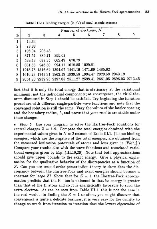
111. Atomic structure in the Hartme-fick appro~mation 83
Table IE1X.X: Binding enerees (in eV) of small atomic sysLems
fact that it is only the total energy that is stationary at the variational minimum, not the individud cmpaoeats; a f ; convergence, the virid the- orem discussed in Step 1 should be wtisfied. Try bednning the iteration procedure with different single-particle wave functions and note that the converged solution is still the same. Vary the values of the lattice spacing and the bovndmy radius, &, and prove that your results are stable under these chmges*
m Step 5 Use: your progrm to solve the Eatre-Fack equation8 for centrd chases Z = 1-9. Compare the total, energies obtained with the experimental values @WE in N = 2 column of Table III.1. (These binding energes, wkich are the negative of the toed energies, me obtined from the measured ionization potentids of atoms and ions given in [WeTl].) Compare your results &so with the w w e .functions and msociated varia- tional energies given by Eqs. (III.19,20). Note that both approximations shatlld give upper bounds to the =act energy. Give a, physical expla- nation for the quafitative behwior of the discrepancies as a functioa of Z. C m you use second-order pc?ft;urbation theory to show that the dis- crepancy between the Bartree-Fock a ~ d exact eaergies should become a mnstztnt for large Z? Show that for Z = 1, the Hartree-Fo& approxi- mation predicts that the H- ion is unbound in that its energ is greater than thnt, sf the H &torn and so it is energetically hvorabb to shed the extra electron. As can be seen from Table 111.1, this is not the ease in. the red world. In finding the Z .= 1 sdution, yaa might discover thhal convergence is quite a delicate business; it Is very emy for the density to change so much from iteration to iteration that $fie lowest eigenvdue of
84 9. Boundary Value and Ei~c~inutxlue Pmblemsr
the sinde-particle H I t o ~ m bwames positive. One way to dleviate this problem is to prewnt the density from chmging too m a d from one itePation to the next, for exmpfe by averagng the new density and the old following step ii) above.
m SIep 6 Modify your tw&-electron program to treat systems in which several orbitds are involved. let is ea~iest to first modify the c d c d a t i ~ n of the total enesw for a @ven set of r d i d wave firactions to indude G,, This ia most convedeatly done by cdcnlating and storing the E",l of Eq. (III.28b) and using Eq. (III.29). Because of the Fock term, the eigenvalue equations (III.28a) cannot be treated by the shooting met hod we have discussed. However, one krcheme is to treat the cdeulated from the previous set of wavf? funetions as infiomogeneous $ems in solving for the new set of wave functions, For tr id vatues of the t.,l cdcu1a;t;ed from (111.30) using the previous set of wave functions, (III.28a) can be sdved as uncoupled inhomogeneoas bmndasy vduts problems using: the Green's function method of Eq. (3.18); after normalization according to (III.24), the solutions serve as a new set of wave functions. The two- electron systems can be used to check the accuracy of your modifications; for these systems you should find that the exchange energy i s - 1/2 of the direct inter-electron intewtim enerfSy and that the dut ioas converge to the same results as those generated by the code in Step 4. Use this Bartree-&ck code to cdcdate the wave fundons and merges for some of the other systems listed in Table 111.1 and compare your results with the experimental values; interpret what you find. A convenient set of initial wave functions are the hydrogenie orbitals, given by (111.19) for the 16
for the 29 and 2p states, respectively. The optimal common value of Z* in these expressions should be determined for any system by minimizing the toed energy.
Chapter 4
Functions .S
and Gaussian Quadrature
In this chapter, we discuss two loosely related topics: algorithms for com- puting the special functions of mathematical physics (Bessel functions, orthogonal polynomials, etc.) and eflicient methods of quadrature based on orthogond functions. In most scientific computing, large libraries sup- ply almost all of the subroutines relevant to these tasks and so relieve the individlzd from the tedium of writing code, h f x t , there is usually little need to know very much about hovv these subroutines work in detail. However, a roug6 idea of the methods used is useful; this is what we hope to impart in this chapter.
4.1 Special functions The speclaI functions of mathematicd physics were largely devdoped long before large-scde numeric& camput ation became feasible, w h n mtll ytical methods were the rule. Neverthefess, they are still relevant today, for two reasons. One is the insight mdyt icd solutions offer; they mide our int&tion and provide a framework for the qualit(ative interpretation of more compEcated problems, However, of particdar importance! to numerical work is the fact that specid functions often aflow part of a problem to be solved analyticdly and so dramatically reduce the motlM of computation required for it full sdution,
As aa inustratian, con~ider a one-dimension4 harmonic osciUator moving under an externd perturbation: its f requmc~~, W, i~ being changed with time. Suppose that the frequency h a its unperturbed value, wo, for times before 2 == 0 and for times after t > T, and that we are interested in the motion for times long after the perturbation ceaws. Given the oscilfator" sinitid coordinate m d vf?focity, one strdghtforwmd methad of
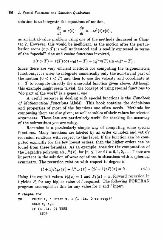
solution is to integate Lhe equations of motion,
as an initid-vdue problem using one of the methods discussed in Chap- ter 2. However, t h i ~ would be ineaicjient, M the motion after the pertur- bation stops (t > T) is well understood and is readily expressed in terms of the "specid- sine md cosine fuacttio~s involved,
I($ > T) = s(T) cos - T) + w c ' v ( ~ ) sin wo(t - T ) . Sinw thwe are very efficient methods I;or computing the trigonometric functions, it is wiser to integate numericalb only the non-trivial part of the motion (0 < t < T ) and then to use the velocity and coordinate at 1: = T to compute directly the sinusoidd function @ven above. Aftbough this example might seem trivial, the concept of using special functions to "do part of tht? arork" is a general one.
A useful resource in deali~g with specid functions is the findbook. of Mathematical Functions [Ab64]. This book contains the definitions and properties of most of the functions one often needs. Methods for computing them are also given, as well as tables of their values for selected arguments. These last are particularly useful for checking the accuracy of the subroutines you are using,
Recursion is a pwticdarly simple way of computing some sgeGid functions. Many functions are labeled by an order or index and satisfy recursion rel&ions with re~pect to this labd. If the function can be corn- puted explicitly for the few lowest orders, then the hkher orders can be found from these formulas, As an example, consider the computation of the Legendre polynomiais, &(I), for is1 _< I and 4 = 0,1,2,. . .. These are important in the solution of wave equations in situations with a sphericat symmetry. The recursion relation with respect to degree is
Using the explicit values Fa($) = 1 and PI(%) = I, forward recursion in I yields PI for any higher value of I required. The following FORTRAN program accomplishes this for any value for s and I input.
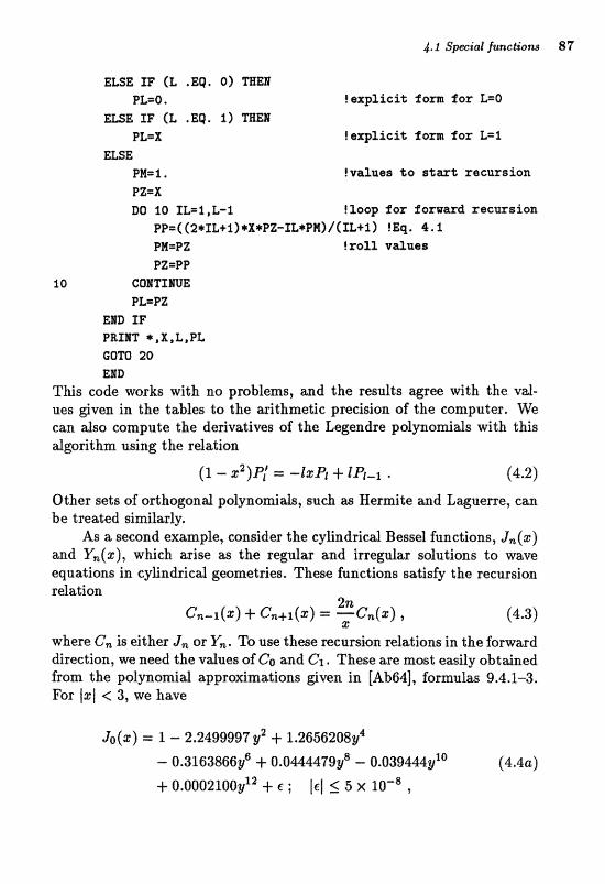
ELSE IF (L .Eq. O ) mm PL=O . lexplick* form for L=0
ELSE IF (L .EQ. 1) TBm PL=X !axpXicit i o m for L=%
ELSE PH=i .. !valass to s t a r t re~wsion PZ=X DO 10 XG=I,L-1 !loop f o r forti~md recwsion
PP=( (2+f L+ l) *X+PZ-EL,*PM) /(IL+l] ! &q. 4.1
PM=PZ !rolil vdaes PZ=PF
GOWTIW$ PL=PZ
EBB T F PRIm *,X,L,PL GOTO 20 EBD
This eode works wlth no problem, md $he r e ~ d t s wrw with the v&- ues &ven in the tables to the arithmetic precision of the computer. We can d ~ a mrngute the derivlatives of the Legendrt, pdynamids with this dgorithm using the relatioxl
Otber sets of arthoganal palynomials, such as Hermite and Laguerre, can be treated similwly.
As a second example, consider the cylindrical Bessel functions, $,(I) and Y,(s), which arise as the regular and irregular solutions to wave equations In cylindr'rcd gwmetries. These funetions satisfy the recursion relation
2% C,-'(Z) + Cn+1(5) = ;Cn(%) , (4.3)
where C,, is either J, or Y,. To use these recursion relations in the forward direction, m need the vdztes of and @I. These me most ewify o b t ~ e d from the polynomial appravimations given in [Ab64], formulas 9.4.1-3.
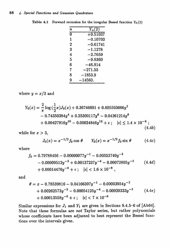
88 4, Spc id Functions and Gau~lsian Quadratam
Table 4.1 Forward recursion fbr the irregular Bexssel function Vn(2)
where y = $13 and
Jo(z) = z-'/2fo cos B &(g) = z-'i2fo gin B (4.w
where
fo = 0.79788456 - 0.00000077~-' - 0.00552740~-'
- 0.00009512y-~ + 0.0013723~y-~ - 0.00072805~-~ (4.4d)
+ 0.00014476~-~ + E ; IE
Similar expressions for J1 and Yl are given in Sections 9.4.5-6 of [Ab64]. Mote that these formalas we not Taylar sedes, but rather polyna~a;fs whom coefficients have been djusted to best represent the Bessd func- tions aver the Intervds dverr.
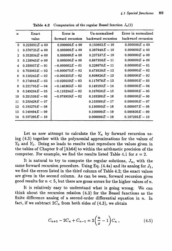
Table 4.2 Gannputatian af the regulrr~: Bmeel funetian Jn (2)
Pt Exact vdae
0 0,223891E + 00 1 O.ti76725E $- 00
2 0,3528346 -5.00 3 0.1289436 4.00
4 0.339951E - 01 5 0.703963E - 02 6 0,120243E - 02 "7. J74944E - 03 8 0.221795E - 04 9 0.2492346 -. 05
i o a.251s39~ - 06
11 0,2304286 - 07 l2 0.193270E - 08
13 0,14949414: - 09 14 0.101295E - 10
famrr~:d rmrsiran backward recursion
0,OQOOQOE -+ 00 0.1506Q2E -. 10
0.000rt00E: + 00 0.38794OE - 110 0.000@OOi5' + 00 0,233337E - g0
0.000000E -+ 00 0,867350E - 11
-0,0000Q2E - 01 0.228676E - l1
-0.OO0075E - 02 0.473828E: - 12
-O.o@@355rs" - 02 0.808826E - 13
-0,0205596 - 03 0.117678E - 13
-0.1403Ei3E - 03 O.l4Sr93E - f 4
-0.110234B - 02 0,167650E - 15 -0.978959B - 02 0.169200E -- 116
0.155000E - 17 0.1300003 - 18 Q.100000E - 19 0.00000OE - 19
b d w a r d recursion
tt.oooaooE + oo o.ooooo0E + 00
0,0000006 -I. 00
0,000@00E + 00 o,ooooooE - or a , o o a a o ~ ~ - oz 0,ooooooE - oz 0,000o00E - 03
0,~oooooE - 04 0,000000E - 05
O.OOO0OOE - 06 O.oOo000E - 07 o.oooao'i"~ - 08
0.000830E - 09
0.1072956 - IQ
Let us now attempt to cdenlate the Y, by fomard recursion us- ing (4.3) together with the polynomial approximations for the values of Yo and Yl. Doing so leads to results that reproduce the values given in the tables of Chapter 9 of [Ab64] to within the arithmetic precision of the computer, For exap le , we find Ghe results fisted Table 4.1 for a -- 2,
1% is natural to try to compute the regular solutions, J,, with the same forward recursion procedure. Using Eq. (4.4a) and its analog for Jx, we find the errors listed in the third column of Table 4.2; the exact values are given in the second column. As can be seen, forward recursion gives good results for n < 5, but there are gross errors for the higher values of n.
It i, relatively easy to understand what is going wrong. We can think about the recursion relation (4.3) for the Bessel functions as the finite difference analog of a second-order differential equation in n. In fact, if we subtraet 2C, from both sides of (4.3), we obtain
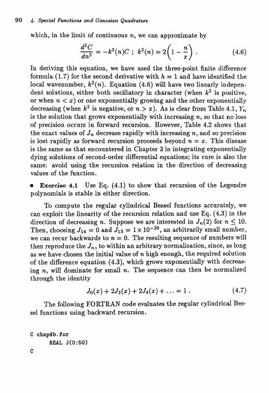
which, in the l i ~ t of continuous n, we can czpproxinzate by
In deriving this equation, we have used the thrc?e-point fiaite diEesence formula (1.7) for the second derivative with h. = 1 and have identified the local wavenumber, k2(n). Equation (4.6) will have two linearly indepen- dent solutions, either both oscillatory in character (when k2 is positive, or when n < r ) or one exponentidly growing and the other exponentidy decreasing (when k2 is negative, or n > I). As is clear from Table 4.1, Y, is the sdution that grows exponentidly with inerea~ing sz, scr that no loss of predsion occurs in farwad recursion. However, Table 4.2 shows that the exact vdues of J, decreahse rapidly with incmwing n, and so preci~ion is lost rapidly as forward recursion proceeds Beyand n = g, TEs disease i s the s m e as that; errcountesed in Chapter 3 in integrating exponentidy dying solutions of second-order differentid equations; its care is &so the same: avoid using %be recursion relation in the direction of decrewing vdues of the function.
Exercise 4.1 Use Eq. (4.1) to show that recursion of the Legendre polynomials is stable in either direction.
To compute the regular cylindrical Bessel functions accurately, we can exploit the linearity of the recursion relation and use Eq. (4.3) in the direction of decreasing n. Suppose we are interested in J,(2) for n 5 10. Then, choosing Jlq = O and JI3 = 1 X &B arbitrarily small number, we c m recar backwards to n =; 0. The resulting sequence of numbers will then reproduce the J,, to within an arbitrary normalization, since, as long as we have Ghosen the initial vdue of n high enaugh.? the required solution of the difference equation (4.3), which grows exponentially with decreas- ing n, will dominate for small n. The sequence can then be normalized through the identity
The following FORTRAN code evaluates the regular cylindrical Bes- seX functionts using badward recursion.
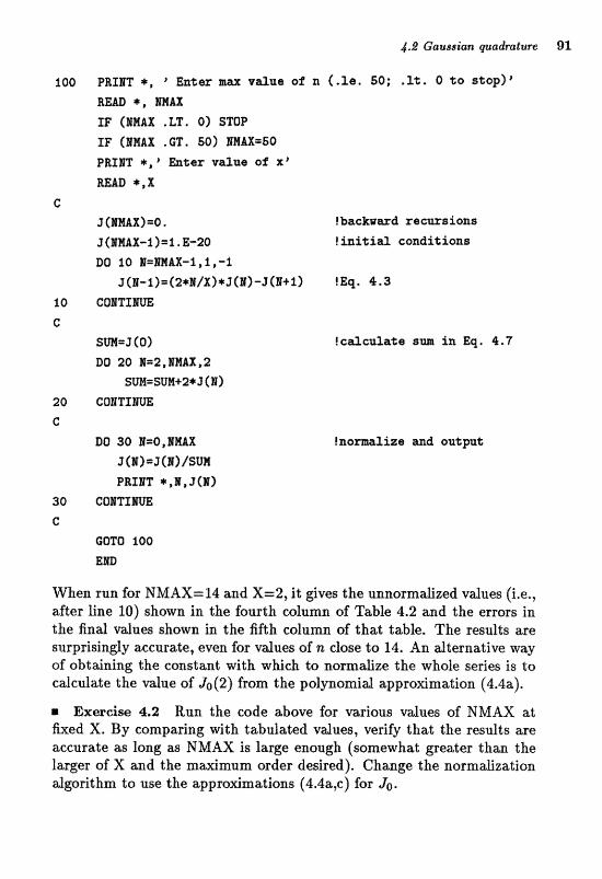
g00 PRXIT +, "%er nax v d x e 09 n (.Jle. 60; .It. O t o stop)" R W *, mILx IF (IMAX ,LT. 0 ) STOP I F (IHAX . GT. 60) mAX=60
PEGIT *,# &%ex vazue o f x p
READ * , X
C
3 f la3mX)=Q .. !baekwwd recwsia~s
When run for NMAX=14 and X=2 , it gives the unnormalized values (i.e., after line 10) shown in the fourth column of Table 4.2 and the errors in the find d u e s shown in the fifth calurrrn of %hat table. The results are surprisingly aecur;zte, e m far vdues of sz dmtl to 14. An dkrnatiw way of obtaining the constant with which to n o m a z e the whole series i s to calculate the value of Jo(2) from the polynomial approximation (4.4a).
m Exercise 4.2 Run, the code above for various d a e s of MMAX at k e d X, By wrnparing with tabulated vdues, verify thaG the resufts are accurate as long as NMAX is large enough (somewhat greater than the larger of X and the maximum order desired). Change the normalization algorithm to use the approximations (4.4a,c) for Ja.
92 4. S p i d Funclr"or?9 and Gau8arian Quadratam
Exercise 4.3 The regular and irregular spherical Bessel functions, jr and nj, safisfy the recursion relaeion
whae 81 is either jr or % l . The explicit formalas far the few laarest mders atre
sin a sin z cos 3= I== - ; jl=.--- 3 sin rt: -- - cos X: ,
IZ: %g 8 %g
COS z cos z sin, z = -- ; ' --c- 3 COS 2-- z2 sin z .
*2: $2 Z
At z = 0.5, the exact vdues of the fultetiotrs of order 2 are
Show that 122 can be c&ulatced either by explicit evdu&ion or by for- ward mcur~ion and canvim yourself that the latter method will work for all 1 and z. Investigate the calculation of jz(0.5) by forward recursion, exglieit evduatim, and by backward reeursioa and show that the first two methods c m be quite inaccurat;e, Can you see why? TZlus, even if expl;lcit expressions for a fnneLjon me available, the stability of backward recursion can make it the method of clrdce.
Our discassion h a iflvstr&ed s m e pitfds in comput;ing the some commonly used spedal functions. Speeifie methods useful for other func- tions can be found in the appropriate chapters of [Ab64].
4.2 Gaussian quadrature In Chapter 1, we discussed several methods for computing definite inte- grals that were most convenient when the intepand was known at a series of equally spaced lattice points. While such methods enjoy widespread use, espeddly when the integrand involves a numerically-generated solu- tion to a differential equation, more efficient quadratare schemes exist if we can evaluate the integrand for arbitrary abscissae. One of the most useful of these is Gaussian qu&ature.
Cansida the problem of evaluating
The f"omdas discussed in Chapter 1 were of the form
where
are the equatly spaeed lattice points. Here, we are referring to the "el- ementaryn quadrature formulas [such as (1.9), (1.11), or (1.13a,b)], and not to compound formulas such as (1.12). For example, for Simpson's rule (1.11), N = 3 and
fiom the derivation of Simpson's rule, it is clear that tfie fbrmula is exact when f a pdyno~al of degrw 3 or less, whi& is comrneasurate wigh the error estimate given in Eq. (1.11). More generay, if a quadrature formda based on a Taylor series rrses N points, it will inteqate exactly a polynomial of degree N - l (degree N if N is odd). That is, the N wei&ts PU, can be &men to satisfy the N binear equatioas
(When N is odd, the quadrature formula is also exact for the odd mono- mid zN.)
A greater predsion for a given amount of numerical work can be achieved if we me willing to give up the requirement of @quay-spaced quadr&are points. That is, we will choose the x, in some aplimaS sense, subject only to the constraint that they lie within the interval [-l, 11. We then have 2N parametefs at our disposd in co~structing the quadrature formda (the N z,'s and the N w,'s), and so we should be able to choose them so that Eq. (4.9) is satisfied far p ranging from O to 2N - 1. That is, the quadrature formula using only N arefulfy chwen poinks cwr be made exwt for pdynomials of degret! 2N - 1 or bss, This is clearjy mare emcienl than using equdly-qaced abscissa,
To see how to best choose the 2,' we corrsidef the Legendre palyns- mids, which are orthogonal on the interval [- 1,1]:
944 4. Specl'af Furactions and Gaussl'sn Quadraturn
It is easily shown that Pi is a polynomial of degree i with i roots in the interval [-l, l]. Any polynomial of degree 2N - 1 or less then can be written in the form
where Q and R are polynomials of degree N - 1 or less. The exact value of the required integral (4.8) is then
where the second step Wows from the orthagondity of .PN to all poly- nomiats of degree N - 1 or less. If wa now take the s, to be the N zeros of &, then application of (4.8) gives (exactly)
It remains to choose the W, so that; R (a poly~omid of degree N - 1 or less) i s integrated exactly. That is, the W, satisfy the set of linear equations (4.9) when the 2, are the zeros of PN. It can be shown that W, is related to the derivative of .PN at the corresponding zero, Specifidly;
20% = 2
(1 - sk)[P~(z,)12 ' TMs completes the specification of what is known as the Gauss-Lt;$endre quadratare formda. Note that it c m be appl-ied to any d e f i ~ t e in_r;egraf between finite lirnits by a simple linear cbange of variable. That is, far an integral between limits I = a and I = b, a change of variable to
redues the integrd to the form required, Other non-linear changes of variable that make the integrand as smooth as possible wilt alao improve the accuracy,
Other types of wthogond pdynomids provide useful Gaussian quad- raturn formulas when the inlegrand has a particular form, Ebr example, the Laguerre polynomials, .Li, which are orthogond on the interGd [O, m] with the weight function e-", lead to the Gauss-Laguerre quadraturn
4.3 B ~ r n and eQonal approsimatr'ons to quantum scattering 95
where the z, ase the roots of LN and the W, are related to the values of LN+I at these points. Similarly, the Kemite polynomials provide Gauss- Hermite quadratare formulas for integrals of the form
OQ
ems' f (z) dz . These Gaussian quadrature formulas, and many others, are given in Sec- tion 25.4 of [Ab64], which also contains tables of the abscissm and weights.
In the practical application of Gaussian quadrature formulas, one does not need to write programs to calculate the abscissae and weights. Rather, there are usually library subroutines that can be used to establish arrays containing these numbers. For example, subroutine QUAD in Ex- ample 4 (see Appendix B) establishes the Gauss-Legendre absdssae and weights for many different values of N.
As a general rule, Gaassian quadrature is the method of choice when the integrand is smooth, or can be made smooth by extracting from it a function that, is the weight for a stmdard set of orthogond polynomid~. We must, of course, also have the abs ty to evduate the integrmd at the required abscissae. H the integrmd varies rapidly, we can compound the basic Gsussiaa quadra;t;ure folrmula by applying it w r ~eve rd gub- intervds of the range of integrat;ion, Of course, wkea t be integfand east be evaluated only at equally-spaced abscissm (such as when it is generated by integrating a differential equation), then formulas of the type discussed in Chapter 1 must be uged.
As an iBustration of Gaussian qudrature, coxtsider using a 3-point Gauss-Legendre quadrature to evduate the inter&
Making the cSIange of variable to
results in
For N = 3, the Gauss-Legendre abscissae and weights are

96 4. Smeial fineEs'ow and Gaussian Quadmture
Straightforward evaluation of the quadrature formula (4.8) then results in I = 4.66683, while a Simpson's rule evaluation of (4.14) with h = 1.5 gives 4,66228. Gaussian quadrat me is therefore more accurate than Simpson's rule by about a fxtor oT 27, yet requires the same number of evalluations of the integrand (three).
r Exercise 4.4 Cansider the integal
Evduate this intega3 using some of the quadratare formulas discussed in Chapter 1 and using Gauss-Legendre quadrat are. Note that the behavior of the integrmd near z = f l i s cause fsr some caution. Compme the accuracy and eficiexley of these v&ous methods for diRerent numbers of abscissa^. Note that this integral can be evatuated exactly with a 4bone- point" Gauss-Chebyshev quadrature formula oE the foMn
with rZ, 71" 72
sm col3 3 1 " ; wn=- sin2 -T . N-4-1 N + 1 N + 1
(See Section 25.4.40 of [Ab64].)
4.3 Born and eikonal approximations to quantum scatter- ing In this example, we will investig;ate the Born and eikonal approximations suitable for describing quantum-mechanical scattering at high energies, and in particular cdculate the scattering of fast eledrons (energies greater than several 10's of eV) from neutral atoms. The following project deals with the exact partial-wave solution of this problem.
Extensive discussions of the quantum thwry of scattering are given in many texts (see, for example, [Me68], [Ne66], or [Wu62]); we will ody review the essentials here. For particles of mass m and energy
scattering from a central potential V( r ) is described by a wave function
4.3 Born and eikonal ~pppodnzatians to flantun scerlteriw 97
l@ (r) that satisfies the Schroedinger equation,
with the botrndary conditian at l a r e distances
Here, the beam is incident along the z direction and B is the scattering angle (angle between r and a). The complex scattering amplitude f em- bodies the observable scattering properties and is the basic function we seek to detmine. Tbe digeratid cross section is given by
a d the tot& crass section is
In general, f is a function of both E" ajnd B. At this point, many elementmy trc~at;meab of scattering introduce a
partid-wave demmpositim of !P, express f in terns of the phase shifis, m d then proceed to discuss the radid S&roc?&nger equation in each pasdid wave, from wEch the phwe shift and hence %be exwt cross wetion, e m be cdculat-ed, We will use this method, wki& is most apprapri&e when the energies are low and only a few partial waves me important, in Project IV bdow. However, in this example, we will con~ider two approximation schemes, the Born and eikond, which are appropriate to high-mergy situations when many partial waves conkibute,
Both, the Born and dkanait approximations are based on an exact integral expression for the scattering amplitude derived in many advanced treatments:
m f ( B ) = -- e r V ( ~ ) g (p) d3r .
2rfi2 Here, the wavenumber of the scattered particle is kf, so that and kr*i = cos B. It is also convenient to introduce the wavenumber of the ixrcident particle, ki = kg.
The Born approdmation (more precisely? the firs% Born appro~ma- tion) congists of wsuming that the scattering is weak, ao that the fult scattering wave function @ differs vefy littb from the incident plane wave,
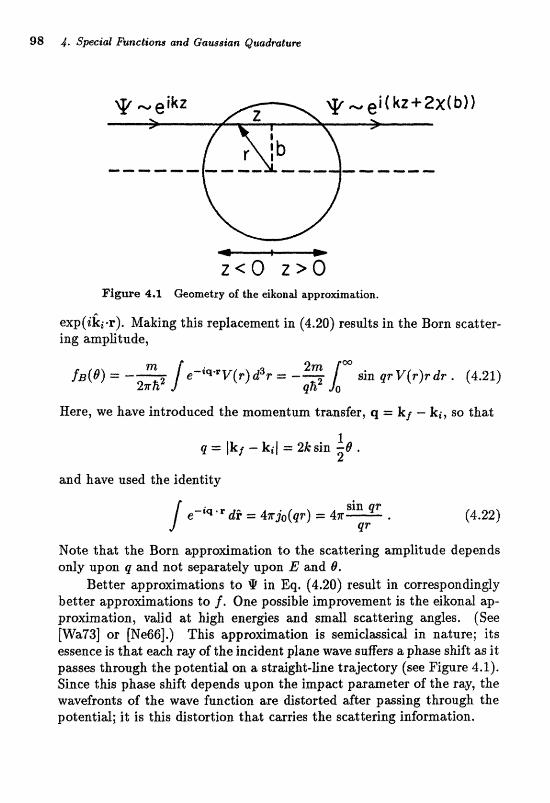
98 $. Spct'ctl Fsnctzt'ons and Gawsdarn Quarfralure
exp(iki*r). Making this replacement in (4.20) results in the Born scatter- ing amplitude,
Here, we have introduced the momentum transfer, q = kt - ki, so that
and have used the identity
Note that the Born apprasmation to the scattering amplitude depends only upon q and not separately upon E &ad 8.
Better approximations to l! in Eq. (4.20) result in correspondingly better approsnaations to f . OM pogsible improvement is the eikand &p- proximation, v d d at high energies and small scattering angles. (See [Wa73] or [Ne66].) This approximation is semiclassical in nature; its essence is that each ray af the incident plane wave suBers a phase shift as it passes tbrough the potential on a straight-line trajectory (see Figure 4.1). Sin= this p h a e shift depends upon the imp& pasameter af the raLy, the wavefronts of tbe wave fitnction asle distorted after passing through the paential; it i s tlris distortian that carries the scattering information.
To derive the dkond approimatioa, we will put, without lass of generafit y,
@(F) = eiki"@(r) , (4 2 3 )
where + is a slowly-vaving function describing the distortion of the h- cident wave. Tfpoa inserting thhis into the origind Schmedinger equatian (4.161, we obtain an equation for +:
If we now assume that y5 varies slowly enough so that the + term can be ignored (i.e., k is very large), we have
Here, we have introduced the coordirtilLe b in the plane transverse to the incident be=, so that
Rom synrmelry considerations, we expect that y3 will be azimnthdy symmetric and so independent of 6. Equation (4.25) can be integrated immediagefy and, using the boundmy condition that; $I -.a 1 rua x -4 -W
since there is no distortion of the wave befare the pasticle reaches the potentid, we have
V (h, zf ) dz' . (4.26)
Having obtained the eikonal approximation to the scattering wave function, we can now obtain the eikonal scattering amplitude, f.. Insert- ing Eq. (4.23) into (4.20), we have
Using (4.251, we can relate V $ directly to &$/at. Furthermore, if we restrict our consideration to relatively small scattering angles, so that q, W 0, then the z integral in (4.27) can be done immediately and, using (4.26) for 4, uve obtain
with the '"rofile fuactian"
Since X is azimuthally symmetric, we can perform the azimuthal integra- tion in (4.28) and obtain our final expression for the eikonal scattering amplitude,
In deriving this expression, we have used the identity [compare with Eq. (4.22)]
e-iqb cos 4 d ~ ,
Note that in contrast to fB, f, depends upon both E (through k) and p. An impurtmt praperty of the exact scattefiag mp2itude is the op-
tical theorem, which relates the total cross section to the imaginary part of the forward scattering amplitude. After a bit of algebra, one can show that jC, satisfies this rela4ion in the limit that the inddent momentum be- comes large compased t s the length scde over wkicb the potentid vwies:
The Born appro~mcat;ian cannot lead to a scattering mplitude that re- spects this relation, as Eq. (4.21) shows that fr, is purely red. It is also easy to show that, in the extreme high-enerw Emit, whre K -+ oo a ~ d X becomes small, the Born and eikond amplitudes become equal (see Ex- ercise 4.5). The eibonal formula (4.30) also can be related to the usual partial wave expression for f (see Exerdse 4.6).
One practical applie&ian of the appradmatiuns discussed above is in, the calculation of the scattering of hi&-energy electrons from neutral atoms. In general, this is a complicated multi-channel scattering problem since there can be reactions leading to find states in which the atom is excited. Hov~ever, as the rewtion pmbabillties ase smdl in comparison to elastic scattering, for many purposes the problem can be modeled by the scattering of an electron from a eentrd potential. This potential represents the combined influeam of the attraction of the central nuclear charge (Z) and the screening of this attraction by the Z atomic electrons. For a neutral target atom, the potential vanishes at large distances faster than r-l. A very accurate approximation to this potential can be had

4.8 Born and eQonal appwdmations to quantum scattering 201
by solving for the sel&consistent Eartree-Fodc potential of the neutral atom, as was done in Project III. However, a much simpler estimate can be obtained using an approximation to the Thornas-Fermi model of the atom given by Lenz and Jensen [Go49]:
with
and
S = 4 . 5 3 9 7 ~ ' / ~ ~ ' / ~ . Here, the potentid is measured in eV and the radius is measured in A. Note that there is a possible problem with this potential, since it is sin- gular as r-' at the origin, and so leads to a divergent expression for X at b =. 0. However, if the poten.tial is regularized by taEng if to be a can- stmt within some small radius r,iB, (say the radius of the atoms ls shell), then the cdculated cross sectian will be unaEected except at xnornentnm trmsfers fage enough so that gqrmin > 2.
Qur god is to cmpute the Born and eikond wpro~mations to the differential and totd cross eections for a given cetllrd potentid at a speci- fied incident energy, and in particular for the potential (4.32). To do this, we must compute the integrals (4.211, (4.29), and (4.30) defining the scat- tering amplitudes, as well as the integral (4.19) for the total cross section. The FORTRAN progrm for Example 4, whose source code is @yen in Appendix B, as; well in the file EXMPL4,FQR, does these edcdadions and papbs the results on a semi-log plot; the t s t d cross se~tion given by the opticd theorem, Eq. (4.31), is also ealcufated.
The incident paticle is wsunned to have the mzlss of the electron, and, as is appropriate for atomic systems, all lengths are measured in A and d l energies in eV, The potentid can be chosen to be a square well of radius 2 A, a Gmssian well af the farm
or the Lenz- Jensen potential (4.32). All potential8 are assumed to van- ish beyond 2 A. hrthermore, the r-' singularity in the Lenz-Jensen potentid i s cutoff inside the radius of the Is she11 of" the target atam,
102 4. Speial hnctions and Gaussian Quadmlure
Because the diRerentiaf crws sections 'become very peaked in $he forward direetion at the high energies where the Born and eikond ap- profirnations are vdid, the integration over cos 6 in Eq. (4.19) is divided into two regions far a mare accurate integraiola of tbe forward peak. One of these extends from B = 0 to B = Bcut, where
f ~cut&,r = 2~ = 2kR,.t sin 58,ut
and RC.& is 1 .k for the Lenz-Jensen potential and 2 A for either the square- or Gaussian-well potentials, and the other eaends from B,,b to x. AU integrds are done by Gauss-Legendre quadraturn usiny; the s m e number of points, and the Bessel function of order zero required by Eq. (4.30) is evaluated using the approximations (4.4).
The fouowing exercises are aimed at improving your understanding of this pmgrm and the physics it describes.
m Exercise 4.5 Verify the dgebrs in the derivations above. Show that in the limit of very high energies, where X is small, so that sin X w the Born and eikond results are identicd, Also prom that the eikand amplitude satisfies the optical theorem (4.31) in the limit where the in- ei&nt momeaturn becomes large in comparison with the length scde of the potentid.
m Exercise 4.6 Show that if the eonventiond expression for f in terms of a sum over partial waves [Eq. (IV.4) below] is approximated by an integal over I (or, equivdently, over b = Ilk) and the sma-ll-&/lmge-l approdmation
&(cos 8) F;I JO ( l@)
is used, Eq. (4.30) results, with the identification ~ ( b ) = Investigate, either numerically or mdytically, the vddity of this; relation between the Bessef function of order zero and the Legendfe polynomids.
m Exercise 4.7 Test the Born approdmation. crass sections generated by the code by comparing the numerical d u e s 4 t h the analytical Born results for a square or Gmssim well of depth 20 eV and for varying incident energies from 1 eV to 10 keV. Verify for these cases that ~ ( b ) as computed by the code has the expected values. bestigate the variat;ion of the nunrezlicd results with &ages in the number of quadratare points. (Note that only particular values of N are allowed by the subroutine generating the Gauss- Legendre abscissx and weights.)
IV. Partial wave sohtion of quantum scattering 103
m Exereise 4.8 Fix the depth of a square well at 20 eV and cdculate for various incident energies to get a feeling for how the differential and total cross sections vary. Compare the square well cross sections with those of a Gaussian well of comparable depth and explain the differences. Show that the Bmn and eikond results i c p p ~ s d each other at high energies for either potential and that the optical relation for the eikonal amplitude becomes better sadisfied at higher energies.
Exercise 4.9 Using the Lenz-Jensen potential m d a fixed charge and inddent energy, say Z = 50 and E = 1000 eV, investigate the sensitivity of the calculation to the number of quadrature points used and to the small-r regularization of the potential. Calculate the cross sections for various Z ranging from 20 to 100 and for E ranging from 10 eV to 10 keV; intergmt the trends you observe,
m Exercise 4x0 Use the program constructed in Project I to calculate the classical differential crass wctim for electroas scattering frem the Lenz-Jensen potential for various Z and incident energies. Compare the results with the Born and eikonal cross sections, Cm p u e~titblish m analytic& connection between the classical description and the quantum approximations:' (See [Ne66] for a detajled discussion.)
Project IV: Partial wave solution of quantum scattering Ta this project, we will use the method of partid waves to solve the quan- tum scattering problem for a partide incident on a central patentid, and in particular consider the low-energ scattering of electrons from neutrd atoms. The strategy of the method is to employ a pafliaI wave expan- sion of the scattering wave funetion to decampme the thr~-dirmensiond Schroedinger equation (4.16) into a set of uncoupled one-dimensional or- dinmy diEerentid equations for the radial wave functions; each of these is t b n soltved as a boundary-vdue problem to determine the phme shift, and hence the scattering aplitude.
IV.1 Partial wave decomposition of the wave function The standard partial wave decomposition of the scatLering wave funetion @ ie
When this expmsion is substituted into tbr! Schroedinger equation (4,161, the ra&aX wave functions we found to satisfy the r d i d diEerengiaf
Although this is the same equation as that satisfied by a bound state wave function, the boundary conditions are different. In particular, R vanishes at; the origin, but it hils the large-r aaymgto-tic behdor
RI -+ kr[cos Grjr(kr) - sin 61nl(ks)] , (IV.3)
where jl and nl are the regular and irregular spherical Bessel functions of order I. (See Exercise 4.3.)
The scattering amplitude f is related to the phase shifts by
f ( B ) = 5 (2f + l)ei61 sin 6rq(cos 8) , (N.4) I=O
and the total cross section is easi?y found from Eq. (4.19) and the arthog- onality of the Legendre polynomials, (4.10):
Although the sums in (W.4,5) extend over all I, they are in practice limited to only a finite number of partid waves, TUs is because, for large I, the repulsive centrifugal potential in (IV.2) is effective in keeping the particle mtside the rmge of the potential and so the phase sh i f t is very s m d . If the patentid is negiigible beyond a radius r,,, an estimate of the highest partial wave that is important, lmax, cm be had by setting the turning point at this radius. Ths ,
~max(lmax + = E , 2mrkax
wbich leads to E,,, brm,,, This estimat;e is usuatly slightly low, since penetration of the centrifugd barrier leads to non-vanishing phase shifts in. part;ial waves somewhat, higher %hag this.
IV.2 Finding the phase shifts To find the phase shift in a given partial wave, we must solve the radiat equation (TV.2), using, for example, the Numerov method discussed in Chapter 3. Although the boundary conditions specified by (IV.3) and the vanishing of R at the ongin are non-local, we can still integrate the
f V, I""art;ial wave klolution of qvrantvna scattering 105
equation as an initid value problem. This is because the equation i s linear, M) that the bonndary condition at large r can be satisfied simply by appropriately normalizing the solution.
If we put Rl(r = 0) = 0 and take the value at the next lattice point, R I ( ~ = h), to be any convenient smdl number (R will generally rise rapidly through the centrifugal barrier and so we must avoid overflows), it would seem that we were ready to use the Numerov method. However, k(r = 0) is infinite. The solution is to use Eq. (1.7) for Ry(h), along with the known valuesRI(0), Rt(h), and k(h) to find R1(2h). Now we can integrate outward in r to a radius r(') > P,,,. (See Figure IV.1.) Here, V va~shes and B must be a line= cambination of the free solutions, krji(kr) and kmr(kr):
R[') = ~kt(')[cos brjl(kr(')) - sin 61nr(kr('))] . (m6)
Although the constant A depends upon the vdue chogen for R(T = h), it is largely irrelevant for our purposes; however, it must be kept small enough so that overflows are avaided*
Knowing anl y R!') does not allow us to solve for the two unknowns, A and 61. However, if we continue integrating to a larger radius > t(l), then we dsa have
&I2) = ~ k r ( ~ ) [ c o s 6tjr(kr(2)) - sin 61nl(kr(2))] . (IV.7)
Equations (IV.6,7) can then be solved for tir. After a bit of algebra, we
where jj') = jr(kt(')), etc. Note that this equation determines sl only within a multiple of n, $though this does not affect the physical observ- ables [see Eqs. (IV.4,5)]. The correct number of ir's at a given energy can
ned by comparing the number of nodes in R and in the free solution, krjr , which oecar for T < pmX. With the conventionid deeni- tims we have used, the phase shift in each paftial wave vmishes at hi& energes and approaches fia at zero energy, where Ni is the number of bound states in the potentid in the b'th partial wave.
IV.3 Solving the equations Our gad in a nrtmesicd treatmenL of this problem is to investigate the scattering of electrons with mer@ies ffom 0.5 tlV to 10 keV from the potential (4.32); a radius r,,, = 2 A is reasonable. For the charge Z
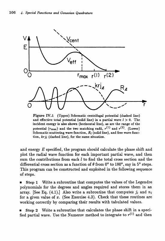
106 4. S m i a l Elmctiaw and Gausst'an Quadraturn
Figwe IV.1 (Upper) Schematic chentGfagilrl potentid (dahed line) and eRective tot& pakntid (saEd line) in a pastlid wave I r 0. The inden* energy is Am shawn (horizontal Iiae), as are the range of the potential (rmax) and the twa matching radii, r(') and F('). (Lower) Schemagc scattering wave fnnction, RI (solid line), and free wave func- *ion, &P& (dwhed line), fox "the same erituadian.
w d energ E spedfied, the program should cdculate the p h a e sMft and plot the ra&d wave function for each imiportaant pastid wave, and then s m the contributions fram each t to find the total cross section and the diRerent;id crass section a9 a function of 8 from 0' to 180°, say in 5' steps, This program can be constructed and exploited in the following sequence of steps.
Step 1 Wdte a subrougiae that camputea the values of the Legendre polynomials for the degrees and angles required and stores them in an array [See Eq. (4.1).] Aiso write a subroutine that computes jl and nr for a given value of r . (See Exercise 4.3). Cheek that these routines are working correctly by comparing their results wit h tabulated values.
r Seep 2 Wrige a a;ubrontiae f iat calculates the? phwe shift, in a speci- fied partial wave. Use the Numerov method to integrate to r(') and then

JV. Padial wave solution of quantum scattering 107
Figure IV.2 WeaHy-bound levefs of the LeneJanmn posential. Lev- ek with a negative p;trity (p and f) are shown by dwhed curves.
to and then determine the phase shift from Eq. (IV.8). Note that if is too close to rfl), problems with numerical precision may arise (both the numerator and denominator of (IV.8) vanish), while too great a distance between the matching radii leads to wasted computation. Check that your subroutine is working properly by verifying that the calculated phase shift vanishes when V(T) is set to 0 and that it is independent of the choice of the matching radii, as Iong as they are grea;2;er t b a v,,,. .&so check that the phase shifts you find far a square-well poteatid agree with tharse that y o ~ can cdcufate andytically, Note th& since quite a bit sf numel.ical work is invdved in the cdculation of the Lenz-Jensen potentid (4.32), it is most efficient if the d u e s of V at the lattice points are stored in an array to be used in the intqration of all impartant partial w&veS.
Seep 3 Write a mdn pragram that, for a e b q e m d energ, calls the subroutines you have congtructed in pedaming the sum aver partial waves to calculate the totd md diEerentia2 croh;s sections. Verify that your estimate of I,, is reasona;ble in that 4 non-vmisbing phwe shifts are computed but .that no computationd eEort is wasted an partid waves for whiCh the phase sEA is negZi&ble.
m Step 4 Study the cross section as ia function of enero for severd Z, say 20, 50, and 100, Show that, at low energies, resonances occmring in particular partid waves m&e the m&ar distributions quite camplex and the told cross sections very ener&y-dependent, bat that alT[ quantities
become smooth &ad monotonic at Egh energies. Tabulations of experi- mental data with which to compare your results are given in [Ki71]. Also compare your high energy results with the Born aad eikond approxirna- tisns genera;ted by the prs ram in Example 4,
m Step 5 To unhstafld the ]low-energ resoaances, colasider F i e r e N.2, whi& gives the enerdes of weAy bound levels in the Lenz- Jensen potentid as a function of Z. By studying the cross section at a fixed energy of 5 eV as s function of Z, how th& the regions new Z = 46 and Z = 59 reflect the extensions of the 2p and Id bsuad st&es into the continuum. By examiaing the Z =. 59 cross swtion, anguIas distribution, p h ~ e shifts, and rodid wave funetiona as functions of eneru mrar E = 5 eV, show that; the resonance is indeed in the I = Oar t i a l wave. Note that sin= the Lenz-Jensen poteatid is bwed on the Thornas- Fermi approfimation, it is not expected to be accurate in the outer region of the atom. The resonance energiw and widths you find %herefore diRer guantitatively from tho8e that are foand in experiment.
m Step 6 Use the UlarItree-Fock code from Ffoject 111 to generate the direct potential, @, for the neutral He atom and modify your program to calculate the scattering of electrons from this potentid. Note that when the energy of the inddent electron is large, it is easily "distinguishable" from the electrons in the atom, and so any effects of the Pock (exchange) potential wil l be small. Compare your results with those produced with the Lenz- Jensen potential. A further discussion of the electron-atom scattering problem can be found in [Bo74].
Chapter 5
Matrix Operations
Linearization is a common assumption or approximation in describing physical processes and 80 finear systems of equations are ubiquitous in computational physics. Indeed, the matrix manipulations associated with finding eigenvalues or with solving simultaneous linear equations are often the bulk of the work involved in solving maay physical problems. Ia this chapter, we will discuss brieffy twa of the more non-trivid matrix opera- tiormst inversion and diagondization. Our treatment here will be confined largdy to @directB methods appropriate fm "dense" mattries f where most of the elements are on-zero) of dimension less than severd hundred; it- erai;tive methods for treating the very large sparse matrices that wise in the discredization of ordinary and partial dcligerentid equations will be discussed in the foaming two chapters. As i s the case with the special functions of the pmvious chapter, a vwiety of library subroutines ern- ploying several different methods for golving matrix problems are usudly avdlable m any large computer. Our dis;eussions bere me therefore lim- ited to selected basic methods, to give a Aavor of whad has to be done, More detailed treatments can be found in many texts, for example [Ac70] and [Bu81].
5.1 Matrix igxversian Let us consider the problem of inverting a square ( N x N ) matrix A. This might arise, for example, in solving the linear system
for the unknown vector X, where b i s a known vwtor. The most naturd way of doing this is to follow our trJning in elementary algebra m d use Cramer's rule; i.e., to evaluate A-' as being proportional to the transpose of the matrix of cofactors of A. To do this, we would have to cdcnlate
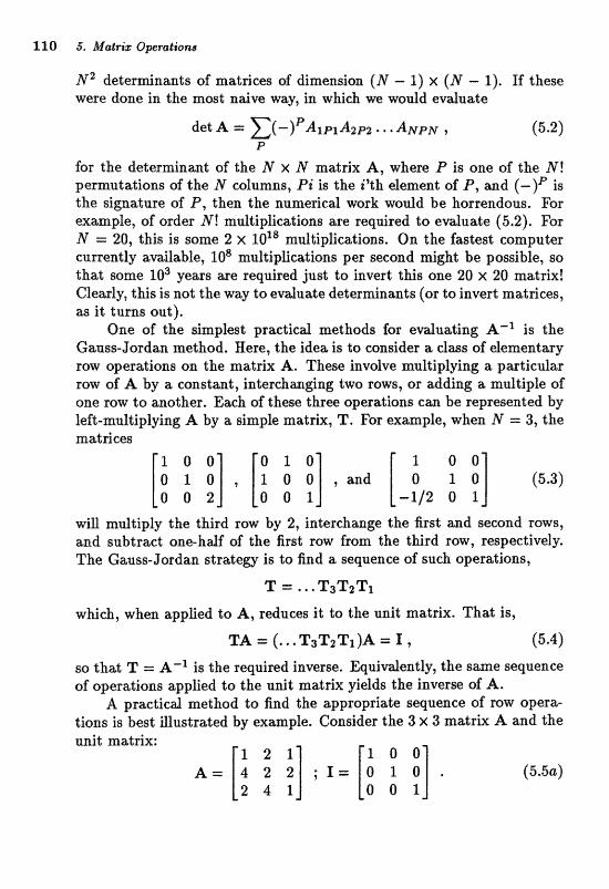
110 5, Matrig Operations
N2 deterdnants of matrices of dimension ( N - 1) X ( N - 1). If these were done in the most naive way, in which we wuld evduate
for the determinmt of the N x N mat;rix A, where P is one of the N ! permutations of the N columns, Pi is the i'th element of P, and ( - ) P is the signature of E", then the numericd work would be horre~bo.tls. Far example, of order N ! multiplications are required to evaluate (5.2). For N = 20, this is some 2 x 10%~ multiplications. On the fastest computer currently available, 10s multiplications per second might be possible, so that some years are required just to invert this one 20 x 20 matrix! Clearly, this is not the way to evaluate determinants (or to invert matrices, as i t turn8 out).
One of the simplest practical methods for evaluating AmS is the Gauss-Jordan method. Here, the idea is to consider a class of elemen_t;asy row apttrations on the matrix A. These Involve multiplying a pat icdar raw of A by a canstant, interchmging twa rows, or adding a multiple af one row to another. Each of these t h r e operations can, be represented by left-multiplying A by a simple matrix, T. For example, when N = 3, the
will multiply the third row by 2, interchmge the first and second rows, ancl subtrwt one-half of the first; row from the tKrd row, respectively. The Gauss-Jordan strategy is to find a sequence of such operations,
which, when appEed to A, reduces it to the unit matrix. That is,
so that T = A-' is the required inverse. Equivdently, the same sequence of operations applied to the unit matrix yields the inverse of A.
A practical method to find the appropriate sequence of row opera- tions is best illustrated by example. Consider the 3 X 3 matrix A and the unit matrix:
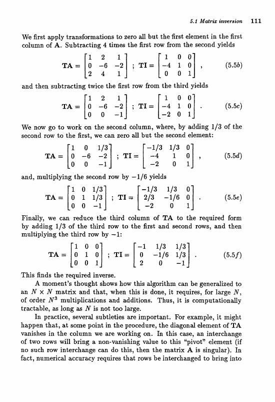
We first apply transformations to zero all but the first element in the first column of A. Subtracting 4 times the first row from the second yields
and then subtracting twice the first row from the third yields
We now go to work on the second column, where, by adding 1/3 of the secscoad raw to the first;, we can zero EtU but the second element:
and, multiplying the second row by -1/6 yields
Findly, we can reduce the third column of TA to the r e q ~ r e d form by adding 113 of the third row to the fimt and sec-ond rms, and then mdtiglying the tErd row by -1:
This finds the required inverse. A. moment's thought show8 how t k s dgadthm c m be geaera-lized to
an 1V x N rnafix and that, when this is done, it requires, for Iwge N, of order N 3 multiplications and additions. Thus, it is computationally tractable, as long as N is not too fwge.
In practice, several subtleties are important. For example, it might happen that, at some point in the pracedure, the diagond element of TA vanishes in the column we are working on. In this case, an interchange of two rows will bfing a noa-va~shing d u e to this '"ivotn element (if no such row interchange can do this, then the matrix A i s singular). In fact, numericd accuracy requires that; rows be interchanged to bring into
f l2 5. Matrix Operations
the pivot pasition that element in the column being worked on that has the largest absolute vdue. Problems associated with numerical round- off can also arise during the inversion if elements of the matrix differ greatly in magnitude. For this reagon, it is often useful to scale the rows or columns so that afl entries have roughly the same magnitude ("equilibration"). Various special cases (such as when A is symmetric or when we are only interested in solving (5.1) for x and not for A-' itself) can result ia reductioas of the numerical work. Far exmple, in the latter cae , we can apply T only to the vector b, rather than ta the whde unit matrix. Rndly, if we are interested in computing only the deterdaant of A, successive row transformations, whicfi have a simple and easily calculable egect on, the determinant, can be used to bring TA to lower or upper d i ~ o n d form (all ekntents vmishing a b m or b d w the diagonal, respectively), and then the deteminant can be evaluated simply as the product of the diagond elements,
m Exercise 5.1 Use Eq. (5.2) to show that interchanging the rows o f a matrix changes the sign of its determinaxlt, that adding a multiple of ane row to anot her leaves its determinant unchanged, and that multiplying me row by a consta t mdtipfies the deteminant by that saxne constant.
E Exercise 5.2 Write (or just flowchart) a subroutine that will use the Gauss-Jordan method to find the inverse of a given m&rix, 1ncorporat;e pivoting as described above 2 0 Improve the numerical accuracy.
5.2 Eigenvalues of a tri-diagonal matrix We turn now to the problem of finding the eigenvalues and eigenvectors of an PC7 X N matrix A; that is, the task of finding the N scdars X, and their associakd N-component vectors 4, that satisfy
Equivdently, the eigenvalnes are zeros of the N" %h degree characteristic polynomid of A:
N
PA(A) det (A - XI) = n(xn - A) . (5.77 n=l
For simplicity, we will restrict our discussion to matrices A that we red and symmetric, sa that the eigenvalues Etre always r a l and the c?igenwc- tors can be chosen to be arthanormal; this is the most common: type of matrix arising in modeling physical systems. We will also consider only cases where atl or many of the eigenvalues are required, and possibly their
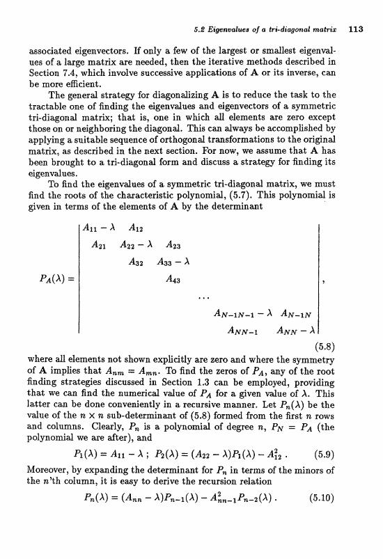
&,l? bf"igc3nvotues a tri-diagonal ntcrkria: 3.13
associated eigenvectors. If only a few of the largest or smallest eigenval- ues of a large matrix are needed, then the iterative methods described in Seetion 7.4, whicb invalve successive applications af A or its inverse, can be more eaeient.
The generat strategy for diagonalizing A is to reduce the task to the tractable one of finding the eigenvdues and eigenvectors of a symmetric tri-diagonal matrix; that is, one in which all elements are zero except those on or neighboring the diagonal. This can always be accomplished by applying a suitable sequence of orthogonal transformations to the original matrix, as described in the next section. For now, we assume that A has been brought to a tri-diagonal form and discuss a strategy for finding its eige~vdaes,
To find the eigenvdues of a symmetric tri-diagonal matrix, we must find the roots of the characteristic polynomial, (5.7). This polynomial is &wn in terms of the element8 of A by the deterzninmt
(5.8) where all elements not shown explicitly are zero and where the symmetry of A implies that A,, = A,,. To find the zeros of Pay any of the root finding strategies discussed in Section 1.3 can be employed, providing that we can find the numerical value of PA for a given value of X. This latter can be done conveniently in a recursive manner. Let P,(A) be the value of the n x n sub-determinant of (5.8) formed from the first n rows and columns. Clearly, P, is a po?ynomid of degree n, PN = .PA (the polynomial we are after), and
p ~ ( h ) = At1 - X ; &(X) = (A22 - A)& (A) - A& . (5.91 Moreover, by expanding the determinmt for P, in terms ol' the minors of the n'th colurn, it is easy to derlve the reearsion relakion
This, together with the starting values (5.9), allows 8n efficient evaluation of pA *
m Exercise 5.3 Prove Eq. (5.10) above.
Several features of the problem above help considerably in finding the roots of .PA. If m algorithm like Neartank s m h ~ d is used, it is quite easy to differentiate (5.10) once or twice with respect to X and so derive recursion relations altovving the simple evaluation of the first or second derivatives of PA(X). More importantly, it is possible to show that the number of times the s i p chastge~ in the sequence
is eqad to the number of eigenvdues less than X, This faet is umful in several. way~3: it is a, means of m&ing sure Lbat no roots are skipped in the search for eigenvduea, it provide8 a gimple lay of loedzing a root initially, and it can be used with the simple search prowdue to locate the root accurately, althou@ perhaps not in the most efieient vvay possible.
To make a systematic search for all of the eigenvdues (roots of Pa), it is esserrtid to know where to b e n looking. If we me working through finding the entire sequence of eigenvalues, a natural guess for the next- highest one is some distance above that eigenvdue just found. Some guidance in how far above and in how to estimate the lowest eigenvalue can bo found in. Gerschgorin" bbounds an the eigenvdurss. It is quite simple to show that
and th&
for dl n. For the tri-diagonal forms under consideration here, the sums over j in these expressions involve only two terms. The lower bound, Eq. (5.11a), is a convenient place to begin a search for the lowest eigen- value, and the difference between the upper and lower bounds gives some measure of the average spacling between eigenvdues,
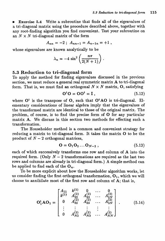
5.3 ReSduetion to tri-diagonal form 125
t lExwcim 5.4 Write a subroutine that finds aS1 of the dgenvalues of a tri-diagonal maitrk using the procedure &&crib4 above, together vvith any root-finding dgorlthm. p u fincl convenient. Test your subfoaine on an IV x N tri-diagond matrix of the form
whose eigenvalnes are known andytically to be
5.3 Reduction to tri-diagonal form To apply the method for finding eigenvdues discussed in the previous section, we must reduce a general real symmetric matrix A to tri-diagonal form, That, is, we must find an orthogo~al N X N matrix, 0, satisfying
where Ot iis the transpose of 0, such that O'AO is tri-diagonal. El- ementary considerations af linear algebra imply that the eigenvdues of the transformed matrix are identical to those af the oiiginail matllix. The problem, of m r s e , is to fiad the preGiaje farm *of 0 for my pafticular matrix A. We discuss in this section two methods far egecting such a trm~formatisrr.
The Householdt?r method is a common and convenient strategy for reducing a rxraldx to tri-8iagond form, It takes the miltrh Q to be the prodnct of N - 2 of'chogond m&rices,
each of which sucetlissively traasforms one roar and column of A into the required form. (Only N - 2 transformations are required as the last two rows and columns are already in tri-diagonal form.) A simple method can be applied to fixrd each of the 0,.
To be mose explidt about how the Wouseholdftr dgorithzn. ucrorks, let us consider finding the Brst mhogonal transfomation, Q which we will choose to a;nniPuilate mmt af the first row and column of A; that; is,

Here, k(') is a possibly non- ishing element and the matrix is the result of applying the transformation to the last N - 1 roars and columns of the original matrix A. Once O1 is found and applied (by methods discussed below), we can choose 0 2 80 that it effects the same kind of transformation on the matrix A(?); that is, it annihilates most of the first row and column of Lkizt matrk a d Lrmsforms its last N - 2 rows m d coltlmns:
Continued orthogonal transformations of decreasing dimension defined in this way will trmsform, the ori&nd maLrix into a tri-diagond one dtes a total of N -. 2 transformations, the diagonal elements of the transformed nrat;rix being
and the OR-d;iagond elements being
It remdns, of courm, to find -the predse form 0.f each of the Q,, We IUzzstra;te the proceduze with Ox, which we take ta be of the h rm
where O is an N - l-dimensional column vector of zeros, at is a similar row vector, and P is an (H - l) x ( N - l) symmetric matrix satisfying
if 0 is to be arthogond. (In these expressions and the following, for simplicity we have dropped all superscripts and subscripts which indicate that it is the first orthogonal transformation of the sequence (5.13) which is being discussed.) A choice for P that satisfies (5.17) is
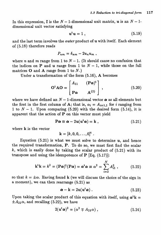
In this expression, I is the N - l-dimensional unit matrix, u is an N - 1- dimensionat unit vector satisfying
and the last term involves the outer product c& U with itselt Each element of (5.18) therefore reads
where n and m range from 1 to N - 1. (It should cause no confusion that the indices on P and u rmge from 1 to N - l, whife- thase on the full matrices 0 asld A range fram 1 to N.)
Under a transformation of the form (5.16), A becomes
where we have defined an N - l-dimension& vector ar ss all elements but the 6rst in the first column of A; th& is, ai =: Aicr,z for i ranginl; ffom l to N - l. Upon comparing (5.20) with the desired form (5.14), it is apparent that the action af l? on, this vector must yield
where k is the vector k = [k,0,O ,..., 01'.
Equation (5.21) is what we must solve to determine U, and hence the required transformation, P. To do so, we must first find the s d a r h, which is easily done by taking the scalar product of (5.21) with its transpose and using the idempotence of P [Eq. (5.17)]:
so that k = fa. Raving found k (we will discuss the choice of the sign in a moment), we can then rearrange (5.21) as
Upon taking the scalar product of this equation with itself, using akk = rtAzla, and recalling (5.22), we have

so that we can then solve (5.21) for U:
This completes the steps necessasy to find P, To recapituJaLe, we first solve (5.22) for k, then calculate the square of the scalar prod- uct (5.24), form the vector U according to (5.25), and then finally P according to (5.18). In evaluating (5.24), considerations of numerical stability recommend taking that sign which makes the right-hand side largest. Note that we need evduate only the square of the scalar product as the vector u enters P bilinearly. Note also that a full matrix product need not be performed in evaluating A@). Indeed, from (5.18,20) we have
where the symbol A ia tlzis exprese~ion rstands for the square symmetric m&rix famed from the last N - l rows m d columns of the origind matrix. Thus, to evaluate A@), once we have the vector u we need only calculate the vector Au and the scalar ut Au. Finally, we note that n a m e ~ c d stabigty durhg the successive trasfarmations is improved if the diagonal element having largest absolute m a g ~ t u d e is in the upper ldt-baad corner of' the sub-nz&fix being trmsfo~med. Tlris can dwaye~ be arranged by a suitable interchange of rows and columns (which leaves the eigendues invwimt) &er each of the arthogand traasfamations is applied.
r Exmciae 5,5 By writing either a detailed flowchart or aa w t u d sub- routine, convince yourself that you understand the Householder algorithm descdbed above.
With an algorithm for transforming A to tri-diagonal form, we have specified completely bow to find the eigenvalues of a real symmetric ma- trix. Once these are in hand, the eigenvectors are a relatively simple matter. The method of choice, inverse vector iteration, works as foEows. Let 4:) be any guess for the eigenvector associated with X,. This guess cm be refined by evduating
Here, E is a s m d , non-zero scalar that allows the matrix to be inverted. It is easy to see that this operation enhances that component of 4:) along
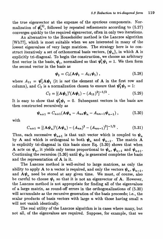
5.3 Redu~tirrn If0 Eri-diagonal farm 119
the true eigenvector at the expense of the spurious components. Nor- malization of (p?), followed by repeated refinements according to (5.27) converges quidtly to the required eigenveetor, often in only two iterations.
An dternative to the Householder method is the Lanczas dgodthm [Wh77], which is most suitable when we are interested in many of the lowest eigenvalues of very large matrices. The strategy here is to con- struct iteratively a set of orthonormal basis vectors, ($,), in which A is explicitly tri-diagonal. To begin the construction, we choose an arbitrary first vector in the basis, normalized so that = 1. We then form the second vector in, the basis as
where All = +:kgbl (it i s not the element of A in the first row and column), and Cz is a normalization chosen to ensure that $i$2 = 1:
It is easy to show that = 0. Subsequent vectors in the basis are then constructed r-ecursively W
with
Thus, each successive is that unit vector which is coupled to qb, by A and which is orthogonal to both gb, and The matrix A is explicitly tri-diagonal in this basis since Eq. (5.30) shows that when A acts on @,, it yields only terms proportional to and $,+l. Continuing the recursion (5.30) until +N is generated completes the basis md the representation of A in it.
The Lanczos method is well-suited to large matrices, as only the ability to apply A to a vector is required, and only the vectors $,, and A*, need be stored at any given time. We must, of course, also be careful to choose 9% so that it is not an eigenvector of A. However, the Lanczos method is not appropriate for finding all of the eigenvalues of a large matrix, as round-off errors in the orthogonalizations of (5.30) will accumulate W the recur~ive generalion of the basis proceeds; i.e., the scalar products of basis vectors with large n with those having small n urilji not mnish identiedy.
The red utility af the La-nczw dgorithm is in cwes where many, but not dl, of the eigenvd~es are required, Suppose, for example, that W
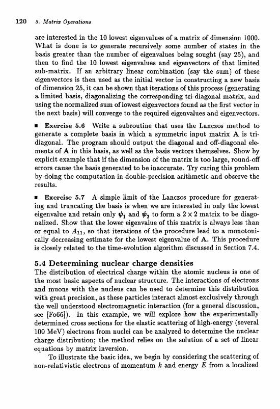
are interested in the 10 lowest eigendues of a matrix of dimension 1000. What is done is to generate recursively some number of states in the basis greater than the number of eigenvdues being sought (say 25), and then to find the 10 lomst eigenvdues and eigenvectors of that lirnited sub-matrix. If an arbitrary linear combination (say the sum) of these eigenveetors is then used as the initid vector in constructing a new basis of dimension 25, i t can be shown that iterations of this process (generating a linrited basis, diagon&zing the correspondint.; td-diagonal mdrix, and using the normazed sum of lowest eigenvectors found as the first vector in the next basis) will converge to the required eigenvalues and eigenvectors.
m Exaeise 6.6 Write a subroutine that uses the Lanczos method to generate a complete basis in which a symmetric input matrix A is tri- diagonat. The proearn should output the diagonal and a@-diagond ele- ments of A in this bmis, m well W the biit~ii~ vectors themriidves. Show by explicit exmple that if the &mensim of the matrix is too large, round-0% errors cause the basis wera ted to be inwmrate. Try cming this problem by doing the computation in double-precision. withmetic and obwwe the resdts.
Exercise 5.7 A simple limit of the Larrczoa3 procedure far generat- ing and truncatiag the bads is d e n we ~e interegted in only the! lowest eigenvdue and retain only and to form a 2 x 2 matrix to be diago- ndized. Show thae tlre lawer eigenvdue of this matrix is dways less than or eqaad to AI1, so that iterations of the procedure lead to a monotoni- c d y decreasing estimate far the Iawe8t eigenvdue of AL. This paocedure is d a ~ d y related to the time-evolution alga~ithm diseusmd in Section 9.4.
5.4 Determining nuclear charge densities The distribution of electric$ charge within the atomic nudeus is one of the mast basic wpects of nuclear structure. The interxtions of decbrons and muons with the nucleus c m be used ta determine this distr3bution with great precision, as these particles interact almost exdusively t hrongh the well understood electromagnetic interxtion (for a general discussion, see (Fo661). In this example, we will explore how the experimentally determined cross sections for the elastic scattering of high-energy (several 100 MeV) electrons from nudei can be andyzed to determine the nuclear charge distribution; the method relies on the solution of a set of linear equations by mt;tLrix inversion.
To illustrate the basic idea, we begin by considering the scattering of non-relativistic electrons of momentum k and energy E from a locatized
5.4 Determining nuclear &awe densitias 121
charge distribution, p(r), that contains Z protons, so that
and that is fixed in spaee. The electrons interact with this chmge distri- bution through the Coulomb potential it generates, V(r), which satisfies IPai~~on's equation,
V'V = 4nap, (5.33)
where a = 1/137.036 is the fine structure constant. (We henceforth work in wi ts where K -- e = 1, unless explicitly indicated, m d note that he = 197.329 MeV-h.)
The Born appro~matian to quantum sc&tering t2iscussed in the pm- vious chapter illustrates how electron scattering cross sections carry in- formation about the charge distribution, atthough precision work r e q ~ r e s a better approdmat;ion to the sc%ttering, as discussed bdow. Equa- tions (4.18,4.21) show that the Born cross section for scattering through an mgle 8 is proportional to the square of the Fourrier tran~forsn of the potential at the momentum transfer q, where q = 2k sin +B. The Fourier transform of (5.33) results in
where
is the Faurier transfom of the charge density; Thus, the difirentid cross section can be written as (we use o as a shorthand notation for dgjdS1):
Here, the Rutherford cross section for scattering from a point charge of strength Z is
m is the electron mass, and the nudear 'form factor" is F(q ) = Z-'p(q). For the spin-0 nudei we will be considering, the charge density i s spheri- cdly symmetric, so that p(r) = p(r) , and
Fh) = F(p) = dr r sin qrp(r) .
Equation. (5.36) illustrates how dectron scattering is used to study nude= structure, Deviations of the mewured c ra~s section from the Ruthefiord vdue are a, &reet mewure of the Fourier trmsform of the nuclear chmge density, It dso shows that scatterings at hi& momentum trmsfers are needed to prsbe the nucleus on a fine spatial scale, As nuclear sizes are typically several fermis (10- l~ cm), a spatial resolution better than 1 fm is desirable, implying xnomeaturn transfers of sewraj. fm-' and so beam energies of several hundred MeV. (Recall that 2k is the =&mum momentum. transfer that can be whieved with a beam of momentum h.)
At energies of sew& handfed MeV, the electron is highly dativistic (the electron mass is only 0.511 MeV) and so the discussion above must be redone beginning with the Dirac equation rather than the Sehroediner equation. One trivial. change in the find expressions that result is tha'c ultra-relativistic kinematics are used for the electron (i.e., its momentum is proportional to its energy), so that the momentum transfer can be
The only other modification to Eq. (5.36) is that the Rutherford cross section is reptwed by the Mott cross section,
where the additional factor of cos )B in the scattering amplitude arises from the spin-$ nature of the electron.
Let us now consider haw meaured crass sections are to be andyzed to determine the charge density. Suppose that we have a set of I ex- perimental values of the cross section for elastic scattering of electrons from a particular nudeus at a variety of momentum transfers (e.g., an- gular distributions at one or several beam energies). Let these values be @,P and their statistical uncertainties by Ai. Suppose also that we parametrize the nuclear chmge density by a set of N pwameters, C,, so that p( r ) = p(r; {C,)). Of course, the C's must be chosen so that the normalization constraint (5.32) is satisfied. That is,
A specific choice for this parametrization will be discussed shortly.

5.4 Determining nuclear charge ctensilieil 123
The usual methods of data andysis [jCSe69] state that the "best" val- ues of the parameters C, impled by the data are those that minimize
subject to the normalization constraint (5.41) above. Here, of is the '%heoreticdw cross section cdeulated from the appropriate Matt cross section and nuclear form factor; it depends parametriedly upon the C%. This minimum value of xZ measures the quality of the fit, a satisfactory value being about the number of degrees of freedom (the number of data points less the number of parameters).
There are several computational. strate@a for finding the parameters that minimize xZ or, equivdently, that satisfy the N non-linear equations
This is a, specific: exmgle of the commonly encountered problem of &ni- rnizing a non-lineas function of several parmetws; it is d e n fraught with &Bedties [Ac70], not the least of which is finding a local minimum, rather than the globd one usudly mug&, Most strat&es are based on an itera- tive refinement of a ""g%essn for the sptinrd C,, sad, if this guess isr dose to the required solution, there is usudly no problem. One ~ommonly used approarh i s to compute the direction of the N-dimensional gradient [left- hand side of (5.43)] either analytically or numerically at the current guess and then to generllte the newt guess by stepping some distance in C-space directly away from this direction. Alternatively, a multi-dimensional gen- eralization af the Newton-Raphson method, Eq. (1.14), can be used. The simple approach we will adopt here is based on a local linearization of of about the current guess, C:. For small variations of the C's about this point,
C, = c:+Gc,, the theoretical cross sections can be expanded as
so that x2 is given by
where of is the theoretical cross section corresponding to the current guess, C'. The charge normalization constraint (5.41) can be linearized similarly a
where we have assumed that the current guess is normalized properly, so that Z({C:)) = Z.
Equations for the &C's which make x2 stationary can be had by requiring
Eere, we have introduced a Lag rwp multiplier, 2X, to ensure the proper charge normalization. Some simple algebra using Eqs. (5.44,45) then re- sults in the Eineatr equations
h r a given guess for the C", Eqs, (9.47) can be sofved to de2;erdne what change in the C's will reduce XZ, subject to the validity of the linearization, The new impraved values can thm be amd as the next guess, the process being continued until X Z converges to a minimum. To solve Eqs. (5.471, i t is convenient to define the (N + 1) x (N + 1) matrix
and the N + l-component vector
aad identify X (The inctices m a ~ d n in thege expressions range from 1 to N.) Equations (5.47) can therefore be written as
which is simply sdwd by inversion o;f" the symmcetpic matrix A:
After the process described above caBverges to the optimal values to the C'ss, m can then enquire into the precision with which the parameters are d e t e r ~ n e d , This can be related to the matrix A defined above as faBaws. Let us consider an ensemble of data mts in whicb each experi- mental cross section fluctuates independently abaut its mean vdue. That is,
(aoyb~;) = ~ t & ~ ~ , (5.52)
where (. . .) denotes ensemble average, and 6of is the deviation of of from its; mean d u e . Such fliuetuations lead to fluctuations of the G'"s about their optimal value. Since the b, are linearly related to the experimental cross sections by (5.48), these fluctuations are given by (5.51) as
Upon using this equation twice (for 6C, and &C,) and taking the ensem- ble average, we have, after some algebra,
The uncertainties in the density parameters can be translated into a more physical statement about the correlated uncertainties in the density itself by expanding the parametxized density about the optimal parameters. In particdar, the correlated ancertdnties in the densities at radii r m$ r f can 'be writtemr as
Thus, ( 6 p ( ~ ) b p ( r ) ) 2 / 2 can be taken as a measure of the precision with which p ( ~ ) is determined, although it should be remembered that the
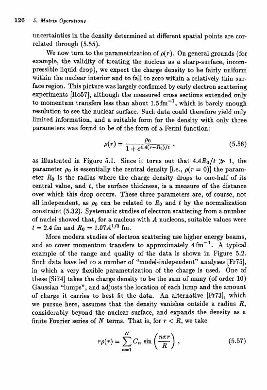
uncertainties in the density determined at different spatial points are cor- related through (5.55).
We now turn to the parametrisation of p(?). On general grounds (for example, the validity of treating the nucleus as a sharp-surface, incom- pressible liquid drop), we expect the charge density to be fairly uniform within the nuclear interior and to fall to zero within a relatively thin sur- face region. This picture was largely confirmed by early electron scattering experiments [Ho57], although the measured cross sections extended only to momentum transfers less than about 1.5 fm-' , WE& is barely enough resolution to see the nuclear surface. Such data could therefore yield only limited information, and a suitable form for the density with only three parameters was found to be af the form of a Fermi function:
as illustrated in Figure 5.1. Since it turns out that 4.4&/t > 1, the parameter p0 is essentidly the central density [i.e., p(r = Q)] the param- eter &J is the radiua where the charge demity d rop to one-hdf of its centrd vdue, and g, the surfaGe tEckn-s, is a measure of the distance over which this drop occurs, These thrw parametm are, of course, not all independent, as po c m be related to & and d by the normalization constraint (5.32). Systematic studies of electron scattering from a number of lrudei showed that, .for a nucleus with A nucjmns, suitable vdues were t = 2.4 f a = 1 . 0 7 ~ ' / ~ fm.
Mare modern studies of eleclron scattering use higller energy b e a s , and so cover momentum transfers to approximately 4 fa-'. A typical crxampfe of the r a g e and quality of the data is shown in F i ~ r e 5.2. Such data have led to a number of "modei-independent'' analyses [Fr75], in which a very flexible parametrization of the charge is used. One of these [Si74] takes the charge density to be the sum of many (of order 10) Gaussian Yumpsn, aad adjusts the location of each lump and the amount of charge it carries to best fit the data. An alternative [Fr73], which we pursue here, assumes that the density vanishes outside a radius R, considerably beyond the nuclear surface, and expands the density as a finite Fourier series of R" terns, That is, for r < E, we take
N
rp(r) = C, sin ta=2
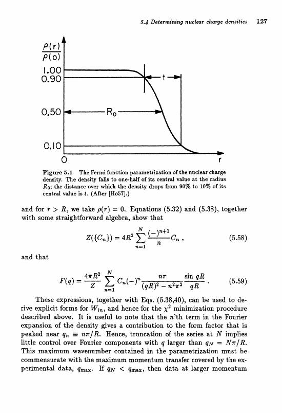
5.4 Determining nuclwr &aqe densities 127
Figure 5.1 The Fermi function parametzization of the nuclear charge denkty, The density fags ta axle-hdf of its centrd vdne at the rdiua Ra; the dktmce aver which the dendty drops from 90% tto 10% of i ts central vdue is .t. (Aftm lE0571,)
and for T > R, we take p(r ) = 0. Equations (5.32) and (5.381, together with some stm&&tforward dgr?bra7 show that
4rR2 N nn sin qB F(q) = E CB(-)" (qR)Z - n2r2 qR (5.59)
%=l
These expressions, together with Eqs. (5.38,40), can be used to de- rive explicit foms for Win7 and hence for the x2 minimization procedure described above. It is usefd to note that the n'th term in. the Fanrier expmsion of the dendty &ves a csntributhn to the farm factar that is peaked neaf q, E nn/R. Hence, truncation of the sedes at N implies little control over Fourier components with q larger than q~ = N Z / & . This m ~ m u m waveaurnber contained in the pmametrization must be wmmen;urate wit h the nrdmunr moment urn transfer caver ed by the ex- perimeatal data, gm&,. If QN < then data at lager momenturn
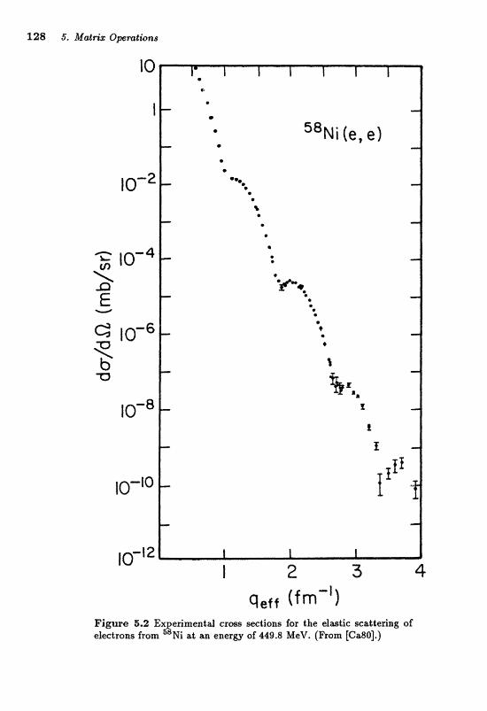
Figure: 5.2 Experimentd cross iaaitions fcx the dasfic scattering of dectrans from " ~ i ,I an energy of 449.8 MeV. (Born [6;180f.)
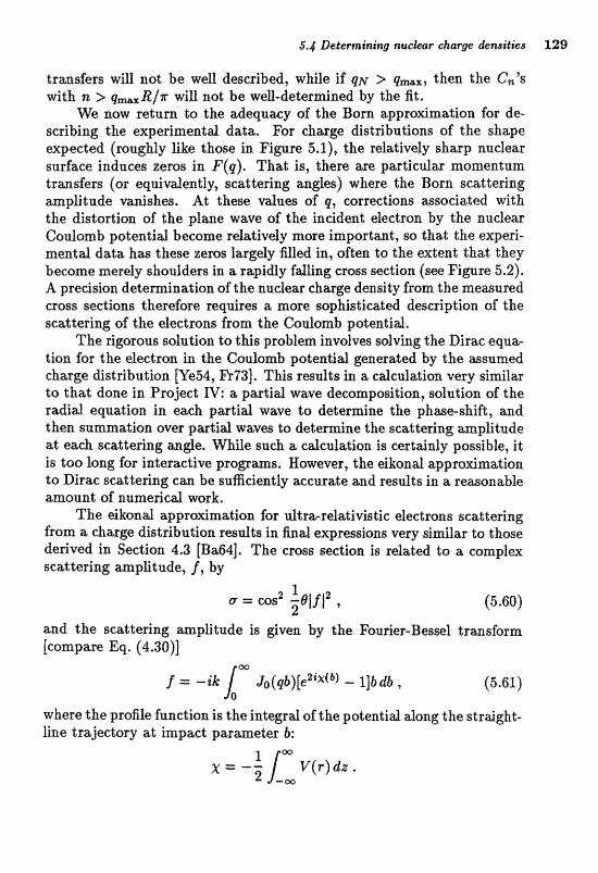
5.4 Determining nccclear charge dera~ilies 129
trmsfers wil l not be well described, wK1e if qjy 3 qwX, thm the CB's with n > q,,R/n will not be we#-determined by the fit.
We now return to the dequwy of the Born appradmation far de- scribing the experimental data. For charge distributions of the shape expected (roughly like those in Figure 5. l), the relatively sharp nuclear surface induces zeros in F(q). That is, there are particular momentum transfers (or equivdently, scattering angles) where the Born scattering amplitude vmishes. At these d a e s of q, correctians assoei&edi with tbe distortion of the pladle wave of the incident electron by the nuclear Coulomb potential becorne reldively mare impoftant, so that the experi- mentd data has these zeros largely filled in, often to the extent that they become merely shoulders in a rapidly falling cross section (see Figure 5.2). A precision determination of the nadear charge density from the meaured m s s sections therefore requires a mare sophisticated description of the ~ ~ a t t e r i n g of the electmns from the Coulomb potential.
The rigorous solution to this problem involves salving the Dirac equa tion for the dectran in the Coulomb potentid generated by the assumed charge distribution [Ye54, Fr73]. This results in a calculation very similar to th& done in Project IV: a partid wave decompositioa, solution of the radial equation in each partial wave to determine the phase-shift, and then summation over partial waves to determine the scattering amplitude at each scattering angle. While such a calculation is certainly possible, it is too long for interactive programs. However, the eibond approximation to Dirac scattering c m be sufieiently accurak and resuXts in a reasonable amount of a n s m e ~ d work.
The eikond approximation for ultra-relativistic electrons scattering from a charge distribution results in final expressions very similar to those derived in Section 4.3 [Ba64]. The cross section is related to a complex sea2;tering ampgtude, f , by
and the scattering amplitude is given by the Fmrier-Bessel transform [compare Eq. (4.30)]
where the profile function is the integral of the potential along the straight- line trajectory at impact parameter b:
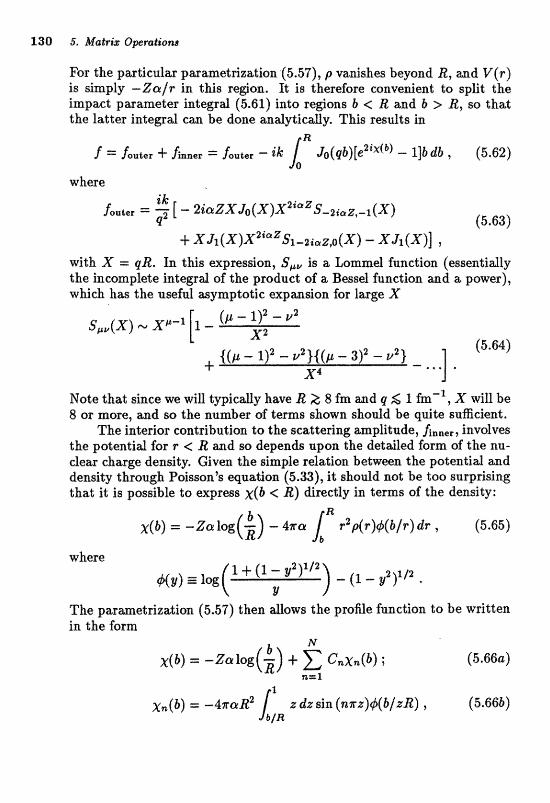
For the particular parametrization (5.571, p vanishes beyond R, and V ( r ) is simply -Zn/r in this region. It i s therefore convenient to split the impact parameter integral (5.61) into regions 6 < R and b > R, so that the latter ixl le~al cm be done analyticdy. This results in
R
f = h u t e r + hnner = fauter ik: ~ ~ ( p b ) [ e " ~ ( ~ ) - l ] b db , (5.62)
where
with X = qR. In this expression, S,, is a Lommel function (essentially the incoxnplete in tegd of tfie produe$ of a Bessel function and a power), which has the usefd aymptotic expaslsion for l age X
S,,(X) x ' -~ [l - ( p - - vZ X2
{ ( p - - v 2 ) ( ( p -- - vZ} (5.64)
4" - X4
Note that since we will typically have R 2 8 fm a i d q 6 1 fm-I, X will be 8 or mare, sknd so the number of terms shwn shodd be q ~ - t e sufficient.
The inLerior contributim to the scattering ampEtude, h,,,,, involves the potential far r < R m d so depends upon the. detailed form of the nu- dear charge density. Given the simple relation between the potential and density through Poisson's equation (5.33), it should not be too surprising that it is possible to express ~ ( b < R) directly in terms of the density:
a ~ ( b ) = - zcu log ~~p(~)#(a lp ) d~ , (5.65)
where
#(g) = log
The parametrization (5.57) then allows the profile function to be written in the form

with the change of integration vmiable z = P / R . Equations (5.61-64,66) complete the specification of the eikonal cross
section in terns of the nuclear charge density. It is also easy to show that the quantities Win are @wn by
Several fine points remain to be discussed before turning to the pro- gram. One is that the nucleus is not infinitely heavy, and so recoils when struck by the electron. To correct for thig, the cross sections calculated above, which have all been for an electron impinging on a static charge distributian, must be divided by the factor
where M is the target mass (roughly A x 940 MeV). Note that this correction vmishes as M becomes lage compared to E. Second, beemm of the e ~ ~ l ~ m b attrxtion, electrons at the nucleus have a sfightly fiigher momentum. than the beam vdue, h the eikonal treatment, tMa c m be approAmalely corrected for by replacing q in afl of the formdas by
and by multiplying the eikonal scattering amplitude by (q.~/q)'. Bere, v is a suitable average of the Coulomb potential over the nuclear volume, conveniently given by
- 4 Zahe
where R. i s the nuclear radius. SimilaIy, in the Born approximation (5.40), the nudear form factor is to be evduated at q e ~ , 'bad the Matt eroBs sec- tion is still to be evduated at q.
The FORTUN pro@- for Exmple 5, whose listing cm be found in Appendh B and in the file EXMT"LS.FOR, uses the method described above to analyze electron scattering cross sections for the nuclei 'OCa ( Z = 201, S8Ni (Z = 28), and 208Pb (Z = 82) to determine their charge densities. Many &Ee;rent daka sets for each target, taken at a mriety
of beam energies and angles (see, for example, [Fr77]), have been con- verted for equivalent cross sections at one beam energy [Ca80]. The inte- grds (5,62,Ii6b967b) are eduated by 20-paint Gauss-Legendre quadratwe a d the matrix inversion repired by (5.51) is pedarmed by rul eficient implementation of Gauss-Jordan elimination [Ru63].
After requesting the target nucleus, the boundary rd ius R, a d the number of sine functions N, the program iterates the procedure described above, displwing at ewh iteration plots of the fit, fractiond emor in the fit, m d the char@ density of the nucleus, tagether with the dacss of the G's and the density. The progrm also d10ws for initid iteratiorits with fewer sines t h m we ultimately required, the number then being increased on request, This technique improves the convergence of the more rapidly oscillating campone~ts of the density as iL reduees the effective dimension of the X2 search by first converging the smoother density components. Mote that, a;e each iteration, only points at an eEective marn~?~ftum trans- fer smdler tkim that described accuratdy by the current number af sine8 are used in calculating
The following exercises wil l be useful in understanding the physical ;md numericd principles iraportmt in this cajcalation.
= Exercise 5.8 To deck that the progrm is working properly? use the tzlikond famulas and Fermi-function chmge density described abave ta generate a set of "pseudo-data" cross sections ranging from p between 0.5 and 4 fm-'. Make sure that these cross sections are given at intervals typical of the experimental data and also assign errors to them typical of the data. Then verify the extent to which the correct (i.e., Fermi- function) charge distribution results when these pseudo-data are used as input to the program. One potential source of error you should investigate is the "completeness error". That is, the ability of a finite Fourier series to reproduce densities of the tom expected. This can be studied by changing the number of eines used in the fit.
Exercise 5.9 Run the eode with the actual experirnentrtl data to de- termine the charge densities for the three nuclei treated. Study the qual- ity of the fit and the errors in the density extracted as functions of the number of expansion terms used. Also vedfy that the fitting' procedure converges to the same find solution if the initial guess for the density is varied within reasonable limits. Note that the converged solutions do not have a uniform interior density, but rather show "wiggles" due to the specific shell-model structure of each nucleus.
V: A schematic shell model 133
m Exercise 5.10 Extend the program to calculate the moments of the density,
and their uncertainties for integer k ranging from 2 to 5. This can be doneconveniently by using Eq. (5.57) to express these moments directly in terms af the C,. VePify that the size of these raomeats is consiskd with an scaling of the nuclear radius.
U Exercise 5.11 A simple model for the doubly-mqic nucleus 40Ca is a Slater determinant constructed by putting four nucleons (neutron and proton, spin up and down) in the 10 lowest orbitals of a spherically- symmetric harmonic osdllator potential. Show that the charge density predicted by this model i s
where ro = m being the nucleon mass and w being the har- monic oscillator frequency. Determine the value of ro (and hence w ) re- wired to reproduce the experimentd vdue af t he road-mean-square radius (Mz)9 and then compare the detailed form of p predicted by this model with thag obtatined from the data,
m Exercise 5.12 Modify the progam so tEt& it crilculates the Born, rather thaa. eikond, cross seetim a;nd show that the fomer is grossly inadeqaate to describe the data by compasing the Born cross sections for
cljstribution with the experimental data.
m Exercise 5.13 Modify the program to calculate the "off-diagonal" uncertainties in the density determined using Eq. (5.55) and show that the correlation in the uncertainties largely decreases as the separation of dke points increases.
Project V: A schematic shell model The assumption of particles moving independently in a potential is a com- mon approdmation in treathg the quantum m e c h ~ c s of many-partide systems, For exmple, this picture underlies the Wa&ree-Fock method for treating the many electrons in an atom (see Project III), the shell model for treating the many ~aclt?ons in a ~ueleus, a d rnaxly models far treat;- ing the quwks in a badron, Bowever, it is only a r ~ u g h appro~mat;ion
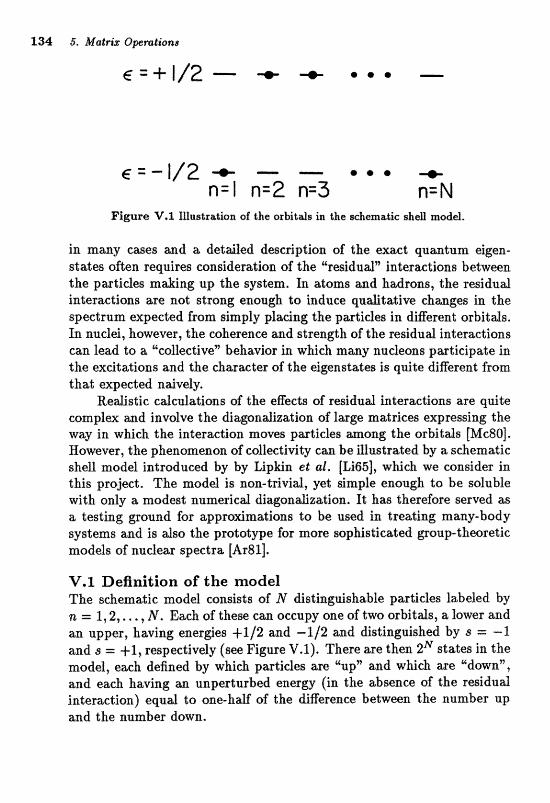
Figwe V,% Zllnstra,Ibn, of the orbitals in the s~hematic shell modd.
in many cases and a detailed description of the exact quantum eigen- states often r e q ~ r e s consideration of the "residual" interactions betwen the particles makiing up the system;. In atoms and Badrons, the residual interactions we not strong enough to induce quatative chane;es in the spectmnr expected horn simpfy placing the partides in digezent arbilds. In audei, however, the coherence aknd s t rag th of tfre reddud interactions can l e d to a 'kollective" behaviar in whieh, many nucleons pitstieipate in the meitations and the charmter of the dgeastates is quite diEerent from that expected n~vely.
Reastic cdculatians of the eEeets of residual interactians are quite campalex astd involve the diagaaaifizattion of large matrice8 expregsirng the way in which the interaction moves particles among the orbitals [Mc80]. Hoatever, the phenomenon of cdle~tivitJt can be illustrated by a schematic shell model introduced by by Lipbin et al. [Li65], which we consider in this project, The modd is non-trivid, yet simple enou& to be soluble with only a mo&st aumericd diaganalization. It has therefore served as a testing ground for approximations to be used in treating many-body systems and is &so the prototype for more sophisticated group-theoretic models of nuclear spectra [Ar8l].
V.1 Definition of the model The schematic model consists of N distinguishable partides labeied by n = 1 , 2 , . . . , N. Each of these can occupy one of two orbitals, a lower and an upper, having energies +1/2 and -112 and distinguished by s = -1 and s = + 1, respectively (see Figure V.1). There are then zN states in the model, each defined by which partides are @up'' and which are "down", and each having an unperturbed energy (in the absence of the residual interaction) equal to one-half of the difference between the number up and the number dawn..
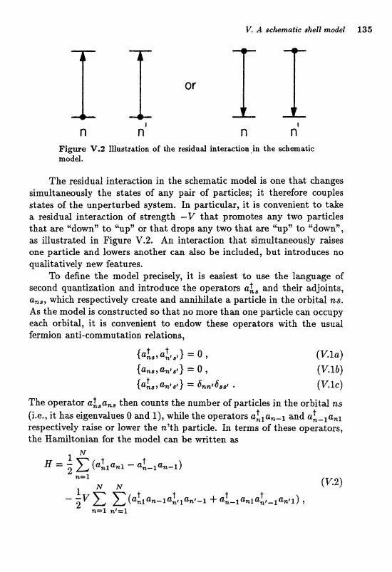
V. A schematic shell modd 135
or
Figwe V.3 IBuatration of the re~idrrd irtter~tion~in the wrefiematic modd.
The residud interaction in the stllilematic model is one that changes simultaneously the states of any pair of pils'cicks; it therefore cottpks sta?t;es of the unpertuhed system. In particular, i"tis convenient to take a residual interaction of rjtrmgth -V that, promates any two partides that are CEdown" ta gL"up'9 or that drops any two that are "up" to "dawn", as illustrated in Figure V.2. An interactiart that simultanwusly rrtises one pasticle m d lowers m ~ t h ~ f l : c m &so be included, but introduces no quatatively new features.
To define the model preGi~dy, it i~ ewiest to use the lanf5rzag;e of second quantization and introduce the operators ai , and their adjoints, a,,, which. re~pectively cre& and ~lnnikifate a padicle in the srBitrtl ns. As the model is constructed so that no mofe than one particle earn occupy each orbital, it is convenient to endotv them operators with the usual fer&on wti-c~rnmutation relzn;tions,
(V. l a)
(V* 1 b) (V. le)
The operator ai,a,, then counts the number of particles in the orbital ns t (i.e., it has eigenvaiues O and l), while the operators aLla,-l and anela,l
respectively raise or lower the n'th partide. In terms of these operators, the I fa~l tan im for the model can be mitten as
where we nmd not worry about the unphysied ra9 = =L: term h the residual interaction since an attempt to raise or lower the s m e particle twice yields a van_isEng state.
V.2 The exact eigenstates The Hamiltonian described above can be represented as a matrix coupling the gN states among themselves. Apart from symmetry and a vanishing of many of its elements, this matrix is not obviously special, so that its numerical diagonalization to find the exact eigenstates md eigenvalues is a substantial probiem'for all but the smallest values of N. Fortunately, the relatively simple structure of the problem allows it to be expressed in the
liar language of the group SU(2) (the quantum angular momentum operators), a transformation that carries us a good deal of the way to an exact diagonalization and also affords some insight into the problem.
Let nk; define the operakors
Thus, J, measures (one-half of) the difference between the number of "upn partides and the numb= of "dawn" particles, wKk-? J+ m d J- coherently raise or lower all of the partides. Using these operators, the Hamiltonian (V.2) can be written as
where we have iatrodueed the opclra;t;ors I 1
J, = -(J+ f J - ) , J, = --i(J+ - J-) . 2 2
Using the fundamental anti-commutation rules (V.1), it is easy to show that the three operators J,, J* satisfy the commutation rules of a quantum angular mumeaturn:
Thus, although these L6quasi-spinn operators have nothing to do with a physical angular momentum, all of the techniques and experience in deal- ing with quantum spin operators can be applied immediately to this prob- lem.
V. A schemalie shell model 137
We can be@n by realizing that ~ i n e the total quasi-spin operator
commutes with J,,,,,, it commutes with the H l h d a n and thus each eigenstate of II can be labeled by its total quasi-spin, j , where j ( j + 1) is the eigenvalue of J ~ . The eigenstates therefore can be classified into non- degenerate multiplets of 2j + 1 states each, all states in a multiplet having the same j; the Hadltoaian has a non-wnishing matrix element between two states only if they belmg to the same multiplet, Bowever, since B does not cornraute with J,, its eigenstates wiB R& be simultaneously eigenstate~ of this frt'tter operator.
To see what values of j are allowed, we can dassify the zN states of the model (not the eigenstates of H) according to their eigenvdues of &, The m e state with the largest eigenvdue of Jz has all particles up, corresponding to an eigenvdue m = * N . We therefore expect one multiplet of 2 - 3 N + 1 = N + 1 states corresponding to j = i N. Turning next t o states with n = 4 N - 1, we see that there are N states, cor- responding to one of the & particles down and all of the rest up. One linear combination of these N states (the totally symmetric one) belongs to the j = multiplet, implying that there are N - 1 multiplets with j = $ N - 1 . Continuing in a similar way, there are # N ( N - 1) states with m = -$N - 2 (two particles down, the rest up}, of which one linear combination belongs to the j = $ N multiplet and N - 1 linear combina- tions belong to the j = f N - 1 multiplets. There are thus ~ N ( N - 3) multiplets with j = # N - 2. By continuing in this way, we can classify the 2N states of the model into multiplets with j running from $ N down to 0 or i, if N is even or odd, respectively.
Because W involves only the quwi-win aperat;ors, its action within a multiplet depends only upon the value of j involved. For a given N , the spectrum of one multiplet therefore serves for all with the same j and, in fact, also serves for multiplets with this j in systems of larger N. We can therefore restrict our attention to the multiplet with the largest value of j , + N .
By these considerations, we have reduced the problem of diagonal- izing the full Kamiltonian to one of diagondizing (V.4) in the N + 1 eigenstates of J, belonging to the multiplet with j = -$N. We can label these states as im), where m runs from - j to j in integer steps. Using the usual formulas for the action of the angular momentum raising and lovvering operators,
we can write the elements of E in this basis a%i
Thus, R is tri-diagonal in this basis and in fact =parate8 into taro un- coupled problems invo1.ving t h ~ state6 m =. - j , - j + 2, *. , , + j azd m =L
- j + l, - j + 3, . . . , f j - 1 when N is even ( j is integral) and the states m =;: - - - j , - j +2 , . . . 1+ j - - 1 and m = -j+1, - - j + 3 ,..., +j when N is odd (j is half-integral). For smdl values of j , the resulting matFices can be diagondized rtsldyticdy, while for 2mger systems, the namericd methods discussed in this chapter can be employed to find the dgenvdues m d eigenvectors,
The quasi-spin method daws us to m&@ one ather atatemat about the exx t solution of the model. Let
be the unitary operator effecting a rotation in quasi-spin space by an angle of n about the axis (2 + $ ) ~ 2 ' / ~ . It i, emy to see that this rotation t r a~ fo rms the quwi-spin operators as
ltonian (V.4) transforms as
Hence, if tj is an eigenstate of H with energy E, then R+ is an eigenstate of JI with energy -E. Thus, the eigenvdues of H come in pairs of equal magnitude and opposite sign (or are 0). This also allows us to see that if N is even, at least one of the eigenvalues will be zero.
V.3 Approximate eigenstates We turn now to approximate methods for solving the schematic model and consider fin t ordinary Rayleigh- Schroedinger perturbation theory. If we treat the J, term in (V.4) as the unperturbed Hamiltonian aod the Jz - Ji term as the perturbation, then the unperturbed eigenstates are
Im) with unperturbed energies EC) = m and the perturbation series is an expansion in powers of V. Since (m m) = 0, the energies are unperturbed in first order and are perturbed in second order as
V, A schematic shelf model 139
Using Eq, (V.9) for the matrix elerrxents irtvolved, expgcit expressions for $be? ~ecould-order ener@es can be derived; the fourth-srder t e rm can. dso be done wi"c a bit of patient dgebra.
While the weak-coupling (smdl-V) limit can be treated by straight- forward perturbation theory, m agproxirnahn for the strong-coupling (large-V) situation is not so obvious. One appealing approach is the semidassicd method, vdid in the Emit of large N [Ka79, ShSD]. The dimssion be@ns by considering the equ&ions of motion far the time- dependence of the expectat;ion values of the quai-spin operators:
d i- (Ji) = ([Ji, E]) 9 (V. 13) dt
where Ji is any one of the three components of the quai-spin, Using the Hamiltonian (V.4) and the commutation rules (V.6), it is easy to write out Eq. (V. 13) for each of the three components:
d z (Jz ) -2v(JyJz + JZJ,) (V. 14e)
UnfortunaLely, these equations do not form a closed set, the time deriva- tives of expectation values of single quasi-spin operators depend upon ex- pectation values of bilinear products of these operators. However, if we ignore the fact that the J's are operators, and put, for example,
then a closed set of equations results:
(V. 15a)
(V. 156)
(V. 15c)
It is easy to show that Eqs. (V.15) conserve
J 2 ( ~ 2 ) ~ f ( J ~ ) ~ + (JZ )? , so that a convenient parametrization is in terms of the usud polar angles,
( J , ) = J cos 8 , (J,) = J sin 8 cos t$ , (JY) = J sin 8 sin 6 , (V.16)
where
If we further define ithe variables
p1 5 and O 5 q 5 2n, then, upon introdudng the convenient coupling constant
xzdVVssz2JT,,
Eqs. (V.15) can be written as
@E(p, q) (V. 18a)
X 3 = I + 2-33 sin 2q = @E@, g) dt RT @P *
(V. 186)
Here, E is the eqeetation vdue of the H
E(P, q) g ( H ) = (Jz) - ~ ( ( J z ) ~ - ( J V ) ~ ) (V. 19a)
(V. 196)
By these manipulations, we have transformed the quasi-spin prob- lem ialo om of a time-dependeat classical system with 6Lmomentum'" and "coordinate" q satisfying equations of motion (V.18). As these equa- tions are of the canonical form, p and q me canonicay conjugate and (V.19b) can be identified as the Hamiltonian for this classical system. Our hrivation h a been heuristic, but not rigomus, A more careful cal- culation defines the classical Eamiltonian as the expect ation. vdue of the quantum Hamiltonian between coherent states [Ya82]. However, the only modification this procedure gives to our results is the redefinition:
Note that the EX ltonim so derived is a va~a t ioad one, therefore the quantum ground state energy will be lower than the minima in the das- sical energv:
We can now infer properties of the quantnm eigenstates by analyzing this classical system. Using Eq. (V.ISb), we can calculate the trajectories in phase-space; i.e., the value of p for a given q and E = (H). Equivalently, we can consider contour lines of E in the (p,q) plane. In an analysis of
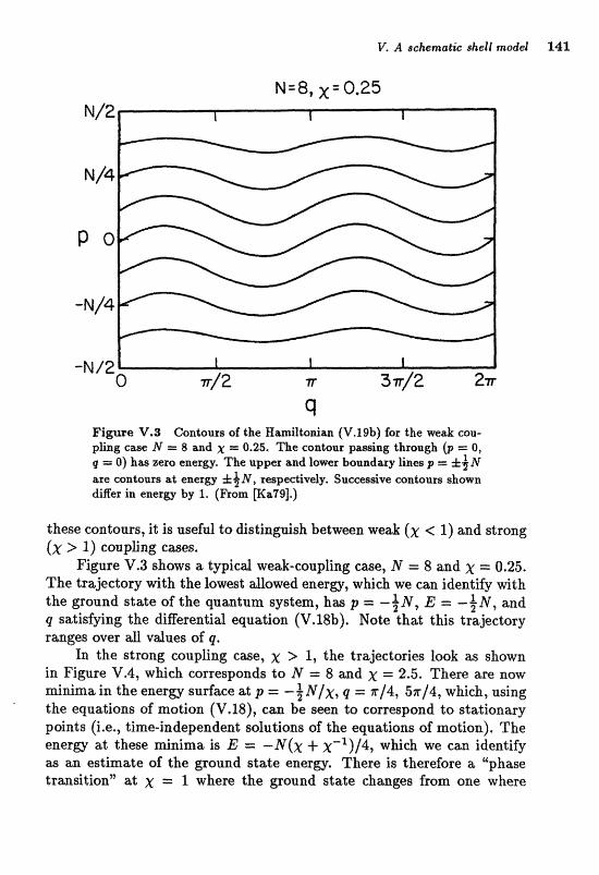
9 F l m e V.3 Contours of the HwiIlaGan (V.29b) for the we& eau- p b g c- M = 8 and X = 0.25. The contour pm&aig through Cp = 0, g = 0) has zero energy. The upper and lower boundary lines p = f are contours at energy &*N, respectively. Successive cantoars shown diger in energy by 1, (F~arn Ks791.)
these contours, it is useful to distinguish between weak (X < 1) and strong ( X > 1) coupling cases.
Figure V.3 shows a typical weak-coupling ease, N = 8 and X = 0.25. The trajectory with the lowest allowed energy, which we can identify with the ground state of the quantum system, has p = - $ N , E = - $ N , and q satisfying the differential equation (V. 18b). Note that this trajectory r ages over aJ1 v d u e ~ of Q.
LR the strong coupfing case, X r 1, the tr;t,jectaries look as shown in Figure V.4, which mrresponds to N = 8 and X = 2.5. There me now minima in the energy surface at p = - $ N I X , Q = a/4, 5~14, which, using the equations of motion (V.18), can be seen to correspond to stationary points (i.e., time-independent solutions of the equations of motion). The energy at these minima is E = - N ( x + X-')/4, which we can identify as m estimate af the ground 8taGe enexggr. There is therefore a "phase ternsition" at X = 1 where the g o ~ n d state chmges h x n one whercl
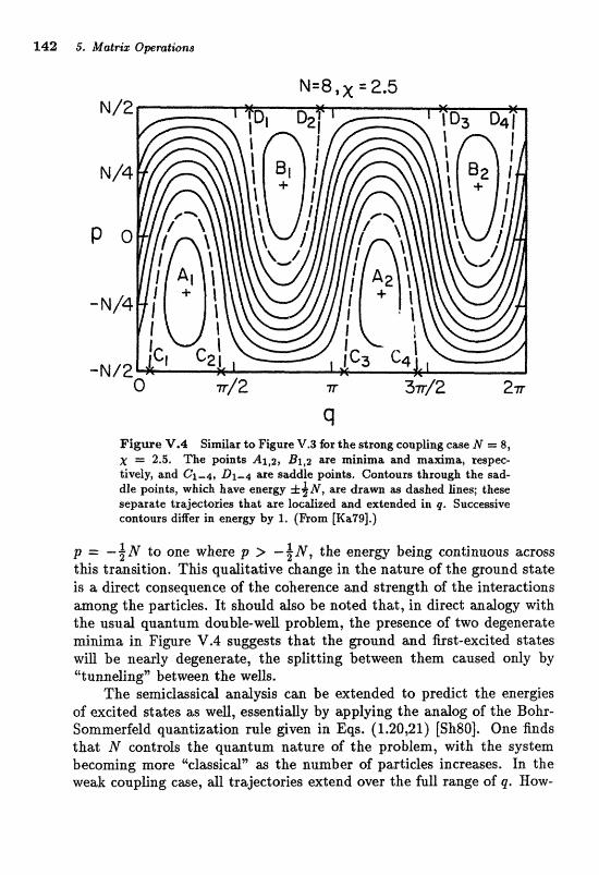
Ffgwer V.4 Sim2ar lo Figure V.3 for the stro~g coupling, cam ll\C = 8, X = 2.5. The points Al,ar B1,2 me minima masma, respec- tively, and CJ- .~~ .Dlm4 are sacliae points. Gontours through the sad- dle points, which have energy A ~ N , are dram as dashed lines; thme separ&e trajectories that are locdbed and exleadd in tp. Succwive caatours diger in energy by l. (Ram [Ka73],)
p = - N to one where p > - { N , the energy being continuous across this trmsition. This quditative clsmge in the nature of the ground state is a direct consequence of tfie coherence and strength of the interactians among the particles. It should dso be noted that, in direct andogy with the usud quaatuln double-weU, problem, the presence of two degenerate minima in Figure V.4 suggests that the ground and first-excited states will be nearly degenerate, the splitting between them caused only by '%tunnefingB between the wells.
The se~clmsica-l andysis can be extended to predict the energies of excited states as 4 1 , essentially by applyinf~ the andog of the Bahr- Sommerfeld quantization rule given in Eqs. (1.20,21) [Sh80]. One finds that M controls the quantum nat;ure of the problem, Prith the system becoming more ""classicaln as the number of particles inaeitses. In the weak coupling case, all trajectories extend over the full range of q. How-
V, A schematic shell mode2 143
ever, for strong coupling, there are two types of trajectories: those that vibrate around the energy minima or maxima (and are hence confined to limited regions of p) and those that extend throughout all q. It is easy to show from (V.1Sb) that the transitions between these two behaviors oc-
El = J (e.g., the dashed lines in Figure V.4). In andogy with the usual quantum double-well, we expect states associated wit h the confined trajectories to occur in near?y degenerate pairs, the degeneracy being bro- ken more strongly as the energy increases above the minima or decreases below the m&ma.
V.4 Solving the model The simple semidassical picture we have discussed above can be tested by an analysis of the exact eigenstates of the model. This can be carried out through the fQllowia(~ sequence of steps.
m Step 1 Verify the algebrzhia the di~cussioa above. In particular, s h w that Eq. (V.4) is a valid representation of the Hamiltonian. Also evaluate the second-order perturbation to the energies, Eq. (V.12).
m Step 2 Verify the correctness of Eqs. (V. 14,18,19) and the discussion of the energy emtours in the strong md weak coupgng cwes, h the strong coupling case, liaemize the equations of motion about the xaifiima as m d m a a ~ d show that the frequency of harmonic moticm about these points is [2(xZ - This is the spacing expected between the pairs of newly degenerate states in the exact spectrum.
U Steg 3 Write a prqram that finds the eigenvduer~ of the tri-rliagond Hamiltonian matrix (V.9), perhaps by modifying that written for Exer- cise 5.4. Note that the numerical wvork can be reduced by treating basis states nrith even and odd m separately and by using the symmetry oE %he spectrum about E = 0. In addition, yoiu can save yours& some tedious bookkeeping concerning the size of the bases by taking N even only.
Seep 4 Use the p r o e m written in Step 3 to cdcdate the spectrum of the model for selecged vafues of N between 8 and 40 and for valnes of X between 0.1 and 5. At we& coupling, compare your results pvith the perturbation estimates (V. 12). For strong couplings, compare your ground state energy with the sa idass icd ~jstimate and verify the? ex- pected paifwise degeneracy of the Isw-fying states. Also cornpase the excitation enerfies af: these states with your estimate in Step 2. Wow doea the accuracy of the semi-classic& estina;ille cfiizlnge with N?

r Step 5 W ~ t e a, proe;ram that takes the eigenvdues found in Step 2 and solves for the ei@;envectors by inverse vector iteration [Eq. (5.27)]. For selected vztdues of N and X , compute the expectation vdue oT J, for e x k eigenvecltor , In a seanidasdcra-f interpret atim, this expectaLioe vdue can be ictentiged with the dime-average of p aver the associatt3d trajectory in phase space. Verify that (J,) changes through the spectrum in accord with what you expect from Figareer V.3, V.4,
Chapter 6
Partia Differentia
Equations
Pmtid differential equations are involved in the description of virtudly every pksical situation whem qumtities vary in space or in: ;apace and time, These indude phenomena as diverse W diRueioa, electramagsetic waves, hydrodynamics, and quantum mechanics (Schroedinger waves). In aILl but the simpXest cases, these equations cannot be solved analytieafly and sa numericd methods must be employed for quantitative resuXds, In a typicd numericd treatment, the dependent vwiatsks (such as tem- pmature or ekctricd potentid) are described by their d u e s at discrete points (a lattice) of the independent variables (e.g., space and time) and, by appropriate discmtizstion, the partial diBerentid equation i s ~ d u c e d to a large set of difference equations. Although these difference equations then can be solved, in principle, by the direct matrix methods discussed in Chapter 5, the large size of the matrices involved (dimension compa- rable to the number of lattice points, often more than several thousand) mitkes such m q p r o z h impractical. Fartunately, the Iocdity of the origind equations (i.e., they invofw only low-order derivatives of the de- pendent vasiables) makes the resulting digerence equa;tims Usparse" in the sense that most of the elemengs of the matrices involved vanish, Far au& matrices, iter&ive methods of inversion and diagonajbization can be vev eaeient. These methods ase the subject of tkis and the fdlfswing chapter*
Most of the physiedly important partid digerentid equatio~s are of second order and can be clwsified into three types: parabolic, eEp- tie, or bypwbofic, Roughly speaking, parabofic equat;ians involve only a

146 6, Elliptic Partial Dr'flesntioE Eguations
first-order derivative in one variable, but have second order derivatives in the remajning vaiables. Examples are the diEasion equation and the time-dependent Schraedringer equation, which are first order in time, but secand order in spitce. Elliptic equations involve second order derivatives in each of the independent variables? each derivativt? having the s m e s i p when &B terms in the equation me grouped on one side. This class indudesj Poisson's equation for the electrostatic potentid and the time- independent SeAroedinger ewation, both in. two or mare spatial variables. Finally, there are hyperbolic equations, wEch involve secand derivatives of opposite sic, such as the wave equatian describing the vibrations of a stretched string. In this chapter, we win discuss some numerical methods appropriate for eUiptic equ&ions, resewing the discussion of parabofit: equations for Chqttlr 7. Hyperbolic equations often can be treated by methods similar to those we discass, although unique difiedties do arise [Ri6?].
For concmteness in our ascussion, FV~? will consider particular farms af'dipLic bounday d u e a d eisnvdue problems fof a fidd q5 in two sp* tial dimensions (I, y). The boundary value problem involves the equation
Although this is not the most general elliptic form, it nevertheless covers a wide variety of situations. For exampie, in an electrostatics problem, 4 is the potentid and S is related to the charge density [compare Eq. (3.2)], while in a steady-st ate heat diffusion problem, q5 is the temperature, and S is the local rate of heat generation or loss. Our discussion can be general- ized strGghtforwardly to other elliptic cases, such as those involving three spatial dimensions or a spatially varying diffusion or dielectric constant.
Of course, Eq. (6.1) by itself is an ill-posed problem, as some sort of boundary conditions are required. These we will take to be of the Dirichlet type; that is, t$ is specified on some large dosed curve in the (z, g ) plane (conveniently, the unit square) and perhaps on some additional curves within it (see Figure 6.1). The boundary value problem is then to use (6.1) to find 4 everywhere within the unit square. Other dasses of boundary vdue problems, such as Neumann (where the normal derivative of 4 is specified on the surfaces) and mixed (where a linear combination of 4 and its normal derivative is spedfied), can be handled by very similar methods.
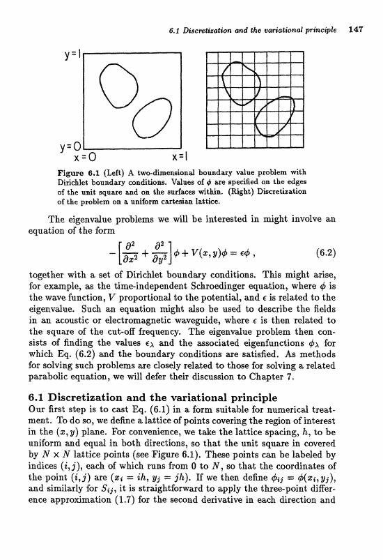
6.1 Dzacmtizatisn and the variational princiiple 141
Figwe @,l (Left) A twedimen~iand boundary vdutr, problem d t h DirichIet boundary conditions, Vdnes af c j aupe speci6d on the edlr;ee of the unit square and on the surfacw Within, (Right) Discre~zalion. of the problem on a uniform carledan lattice.
The eigenvalue problems we will be interested in might involve an equation of the form
toe;e%her with a set of Dir iae t boundmy coaditions. Thia. might arise, fClT exmple, as the time-independent Schroedinger equation, where c(r is the wave function, V proportiond to the potential, and E is refated to the eigenvdue. Sueh an eqtzation nright dsa be used to describe the fields in an acoustic or electromagnetic waveguide, where E i s then related to the square of the cut-oE freque;ec;r, The eigenvdue problem then con- sists of finding the vdues e~ and the associated eigenfunctions for which Eq. (6.2) and the boundary conditions are satisfied. As methods for sdving such problems are closely related, to those .for sdving a relateir parabolic equ;zlion, we will defer their discussion to Chapter 7.
6.1 Discrethation and the variational principle Our first step is to cast Eq. (6.1) in a form suitable for numerical treat- ment. To do m, we degne a laLtice of points covering the region of interest in the (2, y) plane. For convenience, we take the lattice spacing, h, to be uniform and equal in both directions, so that the unit square in covered by N x N lattice points (see Figure 6.1). These points can be labeled by indices ( i , j ) , each of which runs from O to N, so that the coordinates of the point (i, j ) are (+i = ih, gj = jh). If we then define #i j = 4 ( $ i 7 y j ) , and similarly for Sij, it is straightforward to apply the th~ee-point differ- ence approximation (1.7) for the second derivative in each direction and
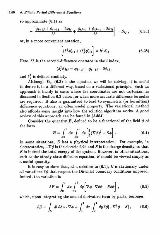
so approximate (6.1) as
or, in a more convenient notation,
Here, 61 is the second-difference operator in the i index,
and 6; is defined similarly. Although Eq. (6.3) is the equation we will be solving, it is useful
to derive it in a digerent way3 based on a vwiatianal principle. Such asr approah is handy in Gases where the coosdinates are not carte&&% W
&iscussed in Sectian 6.3 below, or when mare accurate diRerexlccj. formdas are required. It also is guaranteed to lead to symmetric (or he difirence equations, an often usefd praperdy. The variational method also cords some insight into haw the galufion dgorithnr urorks. A good review of this approach can be found in [Ad84].
Consider the quantity E, defined to be a functional of the field 4 of
In some situations, L": has a physic-zll interpretation. For exmple , in ekcdmstatics, -V# is the electric field and S is the charge drmsity, so that E is indeed the total energy of the system. However, in other situations, such as the steady-state diffusion equation, E should be viewed simply as ;z useful quantity,
It is easy to show that, at a solution to (6.1), E is stationary under all variations 64 that respect the Diridlet boundary conditions imposed. Indeed, the variation is
which, upon integrating the second derivative term by pmts, becomes
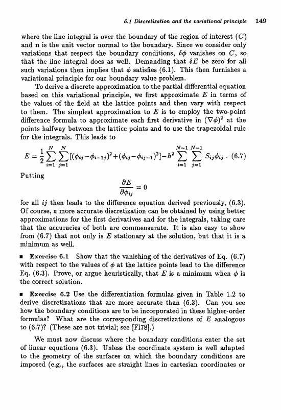
6,l Biscretization and the variational principle 149
where the line integral is over the boundary of the region of interest (C) ancl n is the unit vector normal to the boundmy. Since we consider ody vasiations; that respect the bouadau conditions, S# vanishes an C, sa th& the line integrd does W well, Demanding that 6E be zero for d such variations then implies that q5 satisfies (6.1). This then furnishes a vaiatioad grindple fi>P our boundary d u e problem.
To derive a discrete approsnnatioa to the partid diEerentid equation based on this vafiational principk, are first approximate E: in terms of the d u e s of the 5eld at the lattice points m d then vary with respect to them. The sirnplest approximatim to E is; to employ the two-point difference formula to approximate each first derivative in ( ~ 4 ) ~ at the points halfway betwwn the lattiee poiats and to use the trapezoid2 ruk for the integrds. This bads to
Putting @E - = o
@+ij
for all i j then leads to the difference equation derived previously, (6.3). Of course, a more accurah diser&iztttion cm be abtdned by using better approfimations for the first derivativw a d for the integds, t a E ~ g case that the accuracies of bath are commenszlrate. It is also emy to show from (6.7) that not only is E stationary at the solution, but that it is a d~rnunr as ~4311,
Exercise 6.1 Show that the vanishing of the derivatives of Eq. (6.7) with respect to the vdues of 9 a,t the lattice points lead to the difFerence Eq. (6.3). Prove, or argue heuristicdy, that E is a minimum when 4 is the cmrect solution.
R Exereilre 6.2 Use the diRertsntiation fbsmulas @ven in Table 1.2 to derive discretizations that are more accurate than (6.3). Can you see how the baandary conditions are to be incorporated in these higher-order form&=? What are the correspon&ng discretizaLions of E andogous to (6.7)? (These are not trivial; see [F178].)
We must now &scuss where the boundary conditions enter the set; of Ijnear equations (6.3). Unless the coordinate system is we11 adapted to the geametry of the surface8 on wbicb the boundam conditions are imposed (e.g., the surfaces are straight lines in cartesian coordinates or
150 6, Elliptic Partial Diflerential Ewationol
arcs in cylindrical or spherical coordinates), the lattice points will only roughly describe the geometry (see Fig. 6.1). One can always improve the accuracy by using a. non-uniform lattice spacing and placing more points in the regions near the surfaces or by transforming to a coordinate system in which the boundary conditions are expressed more naturally. In any event, the boundary conditions will then provide the values of the 4ij at some subset of lattice points. At a point far away from one of the boundaries, the boundary conditions do not enter (6.3) directly. However, consider (6.3) at a point just next to a boundary, say (i, N - 1). Since 4iN is spedfied as part of the boundary conditions (as it is on the whole border of the unit square), we can rewrite (6.3b) as
that is, +ilv enters not as an unknown, but rather as an inhomogeneous, known term. S i~ la r fy , if a Neumann bollndary mndit;ion were imposed at a surface, say a+/ay = g(%) at y = 1 or, equivalently, j = N , then this could be approsmated by the discrete boundary candition
which means that at j = N - 1, Eq. (6.3) would become
These consideratims, and a bit more thought, show that the discrete approximation to the differential equation (6.1) is equivalent to a system af Enem equations for the unknown vdues of tt, at the intex;ar poi~ts , In a matrix notation, this cm be written aa
where M is the matrix appearing in the linear system (6.3) and the inho- magentjous term s is proportional to S at the interim points and is linewly rdated to the specified vdues of g) or it-s derivatives on $he boundafies, In any sort of prrtcticaf situation there are a very lasge number of these equations (some 2500 if N = 50, say), so that solution by direct inversion of M is impraetied, Fortunately, since the discrete approximation to &he Laplacian involves only neighboring points, most of the elements of M vanish (it is sparse) and there are then effident iterative techniques for solving (6.9). We begin their discussion by considering an analogous, but simpler, one-dimensional boundary value problem, and then return to the two-dimensiond case,
6.2 An iterative method f ~ r boundarg value problems 3.51
6.2 An iterative method for boundary value problems The one-dimensional bounday vdue problem analogous to the two-dimen- sional problem we have been discussing can be written as
with +(0) and 4(1) spedfied. The related variational principle involves
which can be discretized on a uniform lattice of spacing h = 1/N as
when varied &h rtlspect to cbi9 thls yields the difference equation
which is, of course, just the naive discretization of Eq. (6.10). M&hods of solving the boundary value problem by integrating for-
wmd m d backwad in a: were Gsenssed in Chapter 3, but we can dso consider (6.13), together with the known values of and +N, as a set of linear equations. For a modest number of points (say N 6 loo), the liaear system above c m be solved by the direct methods discussed in Chapter 5 and, in fact, a very eEcient specid dircrct method e ~ s t s for snch ""ti-distgand" systems, as discussed in Chapter 7. Howwr, to illus- trate the iterative methods appropriate for the large sparse nnatriees of' elliptic partial diEercr;ntial equatiians in two or more dimensions, we begig by rewriting (6.13) in a "solved" form for 4i:
Although 'this equation i s not manifestly useful, since we don% know the 4's on the right-hand side, it can be interpreted as giving us an "improved" value for 4i based on the values of 4 at the neighboring points. Hence the strategy (Gauss-Seidel iteration) is to guess some initial solution and then to sweep systematically through the lattice (say from left to right), succesasivelly replacing cif, at each point by an improved vdue. Note that the most "ccurrent'p vdne8 of the 4ikl are to be used in the right-hand side of Eq. (6.14). By repeating this sweep many times, m initial guess for q5 can be "relmed" to the correct solution.
152 6. Elliptic Partial Digerential Eggation8
To investigate the wnvergenee of this p r o d m e , W generdize Eq. (6.14) so that at each step of the relaxation is replaeed by a linear mixture of its old value and the Uimproved" one given by (6.14):
Here, w is a parmeter that can be djluisted to control the rate of r d w - ation: "over-relmation" corresponds to w < l, wG1e @under-relwittian" means w > 1. The optinzaf vdue of'w that n r ~ m i z e s the rate ofre1;txil;tian will be discussed below. To see that (6.15) results in an 'improvement" in the solution, we calculate the change in the energy functional (6.12), re- membering that all 4's except +i are to be held fixed. After some algebra, one finds
so that, M long W 0 < u < 2, tbe, energy nevw incmases, and should thus converg;t! t;o the r e q ~ r e d minimum vdne as the sweeps proceed. ( The existence of other, spurious minima of the energy would imply tb& the Enear system (6.13) is not well posed.)
Exercise 6.3 Use Eqs. (6.12) and (6.15) to prove Eq. (6.16).
As au. example of this relmation method, let us consider the me- dimensional boundary-value problem of the form (6.10) with
The e x x t solution is +(g) = %(l - 2)
and %he energy is 9
_E7=--- 14
= -0.64286.
The following FORTRAN code implements the relaxation algorithm and prints out the energy after each sweep of the 21-point lattice. An initial guess of +i = O is used, which is clearly quite far from the truth.
C cbpba,for PARAHETER (ISTEP=20 !la$fies size BfHEEilSIDXIT PHX(O:XBST~),~(~:ISTEP) !fie26 ancl h**r?*s@nrce
60 PRINT * , "n%sr msga ( .X@. O f o atop) p
READ *, OmGA ! relmaeioxz parmet er IP (QEEGA .LE. 6) STOP
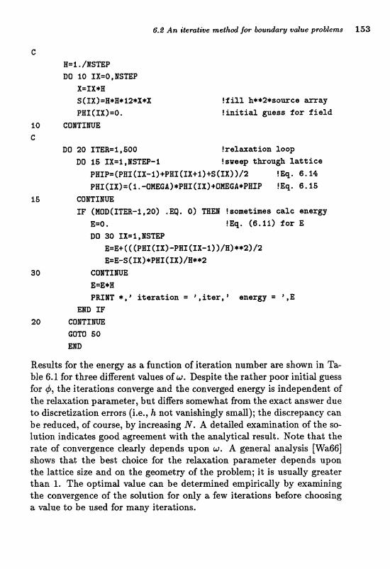
6.2 An i;tclrabiue method for kundarg vadus pmbkms 3153
C H=%. /ISmP DO 10 IX=O,ISmP
X=IX*B S(ZX)=B*H*I2*X+X !fill h**2taomcs PHI C X X ) = ~ . ?iafffal guess for f i e l d
10 CORTZlB(iJ1E C
DO 20 ImR=i ,500 !rsla.alion loop DO iS %X=1,1STW-l !sweep tkoagh laittice
~ r r r ~ = ~ ~ a n ( r ~ - ~ ~ + ~ a x ~ x ~ + i ~ + s ~ ~ x ~ ~ t ~ !Q. 6.34
PHI (rz>=<i. -~MEGA)+PHI[IX)+OMEGA*PE~IP FE%. 6.15 15 COmf Em
IF (HQD(XTER-1,201 .me 0) mm ! soaretimes talc energy E=O . t ~ , (e,gi> E DO 30 IX=l,BS%P
E=E+ C ( P H ~ (IX)-PBX (IX-i> >/fx>**2)/2 R=E-~(Z~I*P~I(IX)/I~*+~
CQ#TIBrNE ]E=E+B PRIIT *,# itssation = ',itsr,Qensra = \,E
Ern IF 20 G O m X m
GOTO 50 =D
Resufts for the enere;y as a fnnct;iart of iteration number we shmn in Ta- ble 6.1 for t h r ~ &Rerent vdues of u, Desgite the rather pom initid guess for #, the iterations converge m d the converged eaergy is independent of the relaation pafameter, but digers ksomewhtat h a n the exact answer due to discretization enors (i.e., h not vanishingly small); the discrepancy can be reduced, af course, by increshsing N. A detiled =amination of the so- lution indicates good agreement with the analyticd result. Note thitt the rate of convergence clearly depends upon U. A general analysis [Wa66] shows that the best choice far the relwation pa rae t e r depends upan the lattice size arrd on the &-metry af the problem; it is u s u d y $reater thm 1. The ap%irnd d u e can be determined empiriedly by exadning the convergence of the solution for only a few iterations befare chooaing a d u e to be used for many iterations.
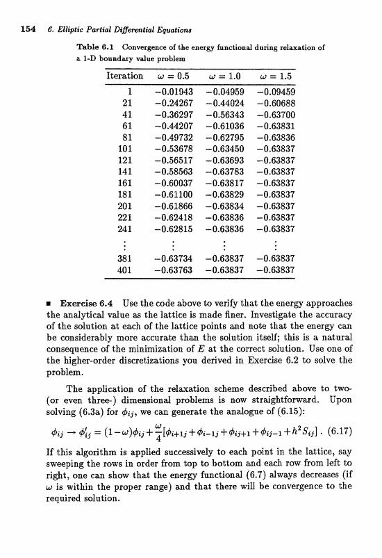
154 6. Elliptic Partbl Difirenttaf Equations
Table 6.1 Ca~vergence af the energy functiand dnkng relaxation sf a l-D bounday vdtlue problem
Iteration = 0.5 o = 1.0 w = 1.5
Exercise 6.4 Use the code above to vefify that the e n e w approaches the analytical vdue as the lattice is made finer, Investigate the accuracy of the soiutioa. at each of the lattice points and note thatt the enerw can be considerably more accurate than the sdutim itself; this is a naturd consequeaw of the minimization of E at the comeet solution. Use one of the higher-order discretizations you derived in Exercise 6.2 to solve the problem.
The itppdication of the relaxation scheme described above to two- (or even three-) dimensional problems is now straightforward. Upon solving (6.3a) for 4i j , we can generate the analogue of (6.15):
If this algorithm is applied successively to each point in the lattice, say sweeping the rows in order from top to bottom and each row from left to right, one can show that the energy functional (6.7) $ways decreases (if w is within the proper range) and that there will be convergence to the required golution,
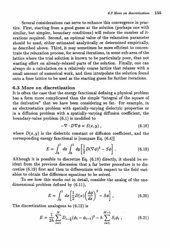
Several emsideratioas c m seme to enhance this convepnce in prac- tice. First, starting from a good guess at the solution (perhaps one with simitar, but simpler, boundary conditions) will reduce the number of it- erations required. Second, an optimal d u e of the relaxation parameter shoufd be used, either estinrahd a;nalyticdy or determined empiricay, W described abave. Third, it may sometimes be more efficient to concen- trate the relaxation process, for several iterations, in some sub-area of the lattice whex the trial sdution is k m n to be particularly poor, thus not wasting effort on already-relaxed parts of the solution. Finally, one can always do a calculation on a relatively coarse lattice that relaxes with a s m d amount of numerical work, aad then interpalate the solution found onta a h e r lat2;ice to be used as the s t e i n % guess for further iterations.
6.3 More on discretiza$iam It is often the c a e that the energy functimaf defining a physicaf problem has a form more complicated than the simple "htegrd alof the square oi' the derivativrs'9that we have been considering so far. lFor example, in m dectrostaties problem with spatidy-varying dielectric properties or in a &@usion probfern with zb spatidly-varying diffusion caeBcie?nt, the boundary-value problem (6.1) is modified to
where D ( s , y) i 8 the dielectric constant or difigion eoeificient, and the corresponding energy functional is [compare Eq. (6.4)]
Although it is possible to discretize Eq. (6.18) directly, it should be ev- ident from the previous discussion that a far better procedure is to dis- cretize (6.19) first and then to differentiate with respect to the field vari- ables to obtain the diEermee equations to be d w d .
To see how this works out in detail, consider the analog of the one- dimensional problem defined by (6.11),
The discretization andagous to (6.12) is
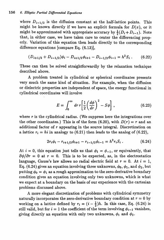
E56 6. Elfliptic Partial Diflema#id Equations
where Di-1/2 is the diffusion mnstant at the half-lattice points. This might be known directly if we have an explicit formula for D(%), or it might be approximated with appropriate accuracy by $ (-Di + ~ i - l). Note that, in either case, we have taken care to center the diEerendng prop- erly. Variation of this equation then leads directly to the corresponding difference equations [compare Eq. (6. U)],
These can then be solved straightforwardly by the relaxation technique described above.
A problem treated in cylindrical or spherical coor&aat;es presents v(3f~ much the s m e kind of situta2;ian. For example, whea the diffusion or dielectric properties are independent of space, the energy functional in cylindricd cooranates wiB involve
where r is the cylindricad radius. (We suppress here the integrations over the other coordinates.) This is of the form (6.201, with D(T) = r m d an additional factor of r appemiag in the source i&graX. Discretization on a lattice ri = hi in analogy to (6.21) then leads to the analog of (6.221,
At i -- 0, this equation just t d s us that rpL = or equivdentfy; that @+/@F = 0 at T = 0. This is to be expected, as, in the electrostatics l a n g a ~ e , Gauss" llaw allows no radial electric field at r = 0. 1"IC i = 1, Eq. (6.24) gives an equation involving three unknowns, +a, and 42, but putting 450 = W a rough approAmation ta the zero-derivatim boundwy condition gives an equation involving only t w unknowns, whi& is what we expect a% a boundary on the basis of our experience with the ca_rtesim problems discussed above.
A more elegant discretization of problems with cylindrical symmetry naturaUly incorparatw the zero-derivative baunda~y condition at F =r. 0 by working on a lattice defined by = ( i - 3)h. In this case, Eq. (6.24) is still v&d, but for i = 1 the eoeffieient oftbe term involving $i-2 m&~hes, giving directly an equation with only two unknowns, 41 and #z.
6.4 Elliptic equations in iwo dimensions 157
Exercise 6.5 Verib that variation of Eq. (6.21) leads to Eq. (6.22). Write down explicitly the discretizations of Eq. (6.23) on the Ti = ih and ri = ( i - f )h lattices and verify their variation leads to (6.24) in either ease. Why can the contribution to the ener$y funet iod from the region between r = O and F = # h be safely neglected on the ri = ( i - $)h lattice to the same order as the accurxy of approdmation used for the derivative?
6.4 Elliptic equations in two dimensions The application of relaxation methods to elliptic boundary value prob- lems is illustrated by the program for Example 6, which solves Laplace's equation, V2+ = 0, on a uniform rectangular lattice of unit spacing with Dirichlet boundary conditions specified on the lattice borders aad on se- lected paints Psithin the lattice, This situattion might describe the shady- state temperature distribution within a plate whose edges and certain interior regions we Held at specified temperatures, or it might describe an dectrostatics problem. speGiEed by a nuIliber of equipotentid surfwes. During the iterations, the potential is displayed, as is the energy func- tional (6.7) to monitor convergence. The code's source listing c m be found in, Appendix B and in the file EXMPL6.E"OR.
The following exercises, phrased in the language of electrost atits, might hdp you ta understaind better the physicd and numeric& prindpres ilfustrated by this example.
m Exerelsc? 6.6 Vctrify that- the sdutions comesponding to particular boundary conditions in the interior af the lattice agee with your into- ition, You might try M n g a single interim point to a potential &Rereat ;from that of the boundary, Ring tvvo symmetricalfy located points to different potentids, or fixing a whole line to a given potential. Other pas- sibilities include constructing a "Faraday cage" (a closed region bounded by a surface at fixed potentid), studying a quadrupaie pattern of bound- ary cmditians, or cdculating the capacitance of various configurations of conductors. Study of what happens when you inerease or decrease the size of the 1at;tice is dso interestiw.
m Exercise 6.7 For a given set of boundary conditions, investigate the effects of under-relaxation and over-relaxation on the convergence of the relaxation process. Change the discretization of the Laplacian to a higher- order formula as per Exercise 6.2 and observe any the changes in Ihe solution or the eficiency with which it is appmached.
Exmcise 6.8 Modify the code to solve Poissonk equation; i.e., d o w for a charge density to be specified throughout the lattice. Use this to study the solutions for certain. simple charge distributions. For exam- ple, you might try computing the potential betwen two (line) &ages as a function of their sepafation and comparing it vvith yonr malyticd apec t ationa.
W Exe-reisfs 6.9 Modify the code to use Neurnann boundary conditions on sdected borders and iderior regions of the l a t t i ~ , Study the solution for simple geoanetries and compare it with what ycru expect.
r Exercise 6.10 Modify the code to allow for a spatidy-varying dielec- tric constant. (Note that you must change both the relaxation formula and the energy functional.) Study the solutions for selected simple ge- ometries of the dielectric constant (e.g., a half-space filled with dielectric) and simple boundary conctitions,
W Exereiscl 6.11 An dter~at ive to the Diridlet bounday conditions are periodic boundary conditions, in which the potedials on the left and right and top and bottom borders of the rectangle are constrained to be equd, but otherwise afbitraq. That is,
for all i and j . This might correspond to the situation in a crystal, where the charge density is periodic in spaee. Modify the code to incorporate these boundary conditions into Poisson's equation and verify that the solutions look as expected far simple &age distributions.
m Exercise 6.12 Change the relaxation formula and energy functional to treat situations with an wimudhd symmetry by re-interpreting one of the coordinates as the cylindrical radius while ret4ning the other as a cartesim coordin&e. Use the resulting pragrm to mod4 a eapacitof made of two circular disks, and in particular calculate the capacitance and potential field for varying separations between the disks. Compare your results with your expectations for very large or very small separations.
Project VI: Steady-state hydrodynamics in two dimen- siorrs The description of the flow of fluids i s one of the richest and most chd- lenging problems that can be treated on a computer. The non-linearity of the equations and the complexity of phenomena they describe (e.g., turbulence) sometimes make computational fluid dynamics more of an
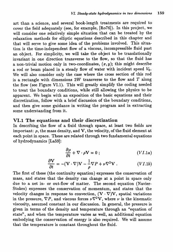
art than a science, and several book-length treatments are required to cover the Geld adequately (see, for example, [Ro76]). In this project, we will consider one relatively simple situation that can be treated by the relaxation methods for elliptic equations described in this chapter and that will serve to give some idea of the problems involved. This situa- tion is the time-independent flow of a viscous, incompressible fluid past an object. For simplicity, we will take the object to be translationally invariant in one direction transverse to the Bow, so that the fluid has a non-trivial motion only in two-coordinates, (I, g); this might describe a rod or beam placed in a steady flow of water with inddent speed Vo. We will also consider only the case where the cross section of this rod is a rectangle with dimensions 2W transverse to the fiow and T along the flow (see Figure VI.1). This will greatly simplify the coding needed to treat the boundary conditions, while still allowing the physics to be apparent. We begin with an exposition of the basic equations and their discretization, fouw with a brief disevssion of $he boundmy eon&tions, and then give some guidance in writing the pragarn and in a t r x t i n g some understanding from it.
VI.1 The equations and their discretization In describing the flow of a f i ~ d through spxe, at least two fields are important: p, the arms den~ity, and V, the vdacity, of the Aluid eft3ment at ea& point in space. These are related throu& two fundamental eqnatims
The first of these (the continuity equation) expresses the conservation of mass, and states that the density can change at a point in space only due to a net in- or out-flow of matter. The second equation (Navier- Stokes) emresses the emserva%ion of momentum, ltnd states thaL the velodty changes in response to convection, (V g V)V, spatial variations in the pressure, VP, and viscous forces pV2V, where U is the kinematic viscosity? arisunzed constant in our discussian, In generd, the pressure is given in brms Of the density and temperature through an "equation of state'" and when the temperature vwiee3 m weB, m addition& equation embodying the conserntion of energy is dsa required. We win assume: that the temperature is constant throughout the fiuid.
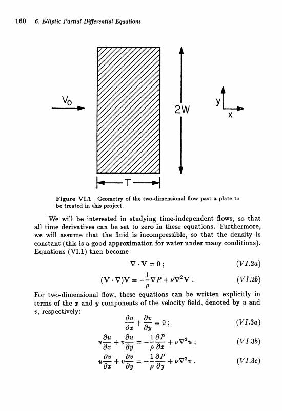
l60 6. Elliptic Partial Digerential Epations
Figure VI.1 Geometry of the twdinrensiond Aow past a pfa~Ie to be treated in this project,
We vviU be interegted in studying time-independent fioars, so that time derivative8 can be die2 to zero in them equations. firthermore,
we win assume that the fiuid is incompressible, so that the density ia constant (this is a good approximation for water under many conditions). Equations (VI.1) then become
V*"GI=O; (V1.2~)
1 (V* V)V = --VP+vv2v. (V1.2b)
P For two-dimensional flow, these equations can be written explicitly in terns of the I and y components of the velocity field, denoted by zl and v , respectively:
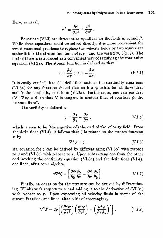
Equations (VL3) are three scalar equations for the fields u, v, and P. While these equations could be solved directly, it is more convenient for two-dimensional problems to replace the velocity fields by two equivalent scalar fields: the stream function, $(z, g), and the vorticity, ((S, g). The first of these is introduced as a convenient way of sa-ti~fyiag the continuity equation (VI.3a). The stream function is defined so that
It is easily verified that this definition satisfies the continuity equations (VI.3a) for any function $ and that such a + euists for all flows that satisfy the continuity condition (VI.2a). hrthermore, one can see that (V = V)$ = 0, so that V is tangent to contour lines of constant +, the "stream lines".
The vorticiey is defined a8
which i s seen to be (the negative of) the curl of the velocity field. From the definitions (VI.4), it follows that C is related to the stream function 'Ztt by
v2+ = C = (V1.6)
An equation for C can be derived by differentiating (VI.3b) with respect to y and (V1.3~) with respect to I. Upon subtracting one from the other and invoking the continuity equation (VI.3a) and the definitions (VI.4), one finds, after some dgebra,
Findly, an equation for the pressure can be k i v e d by diaereal;i&- ing (VI.3b) with respect to z and adding it to the derivative of (V1.3~) with respeet to ye Upon expressiag a;LI velocity fidds in tezm~ of the s t r e m function, one finds, dter a bit of rearrm@ng,

162; 6. BllipEic Partial Riflerential Eqwotionkr
Fimrct Vf .2 The lattice to be used in c&culathg the fluid flow P~ISTL the plate illustrate;$ in Figure V1.1,
Equations (VI.6-8) are a set of non-linear elliptic equations equiva- lent to the origind hydrodynamic equations (VI.3). They are particularly convenient in that if i t is just the velocity field W wmt, ody tne two equations (VI.6,7) need be solved simultaneously, since neither involves the pressure. If we do happen to want the pressure, it can be obtained by solving (VI.8) for P after we have found + and C.
To solve Eqs. (VI.6,7) numerically, we introduce a two-dimensiond lattice of uniform spacing h having N, and N, points in the r and y directions, respectively, aod use the indices i and j to measure these coordinates. (See Figure VL2.) Note that since the centerline of the rectangle is a line of symmetry, we need only treat the upper half-plane, y > 0. Moreover, it is convenient to place the lattice so that the edges of the plate are on lattice points. The location of the plate relative to the up- and downstream edges of the lattice is arbitrary, although it is wise to place the plate far enough forward to allow the 'Lw&e" to develop behind it, yet not too close to the upstream edge, whose boundary conditions can influence the flow pattern spuriously. It is also convenient to scale the equations by measuring all lengths in units of h and all velocities in units of the incident Buid velocity, Vo. The stream function is then measured in units of &h, while the vorticity is in units of &/h, and the
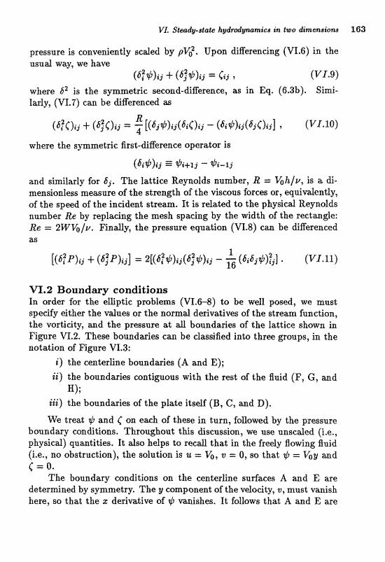
VI. Steodg-stab ftyddgnamr'cs in two dimensions 3.63
pressure is conveniently scaled by pv. Upon differencing (VI.6) in the usud way, we have
(8; @)id + (fi!+)ij = Cij 9 (V1.9)
where 62 is the symmetric second-difference, as in Eq. (6.3b). Simi- larly, (VI.7) can be differenced as
where the symmetric first-difference operator is
and similarly for The lattice Reynolds number, R = &h/v, is a di- mensionless measure of the strength of the viscous forces or, equivalently, oE the speed of the incident stream. It is rdated to the physical Reynolds a m b e r Re by repking the mesh spacing by the width of the reetage: Re = 2WKIv. Finally, the pressure equation (VI.8) can be differenced as
VI.2 Boundary conditions In order for the elliptic problems (VI.6-8) to be well posed, we must s p e w either the d u e s or the narmd derivatiws d the dream. function, the vorticity, md the pressure at boundaries of the lattice shown in F i p r e VI.2, These boundaries c m be classified into three groups, in the no ta im af Figure VX.3:
i) the centerline boundasies (A and E); ii) the boundaries contiguous with the rest of the fluid (F, G, and
H); iii) the boundaries of the plate itself (B, C, and D).
We treat t$ and (' on each of these in turn, followed by the pressure boundary conditions. Throughout this discussion, we use unscaled (i.e., physical) quantities. It also helps to recall that in the freely flowing fluid (i.e., no obstruction), the solution is u = V& v = 0, so that II, = Voy and 5 = 0.
The boundary conditions an the centerline su&aces A md E are detemined by symmetry, The y camponeat of the velocityf v, must vanish here, so that the 2 dell-ivative of $ mnishes. It follows that; A and E are

l64 6, Elliptic Partial Eziflerential Eguations
Figwe VI.8 Boundw candjitionsr to be i m p a d on the stream func- tion and vorticity.
each stream lines. Moreover, since the normal velocity (and hence the t angentid derivative of +) also s h ~ on B, C, and D, the entire snrfaee ABCDE is a single stream line, and we may arbitrarily put $ = O on it. Note that the velodties depend only upon the derivatives of +, so that the physical description is invariant to adding a spatially independent colnstant to the s t r em funetion; the ef io i~e of $l on this stmmEne fix@@ the constant. Ekom syanmetry, we can also conclude %h& the vortidty vmishes on A, and E.
The boundary conditions on the upstream surface F are also fairly straightforward. This surface is contiguous with the smoothly flowing incident Auid, so that specifying
as is the case far upstream, seems reasonable. Similarly, if the lattice is large enough, we may expect the upper boundary G to be in free flow, so
is one appropriate choice. The downstream boundary H i s much more am- biguous and, as long as it is sufficiently far from the plate, there should be
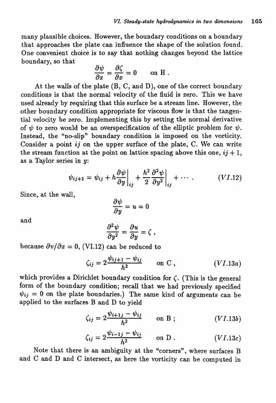
many plwsible choices, Hawever, the boundary coar&tions on. a boundary that approahes the plate can influace the shape of the solutioa foa~d. One conveaient ghoice is to say that nothing changes beyond the lattice boundarv. so that
At the walls of the plate (B, C, and D), one of the correct boundary conditions is that the norxxlairl velodty of the Buid is zero. This we have used &ready by ~ t q d r i a g that this surface be a sr;tream line, Wowever, the other boundary condi.eion appropriate for viscous Am i s that the tmgea- tid velocity be zero. hplementing this by setting the normal derivative of $ to zero wauld be aa overspecific&ian of the emptic prObkm for $J, Irtstead, the "na-sEp" boundary condition is imposed on the vodieily; Consider a point z'j m the upper surf"ace of the plate, C. We c m write the s t r e a fanctian at the point on lattiw spacing above this one, i j -+ l, as a Tqlor series in 9:
Since, at the wall,
and a2+ a% -=."m-=
ay2 @Y C 5
because av/@z = 0, (VI.12) can be reduced to
which provides a Dirichlet boundary condition for C. (This is the general form of the boundary condition; recall that we had previously specified eij = O on the plate boundaries.) The same kind of arguments can be applied to the sudaees I3 and D to yield
Note that there is an ambiguity at the 'corners", where surfaces B and C and D and C intersect, as here the vorticity can be computed in
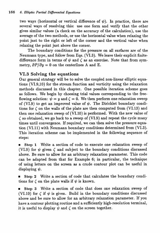
two ways (horizontal or vertical difference of $l). In practice, there w e severd ways of resolving this: use one form and verify that the other gives similar values (a check on the accuracy of the calculation), use the average of the two methods, or use the horizontal value when relrwring the point just to the right or left of the corner and the wrticd vdue when rel&ng the poine jlrst above the cosaer,
The boundary cmditians for the pressurn on ~uflf(izce~ we of the Neumann type, and follow from Eqs. (VI.3). We leave their explicit finite- agerence form in terms of $ and. f as m exercise, Note that from sym- metry, aPl8y = O on the centerlines A and E.
VI.3 Solving, the equations Our general strategy will be ta d v e the coupled non-linear @Uptic equa- tions (VI.9,10) for the stream function and vorticity using the relaxation methods discussed in this chapter. One possibb iteration scheme $aes as follotirs. We bedn by chwsing trial vdues comc3span&ag to the free- flawing solution: 2E, = y and f =. O , We then perform one relruration sweep of (VI.9) to get an improved d u e of +. The Dirichlet boundary condi- tions for ( on the walls of the plate are then computed from (VI.13) and then one relaxation sweep of (VI.10) i s performed. With the new value of C so obtained, we go back to a sweep of (VI.9) and repeat the cycle many times until convergence, Xf required, we can then salve the pressure equa- tion (VI.11) with Neumann boundary conditions det ned from (VI.3). This iteration seherne can be implemented in the fauowing sequence of steps:
m Step X, Write a section of code to execute one relmatiorz sweep af (VI.9) for given C and subject to the boundary conditions discussed above. Be sure to d o w for an arbitra3i.y ~ e l m a t i ~ n parameter* This code c m be dapted from that for Example 6; in gmtiedaf, the technique of using letters on the scrwn as a crude contour plot can be useful in displibying +.
Step 2 Write a section of code that cdculates the boundary condi- tions for on the da t e wdls if $J is known.
m Step 3 Write a section of code that does one relaxation sweep of (VI.10) for C if i j , is given. Build in the boundwy conditions discussed above and be sure to allow for an arbitrasy relaxation pmameter. If you have a contour plotting routine and a sufficiently high-resolution terminal, it is usefrt2 to display w d C on the screen together.
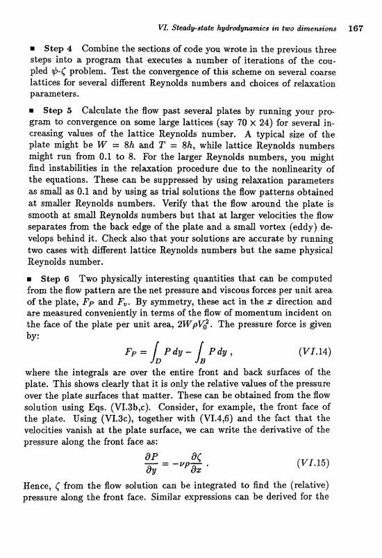
Step 4 Combine the sections of code you wrote in the previous three steps into a program that execute6 a number af itera;tions of the em- pled $-C problem. Test the convergence of this scheme on several coarse l a t t i e ~ far several different Eeynolds ~umbers and chaices af relzwration parameters.
Step 5 Calculate the flow past several plates by w i n g your pro- gram to convergence on some large lattices (say 70 X 24) for several in- creasing values of the lattice Reynolds number. A typical size of the plate might be W = 8h and T = 8h, while lattice Reynolds numbers might run from 0.1 to 8. For the lager Reynolds numbers, you might find instabilities in the relaxation procedure due to the nonlinearity of the equations. These can be suppressed by using relaxation parameters as s m d as 0.1 and by using as trial solutions the fiow patterns obtained at smaller Reynolds numbers. Verify that the flow around the plate is smooth at small Reynolds numbers but that at larger velocities the flow separates from the b a d edge of the plate and a small vortex (eddy) de- velops behind it. Check also that your solutions are accurate by running two ernes with digerenit lattice Eeynolds numbers but the same physicd fteynolds numb=.
m Step fi Ttvo physicdly interesting quaatities that can be compu.t;ed from the flow pattwn we the net pressure and vis~ous forces per unit area of the plate, FP and F@, By spnnetry, these act in the z directian and are measured conveaientfy in tarns of the flow of momentum incident on the face of the plate per unit area, 2Wpr/02. The pressure force is given
where the integrals are over the entire front and back surfaces of the plate, T h i s shows dearly that it, is only the rdative d u e s of the pressure over the plate surfaces that matter. These can be obtained from the flow solution using Eqs. (VI.3b,c). Consider, for example, the front face of the plate. Using (V1.3~)~ together with (M.4,6) and the fact that the velocfties vmish at the plate surface, we can write the &rivif,tie of the pressure along the front face as:
Hence, C from the Bow solution can be integrated to find the (relative) pressure along the front face. Similar expressions can be derived for the
3.68 6". Elliptic firdial Bigerential Equations
top and back faces, so that the pressure (apart from an irrelevant additive constant) can be computed on all faces by integating up the front face, across the top, axld dawn the back face. The net viscous fbm per unit area of the plate is due only to the flaw past the top (and bat tom) surfaces and is given by
However, since the boundary canditions on the top surfwe of the plate require av/8z = 0, this can be written as
wfsieh i s conveniently ev;iiuat;c;d from the flow solation- fnvestigate the v ~ i a t i o e of the viscous and presjsure forces with Eeynolds number and compare your re8uXt.s with vrvhat you expect.
Step 7 Three other geornedries can be investigated wit;& ody nrinar modifications of the code you've constructed. One of these is a Ujumg", in which. the thickness of the plate is increased until its Bownstrem edge meets the downstream border of the lattice (H). Another is a pair of rect- angular plates placed symmetrically about a centerline, so that the fluid can flow between them, as well around them (a crude nozzle). Finally, two plates, one behind the other, can also be calculated. Modify your code to treat each, of these cases and explore the flow patterns a% various Reyndds numbers.
Chapter 7
Differentia Equations
Typical parabolic pwtid differential equations one encounters in physical situations are the diffusion equation
where D is the (possibly space dependent) digusion constant and S is a souree fun&ian, and the time-dependent Schroedinger equation,
where V is the poterrtid, In cantrat to the boundary d u e problems encountered in the previms clrapter, thesje problems me generdly of the initial d u e type. That is, we are @wn the field 4 at an initid time and swk ta find it at a later time, the evolutian being subjtsct to ccjrtgn spatial boundary conditions (e.g., the Schroedinger wave function van- ishes at very large distaaces or the temperature or he& flux is specified on some surfaces). The methods by which such problems are solved on the computer are b a s i d y straightforward, although a few subtfeties are involved. We will dm see thiLt t h q provide a n&ur& way of solving eEp- tic eigetnvdue problenrs, particdasly if it is o d y the few lowest or highest eigenvdues that we required.
7.1 Naive discretization and instabiliitie~ We begin oar diseus~ian by treating digusion in one dimension with a uniform diausion constant. VVe take z to vmy between 0 and 5 and a6sume Diriehlet boundary conditions that s-pedfy the valiue of the fi&d

170 7. Pambslic Partial Diflemntial Eqaotions
at the end points of this irrtervd. After appropriate scalirtg, the andague
As usud, we appru~mate the spatial derivatives by finite diRerenees an a uniform lattice of N + 1 points having s p i n g h = 1/N, while the time derivative is apgmdmated by the simpkst first-order diAFerexzce fomala assuming a time step A$. Using the supesacript .n: to l&d the tirncl step (that is, I 4(t,), 1, = nag), we can approximate (7.3) as
At i = 1 and i = N - 1, this equation involves the Dirichlet baundasy conditions specifying fbo and + N .
Equation (7.4) is an ezplicit differencing scheme since, given q5 at one time, it is straightforward to solve for 4 at the next time* Indeed, in an obvious matrix notation, we have:
where the action of the operator E is defined by
As an exmple of haw this expUcit acheme d g h t be applied, consider the case where S = O with the boundary conditions #(O) = 4(1) = 0. Suppose that we are given the initial cundit;ion sf a Gausaian catered about 2 = 112,
where the latter two "image" Gaussians approximately ensure the bound- ary conditions at + = 1 and s = 0, respectively, and we seek to find # at later times. The following FORTRAN code applies (7.5) to do this on a fatdice with. R = 25.
G chp"l".Por PIRMmER (ISmP=2S) CIIMEHSIOI PEP (0 : I S T B ) ! ay f o r etalut ian
! iom of the malytical solutfon GAUSS (X ,T)=EXP(-20 *[X-, Q)**2/ (1.. +~o*T) )/SQRT< $+80*T> EXACT(X,T)=GAVSS(X,T)-GAUSS(X-~. pT)-GAPIS5(X+f.f.,T> H= =.I. /#STEP
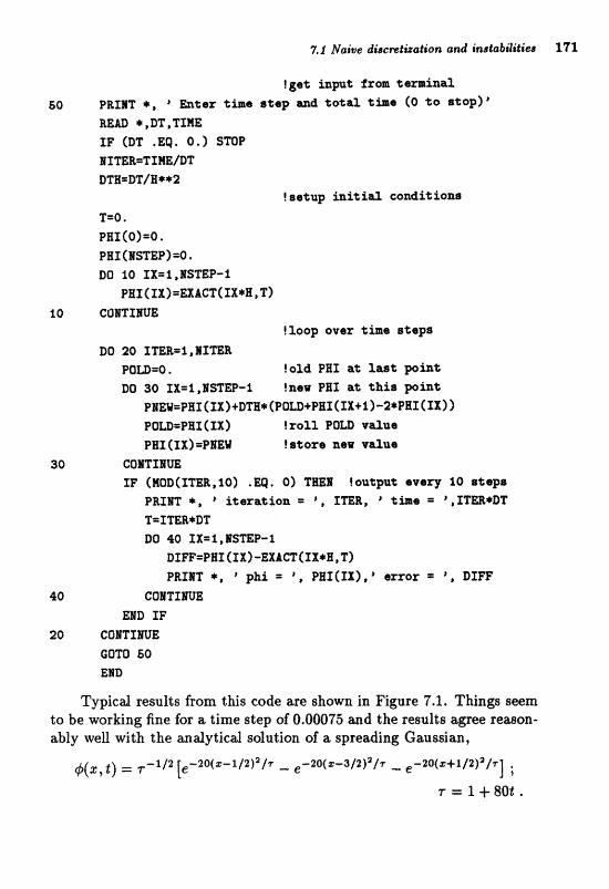
7.1 Naive diacmtizotion and indltabilities 111
!get input irom t e m i W
60 PRIaT *, R &%er tiars step and C D c a l tbs (Q t o s t o p ) ' RBAf) *,BT,TIME I F (DT .EQ. O ,) STOP MImR=TXMB/DT DTH=BT/E**2
T=O , Paxfo)=o. PHI(ISEP)=O I
DO 1 0 ZX=i,ISmP-1 ~ ~ ~ ( a x ) = a i ~ c l e t r x * a ~ T ~
10 COrnXrnE !loop aver time steps
DD 20 ImR=l,IXTER POD=O , !old PBX at l a s t ph* DO 30 XX=l,lS4I"W-I !aaw PHI a% this poh%
P ~ M = P B x ( I X ) + D ~ * ( P ~ U + P B X CII+1)-2*PHI (IX> 1 P O ~ = P H X ( IX) !roll P a w valtrs PEX (1x1 = P ~ V ?stars new v a n e
30 COVXXFIm I F (MOO(TTm,i0) .m, Q) mEl !@=%pm% evarg SO steps
PRIm *, "iteration = ,=B, t h s = #,X-*BT T=XmB*DT Da 40 ~ ~ = ~ D ~ $ ~ ~ ~ %
D I ~ = P E L crx)-gnm(ax*a, T)
PRIIT *, "hi \ PHI(XX),' emor R , DDTW 40 GOBTTXm
M D IF 20 60WIWE
GOTO fiO
EHIt
Typical results from this code are shown in Flgure 7.1. Things seem to be working fine far a time step of 0,00015 and the results agree reason- ably well with the matyticd solution, af a spreading Gau~sian,

172 7. Parablie Partial Diflemnts'al Equation8
This time step is, however, quite small compared to the natural time scate of the solution, t sc! 0.01, so that many steps are required before anything interesting happens. If we try to increase the time step, even to only 0.001, things go very wrong: an unphysicd instability develops in the numerical solution, which quickly acquires violent oscillations from one lattice point to another soon after t r= 0.02.
It is easy to understmd what is happening here. Let the set of states II?\ be the eigenfunctions of the discrete operator A with eigenvdues ex. Since R is an hemitian operator, the eigenvdues are real and the eigenvectors can be &wen to be orthonormial. We can expmd the solu.tian at m y time in this basis as
The exact time evolution is given by
so that each component d the solution should evolve as
This eorrespmds to the correct bebavior of the diEusion equation, where short-wavelength components (with larger eigenvalues) disappear more rapidly as the solution 'smooths out". However, (7.5) shows that the expLidt scheme will evolve the expmsian eoeScimts a9
As long as At i s chosen to be small enough, the factor in (7.6) approx- imates e-mt~.L\t and the short-wavelength components damp with time. However, if the time step is too large, one or more of the quantities 1 - exAt has an absolute value larger than unity. The corresponding components of the initial solution, even if present only due to very small numerical round-off errors, are then amplified with each time step, and soon grow to dominate,
To quantify this limit on At, we have same guidance in that the eigenvdues of H are known analytically in this simple madel problem. It is easily verified that the functions
Xni (+A)i = sin -
191
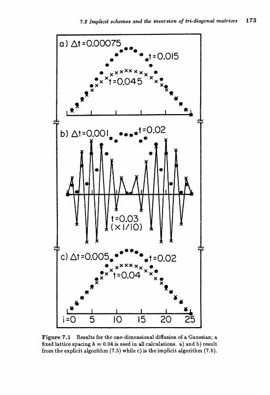
7,& Implicit; schemes and the inuer~irtn of trCdiagona2 matrims 173
Figwe 7.1 Results for the one-dimexldonal diffusion of a Grtussian; a fixed lattice sgaeing k rs 0.04 i~ used in. calculations, a) and b) result from the ex,pficit algorithm (7.5) while c) is the irnpEcit alg;orilhm (7.8).
174 7. Parabolic Partial Difierential Elquatiom
are (un-normalized) eigenfunctions of H with the correct boundary con- ditions on a lattice of N +- l points far X = 1, 2, . . , , N - 1 and that the assodilLed eigenvdues are
The largest eigenvalue of H is EM-I M 4hma, which corresponds to an eigenvector that; dternates in sign. from me latiee point to the next.
1 - ~ ~ - ~ A t l < 1 then restricts At to be less than $h2, which i s 0.0008 in the exmfle we are considering.
The questim of stabiEty is quite &stinct from that of zcuracy? as the lilnit impose4 on the time step is set by the spatial step used a d not by the characteristic time scde of the solutian, which is much larger. The expEcit scheme we have Biscusmd is ansatisfwtory, as the instabaity forms us to use a much smder time step thm is required to describe the evotution adequately. Indeed, the situatiorr. g a s ewn worse if we try to use a finer spatial lattice to obtdn a more accurate solution. Athough the restiction on At that we have derived is rigorous only for the simple case we ha-ve considered, it does pfctvide a useful gaide for more compEcated situations, W the eigenvector af H with the largest eigenvdue will dways oscillate from one lattice point to the next; it8 eigenvdue is therefore quite insensitive to the glob4 feat;ures of the problem.
n Exerdse 7.1 Use the code hove to verify that the i,nstabiEty sets in for smaller time steps if the spatial lattice is made finer and that the largest possible stable time step is roughly f h2. Show that the instability is present for other initial conditions, and that round-off causes even the exact lowest eigenfunction of E to be unstable under numerical time evolution.
7.2 Implicit schemes and the inversion of tri-diagonal ma- trices One way around the instability of the explicit algorithm described above i s to retain the general farm of (7.4), but to replace the second space derivative by that of the solution at the new time. That is, (7.4) is modified to
4 4 1 2 n+l
At = --(6 4 )i + S? * h2
This is an implieit scheme, since the unknown, +"+l, appears on both side of the equation. We can, of course, solve for #"+l as
1
7.1 Implicit scheme8 and the tneersisn of tri-dicganal matrices 175
This scheme is equivalent to (7.5) to lowest order in At. However, it is m& better in that larger time steps can be used, as the operator (1 + Bat)-' has eigenvdues (1 + exAt)-', all of whose moduli are less than I. for any At. All components of the solation therefore deersme with eaCh time step, as they should. Although this decrease is inaccurate (i.e., not exponential) for the most rapidly osdllating components, such cosnpsnents should not be large in the initid concllitions if the spatid discretization is accurate. In any eve&, there is no amplification, which impties stability. For the lowly varying wmpoaents of the ~olution ear- responding to s m d eigenvdues, the evolution closely approdmates the exponentid at each dim@ ajtep.
Note that; if m had tried to be more accurake than (7.7) and had used the average of Ghe second space defiva;tiws at the two time steps involved,
so that the time kolution is effected by
this wodd h w been h o s t as good as the implicit @&erne, because the c0mponent;s of the solution are diminished by fwtors whase absolute V ~ U E E S are lese t bm one,
A potential drawback of the implicit scheme (7.8) is that it requires the solution of a set of linear equations (albeit tri-diagonal) at each time step to find 4n+'; this is equivalent to the application of the inverse of the matrix 1 + Hat to the vector appearing in brackets. Since the inverse itself is time-independent, it might be found only once at the beginning of the calculation w d then used for all times, but application s t i l l requires of order N2 operations if done directly. Fortunately, the faflowing algorithm (Gaussian elimination and bzk-substitution, [Va62]) provides a very efficient solution (of order N operations) of a tri-diagonal system of equations such as that posed by Eq. (7.8).
Let us consider trying to solve the tri-diagonal linear system of equa- tions At$ =. b for %he unknowns $i:
Here, the A:" are the only non-vanishing elements of A and the bi are k n w n vasttities. This is the form of the problem posed by the evaluation

of (7.8) for where t$o and $N are given by the Dirichlet boundary conditions, In pafticular ,
To salve this system. of equat;ions, we assume that the sdution satisfies a one-term forward recursion relation of the form
where the c*i and pi are coefidents to be determined. Substituting this into (7.11), we have
which can solved for qSi to yield
with 1
Upon comparing Eq. (7.14) with (7.12), we can identify the following backward recur~iaa refation8 far the a" and P%:
= r i ( ~ t p j - bi) . (7.166)
The stratem to solve the system shodd naw be clear. We will use the recursion relations (7.15,16) in a backwards sweep of the lattice to d e t e r ~ n e the ai and pi for i running from dV - 2 down to 0. The starting vdlzes to be used are
which will guarantee the correct value oft$ at the last lattice point. Having determined these coefficients, we can then use the recursion relation (7.12) in a forward sweep from i = O to N - 1 to determine the solution, with the starting value q5o known from the boundary conditions. We have then determined the solution in only two sweeps of the lattice, involvinlg of arder N withmetic operations.
The foUowing code implements the algorithm (7.8) for the model diffusion problem we have been considering. Results are shown in Fig- ure 7 . 1 ~ ~ where it is dear that accurate solutions ean be obtained with a much larger time step than can be used with the explidt scheme; the
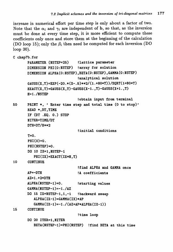
7,s Implicit scheme8 and the inversion of Ini.diagcmal madrias f 77
increase in numerical effort per time step is only about a factor of two. Note that the ai and -(i are independent of b, 8o that, as the inversion must be done at every time step, it is more effcient to compute these coefficients only once and store them at the beginning of the calculation (DO loop 15); only the Pi then need be computed for each inversion (DO loop 30).
G chapm.rfor PmAMmEB (ISmP=25) !lattice paa-mater DJMEgSIOB PBI(0:NSTEP) ?=ray for eola%ion PrmEsraH aLpaA(o:~s~~~),~rnh(o:~smpl , C R M N A C O : ~ ~ ~ S T E P ~
tmalflical soXu%iaa GAUS~(X,T)=~P(-~~,*[X-~~)**~/(~.+~Q*?~))/SQRT(~+~O*T) EXACT(X , T)=GAUSS (X, T)-GAUSSf X-S. ,T) -GADS$ (X+$ + ,T) EI=I. IISTEP
!abt&in h p a t fzem % @ m i n a 50 BBTm *, E h t e r tiS11~l s$ep d z;otal tbs (0 to e-t;op)*
R E 0 *,BT,TI#E XF (DT .EQ. 0 . ) STOP
L)TH=BT/H*+2
T=O. PPICO)=O. PHI ( I S ~ P ) =Q. DO l0 XX=$,'IPSmP-I
PHI ( EX) =EXACT( IX*H, T)
1 0 C O ~ I ] r J U &
! i h d &FHb md t?ArnB once AP=-Dm !A coeff icien$s AZ= i , +2*am ALPBA(~VSTEP-I)=o. Istwting valuaa G ~ ~ A < H S T B P - ~ I=- i . /AZ DO 5 = l - !backumd svsgip
ALPHA( E X - % ) =GAM[MA(IX) *l@ GAMA(XX-l )=-%, / (AZ+AP*ALPEfA (EX-1) 1
15 CQITImE: ! t h e loop
ao zo I T g R = i , g r m E BETA(EJSTEP-.I)=PHE(ESmP) !find BETA a t thisj; the
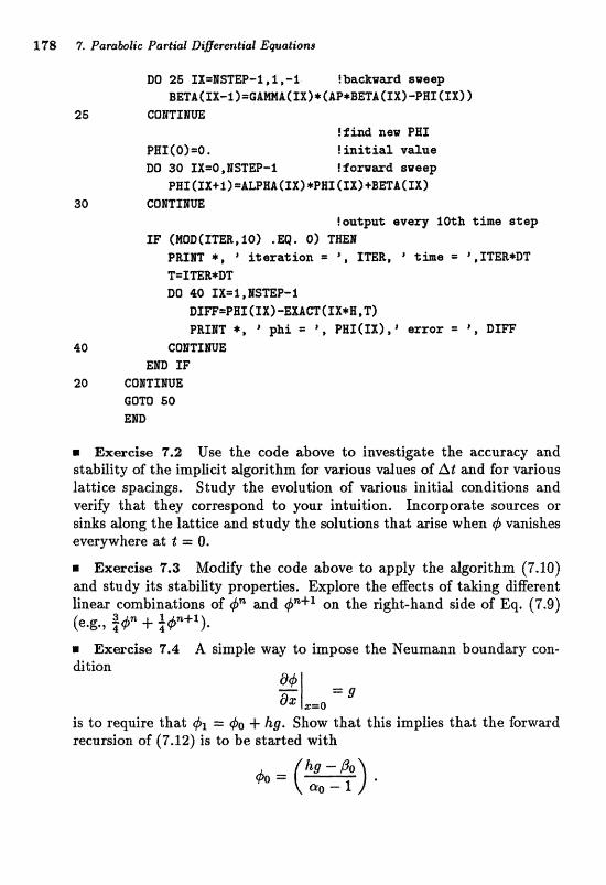
DO 25 IX=HSTW-~,X,-% Iba~kward sweep B~~(Ix-~)=GA~~~Ix~*~AP*BETA(IIC)-PBX~XX~ 1
comxm !find new Pfff
PHI (Q) =O. !a i$ ia l value DO 30 IX=O,ISTEP-1 ! fomad sweep
~ar(rx+l)=~~aa(xX)*PHICfx)+Elma~XX~ 601TI8W
!aa%pa% e v s q 10th time step IF fMaD(ITBR, IQ) .EQ. 0 ) THEI
PBfm *, "ee~a%ion = l , I=&, t b s = 8,XTEB+I)T T=T;mR*DT DO 40 IX=%,BfSmP-I
DIP=PHI (1x1 -EXACT( f X*E ,I'] PRXIT *, phi = \ PPHI(IX), Qrrox = 5 DIFF
40 CQHTIEFIJE; Ern fH
20 GOETIMUE GOTO 50 EBB
= Exrtrdm 7.2 Use tHe, code above to investigate the accurwy and stabady of the ixnpgcit dgorithm for various vdues of At and far vmious lattice spacings. Study the evdutim of various initid conditions and verify that they correspond to your intuition, Incorporate sourGes or ginks &ng the lat.tiee and study the solutions that arise when 4 vanishw everywhere st; t = 0,
m Exercise 7.3 Modify the code above to apply the algorithm (7.10) and stn* its stability properties. Explore the eff:ects of taking digereat linear combinations of 4" and #"+l on the right-hand side of Eq. (7.9) (e.g., $4" f a@"+'). m Exercise 7.4 A simple way to impose the Weummn boundary can-
is to require that ltbl = Gfto + hg. Show that this iropi_les that the forward recursion of (7.12) is to be started with
7.9 Diflusion and Boundary value problems in two dimensions l79
What is the analogms expression impfied by the more a~eur&e con- sGraLint 4% = #,% + 2hg? mat we the initial conditions for the backward recursion of the a and p coeacicients if Neunxann boundary caditions we imposed at the right-hand edge of the lattice? Modify the code above to incorporate the boundary condition that 4 have vanishing derivative at I = 0 (as is appropriate if an insulator is present in a heat conduction problem) and observe its effect on the solutions. Show that the inver- sion scheme for tri-diagonal matrices discussed above cannot be applied if periodic boundary conditions are required (i.e., @N = #@).
Exercise 7.5 Solve the boundary &e problem posed in Exerdse 3.4 by diseretization and iwer~ion of the resulting tri-diagonal matrix. Corn- pare your solution with those obtained by the Green's f~nction method and with %be andyticd resdt.
7.3 Diffusion and boundary value proble in t;wa dimen- sions The diseustsion above shows that diEusion. in one amension. is best handled. by an impliGit method and that the required inversion of a tri-&&&and matrix is a mlativtlly ~isnplle task. It is therefore nal;urat to attempt to extend, this approach to two or mare spatid dimensions;. For the two- dimensional dilfnsion equation,
the discretization is straightforward and, following our development for the one-dimensional problem, the time evolution should be effected by
where
Unfortunately, while H is very sparse, it is not tri-diagonal, so that the algorithm that worked so well in one dimension does not apply; some thought shows that H cannot be put into a tri-diagonal form by any permutation of its rows or columns. Wmw, the fact that W em be witten as ak sum of verators that sepatttely iavolve digerences only in the %" or g' indices:
X 80 7, Parvxbiolic Partial Llriflerential Epations
means that an expression equivalent to (7.17) through order At is
This c m now be eduaded exaetly, as ea& of the required inversions involves a tri-diagonal matrix. In particulw, if we define the auxiliary function 4n+1/2, we c m write
Thus, (1 + ~lj&t)-' is applied by forward and badtward sweeps of the lattice in the j direction, independently for each value of i. The applica- tion of (1 + Hiat)-' is then carried out by forward and backward sweeps in the i direction, independently for each value of j . This "alternating- direction" scheme is easiiy seen to be stable for all values of the time step and is generdized straightfommdfy to three dimen~ions.
The ajbility to invert a tri-&&%on& matrix exaetIy itnd the idea of treating mpwatdy each of the second derimtives of the Laplacia~ dso provides a dass of iterative alternating-direction methods [Wa66] for salv- ing the elliptic bsundmy value problems discussed in Chapter 6. The m a t ~ x i n v o l d is witten as the sum, of sewrd parts, each cont~ning second &Rerences in a d y one of the lattice indice@, h two dimensions, for example, we seek to solve [see Eq. (6.3b)j
If we add a term w 4 ta both side8 of this eqzxatios, where w is a can- sbant discvssed below, the re~ulting expression can be sdved for # in Wo dieerelrrd ways:
This pair of equations forms the basis for an iterative method of solution: they are solved in turn, 4 on the right-hand sides being taken as the previous iterate; the solution involves only the inversion of tri- diagonal matrices. The optimal choice of the @acceleration paramet er". w , depends on the matrices involved and can even be taken to vary from one iteration to the next to improve convergence. A rather complicated
analysis is required to find the optimal values [Wa@6]. However, a good r d e of thumb is to t&e
where cu and p are, respectively, lower md upper bounds to the eigenvdues of Ifi and Hi. In generd, these alternating direction methods are much mare efficient than the simple rdaxatioa scheme &iseu~hsed in Chitpter 6, dthough they are sfightly more: complicated to program. Wote that there is a stight campgcation when bounday conditions are also wecified in the interior of the lattice,
7.4 Iterative methods for eigenvalue proble Our analysis of the diffusion equation (7.1) shows that the net result of time wolutian is to enhance thorn components of the solution with snnder eigenvalues of E relative to those with laxger dgenvdacjs. Indwd, for very long times it is only that cornponeat Pviah the lowest eigenvdue that is sipificant, dthou& it has very snn& mplitude, This situat;ion sugests a sckeme for fin&ng the lowest eigenvdua of an el&ptic aperator, a8 de- fined by (6.2): guess a t r id eigenvector and subject it to a Gctitious time evolution that will "filtern it to the eigenvector having lowest eigenvalue. Since we are dealing with a linear problem, the relentlessly deereasing or increasing magnitude of the solution can be avoided by renormalizing mtinuoudy a63 time proceeds,
To make the discussion concrete, consider the time-independent Schroedinger equation in one dimension with h = 2m = 1. The eigenvdue problem is
with the narmazation condition
(4 can always be chosen to be red if V is). The corresponding energy functiond is
On general grounds, we know that E is stationary at an eigenfunction with respect to variations of C$ that respect the normalization condition and that the value of E at this eigenfunction is the associated eigenvdue.
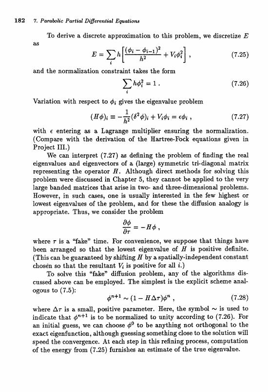
282 7, Pambalic Parlial Diflewntial Equations
To derive a discrete approkmation to this proMem, we discretize E
and the uram&zation constrdnt t&es the farm
Varia'cion with re~pect to g5i gives the eigendue problem
pJith E entering as a Lagrange maltiplittr ensuring the no~malization, (6ompwe d t h the, derivation of the Rartrw-f"o& eq~ations given in Project 111.)
We can interpret (7.27) as defining the problem of finding the real eigenvdues and eigenvectors of a (large) symmetric tri- diagond matrix representing the operator B. Although direct methods for sdving this problern were discussed in Chapter 5, they cannd be applied to the very large banded matrices that arise in two- and three-dimensimd prablems* However, in such ernes, one is usadly intemted in the few Mghes;t or lowest eigenvalues of the problem, and for these the diffusion analogy is appropriate. Thus, we consider the problem.
wkem r is a 'Y&en time, For convenience, we suppose that things have been arranged so that the lowest eigenvdue of X is positive definite. (This can be guaranteed by shifting B by a spatially-independent constant chosdn so that the regultant V;; Is positive for all d.)
To solve this "fake" digusion problem, any of the atgoritbms dig-
cussed above can be employed. The simplest is the explicit scheme and- ogous to (7.5):
4"+' - (1 - HAT)^^ , (7.28)
where Ar is a small, positive parameter. Kere, the symbol m i s used to indicate that is to be norm&zed to unity according to (7.26). For an initial guess, we can ehoose q5O to be anything not orthogond to the exact eigenfunction, although guessing something close to the solution will speed the convergence. At eadt step in this refining process, computation of the energy from (7.25) furnishes an estimate of the true eigenvdue.
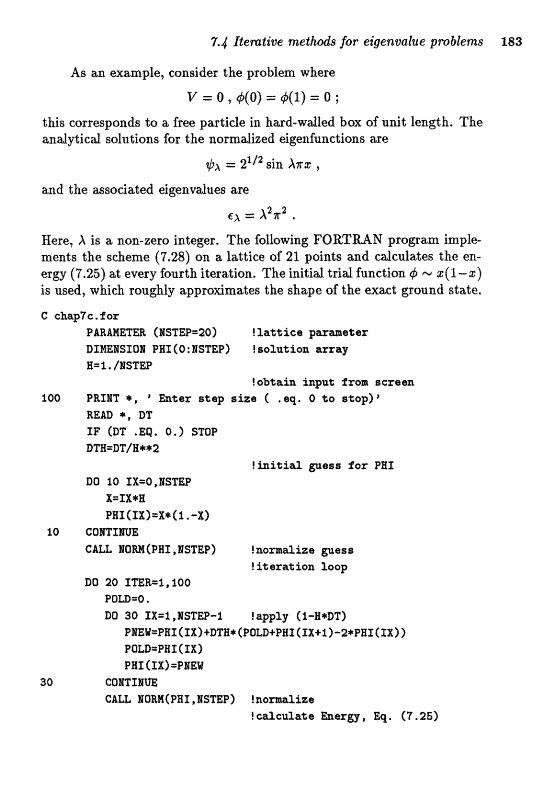
As an example, consider the problem where
this corresponds to a free partide in hard-walled bax of unit length. The anafytied solutions for the normatized eigenfnnctions as@
and the associated eigenvalues are
Here, X is a --zero integer. The following FORTRAN progam imple- ments the scheme (7.28) on a lattice of 21 points and calculates the en- ergy (7.25) at every fourth iteration. The initial trial funetion q5 %(l-s) is used, which rou&fy approdmates the shape of the exaet gzound state.
C ckap7c.for PBRAEETm (NSTW=20 f la%%i68 parneter DT~ISIOI PHI CO : I S ~ P ) ! scx~tio~ E= r , /BSTEP
! obtah inpa% irom screen %OQ PRIIT *, R &tar step size ( ,sq. O to stop)R
BEAE) *, DT
XF (DT .EQ, Q. ) STOP DTE=BT/t3**2
!initial guess for PBX DQ 10 IX=O,BSmP
X=IX*H arrx(xx>tx+( i , - X )
10 COrnIrnE: CALL I Q a (PBX ,'lQSTEP] t nomaize guess
! f t era% ion loop DO 20 f TEE=%, 200
POrn=O * DO 30 IX=I,ISTP-I !apply [%-E*DT)
P%EV=PEZ (IX )+DTB* (POf,D+PEII ( I21+1)-2*PIXI (XX) ) POU=PBf (IX) PEILS (IX) =PHgv
30 COmXMa
! caJccaa%e hergy, Eq. (7.25)
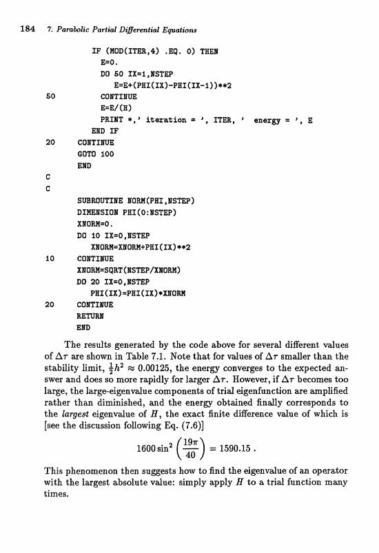
184 7. Parobolic Partial Bifierenlial Bpations
E=E+ (PHI (IX) -PE1 (IX- 11 )**S? 50 68m11fila
PRSIT * , I itera%ion = \ ITER, energy = ', E mT) XF
SWWVTXMEZ HOW (PHI, BilSTEP) RImISIOl PHX(0:HS"X"EP) XIORM=O. DO 10 TX=Q ,ISTEP
mOM=X;1POEH+B&XCIX)**2 l. Q COmSmE
XNORB=SqRT(BTSTEP/XHORN> DO 20 TX=O ,BSmP
Pax(xx)=PEI(xx)+maw 20 COWXmE.
RErnW END
The xsufts generated by the code above for severd diEerent vdues of AT me shown. in Table: 7.1 Note that far vatues of AT ~f~l&er than the stability limit, $ hZ fi. 0.00125, the energy converges to the expected an- swer and dws so more rapidly for larger AT. Eowever, if AT becomes too large, the large-eigenvdue componeats of trid dgenfuactian me aplified r&her than diminished, and the eaerD obtdned finally wrresponds to the lawest eigenvdue of H , the exact fisite diEerenw value of which is [see the discussion following Eq. (7.6))
Tkis phenamenm then sugesgs h m to find the eige~value af: an operator with the largest absolute value: simply apply H to a trial function many times.
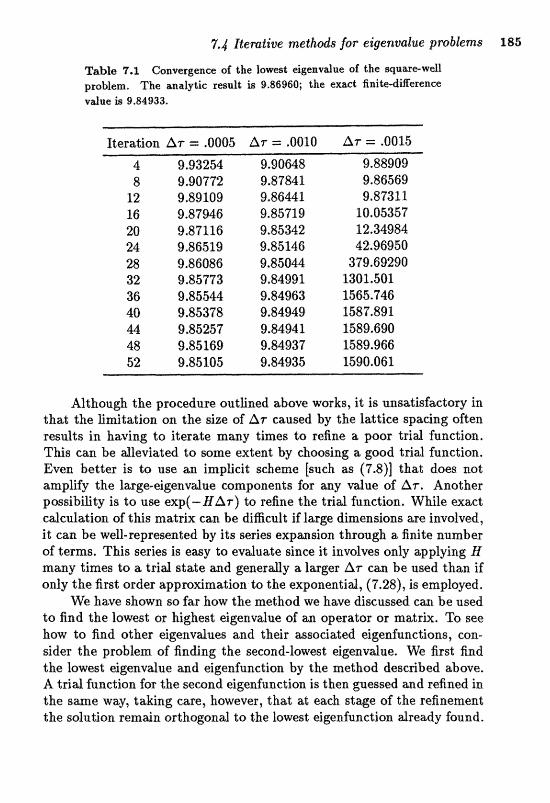
7.4 Itemtive methodsfor eigenvalue problems 185
Table "11 Ganvergence a-f the lowest eigenvdue of the maare-wdl problem. The analytic rmult L 9.85960; the e x a t finile-difference vdue is 9,84933.
Although the procedure outlined above works, it is unsatisfactory in that the Braitation on the size af AT caused by the laLtice spacing often result;s in having to iterate many times $a refine a, poor trid function. This can be alleviated to some extent by choosing a good trial function. Even better is to use an implicit scheme [such as (7.8)] that does not amplify the large-eigenvalrue eamponents for my value of AT, Another possibility is to use exp(- HAT) to refine the trial function. While exact c d d a t i o n of this nrzltrix can. be diseult if large dimensionrs me imvdved, it can be wea-=presented by its series expmsion tbrougb a finite nunrber of terms. This series is e a y to evduaLe since it involves only applying _IS many times ta a trial ~ t a t e and generay a larger AT can be used than if only the first order approximation to the exponential, (7.281, is employed.
We have shown sa far how the method we have discussed c m be used to fiad the lsvvest or highest eiigenvdue of m operator or matrix. To see hovv to find other eigenvdues and their assacirtLed eigeduaclions, con- sider the problem oT finding the second-lawest eigeavdue. We fir& find the lowest eigenvdue and eigenfunction by the method described above. A t r jd function for the ~econd eigenfunctim is then guesged and refined in tbe s m e way, tikking care, however, that at each s t q e of the refinemeat the solution rem&n orthogonalI;a the lowest dgextfunctian already faund.
This can be done by continuously projecting out that component of the solution not orthogond to the lowest eigenfunction. (This projection is not required when there is some symmetry, such as reflection symmetry, that distinguishes the two lowest solutions and that i s preserved by the refinement algorithm.) Having found, in this way, the second-lowest eigen- function, the third lowest can be found similarly, taking care that during i ts refinement, it remains orthogond to both of the eigenfunctions with lower c?igenvdues. This process cannot be applied to find more than the few lowest (or highest) eigenvectors, however, as numerical round-off er- rors in the orthogonalizations to the many previously-found eigenvectors soon g o w to diodnate,
Although the methods described hove have been iuustrated by a one-dimensional example, it should be dear that they caa be appIied directly to find the eigenvdues and eigenfunctions of elliptic operators in two or more dimensions, for example via Eq. (7.19).
r Exercise 7,8 Extend the code giwn &m to find the eigenfunctiaas and eigenvdues af the fifst t-wo exeited sta"ces of each parit;y in the one- dimensional square-well. Compare your results with the: exwt solutions and with the analytic4 finite-difference vdues.
Exercise 7.7 Write a program (or modify that given above) to find the few lowest and few highest eigenvdues and eigenfunctions of the Laplacian. operator in a two-dimension& region consisting af a squm with a square hole cut out of its center. Investigate how your results vary as functions of the hiize of the hole,
7.5 The time-dependent Schroedinger equation The nummical treatment of the tinte-depe~dent Schroedinger equation for a particle moving in one dimension provides a good illustration of the power of the techniques discussed above and some striking examples of the operation of quantum mechanics [Go67]. We consider the problem of findjng the evolution of the (complex) wave function 4 under Eq. (7.2), given its value at some initial time. After spatial discretization in the usual way, we have the parabolic problem
where H is the operator defined in (7.27) and we have put h. = 1. To discretize the time evolution, we have the possibility of employing the analogue of any of the three methods discussed above for the digusion equation. The explicit method related to (7.5), in which the evolution
7.5 The time-dependent Sehrdinger eqzscgtio~z 187
is effected by (1 - iHAt), is unstable for any value of At because the eigendues of this ape~ator,
have moduli (1 + e:&t2)2/2
greater than unity. The implicit scheme analogous to (7.8), in contrast, is stable far all At, as the moduli of the eigenvdues of the evolution operator,
(1 + E I A ~ ~ ) - ' / ~ 9
are always less than one. This is still unsatisfactory, though, as the numer- ical evolution then does not have the important uaitarity property of the exact; evolution; the norm of the wave function contimally decreases with time. Fortunately, the a n d w e of (7.10) turns out to be very suitable. It is
This evolution operator is manifestly unitary (recd that B is hemi tian) with eigenvdues of unit modulus, so that the norm of 4 cornpaged ac- cording to (7.26) is the same from one time to the next. (Of course, the square of the real wave function in (7.26) is to be replaced by the modu- lus squared of the complex wave function.) The algorithm (7.30) also has the desirable feature that it approximates the exact exponential evolution operator, exp(- i H At), through second order in At, which i s one more pQWeF than would h~ been supposed
For wtud numeric& computation, i t is efficient to rewrite (7.30) as
This form eliminates the sweep of the lattice required to apply the nu- merator of (7.30). To find, at each time step, the intermediate function X defined by
l (1 + i5 HAt)x = 2Q ,
we write this equation expficitly as
3.88 7, Parabolic ParEt"nl Differential Equations
which, upon dividing by -i&t/2hz becomes
This has the form of (7.11), and can therefore be aolved by the twc~sweep method discussed in. connection with that equation,
The FORIICRAN program for Exmple 7, whose sour= code is con- tained in Appendix Ef and in the file EXMPL7,FQR, nses the method de- scribed above to solve the time-dependent Schroedinger equation, Severd analytical forms of the potential (square well or banier, Gaussian well or barrier, potential step, or parabolic well) can be defined on a point lattice whose size is set by the pasameter BPTS. An initial Gaussian or Lormtzim wavepacket of specified average position, average momentum, and spatial width can {;hen be set up on the lattice and evolved under the boundasy condition that d, v d s h at the lattice boundaries. The probability density, l+lz, and potentid are displayed at the requested frequency, while the to- tal prohabillties and average positions of those portions of the wavepacket to the left and right of a specified point are displayed at every time step. The time evolution is continued until the user requests termination of the program *
The following exercises will be useful in improving your understand- ing of' this example.
m Exercise 7.8 Test the accuracy of the integration by integrating for- ward for some time interval, changing the sign of the time step, and then continuing the integration for an equal time i n t e d to see if you return to the initial wavepwke. Note that the mergy edctllated in subrcrutine E~EBcY is conserved independent of the time step. Verify that this should be so using Eq. 7.30.
Exereise 7.9 Verify that wavepackets in the absence of any potential and wavepackets in a parabolic potential well behave as you expect them to.
m Exercise 7.10 Send wavepackets of varying widths and incident ener- gies at barriers and wells of various sizes and shapes. Interpret all features that you observe during the time evolution. For square-well and step po- tentials, compare the fractions of the initid probability transmitted and reflected with the analytic$ values of the usual transmission and refiec- tion coefidents. Set up a resonance situation by considering scattering from potential8 wit6 a "pocket" in them and observe the separation of the initial wavepacket into prompt and delayed components. Set up a "double-well" tunneling situation and observe the evolution.
m Exercise 7.11 Replace the evolution algorithm (7.30) by the unsta- ble explicit method or the non-unitary implicit method and observe the eEects.
a Exercise 7.12 Replace the vanishing Diridlet boundary condition iibt one lattice end by s zero-derivstivr! Neuxnann botxndary ca~ditiom axld observe what happens when a wavepadet approaches.
r Exereri~e 7.13 In two- m d thr~dimensiond cdculatioas, the lage number of lattice points forces the use of as lwge a lattice spacing as is possible, so that higher-order approximations to the spatial derivative become necessary [F178]. Replace the 'three-pointn formula for the spatial second derivative by the more accurate afive-point" one listed in Table 1.2. Dwdop an algorithm, to invefi the pentacdiqmaf matrix indved in the time evolution. Itrapfern& this in the code aad observe any &ages in the results or the computationd cadency.
Project VII: Sel&organization in chemical reactions Recent work in several branGhes of physic~ h= shown that the solutions of nm-linear equations can display a rich mriety of phenomena. Among these i~ "patdesn selectionn, in which stabb, non-trivid patterns in space and/or time emerge spontaneously from structureless initial conditions. In this project, we win invwtigate axlafyticdly and name~cdly a model of chenaied rextions, the "Bmsalator", whose solutions exhibi.t; behavior thal, is very s i d a r to the striking phenomena, observed in actud chernied systems [Wi74]. Our discussion fdlows that of [Ni77] and [Bo76].
VII.1 Description of the model We consider a network of chemical reactions in which reagent species A and B are converted into product spedes D and E through intermediates X md Y :
( V l l . l a ) (Vl l . l b ) ( V l l . le)
( V l l . l d )
We assume that the concentrations of A and B are fixed and are spatidy uniform and that the species D and E are 'dead" in the sense of being chernicdly inert or being removed from the reaction volume. We adso assume that the processes (VII.la-d) are sufficiently exoergic to make

190 7. Parabodic Partial Bigerential Equations
$he reverse reactions negEgibft3. Under these conditions, we can mite the foflowing equations for the evdution of the conwntratims of X and Y :
Here, kn-d are the rate constants for the reactions (VII.la-d), respec- tively, and Dxtu are the diffusion constants of the species X,Y.
It is convenient to scale the non-linear diffusion equations (VII3) to a dimensionless form. If we measure time in units of k;', space in units of l , a &asacteristic size of the reaction vsfume, X asld Y in uaies of (kd/k,)fr A in units of (k$/kEk,) i , B in units of kd/kb , and DXPY in units of kd12, then Eqs. (VII.2) become
horn t ~ s seang, i t is clear that the caastmdh; A and B can be of order unity, although DXty might be considerably smaller, depending upon the vdue of I.
One trivial golutian ta these equations can be fauad by assudng that X and Y are independent of space and time, Setting all derivatiws .to zero yields a set of dgebraic eguatians that can be aofved for the equilibrium point. After a bit of algebra, we find that equiifibrium fs at
To completely specify the model, we must give the spatial boundary condiLions. Of the various passible ehoices, t w we of parlicular pbJrsi- d interest. Il"bese are the 'no-flux" boundaq conditions, in whi& the nosmajl derivatives d X and V are reqdred to vmish sn the surface of the reaction volume (as might the case if the chemistry takes plwe in a closed vessel) and the "fixed" boundary conditions, where X and Y are required to have their equilibrium vdues on the surface of the reaction volume.
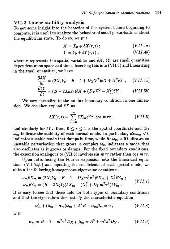
VII.2 Linear stability analysis To get some insight into the behavior of this system before beginning to compute, it is useful to andyze the behavior of smdl perturbations about the equilibrium stiitte. To do so, W pnt
where F represents the spatial variables and &X, 6Y are small quantities dependent upon space and time. Inserting this into (VII.3) and linearizing in the g r n a qnantities, we have
We now speci&ze to the no-flux boundary condition in one dimen- sion. We can then expand SX as
Q0
bX(r, t ) = X G x , ~ ~ ~ ' cos mzr , (V11.6) m=@
and similwly for SY, Were, Q r 2 1 is the spatid camdinate and the w, indicate the stability of eea& n o m d mode, fn particdw, Re w, < O indicates a stable made thzbt damps in time, w&le Re c ~ , >. O inrficalles an unstable perturbatioa that grows; a complex o, indicates a mode that afso oscillates as it grours or damps. For the fixed boundary conditions, the expansion analogous to (VII.6) involves sin mrrr rather than cos mrr.
Upon introducing %he Faurier expmsion into the lioearjzed equa- tions (VII.5a,b) aad equating the coefficients of each spatial mode, we obtda the fanowing hamageneous eigendue equations:
Xt is easy to see that these hold for both ltypes of boundary conditions and that the eigenvdues then saeisfy the characteristic equ;ktion
with
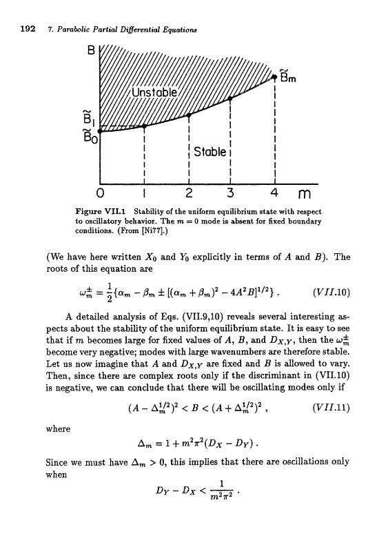
292 7, PamboZie Partid Diflerentiot Equations
Figure VX1.Z Stabgity of the u ~ f a r m equilib~um st9;te with rapect to osaatory beha~ar, The m = 0 mode is isbent for fixed boundary conditions, (Ram [%i77f.)
(We have here written X. md l$ explicitly in terms of A and B). The roots of this equation are
Z = ,{a, - pm f [(a, + - 4 ~ ~ ~ 1 ~ ' ' ) *
A detailed ana?ysis of Eqs. (VII.S,10) reveals several interesting as- pe&s about the &ability of the aniform eqvllibrium state. It is ewy to see that if m becomes large for fixed values of A, B, and DX, y, then the w$ become very negative; modes wit h large wavenumbers are therefore stable. Let us now imagine that A and Dxev are fixed and B is allowed to vary. Then, since there we complex roots only if the discriminant in (VII.10) is negative, we can conclude that there will be oscillating modes only if
Since we must have A, > Q, this implies that there are oscillations only
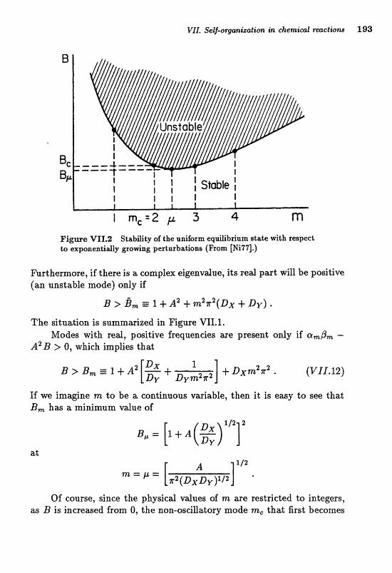
t I
t 1 I I Stable
Figme lr61.2 StabiXity of the uniform. eqrrilibrium state with respect ta exponentiay grourine, pertuxbati~ns (From [Ni77].)
Furthermore, if there is a complex dgexvdue, its real part will be pasitiive (an unstable mode) only if
The situation is sururmsized in. Figure TJ1f.l. Modes with red, paitive frequeades are preseat only if ampnt -
A ~ B 1 0, which implies that
If W imagine m to be a continuous variable, then it is easy to see that B,, h= a minimum vdue of
Of course, siftce tbe physied vdues of m are restricted ta integers, as B is increased from 0, the non-oscillzjttory mode m, that first becomes
I94 7. ParaBolic Partial Diflerendial E w a l i ~ n s
unstabfe at B --- B, is that wWhjch i~ c l o ~ e ~ t to the minimum, as show in Figure VXI .2,
To summafiee thia discussion? the uniform eq~librium state is unsta- ble with respect to perturbations that osdllate in time when B > B. or B1 for no-Bux and fixed boundary conditions, respectively. Similarly, it is nastit,bIe with respect to perhrbalions %had grow exponeatidy in time when B > B,,
'VI1E.3 Numerical solution of the model Although the stability analysis presented above gives some hint at the be- havior of the system for various ranges of the pxameters, the hXl ridness of the model in the non-linear regime can be revealed only by numerical experiments. These can be carried out through the fallowing steps.
m Step 1 V e ~ f y the dgebra in the stability andysis discacased above, Assame a fixed. value of A = 3: in a ane-dimension& situatiamr, and cdcdate the h, and B, for a set of values of the diffusion constants of order 1 0 ~ ~ . How do your results change if the reaction t&es place in the unit square in two space dimensions?
r tet~p 2 m i t e a progam that solves the non-linear digusion equa- tions (VII.3a,b) in one dimension on the interval [0,1] for the case of no-fittx boundary conditions; a rewonable number of spatid points might be between 25 m d 100. The diRasion t e rm shodcl be treated. irnpEcitly to preved unphysicd numericat inst&ili-ties, mrhile the reaction terms can be tre&ed exp2icitly. ZIave your progrm plot out X and V at each time step.
m Step 3 Use your one-dinze~siond proerram to investigate the behav- ior of the solutions for different values of B, DX*y. A reasonable place to start might be Dx = 1 x IO-~ , D y = 4 X l@-$; the linear stability analysis should then give some guidance as to what values of B are inter- esting. Investigate initial conditions corresponding to smooth sinusoidal and point-wise random perturbations of the uniform equilibrium config- uration (the latter can be generated with the help of function RANR~S, found at the end of Appendix D.3, or your compiler's intrinsic random number generator). Verify that you can find cases in which the system refmes back to the u n i h m state, in whieh it ampto t icd ly a~>proa&es a time-independent solution with a non-trivial spatial variation (dissipa- tive structure), and in which it approaches a space- and time-dependent oscillating solution. Throughout, make sure that your time step is small enough to allow an accurate integration of the equations.
Vile Se~-c3rganixation in chemical reactions 195
Step 4 Extend your one-dimensionat. mde la szolve the Brusselator with no-flux boundary conditions in two spxe dimensions using, for exam- ple, an alternating-direction algorithm like Eq. (7.19). Plot your results for X at each time. (The technique of displaying an array of characters, as in Example 6, can be useful.) Investigate parameter ranges and initial candiltions as in Step 3.

This page intentionally left blank
Chapter 8
Monte C Methods
Systems with a large number of degrees of freedom are often of interest in physics. Among these are the many atoms in a chunk of condensed matter, the many electrons in an atom, or the infinitely many values of a quantum field at all points in a region of space-time. The description of such systems often involves (or can be reduced to) the evaluation of integrals of very high dimension. For example, the classical partition function for a gas of A atoms at a temperature l/@ interacting through a pair-wise potential v is proportional to the 3A-dimensional integral
The straightforward evafzration of an in tagd like this by one of the quadr&ure formulas discussed in Chapters 1 or 4 is conrpletely out sf the question except for the very smdest values of A. To see why, suppose that the quadraturn allows ea& coordin&e to take on 10 digerent vdues (not a very fine discretization), so that the integrand must be evaluated at points. For a modest value of A = 20 and a very fast computer capable of some 107 evaluations per second, this would take some 2 . 0 ~ ~ seconds, more than 1oa4 times the age of the universe! Of course, tricks like exploiting the permutation symmetry of the inteffrand can re-duce this estimate considerably, but it still should be dear that direct quadra1;ure is hopeless,
The Monte Carlo methods discussed in "this chapter we ways of effi- cierttty evaiuading integrds of Egh dimension. The name &Monte Carlo" arises f"rom the random or U&mce" chwacter of the method and the f a o u s casino in Monaco. The essentid idea, is not ta evaluate the in- tegrand at every one of a large number of quadrature points, but rather
198 8, Monte Carlo Method8
at only a representative random sampling of abscissm. This is and~goua to predicting the resalts of an election on the basis of a poll of a smdl number of voters. Although it is by no means obvious that aoything sen- sible can come out of random numbers in a computer, the Monte 6x10 strateg turns out to be very appropriate fof a brad dass of: problems in statisticd a d quantum mechanics, Mare d e t ~ l e d preseat;ttions of the method than that given here can be found in [Ha641 and [Ka85].
8.1 The basic Monte Carlo strategy Even though the reai pawer of Monte Caflo methods is in evduating multi-dimensional intepds, it is easiest to illustrate the basic ideas in a one-dimensional siluation. Suppose that; we have to evduate the iatepal
for s m e padicular function f . Chrtpters 1 and 4 discussed several &E &rent qudratare formulw that employied vdues of f at very particular values of 2. (e.g., equally spaced). However, an alternative way of evalu- ating I is to think about it as the average off over the interval [Q, l]. In this bight, a plau~lible quadrature formula is
Heref the werage of f is evaluated by consideriag its values at N abscis- sae, {si), chosen at random with equal probabitity anywhere within the interval [0,1]. We discuss below methods for generating such "randomn numbers, but for now it is sufident to suppose th& there is a computer function that provides as anmy of them as are required? one after the other, Note thia't these is n s such FOETRAN-"7 function, but many com- pilers provide their own (e.g., RAN in VAX FORTRAN) and we provide function RANNOS (found in the file UTIL.FOR and listed at the end of Appendiv D.3).
To estimate the uncertainty agsoeiated with this quitdrature fornufa, we can consider fi ziii f ( z i ) as, a random variable and invoke the central limit theorem for large N. From the usud laws of statistics, we have
where o; is the variance in f ; i.e., a measure of the extent to which f deviates from its average value aver the region af integration,
8.1 The basic Monte Carlo s t r a t ~ g 199
Equation (8.3) reveals two very important aspects of Monte Carlo qudratun;. Rrst, the uncertainty in the estimate of the integd, 01, decreases as Hence, if more points are used, we will get a more precise ansarer, although the error decreases very slovvly with the number of points (a factor of four more numericd work is required to halve the uncertainty in the answer). This is to be contrasted with a method like the trapezoidal rule, where Eqs. (1.8,1.9) show that the error scales like N m 2 , which affords a much greater accuracy for a given amount of numerical work. (T6is advantage vanishes in multi-dimensional cases, as we discuss below.) The second important point to realize from (8.3) i s that the precision is greater if of i s smaller; that is, if f is as smooth as possible. One Irimit o f tEs i s when. f i~ is aconstant, in which cwe we need its vdue at only me point to define its aver%@. T"a see the other limit, consider a situation in whi& f i s zero except for a very narrow peak about gome vdue of 2, If the 86 have an equd probabiliv to lie anywhere between 0 and 1, it is probable that a;U but a few of them will lie outslide the peak of f , and that only these few of the f i will be non-zero; this will lead to a poorly defined estimate of I.
As an example of a Monte Carlo evaluation of an integral, consider
The following FORTRAN program calculates this integral for the value of N input, together with an estimate of the precision of the quadrature.
G cbp8a.lBor XITEGER S m !seed 203: amber generator DATA SEm198765432 g/
DATA E;ZIACT/, 78640/ !aaPytic aawer NgG(X)=CEI./(1 .+X*+2) t fmct;ioar t o int e p a t e
C
10 PRTBfT *, "%er nmber of posts (Q to stop) B
REAII) *, M XP (I .EQ, 0) STOP
C SUW=O. !zero s w s 5VW2=01 DO 20 IX=Z,li l !loop over s w l e s
F X = W C (EkBI(SEm)) SGW=SMF+FX !&d con$ribations to s m s
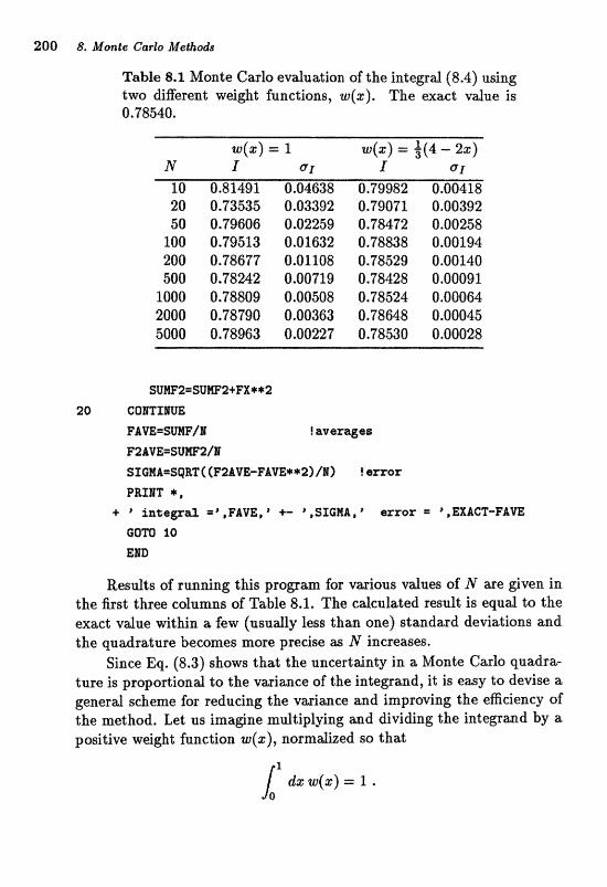
200 8. Monte Carlo Me&&#
Table 8.1 Monte Carlo evaluation of the integral (8.4) using two digerent wei&t functions, ~ ( 8 ) . The exact vdue i s 0.78540.
Results of running this program fur various values of N are given in the first t h~ee columns of Table 8.1, The cdculated result, is eqnd to the exact value within a few (usually less than one) standard deviations and the quadratare becomes more predse as N increases.
Since Eq. (8.3) shows that the uncertainty in a Monte Carlo quadra- tare is proportional to the variance of the integrand, it is easy to devise a general scheme fur reducing the variance and improving the efficiency of the method. Let us imagine multiplying and dividing the integrand by a positive weight function w(z), normalized so that
8.1 The bosic Monte Carlo utmb-egy 201
The integral can then be written as
If we now make a Change of variable from z to
then the integral becomes
The Monte Catlo eduation of this integral proceeds as above, namely ayeraging the values of f /w at a random sampling of points uniformly dis- tributed in y over the interval [0,1]:
The potentiat benefit of the change of &able should now be clw. If we choose a m that behaves approurimately as f does (i-e., it is lage where f is large md small where f is small), then the integrand in (8.7), f /w, can be made very mooth, with a consequent reduction in the variance of the Monte Carlo estimate (8.8). This benefit is, of coarse, contingent upon being able to find an appropriate w and upon being able to invert the relation (8.6) to obtain z(y).
A more general way of understanding why a change of variable is potentially useful is to realize that the nnifonn distribution of points in y implies that the distribution of points in x is d y l d x = w(s). This means that points are concentrated about the most "importantn values of x where w (and hopefully f ) is large, and that little computing power is spent on calculating the integrand for "unimportantn values of s where PD and f are small.
As an example of how a change of variable can improve the efficiency of Monte Carlo quadrature, we consider again the integral (8.4). A good choice for a weight function is

202 8- Monte Carto Mei;ho&
which is positive definite, decreases monotonicdly over the range of inte- gration (as does f), and is normalized correctly. Moreover, since f l w = 314 at both s == O and a: =I I, W well appraimat;es the behavior of f . According to (8.6), the new integration variable i s
WE& can be inverted to &ve
The following FORTRAN code then evaluates I according to (8.8).
G ch@b. for IETEGER S W !seed f a r radom &-&er g a e r a t o r DATA Sm18878543221 DATA =ACT/. 78640/ !=aytic vazua mMC(X)==:./(i,+X**2) ! imctf on to i n t e ~ a t s
WEZGBT(X) = (4, -2+X)13, ! neigh% fact f on XX<Y)=2, -SQRT(4, -3, +P) !X as a imcdion of P
C $0 PRIIT *, P &tax nwber of p o h t s (0 t a srop)
mm +, l4 IF' (R *EQ* 01 STOP
C
SUm=o. ?~eZ?a SW8
s~m2=0. DO 20 III=I,B !Isop ovax smp2ss
Y=RAE(SEa) x=xx (Y) F X = F ~ C (X) /%IEILGET(X) ? i ~ r e g ~ ~ d SWW=SWF+m !adcl contritnrtions ts s m
2=mW2+FX*+2 28 COlJTf l U E
FAVE=SW/I ? averages F21VE=SUMF2/1 SXGMA=S~RTC(F~AVE-FAVE**~]/I) !emox PRXsfT *,
+ 8 i n t ~ e a f =PrFAVEr8 +- ',SLGldhr) ttrrof "EXACT-FAVE
GOTO 10 EHD
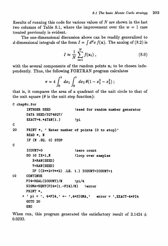
8.1 Tbe Zta&t"c Monte Carlo stmlegg 203
Results of running this code for various values of N are shown in the last twa colurns of Table: 8.1, where the improvement over the zo = 5, case treated previously is evident,
The one-dimensional discussion above can be readily generazed to d-dimensional integrals of the form I = j ddz f (X). The analog of (8.2) is
with the severat components of the random points xi to be dosea inde- pendenlf y, Thus, the following FORTRAN proe;~am cdedat;es
that is, it eolnpares the area of a quadrant of the unit eirde to that of the unit square (B is the unit step function):
C c;hp8c*fox XmEGm SED !seter& fox r d o n nmber gsnera%or DATA SEm/3274927/ EXbm=4. *ATAP 1 . ) !pi
C
20 PRIHT *, heer srubsr af ph%s (0 %a atop)" RErn *, P IF (H .EQ. 0) STOP
C IGQWT=O !zero comt DQ 20 XX=1,B $loop over santplsa
X=Ml CSErn) U=MlaT ( $Em> SF ( (X**2+V**2) . LE 1. ) XCOWT=ICOVET+ 1
10 COITXrnB vra=m~(zcov~~)/~ ?pa/?r SICM=SQRTCPI4* (1, .-PZrlr) /I] f emor faRXlT *,
e B p i = 4*PX4,"- p",4+S3C;MiA,hrxar = ',EXACT-WPI4 GOTO 20 EEL)
When run, this program generatc3d the satisfactory result of 3.14241= 0.0232.
U Exercise 8.1 verify that the error estimate used (two Enes &er line 10) of this program is that given by Eq. (8.3).
The & a g e of vwiable discusmd above can dso be generdized $0 many dimensions. For a weight function w(x) normalized so that its integrd over the re@on of integration is unit& the approp~ate new mri- able of integration is y, where the Jacobian is = w(x). It is generally very difficult (if not impossible) to construct x(y) explicitly, so that it is more convenient to think about the &an@ of variable in the multi-dimensiond c a e in the Ben- discussed above; i.e., it distributes the points xi(yi) with distribution W. Various practical methods for doing this fof a r b i t s q w will be discussed below,
Although the results were satisfactory in the examples given above, Monte Carlo quadmure does not wpear to be pasticulaly efficient, Even with the "pod" choice of W, the rc3sdts in Table 8.1 show a precision of only about 10-' for N = 5000, whereas the conventional trapezoidal for- mula with 5000 points is accurate to better than 1 0 ~ ~ . However, consider evaluating a multi-dimensional integral sueh as (8.1). Suppose that we are willing to invest a given amount of numerical work (say to evaluate the integrand N times), and wish to compare the effieiencies of conven- tiond arid Monte Carlo quadratuma. In a conventioaiaf quadrature, say a mdti-dimension4 analog of the trapezoid4 rub, if $here are a totd af IV points, then e x h dimeadon of a d-dimensiand intern& is braken up into ~ ' 1 ~ intervds of spwing h N - I ~ ~ . The analog of (1.9) shows that the emor in the integral over eaeh cell of volume hd in the integration region is o (hd+l), so that the total error in the conventional quadrature i s
for large d, this decreases very slowly with increasing N. On the other hand, Eq. (8.3) above shows that the uncertainty of a Monte Carlo quadra- tare decreases as N - ' / ~ , independent of d. Assuming that the prefactors in these estimates we dl of order unity; we see that Monte Cwlo quadra- tare is more eficient when d 2 4. Of course, this estimate depends ia detail upon the conventional quadrature scheme we use or how good a weight function is used in the Monte Carlo scheme, but the basic point is the very different way in which the two errors scale with increasing N for large d
83 Generating rcrtlciom variables wi& a $pi$~iecl dzstr-s"bul;iots 205
8.2 Generating random variables with a specified distribu- tion The discussion above shows that Monte Cm10 qndratnre involw two basic operations: generating abscissm randomly distributed over the in- tegration volume with a specified distribution w(x) (which may perhaps be unity) and then evdaating the function f l w at these abscissae. The second operation is straightforward, but it is not obvious how to generate "random" numbers on a deterministic computer. In this section, we will coyer a few of the stmd;asd method8 umd.
The generation of uniformly distributed random numbers is the com- puter operation that underlies any treatment of a more complicated dis- tribution. There we numerous methods for pedoming tkis bwic task and for cheching that the results do indeed correspond to the uniform random numbers required. One of the most common algorithms, and in fact that used in the VIAX FORTMM RAN function, is a '"near cm- gruential" method, which "grows" a whole sequence of random numbers fram a, nsr?ed" n u b e r . The cunent member of the sequertee is rauftiplied by a first "magic" number, incremented by a second magic number, and then the sum is t&en moduk, a third magic number. Thus,
where i is the mquerrce label and, a, c, and m are the magic numbers, The littder me often very h g e , with their precise values depending upan the word length of the c-ornputer being used. Note tha% the zi cmnot be truly "random" W they aise from the swd in a well-defined, determin- istic algorithm; indeed, two sequences g rwn from the the s m e seed are identical. Fbr this remoa, they are often termed "'pseudo-random", Nev- ertheless, for m a y practicd purposes pseudo-random numbers generated in this way can be used as if they were truly random. A good discussion of uniform random number generators and of the tests that can be applied to determine if they are working properly can be found in [Kn69].
We have dready seen how to choose one-dimensional random vari- ables distributed as a specified weight function W(%). According to the discussion in the previotxs section, the procedure is to choose y, the ineom- plete iaf;egra-l of W , u n i h d y , and then to find z by inwrting Eq, (8.6). Thus, if we are faced with evduating the integrat

with g a relatively smooth function, it is sensible to generate z between 0 and oo with distribution and then to average g over these d u e s . According to (8.5), we have
The followi~~g FORTRAN subroutine generates values of X with the re- quired distribution,
c chap8d.for suBRawrm WCDST(X) XBTEGm SED DATA SEm /88341927/
C X=-LOG ( I . -UIEI(SEm) ) REmm EID
m Excsreim 8.2 Verjfy that the code above generatea X with the re- qlrired distribution, for example by generating aad h i s t o g r m ~ n g a large number of vdues of X. Use these v d u e ~ to evitluii;te 1 and its uncertainty for 9(2) = 5, zZ, md z3 and compare your results with the analytical vdueg. Can you understand the trend in the uncertainties cdcdaled?
WMe the method of generating the incaqlete integral is infdfible, it requires that we be able to find + ( g ) , which can be done analytically only far it relilrtively s m d class of functions. For example, if we had wmted to US@
in our efforts to evaluate Eq. (8.4), we would have been faced with solving a cubic equation to find g(%). While this is certainly possible, choices of w that might follow more closely the behavior of f generally will lead to more complicated integrals that cannot be inverted analytically. However, it is possible to do the integral and inversion numerically. Let us imagine tabulating the values for which the incomplete integral of w takes on a series of uniformly spaced values y(j) zz j /M , j = 0, 1 , . . . , M that span the interval [Q, l]. Thus,
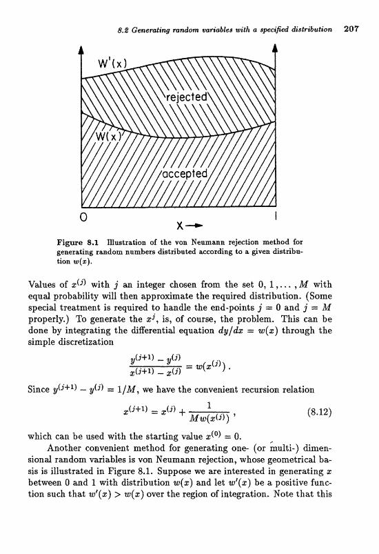
8.2 aneratin@ r a n d ~ m variables with a specified distribution 307
Figwe 8,1 fllmtration of the von Nemmann rejection method fox generating raindom numbers distributed =carding to a gven di~triba- $ion w(a;).
Values of z(j) with j an integer chosen from the set 0, 1 , . . . , M with equd probability will then approximate the required distribution. (Some special treatment is required ta handle the end-point6 g' = 0 and j = M properly.) To generate the d , is, of course, the problem. This can be done by integrating the differential equation dyldz = w(z) through the simple discret;ization,
Since - = 1/M, we have the convenient recursion relation
which can be used with the starting vdue I(@) = 0. Another convenient method for generating one- (or hulti-) dimen-
sional random variables i s von Neurnann rejection, whose geometrical ba- sis ia illustrated in Figure 8.1. Suppose we are interested in generading a: between O and 1 with distribution W(%) and let cul(z) be a positive func- tion such that W'($) > W ( $ ) over the region of integration. Note that this
means that the definite integral of W' is greater than 1. A convenient, but not always useful, choice for wf is any constant greater than the max- imum value of W in the region of integration. If we generate points in two dimensions that uniformly fill the area under the curve W'(%) and then "accept" for use only those points that are under zu(z), then the accepted points will be distributed according to W. Practically, what is done is to chohse two random variables, gi and q, the former distributed proportional to W' and the latter distributed uniformly between O and 1. The value zi is then wcepted if q is less than the ratio w(z i ) /wf ( s i ) ; if a point is rejected, we simply go on and generate another pair of and ?,I. This technique is dearly @%dent only if zuf is close to W throughout the entire range of integration; otherwise, much time is wasted rejecting useless points.
Exercise 8.3 Use von Neumann rejection to sample points in the interval [Q, l] distributed as w(z) = $(l - !p2) and evaluate the inte- gral (8.4) and its uncert$nty with these points. Compare the efficiency af your cdculation far vmious choices af W'.
The Gaussian (or normal) distribution with zero mean and unit vari- ance,
w(g) = (2r)-'/2e-"'/2 , plays a central role in proobablliity thwry and so is often needed in Monte Carlo cdcdatims* It, is possible, but not too efficient, to generate this distribution by inverling its incomplete integrd using pofynonaial approx- imations to the emor function, A more ""clever" method is based an the central L i ~ t theorem, which states th& the sum of a large number oE uniformly distributed r a d m numbers will appraach a Garnssian distri- bution. Since the mem and varianm of the unifom distribution on the interval [0,1] are 1/2 and 1/12, respectively, the sum of 12 unifo* dis- tributed numbers will have a mean value of 6 and a v%sianee of 1 and will very dosely approximate a Gaussian distribution. Hence, the follow- ing FORTRAN subroutine returns a Gaussian random variable, GAUSS, with zero mean md unit w iwce :
C chafle, %or G apubrowt;ine to gsllnsraeer the n o m a l y distrih%ed amber GAUSS
SUBBQWIEB IIIST(GAUSS1 xaJmem s m DATA SEEf)/39249287/
c
8.8 Generating mndom variable& with a specified distribution 209
m Exercise 8.4 By histagramming a large number of the values of GAUSS produced by the subroutine above, convince yourself that their distribution is very close to normat. Can you derive a quantitative esti- mate of the extent to which this di~txibutian deviates from a Gaussian? Compare with the results of summing 6 or 24 uniformly distributed ran- dom numbers. (Note that these latter sums have means of 3 and 12 and varimces of 4 and 2, respectively.)
Another efficient method for @witting normally distributed vmi- ables is to consider a Gaussian distribution in two dimensions (gI, zz), for which the number of points in a diRerentiail area is pmportional to
Zn. terns of the usual polar coordinates
the distribution is e - * P ~ dr d@ ,
or, if u = )ray the distribution is
Hence, if we generate u between 0 and m with an exponential distribution and B uniformly between O and 2 1 ~ ~ then the corresponding values of
21 = (2u)'i2 COS B , 1 2 = ( 2 ~ ) ' / ~ gin B
will be distributed normally. Thus, the following FORTRAN subrou- tine returns two normdy distributed random variables, GAUSS1 m d GAUSS2:
210 Monte Carlo Methda
DATA 53B/39249181/ ~~13 .24159261
C TWoU=-2.*LoG(i.-R4E(SEED)> RADIUS=SQBT(T~~~OUI TWETA=2*PX*RAI (SEEf)) GAUSSI=RADIUS*CflS (T13:ETA) GAUSS2=RUXUS*SIl(mETA) RETUM END
To generate a Gaussian distribution with mem 3 and variance c2,
we need only take the vdues pnerated by this subroutine, mdtiply them by a, and then increment them by g.
8.3 The algorithm of Metropolis et al. Prltbugh the methods we have discussed above for generating rmdom numbers according to a specified distribution can be very efficient, it is cliEcdt ar impossiMe to generalize them to smple a complicated weight function in many dimeagions, and so can &ernative approach is required. One vary generd way to produce random vasiables tvith a given probabil- ity distribution of arbitrary form is known as the Metsopofis, Rosenblut h, Rosenbluth, Teller, and Teller algorithm [Me53]. As it requires only the ability to calculate! the weight function for a givcln vdue of the integration vwiablest the allgorithm has been appliecl widely in statisticall rnechanies problems, where the weight &netion of the eanoaicd ensemble can be a very complicated function of the coordinates of the system [see Eq. (8. l)] and sa carrot be sampled conveniently by ather methods, Howevm, it is not without its drawbacks,
Although the dgorithm of Metrc)pOXi~ et laE, can be ixapiemen~ed in a variety d ways, we begin by describing one simple realization. Suppose that we want to generate a set of points in a (possibly multi-dimensional) space of variables X distributed with probability density w(X). The Metropolis algorithm generates a sequence of points, X@, XI,. . . , as those visited successivefy by a randam w&er moving through X space; as the wdk become8 longer asld longer, the points it connects appro~mate more closerly the desired Bistribution.
The rules by whieh the randam wdk proceeds through canfiguratlm space are as follows. Suppose that the wdker i s at a pojnt X, in the
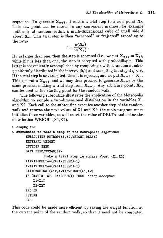
8.8 The algorithm of Metropofs's et d. 21 l
sequence. To $emrate X,+1, it makes a trial step to a new paint X,. This new point caa be chosen in any convenient manner, for example uniform at random within a multi-dimensional cube of small side 6 about X,. This triaf step is then "aecepted" or @reJlectedn according to the ratio
If r is larger than one, then the step is aecepted (i.e., we put X,+1 = Xt), while if r is less than ane, the step is wcegted with probability r . This latter is conveniently accomplished by comparing r with a random number q uniformly distributed in the interval [0,1] and accepting the step if q < r . If the trial step is not accepted, then it is rejected, and we put X,+x = X,. This generates X,+x, and we may then proceed to generate Xnf by the same process, making a trial step from X,+1. Any arbitrary point, Xo, can be used as the starting point for the random walk.
The following 8ubrout;ine illustrates the app1ieat;ion of the Metropolis dgarithm to s a n k a two-dimensioad distribution in the vmiables X1 m d X2. Each edE do the subroutine executes mother step aif the raadam wdk and retarns the n a t vduw of X1 and X2; the m ~ n progrm mast irritidze these variables, as well as set the vdue of DELTA and define the distribution WEIGHT(XI,X2).
C chap8g.f"~~ C subroatlne to %&B a slap in Ihs Watropolis algorith
SWROWZIE MEmOF(Xl,X2,UEIGRT,D&T&) EXTEWAL WEIGBT ICITEGER SEED DATA SEm/39249%87/
!%as a trial stevp in squme aben% [X1,X2) XIT==XI+DELTA+ (2*RAI (SaD)-J,) X2T=X2+DaTA* (2*RAB (S-)- 1) RATEO=WIEXGmf XIT , X22")/GifFSTGHT(X%, X2) SF (RATLO . GT. RAB(SEED)) THEE ! s2ep accctpled
Xi=X1T X2=X2T
EEB LF" REwm EHD
This code cauld be made more efficient by saving the weight function at the current point of the random walk, so that it need not, be computed
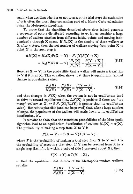
212 8. Monte Carlo Methds
again when deciding whether or not to xcept the trial step; the eduat ion of W is often the most time-consuaaing part of a Monte Cm10 cdcdation. using the Metropolis algofithm.
To prove thatr the dgorithm described above dow indeed generate a sequence of points distributed according to W, let us consider a large number of wdkers starting from diRerent initid points and moving inde- pendently through X space. If N,(X) is the density of these walkers at X &er rs steps, t b a the ne% number of wdkers moving from paint X to point Y in the next step is
Here, P ( X -r Y) is the probability that a walker will make a transition to Y if it is at X, This equation shows that there is equi2ibrium (no net change in population) when
and that changes in N ( X ) when the system is not in equilibrium tend to drive it toward equilibrium (i.e., AN(X) is positive if there are @too many" walkers at X, or if N,(X)/N,(Y) is greater than its equilibrium value). Hence it is plausible (and can be proved) that, after a lmge number of steps, the population of the wdkers will settle dawn to its equiEbrirxm distribution, l&,
It rennalns to show that the transition probabilities of the MetropoEs aigorithm lead to an equilibrium distribution of walkers N , ( X ) u (X ) . The probability of maEng a, s$ep f r m X to Y is;
where T is the probability of making a trial step from X to Y and A is the probability of accepting that step. If Y can be reached from X in a single step (i.e., if it is within a cube of side 6 centered about X), then
T ( X + Y) = T(Y -r X ) ,
so that the equilibrium distribution of the Metropolis random walkers satisfies
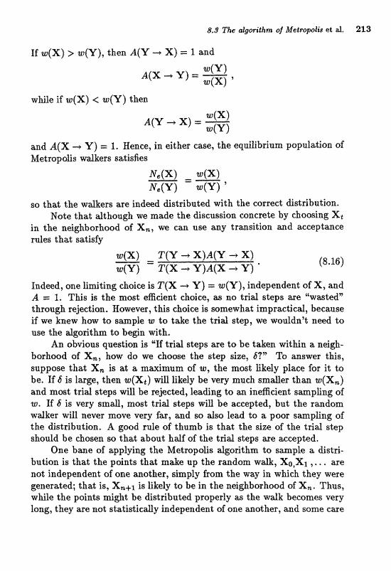
If w(X) > w(Y), then A(Y 4 X) = 1 and
while if w (X) < w (Y) then
and A(X -r Y ) = 1. Hence, in either case, the equilibrium population of Metropofis walkers satisfies
so that; the wdkers axe isrdwd distributed with the correct distribution. Note that although we made the discussion concrete by choosing Xt
in the neighborhood of X,, we can use any transition and acceptance mles that; satisfy
Indeed, one limiting choice is T ( X -r Y ) = w(Y), independent of X, and A = 1. This is the most efficient choice, as no trial steps me '%.wtzstedn through rejection. Hawewer, tkis doice is sonnewhat impractical, because if we knew haw to sample W to take the trial step, we wouldn't wed to use the dgodthm. to be@n with.
An obvious que~tion i s "If trial steps are to be t&n within a nei&- borhood of X,, bow do W choose the step size, S?" To answer this, suppose that X, is at a maximum of W, the most likely place for it to be. If 6 is large, then w(Xt) will likely be very mu& smaller than w(X,) and most t r id steps will be rejected, Leading to an ineficient s ap l ing of W . E 6 is very s m d , most trial steps will be accepted, bnt the rmdom w d h r will never move very fm, and so &so lead to a poor smpfing of the distribntion. A good r d e of thumb i s that the size af the trial &ep shodd be chosen so th& about half of the t ~ d gteps me accepted.
One bme of applying the Metropolis dgorithm. to sampfe a distri- bution is that the points that m&e up the random walk, Xo,XI , . . . are not independent of m mother, simply from the way in wEch they were generated; fhat is, is likely to be in the n4ghborhood of Xpbe T~us, while the points might be cfistributed properly W the walk becomes very long, they are aot statidicay independed of one another, and some w e

214 8, Monte Carlo Methd8
must be taken in using them to calculate integrals. For example, if we cdcul ate
I = S w ( X ) f (X) S w(X)
by averaging the vdues of over the pojnts of the raadom wdk, the usual estimate of the variance, Eq. (8.3), is invalid because the f ( X i ) are not statistically independent. This can be quantified by cdculating the auto-corrdation. function
Here, ( . . . ) indicates average over the random walk; e.g.,
Of course, C(O) = 1, but the non-vanishing of C for k + 0 means that the f 's me not independent. Whal can be done in practiw is ta compute the in tepd and its variance using psints dong the raxrdam wdk separated by a fixed intervd, the intervd being chosen so that there is eRecliveiy no cofrelation between the points used, Aa appropriate sampliag intervd can be estimated the vdue of k: for which C becomes smaa;l (say
O.I)* Another issue in. applying tbe Metrapofis algorithm is where to stmt
the random walk; i.e., what to t h e for X@, In prindple, w y location is suitable and the rehs~ft~ wiU be independent of tEs choice, m tbe wdker will ""term&zc?" after some number of steps. In practice, an appropri- ate starting point i s a probable one, whefe w i s large. Some number of" themalization steps then can be taken before actual sampling be@ns to remove m y depeadence on the starting point.
R E x e r c i ~ 8.5 Use the dgorithm of Metropolis et al. to sample the norrmd ddistribntion. in one dimension. For various erid step sizes, study the acceptance ratio (fraction of trial stepa accepted), the correlation function (and hence the appropriate sampling frequency), and the over- all computational efficiency, Use the randam vasiables you generate to
and estimate the nncestainty in youf ansarer. Study how your resdts depend upon where the random wdker is started afzd on how many ther- malization steps you take before beginning the sampling. Compare the efficiency of tbe Metropolis algorithm with that. of a cdcuhtim that uses one of the methads discussed in Section 8.2 to geaerate the narxnd dis- tribution. directly,
8.4 The Ising model in two dimensions Models in which the degrees of freedom reside on a lattice and interact locally arise in several areas of condensed matter physics and field theory. The simplest of these is the Ising model [Hu63], which can be taken as ;z crude description of a magnetic materid or a binary doy , h this ex- ample, we will use Monte Carlo methods to calculate the thermodynamic properties of t;his model,
Xf we spe& in the magnetic laaguage, the rsing model consists of a set of spin degrees of freedom interacting with each other and with an external mqnetic field. These might represent the magnetic xnonzents of the &oms in a solid, We will consider in particular a model in two spatial dimensiws, where the spin mriablee are locat;ed on the sites of an N, x Ny square lattice. The spins can therefore be labeled as Sij, where i , j are the indices for the two ~ipittiill, directions, or as S,, where a is a generic site label. Each of thme spin variables can be either "up" (S, = f l) or "down7' (S, = - 1). This mimics the spin-1/2 situation, although note that we take the spins to be c l ~ s i c d degrees of freedom and do not impose the angular momentum earnmu tat ion rules characteristic of a quantum description. (Doing so would correspond to the Heisenberg model.)
The Bmiftoaian. for the system is conventionalfy written as
Here, the notation (up) means that the sum is over nearest-neighbor pairs of spins; these interact with a strength J (see Figure 8.2). Thus, the spin at site i j interacts with the spins at i f U and i j f 1. (We %same periodic boundary conditions on the lattice, so that, far example, the l m r neighbars of the spins with i == IV, are thaw with i = 1 m d the left-hand neighborn of those with j = 1 are those with j = Ng; the lattice therefore has the topology of a torus.) When J is positive, the energy is lower if a spin is in the same direction as its neighbors (ferromqnetism), while when J is negative, a spin wifl tend to be mti-aligned with its

226 8. 2Monl"e Carlo Me?&&&
*
Figure 8.2 Schematic illu;stCratian of the tww&mea~ionaJ. hing mad$,
neighbors (anti-ferromagnetism). The term involving B represents the iaterwtion of the spins with an extern& magnetic field, which tends to align aU. spins in the s m e dimc$ian.
We will be interested in the therxnodynmics of this system. In this case, it is convedent da measure the coupling energies J md B in units of the temperature, so that heating the system corresponds to decreasing these couplings. Configurations of the system axe spedfied by gjving the values of all N, x N, S N, spin variables md the weighting of any one of the 2N8 spin configurations, S, in the canonical ensemble i s
where the partition function is
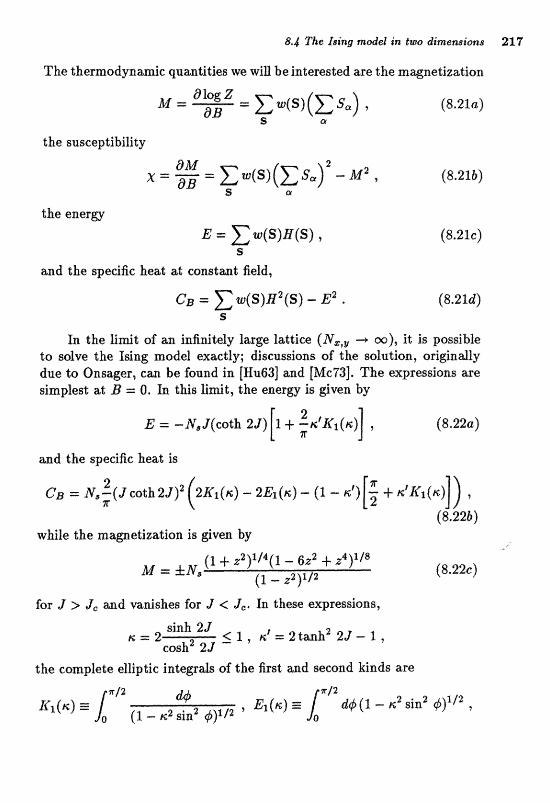
8.4 The fsing model in two dimensions 237
c quantities we will be intertlsted are the nzagnetizal;ion
the susceptibility
the energy
E = E ~ ( s ) H ( s ) V (8.21~) S
and the specific heat %t constant field,
In the limit of an infinitely large lattice (N,,, -+ m), it is possible to sdve the Ising modd exactly; discussions of the solution, origindy due to Onsager, can be found in [Hu63] and [Mc73]. The expressions are sinnpled at B == 0, In this limit, the - e rg is dven by
and the specific heat is
wMfe the mapetization i s given by
for J r Jc m d vanishes for J < JC. In these expressions,
the complete elliptic integrals of the first and second kinds are
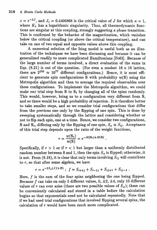
228 8, Monte Cark Methods
z = em2', and J, = 0.4406868 is the critical value of J for which K = 1, where Kl has a logilrithmie singdwity, Thus, a& thermodynmic Tune tians are singular at this caupli~g, strondy sugesting a phase transition. Tbis is confirmed by the behavior of the mametization, which vanishes below the critic4 coupling (or above the critical temperature), and can take on one of two equal and opposite values above this coupling.
A numericat solution of the fsiag model is usefd both W an illus- tration of the techniques we have been discufjsing and because it can be generalized readily to more complicated Hamiltonians [Fo63]. Because of the la-rgt, number of terms invoked, a direct evaluation of the sums in Eqs. (8.21) i s out of the question. (For even a modest 16 x 16 lattice, there are 2256 M 1 0 ~ ~ different configurations.) Hence, it is most eE- cient to generate spin configurations S with probability w(S) using the Metropous algorithm and then, to average the required observables over these configurat;ims. Z'o impjeraent the Metropolis dgorithm, we could make our %rid step from S to St by chan@ng a l l of the spins randomly. This would, howenr, brine; us to a canfiguration very &Rerent from S, and so there vvould be a, high probability of rejection. It is therefore better ta take smdler steps, and so W consider tnid confipratioas that differ from the previous one only by the fiipping af one sjpin. This is done by sweepiing systemalIcally through the l& tic@ and considering whether or not to flip each spin, one at a t h e . Hence, we emsider two configurations, S and St , differing only by the Aipping of one spin, S, E Sa. Acceptance of this t r id s t q depends upon the ratio of the w&ght functions,
Spedficdy, if r > 1 or if r < 1 but larger than a nniformiy distributed random number bet;ween O and 1, then the spin S, is flipped; othervvise, it is not. From (8.18), it is dear that only terns involving Si j will contribute to F , so that after some algebra, W have
Here, f is the sum of the four spins neighboring the one being flipped. Because f can take on only 5 different values, 0,352, f 4, only 10 different values of r can ever arise (there are two possible values of S,); these can be convenient?y calculated and stored in a table before the calculation begins so that exponentials need not be calculated repeatedly. Note that if we had used trial configurations that involved flipping several spins, the cdculation of r would have been much more cormplic;zted.
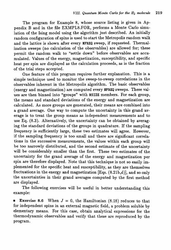
VIII. Quantum Monte Cads for the H2 molecub 219
The program for Example 8, whose source listing is given in Ap- pendix B and in the file EXMPL8.FOR, performs a Monte Carlo simu- lation of the Ising model using the algorithm just described. An initially random configuration of spins is used to start the Metropolis random walk and the lattice is s h m dter eltery WREQ @weep, if requested. Thermal- ization sweeps (no calculation of the observables) are allowed for; these permit the random w d k to "settle dow" before abservables are aecu- mdated, Values of the energy, mametization, susceptibility; and speeigc heat per spin are displayed as the calculation proceeds, as is the fraction of the trial steps mcepted,
One hatare of this p r a g r a requires further explmatian. This is a simple technique used to monitor the sweep-tosweep correlations in the observables inherent in the Metropolis algorithm. The basic obsenrables (energy and magnetization) are computed every )IFRW sweeps. These v&- ues are then binned into L"groupsw with HSIZE members. For e ~ h goup, the means and standard deviations of the enero and m~gaetiz&ion me ca-lcdated, As more groups are generaled, their means are combined into a p n d aver%@, One wa;v 80 campute the uncert&nty in this grand av- erage is to treat the grwp means as independent measurments and to use Eq. (8.3). Alternatively, the uncertainty can be obtained by averag- ing zGhe standard deviatians of the goups in quadrature, If the sap l ing frequency is sufficiently large, these two estimates wiU agree. However, if the sampfing frequency is toa snnafl and there are significant correla- tions in the suecessiw measurements, the vdues witbin each group will be too narrowly distributed, and the second estimate of the uncertainty win be considerably smdler thm the first. These two estimates of the uncertainty for the grand average of the energy and magnetization per spin are therefore displayed. Note that this technique is not so easily im- plemented for the specific heat and susceptibility, as they are themselves Auctuations in the energy and magnetization [Eqs. (8.21b,d)], and so only the uncertainties in their grand averages computed by the first method are displayed,
The following exercises will be useful in better understanding this example:
S Exercise 8.6 When J = 0, the Hamiltonian (8.18) reduces to that for independent spins in an external magnetic field, a problem soluble by elementary means. For this ease, obtain analytical expressions for the thermodynamic observables and verify that these are reproduced by the program.
220 8. Monte earls Meth&
m Exercise 8.7 Use Eqs. (8.22) to calculate and gfaph the e x x t energy, spedfic heat, m d mqnetization per spin Ior an infinite latticc? at B ==; 0 and far J running from O to 08.
m Exercise 8.8 Modify the code to compute the sweep-to-sweep corre- lation functions for the energy and the magnetization using (8.17). Using runs far a 16 X 16 lattice far B == Q a d for severd d u e s af 9 be- tween 0.1 and 0.6, estimate the proper sampling frequency at each cou-
strength. S h m that the two estimates of the ancert&nties in the energy and magnetization we when a proper sampling frequency is used and that they disagree when the samples are taken too often (a reasonable group size is 10). Also show that the sweep-$*sweep correlations become stronger when the system is close to the phase transition (critical slowing down).
m Exereim 8.9 Run the code to obtdn rwdds for 8 X 8, l6 X 16, and 32 x 32 lattices at B = O for a sequence of ferromagnetic couplings from 0.1 to 0.6; pay p&ieulw attention to the region new the expected phwe trmsition. Compare youf results with the exact behavim of the infinite lattice and show that the finite size smooths out the singularitim in the
c obsermbles. Notice that the size of the mqnetic dom&n~i\ becomes very 1mge new the critical coupling.
rr Execiee 8,20 Urn %he code to explore the themodynmics of the model for finite B and for mti-ferromagnetic couplings ( J < 0). Also consider simdations of a model in which a given spin Sij interacts with its neighbors ferromagnetically and with its diagonal neighbars SiWl j-l,
m Exercise @.l2 The ""heat bath" adgarithan is an dtemative to the Metropolis dgori%hm for saxnpliq the citnodcd ensemble. h this method, the particular spin being considered is set to -1 with probability l/(l +g) and to f 1 with probability #/(l +g) , where g = exp[2(J f + B)]. This can be interpreted as plitcina; the spin in equiiPibriurn with a heat bath at the speded te:mpera;ture. Verify that this d p i t h m comsponda to putting A - f and t&ng
T(S -+ S') = w(sl) w(S') + w(S)
in Eq. (8.16) and so leads to a correct sampling of spin configurations. Modify the code to use the heat-bath dgorithm and compare its efficiency with that of the convention& Metropolis dgorithm.

VJlJ, Quantum Hontt? Carlo for the If2 molecule 221
Project VIII: Quantum Molite Carlo for the H2 molecule In this project, we will consider Monte Carlo methods that can be used to edculate the ezaeb p~operties of the graund states of qua~ltunr many- body systems. These methods are based on the formal similarity between the Schmedinger equation in imaginary time afld a multi-dinzeasional dif- fusion equation (recall Section 7.4). Since the latter can be handled by Monte Carlo methods (ordinary diffusion arises as the result of many random microscopic collisions of the diffusing partides), these same tech- niques can also be applied to the Schroedinger equation. However, the Monte Carlo method i~ no panacea: it can make exact sta;tements about only the ground state energy, it requires an already well-chosen vafia- tiond wave function for the ground state, and it is generally intractable for f e r ~ o n systems. Hawever, them have been successful appfications of these techniques to liquid 4 ~ e [Ka81], the electron gas [Ce80], small molecules [Re82], and lattice gauge theories [Ch84]. More det d e d diseus- sions can be found in these references, as well as in [Ce'TS], which contains a good e n e r d overview.
VIII.1 Statement of the problem The specific problem we will treat is the sdmcture of the H2 molecule: two protoas baund by two electrons. This will be done within the context of the =curate Born-Oppenheimer approximation, which is based on the notion that the heavy protons move slowly compared to the much li&ter electrons. The potential governing the protons' motion at a separation S, U(S), is then the sum of the inter-proton electrostatic repulsion and the eigenvalue, &(S), of the two-electron Schroedinger equation:
The electronic eigenvdue is determined by the Schroedinger equation
Here, the electronic wave function, !Po, is a function of the space co- ordinates of the two electrons, r1,2 and depends parametricdy upon the inter-proton separat;im. If we are interested in the electron;ic gound stitte of the molecule and are willing to neglect small interactions involving the eleedro~shspin, then we e m =same that the electrons are in m mti- symmetric spin-singlef; state; the PauE principle then =quires tfta$ !Po be symmetric under the interchange of rl and r2. Thus, even though the electrons are two femims, the spakid equation sart;i&ed by their wave
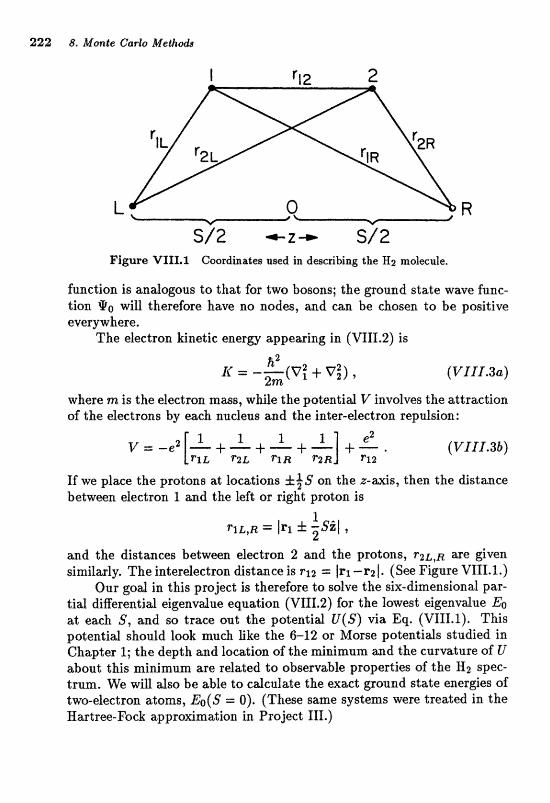
222 8* lMorsle Caris Methods
Figure TJ1l;I.l Coordhate~ used in de~ribing the E2 maEecuEe,
firnetion is andogous to that for two bosans; the ground state wave func- tion !Po will therefore have no nodes, md can be chosen to be positive every where.
The electron kinetic energy appearing in (VIn.2) is
where m is the efeetron mass, while the potentid V involves the attraction of the e l w t m s by each nudeas and the inter-.electron repalsion:
If we place the protons at locations rt f S on the z-axis, then the distance betwen eleetmn I tznd the left or right proton is
1
and the dktances betwwn electron 2 and the protons, r ~ h , ~ axe $jven sirnilwly, The interelectmn distmce is ~ 1 % = * (See Figure VIII.1.)
Our goal in this project is therefore to solve the six-dimensional par- tial differential eigenvdue equation (VIII.2) for the lowest eigenvalue E. at each S, and so trace out the potential U ( S ) via Eq. (VIII.1). This potential should look much like the 6-12 or Morse potential8 studied in Chapter 1; the depth and location of the minimum and the curvature of U &out this minimum are related to observable properties of the NIz spec- trum. We will also be able to calculate the exact ground state energies of two-electron atoms, Eo(S = 0). (These same systems were treated in the Hastree-Fock apprasmation in Projject ID.)
VIII. Quantum Monte Carlo for the H2 molecule 223
WIf.2 Vargwtional Monte Carlo and the trial wave function We begin by discussing a variational Monte Carlo solution to the eigen- value problem. If @(r) is any trial wave function (which we can choose to be real) not orthogond to the exact ground state qo, then an upper bound to the electronic eigenvalue is the variational energy
where we have used r as a shorthmd notation far the six coordinates of the problem, rl,z, and have written (VIIIAb) in a somewhat unconven- tional way. Note that this last equation can be interpreted as giving the variation4 energy as the average of a 'local energy",
over all of the six-dimensional F-space with weighting w(r) m e2(r). Hence, to evdnale the vaGalioad energy by a Monte Caslo quadrature;, all we need do is generate configurations (values of r l , ~ ) distributed accord- ing to (by the Metropolis algorithm, for example), and then average E wer these configurations. It should be clem thaL this method can be generalized readily to spterns invofving a l m p r number af coordinates.
The choice of QF is crnstr.iZined by the requirements that it be ~imple enough to allow a convenient evaluation of e2 and E , yet dso be a good approximation to tht? true gound state, go. hdeed, if we are fortunate enough to choose a @ that is the exact solution, then E is independent of r, so that; the, Monte Carlo quadratare gives the exact e w r a with zem vari- ance. Thns, not only will the v;triadiond baand become better as Q[, better approdmates P, but the vasimee in tlxe Monte Carlo quadra;t;ure will be- come smauer. The trid wave function should &so be symnaetdc under the interchange of the t w electrons' sspatid coordin&es, but it need not be normatized properly, as the normalization cancels in evaluating (VIII.4).
One plausible choice far the drid wave functian ie a correlated product of molecdar orbitds:
224 8. M~rate Carlo Me&&#
Here, the first two factors are an independent-particle wave function plac- ing each electron in a molecular orbital in which it is shared equally be- tween the two protons. A simple choice for the molecular orbital is the symmetric linear combination of atomic orbitals centered about each pro- ton,
(b(ri) = empi&/" + e - p i ~ / a ( V I I I , 6b)
with the variationd parmeter a to be determined below. The find factor in the trid wave function, f , =presses the correlation between the t w electrons due to their Coulomb repulsion. That is, we expect f to be smd when rl2 is smdl and to approach a large constant value as the electrons become well separated. A. convenient and reasonabk choice is
where a and p asle additional positive variaLional parmehrs. Note that ,8 controls the distace over which the trid wave function @healsR $0 its uncofrelfated vdue as the two electrons mpwate,
The s i n d ~ i t y of the Coulomb pstentid at short distances places addition& constraints on the trial wave function. ff one of the electrons (say 1) approwhes one of the nudei (say the left one) while the other electron remains fixed, then the potential t e rn in c becomes large ands negative, since T ~ L becomes smdl. This must be cancelled by a corre- sponding positive divergence! in the kinetic energy term if we are to keep E smooth a d have a smax variance ia the Monte Carlo quadratare. Thus, the trial wave function shoald have a Ckusp*bt r l ~ = 0, which means that the molecnlar orbit& shotlfd satisfy
e2 V ~ $ ( ~ I L ~ - G = finite tefnrs. (VIIl.7)
Similar conditions must dso be sat;isfied whenever any one of the distmces FZR,L, or va~lishe~. Using (VIII.6) and a bit of algebra, it is easy
to see that these constraints imply that a satisfies the transeendentd equation
and that a = 2ao, where a0 = h2/mez is the Bohr radius. Thus, P is the only variational parameter at our disposal. Note that these Coulomb cusp conditions would not have been as important if we were to use some other quadrature method to evaluate the variational energv, as then each
VIII* QetanGttm Mante Carla for the H2 molecule 225
of the divergences in E would be cancelled by a geometrical rZ weighting in the associaLIed dis;tanee.
With the trial wave fundion specified by Eqs. (VZ11.6), explicit ex- pressions can be worked out for ~ ( r ) in terms of the values and derivatives Bf: cfZ and f . Note that; this form of the trid function is not appropriate for very large proton separations, as it contains a finite amplitude to find the two eleetrans close to the same proton.
VIII.3 Monte Carlo evaluation of the exact energy We now turn to a hrlo~te Cwla method for evduatiag the egaet elec- tronic eigenvalug, E@. It is baged upon evolution of the imaginary-time Schroedinger equation to refine the trial wave function to the exact ground state. In particular, the latter can be obtained by applying the opera- tor exp(-at/&) to the trial state @ and considering the long-time limit t -+ W. (See the discussion concerning eigenvdues of elliptic operators given in Section 7.4 for further details.) Thus, we define
where E,(tf) is an as-yet-undetermined c-number function. Note that as long as (Po/@) + 0, @(t) wig approach the (un-normalized) exact ground state !Ifo as t becomes large. Our method (Path IRtegsal Monte Carlo) is equivalent to evaluating the path integral representation of (VI1I.S) nu- mericdy. An alternative method (Green's Function Monte Carlo, [Ce79]) would be to filter with the inverse of the skif'ted Hamiltonian, instead of the exponential in (VIII.9).
To compute the exact ground state energy &, we consider a slight generalization of the variational energy (VIII.4) using the hermitidty of
It should be clear that E(t = 0) = E,, the variational energy associated with m, that E($ --. m) = Eo, and that E( t ) is independent of the function E,(tt).
Equatian (VIIZ.10) expresses the exact enerlir;l)" in a form suitable for Monte Carlo evaluation. To see this, we define G(r, t ) = @(r)@(r, t), so that (VIXL. 10) becames
236 8, Monte CarloMethods
The exact energy E(t ) is thus the average of the local energy E over the distribution G(r, t). (Note that for the problem we are considering, G is positive definite since neither @ nor has any nodes.) A Monte Carlo evduation of E therefore mquires an "ensemble" of N configura tions (rl , . . . , rN) distributed according to G(r, l ) , through which E($) can be estimated by
, N
with an expression for the variance in analogy with (8.3). Note that if @(r) is in fact the egaet ground state go, then ~ ( r ) = E@, independent of r, and so E($) = E. with zero variance.
Of course, the expressions above are of no practical use withoat a way to generate the ensemble of configurations. At t = 0, G(r, t ) = ao th& a method like that of Metropolis et al. can be used to generate the initial ensemble, typiea3ly having N ss: 30 members, To evolve the ensemble in tim% note that since
dlJL! a-- = (E, - H ) @ , at
G satisfies the evolutiorr equation
We have used here an obviaus notation far the spatid derivatives, Equation (VIII.13b) em be interpreted as a diffusion equation for G,
with a drift function
It shows that the kinetic energy acts to diffuse G, that D tends to keep G confined to regions where i s large, and that the Usource'' increases G where e(r) is smallest.
The evoftttiorr of G over a short time from t to t + At can be repre- aented thmugh order At by the integrd ktzrncll
W1II. Quantum Monte Car20 for the molecule 227
whem P(,, r'; At) = exp { - [~(r) - ~ , ( t ) ] ~ t / h . )
This kernel (which is positive definite) can be interpreted as the condi- tional probability for a configuration to evolve from r' at time t to r at time + At. This probability contains a factor associated with the kinetic energy, whieh, acts to diffuse the system about r' through a normalized Gaussian probability distribution wit h variance &At / m and mean DA2. The other fxtor in B is associated with the locd energy, which acts to keep the system in regions of space where e is most negative by enhanc- ing the probability for jumps to occur to such locations. The quantum mechanical structure of the exact ground state is thug determined by the balazlce between these t~vo competing tendmcies,
The algorithm for evolving the ensemble should now be evident. A configuration at time 1 at the point r' generates a contribution to G(r, t f At) equd to P(r, r'; At). This is realized by placing in the new ensemble a eonfipration, r chosen according to the distribution
and then weieting the importance of this configuration by
One way of effecting this weighting in prwtiec? is to replicate or delete the configuration in the new ensemble with probabilities given by this latter function. In this case, N fluctuates from time step to time gtep but can be held roughly constant by continuous adjustment of E,. Indeed, to keep
drG(r, t ) (and hence N ) constant, E,(t) should be equal to E(t) , so that E, also furnishes an estimate of E(t). An alternative way of effecting the weighting is to assign an importance (i.e., a weight Wi) to each config- uration in the ensemble when aver&ng E. to compute the energy. Th& is, the aummand in (VIII.12) is modified to W i ~ ( r i ) . At each time step, Wi for each c0nfiguril;tion is multiplied by the first f w b r in (VII1.f 61, with E, readjusted to keep average weight of ewb configuration in the easem- Me equd to 1, This latter method requires less bookkeeping than does that of rqlicating and deleting, but can be heficient, as a ~0nfigurat;ion thag lzappents to acquire a very small weight is stiU. followed during the evolu tion,
228 8. Monte Carlo Hethdg
h summay, the method is aa fonows. The system is described by an ensemble of coniipratians, each having a relative might in desmibing the propertie8 of the system and initiaUy distributed in r aecarding to the trial function l@(r) The overall efficiency of the method is clhse?y related to the akccuracy af this trial function. To evolve the ensemble in, time, each member is moved in r with a shifted Gaussian probabgity function [the second factor in Eq. (VIII.IG)] and its weight is multiplied by the first fwtor in Eq. (VlII.15). The quantity En(t), wU& is ad;jnsted after each time step to keep the average vveight of the ensemble equd to 1, provides an estimate of the energy, as does the ateighted aver%@ af ~ ( r ) over the ensemble at any time. Furthermore, once the total evolution time is sufficiently large to filter the trial wave function, continued evolu- tion generates independent ensembles distributed according to the exact ground state wave function, which allows the statistics to be improved to any required accuracy.
Note that since the ensedle move8 through c d g u m t i a n space ed by At, which must be sufficiently s m d so that
Eqs. (VIII.I5,16) are accurate, the estimates of the energy at successive time steps will not be statistically independent. Therefore, in forming averages and computing variances, care must be taken to use ensembles only at intervals of t sufficiently large that the values are uncorrelated. SuGh in t e rds are cenveniently d e t e r ~ n e d by exad~ng; the autocome- ldion fumtions of the estimate. Alternatively, one can use the method af binning the values into groups, as discussed in connection wit h the Ising cdcalation in. Section 8.4, It shodd dso be noted that the finite time step requires that calculations be done for several different values of At and the results extrapdaed to the At = O li&t. A useful way to set a scale for At i s to note that the average step the Gaussian distribution in (VIII.16) is roughly ( h ~ t / m ) ' / ~ ; this must be s m d compared to the length se&s in the wave function.
Expectation values of observables other than the energy in the exact ground state are not simply given by this method. To see this, consider the gound state expectation value of some observable A that does not commute with the H
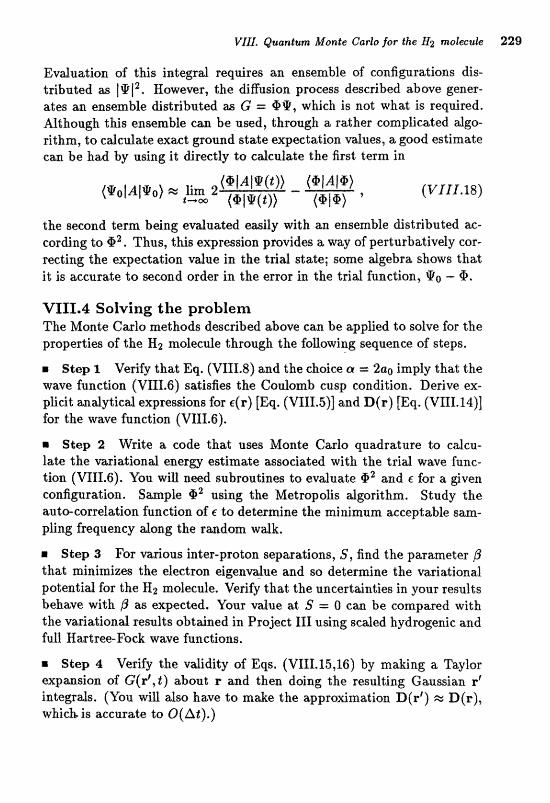
VlIl. Quantum Mmte Carlo for the H2 molecule 229
Evaluation of this integral requires an ensemble of configurations &S- @ 1'. However, the diffusion process described above gener-
ates an ensemble astributed as G = g?@, wKch is not what is required, Although this ensemble can be used, through a rather complicated dgo- rithxn, to cdcdate ex& gfound st& expectation values, a good estimate can be had by using it directly to cdculate the first term in
the second term being evduated easily with an ensemble distributed W-
cording to g2. Thus, this expression provides a way of perturbatively car- recting the expectation value in the trial state; some algebra shows that it is accurate to secand order in the emor in, the trial function, -- @,
VIII.4 Solving the problem The Monte Calo methods described above can be applied to solve for the properties of the H2 molecde throagh the faaowing sequence of steps.
r Shp I Verify that Eq. (VII1.8) and thechcsicecu = 2ao imply that the wave fnnction (VTT1.6) satl~fies the Coulomb cusp condition. Derive ex- plicit analytical expressions for ~ ( r ) [Eq. (VIII.5)] and D(r) [Eq. (VIII.I.I)] for the wave function (VIII.6).
r Step 2 Write a code that uses Moate Cm10 quadrature to cdcu- late the mriat;iond e m r g estimate associ%ted with the trial wave hnc- tion (VIII.6). You will need subroutines to evaluate m2 and E for a given configuration. Sample Q' using the Metropolis algorithm. Study the mto-cornelation funceSon of E ta deternnine the minimum acceptable sam- pling frequency along the random walk,
Step 3 For various inter-proton separations, S, find the parameter P that minimizes the electron eie;envdae and so determine the variatianal po ta t id for the Mz molecule. Verify t h t the nnce;rtaint;ies in your results behave with P as expected. Your vdue at S = O can be compared with the variational results obtained in Project III using scaled hydrogenic and fttl.1. XIEartrw-Fack wave functions.
Step 4 Verify the validity of Eqs. (VIII.15,16) by making a Taylor expansion of G(rt , t ) about r and then doing the resulting Gaussian r' integrals. (You will also have to make the approximation D(rt) E;: D(r), which is accurate to O(ht).)
= Sdep 5 Test the Path In teed Monte Carlo scheme for finding the exact graund state enerw of a Eamiltonian an the simple situation of a particle in a one-dimeneion-ali hamonic-oscif2ator potentid. Write a p r o g r a that assumes a Gaussisur trial functian with an incorrect; width and verify that the time evolution refines the merw in the expected way. An ensemble of 20-30 members &odd be snseient;, hvestigate how the y & t y of your reslllts vmies with the error in the trid wave funclion and with the time step you use,
m Step f3 Carrrrbine the progrms you wrote in Sttlrps 2 and 5 into one that d e t e r ~ n e s the exact eigenvdue of the ground state elf the two- electron prablem and so determine the exact Kz nildeculm potentid ad vaious separations. In particular, deterdne the location of the mini- mum in the paentiitl and coaapae with the empirical vdnes @wn in Section 1.4, Use the t r id functions deterdned in Step 2 and verify that your exaet ener@es are always lower thaa the vasiatimd vdues. Also verify that your exact r e d t e are independent of the preciae choice of P and that they extrapolate srnootlrly as a fuflction of Bt. Determine the binding energy of the He &om by considering S = 0 and eompme urith the exact vdue given in the di8cus~ion of Project 111.
Appendix A
How to Use the Programs
This appendix contains the information needed to execute the Compu- tational Physics codes. To foEow the instructions below, you must be familia with your computer's operating system, FORTRAN compiler, linker, editor, and graphics package. If you are unfamiliar with any of these, consult your computer system documentation before proceeding. You may also find it useful to have a FORTRAN language reference (e.g., [Ko87]) handy.
A.1 Ixrstdf&iomz Before anything else can be done, you must install the codes by down- loading them from diskette to your computer or transferring them over the Internet network. Network transfer is much quicker and free (see Appendix E for details), but requires software and network connections that; are not uxriversdy avdable. The other modes of distribution are fBM-PC or Macintcssh fomatted diskettes; m order farm for these is in the b x k of tEs book.
For those users who purchase the disketta md astj glmning to run the codes on an IBM-PC as Mac the irhstallatim proseduse is simply $0
copy the codes into a directory on the hard drive. Mwever, if you are not planning to run. the codes on m IBM compatible or Mac, then download- ipg may not be simple. and will depend on the details of yaur hardwme. The general scheme i s to find a PC or MW connected via modem or net-urork to your machine, and then to use a file trmsfer p r o ~ r m (e.g., KERMIT) to trafzsfer the Computaliclnal Physics files. Yatr &ght even find it necegsary to go through. one or more intermediate machines to get to yaurs. If you are inexperienced with file transfer, consult a locd expert, Once you download the files on your machine, we suggest you back them up immediate& on media that caa be read directly by that machine.

232 A, How to &7&e the Progranas
A,% Fifes There me five categories af file8 included on the fimpzrtatio~aal Ph~lsics diskette: t e e codes, common utilie programs, physics p r ~ p a m s , data aes , and indude files. These were written in xeordance with FORTRAN- 77 st mctmds (wit h two exceptions noted below) and therefore should run on my ma&ine with a FORTRAN-77 compiler. The Estings for the examples are in Appeadix B, the projects in Appendix C, and the conamon uf;ifity codes in Appendix D. 1) The text codes are the short codes that appear in the text. They
are n m e d CHAPnx.FOR, where 6x1' indicatles, the &apter nuaaber, m d 'X' is a letter to digereatiate codes within the s m e chaplter. Due to l a d of space on tbe diskette, only the longer of these codes we induded; the others; cm be entered from yovr keyboard. These =quire no editing to m, with the exception of those in Chapter 8 wfiich requipe a random nunber generator that is non-standard FORTRAN-77, E your compibr does not provide one, use the function RAHH~S, wh_ich is in file T7TXL.I"OR.
2) The first five common utiiity FORTRAN codes are called by, and therefore must be Enked with, each of the physics p r q r m s , UTIL.FOR contains the routines for menuing, 110, file opening/dosing, etc. SETTJP.FOIR contdns xl'l the vadables a d routines that are hmd- wwe and compiler dependent, e.g., sereen length m d terminal unit mm- Ber. Uou may need to edit this file to get the motst eacient and attrmtive output. (See section A.3.) The three remaining utility codes are graphics files: GRAPHIT.EI1, GUPHIT,XIO, m d GRAPEIXT,BLK, which, provide the interface between the physics code and your grapKcs pacbge, These three files contajxl the same subroutines, but for digerent typeer of grapucs packages. You will need to link in only one of these. GRAPHIT-HI calls a high-level package, e.g., a paehage that can draw axes with one call; GRAPHXT.LO calls a low-level pwkage, e.g., a paekage that is only ca- pable of drawing primitives such as lines and circles and so requires many c d s to draw the axes; and GRAPHIT.BLK contains empty subroutines for a non-existent package. This last file is included so that there are no unsatisfied calls at link time. If you want to prodam plots, see section A.5.
The last utiliLy code, STRIE",FQR, strips all V'-deimited comments out of FORTRAN wdies. The '!' is not standwd but we have ased it for clear documentation. 3) The sixteen physics codes for the examples and projects are named
EXMPLn.FQR md PEOJs,PQR, where 'n' indicates the chapter, With two exceptions, these do not require editing to run (see A.3).
A,$ Compilation 233
4) The three data files all have the .DAT extension and contain data to be read into EXMPL5.lFOR at; run time. They requim no editing.
5) The indude files contain common blocks and variable type declara- tions that must be included in the FORTUN codes to compile: them. (We have not conformed to the default typing supported by FORTRAN, e.g., not all variables starting with the letters 'I' through 'N' are integem).
The file n m e extension indicate^ in which, codes the file mast be included, Those $hat have $he ALL a t e n ~ i a n must be included in d the programs except STRIP.FOR and the text codes. They contain variables for graphics (GRFDAT.ALL and UISGRF.ALL), menuing (MENU.ALL), and I/O (IO.ALL). Those that have the extension En or Pn (where 'n' indicates the chapter) belong to a particular example or project. The file rime indicates the funetion of the wriables included in. the common block. The MAP files cont&n variable^ to map the menu items to the program parameters. There are only seven of these. The PARAM files contain all the parameters that are constant during one calculation. There are sixteen of these. The one exception to t h w n ng conventions is tBe file UISGRF.ALL. Thia file i~ onlg used with GEAPWIT.LO. Each include file is list& with the mast closdy relatd code: t h w with E h or Pa extensions we listed with the corresponding emmple ar praject in Appendix B or C, GEFDAT.ALL and 'EIISGRF".ALL me in Appendix Da4, MENU.ALL i s in Appendix D.3, a~nd IO.ALL is in Appendix D.2.
All of these files are induded in the pmgrarxls by the compiler with the XICLWE statement, Tbis is the other non-stmdard stitt-emeat i~ the codes. We have used it both because rniuly compiler^ support it, and because it is a sfmificant aid in program development and maintenance,
A.3 Compilation To prepme the codes for compilation is a matter of simple (but possibly tedious) editing. 1) First, if your FORTRAN compiler does not support the rrnuDB state-
ment, you muse edit each d the physies and utility progras ta inehde the common block files. (See the previous section for a description of these files.) Before doing so, heck your compiler manud to see if it provides this statement or one with a different name but serving the same purpose (e.g., USE). In some compilers, this command is treated as a FORTRAN statement, while in others, it is a compiler directive, if m& a statment is provided, simply repIwe ~ ~ G L W E with your compiler's equivdent state- ment. Note that the indude file nrtrnes muet be ezactlgl the same in the
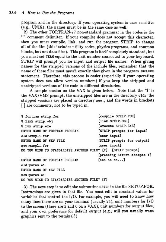
234 A. Haw to U8e the Pmgmm;s
program and in the directory, If your operating system is c a e sensitive (e.g., UNIX), the names must be in the same case as well.
2) The other FORTRAN-77 non-standard grammar in the codes is the '!!" comment; delimiter. If your compiler doea not xcept this &ar%cter, then you must compile, link, astd run the progrm STRLP to change all of the files (this includes utility codes, physics programs, and common blocks, but not data files). This program is itself completely st;andasd, but you must set TEm equd to the urrit number connected to your keybowd. STRIP will prompt yen for input and output file names, Wfim @ving names for the stripped versions of the indude Eles, remember that the name of these files mast match exactly that @wn in the grogram XHamE statement. Therefore, this process is easier (especially if your operating system does not allow version numbers) if you keep the stripped and unstripped versions of the code in BiRerent direetaries.
A sample session on the VAX is given below. Note that the '9' is the VAX/VMS prompt, the unstfipped files are in the directory old: the stripped versioas are placed in directory new:, abnd the words in brackets [ ] are comments, not to be typed in.
$ foreran strip.for Cco~pi Ja STEXP. FOR] $ l i n k strip.obj f 3 M STBIP.QEIJI $ x m strip,sxa fexe~u~e SmIP. EXE] ENTER MAME QF FOBmAM BMGRAN [STRIP prampts f o r inpatl old:ampZf,for [user input] ENTEB IRHE OF MEW FILE [STRfP prempts far outpn%l nsa:empll,ior [user h w t 3 DO YOU UXSB TO STAIIZAWIZE ABOTHER F I U ? fSTlkIP proafpt3
EBTEE lAME OF FOEaAW PWGRPM fa so ~ n . . L ]
neru:pwm.si DO YOU WISH TO STAIOIARI)TZE ABOTtfER FfLE? fY3
3) The next step is to edit the subroutine SENP in the file SETUP.FOR. Instructions are given in that file. You must edit in constant values for variables that control the I/O. For example, you will need to know how many lines there are on your terminal (usually 24), unit numbers for I/O to the screen (these are 5 and 6 on a VAX), unit numbers for output files, and your own preference for default output (e.g., will you usually want graphics sent to the terminal?)
4) This last step is optional, and involves the three other routines in SETUP,FQR that are also hardware dependent, These rautines come with dl the Iines commented out, excqt SWWWSbfE, H, and EBB. Subroutine CLIEhR clears the scrmn by sending escqe characteris to the terminal. The appropriate sequence for your terminal is located some- where in the terminal manual-probably in one of the appendices. This routine simply keeps the screen from looking too cluttered; it is not es- sentid. Code far VT200, Tektronix 4010, and PST screens is provided and can be used as a template for other screens. The last two routines (onoo~ and TMODE) switch the terminal between graphics and text mode and viCf? versa, These are only applicable if you have a te both graphics and text screens (e.g., GO-235 and HDS3200 terminals) and plan to use graphics. Again, the appropriate escape sequences are in the t e r ~ n a l manud.
With these changes completed, you can now compile the physics program, UTIL.FOR, SETUP.FOR, and GRAPHIT.BLK; link them to- gether; and execute. For example, on a VAX you would type:
$ i o r l r a e~2i.for,satup.ior,uti1.i~x~graphkt.b1k; $ I f& exmpli, obj , sstap. ob j ,at i.1. obj , graphi.2;. obj $ run amp1 l, csxe
During compilation, you must be sure thaL the SMCLWE files are present in the default directory*
A.4 Execution Background: Befolre ruxlning a y code, you should read the relevmt chapter and the preface to the code in Appendix B (for examples) or C (for projects). The text provides general infarmation about the algorithms and physic~, the Appendix provides details that will be of interest o d y if you run t h s e codes.
Execudion: Here we discuss the canventions that me fallowed, more or less closdy, by $1 af the programs; exceptions are noted in Appendicw B and C. All of the programs are designed to be run interactively. Each begins with a; ei tle page describing the physied problem to be investigated and the output that will be produced. Next, the m4rr menu is displayed, $iving you the choice of entering parameter vdues, exmining parameter v d ~ e s , running the pmgrm, or teminating the pragfam. Xf you ehoose to run the pragrm, execution proceeds w d output is sent to the requested devices, Far many of the progrms, the ed~ulittioxl has a definite end
(e.g., finding the cross section at a given energy), while for other programs (e.g., those involving time evolution) there is no clear end. In the second case, you are asked (at a frequency that you spedfy) whether you wish to continue the mn or return to the mdn menu. When the edcdation is finished, all values are zeroed (except the default parameters), and the main menu is re-displayed, giviv you the opport;uoity to redo the cdcufation with a new set of parmeters or ta end execntion.
IlnipuG: There me two time8 when the pro@- waits for input, First, the progam pauses for you to exmine output to the screen (e.g., the title page, o page of resdts, a plot); the execution is resumed when you press the fiturn. key. Second, the p r o p m will pause for you to enter ib parameter vdue. M paameter values have default d u e s &splayed in brackets [l; to accept the default value, press &returnv at the prompt. g you choo~e to input a new value, but use the incorrect fomat, the program reprompts for input, If you input a d u e ontside the range set in the menu, the program prompts fur input, s t a t i ~ g the rmge of vdues dowecf.
Reall numbers must be input in 89.2 far t, TEs is a cornpro- mise in order to allow default d u e s , The user input fanctioas ( G E T ~ T and G.~IIT) accept default d u e s by reading the input into a string variable and &ec&ng for zero length. If the string is not empty, the pasme- ter d u e m s t be read from the string wbich aet~ a m internal unit.. Therefore, the read m s t be formattd since list-directed r e d s from in- ternal files are nat standad. Note that some compilers do not insist on. the exponential (i.e., 1.23 and 1.23~+0 are both understood), or do allow Est-directed reads to internd units, so the formzbLting restrictions can be relaxed. Fortunately, integers may be entered in the "natural" way, as left justified numerals with no decimal. This is because the program twks a decimal point after the last non-blank character in the input string, and then r e d s the number from the string using F?. 0 famat,
In many programs you will be prompted for input outside of the main menu. This hitppens for several reasons. first, if the input paam- eters failed to pass a check, the program re-prompts for input. Second, guidance may be needed in choosing parameter values (e.g., the range of partial waves in PROJ4 depends on the input energy), and the pro- gram prompts for these values after reasonable default values have been cdcda"ced. Third, cafculations can often dfow the cfimge of parmelers during the run (e.g., the time step can be altered during time evolution), and the propam prompts for these value8 during a run.
Please note that our "defensive programming" has not been airtight. It is possible to crash the program or get meadngiess results by entering inappropriate parameters. The default parameters for each code are listed in Appendix B or C in brackets [l. See A.8 for details on chan@jng default vdues*
Output: To accommodate a variety of situations, there are several choices for run-time output. Text output can be displayed on the screen and/or sent to a file. Graphics output can be displayed on the screen and/or sent to a hardcopy device. The data used to generate graphics can also be sent to a file. You may choose the type of output by changing the default values in SETUPSFOR or by altering I/O parameters from the menu at run-time,
A.5 Graphics One drawbad to programming in FORTRAN is that there are no stan- dard F0 RTRAN graphics. This puts you in one of three situations: l) you have no graphics package at &l or 2) your graphics pacbge is executed in- dependently of the program that creates the data (i.e., it reads in the data from a file) or 3) your graphics packwe can be called from a FORTRAN progam,
If you have no graphics package, you should edit SETUP.FOR and 0, and GWFIL=O so that no graphics ilse produced.
Because the gapkica output geatty enhances many of these progrms, you Illight wish to consider purehaajing such a packwe.
For those users whose paphics package mast read the data from a file, the propams wiU (on request) output graphics data to a file. If you edit SETUPSFOR so that GWFIL=I, GRFBRD=@, and O ~ R H = O graphics data will always be sent to a file, but never to the screen or hardcopy device.
Findly, for those who have a FORTRAN cdable package, you will have to modify our codes to work with your package. To facztate this task, we provide a set of routines (contained in GRAPHIT.HI and GRAPHIT.LO) to act as an interface between the physics programs and a gc?nerd @;rap&= pwkage. The pbsics programs cdl the routi~es in the GRAPHIT files, which in turn call graphics package routines. This way, you only need to modify one GRAPHIT code instead of all of the physics codes. The code is docmented far ewe of nno&fication. GIRAPEXIT.EX calls the high level graphics package CA-DISSPLA; GRAPHIT.LO calls the low-level package UIS graphics (for the VAXstation). If you have either one of these packages, you can produce graphics with no further work, although you should read Appendix D.4 for information spedfic
238 A. How Ijg Eiae the P ~ m t n s
to your package. Also, routines for GKS on Sun workstations (written by Michel Valli&,res at Drexel University) are a d a b l e over the network (see Appendix E). Otherwise, use either GRAPHIT.HI or GRAPIIIT.LO, whichever i s more appropriate, as a template to create routines to call yonr graphics pachge.
A.6 Program Structure To facilitate code modification, we have attempted to conform to general "good" programming practices, sueh as those discussed in [Ke78]. The code far e d p r ~ e a m h= been formatted to m&e it easiex fo r e d , To the extent possible, variable names have been &own mnemonically and loops have been indented, as have sections of the cod- con$raUd by IF statements. Running comments on the right-hand side of many statment EEG@ indicate what; coxnputation is b&nl~; done. "I"o keep c d a to subroufinee as undnttmd, but as informadive, acl pasible, v&ables that me c o ~ s t m t for one run are passed in cornman blo&~, while vhatiles that change are passed in d s . Afl vdab1es met apficitly typed. T h i s gives a check on typographical errors (using a VAX FORTUN compiler switch) and provides a dictionary for variable namee.
The progr-8 are o r g ~ z e d in mbfoutinw, pdor&ng Iiidtd w d W& defined %=XI&. The subrautines that pdoraa the edcdations are at the beginning of the code, and within thwe routines the most important lines are listed in boldface. The bookkeeping and I/O routines ws Ested at the end, atnd we have tried to keep these adfarm from chapter to chapter. A header deseE.ibes the pmpoae Of the subzaatjne axld the vaiables it uses. These are five types: XIPUT and oWPW wiables (which are passed to the subroutine in the call statement), variables (which are used only within that subroutine), NlrcTIOIS (which are de.fi.~i& by FORTRAN mrcnor routines), and oLoefi variables (whieh are passed in common blodts). Below we list the purpose of the subroutines that are eammoa $0 aU the codes, wEle specific details for eaeh code prwede the wde listing in Appendices B and C.
f Em" displays header screen, initializes constants (e.g., PI = 3.1415826), and sets up the array8 needed for the menu. It is in this raul-ine that defadt dues aab firrrits for input parweters we get,
P A ~ M calls the menuing routine to obtain input parameters and then cdcul&(es any pasakanete~s that are functions of other input pmmeters. Eiks are opened and do154 here, and the
A, 7 Menu Stm~I~rt? 239
program stops in this routine, if so requested. Chedrs are performed to ensure that paramet er values are reason able.
outputs parameters to the teminal or file.
outputs text data to a terminal or file.
outputs graphics data to a terminal or file.
presides over the calculation. It calls the output routines we11 ills the routines that do the cdcdatioaa, and often.
performs cdeu1ations itself.
A,7 Menu Structure We give here a brief overview of the variables and subroutines that cre- ate and execute the menu. The menu is made up of up to 99 individual items, each item is described by eight pasameters: BaPE, YITETS, IRULS, HLOLIH, HHIltm, NSTWG, MPRHPT, HTAG, mo5t imgortmt p a m & @ ~ is HWPE wbielz describes the action to be perfbrmed. T h i ~ parameter f d s into one of three categories: 1) those that get input from the screen non^, rvx, BOOLUX, CBSTR), 2) those that provide flow control within
d;i; con- the menu (YESKIP. AOSKTP , HCADIC, SKIP, ~UIT), 3) and thwe the trol the display of information ( W ~ X T . PPRIBT, CUTM, #TITLE. TT=). The function of the other parmeters depends on the vdue of WPPE and are given below. Each of these pmameters are FORTRAN arrays dimen- sioned to 100. The index of the array corresponds to the index of the menu item. The one exception is MSISTRIC which (since rarely used) is di- mendoned to 10. These parameter &nays are: passed via in the indude file MEllilff.ALt,
There we four routhes that are used in running the menu. Subrou- tine (in file UTIL.FOR) initializes menu parameters that are common to all programs; subroutine TEXT (in each example or project) initializes the m e ~ u parameters speGjfic to th& pro@&=. Subroutinfl ASK (in fife UTIL.FQR) executes the menu items by pedorming the aetion dictated by MWPE. Subroutine P~~TAGs (in file UTIL'FOR) prints a aummasy of menu items.
Presiented here is a summary of menu pwmeter fuactians for each vdue of HTPPE. Any parameter not listed for a pwticdw type is not zl~ed.
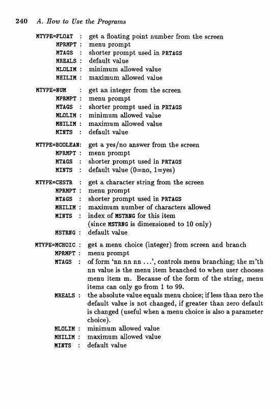
240 A, Now to Use the Pr0gmnz-s
get a floating point %umber from the screen menu prompt shorter prompt used in. PRTAGS default value minJmum dowed value m&muan &lowed vdue
get an integer from the screen menu prompt shorter prompt used in PBTACS minimum. dowed vdue m ~ m u m &awed vdue defadt value
get a yes/no mswer from the screen menu prompt shorter prompt used in BETAGS default value (O=no, l=yes)
get a chaacter string &am the aacrwn menu prampt @hartex prompt used in PRTAGS milximum number of chmacters dowed index of ~ [ S ~ H G for this item (since nsTmG is dimensioned to 10 only) default vdue
get a menu choice (integer) from screen and branch meau prompt of form 'm nan an . . .', controls menu brmching; the m'th nn vdue i s the menu item brached to when user chooses menu item m. Because of the farm of the string, menu items c m only go from I to 99. the absolute vdne equds menu choice; if less dfrm zero the default vdue is nat ebmed, if greiates than zero default is &aged (useful when a menu choice i s dsa a pwametef choice). minimum sowed value m&mum &lowed vdue default vdue

A, 8 Def~ul f flalzbe Revision 242
MTYPB=YESXIP: get a yesfno answer from screen, skip on yes WMPT: menu prompt RTAGS : shorter prompt used in fmhGs MMALS: menu item to skip to on yes nrms : default value (O=no, l=yes)
RTYPB=IOSKIP: get a yes/no answer from screen, skip on no hfPWT: menu prompt TAGS : shorter prompt used in PRTICS 8mkLS: menu item to @kip to art no arrTs : default value (O=no, l=yes)
E ~ P E = S K I P : skip uncon&tionally W ~ A L S : menu igem to skip $0
RTYPE=UIIT : pause a ~ d wait for user to press return before coxltioiuing
IIIIPHPT: menu prompt
H ~ P E = Q ~ ] X T : quit menu and return to cding routine
HnPE=PPRIHT: print description of a range of menu items by calling PRTAGS
8LQLXM: index of first, menu item MHILIR: i n d a af lwt menu item
HnPE=TITLE : print information without getting input (in i s K and PRTAGS)
EPWT: infamation to be prhted HMLIM: number of blank lines ta s u p bdore printing nltrxLxn: number of blank iines lo skip after prhting
I(TYPE=HTITLE: print information without getting input (in ASK only) HPEWT: infornation to be printed RLoLxn: number of blank Enes tm 8Eg befare printing ~ I L I M : number of blank lines to skip after printing
A.8 Default Vdue Revision At some point the default vdues set in the progrms will rrot carrespond to your needs, a d chwging vdues at run-time throngh the menu will become tedious. When this happens you will want to dhange the default
*sly apnlau! ~vxyd apl E! pale~ol s%aama$v$s 3nmwvd Aq panyap are q3g~ 'sao!~aam!p rCem aaaql alp 12123 no^ .uo!snauIp rCvaa aqlol pnba sl azp a3!93~1 mnmpm aql os 'aqs Xv~re pampap aql wql ~a-l An% aq aoum~ ppg v ~OJ 8$u~ad a~!$$'itj p aaqurnu eyl baldmm za~ *waw -a%Q%s tfat&ZXn'fld Nvx&xoJ aqS Aq paayiap @alqQYeh 03 $as @m @%PR @say3 saw~$amo~ *sA:r?sm WX~~H pm nz?xW a! paafrcr)~:, am sranpA alq%aap mnurptxr pm rurn-uxTam *s1plap asam JCBJ a~aqq tey qa3as aq$ aa~ "saa -FA ral3esep JQJ at pm 'sap fear ;rqj mm a1 %anpn au/saA
sanp sa%aauf mj ui am SanpA ap~jap may$ -sAem naam nf pars$% an saap ay$ !&~gr aafltnozqas ut! $as s$p%jap pisamnu pm @3!skqfirld *(anoqv g*y -g) XO~*~Q~BS n! am sa3~oq3 011 ~F%J~(I
*apes aqg a! ~anp~
Appendix B
Programs for the Examp
B.1 Example 1 Algorithm This program finds the semiclassical approximations to the bound state energies of the Lennard-Jones potentid for the input vdue of 7 = ( 2 m a 2 ~ o / ~ 2 ) ' / 2 . The basic problem is to find, for each integer n, the vdue of E, for which Eq. (1.22) is satisfied. After the number of bound states is estimated (end of subroutine PAW), the energy for each level is found (DO loop 100 in subroutine arrclroar) using a secant search (subroutine SEARCH) to locate the zero of f = s- (nf$)rr. Subroutine acTxog calculates the action, s, for a given energy by using simple searches to locate the inner and outer tmoing pdnts m d then using Simpson's rule to edcdate the integral, with. a special treatment for the squae-root behavior near the turning points,
The patentid is defined by function POT, If you dedde to chmge the podefiial, be sure tha'c the minimum is norm&aed to a vdue olF -4 axrd that POmXM in. subroutine IHXT is set eqnd to the eqdgbriurur .X vdue of the new potentid. These requirements ensure that both the energy m d turning point s eache~ begin at remonable vdues: the mergy sear& at --l and the tnrnixrg point search at PDTMIIII.
Input The only physical parameter is 7 [SO.] which i s the dimensionless measure of the qumturn nat;ure of the problem. The rnf imum number of bound levels that can be found is k e d by the parameter M A X L a = f 00. If NLEVEE is calculated to be luger than this, you will be prompted for a new value of y until NLEVEL is small enough (subroutine PCAECK). The numerical parameters are the energy seach tolerance [.0005], the turning point search tolerance [.0005], and the number of points used in evaluating the action integral [100]. The graphing parameter ECRF [80] determines the number of points used in drawing the pha~e-spxe trajectories (subroutine GRFOUT), The limit on WGRF i s set by the parameter BAXGRF= 1000,
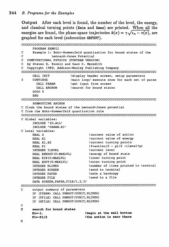
Output After each Ievd is found, the number of $he level, the energy, and dassied turning points (bin and wax) axe printed, Whea a;U the energies are found, the phase-space trajectories k ( s ) = y graphed for each level (subroutine CRFOUT).
cCCCCcCCCcccccCccccCcCCccccccCccccccccccCCCcccCcCcccccccccccccCc~cCccccc PRmM EXWLI
C E x m l e 1: Bohr-SomerEeld quan t lza t ion f o r bound s t a t e s of t h e C Lennard-Jones P o t e n t i a l C COWUTATTONAL PHYSICS (FORTMM WRSXON) C by Steven E, Roonin and Dawn C, Meredith C Copyright 1989, Addison-Wealay Publ ishing Company ccCcCecccececcc~ccccccccccccceccccc~ccceccecccecccceccccccecccccccc~cccc
G A U INIT !display header screen, s e t u p parameters S CONT & RUE fmain loop/ execute once f o r each set of param
CALL PAMM !get inpu t from screen C&LL MCWON !search f o r bound s t a t e s
GOTO 5 END
CCCCCCCCCCCCCCCCCCCCGGCCCCGCCCCGCCCCCGCCCCCCCCCCCCCCCCCCCCCCCCCCCCCCCCCC SUBROUTINE mCEEIN
C f i n d s t h e bound s t a t e s of t h e Lennaxd-Janes p o t e n t i a l C from t h e Bohr-Somerfeld quan t iza t fon r u l e C~CCCCCGCCCCCCCGCCCCGCCCCCGCCCCCCCGC~CCGCCCGCCCCCCCGCCCCCCCCCCCCCCCGCCCC C Global v a r i a b l e s :
INCLUDE "SO.ALLe IMCLUDE VPAMMeE1'
C Local va r iab les : =&L S !current va lue of a c t i o n m& El !cur ren t va lue o f energy MU X I , X2 f c u r r e n t tu rn ing p o i n t s M U F1 I f ~ a c t i o n l 2 - p i 1 2 - i l eve l*p i TNTeGER X M a L ! c u r r e n t Level mAL ENERGY ( Q : M L V L ) !energy of bound s t a r e M& XZN (0 : WLVL) ! inner t u r n i n g p a i n t REAL XOUT ( O : WLVL) !outer t u r n i n g p a i n t INTE(;ER NLINES !nu&er of l i n e s p r i n t e d t o t e rmina l INTEGER SCmEN !send t o t e rmina l TNTECER PAPER !make a h d r d ~ o p y INTEGER FILE Isend t o a f i l e DATA SCmEN, PMER, FTLE/f, 2,3/
cc~~~~cc~cc~c~Ccccc~cccccceccc~ccccccccccccec~c~e~ccccC:cccc~cccccc~cc~ec C output s u m a r y of parameters
I F (TTERN) CALL PRPllOVT {OUMIT, NLIMES) I F (TFILE) GALL PRIUIQUT (TUMf T, NLTNES) JF (GFXLE) CALL PWOUT(GUWZT,NLINES)
c C oeazab for b a n d rrtateo
Elm-5. tt>eqAn at the wall bottam El=-PT42 !the acrtion i a erro tharo
C:
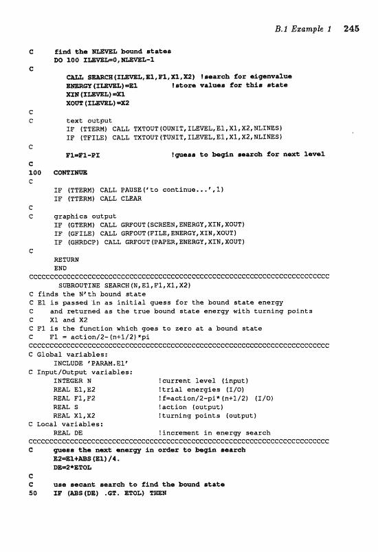
states -1
G L t H T , F 1 , X J , ~ ) fsrolr& f o r e%gesvaXae
I rrteze va3urar th i s s t a k e
C C text output
IF (TTERM) CALL TXTOUT {GUNIT, I L E n L , El, XI, X2, NLXNES) I F (TFTLEf CALL TXTOUT TUN^ T, f LEVEL, El, X1 , X2, ElLINES f
e h"l=EX-BX !mess t o bagAn mazah f o r m a t ZCWQI,
C roa comzm c
IF ITTERM) CALL PAUSE ("0 continue * . ' ,l) IF (TTERM) CALL CUAR
C C graphics output
TF (GTERH) CALL GWQUT (SCREEW, ENEKY, XTN, XOUT] TF (EFTLE ) CALL GWOUT (FTLE, ENERGY, X f I XOUT 1 IF" (GWRDGP J CALL GWOUT (PAPER, ENERGY, XIN, XOUT)
C RETURN END
ececcc~ccecccccccccccccccccccceccceccccccccecccccecccccccccccccececccecc SUBROUTINE SEARCH (M, El, F1, XI, X2f
C finds the N t t t h bound state C El is passed in as initial guess for the bound state energy G and returned as the true bound state enercfy with turning paints C XI and X 2 C PI fs the function which goes to zero at a bound state G F1 = actlon/2-(ntl/2jxpl cccccccccce~Cccccccccce~cccccceecccccceccce~~~cccccccccccccccc~c~ccccccc C Global variables:
INCLUDE v P m M . E 1 ' C Input/mtput variables:
INTEGER N !current Level (input) El, E2 ! trial energies ( I I O )
RE= F1, F2 ! f =aetion/2-pi* (n+l/2f f 1/01 RE& S taction (output 1 REAL X1,X2 !turning paints (output)
C Local variables: W% BE !increment in enerw search
ccCccccecccccccccec3cceccceccccecc~cccccC:cceccccccccccccccccceccccccccc~c C me@@ am% arnesrw i n oder t;o h g i n sear&
L2=81+=5 ( E l ) /4, BE=2*EZOL
C C use reeonnt; aaart=h to fAnd tbe hemd ataka ao XF (ms {DE) .@E. EZOL)
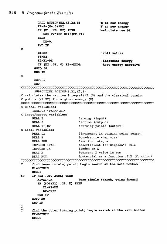
&C3eXOkE(EZ,n,X2,8) - (R+. 5 ) *F1 rs (xn *m. s 2 ) F-
Dm-Ez* (E2-El) / (82-F1) ELSE
Dma *
Ern ZIr C
El=RZ E*"%=F2 EP=El+DTZ IF (E2 .tBl. 0 ) ]EIP=-BTQ&
50 E m IF
e RETURN END
~C~~~~~C~CCCCCCCGCCCCGCCCCCCCCCCCCCCC~~~~~~C~~CCCCCCC~CCCCCCCCC~CCCC~CCC SUBRQUTINE ACTION (E, XI, XZ, S)
C calculates the (action intagra2)/2 ( S ) and the classical turning C points (XI,X2) for a given energy (E) cCccCceecccecccccccccceccceccccccecceccccecc~cccc~cccccecccccccecccccccc C Global variables:
C Inputloutput variables: mAL E fenerw (Input) mAL S ! actf on toutput) REAL X I , X 2 ? turnf ng points (output 1
C Locaf variables: DX !increment in turning point search
=&L M ! quadrature step size SUM !sum for integral
INTEGER IFAC !coefficient for Simpsonts rule INTEGER SX ! i n d e x cm X REAL X !current X value in sum MAL POT !potential as a function of X (function1
cccecccccccccceccccccceeccccccceccccccccccceccceccccccecccccccc~ccccecec C $id inner tumAng poink; bgin @ameh at Che w d l bottom
=*Q-% DX=. l
so ZIP (DZ .@l!* XTQL) XI-XI-DX lusar a 5 i ~ k e sear&, p i n g iawwd ra (Pm (m) .GB. E) PrnH
X1e.CDx DX=DX/Z
E m 33' -'TO 50 rnD m
C G fie Che -tar turning polnk; bagin sararab at tba w a Z l bottom
DX=. 2
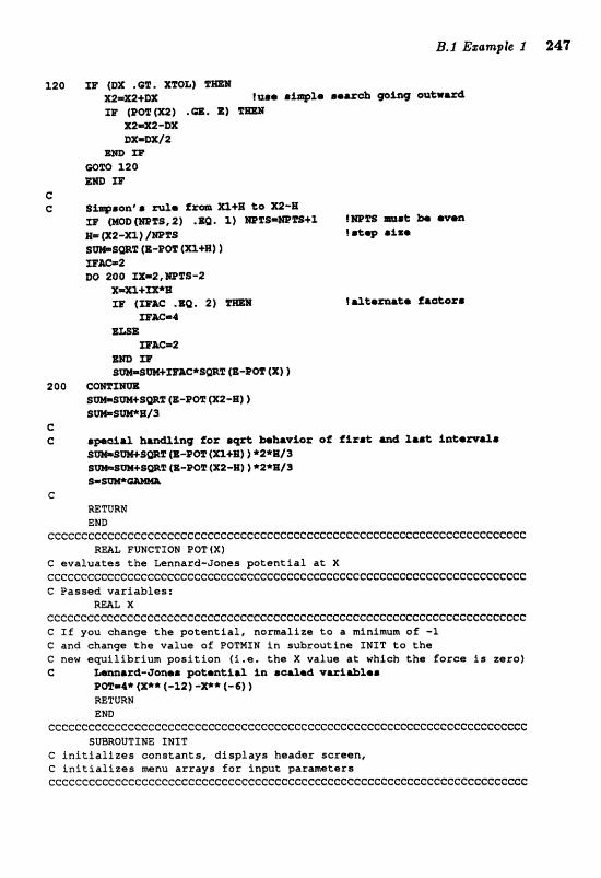
120 fP {OX .G%. moL) %m X2=Z2+aX lwre &-2r aaaz& pi- @a%w*rd m' (Pm 4x2) .a. m
X2mX2-DX DX=DX/I
E m ZB GQlM 12Q g m
C C S*+onC E mte fzm XT+B t o XZ-B
x r {rnD (WE@, 2) .m. 1) 'IQPIPI=m"IPSS.f mut; h H= (x2-~1 ) /=TB t &&up .fee B m S m P (E-EOT (=+g) Z a-2 DO 200 ==2,=TS-2
x=n+=*If Ik* {=&C .SQ, 2) T m
r n z m . 1 4 Bt-
=A-2 m X@ SW=SW+m&C*S@Z (B-POT (X) )
200 camzm s-sm+smv (E-@= (xz-n) I amSwH/3
C C ap(;;tp3, for h b v i o r oE firs& Iaet ifttam&e
SmBW+SmZ {S-Pm (XltB) ) *2*fI/9 S-BW+B=F (a-~ae (~2-IP) *2*l~f/3
C MTVRH BND
cccccccccccc~ceccccccccccccecccceccccecceccccceccccccccccccc FUNCTION POT (X) the Lannazd-Jones potential at X
ccccccccccccI;ccccccceccccceccccccccceccccccceccccceccccceecccccceccceccf:
ccccccccccccccccccccccccccccccccecc3ccccccceccccccccccccccccccccccccecccc C If you change the potential, normalize to a minimum of! -X C and change the value of POTHIN in subroutine INfT to t h e C new e~ilibrium position (i.e. the X value at which t h e Ecrce is zero) C Um11~4-Je~ae p%mtiljl in re8Zed ttrriiblrr
P m r * (X** (-3.2) -X** ( -6) ) RETURN END
cccccccccccccccceeccccccccceecceccccccccccccccccccccccccccccccececccccf:c SUBROUTINE IWIT
C initializes constants, displays header screen, C initializes menu arrays for input parameters cccceececcecceccceccccccccccccC:ccceceC=Cceccceccceccccccccccccccccccccccc
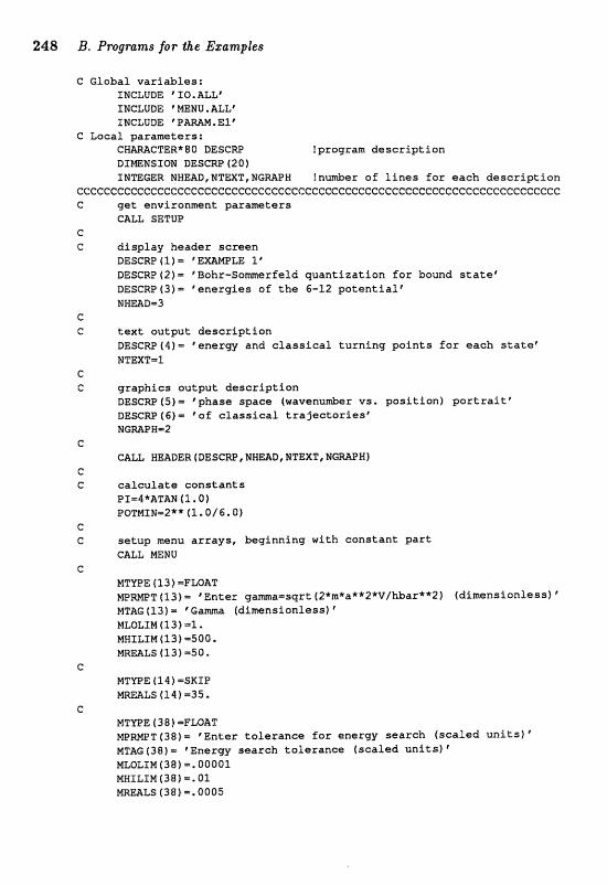
248 B. Pr~granzs for the Ezamples
C Global v a r i a b l e s : INCLUDE 'IIO.ALLC INCLUDE "MU *ALLf INCLUDE 'PWM,EI"
C Local, parameters : GHmCTERe80 DESCRP {program d e s c r i p t i o n DTaNSION DESCRP (20) ZNTEGER NHEAD,NTEXT,NCMPH !nu&er o f l i n e s for e a c h d e s c r i p t i s n
ceccecccc~cccCccccccece:ccccccceccccccccC:cececccccccccccccc"ccC:ecccccccccc C g a t environment parante ters
CALL SETUP c C d i s p l a y heade r s c r e e n
DESCRP (1 ) ' EXMLE 1 ' 83SCW(2)= 'Bohr-Somerfe ld q u a n t i z a t i o n f o r bound s t a t e t DESCRP(3)- % n n ~ g l a s o f t h e 6-12 p o t e n t i a l " NXEA8=3
c C t e x t o u t g u t d e s c r i p t i o n
DESCjRP(9)= ?ene rgy and c l a s s i c a l t u r n i n g p o i n t s f o r each s t a t e f NTEXT=1
C G g r a p h i c s o u t p u t d e s c r i p t i o n
DESCRP/S)= "phase space (wavenuniber v s , p o s i t i o n ) p o r t r a i t f BESCW ( 6 ) o f c l a s s i c a l t r a j e c t o r i e s e wcm~a=a
c CALL WEADER (DESCRP , NBmD, XJ"L"EXT, M G W W )
G G c a l c u l a t e c o n s t a n t s
PI=4*ATAEJ (I. 0) PQTMfN=2** (l .0/6.0)
C C: s e t u p m n u a r r a y s , beg inn ing wi th c o n s t a n t p a r t
CALL MEMU e
M T P E 113 ) -FLOAT M P W T (13 f = "ntar gamma-sqrt f 2*m*a**2*V/hbar**2} ( d imens ion les s ) " MT&G (13) = "ama (dimensionless) ' WEOLIM (53)=1. MHILIM (13) =500.
e MTYPE t 14 ) =SKIP
LS (14j.535. G
MTVPE ( 3 8 f =FLOAT MPWFT (381 = , E n t e r t o l e r a n c e f o r energy s e a r c h ( s c a l e d u n i t s ) MTAG fJ8) - ' Energy s e a r c h t o l e r anca ( s c a l e d u n i t s ) " MLQLIM (38) =. 00001
TM(38)=, 01
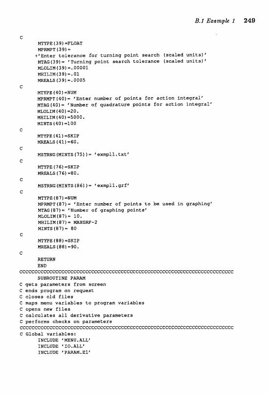
C NTYPE (3 9 ) =FLOAT MPmPT (391.. +'Enter tolerance for turning point search (sealed unitsf' MTAG ( 3 9 ) = Turning point search tolerance f sealed units) ' MLOLZM (381 =. 00002 MWILIM(39)-.0l MREALS (39) -. 0005
c MTYPE ( 4 0 1 -NUM N P W T I Q O ) = 'Enter nu&er of points for action Integral' MT&G(40/= *Nu&er of quadratuse points for action integral' MLQLIM (40) 120. MXILIM(4Of =SOQO. MINTS (40) -100
c MTYPE ( 4 I ) =SKIP M A L S 1 4 1 ) =GO.
C MSmNG (MIMTS [ "65) 1 = eexmpll, txtf
e MTVPE f 7 6 ) =SKI P
L5 ( 7 5 ) =80. C
MSTRNG(MINTS(86))= %exmpll.grf' C
MTYPE 4 87 1 =NUM lrlPMPT(87)m "nter nu-r of points to be usad in graphing' MTAG(87)a 'Nu&er of graphing pointsf MLaLfM(87)= 10. NN3LIM 4 8 7) PIIAXGW-2 MINTS(87)- 80
C MTWE (8 8) =SKIP MRMLS (88) =%Q
C RETURN END
c~~ec~~~~c~ccccec~cccc~cceccccc~cecccccc~ccc~~~cccccccccccec~c~e~~e~c~~~ SUBROUTINE P A W
C gets parameters from screen C ends grogram on request C closes old files e maps menu variables to program variables C opens new files C! caZeuXates all derivative parameters C performs cheeks on parameters CCCCCCCCCCCGCCCCCCCCCCCCCCCCGGCGCCFCCCCCCCCCCCCCCCCCCCCCCCCCGCCCCCCCCCCC C Globaf variables:
INCLUDE %MEN U, ALLF INCLUDE @ZO.ALLe IHCLUDE 'FAWM,El"
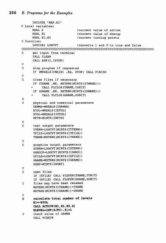
INCLUDE *=.Elt C Local variables:
REAL S fcurrent value of action R m L El !current value of energy REAL X1,X2 !current turning points
C Function: LQCTCAL LQGCVT !converts 1 and O to true and false
ccc~cccc~ccccccc~cccccecccc~ceccccccccc~ccceccccecf:eeccccccceeccccccCccc G gatinputfromtermlnal
CALL CLEM CALL ASK (1, ISTOP)
c G stop program if requested
IP ( r n m ~ ~ (XMASNI .ea. STQP t caLL FINISM C C close fi fes if necessazy
IF (TNA14E .m. MSTRNG (MINTS f ITMAMEt)) + CALL FLCLQS (TNRME, TUNITf IF (GHAME .NE, MSTRNG (MINTS (ZCMmE) ) )
+ CALL PLCLQS (GHAME, GUMIT) e C physical and numerical parameters
XTOL=mALS (EXTOL) NOTS=MINTS IINPTS)
C C text outfrut parameters
TTERM=LoGCvTtMXHTS(lTT&RMl} TFILE=LWeVT(NIMTStTTFILB)f TH~=MSTRMC (MINTS ( x T N a w
graphics output parameters GTERM=LoGCVT (MINTS (TGTERM] f GBmCPmLOGCVT (MXMTS (IGBRD) ) GFXLE-LQGWT(HXHTS(5GFILE)f GMM=MSTRNG (MINTS tXGNAm1 f MGRT=MINTS (IHGW 1
open files JF (TFILE) CALL FWPEN (TEA=, TUNIT) IF (EFILE) GALL FMPEN(GMm,GUHXT) files may have been renamed WSTRMG (MINTS 4 XTNAmf 1 =TNAME MSTRHG (MINTS (IGMAW) f =GHAME
cal&rtaa total n-ar sf fsvcrls Elm-EZQL
IHT (B/PZ-. 5 ) +l check value of GA)IMA CALL PCNECK
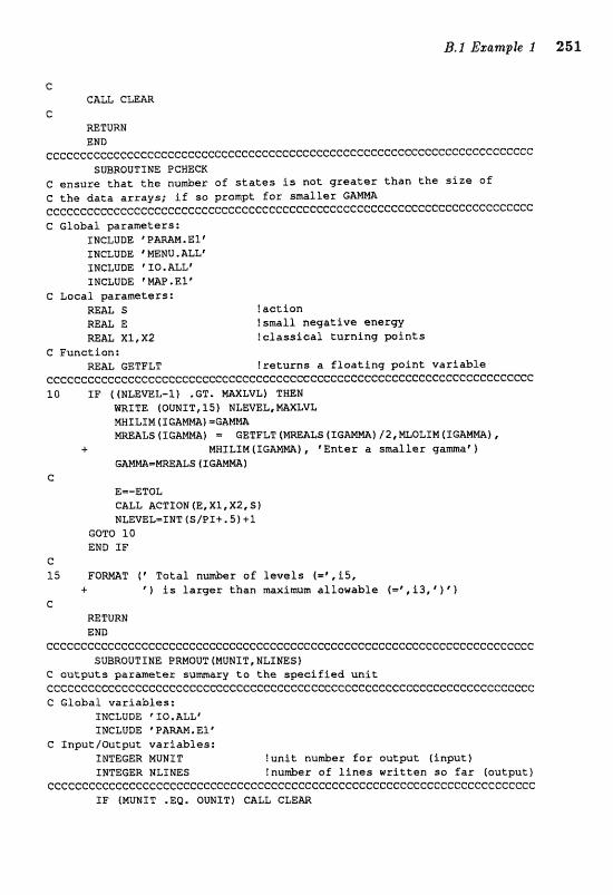
C CALL CLmR
C RRTrnN
SUBROUTINE OCWECX C ensure that the nuniber of states is not greater than the size of C the data arrays; if so prompt for smaller G ~CCCCCCCGC~CCCCCCC@CCC~CCCC"CCCGCCCGC1CGCCC~CCCC~CCCCCCCCCCCCCC~CCCCCCCCCC C Global parameters:
IMCLUDB 'PAMH.EIf INCLUDE * =NU. ALL" INCLUDE * IOIALLe INCLUDE * m P . E l r
C Local parameters: mAL S ! action R E a E !small negative energy W A t XI, X2 lclassical turning points
C Function: GETFLT !returns a floating point variable
ccCceCcccccCcceccceccccccccccccecceecccccecccccccccccccecccccccccceccccc 10 TF ((NLEVEL-I) .GT. mXLVL) THEN
WRITE (QUNIT,lS) NLEWL,mXLVL MHSLIM (IGAMm) =G&-
TPLT ( m ~ ~ s (rcmm) / ~ , ~ O L T M t1:GAnmj @
.c MWILIM(IGAMW), 'Enter a smaller gama')
E=-ETOL CALL ACTION (E, X I , XZ, S ) NLEVEL=INT (S/PI+. 5) 4-1
GOTO 10 END IF
C 15 P O m T ("'rota1 nu&er o f levels ,is,
+ ' 1 i s larger than maximum allowable (=f,i3,t)r1 C
=TURN END
cceccccccecccececccceccccc~cccccccccecceeccecceccccceccccccF:cccceccccccc SUBROUTINE PRMOUT(MUNfT,NLINES)
C ourputs parameter: sumary to the specified unit cccccccccccccececec~cccecccccccccccccccccecccccccecccccccccccecccccccccc C Global variables:
INCLUDE ' X0.ALL6 INCLUDE *PPARAM.EI"
C Inputloutput variables: INTEGER MWbT !un i t nuaer for output (input J INTEGER NLINES !nu&er of lines written so far (output)
ce~cccc~cc~~cecc~cccccc~ccecccccccccccccec~ccecccccecceeccccccccccc~cccc XF (MUNIT .Ea. OUNST) CALL CLEm
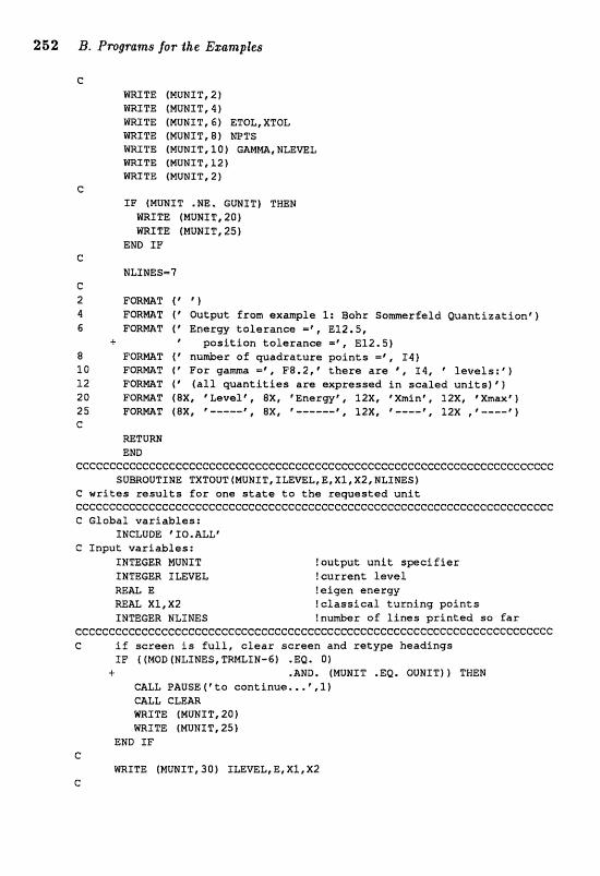
252 B. Programs for the Erctsmples
C WRITE (MUHIT, 2) mITE (MUMIT, Q) mITE (MUM1 T, 6 ) ETOL, XTQL WmTE (MUNIT,B) PEPTS WRITE (MUMIT, f Cl) G A M , NLEmL m I T E (MUMSK 1 2 ) m I T E (MUNIT, 2 )
C I F (MUNf T .ME. GWf Tf THEN
m I T E (MUMST, 201 W I T E (NUNIK ,251
END SF C
HLIMES=? C 2 FORmT ( * 1 4 FQRMT f * Output ffom example 1: Bohr S o m e x f a l d Q u a n t i z a t i o a v ) 6 FO-2" ( ' E n e r w t o l e r a n c e =l , E12, S,
+ p o s i t i o n t o l e r a n c e m*, E12.5) 8 FORmT ( * nnuder of q u a d r a t u r e p o i n t s =\ XI$) 1 0 F O m T ["or g a m a =@, FF8.2,* t h e r e a r e ', 14, * l levels :*) 12 F O W T ("all w a n t i t l e s are expressed in s c a l e d u n i t s ) ' ) 20 F O M T (8X, rLeve f l , @X, @EnergyPt 112X,'Xmfnt, 12X, eXmaxcl 25 F Q W T (8X, '-----P , ex, , 12X, "---p , 12X , ,----" 1 C
MTUW END
ccccccCcccccccCccccccceeccccccccccccccecccccccccccccceccc~cccecccccccccc SUBROUTINE TXTOUT (MUNI T, XLEVEL, E, X I , X2, NLINESI
C writes r e s u l t s f o r one s t a t e to t h e r eques t ed u n i t cecccccccccccccccccccccccecccccccCccccccccccccccccccccccccC:cccceC:ccececc C Global v a r i a b l e s :
INCLUDE 'IO.ALLv C Inpu t variables:
INTEGER MUNIT !ou tpu t unit s p e e i f i e r INTEGER XLEVEL !current l e v e l mAL E Ie igen enerr3y REaZ X1,X2 ! c l a s s i c a l t u r n i n g points INTEGER NLINES Inu&er of l i n e s p r i n t e d so f a r
ccccccccceccccceccccccccceecccecccccc~cccccccecccccccccccccecccccccccccc C if sc reen i s full, c l e a r s c r e e n and r e t y p e headings
IF f (MOD (NETNES, m L I N - 6 ) . EQ. 0) -4- .AND. (NUNPT .E@. OUNIT) t THEM
CALL PXLUSE(ftto c o n t i n u e , , . ' , l ) CALL e z E m @RITE (MUMIT, 20) m f T E (MUNIT,25)
END I F C
mXTE (WUNIT, 30) ILEVEL,E,Xl, X2 e
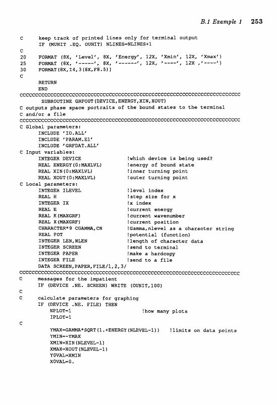
C keep t r a c k of p r i n t e d l i n e s only Ear t e rmina l ou tpu t XI? (WHIT .&Q. OUNIT} NLINES=MLINES+l
c 20 F O m T (8X, tZevel\ ,X, ' E n n e ~ " 12X, 'XXrninf, 12X, fXmax@l 25 F O W T (834, *-----' # @X, "- ." - - -P , , - - 12X ,? - - - - " 1 30 F O m T (8X,T4r 3 (8X,FBe5)f C
RETURN END
CCCCCCCCCCCCCCCCCCCCGCCCCGCCCCCCCCCCGCCCCCCCCCGCCCCCCCCCCCCCCCCCCCCCCGCC SUBROUTINE GRFOUT(DP;IIICE,ENERGY,XTES,XOUTi
C o u t p u t s phase space p a r t r a i t s aE t k s bound s t a t e s t o t h e t e r m i n a l C and/or a f i l e CCCCCCCCCCCCCCCCGCCCGCCCCGCCCCCCG~CCCGCCCCCCCCCCCCCCCCCCC~CCCCCCCCCCCCGC C Global parameters :
1 NCLUDE ' IO . ALL* SMCLUDE ' P A W - E l ' INCLUDE "WIIAT. ALL *
e I n p u t v a r i a b l e s : INTEGER DEVICE !which &vice is being used? MAL ENERGY ( D : W L V L ) ienercjry of bound s t a t e
XIN (O:rclAXLVLl ! inne r t u r n i n g p o i n t REAL XOUT (Q:mLVL) !ou te r t u r n i n g p o i n t
C Local p a r a m t e r s : XIJIPEEER ILEVEL ! l e v e l index R U L N ! s t e p s i z e f o r X INTEGSR I X I x index RE& I2 ! cu r ran t energy m& K t W G W ) ! cu r ren t w a v e n d e r
X [MXGRF 1 ! cu r ren t p o s i t i o n CTER* 9 CG&MM, CM !Gama,nlevel as a & a l a e t s r s t r i n g
REAL POT ? p o t e n t i a l ( func t ion) TMTBGER LEN,NLEN ?length of c h a x a ~ t e r d a t a INTEGER SCWEN !send t o t e rmina l INTEGER PWER !make a hardcopy INTEGER FfM Isend to a f i l e DATA SCREEN,Z>APER,FILE/1,2,3/
~cceCc~ccccc~~ccc~ccccceccececcccccccccecc~ccceeccccc~~c~c~~c~cc~~cccccc C messages f o r t h e impa t i en t
XP [DEVICE ,NE, SCREEN) WRITE (OUNIT, 2 0 0 ) c C c a l c u l a t e parameters f o r graphing
IF (DEVICE .NE, FILE) THEN NPLOT=l !how w n y p l a t s XPLOT=I,
c *SWT(l.+ENERGU(NLEVEL-1)1 !limits on d a t a p o i n t s
YMINm-VmX XMIN=XIN (NLEmL-1) XmX=XOVT (@LEVEL-1 ) YOVAL=XNTN xavax_l=o.
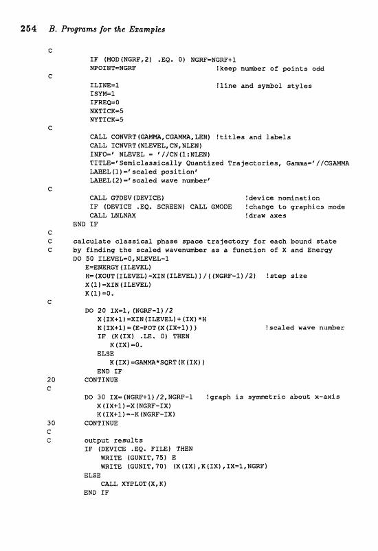
IF (MOD ( N G W , Z ) .EB. 0) NGW=NGRF+1 NPOINTmNGW !keep nu&er a f p o i n t s odd
C X L X ~ = I I l i n e and sy&al s t y l e s ISYM=I IFREQ-0 NXTICKeS NVZIICX=5
CALL CONVRTfaW,GGAm,LEN) l t i t les and labels caLL IGWRT (NLEWL, CH, NLEN I INFo=* NLEVeL = V / C N (1 ; NLEN) TXTLE=9emielass ica l ly Quantized T r a j e c t o r i e s , Gama=l / /CGMm m E L , (2 ) =f s s c l e d p o s i t i o n * -EL ( 2 f =* acalecf wave nu&srf
CUL GTDEV (DEVICE) !device nomination TP (DEVICE .EQ. SCREEN) CALL GMODE !change t o g r a p h i c s mode CALL I;NLNm !draw axes
END SF C C c a l c u l a t e c l a s s i c a l phase space t r a j e c t o r y f o r each bound s t a t e C by f i n d i n g t h e s c a l e d wavenuder a s a f u n c t i o n o f X and E n a r w
DO 50 ILEVELmO, NUVEL-1 EsEMERGV ( XLEVEL) W= (XoUT (XLE-Lf -XIW (ILEVEL1 f / ( 1MGRF-I f I 2 1 ! step s i z e X (1 J =KIN (ILE-L) R (1) 43.
C DO 20 IX-1, (NGW-1) 12
X (IX+1) =XIN (ILEVEL) + (1x1 *H K (IX+1) - (E-POT (X (IX+1) f 1 IF (R(IX) .LE, O f THEN
K (XXI =O. ELSE
K (1x1 =GMm*SQRT (K IXX)) IF
2 Q CONTINUE:
! s c a l e d wave n u h e r
G DO 30 X X I ( M C W + ~ ) / ~ ~ N G W - ~ !graph i s s y m e t r i c about x-axis
x (IX+lI =X (wGw-Ixt K (IX+1) =-K (NGRF-XX)
3 0 COWTXHUE C C output r e s u l t s
IF fDEVICE .EQ. FXLE) THEN WRSTE (GUNST,?S) E WRITE (GUNIT, 70) (X (1x1 ,R(fX), IX=I,NGml
ELSE (=;ALL XYPLO"IC(X, X )
END IF
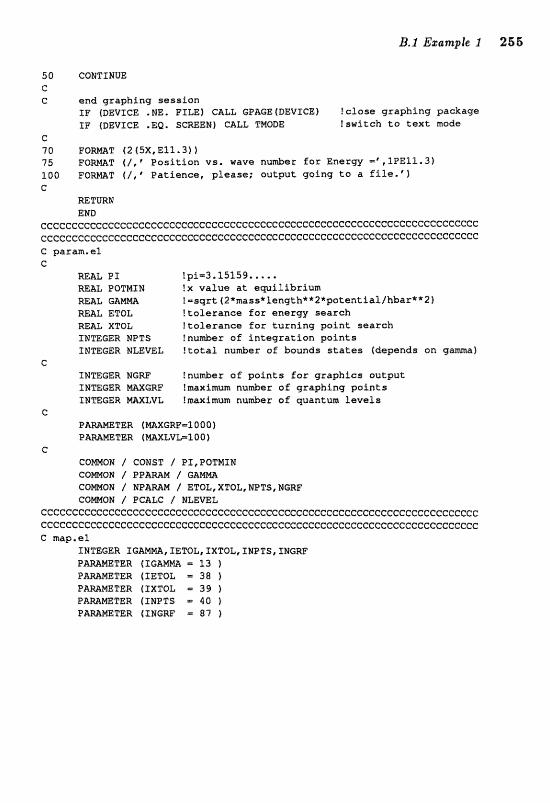
50 CONTI HUE e c end grapbing session
I F (DEVICE .ME, F I L E ) CALL GPAGE(DEVICE1 !close graphing packaw I F (DEVLCE .Ea. S M E N ) CALL TMODE !switch to text mode
C 70 F O M T (2 (5X,E11.3) 75 F O W T (/,VosiGion vs , wave n u d e r for Energy =r,IPE11.3) 100 F O W T f / , * Patience, please; autput going to a file-'l C
RETURN END
e~~c~~~~~ec~c~~c~cecc~ccccceeccccceeee~cceccccc~ccccccccc[ :ccccec~ccccccc c ~ ~ c c ~ ~ e c ~ e ~ ~ ~ ~ ~ ~ c c ~ c c ~ ~ c c e c c c e c e c c c c c ~ c c ~ c c c c c e c ~ c e e c C : c c c c c c c ~ c ~ c c c ~ c c c C param.el G
RE& P I ! p i = 3 , 1 5 1 5 9 ...., M& POTMXN !x value at equilibrium =&L G A M M !=sqr~(2*mass*length**2*patc?ntia1/hbar**2~ REAL ETOL !tolerance for energy search MBZ XTOL !tolerance for turning paint search INTEGER NPTS ! n u W r of integration paints INTEGER NLEVEL !total nunber o f bounds states (depends on gama)
C INTEGER NiERF !nu&er of paints far graphics output G F !maximum number of graphing points XMTeGER m L V L !m;ucinrum nudax of wanturn levels
C F m a T E R ( W G W = f 000) PAMMETER ( W L V L = 1 0 0 1
C COMOH / COHST / Pf,POTWIN como~ / p e m M I
/ ETOL, XTOL, NPTS, WGRF COMON / PCALC / NLEVEL
GCCCCCCCCCCCCCCCCGCCCCCGCCCCCCCCCGC~CCCCCCCCCCCCCCCCCCCCCCCCCCCCCCCCCC CCCC(J~CCCCGCC~CCCGCCCCCCCGCCCCC~CCCCCCCGGCCCCCCCCCCCCCCCCCGCGGCCC:CCCCCCC C map,ef,
f NTEGER X G m m , ZETOL, TXTOL, f NPTS, f M G W PARAMErnER ( I G A M = L 3 1
TER (XETOL = 38 ) TER (XXTOL = 39 )
PAMMETER (INPTS = 48 ) PAMWTER (XNGW = 87 )
256 B. Programs for the Ezamples
B.2 Example 2 ALlgorilthm The propam integrates trajectmies in the Ffdnon-Heiles po- tential (Eq. 2.35) and finds the corresponding surfaces of section (abbrevi- ated to SOS in the code). Subroutine ARcAaB creates the surface of section for one d u e of the energy by c&ng subroutine ws once for each set of initid conditions request&, Subroutine SOS prompts for initial vdues of y and p,, calculates p, from energy conservation (recall r = 0 on the surface of section), and executes the time integration (subroutine S ~ P ) until the =quested number Df s~lrf.$ee of section points have been found. Subroutine STEP takes a time step using the fourth-order Runge- Kutta step (subroutine RUBICE); derivatives of the coordinates and momenta are cdcdated by subroutine ~ A L and functions ~ E ~ z I V and mE;m. This row tine also checks for crossings of the the trajectory with the y-axis (i.e., whenever z = 0). If a crossing is found, it temporarily switches to I as the independent mriable and idlegrates bwk to find the surfxe of section intersection as described h the text.
Tbe form. of the potential may be chmged by editing the potential v and its deriv;zt;ives DERIV and ~ B X V wEch axe located in function V. You will also need to & w e the grapMng limits far the trajectory in subrou- tine T R J I ~ and should review the values DYO and TOLY (subroutine IBIT) used in seaching. The limits on the energy (also subroutine IPIT) should be the sxnaUest and largest vdues of energ that @ve rise to bounded moLioxl.
Input The physical parameter entered from the main menu is the en- ergy [.l]. The initial conditions for y [O.] and pp [Q.] are requested from subroutine SOS so that more than one get can be used in creating a, sin- gle surface of section. Limits on y depend only on the energy and are calculated by subroutine LIMITS; limits of p, depend on the energy and g, and are cdculated in so$. The numerical parameters are the time step [.l21 and the number of surface of section points 11001. As soon as the requested number of surface of section points are calculated for one set of initial conditions, you will be prompted for the number of additional surface of section points [O]; if you answer none, you will be asked if you want additional initial conditions; if you answer no, the surface of section is complete and you return to the main menu. The maximum surface of section points is fixed by M I X S S = 10,000. The only graphics parameter is the number of points in the trajectory to be plotted [4000]. This is needed to prevent output files from becoming too large and plots from becoming too cluttered.
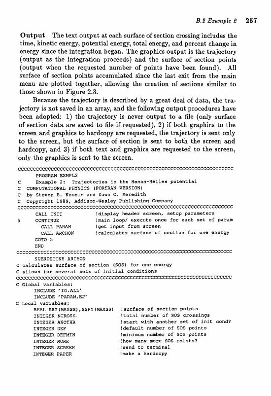
Output The text output at each surface of section crossing includes the t h e , kinetic mergy, potential energy, totd eRer0, a d percent change ia energy since the integration began. The graplria output is the trajectory (output as the integration proceeds) and the surface of section points (output when the requested number of points have been found). All sarface of section paints wcrtmulated since the exit from the m&n. menu ape plotted together, dowing the creation of sections similar to those s h a m in Figure 2.3.
Becmse thc? trajwtory is described by. a great deal of data, the Lra- jectory is nafi saved in an array, acnd the foaawing output procedures have been adopted: 1) the trajectory i s never output to a Be (only surface of section data are saved to file if requested), 2) if both graphics to the screen and graphics to hardcopy are requested, the trajectory is sent only to the screen, but the surface of section is sent to both the screen and hardcopy, and 3) if both text and graphics are requested to the screen, only the graphics is sent to the screen.
ccccccccCeccccccccccccccccceccccccccccccccceccccceccceceeccE:ccc~eccccccc P R W M M EXWL2
C Example 2: T r a j e c t a r i e s in t h e Henon-Weiles p o t e n t i a l C COWUTATXONAL PHYSICS (FORTRAN VERSION) C by Steven E. Koonin and Dawn C, Meredith C Cornr igh t 1989, Addison-VuTesley Pub l i sh ing Company eccCeccccccecccCceccccccccccccccccececcccecceccececcceceeccccecc~ccecccc
CALL fNIT !d i sp lay header seraan, s e t u p parameters S CQWTIEIUE !main loop/ execu te once for each s e t of param
CALL PAmN !get i n p u t from sc reen CALL ARCNON t e a l c u l a t e s s u r f a c e o f s e c t i o n f o r one energy
GOTO 5 END
C~CCCCCC~GCCCCCCCC~CCGCCCCGCCCCCCCCCCCC~CCCCGCCCC~CCCCCC~CCCCCCCCeCCCCCC SUBRQUTXNE ARCWON
C c a l c u l a t e s s u r f a c e of s e c t i o n (SOS) far one energy C a l lows f o r s e v e r a l s e t s of i n i t i a l c o n d i t i o n s ceeee~cE:~~ecceecceccc~cecc~cceccccccccceecccccf:~cc~ccccccccccccccccccccc C Global v a r i a b l e s :
INCLUDE: * IO. ALL' ZNCLUDE *Pmm.E2'
e Local variables: M A L SSU (MAXSS) , SSPY (FfRXSS) ! s u r f a c e o f s e c t i o n p o i n t s INTEGER NCROSS ! t o t a l number of SOS c r o s s i n g s INTEGER ANQTRR ! s t a r t w i th ano the r set a f i n i t ecnd? INTEGER DEF ! d e f a u l t number a f 505 p o i n t s TNmGER DBFNTW !minimum number of SOS p o i n t s XMmGER MORE !how many more SOS p o i n t s ? TNTEGER SCREEN Isend t o t e rmina l IMTEGER PAPER !make a hardcopy
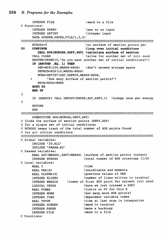
288 B. Pmgrams for Me Ezawles
INTEGER FILE !send t o a f i l e C Functions:
INTEGER YESNO !yes o r na input TMTeGER GETINT ! i n t e g e r input DATA SCREEN, PAPER, FXLE/1,2,3/
ccccccccccCcCccccccccccccccccccccccccccecccccccceecccecccccccccccccccc~c NCROSS=O !no s u r f a c e of sec t ion p o i n t s yet
50 CQmIliifm !loop ever: inSfirJ aaad2lt;ions SQS (E-SS, SSEY, SSY) ! aal&atr @=fa- of section
CALL CLEM !allow f o r another set. of i n l t cond WNQTWR=YESNQ{O,'Do you want another set of i n i t i a l e a n d i t i a n s ? @ )
mQzm *EQ* 21 DEF=MIW(100,WSS-N50S1 !donPt exceed s to rage space DEFWTN=MI N (1 0, M X S S - N W MaREmGETI NT (D@, DEFMIEJ , =SS-NSOS,
+ "NW m n y sur face of sec t ion points? ' ) NSOS=NSOS+MOm
50
C I F (GWRDCP) CaLL GWOUT(ITAPER,SSY,SSPV,l) !lzrdepy once p e r energy
G
RfSTURPJ END
cccceccc~ceecccceccccccceccccccccceecccecccccccccceccccc~~cccece~ccccccc SUBROUTINE SOS (NCROSS, SSPY, SSY j
C f i n d s t h e s u r f a c e of sec t ion p a i n t s (SSPY,SSYl C fa r a s i n g l e s a t o f i n i t i a l conditions; C MCROSS keeps t r a c k of t h e t o t a l number of Sot3 poin t s found C for a l l i n i t i a l condit ions c~CcccccGeeecCcccccccceccccccceecccccccccccccececceccccccccccccceccccc~c C Global var iab les :
INCLUDE "O.ALLC INCLUDE "PAW. E2"
C Passed variables: m& SSV ( M S $ ) , SSPY ImXSS) I surface of sec t ion po in t s (output) INTEGER NCROSS ! t o t a l n w s r of S05 c ross ings ( 3 / 0 )
C Local var iab les : mm T ! tim M A L V m f 4 f ?coordinates and momnta m& OLDVm 44) !previous values of VAR INmGER NLf NES !nu&er of l i n e s w r i t t e n t o terminal INTEGER NBEGXN !index of f i r s t SOS point f o r cur ren t i n i t eond LaGICAL CROSS lhave w e jus t crossed a SOS? =L PY-X I l i m i t s on PV f o r t h i s E INTEGER MOW !how many more SOS p a i n t s ? INTEGER TV= !dependent v a r i a b l e index REAL TSTOP ! t i m e a t l a s t s t o p i n i n t e g r a t i o n IPTmGER SCWEN !send t a terminal INmGER PAPER !make a hardcopy INmGER FILE !send t o a f i le
C Functions:
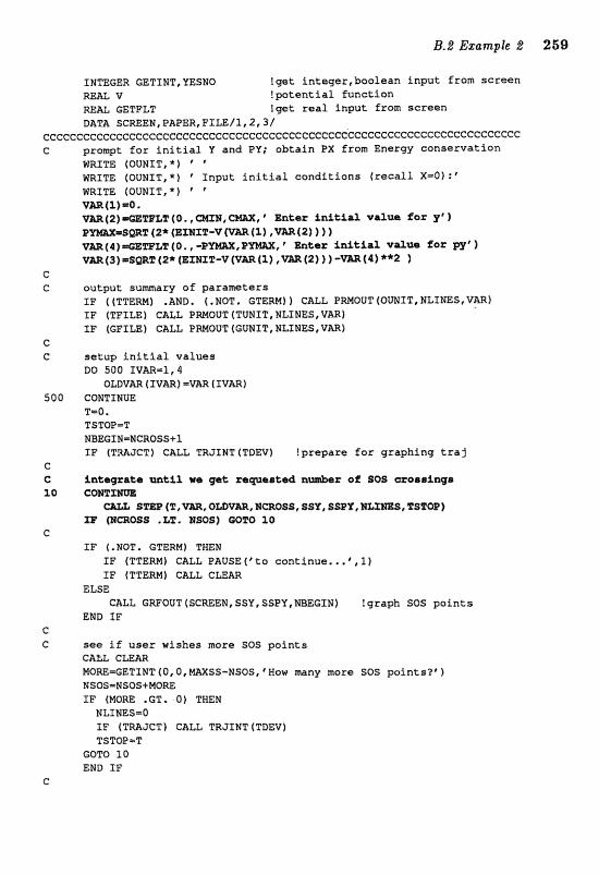
INmGER GETSMT, YESNO !get intagereboolean input from screen REAL V !potential function %AL GETFLT !get real input from screen DATA SC~EM,PWPER,FELE/1 ,Z13 /
cccccccccccccceccccecccceccccccecceeecccc"~cce~ccccccccccccccccceeC:~c~c~c C prGmpt fox: initial V and PT; obtain PX from E n e r g y conservation
WRITE (OURIT,*) " %RITE (OUNXT, *) ' Xnpt i nf tial conditions (recall X501 : ' WltX"f {(OUEJIT, * l ' '
Entar faitiar va1wa for ye )
C C output sumary o f parameters
XF ( (TTEM) . AHD , ( .MOT, GTERM) ) CALL PWGUT ( O m I T , NLINES, V?Rj IF (TFPLE) CaLL PRMOUlC (TUNIT, NLlCNES, V-) EF { W I L E ) CALL PMOUT (GUNIT, NLIN&S,VAR)
setup initial values DO 5 0 0 I V m = 1 , 4
OLDVm f XV&R) =VAR ( IVARf CONTINUE T=0. TSTOP=T NBE-f;ZEs=wCROSS+l XF (TmJCT) GALL TRJXNTtTDEVI !prepare for graphing traj
IF (.NOT. GTERMf TWEW IF (TTERM) e a L L PAUSE f p to continue, . . ', ,3 J I F (TTERM) CALL C m R
ELSE CALL GRFOUT(SCREEN,SSY,SSPY,MBEGSN) ?graph SOS points
END I F
see if user wishes more SOS paints CA= CLEAR MQm=GETINT(O,O,WSS-NSOS,'Wow m n y more 502% poinr~?~) NSOS=NSOS+MOm IF (MORE ,GT. O f TEEN
NLIPJES=O XP ( T M J C T ) GALL TRJGNT (TDEV) TSTOPmT
GOTO 50 EMD I F
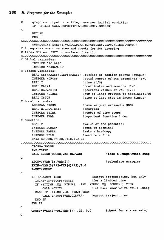
260 B* P~ograms for the EzckmpTes
C graph ics output t o a f i l e , once p e r i n i t i a l ~ o n d f t i o n I F (GFXLE) CALL GMOUT (FILE, SSYf SSPVI EIBEGXN)
C RETURN END
cccccccccccCcccccceecccccccccccccccccccccccccccceccccccccccccccccccccccc SUBROUTINE STEP (T, VAR, OLDVAR, NCROSS, SSV, SSPY, NLINES TSTOP)
C i n t e g r a t e s one t i m e s t e p and ehscks f o r SOS c ross ing C f i n d s SSY and SSPY on s u r f a c e of sec t ion ccccccccccceccccccccccccc~ccccccccccccccccccc~ec~ecccccccecccccccccccccc C Global v a r i a b l e s :
INCLUDE "IQ. ALLr INCLUDE " PAMM,E2f
C Passed. va r iab les : MU SSY (WXSS), SSPY ( m X S S ) ! surface of s e c t i o n p o i n t s (output) INTEGER NCROSS ! t o t a l nuniber of SOS c r o s s i n g s (X/O) REAL T !rim ( X l Q ) -L VAR(4) !coordinates and moments [T/0) =L OLDVM (4 1 !previous va lues of V= (I/O) INTEGER NLINES Inurn of lines w r i t t e n t o t e r m i n a l ( l l 0 ) REAL TSTOP ! t i m e a t l a s t s t o p In i n t a g ( inpu t )
C Local va r iab les : LOGICAL CROSS fbave w e j u s t crossed a SOS? REAL E,EPOT, EKXN !energies INTEGER ETIME ?nu&er of t im s t e p s INTEGER IVAR !dependent funct ion index
C Function; REAL V !value af t h e p o t e n t i a l INTEGER SCWEM !send t a terminal INEGER PAPER !mke a hardcopy INTEGER FILE !send t o a f i l e DATA SCMEM, PAI?ER, FXU/1,
ccccccccccc~c~cc~cecccccccccccccccecccccC:ccccccccccccccc~ccccccc~ccccccc =as@=. EUSE. IP=wTSm
! t a b a -K*ta statpi
G 1) ,Vm(2) ? leralauliate ana=Alas ) * * 2 t W (4) **2) 12-0
C I F (TRAJCTf THEN !output t r a j e c t o r i e s , bu t on ly
ITIME=(T-TSTQPIITSTEP ! f o r a f inr i ted t i m e I F ((ITINE .EQ, NTRJ+I) .AND. (TDEV .EQ, SCmENlf THEH
CALL 105JeE: !let user know we're s t i l l i n t e g ELSE XI?' (XTIm -LE, NTRJ) THEM
CALL TR30UT(VAR,QLDVARJ !output t r a j e c t o r i e s END TP
END I F e
!&ck; for so@ cz~seSng e
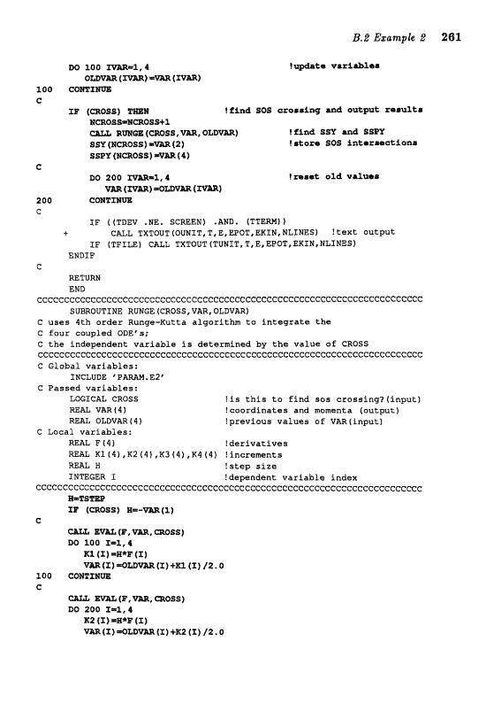
M) I: )==(mm)
100 C O r n X r n C
33' (moss) !gin& 50s crooslinc~ m& oukpk r a d C a ~~afPS~B~Ss.t.1
R W a (-SS, m, Q & D W ) ! ifin& 8SV and SSPY SSul (H-OSS) =W (P) ! @tom SOS inlaraerction@
!=sat old vaueo
IF ((TDEV .NE, SCmEN) .&BID. (TTEW)) + CALL TXTOUT (OUNIT* T, E, EPOT, EKf 16, XVtf16E51 !text output
IF (TFILE) CALL TXTOUT TUN^ T, T, E, EFQT, ERININLIXJE5j ErJDZE
G =TURN END
~ ~ ~ ~ ~ ~ ~ ~ ~ ~ ~ c ~ ~ l ~ e ~ ~ e ~ c c c ~ c ~ c c ~ ~ c ~ c c c c c c c c c c c c c c e ~ c c c ( I : e e c c ~ c c c ~ c c ~ c c c c e c ~ c SUBROUTINE RUN= (CRQSS, V M , OLDVAR]
C uses 4th o rder Rung@-Kutta algori thm t o i n t e g r a t e t h e G four coupled ODE'S: C t h e independent var iab le is determined by the value of CRQSS ccceecccccccccccccceccccccccccccccccccccec~ccccccccccccccccecccc~cccccc~ C Global var iables:
INCLUDE ' PkmM. E2@ C Passed variables:
LOGIC= CRQSS !is t h i s t o f i n d sos cross ing?( input ) RE= V M f 4 f !coordinates and momenta {output) REAL OLDVAR 1 4 f !previous values of Vmtlnyzut)
C Local var iables: mAL F ( 4 f !der iva t ives REAL K l ( 4 f ,R2(4),K3(9),R40 l i n c r e m n t s mAL X !step size? INTEGER I ?dependent v a r i a b l e index
eccCcccccCcccccccccccccccccccececcccccccccccccccceeecccecccccce:ccccccccc * T S W
C
X% (X) =E*F {S f v ~ { I ~ ~ m m ( I ) + x l (I] 12. Q
%Q0 C O g T Z m C
D6 200 X=%, 4 I2 (X) =E*F (X) v= ( 2 ) =OLDVrn (X) +E2 (X) 12.0
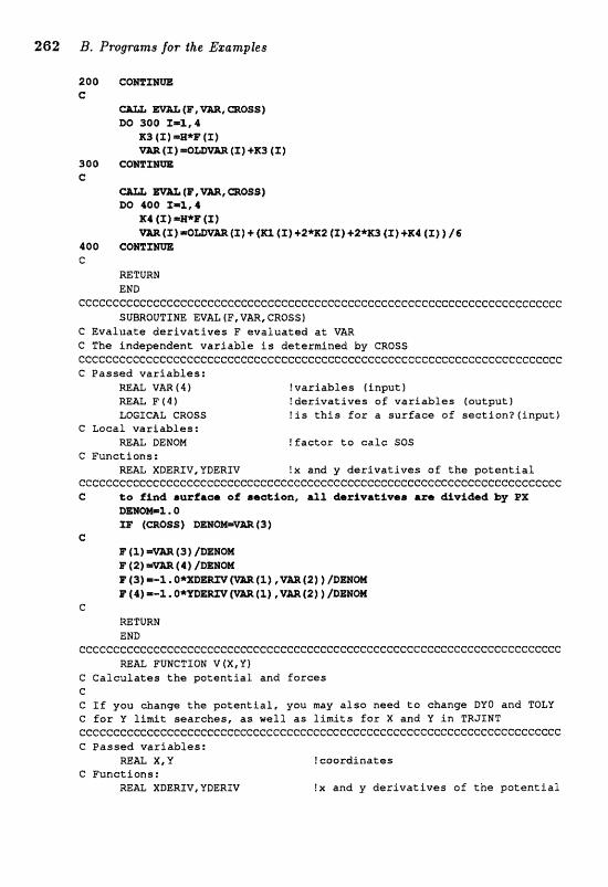
262 B, Pr~granas for the Ezamples
290 C O m I m C
K3 (I) =R*F (X) VAB (Z) &LW= (I) +R3 (X)
300 C Q W X m C
DO 400 I=%, 4 nr (11 =M*E (3)
(X) + (X2 ( X ) +2*K2 (X) +2*K3 (1:) +K1 (3) ) / 6 400 CWZIlLifm c
RETURN END
CGCCCCG@CCCCCCCCCCCCCGCCCCCCCCCCCCCCCCCCCGCCCCCCCCCCCCCCCCCCCCCC~CCCCCCC SUBROUTINE EVAL (F, VAR, CROSS 1
C Eva lua te d e r i v a t i v e s F e v a l u a t e d a t VAR C The independent v a r i a b l e is determined by CROSS cccccecccCcccce~tccccccccccccccccccccceecccccccccccccceccccccccccccccccc C Passed v a r i a b l e s :
WAL VAR ( 4 ) ! v a r i a b l e s ( i n p u t ) m A L F f 4 ) ! d e r i v a t i v e s of v a r i a b l e s (output1 LOGICAL CROSS !is t h i s f a r a s u r f a c e of s e c t i o n ? ( l n p u t )
C Local v a r i a b l e s : RBAL DIENON ! f a c t o r t o caXe SQS
C Funct ions: REAL XDERIV,YDERSV !X and y d e r i v a t i v e s of the p o t e n t i a l
ccccCc~c~c~ccec~ccce~c~ccccccccccccccecc~c~cccccccccccccc"cccccccccc~cccc C &o iZnd swzfrcrr o f rrocrtion, aZ3, dmrZvoltAvarr .*re div ibd by EX:
DmoM=2 ' 0 XF (-0ss) D E N Q W m ( 3 )
C
P ( 2 ) *a (4) /DESOM ( m ( r j ,-(g) /ama~ (m 8 (2) 1 /Dma
C =TURN END
cccccccccccccccccccccecccceccccccccccccccccccecccecceccccccccccccccccccc RE& FUNCTION V ( X , Y 1
C CalculaGes t h e p o t e n t i a l and f o r c e s c C If you change t h e p o t e n t i a l , you may a l s o need t o change DYO and TQLY C for Y l i m i t searches , as w e l l a s l i m i t s f o r X and Y i n TRJINT ccccecccCcccc~ccccccccccccecccccececcccccccccccccccccccccccccccccccccccc C Passed v a r i a b l e s :
REAL X.Y ! coord ina tes C Funct ions:
mhL XDERIV,UDERIV !X and y d e r i v a t i v e s of the p o t e n t i a l
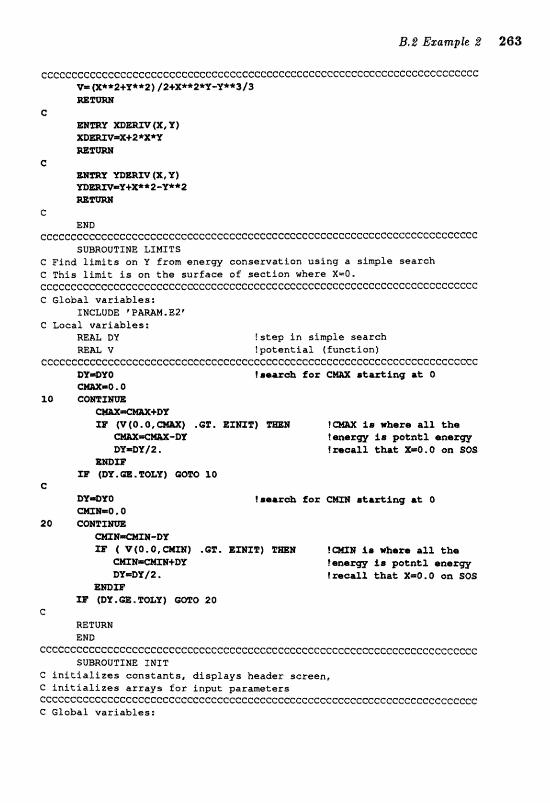
~c~c~ccccccc~ce~~~~~e~c~cccccc~ccecccecccccecccccccccceeeccccccccccccccc V= (X**2+Y**Z) /2+X**2*V-Y**3/3
C
C
=F- e
END ecc~ec~c~~c~c~~~~~cceccec~ccccccccccccceccc~ccccccccccecc~cc~ccccccccccc
SUBROUTINE LIMXTS C Find l i m i t s on U from energy conservat ion us ing a s i n p l e search C This l i m i t i s an the sur face o f sec t ion where X=O, ~~c~~c~c~~~c~e~c~~c~ceccccccecccccccf :ecccecccccccccccccc~ccceccccccccccc
RE& DV ! s t e p i n simple search RE-AL V ! p o t e n t i a l ( funct ion)
Ccccccccccc~cecccceecccccccccccccccccccccccceccccccccccccccccccccccccccc !@a=* far atarGing a% 0
fa
1. i a where all the
imcrall that: X=Q.O on SOS m f P tDT*rn*%QLY) %a
C DTaYQ 8 sear& fozr atncting at O
1 .@E. I&XNIE) -H !-H i a wbsra a21 the ?amarm i r potat2 eaers
DYmDTl2. fm~a1 x d . 0 OR SOS EHBf E
rr (oxem TQLT) ~o 20 C
RETURN END
ccccc~ccccccceecccccececcccccceeccccccccccccccccccccceeccccccceecccccccc SUBROUTTHE SNIT
C i n i t i a l i z e s cuns tan t s , d i s p l a y s header screen, C i n i t i a l i z e s a r r a y s f o r inpu t parameters cccc~ccccccccccccccccecccccccccceccecccccceccecccccccccccccccccccccccccc C Cfcbal va r iab les :
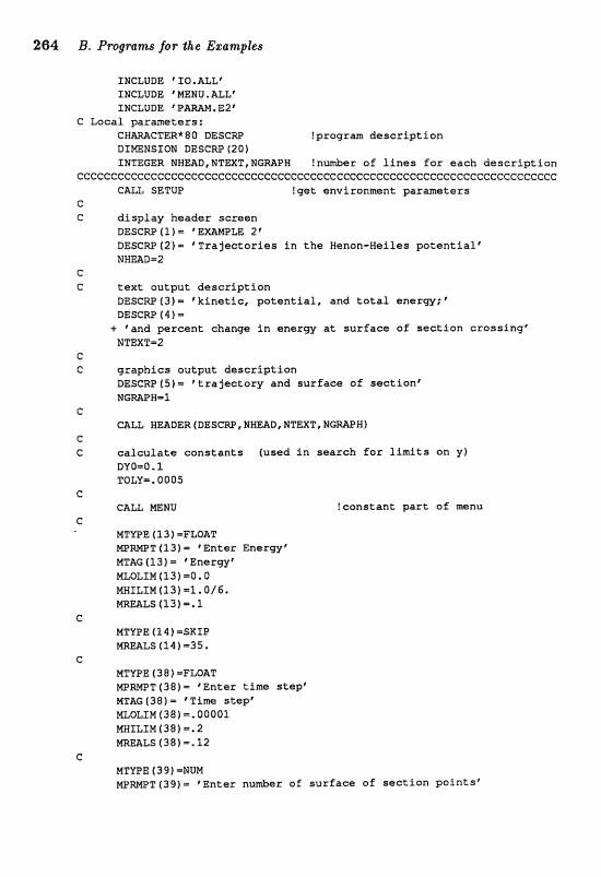
XNCLUDE "Q.ALLe INCLUDE * mNENU, ALL' INCLUDE "PAMN.E2$
C! Local parameters: CWmCTERX80 DESCRP !program description BImNSIQN DESCm (20) INmGER NHEAD,NTEXT,NGMPM In-er of lines for each descriptian
eccccc~eceeeeccceccccccccc~ecccccccccE:ccccc~ccccccccc~c~cccccc~C:c~cc~ece CALL SETUP !get environment parameters
C C display header screen
DESCW (1 ) = "&&@LE Zr DESCRP(2)= qrajectories in the Wenon-Neiles potentialf NWmD=2
C C text output descriptf on
DESCRPf3)m 'kinetic, potential, and total enerwi' BESCBP ( 4 1 =
+ %and percent change fn anerg?l at surface o f section crossing" ETTEXTmZ
C: C graphics output description
DESCRPf5)= 'trajectory and surface of section" N G W H = X
c CALL READER (DESCW, NHEAD, NTEXT, NGRAPN 1
C! C calculate constants (used in search for limits on yl
aYcz=a, I Tom=. 0005
e (C=ALL mNU lcanstant part of =nu
C MTVPE 1 I S ) -FLOAT M P W T f 33) C Enter Energyf MTAG (13) = *Energyr MLQLIM (131 =Q. Q MWILIM (23) =l, 016. M W L S (13) =. 1
C: HTWE f l4 1 =SKSP m m s (14) =35.
C MTYPE (38 ) =FLQAT MPWPT 138) = 'Enter time stepf NTAG (38) = ' Time? step' MLOLfM(38)=. 000QI MWTLIM (38) =.2 mEats (38) -. 12
G NTYPE ( 3 9 ) -NUM MPMPT(39)= *E~tee rn&er of surface of section points"
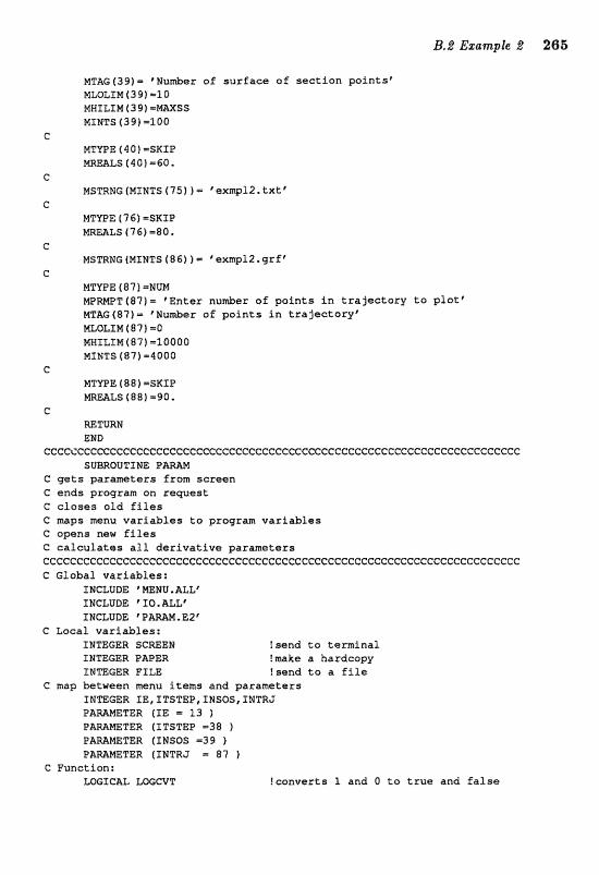
MTAG(39)- ' N u h e r of s u r f a c e of s e c t i o n p o i n t s ' MLOLIM(39) 110 MMXLIM 4 3 9) ==SS MINTS (39) -100
C MTYPE (4 0 f =SKZP MRmLS (401 =GO.
C MSTRNG (MINTS (75) ) = eexmpl2. t x t
C MTVPE (7 6 ) =SKIP mEA1;S (761 =80.
C MSTRNG (MIWTS (86) ) - *exmpJ2,qrf *
C
M T E E (87 f =NUM NPMPT(87)= 'En te r nu&er of p o i n t s i n t r a j e c t o r y t o p l o t ' MTAG (87) = 'Nu&er af p o i n t s i n t r a j e c t o r y R MLGLZM ( 8 7 f =B HHILIM (87) -10000 MINTS (87) -4080
f: MTUPE ( 88 1 =SKIP M-LS (88) =$a.
C RETURN END
cccccccccccccccceccccc~cecccccccccecccccecccccccceccccccccccccececcccccc SUBRQUTZIVE P
C p t s parameters from sc reen C e n d s p r o g r m on rewest C c l o s e s o l d f i l e s C maps m n u v a r i a b l e s t o program v a r i a b l e s C opens new f f les C c a l c u l a t e s a91 d e r i v a t i v e pa ramete r s ceecccccccceccccecccceccccccecceccccccccccceccccccccccceccccccccccccc~Cc C Global v a r i a b l e s :
INCLUDE * MENU. ALL"
C Local v a r i a b l e s : INTEGER SCMEN !send t o t e r m i n a l INTEGER PMER !make a haxdcogy INTEGER FILE ?send t o a f i l e
C map h t u e e n m n u items and paramete r s INmaR SE, ITSTEP, INSQS, TNTR3 P-METER (IE 23 )
TER (ITSTEP m38 1 P m m T E R (INSOS =39 )
P-METER (XNTRJ - 87 1 C Function:
WGSCBL LBGGVT !conver t s 1 and O t o t r u e and f a l s e
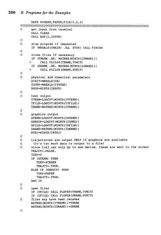
266 B. Programs for the El~amples
DATA SCREEM,PAPER,FTLE/1,2,31 CCCGCCCCCCGGCGCCCCCCCCCCCCCCCCCCCCCCCCCCCGCGGCCGCGCCCCCCCGCGCCCCCCCGCCCC C get input from terminal
CALL CLEAR CALL ASK ( 1, ISTOP )
stop program if requested I F ( m A L S ( I m T N ) .EQ. S T W ) CALL FINISH
close files if necessary IF (TNAm . NE, NSTRNG (MINTS (ITHAHE) 1 )
+ CALL FLCLOS (TNAME, TUNIT) I F (GMAME .NE, MSTRNE (MIHTS (IGHAME) ) 1
+ CALL FLCLOS (GMAm, GUNIT )
physical and numerical parameters E I N I T m m U S ( I E ) T S T E P = W A L S (ITSTEP 1 NSOS-MINTS (INSOS)
text output TTERM=LoGCVT (MINTS ( I T T E N ] 1 TFXLE=LOGCVT(MXHTS(ITX"XLE)l TMM-MSTRNCfMIHTS(ETNANE})
graphics outr>ut GTEM-LoGCVT f MINTS [IGTERNI 1 GmCP=LOCCVT (MINTS (XGXRf)] f GFK~=LoC@VT(MINTS(IGFZLE]) GNM-HSTRNG (MINTS ( XGNAlulE) 1 HTRJmMINTS ( INTRJ)
trajectories ere output ONLY if graphics are available (it's too =eh data to output to a file)
since traj can only go to one device, these are sent to the screen TMJCT=,FALSE. TBEV=O IF (GTERM) THEN
TDEV=SCB&EN TMJCT=."TRUE.
ELSE I F fGRRDCF) m N TDEVmPmER TMJCT=.TRUE.
END I F
open fi les IF (TFILE) CALL PWPEM (TNAME, T m I T l I F (GFILE) CALL FWPEN(GMAm,GWZT) files may have been renamed M S m G (MIWTS (ITN=) > =THAm MSTRNC (MINTS ( IGrJAmf ) =ENAME
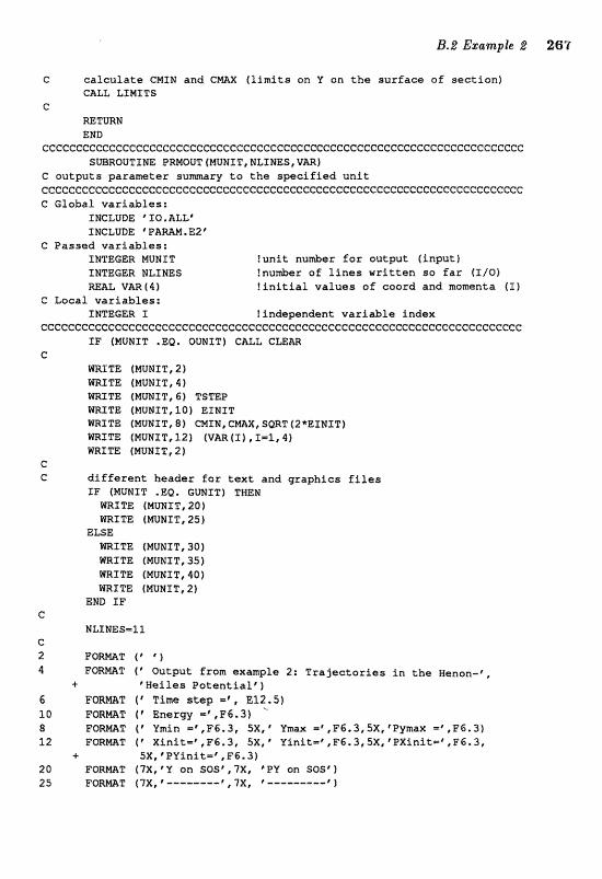
C c a l c u l a t e CHIN and CMaX ( l i m i t s an Y on t h e sur face of s e c t i a n ) CALL LIMITS
G RETrnN END
ccccccecccccceCccccccccccccccccccccccccccccecccccceccccccccecccccccc~ccc SUBROUTINE PMOUT (NUMXT, NLINES, V m )
C outputs parameter s u m a r y t o t h e s p e ~ i f i e d u n i t cecccecceccccccec~~ccccc~ccceccccccccccccccccccCccccccccccccccccccCcccc!~ C Global var iab les :
INCLUDE "IQ.ELLLe INCLUDE CPAMM.E2"
C Passed var iab les : INTEGER MUNXT !uni t nurnber Ear output ( input ) ZMTEGER NLINES I n u h r of l i n e s w r i t t e n so f a r f I / O ) MAL V M ( 4 ) ! i n i t i a l va lues of ~ o o r d and mamenta (1)
C Lacal var iab les : INTEGER Z !independent variaZIle index
ccccc!cccccccecccccccceeccecececccecI:ccccce~ccecccccccccccc~ccC:cc~ccccccc I F (MUNIT .EQ. OUNIT) CALL C M A R
C WTE fMUNIT,2f WRITE (MUNIT,4) WRITE (MUBIT, S) TSTEI? m1TE (MUMIT? la) EXNIT WRITE (MUNIT, 8 ) mIH, C M , SQRT (2"EXMZT) mITE (MUNIT, 12) (VAR ( X I , I=I, I ) WRITE (NUNIT, 2)
e C d i f f e r e n t header f o r t e x t and graphics E f l e s
XF (MUNIT -EQ. GWIT) THEN mTTE (MUNIT, 20) WTTE (MUMIT, 25 )
E U E mITE (MUNIT, 30) llaRITE (MUHIT, SS) mIm [PIUNIT, 4 0 ) RRITE {MUNIT, 2)
END I F C
PlLXNESrll c! 2 F O m T ("1 4 F O m T ( I Output from example 2: T r a j e ~ t o r i a s i n t h e H e n ~ n - ~ ,
+ 'HHeiles P o t e n t i a l * )
6 T f Time step , E12 * 5 t
8 F O m T ( V m i n -rfF6.3, 5 X , # Y m x =f#F6,3,5X,T~max =%F6,3) 12 FORMT ( @ Xinit=" ,F6,3, 5X, ' YVPnSt-f ,F6.3, SX, ?PPX1.nit=f ,F6.3,
4- 5XI?PYinit=6,F6.3) 20 FOMT (?X, 7 aon SOSC, ? X I 'PY on SOSf 1
,?X, F 1
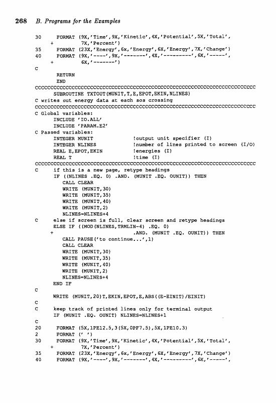
268 B. Programs for the Bzrampiles
30 F O M T (S~,'Time\,SX,~Binet1c~,4X,*Pot:ent1,a1,'~~X~~Total~, + 7X,*P@rcentf}
35 F O W T ( 2 3 ~ , Energy', ,Gx, 9 n e r g y f 6X, e E n e r ~ t , 7% @Change8 1 40 FamT {CJX, F ----\ H, -------F 4X, L--------5 GX, @
+ 6X, f 1 C
MTURW EWD
c~ccccccc~cccccecccccccccccccccccccccc~ccccccccccceccccc~cececccceeccccc SUBROUTINE TXTQUTfNUNIT,T,E,EPOT,EKfN,NLfNES]
C writes out energy d a t a a t each sos c r o s s i n g cc~ecc~~~ecceccccc~cccccccecccc~c~cccE:f:cccccccccccC:C:eccc~ccccccce~eeeecc C Global v a r i a b l e s :
INCLUDE 'fO.ALL* INCLUDE * PAMN . E2'
C Passed v a r i a b l e s : TNmGER MUNIT lou tpu t u n i t s p e c i f i e r (I) XWmGER NLIHES !nu&er of l i n e s p r i n t e d t o s c r e e n (ZlC3) WaL E, &POT, EKIN ! e n e r g i e s [X) RmL T !tim (1)
cCccecccccccccccccceececccccceeccccccccccc~ccccccceccceecceccecccccccccc C if this is a new page, r e t y p e headings
f F ((NLINES .EQ. 0) .AND, (MUHIT .EQ. OUIST)) TmN CALL CLEAR mIITE tMDNIT, 3 0 ) 'IrJRfTE (MUNIT, 35) m I T E (MUMIT, 40) m I T E (MUNIT, 2 ) NLImS=ILINES+4
C else if s c r e e n is f u l l , c l e a r s c reen and r e t y p head ings ELSE TF f (MOD (NLIHES, TRMLIN-4 f .EQ. 0)
+ .AND. (MUNIT .EQ, OUNIT) 1 THEN CALL PAUSE['I;o cont inue, . .* , , l f CALL CLEAR mIm (MUMIT, 30) m I T E (MUNIT, 35) WTTE {MUNXT, 40) m I T E IMUWIT,2) NLXN&S=MLfNES+4
END IF G
mSTE (MUNIT, 20) T, EKIN, EPBT, E, ABS ( (E-EINIT) IEINIT) c G keep t r a c k o f p r i n t e d l i n e s o n l y f o r t e r m i n a l ou tpu t
I F (MUNIT .EQ, OUNIT) NLINES=NLXRES+I c 20 FORNAT (5XflPE12,5,3 (5X, aOF7.5) ,5X,3PESOt3) 2 F O m T ("1 30 F O m T ($X, 'Time\ 9 X , * K i n e t i c t , 4XI @E"ot@nt:iaL* , 5X, * T o t a l p , i ?X, ' Percen t ' 1
35 PORMT (23X, "nargy' c6, 'Energyf I 6X, t E n e r w r , ?Xt 'Change8 1 40 FORmT (9X, - - - - F , 9X, @ - - - - - - - I , 4X, @ ---------E, fjXt
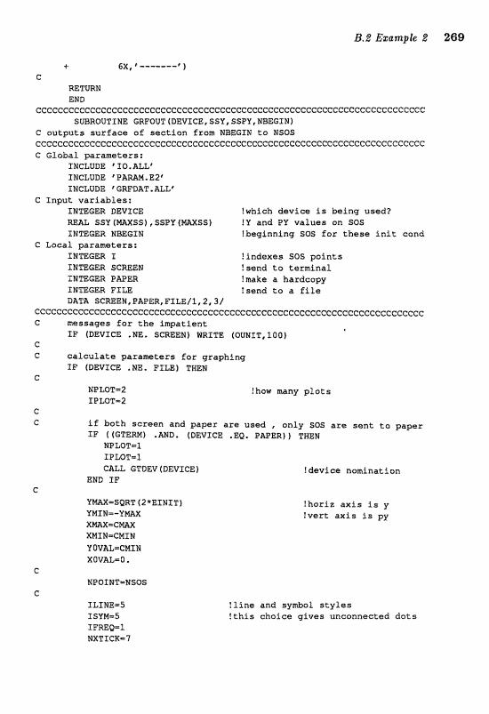
4" fjx* ' 1 c
mTURN END
eccccccccccecccCcc~cecccceccccecccccccceceec~ccccccccceececccccccccccccc SUBROUTINE GRFOUT (DEVICE, SS%'# SSDV, MBEGTNI
C outputs surface of section from WBEGIN to N50S CCCCCGCCCCCG~CCGCCCCCCCC~CCCCCCCCCCC~CCCCCG~CCCCCGCCC~GCCCCCCCGCCCCCCCCC C Global parameters:
INCLUDE ' IQ, ALLt I WCLUBE VAmM. E2 C
INCLUDE *GWDAT*ALL" Xnput variables;
INTEGER DEVICE ?which devim i s being used? RE& SSY (mXSS), SSPV ( W S S ) f Y and PY values on SOS SNTEGBR MBEGIN !beginning SOS for these init cond
G Local parameters: INTEGER I !indexes SOS points INTEGER SCWBN !sand to terminal INTEaR PAPER !make a hardcapy INTEGER FILE !sand to a file DATA SCmEN, PAPER, Ff LE/1,
ccccccceccccceecccccc~c~cccccecccc~ecccccceccecccccecccc~ceccccccccccccc C messages far tba Lpatient
e IF (DEVICE .NE. SCREEN) WRZTE (OUNIT, 100)
C C calculate paremters for graphing
IF (DEVICE .NE* FIL;E) TWEN G
'IJPLOT=iE !how many plots IPLOTm2
e e if both screen and gapes are usad , only SOS axe sent tc paper
IF I (GTERM) .MD. (DEVICE . EQ, PAPER) ) TWEN WPLOT=1. XPLOTmP
GTDEV (DEV~CE~ !device nomination END IF
C VmX-SQRT (2"EINI T 1 !hoxiz axis i s y YMIM=-YmX !ver t axis is py xmx=eMAX XMIN=CMf;E;I YOVAL=CMIW XOVAL=O.
C EIPQINT=NSQS
c ILINE-S 1 SYMm5 f FREQ=l NXTICKm7
!line and symlr>ol styles !this choice gives uneanneeted dots
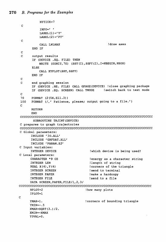
21"Q B. Pr~grams for .the Ez~mples
NYTICK-7 C
IhlFO=" -EL (3,) =.."U" W E & (2) ='PYf
c CALL LNLHm
END I F C C ou tpu t r e s u l t s
IF (DEVICE .EQ. FILE) THEN WRITE (GUNIT, 70) (SSY ( I ) , SSPV (I) c I-NEEGfNt %SOS)
ELSE CALL XUBLOT f SSY , SSPY)
END fF C C and q rapb ing s e s s i o n
I F (DEVICE .NE. FILE) CALL GPAGEfDEVICE) !c~ose g r a p h i n g package IF (DEVICE .E@. SCREEN) CALL TMODE !swi tch back t o t e x t mode
c 70 F O m T (2f5X,E12.3)) 100 F O m T l / , V a a t i e n c s , please; ou tpu t gaing to a f i l e e e l c
RETURN END
cccccceccCccccccceeccccccccccccccccccccecccceccccccccccccccceecccecceccc SUBROUTINE TRJINT (DEVICE)
C prepares t o g raph t r a j e c t o r i e s ccccccccccccccccccccccccccccccecccccceeccccCcccccccecccccccccccccccccccc C! Global parameters :
I NCLUDE "0. ALL' INCLUDE GWDAT , ALL1
C Inpu t v a r i a b l e s : INTEGER DEVICE !which dev ice is b e i n g used2
!energy as a c h a r a c t e r s t r i n g INTEGER LEN ! l eng th s f s t r i n g WAL X(4 t ,Yx t (4 ) ! co rne r s of the t r i a n g l e ZNTEGER SCmEW Isand to t e r m l n a l INTEGER P&PER !make a hardcopy INmGER FILE !send ts a f i l e DATA SCaEN, PAPER, FTLE/1,2,3/
cccc~cccccCccecccccccecccecccceccceccccecccccccccccccccecccceecccccccccc NPmT-2 ?how mny p l o t s IPLoTml
c Y W - 3 . ! co rne r s af bounding t r i a n g l e YMIN=-, 5 X M = S O R T ( 3 . ) / 2. XMINm-XMX Y OVAL=O,
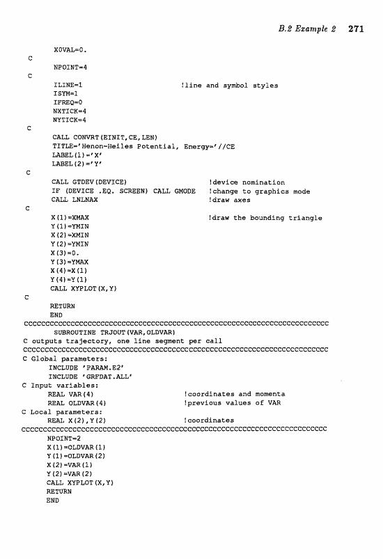
?fine and s y d o l s t y l e s
XOV;AL=O, I:
NPOIMT-4 C
ILINEm1 ISYMm5. IFWQ=0 MXTICRm4 NY "I1CF[=4
C CALL CONmT (EINIT, CE, LEM) TXTLE=tHenon-Wailea P o t e n t i a l , Energym8//CE MBELflf s r X ' mBEL(2)='Yv'
C CALL GTDEV (DEVICE) !device nomination I F (DEVICE .EB. S W E N ) CALL GMODE !change t a graphics made CALL LNEhlAX !draw axes
C X (l) = X M X !draw t h e bounding t r i a n g l e V (1)=YMXN X (2) =XMIN Y (2) =YMXW X/3)=0. V (3) = Y W X( . l r t=X( l ) V (4)=Y l l f CUL XYPLOT ( X , Y 1
C RETURM END
cccccccccccceccccccccccccccececcccccccccccecccccccccccceccccecccccc"ccccc" SUBROUTIRE TRJOUT (V=, OLDVAR)
C ou tpu ts t r a j e c t o r y , one l i n e segment per c a l l eccccceccccccccccccccccccccccccccceccccccccccccccccccccccccccccccccccccc C Global parameters:
INCLUDE ' PARAN. E2 ' INCLUDE @GRFXIAT.=Lr
C Input var iab les : mAL VAR 1 4 1 !coordinates and nomtpnta RE= OLDVm ( 4 1 Ipreviaus values of VAR
C Local parameters: RE= X ( 2 ) , Y 1 2 1 !coordinates
c~eccccccceccecccccecceccceccccccccccccceceec~cccC:ccc~cccccccccccccccccc NOOINT-2 X ( l ) = O L B V M ( 2 ) Y (l} =OLDVAR (2) X (2)=Vrn(ll Y 12) =VAR (2) GALL, XYOLOT (X, V) rnTURN END
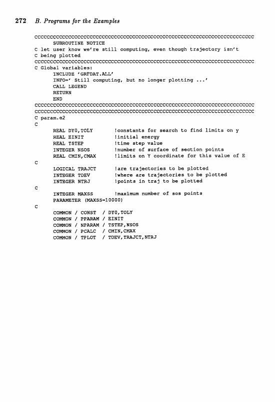
63. Pr~gmna9 for the Ezamples
CCCCCCCCCeCCCCCCCCCCCCCCCCCCCGGCCCGCCCCCCCCCCCCCCCCCCCCCCCCCCCCCCCCCCCGC SUBROUTZNE NOTICE
C 1st u s e r know wapra s t i l l computing, even though t r a j e c t o r y i s rz f t C being p l o t t e d ccc~ccccccccc~c~cccc~c~ccC:cc~ccccccccececcccccc~ccecc~ccccceccc~cccccccc C Global va r iab les :
INCLUDE GRFDAT, ALL* ZNFO=? S t i l l cornouting, bu t no longer p l o t t i n g ...@ CALL LEGEND =TURN END
ccccccCe~eCecCeecccccccccccccccecccccccccccceccccccccccccccccccccecceccc ccccccceceeccecceccceccccccceccccC:ccccc~ecceccccececccccccccecccc~~ceccc C param.c32 e
m& DYO, TOLY !constants f o r sea rch t o f i n d l i m i t s on y m= EINIT ! i n i t i a l energy m= TSTEP ! t i m e s t e p va lue TNTEGER NSOS tnunber of surface of s e c t i o n p o i n t s REAL CMIN, CMX ! l i m i t s an Y coordinate fox t h i s va lue of E
G LOGIC= TRZIJCT Eare t r a j e c t o r i e s t o be p l o t t e d INmGER TDEV fwbera are t r a j e c t o r i e s t o be p l o t t e d I ImCER 1VTR+T l p o i n t s i n t r a j to b @ r o t t e d
e INTEGER =SS tmrzxirnum nunber of sos p o i n t s
TER (mXSS=100QO) c
coma^ / C ~ N S T I nuo,Tol;i como~ / ePaw / EZMIT COWQM / W A M M I TSTEP,NSOS COMON / PCALG / CMSN,CMX COmOM / TPLOT / TDEV,TRWJGT,NTRJ
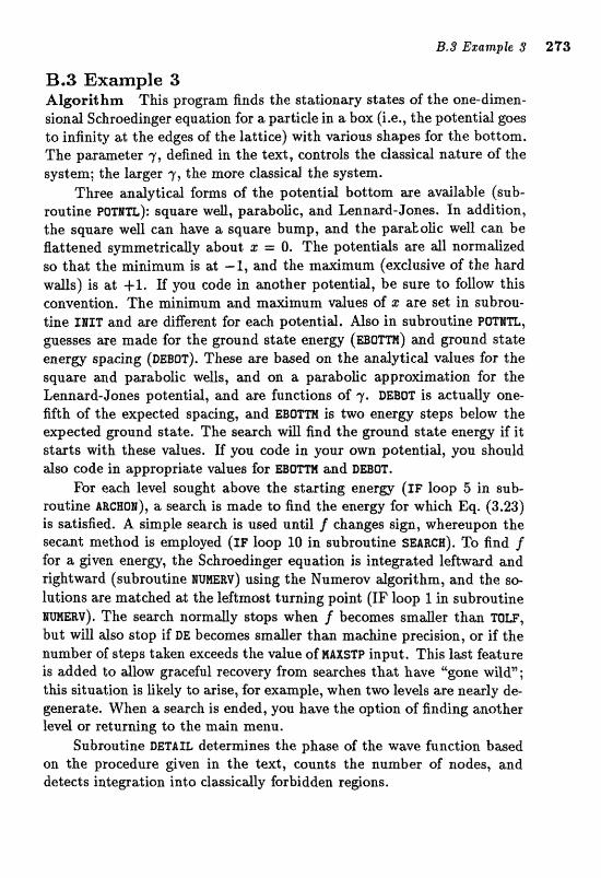
B.3 Example 3 Algorithm This program finds the stationary state8 olt" the one-dimen- sional Schroedinger equation for a particle in a box (i.e., the potential goes to infinity at the edges of the lattice) with various shapes for the bottom. The parameter r, defined in the t a t , controls the daasical nat;nre of the system; the larger 7, the more classical the system.
Three analytical foms of the potential bottom are available (sub- routine P O T I ~ ) : square well, paraboBc, and Lennard-Jones. In addition, the square well can have a square bump, and the paratolic well can be flattened symmetrically about z = 0. The potentids are a i l normalized so that the minimum is at - 1, and the maximum (exclusive of the hard walls) is at +l. If you code in another potentid, be sure to follow this conv~ntion. The minimam and nr~murn vduea of z are set in subrou- tine IBIT and axe digerent far each pdentid. Also in subroutiae PC)Tm, guesses are made for the ground state energy ( = a m ) and ground state energy spacing (DEBQT). These are based on the analyticlll values for the square asld paraboIic weus, m d sn a parabolic appro~mation for the Zmard-Jmes potential, m d are funcr;ions of 7. ClElgm is aetually one 5fth of the expected spacing, and E& is t w energy steps belaw the expected pound state. The search win find the ground state energy if it starts with these vdues. If you code ia your own potentid, y m should dso code in appropriate vdues for E B O T ~ a d DEBQT.
lFor each level gought above the stwt;ing e n w g (IF loop 5 in sub- routine nrcaor), a search is made to find the energy for which Eq. (3.23) is satisfied. A simple seuch is used until f changes sign, whereupon Lhe secant method is employed (IF loop 10 in subroutine ssn~ca). To find f for a given energy, the Schroedinger equation is integrated leftward and rightward (subroutine RUNERV) using the Numerov dgorithm, and the so- lutions are matched at the leftmost turning point (IF loop 1 in subroutine IYUYIERV). The seafch normally stops when f becomes smaller than TOLF, but will also stop if DE becomes smaller than machine precision, or if the number of skps taken exceeds the vdae of EIAXSTP input, This last feature is added ta dlow gracefd recovery from searches that have "gone wild"; t h i ~ situation is Ekely to anrise, for example, when t w levels are newly de- generate. When a search is tjnded, you have the option of finding another hvel or returning to the m&n menu.
Subroutine DETAIL deterdaes the phwe of the wave function based on the procedure given in the text, counts the number of ~ades , and detects inteigat;ion into dassicdly forbidden re@oas,
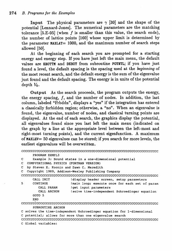
274 IS, P~ograpns for the gzamples
Input The physicd parameters are 7 [30] and the shape of the potential [Lennard-Jones]. The numericat pzmeters are the matching tolerance [&.E-051 (when f is smder than this value, the search ends), the number of lattice points [l601 whose upper limit is determined by the parameter WAXLhT= 1000, and the maximum number of search steps allowed [50].
At the beginning of each search you are prompted for a starting energy and energy step. If you have just left the main menu, the default vdues are E B O ~ H and DEBoT from subroutine P O T m ; if you have just found a level, the default spaeing is the spacing used at the kginning of the most recent search, and the default energy is the sum of the eigenvalue just found and the default spaeing. The energ is in units of the potential depth G*
Output As the search proceeds, the progam output8 the energ, the energy spacing, f , and the number of nodes. In addition, the last column, Meled 'Wbrbddn", displays a "y~!s" if the integmim has entered a dassiedly forbidden re@on; otherwiw, a "no", W e n m &genvdue is found, the dgenvdue, number of nodes, and elassicd t;unti~g poinf;~ are disp1~1~red. At; the end of each se~wrch, the graphics display the poterrtid, all eigenvdues found since you lwt left the main menu (indicated on the gaph by a line at; the appropriate level betweea the l&-most m& right-most turning points), and the current eigenfunction. A maximum of KAXUV.= 50 eigenvdues can be stored; if yau seach for mare levels, the earliest eigenvdues will be averwritten. c~c~cccccccccecceccec~ccccc~~ccccccc~cccc~e~~ce~c~ccc~ccccc~cc~ccccccc~~
P R Q G W EXNPL3 C Exmple 3: Bound states in a one-dimensional potential C COmUTATIOEAL PNUSSCS (FORTMH VERSIQIJ) G by Steven E. Roonin and Dawn C. Meredith C Copyright 1989, Addison-Wesley Publishing Company CCCCCCGCCCCCCCCC~~CCCCCCCCf:CCC~C(31CCCCCCCCCCCCCCCCC(31CCCGCCCCCCCCCCCCC~CC~
CALL INXT !display haades screen, setup parameters 5 CONTINUE tmain loop; execute once for each sat of param
CALL P A ~ M !get input parameters CALL BTtGf-ION !salve tim-independent Schroedinger equation
GQTO 5 EYD
CCCCCCCCCCCCCCCCCCCCCCGCCCCCCCCCCCCCCCCCCCCCCCCCCCCCCCCCCCGCCCCCCCCCCCCC SUBROUTINE MCBOhl
C solves the time-independent Bchroedinger ewation for I-dimensional C potential; allows for m r e than one elganvalus search ~ccceCcccce~Ccc~~Cccccccccccccceccccccccc~ccc~ceccccc~~ccccccC~cccccccc~ C Glabal variables:

INCLUDE '10.ALL2 INCLUDE ' P m M . E 3 *
e Laca l v a r i a b l e s : mAL ENERGY (mXmV) ! a r r a y o f e igenva lues INTEGER LEFTTP (WLEV) , RGXTTP ( V) t a r r a g of t u r n i n g p o i n t s INmGER NFOUND . n u a s o f l e v e l s found
PSI (mXXIPIT) !wave f u n c t i o n INTEGER ITER !con t inue f i n d i n g l e v e l s ? INTEGER NOIZaS Inumber o f nodes RE& E ! t r i a l efgenenergy XMTEGER LTP, RTP ! c l a s s i c a l t u r n i n g p o i n t s ( l a t t i c e ) WAZ DE, DESAm ! s t e p i n enerc%y s e a r c h
INTEGER NSTP I n u d e r of s t e p s t aken i n s e a r c h INTEGER SCaEN !send t o terminal INTEGER PWER !make a hardcopy INTEGER FILE ? s e n d t o a f i l e
C Funct ions: WAL GETFLT ! o b t a i n r e a l i npu t INTEGER mSMO !ob ta in y e s o r no i n p u t DATA SCREEN,PMAPER, FILE/1,2,3/
e~~~~c~~ccccccc~~cccccccccecccceccccc~eccccccccceceeccccecccccccccccc~cc C ou tpu t s u m a r y o f paramete r s
SF (TTBM) CALL PMOUT f OUNTT ) I F (mILE) CALL PWOUT (TONIT) IF (GFILE 1 CALL PMOUT (GUNTTI
C ITERmJ. ! i n i t i a l i z e s sa rch fng v a r i a b l e s NFOUND=O EmEBOTTM ! reasonab le s t a r t i n g v a l u e s DE=DEBOT
C 5 ~ ( X ~ e B Q . % j T ~ tZool, ever axurrw TaweIa C
EsGETFLT (E, ENIN, E m , # E n t e r e n e r w P 1 !get s t a r t i n g v a l u e s DE=GETFLTIDE,DE#XN,BE~X,@Enter s t e p i n e n e r w search1) DESAVEmDE: !save f o r next l e v e l
C I F (TTERM1 CALL CTITL (OUNITl !output. t i t l e a I F (TFILE) CALL CTSTL (TUNIT)
(E, PE, Lm, R%%, Barns, W=, ESX) t saarcrh for anarm
p r o w t f o r new E and DE i f t o o many s t e p s t aken i n s e a r c h I F (NSTP .Cj&, M S T P ) THEN
mZTE (QVMST, *) ' ' m I T E (OSJMIT,*) E i g e n s t a t e n o t y e t foundr I TERmVESN0 ( 2,
-t= *Do you want t o t r y a g a i n w i t h new E o r DE?#I ELSE o r ou tpu t e igenva lue in fo rmn~t i an
SF (TTEm) CALL ROUT (E, LTP , RTO , NQDES , OUNI T f I F (TFSLE) CALL EOUT {E, LTP, RTP , NODES, TUMZT)
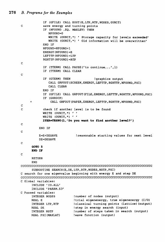
I F (GFILE) CALL EOUT (E, LW, RTP,NODES, GUNIT) save e n e r m and t u r n i n g p o i n t s IF (NFQUND .EQ. WXLEVf TmN
NFQUNEI=O RRXTE (QIZNIT, * 1 Sto rage c a p a c i t y f o r l e v e l s exceeded* m I T E (OUNIT,*J Old i n fo rma t ion w i l l b e a v e r w r i t t e n "
END XF NFOUND=HFOUNDtl ENERI;V (NFOmD) =E LEFTTP (NFOUND) =LTP RGWTTP (NFOUND) =RTP
I F (TTERM) CALL PAUSE(%o c o n t i n u e , . . * , l ) I F (TTEW) CALL CLEAR
I F lGTERNf THEN ! g r a p h i c s a u t p u t CALL GRFOUT(SCREEN,ENERGY,LEFTTPIRGHTTP~NFOUND~PSZ) CALL CLEZAR
END I F SE (GFTLE) CALL GWOUT (F1 LE, ENERGY, LEFTTP, RGHTTP NFOUNDIPSX) SF (GWRDCP)
-+ CALL GmQUT (PAPER, ENERGY LEFTTP , RGXTTF , NFQVND, PSX 1
t r easonab le s t a r t i n g v a l u e s for next l e v e l
cheek i f ano the r l eve l is t o be found WXTE (OUMXT,*) C " mZTE fOUNTT,*) " f
C END I F
C
E=E+DESAW DEmDESA-
c G10m 5 zm m
c RETURN END
~ccc~~C~ccccc~cccec.ccc~ccC:C:cccccccceccccccccccc~ccccc~c~cc~ccc~ccc~ccccc SUBROUTINE SEARCH (E, DE, LTP, RTB, NQDES, NSTP PSI 1
C search f o r one e igenva lue beg inn ing wi th e n s r s E and step DE cccccccccccccccccccccccccccccccccccceccccccccCcccccccccccccccccccccccccc C Global v a r i a b l e s :
INCLUDE "%O.ALL6 INCLUDE ?PmM.E3'
G Passed v a r f a b l e s : INTEGER NODES !nu-r of nodas (ou tpu t ) WAL E ! t r i a l e igenenergy, t r u e e igenene rgy (XL01 INTEGER LTP , RTP I c l a s s i e a l t u r n i n g p o i n t s f la t t ; fc@) (ou tpu t ) m L DE f step i n energy s e a r c h ( i n p u t ) INTEGER NSTP !nu&er s f steps t aken i n s e a r c h ( o u t p u t ) REAL PSI (mXULT1 !wave f u n c t i o n f o u t p u t )
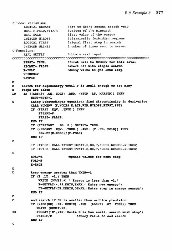
C Local var iab les : LOGICAL SECANT !are w e doing secan t search yet? REU F,FOLD, PSTmT !values of t h e mismatch M& EQLD ! l a s t value o f t h e e n e r w INTEGER NCROSS lelassleally forbidden r e g i o n s LOGICAL FXRST !s igna l first seep in search XNmGER NLINES !nudes of f i n e s s e n t t o s c r e e n
C Funct ions: REAL GETFLT !obtain real inpu t
ccccccc~ccccccccc~ccccccccceececCf:cceccccee~ceeccccf:cccececccecccccC:cccc FZmZ=. =m. Ibirat (=.a28 t o M for khla hwel B g m z = * F m E * P=WW ! vaXw to gat fa&@ loep mzms=2 HSrn=O
C C seazd f o ~ ~ i g e n e a a w une25 F 3.8 8-22 dmeugh or toe C IJtmpa t&aa 3.0 XF [[rnStPj .a* zam) .mD* (MSZP .L%* W S W ) l %mm
R9m=Bsm+2 C
FSFmT-F Bf . Fame
m X?#
TF ( (BEmT "EW* .%R=.) .mD. (F .m, Fa=)) TmM Dm-F* (E-EOm) / {F-ETOLD)
E m m
SF (TTEW) CBLL TXTOUT f OUNIT, E, D&, F, %ODESI EICROSSr MLINES 1 %F (TFEm) CALL TXTQUT (TUNIT, E, DE, F, NQDES, HCROSS, HLXNES]
end sear* ff DE i s sa2ler than. m-lne pmoision ZF ( (mS (DE) .L%!. D@=&) .&.RD. [=B (F) , O%, TOW) l I"mI
=TB (OmXT, 20) Fa-9 ( f Q', 21X, p BeZta E i8 too a-52, seareb mst atop' ) EI=ZIOW/Z ? warm to search
END IF
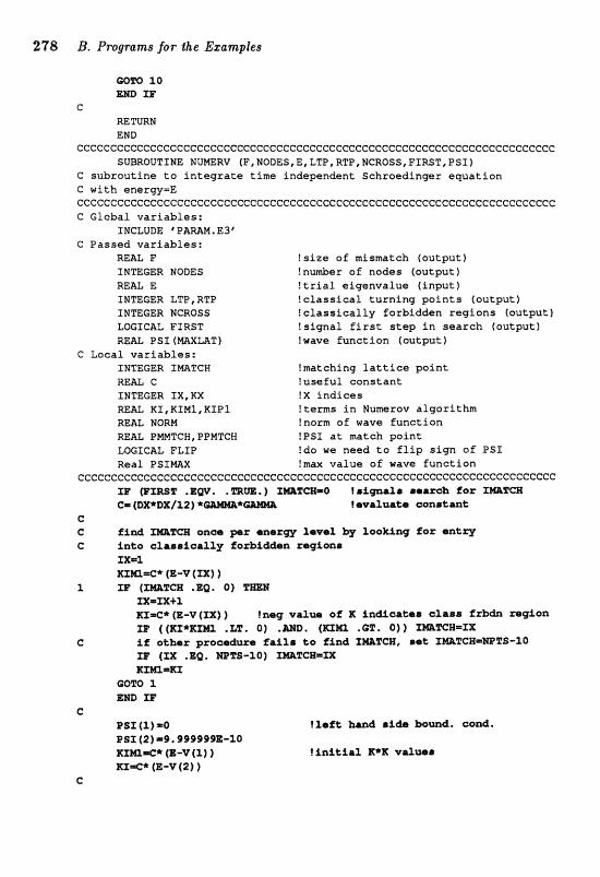
278 B, Progmnzs for tke Ezana_pfes
60iC8 l0 BMD m
C
MTURN END
ccceccccccccccccccceeccccccccccceccceccccccccccccccccccccecccccccccccccc SUBROUTINE MUmRV fF,NODES,E,LTP,RTP,WCROSS,FIRST,PSI)
C subroutine ta integrate time independent Schroedinger ewation C with energy=E cCcCCCCcCcccccCeccccCCcGccCeecccCCeCccccCCCCCcCCcCceeccccccccccccc~ccccc C Global variables:
INCLUDE 'PhMM.E3' C Passed variables:
REAL F !size of mismatch (output) INTEGER NODES !nWer o f nodes (output) RE& E !trial eigenvalus (input) INTEGER LTP , RTP !efassical turning points (output) INmCER %CROSS !classically forbidden regions (output) LOGICAL FIRST ! signal first step in search (output) RE= PSI (MXLAT) !wave funet %on f output)
C Loeal varltlbles: INTEGER I M T C H !matching lattice point REAL C !useful constant INmGER EX, XX !X indices
K1 , RIM1 , KIP1 !terns in Numerov algorithm MllL N O W ! norm of wave function REAL PMMTCH,PPMTCN !PSI at match point LWICAL FLIP !do we need to flip sign of F51 Real PSTmX ! m a value of wave function
ccccccccecccccccccccccecccccccccccccccccccccecccc~~cccccc~cecccccc~ccCcc (B-P .fbQV, ,mm.] fm%a=0 Ie ipalr 8aaxab Effor Immkf
C= (DX*DX/f2 1 * fsvaluatr aon+tm% G C fin& XmTCB onas psr enaza 1awe1 by fookiag for ankq C into clraaicalXy 1CorbSdhn reg%aa
Xx=l mm&* (E-V (SX) )
1 ra ( X m T e a .@Q. 0) rn=IZ+f m<*{E-V(XX)) Inrscj valm a% K lnaeatsrar olrata f z m region m ( (~ic~&xzm . %T, a) . m ~ . .m. 01 X ~ Z C W = I X :
C jltP otbrr pze&wa faiZ8 to find fmTCH, raC X=TCH=W1"S-10 m {ZZ .EQ. mzs-lQ) x m T c H = n kfXm=KX
WTO 1 EHD XF
G PST (l) =O BSI (2) .x9, P99999E-10 X T M t e * ($-V (3)) KTe* (E-V f P f )
c
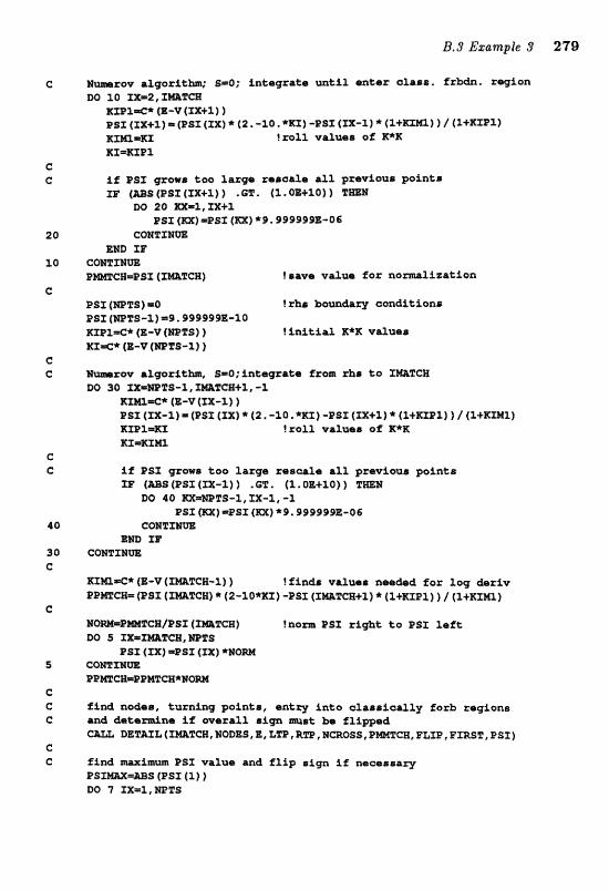
zew a l g o x i t h ; S=O; int;agratlrr u n t i l eatss alas@, fz-. reggon TU) 10 3Xm2, f =Tea3
Eraxe* (E-v (zxs.~) 1 asx (xx+i) (asx (xx) * (2. -30. *Ex) -PSZ [XI(:-I~ * (1+mmf / ~ X + E X P ~ ) E m = E f troZl value. of K*X: Kf &zEl
i f 953 gzowo too l a rge zesaale a11 p r e v i o u ~ poin ts X&? (=S (PSI (fXS.1) ) . OT . (2.5E+10) ) T m
M) 2Q ==2,=+1, PSX (a) .PLeSI (a) *S. 999999E-06
cowxsm Ern SE"
COMPXm PrnCBmP ss ( z a z c a )
PSX (WZIS) =O !rhe beundary e o a d f t i o n ~ PSf (WTS-1) =9.999998&-10 AIPIe* ($-V (mTS) ) !&nitiaZ IC*A vauerr K X e * (E-V (=TB-I) )
M) 30 ZXmWT8-1, =2CH+2, -1 E w e * (&-V (=-l) ) R s Z (XX-l)m (PS% (aX) * (2. -10 *KT) -EOX [3X+l) * (X+fCIPl) ) / (1+IImZ) KfEl=Kf trolX values of R*K Kz=xfm
i f POX grow8 too Zarge reecpZs %If pzeviouis poin ts I:.F ( M S (PS% (XX-Zj ) . GT, (1, OE+lO) ) T m M
DQ 40 ===%S-2, m-1, -1 ESI (m) =PSZ (m) *S. 999999P1-Q6
caR%mm Brn XF
CONTXNW
EI:m&* (E-V (X=TCB-%) ) c k c i f o r log &+iv P P ~ G B - (asx (rmFeE) * (2-3,~*a~) -PSI ( Z ~ T C H + Z I * ~ X + K X P Z ~ 1 f { ~ + ~ C I M T ~
HOW=PmCB/PSX (I=%-) f no= PSI: right; t o PSf l e f t DO S m=mTCE,'1SPfeS
PSI ( 3 X f =PBX f XX) *HOW comxm f n m c R = a P m a * w Q ~
I ind nodms, ewnfng poiata, en t ry In to eZasaIcally tie& regiona and &%te&na i f m e r a l l sign ansat h f l i w d
DBTmL (XMTa, NODES, E L%P t R=, NCROSS I Bmr"CBI FLXP I Bf WT, PSZ 1
1t.m and f l i p s i p i f neaaasary
86 7 I X m 1 , PJPZS
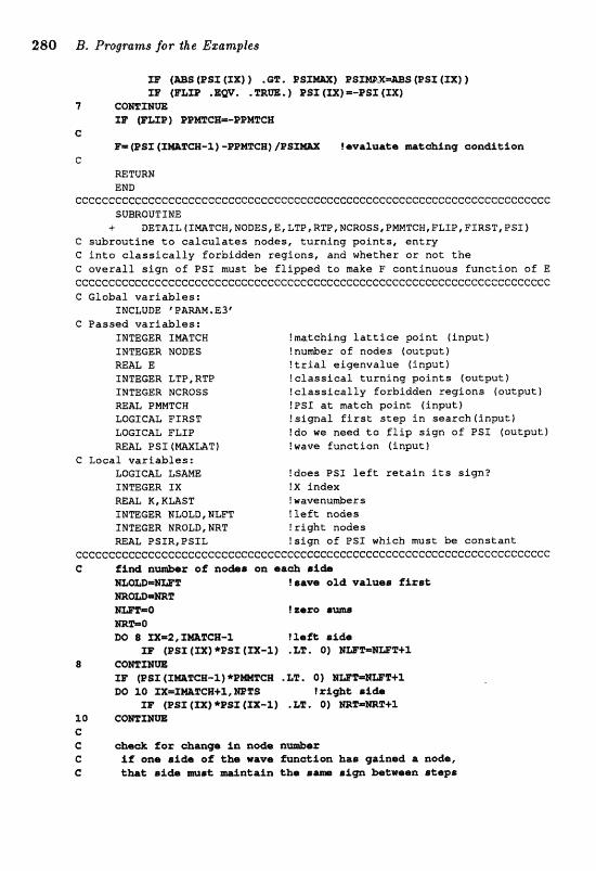
XE' (=B (PSf ( X X ) ) . GT. PS %P tF&IP .gm* .%R-* 1 R
7 CQrnINrn TF (mXE) EPM%CB=-PPMXH
C levrluats mkcrhLng conation
C =TURN END
CCCCCCCCCCGCCCCCCCCCCCCCCCCCCCCCCCCCCCCCCCCCCCGCCCCCCCCCCCCCCCCCCCCCCCCC SUBROUTLNE
+ DET&IL ( ImTCW, NODES, E, LTPI RTP, NCROSS@ PWTCH, FLIP, FXRST, PS5 j C subroutine to ealclulates nodes, turning points, entrqr C into classically forbidden regions, and whether or not the C overall sign of PSI must be flipped to make F continuous function of E CCCCC6CGCCCCCCCCC6CCCCCCCCCGCCCCCCCCCCCCCCCCCCCGCCCCCCCCCCCCCCCCCCCCCCCC C! Global variables:
INCLUDE C P N M . E 3 ' C Passed variables:
INTEGER TmTCN !matching Jattiee point (input) INTEGER NODES !number of nodes (output) ReAL E !trial eigenvalue (input) INTEGER LTP, RTP !classical turning points foutputf IMTEGER NCROSS !classically forbidden regions (output) RE& PMMTCM !PSI at match point (input) LOGICAL FIRST l signal first step in search (input) LmICAZ FLIP !do we need to flip sign o f PSI (output) M U PSI (mXLAT1 twave function (input)
C Local variables: LOGIC& LSAME !does PS5 left retain its sign? INTEGER TX !X index W& K,KmST Iwavenu&ers INSEGER WLOLD, NLFT ?left nodes XNmGER NRQLB, TttRT ! right nodes mAL PSXR, PSIL !sign of PSI which must be constant
CGCCCCCCCCCCGCCCCCCCGCCCCCCCGGCCCCCGCCCCCCCCCCCCCCCGGCCCCCCCCCCCCCCCCCCC C fixid r sf nods. on ra& r i b
m Q L D = m T !save old valuse Xirst m a m m m T NrnF=Q lzero 0
m-0 XZO 8 ==2,5=2CE-l !leg& .%&cl
KlP (PBX 4ZX) *PSI (XX-l) . LP. 0 ) HWT=m?P+3 8 C Q m Z m
ra (as1 ( I ~ W E - I ~ * P m c a .%F. of wmT=wge+n M3 50 ~ = K m T G B S 1 , ~ T i S I ?rSgb& aid+
r~ (esz (m) *PSI (EX-W .LT. 01 mg=mg+r 10 c m z m C C desk for a h w e in no- C i% ens aide of tkrrn wave Raa galned a node, C tbaC &Act% mst dntagn afw htween irkalp@

now, f%noflg, &lsdn% if the nseds to be f3ippad mm=. F==.
.-D, (nsxlt*nsr ( 2 ) . tr. o . ) FGZP-. mm. ) .m. (PsrR*psr (wrs-11 .LT. Q. 1
+ F&a=*mm*
ram v&ms bor rkrp 9sxmPsrx (2 1 asn=psr (=vs-%) m (mxre) asxm-laaxr, m (PLxa) asrw-ssxa
zind rigkkmot turning pia* Rm=a m ~ Z s . t l za (Rm *m. 0 ) TmH
Xz=xx-% ZF 4 (E-V {a) .a. Q) Rm=ZX
mm 120 mlig
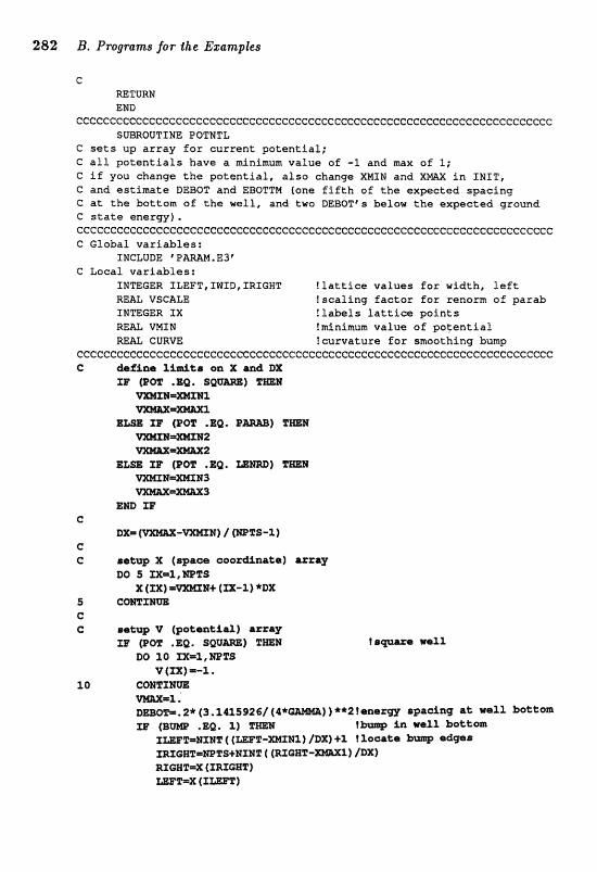
282; B, Progmms for the Eszamples
C RETURN END
cccccccccccccccecccccccceccccccccccceccccccccccccccccccccccccccc~ccccccc SUBROUTINE POTMTL
C sets up array for current potential; C all. potentials have a dnimum value o f -1 and max of 1; C if you change the potential, also change XMSN and XPlAX in INIT, C and estimate DEBOT and EBQTTM (one fifth of the expected spacing C at the bottom of the well, and two DEBQT% below the expected ground C state energy). ccecccccccc~cecececccccccccccccceccceeccccccececcccccccccccccccccccccccc C Global variables:
INCLUDE PMM,E3' C Local variables:
INTEGER ILEFT,SISJID,IRIGBT !lattice values for width, left RE= VSGALE !scaling faetor for renorm of parab IWmGER IX I l a h Z s lattice points
VMIN ?minimum value of: potential =&L GURW !curvature for smoothing bump
ccccccccccccccccecccC:cccccccccccccccccccccccccceccccccce~cccccc~cccccccc C &sane 2lidt;s on X and DX
33' (POT .EQ.
EHB 33' C
H) / (taees-1) C C getup If (=I- @eerdina%e) array
DO 5 X (EX) .c (m-l) *W
f cmmm C C setup V (pcl.tea%id) =ray
IB (P6E .BQ. S Q U m ) %=H f ~ p a a M~B%%
BC! 10 TX=l,mllS V {IX) m-3.
10 CoHrTWm 1 * S., 2* (3,1415926/ (4*
SE" (B- .BQ, 1) %=I I h well bottm XWP=ErnT { (mP%-~Xlfl) I edge&
RIQHTmX (ZmGHF) -%=X (ImF1C)

cm==-. o m / 4 (maaz-m~j / a 4 **2 C top ~f is t o avoid &naenLimit;ier
V (ZZ) U-1, + ~ X W Z * (2,. (X(=) R fma%+WT1/2.) * * g ) 20
Brn IB C
E m 33' (POT .BO. f tgrrm%f G mr13 W 30 ZX=l,mTO
v (XZ) m- (1 * -. $*X ( %X) *X (m) 1
4.
l3 .EQ. X) ths parrbolic potential i r f2at ta~ld m W Z M T (EmD/DX) ZR (HOD (=D, 2) .m. MQD (MP%#, 2) ) =-=P-l
D) /Z+l
40 e
Db 50 ZZ=l,mfS
so cOB%xm m m
C =g12 IE (801: .Ea. M m ) IfmM f Umrzd-amaa w e n t i r l
W 60 m=%, =TB
bQ
tenmrm apcaing at we12 bott~lla (&re Ex. 2.8) G
Ern XIF C= C -mated gua@rar for we-& @Late raaza mamzm @p&aimg; G wkkh therm valwaa, it wiz1 L&* thzrr, ntqm ZOE P d0 riqn
~ ~ ~ - 1 . + 2 . J * B ~ F C
=TURN END
cccccccccccccccccccccceccccccccccccccccccccccccecccecccccceccccccccceccc SUBROUTINE I NIT
C i n i t i a l i z e s c o n s t a n t s , d i s p l a y s header screen, C i n i t i a l i z e s a r r a y s f o r i n p u t pa rame te r s ccccccccccee~cccec~ccccecceccccccccccecccccccc~ccccccccccccccccccccccc~c G Global variables:
INCLUDE 'IOIALLe INCLUDE ' MEMU. ALL'
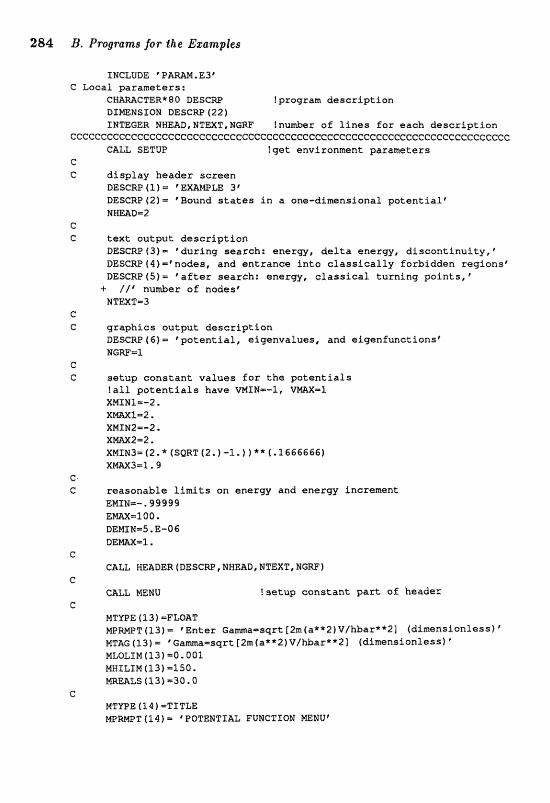
284 B. Programs for the Ezamples
!program d e s c r i p t i o n DXmNSTQN DESCRP f 22 1 IHTEGER NBEAD,NTEXT.NGRF !number of l i n e s f o r each d e s c r i p t i o n
CCCCCCCCCCCCCCCGCCCCC:CCCCGCCCCGCCCCCCCCCC:CCCGCCGCCCGCCCCCGCCCCCCCCCCCCCC CA= SETUP !get environment p a s a m t e r s
e C d i s p l a y header sc reen
DESCRP ( 1 1 p EX-LE 3 DESCRPt2f= 'B~ound s t a t e s An a one-dimensional p o t e n t i a l t NEmD-2
C C t e x t o u t p u t d e s c r i p t i o n
DESCW(3)- ' d u r i n g seagch: e n e r w , d e l t a energy, d i s c o n t i n u i t y , ' DESGRP(4)=6nadas, and e n t r a n c e i n t o c l a s s i c a l l y forbidden reg ions r DESCRP(S)= ' a f t e r search: e n e r w , c l a s s i c a l t u r n i n g poin ts , "
+ //"umber o f nodes6 NTEXT=3
C g r a p h i c s output d e s c r i p t i o n DESCm(6f- "potential, e igenvalues , and e igenfunc t ions ' XdGW=l.
s e t u p c o n s t a n t v a l u e s f o r t h e p o t e n t i a l s f a l l p o t e n t i a l s havs VIJIINm-1, V W = 1 XNINl=-2. XWI-2, XMXM2=-2. XM2-2. X%IN3=12.* (SQRT[21)-1.)j** t.1666666) X M 3 = 1 . 9
r easonab le l i m i t s on energy and energy Increment EMIN=-.99999 EM-lO0 . DEMIWm5.E-06 D E M = 1 ,
GALL WEEhDER f DESCRP , NNmD, NTEXT, HGBF)
CALL MEMU ! sa tup c o n s t a n t p a r t o f haadar
NTWE (1 I ) =TITLE W M P T (1 4 ) = * POTENTIAL FUMCTION =MUt

NLOLSN (14) =2, MHZLIM (14)=1.
C %TYPE f 15) =MTSTLE W W T (15) -' 1 ) Square-well p o t e n t i a l p MLOLIM (25) -0. NNILIM(~S)-O.
C MTYPE (1 G) =MTTTLE E W T (16) ='2) Patabof i c -we l l p o t e n t i a l " MLOLIM (16) 90. MWILIH (1 6f =Q.
G MTYPE (17) =MTITLE MPWT (171 -' 3) Lennard-Janes p o t e n t i a l * MLOLTM (2.7) =Q. MWILIM(17f-l.
c MTYPE f 18) =HCWOXc W W T ( 1 B ) m 'Make menu c h a f c e and p r e s s Re tu rn r MTAG(18)='19 24 26' MLOLIM (1 8 1 =l. MMIL1M ( 1 8 1 =3. MTNTS ( 2 8 ) -3 W A L S (28) 4.3.
C MTICP& 62 9) =NOSKIP W m P T ( 1 9 ) = 'Do you want a bump i n t h e s q u a r e we l l ? ' MTAG (2 9) = Square Rel l Bump: ' m m ~ s (19) -35. MINTS (19) =O
C NTIVPE (2 0 ) =FLOAT NPmPT(20)= 'En te r t h e l e f t hand edge o f bump (scaled u n i t s ) ' MTAG (20)m "eft hand edge o f bump ( s c a l e d u n i t s ) ' MLOLIM (20) -XMINI MHILIM (20) =XmX1 MREALS (20) m-. 1
C MTYPE (21 ) -FLOAT MPWT(21)= 'En te r t h e r i g h t hand edge o f bump ( s c a l e d u n i t s ) ' MTAG(21)= @ R i g h t hand edge of bump ( s c a l e d u n i t s ) " MLQLIM (21 ) =XMTNL NWILIM (211 = X m X 1
~ s ( z z ) - . r C
MTVPE (22) =FLOAT W W T ( 2 2 ) = 'En te r t h e h e i M t of t h e bump ( s e a l e d u n i t s ) " MTRG(22f = 'Weight o f t h e bump ( s e a l e d u n i t s ) @
WOLTM (22) =Q. MHILTM (221 =20 MREALS (22) -1.
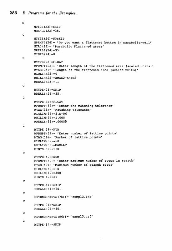
MTYPE (24 1 =NOSKZP MPRMPT(24)= 'Do you want a flattened bottom i n pardwfic-well0 MTAG (24) = rParabolic Flattened area:' MFtEALS(24) =3S. MINTS (24) =0
mt'ypB ( 25) =FLOAT MPRMPli(25)= 'Enter length of! the flattened area (scaled units)' MTAG (25) = Length o f the frattened area (scaled units) HLOLXM (25 1 -0 MHILXM (25) -XMAX2=-XMZN2 ImEaLs (25) =* 1
MmPB (38 =FM)AT WRMPP(38)= 'Enter the matching tolexancrec MTAG (38) = ' Matching tolsranca' WLoLIH (38) 15.E-06 MHXLIM (38)=1.000 MREALs(38)=.00005
MTWE (39) -NUM WPRMPT(39) - 'Enter number of latt ice pointsf MTAG (39)- "Rumber of la t t i ce pointsp MLOLfM(39) =SO WILXM (39) rzIIAxLAT MIWTS (3 9) =160
WXFE (40) =NUM MPRMPT(40)- 'Enter maximtan number of steps i n searcht MTAG(40)- f M a x i ~ number of searoh steps' MLOLIM (40 ) 110 MHILXM(4O) 1300 MINTS (401 -50
W'PRNG (PIXITS (-75) ) = ' exffqpl3. txt '
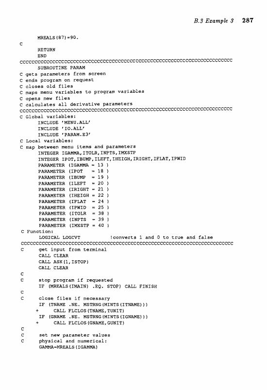
LS (871 -90. C
RETURN END
c ~ ~ c c c c ~ ~ ~ ~ ~ ~ ~ ~ ~ ~ ~ ~ c c e ~ ~ c c c c c c c c c c c c c ~ c c c c c c c c c c c c c c c c c c ~ ~ e e c c c c e c c ~ c ~ c SUBROUTlNE n
C gets parameters from screen e ends program an reguest c eJosas old files c m p s menu variables to program varlhles c apens new files C calculates all derivative parameters e c ~ ~ ~ c e ~ ~ ~ ~ c c ~ ~ ~ c c e c ~ c ~ ~ ~ e ~ ~ c ~ c ~ c c ~ c ~ c c c c ~ c e E : c c c e c ~ c c c ~ c c e c c c c ~ c c c c c c c c C Global variables:
INCLUDE W N U M U , A L L e XMCLUDE ' 10.ALLr INCLUDE T W W . E 3 t
c Local variables: C map &tween menu items and p a ~ a m f e r s
INTEGER IGAMm,ITOm,INPTS,fPlrXSTP TNmGER IPOT,fSUW,I~FT,IHE,IGW,IRIGNT,TFMT,IE"WID
P A U E T E R (ITOER = 38 )
P m W T E R (INPTS - 39 f P TER (XWXSTP = 40 }
C Functian: WGJCAL LWGVT !converts 1 and 0 to true and false
C C C C C C C C C C C C C C C C C C C C C C ~ C C C C ~ ~ G C C C G C C C ~ C ~ C ~ ~ ~ ~ ~ ~ ~ ~ C C G C ~ ~ ~ ~ C ~ ~ ~ C ~ ~ G ~ ~ ~ ~ ~ ~ ~ C get input from terminal
GAU C-R CALL ASK fl , I S T O P ) ZIllm cmm
C C stop program if requested
I F (MmALS(IE4AIN) .EQ, STOP) CALL FXWPSH c C close f i fes if necessary
IF (TNPIWE .HE. MSmHG IMIMTS f ITNAME) )f + CALL FLCLOS f TNAHE , TUMITf IF 1 G N W . NE . MSmNG (MINTS ( TGWm) 1 1
+ CALL FLCLOS (GMAm, GUMXT f c C set new parameter values C physical and numerical:
G A W = M M A L S ( I G A m )

288 B. Programs for the Ezamples
T O W = m A L S ( ITOLR) NPTS=MIWTS (LNPTS) WSTP=MIKTS (XMXSTP f
C C potential parameters
POTfNWLS ( f POT) BUW=MIWTS (IBUMP) LEFT=MWALS (TZEFT ) RIGHT-mALS (IRIGXT) WEIGHT=MmALS f XHEssH) FLAT=HINTS (XELAT)
G CALL PQTNTL !setup p ~ t e ~ t i a l a r r q
e C
TTERH-LQGCVT (MINTS (ZTTERM) f TFXLE-LOGWT (MINTS (X TFILE j 1 TMMEoMSTRMG (MINTS l XTNAm) 1
G G graphics output
GTERM=LQGCVT (MINTS { ZGTERM] cnmcP=LacmrT (MINTS (IGWRDI 1 GFmL,e=LwcvT ~HXNTS (IGFTLE~ 1 GEm=MSTRNG (MINTS (XGMAE 1 1
C C openfiles
I F [TFILE) CALL FWPEN (TNkm, TUMI T) I F (GFXLE) CALL FWPEM(GRAm,GUHXT) !files may have been renamed MSTRNG (MINTS (XTNAW) t 5TFaA.m MSTRNG (MINTS [XGPsAm) 1 =ENAm
G RETURN EPJD
ecccccccCccccccccccecccccccccecccccccceccccccccecccccccccceccccccccccccc" SMROUTINE PRMOUT (NUNIT)
C outputs parameter sumary to the spcifiad unit c~~~ce~ce~cccccccccceccccccccccccccccccccccccceceecccccccceccccccccc~ccc C Global varfabfes:
INCLUDE 'XO.ALLt INCLUDE 'PAmM.E3'
C P a s s e d variables: INTEGER MUNLT !unit n u d e r f o r output RE&L VAR [ 4 1 !initial values of coosd and momnta
ccccccccceccceececcccecccccccccccccceecccccccccccceccccecccccccecceecccc IF (MUNIT .&Q, OUNITI CALL eLEm
C WRITE (NUNTT, 2 1 a I T E (MUNST, -4) KRXTE (NUHIT, G) GAMME1 WRITE (MUNIT,8) TOLF
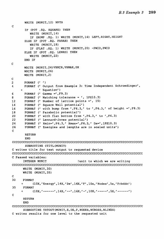
WRITE (NUHIT, 12) NPTS C
IF (POT .EQ. SQUmE) TWEN mZTE (MUNIT,14) IF (Bum ,Ea. 2 ) WRITE (MUNIT, 2 6) LEFT, RIGHT, EEIGHT
ELSE ZF lPOT .EQ. P A W ) T m H mIT& (MUNIT, 18) IF / P U T .EQ, 1) TnlXlITE (MUNIT,PO) -PWID,PWTD
ELSE IF (POT .EQ. ZENRD) TWEN WRITE (MUHIT, 22)
END IF G
m I T E fMUMIT,24)VXM?IIM,VXIIIYIIX,DX WRITE (MUNIT, 2 6) WRITE (NUNIT, 2)
C 2 FORMAT (' t ' )
4 F O W T I r atput from Exa-le 3: Time Zndependent Schroedingert8 i qwation' )
6 FQ-T ("~enuna =*,,F9.3) 8 FORMT (' Matching tolaran~e = ', IPE20.3) 12 FORmT ( * Number of lattice points =\ 15) 14 F a W T ("ware Well potentialr) 2 6 FO~Tf~with~umpframr,,E"6.3,~o~,F6.3,toofheight=C,E'8.3) 18 F O m T ( ' ParabaLZc potential') 20 F O m T ( * with flat bottom from ',FB.J,' to ',F6,3) 22 FORNGLT ( * Lennard-Jones potential'] 24 FORWT f r Xmir\=',P6.3,~~ma=~,FB.3,* I>x==* ,lPE10,3) 26 FORmT ( V ~ ~ e z g l e a and lengths are in scaled unitst) C
W T U W EHD
CCCCCC~CCCCCCCCCCC3GCCCCCGC~CCCCCGCCCCCCCGCCCCCCCCCCCCCCCCC~CCCCCCCCCGCCC SWROUTINE GTXTLIMUNET)
C wtites title for text output to xe~uested device cecceecccccccc~eccccccc~cccccccccccccccccccccccccccE:ccccccccccccccccc~cc C Passed variables:
INTEGER MUNIT !unit to which we are writing cccccceccec~cccceececcccccccccceececccccccccececcecceccccccccccccccccccc
WRITE: (MUNIT, 30) WRITE (NUNIT, 35)
C 30 F O M T
-c. t lOX, 8E~ergqtt, l 4 X , 'Deft 16X, * F#, 1Ox, tN~dasr ,5xp *Frbddnt 1 35 F O m T
4" (lax, P , 1 4 ~ , ~ - - ~ , ~ ~ x , ' - I , J J J ) I , I ---I- * , 5 ~ , e...,..----r 1 C
RETURN END
~cec~ccc~cccccccccc~ccccceccccccccceeccccccccccccccccccccccccccccccccccc SUBRQUTIME TXTQUT (MUNIT, E, DE, F, MODES MCRQSS, NLINES 1
C writes results for one level to rbe requested unit
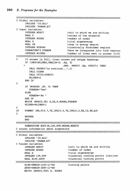
290 B. Programs for the Ezamples
ccccccccccceccccccceccccccccccccccccccceccccccccccc=ccccccccccccccccccccc C Global variables:
INCLUDE *1SB.ALLe INCLUDE 'PWM.E3'
C Input variables; INTEGER MUPjf T tunit to which we are writing REAL F !values of the dsmatch INTEGER NODES !nu&er of nodes MWL E !trial efgenenergy RE& DE !step in enerw search INTEGER NCROSS !classically forbidden regions CHmCTER*3 FQRBBN !have we integrated into forb regions INmGER NLINES !nuPnber of lines sent ta screen (I/O)
~ccccccccccccc~cccccccccI:e:cccccccC:cccccccccccccccccccec~ccecccccccec~ccc C if sereen i s full, clear sGreen and retype headings
IF ( (HQD (NLXNES, TWLXN-4) .Ea. 0) + .AND, (WEIT .EQ. OUNIT)) THEM
CALL PAUSE(ftto continue ...*, l) CALL C-R CALL CTITL [QUNIT) NLINES-2
END XF C
IF (NCRQSS .GT, 01 THEM F"QmDN=' Yes *
ELSE FORBDM-eNa
END SF m1TE (MUNTT,20) E,DE,F,TJODES,FORBD# ULPNES=NLIN&S+I
c 20 F O m T (8X,F10.7,7X,EPE20e3,7Xr1PEZOIJ,8Xrf2r8X,A3~ c
=TURN END
ccccecccccccceccccccccccccccccccC:cccccccccc~cceecccecceccccccc~ccccccccc SUBROUTINE &OUT (E,LTP,RTP,NODESCMUNIT)
C output information about eigenstate c c c c c c c c c c c c c c c c c c c c c c c c c c c c c e c c c c e c c ~ c c c c c c c c c c c c C Global variables:
INCLUDE 'fID,ALLf INCLUDE 6PAm.E3'
C Passed variables: INTEGER NUNTT funit to which w e are writing SNTEGER NODES fnuder of nodes REAL E !trial efgenenerw f NTEGER LTP , RTP ! cjlassi~al turning points (lattice) m& XL-, XRTP Iclassical turning points
ccccccccccccccccccCCeccccccccccccccccccecc~ccccccecccccc~ecccccccccccccccc XLTP=VXMTN+ (LTP-1) *DX !turning paints XR3CP=aNIN+ (RTP-1 )"DX
mITE (MUNTT,SOO) E, NODES
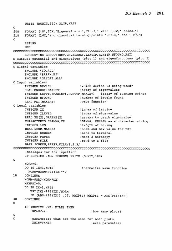
mITE (MUNI T, 53.0 ) XLTP, XRTP C 500 F Q m T fV0' ,20X, "igenvalue F,F10.3, V i t b ' , I 2 , ' nades.' 1 510 F Q W T (IGX,'and c l a s s i c a l t u r n i n g p o i n t s *,,F7.4,' and ',F7.4) C
=TURN END
~ c ~ e ~ ~ ~ c ~ ~ c ~ ~ c ~ ~ e c c c c e e e c ~ c c c c c c e c c c c c c c I : c c c c c c c c c c ~ c c c c c c ~ ~ c ~ ~ e c ~ c c c c e c SUBROUTINE GRFQuT(DEvIcE,E~RGY,ZEF~CTP,RGWTTP,NFQUMD,PSI)
C o u t p u t s p o t e n t i a l and e i q e n v a l u s s ( p l o t l ) and e i g e n f u n c t i o n s (plot 21 cec~cccccccccCccccccecccceccccceccccceccccccceecccccccee~eccccccccccccec C Global v a r i a b l e s
INCLUDE 'IXO.ALLf
INCLUDE GRFDAT . &Lf C I n p u t v a r i a b l e s :
INTEGER DEVICE !which d e v i c e is b e i n g used? mAL ENERGY ( D L E V ) ! a r r a y aE e i g e n v a l u s s IMTEGER LEFTTP f W L E V t , RGWTTP (mXLEV) ! a r r a y of t u r n i n g p o i n t s INTEGER NFOUESD !number of l e v e l s found mAL PSI (MXMT) !wave f u n c t i o n
C Local v a r i a b l e s INTEGER I X !index of l a t t i ce INmCER XLEVEZ !index o f e igenva lue RE& XE (21, G W H E (2) l a r r a y s t o graph e igenva lue CBmCTER* 9 CGAHM, CE !GBXm, ENERGY a s a c h a r a c t e r s t r i n g INmGER LEM ! l eng th af s t r i n g RE& NOW, m P S % fnarm and nrax va lue for PSI INTEGER SCmEIJ !send t o t e r m i n a l IBmGER PAPER !make a hardcopy INmGER FILE ?send t o a f i f e DATA SGREEN,PWPER,FILE/I, 2,31
cccc~ccc~ecc~c~~~cceccc~eccc~ccccE:ccecccccccc~cc~ceceecce~cc~cee~c~ccc~~ !messages f o r t h e inrpat ient IF (DEVICE -ME. SCREEN) HRITE (OUNIT,Z00)
C NOm=O. BQ 10 IX=l, MPTS !normal ize wave f u n c t i o n
MORM=MORM+PSI ( f X I * * 2 10 CONTINUE
NQW-58RT (NQRM*DX) WXPSI=O. DO 30 IX=l, NPTS
PSI (xx)=psr trxt /NORM IF (ABS (PSI (IX) 1 . GT, mXPSI) mXPSI = WBS (PSI (IX) )
30 CONTINUE e
I F (DEVICE .NE. FILE) THEN NPLQT=2 !how many p l o t s ?
C1
G p a r a m t e r s t h a t a r e t h e same f o r bo th p l o t s XMINmVXMIN ! a x i s parameters
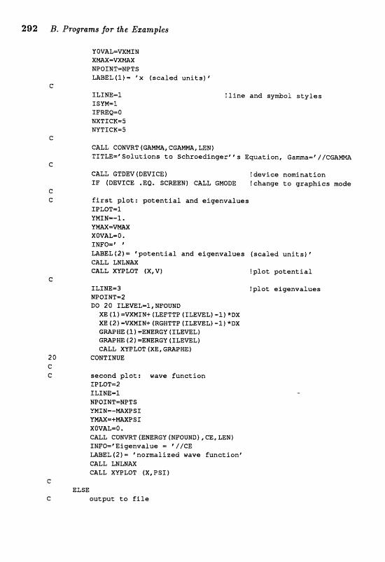
yo~qua3acl 30rd i [&'XI ZOqdlUS ??W
mH1MT T2V3 , (s3yun payeos) ssn~shuafifa pue ~o~~ua3od~ (2) ?a[gw
r rmOdNT * O=TVAOX
" Z-=MfWt 513r01dT
sen~enua6ya pue ya~?ua?od :qa~d 3srt3

mIT& (GUMIT, 801 W I T E f GUM1 "P 85) m I T E (GUNIT,?QO) t X ( I X 1 ,V(XX) ,PSI (XX1, XX.-1,NPTS)
END fF C C end graphing session
IF (DEVICE .NE. FILE) CALL GPAGEtDEVLGE) !end graphing package IF (DEVICE .EQ. SCMEN) CALL TMODE ?switch to text made
C
1 0 0 F Q m T (/,-atience, please; output going te a Tile,') 8 0 F O m T 4" 0 % ,93X, 'PosStf onp, 14XI C Potentialp, E3X, v function@ 1 8 5 F O m T (E3X, ' --------' , ~-----...---~ , 1 3 ~ , C --..---m - -m--" f 70 F O m T ( 3 (11X, IFE12.5) ) c
mTVRN END
ccccccecccccecccecccccccccceecccceccccccccccccccccCcccccccccccccCccccccc ccccccce~cccccccceccccccccccccccecccececccecceccccceccec"ecceecceccc~cccc C param.e3 C
!degree of "antumness* RE= T ?tolerance in search INmGER W T S !nu&er aE lattice paints XW"LTEGER MaXSTP ?m= nu&er of steps in search
e XNTEGER MXLWT !maximum n u h r aE lattice points
TER ( W m T = f Q O O f C
XWTEGER s Q u A ~ , P ~ B , L E ~ ~ ~ R B !potential types
PARAMETER (PAW-2 1
C INTEGER POT f ukicb potential INmGER B W , F L A T !which features do we want BE= LEFT,RZGHT,WEfGRT,PWID !potential charaeteristrcs
V t M U T ) !potential array X ( m X M T t ?space coordinate
M A L V W fmgix value o f potential RE= EBOTTM,DEBOT !guesses far g , s . energy and spacing
G W& ENZN,EW,OEMXN,DEWX !limits on energy and energy increment
C XMZN1,X~frDX1 !limits on each patential XMIN2,XMXZIDXZ
mm XMXP(13,XmX3,DX3 REAL VXE/Xlf,WmXIBX
C INTEGER MXLEV P h m m T E R ( m L E V = 5 0 )
c ZOMGN / PPAMN / GAMMA
?maximum nu&er of levels

COMON / N P W M / TOLF, MPTS, mXSTP GOWON / POTPRH / POT, BUEIP, ELRT, LEFT, RXGM'PI WEXGWT, PWTD GOWQN / GOWST /
C
COHON / PCALC /
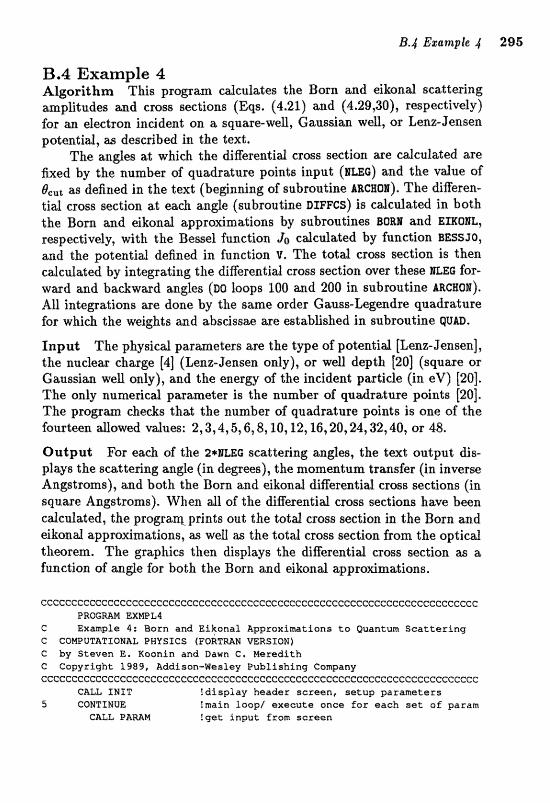
Algorithm Tbis program calculates the Born and eikonal scattering amplitudes and cross sections (Eqs. (4.21) and (4.29,30), respectively) for an electron incident on a square-well, Gaussias well, or Lenz-Jensen potendid, as de~cribed in the text.
The angles at which the differential cross section are calculated are fixed by the number of quadratare points input (BLEO) and the value of BCut as defined in the text (beginning of subroutine nrtcaox). The diEeren- tial cross section at each angle (subroutine DIFFCS) is calculated in both the Born and eikonal approximations by subroutines BoRR and EIKOBL, respectively, with the Bessel function Jo calculated by function BESSJO, and the potential defined in function v. The total eross section is then calculated by integrating the differential eross section over these ELBG for- ward and backward angles (DO loops 100 and 200 in subroutine nrc~ow). All integrations are done by the same order Gauss-Legendre quadrature for which the weights w d absdssae are established in subroutine 9 ~ 0 .
Input The physical parameters are the type of potentid [Lenz-Jensen], the nuclear charge [4] (Lenz-Jensen only), or well depth [20] (square or Gaussian well only), and the energy of the incident partide (in eV) [20]. The only numerical parameter is the number of qudrature points [20]. The p r o g m &e&s that the number of quadratare points is one! af the fourteen dowed vdue!~: 2,3,4,5,6,8, 10, 12,16,20,24,32,40, or 48.
Output Far eaeft of the 1*WILEG sc&tering angles, the text output dis- plays the scattering angle (in degrees), the momentum transfer (in inverse Angstroms), and both the Born and eikonat differential crms sections (in square Angstroms). When all of the differential cross sections have been cdedated, the progrq- prints out the total cross section in the Born and eikond approximations, as well as the total cross section from the optical theorern. The graphics then displays the dierentid cros8 section as a function. of a g e fox both the Born iztnd eikond approgmat;ions.
cccccccccccce~ecceccccecccecC:cc~cccccccccccccecccc~ccccccccccccccccccccc PROGMM EXWL4
C Exmple 4: Barn and Elkanal Appraximatians to Quantum Scattering C COMPUTATXONU PHYSICS taoalfww v e ~ s x o ~ j C by Staven E. Koanin and Dawn C, Heredith C Copyright 1989, Addison-Wesley Publishing Company ccccccccccecccecccecccccccecccecccccecccccccccccccccccc~cccccccccccccccc
CALL INIT Idisplay header screen, setup parameters 5 CONTINUE ?main loop/ execute once for each set of param
CALL P W M !get input from screen
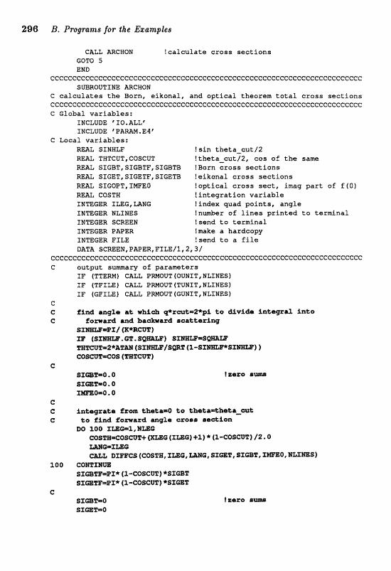
CALL ARCHON ! c a l m l a t e c r o s s s e c t i o n s GQTQ 5 END
cccccccccccccccccccccccccccccccC:ceccccccccccccccccccccccecccccccccccecec SUBROUTINE ARCWON
C c a l c u l a t e s t h e Born, e ikona l , and o p t i c a l theorem t o t a l c r a s s s e c t f o n s ccceccccec~ccccccccccccccecccccccecccccccccccc~ccccccccccccccccccccccccc C Global v a r i a b l e s :
INCLUDE ' IIa.ALLt
C Local v a r i a b l e s : W& SSNWW ! s i n the t a__cu t /2 REAL TWTCUT, COSCUT !theta-cut/2, cos o f t h e same MAL SIGBT,SIGBTF,SIGBTB !Born c r o s s s e c t i o n s mAL SIGET,SIG)&TF,SIGElCB !e ikonal c r o s s s e c t i o n s =L SIGQPT,IMEEO l o p t i c a l cross sect, imag part of f (0 ) REAL COSTE ! i n t e g r a t i o n v a r i a b l e f NmGER ImG, LANG t indax wad p a i n t s , a n g l e INTEGER MLINEG in-er o f f i n e s p r i n t e d t o t e m i n a l INTEGER SCREEN !send t o t e r m i n a l IMTEGER PMER ! make a hardcopy INTEGER FILE !send t o a f i l e DATA SGmEN,PAPER,FTLE/1,2,#
cccccccccecceccCccccccccccccccceecccccecccccccccccccccc~cccccccccccccccc C o u t p u t s u m a r y of pa ramete r s
If (TTERM) C&LL BWOUT (OUNIT, NLINES) SF (TFIm) CALL EmOUT (TUNIT, NLXNES) I F (EFZLE) CALL PmQUT (GUNLT, NLINES)
I= C aglar at w h i d @1@at=2*pi ta &v&& fnestgsrl, fnto C
C
C C in%agratsr fxem thstka=O Lo thata*hata-aak C Co fixrd farwaz& mg2ca croira irscltiaa
(rusj +a j * ( z - c o s e v ~ ~ /2 0 wmzma -L BXmCS (COSTICl, f LEG, IABO, SIaZI, S f GB%, P m O , BLZmS>
100 CQrnXMW SX-TFmPZ * (X-C@SCUT) *STaT SIa%F=PI* (l-CGSCW) * S X a T
C sxmz=o SxaEm0
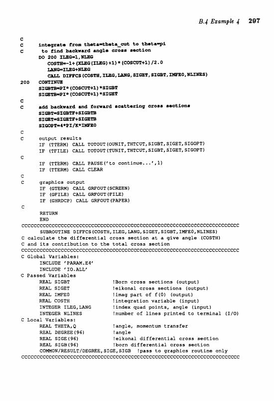
C e inr;sqracs f~om thatr*hd&-mt eo tbeC&q% C eo find b&&wazd aqXa areas @w%&@n
M, 200 X==%,
WmKmO
200 cmzam SImm=EP* (C:06CU~+Z) *sxmz STW-PI* f COSGUWl) * @ Z a p
c C ba&wrzd und fomrxd @catdaring crroor 8rokion@
sX~~sKamt.sxCffi)TB Sfml)=hlaam+SZam SKWEF=Q*PI/KfXbdBEO
c C ou tpu t r e s u l t s
I F (TTEM) CALL TOTOUT (OUNIT, TNTCUT, SIGBT, SZGET, SIGOPTI I F (TPILE) CALL TOTOUT [TUNIT, TNTCUT, SIGBT, SZGET, SIGOPTI
C IF (TTERM) CALL PAUSE ( * t o con t inue , . . l , l) IF (TTERE"I1 CALL CmAR
G C g r a p h i c s ou tpu t
IF lCTERMf CALL GWOUT (SCREEN) IF (GFILE) CALL G m 0 0 T (FT=) IF (GNRDCP) CALL GRFOUT (PAPER)
C =TURN END
cccccccceceCc~cccCcc~ccccccccccececc~cccccccccc-C:ccccccc~c~cccccccccccccc SUBROUTINE DIFFCS(COSTW,XLEG,~NG,SXGET,SJGBT,IMFEO,NL~~ES~
C c a l c u l a t e t h e d i f f e r e n t i a l c r o s s s e c t i o n a t a g i v e ang le (COSTHI C and i t s c o n t r i b u t i o n t o t h e t o t a l c r o s s s e c t i o n c~cCcccccecc~cccccccccccccccccccccce:cccf:cccccceecccccccccccccccccc~cccc~ C Global Var iables :
INCLUDE *PAMMM,E4' INCLUDE 'fO.ALLP
C Passed V a r i a b l e s REAL SIGBT !Born c r o s s s e c t i o n s (output) = A t SIGET !e ikonal c r a s s s e c t i o n s ( au tpu t ) REAL IMFEO ! imag part o f f [D) (output 1 REAL GOSTH ! i n t e g r a t i o n v a r i a b l e ( inpu t ) IWTEGER ILEG, LANG ! index quad p a i n t s , ang le t i n p u t 1 IMTEMR NLINES !number of l i n e s p r i n t e d t o t e r m i n a l (I/Of
C L o c a l Var i ab les : N & L THETA, Q !angle , momentum t r a n s f e r M A T , DEGREE ( 96) ! a n g l e REAL SIGE 196) ! e lkana l d i f f e r e n t i a l c r o s s s e c t i o n RE& SIGB(96) !born d i f f e r e n t i a l c r o s s s e c t i o n COmOW/RESULT/DEGmE,SIGEISICB !pass t o g raph ics r o u t i n e only
CGCCCG"CCCCCCCCCCCCCCCCCCCCCCCCCCCCCCCCC:CCCCGCCCCCCCCGCCCCCCCCCCf:CCCCCC~C
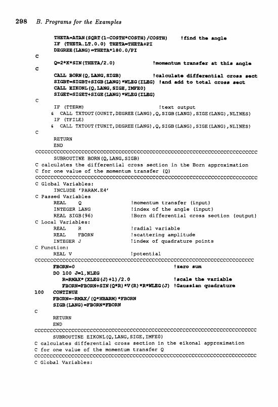
%=T&dTM (SWF (1-C652S*GOSlCX) [COSTHI I Find LXza q g Z a XF (%m=. LP. 0 0 ) T ~ F & ~ ~ T A + P X
G 0-2*~*sm (~mra/n, Q) 1mwnLm fzans$er ad this -@,a
G B m (Q, W@, SIC;IB) !ea2&ade dUCf-c~lmnkiaZ arosr sscf
C
IF (TTERM) !text output & CALL TXTOUT (QUWIT, DEGREE (mNG1 I Q, STGB (mNG1 , SIGE {LANG] , EJLINES) IF ITPILE)
& CALL TXTOUT (TUNIT, DEGmE (mNG1 t Q C SIGB (LANG) I 51GE (LWMG] , NLXEES C
RETURN END
eececccccccccccccccccccccccccccccccccccccccecccccccccceceecccccccceceC:cc SUBROUTINE BORN (Q, LANG, STGB)
C calculates the differential eross section in the Born approximation C for one value of the Inamenturn transfer (Q) cecccceccceccceecccccccecccccecccccccecccecccccecceecccccccccccccccccccc C Global Variables:
f MCLUDE "PAW. E$" C Passed Variables
L Q !momentum transfer finput) INTEGER LANG !index of the angle (input) WAL SIGB (96) !Born differential cross section tautputf
C Local Variables: REAL R !radial variable REAL HBQRN !scattering amplitude INTEGER J findex of quadrature points
C Function: RE& V !potential
CecccccccccceccceccccccecccccccccecccccceccccccccccccccC:ccccccccccccccc =Q==@ !zero a m
?male $he v ~ A d 2 a BOM+SXN (Q*%) *V (R) *R*=@ (3) ! Caussim c~;xad~r&urs
3.00
s r a =nam*mom e
=TURN END
~~~c~~~ce~~~cccc~~ccccccccccC=ccccccccccccccccceccccccccccceccccccccecccc SUBROUTINE EI KONL (Q, mNG, SIm, TlvlFEof
C calculates differential eross section in the eiksnal approximation C for sns value of the momentum transfer Q e~~~~cec~~~~cc~~~cecccccccI=eccccce:ccccccccecccecccccccccccccccec~ccccccc C Global Variables:
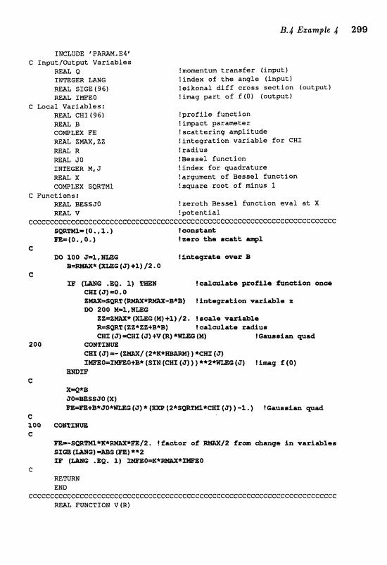
I N a U D E ' PAMM. E4' C InputlQutput Variables
m A L Q !momentum t r a n s f e r ( input ) INTEGER LANG ! index of t h e angle (iny>ut) REAL SIGE(961 !e%konal d i f f c ross s e c t i o n (output) REAL ImEO ! imag p a r t a f f (0) [output
C Local Variables: RE& CWI 496) ? p r o f i l e funct ion mAZ B !impact parameter COWLEX PE ! s c a t t e r i n g a m f i t u d e mAL ZmX, ZZ ! i n t e g r a t i o n v a r i a b l e f o r CWI
REAL R ! r a d i u s REAL JO !&ssel funct ion INTEEER M, J: !index f o r quadrature REU X !argument of Bessel func t ion COmLEX SQRTCMl !square root o f a n u s 1
G Functions: MAL BESSJO f z e r o t h Bessef funct ion e v a l a t X m&L V !patent% a l
~cc~~~c~~eec~cecccccccccccccef:cccccccccceccceccc~ccccccccccccccccceccc~~ SWm=(0.,1.1 t aonrptane -(Q., 0. ) !zero %be @oat;& amp&
C: t irrt;aqxaka ever B
* (=G(J)+1)/2.0 C
33' (m@ .EQ. 11 Ica2sulaks pzafiZe funation @ace CRI (3) =O * O
DO 200 M=1, -Q Z Z = g W * [=G (M) +I) / Z . l ~ o a l a varf &Za
fcralalata xadiur tQZaar~aIm m a d
G (a) f f ( Q )
C Z**B 30==6550 rn=FE+B*J
C 2.00 C m X m C
ZF (W@ *EQ* 2,) C
RETURN END
ccccccccccccccccecccccccccccccC:ccccC:cccccecccccccccccecccccccccecccccccc m A L FUllrCTXoPJ V (R)
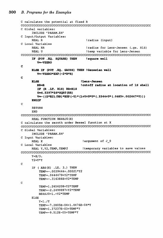
300 B. Progranas for the Bsamples
C calculates the potential a t fixed R cccccccccccccccccccccceccceccccccccccccccccccccc~cccccc~cccccccc~~cccccc C Global variables:
INCLUDE ' P B W . E I 8 C InputlOutput Variables:
REAL R ! radius [Input) C Local Varfables
W& RR !radius for Lenz-Jensen (.ge. R151 REAL U !temp variable for Lenz-Jensen
CCCC~CCC~CCCCCCCCCCCCC~GCCC~CCCG~CCCGCCCCC~CCf~~~CCCCCCCCCCCCCCCCCCCCCCC~ IB" (POT .ZQ, SQUm) TmH Is-axe well
v=-vzne C
E&= 3 3 (POT SQ. aVSS) fWmseipn weXL V=-==@*- (-2W*R)
C EL= fmr-3ansen
!=%off r a u r at, loaakion of JS aheX1 TP (R .%S, IXJAf) ===S W4. Jli97*Z5*SWT (m) V=- ( (Z*E2) /nf *m (-U) * {l+UEf.I.WIll* ( .3344+W* ( .04&5+. 002647*8) ) )
C
=TURN END
cccccccceccceCcee~eececcccceeccccccccccecccccceccceccccccceccccccccccccc FUNCTION BESSJO ( X ]
C ealalates the zerath order Bessel functian at X cceecceccccc~cccccccceccceccccccccccccccccccc~eccecccccccc~eccccccceccE:c C Global Variables:
C Input Variables: mm X !argument of J-O
C Loeal Variables REAL V,Y2,TEWeTENP2 !temporary variables to save values
c~cc~ce~ccccc~ccccIcecec~eccccccccecccccc~c~cceccccccccccccccIccccccccc~cc V=X/3 *
Y2=Y*Y C
IF ( ABSfX) .LE. 3 . ) TWEN TE;W=-,0039444tI00021*Y2 TEMP=.O4444?9+Y2*TW Tern=-. 3 1 63866+V2*TEEIP
TEMP=1,2656208+Y2*TElvae TEW=-ZS2499997+V2*TEKP BESSJO=I,+VZ*mMg
ELSE U-1. /V TEPaP=-7.2805E-04+1.44?6E-O4*V TEW=1.3?237E-O3+TEMP*V TEW--9.512E-OS+TENP"V
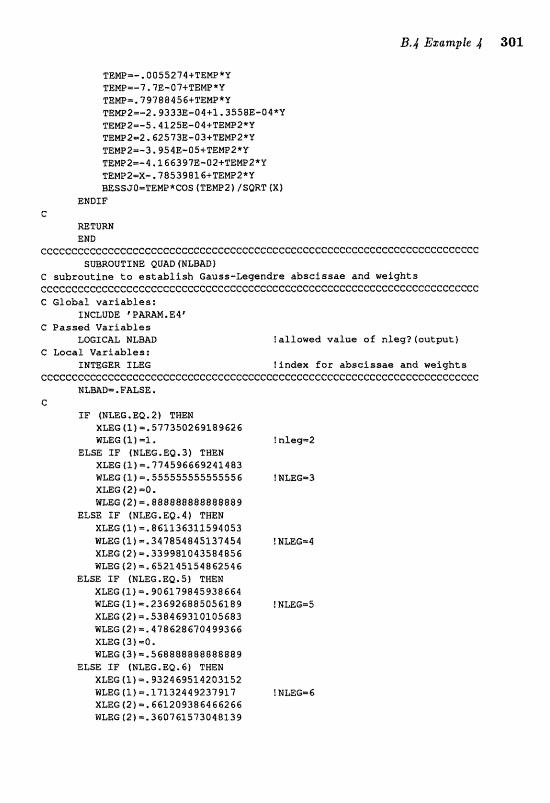
TEMP=-,0055274+TEMP*Y TEMP=-7.7E-O7+TEMP*U TEMP=.79788456+TEMP*V TEKP2=-2.9333E-04+1.3558E-O4*Y TEW2=-5.4125E-04+TEWP2*Zr' TEtJu?2=2.6257JE-Q3+TEW2*V TEMP2=-3.9$4E-QS+TEEin?2*Y TEm2=-4,l66397E-02+TEpllP2*Y TEMP2-X-.78539816+TEMP2*V ~~ss~a-rawxcas ITEMPZI /SQRT (XI
ENDIF C
=TURN END
GCCCCGCCCCCCCCGCCCGCCCCGCCCCCCCCCCCCGCCCGCCCCCCCCCCCCGCCCCCCCCCCCC~CCCCG smRovTrHe QuAotNLBae)
c subroutine to establish Gauss-Legendrs abscissae and weights CCCGGCGCCCCCCCCCCCCCCCCCCCCCGCCGCGCCCCCCCCCCCCCGCCCCCCCCCCCCCCCCCCGCCCCC C Global variables:
INCLUDE ' P A W , E 4 * G Passed Variables
LOGICAL PIILBAD !allowed value of nleg?(output) G Local Variables:
INTEGER f LEG ?index fox abscissae and weights ccccccccccccccccccccc~ceeecccceccccccccccc~~cccccc~ccccccccccc~cc~cccccc
NLBD=.FALSE. C
I F (NLEE.EQ.2) THEM XLEG (l} =,577350269189626 MLEG(1)=l. ! nleg-2
ELSE IF fNLEG.EQ. 3) THEN XLEG 41) 1,774596669241483 WLEG (l ) =, 555555555555556 ! NLEGmS XLEG {2)=O, WLEG (2) =* 888888888888889
ELSE IF (NLEG,EQ,I] THEN XLEG (l)=. 861236311594053 @LEG (1) m. 347854845137454 ! NLEG=4 XLEG (2)=.339981043584856 WLEG ( 2 ) -, 65214555486254g
ELSE IF (NLEG-EQ. 5 ) TmN XLEG (l)=. 906179845938664 @LEGE1)=,236926885056289 f NLEG=$ XLEG12)=.538469320105683 M U G (21 =. 478628670499366 XLEG (3 ) =0, WLEC ( 3 ) ~ . 568888888888889
ELSE IF (NLEG.EQ, 6) THEN XLEG (If 932469514203152 WLEG (I)=.17132449237917 ? MLEGa6 XLEG (2) -. 661209386466266 WLEG ( 2 ) =.3607&1573048139
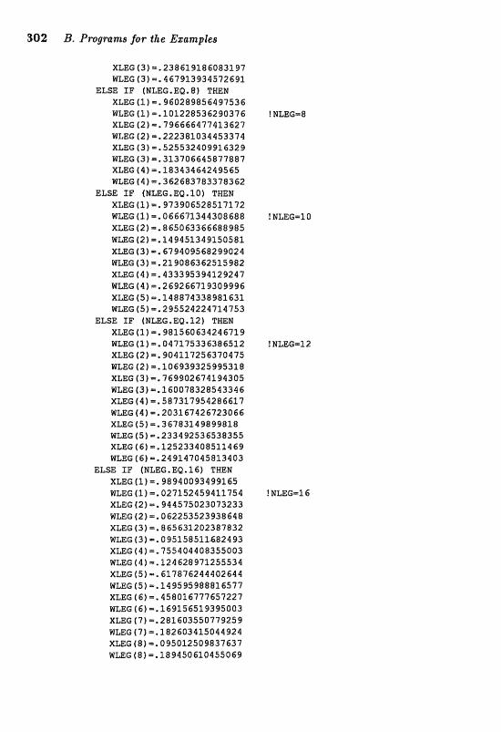
302 B. Programs for dl8e Ezamplea
XLEG (3)=.238619186083297 &LEG (3) =;. 467713934572691
ELSE I F (NLEG,EQ, 8) THEM XLEG (1) =. 960289856497536 hlLEG(1)=.10122853629Q376 !NLEG=8 XLEG (2) =, 796666477413627 WLEG (21 1.222383034453374 XLEG (3) m.525532409916399 WLEG (31 m, 313706645877887 XLEG 14) -, 18343464249565 WLEG (4) =. 362683783378362
ELSE IF (NmG.EQ.10) THEN XLEG ( X ) = , 973906528517172 WLEG 111 =.066671344308688 !NLEG=lO XLEG (2) =.865063356688985 RLEG (21 1.149451349150581 XLEG (3) =, 679409568299024 @LEG (3) =. 219086362515982 XLEG (4) =, 433395394129247 1LEC (41m.269266719309996 XLEG (5) =.148874338981631 @LEG (5) =. 295524224711793
ELSE IF (MLEG.EQ.12) THEM XLEG (1) m. 981560634246719 WLEG(1)=,047275336386512 ?NLEG=12 XLEG (2)=.904117256370475 WLEG 12) =.l06938325995318 XLEG (3) =, 769902674194305 WLEG (3) =,l60078328543346 XLEG (4) =. 587317954286617 RLEG (41 =. 203167426723066 XLEG (5) =, 36783149899858 WLEG (5) =,233492536518355 XLEG f 61 m, l25233408511469 WLEG f 6) =.249147045813403
ELSE IF (NLEG.EQ.16f THEN XLEG (l)=. 98940093499165 WLEG (l) =. 027152459411754 !NLEG=16 XLEG (2) =. 94457502307J233 @LEG (2) ==. 062253523938648 XLEG (3) =.865631202387832 WLEG (3) =. 0951585126&2493 XLEG(4]=.75540440835JQa3 WLEG f 4) =.l24628971255534 XLEG (5)-. 617876244402644 @LEG (5) =. 149595988816577 XLEE (6) =. 458016777657227 KLEG (6) -, 169156519395003 XLEG (7) =.281603550779259 @LEG (71 =.l82603435044924 XLEG (8) =. 0950125Q9837637 WLEG (8) =. 189450630455069
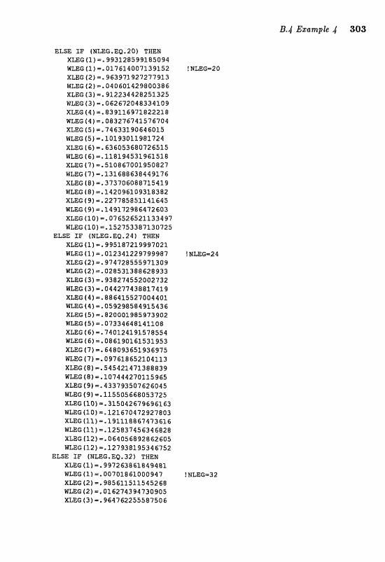
ELSE XP (%LEG-EQ. 20) TUEM XLEG [l) =. 993128599185094 WmG(1j =. QL76140072.39152 !NLEG=20 XUG ( 2 ) =, 963971927277913 @LEG (2) -. 090601429800386 XLEG (3)=. 912234428251325 WLEG (3) -. 06267204833W XLEG (9) =. 839116971822218 WLEG(4) =, 083276741576704 XLEG (5) ==, 76633590646015 1LEG (5) ==, 10193021981724 Xm6 16) =. 636053680726515 WLEG {6) -- 2181945329CiI518 XLEG f 7) ==. 510867001950827 WLEC (7 ) =,131688638449176 XmG (8) =,37370608873.5419 WLEG (8) -. 142096109318382 XLEG (9) =,227785851141645 WLEG (g)=. 1491729864726.03 XLEG(lO]=. 076526521133497 WLEG(20)=,152753387130725
ELSE IF (NLEG. EQ. 24 1 TNEN XLEG (l) =,995187219997Q21 WLEG (1) 0.012341229799987 !NLEG=24 XmG (2) =, 874728555971309 WLEG (2) =.Q28531388628933 XLEG (3) =. 938214552002732 WmG (3) =. 014277438817419 XLEG (4) P. 886415527004401 %LEG (4) =- 059298584415436 XLEG f f 1 =. 820001985973902 RLBG ( 5 ) -*07334648141108 XLEG (6) m. 740124591578554 aEG (6) m. 086198161531953 X m C 172 =, S48093651936975 WLEG (7) =,097618652104113 XLEG t81--545421471388839 WLEG f 8) =. 107449270215965 XLEG (9) =. 433793507626045 WLEG (9) ~~115505668053725 X a G (10) =- 315042679696163 WmG 110) ==. 121S704725327803 XLEG (11)-.l91118857473614 MLEG (11) =.l25837456346828 XLEG (12)=, 064056892862605 W U G (12)=.227938195346752
ELSE XF (NLEG.EQ.32) THEM XWG(1) =.991263861849482 HLEG ( 3 ) =. 00701861000947 ! NLEG-32 XmG (2) =. 985611SlSS45268 WLEG (21 =.016274394730905 XLEG ( 3 ) -. 964762255387506
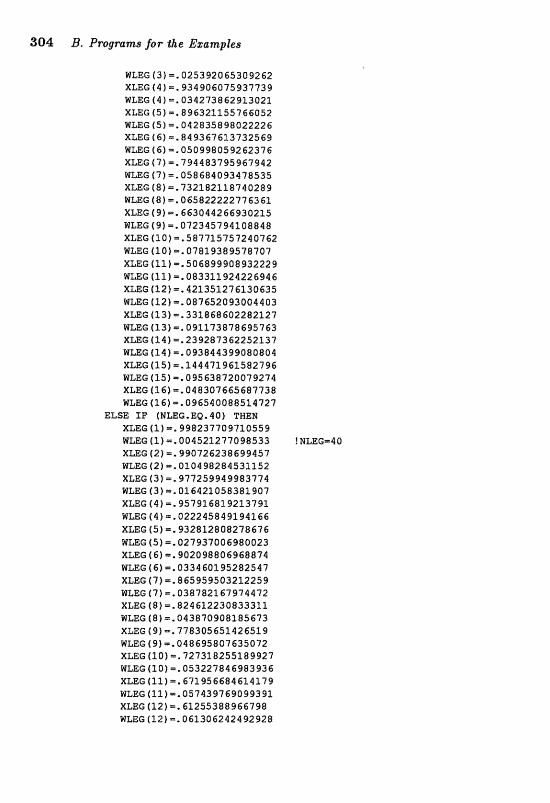
304 B. Progmrnt~ for the Esamples
WLEG (3) =, Q2539206530W XLEGl41 =. 934806075937739 WLEG (41 =. Q34273862913021 XLEG 451 =. 896321155766Q52 lLEG (5) -. 042835898Q2222& XLEG [6) =. 849367623732569 WLEC (6)=,050998059262376 XLEG (7) P. 794483795967942 WLEG 17) =.058684093478535 XLEG (8) =,732182118740289 WLEG (8) =. 065822222776362 XMG (9) -. 663044266930215 WLEG (9) =. 072345794108848 XLEG (10) =.587725757240762 WLEG (10)-. 07819389578707 XLEG (11) =. 506899908932229 WUG fllf -.083311924226946 XLEG412)=.421353276130635 RLEG u.2) -. as76szos3004403 XLEG (13) -. 331868602282127 WLEGf13)=.091173878699763 XLEGf141=.239287352252337 RLEG(24)=,093&44399080804 XLEG f15)=.144471963.582796 WLEG (15) =.09563872o079274 XLEG (261m. 048307665687738 WLEG (16) P. 09654008853.4727
EL% IF (NLEG,EQ,$O) THEN XLEG (l) m , 99823770971Q559 WLEG(1)=,004525277098533 !NLEG=40 XLEG (2) =. 990726238699457 =G (2) -. 010498284531152 XLEG (3)=. 97725994998J734 @LEG f 3) =. 0164210583811307 XLEG (4) =. 957916819213791 HmG (411.022245849194165 XLEG (5) =, 932812808278676 WLEG{5)=.027937006980023 XUG (6) =. 902098806968874 M m G (6)=, 033460195282547 XLEG (7) -. 865959503212259 @LEG (7) =. Q38782167974472 XLEG (8) m. 82461223083331L R m G (8) =, 043870908185673 X m G t 9) -. 778305651426519 WLEG ( 9 ) =. 048695807635072 XLEG 13.0) =, 727318255189927 WLEG (10) 1,053227846983936 XLZG (11)=.671956684614L79 WLEG (2.1) =. 057439769099393 XLEG (121 =. 61255388966798 WLEG f12)==. 061306242492928
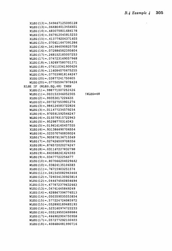
a2 'Q
" It 0
2
z
l-i P
m
l-i 0
P- 0
a3 tn r- Q
I 19
Cy
cn rl *
ft A
CO
=;t CI
3 X
E9
Cu
W
d 0
m
rl
U)
m
0
r-4 (-1
U
;)
P
Q
U C
4
Q)
e
CI
S
Q"
m
M
CR
r- m
CJI m
N
P
r- 'Q
"
r4
rl
0, '4. LI?, U
5 g:
W r-
m W
m
N
a2
'Q"
0 P
- r-
(V
ar a
Q
RI
m c3
U7 N
Rl P
8" Ln
P CD
C*t P
Q c3
*L
tl l1
6 X
z 52 (If
Q
m
ID
ID
N
m
U;)
QI
r- n
Xy
r- (0
P
r- CD I)
C c.
m
ttr W
2
m
rl
m
U)
r- e- U
;)
(r, m
P
W
41
Q)
CV (0
il - W
!2 0
3 X
'Q"
U)
CO m
rS
) m
U)
n
€3 Q
\
m
m 0
wr) C)
If 6
'Q"
5
0
W
4
3:
m
n
CV N
rJ
PC
Q
"
P
m
0
E9
r'i m
CV m
C r"-
CD
r;j U
5 X
Q"
m
m
m
Q\
U3 m a
rl) Q
\ m
r-i U
) rr] Ga 1
a C9
W
G
3

'j.
U7
CV U
)
CO N
€U
Q
\
rl
9"
rl
r-l
0
U)
0
II .-. d
2 €5
3 5
C
a#
U
k
3 C V)
3*
rJ
8 "cl 7J
9) 3
a
CI
C
0
m a#
4
4
4
4.j 41
-Pf
U
4 a
0
A
-4
B2
2 C:
0
m
LI Bf. 'U
.
tO M
C G
(11 0
k
.A
C,
U
E
a, 3 m
C, C
m
-4 0
&
@E
0
3 .4
k
@e
U
-1
-4
M @c,
Bl
CG
a &a
a#
cr g,
1
II W
a
~t
o
Cl -4'4
S -a
O&-
-c,
@U
"..
X v,
d;l W
4J
Gl +
U
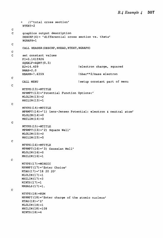
c / /%total c r o s s s e c t i o n p NTEXT-2
grilphics ou tpu t d e s c r i p t i o n DESCRP ( 6 ) = # d i f f e r e n t i a l Gross s e c t i o n vs. t h e t a f NCNPH=Il
C A U HEADER (DESCm, NNmEl, NTEXT, NGMPM 1
set c o n s t a n t v a l u e s PX-3.1415926 SQmLFmSORT ( 0. S ) E2=14 * 409
=2*0 HBmM=?. 6359
! e l ec t ron charge, s w a r e d
Ihbar**2/mass e l e c t r o n
CALL MENU I se tug cons tan t par t o f =nu
MT1IPE 413) =%TITLE M P W T ( 1 3 ) = ' P o t e n t i a l Funct ion option^:^ MLOLIM (1 3 ) m2 WHILIH f l 3 1 11
MTQE ( f 4 1 -MTTTLE N P W T ( 1 9 ) = * 1 3 ) Lenz-Jensen P o t e n t i a l : e l e c t r o n & n e u t r a l atom' HLQLIM ( 1 4 1 10 MNXLf M ( 1 4 ) 50
MTYPE 4 15 ) =MTI TLE m M T ( 1 5 ) m e 2 f Square W e l l t MLOLTM (IS =Q MNILIM (15 1 =Q
WTYPE (1 8 ) =NUM M P W T ( l 8 ) = * E n t e r charge of t h e atomic nuclsus ' MTAGfl8f m 6 Z f NLDLZN (18) =l MHILIM (18) -108 MIWTS (18) m4
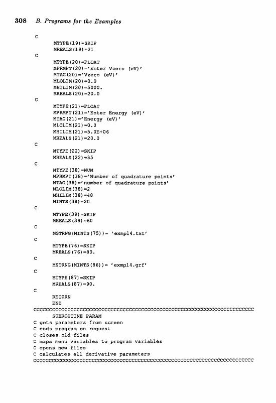
308 B. Programs for the Bgamples
C PdlTPE (1 9) =SKIP mmLS (1 9 ) =21,
C MTVPE ( 2 0 1 =FLQAT M t " M T (20) ='Enter Vzero (@V) #
MTAG (20) =p Vzero (@V) p mQLINt20)=0,0 MNXLTM f 20) =5000.
LS (20) -20.0 e
MTYPE (21 1 =FLOAT (21) =?Enter Energy (aV) *
MTAG (21 f l* Energy (eV) MLQLIM(23) -0.0
IM121)=5,0E+06 es(2~1=2a.o
C MT'YBE (22) =SKIP mmLS (22) 7135
C M W E ( 3 8 ) =MUM WRNPT ( 3 8 ) -* Munrber o f wadratare pints* NTAG ( 3 8 ) nu-r of wadrature paintsC nLaLxn t 3 8 1 =a MHSLIM (38) 5.48 MINTS f 3 8 ) 120
C MTYPE ( 3 9 1 =SKI P
LS (39) -60 c
MSSRNG (MINTS (75) 1 = exmpl4, t x t * C
("I) =SKIP s (761-80.
C
MSTRHG(MTNTS(86) f = '@exmpl4,grft C
E (87) =SKIP LS (87) -90.
c RETUW END
eccc~ccCcececceccccccI:cccccecceeceecc~ccccC:ccccccccceeccccccececcccecccc SUBROUTINE P m N
G gets parameters from screen C ends program an request C closes old files C maps =nu variables to program variables C opens new files C calculates all derivative paramters ccccccccccccccecc~cccccccccceccccccccceccecccceecceecccC:cccccE:cecccccccc
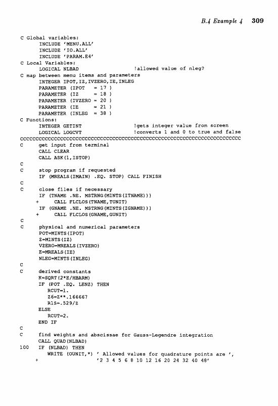
c Global variables: ZNCLODE ' MENU. ALL" INCLUDE ' I 0. ALL" INCLUDE ' PARAM. E4 C
C Local Variables: LOGICAL NLBAD !allowed value of nleg?
C map between menu items and parameters INTEGER IPQT, IZ, IVZERO, IE, INLEG P-METER (XPOT 1'7 ) PAMETER(IZ = l @ ) P m m T E R (TVZERO - 20 1 FAmMETER (ZE 21 1 PAmNETER (INLEG = 38 1
C Functions: ZNTEGER GETINT ?gets integer value from screen ZWSCAL, MGCVT !converts l and O to true and false
~c~c~cccC~cccceccccccc~ee~ecc~ccceceececcccccccc~cccc~e~ccccccccCccccccc G get input from terminal
CALL CLEAR CALL ASK (1, I STOP
c C stop program if requested
SF (MmALS ( T a I N ) .EQ. STOP) GALL FINISH C
C close Eilas %f necessary SF (TN&ME . NE, MSTRNG (MINTS (TTNAXE) ) )
+ CALL FLGLOS ( T H m , TUMIT1 SF f GHME . NE. MSTRNG {MINTS (IGNAME) ))
+ CALL FLCLOS (GMAHE, GUNTT) C C physical and numerical parameters
POT=MXNTS (SPOT) ZmMLNTS ( IZ ) VBERO=WALS 4 XVZERQ) EsMREALS (X E 1 NLEGmNf NTS I INLEG)
e C <derived constants
R=SQRT (2*E/NMM) IF (POT .E@, LENZ) THEN
RCUT=l. Z6=Z**. 156667 RIS=.S29/Z
ELSE RCUT=2.
END IF C C f i n d weights and &scissae for Gauss-Legendre intagration
C&LL QUAD ( NmAD 1 100 IF (IdmAD) THEM
WRITE (OUNIT,*) Allowed values for quadrature points are e e
+ '2 3 4 5 6 8 10 12 16 20 29 32 40 48'
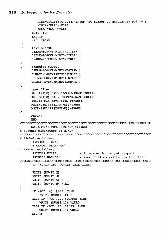
31 O B, Pragmnas far the Esamples
NLEC=GETINT (20,2,48, ' E n t e r new n u d e x o f wadrature points' 1 MINTS ( INLEG) -NLEG CALL &U&D (NLBm)
GOT0 100 END fJ? CALL C M m
G C text output
TTW-LoGCvT (MINTS ( I T T E M ] ) TFILE=LOGCVT (MrWTs (XTFILEI 1 THmE-MSTRNG IMXNTS (XTNANE}
C C graphics output
GTm-LQGCVT (MINTS (XGTERNf 1 GBmCP-LOGCVT (MINTS 4 IGHRD} f CPXLE=LQGCVT (NI NTS (XGFXLE) f GHm=HSTRNG (MINTS (ICN&m) 1
C C o p e n f i l e s
f F (TFILE) CALL FLOPEN ( T N m , TUNIT) IF (GFIm) CALL FmPEN(GNWE,GUNIT) ! f i l e s may have been renamed nsmNG (MINTS ~ Z T H M ~ j = m m MSmNG (HINTS (XGMAm) f =GM-
C =TURN END
cccccccccccCc~ccccc~c~eeccccccececcccccccccccccceccccecccc~ecccccccccccc SUBROUTINE PRMQUT(MUNIT,MLXNES)
C outputs parametera to NUNIT ~eccccccccccccCccecceccecccccccccececcccceccccceccccccccccccccccccecccec C G l o b a l variables:
INCLUDE ' 10-ALL'
C Passed variables: XNTEGZR MUNIT !unit numf>ar fox output (Input) IMTEGBR MLIMES f nuder of lines written so far ( I I Q I
cccecccccccccccccc~cccccccccccceccccccecc~cccccccccc~~~~ccccccccc~cccccc IF (MUNIT .EQ. OtRSIT) CALL CLEM
C
m 3 T E (MUNIT, 2) HRITE (MUNXT,rl) W T E (MUHIT, 61 E WRITE (MUNXT, 8r NLEG
c SF (POT .EQ. LEMZ) THEN
WRITE (WFIMIT,10) 2 E U E I F O?QT ,Ea. SQUARE) THEN
BRSTE (NUNIT, 1 2 ) VZERO ELSE I F (POT .EQ. GAUSS) THEN
m I T E (MUNIT, 1 4 ) VZERO END IF
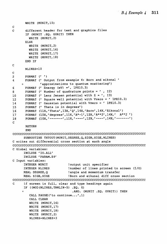
WRITE [MUNIT, 1 5 ) C C d i f f e r e n t h e a d e r f a r t e x t a n d g r a p h i c s f i l e s
I F (MUNIT .EQ. GWIT) THEN WRITE (MUMIT, 2)
ELSE m I T E (NUBSIT, 2) m I T E (MUNIT, 3.6) WRITE (MUNXT, 3-71 BRTTE (lollTMST,lElf
END XF c
NXIINESml O C 2 FORmT f ' ' ) 4 F O W T ( ? O u t p u t f r o m e x a m l e 4: Born a n d e i k o n a l '
f ' a p p r o x i n t i i t i o n s t o quantum s c a t t e r i n g E l 6 FORmT f "nexgy (@V) m', 11PE10. 3) 8 F O W T Numbo?r af q u a d r a t u r e p a i n t s ;= ' , X21 l 0 FORmT f q e n z J e n s e n p o t e n t i a l w i t h 2 -. 5 ,113) 52 FQRMAT ( q q u a r e w e l l p o t e n t i a l wbeh V z e r a = ' 12PEl@,3) 14 FORMT f r G a u s s i a n p o t e n t i a l w i t h Vzero = ? 1PE10.3) 15 FORMT ( @ T h e t a is i n degreesf 1 IS F6Rm5 (IXX, "Theta' , l3X, "I, 14XI @Ba;tnf , 14XP # E i k a n a l t 1 1 7 FORmT flQX, d e g r e e s r , llX, #A*-l@ I 12X, * A * * 2 * , 1 4 X AX*2 1 1 8 FORESAT (10X, ---S--- * , llX, @ ---- f , 1 2 ~ , 8 ----E, 1 4 ~ , ~---..--t 1 C
=TURN END
cccccccccccccccc~cccccecccccceeccccccccccccccccceeccccceccccccccccccc~cc SUBROUTXNE TXTOUT (MUNIT, DEGREE, Q, SIGB, SXGE, NLI NE51
C writes o u t d l f f a r e n C i a l G r o s s s e c t i o n a t e a c h a n g l e cceccccccc~~cccccccccceccccccccI=ecccececccccceccccc~cccc~cecccccccc~cc~c C G l o b a l v a x i a b l e s :
ZNCLUDE ' I Q , ALLe INCLUDE *PAMMN,EI6
C S n p u t v a r i a b l e s : SITEGER MUNIT l o u t p u t u n i t s p c i Eiar INTEGER NLINES !nu&er of l i n e s p r i n t e d t o s c r e e n ( I / O ) RML DEGREE, Q ! a n g l e a n d mamentum t r a n s f e r WAI, SITGB,SXGE !Born a n d s i k o n a l d f f f c r o s s s e c t i o n
CCCCC~CeCCCCC~CCCeG~CCCCCCCCCCCGCCGCeCCCGCCCGC~CCCCGCCeC~CCCCCCCC~CCC~CC C i f s c r e e n is f u l l , clear a n d t y p e h e a d i n g s a g a i n
f F ( (MOD (NLINES, TRNLIN-51 . EQ . 0) + .AMD. (NUNIT .EQ. DUNZT)) THEN
CALL PABSE(%ta c o n t i n u e , .,\l) CALL CLEAR KRITE (ElfUMST, I61 RRTTE (MUNIT, l ? ) mXTE (MUWIT, 181 l R I T E (MUNJT,ZJ hlLINES=NLINES+3
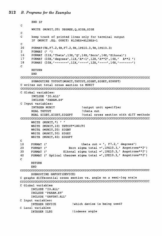
END I F C
m I T E (HUNIT, 20) DEGREE, Q, SIGB, SIC23 c C k e e p t r a c k o f p r i n t e d l i n e s o n l y f o r t e r m i n a l o u t p u t
I F (NUNIT .E@. QUNIT) N&IMES=MZTNES+l c 20 F O ~ T ( 9 X , F 7 . 2 , 9 X I F 7 , 2 , 9X,1PE10.319X,1nEZQ.31 2 F O m T ("1 16 F O M T W X , ' T h e t a t , ,l%, @ Q 8 , 14Xp B o r n f , l4X, # E i k o n a l f 1 1 7 F O W T ( lQX, ' degreesp, l l X , *Ak-1' , 12XI pA**2t, 1 4 , A**2 @ ) 1 8 F O m T (IDX, * ------- p , I ~ X , p ."---\ l&, p ----I I 1 4 ~ , p ----m-- 1 c
RETURN END
cccccccccccccccccccccccccccccccccccccecceccccccccccccccccccccccccccccccc SUBROUTINE TOTOUT (MUNIT, THTCUT, SXGBT, SICET, SZGOPT)
C w r i t e s o u t t o t a l c r o s s s e c t i o n t a MUNXT ccccccccccccecccceeccccccccccccccecccccccccccccccccccccceccccccccccccc~c G G l o b a l v a r i a b l e s :
f NCLUDE "PO. ALLC INCLUDE 'P&MM.E4"
G Inpu t v a r i a b l e s : INTEGER MUNIT ! o u t p u t u n i t specifier
TWTCUT ! t h e t a cut, REAL SIGBT,SSGET,SIGOPT ! t o t a l cross s e c t i o n w i t h d i f f m e t h o d s
ccccceccccccecccecccccccccccececccccccccccecccccccccce~cceeccccccccccccc m I T E (PIUNIT,*) " m I T E IMUNf T, 10) TWTCUT*1SO/PT YVXITE (MUMIT, 2 0 ) SLGBT WRXTE (MUNIT, 30) SXGET WRITE (MUNST, 4 0 ) SIGBPT
C 10 FO-T (' t h e t a c u t I , F7.2, degreesf 1 2 0 F O M T ( * B o r n sigm to ta l , ,1PE10,3, ' A n g ~ t r o m s * * 2 ~ 1 30 FO-T (' E l k o n a l s i g m a to ta l =' , lPE10.3,Vnggstroms**2') 40 PO-T (' O p t i c a l t h e o r e m s i g m a t o t a l =%,IPE30.3,' A n g s t r o m ~ * * 2 ~ ) C
RETUEZlV END
cccccceccceecccCccccccecccccccccccccecccccccccccccccccccececcccccccc~ccc SUBROUTINE GRFOUT(DEVICE)
C g r a p h s d i f f e r e n t i a l Gross s e c t i a n v s . a n g l e on a s a d - l o g scale cccccccceccccceccecccccccccccccccccccccccccccecc~cccceccccccccccce~ccccc C G l o b a l v a r i a b l e s
IWCLUDE ' 10. ALL"
INCLUDE ' GWDAT . ALL" C I n p u t v a r i a b l e s :
INTEGER DEVICE !which d e v i e e is b e i n g used? C Local v a r i a b l e s
SMg'EGER ILEG ! i n d e x e s a n g l e
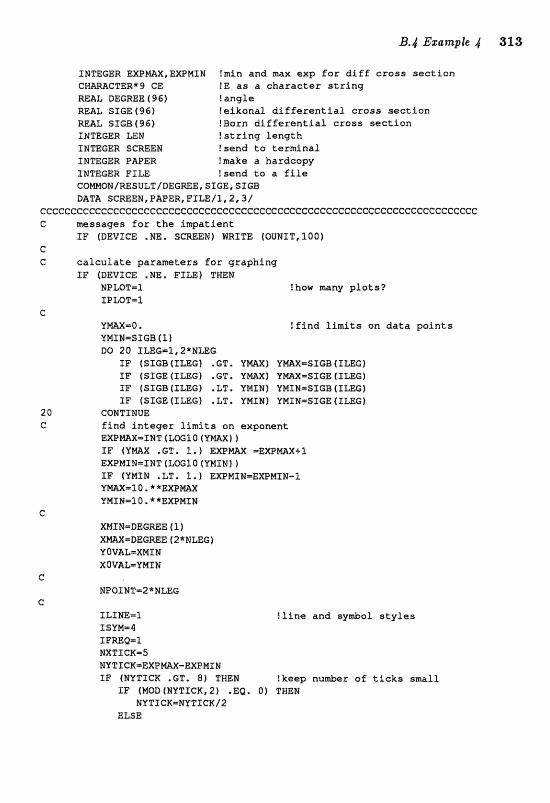
INTEGER EXPMW,EXPMIN !min and max exp f o r d i f f cross sect ion CHaRACTER*9 CE tE a s a character s t r i n g REAL DEGREE ( 9 6 ) !angle REAL SIGE(96) !eikonal d i f f e r e n t i a l cross sect ion REAL SfGB(96) !Born d i f f e r e n t i a l cross sect ion INTEGER LEN ! s t r i n g length INTEGER SCREEN !send t o terminal INTEGER PAPER !make a hardcopy INTEGER FILE !send to a f i l e COMMON/RESULT/DEGREE,SIGESIGB DATA SCREEN, PAPER, FILE/I, 2,3/
CCCCCCCCCCC(=CCCCCCCCCCCCcCCCCCCCCccccccc~cmcccccccccc~ccccccccccccccmc C messages for the impatient
IF (DEVICE .NE. SCREEN) WRITE (OUNIT, 100) C C ca lcu late paramtars f o r graphing
IF (DEVICE .NE. FLm) THEN NPLOT-1 !how many p lots? IPLoT=1
C YE(asx*O. ! f ind l i m i t s on data points YMINPSIGB (I) DO 20 f U G = l , P * N L E C
IF (SIGB (ILEG) .GT. YMAX) YMAX=SIGB tILW;) IF (SIGE (ILEG) .GT. YPYIX) YMAX=SIGE (ILEGJ XF (SIGB ( ILEG) -LT. YMIN] YMIN=SIGB (ILEG) IF (SIGE (ILEG) .LT. YMINf YMINmSIGE (ILEGj
CONTINUE f ind integer limits an exponent EXPMAX-INT (LOG10 (YMAX) 1 IF (YMAX .GT. I.) EXPMAX =EXPMaXtl EXPMXN-IMT (~ocio (mIw IF (YMIN .LT, 1. ) EXPMINmEXPMIN-1 YMAX=lO.**EXPMAX YMIN=10.**EXPHIN
! l i n e and symbol s t y l e s ILI NE-1 ISYM=4 IFREQIl NXTICKaS NYTICK=EXPMAX-EXPMIW IF (IJYTXCX .GT, 8) THEN !keep number o f t i cka small
IF (MOD (MYTICK, 2) WEB. 0) THEN NYTICK=NYTICK/P
ELSE
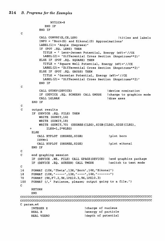
NYTICRm8 END S F
END XF
GALL GONVRT (E, CE , LEN ) !titles a n d labels IMF0 = ' B a r n ( X ) a n d E i k o n a l ( O 1 A p p r o x i m a t i o n s t L m E L ( 2 ) = ? A n g l e ( D e g r e e s ) * IF [POT .EQ. LENZ) TWEN
TITLE Lenz-Jensen P o t e n t i a l , E n e r g y (e!-vf=V//CE LWEL12)= @ D i f f e r e n t i a l C r o s s S e c t i o n (Angstroms**2)
ELSE I F (POT .EQ. SQUARE) T m N TITLE = * Svare W e 1 l P o t e n t i a l , E n e r g y ( W ) /ICE -EL (21.. ' D i f f e r e n t i a l C r o s s S e c t i o n (Angstroms**2)
ELSE I F (POT .EQ. GAUSS) THEN TITLE y G ~ u s s i a n P o t e n t i a l , Enerc3y (sV)=V/GE MBEL12)= r D l f f e r e n t i a l C r o s s S e c t i o n [Angstroms**2If
END I F
GTDEV (DEVICE) ! d e v i c e n o m i n a t i o n SF (DEVICE .EQ, SCREEN) CALL G W D E !change t o g r a p h i c s mode CALL LGLWAX !draw a x e s
END I F C C o u t p u t r e s u l t s
XF (DEVICE .EQ, FILE) TWEN WRITE (GUNIT, 16) m I T E (GUNIT, 18) WRITE (GUNI T, 70) (DEGME (IL;EG), SIGB (ImG), SIGE (XLEG) ,
"r ILEG=f,2*NLEG) ELSE
GALL XUPLOT (DEGME, SSGB) ! p l o t b o r n ISVM=1 CALL XUPLOT BEGmE, SIGE) ! p l o t e i k o n a l
END I F C G e n d g t a g h i n g s e s s i o n
I F (DEVICE .NE, FILE) CALL GPAGE(BEVIGE) ! a n d g r a p h i c s p a c k a g e IF (DEVICE .EQ. SCmEE) CALL TMQDE ! s w i t c h t o t ex t mode
C 16 F O m T (10X, "Theta', 13X, * Bornf I 24X, Eikonal") 1 8 F O M T (10X, ' -----' , lax, @ 14x, e ------- * 70 F O m T (9X,F7,2, 934, 1PE10.3# 9X, lPELCI.31 100 F O m T (I,' P a t i e n c e , p l e a s e ; o u t p u t g o i n g t o a f i l e . " 1 G
m TURX END
ccccceccCcccccccccc~ccccccecccccccceccC:cecccecccccccccccccccceeccccccccc cc~cecccccccec~ecccccccccccE:eef:cccccccccceccececcccccccccccccc~ccccccccc C p a r a m m e $
XNmGER Z ! c h a r g e a f n u c l e u s REAL E ! e n e r g y o f p a r t i c l e REAL VZERO ! d e p t h o f p o t e n t i a l
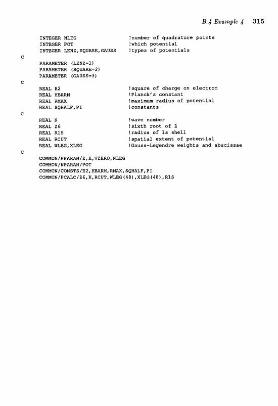
SMTEGEA NLEG !nuber of quadra tu re points fEamGER POT !which potential IMTEGER UNZ,SQUm,G&USS !types sf potentials
C PBmMTER (LENZ=1) PBWETER 688Um=2 1 PAmMETER [GAUSS-3 f
c RE& E2 !square of c h a r g e on electron RE& H B W ! P l a n c k e s coanstant RML R m !-ximum r a d i u s of potential
SQH&LF,BI ! constant S C
REAL K I wave R U ~ T
MAL Z & !sixth root aE Z RE= RlS !radius of Is shell W L RCUT Ispatial extent o f patential R= W m G XLEG !Gauss-Legendre weights and abscissae
C COWON/PPAmM/Z,E,VZERO,NLEG GOMOM/NPAMM/POT CQmON/CONSTS/E2, WARM, = X , SQmLF, PI 68mON/PCAlCC/Z6,K,RCUT,WLEG (481 eXUG{48f ,RI$
AIgarithm This prosam fits ekctron-nudeus elastic sattering crass section8 to dete ne the nuclear &age density ucsing the method de- scribed in the text. Once the target nucleus is chogen, the experirnerttd data is read in (from file CA. DAT, HI. BAT, or PB . DAT), and the recoil and Goalomb corrections are made (subroutine RDATA). Before iterations be&n, the prosam cdcdates the quantities that do not depend on the Faurier expansion coeEdents: (Eq. 5.63), part of the profile function X, (b ) (Eq. 5.66b), and a factor in the integrand for fin.., (subroutine TABLES). M1 ixrtegrds are done by 20-point Gauss-Legendre quads&urt?l. The ini- t i d dmsi.(;;y is t;aken to be the Fermi function, and the initial Fonrier coeBeients are obtained from a discrete Fourjer trmsform of that func- tion properly normalized to the total charge of the nudeus (subroutine FERMI). For each iteration (DQ loop 100 in subroutine ARCHOH), the improved expansion coefficients are found (subroutine w~nmz) by constructing the matrix A and vector B defined by Eq. (5.491, inverting the matrix (sub- routine nn~xw), and solving Eq. (5.51). Note that since Eq. (5.4713) is homogeneous, it can be suitably scded to the s m e order of mawitude as the rest of the rows of A. At each iteration, the profie function, scat- tering amplitude, theoretical cross section, x ~ , density, and uncertainties in the density are calculated (subroutine FIT).
Input The only phyeical parameter is the nudeus [Ca40]. Once the nu- dew data has been r e d in, the progam displcays the beam energy, m&- mum momentum transfer, and estimated nudear radius. (All energies are in MeV, all lengths in fermi, and all cross-sections in mbarns/ster You are then prompted for the value of the m&mum radius R [l. fermis], the total number of basis functions to use [Q&u*RMX/~] (see dis- cussion in text after Eq. 5.59), and the number to start with. The mm- imum number of sines is fixed by CnAX= 15. After each iteration (except the "zeroth") you are given the chance to increase the number of sines (if the current basis is smdler than the total requested), to continue iterating (if the current basis is the total requested), or to end iterations.
Out put After each iteration (including the Uzeroth" iteration when the Fourier coefficients are determined only by the Fermi function), the text output displays the iteration number, X2, degrees of freedom, number of sines used, total charge, maximum momentum transfer for this basis, expansion coefidents, and their uncertainty. The graphics then displays both the experimental cross section (with error bars) and the theoretical fit on a semi-log plot. The density and its uncertainty as a function of radius are also plotted. The number of radii at which the density is
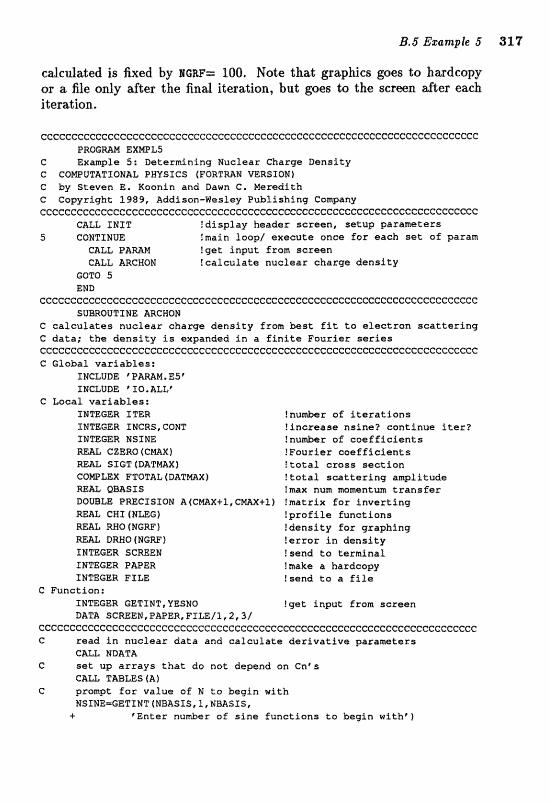
edcdated is fixed by HGW= 100. Note that graphic8 $oes to hardcqy or ab file only dter the final iteration, but goes to the semen dter each iteration.
cccc~ecccccccccccccceccccccccecceF:cececc~ccccccccccccccccecCcccccccceecc P R W W EXMPLS
C Exmple 5: Determining Pd-uelear Charge Density C GOWUTATIONAL PHYSICS (FORTmN VERSION) C by Steven E. Koonin and Dawn C. Mereditk C Copyright 2989, Addison-Hesley Publishing Company ccccccce~cc~cccccce~cccccccccccccccccceccc~ccccceccccccc~ccccccccccccccc
GALL SNXT !display header screen, setup p a r a m t e r s 5 CONTIEIUE !main Joopl execute once f e r each set of param
CALL P ? g e t input from screen CALL mCHOH !ca lcu la te nuclear charge dens i ty
GOT0 5 END
cccceeccccecceccece~cceccccccccecccccceccccccccccccccccc~ccccccccecccccc SmROUTINE ARCROM
C c a l c u l a t e s nuclear charge dens i ty from b e s t f i t t o e l e c t r o n s c a t t e r i n g C data; t h e d e n s i t y i s expanded i n a f i n i t e Fourfes s e r i e s C C C C C C C C C C C e C C C C C C C i l : G G G C C C C C C C C C C C C C C C C C C C C C ~ C Global var iab les :
IHCLUDE ' PAWM. E5' INCLUDE 'IO,ALLf
C Local var iab les : ZNmGER ITER !number of i t e r a t i o n s INTEGER INCRS, CONT ! increase n s i n e l continue i t e r ? IWTEGER NSIEJE !nu-r OE c o e f f i c f e n t s M& GZERO (CMAX) !Fourier c o e f f i c i e n t s m L SIGT (DATmX) ! t o t a l c ross sec t ion COWLEX FTOTAL ( DATMX J ! t o t a l s c a t t e r i n g a m l i t u d s
QBASIS ! m x num mmentum t r a n s f e r DOUBLE PRECXSXON A (CmX+1, CmX+1) !matrix f o r i n v e r t i n g mAL GRf (NLEG) ! p r o f i l e f i n e t i o n s WAL RHO (NGRFI ! densif y f o r graphing
DRWO (NGRF) ! e r r o r in dens i ty INTEGER SCREEN !send t o terminal XNmEER PAPER !make a hardcopy IPJmEER FXLE !send t o a f i l e
C Function: INmGER GETIHT,YESNO !get input from screen DATA SCWEN, PAPER, FIILE;/l, 2,3 /
cccccccccccccccccccccccceccccccceccececccccccccccccccccccccccccccccccccc C read i n nuclear da ta and e a l c u l a t a d e r i v a t i v e parameters
CALL NBATA C set up a r r a y s t h a t do not depend on Cncs
CALL TmLES (AI C prompt f a r value of N t o begin with
NSTNE=GETINT (NBASZS). l, EdBASIS, + 'Enter number o f s i n e func t ions t o begin w i t h p )

318 B, Programs for .the EzampZes
CALL C== C C o u t p u t s u m a r y o f paramters
I F (TTERM) CALL PMOUT (OUNIT) If (TFSLE) CALL PmOUT (TUNIT) f F {GFf LE) CALL PWOUT (GUNIT)
G C o b t a i n i n i t i a l Cn* S f r o m F e r m i d i s t r i b u t i o n
X TER=O !lazqest Q - 8 c r f M by basis
CALL FERMI (NSINE,CZERO) G c a l c u l a t e i n i t i a l f i t and d i s p l a y
CALL F I T (NSXHE, CZERO, ITER, SIGT, FTOTAL, QBASIS, CWIt A, RHO, DRHO] C 100 COlli[lCXm llaop wer itarigtionlsp
XTER=ITER+I C f i nd changes i n C Z & R O b t o o n i m i z e the e r r o r
CALL MXNIMZ (CZERO, WSLNE, SIGT, FTOTAL, QBASXS, CH3 I A) C calculate w a l i t y o f f i t , errors; d i s p l a y r e su l t s
CALL FIT (WSINE, (=ZERO: ITER, SXGT, FTQTAL, QBASIS, CMT, A, RBQ, DRHO) C G v a r i o u s o p t i o n s for c o n t i n u i n g
I F (NSLWE .LT. NBASXS) THEN TNCRS-
+ YESNQ(O,'Do y o u want t o i n c r e m n t n u & e r o f s i n e s b y one?') I F (INCRS .EQI If THEN
ISSNE=NSXMEfl CZERO (NSLNE) =O. CONT..%
Ilazqe@t Q ascribed ltsasia ELSE
CONT=YESNO(I,'Do y o u w a n t t o c o n t i n u e i t e r a t i n g ? ' ) END IF
ELSE CONT=YESUO(I,@Do you w a n t t o c o n t i n u e i t e r a t i n g ? f )
END IF C
IF (CQRT .EQ. I) W T Q I00 C C w r i t e sut only t h e f i n a l v e r s i o n t o a f i l e
I F (GWRDCPf CALL GRFOUTfPAPER,RWO,SZGTCNS1:;FilEIDfi:BO] S F (GFILE) CALL GWOVT (FILE, RHO, STGT, WSX NE: DRWOI
G RETURN END
ccc~c~~~~~cc~~c~c~c~~c~e~cecc~ccccccc~ceccceccceccceceeecccccccccccccccc SWROUTINE NDATA
C read i n nuclear data G d e f i n e v a r i a b l e s t ha t are n u c l e u s - d e p e n d e n t C t a k e recall ou t of data; c a l c u l a t e e f f e c t i v e momentum t r a n s f e r C p r o m p t for NBASfS and R M X ~ c ~ ~ c c ~ c ~ ~ ~ c e ~ c c ~ ~ c ~ ~ c ~ e c c c c ~ : ~ c c c ~ ~ ~ c ~ ~ c c c c c c c c c ~ c c c c e c ~ c ~ c ~ ~ ~ ~ c ~ c c c c c c c
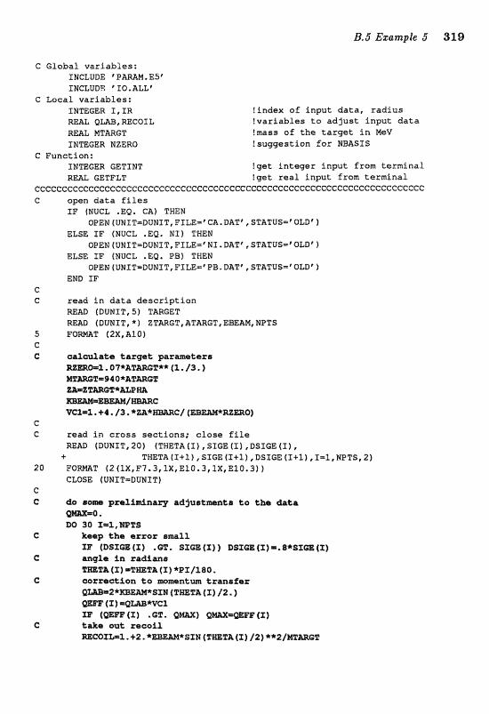
C Global variables: INCLUDE ' P A M . E S t INCLUDR @ I O . ALL1
C Lacal variables: INmGER I, I R !index of input data , rad ius
QW, RECOIL !variables t o ad ju s t input da t a m L NTARGT !mass of t he t a r g e t i n MeV INTEGER NZERO ?suggestion for NBASIS
C Function: INTEGER GETINT !get in tager inpu t from terminal
GETFLT !get real i n w t from t e r h n a l CCCCCCCCCCGCCCCCGC~CGCCGCCCC:CCCCCCCCCCCCCC:CCCCCCCCCCCCCCCCCCGE:CCGCCCCGC:C C open data P i l e s
IF (NUCL .EQ, CA) THEN OPEN (UldITmDUNIT, FXLE='Cha DATt, STATUS=* OLD' 1
ELSE IF (NUCL .EQ, NZ 1 THEN OPEN (VNX T-DUNI T, FILE-' M1 1: DAT* I STATUS='0LDf 1
ELSE I F (NUCL .EQ. PB) THEN OPEN (UNIT-DUNIT, F I L E = @ PB. DATe , STATUS=' OLDf 1
END IF c C r e a d i n d a t a d e s c r i p t i o n
READ (DUMIT, 5 I TARGET W A D (BIINZT, *) ZTARGT, ATARGn EBEAM, NPTS
5 F O m T (2X,AlQ) c
MZ=T.s94 0*&TMGT m=zFmG111*mm
C C read i n c ross sections; c lose f i l e
RE31CI {DUNIT, 20) (THETA ( I ) , S f C E ( I f ,BSI68 ( I ) , C TWETA(I+1) ,SSEE(I+X) , D S I G E ( I + l ) , I = 1 , N P T S 6 2 j
26 F O M T (2 (IX,F7,3,1X,E10.3, 1X,E1013) 1 CLOSE (UMIT=DUNIT)
c G prcsllifinv ad3usttarsne~ t o Lhe &aka
C ker~pl the arrox small I B ( D S I a (I) . CT , SX- ( X ) ) D8IGE ( I ) = , (X)
C aagla i n radians (X) (X 3 * P X / ~ so.
C oocrection to ~troarcltntm transfer sr# ( z a m [X) /zm )
W E (I) =Q-%% nf [QErn{Zj *G%' {It
C take eat zecoiT mCoXW2 +2. *=-*SIN (TmTA (X) / 2) **2/mmGT
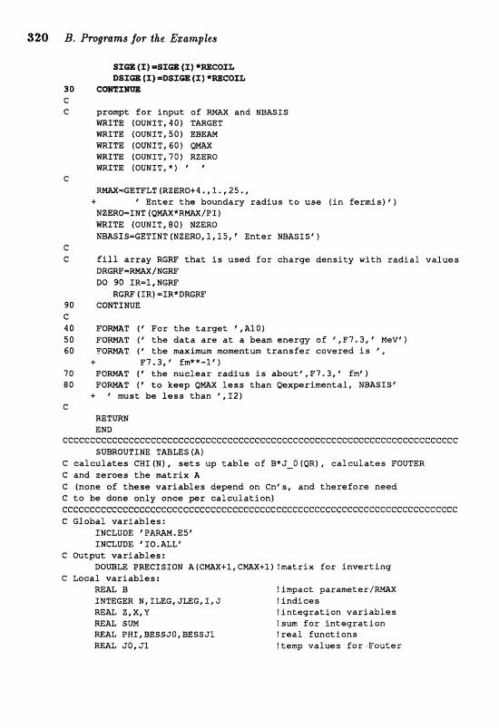
320 B. XL"rq~"rams for t i e Ezamples
s r a 4x2 =arm (X) *=cox& osxa (X = ~ s x a l r *mcarIi
30 C O W X m C C prompt f o r i n p u t o f R M and NBASXS
W I T E (QUNIT, 40) TARGET m X T E IQUNST, SO) EBEM WRITE (OUNXT, GO] -X WRTm (OUNIT, 70 f RZERO WRITE (QUNIII,*) "
C
Rm=GETFLT(RZERQ+4,,1.,251, + Ente r t h e boundasy r a d i u s t o use ( i n f e r m i s I t j
NZEFPO-XMTfQmX*RW/PI) W I T E (OUF\ff T, 80) NZERO NBASIS=GETXNT (NZERO, l , 15 , * Ente r NBASXS8 1
c C f i l l a r r a y RGW t h a t is used f o r charge d e n s i t y wi th r a d i a l v a l u e s
I)RGW=RmINGRF DO 90 XR=I, NGRF
RGRF f 1 R) =XRXDRGRF 90 CONTINUE C 40 F O m T ( # For t h e t a r g e t \ , A f O ) 50 F Q m T (' ttrh d a t a a r e a t a beam energy of 5 F 7 . 3 , ' MeV" 60 F Q m T ( @ the maximm momentum t r a n s f e r covered i s ' @
+ F7.3, @ fm**-1' 1 70 F Q W T ( ' t t h nuc lea r r a d i u s i s abou t r tF7 .3 , ' fm@j 80 F O m T ( @ t o keep QW 2e35 than Qexgsrimental, RAJBZISXS"
+ must h l a s s than " , X 2 1 C
RETURN END
CCCCCCCCCCCCCCGCCCCGCCCCCCCCCCCGCCCGCCCCCeCCCCCCCCCCCGCCCCCCCCCCCGCCCCCC SUIlRoVTINE TmLES (A)
C c a l ~ u l a t e s CBI(&), sets up t a b l e o f B*J-QfQR), c a l c u l a t e s FOUTER C and ze roes the mat r ix A C (none of t h e s e v a r i a b l e s depend on Cn's, and t h e r e f o r e need C ta be dane only once per c a l c u l a t i o n ) CCGCCCCCCCCCCCCCCCCCCCCCCCCCCGCCCCCCCGCCCCCCCCCCCCCCCCCCCCCCGCCCCCCCCCCC C Global v a r i a b l e s :
INCLUDE "PAW. E5' XNCLUDE 'IIO.ALLr
C ou tpu t v a r i a b l e s : DOUBLE PmCESEON A ( C m X + l , C m X + l ) !matr ix f o r i n v e r t i n g
C Local v a r i a b l e s : lWxd IF3 !impact p a r a m e t e r l m X INTEGER N, ILEE, JLEG, I, J ! i n d i c e s REAL 2 , X , Y ! i n t e g r a t i o n v a r i a b l e s =&L SUM !sum f o r i n t e g r a t i o n REAL PWX, BESS JO, BESSJ1 ! r e a l func t ions RE= J O , Jl fternp va lues f o r Pou te r
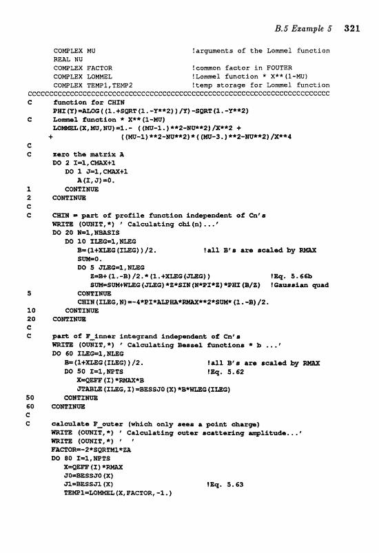
COmLEX MO !arguments o f the Lame1 function m& COWLEX FACTOR !cowon factor in POUTER COWLEX LOMMEL 1 function * X** (3-MU) COeLEX TEMP1, TEW2 storage Ear Lomel E u n c t i ~ n
ccccceccccccccccccccecceccccceeccccceecccccccecccccccccccccccccccccccccc C fwedioa for CWXN
( (l. +@mF ( l . -Y**2) ) l Y ) -SmT (P P -Y**2 1 C
(X,W,NU)=f .- ((W-l.)**2-@0"c*2)/X**2 + + ( (m-l) **2-W**2) * ( (m-3.) **22EIO**Z1 /X:**4
C C zsro the =trfx A
DO 2 I=%, 3. DO 1 if=%, C=+%
&(I, J)=O. 1. CQHTINm 2 CQMEXrn C C CEm L. part: of p r ~ f i l e fwat ion ia&@psa&at of Cm's
) ' Caloulaking cki (n) , . , "
81 (l+X=G (IU6) ) 12. Ir2.1 33% a m a c a l ~ d by SW=@. D43 5 m011.3rRmG
Z=B+ (l, -B) 12. * ( 2 . +=G 4-C)) ?Bq. 5.6635 s m = S W m @ (-G] *2*Srrsl (H*PZ*Z) * B E { & / E ) t Gaassiw wad
S Ca%XHa CmrJ (XmG, N) m-4*PX*Wm*
10 CQHTXNW 20 CQmHHa C C garctr, of E-gmcrs fntecgrand iadep@&ant of Cmc&
(OmIT,*2 ' C~alaalat;?lng Eksmrael gmationi~ * B ...* fla 60 SmQ=X, N m G
E= (%+-G (ImC) ) 12. I a Z l B" am S C P X B ~ t l Q . 3.62
50 C O R 1 " Z m 60 COmXBFUE. C C calculaka E-oatax (whfah only aaea a point em*)
(OWIT,*l Crlculating mkar ecatdaring -lie*..,@ (OWIZl,*f '
F&aQ--2*SQRM*a DO 80 X=%, MPES
x*mF. (I) * 30=mssao ( X )
( X , FaCTOR, -1. )
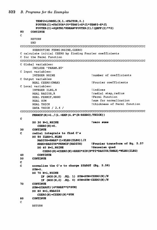
322 B. Programs for the Ezamgles
*n (X) **2)
8 0 c
=TURN END
ccccccccccccccccccccceecccccccccc~cceccccccccccccccccccccccccccccccc~ccc SUBROUTINE FERE(IX(NSTNE,CZERQ)
C c a l c u l a t e i n i t i a l CZERO by f i n d i n g Four ie r c o e f f i c i e n t s G f o r t h e Fermi Funct ion cCecCcccCCC@ccCCcCcCCCcCcCccCCeCCCCccccccccccccc~ccc~ccccGccc~ccccCccccc C Global v a r i a b l e s :
INCLUDE ' P A W . E S C C Input v a r i a b l e s :
INTEGER NSINE !number of c o e f f i c i e n t s C ou tpu t v a r i a b l e s
R a L CZERO (CIUIAX) IFour ie r e a e f f i c i e n t s C Local v a r i a b l e s :
INTEGER ILEG, N t i n d i c e s REAL M D T U S , R ! r a d i a l s t e p , r a d l u s REAL FERMIF, m W O !Fermi Funct ion REAL SUN !sum f a r normal i za t ion RmL TWXCX l t h i e k n e s s af Fermi func t ion DATA THICK / 2.4 /
cceccccccccccccccccecccecccccC:ccccccccccccccccc~cccccccccccccccccccccccc
C BO 30 B=%, RSfm ! zeze
czmo (M) =0. 30 C a T I m C
fP~mrAmr tzanrigea of Eq. 5.37
4 0 caNZ"fMm 50 C a T X m C C
70 M=%,WSICESE Xi? (MOD (E, 2) . $0. 2.2 Sm=SW+CIZ;ERO (M) /M ra (MOD (B, 2) . PZQ . 0) sw=m-ezmG (E) /H
70 C a r t I m
BQ 80 M=%,mSJS ceno (H) ezma (H) *SW
80 C W T X m C
=TURN
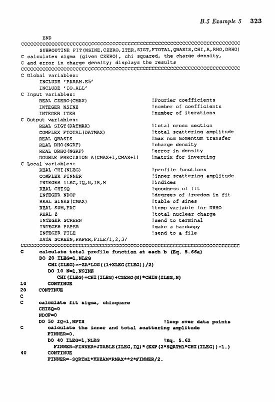
Em c ~ ~ c ~ C ~ ~ C ~ ~ C ~ ~ C C C G G C C C ~ ~ C C ~ ~ C C ( Z C ~ ~ ~ ~
SUBROUTINE FIT (MSXNE, GZERO, ITER, SSGT, F"f8TALC QBASIS, CWI, A., RHQ, DRWO) C calculates siva (given CZERO), chi squared, tba charge density, C and error in charge density; displays the results cc~~~ceccc~~~cece~cccececcccc~ccccccccc~cceccccccccccecceccccC:eecc~cc~cc G Global variables:
INCLUDE 'P&MM,E5' INCLUDE ' IQ, ALL"
C Input variables: W&L GZERQ { c ~ x ) !Fourier coefficients INTEGER NSSNE !number of coefficients INTEGER ITER !nu&er of iterations
C Output variables: RE&L SXGT f DATMaXf !total cross section COWLEX FTOTAL (DATNX) !total scattering amplitude REAL QEASI~ !max num momentum transfer REAL RHO (NGRFI t~harge density M& DRWO (NGRFI lerror in density DOUBLE PRECISSON ACCmX+5,CMX+S) !matrix foz inverting
C Local variables: R B U CH1 (NLEG) ! grof ile Eun~ti ~ n s CQWLEX FINNER !inner scattering amplitude INTEGER ILK, IQ, M, IR, M ! indices
CNISQ !goodness of fit INTEGER NDOP !degrees of freedom in fit RE& SIMES (CPECAX J Itable of sines W a SUM, FAC ltentp varialr>le for DRWO RE&L Z !total nuclear charge INTEGER f CREEN !send to terminal INTEGER PAPER !make a hardcapy SNTEGER FILE ! send ta a file DATA SCREEN, PAPER, FImlf, 2,31
GCCCCCCCG~CCGGCCC~~~CCCCCeCCCCCCC~CCCCCG~CCCCCCGCCCCCCCCCC~CCC~CCCCGCCCC C oalmlatca Lotal pzofJils gmoLion ae ea& b (W. 5.66;ar)
DQ 20 IrnWl, HrnQ c s x (ZmG) =-ZA*WG ( {%+=G f 2-1 ) 12) DO 10 N=l,Nsm
C m f X-) -X (XmG) +CEma (NI * G E M (X=, M) 10 C Q r n Z r n 20 COrnXHW C G alouXata &it a i m , abfacyuare
cmsq=o rnOF=Q DO SO fQm1,mTS TZoop mar data poinee
G oaXcu%aka t h fnner and tofa2 om%+arfng ~ Z i t u d e PX 0 .
!Zq. 5.62 *SWTrn*CB (ZrnG) ) -1 * )
4 0
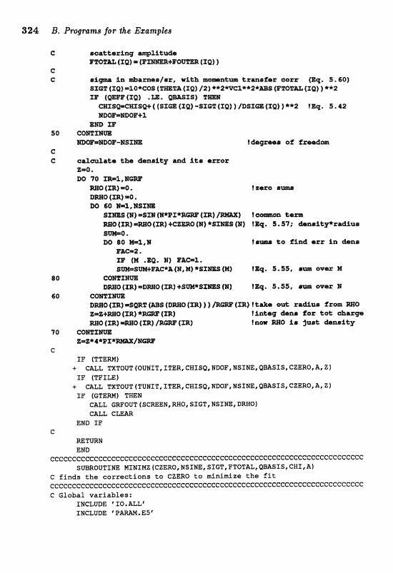
324 B. Programs for ihe E~amples
C 8iaatt;arSng -3Jltuda FTWU (IQ) .+ (F
C C @ i p i n *rmes/sr, w & t h -mat- transger corr {E%. 5.60)
s x a ~ (rg) =xo*cos ( X Q ~ 121 **2*vca,*i*a*ms (sr?0"11m ~ X Q ) **2 X% (-H (ZQ) "LE. mS18) F=
mxswcarsg+ ( ( s r a ( x ~ ) -src;z (XQ) fclsrnm (IQ) 1 **2 !IQ, 5 - 4 2 NDQF=HDOY+3
END 1IT 50 C m Z m
~ @ = ~ ~ ~ ~ - @ s ~ ~ f &-me@ @P f mda C G oaZd8l ts the disanaify. and its arroz
Z=0. DO 70 I m 3 , N m
REIs (m) =O . l trro smr D=@ (lx) -0 *
60 ~ 2 , X S S Z ~ sxms (a) =sm {rs+~rmm tarn WO (f R) ==Q (XR) (I) * 7; h n a i t p r d % m ~ 8-0. BQ $0 M=X,ZJ gAnd QZZ i n dclnmr
F=-2 *
XF {M B] FAC=Z* SW=SWHAC*A (W, M) * S X m (M) f Pq. 5.53, awe= B4
80 GOZJFIET~ DmO (m) =DmQ (IR) +SW*SZm {M) f Eq 5.55, eullt ever
60 CQEOXm D-o (m) =SW% p 6 ( D ~ O (m) ) ) (IR) l take o\;li: racxriula Exam W@
?inkeg dens ;Per= CcrZ, charge RE347 (m) ==Q (m) /=M (m) Iaam =Q i s juat &nai.t;y
C IF (TTEW)
+ CALL TXTOUT (OUNIT, ITER, CNISQf NBQP, MSXNE, QBASIS* CZERQ, Z j XF (WILE)
+ CALL TXTOVT(TUNZT,ITERtCHISQeNDOFIISI:ME~QBAfTSICZEROtA~ZI XF (GTERM) THEN
CALL GWOUT f SCREEN, RHO, S%GTf IdSZNE, DRHO) CALL CLEAR
END 3F G
REWURN END
ecccccccecGceecccccccecccccccecccecccce:cececcccccccececccccecccli:cecccce.c SUBROUTINE MINIM8 [CZEROc NSXNE, SXGT, FTOTAL, QBASI5, CH1 A I
e f inds the corrections to CZEFIO to minimize the f i t c e c c c c c c c c c c c c c c c c c c e c c c c c c c c c c c c c c c c c c c c C Glabal variables;
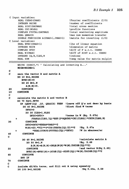
C Znput variables: m& CZrSROfCm) lFourier caefficients IZ/o) INTEGER NSIHE I nuder of ~ o e f f iciants WAL SZGT(DATW) !total cross section RE& CH1 (NLEG) f profile functions CQWLEX FTQTAL (D&TE(IAX) !total scattering amplitude M h L QEaSIS !max num momentum transfer DOUBLE PRECISEON A (CMAX+1, CmX+1) ! mtrix for inverting (IIO)
C Lacal variables: REAL BWC (6mX.tl) !lhs of linear equation INTEGER NDIM I dimension of matrix ~ O W L E ~ D F D ~ ldfff of F w . r , t . czeR0 REAL W ( C M X l fdiff of SIGT w , r , t . CZERB INTEGER IQ, N, ILEG, M l indices M A L SUM !temp value for matrix mulplet;
ccccccc~ccccccccec~ccccccceccccececccc~cccece(scccccccccc~ccccccecccccce~ WRSTE (OUNIT, *) Calculating and f nvaxt ing 8. . . mm=@Szm+T
C C zsm the vacear B and mtrix, A.
m E0 B = 1 , I S X m m c (El =o IDQ 20 *1,1
&(H, M)=@, 2 0 c a M % m m 30 C O m X m C C calmlate Lhe m t r g x A and vactor 8
DO 70 XWl, NPTS X@ (WEE (Xg) .LT, Q-ZS) IIm i & s a v e ofP Q' is net &ao ky barriis
110 40 l=l, NSXMF?: I F A r i s t g&nd W ts DEDCm0 DO 30 f =@l, M W @
BC+ +
3 0
%?a (rQ) /2) **2 ! Eq, S. 67a +
cw91xm
DO 60 W = & , N S m Icaculaka matrix A DO $0 W2,W 882%. 5.48
A (M, M) a (B, M) +BB= (W (H] *W {M] jbS5a f %Q) **2) 5 0 CQHZ !an& vatckor B(Zq 5.48)
B ~ C (NI - m e fw) + ( s x ~ g (XQ) -sscr (IQ) W (E) /xlzsza (rq) **2 60 CaMICXMm
Ern XF 70 CQRTXNm C C inc%ude &Z/dCn %em@, ruld f l & 2 or& A ue;ilirlf
DO 1 0 0 M=2, NSfm !l& 3,49a, 4,58
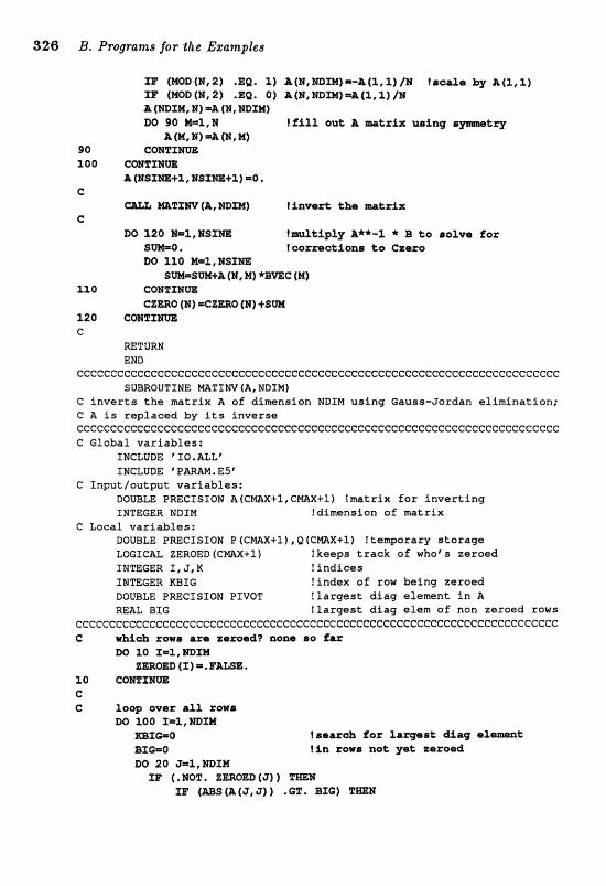
326 B.. P;rogrenzs for $he Ezanzplea
XF fMQD(N,P) .Ea. P) A(E1,MDm)=-&(Tt2)/N !seale A(2,Z) XF (MOD(N,P) .EQ. 0) AfR,NDm)=&(1,31)1'M A (MDXN, H) =A (M, HDXM) DO 90 M=l,tS f f A l . 1 @U% l = & x b ue;inq
A(M,E)e(W,M) 30 COMZX- 100 C a T T m
iR (NSXm+X, HSTmSP) =0. C
mZm (R, HDXN) rlnve* the m k r l x C
DQ 120 H=a,lifSIm I e t i p Z y &**-X * B t o soJlva ;fa*: S-0 . loormc;%ions to Cawe M) 310 mZ,NSXm
s-svM+A (g, M) *=C {M) 110 COlroTTBW
C%BRO (W) =CZERO (N) +SW 120 C@H%ZHrn C
=TURN END
cccccccceccccceccccecccececceecccccccecccccecceccccccccccccccccceccccccc SUBROUTPNE mT%W (A, NDXH)
C i n v e r t s t h e m a t r i x A of dimension NBIN u s i n g Gauss-Jordan e l imina t ion ; C A. is replaced by Its i n v e r s e ccccccccc~ccccccccccecccccccceccc~cc~cc~ccccccccccccececcccccccccccccccc G Global v a r i a b l e s :
INCLUDE 'IC).ALLP INCLUDE P m M . ES"
C Inpu t /ou tpu t v a r i a b l e s : DOUBLE PRECISION A(CW+I,Cm+I) !matr ix f o r i n v e r t i n g INTEGER NDXM !dimension of m a t r i x
C Local v a r i a b l e s : DOUBLE PmcIs l aM P (CmX+1), Q (emX+l) ! temparary storage LQGICAL ZERQED (CmX+l) !keeps t r a c k a f who" ze roed INTEGER I, J, K ? I n d i c e s TNTE(;ER KBXG !index o f tow b e i n g ze roed DOUBLE PRECISION PIVOT ! l a r g e s t d iag e l e m n t i n A REAL BIG ! l a r g a s t dfag e l e m of non zeroed rows
ceccccccecccccecCeccccccccceccccccccccc~cccccccccccccccccccccccccccccccc C whicrh raws are ztbxsed? none so
DO 10 Xm1,NDXM EEROED {X ) = . F m E
10 CQrnrnW C C l o w over a l l rows
W 100 f=%,mlM mXdloP.O l sssrrclh fo r laqast &a9 al BX-0 fin rows noL yet rsread BQ 20 G=Z,HDfM
I, IOT, z m E a (3) ) rmH IF (ms (a{J, a) ) .cr. sxc)
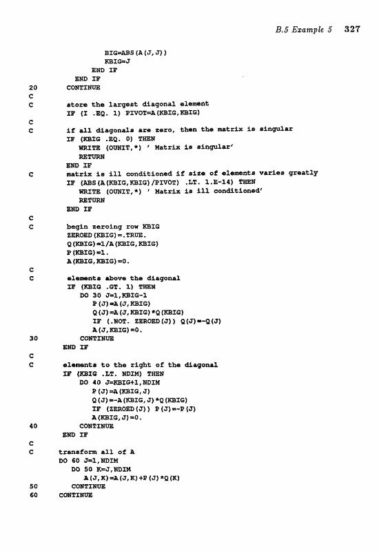
store &ha largest diagonaz eSenten% XI? (I .EQ, 1) PXVO"P=A(KBIG, m f G )
i f a21 dAag~niels are rtexc, than the i e s l a p l a r 33' (=X0 .EQ. 0 ) rmP3
( O m T , * ) * Matrix f s s i a ~ 3 a r '
XF mtrix i c a S12 oondiLionsd if s fzs of I H I ~ ~ ~ R L I B varAaa qzeatly I1 (-S (A (-IQ, mIC) /PIVOT) .LT!. 3. E-14) f REP3
mf2E (OmXT, *) Matrix iai ill caa&tionerdt
E m LP
bagin ze3rofag row m X G zERoEa (mxoi mm. g (=X@) =l/& (mXG, B X G ) P fmxe) =X. I (ESX Q, =LE) =Q,
ate above the diagonal IE (-X@ *az* %j
fX) 30 3m2,mXQ-X P (a) =A (G, mXC) S (a =A ts, mrc) *a tmzo) IF ( , M W . ZEROEB (3) ) Q (3) =-Q 147) R (3, mIG) =a.
CONTZHW ZEZD IP
efemnts to the right of the diagomx 33' (=X@ .L%. mXM) TNEN
D8 40 G=~fG+l,IDIM P (G) =& (mTO, JZ Q (3) =-A (rnXC, 3) *Q (rn1G) IF (ZEROED 4 a) ) P C 2) =-P [ 3) A(ICElfG,3)=0,
CQHTXMrn m XE

328 B. Programs for the Ezanzples
100 CWXMfJ& C C
DO 110 ib2, mXM BQ 120 E=%, +l
fir (3, K1 =A (K, J) 120 CrnTZRW 110 comxm C
RETURN END
cccccccccccccccccccccceeccccccccccceccceccccccecccccccccccccccccccccc~cc SUBROUTINE INST
C initializes constants, displays header screen, C initializes arrays for input parameters ccCcCcccecccccccccccceccccccce:cececccccceI:cccceccccc~cccccccccccccccccec G Global variables:
INCLUDE 'ITO.ALLP INCLUDE "MENU, ALL" INCLUDE 'PAW,ESC
C Local parameters: CHWCTER*BO BESCRP ?program description DrmNsIaw DESCRP ( Z O ) ZNTEGER NHEAD,NTEXT,NGMPW !n&er of lines for each description
ecCcccccccCccccccccccccccccccccceccceccccccccccccc~ccccccccccccccccccccc C get environment parameters
CALL SETUP e C display header screen
DESCRP (1 1 "EhMPLE 5 ' DESCRP ( 2 ) Determining Nuclear Charge Densitiesf NWMGlm2
c C text output description
DESCRP ( 3 ) = 'Density parameters and quality of fite NTEXT=l
C C graphics output descriptian
DESCRP(4)- fCCarqe density and scattering cross section6 N G M P W m 1
C CALL HEADER (DESCRP, NHEAD, IdTEXT, NGMFH 1
C C calculate constants
PI=4*AThN (1.0) ALPWA=l.jl37.036 WBmC-197.329 SQRTM1=(0., 1,)
C get data for Gauss-Legendre integration CALL GAUSS
C C setup menu arrays, beginning with constant part
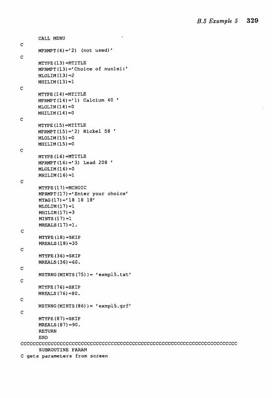
B.5 Example 5 329
CALL MENU I
C MPRMPT (415' 2) (not used) *
C MTYPE (13) mNTITLE HPRMPT (13) =* Chaice of nucf ei : ' MLOLXMtS3)=2 MHSLIM ( 13 ) =l
C MTYPE ( 1 4 1 =MTITLE PIIPRMPT (I4)='1) Calcium 40 MLOLIM(14) -0 MHXLIM(14)aO
C MTYPE (15) =MTITLE MPRMPT(15)='2) Nickel 58 ' NLOLIM (15) -0 MXILIM (15) -0
C MTYPE ( I 6 ) =#TITLE MPI?HL?T (16) 1'31 Lead 208 ' MLOLIM (1 6 ) PO MHILIM ( 1 6) =1
C HTYPE (17) =MCHOIC MPRMPT (17) ='Enter your choicer MTAGfl7)='18 18 18' MLOLIM (1 7 ) -1 MHILIM ( 17 1 -3 MINTS (17)=1 MREALS tl7)=1.
C MTYPE (1 8 1 =SKIP MREALS f 18)*35
C MTYPE (36) =SKIP MREALS (36) =60.
C MSTRNG (MINTS (75) 1 * * sxmpf5. txtr
C MmPE ( 7 6) =SKIP MRERLS (76)-80.
C MSTRWG [MINTS (86) ) 1 texmp15.grf
C MTYPE (8 7 ) =SKIP MREALS (87)=90. RETURN END
CCCCCCCCcCCCccCCCCCCCCCCCCCcCCCCCCCCCCCccccccccc~cccc~cccccccccccccc~c SUBROUTINE PARAM
C gets parameters from screen
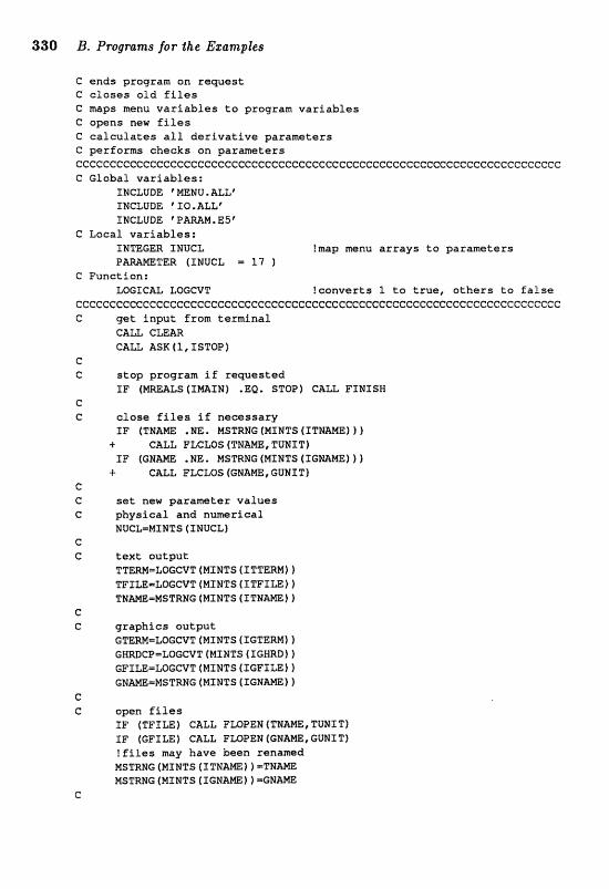
330 B. Programs far tFse Ezamples
C e n d s program on r e q u e s t C c l o s e s old f i l e s C naps menu v a r i a b l e s t o p r o g r a m v a r i a b l e s C o w n s new f i l e s C c a l c u l a t e s a l l d e r i v a t i v e paramtezs C p e r f o r m s c h e c k s a n ga rmte r s ccece~ccccccecccccccccccecceceeeccccccccccecccccccccccecccP:cccccec~ccccf: C G l o b a l v a r i a b l e s :
XNCLUDE *mNU.ALLf SNCLUDE ' IQ. ALLf INCLUDE 'PAMN.ESr
C L o c a l v a r i a b l e s : INTBGER INUCL !map menu a r r a y s to p a r a m e t e r s PAMNETER (IMUGL = 1 7 )
C F u n c t i o n : LWICAL LOGCVT ! c o n v e r t s 1 t o t r u e , o t h e r s t o f a l s e
ccccccccccCccccCcccccece~cc~ceccccecccccececcececceccccceecCcccccccccccc C get i n p u t Eram t e m i n a l
GALL CLEM C A U ASK (I, ISTOP)
C C s t o p program i f r e q u e s t e d
I F I m A L S ( I m I M ) .EQ, STOP) CALL FINISH c C clase f i les i f n e c e s s a r y
%F ( T N W l NE. MSTRNG (MINTS (ITHME) 1 ) + CALL FECLOS (TNWEI TUMIT)
I F (GNAW ,NE. MSTRHG (MINTS ( T G W E ) ) ) c FLCLQS (GNAME, GUNIT)
e C set new p a r a m e t e r v a l u e s C p h y s i c a l and n u n t e r i e a l
NUGL=E/ISNTS ITNUCL) C C t ex t o u t p u t
Trem=LoccvT (MINTS (ITTERM) 1 T F I m = L E W T (MINTS (ITFfWlj TNU-MSTRNG (MINTS ( ITNAm} 1
e C g r i r p h i e s o u t p u t
GTEM=LQGCVT (MINTS f IGTEW) ) GHNCP=mGCVT (MINTS ( X GBRt)] 1 GFILE=LOGC~T {MrNTs (SGFXWI 1 GNmmMSTRNG (HINTS ( I G W m ) )
C C o p e n f i l e s
XF (TFILE) CALL FmPEN (TN-, TUWX T) IF (GFILE) CBLL FmPEN (GM=, GUMIT) ! f i l e s may h a v e b e e n r e n a m d MSTRHG [MINTS (ZTWW] ) =TNAXulE MsrRBG (MINTS ( r c N m ) f =GM=
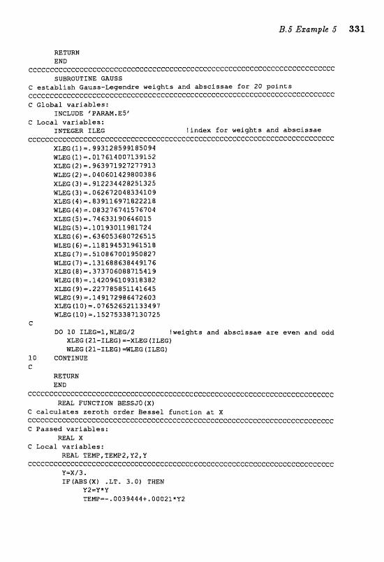
RETURN END
~c~~eeee~c~~~ceee~~cccccccccccccccccccccecccccccccccceecccc~cccccccccccc SUBRQUTINE WUSS
C establish Gauss-Legendre weights and abscissae for 20 paints cc~e~c~c~~ceec~e~e~~cccccccccccccecceecccccccccccccccccccccccccccccc~ccc C Global variables:
INCLUDE 'PPAMM.ESt C Laeal variables:
INTEGER ILEG !index for weights and abs~iasae ccec~~c~~~~~c~~c~~ecccccccecccecccccceccc~ccccccccccccccccccc~eccccccccc
XLEG (l) =. 99312859918W WLEG (1) =. 017614007139152 XLEG (2) =. 963971W7277913 WLEG (2) =. 040601429800386 XLEG (3) c. 912234428251325 Km6 (3) =,062672048334108 XLEG (4) =. 839116971822218 MLEG ( 4 ) =. 083276741576704 XLEG f5]=. 74633190646015 @LEG (S)=.l019301198L724 XLEG ( 6 ) =. 636053680726515 WLEG ( C ) -. 118194532961518 XLEG [71-. 510867001950827 W=G(71-.131688638449f76 XLEG ( S ) =,373?06088715419 WLEG (8) -. 14209610931.8382 XLEG (9) -. 227785851141645 ~ L E G C ~ ) =.1ss17298s4726a3 XLEG(10) =, 076526521133497 66LEG(l0)=,152753387130725
C DO 10 ILEG=l,NLEG/2 !weights and abscissae are even and add
XLEG (21-XLEG) =-XLEG (1LEG) WLEG (21-XLEG) =WLEG (rLEc)
10 CONTfNVE C
RETURN END
cccCcccccccecccccceccceccccccecccececccccccccccccecccceccccccccccccccccc R a L FUNCTION BESSJO(X)
C calculates zerotk order Bessel function at X ccc~ecccccccceccccccccccccccccccccecccceccccccccccccccc~cccccccccccccccc C Passed variables:
=L X C LacaL variables:
REAL TEMP,TEMP2,Y2,Y ccccccc~ccc~cccc~~cccccccccecccccccecccccccccccccccecccccccccce~cccccccc
?I-X/3 .. IF(ABS(X1 .LT. 3 . 0 ) THEN
Y2=Y*U TEMP=-.0039444+,00021*Y2
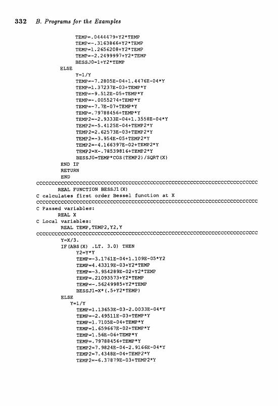
332 B, Progmms for the E~amples
TEPgp=,0444479+Y2*TEW TEMP=-.3163866+Y2*TapIe TEMPsle2656208+Y2*TEMP TEMP=-2,2499997+Y2*TEMP BESSJO=l+Y2*TENP
ELSE Y=l /Y TENP=-7.2805E-04+1.4476E-O4*Y TEMP=1-37237E-Q3+TEPilP*k" TEMPs-9,512E-05+TENP"Y TEMP=-.OQ55274+TEMP*Y TENPs-7.7E-O7+TEMP*V TBMP=.79788456+TEW*Y TEMP2=-2,9333E-04+1.3558E-O4*Y TEm2=-S14125E-04+TEMP;Z*U TEMP2=2.62573E-O3+TEMP2*V TENP2=-3,954E-O5+TEW2*Y TEW2--4.166397E-O2+TEMP2*Y TEPa?2=X-.78539816+TEEilP2*Y BESSJ0=TEMP*CoS (TEME"2) /SQRT ( X }
END IF =TURN END
cccceccccccccccccceecccccccccccccccccccccccccccceccC:ceeeeccccccccc~eccC:~ W L FUNCTION BESSJl (X)
G calculates first order Bessel function at X CCCeCGCCCCCC~C~CC~CCCC~CCGCCCCCCCeCCCC~~CC~CCC~CCCCCCCGCCCCCCCCCCCCCCCCC C Passed variables:
ReAL X C Local variables:
REAL TEMP,TEW2,Y2,Y ~cccceccccccccccCecccccccceeccccccccc~cccccccccecccc~cccceccceccccccCccc
V=X/J* xetAss(x1 .LT, 3-01 THEN
Y2=Y*k" TE~=-3.1761E-04+11109E-05*Y2 TEW-4,43319E-O3+V2*TEMP TEm=-3.$54289E-Q2+V2*TEW TEMP=.21093573+Y2*TEMP TEMP=-.56249985+Y2*TEMP BESSJl=X*(.5+V2*TEWW
ELSE Y=1 IY
TEMP*l.lJ653E-03-2.0033E-O4*Y TEW=-2.49511E-OJ+TEMP*Y TEMP=1,7105E-04+TEP?[PXY TEMP*1.659667E-Qi!+TEMP*Y TEm-2,56E-06+TEW*Y TEMP=.79788456+TEHO"Y TENP2r7.9824E-04-2.9166E-W TEMP2=7.4348E-O$+TEMP2*k" TEMp2=-6.37879R-O3+TEMP2*V
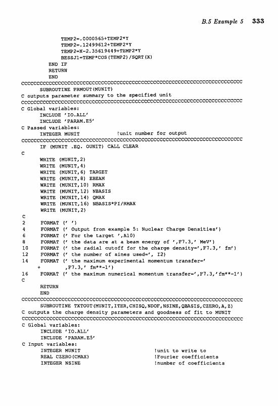
~EMP2=.0000565+TENP2"Y ~EH2=.12499612+TEMP2*V TEa2-X-2.35619449tTEm2*Y BESSJ~=TEMP*C~S (TEW2) /SQRT (X I
END I F RETrnM END
cc~~cc~cec~c~c~eceec~ccc~~ccc~ecc~cc~c~e~ccecc~ccccecccC:cccce~eecccccccc s u ~ ~ o u ~ x m BRMOUT (MUNIT)
C o u t p u t s parameter s u m a r y t o t h e s p e c i f i e d u n i t ~cc~c~cc~ceccecccccc~~~~cc~~eccccecccccccecccccccccccC:ecc~ccccccccc~cccc C Global v a r i a b l e s :
INCLUDE 'IIO*ALLf INCLUDE ' PPAMM. ES'
C Passed v a r i a b l e s : INTEGER MONIT ! u n i t nu&er Ear ou tpu t
~ e ~ ~ ~ ~ ~ ~ c ~ ~ ~ c ~ e ~ ~ ~ ~ c ~ ~ c ~ : c ~ c c ~ c c c c c e c c e c c c ~ c ~ c c c c c ~ e e e c c c ~ c ~ c c e c c C : c c c c c c c I F (MUMIT .EQ. QUHIT] CAZL CLEAR
G mITE (MUNXT,2) mXTE fMUNIT,4) WRITE (MUNIT,C) TmGET WRITE (MUNIT, S ) EBmH WRITE (MUNXT,10) W X WITE (WNfT,12) NBASIS &RITE (WUNIT, 11) -X mITE (MffM?eSP116) IJBEISISkPL/RWX WITE (MUHIT, 2)
C 2 F o m T ("1 4 F O m T t r Output from example S : Nuclear Charge D e n s i t i e s p ) 6 F Q M T ( ' For t h e Cargat ' ,A101 8 F O m T t f t h e data are a t a beam e n e r w o f ',F7.,3,' MeVC) 10 F O M T (Vth eradial c u t o f f f o r t h e cha rge dens i ty=r ,F7 . J ,p fmf ) 12 F O m T f1 t h e nu-r a f sines used=\ 12 ) 14 F O m T ("the maximum e x p r i m e n t a l momntum t r a n s f e r = '
5 , F7.3, "m**-le 1 1 6 F 0 m T f ' t h e maxirnum numerical momentum tran~fer=~,F'1,J,~frn**-l~) c
m T U w EED
c~ccccccccccccccccecccccccccccccccccccececececcccccccccccccccccc~cccccec SUBROUTINE TXTOUT (MUNIT, ITER, CWXSQ, hfDQFI ISIEJE, QBASXSI QZERO~A, Zl
C o u t p u t s the cha rge densi ty p a r a m t e r s and goodness o f f i t t o MUNIT ceccc~cccccCecceccceccceccccccccccceececccceccccccccccccccccccccccc~cccc C Global v a r i a b l e s :
INCLUDE * Ila.ALLe INCLUDE 'PAMM.ESe
C Inpu t v a r i a b l e s : INTEGER MUNXT a A L GZERO [CMAX) INTEGER NSINE
l u n i t t o w r i t e t o t P o u r i e r coefficients tnunloer aE c o e f f i c i e n t s
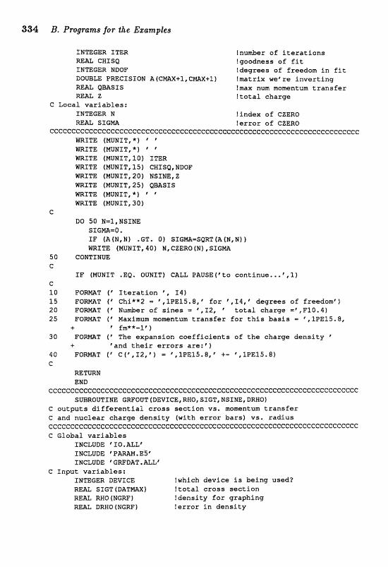
334 B, Pmgrams f ~ r the Ezamples
XNTEGER ITER !nu&er o f i t e r a t i o n s mRZ, CNTSQ !goodness o f f 4 t INTEGER NDOF f degrees of freedom i n f i t DOUBLE: PRECISION A(CWX+l,CW+1) !matr ix we're i n v e r t i n g m& QBASIS tmax num momentum t r a n s f e r RE& Z l t o t a l cha rge
C Local v a r i a b l e s : INTEGER N !index o f GZERD REU SIGM ! e r r o r o f CZERO
cceCceCcccecccc~cccc~cccccccccccccccccccccccccecccc~ccccccccc~:ccc~ceccc~ WRITE (MUNIT, *) * @
m1TE t#UNIT,*f ' * WITE (MUNIT, 10 ) ITER WRITE (NUNIT, 1 5 ) CHISQ, NDDF WRITE (MWXT, 20) NSZME, Z WRITE (MUNST,25) WASIS m f T E (MUNIT,*) ' " WRITE fMUNZT, 30)
C DO 50 N-1,MSZME
SIGPIGA=O. I F 1A(N,Nf .GT. 0) SIGM=SQRT(A(N,W)) WaITE (MUNIT, 40) N, CZERO (M) , S I G m
50 GQNTIPJUE C
I F (NUNIT .EQ. OUNXT) GALL PAUSE[@to cont lnue. , .@, , l ) c 10 F O m T ( * I t e r a t i o n 5 14) 1 5 F O m T ( ' C h i * * Z = t , l P E 1 5 , 8 , ~ o r ~ , f 4 , t d e g r e a s o f f reedomf) 20 F O W T ( * NuPhber af s i n e s = * , I 2 , t o t a l charge =',F10.4) 25 F O m T ( ~ ~ a x i m u m momentum t r a n s f e r f o r t h i s basis = .',1PE95.8,
4- ' fm**-1') 30 F Q m T ("he expansion c o e f f i c i e n t s of t h e charge d e n s i t y
+ ' a n d t h e i r e r r o r s a r e : ? ) 40 F O W T ((' C(',,X2," *,1,lf?E15.8,Q- "lPE15.8) e
=TURN END
ccccccccccccccccccceecccccccceecccceeccccccccccccccccc~ccccccccccccccccc SUBROUTINE GRFQDT (DEVICE, RHO, SIGT, NSINE, DRHQI
G o u t p u t s d i f f e r e n t i a l c r o s s s e c t i o n vs . momentum t r a n s f e r C and n u c l e a r cha rge d e n s i t y (wi th e r r a r b a r s ) v s . r a d i u s cccccc~c~ccccccCcccccceecceccccccccceccceccececccc~ccccccccccccccccccccc C Global v a r i a b l e s
INCLUDE IO.ALLP INCLUDE "ARBM, E5" INCLUDE %=BAT. ALL"
C Inpu t v a r i a b l e s : INTEGER DEVICE !which d e v i c e i s be ing used? REAL SIGT ( D A T M ) ! t o t a l c r o s s s e c t i o n RE= RNQ (NGRF) !density f o r g raph ing REAL DRNO (NGRF) t e r r o r i n d e n s i t y
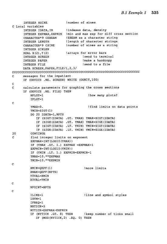
INTEGER NSINE ! n u & e r o f a i n e s C L o c a l v a r i a b l e s
XMTEGER IDATA, XR ! i n d e x e s data, d e n s i t y XMTEGER EXPMAX,EXP#XPT !min a n d rnax exg for cliff cross s e c t i o n CHMCTER"9 GEBEm !EBEAM as a c h a r a c t e r s t r i n g ZNTEGER LEPJGTN ! l e n g t h a£ c h a r a c t e r s t r i n g s CH-CTER* 9 GSI NE ! n u h e r o f s i n e s as a s t r i n g TWmGER SINLEN RE& X (2), Y (21 Iarrays fox error b a r s XNmGER SCREEN ! s e n d t o t e r m i n a l INTEGER PAPER !make a h a r d c o p y INTEGER F I L E lsend t o a f i f e DATA S C ~ E N , P A P E R , F I L E / ~ , 2,3/
cc~cccc~~cccc~cc~ccccceccc~c~ccccc~ec~cccececcccc~cccccec~c~cc~cccc~c C n e s s a g e s f o r t h e i m p a t i e n t
Tl? (DEVXCE .NE, SCREEN) RRITE (oUNIT,100) e C calculate parameters f o r g r a p h i n g the crass s e c t i o n s
I F (DEVICE .HE. FTZE) TMEN NPLOT=l !how many p l o t s ? IPLBT=1
C YE"IZIX=O. fflnd l i m i t s on data p a i n t s UNINmSIGT IT l DO 20 1D;ATA-1,NPTS
I F (SIGT (IDATA) . GT . Y W X ) YNAX=STGT (IDBTA) I F (SZGE (SDATA) . GT. YWX) YmX=SXGE IIDATAI I F (SIGT (IDA1;"A) . LT. YMZN) YMIH=SIGT (IDATA) I F (SSGE ( IDATAJ ,LT, UMIN} YMIN-SIGE (IDATAI
CONTXWUE f i n d i n t e g e r l i m i t s on e x p o n e n t E x a m x = r N T (LOGI~ (YMW I F ( Y W .GT. 1. ) EXPmX =EXPPFLAX+I EXPMXNmINT ( L W 1 0 f"xlMXN1 f XF (YMIW .LT. 1.) EXPMIN=EXPMIM-2 V M = l a . * * & X P m X YNTN=10.**EXPMIM
!Line a n d sy&ol s t y l e s XLINE=I SSVM=1 IFREQ=f. NXTICK=5 NYTICR=EXPmX-EXPMIN I F (NYTICK .GT, 8 ) TEEN ?keep nunrber a f t i e k s s m a l l
I F (MOD(MYT%CK,Z) .EQ. 0) TMEN

336 B. Prqclranas for the EzumpZe~
WVTICK=NYTIGR/2 ELSE
NYTICIC=B EMD I F
END 3 F
CALL C O m T (EBEAM, CEBEAM, LENGTH) !titles and labels IMF0 = C C a l c u l a t e d ( X ) a n d E x p r l m @ n t a l ( O ) W E L ( 1 ) = ' B e f f t 3 c t S v e (h**-l)" -EL (21 = # D i f f e r e n t i af C r o s s S e c t i o n I M a r n e s l a r ) " TITLE ' E Z e c k r o n S c a t t e r i n g o n '///T=GET
+ // ' a t ' / /CEEEAM(I:BNGTWj// ' MeVt c
CALL GTDEV (DEVICE) !device n o m i n a t i o n IF ( D m I C E .Ea. SCREEN) CALL GMODE ! c h a n g e t o graphics mda C&L WLNAX ! d r a w axes
END IF C G c u t p u t crass s e c t i o n s vs , angle
TP (DEVICE .EQ. FZLE) THEN WRITE (GUNTT, POO) m I T E (GUNZT,PIQ) m 9 T E (GUMIT, 220) (QEFF (XDAZIA) , S I G T (IDAT&) , IDATA-I, EilPTSf
ELSE CALL XUPLOT (QEFF , SXGE 1 !piat exgerimntal data NPDINTm2 apREag.o DO 80 ICtATA=l,N&TS f w i t h e r r o r bars
X ( 1 ) =QEFF (SDATA 1 X f 2) =QEFF (IDATA) Y (XI =SXGE fxaATA) +DSICE ~IBATAI Y (21 =SXGE trDATA) -DSIGE ~IDATAI CALL XYPLClT f X , V)
8 Q CONTJMUE NPOINT=NPTS IPREQ=1 TSVMmII CALL x v p L o a (QEFF, SLGT CALL GPAGE: (DEVICE)
END I F C C c a l c u l a t e p a r a m e t e r s fo r charge d e n s i t y
I F (DEVICE .W. F I L E ) THEN Y m = B . ! f ind l i m i t s o n data p o i n t s YNTN=O . DQ 120 IR=I ,NGW
IF (RHO(IR1 .GT. =X) Y m = M O ( I R ) 120 CON"rNUE
XMTN=O . X M A X - m x Y OVAL=XMIPd XOVAL=YMIN
!plot c a l c u l a t e d s i g m a
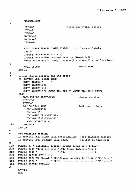
!fine and s y d o l styles
CALL XCNVRT(NSINE,CSIME,SINLEMl ?titles and labels IPaFO=" L-EL (I) ' Radius (fermis) ' =EEL (2) i.. *Nuclear c h a r g e density [ f e r m i x * - 3 ) " TITLE = TARGET//* using /IICSXNE (I : SINLEN) /I' sine functions"
CALL LNZNAX END IF
output charge density and its error IF (DEVXGE .EQ. FXLE) THEM
mrre (GONIT,*) m
WRITE (GUNIT, 3QO) WRITE (GVNTT, 310) mITE {GONIT, 320) (RGRF fIR) ,RHO (IRf ,DRNO {SRI, XR=l, NERF)
ELSE GSILL XYELOT (RCW, RHO) !charge density NEOXNT=P rpma=o D8 180 XRm1,NI;RF !with error bars
X (1) -RGRF (ZR) X (2) =X (1) Y (1 ) =RHO ( I R ) -DRWO ( I R ) Y (2)=Y(ll+2*DRRQ(IRt CALL XYOLOT ( X , Y)
GONTZNUE END I F
end graphing session XP (DEVICE .NE. FILE) CALL GPAGE(DEVICE1 f e n d graphics package r~ ( D ~ I C E .EB, SCWEHI CALL TMODE !switch to text mode
F O m T (/, Vatienee, please; output going to a file.6) F O W T (1 O X , "@E% (l/fermf f ' , SX, @ Sigma (m&rnes/srl@ 1 H O m T ( IQX, --------------f CJX, t ------------------' ! F O m T (2 (1 O X I IPE15.8 f 1 F O W T (32X, [(fermi) @ X , T G h q e density (fm**-3) ', f0X, "Error")
(12X, f ---------" ,8X,6- - - - - - - - - - - - - - - - - - - - - - - f i ,10] i :C ' - - - - -8 1 Fa-T (3 f9X, 2PEI5.8) )
RETURN END
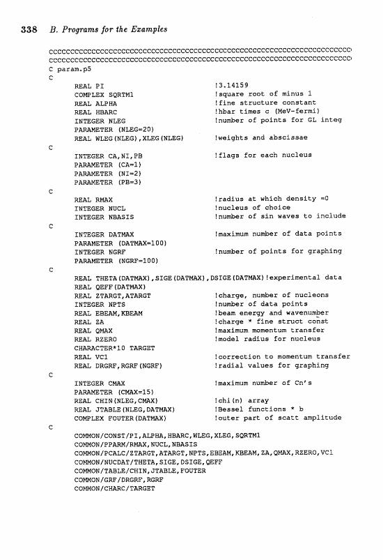
338 B. F"~.ograms for $he Bzanzpfes
C pnram.pfj C
m k L P I !3.14159 COWLEX SQRTM1 f a w a r e r o o t a f minus 1
RE& ALPm ! f i n e s t r u c t u r e c o n s t a n t REAL HBAaC fhbar t i m e s c (MeV-fermi) INTEGER NLEG !number af p o i n t s f o r EL i n t e g PAWMETER f NLEG-20 1 REAL WLEG (NLEG Z , XLEG (MZEG ?we igh t s and a b s c i s s a e
C INTEGER CA,NT,PB ! f lags f o r each nuc leus PAMETER (CA=1J P h W E T E R (WTm2f
C RE= RmX ! r a d i u s a t which d e n s i t y =Q INTEGER NUCL ? n u c l e u s of c h o i c e INTEGER NBASIS !nu&er of s i n waves t o i n c l u d e
C" INTEGER DATMX !maximum number o f d a t a p o i n t s PAWWETER (DATMAX-1001 INTEGER HGRF ?number of p o i n t s f o r g rapb ing PAMNETER (NGRE"=Z 0 1
C REAL THETA (DATMX) , SIGE (DATMX), DSIGE (DATNAX] f e x p e r 1 . m e n a d a t a RE= QEPF ( DATmX) REAJI ZTARGT,ATARGT !charge, n u d e r of nuc leans INTEGER NPTS !numker of d a t a p o i n t s m& EBEAN, KBEAPil !beam energy and w a v e n u e e r mAL BA !charge * f i n e s t r u c t c o n s t RE& QMX !maximum momentum t r a n s f e r mAL RZERO !medal radius f o r nuc leus CWmCTER*10 TARGET mI, VG1 ! c o r r e c t i o n t a momentum t r a n s f e r REAL D R G E , RGRF (NGW) ! r a d i a l v a l u e s f o r g raph ing
G INTEGER CMX !maximum number o f Gnc s PAMMETER (CmX-IS) REAL CHIN (MLEG,CmX) ! c h i (n) a r r a y %AL JTABLEfNLEG,DATmX) IBessel f u n c t i o n s * b CQWLEX POUTER 1DATmX) ! o u t e r p a r t o f scatt amplitude
C ~O~ON~CQMST/PI~A~HA,WBAR~,~JLEG,XLEG,SQRTM~ CQmON/PPM/MX,NUCL,NB&SIS C~~QN/PCALG/ZT~GT,ATARGT,NPTS,EBEAM,KBEAN,ZA,QM1ZX6RZERO,VC~ COE"340N/NUCDAT/THETA,SIGE,DS5GEIC2EFF COM0N/T~LE/CRIN,JTABLE~FOUTER COmON/GRF/DRGRF,RGRF COrnON/CWRC/TARGET
B.6 Example G Algorithm This program solves Laplace's equation in two dimensions on a uniform rectangular lattice by Gauss-Seidel iteration. The p r o e m currently dotvs the input d Dirichlet boundary conditions ody. Wowever, the mray smca can be used to indicate other types of boundary conditions (i.e., periodic and Neumann). Once all parameters are input, the relax- ation iterations proceed with Eq. (6.17) being solved successively at each lattice point (subroutine RELAX). If requested, these relaxation sweeps will be mstricted to a sublatlice. The total e m r g per wea is d sa calculated in R ~ U . Note that the lattice @pacing in both a: and y is set equal to one. Every ~ F R E $ % ~ iteration, you are given option to continue it;era$ing or to return to the m;zin menu.
Input The input procedure is a bit difirent for this program, as well as fm PrOject 6. R r tl-iese two codes, yau may find that during the iteration procedure you want do keep the Add vdues and d l parameters, except one or two, the same. Far exmple, you may wish to dter just the relax- &ion parameter, change a boundary condition, or change the ffequeney at wEeh the field is displayed, Such a procedure is straighhrwmd, but only as long as tbe la;t;tice dirnendons remain the asme. Therefore, the menu is braken into two pieces: the first level obta;ins the lattice dimensions; the second level (or rnajn menu) obtains alf. other parameters. As bng as you, do not enter the first level menu, all prametem and field vml~res are ~nchangd unkess you s;neeificakly request atheruthe.
The first level prompts you for the lattice parameters IX [20] and AY [20]. The maximum lattice sizes are fixed by two considerations: first, the parameters NXWAX= 79 and NYNAX= 79 which determine the array sizes; second, the size of your terminal as defined by T B E V ~ and TMLIR in sub- routine SETUP* This last restriction is imposed so that the fidds can be displayed on the screen, using characters to indicate field strength (sub- routine DISPLY). If you will be using a graphics package, you can remove the t e r d n d size restrictions an WX and hlY in subroutine LAmIC, If it is not your first time through this menu, you will also be given the option of ending program executioll [no], and (if that answer is no) resetting input parameters to their default vdaes. Note th& aU pmameters th& depend on lattice dimensions (Le., the field vdaes, interior boundary conditions, and sublattice parm~eters) are automaticdly reset evary time you enLer this first level menu. The main menu allows for input of all remaining parameters. The pltysicaf. parameters are the v d ~ e of the field on, the upper [O.], lower [25.], left [25.], and right [O.] boundaries, which are fixed
for DiricMet boundary con&tions. The limits on field vdues are given by FBZI= 0 a d mAX= 25, and are imposed 80 that the scde for char- acter display of the field can be fixed (sw Output belovv), You can dso fix Dirichlet boundary conditions on the interim of the lattice. Two ge- ometries are allowed (subroutine B ~ R P ) : rectangles defined by the lower left and upper right corners; and "45 depeen Hnes defined by one corner, the quadrant, and the length (i.e., quadrant one produces a line at 45', quadrant two at I S a , three a& 225', and four at $Is0, all with respect to the positive z-axis). Note that z and y locations are input as integers to indicate the mrresponding lattice point, A n z ~ m u m of BCMAX= 10 interior boundary conditions are permitted. The menu also dims for the display (subroutine DSPLBC or GRFBC) and review (subroutine RWIEU) of inteI.ior boundary conditions. WIEW 4ows for deletion of interior boundary con&tions or dteration of their h e d field d u e s ,
The numerical parametem are the relaxation parameter [l.], the op- tion to relax a sublattice [no] spedfied by the lower left and upper right cornas, and the initial fidd vdue. Initid field vdueg at nm-boundary points can: 1) be read in from a file [exmpl6.in] created earEer by this program; 2) be set to a specified vdue [12.5]; or 3) remain unchanged. Option 2 is the dr;faalt if the calculation ie just beginning; .otherwise, option 3 is the default;, The two graphieg parametas are the mmber of contours for plotting [l01 (used only if you have a graphics package), and the frequency at which the field is displayed [IQ]. This is also the frequency at w&ch you me aked if you, would Eke to continue iterations. The r n ~ m u x n number of cantoars is fixed by U ~ V = 20.
Oue put After each rdaxatim sweep, the text output displays the iter- ation number (iteration count is zeroed on return from the main menu), energy, change in enerw from the last iteration, md the maximum change in the fidd. Every ~~mq%t;b iteration, the prosam will display the field, Note that the field will be displayed as contours (if you have requested grap hics sent to the screen, see subroutine GRFWT) or as characters (if you hatre requested text to the screen, see subroutine DISPLY). In the char- acter display, sm& letters in&Icate boundary points and capitaf letters indicate non-boundary points. Currently the progam sets the maximam. field d u e to 25 m d the minimum. to 0, so that the letter A cmrespands to a field vdue of O and the letter Z ta a gel& vdue of 25. k r the contour plotg, the boundary points are indicated by dashed Bnes; the appearance ol" the contour lines will depend on your graphics package, Because dis- play of the field can slovir down cdcdations considerably, yon may want to set BREQ to a large number.
Ag&rs, to avoid volurnirroues output, the field is not written out to a file or sent to a h a r d w j ~ ~ devjce each. time it i s digplayed on the screen. Instead, when you request to stop iterations, p u PrifZ be wked if you waat the fidd valnes to be written to the requested output devices. Nate that the field may be written out in three ways: as character data (if text is requested to a file), as numerical data (if graphics is requested a file), or as a contour plot (if graphics i s requested to a hardcopy device).
cc~cce~cecCcccecccccccc~ccccccccccccccccccc~cccccccccccccccecc~ccccccccc P R E W EXWLC
C E x a p l e 6: So lv ing Laplace 's e ~ a t i o n i n two dimensions C COE3PUTATPOMAL PHYSICS (SORTmN WRSION) C by Steven E , Koonin and Dawn C. Meredi tb C Copyr ight 1989, Addison-Wesley P u b l i s h i n g Company CCCCCCCCCCCCCCCCCGCCCCGCCCCCc"CCCCCCCCCCCCGCCCCGCCCCCCCCCCCCCCCGCCCCCCCCC
CAU INXT ! d i s p l a y header sc reen , s e t u p parameters 5 CONTINUE !main loop/ e x e c u t e once f o r each set o f param
CALL mTTXC !get l a t t i c e s i z e , a l low f o r end ing CALL ARCWON !ge t d e t a i f e d bound cond and r e l a x l a t t i c e
GOTO 5 EWD
ceccc~cc~ccccCeccccecccccccecccccccccccccccccccccccccccc~ccccc~ccccccc~c SUBROUTINE ARCMQN
C s u b r o u t i n e t o g e t p a r a m t e r s , r e l a x t h e l a t t i c e , and ou tpu t r e s u l t s CCCCCCCCCCCCCCCCCCCCCCCCCCCCCCCGCCCGCCCCC~CC(3CGCC~CCCGGCCCCCCCCCCCCCCC~C
C Global v a r i a b l e s : INCLUDE ' PhMM. ECr INCLUDE 10. ALL'
C! Local v a r i a b l e s : RE= P ( N X ~ X , NYW 1 ! f i e l d v a l u e s RML PGW (NXMAX, MYMAXI ! f i e l d v a l u e s f o r grap.b%ng INTEGER X M X H , X m X , Y M I N , Y m ! c o r n e r s o f r e l a x i n g l a t t i c e
RE= D E L W , Q L D W !keep tzaek of changes i n P
=&L ENERGY, DELE ! c u r r e n t and d e l t a energy XNTEGER NfTER !nu&r o f i t e r a t i o n s LOGXCBL TTER ! con t inue i t e r a t i n g ? LOGXGAL PRM ! p r i n t ou t p a r a m t e r s l LOGICAL END !end t h i s run? INTEEER I X , I Y ? l a t t i c e i n d i c e s INTEGER CHOXCE !write o u t f i e l d now? XNTEGER NLINES Inu-r o f l i n e s s e n t t o t e m i n a l
XMTEGER SCREEN !send t o ternt inal XNmGER PAPER !make a hardcopy INTEGER FILE Isend t o a f i l e
C Funct ions: REAJ, GETFLT t u s e r i n p u t fune t i o n XNTEGER GETXNT, VESRQ !use r i n p u t functions
LQGZCAL LOCCVT !conver t 0 , f t o f a l s e , t r u e
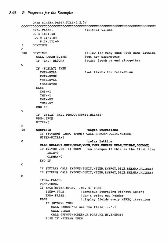
342 B. Progrgms for the Esanzples
DATA SCmEN, PWER,FXLE/I, 2,3/ ceeccccccccceccccccccecccccec~cccccccccccccceccccccccccccec~cccccccccccc
END=.FIILSE, ! i n i t i a l va lues DO 5 IX=1, WX 06 5 XY-3,NY
P (IX, XU) =O 5 CON"PNUE C 200 CONTINUE ?allow f o r m a y suns with same l a t t i c e
CALL P W H (P, END 1 !get new parameters I F (END) =TURN ! s t a r t f r e s h o r end altogether
e XP (SUBLAT) THEN
XMINcNXLL i s e t l i m i t s f o r r e f a x a t i a n
VMXE=NVLL YM-NYUR
ELSE XMIN=1 YMIN=I x m m m YmX-NY
END I F e
I F (TFZLE) CALL PRMQUT [ TvrJIT, WLLNES] PM=. TRUE NITER=@
C 99 !*in iCeraelonlr
I F ( (TTERM) .AND, (Pm) 1 CALL PWOUT (OVNIT, NLXNES) NZTER=NXT&R+l
e f ~ a a m l a k k i e e , rQm-1
SF (NITER .Earn l) TREN !no changes i f t h i s is t h e f i r s t t ime DP;LE.=O QLI)NAX=O
END IF
SF. (TFIm) CALL TXTOUT (TUNIT, NITER, ENERGY, EfBLE, D E W X , IICIIEJES) XF (TTERM) CALL TXTOUT [OUNIT, Nf TER, ENERGY, DELEI DELMAXI NLIWS 1
I TER.=. FALSE. PRM=,TRUE, XF (MOD(NITER,MFWQI ,NE, 0) THEN
ITER=,TRW. !continue i t e r a t i n g without asking PRM=,PALSE, !don't p r i n t out header
ELSE !display f i e l d s every NFmQ i t e r a t i o n I F (GTEM) TWEN
CALL PAUSE(rtto see the fLe ld ...', 1) CALL CmZLR CALL GWOUT [SCREEN, P, PGRF, NX, MY, ENEWV)
ELSE ZF fTTERM] TWEN
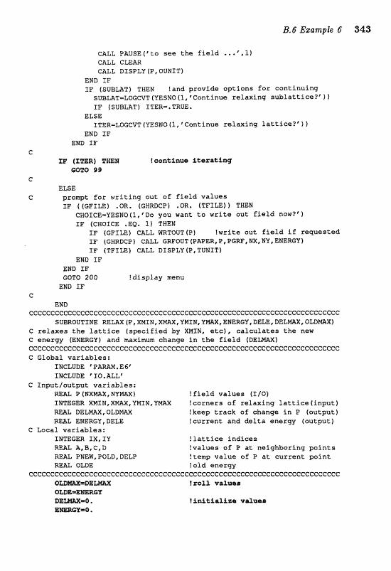
CALL PAVSfS('to see the f i e l d ... "1) CALL CLEAR CALL DTSPLY (P, OUNIT)
END ZF IF (SUBWT) THEN !end provide opt ions f a r cant inuing S U ~ L A T = L O E C V T ( Y E S N O ~ ~ . , ~ C ~ ~ ~ ~ ~ ~ ~ relaxing s u b l a t t i c e ? ' f f IF ( SUBL&T ) I %'ER=. TRUE -
ELSE ITER=ZQGCVT(YESMD(~~~CO~~:IRU~ re lax ing l a t t i c e ? ' ) )
END IF END IF
C m ( x ~ R ) E ~ N foonkinua itsratfng
WTQ 99 C
ELSE C prompt f o r w r i t i n g out o f f i e l d values
IF ( (GFILE) .OR. (GWRDCP) .OR, (TFILE)) THEN CMO~ C E = Y E S N O ( ~ , W ~ ~ you want t o write out f i e l d now?@> IF (CHOICE .EQ. f f THEN
IF (GFILE) CALL WRTOUT (P) !wri te out f i e l d i f requested I F (GMRDCP) CALL GWOUT (PMERc P, PGRF, NX, NU, ENERGY) IF {TPILEI CALL DISPLV (P, TUNIT)
END IF END IF GOTO 200 !display menu
END I F c
END cccccccccceccccccccccccccccccccccecccceccccccccccecccccccccccccccccccccc
SUBROUTINE RE-X (P, XMLN, XMX, VNIN, Y M X , ENERGY I DELE:, D E M X , OLDMX) C re laxes t h e l a t t i c e ( spec i f ied by XMIN, etcf, c a l c u l a t e s t h e new C energy (ENERGY) and maximum change i n t h e f i e l d (DELWf ccCccccccccccccccccccececccecccccccccccccccccccccccccccccccccccccecccccc C Global var iab les :
INCLUDE 'PAMM.EGf INCLUDE -0,ALL'
C Ingut/output var iab les : REAL P (NXMAX , N U M M 1 ? field v a l uas (I/O) INTEGER XMIM,XMAX,YMIM,VMX !corners of re lax ing f a t t i c e ( i n p u t f mAL D E L W , OLDMM !keep t r a c k of ehange i n P (output) R E U EEM&RGY,DELE !current and d e l t a energy {output)
C Local variables: INmGER IX, I Y ! l a t t i c e ind ices REAL A,B,C,D !values of P a t neighboring p o i n t s m A L PNEW,POLD,DELP !temp value o f P a t cur ren t po in t M A Z OLDE !old energy
cccCccccccccc~cccccccC:ceceeeeccccecccccecccccccccccccccccccecccceccccccc troll vaZaas
tinftfaliza vdaea s=w=a *
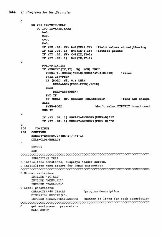
344 B. Pr~granas fo r the Bganb;ples
C aa 200 X
DO 10 &m0. B=O e C=Q . B=O , XF (XX .ET. EX) A=P (IX+Z, TT) I field wa2-s at aefgWarAng IF (EX: .GP. 1) mP(ZX-l,m) I lakt fcrs poknkes IF (IT . LT * m) C=P (lx, n+1) IP (XY .CF. 1) D=F(SX,a-l)
POW=E (IX, 3?I) ZF {BmCm {ZX, ZX) . EQ. MQM) P m H
/c* (A+WC+D) ! relax B (EX, TV) =EmW n {Earn *m* 0 . )
B E a a s ( (PQW-Prn) IPOLD) EL=
DHm=mS (PmW) EHD XF
LP ELSE
Em=Pam fdanfe relax DIR-2 b e d con& m fF
C IF (IX .or, r) f ~ m - ~ ) **2 m (3Y .elf. 5) (Pm-D) **P
C 100 C O H T X m 200 C O m X m
G MTUREI END
ccceccccecccccccecccccccccccccecccceccccc~cccccc~ccccccccccccccccccccccc SUBROUTINE f NIT
C initializes constants, displays haader screen, C initializes menu arrays for input parameters cccccccccececceeeeeeL:cccccceccccccecccccecccccccccccecccccccccccccccce~c C Global variables:
INCLUDE 'IX0,ALL8 INCLUDE @ MENU. ALL' INCLUDE PAMM . E G'
!program description DfmMSI ON BESCRP (201 INTEGER MREAD,NTmT,NGMPH !number of lines far each descriptian
ccecccececccccec~ccccccecccccecccccccceccc~ccccccccccc~L:cccccccccccccccc C get envir~nment parameters
GALL SETUP
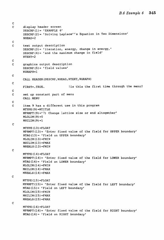
d i s p l a y header sc reen DESCRP (1 ) = ' EXAMPLE 6 DESCW(2)= 'So lv ing LaglaceH"s E w a t i o n i n Two Dimensions' MME&D=2
t e x t ou tpu t d e s c r i p t i o n DESCRP ( 3 ) = ' i t e r a t i o n , energy, change i n energy, ' DESCRP (41 = ' and t h e maximum change i n f i e l d ' NTEXTa2
g r a p h i c s ou tpu t d e s c r i p t i o n DESCW (5) = f i e l d values ' N G W H - 1
FIRST=, TRUE, !is t h i s t h e f i r s t t i m e through t h e menu?
set u p cons tan t p a r t of menu CA% muu
item 9 h a s a d i f f e r e n t u s e i n this program MTYPE (9) =NTTTL& MBMPT (9) =V) Change l a t t i c e s i z e o r end a l t o g e t h e r ' MLOLIM ( 9) =Q NWILXM (9) -1
MTYPE (2 3 f =FLOAT NPWT (13) = ' E n t e r f i x e d value 05 t h e f i e l d f o r UPPER boundaryt MFAG(13)= ' F i e l d on UPPER boundary6 MLOLIM (13) =FMXW MHXLIM (13) = F m X
LS (13) =FMfN
MTVPE ( 1 I 1 =FLOAT M P m T ( 1 4 ) = 'En te r f i x e d v a l u e of t h e f i e ld for MTAG(14)= ' F i e l d on WWR boundaryr MLOLIN (14) -PHI@ MNILXM (l 4 ) =FMAX m A L S ( 1 4 3 =FEiLAX
MTmE ( 1 S 1 -FLOAT MPWT(1S)- ' E n t e r f i x e d v a l u e OE t h e f i e l d f o r LEFT boundary' NTAF (15) = ' F i e l d on LEFT b o u n d a q r NLOLIM (15) -FMIN MHILIM [IS) =FMAX W A L S ( 5 5 1 -FMX
MTmE 11 6 1 -FMAT W W T (16) - * E n t e r f i xed v a l u e of t h e f i e l d f o r RIGHT boundaryf MTAG (1 6) = ' F i e l d on RXGNT boundaryf
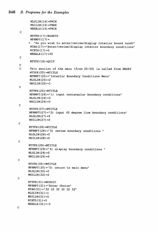
MTYPE (1 7 f =NOSKIP mWFT (171 =
+ 9 o you wish t o en te r l rev iew/d i sp lay i n t e r i o r bound cond?" NTAG~S7)-"Enterlreview/dI,sp~ay i n t e r i o r boundary condi t ions8 MINTS (17) =0 mmLS (1 7) =35
T h i s s e c t i o n of t h e menu (from 25-33) is called from BNDRP MTYPE (25) -MTITm MPWT(Z5f-"Interior Boundary Conditions Menu* MLOLTM (25 f m 2 mTLSM ( 2 5 ) =1
MTVPE f 26) =MTITLE W W T (26) 11) inpu t r e c t a n ~ l a r baundary eondf t i o n s ' MLOLTM (26) -0 MHILIM (26) -0
MTUPE (271 =MTITLE M P W T 127) -' 2) inpu t 45 degree l i n e boundary condi t i o n s " MLQLIM (27) -0 MHILSN (2 7 ) =Q
MTVPE f 281 =MTTTLE WREIIPT ( 2 8 ) m-3) review boundary condi t ions " ML0LIM (28) =Q Mf-fILXM (28 f =Q
MTUPE 129) -MTXTM MPWT129)="4) d i s p l a y boundary condi t ions mQLTN (291 m0 MWXLIM (291 -0
NTVPE f 30 1 =NTTTLE plIpWTt30)="5) r e t u r n t o main menu" MLOLXM ( 3 0 ) =0 MWTLIN (30) =0
M T E E (31 1 =MCROIC NPWT (31) = 9 n t e r Choice" MTAG (31)=p3J 232 32 32 32 32' MLOLIM (33.1 =l MHILIN f 31 1 =S MINTS (31 1 =S WmLS (31) =-S

MTUPE f 3 B 1 =FLOAT MPMPT(38)- 'En te r r e l a x a t i o n parameter" MTAG (38) = ' Re1 a x a t f an parameter ' MLOLIM (38) =0, HWILIM 111(38) =2. mEBLS (38) =l.
MTVPE f 3 P f =NOSRIP mWT(39)='Do you want t a s p e c i f y a s u b l a t t i c e t o r e l a x f i r s t ? # M T E (39) - 9 e Z a x a s u b l a t t i c e first?' MINTS f 39) =0 MREAZS (39) 4 4 .
MTVPE ( 4 0 ) =NUM NPMPT(4O)=9nter lawer l e f t X va lue for s u b l a t t i c e ' NThG(bO)=%~owr l e f t X s u b l a t t i c e va lue8 MLOLfM (40) =l E31.IILlN ( 4 O ) =NXHAX HlMTS t4Of =l
MTWE (41) =NUN @ W T ( 4 1 ) = @ E n t a r lower l e f t Y va lue f o r s u b l a t t i c e # NTAG f41 ) Lower l e f t V s u b l a t t i ~ e v a l u e p MZQLXM(41)=1 MNILTM ( 4 l ) =NUHAX EIHT5 (41 1 m1
MTYPE ( 4 2 ) =NUM W M F T 142) E n t e r upper r i g h t X v a l u e f o r s u b l a t t i c e ' MTAGf42J='Upper r i g h t X s u b l a t t i c e v a l u e t MLOLTN (42) =l HIWILIM ( 42 1 = N X m X MINTS (42)=1
MTVFE (4 3 ) =NUM I r lPmT(43)= 'Enter upper r i g h t Y va lue f o x s u b l a t t i c e " MTAG(43)=?Upper r i g h t Y s u b l a t t l c e va lue" MLOLZM ( 4 3 ) =l MWILLN (43 =KXMAX WTHTS f 4 3 f =l
NTYPE f 4 4 f EMTITLE WMPT 144) =' f n l t i a l F i e l d Value Menut MLOLIM (44 1 1.1 MNILfM[44)=1
MTYnE ( 4 5 f -HT1 TLE H P m T ( 4 5 ) = " ) Read i n i n i t i a l v a l u e s from a f i l e ' MLOLIM ( 4 5 f =Q MNTL1W (45) =O
MTYPE ( 4 6 ) =NTITLE
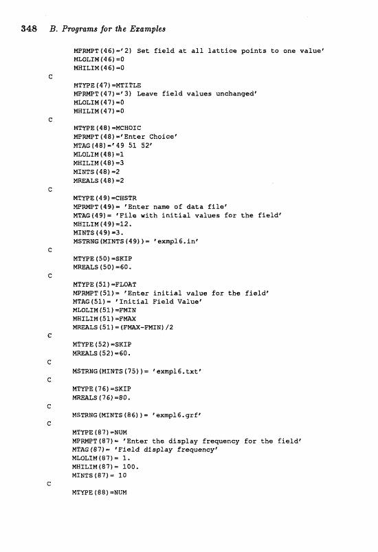
348 B, Pr~gr~rns for the Ezamples
M P W T t 46 )= f2 ) Set f i e l d a t all l a e t f c e p o i n t s to one valuee NLQLIM 14 6 ) =0 MWILI M f 4 6 ) =O
N T P E 4 47) -MTITm m M P T (47) -' 3) h a v e f i e l d v a l u e s unchanged1 NMLTW (47 ) =0 MHXLXM ( 4 7 1 ~ 0
NTYPE ( 4 8 ) =MC- M P m T 148) =qnnter Ghcica" NTAG (48)='449 51 5 Z r NLOLTN ( 4 8 f -1 NMTLTN (4 8 ) -3 MINTS (48) m2
MTVPE (4 9) =CWSTR a W T (491 = 'Enntr name af d a t a file* MTAGf49)- * F i l e with i n i t i a l values far t h e f i e l d ' MNXLIM (49) -12, MZMTS (49) 1 3 . MSTRMG IMTNTS (49) ) %exmpl S, i n r
WTYPE f 50 f -SKIP tS ( S O ) ..SO *
NTYPE (51 ) =FLGCAT W W T ( S 1 ) = 'En te r i n i t i a l v a l u e for the field ' MTAG (51) = q n i t i a l Field Value' MLOLJN (51) =FM1 N WMILIM (S1 ) mFM2PX
LS (51 1 = (FmX-FMXE)/2
MSmNG (MINTS (86) ) = 'exmpl6. g r f
MTVPE { 87 ) =NUM W W T 1 8 7 f = 'En te r the display f r s w e n c y f o r t h e fieldr MTAG187)- ' F i e l d display frequencyt NLQLIM(87)a 1. MBTLXH(87f- 100. MINTS (87) = 10
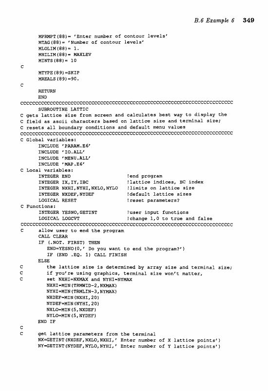
M P W T (88) - ? E n t e r n u a e r of con tour l e v e l s ' MTAG (881 = * Hu&er o f con tour l e v e l s @ MLOLIM(88)= 1. MKILTM (88 ) M L E V MINTS (88) = IQ
c PITYPE (8 9) =SKIP maLS (89)=90.
C MTURN END
~ece~e~c~~~c~~~ee~~~cecccceeccccccccecccecccceccccccecc~ccccccecccccccc~ SUBROUTINE UTTIC
e g e t s l a t t i c e i i z e from s c r e e n and c a l c u l a t e s best way t o d i s p l a y t h e C f i e l d a s a s ~ i i c h a r a c t e r s based on l a t t i c e s i z e and t e r m i n a l s i z e ; C resets a l l boundary c o n d i t i o n s and d e f a u l t menu v a l u e s ccc~~~~c~cc~cccce~cecccccccccccccc~ecccccccccccceccccccccc~ccccccccccccc C Global v a r i a b l e s :
INCLUDE ' P A W . EC' INCLUDE "IOIALLs INCLUDE ' MENU, ALL' INCLUDE 'mP,E6*
C Local v a r i a b l e s : INTEGER END !end program XNTZGBR I X , I V , IBC !lattice i n d i c e s , BC index TMmGER MXHI,NYHI,NXLO,NPLO ? l i m i t s sn l a t t i c e size INmGER NXDEF,NYBEF ! d e f a u l t l a t t i c e s i z e s LOGICAL MSET f r a a e t parameters?
C Functions: XNmGER YESMQ, GETGNT ! u s e r i n p u t f u n c t f a n s WGIGAI, LOGCVT !change f , O t o t r u e and f a l s e
cccccccccccccccccccccccccccccccecccccceccc~ccccecceccccccccccCeccccccccc C al low user t o end t h e program
CALL C L E a I F (.NOT. FIRST] THEN
EMD=YESNQ(O,? Do you want t o end t h e program?@) IF (END .ea. 11 CALL FGNXSW
ELSE C the l a t t i c e s i z e is determined by a r r a y s i z e and t e r m i n a l s i z e ; G i f you're u s i n g g r v h i c s , t e r m i n a l s i z e won" t a t t e r , C set NXNI=%XfrYIX and NYHX-HYM
NXHX=MIN (TRWXD-2, WXWX) NYHSmMIM (TMLIN-3, M Y W ) NXDEFmMZN {MXHI, 20) NVDEF-MIN (WVMI,201 NXLQ=HXM (S, NXDEF) NYLQ-MIN (S, NVDEF)
END I F C G cpt lattice g a r a m t e r s from t h e t e rmina l
NX=GET3NT(HXDEF,NXL0,TJXNI,r E n t e r number o f X l a t t i c e p o i n t s r ) MY=GETINTINVDEF,NVLQ,NYWIIP E n t e r number o f Y l a t t l c e p a i n t s r )
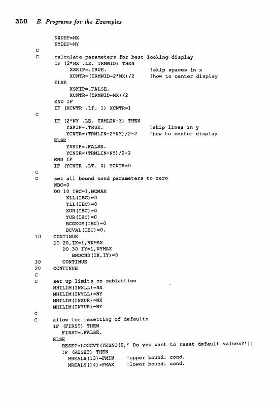
350 B. Programs far the Ezamples
calculate parameters fcs best looking display IF (2*MX .LE, TRMID) THEN
XSfCIP=.TRm. !skip spaces in x XCNTR=(TRWID-2*WX)/2 Ikow t o center display
f LSE %SKIP=. FALSE, XCNTRm f rnMZD-NX) 12
END I F IF (XGNTR .LT* 3.1 XCWTRmI
I F (2*NU .LEe TmLIN-3) TWEN YSRIB=.TRUE. !skip lines In y YCMTR=(TMLTN-2*NVf/2-2 !how to canter display
ELSE YSKIP=.FALSE. YGNTRm (TWLIN-NY) 12-2
END I F IF fVCNTR .LT. O) YCNTRmO
set all bound ccnd parameters to zero NW..@ DB 26 IBC=I,BCmX
XLL (IBC f =O VLL (IIBG) =B XUR (IBC) =O YUR IIBCI =O BCGEOH (TBC ) =6 BCVWL ( IBC 1 =O
CONTIPJUE ao zo, rxml ,~xmx
DO 30 TY=I,NYmX BNDCND ( JX , IY l =Q
CONTINUE CONTINUE
set up- limits on sublattice MHIZIM 4 INXLL) =NX HEELIN (SNYLL) =MY NHILIN IINXUR) =NX MNILIM ( INYW) =NV
allow for resetting of defaults IF (FIRST) TWEN
FIRST=.FUSE, ELSE
MSET-LOGCVT (YESNO (0, p Da you want t o reset default values?' 1 1 IF (-SET) THEN
mMLS ( 1 3 ) =mTN ! upper bound. eond. W A L S ( 1 4 ) =FWX ! lower bound. eond.
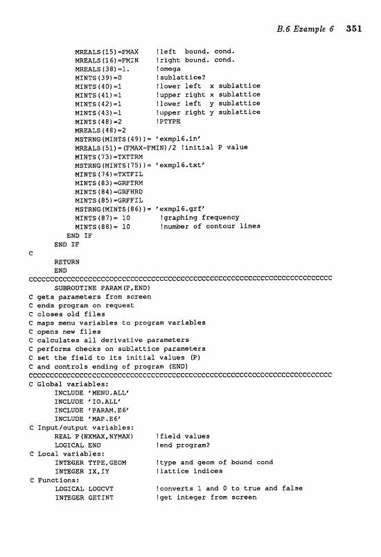
NmALS (15) -FMX ! L e f t bound. eond. MREALS (S 6 ) =FMIN ! r i g h t bound. eand. MREZLLS (38) =l, ! amega MINTS (391 ! s u b l a t t i c e ? MINTS f 40) =l f lower l e f t x s u b l a t t i c e MINTS ( 4 1 f =l !upper r i g h t x s u b l a t t i c e MINTS ( 4 2 ) =1 !lower l e f t y s u b l a t t i c e MINTS ( 4 3 ) =l !upper r i g h t y s u b l a t t i e e MINTS (48 )=Z ! PTYPE MREALS ( 4 8 1 -2 MSTRNG [MINTS f 49) 1 ' exmpl G. i n r W A L S (51) - (FmX-FMIN)/2 ! I n i t i a l P v a l u e MIMTS (73) -TXTTRM MSTRNG (MINTS (75) 1 - "exmpl 6,txtt MINTS ( 7 4 ) =TXTFI L MINTS ( 8 3 ) -GWTRM MINTS (84 ) =GWWRB MINTS ( 851 -GRFFXL MSTRNG(HfNTS(86) ) = 'exmpl G.grEp MfNTS(87)- 10 ! graph in9 f requency MINTS (88)- 10 !nu&r of can tour l i n e s
END I F END IF
e RETURN END
cccccccccccccccCccccccccccccccceceeeccecccccceccccccccccccccccccccccc~cc SUBROUTINE PARAM (P, END )
C gets paramete r s from sc reen C e n d s program on r eques t C c l o s e s a l d f i l e s C maps menu v a r i a b l e s t o program v a r i a b l e s C apsns new f i l e s C c a l c u l a t e s a l l d e r i v a t i v e pa ramete r s C performs checks an s u b l a t t i c e pa ramete r s C set t he f i e l d t o its i n i t i a l v a l u e s (P) C and c o n t r o l s end ing o f program (END) cecceecccec~cc~ccccccccccccC:cccc~ccccccC:ceccceccceec[:ecccccccccccccccccc C Global v a r i a b l e s :
INCLUDE %MENU. ALLt INCLUDE IIO,ALLf INCLUDE VAMN. E6' INaUDE W P . E 6"
C I n ~ > ~ l t / o u t p u t v a r i a b l e s : WAL P { N X M , N Y W ) ! f i e l d v a l u e s LOGICAL END lend program?
C Local v a r i a b l e s : INTEGER TYPE, GEOM ! type and gesm of bound cond INmGER I X , I Y ! l a t t i c e I n d i c e s
C Funct ions: LOGSGAL LOGCVT !conver t s 1 and O t o true and f a l s e INTEGER GETlNT !get i n t e g e r from sc reen
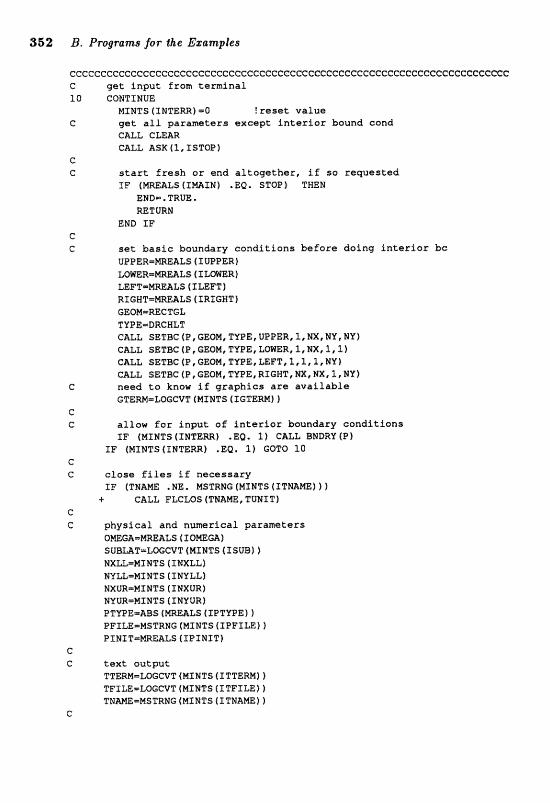
eccecccccccccCcceccccccccccccccceccccecccccccccccccccCcccccccccccccccccc G get input from terminal 10 CONTINUE
MINTS (INTERR) =O f reset value e get all parameters except interior bound cond
CALL CLEAR CALL ASK(3,ISTOP)
C C start fresh or end altogether, if so requested
IF (MmALS IImIN) e E Q * STOP) THEN END=.TRUE. RETURN
END IF c C set basic boundary conditions before doing interior bc
UPPER=mEBLS ( f UPPER) LomR==ALS (I L m R 1
RIGHT-mEALS (IRIGHT) GEQMmmCTGL TYPEmDRCWLT CALL SETBCfP,GEOM,TUPE,UPPER,~,NXINVINY~ CALL SETB@(P,GEOM,TYPE,LOIER,lIMXI~,If CALL sETBC(P,GEOM,TVPE~~FT,~,I,~,NY~ CALL SETBC (P, GEQM, TYPE, Rf GET, M, NX, 1, MY)
C need to know if graphics are available GTEM=LoGCVT (MINTS ( XGTEWI j
C C allow far input of interior boundary conditions
IF (HINTS (INTEm) .Ea. 1) CALL BNDRV (P) IF (MINTS (INTERR) .EQ. 1) GOTO 10
G C close files if necessary
IF ( T N m .NE. MSTRMG [MINTS (ITNAME) 1 + CALL FLGLOS (TNANE, TUNIT)
G C physical and numerical paramters
OMEGAmWALS ( XOmC1A) S~UT=LOGCVT (MrNTs gzsvs)f NXLL-MINTS (IMXLL) NYLLmMINTS (INVLL) MXm-MINTS (SNXUR) NYUR=MIMTS (INYUR 1 P TYPE=&BS (MREALS 4 ZPTUBEI PFILE=MSTRBG (MINTS (IPFILE) ) PINITmmALS f IPINIT)
e e text output
TTERM=LQGCVT1MfNTS(ITTERM)f TFILE=LOGCVT(MIMTS(XTFILEfj TNm-MSTRNG (MINTS (ITMAMEf
c
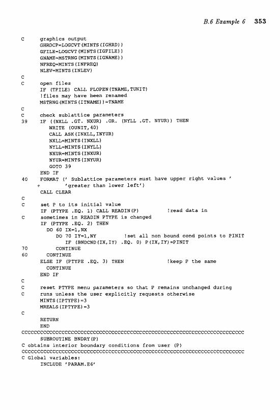
g r a p h i c s o u t p u t GHRDCP-LoGCVT (HINTS (IGWRD11 GFILE-LoGCVT(MINTS(fGFILEf1 GNMEmMSTRNG (MINTS (IGHAME 1 1 NFBEQ-MINTS INFREQ) NLEVzMINTS ( XMLEV)
open f i l e s I F (TFILE) CALL FLOE)EM(TE;IAME,TUNITl ! f i l es may h a v e b e e n renamed MSTRNG (MS WTS (ITHA=] 1 =TNME
c h e c k s u b l a t t i c e p a r a m e t e r s I F f fNXLL .GT. NXUR} .OR, (NYLL .GT. NYUR)) THEW
m I T E (OUNIT, 40) CALL ASK ( ENXLL, TNYURI NXLLmMINTS (INXLL) NYLL-MINTS f INYLLf UXUR=MINTS (XNXUR 1 NVUR=NINTS (SNYUR) GOTO 39
END I F F O m T (' S u b l a t t i c e p a r a m e t e r s must have u p p e r r i g h t v a l u e s p
+ "greater t h a n l o w e r l e f t ' } GALL CLEAR
set P t o i ts i n i t i a l value I F (PTYPE .EQ. 1) CALL MADSN (Pf f read d a t a i n s o m t i m e s i n READIN BTYPE is changed IF (PTYPE .EQ. 2) THEN
DQ 60 XX-I, NX DO 70 IY=l,HV !set a l l non bound cond p o i n t s t o BSNIT
I F (BMBCND (IX, I Y ) .EQ. 6) P ( I X , I V ) ..PINIT CONTINUE
CONTINUE ELSE I F (PTYPE .EQ. 3 ) THEN ? k e e p P the same
CONTINUE END SF
L
C reset PTYPE menu p a r a m e t e r s s o t h a t P r e m a i n s unchanged d u r i n g C r u n s u n l e s s t h e u s e r e x p l i c i t l y r e q u e s t s o t h e r w i s e
NSMTS (IPTYPE) = S MRmLS (IPTVPE) 13
e RETURN END
cccc~ccecCCccccccecccccccC:ccccccccccccceccccccC:cccccecccccceccccccecC:ccc svBRovTn ME BNDRY (P
C o b t a i n s i n t e r i o r b o u n d a r y c o n d i t i o n s f rom u s e r (P) ccccccccCCcccccccccccccceccccceccccccccccc~c~ccccccccccccccecccccccccccc C G l o b a l v a r i a b l e s :
INCLUDE VPAMM.EG1
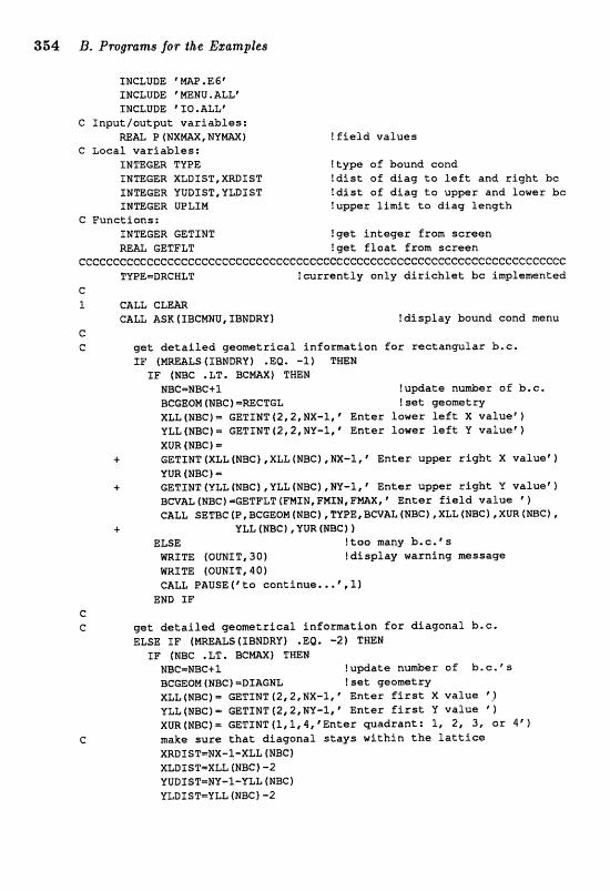
354 B, Progmms for the Egamptes
INCLUDE I W . E 6 @ INCLUDE WENU. ALL' INCLUDE ' 10. ALLC
C I n g u t l o u t p u t v a r i a b l e s : m& P ( N X W , N V W ) ! f i e l d v a l u e s
c L o c a l v a r i a b l e s : INTEGER TYPE !type of b a u n d c o n d INTEGER XLBXST,XWIST ! d i s t a f d i a g t o l e f t and r i g h t b c INTEGER VUDIST, YLDIST ! d i s t o f d i a g t a u p p e r a n d lower b e INmGER UPLIM ! u p p e r l i m i t t o diag l e n g t h
C F u n e t f o n s : ZNmGER GETZNT ! g e t i n t e g e r f r o m s c r e e n I Z E U GETFZZ" E g e t f L o a t f r o m screen
ceCcecce~c~cc~eec~cceccecccccccccccccceeccecccceccccccccccce:ccccecccccc~ TUPBcDRGWLT ! c u z r e n t l y o n l y d i r i e h l e t bc implemented
C 1 CALL GLEm
CALL ASK ( IBCWU, ICBNDRY l ! d i s p l a y bound cond menu G C get d e t a i l e d g e o m e t r i c a l i n f a r m t i o n f a r r a c t a n w l a r b.c.
I F (M-LS IBNDRY ) . EQ. -1 ) THEN XF f m C .LT. W W ) THEN
NBC=NBC+ I !u&ate nulnber aE b-e. BcCEOM (NBC) =mCTGL !set g e o m t r y XLL [ N E ) = GETINT IZ,2, NX-I, @ E n t e r l o w e r l e f t X v a l u e p j YLL (=C) = GETIMT (2,2, NU-1, @ Ente r l o w e r l e f t U valuer 1 XUR INBC 1 =
+ GETINT (XLZ (NBC) , XLL(NBC1 eEX-lC @ E n t e r u p p e r r i g h t X v a l u e * 1 YUR f WBC ) =
4" GETINT (YLL (NBC), YLL (NBC1 W-1, g E n t e r upper r i g h t Y v a l u e ' B~vAL(NBc)~ETPLTIPNJN~FM~M~FMX~* E n t e r f i e l d v a l u e CALL SETBC (F, BCGEOM (NBC) , TYPE, BCVG (NBC j C XLL { B C ) I XUR (mC)
4" YLL (NBC) , VUR (%BC) 1 ELSE 1 t o o many be a. S
WRITE (OUWIT, 30) ! d i s p l a y w a r n i n g m s s a g e a I T E (OUNIT,4@) GALL EIAUSEftto continue...',%)
END I F G C get d e t a i l e d geometrical i n f o m t i o n f a r d i a g o n a l b.c,
LS fIBNDRYf .EQ* -21 THEN IF fNBC .LT. E M X ) THW NBC=NBC+ "l ! u p d a t e n u d e r o f b . ~ . ~ s BCGEOM (NBC) =DXAGNL !sat g e o m t r y XLL (NBC) - GETXNT (2 ,2 , NX-2, ' E n t e r f i r s t X value ') VLL (NBG) = GETINT (2 ,2 , MY-lc "nter f i r s t Y v a l u e ' 1 XUR(NBG) = GETINT ( 3 , l, 4, ' E n t e r q u a d r a n t : 1, 2, 3, o r 4' )
make s u r e t h a t d i a g o n a l s t a y s w i t h i n t h e l a t t i c e XRDZST=HX-l-XLL(HBC) XLBISTmXLL (NBC) -2 YUDTSTmMV-l-YLL(NBC) YLDIST=VLL (NBC) -2
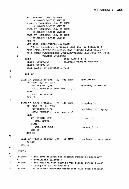
XP (XUR(NBG) .EQ. 1 ) TWEN UPLIM=MIN (XRDIST, YUDIST)
ELSE I F fXUR (NBGJ .EQ. 2) THEN UPLlM=MIM (XLDIST, YUDXST}
ELSE I F (XUR (NBC) .EQ. 31 TWEN UPLXM-MIN (XLDf ST, YLDIST)
ELSE f F (XVR (NBCf .&Q. 4 ) THEN UPLIM=MTU (XRDZST, YL-)
END I F YUR (MBC) = GETINT (UPLXM, 0, UPLTM,
+ C E n t e r l e n g t h o f 45 d e g r e e l i n e (max is d e f a u l t ) * ) B ~ A L (BBC) =GETFLT (EMTEJ, FMINI FmX, * E n t e r f i e l d v a l u e @ f CALL SETBC f P, BCGEOM f NBC ) , mPE, BWAL (NBC 1 , XLL {NBC j I XUR
-k YLL (NBC) , VUR (NBC) ELSE ?too m n y b . c ~ * ~ s
WRITE (QUWIT, 30) ! d i s p l a y w a r n i n g message WRITE (OUNIT,4Q) CALL PAUSE('t0 ~ o n t i n u e . * . ~ , l )
C ERE) I F
C ELSE I F (MREALS (IBNDRY) . EQ . -3 1 THEN ! r e v i e w bc
I F (MBC .EQ. 0) THEN m1TE (OUNISP, 2) !nothing t o r e v i e w CALL PAUSE('to c o n t i n u e . . . * , , l )
ELSE GALL REVIEW (P 1
END I F G
ELSE I F (MREALS(IBNDRY1 .EQ, -41 TWEN ! d i s p l a y b c I F fNBC .&Q. 0) TWEN
WRZTE (OUNf T, 2) ! n o t h i n g t o d i s p l a y CALL PAUSEl'ta c o n t i n u e . . . " , l )
ELSE TF (GTEWJ THEN ! g r a p h i c s
CALL GRFBC ELSE
CALL DSPLBC (P ?ns g r a p h i c s END I F
END I F C
ELSE I F (MRERLStIBNDRU) .EQ, -5 ) TWEN ! g a b a c k to Main menu RETURN
END IF C
GOTO 1 C JO P O m T ( Y o u have e n t e r e d t h e maximm nu&er o f baundaxy"
+ ' c o n d i t i o n s a l l o w e d f ) 90 F O m T ( ' You c a n a d d more o n l y i f you d e l e t e o t h e r s f i r s t e
+ u s i n g t h e REVIEW o p t i a o l ) 2 F O m T ( @ N o i n t e r i o r b o u n d a r y c a n d i t i o n s h a v e b e e n e n t e r e d r )
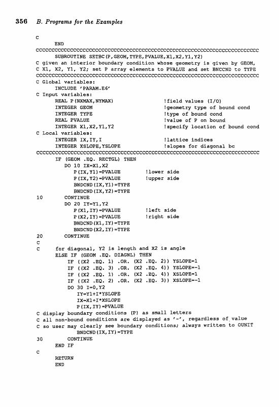
358 B. Programs for the E g ~ m p k f i
c END
cccceccccCccccc~ceecccccecccccccccccccc~cececece~eeceeccce~ccc~ccccccccc SUBROUTSHE S E m C (P, GEQM' TYPE, PVALW, XII 242, Y l , V21
C g i v e n an i n t e r i o r boundary c o n d i t i o n whose geometry is g iven by GEOM, G XI , X2, U1, Y2; set P array e lemen t s t o PVUUE and set BMCCND t o TYPE CCccceccc~ceccc~eccccececcccceeccecccccccccccccccceccceccccccccCcccccccc G Global v a r i a b l e s :
INCLUDE PAmM. E 6f C I n p u t v a r i a b l e s :
=AI, P (NXNa,X, # Y M f ! f i e l d v a l u e s t I l 0 ) INmGER GEQN !geometry t y p e o f bound cond INTeGER TYPE ! type of bound cond
PVALUE !va lue o f P on baund INmGER X1,X2,Yl ,V2 ! sgmcf fy l o e a t i o n of bound ~ o n d
C Local v a r i a b l e s : TNTEGER XX, I Y , I ! l a t t i c e i n d i c e s XNTEGER XSLaPB,YSLQPE ! s l o p e s for d i a g o n a l b c
ceccccccccccccccecccccccccc~ccf:cecccccccccccccceceeccccccccccccceccccccc SF [GEON *EQ. RBCTGL) THEN
no ro 1x=xl,x2 P I I X , V 1 1 =PVALOE flower s i d e P ( IX , U2 ) =PVALUE f u m e r side BNDCND ( I X , P1 1 =mPE BNDCNB (IX, V2 1 =TYPE
CONTINUE 00 20 SY=Yl,VZ
P (XI, IY) =PVALUE !left s i d e P 4x2, I Y f =OVALU& I right s i d e BHOCND (X1 , Ifl) -TYPE BNDCND (X2, IY) -TYPE
20 CONTINUE c C f o r d i agona l , V2 is l e n g t h and X2 is a n g l e
ELSE IF fCEOM *Ea. DIAGML) THEN I F ((X2 .EQ, 1) .OR, ( X 2 .EQ, 21) YSLOPE=1 EF ( ( X 2 *EQ. 3) .OR, fX2 .EQ, 4)) YSLOPEm-1 I F ((X2 .EQ. l! .OR. (X2 .EQ. 411 XSLOPE-1 I F ( (X2 . EQ. 2) . OR. (X2 .Ea. 3) 1 XSLOPEm-1 DO 30 I=O,Y2
/Y=yl+I*?ISLOPE IX=Xl +X *XSLOPE P (IX, fYZ =PVALUE
c d i s p l a y boundary c o n d i t i o n s (P} a s sma l l letters C all nan-bound c o n d i t i o n s are d i s p l a y e d as ' - # , r e g a r d l e s s o f v a l u e
C s o u s e r may c l e a r l y see boundary c o n a t i o n s ; always w r i t t e n t o QUNLT BNDCMD (IX, I Y 1 -TYPE
30 CONTIMUE END I F
c =TURN END
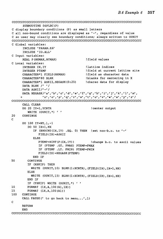
ccccccccecccecccecccccccccccceeccccccccccccccccccccccccccccccccccccccccc SUBROUTINE DSPLBC (P)
C display boundary c o n d i t i o n s (PI as smal l letters C a l l non-bound conddtdons are d i s p l a y e d as ' m - " , r e g a r d l e s s of vafua C ss u s e r may c l e a r l y see boundary cand i t fons ; always w r i t t e n t o OUNIT c~c~eeccccccccecccecceccccc~~cecccccccccecccccccC:cccccccceccccecccccccec C Global v a r i a b l e s :
INCLUDE ' PARAM. E 6' INCLUDE ' IQ. ALLs
C Znput v a r i a b l e s : REAL P [NXmX, W U W ! f i e l d v a l u e s
C Local v a r i a b l e s : INTEGER XX, IV l l a t t f e e i n d i c e s INTEGER PTEMP ! f i e l d a t c u r r e n t l a t t i ce site C a'&RX1 F JELD (NXMAX) ! f i e l d a s c h a r a c t e r data C TER"80 BLEK !blanks for c a n t e r i n g In X CHWCTER* P ASRI S, NEC;ASK O : 25 ) ! cha rae d a t a for d i s p l a y BA= BLNK / " 'I DATA &SKXI/'-* / DATA NE[;ASX/faa',fb~,'et,'dr,~e~,FZt,~~~,'h~Eei@,ljf , 6 k t , e l e , s m 8 ,
4 r n r l r ~ ' , " p " , " ' , " r ,'aF ,'t',~u~,'~~,~w~,~x',*yf f * z @ / ceccccececcccccceceeccc~cececcccccececcccccccccccccecccccceccccccccccccc
CA= CLEAR DQ 20 IY-l, YCNTR ! can te r o u t p u t
WRITE (OUNIT,*f 20 CONTINUE c
DO 100 IV=NY,1,-1 DD 50 IXm1,NX
I F (BMDGND(IX,IY) .EQ, 0) THEN !set non-b,c. t o ' - P
FIELD (ZXI =&SKI1 ELSE
PTEMPsNINT (P ( I X , TY) 1 !change b.c, do a s c i i v a l u e s I F (PTE1VIB .GT, F M X ) PTEMPmFWX IF (PTEMP .LT. FNIN) PTEmmFMIN FIELD (SX) =NEGASK (PTEMP 1
END I F 5 0 CONTZNUE
I F (XSKXP) THEM m Z T E (OUNIT, I O BLMK (1 : XCNTR) , IFIELD f TX) , IXm1, NX)
ELSE WRITE (OUNIT, 35) BLMK 4 1 :XCNTRf , {FIELD ( T X ) , IX=b, MXf
END SF TF (YSKIP) WRITPZ (OUNIT,") '
10 F O m T ( I X , A, 100 (AI, 1X) f 15 FORmT ( l X , A , TOO (Alf 1 100 CQISTINUE
CALL PAUSE(' t o ga back t o menu..,@ ,l) c
WTURN END
cccccccccecceccecccccccccccceccccecccccccccecccccccccceccccecccccccccccc
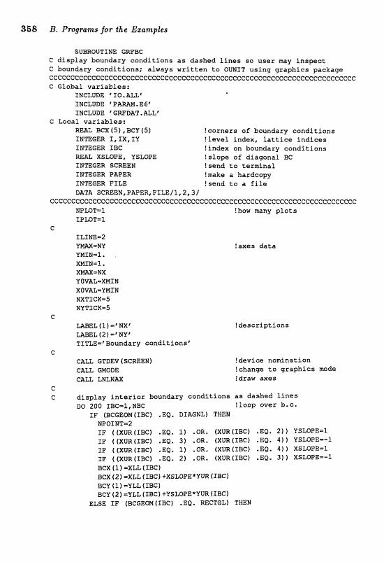
358 B, Programs far tbe Ezamples
? a x e s d a t a
SUBROUTINE GRFBC C d i s p l a y b o u n d a r y c o n d i t i o n s as d a s h e d l i n e s s o u s e r may i n s p e c t C boundary c o n d i t i o n s ; a l w a y s w r i t t e n t o OUNIT u s i n g g r a p h i c s package c~c~cc~ce~~cCe~~cccccccccccccecceeee~ceccc~eec~c~cc~~cec~~~cc~cc~ccecc~c C G l o b a l v a r i a b l e s :
SMCLUDE ' I0.ALL8 I
INCLUDE V&-, E6" XNCLUDE "WDBA. ALL6
C L o c a l v a r i a b l e s : REAL BCX (5) ,BGV (S) ! c o r n e r s of b o u n d a q c a n d i t i o n s INTEGER X, IX, I Y ! l e v e l i n d e x , la t t ice i n d i c e s INTEGER IBC ! i n d e x on b o u n d a r y c o n d i t i o n s RE& XSLOFE, VSLOPE ! s l o p e o f d i a g o n a l BC INTEGER SCREEN ! s e n d t o terminal INTEGER PAPER !make a h a r d c o p y INTEGER FILE ! s a n d t o a f i l e DATA SCmEN,FAPER,FILE/1, 2@ 31
cecceecec~ec~~cc~cccccccc~cccceccccecccccccceccc~ccccececcccccccc~eccccc NPU)T=l !how many p l o t s TPLOT-1.
C ILINPJE=Z Yrn=MY YMINml. XMf N-1, X M = P J X YOVAL-XMIN XOVm=Y HIM NXT1CTC=5 MY TI@K=5
C M E L ( l j = ' H X @ ! d e s e r i p t i o n a =EL (2) =wNksr T I T L E = % ~ o u d a r y c o n d i t i o n s t
G CALL CTDEV (SCREEN) ! d e v i c e n o m i n a t i o n @A& GlrlODE !change t o g r a p h i c s mode
CA= LNLNAX t draw a x e s e C d i s p l a y i n t e r i o r b o u n d a r y c o n d i t i o n s a s d a s h e d f i n e s
DO 200 IBCm1,NBC ! l o o p o v e r b , c . TP (BCGEQM(IBC1 .EQ. BLAGNL) THEN
NPOINTm2 I F ((XUR(IBC1 .EQ, 1 ) .OR, (XUR(IBC) .EQ. 2 ) ) YSLOPE=I I F ((XUR(IBC) .Ea. 3) .QR. (XUR(TBCl .EQ. 41 1 y S ~ 0 ~ ~ m - l IF ((XUR(EBC1 .EQ, 1) .OR. (XUR(1BC) .EQ, 4) 1 XSLOPE=~ 1F ( ( X U R ( I N ) .EQ, 2) .OR. (XUR(1BG) .EQ. 31 1 XSLOPE=-1 EICX (1) =XLL (IBCI sex (2) =XLL ( x a c t +~SLOPE*VUR IIBCI BCV ( 1 ) =ULL (IBG) seu (2) -VLL f IBC) +YSLOPE*YUR (1:BCl
ELSE I F (BCGBOHfIBCf .EQ, WCTGL) THEN
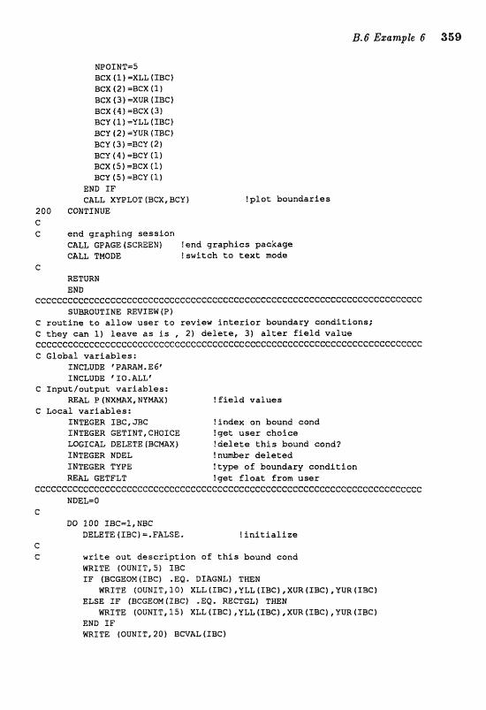
NPOINT=5 BCX (1) =XLL (IBC) BCX ( 2 ) =BCX (11 BCX (3) =XUR (IBG) BCX ( 4 ) =BCX ( 3 ) BCV (1) =YLL (IBC) BCY (2) =YUR IIBC) BCV (3) =BCV 421 BCY (4 ) =acu (1) BCX (5) =BC% (1) BCV ( S ) =BCV (1)
END I F GALL XYPLOT (BCX, BCY) fpfat boundaries
2 0 0 CONTIMUB C C end graphing session
CALL GPAGE(SGREEN1 !end graphics package CALL TMODE !switch to text mode
C RETURN END
~c~~~~~~~e~~~ccccceceeccecccccccI:ccccccceccc~cccccccc~cccccce~ccccccccc~ SUBROUTINE =VIEW (P )
G routine to allow user to review interior boundary conditions; C they can 1) leave as is , 2) delete, 3) altar field value c~ccceccccCccceeccccccccccccccccecccccccceccce~ccceccccccccecceeeccccec~ C Global variables:
T NCLUDE ' PZIMN. E INCLUDE C 10.ALLt
C Inputloutgut variables: REAL P (NXNAX, NVmX) ! field values
C Local variables: INTEGER IBC, JBC !index on bound eond INTEGER GETINT, CHOICE: ?gat user choice WGICAL DELETE (BCmX) !delete this bound eond? INTEGER NDEL !nu&er deleted INTEGER TYPE !type of boundary condition RE& m"I1FLT !get float from user
ccccecceccccccecccccccccccccecceccceccec~ccccccce~ecccGceccccccccccccccc NDEL-Q
e Do 1 0 0 IBC=l,NBC"
DELETE ( IBC) = . FALSE. !initialize C C write out description af this bound con4
WRITE (OUNTT,S) IBC TF (BCGEON(XBC1 .Ea. DIAGNL) THEN
WRITE (OUNST, 10) X L L ~ X B C I ,YLL (SW) , x m t x B e j I ~ ~ ~ t ~ ~ ~ ~ ELSE XF (BCGEQM (IBG) .Ea. RECTGL) T m N
m I T E (OUNIT, 15) XLLfIBC) ,YLL(IBC) ,XUR(IBC) ,VUR (IBC) END I F WRITE (OUMIT, 20f &CVAL(IBC)

360 B. Pmgmms for the Ezamples
CWOZCE=GETINT (1,1,3, + 'Do y o u w a n t t o l l k e e p it 2 ) d e l e t e i t 3) c h a n g e f i e l d v a l u e ? F )
I F (CHOICE .EQ. 1 ) THEN ! d o n o t h i n g CONTINUE
ELSE ZF (CHOICE .EQ. 2) THEN !delete it NDEL=NDEL+Z DELETE ( SBC ) = . TRUE, TYPE= WON !releases b.=. C U L SETBC (P, BCCEQH ( f BC) , TYPE, BCVAL (IBCf , XLL (XBC) , XUR f IBC) ,
+ YLL ( r a e ) ,YUR ts~ct t ELSE I F (CHOICE .Ea. 3 ) THEN !get new f ie ld v a l u e
BCVAL [IBC) =mTFLT (FMTNPFN3:N?FWX, @ E n t e r f i e l d v a l u e ' ) END I F
CONTXMUE
get. rid of spaces left i n b o u n d cond set when o n e o r m o r e is deleted XF (NDEL .NE. O) THEN IK=O IJBG l a b l s old set o f b o u n d c o n d no 200 J B C = ~ , ~ ~ B C l IBC labels new set of b o u n d c o n d
SF 4 DELETE (=C ) ) THEN GOMT f HUE
ELSE: IBC=IBC+1 ! n e x t empty place XLL ( f B@) =XLL f JBCf ! m v e up p a r a m e t e r v a l u e s t a VLL (SBC) PVLL (JBC) t mxt empty piace x v ~ { r s e j = x v ~ ( J B ~ ) YUR (EBC) =YUR (JBC) BCGEOM ( IBC f =BCGEOM (SIBC) BCVAL 4 TBC f =BCVAL ( m C )
mI) I F CONTINUE NBC=NBC-NDEL !uMate n u & e r o f b.c.@s
END XF
DO 300 IBC=Z,NBC reset b o u n d a r y c a n d f t l o n s i n case some of deleted b o u n d c o n d w r a t a over o t h e r s a l s o a d j u s t s t h a s e f a r w h i c h t h e f ie ld v a l u e w a s c h a n g e d TYPE-DRCNLT CALL SETBC (P, BCGEOH (IBC) TYPE, BCVAL (XISC) , XLL (IBC) , XUR
+ YLL (XBC) , VOW (IBCI CONTINUE: RETURN
FO-T (@ B o u n d a ~ C o n d i t i o n # u & e r 6,12) P O M T ( * D i a g o n a l w i t h f i r s t e 0 o r d i n a t e s = ( \ I 2 ~ ~ , ? , 1 2 ,
+ 1 , quadrant =' , I 2 , ', a n d 1 e n g t h m f 1 2 ) F O m T ( * R e c t a n g l e w i t h l o w e r l e f t a t [' ,I2, ' , ', 1 2 ,
+ * ) a n d umer r i g h t a t ( p , Z 2 8 @ , t * S 2 t f ) ' j F Q m T C * T h e f ie ld i s fixed a t ',,ZPIE;l2.5)

c END
~~~ccc~~~c~cc~cc~ceccccceccccccecccccceccccccc~cc~ccccccece~cccccccccccc SUBRoUTIHE READIN (P )
C r e a d i n f i e l d v a l u e s and boundary cond i t ions ; C r e a d s i n on ly files w r i t t e n by subrou t ine IrORTOUT, and f i l e s w r i t t e n
C w i t h same l a t t i c e s i z e c~~~~cc~~e~~~~~~ccc~cccccccccc~ccccceccceccc~ceecccI:~ccccccccc~cccceeecc C Global v a r i a b l e s :
INCLUDE '1OlALir" INCLUDE @PA=M. E6' IPICLUDE ' =NU. ALLf f NCLUDE "P. E 6"
C Output v a r i a b l e s : RE& P (NXmX, M \ I ' S ( M l f i e l d v a l u e s
c Local v a r i a b l e s : INTEGER IX,IV ! l a t t i c e i n d i c e s
CTER*aO JUNK ! f i r s t l i n e i f af no i n t e r e s t AL SUCESS !d id w e f i n d a f i l e t o open?
INTEGER CHOICE Iuaer answer INTeGER MX, MY, MOaGA !parameters from PFILE
C Funet ion: INTEGER YESNO !get yezsno i n p u t from u s e r GHMCTERX40 CHARAC ! r e t u r n s c h a r a c t e r i n p u t
ccccceeccccccccccceccccccccCcceccccccceccccccceccccccccccccccccccccccccc 10 C U z l FZOPUZ (&FILE, DtfNZT, SUCESSf !open t h e f i l e f o r i n p u t
MSTRNG (MINTS ( I P P X ~ ) f =&FILE !file may have been r e n a m d
I: I F (,NOT. SUCESS] THEN
CALL =ASK !prompt a g a i n f a r inft P mTURI !if no f i l e was found
ELSE C
READ (DUNIT,S) JUMK ? s k i p aver t i t l e 5 FORWT (A) C C l a t t i c e s i z e s must match; If they d o n e t , a l low f o r o t h e r o p t i o n s
mAD (DUNIT,*) K,MU,MOMEGA I F ( (W .NE, NX) .OR. (MY .NE. M Y ) ) THEM
CALL FLCLOS (PFILE, DUNIT) ! c l o s e it up m 3 T E (OUNIT, 15) NX,MV
15 PORMT (' Inpu t f i l e h a s does no t have t h e c o r r e c t t C ' l a t t i ce sf ze, I t is 5 12, C by * , I 2 f
CHOICE=YESNO(~,~D yyou want t o try ano the r f i l e T c ) I F (CHOICE .Ea. 0) THEM
CALL WASK !pronrpt a g a i n f o r i n i t P RETUREa
ELSE c (FFILE, 12, ' En te r a n o t h e r fi lename' 1
MSTRNG (MrMTs (IeFILEI f =eFILe GOTO 10 ! t r y t o open t h i s ane
END XF
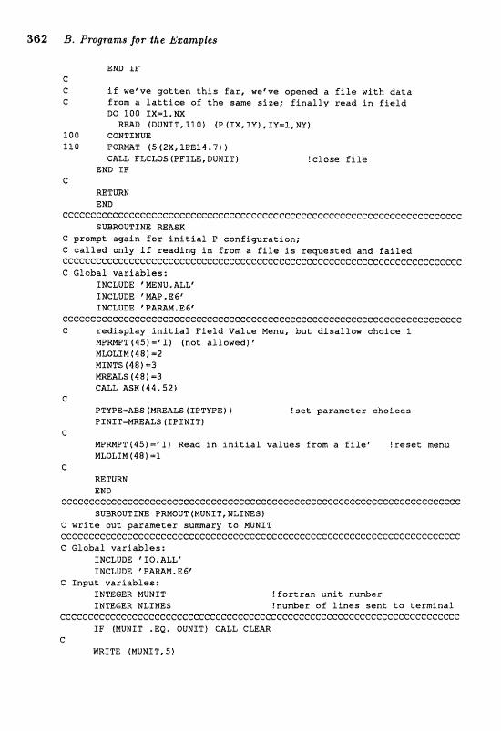
END I F c C i f we've g a t t e n t h i s f a r , we've opened a f i f e w i t h d a t a C from a l a t t ice o f the same size; f i n a l l y r e a d i n f i e l d
DO 1QO IX=l,NX READ (DUNIT, l l O f (P (IX, 1"k") , IU=1, WU)
100 CONTINUE 3.10 FORrJlAT ( 5 (2X, 1PE14.7)
CALL FLCWS (PPILE, DUNIT) ? c l o s e f i l e END I F
C MTURtJ END
cccccce~cccccccceecccccceccccccccccccccccccccccccccccccccccc~ccecccccccc SUBROUTINE REASK
C prompt again for i n i t i a l P c o n f i g u r a t i o n ; C c a l l a d on ly i f r e a d i n g i n from a f i l e i s r e q u e s t e d and f a i l e d CCCCCCCCCCCGGCCCCCCCGCCCCCCCCCCCCCCCCCCCCCCCCCGCCCCCCCCCCCCC:CCCCCCCCGCGC C G l a b a l v a r i a b l e s :
INCLUDE ' MEMU. ALL' INCLUDE 'WP.E6" INCLUDE ' P W M , E G f
CCCCCCCCCCCGCCCGGCCCCCCCCCCCCCCCCCCCCCCCCCCCCCCCCCCCCCCCCCCCCCCCCGCCCCCC C r e d i s p l a y i n i t i a l F i e l d Va lue Menu, b u t d i s a l l o w c h o i c e 1
W W T (45) =@l) ( n a t a l l owed) MLOLIM (481 12 MINTS [481=3 EIRaLS (481 -3 CALL ASK(44,52)
c PTWE-mS (MREALS tXPTYPE) 1 !set pa rame te r c h o i e a s PINIT=MMALS (IPIMIT)
C MPMT(451- ' l I) Read i n i n i t i a l v a l u e s from a f l l e Y r s s e t menu MLOLXM 4 4 8 1 =l
C RETURN END
c~cccc~ccc~ccccCcccccceeccccccccccecccccecccccccccccCccccccccccccccccccc SUBROUTINE PRNOUT(MUNIT,NLINES)
C w r i t e o u t p a r a m e t e r s u m a r y t o MUNIT ~cccccccccccccccccccccccccccccccccccccceeccccccccccccccccccccccccc~ccccc C G loba l v a r i a b l e s :
INCLUDE TTO.ALLt INCLUDE ' PPAMM.E6'
C I n p u t v a r i a b l e s : XNTEGER MUNIT ! f o r t r a n u n i t nunber INTEGER NLINES ?number o f l i n e s s e n t t o t e r m i n a l
ccceccccc~ccccccCccccceccccccccccccecececccceccccccccccccccccccecccccecc I F (MUNIT .EQ, OUMIT) CALL CLEM
C m I T E (MUNIT, 5)
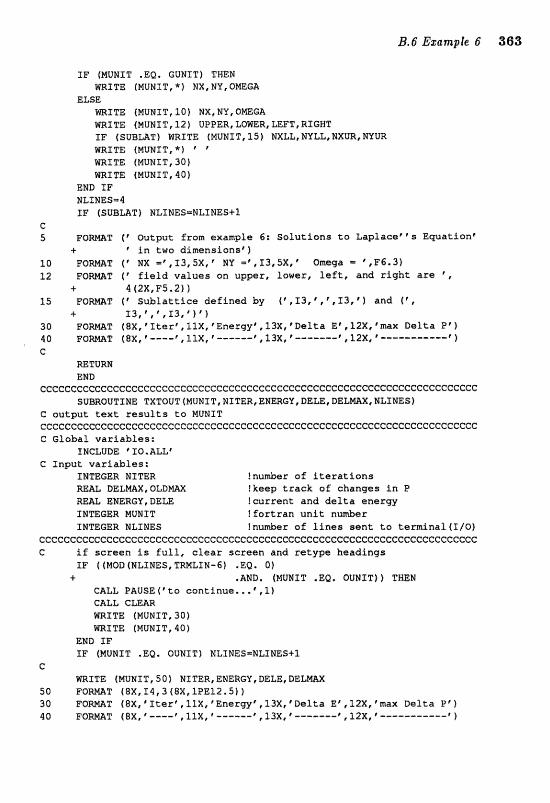
I F (MUNIT .EQ, GUNIT) THEN WRITE (MUNIT, *J HX, WY, O M E m
ELSE a I T E (MUNIT, 1 0 ) WX, MY, Om(;A WRITE (MUMIT, 1 2 ) UPPER, LOmR, LEFT, RIGHT I F (SUBUT) WRITE (MUNIT, 15) NXLL, MVLL, NXUR, NYm WRfTE (MUNIT,*I ' ' m f T E (MUNIT, 30) WRITE (MUNXT,4Q)
EMD TF WLINESm4 SF (SUBUIT) MLINES=NLIMES+l
C S F O m T f O u t p u t f r o m example 6: S o l u t i o n s t o L a p l a e e t 's E q u a t i o n f
+ * i n t w o d i m e n s i o n s 4 1 lO F O m T ( t N X = f , 1 3 , 5 X , ' N V = t , , S J , S X , * Om@ga= ' , IF6 ,3) l 2 F O m T (' f i e l d vaf u e s o n u p p e r , l o w e r , l e f t , a n d right are ' ,
+ 4 (2X,F5.2) 1 1 5 F O m T ( # S u b l a t t i c e d e f i n e d by (' , 13, , l , I 3 , ' I a n d t f ,
4- 1 3 , " f " r f 3 f ' ) ' ) 30 F Q m T (@X, " ~ t e r ' , llX, 'Energy' 13X, * D e l t a E* , 12X, 'max D e l t a F' b 40 F Q M T (8X,*----',1lX,'---m--' , 1 3 ~ , @ ----m-- @ , 1 2 ~ , t --...-------- 8 1 C
RETURR END
ccccecc~cee~ccccccccecccccececcccccccccecccccccecccecececccccccccc~ccccc SUBROUTIME TXTOUT(MUNIT,NITER,EN~GUIDELE,DEL~,MLINES]
C o u t p u t t e x t r e s u l t s t a MUMIT ccccceccccccccccccceccececccccccceccccccccccccccceccccC:ccecccccccccccccc C G l o b a l v a r i a b l e s :
INCLUDE XXO.ALLf G Znput v a r i a b l e s :
INTEGER NITER ?nu&er o f i t e r a t i o n s RE& DELmX, QLI)m ! k e e p t r a e k o f c h a n g e s i n P m& ENERGY, DELE ! c u r r e n t a n d d e l t a e n s t g y INTEGER MUNIT ! f o r t r a n u n i t nu&er IMTEGER NEZNES !nu&er o f l i n e s sent t o t e r m i n a l ( I I 0 )
ccceecececccccceccccceccccccccccccccccccccccccccccccccceccccccccc C I f s c r e e n is f u l l , clear s c r e e n a n d r e t y p e h e a d i n g s
IF ( (MOD (WLI HES, TBMLXM-5) .EQ. O f + .AND. (NUWST .EQ. OUNIT)) THEN
CALL PAUSE('to c o n t i n u e . . .@,l) CALL CLE&R hlRITE (MUNIT, 30) liaBP"1" ((MUNZT, 40)
END PF I F (NUNST .EQ. OUNIT) NLINES=ULINES+f
C ~ T T E (MUNIT, 5 0 ) NITER, ENERGY, BELE, a e L m x
5 0 F Q m T (8X,I4,3(8X,lPE12.5)) 30 F Q m T (@X, I terf , I l X , ' E n e r g y i , 13X, ' D e l t a E t , 12X, "max D e l t a P') 40 F O m T ( @ X , ' - - - - ' ,11~, L ---m- p -------@,12~,"-- ----------... r 1
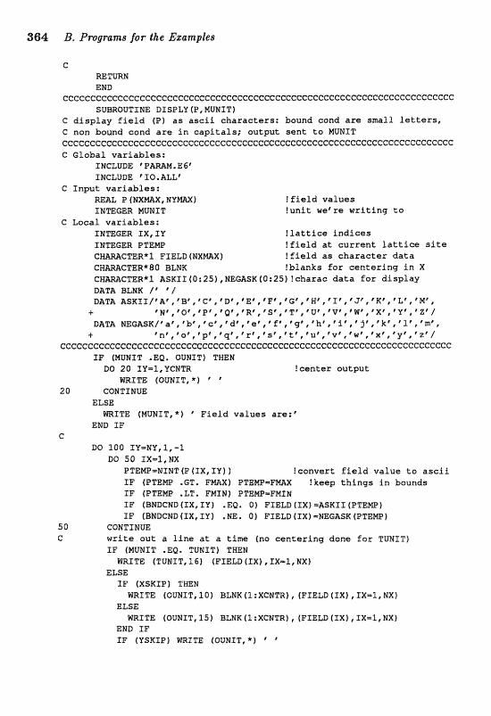
564 13. Programs for the Es~mpfeg
e =TURN EMD
cccccccccccccccceceeecccI:cccccCeccccccceccccecceccceccccececcccccccccccc SUBROUTINE DSSPLY(P,MONIT)
G d i s p l a y f i e l d (P) a s a s c f l c h a r a c t e r s : bound cond a r e sma l l letters, C non baund cand a r e i n c a p i t a l s ; ou tpu t s e n t t o MUMIT ~ c e e ~ ~ e c ~ ~ e ~ ~ ~ e ~ ~ ~ e ~ c ~ c c ~ c ~ c c c ~ c c e ~ ~ e c c c ~ ~ c e c e e c ~ ~ e e ~ ~ ~ c ~ ~ ~ e ~ e c c ~ c c ~ e ~ c ~ G Globa l v a r i a b l e s :
INCLUDE C P m M , E 6" INCLUDE 'IIO.ALLC
C I n p u t v a r i a b l e s : REAL P ( H X m X , NVW) I f i e l d vaZues INTEGER MUNIT ! u n i t weCre w r i t i n g t o
G Local v a r i a b l e s ; INTEGER IX, IY ! l a t t i c e i n d i c e s INmGER PTEWP ! f i e l d at c u r r e n t l a t t i c e site
! f i e l d as c h a r a c t e r data !b lanks for e e n t e r f n g i n X
WEGASK (0 : 25) 1 c h a r a c data f o r display DAT& BLNK / " / DATA ASKII /~A@, , "B\*C ' ,'D~C'EC,'F',CG~,~H~,rI*~pJ',pKf,'LC,'M',
4- ~H',~~','p',~q~,rptr~*S'I'T~,*U~"V~*~liJC,'x',~Y'*r~'/ DATA N E 6 9 S I C / ~ f , r b * ~ 6 " c ~ ~ d ~ , ~ f ' , ~ f * , * ~ C I C b ~ p ~ i 8 , ~ J*,pk~,fle,'m*,
+ r n f , r o f , ~ ' p * , p ' q ~ , ~ r e I ~ s C , r t ; f , * U ~ , * ~ ~ , ~ W ~ , * X ~ , ~ ~ ' , * Z ' /
cccccccccccceecccccccccccccccccecccccccceccccecccccccececccccccceccccccc I F (MUNIT .EQ. OURIT) THEN
D 6 20 IV=I,VCNTR !cen te r o u t p u t WRITE (OZJNIT, * f ' '
2 0 CONTINUE ELSE
m I T E (MUNIT,*) 'E'Fild v a l u e s arc?:' END I F
e DO f O O X V = N V , l , - 1
DO 50 IX=I,NX PTENPmWINT (P (IX, 1x1 ) !conver t f i e l d v a l u e t o a s c i i I F (PTEMP .GT, FmX) PTEMf"=FmX !keep t h i n g s i n bounds IF (PTENP .LT, FNIN) PTEIUaemFMfN I F (BMBCND ( IX, IU) . EQ. O) FIELD [IX) =ASK11 (PTEMP) IF (BNDCND (IX, IV I . NE. 01 FIELD (1x1 =NEGASK I P T e w j
50 CONTINUE C: w r i t e a u t a l i n e a t a t i n i f 3 fno c s n t e r i n g done f o r TUNIT)
IF (MUEIZT .EQ, TUNITf THEW W I T E (TUWTT, 16) (FIELD (1x1 , IX=1 , NX)
ELSE I F (XSKIP) T m N
WRITE (OUEIIT, IQ) BLNR f l :XCNTR) , (FIELD (EX) , IX=l, NX) ELSE
WRITE (OUNST, IS) BLNK (1 :XCPJTR) , (FIELD (IX) , I X = l , NXf END I F 1F (YSRIP) m I T E (QUNIT,*) '

END IF 10 FORmT (1X,A, 100 (AI, 1X) ) 15 FORmT (1X,A,100 ( A I ) 1 16 FORmT (1X, 100 (AI f 1 100 CONTINUE C
RETURN END
CCCCCCCCCCCC~CCCCCCCCCGCCCCCGCGCCGCCCCCCCCCCCCGCCCGCCCCCCCCCCCCCGGCCGCCC SUBROUTSHE GRFOUT(DEVICEpPrPGRFIrJIXIWtE)
C display contours o f the field P C the field valuas must be in an array that is exactly NX by NY; C this ean be aecamglished with implicit dimensioning which G rewires that PGRF and its dimnsians be passed to this routine ccccccc~c~cccC~cc~cccCccccccccccccccccccccccccceeccccceecccccc~cccccccc~ C Global variables:
XNCLUDE * 10,ALLf INCLUDE rFAW.E6' INCLUDE 'GWDAT,ALLt
C Input variables: INTEGER DEVICE tuhich device R&RL P (NXmX, N Y W I ffield values INTEGER MX, MY !NX and NU in dis~ise a E ; U PGRF(MX,MV) !field values for gxaphing REAL E ?energy
G Local variables: REAL 8CX (5) ,BCY (51 !corners of boundary conditions INTEGER I, IXr XY !level index, lattice indices REAL PmX, PMSU !largest and smllest field value INmGER FBG !index on boundary conditions =AL. XSLOPE, YSLOPE !slope of diagonal BC
GTER* 9 CMIN, CMX, CE !data &S chaxaeters INTEGER LMIN , LMAX, ELEN !string lengths INTEGER SCMEN !send to terminal INTEGER PAPER !make a hardcopy INmGER FILE !send to a file DATA SCREEN, PAPER, FILE/l I 2 31
c~~cc~l~c~~~c~c~eccccec~cccccecccccecccccceccccecccccccccc~~ccc~ccccccccc P W = O !set scale PMXN-P (1,I) DO 10 XXmf, M X
DO 20 IVm1, MY IF (P(IX,IY) .GT. PmX) PW=P(IX,IY) IF (P (XXI IY) .LT. PMTN) PMIN=P (IX, IY) PGRF (XX, T Y ) =l? (IX, IV) !load field into P G W
2 0 CONTINUE 10 COE3"PSNlfE G C messages fo r the i~patlent
IF (DEVICE .NE. SCmEH) mITE (OUNIT, 100) C C calculate parameters far grapking
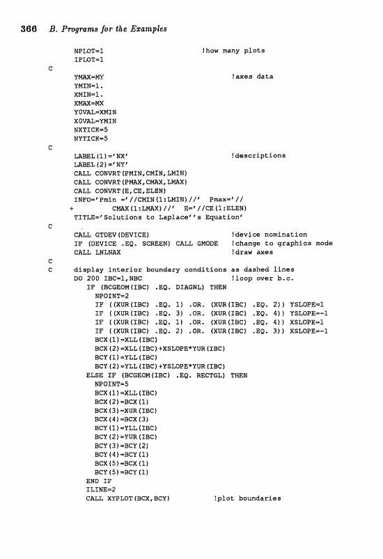
NPW'I"=Z XPMT=l
C Y m = m VHIN=1, XMIN-I . xm=m YOVAL=XMIW XQVAZ-VMZN =TICK-S HY Z15 CK=5
c =EL(l)=@WXt ! descripti ons UBEL f2)=1NY@ caLL c o ~ v a ~ (PMIN, e~xw, L n m CALL CONVRT (PW, emx, LW) CALL CQKWT (E, CE, ELEN) INFQ="Prnln IIGMXN (I : ZMLN) / / V m a x = ' / l i CMX(I:LM) I/@ E=r//CE(l:ELE%) TZTLE=eSolutSons ta Laplacee*"s Equation'
G CALL GTDEV (DEVICE) fdeviw nodnation IF (DEVICE .BB. SCREEM} CaLL GNODE !change to graphics mode GALL LNLMAX !draw axes
C C display interior boundary conditions as dashed lines
DO 200 IBC=1,NBC !loop over h.e. IF (BCGEOM (IBCf .EQ. DIAGNLf THEE RPOINT=2 IF ( (XUR (SBG) .EQ. 1) .OR. (XUR IIBG) .EQ. 2 ) Z YSLOPE=1 XF ((XURtIBC) .Ea. 3) .OR, (XUR(IBG1 .Ea. 4)) VSLOPE=-P IF ((XUR(IBG) .EQ. 1) .OR. (XUR(XBC) .EQ. 4)) XSLOPE-1 XP f (XURfZBCf .E@, 2 ) .OR. [X@R(XBC) .EQ. 3 ) ) XSLOPE=-I scx (1 =XLL (see) BCX (2) =XLL (IBCf tXSLOPErCYUR (XBG) BCY t l ) =YLL (rset BCU 42 1 =YLL (IBC) tYSLQPEXYUR [ZBC)
ELSE IF fBCGEOM{fBC) .EQ, WCTGL) THEN NPOf NT=5 sex (11 =XLL (zsc) acx (2) =sex (11 BCX (3)=XUR{IBC) BCX ( 4 ) =BCX ( 3 ) BCY (1)=VLL (IBG) BCY (2) =YUR (XBCT) BCV f 3 1 =BGY (2) BCY (4)-BCY (I) sex (5) =~cx (11 SCU ( S ) =BCU (l)
END IF ILINE=2 CALL XYPXIBT(BCX,BCY)
!how many plots
?bxtzcs data
!plot boundaries
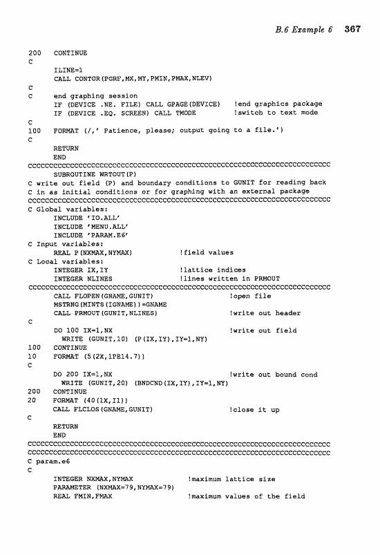
200 CONTINUE C
ILIPJE=I CALL CONTOR(PGRF,MX,MY,PMIN,P~XINLEV)
C C e n d g r a p h i n g s e s s i o n
I F (DEVICE .NE, FILE) CALL GPAGEfDEVICEf lend g r a p h i c s p a c k a g e I F (DEVICE .EQ. SCMEN) CALL TMODE ! s w i t c h t o t ex t mode
C 100 F O m T (/, P a t i e n c e , p l e a s e ; a u t p u t g o i n g t o a f i l e " ' 1 C
RETURN END
cccccCccccecccecccc3ceecccccccccccceccccccccccccccccccccccccccccccccccccc SUlEIRoUTIME WRTOUT f P )
C w r i t e o u t f i e l d (P1 a n d b o u n d a r y e a n d i t i o n s t o GUNZT fo r r e a d i n g b a c k C i n as i n i t i a l c o n d i t i o n s a r f o r g r a p h i n g with a n external p a c k a g e ccCeccccccccCcccceccccccccceccccccccceeccccccceccccccccccccccccccccccccc C G l o b a l v a r i a b l e s :
f NCLUDE 10, ALL" INCLUDE MENU. ALL" INCLUDE * PAMM. EG'
C I n p u t v a r i a k l e s : MAL e (NXWX,NYWI ! f i e l d values
G L o c a l v a r i a b l e s : INTEGER IX, XY ! f attice i n d i c e s INSPISGER MLINES ! l i n e s w r i t t e n fn PMOUT
cccccceccccccccccccccccc~ccccccccccccccccceecccccccccc"ccccccc~cccccccccc CALL FLOPEIN (GNWME, EUHIT) f o p n f i l e NSTRMC (HINTS (reNAm1 I =GNAW CALL PRNOUT (GUNIT , NLSNES 1 ! w r i t e o u t h e a d e r
c DO 100 XX-l, E X ! w r i t e a u t f i e l d
WRITE (GUN3TI10) (P(IX,IY),IY=1,NU) 3.00 CONTINUE 10 F O M T (5 [2X, ZPEl4.7) ) C
DO 200 IX=I,NX ! w r i t e o u t bound c o n d WRITE (GUNIT, 20) (BNDCND @X, IY) , TV=L, NY)
200 CONTINUE 2Cl F Q W T ( I D f l X , T Z ) f
CALL FLCLOS f GNAWE, GUNITf ! c l o s e i t up C
=TURN END
cccccccc~ccccc~cccccccccccccccccccF:ccccccccccccecccccc~ccc~ccccccccccccc c~cccccccccccceeccccccccccccccccceeccccccccccccccceccccceccccccccceccece C param.eC, C
INTEGER NXW,NYNZV(; !maximum l a t t i c e s i z e TER (NXmX-7 9, N V m = 7 9)
REIUL FMIN, FE?IAX !maximum v a l u e s of t h e f i e l d
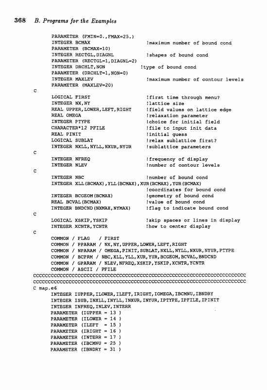
368 B. Plrograms for the E~asrtples
P W M E T E R (FMIN-O ., FE(IlLXm25 ,) INTEGER 3 C M !maximum nuniber o f bound cand P A M a T E R f B C W - 1 0 ) IWTEGER MCTGL, DIAGNL !shapes of bound cond P W m T E R (mCTGL=I, DIAGNLm2 ) IMTEMR DRCNLT,NON !type af bound eond P-METER (DRCBLTm1, NON10 ) INTEGER mXLEV !maximum nu&er of contour l e v e l s
G LETGAL FIRST 1 f i r s t t ime through menu? INTEGER NX, Nll ! l a t t i c e s i z e REAL UPPER,LQWER,LEFT,RIGNT ! f i e l d va lues on l a t t i c e edge RE= OMEGA ! re laxa t ion parameter INTEGER PTYPE !choice for i n i t i a l f i e l d CHWCTER*IZ PFILE ! f i l e t a inpu t i n i t d a t a RE% P I N I T ! i n i t i a l guess LmZCAL S U B U T ! r e l a x s u b l a t t i c e f i r s t ? XNmGER NXLL, NYLL, mUR, NVUR ? s u b l a t t i c e p r a m e t e r s
c INTEGER NFREQ !frequency of d i s p l a y INTEGER NLEV !nuWer of contour l e v e l s
e INTEGER BBC !numbe?r of bound eund
XLL (BCWI , YLL ~BCW) , XUR ( B C ~ X ) , YW (BCM leoard ina tes f o r bound cond
INTEGER BCGEOM (BCWX 1 Igeometq of bound cond a W L BCVAL (BC=) !value of bound cand INTEGER BWDCND ( M m X , M Y M X ) ! f l ag t o indicate bound cond
G LWICAL XSKIP,YSRIP ! sk ip spaces or l i n e s i n d i s p l a y INTEGER XCNTR,YCNTR !how t o c e n t e r display
c COWON / F m G / FZRST
/ NX, MY, UPPER, WmR, LEFT, RIGHT / O~GA,PINITISUB~T,NXLL,NYLL,NXUReN?IURtEZTYPE
/ NBC, XLL, VLL, XUR, VUR, BCEEOM, BCVAL, BNDGND / NLEV,WFREQ,XSKIPrVSKIPtXCNTReYCNTR
COWOR / ASCIZ / PFILE ~~~c~c~cccccc~ce~ecececeeccccccccceccccccccc~cecccccccccccccccccC~c~cccc cecccccccccr=cecccccccccccccccccccccccecccccceccccccccccccccccccccccccccc C map.e(i
INTEGER IUPPER,fLWR,fLEFT,IRIGHTtIOMEGAfIBC~UfXBEaDRU INTEGER f SUB, INXtE, INYLL, ENXUR, IWURC XPT'VPE* IPFXLE, ZPIHXT INTEGER X N F ~ Q , I N ~ V , Z N T E ; ~ P A M E T E R (IUPPER - 13 ) PAmmTER (ILOMER = 2 4 1 P A M m T E R ( T U F T E 15 1 O A m E T E R (IRIGWT = 1 6 f P W W T E R (INTERR - 1 7 1
TER (XBCMNU 1 25 1 P m M E T E R (XBNDRY = 31 1
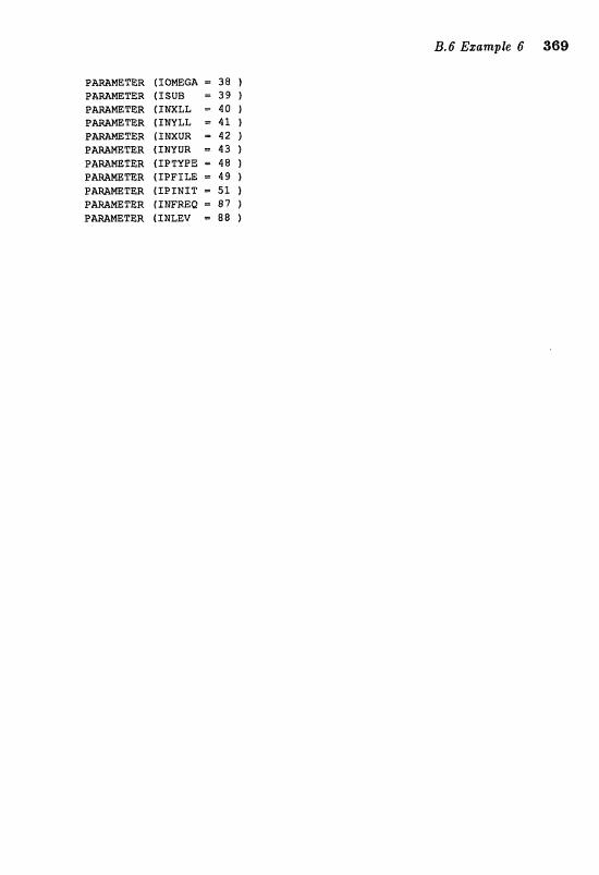
P-mTEW, (IONEGA 38 )
TER (TSUB 39 f TER (INXLL $0 ) TER (TNYLL = 41 )
P a H T E R (SNXUR = 42 ) TER (INVUR = 43 1 TER {IPTYPE 48 1
O A M W T E R f IPFILE p 49 ) P m m T E R (TPINIT - 51 )
TER (INmV = 88 )
B.7 Example 7 Algorit hrn This program solves the time-dependent Schroedinger equai tion for a particle moving in a one dimensional box (i.e., the potential is infinite at the edges of the lattice: z = -1 and I = f l), allowing for var- ious potential obstades in the bottom of the box. After the potential and initial wavepacket shape have been defined, the time evolution proceeds (loop 15 in subroutine IRCHOA). Here, the basic task is to find the new wave function at each time step by solving Eqs. (7.31,7.33) in subroutine EVOLVE using the matrix inversion scheme (7.12-7.16). For this purpose the cx and y coefficients are computed once for each value of oT before the time evolution begins (subroutine TRDIILC). At each iteration the en- ergy and normalization are computed in subroutines EEERCY and EoRmZ, respectively. Every BSTEP'~ h iteration you have the option to continue i teratiom, change DT or NSTEP, or return to the main menu.
One important physical parameter is the wavenumber ko which de- scribes the osdl&ioas of the initial wavepacket. For an iGdial Gausgian
This number fixes the energy and the momentum of the particle. (The energy and momentum of a f ree Gaussian packet are lei + 3/(402) and h@, where ti = 2m = 1. For wide Gaussians p d e t s , the dominates the energy.) KO is not entered directly, but is fixed by entering the number of cycles on the lattice, where number of cycles on the lattice equals Cl;a xlmgth of lattice f an. The m ~ m a m number of cyeles dowed on the lattice is Rpm/&, This restriction ensures that one cycle i s described by at least 4 l&tice points, and therefore the ssdlating past of the wavepaclret cm be described on the lattice.
From the discussion above, it is clew that the ;ylpropdate scale for both the energy of the particle and the height of the potential is given by kg. In addition, the size of the time step is conveniently scaled by kc2. To see this, note that the error term scales as For accurate time evolution we must have (taking H W k;) At < 1/k;, or in scded units At < 3 ,
Input The physical parameters indude the potential [square well] and the initial wavepacket shape [Gaussian]. Various analytical forms for the potential are possible (square-well, Gaussian barrier, potential step, or parabolic well), as defined in subroutine POTIITL. You must also specify the potential's center [.S], half-width at one-twentieth of the maximum 1.081, md height (in units of ~ 0 + + 2 ) [.3], as well as the I value [.S] that
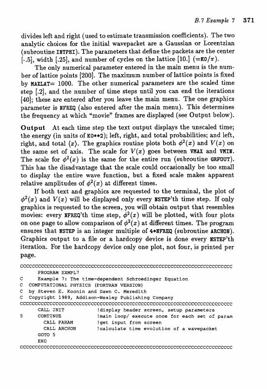
divides left and right (used to estimate transmission coefficients). The two analytic choices for the initid wavepacket are a Gaussim or Lorentzian (subroutine I ~ P H I ) . The parameters that define the packets are the center [-.5], width [.25], and number of cycles on the lattice (10.1 ( = K o / ~ ) .
The only numerical parameter entered in the main menu is the num- ber of lattice points [200]. The maximum number of lattice points is fixed by HAXLAT= 1000. The other numericd parameters are the scaled time step [.2], and the number of time steps until you can end the iterations [M]; these are entered after you leave the main menu. The one graphics parameter is EFREQ (also entered after the main menu). This determines the frequency at which "movie" frames are displayed (see Output below).
Output At each time step the text output displays the unscded time; the energy (in units of KO*.~) ; left, right, and total probabilities; and left, right, and total (s). The graphics routine plots both 42(z) and V(%) on the same set of axis. The scale for V(%) goes between and WIH. The scale for is the same for the entire run (subroutine GRFOIIT). This has the disadvantage that the scale could occasionally be too smdl to display the entire wave function, but a fixed scale makes apparent relative amplitudes of +2(z) at different times.
If both text and grqbics we rcjqucrsted to the terminal, the plot of +2(z) agd V(%) will be displayed only every rsmp'th time step. If only graphics is requested to the screen, you will obtain output Lhat resembles movies: every W F R E P ' ~ ~ time step, 4 2 ( ~ ) will be plotted, with four plots on one page to allow comparison of +2(s) at different times. The program ensures that lrsTEP is an integer multiple of 4rEFRBq (subroutine ARCHOB). Graphics output to a, file or a hardcopy device is done every w ~ m ~ ' t h iteration. For the hardcopy device anly one plot, not four, is printed pm
cccccccccccccCccccCccccccccccccc~ccccceccccccceccccecccceccccccccccccccc PROCMM EXMPL7
G E x w l e 7: The time-dependent Schroedinger Equat ion C C0NPUZ"ATIONAL PHYSICS (FORTmN a R S I O N ) C by Steven E. Koonin and Dawn C. Mereditb C Copyr ight 1989, Addison-Wesley Pub l i sh ing Company cccccccCcccccccccccceccccccccccceccceccccccccccccccccccccccccccccccccccc
CALL I N I T !dispLay header sc reen , s e t u p parameters 5 CONTINUE !main leap/ execute one@ for each set of param
CALL PAMM !get i n p u t fram s e r a e n CALL, ARCHOH l c a l e u l a t e t i m e e v o l u t i o n a f a wavepacket
GOT0 5 END
cccccccceccccccccccccccecccccccccccccccccccccccccccccccccccccccccccccccc
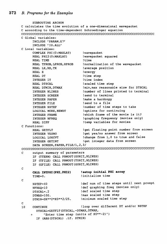
312 B. Prqgrams for .the EzampZes
SUBROUTINE ARCHON C c a l c u l a t e s t h e t i m e evo lu t ion of a one-dintensional wavepacket C according t o t h e time-dependent Scbroedinger equat ion eccceecccccccccccccceccc~ceecccccccccccccecccececcc~eeeeccccccc~cccccccc C Global va r iab les :
C Local va r iab les : COWLEX PHX ( 0 : M f r A T 1 !wavepacket m& PHI2 { Q : M U T ) !wavepackat squared RE& TIrn ! time RE& TPRQBIFS'RQB,IPPROS !normalization of t h e wavepacket REAL LX, RX , TX ?average p o s i t i o n m= E ! energy RE& DT !time s t e p XNTEGER XT !time index
DTSCAL ! scafed t im s t e p R W DTNZM,DTMAX !min,max reasonable s i z e f o r DTSCAE IMTEGER BLTMES !n&er of l i n e s p r i n t e d t o t e r d n a l INTEGER SCMEN !send t o tecminal IMTEGER PWER !make a hardcopy XNmGER F I U !send t o a f i l e INTEGER NSTEP !nu&er of t i m e s t e p s t o t a k e LOGICAL MORE,NE%BT !options f o r cont inuing XNmGER Pmm !which frame of t h e movie i s i t ? INmGEEP NmEQ !graphing f r e w e n c y (movies only) M A L DIFF ! t e v v a r i a b l e s for movies
C Functions: =L GETFLT !get f l o a t i n g p a i n t n u h r from sc reen INTEGER YESNO f g e t yes/na answer from screen LOGICAL LOGCVT l change from 1 , 0 t o t r u e and f a l s e INTEGER GETLNT !gee I n t e g e r d a t a from screen DAIIA SCWEM,PAPER,FlLE/1r2t3/
I F (TFSLE) CALL PRMOUT (SUNIT, NLINES) IF (GPZLE) CALL PmOUT (GUNIT , NLINES)
e 31rrPHX (PBX, PBX 2 ) !satup i d k i a l B= arzq
TIm-0. ! i n i t i a l i z e time C
NSTEP=40 ?def nun of t i m e ? steps u n t i l next prornpt
WFmQ=lO !def grapbing f r e q fmavies only) DTSCAL- .2 !def sca led t im s t e p
DTmX=lQO. tnax sca led time s t e p BTNIN=DX**2*KO**2/% !minimum sca led t ime s t e p
C 10 CONTINUE !loop over d i f f e r e n t DT andlor WSTEP
DTSCAL-GETPLT (DTSCAL, - r ) T W I DTMm, + ,Enter time s t e p { u n i t s of KO**-21'1
IF (ABS (DTSCALJ . LT, DTMZN f
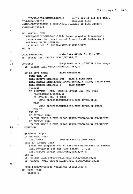
DTSCAL=SIGN(DTMIH,DTSCALf !donft let it get too small DT=DTSCAL/KO**2 !physical time NSTEP=GETIWT(NSTEP,1,1O0OtfEnter numBar of t im seepsr} NLINES=WLIMES+4
IF (NWIES) THEN . mJFREQ=GETIMT(MFREQ,P,1000,*Enter graphing f r e q e n c y ?
!make sure t h a t t o t a l nurn of frames is divisible by 4 DIFF=NOD (NSTEB "4 *NFmQj TF (BIFF .NE. Q) NSTEP=NSTEP+Q*NFMQ-DIFF
END IF
(DT) l ca1~28if;e far thia D2 IF (TFTLE) CALL TITLES (TUNXT, NLIMES,DT)
CONTINUE: !loop over sets of WSTEP time steps XP (TTERN) eau, TITLES cou~x~, WLIWESI DTI
DO 20 ImZ,]LBSWP It* ervalutf an TTH3eMm+B91 -L mOLm (PBX, PET2, Dlt ) !tee a t S m @tap a& H Q m Z (BE2, WRQB, m O B , ZERQB, U, m, m) t cralc a o m
(PBX, BETP, E) ! oala enerrw
IF ((MOVXES) .AND. (NOD(IT,NFREQ) .Ea. O) 1 THEN FmE-MOD (ITt WREQ, 4 1 IF fF .EQ, 1) TmN
CALL GRFQUT (SCREEMrPWI2, TIME, TPROBI TXrEI ELSE
C a L GWSEC (SCREEN, PN12, TIW, TPROB, TXI F END XF
END IF IF (TTERM) CALL TXTOUT [OUMIT,E, TTm, LPROI3, WROB, TPRQB, LX, RXr TX,HLIWES] IF (WILE) CALL TXTOUT (TUMIT, E, TIME, LPROB. RPROB, TPRQBC LX, RXe TX, HLINESl
C O N T X m
graphics autpue IF (MOVIES) THEN
CALL TMQDE tawitch back to t ex t made ELSE ZP (GTEM) THEN
print aut graphics now i f t e x t was being sent t a screen CALL PAUSE ( * t o see t h e wave packet . . , ' ,l) CALL GRFOUT (SCREEN, PRTZ, TIME:, TPROB, TX,Et
END IF IF {GFSLE) CALL GRF6UT (FILE, PHI2, TIMEr TPROB, FX, P,) IF (GRRDCP) CALL GRFOUT (PAPER, PN12, TINE* TPROB, TX, 8)
MORE-LOGCVT (YESNO (l., Continue iterating?' f 1 IF (MO=) THEN
NLINES-Q
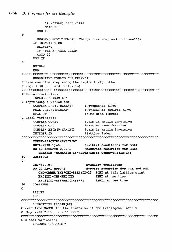
3"1 4. Programs for the Ezanzples
IF (TTERM) CA&& C L E m GOTO 15
END I F C
MEEDT=LQGCVT(YESNO(TpfChange t i m e s t e p and c o n t i n u e ? ' ) ) I F (NESDT) THEW NLLNESmO I F (TTERM) CALL C L m R GOTO f 0
END IF c
RETURN END
ccccccccccceccceccccececccecceccccccccccccccc~cccccccc~ccccceccccccccccc SUBROUTINE EVOLVE (PHI, PNI2, DT)
C t a k e one t i m e s t e p using t h e i m p l i c i t a lgor i thm C (Eq. 7.30-7.33 and 7.11-7.161 ccccccccecCccccccCcccccccccccccccccccccccc~cccccecccccccececcccccccceccc C Global v a r i a b l e s :
INCLUDE @ P A W . E?' C I n p u t l o u t p u t v a r i a b l e s :
COWLEX PHI (O:mXLAT) ! wavepacket ( I f 0)
REAL PHI;? ( O : m U T ) ! wavepacket swared (I/O) RE= I3T !t ime s t e p ( inpu t )
C Local v a r i a b l e s : COWLEX COMST !term i n ma t r ix i n v e r s i o n COMPLEX CHS !pa r t of wave func t ion COWLEX BETA 4 O : m L A T ) ! t e r m i n ma t r ix i n v e r s i o n IMTEGER I X ! T a t t i c s index
cccccccccc~ccccc~cccccccccecccccC:eccccccccccccccccccceccccccccccccccC:cee CQH8"rorr8*SWTM%*DX*DX/PI?C mm fmlCS-J,) =O . f i e t i a l ean&t$ons far =FA DO 10 XXmWTS-2,0, -3 Ibaward recurslion for BEFA
(lX+l) * (=E& (XX+lj -COEST*X?HX (IX+X) 1 50 COWX- C
CHT=(O., 0 . ) !bma&ny aonditions DO 20 TB-3. lfomard rao-ur~9en fez CHX and PBX
CEX 1 C X - !Cm a& thio la t t ios poinf aax (1x1 = C E Z - P ~ (ZX) !FBI at new LA- ~ n s 2 (zx) =-B {PE (xx) } **2 !BHX2 at new t ima
20 cammm C
RETURN ERD
cc~ccce~~cccccc~~ccccccccccccccccecccccccccccccccccccccccccecc~cccccccc SUBROUTINE TRDIAG (DT)
C c a l c u l a t e GAMm f o r t h e i n v e r s i o n of t h e t r i d i a g o n a l ma t r ix C (Eq* 7.30-7.33 and 7.11-7,161 Ccccccceccc~cccecccccececcccccccccccccccccccccccccccccc~ececcecccce[:cccc C Global v a r i a b l e s :
XNCLUDE 'PAmM,E7'

C Xnput variables: M U DT !time step
C Local variables: INTEGER I X !lattice index COWLEX WZERO,CQNSTl !terms in mtrix inversion M A L CONST2 !useful constant
cccccccccceccccccccccecccccceccccccccccccccccceccccccccccccccccccccccccc CWSTl--2.+2*SQRTm*DX**2/I)T CQHS2"2-+m]DX*DX*KCk*RO
{=%S) =Q. lSnikia2 ooa&it&ons for DO 20 IXmWTS-1,0, -1
u m M o w s r z - c 0 ~ ~ ~ 2 * v (1x1
20 comxm C
RETURN END
ccccccceccccCcccccccccecccccceccccccecccccccccccccccccccccc~cccccccccccc SUBROUTINE NOWLZ (PHI2, LPROB, WROB, TPRQB, LX, RX, TXf
C given PHIZ, finds left, right, and total probability of the wavepacker C as well as the average X value (left, right, and total} ccccc~ceccccccccccccccccccccccccceccccceccec~eccccccceccccccc~cccccC:cccc c Global varfbfes:
INCLUDE: "&RAM. E?' C Input variable:
R= PHI2 ( 0 : M X M T ) !wavepacket squared C Output variables:
RE& ZPROB, RPEOB, TBROB ! left, right, and total prebabilf ty -L m,RX,TX ! lef t , right, end total average position
G Local variables: INTEGER IX t lattice index
cccccccccccc~ceccecccccc~cccccccccccccccccccccccccccccecc~cccc~ccceccccc 0 . f zezo a
Lx=@ * PQ 10 XX=Z,ZMID-l lin%egxata with -l;rapaxoiderl rule
mRQmWROBf PBX2 (IX) ===+X (IX) *PBX2 (IX)
3.0 c m x m mWmmROB+BSX2 (XMZD) / Z I d w e pink i s shared bartween ~ = ~ + ~ D + P w x P (XMTD) 12 r leg% &U&& ~ i g b %
C 2 (IMID) 12 t d d a e ~ P n k oonlx&ba%ion nr;? (rms) 12
tin&sqzatsl w i k h t.rapzo&dirl rule mRQB=WROE+EHI 2 ( XX) ===+X (XX) *Pm2 (XX)
20 G O S Z X r n G
EPmB=WROB+mEOB Iteta2 pzabpbi2At:y R . Q. ) R t no tmRoB .m * 0 . ) m=m/wRQB
TX=a*WROB+U*WROB Ikotal a> 5s a neighteail a m
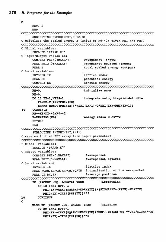
376 B, Pmlgram~ for the EgampZes
C
RETURN END
CCCCCCCCCCCCCCCCCCCCCCCCCCCCCCCCCCCCCCCCCCCCCCCCCCCCCCCCCCCCCCCCGCCGCCCC SUBROUTINE ENERC;U(PWI,PWI2,E)
G c a l c u l a t e t b a sea led energy E ( u n i t s of KQ**2) given PWI and PHI2 cecccccccccccccccccccccccccccccccccccI:ccccccccccceccccccccccccccc~cccccc C Global var iab les :
INCLUDE ' P A m , E ? ' C Input/Qutput var iab les :
COWLEX PWS (0: W U T l t wavepacket ( input 1 PE12 (0:MAXUT) ! wavepacket squared ( Input )
mA3, E ? t o t a l sca led e n e r w (output) C Local var iab les :
INTEGER IX ! l a t t i c e index m= PE] ! p o t e n t i a l e n e r w CQWmX RE ? k i n e t i c energy
~cccc~cccccc~ccc~~~ccccccececceccccccccccc~cccccecececccccccccc~ccc~cc~c BE=Q . lid;tCialine m*. BO I Q ZX=l,NPTB-1 lintblqra%a using t;rapzaiW m l s
PEmPE+V (XI) 3rpE3 (TX) m=m+CQH3(;f (F= (XX) ) * (FIJI (m-3.) -2*P85 (ZX) +PBX (=+l)
X0 cornmm rn-rn[DX**2/PtO+*2
Isrurzm ooala 1RQ**2 =TURN END
ccc~e~~~cccc~~cececcceecccccccccccccccccccccccccccccccc~ececcccccccccccc SUBROUTIRE XXVTPNI(PWf,PXI2)
C c r e a t e s i n i t i a l PHI ar ray from input parameters ccc~C~ccCc~~CcCcccc(=CcCGGeGCCcCCCCcCccccccccccC~c~cc~cCccccccCcCccCccc~cc C Global var iab les :
INCLUDE VPAW.E?' C Output var iab les ;
COWLEX PWX ( O : W L A T l !wavepacket m= PHI2 f 0:MaXLAT) !wavepacket s w a r s d
C Local var iab les : IMTEGER I X I l a t t i c e index m& NOW,LPROB,RPRBB,SQItTM !normalization sf t h e navepacket M& LX,RX, TX !average p o s i t i o n
ccccccccccccccccccccccccccccccccccccceccccccccccccccccccccccccccccceccec f Wrenit xi-
DO 10 XX=X,NBTS-3. ( s m w * n o * x (m) ) / (sx-**z+ ( X ( = ) -w0)**2)
3.0 C O H r z m C
B- XI?' (E&-T .m, aUSS) T m ! 6iruoei- W 20 n=%,wStS-l
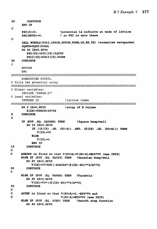
2 0 CQHTXNUE =D I F
C P H I (0) =Q. !potential io infiniLa at ends of Laktfca fPES (=PIS) -0 , f ao PIXX 18 xaro there
C: IamZ (PBX 2 , =ROB, WRQB, %Wp m, a, m] RQ
SWW=SWT (Horn) PO 30 IX=O, WTS
Pas (xx) =PHX (2x1 /SQRTB PHI2 4 PX) =PHI2 f X X ) /HOW
30 COmXEW C
RETURN END
ccccccccccccccecccceccccccccccccccccccccccececcecccccccccccccccccccccccc SUBROUTINE POTNTL
C fills the potential array ccceecccccccccccccccececcccccccccccccccccccccccccccecccccccccccccccccccc C Global variables:
IHGLUDE ' PAmM, ET" C Local variables:
INTEGER TX f lattice index cccccccccccccccccccceccccccccccccccccccccccccccccccccccccccccccccccE:cccc
S laiszax off X va2aea N+IX*I)X
C IF (pm .age sag-) T a a
D0 10 a=O,NPTS ns t t x t r x ) .a. t x o - ~ t ) .m. (x(zx) .LIE. (xo+k))f P ~ I
v trxj -vo ELSB
v (XX) -0. E m IF
X 0 CaBTf BUe C C SS i a fixed. so that V(XO+&) IDV [xO-A)=w
IF (POT .W. a V s S ) TmH tOauar~fan PO XX=O,mTS V (IX) =VO*Ea (-AaVSS* (X (1x1 -X01 **Z/A**21
2 0 CQM"L"rn C
I)(3 30 XX=OINPTS v {ZX) =W* ( X (rx) -xo) **2/~.**2)
30 CONTIHa C C RSm Star Xixscl so that: V/XOS.A).rl.-BS*VO and C V (XO-A) = m S V O (me PIIF)
E m IE (POT .%Q. STEP) T a B tgmokb r t q fanetion oa do sx=o,llinzr~
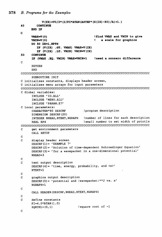
378 B, Programs for Ike Ezamples
v (XX) =vo/2* (2/PX*&Trn (AS=* [X (1x1 -XO) /A) +X " 1 4 0 coa%lm
rnD 33' G
(01 40)
DO 90 XX=l,IWPTP xle (FT(1X) .Gin!. (=l X F V f X X ] .&!l!.
50 C@mlW TF
C RETURN END
c~cccccccccccceccccccccccceccccccccceccccccecccccc~eccccccccc~cc~ccc~ccc SUBROUTINE I N I T
C i n i t i a l i z e s cons tan ts , d i sp lays header screen, C i n i t i a l i z e s menu a r r a y s f o r input paranteters ~ccccccccccccCccccccececcccccccccccccccccccccccccccccccecccccc~cC:ccccc~c C Global var iab les :
SNCLUDE "0. ALL' INCLUDE 'MENUSALL' INCLUDE V m M . E?;
C Local p r a m e t e r s : CW=CTERk80 DE5CW !progran descr ip t ion DxmHsroH DESCW (201 INTEGER NHEAD,NTEXT,NGWN !n*er of l i n e s f o r each descr ip t ion REAL EPS !small nu&er t o set width o f p o t n t l s
CCCCCC6CCGGCCCCCf=@CCCCCCCCCCCCCCCCCCCCCCCCCCCCCCCCCCCCCCCC~CCCCCCCCCCCCC C gee environment parameters
CALL SETUP c C d i sp lay header screen
DESGW ( 1 1 "EXWPLE 7' DESCWf2)m *Solut ion of time-depndent Sehroedinger Equation" DESCRP(3)r -@for a wavepacket i n a one-dimensional p o t e n t i a l i NHmDm3
C G t e x t output descr ip t ion
DESCRP (4) = "time, energy, p robabi l i ty , and €X>@ NTEXTml
c C graphics output descr ip t ion
DESGRP(5)- ' p o t e n t i a l and Iwavepackett**2 vs, X" N G W W-1
c CALL HERDER (DESCE, MWEAD, NTEXT p NGMPNI
C C def ine cons tan ts
PT=4,0*ATAN(I. 0) SQRTNI- (O,1) I s w a r e root of -1
C
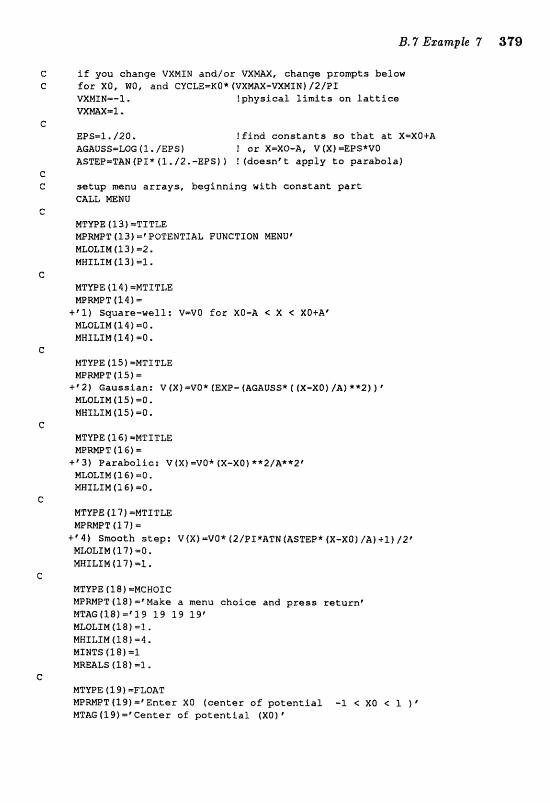
i f you change VXMIN and /o r VX-X, change prompts below for XD, %a, and GVGLEmKQ* (VXMAX-VXMXN] /2/PX VXHINm-1, !phys ica l l i m i t s on l a t t i c e VXPIAX=l..
EPS=I. /20 , l f i n d c o n s t a n t s s o t h a t a t X-XO+A AGAUSS=&~G (l, /EO% ! or XmXO-A, V(X)-EPS*VO ASTEPmTAN {PI* ( l , / 2 . -EPSlj ! (doesn* t app ly t o pa rabo la )
s e t u p -nu a r r a y s , beg inn ing wi th c o n s t a n t p a r t CALL MENU
NTWE (13) =TITLE M P W T ( 1 3 ) ='POTENTIAL FUNGTSON MEHU" MLOLIM (13) 4 2 , MNXLIM (131 =l.
MTSE (11) =MTTTLE M P W T (2.4)- +'l) Square-well: V=VO f o r XO-A < X < XO+A@ NLOLIM (141-0. NHILINfl4f -0,
MTEE (15 1 -MTITLE M P W T (3.5) =
+ " 2 ) Gaussian: V (X) =VO* (EXP- (ACAUSS* 4 ( X - X 0 1 /A I **2} j ' MLQLIM (15) =0. MWILIM (15) -0.
MTVPE (3.6) -MTITLE 1?4PMPTf16]=
+"J) Parabo l i c : V ( X f =VO* (X-XO) **2/A*"2" MWLfM (16) -0. MWXLEM (1 C ) -0.
MTVPE f l 7 1 =MTI TLE WMPT (171
+' 44) Smooth s t e p : V I X ) =V0* (2/PI*ATN (ASTEE* (X-X01 [A) + I ) / 2 f MLOLTM (17) PO. mXLIM(173 =l.
MTYPE ( I 8 1 =MGWOIG WR?ilPT(18)=@Make a menu cho ice and p r e s s r e t u r n ' NTAGf28)=f I 9 l 9 1 9 19' MLOLIM (18) =l. WHXLIMfl8) =4,
( l a ) = l MR~L5(18)-I,
NTVPE (1 9 1 =FLOAT MPWT(l9f = 'En te r XO ( c e n t e r o f p o t e n t i a l -1 < X0 < 1 * MTAG (19 )= '@en te r of p o t e n t i a l (X01 "

380 B. Programs for $he Egamples
MTYPE (20 1 =FLOAT W m T (20) -"nter A (half width sf one-twentieth max) @
MTAG (201 Half-width of potential (A) MLQLXM (20 t =so* (wmx-VXMTNI I ~ X ~ T MHXLIM(20) = (VXW-VXNIN} *ha, MRMLS (20) = (VXmX-=MINI /25,
MTYPE ( 2 1 ) -FLOAT MPRMPT(Zll=eEnter V0 (height of potential in units of RO**2)' NTAG (21) r f Height af potential VQ funits of KO**2) MzoLxn (21 I =-loo, MHLLTM t21)=100.
MTWE (22 ) =FLOAT m m P T (22) =
+ 'Enter XMTB which separates right from left (-S C XMZD C 1)' HTAG (22) -'middle X value' MLOLX M (22 ) =mMLN MHILXM (22 f =V"
LS (22 f =WMXN+ J* (V
NTYPE (23) =TITLE WRMPT (23 J =' Wh-PACRES ml(fU* MLOLX M C23 1 92. NWTLIM (231 -1.
MTYPE (251 =MTITLE W M T (251 =
+* 22) Gaussian: PHI ( X f =EXP (I*KO*XJ *EXP t- (X-WO) **2I2/STGM**2Ie MLQLXM (251 -0. MHTLIX (25 1 -1,
NTUPE (26) =MCWOIC NPmT(ZC)='Nake a menu choice and press returne MTW (26) 1' 2'7 27@ NLOLIM (26) -h. MHTLIM (261 =2. MINTS (26) -2 MREALS (261 -2.
MTYPE (27) =FLOAT
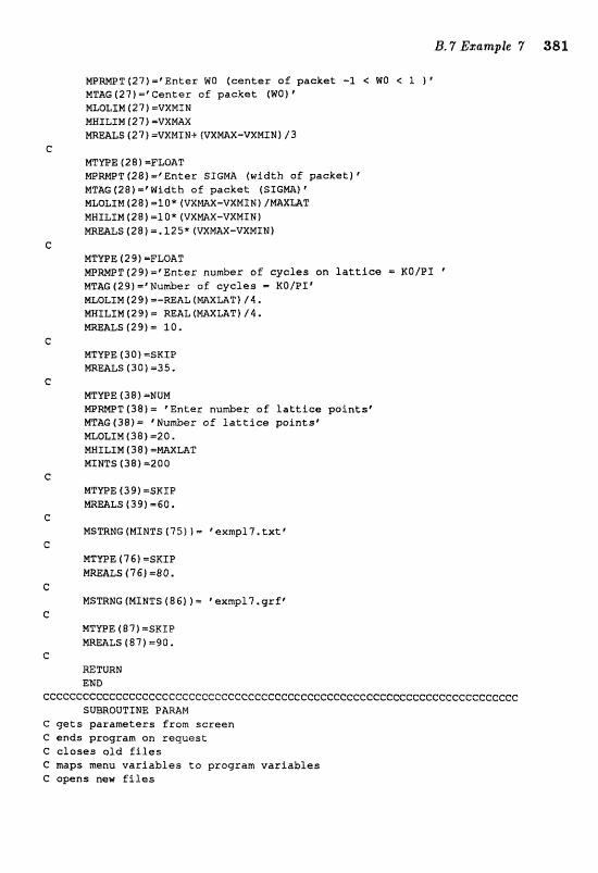
HPRMPT(27f = ' E n t e r W O ( c e n t e r o f packet -1 < WO < 1 ) '
MTAG (27) PVeentr of packet (WO} ' HLQLIM (27) =VXMTN MWILIM 2 '2 ) =VXMAX mEALS (27) =VXf?lf N+ (CrXlr9AX-VXMIN) /3
C MTmE (28 1 =FLOAT MPMPT (28) ='Enter SXGMA (width of packet) MTAG (28) mrNidth of packet (SZGM) ' MLQLIPI (28) = l 0 * (VXfiLAX-VXMIMI /MIXmT MHXLXM (2s =l o* ( V X ~ - V X M S N I M W L S (28) =. 125* (vXMAX-VXMINZ
C MTYPE f 29) =FLOAT MPWPT(29)ofEnter number sE c y c l e s on l a t t i c e KOIPI ' MTBG t29) ='Number of c y c l e s = KO/PIr MLOLIM f 2 9) =-REAL (P4AXLAT) / 4, MHILIM(29)m REAZ(MAXLAT1 f 4 . rnE&LS(29)= 10.
C MTYPE { 3 0 1 =SKIP mEWLS (30) =35.
C MT'YPE (38 1 =HUM MPWPT (38) = ' En te r nuarber o f l a t t i c e p o i n t s r MTAG(38)- 'Humber o f l a t t i c e p a i n t s t MLOLIM(38) 420. MNILIM (38 1 =mXLAT HINTS (38) =200
C MTVPE C391 =SKIP m m L s ( 3 9 ) =so.
C NSTRMG (MfNTS (75) 1 = @ eexmpl7, t x t '
C NTVPE (7 C) -SKIP
C MSTRHG(MINTS(86))= %exmp17.grff
C MTVPE (871 =SKIP MREALS (87) -90,
62 RETURN END
cc~~eccccccceccccccI:ccccceeeeccccccccccccccccccCccccCc~ccccccccccccccccc SUBROUTXNE PARAM
C g e t s p a r a m e t e r s from screen C ends program on r eques t €! c l o s e s o l d f i l e s C maps menu v a r i a b l e s t o program v a r i a b l e s C opens new f i l e s
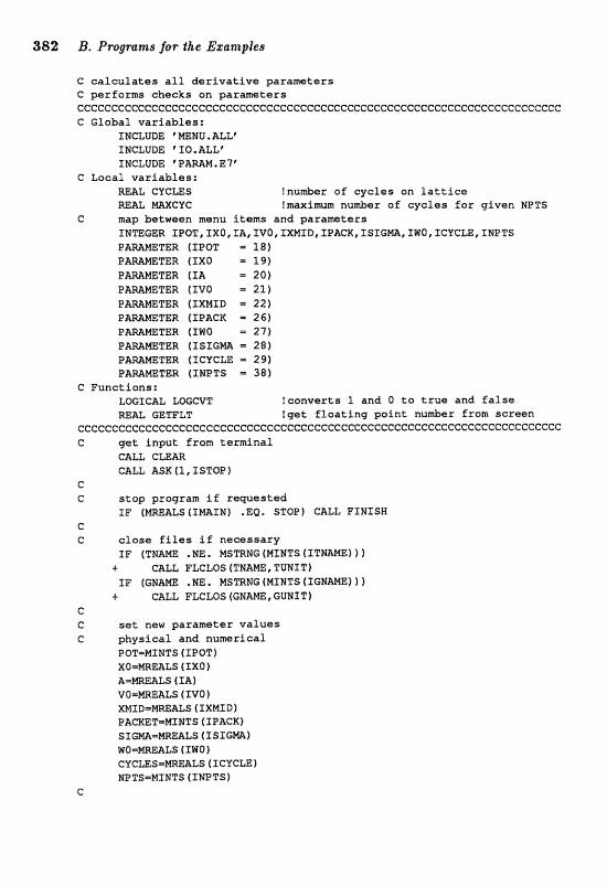
381: B. P~.sgrams for .the Exgmples
C caleuZates all derivative parameters C performs checks on parmeters cccccecccccCccccccceeecccccccccccecccccccccccccccecccccccccecccccccccecc C Global variables:
INCLUDE @ =MU. ALL' INCLUDX.: *IIO,ALLf INCLUDE VPABAM.E7f
C Local variables: =L 611CmS !nu&er of cycles an lattice mAL m C U e !maximm nuder o f cycles for given HPTS
C map between menu items and paramters INTEGER ZPOT, IXO,lA, IVO, TXMID, EPACK, XSfGMAI IWQI ICYCLEt XNPTS PAWNETER (IPOT 181
TER ( I X Q = 19) P-METER (IA = 20) PAWETER (XVO = 21) PmMETER (IXNTD - 221
TER (XPACK - 26) TER (IMO = 27)
( I S I G M .= 28) P A M m T E R (TCVCLE - 29) P-METER ( INPTS = 3 8 )
C Functions: LOGICAL L m C V T !converts 1 and O to true and false m A L GETFLT !get floating point nu&er from screen
ececccccccecccccc~ccccC:cccccccecccccccccccccccccc~ecccccc~c~cccccccc~c~cc C get inpu t from terminal
CALL CLEAR CALL ASK f l, ISTOP 1
C C stop program if requested
f F (=&L$ (ImIN) .Ea. STOP) (=ALL FJNXSH C G close files if necessary
IF (TB= .NE. M S a N G (MINTS (ITNAME) )) t CALL FLCLOS [TNhME, TUNIT1 IF ( G R M . NE. MSTRNG (MINTS ( IGgME) I I
t C A U FLGLOS (GNAME , GUNIT 1 C C set new parameter values C physical and numerical
POT-MINTS ( IPOT) xa=cMREaLs (rxo I
VG-MREALS ( IVQ ) XMTD-mALS ( IXMf D 1 PACKETmWINTS (ZPACK) SIGmmMREALS ( I S Z G M ) wommats irwo) GYCLES=NREALS(ZCYCLE) NPTS=WIMTS ( INPTS)
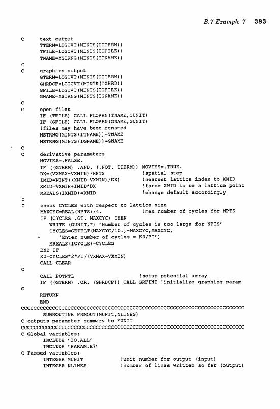
c t e x t output TTERNmLOGCVT (MXNTS (ITTERM) ) TFIM=L~GC~T~MIMT~(~TFI:LEII TNME-MSTRNG(NINTS(ITTJAtriEl}
C C graphics output
GTERM=LGGCVT(MINTS(TGTERMll GHRD~P-L~G~VT(MXNT~(IGHRDI) c F x m = L o c c v T (MINTS 4 IGFILE) 1 GN~E=MSTRNG(MINTSlXGNAKE~ 1
c C o p e n f i l e s
I F fTFILEf CALL FWPEN (TNAME, TUNIT) XP ( E F P M ) CALL FWPEN (GNAME, EUNI T) ! f i l e s may have been renamed MSTRNG (MINTS (ITN=) 1 =THAW MSTRHG (MINTS ( I G H A m l l =GFJAME
c C d e r i v a t i v e parameters
MOVIES=.FALSE, SF ((GTERM) .&RD. (.NOT, TTERMII MOVTES=,TRUE. DX= (~XMAX-WMIW 1 /NPTS ! s p a t i a l s t e p IMXD-HINT~(XM~D-~XMIN~/DXI !neares t l a t t i c e index t o XNXD XNID=mIN+INXBxDX ! fo rce XMID t o be a l a t t i c e po in t
LS (IXMID) =XMID lehange d e f a u l t accordingly C C c h e ~ k CYCLES with respec t t o l a t t i c e s i z e
MRXCYC=WAL (NPTS f /4. I m x nuntber of c y c l e s f o r NETS IF (CYCLES .GT. mxeue) Twaw
m Z T E (OUNIT,*) @Wumlt>er of cyc les is t o o l a r g e f o r NIPTSf CYCLES=GETFLT(~CVC/1O0,-MAXCYC,MXCVC,
-I. "nnte ru&er of c y c l e s K O / P I t I MmALS(ICVCLE)=CVCLES
END I F ROmCYCLES* 2*PI / (VM&X-VXMIN} CALL CWAR
c CALL POTNTL ! s e t u p p o t e n t i a l a r r a y XF ((GTERM) .OR. IGHRDCPI) CALL GRFINT ! i n i t i a l i z e qrapbing param
c MTURN END
cccccccccccccccccceeccccccccccccceccceccccccccccccceccc~cccecccccccccccc SWROUTINE PRMOUT (MUNIT, NLTNES)
C o u t p u t s parameter sumary t o MUNIT c~ccceccccccccccc~e~cccccccc~eccccccccccccccccccccccccc"ccccccccccccccccc C Global va r iab les :
INCLUDE TO, ALL" SNCLUDE C PAMM . E7 '
C Passed var iab les : fNTEGER NUHIT INTEGER NLTMES
!un i t nu&er for output ( inpu t ) !muder of l i n e s w r i t t e n s a Ear (output)
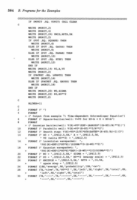
384 B. Pragrams for the EsckmpEes
cccccee~ccccccecceccccceeccccceccececcccccccccccccccccccccceC:cccceecccee IF (MUNIT .E@, QUNITl GALL CLEm
C mTTE (MUNIT,2) mITE (MUNLT,4) WRITE (MUNST, 24) X&TIZ,NPTS, DX kJRTTE (NUNIT,2) SF (POT ,EQ. S B U m ) THEN HRITE (MOMXT, G)
ELSE IF (POT .Ea. GAUSS) THEN WRITE (MUNIT, 8)
ELSE IF (POT .EQ, P A W ) THEN WaZTE (WNf T, lOf
ELse aF (par .EQ, STEP) THEN m S T E (NUNIT,12)
END TP @RITE (MUNIT, 14) XOIAIVO WRITE (MUHIT, 2) IF (PACKET .ea. LQRHTZI THEN lriIRITE (MUNIT, 16)
ELSE IF (PACKET .EQ, C;AUSS) TWN MlRITE (MUNIT, 182
END IF mETE (MUNIT, 201 WO, SIGm mITE (HUMXT, 22) KO, KO**2 WRITE fMUNX1,2)
e EIEINES-11
e 2 FOWZt (' C 1 4 F o m T
C (I Output from example 7: Time-dependents Schroedinger Equationr> 6 F Q W T t t Square-barrierlwell: V=VO fo r XO-A < X XO+Afj 8 F O W T
+ Gaussian barrrierlwell : V (X) =VOX (BP- (AGAUSS* I (X-XQ} /AI **21 I 1 f 0 F O W T (' Parabolic we1 L: V ( X ) =VO* (X-X0) **2/&**zr 1 12 F O m T ( q m a o k h step: V (X) =+(I* (Z/PI*ATN (ASTEP* ( X - X 0 1 /A} +l) /2 * 1 14 FQWT('XXO=\1PE12.5,5X,'kAf,lPE12,5,5X,
C V0 (units KOX*2) = f,1PE12.5) 16 FORMAT (' Larentzian wavepacket: * ,
+ * PHI (X) =EXP (x*K~*x] / (SIC;M**~+ (X-WO) **a 1 18 FORmT ( * Gaussian wavepacket: I ,
+ 'PHI (X) =EXP (I*KO*X) *Em f - [X-MO) **2/2/SIGm**2) ' ) 20 FORWT ("WO = ' ,lPE12.5,5X, SIGMA = ", IPE12.5) 22 FORPllAT (' KO - * , lPEIZ,5,5X, F KO**2 (energy scale) = f , fPE12 .S) 24 FQ~T('XXNPDDUe9r1PE12rStSX,@NPTSPf,15r5Xe
C space step = ',1PE12.5) 26 FORMT (18~,%ener~\r9~,~p~:ababi2.ity~,19X,'~x>~l 28 FORE'lZlT (?X, 'time*, ?X, C KO**2 ' , 5 X 9 F left.@, 3X, ' rightp, 3 X C I total8 , l i X I
+ "eftf *4X, "rightf, 4X, "total") 30 PO-T (?X, L=--\ ? X , "-----I, 5x, f ----I, 3 x , ----W' , sx, ----W-' , GXt
+ r - - - -@, , q ~ , l&, F ---& f
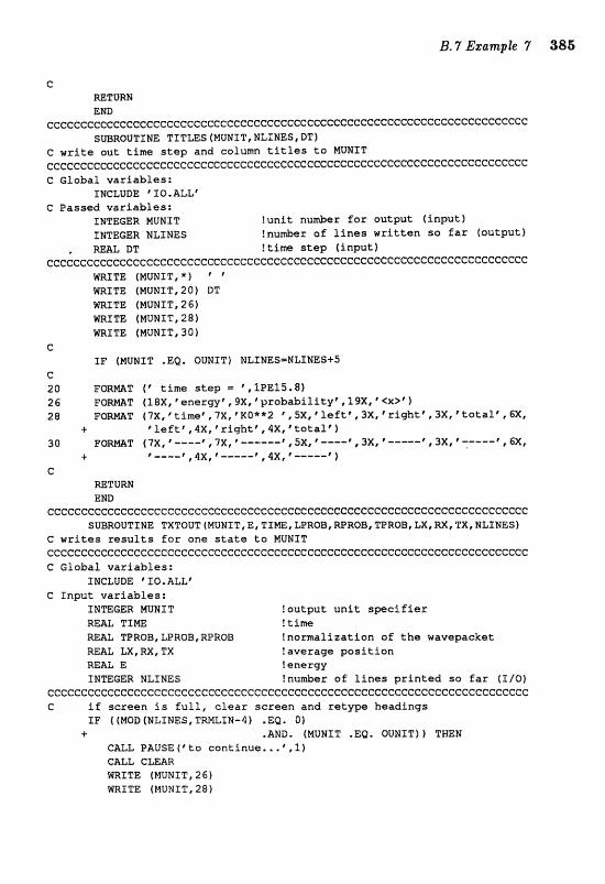
c =TURN END
~ c c c ~ ~ ~ ~ c c e ~ ~ ~ e ~ c c c ~ ~ ~ e ~ ~ ~ ~ c ~ e ~ c ~ c c ~ ~ e ~ c c ~ e c ~ e ~ c ~ c e ~ ~ c c c c c c ~ c c c c c e c c c c c c SUBROUTINE TITLEs(MuNIT,WLTNES,DT)
C w r i t e o u t t im step a n d column t i t l e s t o MUNXT ccc~cc~cc~cccc~~ce~~ce~ce~cccccccccccccccecccccccccccccecccccccecccceccc C G l o b a l v a r i a b l e s :
INCLUDE "0. ALL" C P a s s e d v a r i a b l e s :
INTEGER MUNIT ! u n i t n u d e r f o r o u t p u t ( i n p u t ) INTEGER NLIMES ! n u b e r o f l i n e s w r i t t e n s a E a r ( o u t p u t )
, RML DZ" ? t i m e step ( i n p u t ) c~ccc~~~~~~c~~cec~~~cccccccccccceccecccccecccc~ccceccccc~cccc1ccccccccccc
WII;ITE (MUNIT,*) ' WRXTE (WUNTT,20f BT W I T E (MUNIT, 26) MR5Z"E (MUMIT, 28) mSTE (MUNIT, 30)
c IP (NUNIT .EQ. OUNITf NLINES=NLINES+5
c 20 PORmT f p t i m e s t e p = \ IPEl5 .8f 26 F O W T (18XI*energy',,3X,fp~obabf3.Zt:yf,19X,*~~~'~ 28 FORmT (?X, ' t ime" ?X, 'K0**2 rSX, " e f t * F ,JX, r i g h t ' , 3X, @ t o t a l * , 6X,
+ g l e f t r ,4X, * r i g h t t , 4X, ? e o t a , l t 1 30 PO-T (TX, # ?X, - - - - - - I , f ix, ---I@, 3X, -----P, 3x, * ----S-@ #
+ r ,,- ...r 4 ~ , "--..--C , 4 ~ , 6 t e
rnTURN END
CCCCCCCCCCCCCCCCGGCCCCCGCCCCCCCCCCCt:CCCCCeCCCC:CCCCCCCCCCC"CCCCCCCCCCCCC~C SUBROUTINE TXTOUT ( M U N I T, E, T I W , LPROBI RPR6Bt TPROB, LX,, TX, MLXNES}
C w r i t e s r e s u l t s f a r o n e s t a t e t o MUNIT ccccccccccccc~cc~cc~ccC:ccecccc~ccccccececcccccccecccccccececcceccccccccc C G l o b a l v a r i a b l e s :
INCLUDE "IO.ALL1 C I n p u t v a r i a b l e s :
INTEGER NUNTT ! o u t p u t unit s p e c l EIer REAL TXNE ! t;im
Z"PROB,LPRQB,RPROB ! n o r m a l i z & t i o n of t he w a v e p a c k e t REAL LX,RX,TX ! a v e r a g e p o s i t i o n REAL E !energy INmGER NLTNES ! n u n b e r of l i n e s p r i n t e d s o far II /O)
CeecccccccccccccCceccccccccceccccccccccccccccccccccccccccccccccccccccccc C i f s c r e e n is f u l l , clear s c r e e n and refype h e a d i n g s
IF ( (MOD (MLTNES, TRHLIN-4) .EQ, 0) + .AND. (MUNIT .EQ. OUNIT) ) THEN
CALL PAUSE: 4 @ t to c o n t i n u e . . . \ ,l 1 GALL CLEAR @RITE (MUNTT, 26) m I T E ( M V N I & , 2 8 )
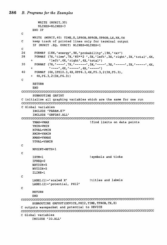
386 B. Programs for the Bgamples
mITE (MUMIT, SO) MLINES=NLf NES+3
END IF G
mITE (MUNXT, 40) TIME, E, LPROB,WROB, TPRQB, =,W, TX C kaap track o f printed lines only Tor terminal output
IF (MUMIT .EQ. OUNIT) NLINES-NLINES+1 G 26 F O m T ( I S X , r e a n a ~ " l S X , @ p r ~ b a b i l i t y f C 1 9 X 1 7 ~ < ~ ~ ~ ) 28 FORmT f 2 X , time 7X, KRO**2 ', S X , * leftc, 3X, ' rightp, 3X, tc)taIt I 6X,
+ tllaftf ~ 4 X , r r i g h t ~ r 4 X t @ t ~ t ~ 1 f 1 30 FQRmT (?X, ' ----m\ ? X , ------t, 5)E, 8 - - - - I I 3 X t f - - - - - F ,3X,
1 m, .c l ,4X,f-----t,4X,t-----f 1
40 F O M T (4X,1PE10.3,4X,0PF6,3,4XIF5.3,2~3X,]F5.3~, + 4X,F6.3,2 {3X,F6.3) )
c WIfURH END
cCccccccccc~eccccccccccccceceeeccccccceecee~cccccccccecceccccecccccecccc SUBROUTINE GWINT
C initialize a12 graphing variables which are the same far ane sun ccccccceccccccecccecccceC:ceccccccccccccecccccceccc~ccecccccccccccccccccc C Global variables
INCLUDE @PAmIVI.E7" INCLUDE GRFDAT .ALLe
ccccccecceeccecececcccccccccc~eeecccccC:ccccccccececceccccccccccccccccccc Y W - V W !find limits on data pafnts W 1 N=Wf N X OVUmVNXN XMIN=WWTN X W = r n r n UI)VAL=VXE"IJN
e WPOINT=NPTS+l
G x s m = ~ IFmB=O NXTICK-5 MYTICKm5 ILINE=I.
c ME1EL (I ) =' scaled X* ?titles and labels MBEL (2) ="otential, PMI2*
e =TURN END
~~ecee~~~cecc~cccccccc~c~eecc~ec~cccccccccccececcecccc~cccce~~~ccc~eec1ec SUBROUTINE GRFOUT (DEVICE, PHJ2, T1mI TPRQB, IIX, E)
G outputs wavepaeket and potential to DEVfCE c~~e~c~e~~~c~e~c~~ecccc~~cccc~c~~~c~cccccccccce~ccceccccccccecccccceccc~ C Global variables
INCLUDE pIO.ALL"
!sy&ols and ticks
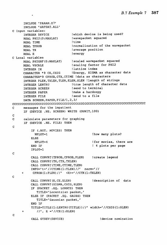
INCLUDE C PAMM . E7 ' INCLUDE * CWDAT . ALLt
e Input v a r i a b l e s : INTEGER DEVICE !which d e v i c e is b e i n g used? ~ A L PHI^ ( O : ~ X ~ T I !wavepacke t s q a r e d
TINE ! t i m e W f i TPROB ! n o m a f i z a t i o n of t h e wavepacke t
REAL TX ! a v e r a g e p o s i t i o n REAL E ! e n e r w
G L o c a l v a r i a b l e s REAL PNTGRF(O:mXUT) ! s c a l e d w a v e p a c k e t s w a r e d RE& VSCALE ! s c a l i n g f a c t o r f o r PHI2
INTEGER XX ! l a t t i c e i n d e x CH-CTER "9 CE, CSIG !Energy, SIGM as c h a r a c t e r d a t a CMmCTER*9 CPROB,CTX,CTINE ! d a t a as c h a r a c t e r s INTEGER PLEN,TXLEN,TLEN,ELEM,SUN ! l e n g t h sf s t r i n g s ZMTeGER LENTRO ! t rue l e n g t h o f c h a r a c t e r d a t a SMTEGER SCREEN !send t o t e r m i n a l INTEGER PAPER ! m k a a h a r d c o p y INTEGER FILE ! s e n d t o a f i l e DATA SGREEM,PAPER,PILE/1,2,3/
cCccCccc~ceeecccc~cccccccccC:cc~ccccecceccceecceeecccccccccceeceeccccccce G m e s s a g e s f o r the i m p a t i e n t
I F (DEVICE .NE. SCREEN) WRITE (QUNST, 100) C c2 c a l c u l a t e p a r a m e t e r s f a r g r a p h i n g
I F (DEVICE .NE. FILE) TWEN C
IF (.NOT. MOVIES) TWEN NPLOT=1 lhow m n y p l o t s ?
ELSE NPLOT=4 ! for movies , t h e r e are
END fE ! 4 p l o t s p e r p a g e I P ~ T = X
CALL GOWRT (TPROB, CPROB, P L W l create l e g e n d CALL CONVRT (TX, CTX , TXLEM 1 CALL CONVRT fTINE,CTINE,TLEEJj IWFO-' t=V/CTTME (1 ; TLENI I " / p norm-' l /
+ GPROB(l rPLEN) / /V<X>='/ /@TX(l:TXLEN) C
CALL CQNVRT (E, c ~ , ELEM) ! d e s c r i p t i o n o f data GALL COMVRT (SICMA, CSIG, SLEM) XP (PACKET .EQ, LORNTZf TEEN
TTTZE='Lorentzian p a c k e t , ' ELSE I F (PACKET .EQ. GAUSS) THEN
TITLE=fGau%sfan p a c k e t , " END I F TITLE=TZTLE (l: LENTRU (TZTLE] b / / I width= ' //CSIG f l :SLEN)
4- / / I , E =I //CB (I:ELEN) e
GALL GTBIEV (DEVICE) ! device nomf n a t i o n
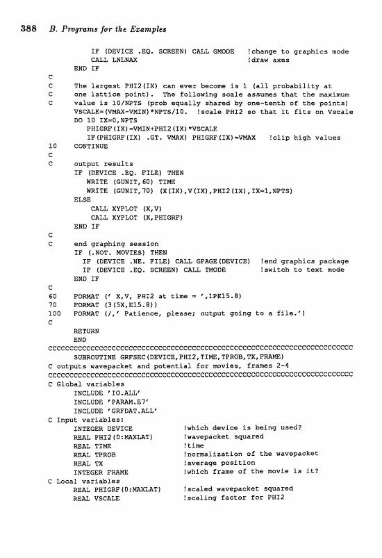
IF (DEVICE .EQ, S a E E M ) CALL GMODE !change to graphics mode GALL LNLNAX !draw axes
END IF c C The largest PHI24XX) can ever become is 1 (all probability at C one lattice point). The following scale assumes that the maximum C value is 1OINPTS (grob equally shared by ane-tenth a f tbe points]
VSCALE=(VIVYIX-VMXN~*NPTS/lO. fseafe PM12 sa that it fits on Vscale DO 10 TX=O,NPTS
PHIGRF (SXI = w r ~ + ~ ~ s z ~ S X ) *vscaLE IF (PHIGW (XX) . GT. V=) PHZGRF ( I X ) - V W I clip high values
10 CONTINUE e C output results
XP (DEVICE .EQ, FILE) THEN @RITE (EONXT, GO) TINE m S T E (GUNZT, 70) fX (XX) ,V (1x1 ,PHI2 ( I X ) , IX=l,HPTS)
ELSE CALL XUPLOT (X,V) CALL XYPLOT (X, PWIGRF)
END I F e C end graphincg session
XE" ('NQT. MOVIES) THEW IF (DEVICE .HE, FILE) CALL GPAGE(DE;VIGE) tend graphics paekat~e S F (DEVICE .EQ, SCMEN) CALL TMODE !switch to text node
END XF C SO F O W T f ' X,V, PMS2 at time = * 6,1PE/5-8) 70 F O m T (3 (5X,E15.8) 1 100 F Q M T (/, Vatience, please; output going to a file, ' 1 C
=TURN END
~cccc~~ccc~cCcccecceceecccccccccccccceccccccceccccccccccccccecccccccccce SUBROUTIM GRFSEC (DEVICE, PHI2, T I m , T X ,
C outputs wavegaeket and potential for msvlas, frames 2-4 e~~c~~~~~c~~~c~ccccc~eccccceccc~c~ccecc~c~ceccccc~cccc~c~ce~ccc~cccccc~e C Global variables
INCLUDE @ITQ,AZLt ZNCLUDE ' P m M , E 7 ' INCLUDE ' GWDAT . &LF
C Input variables: XNTEEER DEVICE ?which device Ss being used7 REAL PHI2 (0:MAXLAT) fuavepaeket squared WAT T X a !time M f i TPROB !narnalization of tka wavepacket M U TX !average position INllEGER F M = Iwbieh frame of the movie is it?
e Local variables REAL PWIGRF (O:kIAXMT) ? sealed wavepacket squared REAL VSCALE tscalinq factor for PHI2
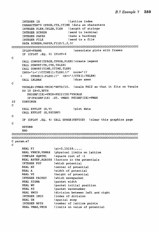
INTEGER IX ! la t t ice i n d e x CTERI9 CPRQB,CTX,CTIME I d a t a as c h a r a c t e r s
XNTEGER PLEM,TXMN,TLEN ! l e n g t h of s t r i n g s INTEGER SCREEN f s e n d t o t e m i n a l INTEC;ER PAPER !make a h a r d c o p y INTEGER FILE !send t o a f i l e DATA SCREEW,PAPER,FILE/1,2,3/
ce~cecc~ccc~eccccc~cccccccce:ceccccecccccccccccccr:ceccccccccccccccccccccc XPLOT=FmME ! a s s o c i a t e p l o t s w i t h f r a m e s I F [IPLOT .EQ. 0) IPLaT14
C CALL CQNmT (TPROB, CPROB, PLEklj I ereate l e g e n d CA& COPIIVRT (TX, CTX, TXLEN) CAm GONVRT (TINE, CTINE, TLEN) INFO=* t=* //CTIME ~I:TLE:N] / / I n o r m * / l /
+ CPRQB(1:PLEN)/If <X>='//CTX(I:TXLEN) CALL LNLNAX !draw a x e s
e VSCUE=(VPILaX-WIN)*NPTS/lO. !scale PHI2 sa t h a t it f i t s on Vseale Do 10 IX=O,NPTS
PHXGW (1x1 =VMIN+PWI~ 1x1 *VSGALE I F (PHIGRF ( I X ) .GT. V M X f PWIGRF ( I X ) = V m X
IQ CONTINUE G
CALL XVPLOT (X,V) f p l o t d a t a CALL XYPLOT (X, PHIGW)
C XP (XPLOT .Eg. 4 ) CALL GPAGE(DEVXGE1 !clear t h i s g r a p h i c s page
C RETURW END
cccccccccccccccCcccececcccecccceccccccccccccccccccccccccc~cccccccccccccc ccceceeccccCccccee~ccccceccccccccceec~cceecccccccecccccccccccccccc~cccc~ C param.ot7 c
RE& P I !pi=3.15159. . , . , MAL VXMXN,mmX ! p h y s i c a l l i m i t s o n lat t ice COPIIPLEX SQRTIJ11 ! s q u a r e r o o t o f -2 REAL ASTEP,AGAUSS ! f a c t o r s i n t h e p o t e n t i a l s IWTEGER POT ? w h i c h p o t e n t i a l =&L X0 ! c e n t e r o f p o t e n t i a l RE= A ! w i d t h o f p o t e n t i a l =U V0 ! h e i g h t o f p o t e n t i a l INPEGER PACKET !which wavepacke t REAL S I G m f p a c k a t w i d t h mAL WO ! p a c k e t i n i t i a l p o s i t i o n REU KO ! p a c k e t wavenumber M& XMXD ! d i v i s i o n be tween l e f t a n d right INTEGER IMID ! i n d e x o f d i v i s i o n
DX ! s p a t i a1 s t e p SNTEGER NPTS !number of lat t ice p o i n t s RE& =X,VMIM ! l i m i t s o n value of p o t e n t i a l
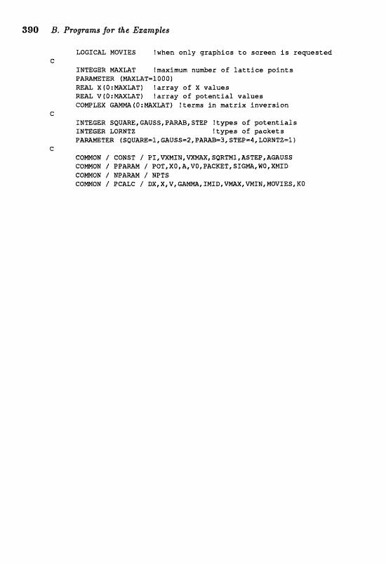
390 B, Pr~grams for the Egamples
LOGICAL MOVIES !when only graphics to screen is requested e
IWTEGER W L A T !maximum number of fattie@ points PAMmTER (mXLAT=100Q J M& X (O:mXmT) !array of X values mfi V(O:MAXLAT) tarray of potential values COWLEX GaM(O:MAXLAT) !terms in matrix inversion
C
INTEGER SQUmE,C;AUSS,PAMB,STEP Ityphs o f potentials INTEGER LORNTZ !types of packets PW1VIETER fSQPIARE=I,GAUSS=2,PARBB=3,S~P=4,LORNTZ=fl
C
COMMON / COMST / PI,VXMIN,VXM,SQRTNIIASTEP,AWUSS 6OMOH / PPWM / POT,XO,A,VO,PACKET,STGEIA,WOIMXD COWON / N P W N / WPTS COMOhl I PCALC / DX,X,V,(;IL~,IMXD,WX~VMIN~MOVIES,KO
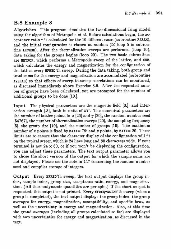
B.8 Example 8 Algorithm This program simulates the two-dimension& Ising model using the algorithm of Metropolis et al. Before calculations begin, the ac- ceptance ratio r is calculated for the 10 different cases (subroutine PARAR), and the initial configuration is chosen at random (DO loop 5 in subrou- tine nrrclroa). After the thermalization sweeps are performed (loop 10), data taking for the groups begins (loop 20). The two basic subroutines are PIETROP, which performs a Metropolis sweep of the lattice, and sm, which calculates the energy and magnetization for the configuration of the lattice every 1 1 ~ ~ w ' t h sweep. During the data taking, both group and total sums for the energy and magnetization are accumulated (subroutine AWRAC) so that effects of sweep-to-sweep correlations can be monitored, as discussed immediately above Exercise 8.6. After the requested num- ber of groups have been calculated, you are prompted for the number of additional groups to be done [IO.].
Input The physical parameters are the magnetic field [O.] and inter- action strength [.$], both in units of kT. The numerical parameters are the number of lattice points in 1 [20] and y [20], the random number seed [54767], the number of thermalization sweeps [20], the sampling frequency [5], the group size [10], and the number of groups [10]. The maximum nmber of s points is fixed by HllXX= 79; and y psints, by MAXY= 20. These
ts a-re to ensure that the charxter display of the con6guration will f i t on thc; typical scrmn whi& is 24 lines long and 80 chrxsacters ryide. If yaw t e r d n d is not 24 X W, or if ;you won't be displaying the csn6mra;tion, you c m adjrrst these parmeterss The text output paxrameter &ows you to chose the shod version sf the output for which the smple sums are not displayed. Please see the note in C.7 concerning the random number seed and compiler storage of iaegers.
Output Every ~m~g'tlr sweep, the text output displays the goup in- dex, sample index, poup size, abcceptasce ratio, energy, and magnetiza- tion. (All thermodynamic quantities are per spin.) If the short output is requested, this output is not printed. Every EFREQ*#SXZE'~~ sweep (when a group is completed), the text output displays the group index, the group averages for energy, magmtization, ausceptiWity, and speei3ic heat, as W& aa the u~cert;ainty in enerm and magnetization. Also, at this time the grand averages (including all groups cdcdated so far) are displayed with two uacertajlnties for energy and magnetization, m discussed in the text e
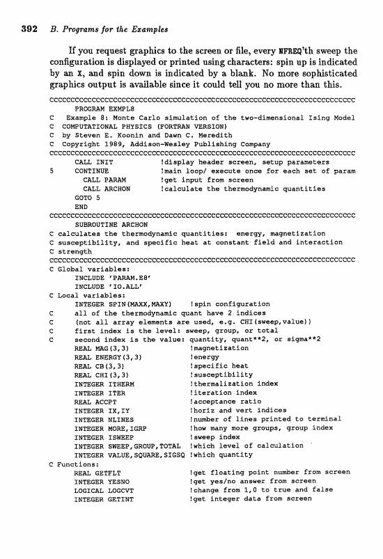
E ycru requegt g a p f i m to tohe screen or file, eveq IF RE^'^^ gweep the congguration is displayed or pinted u ~ i n g characters: spin up i s indicated by m X, and spin down is indic&ed by ib bIaak. No more sopkistica2;ed g q h i c s autput i s available since i% caufd tell you no more than this. ccccc~ccCccccccccccccecccccccccccccccccccccccccccccccccc~ccccceccceccccc
BRQC;MN EXWL8 C Example 8; Monte Carlo simulation o f the two-dimensional Ssing lulodel C COWUTATIOMAL PHYSICS (FORTmN mRSION) C by Steven E. Koonin and Dawn C, Meredith C Copyright 1989, Addison-Wesley Publishing Conrpany cccCcccecccccccCcecccccccccccccccccceeccececcccceecccecccccccecccccccccc
CALL IWIP !display header screen, setup parameters 5 CONTINUE !main loop/ execute once for each sat of garam
CALL P a M !get input from screen CALL ARCWON !calculate tbe thermodynamic -antities
GOTO 5 END
CCCCCGCCCCCCCCCCCCCCGCCCCCCCCCCCGCCCCCCCCCCCCCCCCCCCCCCCCCCCGCCCCCGCCCCC SUBROUTINE ARCHOW
C calculates the thermodynamic quantities: enerrgy, magnetization C susceptibility, and specific heat at constant field and interaction C strength cc~cccccc~ceccccceccccccccccccccceccccccececccccccccccecccccccccccccccCc C Global variables:
INCLUDE ' PARIIM, E8' INCLUDE 'IXO.A&L*
C Local variables: INTEGER S P I N ( W X , M Y ) !spin configuration
C all of the thermdynamic quant have 2 indices C (not all array elements are used, e.g. CWI fsweep,value) 1 C first indax is the level: sweep, group, or total G second index is the value: quantity, quant**2@ or sigma**2
mG(3,3) !magnetization ENERGY f 3,3 1 ! energy
RE& CB(3,3) I specific heat M A L CHI (3,31 !susceptibility TNTEGER f THEW !thermalfzation index INTEGER fTER !iteration index REAL ACCBT !acceptance ratio INTEGER IX, SY !hoxiz and vert indiees IWTEGER NLIMES D of lines printad to terminal II?JmGER MORE, Imp !how many more groups, group index INTEGER ISmEP !sweep index XNTEGER SmEP,CRQUP,TOTAL !which level of calculation '
INTEGER VALUE,SQUARE,STGSQ ?which wantity C Functions:
REAL GETFLT !get floating point nu-r from screen INTEGER YESNO !get yeslno answer from screen LOGICAL LOGCVT Ichanc~cs from 2 . 0 to true and false 1NmEER GETINT !get integer data from screen
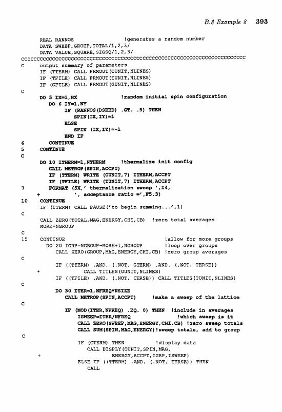
W& =%NOS !generates a randam number DATA S W E P , C R O U P , T ~ T A L / ~ , ~ ~ ~ / DATA VAGUE, S Q V m t SIGSQf 1 t 2,3f
~ c ~ ~ ~ ~ ~ ~ c ~ ~ ~ ~ ~ c ~ ~ ~ c c ~ e c c ~ c c c e ~ e c c ~ : c c ~ ~ ~ ~ c c ~ c c c ~ c ~ c c c c c c c c c c c ~ c c ~ ~ ~ c c c c c c C outwt sumary of parameters
TF ( T T E M ) CALL PMOUT (QUWXT, NLINESf XP (TFLLE) GALL PRNOUT (TUNXT, NLINES SF (GFILE) CALL PRMOUT (CUNTT, NLIMES)
e DO fi XX=Z,m lr&om initial, tspb caofAf;lura%ian
m3 6 xx=z,NV IF (D-D) .G!E. .S ) T a w
$ XI?) =l E m
SPTM (XX, m) =-a
3. l.0 comxm
IF (TTEM) CALL PAUSE ( ' t a k q l n suming . . . ' ,l) C
CALL ZERO(TQTAL,~G,ENERG?IIGHZtCB] !zero total averages MOM=NGROUP
C
15 CONTINUZ !allow for mare groups DO 20 XGmmNGRBUP-MOW+l,NGRoUP !loop over groups
CALL ZERQ(GROUP,MG,ENERCV,CMI,CBJ !zero graup averages c
XP ( ( T T E W ) .ANB. (.NOT. GTERM) .AND. (,NOT. TERSE)) + CALL TITWS(OUNZT,NLTNES)
IF ( (TFILE) -ANB. ( "NOT. TERSE) 1 CALL T I T a S (TUNZT, NLINES) G
DO !-a r #wezap of the lakLXca
C Iinclu&e in avrragea
!which s w e q is it CX,W.J Z m o (=ET?, WU2, , CRX, m) rzera meep d o t a e
S W (SE)Strl, - , E a r n ) ? eweerp total&#, rdld t o grow G
IF (GTEWl THEM !display data G U L BTSPLY (OUNIT, SPIN, MAG,
ENERGY,ACCPT,XGW,ISIEEPf ELSE SF 1 ( T T E m ) .AND, ( .NOT, TERSE) ) THEN
C a L
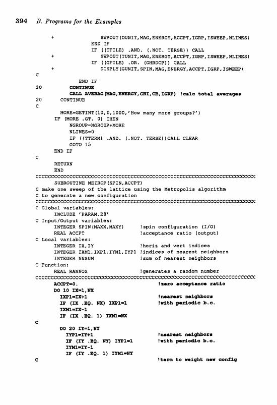
394 B, Prognrnas for the Eza~npilet~
+ SWOOUT [OUNXT, b%G, ENERGY, ACCPT, IGRP, ISWEEP, NLXNES) END I F I F ((TFILE) .AND. (.NOT. TERSE)) CALL
+ SWPOUT (TUNIT, =G, ENERGY, ACCPT* IGRPt I S m E P , N L S I I F ( ( G F I W ) .OR, (GHRDCP)) CALL
+ DTSPLY (GUNIT, SPIN, WG, ENERGYI ACCPI", IGRP, ISWE:EP) F:
END I F 30
2 0 CONTINUE e
NORE=C;ETINT (10,0,1000, 'How many more g r o u p s ? ' ) SF (PliORE .GT. 0) THEN
NGRQUP=NGROUP+MORE NLXNESmO SF ( (TTERMj .AND, ( , NOT, TERSE) ) CALL CLEm GQTQ 15
END I F c
RETURN END
cccccccccccccccccccccccccceccccceccccccccI:cccecccecccccccccccccccccccccc SUBROUT1 WE METROP (SPIN, ACCPT)
C make one sweep of t k e lat t ice u s i n g t h e M e t r o p o l i s a l g o r i t h m C to g e n e r a t e a new c o n f i g u r a t i o n ccF:cCcccccccccCccccccccccccccccccccccccccccccceccccceccccccccecccecccccc C G l o b a l v a r i a b l e s :
INCLUDE 'PMM.E8 ' C f n p u t / O u t p u t v a r i a b l e s :
INTEGER SPIN (mXX, mXY) ! s p i n c o n f i p r a t l a n f I l O ) REAL ACCPT ! a e c c g t a n c e r a t i o (ouCput )
C Local v a r i a b l e s : XNmGER XX, SV ! h o r i z a n d v e r t i n d i e e s INTEGER IXMX,IXP1,XYM1,IYP1 ! i n d i c e s o f n e a r e s t n e i g b b o r s INWEER NNSUM !sum o f n e a r e a t ne2ghbors
C F u n c t i o n : M& MNNOS ! g e n e r a t e s a random R U ~ T
cccc~ccc~cce~~c~ccccceccc~cceecccccceccc~ccccccccccc~ceecccccccccccccccc X-%=@. 8~a~Gt 1QwemQII r8t%b
BC1 10 ZZ=1,= X=1==+1 I m @ r r r r t :
zx .SQ. lax) m%=% .C.
C DO 20 rx=z,m
f m1=n+1 m? {m 'EQ' m1 znz=x f rn=SY-l 38 (3V .&Q. 1) f m = W
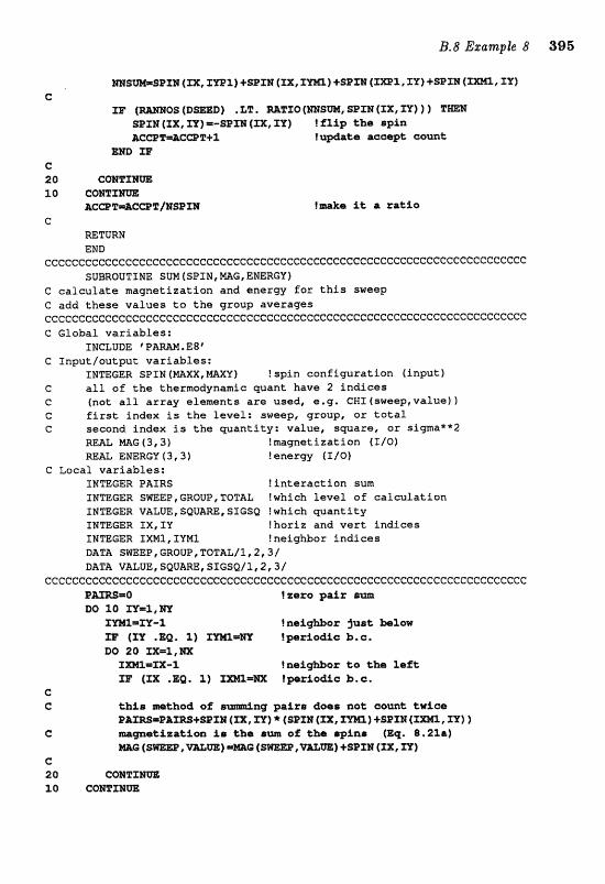
WSM=SPXB (m, IVIE"1) +WIN (ZX , Iml) +SPIlSI [Jm1, IP) +SEX8 4
(D=@) .LT. (mSUN, SPIN (f X, m) )) T m SEX% (XX, ZX) m-SPJN (m, Il'] ! f l ip t;ha apf n ACmT*CmT+1 !mdate aampe ceant:
Ism XE" c 2 Q C w x m 10 caH2mm
&CmT=ECPT/NSE"XB C
=TURN END
ccccccccccccccccccccecccccccccccccccccccccC:eccecccccccccccccccccecccc~cc SUBROUTINE SUW(SPIN,mC,RmRGY)
C calculate magnetizatian and energy for t h i s sweep C add these values to the group averages ccCccccccceccccccccecccccceccccceccccccccccccccccccccccceccccccccccccccc C Global variables:
INCZIUDE T A W . E8 ' @ Inputloutput variables:
INmGER S P I N ( m X , W V ) !spin configuration (input) G all of the thermodynamic quant have 2 indices e (not a1 l array elements are used, e.g. CWI (sweq,value) 1 C first index is the level: sweep, group, ox total C second index is the quantity: value, sware, or sigma**2
ltEG mG(3,3) !magnetization (IIO) mAL ENERGY (3 ,3 ) !energy (I/Cl)
C Local variables: INTEGER PAIRS !interaction sum INTEGER SmEP,GROUP,TOTAL !which level of calculation INTEGER VALUE,SOUAW,SIGSQ Iwhich quantity INTEGER XX, IY !horiz and vart indices INmGER IXM1,IYMl fneighbor indices DATA SWEEP,CROUP,TQTAL/1,2,31 DATA VALUE, SQUME, SZGSQ/1,2,3/
cccccceeccCCccccccccccceccccccccccccccceccecccccccccccccccccccccccccccc~ 1.0 !zero paSr a m ry=z, m
Xrn1=XY -2
DC7 20 xx=r,m X===-% !aefgmor to khe left; 33' ( X X .EQ. 1) Ipri@&c b.c.
C C this -&bed of s pairs demo not; oean& &W%-
~ a z m = ~ ~ x m + s P r w (Ex, x r ) * ( S B ~ (m, xm)+s~m (X=, =) 1 C mmmtization is the S- c i tlw wino (Eq, 8.23.a)
W ( S ~ L " , W W ] = W ( S ~ E P , W ~ ) + S P I N ( ~ , a) C 2 0 CaHIPXm 10 CQRTXBW
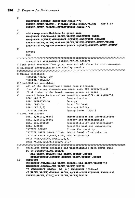
396 B. Programs for the E~ramples
C
1 !Eq 8.18
C G
G
=TURN END
cc~~le~~c~cccc~~cc~~eccec~cccce~~cccccccccececcccccccccccc~ceccccccccC:ccc SUBROUTINE AVE~G~MP*G,ENERGY,CNI,CB,IGROUP~
C find group averages from graug sums and add these to total averages; e calculate uncertainties and display results c~~~cccccccccccccceccccccccccccecccceccece~ccccC:ccccccc~cccccccccccccc~c e Global variables:
INCLUDE "&MM. E8' INCLUDE IO, ALL'
C Input/Wtput variables: C all af the thermodynamic quant have 2 Indices C (not a l l array elements are used, @.g. CNIfsweap,value)) C first index i s the level: sweep, group, or total C second index is the value: qantity, guant**2, or signra**2
REAL mG(S,31 !magnetization R m L ENERGY ( 3,3 ) !energy REAL CB(3,3) ! s~eific heat
CWT (3,3) !susceptibility INTEGER IGROUP ? group index (input 1
C Local variables: RE- M, MSIG1, MSIGZ ?magnetization and uncertainties RE& E,ESTGl,ESIG2 I energy and uncertainties REAL SUS, SUSSIG f susceptibility and uncertainty REAL C, CSTG Ispcific heat and uncertainty INTEGER IQUAMT !index the wantity INTEGER SWEEP,GROVP,TOTAL !which level o f calculation INTEGER VALUE,SQUAW,SIGSQ !which quantity DATA SbJEEP, GROUP, TOTAL/l, 2,31 DATA VALUE, SQUAm, S f GSQ/S, 2,3/
~ecccccec~cc~ccceccccecce~eccccccceccccceccccccC:c~c~ceccc~cccccceccccccc C aal-lats gzoup averamr m d m=rtalnkiarr f r o m group a m a
, XQVMT) /%SIZE
10 ) **2
CB f a O W , Vam) =BmWY {a@=, SQU-} - B m R a [mow, V U m 1 **2 E m = f a O W , SXGSQ) =C33 (aOW, VUGE} INSIZE
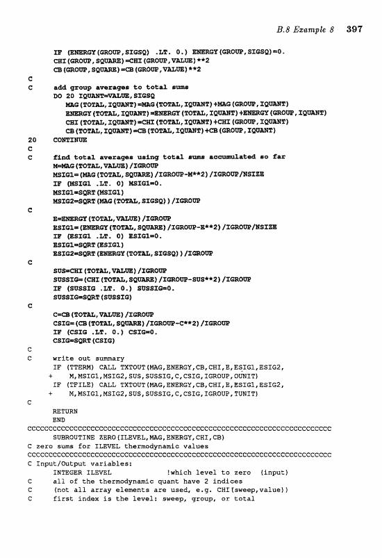
(m@=, s x a s q ) . LT. 0 , ) E ~ R G Z ( a o m , SZCSO~ =O . CBI ( CB ( a O W , SQU-) =Cl3 (=Q=, V U m ) **2
C C a& gxew avaraprs lea total smo
DO 20 1 , SZGSQ m (TOT=, I Q W T ) =m@ (ZWU, XQUMT) Ern&= ( T 0 2 U ' X Q g m ] - m m ( rnTU, X
(9?0Tm, XQBmZ) =a (TOE=, XQVmZI) +CBX (=am, XQQM5")
20 c m C C find toleal a v a r w o u s i q &eta%
(TOT=, m m ) fxmm MSZGZ= ( m ~ (TOT=, S Q U ~ ) /XWW-N**2) / I a O m / H S T Z I Z TB" ( W I G % ,W. 0 ) WXGX=O,
c , m m ) /xmm
BsrGi=.s@T ( ; e s x ~ z ) (Tap=, sxGsQ) ) lzaQm
e
sossx- (mr ( T ~ T U , s ~ o m l t x = o m - ~ u s * * 2 j I Z ~ O U I ! m ( s w s s x o .LT. 0. ) sussre-o. S V S S l * S ~ T (SUSSXO)
e
aow-c**2] /zmam flP" (CSXQ .LT. 0. ) CST(;la20, CSX-SWT ( e s x c )
c C write out s u
XF (TTEM) CALL TXTQUT(mG,&NERGY,CB,CHI,E,ES,5:G1,ESIG2, + M, MSXG1, HSTG2, SUS, SUSSIG, C, C S I G, TGROUP, OUNXT)
I F (TPILE) CALL TXSOUT (NG, ENERGY, CB, CBI , EI E 5 1 GI , ESTG2, + M, NSIG1, MSXG2, SUS, SUSSXG, C, CSXG, TGROUP, TUHXT)
C
RETURN END
cccccccccccccccccccccccccccecccccccccccccccccccccccccccccccccccccccccccc SUBROUTINE ZERO ( ILEVEL, E?IAG, ENERGY, CBI , CB)
G zero sums Ear SLEVEL thermodynamic values ccceCcccccccccceccc~cccccccccccccccccccccccccccccccccccccecccccecccccccc C Xnput/Output variables;
INTEGER XLEmL !which level t o zero (input} G all of t h e thermodynamic w a n t have 2 i n d i c e s G (not a l l array elements a re used, e.g. C H X l s w e e p , v a l u e ) f C f i r s t index i s t h e level: sweep, group, or t a t a l
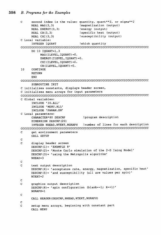
398 B. Programs for the Ezamples
C second index is the value: quantity, quante*2, or sigma**2 MA6 (3,3) !magnetization (output)
=L ENERGY (3,3) !energy {output) REAL CB63,3) ! spcific heat (output) REAL CHS ( 3 , 3 ) !susceptibility (output)
C Local variable: INTEGER IQUANT !which quantity
cccccccccccccccccceccccccccecccccccccccccccccccccecccccccccccccc~(1:cC:cccc DO 10 IQUAMT=1,3
MAG ( ILEVEL, IQUAPJT) =a. ENERGY ( ILEmL, 1QUANT)PQ. CNI (ILEVEL, f QUANT) =Q. CB (ZLEVEL, IQUANT) =Q.
3.0 CONTINUE RETURN END
ccccccceceCccccccecccccccccccceccccccccccccecccccccccecccccccccccccccc~c SUBROUTZME INIT
(1: initializes constants, displays header screen, G initializes menu arrays for input parameters cccccce"cccccccccccccecccccccceccccccccecccccccccccececcccccccccc~ccccccc C Global variables:
INCLUDE "IO,ALLt INCLUDE ' MENU. ALLt
!program description DTmNSION DESCRP (2aI INTEGER NWEAD,NTEXT,NGRBPN Inuntber of lines for each descript;ian
cccccccccecccccccccccccccccececcccccecccccccccc~ccccccccccccccccccccccc~ C get environment parameters
CALL SETUP C C display header screen
DESCRP 4 1 1 = ' EXAMPLE 8 " DESCW(2)= 'Monte Carlo simulation of the 2-43 Isin$ Model* DESCRP (3) 'using the Metropolis algorithm" NUmD=J
C C text output description
DESCW (4 ) = ' acceptance rate, energy, magnetization, specific heat ' DESCRP ( 5 ) = ' and susceptibif ity (all are values per spin) ' NTEXT-2
c C graphics output description
DESCRP f G)= * spin conf igurat i on (blank=-l; X-+l) " MGMP W=1
C CALL WEADER~DESCW,NWEAD,WTEXT,NGRAE"H~
c C setup menu arrays, beginning with canstant part
CALL MERU
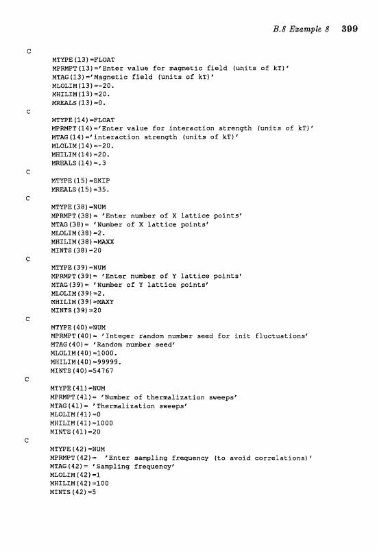
MTYPE ( 1 3 1 -FLOAT M P a T f l 3 ) - ' E n t e r v a l u e f a r m g n e t i ~ f i e ld ( u n i t s o f kTI1 MTAG (13) =;%agnetic f i e l d f u n i t s of kT) " MLOLIN(f3)--20e MHILPM (131 ~ 2 0 . MEALS (23) -0.
MTYPE ( 1 4 ) =FLOAT MFMPTf14)=eEnter v a l u e f a r i n t e r a c t i o n s t r e n g t h ( u n i t s of kT)@ MTAG (3.4) = q l n e r a e t i o n s t r e n g t h f u n i t s of kTf ' MLOLIM (14) P-20 MWTLIM(14) -20. m m ~ s ( 1 4 ) = . 3
MTYPE 11 5 ) =SKIP LS (15) ~ 3 5 .
MTYPE ( 38 f =NUM e W T ( 3 & ) = "En te r number o f X l a t t i c e p o i n t s F MTAG(38f- ' H u d e r of X l a t t i c e p o i n t s t NLOLXN ( 38 1 =2, MWILf W (38) = m X MINTS 1381 -20
HTYPe ( 3 9 I =NUM NPMPTf39)m 'En te r n-er of Y l a t t i c e p a i n t s p MTAG (391 = ' R u d e r o f Y l a t t i c e po in t s ' MLOLXM (39) -2. MBILIM 43 9 f - m X Y MINTS (391 m20
M m E (40) =NUM MPWPT(401= * I n t e g e r random nrrmber seed for i n i t f l u c t u a t i o n s " #TAG (40) "Random number seedr HLOLXM (40) = I O Q O . MWfLIM(40) m99989, MINTS (40) =S4767
NTYPE f 4 1 1 =NUM MPWPT(4T)m " N u d r o f t h e r m a l i z a t l o n sweeps' MTAG (41) - ' Thernralizatlon sweepsf NLOLIM 1 4 3. ) =Q MHILIM f 41) *l000 MINTS (42 1 -20
MTSE ( 4 2 1 -MUM MPWT (42) 'En te r sawling frequency ( t o w a Z d c o r ~ e l a " c o n s 1 ' MTAG (42) = ' Sampling f requencyt MLOLIM (42 ) =l HHILLM f 42) =l00 MINTS (421 -5
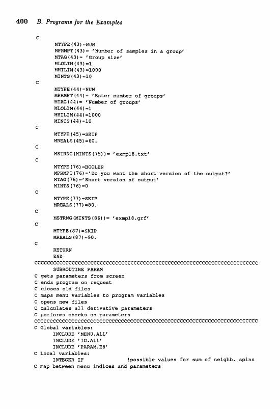
400 B. P~ogmms for ithe Ezan~ples
C
MTmE ( 4 3 1 =NUM WRMPT f 43) 'Number of samples in a groupf MTAG(43)= 'Group size' MLOLSM (431 =l MXLIN ~ 3 1 =loo0 MINTS (43) m10
C
MTYPE ( 4 4 f =NUM W M P T f 4 4 ) - 'Enter nuder of groupsv MTAG (44) Wuher of groupst MLOLSN t 4 4 f -1 MHXLIPI f 44) m1000 MINTS (44) =l0
c MTWE ( I S ) =SKIP W m L S (45) 060.
C E15TRMGfMTNTS (751 l = 'exmplff.txt8
e MTmE ( 7 6 ) =BOOmM m ? W T ( 7 6 ) = t D o you want tbe short version of the output?" MTAG (761 mf Short version of output* NLNTS (76) -0
C MTmE ( 77 f =SKIP
LS 677)=80, c
MSmKG (MINTS 186f 1 = 'exmpl8 .grf C
MTWE ( 8 7 1 =SKIP LS (87) t.190.
c m TURI END
~CCCCGCCCC~CCC~CC ~ ~ ~ C C C C C C C ~ C C ~ C ~ C ~ C C C C ~ ~ ~ ~ ~ C ~ ~ C C ~ ~ ~ ~ C C C G C ~ ~ C C ~ C ~ ~ SWROUTINE P
C gets parameters from screen C ends program on request C closes old files C maps menu variables to program variables C opens new files C calculates all derivative paramters C performs checks on parameters cccCccecccceccccccccccccccccccC=cccecccceccccccccceccccecceccceeccceccccc C Global variables:
INCLUDE "NU. ALLp INCLUDE *ITO.ALLf
C Local variables: IMImGER IF !possible values for sum o f neighb. spins
C map btween =nu indices and paramters
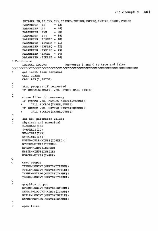
INTEGER IB, TJ, INX, XNY, f DSEED, I N T m , TNFREQ? fNSIZE# XNGRE", ITERSE T E R ( I B =I31 TER (TJ = 14)
TER (IDSEED - 40) TEE4 (IWTWRM = 4 1 )
PAmMETER (INFREQ = 42) P m m T E R (INSIZE = 43)
TER (INGRF = 4 4 1 TER (ITERSE - 76)
C Functions: LOGICAL LQGCVT !converts 2 and O t o true and fa l s e
cccccccccccccccceccccccececccccccecceecccccccccccccccC:cecccccccccccccccc get inpu t from temf n a l C&& C L m R CALL ASK (I, I STOP
stop program if requested TP f m A L S (XNEllIM) .EQ, STOP) CALL FXNXSW
e l o s e f i l e s i f necessary I F (TB= . NE, MSmNG (MXMTS ( I m m ) 1
+ CALL PLCLQS ( T H W , TUMIT) f P (GM- .WEe MSmNG (MINTS (IGWME) ) )
+ C&LL FWLOS (W-, GUNIT)
set new parameter va lues physical and numerical
J==ALS ( f 3 1 NXmMIWTS (INX) Pa?l=MINTS (XWV) DS~D-DBLE (MINTS ( I D s a E m NTHEWPlr=MXHTS (INTHW) NFmQ-MINTS ( INFmO) NSIZE=MXUTS (INSSZE) NGROUP=MINTS (INGM f
t e x t output TTERM-LOCCVT (MINTS (ITTERN) f TFILE=taGCVT(WXNTStj:TFIUjj T N ~ - H S T R N G (nrNTs (ITHW) 1 TERSE-LOGCVT (MINTS (ITERSE f 1
graphics outpu t GTERM-LOGCVT (M1 WTS ( fGTERH1 1 c H m c e = w c C v T f n r N a s ( I G ~ D J 1 WILE-LWWT(MXNTS(IGF3LEI) GNM=MSTRXJG (MINTS (ZGNmE) )
open f 2163s
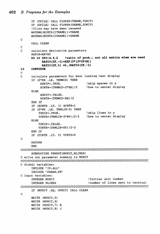
IF (TFILE) CALL FLOPEN (TNWI"IE, TWIT) XF (GFILE) CALL FIXIPEN (EH-, GUNIT) !files may have been renamed MSTRNG (MINTS (ITNAm) ) = T H W HSTRMG (newrs ( I G N ~ I = G N A ~
c CALL CLMR
C C ~alculate derivative parameters
NSPIN=NX*#Y PO 50 Z F * ~ - 4 , 4 ~ 2 tr~lt.te ef pzebi.; net: alf
mzro (m, -%)=m (2" (J*ZI+BI I m z ~ ~ ( s ~ * l ~ ~ x * / ~ T I a ~ n , - % l
ZQ c G calculate parameters Esr best looking text display
IF (2*NX .LE. TRmXB) THEN XSKIBm, TRUE. Iskip spaces in x XCNTR={TRWIB-2*NX)/2 thaw to center display
ELSE XSKIPm. FALSE, XCNTR= (TWID-NX) /2
END TF IF fXCNTR .LT, 1) XCMTR=I IF (2*NY .LE. TRMLIN-5) THEN
YSKTP=, TRUE. !skip lines in y YCNTR=ITRHLIN-2*NV)/2-3 !how ta centsr display
ELSE YSKXP=,FALSE, VCNTRm f TmtIN-NV) /2-3
END IF IF (YCNTR .LT, O f YCNTRmO
C RE;TURN END
cccccccccccceccc~ccccecccccccecccccecccccccccccccccccccccccccccccc~ccccc SUBROUTINE PRMOUT(NUNIT,NLINES)
C write out parameter sumary to MUNXT cccec~~~ccccc~cccecccccccccccftcccccccccecccccccccccccccccceccccccccccccc C Global variables:
INCLUDE @I0.ALL8 INCLUDE ' PAMM. E&'
C Xnput variables: XNmGER NUNIT !fortran unit nuaer INmGER NLTNES !nu&er of Lines sent to terminal
CCCCCCCCGC~CCCCCCCCCCCCGCCCCCCCCCC~CCCCCCGCCGCCCCCCC~C~CCCCCCCCCCCCCCCCC IF fMUNf T .EQ, OUNIT) CALL CLEAR
C WRITE (MUNIT, 5 1 WRITE (NUNIT, 61 WRITE (NUNXT, 7) B WRITE (NUNIT, 8) J
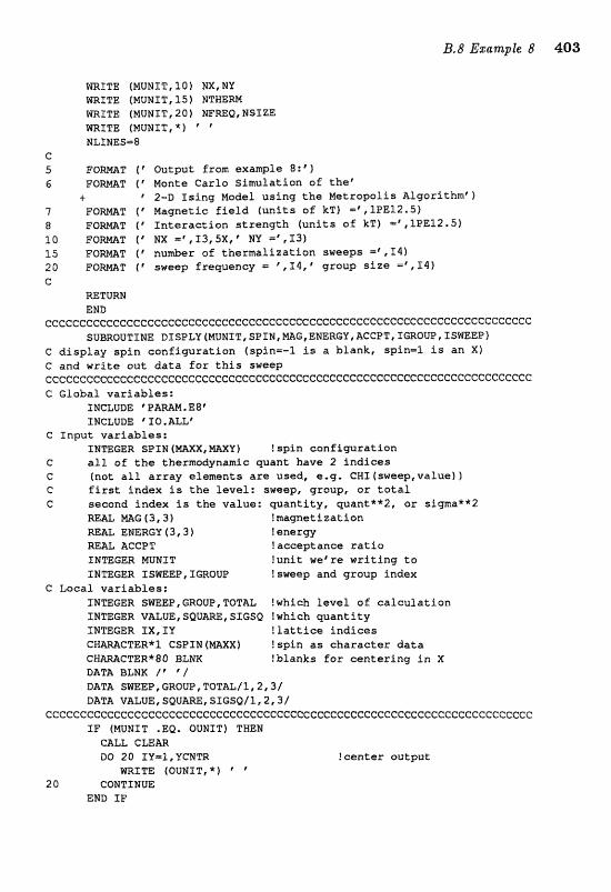
MTRITE (HUNZT,101 NX,NY WRITE (NUNIT, 15) NTBBRM WRf TE (MUNIT, 20) WMQ, NSTZE MRXTE (MUNST, *) " NLTINESm8
c 5 F O M T f"utr;lut fromexample 8 z C ) 6 FOMT f t Monte Carlo S i m l a t f o n of t h e t
+ 2--D I s i n g Model us ing t h e Metropolis Algori thmr) 7 F O m T [ @ M a g n e t i ~ f i e l d f u n i t s o f k T ) = ' , 1 P E ~ 2 , 5 ) 8 FOmY ( @ Intezraction s t r e n g t h ( u n i t s of k T f =\lE"E12.5) l0 F O m T [' NIX=',f3,5Xrf NY ='#X31 15 FOMT ( l nn&er aE the rmal iza t ion sweeps =',S41 20 P O W T ( f s v e e p f r e q u e n c y = "H,' g r o ~ p s i z e = ~ , f i 4 ) C
WTURH END
CCCCCCCCCCCCGGCCCCCCCCCCCCCCCCCCCCCCCCCCCCCCCCCCCCCCCCCCCCCCCCCCCCCCCCCC SUBROUTINE DISPLY (HUNTT, SF IM, N G , ENERGY, ACCPT, ImOUP TISWEP 1
C d i s p l a y s p i n conf igura t ion (spin=-l i s a blank, spin51 i s an X I C and write ou t d a t a f a r t h i s sweep cc~cccccc~~cce~ccccccccccccceccccccecc~eccecC:ccccc"cc~ccc~cccccccc~c~cccc e Global va r iab les :
SNCLUDE fFAmH.E8Q INCLUDE "IQ.ALLf
C Input va r iab les : INTEGER SPIN ( W X , W Y ) ! sp in conf igura t ion
C a l l of the thermdynamic w a n t have 2 f n d i e e s C" (not a l l a r r a y elements a r e used, e.g. CHX (sweep, value) 1 C f i r s t fadsx is the l eve l : sweep, greup, o r t o t a l C seeand index is the value: cy~an t i ty , quant**2, ar sigma**2
m&L mG(3,3f !magnetization RE= EHERGY (3,3 f ! e n e r w
ACGPT !ameptance r a t i o INTEGER NUNIT !uni t wet re w r i t i n g t o INTEGER ISmEP, TGROUP !sweep and group index
C Local va r iab les : INmGER S&TEEP,GROUP,TOTU !which l e v e l of c a l c u l a t i a n XNmGER VALUE,SQUAm,STGSQ !which q u a n t i t y TNTEGER I X , IV ! l a t t i c e i n d i c e s CMmCTER*1 CSPIN(mXX1 !spin as charac te r d a t a
!blanks f o r eezntering i n X s s l ~ h aLxE Q I DATA SmEP,GROUP,TOTALf1,2,3/ DATA VALUE,SQUmcSIGSQ/1,2,3/
CCCCCCCCCCCC~C~CCG~CCCGCCC~CCCCGCCCCCCGCCCCCCCCCCCCCCCCCCCCCC~CCCCCCCC~C I P (MUWIT .EQ. OUMIT] THEN
CLEAR DO 20 I V = ~ , YGNTR !center output
mITE (OUNIT, *) ' ' 2 0 CONTINUE
END SE"
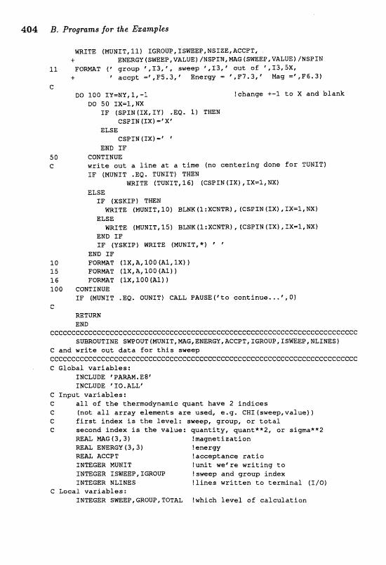
404 B, Programs far the Zz~mples
WITE (MUNIT, 11) IGROUP, ISmEP,NSXZE,ACCPT, -8- ENERGY ( SmEP, VALUE) INSPIN, MAI; [SWEEP, VALUE 1 /NSP I N
f l F O m T f r group \ I 3 , ' , s ~ e e p ' , I 3 , Q u t o f ' ,53,5X, + aaccpt , l f 5 . 3 , t Energy = #,F7.3,' Nag =' , ,F6 .3)
C
DO 100 IU-MY, 1, -1 !change +-1 t o X and b lank DO 50 IX=Z,NX
I F (SPLN(IX,IV) .Ea. 1) THEW CSPIN (IX) =' X @
ELSE GSPIN f IXl="
END I F CONTINUE w r i t e o u t a l i n e a t a t ime (no c e n t e r i n g done f a r TUMIT) EF (MUMIT .EQ. TUNIT) THEN
WRITE (TUNf T, 16) (CSPIN (IX) , I X = 1 , MX} ELSE
I F (XSKIP) T B N mXTE (MUHIT, 10 ) BLNK (l:XCHTR), (GSPXN (XX) , IX-1, NX)
ELSE m J T E (HUMI"IC15) BLMK(I:XCMTR), fCSPXt3fIX),TX=l,MXf
END I F I F (VSKIP) WRITE (MUNIT, * f ' '
END JF 10 F O M T (1X,A, I O O (AI, 1x1 ) 1 5 FORMAT (Ix,a, 100 (AI) 1 16 FBRMT (1X,100(All) 100 CONTINUE
I F (MUNIT . EQ. QUN1T) CALL PAUSE ( * t to c a n t i n u e . . ' , Q ) G
RETURN END
cccccccceccccccccccccccc~ceccccceccccccecccccecccecccc~ccccccc~ccc=cc~ccc SUBROUTINE SWPOUT(MUNIT,~G,E1"9ERGYt&CCPT,IGROUP,ZS1EEP,HLXNES)
C and w r i t e o u t d a t a f o r t h i s sweep cccccceccccccccccceccccccccececceeeccccecccccceecccccccccccccccccccc~~cc C Global v a r i a b l e s :
INCLUDE fPMM,E81 INCLUDE 'XTO.ALLt
G Inpu t v a r i a b l e s : C all af t h e thermadynamic w a n t have 2 i n d i c e s C (not a l l a r r a y e lements are used, @.g. CH1 (sweep,valua) ) G f i r s t index i s t h e l e v e l : sweep, group, o r t o t a l C second index i s t h e value: q u a n t i t y , wan t**2 , or sigma**2
RE& M G { 3 , 3 f !magnet iza t ion WBL ENERGY f3 ,3f ! e n e r w mm ACCPT Eaeceptance r a t i o INTEGER MUNIT I u n i t wef re w r i t i n g t o ZNmGER ISMEEP,TGROUP !sweep and group index ZNmGER NLINES !k ines w r i t t e n t o t e r m i n a l (X/Q)
C Local v a r i a b l e s : XWTEGER SmEP,GROUP,TOTAL [which l e v e l o f c a l c u l a t i o n
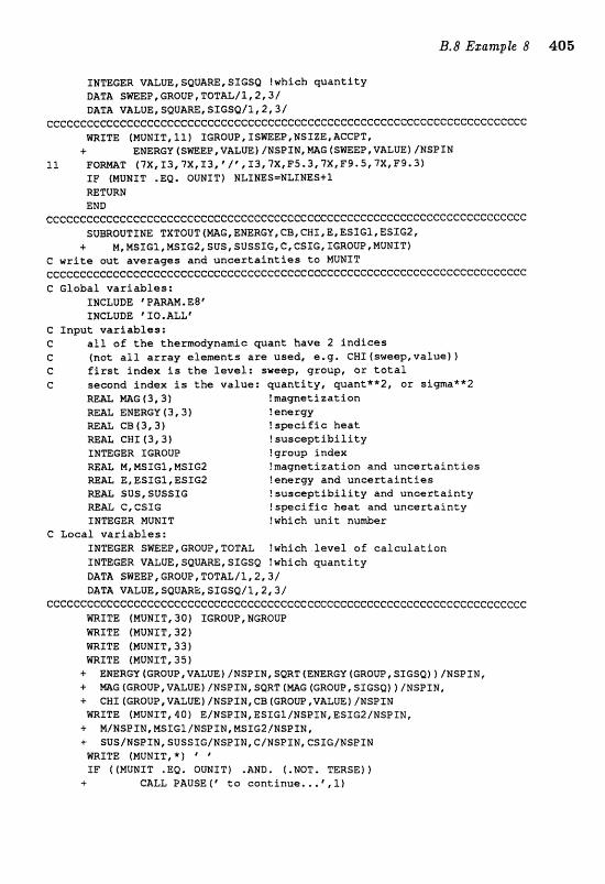
INTEGER V&LUE,SBUAm,SIGSQ !which quantity DATA SmEP c GROUP, TOTAL/ 1,2,3 / DATA V&LUEt SQUARE, SXGSQ/l.# 2? 3/
cccccccccccecCccccccccceccccccccccccccceccccccccccC:ccccccccccccceecccccc WITE (MUNIT, 11) IGROUP, ISWEP, NSIZE, A m ,
+ ENERGY (SmEP, VALUE) /NSPXN, m G {SWEEP VALUE) /NSPIH 11 FO-T (7Xe13,7X,13, ' / " €13, "1X,FSS3,7X,F9.31
IF (NUNXT .EQ. OUNITf NLINES=NLZNES+l RETURN END
ccccccccccccccccccccccccccecccecccccceeccccccccccccccccccccccccccccccccc SUBROUTINE TXTOUT (MAG, ENERGY, CB, CWf, E, ESIGl, ESZG2,
+ M, MSTG1, MS162, SUS, SUSSXG, G, CSIG? IGROUP, MUNfT} e write out averages and uncertainties to MUNIT CCGCGCCCGCCCCCCCCCCCCCGCCCCCCGCCCCCCCCGCCCCCCCCCCCCCCCCCCCCCCCCCC~CCCCCC C Global variables:
INCLUDE tPAM*E8" INCLUDE 'IOIALrL6
C Input variables: C all of the thermodynamic want have 2 indieas C (not all array elements are used, e.g. CMl(sweep,value)) C first index is the level: sweep, group, or total C second index is the value: cfuantity, cyuant**Z, or si9ax*2
Mm mG(3,3) !magneCizatian R m L ENERGY 4 3,3 ) f energll
CB 43,33 ! specific heat CB1 (3,3) !susceptibility
TNmGER IGROUP !group index M, NSIGI, MSIG2 !magnetization and uncertainties E, ESIGZ, ESIGZ !energy and uncertainties SUS, SUSSXG !su~ceptibility and uncertainty
mm CrCSTG !specific heat and uncertainty INTEGER MUNZT !which unit nu&er
C Local variables: INWGER SWEEP,GROUP,TOTAL ?which level of calculation INTEGBR VALUE,SQUm,SIGS& Ewhich quantity DATA SWEEP, GROUP TOTAL/ l, 2,3 / X>ATA V U U E , SQUmE, SIGSQ/I, 2 , 3 /
ccccccccccc~ceccccccccccccccecccccccccc~cccc~ccccccccccccccccceccccccccc MRlTE: (MUN1 T ,3 0 ) IGROUB , NGROUP mITB (MUNIT, 32) mITE (WUNf T, 33) mITE (HUN1 T, 35)
+ EHERGU(CROUP,VALUE~/MSP1NISQRT(ENEWGY(GROUP~SIGSQ~]/HSPXE, + m G (GROUP, VALUE) /NSPIN, SQRT (=G (GROUP, SIGSQ) ). /MSPIN, + CWX(GROUP,VALUE)/NSPXMeCBIGROUPvVALUE~/PJSPIN fhlRITE (IUXINIT,r10) E/NSPIN,ESIGI/MSPIHtESXG2/AISPIN,
+ H/NSPIN,MSIGI/NSPIN,MSZE2/WSPfNli + SUS/NSPIN,SUSSIG/NSPIN,C/N5PIPJ~GSIG/MSP1N WRITE (MUNIT,*) " fF [(MUNIT .Ea. OUNIT) .AND. (.MOT. TERSE))
-4- CALL PAUSE t f to continue. , . 5 l.)
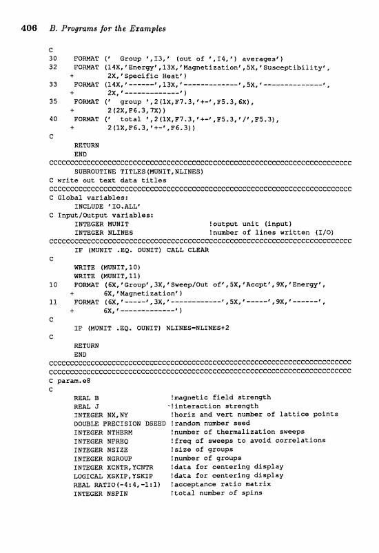
C 30 F Q m T ( q r o u p ' , I3 , ' (out of: ',I4,') averagesr ) 32 F O m T ( I qX , 'Energy1, 13X, *Magnetizationt, 5 X , ' S u s c e p t i b i I & t y y ,
.I- ZX, "peeif ic Weat') 33 F O M T (l 4X, L-----* , 1 3 ~ , --m-- ---...---- t 15~,f-------------..."
C 2X, * ----------""-- 6 1 35 F O m T (' group ' "2 (1X,F7.3, * + m f ,F5,3,6X),
-5 2 (2X,F6,3,7X) )
40 F O m T I t ttotl * ,2 (1X,f"7.3, +-* , F5.3, V/" PF5.3), i 2 ( I X , F6.3, " m - ' ,F6,3))
G RETURN END
ccccccccccccccccccccccccccccccccccccccccccccccceeccccccccccccc~ccccccccc SUBRQUTINE TITLES (MUNIT, NLINES)
C write out t e x t d a t a t i t les cccccccccccecccccccccccecccecceccccccccecccccccccccccccccccccccccccccccc C Global var iab les :
INCLUDE, XIO ,ALL* C I n p u t l O u t p t var iab les :
INTEGER MUNIT ! output u n i t f inpu t 1 XNmC;ER NLINES !nu&er of l i n e s w r i t t e n (5/0)
cccecccccccc~ceeccccccccceeccccceceeccccccceccccccccecc~cccceccccccccccc IF (NUNZT .EQ. OuNIT) CALL CLEAR
C WRITE (NUNfT,IO) NRITE (MUWXT,11)
10 F O M T (bX, 'Group*, 3 X , 9weepIQut o f f , 5X, ' A ~ e p t ' , 9X, "nergyp + 6XffM)rlagnetization'f
11 F Q m T (a, 3X, ------------p 5X6 ~ ~ - - - f , g x , f ----m-#
.I. 6X,f,..------------t 1 c
IF (MUMIT .EQ, QUNIT) MLINES=NLJWES+2 c
=TURN END
CCC~CCCC~~CGCCCC~GCGCCGCCCCCCCCCCCCCCCCCCCGCCCC~GCCC"CGCCCCCCCCCCC~~CCCGC ccc~cccce~~~ccccccc~cccc~ccccccecccccc~cceccccccc~cccecccccccc~ccccccccc C param.@@ e
=U B !magnetic f i e f d s t r e n g t h m& J - ! in te rac t ion s t r e n g t h XNTEGER NX, NU !har iz and v e r t n u a e r of l a t t i c e p o i n t s DOUBLE BRECXSION DSEED !random n u d r seed INTEGER NTXERM !nu&er of thermalizat ion sweeps INTEGER MFREQ ? f r & g of sweeps do avoid correlations INmCER NSXZE ! s i z e of groups IMTEGER NGRQUP !number of groups INTEGER XCNTR,YCNTR !data f o r een te r ing d i sp lay LOGICAL XSKIP,YSKIP ? d a t a f o r cen te r ing d i sp lay M L R1?ITXQ(-4;B,-l:f) !a,ceepCan~e r a t i o matr ix INTEGER WSPIN ! t o t a l nu&er of s p i n s
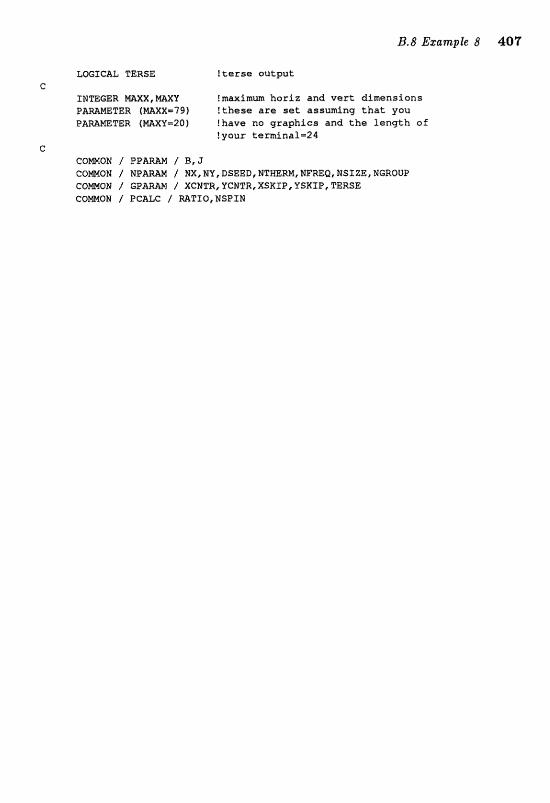
LOGIC& TERSE !terse outpat e
IUmGER mm, M X Y !maximm horiz and vert dimens5ons PAWETER ( W X - 7 9 1 !these are set assuming that you
TER ( W U = 2 0 ) !have no graphics and the length sf !your terminalm24
G COMQN / P P A m / B, J
/ NX, NY, BSEED, NTmRM, NFReQ, fVSIZEI NGROUP COMON / GOAMM / XCNTR,VCWTR,XSKfP,VSXIP,TERSE COWON / P C U C / RATIQ,NSPIN

This page intentionally left blank
Appendix C
Programs for
C.1 Project 1 Algorit hrn This program calculates, for a given energy, the deflection function for scattering from the Lennard-Jones potential at NB impact parameters covering the range from enrl to ennx. The basic task is to evaluate Eq. (1.8) for each impact parameter requested (DO loop 25 in subroutine n~ceoa). This is done in subroutine TaeTn, where first a simple seareh is used to locate N T N , the t u r ~ n g point. Then the integrds are evafuated by the rectangle rule, with a cfiange of variables to regul&e the singulmities, Ysu may dter the potentid by cfla@ng m ( ~ ) at the beginning of subroutine THETA. If you; do, don't forget to find the new vdue for RMAX such that V(r,,,) M 5 x 10-~&.
Input The physical parameters are the Energy [1.0], the minimum and maximum impact parameters [.1,2.4], and the number of impact param- eters for which the guadrature is performed [20]. The maximum number of inzpaet parameters is fixed by the FORTRAN parameter WX= 100. Energy is in units of 6, lengths are in units of a. The program chedts that BMIN cr BMAX < M A X in subroutine PCaEcK. The numerical p a r m e ters include the tolerance for the search on the turning point [.0001], the radius beyond which the potential is negligible [2.5], and the number of quadrat- points [40].
Output Far each impact parmeter the text output disjplays the impact parameter, B; the radius of dogest a.pproa&, MII; a9d the scaltering angle in d e g r ~ s ; ~ ANGLE. After all values of UGLE have been cdculated, the deflection (scattering) an@e is maphed asr a function of imprtet pasmeter,
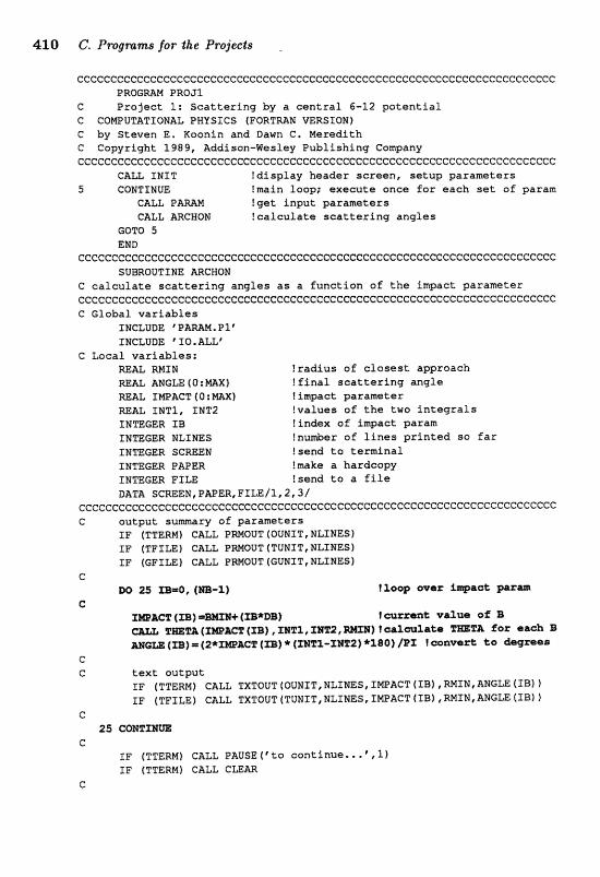
cccccceccccccccccccccccccccccccccccccccccccccecccccececcceccccccc~cccccc PROGmM PR091
C P r o j e c t l: S c a t t e r i n g by a c e n t r a l 6-12 p o t e n t i a l C COmUTATIDHkL PHYSICS (FORTWN VERSIOW) C by Steven E. Raonin and Dawn C, Meredi tb C Copyright 1989, Addison-lesley P u b l i s h i n g Cowany ccecccccccccccccccccceccc~~cccccccc~cccce~cccccccccccccccccccccccccc~ccc
CALL IEJIT !d i sp lay heade r sc reen , s e t u p pa ramete r s 5 CONTINUE !main loop; e x e c u t e once f o r each set aE pasam
CALL PAMM !ge t input paramete r s CALL ARCWON ! c a l c u l a t e s c a t t e r i n g a n g l e s
GOT8 fi END
ccccccccceceecccccccccecccccccecccc"cececececcccccccceccccccccccccccccccc SUBROUTINE mCNON
C c a l c u l a t e s c a t t e r i n g ang les a s a f u n c t i o n of t h e impact parameter cccccccceccccce~eecceccccccccccccccccccccCiccccececcccccccccceccccccccecc C Glaba l v a r i a b l e s
INCLUDE 'PARAM.PI6 INCLUDE ' I Z O . ALL'
e Local v a r i a b l e s : REAL RMZN ! r a d i u s o f c l o s e s t approach RE= ANGLE (0 :W) ! f i n a l s c a t t e r i n g a n g l e REAL SNPACT(O:MAX) !emact parameter REAL INT1, INT2 !va lues cf t h e two i n t e g r a l s INTEGER IB ! index o f inrpact param INTEGER NLINES ?nu&er of l i n e s printed so f a r INTEGER SCMEN ?send t o t e r m i n a l INmGER PAPER !make a hardcopy INTEGER FILE !send t o a f i l e DEITA SCMEN, PMER, FILE/%# 2 I 3 I
cccCcccccccec~~cccccccccccccccccccccecccc~cccccccccceeecccccccccccccccc~ C ou tpu t s u m a r y o f parameters
XP (TTERM) GALL PRMQUT (QUNIT, NLZNES) f F (TFILE) GALL PMOUT (TUNZTe NLINES) IF (GFILE ) CALL PMQUT IGUNXT, NLINES)
c DO 25 PB=O, (=-l) I l o q w a t % q a a t garm
c T (PB) ==M;(. (m*DB) ! t value o f B
(-XI (fa) , zwxz , m 2 , m w ) r aka FmT& for each B mGm (m) = (Z*ZWACT (m) * (XET"P4m2) *TB@) /BX f czonvee ta
C e t e x t output
IF (TTERM) CALL TXTOUT (OUNIT,NLIE~ES~ IWACT RNIE~ANGLE 1 I F (TBILE) CALL TXTOUT [TUNITINLIMES, IMPACT (XBf RMIN,PiNGLE {IBl)
e 25 CmlrIm
c IF ITTERM) CALL PAUSEffto cont inue. . .',l) XP (TTERW1 CALL Cmm
C

C.1 Project 1 415,
SF IGTERM) CALL GWOUT(SCRE&N,AMGW,IWACTf !graphics o u t p t IF (GFILE) CALL GWQUT (FILE I AMGm I IMPACT) I F (GMRDCP f CALL GRFOUT (PAPER, MGm, IRACT)
c RETURN END
~cccc~cCcee~~ccccccccccccccccceccc~cccccceccccccceccccccccccccceccccc~cc SUBROUTINE THETA (B, TNT1 , INT2, MIN)
C searches t o f i n d RMXN (c loses t approach) C integrates FNT1 from El t o R m X t o find INTl C i n t e g r a t e s FN12 from RMTM t o -X t o f i n d INT2 ce~~cc~~c~ce~cccccc~~ccccccccccC:cccccccececcc~cccccccccccccccccceccccccc C Global variables:
INCLUDE ' PPBMM. P1 " e Ingut fWtput var iab les :
W L B l i ~ a c t p a r a m t e r ( f n p t f R E U XNT1, INT2 !values far t h e two i n t e g r a l s (crutput) RE= RMZN ? r a d i u s of c l o s e s approach (output)
C Local var iab les : BE& R ! current radf us REAL BR ! cur ren t search step s i z e RE= U ! U=SQRT (R-8) o r S a T ( R - M I N I MAL UMAX ! @-=SORT (R=-B) or SQRT 1 R W - R M E M ) RE& H ! rad ia l s t e p fo r w a d r a t u r e M U S U M !sum f o r w a d r a t a r e INTEGER I U !index on U REAL FNV t s c a t t e r i n g p o t e n t i a l {funct ion) M U PNII,FMI2 ! f i r s t and second integrands (funct ion)
c e c c e c c e e c c ~ c e c c e c c c c c c e e C c c C c c e e G c c c C C &fine Zaac%ions
m (R1 1 4* (R** (-%a) -]R** ( -6) ) mzz (B, R) TIR**~/SWZ (1- (sm) **2) B'Mf 2 (B, R, E) - l fR**2/SWZ (1- (LS/R) **S-W fR) /E)
C !$nwmd m a d for turning point
DR ap- 0.2 1 XF
1% M&=&
) ) .&P.O*O) i a w h r e i r i a f f d t a
fi.e., the W d n a t o ~ O m m
GO 1CO 5 Ern
C Sm=O ! f i r s t i n t q r a l kg- recdaaqle raXa
IaMge vrr2&1% do G=B=E(R-B) !to mmve ainplariky at; R@
M) l0 IfJ=l, WTS V=E* (f U-@. 5 ) R=@* *2+B fahaage ba& te R eval i n t q z m d S ~ S W + @ + ~ I l (B, R)
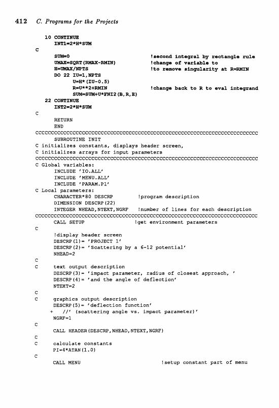
10 C a M T x m XlI"I=2*W*Srn
G 6-0 !@e@oa& inte9z.l by roetangas rule
tebmgm of vari&&r t o !CQ rrmmove riaplarity at R = m M
DO 22 XUm1,NnTS mm* (XU-0.5) R=U**2+WXM tahango b a d to R to oval, Snt;sg%ad SW=SW+U*m12 (8, R, E)
22 COmSm kl%2=2+P*SW
c RETURN END
GCCCCCCGCCCCCCCCGCCCCCCCC~CCCCCCCCC~CCCCCCCCCCCGCCCCCCCCCCCCCCCCCCCCCCCC SUBRQUTINE TNlT
C initializes constants, displays header screen, C initializes arrays for input parameters cc~cccceccCccccccccccccecceccccccccc~ccccccccc~~cccc~cccccccccccccccccc~ C Global variables:
INCLUDE ' I0 . ALLF INCLUDE ' MENU. ALL' INCLUDE 'PAmM.OIt
C Local parameters: CHWCTER*BO DESCRP !program description DINENSION DESCRP (22) INTEGER NHEAD,NTEXT,NGRF fnuwr o f lines f o r each description
cccceccc~~~cccce~ccccccccccccccccccceccccccc~ceccc~ccccccccecccc~ccccccc CALL SETUP !get environment parameters
G !display header screen DESCRP (E ) PROJECT 1 ' DESGRP(2)= #Scattering by a 6-12 potential' NNEAD=2
e C! text output description
DESCBP 131 = F Iwact, parameter, radius of closest approach, " DESCRP (B) = and the angf e af dafleetlan" WTEXZ"s2
C C graphics output description
DESCRP f 5) = #ddelectf on function* + //Vseattsring angle vs, impact parameter)'
PJGRF=1 G
CALL WEADER(DESCRP,NHEAD,NTEXT,NaFI c C calculate constants
PI=B*ATAN (1. 0) C
CALL MENU !setup constant part of menu
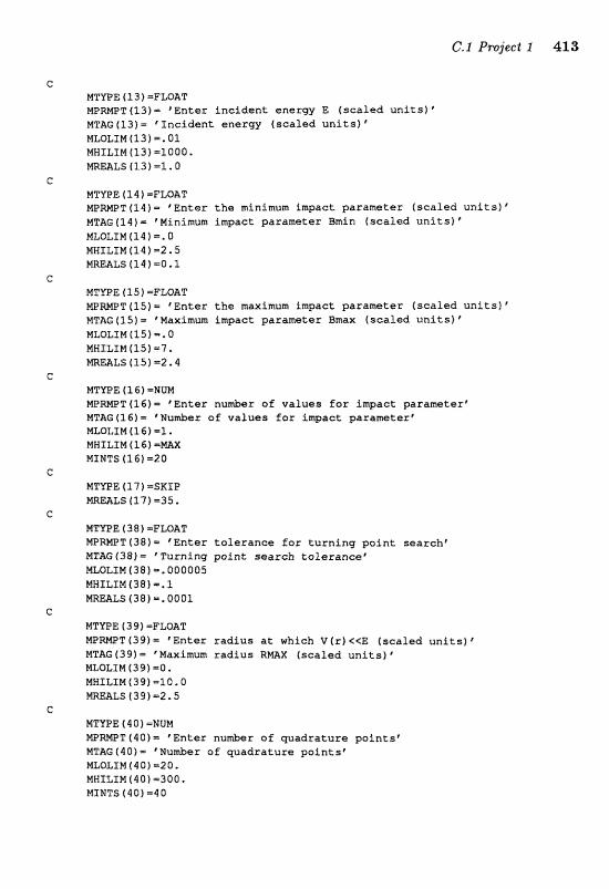
NTWE ( 1 3 ) =FLOAT M P W T (13) = ' En te r i n c i d e n t enerc?ry E ( s c a l e d u n i t s ) NTAE (13) - q n c f d e n t energy ( s c a l e d u n i t s ) ' MLOLIN (13) -. 01 MHILIM (13)=1000, mmLS (13) -1.0
NTYPE ( 14 ) =FLOAT MPFUrlPT(14)= ' E n t e r t h e minimum impact parameter ( s e a l e d units)* %TAG (14) - %Minimum impact parameter Bmin ( s e a l e d units) ' MLOLTM (3.4) ;=. 0 MWILIM(14)-2.5 M m L S (14) -0.1
NTYPE (1 S) =FLOAT MPmT(15)= I E n t e r t h e maximum impact parameter ( s c a l e d u n i t s I r MTAG (15) = @ Maximum impact parameter Bmax ( s c a l e d u n i t s ) MLOLXN(lSI=.O NWSLIM(15)=7. mEZILS 4151-2.4
MTWE f f 6)=NUN MPWT{SG)= ' En te r nu-r a f values Ear impact parameter" MTAG (1 61 = "umber o f vaf u e s f o r impact parameter* MLOLIM (3.6) =l, MHILf M t 16) =MAX MINTS (16) -20
MTVPE ( 3 8 ) =FLOAT MPRMPT (38) 1 ' En te r t a l e r a n c e f o r t u r n i n g p a i n t s ea rch" MTAG (38) = Turning p o i n t s e a r c h tof e r a n c e F MLOLSM ( 3 8 ) ~ ~ 00a005 NHTLTNf38) =. 1 maL5 (38) =. 0001
NTUPE ( 3 9 f =FLOAT MPmPT ( 3 9 ) = * E n t e r r a d i u s a t which V ( r ) <<E ( s c a l e d u n i t s ) NTAG (39) = 'Maximum r a d i u s R M X ( s c a l e d u n i t s ) " MLOLXM 139) =Q. M'NILIM(J9f =IO. O
LS (391 -2.5
NTUPE ( 4 0 ) =NUM M P M T (40) @ E n t e r nu&er o f q u a d r a t u r e p o i n t s r MTAG (401 - Wu&er of q a d r a t u r e pof n t s p MLQLIM(40) =20. MNXLIN(9Of -300. MINTS (40) =40
414 G. Pmgmms for .the Projects
C NTVPE (41) =SKIP MRmLS (41) =60.
C MSTRNG(MINTS(75) ) = r p r o j l . t x t '
C MTWE ( 7 6 1 -SKIP m m L S (76) 4 3 0 .
c MSTRNG (MINTS (86) ) = ' p r o j l . g r f *
c MTYPE ( B7 1 =SKIP
C RETURN END
ccceCc~cccccceccccccceeeccc~ccccccccccccceecccccceccccccccececcccI:cccccc SUBROUTINE P-M
C g e t s parameters from screen C e n d s program on request G c loses old f i l e s C maps menu v a r i a b l e s t o program var iab les C opens new f i l e s C c a l c u l a t e s a l l d e r i v a t i v e parameters cCccccececcccceccccceccC:ccccccccccccccC:ccccccccccccccccccccccccccccccccc C Global var iab les :
INCLUDE =PIENU I ALL" INCLUDE "(2. ALL' INCLUDE ' P A m . P I 8 INCLUDE %P. "
C Function: LOGICAL LOGCVT ! canverts 3 and O t o true and f a l s e
c~cccccecceccccccccceccecccccccccccccccecceccccccccccccccccccccccccccccc C g e t input from terminal
caLL CLEAR GALL ASK(1,ISTOP)
c C s top grogram i f r e w e s t a d
I F (MREAtS f l M I N ) .EQ. STOP) CALL FINISH G C c lose f i l e s i f necessary
ZF f TNAME . NE. MSTRNG (MINTS (ITHAME) 1 1 + CALL FLCLOS (TMAME, TUNTTI
I F (GNAME .NE. MSTRNG (MINTS (IGNAME))) + CALL FLCLOS (GNBME, GUNIT)
c e physical and n u m r i c a l parameters
EmmEALS 4 I E ) BMINmMREALS (IBMIN) BWmNREALS ( SBmX) NB-MINTS (INB) RW=MREALS 4 IRMAX
TOLR=mEALS (ITQLR) NPTS=MINTS (INPTS}
C e t e x t output
TTERMmLOGCVT (HINTS I TTEMI 1 TFILE=LoGCVT (MINTS (ZTFILEI Z TNm=MSTRNG (MINTS (ITHAW] 1
C C graphics output
GTERM-LNCVT {MINTS ( I G T E M l f GHRDCP-LoGWT (MINTS (IGHRDI j GFILE=LOGe\lTfMINTS(IEE"ILE)~ G N W - M s T R H G ( M I N T S ( l G N A M E ~ )
f: e openfiles
XF fTFZLE) CALL PZaPEN(TNAm,TUNIT) I F (GFILEf GALL FZOPEN(GNAm,GUNIT)
C files may have been renamed MSTRNG (MZWTS (ITHAW1 ) =TNAME MSTRNG [MXNTS (XcHArn) I = G M A ~
e CALL PCHECK DB- (BWX-BMIN) I (NB-11 ?calculate step in B CALL C L E m
C RETURN END
CCCC~CCCCCCCCCCCCCCCCCCGCCCCCCCGCGCCCCCCCCCCCGGCGGCCCCCCCCCCCCCCCCCCCCCC SUBROUTIRE PCmCK
C to ensure that O<BMIMCBMX<=WX eccc~cccc~ccccc~ccCcccccccccccccecccccccccccccccccccccccccc~cccccccccccc C Global variablas:
XNCLUBE ' m N U , ALL" INCLUDE 130 .ALLt INCLUDE * P a M . P l r INCLUDE: @Mi%l?. PI"
G Function: GETFLT !gets f loating point number
ccccC=cCccCccccec~ccccccccceeeceecccccec~ecccceccecccccccccecccccccf:ccccc 40 IF (BmX .LE. BMINf THEN
m I T E (OUNIT, 10) B W , BMZN m P T E (OUNIT, 20) H m L S fXEMXN1 -C;ETFLT (MREALS (IBMINf NLOLEM (IBNIN} , MEIXLIM (IBMIM) ,
.I- @ E n t e r BMIHp 1 m M L S 4 I B m l =GETFLIP (mEALS ( f BmX) , BMXN, MWTLIM ( SBmX 1
+ @Enter BNAX*) BM=PIREALS ( ISiElAX) BMIN=mEALS ( IBMIN )
60 TO 40 END XF
C sa IF (=X .LE, BM) T ~ N
416 C. Pcrognsms for the Pr0jec.t-s
m I T E (OUNIIX", 30) RPIIAX,BmX WRITE (OUNXT, 20) !prompt f o r new va lues MREALS ( IBWX) 6 E T F L T (MREPILS ( I B m X ) I SWTN, MN.XtI:M f IBfutAX) ,
-I- "ntsr B M X @ 1 BMAX=MREALS (TBMX) NReALs t I R ~ ) -GETFLT (HREAZS I R ~ X ) , XAXI ,
-4- q n t e r R m X f j RWXmMREBLS ( I m X f
GQ TO 50 END IF
e 10 F O m T (/,' B m X ( = r e , F 6 . 3 , t 1 f ," hi isass than BNIN (==',
+ F6.3,r),t) 20 F Q m U f " but it should be3 the o t h e r way round; "
-I- f r e e n t e r parameter valuesp 1 30 F O m T (/,"W X=8,F6.3,e)r,p Is less than B M fmf , , F 6 . 3 , r ) f f C
RETURN END
cccCccccecccccceeccccccccccceccceccceccccccccecceccceccceccceccceccccccc SUBROUTINE PRMOUT(MUNIT,NLIWESI
C ourpu ts parameter sumary ta the s p e c i f i e d u n i t CCCGC~CCCCCCC~CCCGC~CCCCCCC~CC~CC6CCCGCCGCCGCCCCCC~CCCC~CCGCCCCC~GCCCCCC C Global v a r i a b l e s
INCLUDE *SQ.BLZ' INCLUDE * P W M . P 1"
c Passed v a r i a b l e s INTEGER MUNIT !un i t n u w r f o r output f i n p u t ) INTEGER NZINES !number of l i n e s w r i t t e n so Ear (output)
eCc~ccccecc~cccc~c~ccecccce~ecceecC:ec~ccc~cccc~cccccecccccecccccccccc~~c I F (MUHIT .EQI OUNIT) CALL CLEAR
G
WRITE (MUNIT, 3.91 m I T E (MUHI T, 21 1 m I T E (MUNIT,27) E m X T E (MUNl"lZ23) R m X , W T S m I T E (MUNXT,25f TOLR WRITE (MtlNIT,29) BMIN,BMX,NB m I T E (NUNIT, 30) WRITE (NUNIT, 1 S 1
C C d i f f e r e n t d a t a headers for graphics and t e x t output
I F (MUNIT .NE, GUNIT) THEN WRITE (NUNIT, 31) mSTE (MUMIT, 321 bJR32"E (MUNIT, 33)
ELSE m I T E (MUNTT, 3-51
END I F e
WLIWES = 11
G 19 F O M T (' ' 1 21 F O m T (' Output from p r o j e c t l: '
+ S c a t t e r i n g by a c e n t r a l 6-12 p o t e n t i a l 23 FO-T (' Rmax=', FE;, 3,SX, numbier of quadrakure p o i n t s =% 14) 25 F O M T ( * Turning p o i n t t o l e r a n c e = ' ,E12-5) 2 " 1 O W U 8 I n c i d e n t energy = 'PF8.31 29 F O W T ( ' BnIn = \F6,3,SX,'Bmx ' ,F6.3,
+ SX, nuumber of B v a l u e s = ', I31 30 Fa-T (' Lengths a r e i n s e a l e d u n i t s , a n g l e s i n degrees ' 1 31 P O m T (%$X, ' Impact" 14X, C l ~ s e s t ' , 16X, @ s c a t t e r i n g a 1 32 F O M T 'Parameter* , l 3 X , t A p p ~ o a ~ h p 17X, 'Anglei 1 3 3 F O W T (13X, "-------- 5,13~,"------- t 1 7 ~ , @ ---...-f
35 F O N T f2X,'I1mpact parameter',2X.'S~ettering Angle f ) C
RETURhl END
eecceeccccccccccececccccccccccccccccccccccccccccccccccccccccc~cccccccccc SUBROUTINE TXTOUT(NUNTT,NLINES,BIWINIANGLE}
C writes r e s u l t s f o r one i n p a c t parameter t o t h e r eques t ed u n i t ccccceccccccccecccccecccccccccccceccceecccccec~ccceccccccccccccccccccccc C Global v a r i a b l e s :
INCLUDE XIO,ALLf C Passed v a r i a b l e s :
INTEGER MUNXT i o u t p u t u n i t s p e c i Z le r ( i n p u t ) INTEGER NLINES !nu&er of l i n e s p r i n t e d s o f a r ( I / O ) REAL B l impact parameter ( i n p u t ) REAL RMIM ! r a d i u s o f c l o s e s t approach ( i n p u t ) a& ANGLE ! s c a t t e r i n g ang le ( inpu t1
ccccccccccccccCcccccccccceeccccccccccccccceccccccccccccccccccccc~ccccccc C I f s c reen i s f u l l , c l e a r s c r e e n and r e t g p headings
PF 4 (MOD (HLINES, mMLIN-4) . EQ. 0) + .AND. (MUNIT ,EQ. QUNfTfl THEN
CALL PAUSE tt oco t inue , . . @,,l) CALL CLEm MRITE (MUNIT, 31) FJRITE (MUNIT, 32) WRITE (MUMf T, 3 3 ) NLIMESSm3
END I F C
VIfRITE (MUNIT, 35 f B, RMIM, AhlGLE C C keep t r a c k of p r i n t e d l i n e s o n l y f o r t e r d n a l ou tpu t
I F (MUNIT .EQ. OUNTT) NLXNES=NLINES+I C 31 F O W T f %5X, qnpaact r , 1 4 X , C l o s e s t 8 , 16X, I S c a t t e r i n g r ) 32 F O m T 113X, 'Parameter t I 13X, #Approach1 17X, @Angle@ 1 33 P O m T (13X, ' ---------' ,13~,t-------- "?X,"-- 1 35 F O M T (15X,F6.3,15XtF6.3, 15XIF9.3f C
=TURN
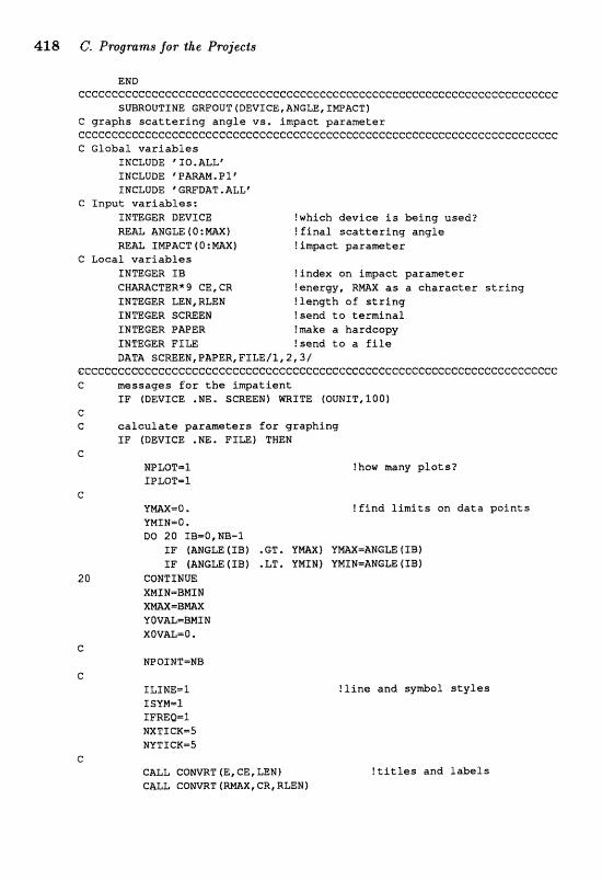
END GCCCCCCCCCCCCCCGC@CCCCCCCCCCCCCCCCCCCCCCCCCCCCCCCCCCCCCCCCCI:CCCCCCCCCCCC
SUBROUTINE GRFOUT(D&VICE,AHGLE,fWAeT) C g raphs s c a t t e r i n g a n g l e vs, Impact parameter ~CCCCCCCCCCCCCCGCCGCCCCCCCCCCCCCCCC:@CCCCCCCCCCCCCCCCCCCCCCCCCCCCCCCCCCCC C Global v a r i a b l e s
INCLUDE 'I0 ,ALLf
INCLUDE ' GRFDAT . ALLf C I n p u t v a r i a b l e s :
INTEGER DEVICE !which device is being used? RmL ANGLE (O:MZ1X) ! f i n a l s c a t t e r i n g ang le RE& IWACT f 0 : M X J !impact parameter
C Local v a r i a b l e s INmGER ZB !index an impact parameter CNmCTER* 9 CE , CR !energy, R M X a s a c h a r a c t e r s t r i n g INTEGER LEN, RLEN ! length of s t r i n g INTEGER SCREEN ! send t o t e r m i n a l INTEGER PAPER !make a hardcopy INTEGER FILE !send t o a f i l e DATA SCREEN,PAPER,FILE/1,2,3/
f"CCCCCCCCCCCCCCGCCCGCCCCGCGCCCCCCCCCCCCCCCCCCCCCCCCCCCCCCCCCCCCC~CCCCCCC C messages for t h e impa t i en t
I F (DEVICE .ME. SCREEN) m I T E (QUNIT,I@O) C G calculate p a r a m t e r s f o r g raph ing
I F (DEVICE .NE. FILE) THEN C
NPLOT=3 !how many p l o t s ? IPLOT=l
c Y m X m O . tfind l i m i t s on d a t a p o i n t s YWIM-0. DO 20 IBmO, NB-1
IF (AKGLE (TB) . GT , YmX) U W = A N G U (IB) IF (ANGLE ( IB) . LT. YNINl VMTN=ANGZpe (XBl
CQNTIMUE XWIN=BMTIJ X M = B r n X VOVAL=BMIM XOV&L=O.
CALL C O W T (E, CE , ZEN I CALL COWRT (=X, CR, RLEN 1
! l i n e and sy&ol s t y l e s
{ t i t les and l a b e l s
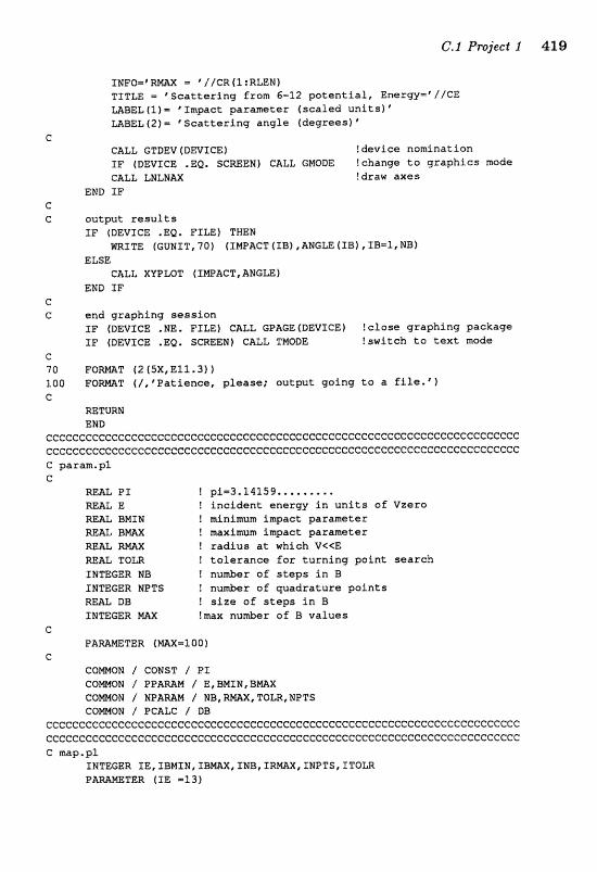
I N F O o ' m X = ' / /CR(l:RmWI TITLE = ' S c a t t e r i n g f r o m 5-12 p o t e n t i a l , Energy=' / /CE LABEL (1) a ' Tmpaet p a r a m e t e r ( s c a l e d u n i t s ) ' LAWL f 21 = ' S c a t t e r i n g a n g l e ( d e g r e e s 1 '
CALL GTDEV (DEVICE) !device n o m i n a t i o n I F [DEVICE .EQ. SCREEN) CALL GEvlODE !change t o g r a p h i c s mode CALL LHLNAX !draw axes
END I F C C o u t p u t r e s u l t s
I F (DEVICE .EQ. FILE] THEN WRXTE (GUNXT,70) (XNPACT(IB),ANGLE(LBf ,IB=1,PJ£3~
ELSE CALL XVP LOT ( IWBCT, ANGLE
END I F c C e n d g r a p h i n g s e s s i o n
I F (DEVICE .MX?. FILE) CALL GPAGE(DEVECE) ! c l o s e g r a p h i n g p a c k a g e XF (DEVICE .EQ. SaEEM) CALL TMODE ! s w i t c h t o text mode
c 70 F O M T (2 (5X, E 1 1 -31 1 I Q 0 P O W T (/, ' P a t f e n c e , please; o u t p u t g o i n g t o a f i le . ' 1 C
RETURN END
CCCCCCGCCCCCCCCCCCCCCCCCC~CCCCGCCCCCCGCCCCCGCCCCCCC~CCGCCCCGCGGI=CCCCGC~C cec~ccecccccccccc~ccccccc~ccccccccccccccC:cecccceccccccec~cc~cccccccccecc C param.p l C
R E U P I ! pim3.14159 ..,...... REAL E ! i n c i d e n t e n e r g y i n u n i t s o f V z e ~ o mAL BNIN ! minimum i m p a c t p a r a m e t e r MAL B= ! maximum Impac t p a r a m e t e r REAL R W ! r a d i u s a t which V<<E =&L TOLR I t o l e r a n c e f o r t u r n i n g p o i n t s e a r c h INTEGER NB ! n u d a r o f s t e p s i n £3 TNmGER NPTS ! n u h e r of w a d r a t u r e p o i n t s R- DT3 I size of s t e p s i n B XNmGER =X !max number o f B va lues
e PAWmTER fmX=1001
C COMaN / CONST / PI COWON / PPAMM / E, BMIN, 8 m X COMON / HP&- / NB, RmX, TOLR,NPTS COMON / PCALC / DB
ececccccccc~ccccccCcC:cecccccccceccccccecccccc~~ccc~ccc~cccccccccccecccec cccc~cccccccccceccecc~cec~ccccccc~ccccccc~ccccccccccccccccccc~ccccc~cc~c C map.pl
INTEGER IE , f BMIN, IBmX, INB, T R m , TNPTS* ITOLR e a m m T E R (re -13)

P A W E T E R (IBMXN 114) PAMMETER ( IBMX =l51 PWMeTER (1NB =l&] PAMMETER (ITOLR 538) P m M E T E R (IRMAX =39) PAMMETER (ZNPTS m401
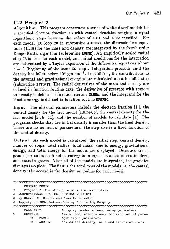
42.2 Project 2 Algorithm This program constructs a series of white dwarf models for a specified electron fraction m with central densities ranging in equal logarithmic steps between the values of RH@^ and RHQZ specified. For each model (DO loop 20 in subroutine ir~c~oar), the dimensionless equa- tions (11.18) for the mass and density are integrated by the fourth order Runge-Kutt a algorithm (subroutine R ~ G E ) . An empiricdy scaled radial step DR is used for each model, and initid conditions for the integration are determined by a Taylor expansion of the differential equations about r = 0 (beginning of the same DO loop). Integration proceeds until the density has fallen below 103 gm emm3. In addition, the contributions to the internal and gravitational energies are calculated at each radial step (subroutine I~TCRT). The radial derivatives of the mass and density are defined in function routine DEIR~;; the derivative of pressure with respect to density is defined in function routine okann; and the integrand for tbe kinetic is defined in function routine EPSWO.
Input The physical parameters include the electron fraction [l.], the central density for the first model [1.OE+05], the central density for the last model [I.OE+ll], and the number of models to calculate [4.] The progrms checks that the initid density is smde r than the final density, There are no mnterical paslzbnneters: the step size is a fixed function of the central density*
Output; As each model is cdeulated, the radid step, central densit& number of stegs, totd rrtdius, total mus, kimtie enero, gravitatiartal enera, afld total tsnergy for the model are displayed, Densities are in
per cubic centimeter, energ is in ergs, &stances in ~f?ntimeters, and mass in grams. After all of the models are integrated, the graphics displays two plots, The first is the totd mws o-f the rnadefs vs. the central density; the second i s the density vs, radius for e x h model.
CGCCCCCCCGcCCCCCeCCCCCCcCCeCcCcCCCCGcCeCcCCCCCc~CccCccc~ccCcGcccc~ccCccC PROGMM PROJ2
C Project 2: The structure of white dwarf s t a r s e c o n P v T A r r o H A L PHYSICS { F a R r R a H w~s~oru) C by Steven E, Koonin and Dawn C. Meredith G Copyright 1989, Addison-Wesley Publishing Company CCCCGGCCCCCeCCCCCCCCCCCCCCCCCCCCCCCCCCCCCCCGCCGCCCCCCGCCGCCCCCCCCCCGCCCG
GALL INIT !display header screen, setup parameters 5 COEITXZNUE !main loop; execute once for each set of param
GALL PAMM !get input parameters CALL WRCNQNI !calculate density, mass and radius of stars
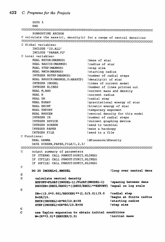
422 C. Pmgrams for the Projects
GOTO 5 END
GCCCC~CGCCCC~CCCICCCC~CCCCCCCG~CCCCC:CGCCCCCCCC~CCCCG~CCC~~C~CC~~C~CC~GCCC SUBROUTINE ARCHON
C calculate the ntasslr), densityfr) for a range of central densities cccc~eee~cc~~cccccccccccec~e~cc~cccccccccccecccc~cecc~cccccec~c~~~~~cc~:c C Global variables:
INCLUDE "0*WLL6 TNCLUDE 'PAMM.P2'
C Lacal variables: W A L MSTOR (mXMBD) !mass of star REAL RADIUS (mXMOD) !radius of star m& STEP (MMBDf ?step size REAL RMIU (WXMOD) !starting radius INTEGER NSTEP (MZImOD) lnunrbsr of radial steps -L REIOSTR tmXMOD, O:mXSTPl ! &nsity (r) of star INTEGER SMODEL !index of current model INTEGER NLINES lnunber a f lines printed aut RE& tvlc RHO !current mass and density REaZ R ? current radius
IZR !radial step RE= E G B V !gravitational energy o f star RE= EKZNT ?kinetic energy o f star W A L EXFOMT !teworary exponent REAL RROGEN !central density for this model IMTEGER IR !nu&er of radial steps INTEGER DEVICE ! current graphing device INTEGER SCmEN fsend to terminal XNTEGER PAPER !make a bardcopy INTEGER FILE Isend to a file
C Functions: REAL GAMlulll !dPressure/dDensity DATA SCRE&N,PWPER,EI~/1,~
~ececcccccc~eccCcccccecccecccccceececcecceccc~ecccececcc~ccccecc~c~c~ccc C output sumary of parameters
IF (TTEW) CALL PEtIVIQUT (OUNIT, HLINES) IF [TFTLE) CALL PFi?MOUT (TUNIT, NLLN&S) IF (GFTLE) CALL PMOUT (GUNIT, NLINES)
C BQ 20 I@ODEW%, WDZ3b 33ioop over aaneral den&
C C oalmaatr oanttal hnsity
= F L / P ( L ! rppadng htoossem 4-B mQaB= (=@%/MW) * f (Wa2/mQX) *+mQmj f mwa on log soale
C DEW ( (3.0*0,00?L/mmHj ** (1.813.0) ) 13.0 I ra&aT, sdep R=BR/ l0 . Ibsgin ad finite radius
(f MOD=) =R*R0/11). E+08 l a d e i n g raausr (XMODm) =BR%@ 12.0. E+O8 ? s t q size
C C uas TayZot ezpaneion to abtain initial con&kfont~
M= (R**3. O) * (MWH13 .. 0 ) lfnitial mar&
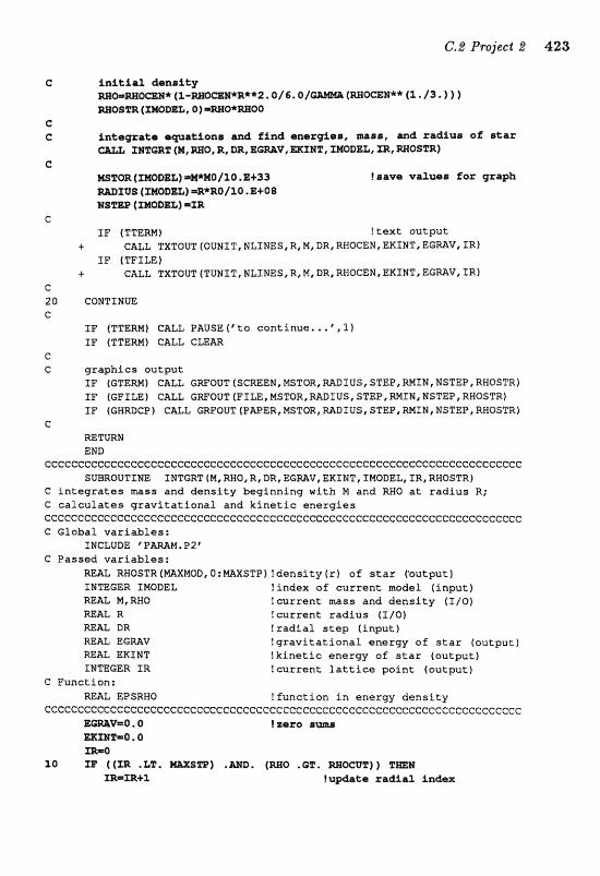
C ini t io2 density ~ ~ ~ ~ E R * ( l - ~ Q ~ H * R * * 2 . 0 / 5 . 0 /
( m D B L , 0 ) ==o*m00 G C graCsl aqluafienr and find energies, raairara, and radiulrl @F @tar
XBFaT (M, =a, R, DR, E-V, mXWrP, XMODELI IR, mOS1:Rj C
MSTaR (IMODEL) =M*M0/1Q .1&+33 !cave values for graph mXQS (XMQDEL) m~*R0/10. E+08 N S m (IMODBZ) =XR
C
I F (TTERPII) ! t e x t ou tpu t -C CALL TXTOUT [OUNIT, NLINES~ R, H, DR, RMocEN, ERINT, EGmV, IRI
IF (TFILE) + CALL TXTOUT(TUNIT,NLTUES,R,H,DR~RNOCEN,EKINT~ECRAV~IR~
C 20 CONTINUE c
IF f TTERMf CALL PAUSE ( @ t o eon t i nue . . . C , I ) XP (TTERN) CALL CLEAR
C e g r a p h i c s ou tpu t
ZF (GTERZJI) CALL GWOUT f SCmEN, MSTOR, EVLDS US, STEP, RMXN, NSTEP , RHOSTR) f F (C;f"PLEf CALL G E O V T (FILE, MSTOR, M D 1 US, STEP, WIN, NSTEP, RHOSTR} IF [GRRDCP ) CALL GRFOUT (PkPER, MSTOR, MDIUS, STEPC RNThT, WSTEP, RWOSTR)
C RETURN END
cecccccccCcCcceccceE:cccccccccccecccecccccccecccccccccecccccccccc~ccceCcc SUBROUTINE INTGRT (M, RHO, R, DR, EGMV, EKIHT, XP40DBLe TR, RHOSTR)
C i n t e g r a t e s mass and d e n s i t y beg inn ing with N and RHO a t r a d i u s R; C c a l c u l a t e s g r a v i t a t i o n a l and k i n e t i c e n e r g i e s c c c c c e c c c c c c c c c e c c c c e c c c c c e c c c c c c c c c c ~ c c c c c c c c c c c c c c c c c c C Global v a r i a b l e s :
INCLUDE TAmN.PZ" C Passed v a r i a b l e s :
mAL RMOSTR (mXMOD, 0:MWXSTPl ! d e n s i t y (rl o f s t a r t ou tpu t ) INTEGER IMODEL ! index of c u r r e n t model ( i n p u t ) REAL M, RHO ! c u r r e n t mass and d e n s i t y ( I l O f =At, R ! c u r r e n t r a d i u s fT /O) REAL DR ! r a d i a l step ( Inpu t 1 REAL EGMV ! g r a v i t a t i o n a l energy of s t a r (ou tpu t ) REAL ERlNT ! k i n e t i c energy of s t a r (ou tpu t ) INTEGER ZR ! cu r ren t l a t t i c e p o i n t (ou tpu t )
C Function: REAL EfSRWO i f u n c t i o n i n energy d e n s i t y
cccccce~~cc~ceccc~eccccecccccccccccccc~ec~ccccccccecec~cec~ccccccccccccc 0 . 0 !zero smrs 0 . 0
ER=@ ZzP ( (lR -LT. =S=) .XBD. ( m 0 .GP. MQCUT) )
XR=XR+l t u w e e raaal f n & a
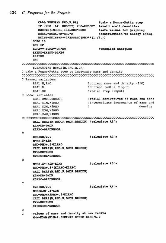
€%L% RWm {M, M O c R, DR) !take a Rmge-Katta step XF (m0 .L%. mm112") M-WOCTJI !avoid 8-22 hn@iCi@a~ =OS= (XMODEL, XR) = M Q * m 0 0 !save vauea far gzaphirtg $WV=mmV+M-Q*R !cenkrmtlen +a enexw intag. ERXH~~ZH%+R**Z*~SW0{REIO**r(31./3.])
GOIN) 50 Ern XE" L-Vm-EWV*DR*ZdO Imsc&Z@d e n e ~ g i e ~ ~ maF=mxMIC*m*EQ RETURN END
ccccccccccccccccccccccccccccccccc~ccccccccccccccccccccccccccccccccccc SUBROUTXNE RUMGE (M, RHO, R, DR)
C take a Runge-Kutta step to integrate m s s and density cccecccccccccc~c~ccccccccccccccccccceccccccccc~ccccccccccccccccccccccccc G Passed variables:
REAL M, RNQ !currant mass and density (I/Q) W& R tcusrent radius (input) REAL I3R ! radial step f input)
C Local variables: RE& DMDR, DRHQDR !radial derivatives of mass and dens m u KIM,KbRMO lintexmediate increments of mss and REAL K2M, R2RNO I density mAI , B JM, K3RBO REAL K483, K4RWQ
cccccccccccccccccccecccccccccecccccccecccccccccccccccccccccccccccccccccc DEW (M, MQ, R, D m R , DWQDR) ! &=late M B
mmDR*DmR KXW*DR*DmODR
C R=R+DR[2.0 i oaXdak% U" a M*. 5*ltSXM
0 , R, DmR, DrnODR]
E2=05DR*WQDR C
M=*. S* (K2M-XlHf ! c a d a t e kSf s =+MW. S* ( I S m 0 - K T M O )
D- {M* m0, R* DmBe DrnQDR] R3MBR*DmR R3m+DR*Dm0DR
C E=R+BR/2.0 ! calculs&e k4' @
M=WK3M-.5*82M
D- {M, RHO, R, D m R , DmODR) ltS4mDR*DWR K4=Q=DR*DMODR
C C v;orZusra: sf! =ss ~ n d dcnrAty at; new rcraius
M=M-I(~M+(~M+~.~*~M+~.o*K~M+~~SQM]/~.O
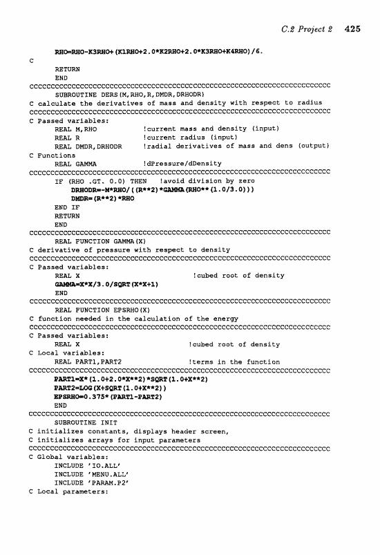
w - ~ Q - K ~ ~ W (KXWW2.0*~~0+2.0*A3mOSK4~0) /g. c
MTURW END
cccccccccccccccccccccccccecccccccccccccccccccccccccccccccccccccccccccccc SrnROUTINE DERS (M, RHO, R, DNDR, DRMODRf
C c a l c u l a t e t h e d e r i v a t i v e s of mass and d e n s i t y wi th r e s p e c t t o r a d i u s ~c~~e~ccccc~cccccccccccccccecccccccccccccccccccccccccccccceccceccccccccc C Passed v a r i a b l e s :
=&L MIRE0 !current mass and d e n s i t y ( i n p u t ) M U R ! c u r r e n t r a d i u s ( inpu t ) m u DmR, DRHQDR ! r a d i a l d e r i v a t i v e s o f mass and dens (ou tpu t )
C Func t ions m= GMW !dPressure/dDenslty
cceccccccccccccccccccccccccccccecccccccccccccccccecccccccecccccccccccccc IF (RN0 .GT. 0.0) THEN !avoid d i v i s i o n by zero
D ~ O D R = - M * ~ O / ( (R* *2) * (m~**(r.ot3.a11) DWR= (R**2) *m0
END IF rnlllfRtJ END
cecccccccccccccccceccceccccccccccccccccccccccccccccccccccecccccccccccccc M& FUHCTIOM G A m ( X )
C d e r i v a t i v e of p r e s s u r e wi th r e s p e c t t a d e n s i t y cccceccccccceccccceccccccccccccccccccccccccccccccccccccccccccccccccccccc G Passed v a r i a b l e s :
!cubed roo t of d e n s i t y *x/a. olsaz (x*xcr 1
END cccccccccccccccccccccceccccccccccceccecccecccccccccccccccccccccccccccccc
RE& FUNCTION EPSRHO [X) C func t ion needsd i n t b a c a l c u l a t i o n of t h e energy cccccccccceccccCcccccccccccccccccecccccccccccccccccccccccccccccccccccccc C Passed v a r i a b l e s :
m= X !cubed r o o t of d e n s i t y C Local v a r i a b l e s :
M A L PARTI,E"ART2 !terms i n t h e func t ion GCCCCCCCCCCCCCCCCCCCGCCGCCCCCCCGCCCCCCCC~CCCCCCCCCCCCCCCCCCCCCCCCCCCCCCC
EmTZmX* (1.O+Z .0*X**2) *BmT (2. Q+X**2) P M T 2 = m (X+SrnT (%.O+X**2) ) ==WO. 3751 ( ~ ~ n - ~ m r 2 ) END
cccccccc~ccccecccccccccccccccccccccccccecccccecccccccccccccccccccccccccc SUBRQUTINE INIT
C i n i t i a l i z e s c o n s t a n t s , d i s p l a y s header screen, C i n i t i a l i z e s a r r a y s f o r inpu t parameters c~ccc~cccccccccccc~ccccccccccccccccccccccccccecccccccccceccccccccccccccc C Global v a r i a b l e s :
INCLUDE * 10. ALL' f WCLUDE ' MENU. ALL' INCLUDE ' PARAM, PZ"
C Local parameters:
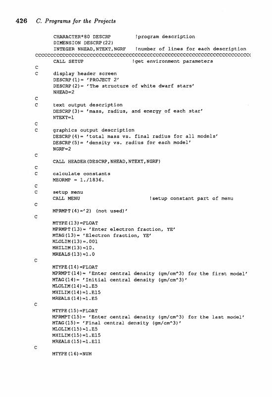
426 C. Progrranzs for the Prajeets
!program d e s c r i p t i o n DXmMSXON DESCRP (22 1 IMWGER NNEAD,NTEXT,NGRF !nu&er af l i n e s f o r each d e s c r i p t i o n
cGcccccccccccecccececccccccccccccccccccccccecccccccc~cccccccccccccccccct GALL SETUP !get e n v i r o n m n t parameters
C d i s p l a y header sc reen DESGIZP (11= 'OROS&CT 2' DESCRPf2)- cThe s t r u c t u r e o f white dwarf s t a r s " NHEAD=2
e C t e x t o u t p t d e s c r i p t i o n
DESCRP (3 )= ?mass, radius, and energy o f each s t a r " NTEXT-I
G C g r a p h i c s ou tpu t d e s c r i p t i o n
DESCRP(4)- "tataf mass vs, f i n a l r a d i u s f o r a l l models' DESCRP ( 5 ) - ' d e n s i t y vs. r a d i u s f o r each made18 NGW=2
C CALL HEADER (DESCW , XJWEAD, PJTEXT , NC;RE" I
C G c a l c u l a t e c o n s t a n t s
MEORMn = 1./1836. C C s e t u p menu
CALL MENU c
WmPT(4)= '2 ) (not used) c
NTWE (1 3 f =FLOAT M e m T (131 = EnRte e l e c t r o n f r a c t i o n , YEC MTAG (13) = 'E l ec t ron f r a ~ t i ~ n , YE1 MLQLIM(l3)-"001 MBILIN f13)=10, mBLS (13)=1. Q
C N T e E (1 4 ) =FLOAT W W T (14)= "nntsr c e n t r a l d e n s i t y (gm/cmA3) f o r t h e f i r s t model' MTAG f14)= ' X n i t i a l c e n t r a l d e n s i t y (gm/cmA3) * NLOLTM ( 2 4 ) =1 .E5 MNILTM(L4)-1.E15 mmLS (14) =l.E5
C MTYPE (l 5 I =FLOAT WMBT(l5)= "nter c e n t r a l d e n s i t y (gmlcmA3f f o r t h e l a s t modelf MTkG(IS)= 'PFiaal c e n t r a l d e n s i t y lgm/cnA3)" MLOLIM 115) -1 .E5 IVIWZLXM (2.5) =1.E15 M-LS (15) =l.Ell
e MTUPE ( 3.6) =NUM
! s e t u p cons tan t part of menu
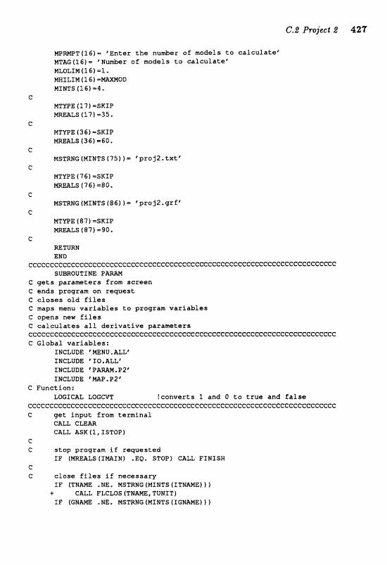
M P W T (1 6) 1 ' Enter t h e n u d e r of models t a c a l c u l a t e F M T Z ( 1 6 ) - quunzber a f mdeXs t o ca lcu la te" MLOLIM (161 =l, MHILIM (1 61 -=MOD MINTS 416) 4.
G M T S E (1 7 l =SKIP ~ E A L S (171 =35.
C MTYPE (36) =SKIP m A L S (JG)=CSD.
C MSmNG(MINTS(75))- t p p r o j 2 . t ~ t "
C MTYPE (76) =SKIP mMLS (76) -80.
C MSTRMG tMTMTS(86) ) = ?pro j2 .gr f t
e MTWE f 87) =SKIP NRmLS (871 =90.
C RETURN END
CccccccccccccccccccccccccccceecceececccccccccI:cccccccccccccccccccccccccc SOBROUTTHE P W M
C g e t s p a r a m t e r s from screen C ends program on request C c l o s e s o ld f i l e s C maps menu v a r i a b l e s t o program v a r i a b l e s C opens new files C! c a l c u l a t e s a l l d e r i v a t i v e parameters ccccccccccccCcccccc~cccccccccccccccccccccccccccccceccceccecccccccccceccc C Global var iab les :
INCLUDE ' m N O , ALLf IHaUDE ' XQ, ALL' INCLUDE * P A W . P 2 " IN~LUDE 1 m ~ . ~ 2 t
C Function: LOGICAL LOGCVT ?conver t s 1 and O t o t r u e and false
cCcccccCICtCcccccccccceccecce~cecccccccccccccccccccccccccccccccccecccccccc C g e t input from t e m i n a f
CALL CLE- CALL ASK(1,fSTOPJ
c C s top program i f requested
IF (NREALS [INAINI .m. STOP> CALL FINISH C C c lose f i l e s I f necessary
IF (TMME .NE. NSTRNG (MINTS (ITNAMEW + CALL FLCLOS (THAW, TUWIT) IF (GNRM .WE. MSTRNG [MINTS (TGNANE) ) )
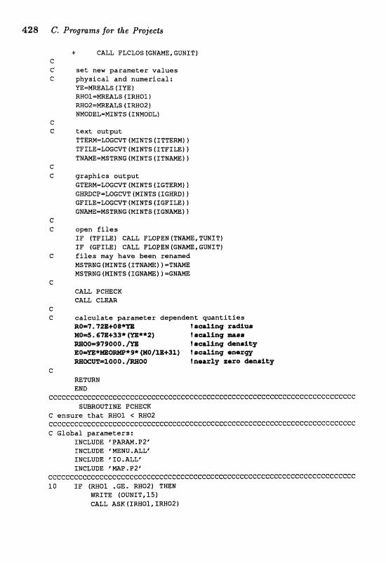
428 C, Progrrrnts for $he Pr~jects
+ CALL FLCLOS {GNAW, GUNIT) C C set new parameter values G physical and numerical:
UE=WALS ( IUE ) RBOZ=NWALS ( IRNO1) R H 0 2 m M m L S f IRWQ2 ) NHODEL-MINTS (INMODL)
C C t ex t output
TTERM=LaGCVT(MXNTS(XTTERMj) TFILEmWGCVT (HINTS ( I T F I U 1 1 TNN-MSTRNG (MINTS (ITEaMEl f
C C graphics output
GTERH=LOCCVT (MINTS [ZGTERM) ) GHRDCPmLmCvT (MINTS (TGNRDI 1 GFILE=L,~GCVT (MsNas (rC;Fxze) I GNME=MSTRNG (MINTS ( I G N m ) }
C C open f i l e s
I F ( T F I m ) CALL FWPEN (TNAm, TUNIT) IF (GFILB) c a L L F ~ P E N ~ G N A ~ , G ~ T T )
C f i f e s may have been renamed MSTRHG (MIWTS ( ITHAM) 1 =THAW MSTMC (MrWTs ( I G N ~ ~ = E ; N A ~
C CALL PCWECK CALL CLMR
c C ca lcula te parameter dependent quant i t ies
R0=?.72E+08*= laaZf1~c~f radiuo MO*. 63E1+33* (=**2) ! @&in9 gltsrro
~W=97?)000./~ foealinq W r i t y E O m + m @ m * 9 * (M0/=+32) t scaling %Inex= ~ ~ ~ = Z O t l O . / W O O InearXy zero dmaiey
e mTUR'1\1 END
ccccccccceccc~cccccccccccccccccccccccccccceccccccccccccccccccccccccececc SUBROUTINE: PCHECK
C ensure t ha t RH02 < RN02 cc~~C~cCccccccccccceccecccccccc~eecccccceC:cccccccccccccecccccc~~ccccc~cc C Global paranteters:
INCLUDE ' PPAMM. P2" INCLUDE ' =NU, ALLp INCLUDE ' IO.ALL* INCLUDE ' m ~ . ~2
cccccecccccccccccecccccceccccccccccccccccccccccccececccccccccccceccccecc 10 I F (RHO1 .GE. RH021 T m M
m I T E (OUNIT, 15) CALL ASK [ IRHol , IRHQP 1
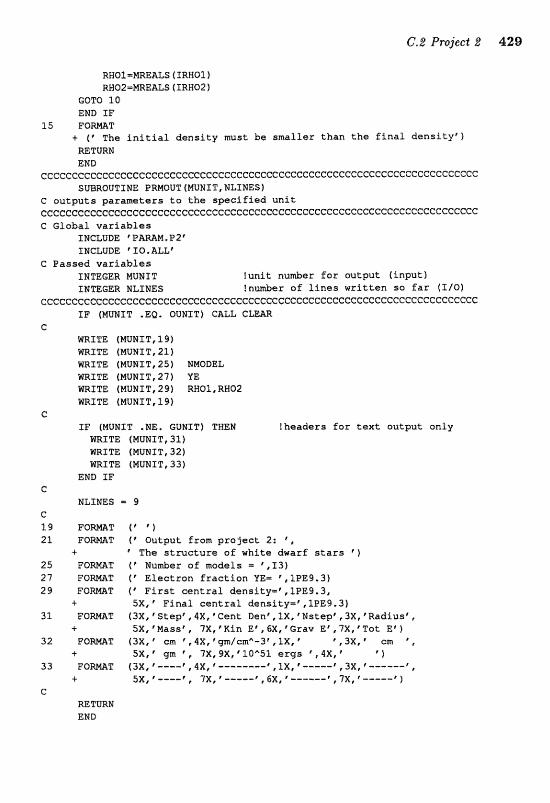
RWO1-lylREALS (IRWO1) RM62=MREALS (IRWQ2 )
GOTO 10 END IF
25 F O m T + ("The initial density mst be smaller than the final densityCl RETURN END
cee~~c~cccccc~cccccccceccecccccccceccceccccccccccccecccccccccccccc~ccecc SUBROUTINE PRMOUT{WUNIT,NLINES]
C outputs parameters to the specified unit ~ec~ce~eccccc~cccccccccc~cc~cecccC:ccccccececcccccceccccececcccecccecccce e Global variables
IMCLUDE ' PmM.P2" INCLUDE C SO. ALLt
C Passed variables INTEGER NUNIT !unit nu&er for output (input 1 INTEGER NLTNES !nu&er af lines written so far (X/O)
ccecccce~ccccccce~ccccceecccccccccccccceccc~cccccccccceccccccecccccccccc 1F (MUMIT .EQ. QUNIT) C&LL CLEAR
e mITE (NUPJLT, PS)) m%TE (ErlUNST, 21) WRITE (MUNIT, 25) NMODEL mZTE (MUPJIT,27) YE mITE (HUNIT, 29) RRO1, RHO2 WRITE (MUNIT, 1 9 )
C fF (MUNIT .NE, GUNIT) THEN mITE (MUNIT, 31) WRITE (MUNIT, 32) tVRXTE (MUNIT, 33)
END IF G
WLINES = 9 C 19 F O W T ("1 21 F O m T (' Output from project 2: ' ,
+ * The structure of white dwarf stars ' )
25 F O m T ( * MuntberoEm~d@1s=~,S3) 27 F Q M T ( ' Electron fraction YE= ',1PE9,3) 29 F Q m T ("Fist. central density=',lPE9.3,
+ SX,VFinl central den~lty='~,lPE9.3) 31 F O m T I3X, 'Step" ,4X, 'Cent Den" I X , Mstepf , ,3X, 8RadI~s8,
+ SX,'Masst, 7X,'Kfn E\,CiX,'Grav E\7X, 'Tat E' ) 32 F O W T (3X, "em ,4X, " r n / ~ m " - 3 ~ , 1X, \ , 3 X I r cm ', i 5 X , "m @ , ?X, 9X, 1QA51 ergs ', ,4X, @ ' 1
33 F Q ~ T (3~,r----r,4~,*--------1,2~~r----- r , ,3~, L--..-...I
3- SX, " - - - F , 7X,@-----',6X,f - - - - -m. * ' " 1 X , I ----' 1 C
RETURN END
!headers for text output only
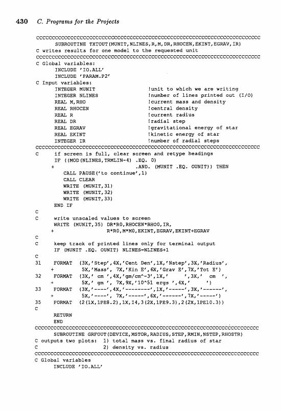
$30 C, Pmgrams for $fie Projects
ccccccccccccceccccccccccccccf:ceccecc~ccccccccccccccceccceccccccceccccccc SUBROUTINE TXTOUT (MUNIT, NLXNESc R, M, DR, RROCEM, EKINT, EGMV8 I R )
C w r i t e s r e s u l t s f o r one model t o t h e r e q u e s t e d u n i t cceeeecccccccccccccccccccccccccccccccccc~ccecccccccccccccccccccccccccccc C Global v a r i a b l e s :
INCLUDE IO -ALLf INCLUDE * P P A M . PZ*
C Inpu t v a r i a b l e s : INTEGER MUNIT Iunit t o which w e a r e w r i t i n g XNmGBk! NLZNES t n u a r of l i n e s p r i n t e d ou t ( 3 / 0 ) REAL H, RHO f e u r r a n t mass and d e n s i t y R W RHOCEN ! c e n t r a l d e n s i t y
R t c u r r e n t r a d i u s m= I3R ! r a d i a l s t e p RE& E G M V ! g r a v i t a t i o n a l energy of s t a r RE& ZKINT ! k i n e t i c e n e r w of s t a r INmGER IR !nu&er of r a d i a l steps
e~~ccccccceeccecccccccccccccf:cccccccccccccccccccC:ccc~cecccccccccccc~eccc c if s c r e e n f s f u l l , c l e a r s c r e e n and r e t y p e headings
3F ( (NOD (NLINES, TRMLIN-a . EB. 01 i .AHD. (MUNIT .EQ, OVNTTI THEN
CALL PAUSE(%o con t inua f ,,l) CALL CLEAR WRITE (MUMIT, 31 1 W I T E (MUNIT, 32) m 3 T E (MUNIT, 33)
END I F c C write unsca led v a l u e s t o s c r e e n
WRf TE (MUNTT, 35) DRXRO1 RMQCEN*RM00, 3% i R*RO,N*NO,EKINT,EGMV,EKINT+EGMV
e C keep track of p r i n t e d l i n e s on ly f o r t e r m i n a l output
IF (NmIT .EQ. OUNIT) NLIMBS=MLZNES+1 C 31 F Q m T f3X,~SStep~,4XfTeent Den~1X,~NNstepa,3X,~Rad4.usf,
1. SX, *Mass\ ?X, "in E t , SX, "rav E 1 l ? X , 'Tot Et ) 32 F Q m T (3X, C cm ?, ,4X, ~gm/mh-3', IX, \3X,' cm ',
1. 5Xtt gm gm, ?X, 9X, "QA% ergs " ,4X, C * 1 33 F Q m T ( 3 X I '-----" ,4X,' ".------- t *,IX,' --m-.". I , 3 X , 1 ---...-.," t
+ sx, &--.,.p "&, 1 6X, L...----@ ?X, L----f f 35 F O W T (2 (1X,1PEBe2), 2X,I4,3 (2XI1PE9.3) 2 (ZX, ZPElO-3) 1 C
RETURN END
~eceecc~~ccc~ccc~cccc~~cC~~~cc~~ccc~~ccccccccccccccccccccc~ccc~ccccccccc SUBROUTINE GWOUTfDEVZCE,MSTOR,MDIUS,STEPIRMINfN5TEI",RHOSTR)
C o u t p u t s two p l o t s : 1) t o t a l mass vs . f i n a l r a d i u s of s t a r C 2) d e n s i t y vs . r a d i u s ccceec~cCcccccccce~ccccccccecccccccccccccceecccecccccccccccccecccccccccc C Global v a r i a b l e s
SMCLUZZe 'X0.ALL8
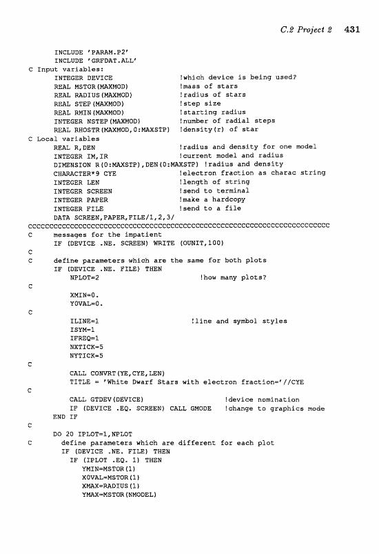
INCLUDE ' PARAN, P2' INCLUDE ' GRFDAT .ALLp
G I n p u t v a r i a b l e s : INTEGER DEVICE !which d e v i c e i s b e i n g u s e d ? REAL MSTOR (MaXMGDf !mass o f s t a r s RE& MDTUS (WNOD) ! r a d i u s o f s t a r s REAL STEP ( W M O D 1 ! s t e p s i z e REAL RMIM (MAXMOB 1 ! s t a r t i n g r a d i u s INTEGER NSTEP(WXM0D) !nu&er o f r a d i a l s t e p s REAL RHOSTR[MAXMQD,O:MSTP) ! d e n s i t y ( r ) o f star
e L o c a l v a r i a b l e s REAL R, DEN ! r a d i u s a n d d e n s i t y for o n e model INTEGER IM, IR ! c u r r e n t model a n d r a d i u s DlmNSIOH R (0 :MAXSTP), DEN (0:msTp) ! r a d i u s and d e n s i t y
CBWCTER* 9 GYE ! e l e c t r o n f r a c t i o n a s e h a r a c s t r i n g INmEGER LEN ! l e n g t h o f s t r i n g INTEGER SCREEN !send t o t e r m i n a l INTEGER PAPER ?make a h a r d c o p y TNmGER FILE ! s e n d t o a f i f e DATA S C R E E N , P A P E R , F I L E / ~ , ~ /
~~~~~c~~~cc~ccc~cececcc"ccccccccececcccc~ecccccccccceccecccc~cccccccccccc C messages f o r t h e i n r p a t i e n t
I F (DEVICE .NE. S@W&N) M I T E (OUHIT.100) G C d e f i n e p a r a m t e r s which are t h e same f o r b o t h glats
r r (aEvrcE .NE. FXLE) THEN NBLOT=2 !how many p l o t s ?
C XNIN=Q . VOVAL=O.
G
IL1NE=1 ISYM=1 XFREQ=1 NXTICKm5 NV'P"ICK=5
C CALL C O m T (YE, CUE, ZEN) TITLE = 'Whi te Dwarf S t a r s w i t h e l e c t r o n f r a c t i o n - @ / l / C Y E
C CALL GTDEV (DEVICE) ! d e v i c e n o m i n a t i o n I F (DEVICE .EQ. SCREEN) CALL GNODE !change t o graphics node
END I F C
Do 20 IPLOT-1,NPLOT C d e f i n e parameters which a r e d i f f e r e n t for each p l o t
TF (DEVICE .NE, FILE) THEM IF (IFLOT .EQ. If THEN
YMIN-NSTOR [l ) XOVAL-MSTDR (1 ) xm=morvs (I l YMAX=HSTm (NMODEL)
! f i n e a n d sy&ol s t y l e s
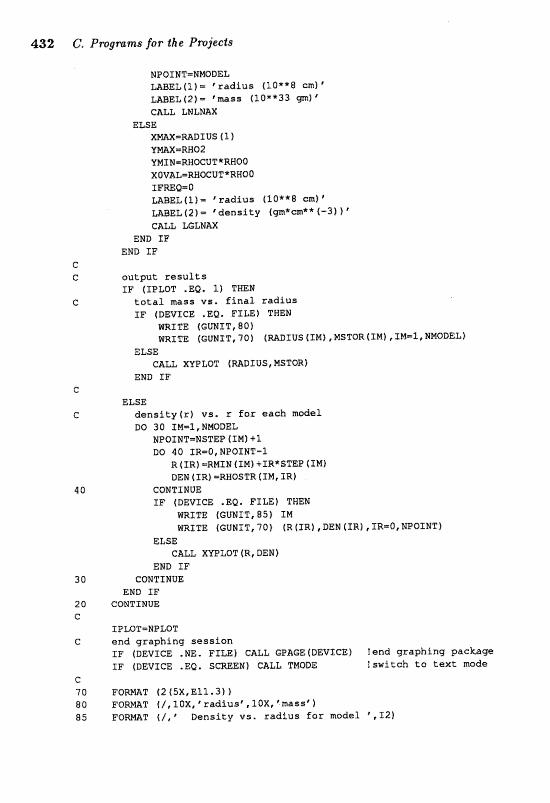
432 C. Pmgmsnrs for the Projeds
NPOINT=NMODEL LABEL (1) = "radius t 10**8 cm) ' L&BEL (2) = #mass (10**33 p) CALL LMLMAX
ELSE XP(YLX=MB I US ( 1 ) IImXmRX02 YMIN=RHOCUT*RHOO XOVU=RHOCUT*RWOQ IFWQ=O LAB&L(I)= badfus f10**8 cm)" m E L ( 2 ) = "ensity tp*em** (-3) 1 ' CALL LGLMAX
END If END IF
C C output results
IF (IPLOT .EQ, 1) THEN G total mass vs. final radius
IF (DWICE .EQ. FILE) I'MEFJ WRITE (EVNIT,80) WRITE [GUMIT, 70) (RADIUS (IN), MsTOR [IM) , 3:N=lI MMODEL~
ELSE GALL XVDLOT (RADIUS, NSTm)
END IF G
ELSE C denslty(r) vs. r for each model
DO 30 IM=1,NMQBEL NPOINT=NSTEP (IM) 4-1 no 40 IR-Q, NPOINT-I
R (XR~ =RMIN (IN) +rR*sTEP 4 1 ~ 1 nEH ( IR} =RHOSTR IM, IN-
CQWTSNUE IF (DEVSCE .EQ. FILE) THEN
WRITE (GUMIT,85) IM mXTE (GUNIT, 701 (R I IR) , DEN (TR) , IR=O, NPOINT)
ELSE CALL XYPLOT (R, DEN)
END IF 3 0 CONTINUE
END IF 20 CONTINUE C
IPLOTmNPLOT C end graphing session
IF (DEVICE .NE. FILE) GALL GPAGE f DEVICE) f end graphing package eF (DEVICE .EQ. SWEN) CALL TMODE !switch to text made
C '70 F O m T (2 15X,E11e3) 1 80 Fa-T ( I , LOX, ' radius', lOX, 'mass' 85 F O m T (/, Deensity vs. radius for model \ ,121
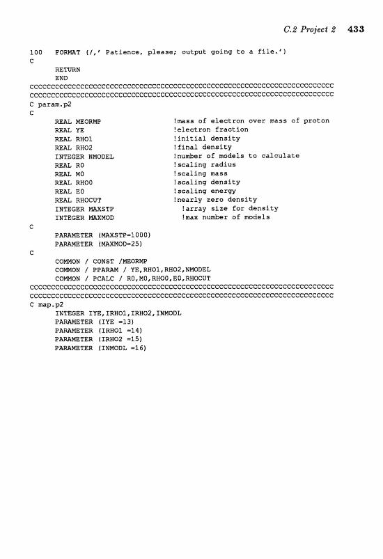
100 F O m T f / , @ Patience, please: output going to a file.@} c
MTURN END
~~ecc~~~cccccccccccccecccccccccccccccccccccc~ccccccccccccccccccccccccccc ~ C C C G C C ~ G ~ G ~ C C C C C C ~ ~ ~ C G ~ ~ C C ~ ~ C G C ~ ~ ~ C ~ ~ C ~ C ~ ~ ~ C ~ ~ C C ~ ~ ~ C C ~ ~ G ~ C C ~ C C C C C ~ ~ ~ ~ ~ ~ C param.g2 C
REAL M3eQRW !mass of electron over mass of pratan m= YE !electron fraction =&L RHO1 !initial density M&L RA02 ! final density IWTEGER NMODEL fnudcr o f models to calculate REAL RO !sealing radius W A L MO !scaling mass WAS, RWOO !scaling density m A L E0 !scaling enerw RE& RWOCUT Inearly zero density INTEGER MAXSTP !array size for density INTEGER MXMOD !max number o f models
c P m M E T E R ( W S T F = I Q 0 0 ) P M m T E R (MAXMODa25 1
c GOmQN / CQNST /MEORW COmON / PO&MM / VE,RXQI,RHOZ,NMODEL CQMGN / PCALC / RO, WO, RWOD, EO , RHOCUT
ccccccccccccccccecceeccecceccccccccccce:ccccceccececccecccccccceccccccccc cccecccecccecceccccccccccccccceccccceccecccecceccccceccccccccc~cC:ecccecc C map,p2
TNTEGER IVE,ERHOL,fRWQ2,INMODr P A W E T E R (IUE =l31 P h W E T E R (SRN01 13.41 P m m T E R (SRN02 -3.5) P m M E T E R (INNQDL =I 6)

434 3. Programs f ~ r %he Pr~jects
C.3 Project 3 Algorithm This grogram sdves the Bartree-Focb equations ia the R1l- ing appro~mation for atomic systems tvith electrons in the Is, 29, and 2p shells. To be&n the iter&ive procedure? normdzed hydrogenie wave functions (subroutine BMRCR) and their energies (subroutine EIERGY) are calculated, the virid theorem is umd to det ne the variational parme- tes ZSTAR, whieh is in tarn used to cafedate the aptimd scaled hydrogenie wa;ve functions and their energies. These wave functions serw as our ini- t i d &e;uess".
Then 'fOp each iteration requested the s i n e particle eigenvduc! equik tions (IE.28) are solved as inhomogeneous boundary value problems (sub- routine saouw) using the single partide energies, electrostatic potential, and Fock terms cdculated from tht? pfevious wave functions. The homo- geneous solutions are found using Numerov's method, and these solutions are then u s 4 to cafcalate the inhomogenmus aotutioxls usiag the Green's Eunction method. Care is t&en to ensure that the 28 orbital is arthogonal. to th& of the 1s. When the repest& iterations are completed, you can request more or allow the cdcdation to t e r ~ n a t e .
Mu& of the computational eEod is in the cdedadion of the sinde particle energies (111.30) and totd energy (III.26,27) for each set of single partide wave functions (subroutine EBERGY). In subroutine SOVRCE the to- t d electron dertsity is calculated as a weighted mrage of the current and previous densities, and the Fock terms (111.28 b,c) are evaluated using the trapezoid& rule for the integrals md the t h r e j symbds from subroutine SqmJ. The dectrostatic potentid due to the electrons is cdcdated in sub- routine POIS~E where the Numerov method is used to integrate Poissads equation (III.18), and the unwanted linear behavior is subtracted off. The remaining energy integrals are calculated in subroutine EWERCY using the trapezoidd rule.
Input The physical parameters are the nuclear charge [G] , and the occupations of the i s [2], 29 [2], and 2p [2] states. The numeri- cal parameters are the ranlid step size (Angstroms) [.01], the outer radius (Angstroms) [2], and the initial number of iterations. The program checks that the totd number of radiaf, steps does not; excwd B I I X ~ P = 2000; if it b e s , yau xe prompted for a larger fadid step.
Output After each iteration all of the single particle energies (E- netic, elearon-nudeus, electron-dectron, exchange, totd potentid, and total) are displayed for each occupied state, as well as the total for all states, Ml ener&es are in. electron v01tg. When iterations we completed,
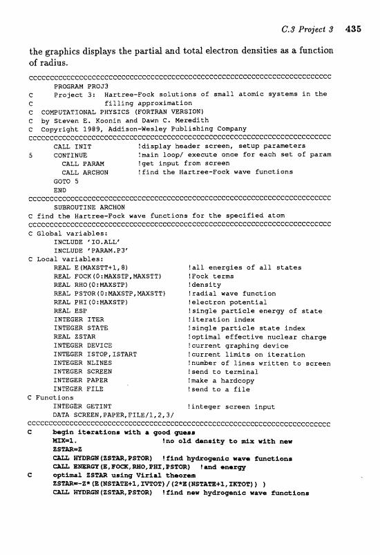
the graphics displays the partial and total electron densities as a function of rdius .
cccccccCcccccccccccccccccccccccceccccccccccccccceccccecCcccccecccecccccc OROGmN PROJ3
C Project 3: Wartraa-Pock solutions of smll atomic systems in the C filling approximation C COMPUTATICtNAL PHYSICS (FORTMN VERSZOM] C by Steven E. Moonin and Dawn C. Mereditk C Copyright 1989, Addisan-Wesley Publishing Company ceeccccccecccccccceccccccccccccccccccccccccc~ccceccccccccccccccccccccccc
CALL I M X T Idisplay header screen, setup parameters 5 CONTINUE !main loop/ execute once for each set of param
C"ALL P A M !get input from screen CALL ARCHOH !find the Hartree-Fock wave functions
GOTO 5 EBB
ccceccccccccccccccccccccecccccccccccccccccccccccccccccc~cccccccccccccccc SUBROUTINE ARCHOW
C find the Nartree-Fock wave functions for the specified atom cccc~cccceccccccceccccccccccccccccccccccc.cccccc~cccecececcccceccc~c~cccc C Global variables:
INCLUDE " 0 . ALL' INCLUDE * PARAM, P 3'
C Local variables: REAL E (mXSTT+1,8f !all energies o f all states REAL FQGK 4 0 : M S m , NXSTT 1 ! Fock terms REAL RWO(0:MAXSTP) !density REAL PSTOR 4 O :mXSTP, MXSTT) !radial wave function REAL PHI: (0:NAXSTP) ! elect ran potent ial REAL ESP !single particle energy of state INTEGER XTER !iteration index INTEGER STATE !single particle state index m& ZSTm !optimal effective nuclear charge INWCER DEVICE !current grapking device INTEGER ISTOP, ISTART !current limits on iteration INTEGER MLINES Inu&er o f lines written te screen INTEGER SCREEN !send to terminal INTEGER PAPER !make a hardcopy INTEGER FILE !send ts a file
C Functions XNEGER GETINT !integer screen input DATA SCREEN, PAPER, FILE/1,2,31
cccccccceccceecCecccccccccceececcecccccccccecccccccecccccccccccccccccccc C begin itazakiona wtlth a good p e a .
E X = l . !no old denoitg t o d x witb new ZSTrnmZ
W D M R (%S%=, PSFm) I find hydroqenlo wave funeelens
I Z S T m using Virfaf theorcsm %SPm=-Z* (E (RBFATE+X, IWO'P] / 42*E (NSPAPEile XKTQ2) 1 1
WltDWE (%SF=, PSTW) ! find new hycfsogenSc wave fwct icne
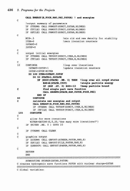
436 S. Programs for the Pvojects
E m R m (B, B o a , EEC?, Pas , PSTOR) 1 and snrrzg%err- C
! o u t p u t s u m a r y o f p a r a m e t e r s I F (TTERM) CALL PmOUT (OUNIT, ZSTAR, N L I m S ] I F (TPILE) CALL PRMOUT (TUNIT, ZSTAR, HLINESj I F (GFILE) CALL PWOUT (GUNIT, ZSTAR, NLXHES)
C
MIX==, 5 !mix old and new d e n s i t y Ear s t a b i l i t y I TEE= Q ! z e r o i t e r a t i o n c o u n t e r s ISTARTSO Z STOP=O
c G o u t p u t i n i t i a l e n e r g i e s
TF (TTERM) csLL TXTOUT (OUNIT, ITER, E, NLINES I I F (TFTW) CALL SXTOUT (TUNIS, ITER, EI NLIMESI
c 1 0 CQUTLNUE !loop o v e r i t e r a t i o n s
fSTAWT=ISTOP+l ! u p d a t e i t e r a t i o n c o u n t e r s XSTQP=ISTOP+NTTER W ) 100 Im=ZS%mT, f STQP
DO 50 ST&-1, f f p (NOCC (SF&=) .HIE. 0 ) ?.Loop ever @a+ states
ESE* (SZAZB, IPOT) tsin@e m ~ i a T a , mnara IP ( U P .QT. O) ESP=-ZO !keep g r r t t i c i ~ bunad
part: wave 2uncrtion (STaTE, ESP, PSTGR, P-, PHT)
m CoBSImVI& colZaala%e saw eaergiss and output:
(E, EQCK, =Q, PHI, BSTQR) I F (TTERM) CaLL TXTOUT (OUNIT, ITER, E, NLIEE51 I P (TFTLE) CALL TXTQUT (TUNIT, ITER, E, NLINES)
100 C 8 N 3 t X m C C a l l o w E a r m o r e i t e r a t i o n s
NITER-GETTNT f 0 , 0 , 2 0 , "Wsw many m a r e i t e r a t i o n s ? ' 1 TF (NITER .NE. 0 ) GOTO 10
C IF (TTERM) CALL CUAR
C C g r r s p h i c s o u t p u t
I F (GTERM) CALL GWQUT (SCREEN, PSTOR, RHO, E 1 I F (GPXLE) CALL GWOUT (FILE, PSTOR,RHQ, E] I F f GXRDCP f CALL GWOUT (PAPER, PSTOR, RMO, E)
C RETURN END
cccccccecccccccccecccccccccccccccccccccccccccccccc~ccccccccccccccccccccc SUBROUTINE HYDRGN(ZSTWR,PSTORI
C creates h y d t o g e n i c w a v e f u n c t i o n s PSTOR w i t h n u c l e a r c h a r g e = Z S T m e~cccccccceccccCcCccceccccccccecccccceecccccceccecccccceccceTcccccccccccc C Glabal v a r i a b l e s :
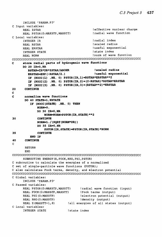
C Input var iables: W a ZSTAR ! e f f e c t i v e nuclear charge RE& PSTQR (0 : MXSTP, W S T T I ! r a d i a l wave funct ion
e Local var iables: INTEGER ER ! r a d i a l index RE& RSTAR ! scaled rad ius WEAL ERSTAR !useful exponential INTEGER STATE ! s t a t e index W& BOW !norm a f wave funct ion
~ ~ c ~ ~ ~ c c c ~ l c ~ c c c c ~ ~ c ~ c ~ c c c ~ : c ~ c e c c c c c c c c c c ~ c c ~ c c c c c c ~ c c c ~ ~ c c c c c c c ~ c c c c c c c c C aes~a zmU.of parks ef. hyd*.og.enAc nave functions
DO I rclaled
WEm/2 . 1 t umefuz n%iaf za ( N ~ C (2) .m, 01 ES~COE~ (SR, 22 = R S ~ * W T ~ * XI!' (SWC (2) .m, O) PSTQR (XR, 2) :.(2-=T=) . f R S m * m T m XE (BWC (3;) . NIC. 0 ) PSgQR (SIC, 3) = (MZm**2) *W%=
20 C a F X M m G e
ZEi' (NWC (SPA=) 0 ) T m B MO-O DO 3Q X w O , W R
M@-%. I (sag [HW*DR) 1 DO 35. =m@,=
Ps1Cm (332, smPE) =PsmR (m, SPATE] *HOW 315 CQIPSIXI~
m XB
C mTURH END
CCCCCCGCCCCCCCCGCCCCCCeCCCCCCCCCCCCCCCCCCCCCCCCCCCCCCCCCCCCCCCCCCCCCCCC~ SUBROUTINE ENERGY (E, POCK, RHO, PHI, PSTQRf
C subrout ine t o c a l c u l a t e t h e energ ies of a normalized C set of s i n g l e - p a r t i c l e wave func t ions (PSTQR); C a l s o c a l c u l a t e s Fock terms, density, and e l e c t r o n p o t e n t i a l eccccccccccCccCCcccccf:ccccC:ccccccccceccc~e~cccceccecccI:cccceecceccccf:c~c C Global var iab les :
INCLUDE 'PARAM.P3' C Passed variables:
W& PSTOR(O:WSTP,mXSTT) ! r a d i a l wave funct ion ( input) POCK ( 0 :mXSW, WSTT) ! Fock terms (cutput 1
mAL PM1 (Q:PIAXSTP) !e lec t ron p o t e n t i a l (output) RE= RXQ O : m X S T P 1 !densi ty (output) MAL E (WXSTT+3,8) ! a l l energ ies of a l l s t a t e s (output)
G Local var iables: INTEGER STATE ! s t a t e index
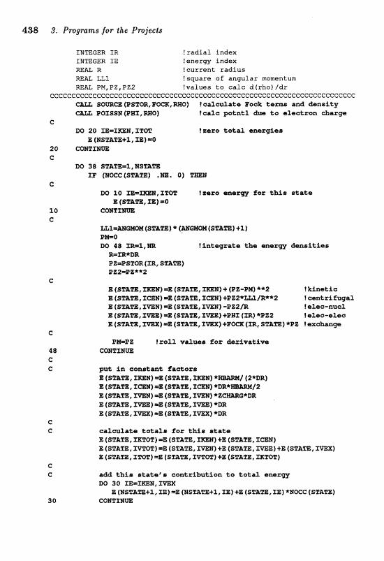
438 3, Pr~grams far bhe Pmjeets
INTEGER IR !radial index INTEGER IE !energy index REAL R ! current radius REAL LLZ !square of angular momentum mm I?M,OZ,PZZ !values ta ealc d(rho)/dr
ccccccccc~cccccccc~cccccccccccceecccceececee~ccccccccecceccccccccccccccc SOW= (PSPaR, F-, =Q) ! aaleulate Rook ta- an4 arnoity POISS~ (FEE, =a) Icdc ptnC1 dne to electlron ekargs
C DO 20 XE=XmR, I21o.T fzrru toksl maxg%am
E (NS2&TE+f, IE) m0 20 eomxwf7E: C
DO 38 ST&m=%,NSam rs (EOCC~STA~B) .m, 0 )
C W 10 SP=TmB,TTOT !zero saaza Eor thh state
E (SPATS, XL) =0 10 C a m f Elm C
LL%=MWW (S%&=) * (VaQH (ST&rn) $1,) PM=Q 130 48 X R = l , m !integrate the enarw drtxzr~ftias
R==* BR BE=PSTQE (m, STATE) PZ2=PZ**2
? kinrticr loentri2uqal
E (SPATE, XWH) =E (SZ&TE, m N ) -EZ2m !~L&@o--c~ E (STAgE, I-) =B (STAEE, I-) +PHI {IR} *F22 falea-else
) =%E (SE&=, E m ) +F= (ZR, STam) *PZ ! exabap
?&l t h f s a+a&a@o ~onts ibutfan to %eta2 smszw DO 30 XE=mH, -X
E (WsTAm+l, ZE) =E [W5Z1A~+ZI IZ) f E I E) *NOCC (SFA,trE) CONPXNW
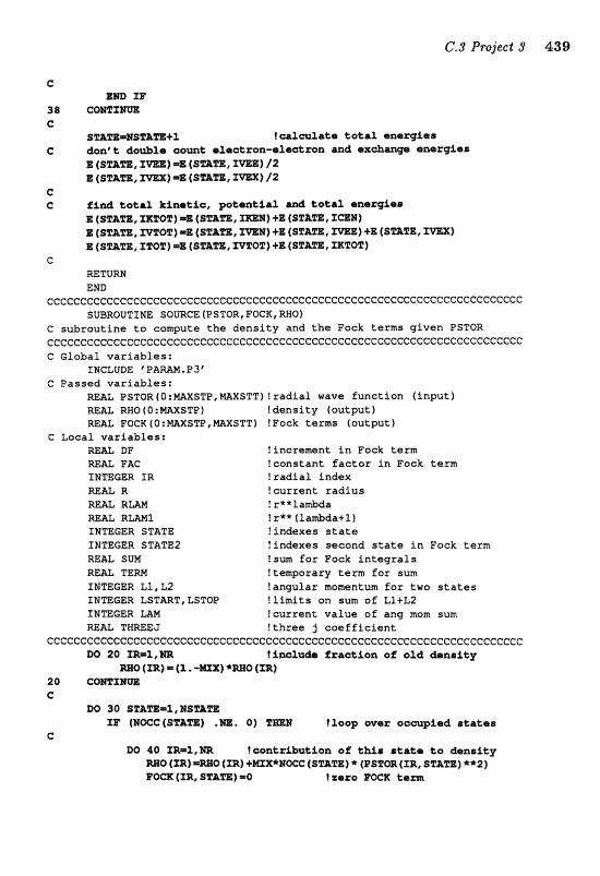
C Ern 33'
C !=%&ate toLa2 mazgAes
0 (SF&=, I=$) =S [S==,
C C ~i& totrf kinatio, ]~~)tmntiorl. and ta tr l ertexrgfso
a f sT&m, me%) =E (STArn, Ims) +E ( SZPArn, f a w l E (STArn, m%=) =E (ST&ZZ, XmE) t E [S%&rn, =E) +E tsmm, = X ) E (S%&=, xzozl) =E (SF&=, mar 1 +E ( s z ~ , ZTBT~
c RETURN END
C~ccccc~~ccccccc~cccccccc~cc~c~~c~cccc~cccc~~cccccccccccccccccccccccc~cc SWROUTIME SOURCE (PSTOR, FOCR, RN01
C subrou t ine t o c o q u t e t h e d e n s i t y and t h e Fock t e r m s g iven PSTQR CCCCCCCCCCCCCCCCCCCCCCCCGCCCCCCCCCCCCCCCGCCCCCCCCCCGGCCCCCCCCCCCCCCCCCCC C Global v a r i a b l e s :
INCLUDE ' PAmM. P 3' C Passed v a r i a b l e s :
RE= PSTOR [O:MAXSTP, MXSTTI ! r a d i a l wave fune t ion ( i n p u t ) REAX; RWQ(O:mXSTPl !dens i ty f a u t p u t f =&L FOCK (O:WSTP,MAXSTTf ! Fock terms (output f
C Local v a r i a b l e s : W% BE" l i n ~ r e n r s n t i n Fcck t e rm REAL PAC !constant factor I n Fock t e r m INTEGER IR ! r a d i a l index WAL R !cu r ren t r a d i u s
R U M ! r**lat&da M A L RMM1 t re* f lanbdatL) TWTEGER STATE ! indexes s t a t e IM'PEWR STATE2 !indexes second s t a t e in Fock term RE& SUM !sum f o r Fock i n t e g r a l s
TERM !teny>orary term f o r sum GER Lfi, L2 !angular momentum f o r two s t a t e s
INTEGER LSTART, LSTOP ! l i m i t s on sum of LltL2 INmCER M !cur ren t v a l u e of ang mom sum REAL TNREEJ l three j c a e f f i c i e n t
CCCCCCC~CCGGCCCCCCCCGCCGCGCCCCGCCCCCCCCCCCCGCCCCCC~CCCCCCCCCCCCCCCCCCCCC DO 20 S1R..rT,m linaImb fractfan aL 03.4 dsnelty
{m} = 4% ' * N O (ZR) 20 CQ1J"r C
DO 30 SZ&ml,fQSmm X ( S ) . 1 !loop we6 oompfsd 6tatolir
C DO 40 m=X,lfnz !eon%rfW%ion of tbis 6tat;e t o b n s i t y
M O (XR) -0 (XR] t m X * E a (S2&=) * (BSSCOR (XR, STAm) **2) P m (XI?.@ BTAmf m0 I s;sra mCIC, CS=
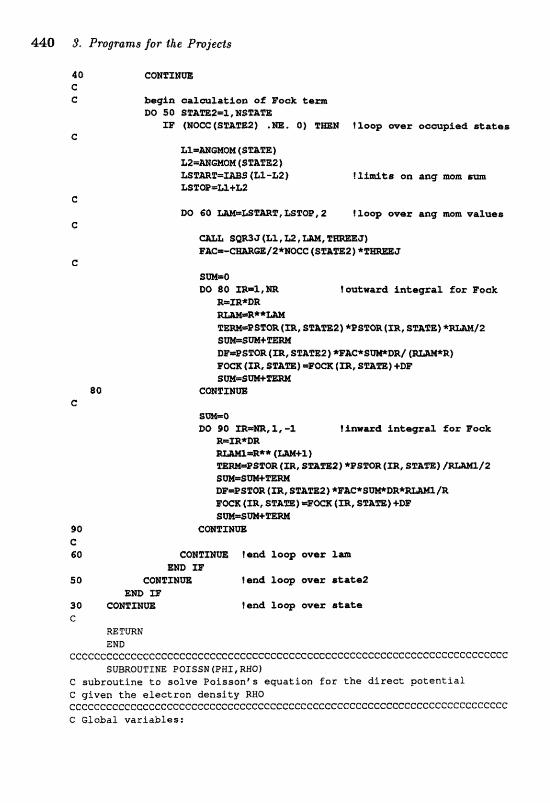
5W=0 DC) 90 mm, 1, -3, linwrrd InCaglzal for F o e
WXR*DR
s m (ZR, sTam) = E m tzR* s s-sm+mw
90 c m x m C 50 ! a d low ever 2-
EMD IE" 5 0 C O N Z I H a fear3 reap mar rtaem2
EBB 3 3 tend toop over stake
C RETURN END
ccccccccccccceccccccccccceccecccccececcceeccccccecccccccccccccccccc~cccc SUBROUTINE POISSN[PWX,RBO)
C subroutine to solve Poissan- sec_yuation f o r the direct potential C given the electron density RHO cccccecceccccececcccccecececcccccccccccceccecccccccccceccL:cccceccccccccc C Global variables:
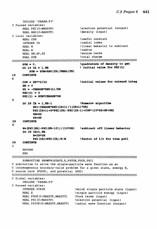
INCLUDE rPAMM.P3' C Passed vaziables:
REAL PNI(O:MSTP) !electron potential (output) REAL RHO ( O : mXSTP J !density (input)
C Local variables: M U CON !useful constant INWGER IR !radial index W L M !linear behaviar to subtract M& R ! radius =L SH, SP, 52 !source terms
SUM !total charge ~ c e ~ ~ e ~ e e ~ ~ ~ ~ ~ ~ ~ e e e c c ~ ~ c ~ e c ~ ~ e c ~ c ~ c c c c c c c e c ~ c c c c c c c e c c ~ ~ c c c c ~ e ~ ~ ~ ~ ~ e ~ ~ e c
Cl . iqa&a%uru of! &arri%g t o p t : M) 19 +c l.,= 1 la i t f rl wag- 2or P m (11
l.9 C W X N m C
CON DR**2/12 Ilaftial V ~ W B for -@W&& in%w
C
*ss S Z = S
29 CmTN'IJE C
( P 1 I l / R ) f r ~ k r r o 0 ; of 8 If n r u bbrvior DO 39 3R=Z,N]6t
R=I]a*DB B= (XRZ =Pm (XR) /R-H t iaeor of! %/X for t
39 c m z m e
RETURN END
ecececceccccccccccccccccececcecccccecccecccecccceccccccccccccccccccccccc SUBROUTINE SNGWN f STATE, E, PSTOR, FOCKi) PWT 1
C subroutine to salve the singfa-particle wave function as an C inhsmogeneous boundary-value problem for a given state, energy E, C source term (POCK), and potential (PWZ) CcCcccecccc~cecec~ccccecceccccccccecccccceeccccccccceeccccC:ccceeccccecce C Global variables:
INCLUDE 'PWN,PJ* C Passed variables:
INTEGER STATE !which singfe particZe state finput) WAli, E !single particle enerw (input) REAL FOCB (O:MBXSTP, mXSTT) !Pock terms (input) REAL PHI (0:MAXSTP) ?electran potential finput) REAL PSTBR(O:MXSTP,mXSTIIf !radial wave function foutputf
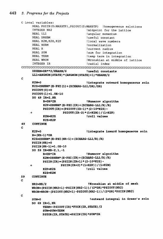
442 3. P~ogrants f:or the Pmjects
C Lacal variables: REAL PSfIN(O:MSTP),PSIOUT(O:~XSWl !homogeneous salutions INmGER NRZ !midpoint for the lattice
LL1 !angular momentum REAL DRHElPl !useful constant m& K2M, K2Z, K2P ?local nave numbers =At NORM !normalization REAL R !currant radius
SUN !sum far integration REAL 91Em !tamp term in integration =At mON !Wronskian at ~ d d l e of lattice INTEGER ZR !radial index
CCCCCCGCCGG~CCCCCCGGCGCCCCCCCCCCCCCGCCCCGCCCCCCCCCCCCCCCCCCCCCCCCCCCCCCC t use
U l M a O M (STAEE) * (==OM (SF&=) +2 12 c
PSXQgT (l) =l, @E-%Q DO 49 Xm2,m
4 aszau~ (m-2) * (z+x~M) ) / (I+XK~P~ AZB=K2Z !roll va&ues mXmK2P
49 e a m x m G
R2PmranO ?fnke@zae~t ?Lnwad bemgamouri B O ~ R
* (E-P= (m-2) + (ZC PSXX t-4 (m) =O ESXXE (=-l 1 S OE-30 80 59 ==m-2,1, -1
(E-PHI (m) + (2 (asrxg (IR+~) *
3. ESZZI (ZR+2) * (3+X:2E> 1 / (1+A2Mj mBe2B ?roll ualuersc K28=X%M
S9 eamxm C
===l2 ISronrtkian at atfWe of msh mo~= (Psrnsr ( ~ P + I ) -PSIXI (m-%) ) 1 (~*DR] *PSZB~T (m) mm-a~- (nsxavrc (m+%) -psrarr% (m-%) f 1 (Z*BR) *PSZXI (m21
C S=-@ !oudwwd fnteqzal in Cmenps soln DO 69 Wa
-nszouT (a) *P- (XR, STATE) I2 S W = S W T r n ~srm (rR, sm~~j =ESXII (XRI *SW*OIZ
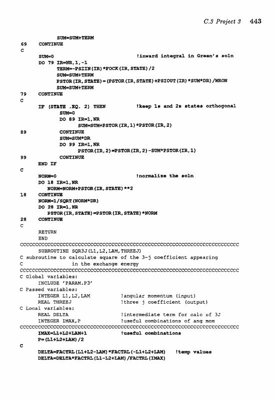
s-sw+ 69 CQmmVE C
S W 0 tinwrzd inestgra% in Oraenb edla DO 79 XR=rn,X,-11
-PSf f N (XR) (ZR, SmTE) / a s m s m + m m PsTOR (ZR, S-=] = (PsTm (XR, STA.ZEj +PSXQR {XR] *SUM*DR) /=OH sm=sm+
79 COrnfErn C
23' (SF&= .Ea. 2 ) "rEOZN fkew 1s and 2n o*hagmaI SW=@ M) 89 ZR=I,MR
SW=SW+PSTa (m, 1) *PSToR [m, 2 ) 89 C O m X m
SW=SW*BR DO 99 XR=X,rn
!l?€%, f ZR, 2) =PSTQR (m, 2) -SW*IeSTrn f IR, 1) 9 9
EMD fzf C:
Horn* DO 118 X-1, HR
BQM=B0m+PSP= (m, SF&=) **% 18 C W T E m
EX? 28 ZR=Z,m PSWR (z~, smm) (ZR, s ~ ~ m j *HOW
28 C C
=TURN END
cccccc~cccccec~ccccccccccccccc~cecccccccccccce~ccceccccccccecccecccccccc SUBROUTINE SQR3J (L1 , L2, M&, TWREEJ)
subroutine to calculate square of the 3-3 coefficient a m a r i n g C i n t h e exchange energy ccccccccccccccc~c~cccc~ccccccccccccccccccccccccccceecccceccccccccccccccc G Global variables:
INCLUDE VmM. P 3' C Passed variables:
INmEER Cl, L2, M !angular momentum (input) mAX, ITWREEJ !three -j coefficient (out&tutf
C Lacal variabl es: Wdll, DELTA !intermediate t e r m for calc of 3J INTEGER ZmX, P ?useful co&fnatians a f ang mom
c~~ccccecccccccececcccececccceccecccceccecccccceccccccceceec~ceceecccec~ Xm=LZ+X12+W+X !uaefa11 oo&fnatfons P= (LL+&2+U) f 2
G DE&Fk=E&CPm (XIX+L2--) *F&C%& (-L1+L2+W) ! tm valaas DE&FA=DBLZ&*EACXm [XI%-L2+Uj /F=- (X=)
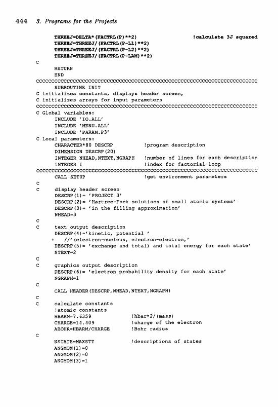
444 8. P~agranzs for the Pwjects
@AC- (P) **?l
e RETURN END
ccc~cccccccccceccccec~ccccce~ccccccccceecccccc~cceeccc~ccec~cccc~ccccccc SUBRQUSINE IMIT
C I n i t i a l i z e s c o n s t a n t s , d i s p l a y s header sc reen , C i n i t i a l i z e s a r r a y s for i n p u t pa ramete r s ~~CCCCCC"CCCCCGCCCCeCCeCCccCGCcCGcecCCCCcCeGcecCCcCCCCCCCCCcCCcccCcCccCcC C Global v a r i a b l e s :
INCLUDE ' IQ .ALLr XNCLUBE * MENU. ALL" INCLUDE 'PAMM.P3"
C Local parameters : CHWCTERX80 DESCRP {program d e s c r i p t i o n DIWNSXOmJ DESCRP (20) XNTEGER NWEAD,NFEXT,NGWH !number of l i n e s f o r each d e s c r i p t i o n INTEGER I ! index f o r f a c t o r i a l l o o p
CCCCCCCCCCCCCCCGCCCCCCCCCCCCCCCCCCCeCCCCCCCCCCCCCCCCCCCGCCCCCCCCCCCCCCCC CALL SETUP ! g e t (environment pa ramete r s
e C d i s p l a y heade r s c r e e n
BESCRP(1)- "PRO;PEGT 3 I BESCRP (2) - Hartree-Fock s o l u t i o n s of sma l l a tomic sys temsf DESCRP(3)- ' i n t h e f i l l i n g approximation' NHCIEAB.-3
C C t e x t ou tpu t d e s c r i p t i o n
DESCW ( 4 ) -"kinetic, p o t e n t i a l @
+ / /V(eleet ron-nucleus , e l e c t r a n - e l e c t r o n , * BESCRP(S)= t e e x c k a n ~ and t o t a l ) and to ta l . e n e r g f o r each s t a t e " NTEXTs2
C C g r a p h i c s o u t p u t d e s c r i p t i o n
DESCRP(6f= e e f e e t r o n p r o b a b i l i t y d e n s i t y f o r each s t a t e f P3GmPW-1
G GALL READER(DESCW,NWEAD,NTEXT,NGRAPW)
C C c a l c u l a t e c o n s t a n t s
?a tomic c o n s t a n t s HBmM-7.635 9 ! hbar*2/ (mssf CMGE-14.409 !charge of t h e e l e c t r o n ABOWR=NBARM/CWARGE !Bohr r a d i u s
C NSTFLTEmMXSTT ! d e s c r i p t i o n s of s t a t e s ANGMOM (11 -0 ANGMOM I 2 1 =C? ANGMOH ( 3 1 - 1
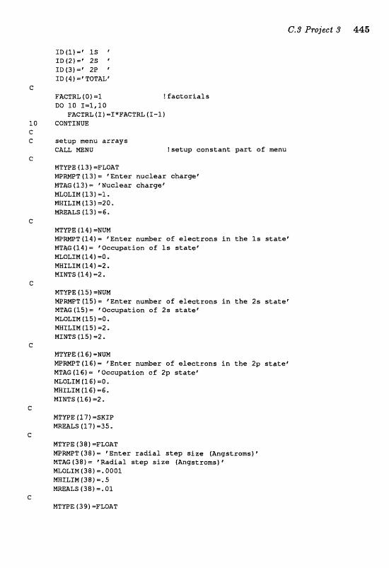
IO(l)="IS ' ID(2)m' 2S F
ID(3f =' 22P ' I D f 41 =' TOTAL"
FAGTRL f O 1 =l ! f a c t o r i a l s DO 10 I=1,10
FACTRL f P) =TXFACTRL f 1-11 CONTINUE
s e t u p menu a r r a y s CALL =NU f s e t u p c a n s t a n t p a r t o f menu
MTWE ( 1 3 1 =FmAT E/IPWT (13) = E n t e r n u c l e a r charge1 MTAG (13) fNuc lea r charge ' MLOLZM 113) -1. MWfLIM(13)=20. mEALS f 13) =G.
MTWE ( 14 1 =NUM W W T (3.4) = @Enter nu&z o f e l e c t r o n s i n the 1s s l a t e p MTAG (1 4 ) = eOccupatlon oE Is s t a t e r MLOLIM(l4f -0. MMTLTM I141 =2. MINTS (14)mZ.
MTYOE (15) =NUM MPWT115)- 'En te r n u d e r of e l e c t r o n s i n t h e 2s s t a t e f NTAG(1S)- Wecupat ion of 2 s a t a t e t MLoLrn (lsj =a. NWILIM (15) -2. MINTS [ l 5 1 -2.
MTMtE (3. G ) -NUM M P W T ( l 6 ) = I E n t e r n u d r o f e l e c t r o n s i n t h e 2g statef MTAG(16)- Wccupat ion o f 2p s t a t e r ML6LXM (161-0, HNILIM (3.6) =6 , MINTS (161 -2.
MTUPE [ 3 8 1 -FLOAT W W T (381 = ' En te r r a d i a l s t e p s i z e (Angstroms) " MTAG (38) 'Radia l s t e p s i z e {Angstromsf ' NLOLIN(38) =,0001 MNILIM(38) =. 5 WEAL5 (38)=.01
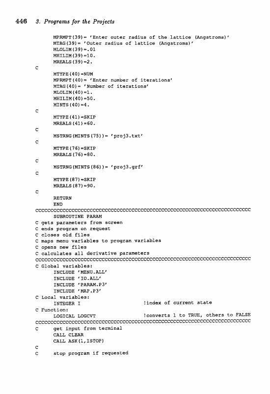
446 3, Proglrams for tke Pro;iec$e
mm11 (39) = 'Enter o u t e r rad ius o f the l d t t i ce (Angstroms) ' NTAG (39) = t o u t e r rad ius of l a t t i c e fftngstroms) " MLOLXM (39) -, 01 NWILIM (391 -20.
C
MTWE f 4 0 ) =NUM MPmPT (40) = Enter number of i t e r a t i o n s e NTAG (40) = %user of i t e r a t i o n s e MLOLIM (40) =l. MHILIN(40f -50. MINTS (40) -4.
c MTUPE ( 4 I ) =SKIP NREALS (41) =GO
c MSTRNG (MINTS f 7 5 ) )m "roj3. t x t t
C WTYPE ( 7 6) =SKI P M W L S (761 =80,
c MSmNG (MINTS (86) )= 'proj3.grf6
c M T F E (87) -SKf P #=L$ (87) -90,
C
=TURN &%D
ccccccccccccecec~~cccccceccccccccccccccccc~ccc~cccccccccccccccccccccccce SUBROUTINE PAMM
C g e t s parameters from screen C ends program on request C c l o s e s o l d f i f e s C maps m n u v a r i a b l e s t o pragram v a r i a b l e s G opens new f i l e s G c a l c u l a t e s a l l d e r i v a t i v e parameters ccccccc~ceccec~~ceccecccccccccccccccccccccccccccccccccecccc~cccccc~ccccc C Global var iab les :
XECLUDE =%U. ALL8 INCLUDE "0. ALLf XNCLUDE ' PAmN. P 3' INCLUDE W . P 3 '
G Local var iab les : JNTEGER I !index of cur ren t s t a t e
Function; LOGICAL LOGCVT !converts 1 to TRUE, o t h e r s ta FALSE
ccceccccccccceccecccccccceccceeccccccecccccecccccccccccecccccceccccccccc C get inpu t from terminal
CALL GLEm CALL ASIC(1, TSTOP)
C C s t o p grogram i f rewasted
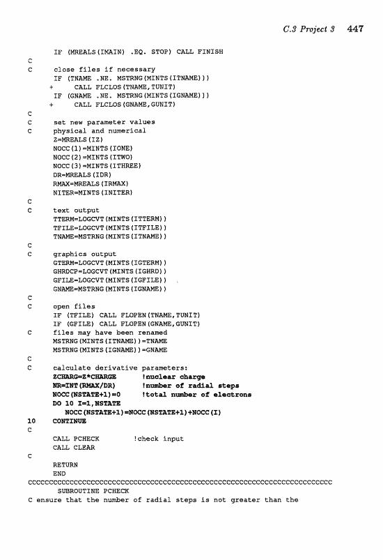
I F (MRmLS f ImI M) .EQ. STOP) CALL F INISH C;
C close files if necessary XP (TNAm .NE. NSmMG (MINTS (TTHME) 1 )
+ GALL FLGLOS (TNAME, TUNIT) TF ( G N W .NE. MSTRHG (MINTS ( IGNMEI 1 i CALL FLCLQS (ENAm, GUNIT)
c G set new parameter values e physical and numerical
Z=mEALS 1 I Z ) NOCC (1) =MINTS (IONEI UOCC ( 2 ) =MINTS (ITWO) NOCC ( J 1 =MINTS r TWWE t D R = W A L S ( 1 BR)
G
C textoutput TTEM=LoGCvT (MINTS (ITTERM) 1 TPXLE=LQGCVT (MINTS ( I T F f LE) 1 THME=HSTRNG (MINTS (ITN-))
C G grapbfcs output
GTEW=LoGCVT (MINTS (XGTERM1) s a w c P = L o c c v T CMTMTS (IGHRD) I c F x L E = k o c m r (MxNas ( XGFILEI GNW=HSTRNG [MINTS (JGHAm))
(3
C openfiles I F (TFILE) CALL F W P E N ( T N m , T U N I T ) IP (GPIr.P.1 CALL FWPEN (Gl\aMEI GU1JIT)
C f i l e s may have been renamed MSTRNG (MINTS ( I T N M ) 1 -TEAME MsTRnc (MINTS (IGNM) t = G E & ~
c C calcul. ative parameters;
Z C m G !nualaar &azge
DO 10 1=1,1~2~m WOCC (NST&m+1) =BXC 615SP&m+3) +NQGC (X)
10 C O m X m C
CALL PCWECX. !cheek input CALL CLEAR
e RETURN END
cccceeceececeec~eccef:ccccccecceccccecceccccccccccc~ccc~ccccCccecccc~cccc SWRQUTINE PCHECH
G ensure that the nu&er a f radial steps is not greater than the
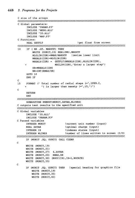
448 3. Programs for the Pmjects
C s i z e o f t h e a r r a y s ccccccccccccceccceccccccecceccccccccceccccccccccccccccCcccccc~cccccccccc C G l o b a l p a r a m e t e r s :
SNCLUDE ' P A M . P 3 ' INCLUDE 'mMU,ALLP INCLUDE 'TO,ALLj IMCLUDE "P .P3'
C F u n c t i o n s : R= GETFLT ! gat f loa t f r a m s c r e e n
ccccccccCc~ccccccceeeccccccccccccccccccccccccccccccecccccccccccecccccccc l 0 I F ( N I 4 .GTI m X S T P ) THEN
VRETE (OUNIT, I S ) REAL (NR) , W S T P HWLIM fIDR) = m X / M X S T P t r e v i s e l o w e r I l r n i t MWALS f SBRf =E"n;OLSM ( IBR)
LS( IDR) = GETFLTfNREALS(TDR),NWLSM(IDRf, -E. MWILXN(TDR),%nter a larger s t e p f )
DR=MmALS ( I DR) NRmTNT (RMAX/DR)
GOTO 1 0 END I F
C 15 F O M T ( j T o t a l n u m b e r o f radial steps f=r ,1P.E9.2 ,
+ * ) is larger t h a n m a x s t p ( = t , i 5 , q r 1 G
RETURN END
ccccccCcccccccccecccccccccccccccccccce~ccccccccceccccceccecccccceecceec~ SUBROUTINE PRMOUT (MUMf f , ZSTAR, NLTNES)
C outputs text. r e s u l t s t o t h e swcified u n i t ccccccccceccccccccccccccccccccccccccccccceC:cccccccccccccccccC:ccccccccccc G G l o b a l v a r i a b l e s
INCLUDE C XOIIILL8
C Passed v a r i a b l e s IMTEGER MUNIT ! c u r r e n t unit n-er ( i n p u t ) RE& ZST&R ! o p t i m a l c h a r g e ( i n p u t ) INmGER IS ! f ndexes s t a tes ( i n p u t ) XNmGER NLSNES !nu&sr of X i n a s w r i t t e n t o s c r e e n ( f / O )
cccccecc~eccccccccceGecccccCcccc~cccccccccC:ccccccccccceccccccccceccccec~ IF (MUNIT .EQ. OUNIT) CALL CLEAR
e MBSTE (E"IUMST,19) m I T E (MUNIT, 21) RRITE (NUNIT, 27) Z, ZSTAR m T T E (MUMIT, 231 R m , LIR m I T E (MUNIT,30) (NOCC(TS),IS=I,NSTATE) m I T E (MUWTT, 33)
C I F (NUNIT .EQ. GUNIT) THEN t s w c f a l h e a d i n g for g r a p h i c s f i l e
WRITE (MUNIT, 19) In7RTTE {MUNIT, 351 WRITE (MIINIT,$a)
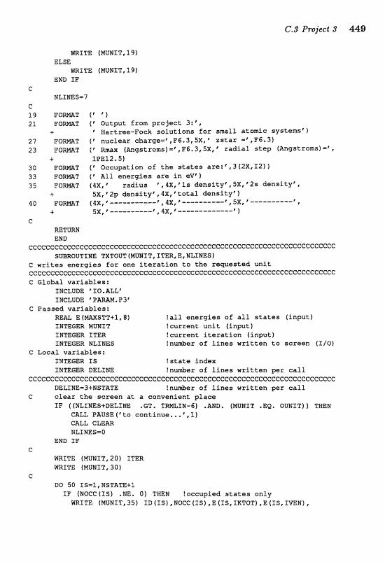
WE3ITE (MUNIT, 191 ELSE
mI"P ((MuNI T, 191 END IF
C 1?3LINE5=7
C l 9 P O M T 4' ' 1 2 1 F O M T (Wwt from p r o j e c t 3:',
.c. Hartree-Fock s o l u t i o n s f a r small atomic systems' 1 27 F o W T IQuclear charge="rF5.3,5X, ' zst i i r =' @,F6.3) 23 F O m T I f Rrnax fAngstroms]=",F6.3,5XIf r a d i a l s t e p (Angstroms)=',
+ IPEIZ. 51 30 F O M T (' Oecupatlon of t h e s t a t e s a re : 5 3 (2X,I2) f 33 F O m T fQLl, e n e r g i e s a r e I n e V ' f 35 F O m T (4X, "radius ', 4X, Is dens i ty ' , 5X, "2s dens i ty ' i dlctnsity\r4XltttataI d e n s i t y * }
40 F Q m T (4X, 44XI "--------m-' , $ X I f ------m
4- ejx, I ----.,,----.'" 1 4X, 1 --.".------- ---' l e
m T U W END
~~c~~~ccccccc~cecccccecccccccccecccccccecccccccccccccceccccccccccccccccc SUBROUTINE TXTOUT(MUNIT,TTER,E,NZI:MES~
e writes enexgies f o r one i t s r a t i o n t o t h e r a m e s t e d u n i t cecceccccecceeccccecccccceccccccccccceccceccccccccc~ccecccccCccccccccccc C ELobal va r iab les :
INCLUDE 'IO.ALL6 INCLUDE ' P M M . P3'
G Passed var iab les : E (MAXSTT+1,8) ! a l l e n e r g i e s o f a l l s t a t e s ( inpu t )
INTEGER MUNIT ! cur ren t u n i t ( inpu t ) INTEGER ITER ? c u r r e n t i t e r a t i o n ( inpu t ) INTEGER NLf NES !nu&er o f l i n e s w r i t t e n t~ screen (flo)
C Local va r iab les : INTEGER fS ! s t a t e index INTEGER DELIME Inu&er o f l i n e s w r i t t e n per call
ccccecececec~ccecccccccccccccccccccccccecccceccceccccccccccccccccccccccc DELIME-J+NSTATE ! n u h e r of Lines w r i t t e n per c a l l
C c l e a r t h e screen a t a convenient p lace IF ((NLfNESfDELIm -GT. TmLXN-6) .&MD. fNUMLT .EQ. OUNZT)) TWEN
GALL PAUSE ( ' t o cont inue, . . * , l f CALL CLEAR N&XNES=O
EWCI IF C
WRITE (MUNIT, 20) ITER WRITE (MUMIT, 3 0 )
c Da 50 IS=l,NSTATE+I
IF (NOCC (IS) .NE. Q ) TWEN !occupied s t a t e s anfy WRITE IMUulT, 35) XD (f S ) ,NOCC ( IS) ,E (IS, XKTQT) ,E (LS, I a N ) ,
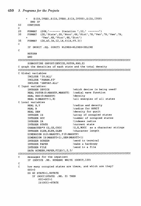
450 9. Programs for the Projects
+ E (IS, X-E), E [IS, TVEXf I E (IS, IVTOTj #E (IS, ITQT] END IF
50 CONTINUE c 20 F O m T (26X, ' ------- Iteration ,12, b.------? 1 30 F O W T (2X, c Statet, ,2X, 'Huecf, 4 X I Ktotr , ?'X, 'Vene, ? X , (Veer, ?X9
+ Tex6,,GX,*Vtotf, ,GX,*Etutf 1 35 F O m T (2X,A5,3X, 12, >X, 6 (lX,F993j 1 e
IF [MUWZT .EQ. QUNIT} NLSNES=NLINES+DELINE C
RETURN END
cccccceccecccccccccccccC:cccc~ccceccccecccceccccccccccccccceccccc~cccc~cc SUBROUTINE GRFOUT(DEVICE,PSTOR,RWO,E)
C graph the densities of each state and the total density ccccC:cccccccccccccccecccecccccccecceeccccccccccceccccccccccccccccccccccc C Global variables
INCLUDE 10, ALL" INCLUDE " W N . P 3 ' I NCLUDE * GRFDRT .%L'
G Input variables: IMTEGER DEVICE !which device is being used? REAL PSTOR (0 : L"IAXSTP, W S T T ) ! radial wave function RE= RHO ( O : MXSTP 1 !density RE& E (MAXSTT+l, 8) !all energies of all states
C Local variables REAL X, U !radius and density mAL R !radius for GVNXT REAL DEN !density far gunit INTEGER IS !array of occupied states INTEGER OGC !nu&er of occupied s t a t e s INTEGER IR lfnciexes radius INTEGER STATE !current state
CTER* 9 CZ , CE, CQCC !Z,E,NOCC as a character strings INTEGER ZLEW, ELEN, OLEN Ichars~ter length DImNSION XtO:E?taXSTP) ,VfO:mXSTP) DImNSIoN IS (FylXSTTtI) , DEN (WXSTT.f.1) I NTEGER SCREEN !send to terminal INTEGER PAPER !make a hardcoay INTEGER FILE !send ta a file DATA SCREEN,PBPER,FILE/I,~,JI
~~~cc~~~~~~cc~c~cccccccccccccccccccc~cccccc~cceccceccccccecccceccccc~ccc C messages for the impatient
IF (DEVICE .NE. SCREEN) WRITE (OUNLT,1001 e C how many occupied states are there, and which are they?
ace= 0 DO 60 STATE-S, NSTPATE
IF (NOCCfSTATE) .NE. 0) THEN OcC=OCC+l IS (OCC) =STATE
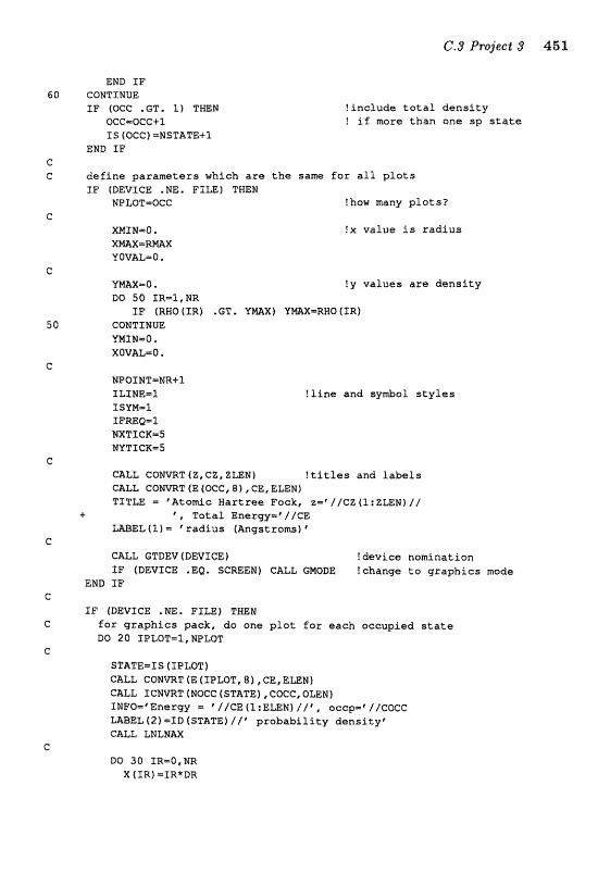
END I F 6 0 CQEJTINUE
IF (OCG .GT. I f TWH !include total density OGC=OCC+ 1 ! i f more than one sp state IS (OCG) =WSTATE+I
END IP e C define parameters which are the same far all plots
n p ( a m r c E .NE. FILE) THEM NPLOTmQCC !how many plots?
C XNIM=0. ! X value is radius XmX=RMX YOVAL=0,
c YmX=O * !y values are density DO 50 fR=l,NR
TF (RNO(IR1 .GT, YmX) VMX=RHQ(XR) CONTINUE VMIM-0, XOVAL=O,
!line and symb~1 styles
GALL COMVRT IZ, CZ, ZLENI !titles and labels CALL C O m T f E (OCC, 8 1 , CE , ELEN) T I T M = eAtomic Bartree Fack, z=' //C8 (l: ZLEWI / I
+ \ rota1 Enexw=V/eE M E L (1 1 "adius (Angstroms)
C CALL GTDEV (DEVICE) !device nomination XF (DEVICE .&B. SCREEN) CALL GNODE !change to graphics mde
END IF C
IF {BEVZCE .NE. FILE} THEN C for graphics pack, do one plot for each occupied state
DO 20 fPLOT=1, NPLOT C
STATE=IS (TPLQT) CALL GONVRT (E ( f PLOT, 8 1 , CE, ELEM) CALL ICNVRT f NOCC (STATE f , COCCI QLEkr 1 INFO="nergy = ' /ICE (1 :ELEM) I /% ooccpr' /l6066 U B E L ( 2 ) =ID (STATE] / / ' probability densityf GALL LNLNAX
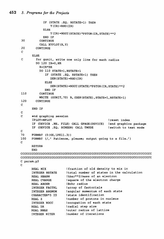
452 13. Progsurnzs for .Ihe Pmjects
SF (STATE .EQ* NSTATE+1) THEN Y (1R) =RHO (IR)
ELSE U ( I R ) -NOCC f STATE) *PSTQR (IRI STATE} **2
END 3F 30 COMTLMUE
CALL XYPLOT f X , V ) 2 0 CONTINUE C
ELSE C f o r gzlnit, write one only l i n e f o r each r a d i u s
DO 120 IR=O,NR R=IRX DR DO 110 STATE-1,NSTATE+1
IF (STATE .EQ, NST&TE+1) THEN DEN (STATE) =RHO (IR)
ELSE DEN (STATE) =NOCC (S31ATE) *PSTQR (XR, STATE) **2
END IF 110 CQNTXNUE
mITE (GUNIT,70) R, (DEEJ(STATE),ST&TE*r;l,NSTATE+lf 120 COEJTIMUE C
END IF C G end graphing sess ion
IPWT-NPLOT !reset index XP (DEVICE .m. FILE) CALL GPAGE (DEVSCE) ! end graph ics package IF (DEVICE .EQ, SaEEH) CALL TNODE !switch t o t e x t mode
C 70 F O m T f 5 f 4X, IPE12.3) ) 100 F O m T (/, * Patience, please: output going t o a Ef l e , * 1 C
m TURH END
cccccceccecccccccccceccecceccccccccccccccccccccccccccccccccCcccecccccccc ~ ~ c ~ e ~ c ~ e c ~ ~ c e c e ~ c ~ : ~ ~ e e c c c ~ ~ c c c c c ~ ~ ~ c c ~ ~ c e ~ c e e c c ~ ~ ~ e ~ ~ c ~ ~ ~ c c e ~ ~ ~ c ~ c ~ c c ~ c G param.p3 e
M& NIX ! f r a c t i o n cf o l d d e n s i t y t o n i x i n XNTEGER ESTATE ! t o t a l n u w s of s t a t e s i n t h e c a l c u l a t i o n
!hbar**2/mas cf an e l e c t r o n R= CWARGE !square of t k a e l e c t r o n charge REAL mOWR tBohr r a d i u s XHTEGER FACTRL !a r ray of f a c t o r i a l s XNmGER AMGHOM l a n w l a r momntum of each s t a t e 6HM@TERX5 ID Istate i d e n t i f i c a t i o n
Z lnuntbar af pro tons i n nucleus INTEGER N6CC !occupation o f each a t a t a mAb, DR f rad ia f s t e p s i z e m L M X foutex r a d i u s of f a t t i e e INTEGER HITER !nu&er of i t e r a t i o n s
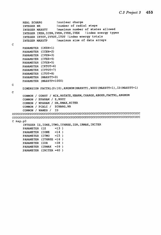
REAL Z C W G !nuclear charge INTEGER NR !nu&er of radial steps INTEGER m S T T !maximm nu&er of states allowed INmGER fKEN,IcEN,ImN,IWE,IWX !index enerw typrts INTEGER %KTOT,IVTOS,ITOT !index enerw totals IBTEGER NAXSTP !maximum size of data arrays
G
C DZWNSIO% FACTRL (0 : 30) , ANGHOM (mStfT1 , NOCC (WSTT+l B SD 4 m S T T + l l
C COMON / CONST / MIX,NSTATE,WBW,CWMGE,RBQMR,FACTRL,ANGMOM
/ DR,mX,NITER
CQmON / NAmS / ID cccccecececcCcccccccccecceccccceccccccccecccceceeececceccccccceccccccccc ccccccccccccecceccccccccccccceccecccccceccccecceccccccccccecccccccccccc~ C map,p3
INTEGER IZ, IONE, ITWQ, ITHME, IOR, I m X , TRITER PmMETER (IZ =l3 ) P W M T E R f IONE m14 1 PAMMETER (ITWO -55 1
rnR (ITHREE, =l6 f P m m T E R [IDR -38 )
TER (SRMX =39 f PAmmTER (1lr;lZTBR 4 0 )
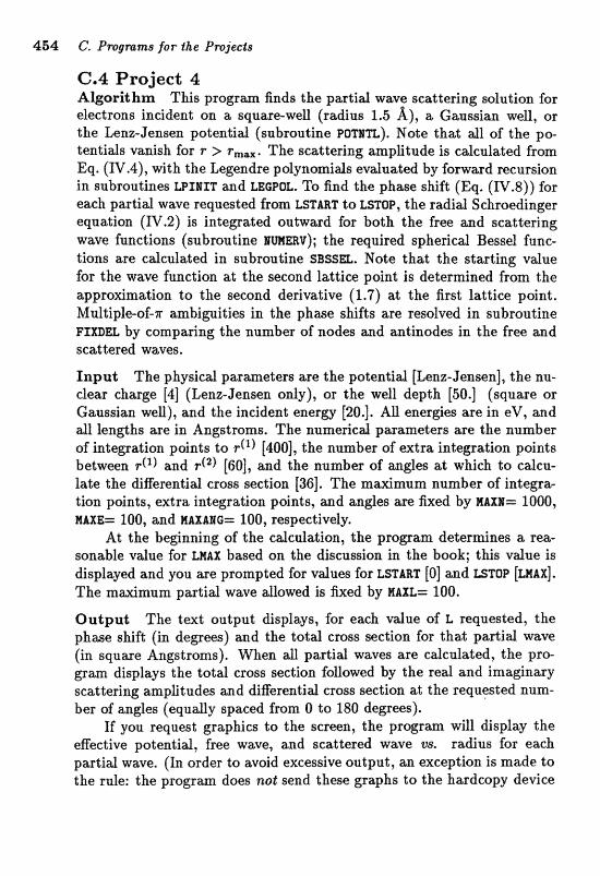
454 C. Pmgmrrss for $he Pmjeels
C.4 Project 4 Algorltfxm This progrm finds the partid wave scaltering solution for electrons incident on a square-well (radius 1.5 A), a Gaussian well, or the Lenz-Jensen potential (subroutine POTBTL). Note that all of the po- tentids vanish for r 2 r,,,. The scattering up2itude is calcul&ed from Eq. (IV .4), wit h the Legendre polynomials evaluated by forward recursion in subroutines LPIAIT and LECPOL. To find the phase shift (Eq. (IV.8)) for each partial wave requested from LSTART to LSTOP, the radial Schroedinger equation (IV.2) is integrated outward for both the free and scattering wave functions (subroutine rwwv); the required spherical Bessel func- tions are calculated in subroutine S~SSEL. Note that the starting value for the w m function at the second lattice point is determined f r m the approximation to the second derivative (1.7) at the first lattice point. Mrrltiple-of-X ambiwitie~ in the phase shifts are resolved in subroutine FIIOEL by comparing the number sf nodes and antinodes in the free and scitttesed waves,
Input The physical parameters are the potentid [Lenz-Jensen], the nu- dear charge [4] (Lenz-Jensen only), or the well depth [SO.] (square or Gaussian well), and the incident energy [20.]. All energies are in eV, and dl lengths are in Angstroms. The numerical parametc;rs are the number of integration points to r( ' ) [400], the number of extra integration points between a d [GO], and the number of angles at which to calcu- late the differential cross section [36]. The maximum number of integra- tion points, extra integration points, and angles are fixed by R A X ~ - - 1000, MAXE== 100, and EZAXAIG= 100, mspectively.
At the be@nning of the cdculatim, the p r o g m determines a =a- sonable vdue for LKAX bmed on the discussion in the book; this value is displayed and you are prompted for values for LSTW [O] and LSTOP [MAXI. The maximum pmtial wave sawed is k e d by MXL= 100.
Output, Z"he t a t output asplayn;, for each vdue of L =quested, the phase shift (in degrees) and the totd cross section for that partial wave (in square Angstroms). When all partial waves are calculated, the pro- gram displays the total cross section followed by the real and imaginary scattering amplitudes and differentid cross section at the requested num- ber of angles (equally spaced from 0 to 180 degrees).
If you request graphics to the screen, the program will display the effective potential, free wave, and scattered wave vs. radius for each partid wave. (In order to avoid excessive output, an exception is made to the rule: the program does not send these graphs to the hardcopy device
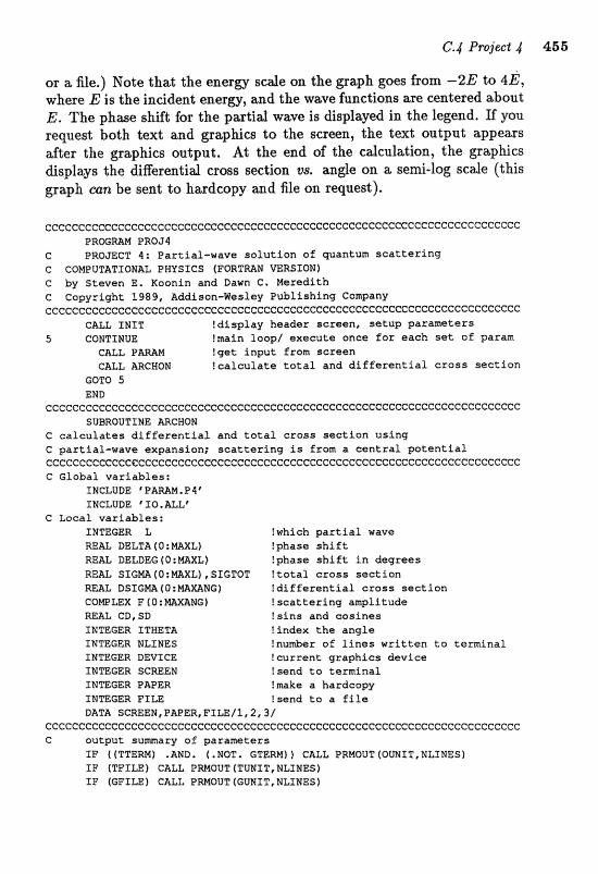
or a Be.) Note that the energV scale on the graph goes from -2E to 423, where E is the inddent energy, and the wave functions are centered about E. The phase shift for the partial wave is displayed in the legend. If you request both text and graphics to the screen, the text output appears after the graphics output. At the end of the calculation, the graphics displays the differential cross section vs. angle on a semi-log scale (this graph can be sent to hardcopy and file on request).
c~~cc~ec~ccccccc~~c~~ccccccccccecccecccccccccccccccccccccccccccccccccccc P R O G W PROJ4
C PROJECT 4: Par t ia l -wave s o l u t i o n af quantum s c a t t e r i n g C COMPUTATIONAL PHYSICS (FORTmH aRSIOPJ) C by Steven E. Koonin and Dawn C. Mereditb C CapyricJht 1989, Addison- les ley Publbsbing Company cccccce~cccc~cccccccccccccccccccccccccccccccccccc~ccccccccccccecccccccec
CALL INIT ! d i s p l a y header sc reen , s e t u p pa ramete r s 5 CONTINUE tmain loop/ execu te once Ear each set o f param
CALL PAW ! g e t i n w t from s c r e e n CALL ARCHON ? c a l c u l a t e t o t a l and d i f f e r e n t i a l c r o s s s e c t i o n
GQTO 5 ERB
ccccecccccccc~cccccccccceccccccccecccccccccccceccccceccccccccccccCcccccc SUBROUTINE mCBOH
C c a l c u l a t e s d i f f e r e n t i a l and t o t a l c r a s s s e c t i o n u s i n g C par t ia l -wave expansion; s c a t t e r i n g is %ram a c e n t r a l p a t e n t i a l cccc~ccccccccecccccececccccceccccccccccccccccccccccccccececcccccccccecec C Glaba l v a r i a b l e s :
INCLUDE fPMM.P$" INCLUDE 1 0 . ALLt
C Local v a r i a b l e s : INmGER L !which p a r t i a l wave m& DELTA t 0 : =L) !phase s h i f t RE& DELDEG ( O : MAXLf !phase s h i f t i n degrees REAL SIGm(O:mXL),STGTOT ! t o t a l c r o s s s e c t i o n WAL DSIGm (O:MMNG) ! d i f f e r e n t i a l c r o s s s e c t i o n COmZEX FIO:NXAWGI ! s c a t t e r i n g ampl i tude RE= CB, SD ! s i n s and c o s i n e s IMTBGER ITHETA !Index t h e a n g l e INTEGER NZTNES !number of l i n e s w r i t t e n t o t e r m i n a l INTEGER DEVICE ! c u r r e n t g r a p h i c s d e v i c e INTEGER SCREEN !send t a t e r m i n a l INTEGER PAPER !make a hardcopy INTEGER FILE !send t o a f i l e DATh SCREEN, PAPER, FILE/1,2,3/
ccccccccccccccccccccccccccccccccecceccccccccceccccccc~ccccccccc~ccc~c~~c C ou tpu t s u m a r y of pa ramete r s
I F ( (TTERM) .AND. ( .NOT. ETEM) } CALL PRMOUT (OWXT, NLINES1 IF (TFILEI c a u P R J M ~ U T (TvNrT, NLIMES) I F (GFILE) CALL PWOUT [GUNIT, NLINES)
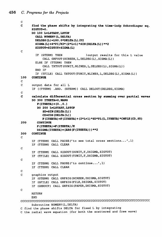
C G fAnd, the pharae ~lhiffea by A ~ t q z a t I n ~ ~ khai %--in@ S-OCIingm a%.
SICT-O . W 100 MwFm2,mmB
(L, BELT&) 80.0*DmFA (L) !PE
s r m (L) =~*PXIKZ* ( 2 * ~ 1 1 *S= ~DELT~FL (L) **2 srommerolcoz+sx- (S)
C If" (GmRM) T m N tsutput results for this L value
CALL GmOUT (SGmEN, L, BELDEG (L) , S I G m {L} 1 ELSE I F (TTERM) THEN
CALL TXTQDT (OUNIT, %LZNE:SI L, DELDEG (L) , S T G m (L) 1 END IF I F ( T F I a ) CALL TXTOUT fTUNIT,NLINES, L, DELDEG (L) C SXGlvra (L,) 1
100 COrnIrn C C output data fox all L
IF ( (TTERMI .AND. (GTERM) ) CALL DELOUT (DELBEG, SIGNA) C G cal&at;r &ggmzaaeia ororas aect;fon by
DO 300 2TmT&=Q,mG 1 % ( S m n ) = ( o * , o . ) DO 240 W&SmP,LS5?0P
so=sxH (DEL= (t) ) CD*QS (D== (L) ) s tzrmr~) =P(S-T~) + (z*xic~) *SD*PI; (X,, S T ~ T B J (CD' SDI
200 c @ B l c I m F ( r m a ) =P ( r m n j /a: BSI- (X %=TA) (-8 (P" [XTmT&J ) ) **g
300 CQH9CXm C
IF (TTERM) GALL PADSEf8 to see total cross sect ions. ..',l) IF (TTEW) CALL CLEm
C I F (TTERM) CALL 53GOUT (BUNIT, F, DSIGMA, 5IC;TOT) I F (TFXLE) CALL SIWUT (TUNIT, F,DSXGmI SIGTQT]
C f F (TTERM) GALL PAUSE ( * t o continue. . . ' 1) I F (TTEM) C"ALL Cmm
c C graphics output
I F (GTEW) CALL CWSIG (SCREEN, DSXGMA, STGTOTI IF (GFILE) Cam GWSIG (FILE, DSIGMA~ SXGTOTI IF (GHRDCP ) CALL ~ F S I G (PAPER, D S I G ~ ~ SIGTQTI
G =TURN END
~~~~cc~~c~ccc~~~e~cc~cec~ccccccc~ccccc~cccccceecccceccccccf :~ccc~ccccccc~ Subroutine NUMERV(L,DBLTA>
C find the phase shifts DELTA for fixed L by integrating C the raddal wave a w a t f o n (for both the scattered and free wave)
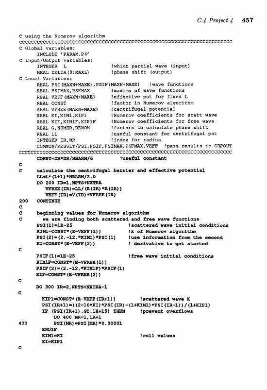
C using the Numerov algorithm ccc~cccecccccc~ccccccccecccccecce:cccccccccccc~ccccc~cccccc~~cccc~c~ccccc C Global variables:
INCLUDE @ O W M . P 4 " C Tngutlmtput Variables:
INTlEGER L ?which partial wave (input 1 M& DELTA ( O : =XL) !phase shift (output)
C Loeal Variables: ),PSSF(mm+MXE) !wave functions
WE= P S T W , PSFMAX Imxima of wave functions Mm VEFP 1 W M S . M E 1 !effective pot for fixed L RMX, COHST mAL W R E E ( W N + a X E ) !centrifugal potential REAL KZ,KIfoll,lKXP3 IWumerov coefficients far scatt wave M A L KIFIKIE41F,RIP1F !Mumrow coefficients for free wave REAL G,NUmR,DENQM tfactars to calculate phase shift RE& LZ !useful constant Ear centrifugal pot IPJmGER IR,MR !index for radius CO~GN/~SULT/PST8P%IF,PSTM.IPSFMAXI~FF !pass results to GWOUT
~ C G C ~ C ~ C C ~ ~ C C ~ C ~ C C ~ ~ ~ ~ c c c ~ c c ~ ~ ~ ~ ~ c ~ e ~ c ~ ~ e ~ ~ ~ ~ c e c ~ c c c c ~ ~ e ~ ~ c c c c c c c c t usegujl comstae
C C oa ldata t
2 0 0 cmzZNU]& e G h@m%w vdnms for C w a a m f%m&nq bokh srcrtLmred ancl f~ee wave &aaeione
PSZ ( l } =ZE-PS iocrarttrzed wave iniCirZ aan&t&ons XIaeOZirSZ* (B ( 3 ) 1 as% $21 = 42. -22, *mm) *PSI (21 K I e m S T * (E-=@ (2) ) I 4 a r i v a k i v e to get a t a r d e d
C PSm (a) =2E-2 !free rave i e t i a2 , canatiorrra 1 I S I ~ ~ ~ ~ S I P * P S ~ (2) = ( 2 . - ) *pslCr ( l ) m@wmsr"* {B 1
C W 3 0 0 1 R = P r ~ 1 C S + ~ ~ - l
C: t r c a t t e r e d wave E
PSX (ZR+2} 1 ( (2-%0*KX) *as1 {XRZ - (%+mm) *PSI {XR-1) 1 I (f.+-X) I P (PSX (IR+l ) . G??, 1E+25) 5(= f gzewent; werZ2ows
W 4 0 0 M#.%=%, XR+l QOO ~ s r (m) = ~ s r (m) *a. ooooz
E W I P R ~ = K I EZ=XZE2
C

mhFMWS"r* ($-W= (TR+l) ) l fmha nave X PSXZ {rftti) = ( (z-ia*xm) *PSI:%I (m) - ~a+mm~j *BB= (m-11 1 I RIB=) IYP {PBEP (=+S) .G%. 1E+1S) T m i lgzavan& ovarf lwr
DO 500 ==1,1R+1 300 PS= {m] ~ ~ s m (m) *a. oaool
-XB mW=mE !roll vdaas rnZ=EXl?1F
C 300 C m CI G oal&rtrr b l t a (8- W. IfP.8)
G*&(l,L)-fi(2,L) DEmMe*EL [l, &l -m (2, L)
LI"XmEL (DZL3A {L) , PST, PBZE, PSI=, P C
=TURN awa
ccccceecceCccccceccccccccccccccccccccccccccccccc~ccccccccccccccccccccccc SUmOUTINE FSXDEL(DELZ"A,PSI,PSI:F,PSI~X,PSF~1
C r e s o l v e s the a d i ~ i t y in DELTA using info from t h e wave f u n c t i o n s C PSX and PSZF; f i nds maxim i n wave f u n e t i o n s OSSMX, PSXFW ~ccc~ccCcc~cccccccceccccceccc~cccccccecccccccccf:ccccccccecc~eccccccccccc C Global v a r i a b l e s :
C Passed Variables : MAL DELTA ?phase s h i f t (I/O) &E= PSX ( W N + m X E I , PSIF (mXN+mm) !wave fancf i o n s ( inpu t 1 M L P S I m , P S F W !mix o f wave f u n e t i o n s ( a u t p u t f
C Local Variables : INTEGER BUW,NODES,BUWF,HODESF ! n u W r of nodes and an t inodes INTEGER T ! r a d i a l index LOGICAL DP0S !Is t h e phase s h i f t p o s i t i v e ? INTEGER N !how many f a c t o r s of p i t o add
C Function: ! r e t u r n s s i g n of a rwment
f o r the .cattarad wave
TB ( B a {P63 {I)) .m. B
XR ( SGM (PBX (X+%) -PBX I . s a (asz (X) -PBX v-%) 1 + li3W=BW+5
500 C O m X m C
ata, nobs, a d psi for the free wavm B-FmO
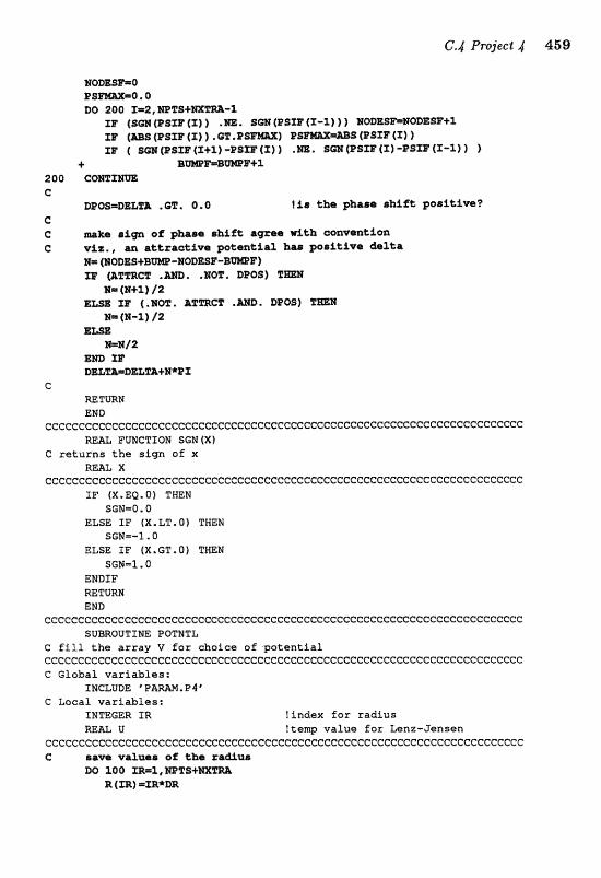
NORE5l=0 P a.o D 5=2, WTS+mm-1
xs (sm(asmtz) 1 .m. DESS+X XF (m (ss= (X} ) .er .as
+ 204 Cmf l13m C
DPOS=Dm%& .G%. 0 - 0 !is the phase shffe gooft%ve3 C C s i p of phase sWZ"t; as- nieh eonveation C vlz,, an at;tz&&ive pkential has lpoaitivrl &Xta
R= (%ODES+BW -HQDESZ-BmE") n;p (aTmca .m. . ~ a r . BEOSI T-
W= (El-3 1 /2 EL= XF ( .HOP. .W. DPOS)
B= (%-l> /2 EL=
M=H/2 XBD XF DELFA=BmZ&+B*iPX
C =TURN END
ccccccccCcccccecccccc~cccc~cccceccc~ccccccccecccccccccceccccC:ccccccccecc B& PUNCTlOXJ SGPJ (X)
C returns the sign a f x REAL X
cecccecccccccc~cccccccccccecccccccccccceececccecccccccccececcccccccccccc IF (X.EQ.0) THEN
SGN-Q . O ELSE IF (X.LT, 0) THEN
$GM=-1.0 ELSE IF (X,GT, 0) THEN
SGN=l. Q EEJDXF RETWH END
ccccccccccec~ccccceeececcccccccccccccccccccccccccccec~cccccccecec~cccccc SUBROUTINE POTMTL
C fill the array V for choice of potential cccccccc~ccccCccccccccccccceccccecccceecccccecccccccccccccccccccccccccec C Global variables:
INCLUDE 'PPAMH.PIt C Loeal variables:
INTEGER I R !index for radlus =&L U ttenrp value for Lenz-Jensen
CGCCCCCCCCGCCCCCCGCCCGCCCGCCCCCGCCCCCCCCCCCCCCGCCCCCCCCCCGCCCCCCGCJCCCCCC C &awe woiluea of the raaua
DO 100 ==l,mTS R (IR) =ZR*DR
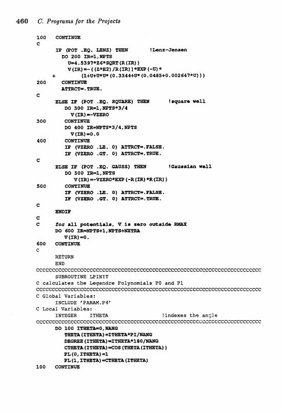
460 C".. Pmgmnas for the Projecla
1 0 0 comxm C
XE (POT SQ. =NZ) =I fUn&-aansen DO 2 0 0 XR=X, m2"s Um4.53 97*26*SWT (R (f R) ) V (%R) m- ( (Z*E2) /R (m) 1 *Em [-V> *
+ (1+V+V*V*(0.3344+~*~0.048~+QQ0Q2d17*tl~Z) 2 0 0 c m x m
&%=Cm. mm. C
IF (par( .EQ. s ~ ~ m ) rrm~ I @pm@ W~BZL 00 300 -1,=111*3/4
v (m) =-TB=@ 360 C a H T Z m
DO 4OO TR=R98*3 /4 ,mTS V(XR)=O,O
400 CORTXm TF {rn%RO .m. 0 ) A%rnC%.FU8E* XF {W=@ .@!E. 0 ) &%%RC*.
C ELBE EF (POP .E@. aQSS) SImB fGaalrrian we21
W 5QO XR=l,=l?S v (ER) = - v z E ~ * E ~ (-R (5af *R ~ X R ) 1
5 0 0 CGE1Cxm I F p%mO .Wa Q) &ZmCm. x F w m a *@E' 01 &Prnrn=.
C: m m
c C far a11 ptmtia2s, V i s rcero atsidsrr
PO COO l E W F S + Z , m T S + V (XR) 4.
606 C a m X N m C
Rf?IPum END
eecccceCcceccce~cceecccececcccccccceccceccc~cecccccccccccccccccceccecccc SUBROUTINE LPfNfT
C calculates t h e Legendre Polynomials PO and PI eeeccc~c~ccccccceeccceecc~eccccccceccccGtce~ceccccccecceccC:cccee~cccccccc f: GXabal Variabl
C Local Variables: INTEGER ZTWETA ! indexes t h e an2l.e
CCC~GCCCC~CCCCCCCC~CGCCCCCCCCCCGC~CCCCCC~CC:CCCCCGCCCCCCCCC:CCCCCCCCCCGCCC m ZOO remT*o,-o
%=%A (Z%m2"&) =ZT=ZA*EI/%M@ (ITmEA) PLfWTB*110 /m@ grmlrrr ) e o s (rmrrh ( I Z ~ T A I
P& (0, X W T A ) =l P& ( l , X-%&) 4 m Z k (ZTrnrn)
XQO C m X m
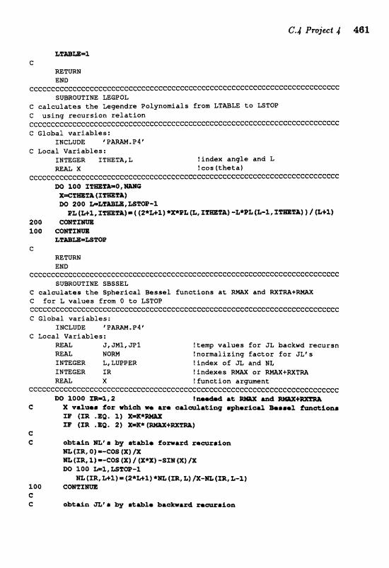
C RETURN EHD
~~~~~~~ec~~e~cc~~ccc~ccc~ccccceccccccccccecccccccecccccccccccccccccccccc SUBROUTINE mGPOL
C calculates the Legandre Polynomials from LTABm to LSTOP C using recursion relation e~~~~~cccccccecccceccccccccceccc"ccccccccccccececceccccccccccccccC:ccccccc C Glabal variables:
C Local Variables: INmGER ITNETA, L f index angle and L M& X !cos [theta)
~~cccccc~c~c~c~ccceI:cccceccccccccccccccccccccccccccccceccceccceccccccf:c~ DO 160 I11mTb0,mG
$ * & S W - 1 1 - (z*wi) *X*PL (xi, r m a ~ j -L*PI( G P ~ , X ~ T ~ I j I CL+Z)
200 a00
C RETURM END
ccccccccc~~cccc~ccccccccccccccccccccccccccccccccccccececcccccccccccccccc SUBROUTINE SBSSEL
C calculates the Spherical Besael functions at R M X and W T M + C for L values from O to LSTOP cccccccccccccccccccccccccccceccccccccccceccccccccccccccccccccccccccccccc C Global variables:
INCLUDE ' P A W , P 4 * C Local Variables:
=L J, JM1, JP1 !temp values fox JL backwd reeursn M A L NORM !normalizing factor for JLrs ENTEGER L, LUPPER findex of JL and Nt
!indexes R W or R m + R X T a A Ifunction argument
ccccccccccccccccccecceccccc Em XOOO XWl, l t nmmhd
C X v&lae# for W&&&
XP f I R '134. 1) I k K *
C C ebealtn XLf& by alabla korvrrd raaruion
( f R, Q ) =-COS ( X ) 1 X E& (TR, l) m-COS (X) / (X*X) -SXH [X) /X W 100 -1,LSTQP-I.
RL (ER, ( z * t ~ s ~ *m (ERI xc} /X-HL L-21 100 CCINTIrn C 6 obealn u.taX>Xa frJ&akw&xd rawrafon
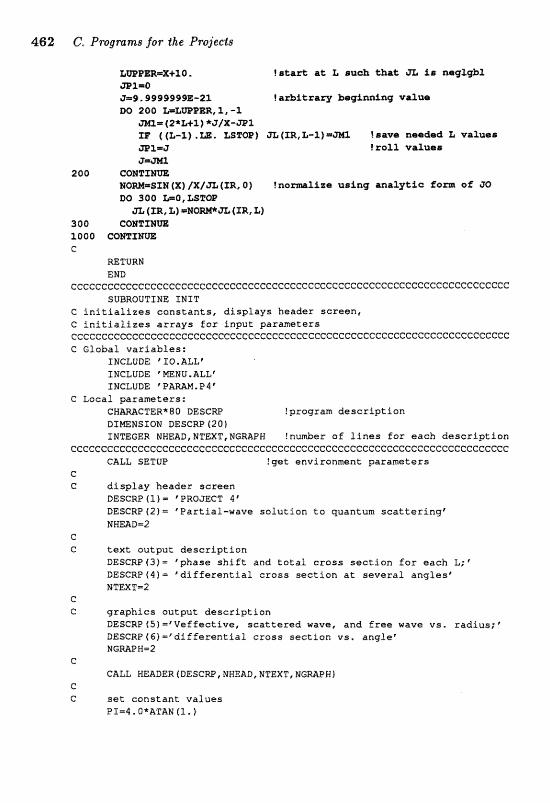
LWBER=X+ZO. letart at fc suoh that JL is naagb1 3215=0 9=9.999999983-21. ?azbitraq bginninq value DO 200 L=LWPER,1,-1 a= (2*ttl) *J/fC-a1 EE ( (L-S) .m, &STOP) JL (ER, fc-1) =m ! saw@ nsc~cS9d L va1uer ;JIPI=Z IroU valucallr gm-l
200 CONTTrn IOM=SII (X) J X / a (m, 0 ) ? nomllzs u@ln(~ analytic fern of $0 DO 300 wO,uraF a' (ZR, L) =HOW& {XR, L)
300 COWTEN= 1.000 CONTPNUT?: C
MTURIJ END
c~ceeccccecececccccccceccccccccececccecccccccccecccccccccccccccccccccccc SUBROUTINE INlT
C i n i t i a l i z e s c o n s t a n t s , d i s p l a y s heade r s c r e e n , C i n i t i a l i z e s a r r a y s f o r i n p u t p a r a m e t e r s cceeccce~~cececccccccccececececceeccccecccccccccccccccceccccccceccf:c~eec C G loba l v a r i a b l e s :
INCLUDE 'IO,BLL' INCLUDE p MENU ,ALL" INCLUDE cPWM.P4'
C Loea l pa r ame te r s : CHmCTER*80 DESCW ?program d e s c r i p t i o n BIWNSLON DESCRP (20) INTEGER NHEAD,NTEXT,NGWPH f n u d e r o f l i n e s f o r e a c h d e s c r i p t i o n
ecccceccccceccCccccceccccccccececcccccc~cccccccccccccccccccceccccccecccc CALL SETUP ! g e t envi ronment p a r a m e t e r s
f: C d i s p l ay h e a d e r s c r e e n
DESGRP (1 ) = "PROJECT 4 " DESCRPtZ)= fPgart ial-weve s o l u t i o n to quantum s c a t t e r i n g " NHEADg2
c C t e x t o u t p u t d e s c r i p t i o n
D E S C W 4 3 f m "phase s h i f t and t o t a l c r o s s s e c t i o n f o r e a c h L;f DESCRP ( 4 ) = ' d i f T e r e n t i a l c r o s s sect ion a t s e v e r a l a n g l e s t P3"P"EXT-2
C C g r a p h i c s c u t p u t d e s c r i p t i o n
DESCRP(5)-fVVeffe~tive, s c a t t e r e d wave, and f r e e wave v s . r ad iu s ; ' DESCRP (61 = 'd i f f e r e n t l a l c r o s s s e c t i o n v s , a n g l e ' NGmPW=2
C CALL HEADER (DESCW , NHEAD, NTEXT, ESGMPW)
C C set c o n s t a n t v a l u e s
PZ=4.0*ATAN (3. )
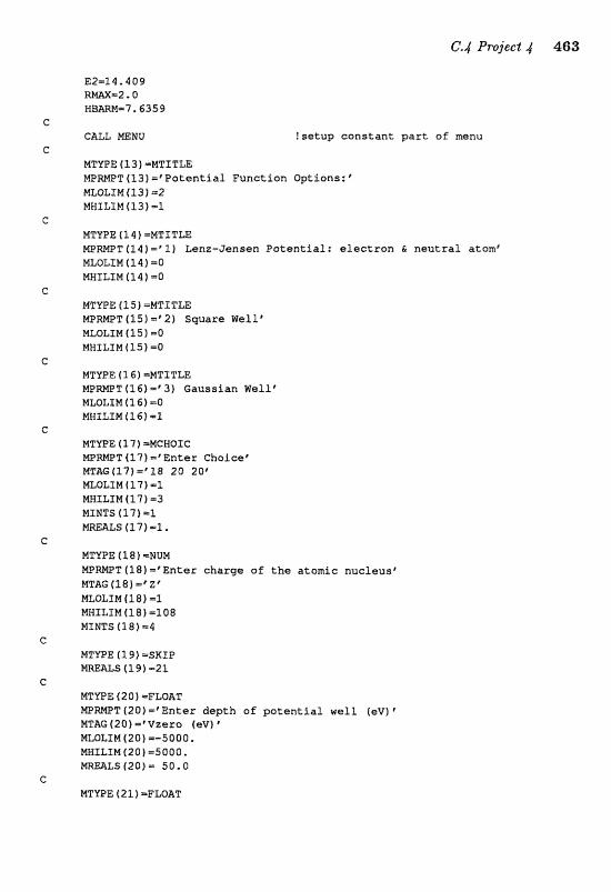
CALL MEHU !setup constant part o f menu
MTYPE f l3 ) ='DVITITLE FIPR14PT(13)-Votentia5 Function Options:' MLOLIN ( 1 3 f -2 WNIEZM (13) =l
MTWE ( 14 ) -MTITte MPMFT(14)="1j Lenz-Jensen Potential: eleetxsn & neutral atomf MLOLSM (1 4 1 =Q MHXLSM [14) -0
MTYPE (25 ) =XTITm mmPI[" (15) Spars Welle MLQLZM ( 15 1 m0 MHSLSM (151 -0
MT?IPE (1 6) =MTJTLE M P W T (3.61 =' 3) Gausslan Well' MLOLIM (261 m0 MNfLIM 4 3.61 -2
NTVPE (1 7 ) =MCHOIC M P W T (L71 =qntsr Choicer MT&G(17)='18 20 206 MLOLZM (17) a1 MHXLIM f 3.7 ) m3 MINTS (17) 11 m A L S (17)=1.
MT-E (1 8 1 -NUM M P W T (18) =*Enter charge of the atonic nueleuae NTAG f18) m' Z p MLOLLM f 18) -2 MXTLXMf18) =l08 NZNTS (181 -4
MTYPE (1 9 1 -SKIP MmALS f 1 9 1 m2 1
MTWE f 2 0 f =FLOAT N Z t W T (201 -'Enter depth of potential well (@V) * MTAG (20) ='Vzefo (eV) @
MLoL3N (20) m-5000. MHSLZN (20) =S000 MmALS(20)= 50.0
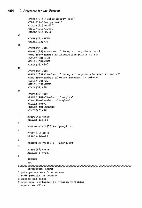
464 C. Pm?gmms for the Pr~jects
N B m T (21) ='Enter Enslcs (eV) ' MTAG (21) =%nergy (eV) MLOLIM (21) =OIQQO1 MMILIM 121) =za1000. MRrnLS (23.1 420.0
C MTYPE 122 f =SKIP
LS (22) -35 C
M W E (38) =NUM M P W T (38) ='Number of integration points to rlr MTAG (38) n u h r o f integration points to rlr MLOLlH (38) -100 MRSLXM (3 8 1 =mXN MINTS (381~400
G MTVPE ( 3 9) =NUM @WT(39)=@Hu&er of integration points between rl and r2' MTAG (39) =' nu&er a f extra integration points? MLOLIN (39) 220 MWILf M ( 3 9) = W E MINTS (39) =SO
c NTWE ( 4 0 f =NUN MPWTl4Of=*Numker of anglesf MTAG ( 4 0 ) m f numjber o f anglesv ~QLIP?r(40)=1
MfNTS 4401-36 G
NTUOE (41) =SKZP LS (42) -60
G NSmNG (MINTS (35) ) - 'proj4. t x t *
G ( 7 S) =SKXP S (76) -80-
C MSmHG (MINTS (86) ) = "proj4,grf*
C MFVPE f 8 7 1 =SKIP M m L S (87) =90.
C mTUR# END
cccccCccccccccec~c~ceccececccccccccccceec~cceceC:eccccccccccceccccec~ecc~ SUISROUTIHE P-M
C gets parameters fxom screen C ends program on request C closes old files C maps menu variables to program variables C opens new files
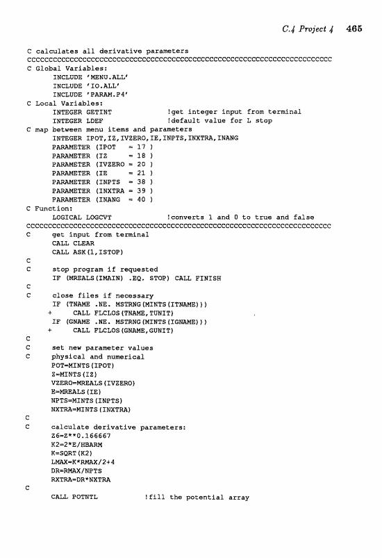
C calculates a l l d e r i v a t i v e p a r a m e t e r s CCcCccCcccceCcccccccccecccccccccccccccccccccccc~ccccccccc~ccf:ceccccecccc C G l o b a l V a r i a b l e s :
INCLUDE "@U. ALL" INCLUDE: '10.ALL' INCLUDE 'PARAM,P4'
G L o c a l V a r i a b l e s : INWGER GETINT !get i n t e g e r i npu t f r o m t e r m i n a l INTEGER LDEF ! d e f a u l t value far L s t o p
G m a p b e t w e e n menu i t e m s a n d p a r a m e t e r s INTEGER IPOT, I Z , IVZERO, XE, INPTS, XMXTM, INANC
TER ETPOT = 1 7 1 TER [ I Z 18 1
P m H E m R (IVZERO = 20 1 TER ( I E -. 21 1 TER ( INPTS = 38 )
P-WTER I I N X T M = 39 1 P m W T E R (INAN6 = 40 1
G F u n c t i o n : LM-;fCAL LOCCVT i c a n v e r t s 1 and Q t o tme a n d f a l s e
Ccccc~cc~cccCCccccccceecee~eeccccccCcccceccccc~cccccccecccc~ccc~cccceccc C get i n p u t f r o m t e m f n a l
CALL CLEAR. CALL ASK f S, ISTOP f
C C stop p r o g r a m i f requested
IF ( W A L S ( I m I M ) .EQ, STOP) CALL F I N I S H C C close f i les i f necessary
IF ( T H M .NE. MSmBG (MINTS (ITNAME) ) 1 + CALL FLCLOS (THAm, TUWIT) TF (GMM& . NE, MSZ"RNG (MINTS IIGH&ME) 1 }
+ CALL FLCLOS (CNAHE, G U N W C C set new paramter v a l u e s C p h y s i c a l and n u m r i e a l
POT=MINTS ( IPOT) Z=MINTS (1 Z1 V Z m Q = m A L S ( IVZERQ) E = m A L S I I E ) NPTS-MINTS ( I W T S ) NXm=MSNTS 4 INXTRZL)
C C calculate d e r i v a t i v e p a r a m e t e r s :
Z&=ZkC8. 266567 X(2=2*E/E4f3ARMt K-SWT (X21 L W = K * W X / 2 + 4 DR=RWX/NL?TS M m = I Z R * H X T U
C C&LL BQTNTL ! f i l l t h e p o t e n t i a l a r r a y
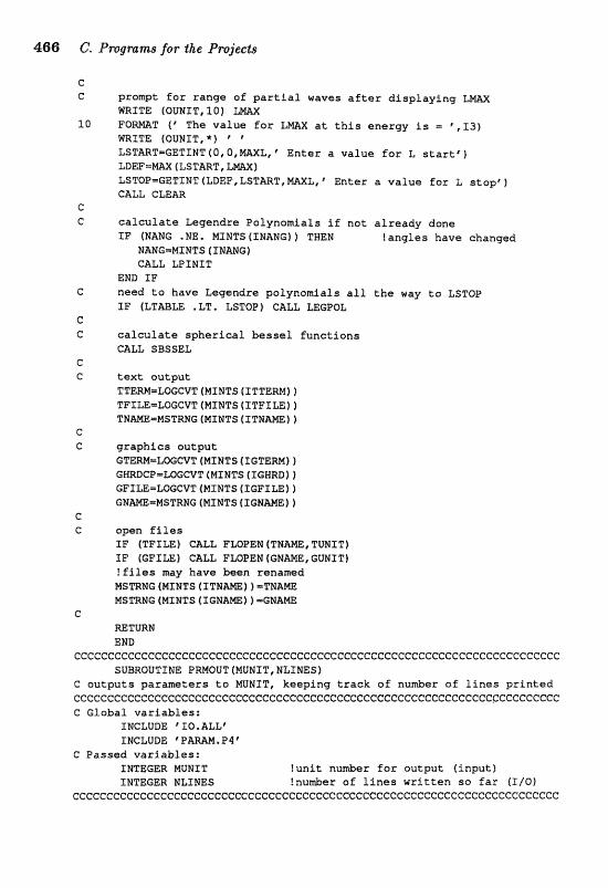
prompt f o r range of p a r t i a l waves a f t e r d i s p l a y i n g LmX KRITE (OUNIT, 10 ) F O M T f r The v a l u e f o r =X a t t h i s enert3y is = ',I3) m I T E (OUNIT,") " LSTmT=GETINT(O,O,mXL, E n t e r a v a l u e for L s t a r t ' ) ZDEF-mX (LSTART, L m X f LSTOP=GETINT(LDEF,L5TART,KIIXL,e Ente r a v a l u e f o r L s t o p ' ] CALL CLEM
c a l c u l a t e Legendre Polynomials i f no t a l r e a d y done I F (HANG .NE* MINTS 1INANG) 1 THEN !ang les have changed
[email protected] ( IHmG) GALL LPINZT
END I F need t o have Legendre polynomials a l l t h e way t o LSTBP I F (LTmLE *LT * LSTQP) CALL LEGP5L
c a l c u l a t e s p h e r i c a l bes se f f u n e t i o n s CALL SBSSEL
text: a u t p u t TTERMoLoGCvT (MINTS ( ITTEMj 1 TFILE=LoGCVT(MIMTS(STFILEjf TKMoMSTRMG (MINTS (ITP3ANE f 1
graphics ou tpu t GTBW=LOGCVT (MINTS 4 IGTERMI ) GmCP-LOGCVT (MINTS f7:GWRD) 1 GFXLE-L5GCVT(MINTS~IGFILE~) G M ~ = M S T R N G (MINTS ( r@HAME 1
open f i les I F (TFILEf CALL FU1PEN (TMAm, T a l T f IF (GFILE~ cam F ~ P E M (CH=, GUNIT) ! f i l e s may have been renamed MsraUG (MINTS (ITN-) I =THW MSTRHG (MIHTS {XGrJAM) ) =GNAm
C
=TURN END
CccccceccccccccccccccccccccceIzcecceeccccccccGccccecc~cccccccc~eccc~ccccc SUBROUTINE PRMOUT(XUNXT,NLINES)
C o u t p u t s pa ramete r s t o MUNIT, keep ing t r a c k of n u d e r of l i n e s p r i n t e d cCcCccccccCccttccccccccccccccccccccccececcecccccccccccccccccccccccccccc~ C Glabal v a r i a b l e s :
INCLUDE IQ. ALL' INCLUDE 'PAM.P9 '
G Passed v a r i a b l e s : INTEGER MUNIT ! u n i t nuniber f a f ou tpu t ( i n p u t ) INmGER NLINES !nu&er a f l i n e s w r i t t e n s o f a r (XI01
~ceccccc~cccccccc~ecccc~eeccececC:cccC:cccecc~eccccccccccccccc~ccccccccccc
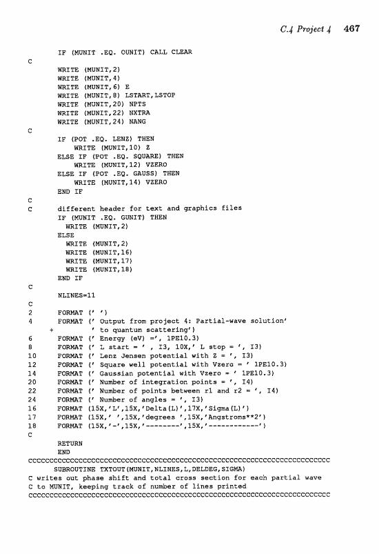
I F (MUNIT .EQ. OUNIT) CALL GLEaR e
WRTm [NUNIT, 2 ) m I T E (MUNIT, 4 ) mZTE (NUNIT,G) E tJRXTE (MUMXT, I)) L S T m C LSWP FJRf TE (NUNTT, 2 0 ) NPTS WRITE (MUNTT, 22 1 NXTM m T T E (MUNIT,24) M M G
c I F (POT .EQ. I;ENZ) THEN
m J T E (MUNXT,lO) Z E m E I F (POT ,Ea. SQU&m) THEN
HRfTE (NUWST,12) VZERO ELSE IF fPQT .EQ. GAUSS) TXEN
mXTE (MUNIT,lrl) VZERO END SF
e C d i f f e r e n t h e a d e r E a r t ex t and g r a p h i c s f i f e s
I F (MUMXT .EQ. GUMIT) THEN W I T E (MUNTT, 2 )
ELSE m I T E (NUNIT,2) m I T E (MUHIT, 1 6 ) m I T E (MUNIT, 17) WRITE (MUHIT, 18)
END I F C
NLTWES=l l c 2 FORMT (' ' 1 4 PQRmT ( V u t p u t f r o m p r o j e c t 4: P a r t i a l - w a v e s o l u t i o n e
+ "to quantum s c a t t e x i n g r 1 6 FORNBT f f E n e r g y (@V) =" lPE10.31 8 FORMT f ' L s ta r t = @ , X I , % O X , * L stop 5 XI31 10 FORmT 4' Lenz Jensen p o t e n t i a l wi th Z = ', 133) 1 2 F Q m T ( * Swaar w e l l p o t e n t i a l with V z e r s = 1PE10.31 1 4 F O W T ( q a u s s i a n p o t e n t i a l w i t h V z e r o .; 1lPE10.3) 20 F O M T 1 " N u d e r of i n t e g r a t i o n p o i n t s = ', 1 4 ) 22 FORMT ( * Humker o f p o i n t s b t w e e n r f a n d r 2 = ', 1 4 ) 24 FORmT ( " u m b e r o f a n g l e s = ' , I 3 f 26 FORMAT (15X, * L r , l5X, ' D e l t a (Lf', 17XI * SfgmafLf 1 1 7 F O W T (15X, * ' ,1!5X, ' d e g r e e s * , lSX, ' A ~ g s t r o m s f x Z ' 1 1 8 FORMAT (TSX, ' --' , 1SX, ' ------A ,15x,~-----------e 1 G
MTURN END
ccccccccccccccccccccceccccccccccecr:cececccccecccccccccccccccceeecccccccc SUBROUTINE TXTOUT (MUNIT, NLINES, L, DELDECf S f G M )
C w r i t e s out phase s h i f t a n d t a t a l c r o s s s e c t i o n f o r each p a r t i a l wave G to NUNZT, k e e p i n g t r a c k of n u d e r of l i n e s p r i n t e d ccccccceccececcccccccecccccccccccccccccccccccccccccccecccccccecccccccccc
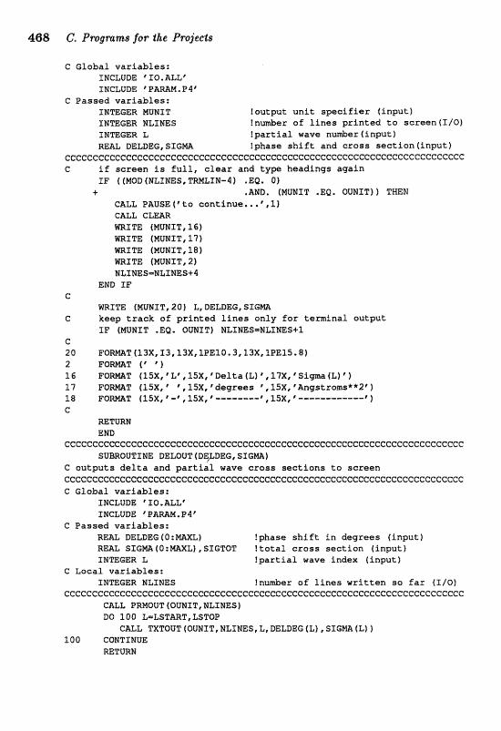
468 C, Pmgmtms for the Pr~ jee f s
C Global variables: INCLUDE * XIQ. ALL' INCLUDE @PAWH.P4'
Passed variablas: XNmGER MUNIT !output unit specifier (input 1 INmGER NLINES !rider of lines printed to screen(l/Oj 1NTEC;ER L !partial wave nu&er (input ) RE& DELDEG, 5IGm Iphase shift and cross section finput)
CCCCCCCCCCCCCCCCCCCCCCCCCCCCCCCCCCCCCCCGCCCCCCGCC~CCCC~CCC~~CCCCC~CCC~CG C if screen is full, clear and typ headings again
IF ( (MOD (NLINES, TRMLXM-4f . EQ. 0 ) + .WD, (MUNTT .EQ. QUMITf) THEN
CALL PAUSE(*to eontinue,..f,lf CALL CLEAR IISRITE (MUNLT,iG) WRITE (MUNIT, 17f mITE (MUNIT, 18) WRITE fNUMXT, 2) NLXNES=MLSMES+4
END IF e
WRIm fMUNIT,20) L,DELDEG,SEGXYIA C keep track of printed lines only far terminal output
IF (MUNIT . EQ, OUNTTf NLINES=NLIPSES*I e 20 F O m T f ISX, I3,13X, iPEf O13,13X, 1PE15 1( 8 ) 2 T " O r n T ( " ) 16 F O m T EfSX, 'L*, 15X, 'Delta (L) I?XI Sigma (Lf p 1 17 F O m T (l5X, ' 5 15X, 'degrees ,1SX, %~ngstrams**2~ 1 18 F Q m T (15X, --" ,15X, " - - - - - - - p , ISX, ------------ > e
RETURN END
ccccccccccccccccccccccccccccccccccccccceccceccecccccccccccceccccccccccec SUBROUTINE DELOUT (DE&DEG, SIG-)
C autputs delta and partial wave cross se~tians ta screen ccccccecccccccccccccecececccecccccccccr=:ecccccccecccecceC:cC:cc~cccec~ccccc C Global variables:
IMCLUDE * IO. ALLr INCLUDE ' PmM.PI '
G Passed variables: REAL DELDEG ( O : mXL) !phase shift in degrees (input1 W& SIE~(B:~XEl,SIGTO"XItatal cross section (Input) IPJTEGER L !partial wave index (Pnput)
C Local variables: XNIIEGER NLPNES !nu&er of lines written so far (I/O)
cceccecccececccce~cecceccecccccccccccccccccccceeccccecccccececcccccceccc CALL PRMQUT (OUNIT, NLINES) DO 100 L-LSTART, LSTOP
CALL TXTOUS (QUhlIT, NLXMES, L, DBLDEG (L), SIGMA (L) 1 100 CWTIEtfUE
RETURN
C.4 Project 4 469
END cccccccccccccCcecccccccecccccccccccecccccccccccceccccc~cccccccccccc~cccc
SUBROUTINE SIGOUT(HUNIT,F,DSIGMrSSGTQT) e writes o u t s c a t t e r i n g angle , s c a t t e r i n g ampl i tude, C d i f f e r e n t i a l c r o s s s e c t i o n and t o t a l c r o s s s e c t i o n t o MUNIT ecccecccccccc~ccecccccccccccccccccccccccccceccccccccccccccccccccccc~cccc e GlobaZ v a r i a b l e s :
INCLUDE qIO.WLLf INCLUDE 'PAmM,P4'
C I n p u t v a r i a b l e s : INTEGER MUNIT !output u n i t s p e c i f i e r m& DSIGm(0:mmNG) ! d i f f e r e n t i a l a r o s s s e c t i o n COWLEX F 4 O : M X A N G 1 ! s c a t t e r i n g a q l i t u d e INTEGER TTNETA f index o f t h e t a REBL SIGTOT ! t o t a l c r o s s s e c t i o n
C Local v a r i a b l e s : INTEGER N L T m S lkeap t r a c k o f l i n e s p r i n t e d o u t
~~ccec~~cccccc~cceccccccccccccccccc~ccceccccccccc~eccccccccecccccecececc WRITE (NNT T, 2) m I T E (MUMIT, 2 1 mLTE {MUNf T, 4 f SIGTQT WFtITE fMUNfTt2f WRITE (MUIJIT, 2) WRITE (MUNIT, 10 ) WRLTB {WEST, 11) mXTE (WMXT, 12)
C NLXSES=..EI
C G w r i t e o u t data, a l lowing t i m e for u s e r t o exen ine f u l l pages
DO 100 ITHETA=O,mG WITE (MUNIT, 14) D E G W E (ITHETA) ,F (ITHETA), DSIGm (ITWETA) WLINES=HLINES+P SF ( (MOD (NLINES, TRMLXN-4) .Ea. 0) .AND.
+ (mNIT .EB. OUWIT) ) TEEN CALL PAUSE("o con t inue , . . \l) c&L CLEM
EHD SF 100 CONTINUE c 2 4 'TOTAL CROSS SECTTON - %1PE15,8,? Mgstzams**2') 20 FORmT ( I Q X , Theta* , 14X, @ AmlCtude (E,r. Xm) ,15X, ' d S i m / d T h e t a t } 11 FQRmT EBX, d e g r e e s t , 13X, Angst rc.trs**=! * ,25Y, * %qgst~ims**2~ 1 12 F Q m T (9X,t-------e,23X,G-------------"rf5,?-------------@
14 F Q W T (7X,F8.2,6XS (' ,1PE1Se8, ', "19E15.8, ' 1 C I X , 1PE15.8) G
=TURN END
ccccccccccccccccceccccccceecccceccccccccceccecccccccccccccccecccC-ceccC:~c SUBROUTINE GWOUT (DEVf CE, L, DELDEG, SIGMI
C o u t p u t s p o t e n t i a l and both f r e e and s c a t t e r e d wavefunct ions f o r one L:
470 C. Prr?gmms for the Projects
C d o e s n o t a l l o w f o r h a r d e o p y o r f i l e a u t p u t G i n o r d e r t o a v o i d t h e c r e a t i o n o f v o l u m i n o u s f i l e s ccececccccccccecececccccceccccccc~cc~c~cccccccccc~cccc~c~ccccccc C G l o b a l v a r i a b l e s
INCLUDE 'IQ,ALLf INCLUDE @PA=M.P$' INCLUDE ' GRFDAT, &L"
C I n p u t v a r i a b l e s : INmGER DEVICE Iwbich device is b e i n g u s e d ? TNmGER L ! p a r t i a l wave
DELDEG SXGM ! p h a s e s h i f t a n d c r o s s s e c t i o n RE= PSI ( m X N i W E f , f Sf F ( m N + W E j !wave f u n c t i o n s REAL PSIMX,PSFW !maxima o f wave f u n c t i o n s REAL VEFF ( W N + W E ) ! e f f e c t i v e p o t f o r f i x e d L CQWONfRESULT/PSI,PSIF,PSfW,PSFMAXIVIEFF!pas r e s u l t s from Numerv
C L o e a l v a r i a b l e s INmGER IR ! i n d e x sE la t t ice REAL VGRF IMA)EE+WIN) !V s c a l e d for g r a p h i n g R23AL PSIG(MXE+MAXN),PSIFG(mEfWXtJf I r e s e a l e d wave f u n c t i o n s RE& ENERGY (2 1 , mDIOS (2 ), ! a r r a y for p l o t t i n g e n e r g y CMWCTER*9 CL,CDEL,CSIG,CE ! c h a r a c t e r v e r s i o n o f d a t a INTEGER LE%, LCDEL, LCSIG ! l e n g t h of s t r i n g s INllEEEER SCREEN ! s e n d t o t e r m i n a l INmGER PAPER !make a h a r d e a p y INTEGER FILE ! s e n d t o a f i l e DATA SCREEN, PAPER, FILE/1 ,2 ,3 /
CCCCCCGCCCCCGCCCGCCCCGCCCGCGCCCCCCCCCCCCCCCCCCCCCCCCCCCCCCGCCCCCCCCCCCCC C m e s s a g e s f o r t h e i m p a t i e n t
SF (BEVICE .NE. SCREEN) WRITE (OUNIT, 100) c C a e t v p g r a p h i n g p a r a m e t e r s
IF (DEVTCE .NE. FILE) THEM NPLBT=1 !how many p l o t s ? IPLOT=1
C XMIN-O . O !axis p a r a m e t e r s
YOVAL=XMLN YNIM=-2*E ! e n e r g y a x i s v a r i e s b e t w e e n UmX=+ 4 *E !-2E and 4E XOVAL=O
LABEL(I)= ' r a d i u s angstrom^)^ !titles a n d l a b e l s UBEL (2)= 'VeEf feV), s c a t t e r e d wave ( s o l i d ) , @
+ I/ ' a n d free ( a s o ) wave8 CALL CONVRT (E, CE, LEN ) I F (POT .EQ. LEMZ) THEN
TXTLE = ' M n W - ~ e e n P a t e n t i a l , E n e r g y 4eV) ='/LICE ELSE IF {POT .EQ. SQUmE1 THEM
TITLE = ' S w a r e W e l l P o t e n t i a l , E n e r g y 4eV) - I //CE

ELSE IF (POT .EQ. GAUSS) THEN TITLE = ' G a u s s i a n Potential, Energy (eV)='//CE
END I F
arrays for plotting energy mar u s (I -0. RaDIuS (2) = X M ENERGY ( 1 ) =E ENERGY [ 2 ) =E
plot Veffective between -2E and 4E DO 30 IR=1,NPTS+WXTM ! normalize WFF
VGRF (IRI =VEFF (XR) I F IVGRF (ER) . GT . Y W 1 VGRF ( I R 1 = Y m X IF (VGRF (XR) .LT, YHIN) VGRF 4 I R ) =YMIN
CONTINUE
rescale wave functions so that it fits on the energy scale DO 10 IR=1,KPTS+MXTM
P S I G (ZR) ==PSI (1R) * 3 * E / P S I W + E : PSIFG (IR) =PSXF ( I R ) *3*E/PSFmX+E
CONTINUE
!line and syhol styles
CALL GTDEVfDEVICE) !device nomination I F (DEVZCE .EQ. SCWEW) CALL GMODE !change to graphics mode
create the legend GALL XCWRT (L, CL, LEN) CALL CONVRT (DELDEG, CDEL, LCDELI CALL CONVRT ( S I G m , CSXG, LCS1Gf IMFO=W@lta(L="/CLt1:LEN) // ' l = * //CDEL(l:LCDEL) / /
* deg' / / //GL(I:LEHJ / I # 1 =v/csrc t i : L c s r G l / j t ~**2'
CALL LNLHAX
CALL XVFLOT (R, VGRF ) NPOZNTm2 CALL XYPLOT (MDIUS, ENERGY)
NPOINT=NPTS+NXTRA CALL XYPLOT (R, PSIG) XFREQ=4
XYPLOT (R, PSXFG)
!plot potential
!plot energy
!plot wave function
!plot free wave function
END I F
472 C. Pwgmms for the Projects
C C e n d g r a p k i n g s e s s i o n
I F (DEVZCE .HE. FILE) CALL GPAGEtDEVICE) l e n d g r a p h i c s p a c k a g e IF (DEVICE .EQ. S ~ E E N I C&LL T ~ D E ! s w i t c h t o t e x t mode
C 100 F O W T ( / , V a t i e n c e , p l e a s e ; o u t p u t g o i n g t o a C
mTUEZU END
cccccccccccceecccccec~ceccccceccceccececccc~cccccccccecccccccccccccccc~c SUBROUTINE GRFSIG (DWI CE, BSIGmf SIGTOTf
C graphs d i f f e r e n t i a l c r o s s s e c t i o n vs. a n g l e f o r a l l par t ia l waves G on a s e m i - l o g scale cccccccccccceeccccceceecc~ecccccccecccccccccccccccccccccceccC:cccce~ccccc C G l o b a l v a r i a b l e s
INCLUDE "IO.ALLc INeLtUDE ' P A M . P $ " INCLUDE ' GRFDAT . ALL'
C I n p u t v a r i a b l e s : INTEGER DEVICE !which d e v i c e is b e i n g u s e d ? REAE SfGTOT ! t o t a l c r o s s s e c t i o n WAL DSIQm 10 :MXAWG) ! d i f f e r e n t f al c r o s s s e c t i o n
G L o e a l v a r i a b l e s INTEGER ITHET& ! i n d e x e s a n g l e INTEGER EXBmX,EaMII ? m i n and max c3xp for d f f f c r o s s s e c t i o n
TER*g CE,CSIG I e n e r g y , s i g m as a c h a r a c t e r s t r i n g INTEGER LEN ! s t r i n g l e n g t h INTEGER SCREEN ! s a n d t o t e r m i n a l INmGER PmER !make a hardeopy INmEER FILE ! s e n d t o a f i l e DATA SCREEN, PAPER, Ff L E / l I 2 t 3 I
e~~~c~ee~~~ce~c~~cccccccceccc~~cccccccccececcccccccccecceecccccceccccccc C m e s s a g e s f o r t h e i m p a t i e n t
IF (DEVICE .HE, SCREEN) WRITE (OUNIT,100) C G c a l c u l a t e p a r a m e t e r s f o r g r a p h i n g
I F (DEVICE .HE, PILE) THEN c
MPLOT=l !how many p l o t s ? ICPLBT=l
c YMAX=O. ! f i n $ l i m i t s an d a t a pa in ts UMIN-DSIGMA (1) DQ 20 ITWETA=O,NAPJG
fF ( D S T G M (XTMETA) .GT, YE*PAX) Ymx-DSIGm (ITHET&) IF (DSZGMA (ITHETA) .LT. W Z N f VMINmDSIGm (ITWETA)
COHTIIUE ! f i n d i n t e g e r l i m i t s on e x p o n e n t ExPmx-rNT (LWIO ( u r n ) j I F ( V W .GT. 1, ) E X P M -EmPIL11X+I ExPMIW-fHa (LOGL o (UMXM) I I F (VMIN , LT. 1. ) EXPMIN=EXPMIM-1
XMIN-DEGrnE (Q) XmmDEGREE (N&NG YOVAL=XMIPJ XOVAL=YMIN
!line and s y d o l styles ILINE=I XSPM-4 IFm8=1 XJXTLCK=4 NYTICK-EXPmX-EXPMIN IF (NYTICK .CF. 8) THEN !keep nu-r of ticks small
IF (frlOD(WTICK,2) .EQ. 0) TWEN NPTIGK=NUTXCK/2
ELSE NVTICK-8
END IF END IF
CALL G O M T (E, CIE, LEM ) !titles and l a h l s IF (POT .&Q, mMZ) THEN TITm - ' hnz-Jensen Potential, Energy (eV)=V/CE
ELSE TF (POT .EQ. SQUME) TmN TITLE = "ware Well Potential, Energy (eV)mr//CE
ELSE IF (POT .EQ. (;AUSS) THEW TITLE = "aussian Potential, Energy [&)='/ICE
END IF CALL CQWRT (SXGTOT, CSZG, LEN) INFO-'Total cross section in A**2 I//CSIG LABEL(lI1 "gle (dsgrse~)~ LABEL (21 = ' D i f fsrentiaf Cross Section (Wngstroms**2)
CALL GTDEV (DEVICE) !device nomination IF [DEVICE ,&QI SCmEN) (=ALL GMQDE !change to graphics made CALL LELNM !draw axes
END XF e C output results
IF (DEVICE .EQ. FILE) TWEN HRSTE (GUNIT, 10) mITE (GUNLT, 11) WIZI"E1 EGUNlT, l21 WRITE (GUNST,l1) (D&GREE(ITNjeTA),DSIGMIIT~TAI,ITHETA=.O,NAPJGI
ELSE CALL XmLOT (DEGREE, DSIGM)
END TF G C end graphing session
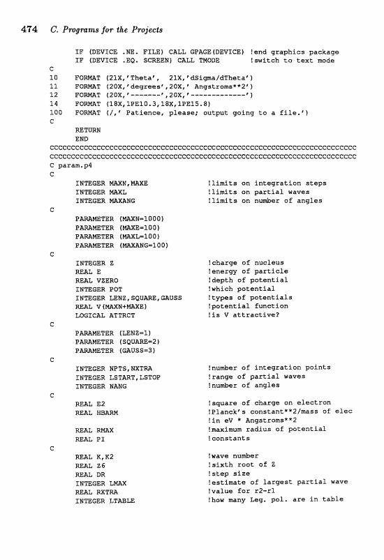
TF (DEVICE .NE. FILE) CALL GPAGEtDEVICE) !end g r a p h i c s package I F (DEVICE .EQ. SCMEH) CALL TNODE !swi tch t o t e x t mde
C 1 0 F Q m T (2PX, ' TThtaa" , 21X, c d S i p a / d T b e t a 6 1 I1 P O m T (2DX, "esgr@esf I 20X, 9 n g ~ t r o m s * * 2 ~ 1 12 F O M T (20X, ' ----m--@ ,2QXIt-------.,...,----fl 1 1 4 F O m T (18X,1BE10.3,18X,lPE15.8] 100 F O W T f l , V a t i e n c e , p l ease ; ou tpu t g o i n g t o a f i l e . ? ) C
=TURN END
ccccccceccccccccccccccccccccccccccccccccccceececcecccccccccccccccccccccc cccccceccccccccccccccccccccccccccecccceccccecccccccccci=ccccccccccccceccc C param.p4 c
INmGER mXZd, M X E ! l i m i t s on i n t e g r a t i o n s t e p s INTEGER NXL ! l i m i t s on p a r t i a l waves SNTE;GER WANG ! l i m i t s on nu&er o f a n g l e s
C PAamTER (WN=1000) PAmWTER (mXE=f 00 1 PAMWTER (=L-100)
C INTEGER Z !charge of nuc leus mAL E ! e n e r w o f p a r t i c l e RE& VZERO tdap th o f p o t e n t i a l XNmGER POT !which p o t e n t i a l INTEGER LENZ,SQUW,GAUSS I t y p s o f p o t e n t i a l s
V (MAXN+mE) ! p o e e n t i a l f u n c t i o n LOGICAL ATTRCT ?is V a t t r a c t i v e ?
C PAaMETa f mNZ=1) PAWBTER {SQUAm-2) P-METER (GAUSS-3 1
C
INTEGER NPTS , NXTM INTEGER LSThRT, LSTOP INmGER HANG
c REAL E 2 REAL MBmM
RMWX REAL PI
C REAL K, K2 REAL 26 mAL DR INmGER LMAX REAL RXTM INTEGER LTE?rBLE
Inuntber o f i n t e g r a t i o n p o i n t s !range af p a r t i a l waves !nu&r of a n g l e s
!square of charge on e l e c t r o n ! P l a n c k t s sms tan t**2 /mass of elec t i n sV * Angstroms**2 !maximum r a d i u s o f p o t e n t i a l ! c o n s t a n t s
!wave nu&er !sixth r o o t o f Z ! s t e p s i z e ! e s t i m a t e o f l a r g e s t p a r t i a l wave !value f o r x2-rl !how many L e g , pol, are i n t a b l e
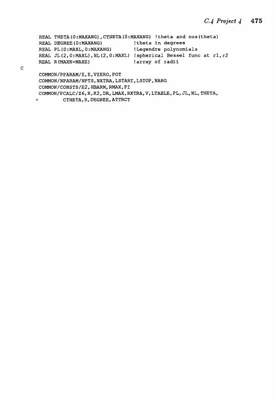
REAL TNE1PZalO:MA~MG),CTHETA(O:~~HG) !theta and cos(tbeta1 =&L DEGREE c 0 : MMHG} ! the ta fn degrees
!Legendre polynomials :mXL) ! spherical BssseL Eunc at rl, r2
R [ mXM+mX& ) !array of radii C:
COMONIPPARaM/Z, Et VZERO, PQT CQMON/NPARAM/NPTS,NXTM,LSTART,LSTOEl,NAHG CQMOH/CONSTS/B2,mARN,mX,P1: GOE4MON/PCALG/Z6, R,R2, BRI LMAXI RXTM, V, LTWBLE, PL, JL,NL, THETA@
+ CTBETA, R, DEGREE, ATTRCT
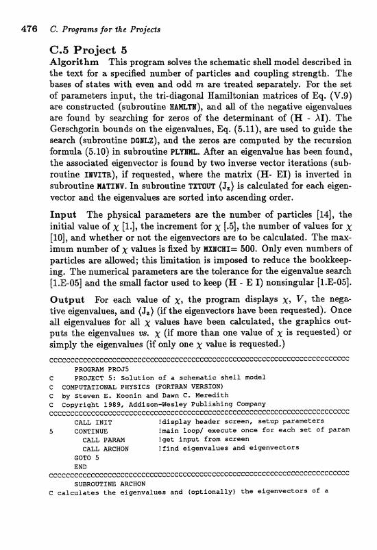
C.5 Project 5 AIgorbhm This proe;rm solvw the sGbenratic shell model described in the text for a specified nnmber of p e i d e s and cm$ing streagth, The bases of etates with even and odtd m are treated wparately, For the set of parmeters input, the tri-diwonal H ltonian matrices of Eq. (V.9) are constructed (subroutine WWH), and aJ1 of the negative eigenvdues are found by searching for zeros of the determinant of (H - XI). The Gerschgorin bounds on the eigenvalues, Eq. (5.11), are used to guide the search (subroutine D G ~ Z ) , and the zeros are computed by the recursion formula (5.10) in subroutine PLYIHL. After an eigenvalue has been found, the associated eigenvector is found by two inverse vector iterations (sub- routine ZRVITR), if requested, where the matrix (H- EX) is inverted in subroutine WATIW. In subroutine TXTQUT (J,) is calculated for each eigen- vector and the dgendues are sorted into ascen&ng ofder.
Input The physical parameters are the nnmber of partides [14], the initial value of X [l.], the increment for X [.5], the number of values for X [10], and whether or not the eigenvectors are to be calculated. The mm- imum number of X vdues is fixed by HxBcaz= 500. Only even nurnbers of partides are dlawed; this limitation is imposed to reduce the badkeep- ing. The numerical parameters are the tolerance for the eigenvalue search [ l .&Q51 and the small factor used to keep (H - E I) nonsingular [1.&05].
Output For each value of X, the program displays X , V, the neg* tive eigenvalues, and (J,) (if the eigenvectors have been requested). Once all eigenvalues for all X values have been calculated, the graphics out- puts the eigenvalues vs. X (if more than one value of X is requested) or simply the eigenvalues (if only one X value is requested.)
cc~ccc~ccccccccccccc~cccccc~cccccccccccceccceccccccececcccc~cccccecccce~ PRmUM PROJS
C PROmCF 5: SolutSon of a schematic shall nodal C COMPUTAT JOHAL PHYSICS (FORTmN VERSION) C by Steven E, Koonin and Dawn C. Meredlth C Copyright 1989, Addison-Wesley Publishing Cowany ceccCeeCeCCCCceGGcGccCCcCCCCcGCccCccCCcCC:CCCCccCccCCcCCCccCGcCccCccccccC
CALL IS14 fdfspfay header screen, setup parameters 5 CQNTINUE !main loop/ execute onee for each set of param
CALL P A W !get input from screen CALL mCI.ION !find eigenvalues and eigenvectars
GOTO 5 END
ccc~eccec~cceccc~~ccc~cc~cccccccccccccccccccc~ecc~ccccc3ccceccccccccccc~~ SUBROUTINE ARCHON
calculates the eigenvalues and (optionally) the eiganveetors of a
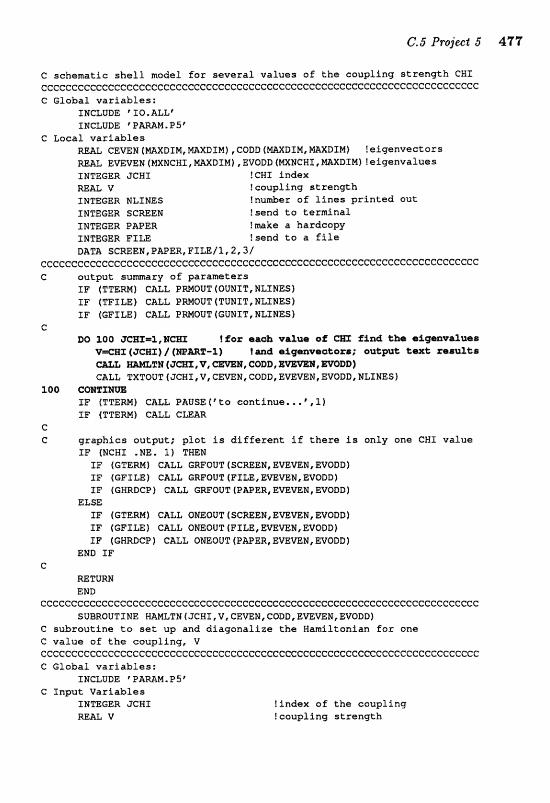
C s c h e m a t i c she l l m o d e l f o r s e v e r a l v a l u e s o f t h e c o u p l i n g s t r e n g t h CBI c~cccccCcccccccccceccccccccccccccccccccc~ccecccccecccceecccccccccceccccc C G l o b a l v a r i a b l e s :
INCLUDE I Q *ALLr INCLUDE ' P m M . PS'
c L o c a l variables REAL CEmN [ m x D I N , MAXDIMf , CODD (=DIM, =DIM) l e i g e n v e c t o r s RJZAL EmVEN (MNCMI , m D X M ) , EVODD (MXNCNI M X D I W ) I e i g e n v a l u e s INTEGER JCWX !CHI i n d e x REAL V ! c o u p l i n g s t r e n g t h INTEGER %LIMES !nu&er o f l i n e s p r i n t e d o u t INTEGER SCREEN ?send t o t e r m i n a l INTEGER PAPER !make a h a r d c o p y INTEGER F I L E !send t o a f i l e DATA SCWEN,PAPER,FII;E~~,~,~/
~ccccccCcccccccccecccccccceccccccccccccccccecccccccc~c~cc~cccccc~~cccccc C o u t p u t s u m a r y o f p a r a m e t e r s
XP (TTERM) G a L PMOUT (OUNIT, NLXNES) I F (TFXLE) CALL PMOUT (TUNIT, NLTNES) XF (EFILE cam P ~ O U T (GUNIT, NLXNES
C M) 100 qCBf-5,E- 12"or aaeb va2me of CBX find %he aigmvdu@o
V = a 1 ($CBI) I (mMT-1) ! af ganvacltsrr; @new% t a k r"eaul%s FN (XBZ, V, , CODD, @ W O D D j
CALL TX"XIOUT (JCHI , V, CEmW, CQDD, E a W N , EVODD, %LINES f 100 comxm
fF (TTERN) CALL PAUSE [ ' to c o n t i n u e . . . ?, If I F (TTEW) CALL CmAX
C C g r a p h i c s o u t p u t : plot is d i f f e r e n t i f t h e r e i s o n l y one GHX v a l u e
IP (NGHS .HE. 1) THEN SF (GTEMI CALL GRFOUT (SCREEN, EmVEN, EVODD] I F (GFII*E) CALL GWQUT(E"ILE,EWVEM,EVODD) I F (GHRDCP) GBLL GWOUT{PWER,EmVEN,WODD)
ELSE IF (GTEM) CALL ONEQUT (SCREEN, EWVEN, EIVODQ) TP ( E F I ~ ) c a L L ONEOUT (FILE, ~ V E W , EVQDD) IF (GHRDCP 1 CALL ONEOUT (PAPER, EaVEM, EVODB)
END IF C
RETURN END
cecccccccccccc~ccccccccC:ccccccccccccccccccccccccccccc~cccccccccc~cccc~cc SUBROUTINE HAMLTN (JCWI , U, CEmM, CODDI E-VEN, EVQDD)
C s u b r o u t i n e t o set up a n d d i a g o n a l i z e t h e W a m i l t o n l a n f o r o n e C v a l u e of t h e c o u p l i n g , V G C C ~ ~ C C ~ ~ C C C C C C C ~ C C C C C ~ C ~ C C ~ C C ~ C C ~ ~ C C C ~ C C ~ ~ C C C ~ ~ ~ ~ ~ ~ C C C ~ ~ ~ C ~ C ~ ~ C ~ C ~ ~ C ~ C ~ @ G l o b a l v a r i a b l e s :
INCLUDE ' P A N , P s 8 C I n p u t V a r i a b l e s
INmGER JGWI ! i n d e x o f t h e c o u p l i n g RE& V ! c o u p l i n g s t r e n g t h
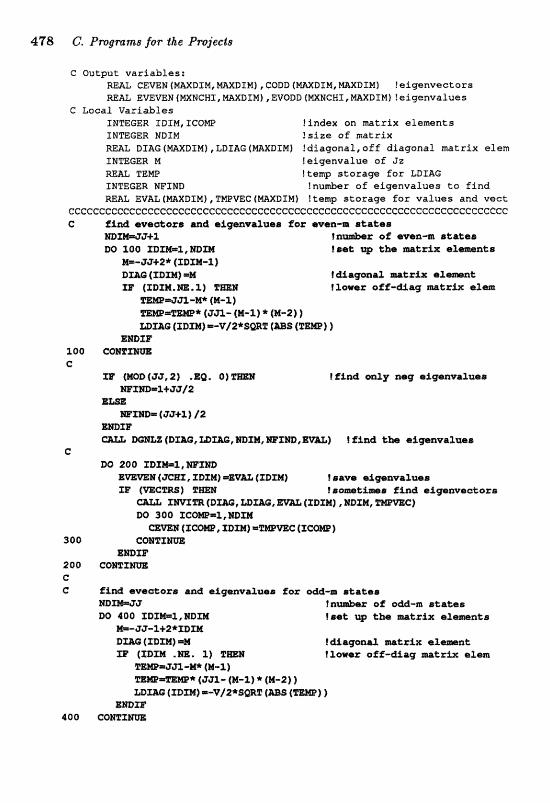
478 C. Pmgnarms for the Pr~jects
C Output variables: CEVeN ( W D f M, W X B I N ) P CODD I W B S N I mXDIN1 ! eigenveetors EmVEW (MNGWT, mXDIMj , EVODD (mNCIfT, M X E l I M j ! eigenvalues
e Local Variables INTEGER XDTM, XCOXUIP !Index on matrix elemnts INTEGER NDfM !s ize of matrix
DIAG (MlaXDXlvr) , LBIAG (mXDIE"I) ! diagonal, af f diagonal matrf x e l m INTEGER M leigenvalue o f Jz
TEW ?temp atorage far LDfAG INTEGER HFIND !number of eigenvalues to find W A L EVAL(~XDIM),TIUIP~C(MAXDXM) Item storage for values and veet
C ~ C C C C C ~ C G ~ ~ C C ~ ~ ~ C C C ~ ~ ~ C C G C ~ C ~ C ~ C ~ C C ~ ~ C C C ~ C C ~ C C ~ C ~ C C ~ C ~ C C ~ C C C ~ C C " ~ C ~ C ~ C ~ C
rnm=aJ+% t DO 3.00 XDZ-X, EPDm
*-3a+2* {ZDrn-Z ) I)X&@ (TDTM) 4 4 i&agmal mkr2x alemat:
flawer off-&ag m f x b a 3 a
=mm* (m- (M-%) * (M-2) &D=@ (XDm)=-Vl2*5WE [=S I
=mm 100 c a m x m C
33' (mB635,2) .&Q, 0 ) Z m B !find only nag eAgavausrr rnrnD=2+JJ12
E-
== D a m (D=@ m X W p mTMr mXm#
C W
!save amva2uern
C )
3 0 0 EmXF
2 0 0 C o m x m e C find ~vacrtos@ m& ellganvalluer fez &-m strfss
NDmmJa f DO aos XDrn=%, mm
~ - 8 G - l + 2 * X D T M IZW (XDXI) =H I &agenaX mkr ix ~Immat EH' {XBZE .m. 2 ) T- f l a w e r o f f %%em
-MP* (iFEl- (84-3) * (M-2) (XDXM) =-V[2*SWE (=S (
gmzr 4 0 0 eamxHm
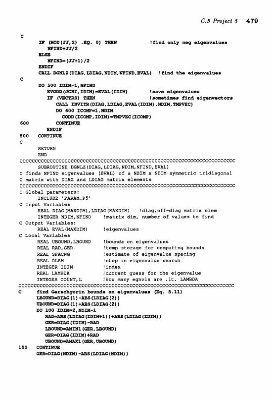
C X#' (M@D{gG,2) .EQ. 0 )
WZm=G;7/2. BE-
Isan- (a8+1) /2
D=% ( D W , D I M , mIM, W Z MB,mUl i f f nd t h rigonvrZme. C
BQ 5QO XBI24=%, BW"m -ODD (acm, ID=) (ram) !save aigbtnv~uallr
loorrrcbtima find sigemea%orer Xrnrn{DW, m m ,
W SOO f C W m I , IDIM COBB f f C-, XDXM) = P W a C (TCOW)
CrOQ CrnTXErn -TB"
500 CQ@%ZWOE. C
=TURN END
ccccccccccccecececccceccccccccccceccccccccccccc~cccccccccccccecccccccccc SUBROUTINE DGNLZ (DTAG, LDIAG, NDXMt NFINDI EVAL)
@ f i n d s HFIND e igenvafues (EVAL) of a NDIM X M D I M s y m t r l c t r i d i a g o n a l C m a t r i x with DIAG and LDIAG matrix elements cccccccccccCcccccecccccccccccccccccc~ccccccccccccccccecccccccccccccccccc C Global p a r a m t e r a :
INCLUDE ' P m H . PS * C Inpu t Var i ab le s
DSAG (mXDTM), LDIAG ( W D X M J ! diag, off -d lag ma t r ix elam IMTEGER NDXX,NFIND ? m a t r i x dim, number of v a l u e s ta f i n d
C Output Var i ab le s : REAL EVAZ ( W D E M ) l e iqenva lues
C Local V a r i a b l e s =&L UBOUND,LBOUMD !bounds on etigenvalues =m MD, GEE !ten\p s t o r a g e f o r c o m u t i n g bounds W& SFACNG !estimate o f e l p n v a l u a spac ing
DLAM ! s t e p i n e igenva lue sea rch INTEGER I D I M ? f ndex a& M B D A ! c u r r a n t guess fox t h e e i g e n v a l u s INTEGER COUNT, L !how many e q n v l s are .It. LdLMBDA
ccccccccccecccecccccccccccccccccccccccceccccF:ceccccccccccccccccccccccccc C gin hunde cm eigewdaoe (Eq* !5*ZZ]
1 -=g ( m m 421 1
asam1 TOO C Q m I m
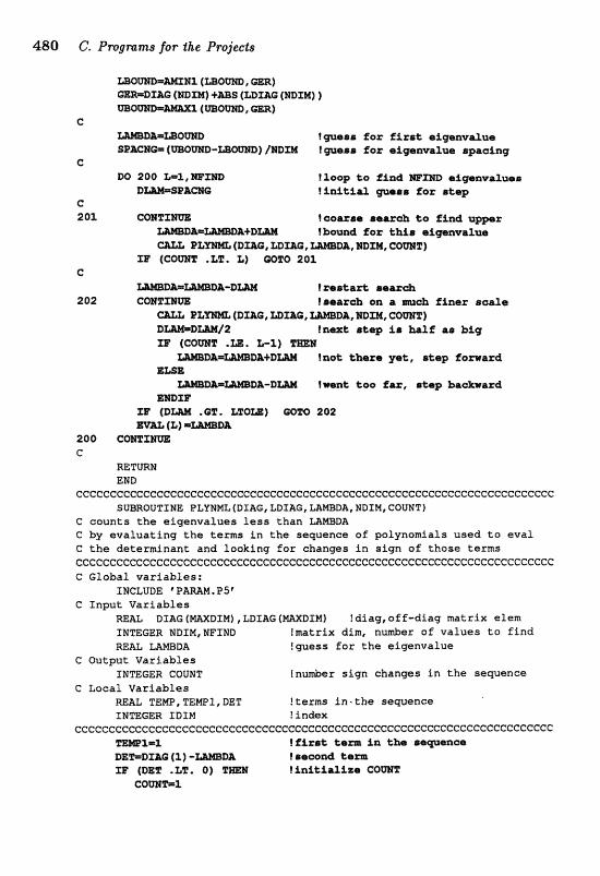
480 C. Pmtgrmnzs for Ihe Projects
mom=mxn tmom, @ER) -=D- (rnXM) +ms (LDrnG (mm) )
C
!*a.. for ffrsd eigenvakue - W m ) / B D a Iwesa fop: siwnva%ue apa~inq
C DO 200 b&, Floop to %An& WTm a3~ava1nea
D U = S E & a G linftloLf gnaso for et* C ZQ3. COBICIm tcoorae saarcb Co g%n&
Ibam4 for t h i s eiwnva , MDXW, CQWT)
m (COrnT .LE* G) WFO 201 c
!=@et& search, 2632 e& an a m& f%nar ecdar
* mzu, Cam] step A.. hg2f a@ big
D - !m=& too far, seep ba&waxd
200 c a m x m e
RETURN END
cccccccccccccceeecccecceccececcccccccccccccccccc~cccccccccceccccccccccec S WROUTIME ELYNML (DSAG, LDIAG,
C counts the eigenvafues less than C by evaluating the terms in the sa a i s used to eval C the determinant and looking for changes in sign of those terms ccccecccccccecccccccccccccceccccccccccccccccccceccccceccccccccccccccccee C Global variables:
INCLUDE 'PPAW.PSr
DIAG (MXDIM) , LD1AG ( M D T N ) ! diag, off -dlaq matrix elern TEGER NDIM, NFZND ?matrix dim, nuder a f valves to f i n d
!guess for the sigenvalue C Outpat Variables
INEGER GQUNT Inurtrbar sign changes in the sequence C Lacal Varlabfes
mAL FEPIE", TEWI, DE T !terns insthe sewencs TMTEGER SDIM ! index
t f%z& C@= La tb ser-ence DX&G (1) - I'samd tarn
E@ (DEZ .LP. a) Z m linEtZdize COUMT cawI"=2
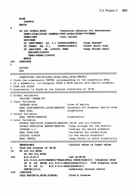
ELSE corn*@
Ems C
IEO 3.063 XDIMm2, mIM =W= ID- (XDZM) -
X=DZ% Dzll=zm 33" (DZZ*rnWX .I,%. Q.) C
I .Ea. Q, ) G0W%40mT+X ?@mm% zazes SF (m (BE%) .€%l. 100090)
l=zEmziloaooo
ZOO e e
MTURN END
ccccc~cCccccccecccccccccccccccccccf:cccccccccccccC:cc.cecceecceeccccccccccc SUBROUTINE 3WITR(DIAG,LDfAG,EVAL,NDIMITMPWCf
C finds the eigenvector m V E C corresponding to the eigenvalue EVAC C of a spetric, tri-diagonal NDIM x MDIM matrix with mtrix elements G DIAG and LDIAG C eigenvector is faund by two inverse iterations af (E-X) CccceccccccccceCcccccecccceecececccccccccecccccccccccccceccccccceccccccc C Global variables:
INCLUDE ' P W M . PS" C Input VariabTes
INTEGER NDIM !size of ntatrix DTAG[WXDIM),LDIAG(mDPM) !diagonaltoff diagonal mtrix elem
m L EVAL !eigenvalue G Output Variables
M L T1?"XPmC (MXDIN) ! eigenvector C Local Variables
DOWLE PRECTSIOB A (MAXDTH, NXDIN) ! (E-W) and its inverse DOUS3LE PWCISION BWC(NXDfM1 ltentp starage for the evector XNmGER I, J !indices for matrix elements mBL NORM, SUM !variables for normalizing LOGICAL SINGLR Ifs the matrix sincgular?
TMPEPS !temp factar to avoid singularity c c c c c e c c c c c e e c e c c c c e c c c c c c c c c c c c c c c c c
S m m S linitSal vdua i a inmk vaua C fincl %he imarss sf {E-W) 10 DO 200 X=Z,mm
w, aoa J = X , H D ~ 200 &(I, ~)=o.o l sat M (11-g)
A (X, X)= (1 ,mOO+%mm5) *DBm ( 3 -@B= {DIAG (I) 1 idiagsaal e l m 337 (I ,LE. LJ13f H) ;R (I, X+%) ( W X X (S+%) ) ! off d%ag~rzaX a3em 3 3 f 3 . OT . l) A (X, E-l 1 =-BB= {LDXm (X) )
C (X)=%. iazb%trrry fnieirX vector
a%XW (I, mXN, SmGm) !%An& A invatres
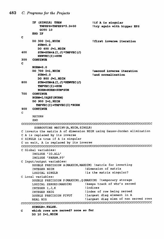
23' {SIN-) T m
END m G
oa soa X=T,NDIM: SW=O, 0 W 400 3=l,]LQDm
400 S m B m & {X, 3) * c {X) =Bm
300 C a W I W C
Ham0 * 0 -W _?00 T=%,EDm
swmo. 0
800
700 C O m Z m Bam=1/Smz ( N W ) DO 300 I=l,mIM
==c (X) = m a c (I) *Born 900 C O m Z m C
RETURN END
~ccceccccceecccccccccccecceceecccecccccccccccccccccccccc~~cccccccccceccc SUBROUTXME M T I W (A, NDIM, Sf N U
C inverts the matrix A of dimension NDIM using Gauss-Jordan el inr inat ion G A is replaced by its inverse C SINGLR is true if A is singular C on exit, A, is replaced by its inverse C@CCC~CCCCCCCC~CCCCCCCCCCCCCCGCCCCCCCCCCCCCC~C:CCCCCCCGCCCCG~CCC~CCCCCCCC C Global variables:
INCLUDE XIO,mL" INCLUDE T & M . P 5 '
G Input/autput variables: DOUBLE PmCISION A(MD X N , m D Z M 1 !matrix far inverting XNTgGER NDTM !dimension of matrix LOGXCAL SXNGLR !is the matrix singular?
C Local variables: DOUBLE Pmcrsra# P (Warn) , Q (WDmt I temporary storage LOGICAL ZEROED ( m D f M) !keeps track of whops zeroed INTEGER I, 3, K I indices INTEGER KBfG !index of row being zeroed DOUBLE PRECZ510N BIVQT !largest diag element in A
BIG !largest diag elem of nan zeroed saws ~~c~cc~~c~cCc~~~ccccceccccccecccccC:ceececcccceccccecccccccccccI=ceccccccc
s x B a m . F u s * C wM& zows are zermb? none eo gar
DO 10 1=z*mm
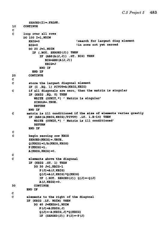
D (m)=*F-E. 10 e e C loop avar ail sows
W SQO S=l, MDXM mXG=O !@err& for laqmst; diag e1 BXWO tin rowa not ye* zeroad W 20 z=2,]NBIZ?I
mXwJ m XW
E m XF CQESX N W
adorn *he Xawest dlagona rlamnd XE {X .EQ. 2 ) PmOZd{mXG,mX@) $.f a3.P aagenalrr alra zero, %Mn the mesix is oin@&x 33' (=X@ .EQ. O) EmB W= f O m l t , * ) mkxlx ie siamart SXHGW,ZRrn.
- n C is ill cm&tiosmd I f the 8tza oP et
ms (ms(A(mxQ,mrnej/~mm) .L%. z.E-z~) m m {OrnP**] ' A@ gl.2 ean&t%aad"
E m l 3 C G -gin zeroing raw E33516:
(=X@] * a=. Q (=X@) =l l& {=X@, =I@) l? 4rnZG) =l " P (=X@, =I@) SO.
DO 30 J=l,mXO-l B (8) (3, =X@)
f=xG) (8 ) ) QtJ)=-QtJl
3 0 CQNICX m am 33'
G C s t o tba rSgbt of the &amnaP
m 4mxo .LP* mXN) DO 40 8=mGf 1,na
P (3) (mTG, RT) Q (3) =-a (mxo, a) *Q (=IQ) XB' (ZmaD ($1 ) P ( i t ) =-B (a)
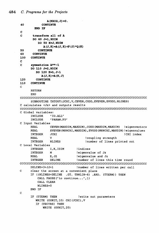
484 C. Prvrgmms for the Pr~jecls
A (rnXCi, 3) =O *
4 0 C W T m m m TIi"
C C tzmafom a11 e f A
W bQ J=1, Wr)XM DO 50 Em,XltDm
A fir, A) a (3, K) +p ($1 "Q 4x1 5 0 C m T l m 60 CWqtXSW 100 cmzsm C C Criza &**-I
O g52,WDfl DQ 120 Z=1, 3-3.
3L (3, =A (E, J) 120 C o M T x m 1JO C Q B T m G
RETURN END
cccccccccc~cecccececccceccccccccecccccccecccC:ccccceceeceeccccccccceccccc SUBROUTINE TXTQUT(JCHX,V,CBWM,CODDIEWWEl,EVODD,NLI:NESj
C calcufatea <JzT and outputs results ccccccccccccccccccccccecC:cecccccececcccccccccccccceccccccccccccceccccccc C Global variables:
INCLUDE F 10. ALL'
C Input Variables FtmL CZaN (WDIM, =DIN) , GoDD ( W B X M , MXIIIHI I ef genveetars m L EVE-N (NXMCWI, WWXDIMZ , EVODD fmNCWI, WDIMI i eigdnvalues INTEGER JCWI !CH1 index RE& V !coupling strength INTEGER NLINES ?number o f lines printed aut
C Local Variables INTEGER I, K, IBIM l indices INTEGER M !eigenvalus of Jz
E, JZ teigenvalue and Jz G DELIm !nu&er of lines this time round
cccccceececccccccccccccccceccccccccccccccccccccccccccecccccecccccccccccc BELINE-3CJ3+1 !nu&er of lines written per call
G elear the screen at a convenient place IP ( (NLTNES+DELTME . GT. TREZIN-6) .AND. (TTERM) ) T m N
CALL PAUSEfrto continue.,,*,l) CALL cLEm NLIMESmO
END IF C
IF (TTEM) THE% !write out parameters WITE (OUMXT, 10) CBI (JCWI) , V IF (mCTRS) THEM
mITE fOUNZT,2D)
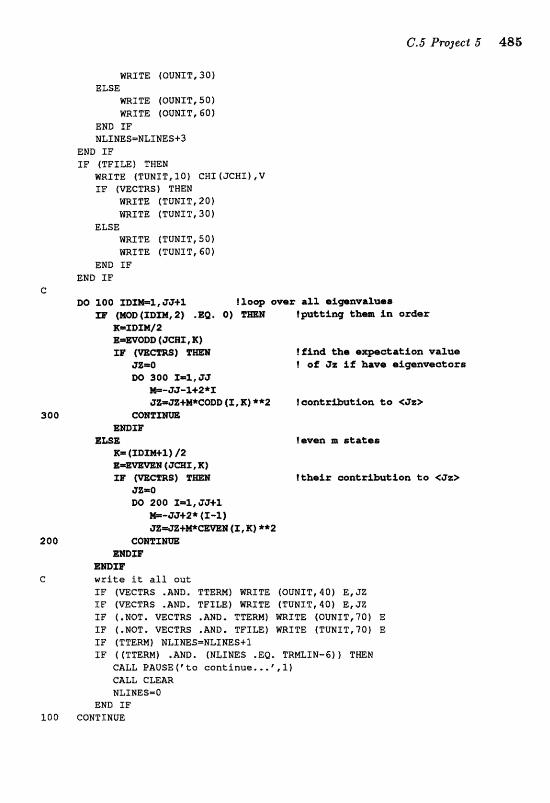
mITE (OUNIT,30) ELSE
WRITE (OUNXT, 50) m I T E (OUNIT,SO)
ENiD IF NLZNES=NLIMES+3
END I F IF (TFILE) THEN
WRITE (TUTJZZI,IC)) CNL(JGNI),V I F (VECTRS) THEN
mI%E (TUWIT, 201 m I T E (TUWET, 3 0 1
ELSE m I T E (TUWIT, 50) m I T E (TUNZT, 60)
END I F END IF
C ]DO 100 TB-%, &J'I-l I -1: a l l a 88
IF (MQD(XBm, 2 ) .EQw 01 ! p t t i in o z h r K=IDf M/Z Xk=WQDf) (acEx, E) XF (-Cm) FmM I f&nd %he ezpckation vau@
aE=D t of iFz i f ? have chigenmators B6 SO@ 1=1,3;7
*-88-2+2*X aEm+M*CQDD (I, R) **2 ! aan%
CBNSCIlrMC. mDm
Em& rewen a state@
33' {mCZM) !their aakriMtien t o <Jz> $%m0 W 200 I=%, &3+2
CrnPIrn W Z F
E m I F write ft a l l out SF (WCTRS .AND. T T E W ) m X T E (OUNIT, 401 E, JZ TF (VECTRS ,IIND. TFILE) mITE (TUNIT,40) E,JZ IF ("NOT. VECTRS .AMD. T T E M ) WRITE (OUNIT,70) E IF (.NOT. VECTRS .AND. TFTLE) m I T E {TUNIT,70] E IF (TTERM) NtZmS=NLINES+l IF ( (TTEm) .AND. (NLINES .EQ. TRMLEN-6) 1 THEN
CALL PAUSE(*t to cantinue,..\,lf CALL CLEAR NLINESmO
EWD IF 100 CONTINUE
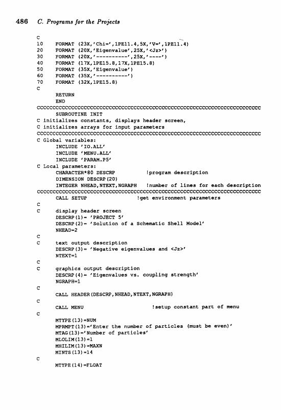
C -. 10 F O M T f23X,'Chf=r,1PBfl.l,SX,CV~*11PE:11.4~ 20 FQ-T (20X,~Eigsnvalue\,2SXfe~31:>~l 30 F O m T (ZOX, ?----------* ,25X; ' ---M' 1 $0 F O m T (17Xr1PE15.8, 17X, 1PE15.8) 5 0 FO-T (35X, * EQgevalue' 1 60 F O m T (35X, * ----------' 1 70 F O m T (J2Xr1PE15.8) c
=TURN END
cecc~ceccccceccccccccccccccccecccecccccccccccccccccccccccecccccccccccccc SUBROUTIRE INXT
C i n i t i a l i z e s constants , d i sp lays header screen, C i n i t i a l i z e s a r r a y s f o r input pazameters cceeecccccccccccecCccccccccccccccccccccccccccccccccecceccccccccccccccccc C Global var iab les :
INCLUDE ' ZTO. ALL' INCLUDE ' =NU. ALLr INCLUDE V A W , B S 6
C Local p a r a m t e r s : !program d e s c r i p t i o n
SNmGBR N W a D , MTEXT, N G W W In r of l i n e s for each d e s c r i p t i o n cccececcccccccccccccf:ecccccccccccccccccccccccccccccccccccccccccccccccGcc
CALL SETUP !get envi ronmnt parameters C
C dPsplay header screen BESCRP 4 f 1 = ' P R O a C T 5' DESCm (2) = * Salu t f on of a Schematic S h e l l Model* NH=D=2
G C text output descr ip t ion
DESCRP (3 1 = ' Negative e i genvaluas and NTEXT51
c C graphics output descr ip t ion
DESCRP(4}= 'Eigenvalues vs, coupling s t reng th" N G W H = 1
c CALL WEADER (DESCW , NHEAD, NTEXT I N G W R f
C CALL =NU ! se tup constant p a r t af menu
c MTmE f f 3 1 =NUN W W T ( l J )= 'Ent+r t h e nu-r of p a r t i c l e s (must h even)' MThG (1 3) =Wu&r of p a r t i c l e s p WLQLIM 113) -1 MNILXH (13 f = W N HINTS 43.31 -14
e MTUPE ( 3.4 ) =FLQAT
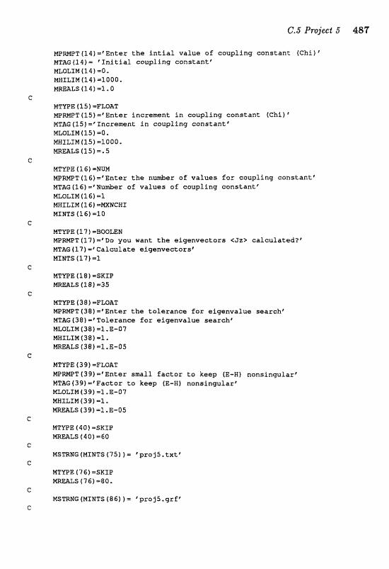
MPMPT(14)=%nnt@r the intiaf value of coupling constant (ChSI6 MT"AG414)- 'Initial coupling constante NLQLIM (14 1 4. MMILIN (14) -1 000. NRmLS(14)=1,0
MTYPE ( 15 1 =FLOAT M P ~ T (251 my Enter increment in coupf ing constant (Ghl) @
MTAG1151='Tncrement in coupling canstant* MLOLIW f15)=Q. NNfLIM(25)=100ae mmL5 (15jm.5
MTJEPE ( 1 G) -NUM WWT(SG)='Enter the nuntber of values for coupling constantF MTAG(I&)=~~umber of values o f couglfng constante MLOLTM (1 6 ) =l MRILIM (1 61 =KXNCWI MINTS (1S)=lO
NTYPE ( S 7 ) =BOOLEE WWT(271=*Do you want the eigenvectors <Jz> calculated?" MTAG(17f=*Cal~uletta eigenveetors6 MINTS (17) 51
NTYPE 11 8 ) =SKIP mEALS f18)=35
MTMZE (38 1 =FLOAT W W T f 38) =#Enter the tolerance for eigrrnvalue searchy WTAG (38) =' Ta f erance for aigenvalue search* mOLIM ( 3 8 ) =I .E-07 MNILIM (38 f 51.
LS ( 3 8 ) -1 .E-05
NTWE 4 3 9) =FLOAT M P M T (3531 =*Enter small factor to keep (E-M) nonsingular? NTAG (391 ="actor to keep (E-W 1 nonsingular' MLOLIM (39) =X ,E-07 NRILIN (381 =l. mmL5 (391 m1 .E-05
MTYPE (4 O ) =SKIP L5 140) =GO
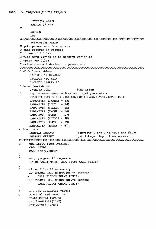
488 C- Pragnrma for the Projects
NTPE ( 8 7 1 =SKIP L 5 (871=98.
c RETURN END
c c c c c c c c c c c c c c c c G e C e c e c c e c c c c c c c c c c ~ ~ SUBROUTINE PAMM
C g e t s pa ramete r s from s c r e e n G ends grogram a n r e q u e s t C c l o s e s o l d f i l e s C maps =nu v a r i a b l e s t a progrclrn v a r i a b l e s C opens new f i l e s C c a l c u l a t e s a l l d e r i v a t i v e pa ramete r s ecc~C~cccecc~cccceccccec~cccccccC:ccccccceccc~ccccE:ccccccccccccccccc~~cc~ C Global v a r i a b l e s :
INCLUDE * MENU, ALL' INCLUDE qO.ALLP INCLUDE ' P W M , 3 5'
G Local v a r i a b l e s : INTEGER 3CWI !CBI index
C map between nzenu i n d l e e s and i n p u t pa ramete r s XNTEGER INPmT, ICNT, IDELCN, INCH5 C IVEC, ZLTQLE, XEPS, INGRF
(sNamT = 131 P-METER (ICMf = 14 1 PmMETER (XDELCN = 15) P W W T E R (INCH1 = 3 6 )
TER (FVEC - 17) P m W T E R (ILTOZE 38)
TER (IEPS = 39) TER (INGRF = 82 f
C Funct ions: LOGICAL LOGCVT ! conver t s 1 and O t o t r u e and f e l s s INTEGER GET1 HT !get i n t e g e r i n p u t from screen
ccccc~ccccccccccE:cccececccccceccceecceccececccccccc~cccccccecccccceccccc C g e t i n p u t Pram t e m i n a P
CALL CLEm CALL ASK (2, ISTOP)
C C s t o p program if r eques t ed
IF (E?IREALS (INAIN) .EQ. STOP) CBLL FfWlCSW C C e l a s e f i l e s i f necessa ry
IF (%HA= .NE. MSTRMG (MINTS IITNW) ) 1 + CALL FLCLOS (TNAm, TUNTT)
I F (GNmE .NE. NSTRWG (MINTS (IGNMEf 1 ) + CALL FLCLOS (GBAME, GUNIT)
C C set new p a r a m t e r v a l u e s e p h y s i c a l and numerical
NPmT=MINTS ( INPART) cwr (1 = ~ E A L S frees) MCWIPMINTS (XNCHf k

D E N H I = M m L S ( IDELCN) nCTRS-LWCVT (MINTS ( I m C ) ) LTOLE-mEEILS CILTQm 1 E P S = W A L S { I E P S
t2 C text o u t p u t
TTERM=W)GCVT (MINTS (ITTERM) f TFILE=LOGeVT (MINTS { ITFILE1 1 THW=MSTRNG {MrMTs ( I a W h r n j 1
c C graphics output
GTmH=LOGCVT (MXMTS (IGTERMj 1 GHRDCP=L~GWT (MIWTS r r E r n a 1 1 GPXLE-LOGCVT(MIPJT~(IGFIL,E:~~ GNWPMSTRNG (MINTS t IGNW* :
C e o p e n f i l e s
I F (TFILE) CALL FWPEN ( T N m , TUNTT) IF (GFXm) CALL FmPEM (GNME, BUMIT)
C files may have b 8 e ~ renmed NSmHG (MINTS ( I T H A W ) ) =THAM MSmNG (MINTS ( I G N W ) 1 =GM-
e C make sure that WBART i s even ( t o avoid l o t s of b o o k k e e p i n g ) IQ IF (MOD(NPART,Z) .NE. 01 THEN
NPmT-GETINT 4NPMT-1,2, W N , + Mumber of particles must be e v e n , t r y again')
MINTS ( I N P m T 1 =MPBRT GOTO IQ END TF CALL C & E m
I: G calculated parczmters
3 JmMPmT / 2 JJ1-JJ* CJJ-42 I DO 1QO JCNI=2,NCWI
CH1 (JCHI 1 =eHZ (1 ) + (JCHE-1) *DEXICEi(T 100 CONTTNUE C
RETURN END
~cccccceccccccccececcccccccccecccccececccccecccccccccceececcccecceccI:ccc SUBROUTINE PMOUT(MUWIT,NLINES)
C o u t p u t s p a r a m e t e r sumary t o t h e specified u n i t ccccccccccccceZ;"~cccceeecc~eccccceccccccecccccccccccccccccc~c~ccc~c~cI:~cc C Global variables:
INCLUDE ' I Q .ALL* INCLUDE V&W.P5 '
C Input v a r i a b l e s : INTEGER MUNZT t u n i t n u & e r for o u t p u t INTEGER NLINES !nu&er o f l i n e s p r i n t e d o u t f I / O )
cccccccccccccCccccccccccceccecceccc"ecceccceccccccccccccI:ccc"ccI:cI:cccI:cccc
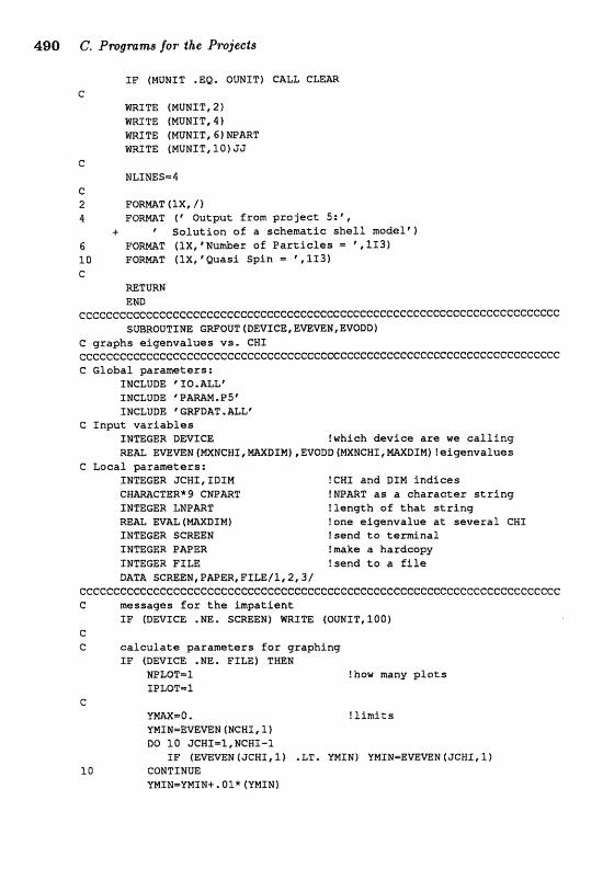
490 6. Pmgmms ,for the Projects
TF (HUNIT .EQ. OUMIT) CALL CLEm C
m I T E (MUNIT, 2) RRXTE (NUNIT,4) Wf TE (HUNIT, 6 ) =ART WRITE (NUHfT,l0)JJ
C NLINES-4
C 2 FORMAT ( I X , / l 4 FORmT ( ' Otltput from p r a j e c t S : ' ,
C S o l u t i o n of a schemat i c s h e l l model*) 6 F O m T { I X , * N u h e r of P a r t i c l e s = 5,113f 20 FORmT ( l X , W ~ u s i S p i n = * , l I 3 ! C
=TURN EMD
~~cc~~ce~c~~cc~cccccccceccccccceccccccec~cecceccccc~cccccccccccccc~cccc SmROUTIME CWQUT(BEVSCE,EVEVEN,EVODDI
C graphs e i g e n v a l u e s vs . GHT CccccecccceccceccCcccecccccccccccccccccccccccccccccceccccecccccccccccccc @ Global parameters :
f NaUDE IQ. ALL' TMCLUDE * PAMM. PS' INCLUDE ' GGRFDA . ALLf
C I n p u t v a r i a b l e s TNmCER DEVICE !which d e v i c e a r e w e c a l l i n g m& m W N (NXWGWT, M D I N ) , EVODD (mPJCWI, =DIM) !eitgenvrllues
C Loeal parameters : INTEGER JCW1,TDIM !CWZ and DZM i n d i c e s CHmCTER* 9 GNPART !BPMT as a c h a r a c t e r s t r i n g INmGER LNPmT I l e n q t b o f t h a t s t r i n g
Et'AL ( W B I M ) !one e igenva lue a t several CBI INmGER SCREEW ! send t o t e r i n a l XWSfI5GER PAPER !make a hardcapy ZUTEGER FILE ?send t o a f i l e D&T& SCREEN, PAPER, PILE/l, 2,3/
ccecccccccccccccccecccccccccecccecceccccccccccccecccC:cccccccccc~~ccccccc C m s s a g e s f a r t h e inrpat iant
TF (DEVICE .M. SCREEN) WRITE (OUMIT,100) C C c a l c u l a t e p a r a m t e r s f o r g raph ing
IF (BEVTCE .NE. PILE) TWEN MPLOT=T !how nrany plots TOLQT=S,
C VmX=O . ! l i m i t s YMIN=EVEVEN (NCHZ ,l ) DO 10 JCHX=I,NCWI-1
IF (EmVEM (JCHX, 1 ) .LT. YMINf VMLN=E CONTINUE YWIN=YMTW+. O l * (YMXN)
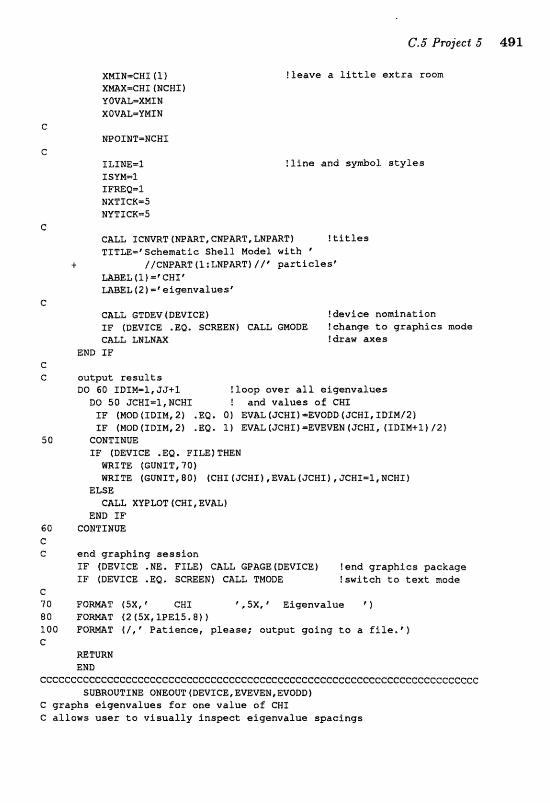
!leave a little extra room
!line and syml>al styles
I C ~ T (EJPPIRT, CNPART, L N P ~ T I !titles TfTLE=~~chemadlc Shell Model with "
t. //CNPART(l:LNPARTZI/" particlesC LABEL(%)=*CWX' MBEL (2 1 =?eigenvalues"
CALL GTDEV 4 DEVICE1 !device nomination IF (DEVXCE .E@. SCREEN) CALL GMODE !change to graphics mods CALL LNLHM !$raw axes
END IF C C output results
DO SO TDIW=l,JJiI !loop over all elgenvalues ~a 50 JCBX-~,NCH~ ! and values of CXI SF (MOD (ZBTM, 2) *E@. 0) EVAL (JCHX) mEVOBD [ JCHII IIZIM/2) IF (NOD (IDIM, 2) .Ea. 1) EVAL(JCHX) =EVEaN (JCWI, (IDXM+1) 121
50 CONTINUE IF (DEVICE .EQ. FILE) THEN WRITE (GUNIT, 70) VVRITE (GUNIT, 80) (CH1 (JCWT) ,ZVa fJCHI), JCHI=l, NCHXf
ELSE CALL XYPLOT f GWI , BVAL 1
END IF 60 CONTINUE c C end graphing session
IF (DEVICE .NE. FILE} CALL GPAGE(BEVICE1 !end graphics package f F (DEVICE .EQI $WEN) CALL TMBDE !switch to text made
G 70 F O W T ( 5 X , * CH1 ' ,5X, ' Eigenvalue ' 1 80 Fa-T (2(5X11PET5,8)f 100 F O m T (l,' Patience, please; output going to a file.p) G
mTmH END
CCCCCCCGCCCCCCCCCCCCCCCCCCCGCCCCCCCCCGGCCCCCCCCCCCCCCGCGCCCCCCCGCCCC(SCCC SmROUTIME OHEOUT(DEVICE,EVEVEN,EVOBD)
C graphs eigenvalues for one value o f CH1 C allows user to visually Inspect eiqenvalue spacings
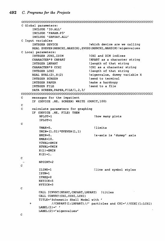
482 C. Pragmms far the Projects
eccCeCcccccccccccceccecccceccccccccc~~~ccc~cceecccc~cccccceecceccccccccc C G l o b a l p a r a m e t e r s :
INCLUDE #IO.ALLf INCLUDE # P N N . P 5 * INCLUDE SGRFBAT . ALL'
C I n p u t v a r i a b l e s INTEGER DEVICE !wh ich d e v i c e are w e c a l l i n g REAL E ~ ~ N ( ~ U C N I , ~ X D X M ) , E V O D D ( ~ N C W I , ~ X D L M ~ f e i g e n v a l u e s
C L o ~ a l paramters: fNmGER JCWX,IBSN !CH1 a n d DTM indices C B m C T E R * 9 CNPART !NPART as a character s t r i n g INTEGER LNPART ! l e n g t h o f t h a t s t r i n g CHWCTER* 9 CCWI !CH1 as a c h a r a c t e r s t r i n g INTEGER LCXE ! l e n g t h o f t h a t s t r i n g
EVAL(2) ,X (21 t e i g e n v a l u e , d a m y v a r i a b l e X INTEGER SCmEN !sand t o t e r m i n a l IEJmGER PAPER ?make a h a r d c o p y IXTmGER FILE !send t o a f i l e DaTA SCREEM,PAPER,FELE/I,2,3/
CCCCCCCCCCCCCCGC'CCCCCCCCCCCCCGCCGCCCCCCCCCCCCCCCCCCCCCCCCCCCCCCCCCCCCCCC C m e s s a g s s f o r t h e i m p a t l e n t
XF ( D N X W .NE. SGREBN) m I T E (OUNIT, 2 0 0 ) C C! calculate p a r a m e t e r s f o r graphing
f F (DEVICE .NE. FILE) THEN NPLOT=1 I P W T = 2
?how many p l o t s
! l i n e a n d s y & o l s t y l e s
CALL XCmT(XSZ)ART,CMPMT,LNPART) ! t i t les CALL CGHmT (CHI , CCHf , LCHl f TITLE=tSSchemet ic S h e l l Mode l w i t h
+ //CMPART(1:ZHPMT)//' particles and CHI='l/CCHI(1:LCWT) =EL (1) ="" m B E L (2) = t e S I g e n ~ a l t l e b @
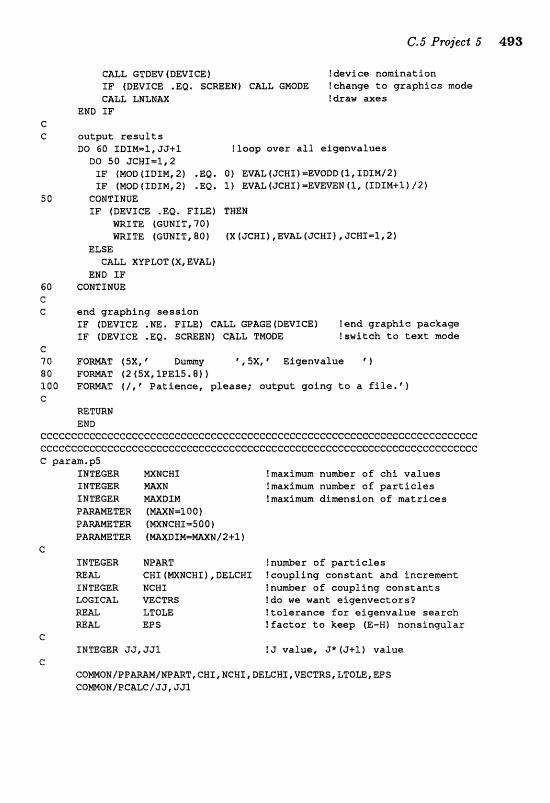
C m L GTI>EV(DmICE) !device nomination IF (DEVICE .EQ. SCREEN) C&L GMODE ! change to graphics mode CALL LIJLHU !draw axes
END IF G C output results
DO 60 IDIM=1, JJi-1 !loop over all elganvalues DO 50 JCMT=1,2 IF (MOD (IDIM, 21 .EQ. Q) EVAL (JCBI) =EVODD (I, XDZM/2) IF (MQD(TDIIH,2) .EQ. I) WAL(JCHI)=E~WN(l, (IDIMS1)/2)
5 0 CONTINUE IF (DEVICE .BQ. PIU) THEN
WRITE (GUNIT, "10) meTE (GUEIT, so) (X (JCHI:~ ,EVAL (JCHI), JCWI=I, 2)
ELSE CALL XmLOT (X, EVAL)
END XF 60 CONTINUE G C end graphlng sessf on
IF (DEVICE .NE. FILE} CALL GPAGE(DEVICE1 land graphic package IF (DEVICE .EQ, SCmEN) CALL TMODE !switch to text made
c 70 F O m T (5X , ' B , 5 X , C Elgenvalua 1 80 F O m T f 2 f5X, 2PE1 100 F O m T f /, Vatience, please; output going to a file.' 1 C
=TURN END
~cc~cc~ecc~cccccccccccceecccccceccccccccecccecC:cccccccccccceccccccccccc~ eeccccecccc~ccccecccccccceccecccccccccccccccCccc~cc~ccccccccccccc~ccccce C patam,p5
INTEGER mNCRI !maximum nuder af chi values XNmGER MAXPd ?maximum nuher of particles XNZFEGER m D S M !maximm dimension of matrices
PAMmTER ( MXNCHImS OO ) PAWETER (P I I1XDIM=WN/2+1)
e IEJEGER NPART !nu&er of particles R E U CRI(~NCXI),DELCHZ !coupling constant and increment SMTEGER NCRI tnuhr of coupling constants
CkL VEGTRS ?do w e want eigenvectars? LTOLE Itafarance fox eigenvalve search
mm EPS !factor to keep (E-H) nonsingular C
f NTEGER JJ, JJS ! J value, J* (J+1) value G
COMMObJ/PB~~%/NP~T,CNIINCRTICtE~NtIIVECTRSILTO~~EPS COM?ION/PCALC/JJ, JJ1
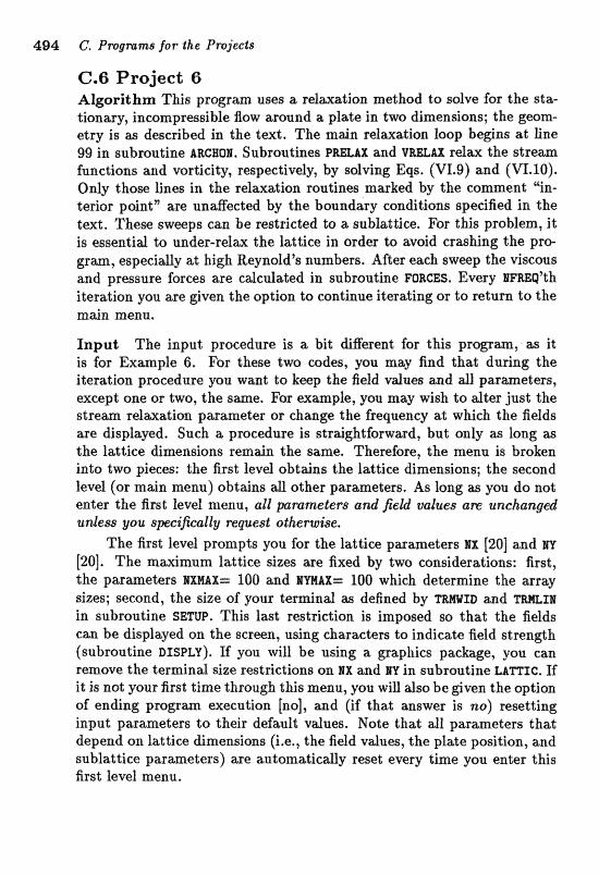
484 C, Prognams for the Pmjeets
C.6 Project 6 Algarithm This program uses a relawation method to solve for the sta- tionary, incarmpressible gow around a plate in two dimensions; the gem- etry is as described in the text. The main relaxation loop begins at line 99 in subroutine ARCffOAf. Subroutines PRaAX: -and V B S A I I relm the stream functions and vorticity, respectively, by solving Eqs. (VI.9) and (VI.10). Only those lines in the relaxation routines marked by the comment "in- terior point" are unaffected by the boundary conditions specified in the text. Thse sweeps can be regtsicted to a sublattice. For this problem, it is es~elltid to under-refm the lattice in order to avoid cras&ag the pro- gram, especially at high Reynold's numbers. After each sweep the viscous and pressure forces are calculated in subroutine FORCES. Every B F R E P ' ~ ~ iteration you are given the option to continue iterating or to return to the main menu,
Input 'Fhe input procedure is a Bit diEe~eat for this p rog ra , ifrs it is for Exaraple 6, For t h s e two codes, yau may find that during the iteration procedure yau want to kmp the field vdws and all parmeters, except one or two, the sme. For example, yea may wish to alter just the s t r e w reiwatim parameter or change the fieqnency at which the fields are? displ-d. Such a pmcedure is straightforwwd, bat only as long ans the 1;Lt;tice dimensions remisin. the same. Therefore, the menu is broken into two pieces: trhe first level obta;ins the ldtice dimensions; the second level (or main menu) obtains all other parameters. As long as you do not enter the fimt bvel menu, aid prameter& a d field 1vaIues am u~lehangd zlnless you &peificaaf& request otlaep'wise,
The first level p~ompts you for the lattice parameters BX [20] and ay [20]. The maximum lattice sizes are fixed by two considerations: first, the parameters BxWAX= 100 and sunrx= 100 which determine the array sizes; second, the size of yovs terminal as defined by TRnVfB and in subroutine SETUP. This last restriction i s imposed so that the M d s can be displayed on the screen, using characters to indicate field strength (subroutine DISPLY). If you wilt be using a graphics pachge, you can remove the terminal size restrictions on EX and W in subroutine LATTSC, If it is noZk your fipst time through this menu, you will also be given the option of ending program execution [no], and (if that answer is no) resetting input; parmeters to thdr defadt values. Note that df parameters that depend an lattice dimensions (i.e., the field vdues, the plate position, and sublattice parameters) are automatically reset every time you enter this first level menu,
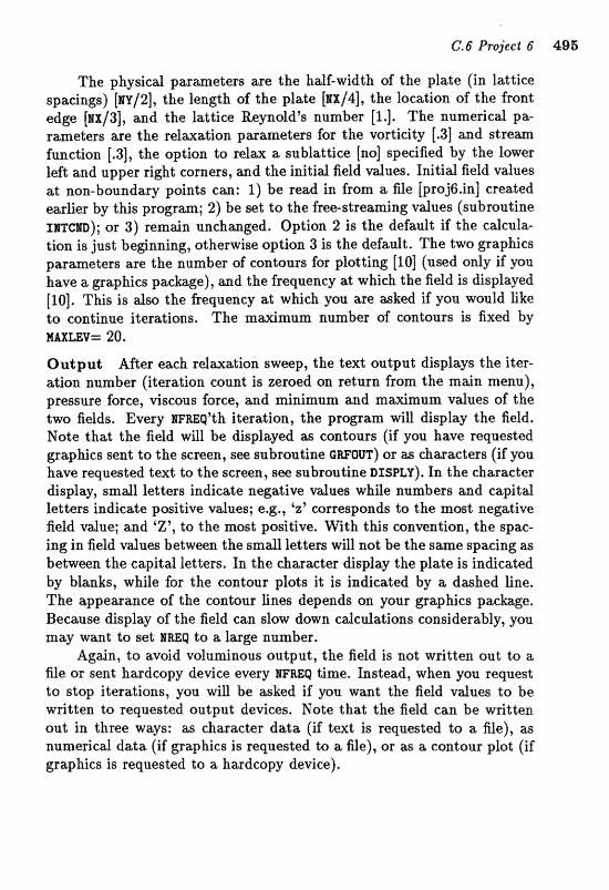
The physical parameters are the half-width of the plate (in lattice spacings) BY/^], the length of the plate [I(x/~], the location of the front edge [BX/~] , and the lattice Reynold's number [l.]. The numerical pa- rameters are the relaxation pasameters for the vorticity [.3] and stream function [.3], the option to relax a sublattice [no] specified by the lower left and upper right corners, and the initial field values. Initial field values at non-boundary points can: 1) be read in from a file [projG.in] created earlier by this program; 2) be set to the free-streaming values (subroutine ~ m m ) ; or 3) remain unchanged. Option 2 is the default if the calcula- tion is just be@nning, otherwise option 3 is the default. The two graphics parameters are the number of contours for plotting [l01 (used only if you have a graphics package), and the frequency at which the field is displayed [IO]. This is also the frequency at which you are asked if you would like to continue iterations, The n n ~ n a u m number of contours is fixed by nawv= 20.
Output After each relaxation sweep, the text output displays the iter- ation number (iteration count is zeroed on return from the main menu), pressure force, viscous force, and minimum and maximum values of the two fields. Eve~y EFREQ"~ iteration, the progam will display the field, NoGe that; the field d l be displayed as emtours (if you have requested graphics sent to the screen, see subroutine CRFOUT) or as characters (if you have requested text to the scrwn, see subroutine DISPZ;Y). In the character display, small letters iIldicat?e negative d u e 8 while numbers and capitd letgers indicate posigive vdues; e.g., 'zz' corresponds to the mast negative field vdue; and %', to the most positive. With tEs convention, the spac- ing in field vdues between the small lettem will not be the same pacing as between the capitd letters. In the eharater display the plate is indicated by blanks, while for the contour plots it is indicated by a dashed line, The appeasance of the contour Lines depends on your graphics package. Because display sf the field cm dovv down cdcufations considerably, you may want to set BREQ to a largc3 number.
Again, to avoid volurninaus output, the field is not written, out to a file or sent bardcopy device every M E ; a Q time. Instead, when you request to stop iterations, you will be asked if you want the field vdrtes to be written to requested output devices. Note that the field can be written out in three ways: as character data (if text is requested to a file), as numerical data (if graphics is requested to a file), or as a contour plot (if graphics is requested to a hardcopy device).
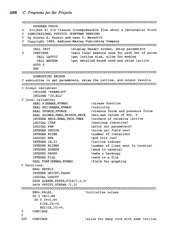
496 C. Pmgmms for $he Pr~jeels
cccccccccccccCceeccccccccccccccccctcccccccccecccccccccc~cccccccccccccccc~ I"RQGmM PR036
C Project 6: 2-D viscous incowsessible flow about a rectangular block C COMPUTATIONAL PHYSICS [FORT-% VERSION) C by Steven E. Koonin and Dawn C. Meredith G Copyright 2989 , Addison-Wesley Publishing Company cteeCccceccccccccccccccccccecccceeccccccceccccccccccceecccccccccccccccccc
CALL TNIT !display header screen, setup parameters 5 CONTINUE ?main loop/ execuka once for each set of paran
CALL LATTEC !get lattice size, allow for ending CALL, ARCNON !get detailed bound eond and relax lattice
GOTO 5 END
ccccccccccccccccccecccccccecccccccccccccccccceccccccccecccccccc~ccccc~cc SUBROUTINE ARCNQN
C subroutine to get parameters, relax the lattice, and output results cccce~ccecc~ccccccccccccccccceccceeccccccccccccecccc"ceccccc~ccccecccc~~~ C Global variables:
INCLUDE ' P W M , P INCLUDE '1XO.ALLt
C Local variables: REAL P (NXmX, N Y U I I stream function
!vorticity REAL VE"ORGEpPF0RC1E: 2viseous force and pressure force REAL XSImX, P m , XSTMIN, PMIN !min. max values of XSI , P INTEGER XMIN,XmX,YNIN,YW feornsrs of relaxing lattice LOGICAL ITER !continue iterating1 LOGICAL PRN !print aut parameters? INTEGER CHOICE !write out field now? INTEGER MITER !nuAer a f iterations LQGLCAL END fend this run? INTEGER IX, IY !lattice indices INTEGER NLINES !number of lines sent to teminal INmGER SCMEN !send to terdnaf 3Nr"EGER PAPER !make a hardcopy ZNmGER FILE !send to a file m& FGRF I W-X, NVmX ) ?field for graphing
C Functions: mAL GETFLT INTEGER GETINT,YESNO LOGICAL LOGCVT DATA SCREEN, PAPER, FXLE/l,2,3/ DATA VRTCTY,STmM / 2 , 2 /
ecccccccccccccceccccccC:ccccccccccccccccccccccccccccccccct~cccccccc~cccccc END=-FALSE, !Initialize values DO 5 IX=1, NX DO 5 IV=I,NY
P (IX, IY) -0. x s ~ (rx, su) =o,
5 CONTINUE C 200 CONTINUE !allow for many runs with same lattice

CALL P A W (P, XSI END ) IF (END) RETURN
I F (SWLATf THEN XMIN=NXLL XWX=NXUR YWIN=NYLL Y W = N Y UR
ELSE XMIN-I. Y MIN=1 XmX-MX YWX=NU
END I F
!get new p a r a n r a t e r s !start f r e s h o r end altogether
!set l i m i t s f o r r e l a x a t i o n
I F (TFILE) CALL TXTOUT (TUNIT, NITER, VFORCE,PFORCE~XSIW,P~,XSIWIN,PMXN,MLXNESf
XF (TTERM) CALL TXTQUT (OVNIT, NXTER, WORCE,PF~RCE,XSI~,P~X,XSXMIPiJIPMIrCaCNLXATES~
ITER=. FALSE. PRM-.TRUE. IF (MOD [Nf TER, NFWQf .NE. O) T m M
I TERm. TRUE. ! continue i t e r a t i n g w i t h o u t asking Pm=. FALSE. ! don" p r i n t o u t header
ELSE ! o t h e r w i s e display f i e l d s I F (GTEM) THEN
CALL PAUSE(-o see s t r e a m f u n e t i o n a n d vorticity ...', l) CALL C a m CALL GWQUT(SCREEN,STmM,P,PNTfJIPWIFGBFINXyNV} CALL GmOUT (SCWEM, VaTCTY, XSI , XSIMZWt X S I m X I FGWI NX8 HY)
ELSE IF (TTEW) THEM GALL PAUSE(*tta see stream % u n c t f o n . , . ' , l ) CALL GmAR GALL DXSPLU(P,OUNTT,STREEhMIPlvtAX,PM3:M> CaLL PAUSE(*to see varti~IQ., .\ 0) CALL C L m R GALL DISPLY(XS~,BUNITyVRTCTY,XSI~XtXS3E"IXN~
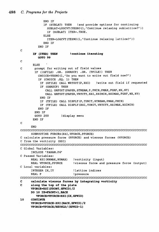
498 C Progrcams for the Pmjects
EMD XF IF (SUBMT) THEN !and provide options for continuing SUBmT-L,OGCVT(YESNO{lI'Co~tinu(? relaxing sublattiee?')) SF (SUBMT 1 I TER=. TRm .
ELSE ITERmLOGCVT (YESNO (l, * Continue relaxing lat tic@?' 1 1
END 5F EEJD SF
C 3 3 (I=) FmH ?~oneLma fdaza&ing
W T O 09 C
ELSE " C pxomt for writing out a f f i e l d values
IF ((GF2LE) .C%%, (CBRDCP) .OR. (TFILE)) THEN GHOSCE=VESNO(I,tDo you want l a write out field now?') IF (CHOICE .EQ, l) THBH SF {GFXLE) C U L mTQUT(P,XSI) ?write out, field if rewest;ed I F (GHRDGP) WEB
CALL GWOUT (PBPER, ,P,P~IM,PMAX,FGRF,HX,NY) CALL GRFOUT (PBPER, ,XSI,XSIMIM, X S S ~ X , FGW, NX, NY!
END IF f F (TFILE) C&L DS SPLY (P, TUNTT, STREaEUI,PM, PMXPJ) IF (TFILE) C&& DISPLY(XSX,TUWIT,VRTCTY,XSIW,XSINSN1
END IF END IF GOTO 200 !display menu
END f F C
END ccccccccceecccccc~ccecccccccccccecccccccccceccce~ccccecccccccccccccccccc
SUBROUTINE FQRCES(XSI,WORCE,PFORC&) C cafcuf2nt;a pressure Eores (PFORGEl and viscous forces IWORGE) G from the vorticity (XSS) cccccc~cccCccccccccccccccccccccccccccccccecccecccceeccccccecccccI:ccccccc C Global Variables:
INCLUDE ' P & U . P 6' C Passed Variables:
) ! vsrtieiey (input) !viscous Eorca and pressure force (output 1
C L o ~ a l variables: 6ER I X , I Y !lattice indices P ! pressure ccccceccc~cceccccccecccecccccccccccccccccccccccccceccccccccccc
C cralculakat v i a a ~ u a Eoz-s by inkwza%ing vortrie%kp C almg %be top of the pfate
X 0 CONTma

C.6 Project 6 499
C C clalwZate tb pge~mm force bjl fntepnrlslng vort;ioity along the C ad-@ of t:be pXaLa to ob%oSn the prac~lsuze, Lban intsgfating G the praamze to ohta?ta t:ha prsir-a iPorcre
Pm0
t up front: E=P- (=I (mm, ZY) -X91 (m@N1C-5, IT]
+ +XSI (=m%, %X-1) -rnI (mm%-1, ZX-%] ] /2/
~ ~ a m = P F a m - g r l 2 C
EX) 30
+ 30 C O m Z m
PrQm=EFrna-P/2 C
00 40 1,-3 1 P# I, PT) -XSI
.c +a, XX+%) - BZ?"QRWP@aa-P
40 C@mIIJUE
G mTURPd END
cccccccccc~cccccccceeccccccecccccccccccceccccccccccccccccecccI:cccccccccc SUBROUTINE P M = (P, XSP , XMSN, X U X , UNf N I ?IW, P m t PMIPJ]
G relaxes the stream function (P) given previous P and vorticity (XSI) C on a lattice w i t h corners at XNIN,Xm,YMTH,VMAX; C returns nin, m x value of F in PMIN, P M c~cccceccc~ccceccccceecceccccc~ceccccccccccccecccccccccccccccccccccccccc C Global variables:
INCLUDE *PAm.P6f C Passed variables:
RE& P ( N X m , M Y W ) !stream Eunetf on ( I l o f M& XSI: ( N X W , WVmX) lvarticity (output) INmGER XMTN,Xm,YMI:N,YE3AX !edges of relaxing lattice (input) -&L, O W X , FMIM !min,max valve of P (output)
C Local variables; IMTEGBR TX, I Y tfatticc indices R m L TEHP f temporary storage
cccccecccceCccI:cccc~cccccccccccccccceccccccccccccccccccccccccccccccccccc Prn=O. p m = @ . DO 100 zx
DC! 200 I Y = m W , IF ( B H D m (XZ, Et') . EQ. 0) Tma t reLax only noa-bmmd pof rsts
C 3H" (TUT .BQ, W-1) E a H I3uat b l e w top e*e
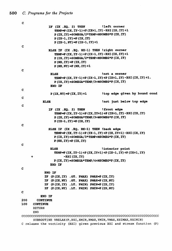
500 C. Programs for IRe Projects
c IJf (XX .EQ. 2) TEIEET ! l e f C corner m e ~ I X , XY-11 +P ( x x + ~ . XY) -XSX rm, Ir,+r P ( IX, I Y ) =SwOA/z*=+MsONEF*P I I X , I Y ) I? (fX-l r I Y f IPP ( IX, I Y ) P (IX-1, mj PliB ( IX-1 , I Y ) +1
ELSE f lP (IX .EQ. NX-X) TEBZS f r i g h t cosnsr ieQ! (XX, IY-1) +a (XX-1, nc) -XSf ( IX, I Y ) +Z
p ( I X , I Y ) .rSw(;B/2*mww-*p (W, TYI P (m, r Y ) = P [ IX, I Y ) P (rn,NY) ap (NX, I P ) + 1
ELSE fnot a sonaer !mmPg ( I X , KY-1) +P (IX-1, I Y ) f P fIX+1, I Y ) -=I. /a, nt) +I. P (nt, IY) : mSMa*TEMP/3*blSONlbG*P (We I Y )
END IF
E! (IX,NIC) =P) (SX, rY) + l !top cadge given by b w d aond
ELSE tnat: julpt b a a v toy , edge
33' (XX .=. 2) TRWJ ?front edga nP m, , XY41) +P f I X + l , I T ) -XS3 (U[, IY) .rU).LS /3lrnW**P (IX, rYI
P (IX-I., I Y ) e f IX , IY)
ELSE I B ( I X .EQ. Wt-1) Hfel fbacrk edga ..P f I X , TY-1) 4P [(XX-I., X l f j 4P fXX, I Y + l ) -XSI (TX, SY)
P ( I X , XY} = S O M E C i A / 3 * T W + H S m * P ( E X , IY) o (la, XY)=P (IX, M )
ELSE l i m t ~ t i o r point FEhOlieQ! ( X X , SY-1)SP (XX*SP+l)+P (XX-1, I Y ) +B [IX+1, ST)
- X S I ( I X , TP) P (TX, I Y ) wSOWgGAk
E m KF
END W fE (B(M,XY) .OF, PWiX) P W * ( I X , S Y ) IF (P(IX,NY) .DT, Pb6AX) PW=E(XLX,m) IlrP (B(SX,EY) .LT. PMZS) P M l a P ( U C , f Y ) XF (P(TX,NY) .ST. EMlX) PMCN=F(a(,blY)
C END IF
200 CONZfNoE 100 c-m
RETURN END
CCCCCCCCCCCCCCCCCCCCcCCCCCCCcCCCCcCCCCCCCCCCcCCcCCCCCCccc~CccccCcccccccc SUBROUTINE VRELAX(P,XSI,XMIN,XMAX,YMIN,Y~X,XSIMAX,XSIMIN)
C r e l a x e s the vorticity (XSI) given previous XSX and stream function (PI
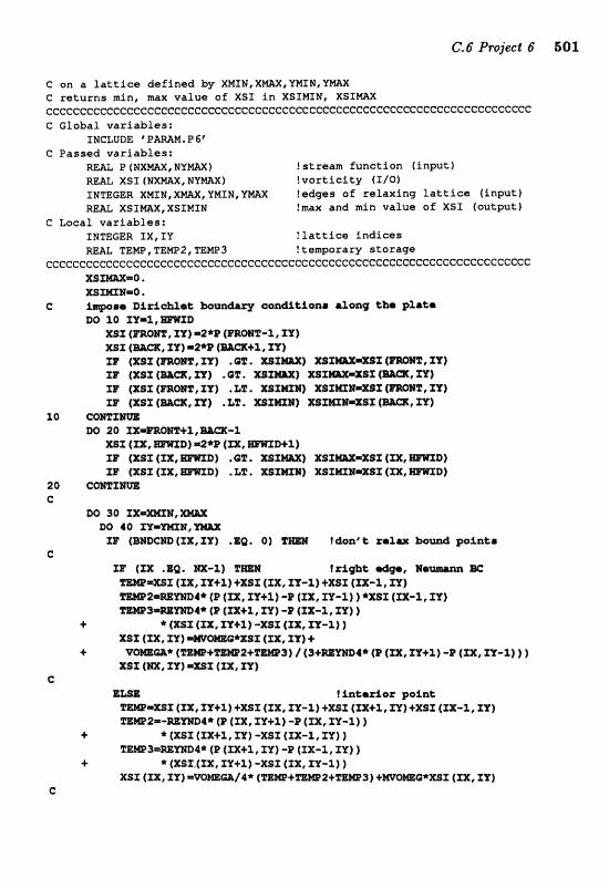
C on a lattice defined by XNIN,XNAX,YMIN,Ym C return@ min, max value of X f I in XSIMIM, X S X m ceecc~~~cceccccccccccccceecccecccccccccceecccccc~~cccccccccccce~ccceecec e Global variables:
INCLUDE ' P W M . P 6' C Passed variables:
M U P ( N X W , N V m ) ?stream function (input) WEAL XSI (NXMAX, NYmX) !vorticity (X/O! I N T E G E R X M T N , X ~ , P M X N , V ~ X !sdgesof relaxing lattice (input]
XSXM,XSJMIM !max and min value of XST [~utput) C Local variables:
INTEGER IX , SV !lattice Indices REAZ TEHP, TEIVIPZ, TEMPS !temporary storage
c~e~cccccccecccCcecceccccccccccccccccccccccc~ccccccccccccc
hanary a@n&Lion. rL@ng Lhe p Z a & r
2 0 G O M T I ~ C
W 30 ===M, D43 4 0 I Y = m H , m ( ~ w ~ e r r c l ( r x , r r ) .SQ. 01 l &onp t re%= h d pint;&
C I P (ZYC .EQ. =-l) F- BC
=XSI (XZ, IY+T) +X91 (XX, m-2) 2 m M m 4 * (P (ZX, E#+%) -P (ZX, I Y - l ] ) *=X [IX-l, I Y ) 3-m4+ (P ( r x + i , ZY) -P (IZ-i ZY 1 )
d.
+ ) / (3+rnrn4* (P (ZX, JZ+l) -P ( IX , I F - l ) ) )
C E !i,nt%rAor poine
2m-=WD4* (P (IX, IY+1) -l? (XX, I Y - I ) ) + * (XSI (IX+T,xT) -XSI (1X-3, ZY) )
3-8-W=4* ('P (3CX+Z, f l) -E (IX-1, I Y ) ) + * ( x s r j r x , r x + r ) -xsz ( X X , XY-1) )
X s I ( IX, r u ) =voma/4n( C
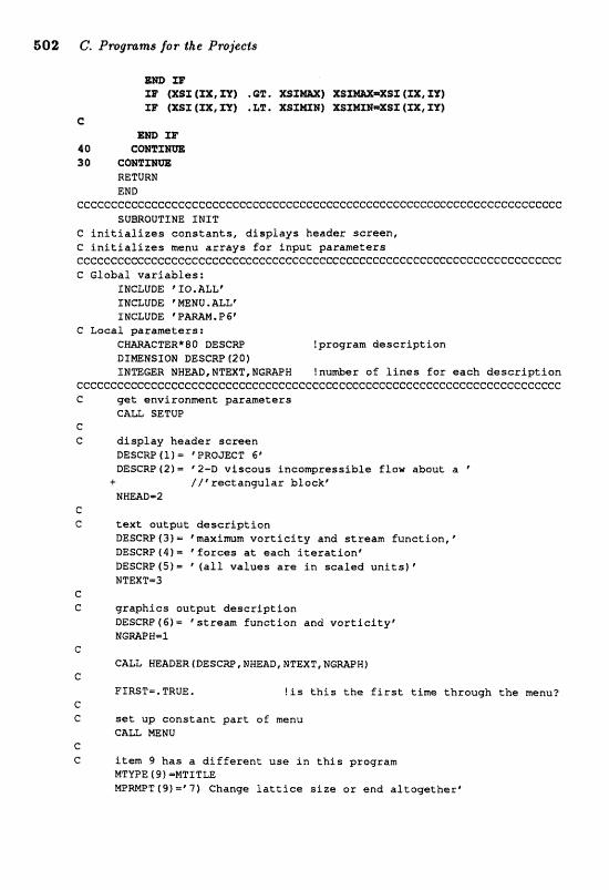
m S F I H (XSX (X%, XV) .6T, =I=) XS SI (IX, IY) IF (XSZ (XX, IT) . LT, mnMliH) x S ~ % = X s Z ( Z X , Xluc.)
C E m m
40 CQE%IEm 30 C O m I m
RE"XIUR% EHD
eccceccccccccccccccccccccc~ccccecccccc~cccc~ccc~ccccecccecccC:ccccccccccc SUBROUTIUE ZNXT
C initializes constants, displays header screen, C initializes menu arrays for input parameters cccccccccC:cc~Cccecccccccceecceccccccecccccccccccccccceccccccccc~cccccccc C Global variables:
INCLUDE * IQ. ALLt INCLUDE *mEIU.ALLr INCLUDE T N M . P 6 p
C Local parameters: CHWCTER*80 DESCW !program description DXNElNSION DESCRP (20) INTEGER NWMD,NmXT,NGWH !number o f lines for each description
cc~ccc~ccceeccccccc~ccccccceccccceeccccceccccccccc~ccccccccccecccccccccc C get environment parameters
CALL SETUP e
display header screen DESCW (1) = PROJECT GC DESGRP(Z)= "2-8 viscous incompressible flow about a '
+ //'rrectangular blockr NXmD=2
text output description DESCRP 13) = rmaximum vorticity and stream function, ' DESCRP(4f 'ffotces at each iteratione DESCRP(5)- ' (all values are in scaled units)' NTEXTm5
graphics output description DESCRP ( 6 ) = "trean function and vortieity* NGMPEI=I
CALL HEADER (DESCm, NHEAB, NTEXT, NCRAPH }
PIRST=.TRUE. !is this the first time through the menu?
set up constant part of -nu CALL MENU
item 9 has a different use in this program MTUPE t 91 mNTITL8 M P W P T ( 9 1 = @ 7 ) Change lattice size or end altogetherr
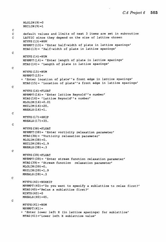
MXIOLIM (9) -0 NWILXM (9) =l
d e f a u l t v a l u e s and l i m i t s o f next 3 i t ems a r e s e t i n subrau t fne LATTIC s i n c e t h e y depend an t h e s i z e o f l a t t i c e chosen MTWE (13) -NUN N P m T f l 3 ) = "nter hal f -width o f p l a t e i n l a t t i c e spzlcings' MTAG(l3)= 'Half-width o f p l a t e i n l a t t i c e spacingsr
MTmE (I I ) =MUM MPWT (14) = 'En te r f e n g t h a f p l a t e i n l a t t i c e sgacingsC MTAG(14)= 'Length o f p l a t e i n l a t t i c e spac ings l
MTVPE ( 1 S ) -NUH MPWT ( l51 =
+- 'En te r l a c a t i a n o f p l a t e f ' s f r o n t edge i n l a t t i c e spacfngs" MTAE;IlS)= " ~ o a t i a n o f p l a t e M ' s f r o n t edge i n l a t t i e a spae ings"
MTYPE (1 61 =FLOAT M P m T (16) = 'En te r l a t t i c e Reynofdt 9 number" MTAG f 16) = * L a t t i c e Reynoldl S n u d e r e MmLIM(16)=0.01 nszLxM (1s) =ao.
L5(26)=lr
MTUPE (17) =SRTP WmLS (17)-35.
MTWE 4 3 8 ) -FLOAT N P m T ( 3 8 ) = 'En te r v o r t i e f t y r e l a x a t i o n parameter ' MTAG (38) = 6 V o r t f e i t y r e l a x a t i o n parameter t MWLIM (38) PO. MRZLIM (38) -1.9 mmzs (38)= .3
NTVPB ( 3 B) =FLOAT W m T (351) =. @ Ente r stream func t ion r e l a x a t i o n parameterf MTAG (39) - * Stream f u n c t i o n r e l a x a t i an parametere MLOLIN(39f -0, HMILIN (39) ==1.9 mmzs 1391 a. 3
MTUPE ( I 0 ) =NOSKf P m m T f401=@Da you want t o s p e c i f y a s u b l a t t i c e to r e l a x f i r s t ? " MTAG (40) ='R~efax a s u b l a t t i c e f g r s t ? ' HINTS (40) =O NRmLS (40) 145,
MTWE ( B 1 ) =NUN WMPT f 4 1 ) =
+ 'En te r lower l e f t X ( i n l a t t i c e spaeingsf f o r s u b l a t t i c e ' MTAG (41) = % w e r l e f t X s u b l a t t i c e value"
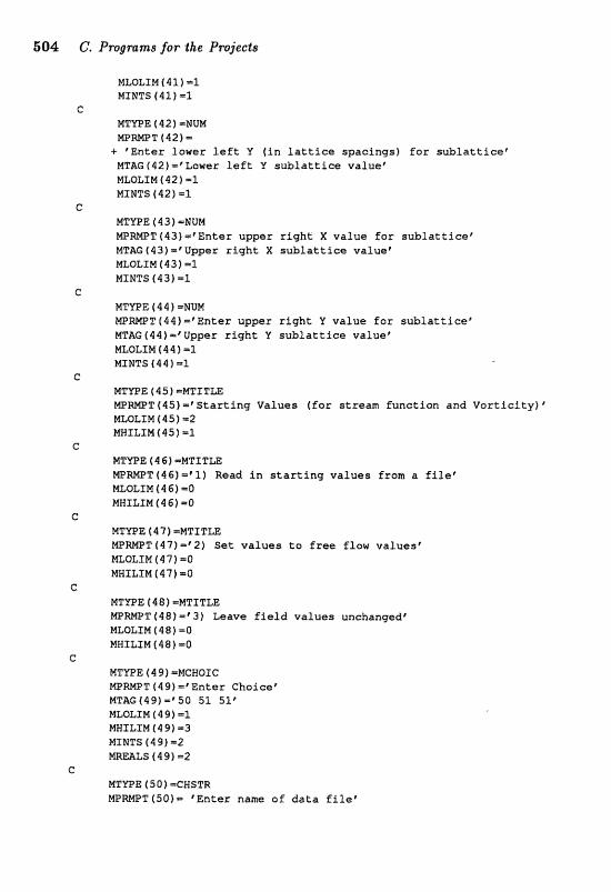
504 C. Pmgmms for the P r ~ j e c f s
MTWE ( 42 1 -NUM m m T 142) =
+ * E n t e r lower l e f t V ( i n l a t t i c e spac ings ) f o r s u b l a t t i c e ' MT&G(42)=%~ower l e f t Y s u b l a t t i c e va lue f MLQLTM (42) =l MINTS (42) -1
MFYPE (4 3) =NUN M P m T ( 4 3 ) = t E n t e r upper r i g h t X v a l u e f o r s u b l a t t i c e ' MThG(93)~'Upper r i g h t X s u b l a t t i e e v a l u e C MLOLIM ( 4 3 1 -1 MINTS (43) =l
MTUPE 14 4 1 =NUM lun?Mll"(48)=tEnter upper r i g h t Y v a l u e far s s sb la t t i ce r MTELG (44 ) Upper r i g h t U s u b l a t t i c e value ' MLOLLM ( 4 4 1 =l MINTS ( 4 4 ) =l
MTYPE ( 4 S f =MTI TLE W W T ( 4 S ) = ' S t a r t i n g Values (far stream f u n c t i o n and V o r t i c i t y ) " MLOLXH ( 4 5 f m2 IUIMILIM (45) m 1
HTYPE ( 4 6 ) =MTITLE MPmPT(46)=C1) Read i n s t a r t i n g v a l u e s from a f i f e " mOLIM (4 6) ==Q M M I L I M (4 6) =@
MT"UPE ( 4 7 ) =MTITLE W W T ( 4 7 ) = = " 2 ) S e t v a l u e s t o free f law v a l u e s e NLOLZM (4 7 ) -0 MHILTM ( 4 7 f l0
MTVPE ( 4 8 1 =MTf TLE W W T (48) 1' 33) Leave f i e l d v a l u e s unchangedp MLOLIM (48) =0 MWILTW (481-0
MTWE (4 9) =MCHQIC m W T (4% =*Ente r Choicep MTAG(49)='50 51 51' MLOLIM ( 4 9 1 -1 MWILfM (491 =3 MINTS (4 9) a2 E?UREALS (49) =2
MTUPE (SO ) =CHSTR WmPT(SO1- "~nter name aE d a t a f i l e C
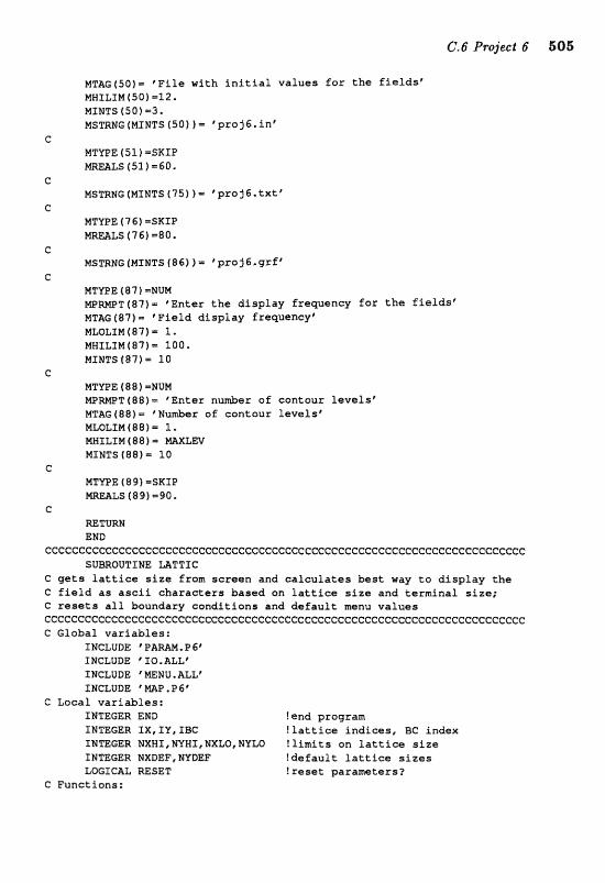
MTAGf50)m ' F i l e wi th i n i t i a l v a l u e s f o r t h e fieldsf MHZLIM (50 1 =12. MINTS (SO) 4 3 . MSTRNG(MINTSf50))= vpxoj6 . inp
C MTYPE (51 1 =SKIP
C MSSRNG (HINTS (75) f l ' p ro3 6 * t x t "
C MTWE ( 7 C ) =SKIP mmLS f 761 =80.
C MSTRHG (MINTS (86) l prajG.grE1
C MTVPE (8 7 1 =NUM MPWT (87) = @ Ente r the d i s p l a y f requency f a r t h e f i e l d s t MTAG(87)m * F i e l d d i s p l a y frequencye MLOLIM(87)= 1, MXILIM(87) = 100. MINTS(87)- 1 0
C MTmE ( 8 8 1 =NUN M e W T ( 8 8 ) - * E n t e r n u d e r of contour l e v e l s " MTIIC;(88)= 'Number of con tour l e v e l s " MLOLlM (88 t - l. MHIZXM ( 88 1 = PIAXLf;V MINTS {88)= 10
e NT"IIPE (89) =SKIP m a ~ s (ss) -90.
C RETURN END
cccccccccccccccccccccecccccccccccccccc~cccccccccccc~c~c~cccccc SUBROUTINE UTTIC
C g e t 8 l a t t i c e s i z e from s c r e e n and e a l ~ u l a t e s b e s t way to d i s p l a y t h e c f i e l d a s a s c i i c h a r a c t e r s based on l a t t i c e s i z e and t e r m i n a l size: C resets a l l boundary c o n d i t i o n s and d e f a u l t menu v a l u e s ececCcccCccccccccccccccccccccccccccccccccccccccccccccccccc~ccccccccccccc C Global v a r i a b l e s :
INCLUDE P A M . P 6' INCLUDE 'XIQ,ALLp INCLUDE WIUIE .ALLr INCLUDE ' W . P 6 *
C Local v a r i a b l e s : INTEGER END !end program INmGER IX, I Y , IBC f l a t t i e e i n d i c e s , BC index INmGER NXWX,MYHI,NXLO,~LCI ! l i m i t s on l a t t i c e size INTEGER NXDEF,MVDEF ! d e f a u l t l a t t i e a s i z e s LOGXCAL RESET !reset pa ramete r s?
C Funct ions:
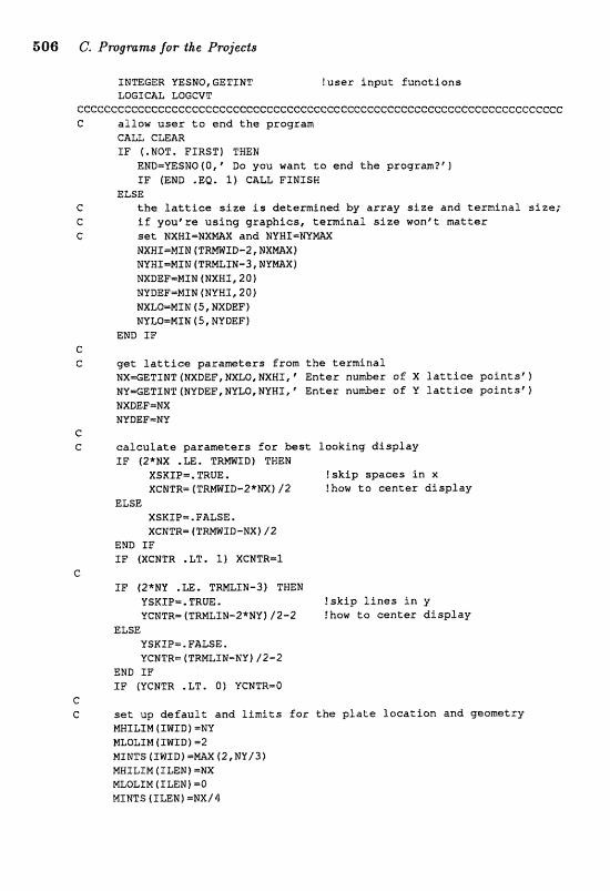
506 C. Pmgmntsf~rthe Projects
I N T E G E R VESMO, G E T I N T !user input functions LOGICAL W G C V T
cccccecccccccccecceccccccccccccccccccceceeeccccccceccccccccccccccccccccc C allow user to end the program
CALL CLEAR IF (.NOT, F I R S T ) THEN
END=YESNO(Or f Do you want to end the I F (EWD .Ea. 1) CALL F I N X S H
ELSE C the lattice size is determined by array size and terminal size; C if you8re using graphics, taxmina1 size wonCt matter G set NXWS-MX-X and N Y H I = N Y m
N X H T = H X N ( T W I D - 2 , N X m X ) NYHX=MIN (TWLSN-3, N Y M X f NXDEF=NIE (NXHI ,201 NYBEF=MIN (NYHI , 20) NXLO=MIN f S, NXmE ) NVLO=MTN ( 5 , MYBEE)
END TP C C get lattice parameters from the terminal
NX-GETINT(NXDEF,NXLQ,NXBS,* Enter nu-r af X lattice pointsr) NV=GETSMT[NYDEF,NYL0,NYEZI6 Enter nuhar o f Y lattice paints') NXDEF=NX NYDEFmNY
C C calculate parameters Ear best looking display
I F (2*NX .LE, T R W I D Z THEN XSKIP= .TRUE. !skip spaces in x X C N T R = ( T R M Z B - 2 * N X 1 / 2 !hew to center display
E L S E X S R I P m . FALSE. XCMTR- ( T R m x a - N x w
END I F I F (XCNTR .LT. I) XCNTR-l
C I F (2*NV *LE* T M L I N - 3 f THEN
YSKIB-,TRUE. !skip lines in y YCNTR=fTRMLIN-2*NY) /2 -2 !how to canter display
E L S E Y S R S P = , F A L S E . YCMTR= (TMLZM-NV) /2-2
END I F I F (YCNTR .LT. O f YCNTR-O
e C set up default and limits for the plate location and geometry
MHf L I M ( X H I D f =NU MLQZIM ($MID) -2 Hrl.srs tawraj -mx [ ~ , N E ! / ~ I MHELEM (ZLENI =NX MLQLfM ( S L E N J =O M I N T S (IEENf =MX/ 4
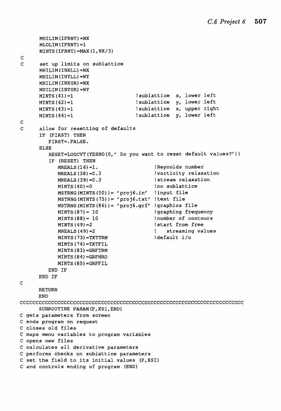
MNILIM (IFRNTI =MX MLOLTM ( TFRNT ) -3 MINTS ( rPRUT 1 =mx (1, ~ ~ 1 3 f
C C set up limits on sublattice
MHZLf W (IWXLL) =NX MHZLIM (INYLLI =NY NWILXM ( INXm) =NX MNI Lf N (INYOR) =W MINTS (4If =I f sublattice X, loner left MINTS (421-3 !sublattice y , lower left MINTS (431-1 !sublattice X, upper right MINTS 1441-1 ! sublattice y, lower left
C C allow Ear resetting of defaults
IF (FIRST) TWEM FIRST=.FACSE,
ELSE MSET=LOGCVT(VESNO(Otf Do you want to reset default val~es?~)f) I F (MSET) THEN
MMALS (15)=1. ! Reynolds nunber MmALS (38) m0.3 !vorticity relaxation mE&LS (31)) =O. 3 ! strem relaxation MXNTS (40) =Q !no sublattice MSTRNG [MINTS (SO) ) = 'proj6,int !input file MSTRMG (MTNTS (75) ) = "raj 6 txt * ! text f i l e MSTRNG (MINTS (86) ) - proj6.grf * !!graphics file MINTS ( 8 7 ) 10 !graphing frepency MfMT5 (88) - 30 !nu&er of contours MINTS (49112 ! start from free
! streaming values MINTS ( 7 3 ) =TXTTRM !default ilo MINTS (74) -TXTFXL MINTS (83) =GRFTM MINTS 48 4 ) =GRFMRD MSNTS (85) =GIIF"PIL
END I F END 3E"
C =TURN END
Cec~cCccccceceecccceccccC:cccccccececeeccccCccccCc~cc~cccccccccccc~cccc~c
C gets parameters from screen G ends program on rewest C closes old files C naps mnu variables to program variables C opens new files C calculates all derivative parameters C performs checks an sublattice parameters C set the field to its initial values (P,XSI) G and controls ending aE program (EMD)
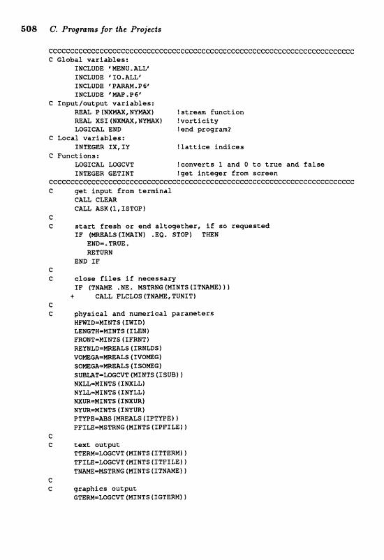
608 C. Pmgmms for $Be Projec;ts
ccCCccCceccccccccccccccecccccccccceccccccccccccccccecccceccceccceccccccc C CZobal v a r i a b l e s :
INCLUDE "NU. ALL" INCLUDE @1IO.ALLt INCLUDE @P=M.P6@ INCLUDE ' MM?. P 6 C
C I n p u t l o u t p u t variables: MAL P (MXmX, N V W ) I stram E u n c t l o n RE&XSI(NXmX,NUW) ! v o r t i c i t y LOGICAL END l a n d program?
C L o e a l v a r i a b l e s : INTEGER IX, ZY l l a t t i e s i n d i c e s
C P u n c t l o n s : LOGICAL LOGGVT ! c o n v e r t s 1 and O t o t r u e a n d false INmCER GETINT ! g a t i n t e g e r Exam s c r e e n
ccc~ccc~c~~cC~~ccc~cc~ccceccE:~cccce~ccccecccece~cccccecc~ccccecccceccccc C get input f r o m t e r m i n a l
CA& C W R CA& BSR(l , 1STQfZ.I
C C start f r e s h o r e n d a l t o g e t h e r , i f so reguasted
I F ( m A L S ( I M I N ) .Ea. STOP) THEN EMD=.TROE. RETURN
END TF C C close f i l e s i f n e c e s s a r y
I F f T N m .NE. MSTRNG (MINTS (ITNAME) 1 1 + CALL FLCLOS ( T H W , TUNXT)
c C physical a n d n u m e r i c a l parameters
RmID-MXNTS (XWXDI LENGTW=NINTS (SLEN) FROMT=MINTS (XFRNT 1 MYMLD=WALS (IRNLDS 1 V O a a = M A L S ( IVIOmC;) SQmGh=WALS(XSOmG) S U B ~ T = W G C ~ T (ISUB) t NXUrMINTS f INXLL f MY&-MINTS (INYLL) N X m 4 I N T S (XEIXUR) NPm=MIMTS ( IMVUR) P T Y P E = ~ S (MREnLs ( IPTVPEI 1 PPILE=MSTREaG (MXHTS I S P F I ~ I I
C C text o u t p u t
TTERHmLOGCVT (MINTS ( ITTERM) 1 TPILE=LWCVT [MINTS ( ITFPt&l l TNMBmMSTRHG (MINTS ( I m M l l
C C g r a p h i c s o u t p u t
GTERNmLOGCVT (MXNTS ( ZGTERM] f
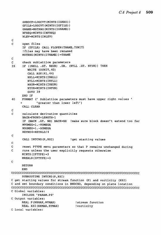
c W m c P = L a c C v T ( H r N a s t I G M ~ t 1 GFXLE=L~GCVT~MXMT~~TGFXLE~I~ G N m = M S T R M G ( M I H T S (XGHAMI5 1 1 NFREQ=MXNTS ( I H F m Q ) NLEVzMINTS ( IMLEV)
G C openfiles
IF ( T F I L E ) CALL FWPEN (TNAm, T W I T ) l f Ales may have been renamed MSTRNC (MINTS ( I TBAm 1 )
e C check sublattice parameters 39 fF ( ( N X L L .GT, NXUR) .QR. (NVLL .GT. NYUR)) THEN
m X T E (OUWfT, 40) C A L L R S X 1 4 1 , 4 4 ) NXLLmMINTS ( I N X L L ) N Y L L M I M T S ( I N Y L L ) MXUR=MIMTS ( INXUR) NVUR=MIMTS ( T N Y m ) GOT0 39
END IF 40 F Q W T (' Sublattice parameters must have upper right values "
+ 'greater than lawer leftf 1 CALL CLEAR
C C calculate derivative quantities
BAGX;=FROHT+~NGTW-l IF (BACK .GT, MX) BAGK=NX !make sure bloek doesnit extend too far M V ~ G = l . - V Q ~ G A M S W G = I , - S Q m G A REYND4=='1THLD/4
C CALL I N T C H D ( P , X S I I !get starting values
C C reset PTUPE menu parameters so that P remains unchanged during C runs unless the user explicitly rewests otherwise
M I N T S (IPTVPE) m 3 M A L S ( E P T U P E ) -3
C RETURN END
cc~cccccceccccccccc~cccccccceececccccccccccceeccccececccceccccccccF=ccccI: SUBROUTTME I M T C N D ( P , X S I )
C get starting values for stream funetion (P) and vorticAty ( X S X ) C and set boundary conditions fn BNDGND, depending on plate location ~ccccecceecccc~cccccececcccccccccccccccccececceccccccccccccccccccF=cccccc C Global variables:
INCLUDE p P m M . P 6' C Outpt variables:
R E U P ( r J X m , N Y m ) W& X S I I N X m X , N Y W )
C Local variables:
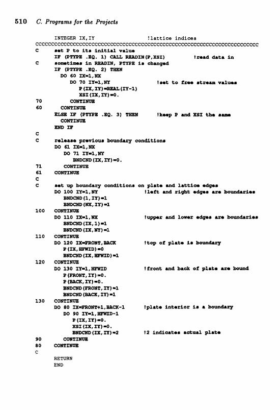
INTEGER IX, TY ! fat t ie@ indices CCCCCCCCCCCCCCCCCeGCCGCCCCCCCCCCCCCCCCGCCCCCCCCCCCGCGGCCCCCCCCCCCCCCCCCC e .et P C@ A+# idrcu vaima
fB ( P m E .E fxaalf &&I in i. ohmgad
DO 60 m m 1 , a
M) 70 X%=%, '1SY !.at to fm 8k~8- ~ 8 3 ~ ~ 8 (m, (XY-1)
ImI. (SX, 3x1 -0. 74 C r n % X r n 50 @bMmW
mm nP ( P m $ .acQ. 5 ) "rm C a B Z x m
gm ra' C C xelrare px8wAou.
DO SI XX-l,rn DO
rx, m) no, 71 C W T X m 63. C m Z m
e d i t i o n * on plaCe U& Iatt;icl+ mdger $&age =I@& m d p ~ axe
am- (l, 11) =l Bmm (m, 3Y)=l
!U-= a& %OW(IE 8.
l? (mm, 3x1 -0 *
-1
?+@p oi g&&&@ I8
!froat m4 llJ& OF plate IZNI
RETURN END
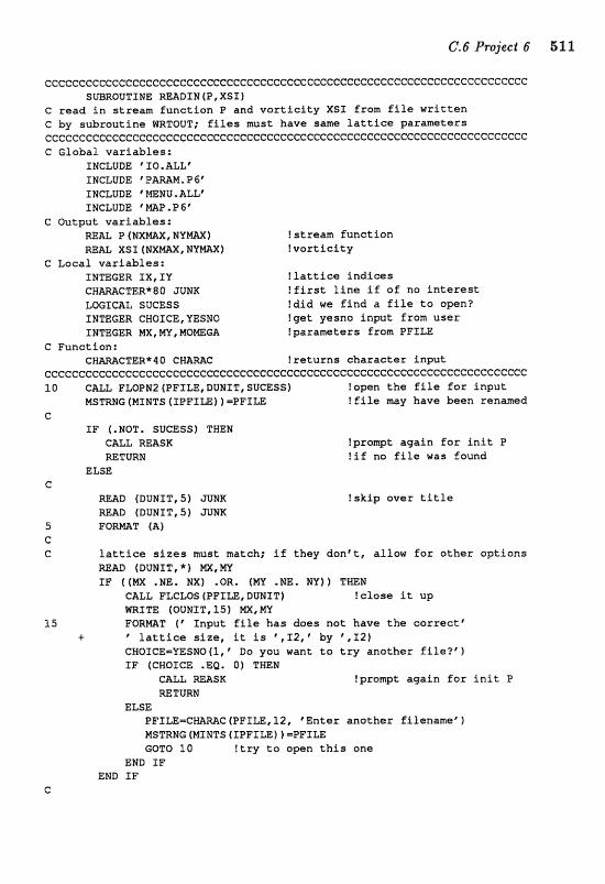
cccccecccceccceecce~ccccccccccccceceececcccccccccccceecc~ceccc~ccccccccc SUBROUTINE m&BXM (P, XSI )
C read i n s t ream func t ion P and v o r t i c i t y XSI from E i l e w r i t t e n C by s&raut ine mTOUT; f i l e s must have same l a t t i c e parameters CCCCGGCCCCCCCCCCCGGCCCC:~CGCCGCCCCCCCCGCCCCCCCCCC~CCCC~CGCCCCCCCCCCGGCCCC C Global var iab les :
INCLUDE 'IQ.ALLt INCLUDE @ P a N . P 6' INCLUDE * mNU. ALL" INCLUDE %P, P 6 "
C Output var iab les : REAL P (NXm, ldlrlw) !stream funct ion REAL XSI (NXNAX, N Y m ) ! v o r l i c i t g
G Local var iab les : IMmGER IXc IY ! l a t t i c e Ind ices CH-CTER* 8 0 JUNK !Eirst l i n e i f of no i n t e r e s t LOGICAL SUCESS ! d i d w e f i n d a f i l e t o open? INTEGER CNQIGE, YESNO !get yesno input from user INTEGER MX , MY, MOmGA !parameters from PFILE
C Function: CHWGTER* 4l? GMWC f r e t u r n s charac te r input
eccCceccc~cccccc~ceeeecceccccccccccecccceccccccC:cccecceececcc~ccc~cc~cc~ 50 CALL PLQZ"N2 (PFILE, DUNIT@ SUCESS) !open t h e f i l e f o r input
MSTRNG (MINTS (IPPXM) 1 =PFILE ! f i l e may have been renamed C
IF (*NOT. SUCESS) THEN GALL REASK ?prompt again f o r i n i t P RETURN ! i f na f i f e was found
ELSE c
=AD (DUNIT, S ) JUNK !skip over t i t l e READ (DUNIT, S) ;TUEtffC
5 FORmT (A] G C l a t t i c e s i z e s must match: i f they d a n f t t , allow f o r o ther opt ions
W A D (DUNIT, * f MX, MY IF ( (m .NE. NX) .OR. (NV .NE. MY)) THEN
CALL FLCmS (PFILE,DUNIT) !close it: up WRITE (OUNIT, 2-51 MX, MY
15 FORmT ( @ Input f i l e has does not have t h e c o r r e c t r + l a t t i c e s i z e , it i s "12, * by "12)
CNOIGE=VESNOfl,C Do you want t a t r y another f i l e ? ' ) ra (caaxcE .EQ, 01 THEN
CALL MASK !prompt again f o r l n i t P MTURN
ELSE PE'ILE=CKZImC(PFTLE,12, 'Enter another f i lename*) MSTRNG fMZEtfTS {IPPXLE) ) =PFILE GOTO 10 ! t r y t o open t h i s one
END SE' END IF
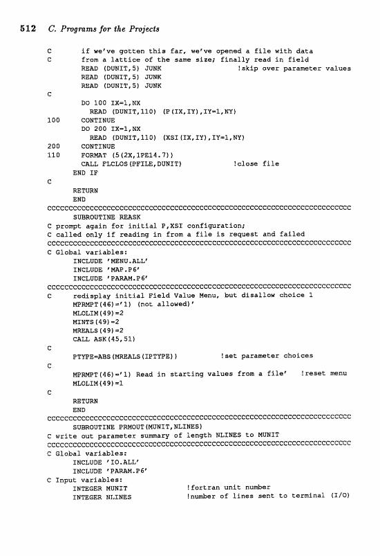
512 C. Programs for $he Projects
C i f wetve qgotten t h i s f a r , we've opened a f i l e with d a t a C from a l a t t i c e of t h e same size; f i n a l l y read i n f f e l d
READ (DUNIT, S J ;J"UWK !skip over parameter va lues READ (DUNIT, S ) JUW READ (DUNIT,$) SUNK
C aa 100 ~ x = i , ~ x
READ (DUMIS, 3.10) (P ( I X , I Y ) , I V - 1 , NU) 100 CONTINUE
ao 200 IX=I,NX =AD (DUNIT, 1101 (XSI (XX, I Y ) , IY=Z,NY)
200 CONTINUE 110 FORNaT (5(2X,1PE14.7))
GALL FLCZOS (PFTLE, BUNIT) !close f i l e END I F
C RETURN END
cccccc~ccecccccccccecccccccceccccccccecccceccccceccccecccccccccccccccccc SUBROUTINE REASK
C prompt again for i n i t i a l P,XSI c o n f i w r a t i o n ; C c a l l e d only i f reading i n from a f i l e I s request: and f a i l e d [email protected]~CCCCCCCCCCCCCCC C Gfakal var iab les :
INCLUDE P =W. ALLt INCLUDE 'mP.P6' INaUDE ' P A W . P 6*
ccccccec~ccccccc"cccceecccccccccccccc~cccccccccccecccccce~ccccC:cecceC:ccc C red isp lay i n i t i a l F i e l d Value Menu, but disal low choice I
m W P T ( 4 6) =' 1) (not af lowad) " MLOLIM ( 4 8) =2 MINTS ( 4 9 ) m2 mmLS (49) m 2 CALL ASK(45,51)
C PTWE==S ( M ~ L S (XPTYPEH !set p a r a m t e r choices
e WMPT (46) -'l.] Read i n s t a r t i n g va lues from a f i l e t t reset menu
MmLTN 149) =l C
RETURN END
c c ~ ~ ~ c ~ ~ ~ c c ~ e ~ ~ ~ c ~ c c c c e c ~ c c c ~ c c c c c c ~ e c c c c c c c c c c c c c c e ~ c c c c c e e e e c C : c ~ c ~ ~ c c ~ SUBROUTINE PWOUT(MUNXS,NLINES)
C w r i t e out parameter s u m a r y of l eng th NLINES t o NUNST ~~c~c~~~ce~~ccccccccccccc~cccc~ccccccc~ceccccc~ecccc~cccccc~cccc~c"cccccc C Global var iab les :
INCLUDE ' I O . ALLf INCLUDE @ PAMM. 9 6"
C Input var iab les : INTEGER MUNIT INmGER NLIMES
! f o r t r a n u n i t nurriber ! n d s r of l i n e s sent t o terminal (I/O)
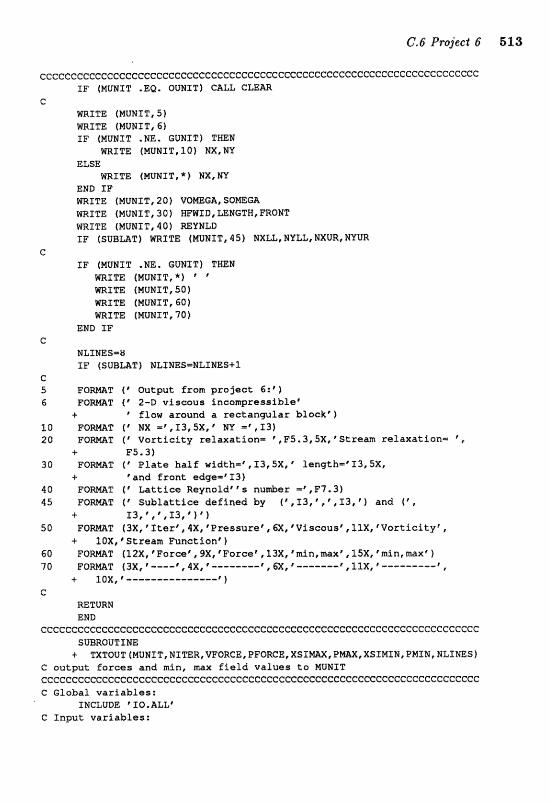
e~~~~e~~~~cc~~~eccc~c~~ccccccceccccccccc~cccc~~cccccceccccccccccce~c~cc~ I F (NUNST .EQ. OUNIT) CALL CLEAR
C HRXTE (MUHIT, S 1 mITE (MUNIK 6 ) I F (MUNIT .NE. GUNIT) THEN
mZI"E {MUNIT,10) NX,W ELSE
WRITE ( M U N I T , * ) EX, NY END I F mITE (MWMIT,20) VOmC;II,SOMEGA WRITE (NUNIT, 30) WWID, UNGTW, mONT WRITE (MUNXT, 401 mVNLD I F (SUBLBT) Wf TE {MUWIT, 4 5) NXLL, NYLL, NXUR, MYUR
c I F (NtMJIT .NE. GWIT] THEN
NRITE (MUNIT,*) ' ' WBTTE; (NNITI 50) mITE (MUPaXT,6Of mITE (mMTT, 70)
END IF c
EILTNES-8 IF (SUBZAT) NLXNES=NLLEES+l
G 5 F Q m T ( w t p u t from pro jee t 1 6 FQ-T f r 2-D viscous incompressible*
i "low around a r e c t a n m l a r black*) 10 F O m T (" NX mf , I3,5X, "#Y = I , I31 20 F O W T ( * V a r t i e i t y re laxa t ion= *p,F"S.3,SX,*SSrem re laxa t ion= ',
i F5.3) 30 F O m T P l a t e h a l f width=', X3, 5X, ' langlth=@ 13,5X,
C @ and f r a n t edge4 LT3 1 40 FOWT ( C Latticc;Reynald*p"snu&er=y,,F7.3) 45 F O M T ( C S u b l a t t i c e d e f i n e d k t y ( t , ,13, t , \131V and t C r
+ 13 , t , ' I13p '} ' ! 50 FOMT ( 3 X , ' l ee r t , $X, * Pressurer c a, e V i ~ c a ~ ~ t l l X r r V o r t i c i t y y ,
-t 10X, Stream Function' ) 60 F Q M T (12X, * Forcef I 9XI Foreet 13XP min, maxf ,1,5Xt *mint max* 1 70 FO-T (3X, G---" ,4X, *--------I, @, t ------- ' , ,11X, 8 ---------F
+ ~ Q X , r ---------------P f c
RETURM END
GCCGCCCCCCCCCCCCGCCGCCCCCCCCCCCCGCCCCCC~CCCCCCCGC~CCCCGCCCCGCCCCCC~CCCCC SUBROUTINE
+ TXTOUT(NUNIT,NIT1ER,WORCEIPFORCE,XSX~X~P~XIXSIMTPaIPMZN,NtINES~ C ouctwt f a r c e s and min, max f i e l d values t a MUNIT CCCCCCCCCGCCCCCGCCCCCCCGCCCCCCCCCCGCCCCCC~GCCCCCCCCCeCGCCCCCCCCCCCGCCCCC C Global var iab les :
INCLUDE *IQ.ALL" C Inpu t var iab les :

514 C. Pmgmms for the Projects
INTEGER NITER !number of iterations REAL VFORCE,PFORCE !viscous force and pressure REAL XSIMAX, PMAX, XSIMIN, PMIN 1 min, max values of XSZ, P INTEGER MUNIF !fortran unit number INTEGER NLIUES !number of lines sent to terminal(f/O)
CCCCCCCCCCCCCCCCCCCCCCCCCCCCCCcCCCCCCCCCCCCCCCCCCCCCCCCcCCCCCCCCCCCCCCCC C if screen is full, clear screen and retype headings
IF ( (MOP (NLIMES, TRMLIM-6) .EQ. 0) + .AND. (MUNIT .EQ. OUPIIT)) THEN
CALL PAUSE(*to continue...*,l) CALL CLEAR BORITE (HUNIT,SO) WRITE (MUNIT, 60) WRITE (MUNIT, 70)
END IF c
IF (MUNIT .EQ, OUNIT) NLINES=NLlNES+l WRITE (MUNXT,40) ~TER,PFORCE,WORCE,XSIMfN,XS~,PMIN,P14AX
C 40 FORMAT (2X, 15,2 (ZX, 1PE12 - 5 ) ,2X, 4 (1PE10 3, 1x1 1 50 FORWLT ( 3 X , *Iterf ,4Xf 'Pressuref , 6XI *Viscousf llX, * VorticityO
+ 10X, "Stream FunctionF 60 FORMAT (12X, 'Forcef, 9X, *Forcet 13X, *minemaxf , 15Xf tnin,ntitx' 70 FORMAT (3X, ' ----f, 4X, * m, f -------* ,11X, r --------- *
+ 10X,f---------------'
C RETURN END
C C C C C C C C C C C C C C C C C C c C C c C c C C C C C C C C C C C C c C C c SUEROUTIPIE DISPLY (F, MUNIT, ITYPE, FMAX, FMIN)
C display stream function (P,ITME-STREAM) or vorticity C (XSI,ITYPE=VRTCTY) as letters; positive values are capitals or C numbers, nwative values are small letters CCC~CCCCCCCcCCCCcccCCCCCCCCCCCCCCCCCcCCC~cccccccccccccccccccccccccccccc C Global variables: ,
TNCLUDE PARAM.P6* XNCLUDE * 10 ALL'
C Input variables: RFZAL F(NXMAX,WYMAX) !stream function or vorticity INTEGER MUNIT luni t wef re writing to INTEGER ITYPE !which field are we dfsplaying? REAL FMAXIFMIN f min and max field values
c Local variables: INTEGER IX, IY !lattice indices INTEGER TEMP !field at current lattice site CHARACTER* 1 FIELD (NXMAXl !field as character data CHARACTER*80 BLNK !blanks for centering in X CHARACTER*X AsKII (0: 35) ,NEGASK (1 2 6 ) f charac 'data for display DATA BLNK / * ' / DATA ~ ~ ~11/'0'~*1~~*2'~*3','4*~*5'~*6*~'7*~~8'~~~~~
+ ~ A ~ , ~ B * , * C * ~ ~ D ~ , * E ~ ~ ~ F ~ , ~ G ~ , * I . I * , * I ~ , ~ S ~ , * K * , ~ L * , * M * ~ 4. ~~~,*Q~,*~~,*Q*,*R*,*S~,*T~,~U~,*V*,*W*,'X* IfY*,fZ*/
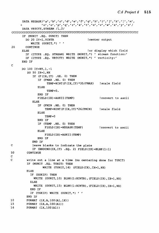
DAT& MEGASK/*af c % b ' , f e ~ ~ d ~ , f e 1 , @ f * t t g 6 , f h f , r i t t ~ j f t f k t , e l p , ' m f , + r n r r r o * , t p p " , ~ q ' ~ ~ ~ ~ , ' s C I ' t t , ' ~ ~ C * ~ l , t ~ ~ , t x ~ , ~ ~ f , f z ' /
cecccc~c~ececee~c~ccC:ccccccccccccccceeeeccccccceccec~ceccccccc~~ccccc~c IF (MUNIT .EQ, OUNST) T m M DO 20 XY=T,YaTR !canter output
WRITE (OUNIT,*) ' 20 GQNTXNUE
ELSE ?or display which field IF (TTVPE ,&Q. S T W M ) WRITE fMUHITIX) * stream function:' IF (ITPPE .EQ. WTGTY) mSTE (MUNIT,*) "vorticity:'
END IF C
DQ 180 IU=NV,l,-1 DQ 50 IX-1,NX
ZF (FfZX,SV) .GE. 8) THEM IF (F= .NE* O) THEN
TEW-NIWT (F (IX, IYf *35/FMAX} ! seafe field ELSE
TENPmO, EPlrD IF FIELD (IX) =ASKIX (TEMP) !convert to a s c f i
ELSE SF (FMXM .ME, O) THEN
TEW-MINT (F ( I X , 1% *26/FMXNf ? scale f i e l d ELSE
TEem0 END IF SF {TB= .NE. 0) THEN
FIELD (SX) =NEGASR (TEW) !convert to a s c i i ELSE
FXELD f sx t =&SKI I ( T e r n END %F
END IF C leave blanks to Indicate the plate
sa (swacao tzx, r w -EQ. 21 FIELD (3x1 =ELM (1 : 1) 5 0 CCIETTNVE C C write out a line at a time (no centering done for TUNIT)
IF (NUNIT .EQ, TUWXT) TWEN VIIRJm (TUNIT, 16) (FIELD (XXf , XX=J., m1
ELSE XF (XSKXP) THEN liJRXTE (OUNIT, IO) BLHK 41 :XCMTR), (FIELD ( I X ) , PX=l,NX)
ELSE WRITE (OUNIT, 15) BLNX (1 : XCNTR) , (FXELD tIX1, IX=1, NX)
END IF XF (VSXTP) MRITE (OUNIT,*) * p
END IF 10 F O W T (1X,A, 100 (AI, 1x1 ) 15 FO-T f lX, A, 108 (All ) l6 F O m T (lXrlOO(A1))
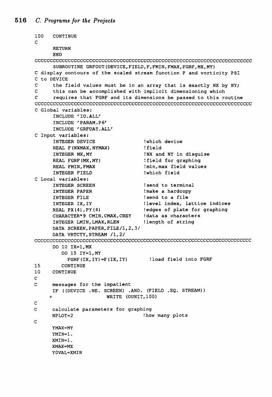
5 l6 C. Pmgrrrms for $We Projects
100 CONTINUE e
RETURN END
cccccccccccccccccceccccecccceccccccccececccccccccccccccccccc~ccccccccccc" SUBROUTINE GRFQUT~DEVICE,FIELD,F,FMXN~FMAX,E"GW,MX,MV~
C d i s p l a y con tours o f t h e s c a l e d s t feam func t ion P and v a r t i ~ i t y PSI C t a DEVICE C t h e f i e l d v a l u e s must be i n an a r r a y that is e x a c t l y NX by NY; C t h i s can be a c e o w l i s h e d wi th imlieit dimensioning which C r e q u i r e s t h a t FGRF and i ts d inens ians be passed t o t h i s r o u t i n e ccceccccccccccccccececccccccccccceccccccccccccccecccccccf:cccecccC=cC:ceccc C Global v a r i a b l e s :
INCLUDE "Q,ALL*
INCLUDE * GRPDAT .&L" C Inpu t v a r i a b l e s :
t whf ch dev ice ! f i e l d
INTEGER MX, W !NX and NV i n d i s g u i s e FGRF (MX , MY 1 ! f i e l d f a r graphing
mAL PMIN,FW ! min, max f i e l d v a l u e s INTEGER FIELD !which f i e l d
C Local v a r i a b l e s : IMTECER SCREEN Isend t c t e m i n a l INTEGER PAPER !make a hardcapy INTEGER FILE !send t o a f i l e INTEGER I X , l Y ! l e v e l index, l a t t i c e i n d i c e s REAL PX ( 4 1 ,PV ( 4 1 [ edges of plate f o r g raph ing eHmCTER*S CNIN,CWX,mY !data as c h a r a c t e r s INTEGER LMLM, LMX, RLEN ! l eng th of s t r i n g DATA SCRE&N,PABER,FILe/l12,3i DATA VRTCTY, STmAM /1,2/
eccccc~Ccccccccccccec~cccccccccccccccecccccccccccccccccecccccc~ceececccc DO 20 EX=%, MX
DO 15 IY-1,W FGRF ( I X , I Y 1 =F [IX, IU) ! f aad field i n t o FGW
15 CONTINUE 3.0 CQPJTINUE c C messages f o r t h e impa t i en t
I F ( (DEVICE .WE, SCMEN) .AMD. (FIELD . EQ, S T m M j 1 + WRITE (QUNIT, 1001
C C c a l c u l a t e p a r a m t e r s far graphing
NPmT=2 !how many p l a t s C
Y W - - M Y VMXN-1. X M I N m 1 . X W - M X YOVBL=XXIAI

XOVALmVNXN NXTICKm5 NY TICKm5 EPOINT=5 W E L (1) =F NX' -&EL (21 m' NYr GALL C O m T [FMIW, CNIN, WIN) CALL C O m T f F W , C m , L M X 1 CALL CQWRT (RIEYNLD , CmU, RLEN )
IF (FTELD .EQ. STmM) THEN 'ID LQT=1 TNFO=fPmin-*//CMX#(l%LMXNf / / I Pmax='/l/CmX(l:LmX)
ELSE IF [FIELD .EQ. VRTCTP) TWEN IPLOT-2 rNFo=fXsInin=~//CMrN(l:LMIIV~//C XsZrna~=~ //CmX(l:Lm)
END XF TXTLE=fSStxeam Funct ian and Vorticity, R@gmoldfls n u d e r -'
3. //GREY (1:RmN)
IF (FIELD .EQ. STWAM) THEN . CALL GTDEV (DEVXCE ) !device namfnatlon IF (DEVXCE .EQ. SCREEN) CALL GHODE ?change to graphics mode
END IF CALL LNLINAX idraw axes
draw in plate 15 i t ' s big enough IF [LENGTH .GT. 21 TWEN PX 4 1 ) =REAL (FRONT+I ) PY(11-1. ax(aj=Px(l) PU ( 2 ) =REAL (HFWXD-1) PX ( 3 ) =REAL (BACK-l f PY f 3) =PY (2) PX (4j=PX (3) aY(4)=n* EaPOINT=4 ILXMEm2 CALL XYPLOT (PX,PY)
END IF
CALL COMTOR(FGRF,mem,FMINIFMAX,NUV)
end graphing session sa tPrnazD .&Q. VRTCTY) THEN TF (DEVICE .ME. FTLE) GALL GPAGE(BEVZCE) !and graphics package IF (DEVXCE .EQ. SCREEN) CALL TX"lODE !switch to text mode END IF
Fa-T (I,' Paatience, please; output going ta a fi le.*)
RETURN
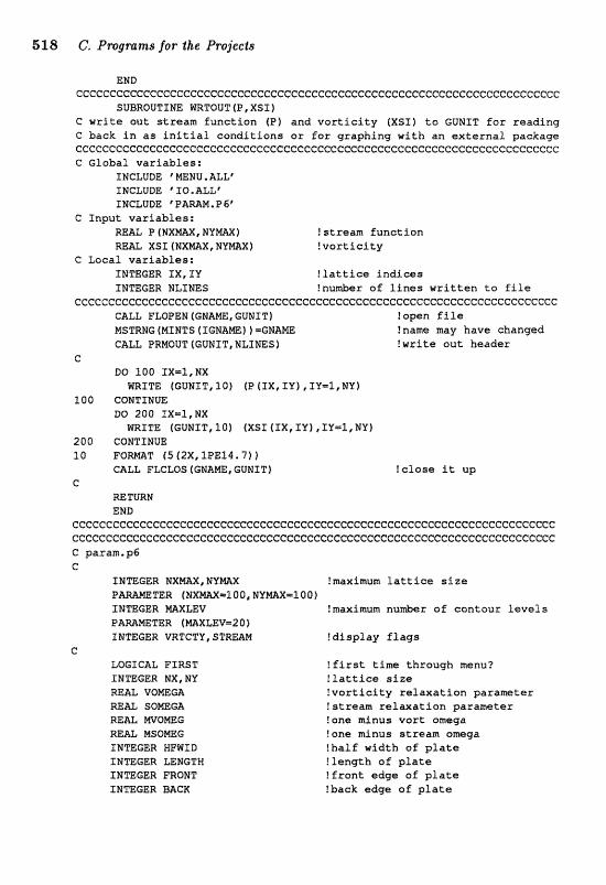
528 C. Pmgrans for the Projects
END ccccccececcccccccccccccccccccccccccccccccccccccccccccccceecccccccccccccc
SUMQUTINE mTQUT (P, XST 1 C write out stream funct ion (P) and v o r t i c i t y (XSI) t o GUNIT for reading C back i n as i n i t i a l condit ions ox for g r q h i n g with an e x t e r n a l packaqe ccccCccceccccececccccccccccccccccccccccccccccccccccccc~cccc~cccccccccccc C Global var iab les :
INCLUDE ' 2IIENU. ALLt INCLUDE ' f O.ALL' f NCLUDE " PAmM, P S"
C Input variables: REAL P ( N X M X , N Y M ) !stream funct ion WAL XSI ( N X m , M f v o r t i c i t y
C Local var iab les : INTEGER I X , ZY ! l a t t i c e i n d i c e s INmGER NLIMES ! n u h r o f l i n e s w r i t t e n t o f i l e
c~cccccccccecccccccccccccccccccccccccccccccccc"ccccccccceccccc"ccccccccccc CALL FLOPEN (GNANE, GUNXT) !open f i l e MSmBG (MINTS (XGBAM) t =GN;Am !nam may have changed CALL PMQIIT (GUMIT, NLINES) !wr i te out header
C DO 3.00 I X m 1 , N X
WRITE (GUNIT, 10) [P ( I X , I Y ) , l Y = l . , MW 100 CONTINUE
DO 200 I X - 1 , WX m T T E (GUMIT, 10) (XSI ( I X , SY) , IY=L, NY)
206 CQNTINUB l 0 F O m T (5 ( 2 X , lPE34,?) )
CALL FLCLOS (GNAm, GUNfT) C
=TURN END
ccccccccecccccccccc~cccccccecccccccccccccccccccccccceccccccc6rccccccccccc c c e c e c c c e c c c c c c c c c c e c c c c c c c c c e c c c c c C. paran.p6 C
IMmGER HXPIAX, NVmX !=ximm l a t t i c e size P A R A ~ T B R t~xmx-z 0 0, Nrmx=i oo ) ZMTEGER W L E V Imaxlmum nu&er of contour l e v e l s PAMmTER (MXLEV=2 0 ) INTEGER VRTCTU, STREAM ! d i s p l a y f l a g s
e LOGICAL FIRST ! f i r s t t i m e through menu? IMTEGER NX, NV ! l a t t i c e s i z e REAL VOmC;I1 !vortfcPty r e l a x a t i o n parameter m& SOMEGA !stream r e l a x a t i o n parameter REAL PIPVOmG !one minus v a r t omega RE& MSOMEG !one minus s t ream omga INmGER HFWID !ha l f width of p l a t e INTEGER LENGTH !length o f plate INaGER FRONT ! f ron t edge o f p l a t e INTEGER BACK !back edge a f p l a t a
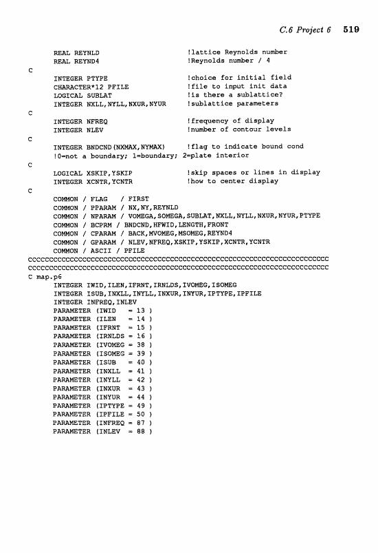
M& WMLD ! l a t t i c e Reynolds nuniber REAL REYND4 tReynolds nurnber / 4
c INmGER PTYPE !choice f o r i n i t i a l f i e l d C B m C T E R * 1 2 PFILE ! f i l e t o input i n i t d a t a LOGICAL SUBUT !is t h e s e a s u b l a t t i c e ? INTEGER NXLL,NIILL,NXUR,NYUR ! s u b l a t t i c e p r a m e t e r s
C INTEGER NFREQ !frequency a f display INT'&C;;ER NLEV !nu&er o f contour Levels
c INTEGER BHDGND (N !flag t o i n d i c a t e bound @and t0-at a boundary; lmboundary; 2c1plate i n t e r i o r
G
LOGICAL XSKXP,VSKIP ! s k i p spaces o r l i n e s i n d i s p l a y INmGER XCHTR, YCNTR !how t o @enter display
c CQmON / FxdG i' FIRST CQMQN / P P M M / NX,NY,REYNLB COWON f N P A W / VOMEM, SQmGA, SUBmT, mLLI NYLL, NXURI NYURI P T W E COMQN / B C P M / BNDCND,HmXD,mMGTW,FRQNT
, MTOMEG I NSOWG, REYND4 p NFmO, XSKIP, YSRZP, XCNTR, YeNTR
Ccccccccccccccccccccccccccceceeececcccccccccccccccceccccccceeecccccccccc ec~ccce~c~cccccccccccccecccccccccccccccceccccccce~ccccccccC:ecccccc~ccccc C! map-p6
INTEGER IITD,Z~N~SFREJT,IREILDSffIVONEG,ISOMEG INTEGER XSUB, IMXLLr XNYLL, INXUR, INVURI XPTPPE, I F F I L E INTEGER I N F R E Q , I m V
TER (IFIID ;.F 13 )
TER (XLEN 14 ) 'PER (IFRPIT 15 f
P & m m T E R (IIINLDS - 16 ) TER f XVOMEG = 38 f TER (ZSOMEG - 39 f
P-MTER (ISUB = 40 )
P m M E T E R (INXLL - 91 ) P m m T E R f IMVLL = 42 f P m M E T E R ( I N X W = 43 ) P W m T E R (TNVUR = 44 )
e a m m T E R (IPTYPE = 99 ) PAMWTER ( I P F I m 1 50 )
F m m T E R (INFREQ = 87 ) PAmmTER (IMLEV = 88 )
520 6, Pmgranas for the E"r0jeet;s
C.7 Project 7 AILgorit hm This program d v e s the non-line= reaction-digusion equa- tions of the Brusselator [Eqs. (VII.3)] in two dimensions (0 5 2 5 1 and O < y 5 1) with no-Rux boundary conditions. You can make the problem one-dimensiod by setting BP= 1 (if you set EX= 1 instead, the reaction terms are lwt? and it become8 a simple diffusion problem). Initial condi- tions for the X and Y eoncentratio~s are taken to be random fiuctuzl;tions about their equiiibrium values (DO loop 5 in subroutine mceor). Time evolution (DO loop 20 in ARCHOH) is then carried out by the alternating- direction method (7.19 along with 7.1 1-7.16) in subroutine EV~LVE. Note that some of the coeficie~ts reqered for the inversiQns of the tri-diagond matrices are calculated only once for eaeh d u e of D%" (subroutine m r l c and between lines 10 and 15 in subroutine n~caor). Every I ISTEP '~~ iter- at;i~n, you haw the option to continue &eration@, &mge DT or ISTEP, or return, to the main menu,
Note that X and Y refer both to species and direction (horizontal or verticd); if they appear twice (e.g., BETIIXX) the first reference is to the species, the wcond ti, the direction; if they q p e w once, the meadng shoul d be clear from the context.
Input The physical parameters are the concentrations of A [2.] and B [4.], diffusion constants for X species [.001] and Y species [.003], and the size of the initial fluctuations for X spedes [.Q11 and Y species [.01]. All &es are scded as described in the t a t , Mter leaving the mafin mean, subroutine SVGGST cdculates and displays limiting vdaes of B ba~ed on the linear stability analysis presented in the text (e.g., what values of B give stable or unstable oscillations). You are then given an opportunity to revise your value of B based on this information. The program will also calculate and display the frequencies (VII.10) for the largest and smallest m values (these limits are based on boundary conditions and lattice size).
The numerical parameters are the number of lattice points in s [20] and y [20] directions and the random number seed used for the initial Buctuations. The maximum number of r points is fixed by M== 79 and y points by HAZY= 20. These Emits are to ensure that the character display of the concentrations will fit on the typical screen, which is 24 lines long aad 80 characters wide. If you are using graphics, or y ~ m ter 24 X 80, you can adjust these parameters. The graphics parameter is the number of contours for plotting the concentrations and is used only if you have graphics. After you have left the main menu, you will be prompted for the time step [.Q?'], the number of steps (*STEP) until you can end the
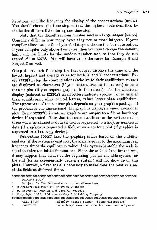
iterations, and the frequency for display of the concentrations (BFREQ). Uou sho~ld choose the time step so that the highest mode described by the lattice &Rases little during one time step.
Note that the default random number seed is a large integer (547651. Compilers differ in how many bytes they use to store integers. If your compiler &lows two or four bytes for integers, choose the four byte option. If your compiler only allows two bytes, then you must change the default, high, and low limits for the random number seed so that they do not exceed 215 = 327658. Vou will haye to do the s m e for Exmple 8 and Project- 8 tts well.
Output At each time step the text output displays the time and the lowest, highest and average value for both X and Y concentrations. Ev- ery A F R E ~ ' ~ ~ step the concentrations (relative to their equilibrium values) are displayed as characters (if you request text to the screen) or as a contour plot (if you request graphics to the screen). For the character display (subroutine DISPLY) small letters indicate species values smaer than equjlibrium, while capital fetters, vdues larger than equilibrium. The appearance of the contour plot depends on your graphics package. If the prabk?m is one-dimeasiond, the graphics displays a one-dimensional plok Every I P S T E P ' ~ ~ iteration, graphics are output t s a file or hardeopy device, if requested. Note that the cancentraLions be written out in three ways: as character data (if text is requested to a file), as numerical data (if graphics is requested a file), or as a contour plot (if graphics is requested to a hardcopy device),
Subroutine SUGG~T k e s the gaphing scales based on the stability andysis: if the sy~tem i~ unstable, the scale is aqud to the m k m n m real frequency times the eq~Ebrium vdae; if the aystem is strtble the scale is equd to tvvictr the initial fluctuar;ians. Since the scde is k e d for the run, it may happen that values at the beginning (for an unstable system) or the end (for an exponentidy decaying system) wil l not show up on the plot;& However, a fixed scde is necessary to make elear the relative sizes of the fields at diEerc3nt times. cccccccccceccccccccccccc~ccceccccccccececcccccccccccccccccccccCccccceccc
P R E M M PRQJ7 c Pro jec t 7: The Brusse la tor in two dimensions C COmUTATZOEJAL PHYSICS (FORTMM WRSION) C by Stcyven E, Koonin and Dawn C. Neredith G Copyright 1989, Addison-Hesley Publishing Cantpany eeccCceccccccccccccccccccceccccccccccceeccccccccccccccccccccccccccccce:cI:
C A U INXT !display header screen, se tup parameters 5 CONTINUE Inrain loop/ execute once f a r each s e t of param
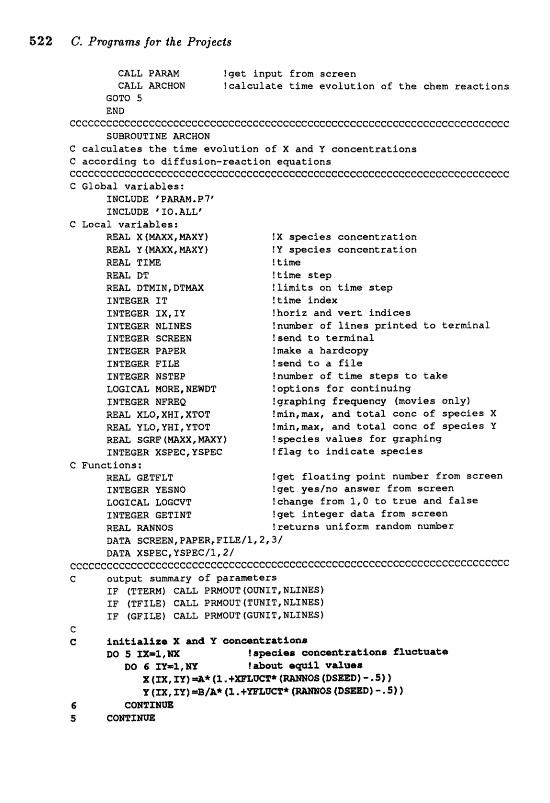
622 C. Pn?gnams f i r the Projects
CALL P m M !get input from screen CALL ARGWQN !calculate time evolution of the chem reactions
GOT0 5 ENT)
cccccccc~cecc~ccc~cccccccccccceccceeE:cecceccccc~~~~~cc~c~cccccc~cccccccc SUBROUTINE MCWQ'E3
C calculates the time evolution o f X and Y concentrations G according to diffusion-reaction equations CCCCCCC~CCceCeecCCCcccCCcCCCGcCeCcCceCcccccccCccccccecccecc~e~ccc~~~cccc C Global variables:
INCLUDE 'P-M. P7' TNCLUDE ' 56. ALLt
C Local variables: m= X (NAXX, 1UZAXY f !X species on cent ration RE= Y (WX,MAXYl !Y species concentration RE= T I m !time R- DT !time step REaL DTNIEd,DTM !limits on time step INTEGER IT !time index TNTEGER XX, TY ! horiz and vert indices INTEGER MLXNES !nudes of lines printed to tedna2 IN"fGER SCmEld ?send to terminal INTT&GER PAPER !make a h a r d c q y INTZGER FILE !send t o a file INTEGER NSTEP ! n d s r of time steps to take LQGf CAL MORE, KEWDT !options for continuing XNmGER NFREB lgraphing frswency (movies onlyf BE= XLO, XHX, XT02 !min,max, and tatal conc of species X
YLQ, YWT, VTQT !min,max, and total conc of species Y m A L SGRF (MBXX, M Y ) ts~cies values for gxapking INTEGER XSPEC,VSPEC !flag to indicate apcfes
C! Functions: RE& GETFLT !get; floating point nuder from screen INTEGER YESNO !get yeslno answer from screen LQGIChL LOGCVT !change, from 1.0 to true and false INTEGER GETIHT !get Integer data from screen REAL MNN05 !returns uniform random nuder DATA SCWEN,PAPER,FIm/1,2* DATA XSBZC,YSPEC/1,2/
~~~~~~~cc~~~ee~eceeece~eccccccecececec~C:ccc~~eI:cc~ccccccce~ceccceccccccc C output sumary a f parmeters
IF (TTERM) CALL PI-IMOUT (OUNIT, NLXNEf) I F (TFILE) CALL BMQUT (TUNXT, NLXNES) IF (EFILE) CALL PRMOUT [GUMIT, NLINES)
G G ixlllt;ialiaa Z an4 ff et@a~nkrslsAcnrr
BQ 5 EX=%,= f~pcira conaenkzakion@ f%mataata DO 6 m=%,=
X [ZX , XT) a* [%. +-GC%*
6 C W T I m fi coN2IHm
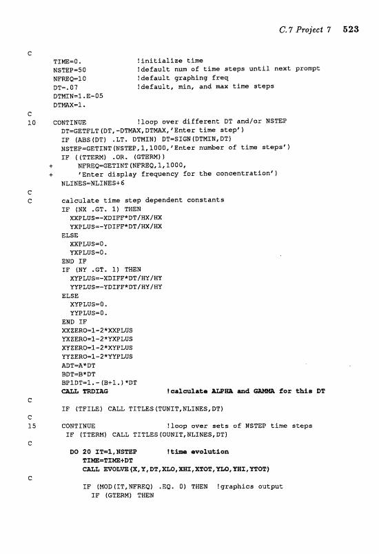
C. ? Project 7 523
? i n i t i a l i z e t ime ! d e f a u l t num of time s t e p s until next prompt ! d e f a u l t graphing freq ! d e f a u l t , min, and max time s t e p s
CONTINUE !loop o v e r d i f f e r e n t DT andlor NSTEP DT-GETFLT (DT, - D m X , DTMAX, I E n t e r t i m e s t e p ' > SF (ADS (BT) .LT. DTMIM) DT-SIGN (DTHIN, DTJ NSTEP=GETINT(WS~P,1,100OC1Enter nu*er o f time s t e p s ' l XP ((TTERM) .OR. (GTERI"I1)
+ NFREQ=GETlNT IWFREQ, I, 2 000, + 'En te r display frequency f o r t h e concen t ra t i an ' l
NLINES=NLINE5+6
c a l c u l a t e t i m e s t e p dependent c o n s t a n t s IF (MX .GT. 1) THEN XXPLUS=-XDIFF*DTINX/HX YXPLUS=-YBIFF*DT/HXIWX
ELSE XXPLUS=O. YXPLUS=O *
END IF fF (MY .GT. 1) THEM XYPLUSm-XDIFP*DT/HY/NV YYPLUSm-YDIFF*DT/HYW
ELSE XYPLUS-0 * VYPLUS=O
END IF XXZEROm1-2*XXPLUS YXZEROol-2*YXPLUS XUZERO-1-2XX'VPLUS YYZERO=1-2*nPLtUS ADITmA* DT BDT=B*DT BPZDll-I. - (B+%. j *DT
TmX&G IcalauXaka, m m and Eos tbis DT
IF (TFILEI CALL TITLES (TUNTT, NLXNES, DT)
CONTINUE ! loop ave r s e t s of NSTEP t ime s t e p s IF (TTERM) CALL TITLES f QUNIT, NLXNES, DT)
IF (MOD (IT, MFREQ) . EQ, O) THEM !graphics ou tpu t LF (GTERN) THEN

IF (TmRM) CAWL PAUSE f * tto see concentrations. . , l , lf CALL GRFOUTfSCREEN,XSPECtX,XLO,XMS,XTOT,SGW,NX,~Y] C a L GWOUT (SCWEN, YSPEC, '15, YLOt YHI, YTQT, NX, RV) IP ( (TTERMI "AND* (IT .WE. NSTEP) 1
CALL TITLES [OUNIT, NLINES,DT) ELSE SF (TTEM) THEN CALL PAUSE(@tto see X eoncentration..-',l) CALL DISPLY ~X,OUNIT,XLO,XHI,XTOT~XSPEC~ CALL DI SPLY IY, OUNIT, YLO, YWT, YTQT, VSPEG) CALL CLEm NLIHES=O IF (IT .HE. NSTEP 1 CALL TITLES (OUNXT, NLPMS, DTf
EPdB IF ELSE ! text outlput
3F (TTEW) + CALL TXTOUT(OUMIT,NLEmS, TIME,XLQ(rXWSIXTQI:IYL~,YHEeYTOT~
IF (TPTLE) + CALL TXTOUT (TUWIT, NLINESI TIME, XLO, XWZ, XTOT, YLO, YHX8 YTOTI
END IF 2 0 C 0 M Z " Z m C
SF fTFILE) THEM f graphics output CALL DISPI;Y (X, TUNXT, XLO, XWI , XTOT, XSPEC) CALL DISPLV (Y, TUNIT, YLO, YHI, '15TOTt YSPECI CALL TIT~S(TUNIT,RIZIBJES,DTl
END SF SF (GIIRDCP) THEN
CALL GWOUT (PAPER,XSPEC,X,XLQtXWItXTOT,SGRh",MX,NY) CALL GWOUT (PAPER, VSPEC, V, YLO, YWI, VTQT, S G W , HX, NY 1
END XF IF (EFILE) CALL WTOfJT (X, Y, TIMEI D311
C MO~=LOGCVT(~SNO(l,fC~ntin~e iterating?"))
IF (MORE) THEM NLINESmO IF (TTEBM) CALL CLEm EQTO 15
BND IF C
WEtQBT- + ZOGWT(YESNO(1,'Change time step ar frequency and cantinue2'))f IF tNEHDT) THEN WLIWES=O IF (TTERM) CALL CLmR GQTQ 10
END IF e
=TURN END
~ ~ c c ~ c c ~ ~ ~ ~ ~ ~ ~ ~ ~ ~ ~ ~ ~ e e ~ ~ ~ " ~ c c ~ c c ~ ~ e ~ ~ ~ ~ ~ ~ ~ ~ c c c ~ ~ c c c c c c ~ c c c ~ c c c ~ c c c c c c c ~ ~ ~ SUBROUTINE EVOLVE (X, H, DT, XLO, xHI~xTOT, VLOI YBI, YTOT")
C evolves the species X and Y according to the diffusian-reaction
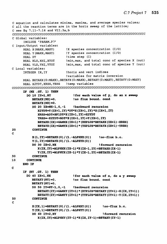
C equation and c a l c u l a t e s minima, maxima, and average s w c i a s values; C a l l t h e r e a c t i o n t e r m s are i n t h e h a r i z sweep of t h e l a t t i c e ; C see Eq 7.11-L16 and VXIe3a,b cccccccc~Cccecccccf:cccccccccceeeeccccccc"ccececeCcccccccccccccccccccCcccc C Global variaLzJes:
INCLUDE 'PARaP9.P7' C Iny>ut/Output var iab les :
WAL X(MXX,mXY) !X species concentrat ion ( I / O ) l%EZ& Y ( M X X , m X Y ) !Y spec ies concentrat ion fI/Q)
DT ftim s t e p (1) RE= XLO, XHX, XTQT Imin,max, and t o t a l eonc of spec ies X (out) REAL YLO,YHI,YTOT !min,max, and t o t a l conc of spec ies V (ou t )
C Local var iab les : XNWGER XX,IU lhor iz and v e r t indices
!var iab les foz m t r i x invers ion =&L BEzlllXX (0 :mm) , BEThYX ( 0 : M X X ) , EETaXY t O : mXV) , BET&= ( O : m X Y f RE& X2VDT,XRHS,VRHS !tamp v a r i a b l e s
cc~cceccccceccccccCcccccccceecceccccccccccccceecccccccccccccecccccccc~cc 33' (m "@2* Z) P-
Ifer ea& val- of yr , do an x @
Ins 2 1 ~ haad* C Q ~ S
DO 20 ===-1,0,-1 tba&wm4 racgttrrion ttZmT.iJt (=+l, rtr) +DV*% (=+l, 1x1 m {XX+I, IT) ~ S ~ % + ~ l D T * X , (XX+l , ZY) +X2mII W S = - X m T + m T * X (ZX.C.1, TP) +X (f X+%, m)
C O R g X m
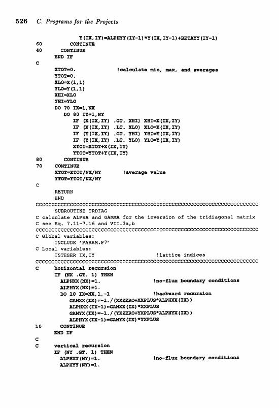
t
Y (IX, XY);r;AW?fm (1Y-1) VY (XX, IY-1) +BET&= (IY-lf 60 CCnsTXblmL 4 0 CONTIMW,
END IP C
XTOr=O. YTOWO. - x ( 1 , 1 ) Y L b Y ( 1 , l ) XBI=xLQ m=m DO 7 0 I X = l , WK
DO 80 3Y=&,MI 5E ( X ( I X , N ) .GT. XXXJ XgI=X(IX,XY) I H ( X ( I X , I Y ) .LT. XLO) XLt%XtTX,EY) IF (Y(TX,IY) . 6 T . XEI) YbIIWcY(IX,TY) XE ( Y ( r x , x Y ) .LT. YLO) rm=Y(XX,TY) xromai9lcor+x f r x , XY) n w x = Y T O T s P ( x x , XY?
80 COWTIBUR 70 CONTINUE
XTBT=XmY/NX/MI faweraw value YTM1=YTOT/NX/WY
C
ILETURM END
cCCCCCCcCCCCCCCCcCCCCCCcCCCCCCCCCCCCcCCCCCcCCCCCCCCCCCCCCCccCCCCcCCCcCGe SllBROUTINE TRDIAG
C c a l c u l a t e ALPHA and GANMA f a r t h e i n v ~ r ~ i o n o f t h e t r i d i a g o n a l matrix C see Eq. 7.11-7.16 and VfI.3a,b cccccccccccccccceccccccccccccccccccccccccccccccccc=Cccccccccecccccccccccc C G l o b a l variables:
INCLUDE ' PARAM.P'18 C L o c a l v a r i a b l e s :
INTEGER I X , TY ! l a t t i c e i n d i c e s cccccccccccccccccccccccccccccccccccccccccccccecccccccccccccccccccccccccc C hoxizantal rear8lrion
I?? (HX .GT. 1 ) TEEX aZPiMX (WX) =I. !no-flw bowday conditions A L P W X (NX) 4. DO 1 0 M=WX,X,-I !traJrward racuraion
GAMXX{IX) =-1. / ~ Z E R w X W L u s * A L P m (IX) AfrPmx { I X - l f =wmm (Uf) *XXPLUS
(nt) --I. / (YX&$RO+'IRCBLUS*mW ( I X J ) PUsm fIX-XJ=mkmx (3x1 *n[PLUS
10 CONTINDIE E M XP
C C vertical rcrcursian
a (WY .ST. 1) TEEN &mIIXY (El) p e l .
ALPm (W) 4. ?am-flw boundary maditions
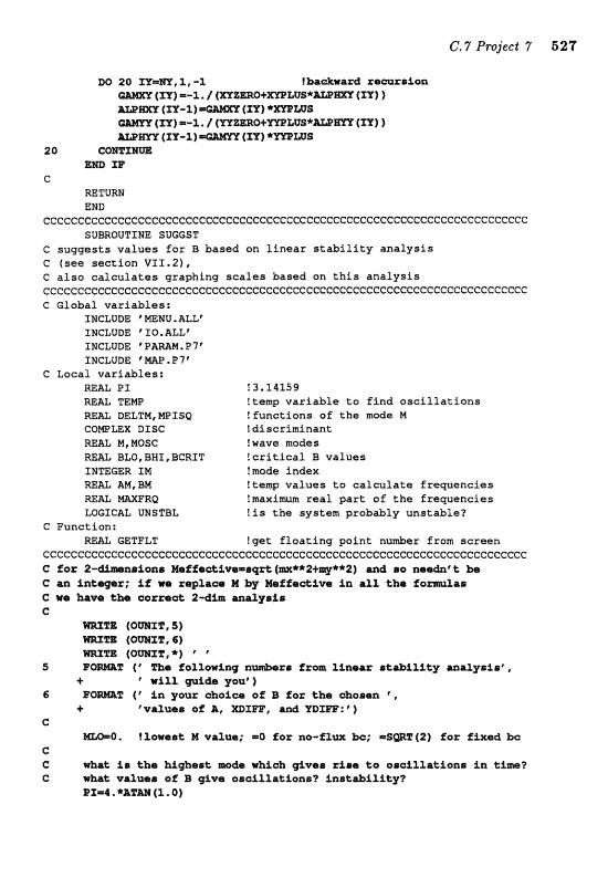
2 0 C@%SZrn m m
C =TURN END
cccccccccccceccc~ccC:cceeccccccccccc~ececccceccccceeccec~ccccccccccccc~cc SUBROUTINE SUGGST
G suggests va lues f a r B based on l i n e a r s t a b i l i t y a n a l y s i s C (see sec t ion V I I . 21, G a l s o c a l c u l a t e s graphin$ s c a l e s based an t h i s a n a l y s i s ~ceccccecccccccecCcccccceecccccecccccceccccccccccccccccccccccccccccccccc C Global var iab les :
INCLUDE "MENU. ALL' INGZUDE F IQ.ALLC INCLUDE ' &&MM. P7' INCLUDE ' W . P ? '
C Local var iab les : REAL PI ! 3 . E4159
TEMP !temp v a r i a b l e t o find. o s c i l l a t i o n s m L DELTM,WTSQ !funct ions of t h e made M ComLBX DISC ? diserimf nanr =&L N,MQS@ !wave modes m L BLB, BWT , BCRIT ! c r i t i c a l B values INmGER I M !made Index
M e BM !temp va lues t o c a l c u l a t e frequencies =&XI =FRO !maximm r e a l p a r t of t h e frequencies LOGICAL UNSTBL !is the system probtrbly unstable?
C Function: !get floating poin t n u d e r from screen
l4 by MEfe&iva An all %ha lao G wa bye %be corracJt ma2ysis C
=SE (am%, S) (Q-E, 6 ) ( Q r n X P , * ) ' '
5 (' me Iclol%owAng +
6 Earn9 ("in p w r o f B f a %h d a 8 e ~ * , + Wvrlues of A, and Y D m : ' )
e 6- !lcnoasC M value; a6 for ne-6Zm be; m S a F ( 2 ) for fixed bc
C C what: i s tba higheat ~todsb wbiah gSvaa rfam f o oaciXl.oLtioaa fn tfm? C w ~ a & v ~ l ~ e s o ~ B g & v e o s c l i X l a t i o n ~ ? i a s t & f X f t y ?
BX=Q. *A%= (l, 0 )
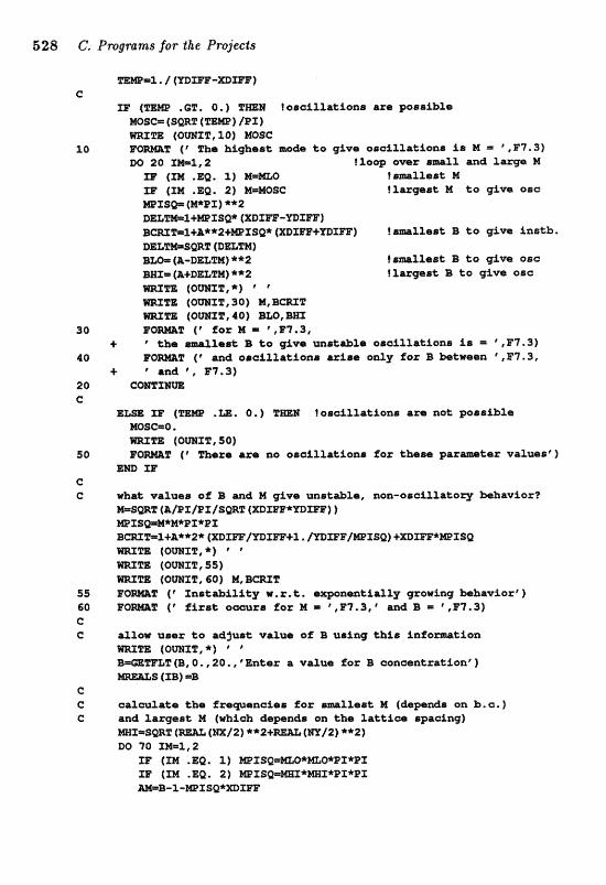
528 C. Programs for the Pr~jeels
mm=% / ( m m - x D m ) e
TmM !osaillatlona are possible
20 ("be hiqhecrt mdk, t o give oocrillationr i n M 5 @,,H7.3) floep ovmr a d 1 and 5wgm M
XF (ZM .Ea. 1) ! sarallaat M IF (TM .BQ. 2) HMOSC ! l u g e a t B# &to give oec =IS* (M*PI) *"2 DE&m%+mIsQ* {XDmF-mm) ~X%=I+&**2+~ZSQ*(DIFP+~Z~) ! s m l l s a t t3 CO @vs inartb. DBLZM=BWF (B=%%) B- (&-DELm) **2 tam2ler t B t o give osc =Zap [A+Dnmj **2 f l egas r t B t o g%ve osc
a X T R (OmZF, 30) (owrzl, 40)
3 0 for M = *,)e"7,3, + mllcr i r t B to #ve watafile eaof?LlttLlons 1s ' 2 7 . 3 1
4 0 FO-2 ( W d osafllakiona w i a a onfy f a r B betwetam @,F7.3,
20 C
,%E. a.) PmI toarcillations aza not. goselbZa
(QWX31,30) 90 EO-T (' %era are no oscrillationar Pox thvass pa
Ern 3x e C W&& vdues o i B a d M e v e una td le , non-ol~ioillatoq babavioz?
e B m T (&/PX/PX/sQR% (DIm*PDXBP) ) mSSW*@BX*f?f. 9~T=l+A**2*(XBX~/DX~+l./UID~F/@SSQ)+~X~*WISQ m m (QrnXT, *) ' ' m m (OmXT,55)
(QaXg, 6Qj 24, B W F 55 (' Xnot&llity w,z.(e. avnenLZoXly growing hbarviorF) 60 ("%rat ocranxm PQE M = f,,F7.3,* aand Er r,,F7.3) C C aZlw meat. t o aeXjusC value o f B usfag t h l s info
(owl%,*) p
t =l =B C C a a a l a t e the f ~ e @ a a e i r s fox amlXeot I# (&pnda on b.c.) C ancl lazgr#t I (whS* depaadrr on t;kr I a e C i a spacing)
IF ( f M ,EQ. 2) WISQ=WZ*mX*PT*PI M=B-%-HBZSQ*=Xm
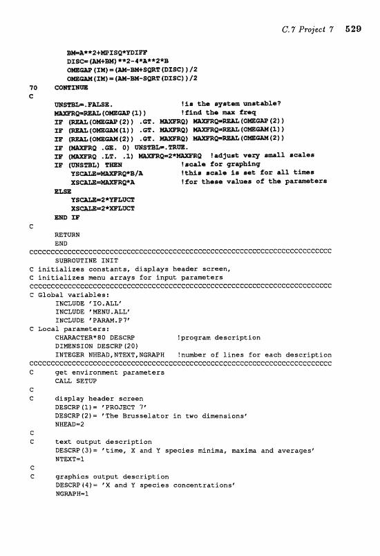
BM=A**2+~TOQ*~fIi'ZT DXSCm (m+M) **2-4*A**2f B
(ZM) (M-mtS@T (DISC) ) 12 f XMf = (U-rn-SWF (DISC) ) 12
70 COmXBm C
O1QSTBL=-FUSE.
!alljust verlf am21 sealas tsaale for graphlng ithis scale 5s scat fop a l l Cfms !for thess vaXnaa o f &he par-l;iarra
m XI)" c
ETURIOI END
cceecccccccccccccccc~ccccccccccccccccccccececcecccceeccccccccccccccccccc SUBROUTINE IHJT
C initializes constants, displays keader seresn, C initializes mnu arrays for input parameters cccccccccCcccccccGeccccccccccecccccccccecccccccccccccccccccccccccccccccc C Global variables:
INCLUDE XIO.ALLt INCLUDE @ MENU. ALL* ZMCLUOE * P A W . P 7'
C Local parameters: CNmCTER*80 DESCRP ?program description DIMMSIoN DESCRP (20) XNTEGER WWEAD,NTEXT,NGMPW !nu&er of lines for each description
ccccccceccecCCececccecceccccccccccc~cceeccccc~cccccccccccccccccccccccccc C get envf ronment parameters
CALL SETUP c C display header screen
BESCRP (1 1 = PROJECT 7 " DESCRIPIZjm "The Brusselator in two dimensionsf HHE&D=2
C C text output description
DESCRP ( 3 ) = 'time, X and V species minima, maxim and averagesf NTmT-2
C C graphics output description
DESCRP ( 4 ) = 'X and V species concentrations" WGmPN=l
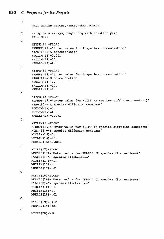
830 C. Pmgram~ for the .P mjeets
CALL READER(DESCW,NWEAD,NTEXT,NaPH)
setup menu a r r a y s , begfnning wi th c o n s t a n t p a r t GALL =NU
MTYPE (13 1 =FLOAT WmPT (13) = 9 n t a s v a l u e f o r A spcies concen t ra t ion ' NTAG (13) =Q cconcentration" ML0LIM(13) =Q* 001 MWILIM (13) 420. m m L S (93) =2*
MT-E f l 4 1 =FLOAT W W T { l $ ) = % n t e s v a l u e fox B smcies c o n c e n t r a t i o n p MTAG (141 m* 8 concen t ra t ion" MLOLXM(14) =Q I
MHILTM(I4f =20.
MTYPE ( l S ) =FLOAT M P W T (15) =*Enter v a l u e for XBIFF ( X spcies d i f f u s i o n c o n s t a n t f * MTAG (15) =% s p e c i e s d i f f u s i o n c a n s t a n t " MLQLIM (15 1 -0. HHTLIM ( 1 5 ) -l 0.
LS (15) =a. 001
MT*E ( 1 G 1 =FLOAT M P m T (161 = # E n t e r v a l u e far YDTFF (U s p c l e a d i f h s i a n c o n s t a n t ) NTAG (1 61 my Y s p e c i e s d i f f u s i o n c o n s t a n t @
moLsn ( 1 61 =a-. MHIEXM (16) -10. MmLS(16)-0.003
NTWE ( 17 ) =FLOAT W W T (17) m* Enter v a l u e f o r XFLUCT (X s p e c i e s f l u c t u a t i o n s ) MTAG f 171 ='X s p e c i e s Ef u c t u a t i a n ' MLQLXM (17) --I, E(UUILXN(f 7)=1. mmzs (17) 1.. 01
MTrPE (1 8) =FLOAT W W P T (18) = ? E n t e r v a l u e f o r YFLUCT f Y s p e c i e s f l u c t u a t i o n s 1 MTAG (18) = @ Y sspeeies f l u e t u a t i o n f MLOLIN (18) m-1.
MHILIM (1 B 1 =l. mEALS (181 -, 01
NTUPE (1 9) =SKTP mALS(19)=35 .

MPRMRT(38)- #Ente r nu&r of X l a t t i c e points1 MTAG (3814 ' N u m b e r of X l a t t i c e po in t s f MLOLIM(38) -1. MHILIM (38)=MAXX: MINTS (38) -20
C MTYFE (39) =NUM MI?RMPT(39)= 'Enter number o f Y l a t t i c e points ' MTAG (39) - 'Number of Y l a t t f ce points1 MLOLIM(39) =l. MNILfM(39)=MAxY MINTS 139) 4%
C MTYPE (401 -NUM MPRMPT (40) - * I n t e g e r random number seed f o r i n i t f luc tua t ions1 MTAG ( 4 0) = * Random number seed1 MLQLIM(40)*1000. MHILXM (40) r99999. MINTS (40) ~ 5 4 7 6 5
C MTYPE (41) *SKIP MREALS (41) -60.
C MSTRNG (MINTS (75) )= ' proj7. t x t t
C MTYPE (76) =SKIP MREALS (76) -80,
C MSTRNG (MINTS (86 ) I = "proj7. grf
C
EmPE (87)=HUM NPRMPT(87) - 'Enter number of contour l e v e l s 1 MTAG ($711 Number of contour l eve l s ' MLOLIM (87)=2. MHILIM (87) 450. MINTS (87) 1 6
C HTYPE (89) =SKIP MREALS (88) =go.
C RETURN END
CCCCCCCCCCcCCCCCcccCCcccCCCcCcCCCCCCC~ccccccccccccccc~~c~cccccccccc~c SUBROUTINE PARAM
C g e t s parameters from screen C ends program on request C c l o s e s old f i l e s C maps menu v a r i a b l e s t o program var iab les C o w n s new ff les C c a l c u l a t e s all d e r i v a t i v e parameters C performs checks on parameters CCCCCCccccCCCCCCCCccCCCCCCCCCCcCCCCCccCcccccccccccccc~ccccccccccccccccc

532 C. Programs for the Projects
C Global variables: JNCLUDE " m N U , ALLf JNCLUDE ' 10. ALL" INCLUDE @ P m M . P 7 * INCLUDE ' W - P ? '
C Functions: LWICAL LQGCVT !converts 1 and O to true and fa lse m L GEmLT ?get floating point numSser from screen INTEGER GETXNT !get integer from screen
CCCCGCCCCCCCCCCCCCCCGCCCCCCCCCCCCCCCCCCCCCCCCCCCCCCCGCCCCCCCCCCCCCCCCCCC C get input from terminal
CALL CLEAR e a L ASK(I,~STQP)
C C stop program i f rewasted
IF (HMALS ( I M A I N ) .EQ, STOP) CA& FTNISW C C close files it necessary
SF (TMAWE . NE. NSTRNG (MINTS (ITNWE) 1 ) + CALL FLCLOS (THME, TUNIT) J F fGNAm . NE, MSTRNG (MINTS (TGHAKE) ) )
+ CALL FLCLOS (GHME, GUNIT) C C set new parameter values C physical and numerical
B - m A L S ( I B ) XDSFF=W&LS TXDXFF) YDXFPmmALS (IYDIFF) XFLUCTmNREALS ( IXFL) YFLUCT-M-LS (TVFL) w x - ~ z ~ ~ s ( rMx) NV=MTNTS (INY) DSmD-DBLE (MINTS ( I D S E W
C C text output
TTERM=LQGCVT (MINTS ( ZTTERM) ) TFXLEmmGCVT (MINTS (1 T F I W f 1 aNm=MsTRWG (MrWrs ( r T N m 1 1
C C graphics output
GTERH=LaGCVT (MINTS lrGI"ERM1 f c a m c P = L s s c v T {MINTS ( IGWRB 1 1 GFZLE=LQCCVT(MXWTs(XGFIZE)) GHME=MSTRNG (MINTS ( XGNAmj 1 NLEVmMXNTS ( IMLEV)
G C openfiles
IF ( T F I M ) CALL FWPEW (TNAm, TUNIT) XI? (GEILE) CALL FLQPEN (GHAm, GUNET) ! f Ales may have been renamed MSTRNG {MINTS (ITN=) ) =TNAm
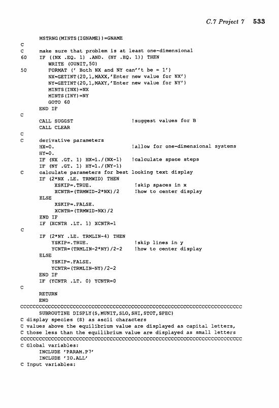
MSTRNG ( M r N T s trcNAMe) =GM- e C make, s u r e t h a t problem i s a t l e a s t one-dimensional 60 IF ((NX .eg, 1) .ma. (MU .EQ, a, , Twew
irJRITE (QUMLT, 50) 5 6 F O R M T ( I Bath NX and NY c a n w t be = 1')
NXmGETINT (20,1,mm, "Enter new value Esr NX' 1 NY=GETINT(20,1,mXY,%nter new value f o r NLMTS ( I N X I =W M I N T S (SNU) =NU EOTQ 60
END L F e
CALL SUGGST !suggest va lues f o r B CALL C m A R
C e d e r i v a t i v e parameters
HX-0. !allow far ane-dimensional systems HU=O. IF (NX . GT. If WX-1, / (NX-1) ! c a l c u l a t e space s t e p s I F (NY . GT. 1) HUm1. / (NY-11
C c a l c u l a t e p a r a m t e r s far best looking t e x t d i s p l a y IF (2*NX .LE, T W X D ) THEN
XSKIP=. TRUE. !@kip spaces i n x X C N T R = ( T W X D - 2 * W X ) / 2 !how t o een te r d i s p l a y
E L S E X S K I P m . PALS E I
XCHTR= ( T R W I D - N X ] /2 END IF Sl? (XCNTR .LT, 1 1 XCMTR=1
C L F (2*NY .LE. T W I N - 4 ) THEN
YSKSP= , TRUE, !skip l i n e s i n y V C N T R = f T M L T N - 2 * N Y f / 2 - 2 !how t o cen te r d i s p l a y
E L S E Y S K I P = . F A L S E , YCNTRm ITRMLIN-NY 1 /2-2
END Z F I F (YGMTR .LT. 0 ) YCNTR-O
e =TURN END
eee~ccceccecceccccccccceeecccceccccccecccececeeecccceccccceeec~ccccccecc SUBROUTINE D I S P L Y (S, MUNTT, SLO, SRI, STQT, S P E C )
G d i s p l a y s p e c i e s ( 5 ) a s a s e i l charac te r s G va lues above t h e equi l ibr ium value are displayed a s c a p i t a l l e t t e r s , C those less than the equi l ibr ium va lue a r e d i sp layed a s small, betters ccccec~ccccccccc~ccccccccccccccccccccccc~cccccccccccc~eC:ceccccecccceccc~ C Global va r iab les :
XNCLUDE P W M . P 7 ' INCLUDE ' I O , ALLe
C Input va r iab les :

534 C. Pmgmms for $he P~ojects
RE& S ( M X X , M Y 1 I s p e ~ i e s v a l u e s INmGER MUWXT !un i t w e t re w r i t i n g t o M A L SLO, SW3, STQT !min,max, and t o t a l conc of s p e c i e s S INTEGER SPEC ! whf ch s p e c i a s
G Local v a r i a b l e s : INTEGER I X , IY ! l a t t i c e i n d i c e s TNmaR STEW ? S a s an i n t e g e r CWmCTER*1 SPECS(MX) ! spec ies as c h a r a c t e r d a t a RE& SZERO !fzero"alue for s p e c i e s BE= SCALE ! sca le for s p e c i e s
!blanks Eer cen te r%ng i n X INTEGER XSPEG,YSPEC l f f a g ta i n d i c a t e s p e c i e s INTEGER CSCBLE l s c a l e aE a s c i i d a t a CWmCTER*1 ASKIII0:2S),MEGASK(O:25) ? c h a r a c data f o r d i s p l a y DATA BLNK I " / D A m A~~I~/~f,t~f,fC~,~*,cE@,'F~,fGf,tB4,fT't'J' e'Kr,'Lf , ' M f ,
4- t ~ ~ , f O t I ~ P * , f Q ~ , ~ R t r F S ' , ~ T e , f U ~ t C V * t f ~ r I'X',fY',8Zf / DATA M E G A S K / * a ~ , f b t , ~ c \ f d * , f e ~ I @ f ~ , * g f , * h @ r f ~ t , r j t ~ ~ k ~ t f ~ p p ~ m r ,
4- ~ n ~ I ~ o ? , @ p * t p q f , ~ r t , f ~ t C 6 t t , ' ~ t , t ~ ~ , F ~ C f ' ~ f , f ~ t y ' ~ r / DATA XSPEC,VSPEC/f,2/ DATA CSC&ZE/ZS/ ! s i n c e t h e r e a r e 26 cha rac
~~~~~~cc~cccCc~ccc~~cccccccececcccccccecccccccccccccccc~cceccecccecccccc IF (MUMET .Ea. OWNIT] THEN CALL CLEM DO 20 IYm1, YCNm ! can te r output
WRITE (OU#TTI") ' 20 CONTINW ! p r i n t ~ u t d a t a
IF (SPEC . EQ. XSPEC) W I T E fOUNXT, 25) SLO, SHI, STOT IF (SPEC . EQ. YSPEC) WRITE (OWIT, 26) SW, SXI, STOT
2 5 PORMT(1SX,'X min =ifjF?,3,f X max *",F7-3rf X average =81F7s3) 26 FOmT(15X,rY min =t , ,F7.3 , t Y max af,F7,3,@ Y average =f8,E"7.3f
ELSE, WXTE (MUNIT, *) ' IF (SPEC . EQ. XSPEC) mITE (NUWIT, *
+- * X s p a c i e s c a n c e n t r a t i o n - A:@ IF (SPEC . EQ. YSPEG) WRITE (MUNIT, *)
4" * V s p e c i e s concen t ra t fon - A/B;" END IF
c IF (SPEC .EQ. XSPEC) THEN !set, s c a l e s
SZERCI=& !X e q a i l v a l u e SCALE=XSCAW/CSCAm
ELSE: XF (SPEC .EQ. VSPEC) THEN SZERO-S/A !P e q u i l v a l u e SCALE=YSCAm/CSCBm
END TF c
DO 100 TY-RV, 1, -1 DO 50 IX=1,NX !STEM? is s c a l e d d e v i a t i o n from SZERO
STEW=NINT ( (S ( X , EY) -SZEROj ISCAU) IP (STEW .GT. CSCAm) STEMP=CSCALE IF ( S m W .LT. -CSCALE) STEMPm-CSCAm
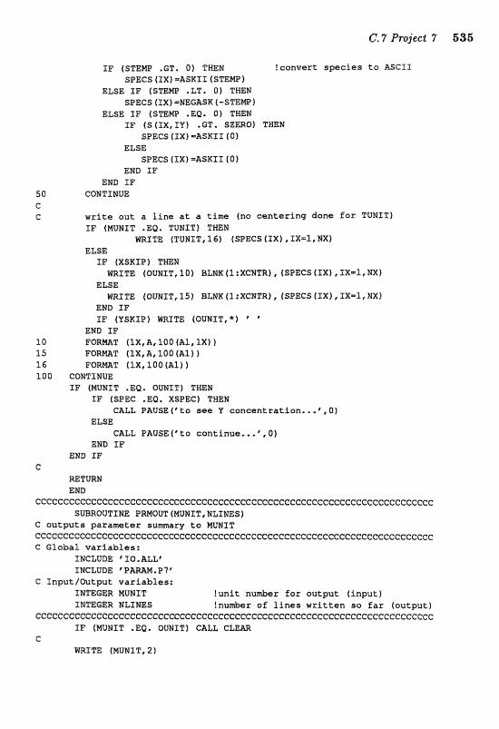
I F (STEMP .GT. 0 ) THEN ! c o n v e r t species t o ASCI I SPECS EXX) -ASKIX. (S"PEEZP)
ELSE IF (STEMP .LT. 0) TEEN SPECS [XX) =NEEASK (-STEW)
ELSE I F (STEMP .EQ, 0) THEN I F ( S (SX, I Y ) .GT. SZERD) TEEN
SPECS (SX) =ASK11 (0) ELSE
SPECS [ IX) =&SKI I ( 0) END I F
END I F CONTINUE
w r i t e o u f a l i n e a t a t i m e r (no c e n t e r i n g d o n e for TUNITI f F (MUNIT .EQ. TUNIT) THEN
%RITE {TUNIT, 1 6 ) (SPECS {IX) , IX=I , EX] ELSE
I F (XSKIPI WEN WRITE (OUNZT, 1 0 ) BLNK ( I :XCNTR) , (SPECS (1x1 , IX=1, NXI
ELSE WRXTE (OUNIT, 25) BLNK(l:XCNTR), (SPECS ( IX), X X = I , NX)
END I F I F (YSKIP) WRITE (OUNITI*I ' '
END I F 1 0 FORMAT ( l X , a , 1 0 0 (A1,IX) 15 FORMAT ( l X , A , 1 0 0 ( A l l I 1 6 FORMAT f l X , 1 0 0 ( A l l f 1 0 0 CONTXNUE
I F (MUNIT .EQ, OUNIT] THEN I F (SPEC .EQ. XSPEC) THEN
CALL PAUSE(-o see Y c o n c e n t r a t i o n . . . ' , O ) ELSE
CALL PAUSE( ' to c o n t i n u e . , . ' , O ) ehia IF
EHD IF I
RETURN END
cccccccccccccccccccccccccccccccccccccccccccccccccccccccccccccccccccccccc SUBROUTXlsE PRMOUT (MUMIT, NLZtdES)
C o u t p u t s p a r a m e t e r summary t o MUWZT ccccccccccccccccccccccccccccccccccccccccC(:ccccc~"cccccccccccccccccccccccc C G l o b a l v a r i a b l e s :
INCLUDE ' I0 .ALLF LNCLVDE 'PARAM.P?'
6 I n p u t / O u t p u t v a r i a b l e s : INTEGER MUNIT ! u n i t number: f o r o u t p u t ( i n p u t ) INTEGER NLINES !number o f l i n e s w r i t t e n so far ( o u t p u t )
CcecCCCcCcCCcCCCCCCcCCcccccCcCCcCcCCccccccccccccccccCcccccccccccccCccccc I F (NUNIT .EQ. OUIIT) CALL CLEAR
e WRITE (MUNIT, 2)

536 6. Pwgmnas JOP" the IJro;lieets
&JRTTIT, (MUNIT* 4) W f T E (MUNIT, 6 ) B,B WmTE (MUNIT, B ) XDIFF, YDIm lrJRITE (MUNIT, 10) XFLUCT, YFLUCT T?SBI"f (NUNIT, 12) EJX,NV WRITE (MUNST, 16 ) MLO, OMEGAP (l ) , OmGAW (1 1 WRI TE (MUNIT, 16) M H I , OMEGAP (2) ,0MGAM (2) mITE (MUNIT, 14) m I T E (MUHIT, 2)
C NLII"JES=10
c 2 F O m T ("k 4 F O m T ("~roject 7: B r u s s e l a t o r i n two dimensions" ,
6 FORWT (Q c o n c e n t r a t i o n ,F8,3,5X,'B c o n c e n t r a t i o n =\,F8.Jf 8 F O m T (" X s p e c i e s d i f f u s i o n = \,19EX2.5,5X,
-I- @ Y s p e c i e s d i f f u s i a n = ',lPE12.5) 10 F O M T (' X species i n i t f l u c t = qSPE12.5, 5XI
-i- U s p e c i e s i n i t f l u c t = 1PE12.5) 12 F Q R M T ( 6 N X = * , S 4 , 5 X , ' N Y m * , , % 4 1 14 FORMAT (' a l l v a l u e s are i n s c a l e d u n i t s r ) 1 6 F Q M T (' f o r H=\ ,FT, 3, * tba f r e q u e n c i e s a r e ' p
+ 2 t 2X,* { " r F 7 . 3 , * e 6 , r F 7 . 3 , r f i ) 1 C
rnTURH END
~ c e c c c c c c c c c c c c c C c c c c c c e c c c c c c c c e c c c c ~ SUBROUTINE TXTOUT (NUNJT, MLLHESt TXW* XLO, XWI XTOZ", VLO, Y H I VTOT)
C w r i t e s r e s u l t s f o r one t i m e s t e p t o MUMlT eecceccccccccc~ccccccccccceccceccccceccccccccccccccceecf:ccceccceeccccc~c e Global v a r i a b l e s :
INCLUDE @ X 0 . ALL" C Inpu t v a r i a b l e s :
INTEGER MUMIT t ou tgu t u n i t s p e c i f i e r RE& TINE !time INTEGER NLImS !number of l i n e s p r i n t e d so f a r ( I l o ) =U XLO, XHT , XWT !min,max, and t o t a l cone of s p e c i e s X MAL YLO, YHX, UTOT !min,mnax, and t o t a l conc af s p e c i e s V
CCG~GCCCG~CCCGCC~CCGCC~CCCCCCCGCCCCGCCCGCCCCCCCCC~CC=CCC:CCCCCC~~CCCCCGCCC C i f s c r e e n is f u l l , efaar s c r e e n and r e t y p e head ings
I F ( (MOD (NLXmS, TRMLIN-4f .EQ. Q)
-k .AND. (MUNIT .Ea. oUNJT) ,AND. (.NOT, GTEm) ) THEN CALL PAUSE:tPto c o n t i n u e , . . @ , l f CALL CLzm m I T E (MUHIT, 14) WRITE (MUMPT, 16) NLfMES=.;NLSN&S+2
EAlD PP C
m I T E (MUWIT, I Q ) TIME, XLO,XRI, XTOT, YLO,YWI, VTQT C keep t r a c k o f p r i n t e d l i n e s on ly Ear t e m i n a l ou tpu t
I F {MUNIT .EQ. OUNIT} NLINES=NLINES+1
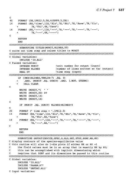
C 40 F Q m T (3X,lPE12,5,5X,6fOPF8.3,2X]) 24 F O W T (8X,~tfne~,llX,*Xxl0~~7X,~Xhi~~7X~@Xa~e~,7X,~Yl~',
+ 7X, Thicr 6X, "avee" ) l6 F O m T (8X,"---8 , l l x , ~ - - t , ?X, P ---t ?X, L=--*, ?X, f - - - t ,
i ? X , 1 ---" ,6, ' ----I 1 C
RETURN END
ccccccccccccc~ccCcecccccccccccccccccccccccecceececC:ccccccc~cccccccccceec SUBROUTIRE TITLES (MUNI T, NLIWES, DTf
C write out time step and column titles to NUNIT ccCccccccccccccccccececccccccecccccceccccccceccccccccc~ccccccccccccccccc C Global variables:
INCLUDE ' I T O .ALL' C Passed variables:
1MTEC;ER MUNXT !unit number for output (input) INTEGER NEIRES !nu&er o f lines written so far foutputf =L DT !tfm step (input)
cccccccecccccccccccccccccececcccccccccceccec1ccccc~ccccccccccceccccCccccc I F ( (MOD (NLIWES, TRMLTN-7) .EQ. Of
+ .AND, (NUHIT .EQ. OUNTT) .AND, (.NOT. GTERM) J + CALL C L E M
c m I T E (MUNIT,*) ' mZTE (MONIT,PO) BT WRITE (MUNIT, 14) mITE (MUWIT, 16)
e SF (MUWIT .EQ. OUEaIT) NLINES=NLINES+B
C 20 FORElAT fqteme step E. t,1PE12.S) 14 FORmT I 8 X , rtime% IlX, 'XXT*, ?X, 'Xhir , ? X , IXavei '?X8 6 Y l a r ,
4" "?X, "hi * ,6X, * Yavef ) l6 FORmT (@X, '----" ,11X6 '--mf ,?X, " - - F , ? X , P ? X , - - -@ ,
+ ?X, f ---I, ,CX, p m---" 1 e
RETURN END
Ccccccccccc~cccceccccccccccceccccccC:cccccccccccccccccccccccccccccccccccc SUBROUTINE CWOUT (DEVICE, SPEC, S, SLO, SWI, STOT, SGWI MX, MY)
C display contours of- the species-equilibrium value C this routine will also do l-dim plots if either NX ar NI' -3. C the field values must be in an array that is exactly NX by NY; C this can be accomplished with implicit dimensioning which C rewires that SGRF and its dimensions be passed to this rautine c c c c c c c c e c c c c c c c c c c e e c e c c c c c c e c c c c c c c c C Global variables:
INCLUDE @ IQ. ALLf INCLUDE 'PAMN.P7" INCLUDE ' GRFDAT . ALLF
C Input variables:
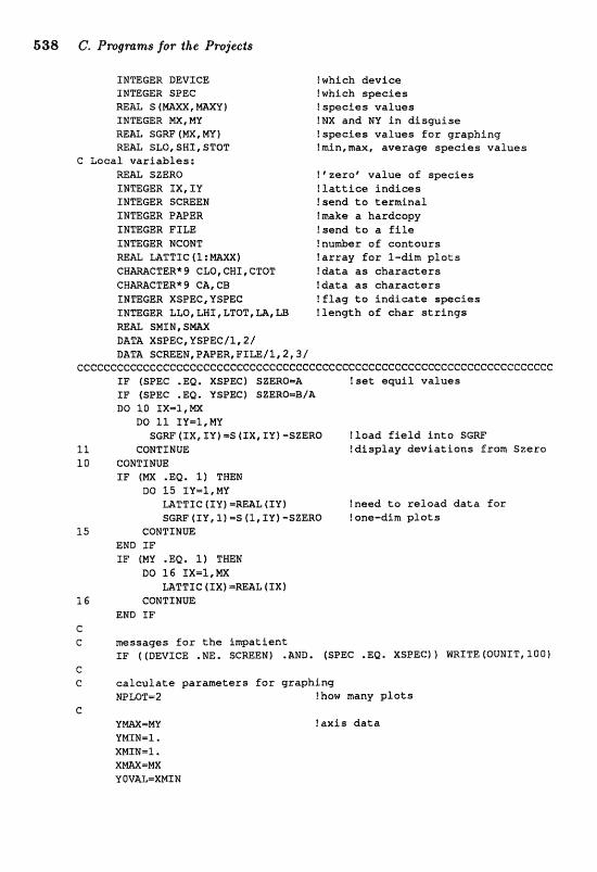
INTEGER DEVICE !which device INTEGER SPEC ! which spcies RE& S ( W X , M U ) !species values INTEGER M , N Y !NX and NU i n d i sgu ise RE= S G R F ( m , W ) !species va lues f o r graphing REAL SLD, S H I , STOT ?min,max, average spec ies values
C Local var iab les : mAL SZERQ !"zero' value of spec ies f NTEGER f X , I Y ? l a t t i c e i n d i c e s INTEGER SCREEN !send t o terminal I;P;IEGER P W E R !make a hardcopy XWmGER FILE ! sand t o a f i l c INmGER EJCONT ! n u d e s of contours
!array for 1-dim p l o t s C R m C T E R * 9 CLQ,CWI,CTOT !data a s c h a r a c t e r s CWWCTER* 9 CA, CB !da ta as charac te rs INTEGER XSPEC, IFSPEC ! f l a g t o i n d i c a t e spec ies TNmGER LLQ,LWI,LTOT,M,LE ! length of char s t r i n g s WAL, SMIN, S m X rlATA XSPEC,IFSPEC/1,2/ DATA SCmEPJ ,PAPER,F Im/1 ,2 ,31
ececccCcccccc~e~eeeccecccccccccccCececcce~cceceeceeecccecceccccec~cccccc I F (SPEC .EQ. XSPECI SZERO=h !set equif va lues I F (SPEC .EQ. YSPEC) SZERO=B/A DO 1 0 3 X = 1 , m
BD 11 XY=1,MY S C W ( I X , f Y) =S ( IX , SV) -SZERO ! load f i e l d i n t o SGW
11, CONTINUE !display dev ia t ions from Szero 1 0 COWTIWUE
SF (m .EQ. l) THEN ao 1.5 XV=I,W
U T T I C f IY) ==&L (XY 1 !need t o re load d a t a for SGW(IY,l)-S(1,XlP)-SZZRQ !one-d inp lo t s
15 CONTZNUE END XF IF (MY .EQ. 1) THEN
DO 16 PX=l,NX M T T I C f f X f ==&l, ( I X )
16 CONTINUE END I F
C C messages f o r t h e impatient
I F ( (DEVICE .NE, SCREEN) .AND, (SPEC .EQ, XSPEC) 1 m I T E (OUNIT, 100) e C c a l c u l a t e paranreters f o r graphing
WLOT=2 !how many p l o t s C
U W = N ? Y !ax i s d a t a VNIN=l, X M I N m l . X W = N X YOV~Z=X1VIXW
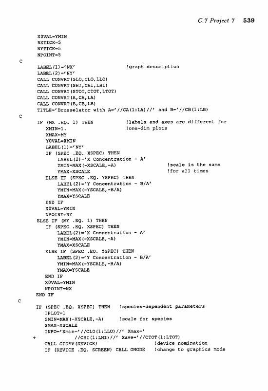
XOV"AL=YMf hT NXTZCICm5 NVTICK-S NFOINTm5
C: U B E L (1) ="X8 ! g r a p h d e s c r i p t i o n m E L (2) ='NU8 CALL CON-T 1 SLQ , CLO, LLO) CA& e a m t f (swr, CHS , LWI I CALL COMVRT (STOT, CTOT, LTQT) G&& CONmZ: (A, CA, LA) CALL C O m T ( B , C B , a ) TITLE=' B r u s s e l a t o r w i t h A="/CA(l:zzl) / / h a n d B=' / / eB( l :LB)
C: I F (NX .EQ. f ) THEN !labels and a x e s are differenf for
XMTN-1. !one-dim p l o t s XrnXmPIM YOVAL-XMIN -EL (3.1 NVe I F (SPEC .EQ. XSPEG) THEN
LABEL ( 2 ) =*X C o n c e n t r a t i o n - A' UMf PJmMX 4-XSCALE, -A) !scale is the s a m e YmX=XSCUE !for a l l t i m e s
ELSE I F (SPEC .EQ. VSPEC) THEN =EL (21 m' lr" C o n c e n t r a t i o n - B/At uarW=mx (-YSCALE, -B/A) U M a Y S C S E
END XF XOVAL=YXXM NPOINT=NU
ELSE I F {MU . EQ. 1) THEN SF (SPEC .EQ. XSPEC) THEN
LABEL (2) m r X Concent r a t i o n - A* YMINmW [-XSCALB, -A) 'I"mX=XSC&E
ELSE SF (SPEC .EQ. YSBEC) TmM M B E L ( 2 ) mfY G o n e a n t ~ a t ; i o n - B/Ar YNIIU=MX ( - Y S C U , -B/&) YW=YSG&E
END I F XOVAL-VMXEJ NPOINT=I?JX
END I F C
I F (SPEC .%Q. XSPEG) THEN ? s p e c i e s - d e p t s n d e n t pa ramc3 texs IPLOT=1 SMZN-mX f -XSCALE, -A) tseale f o r species SMX=XSCALE IN FOP^ XmPn=' / /CL0 (1 : LLO) I / @ Xmaxmt
+ / / C H I ( ~ : L H I ~ / / * X ~ V ~ = ~ / / C T ~ T ( S : L T O T ) CALL GTDEV (DEVICE) !device nomination I F (DEVICE .E@. SCmEN) CALL GMOBE ! c h a n g e ta graphics mode
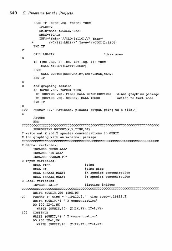
540 C. Pmgnanas for #he Projects
ELSE XF (SPEC .EQ, YSPEC) TNEN IPLOT-2 S M I N n W ( - Y S C U , -B/A) SW=')ISCALE XMFQ=yYdon=f //C&O(1:LLQ} / / I Y w x = '
-6 //CNI(l:LBS)//' Yave='//CTOT(1:LTOT) END IF
c CALL LNLNAX l draw axes
G IF ((m .EQ, 1) .OR. (MY ,Ea. 1)) THEN
CALL XYPLOT (MTTXG, S G W ) ELSE
CALL GQNTOR ( SGRF, W, m, SMIM , SmX, NLEV} END IF
I;
C end grapbing session SF (SPEC .EQ. YSPEC) TNEN IF (DEVICE .NE. FILE) GALL GPAGE(DEVICE1 ?close graphics package SF IDEVXCE .EQ, SCmEN) C U L TMODE !suiteh to text made
END IF e 100 F O m T (/,"aatienc, gfaaee; output going t~ a fiXee8) C
RETURN END
cccccccccccccccccceccccccceccceccccccccccccccccccecccccCccc~cccceccccccc SUBROUTIlldE mTOVT (X, V, TIW, BTf
C write out X and Y speeiss concentrations to GUNIT C for graphing with an external package cccccccccccccccceccccccccccccccccccccccccccccccccccccccccccccccccccccccc C Global variables;
INCLUDE @ mNU. ALL' INCLUDE ' XO. ALLe
C Input variables: =L T I m !time M U DT !time seep REAL X IMAXX,mXY) !X species concentration Mm Y ( W X , m X Y ) !Y spscfas concentration
G Local variables: ZNTEGER IXI XV !lattice indices
ccccccccccccc~cc~ccccccccccccccc~cccccccccccccecccccccc~ccccee~ccccccccc WRITE (GUNIT, 20) TIm, DT
20 F O m T (' time = IPEf 2.5, V i m e stepmf, lPE12.5) m I T E (GUNIT,*) X conceentratfonr Do 100 IX=E,MX m I T E (GUN1 T, l O J (X (SX, IY) , IY=I, NY)
100 COWTIWUE m I T E (GUNIT,*) @ Y cooncen$ratione B0 200 SXm1,NX WRITE (GUN&$ ,101 fY ( X X , XY) r ZY-1 , W')
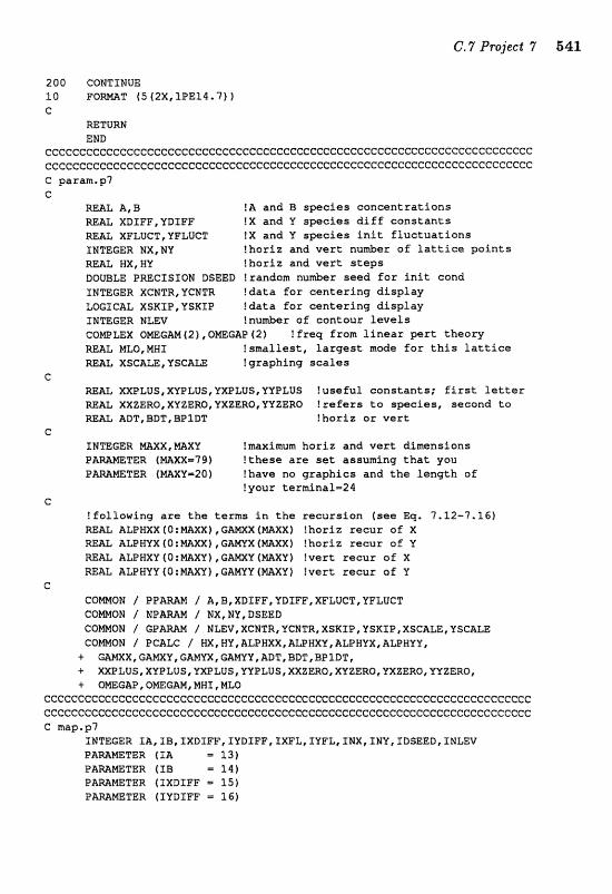
200 CONTINUE 10 F O m T 45 ( 2 X , IPE14.71) C
RETURN END
CCGCCCCCCCCC@CCCCCCCCGCC:CGCCCCCGGCCCCCCCCCCCCCCCCCCCCCCCCCCCCCCCCCCCCCCC ccc~cccccccccccccccecccccccccccccecccccccecccccccccccccccccccccccccccccc C param.p7 c
REAL A,B l & and B spec ies concentrat ions XDIFF, YDIFF !X and Y spec ies d i f f cons tan ts
RE& XFLUCT,YFLUCT ? X and Y spec ies i n i t f l u c t u a t i o n s INTEGER NX, NY !horbz and v e r t nu&er aE l a t t i c e po in t s REAL HX, HY !horiz and v e r t s t e p s DQUBLE PRECISSON DSEED trandam nurnber seed f o r i n i t cond INTEGER XCMTR,YCNTR !da ta f o r cen ta r ing d i sp lay LOGZGAL XSKfP,YSKZP !data f o r centesing d i sp lay INmGER NLEV !number a f contour l e v e l s COWLEX OmGM (2),0MEG&P (2) l Ereq from l i n e a r p e r t theory -6, MLO, M W I !smallest , Largest made f o r t h i s l a t t i c e m A L XSCUE,YSC&M Igraphing s c a l e s
C miql XXPLUS,XYPLUS,YXPLOS,TYPLUS !usefu l constants ; f i r s t l e t t e r REAL XXZERO,XYZERO,YXZERO,VYZERQ ! r e f e r s t o species , second t o RE- BDT,BDT,BPIDT fhor iz o r v e r t
C IN 'XIEaR m X X , m X V !maximum hor iz and v e r t dimensions PmMETER (=X1791 ! these a r e set assuming t h a t you
ETER (WY-20) !have no graphics and t h e length of !your terminalm24
C !following a r e t h e terms i n t h e recursion (see Eq. 7-12-7.16) RE= ALFHXX([Z:WXI,G~XX(WX) !boriz xeeur of X
1 , GAWX ( W X ) !horiz recur of Y ) , GAMXV ( m y f ! w e l t r ecur aE X 1 , f m V ) l v e r t recur of P
c COWQN / P P A m I A,B,XDTFF,YDIFF,XFLUCT,YFLUGT COM016 / HP&= / NX,NY,DSEED COWQN / GPAMM / NLEV~XCNTR,PCNTR,XSKJP~VSRXP~XSCALE,YSCALE
MV,AZIPWXX,WLPHXV,ALPWYX,ALPBVU,
+ OmGAP,OmGAM,MHX,MLO cccccecccc~ccceccccc~c~cccccccc~ec~cceccccccccccccccccccccccccecC:ccccccc c~cccccccceccccccccccceccccccecccccccccccccccccccccccccecceccccceccccccc C mag.p7
IMTEGER I A , IB, SXDIFF, IVDSEF, XXFL,, SVFL, ENX, ZNY, IDSEED, 1EJLEV T E R ( I A =l31
PAMmTER (IB = 141 P m m T Z R f IXDXFF - 25)
ETER (IYDIFF = 16)

P m M T E R (XXFL = 2 7 ) PAmmTER (IVFL 18) PAMmTER (INX = 38)
'I 'ER(TW = 3 9 ) PAMmTER (SDSEED 9 40) PAMmTER ( I N a V = 87)
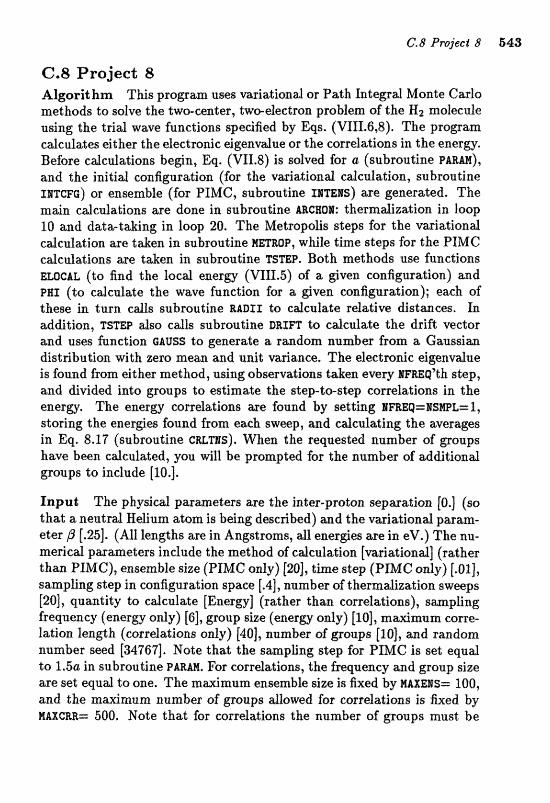
C.8 Project 8 Algorithm This program uses variational or Path Integral Monte Carlo mthoets to solve the two-center, twwelectron problem of the H2 mdecule using the trial wave functions specified by Eqs. (VIII.6,8). The program calculates either the electronic eigendue or the correlations in the energy, Before calculations begin, Eq. (VII.8) i s solved for a (subroutine FARM), and the initial configuration (for the variational calculation, subroutine IITCFC) or ensemble (for PIMC, subroutine IITERS) are generated. The majn cdculations are done in subroutine AacsoH: thermazation in loop 10 and datatabing in loop 20. The Metropolis steps for the variational edculation are t&en in subroutine R ~ B O P , while time bsteps for the PIMC caleul;3ltions me t&en in subroutine " f ~ m ~ . Both methods use fanetions ELoCnL (to find the local energy (VIII.5) of a given configuration) and PAI (to calculate the wave function for a given configuration); each of these in turn calls subroutine RABXX to cdcalate relative distmces* IE ddition, 3["sTP &so c d k stt"fiout;iae BR3[m to cdcalate the drift vector and uses function GAUSS to generate a random number from a Gaussiw distdbution with, zero mean a d unit =dance. The electro~c dgenvdue is found from either method, adng observatians t&en every E F R E Q ~ ~ step, aad divided into goups to estimate the step-to-step carmlations in the enera. The merlgy correlations ase faund by setting E ~ E Q = = A ~ S M P L = ~ , staring the energies found from each sweep, and calculating the aver- in Eq. 8.17 (subroutine CRLTIIS). When the requested number of p u p s have been calculated, you will be prornpted for the number of additional groups to include [IO.].
Input The physical parameters are the inter-proton separation [a.] (so that a neutral Helium atom is being described) and the variational param- eter p [.25]. (All lengths are in Angstroms, all energies are in eV.) The nu- meric& paameters include the method of cdculation variational] (rather than PIMC), ensemble size (PIMC only) [20], time step (PIMC only) [.Ol], sampling step in configuration space [.4], number of t hermdization sweeps [20], quantity to calculate [Energy] (rather than correlations), sampling frequency (energy only) [G] , group size (energy only) [IQ], maJrimum corre- lation length (correlations only) [40], number of poups [IQ], and random number seed [34767]. Note that the sampling step for PIMC i s set equal to 1.5~ in subroutine PnRnn. For correlations, the frequency and group size me se% equd to one. The maximum ensemble size is fixed by WAX=S= 100, and the maximum number of groups al10wed for correlations is fixed by RAXCRE= 500, Mote that for corrddions the number of noups must be

sipificmtly larger than the maximum correlation length (so the av- erages in Eq. 8.17 are st&isticdly sig&fiemt), but must &so be smder than HAXCRR. These checks are perfarmed in subroutine PARAN. The text output parmeter dows you to choose the short version of the output for which the sample sums are not displayed [long version enabled]. Please see the note in C,? concer~ag the random number seed and compiler storage of inlegtlrs.
Output Every NFREQ"~ step the text output displays the goup index, sample index, group size, and energy (unless the short version of the out- put is requested). For the electronic eigenvalue calculation, when each group is finished (every ~ F ~ Q * E S W P L ' ~ ~ step), the text displays the group index, number of goups, average group eneru, and g r o ~ g uncertainty as well as the total (inclading all groups calculated so far) average energy, the two estimzltes for the uncertainty in the enerm, the total energ of the Hz system, and the acceptance ratio (variational method only). For the correlation calcul&ions, when ajli g r o q are complete, the program dis- plays correlation vs. correlation length; the results are plotted if graphics are requested, or &e we vrritten as text.
ccc~ccccccccecccccc~ccccccecccccccecccccccccccccccceccccccccccCccccccccc PRQGMM PR038
C Praject 8: Monte Carlo solution of the H2 molecule C C0WUTATIONAL PHYSICS (FORTMM VERSION) C by Steven E, Koonin and Dawn C. Neredith C Cowright 1989, Addison-Wasley Publishing Company ccccceccccccccccccceccccccce~ccceeccccccccccccccccccecccccccccceecccC:ccc
CALL INXT ?display header screen, setup parameters S CONTXMUE !main loop/ execute once for each set of param
C U L PARAM !get input from screen CALL ARCMON !calculate the efgenvalue far this value of S
EOTO 5 END
CCCCCCCCCCCCCCCGCCeCCCGCCCCCCCCCGCCCCCCCCCCCCCCCCGCCCCGCCCCCCCCCCCCCCCCC SUBROUTINE mCHOM
C calculates t h e electronic eigenvalue or enerm auto-corralation C for a given separation of the protons cccccccccccc~ccC~ecccceceeccccccccceccecceccecccccccccccceecccccc~cccccc C Global variables:
INCLUDE q m M . P 8 " INCLUDE CIO,ALL'
C Local variables: C enerw has two indices C first index is the level: sweep, group, or total C second index is the value: quantity, quantex2, or signa**2
R m L ENERGY [ 3‘3 ) ! energy REAL COlilFXG lhfCOQRD) !configuration

REhL W !weight Ear s i n g l e v a r i a t i o n a l c o n f i g W L WEIGHT (WENS 1 !weight of ensefirble meders R N eNSIYLI3&(MCOOW,mXEMS) !ense&le of c o n f i g u r a t i o n s R W ESAVE ( m X C m ) ! a r r ay of f o c a l e n e r g i e s f o r c o r r REAL EPSILN t l a c a l energy of CONFIG =&L ACCPT ! acceptance r a t i o XNTEGER ITHEW t t h e r m a l i z a t i o n index INTEGER ISWP,TSMPL !sweep and sample index INTEGER IQUAWT I w a n t f t y index INTEGER IGRP !group index INmGER NLINES !nu&er of l i n e s p r i n t a d to t e r m i n a l
INTEGER MO= !how many mre groups INmGER SaEQ,GROUP,TOTAL !which levef of c a l c u l a t i o n INTeGER VALUE,SQUW,SICSQ !which q u a n t i t y INmGER CORR, EPS !what i s be ing c a l c u l a t e d ? INmGER P IMC , VARY !which methad?
C Functions: REAL ELOCAL !local energy INTEGER CETINT !get i n t e g e r d a t a Eran s c r e e n DATA SWEP , GROUP, TOTAL/I, DATA VALUE, SQUAM, SXGSQ/1,2,3/ DATA EPS,COm /1,2/ DATA VARY,PXMG /1 ,21
cCcecCCccccccccccccccccccccccecceecccccccccccceaccccceccccccccccccccccccc C o u t p u t s u m a r y o f p a r a m e t e r s
IF (TTEW) CALL PWOUT (OUNIT, NLINES 1 IF (TFIm) CALL PRPIIOUT f TUNTT, %LINES) If (GFILE) CALL PMOUT (GUMIT, NLINES)
G G gmnrr~t~ ialtial mnfi~urrtion or ansdle of oonflgurationa
(W2fBOD .EQ. V-%) TmE IE%WG (C-%C, I)
a&= C ~ F B O D .W. BZMCI m m
Ern m C
EBD IE X 0 c m 2 x m C
DO 11 IQUANT-1,3 ENERGY (TOTAL, IQUANT} =Q.
11 CONTXNUE ACCPT=O WOE-NGROUP
!ze ro t o t a l sums
!zero accep tance ! i n i t i a l number of groups
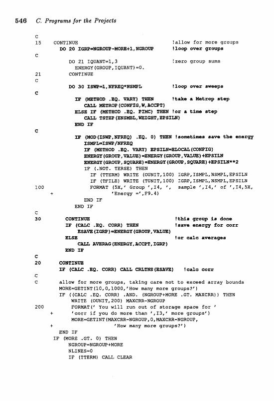
546 6. P ~ m m s for the Pprgjects
!allow f o r more groups !l@* over 9ze-e
!zero group sums
C 15 CONTINUE
ao zo zm=~aom-~am+1,~aom C
DO 21 IQUANT=1, S ENERGY(GRoUP,IQVANTw
23 CONTINUE G
!loop evmr @weep# C
tt- a @&cap =L mTRoF (CaWf @,W, & C a ( r )
ELSE IB" (aTBOB .BQe PXHC) for a t h step TSTW (EMS=%, m G a T , WSXLE)
EH@ PE
nE1- (HOD (XSrn,
IF (.NOT. TERSE) TNEN I F (TTERM) m I T E (OUNf T, 3 0 0 ) XGRP, XSWL, NSWL, EPSILN IF (TFf LE) WRXm (TUWIT, 100) IGRP, TSHPL, NSMPL, EPSXLN FORNAT ( 5 X , "roup * ( 1 4 , * sanrple "19,' of \,X4,5X,
"nergy =*,F9,4) END IF
END IP
CQWZNm !tkis %reap f a dexm 4 .BQ. CO=) F= laava ahnaarw for csrr E a r n ( Z m ) =EmRGY {=@m,
=BE !or O.ZLZQ a w e z ~ q e ~ { g m = , XCEZ, X-)
Ern X@ C 20
3 3 Q . S E l czab aorr C C affaw f o r mare groups, taking care not to exceed a r r a y bounds
MQRE=GETXMT (10,0, 10QOI WOW many more graups?? 1 I F ((CALC .EQ, GORR) .AND. (N@OUP+MORE .GT. NXGRR)) TNEN
WRITE (OUNIT, 200 ) mXCRR-HGROUP 200 FORmT(' You will run out of s t o r a g e space f o r "
+ "err if you do mare than "I3, ' more gr@upse) MOREmGETINTtMXCRR-NGROUP,B,mXCRR-NGROOP,
f # How many mare groups3' 1 END IF
IF (NORE .GT. 0) THEN NGRQUZI=NGROW+MQRE NLINESmO IF (TTERM) CALL CLEAR
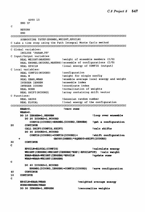
GQW 115 END IF
C ftETURX END
cccccccCccccccccccccccccccccccccccccccccccccecccceeecceceeccf:cccccccccc~ SUBROUTINE TSTEP(ENSNBL,WEIGHTCEE"51:tNl
C take a tim step using the Path Sntegral Nante Carlo method ~~cc~~cCcccc~cccccceccccecccccccccccc~ccccceecececcccececccccccccccccccc C Global variables:
INCLUDE 'PAM,P8' C Input/<put variables
RE&L InJEIGHT (WENS) !weight o f ansemble m e w r s fI/O) REAL ENSmL(NCOOm,WXENS) !ense&la o f configurations (X/QZ m L EPSZLN !Sacal enerw o f CONFIG (output)
C Local variables: REAL CONFIG (NCOORD ! conff guration RE& R !weight for single config R m L E B m , lclrnsnrble average local. energy and weight: INTEGER XENSEM !anse&le index INmGER XCOQRD !coordinats index N A L NQW tnamalfzation af weights REAL SHIFT (NGQORB) !array containing drift vector
C Functions: RML GAUSS !Gaussian random nu+r W& EWCAL !30ml. energy o f t h e conflpration
ccccecccccccccccccccecccca;.ecccccccccceccccccccccc~cccccccecccccccccccccc 0 , 0 .
!log, war mueeZr
20 cONTIIx= a m l (cOm16, saw% 1 Icra%cr rhi_irCn
M) 3.0 XCW~11,8CWrn
+ J 0 C
C
4 0 110 comxm e
DO 90 =88==5, -SEX
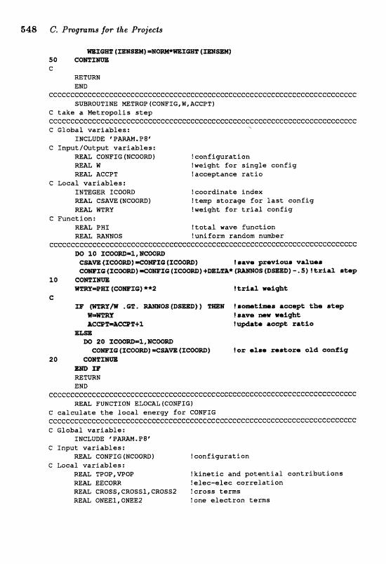
548 C. P.rogrmms for the Projects
(mSm) = B m m I G E F (TrnSEM) SO Cam G
RETURN END
cccceccceeecccceccccccceccc~cccccccccccccccccccccceccccceccccccceccecccc SUBROUTINE mTROP (COWFZG, W, BCCPT)
C t a k e a W t r a p e l i s s t e p CCCCCCCCCCCCCCCCGCCCCCCCCCCCCCCCCCCCCCCCCCCCCCeCCCCCCGGCCCCCCCCCCCCCCCCC G Global var iab les :
INCLUDE PAMM. P 8' C Xnput/Output var iab les :
WAL COKFIG IP;ICOORD) ! c o n E i p r a t i o n =U H !weight for single conf ig REAL ACCPT !acceptance r a t i o
C Local var iab les : I N T E ~ R r e a o ~ ~ !coordinate index R ~ L CSAVE (WCOORD) !temp storage f a r l a s t conf ig =&L, MTRY !weight f o r t r i a l conf ig
C Function: RmL PBX ! t o t a l wave funct ion REAL MNWOS !uniform random n u d e r
CCCGCCCCGCCCCC@CCCCCGCCCCCCCCCCCCCC~CC~CCCCGCCCCCC~CC~CCC~CCCCCCCCCCCCCC m 10 ICO~m=~,XCOom
e valuea I--5)itrial ateg
10 C m % = W m - P m (CGWXQ) **2 I tz1,al weigh&
C 33' ) ) T m N laemtiraaa aaaepg the
taave m u wef** XWF-aF+% fu@rtcl: acw& rak lo
E-
!or also = @ t o m old config 2 0 CQMZZrn
IZ =TURN END
ccccceccccc~cccccccccecccccccccececccececccccccccceccecccccccccccece~ecc REAL FUNCTXOPll iaL~A&(COBFXGj
C c a l c u l a t e t h e l o c a l e n e r w for COEFIG c~ccCcccceeccccecccceccccccccccccccccccccccccccccecccccccccceccccccccccc C Global var iab le :
TMCLUDE V A M M . 9 8 ' C Inpu t var iab les :
REAL CoPJFIG(E3COf)W) ! configurat ion C Local var iab les :
REAL TPOP, VPOP ! k i n e t i c and p o t e n t i a l con t r ibu t ions REAL EECQM felec-alec orr relation REAL CROSS, CR0551, CROSS2 ? c r o s s terms REAL ONEEl,ONEE2 !an@ e l e c t r o n terms
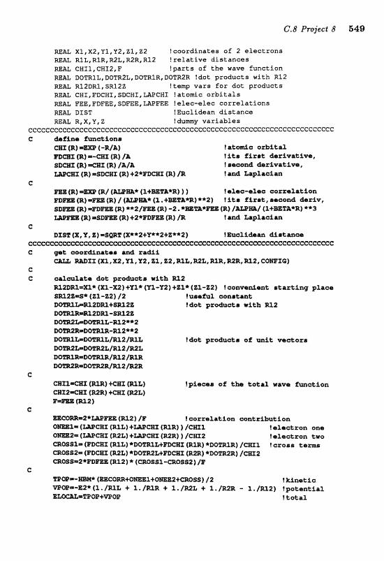
a& XI,XZ,YI,Y2,21,22 !coordinates of 2 e l e c t r o n s RE& RIL,RIR,R2L,R2R,RJ2 ? r e l a t i v e d i s t a n c e s WAL CMX1,CHI2,F !parts o f tba wave func t ion m& DOTRIL,DQTR2L,DOZ"RJR,DOTR2R !dot products wi th R 1 2 W& RJ2DRI,SR12Z !tsnrp vars f o r dot products RE& CWI,FDcMI,SDCNT,UPCHf ! a t a d c o r b i t a l s mAE FEE,FDFEE,SDFEE,WFEE !else-@lee c o r r e l a t i o n s RE& DTST IEuclidean d i s tance RE& R , X , Y t Z !dumy variables
cccccecccccccccecceccccecccecccccceccccccccccccccccccccccccccccccccccccc G &fin* fmction.
CEX (R) 2 -R/&) l a t o d e orb& t a l maX (R) =-CH1 (R) /A t i t * f i r a t diQr%wa%ive, SD-Z (R) -I (R) /;A/& I semnd &rivat ivs , W a r (R) =$DC= (R) +2*EBCBI (R) /R ! a d I;aplacim
C EEZ (R) =m (R f (U=* (l+mrrAW) ) ) !aXcro-%lea cosrelat ion F D m (R) =m (R) / (W=* (l. +mT&*E) **2) l i t c f i rak , aeaond Blariv, SBmE (R) aPBm8x (R) **a/- (R) -2. -m*- (R) /U=/ (X+W%&*R) **3
(R) =BD- (R) f 2 * F D m (R) /R faad U p l a c i m C
DXIP ( X , X, Z) =SWZ (W**2fV**2+Z**2) I E%ali&m a m t m c a ccccccc~cccccccccecccccccccxccccccccccoececccccecc~c(=ccccceccccececc~ G gat aoordinatee rad r-i
m X Z ( X I , Xz,T%, YZ, I t r l , L2, Rllr, =L, =R, R2R, R3-2, GWTG) C C aleaXat;e &et products with XL2
Rl2@===* (SEX-X2) +Yl* (XI-Y2) +%I* (21-ZZ) !convenient s t a r t i n g plaocl Im2b=S* 62%-22) 12 tusaful wrrctant W W b m 2 B m + a 1 2 2 !et praducts wfth RA2
2mm-m122 mwhBOmL-m2**2
R=BO=R-m2**2 rdot pr&uaea of unit veators
D@=R=DamR/mP m R C
C = T = a I (RlR) +Gal (m&) (=R) +mx (M&) 3 1
e Icurzelation cxontribution
(mCRX (Rlt) +WCHX (RXR) ) /Cm1 f rrlcrckron on* ( m c ~ r + W C H ~ (m) ) /cm2 l electron t w o
aOSSl= (EaDaI (R%&) * W ~ M E D G E l (R=) *DQa%R) /Cm% l ozorrrs Lams GRWS2m (FDGWX (=L) *DOWWPDCHX *D@m2R) 1-2 ~SS-2*SD~E(Rl2)*(~OSS1-~~S82)/B"
c OmZ+=SS) 12 t kinet i a R + l./R2L + l.lR2R - 2./=2) !potential
! t o t a l
!piaeras of! the t o t a l rave fwct;fon
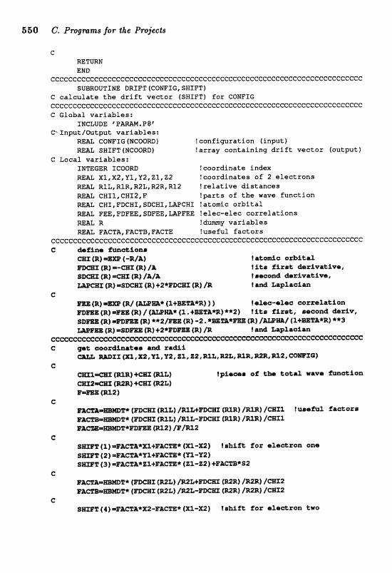
5 60 C. Pwrmms for b&e Projects
C RETURN END
cccccccc~Ccccccecceccccccccccccceecccccccccccccccccccccecccccecccccccccc SUBROUTINE DRIFT (GQNFIG, SHIFT)
C c a l c u l a t e t h e d r i f t v e c t o r (SHIFT) for CONFIS cecccccccccccccccccccccccccccccccccccccccccc~ccceccccccccccccccccccccccc C G l o b a l v a r i a b l e s :
C- Iny>ut/Outgut v a r f ables: =U COWLG (WCWRD) ! e a n f f g u r a t i o n ( i n p u t ) RE= SHIFT (NCWRD) ! a r r a y c o n t a i n i n g d r i f t vector ( o u t p u t )
C L o c a l v a r i & l @ s : INTEGER TCOQRD ? c a o r d i n a t e i n d e x R m L XI,X2,Pl ,Y2,Z1,22 ? c o a x d i n a t s s af 2 e l e c t r o n s REAL RXL, RIR, R2L, R2R, R12 ! r e l a t i v e distances M A L CWTf,CHJ2,F ! p a r t s o f the wave f u n c t i o n -L CWI,FDCHI,SDCWI,WCMI. ! a t o d e o r b i t a l M A L FEE,FDFEE,SDFE;E,WFEE !elec-elec c o r r e l a t i o n s =&L R !dumy v a r i a b l e s aAl, FhGTA,FACTB,FACTE !useful f a c t o r s
CCCCCCCCCCGCCGCCCCCCCGCCCGCCCC~GCCCCCCCCCCCCC~C:CCCCCCCCCCCCCCGC~CCCCCCCC C dar f iner f=a&ior ta
CHX (R) (-R/&) l at-o orbital $B- (RI =-Cgl: (R) /A f f ta Z S r s t hasrivatAve, saax (R) =CB% (R) /&/A ! .scod d e r i v a t i m ,
(R) =SW= (El) +2*FDCB3 (R) /R !& MpXaoiaa C
Si'ES (R) =m (R/ (W=* (2 +=%&*R) I ) l o l a c - s f s a aozzelatian mmE (R) =m (R) / (mm* (2. +=Taw) **2) f i &B fArat, @0aaad b r i w ,
(R) =mm (E) **2/mz (R) -2 * *==*m (R) /W=/ (%+==*R) **3 w p m (R) e ~ m (R) +2q~m ( a ) /R f a d Laplrai-
c t ctoo=*m&ss imd xa&i W I Z (m, xZ?,'%l, Y2, E2,22, R11*,R2L, XbR, =R, R12, C-50)
d" (=R) (=L) !piecar of thr t;oCaP wave aa&ion
C !P* ( E m 5 (=L) /mWFXE13 tmR) /=R) /CBI3 ! uacafal flaeors g* (E"-3 (=L) / ~ L - F D C ~ ( ~ 1 ~ 1 I-) /cm1
C SlIImT ( l ) =FACTA*m+E&C!Pg* ( X l - n f f &Aft f o r e l a & r o n samr (2) = F A ~ ~ A * Y Z + ~ A C ~ E * ) s m z (3) =FACT~*ZX+FAC~* far -%a) + ~ x m * s 2
C P* ( s a c g x (ML) / ~ L + F D ~ ( 1 ~ 2 ~ ) /=RI / m z 2 'E* (EDCE3 (W%) /R2L-FDCm (R2Rj /R=) [CBI2
e S-T (4) =FMT&*X2-FACTE* (X%-S) ! shift, for e l a o t r o n t w o
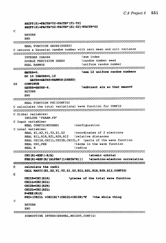
S=% (S) =FAcn*'P2-FAcm* (Zl-Z2) S m T ( 6 ) =EACa*Z2-FXm* (21-ZZ} +B"A6FB*S2
C mTURN END
cccc~ccccccccccccccccccccccccecccecccceccccccccccecccccccccccccecccccccc FUNCTION GAUSS(DSEED)
C! returns a Gaussian randam nu&@r with zero mean and: unit variance ccccccccccccCccccccccceeccccccccecccF:ccccccccccccccccccccccccccccccccccc
INTEGER IGBUSS ! sum index DOUBLE PMCXSXON DSEEXS !randon nu-r seed RE= MNPJQS !uniform random nu&er
~~cC~cCcc@Cc@cCCcCcCCCCCCcCCcCCcccccc~ccccceccccccccccccccccccccCcccccccc avSS=O * t @%m 12 =i fem rmdoar it6
50 COmIm aQS5-US5 - 6. ?sa%rrcL s i x so that man=O MTURN END
cccccccccc~ccccccceecceccccccceccccececcccccccccccccccccccccceceGccccccc RE= PUNGTIOlrJ PM1 (CONFIG)
C calculates the total variational wave function for CONFIE cccccccccccccccccccccccccccccceccccceccccceccccccccccccccccccccccccccccc C Global variables:
INCLUDE C P a M . P B ? C Input varSablss:
RE& CONFIG (NCOOm) feonfiguration C Local variables:
M& X1,X2,YlrY2,21, 22 Ecaardinatas o f 2 electrons RE= R1LIRlR,R2LrR2R,R12 ! rel ative distances
CHXIR,CWIlL, CHI2R, CW12L, F !parts o f the wave function CNX, FEE !terms in the wave function
m u R ! radius ecc~~cccccc~e~ccccccccccccccccF:cecccccccccccccccccc~~ccc~~ecccccc~~~c~c~
f akeda oxbf trl . EBH (W)=- (RI I-=* (%+mP&*EZ) ) } f rl2eotzan-rlcrclsron tserzelakion
C aaulrtr thr ~ a & i W Z X (X%, 152,Y%, Y2, El, Z2, =L,=&, RZR, 5'428, RIZZ, COWPIG)
e -X=&= (=W) !~IOMB ef Lha te+al wave fmcrL-ion
Z !
Par (af 2t MHTlR) * (aISLI-CHXm) *E" ! khm whole lsung C
=TURN END
ccccccce~cccccecccccccccccccccccccccccceeccccccccccceccccccecc~ccccccccc SUBROUTXNE fNTENS(EMS~L,WEIGWT,CONFSG~
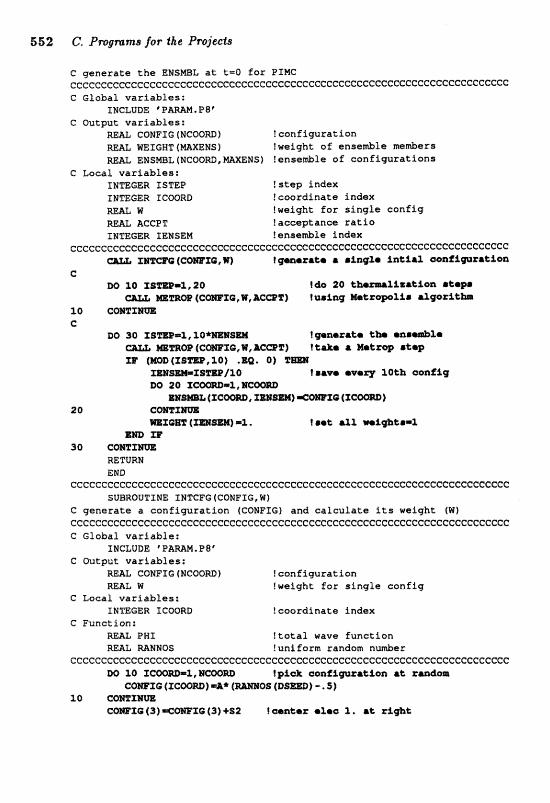
C generate the ENSmL at t=Q for PfMC ~~~~e~~cc~~~~cc~~c~c~~~ccccccccecccceccccccccccccccccccc~ccccccccccccccc C Global variables:
INCLUDE 'F&W.P8 ' C Output variables:
R E U CONPTG (NCOOM) !configuration WAL mIGHT (mXENS1 !weight o f ens~ntble meders mm ENSWL(NCO0m,MENSf rensenble of canfigurations
C Local varSables: INT&GER XSTEP !step index TMTEGER TCOORD !coardlinats index R E U W !weight for single eonfiq
KCPT !acceptance ratia INTEGER f EWSEM ?snse&le index
c~~c~~~~c~~cc~cc~c~cec~ccccccccecccccccccccC:ecccccccecccceccccccccccccc~ IW-G (Cmfc; l , W) fgmaraea r riag2a fn t ia l
e
*EQ' a1 %mm 1sawa1 wazy 10th oonggg
mm
mIaT [=S=) 11 c IraL rrll migher=l
30 C R END
cCcccccecccccccccccccccccccccccccccccccccccccecccecccceccccccccecccccccc SUBROUTINE INTCFC [CONFIG, W)
C generate a e~nffguration ICONFIG) and calculate its weight (W) ccccccecccccccc~ccccccccccccccccccccceccccccceccceccccccccccccceccececcc G Global variable:
INCLUDE *PAWM.P8' C Output variables:
MAL CONFIG {M~WRD) !configuration m L W ! weight f or single con fig
C Local variables; XMTEGER ICaORD !coordinate index
C Function: RE= PWS ! total wave function WAL MNNOS !uniform random n-er
ccccccceecccc ~ ~ e e ~ ~ ~ c ~ ~ c ~ e e ~ ~ e ~ ~ ~ c ~ ~ c c ~ c ~ c c c c e e c ~ c e ~ c c c c c DO 10 X !p&& configuration rk r m h
cam B [DSrnj-.S) 310 comxm
CQmIG ( 3 ) *-X@ (3) 4-52 f canter *lac. 3. at rf@t
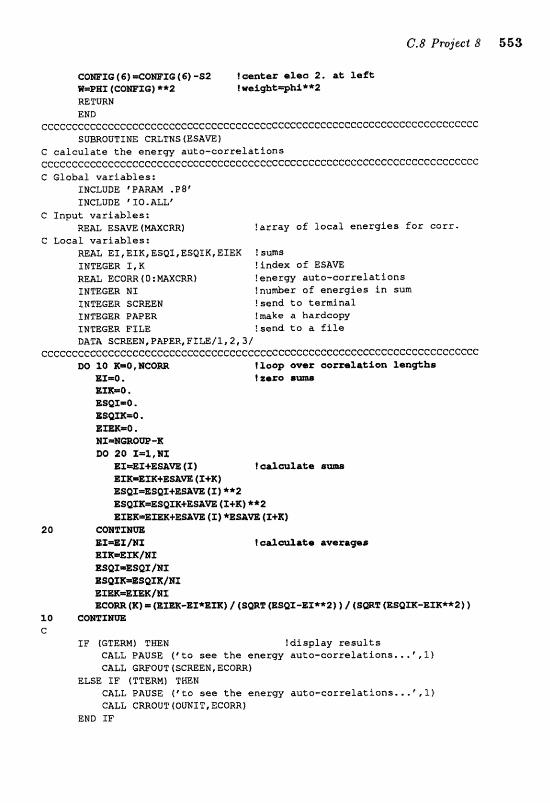
GOWXQ ( 6 ) EPrCOWIC (6) -S2 ? senter @%%a 2, at lafC W-PBX (comze) **2 lwcsigbd~hi**i? RETURN END
ecccecc~~~cc~c~e~~~cceccccccccccccecc~~eccccecccccc~cecccccceecccce:cccc~ suBRavTxMe C R L T N S ( E S A ~ )
C c a l c u l a t e t h e energy a u t o - c o r r e l a t i o n s ~c~cccc~cccccc~cc~~~cccecccccececc~ccccccccecceccccccccccccceccccceecccc C Glabal v a r i a b l e s :
INCLUDE fPARAM .P@' TMCLUDE 'TO I ALL'
G Inpu t v a r i a b l e s : REAL ESAVE f ~ c m ) !a r ray of l o c a l e n e r g i e s f o r e o r r .
C Local v a r i a b l e s : RE= EI,EZK,ESQT,ESQPR,EIEK !sms INTEGER I, K ! index o f ESAm
RE= ECQm ( B : mXCRRf !energy a u t o - c o r r e l a t i o n s INTEGER M1 !nu*r o f e n e r g i e s i n sum INmGER SCREEN !send t o t e rmina l INmGER PAPER !make a hardcopy INTEGER PILE i send ta a f i l e DATA SCMEN,PAPER,FfLE/1,2,3/
c~cccC~ccccccccccccccccccccccccc~ccccccecccecc~e~cccceccccccccc~cccccccc M3 3.0 Z=O,HC= lloep w@t: c?ormlr&ion fen#b@
PT=O, EZXmO. BSQZmO. ESQm=O, EXm=O, nr=Haaw -a 00 acr *%,m
E X ~ E X + B ~ ~ 4x1 t eali@rulata EIZ=Ef EC+ES&a (ItK) ESQX =ESQZ+ES&m (I) **2 ESQXX=EsQXK+ESAm (XtZ) **2
IEK+rn&rn [X 1 *ES&rn {Z+K)
EX =EX /MT t-2alat;e av%ragms EIE=EXB/NI ESQX=ESQI/NX rzsqm=ssaxa/Nr I&IBK=EXmIMI EGO= (X) (E~K-BX*EIKI (swv (gsox-Bx**aj 1 1 fs(zri2 IESQ~-BXK**~?I 1
10 c a m z m C
XF (GTERHI THEN !d i sp lay r e s u l t s CALL PAUSE [*to see t h e energy a u t o - c o r r e l a t i o n s . ..W CALL GBFOUT (SCREEN, ECORR)
ELSE I F (TTERN) TmN CALL PAUSE (*CO see t h e energy auto-correlatians,..@,l) caLL emavT (ounxT, E c a m )
END I F
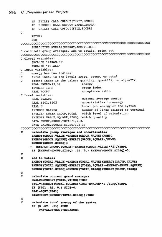
5 54 C. Pmgmnas for Ihe Projects
IP [TFILEf CALL CmOUT (TUNIT, ECORR) IF (GHRDCP) CALL GRFOUT (PAPER, ECOm) SF (GFILE) CALL GWQUT(FILE,ECORR)
c RETURN END
CCCCC~CCCCGCCCCCCCCCCCGCCCCCCCGCC~CCCCCCCCCCGCCCCCCCCCCCCGCCCCCCCCCCCCCC SUBROUTINE AVEWG (ENERGY, ACCPT, SCRP)
C c a l c u l a t e group a v e r a w s , add t o t o t a l s , p r i n t o u t ~c~ceecccceccC~ceecccccccceccceccccccec~eccccccccc~cccccC:ccccccccccccccc C Global v a r i a b l e s ;
INCLUDE *PAmM.P8' INCLUDE *1IO.ALL8
C Inpu t v a r i a b l e s : C e n e r g y b a s t w o i n d l f c e s C f i r s t Index i s t h e leve l : sweep, group, o r t o t a l C second Sndex Ss t h e value: q u a n t i t y , quant**2, o r sigrrmae*2
REAL ENERGY ( 3,3 2 ! energy INTEGER XGRP !group index REAL AGCPT !acceptance r a t i o
C Local v a r i a b l e s : =&L EVALUE ! c u r r e n t average energy REAL SIG1,5162 ! u n c e r t a i n t i e s i n energy RE& U ? t o t a l p o t energy of t h e system INTEGER NLINES !number of l f n s s p s i n t e d t o t e rmina l INmGER SFIEEP,GROUP,TQTAt !which level sf c a l c u l a t f a n 3CNmGER VALUE,S@rUARE,SIESQ ?which q u a n t i t y DATA SmEP,GROUP,TOTAL/3,2,3/ DATA VALUE, SQUAm, SXGSQ/1,2,3/
cccccccccccccccccccecccceeeccecccccccccccccccceecccccccccccccecccecccccc C e7rrJalatr gza~p amrager m& wmrtaAntfsrr
faam, =W) (=am, m m ) /@SW& ( m m , sQU-3 /NSW&
{=am, s1osqt =
(=Q-, SIGSQ) .&!E, 0 . ) G
(%OS&, mm)
(%Q%=, SXCrSQ) C C
X-
(%OF&, SXQSQ) ) /X- C C aaleulrcrs t o t d . o f tha @yet-

]ZEga D=Q.
Em? IF c
1F (TTERM) CALL TXTOUT(IGRP,ENERGY,EVALUE,SIG~~SXG~~U,ACCPT~OUNIT~ IF (TFILE) CALL TXTOUT(IGRP,ENERGY,EVALUE,SI,G~.,~XE~~U,ACCPT,TUHXT~
c RETURN END
~~c~e~~c~~~ee~e~~c~~c~ccceee~ceecceccccccc~ccccccccccccccccccccccccccccc SUBROVTIME AaD11 (XI, X2, V % , V 2 p 211Z2 I R2Le R2LI RLRI R~RI coHpxGI
G c a l c u l a t e s c a r t e s i a n c o o r d i n a t e s and r a d i i g iven CONFIG ~ccc~e~~~~~ec~c~~ccccecc~~~c~~c~c~ceccccccccccccccccc~ccccccecceec~ccccc C Global v a r i a b l e :
INCLUDE "PAM.P8' C xngut v a r i a b l e s :
WAL CONFIG (NCBOm) !conf igu ra t ion C o u t p u t v a r i a b l e s :
REAL X1,X2,VI,V2,Zl,Z2 f e o e r d i n a t e s of 2 e l e c t r o n s WAL RIL, RIR, R2L,R2R, R12 ! r e l a t i v e d i s t a n c e s REAL DIST ! Euel idean d i s t a n c e
ccccccccc~cccecccccccccccecceccccecccccccccccccccccccccccccccccccccccccc DXST ( X X , XI,,!&%) =GmT (X1**2+X1**2+81**2) !Eucll&ean &atan-
C X 1 4 0 r n I G i (l) X 2 d m X 0 (4) X l e W T 0 (2) Y2*0rnXGi (5) aoeamrc; ( 3 ) Z 2 e w I G (Q)
e mWDXSZ (X%, Yl , Zl+S2) t ealmlrtr reparation* mmD282" (Xl, Vl , E2-82) mWDZST (X2, ?C2,22+32) WmD1Sa" [X2, Y2,22-62) U2=DSSIP [XI-x2, Yl-X2,21-82)
C =TURN END
CCCCCCCCCCCCCCCCCCCCCCCCCCCCCCCCCCCCCCCCCCCCCCCCCCCGCCCCCCCCCCCCCCCCCCCC SUBROUTINE INIT
C i n i t i a l i z e s c o n s t a n t s , d i s p l a y s header sc reen , C i n i t i a l i z e s menu a r r a y s f o r i n p u t pa ramete r s ccecec~cccecccccccccecccccecccccec~ccccccccceccccc~~~cec~cc~cccccccccccc C Global v a r i a b l e s :
INCLUDE ' 10, ALL' INCLUDE ' NENU. ALL' XNCLUDE 'PAmW.P8'
C Loeal parameters : !program d e s c r i p t i o n
DXMENSIOET DESGBE (20) INTEGER NNEAD,NTEXT,NGRAPM !nu&er o f l i n e s for each d e s c r i p t i o n
558 C. Pmgrams for the P.rojects
ecccCcccccccccccccccccccecccececcceeecceeeeccccc~eccccGccccCcccccccccccc C get environment paramters
CALL SETW c C display beader screen
DESCRP (1 ) = ' PRQJECT 8 * DESGRe(2)m 'Monte Carlo solution of the K2 molecule" NBEADm2
C C textoutputdescription
DESCRPf3f= 'eelectronic elgenvalue and its uncertaintyf DESCRP (4) - 'or energy auto-correlationt NTEXTa2
G graphics DESGBQ (S) NGMP W=1
output description = *enerw auto-correlation vs. correlation length'
C m HEADER (DESCRI,, MWEAD, NTEXT, N a P W )
calculate constants mHm7.6359 i hbar*2l (mass) E2=14.409 Icharge of the electron ABOHR=WBN/EZ
setup menu arrays, baginning with constant part MENU
MTYPE f 12) = T T T U IVIPWT (12) - 'PHYSICAL E"-=TEES* MLOLXN (1 2 1 -0. MHILIN (12) -2.
MTEE f l3 f =FLOAT MBMPT(13l='Enter the interproton separation S (Angstroms)' MTAG f l 3 ) ="Iner proton separatf on (Angstroms) * MLOLXM (23) =Q. WWILIM 113) =IQ. m a L S (13) =Q.
MTWE ( 14 1 =FLOAT W W T [14)=
+ #Enngr va lue for variational parameter Beta (Angstramsx*-l)@ MTAG(ll)=rvvriatianal parameter Beta (Angstrams**-l)" NLOLIM (l. 4 ) =Q. MHILIM (14)-IQ. MmLS(l4)=.25
m W T 137 1 = NUMERf GAL PAmETERSf MLOLIM (371 -1. MWTLTM[37)=1.
C MTmE (381 =TITLE M P W T f 38) =%ethods of calculation: MLOLTM(38) -0. MNILIM f 38 1 4 3 .
C MTYPE (39) =@TITLE IyIPWT (39) =Q) Variationalf MEOLSM(JB)=O, MHILXM (39) =Q.
C MTWE (40) =MTITm NPRMPT (4Q) 2) Path Znteqral Monte Carlo' MLOLTM (40) ==Q, MNILIP1(40)=1.
C MTYEE (41 ) =MGWOIC M I ? W T (41) ='Make a menu choice and press return' MTAG ( 4 2 ) - 9 4 42' ~~o~rn(41l =I. MHJLZM(41)=2. MINTS (41 ) -1 m A L S (41) =X.
C MTWE ( 4 2 ) -MUM M P m T (42) * Enter size of the enss&lec MTAG 142) = 3nse&le sizet NLQLIM (42 1 ==l. MWILIM (42 f =MXENS MINTS (421 =ZO.
C
MTVPE ( 4 3 ) =FLOAT W m T (431 =@Enter time step (units o f 1E-16 secthbar) MTAG (43) =*Tine step (units of lE-l6 sec/hbar) NLOLSN143f PO. MWILSP4[(43)=lOI M W L S (43) =.a1
C NTYPE ( 4 4 ) =FLOPIT MPMPT(44)= 'Enter step size far sampling PHI (Angstroms)' MTAG (44 1 - "ampling step size t&gstrans) MLOLIM(44) m.01 MHIXIIN (441 =10. MRmLS (441 =.4
C
MTVPE (4 5 ) =NU% m W T (451 = 'Mu&er of tbermalization sweeps" MTRGf45f 'Thermalization sweepst MLOLZM (45 1 =a
558 C. Pmgmms for the Projects
MWILIM (45) =100Q MINTS ( 4 5 ) -20
MTUPE ( 4 S) =TITLE M P M T (46)=1Quantlty to calculate: ' FILOLfM(46)=1, MHILIM (46) =Q.
MTYPE f 47) =MTITLE MPmPT (47 f =@ b 1 Energyf mQLTM(47) =0, MHILIM (47) -0.
MTYPE ( 4 8 ) =MTITLE W M P T (481 =22) Correlationsc WLOLIM (48 f 4. MHILIM ( 4 8 ) =l.
NTWE ( 4 9 1 =NCHOT C MPMPT 4 9) =' Make a menu choice and press returnf MT&G(49)-'50 53# NLOLIM (4 9) =l. MNILIMi49)-2, MfNTS (49) =l
LS (49)=1.
MTDE ( 5 O ) =NUM MPmPT { S O ) = *Enter sampling f requency (to avoid correlations) @
MTAG ( 5 0 ) = Sampling frequency" MLOLIM (SO) -1 MHILIM (50) m100 MINTS (50) =6
MTZSIIE (51 1 -NUM M P W T ( S L ) = *Enter nudar of samples in a groupC MThG (53.1~ Group sample s i z e t MLQLIM (51 1 =l. NHILTM (51 f =l000 MINTS (51) =IQ
MTWE (5 3 1 =NUM MPWT(53)m 'Enter maximum correlation Lengthe MT&G153)= eMaximum carrelation length8 MLOLIM ( 5 3 f =l MWILIM (53) =100. MINTS ( 5 3 ) -40
MTVPE ( 5 1 ) =NUN M P W T (54) = 'Enter nun\ker of groups"
MTAG(54)m q u & e r o f groups' MLOLIM ( 54 1 =X MBILZM(54f -1000 MINTS (54) =10
C MTYPE (S5 1 =NUM MPmPT155)= "Integer random nu&er s e e d f o r f n i t f l u c t u a t l s n s f MTAG (55) = "andam n u d e r seed" HLOLIM (55) =1ODO. MHILIM (55) -99999. MINTS (55) =J4757
e MTYPE ( 5 6 ) =SKIP NmALS (561 =GO.
G MSmMG (MINTS (75) ) = 'proj8, t x t '
c NTYPE ( 7 6) -BOOLEN ME)MPT(76)=9o you want t h e SHORT v e r s i o n a f t h e ou tpu t? ' MTAG (761 =%Short: v e r s f on o f ou tpu t " MINTS ( 7 6 ) m 0
C MTVPE ( 7 7 ) =SKIP NRMLS 177) =80,
C MSTRNG(NINTS(86f ) = " ro j8 ,g r f t
C
MTWE 4 87 ) =SKIP Mm&LS (87) 0.90.
c RETURN END
ceccccccccccccccccccccccccccccececcceccccccccccccccccccccccccccccccccccc SUBROUTINE P m M
C g e t s pa ramete r s from sc reen C ends program on r e q u e s t C c l o s e s old f i l e s C maps menu v a r i a b l e s t o program v a r i h l e s C opens new f i l e s C c a l c u l a t e s a l l d e r i v a t i v e pa ramete r s C performs cheeks on parameters ccccccccecccCcccceCcccccccccceccccccccccccccceccceccec~cccccccccccc~cccc C Global v a r i a b l e s :
XNCLUDE " mNU. ALL' INCLUDE ' TO. ALLe SNCLUBE ' PAMM, P@'
C Local v a r i a b l e s : WAL AQLD !temp v a r i a b l e t o s e a r c h f o r A IMTEGERCORR,EPS ! w h a t 1 s b r ? i n g c a l c u l a t e d ? INTEGER PIMC, V-Y !which method?
C g i v e s t h e map between menu indices and paramete r s INTEGER f S, IBETA, IMETRD, XNENSM, IDT, IDELTA, f THEW, ICALC,
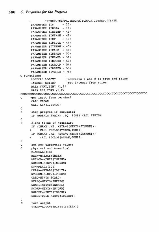
560 C. Programs for the Projec.l;r
+ INFREQ, TWSMPL, INCGm, IGROUP, EBSEED, ETERSE PARAMETER ( I S = 3-31 PAWMETER (IBETZL 2 4 ) P m m T E R fZMETMD 41)
TEIR (TNEMSM = 421 PAMMZTER t I D T = 431 P A W E T E R (IDELTA = 44) PAmMETER (ITHERM P 451 PAmHETER (XCALC = 49) P A N E T E R ( I N F M Q - SO) P m m T E R (INSMPL m 5 1 ) P A m m T E R ( I U C O m 53) P A m m T E R (IGROUP 54) P W M E T E R (TDSEED = 55) P A M m T E R {ITERSE - 76)
C Functions: LOGICAL LOGCVT !converts 1 and O t o t r u e and f a l s e INIIISE;ER GETIWT !get i n t e g e r from screen DATA VmU,PIMC / l , a / DATA E P S , C O M /1,2/
~~~c~~~cccc~~cCccccceccE:ecc~ce~cccccccccccccceccccccec~ccc~cr:ee~ccccccsec C g e t i n p u t f r o m t e r m i n a l
C&= CLEAR CALL ASK ( I , ISTOP)
C c stap program i f requested
I F [ m A L S ( I M S # ) .EQ, STOP) GALL FINIS& C C close files if necessary
f F ( T N B .NE. NSmHG (MINTS (ITHAME) ) + CALL FLCLOS f TNAm, TUNI Tf
I F (GNAm .NE. MSTRNG (MINTS (SGNAMEI )) + CALL FLCLOS (GHME, GONIT)
e G s e t new parameter values C physical and numerical
S - W A L S 4 I S ) B E T f l m m A L S (3BETA) mT&oD=MINTS (IMETHD) NENSEN=NINTS ( INENSM f D T = m A L S (IDTI DELTAmWALS ( IDELfl"A1 NTmW=MIHTS I I T N E M ) CALG=MTNTS (TCALC f MFmQ=MINTS ( INFREQ) NSWL-MENTS (INSM?.I,j NGORR=MTNTS ( I N C O m ) NGROUPmMXNTS (IGROUP ) DSEED-DBLE {MINTS (IDSEED) f
C C tex t output
TTERM=LQGCVT (MINTS ( ITTERM) )
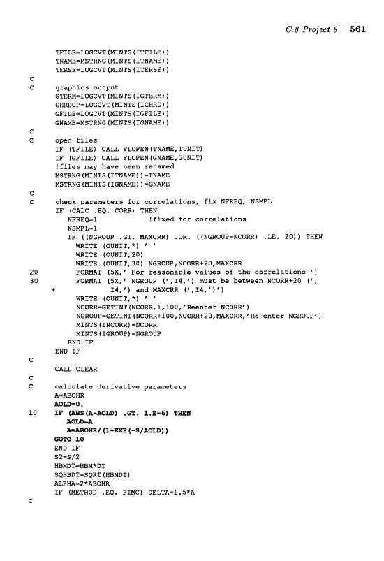
TFILE=LoGCvT (MINTS ( ITFILE! ) THMaMSTRluG (MINTS ( I T N A B 1 f TERSE=LOGCVT(MINTS(ITERSE))
e C graphics output
GTERN-LOGCVT (HINTS ( X GTERE(I1) GHIIDCP-LOGCVT (MINTS (IEBRD) 1 GFILE-WGCVT(MZNTS(TGFILE11 GNAME=MSTRNG(MfNTS(IGHAHE))
C G openfiles
TF (TFILE) CALL FLOPEM ( THAm, TUNIT) IF (GFILE) CALL PLQPEN [GM-, GUMI T) !files may have been renamd MSTRNG (MINTS (ITNAmf f =TM&M MSTRHG [MINTS (XGMAm) f -GNAME
c C check parameters for correlations, fix NPREQ, N S m L
IF (CALC .EQ, cow) THEN NFREQ=1 !fixed for correlations NSMPL-5 I F ( (WGROUP . GT. mXCRR) . CIR. ( (NGRQUP-NCOM) . LE. 20 f f THEN
FJRTTE (OUI\IIT,*) ' m I T E (QlfNZT, 20) m T T E (OUNIT, 30) MGRQUP, N C Q m t 2 0 , M C R R
2 0 F O W T (5X,Vor teasongble values of the correlations ' )
30 F O W T f5X I f 1GROUO ( r , I 1 4 , * j must be btueen NC0=+20 (', + fQ,*f and mXCRR (*f14tt)@)
WRXTE (OUNIT, * l * ' NCOM=GETINT (NCORR, 1,100, C Reenter NCOm' )
NGROUP=GETINT(NCORR+lOO,WCO~+ZO,WC~,fRe-ent;dr NGROUPrl MTNTS [ INCORR) =NCO= MINTS (f CR0UP) mNGROUP
END fF END I F
e CALL CLEAR
G C calculate derivat ive parameters
A=mQRR AQ~I.Q.
10 fP (&-A@=) .G%. 1.E-6) T a H & O & M &-@m/ (S+- (-51AOW) )
-0 50 END IF s2=s/2 WBrnT=HBM*DZ" SQWBDT-SQRT (NBMDT) ALPWII=2*ABQWR IF (METHOD .&Q. PIMC] DELTA=l.5*A
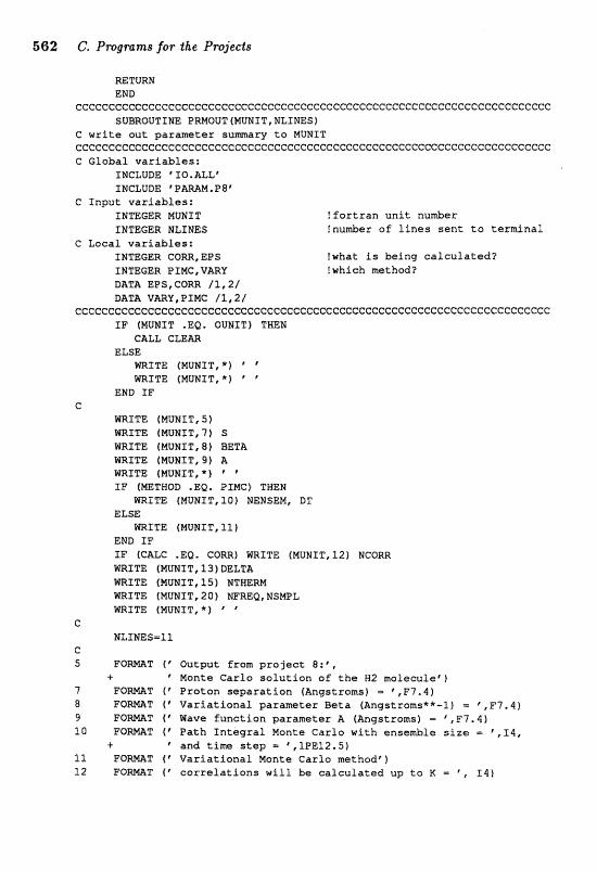
582 C. Programs far $he Projects
=TURN END
e~ec~e~e~cceec~ce~ecccccf:ecccccccccccccccc~ccccececccf:ceececcc-~~~cc~cccc SUBROUTINE PRNOUT (MUNIT, NLINESI
C write out parameter su CCCCCGGCCCCCCCG~CCCCCCCCCCCCCCCCCCGCCCCGCCCCCCCC~~~CCCCCCCCCC~CCCCCCCCCC C Global variables:
INCLUDE ' X 0 .ALLC INCLUDE V m M . P 8 "
C Input variables: INTEGER M U N I T !fortran unit nu&er INTEGER NLINES !nu&er of lines sent to terminal
G Local variables: INTEGER CORR,EPS !what i s being calculated? INTEGER P IMC, VARY !which methad? DATA aas,com /r,2/ DATA VARY,PZMC /li,a/
~e~~~~~~ceccccccecccccccecc~cccccc~cC:c~ccccccccccccccccccccc~ccccccccccc XF (MUNIT .E@. OUMIT) THEM
GALL C L E M ELSZ
m I T E (MUHIT,"] " WRITE (NUNIT,") "
END IF G
Ir3RITE [MWIT, t i ) WRITE (NUNIT, 7) S WRXTE (MUNIT, 81 BETA WRITE (MUNIT, 9) A WRIm (NUNXT,*) ' ' I F (MTNOD .EQ. PXMC] T8EN
W I T E (MUNLT,IQ) NENSEM, D5 ELSE
WRITE (MUMIT, 11) END I F IF (CALC ,Ea. CORE) hlRITE (NUNIT, 12j NCQRR m I T E (MUNIT, 13 f DELTA WRITE (MUHXT,15) %THEW WRITE (MUNIT, 20) WMQ, IJSMPL WRITE (MUNIT,*) ' '
e NLXIJES=11
e 5 P O M T ( c Output from project 8: * ,
+ "ante Carlo solution of the 82 mo2eculetj 7 F O M T (' Proton separation (Angatrams) = * , F 7 . 4 ) 8 F O a T IVariationfll parameter Beta (Angstroms**-2) = ',E"7.4) 9 F O m T (' Wave function parameter A (Angstroms] = @,,FT. 41 10 E"QW"Pf Path Integral Monte Carlo with ensemble s i z e = 5 x 4 ,
+ "and time step = ',lPE12,5) I2 F O W T t Y Variational Monte Carlo mthode) l2 F Q m T ( ' correlations will. be calculated up to K = 5 14)
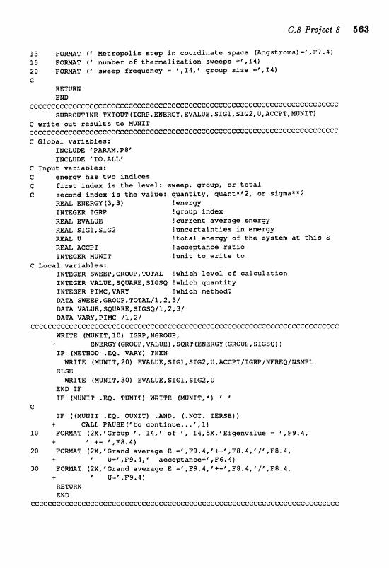
13 F O m T ("et r o p a l i s s t e p i n c o o r d i n a t e space (Angstroms) =' ,F7.41 1 5 FOWT ( f nnuder of t h e r m a l i z a t i o n sweeps =@ ,141 20 F O W T ( * sweep fraqrlency t 14, "group s i z e I41
E: RETURN END
c~e~~cc~e~c~~~~~~~~~cccccccccccccccccccecccccccceccccI :ececc~cccceccE:cccc SVaOUTTME TXTOUT (IGW, ENERGY, EVUUEI SIGI, SIG2, U t AGCBT, MUNXT]
e w r i t e out r e s u l t s t o MUNIT ~~c~~~ee~e~ec~~~~~~ecceccccccccccccccececcccccE:cccC:~cecccE:cc~cecE:cE:ccE:cc e Global v a r i a b l e s :
INCLUDE * I0.11LL8 C I n p u t v a r i a b l e s : e energy has two i n d i c e s C f i r s t i ndex is the l e v e l : sweep, group, o r t a t a l C nd index is t h e value: w a n t i t y , wan t**2 , o r sigma**2
LNERCjY (3,s) t energy !group index
EVALUE ! c u r r e n t ave rage e n e r w SIG2, SIG2 ! u n c e r t a i n t i e s i n energy U ! t o t a l energy a f t h e sys tem a t this S
REAL ACCPT ! acceptance r a t i o TWmGER M m I T ! u n i t t o wzlte t o
C Local v a r i a b l e s : INTEGER SmEP,GROUP,TOTAL !which l e v e l of e a l e u l a t i o n INTEGER VALUE,SQUm,SIGSQ !which c.fuantity INmGER PIMC, VARY !which ntrithod? XIA"X "AEF,GROUP,TQTAL/1,2,3/ DATA VALVE, SOU-, SIGSQII, 2,3/ DATA VARY,PIMC /1,2/
GcccccccccccccccccccccccccccccccccccccccccccccccccccccccecccccE:ccccccccc WRITE (MUNIT, 10 ) IGm, WGROUP,
+ ENERGY (GROUP, VALVE ) , SORT (ENERGY (GROUP, SIGSQI 1 I F (WTRQD .EQ. V m Y ) THEM
mITE (WHIT, 20) EVUUE, SIGl,SXGZ, U,ACCOT/TGW/NFmQ/NSE(VeL ELSE
WITE {MUNIT, 30) EVALUE, SIG1, SS62, U END SF I F [NUNIT .EQ. TUNIT} WaITE (MUNIT, *) ' *
G SF ((MUMIT *EBI OUMIT) -AND, (.NOT, TERSE))
+ CALL PAUSEtftta con t inue . . .C,l) 10 FQ-T ( 2 X F f G r a u p \ X64,' o f t , I4,SX,"Eigenval~e=~,,F9,4,
+ +- ' , F 8 . 4 ) 20 F O W T (2X,fGrandaverageE=f,F3,4,~-\F8.4,1/F,F884,
4 U=',F9.4,' acceptance=* ,,F6.4) 30 FO-T (2X,CG~andaveragsE=*,,F9.4,r+-~F8.4,*/1,F8.4,
+ I U=*,F9.4) RETURN END
ccE:cccecccccccecccceccecccccccceccccccccccccccC:ccccccccccccccccccccccccc
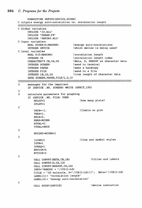
664: G. Pvogmnzs for the ProjeeZs
SUBROUTINE GRFQUT(DEVICE,ECORR) C outputs enerw auto-correlation vs, correlation length CCCCGCCCCCCCCCCCC@CCCCCCCCCCCCCCCCCCCCCCCCCCCCCCCCCCCGCCCCCC:CCCCCCCCCCCC C Global variables
INCWDE ' IQ. ALL' INCLUDE * F M M . '!?Bf XNCZUDE GRFDAT . ALLC
C Input variables: REAL ECOm ( O : W C R R ) tener~yy auto-correlatians IMmGER DEVICE !which device is being used?
C Local variables mAL K ( 0 : W C R R ) !correlation length INTEGER IK !correlation length index
!Beta, S, NGROUP as character data JNTEGER SGmEM !send to terminal INTEGER PAPER tmake a hardcopy INTEGER FILE !send to a file IMmGER LB, LS , LG !true length o f character data DATA SCREEN, PASER, Ff LE/1,2,3/
ccceCcc~cccecccccc~ccccec~ccccccccccccccccccccceccc~cccccccccceccccc~ccc C mssagss for the impatient
IF (DEVICE .NE, SCREEN) mITE tOUNIT,l08) C C calculate parameters for graphing
IF [DEVICE .NE. FILE) THEE NPLOT=I !haw many plots? IPLDT=1
!limits on plot
!line and sy&ol styles
CALL C O m T (BETA, CB, LE) !titles and labels CALL C O m T [S, CS, LS) CALL XCNVRT (NGRQUP, GG, LG) fNFOmfNGRoUP = *//CG(l:LG) TITLE = ' H2 molecule, S="/CS (5:LS) //', Beta='//CB f1:LB) MBEL (1) = T~crelation lengthr MBEL (2) = *Energy auto-carrelation'
CALL GTDEV (DEVICE) !device ncmination
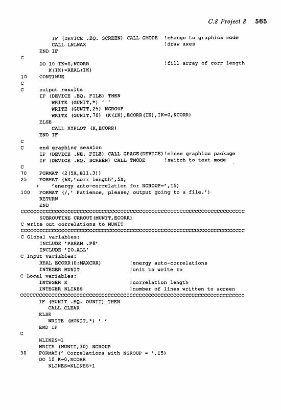
I F [DEVICE .EQ. SCmEN) CALL GNODE !change t o g r a p h i c s mode CALL WLNAX !draw axes
END IF C
D0 10 IKeO, NCOM ? f i l l a r r a y aE corr l e n g t h
K ( I K ) =mAL (XRf l 0 CQHTINIEB c C ou tpu t r e s u l t s
I F (DEVICE .Ea. FILE) "rW% mXTE (GUNIT,") ' * WISZTIF: (GUPJIK2S) NC;ROUO mxTE (GvraxT, 701 (K ( IK) , ECOm (IKI, IK-0, P;ICOm)
ELSE CALL XmLOT (K, ECORR)
END I F e C e n d g r a p b i n g s e s s i o n
I F (DEVICE .NE. FILE) GALL GPAGEtDEVICEf O S g r a p h i c s package EF (DEVICE .EQ. SCREEN) CALL TMODE !swi tch t o t e x t m d e
C 70 F O m T (2(5X,E21,3)) 25 F O m T ( CX, @ ccrrr l e n g t h f , ,5X,
+ ' energy a u t o - c o r r e l a t i o n Ecr NGROUP=',XS) 100 F O M T (I,' Pa t i ence , p l ease ; ou tpu t g o i n g t o a f i l e . ' )
m"Pm END
cceeecceccceccccccceccccccceecccC:ccceccccccccccccccccececccccccccceccccc SUBROUTINE CRRQUT (NUIUIT, ECOW)
C write ou t c o r r e l a t i o n s t o MUBIT c c c c c c c c c c c c c c c c c c c C : c c c c c c c c c e c c c c c c c c C Global v a r i a b l e s :
INCLUDE 'P , P8, INCLUDE 'XIQ.ALLr
C I n p u t v a r i a b l e s : W& $Corn 0 : M C R R ) !energy a u t o - c o r r e l a t i o n s INTEGER MUNIT !unit t o write t o
C Local v a r i a b l e s : INTEGER X. ! c o r r e l a t i o n l e n g t h TNmCER NLIMES !nu&er o f l i n e s w r i t t e n t o sc reen
cccccccccecceccccccccccccccccccccccccccccecccccccccceccE:ccceeccccccccccc I F (MUWIT .EQ. OUMITf THEM
GALL CLIF:&R ELSE
m I T E (MUNIT,*) END I F
C NLINES=I YilR1'L"X [MUNIT, JO) NGROUP
30 F Q W T ( * C a r r e l a t i o n s wi th NGROW "151 DQ 10 K=O , EGORR
NLINES=NLINES+l
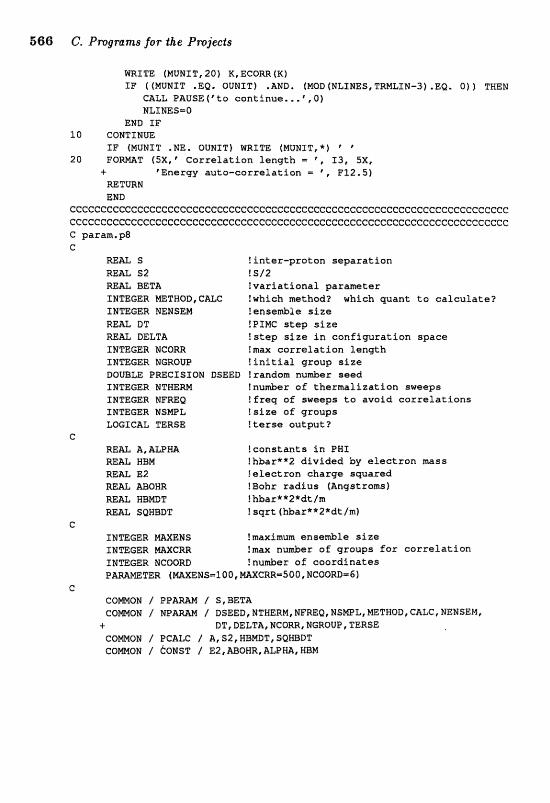
666 6, Programs for the Projects
WRITE (MUNIT, 20) K, ECORR (K) IF ( (MUNXT .EQ. OURIT) .AND, (MOD [NLIMES, TRMLIN-3) .EQ8 O) ) THEW
CALL PAUSE {*to eontlnue., . v 0) NLINES=O
EMD I F 10 CONTINUE
IF (MUHST .NE. OUNIT) WRITE (MUNIT,*) p
20 FQ-T ( 5 X , Correlation length = ', 13, 5X, + -nerg_y auto-correlation = FF12.51
MTURN END
cccccccccccCcccccccccccccccccccccccceccccececcc~cccccccccccccccccccccccc ceecc~eccccceccccccccccccce~ccecccccccccccceccceccccccccc~ccccceccccccc~ C paramlp8 C
=U S tinter-praton separation WAL S2 ! S/2 M& BETA ?variational parameter INTEGER ~ S W O D , C ~ !which method? which want to calculate? ZNmGER NEMSEM !anse&le size MU IZT !PIMC step si ze RE= DELTA ?step s i z e in confirguration space INmGER MCQm !max correlation Length I N m G E R NGROUP !initial group size DOUBLE P m C I S I O N DSEED frandom nu-r seed INTEGER M T m m tnufier of thexnalfzatfon sweeps Jc#mGER NFMQ !freq of sweeps to avoid correXatlans INTEGER MSElIDL !size of groups LOGICAL TERSE !terse output?
c WAb, A,ALPm !constants in PHI mm HBM !hbar**2 divided by electron =ss RE& E2 !electron charge swared
AI3OHR ! Bohr radius (Angstrams) RBMDT !kbar**2*dt/m SQmDT ! sqrt (hbar**2*dt /m)
C TNTE(;ER M;E:MS !maximm ense&fe size INTEGER mX(3RR !max n d s r of groups fss correlation SMBGER NCOIORD !nu&er of coordinates P W m T E R (MENs=ZO O , MCRR=SO O, NCOORDm6 1
G COmON / PP / S,BETA
/ DSEED, NTWERM, NFREQr NSNPL* NETHOD' CALC, NENSEM@ + DT, DELTA, WCORR, NGROUP , TERSE
GONMON / PCALC / A, $2, WEIMDT, SQWBDT CQmON / CONST / E2,ABOMR,ALPHafWBM
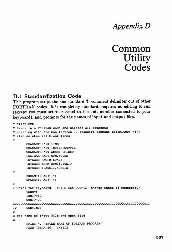
Appendix D
Common
D.1 Standardization Code This program strips the non-standard '1' comment delimiter out of other FORTRAN codes. It is completely standard, requires no editing to run (except you must set TEM equd to the unit number connected to your keyboard), and prompts for the names of input and output files. C STR1P.FOR C Reads in a FORTMN code and d e l e t e s a l l c C s tart ing with the non-fortran-77 standard C a l s o d e l e t e s a l l blank l i n e s e
TER*@D ANSWR, FIRST L G T C A L EXSK OPN, FOUND INTEGER EXCLN, SPRCE INTEGER TEW,OUNIT,IUNIT INTEGER I,ASCI%,NQMBLK
C EXCLM+xlCNAR f ! ' 1 spAce=xcrusa(r * I
G €2 u n i t s for keyboard, XNPXLE and DUTFIL (change thess if necessary]
TERM=5 EUMITm10 OVNIT=20
CCCCCCCCCCCCCCCCCCCCCCCGCCCCCCCCCCCCCCCCCCCCCCCCCCCCCCCCCCGCGCCCICCCCCCCG l 0 CQNTXNUE C C get nam of input f i l e and open f i l e C
PRINT *, IEWTER N M OF FBRTMN PRBGmM' =D (TERH, SO) INFXLE
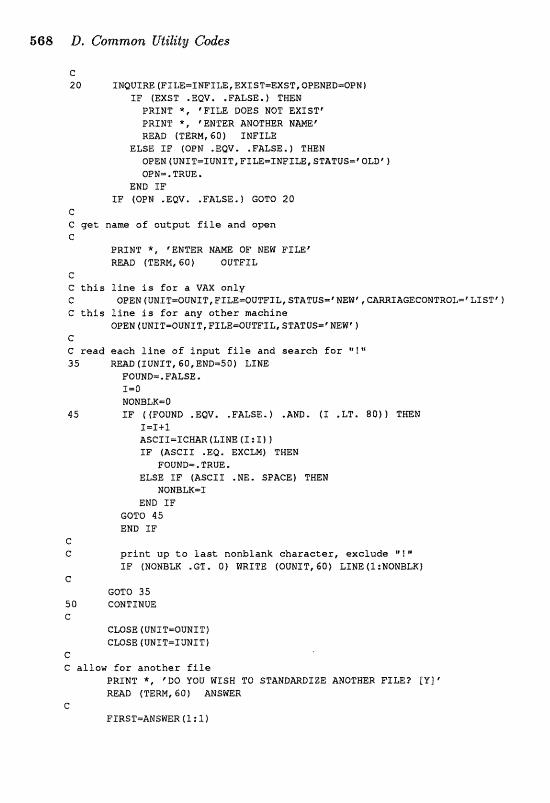
C 20 INQUIM(FIZE=lNFILE,EXIST=EXSTIQPE:NED=OPN]
IF (EXST . EQV. .FALSE. ) THEN PRfNT *, 'FILE DOES NOT EXISTf PRINV, 'ENTER ANOTHER N M ' READ (TERMI6O) INFILE
ELSE IF (OPN .EQV. .FALSE. 1 THEN QPEN(UNIT=IUNfT,FIZE=fNFILE:,5TWTUS=fOLDr) QPW=.TRUE.
END IF IF (OPM . EQV, . FaSE, 1 GOTO 20
C G g e t name o f output f i l e and open C
PRINT *, "EMER %AME OF NEW PIUp RmD (TERM, 60) OUTFEL
G C t h i s line is f o r a VAX only C ~PEN(UNIT=OUMIT,FTLE=OUTFIL,STATUS='NE1f,CARRIAGECONTROL=rLXSTf~ C this line is f o r any other machine
OPEN(UNIT=OUNIT,FILE~OUTF~L~STATU~E+'NEW~~ C C read each line o f i n p u t f i l e and sea rch f a r * ! " 35 =D (IUMIT, 60, END-50) LINE
FOUND=.FBLSE. S=0 NONBLKsO
4 5 IF ( (FOUND .EQV. .FALSE* 1 .AND. (I .LT. 80) ) THEN X=I 41 ASCII=ICHAR f LIME (1 : Iff I F (ASCL1 .EQ. EXCLH) THEN
FOUND=,TRUE. ELSE IF [ASGII .NE. SPACE) THEN
NOHBLIC=I END IF
GOTO 85 END IF
C G p r i n t up t o last nonblank c h a r a c t e r , exelude "!"
IF (NONBW . GT , Q1 WRITE (00NET, 60) LINE 41 :NONBLR) C
GOTO 35 5 0 CONTINUE e
CLQSE (UNITmOUNI T) CMSE (UN1 TmIUMIT)
C C al low for ano the r f i l e
PRlClJT *, 'DDO YOU WISH TO STANDmDIZE ANOTHER FIm? [Yj' READ (TERN, 60) ANSWER
G FIRST-ANSWER (l ; 1 1

IF ([FIRST .EQ. .OR. (FIRST .EQ. 'n')) STOP C
GOTO 10 C 60 FORWT (A )
END
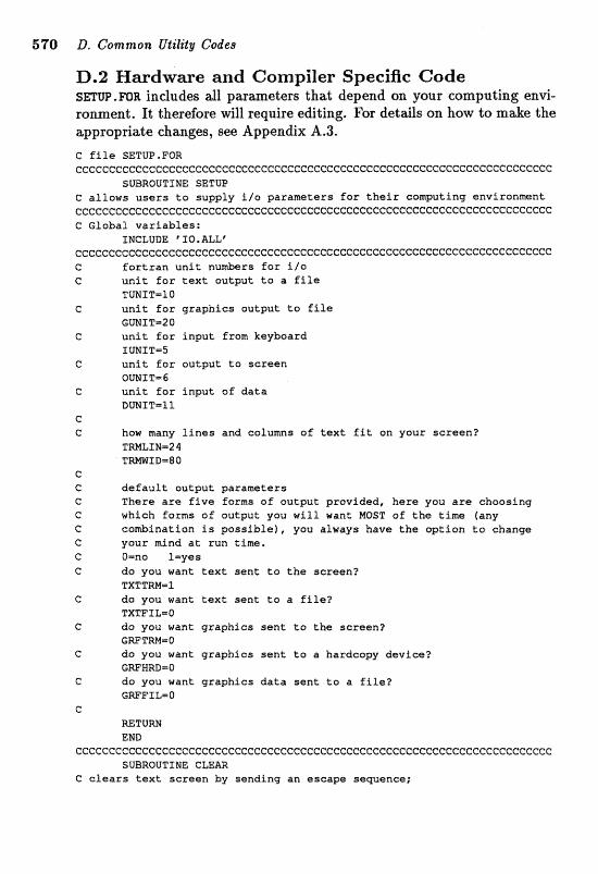
570 D. Commosz Utility Codes
D.2 Hardware and Compiler Specific Code SETUP.FOR includes afl parmeters that depend on Jrour computing envi- ronment, ft therefore w111 require @&tinge For details on how to make the appropriate changes, see Appedix A.3. C f i l e SETUP-FOR CC~CCCCGCSCcC~CCCCC~CCCC[:CCCCCCCCCCCCCCCCCCCCCC~I:C~CCCCCCCCCCCGC~CCCCCCCC
SWROUTINE SETUP G al lows u s e r s t o supply i l o parameters f o r t h e i r computing e n v i r a n m n t c~c~cccccccccc~cccccccccccccccccccccececcccccccccececccccccccccccceccccc C Global va r iab les :
INCLUDE ' IQ ,AIL&" e~~c~ecccC~cccc~c~eecccecc~cccccccccccceccef:eccccccccC:eccecccccccccccccc C f o r t r a n u n i t nu-rs f o r i l o G u n i t f o r t e x t output t o a f i l e
TUNTT-10 C u n i t f o r g raph ics output t o f i l e
GUNIT-20 C u n i t f o r inpu t from keybaard
IUNIT-5 C u n i t f o r output t o screen
QEZNIT-6 e u n i t f o r inpu t of d a t a
DONIT=11 c C how many l i n e s and colurns of text f i t on your sc reen?
TmLIN-2 4 T m X D m 8 0
C e d e f a u l t output parameters C There a r e f i v e farms of output provided, he re you a r e chaosing C which forms of output you w i l l went MOST o f t h e t i n e (any C coMina t ion is p a s s i b l e f , you always have the opt ion t o change C your mind a t run time. G O=RD f = y e ~ G do you want text sent to the screen?
TXTTRM=1 C do you want t e x t sen t t o a f i l e ?
TXITFIL=O C do you want graphics s e n t t o the screen?
GRFTRNmO C do you want graphics sent t o a hardeopy device?
GWBRD-0 C do you want graphics d a t a s e n t t o a f i l e ?
EWFEL=0 C
WTURM END
Cccccccccccccccccccccccccceccccecceccccccceccceccccccceecccccececccccccc SUBROUTINE CLEm
C c l e a r s t e x t screen by sending an escape sequence:
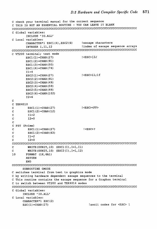
-D,$ Bardwane and Gnapiler Specific Code 571
C check your terminal manual f o r t h e cor rec t seguence C THIS IS NOT AN ESSENTTAL ROUTINE - YOU CAN LEAVE IT BmNK C:cccccccccccccccc~C:ccccccccccccceccccCccccccccccccccccccC:ccccccccccccccc C Global var iab les :
INCLUDE ' 10 ,ALLf C! Local var iab les :
CNAmCTER*l ESC2(4),ESe2(6) !escape charac te rs IHTEGER I,11,22 !index 05 escape sequence a r rays
~ecce~~e~c~~~ecc~~~~eccccc~cccccec~ccccccccececccceececccc~ccccc~ccccccC: C VT200 terminal; t e x t made
ESCl (l) =CHAR f271 ! <ESC> [i?J ESCI(2) =CH= (91 1 ESCI(3) =CH&R (50) Esclf4f =CmR(741 114 ESC2 fl)=CH&R (27) ESC2 (2) -CH&R(91) ESC2 (3 ) =CHAR (4 9) ESC2 ( 4 ) =CHAR (5 9) ESC2 45) =CHAR (4 91 ESC2 (6) -CMR (102) f 2 = S
C C TEK4OlQ C ESCl (l) =CHAR (27) C ESCl f 2) =CHAR (121 C 21.12 e I 2=0 C C PST [Prime) C ESCllf )=CRARf27) C: ESCl(2 f =CHAR (63 f C P 1=2 C X2-0 ccccccC:c~cccccccCcccccccceccccccccccccccccccc~cccceccccccccccccc~ccccc~c C m I T E (OUMIT, 10) (ESCl(I1, I=l, I11 C bJliZITE (OUNIT, ZO) (ESC2 (P),3=1,T2) 10 FORmT ( 1X ,6A1)
RETURN EPJD
ccccccccccccecccccccccccecccecccccccccccc~ccceccceccccccccccccec~ccecccc SUBROUTINE GMQDE
C switches t e m i n a l from t e x t t o graphics mode C! by wr i t ing hardware dependent escape sequences t o t h e terminal C This rou t ine con ta ins the escape sewence f o r a Graphon terminal C t o switch between VT200 and TEK4814 modes ~eC:cccccc~ccec~ccccc~ccccccccccccec~ccccce~ccccccccccceccccccecccccccccc C Global var iab les :
INCLUDE ' IQ. ALL" C Local var iab les :
CHmGTER*l ESC (2) ESC (l) =CHAR (27) ! a s c i i codes for eESC> 1
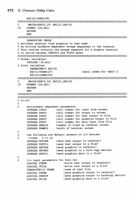
572 D. Common Ufililp Codes
ESC(2)=CW{492 ccccccc~cccccccccceccccccecccccccccccccccceecccccccecccccccccccccccccccc C mZTE(OUNI&IO) ESC(lf ,ESC(2) 10 F O W T flX,2Al)
=TURN eEaa
cccecccccceccccc~ceecccceccccccecccccccecccccccccccecccecccecce~cec~cccc SUBROUTINE TMQDE
C switches terminal from graphics t a t e x t made C by w r i t i n g hardware dependent escape sewences t o t h e terminal C This rou t ine con ta ins t h e escape sequence f a r a Graphon terminal C t o switch between TEK4014 and VT200 m d e s ccccecccccccceccc~cf:ccecccccceeececccccecccccccccccecccccccccccccccccccc
Global v a r i b l e s : INCLUDE * 10. ALL8
C Local var iab les : CHmCTER*P ESC (2 f ESC flf =CmR(27f l a s c i i codes for <ESC> 2 ~ s c (z)=ewmfset
ccccccccccccccccccececcccccccccccccccccceccccceccccccccccccccccccccccccc C m I T E (oUHIT, 10) ESe (l) ,ESC f2) 10 F O m T (1X,2AT)
=TURN END
cccc~~ccccccecccccccccccccccccceecccccccccccccccc~cccccccccc~c~cccc~cecc cccccccccccccccecccecccceecccccccccccccccccceccceccceccccccccccccccccccc C io.aX3. C G enviranment dependent parameters
INTEGER IUNIT ! u n i t n u a r f o r input from screen INTEGER OUMIT !uni t nu&@r Eos output t o sereen INTEGER TUNI 'r !un i t nuniber f o r t e x t output t o f i l e INTEGER GUNIT !un i t nu&er Ear gra&ics output t o f i l e INTEGER DUNIT !un i t nu&er far da ta input from f i l e INTEGER TRMLZN !nu&er of l i n e s an terminal sc reen INTEGER T W I D !width of terminal screen
C C t h e fol lowing a r e d e f a u l t answers t o i l o chaices C I==yes 0 == no
XMEGER TXTTRM !send t e x t output t o terminal? INTEGER TXTFIL !send t e x t output t o a f i l e ? INTEGER GRFTRM !send graphics t o terminal? INTEGER GRFHRD !send graphies t o a hard copy device? INTEGER GRIFFIS, !send graphics d a t a t o a f i l e ?
C C i / o input parameters f o r t h i s sun
LOGICAL TTERM ? w r i t e t e x t autput t o terminal? LOGICAL TFILE !wri te t e x t output t o a f i l e ?
!name of t e x t f i l e LOGICAL GTERM !send graphics output to t e rmina l? LOGICAL GHRDCP !send graphies output t a hardcopy device?
LOGICAL GFTLE !send graphics d a t a t o a f i l e ?

!nam of graphics data f i l e c
COWON /IO/TUMST~GUNXT,XUMITIQUNIT~DUMITITRMt1CEJtT~ZDtTXTT~~ 3 TXmXL, GWTW, GRFWRD, GWFXLL -b TTERM, TFf LE, GTERM, GFXLE , GWRBCP
COmON / CTQ / T N m , G N A M E
574 D. Comnaoa Ilti221y Codes
D.3 General Input/Output Codes All of the utility routines that do not need editing are located in the file UTZTIL.FOR. They are as follows:
menu HE@U : defines menu array variables that are the s a e for d l programs
rotrtirres ASK : executes the menu PRTACS : prints menu items and default; vdues PWMS : prints blaak lines FRYORE : prints a 9%' or "0" PARSE : controls menu branching by returning index of
next menu item
f ie FLOPEH : opens a new file manipdatim FuJpla2 : open8 m existing file
FLGLQS : clams a
user : retnrns a floating point aaxmber intedwes GmIIQT : returns an irzteger
YES80 : returns a l (yes) or O (no) CEXARAG : returns a chaxacter string PAUSE : suspends execation until user presses Return key
c~rrversion CO~BVBT : converts a real namber to a stdrrg routines IWWT : converts m integer to a string
LQGCV"P : converts l to .TRUE. , every thing efse to . FAME. dscella~eous H ~ D E ~ : prints the introductov text screen
FXBISB ; clo~es open files m$ stops the p r o g m am^^ : prints default d u e for red numbers in an W -
propriate format IMTBW : prints default d u e for intqefs in m apprwri-
ate fomat LEgmU : returns the fength of a Gfiaracter string exclnsive
of trdfing blmks RAlNaS : returns a unifomly Gstribnted random
between O aad l,
CeccccccCcccccccccccccecceccccecccceccccccccccccccccccccccccccccccccccc~ G f i l e UTIL,fox G COMPUTATIONAL PHYSICS (FORTRAN VERSION) C by Steven E, Koonin and Dawn C. Meredith C Capyright 1989, Addison-Mesley Publishing Csmpany ccecc~ce~ccc~ccceeccccc~cccec~cccceccccccccccccceeccceeccccccccceccccccc
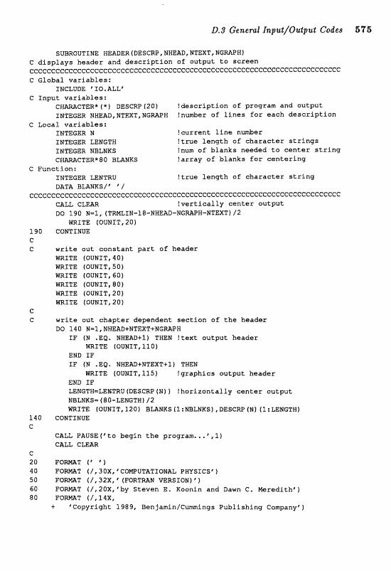
D.3 General 1nputButpu.li Codes 576
SUBROUTINE HEADER (DESGRP , NNEAD, NTEXT, NGMPH] C d i s p l a y s header and d e s c r i p t i o n of output t o s c r e e n CCccececcccccccCcceccccccC:cccceccC:eccceccccccecccceccccccccccccccccccccc C E i a b a l v a r i a b l e s :
INCLUDE ' IQ. ALL1 C I n p u t v a r i a b l e s :
CTER*(*) DESCRP(2Q) ! d e s c r i p t i o n of program and ou tpu t INmGER NWEAD,MTEXT,NGRIIPR !nu&er of l i n e s fox each d e s c r i p t i o n
C Local v a r i a b l e s : INTEGER N ! cu r ren t l i n e rider INTEGER LENGTH ! t r u e l e n g t h of c h a r a c t e r s t r i n g s 1NI"EGER NBLNKS fnum of b l a n k s needed t o e s n t e r s t r i n g CHMCTER"8O BUNKS ! a r r a y of b lanks f o r c e n t e r i n g
C Funct ion: INTEGER LEMTRU ! t r u e l e n g t h of c h a r a c t e r s t r i n g DATA BLAMES / ' ' /
~c~c~~c~~~~c~~~~c~~cccccceccc~ccccccccceccc~cccccccc~c~cc~~ccc~ccccc~ccc CALL CLEAR ! v e r t i c a l l y c e n t e r ou tpu t DO 190 N = 1 , {TRMLIN-X~-NHEAD-MGRAPW-~JTEXT~~~
WRf TE (QUNIT, 20 1 190 CONTINUE e c w r i t e ou t c o n s t a n t p a r t o f header
@RITE fQUNIT, 40) WRITE (OUNIT, 50) m I T E (QUNIT, 601 WRITE (OUNIT, 80) WWITE (OUMIT, 20) WRITE (OUNIT, 20)
C C w r i t e ou t c h a p t e r dependent s e c t i o n aE t h e header
DO 140 N=l,NWEAD+NTEXTfMGWW I F f N .EQ. N M W + Z ) THEN ! t e x t ou tpu t header
WRITE [OURIT, 110) END I F 6P (N .EQ. NMEAD+NTEXT+l) TEEN
WRITE (QUNIT,11S) !g raph ics ou tpu t heade r END I F LENGTWmLEMTRU (DESCRP (NI 1 ! h o r i z o n t a l l y c e n t s r ou tpu t NBLNXS=(SO-LErJC;TW)12 WRITE (OUNIT, 1201 BLANKS (3 : mLNKS) , DESGRP (NI (1 :LENGTH)
140 CONTINUE C
CALL PAUSEt8to begin t h e p r o g r a n , . . f , l f CALL CLEAR
C 20 F o M T ( @ ' 1 40 F O m T {/,3OX,'COMPUTATIOWAL PHYSICSf) 50 F O W T f/,32X,'fFORTMNVERSXON)#) 60 F O M T (/,2OX,%y Steven E. Xoonin and Dawn C. Mezedithe 1 80 F O m T (/,14X,
+ V o p y r i g h t 1989, BenjaminlCumings P u b l i s h i n g Company')
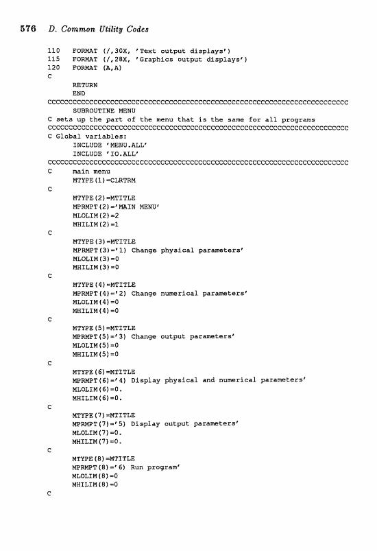
576 D. Common Uilz'ligy Codes
110 F O m T ( / , 3 0 X , 'Text output d i s p l a y s E ) 115 F Q m T ( / , 2 8 X , 'Graphics output d i s p l a y s 8 ) 3.20 F O m T (&A) C
=TURN END
cccccc~ccccCcccccccccceccccccccccccccecccccccccecccccccccccccecccccccccc SUBROUTINE MENU
C s e t s up t h e p a r t o f the menu t h a t i s t h e same for a l l programs cccccccceccccccccccceccecccccccccceccccceececcef:cccccecccccccecccecccccc G Global var iab les :
INCLUDE M N U . ALL' INCLUDE fIO.&LLr
cccccecccccccccccccccccccccecccccccccccccecceccct:ccccccccccccccccccccccc C main menu
MTVPE ( 5 1 =CLRTRM C
MTYPE (2 1 =#TITLE WWI: (2 f =%XPf MENU" H L ~ L X M (2 -2 HHILIM 62 ) -1
c MTVPE ( 3 ) =MTTTLE EdPWT(3)="1) Change phys ica l parameterst MLQLIN 43 f ==a MWILIM (3) 90
c NTWE f 4 E =HTITLE W W T (41 =' 2) Change n u m r i c a l p a r a m t e r s e MLQLICM(4) =O XHLLIM ( I 1 -0
C MTYPE (5) PMTITLE MFmPT(S)=e3S) Ghanqe output parameters" PILOLIM (5 1 =Q MWf LIM (5 ) =a
C NTWE C 6) -MTSTLE MPRMPT ( G ) 41 Display phys ica l and numerical parametersf MLQLIM(6)-0. MHXLZN ( 6 1 -0,
C MSYPE ( 7 ) =MTITLE 13XZMPT (7) 1-51 Display output parametersf NLaLrM (71 =Q. MHILIW (71 =Q.
C MmPE (8) =MTITLE W W T (81 xC B f Run programf MU)LIW I( 8 1 =O MMXLIM (8 1 -0
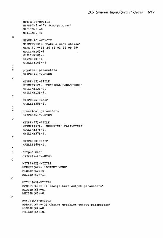
D.$ Generat I n p ~ t / Q ~ t p a ; t Codes 577
WTSE ( S) PMTITLE mMT (9) =@ 7 1 Stop pragramp NLOLPEJI ( S 1 =B MWILIM ( 9) ==l
MTVPE ( 1 0 ] =MCROZC M P W T (10) = Wake a menu choicer MTAG ( 2 Of m' l1 36 61 91 94 99 99" MLQLIEJI (l0 f =I. MHILIN (l O f -7 MINTS (10) -6 NWLSff0)=-6
physical parameters MTEE ( 11 1 =CLRTRM
MTVPE (12) =TITLE MPmPT (12) = "PYSICAX, IFAMmTERS' MLOLIM (1 2 1 =2. MWILIM (12) =l.
numrf eal parameters MTVPE f 3 6 1 =CLRTRM
NTYPE ( 3 7 1 -TITLE W W T 137) - ' NUMERICAL P MLOLIM (37) 4 2 . MWILXN (37) -1.
output, menu MTYPE ( 61 ) =CLRTBM
MTYPE ( 62) -P?ITLTLE N P W T (62) = ' OUTPUT MENUt MLOLIN (62) 10, MHI LIN 162) =l.
MTVPE ( 63 f -%TITLE N P M T (63 ) 21 Change text output parameters" ML0LIM ( 6 3 ) -0. MWILIM f 6 3 ) 10.
MTWE (C4 ) =MTITLE WRMPT (641 -' 22) Change graphics output parametersf MLOLfM(641 =Q. MMZLIN (64) PO.
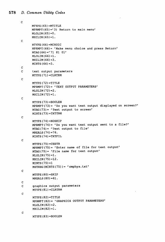
578 D. Common Viila'by Codes
MTYPE (65) =MTITLE MPWT(55)=@33) Return to main menu" MLQLTM (65) P O . MHILIM ( 65) -1,
MTVPE ( S 6 I =MCHOSC M P W T f 64)= 'Wake menu choice and press Returnp MTAG ( 6 6 ) =' 772 81 01' MLOLIM t 6 6 ) =I MHZZXM (661 =3. MINTS (55) =3.
text output paramters MTWE (73, ) =CLRTRM
MTMZE ( 7 2 ) =TITLE PIUPNP 11 ( "1 2) a;- TEXT OUTPUT P&MmTERS " MLOLIM (72 ) 4 2 . MHILTM (721 11,
MTWE ( "1 3) =BBQLEM W W T (73) = .Do you want text output displayed on screen?' HTAG(73)= 'Text output to screent WTNTS (73 f =TXTTRM
MTYPE ( 74 f =NOSKIP MPMPT(74)- Do you want text aueput sent to a file?' MTAG (74) @ Text output to filef
MTNTS (74) =TXTFIL
MTWE (75 1 =CWSTR M P W T ( 7 5 1 @Enter name of file for text output6 MTAG(7S)m 'File nme for text output' NLOLZM 1751 =l. NWXLIM (751=12. MXNTS (75 1 =l MSTRNG (MTNTS (75) ) 1 ' cmhys. txtp
graphics output parameters MTYgE f 8 h f =CLRTRN
MTYeE (82) =TITLE W W T (82) - * GRB,P&WICS OUTPUT P MLQLTM (82 1 -2. M81 LIN (82) -1.
MTVPE (83) =BOOLEN
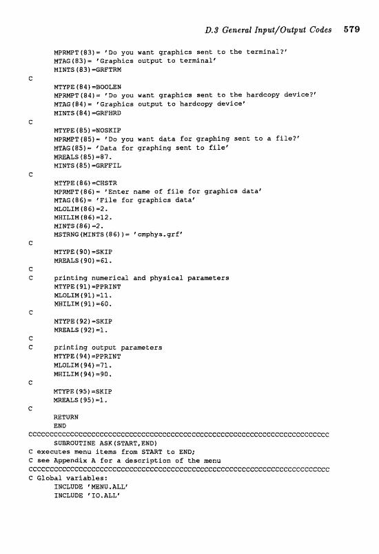
D3 General lapzl.l//Output Codes 679
E m P T ( 8 3 ) = 'Do you want graphics sent to the terminal?" MTAG (83) = Graphics output to terminal' MIWTS (83) =CRFTRM
c MTYPE 4 8 4 ) =BOQLEN WRMPT(84)- you want graphics sent to the hardcopy device?' MTAG181)= "raphics output to hardcopy devicer MINTS (8 4 ) =GREWRD
G %TYPE f 85 1 -NOSKTP N P W T ( 8 5 ) = Wo you want data for graphing sent to a file?" HTAG (85) = Wata for graphfng sent. ta filep
LS 185) ~ 8 7 . MINTS f 85) -GWFIL
C M T S E (86) =@WSTR W W P T (86)= @Enter name of file for graphics dataC MTAG ( @ G ) = Vile for grapbics dataf MLOLTM (86) ==2, MBILIN ( 8 6 ) =l2 I
NIMTS 486) -2. MSTRNGfNINTSf86))- 'cmphys-grf'
C
NTUPE (90) =SKIP M M L S (901 ~ 6 1 ,
C C printing numerical and physical paramtars
MTYPE ( 91) =PPRINT MLOLXM(91)=12. MHTLIW f 91 f =GO.
C
MTPE ( 92) =SRI P W A L S (!321=1.
c C printing output parameters
NTYPE ( 94) =PPRINT MLOLTM ( 94 ) =?l. NWILIM (94) -90.
C NTYPE ( 95) =SKIP MRmLS 4 95 ) -1.
C RETURN END
ccc~cc~ceccc~~ccccccccccccecccccccce~ccccccecccccccccceccccce~cc~ccccc~c SUBROUTINE ASK(STmT,END)
C executes menu items from START to END; C see Appndix A for a description of the menu cmcccccccccccceccccccccccecccccccccceccceccccccccccccccccc C Global variables:
f NCLUBE "MENU. ALLf INCLUDE ' IQ. ALL1
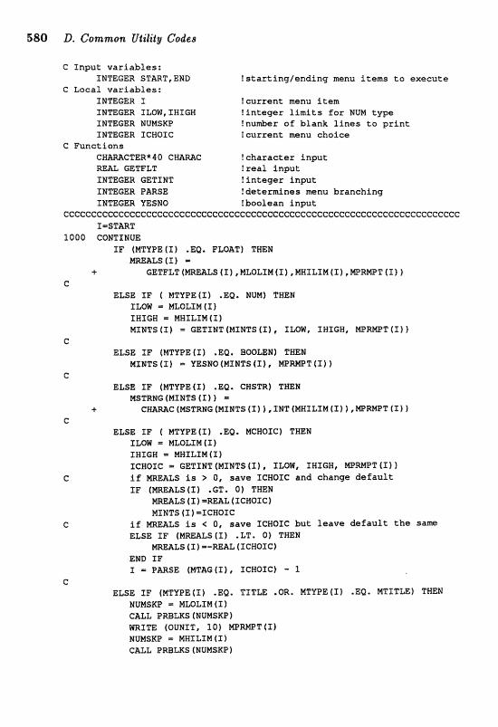
C Xnput v a r i a b l e s : INTEGER ST&RT,END t s t a r t i n g l e n d i n g menu i t e m s t o execu te
C Local v a r i a b l e s : INTEGER 1 ! cu r ren t menu i t e m INTEGER ILC?W, IWIGW ! i n t e g e r l i m i t s f o r NlfH t y p e INTEGER MVMSKP !nu&er a f blank l i n e s t o p r i n t INTEGER ZCBOXC t c u r r e n t menu cho ice
C Funclions C H m C T E R * l O GWAmC !cha rac te r i n p u t RE& GETFLT t r e a i i n p u t IMT&GER GETINT ! i n t e g e r input INTEGER PARSE Idetermines menu branching IHTEGER YESNO ! boolean i n p u t
eeccecccc~ce~cecccccce~ccecccccccccccccccccccccccccccccccccecccC:ccccc~cc f=STrn"1:
l O B O CQHTINUE I F (MTYPE(1) ,EQ. FLOAT) THEN
s a t = i T F L T ( m A L S ( 1 ) ,MLOLIM(l) ,MWILIM{I] ,WRMPT { Ik 1
c ELSE IF [ MTYPE (I) .m. Nun)
ILCIW = NLOLIM(I1 I B f GW = MHILXM ( I ) MINTS (I) 1 GETINT (MINTS {I), XLOW, IHZGH, W R W T (11 )
C ELSE I F (MTVPE ( I ) .EQI 800LE1) THEN
MINTS (f ) VESMO (MINTS ( I ) , W W T ( I ) f G
ELSE SF (MTYPE (I) .Ea. CNSTR) T B N NSTRNG (MINTS ( I 1 ) =
I. e m m c ( ~ s r ~ ~ G [ M r ~ T s (11 I ,XNT ~MHXLIM(X~ 1 c
ELSE I F ( MTYPE (I) .EQ. MCWQIC) THEM ILOR - MLQLIM [X) ZNIGW MHZLTM ( I 1 IcWoxc = CETSNT (MINTS I S ) , ILQN, IWIGB, WFIMPT (S) I if i s > 0, save ICHOXC and change d e f a u l t IF ( W A L S 13)
MZNTS (S) =ICHOIC i f m A L S Ss < 0, save ICMOIC but l e a v e d e f a u l t t h e sam ELSE I F ( M m L S ( I 1 .LT. 0) THEM
mEALS (I) =-REAL f IGWOIC) EMD I F I 5 PaRse (NTAG (I , IcWaIcf - 1
C ELSE If (HTYPE(1) .EQ. TIT= .OR. MTYBE ( 1 ) *EQI MTXTM] THEN
NUNSKB - MWLIM ( I 1 GALL PRBLKS (NUMSRP 1 mXT& (OUNIT, 1 0 ) WRMPT(Z) MUMSKP - MHILIMgI) CALL PRBLKS (PSUMSKP 1
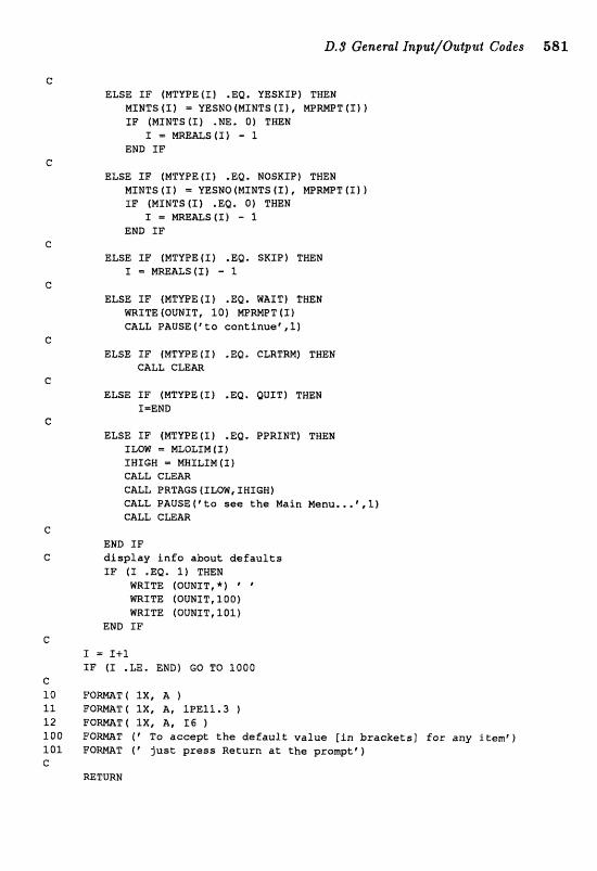
L;), 3 General I.aflzk#/Ou~pzrd Codes 581
ELSE XF (MTIIPE ( I ) .Ea. YESKIP) TWEN MSNTS (I) = YESNQ (MINTS ( I 1 , E(IPNPT (I) 1 IF (MINTStI) .NE. 0) THEN
I MREALS(I1 - 3 END IF
ELSE I F (MTVPE ( X ) .EQI NQSRIP) THEN MINTS (X) = YESNO fMZNTS (I f , mRMPT ( I 1 IF (MINTS(T) .EQ. 0) THEN
X = m & s ( x j - 1 END I F
ELSE I F (MTVPE (1) .EQ. SRTF) THEN Z = MREALS ( X ) - 1
ELSE IF (MTHPE (I) .EQ. RAlT) THEN WRITE (QUMIT, 10) MPRWT (S) GALL PAUSE(@to continuet,l)
ELSE IF [MTPPE (I 1 . EQ, CLRTRM) TWEN CALL GLEm
ELSE I F (MTYPE(T1 .EQ. QUIT) THEN I=END
ELSE I F (MTYPE (I) .EQ, PPRXNT) THEN ILOW = MLDLTM ( I ) IWXGR 1 NWILIM [I) CALL CLEm CALL ORTAGS (ILOW, IBIGN] CALL OAUSEff to osss t h e Main Menutl.%3) CALL CLEAR
END I F display info about defaults IF fI .EQ* 1) THEN
WRITE (OUNST,*) * ' WRITE (OUNIT, 100) WRITE (QUNXT,lOI)
END X!?
F O m T ( 1X, A 1 F Q m T ( %X, A, 1PE11.3 1 F O W T ( I X , A, I 6 ) F O m T ("0 accept the d e f a u l t value [in brackets3 for a n y itemc) FQ-T ( * just press Return a t the p r o m p t ' )
RETURN
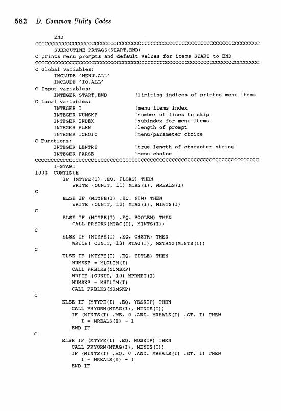
582 D. Common Ufa'lify Codes
END ceccccccccecccccccccccccccccccet:cecccecccccccccccccccccccccccccccccccccc
s v B R o v r r N E PBTAGS(START,END) c prints menu prompts and default values for items S T m T to END cc~cCcecccc~ceeccccceccccccecccccccccecc~ceccccccccccccccceccceccccccc~c C Global variables:
INCLUDE MMGNU, ALL" INCLUDE 'IQ.ALL;
C Input variables: INTEGER START, EMD !limiting Indices of printed menu items
C Local variables: INTEGER I !menu items index INTEGER PfUMSKP !nu&er of lines to skip INTEGER INDEX !subindex for menu items INTEGER PLEN !length of prompt INTEGER ICHOIC Imenulparameter choice
Functions: INTEGER LENTRU ftrus length of character string INTEGER PARSE !menu choice
cccccccccccccccccceecc~cccccccccccccccecccccec~ccccecccccccc~ccc~ccccccc I=S"IE"RT
1 0 0 0 CONTINUE I F (MTVPE (S) .EQ. FLOAT) TNEN
WRITE (OUNIT, 3.11 MT&G ( X ) , NmALS (I) C
ELSE I F (MTUPE (I} .EQ. NUM) THEN WRLTE (OUNIT, 221 MTAG ( I ) , NINTS ( X )
G ELSE IF fMTYPE (1 f .EQ, BOQLEN) TNEN
CALL DRYORN (MTAG (I J , MINTS ( I 1 ) C
ELSE IF (MTYPE (I) .EQ, CHSTR) THEN WRITE ( OUNIT, 1 3 ) MTAG ( I ) , MSTRNG (MINTS (X) )
C
ELSE I F (MSYPE ( I ) .E&. TITLE) THEN NUMSRP = N m L I M (I 1 CALL PRBLKS (MIINSKP) WRITE (OUNST, 3.01 MPRMPT(T1 NUMSKP = MHILIN ( I ) cam PRBLKS (NUMSKP 1
C ELSE I F (MTVPE ( I ) .EQ. YESKIP) THEN
C&LL PRYORN (EITAG (X 1 , NINTS ( I ) ) T F (MIMTS(1) .NE, O .AND. MREALS(I1 .GT. I ) THEN
I = MREALS(I) - 1 END I F
C ELSE I F (MTYPEtI) .E&. NOSXIP) TEEN
CALL PRUQRH (MTBG (X 1 , MINTS (I) 1 I F (MLNTS (I) .EQ. O .AND, MREALS(I1 .GT. I) THEN
X = MREmS(EJ - 1 END SF
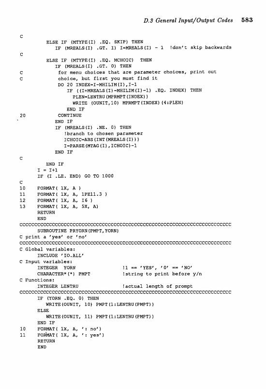
D.3 G"encraZ I R ~ ' I L I / " " Q ~ E ~ ~ L Codes 583
ELSE SF (MTYPE (X) .Ea. SKIP) THEM IF (NREALS ( S ) .GT. I ) XmMMALS f L ) - 1 f d o n r t s k i p backwards
ELSE I F (MTYPE(L) .EQ. NCWOIC) TWEN IF (NmALS(I ) .GT. Oj TWEN
f o r menu c h o i c e s t h a t a r e p a r a m e t e r choices, p r i n t out c h o i c e , but f i r s t y o u mas t f i nd i t DO 20 INDEX=Z-MNTLIM(I),I-1
XF ( (I+MREALS ( I ) - M W I t I M (I 1 -1) .Ea. INDEX) THEN PLEN-LEWTRU (NPRWT [INDEX) f WRITE (OUNXT, 1 0 ) NPRMPT (INDEX) (4:PLENf
END XF COMTINUE
END 11" I F (MmALS(1) .m. O) THEN
! b r a n c h t a c h o s e n p a r m e t e r scwosc=~ss (INT (HmaLs (W X e a R s e ~MTAE ( X , IGROICI -1
END I F c
EWD IF I = 14-1 I F (L .LE. END) GO TO 1000
C 1 0 F O m F ( l X , A ) 11 FO-T ( 1X, A, lPE11.3 ) 1 2 F Q m T ( SX, A, X6 1 1 3 F O m T ( XX, A, 5 X , Af
RETURN END
ccccccccecccccccccccceccc~ccccccccceccecccccccccccccccc~c~ccccccccccc~cc SUBROUTLNE PRYORM (PMPT, YORN 1
C p r i n t a ' y e s 1 aar %no" ccecccccccccccccccccecccccccccccccccccccccccccccccccccccccc~ccccccc~cccc G G l o b a l v a r i a b l e s :
INCLUDE 'IO.ALLt C Xnput variables:
INTEGER YORN 'YES", * a @ mm @NO" CHmCTER* f *) PNPT !string t o p r i n t b e f o r e y l n
C Functions: INTEGER LENTRU !actual length o f p rompt
ccecccccccccccccccccccccccccccc"cccccccceecccccccecccececcccccccccccccccc I F (YORN .EQ, O) TWEN
mXTE (OUNIT, 10) PNPT (1 :mNTRU {PMPT) f ELSE
WRPTE(OUHIT, 11) PMPT(l:LEMTRU(PmT)) END I F
1 0 F Q W T 4 IX, A, : not ) 11 F O ~ T ( IX, a, : y e s t )
M1URM END

584 D, Common Ufzlity Codes
cceccc~ccccccccccccccccceeeccccccceccceccccccccccccccccccccecccceccccccc SUBROUTINE PRBLKS (NUMLIN)
C p r i n t s NUMLIN b lank l i n e s on t e r m i n a l ceccecccccccecccccccccecccccecccccccccccccccccccccccccccccccccccc~ccc~cc C Glaba l v a r i a b l e s :
TMCLUDE 'IIO,ALLf C Passed v a r i a b l e s :
JNTEWR NUNLIN !nu&ar of b lank l i n e s t o p r i n t C Local v a r i a b l e s :
INTEGER I ! d u m index ccccccccccceccce~ccceccccccceecceececccccccceccccccccce~cccccccceccccccc
DO 1000 I=l,NUEEILXM WRITE( OUNIT,*) ' *
aooo CONTINUE RETURN END
cccccceccccccccceecccccccccccccccccccccccccccccccccccccccccc~ccccccccccc SUBROUTINE PAUSE (PHRASE, MSKXP )
C g i v e s user t im t o read s c r e e n by w a i t i n g f o r d u m y Input ; C a l l o w s E a r p r i n t i n g o f PWmSE t o screen; C s k i p s NSKTP l i n e s b e f o r e p r i n t i n g PWmSE cceccccccccccCccccccc~cccccccccccccccccecccccccceccccccccccccccccccccccc C Globa l v a r i a b l e s :
INaUDB ' XXQ.ALL" C Passed v a r i a b l e s :
CHWCTER* f * f PHWE !phrase t o b e p r i n t e d INmGER NSKTP Inumber of l i n e s t o s k i p
C Loca l v a r i a b l e s : CWmCTER*1 DUMMY ! d u m y v a r i a b l e INTEGER XSRIP !MSKIP index
cccceccccccccecccccccccecccccccccceccceceeeccccccccceccccccccccceecccccc DO 10 ISKIP-1, NSKXP I s k i p 1Snes
WRITE (OVMfT,S) 1 0 CONTZMIIE 5 F O m T ("1
RR3TE IOUNIT, SS) BWMSE !write phrase W A D fIUNIT, 20) DUHMU !wait f o r dumy i n p u t
15 F O m T ("ress r e t u r n p ,A) 20 F O m T ( A l )
m TURN END
cecccccceeccccceeccccccccccccccccccccccccccccccccccccccecccccccccccccccc SUBROUTTHE FLOPEN (PHAME, PUNIT)
C opens a new f i l e , u n l e s s one by t h e same name a l r e a d y exis ts ccccccccccccccccecccccceceecceccececcccccccccccccceccccecccccccccccccccc C Global v a r i a b l e s :
INCLUDE pXIO.ALL' C I n p u t v a r i a b l e s :
CTER* (* 1 FNAm ! f i l e name TWTBGER FVNIT !unit: nu&er
C Local v a r i a b l e s : LOGICAL OPN !is t h e f i l e open?
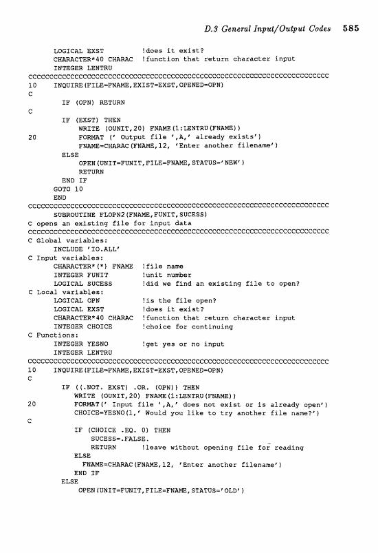
ll.9 General Jiaput/Oufpzt.t Codes 585
LOGICAL EXST Idoes it e x i s t ? CWWCTER*40 CMAMC ! f u n c t i o n t h a t r e t u r n c h a r a c t e r i n p u t INTEGER LENTRU
~c~~c~~~cec~~ccccc~ecceccccc~ceccccC:cc~eecc~ecc~ccccccccccccccccccc~cccc 10 TNQUSm (FILE=FWAMEi EXIST=EXST, OPENED=OPH) C
I F (QPN) RETURN C
I F (EXST) THEN m 6 T E (OVNIT, 243 f FNmE (1 : mNTRU (FNAME 1 1
2 0 F O W T f "tputr f i l e , A, Qlready e x i st S' 1 FRA==CHARAC(FNAME,22, 'Enter a n a t h e r f i lename'}
ELSE oPEN(VNIT=FVNIT,FILE=FNW~STATUS=~NEW'~ =TURN
END I F GOTO 10 EWE)
~~~~~ccc~cccccc~cccC:cccccccccccccccccceccccc~eccc~ccccccccccccccccc~cccc SUBROUTINE FLOPN2(FH&m,FUMIT,SUCE55)
C opens an e x i s t i n g f i l e f o r i n p u t d a t a ccCccccecccceccccccccccccccc~cccecc~ccecccccccccccc~cccccccccccccccccccc C Global v a r i a b l e s :
TNCLUDE ' TO. ALL" C I n p u t v a r i a b l e s :
CHMCTER* f * ) FP3Am ! f i l e Ram INTEGER FUNIT f u n i t nu&er LOGICAL SUCESS !did w e f i n d an e x i s t i n g f i l e t o open?
C Local v a r i a b l e s : LOGSCU OPEJ !is t h e file open? LOGICAL EXST !does it e x i s t ?
! f u n c t i o n t h a t r e t u r n c h a r a c t e r i n p t INTEGER CHOICE ? cho ice f a r c o n t i n u i n g
C Funct ions: INTEGER YESNO !ge t y e s o r no i n p u t INmGER LENTRU
GCCCCCCCCCCCCCCCCCCCGCCCCCCCCGCCGCCCCCCCCCCCCCCCCCCCCCCCCCCCCCGCCCCCCCCC 1 0 INQUI RE (FILEmPNAME, EXIST=EXST, OPENED=OPH 1 C
I F ((*NOT. EXST) .OR, (OPN)) THEN WRlTE (OUNIT, 201 FNAm C1 : mNTRU (FNAEJIW
2 0 PORmT ("nput, f i l e * ,A, ' does no t exf st a r is alreadTy openr} CWOICE=YESNOI1,p Mould you l i k e t a t r y ano the r f i l e narn??)
C SF (CHOICE .EQ. 0) THEN
SUCESS=-FALSE, RETURN ! l e a v e wi thout opening f i l e f o r r ead ing
ELSE FNAME~CWAMC(FNM~l2, "nter ano the r f i l e n a m e 6 )
END I F ELSE
OPEN (UNIT=FUNIT, FILEmFNAm, STATUS=' OLDf f
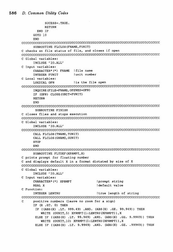
586 D. Common Ufility Codes
SUCESS=.TRUE. RETURN
END IF GOTO 10 END
ccccccCcccccCCccccccccccccccccccccccccccccccccCCcccccccccccccccccccccccc SUBROUTINE FLCLOS(FNAME,FUNIT)
C checks on f i l e s t a t u s of f i l e , and c l o s e s i f open cccececccccccccc~cececccccccc~cccecccccccccceccccccccccccccccccccccecc~c G Global va r iab les :
INCLUDE ' IO,ALLE C Input v a r i a b l e s :
CHMCTER*(*f FM- !file name INS"EGER FUUIT ! u n i t nunjoer
c Local v a r i a b l e s ; LOGX~AL OPN ! is t h e f i l e open
ccceceeccccc~ccccecccccccccccccccecccccccc~cceccceccccce~cccccccccccc~cc INQUIm (Ff m=FNAME, OPENED=OPEd) SF (OPN) CLOSE (UWTT=FUNIT) RETURN END
ccccccc~cccccceccccccccccccecccecccececccccccccccccccceccccccccccccccccc SUBROUTINE FINISH
C c l o s e s f i l e s and s t o p s execut ion cecccccccecccccecccccccc~ccccceccccccccccceccccccccccccccccccccccccccccc C Global v a r i a b l e s :
INCLUDE ' IQ.ALLe ccccceecccccccccccccccccccecccccccccccceccccccccccccccccccceccccccccccce
CALL FLCLOS {TNANE, TUNIT) CALL FLCLOS (GNANE, GUNIT) STOP END
ccccceeceeccccccccccccccccceceeeccccccccccccccccceeccceccccccccccccccccc SUBROUTINE PLTBEF (XPRME"T, X)
C p r i n t s prompt f o r f l o a t i n g number C and d i s p l a y s d e f a u l t X in a format d i c t a t e d by s i z e of X cc~ccccc~cc~cccceccec~cccccccccccccccccceccccccccceccceccccccccccecccccc C Global va r iab les :
TMGLUDE ' IQ. ALL' C Input var iab les :
CHmCTER* ( * 1 XPRWT !prompt s t r i n g m= X ! d e f a u l t va lue
C Function: XNmGER LEMTRU ! t r u e l eng th a f s t r i n g
cccccccceeeecccccccccccC:eccccceccececccccccccccccceccecccccccccccccccccc C p o s i t i v e numbers ( l eave no roam f o r a s ign)
IF [ X .GT. 0) THEN IF ( ( m S ( X ) .LT. 999.49) .AND. (ABS(X) .GE. 99.949)) THEM
WRITE (OUNIT, S 1 XPRMPT (1 : LENTRU (XPRME"T)),X ELSE IF ((ABS(X) .LT, 99,949) .AND. (ABS(X) .GE. 9.9949)) THEN
m T T E (OUMXT, 3.0) X P W T ( I :DNTRU (XPWPT) 1 , X ELSE IF ((ABS(X) .LT, 9,9949) .AND. (ABS(X) .GE, .99949) f THEN
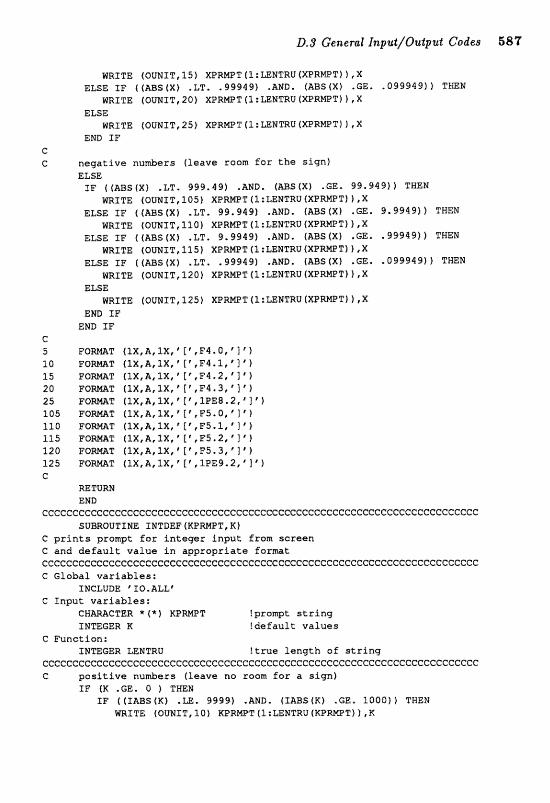
LT.3 General I~pu.t/Qut;rtuf Codes 587
WRITE (OUNIT, 1 5 ) XPRMPT (1:fiEN"rRlf (XPRWTI 1 , X ELSE I F ( (ABS(X) .LT. -99949) .AND. (ABStX) .GE- -099949) f T m N
WRITE (OUNXT,20) XPRMPTIl:mNTRU(XPRNPTf ) , X ELSE
m X T E (OUNIT, 25) XPRNPT (1: UNTRU (XPRWT') 1 ,X END I F
e C n e g a t i v e numbers ( l eave roam f a r t h e s ign1
ELSE I F ( (ABS(X) .LT. 999.49) .AND, IABS(X1 .GE. 99.949)) TWEN
m I T E (OUNX21,105] XPRNPT (1 :LENTRU (XPRWTI 1 ,X ELSE ZF 4 (IIBS(X) .LT. 99.949) .AND, ( m S ( X ) .GE. 9,9949)) THEM
m I T E (OUfdIT, 1 2 0 ) XPRNEIT ( 1 :LENTRU (XPRmT) 1 , X ELSE IF ((ABS (X) .LT. 9,9949) .AMD. (ABS(X) .GE. ,39949)) THEN
m I T E (OUNI'17,115) XPRWT(P:LENTRU(XPRNPT)),X ELSE I F [ (=$(X) .LT, .99949) .AHD. (X) .GE. .099949) ) TBEN
WRITE (OUNZT,12Q) XPRMPT (1:LENTRU (XPRMPTI 1 #X ELSE
WRITE (OUNf T, 1 2 5 ) XPRMPT (1 ; U N T R U ( X P W T f ) r X END 3 F
END I F e 5 F O ~ T ( 1 X , A , 1 X , ' [ ' , F ~ . O Y ' l ' ) 1 0 F O m T ( I X , A , 1 X y 8 ["F1.1,'2"f 1 5 E O m T ( lX ,A , lX , ' f t , F 4 , 2 , ' l") 20 F O m T { I X , A , 1 X , f [ C , F 4 = 3 , ~ f j 25 F Q m T (IX,AIIX,'[',1PE8,2,'1') 105 F O W T (1X,A,1XpP ['t,PS*O,'I 'I 1 1 0 F Q W T (1X,A,1X, f ' ,F5. l , * 1") 115 F O W T ( lX,A, XX, q* ,F5,2, ' 1 'l 120 F Q m T ( IX ,A , PX, " I " ,F5.3, 1 J') 1 2 5 F O m T (1X,A, l X , ' l', 1PE9.2 , ' 1 ' j c
RETURN END
cccceccccccccccccccecc"eccccecccccccccccceccccccccccccccccccccccccccccccc SWROUTXUE INTBEF (RPWPT, K )
C p r i n t s prarnpt for i n t e g e r i n p u t from sc reen C and d e f a u l t v a l u e i n a p p r o p r i a t e f o r m t cc~ccecccccccecccccccccecccceeecececcccccccccecceccccceeceeccccecccccccc G Global v a r i a b l e s :
INCLUDE ' 10,ALLt C I n p u t v a r i a b l e s :
CTER * f * f K P W T !prompt s t r i n g SRTEGER K ! d e f a u l t v a l u e s
C Function: INmGER LENTRU !true l e n g t h a f s t r i n g
cec~cccccceccecccccccccccececccccecceccccccccccccccccccccccceccccccccccc G p o s i t i v e numbers (leave no room f a r a s i g n )
I F {K .GB. 0 f TWEN I F ( ( I A B S ( X ) .LE. 9999) .AND. ( IABStRf ,GE. 1 0 0 0 ) ) THEN
WRITE (OUNXT, 1 Q 1 KPRNPT (1 : LEN"I"RU (KPRlrlPT) f , K
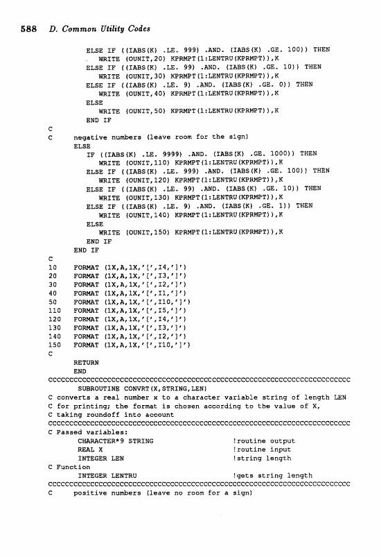
688 D, Gmnzon Ufo'lity Codes
ELSE I F (($mS(K) .LE. 999) .&MD. (TABS(K1 .GE. l Q 0 f f TWEM . WRITE (OUNIT, 20) K P m T ( 1 : 6;EMTRU ( K P R W T W ELSE IF (fImS(K) .LE. 951) .AND. (IABSfEO .GE. 1 0 ) ) TWEN
WITE (OUNIT, 3 0 ) K P W T f l :WEJTRU (XPRMPT) ,K ELSE IF ( f I M S ( K ) .LE. 9) .AND. (IABS(X) .GE. 0) 1 TWEN
m X T E (OWNIT,$Q) KFWPT(1:mXJTRU(KPMPT)I,K ELSE
WRITE (QUNIT, 505 K B m T (1 :LENTRU (KPRMPTI 1 ,K END IF
e C nega t ive numbers ( l eave room f o r t h e sfgnf
ELSE IF ( IIABS ( K ) .m, 9999) .RHD. (IABS~K) .GE. l e o o l I THEN
WRITE (OUHIT, 1 3 0 ) X P M T (1:LENTRU ( R P W T ) 1 ,I(: ELSE I F ( ( IABS(X) .Le. 999) .AMD. (IABSlK) .GE. 3.00)) THEW
~ I T E (swwrT, 1 2 0 ) KPWT (I:LENTRU (XPRWT) I .R ELSE IF ( ( I A B s t a ) .LE. 99) .mn. (IABS(X) .m. 10)) THEN
&RITE (OUNIT, 1 3 0 ) K P W T Il:LENTRU(mRMPT) 1 , K ELSE I F ( ( IABS(KJ .LE, 91 .AND. (IABS(K) .GE. 1)) TWEN
RRXTE (OUNXT, 1 1 0 ) KPRmT f1:LENTRU (ICPRWT))rR ELSE
WRITE (OUMZT, 350) KPRWT (1:LEWTRU ( K P W T ) )rK END I F
END I F e 1 0 PO-T (lXtZL,lX,' [ * , 1 4 , @ J F 1 20 F O m T (ZX,A, l X , * [ # , ' 1 ' 1 3 0 F O m T ( 1 X , A , 1 X , " [ ' , 1 2 , * ] t ~ 4 0 F O m T (1X,A, l& ' E', X % , * ] ' k $0 F O m T (1X,A, I X , ' f f , XlO, * ] ") I 1 0 F O m T ( I X r A t JX, ' [\,IS, ' J ' ) 1 2 0 F O m T f S X , A , l X I f t f , 1 4 , q 1 ' ) 1 3 0 F O m T ( l X e A , l X , l ' , $ 3 t f 1 @ 1 1 4 0 F O m T ( l X , A , l X , ~ f " , 1 2 , C ] ' ) 250 F O M T f lX,A, 1X, I', ,IQ, ' 1 f') C
RETURN END
cccccccccccCceccceccceccccccccccccecccececccccccccccccccccccccccccccccc~ SaRQUTXNE COHVRT ( X , STRING, LEN)
C c o n v e r t s a real nu&er x t o a c h a r a c t e r v a r i a b l e s t r i n g o f length ZEN C f o r p r i n t i n g ; the format is chosen according t a t h e value of X, G t a k i n g raundoff i n t o account ccccc~cc~cccccceccc~ccecccccccceccecccccccce~ccccccecccccccce~ccceccccec C Passad v a r i a b l e s :
! rou t ine output R m L X ! r o u t i n e i n p u t XlOTEGER LEN ! s t r i n g l e n g t h
C Funct ion INTEGER LENTRU ! g e t s s t r i n g l e n g t h
cccccccecccccccccccccccccccccccccecccE:cceceecceccecccccccceccccccccccecc C p o s i t i v e nurnbers ( l eave na room for a s i g n )
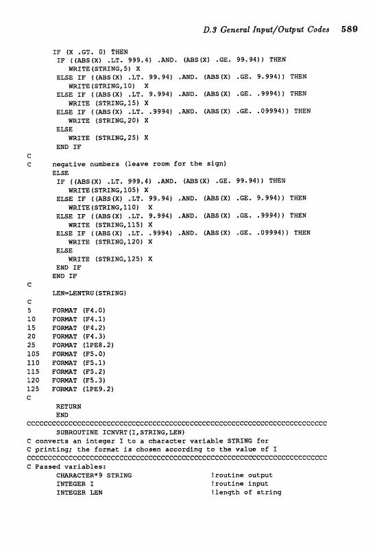
XP [X .GT, 0) THEN IF ( ( m 5 f X ) .LT. 999.4) .AND. (ABS(X) .GE. 99.941) THEN
WRITE (STRING, 5 ) X ELSE IF ((ABS(X) .LT. 99-94} .AND. (ABS(X) .GB. 9.994)) TWEN
mITE [STRING, 10) X ELSE IF ((ABS1X) .LT. 9,994) .MD. (mS(X) .GE. .9994)f THEN
WRITE (STRING, 15) X ELSE SF ( ( M S f X ) .LT. ,9994) .AND. ( m S ( X ) .GE. ,09994)) THEN
aXTE (STRLE16,20f X ELSE
HRTTE (SmIHG,25) X END SF
C G negatf ve nu&ers (leave room for the si*)
ELSE IF ((mS(X) .LT. 999.4) .&tlJD. (ABS(X) .GE. 99.94)) TWEN
mITE (STRIIJG, 105 f X ELSE IF ((mS(X) .LT, 99.94) .AND. ( m S ( X 1 .GE, 9.994)) THEM
WRITE(STRIIJG,IlO) X EmE fF ((ABS(X) .LT, 9.994) .AND, (ABSfX) .GB. .9994)f TWEN
WRITE (STRING,1151 X ELSE IF ( ( m S ( X ) .LT. .g9941 .AND, (mS(X) .€SE. .09994)) THEM
WRITE f STRSNG, 120) X ELSE
WRITE [STRING, 125) X END fF END IF
c UZII=mNTRU (STRING 1
c 5 FOmT(F4,0) 10 F O m T (F4.1) 15 Fa-T (F4.2) 20 F O m T (F4.3) 25 F Q m T flPEB.2) 105 P O M T (F5.0) 110 F O m T (F5.1) 13.5 Fa-T fF5.21 120 F O m T (F5.3) 125 F o m 2 (IPE9.2) C
BETURN END
cccccccccccccccccccccccceccceccccccceccceccccC:ccc~cccccccccccccccccccccc SUBROUTINE IGMVRT (1, STRING, LEN)
C converts an intager I to a character variable STRING for C printing; the format i s chosen according ta the value af I CCCCCCCCCCCCCCCCCCCCCCCGCCCCCCCCC1CCCCCCCGGCCCCGCCCCCCGCCCCCCCCCCCCCCCCCC C P ~ S S Q ~ variables:
!routine output INTEGER X !routine input INTEGER LEN !length of string
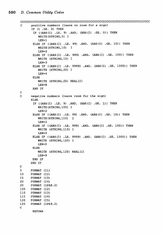
590 D, Common Ultz"lit?;r Codes
cccce~cccecccccceccccccceccccccceccccecccccccccccccccc~~cccccccccccccccc C positive nukers (leave no room for a sign)
IF (S .GE. 0) THEN I F ( ( A B S f I ) .LE. 9) .AND, (ABS(I) .GE. O f ) TmH
WRITE (STRING, 51 I
ELSE TF ( [ A B S ( I f .LE. 99) .ABED. (ABS(1) .G& 1 0 ) 1 TWEN W I T E (STRING, 3.0) I mN-2
EzlsE XF ( ( A B S ( I ) .LE, 989) .AND. (ASSfS) .GE. 100)) TWEN HRT"X" {STRING,SS) I mN-3
ELSE I F ( ( m S ( I ) .LE. 9999) .AND. (ABSt I ) .GE. l o o 0 1 1 THEN m I T E (STRING,20f S LEH-.4
ELSE WRZTE (STRING, 25 ) REAL ( I ) LEN=8
EBB I F (I:
G negative numbers (leave room far the s ign) ELSE
I F ((ABSlIf .LE1 91 .AND. (ABStT) .GE, 1)) THEW m I T E (SmINC;, 1 0 5 f I '
LEN-.2 ELSE SF ( ( A B S ( I ) .LE. 99) .AND, (ABS(I) .GE, 10) 1 TNEN
WRS"SE(STRING,llOf X LEW-3
E U E 3 F ((ELBStI) .LE. 999) ..&MD. (ABSfI) .GE. 100) f THEM WRITE (STRING, 115) I LE8m.g
ELSE IF ( ( M S ( I ) .LE* 9999) .AND, (ABS4T) .GE, 1OOOf) THEN WRITE (STRING, 220) I LEM=5
ELSE: WRITE f STRSMG, 125) REAL ( I ) LENm9
EHD IF END I F
C 5 E " O m T ( T I ) 10 F O W " r I 2 ) 1 5 F Q R K A T f f 3 ) 2Q F O m T I 1 4 1 25 F O m T (IPE8.2) 105 F O m T ( 1 2 ) IlQ F O m T 413) 115 FO-T (14) 1 2 0 FO-T (I51 1 2 5 F 8 m T (1PE9.2) c
RETURN
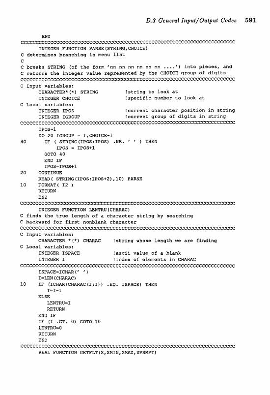
Ern cccccccccccccccccccccccccccccccccccceccccccccccccccccccccccccc~ccccccc3cc
INTEGER FUMCTXOM PARSE(STRING,CNOICE) C d e t e r m i n e s b r a n c h i n g f n = n u list C C b r e a k s STRING (of t he f a r m "nn n n n n n n nn n n ...,' 1 i f n o pieces, and C r e t u r n s the integer v a l u e represented b y t h e CHQICE group of digi ts ccecccccecccccccccccccC:ecccccccceccccccccccc~ccccccccceccccccccccccccecc C I n p t v a r i a b l e s :
C N m C T E R * (* ) STRING ! s t r i n g t o l o o k a t INTEGER CNOXCE !specific nu-r t o l o o k a t
C L o c a l v a r i a b l e s : INTEGER IPOS ! c u r r a n t c h a r a c t e r p o s i t i o n i n s t r i n g INTEGER IGROUP ! c u r r e n t group o f d i g i t s i n s t r i n g
ccccccccccccccececcc~ccccceccccccccccecccc~ccccccceccccccccccccccccccccc JPOS-l Do 20 IGROUF - 1,CHQICE-1
4 0 I F t STRING (1POS:IPOS) .NE. "HEN IPOS = I P 0 5 + 1
G6TO 40 END IF IPOS-IPOS+1
20 CONTINUE RE^ STRING (IPOS: 1 e o s + 2 1 , 1 0 ) PARSE
10 E ' O m T ( I 2 ) m T m N END
cccccccccccc~ccccccec~cccccccccccccccccccccccccccccccccccecccccccccccccc INTEGER FUNCTION LENTRU (CHAmC)
C f i nds the t r u e l e n g t h o f a c h a r a c t e r s t r i n g b y s e a r c h i n g C b a c k w a r d for first n o n b l a n k c h a r a c t e r cccccccccccccecccceececccccccccceccccccccccccccccccccccccccccccccccccccccc G I n p u t v a r i a b l e s :
C H W C T E R * ( * l C B W C ! s t r i n g whose l e n g t h we are f i n d i n g C L o c a l v a r i a b l e s :
INTEGER ISPIICE l a s e i i v a l u e o f a b l a n k INTEGER f !index of e l e m e n t s i n CWAMC
cceccccccccCccccceeccccccecccccccccccccccecceccccccccccccccccccccccccc~c JSPACE=SCmR ( l ' ) I = a N ( C H N C )
1 0 IF (ICHAR (CfYIRAC 6 I : I ) 1 .EQ. ISPACE) THEN I=I-l
ELSE mNTRU=I =TURN
END I F I F ( I ,GT, 0) GOTO 10 LENTRV-O RETURN EMD
CGCCCCCCCCCCCCCCCCCCGCCCCCCCCGCCCCCCCCCCCCCCCCCCCCCCCCCCCCCGCCCCCCCCCCCC REAL FUNCTION GETFLT ( X , XMIlif, X M , XPRWT)
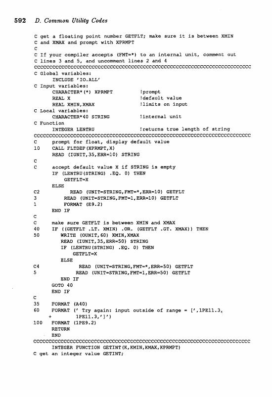
592 D. Gommonb Utzlify Codes
C g e t a f l o a t i n g p o i n t nu&er GETFLT; make s u r e it Is between XNXN C and X m and prompt w i t h X P M T C C I f your e a w i l a r a c c e p t s (FMTm*) t o an Ln te rna l u n i t , c o m e n t out C l i n e s 3 and 5 , and u n c o m e n t l i n e s 2 and 4 c~ccccccccccCcCccccccccceeccccccccccccccccccccceccecceccccccccccccccC:ccc C Global v a r i a b l e s :
INCLUDE 10. ALL' C Input v a r i a b l e s :
!prompt X f d e f a u l t v a l u e
R E U XNIN,XW ? l i m i t s an i n p u t C Local v a r i a b l e s :
! i n t e r n a l u n i t C Func t ion
INTEGER LEHTRU ! r e t u r n s t rue l e n g t h a f s t r i n g ~cGcC~~eceeCccccecccccccccC:cE:cccccccccceccc~eeccceccccccccccecI:ccccccccc C psampt for f l o a t , d i s p l a y d e f a u l t v a l u e 10 C & U FLTDEF CXPRNPT, X 1
(TUNIT, 35, ERR=l0f STRING G C accep t d e f a u l t v a l u e X i f STRING is empty
I F (MMTRU (STRING) -EQc 0) THEN GETFLTmX
ELSE C2 M A D (UWIT=STRING,FMT=*,EM=10} GETFLT 3 (UMIT=SmING, FMTm1, E a = l O 1 CETFLT 5. F O m T (E9.2)
END IF G C m k e s u r e GETFLT %S between X M I M and X m X 40 I F ( (GETFLT .LT. XMIN) .C%, (GEmLT . GT, X=) 1 THEN 50 MRXTE (OUNIT, CO) XMIN, X13AX
mI) [XOMXT,35,ERR=50) STRING TP [LENTRU(STmNG) .EQ. 0) TNEN
GETFLT-X ELSE
C 4 =AD (OMXT=STRING,FMT=*,EM=501 GETFLT 5 =hi[) (UMXT=S"lfIMG,FMT=Z,ERR=50) GETFLT
END I F GOTO 40 END I F
C 35 F O m T (A401 60 F O m T ( V r y ergain: i n p u t o u t s i d e o f range [*,IPE11.3,
+ 1PE11.3,@]@) 100 F O m T (1PE9.2)
=TURN EXVD
ccccccccCcceccccCccccccccecceccccccceccccccccccccccccccccccccececccccccc INTEGER FUNCTION f;ETINT(K,KMXN,K~,KE"RMP"I"}
C g e t an i n t e g e r v a l u e GETINT;

D.5 Cerrerat Inper#/Outpui Codes 593
C check t h a t it lies betwean KNXN and and prompt wi th K P W T C C T h i s f u n c t i o n a l l o w s i n p u t o f i n t e g e r s i n a n a t u r a l way (i.e., wi thau t
C p reced ing b l a n k s o r decimal p o i n t s ) even though w s cannot u s e l ist C d i r e c t e d M A D (i.e., Pm=*) from i n t e r n a l u n i t s c~e~~~ec~ccc~cc~~~~e~eccccC:ccccceccccccccccecccccccceccccccccececccccccc C Global v a r i a b l e s :
INC"LUDE ' TO. ALL* C I n p u t v a r i a b l e s :
CNWCTER* (* 1 KBWT ! s t r i n g prompt INTEGER K ! d e f a u l t v a l u e INTEGER K M I N , K M !upper and fower l i m i t s
C Local v a r i a b l e s : CTER*40 STRSMG ! i n t e r n a l u n i t TEP"IP !temp v a r t o a l low f o r e a s i e r i n p u t
C Funct ions: INmGER LENTRU ! r e t u r n s t r u e l e n g t h o f s t r i n g
cccccccccceccccccccccccccecececcccccccccccccecccccccccccccccecceeecccccc C promptforinput;dlsplaydeEault 1 0 CALL XNTDEF (KPRMPT, K)
READ fSIENST, 35, EM=lO) STRING C C accep t d e f a u l t v a l u e K i f STRING is empty
SF (LENTRU (STRSNG) . EQ. 0) THEN GETIHTmK
ELSE C change t h e i n t e g e r i n t o a r e a l nu&r
STRXNG=S~INGf1:LENTRU{STRIN61f/Ii.~ f r e a d t h e r e a l num$er from s t r i n g
MAD [UBfIT=STRING, FNTa1, EM=l O f TEm I FORMAT (F7.0) C change it t o an i n t e g e r
GETINT-INT (TEW) END I F
C C check t h a t GETIWT lies between KNIM and R m X so TF ((GETINT .LT, WIN) .OR. (GETINT .GT. K M X ) ) THEN 5 0 WRITE: (OUNIT, 60) KNIN, K M
WAD (1 UNIT, 35,EM=50) STRSNG I F [LENTRU (STRING) .EQe 0) THEN
GETIMT-K ELSE
STRLWG=STRING (1 :LENTRU 4STRIMEj f / I" ' . READ (UMITmSTRXNG, PMT=l, m m 5 0 ) TEMP GETINT=INT f TEMP)
EM0 I F GOTO 40 END SF
C 35 F Q m T [AllOf 60 P O M T ( I Try again: i n p u t i s o u t s i d e o f range = f * , I G , I C i , ' 1 100 F O m T f I 1 0 )
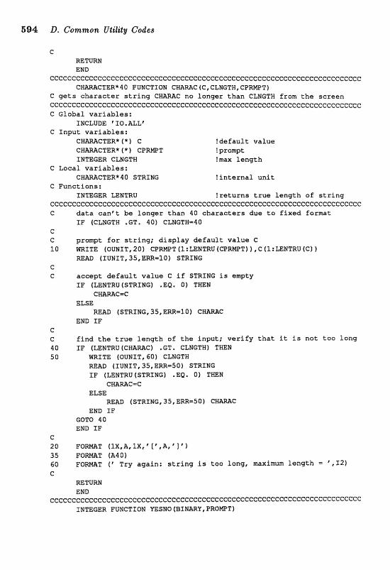
594 D. Common IfgiZitaf Codes
C RETURN END
ccccccccccccccccccccccccccccccccccCcceccccccccccceeccceccccecccecceccce.~ CTER*40 FUMCTIOH CHAMC(C,CLNGTN,CPRWT) a c t e r s t r i n g CBhMC na longer than CLNGTW from t h e screen
ceccce~ccecccccccce~ececcccceeGcccccccccccc~cccccccc~~ccccc~cccc C Global var iab les :
XNCLUDE ' 10, ALL' C Input var iab les :
CHWGTER* (* ) C !defau l t value CHmCTER* ( * ) CPReT f prompt INmGER CLNGTW !nax leng th
! i n t e r n a l u n i t C Functions:
TNmGER LENTRU ! re tu rns t r u e leng th of s t r i n g CCCCCCCCCCCCCCCCCGCCCCCCCCCCCCCCCCCCCCCCCCCCGCC3CCCCCCGCCCCCCCCCCCCCCCCCC C d a t a can ' t be longer than 40 charac te rs due t o f i x e d Esrmat
IF (CLNGTH .GT. 40) CLNETB140 C C prompt f o r s t r i n g ; d i s p l a y d e f a u l t value C lO m T T E fOUNTT,20) CIP~ETfl:LENSRU(CPRMPT)f,Cfl:UeNTRU(C~l
REm (IVNIT, 35, ERR-10) STRING C C a c m p t d e f a u l t value C i f STRING i s empty
XF (mNTRU(STRING) .EQ. O f THEM CWAmG=C
ELSE READ (STRT NC;, 35, Em=10) CWAmC
END IF c C find t h e t r u e length of t h e input; v e r i f y t h a t i t i s not too Long 40 IF (ZENTRU (CHARAC) .GT, CLNGTM) THEN 5 O WRITE (OUMIT, 60) CLNGTW
R m D (IUWIT, 35, ERR-501 STRING IF (LENTRU(STRING) .EQ. 0) THEN
CHmC=C
READ (STRING, 35, ERRmS01 CWARAC END IF
GOTO 40 END IF
C 20 F Q m T (IX,A,lX,'[',A,"'f 35 P O m T (A401 60 F O m T (' Try again: s t r i n g is too long, maximum length = \,I21 c
RETURN END
c~ccccc~~~c~cc~~c~cce~ec~cccccccc~~c~cccccc~~cce~ceccccccce .cccc~cccccccc INTEGER FUNCTION UESEIQ(BIEIARV,PRONPT)

l2.S C;meralInpu$\Outpa-t Codes 5135
C obtains UESMO f r o m the serean; v a l u e Is O f o r na, 1 fo r yes Ccccececcccccc~cccccccccccccccccecccccccc~ccccccc~cccceccceecccccecceccc C Global v a r i a b l e s :
IMcLuae f x ~ . ~ ~ ~ t C Input p a r a m e t e r s :
C H W C T E R * (*) P R O m T ! prompt; f NTEGER BINARY !default value
C L o c a l v a r i a b l e s : CWmCTER'3 STRING ! i n t e r n a l u n i t
C Functions: INmGER LENTRU ! r e t u r n s t r u e l e n g t h of s t r i n g
cccccccccccc~cccccccceeecccI:ecC:ccccC:eccccceeccc~eecceccccccecccccccccccc 1 0 0 0 CONTINUE: C write psantr>t and display default values
f F (BINARY .EQ. 1) WZTEIOU1JXT,IDI PRQMPT(l:L&NTRU(PRQMBT)) I F (BIMARY .E($, 0 ) WRITE (QUNf T, 31) PROWT (I ; LENTRU (PROWTI 1
C RE= fIUNXT, 20,ERR=1000) STRING
G e accept default valua; c h e c k that i n p u t Is # y e or 'n6
IF (LENTRU(STRING1 .EQ, 0) THEN VESMa g BZNARY
ELSE IF (STRINGI1:I ) .Ea . * y f .OR. STRINGf1 : l ) .Ea . Y Y " ) TWEN VFSNQ = I,
ELSE I F (STRSNC(1:I) .EQ. 'nn" .OR. STRIUG(l:lf .Ea. ? H N " ) TWEN YESNO c- O
e t s E WRITE (OUNIT, 2 0 0 ) GOTO 1 0 0 6
END I F C 10 F O M T ( IX ,A , I X , * [yes) ' ) 15 F Q M T 41X,A, 1X, [ no ] " 1 ao F o m r t a ) 2 0 0 F O W T t f T r y again, a n s w e r mst be y e s or no') C
MTURN END
CGCCCC~GCCCCCCCCCCCCCCCCGGCCCG~CC~CCCC~CCCCCCCG~CCCGCCCCCCCCCGCCGCCeCC~C LOGICAL FUNCTION MGCVT ( IdK)
C c o n v e r t s l t o true a n d a n y t h i n g else ta false ccccccccceccccCcccccccc~~ccccecccccceeccc~c~ccccccccc~cccccecccc~ccccccc
INTEGER I J K ! i n p u t I F (IJE ,EQ, 1 ) T m N
LIOGCVT=.TRUE. ELSE
MGCVT=. FALSE. END I F =TURN END
CCCCCCCCCCCCCCCCCCCCCGCCCCCCCCCCCeCC~CCCCeGCCGCCCCC~CCCCCCGCCCCC~~CCCC~~ REAL FUNCTION RANNOS (DSEED)
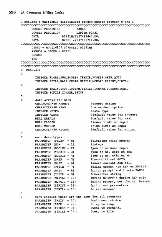
598 D, Common Utility Codes
C r e t u r n s a uniformly d i s t r i b u t e d random numb.er between O and 1 ccccccccecccccccccccceccceccccccccccccccceececcccccccecccccccccccccccccc
DOUBm PWCISXON DSEEE) BOUBU PmCISION D2P31MYI, D2P3f DATA ~ z e 3 1 ~ / 2 1 4 7 s s 3 ~ 4 7 , ~ o f DATA B2P32 /2147483711,00/
cccccccececcccccccccccccccccccccccccccccccccccccccccccccccccccccccccccec DSEED = MOD (1 6807. BQ*DSE&BI B2P3IM) MmOS = DSEBD / D2P31 =TURN END
ccccccccccccccececcccccccecceceecccccecccccccccC:cccC:cccccccccccccccccccc cccccccccccccccc~ccecccccccccccccccccccccccccccccccccccceccccccccccccccc C menu.alil C
XNTEGER FL~~T,MVM,BOO~M,YES%IPIP30SX:IE"ISKZP~QV1T INTEGER TITLE,lrBATT,CHSTR,MTXT~,MCNOICCPE"RPfdT,CLRTW
C IRTEGER I~TN,STOP,TTTERM,ITE"TLEtXTNA~fTGTERM(rXGHRD INTEGER IGFILE,TGHWE,ZSTQP
c C d a t a a r r a y s f o r menu
!prompt s t r i n g !terse descr ip t ion
INTEGER MTYPE I d a t a type INTEGER NTMTS !defau l t value f o r i n t e g e r MU m A L S !defau l t value for r e a l W A L MWLIM !lower l i m i t on input R M L MHILXM !high l i m i t an input
!defau l t value f o r s t r i n g G G menu d a t a types
PWmTER (FWAT Of ! f l o a t i n g po in t number PAWMETER (NUM 1) ! i n t e g e r PAWET= (mmN - 21 !yea o r no u s e r input
!yea o r no, s k i p on YES !Yes o r no, s k i p on NO !Unconditional GBTO fabort cur ran t ASK c a l l !print: prompt (in ASK o r PRT&GS) ! p r i n t pronrpt and invoke PAUSE ! charac te r a t r i n g ! p r i n t IYIE"WT ( 1 ddrlng ASK only ! p r i n t prompt, get choice, branch
BAmMETER (PPRSNS - f 2) ? p r i n t out parameters PAaAMETER (CLRTRB 13) ! c l e a r screen
G e menu e n t r i e s whieh a r e t h e saw f o r a l l programs
PMmTER (ZMAIN - 50) !-in menu cbolcc P-METER f STOP = -2) l f l a g t o s t a p
TER (ITTEM - 73 ) ! t e x t t o t e m i n a l P m m T E R (ITFILE - 74 ! t e x t t o f i l e
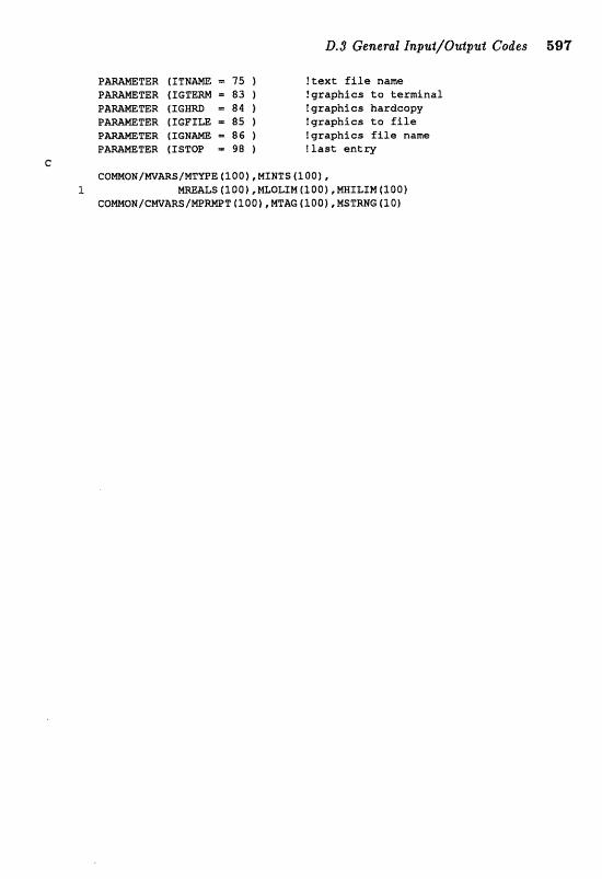
B.3 General I~p~~\Q"utpat Codes 597
P m m T E R (TT%- '75 1 !text file nam P m M E T E R (TGTERN 83 1 !graphics to terminal P W W T E R (IGWRD = 84 1 tgra@ies hardcapy P m m T E R (IGFTLE = 85 ) lgraphics ta f i l e
TER I f C N M = 86 f t graphics f i l e name TEE (ISTOP 98 f E last ent ry
C CoWON/WARS/MTYPE t l o o ) , MINTS {l001 ,
1 L5 (loot ,MLoLIM(lOo) ,MX1LTM[1.00} C O m O % / C W m $ / W W T (loo), MTWG (lOO} ,MSTRNG (3.01
D.4 Graphics Codes The two FORTRAN files, CRAPBIT.HI and oRnpaIT.Lo, are collections of subroutines that produce two-dimensional or contour plots. They allow one to four plots per saphies page. The two-dimensional axes can be either linear-linear, log-linear, or log-log, while both the axes for con- tour plots must be linear. To produce a plot, all of the variables listed in cmnr .nu must be defined, ss well as the data array8 (X and Y for two-dimensional plots; and 2 , ECONT, EX, EY, WII , a d MIX for con- tour plots) and the device type (DEVICE). To create a graph the program must first c$l CTDEV to nominate a device and GnoDE (in file SE~P.MR) to change to graphics mode (if necessary). For each plot on the page, the program calls LBLIAX, LCLIAX, or LGLCAX to draw the appropriate axes; and for each data set to be plotted on the same set of axes, the program calls XVPL~T (two-dimensional plots) or COBTOR (contour plots). When the graphics page is finished, the program calls GPAOE to dose the graphics pachge and THoDE (in file SE~.FOR) to switch back to text mode (if necessary).
cRnparr. a1 calls CA-DIS SPLA (version 11.0) routines; oRnparl. LO c& UIS routines. For users who do not have access to either CA- DISSPLA or UIS graphics, these programs are intended as templates to fadlitate the development of code for their graphics package. For users who do have one of these pacbges, please read the information below that is sspecific to your software.
CA-DISSPLA OMPHIT . III indudes the following subroutines, which ase not cded directly by the physics pp~grams: SUBPLT, wkich sets the area of the device to be used for plotting, BARBIER, which prints the title, uam, which writes wt; axis lab&, and U G E ~ , wkich wribs m t an infarnational message. Device namin&ion is often instatlation dependat, so you anight need to edit subroutine GmEV before the code will m k . Note that XQvfi a;ad PovaL are not used by CA-DISSPLA.
'UIS Graphics GMPHI%LO calls to the TTIS gfalphics routines, whi& me avdabie on VAXstations. A11 non-stmdad FORTRAN-77 syntw i s W-
sociated solely with UIS calls. The subroutines not explicitly cded by the physics progrms ape SUBPLT, which sets the area fjor plotting, &es eharaeter size, creates virtud displi~ys dong with Prindo~rs a ~ d transfor- mations, writes the title, and enables the display list (for hard copy); XAXIS and YAXIS, which draw and label the axes (either linear or log); LEGEBD, which prints an informationd messqe at the bottom of the page; GSm, whi& draws symbols on the dot; and COBTq wBi& does the c&-
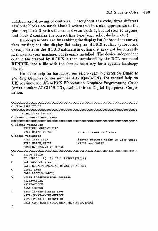
Lr.4 GmpAics Codes 599
culation and drawing of contours. Throughout the code, three different attribute blocks are used; block 1 writes text in a size approprizELe to the plot size; block 3 writes the same size as block 1, but rotated 90 degrees; and block 2 contains the correct line type (e.g., solid, dashed, etc.)
Hardcopy i s obtained by enabling the display list (subroutine SWPLT), then writing out the display list using m HCUIS routine (subroutine c~nce). Because the HCUIS software is optional it may not be currently available on your machine, but is easily installed. The device independent output file created by HCUIS i s then translated by the DCL command IRENBIGR into a Me with the format necessary for o specific harrdcopy device.
For more help on hardcopy, see MieroVMS Workgtslation Guide to Printing Gmphies (order number AA-HQ8BB-TB). For general help on U1S routines, hie M i w VMS Work:sta.tion Gmphics P q m m i n g Guide (order number AI-GIIOB-TN), available from Digital Equipment Corpo
eccecccccccccccccccccccececccccccccccccccccccccccccccccccccccccccccccccc C file GaAPXfTeHX eCcCcC~CCcCCCCCeCGCCcCCCcCCCcCCCcCCCCccCcCccCcCCCCccCCCccCCCcccccGc~cccc
SUBROUTINE LNLHAX C draws finear-linear axes cccccccccccccccccccccccccccccccccceccccccccccccccccecccccccccccccccccccc G Global variables
INCLUDE ' GWDAT ,ALL* XSIZE, USIZE ! s i z e o f axes in inches
C Local variables m L XSTP, USTP Ilength between t i c k s in user units REAL VSIZE, WSIZE IXSXZE and VSIZE CWONISIZE/VSIZE,HS%ZE
eecccccccccccccc~cccccccccccccecec~cccccccccCc~ccccccccccccceccccccccccc C write title
I F (IPLOT .EQ. 1) CALL BANNEW (TITLE) C set subpf at area
CALL SUBPLT (IPLOT, NPLOT, XSIZEt YSXZE) C label axes
CALL mBELS (MBELI C write infoxmtianal message
BSIZE=XSIZE VSIZE-VSTZE CmL LEGEMB
C draw linear-linear axes XSTP- (XmX-XMIN) /NXTzeK rsTP= ( Y ~ - Y M I W I INYTXCK CALL G W (XMSN, XSTP, X M X , YMIN, YSTP, VlrylXj
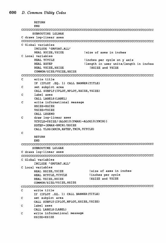
WTURN END
cccccccccccccccccccccceccccccccecccccccccccccccccccccccccccccccccccccccc SUBROUTINE LGLNAX
C d r a w s l o g - l i n e a r axes ccccccccceccccccccccccceccccc"cccecccecccccccecccC:ccccccceccccc"ecccccccec C G l o b a l v a r i a b l e s
INCLUDE WRFDDAT.AZL~ R a L XSIZE,YSXZE ! s i z e of axes i n i n c h e s
C L o c a l v a r i a b l e s REAL YCYGLE ! i n c h e s p e r c y c l e on y axis =L XSTEP ! l e n g t h i n u s e r u n i t ~ / l @ n g t h i n i n c h e s RML VSIZE, WSIZE !XSIZE and YSIZE CO~QN/SIZE~VSIZE,HSXZE
ccCcececcccccccecceccccceccccccccceccccc~cecccccccccccceeecceccecccccccc C w r i t e t i t l e
I F {SPLQT .EQ. 1) CALL BAEJNER (TITLE) C set s u b p l o t area
GALL SUBPLT ( I f LOT, WPLOT, XS5ZEI YSIZE) C l a b e l taxes
CALL MBELS (L&BEL) G w r i t e i n f o r m a t i o n a l mssage
WSIZE=XSIZE VSJZE=VSTZE C G L LEGEND
G draw l o g - l i n e a r axes YCuCLE=YSIZE/ (ALmlO (IImX) -AL%lO (YMENb 1 XSTEPm ( X M - X W I N ) /XSIZE CALL YLOG (XMIN, XSTEP, VMIN, UCUGLE)
C RETURN END
ccc~ccccccccccccccceccccccccccceccccccecccccccccecccccccccccccc~cccccecc SUBROUTINE LGLGU
e draws l o g - l i n e a r axes cec~ccccccc~ccccccccc~cceeccccccccccececcccceeccccceccccccc~cccccccccecc C G l o b a l v a r i a b l e s
INCLUDE GGRFDAT .ALLt G L o c a l v a r i a b l e s
mX1 XSIZE, YSTZE ! s i z e o f axes i n i n c h e s
-L XCVCLE,YCYCLE ? i n c h e s per c y c l e m L VSIZE, BSEZE lXSfZE and VSIZE COWQM/SIZE/VSIZE,RSIZE
c ~ ~ c ~ ~ ~ ~ c c e ~ ~ ~ ~ ~ ~ ~ ~ c ~ c ~ c c c c c ~ c ~ c c c c c C : c c e c c c e c e e c c c c c e c c c c c c c c c ~ c c c c c c c c c C w r i t e t i t l e
I F (PPLQT .%Q, 1) CALL BANNER(TITLE1 C set s u b p l o t area
CALL SUBBLT (IPLOT, NPLQT, XSIZE, YSf ZEj C l a b e l axes
C&L UBELS [UBEL) C w r i t e i n f o r m a t i o n a l message
NSIZE-XSXZE

D.1 Graphics Codes 801
VSIZE=YSIZE CALL LEGEND
C draw log-log axes XCYCLE=XSIZE/ (ALoGlo {XMAX) -&LOGXI) (XMIN) ! YCYCLE=YSIZE/ (ALE10 ('VNX] -ALOG10 [YMIN) ) CALL LOGLOG (XMIN, XCYCLE, YMIPJ, YCYCLE 1
C RETURN END
~cc~e~~c~~c~Cccccccccccc~ccecccccc~cccc~ccccc~cccccccccccccccccccccceccc SUBROUTINE LEGEND
G write information at the top left o f the plot c~c~~c~~~~~c~~~e~cccccc~e~cccceccccccccc~ccceccccccccccccccccc~ccccccccc C Global variables:
INCLUDE ' GWL1AT. ALL' C Passed variables:
REAL XSXZE,YSIZE c Local variables:
IWTEGeR LEN, LENTRU !length af char string RaL VSIZE, HSIZE !XSTZ& and YSIZE COMON/STZE/VSEZE,MSIZE DATA INFOk* ' /
CcCcc~ecccccccceeccecccceccccecccccccc~ccccccc~cccccccccccccccccc~cccccc C prints mssage at t op of plotting area
LEE-LENTRU f INFQ) IF (LEN .GT. O f THEN
CALL ~SSAGIINFO(1:LENI,LEN,MSXZE*X05,VS12E*1.03~ END fF RETURN END
cccccccccccccccecccccccccccccccccccccccccccccccecccccccccccccccccccccccc SmROUTIEE XYPLQT (X,Y)
C plots xy data c c c c c c c c c c c c c c c c c c c c c c c c c c c c c c e c c c c c c c C Global variables:
INCLUDE @GRFDAT.ALLP -L X !independent variable data array =L Y ?dependent variable data array DImNSION X (WOINT) , Y (NPOINTf
CCCCCCCCCCCCCCCCCCGCCCCCGCCCCCCCCCCCCCCCCCCCCCCCCCCCCCCCCCCCCCCCCCCCCCCC C set line type
IF f ILXNE .EQ. 2) CALL DOT IF (ILINE .Ea. 31 CALL DASH IF (ILINE .EQ. 4 ) CALL CWHDSH IF (ILINE .EQ. 5) IFmQ=-IFMB !no line at all
C C set syhol type
IF (ISYM .EQ. If CALL mRKERf16) !circle IF (TSVM .EQ. 2 ) CALLmRKER(2) !triangle IF (ISYM .Ea. 3) CALL mRKER(O1 !square IF (ISYN .EQ. 4 ) CALL mWER14) !cross IF (TSYM .Ea. 5) THEN !point
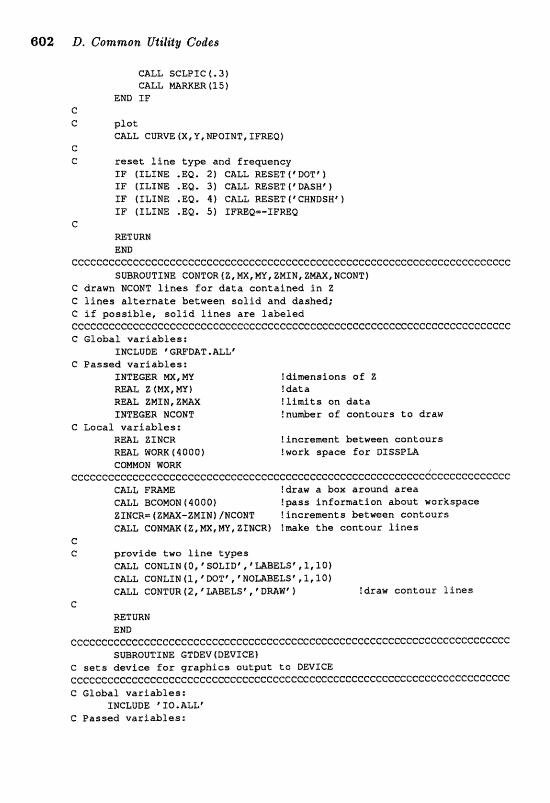
602 D. Common Utility Codes
CALL SCLPIC ( ,3)
END I F e C p l o t
CALL CURVE (X, Y, WOINT, IFWQ) G C reset l i n e t y p e a n d f r e q u e n c y
I F (%LINE .EQ. 2) CALL M S E T t r D O T * ) I F ( I L I N E .EQ* 3 ) CALL =SET ('DASHf 1 SF f I L I N E .EQe 4) CALL RESET (*CCHNDSHf ) SF f I L I N E .Ea. 5) IFREQm-1FREQ
G RETURN Ern
CCCCCCGCCCCCCCCCCGCCCCCCCCCC~CCCCCGCCCCCCCCCCCCCCCCCCCCCCCCCCCGCCCCCCCCC SUBROUTTME COMTQR (Z, MX, MY, ZNSN, ZMAX, NCONT]
C d r a w n MCONT l i n e s for data c a n t a i n e d i n Z C l i n e s al ternate b e t w e e n solid and dashed; C i f passible, sa l id l i n e s are l a b e l e d CCCCGCCCCGCCCCCCCCCCCCCCCCCCGCCGCCCCCCCCCCCCCCCCCCCCCCCCCCCCCCCCCCCCCCCC G G l o b a l v a r i a b l e s :
INCLUDE @ GGRFDAT .ALL8 C P a s s e d variables:
XNTEGER MX, MY I d i m e n s f o n s o f Z =L Z ( M X , m ) !data R m L ZMIN, Z M X ffirnits sn data INTEGER NCaNT ! n u e r of c o n t o u r s t o d r a w
C L o c a l variables: REAL ZlNGR ? i n c r e m e n t b e t w e e n c o n t o u r s =I, ~ ~ ~ ( 4 0 0 0 ) !work space f o r D S S S P m COMMON WOM
~ ~ ~ ~ ~ ~ ~ ~ ~ ~ ~ ~ c c ~ ~ c c c ~ c c ~ ~ ~ c c c ~ ~ c ~ ~ ~ ~ ~ c ~ c ~ c c c c c c c c ~ c ~ c c c c ~ c ~ ~ c ~ c ~ ~ c c c ~ c c ~ c CALL F W E !d raw a b o x a r o u n d area C&L BCOMON ($000) !pass i n f o r m a t i o n a b o u t w o r k s p a c e ZINCR=fZW-ZMSN}/WCQW ! i n c r e m e n t s b e t w e e n c o n t o u r s C S L C O g W (Z, MX, MY, ZINCR) f make the c o n t o u r l i n e s
C C p r a v f d e t w a l i n e t y p e s
CALL CONLINfO, VSOLTD","648ELSff 1.,10) CALL GaNLINfL,'DO"r,'EOWELS\,1,18) GALL CONTUR 1 2, P WIBELS' , @ 'DWW9 ! d r a w c o n t o u r l i n e s
e RETURN END
c c c ~ ~ c c ~ ~ ~ ~ ~ c ~ c ~ c c ~ ~ ~ ~ c ~ c c c ~ ~ ~ ~ c c ~ c ~ ~ c c c S : c c e C : c ~ c c c c ~ c c c c c c c c c ~ c ~ c ~ ~ c c ~ c c SWRQUTINE GTDEV(DEVICE)
C sets d e v i c e f a r g r a p h i c s o u t p u t t o DEVICE ~~~~~~~~c~c~~~ee~cc~e~ccccccc~~~c~cc~cceccccc~cccc~~~cccccccccccccccc~cc C G l a b a l v a r i a b l e s :
INCLUDE ' IQ. ALL@ C P a s s e d v a r i a b l e s :
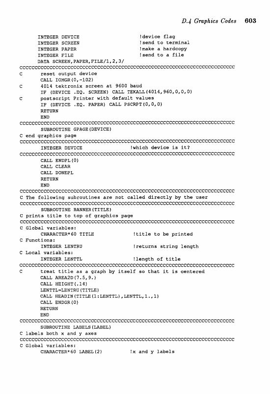
INTEGER DEVICE ! d e v i c e f l a g INTEGER SCREEN ! s e n d t o t e r m i n a l INTEGER PAPER ! m k e a h a r d c o p y INTEGER FILE ! s e n d La a f i l e DATA sCREEN,PAPER,FXLE/I~~~~/
ecccecccccccccccccceccccccccccccccecccccccceccccccceccccc~cccccccccccccc C reset o u t p u t device
CALL I0MGR (a, -102) C 4014 t e k t r o n i x s c r e e n a t 9600 b a u d
IF (DEVICE .ea. scmEN1 CALL T E ~ L L ( ~ O I ~ , ~ ~ O , O , O , ~ ) C p o s t s c r i p t P r i n t e r w i t h d e f a u l t v a l u e s
I F (DEVICE .EQ, PAPER) CALL PSCWT ( 0 , 0 , 0 ) =TURN END
~cc~~c~~~c~~~~~c~ccccccccccccccccccccccccccccccececccccccccccccccccccccc SmROUTINE GPAGE(DEVICE1
C e n d g r a p h i c s p a g e cecccccccccccccccccceccccceccccccccccccccccccccccccccccccccccccceccccccc
INTEGER DEVICE !which d e v i c e is i t ? cccccccccccccccccceccccccccccccccccccccccccccccccccccCcccecccccccccccccc
CALL ENDPL { O f C m L CLEAR CALL BOEaEPE RETURN END
ccccccccecccccccccccccccccccecccccccccccceccccccc~cccccccccccccccccccccc C The f o l l o w i n g s u b r o u t i n e s are not: called d i r e c t l y b y t h e u s e r cccccceccceCcc~cccccecceccccccccccccccccccccccccccccccccccccccccce:cc~ccc
SUBROUTINE BAHNER(TITLE1 C p r i n t s t i t l e t o t o p o f g r a p h i c s p a g e ccccccccccceccccccccccceccececcccccccccccceccccccccccccccccccccccccccccc C G l o b a l v a r i a b l e s :
! t i t le t o 12(? p r i n t e d C F u n c t i o n s :
INTEGER LENTRU ! r e t u r n s s t r i n g length C L o c a l v a r i a b l e s :
I NTEGER LENTTL ! l e n g t h of titZe cecccccccccc~ccccccccccccceeccccccccccccccccccccccccec~cccccccc~cccccccc C t r e a t t i t l e a s a graph by i t s e l f s o t h a t i t i s c a n t e r e d
C&L mEA2D("75,9.) CALL HEIGHT 4.14 f LENTTL=LENTRU(TITLE) CALL READIN (TIT= ( 3 : LENTTL) , LENTTL, 1. ,l ) CALL BNDGR ( O f RETURN END
cccececc~cccc~cceccccecccccccccccccccccccccecccccc~cecccccc~cccccccccccc SUBROUTINE mBELS f =EEL)
C l a h l s both x and y a x e s cccccccccccccccccceCCGccccccccceGC"ccecccccccccccccccccccccccceccccc C G l o b a l variables:
!X and y l a b e l s

604 D. Commolz Utilitg Codes
C F u n c t i o n s : INTEGER LENTRU ! r e t u r n s s t r i n g l e n g t h
C L o e a l v a r i a b l e s : INTEGER LENX , LEMY ! l e n g t h o f l a b e l s
ccccccccccccceccccccccccccccccccc~ccccccccc~cccccccccccccecccceccccceccCt LEHXsLENTRU [-EL ( 1,) 1 LENY=LEHTRU (mBEL f 2 f )
C&LL XNkm ( M B L ( 1 ) fl:LENX) ,LE%X) C&L YNAm(MBELt2) (1:LENV) ,LENY) RETURN END
ccccccccececccccccccccccccccccccccccccccccccccccc~cccccccccce~eccccccccc SUBROUTINE SUBPLT (IPLOT, NPLOT, XSIZE, YSIZE)
C d e f i n e s s u b p l a t t i n g area cccccecccccccccccccccccccccccccccccccccccccecccccccecccccccecccccccccccc C The c h o i c e o f s u b p l o t s ize a n d p l a c e m n t is d e p e n d e n t a n t h e C d e v i c e a n d g r a p h i c s package ; t h o s e g i v e n h e r e are fox a n 8 - 5 X 11 C i n c h p a g e u s i n g DXSSPm ccccccccccc~cccccccccccccccccccccccccceccccccccccecccccccceeccc~ccCccccc C P a s s e d v a r i a b l e s :
INTEGER NPLOT ? t o t a l nu&ar o f p l o t s o n page INTEGER IPLBT !nu-X o f c u r r e n t plot R a L XSIZE,YSXZE: ! s i z e o f p l o t t i n g area i n i n c h e s
C L o c a l v a r i a b l e s : REAL XORFG, UORIG ! l o c a t i o n o f lower l e f t c o r n e r f inches )
cecC~CccccccCccCCCcCCCCCCCC@CCCCCeccccccccceccccc~ecccccccc C f i n i s h last p l o t ( s e t s DISSPLW back t o l e v e l I)
I F (IPLOT .NE. 1) CALL ENDGR (0) C C d e f i n e s u b p l o t t i n g area ( i n i n c h e s ) ; whole p a g e is 8,5 x 11
I F (MPLOT .EQ. 1) THEN XSSZE="I .S YSIZE=9. CALL NEIGBT ( .l1 1
E M E I F (NPLOT .EQ, 2) TEEN YSIZE-4.25 XSIZE-6.5 XORIG=1, I F (IPLOT .EQ. l) UQRIG-5.75 TF (TPLOT .EQI 2 ) YORIGm.75 CALL HEIGHT (. 325)
ELSE I F (NPLOT .EQ. 3 ) TBEN VSIZE=2.80 XSIZE=6 5 XORTG=l, I F (IPLOT *EQ. 1) YOR16=7.20 I F (XPLOT "EQ. 2) UORIG=3.9 XP (IPLOT ,EQ. 3 ) VORXGa. 6 CALL WEIGHT ( . l 2 5 1
ELSE I F (NPLOT .EQ. 4 ) TBEN XSXZEm3.25 YSSZE=4.25
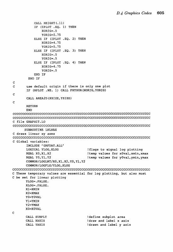
D.4 Gmphies Codes 605
CALL HEIGHT( .Ill IF (IPLOT .Ea. 1) THEN
XORIG- .5 YORLG=5.75
ELSE IF (IPLOT .EQ. 2) THEN XORXG=4.?5 YORIG-5.75
ELSE IF f SPLOT .EQ. 3 ) THEN XQRSGm. 5 'IORSG= * S
ELSE TF (IPLQT .m, 4 ) THEN XORIG=4,75 YORIGm * 5
END I F END IF
C C use d e f a u l t o r i g i n i f there i s only one p l o t
IF (NPLOT .ME. 1) CALL PRYSOR(XORIG,YORIG) c
CALL AWA;?D (XSXZE, VSIZE) C
RETURN END
cecccccccccecccccc~ccccccccccccccccccccccccceccccccccccccccccccccccccccc cccccccccccccccccccccccececccccccccccccecccceccccceccccceccccccccccccccc C f i l e G W H I T , L O ccCccccccccccc~eccccccccccccccccccccccccccccecccccccf:ccceccccccccccccccc
SUBRQUTXNE LNLNAX G d r m s f i n e a r xy axes ccccccccccccc~ccccecccccccccccccccccccccccccecccccccccccccceccccccf:c~ccc C Gfobaf variables:
INCLUDE GGRFDAT .ALLf LWICELL YLQG, XLQG ! f l a g s ta s i g n a l l o g p l o t t i n g
XO,XZ.,X2 ! tamp va lues for x0va1, xmfn, xmax W t Y0,Yl,U2 ! t a w values f o r yOval,yrnin,ymx CO~0N/LQGLMT/XO,XI,X2,YOIY1,V2 COMMON /LOCFLG/YLO(;, XLOG
c c e c c c c c c c c c c e c e c c c c c c c e e e c c c c c c e c C These temporary values a r e e s s e n t i a l for l o g p l o t t i n g , but also must C be set for l i n e a r p l o t t i n g
YZIQC;=.FALSE. XMG=.E'USE. Xl-XNIAI X2=XrnX Y 0lt.YOVAL Vl=YMIN V2=UMAX XO-X OVAL
GALL SUBPLT CALL XAXSS C&L YAXIS
!define subplot a r e a !draw and l a b e l x a x i s !drawn and l a b e l y a x i s
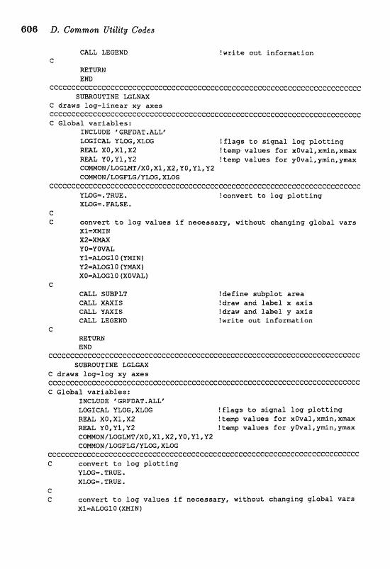
D. Common Utility Codes
CALL LEGEND f w t i t e o u t i n f o r m a t i o n C
=TURN END
cccccccccccccccceccccccccccccccccccccccccccccccccccecccccccccccccccccccc SUBROUTINE 1CIC;LNAX
C d r a w s l o g - l i n e a r xy axes cccccccccccccccccccecccccccccccccecccccccectcccccccceccccccccccccccccccC: C G l o b a l variables:
INCLUDE ' GWDAT .ALLc LO%ICAL YLOG,XLOG i f l a g s t o s ignal log p lot t ing REAL X O , XI, X 2 ! t e m p values for x 0 v a l , x m i n , x m x WAL YD,Y1,Y2 ! t e m p v a l u e s f o r y 0 v a l , y m i n , y m a x COMP30N/LOGLHT/X0,X1,X2,Y0,Y11Y2 CO~ON/LQGFLG/YLQG,XLOG
ctccccccccccccceccccecccccccccceccccccccccCccccctccccccccccccccccccccecc YLOG=. TRUE, ! c o n v e r t t o l o g p l o t t i n g XLQG=.FWLSE.
c e c o n v e r t t o log values i f n e c e s s a r y , w i t h o u t changing global v a r s
XI=XHIN X ~ - X ~ X Y O=VOVAL Y1=AL,OGla (mIM) Y2mALOGl O ( Y m X f XO=ALOG10 (XOVAL)
c CBLL SUBPLT CALL mxIS CALL UAXIS CALL LEGEND
e =TURN END
cccec~ccccceccccccccccccccccccccccccecccccccccccccccc~ccececcccceccccccc SUBROUTINE LGLGAX
C d r a w s log-fag xy axes CC~CCCtCCGCCCCCC@CCC~CCCCCCCCCCCCCCGCC~CCCGCCCCCCCCCCCCCCCCCG~CCG~CCCCGC C G l o b a l v a r i a b l e s :
INCLUDE 'GRFDAT.ALL6 LOGICAL YLOG, XLOG ! f l ags t o signal 1ag p l o t t i n g =L XO,XZ,X2 ! t e m p vafuss Ear x 0 v a l , x m i n , x m a x R m Z Y O , Y I , Y 2 ! t e m p v a l u e s f a r y 0 v a l , y m i n , y m a x COMMQN/LQGLMT/X0,Xl,X~,VQ,Y~IV2 COMPIOH/LOGFLG/1SrL06;,XL8G
cccccccccccccccccccccecccccccccccceccccccceccccccccccccccccccccccccccccc C c o n v e r t t o log p lot t ing
YLOG=.TRUE, XL,OG=.TRUE.
e C c o n v e r t t o l o g values i f necessary, w i t h o u t c h a n g i n g global vars
X f 4LDG1O ( X M I M )
! d e f i n e s&plot area ! d r a w a n d label x axis ? d z a w and label y ax is ! w r i t e o u t i n f o r m a t i o n
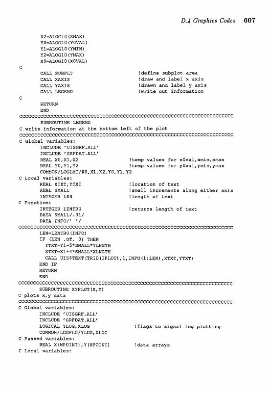
D.4 Gmpha'cs Codes 607:
!define subplot area !draw and label x axis !drawn and label y axis !write out information
L
CALL SUBPST CALL XAXXS CALL YAXIS CaLL LEGEND
e RETURN END
ce~e~c~~ec~e~~cc~eccececcecccccceccccecccccccccccccc~cccccc~cccccccccccc SUBROUTSHE LEGEND
C write information at the bottom left of the plot ce~~~cccc~cccccccceccececcceecccececceccccccC:ccccceccccccccccccccccccccc C Global variables:
INCLUDE ' UISGW.ALLr INCLUDE %GRFD;AT.ALLr R&AL XD,XI,XZ !temp values for x0val,xmln,xmax R m L YO,UI,Y"2 Itentp values far yQval,ymin,ymax ~0MMOM/LOGLNT/X0,Xl,X21Y~IY11Y2
C Local variables: REAL XTXT, VTXT ll~eatfon of text 2EAL SMALL !small incremnts along either axis INTEGER LEE !length of t ex t
C Function: INTEGER LENTRU !returns l e n e h of text DATA SrnLL/.Ql/ DATA INFOjf ' /
ec~ccceccccccccccccC:cecccceccccccccecceccccC:cccccccc~ccccccccccccc~cccce LENmLENTRU ( INFO) IF (LEN .GT. 0) THEN YTXT=UP-S*SMALLxULNGTH XTXT=Xl+$*SmLL*XLNGTN CALL UISSTEXTITRID(fPL,OIp) ,IIINFO(~ZLEN] ,XTXT,YTXT}
END SF' =TURN END
cecccccccccce~cccccccccecccccceccceeeecccccccccccccccccccccccccccccccccc SWRQUTINE XYPLOT (X,Y)
C plots x, y data ccccceccccccccccccccccccccceccccccccccccf:cccceccccccccceecececcccccccccc C Global variables:
IMCLUDE ' UISGRF.ALLe INCLUDE ' GRFDAT .ALL" LWICAL YLOG, XLOG ?flags to signal log plotting COMMOW/WGFLG/YLOE,XLOG
C Passed variables: RML X (NPOINT) , V (NPOIIJT) !data arrays
C Local variables:
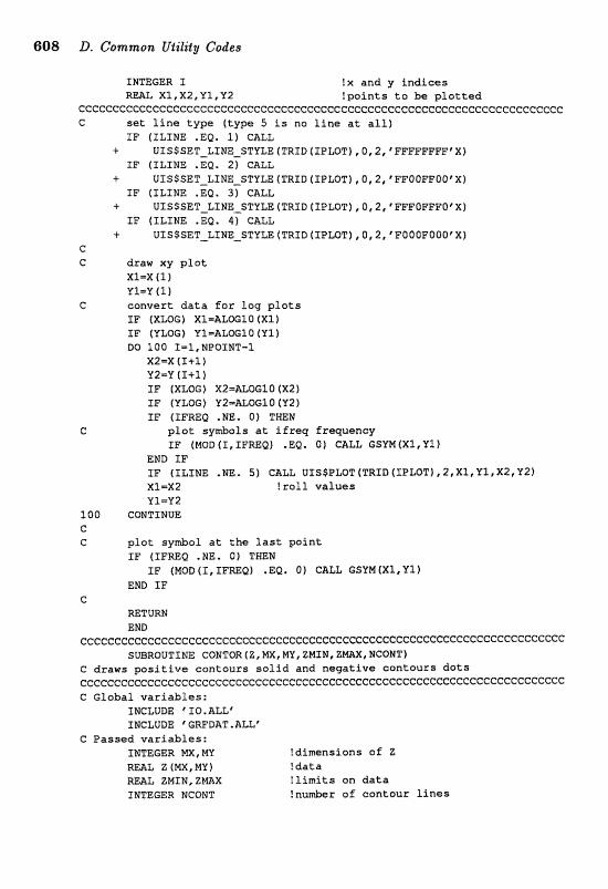
608 D. Common Uta'li2y Codes
INTEGER 3 ? X and y indices R m L Xl,X2,UI,Y2 !po in t s t o be p l o t t e d
cccccceeCc~ceCececcceccccccccccccccceccccccccceccccccccccccececccceccccc C set l i n e type ( type 5 is no line at all)
I F (ILINE -EQ. I f CALL + vIsSsaT-%rHE-sTrLE ITRID ~IPZOT), O, 2 # 8 ~ ~ ~ ~ ~ ~ m 8 x ~
SF (ILINE .EQ. 2 ) GALL + UXSSSET-LIWE-STYLE (TRED fIPLOT1 I O C 2, ' FFOOFFOOtXI
I F (%LINE .EQ, 3) CALL + UISSSET-LINLSTYLE (TRZD IIBLO"P , ,Q, 2, VFFOFFFO' X)
XF (ILIME .EQ. 4 ) CALL + UISSSET-LXHE-STYLE {TRID ( I P W T ) p 0 ,2 , FOOOFOOOrX]
C C draw xy p l o t
Xl=X (l ) V1=Y (l}
C convert d a t a f o r Log p l o t s ra IXLOGI XI=UEIO I F (YLOG) Yl=ALSIO (Ul ) DO 1 0 0 X = I , NPOINT-2
X2=X (I-kl)
u2=u ( I + 1 ) fF (XZOG) X2-AL0610 ( X 2 1 I F (ULQG) Y2==8GIO fV2) fF (IPREQ .ER. 0) THEN
plot s y d a l s a t ffraq frequency f F (MOD (X, IFREQ) . EQ, 0) CALL GSYM 4x1, Y1)
EWD I F I F (ILIME .NE. 5) CALL UIS$BLOTfTRfD(fPLQTf12tX%,Y~IX2,Y2~ X1=X2 !roll values lll-Y2
5 0 0 CQMTINUE C C p l o t sy&oZ a t the l a s t po in t
XF (ZFREQ .NE, Q) THEN I F (HOD(I,XFm&) .EQ. 0) CALL CSYM(X1,YL)
END I F C
WTURIJ END
C C C ~ C ~ G C C ~ C C ~ ~ C ~ C ~ C ~ C ~ C C C C ~ ~ ~ C ~ ~ ~ C G ~ C G C ~ ~ C C C G C C C ~ ~ G C ~ C C C C C G C C ( ~ C C ~ C ~ ~ ~ ~ ~ ~ SUBROUTSHE CONTOR (25, W, MY, ZNXN, NeQMTl
C draws p o s i t i v e cantours s o l i d and negat ive contours dots ~e~~~ececcec~~~eec~~eee~~ccccccc~ecce~~~~ec~c~ccceccececcce~ceccc~ccccc~ G Glabal var iab les :
INCLUDE ' IQ. ALL" INCLUDE @GGRFDAT.ALLe
C Passed variables: INTEGER m, MY ?dimensions of Z REAL Z (MX,MY) !data -L ZMIEJ, ZMAX ! l i m i t s on data INTEGER NCONT ! n u e r of contour Lines
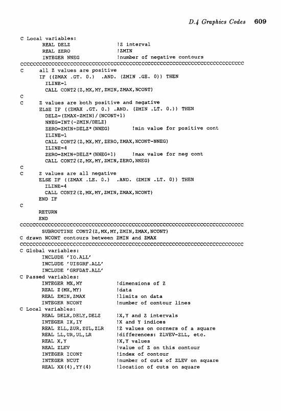
0.4 Gmphics G~ckes BOB
C L o c a l v a r i a b l e s : =L DELZ !2 i n t e r v a l =L ZERO ! ZMIN INTEGER NNEG ! n u d r o f n e g a t i v e c o n t o u r s
cccccceccccccccccceccccccccccceccccccccccccccccceccccccccccccccccccccccc C a l l 2 v a l u e s are p o s i t i v e
IF ( ( Z m X .GT, 0.1 .AND. (ZMIN .GE. 0)) THEN ILINE=T CALL COWT2 (Z,MX,MY,ZMIN,ZMX,NCONT)
e C Z v a l u e s are b o t h p o s i t i v e a n d n e g a t i v e
ELSE I F ((ZMAX .GT. 0.) ,AND. (ZMIN .LT, 0,)) THEN DELz-tzmx-zMrWj/(weopIT+1b NNEs=rWT[-zMxN/tleLz) ZERD=ZMIPa+DELZ*{NNEGl !mln v a l u e f o r p o s i t i v e c a n t SLIEJE-S, CALL CONT2 (2, MX, MY, ZERO, ZluLAX, UCQNT-NNEG) ILINE=$ ZERO=ZMTPJ+DELZ* fNNEG+1 f !max v a l u e f o r neq c o n t CALL COMT2 (Z, HX, MY, ZMLN, ZERO* NPaEG)
e 2 v a l u e s are a l l n e g a t i v e ELSE ZF ( (ZMX .LE. 0.1 .AND. (ZMIN .LT. Q) ) THEM
ILINE=$ CALL CQNT2 (Z , HX, MY, ZMZN, Z m X , MCONT)
END I F c
RETURN END
cCccccccc~cccccccccccecccceccccccccceccccceeccc~cccceececcccccGccccccccc SMROUTINE CONT2 (Z, MX, MY, ZMIN, ZMAX, WCONT 1
C drawn WCONT c o n t o u r s be tween ZMIM a n d ZNAX c~CccCccccceeCccccccccceccccccceeccceccccccccccccccceccccccccccecccccccc C G l o b a l v a r i a b l e s :
INCLUDE ' IO.ALL' INCLUDE ' UUIGRF .ALLf INCLUDE "GRFDAT, ALL"
C P a s s e d v a r i a b l e s : IMTEGER m, MY ! d i m e n s i o n s of 5 R m L Z [1?4X,W) t d a t a =L ZMZN, Z m X ! l i m i t s on d a t a INTEGER NCONT !nu&er o f e o n t o u r T i n e s
C L o c a l v a r i a b l e s : MAL DELX , DELY , DELZ !X,Y a n d Z i n t e n r a l s INTEGER lX , IU !X and Y i n d i c e s =L ZLL,ZUR,ZUL,ZLR fZ v a l u e s on c o r n e r s of a a w l a r e WAL LL, UR, UL, LR i d i f f s r e n c e s : ZLmV-ZLL, etc. =L X,Y !X, k' v a l u e s R m L ZLEV ! v a l u e o f Z o n t h i s c o n t o u r INTEGER ICONT ! i n d e x of c o n t o u r INTEGER WCUT !number o f c u t s of ZLEV o n s q u a r e RML XX(4),YVf4) ! l o c a t i o n o f c u t s o n s q u a r e
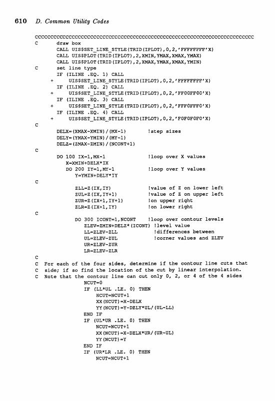
ccccccCececccccccc~ccccccccccccccccceccccccccccccccccceCcccccccce~cccccc C draw box
CALL UISSSETLTm-STYLE (TRZD (IPLOT] , 0 I ZC ' FPFFFFFF' X } CALL UXSSPLOT (TRTD (IPLQT] , 21XMIEat VmXI XmXC CALL UISSPLOT (TRID (TPLQT) , Z,X~X,YMX,XE~AX, YPIINI
C set line type IF (TLTNE .Ea. 1) CALL
+ UIS$SET-LINZ-STYLEfTRID{IPLOT]IO12,t~FFI"FFFfX~ IF fELTNE .EQ. 2) CALL
+ UISSSET-LINE-STYLE (TRID (SBLOT), 0,2? FFOQFFoOrXl fF fILINE .EQI 3) CALL
+ UZS$SET-LINE-STYLE (TRXD (1PI;OT) ,a, 2, @PFFOFFPOr X) IF (ILINE .EQe 4 ) CALL
+ UXSSSET-LINE-STYLE {"rWXB (XPWT) I Or 2, 'FOFOFOFarX> C
DELX- (xmx-XHXN) / ~MX-I 1 !step sizes DeLy- (umx-unr~) (NY-I t DELZ= (ZMaX-ZMfN) / [NCONT+ll
C DO 100 IX-1,MX-1 !loop over X values
X=XMIN+DELX*TX DO 200 IV=1,Pn-1 !loop over Y values
V-VPIIN+DELU*IY
ZLL=Z ( X X , IY) !value of Z on lower left ZUL=Z (IX, IY+E) ?value of Z an upper left ZUR-S (IX+1, IY+l f !on upper right ZLR-Z (SX+1, IY j fan lower right
DO 300 IGONT=I,#CONT !loop over cantaur levels ZLEV=ZHI#+DELZ*(XCQNT) ?level value LLmZLEV-ZLL !differences between UL=ZLW-ZUL !corner values and ZLEV URmZLEV- ZUR LR-ZLm-ZU
G C Far each of the four sides, determine if the contour line cuts that C side; if so find the location of the cut by linear interpolatian- G Note that the contour line can cut only 0, 2, or 4 o f the 4 sides
NCU[S=O IF (LL*UL .LE, 0) THE%
NCUT=NGUT+% XX (MCUT) =X-DELX YU (HCUT)=U-DELY*UL/ (UL-LZ)
END IF XF (UL*UR .LE, O f T m %
PJCUT=NCUT+f X X (NCVT) =X-DELX*VR/ [UR-UL1 VY (MCUTf -Y
END TF IF (UR*ZB .LE. 0) THEN
NCUT=NCUT+I
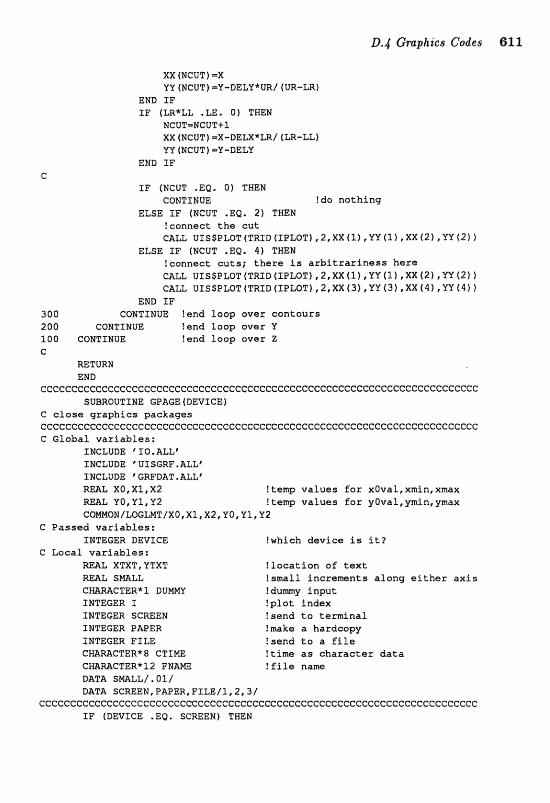
D.4 Graphics Codes 611
XX INCUT) =X YY (%CUT) =y-aELY*uR/ (UR-LP,)
END IF XF (LR*LL .LE. 0) THEN
NCUT=NCUT+I XX (NCUT) =X-DEzXrXIR/ (LR-LLf YV (NCUT) =Y-DELY
END IF
IF (NCUT . EQ. 0) TWEN CONEENUE !do notching
ELSE IF (NCUT .EQ. 2 ) TWEN ? cannect the cut C A U UfS$PLOT(TRTD(IPLOTII2,XX(1~ ,YYff 1 IXX(2j eYY(21 1
ELSE IF (NCUT ,EQ, 4 ) THEN f~onncct cuts; there is arbitrariness here
vssSPLoT[TRrD(xPLoTl f2,~X[1) C ~ Y (11 ,XX(21 tYY421 1 GALL UXSSPMT(TRID(IFLOT),~,XX~~~ ,YV(3),XX(4),YU(4)f
END IF 300 COWTINUE !end loop over contours 200 CONTINUE !end loop over V 100 CONTINUE !end l ~ o p over Z C
mTURN END
CCCCCCCCCCGC~CCCCCCCCCCCCCCCCCCGCCCCCCCCGCCCCCCCCCCCCCCCC~CCCCCCCCCGCCCC SUBRGUTINE GPAGEtDEVICE)
C close graphics packages ccecc~ccceccccccccccccccceccccecccceccccceccccecccccccc~cecccccccccccccc C Global variables:
INCLUDE "0. ALL' f NCLUDE ' UU1SGRF .ALLf INCLUDE p GRFBAT .ALLf =L XO,XI,X~ Itam values for x0val,xmfn,xnax WAL YO,Yl,YZ ! temp values for yaval, ymin, ymax CQMMON/LOGLMT/X0,X1,X2,Y0,YlIY2
C Passed variables: INTEGER DEVICE !which &vice is it?
C Local varf ables: !3.EAL XTXT, VTXT !location of text mt SMALL fsmll increments along either axis
! dumy input: !plot index
INTEGER SCWEN ! send to ter&nal INTEGER PAPER !make a hardsopy INTEGER FILE !sand to a file
!time as character data GKAMCTER*12 FNAMe ! file name DATA S m L L / . O l / DATA SCmEN,E-'MER,FIILE/1,2,3/
cCcc~ccccccceccccccccccccccccccccccccccccccccccccceecccccccccccccccccccc IF (DEVICE .EQ, SCREEN) THEN
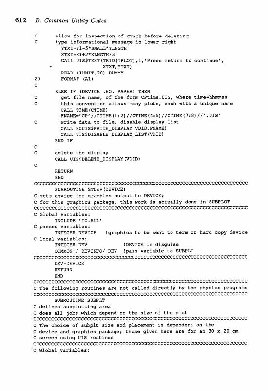
812 D, Conaman UtiZily Codes
C allow for inspection of graph before deleting C type informational message in lower right
YTXT=ZV~-~*S~U*VLNG%N XTXT=X1+2*XLNGTN/3 CALL UISSTEXTfTRID(IPLQT~,lCfPre~~ return to continue*,
+ XTXT, YTXT) READ (IUlcffT,20J DUMW
20 FQRMazl ( A I ) c
ELSE IF (DEVICE .eQI naPaRj THEM C get file name, of the form CPtim.UIS, where tim=bhmss C this convention allows many plots, each with a unique name
CALL TIME (CTICm) F~AME=*CPV/CTI~~l:2)//CTIME~14:5~//CT1CFIlE(7~81 / l r .UISt
C write data to file, disable display list CALL HCUTSSWRITE-DXSPMY fVDID, FBJAMEf CALL UISSDTSBBLE-DXSPmY-LIST [VDXD)
END EP c C delete the display
CALL UISSDELETE-DISPmV(VDID) C
=TURN END
ccecccccccecccccccecccccccccccccccccccc-cccccccccccccccccccccccccecccccec SmROUTXNE GTDEV(DEVICE1
C sets device for graphics output to DEVICE; C for this graphics package, this uark is actually done in SUBPLOT cccccccccccccccceccccccceccccccccccccccccccecccccccccccccceccccccccccccc C Global variables:
INCLUDE 'XIO.ALLt C passed variables:
INTEGER DEVICE !graphics to h sent to term or hard copy dorvi~e C lacal variables:
INTEGER DEV !DEVZa in disguise COMHON / DEVTNFO/ DEV !pass variable to SUBPLT
eCCCcGccCecCcCCCecCCcCcGcGcCCcCCcCGCcCcCccCCCccCGcCcCCCCcCccc~cccc~~cccc DEV=DEVLCE =TURN END
cccccCccccccccccceccccccccccccccccr=ccccccccccccccccccccccccccccccccccccc C The following routines are not called directly kzy the physics programs ccccccccccccccccccccc~ccccccccccccccccccccccccccccceeccccccccc~cc-ccccccc
SUBROUTINE SUBPST C defines subplotting area C does all jobs which depend on the size of the plot CcccccccccCcecccccccccccccccccccccccccccccccccccccccccccccccccccccc~cccc C The choice of subplt size and placement is dependent on Lbe C device and graphics package; those given hers are for an 30 x 20 em C screen using UIS routines cccccccccccccc~ccccccccccccccccc~cccecccccccecccceccccccccccccceccc~cccc C Global variables:
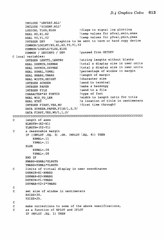
INCLUDE 'GRFDAT.ALLr INCLUDE ' UISGRF ,ALLr LaICAL YLOG,XLOG !flags ta signal log plotting R a L XO,XZ,X2 !temp values far x0val,xmin,xmax REAL UO,Y1,Y2 !temp values for yOval,ymfn,ymax INTEGER DEV !graphics to be sent to term or bard copy device
~ o I U I E ~ Q N / L O G L M T / X O , X ~ , X ~ , V ~ ~ Y ~ ~ V ~ COMMON/WGFLG/YLOGrXLOG COmQH / DEVINFO / DEV !passed from GETDEV
C focal variables: INTEGER LENTTL, UNTRU Istring lengths without blanks =L BSXMIN , BSXmX !total x display size in user units R m L DSUMIEI,DSYmX ?total y display s i z e in user units R m L XSML, YSmL !percentage of window in margin R=& XmRG, Y W G !length of maxgin REAL WIDTW,HEIGHT ?character size INTEGER SCREEN !sand to terminal INTEGER PAPER !make a hardcopy INTEGER FILE !send to a file CMMCTER*6O FONTID !type of font m L WID-TO-LEW !width to length ratio for title =L XTXT !X foeation of title Pn centimeters INTEGER FIRST, YES, NO !first time thraugh? DATA SCREEN,PAPER,FILE/I,W DATA FIRST, YES, NO/lt l, 21
ccCcccccceCcCcceccceececcccecccccccccecceccceccceccc~cccccce~ccCcccccccc G length a f axes
XLEaGTN- (X2-XI) PmGf W= (Y2-P1 f
C a reasonable margin IF ((MPLOT .EQ. 3 ) .OR. (NPLOT !EQ. 4) 1 THEM
XSMAL=. 12. YSPIIALm. 11
ELSE, XSP31AL=. 08 YSML-. 08
END IF XMRG=XSNL*XLHETW YrnRG=YSMAL*YLNGTM
C limits o f virtual display in user coordinates DSXMIM-XI-XmG QSXMAX=X2+XWG DSYNIN=YI-YWRG DWmX-Y2+2*YmRG
c f: set size 05 window in centimeters
XSXZE-36, YSIZEm25.
c C make eorrectians to some of the above soecifications, C as a function of NPLQT and SPLOT
IF (NPLOT .EQ. 1) THEN
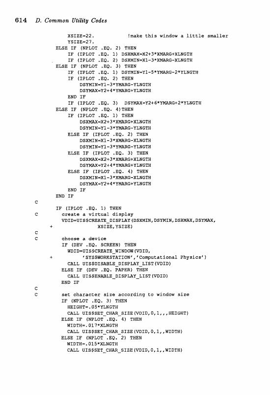
81.4 L?. Common Utility Codes
XSIZE=22. !make this w i n d o w a Little srmsller YSIZEm27,
ELSE XP (NPLOT .EQ. 2) THEN IF (IPLOT .EQ. 1 ) DSXMX=X2+3*XmRG+XLNGTf3 IF (IPLOT .E@. 2) DSXMINrXI-3*XmRG-XLNGTN
ELSE I F (NPLOT .BC?. 31 THEN SF (XFLOT .E@. 1) D S Y M I N = Y l - 5 * Y ~ R G - 2 * Y L N G T H IF (IPLQT .EQ. 2) TWEN
DSUNIN..OV1-3*YMRG-VLNGTH DSYMAX..Y2+4*YmRG+YLNGTR
EPaD I F I F (IPLOT , EQ. 3) DSYM=Y2+ 6*UPgRRG+2*YLNGTtt
eLsE rF (NPLOT .EO. $ 1 THEN I F (TPLOT .EQ. I) THEN
DSXmX=X2+3*XmRG+XLNGTW DSYMIN=Y1-3*k'~RG-VLNGTB
ELSE IF (TPLOT .EQ. 2 f TWEN DSXNTN-XI-3*XMARG-XLNETW DSYNIN=Vl-3*YmRG-YLHGTR
ELSE I F (ZPLOT .EQ. 3) THEN DSXmX=X2+3*XmRG+XLNGTW BfYMAX=Y2+4*'JlMRG+YLNGTH
ELSE SF (IPLOT , EQ. 4 1 THEN DSXMIN=Xl-3*XMRG-XLNGTW DSVMX=Y2+4*YmG+VLNGTH
END TF END IF
TF (TPLQT .EQ, 1) TWEN create a virtual display VDID=UXS$CREA~-DlSPLAY(DSXNXM,DSYMIN,DSX~X,DSY~X,
XSSZB, YSXZE)
choose a device IF fDEV .EQ. SGREEM) THEN WDID=UISSCmATE-WINDOW(VDID,
~SYSSWQRKSTATTONf,~Co~ut.atIonal Physicsr) CALL UIS$DISABLE-DfSPLAY-L7:ST(VDXD}
ELSE IF (DEV .EQ. PAPER) THEN GALL UZSSENmLE-E)ISPMZI_LIST(VDID)
END IF
sat character s i z e according ta window s ize IF (NPLoT .EQ. 3) THEN MEIGWT=.05*YLNGTW CALL UISSSET-CHAR-SIZE (VDIB, 0 , 1 , I HEIGHT)
ELSE IF (NPLQT .EQ. 4 ) THEM WfDTH=.017*XZ1VGTH CALL ULSSSET-CHAR-SIZE (VD1 D, 0, I,, WIDTH)
ELSE XF (NPLQT .%Q. 2) THEN WIDTW=.015*XLNGTH CALL UISSSET-CHAR-SIZE fVDIB, OI 1, ,1?9I:DTNI
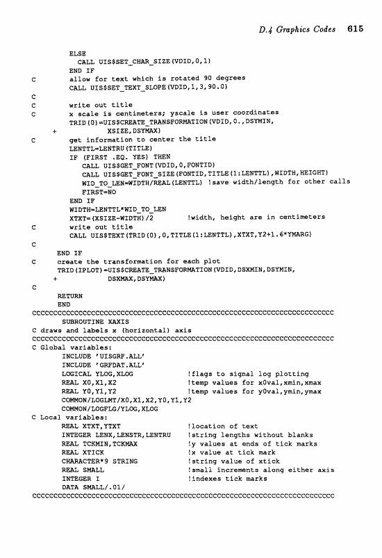
ELSE CALL UISSSET-CM~-SIZE (VDID, 0,1)
ERD IF c allow fox text which is rotated 90 degrees
CALL UTS$SET-TEXT-SMPE~VDID~I,~~~O~~~ e C write out title C X scale is centimet~rs; yscale is user coordinates
TRIP (0) ~uI~$~~TE-TMMSF"OMTXON fVDZD, 0 DS'PMSM, C XSXZEp D S Y W )
C get infarmation to center the title LEITTL-LENTRU (TITLE) SF (FIRST .EQ. YES) THEN
CALL UISSGET-FONT (VDID, Q, PO'EJTID) CALL UXSSGET-FONT-SIZE(PQNTID,TI:TLE:~I:LENTTL~~WXDTH,HEXGHT~ WIDTO-LEN=WXDTH/MAL(LENTSL~ Isave width/length for other calls FIRSTmEIQ
END IF WIDTW=UNTTL*WIDTO-LEN XTxT- (XSIZE-WIDTH) l2 !width, height are in centiwters
C wrlte out title CALL UXSITEXT (TRXD ( O f , 0, TITLE I I :LENIITL), XTXTfiY2+l.6*YMZIRGf
G END TF
C create the tcansfarmtian f o r each pZot TRTD(IPLOTf=~JS$C~&TEET~NSFO~TIOEO~VDID,DSXMJM,DSYM~~, i- BSXm, DSYMX)
C mTURM EHD
ccccccccceeccccccccccceccccccccccceccccccCccc~cccccccccccc~ccccccccc~ccc SmROUTIME =IS
C draws md fabef S x (hoxizantal) axis ccccccceecc~ceccccceC:ecccecccccccccccecccccccccceecccc~ec~cccccccccccccc G Global variables:
INCLUDE ' UI SGW ,ALLe INCLUDE ' GWDAT .ALL" LWICAL YLW,XLOC; !flags to signal log plotting W L XD,XI,X2 l tenrp values for xaval, xmin, xmax RmL YO,YX,YZ !temp values for yOval,yrnin,ynax COMMON/LOG~T/XOIXZ,X2,Y0,Y1,Y2 COFIMON/LOGFLG/VLOG,XZOG
C Local variables: R W XTXT , YTXT !location af text TMTEGER LENX,LENSTR,LENTRU !string lengths without blanks =L TCXHIN , TCKMX !y values at ends of tick marks W L XTIGK !X value at tick mrk
!string value aE xtick =L SmLL !small ineremnts along either axis INmGER 5 !indexes tick marks DATA SIUIALL/.OI/
ceccccc~cccccccccccccccccccecccccccccccccccccccccecccccceccceecccccccccc

C draw x axis CALL UISSPLOT (TRID (IPLOT) , a, XI, XQ,X2, XO)
C C lake1 X axis
LENX=LENTRU (MBEL (1 ) ) XTXT-X2+5*SMLL*XLUGTW YTXT=XQ+S*SMLL*YLMGTN CALL UISSTEXT(TRIDfIBLOT) 3 , U B E L ( I . ) (1:LENX) ,XTXTf YTXT)
C C tick marks C set length o f ticks
TCKNS#=XO-SNALL*YLMGI"B TCKWXmXO
C DC3 SO I=O,MXTICK
C draw tick marks XTICK=X1+I*XLNGTH/NXTIeK CALL UISSPLOT (TRID ( XPLOTf ,Q, XTXCX:, TCKMXN, XTSCfS., TCKmX]
c C label tick marks
XTXT-XTECR IF (XL%) XTIa=3O**XTICK CALL C O m T (XTSCK, STRZNG, LENSTRI CALL OXS$TEXT (TRID (IPLOT) I I t STRING f 1 : LEHSTR) XTXT, TCKMIH}
16 CONTINUE C
RETURN END
CcCccccccccczccccccccccccecccccccceccccccccccccccccccccceccceccccccccc~c~ SUBROUTINE UAXIS
C draws and labels y (vertiealf axis ccc~cccccccccccccccccccccccccccccccccccczcccccceccececcccccccccccccccccec C Global variables:
IZJrCLODE ' UISGW .ALLp INCLUDE ' CRFDAT .ALLr LEICAL YLQG,XEOG !flags to signal log plotting REAL XO,Xl,X2 !tee values far x0val,xmin,xmx lU3AL YO,Yl ,Y2 !tamp values for y0val,ymin,ymax CQMM0H/LOGLMT/XO3XI,X2,Y~,Y~,Y2 COMMON/LQWLG/YLW,XLOG
C Local variables: =L XTXT, UTXT !lacation o f text INTEGER LENV,LENTRU,UNSTR !string lengths without blanks R M L TCKMIN , T C K m !x values at ends a f tick marks R&AL VTICK fy value at tick mark CBMCTER*9 STRING !string value o f xtick R m L SWLL !smll fncrewnts along either axis INTEGER I ?indexes tick marks DATA SmLt/.Ol/
~ccCccc~cc~ecceccccccccccccecccccccccccccccccccccccccccccccceccccccccccc C draw y axis
GALL VSSSPLOT(TRID(IPL.OT1, O,Y0,VTfYO,Y2)
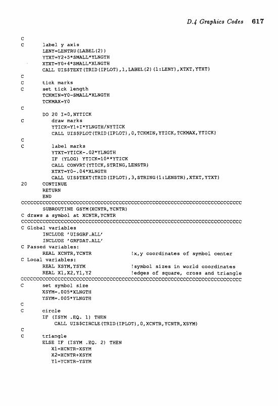
D.4 Gmphies Codes 817
C C label y axis
UNY=LENTRU (UBEL (21 f YTXT=Y2+S*Sf?lBLL*YLNC;TH XTXT=U0+4*SMBLL*XLNGTW CALL UXSSTEXT (TRID (IPLOT) 1, UBEL(21 (1. :LEP;IV) ,XTXT, YTXT}
c C tick marks c set tick length
TCKMfU-VQ-SMALL*XLNGTH TCKMAX-Y 0
C 80 20 I=O,NYTICK
C draw marks YTfCK=Vf+X*YLNGTH/NVTICR CALL UXSSPLOT fTRID (XPLQTJ , ~,TcKMTN, YTIcK, TCK~X,YTIC:K]
e C label marks
YTXTmYTICK-.02*VLNGTH IF (YLOG) YTICK=IU**YTICK CALL C O m T f YTICK, STRING, LENSTR) XTXT=YO-.QB*XtNGTW CALL UISrTEXT (TRIO (SPLOT) '3, STRIP36 4 1 : mNSTR1, XTXTt YTXTI
20 CONTTNUE =TURN END
cccccccccccecceccccccccccceccf:cecccecceecccccccccccccccccccccccecccccccc SUBROUTINE GSYM (XGNTR, YGNTR)
C draws a sy&ol at XCNTR,YCNTR ceeccc~c~cccecccccccccccccccccecccccccccc~cc"cccccccccecccccccceccccccccc G Global variables
INCLUDE ' UI SGRF .ALLe INCLUDE ' GGRFDAT .ALLe
G Passed variables: REAL XCNTR, YCNTR !x ,y coordinates of symbol center
C Local variables: RML XSYM,USYM !symbol sizes in world coordinates WAL Xl,X2,Yl,Y2 ledges of square, cross and triangle
eCccc~cccecccc~ccccecccceeceeccceccceeecccecccccceececc~cecc~cccccC:ccccc C set symbol size
XSVN=.005*XLNGTH YSYM=.UOS*YLNGTB
C C circle
IF fISVN .EQ. If THEN CALL UISSGIRCLE ITRID (IPLOT] ,Q, XCNTR, YCNTRI XSYM)
C: C triangle
ELsE IF (ISUM .Ea. 2) THEN XI-XCNTR-XSYM XZ=XCNTR+XSYN UI-YCMTR-YSYM
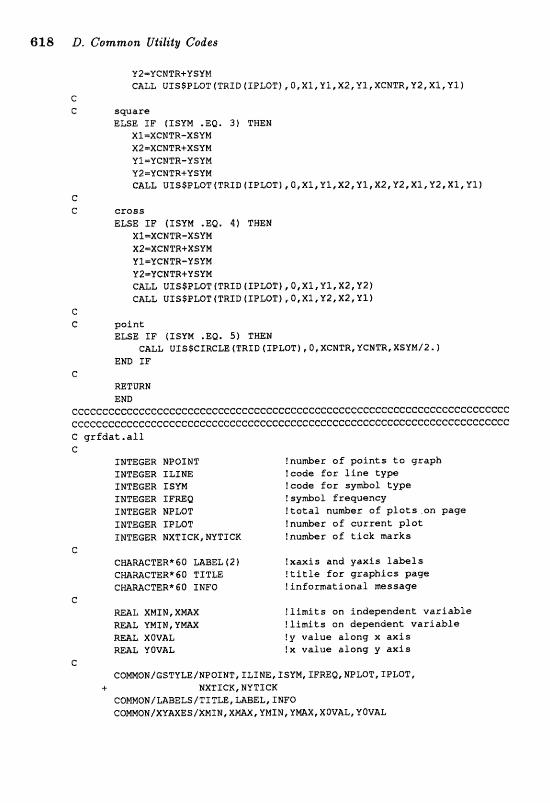
61181 D. Common U#ifitg Codes
Y2=YCNTR+YSYM CALL ~ I ~ ~ P L ~ ~ ~ T R I ~ ~ ~ P L ~ T ~ , ~ , X I , Y ~ , X ~ , Y I , X C N T R , Y Z , X ~ , Y ~ ~
e G sware
ELSE fF (ISYM .EQ. 3 ) THEM XI-XCNTR-XSYM X2mXCNTRf XSYN YI=YCNTR-YSYM Y2=UCNTR+USYW CALL UIS$PLQT(TRID (IPLOTf I 0 , X 1 r V 1 1 X 2 1 Y 1 1 X 2 1 Y 2 , X ~ e Y ~ , X ~ , Y ~ ~
c C cross
ELSE ZF {ISVM .Ea. 4) THEN XI-XCNTR-XSYM X2=XCNTR+XSYM YI=YCNTR-VSYN YZ=YGNTR+YSYM CALL UZSSPLOT (TRID (ICPLOT), a,xl, U, xz, V ~ I CALL UISSPLOT (TRZD (IPLOT] , O,X1, Yz, X2# Y11
C C point
ELSE IF (ZSYM .EQ. 51 THEN eau., U~SSCXRCLE (TRID (XPLOT), 0, XCNTR~ YCWTR, XSYM/~. 1
enta IF c
RETURN E%D
c~~~~~~~~ccc~~cececccccccccccccccccccccccccccccecccccccccecccecccccccccc c~ccceccccccc~cecccccccceccccccccecccc~ccccccccccccccccc~cccccc~cccc~ccc C grfdat.all C
INTEGER HPOTNT !nu&er of points to graph SNTEGER ILINE !code for line type INTEGER ISVN !code far sydol type INTEGER IFmQ ! sy&ol f requeney INTEGER NPLOT !tatal nuder of plots on page INTEC;eR IPEOT !number of current p lo t INTEGER NXTICR,MYTICX !nunrber of tick marks
C" GmRACTER* 60 LABEL [ 2 fxaxis and yaxfs labels CmmCTER*GO TZTLE !title for graphics page
t informational message c
RERL XMf N, X W !limits an independent variable m L VMTN, YNX ! L i m i t s on dependent variable R a L XOVAL !y value alang x axis REAL YOVAL !X value along y axis
C COMMON/GSTYLE/NPOf NT, ILTNE, ISVM, IFREQI NFLOT, IFLOT,
+ NXTZCX, NYTf CK COMNOM{LABELS/TTTLE,LAE?;EL,INFO COMMON/XYAXES/XMIN, XIVtAX YMZN, YlvlAX, XOVALI UOVAL
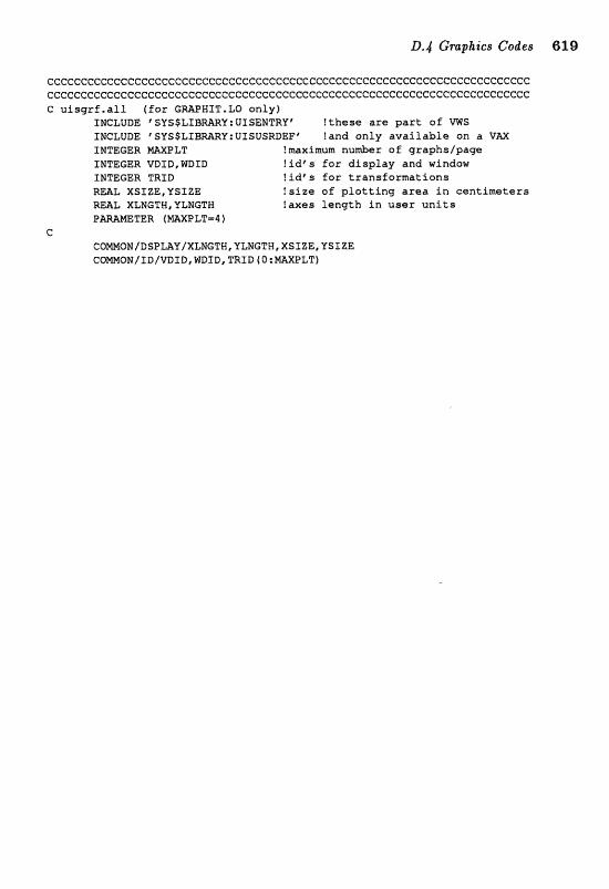
L14 Gmpkies Codes 6119
cccccccceccccecececceccccccccccccccecccccececececccccceccccceccccccccccc cccccc~ccccccccecCececcccccccccccccccccccccceccc~cccccccc~cccccccecccccc C uisgrf.all (for GMPWIT.LD only)
INCLUDE pSYs$LTBMRY:UISENTRV" !these are part of W S INCLUDE WsYS$LIBMRY:UISUSRDEF" !and only available on a V= INTEGER m P L T !maximm n u e r of graphslpage INTEGER VDTD,tflDID ? i d ' s ffor display and window INTEGER TRID ! i d t s for transformations -L XSXZE,VSIZE !size o f plotting area in centimeters R m L XT;NGTH*YLI\IGTW ! a x e s length In user units
C CO~~M/DSP~V/XL~GTW,~LNGTB,XS92EtYSIZE COMMON/ XDlWXD, WDlD, TRTD 4 0 :=FLY)

This page intentionally left blank
Appendix E
Network e Transfer
The ubiquity of network connections has made network file transfer a praetieal option for code distribution. To transfer files you need ftp (file transfer protocol) software and a connection to the Internet network (but not necessari?y a direct connection). Check with your system manager if you are unsure of the avkiIabllty of either,
The files me adlable on the Internet node physf caitp, W&, in the dirwtory pab/c~m~hys. There me thrw sub&rectopies: /fearan con- t&s d l of the FORTRAN codes fisttad in this book, lbasic contaLias AI of the IBM-BASIC codes, and /grap&ics contains subdire~toriea with ad- ditiond FORTRAN interfaws to graphics padtages (i.e., interfaces other than graphit. hi graphit. lo). (At the time of writing, only a GKS interface is available.)
E.1 Sample Session Below is a s a p l e sesdm that transfex's aU of the files en&ing with
the .all exten~ion. Phrases that you type are in bddface, our cornmeals are in. italics, and computer responses are in plain type.
The host camputer is a U N E environment. For those not familiar with UN=, you need only know the following commmds: fs -1 to list files in a directory, CA to change directories, and qnit to logoff. The ftp commands are as follows: prompt to toggle the prompting for file transfer (the default is that it will verify each file before sending), and wet to get files from the remote host. atgee mast be ~QBQWC?~ by the narne af the file to be sent; wild cards (e.g., *.* or *.&EL) are dlowed. UNIX is care sensitive, so nams must; match both letter and ewe.
h t e *ha% sonae features of the host computer may change (e.g., the n m e of the computer, other subdirectoriee;), but every attempt will be made to kwp &he Internet address and directories assaciated with Corn- putational Physics the same. Also, some of the details (e.g., prompts)

depend on the speGific implementad-ion of ftp on your xa lacd expat if you m n into diBcdtim,
2 f tp pbyrf crszep m. edu f i ' P ~ p w - h x O w s
Connected t o mozz.unh.edu,
220 mozz.unh,edu FTP s e r v e r (ULTRfX Version 4.1 Tue Mar 1 9 00:38:17 EST
1991) ready,
Name ( f t p h o s t : ) : ul
331 Guest l a g i n ak, send f d e n t a s password.
Password: ?ypQ h = $ ~ # * &h@
230 Guest l o g i n ok, access r e s t r i c t i o n s apply,
f tp> 2.8 -1 Iwk at c@-- clfd&@q <Opening d a t a connect ion f o r / b i n / l s (332,177,128.8,3763) ( 0 bytes),
t o t a l 3
dx-xr-xr-X 2 O 512 May 24 10:26 b i n
dr-xr-xr-X 2 0 512 Hay 24 10:26 etc
dr-xr-xr-X 4 O 512 May 24 10:26 p&
<Trans fe r complete.
T k "d" a, rl;ut k g i n n h finc * m m a &#c&q;
of rkc d&#~roo orfilc iP QI md ufrk Zinc. Etp> oa, pwh c b g c ro rk pub & e & u ~
<CWD cornand s u c c e s s f u l .
f t p > l. -2
<Opening d a t a connect ion f o r /bSn/ls [132.177,128.8,3764) (Q b y t e s ) ,
t o t a l 1 7
druxr-xr-X 5 O 512 Hay 24 10:26 c a w p h y s
drwxr-xr-x 5 O 552 Hay 24 10:2S NeXT -r~-r--r-- 1 0 14754 Nay 24 10:26 ncp ,de f inss
<Trans fe r complete,
ftp> od w w b g r
Etp> 3.a -1,
<Opening d a t a connect ion f o r / b i n / l a (132.177.128,8,3767) 10 b y t e s ) .
t c l t a l 4
drwxr-xr-X 2 O 512 Hay 24 1Q:26 basic
drwxr-xr-x 2 O 1536 Jun 12 11:3J f o r t r a n
drwxr-xr-X 2 0 512 May 24 1 0 ~ 2 6 g raph ics
<Trans fe r template,
Etp> c4d fartrm c h g e l@ Ikfw&an dk@cfq
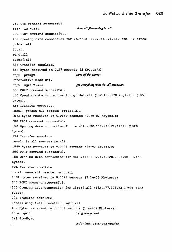
E, Network: File %mjer 623
Etp> 1s; *.rX1 allfires k m#
200 PORT comand successful.
150 Opening d a t a connect ion f a r / b i n / l s (132.177.128.23,1790f (0 b y t e s ) ,
g r f d a t - a l l
3.0, a l l
menu. a11
u i s g r f . a l 1
226 Trans fe r complete.
538 b y t e s r e c e i v e d i n 0.27 seconds (2 f.(fsytes/sf
f t p > rwa flihe pronylt
I n t e r a c t i v e node o f f .
Etp> we& *.a%l get ntsqtm wilh fk df a & w b
200 PORT comand success fu l .
150 Opening d a t a connect ion f o r g r f d a t , a l l f132,177,128,23,1736) C1050
b y t e s ) .
226 Trans fe r complete.
l o c a l : q r f d a t ' a l l remote: qrfdat .a lX
10'73 b y t e s r e c e i v e d i n 0,0039 secands (2,7e+02 Kbytes ls)
200 PORT comand s u c c e s s f u l .
150 Wening d a t a connect ion Eos i o . a l l (132.277,228.23,1797) (1528
b y t e s ) .
226 Trans fe r completa.
l o c a l : i o . a f l remote: i o . a l l
3560 by tes r e c e i v e d i n 0.0078 seconds (2e+02 Rbytasls)
200 PORT c o m a n d success fu l .
150 Opening d a t a connect ion f o r m n u . a l l (132.177,128.23,1798) (2455
b y t e s ) ,
226 Trans fe r complete,
l o c a l : menu.all remote: m n u , a l l
2504 b y t e s r e c e i v e d i n 0.0078 seconds (3,2e+02 Kbytes/s)
200 PORT c a m a n d s u c c s s s f u l ,
150 Opening d a t a connect ion f o r u i s g r f , a l l (132.177,228.23,1789) (625
13ylCes) *
226 Trans fe r complete,
l o c a l : u i s g r f . a l 1 remote: u i s g r f - a l l
637 bytes r e c e i v e d in 0.0039 seconds (3,6e+02 Kbytes lsf
ftg> quit: logcfjrrmte hDsl
222 Goodbye.
> puvre back to yclur cnvn mehint

This page intentionally left blank
References
[Ab64]
[Ab 781
IJandboook of Mathematical Functions, eds. M . Abramowitz and I. A. Stegun (Dover, New York, 1964).
R. Abraham and J. E. Marsden, Foundations of Mechanics, Sec- ond Edition (Benjamin- Cummings Publishing Corp., Reading, 1978) Chapter 8.
F. S . Acton, Numen'eal Methods that Work (Harper and Row, &W York, 1910).
S, L, A&er and "F, Pirm, Rev, Mod, Phys, 56, 1 (1984).
V. I. Anndld and A. Awz, Eqodie Pwblems in CIagsicat m- chanics (Benjamin Publishing Corp., New York, 1968).
A. Baker, Phys. Rev. 134, B240 (1964).
H. A, Bethe and R. W, Jwkiw, Intemdiate Quantum Mechan- ics (Benjamin Publishing Corp., New York, 1968).
P, R. Bevington, Data Rductriora and Ewor Artalgsia for the Physical Sciences (McGraw-Hill, New York, 1969).
R. A. Bonham and M. Fink, Higia Enevy Elwtmn Sctitte&ng (Van Nostrand-Reinhold, New York, 1974).
J. A. Boa m d D. S. Cohen, SIAM Je AppL Math,, 90, 223 (1976).
R. L. Burden, J. D. FGres, and A. C . Reynolds, Numerical Araalgsb, Semnd E&itiost (Priadfe, Weber, and Sck&dt, Bosto~, 1981).
D, M. Brink and G . R. SatcMer, Angular Momentum, Second edition (Clarencfon Press, Oxford, 19680,
J. M. Cavedon, Thesis, tfniversitb de Paris-Sud, 1980.
[Ce79] D. M. Ceperley and M. H. Kalos in Monte Carlo Methods ia Statkticair Physia, ed, K. Binder (Springer-Verlag, New Yark/BerEn, 1979).
D, M. Ceperley and B. J. Alder, Phs. &V. Lett, 45,566 (1980),
S. Chadrmekhar, An IntducEion $0 the Studg of Skkkalr Stmc- tare (Dover, New York, 1957).
S. Chandrasekhar, &v. Mod. Phys. 58,137 (1984).
S. A. Chin, J. W. Negele, and S. E. Koonin, Aan. Phys, 187, 140 (1984).
H. nocard, S. E. Koalain, wd M. S, Weicrs, Phys, Rev. G 17, 1682 (1978).
L. D, Fosdick in Methods in Cosnrp'1ctataltmaf Ph~ic8, ml. 2 , ed, B. Alder et a t , p. 245 (Academic Press, New York, 1963).
T. deForest, Jr. and J. D. Wdedta, Adv. Phys. 15, 1 (1966).
J. L. hiar and J. W, Negele, Nucf. Phys. A212, 93 (1973),
J. L. Friar and J. W. NegeIle, Adv. Nucl. Phys. 8, 219 (1975).
B. Rais et at., Phys. Rev, Lett;. 38, 152 ( 1977).
P. Gombaci, Die Statische Theorie des Atoms (Springer, Vienna, f 949).
A. Goldberg, B.M. Sch;ay, and J. L. Schwartz, Am, J. Phys. 35, 177 (1967).
H. Goldstein, Classical Mechanics, Second Edition (Addison- Wesley Publishing Company, Reading, 1980).
J, M. Hmmersley and D. C. Handscomb, The lWonte Carlo Method (Methuen, London, 1964).
G. Herzberg, Spectm of Diatomic Molecules (D. Van Nostrand Compa;ny, Inc., NW York, 1950).
M. I-Idn~n and C, Heiles, Astron. J. 88, 73 flg(i4).
E, H. G. Helleman in findamentat Pmbbms ira- Statiatrial Me- chanics, vol. 5 , d. E. G. D. Cohen (North Holland Publishing, Amsterdam, 1980) pp. 165-233.
R. Hofstadter, Ann. Rev. Nuc. Sd., 7, 231 (1957).
K . Ruang, Statistiml Mechanics (John Wiley and Sons, New York, 1963).
K. K. Km, J. J. Griffin, P. C. Lichtner, and M. Dworzecb, Nucl. Phys. A3S2, 109 (1979).
M. K. Kalos, M. A. Lee, P. A. Whitlock. and G. V. Chester, Phys. Rev. B 24,115 (1981).
M. H. Kdos iwnd P. A. Whitlad, TIae B w k s of Monte GrIo Methods (J. Wiley and Sons, New York, in press).
B. W. Kernighan and P. J. Piauger, The Elements of Progmm- ming Style, Second Edition (McGraw-Hill Book Company, New York, 1978).
L. J. KieEer, At. Data, 2, 293 (1971).
D, Knnth The Art of &napater Pwmmmingf &&me 2: Seminu meriwl Algorithms (Addison- Wesley Publishing Corn- pmy, Reading, 1969).
E. B. KaEman and F. L. FZriebman, Problem SolPlilrqg and Strere- tuwd Programming in FORTRAN 77 (Addison-Wesley Publish- ing Campmy, hc., Reading, 1987).
E, D. Landau and E. M. Lifshitz, C o u p # @ of Z"laeoretiwI Php~ics~ Volume 6, Nuid Mechanics (Pergamon Press, Oxford, 1959).
B, Lipkin, N. Meshkov, and A. J. Click, Nud. Phys. 62, 188 (1965), and the two papers following.
B. MeCay m d 'X'. T. Wu, The Two-Dimewioottal d s i y Model (I-famard University Press, Camb~dge, 1973).
[Me531 N. Metropolis, A. Rosenbluth, M. Rmnbluth, A. Tder , and E. Teller, J. Chem. Phys. 21, 1087 (1953).
A. Messiah, Quantum Mechanics (J, Wley & Sons, Inc., NW York, 1968)
R. G. Newton, Scattering Theory of Waves and Particles (McGraw-Hill Book Co., New York, 1966).
G. Nicolis and I. Prigogine, Self-organization in Nonquilibrium Systems (J. Wley and Sons, New York, 1977), Chapter 7.
W. H. Press, B. P. Flannery, S. A. Teukdsky, and W. T. Vet- terling , Numerical Recipes (Cambridge University Press, Cam- bridge, 1986).
P. J. Reynolds, D. M. Ceperley, B. J. Alder, and W. A. Lester, Jr., J. Chem. Phys. 77,5593 (1982).
R. D. Echtaneyer and K, W. Moslon, Diflemnce Metfad8 for InitiaGvalue Problems, Second Edition (Interscience, New York, 1967).
S. A. Rice in Quantum Dynamics of Molecules (l$&@), ed. R. G. Wolley (Plenum Publishing Corp., New York, 1980) pp. 257- 356.
P. J. Roache, Computationat Fhid Dynamics (Hermosa, Albu- querque, 1976).
H. Rufisbauser, C ~ m m . of the AGM, 8, 67, Mgorithatl 150 (February, 1963).
R. Shankar, Phys. Rev. Lett. 46, 1088 (1980).
S. L. Shapiro md S. A. TeukaXsky, Black Hoks, m i t e Dwarf@, and Neutron Stars (J. Wiley & Sons, Inc., New York, 1983) CHapder 3.
T, E.. Shoup, AppEe'ed Nemerical Me&&& for the Mic (Prentiee Hall, Inc., Englewood Cliffs, 1984).
I. Si&, Nucl. Phys. A218,509 (1974).
[W21 R. Varga, Mat riz Item tive A natysis (Prentiee-Hdl, Englewood CliRs, 1962).
E. L. Wachspress, Itemtive Solvtion of Elliptic Systems and Ap- plications to the Neutron Diffusion Equatioras of Reactor Physics (Prentice- Hall, Englewood Cliffs, 1966).
S. J. Wallace, Ann. Phys. 78, 190 (1973); Phys. Rev. D8, 1846 (1973); Phys. Rev. D9,406 (1974).
R. C. Weast, Handbook of Chemistry and Physics, $pd edition, (The Chemical Rubber Company, Cleveland, 1971).
M. Weissblutb, Atoms and Molewles (Academic Press, New York, 1980).
R. R. Whitehead, A. Watt, B. J. Cole, and I. Momison, Adv. Nucl. Phys. 9, 123 (1977).
A. T. Winfree, Sci. Amer. 220, 82 (June, 1974).
T,-U. Wu and T . Ohmura, Quantum Theorgr o f Scatte9-ing (Prentice-Hd, Englewood Cliffs, 1962).
L.C. YaRe, Reviews ol" Modem Physics, 54,407 (1982).
33, R* Yennie, D. G. rtavenh&, md D. N. WiXmn, Physi, Rev. SS, S00 (1954).

This page intentionally left blank
Index
40 Eri B, 53. sfruetu~e, I2& 6-12 potential, 14, 222. atom,
see also Lennmd-Jonw potential. low-energy resonwces, 108. absciasm, gausisian quadrtlture, 9.5. mu1 tkelecf ron , 72. acceleration par met=, elliptic patial auto-correlatiorr , Metropolk ~ lgod t hm,
biEerentid equations, 180. 214, 219. accuracy monitoring, ordinary differ-
ential equations, 32, a;Ccuracy,
ordlinary differential equa t io~~ , 68. plwltial diRerentiaf equation, 114, quadrature, 8, 13.
action, 313.. Ad forth,
method, 30. tvvo-step method, 29.
RlIioulLo~ method^, 31. altern~tine;-direction methods, pz~stial
digerentid equation, 180. wgle, scat trrring , 20. annihilation oper(zt;or, 135, anti-ferromagnetic couplings, 220. anti-ferromagnetism, 2 16. approximation,
Born, Stjfl., 121. Barn-Oppenhrrimer, 14, 221. centrd-Aeld, 78. Hatree-Fock, 728., 222. eikonal, 96@, 99, 129. fillhg, 78. linear, 109, 123. self-consistent field, 72, se~elmsical , 114, 98, 139. WKB, 16.
Besstjl function, cylindrical, 67, 81.
polynodal appraxirn&iioxl, 87, recursion relation, 87'
aphericd, 92, 104. binary alloy, 215, Bode" rule, 9, Born approximation, 96#., 121. Born-Qppenheimer approximation, 14,
221. Born scattering amplitude, 98. bound salutions, 14, 67, boundmy conditiollls,
Dirichled, 146, 169, fixed, 190.
Neumann, 146, 150, 178. no-fjtux, 190. no-slip, 165. periodic, 158..
boundmy value problem, 55g, Green" function solution, 6 18. round-aE error, 60. shooting method, 64, 67..
Hrusselator, 189g equilibrium values, 190. linear stability andysis, 1918
a t o ~ e , '@C&, 133. nucleus, 120. canonical ensemble, 216, arbitah , linear combination, 224. canonical tradormation, 45,
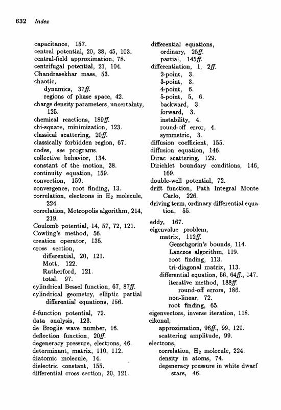
capacitance, 157, central potential, 20, 38, 45, 103. centr~l-Geld apgraxim&ion, 78. centrifugal pokntid, 21, f 04, Cfiwdrasekfiar mms, 53. chwtic,
dynmics, 378. regions of phase spwe, 42.
&age density pmmeters, uncertainty, f 25-
chernicd reactions, 189g chi-a~quare, xninimitaation, 123. cfwicd sc;attrtring, 208. clmicdly forbidden re@an, 67. codes, gee program. eofleetivc? behavior , 1134. constant of the motion, 38. continuity equation, 159. convecdion, 159. convergence, root finding, 13. ernrelation, electram in Ill2 mobcule,
224, eorrelratioa, Metropolb algorithm, 214,
219. Coulomb potential, 14, 57, 72, 121. Cowtintg's method, 56. creation operator, 135. erws r~ection,
dserential, 20, 121. Mott, 122, Rutherford, 121, tat&, 91.
cylindrical Besel function, 67, 8Tfl cylindrical geometry, elliptic pastial
diRerentid equations, 256.
S-funclia~ pote~timl, 72. data analysitjr, 123. de Brofie wave numb=, 16, deaection function, 20' degenerwy paegsure, electrons, 46. d e t e r ~ n m t , matrk, 110, 112. diatomic mokcule, 14. dileiectric constant, 155. tliEerentid crws wetion, 20, 121-
diffewatial equations, ordinary, 25& partial, 145fi
diflerentiation, 1 I 28. %point, 3. gpoind, 3, &point, 6 , &point, 5, 6. b~kvvard, 3. forward, 3. hsta'biliCy, 4, round-oR error, 4,
diffusion coeacient , 155. digusion eqrratbn, 146. Dirac gcatterirrg, 129, Diricblrtt boundary conditions, 146,
169. double-well potential, 12. drirt funetion, Path Ixltegaj. Monte
Cmlo, 2263. driving term, ordhasy diaerent ial equa-
tion, 55.
eddy, 167. eigenvalue problem,
matrix, 112@ Gerselrxgorin's bounds, 1 14. Lanczos algorithm, 1 1 9. root finding, 113. trkdiagonaf madrh, 113.
digerential equation, 56, Mg,, 147. iterative method, 188@
round-oE errors, 186. non-finear , 72. root finding, 65.
eigenvector~, inverse iteration, 1 18, eikond,
approximation, 9ISfF., 99, 129. scattering amplitcude, 99.
electrons, correlation, Ha molecuIe , 224 ., density in atoms, 74. degenerit-ey prMsure in white dwarf
s(tara~, 46.
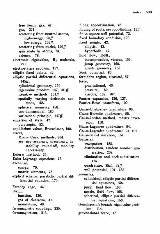
free F e r ~ gas, 47. g=$ 221. scatferhg from neutral atom,
Ggh-enerm, 968. low-energ, 1038.
scatterhg from nuclei, 120fjF. spin state iP1 &Q-, 73. vdence, 78,
electronic eigenvdue, H molecule, 2231.
electrostatics problem, 157. elliptic fixed points, 42. elliptic partial digerentiaf equatioas,
146fi, cyXindrial geomtry8 156. ei(~-tnvslue problem, 147, 1818 iterative metha&, 151fjF: spatidly vmfing dieketric con-
stant, 155. aphczficait gmmetry, 156. twedimensional, 180. vmiatianal priaciple, 1478
equlzzdion of state, 47, polylropic, 52.
equifiiibriurn vdues, Brusrrelatsr, 190. errorsp
Monte Cetrb methods, 204. see also wcuraey, inaecurailcy, in-
dabgity, round-OR, stability, nncer t&tyl
Euler's method, 26. Eu br-Lagrage equations, 75. exehaagel
energy, 7'9. matrk elements, 75.
explicit acheme, pasabolic partial dig fereritial equaLLion, 170.
filling appro~matiorx, 78. fin&g of roots, sw rool-finding, 1 1fi finite square-welf potentid, 72. fixed bounda?ry condition, 190. fixed pdnts, 42,
dliptie, 42. hyperbdicic, 42.
fluid flaw, 158fl, incompressible, v.isco.u~, 169. jump gwmtry, 168. nwale g ~ m e f r y ~ 168.
Fack pohntiaf, 88. forbidden regio~, cfwiesf, 67. force,
pavitational, 46. prmsure, 159. vihlcoubs, 159, 167.
Fourier expasion, 126, 127. Fourier-BweX trmform, 129.
GauseChebyshev quadrature, 96. Gaumflierrite qudraiture, 95.
Jordm methd, matrk inver- sion, 1x0.
GaueLamerre quadrature, 94. GaueLegendre quaxfrature, 94, 202. GaueSeidel iteratioxl, 1151. Caumian,
wavepacke t , 188. dbtribution, rmdom number gen-
eration, 208. elhinalion and back-substitution,
175. quabrature, 85&, 928 well potentid, 101, 188.
geometry, cyUmdrical, diptic partial diReren-
tiaf equations, 156. ~ m t b ~ ~ a y cage, 157. jump, fluid flow, 168. Fermi, nozzXe, fluid flow, 168.
function, 126. spherical, elfiptic: ial diReren- g= of electrons, 47, t i d equatio~a, 156, momentum, 48, Gerschgoria's bbounds, eigenvajue prob-
ferromapetic couptings, 220, lem, 114. ferromg~ethnn, 2 15, gravilhational force, 46.
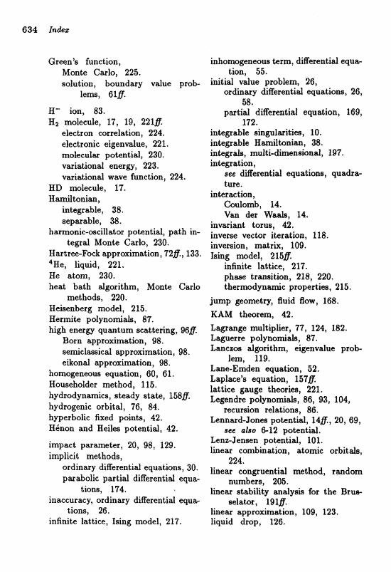
Green's function, Monte Carlo, 225. solution, boundary value prob-
lem, 618.
H" ion, 83. E2 molecule, 11, 19, 221$.
electron correlation, 224, electronic eigenvdue, 221. moleculas potential, 230, variational enere, 223. variationd wave function, 224,
HID molecule, 17. Efmilkonia,
integralble, 38. separable, 38.
hmmonic-o~cillator potentialtl, path in- tegral Monte Carlo, 230.
Hartrw-Foch apgroimtion, 72', 133. %e, liquid, 221. Ze atom, 230. heat bath dgorithm, Monte Carlo
methscls, 220. Hebenberg model, 2 15. Eermite poiynodah, 87. high energy qumturn scattering, 96fi
Born agpr~xirnation, 98. s e m i c l ~ i c d approximatiart, OS. eikonal approximation, 98,
homogeneous equation, 60, 6 1. I-fou~eholder method, 1 15, hydrodynmies, s t edy state, 1588, hydrogerric orbit&, 76, 84. hyperbolic fixed points, 42. IX6non and Heila potentid, 42.
inhomgeneow term, digerentid equai- tion, 55.
initial value problem, 26, ordinary digerendid equatiow, 26,
58. paurtial dsererttitli equation, 169,
172. integrable shgularidim, 10. integrable Efmiltonim, 38. inbgrab, multi-dimeasianal, 197. inkgation,
see &&erential equation^, quadrai- tare,
ixlfermlion, G u l a d , 14. Van der W d , 14.
invdant torus, 42, inverse vector iteratbn, 118. inversion, m&rkp 1109. Ising mdel , 215fi
hfinite lattice, 217. p h m transition, 2118, 220.
c properdim, 215. jump geometry, fluid Aow, 168, KAN theorem, 42, Lagrmge multipkar, 77, 124, 182. Laguerre polynodak, 87. 111ac~w alprikhm, eigenvalucs prob-
lem, 119. Lane-Emden equation, 52, Laplwe" equation, 157fl. lattice gauge thmrim, 221. Legendre polynomi&, 88, 93, 104,
recursion reE&iona, 86. hnnard-Jones potential, 14g, 20, 69,
set: lxbo 6-12 potential.
impact par&meba, 20, 98, 129, Lenz-Jensen poteitial, 101. linear cornbindion, atomic orbit&,
impiieit methods, 224. ordinary differential equations, 30. linear congruentid method, rsndom parabolic partial differentid equat numbers, 205.
tions, 174. linear &ability analysis for the Glrus- inttccurmy, ardhary diaerentid equa aelator , 191ff:
tions, 26, linear agproximaction, 109, 123. infinite lattice, Isirrg mdef, 217, liquid drop, 126.
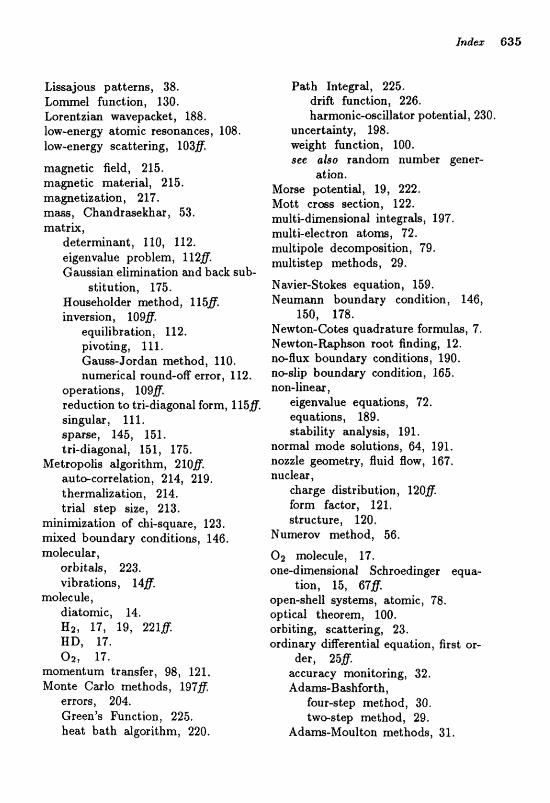
Limajous patterns, 38.
Lorentzim wwepacket , 188, IOW-energy atomic ressonmces, 108. low-energy scattering, 103fl.
magnetic field, 215. magnetic material, 215. magnetizlztion, 227. m-, Chandraseaar , 53. matrix,
d e t e r ~ n a n t , 110, 212. eigenvalue problem, l 1 2,ff. Caussian efiAnation and back sub-
stitution, 175. Hou~ehof d w method, 1 15$, inversion, 1098.
equilibration, 112. pivoling, l 1 l. Gauss-Jordan method, 110, numericd round-OR error, 112.
operations, 109g reduction to tri-diagonal form, Il5jJ. singulas, 11 1. spar=, 145, 151. tri-diagonal, 151, 175.
Metropolis dgorithm, 2108. auto-correjation, 214, 219. thermalization, 214, triral step size, 213.
mixliHlization of chi-square, 123. mked boundary conditions, 146. molecuiar ,
orbitafs, 223. vibrations, 14&
moEeculfE?, d i a l o ~ c , 24. Hz, 17, 19, 221F ER, 17,
17. momentum trmsfer, 98, 121, Monte Csuclo methods, 1978
errors, 204. Green's hnetion, 225. heat bath dgmithm, 220.
Path Xntegal, 225. drift function, 226. harmonic-oscillator gotentid, 230.
unmrlaikirnty, 198. weight function, 100. see also random number gener-
ation. Morse potentid, I f ) , 222. Motd crws metion, 122, mult&dirnensionaI integrals, 197. multi-elec tran izCom, 72. mult ipole decomposition, 79. multistep mthods, 29,
M &vier-Stokes equation, f 59. Neumann boundary condition, 146,
150, 178. Newdon-Got= quadrature formulw, I. Newton-bphson root fincling, 12. no-flu boundary conditione, 190. no-slip boundary condition, 165, non-libear ,
eigenv~lue equations, 72. equations, 289. atability aadysis, f 91.
normal mode solutions, 64, 191. noz;zle geometry, fluid Aow, 167. a u e l e ~ ,
charge BZsLribution, 120g form facfor, 121, structure, 120,
Numercav method, 56.
Qz molecub, 17, ane-dimexlsional Sebroedixrger equa-
tioa, 25, 678. open-sheH systems, atomic, 78. optic& theorem, 100. orbiting, scattering, 23. ordinary diEerential equation, Rrst or-
der, 258. aecurmy monitoring, 32. Adam-Bmhforth,
four-step met hod, 30. twestep mthod, 29,
Adam-Moulton methodsr, 31.
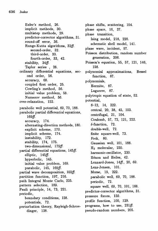
Eulerk method, 26, implicit methods, 30. multistep methods, 29. predictor-corrector dgorithms, 31. raund-OR error, 38. Rung*Kuttsa, dp;orithm, 328,
mcond-order , 32. third-ardw, 33. fourth-order, 33, 42.
s tability, 34g Taylar series , 28.
ordinary diRerentia1 equation@, WC-
orrd order, 56. accuracy, 68. coupled first order, 25. Cowlingy& method, 56. initial vdue probhnn, 58. Numerov method, 56.
over-relaaLlion, 152.
parabolic we12 potential, (513, 70, 188. patabdic partial digeren t i d equations,
1a9g aeuracy, 174, alternating-direction methods, 180. explicit scheme, 170. implicit scheme, 174. inst abililEy, 112. stability, 174, 175. twg.dhensiona1, 1 79g.
partial diEerentid equatiom, 1458. elliptic 1458. hyperbolic, 145. initial vdue problem, 169. pmabolic, 145, 1698.
part i d wave decompasitio~ , 103fl". parlidion function, 107, 218.. path Integral Monte Carlo, 225. pattern sdection, 189. Pasttli principle, 14, 73, 221. peit.iodic,
boundmy conditions, 158. gotentids, 72.
perturbation theory, Ra~yleigh-Schrae- diager, 1 38.
phme shifts, scattering, 104. ghwe space, 113, 31. phae transition,
lsing model, 218, 220. scbemtic shell model, 141,
plane wavet incide~t, 97. Poimoa distribudion, random number
$@aeration, 206. Poisson's equation, 55, 57, 121, 146,
158. poly n o ~ d approxhations, Bessef
funet ion, 87. polyno~zmjts,
Hermite, 87, Lquerre, 87,
polytropic equzttion of atate, 52. potentid,
6-12!, 14, 222. centrd, 20, 38, 45, 103. centrifugal, 21, 104. Goulod, 5.7, 72, 121, 222, B1funcf ion, 72. double-well , 72. finite square-well, 7% Fock, 80. Gauissian well, 101, 188. Hz molecular, 230. hwmnic-oscillatof, 230. Hknon and Eeiles, 42. Lennard-Jones, 14g, 20, 68. LenltJe~sen, 101. Mars, 19, 222. pwiabolic well, 69, 70, 188. periodic, 72, squme well, 69, 70, 102, 188,
predictor-corrector dgorithms, 31. prwsure farem, 159, profile function, 100, 129. program, how to use, 2318. pseudo-random nude r s , 205.
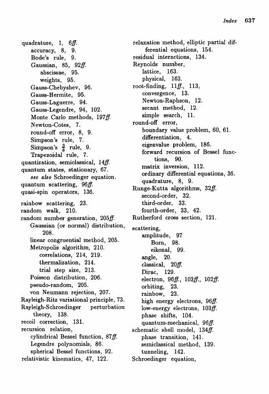
quadrdure, 1, 6fl. accuracy, 8, 9. Bode" rule, 9. Gamsian, 85, 928.
abscimm, 95. weights, 95.
Gauss-Chebyshev, 96, Cam-Eermite, 95. Gauss-Laguerre, 94. Caum-Lesndre, 94, 102. Monte Carlo methods, 197G Newton-Gates, 7. round-off error, 8, 9. S h p m n k rule, 7. Simpson's # rule, 9. n ~ p e ~ o i d a l rule, 7,
quantbation, semiclassical, 148 quantum states, stationary, 67.
see alrso Schroedhger equation. quantum scattering, 988. quasi-spin operators, 136,
rainbow scattering, 23. randam walk, 210. random number generation, 2058.
relmation method, eliptic partid dif- ferential equations, 154.
residud interactions, 134. Reynolds number,
lattice, 163. physicd, 163.
root-finding, llg, 123, convergence, 13. Newton-Raphson, 12. seeant method, 12. simple =arch, If.
round-oR error, boundaq value problem, 60, 61, &Eerentiabtion, 4, eigigenvalue problem, 186. forward recursion of Beml fume-
$ions, 90. matrix inver~iom, l f 2. ordinary digere~tial equations, 36, quadrature, 8, 9.
RtlngeIiCut ta dgorikhm, S2@ mcond-order , 32, third-order, 233. fourth+rder, 33, 42.
Rutherford crws section, 121, Gaussian (or normal) distribution, scattering,
208. mplitude, 97 line= congruentiali method, 205. Born, 98. Metropolis algorithm, 21 6. eiko~al, 99.
correlations, 214, 219. wgle, 20. thermdizstion, 214. classical, 20g. trid step size, 213, Dirrac, 129.
Poisson dktribudion, 206, electron, 96$, IQ$&, 1028 pseudo-random, 205. orbiting, 23. von Neumann rejection, 207. rahbow, 23.
Rayleigh-Eitz variational prineipb , 73, Ray E&gh-Schroedinger perturbation
theory, 138. recoil correction, 13 l. recursion relation,
cylindric& Bessel function, 87g. Legendre pof ynornih, 86. spherical Bessel functions, 92.
relativistic kinemtics, 47, 122,
high energy electrons, 96& law-energy electrans, 1038. p h m shifts, 104, qumtum-mr;chanieaX3 9Sg
schematic shell model, 1348. phme traxlsition, 141. serniclwsieal method, 139. tunneling, 142.
Schroedinger equation,
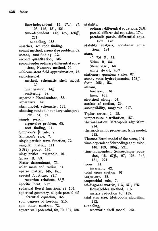
time-independent , 15, 67@, 97, 103, 146, 181, 221.
tirn+dependent, 146, 169, X8Bfl, 221.
tunneling, 188. searchm, see root finding. secant method, eigenvdue problem, 65. secant, rosbfinding, 12. secand quantia&iaa, 135. second-ctfrder ordinary diflerentid eque
tions, Numerav method, 66, seE-consiste~t field approsmatio~, 72. sedclassicd,
method, schematic shell model, 139.
quantization, 148. scattering, 98.
segaratrix, 42. shell mdel , schematic, 133. 8hootirzg metbad, boundary vdue prab-
lem, 64, 67. s b p b =web,
eigenvdue problem, 65, root findiag, 11.
Simpson's 8 rule, Q. Simpson3s ruXe, 7. single-pitrtiele wave function, 72, singular martrH, 111. sv(a) group, 136. singufaritia, integrabb, 10. Sirius B, 53. Slater determinant, 73, solar m= m d radius, 51, spar= matrix, 145, 151. special liunctions, 858,
recursion relations, 86f. specific heat, 217. spherical Bern1 functions, 92, 104, spherical geometry, elliptic partid dif-
ferentid equation, 156. spin degrem of freedom, 215. spin state, electron, 73. sfluare m11 potentid, 69, 70, 101, 1188.
stability, or dhar y diRerentid equations, 34' pm tial diRerential equation, 174. pasabolic partial dieerential equzt-
tioxl, 275. stability an&is, non-linear equa-
tions, 191, @tars,
40 Eri B, 53. Skius B, 53. Stein 2051, 83. white dwad, 46g.
stationary quadurn @traLes, 67. steady state hydrodynamics, 158fl. Stein 2051, 53. s t rem,
function, 261. linea, 161.
stretched strhg, 64. surface of eection, 39, swceptibilify, magnetic, 217, Taytor wries, 2, 28. temperature distribution, 157. t hermalizlation, h"l;etropolis algorithm,
214, t hermadynahc pr~pertiw, Xsing model,
215. ThomeFemmi model of the atom, 101. t imedependent Schroedinger equation,
146, 169, 1888, 221. thekdependant Sehroedinger equai-
tioa, 15, 67fl., 97, 103, 146, 181, 221,
torus, 41, invmi~nt, 42.
total erws section, 97, trajectory, 338, trapezoidal rule, 7. trtdisgond matrix, 113, 151, 175.
Eouseholder met hod, 115. matrix reduction to, 115.
trial a;.teg size, Metropolis algorithm, 213.
tunnelling, schematic shell model, 142,
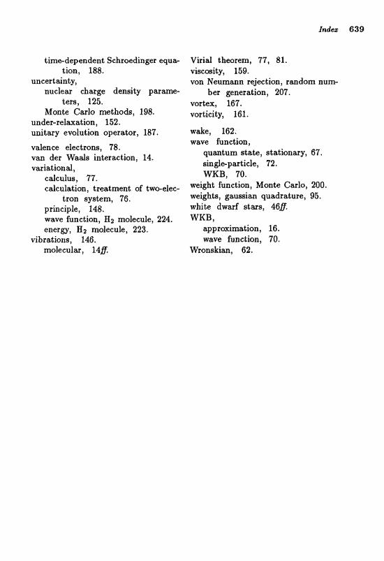
timedependent Scfirwdi-xzger eqirra- Lion, 188.
uncertainty, nuclear cha r s (Xenb~ity parrame-
ters, 125. Monte Carlo methods, 198.
under-relaation, 152. unitary evolutioon operator, 187,
valence electrons, 78. vim der W 4 s interaction, 14. variati~nd,
cBJcuIuki, 77, csleuXation, treatment of twae1e~-
tron system, 76. principle, 148. wave fuxlction, Hz molr~-euXe, 224- energy, H2 molecule, 223.
vibralioaa, 1-46. moIecuIa, Idfi
Virid dhmrem, 77, 81. vheaity, 159. von Neumann rejection, random mum-
ber generation, 207. vortex, 167. vorticit y, f 61.
wake, 162. wave function,
qumtum state, stationary, 67. shgl~particle, 72. WKB, m.
weight funetion, Monte Carlo, 200. weighb, gaussim quadrature, 95, white dwarf stm~, 46' WKB,
approximtion, 16. wave function, 70.
Wr~nskiran, 62.