FORTRAN algorithms for evaluating Fourier transforms of line spread functions

Eur J Nucl Med (1983) 8:262-278 European Nuclear Journal of

Medicine © Springer-Verlag 1983

FORTRAN Algorithms for Evaluating Fourier Transforms of Line Spread Functions John R. Prince 1, Liang C. W u 2 and Hisham Dawalibi3 1 Oklahoma Children's Memorial Hospital, Oklahoma City, Oklahoma, USA 2 Veterans General Hospital, Taipei, Taiwan, ROC 3 King Faisal Specialist Hospital, and Research Centre, Riyadh, Saudi Arabia

Abstract. F O R T R A N IV algorithms are presented for calculating the modulation transfer function, the phase transfer function, the modulation transfer function area, an information transfer function, and the optimum frequency response as well as plotting the curves for these metrices. An important feature of the programs is an editing routine.

Introduction

Frequency domain techniques are widely accepted as the method of choice for specifying the resolution capabilities of imaging equipment in radioscintigraphy [1, 2, 10, 12, 13, 16, 17]. The frequency fidelity of such instrumentation is most often determined by taking the Fourier transform of an appropriately determined line spread function (LSF) [18]. While numerical formulas are available in the litera- ture that can be implemented on computing equipment, including programmable calculators [11, 21], publication of complete programs is useful as they aid the inexperienced non-computer scientist in implementing these formulas on their own equipment.

Benedetto and Nusynowitz [4] have published their FORTRAN program for calculating the modulation transfer function (MTF). Their program presumes that the investigator is dealing with the symmetric LSF so that only the real component of the optical transfer function (OTF) [15] is important. Stimulated by Benedetto's and Nusyno- witz' and other publications we were encouraged to present our own programs which take into account asymmetric line spread functions which can be important in some circum- stances [20] and allow for the calculation of other important parameters such as the modulation transfer function, the phase transfer function, the modulation transfer function area, an information transfer function, and the optimum frequency response. Curves of these parameters are plotted and an important feature is the provision for editing the input data, The version of our programs presented here in standard F O R T R A N IV has been patterned after the interactive conversational mode of that by Benedetto and Nusynowitz.

Address offprints requests to. John R. Prince, Ph.D. Department of Radiological Science, Oklahoma Children's Memorial Hospital, Post Office Box 26307, Oklahoma City, OK 73126, USA

Nomenclature

The equations used and methodology of obtaining Fourier transforms are available in a variety of textbooks [7, 9, 15, 19] but the nomenclature when applied to radioscintigraphy is not standardized [3]. Thus it is prudent to define the terms as used in this paper.

The Optical Transfer Function (OTF)

The OTF is the Fourier transform of the LSF [15]. Mathe- matically it can be written as:

+ o o

OTF(jk)= ~ LSF(x)*EXP[-jkx]dx (1) - c o

It is usual to work with normalized transforms for ana- lytical or numerical work and to adjust the input-output relationships to fit a specific array of data by means of the superposition principle, i.e.

a*LSF(x)~a*OTF(jk) (2)

The normalized OTF is given by

OFT(jk) - LSF(x)*EXP[- jkx]dx LSF(x)dx (3)

Expanding the complex exponential into its trigonometric equivalent and writing Eq. (3) in a form compatible with numerical calculation:

OTF(jk) - XLSF(x)*cos(2 kx)Ax ZLSF(x)Ax

_ j _ Z L S F ( x ) sin(2~kx)Ax Y~LSF(x)Ax (4)

o r

OYF(jk) = ReOTF(jk)-ImOTF(jk)

where

ReOTF(jk) = the real part of the Fourier transform ImOTF(jk) = the imaginary part of the Fourier transform

Equation 4 is general and can be used for both asymmetric and symmetric LSFs. However, if one knows in advance that the LSF is symmetric then the imaginary part of Eq. (4) is equal to zero and one can write

OTF(k) ZLSF(x)*cos(2rck2)Ax XLSF(x)~x (5)

1 INPUT NL: [ number of ] ate points /

NO

Input Which/ Graphs A r e /

Wanted /

/ WOFR: \ w!, FREQUENCY/ ~ TRANSFER / RESPONSE ~ ~ FUNCTION /

The Modulation Transfer Function (MTF)

An alternate method of formulating the OTF is

OTF(jk) = MTF(k)*EXP[jPTF(k)] (6)

where

MTF(k) = the modulation transfer function,

PTF(k) = the phase transfer function.

It is instructive to expand the complex exponential in Eq. (6) into its trigonometric equivalent.

OTF(jk) = MTF(k)[Cos(PTF(k)) +j Sin(PTF(k))]. (7)

From Eq. (7) it is apparent that the absolute value of the OTF equals the MTF, however, they are not the same quantity. For symmetric line spread functions the MTF is given by

MTF(k) = ZLSF(x)*Cos(2nkx)Ax. ZLSF(x)Ax (8)

For asymmetric line spread functions the MTF is given by

MTF(k) = [(ReOTF(jk)) 2 + (ImOTF(jk)) '~] 1/2. (9)

The Phase Transfer Function (PTF)

The phase transfer function is defined as:

1 FImOTF(jk)] PTF(k) = tan- LaeOXF(jk) ] . (10)

The Modulation Transfer Function Area (MTFA)

Biberman [5] attributes to Charmin and Olin [8] the origi- nal concept of the modulation transfer function area as a global estimate of the resolution characteristics of photographic systems. Quoting Biberman, ' the ... MTFA ... is broadly applicable for general scenes but not necessarily a good metric for specific objects.' Bourough et al. [6] have applied Charmin and Olin's concept to raster scan displays. The MTFA, as originally proposed, was the area between the system MTF curve and the threshold detectability curve. The threshold detectability curve is not used in radioscintigraphy and the MTFA is simply taken as the area under

263

Fig. 1. Simplified logic flow diagram demonstrating program architecture

the system MTF curve (8). Numerically,

MTFA = EMTF(k)*Ak. (l 1)

The Information Transfer Function (IT[') Jones [14] has shown that the information transmitted by a system is given by the square of the MTF rather than the MTF alone. Thus one can define an information transfer function which is given by

ITF(k) = [MTF(k)]2. (12)

The Optimum Frequency Response (OFR) Wyper and Gillespie [22] have shown that a useful meta- meter is the optimum response wave length which is defined as the maximum of a curve of MTF (2)/2 vs 2. The value of the MTF at the optimum response wave length is called the modulation index (MI). This is a useful concept and in this paper has been modified to the optimum frequency response where:

OFR = [MTF(k)*k]max. (13)

The MI is not automatically output on the computer program but by iteration can be quickly found and read as the maximum of the printed graph of the OFR.

Program Description The programs described in this communication have been implemented on a Digital Equipment Corporation PDP/ 34E with a 16-bit word memory. The programs have been developed in standard F O R T R A N so they may be implemented on other systems with a minimum of modification.

Figure 1 shows a simplified flow diagram of the program architecture.

Embodied within the program are a number of com- ments identifying the major system dependent parts of the program, instructions to aid the user, and the principal equations used for calculating the data.

Listings of the main programs and the required subpro- grams are given in Appendix 1. A didactic example showing selected graphical outputs is shown in Appendix 2. The input data are taken from Benedetto and Nusynowitz [4] for comparison by interested readers.

264

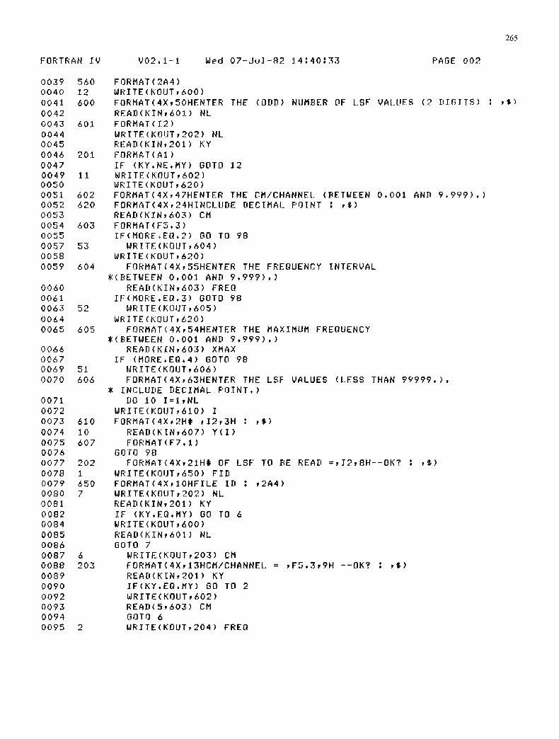
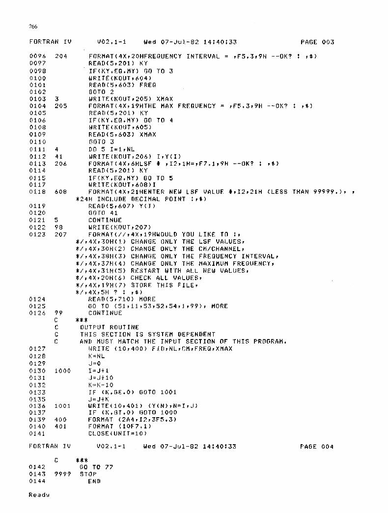
Appendix 1 A Listing of FORTRAN IV programfor the input, editing and file storage of line source response function data.

PIF' MTFED°LST FORTRAN IV V02oI-~ Wed 0 7 - , J u ] - 8 2 ].4:40~33 PAGE 001

0001 0002 0003 0004 0005 0006 0007

0008 0009 0010 0012 0013 0014 0015

0016 0017 0018

0019 0020 0021

OR 00~.~ 0023 0024 0025 0026 0028 0029 0030 0032

0033 0034 0035 0036 0037 0038

C FORTRAN IV PROGRAM MTFED FOR INPUTTING, EDITING, C AND FILE STORAGE OF LINE SOURCE C RESPONSE FUNCTION DATA FOR F'ROGRAM MTFF'Ro C [.IMENSION ON Y IS MAXIMUM NUMBER OF DATA POINTS° C *** 77 CONTINUE

DIME.NSION Y(99),FILEN(3),FID(2) DATA KOUT/5/,KIN/5/ DATA MY/1HY/ DATA FILEN/4HFILE, 2H00,4H ° DAT/

71 WRITE(KOUT,700) 700 FORMAT<4X,67HTHIS PROGRAM CREATES AND EDITS FILES FOR USE WITH

* THE PROGRAM MTFF'R, */,4X,16HDO YOU WANT TO :, */,4X,21H(!) CREATE A NEW FILE, */,4X,25H(2) EDIT AN EXISTING FILE, */,4X,SH<3) QUIT, * / , 4 X , 4 H ? : ' ,$ )

75 READ(KIN,710) IJ 710 FORMAT(It)

IF <[J,EQo3> GOTO 9999 WRITE (KOUT, 801 )

801 FORMAT(4X,8HFILE t :,$) READ(KIN,802) FI[.EN (2)

802 FORMAT(A2) C *** C THIS CALL ASSIGN STATEMENT IS SYSTEM DEPENDENT C ***

CALL ASSIGN (I0, FIL..EN) GOTO(54,70) ,IJ

70 CONTINUE C *** C INPUT ROUTINE C THIS SECFION IS SYSTEM DEPENI'ENT C AND MUST MATCH 'MTFF'R' PROGRAM,

CALL ASSIGN(107FII.EN) READ (~0,400) FID,NL,CM,FREQ,XMAX K=NL J=O

2000 l=J÷l J=J+10 K=K.-IO IF (K.GE.O) GOTO 2001 J=J+K

2001 READ (10,401) ( Y ( N ) , N = I , J ) IF (K,GT,O) GOTO 2000 REWIND 10

C *** WRITE:(KOUT, 8 0 3 ) F I D

80:3 FORMAT(4X,IOI- ' IFII . . .E [D : ,2A4) 80 TO 98

54 WRITE<KOUT,550) 550 FORMAT(4X,44HENTER THE FILE ID (8 CHARACTERS MAXIMUM ) : ,$)

READ (KIN,560) FID

265

FORTRAN IV V02 . I - ' I Wed 0 7 - , J u ] - 8 2 ] 4 : 4 0 : 3 3 PAGE 002

0039 0040 0041 0042 0043 0044 0045 0046 0047 0049 0050 0 0 5 1 0052 0 0 5 3 0054 0055 0057 0058 0059

0060 0061 0063 0064 0065

0066 0067 0069 0070

0071 0072 0073 0074 0075 0076 0077 0078 0079 0080 0081 0082 0084 0085 0086 0087 0088 0089 0090 0092 0093 0094 0095

201

I I

602 620

603

53

604

560 FORMAT(2A4) 12 WRII'E(KOUT,600) 600 FORMAT(4X,5OHENTER THE (ODD) NUMBER OF [.SF VALUES (2 DIGITS) : ,$)

READ(KIN,601) NL 601 FORMAT(12)

WR[TE(KOUT,202) NL REAls(KIN,201) KY FORMAT(A1) IF (KY.NE.MY) GOTO 12 WRITE(KOUT,602) WRITE(KOUT,620) FORMAT(4X,47HENTER THE CM/CHANNE[. (BETWEEN 0.001 AND 9.999).) FORMAT(4X,24HINCLUIiE OEC[MAL POINT ; ,$) READ(KIN,603) CM FORMAT(F5°3) IF(MORE°EQ.2) GO TO 98

WRITE(KOUT,604) WRITE(KOUT,620)

FORMAT(4X,55HENTER THE FREQUENCY INTERVAL ~(BETWEEN 0 . 0 0 1 AND 9°999)°)

READ(KIN,603) FREQ IF(MORE,EQ°3) GOTO 98

52 WRITE(KOUT,605) WRITE(KOUT,620)

605 FORMAT(4X,54HENTER THE MAXIMUM FREQUENCY ~(BETWEEN 0.001 AND 9,999).)

READ(KfN,603) XMAX IF (MORE.EQ.4) GOTO 98

51 t~RITE(KOUT,606> 606 F'ORMAT(4X,63HENTER THE LSF VALUES (LESS THAN 99999.).

INCLUDE DECIMAL POINT°> DO 10 I=I,NL

WRITE(KOUT,610) I 610 FORMAT(4X,2H# ,12,3H ~ ,$) 10 READ(KIN,607) Y(1) 607 FORMAT(F7.1)

GOrO 98 202 FORMAT(4X,21H$ OF LSF TO BE READ =,I2,SH--OK? : ,$) 1 WRITE(KOUT,650) FID 650 FORMAT(4X,IOHFILE ID : ,2A4) 7 WRITE(KOUT,?02) NL

READ(KIN,201) KY IF (KY.EQ°MY) GO TO 6 WRITE(KOLIT,600) READ(KIN,601) NL GOI'O 7

6 WRITE(KOUT,203) CM 203 FORMAT(4X,13HCM/CHANNEL = ,FS.3,gH --OK? t ,$)

READ(KIN,201) KY IF(KY°EQ.MY) GO TO 2 WRITE(KOIJT,602) READ(5,603) CM 80TO 6

2 WRITE(KOUT,204) FREQ

266

FORTRAN IV V02.1-1 Wed 0 7 - J u ] . - 8 2 14:40:33 PAGE 003

0096 204 0097 0098 0100 0101 0102 0103 3 0104 205 0105 0106 0].08 0109 0110 0111 4 0112 41 0113 206 0114 0],15 0117 0118 6O8

0119 0120 0121 5 0122 98 0123 207

0124 0125 0].28 99

C C C C

0127 0128 0129 0130 1000 0131 0132 0133 0135 0136 1001 0137 0139 400 0].40 401 0141

FORTRAN IV

FORMAT(4X,2OHFREQUENCY INTERVAL = ,F5,3,gH --OK? : ,$) READ(5,201) KY IF(KY.El l . MY) GO l'O 3 WRITE(KOUT,604) READ(5,603) FREQ GOTO 2 WRITE(KOUT,205) XMAX FORMAT(4X,19HTHE MAX FREQUENCY = ,F5,3,gH --OK? ~ ,$) READ(5,201) KY IF(KY.EIIoMY) GO TO 4 WRITE(KOUT, 605) READ(5,603) XMAX GOTO 3 DO 5 I=].,NL WRITE(KOUT,206) I,Y(I) FORMAT(qX,6HLSF ~ ,I2,1H=,F7o1,gH --OK? : ,$) READ(5,201) KY IF(KY.EQ.MY) GO TO 5 WRITE (KOUT, 608) I FORMAT(4X,21HENTER NEW LSF VALUE ~,12,21H (LESS THAN 99999.), ,

~k24H INCI.UDE DECIMAL POINT ~,$) READ(5,607) Y(I) GOTO 41 CONTINUE WRI'TE (KOUT, 207) FORMAT(//,4X,19HWOULD YOU LIKE TO :,

~/,4X,30H(!) CHANGE ONLY THE LSF VALUES, ~'./,4X,30H(2) CHANGE ONLY THE CM/CHANNEL, ~/,4X,38H(3) CHANGE ONLY THE FREQUENCY INTERVAL, ~/,4X,37H(4) CHANGE ONLY THE MAXIMUM FREQUENCY, ~/,4X,31H(5) RESTART WITH ALL NEW VALUES, ~/,4X,20H(6) CHECK ALL. VALUES, ~/,4X,19H(7) STORE THIS FILE, ~/,4X,SH ? ; ,$)

READ(5,710) MORE GO TO (51,11,53,52,54,],99), MORE CONTINUE

OUTPUT ROUTINE THIS SECTION IS SYSTEM DEPENDENT AND MUST MATCH THE INPUT SECTION OF THIS PROGRAM°

NRITE (10,400) FID,NL.,CM,FREQ,XMAX K=NL J=O l=J+ l J=J$10 K=K-IO IF (K.GE.O) GOTO 1001 J=J+K WRITE(IO,401) ( Y ( N ) , N = I , J ) IF (KoOT.O) 60TO 1000 FORMAT (2A4,12,3F5,3) FORMAT (IOF'7,1) CLOSE(UNIT=tO)

V02.1-1 Wed 07-Jui-82 14:40~33 PAGE 004

0142 0143 0144

C

9999 GO TO 77 STOF'

END

Re~d~

267

Appendix 1 B Listing qf FORTRAN IV program for calculating the modulation transfer function, the optimum frequency response, an information transfer function, the area under the MTF curve and the phase transfer function.

PIP MTFF'R.LST FORTRAN IV V02,1-1 Wed 07-Ju1-82 13~54C25 PAGE 001

0001 0002 0003 0004 0005 0006 0007

0008 0009 0010 0011

0012 0013 0014 0015 0016 0017 0018 0019 0020 0021 0022 0023 0024 0026 0027 0028 0030 0031

0032

C C C C C C C C C C C C C C C

45 800

810

56 C

C C C

820

900

1998

2000

2001

910

C 999

MTFPR, A FORTRAN IV PROGRAM, CALCULATES THE MODULATION TRANSFER FUNCTION, THE OPTIMUM FREQUENCY RESPONSE, INFORMATION TRANSFER, THE AREA UNDER THE MTF CLIRVE AND THE PHASE TRANSFER FUNCTION, USING THE SUBROUTINES CMTF, WOFR, WNIF, WARA, WPTF, AND THE EDITING PROGRAM MTFED°

FILEN 18 FILE NUMBER FID IS FILE IDENTIFICATION THE DIMENSION ON X AND T IS THE MAXIMUM NUMBER OF DATA POINTS THAT CAN BE USED~ THE DIMENSION ON XMTF AND XPTF IS N WHERE~ N ~ FREQUENCY INCREMERT = MAXIMUM FREQUENCY. TOPI = 2 ~ PI

DIMENSION KK(52), FILEN(3), F]D(2), X(49), Y(49) REAL X~TF(200),XPTF(200) DATA TOPI/6o2832/ DATA KOUT,KIN/5,5/

DATA FILEN/4HFILE,2HOO,4H~DAT/ NRITE (KOUT,800) FORMAT(IHI,4X,16HDO YOU WANT TO :,

~/,4X,42H(1) RUN THE PROGRAM USING AN EXISTING FILE, ~/,4X,45H(2) RUN THE PROGRAM AGAIN USING THE SAME DATA, ~/,4X,SH(3) QUIT~ ~/,4X,4H? ~ ,$)

READ (KIN,810) IJ FORMAT (11) GO'tO (56,999,5000),IJ CONTINUE

INPUT DATA FROM DISK STORAGE THIS SECTION IS SYSTEM DEPENDENT AND MUST MATCH "MTFED" PROGRAM, WRITE (KOUT,820) FORMAT(4X,9HFILE # I ,$) READ (KIN,900) FILEN(2) FORMAT(A2) CALL ASSIGN(10,FILEN)

READ<10,1998) FID,NL,CM,FREQ,XMAX FORMAT(2A4,12,3F5,3)

K=NL J=O I=J÷l J=J+lO K=K-IO IF(K,GE~O) GOTO 2001 J=J4"K READ(IO,910) ( Y ( N ) , N = I , J ) IF(K.GToO) GOTO 2000 FORMAT(IOF7.1) CLOSE(UNIT=IO)

CONTINUE

268

FORTRAN IV

0033 0034 860 0035 0036 20

0037 55 0038 608 0039 0040 601 0041 0043 0044 700 0045

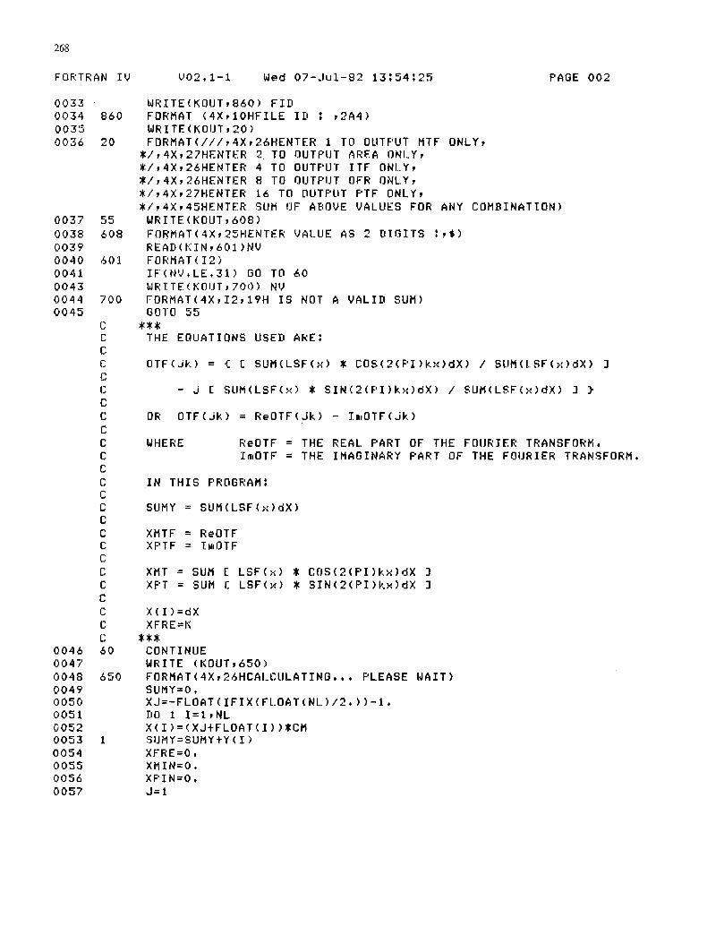
C C C C C C C C C C C C C C C C C C C C C C C C C

0 0 4 6 60 0 0 4 7 0 0 4 8 650 0 0 4 9 0050 0051 0052 0053 1 0054 0055 0056 0057

V02°1-1 Wed 0 7 - J u i - 8 2 13154125 PAGE 002

WRITE(KOUT,860) FID FORMAT (4X,IOHFILE ID ~ ,2A4) WRITE(KOUT,20) FORMAT(///,4X,26HENTER 1 TO OUTPUT MTF ONLY,

*/,4X,27HENTER 2 1"0 OUTPUT AREA ONLY, ~/,4X,26HENTER 4 TO OUTF'UT ITF ONL. Y, ~/,4X,26HENTER 8 TO OUTPUT OFR ONLY, ~/,4X,27HENTER 16 TO OUTPUT PTF ONLY, ~/,4X,45HENTER SUM OF ABOVE VALUES FOR ANY COMBINATION)

WRITE(KOUT,608) FORMAT(4X,25HENTER VALUE AS 2 DIGITS ~,$) READ(KIN,6OI)NV FORMAT(12) IF(NV,LE°31) GO TO 60 WRTTE(KOIJT,700) NV FORMAT(4X,12,1?H IS NOT A VALID SUM) GOTO 55

THE EQUATIONS USED AREI

OTF(Jk) = { [ SUM(LSF(x) ~ COS(2(PI)kx)dX) / SUM(LSF(,.,~)dX) ]

- J [ SLIM(LSF(y) ~ SIN(2(PI)k ' . . )dX) / SUM(LSF(.o:)dX) ] }

OR OTF(jk) = ReOTF(Jk) - [mOTF(Jk)

WHERE ReOTF = THE REAL PART OF THE FOURIER TRANSFORM. ImOTF = THE IMAGINARY PART OF THE FOURIER TRANSFORM.

IN THIS PROGRAM~

SUMY = SUM(LSF(x)dX)

XMTF = ReOTF XPTF = ~mOTF

XMT = SUM [ LSF(×) ~ COS(2(F'I)kx)dX ] XF'T = SUM [ LSF(×) ~ SIN(2(PI)k .x)dX ]

X(1)=dX XFRE=K

CONTINUE WRITE (KOUT,650) FORMAT<4X,26HCAI_CULATING*** PLEASE WAIT) SUMY=O° XJ=-FLOAT(IFIX(F[ .OAT(N[ . . ) /2o)) - I . DO 1 I = I , N L X(1)=(XJ+FLOAT(I))~CM SUMY=SUMY+Y(I) XFRE=O. XMIN=O, XPIN=O° J=1

269

FORTRAN IV V02.1-I Wed 07-Jui-82 13~54;25 PAGE 003

0 0 5 8 2 0 0 5 9 0 0 6 0 0061 0 0 6 2 0 0 6 3 0 0 6 4 3 0 0 6 5 0 0 6 6

C C C

0 0 6 7 0 0 6 8 4 0069 5 0 0 7 0 6 0071 7 0072 0 0 7 4 0 0 7 5 9 0076 0077 8

C C C

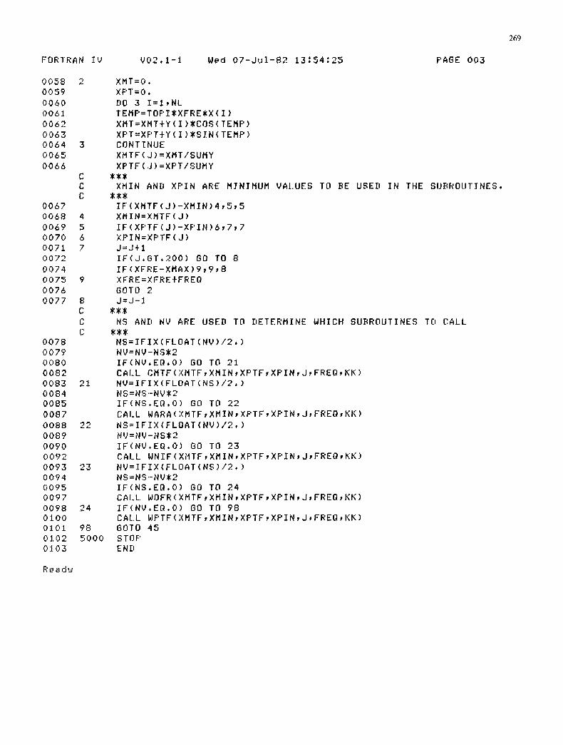
0078 0079 0 0 8 0 0082 0083 21 0 0 8 4 0085 0087 0088 .~9~ 0089 0 0 9 0 0 0 9 2 0 0 9 3 23 0 0 9 4 0095 0097 0 0 9 8 24 0100 0101 98 0102 5 0 0 0 0103

XMT=O. XF'I'=O. DO 3 I= I ,NL TEMF'=TOPI*XFRE~X(I) XMT=XMT+Y(I)*COS(TEMP) XPT=XF'T+Y(I)ISIN(TEMP) CONT:NUE XMTF(J)=XMT/SUMY XPTF(J)=XPT/SUMY

XMIN AND XF'IN ARE MINIMUM VALUES TO BE USED

IF(XMTF(J)-XMIN)4,5,5 XMIN=XMTF(J) IF(XPTF'(J)-XF'IN)6,7,7 XPIN=XPTF(J) J=J4.1 I F ( J . G T . 2 0 0 ) 68 TO 8 I F ( X F R E - X M A X ) 9 , 9 , S XFRE=XFRE+FREQ GOTO 2 J = J - 1

NS AND NV ARE USED T8 DETERMINE WHICH SUBROUTINES TO CALL

N S = I F I X ( F L O A T ( N V ) / 2 o ) N V = N V - N S 8 2 IF(NV.EQ.O) 80 TO 21 CALL CMTF(XM'FF,XMIN,XPTF,XF'IN,J,FREQ,KK) NV=IFIX(FLOAT(NS)/2.) NS=RS'-NV~2 I F ( N S . E Q . O ) GO TO 22 CALL W A R A ( X M T F , X M I N , X P T F , X P I N , J , F R E Q , K K ) N S = I F I X ( F L O A T ( N V ) / 2 . ) N V = N V - N 8 ~ 2 IF(NV.EQ.O) GO TO 23 CALL WNIF(XI4TF,XMIN,XPTF,XPIN,J,FREQ,KK) NV=IFIX(F'LOAT(NS)/2.) NS=NS'-NV~2 IF(NS.EQoO) GO TO 24 CAI.L WOFR(XMTF,XMIN,XPTF,XPIN,J,FREQ,KK) IF(NV.EQoO) GO TO 98 CALL WPTF(XMTF,XMIN,XPTF,XPIN,J,FREQ,KK) GOTO 45 STOP END

IN THE SUBROUTINES,

Read~

270

PIP CMTF.LST FORTRAN IV

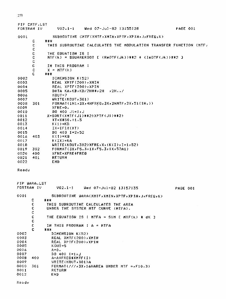
0001 C C C C C C C C C

0002 0003 0004 0005 0006 0007 0008 301 0009 0010 0011 0012 0013 0 0 1 4 0015 0016 403 0017 001S 0019 302 0020 400 0021 401 0022

Re~d~

V02.1-1 Wed 07-Ju ] -S2 13:55:28 PAGE 001

SUBROUTINE CMTF(XHTF,XMIN,XPTF,XPIN,J,FREQ,K)

THIS SUBROUTINE CALCULATES THE MODIiLATION TRANSFER FUNCTION (MTF~

THE EQUATION IS : MI'F(k) : SQUAREROOT [ (ReOTF(Jk))~I2 + ( I m O T F ( J k ) ) ~ 2 ]

IN THIS PROGRAM : X = MTF(k)

DIMENSION K(52) REAL XMTF(2OO),XMIN REAL XPTF(2OO),XPIN DATA KA,KB,KD/2H~,2H , 2 H . . / KOUT=7 WRITE(KOUT,301) FORMAT(1HI,3X,4HFREQ,3X,3HMTF,2X,51(1Ho)) XFRE=O. DO 400 J l = l , J

X=SQRT(XMTF(J1)~2÷XPTF(JI )~2) XT=X~50.+I.5 K(1):KD IX= IF IX(XT) DO 403 I=2 ,52 K(I)=KB K(IX)=KA WRITE(KOUT,302)XFRE,X,(K(1), I=1,52) FORMAT(3X,FS.3,1X,FSo3,1X,52A1) XFRE=XFRE÷FREQ RETURN END

F'IP WARA.LST FORTRAN IV V02.1-1 Wed 07 -Ju l -S2 13:57:35

0001

0002 0003 0004 0005 0006 0007 O00B 0009 0010 0011 0012

C C C C C C C C

400

301

SUBROUTINE WARA (XHTF, XMIN, XPTF p XPIN, J, FREQ T K) :~ W()K

THIS SUBROUTINE CALCULATES THE AREA UNDER THE SYSTEM MTF CURVE (NTFA),

THE EQUATION IS : MTFA = SUM [ Ml'F(k) :~ dK ]

IN THIS PROGRAM : A = MTFA

DIMENSION K(52) REAL XMTF(2OO),XMIN REAL XF'TF(2OO),XF'IN KOUT=5 A=O, DO 400 I=l,J A=A÷FREQ~XMTF(I) WRITE(KOUT,301)A FORMAT(///,3X,16HAREA UNDER MTF =PFIOo3) RETURN END

Ready

PAGE 001

271

F'IF' WNIF.LST FORTRAN IV V02.1-1 Wed 0 7 - J u ] - 8 2 ] 3 : 5 6 : 3 7 PAGE 001

0001

0002 0003 0004 0005 0006

0007 0008 0009 0010 0011 0012 0013 0014 0015 0016 0017 0018 0019 0020 0021 0022

C C C

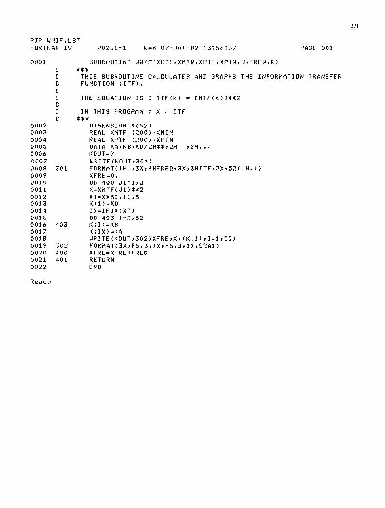
C C C C C

SUBROUTINE WNIF(XMTF,XMIN,XF'TF,XF'IN,J,FREQ,K)

THIS SUBROUTINE CALCIILATES AND GRAPHS THE INFORMATION TRANSFER FUNCTION (ITF).

THE EQUATION IS : ITF(k) = [MTF(K)]$~2

IN THIS PROGRAM : X = ITF

DIMENSION K<52) REAl... XMTF (200),XMIN REAL XF'TF (200),XF'IN DATA KA,KB,KD/2H~,2H , 2 H . . / KOUT=7 WRITE(KOIJT,301)

301 FORMAT(1H1,3X,4HFREQ,3X,3HITF,2X,52(JH°)) XFRE=O. DO 400 Jl=l,J X=XMTF(.JI)~2 XT=X~50.÷I.5 K(1)=KD IX=IFIX(XT) DO 403 I=2,52

403 K(1)=KB K<IX)=KA WRITE(KOUT,302)XFRE,X,(K(1), I=1,52)

302 FORHAT(3X,F5.3,1X,FSo3,1X,52A1) 400 XFRE=XFRE$FREQ 401 RETURN

END

Readw

272

PIP WOFR.LST FORTRAN IV V02.1-1 Wed 07-Jui-82 13156:04 PAGE 001

0001

0002 0003 0004 0005 0006 0007 0008 0009 0010 0011 0012 0013 0014 0015 0016

0017 0018 0019 0020 0021 OOn~ 0023 0024 0025 0026 0027 0028 0029 0030 0031 0032 0033 0034 0035

C C C C C C C C

SUBROUTZNE WOFR(XMTF,XMIN,XPTF,XF'IN,J,FREQ,K)

THIS SUBROUTINE CALCUi..ATES AND GRAPHS THE OPTIMUM FREQLIENCY RESPONSE (OFR).

THE EQUATION IS ~ OFR = [ MTF(k) * k ] max

IN THIS PROGRAM : XOFR = OFR

DIMENSION XOFR(200) DIHENSION K(52) REAL XMTF (200),XMIN REAL XPTF (200),XPIN DATA KA,KB,KD/2N**,2H ,2H../ Kou r=7 WRITE(KOUT,301)

3 0 1 FORMAT(1Ht,3X,4HFREQP4X,3HOFR,2X,51(1H.)) XFRE=O. XM=O. XN=O. DO 400 . J l = l , J XOFR(JI)=XFRE*XMTF(Jl) IF(XOFR(.J1)-XN)401,402,402

401 XN=XOFR(JI) 402 IF(XOFR(,JI)-XM)400,400,403 403 XM=XOFR(J1) 400 XFRE=XFREtFREQ

XFRE=O. DO 500 J 2 = l , J SC=XM-.XN SK=-XN/SC*50.+I.5 KS: IFIX(SK) ST=(XOFR(J2)-XN)/SC*50.÷I .5 IS= IF IX(ST) DO 404 I = I , 5 2

404 K(1)=KB K(KS)=KD K(IS)=KA WRITE(KOUT,302)XFRE,XOFR(J2),(K(I),I=],52)

302 FORMAT(3X,F5.3,1X,F6.3,1X,52AI) 500 XFRE=XFRE+FREQ

RETURN END

Read~

273

PIP WF'TF°LST FORTRAN IV V 0 2 . 1 - 1 Wed 0 7 - J , _ , ] - 8 2 ] 3 C 5 8 : 0 6 PAGE 00].

0001

0002 0003 0004 0005 0006 0007 0008 0009 0010 0011 0012 0013 0014 0015 0016 0017 0018 0019 0020 0021 0022 0023 0024 0025 0026 0027 0028 0029 0031 0032 0033 0034 0035 0036 0037 0038 0039 0040 0 0 4 1 0042 0043 0044

C C C C C C C C

SIJBROUTINE WPTF(XM[F,XMIN,XF'TF,XPINIJ,FREQ,K)

THIS SUBROUTINE CALCULATES AND GRAPHS THE PHASE [RANSFER FUNCTION (PTF).

THE EQUATION IS I

F'TF = ARCTAN [ ImOTF(Jk) / ReOTF(Jk) ] * * * DIMENSION F'TF(200) OIHENSION K(52) REAL XMTF(2OO),XMIN REAL XPTF(2OO),XF'IN DATA KA,KB,KD/2H**,2H ,2Ho./ KOUT -~-~ WRITE(KOUT,301)

301 FORMAT(IH1,3X,4HFREQ,3X,3HPTF,2X,51(IH.)) XFRE=O. XM=O. XN=Oo DO 400 -Jl=l,J IF(XMTF(JI))402,401,402

401 IF(XPTF(,J1))403,408,408 403 F'TF(J1)=-I.571

GO TO 405 408 PTF(JI)=1.571

GO TO 405 402 F'TF(JI)=ATAN(XF'TF(JI)/XMTF(JI)) 405 IF(F'TF(JI)-XN)406,407,407 406 XN=F'TF(JI) 407 IF(F'TF(J1)-XM)400,400,40? 409 XM=F'TF(J1) 400 XFRE=XFRE÷FREQ

XFRE=O. DO 500 J2= l , J SC=XM-XN

IF(SC+EQoOoO) GO TO 4444 SK=-XN/SC*50.÷I.5 KS=IFIX(SK) ST=(F'TF(J2)-XN)/SCt50o+I.5 IS=IFIX(ST)

4444 CONTINUE DO 404 I=1,52

404 K(1)=KB KiKS)=KD K(IS)=KA WRITE(KOUT,302)XFRE,F'TF(J2),(K(I), I=l,52)

302 FORMAT(3X,F5°3,F6°3,1X,52AI) 500 XFRE=XFRE÷FREQ

RETURN END

Read~

274

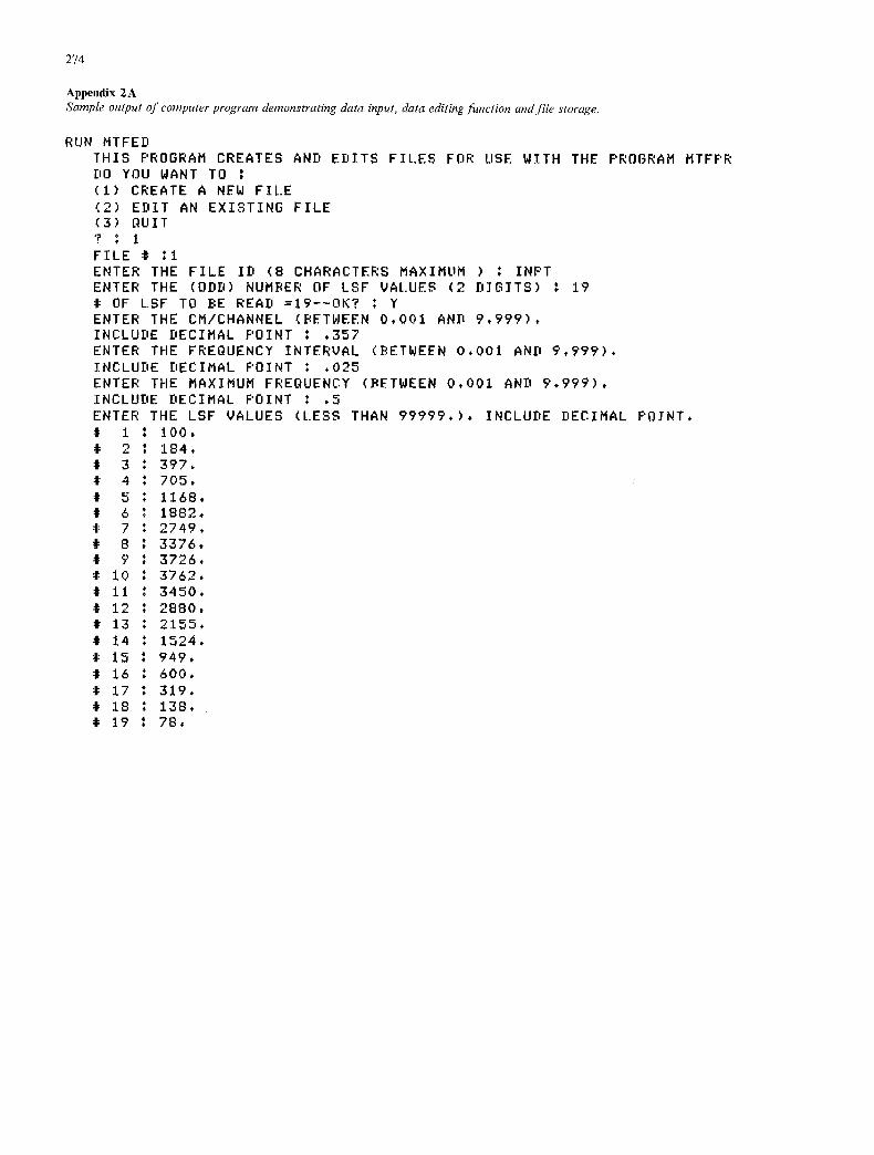
Appendix 2A Sample output of computer program demonstrating data input, data editing function and file storage.

RUN MTFED THIS PROGRAM CREATES AND EDITS FILES FOR USE WITH THE PROGRAM MTFPR DO YOU WANT TO (1) CREATE A NEW FI[.E (2) EDIT AN EXISTING FILE (3) QUIT '~ : 1 FILE $ 11 ENTER THE FILE ID (8 CHARACTERS MAXIMUM ) : INPT ENTER THE (ODD) NUMBER OF LSF VALUES (2 DIGITS) : 19

OF LSF TO BE READ =19--OK? : Y ENTER THE CM/CHANNEL (BETWEEN 0.001 AND 9.999), INCLUDE DECIMAL POINT : .357 ENTER THE FREQUENCY INTERVAL (BETWEEN 0.001 AND 9.999)° INCLUDE DECIMAL POINT : .025 ENTER THE MAXIMUM FREQUENCY (BETWEEN 0o001 AND 9°999)° INCLUDE DECIMAL POINT : .5 ENTER THE LSF VALUES (LESS THAN 99999,), INCLUDE DECIMAL POINT, f 1 ~ i 0 0 . f 2 : 184. $ 3 : 3 9 7 .

4 ~ 705, 5 ~ 1168,

f 6 : 1882, f 7 : 2749,

8 ~ 3 3 7 6 . f 9 ~ 3 7 2 6 ,

I0 ~ 3762. ii ~ 3450.

@ 12 ~ 2880. f 13 : 2155. # 14 ~ 1524.

15 ~ 9 4 9 . 16 : 600. 17 ~ 319.

f 18 ~ 138. 19 ~ 78.

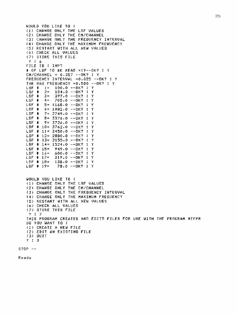
WOULD YOU LIKE TO ( I> CHANGE ONLY THE i.SF VALUES (2) CHANGE ONLY THE CM/CHANNEL (3) CHANGE ONLY THE FREQUENCY INTERVAL (4) CHANGE ONLY THE MAXIMUM FREQUENCY (5) RESTART WITH ALl. NEW VALUES (6) CHECK ALL VALUES (7) STORE THIS FILE

? ~ 6 FILE ID : INPT # OF LSF TO BE READ = ] 9 - - O K ? ~ Y CM/CHANNEL = 0 . 3 5 7 - - O K ? : Y FREQUENCY INTERVAL =0,025 --OK? : Y THE MAX FREQUENCY =0,500 --OK? : Y LSF f 1= 100.0 --OK? : Y LSF @ 2= 184.0 --OK? ~ Y LSF f 3= 397.0 --OK? ~ Y LSF # 4= 705,0 --OK? : Y LSF ~ 5= 1168,0 --OK? : Y LSF f 6= 1882,0 --OK? : Y LSF # 7= 2749.0 --OK? t Y LSF # 8= 3 3 7 6 . 0 - - O K ? t Y LSF ~ 9= 3 7 2 6 . 0 - - O K ? : Y LSF @ 10= 3 7 6 2 . 0 - - O K ? t Y LSF ~ 1 ] = 3 4 5 0 . 0 - - O K ? : Y LSF ~ 12= 2 8 8 0 , 0 - - O K ? : Y LSF # 13= 2 1 5 5 . 0 - - O K ? I Y LSF ~ 14= 1524.0 --OK? : Y LSF f 15= 949.0 --OK? : Y LSF f 16= 600.0 --OK? ~ Y LSF # 17= 319,0 --OK? : Y LSF f 18= 138.0 --OK? I Y LSF # 19= 7B,O --OK? : Y

275

WOULD YOU LIKE TO : ( i ) CHANGE ONLY THE I.SF VALUES (2) CHANGE ONLY THE CM/CHANNEL (3) CHANGE ONLY THE FREQUENCY INTERVAL (4) CHANGE ONLY THE MAXIMUM FREQUENCY (5) RESTART WTTH ALl. NEW VALUES (6) CHECK ALL VALUES (7) STORE THIS FILE "e : 7

THIS F'ROGRAM CREATES AND EDITS FILES FOR USE WITH THE PROGRAM MTFF'R DO YOU WANT TO : (I) CREATE A NEW FILE (2) EDIT AN EXISTING FILE (3) QUIT ? : 3

STOP --

Re~de

276

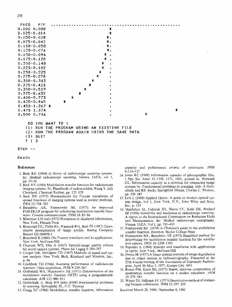
Appendix 2B Sample output of computer program listing data output values and plotting curves.

UN MTFF'R

DO YOU WANT TO ; ( I ) RUN THE F'ROGRAN US.TNG AN EXISTING FII.E (2) RUN THE PROGRAM AGAIN USING THE SAHE [iATA (3) QUIT 9 : 1 FILE # : i FILE IEi : INF'T

ENTER i TO O!.JTF'UT MTF ONLY ENTER 2 TO OUTF"LIT AREA ONLY ENTER 4 TO OIJTPUT ITF ONLY ENTER 8 TO OUTF'IIT OFR ONLY ENTER 1.6 TO OiJTPIJT F'TF ONLY ENTER SUM OF ABOVE VAI.IIES FOR ANY COMBINATION ENTER VALUE AS 2 DIGITS :31 CALCULATING,,, PLEASE WAIT

F R E Q MTF

0 . 0 0 0 1 . 0 0 0 .

0 . 0 2 5 0 . 9 8 5 .

0 . 0 5 0 0 . 9 3 9 •

0 . 0 7 5 0 . 8 6 9 , 0 . 1 0 0 0 . 7 7 8 ,

0.125 0.675 •

O , t 5 0 0 . 5 6 7 •

0.175 0,462 , 0.200 0.364 • 0.225 0.279 , 0 . 2 5 0 0 . 2 0 8 , 0.275 0.151 , 0.300 0.108 ,

0 . 3 2 5 0 . 0 7 7 ,

0.350 0,054 •

0.375 0.038 . 0.400 0,027 ** 0.425 0,018 .~ 0.450 0.012 . * 0 , . 4 7 5 0 , 0 0 8 0 , 5 0 0 0 , 0 0 7

AREA UNDER MTF = 0 . ] 8 8

FREQ 0 . 0 0 0 0 . 0 2 5 0 , 0 5 0 0 . 0 7 5 0 . 1 0 0 0 . 1 2 5 0 , 1 5 0 0 . ] 7 5 0 . 2 0 0 0 . 2 2 5 0.250 0.275 0.300 0.325 0.350 0.375 0.400 0.425 0 . 4 5 0 0 , 4 7 5 0.500

ITF 1 . 0 0 0 0 , 9 6 9 0 ° 8 8 2 0 . 7 5 3 0 . 6 0 4 0 . 4 5 3 0.319 0 . 2 1 0 0 . 1 3 0 0.075 0o041 0~021 0.010 0 , 0 0 5 0,002 0~001 0.000 0.000 0,000 0 , 0 0 0 0.000

.$

277

FREQ 0 . 0 0 0 0 . 0 2 5 0 . 0 5 0 0 . 0 7 5 0 . 1 0 0 0 , 1 2 5 0 . 1 5 0 0 . 1 7 5 0 . 2 0 0 0 ~

0.250 0.275 0.300 0.325 0.350 0,375 0 . 4 0 0 0 . 4 2 5 0,450 0.475 0~500

OFR 0.000 0.025 0.047 0.065 0.078 0.084 0.085 0.080 0 . 0 7 2 0 . 0 6 2 0.051 0 . 0 4 0 0.031 0 . 0 2 3 0.017 0,012 0.008 0.004 0.002

-0.001 -0.003

g

278

FREQ F'TF 0.000 0,000 0.025-0#014 0~050-0,028 0.075-0o042 0 .100-0 .058 0 .125-0 .076 0 .150-0 ,096 0 .175-0 .120 0 .200-0 .148 0.225-0$182 0 ,250-0 .225 0 . 2 7 5 - 0 . 2 7 8 0,300-0 .343 0 ,325-0 .423 0 ,350-0 .519 0 ,375-0 .632 0 .400-0 .773 0o425-0.965 0.450-1.267 0.475 1.374 0,500 0,746

$

&

#

$

rio YOU (1) RUN (2) RUN (3) QUII"

WANT TO : THE PROGRAM USING THE PROGRAM AGAIN

AN EXISTING FILE IJSING THE SAME DATA

STOP - -

Re~du

References

1. Beck RN (1964) A theory of radioisotope scanning systems. In: Medical radioisotope scanning, Vienna, IAEA, vol 1, pp. 35-36

2. Beck RN (1969) Modulation transfer function for radioisotope imaging systems. In: Handbook of radiouuclides, Wang Y, (ed) Cleveland, Chemical Rubber, pp. 123 129

3. Beck RN (1972) Nomenclature for Fourier transforms of spread functions of imaging systems used in nuclear medicine. JNM 13:704-705

4. Benedetto AR, Nusynowitz ML (1977) An improved FORTRAN program for calculating modulation transfer functions: Concise communication. JNM 18:85-86

5. Biberman LM (ed) (1973) Perception of displayed information, New York, Plenum Press

6. Bourough HC, Fallis RF, Warnock RH, Britt JH (1967) Quan- titative determination of image quality. Boeing Company Report D2-114058-1

7. Bracewell R (1968) The Fourier transform and its applications. New York, McGraw-Hill

8. Charmin WH, Olin A (1967) Tutorial-image quality criteria for aerial camera systems. Photo Sci Engng 9 : 385-397

9. Cooper GR, McGillem CD (1967) Methods of signal and system analysis. New York, Holt, Rinehard and Winston, Inc., p. 86

10. Cradduck TD (1968) Assessing performance of radioisotope scanners: Data acquisition. JNM 9:210-217

11. Goldsmith WA, Nusynowitz ML (1971) Determination of the modulation transfer function (MTF) using a programmable calculator. AJR 112:806-811

12. Gottschalk A, Beck RN (eds) (1968) Fundamental problems in scanning. Springfield, Ill., C.C. Thomas

13. Gregg EC (1968) Modulation transfer function, information

capacity and performance criteria of scintiscans. JNM 9:116-127

14. Jones RC (1968) Information capacity of photographic film. J Opt Soc Amer 51:1159, 1171, 1961, quoted in: Brownell GL: Information capacity as a criterion for comparing image systems In: Fundamental problems in scanning. (eds. A Gott- schalk and RN Beck). Springfield Illinois, Charles C. Thomas, pp. 339-347

15. Levi L (1968) Applied Optics: A guide to modern optical system design, Vol 1. New York, N.Y., John Wiley and Sons, Inc., p. 133

16. MacIntyre SJ, Fedoruk SO, Harris CC, Kuhl DE, Mallard JR (1969) Sensitivity and resolution in radioisotope scanning: A report to the International Commission on Radiation Units and Measurements. In: Medical radioisotope scintigraphy, Vienna, IAEA, Vol 1, pp. 391-433

17. Nusynowitz ML (1974) A Clinician's guide to the modulation transfer function. Houston, Baylor College Press

18. Nusynowitz ML, Benedetto AR (1975) Simplified method for determining the modulation transfer function for the scintilla- tion camera. JNM 16:1200-1203

19. Papoulis A (1968) Systems and transforms with applications to optics. New York, McGraw-Hill

20. Prince JR (1977) A linear systems analysis of image degradation due to object motion in radioscintigraphy. Presented at the 25th annual meeting of the Association of University Radiolo- gists, April 30-May 1, 1977, Kansas City, MO

21. Ronai PM, Kirch DL (1977) Rapid, rigorous computation of modulation transfer function on a pocket calculator. JNM 18 : 579-583

22. Wyper D J, Gillespie FC (1971) Quantitative method of evaluating focused collimators. JNM 12:197-203

Received March 28, 1980 / September 4, 1982

FORTRAN algorithms for evaluating Fourier transforms of line spread functions

Documents

Transcript of FORTRAN algorithms for evaluating Fourier transforms of line spread functions