Automatic Tuning of Discrete Fourier Transforms Driven by Analytical Modeling

Basilio B. Fraguela

Depto. de Electronica e Sistemas

Universidade da Coruna

A Coruna, Spain

basilio@udc.es

Yevgen Voronenko, Markus Puschel

Electrical and Computer Engineering

Carnegie Mellon University

Pittsburgh, PA, USA

{yvoronen,pueschel}@ece.cmu.edu

Abstract—Analytical models have been used to estimateoptimal values for parameters such as tile sizes in the context ofloop nests. However, important algorithms such as fast Fouriertransforms (FFTs) present a far more complex search spaceconsisting of many thousands of different implementationswith very different complex access patterns and nesting andcode structures. As a results, some of the best availableFFT implementations use heuristic search based on runtimemeasurements. In this paper we present the first analyticalmodel that can successfully replace the measurement in thissearch on modern platforms. The model includes many detailsof the platform’s memory system including the TLBs, and,for the first time, physically addressed caches and hardwareprefetching. The effect, as we show, is a dramatically reducedsearch time to find the best FFT without significant loss inperformance. Even though our model is adapted to the FFTin this paper, its underlying structure should be applicable fora much larger set of code structures and hence is a candidatefor iterative compilation.

Keywords-automatic performance tuning, discrete Fouriertransform, FFT, high-performance computing, library genera-tors, model-driven optimization, program optimization

I. INTRODUCTION

There is consensus that the complexity of current comput-

ers makes analytical performance modeling exceedingly dif-

ficult and possibly intractable. As a result, adaptive libraries

and program generators such as ATLAS [1], FFTW [2]

and Spiral [3] resort to search or iterative compilation

based on runtime measurements to explore choices and

tune for performance. However, models have successfully

guided optimization processes whose purpose was to choose

quantitative parameters such as the degree of unrolling

or tile sizes [4], [5], [6]. Unfortunately, the structure of

many important algorithms such as fast Fourier transforms

(FFTs)1 produces an optimization search space that cannot

be described using a few values. Rather, FFTs are typically

written as a series of small kernels of varying size that can be

combined in thousands of different ways with very different

nesting and access patterns. Hence, previous work on FFT

modeling [7] was based on large feature sets, large training

data sets, and used an FFT specific approach.

1The terminology that we use in this paper is that FFTs are algorithmsto compute the discrete Fourier transform (DFT).

In this paper, we present an analytical performance model

that aims to replace iterative feedback-driven compilation for

algorithms with regular access patterns. The model takes into

account details of the memory system including the TLB,

branch prediction, and is compatible with SIMD instruction

set extensions. Two novel contributions of this model are the

inclusion of the physically-indexed nature of the lower level

caches, as well as the effect of the hardware prefetchers,

which can play an important role for performance as we

will show.

We have integrated the model into Spiral [3] to guide

the selection of optimal DFT implementations for state-

of-the-art processors. Benchmarks on Intel-based platforms

show that the performance of the code generated this way

is comparable and sometimes even better than the code

produced by iterative compilation based on runtime mea-

surements, while requiring only a fraction of the search time.

This property is particularly relevant since the size of the

search space grows exponentially with the problem size if

all options are considered. As a result, for large sizes the

code generation time without a model can be many hours.

The rest of the paper is organized as follows. Section II

discusses related work and gives background about Spiral

and the DFT. Section III describes our performance mod-

eling approach. The modeling of the memory hierarchy

is particularly complex and includes the two main novel

contributions; thus, Section IV describes it in additional

detail. Experimental results are shown in Section V. Finally,

we offer conclusions in Section VI.

II. BACKGROUND AND RELATED WORK

The increasing complexity of hardware platforms makes

the implementation of high-performance libraries an ex-

tremely complex task. For many important domains, com-

pilers cannot achieve the highest possible performance for

several reasons including the lack of high-level algorithm

knowledge (hence they cannot apply the appropriate opti-

mizations), the lack of a precise model of the underlying

hardware, and the lack of a proper strategy to navigate the

usually large set of compilation choices.

The first and third problem are addressed by a number

of domain-specific automation tools [8], such as adaptive

libraries and program generators. However, these tools often

use runtime performance feedback to guide the optimization

process, because of the lack of a sufficiently precise model

of the underlying hardware.

In this paper we develop a detailed model for CPU

and cache performance that can be integrated into a high-

performance compiler or a program generator. As an appli-

cation, we incorporated our model into the Spiral program

generator [3] to guide the search in the FFT space. We note

that FFTs have rather complex access patterns, in particular

after all necessary optimizations are applied (as done by

Spiral automatically).

Related work. Models are particularly useful for larger

problem sizes, where the performance is strongly impacted

by the memory hierarchy. Several cache models have been

proposed, including the Cache Miss Equations [9], the Pres-

burger formula based approach in [10], the Stack Distances

Model [11], and the Probabilistic Miss Equations [12]. All of

these models support loop nests with regular access patterns

similar to the ones considered in this paper. But to date these

models are restricted to choose quantitative optimizations

parameters rather than the entire structure of the code [4],

[5]. Also, all these models assume virtually-indexed caches,

which does not reflect the reality on most modern processors

and hence can diminish accuracy. As we will explain in

Section IV-B, this affects particularly the modeling of code

that accesses data in strides of large powers of two, as, for

example, is the case for FFTs. Finally, to date no model has

included hardware prefetching, a very common feature in

current processors.

In [7] the performance of FFTs is predicted by applying

machine learning techniques to training data obtained based

on a set of detailed features of the FFT recursion strategy.

The work is inherently restricted to the DFT and the Cooley-

Tukey FFT. Our model is not restricted to FFTs, and could

potentially be used in a general purpose compiler. Further,

it can predict performance on more complex architectures,

and relies on training to a very limited extent (only to select

few key numeric parameters), thus reducing the potential of

overfitting.

Spiral. Spiral [3] is a program generator for linear

transforms such as the DFT, discrete cosine transforms,

digital filters, wavelets, and others. Spiral automates the

optimization and tuning process on a given platform in two

ways. First, it contains a large repository of fast transform

algorithms represented in the domain-specific language SPL

(Signal Processing Language), and it is able to iteratively

choose and recursively combine different algorithms to find

the best variant for a given transform size. Second, it auto-

mates both algorithm level and code level transformations,

which are performed on SPL and lower levels of abstraction.

This includes loop optimizations [13] and SIMD vectoriza-

tion [14]. The choice of the algorithm and algorithm-level

restructuring is driven by runtime performance feedback,

Formula Generation

Formula Optimization

Implementation

Code Optimization

Compilation

Performance Evaluation

Linear transform and size

Optimized/adapted implementation

Se

arc

h

controls

controls

performance

algorithm as formula

in SPL language

C/Fortran

implementation

Algorithm

Level

Implementation

Level

Evaluation

Level

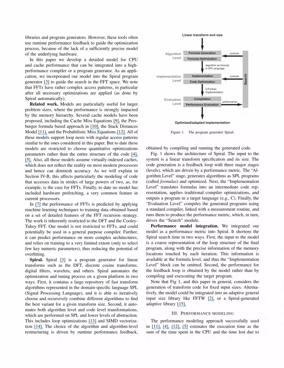
Figure 1. The program generator Spiral.

obtained by compiling and running the generated code.

Fig. 1 shows the architecture of Spiral. The input to the

system is a linear transform specification and its size. The

code generation is a feedback loop with three major stages

(levels), which are driven by a performance metric. The “Al-

gorithm Level” stage, generates algorithms as SPL programs

(called formulas) and optimized. Next, the “Implementation

Level” translates formulas into an intermediate code rep-

resentation, applies traditional compiler optimizations, and

outputs a program in a target language (e.g., C). Finally, the

“Evaluation Level” compiles the generated programs using

a standard compiler, linked with a measurement routine, and

runs them to produce the performance metric, which, in turn,

drives the “Search” module.

Performance model integration. We integrated our

model as a performance metric into Spiral. It shortens the

Spiral search time in two ways. First, the input to the model

is a coarse representation of the loop structure of the final

program, along with the precise information of the memory

locations touched by each iteration. This information is

available at the formula level, and thus the “Implementation

Level” block can be omitted. Second, the performance for

the feedback loop is obtained by the model rather than by

compiling and exexcuting the target program.

Note that Fig 1, and this paper in general, considers the

generation of transform code for fixed input sizes. Alterna-

tively, the model could be integrated into an adaptive general

input size library like FFTW [2], or a Spiral-generated

adaptive library [15].

III. PERFORMANCE MODELING

The performance modeling approach successfully used

in [11], [4], [12], [5] estimates the execution time as the

sum of the time spent in the CPU and the time lost due to

0.75

1.00

1.25

1.50

1.75

2.00

2.25

6 7 8 9 10 11 12 13 14 15 16 17 18 19 20 21 22 23 24

log size

Complex 1D DFT [Core 2 Quad 2.66 Ghz]Run!me ra!o rela!ve to search w/ !ming

best of 10 random

1 random best of 30 random

L1 L2 main memory

data placement

search w/ timing

search w/ model

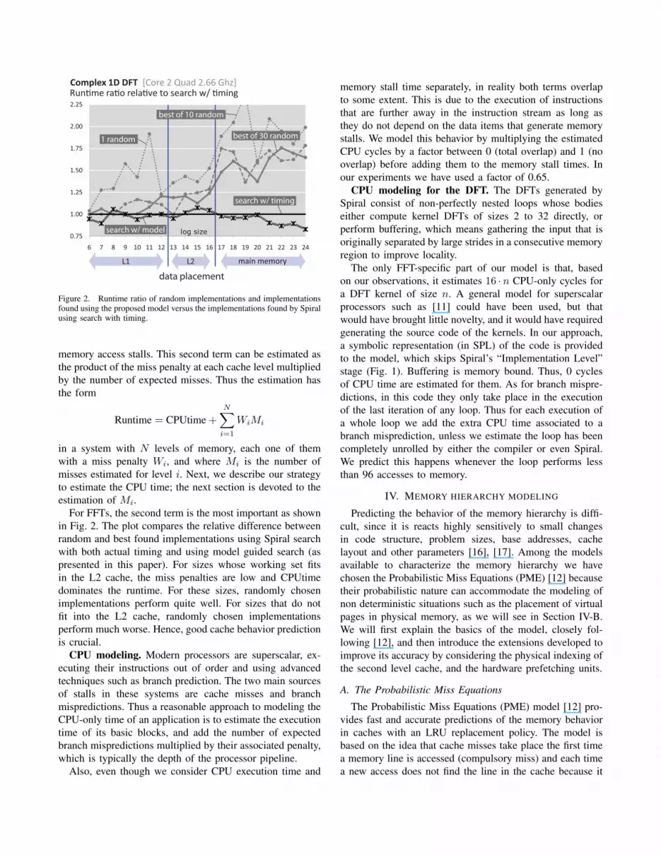
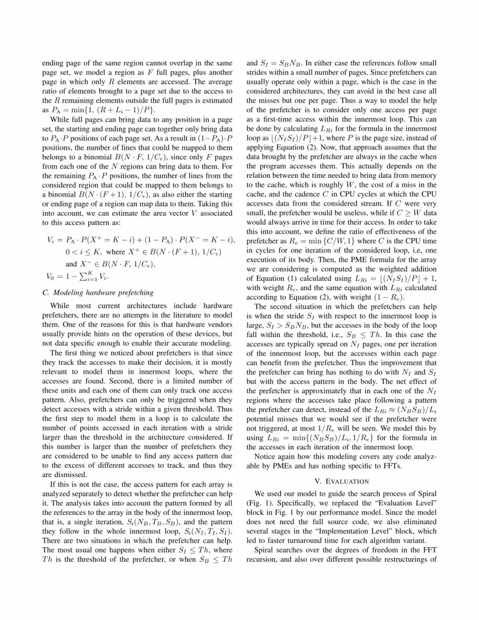
Figure 2. Runtime ratio of random implementations and implementationsfound using the proposed model versus the implementations found by Spiralusing search with timing.

memory access stalls. This second term can be estimated as

the product of the miss penalty at each cache level multiplied

by the number of expected misses. Thus the estimation has

the form

Runtime = CPUtime +

N∑

i=1

WiMi

in a system with N levels of memory, each one of them

with a miss penalty Wi, and where Mi is the number of

misses estimated for level i. Next, we describe our strategy

to estimate the CPU time; the next section is devoted to the

estimation of Mi.

For FFTs, the second term is the most important as shown

in Fig. 2. The plot compares the relative difference between

random and best found implementations using Spiral search

with both actual timing and using model guided search (as

presented in this paper). For sizes whose working set fits

in the L2 cache, the miss penalties are low and CPUtime

dominates the runtime. For these sizes, randomly chosen

implementations perform quite well. For sizes that do not

fit into the L2 cache, randomly chosen implementations

perform much worse. Hence, good cache behavior prediction

is crucial.

CPU modeling. Modern processors are superscalar, ex-

ecuting their instructions out of order and using advanced

techniques such as branch prediction. The two main sources

of stalls in these systems are cache misses and branch

mispredictions. Thus a reasonable approach to modeling the

CPU-only time of an application is to estimate the execution

time of its basic blocks, and add the number of expected

branch mispredictions multiplied by their associated penalty,

which is typically the depth of the processor pipeline.

Also, even though we consider CPU execution time and

memory stall time separately, in reality both terms overlap

to some extent. This is due to the execution of instructions

that are further away in the instruction stream as long as

they do not depend on the data items that generate memory

stalls. We model this behavior by multiplying the estimated

CPU cycles by a factor between 0 (total overlap) and 1 (no

overlap) before adding them to the memory stall times. In

our experiments we have used a factor of 0.65.

CPU modeling for the DFT. The DFTs generated by

Spiral consist of non-perfectly nested loops whose bodies

either compute kernel DFTs of sizes 2 to 32 directly, or

perform buffering, which means gathering the input that is

originally separated by large strides in a consecutive memory

region to improve locality.

The only FFT-specific part of our model is that, based

on our observations, it estimates 16 ·n CPU-only cycles for

a DFT kernel of size n. A general model for superscalar

processors such as [11] could have been used, but that

would have brought little novelty, and it would have required

generating the source code of the kernels. In our approach,

a symbolic representation (in SPL) of the code is provided

to the model, which skips Spiral’s “Implementation Level”

stage (Fig. 1). Buffering is memory bound. Thus, 0 cycles

of CPU time are estimated for them. As for branch mispre-

dictions, in this code they only take place in the execution

of the last iteration of any loop. Thus for each execution of

a whole loop we add the extra CPU time associated to a

branch misprediction, unless we estimate the loop has been

completely unrolled by either the compiler or even Spiral.

We predict this happens whenever the loop performs less

than 96 accesses to memory.

IV. MEMORY HIERARCHY MODELING

Predicting the behavior of the memory hierarchy is diffi-

cult, since it is reacts highly sensitively to small changes

in code structure, problem sizes, base addresses, cache

layout and other parameters [16], [17]. Among the models

available to characterize the memory hierarchy we have

chosen the Probabilistic Miss Equations (PME) [12] because

their probabilistic nature can accommodate the modeling of

non deterministic situations such as the placement of virtual

pages in physical memory, as we will see in Section IV-B.

We will first explain the basics of the model, closely fol-

lowing [12], and then introduce the extensions developed to

improve its accuracy by considering the physical indexing of

the second level cache, and the hardware prefetching units.

A. The Probabilistic Miss Equations

The Probabilistic Miss Equations (PME) model [12] pro-

vides fast and accurate predictions of the memory behavior

in caches with an LRU replacement policy. The model is

based on the idea that cache misses take place the first time

a memory line is accessed (compulsory miss) and each time

a new access does not find the line in the cache because it

has been replaced since the previous time it was accessed

(interference miss). This way, the model generates a formula

for each reference and loop that encloses it that classifies the

accesses of the reference within the loop according to their

reuse distance, that is, the portion of code executed since

the latest access to each line accessed by the reference. The

reuse distances are measured in terms of loop iterations and

they have an associated miss probability that corresponds to

the impact on the cache of the footprint of the data accessed

during the execution of the code within the reuse distance.

The formula estimates the number of misses generated by

the reference in the loop by adding the number of accesses

with each given reuse distance weighted by their associated

miss probability.

The accesses that cannot exploit reuse in a loop are

compulsory misses from the point of view of that loop.

Still, they may enjoy reuse in outer or preceding loops, so

they must be carried outwards to estimate their potential

miss probability. For this reason the PME model begins

the construction of its formulas in the innermost loop that

contains each reference and proceeds outwards. For the same

reason the PME formula for each loop is a function of the

memory region accessed since the immediately preceding

access to the data accessed by the reference in the loop

when the execution of the loop begins. This region is called

RegIn. It is used to estimate the miss probability for first-

time accesses to data within the loop. The formulas are

built recursively, with the formula for each loop level being

built in terms of the formula obtained for the immediately

inner level. In the innermost loop containing a reference,

the recursion finishes and the invocation to the formula for

the inner level with a given RegIn region is substituted

by the miss probability that such region generates. Those

accesses for which no reuse distance has been found when

the outermost loop is reached, correspond to the absolute

compulsory misses, whose miss probability is one.

All the references in the DFT codes follow regular access

patterns, that is, for any loop enclosing the references, they

follow a constant stride with respect to the iterations of

the loop. The PME formula that estimates the number of

misses in loop i of a reference R that follows a regular

access pattern as a function of RegIn, the memory region

whose footprint may interfere with the reuses of the first-

time accesses during the execution of this loop, is

FRi(RegIn) = LRi · FR(i+1)(RegIn)

+ (Ni − LRi) · FR(i+1)(RegRi), (1)

where Ni is the number of iterations of the loop at nesting

level i, and LRi is the number of different sets of lines

accessed by R during the execution of the loop. We can

also define LRi as the number of iterations of the loop in

which the accesses of R cannot exploit reuse with respect to

previous iterations of this loop. Thus this term corresponds

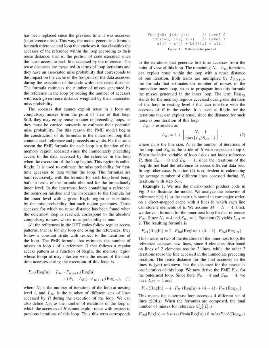
for(j=0; j<M; j++) // Level 0

for(i=0; i<N; i++) // Level 1

a[j] = a[j] + b[j][i] * c[i]

Figure 3. Matrix-vector product

to the iterations that generate first-time accesses from the

point of view of this loop. The remaining Ni−LRi iterations

can exploit reuse within the loop with a reuse distance

of one iteration. Both terms are multiplied by FR(i+1),

the formula that estimates the number of misses in the

immediate inner loop, so as to propagate into this formula

the misses generated in the inner loop. The term RegRi

stands for the memory regions accessed during one iteration

of the loop in nesting level i that can interfere with the

accesses of R in the cache. It is used as RegIn for the

iterations that can exploit reuse, since the distance for such

reuse is one iteration of this loop.

LRi is estimated as

LRi = 1 +

⌊

Ni − 1

max{Ls/SRi, 1}

⌋

, (2)

where Ls is the line size, Ni is the number of iterations of

the loop, and SRi is the stride of R with respect to loop i.When the index variable of loop i does not index reference

R, then SRi = 0 and LRi = 1, since the iterations of the

loop do not lead the reference to access different data sets.

In any other case, Equation (2) is equivalent to calculating

the average number of different lines accessed during Ni

iterations with step SRi.

Example 1. We use the matrix-vector product code in

Fig. 3 to illustrate the model. We analyze the behavior of

reference b[j][i] to the matrix b stored in row-major order,

on a direct-mapped cache with 4 lines in which each line

can store 2 elements of b. We assume M = N = 4. First,

we derive a formula for the innermost loop for that reference

FR1. Since N1 = 4 and SR1 = 1, Equation (2) yields LR1 =2. The resulting formula is

FR1(RegIn) = 2 · FR2(RegIn) + (4 − 2) · FR2(RegR1).

This means in two of the iterations of the innermost loop, the

reference accesses new lines, since 4 elements distributed

on lines of 2 elements require 2 lines, while the other 2

iterations reuse the line accessed in the immediate preceding

iteration. The reuse distance for the first accesses to the

lines is (yet) unknown, but the distance for the reuses is

one iteration of this loop. We now derive the PME FR0 for

the outermost loop. Since here N0 = 4 and SR0 = 4, we

have LR0 = 4 and

FR0(RegIn) = 4 · FR1(RegIn) + (4 − 4) · FR1(RegR0).

This means the outermost loop accesses 4 different set of

lines (SOLs). When the formulas are composed, the final

number of misses for reference b[j][i] is

FR0(RegIn) = 8·missProb(RegIn)+8·missProb(RegR1).

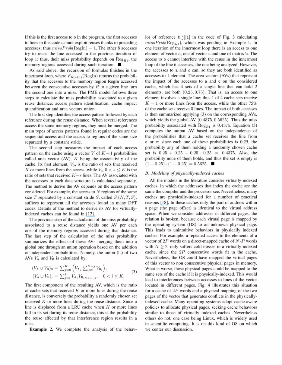
If this is the first access to b in the program, the first accesses

to lines in this code cannot exploit reuses thanks to preceding

accesses; thus missProb(RegIn) = 1. The other 8 accesses

try to reuse the line accessed in the previous iteration of

loop 1; thus, their miss probability depends on RegR1, the

memory regions accessed during such iteration. �

As said above, the recursion of formulas finishes in the

innermost loop, where FR(i+1)(RegIn) returns the probabil-

ity that the accesses to the memory region RegIn accessed

between the consecutive accesses by R to a given line turn

the second one into a miss. The PME model follows three

steps to calculate the miss probability associated to a given

reuse distance: access pattern identification, cache impact

quantification and area vectors union.

The first step identifies the access pattern followed by each

reference during the reuse distance. When several references

access the same memory regions, they must be merged. The

main types of access patterns found in regular codes are the

sequential access and the access to regions of the same size

separated by a constant stride.

The second step measures the impact of each access

pattern on the cache using a vector V of K +1 probabilities

called area vector (AV), K being the associativity of the

cache. Its first element, V0, is the ratio of sets that received

K or more lines from the access, while Vs, 0 < s ≤ K is the

ratio of sets that received K−s lines. The AV associated with

the accesses to each data structure is calculated separately.

The method to derive the AV depends on the access pattern

considered. For example, the access to N regions of the same

size T separated by a constant stride S, called Sr(N,T, S),suffices to represent all the accesses found in many DFT

codes. Details of the method to derive its AV for virtually-

indexed caches can be found in [12].

The previous step of the calculation of the miss probability

associated to a reuse distance yields one AV per each

one of the memory regions accessed during that distance.

The last step of the calculation of the miss probability

summarizes the effects of these AVs merging them into a

global one through an union operation based on the addition

of independent probabilities. Namely, the union (∪) of two

AVs VA and VB is calculated by:

(VA ∪ VB)0 =∑K

j=0

(

VAj

∑K−j

i=0 VBi

)

,

(VA ∪ VB)i =∑k

j=i VAjVB(K+i−j)

, 0 < i ≤ K.(3)

The first component of the resulting AV, which is the ratio

of cache sets that received K or more lines during the reuse

distance, is conversely the probability a randomly chosen set

received K or more lines during the reuse distance. Since a

line is displaced from a LRU cache when K or more lines

fall in its set during its reuse distance, this is the probability

the reuse affected by that interference region results in a

miss.

Example 2. We complete the analysis of the behav-

ior of reference b[j][i] in the code of Fig. 3 calculating

missProb(RegR1), which was pending in Example 1. In

one iteration of the innermost loop there is an access to one

element of vector a, one of vector c and one of matrix b. The

access to b cannot interfere with the reuse in the innermost

loop of the line it accesses, the one being analyzed. However,

the accesses to a and c can, so they are both identified as

accesses to 1 element. The area vectors (AVs) that represent

the impact of the accesses to a and c on the considered

cache, which has 4 sets of a single line that can hold 2

elements, are both (0.25, 0.75). That is, an access to one

element involves a single line; thus 1 of 4 cache sets receive

K = 1 or more lines from the access, while the other 75%

of the cache sets receive 0 lines. The impact of both accesses

is then summarized applying (3) on the corresponding AVs,

which yields the global AV (0.4375, 0.5625). Thus the miss

probability associated with RegR1 is 0.4375. Equation (3)

computes the output AV based on the independence of

the probabilities that a cache set receives the line from

a or c: since each one of these probabilities is 0.25, the

probability any of them holding a randomly chosen cache

set is 0.25 + 0.25 − 0.25 · 0.25 = 0.4375. Also, the

probability none of them holds, and thus the set is empty is

(1 − 0.25) · (1 − 0.25) = 0.5625. �

B. Modeling of physically-indexed caches

All the models in the literature consider virtually-indexed

caches, in which the addresses that index the cache are the

same the compiler and the processor see. Nevertheless, many

caches are physically-indexed for a number of practical

reasons [18]. In these caches only the part of address within

a page (the page offset) is identical to the virtual address

space. When we consider addresses in different pages, the

relation is broken, because each virtual page is mapped by

the operating system (OS) to an unknown physical page.

This leads to unintuitive behaviors in physically indexed

caches. For example, a repeated access to the elements of a

vector of 2P words on a direct-mapped cache of N ·P words

with N ≥ 2, only suffers cold misses in a virtually-indexed

cache, since the 2P consecutive words fit in the cache.

Nevertheless, the OS could have mapped the virtual pages

of this vector to non consecutive physical pages in memory.

What is worse, these physical pages could be mapped to the

same sets of the cache if it is physically-indexed. This would

lead to interferences between accesses to lines of the vector

located in different pages. Fig. 4 illustrates this situation

for a cache of 2P words and a physical mapping of the two

pages of the vector that generates conflicts in the physically-

indexed cache. Many operating systems adopt cache-aware

policies to allocate physical pages, seeking cache behaviors

similar to those of virtually indexed caches. Nevertheless

others do not, one case being Linux, which is widely used

in scientific computing. It is on this kind of OS on which

we center our discussion.

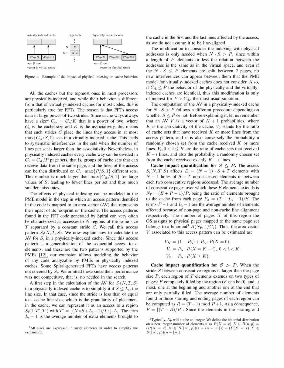
vector in virtual space

VPage N VPage N+1

virtually indexed cache

P

page table

N

N+1

X

X+2

PPage X+1PPage X PPage X+2

physically indexed cache

Pvector in physical space

Figure 4. Example of the impact of physical indexing on cache behavior.

All the caches but the topmost ones in most processors

are physically-indexed, and while their behavior is different

from that of virtually-indexed caches for most codes, this is

particularly true for FFTs. The reason is that FFTs access

data in large power-of-two strides. Since cache ways always

have a size2 Csk = Cs/K that is a power of two, where

Cs is the cache size and K is the associativity, this means

that such strides S place the lines they access in at most

max{Csk/S, 1} sets in a virtually-indexed cache. This leads

to systematic interferences in the sets when the number of

lines per set is larger than the associativity. Nevertheless, in

physically indexed caches every cache way can be divided in

Cv = Csk/P page sets, that is, groups of cache sets that can

receive data from the same page, and the lines of the access

can be then distributed on Cv · max{P/S, 1} different sets.

This number is much larger than max{Csk/S, 1} for large

values of S, leading to fewer lines per set and thus much

smaller miss rates.

The effects of physical indexing can be modeled in the

PME model in the step in which an access pattern identified

in the code is mapped to an area vector (AV) that represents

the impact of its footprint on the cache. The access patterns

found in the FFT code generated by Spiral can very often

be characterized as accesses to N regions of the same size

T separated by a constant stride S. We call this access

pattern Sr(N,T, S). We now explain how to calculate the

AV for Sr in a physically-indexed cache. Since this access

pattern is a generalization of the sequential access to nelements, and these are the two patterns supported by the

PMEs [12], our extension allows modeling the behavior

of any code analyzable by PMEs in physically indexed

caches. Some Spiral-generated FFTs have access patterns

not covered by Sr. We omitted these since their performance

was not competitive, that is, no needed in the search.

A first step in the calculation of the AV for Sr(N,T, S)in a physically-indexed cache is to simplify it if S ≤ Ls, the

line size. In that case, since the stride is less than or equal

to a cache line size, which is the granularity of placement

in the cache, we can represent it as an access to a region

Sr(1, T′, T ′) with T ′ = ⌊(N ∗S+Ls−1)/Ls⌋·Ls. The term

Ls − 1 is the average number of extra elements brought to

2All sizes are expressed in array elements in order to simplify theexplanation.

the cache in the first and the last lines affected by the access,

as we do not assume it to be line-aligned.

The modification to consider the indexing with physical

addresses is only needed when N · S > P , since within

a length of P elements or less the relation between the

addresses is the same as in the virtual space, and even if

the N · S ≤ P elements are split between 2 pages, no

new interferences can appear between them that the PME

model for virtually-indexed caches does not consider. Also,

if Csk ≤ P the behavior of the physically and the virtually-

indexed caches are identical, thus this modification is only

of interest for P > Csk, the most usual situation.

The computation of the AV in a physically-indexed cache

for N · S > P follows a different procedure depending on

whether S ≤ P or not. Before explaining it, let us remember

that an AV V is a vector of K + 1 probabilities, where

K is the associativity of the cache. V0 stands for the ratio

of cache sets that have received K or more lines from the

access pattern, and it is also conversely the probability a

randomly chosen set from the cache received K or more

lines. Vi, 0 < i ≤ K are the ratio of cache sets that received

K − i lines, and also the probability a randomly chosen set

from the cache received exactly K − i lines.

Cache impact quantification for S ≤ P . The access

Sr(N,T, S) affects E = (N − 1) · S + T elements with

N − 1 holes of S − T non-accessed elements in between

each two consecutive regions accessed. The average number

of consecutive pages over which these E elements extends is

NP = (E + P − 1)/P , being the ratio of elements brought

to the cache from each page PA = (T + Ls − 1)/S. The

terms P − 1 and Ls − 1 are the average number of elements

affected because of non-page and non-cache line alignment

respectively. The number of pages X of this region the

OS assigns to physical pages mapped to the same page set

belongs to a binomial3 B(NP, 1/Cv). Thus, the area vector

V associated to this access pattern can be estimated as:

VK = (1 − PA) + PA · P (X = 0),

Vi = PA · P (X = K − i), 0 < i < K,

V0 = PA · P (X ≥ K).

Cache impact quantification for S > P . When the

stride S between consecutive regions is larger than the page

size P , each region of T elements extends on two types of

pages: F completely filled by the region (F can be 0), and at

most, one at the beginning and another one at the end that

are only partially filled. The average number of elements

found in those starting and ending pages of each region can

be computed as R = (T −1) mod P +1. As a consequence,

F = ⌊(T − R)/P ⌋. Since the elements in the starting and

3Typically, NP will not be an integer. We define the binomial distributionon a non integer number of elements n as P (X = x), X ∈ B(n, p) =(P (X = x), X ∈ B(⌊n⌋, p))(1 − (n − ⌊n⌋)) + (P (X = x), X ∈B(⌈n⌉, p))(n − ⌊n⌋).

ending page of the same region cannot overlap in the same

page set, we model a region as F full pages, plus another

page in which only R elements are accessed. The average

ratio of elements brought to a page set due to the access to

the R remaining elements outside the full pages is estimated

as PA = min{1, (R + Ls − 1)/P}.

While full pages can bring data to any position in a page

set, the starting and ending page can together only bring data

to PA ·P positions of each page set. As a result in (1−PA)·Ppositions, the number of lines that could be mapped to them

belongs to a binomial B(N · F, 1/Cv), since only F pages

from each one of the N regions can bring data to them. For

the remaining PA ·P positions, the number of lines from the

considered region that could be mapped to them belongs to

a binomial B(N · (F +1), 1/Cv), as also either the starting

or ending page of a region can map data to them. Taking this

into account, we can estimate the area vector V associated

to this access pattern as:

Vi = PA · P (X+ = K − i) + (1 − PA) · P (X− = K − i),

0 < i ≤ K, where X+ ∈ B(N · (F + 1), 1/Cv)

and X− ∈ B(N · F, 1/Cv),

V0 = 1 −∑K

i=1 Vi.

C. Modeling hardware prefetching

While most current architectures include hardware

prefetchers, there are no attempts in the literature to model

them. One of the reasons for this is that hardware vendors

usually provide hints on the operation of these devices, but

not data specific enough to enable their accurate modeling.

The first thing we noticed about prefetchers is that since

they track the accesses to make their decision, it is mostly

relevant to model them in innermost loops, where the

accesses are found. Second, there is a limited number of

these units and each one of them can only track one access

pattern. Also, prefetchers can only be triggered when they

detect accesses with a stride within a given threshold. Thus

the first step to model them in a loop is to calculate the

number of points accessed in each iteration with a stride

larger than the threshold in the architecture considered. If

this number is larger than the number of prefetchers they

are considered to be unable to find any access pattern due

to the excess of different accesses to track, and thus they

are dismissed.

If this is not the case, the access pattern for each array is

analyzed separately to detect whether the prefetcher can help

it. The analysis takes into account the pattern formed by all

the references to the array in the body of the innermost loop,

that is, a single iteration, Sr(NB , TB , SB), and the pattern

they follow in the whole innermost loop, Sr(NI , TI , SI).There are two situations in which the prefetcher can help.

The most usual one happens when either SI ≤ Th, where

Th is the threshold of the prefetcher, or when SB ≤ Th

and SI = SBNB . In either case the references follow small

strides within a small number of pages. Since prefetchers can

usually operate only within a page, which is the case in the

considered architectures, they can avoid in the best case all

the misses but one per page. Thus a way to model the help

of the prefetcher is to consider only one access per page

as a first-time access within the innermost loop. This can

be done by calculating LRi for the formula in the innermost

loop as ⌊(NISI)/P ⌋+1, where P is the page size, instead of

applying Equation (2). Now, that approach assumes that the

data brought by the prefetcher are always in the cache when

the program accesses them. This actually depends on the

relation between the time needed to bring data from memory

to the cache, which is roughly W , the cost of a miss in the

cache, and the cadence C in CPU cycles at which the CPU

accesses data from the considered stream. If C were very

small, the prefetcher would be useless, while if C ≥ W data

would always arrive in time for their access. In order to take

this into account, we define the ratio of effectiveness of the

prefetcher as Re = min {C/W, 1} where C is the CPU time

in cycles for one iteration of the considered loop, i.e, one

execution of its body. Then, the PME formula for the array

we are considering is computed as the weighted addition

of Equation (1) calculated using LRi = ⌊(NISI)/P ⌋ + 1,

with weight Re, and the same equation with LRi calculated

according to Equation (2), with weight (1 − Re).The second situation in which the prefetchers can help

is when the stride SI with respect to the innermost loop is

large, SI > SBNB , but the accesses in the body of the loop

fall within the threshold, i.e., SB ≤ Th. In this case the

accesses are typically spread on NI pages, one per iteration

of the innermost loop, but the accesses within each page

can benefit from the prefetcher. Thus the improvement that

the prefetcher can bring has nothing to do with NI and SI

but with the access pattern in the body. The net effect of

the prefetcher is approximately that in each one of the NI

regions where the accesses take place following a pattern

the prefetcher can detect, instead of the LRi ≈ (NBSB)/Ls

potential misses that we would see if the prefetcher were

not triggered, at most 1/Re will be seen. We model this by

using LRi = min{(NBSB)/Ls, 1/Re} for the formula in

the accesses in each iteration of the innermost loop.

Notice again how this modeling covers any code analyz-

able by PMEs and has nothing specific to FFTs.

V. EVALUATION

We used our model to guide the search process of Spiral

(Fig. 1). Specifically, we replaced the “Evaluation Level”

block in Fig. 1 by our performance model. Since the model

does not need the full source code, we also eliminated

several stages in the “Implementation Level” block, which

led to faster turnaround time for each algorithm variant.

Spiral searches over the degrees of freedom in the FFT

recursion, and also over different possible restructurings of

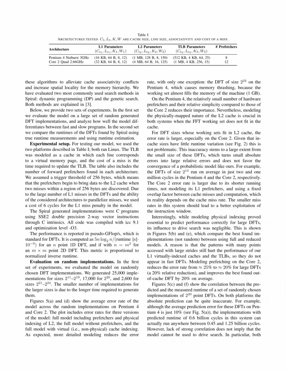
Table IARCHITECTURES TESTED. CS, LS, K, W ARE CACHE SIZE, LINE SIZE, ASSOCIATIVITY AND COST OF A MISS.

ArchitectureL1 Parameters L2 Parameters TLB Parameters # Prefetchers

(Cs1 , Ls1 , K1, W1) (Cs2 , Ls2 , K2, W2) (Cs3 , Ls3 , K3, W3)

Pentium 4 Netburst 3GHz (16 KB, 64 B, 8, 12) (1 MB, 128 B, 8, 150) (512 KB, 4 KB, 64, 25) 8Core 2 Quad 2.66GHz (32 KB, 64 B, 8, 12) (4 MB, 64 B, 16, 125) (1 MB, 4 KB, 256, 15) 12

these algorithms to alleviate cache associativity conflicts

and increase spatial locality for the memory hierarchy. We

have evaluated two most commonly used search methods in

Spiral: dynamic programming (DP) and the genetic search.

Both methods are explained in [3].

Below, we provide two sets of experiments. In the first set

we evaluate the model on a large set of random generated

DFT implementations, and analyze how well the model dif-

ferentiates between fast and slow programs. In the second set

we compare the runtimes of the DFTs found by Spiral using

true runtime measurements and using runtime estimation.

Experimental setup. For testing our model, we used the

two platforms described in Table I; both ran Linux. The TLB

was modeled as a cache in which each line corresponds

to a virtual memory page, and the cost of a miss is the

time required to update the TLB. The table also includes the

number of forward prefetchers found in each architecture.

We assumed a trigger threshold of 256 bytes, which means

that the prefetchers begin to bring data to the L2 cache when

two misses within a region of 256 bytes are discovered. Due

to the large number of L1 misses in the DFTs and the ability

of the considered architectures to parallelize misses, we used

a cost of 6 cycles for the L1 miss penalty in the model.

The Spiral generated implementations were C programs

using SSE2 double precision 2-way vector instructions

through C intrinsics. All code was compiled with icc 9.1

and optimization level -O3.

The performance is reported in pseudo-GFlop/s, which is

standard for DFTs. It is computed as 5n log2 n/(runtime [s]·10−9) for an n point 1D DFT, and if with n = m2 for

an m × m point 2D DFT. This metric is proportional to

normalized inverse runtime.

Evaluation on random implementations. In the first

set of experiments, we evaluated the model on randomly

chosen DFT implementations. We generated 25,000 imple-

mentations for sizes 211–219, 17,000 for 220, and 2,600 for

sizes 221–224. The smaller number of implementations for

the larger sizes is due to the longer time required to generate

them.

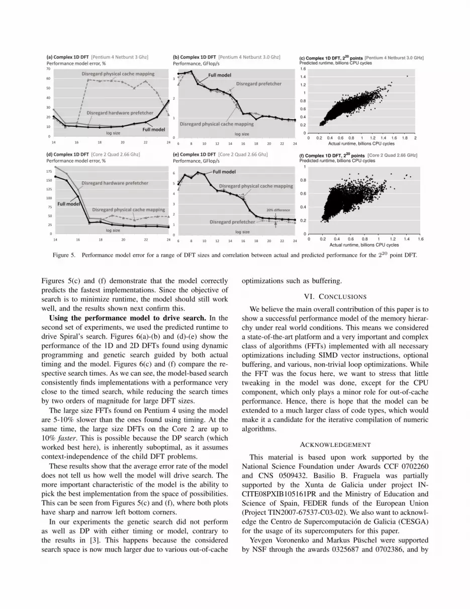
Figures 5(a) and (d) show the average error rate of the

model across the random implementations on Pentium 4

and Core 2. The plot includes error rates for three versions

of the model: full model including prefetchers and physical

indexing of L2, the full model without prefetchers, and the

full model with virtual (i.e., non-physical) cache indexing.

As expected, more detailed modeling reduces the error

rate, with only one exception: the DFT of size 224 on the

Pentium 4, which causes memory thrashing, because the

working set almost fills the memory of the machine (1 GB).

On the Pentium 4, the relatively small number of hardware

prefetchers and their relative simplicity compared to those of

the Core 2 reduces their importance. Nevertheless, modeling

the physically-mapped nature of the L2 cache is crucial in

both systems when the FFT working set does not fit in the

cache.

For DFT sizes whose working sets fit in L2 cache, the

error rate is larger, especially on the Core 2. Given that in-

cache sizes have little runtime variation (see Fig. 2) this is

not problematic. This inaccuracy stems to a large extent from

the small size of these DFTs, which turns small absolute

errors into large relative errors and does not favor the

convergence of a probabilistic model like ours. For example,

the DFTs of size 214 run on average in just two and one

million cycles in the Pentium 4 and the Core 2, respectively.

The Core 2 error rate is larger due to its shorter running

times, not modeling its L1 prefetchers, and using a fixed

overlap factor between cache misses and computation, which

in reality depends on the cache miss rate. The smaller miss

rates in this system should lead to a better exploitation of

the instruction window.

Interestingly, while modeling physical indexing proved

essential to predict performance correctly for large DFTs,

its influence to drive search was negligible. This is shown

in Figures 5(b) and (e), which compare the best found im-

plementations (not random) between using full and reduced

models. A reason is that the patterns with many points

accessed with large strides still hurt the performance of our

L1 virtually-indexed caches and the TLBs, so they do not

appear in fast DFTs. Modeling prefetching on the Core 2,

reduces the error rate from ≈ 25% to ≈ 20% for large DFTs

(a 20% relative reduction), and improves the best found out-

of-cache DFT by 20% on average.

Figures 5(c) and (f) show the correlation between the pre-

dicted and the measured runtime of a set of randomly chosen

implementations of 220 point DFTs. On both platforms the

absolute prediction can be quite inaccurate. For example,

although the average prediction error for these DFTs on Pen-

tium 4 is just 10% (see Fig. 5(a)), the implementations with

predicted runtime of 0.6 billion cycles in this system can

actually run anywhere between 0.45 and 1.25 billion cycles.

However, lack of strong correlation does not imply that the

model cannot be used to drive search. In particular, both

0

10

20

30

40

50

60

70

14 16 18 20 22 24

Full modellog size

(a) Complex 1D DFT [Pentium 4 Netburst 3 Ghz]

Performance model error, %

Disregard hardware prefetcher

Disregard physical cache mapping

0

1

2

3

6 8 10 12 14 16 18 20 22 24

Full model

log size

(b) Complex 1D DFT [Pentium 4 Netburst 3.0 Ghz]

Performance, GFlop/s

Disregard prefetcher

Disregard physical cache mapping

0

0.2

0.4

0.6

0.8

1

1.2

1.4

1.6

0 0.2 0.4 0.6 0.8 1 1.2 1.4 1.6 1.8 2

Actual runtime, billions CPU cycles

Predicted runtime, billions CPU cycles(c) Complex 1D DFT, 2

20 points [Pentium 4 Netburst 3.0 GHz]

0

25

50

75

100

125

150

175

14 16 18 20 22 24

Full model

log size

(d) Complex 1D DFT [Core 2 Quad 2.66 Ghz]

Performance model error, %

Disregard hardware prefetcher

Disregard physical cache mapping

0

1

2

3

4

5

6

6 8 10 12 14 16 18 20 22 24

Full model

log size

(e) Complex 1D DFT [Core 2 Quad 2.66 Ghz]

Performance, GFlop/s

Disregard prefetcher

Disregard physical cache mapping

20% difference

0

0.2

0.4

0.6

0.8

1

0 0.2 0.4 0.6 0.8 1 1.2 1.4 1.6

Actual runtime, billions CPU cycles

Predicted runtime, billions CPU cycles(f) Complex 1D DFT, 2

20 points [Core 2 Quad 2.66 GHz]

Figure 5. Performance model error for a range of DFT sizes and correlation between actual and predicted performance for the 220 point DFT.

Figures 5(c) and (f) demonstrate that the model correctly

predicts the fastest implementations. Since the objective of

search is to minimize runtime, the model should still work

well, and the results shown next confirm this.

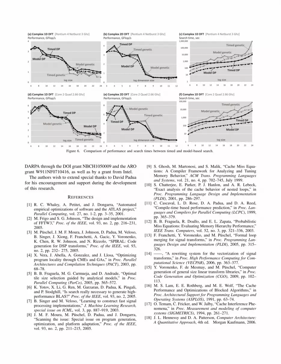
Using the performance model to drive search. In the

second set of experiments, we used the predicted runtime to

drive Spiral’s search. Figures 6(a)-(b) and (d)-(e) show the

performance of the 1D and 2D DFTs found using dynamic

programming and genetic search guided by both actual

timing and the model. Figures 6(c) and (f) compare the re-

spective search times. As we can see, the model-based search

consistently finds implementations with a performance very

close to the timed search, while reducing the search times

by two orders of magnitude for large DFT sizes.

The large size FFTs found on Pentium 4 using the model

are 5-10% slower than the ones found using timing. At the

same time, the large size DFTs on the Core 2 are up to

10% faster. This is possible because the DP search (which

worked best here), is inherently suboptimal, as it assumes

context-independence of the child DFT problems.

These results show that the average error rate of the model

does not tell us how well the model will drive search. The

more important characteristic of the model is the ability to

pick the best implementation from the space of possibilities.

This can be seen from Figures 5(c) and (f), where both plots

have sharp and narrow left bottom corners.

In our experiments the genetic search did not perform

as well as DP with either timing or model, contrary to

the results in [3]. This happens because the considered

search space is now much larger due to various out-of-cache

optimizations such as buffering.

VI. CONCLUSIONS

We believe the main overall contribution of this paper is to

show a successful performance model of the memory hierar-

chy under real world conditions. This means we considered

a state-of-the-art platform and a very important and complex

class of algorithms (FFTs) implemented with all necessary

optimizations including SIMD vector instructions, optional

buffering, and various, non-trivial loop optimizations. While

the FFT was the focus here, we want to stress that little

tweaking in the model was done, except for the CPU

component, which only plays a minor role for out-of-cache

performance. Hence, there is hope that the model can be

extended to a much larger class of code types, which would

make it a candidate for the iterative compilation of numeric

algorithms.

ACKNOWLEDGEMENT

This material is based upon work supported by the

National Science Foundation under Awards CCF 0702260

and CNS 0509432. Basilio B. Fraguela was partially

supported by the Xunta de Galicia under project IN-

CITE08PXIB105161PR and the Ministry of Education and

Science of Spain, FEDER funds of the European Union

(Project TIN2007-67537-C03-02). We also want to acknowl-

edge the Centro de Supercomputacion de Galicia (CESGA)

for the usage of its supercomputers for this paper.

Yevgen Voronenko and Markus Puschel were supported

by NSF through the awards 0325687 and 0702386, and by

0

1

2

3

4

6 8 10 12 14 16 18 20 22 24

Timed DP

Model DP

log size

(a) Complex 1D DFT [Pentium 4 Netburst 3 Ghz]

Performance, GFlop/s

Timed genetic

Model genetic

0

1

2

3

4

3 4 5 6 7 8 9 10 11 12

Timed DP

Model DP

log dimension size

(b) Complex 2D DFT [Pentium 4 Netburst 3 Ghz]

Performance, GFlop/s

Timed genetic

Model genetic

1

10

100

1,000

10,000

100,000

1,000,000

6 8 10 12 14 16 18 20 22 24

Timed DPModel DP

log size

(c) Complex 1D DFT [Pentium 4 Netburst 3 Ghz]

Search time, sec

Timed genetic

Model genetic

0

1

2

3

4

5

6

6 8 10 12 14 16 18 20 22 24

Timed DP

Model DP

log size

(d) Complex 1D DFT [Core 2 Quad 2.66 Ghz]

Performance, GFlop/s

Timed genetic

Model genetic

0

2

4

6

8

3 4 5 6 7 8 9 10 11 12

Timed DP

Model DP

log dimension size

(e) Complex 2D DFT [Core 2 Quad 2.66 Ghz]

Performance, GFlop/s

Timed genetic

Model genetic

1

10

100

1,000

10,000

100,000

6 8 10 12 14 16 18 20 22 24

Timed DP

Model DP

log size

(f) Complex 1D DFT [Core 2 Quad 2.66 Ghz]

Search time, sec

Timed genetic

Model genetic

Figure 6. Comparison of performance and search times between timed and model-based search.

DARPA through the DOI grant NBCH1050009 and the ARO

grant W911NF0710416, as well as by a grant from Intel.

The authors wish to extend special thanks to David Padua

for his encouragement and support during the development

of this research.

REFERENCES

[1] R. C. Whaley, A. Petitet, and J. Dongarra, “Automatedempirical optimizations of software and the ATLAS project,”Parallel Computing, vol. 27, no. 1-2, pp. 3–35, 2001.

[2] M. Frigo and S. G. Johnson, “The design and implementationof FFTW3,” Proc. of the IEEE, vol. 93, no. 2, pp. 216–231,2005.

[3] M. Puschel, J. M. F. Moura, J. Johnson, D. Padua, M. Veloso,B. Singer, J. Xiong, F. Franchetti, A. Gacic, Y. Voronenko,K. Chen, R. W. Johnson, and N. Rizzolo, “SPIRAL: Codegeneration for DSP transforms,” Proc. of the IEEE, vol. 93,no. 2, pp. 232– 275, 2005.

[4] X. Vera, J. Abella, A. Gonzalez, and J. Llosa, “Optimizingprogram locality through CMEs and GAs,” in Proc. ParallelArchitectures and Compilation Techniques (PACT), 2003, pp.68–78.

[5] B. B. Fraguela, M. G. Carmueja, and D. Andrade, “Optimaltile size selection guided by analytical models,” in Proc.Parallel Computing (ParCo), 2005, pp. 565–572.

[6] K. Yotov, X. Li, G. Ren, M. Garzaran, D. Padua, K. Pingali,and P. Stodghill, “Is search really necessary to generate high-performance BLAS?” Proc. of the IEEE, vol. 93, no. 2, 2005.

[7] B. Singer and M. Veloso, “Learning to construct fast signalprocessing implementations,” J. Machine Learning Research,special issue on ICML, vol. 3, pp. 887–919, 2003.

[8] J. M. F. Moura, M. Puschel, D. Padua, and J. Dongarra,“Scanning the issue: Special issue on program generation,optimization, and platform adaptation,” Proc. of the IEEE,vol. 93, no. 2, pp. 211–215, 2005.

[9] S. Ghosh, M. Martonosi, and S. Malik, “Cache Miss Equa-tions: A Compiler Framework for Analyzing and TuningMemory Behavior,” ACM Trans. Programming Languagesand Systems, vol. 21, no. 4, pp. 702–745, July 1999.

[10] S. Chatterjee, E. Parker, P. J. Hanlon, and A. R. Lebeck,“Exact analysis of the cache behavior of nested loops,” inProc. Programming Language Design and Implementation(PLDI), 2001, pp. 286–297.

[11] C. Cascaval, L. D. Rose, D. A. Padua, and D. A. Reed,“Compile-time based performance prediction,” in Proc. Lan-guages and Compilers for Parallel Computing (LCPC), 1999,pp. 365–379.

[12] B. B. Fraguela, R. Doallo, and E. L. Zapata, “ProbabilisticMiss Equations: Evaluating Memory Hierarchy Performance,”IEEE Trans. Computers, vol. 52, no. 3, pp. 321–336, 2003.

[13] F. Franchetti, Y. Voronenko, and M. Puschel, “Formal loopmerging for signal transforms,” in Proc. Programming Lan-guages Design and Implementation (PLDI), 2005, pp. 315–326.

[14] ——, “A rewriting system for the vectorization of signaltransforms,” in Proc. High Performance Computing for Com-putational Science (VECPAR), 2006, pp. 363–377.

[15] Y. Voronenko, F. de Mesmay, and M. Puschel, “Computergeneration of general size linear transform libraries,” in Proc.Code Generation and Optimization (CGO), 2009, pp. 102–113.

[16] M. S. Lam, E. E. Rothberg, and M. E. Wolf, “The CachePerformance and Optimizations of Blocked Algorithms,” inProc. Architectural Support for Programming Languages andOperating Systems (ASPLOS), 1991, pp. 63–74.

[17] O. Temam, C. Fricker, and W. Jalby, “Cache Interference Phe-nomena,” in Proc. Measurement and modeling of computersystems (SIGMETRICS), 1994, pp. 261–271.

[18] J. L. Hennessy and D. A. Patterson, Computer Architecture:A Quantitative Approach, 4th ed. Morgan Kaufmann, 2006.