SQL Tuning Guide
686
Oracle ® Database SQL Tuning Guide 12c Release 1 (12.1) E49106-09 November 2015
-
Upload
khangminh22 -
Category
Documents
-
view
6 -
download
0
Transcript of SQL Tuning Guide

Oracle® DatabaseSQL Tuning Guide
12c Release 1 (12.1)
E49106-09
November 2015

Oracle Database SQL Tuning Guide, 12c Release 1 (12.1)
E49106-09
Copyright © 2013, 2015, Oracle and/or its affiliates. All rights reserved.
Primary Author: Lance Ashdown
Contributing Authors: Maria Colgan, Tom Kyte
Contributors: Pete Belknap, Ali Cakmak, Sunil Chakkappen, Immanuel Chan, Deba Chatterjee, ChrisChiappa, Dinesh Das, Leonidas Galanis, William Endress, Bruce Golbus, Katsumi Inoue, Kevin Jernigan,Shantanu Joshi, Adam Kociubes, Allison Lee, Sue Lee, David McDermid, Colin McGregor, Ted Persky,Ekrem Soylemez, Hong Su, Murali Thiyagarajah, Mark Townsend, Randy Urbano, Bharath Venkatakrishnan,Hailing Yu
This software and related documentation are provided under a license agreement containing restrictions onuse and disclosure and are protected by intellectual property laws. Except as expressly permitted in yourlicense agreement or allowed by law, you may not use, copy, reproduce, translate, broadcast, modify, license,transmit, distribute, exhibit, perform, publish, or display any part, in any form, or by any means. Reverseengineering, disassembly, or decompilation of this software, unless required by law for interoperability, isprohibited.
The information contained herein is subject to change without notice and is not warranted to be error-free. Ifyou find any errors, please report them to us in writing.
If this is software or related documentation that is delivered to the U.S. Government or anyone licensing it onbehalf of the U.S. Government, the following notice is applicable:
U.S. GOVERNMENT END USERS: Oracle programs, including any operating system, integrated software,any programs installed on the hardware, and/or documentation, delivered to U.S. Government end users are"commercial computer software" pursuant to the applicable Federal Acquisition Regulation and agency-specific supplemental regulations. As such, use, duplication, disclosure, modification, and adaptation of theprograms, including any operating system, integrated software, any programs installed on the hardware,and/or documentation, shall be subject to license terms and license restrictions applicable to the programs.No other rights are granted to the U.S. Government.
This software or hardware is developed for general use in a variety of information management applications.It is not developed or intended for use in any inherently dangerous applications, including applications thatmay create a risk of personal injury. If you use this software or hardware in dangerous applications, then youshall be responsible to take all appropriate fail-safe, backup, redundancy, and other measures to ensure itssafe use. Oracle Corporation and its affiliates disclaim any liability for any damages caused by use of thissoftware or hardware in dangerous applications.
Oracle and Java are registered trademarks of Oracle and/or its affiliates. Other names may be trademarks oftheir respective owners.
Intel and Intel Xeon are trademarks or registered trademarks of Intel Corporation. All SPARC trademarks areused under license and are trademarks or registered trademarks of SPARC International, Inc. AMD, Opteron,the AMD logo, and the AMD Opteron logo are trademarks or registered trademarks of Advanced MicroDevices. UNIX is a registered trademark of The Open Group.
This software or hardware and documentation may provide access to or information about content, products,and services from third parties. Oracle Corporation and its affiliates are not responsible for and expresslydisclaim all warranties of any kind with respect to third-party content, products, and services unlessotherwise set forth in an applicable agreement between you and Oracle. Oracle Corporation and its affiliateswill not be responsible for any loss, costs, or damages incurred due to your access to or use of third-partycontent, products, or services, except as set forth in an applicable agreement between you and Oracle.

Contents
Preface ............................................................................................................................................................... xv
Audience ...................................................................................................................................................... xv
Related Documents..................................................................................................................................... xv
Conventions................................................................................................................................................ xvi
Changes in This Release for Oracle Database SQL Tuning Guide................................... xvii
Changes in Oracle Database 12c Release 1 (12.1.0.2) ........................................................................... xvii
New Features .................................................................................................................................... xvii
Changes in Oracle Database 12c Release 1 (12.1.0.1) ........................................................................... xvii
New Features ................................................................................................................................... xviii
Deprecated Features.......................................................................................................................... xxi
Desupported Features ...................................................................................................................... xxi
Other Changes ................................................................................................................................... xxi
Part I SQL Performance Fundamentals
1 Introduction to SQL Tuning
About SQL Tuning ................................................................................................................................... 1-1
Purpose of SQL Tuning............................................................................................................................ 1-1
Prerequisites for SQL Tuning.................................................................................................................. 1-2
Tasks and Tools for SQL Tuning ............................................................................................................ 1-2
SQL Tuning Tasks ............................................................................................................................ 1-2
SQL Tuning Tools............................................................................................................................. 1-4
User Interfaces to SQL Tuning Tools............................................................................................. 1-9
2 SQL Performance Methodology
Guidelines for Designing Your Application ......................................................................................... 2-1
Guideline for Data Modeling.......................................................................................................... 2-1
Guideline for Writing Efficient Applications ............................................................................... 2-1
Guidelines for Deploying Your Application ........................................................................................ 2-2
Guideline for Deploying in a Test Environment ......................................................................... 2-3
iii

Guidelines for Application Rollout ............................................................................................... 2-4
Part II Query Optimizer Fundamentals
3 SQL Processing
About SQL Processing ............................................................................................................................. 3-1
SQL Parsing....................................................................................................................................... 3-2
SQL Optimization............................................................................................................................. 3-5
SQL Row Source Generation .......................................................................................................... 3-5
SQL Execution................................................................................................................................... 3-7
How Oracle Database Processes DML .................................................................................................. 3-8
How Row Sets Are Fetched ............................................................................................................ 3-8
Read Consistency ............................................................................................................................. 3-9
Data Changes .................................................................................................................................... 3-9
How Oracle Database Processes DDL ................................................................................................... 3-9
4 Query Optimizer Concepts
Introduction to the Query Optimizer .................................................................................................... 4-1
Purpose of the Query Optimizer.................................................................................................... 4-1
Cost-Based Optimization ................................................................................................................ 4-2
Execution Plans................................................................................................................................. 4-2
About Optimizer Components ............................................................................................................... 4-4
Query Transformer .......................................................................................................................... 4-5
Estimator............................................................................................................................................ 4-5
Plan Generator .................................................................................................................................. 4-9
About Automatic Tuning Optimizer ................................................................................................... 4-10
About Adaptive Query Optimization.................................................................................................. 4-11
Adaptive Plans................................................................................................................................ 4-11
Adaptive Statistics.......................................................................................................................... 4-17
About Optimizer Management of SQL Plan Baselines ..................................................................... 4-20
5 Query Transformations
OR Expansion............................................................................................................................................ 5-1
View Merging............................................................................................................................................ 5-2
Query Blocks in View Merging ...................................................................................................... 5-3
Simple View Merging ...................................................................................................................... 5-3
Complex View Merging .................................................................................................................. 5-6
Predicate Pushing ..................................................................................................................................... 5-8
Subquery Unnesting................................................................................................................................. 5-9
Query Rewrite with Materialized Views .............................................................................................. 5-9
Star Transformation................................................................................................................................ 5-10
About Star Schemas ....................................................................................................................... 5-11
Purpose of Star Transformations ................................................................................................. 5-11
iv

How Star Transformation Works................................................................................................. 5-11
Controls for Star Transformation................................................................................................. 5-12
Star Transformation: Scenario ...................................................................................................... 5-12
Temporary Table Transformation: Scenario............................................................................... 5-15
In-Memory Aggregation........................................................................................................................ 5-16
Purpose of In-Memory Aggregation ........................................................................................... 5-17
How In-Memory Aggregation Works......................................................................................... 5-17
Controls for In-Memory Aggregation ......................................................................................... 5-20
In-Memory Aggregation: Scenario .............................................................................................. 5-21
In-Memory Aggregation: Example.............................................................................................. 5-26
Table Expansion...................................................................................................................................... 5-28
Purpose of Table Expansion ......................................................................................................... 5-28
How Table Expansion Works ....................................................................................................... 5-28
Table Expansion: Scenario ............................................................................................................ 5-29
Table Expansion and Star Transformation: Scenario ................................................................ 5-32
Join Factorization .................................................................................................................................... 5-33
Purpose of Join Factorization........................................................................................................ 5-34
How Join Factorization Works ..................................................................................................... 5-34
Factorization and Join Orders: Scenario...................................................................................... 5-35
Factorization of Outer Joins: Scenario ......................................................................................... 5-36
Part III Query Execution Plans
6 Generating and Displaying Execution Plans
Introduction to Execution Plans ............................................................................................................. 6-1
About Plan Generation and Display...................................................................................................... 6-1
About the Plan Explanation............................................................................................................ 6-1
Why Execution Plans Change......................................................................................................... 6-2
Guideline for Minimizing Throw-Away....................................................................................... 6-3
Guidelines for Evaluating Execution Plans .................................................................................. 6-3
EXPLAIN PLAN Restrictions ......................................................................................................... 6-4
Guidelines for Creating PLAN_TABLE ........................................................................................ 6-5
Generating Execution Plans .................................................................................................................... 6-5
Executing EXPLAIN PLAN for a Single Statement..................................................................... 6-5
Executing EXPLAIN PLAN Using a Statement ID...................................................................... 6-6
Directing EXPLAIN PLAN Output to a Nondefault Table........................................................ 6-6
Displaying PLAN_TABLE Output......................................................................................................... 6-7
Displaying an Execution Plan: Example ....................................................................................... 6-7
Customizing PLAN_TABLE Output............................................................................................. 6-8
7 Reading Execution Plans
Reading Execution Plans: Basic .............................................................................................................. 7-1
Reading Execution Plans: Advanced ..................................................................................................... 7-2
v

Reading Adaptive Plans .................................................................................................................. 7-2
Viewing Parallel Execution with EXPLAIN PLAN..................................................................... 7-6
Viewing Bitmap Indexes with EXPLAIN PLAN ......................................................................... 7-8
Viewing Result Cache with EXPLAIN PLAN.............................................................................. 7-9
Viewing Partitioned Objects with EXPLAIN PLAN................................................................... 7-9
PLAN_TABLE Columns................................................................................................................ 7-16
Execution Plan Reference ...................................................................................................................... 7-28
Execution Plan Views .................................................................................................................... 7-28
PLAN_TABLE Columns................................................................................................................ 7-29
DBMS_XPLAN Program Units .................................................................................................... 7-40
Part IV SQL Operators
8 Optimizer Access Paths
Introduction to Access Paths................................................................................................................... 8-1
Table Access Paths.................................................................................................................................... 8-2
About Heap-Organized Table Access ........................................................................................... 8-3
Full Table Scans ................................................................................................................................ 8-5
Table Access by Rowid.................................................................................................................... 8-7
Sample Table Scans .......................................................................................................................... 8-8
In-Memory Table Scans ................................................................................................................... 8-9
B-Tree Index Access Paths..................................................................................................................... 8-11
About B-Tree Index Access ........................................................................................................... 8-12
Index Unique Scans........................................................................................................................ 8-15
Index Range Scans.......................................................................................................................... 8-18
Index Full Scans .............................................................................................................................. 8-21
Index Fast Full Scans...................................................................................................................... 8-23
Index Skip Scans ............................................................................................................................. 8-24
Index Join Scans.............................................................................................................................. 8-26
Bitmap Index Access Paths.................................................................................................................... 8-28
About Bitmap Index Access.......................................................................................................... 8-28
Bitmap Conversion to Rowid ....................................................................................................... 8-32
Bitmap Index Single Value............................................................................................................ 8-32
Bitmap Index Range Scans............................................................................................................ 8-33
Bitmap Merge.................................................................................................................................. 8-34
Table Cluster Access Paths .................................................................................................................... 8-35
Cluster Scans ................................................................................................................................... 8-35
Hash Scans....................................................................................................................................... 8-37
9 Joins
About Joins ................................................................................................................................................ 9-1
Join Trees ........................................................................................................................................... 9-1
How the Optimizer Executes Join Statements ............................................................................. 9-3
vi

How the Optimizer Chooses Execution Plans for Joins ............................................................. 9-3
Join Methods.............................................................................................................................................. 9-5
Nested Loops Joins........................................................................................................................... 9-5
Hash Joins........................................................................................................................................ 9-15
Sort Merge Joins.............................................................................................................................. 9-18
Cartesian Joins ................................................................................................................................ 9-21
Join Types................................................................................................................................................. 9-23
Inner Joins........................................................................................................................................ 9-23
Outer Joins....................................................................................................................................... 9-25
Semijoins.......................................................................................................................................... 9-29
Antijoins........................................................................................................................................... 9-31
Join Optimizations.................................................................................................................................. 9-35
Bloom Filters ................................................................................................................................... 9-36
Partition-Wise Joins........................................................................................................................ 9-39
Part V Optimizer Statistics
10 Optimizer Statistics Concepts
Introduction to Optimizer Statistics..................................................................................................... 10-1
About Optimizer Statistics Types......................................................................................................... 10-3
Table Statistics................................................................................................................................. 10-3
Column Statistics ............................................................................................................................ 10-4
Index Statistics ................................................................................................................................ 10-5
Session-Specific Statistics for Global Temporary Tables ........................................................ 10-10
System Statistics............................................................................................................................ 10-11
User-Defined Optimizer Statistics ............................................................................................. 10-11
How the Database Gathers Optimizer Statistics .............................................................................. 10-12
DBMS_STATS Package................................................................................................................ 10-12
Dynamic Statistics ........................................................................................................................ 10-13
Online Statistics Gathering for Bulk Loads .............................................................................. 10-14
When the Database Gathers Optimizer Statistics ............................................................................ 10-17
Sources for Optimizer Statistics ................................................................................................. 10-17
SQL Plan Directives ..................................................................................................................... 10-18
When the Database Samples Data ............................................................................................. 10-26
How the Database Samples Data ............................................................................................... 10-28
11 Histograms
Purpose of Histograms .......................................................................................................................... 11-1
When Oracle Database Creates Histograms....................................................................................... 11-2
How Oracle Database Chooses the Histogram Type ........................................................................ 11-3
Cardinality Algorithms When Using Histograms ............................................................................. 11-4
Endpoint Numbers and Values.................................................................................................... 11-4
Popular and Nonpopular Values................................................................................................. 11-4
vii

Bucket Compression ...................................................................................................................... 11-5
Frequency Histograms........................................................................................................................... 11-6
Criteria For Frequency Histograms ............................................................................................. 11-6
Generating a Frequency Histogram ............................................................................................ 11-6
Top Frequency Histograms................................................................................................................. 11-10
Criteria For Top Frequency Histograms ................................................................................... 11-10
Generating a Top Frequency Histogram .................................................................................. 11-11
Height-Balanced Histograms (Legacy).............................................................................................. 11-14
Criteria for Height-Balanced Histograms................................................................................. 11-14
Generating a Height-Balanced Histogram ............................................................................... 11-14
Hybrid Histograms............................................................................................................................... 11-18
How Endpoint Repeat Counts Work ........................................................................................ 11-18
Criteria for Hybrid Histograms.................................................................................................. 11-20
Generating a Hybrid Histogram ................................................................................................ 11-20
12 Managing Optimizer Statistics: Basic Topics
About Optimizer Statistics Collection ................................................................................................. 12-1
Purpose of Optimizer Statistics Collection ................................................................................. 12-1
User Interfaces for Optimizer Statistics Management .............................................................. 12-2
Configuring Automatic Optimizer Statistics Collection ................................................................... 12-3
About Automatic Optimizer Statistics Collection ..................................................................... 12-3
Configuring Automatic Optimizer Statistics Collection Using Cloud Control .................... 12-4
Configuring Automatic Optimizer Statistics Collection from the Command Line.............. 12-6
Setting Optimizer Statistics Preferences.............................................................................................. 12-8
About Optimizer Statistics Preferences....................................................................................... 12-8
Setting Global Optimizer Statistics Preferences Using Cloud Control................................. 12-11
Setting Object-Level Optimizer Statistics Preferences Using Cloud Control ...................... 12-11
Setting Optimizer Statistics Preferences from the Command Line....................................... 12-12
Gathering Optimizer Statistics Manually.......................................................................................... 12-13
About Manual Statistics Collection with DBMS_STATS........................................................ 12-14
Guidelines for Gathering Optimizer Statistics Manually....................................................... 12-14
Determining When Optimizer Statistics Are Stale .................................................................. 12-16
Gathering Schema and Table Statistics ..................................................................................... 12-18
Gathering Statistics for Fixed Objects........................................................................................ 12-18
Gathering Statistics for Volatile Tables Using Dynamic Statistics ........................................ 12-19
Gathering Optimizer Statistics Concurrently........................................................................... 12-21
Gathering Incremental Statistics on Partitioned Objects ........................................................ 12-28
Gathering System Statistics Manually ............................................................................................... 12-35
About Gathering System Statistics with DBMS_STATS......................................................... 12-35
Guidelines for Gathering System Statistics .............................................................................. 12-37
Gathering Workload Statistics.................................................................................................... 12-37
Gathering Noworkload Statistics............................................................................................... 12-41
Deleting System Statistics............................................................................................................ 12-42
viii

13 Managing Optimizer Statistics: Advanced Topics
Controlling Dynamic Statistics ............................................................................................................. 13-1
About Dynamic Statistics Levels.................................................................................................. 13-2
Setting Dynamic Statistics Levels Manually .............................................................................. 13-3
Disabling Dynamic Statistics ........................................................................................................ 13-5
Publishing Pending Optimizer Statistics............................................................................................. 13-5
About Pending Optimizer Statistics ............................................................................................ 13-5
User Interfaces for Publishing Optimizer Statistics .................................................................. 13-7
Managing Published and Pending Statistics .............................................................................. 13-8
Managing Extended Statistics............................................................................................................. 13-11
Managing Column Group Statistics .......................................................................................... 13-11
Managing Expression Statistics.................................................................................................. 13-21
Locking and Unlocking Optimizer Statistics .................................................................................... 13-25
Locking Statistics .......................................................................................................................... 13-26
Unlocking Statistics...................................................................................................................... 13-26
Restoring Optimizer Statistics............................................................................................................. 13-27
About Restore Operations for Optimizer Statistics................................................................. 13-27
Guidelines for Restoring Optimizer Statistics.......................................................................... 13-28
Restrictions for Restoring Optimizer Statistics ........................................................................ 13-28
Restoring Optimizer Statistics Using DBMS_STATS.............................................................. 13-29
Managing Optimizer Statistics Retention ......................................................................................... 13-30
Obtaining Optimizer Statistics History..................................................................................... 13-30
Changing the Optimizer Statistics Retention Period .............................................................. 13-31
Purging Optimizer Statistics....................................................................................................... 13-32
Importing and Exporting Optimizer Statistics ................................................................................. 13-33
About Transporting Optimizer Statistics.................................................................................. 13-33
Transporting Optimizer Statistics to a Test Database............................................................. 13-34
Running Statistics Gathering Functions in Reporting Mode ......................................................... 13-36
Reporting on Past Statistics Gathering Operations ......................................................................... 13-38
Managing SQL Plan Directives........................................................................................................... 13-40
Part VI Optimizer Controls
14 Influencing the Optimizer
Techniques for Influencing the Optimizer.......................................................................................... 14-1
Influencing the Optimizer with Initialization Parameters................................................................ 14-2
About Optimizer Initialization Parameters ................................................................................ 14-3
Enabling Optimizer Features........................................................................................................ 14-6
Choosing an Optimizer Goal ........................................................................................................ 14-7
Controlling Adaptive Optimization ............................................................................................ 14-8
Influencing the Optimizer with Hints ............................................................................................... 14-10
About Optimizer Hints................................................................................................................ 14-10
ix
Guidelines for Join Order Hints ................................................................................................. 14-13
15 Improving Real-World Performance Through Cursor Sharing
Overview of Cursor Sharing ................................................................................................................. 15-1
About Cursors................................................................................................................................. 15-1
About Cursors and Parsing........................................................................................................... 15-7
About Literals and Bind Variables............................................................................................. 15-10
CURSOR_SHARING and Bind Variable Substitution .................................................................... 15-14
CURSOR_SHARING Initialization Parameter......................................................................... 15-15
Parsing Behavior When CURSOR_SHARING = FORCE....................................................... 15-15
Adaptive Cursor Sharing..................................................................................................................... 15-17
Purpose of Adaptive Cursor Sharing ........................................................................................ 15-17
How Adaptive Cursor Sharing Works: Example .................................................................... 15-18
Bind-Sensitive Cursors ................................................................................................................ 15-20
Bind-Aware Cursors .................................................................................................................... 15-23
Cursor Merging ............................................................................................................................ 15-26
Adaptive Cursor Sharing Views ................................................................................................ 15-26
Real-World Performance Guidelines for Cursor Sharing............................................................... 15-27
Develop Applications with Bind Variables for Security and Performance ......................... 15-27
Do Not Use CURSOR_SHARING = FORCE as a Permanent Fix ......................................... 15-28
Establish Coding Conventions to Increase Cursor Reuse ...................................................... 15-29
Minimize Session-Level Changes to the Optimizer Environment........................................ 15-31
Part VII Monitoring and Tracing SQL
16 Monitoring Database Operations
About Monitoring Database Operations............................................................................................. 16-1
Purpose of Monitoring Database Operations............................................................................. 16-2
Database Operation Monitoring Concepts ................................................................................. 16-3
User Interfaces for Database Operations Monitoring ............................................................... 16-6
Basic Tasks in Database Operations Monitoring ....................................................................... 16-8
Enabling and Disabling Monitoring of Database Operations.......................................................... 16-8
Enabling Monitoring of Database Operations at the System Level ........................................ 16-9
Enabling and Disabling Monitoring of Database Operations at the Statement Level ......... 16-9
Creating a Database Operation........................................................................................................... 16-10
Reporting on Database Operations Using SQL Monitor ................................................................ 16-11
17 Gathering Diagnostic Data with SQL Test Case Builder
Purpose of SQL Test Case Builder........................................................................................................ 17-1
Concepts for SQL Test Case Builder .................................................................................................... 17-1
SQL Incidents .................................................................................................................................. 17-1
What SQL Test Case Builder Captures ....................................................................................... 17-2
Output of SQL Test Case Builder................................................................................................. 17-3
x
User Interfaces for SQL Test Case Builder .......................................................................................... 17-4
Graphical Interface for SQL Test Case Builder .......................................................................... 17-4
Command-Line Interface for SQL Test Case Builder................................................................ 17-5
Running SQL Test Case Builder ........................................................................................................... 17-5
18 Performing Application Tracing
Overview of End-to-End Application Tracing ................................................................................... 18-1
Purpose of End-to-End Application Tracing.............................................................................. 18-1
Tools for End-to-End Application Tracing ................................................................................. 18-2
Enabling Statistics Gathering for End-to-End Tracing...................................................................... 18-3
Enabling Statistics Gathering for a Client ID ............................................................................. 18-4
Enabling Statistics Gathering for a Service, Module, and Action ........................................... 18-4
Enabling End-to-End Application Tracing ......................................................................................... 18-5
Enabling Tracing for a Client Identifier ...................................................................................... 18-5
Enabling Tracing for a Service, Module, and Action ................................................................ 18-6
Enabling Tracing for a Session ..................................................................................................... 18-7
Enabling Tracing for the Instance or Database .......................................................................... 18-8
Generating Output Files Using SQL Trace and TKPROF................................................................. 18-9
Step 1: Setting Initialization Parameters for Trace File Management..................................... 18-9
Step 2: Enabling the SQL Trace Facility .................................................................................... 18-10
Step 3: Generating Output Files with TKPROF ....................................................................... 18-11
Step 4: Storing SQL Trace Facility Statistics ............................................................................. 18-13
Guidelines for Interpreting TKPROF Output................................................................................... 18-15
Guideline for Interpreting the Resolution of Statistics ........................................................... 18-15
Guideline for Recursive SQL Statements.................................................................................. 18-15
Guideline for Deciding Which Statements to Tune................................................................. 18-16
Guidelines for Avoiding Traps in TKPROF Interpretation.................................................... 18-16
Application Tracing Utilities............................................................................................................... 18-19
TRCSESS ........................................................................................................................................ 18-19
TKPROF ......................................................................................................................................... 18-21
Views for Application Tracing............................................................................................................ 18-30
Views Relevant for Trace Statistics ............................................................................................ 18-30
Views Related to Enabling Tracing............................................................................................ 18-30
Part VIII Automatic SQL Tuning
19 Managing SQL Tuning Sets
About SQL Tuning Sets ......................................................................................................................... 19-1
Purpose of SQL Tuning Sets ......................................................................................................... 19-2
Concepts for SQL Tuning Sets...................................................................................................... 19-2
User Interfaces for SQL Tuning Sets............................................................................................ 19-4
Basic Tasks for SQL Tuning Sets .................................................................................................. 19-5
Creating a SQL Tuning Set .................................................................................................................... 19-6
xi

Loading a SQL Tuning Set..................................................................................................................... 19-6
Displaying the Contents of a SQL Tuning Set .................................................................................... 19-8
Modifying a SQL Tuning Set............................................................................................................... 19-10
Transporting a SQL Tuning Set .......................................................................................................... 19-11
About Transporting SQL Tuning Sets....................................................................................... 19-11
Transporting SQL Tuning Sets with DBMS_SQLTUNE ........................................................ 19-12
Dropping a SQL Tuning Set ................................................................................................................ 19-14
20 Analyzing SQL with SQL Tuning Advisor
About SQL Tuning Advisor .................................................................................................................. 20-1
Purpose of SQL Tuning Advisor.................................................................................................. 20-1
SQL Tuning Advisor Architecture............................................................................................... 20-2
Automatic Tuning Optimizer Concepts...................................................................................... 20-5
Managing the Automatic SQL Tuning Task..................................................................................... 20-14
About the Automatic SQL Tuning Task ................................................................................... 20-14
Enabling and Disabling the Automatic SQL Tuning Task..................................................... 20-16
Configuring the Automatic SQL Tuning Task......................................................................... 20-19
Viewing Automatic SQL Tuning Reports................................................................................. 20-21
Running SQL Tuning Advisor On Demand ..................................................................................... 20-24
About On-Demand SQL Tuning................................................................................................ 20-24
Creating a SQL Tuning Task....................................................................................................... 20-28
Configuring a SQL Tuning Task ................................................................................................ 20-29
Executing a SQL Tuning Task .................................................................................................... 20-30
Monitoring a SQL Tuning Task.................................................................................................. 20-31
Displaying the Results of a SQL Tuning Task.......................................................................... 20-33
21 Optimizing Access Paths with SQL Access Advisor
About SQL Access Advisor ................................................................................................................... 21-1
Purpose of SQL Access Advisor................................................................................................... 21-1
SQL Access Advisor Architecture................................................................................................ 21-2
User Interfaces for SQL Access Advisor ..................................................................................... 21-6
Using SQL Access Advisor: Basic Tasks.............................................................................................. 21-8
Creating a SQL Tuning Set as Input for SQL Access Advisor ................................................. 21-9
Populating a SQL Tuning Set with a User-Defined Workload.............................................. 21-10
Creating and Configuring a SQL Access Advisor Task.......................................................... 21-12
Executing a SQL Access Advisor Task...................................................................................... 21-13
Viewing SQL Access Advisor Task Results.............................................................................. 21-15
Generating and Executing a Task Script ................................................................................... 21-18
Performing a SQL Access Advisor Quick Tune ............................................................................... 21-20
Using SQL Access Advisor: Advanced Tasks .................................................................................. 21-20
Evaluating Existing Access Structures ...................................................................................... 21-21
Updating SQL Access Advisor Task Attributes ...................................................................... 21-21
Creating and Using SQL Access Advisor Task Templates .................................................... 21-22
xii

Terminating SQL Access Advisor Task Execution.................................................................. 21-24
Deleting SQL Access Advisor Tasks.......................................................................................... 21-26
Marking SQL Access Advisor Recommendations................................................................... 21-27
Modifying SQL Access Advisor Recommendations ............................................................... 21-28
SQL Access Advisor Examples ........................................................................................................... 21-29
SQL Access Advisor Reference........................................................................................................... 21-29
Action Attributes in the DBA_ADVISOR_ACTIONS View .................................................. 21-29
Categories for SQL Access Advisor Task Parameters............................................................. 21-31
SQL Access Advisor Constants .................................................................................................. 21-32
Part IX SQL Controls
22 Managing SQL Profiles
About SQL Profiles ................................................................................................................................. 22-1
Purpose of SQL Profiles................................................................................................................. 22-1
Concepts for SQL Profiles ............................................................................................................. 22-2
User Interfaces for SQL Profiles ................................................................................................... 22-5
Basic Tasks for SQL Profiles.......................................................................................................... 22-5
Implementing a SQL Profile.................................................................................................................. 22-6
About SQL Profile Implementation............................................................................................. 22-7
Implementing a SQL Profile ......................................................................................................... 22-7
Listing SQL Profiles................................................................................................................................ 22-8
Altering a SQL Profile ............................................................................................................................ 22-9
Dropping a SQL Profile ....................................................................................................................... 22-10
Transporting a SQL Profile.................................................................................................................. 22-10
23 Managing SQL Plan Baselines
About SQL Plan Management .............................................................................................................. 23-1
Purpose of SQL Plan Management.............................................................................................. 23-2
Plan Capture.................................................................................................................................... 23-4
Plan Selection .................................................................................................................................. 23-6
Plan Evolution................................................................................................................................. 23-7
Storage Architecture for SQL Plan Management ...................................................................... 23-8
User Interfaces for SQL Plan Management .............................................................................. 23-13
Basic Tasks in SQL Plan Management ...................................................................................... 23-15
Configuring SQL Plan Management.................................................................................................. 23-16
Configuring the Capture and Use of SQL Plan Baselines ...................................................... 23-16
Managing the SPM Evolve Advisor Task ................................................................................. 23-18
Displaying Plans in a SQL Plan Baseline........................................................................................... 23-19
Loading SQL Plan Baselines................................................................................................................ 23-21
Loading Plans from a SQL Tuning Set ..................................................................................... 23-22
Loading Plans from the Shared SQL Area ............................................................................... 23-24
Loading Plans from a Staging Table.......................................................................................... 23-25
xiii

Evolving SQL Plan Baselines Manually ............................................................................................ 23-27
About the DBMS_SPM Evolve Functions................................................................................. 23-28
Managing an Evolve Task........................................................................................................... 23-29
Dropping SQL Plan Baselines ............................................................................................................. 23-37
Managing the SQL Management Base............................................................................................... 23-39
Changing the Disk Space Limit for the SMB............................................................................ 23-39
Changing the Plan Retention Policy in the SMB...................................................................... 23-40
24 Migrating Stored Outlines to SQL Plan Baselines
About Stored Outline Migration .......................................................................................................... 24-1
Purpose of Stored Outline Migration .......................................................................................... 24-1
How Stored Outline Migration Works........................................................................................ 24-2
User Interface for Stored Outline Migration .............................................................................. 24-5
Basic Steps in Stored Outline Migration ..................................................................................... 24-6
Preparing for Stored Outline Migration.............................................................................................. 24-6
Migrating Outlines to Utilize SQL Plan Management Features ...................................................... 24-8
Migrating Outlines to Preserve Stored Outline Behavior................................................................. 24-9
Performing Follow-Up Tasks After Stored Outline Migration...................................................... 24-10
A Guidelines for Indexes and Table Clusters
Guidelines for Tuning Index Performance.................................................................................................... A-1
Guidelines for Tuning the Logical Structure ........................................................................................ A-1
Guidelines for Using SQL Access Advisor ........................................................................................... A-2
Guidelines for Choosing Columns and Expressions to Index ........................................................... A-3
Guidelines for Choosing Composite Indexes ....................................................................................... A-4
Guidelines for Writing SQL Statements That Use Indexes................................................................. A-5
Guidelines for Writing SQL Statements That Avoid Using Indexes................................................. A-5
Guidelines for Re-Creating Indexes ....................................................................................................... A-5
Guidelines for Compacting Indexes ...................................................................................................... A-6
Guidelines for Using Nonunique Indexes to Enforce Uniqueness.................................................... A-6
Guidelines for Using Enabled Novalidated Constraints .................................................................... A-6
Guidelines for Using Function-Based Indexes for Performance................................................................ A-8
Guidelines for Using Partitioned Indexes for Performance........................................................................ A-8
Guidelines for Using Index-Organized Tables for Performance ............................................................... A-9
Guidelines for Using Bitmap Indexes for Performance............................................................................. A-10
Guidelines for Using Bitmap Join Indexes for Performance..................................................................... A-10
Guidelines for Using Domain Indexes for Performance ........................................................................... A-10
Guidelines for Using Table Clusters ............................................................................................................ A-11
Guidelines for Using Hash Clusters for Performance ............................................................................... A-12
Glossary
Index
xiv
Preface
This manual explains how to tune Oracle SQL.
This preface contains the following topics:
• Audience
• Related Documents
• Conventions
AudienceThis document is intended for database administrators and application developerswho perform the following tasks:
• Generating and interpreting SQL execution plans
• Managing optimizer statistics
• Influencing the optimizer through initialization parameters or SQL hints
• Controlling cursor sharing for SQL statements
• Monitoring SQL execution
• Performing application tracing
• Managing SQL tuning sets
• Using SQL Tuning Advisor or SQL Access Advisor
• Managing SQL profiles
• Managing SQL baselines
Related DocumentsThis manual assumes that you are familiar with the following documents:
• Oracle Database Concepts
• Oracle Database SQL Language Reference
• Oracle Database Performance Tuning Guide
• Oracle Database Development Guide
xv

To learn how to tune data warehouse environments, see Oracle Database DataWarehousing Guide.
Many examples in this book use the sample schemas, which are installed by defaultwhen you select the Basic Installation option with an Oracle Database. See OracleDatabase Sample Schemas for information on how these schemas were created and howyou can use them.
To learn about Oracle Database error messages, see Oracle Database Error MessagesReference. Oracle Database error message documentation is only available in HTML. Ifyou are accessing the error message documentation on the Oracle Documentation CD,then you can browse the error messages by range. After you find the specific range,use your browser's find feature to locate the specific message. When connected to theInternet, you can search for a specific error message using the error message searchfeature of the Oracle online documentation.
ConventionsThe following text conventions are used in this document:
Convention Meaning
boldface Boldface type indicates graphical user interface elements associatedwith an action, or terms defined in text or the glossary.
italic Italic type indicates book titles, emphasis, or placeholder variables forwhich you supply particular values.
monospace Monospace type indicates commands within a paragraph, URLs, codein examples, text that appears on the screen, or text that you enter.
xvi
Changes in This Release for OracleDatabase SQL Tuning Guide
This preface contains:
• Changes in Oracle Database 12c Release 1 (12.1.0.2)
• Changes in Oracle Database 12c Release 1 (12.1.0.1)
Changes in Oracle Database 12c Release 1 (12.1.0.2)Oracle Database SQL Tuning Guide for Oracle Database 12c Release 1 (12.1.0.2) has thefollowing changes.
New FeaturesThe following features are new in this release:
• In-memory aggregation
This optimization minimizes the join and GROUP BY processing required for eachrow when joining a single large table to multiple small tables, as in a star schema.VECTOR GROUP BY aggregation uses the infrastructure related to parallel query(PQ) processing, and blends it with CPU-efficient algorithms to maximize theperformance and effectiveness of the initial aggregation performed beforeredistributing fact data.
See “In-Memory Aggregation”.
• SQL Monitor support for adaptive plans
SQL Monitor supports adaptive plans in the following ways:
– Indicates whether a plan is adaptive, and show its current status: resolving orresolved.
– Provides a list that enables you to select the current, full, or final plans
See “Adaptive Plans” to learn more about adaptive plans, and “Reporting onDatabase Operations Using SQL Monitor” to learn more about SQL Monitor.
Changes in Oracle Database 12c Release 1 (12.1.0.1)Oracle Database SQL Tuning Guide for Oracle Database 12c Release 1 (12.1) has thefollowing changes.
xvii

New FeaturesThe following features are new in this release:
• Adaptive SQL Plan Management (SPM)
The SPM Evolve Advisor is a task infrastructure that enables you to schedule anevolve task, rerun an evolve task, and generate persistent reports. The newautomatic evolve task, SYS_AUTO_SPM_EVOLVE_TASK, runs in the defaultmaintenance window. This task ranks all unaccepted plans and runs the evolveprocess for them. If the task finds a new plan that performs better than existingplan, the task automatically accepts the plan. You can also run evolution tasksmanually using the DBMS_SPM package.
See “Managing the SPM Evolve Advisor Task”.
• Adaptive query optimization
Adaptive query optimization is a set of capabilities that enable the optimizer tomake run-time adjustments to execution plans and discover additional informationthat can lead to better statistics. The set of capabilities include:
– Adaptive plans
An adaptive plan has built-in options that enable the final plan for a statementto differ from the default plan. During the first execution, before a specificsubplan becomes active, the optimizer makes a final decision about whichoption to use. The optimizer bases its choice on observations made during theexecution up to this point. The ability of the optimizer to adapt plans canimprove query performance.
See “Adaptive Plans”.
– Automatic reoptimization
When using automatic reoptimization, the optimizer monitors the initialexecution of a query. If the actual execution statistics vary significantly from theoriginal plan statistics, then the optimizer records the execution statistics anduses them to choose a better plan the next time the statement executes. Thedatabase uses information obtained during automatic reoptimization togenerate SQL plan directives automatically.
See “Automatic Reoptimization”.
– SQL plan directives
In releases earlier than Oracle Database 12c, the database stored compilationand execution statistics in the shared SQL area, which is nonpersistent. Startingin this release, the database can use a SQL plan directive, which is additionalinformation and instructions that the optimizer can use to generate a moreoptimal plan. The database stores SQL plan directives persistently in theSYSAUX tablespace. When generating an execution plan, the optimizer can useSQL plan directives to obtain more information about the objects accessed in theplan.
See “SQL Plan Directives”.
– Dynamic statistics enhancements
xviii

In releases earlier than Oracle Database 12c, Oracle Database only used dynamicstatistics (previously called dynamic sampling) when one or more of the tables ina query did not have optimizer statistics. Starting in this release, the optimizerautomatically decides whether dynamic statistics are useful and which dynamicstatistics level to use for all SQL statements. Dynamic statistics gathers arepersistent and usable by other queries.
See “Dynamic Statistics”.
• New types of histograms
This release introduces top frequency and hybrid histograms. If a column containsmore than 254 distinct values, and if the top 254 most frequent values occupy morethan 99% of the data, then the database creates a top frequency histogram using thetop 254 most frequent values. By ignoring the nonpopular values, which arestatistically insignificant, the database can produce a better quality histogram forhighly popular values. A hybrid histogram is an enhanced height-based histogramthat stores the exact frequency of each endpoint in the sample, and ensures that avalue is never stored in multiple buckets.
Also, regular frequency histograms have been enhanced. The optimizer computesfrequency histograms during NDV computation based on a full scan of the datarather than a small sample (when AUTO_SAMPLING is used). The enhancedfrequency histograms ensure that even highly infrequent values are properlyrepresented with accurate bucket counts within a histogram.
See Histograms .
• Monitoring database operations
Real-Time Database Operations Monitoring enables you to monitor long runningdatabase tasks such as batch jobs, scheduler jobs, and Extraction, Transformation,and Loading (ETL) jobs as a composite business operation. This feature tracks theprogress of SQL and PL/SQL queries associated with the business operation beingmonitored. As a DBA or developer, you can define business operations formonitoring by explicitly specifying the start and end of the operation or implicitlywith tags that identify the operation.
See “Monitoring Database Operations ”.
• Concurrent statistics gathering
You can concurrently gather optimizer statistics on multiple tables, table partitions,or table subpartitions. By fully utilizing multiprocessor environments, the databasecan reduce the overall time required to gather statistics. Oracle Scheduler andAdvanced Queuing create and manage jobs to gather statistics concurrently. Thescheduler decides how many jobs to execute concurrently, and how many to queuebased on available system resources and the value of the JOB_QUEUE_PROCESSESinitialization parameter.
See “Gathering Optimizer Statistics Concurrently”.
• Reporting mode for DBMS_STATS statistics gathering functions
You can run the DBMS_STATS functions in reporting mode. In this mode, theoptimizer does not actually gather statistics, but reports objects that would beprocessed if you were to use a specified statistics gathering function.
See “Running Statistics Gathering Functions in Reporting Mode”.
• Reports on past statistics gathering operations
xix

You can use DBMS_STATS functions to report on a specific statistics gatheringoperation or on operations that occurred during a specified time.
See “Reporting on Past Statistics Gathering Operations”.
• Automatic column group creation
With column group statistics, the database gathers optimizer statistics on a groupof columns treated as a unit. Starting in Oracle Database 12c, the databaseautomatically determines which column groups are required in a specifiedworkload or SQL tuning set, and then creates the column groups. Thus, for anyspecified workload, you no longer need to know which columns from each tablemust be grouped.
See “Detecting Useful Column Groups for a Specific Workload”.
• Session-private statistics for global temporary tables
Starting in this release, global temporary tables have a different set of optimizerstatistics for each session. Session-specific statistics improve performance andmanageability of temporary tables because users no longer need to set statistics fora global temporary table in each session or rely on dynamic statistics. Thepossibility of errors in cardinality estimates for global temporary tables is lower,ensuring that the optimizer has the necessary information to determine an optimalexecution plan.
See “Session-Specific Statistics for Global Temporary Tables”.
• SQL Test Case Builder enhancements
SQL Test Case Builder can capture and replay actions and events that enable you todiagnose incidents that depend on certain dynamic and volatile factors. Thiscapability is especially useful for parallel query and automatic memorymanagement.
See Gathering Diagnostic Data with SQL Test Case Builder .
• Online statistics gathering for bulk loads
A bulk load is a CREATE TABLE AS SELECT or INSERT INTO ... SELECToperation. In releases earlier than Oracle Database 12c, you needed to manuallygather statistics after a bulk load to avoid the possibility of a suboptimal executionplan caused by stale statistics. Starting in this release, Oracle Database gathersoptimizer statistics automatically, which improves both performance andmanageability.
See “Online Statistics Gathering for Bulk Loads”.
• Reuse of synopses after partition maintenance operations
ALTER TABLE EXCHANGE is a common partition maintenance operation. During apartition exchange, the statistics of the partition and the table are also exchanged. A synopsis is a set of auxiliary statistics gathered on a partitioned table when theINCREMENTAL value is set to true. In releases earlier than Oracle Database 12c,you could not gather table-level synopses on a table. Thus, you could not gathertable-level synopses on a table, exchange the table with a partition, and end upwith synopses on the partition. You had to explicitly gather optimizer statistics inincremental mode to create the missing synopses. Starting in this release, you cangather table-level synopses on a table. When you exchange this table with apartition in an incremental mode table, the synopses are also exchanged.
See “Maintaining Incremental Statistics for Partition Maintenance Operations”.
xx

• Automatic updates of global statistics for tables with stale or locked partitionstatistics
Incremental statistics can automatically calculate global statistics for a partitionedtable even if the partition or subpartition statistics are stale and locked.
See “Maintaining Incremental Statistics for Tables with Stale or Locked PartitionStatistics”.
• Cube query performance enhancements
These enhancements minimize CPU and memory consumption and reduce I/O forqueries against cubes.
See Table 7-7 to learn about the CUBE JOIN operation.
Deprecated FeaturesThe following features are deprecated in this release, and may be desupported in afuture release:
• Stored outlines
See Managing SQL Plan Baselines for information about alternatives.
• The SIMILAR value for the CURSOR_SHARING initialization parameter
This value is deprecated. Use FORCE instead.
See “When to Set CURSOR_SHARING to FORCE”.
Desupported FeaturesSome features previously described in this document are desupported in OracleDatabase 12c. See Oracle Database Upgrade Guide for a list of desupported features.
Other ChangesThe following are additional changes in the release:
• New tuning books
The Oracle Database 11g Oracle Database Performance Tuning Guide has been dividedinto two books for Oracle Database 12c:
– Oracle Database Performance Tuning Guide, which contains only topics thatpertain to tuning the database
– Oracle Database SQL Tuning Guide, which contains only topics that pertain totuning SQL
xxi


Part ISQL Performance Fundamentals
This part contains the following chapters:
• Introduction to SQL Tuning
• SQL Performance Methodology

1Introduction to SQL Tuning
This chapter provides a brief introduction to SQL tuning.
This chapter contains the following topics:
• About SQL Tuning
• Purpose of SQL Tuning
• Prerequisites for SQL Tuning
• Tasks and Tools for SQL Tuning
About SQL TuningSQL tuning is the iterative process of improving SQL statement performance to meetspecific, measurable, and achievable goals. SQL tuning implies fixing problems indeployed applications. In contrast, application design sets the security andperformance goals before deploying an application.
See Also:
• SQL Performance Methodology
• “Guidelines for Designing Your Application” to learn how to design forSQL performance
Purpose of SQL TuningA SQL statement becomes a problem when it fails to perform according to apredetermined and measurable standard. After you have identified the problem, atypical tuning session has one of the following goals:
• Reduce user response time, which means decreasing the time between when a userissues a statement and receives a response
• Improve throughput, which means using the least amount of resources necessaryto process all rows accessed by a statement
For a response time problem, consider an online book seller application that hangs forthree minutes after a customer updates the shopping cart. Contrast with a three-minute parallel query in a data warehouse that consumes all of the database hostCPU, preventing other queries from running. In each case, the user response time isthree minutes, but the cause of the problem is different, and so is the tuning goal.
Introduction to SQL Tuning 1-1

Prerequisites for SQL TuningIf you are tuning SQL, then this manual assumes that you have the followingknowledge and skills:
• Familiarity with database architecture
Database architecture is not the domain of administrators alone. As a developer,you want to develop applications in the least amount of time against an Oracledatabase, which requires exploiting the database architecture and features. Forexample, not understanding Oracle Database concurrency controls andmultiversioning read consistency may make an application corrupt the integrity ofthe data, run slowly, and decrease scalability.
Oracle Database Concepts explains the basic relational data structures, transactionmanagement, storage structures, and instance architecture of Oracle Database.
• Knowledge of SQL and PL/SQL
Because of the existence of GUI-based tools, it is possible to create applications andadminister a database without knowing SQL. However, it is impossible to tuneapplications or a database without knowing SQL.
Oracle Database Concepts includes an introduction to Oracle SQL and PL/SQL. Youmust also have a working knowledge of Oracle Database SQL Language Reference, Oracle Database PL/SQL Language Reference, and Oracle Database PL/SQL Packages andTypes Reference.
• Familiarity with database-provided SQL tuning tools
The database generates performance statistics, and provides SQL tuning tools thatinterpret these statistics.
Oracle Database 2 Day + Performance Tuning Guide provides an introduction to theprincipal SQL tuning tools.
Tasks and Tools for SQL TuningAfter you have identified the goal for a tuning session, for example, reducing userresponse time from three minutes to less than a second, the problem becomes how toaccomplish this goal. The Oracle-recommended tuning methodology is covered indetail in SQL Performance Methodology.
SQL Tuning TasksThe specifics of a tuning session depend on many factors, including whether you tuneproactively or reactively. In proactive SQL tuning, you regularly use SQL TuningAdvisor to determine whether you can make SQL statements perform better. Inreactive SQL tuning, you correct a SQL-related problem that a user has experienced.
Whether you tune proactively or reactively, a typical SQL tuning session involves allor most of the following tasks:
1. Identifying high-load SQL statements
Review past execution history to find the statements responsible for a large shareof the application workload and system resources.
2. Gathering performance-related data
Prerequisites for SQL Tuning
1-2 SQL Tuning Guide

The optimizer statistics are crucial to SQL tuning. If these statistics do not exist orare no longer accurate, then the optimizer cannot generate the best plan. Otherdata relevant to SQL performance include the structure of tables and views thatthe statement accessed, and definitions of any indexes available to the statement.
3. Determining the causes of the problem
Typically, causes of SQL performance problems include:
• Inefficiently designed SQL statements
If a SQL statement is written so that it performs unnecessary work, then theoptimizer cannot do much to improve its performance. Examples of inefficientdesign include
– Neglecting to add a join condition, which leads to a Cartesian join
– Using hints to specify a large table as the driving table in a join
– Specifying UNION instead of UNION ALL
– Making a subquery execute for every row in an outer query
• Suboptimal execution plans
The query optimizer (also called the optimizer) is internal software thatdetermines which execution plan is most efficient. Sometimes the optimizerchooses a plan with a suboptimal access path, which is the means by which thedatabase retrieves data from the database. For example, the plan for a querypredicate with low selectivity may use a full table scan on a large table insteadof an index.
You can compare the execution plan of an optimally performing SQLstatement to the plan of the statement when it performs suboptimally. Thiscomparison, along with information such as changes in data volumes, can helpidentify causes of performance degradation.
• Missing SQL access structures
Absence of SQL access structures, such as indexes and materialized views, is atypical reason for suboptimal SQL performance. The optimal set of accessstructures can improve SQL performance by orders of magnitude.
• Stale optimizer statistics
Statistics gathered by DBMS_STATS can become stale when the statisticsmaintenance operations, either automatic or manual, cannot keep up with thechanges to the table data caused by DML. Because stale statistics on a table donot accurately reflect the table data, the optimizer can make decisions based onfaulty information and generate suboptimal execution plans.
• Hardware problems
Suboptimal performance might be connected with memory, I/O, and CPUproblems.
4. Defining the scope of the problem
The scope of the solution must match the scope of the problem. Consider aproblem at the database level and a problem at the statement level. For example,the shared pool is too small, which causes cursors to age out quickly, which inturn causes many hard parses. Using an initialization parameter to increase the
Tasks and Tools for SQL Tuning
Introduction to SQL Tuning 1-3

shared pool size fixes the problem at the database level and improvesperformance for all sessions. However, if a single SQL statement is not using ahelpful index, then changing the optimizer initialization parameters for the entiredatabase could harm overall performance. If a single SQL statement has aproblem, then an appropriately scoped solution addresses just this problem withthis statement.
5. Implementing corrective actions for suboptimally performing SQL statements
These actions vary depending on circumstances. For example, you might rewrite aSQL statement to be more efficient, avoiding unnecessary hard parsing byrewriting the statement to use bind variables. You might also use equijoins,remove functions from WHERE clauses, and break a complex SQL statement intomultiple simple statements.
In some cases, you improve SQL performance not by rewriting the statement, butby restructuring schema objects. For example, you might index a new access path,or reorder columns in a concatenated index. You might also partition a table,introduce derived values, or even change the database design.
6. Preventing SQL performance regressions
To ensure optimal SQL performance, verify that execution plans continue toprovide optimal performance, and choose better plans if they come available. Youcan achieve these goals using optimizer statistics, SQL profiles, and SQL planbaselines.
See Also:
“Shared Pool Check”
SQL Tuning ToolsSQL tuning tools fall into the categories of automated and manual. In this context, atool is automated if the database itself can provide diagnosis, advice, or correctiveactions. A manual tool requires you to perform all of these operations.
All tuning tools depend on the basic tools of the dynamic performance views,statistics, and metrics that the database instance collects. The database itself containsthe data and metadata required to tune SQL statements.
Automated SQL Tuning Tools
Oracle Database provides several advisors relevant for SQL tuning. Additionally, SQLplan management is a mechanism that can prevent performance regressions and alsohelp you to improve SQL performance.
All of the automated SQL tuning tools can use SQL tuning sets as input. A SQLtuning set (STS) is a database object that includes one or more SQL statements alongwith their execution statistics and execution context.
See Also:
“About SQL Tuning Sets”
Tasks and Tools for SQL Tuning
1-4 SQL Tuning Guide

Automatic Database Diagnostic Monitor (ADDM)
ADDM is self-diagnostic software built into Oracle Database. ADDM canautomatically locate the root causes of performance problems, providerecommendations for correction, and quantify the expected benefits. ADDM alsoidentifies areas where no action is necessary.
ADDM and other advisors use Automatic Workload Repository (AWR), which is aninfrastructure that provides services to database components to collect, maintain, anduse statistics. ADDM examines and analyzes statistics in AWR to determine possibleperformance problems, including high-load SQL.
For example, you can configure ADDM to run nightly. In the morning, you canexamine the latest ADDM report to see what might have caused a problem and if thereis a recommended fix. The report might show that a particular SELECT statementconsumed a huge amount of CPU, and recommend that you run SQL Tuning Advisor.
See Also:
• Oracle Database 2 Day + Performance Tuning Guide
• Oracle Database Performance Tuning Guide
SQL Tuning Advisor
SQL Tuning Advisor is internal diagnostic software that identifies problematic SQLstatements and recommends how to improve statement performance. When runduring database maintenance windows as an automated maintenance task, SQLTuning Advisor is known as Automatic SQL Tuning Advisor.
SQL Tuning Advisor takes one or more SQL statements as an input and invokes the Automatic Tuning Optimizer to perform SQL tuning on the statements. The advisorperforms the following types of analysis:
• Checks for missing or stale statistics
• Builds SQL profiles
A SQL profile is a set of auxiliary information specific to a SQL statement. A SQLprofile contains corrections for suboptimal optimizer estimates discovered duringAutomatic SQL Tuning. This information can improve optimizer estimates for cardinality, which is the number of rows that is estimated to be or actually isreturned by an operation in an execution plan, and selectivity. These improvedestimates lead the optimizer to select better plans.
• Explores whether a different access path can significantly improve performance
• Identifies SQL statements that lend themselves to suboptimal plans
The output is in the form of advice or recommendations, along with a rationale foreach recommendation and its expected benefit. The recommendation relates to acollection of statistics on objects, creation of new indexes, restructuring of the SQLstatement, or creation of a SQL profile. You can choose to accept the recommendationsto complete the tuning of the SQL statements.
Tasks and Tools for SQL Tuning
Introduction to SQL Tuning 1-5

See Also:
• Oracle Database 2 Day + Performance Tuning Guide
• Oracle Database Performance Tuning Guide
SQL Access Advisor
SQL Access Advisor is internal diagnostic software that recommends whichmaterialized views, indexes, and materialized view logs to create, drop, or retain.
SQL Access Advisor takes an actual workload as input, or the advisor can derive ahypothetical workload from the schema. SQL Access Advisor considers the trade-offsbetween space usage and query performance, and recommends the most cost-effectiveconfiguration of new and existing materialized views and indexes. The advisor alsomakes recommendations about partitioning.
See Also:
• “About SQL Access Advisor”
• Oracle Database 2 Day + Performance Tuning Guide
SQL Plan Management
SQL plan management is a preventative mechanism that enables the optimizer toautomatically manage execution plans, ensuring that the database uses only known orverified plans. This mechanism can build a SQL plan baseline, which contains one ormore accepted plans for each SQL statement. By using baselines, SQL planmanagement can prevent plan regressions from environmental changes, whilepermitting the optimizer to discover and use better plans.
See Also:
“About SQL Plan Management”
SQL Performance Analyzer
SQL Performance Analyzer determines the effect of a change on a SQL workload byidentifying performance divergence for each SQL statement. System changes such asupgrading a database or adding an index may cause changes to execution plans,affecting SQL performance. By using SQL Performance Analyzer, you can accuratelyforecast the effect of system changes on SQL performance. Using this information, youcan tune the database when SQL performance regresses, or validate and measure thegain when SQL performance improves.
See Also:
Oracle Database Testing Guide
Tasks and Tools for SQL Tuning
1-6 SQL Tuning Guide
Manual SQL Tuning Tools
In some situations, you may want to run manual tools in addition to the automatedtools. Alternatively, you may not have access to the automated tools.
Execution Plans
Execution plans are the principal diagnostic tool in manual SQL tuning. For example,you can view plans to determine whether the optimizer selects the plan you expect, oridentify the effect of creating an index on a table.
You can display execution plans in multiple ways. The following tools are the mostcommonly used:
• EXPLAIN PLAN
This SQL statement enables you to view the execution plan that the optimizerwould use to execute a SQL statement without actually executing the statement.See Oracle Database SQL Language Reference.
• AUTOTRACE
The AUTOTRACE command in SQL*Plus generates the execution plan and statisticsabout the performance of a query. This command provides statistics such as diskreads and memory reads. See SQL*Plus User's Guide and Reference.
• V$SQL_PLAN and related views
These views contain information about executed SQL statements, and theirexecution plans, that are still in the shared pool. See Oracle Database Reference.
You can use the DBMS_XPLAN package methods to display the execution plangenerated by the EXPLAIN PLAN command and query of V$SQL_PLAN.
Real-Time SQL Monitoring and Real-Time Database Operations
The Real-Time SQL Monitoring feature of Oracle Database enables you to monitor theperformance of SQL statements while they are executing. By default, SQL monitoringstarts automatically when a SQL statement runs in parallel, or when it has consumedat least 5 seconds of CPU or I/O time in a single execution.
A database operation is a set of database tasks defined by end users or applicationcode, for example, a batch job or Extraction, Transformation, and Loading (ETL)processing. You can define, monitor, and report on database operations. Real-TimeDatabase Operations provides the ability to monitor composite operationsautomatically. The database automatically monitors parallel queries, DML, and DDLstatements as soon as execution begins.
Oracle Enterprise Manager Cloud Control (Cloud Control) provides easy-to-use SQLmonitoring pages. Alternatively, you can monitor SQL-related statistics using the V$SQL_MONITOR and V$SQL_PLAN_MONITOR views. You can use these views with thefollowing views to get more information about executions that you are monitoring:
• V$ACTIVE_SESSION_HISTORY
• V$SESSION
• V$SESSION_LONGOPS
• V$SQL
Tasks and Tools for SQL Tuning
Introduction to SQL Tuning 1-7

• V$SQL_PLAN
See Also:
• “About Monitoring Database Operations”
• Oracle Database Reference to learn about the V$ views
Application Tracing
A SQL trace file provides performance information on individual SQL statements:parse counts, physical and logical reads, misses on the library cache, and so on. Youcan use this information to diagnose SQL performance problems.
You can enable and disable SQL tracing for a specific session using theDBMS_MONITOR or DBMS_SESSION packages. Oracle Database implements tracing bygenerating a trace file for each server process when you enable the tracing mechanism.
Oracle Database provides the following command-line tools for analyzing trace files:
• TKPROF
This utility accepts as input a trace file produced by the SQL Trace facility, andthen produces a formatted output file.
• trcsess
This utility consolidates trace output from multiple trace files based on criteria suchas session ID, client ID, and service ID. After trcsess merges the traceinformation into a single output file, you can format the output file with TKPROF.trcsess is useful for consolidating the tracing of a particular session forperformance or debugging purposes.
End-to-End Application Tracing simplifies the process of diagnosing performanceproblems in multitier environments. In these environments, the middle tier routes arequest from an end client to different database sessions, making it difficult to track aclient across database sessions. End-to-End application tracing uses a client ID touniquely trace a specific end-client through all tiers to the database.
See Also:
Oracle Database PL/SQL Packages and Types Reference to learn more aboutDBMS_MONITOR and DBMS_SESSION
Optimizer Hints
A hint is an instruction passed to the optimizer through comments in a SQLstatement. Hints enable you to make decisions normally made automatically by theoptimizer.
In a test or development environment, hints are useful for testing the performance of aspecific access path. For example, you may know that a specific index is more selectivefor certain queries. In this case, you may use hints to instruct the optimizer to use abetter execution plan, as in the following example:
SELECT /*+ INDEX (employees emp_department_ix) */ employee_id, department_id
Tasks and Tools for SQL Tuning
1-8 SQL Tuning Guide

FROM employeesWHERE department_id > 50;
See Also:
“Influencing the Optimizer with Hints”
User Interfaces to SQL Tuning ToolsCloud Control, which is a system management tool that provides centralizedmanagement of a database environment, provides access to most tuning tools. Bycombining a graphical console, Oracle Management Servers, Oracle Intelligent Agents,common services, and administrative tools, Cloud Control provides a comprehensivesystem management platform.
You can also access all SQL tuning tools using a command-line interface. For example,the DBMS_ADVISOR package is the command-line interface for SQL Tuning Advisor.
Oracle recommends Cloud Control as the best interface for database administrationand tuning. In cases where the command-line interface better illustrates a particularconcept or task, this manual uses command-line examples. However, in these cases thetuning tasks include a reference to the principal Cloud Control page associated withthe task.
Tasks and Tools for SQL Tuning
Introduction to SQL Tuning 1-9

Tasks and Tools for SQL Tuning
1-10 SQL Tuning Guide

2SQL Performance Methodology
This chapter describes the recommended methodology for SQL tuning. This chaptercontains the following topics:
• Guidelines for Designing Your Application
• Guidelines for Deploying Your Application
Guidelines for Designing Your ApplicationThis section contains the following topics:
• Guideline for Data Modeling
• Guideline for Writing Efficient Applications
Guideline for Data ModelingData modeling is important to successful application design. You must perform thismodeling in a way that quickly represents the business practices. Heated debates mayoccur about the correct data model. The important thing is to apply greatest modelingefforts to those entities affected by the most frequent business transactions.
In the modeling phase, there is a great temptation to spend too much time modelingthe non-core data elements, which results in increased development lead times. Use ofmodeling tools can then rapidly generate schema definitions and can be useful when afast prototype is required.
Guideline for Writing Efficient ApplicationsIn the design and architecture phase of any system development, care should be takento ensure that the application developers understand SQL execution efficiency. Toachieve this goal, the development environment must support the followingcharacteristics:
• Good database connection management
Connecting to the database is an expensive operation that is highly unscalable.Therefore, a best practice is to minimize the number of concurrent connections tothe database. A simple system, where a user connects at application initialization,is ideal. However, in a web-based or multitiered application in which applicationservers multiplex database connections to users, this approach can be difficult.With these types of applications, design them to pool database connections, andnot reestablish connections for each user request.
• Good cursor usage and management
SQL Performance Methodology 2-1

Maintaining user connections is equally important to minimizing the parsingactivity on the system. Parsing is the process of interpreting a SQL statement andcreating an execution plan for it. This process has many phases, including syntaxchecking, security checking, execution plan generation, and loading sharedstructures into the shared pool. There are two types of parse operations:
– Hard parsing
A SQL statement is submitted for the first time, and no match is found in theshared pool. Hard parses are the most resource-intensive and unscalable,because they perform all the operations involved in a parse.
– Soft parsing
A SQL statement is submitted for the first time, and a match is found in theshared pool. The match can be the result of previous execution by another user.The SQL statement is shared, which is optimal for performance. However, softparses are not ideal, because they still require syntax and security checking,which consume system resources.
Because parsing should be minimized as much as possible, application developersshould design their applications to parse SQL statements once and execute themmany times. This is done through cursors. Experienced SQL programmers shouldbe familiar with the concept of opening and re-executing cursors.
• Effective use of bind variables
Application developers must also ensure that SQL statements are shared within theshared pool. To achieve this goal, use bind variables to represent the parts of thequery that change from execution to execution. If this is not done, then the SQLstatement is likely to be parsed once and never re-used by other users. To ensurethat SQL is shared, use bind variables and do not use string literals with SQLstatements. For example:
Statement with string literals:
SELECT * FROM employees WHERE last_name LIKE 'KING';
Statement with bind variables:
SELECT * FROM employees WHERE last_name LIKE :1;
The following example shows the results of some tests on a simple OLTPapplication:
Test #Users SupportedNo Parsing all statements 270 Soft Parsing all statements 150Hard Parsing all statements 60Re-Connecting for each Transaction 30
These tests were performed on a four-CPU computer. The differences increase asthe number of CPUs on the system increase.
Guidelines for Deploying Your ApplicationThis section contains the following topics:
• Guideline for Deploying in a Test Environment
Guidelines for Deploying Your Application
2-2 SQL Tuning Guide

• Guidelines for Application Rollout
Guideline for Deploying in a Test EnvironmentThe testing process mainly consists of functional and stability testing. At some point inthe process, you must perform performance testing.
The following list describes simple rules for performance testing an application. Ifcorrectly documented, then this list provides important information for the productionapplication and the capacity planning process after the application has gone live.
• Use the Automatic Database Diagnostic Monitor (ADDM) and SQL TuningAdvisor for design validation.
• Test with realistic data volumes and distributions.
All testing must be done with fully populated tables. The test database shouldcontain data representative of the production system in terms of data volume andcardinality between tables. All the production indexes should be built and theschema statistics should be populated correctly.
• Use the correct optimizer mode.
Perform all testing with the optimizer mode that you plan to use in production.
• Test a single user performance.
Test a single user on an idle or lightly-used database for acceptable performance. Ifa single user cannot achieve acceptable performance under ideal conditions, thenmultiple users cannot achieve acceptable performance under real conditions.
• Obtain and document plans for all SQL statements.
Obtain an execution plan for each SQL statement. Use this process to verify that theoptimizer is obtaining an optimal execution plan, and that the relative cost of theSQL statement is understood in terms of CPU time and physical I/Os. This processassists in identifying the heavy use transactions that require the most tuning andperformance work in the future.
• Attempt multiuser testing.
This process is difficult to perform accurately, because user workload and profilesmight not be fully quantified. However, transactions performing DML statementsshould be tested to ensure that there are no locking conflicts or serializationproblems.
• Test with the correct hardware configuration.
Test with a configuration as close to the production system as possible. Using arealistic system is particularly important for network latencies, I/O subsystembandwidth, and processor type and speed. Failing to use this approach may resultin an incorrect analysis of potential performance problems.
• Measure steady state performance.
When benchmarking, it is important to measure the performance under steadystate conditions. Each benchmark run should have a ramp-up phase, where usersare connected to the application and gradually start performing work on theapplication. This process allows for frequently cached data to be initialized into thecache and single execution operations—such as parsing—to be completed before
Guidelines for Deploying Your Application
SQL Performance Methodology 2-3

the steady state condition. Likewise, after a benchmark run, a ramp-down period isuseful so that the system frees resources, and users cease work and disconnect.
Guidelines for Application RolloutWhen new applications are rolled out, two strategies are commonly adopted:
• Big Bang approach - all users migrate to the new system at once
• Trickle approach - users slowly migrate from existing systems to the new one
Both approaches have merits and disadvantages. The Big Bang approach relies onreliable testing of the application at the required scale, but has the advantage ofminimal data conversion and synchronization with the old system, because it issimply switched off. The Trickle approach allows debugging of scalability issues as theworkload increases, but might mean that data must be migrated to and from legacysystems as the transition takes place.
It is difficult to recommend one approach over the other, because each technique hasassociated risks that could lead to system outages as the transition takes place.Certainly, the Trickle approach allows profiling of real users as they are introduced tothe new application, and allows the system to be reconfigured while only affecting themigrated users. This approach affects the work of the early adopters, but limits theload on support services. Thus, unscheduled outages only affect a small percentage ofthe user population.
The decision on how to roll out a new application is specific to each business. Anyadopted approach has its own unique pressures and stresses. The more testing andknowledge that you derive from the testing process, the more you realize what is bestfor the rollout.
Guidelines for Deploying Your Application
2-4 SQL Tuning Guide

Part IIQuery Optimizer Fundamentals
This part contains the following chapters:
• SQL Processing
• Query Optimizer Concepts
• Query Transformations


3SQL Processing
This chapter explains how Oracle Database processes SQL statements. Specifically, thesection explains the way in which the database processes DDL statements to createobjects, DML to modify data, and queries to retrieve data.
This chapter contains the following topics:
• About SQL Processing
• How Oracle Database Processes DML
• How Oracle Database Processes DDL
About SQL ProcessingSQL processing is the parsing, optimization, row source generation, and execution of aSQL statement. Depending on the statement, the database may omit some of thesestages. Figure 3-1 depicts the general stages of SQL processing.
SQL Processing 3-1

Figure 3-1 Stages of SQL Processing
Generation of multiple execution plans
Generation of query plan
Parsing
Optimization
Row Source Generation
Execution
Hard Parse
Soft Parse
Semantic Check
Syntax Check
Shared Pool Check
SQL Statement
SQL ParsingThe first stage of SQL processing is parsing. This stage involves separating the piecesof a SQL statement into a data structure that other routines can process. The databaseparses a statement when instructed by the application, which means that only theapplication, and not the database itself, can reduce the number of parses.
When an application issues a SQL statement, the application makes a parse call to thedatabase to prepare the statement for execution. The parse call opens or creates a cursor, which is a handle for the session-specific private SQL area that holds a parsedSQL statement and other processing information. The cursor and private SQL area arein the program global area (PGA).
During the parse call, the database performs the following checks:
• Syntax Check
• Semantic Check
• Shared Pool Check
About SQL Processing
3-2 SQL Tuning Guide

The preceding checks identify the errors that can be found before statement execution.Some errors cannot be caught by parsing. For example, the database can encounterdeadlocks or errors in data conversion only during statement execution.
See Also:
Oracle Database Concepts to learn about deadlocks
Syntax Check
Oracle Database must check each SQL statement for syntactic validity. A statementthat breaks a rule for well-formed SQL syntax fails the check. For example, thefollowing statement fails because the keyword FROM is misspelled as FORM:
SQL> SELECT * FORM employees;SELECT * FORM employees *ERROR at line 1:ORA-00923: FROM keyword not found where expected
Semantic Check
The semantics of a statement are its meaning. Thus, a semantic check determineswhether a statement is meaningful, for example, whether the objects and columns inthe statement exist. A syntactically correct statement can fail a semantic check, asshown in the following example of a query of a nonexistent table:
SQL> SELECT * FROM nonexistent_table;SELECT * FROM nonexistent_table *ERROR at line 1:ORA-00942: table or view does not exist
Shared Pool Check
During the parse, the database performs a shared pool check to determine whether itcan skip resource-intensive steps of statement processing. To this end, the databaseuses a hashing algorithm to generate a hash value for every SQL statement. Thestatement hash value is the SQL ID shown in V$SQL.SQL_ID. This hash value isdeterministic within a version of Oracle Database, so the same statement in a singleinstance or in different instances has the same SQL ID.
When a user submits a SQL statement, the database searches the shared SQL area tosee if an existing parsed statement has the same hash value. The hash value of a SQLstatement is distinct from the following values:
• Memory address for the statement
Oracle Database uses the SQL ID to perform a keyed read in a lookup table. In thisway, the database obtains possible memory addresses of the statement.
• Hash value of an execution plan for the statement
A SQL statement can have multiple plans in the shared pool. Typically, each planhas a different hash value. If the same SQL ID has multiple plan hash values, thenthe database knows that multiple plans exist for this SQL ID.
Parse operations fall into the following categories, depending on the type of statementsubmitted and the result of the hash check:
About SQL Processing
SQL Processing 3-3

• Hard parse
If Oracle Database cannot reuse existing code, then it must build a new executableversion of the application code. This operation is known as a hard parse, or a library cache miss.
Note:
The database always perform a hard parse of DDL.
During the hard parse, the database accesses the library cache and data dictionarycache numerous times to check the data dictionary. When the database accessesthese areas, it uses a serialization device called a latch on required objects so thattheir definition does not change. Latch contention increases statement executiontime and decreases concurrency.
• Soft parse
A soft parse is any parse that is not a hard parse. If the submitted statement is thesame as a reusable SQL statement in the shared pool, then Oracle Database reusesthe existing code. This reuse of code is also called a library cache hit.
Soft parses can vary in how much work they perform. For example, configuring thesession shared SQL area can sometimes reduce the amount of latching in the softparses, making them "softer."
In general, a soft parse is preferable to a hard parse because the database skips theoptimization and row source generation steps, proceeding straight to execution.
Figure 3-2 is a simplified representation of a shared pool check of an UPDATEstatement in a dedicated server architecture.
Figure 3-2 Shared Pool Check
Comparison of hash values
User
Server Process
Client Process
Private SQL AreaUser
Update ...
PGA
SQL Work Areas
Session Memory 3967354608
System Global Area (SGA)
Shared Pool
Private SQL Area
Shared SQL Area�3667723989
3967354608
2190280494
Library Cache
Data Dictionary Cache
Server Result Cache
Other Reserved Pool
About SQL Processing
3-4 SQL Tuning Guide

If a check determines that a statement in the shared pool has the same hash value, thenthe database performs semantic and environment checks to determine whether thestatements have the same meaning. Identical syntax is not sufficient. For example,suppose two different users log in to the database and issue the following SQLstatements:
CREATE TABLE my_table ( some_col INTEGER );SELECT * FROM my_table;
The SELECT statements for the two users are syntactically identical, but two separateschema objects are named my_table. This semantic difference means that the secondstatement cannot reuse the code for the first statement.
Even if two statements are semantically identical, an environmental difference canforce a hard parse. In this context, the optimizer environment is the totality of sessionsettings that can affect execution plan generation, such as the work area size oroptimizer settings (for example, the optimizer mode). Consider the following series ofSQL statements executed by a single user:
ALTER SESSION SET OPTIMIZER_MODE=ALL_ROWS;ALTER SYSTEM FLUSH SHARED_POOL; # optimizer environment 1SELECT * FROM sh.sales;
ALTER SESSION SET OPTIMIZER_MODE=FIRST_ROWS; # optimizer environment 2SELECT * FROM sh.sales;
ALTER SESSION SET SQL_TRACE=true; # optimizer enviornment 3SELECT * FROM sh.sales;
In the preceding example, the same SELECT statement is executed in three differentoptimizer environments. Consequently, the database creates three separate sharedSQL areas for these statements and forces a hard parse of each statement.
See Also:
• Oracle Database Concepts to learn about private SQL areas and shared SQLareas
• Oracle Database Performance Tuning Guide to learn how to configure theshared pool
• Oracle Database Concepts to learn about latches
SQL OptimizationDuring the optimization stage, Oracle Database must perform a hard parse at leastonce for every unique DML statement and performs the optimization during thisparse. The database never optimizes DDL unless it includes a DML component suchas a subquery that requires optimization. Query Optimizer Concepts explains theoptimization process in more detail.
SQL Row Source GenerationThe row source generator is software that receives the optimal execution plan from theoptimizer and produces an iterative execution plan that is usable by the rest of the
About SQL Processing
SQL Processing 3-5

database. The iterative plan is a binary program that, when executed by the SQLengine, produces the result set.
The execution plan takes the form of a combination of steps. Each step returns a rowset. The next step either uses the rows in this set, or the last step returns the rows tothe application issuing the SQL statement.
A row source is a row set returned by a step in the execution plan along with a controlstructure that can iteratively process the rows. The row source can be a table, view, orresult of a join or grouping operation.
The row source generator produces a row source tree, which is a collection of rowsources. The row source tree shows the following information:
• An ordering of the tables referenced by the statement
• An access method for each table mentioned in the statement
• A join method for tables affected by join operations in the statement
• Data operations such as filter, sort, or aggregation
Example 3-1 Execution Plan
This example shows the execution plan of a SELECT statement when AUTOTRACE isenabled. The statement selects the last name, job title, and department name for allemployees whose last names begin with the letter A. The execution plan for thisstatement is the output of the row source generator.
SELECT e.last_name, j.job_title, d.department_name FROM hr.employees e, hr.departments d, hr.jobs jWHERE e.department_id = d.department_idAND e.job_id = j.job_idAND e.last_name LIKE 'A%'; Execution Plan----------------------------------------------------------Plan hash value: 975837011
--------------------------------------------------------------------------------| Id| Operation | Name |Rows|Bytes|Cost(%CPU)|Time |--------------------------------------------------------------------------------| 0 | SELECT STATEMENT | | 3 | 189 | 7(15)| 00:00:01 ||*1 | HASH JOIN | | 3 | 189 | 7(15)| 00:00:01 ||*2 | HASH JOIN | | 3 | 141 | 5(20)| 00:00:01 || 3 | TABLE ACCESS BY INDEX ROWID| EMPLOYEES | 3 | 60 | 2 (0)| 00:00:01 ||*4 | INDEX RANGE SCAN | EMP_NAME_IX | 3 | | 1 (0)| 00:00:01 || 5 | TABLE ACCESS FULL | JOBS | 19 | 513 | 2 (0)| 00:00:01 || 6 | TABLE ACCESS FULL | DEPARTMENTS | 27 | 432 | 2 (0)| 00:00:01 |-------------------------------------------------------------------------------- Predicate Information (identified by operation id):--------------------------------------------------- 1 - access("E"."DEPARTMENT_ID"="D"."DEPARTMENT_ID") 2 - access("E"."JOB_ID"="J"."JOB_ID") 4 - access("E"."LAST_NAME" LIKE 'A%') filter("E"."LAST_NAME" LIKE 'A%')
About SQL Processing
3-6 SQL Tuning Guide

SQL ExecutionDuring execution, the SQL engine executes each row source in the tree produced bythe row source generator. This step is the only mandatory step in DML processing.
Figure 3-3 is an execution tree, also called a parse tree, that shows the flow of rowsources from one step to another in the plan in Example 3-1. In general, the order ofthe steps in execution is the reverse of the order in the plan, so you read the plan fromthe bottom up.
Each step in an execution plan has an ID number. The numbers in Figure 3-3correspond to the Id column in the plan shown in Example 3-1. Initial spaces in theOperation column of the plan indicate hierarchical relationships. For example, if thename of an operation is preceded by two spaces, then this operation is a child of anoperation preceded by one space. Operations preceded by one space are children ofthe SELECT statement itself.
Figure 3-3 Row Source Tree
TABLE ACCESSFULL
jobs
53
TABLE ACCESSBY INDEX ROWID
employees
4
INDEX RANGESCAN
emp_name_ix
6
TABLE ACCESSFULL
departments
1
HASH JOIN
2
HASH JOIN
In Figure 3-3, each node of the tree acts as a row source, which means that each step ofthe execution plan in Example 3-1 either retrieves rows from the database or acceptsrows from one or more row sources as input. The SQL engine executes each rowsource as follows:
About SQL Processing
SQL Processing 3-7

• Steps indicated by the black boxes physically retrieve data from an object in thedatabase. These steps are the access paths, or techniques for retrieving data fromthe database.
– Step 6 uses a full table scan to retrieve all rows from the departments table.
– Step 5 uses a full table scan to retrieve all rows from the jobs table.
– Step 4 scans the emp_name_ix index in order, looking for each key that beginswith the letter A and retrieving the corresponding rowid. For example, therowid corresponding to Atkinson is AAAPzRAAFAAAABSAAe.
– Step 3 retrieves from the employees table the rows whose rowids werereturned by Step 4. For example, the database uses rowidAAAPzRAAFAAAABSAAe to retrieve the row for Atkinson.
• Steps indicated by the clear boxes operate on row sources.
– Step 2 performs a hash join, accepting row sources from Steps 3 and 5, joiningeach row from the Step 5 row source to its corresponding row in Step 3, andreturning the resulting rows to Step 1.
For example, the row for employee Atkinson is associated with the job nameStock Clerk.
– Step 1 performs another hash join, accepting row sources from Steps 2 and 6,joining each row from the Step 6 source to its corresponding row in Step 2, andreturning the result to the client.
For example, the row for employee Atkinson is associated with thedepartment named Shipping.
In some execution plans the steps are iterative and in others sequential. The hash joinshown in Example 3-1 is sequential. The database completes the steps in their entiretybased on the join order. The database starts with the index range scan ofemp_name_ix. Using the rowids that it retrieves from the index, the database readsthe matching rows in the employees table, and then scans the jobs table. After itretrieves the rows from the jobs table, the database performs the hash join.
During execution, the database reads the data from disk into memory if the data is notin memory. The database also takes out any locks and latches necessary to ensure dataintegrity and logs any changes made during the SQL execution. The final stage ofprocessing a SQL statement is closing the cursor.
How Oracle Database Processes DMLMost DML statements have a query component. In a query, execution of a cursorplaces the results of the query into a set of rows called the result set.
How Row Sets Are FetchedResult set rows can be fetched either a row at a time or in groups. In the fetch stage,the database selects rows and, if requested by the query, orders the rows. Eachsuccessive fetch retrieves another row of the result until the last row has been fetched.
In general, the database cannot determine for certain the number of rows to beretrieved by a query until the last row is fetched. Oracle Database retrieves the data inresponse to fetch calls, so that the more rows the database reads, the more work it
How Oracle Database Processes DML
3-8 SQL Tuning Guide

performs. For some queries the database returns the first row as quickly as possible,whereas for others it creates the entire result set before returning the first row.
Read ConsistencyIn general, a query retrieves data by using the Oracle Database read consistencymechanism. This mechanism, which uses undo data to show past versions of data,guarantees that all data blocks read by a query are consistent to a single point in time.
For an example of read consistency, suppose a query must read 100 data blocks in afull table scan. The query processes the first 10 blocks while DML in a different sessionmodifies block 75. When the first session reaches block 75, it realizes the change anduses undo data to retrieve the old, unmodified version of the data and construct anoncurrent version of block 75 in memory.
See Also:
Oracle Database Concepts to learn about multiversion read consistency
Data ChangesDML statements that must change data use the read consistency mechanism toretrieve only the data that matched the search criteria when the modification began.Afterward, these statements retrieve the data blocks as they exist in their current stateand make the required modifications. The database must perform other actions relatedto the modification of the data such as generating redo and undo data.
How Oracle Database Processes DDLOracle Database processes DDL differently from DML. For example, when you createa table, the database does not optimize the CREATE TABLE statement. Instead, OracleDatabase parses the DDL statement and carries out the command.
The database processes DDL differently because it is a means of defining an object inthe data dictionary. Typically, Oracle Database must parse and execute many recursive SQL statements to execute a DDL statement. Suppose you create a table asfollows:
CREATE TABLE mytable (mycolumn INTEGER);
Typically, the database would run dozens of recursive statements to execute thepreceding statement. The recursive SQL would perform actions such as the following:
• Issue a COMMIT before executing the CREATE TABLE statement
• Verify that user privileges are sufficient to create the table
• Determine which tablespace the table should reside in
• Ensure that the tablespace quota has not been exceeded
• Ensure that no object in the schema has the same name
• Insert rows that define the table into the data dictionary
• Issue a COMMIT if the DDL statement succeeded or a ROLLBACK if it did not
How Oracle Database Processes DDL
SQL Processing 3-9

See Also:
Oracle Database Development Guide to learn about processing DDL, transactioncontrol, and other types of statements
How Oracle Database Processes DDL
3-10 SQL Tuning Guide

4Query Optimizer Concepts
This chapter describes the most important concepts relating to the query optimizer.This chapter contains the following topics:
• Introduction to the Query Optimizer
• About Optimizer Components
• About Automatic Tuning Optimizer
• About Adaptive Query Optimization
• About Optimizer Management of SQL Plan Baselines
Introduction to the Query OptimizerThe query optimizer (called simply the optimizer) is built-in database software thatdetermines the most efficient method for a SQL statement to access requested data.
This section contains the following topics:
• Purpose of the Query Optimizer
• Cost-Based Optimization
• Execution Plans
Purpose of the Query OptimizerThe optimizer attempts to generate the best execution plan for a SQL statement. Thebest execution plan is defined as the plan with the lowest cost among all consideredcandidate plans. The cost computation accounts for factors of query execution such asI/O, CPU, and communication.
The best method of execution depends on myriad conditions including how the queryis written, the size of the data set, the layout of the data, and which access structuresexist. The optimizer determines the best plan for a SQL statement by examiningmultiple access methods, such as full table scan or index scans, and different joinmethods such as nested loops and hash joins.
Because the database has many internal statistics and tools at its disposal, theoptimizer is usually in a better position than the user to determine the best method ofstatement execution. For this reason, all SQL statements use the optimizer.
Consider a user who queries records for employees who are managers. If the databasestatistics indicate that 80% of employees are managers, then the optimizer may decidethat a full table scan is most efficient. However, if statistics indicate that fewemployees are managers, then reading an index followed by a table access by rowidmay be more efficient than a full table scan.
Query Optimizer Concepts 4-1
Cost-Based OptimizationQuery optimization is the overall process of choosing the most efficient means ofexecuting a SQL statement. SQL is a nonprocedural language, so the optimizer is freeto merge, reorganize, and process in any order.
The database optimizes each SQL statement based on statistics collected about theaccessed data. When generating execution plans, the optimizer considers differentaccess paths and join methods. Factors considered by the optimizer include:
• System resources, which includes I/O, CPU, and memory
• Number of rows returned
• Size of the initial data sets
The cost is a number that represents the estimated resource usage for an executionplan. The optimizer’s cost model accounts for the I/O, CPU, and network resourcesthat the database requires to execute the query. The optimizer assigns a cost to eachpossible plan, and then chooses the plan with the lowest cost. For this reason, theoptimizer is sometimes called the cost-based optimizer (CBO) to contrast it with thelegacy rule-based optimizer (RBO).
Note:
The optimizer may not make the same decisions from one version of OracleDatabase to the next. In recent versions, the optimizer might make differentdecision because better information is available and more optimizertransformations are possible.
Execution PlansAn execution plan describes a recommended method of execution for a SQLstatement. The plans shows the combination of the steps Oracle Database uses toexecute a SQL statement. Each step either retrieves rows of data physically from thedatabase or prepares them for the user issuing the statement.
An execution plan displays the cost of the entire plan, indicated on line 0, and eachseparate operation. The cost is an internal unit that the execution plan only displays toallow for plan comparisons. Thus, you cannot tune or change the cost value.
In Figure 4-1, the optimizer generates two possible execution plans for an input SQLstatement, uses statistics to estimate their costs, compares their costs, and then choosesthe plan with the lowest cost.
Introduction to the Query Optimizer
4-2 SQL Tuning Guide

Figure 4-1 Execution Plans
Parsed Representationof SQL Statement
Input Output
Final Plan withLowest Cost
GB
HJHJ
Optimizer
1 0 1 1 0 0 1 0 0Statistics
Generates Multiple Plans and Compares Them
Plan1
GB
NLNL
Plan2
GB
HJHJ
Plan2
Query Blocks
As shown in Figure 4-1, the input to the optimizer is a parsed representation of a SQLstatement. Each SELECT block in the original SQL statement is represented internallyby a query block. A query block can be a top-level statement, subquery, or unmergedview (see “View Merging”).
Example 4-1 Query Blocks
The following SQL statement consists of two query blocks. The subquery inparentheses is the inner query block. The outer query block, which is the rest of theSQL statement, retrieves names of employees in the departments whose IDs weresupplied by the subquery. The query form determines how query blocks areinterrelated.
SELECT first_name, last_nameFROM hr.employeesWHERE department_id IN (SELECT department_id FROM hr.departments WHERE location_id = 1800);
See Also:
Oracle Database Concepts for an overview of SQL processing
Query Subplans
For each query block, the optimizer generates a query subplan. The databaseoptimizes query blocks separately from the bottom up. Thus, the database optimizesthe innermost query block first and generates a subplan for it, and then generates theouter query block representing the entire query.
The number of possible plans for a query block is proportional to the number ofobjects in the FROM clause. This number rises exponentially with the number of
Introduction to the Query Optimizer
Query Optimizer Concepts 4-3

objects. For example, the possible plans for a join of five tables are significantly higherthan the possible plans for a join of two tables.
Analogy for the Optimizer
One analogy for the optimizer is an online trip advisor. A cyclist wants to know themost efficient bicycle route from point A to point B. A query is like the directive "Ineed the most efficient route from point A to point B" or "I need the most efficientroute from point A to point B by way of point C." The trip advisor uses an internalalgorithm, which relies on factors such as speed and difficulty, to determine the mostefficient route. The cyclist can influence the trip advisor's decision by using directivessuch as "I want to arrive as fast as possible" or "I want the easiest ride possible."
In this analogy, an execution plan is a possible route generated by the trip advisor.Internally, the advisor may divide the overall route into several subroutes (subplans),and calculate the efficiency for each subroute separately. For example, the trip advisormay estimate one subroute at 15 minutes with medium difficulty, an alternativesubroute at 22 minutes with minimal difficulty, and so on.
The advisor picks the most efficient (lowest cost) overall route based on user-specifiedgoals and the available statistics about roads and traffic conditions. The more accuratethe statistics, the better the advice. For example, if the advisor is not frequentlynotified of traffic jams, road closures, and poor road conditions, then therecommended route may turn out to be inefficient (high cost).
About Optimizer ComponentsThe optimizer contains three main components, which are shown in Figure 4-2.
Figure 4-2 Optimizer Components
Query Transformer
Estimator
Plan Generator
Parsed Query (from Parser)
Query Plan (to Row Source Generator)
Transformed query
Query + estimates
Data�Dictionary
statistics
A set of query blocks represents a parsed query, which is the input to the optimizer.The optimizer performs the following operations:
1. Query transformer
About Optimizer Components
4-4 SQL Tuning Guide

The optimizer determines whether it is helpful to change the form of the query sothat the optimizer can generate a better execution plan. See “Query Transformer”.
2. Estimator
The optimizer estimates the cost of each plan based on statistics in the datadictionary. See “Estimator”.
3. Plan Generator
The optimizer compares the costs of plans and chooses the lowest-cost plan,known as the execution plan, to pass to the row source generator. See “PlanGenerator”.
Query TransformerFor some statements, the query transformer determines whether it is advantageous torewrite the original SQL statement into a semantically equivalent SQL statement witha lower cost. When a viable alternative exists, the database calculates the cost of thealternatives separately and chooses the lowest-cost alternative. Query Transformationsdescribes the different types of optimizer transformations.
Figure 4-3 shows the query transformer rewriting an input query that uses OR into anoutput query that uses UNION ALL.
Figure 4-3 Query Transformer
Query Transformer
SELECT *
FROM sales
WHERE prod_id=136
UNION ALL
SELECT *
FROM sales
WHERE promo_id=33
AND LNNVL(prod_id=136);
SELECT *
FROM sales
WHERE promo_id=33
OR prod_id=136;
See Also:
Query Transformations
EstimatorThe estimator is the component of the optimizer that determines the overall cost of agiven execution plan.
The estimator uses three different measures to determine cost:
About Optimizer Components
Query Optimizer Concepts 4-5

• Selectivity
The percentage of rows in the row set that the query selects, with 0 meaning norows and 1 meaning all rows. Selectivity is tied to a query predicate, such as WHERElast_name LIKE 'A%', or a combination of predicates. A predicate becomesmore selective as the selectivity value approaches 0 and less selective (or moreunselective) as the value approaches 1.
Note:
Selectivity is an internal calculation that is not visible in the execution plans.
• Cardinality
The cardinality is the number of rows returned by each operation in an executionplan. This input, which is crucial to obtaining an optimal plan, is common to allcost functions. The estimator can derive cardinality from the table statisticscollected by DBMS_STATS, or derive it after accounting for effects from predicates(filter, join, and so on), DISTINCT or GROUP BY operations, and so on. The Rowscolumn in an execution plan shows the estimated cardinality.
• Cost
This measure represents units of work or resource used. The query optimizer usesdisk I/O, CPU usage, and memory usage as units of work.
As shown in Figure 4-4, if statistics are available, then the estimator uses them tocompute the measures. The statistics improve the degree of accuracy of the measures.
Figure 4-4 Estimator
Estimator
1 0 1 0 0
0 0 0 1 1
0 1 1 0 1
Statistics
PlanGB
HJHJ Total Cost
Cardinality
Selectivity Cost
For the query shown in Example 4-1, the estimator uses selectivity, estimatedcardinality (a total return of 10 rows), and cost measures to produce its total costestimate of 3:
--------------------------------------------------------------------------------| Id| Operation |Name |Rows|Bytes|Cost %CPU|Time|--------------------------------------------------------------------------------| 0 | SELECT STATEMENT | | 10| 250| 3 (0)| 00:00:01|| 1 | NESTED LOOPS | | | | | || 2 | NESTED LOOPS | | 10| 250| 3 (0)| 00:00:01||*3 | TABLE ACCESS FULL |DEPARTMENTS | 1| 7| 2 (0)| 00:00:01||*4 | INDEX RANGE SCAN |EMP_DEPARTMENT_IX| 10| | 0 (0)| 00:00:01|| 5 | TABLE ACCESS BY INDEX ROWID|EMPLOYEES | 10| 180| 1 (0)| 00:00:01|--------------------------------------------------------------------------------
About Optimizer Components
4-6 SQL Tuning Guide

Selectivity
The selectivity represents a fraction of rows from a row set. The row set can be a basetable, a view, or the result of a join. The selectivity is tied to a query predicate, such aslast_name = 'Smith', or a combination of predicates, such as last_name ='Smith' AND job_id = 'SH_CLERK'.
Note:
Selectivity is an internal calculation that is not visible in execution plans.
A predicate filters a specific number of rows from a row set. Thus, the selectivity of apredicate indicates how many rows pass the predicate test. Selectivity ranges from 0.0to 1.0. A selectivity of 0.0 means that no rows are selected from a row set, whereas aselectivity of 1.0 means that all rows are selected. A predicate becomes more selectiveas the value approaches 0.0 and less selective (or more unselective) as the valueapproaches 1.0.
The optimizer estimates selectivity depending on whether statistics are available:
• Statistics not available
Depending on the value of the OPTIMIZER_DYNAMIC_SAMPLING initializationparameter, the optimizer either uses dynamic statistics or an internal default value.The database uses different internal defaults depending on the predicate type. Forexample, the internal default for an equality predicate (last_name = 'Smith') islower than for a range predicate (last_name > 'Smith') because an equalitypredicate is expected to return a smaller fraction of rows.
• Statistics available
When statistics are available, the estimator uses them to estimate selectivity.Assume there are 150 distinct employee last names. For an equality predicatelast_name = 'Smith', selectivity is the reciprocal of the number n of distinctvalues of last_name, which in this example is .006 because the query selects rowsthat contain 1 out of 150 distinct values.
If a histogram exists on the last_name column, then the estimator uses thehistogram instead of the number of distinct values. The histogram captures thedistribution of different values in a column, so it yields better selectivity estimates,especially for columns that have data skew. See Histograms .
CardinalityThe cardinality is the number of rows returned by each operation in an executionplan. For example, if the optimizer estimate for the number of rows returned by a fulltable scan is 100, then the cardinality estimate for this operation is 100. The cardinalityestimate appears in the Rows column of the execution plan.
The optimizer determines the cardinality for each operation based on a complex set offormulas that use both table and column level statistics, or dynamic statistics, as input.The optimizer uses one of the simplest formulas when a single equality predicateappears in a single-table query, with no histogram. In this case, the optimizer assumesa uniform distribution and calculates the cardinality for the query by dividing the totalnumber of rows in the table by the number of distinct values in the column used in theWHERE clause predicate.
About Optimizer Components
Query Optimizer Concepts 4-7

For example, user hr queries the employees table as follows:
SELECT first_name, last_nameFROM employeesWHERE salary='10200';
The employees table contains 107 rows. The current database statistics indicate thatthe number of distinct values in the salary column is 58. Thus, the optimizercalculates the cardinality of the result set as 2, using the formula 107/58=1.84.
Cardinality estimates must be as accurate as possible because they influence all aspectsof the execution plan. Cardinality is important when the optimizer determines the costof a join. For example, in a nested loops join of the employees and departmentstables, the number of rows in employees determines how often the database mustprobe the departments table. Cardinality is also important for determining the costof sorts.
Cost
The optimizer cost model accounts for the I/O, CPU, and network resources that aquery is predicted to use. The cost is an internal numeric measure that represents theestimated resource usage for a plan. The lower the cost, the more efficient the plan.
The execution plan displays the cost of the entire plan, which is indicated on line 0,and each individual operation. For example, the following plan shows a cost of 14.
EXPLAINED SQL STATEMENT:------------------------SELECT prod_category, AVG(amount_sold) FROM sales s, products p WHERE p.prod_id = s.prod_id GROUP BY prod_category Plan hash value: 4073170114 ----------------------------------------------------------------------| Id | Operation | Name | Cost (%CPU)|----------------------------------------------------------------------| 0 | SELECT STATEMENT | | 14 (100)|| 1 | HASH GROUP BY | | 14 (22)|| 2 | HASH JOIN | | 13 (16)|| 3 | VIEW | index$_join$_002 | 7 (15)|| 4 | HASH JOIN | | || 5 | INDEX FAST FULL SCAN| PRODUCTS_PK | 4 (0)|| 6 | INDEX FAST FULL SCAN| PRODUCTS_PROD_CAT_IX | 4 (0)|| 7 | PARTITION RANGE ALL | | 5 (0)|| 8 | TABLE ACCESS FULL | SALES | 5 (0)|----------------------------------------------------------------------
The cost is an internal unit that you can use for plan comparisons. You cannot tune orchange it.
The access path determines the number of units of work required to get data from abase table. The access path can be a table scan, a fast full index scan, or an index scan.
• Table scan or fast full index scan
During a table scan or fast full index scan, the database reads multiple blocks fromdisk in a single I/O. Therefore, the cost of the scan depends on the number ofblocks to be scanned and the multiblock read count value.
• Index scan
About Optimizer Components
4-8 SQL Tuning Guide

The cost of an index scan depends on the levels in the B-tree, the number of indexleaf blocks to be scanned, and the number of rows to be fetched using the rowid inthe index keys. The cost of fetching rows using rowids depends on the indexclustering factor.
The join cost represents the combination of the individual access costs of the two rowsets being joined, plus the cost of the join operation.
Plan GeneratorThe plan generator explores various plans for a query block by trying out differentaccess paths, join methods, and join orders. Many plans are possible because of thevarious combinations that the database can use to produce the same result. Theoptimizer picks the plan with the lowest cost.
Figure 4-5 shows the optimizer testing different plans for an input query.
Figure 4-5 Plan Generator
Optimizer
Hash Joindepartments 0, employees 1
SELECT e.last_name, d.department_name
FROM hr.employees e, hr.departments d
WHERE e.department_id = d.department_id;
Transformer
Lowest Cost Plan
Join Method
Hash, NestedLoop, Sort Merge
Access Path
IndexFull Table Scan
Join Order
departments 0 employees 1employees 0 departments 1
The following snippet from an optimizer trace file shows some computations that theoptimizer performs:
GENERAL PLANS***************************************Considering cardinality-based initial join order.Permutations for Starting Table :0Join order[1]: DEPARTMENTS[D]#0 EMPLOYEES[E]#1 ***************Now joining: EMPLOYEES[E]#1***************NL Join Outer table: Card: 27.00 Cost: 2.01 Resp: 2.01 Degree: 1 Bytes: 16Access path analysis for EMPLOYEES
About Optimizer Components
Query Optimizer Concepts 4-9
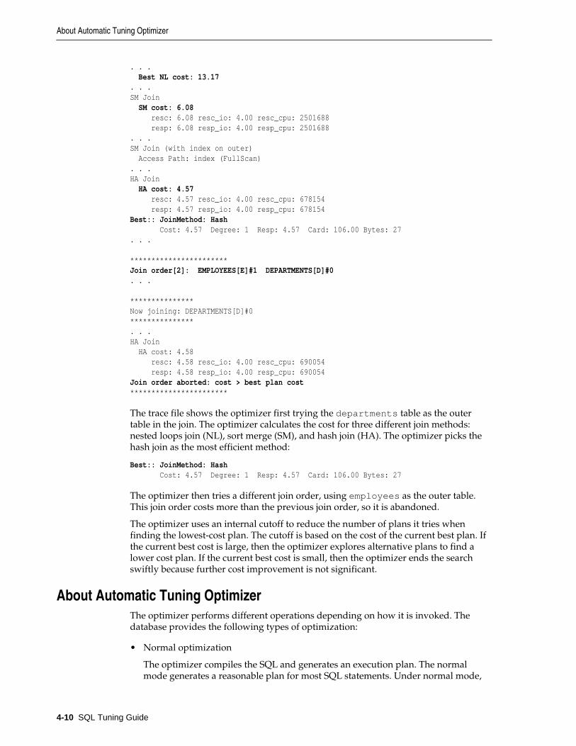
. . . Best NL cost: 13.17. . .SM Join SM cost: 6.08 resc: 6.08 resc_io: 4.00 resc_cpu: 2501688 resp: 6.08 resp_io: 4.00 resp_cpu: 2501688. . .SM Join (with index on outer) Access Path: index (FullScan). . .HA Join HA cost: 4.57 resc: 4.57 resc_io: 4.00 resc_cpu: 678154 resp: 4.57 resp_io: 4.00 resp_cpu: 678154Best:: JoinMethod: Hash Cost: 4.57 Degree: 1 Resp: 4.57 Card: 106.00 Bytes: 27. . .
***********************Join order[2]: EMPLOYEES[E]#1 DEPARTMENTS[D]#0. . . ***************Now joining: DEPARTMENTS[D]#0***************. . .HA Join HA cost: 4.58 resc: 4.58 resc_io: 4.00 resc_cpu: 690054 resp: 4.58 resp_io: 4.00 resp_cpu: 690054Join order aborted: cost > best plan cost***********************
The trace file shows the optimizer first trying the departments table as the outertable in the join. The optimizer calculates the cost for three different join methods:nested loops join (NL), sort merge (SM), and hash join (HA). The optimizer picks thehash join as the most efficient method:
Best:: JoinMethod: Hash Cost: 4.57 Degree: 1 Resp: 4.57 Card: 106.00 Bytes: 27
The optimizer then tries a different join order, using employees as the outer table.This join order costs more than the previous join order, so it is abandoned.
The optimizer uses an internal cutoff to reduce the number of plans it tries whenfinding the lowest-cost plan. The cutoff is based on the cost of the current best plan. Ifthe current best cost is large, then the optimizer explores alternative plans to find alower cost plan. If the current best cost is small, then the optimizer ends the searchswiftly because further cost improvement is not significant.
About Automatic Tuning OptimizerThe optimizer performs different operations depending on how it is invoked. Thedatabase provides the following types of optimization:
• Normal optimization
The optimizer compiles the SQL and generates an execution plan. The normalmode generates a reasonable plan for most SQL statements. Under normal mode,
About Automatic Tuning Optimizer
4-10 SQL Tuning Guide

the optimizer operates with strict time constraints, usually a fraction of a second,during which it must find an optimal plan.
• SQL Tuning Advisor optimization
When SQL Tuning Advisor invokes the optimizer, the optimizer is known as Automatic Tuning Optimizer. In this case, the optimizer performs additionalanalysis to further improve the plan produced in normal mode. The optimizeroutput is not an execution plan, but a series of actions, along with their rationaleand expected benefit for producing a significantly better plan.
See Also:
Analyzing SQL with SQL Tuning Advisor
About Adaptive Query OptimizationIn Oracle Database, adaptive query optimization is a set of capabilities that enablesthe optimizer to make run-time adjustments to execution plans and discoveradditional information that can lead to better statistics. Adaptive optimization ishelpful when existing statistics are not sufficient to generate an optimal plan.
The following graphic shows the feature set for adaptive query optimization:
Adaptive PlansAn adaptive plan enables the optimizer to defer the final plan decision for a statementuntil execution time.
See Also:
• “Introduction to Optimizer Statistics”
• “About SQL Tuning Advisor”
• “About SQL Plan Management”
About Adaptive Query Optimization
Query Optimizer Concepts 4-11

Purpose of Adaptive Plans
The ability of the optimizer to adapt a plan, based on information learned duringexecution, can greatly improve query performance. Adaptive plans are useful becausethe optimizer occasionally picks a suboptimal default plan because of a cardinalitymisestimate. The ability to adapt the plan at run time based on actual executionstatistics results in a more optimal final plan. After choosing the final plan, theoptimizer uses it for subsequent executions, thus ensuring that the suboptimal plan isnot reused.
How Adaptive Plans Work
An adaptive plan contains multiple predetermined subplans, and an optimizerstatistics collector. A subplan is a portion of a plan that the optimizer can switch to asan alternative at run time. For example, a nested loops join could be switched to a hashjoin during execution. An optimizer statistics collector is a row source inserted into aplan at key points to collect run-time statistics. These statistics help the optimizermake a final decision between multiple subplans.
During statement execution, the statistics collector gathers information about theexecution, and buffers some rows received by the subplan. Based on the informationobserved by the collector, the optimizer chooses a subplan. At this point, the collectorstops collecting statistics and buffering rows, and permits rows to pass throughinstead. On subsequent executions of the child cursor, the optimizer continues to usethe same plan unless the plan ages out of the cache, or a different optimizer feature(for example, adaptive cursor sharing or statistics feedback) invalidates the plan.
The database uses adaptive plans when OPTIMIZER_FEATURES_ENABLE is12.1.0.1 or later, and the OPTIMIZER_ADAPTIVE_REPORTING_ONLY initializationparameter is set to the default of false (see “Controlling Adaptive Optimization”).
Adaptive Plans: Join Method Example
The following query shows a join of the order_items and product_informationtables.
SELECT product_name FROM order_items o, product_information p WHERE o.unit_price = 15 AND quantity > 1 AND p.product_id = o.product_id
An adaptive plan for this statement shows two possible plans, one with a nested loopsjoin and the other with a hash join.
------------------------------------------------------------------------------------------------|Id | Operation | Name |Starts|E-Rows|A-Rows|A-Time|Buff|Reads|OMem|1Mem|O/1/M|------------------------------------------------------------------------------------------------| 0| SELECT STATEMENT | |1| | 13|00:00:00.10 |21 |17 | | | ||*1| HASH JOIN | |1|4| 13|00:00:00.10 |21 |17 | 2061K| 2061K|1/0/0||*2| TABLE ACCESS FULL| ORDER_ITEMS |1|4| 13|00:00:00.07 | 5 | 4 | | | || 3| TABLE ACCESS FULL| PRODUCT_INFORMATION |1|1|288|00:00:00.03 |16 |13 | | | |------------------------------------------------------------------------------------------------ Predicate Information (identified by operation id):--------------------------------------------------- 1 - access("P"."PRODUCT_ID"="O"."PRODUCT_ID") 2 - filter(("O"."UNIT_PRICE"=15 AND "QUANTITY">1))
About Adaptive Query Optimization
4-12 SQL Tuning Guide

PLAN_TABLE_OUTPUT------------------------------------------------------------------------------------------------Note----- - this is an adaptive plan
A nested loops join is preferable if the database can avoid scanning a significantportion of product_information because its rows are filtered by the join predicate.If few rows are filtered, however, then scanning the right table in a hash join ispreferable.
The following graphic shows the adaptive process. For the query in the precedingexample, the adaptive portion of the default plan contains two subplans, each ofwhich uses a different join method. The optimizer automatically determines wheneach join method is optimal, depending on the cardinality of the left side of the join.
The statistics collector buffers enough rows coming from the order_items table todetermine which join method to use. If the row count is below the thresholddetermined by the optimizer, then the optimizer chooses the nested loops join;otherwise, the optimizer chooses the hash join. In this case, the row count coming fromthe order_items table is above the threshold, so the optimizer chooses a hash joinfor the final plan, and disables buffering.
About Adaptive Query Optimization
Query Optimizer Concepts 4-13

NestedLoops
StatisticsCollector
Table scanorder_items
Index scanprod_info_ind
HashJoin
Table scanProd_info
Default plan is a nested loops join
The optimizer buffers rows coming from the order_items table up to a point. If the row count is less than the threshold, then use a nested loops join. Otherwise, switch to a hash join.
NestedLoops
StatisticsCollector
Table scanorder_items
Index scanprod_info_ind
HashJoin
Table scanProd_info
Final plan is a hash join
The optimizer disables the statistics collector after making the decision, and lets the rows pass through.
Threshold exceeded, so subplan switches
After the optimizer determines the final plan, DBMS_XPLAN.DISPLAY_CURSORdisplays the hash join. The Note section of the execution plan indicates whether theplan is adaptive, as shown in the following sample plan:
------------------------------------------------------------------------------------------------|Id| Operation | Name |Starts|E-Rows|A-Rows|A-Time |Buff|Reads|OMem|1Mem|O/1/M|------------------------------------------------------------------------------------------------| 0| SELECT STATEMENT | | 1| | 13 |00:00:00.10|21|17| | | ||*1| HASH JOIN | | 1| 4 | 13 |00:00:00.10|21|17|2061K|2061K|1/0/0||*2| TABLE ACCESS FULL| ORDER_ITEMS | 1| 4 | 13 |00:00:00.07| 5| 4| | | || 3| TABLE ACCESS FULL| PRODUCT_INFORMATION | 1| 1 | 288 |00:00:00.03|16|13| | | |------------------------------------------------------------------------------------------------ Predicate Information (identified by operation id):--------------------------------------------------- 1 - access("P"."PRODUCT_ID"="O"."PRODUCT_ID") 2 - filter(("O"."UNIT_PRICE"=15 AND "QUANTITY">1)) PLAN_TABLE_OUTPUT
About Adaptive Query Optimization
4-14 SQL Tuning Guide
----------------------------------------------------------------------------------------------Note----- - this is an adaptive plan
See Also:
• “Controlling Adaptive Optimization”
• “Reading Execution Plans: Advanced” for an extended example showingan adaptive plan
Adaptive Plans: Parallel Distribution Methods
Typically, parallel execution requires data redistribution to perform operations such asparallel sorts, aggregations, and joins. Oracle Database can use many different datadistributions methods. The database chooses the method based on the number of rowsto be distributed and the number of parallel server processes in the operation.
For example, consider the following alternative cases:
• Many parallel server processes distribute few rows.
The database may choose the broadcast distribution method. In this case, each rowin the result set is sent to each of the parallel server processes.
• Few parallel server processes distribute many rows.
If a data skew is encountered during the data redistribution, then it couldadversely effect the performance of the statement. The database is more likely topick a hash distribution to ensure that each parallel server process receives anequal number of rows.
The hybrid hash distribution technique is an adaptive parallel data distribution thatdoes not decide the final data distribution method until execution time. The optimizerinserts statistic collectors in front of the parallel server processes on the producer sideof the operation. If the actual number of rows is less than a threshold, defined as twicethe degree of parallelism (DOP) chosen for the operation, then the data distributionmethod switches from hash to broadcast. Otherwise, the distribution method is a hash.
Figure 4-6 depicts a hybrid hash join between the departments and employeestables, with a query coordinator directing 8 PX server processes. A statistics collector isinserted in front of the parallel server processes scanning the departments table. Thedistribution method is based on the run-time statistics. In the example shown in Figure 4-6, the number of rows is below the threshold (8), which is twice the DOP (4),so the optimizer chooses a broadcast technique for the departments table.
About Adaptive Query Optimization
Query Optimizer Concepts 4-15

Figure 4-6 Adaptive Parallel Query
departments employees
P1 P2 P3 P4
P5
P6
P7
P8
Statistics collector threshold is 2X the DOP
The number of rows returned is below threshold, so optimizer chooses broadcast method.
QueryCoordinator
Contrast the broadcast distribution example in Figure 4-6 with an example that returnsa greater number of rows. In the following plan, the threshold is 8, or twice thespecified DOP of 4. However, because the statistics collector (Step 10) discovers thatthe number of rows (27) is greater than the threshold (8), the optimizer chooses ahybrid hash distribution rather than a broadcast distribution. (The time columnshould show 00:00:01, but shows 0:01 so the plan can fit the page.)
EXPLAIN PLAN FOR SELECT /*+ parallel(4) full(e) full(d) */ department_name, sum(salary) FROM employees e, departments d WHERE d.department_id=e.department_id GROUP BY department_name;
Plan hash value: 2940813933-----------------------------------------------------------------------------------------------|Id|Operation | Name |Rows|Bytes|Cost |Time| TQ |IN-OUT|PQ Distrib|-----------------------------------------------------------------------------------------------| 0|SELECT STATEMENT |DEPARTMENTS| 27|621 |6(34)|0:01| | | || 1| PX COORDINATOR | | | | | | | | || 2| PX SEND QC (RANDOM) | :TQ10003 | 27|621 |6(34)|0:01|Q1,03|P->S| QC (RAND) || 3| HASH GROUP BY | | 27|621 |6(34)|0:01|Q1,03|PCWP| || 4| PX RECEIVE | | 27|621 |6(34)|0:01|Q1,03|PCWP| || 5| PX SEND HASH | :TQ10002 | 27|621 |6(34)|0:01|Q1,02|P->P| HASH || 6| HASH GROUP BY | | 27|621 |6(34)|0:01|Q1,02|PCWP| ||*7| HASH JOIN | |106|2438|5(20)|0:01|Q1,02|PCWP| || 8| PX RECEIVE | | 27|432 |2 (0)|0:01|Q1,02|PCWP| || 9| PX SEND HYBRID HASH | :TQ10000 | 27|432 |2 (0)|0:01|Q1,00|P->P|HYBRID HASH||10| STATISTICS COLLECTOR | | | | | |Q1,00|PCWC| ||11| PX BLOCK ITERATOR | | 27|432 |2 (0)|0:01|Q1,00|PCWC| ||12| TABLE ACCESS FULL |DEPARTMENTS| 27|432 |2 (0)|0:01|Q1,00|PCWP| ||13| PX RECEIVE | |107|749 |2 (0)|0:01|Q1,02|PCWP| |
About Adaptive Query Optimization
4-16 SQL Tuning Guide

|14| PX SEND HYBRID HASH (SKEW)| :TQ10001 |107|749 |2 (0)|0:01|Q1,01|P->P|HYBRID HASH||15| PX BLOCK ITERATOR | |107|749 |2 (0)|0:01|Q1,01|PCWC| ||16| TABLE ACCESS FULL |EMPLOYEES |107|749 |2 (0)|0:01|Q1,01|PCWP| |-----------------------------------------------------------------------------------------------
Predicate Information (identified by operation id):---------------------------------------------------
7 - access("D"."DEPARTMENT_ID"="E"."DEPARTMENT_ID")
Note----- - Degree of Parallelism is 4 because of hint
32 rows selected.
See Also:
Oracle Database VLDB and Partitioning Guide to learn more about parallel dataredistribution techniques
Adaptive StatisticsThe quality of the plans that the optimizer generates depends on the quality of thestatistics. Some query predicates become too complex to rely on base table statisticsalone, so the optimizer augments these statistics with adaptive statistics.
The following topics describe types of adaptive statistics:
• Dynamic Statistics
• Automatic Reoptimization
• SQL Plan Directives
Dynamic Statistics
During the compilation of a SQL statement, the optimizer decides whether to usedynamic statistics by considering whether the available statistics are sufficient togenerate an optimal execution plan. If the available statistics are insufficient, then theoptimizer uses dynamic statistics to augment the statistics. One type of dynamicstatistics is the information gathered by dynamic sampling. The optimizer can usedynamic statistics for table scans, index access, joins, and GROUP BY operations, thusimproving the quality of optimizer decisions.
See Also:
“Dynamic Statistics” to learn more about dynamic statistics and optimizerstatistics in general
Automatic Reoptimization
Whereas adaptive plans help decide between multiple subplans, they are not feasiblefor all kinds of plan changes. For example, a query with an inefficient join order mightperform suboptimally, but adaptive plans do not support adapting the join orderduring execution. In these cases, the optimizer considers automatic reoptimization. In
About Adaptive Query Optimization
Query Optimizer Concepts 4-17

contrast to adaptive plans, automatic reoptimization changes a plan on subsequentexecutions after the initial execution.
At the end of the first execution of a SQL statement, the optimizer uses the informationgathered during execution to determine whether automatic reoptimization isworthwhile. If execution informations differs significantly from optimizer estimates,then the optimizer looks for a replacement plan on the next execution. The optimizeruses the information gathered during the previous execution to help determine analternative plan. The optimizer can reoptimize a query several times, each timelearning more and further improving the plan.
See Also:
“Controlling Adaptive Optimization”
Reoptimization: Statistics Feedback
A form of reoptimization known as statistics feedback (formerly known as cardinalityfeedback) automatically improves plans for repeated queries that have cardinalitymisestimates. The optimizer can estimate cardinalities incorrectly for many reasons,such as missing statistics, inaccurate statistics, or complex predicates.
The basic process of reoptimization using statistics feedback is as follows:
1. During the first execution of a SQL statement, the optimizer generates anexecution plan.
The optimizer may enable monitoring for statistics feedback for the shared SQLarea in the following cases:
• Tables with no statistics
• Multiple conjunctive or disjunctive filter predicates on a table
• Predicates containing complex operators for which the optimizer cannotaccurately compute selectivity estimates
At the end of execution, the optimizer compares its initial cardinality estimates tothe actual number of rows returned by each operation in the plan duringexecution. If estimates differ significantly from actual cardinalities, then theoptimizer stores the correct estimates for subsequent use. The optimizer alsocreates a SQL plan directive so that other SQL statements can benefit from theinformation obtained during this initial execution.
2. After the first execution, the optimizer disables monitoring for statistics feedback.
3. If the query executes again, then the optimizer uses the corrected cardinalityestimates instead of its usual estimates.
Example 4-2 Statistics Feedback
This example shows how the database uses statistics feedback to adjust incorrectestimates.
1. The user oe runs the following query of the orders, order_items, andproduct_information tables:
SELECT o.order_id, v.product_nameFROM orders o, ( SELECT order_id, product_name
About Adaptive Query Optimization
4-18 SQL Tuning Guide

FROM order_items o, product_information p WHERE p.product_id = o.product_id AND list_price < 50 AND min_price < 40 ) vWHERE o.order_id = v.order_id
2. Querying the plan in the cursor shows that the estimated rows (E-Rows) is farfewer than the actual rows (A-Rows).
3. The user oe reruns the following query of the orders, order_items, andproduct_information tables:
SELECT o.order_id, v.product_nameFROM orders o, ( SELECT order_id, product_name FROM order_items o, product_information p WHERE p.product_id = o.product_id AND list_price < 50 AND min_price < 40 ) vWHERE o.order_id = v.order_id;
4. Querying the plan in the cursor shows that the optimizer used statistics feedback(shown in the Note) for the second execution, and also chose a different plan.
In the preceding output, the estimated number of rows (269) matches the actualnumber of rows.
Reoptimization: Performance Feedback
Another form of reoptimization is performance feedback. This reoptimization helpsimprove the degree of parallelism automatically chosen for repeated SQL statementswhen PARALLEL_DEGREE_POLICY is set to ADAPTIVE.
The basic process of reoptimization using performance feedback is as follows:
1. During the first execution of a SQL statement, when PARALLEL_DEGREE_POLICYis set to ADAPTIVE, the optimizer determines whether to execute the statement inparallel, and if so, which degree of parallelism to use.
The optimizer chooses the degree of parallelism based on the estimatedperformance of the statement. Additional performance monitoring is enabled forall statements.
2. At the end of the initial execution, the optimizer compares the following:
• The degree of parallelism chosen by the optimizer
• The degree of parallelism computed based on the performance statistics (forexample, the CPU time) gathered during the actual execution of the statement
If the two values vary significantly, then the database marks the statement forreparsing, and stores the initial execution statistics as feedback. This feedbackhelps better compute the degree of parallelism for subsequent executions.
3. If the query executes again, then the optimizer uses the performance statisticsgathered during the initial execution to better determine a degree of parallelismfor the statement.
About Adaptive Query Optimization
Query Optimizer Concepts 4-19
Note:
Even if PARALLEL_DEGREE_POLICY is not set to ADAPTIVE, statisticsfeedback may influence the degree of parallelism chosen for a statement.
SQL Plan Directives
A SQL plan directive is additional information that the optimizer uses to generate amore optimal plan. For example, during query optimization, when deciding whetherthe table is a candidate for dynamic statistics, the database queries the statisticsrepository for directives on a table. If the query joins two tables that have a data skewin their join columns, a SQL plan directive can direct the optimizer to use dynamicstatistics to obtain an accurate cardinality estimate.The optimizer collects SQL plandirectives on query expressions rather than at the statement level. In this way, theoptimizer can apply directives to multiple SQL statements. The database automaticallymaintains directives, and stores them in the SYSAUX tablespace. You can managedirectives using the package DBMS_SPD.
See Also:
• “SQL Plan Directives”
• “Managing SQL Plan Directives”
• Oracle Database PL/SQL Packages and Types Reference to learn about theDBMS_SPD package
About Optimizer Management of SQL Plan BaselinesSQL plan management is a mechanism that enables the optimizer to automaticallymanage execution plans, ensuring that the database uses only known or verified plans(see Managing SQL Plan Baselines ). This mechanism can build a SQL plan baseline,which contains one or more accepted plans for each SQL statement.
The optimizer can access and manage the plan history and SQL plan baselines of SQLstatements. This capability is central to the SQL plan management architecture. In SQLplan management, the optimizer has the following main objectives:
• Identify repeatable SQL statements
• Maintain plan history, and possibly SQL plan baselines, for a set of SQL statements
• Detect plans that are not in the plan history
• Detect potentially better plans that are not in the SQL plan baseline
The optimizer uses the normal cost-based search method.
See Also:
Managing SQL Plan Baselines
About Optimizer Management of SQL Plan Baselines
4-20 SQL Tuning Guide

5Query Transformations
As explained in “Query Transformer,” the optimizer employs several querytransformation techniques. This chapter contains the following topics:
• OR Expansion
• View Merging
• Predicate Pushing
• Subquery Unnesting
• Query Rewrite with Materialized Views
• Star Transformation
• In-Memory Aggregation
• Table Expansion
• Join Factorization
OR ExpansionIn OR expansion, the optimizer transforms a query with a WHERE clause containing ORoperators into a query that uses the UNION ALL operator. The database can performOR expansion for various reasons. For example, it may enable more efficient accesspaths or alternative join methods that avoid Cartesian products. As always, theoptimizer performs the expansion only if the cost of the transformed statement islower than the cost of the original statement.
In the following example, user sh creates a concatenated index on thesales.prod_id and sales.promo_idcolumns, and then queries the sales tableusing an OR condition:
CREATE INDEX sales_prod_promo_ind ON sales(prod_id, promo_id);
SELECT *FROM salesWHERE promo_id=33 OR prod_id=136;
In the preceding query, because the promo_id=33 and prod_id=136 conditionscould each take advantage of an index access path, the optimizer transforms thestatement into the query shown in Example 5-1.
Query Transformations 5-1

Example 5-1 Transformed Query: UNION ALL Condition
For the query transformation in this example, the optimizer selects an execution planthat accesses the sales table using the index, and then assembles the result. The planis shown in Example 5-2.
SELECT *FROM salesWHERE prod_id=136UNION ALLSELECT *FROM salesWHERE promo_id=33AND LNNVL(prod_id=136);
Example 5-2 Execution Plan for Query of sales
--------------------------------------------------------------------------------| Id| Operation | Name | Rows|--------------------------------------------------------------------------------| 0 | SELECT STATEMENT | | || 1 | CONCATENATION | | || 2 | TABLE ACCESS BY GLOBAL INDEX ROWID BATCHED| SALES | 710 || 3 | INDEX RANGE SCAN | SALES_PROD_PROMO_IND | 710 || 4 | PARTITION RANGE ALL | | 229K|| 5 | TABLE ACCESS FULL | SALES | 229K|--------------------------------------------------------------------------------
View MergingIn view merging, the optimizer merges the query block representing a view into thequery block that contains it. View merging can improve plans by enabling theoptimizer to consider additional join orders, access methods, and othertransformations.
For example, after a view has been merged and several tables reside in one queryblock, a table inside a view may permit the optimizer to use join elimination toremove a table outside the view. For certain simple views in which merging alwaysleads to a better plan, the optimizer automatically merges the view withoutconsidering cost. Otherwise, the optimizer uses cost to make the determination. Theoptimizer may choose not to merge a view for many reasons, including cost or validityrestrictions.
If OPTIMIZER_SECURE_VIEW_MERGING is true (default), then Oracle Databaseperforms checks to ensure that view merging and predicate pushing do not violate thesecurity intentions of the view creator. To disable these additional security checks for aspecific view, you can grant the MERGE VIEW privilege to a user for this view. Todisable additional security checks for all views for a specific user, you can grant theMERGE ANY VIEW privilege to that user.
Note:
You can use hints to override view merging rejected because of cost orheuristics, but not validity.
This section contains the following topics:
• Query Blocks in View Merging
View Merging
5-2 SQL Tuning Guide

• Simple View Merging
• Complex View Merging
See Also:
• Oracle Database SQL Language Reference for more information about theMERGE ANY VIEW and MERGE VIEW privileges
• Oracle Database Reference for more information about theOPTIMIZER_SECURE_VIEW_MERGING initialization parameter
Query Blocks in View MergingThe optimizer represents each nested subquery or unmerged view by a separatequery block. The database optimizes query blocks separately from the bottom up.Thus, the database optimizes the innermost query block first, generates the part of theplan for it, and then generates the plan for the outer query block, representing theentire query.
The parser expands each view referenced in a query into a separate query block. Theblock essentially represents the view definition, and thus the result of a view. Oneoption for the optimizer is to analyze the view query block separately, generate a viewsubplan, and then process the rest of the query by using the view subplan to generatean overall execution plan. However, this technique may lead to a suboptimalexecution plan because the view is optimized separately.
View merging can sometimes improve performance. As shown in Example 5-3, viewmerging merges the tables from the view into the outer query block, removing theinner query block. Thus, separate optimization of the view is not necessary.
Simple View MergingIn simple view merging, the optimizer merges select-project-join views. For example,a query of the employees table contains a subquery that joins the departments andlocations tables.
Simple view merging frequently results in a more optimal plan because of theadditional join orders and access paths available after the merge. A view may not bevalid for simple view merging because:
• The view contains constructs not included in select-project-join views, including:
– GROUP BY
– DISTINCT
– Outer join
– MODEL
– CONNECT BY
– Set operators
– Aggregation
View Merging
Query Transformations 5-3

• The view appears on the right side of a semijoin or antijoin.
• The view contains subqueries in the SELECT list.
• The outer query block contains PL/SQL functions.
• The view participates in an outer join, and does not meet one of the severaladditional validity requirements that determine whether the view can be merged.
Example 5-3 Simple View Merging
The following query joins the hr.employees table with the dept_locs_v view,which returns the street address for each department. dept_locs_v is a join of thedepartments and locations tables.
SELECT e.first_name, e.last_name, dept_locs_v.street_address, dept_locs_v.postal_codeFROM employees e, ( SELECT d.department_id, d.department_name, l.street_address, l.postal_code FROM departments d, locations l WHERE d.location_id = l.location_id ) dept_locs_vWHERE dept_locs_v.department_id = e.department_idAND e.last_name = 'Smith';
The database can execute the preceding query by joining departments andlocations to generate the rows of the view, and then joining this result toemployees. Because the query contains the view dept_locs_v, and this viewcontains two tables, the optimizer must use one of the following join orders:
• employees, dept_locs_v (departments, locations)
• employees, dept_locs_v (locations, departments)
• dept_locs_v (departments, locations), employees
• dept_locs_v (locations, departments), employees
Join methods are also constrained. The index-based nested loops join is not feasible forjoin orders that begin with employees because no index exists on the column fromthis view. Without view merging, the optimizer generates the following executionplan:
-----------------------------------------------------------------| Id | Operation | Name | Cost (%CPU)|-----------------------------------------------------------------| 0 | SELECT STATEMENT | | 7 (15)||* 1 | HASH JOIN | | 7 (15)|| 2 | TABLE ACCESS BY INDEX ROWID| EMPLOYEES | 2 (0)||* 3 | INDEX RANGE SCAN | EMP_NAME_IX | 1 (0)|| 4 | VIEW | | 5 (20)||* 5 | HASH JOIN | | 5 (20)|| 6 | TABLE ACCESS FULL | LOCATIONS | 2 (0)|| 7 | TABLE ACCESS FULL | DEPARTMENTS | 2 (0)|----------------------------------------------------------------- Predicate Information (identified by operation id):---------------------------------------------------1 - access("DEPT_LOCS_V"."DEPARTMENT_ID"="E"."DEPARTMENT_ID")3 - access("E"."LAST_NAME"='Smith')5 - access("D"."LOCATION_ID"="L"."LOCATION_ID")
View Merging
5-4 SQL Tuning Guide

View merging merges the tables from the view into the outer query block, removingthe inner query block. After view merging, the query is as follows:
SELECT e.first_name, e.last_name, l.street_address, l.postal_codeFROM employees e, departments d, locations lWHERE d.location_id = l.location_idAND d.department_id = e.department_idAND e.last_name = 'Smith';
Because all three tables appear in one query block, the optimizer can choose from thefollowing six join orders:
• employees, departments, locations
• employees, locations, departments
• departments, employees, locations
• departments, locations, employees
• locations, employees, departments
• locations, departments, employees
The joins to employees and departments can now be index-based. After viewmerging, the optimizer chooses the following more efficient plan, which uses nestedloops:
-------------------------------------------------------------------| Id | Operation | Name | Cost (%CPU)|-------------------------------------------------------------------| 0 | SELECT STATEMENT | | 4 (0)|| 1 | NESTED LOOPS | | || 2 | NESTED LOOPS | | 4 (0)|| 3 | NESTED LOOPS | | 3 (0)|| 4 | TABLE ACCESS BY INDEX ROWID| EMPLOYEES | 2 (0)||* 5 | INDEX RANGE SCAN | EMP_NAME_IX | 1 (0)|| 6 | TABLE ACCESS BY INDEX ROWID| DEPARTMENTS | 1 (0)||* 7 | INDEX UNIQUE SCAN | DEPT_ID_PK | 0 (0)||* 8 | INDEX UNIQUE SCAN | LOC_ID_PK | 0 (0)|| 9 | TABLE ACCESS BY INDEX ROWID | LOCATIONS | 1 (0)|------------------------------------------------------------------- Predicate Information (identified by operation id):--------------------------------------------------- 5 - access("E"."LAST_NAME"='Smith') 7 - access("E"."DEPARTMENT_ID"="D"."DEPARTMENT_ID") 8 - access("D"."LOCATION_ID"="L"."LOCATION_ID")
See Also:
The Oracle Optimizer blog at https://blogs.oracle.com/optimizer/to learn about outer join view merging, which is a special case of simple viewmerging
View Merging
Query Transformations 5-5

Complex View MergingIn complex view merging, the optimizer merges views containing GROUP BY andDISTINCT views. Like simple view merging, complex merging enables the optimizerto consider additional join orders and access paths.
The optimizer can delay evaluation of GROUP BY or DISTINCT operations until afterit has evaluated the joins. Delaying these operations can improve or worsenperformance depending on the data characteristics. If the joins use filters, thendelaying the operation until after joins can reduce the data set on which the operationis to be performed. Evaluating the operation early can reduce the amount of data to beprocessed by subsequent joins, or the joins could increase the amount of data to beprocessed by the operation. The optimizer uses cost to evaluate view merging andmerges the view only when it is the lower cost option.
Aside from cost, the optimizer may be unable to perform complex view merging forthe following reasons:
• The outer query tables do not have a rowid or unique column.
• The view appears in a CONNECT BY query block.
• The view contains GROUPING SETS, ROLLUP, or PIVOT clauses.
• The view or outer query block contains the MODEL clause.
Example 5-4 Complex View Joins with GROUP BY
The following view uses a GROUP BY clause:
CREATE VIEW cust_prod_totals_v ASSELECT SUM(s.quantity_sold) total, s.cust_id, s.prod_idFROM sales sGROUP BY s.cust_id, s.prod_id;
The following query finds all of the customers from the United States who havebought at least 100 fur-trimmed sweaters:
SELECT c.cust_id, c.cust_first_name, c.cust_last_name, c.cust_emailFROM customers c, products p, cust_prod_totals_vWHERE c.country_id = 52790AND c.cust_id = cust_prod_totals_v.cust_idAND cust_prod_totals_v.total > 100AND cust_prod_totals_v.prod_id = p.prod_idAND p.prod_name = 'T3 Faux Fur-Trimmed Sweater';
The cust_prod_totals_v view is eligible for complex view merging. Aftermerging, the query is as follows:
SELECT c.cust_id, cust_first_name, cust_last_name, cust_emailFROM customers c, products p, sales sWHERE c.country_id = 52790AND c.cust_id = s.cust_idAND s.prod_id = p.prod_idAND p.prod_name = 'T3 Faux Fur-Trimmed Sweater'GROUP BY s.cust_id, s.prod_id, p.rowid, c.rowid, c.cust_email, c.cust_last_name, c.cust_first_name, c.cust_idHAVING SUM(s.quantity_sold) > 100;
The transformed query is cheaper than the untransformed query, so the optimizerchooses to merge the view. In the untransformed query, the GROUP BY operator
View Merging
5-6 SQL Tuning Guide

applies to the entire sales table in the view. In the transformed query, the joins toproducts and customers filter out a large portion of the rows from the sales table,so the GROUP BY operation is lower cost. The join is more expensive because thesales table has not been reduced, but it is not much more expensive because theGROUP BY operation does not reduce the size of the row set very much in the originalquery. If any of the preceding characteristics were to change, merging the view mightno longer be lower cost. The final plan, which does not include a view, is as follows:
--------------------------------------------------------| Id | Operation | Name | Cost (%CPU)|--------------------------------------------------------| 0 | SELECT STATEMENT | | 2101 (18)||* 1 | FILTER | | || 2 | HASH GROUP BY | | 2101 (18)||* 3 | HASH JOIN | | 2099 (18)||* 4 | HASH JOIN | | 1801 (19)||* 5 | TABLE ACCESS FULL| PRODUCTS | 96 (5)|| 6 | TABLE ACCESS FULL| SALES | 1620 (15)||* 7 | TABLE ACCESS FULL | CUSTOMERS | 296 (11)|--------------------------------------------------------Predicate Information (identified by operation id):---------------------------------------------------1 - filter(SUM("QUANTITY_SOLD")>100)3 - access("C"."CUST_ID"="CUST_ID")4 - access("PROD_ID"="P"."PROD_ID")5 - filter("P"."PROD_NAME"='T3 Faux Fur-Trimmed Sweater')7 - filter("C"."COUNTRY_ID"='US')
Example 5-5 Complex View Joins with DISTINCT
The following query of the cust_prod_v view uses a DISTINCT operator:
SELECT c.cust_id, c.cust_first_name, c.cust_last_name, c.cust_emailFROM customers c, products p, ( SELECT DISTINCT s.cust_id, s.prod_id FROM sales s) cust_prod_vWHERE c.country_id = 52790AND c.cust_id = cust_prod_v.cust_idAND cust_prod_v.prod_id = p.prod_idAND p.prod_name = 'T3 Faux Fur-Trimmed Sweater';
After determining that view merging produces a lower-cost plan, the optimizerrewrites the query into this equivalent query:
SELECT nwvw.cust_id, nwvw.cust_first_name, nwvw.cust_last_name, nwvw.cust_emailFROM ( SELECT DISTINCT(c.rowid), p.rowid, s.prod_id, s.cust_id, c.cust_first_name, c.cust_last_name, c.cust_email FROM customers c, products p, sales s WHERE c.country_id = 52790 AND c.cust_id = s.cust_id AND s.prod_id = p.prod_id AND p.prod_name = 'T3 Faux Fur-Trimmed Sweater' ) nwvw;
The plan for the preceding query is as follows:
-------------------------------------------| Id | Operation | Name |-------------------------------------------| 0 | SELECT STATEMENT | || 1 | VIEW | VM_NWVW_1 || 2 | HASH UNIQUE | ||* 3 | HASH JOIN | |
View Merging
Query Transformations 5-7

|* 4 | HASH JOIN | ||* 5 | TABLE ACCESS FULL| PRODUCTS || 6 | TABLE ACCESS FULL| SALES ||* 7 | TABLE ACCESS FULL | CUSTOMERS |------------------------------------------- Predicate Information (identified by operation id):--------------------------------------------------- 3 - access("C"."CUST_ID"="S"."CUST_ID") 4 - access("S"."PROD_ID"="P"."PROD_ID") 5 - filter("P"."PROD_NAME"='T3 Faux Fur-Trimmed Sweater') 7 - filter("C"."COUNTRY_ID"='US')
The preceding plan contains a view named vm_nwvw_1, known as a projection view,even after view merging has occurred. Projection views appear in queries in which aDISTINCT view has been merged, or a GROUP BY view is merged into an outer queryblock that also contains GROUP BY, HAVING, or aggregates. In the latter case, theprojection view contains the GROUP BY, HAVING, and aggregates from the originalouter query block.
In the preceding example of a projection view, when the optimizer merges the view, itmoves the DISTINCT operator to the outer query block, and then adds severaladditional columns to maintain semantic equivalence with the original query.Afterward, the query can select only the desired columns in the SELECT list of theouter query block. The optimization retains all of the benefits of view merging: alltables are in one query block, the optimizer can permute them as needed in the finaljoin order, and the DISTINCT operation has been delayed until after all of the joinscomplete.
Predicate PushingIn predicate pushing, the optimizer "pushes" the relevant predicates from thecontaining query block into the view query block. For views that are not merged, thistechnique improves the subplan of the unmerged view because the database can usethe pushed-in predicates to access indexes or to use as filters.
For example, suppose you create a table hr.contract_workers as follows:
DROP TABLE contract_workers;CREATE TABLE contract_workers AS (SELECT * FROM employees where 1=2);INSERT INTO contract_workers VALUES (306, 'Bill', 'Jones', 'BJONES', '555.555.2000', '07-JUN-02', 'AC_ACCOUNT', 8300, 0,205, 110);INSERT INTO contract_workers VALUES (406, 'Jill', 'Ashworth', 'JASHWORTH', '555.999.8181', '09-JUN-05', 'AC_ACCOUNT', 8300, 0,205, 50);INSERT INTO contract_workers VALUES (506, 'Marcie', 'Lunsford', 'MLUNSFORD', '555.888.2233', '22-JUL-01', 'AC_ACCOUNT', 8300, 0,205, 110);COMMIT;CREATE INDEX contract_workers_index ON contract_workers(department_id);
You create a view that references employees and contract_workers. The view isdefined with a query that uses the UNION set operator, as follows:
CREATE VIEW all_employees_vw AS ( SELECT employee_id, last_name, job_id, commission_pct, department_id FROM employees ) UNION ( SELECT employee_id, last_name, job_id, commission_pct, department_id FROM contract_workers );
You then query the view as follows:
Predicate Pushing
5-8 SQL Tuning Guide

SELECT last_nameFROM all_employees_vwWHERE department_id = 50;
Because the view is a UNION set query, the optimizer cannot merge the view's queryinto the accessing query block. Instead, the optimizer can transform the accessingstatement by pushing its predicate, the WHERE clause condition department_id=50,into the view's UNION set query. The equivalent transformed query is as follows:
SELECT last_nameFROM ( SELECT employee_id, last_name, job_id, commission_pct, department_id FROM employees WHERE department_id=50 UNION SELECT employee_id, last_name, job_id, commission_pct, department_id FROM contract_workers WHERE department_id=50 );
The transformed query can now consider index access in each of the query blocks.
Subquery UnnestingIn subquery unnesting, the optimizer transforms a nested query into an equivalentjoin statement, and then optimizes the join. This transformation enables the optimizerto consider the subquery tables during access path, join method, and join orderselection. The optimizer can perform this transformation only if the resulting joinstatement is guaranteed to return the same rows as the original statement, and ifsubqueries do not contain aggregate functions such as AVG.
For example, suppose you connect as user sh and execute the following query:
SELECT * FROM salesWHERE cust_id IN ( SELECT cust_id FROM customers );
Because the customers.cust_id column is a primary key, the optimizer cantransform the complex query into the following join statement that is guaranteed toreturn the same data:
SELECT sales.* FROM sales, customersWHERE sales.cust_id = customers.cust_id;
If the optimizer cannot transform a complex statement into a join statement, it selectsexecution plans for the parent statement and the subquery as though they wereseparate statements. The optimizer then executes the subquery and uses the rowsreturned to execute the parent query. To improve execution speed of the overallexecution plan, the optimizer orders the subplans efficiently.
Query Rewrite with Materialized ViewsA materialized view is like a query with a result that the database materializes andstores in a table. When the optimizer finds a user query compatible with the queryassociated with a materialized view, then the database can rewrite the query in termsof the materialized view. This technique improves query execution because thedatabase has precomputed most of the query result.
Subquery Unnesting
Query Transformations 5-9

The optimizer looks for any materialized views that are compatible with the userquery, and then selects one or more materialized views to rewrite the user query. Theuse of materialized views to rewrite a query is cost-based. That is, the optimizer doesnot rewrite the query when the plan generated without the materialized views has alower cost than the plan generated with the materialized views.
Consider the following materialized view, cal_month_sales_mv, which aggregatesthe dollar amount sold each month:
CREATE MATERIALIZED VIEW cal_month_sales_mv ENABLE QUERY REWRITE AS SELECT t.calendar_month_desc, SUM(s.amount_sold) AS dollars FROM sales s, times t WHERE s.time_id = t.time_id GROUP BY t.calendar_month_desc;
Assume that sales number is around one million in a typical month. The view has theprecomputed aggregates for the dollar amount sold for each month. Consider thefollowing query, which asks for the sum of the amount sold for each month:
SELECT t.calendar_month_desc, SUM(s.amount_sold)FROM sales s, times tWHERE s.time_id = t.time_idGROUP BY t.calendar_month_desc;
Without query rewrite, the database must access sales directly and compute the sumof the amount sold. This method involves reading many million rows from sales,which invariably increases query response time. The join also further slows queryresponse because the database must compute the join on several million rows. Withquery rewrite, the optimizer transparently rewrites the query as follows:
SELECT calendar_month, dollarsFROM cal_month_sales_mv;
See Also:
Oracle Database Data Warehousing Guide to learn more about query rewrite
Star TransformationStar transformation is an optimizer transformation that avoids full table scans of facttables in a star schema. This section contains the following topics:
• About Star Schemas
• Purpose of Star Transformations
• How Star Transformation Works
• Controls for Star Transformation
• Star Transformation: Scenario
• Temporary Table Transformation: Scenario
Star Transformation
5-10 SQL Tuning Guide

About Star SchemasA star schema divides data into facts and dimensions. Facts are the measurements ofan event such as a sale and are typically numbers. Dimensions are the categories thatidentify facts, such as date, location, and product.
A fact table has a composite key made up of the primary keys of the dimension tablesof the schema. Dimension tables act as lookup or reference tables that enable you tochoose values that constrain your queries.
Diagrams typically show a central fact table with lines joining it to the dimensiontables, giving the appearance of a star. Figure 5-1 shows sales as the fact table andproducts, times, customers, and channels as the dimension tables.
Figure 5-1 Star Schema
customers
products
Dimension Table Dimension Table
channels
sales (amount_sold, quantity_sold)
times
Fact Table
See Also:
Oracle Database Data Warehousing Guide to learn more about star schemas
Purpose of Star TransformationsIn joins of fact and dimension tables, a star transformation can avoid a full scan of afact table by fetching only relevant rows from the fact table that join to the constraintdimension rows. When queries contain restrictive filter predicates on other columns ofthe dimension tables, the combination of filters can dramatically reduce the data setthat the database processes from the fact table.
How Star Transformation WorksStar transformation adds subquery predicates, called bitmap semijoin predicates,corresponding to the constraint dimensions. The optimizer performs thetransformation when indexes exist on the fact join columns. By driving bitmap ANDand OR operations of key values supplied by the subqueries, the database only needsto retrieve relevant rows from the fact table. If the predicates on the dimension tablesfilter out significant data, then the transformation can be more efficient than a fulltable scan on the fact table.
After the database has retrieved the relevant rows from the fact table, the databasemay need to join these rows back to the dimension tables using the original predicates.The database can eliminate the join back of the dimension table when the followingconditions are met:
• All the predicates on dimension tables are part of the semijoin subquery predicate.
Star Transformation
Query Transformations 5-11

• The columns selected from the subquery are unique.
• The dimension columns are not in the SELECT list, GROUP BY clause, and so on.
Controls for Star TransformationThe STAR_TRANSFORMATION_ENABLED initialization parameter controls startransformations. This parameter takes the following values:
• true
The optimizer performs the star transformation by identifying the fact andconstraint dimension tables automatically. The optimizer performs the startransformation only if the cost of the transformed plan is lower than thealternatives. Also, the optimizer attempts temporary table transformationautomatically whenever materialization improves performance (see “TemporaryTable Transformation: Scenario”).
• false (default)
The optimizer does not perform star transformations.
• TEMP_DISABLE
This value is identical to true except that the optimizer does not attempttemporary table transformation.
See Also:
Oracle Database Reference to learn about theSTAR_TRANSFORMATION_ENABLED initialization parameter
Star Transformation: ScenarioThis scenario demonstrates a star transformation of a star query.
Example 5-6 Star Query
The following query finds the total Internet sales amount in all cities in California forquarters Q1 and Q2 of year 1999:
SELECT c.cust_city, t.calendar_quarter_desc, SUM(s.amount_sold) sales_amountFROM sales s, times t, customers c, channels chWHERE s.time_id = t.time_idAND s.cust_id = c.cust_idAND s.channel_id = ch.channel_idAND c.cust_state_province = 'CA'AND ch.channel_desc = 'Internet'AND t.calendar_quarter_desc IN ('1999-01','1999-02')GROUP BY c.cust_city, t.calendar_quarter_desc;
Sample output is as follows:
CUST_CITY CALENDA SALES_AMOUNT------------------------------ ------- ------------
Star Transformation
5-12 SQL Tuning Guide

Montara 1999-02 1618.01Pala 1999-01 3263.93Cloverdale 1999-01 52.64Cloverdale 1999-02 266.28. . .
In this example, sales is the fact table, and the other tables are dimension tables. Thesales table contains one row for every sale of a product, so it could conceivablycontain billions of sales records. However, only a few products are sold to customersin California through the Internet for the specified quarters.
Example 5-7 Star Transformation
This example shows a star transformation of the query in Example 5-6. Thetransformation avoids a full table scan of sales.
SELECT c.cust_city, t.calendar_quarter_desc, SUM(s.amount_sold) sales_amountFROM sales s, times t, customers cWHERE s.time_id = t.time_idAND s.cust_id = c.cust_idAND c.cust_state_province = 'CA'AND t.calendar_quarter_desc IN ('1999-01','1999-02')AND s.time_id IN ( SELECT time_id FROM times WHERE calendar_quarter_desc IN('1999-01','1999-02') )AND s.cust_id IN ( SELECT cust_id FROM customers WHERE cust_state_province='CA' )AND s.channel_id IN ( SELECT channel_id FROM channels WHERE channel_desc = 'Internet' )GROUP BY c.cust_city, t.calendar_quarter_desc;
Example 5-8 Partial Execution Plan for Star Transformation
This example shows an edited version of the execution plan for the star transformationin Example 5-7.
Line 26 shows that the sales table has an index access path instead of a full tablescan. For each key value that results from the subqueries of channels (line 14),times (line 19), and customers (line 24), the database retrieves a bitmap from theindexes on the sales fact table (lines 15, 20, 25).
Each bit in the bitmap corresponds to a row in the fact table. The bit is set when thekey value from the subquery is same as the value in the row of the fact table. Forexample, in the bitmap 101000... (the ellipses indicates that the values for theremaining rows are 0), rows 1 and 3 of the fact table have matching key values fromthe subquery.
The operations in lines 12, 17, and 22 iterate over the keys from the subqueries andretrieve the corresponding bitmaps. In Example 5-7, the customers subquery seeksthe IDs of customers whose state or province is CA. Assume that the bitmap101000... corresponds to the customer ID key value 103515 from the customerstable subquery. Also assume that the customers subquery produces the key value103516 with the bitmap 010000..., which means that only row 2 in sales has amatching key value from the subquery.
The database merges (using the OR operator) the bitmaps for each subquery (lines 11,16, 21). In our customers example, the database produces a single bitmap111000... for the customers subquery after merging the two bitmaps:
Star Transformation
Query Transformations 5-13

101000... # bitmap corresponding to key 103515010000... # bitmap corresponding to key 103516---------111000... # result of OR operation
In line 10, the database applies the AND operator to the merged bitmaps. Assume thatafter the database has performed all OR operations, the resulting bitmap for channelsis 100000... If the database performs an AND operation on this bitmap and thebitmap from customers subquery, then the result is as follows:
100000... # channels bitmap after all OR operations performed111000... # customers bitmap after all OR operations performed---------100000... # bitmap result of AND operation for channels and customers
In line 9, the database generates the corresponding rowids of the final bitmap. Thedatabase retrieves rows from the sales fact table using the rowids (line 26). In ourexample, the database generate only one rowid, which corresponds to the first row,and thus fetches only a single row instead of scanning the entire sales table.
-------------------------------------------------------------------------------| Id | Operation | Name-------------------------------------------------------------------------------| 0 | SELECT STATEMENT | | 1 | HASH GROUP BY | |* 2 | HASH JOIN ||* 3 | TABLE ACCESS FULL | CUSTOMERS|* 4 | HASH JOIN | |* 5 | TABLE ACCESS FULL | TIMES | 6 | VIEW | VW_ST_B1772830 | 7 | NESTED LOOPS | | 8 | PARTITION RANGE SUBQUERY | | 9 | BITMAP CONVERSION TO ROWIDS| | 10 | BITMAP AND || 11 | BITMAP MERGE | | 12 | BITMAP KEY ITERATION | | 13 | BUFFER SORT ||* 14 | TABLE ACCESS FULL | CHANNELS |* 15 | BITMAP INDEX RANGE SCAN| SALES_CHANNEL_BIX | 16 | BITMAP MERGE | | 17 | BITMAP KEY ITERATION || 18 | BUFFER SORT ||* 19 | TABLE ACCESS FULL | TIMES |* 20 | BITMAP INDEX RANGE SCAN| SALES_TIME_BIX| 21 | BITMAP MERGE || 22 | BITMAP KEY ITERATION | | 23 | BUFFER SORT | |* 24 | TABLE ACCESS FULL | CUSTOMERS |* 25 | BITMAP INDEX RANGE SCAN| SALES_CUST_BIX | 26 | TABLE ACCESS BY USER ROWID | SALES-------------------------------------------------------------------------------
Predicate Information (identified by operation id):---------------------------------------------------
2 - access("ITEM_1"="C"."CUST_ID") 3 - filter("C"."CUST_STATE_PROVINCE"='CA') 4 - access("ITEM_2"="T"."TIME_ID") 5 - filter(("T"."CALENDAR_QUARTER_DESC"='1999-01' OR "T"."CALENDAR_QUARTER_DESC"='1999-02')) 14 - filter("CH"."CHANNEL_DESC"='Internet')
Star Transformation
5-14 SQL Tuning Guide

15 - access("S"."CHANNEL_ID"="CH"."CHANNEL_ID") 19 - filter(("T"."CALENDAR_QUARTER_DESC"='1999-01' OR "T"."CALENDAR_QUARTER_DESC"='1999-02')) 20 - access("S"."TIME_ID"="T"."TIME_ID") 24 - filter("C"."CUST_STATE_PROVINCE"='CA') 25 - access("S"."CUST_ID"="C"."CUST_ID")
Note----- - star transformation used for this statement
Temporary Table Transformation: ScenarioIn Example 5-8, the optimizer does not join back the table channels to the salestable because it is not referenced outside and the channel_id is unique. If theoptimizer cannot eliminate the join back, however, then the database stores thesubquery results in a temporary table to avoid rescanning the dimension table forbitmap key generation and join back. Also, if the query runs in parallel, then thedatabase materializes the results so that each parallel execution server can select theresults from the temporary table instead of executing the subquery again.
Example 5-9 Star Transformation Using Temporary Table
In this example, the database materializes the results of the subquery on customersinto a temporary table:
SELECT t1.c1 cust_city, t.calendar_quarter_desc calendar_quarter_desc, SUM(s.amount_sold) sales_amountFROM sales s, sh.times t, sys_temp_0fd9d6621_e7e24 t1 WHERE s.time_id=t.time_idAND s.cust_id=t1.c0AND (t.calendar_quarter_desc='1999-q1' OR t.calendar_quarter_desc='1999-q2')AND s.cust_id IN ( SELECT t1.c0 FROM sys_temp_0fd9d6621_e7e24 t1 )AND s.channel_id IN ( SELECT ch.channel_id FROM channels ch WHERE ch.channel_desc='internet' )AND s.time_id IN ( SELECT t.time_id FROM times t WHERE t.calendar_quarter_desc='1999-q1' OR t.calendar_quarter_desc='1999-q2' )GROUP BY t1.c1, t.calendar_quarter_desc
The optimizer replaces customers with the temporary tablesys_temp_0fd9d6621_e7e24, and replaces references to columns cust_id andcust_city with the corresponding columns of the temporary table. The databasecreates the temporary table with two columns: (c0 NUMBER, c1 VARCHAR2(30)).These columns correspond to cust_id and cust_city of the customers table. Thedatabase populates the temporary table by executing the following query at thebeginning of the execution of the previous query:
SELECT c.cust_id, c.cust_city FROM customers WHERE c.cust_state_province = 'CA'
Example 5-10 Partial Execution Plan for Star Transformation Using TemporaryTable
The following example shows an edited version of the execution plan for the query in Example 5-9:
-------------------------------------------------------------------------------| Id | Operation | Name
Star Transformation
Query Transformations 5-15

-------------------------------------------------------------------------------| 0 | SELECT STATEMENT || 1 | TEMP TABLE TRANSFORMATION || 2 | LOAD AS SELECT ||* 3 | TABLE ACCESS FULL | CUSTOMERS| 4 | HASH GROUP BY | |* 5 | HASH JOIN | | 6 | TABLE ACCESS FULL | SYS_TEMP_0FD9D6613_C716F |* 7 | HASH JOIN | |* 8 | TABLE ACCESS FULL | TIMES | 9 | VIEW | VW_ST_A3F94988 | 10 | NESTED LOOPS | | 11 | PARTITION RANGE SUBQUERY | | 12 | BITMAP CONVERSION TO ROWIDS| | 13 | BITMAP AND | | 14 | BITMAP MERGE | | 15 | BITMAP KEY ITERATION | | 16 | BUFFER SORT | |* 17 | TABLE ACCESS FULL | CHANNELS |* 18 | BITMAP INDEX RANGE SCAN| SALES_CHANNEL_BIX | 19 | BITMAP MERGE | | 20 | BITMAP KEY ITERATION | | 21 | BUFFER SORT | |* 22 | TABLE ACCESS FULL | TIMES |* 23 | BITMAP INDEX RANGE SCAN| SALES_TIME_BIX | 24 | BITMAP MERGE | | 25 | BITMAP KEY ITERATION | | 26 | BUFFER SORT | | 27 | TABLE ACCESS FULL | SYS_TEMP_0FD9D6613_C716F |* 28 | BITMAP INDEX RANGE SCAN| SALES_CUST_BIX | 29 | TABLE ACCESS BY USER ROWID | SALES ------------------------------------------------------------------------------- Predicate Information (identified by operation id):--------------------------------------------------- 3 - filter("C"."CUST_STATE_PROVINCE"='CA') 5 - access("ITEM_1"="C0") 7 - access("ITEM_2"="T"."TIME_ID") 8 - filter(("T"."CALENDAR_QUARTER_DESC"='1999-01' OR "T"."CALENDAR_QUARTER_DESC"='1999-02')) 17 - filter("CH"."CHANNEL_DESC"='Internet') 18 - access("S"."CHANNEL_ID"="CH"."CHANNEL_ID") 22 - filter(("T"."CALENDAR_QUARTER_DESC"='1999-01' OR "T"."CALENDAR_QUARTER_DESC"='1999-02')) 23 - access("S"."TIME_ID"="T"."TIME_ID") 28 - access("S"."CUST_ID"="C0")
Lines 1, 2, and 3 of the plan materialize the customers subquery into the temporarytable. In line 6, the database scans the temporary table (instead of the subquery) tobuild the bitmap from the fact table. Line 27 scans the temporary table for joining backinstead of scanning customers. The database does not need to apply the filter oncustomers on the temporary table because the filter is applied while materializingthe temporary table.
In-Memory AggregationThe basic approach of in-memory aggregation is to aggregate while scanning. Tooptimize query blocks involving aggregation and joins from a single large table tomultiple small tables, such as in a typical star query, the transformation uses KEY
In-Memory Aggregation
5-16 SQL Tuning Guide

VECTOR and VECTOR GROUP BY operations. These operations use efficient in-memory arrays for joins and aggregation, and are especially effective when theunderlying tables are in-memory columnar tables.
This section contains the following topics:
• Purpose of In-Memory Aggregation
• How In-Memory Aggregation Works
• Controls for In-Memory Aggregation
• In-Memory Aggregation: Scenario
• In-Memory Aggregation: Example
Purpose of In-Memory AggregationTo improve performance of queries that aggregate the results of joins between smalltables and a large table, VECTOR GROUP BY transformation optimizes CPU usage,especially the CPU cache. The database accelerates the work up to and including thefirst aggregation, which is where the SQL engine must process the largest volume ofrows. Vector joins and group-by operations (or aggregation) can occur simultaneouslywith the scan of the large table rather than waiting for the table scans and joinoperations to complete.
How In-Memory Aggregation WorksA typical analytic query aggregates from a fact table, and joins the fact table to one ormore dimensions. This type of query scans a large volume of data, with optionalfiltering, and performs a GROUP BY of between 1 and 40 columns. The optimizerdecides whether to use the vector transformation based on considerations such as thesize of the key vector (that is, the distinct join keys) and the number of distinctgrouping keys. The optimizer tends to choose this transformation when dimensionjoin keys have low cardinality.
VECTOR GROUP BY aggregation spends extra time processing the small tables up frontto accelerate the per-row work performed on the large table. This optimization ispossible because a typical analytic query distributes rows among processing stages:
1. Filtering tables and producing row sets
2. Joining row sets
3. Aggregating rows
The unit of work between stages is called a data flow operator (DFO). VECTOR GROUPBY aggregation uses a DFO for each dimension to create a key vector structure andtemporary table. When aggregating measure columns from the fact table, the databaseuses this key vector to translate a fact join key to its dense grouping key. The latematerialization step joins on the dense grouping keys to the temporary tables.
Key Vector
A key vector is a data structure that maps between dense join keys and densegrouping keys. A dense key is a numeric key that is stored as a native integer and hasa range of values. A dense join key represents all join keys whose join columns comefrom a particular fact table or dimension. A dense grouping key represents all
In-Memory Aggregation
Query Transformations 5-17
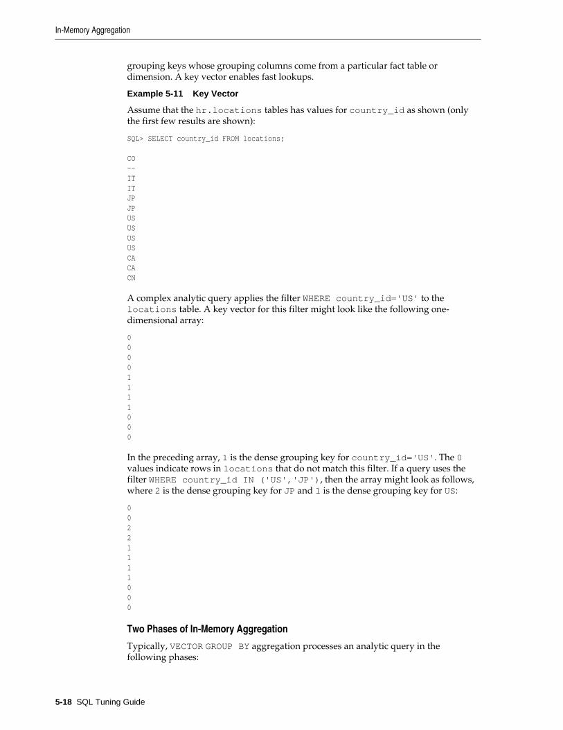
grouping keys whose grouping columns come from a particular fact table ordimension. A key vector enables fast lookups.
Example 5-11 Key Vector
Assume that the hr.locations tables has values for country_id as shown (onlythe first few results are shown):
SQL> SELECT country_id FROM locations; CO--ITITJPJPUSUSUSUSCACACN
A complex analytic query applies the filter WHERE country_id='US' to thelocations table. A key vector for this filter might look like the following one-dimensional array:
00001111000
In the preceding array, 1 is the dense grouping key for country_id='US'. The 0values indicate rows in locations that do not match this filter. If a query uses thefilter WHERE country_id IN ('US','JP'), then the array might look as follows,where 2 is the dense grouping key for JP and 1 is the dense grouping key for US:
00221111000
Two Phases of In-Memory Aggregation
Typically, VECTOR GROUP BY aggregation processes an analytic query in thefollowing phases:
In-Memory Aggregation
5-18 SQL Tuning Guide

1. Process each dimension sequentially as follows:
a. Find the unique dense grouping keys.
b. Create a key vector.
c. Create a temporary table.
Figure 5-2 illustrates the steps in this phase, beginning with the scan of thedimension table in DFO 0, and ending with the creation of a temporary table. Inthe simplest form of parallel GROUP BY or join processing, the database processeseach join or GROUP BY in its own DFO.
Figure 5-2 Phase 1 of In-Memory Aggregation
DFO 0
DFO 1
temporary table create
KEY VECTOR CREATE
dimension scan
VECTOR GROUP BY
2. Process the fact table.
a. Process all the joins and aggregations using the key vectors created in thepreceding phase.
b. Join back the results to each temporary table.
Figure 5-3 illustrates phase 2 in a join of the fact table with two dimensions. InDFO 0, the database performs a full scan of the fact table, and then uses the keyvectors for each dimension to filter out nonmatching rows. DFO 2 joins the resultsof DFO 0 with DFO 1. DFO 4 joins the result of DFO 2 with DFO 3.
In-Memory Aggregation
Query Transformations 5-19

Figure 5-3 Phase 2 of In-Memory Aggregation
DFO 3
DFO 1
hash join 2
DFO 4
DFO 0
DFO 2
temporary table 2
temporary table 1
hash join 1
HASH GROUP BY
fact scan
KEY VECTOR USE 1
KEY VECTOR USE 2
VECTOR GROUP BY
Controls for In-Memory AggregationVECTOR GROUP BY aggregation does not involve any new SQL or public initializationparameters. You can use the following pairs of hints:
• Query block hints
VECTOR_TRANSFORM enables the vector transformation on the specified queryblock, regardless of costing. NO_VECTOR_TRANSFORM disables the vectortransformation from engaging on the specified query block.
• Table hints
You can use the following pairs of hints:
– VECTOR_TRANSFORM_FACT includes the specified FROM expressions in the facttable generated by the vector transformation. NO_VECTOR_TRANSFORM_FACTexcludes the specified FROM expressions from the fact table generated by thevector transformation.
– VECTOR_TRANSFORM_DIMS includes the specified FROM expressions in enableddimensions generated by the vector transformation.NO_VECTOR_TRANSFORM_DIMS excludes the specified from expressions fromenabled dimensions generated by the vector transformation.
See Also:
Oracle Database SQL Language Reference to learn more about theVECTOR_TRANSFORM_FACT and VECTOR_TRANSFORM_DIMS hints
In-Memory Aggregation
5-20 SQL Tuning Guide

In-Memory Aggregation: ScenarioThis section gives a conceptual example of how VECTOR GROUP BY aggregationworks. The scenario does not use the sample schema tables or show an actualexecution plan.
This section contains the following topics:
• Sample Analytic Query of a Star Schema
• Step 1: Key Vector and Temporary Table Creation for geography Dimension
• Step 2: Key Vector and Temporary Table Creation for products Dimension
• Step 3: Key Vector Query Transformation
• Step 4: Row Filtering from Fact Table
• Step 5: Aggregation Using an Array
• Step 6: Join Back to Temporary Tables
Sample Analytic Query of a Star Schema
This sample star schema in this scenario contains the sales_online fact table andtwo dimension tables: geography and products. Each row in geography isuniquely identified by the geog_id column. Each row in products is uniquelyidentified by the prod_id column. Each row in sales_online is uniquely identifiedby the geog_id, prod_id, and amount sold.
Table 5-1 Sample Rows in geography Table
country state city geog_id
USA WA seattle 2
USA WA spokane 3
USA CA SF 7
USA CA LA 8
Table 5-2 Sample Rows in products Table
manuf category subcategory prod_id
Acme sport bike 4
Acme sport ball 3
Acme electric bulb 1
Acme electric switch 8
Table 5-3 Sample Rows in sales_online Table
In-Memory Aggregation
Query Transformations 5-21

Table 5-3 (Cont.) Sample Rows in sales_online Table
prod_id geog_id amount
8 1 100
9 1 150
8 2 100
4 3 110
2 30 130
6 20 400
3 1 100
1 7 120
3 8 130
4 3 200
A manager asks the business question, "How many Acme products in eachsubcategory were sold online in Washington, and how many were sold in California?"To answer this question, an analytic query of the sales_online fact table joins theproducts and geography dimension tables as follows:
SELECT p.category, p.subcategory, g.country, g.state, SUM(s.amount)FROM sales_online s, products p, geography gWHERE s.geog_id = g.geog_id AND s.prod_id = p.prod_idAND g.state IN ('WA','CA')AND p.manuf = 'ACME'GROUP BY category, subcategory, country, state
Step 1: Key Vector and Temporary Table Creation for geography Dimension
In the first phase of VECTOR GROUP BY aggregation for this query, the databasecreates a dense grouping key for each city/state combination for cities in the states ofWashington or California. In Table 5-6, the 1 is the USA,WA grouping key, and the 2 isthe USA,CA grouping key.
Table 5-4 Dense Grouping Key for geography
country state city geog_id dense_gr_key_geog
USA WA seattle 2 1
USA WA spokane 3 1
USA CA SF 7 2
USA CA LA 8 2
A key vector for the geography table looks like the array represented by the finalcolumn in Table 5-5. The values are the geography dense grouping keys. Thus, thekey vector indicates which rows in sales_online meet the geography.state
In-Memory Aggregation
5-22 SQL Tuning Guide

filter criteria (a sale made in the state of CA or WA) and which country/state group eachrow belongs to (either the USA,WA group or USA,CA group).
Table 5-5 Online Sales
prod_id geog_id amount key vector for geography
8 1 100 0
9 1 150 0
8 2 100 1
4 3 110 1
2 30 130 0
6 20 400 0
3 1 100 0
1 7 120 2
3 8 130 2
4 3 200 1
Internally, the database creates a temporary table similar to the following:
CREATE TEMPORARY TABLE tt_geography ASSELECT MAX(country), MAX(state), KEY_VECTOR_CREATE(...) dense_gr_key_geogFROM geographyWHERE state IN ('WA','CA')GROUP BY country, state
Table 5-6 shows rows in the tt_geography temporary table. The dense grouping keyfor the USA,WA combination is 1, and the dense grouping key for the USA,CAcombination is 2.
Table 5-6 tt_geography
country state dense_gr_key_geog
USA WA 1
USA CA 2
Step 2: Key Vector and Temporary Table Creation for products Dimension
The database creates a dense grouping key for each distinct category/subcategorycombination of an Acme product. For example, in Table 5-7, the 4 is dense groupingkey for an Acme electric switch.
Table 5-7 Sample Rows in products Table
manuf category subcategory prod_id dense_gr_key_prod
Acme sport bike 4 1
Acme sport ball 3 2
In-Memory Aggregation
Query Transformations 5-23

Table 5-7 (Cont.) Sample Rows in products Table
manuf category subcategory prod_id dense_gr_key_prod
Acme electric bulb 1 3
Acme electric switch 8 4
A key vector for the products table might look like the array represented by the finalcolumn in Table 5-8. The values represent the products dense grouping key. Forexample, the 4 represents the online sale of an Acme electric switch. Thus, the keyvector indicates which rows in sales_online meet the products filter criteria (asale of an Acme product).
Table 5-8 Key Vector
prod_id geog_id amount key vector for products
8 1 100 4
9 1 150 0
8 2 100 4
4 3 110 1
2 30 130 0
6 20 400 0
3 1 100 2
1 7 120 3
3 8 130 2
4 3 200 1
Internally, the database creates a temporary table similar to the following:
CREATE TEMPORTARY TABLE tt_products ASSELECT MAX(category), MAX(subcategory), KEY_VECTOR_CREATE(...) dense_gr_key_prodFROM productsWHERE manuf = 'ACME'GROUP BY category, subcategory
Table 5-9 shows rows in this temporary table.
Table 5-9 tt_products
category subcategory dense_gr_key_prod
sport bike 1
sport ball 2
electric bulb 3
electric switch 4
In-Memory Aggregation
5-24 SQL Tuning Guide

Step 3: Key Vector Query Transformation
The database now enters the phase of processing the fact table. The optimizertransforms the original query into the following equivalent query, which accesses thekey vectors:
SELECT KEY_VECTOR_PROD(prod_id), KEY_VECTOR_GEOG(geog_id), SUM(amount)FROM sales_onlineWHERE KEY_VECTOR_PROD_FILTER(prod_id) IS NOT NULL AND KEY_VECTOR_GEOG_FILTER(geog_id) IS NOT NULL GROUP BY KEY_VECTOR_PROD(prod_id), KEY_VECTOR_GEOG(geog_id)
The preceding transformation is not an exact rendition of the internal SQL, which ismuch more complicated, but a conceptual representation designed to illustrate thebasic concept.
Step 4: Row Filtering from Fact Table
The goal in this phase is to obtain the amount sold for each combination of groupingkeys. The database uses the key vectors to filter out unwanted rows from the fact table.In Table 5-10, the first three columns represent the sales_online table. The last twocolumns provide the dense grouping keys for the geography and products tables.
Table 5-10 Dense Grouping Keys for the sales_online Table
prod_id geog_id amount dense_gr_key_prod dense_gr_key_geog
7 1 100 4
9 1 150
8 2 100 4 1
4 3 110 1 1
2 30 130
6 20 400
3 1 100 2
1 7 120 3 2
3 8 130 2 2
4 3 200 1 1
As shown in Table 5-11, the database retrieves only those rows from sales_onlinewith non-null values for both dense grouping keys, indicating rows that satisfy all thefiltering criteria.
Table 5-11 Filtered Rows from sales_online Table
geog_id prod_id amount dense_gr_key_prod dense_gr_key_geog
2 8 100 4 1
In-Memory Aggregation
Query Transformations 5-25

Table 5-11 (Cont.) Filtered Rows from sales_online Table
geog_id prod_id amount dense_gr_key_prod dense_gr_key_geog
3 4 110 1 1
3 4 200 1 1
7 1 120 3 2
8 3 130 2 2
Step 5: Aggregation Using an Array
The database uses a multidimensional array to perform the aggregation. In Table 5-12,the geography grouping keys are horizontal, and the products grouping keys arevertical. The database adds the values in the intersection of each dense grouping keycombination. For example, for the intersection of the geography grouping key 1 andthe products grouping key 1, the sum of 110 and 200 is 310.
Table 5-12 Aggregation Array
dgkp/dgkg 1 2
1 110,200
2 130
3 120
4 100
Step 6: Join Back to Temporary Tables
In the final stage of processing, the database uses the dense grouping keys to join backthe rows to the temporary tables to obtain the names of the regions and categories. Theresults look as follows:
CATEGORY SUBCATEGORY COUNTRY STATE AMOUNT-------- ----------- ------- ----- ------electric bulb USA CA 120electric switch USA WA 100sport ball USA CA 130sport bike USA WA 310
In-Memory Aggregation: ExampleThe following query of the sh tables answers the business question "How manyproducts were sold in each category in each calendar year?"
SELECT t.calendar_year, p.prod_category, SUM(quantity_sold)FROM times t, products p, sales sWHERE t.time_id = s.time_idAND p.prod_id = s.prod_idGROUP BY t.calendar_year, p.prod_category;
In-Memory Aggregation
5-26 SQL Tuning Guide

Example 5-12 VECTOR GROUP BY Execution Plan
The following example shows the execution plan contained in the current cursor. Steps4 and 8 show the creation of the key vectors for the dimension tables times andproducts. Steps 17 and 18 show the use of the previously created key vectors. Steps3, 7, and 15 show the VECTOR GROUP BY operations.
SQL_ID 0yxqj2nq8p9kt, child number 0-------------------------------------SELECT t.calendar_year, p.prod_category, SUM(quantity_sold) FROMtimes t, products p, sales f WHERE t.time_id = f.time_id ANDp.prod_id = f.prod_id GROUP BY t.calendar_year, p.prod_category
Plan hash value: 2377225738-------------------------------------------------------------------------------------------------------------|Id | Operation | Name |Rows|Bytes|Cost(%CPU)|Time|Pstart|Pstop|-------------------------------------------------------------------------------------------------------------| 0| SELECT STATEMENT | | | |285 (100)| | | || 1| TEMP TABLE TRANSFORMATION | | | | | | | || 2| LOAD AS SELECT | SYS_TEMP_0FD9D6644_11CBE8 | | | | | | || 3| VECTOR GROUP BY | | 5| 80 | 3 (100)|00:00:01| | || 4| KEY VECTOR CREATE BUFFERED | :KV0000 |1826|29216| 3 (100)|00:00:01| | || 5| TABLE ACCESS INMEMORY FULL | TIMES |1826|21912| 1 (100)|00:00:01| | || 6| LOAD AS SELECT | SYS_TEMP_0FD9D6645_11CBE8 | | | | | | || 7| VECTOR GROUP BY | | 5| 125 | 1 (100)|00:00:01| | || 8| KEY VECTOR CREATE BUFFERED | :KV0001 | 72| 1800| 1 (100)|00:00:01| | || 9| TABLE ACCESS INMEMORY FULL | PRODUCTS | 72| 1512| 0 (0)| | | || 10| HASH GROUP BY | | 18| 1440|282 (99)|00:00:01| | ||*11| HASH JOIN | | 18| 1440|281 (99)|00:00:01| | ||*12| HASH JOIN | | 18| 990 |278 (100)|00:00:01| | || 13| TABLE ACCESS FULL | SYS_TEMP_0FD9D6644_11CBE8 | 5| 80 | 2 (0)|00:00:01| | || 14| VIEW | VW_VT_AF278325 | 18| 702 |276 (100)|00:00:01| | || 15| VECTOR GROUP BY | | 18| 414 |276 (100)|00:00:01| | || 16| HASH GROUP BY | | 18| 414 |276 (100)|00:00:01| | || 17| KEY VECTOR USE | :KV0000 |918K| 20M|276 (100)|00:00:01| | || 18| KEY VECTOR USE | :KV0001 |918K| 16M|272 (100)|00:00:01| | || 19| PARTITION RANGE ALL | |918K| 13M|257 (100)|00:00:01| 1| 28|| 20| TABLE ACCESS INMEMORY FULL| SALES |918K| 13M|257 (100)|
In-Memory Aggregation
Query Transformations 5-27

00:00:01| 1| 28|| 21| TABLE ACCESS FULL | SYS_TEMP_0FD9D6645_11CBE8 | 5 | 125| 2 (0)|00:00:01| | |-------------------------------------------------------------------------------------------------------------
Predicate Information (identified by operation id):--------------------------------------------------- 11 - access("ITEM_10"=INTERNAL_FUNCTION("C0") AND "ITEM_11"="C2") 12 - access("ITEM_8"=INTERNAL_FUNCTION("C0") AND "ITEM_9"="C2")
Note----- - vector transformation used for this statement
45 rows selected.
Table ExpansionIn table expansion, the optimizer generates a plan that uses indexes on the read-mostly portion of a partitioned table, but not on the active portion of the table. Thissection contains the following topics:
• Purpose of Table Expansion
• How Table Expansion Works
• Table Expansion: Scenario
• Table Expansion and Star Transformation: Scenario
Purpose of Table ExpansionTable expansion is useful because of the following facts:
• Index-based plans can improve performance dramatically.
• Index maintenance causes overhead to DML.
• In many databases, only a small portion of the data is actively updated throughDML.
Table expansion takes advantage of index-based plans for tables that have high updatevolume. You can configure a table so that an index is only created on the read-mostlyportion of the data, and does not suffer the overhead burden of index maintenance onthe active portions of the data. Thus, table expansion reaps the benefit of improvedperformance without suffering the ill effects of index maintenance.
How Table Expansion WorksTable partitioning makes table expansion possible. If a local index exists on apartitioned table, then the optimizer can mark the index as unusable for specificpartitions. In effect, some partitions are not indexed.
In table expansion, the optimizer transforms the query into a UNION ALL statement,with some subqueries accessing indexed partitions and other subqueries accessingunindexed partitions. The optimizer can choose the most efficient access methodavailable for a partition, regardless of whether it exists for all of the partitions accessedin the query.
Table Expansion
5-28 SQL Tuning Guide

The optimizer does not always choose table expansion:
• Table expansion is cost-based.
While the database accesses each partition of the expanded table only once acrossall branches of the UNION ALL, any tables that the database joins to it are accessedin each branch.
• Semantic issues may render expansion invalid.
For example, a table appearing on the right side of an outer join is not valid fortable expansion.
You can control table expansion with the hint EXPAND_TABLE hint. The hint overridesthe cost-based decision, but not the semantic checks.
See Also:
“Influencing the Optimizer with Hints”
Table Expansion: ScenarioThe optimizer keeps track of which partitions must be accessed from each table, basedon predicates that appear in the query. Partition pruning enables the optimizer to usetable expansion to generate more optimal plans.
Assumptions
This scenario assumes the following:
• You want to run a star query against the sh.sales table, which is range-partitioned on the time_id column.
• You want to disable indexes on specific partitions to see the benefits of tableexpansion.
To use table expansion:
1. Run the following query:
SELECT * FROM sales WHERE time_id >= TO_DATE('2000-01-01 00:00:00', 'SYYYY-MM-DD HH24:MI:SS') AND prod_id = 38;
2. Explain the plan by querying DBMS_EXPLAN:
SET LINESIZE 150SET PAGESIZE 0SELECT * FROM TABLE(DBMS_XPLAN.DISPLAY_CURSOR(format => 'BASIC,PARTITION'));
As shown in the Pstart and Pstop columns in the following plan, the optimizerdetermines from the filter that only 16 of the 28 partitions in the table must beaccessed:
Plan hash value: 3087065703 --------------------------------------------------------------------------|Id| Operation | Name |Pstart|Pstop|
Table Expansion
Query Transformations 5-29

--------------------------------------------------------------------------| 0| SELECT STATEMENT | | | || 1| PARTITION RANGE ITERATOR | | 13 | 28 || 2| TABLE ACCESS BY LOCAL INDEX ROWID BATCHED| SALES | 13 | 28 || 3| BITMAP CONVERSION TO ROWIDS | | | ||*4| BITMAP INDEX SINGLE VALUE |SALES_PROD_BIX| 13 | 28 |-------------------------------------------------------------------------- Predicate Information (identified by operation id):--------------------------------------------------- 4 - access("PROD_ID"=38)
After the optimizer has determined the partitions to be accessed, it considers anyindex that is usable on all of those partitions. In the preceding plan, the optimizerchose to use the sales_prod_bix bitmap index.
3. Disable the index on the SALES_1995 partition of the sales table:
ALTER INDEX sales_prod_bix MODIFY PARTITION sales_1995 UNUSABLE;
The preceding DDL disables the index on partition 1, which contains all salesfrom before 1996.
Note:
You can obtain the partition information by querying theUSER_IND_PARTITIONS view.
4. Execute the query of sales again, and then query DBMS_XPLAN to obtain the plan.
The output shows that the plan did not change:
Plan hash value: 3087065703 ---------------------------------------------------------------------------|Id| Operation | Name |Pstart|Pstop---------------------------------------------------------------------------| 0| SELECT STATEMENT | | | || 1| PARTITION RANGE ITERATOR | | 13 | 28 || 2| TABLE ACCESS BY LOCAL INDEX ROWID BATCHED| SALES | 13 | 28 || 3| BITMAP CONVERSION TO ROWIDS | | | ||*4| BITMAP INDEX SINGLE VALUE | SALES_PROD_BIX| 13 | 28 |--------------------------------------------------------------------------- Predicate Information (identified by operation id):--------------------------------------------------- 4 - access("PROD_ID"=38)
The plan is the same because the disabled index partition is not relevant to thequery. If all partitions that the query accesses are indexed, then the database cananswer the query using the index. Because the query only accesses partitions 16through 28, disabling the index on partition 1 does not affect the plan.
5. Disable the indexes for partition 28 (SALES_Q4_2003), which is a partition thatthe query needs to access:
ALTER INDEX sales_prod_bix MODIFY PARTITION sales_q4_2003 UNUSABLE;ALTER INDEX sales_time_bix MODIFY PARTITION sales_q4_2003 UNUSABLE;
Table Expansion
5-30 SQL Tuning Guide

By disabling the indexes on a partition that the query does need to access, thequery can no longer use this index (without table expansion).
6. Query the plan using DBMS_EXPLAN.
As shown in the following plan, the optimizer does not use the index:
Plan hash value: 3087065703 ---------------------------------------------------------------------------| Id| Operation | Name |Pstart|Pstop---------------------------------------------------------------------------| 0 | SELECT STATEMENT | | | || 1 | PARTITION RANGE ITERATOR | | 13 | 28 ||*2 | TABLE ACCESS FULL | SALES | 13 | 28 |--------------------------------------------------------------------------- Predicate Information (identified by operation id):--------------------------------------------------- 2 - access("PROD_ID"=38)
In the preceding example, the query accesses 16 partitions. On 15 of thesepartitions, an index is available, but no index is available for the final partition.Because the optimizer has to choose one access path or the other, the optimizercannot use the index on any of the partitions.
7. With table expansion, the optimizer rewrites the original query as follows:
SELECT * FROM sales WHERE time_id >= TO_DATE('2000-01-01 00:00:00', 'SYYYY-MM-DD HH24:MI:SS') AND time_id < TO_DATE('2003-10-01 00:00:00', 'SYYYY-MM-DD HH24:MI:SS')AND prod_id = 38UNION ALLSELECT * FROM sales WHERE time_id >= TO_DATE('2003-10-01 00:00:00', 'SYYYY-MM-DD HH24:MI:SS') AND time_id < TO_DATE('2004-01-01 00:00:00', 'SYYYY-MM-DD HH24:MI:SS')AND prod_id = 38;
In the preceding query, the first query block in the UNION ALL accesses thepartitions that are indexed, while the second query block accesses the partitionthat is not. The two subqueries enable the optimizer to choose to use the index inthe first query block, if it is more optimal than using a table scan of all of thepartitions that are accessed.
8. Query the plan using DBMS_EXPLAN.
The plan appears as follows:
Plan hash value: 2120767686 ---------------------------------------------------------------------------|Id| Operation | Name |Pstart|Pstop|---------------------------------------------------------------------------| 0| SELECT STATEMENT | | | || 1| VIEW | VW_TE_2 | | || 2| UNION-ALL | | | || 3| PARTITION RANGE ITERATOR | | 13| 27|| 4| TABLE ACCESS BY LOCAL INDEX ROWID BATCHED| SALES | 13| 27|| 5| BITMAP CONVERSION TO ROWIDS | | | ||*6| BITMAP INDEX SINGLE VALUE | SALES_PROD_BIX| 13| 27|
Table Expansion
Query Transformations 5-31

| 7| PARTITION RANGE SINGLE | | 28| 28||*8| TABLE ACCESS FULL | SALES | 28| 28|--------------------------------------------------------------------------- Predicate Information (identified by operation id):--------------------------------------------------- 6 - access("PROD_ID"=38) 8 - filter("PROD_ID"=38)
As shown in the preceding plan, the optimizer uses a UNION ALL for two queryblocks (Step 2). The optimizer chooses an index to access partitions 13 to 27 in thefirst query block (Step 6). Because no index is available for partition 28, theoptimizer chooses a full table scan in the second query block (Step 8).
Table Expansion and Star Transformation: ScenarioStar transformation enables specific types of queries to avoid accessing large portionsof big fact tables (see “Star Transformation”). Star transformation requires definingseveral indexes, which in an actively updated table can have overhead. With tableexpansion, you can define indexes on only the inactive partitions so that the optimizercan consider star transformation on only the indexed portions of the table.
Assumptions
This scenario assumes the following:
• You query the same schema used in “Star Transformation: Scenario”.
• The last partition of sales is actively being updated, as is often the case with time-partitioned tables.
• You want the optimizer to take advantage of table expansion.
To take advantage of table expansion in a star query:
1. Disable the indexes on the last partition as follows:
ALTER INDEX sales_channel_bix MODIFY PARTITION sales_q4_2003 UNUSABLE;ALTER INDEX sales_cust_bix MODIFY PARTITION sales_q4_2003 UNUSABLE;
2. Execute the following star query:
SELECT t.calendar_quarter_desc, SUM(s.amount_sold) sales_amount FROM sales s, times t, customers c, channels chWHERE s.time_id = t.time_id AND s.cust_id = c.cust_id AND s.channel_id = ch.channel_id AND c.cust_state_province = 'CA' AND ch.channel_desc = 'Internet'AND t.calendar_quarter_desc IN ('1999-01','1999-02') GROUP BY t.calendar_quarter_desc;
3. Query the cursor using DBMS_XPLAN, which shows the following plan:
---------------------------------------------------------------------------|Id| Operation | Name | Pstart| Pstop |---------------------------------------------------------------------------| 0| SELECT STATEMENT | | | || 1| HASH GROUP BY | | | |
Table Expansion
5-32 SQL Tuning Guide

| 2| VIEW |VW_TE_14 | | || 3| UNION-ALL | | | || 4| HASH JOIN | | | || 5| TABLE ACCESS FULL |TIMES | | || 6| VIEW |VW_ST_1319B6D8 | | || 7| NESTED LOOPS | | | || 8| PARTITION RANGE SUBQUERY | |KEY(SQ)|KEY(SQ)|| 9| BITMAP CONVERSION TO ROWIDS| | | ||10| BITMAP AND | | | ||11| BITMAP MERGE | | | ||12| BITMAP KEY ITERATION | | | ||13| BUFFER SORT | | | ||14| TABLE ACCESS FULL |CHANNELS | | ||15| BITMAP INDEX RANGE SCAN|SALES_CHANNEL_BIX|KEY(SQ)|KEY(SQ)||16| BITMAP MERGE | | | ||17| BITMAP KEY ITERATION | | | ||18| BUFFER SORT | | | ||19| TABLE ACCESS FULL |TIMES | | ||20| BITMAP INDEX RANGE SCAN|SALES_TIME_BIX |KEY(SQ)|KEY(SQ)||21| BITMAP MERGE | | | ||22| BITMAP KEY ITERATION | | | ||23| BUFFER SORT | | | ||24| TABLE ACCESS FULL |CUSTOMERS | | ||25| BITMAP INDEX RANGE SCAN|SALES_CUST_BIX |KEY(SQ)|KEY(SQ)||26| TABLE ACCESS BY USER ROWID |SALES | ROWID | ROWID ||27| NESTED LOOPS | | | ||28| NESTED LOOPS | | | ||29| NESTED LOOPS | | | ||30| NESTED LOOPS | | | ||31| PARTITION RANGE SINGLE | | 28 | 28 ||32| TABLE ACCESS FULL |SALES | 28 | 28 ||33| TABLE ACCESS BY INDEX ROWID|CHANNELS | | ||34| INDEX UNIQUE SCAN |CHANNELS_PK | | ||35| TABLE ACCESS BY INDEX ROWID |CUSTOMERS | | ||36| INDEX UNIQUE SCAN |CUSTOMERS_PK | | ||37| INDEX UNIQUE SCAN |TIMES_PK | | ||38| TABLE ACCESS BY INDEX ROWID |TIMES | | |---------------------------------------------------------------------------
The preceding plan uses table expansion. The UNION ALL branch that is accessingevery partition except the last partition uses star transformation. Because theindexes on partition 28 are disabled, the database accesses the final partition usinga full table scan.
Join FactorizationIn the cost-based transformation known as join factorization, the optimizer canfactorize common computations from branches of a UNION ALL query.
This section contains the following topics:
• Purpose of Join Factorization
• How Join Factorization Works
• Factorization and Join Orders: Scenario
• Factorization of Outer Joins: Scenario
Join Factorization
Query Transformations 5-33

Purpose of Join FactorizationUNION ALL queries are common in database applications, especially in dataintegration applications. Often, branches in a UNION ALL query refer to the same basetables. Without join factorization, the optimizer evaluates each branch of a UNIONALL query independently, which leads to repetitive processing, including data accessand joins. Join factorization transformation can share common computations acrossthe UNION ALL branches. Avoiding an extra scan of a large base table can lead to ahuge performance improvement.
How Join Factorization WorksJoin factorization can factorize multiple tables and from more than two UNION ALLbranches. Join factorization is best explained through examples.
Example 5-13 UNION ALL Query
The following query shows a query of four tables (t1, t2, t3, and t4) and two UNIONALL branches:
SELECT t1.c1, t2.c2FROM t1, t2, t3WHERE t1.c1 = t2.c1 AND t1.c1 > 1AND t2.c2 = 2AND t2.c2 = t3.c2 UNION ALLSELECT t1.c1, t2.c2FROM t1, t2, t4WHERE t1.c1 = t2.c1 AND t1.c1 > 1AND t2.c3 = t4.c3
In the preceding query, table t1 appears in both UNION ALL branches, as does thefilter predicate t1.c1 > 1 and the join predicate t1.c1 = t2.c1. Without anytransformation, the database must perform the scan and the filtering on table t1 twice,one time for each branch.
Example 5-14 Factorized Query
The following query uses join factorization to transform the query in Example 5-13.
SELECT t1.c1, VW_JF_1.item_2FROM t1, (SELECT t2.c1 item_1, t2.c2 item_2 FROM t2, t3 WHERE t2.c2 = t3.c2 AND t2.c2 = 2 UNION ALL SELECT t2.c1 item_1, t2.c2 item_2 FROM t2, t4 WHERE t2.c3 = t4.c3) VW_JF_1WHERE t1.c1 = VW_JF_1.item_1 AND t1.c1 > 1
In this case, because table t1 is factorized, the database performs the table scan andthe filtering on t1 only one time. If t1 is large, then this factorization avoids the hugeperformance cost of scanning and filtering t1 twice.
Join Factorization
5-34 SQL Tuning Guide

Note:
If the branches in a UNION ALL query have clauses that use the DISTINCTfunction, then join factorization is not valid.
Factorization and Join Orders: ScenarioA benefit of join factorization is that it can create more possibilities for join orders.
Example 5-15 Query Involving Five Tables
In the following query, view V is same as the query as in Example 5-13:
SELECT *FROM t5, (SELECT t1.c1, t2.c2 FROM t1, t2, t3 WHERE t1.c1 = t2.c1 AND t1.c1 > 1 AND t2.c2 = 2 AND t2.c2 = t3.c2 UNION ALL SELECT t1.c1, t2.c2 FROM t1, t2, t4 WHERE t1.c1 = t2.c1 AND t1.c1 > 1 AND t2.c3 = t4.c3) VWHERE t5.c1 = V.c1
Before join factorization, the database must join t1, t2, and t3 before joining themwith t5.
Example 5-16 Factorization of t1 from View V
If join factorization factorizes t1 from view V, as shown in the following query, thenthe database can join t1 with t5.:
SELECT *FROM t5, ( SELECT t1.c1, VW_JF_1.item_2 FROM t1, (SELECT t2.c1 item_1, t2.c2 item_2 FROM t2, t3 WHERE t2.c2 = t3.c2 AND t2.c2 = 2 UNION ALL SELECT t2.c1 item_1, t2.c2 item_2 FROM t2, t4 WHERE t2.c3 = t4.c3) VW_JF_1 WHERE t1.c1 = VW_JF_1.item_1 AND t1.c1 > 1 )WHERE t5.c1 = V.c1
The preceding query transformation opens up new join orders. However, joinfactorization imposes specific join orders. For example, in the preceding query, tablest2 and t3 appear in the first branch of the UNION ALL query in view VW_JF_1. Thedatabase must join t2 with t3 before it can join with t1, which is not defined withinthe VW_JF_1 view. The imposed join order may not necessarily be the best join order.For this reason, the optimizer performs join factorization using the cost-basedtransformation framework. The optimizer calculate the cost of the plans with andwithout join factorization, and then chooses the cheapest plan.
Join Factorization
Query Transformations 5-35
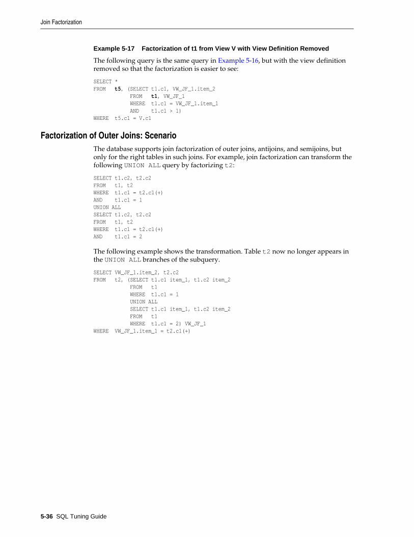
Example 5-17 Factorization of t1 from View V with View Definition Removed
The following query is the same query in Example 5-16, but with the view definitionremoved so that the factorization is easier to see:
SELECT *FROM t5, (SELECT t1.c1, VW_JF_1.item_2 FROM t1, VW_JF_1 WHERE t1.c1 = VW_JF_1.item_1 AND t1.c1 > 1)WHERE t5.c1 = V.c1
Factorization of Outer Joins: ScenarioThe database supports join factorization of outer joins, antijoins, and semijoins, butonly for the right tables in such joins. For example, join factorization can transform thefollowing UNION ALL query by factorizing t2:
SELECT t1.c2, t2.c2FROM t1, t2WHERE t1.c1 = t2.c1(+) AND t1.c1 = 1UNION ALLSELECT t1.c2, t2.c2FROM t1, t2WHERE t1.c1 = t2.c1(+) AND t1.c1 = 2
The following example shows the transformation. Table t2 now no longer appears inthe UNION ALL branches of the subquery.
SELECT VW_JF_1.item_2, t2.c2FROM t2, (SELECT t1.c1 item_1, t1.c2 item_2 FROM t1 WHERE t1.c1 = 1 UNION ALL SELECT t1.c1 item_1, t1.c2 item_2 FROM t1 WHERE t1.c1 = 2) VW_JF_1WHERE VW_JF_1.item_1 = t2.c1(+)
Join Factorization
5-36 SQL Tuning Guide

Part IIIQuery Execution Plans
This part contains the following chapters:
• Generating and Displaying Execution Plans
• Reading Execution Plans


6Generating and Displaying Execution Plans
This chapter contains the following topics:
• Introduction to Execution Plans
• About Plan Generation and Display
• Generating Execution Plans
• Displaying PLAN_TABLE Output
Introduction to Execution PlansThe combination of the steps that Oracle Database uses to execute a statement is an execution plan. Each step either retrieves rows of data physically from the database orprepares them for the user issuing the statement. An execution plan includes an accesspath for each table that the statement accesses and an ordering of the tables (the joinorder) with the appropriate join method.
See Also:
Joins
About Plan Generation and DisplayThe EXPLAIN PLAN statement displays execution plans that the optimizer chooses forSELECT, UPDATE, INSERT, and DELETE statements. This section contains thefollowing topics:
• About the Plan Explanation
• Why Execution Plans Change
• Guideline for Minimizing Throw-Away
• Guidelines for Evaluating Execution Plans
• EXPLAIN PLAN Restrictions
• Guidelines for Creating PLAN_TABLE
About the Plan ExplanationA statement execution plan is the sequence of operations that the database performs torun the statement. The row source tree is the core of the execution plan (see “SQL RowSource Generation”). The tree shows the following information:
Generating and Displaying Execution Plans 6-1

• An ordering of the tables referenced by the statement
• An access method for each table mentioned in the statement
• A join method for tables affected by join operations in the statement
• Data operations like filter, sort, or aggregation
In addition to the row source tree, the plan table contains information about thefollowing:
• Optimization, such as the cost and cardinality of each operation
• Partitioning, such as the set of accessed partitions
• Parallel execution, such as the distribution method of join inputs
The EXPLAIN PLAN results enables you to determine whether the optimizer selects aparticular execution plan, such as a nested loops join. The results also help you tounderstand the optimizer decisions, such as why the optimizer chose a nested loopsjoin instead of a hash join, and enables you to understand the performance of a query.
See Also:
Oracle Database SQL Language Reference to learn about the EXPLAIN PLANstatement
Why Execution Plans ChangeExecution plans can and do change as the underlying optimizer inputs change.EXPLAIN PLAN output shows how the database would run the SQL statement whenthe statement was explained. This plan can differ from the actual execution plan a SQLstatement uses because of differences in the execution environment and explain planenvironment.
Note:
To avoid possible SQL performance regression that may result from executionplan changes, consider using SQL plan management.
Execution plans can differ because of the following:
• Different Schemas
• Different Costs
See Also:
“Managing SQL Plan Baselines ”
Different Schemas
Schemas can differ for the following reasons:
• The execution and explain plan occur on different databases.
About Plan Generation and Display
6-2 SQL Tuning Guide

• The user explaining the statement is different from the user running the statement.Two users might be pointing to different objects in the same database, resulting indifferent execution plans.
• Schema changes (usually changes in indexes) between the two operations.
Different Costs
Even if the schemas are the same, the optimizer can choose different execution planswhen the costs are different. Some factors that affect the costs include the following:
• Data volume and statistics
• Bind variable types and values
• Initialization parameters set globally or at session level
Guideline for Minimizing Throw-AwayExamining an explain plan enables you to look for throw-away in cases such as thefollowing:
• Full scans
• Unselective range scans
• Late predicate filters
• Wrong join order
• Late filter operations
In the plan shown in Example 6-1, the last step is a very unselective range scan that isexecuted 76563 times, accesses 11432983 rows, throws away 99% of them, and retains76563 rows. Why access 11432983 rows to realize that only 76563 rows are needed?
Example 6-1 Looking for Throw-Away in an Explain Plan
Rows Execution Plan-------- ---------------------------------------------------- 12 SORT AGGREGATE 2 SORT GROUP BY 76563 NESTED LOOPS 76575 NESTED LOOPS 19 TABLE ACCESS FULL CN_PAYRUNS_ALL 76570 TABLE ACCESS BY INDEX ROWID CN_POSTING_DETAILS_ALL 76570 INDEX RANGE SCAN (object id 178321) 76563 TABLE ACCESS BY INDEX ROWID CN_PAYMENT_WORKSHEETS_ALL11432983 INDEX RANGE SCAN (object id 186024)
Guidelines for Evaluating Execution PlansThe execution plan operation alone cannot differentiate between well-tunedstatements and those that perform poorly. For example, an EXPLAIN PLAN output thatshows that a statement uses an index does not necessarily mean that the statementruns efficiently. Sometimes indexes are extremely inefficient. In this case, a goodpractice is to examine the following:
• The columns of the index being used
• Their selectivity (fraction of table being accessed)
About Plan Generation and Display
Generating and Displaying Execution Plans 6-3

It is best to use EXPLAIN PLAN to determine an access plan, and then later prove that itis the optimal plan through testing. When evaluating a plan, examine the statement'sactual resource consumption.
Guidelines for Evaluating Plans Using the V$SQL_PLAN Views
As an alternative to running the EXPLAIN PLAN command and displaying the plan,you can display the plan by querying the V$SQL_PLAN view. V$SQL_PLAN containsthe execution plan for every statement stored in the shared SQL area. Its definition issimilar to PLAN_TABLE. See “PLAN_TABLE Columns”.
The advantage of V$SQL_PLAN over EXPLAIN PLAN is that you do not need to knowthe compilation environment that was used to execute a particular statement. ForEXPLAIN PLAN, you would need to set up an identical environment to get the sameplan when executing the statement.
The V$SQL_PLAN_STATISTICS view provides the actual execution statistics forevery operation in the plan, such as the number of output rows and elapsed time. Allstatistics, except the number of output rows, are cumulative. For example, the statisticsfor a join operation also includes the statistics for its two inputs. The statistics in V$SQL_PLAN_STATISTICS are available for cursors that have been compiled with theSTATISTICS_LEVEL initialization parameter set to ALL.
The V$SQL_PLAN_STATISTICS_ALL view enables side by side comparisons of theestimates that the optimizer provides for the number of rows and elapsed time. Thisview combines both V$SQL_PLAN and V$SQL_PLAN_STATISTICS information forevery cursor.
See Also:
• Monitoring Database Operations for information about the V$SQL_PLAN_MONITOR view
• Oracle Database Reference for more information about V$SQL_PLAN views
• Oracle Database Reference for information about the STATISTICS_LEVELinitialization parameter
EXPLAIN PLAN RestrictionsOracle Database does not support EXPLAIN PLAN for statements performing implicittype conversion of date bind variables. With bind variables in general, the EXPLAINPLAN output might not represent the real execution plan.
From the text of a SQL statement, TKPROF cannot determine the types of the bindvariables. It assumes that the type is CHARACTER, and gives an error messageotherwise. You can avoid this limitation by putting appropriate type conversions inthe SQL statement.
See Also:
Performing Application Tracing
About Plan Generation and Display
6-4 SQL Tuning Guide

Guidelines for Creating PLAN_TABLEThe PLAN_TABLE is automatically created as a public synonym to a global temporarytable. This temporary table holds the output of EXPLAIN PLAN statements for all users.PLAN_TABLE is the default sample output table into which the EXPLAIN PLANstatement inserts rows describing execution plans. See “PLAN_TABLE Columns” for adescription of the columns in the table.
While a PLAN_TABLE table is automatically set up for each user, you can use the SQLscript catplan.sql to manually create the global temporary table and thePLAN_TABLE synonym. The name and location of this script depends on youroperating system. On UNIX and Linux, the script is located in the $ORACLE_HOME/rdbms/admin directory.
For example, start a SQL*Plus session, connect with SYSDBA privileges, and run thescript as follows:
@$ORACLE_HOME/rdbms/admin/catplan.sql
Oracle recommends that you drop and rebuild your local PLAN_TABLE table afterupgrading the version of the database because the columns might change. This cancause scripts to fail or cause TKPROF to fail, if you are specifying the table.
If you do not want to use the name PLAN_TABLE, create a new synonym after runningthe catplan.sql script. For example:
CREATE OR REPLACE PUBLIC SYNONYM my_plan_table for plan_table$
Generating Execution PlansThe EXPLAIN PLAN statement enables you to examine the execution plan that theoptimizer chose for a SQL statement. When the statement is issued, the optimizerchooses an execution plan and then inserts data describing the plan into a databasetable. Issue the EXPLAIN PLAN statement and then query the output table.
Executing EXPLAIN PLAN for a Single StatementThe basics of using the EXPLAIN PLAN statement are as follows:
• Use the SQL script CATPLAN.SQL to create a sample output table calledPLAN_TABLE in your schema. See “Guidelines for Creating PLAN_TABLE”.
• Include the EXPLAIN PLAN FOR clause before the SQL statement.
• After issuing the EXPLAIN PLAN statement, use a script or package provided byOracle Database to display the most recent plan table output. See “DisplayingPLAN_TABLE Output”.
• The execution order in EXPLAIN PLAN output begins with the line that is thefurthest indented to the right. The next step is the parent of that line. If two linesare indented equally, then the top line is normally executed first.
Generating Execution Plans
Generating and Displaying Execution Plans 6-5

Note:
– The EXPLAIN PLAN output tables in this chapter were displayed with theutlxpls.sql script.
– The steps in the EXPLAIN PLAN output in this chapter may be different onyour system. The optimizer may choose different execution plans,depending on database configurations.
To explain a SQL statement, use the EXPLAIN PLAN FOR clause immediately beforethe statement. For example:
EXPLAIN PLAN FOR SELECT last_name FROM employees;
This explains the plan into the PLAN_TABLE table. You can then select the executionplan from PLAN_TABLE. See “Displaying PLAN_TABLE Output”.
Executing EXPLAIN PLAN Using a Statement IDWith multiple statements, you can specify a statement identifier and use that toidentify your specific execution plan. Before using SET STATEMENT ID, remove anyexisting rows for that statement ID.
In Example 6-2, st1 is specified as the statement identifier:
Example 6-2 Using EXPLAIN PLAN with the STATEMENT ID Clause
EXPLAIN PLAN SET STATEMENT_ID = 'st1' FOR SELECT last_name FROM employees;
Directing EXPLAIN PLAN Output to a Nondefault TableYou can specify the INTO clause to specify a different table.
See Also:
Oracle Database SQL Language Reference for a complete description of EXPLAINPLAN syntax.
Example 6-3 Using EXPLAIN PLAN with the INTO Clause
EXPLAIN PLAN INTO my_plan_table FOR SELECT last_name FROM employees;
You can specify a statement ID when using the INTO clause.
EXPLAIN PLAN SET STATEMENT_ID = 'st1' INTO my_plan_table FOR SELECT last_name FROM employees;
Generating Execution Plans
6-6 SQL Tuning Guide

Displaying PLAN_TABLE OutputAfter you have explained the plan, use the following SQL scripts or PL/SQL packageprovided by Oracle Database to display the most recent plan table output:
• UTLXPLS.SQL
This script displays the plan table output for serial processing. Example 6-5 is anexample of the plan table output when using the UTLXPLS.SQL script.
• UTLXPLP.SQL
This script displays the plan table output including parallel execution columns.
• DBMS_XPLAN.DISPLAY table function
This function accepts options for displaying the plan table output. You can specify:
– A plan table name if you are using a table different than PLAN_TABLE
– A statement ID if you have set a statement ID with the EXPLAIN PLAN
– A format option that determines the level of detail: BASIC, SERIAL, TYPICAL,and ALL
Examples of using DBMS_XPLAN to display PLAN_TABLE output are:
SELECT PLAN_TABLE_OUTPUT FROM TABLE(DBMS_XPLAN.DISPLAY());
SELECT PLAN_TABLE_OUTPUT FROM TABLE(DBMS_XPLAN.DISPLAY('MY_PLAN_TABLE', 'st1','TYPICAL'));
See Also:
Oracle Database PL/SQL Packages and Types Reference for more informationabout the DBMS_XPLAN package
Displaying an Execution Plan: ExampleExample 6-4 uses EXPLAIN PLAN to examine a SQL statement that selects theemployee_id, job_title, salary, and department_name for the employeeswhose IDs are less than 103.
Example 6-4 Using EXPLAIN PLAN
EXPLAIN PLAN FOR SELECT e.employee_id, j.job_title, e.salary, d.department_name FROM employees e, jobs j, departments d WHERE e.employee_id < 103 AND e.job_id = j.job_id AND e.department_id = d.department_id;
Example 6-5 EXPLAIN PLAN Output
The following output table shows the execution plan that the optimizer chose toexecute the SQL statement in Example 6-4:
-----------------------------------------------------------------------------------| Id | Operation | Name | Rows | Bytes | Cost (%CPU)|-----------------------------------------------------------------------------------
Displaying PLAN_TABLE Output
Generating and Displaying Execution Plans 6-7

| 0 | SELECT STATEMENT | | 3 | 189 | 10 (10)|| 1 | NESTED LOOPS | | 3 | 189 | 10 (10)|| 2 | NESTED LOOPS | | 3 | 141 | 7 (15)||* 3 | TABLE ACCESS FULL | EMPLOYEES | 3 | 60 | 4 (25)|| 4 | TABLE ACCESS BY INDEX ROWID| JOBS | 19 | 513 | 2 (50)||* 5 | INDEX UNIQUE SCAN | JOB_ID_PK | 1 | | || 6 | TABLE ACCESS BY INDEX ROWID | DEPARTMENTS | 27 | 432 | 2 (50)||* 7 | INDEX UNIQUE SCAN | DEPT_ID_PK | 1 | | |-----------------------------------------------------------------------------------
Predicate Information (identified by operation id):--------------------------------------------------- 3 - filter("E"."EMPLOYEE_ID"<103) 5 - access("E"."JOB_ID"="J"."JOB_ID") 7 - access("E"."DEPARTMENT_ID"="D"."DEPARTMENT_ID"
------------------------------------------------------------------------------------------------| Id | Operation | Name | Rows | Bytes | Cost (%CPU)| Time |------------------------------------------------------------------------------------------------| 0 | SELECT STATEMENT | | 3 | 189 | 8 (13)| 00:00:01 || 1 | NESTED LOOPS | | | | | || 2 | NESTED LOOPS | | 3 | 189 | 8 (13)| 00:00:01 || 3 | MERGE JOIN | | 3 | 141 | 5 (20)| 00:00:01 || 4 | TABLE ACCESS BY INDEX ROWID | JOBS | 19 | 513 | 2 (0)| 00:00:01 || 5 | INDEX FULL SCAN | JOB_ID_PK | 19 | | 1 (0)| 00:00:01 ||* 6 | SORT JOIN | | 3 | 60 | 3 (34)| 00:00:01 || 7 | TABLE ACCESS BY INDEX ROWID| EMPLOYEES | 3 | 60 | 2 (0)| 00:00:01 ||* 8 | INDEX RANGE SCAN | EMP_EMP_ID_PK | 3 | | 1 (0)| 00:00:01 ||* 9 | INDEX UNIQUE SCAN | DEPT_ID_PK | 1 | | 0 (0)| 00:00:01 || 10 | TABLE ACCESS BY INDEX ROWID | DEPARTMENTS | 1 | 16 | 1 (0)| 00:00:01 |------------------------------------------------------------------------------------------------ Predicate Information (identified by operation id):--------------------------------------------------- 6 - access("E"."JOB_ID"="J"."JOB_ID") filter("E"."JOB_ID"="J"."JOB_ID") 8 - access("E"."EMPLOYEE_ID"<103) 9 - access("E"."DEPARTMENT_ID"="D"."DEPARTMENT_ID")
Customizing PLAN_TABLE OutputIf you have specified a statement identifier, then you can write your own script toquery the PLAN_TABLE. For example:
• Start with ID = 0 and given STATEMENT_ID.
• Use the CONNECT BY clause to walk the tree from parent to child, the join keysbeing STATEMENT_ID = PRIOR STATEMENT_ID and PARENT_ID = PRIOR ID.
• Use the pseudo-column LEVEL (associated with CONNECT BY) to indent thechildren.
SELECT cardinality "Rows", lpad(' ',level-1)||operation||' '||options||' '||object_name "Plan" FROM PLAN_TABLECONNECT BY prior id = parent_id AND prior statement_id = statement_id START WITH id = 0 AND statement_id = 'st1' ORDER BY id;
Displaying PLAN_TABLE Output
6-8 SQL Tuning Guide

Rows Plan------- ---------------------------------------- SELECT STATEMENT TABLE ACCESS FULL EMPLOYEES
The NULL in the Rows column indicates that the optimizer does not have anystatistics on the table. Analyzing the table shows the following:
Rows Plan------- ---------------------------------------- 16957 SELECT STATEMENT 16957 TABLE ACCESS FULL EMPLOYEES
You can also select the COST. This is useful for comparing execution plans or forunderstanding why the optimizer chooses one execution plan over another.
Note:
These simplified examples are not valid for recursive SQL.
Displaying PLAN_TABLE Output
Generating and Displaying Execution Plans 6-9

Displaying PLAN_TABLE Output
6-10 SQL Tuning Guide

7Reading Execution Plans
This chapter contains the following topics:
• Reading Execution Plans: Basic
• Reading Execution Plans: Advanced
• Execution Plan Reference
Reading Execution Plans: BasicThis section uses EXPLAIN PLAN examples to illustrate execution plans. Thefollowing query displays the execution plans:
SELECT PLAN_TABLE_OUTPUT FROM TABLE(DBMS_XPLAN.DISPLAY(NULL, 'statement_id','BASIC'));
Examples of the output from this statement are shown in Example 7-4 and Example7-1.
Example 7-1 EXPLAIN PLAN for Statement ID ex_plan1
The following plan shows execution of a SELECT statement. The table employees isaccessed using a full table scan. Every row in the table employees is accessed, andthe WHERE clause criteria is evaluated for every row.
EXPLAIN PLAN SET statement_id = 'ex_plan1' FOR SELECT phone_number FROM employees WHERE phone_number LIKE '650%';
---------------------------------------| Id | Operation | Name |---------------------------------------| 0 | SELECT STATEMENT | || 1 | TABLE ACCESS FULL| EMPLOYEES |---------------------------------------
Example 7-2 EXPLAIN PLAN for Statement ID ex_plan2
This following plan shows the execution of a SELECT statement. In this example, thedatabase range scans the EMP_NAME_IX index to evaluate the WHERE clause criteria.
EXPLAIN PLAN SET statement_id = 'ex_plan2' FOR SELECT last_name FROM employees WHERE last_name LIKE 'Pe%';
SELECT PLAN_TABLE_OUTPUT
Reading Execution Plans 7-1

FROM TABLE(DBMS_XPLAN.DISPLAY(NULL, 'ex_plan2','BASIC'));
----------------------------------------| Id | Operation | Name |----------------------------------------| 0 | SELECT STATEMENT | || 1 | INDEX RANGE SCAN| EMP_NAME_IX |----------------------------------------
Reading Execution Plans: AdvancedThis section contains the following topics:
• Reading Adaptive Plans
• Viewing Parallel Execution with EXPLAIN PLAN
• Viewing Bitmap Indexes with EXPLAIN PLAN
• Viewing Result Cache with EXPLAIN PLAN
• Viewing Partitioned Objects with EXPLAIN PLAN
• PLAN_TABLE Columns
Reading Adaptive PlansThe adaptive optimizer is a feature of the optimizer that enables it to adapt plansbased on run-time statistics. All adaptive mechanisms can execute a final plan for astatement that differs from the default plan.
An adaptive plan chooses among subplans during the current statement execution. Incontrast, automatic reoptimization changes a plan only on executions that occur afterthe current statement execution.
You can determine whether the database used adaptive query optimization for a SQLstatement based on the comments in the Notes section of plan. The commentsindicate whether row sources are dynamic, or whether automatic reoptimizationadapted a plan.
Assumptions
This tutorial assumes the following:
• The STATISTICS_LEVEL initialization parameter is set to ALL.
• The database uses the default settings for adaptive execution.
• As user oe, you want to issue the following separate queries:
SELECT o.order_id, v.product_nameFROM orders o, ( SELECT order_id, product_name FROM order_items o, product_information p WHERE p.product_id = o.product_id AND list_price < 50 AND min_price < 40 ) vWHERE o.order_id = v.order_id
SELECT product_nameFROM order_items o, product_information p
Reading Execution Plans: Advanced
7-2 SQL Tuning Guide

WHERE o.unit_price = 15 AND quantity > 1AND p.product_id = o.product_id
• Before executing each query, you want to query DBMS_XPLAN.DISPLAY_PLAN tosee the default plan, that is, the plan that the optimizer chose before applying itsadaptive mechanism.
• After executing each query, you want to query DBMS_XPLAN.DISPLAY_CURSOR tosee the final plan and adaptive plan.
• SYS has granted oe the following privileges:
– GRANT SELECT ON V_$SESSION TO oe
– GRANT SELECT ON V_$SQL TO oe
– GRANT SELECT ON V_$SQL_PLAN TO oe
– GRANT SELECT ON V_$SQL_PLAN_STATISTICS_ALL TO oe
To see the results of adaptive optimization:
1. Start SQL*Plus, and then connect to the database as user oe.
2. Query orders.
For example, use the following statement:
SELECT o.order_id, v.product_nameFROM orders o, ( SELECT order_id, product_name FROM order_items o, product_information p WHERE p.product_id = o.product_id AND list_price < 50 AND min_price < 40 ) vWHERE o.order_id = v.order_id;
3. View the plan in the cursor.
For example, run the following commands:
SET LINESIZE 165SET PAGESIZE 0SELECT * FROM TABLE(DBMS_XPLAN.DISPLAY_CURSOR(FORMAT=>'+ALLSTATS'));
The following sample output has been reformatted to fit on the page. In this plan,the optimizer chooses a nested loops join. The original optimizer estimates areshown in the E-Rows column, whereas the actual statistics gathered duringexecution are shown in the A-Rows column. In the MERGE JOIN operation, thedifference between the estimated and actual number of rows is significant.
--------------------------------------------------------------------------------------------|Id| Operation | Name |Start|E-Rows|A-Rows|A-Time|Buff|OMem|1Mem|O/1/M|--------------------------------------------------------------------------------------------| 0| SELECT STATEMENT | | 1| | 269|00:00:00.09|1338| | | || 1| NESTED LOOPS | | 1| 1| 269|00:00:00.09|1338| | | || 2| MERGE JOIN CARTESIAN| | 1| 4|9135|00:00:00.03| 33| | | ||*3| TABLE ACCESS FULL |PRODUCT_INFORMAT| 1| 1| 87|00:00:00.01| 32| | | || 4| BUFFER SORT | | 87|105|9135|00:00:00.01| 1|4096|4096|1/0/0|| 5| INDEX FULL SCAN | ORDER_PK | 1|105| 105|00:00:00.01| 1| | | ||*6| INDEX UNIQUE SCAN | ORDER_ITEMS_UK |9135| 1| 269|00:00:00.03|1305| | | |
Reading Execution Plans: Advanced
Reading Execution Plans 7-3

-------------------------------------------------------------------------------------------- Predicate Information (identified by operation id):--------------------------------------------------- 3 - filter(("MIN_PRICE"<40 AND "LIST_PRICE"<50)) 6 - access("O"."ORDER_ID"="ORDER_ID" AND "P"."PRODUCT_ID"="O"."PRODUCT_ID")
4. Run the same query of orders that you ran in Step 2.
5. View the execution plan in the cursor by using the same SELECT statement thatyou ran in Step 3.
The following example shows that the optimizer has chosen a different plan,using a hash join. The Note section shows that the optimizer used statisticsfeedback to adjust its cost estimates for the second execution of the query, thusillustrating automatic reoptimization.
--------------------------------------------------------------------------------------------|Id| Operation |Name |Start|E-Rows|A-Rows|A-Time|Buff|Reads|OMem|1Mem|O/1/M|--------------------------------------------------------------------------------------------| 0| SELECT STATEMENT | | 1 | |269|00:00:00.02|60|1| | | || 1| NESTED LOOPS | | 1 |269|269|00:00:00.02|60|1| | | ||*2| HASH JOIN | | 1 |313|269|00:00:00.02|39|1|1000K|1000K|1/0/0||*3| TABLE ACCESS FULL |PRODUCT_INFORMA| 1 | 87| 87|00:00:00.01|15|0| | | || 4| INDEX FAST FULL SCAN|ORDER_ITEMS_UK | 1 |665|665|00:00:00.01|24|1| | | ||*5| INDEX UNIQUE SCAN |ORDER_PK |269| 1|269|00:00:00.01|21|0| | | |-------------------------------------------------------------------------------------------- Predicate Information (identified by operation id):--------------------------------------------------- 2 - access("P"."PRODUCT_ID"="O"."PRODUCT_ID") 3 - filter(("MIN_PRICE"<40 AND "LIST_PRICE"<50)) 5 - access("O"."ORDER_ID"="ORDER_ID") Note----- - statistics feedback used for this statement
6. Query V$SQL to verify the performance improvement.
The following query shows the performance of the two statements (sample outputincluded).
SELECT CHILD_NUMBER, CPU_TIME, ELAPSED_TIME, BUFFER_GETSFROM V$SQLWHERE SQL_ID = 'gm2npz344xqn8'; CHILD_NUMBER CPU_TIME ELAPSED_TIME BUFFER_GETS------------ ---------- ------------ ----------- 0 92006 131485 1831 1 12000 24156 60
The second statement executed, which is child number 1, used statistics feedback.CPU time, elapsed time, and buffer gets are all significantly lower.
7. Explain the plan for the query of order_items.
For example, use the following statement:
EXPLAIN PLAN FOR SELECT product_name
Reading Execution Plans: Advanced
7-4 SQL Tuning Guide

FROM order_items o, product_information p WHERE o.unit_price = 15 AND quantity > 1 AND p.product_id = o.product_id
8. View the plan in the plan table.
For example, run the following statement:
SELECT * FROM TABLE(DBMS_XPLAN.DISPLAY);
Sample output appears below:
-------------------------------------------------------------------------------|Id| Operation | Name |Rows|Bytes|Cost (%CPU)|Time|-------------------------------------------------------------------------------| 0| SELECT STATEMENT | |4|128|7 (0)|00:00:01|| 1| NESTED LOOPS | | | | | || 2| NESTED LOOPS | |4|128|7 (0)|00:00:01||*3| TABLE ACCESS FULL |ORDER_ITEMS |4|48 |3 (0)|00:00:01||*4| INDEX UNIQUE SCAN |PRODUCT_INFORMATION_PK|1| |0 (0)|00:00:01|| 5| TABLE ACCESS BY INDEX ROWID|PRODUCT_INFORMATION |1|20 |1 (0)|00:00:01|------------------------------------------------------------------------------- Predicate Information (identified by operation id):--------------------------------------------------- 3 - filter("O"."UNIT_PRICE"=15 AND "QUANTITY">1) 4 - access("P"."PRODUCT_ID"="O"."PRODUCT_ID")
In this plan, the optimizer chooses a nested loops join.
9. Run the query that you previously explained.
For example, use the following statement:
SELECT product_name FROM order_items o, product_information p WHERE o.unit_price = 15AND quantity > 1 AND p.product_id = o.product_id
10. View the plan in the cursor.
For example, run the following commands:
SET LINESIZE 165SET PAGESIZE 0SELECT * FROM TABLE(DBMS_XPLAN.DISPLAY(FORMAT=>'+ADAPTIVE'));
Sample output appears below. Based on statistics collected at run time (Step 4),the optimizer chose a hash join rather than the nested loops join. The dashes (-)indicate the steps in the nested loops plan that the optimizer considered but donot ultimately choose. The switch illustrates the adaptive plan feature.
-------------------------------------------------------------------------------|Id | Operation | Name |Rows|Bytes|Cost(%CPU)|Time |-------------------------------------------------------------------------------| 0| SELECT STATEMENT | |4|128|7(0)|00:00:01|| *1| HASH JOIN | |4|128|7(0)|00:00:01||- 2| NESTED LOOPS | | | | | ||- 3| NESTED LOOPS | | |128|7(0)|00:00:01||- 4| STATISTICS COLLECTOR | | | | | |
Reading Execution Plans: Advanced
Reading Execution Plans 7-5

| *5| TABLE ACCESS FULL | ORDER_ITEMS |4| 48|3(0)|00:00:01||-*6| INDEX UNIQUE SCAN | PRODUCT_INFORMATI_PK|1| |0(0)|00:00:01||- 7| TABLE ACCESS BY INDEX ROWID| PRODUCT_INFORMATION |1| 20|1(0)|00:00:01|| 8| TABLE ACCESS FULL | PRODUCT_INFORMATION |1| 20|1(0)|00:00:01|-------------------------------------------------------------------------------
Predicate Information (identified by operation id):--------------------------------------------------- 1 - access("P"."PRODUCT_ID"="O"."PRODUCT_ID") 5 - filter("O"."UNIT_PRICE"=15 AND "QUANTITY">1) 6 - access("P"."PRODUCT_ID"="O"."PRODUCT_ID")
Note----- - this is an adaptive plan (rows marked '-' are inactive)
See Also:
• “Adaptive Plans”
• “Table 7-8”
• “Controlling Adaptive Optimization”
• Oracle Database Reference to learn about the STATISTICS_LEVELinitialization parameter
• Oracle Database PL/SQL Packages and Types Reference to learn more aboutDBMS_XPLAN
Viewing Parallel Execution with EXPLAIN PLANTuning a parallel query begins much like a non-parallel query tuning exercise bychoosing the driving table. However, the rules governing the choice are different. Inthe non-parallel case, the best driving table is typically the one that produces fewestnumber of rows after limiting conditions are applied. The small number of rows arejoined to larger tables using non-unique indexes.
About EXPLAIN PLAN and Parallel Queries
For example, consider a table hierarchy consisting of customer, account, andtransaction.
Figure 7-1 A Table Hierarchy
CUSTOMER
ACCOUNT
TRANSACTION
customer is the smallest table while transaction is the largest. A typical OLTPquery might retrieve transaction information about a specific customer account. Thequery drives from the customer table. The goal in this case is to minimize logicalI/O, which typically minimizes other critical resources including physical I/O andCPU time.
Reading Execution Plans: Advanced
7-6 SQL Tuning Guide

For parallel queries, the driving table is usually the largest table because the databasecan use parallel query. It would not be efficient to use parallel query in this casebecause only a few rows from each table are ultimately accessed. However, what if itwere necessary to identify all customers who had transactions of a certain type lastmonth? It would be more efficient to drive from the transaction table because nolimiting conditions exist on the customer table. The database would join rows fromthe transaction table to the account table, and finally to the customer table. Inthis case, the indexes used on the account and customer table are probably highlyselective primary key or unique indexes rather than non-unique indexes used in thefirst query. Because the transaction table is large and the column is not selective, itwould be beneficial to use parallel query driving from the transaction table.
Parallel operations include the following:
• PARALLEL_TO_PARALLEL
• PARALLEL_TO_SERIAL
A PARALLEL_TO_SERIAL operation is always the step that occurs when the querycoordinator consumes rows from a parallel operation. Another type of operationthat does not occur in this query is a SERIAL operation. If these types of operationsoccur, then consider making them parallel operations to improve performancebecause they too are potential bottlenecks.
• PARALLEL_FROM_SERIAL
• PARALLEL_TO_PARALLEL
If the workloads in each step are relatively equivalent, then thePARALLEL_TO_PARALLEL operations generally produce the best performance.
• PARALLEL_COMBINED_WITH_CHILD
• PARALLEL_COMBINED_WITH_PARENT
A PARALLEL_COMBINED_WITH_PARENT operation occurs when the databaseperforms the step simultaneously with the parent step.
If a parallel step produces many rows, then the QC may not be able to consume therows as fast as they are produced. Little can be done to improve this situation.
See Also:
The OTHER_TAG column in “PLAN_TABLE Columns”
Viewing Parallel Queries with EXPLAIN PLAN: Example
When using EXPLAIN PLAN with parallel queries, the database compiles and executesone parallel plan. This plan is derived from the serial plan by allocating row sourcesspecific to the parallel support in the QC plan. The table queue row sources (PX Sendand PX Receive), the granule iterator, and buffer sorts, required by the two parallelexecution server set PQ model, are directly inserted into the parallel plan. This plan isthe same plan for all parallel execution servers when executed in parallel or for the QCwhen executed serially.
Example 7-3 Parallel Query Explain Plan
The following simple example illustrates an EXPLAIN PLAN for a parallel query:
Reading Execution Plans: Advanced
Reading Execution Plans 7-7

CREATE TABLE emp2 AS SELECT * FROM employees;
ALTER TABLE emp2 PARALLEL 2;
EXPLAIN PLAN FOR SELECT SUM(salary) FROM emp2 GROUP BY department_id;
SELECT PLAN_TABLE_OUTPUT FROM TABLE(DBMS_XPLAN.DISPLAY());
------------------------------------------------------------------------------------------------| Id | Operation | Name | Rows| Bytes |Cost %CPU| TQ |IN-OUT| PQ Distrib |------------------------------------------------------------------------------------------------| 0 | SELECT STATEMENT | | 107 | 2782 | 3 (34) | | | || 1 | PX COORDINATOR | | | | | | | || 2 | PX SEND QC (RANDOM) | :TQ10001 | 107 | 2782 | 3 (34) | Q1,01 | P->S | QC (RAND) || 3 | HASH GROUP BY | | 107 | 2782 | 3 (34) | Q1,01 | PCWP | || 4 | PX RECEIVE | | 107 | 2782 | 3 (34) | Q1,01 | PCWP | || 5 | PX SEND HASH | :TQ10000 | 107 | 2782 | 3 (34) | Q1,00 | P->P | HASH || 6 | HASH GROUP BY | | 107 | 2782 | 3 (34) | Q1,00 | PCWP | || 7 | PX BLOCK ITERATOR | | 107 | 2782 | 2 (0) | Q1,00 | PCWP | || 8 | TABLE ACCESS FULL| EMP2 | 107 | 2782 | 2 (0) | Q1,00 | PCWP | |------------------------------------------------------------------------------------------------
One set of parallel execution servers scans EMP2 in parallel, while the second setperforms the aggregation for the GROUP BY operation. The PX BLOCK ITERATOR rowsource represents the splitting up of the table EMP2 into pieces to divide the scanworkload between the parallel execution servers. The PX SEND and PX RECEIVE rowsources represent the pipe that connects the two sets of parallel execution servers asrows flow up from the parallel scan, get repartitioned through the HASH table queue,and then read by and aggregated on the top set. The PX SEND QC row sourcerepresents the aggregated values being sent to the QC in random (RAND) order. ThePX COORDINATOR row source represents the QC or Query Coordinator which controlsand schedules the parallel plan appearing below it in the plan tree.
Viewing Bitmap Indexes with EXPLAIN PLANIndex row sources using bitmap indexes appear in the EXPLAIN PLAN output with theword BITMAP indicating the type of the index.
Note:
Queries using bitmap join index indicate the bitmap join index access path.The operation for bitmap join index is the same as bitmap index.
Example 7-4 EXPLAIN PLAN with Bitmap Indexes
In this example, the predicate c1=2 yields a bitmap from which a subtraction can takeplace. From this bitmap, the bits in the bitmap for c2 = 6 are subtracted. Also, the bitsin the bitmap for c2 IS NULL are subtracted, explaining why there are two MINUS rowsources in the plan. The NULL subtraction is necessary for semantic correctness unlessthe column has a NOT NULL constraint. The TO ROWIDS option generates the rowidsnecessary for the table access.
EXPLAIN PLAN FOR SELECT * FROM t WHERE c1 = 2
Reading Execution Plans: Advanced
7-8 SQL Tuning Guide

AND c2 <> 6 OR c3 BETWEEN 10 AND 20;
SELECT STATEMENT TABLE ACCESS T BY INDEX ROWID BITMAP CONVERSION TO ROWID BITMAP OR BITMAP MINUS BITMAP MINUS BITMAP INDEX C1_IND SINGLE VALUE BITMAP INDEX C2_IND SINGLE VALUE BITMAP INDEX C2_IND SINGLE VALUE BITMAP MERGE BITMAP INDEX C3_IND RANGE SCAN
Viewing Result Cache with EXPLAIN PLANWhen your query contains the result_cache hint, the ResultCache operator isinserted into the execution plan.
For example, consider the following query:
SELECT /*+ result_cache */ deptno, avg(sal) FROM emp GROUP BY deptno;
To view the EXPLAIN PLAN for this query, use the following command:
EXPLAIN PLAN FOR SELECT /*+ result_cache */ deptno, avg(sal) FROM emp GROUP BY deptno;
SELECT PLAN_TABLE_OUTPUT FROM TABLE (DBMS_XPLAN.DISPLAY());
The EXPLAIN PLAN output for this query should look similar to the following:
--------------------------------------------------------------------------------|Id| Operation | Name |Rows|Bytes|Cost(%CPU)|Time |--------------------------------------------------------------------------------|0| SELECT STATEMENT | | 11 | 77 | 4 (25)| 00:00:01||1| RESULT CACHE |b06ppfz9pxzstbttpbqyqnfbmy| | | | ||2| HASH GROUP BY | | 11 | 77 | 4 (25)| 00:00:01||3| TABLE ACCESS FULL| EMP |107 | 749| 3 (0) | 00:00:01|--------------------------------------------------------------------------------
In this EXPLAIN PLAN, the ResultCache operator is identified by its CacheId,which is b06ppfz9pxzstbttpbqyqnfbmy. You can now run a query on the V$RESULT_CACHE_OBJECTS view by using this CacheId.
Viewing Partitioned Objects with EXPLAIN PLANUse EXPLAIN PLAN to see how Oracle Database accesses partitioned objects forspecific queries.
Partitions accessed after pruning are shown in the PARTITION START andPARTITION STOP columns. The row source name for the range partition isPARTITION RANGE. For hash partitions, the row source name is PARTITION HASH.
A join is implemented using partial partition-wise join if the DISTRIBUTION columnof the plan table of one of the joined tables contains PARTITION(KEY). Partial
Reading Execution Plans: Advanced
Reading Execution Plans 7-9

partition-wise join is possible if one of the joined tables is partitioned on its joincolumn and the table is parallelized.
A join is implemented using full partition-wise join if the partition row source appearsbefore the join row source in the EXPLAIN PLAN output. Full partition-wise joins arepossible only if both joined tables are equi-partitioned on their respective joincolumns. Examples of execution plans for several types of partitioning follow.
Displaying Range and Hash Partitioning with EXPLAIN PLAN: Examples
Consider the following table, emp_range, partitioned by range on hire_date toillustrate how pruning is displayed. Assume that the tables employees anddepartments from the Oracle Database sample schema exist.
CREATE TABLE emp_range PARTITION BY RANGE(hire_date) ( PARTITION emp_p1 VALUES LESS THAN (TO_DATE('1-JAN-1992','DD-MON-YYYY')), PARTITION emp_p2 VALUES LESS THAN (TO_DATE('1-JAN-1994','DD-MON-YYYY')), PARTITION emp_p3 VALUES LESS THAN (TO_DATE('1-JAN-1996','DD-MON-YYYY')), PARTITION emp_p4 VALUES LESS THAN (TO_DATE('1-JAN-1998','DD-MON-YYYY')), PARTITION emp_p5 VALUES LESS THAN (TO_DATE('1-JAN-2001','DD-MON-YYYY')) ) AS SELECT * FROM employees;
For the first example, consider the following statement:
EXPLAIN PLAN FOR SELECT * FROM emp_range;
Oracle Database displays something similar to the following:
--------------------------------------------------------------------|Id| Operation | Name |Rows| Bytes|Cost|Pstart|Pstop|--------------------------------------------------------------------| 0| SELECT STATEMENT | | 105| 13965 | 2 | | || 1| PARTITION RANGE ALL| | 105| 13965 | 2 | 1 | 5 || 2| TABLE ACCESS FULL | EMP_RANGE | 105| 13965 | 2 | 1 | 5 |--------------------------------------------------------------------
The database creates a partition row source on top of the table access row source. Ititerates over the set of partitions to be accessed. In this example, the partition iteratorcovers all partitions (option ALL), because a predicate was not used for pruning. ThePARTITION_START and PARTITION_STOP columns of the PLAN_TABLE show accessto all partitions from 1 to 5.
For the next example, consider the following statement:
EXPLAIN PLAN FOR SELECT * FROM emp_range WHERE hire_date >= TO_DATE('1-JAN-1996','DD-MON-YYYY');
-----------------------------------------------------------------------| Id | Operation | Name |Rows|Bytes|Cost|Pstart|Pstop|-----------------------------------------------------------------------| 0 | SELECT STATEMENT | | 3 | 399 | 2 | | || 1 | PARTITION RANGE ITERATOR| | 3 | 399 | 2 | 4 | 5 || *2 | TABLE ACCESS FULL |EMP_RANGE| 3 | 399 | 2 | 4 | 5 |-----------------------------------------------------------------------
In the previous example, the partition row source iterates from partition 4 to 5 becausethe database prunes the other partitions using a predicate on hire_date.
Reading Execution Plans: Advanced
7-10 SQL Tuning Guide

Finally, consider the following statement:
EXPLAIN PLAN FOR SELECT * FROM emp_range WHERE hire_date < TO_DATE('1-JAN-1992','DD-MON-YYYY');
-----------------------------------------------------------------------| Id | Operation | Name |Rows|Bytes|Cost|Pstart|Pstop|-----------------------------------------------------------------------| 0 | SELECT STATEMENT | | 1 | 133 | 2 | | || 1 | PARTITION RANGE SINGLE| | 1 | 133 | 2 | 1 | 1 ||* 2 | TABLE ACCESS FULL | EMP_RANGE | 1 | 133 | 2 | 1 | 1 |-----------------------------------------------------------------------
In the previous example, only partition 1 is accessed and known at compile time; thus,there is no need for a partition row source.
Note:
Oracle Database displays the same information for hash partitioned objects,except the partition row source name is PARTITION HASH instead ofPARTITION RANGE. Also, with hash partitioning, pruning is only possibleusing equality or IN-list predicates.
Pruning Information with Composite Partitioned Objects: Examples
To illustrate how Oracle Database displays pruning information for compositepartitioned objects, consider the table emp_comp that is range partitioned onhiredate and subpartitioned by hash on deptno.
CREATE TABLE emp_comp PARTITION BY RANGE(hire_date) SUBPARTITION BY HASH(department_id) SUBPARTITIONS 3 ( PARTITION emp_p1 VALUES LESS THAN (TO_DATE('1-JAN-1992','DD-MON-YYYY')),PARTITION emp_p2 VALUES LESS THAN (TO_DATE('1-JAN-1994','DD-MON-YYYY')),PARTITION emp_p3 VALUES LESS THAN (TO_DATE('1-JAN-1996','DD-MON-YYYY')),PARTITION emp_p4 VALUES LESS THAN (TO_DATE('1-JAN-1998','DD-MON-YYYY')),PARTITION emp_p5 VALUES LESS THAN (TO_DATE('1-JAN-2001','DD-MON-YYYY')) ) AS SELECT * FROM employees;
For the first example, consider the following statement:
EXPLAIN PLAN FOR SELECT * FROM emp_comp;
-----------------------------------------------------------------------|Id| Operation | Name | Rows | Bytes |Cost|Pstart|Pstop|-----------------------------------------------------------------------| 0| SELECT STATEMENT | | 10120 | 1314K| 78 | | || 1| PARTITION RANGE ALL| | 10120 | 1314K| 78 | 1 | 5 || 2| PARTITION HASH ALL| | 10120 | 1314K| 78 | 1 | 3 || 3| TABLE ACCESS FULL| EMP_COMP | 10120 | 1314K| 78 | 1 | 15 |-----------------------------------------------------------------------
This example shows the plan when Oracle Database accesses all subpartitions of allpartitions of a composite object. The database uses two partition row sources for thispurpose: a range partition row source to iterate over the partitions and a hash partitionrow source to iterate over the subpartitions of each accessed partition.
Reading Execution Plans: Advanced
Reading Execution Plans 7-11

In the following example, the range partition row source iterates from partition 1 to 5,because the database performs no pruning. Within each partition, the hash partitionrow source iterates over subpartitions 1 to 3 of the current partition. As a result, thetable access row source accesses subpartitions 1 to 15. In other words, it accesses allsubpartitions of the composite object.
EXPLAIN PLAN FOR SELECT * FROM emp_comp WHERE hire_date = TO_DATE('15-FEB-1998', 'DD-MON-YYYY');
-----------------------------------------------------------------------| Id | Operation | Name |Rows|Bytes |Cost|Pstart|Pstop|-----------------------------------------------------------------------| 0 | SELECT STATEMENT | | 20 | 2660 | 17 | | || 1 | PARTITION RANGE SINGLE| | 20 | 2660 | 17 | 5 | 5 || 2 | PARTITION HASH ALL | | 20 | 2660 | 17 | 1 | 3 ||* 3 | TABLE ACCESS FULL | EMP_COMP | 20 | 2660 | 17 | 13 | 15 |-----------------------------------------------------------------------
In the previous example, only the last partition, partition 5, is accessed. This partitionis known at compile time, so the database does not need to show it in the plan. Thehash partition row source shows accessing of all subpartitions within that partition;that is, subpartitions 1 to 3, which translates into subpartitions 13 to 15 of theemp_comp table.
Now consider the following statement:
EXPLAIN PLAN FOR SELECT * FROM emp_comp WHERE department_id = 20;
------------------------------------------------------------------------| Id | Operation |Name |Rows | Bytes |Cost|Pstart|Pstop|------------------------------------------------------------------------| 0 | SELECT STATEMENT | | 101 | 13433 | 78 | | || 1 | PARTITION RANGE ALL | | 101 | 13433 | 78 | 1 | 5 || 2 | PARTITION HASH SINGLE| | 101 | 13433 | 78 | 3 | 3 ||* 3 | TABLE ACCESS FULL | EMP_COMP | 101 | 13433 | 78 | | |------------------------------------------------------------------------
In the previous example, the predicate deptno = 20 enables pruning on the hashdimension within each partition, so Oracle Database only needs to access a singlesubpartition. The number of that subpartition is known at compile time, so the hashpartition row source is not needed.
Finally, consider the following statement:
VARIABLE dno NUMBER; EXPLAIN PLAN FOR SELECT * FROM emp_comp WHERE department_id = :dno;
-----------------------------------------------------------------------| Id| Operation | Name |Rows| Bytes |Cost|Pstart|Pstop|-----------------------------------------------------------------------| 0 | SELECT STATEMENT | | 101| 13433 | 78 | | || 1 | PARTITION RANGE ALL | | 101| 13433 | 78 | 1 | 5 || 2 | PARTITION HASH SINGLE| | 101| 13433 | 78 | KEY | KEY |
Reading Execution Plans: Advanced
7-12 SQL Tuning Guide

|*3 | TABLE ACCESS FULL | EMP_COMP | 101| 13433 | 78 | | |-----------------------------------------------------------------------
The last two examples are the same, except that department_id = :dno replacesdeptno = 20. In this last case, the subpartition number is unknown at compile time,and a hash partition row source is allocated. The option is SINGLE for that row source,because Oracle Database accesses only one subpartition within each partition. ThePARTITION_START and PARTITION_STOP is set to KEY, which means that OracleDatabase determines the number of subpartitions at run time.
Examples of Partial Partition-Wise Joins
In both Example 7-5 and Example 7-6, the PQ_DISTRIBUTE hint explicitly forces apartial partition-wise join because the query optimizer could have chosen a differentplan based on cost in this query.
Example 7-5 Partial Partition-Wise Join with Range Partition
In the following example, the database joins emp_range_did on the partitioningcolumn department_id and parallelizes it. The database can use a partial partition-wise join because the dept2 table is not partitioned. Oracle Database dynamicallypartitions the dept2 table before the join.
CREATE TABLE dept2 AS SELECT * FROM departments;ALTER TABLE dept2 PARALLEL 2;
CREATE TABLE emp_range_did PARTITION BY RANGE(department_id) (PARTITION emp_p1 VALUES LESS THAN (150), PARTITION emp_p5 VALUES LESS THAN (MAXVALUE) ) AS SELECT * FROM employees;
ALTER TABLE emp_range_did PARALLEL 2;
EXPLAIN PLAN FOR SELECT /*+ PQ_DISTRIBUTE(d NONE PARTITION) ORDERED */ e.last_name, d.department_name FROM emp_range_did e, dept2 d WHERE e.department_id = d.department_id;
------------------------------------------------------------------------------------------------|Id| Operation |Name |Row|Byte|Cost|Pstart|Pstop|TQ|IN-OUT|PQ Distrib|------------------------------------------------------------------------------------------------| 0| SELECT STATEMENT | |284 |16188|6 | | | | | | | 1| PX COORDINATOR | | | | | | | | | || 2| PX SEND QC (RANDOM) |:TQ10001 |284 |16188|6 | | | Q1,01 |P->S |QC (RAND) ||*3| HASH JOIN | |284 |16188|6 | | | Q1,01 |PCWP | || 4| PX PARTITION RANGE ALL | |284 |7668 |2 | 1 | 2 | Q1,01 |PCWC | || 5| TABLE ACCESS FULL |EMP_RANGE_DID|284 |7668 |2 | 1 | 2 | Q1,01 |PCWP | || 6| BUFFER SORT | | | | | | | Q1,01 |PCWC | || 7| PX RECEIVE | | 21 | 630 |2 | | | Q1,01 |PCWP | || 8| PX SEND PARTITION (KEY)|:TQ10000 | 21 | 630 |2 | | | |S->P |PART (KEY)|| 9| TABLE ACCESS FULL |DEPT2 | 21 | 630 |2 | | | | | |------------------------------------------------------------------------------------------------
The execution plan shows that the table dept2 is scanned serially and all rows withthe same partitioning column value of emp_range_did (department_id) are sentthrough a PART (KEY), or partition key, table queue to the same parallel executionserver doing the partial partition-wise join.
Reading Execution Plans: Advanced
Reading Execution Plans 7-13

Example 7-6 Partial Partition-Wise Join with Composite Partition
In the following example, emp_comp is joined on the partitioning column and isparallelized, enabling use of a partial partition-wise join because dept2 is notpartitioned. The database dynamically partitions dept2 before the join.
ALTER TABLE emp_comp PARALLEL 2;
EXPLAIN PLAN FOR SELECT /*+ PQ_DISTRIBUTE(d NONE PARTITION) ORDERED */ e.last_name, d.department_name FROM emp_comp e, dept2 d WHERE e.department_id = d.department_id;
SELECT PLAN_TABLE_OUTPUT FROM TABLE(DBMS_XPLAN.DISPLAY());
------------------------------------------------------------------------------------------------| Id| Operation | Name |Rows |Bytes |Cost|Pstart|Pstop|TQ |IN-OUT|PQ Distrib|------------------------------------------------------------------------------------------------| 0 | SELECT STATEMENT | | 445 | 17800 | 5 | | | | | || 1 | PX COORDINATOR | | | | | | | | | || 2 | PX SEND QC (RANDOM) |:TQ10001| 445 | 17800 | 5 | | | Q1,01 | P->S | QC (RAND)||*3 | HASH JOIN | | 445 | 17800 | 5 | | | Q1,01 | PCWP | || 4 | PX PARTITION RANGE ALL | | 107 | 1070 | 3 | 1 | 5 | Q1,01 | PCWC | || 5 | PX PARTITION HASH ALL | | 107 | 1070 | 3 | 1 | 3 | Q1,01 | PCWC | || 6 | TABLE ACCESS FULL |EMP_COMP| 107 | 1070 | 3 | 1 | 15| Q1,01 | PCWP | || 7 | PX RECEIVE | | 21 | 630 | 1 | | | Q1,01 | PCWP | || 8 | PX SEND PARTITION (KEY)|:TQ10000| 21 | 630 | 1 | | | Q1,00 | P->P |PART (KEY)|| 9 | PX BLOCK ITERATOR | | 21 | 630 | 1 | | | Q1,00 | PCWC | ||10 | TABLE ACCESS FULL |DEPT2 | 21 | 630 | 1 | | | Q1,00 | PCWP | |------------------------------------------------------------------------------------------------
The plan shows that the optimizer selects partial partition-wise join from one of twocolumns. The PX SEND node type is PARTITION(KEY) and the PQ Distrib columncontains the text PART (KEY), or partition key. This implies that the table dept2 is re-partitioned based on the join column department_id to be sent to the parallelexecution servers executing the scan of EMP_COMP and the join.
Example of Full Partition-Wise Join
In the following example, emp_comp and dept_hash are joined on their hashpartitioning columns, enabling use of a full partition-wise join. The PARTITION HASHrow source appears on top of the join row source in the plan table output.
CREATE TABLE dept_hash PARTITION BY HASH(department_id) PARTITIONS 3 PARALLEL 2 AS SELECT * FROM departments;
EXPLAIN PLAN FOR SELECT /*+ PQ_DISTRIBUTE(e NONE NONE) ORDERED */ e.last_name, d.department_name FROM emp_comp e, dept_hash d WHERE e.department_id = d.department_id;
------------------------------------------------------------------------------------------------|Id| Operation | Name |Rows|Bytes|Cost|Pstart|Pstop|TQ |IN-OUT|PQ Distrib|------------------------------------------------------------------------------------------------| 0| SELECT STATEMENT | | 106 | 2544 | 8 | | | | | || 1| PX COORDINATOR | | | | | | | | | |
Reading Execution Plans: Advanced
7-14 SQL Tuning Guide

| 2| PX SEND QC (RANDOM) | :TQ10000 | 106 | 2544 | 8 | | | Q1,00 | P->S |QC (RAND)|| 3| PX PARTITION HASH ALL | | 106 | 2544 | 8 | 1 | 3 | Q1,00 | PCWC | ||*4| HASH JOIN | | 106 | 2544 | 8 | | | Q1,00 | PCWP | || 5| PX PARTITION RANGE ALL| | 107 | 1070 | 3 | 1 | 5 | Q1,00 | PCWC | || 6| TABLE ACCESS FULL | EMP_COMP | 107 | 1070 | 3 | 1 | 15 | Q1,00 | PCWP | || 7| TABLE ACCESS FULL | DEPT_HASH | 27 | 378 | 4 | 1 | 3 | Q1,00 | PCWP | |------------------------------------------------------------------------------------------------
The PX PARTITION HASH row source appears on top of the join row source in the plantable output while the PX PARTITION RANGE row source appears over the scan ofemp_comp. Each parallel execution server performs the join of an entire hash partitionof emp_comp with an entire partition of dept_hash.
Examples of INLIST ITERATOR and EXPLAIN PLAN
An INLIST ITERATOR operation appears in the EXPLAIN PLAN output if an indeximplements an IN-list predicate. For example:
SELECT * FROM emp WHERE empno IN (7876, 7900, 7902);
The EXPLAIN PLAN output appears as follows:
OPERATION OPTIONS OBJECT_NAME---------------- --------------- -------------- SELECT STATEMENTINLIST ITERATORTABLE ACCESS BY ROWID EMPINDEX RANGE SCAN EMP_EMPNO
The INLIST ITERATOR operation iterates over the next operation in the plan for eachvalue in the IN-list predicate. The following sections describe the three possible typesof IN-list columns for partitioned tables and indexes.
When the IN-List Column is an Index Column: Example
If the IN-list column empno is an index column but not a partition column, then theplan is as follows (the IN-list operator appears before the table operation but after thepartition operation):
OPERATION OPTIONS OBJECT_NAME PARTIT_START PARTITION_STOP---------------- ------------ ----------- ------------ -------------- SELECT STATEMENT PARTITION RANGE ALL KEY(INLIST) KEY(INLIST)INLIST ITERATORTABLE ACCESS BY LOCAL INDEX ROWID EMP KEY(INLIST) KEY(INLIST)INDEX RANGE SCAN EMP_EMPNO KEY(INLIST) KEY(INLIST)
The KEY(INLIST) designation for the partition start and stop keys specifies that an IN-list predicate appears on the index start and stop keys.
When the IN-List Column is an Index and a Partition Column: Example
If empno is an indexed and a partition column, then the plan contains an INLISTITERATOR operation before the partition operation:
OPERATION OPTIONS OBJECT_NAME PARTITION_START PARTITION_STOP---------------- ------------ ----------- --------------- --------------SELECT STATEMENTINLIST ITERATORPARTITION RANGE ITERATOR KEY(INLIST) KEY(INLIST)TABLE ACCESS BY LOCAL INDEX ROWID EMP KEY(INLIST) KEY(INLIST)INDEX RANGE SCAN EMP_EMPNO KEY(INLIST) KEY(INLIST)
Reading Execution Plans: Advanced
Reading Execution Plans 7-15

When the IN-List Column is a Partition Column: Example
If empno is a partition column and no indexes exist, then no INLIST ITERATORoperation is allocated:
OPERATION OPTIONS OBJECT_NAME PARTITION_START PARTITION_STOP---------------- ------------ ----------- --------------- --------------SELECT STATEMENTPARTITION RANGE INLIST KEY(INLIST) KEY(INLIST)TABLE ACCESS FULL EMP KEY(INLIST) KEY(INLIST)
If emp_empno is a bitmap index, then the plan is as follows:
OPERATION OPTIONS OBJECT_NAME---------------- --------------- -------------- SELECT STATEMENTINLIST ITERATORTABLE ACCESS BY INDEX ROWID EMPBITMAP CONVERSION TO ROWIDSBITMAP INDEX SINGLE VALUE EMP_EMPNO
Example of Domain Indexes and EXPLAIN PLAN
You can also use EXPLAIN PLAN to derive user-defined CPU and I/O costs for domainindexes. EXPLAIN PLAN displays these statistics in the OTHER column ofPLAN_TABLE.
For example, assume table emp has user-defined operator CONTAINS with a domainindex emp_resume on the resume column, and the index type of emp_resumesupports the operator CONTAINS. You explain the plan for the following query:
SELECT * FROM emp WHERE CONTAINS(resume, 'Oracle') = 1
The database could display the following plan:
OPERATION OPTIONS OBJECT_NAME OTHER ----------------- ----------- ------------ ----------------SELECT STATEMENT TABLE ACCESS BY ROWID EMPDOMAIN INDEX EMP_RESUME CPU: 300, I/O: 4
PLAN_TABLE ColumnsThe PLAN_TABLE used by the EXPLAIN PLAN statement contains the columns listed in Table 7-1.
Table 7-1 PLAN_TABLE Columns
Column Type Description
STATEMENT_ID VARCHAR2(30) Value of the optional STATEMENT_IDparameter specified in the EXPLAIN PLANstatement.
PLAN_ID NUMBER Unique identifier of a plan in the database.
TIMESTAMP DATE Date and time when the EXPLAIN PLANstatement was generated.
Reading Execution Plans: Advanced
7-16 SQL Tuning Guide

Table 7-1 (Cont.) PLAN_TABLE Columns
Column Type Description
REMARKS VARCHAR2(80) Any comment (of up to 80 bytes) you wantto associate with each step of the explainedplan. This column indicates whether thedatabase used an outline or SQL profile forthe query.
If you need to add or change a remark onany row of the PLAN_TABLE, then use theUPDATE statement to modify the rows ofthe PLAN_TABLE.
OPERATION VARCHAR2(30) Name of the internal operation performedin this step. In the first row generated for astatement, the column contains one of thefollowing values:
• DELETE STATEMENT
• INSERT STATEMENT
• SELECT STATEMENT
• UPDATE STATEMENT
See Table 7-3 for more information aboutvalues for this column.
OPTIONS VARCHAR2(225) A variation on the operation described inthe OPERATION column.
See Table 7-3 for more information aboutvalues for this column.
OBJECT_NODE VARCHAR2(128) Name of the database link used to referencethe object (a table name or view name). Forlocal queries using parallel execution, thiscolumn describes the order in which thedatabase consumes output from operations.
OBJECT_OWNER VARCHAR2(30) Name of the user who owns the schemacontaining the table or index.
OBJECT_NAME VARCHAR2(30) Name of the table or index.
OBJECT_ALIAS VARCHAR2(65) Unique alias of a table or view in a SQLstatement. For indexes, it is the object aliasof the underlying table.
OBJECT_INSTANCE NUMERIC Number corresponding to the ordinalposition of the object as it appears in theoriginal statement. The numberingproceeds from left to right, outer to innerfor the original statement text. Viewexpansion results in unpredictablenumbers.
OBJECT_TYPE VARCHAR2(30) Modifier that provides descriptiveinformation about the object; for example,NON-UNIQUE for indexes.
OPTIMIZER VARCHAR2(255) Current mode of the optimizer.
Reading Execution Plans: Advanced
Reading Execution Plans 7-17

Table 7-1 (Cont.) PLAN_TABLE Columns
Column Type Description
SEARCH_COLUMNS NUMBERIC Not currently used.
ID NUMERIC A number assigned to each step in theexecution plan.
PARENT_ID NUMERIC The ID of the next execution step thatoperates on the output of the ID step.
DEPTH NUMERIC Depth of the operation in the row sourcetree that the plan represents. You can usethe value to indent the rows in a plan tablereport.
POSITION NUMERIC For the first row of output, this indicates theoptimizer's estimated cost of executing thestatement. For the other rows, it indicatesthe position relative to the other children ofthe same parent.
COST NUMERIC Cost of the operation as estimated by theoptimizer's query approach. Cost is notdetermined for table access operations. Thevalue of this column does not have anyparticular unit of measurement; it is aweighted value used to compare costs ofexecution plans. The value of this column isa function of the CPU_COST and IO_COSTcolumns.
CARDINALITY NUMERIC Estimate by the query optimizationapproach of the number of rows that theoperation accessed.
BYTES NUMERIC Estimate by the query optimizationapproach of the number of bytes that theoperation accessed.
Reading Execution Plans: Advanced
7-18 SQL Tuning Guide

Table 7-1 (Cont.) PLAN_TABLE Columns
Column Type Description
OTHER_TAG VARCHAR2(255) Describes the contents of the OTHERcolumn. Values are:
• SERIAL (blank): Serial execution.Currently, SQL is not loaded in theOTHER column for this case.
• SERIAL_FROM_REMOTE (S -> R):Serial execution at a remote site.
• PARALLEL_FROM_SERIAL (S -> P):Serial execution. Output of step ispartitioned or broadcast to parallelexecution servers.
• PARALLEL_TO_SERIAL (P -> S):Parallel execution. Output of step isreturned to serial QC process.
• PARALLEL_TO_PARALLEL (P -> P):Parallel execution. Output of step isrepartitioned to second set of parallelexecution servers.
• PARALLEL_COMBINED_WITH_PARENT(PWP): Parallel execution; Output ofstep goes to next step in same parallelprocess. No interprocesscommunication to parent.
• PARALLEL_COMBINED_WITH_CHILD(PWC): Parallel execution. Input of stepcomes from prior step in same parallelprocess. No interprocesscommunication from child.
PARTITION_START VARCHAR2(255) Start partition of a range of accessedpartitions. It can take one of the followingvalues:
n indicates that the start partition has beenidentified by the SQL compiler, and itspartition number is given by n.
KEY indicates that the start partition isidentified at run time from partitioning keyvalues.
ROW REMOVE_LOCATION indicates that thedatabase computes the start partition (sameas the stop partition) at run time from thelocation of each retrieved record. Therecord location is obtained by a user orfrom a global index.
INVALID indicates that the range ofaccessed partitions is empty.
Reading Execution Plans: Advanced
Reading Execution Plans 7-19

Table 7-1 (Cont.) PLAN_TABLE Columns
Column Type Description
PARTITION_STOP VARCHAR2(255) Stop partition of a range of accessedpartitions. It can take one of the followingvalues:
n indicates that the stop partition has beenidentified by the SQL compiler, and itspartition number is given by n.
KEY indicates that the stop partition isidentified at run time from partitioning keyvalues.
ROW REMOVE_LOCATION indicates that thedatabase computes the stop partition (sameas the start partition) at run time from thelocation of each retrieved record. Therecord location is obtained by a user orfrom a global index.
INVALID indicates that the range ofaccessed partitions is empty.
PARTITION_ID NUMERIC Step that has computed the pair of values ofthe PARTITION_START andPARTITION_STOP columns.
OTHER LONG Other information that is specific to theexecution step that a user might find useful.See the OTHER_TAG column.
DISTRIBUTION VARCHAR2(30) Method used to distribute rows fromproducer query servers to consumer queryservers.
See Table 7-2 for more information aboutthe possible values for this column. Formore information about consumer andproducer query servers, see Oracle DatabaseData Warehousing Guide.
CPU_COST NUMERIC CPU cost of the operation as estimated bythe query optimizer's approach. The valueof this column is proportional to thenumber of machine cycles required for theoperation. For statements that use the rule-based approach, this column is null.
IO_COST NUMERIC I/O cost of the operation as estimated bythe query optimizer's approach. The valueof this column is proportional to thenumber of data blocks read by theoperation. For statements that use the rule-based approach, this column is null.
TEMP_SPACE NUMERIC Temporary space, in bytes, that theoperation uses as estimated by the queryoptimizer's approach. For statements thatuse the rule-based approach, or foroperations that do not use any temporaryspace, this column is null.
Reading Execution Plans: Advanced
7-20 SQL Tuning Guide

Table 7-1 (Cont.) PLAN_TABLE Columns
Column Type Description
ACCESS_PREDICATES VARCHAR2(4000) Predicates used to locate rows in an accessstructure. For example, start or stoppredicates for an index range scan.
FILTER_PREDICATES VARCHAR2(4000) Predicates used to filter rows beforeproducing them.
PROJECTION VARCHAR2(4000) Expressions produced by the operation.
TIME NUMBER(20,2) Elapsed time in seconds of the operation asestimated by query optimization. Forstatements that use the rule-basedapproach, this column is null. TheDBMS_XPLAN.DISPLAY_PLAN out, thetime is in the HH:MM:SS format.
QBLOCK_NAME VARCHAR2(30) Name of the query block, either system-generated or defined by the user with theQB_NAME hint.
Table 7-2 describes the values that can appear in the DISTRIBUTION column:
Table 7-2 Values of DISTRIBUTION Column of the PLAN_TABLE
DISTRIBUTION Text Interpretation
PARTITION (ROWID) Maps rows to query servers based on the partitioning of a table or index using therowid of the row to UPDATE/DELETE.
PARTITION (KEY) Maps rows to query servers based on the partitioning of a table or index using a set ofcolumns. Used for partial partition-wise join, PARALLEL INSERT, CREATE TABLE ASSELECT of a partitioned table, and CREATE PARTITIONED GLOBAL INDEX.
HASH Maps rows to query servers using a hash function on the join key. Used for PARALLELJOIN or PARALLEL GROUP BY.
RANGE Maps rows to query servers using ranges of the sort key. Used when the statementcontains an ORDER BY clause.
ROUND-ROBIN Randomly maps rows to query servers.
BROADCAST Broadcasts the rows of the entire table to each query server. Used for a parallel joinwhen one table is very small compared to the other.
QC (ORDER) The QC consumes the input in order, from the first to the last query server. Used whenthe statement contains an ORDER BY clause.
QC (RANDOM) The QC consumes the input randomly. Used when the statement does not have anORDER BY clause.
Table 7-3 lists each combination of OPERATION and OPTIONS produced by theEXPLAIN PLAN statement and its meaning within an execution plan.
Table 7-3 OPERATION and OPTIONS Values Produced by EXPLAIN PLAN
Reading Execution Plans: Advanced
Reading Execution Plans 7-21

Table 7-3 (Cont.) OPERATION and OPTIONS Values Produced by EXPLAIN PLAN
Operation Option Description
AND-EQUAL Operation accepting multiple sets of rowids, returningthe intersection of the sets, eliminating duplicates.Used for the single-column indexes access path.
BITMAP CONVERSION TO ROWIDS converts bitmap representations to actualrowids that you can use to access the table.
FROM ROWIDS converts the rowids to a bitmaprepresentation.
COUNT returns the number of rowids if the actualvalues are not needed.
BITMAP INDEX SINGLE VALUE looks up the bitmap for a single keyvalue in the index.
RANGE SCAN retrieves bitmaps for a key value range.
FULL SCAN performs a full scan of a bitmap index ifthere is no start or stop key.
BITMAP MERGE Merges several bitmaps resulting from a range scaninto one bitmap.
BITMAP MINUS Subtracts bits of one bitmap from another. Row sourceis used for negated predicates. Use this option only ifthere are nonnegated predicates yielding a bitmapfrom which the subtraction can take place. Anexample appears in “Viewing Bitmap Indexes withEXPLAIN PLAN”.
BITMAP OR Computes the bitwise OR of two bitmaps.
BITMAP AND Computes the bitwise AND of two bitmaps.
BITMAP KEYITERATION
Takes each row from a table row source and finds thecorresponding bitmap from a bitmap index. This set ofbitmaps are then merged into one bitmap in afollowing BITMAP MERGE operation.
CONNECT BY Retrieves rows in hierarchical order for a querycontaining a CONNECT BY clause.
CONCATENATION Operation accepting multiple sets of rows returningthe union-all of the sets.
COUNT Operation counting the number of rows selected froma table.
COUNT STOPKEY Count operation where the number of rows returnedis limited by the ROWNUM expression in the WHEREclause.
CUBE SCAN Uses inner joins for all cube access.
CUBE SCAN PARTIALOUTER
Uses an outer join for at least one dimension, andinner joins for the other dimensions.
CUBE SCAN OUTER Uses outer joins for all cube access.
Reading Execution Plans: Advanced
7-22 SQL Tuning Guide

Table 7-3 (Cont.) OPERATION and OPTIONS Values Produced by EXPLAIN PLAN
Operation Option Description
DOMAIN INDEX Retrieval of one or more rowids from a domain index.The options column contain information supplied by auser-defined domain index cost function, if any.
FILTER Operation accepting a set of rows, eliminates some ofthem, and returns the rest.
FIRST ROW Retrieval of only the first row selected by a query.
FOR UPDATE Operation retrieving and locking the rows selected bya query containing a FOR UPDATE clause.
HASH GROUP BY Operation hashing a set of rows into groups for aquery with a GROUP BY clause.
HASH GROUP BYPIVOT
Operation hashing a set of rows into groups for aquery with a GROUP BY clause. The PIVOT optionindicates a pivot-specific optimization for the HASHGROUP BY operator.
HASH JOIN
(These are joinoperations.)
Operation joining two sets of rows and returning theresult. This join method is useful for joining large datasets of data (DSS, Batch). The join condition is anefficient way of accessing the second table.
Query optimizer uses the smaller of the two tables/data sources to build a hash table on the join key inmemory. Then it scans the larger table, probing thehash table to find the joined rows.
HASH JOIN ANTI Hash (left) antijoin
HASH JOIN SEMI Hash (left) semijoin
HASH JOIN RIGHT ANTI Hash right antijoin
HASH JOIN RIGHT SEMI Hash right semijoin
HASH JOIN OUTER Hash (left) outer join
HASH JOIN RIGHT OUTER Hash right outer join
INDEX
(These are accessmethods.)
UNIQUE SCAN Retrieval of a single rowid from an index.
INDEX RANGE SCAN Retrieval of one or more rowids from an index.Indexed values are scanned in ascending order.
INDEX RANGE SCANDESCENDING
Retrieval of one or more rowids from an index.Indexed values are scanned in descending order.
INDEX FULL SCAN Retrieval of all rowids from an index when there is nostart or stop key. Indexed values are scanned inascending order.
Reading Execution Plans: Advanced
Reading Execution Plans 7-23

Table 7-3 (Cont.) OPERATION and OPTIONS Values Produced by EXPLAIN PLAN
Operation Option Description
INDEX FULL SCANDESCENDING
Retrieval of all rowids from an index when there is nostart or stop key. Indexed values are scanned indescending order.
INDEX FAST FULLSCAN
Retrieval of all rowids (and column values) usingmultiblock reads. No sorting order can be defined.Compares to a full table scan on only the indexedcolumns. Only available with the cost basedoptimizer.
INDEX SKIP SCAN Retrieval of rowids from a concatenated indexwithout using the leading column(s) in the index.Only available with the cost based optimizer.
INLISTITERATOR
Iterates over the next operation in the plan for eachvalue in the IN-list predicate.
INTERSECTION Operation accepting two sets of rows and returningthe intersection of the sets, eliminating duplicates.
MERGE JOIN
(These are joinoperations.)
Operation accepting two sets of rows, each sorted by avalue, combining each row from one set with thematching rows from the other, and returning theresult.
MERGE JOIN OUTER Merge join operation to perform an outer joinstatement.
MERGE JOIN ANTI Merge antijoin.
MERGE JOIN SEMI Merge semijoin.
MERGE JOIN CARTESIAN Can result from 1 or more of the tables not having anyjoin conditions to any other tables in the statement.Can occur even with a join and it may not be flaggedas CARTESIAN in the plan.
CONNECT BY Retrieval of rows in hierarchical order for a querycontaining a CONNECT BY clause.
MAT_VIEWREWITE ACCESS
(These are accessmethods.)
FULL Retrieval of all rows from a materialized view.
MAT_VIEWREWITE ACCESS
SAMPLE Retrieval of sampled rows from a materialized view.
MAT_VIEWREWITE ACCESS
CLUSTER Retrieval of rows from a materialized view based on avalue of an indexed cluster key.
MAT_VIEWREWITE ACCESS
HASH Retrieval of rows from materialized view based onhash cluster key value.
MAT_VIEWREWITE ACCESS
BY ROWIDRANGE
Retrieval of rows from a materialized view based on arowid range.
Reading Execution Plans: Advanced
7-24 SQL Tuning Guide

Table 7-3 (Cont.) OPERATION and OPTIONS Values Produced by EXPLAIN PLAN
Operation Option Description
MAT_VIEWREWITE ACCESS
SAMPLE BYROWID RANGE
Retrieval of sampled rows from a materialized viewbased on a rowid range.
MAT_VIEWREWITE ACCESS
BY USERROWID
If the materialized view rows are located using user-supplied rowids.
MAT_VIEWREWITE ACCESS
BY INDEXROWID
If the materialized view is nonpartitioned and rowsare located using index(es).
MAT_VIEWREWITE ACCESS
BY GLOBALINDEX ROWID
If the materialized view is partitioned and rows arelocated using only global indexes.
MAT_VIEWREWITE ACCESS
BY LOCALINDEX ROWID
If the materialized view is partitioned and rows arelocated using one or more local indexes and possiblysome global indexes.
Partition Boundaries:
The partition boundaries might have been computedby:
A previous PARTITION step, in which case thePARTITION_START and PARTITION_STOP columnvalues replicate the values present in the PARTITIONstep, and the PARTITION_ID contains the ID of thePARTITION step. Possible values forPARTITION_START and PARTITION_STOP areNUMBER(n), KEY, INVALID.
The MAT_VIEW REWRITE ACCESS or INDEX stepitself, in which case the PARTITION_ID contains theID of the step. Possible values for PARTITION_STARTand PARTITION_STOP are NUMBER(n), KEY, ROWREMOVE_LOCATION (MAT_VIEW REWRITE ACCESSonly), and INVALID.
MINUS Operation accepting two sets of rows and returningrows appearing in the first set but not in the second,eliminating duplicates.
NESTED LOOPS
(These are joinoperations.)
Operation accepting two sets of rows, an outer set andan inner set. Oracle Database compares each row ofthe outer set with each row of the inner set, returningrows that satisfy a condition. This join method isuseful for joining small subsets of data (OLTP). Thejoin condition is an efficient way of accessing thesecond table.
NESTED LOOPS OUTER Nested loops operation to perform an outer joinstatement.
Reading Execution Plans: Advanced
Reading Execution Plans 7-25

Table 7-3 (Cont.) OPERATION and OPTIONS Values Produced by EXPLAIN PLAN
Operation Option Description
PARTITION Iterates over the next operation in the plan for eachpartition in the range given by thePARTITION_START and PARTITION_STOP columns.PARTITION describes partition boundaries applicableto a single partitioned object (table or index) or to a setof equi-partitioned objects (a partitioned table and itslocal indexes). The partition boundaries are providedby the values of PARTITION_START andPARTITION_STOP of the PARTITION. Refer to Table7-1 for valid values of partition start and stop.
PARTITION SINGLE Access one partition.
PARTITION ITERATOR Access many partitions (a subset).
PARTITION ALL Access all partitions.
PARTITION INLIST Similar to iterator, but based on an IN-list predicate.
PARTITION INVALID Indicates that the partition set to be accessed is empty.
PX ITERATOR BLOCK, CHUNK Implements the division of an object into block orchunk ranges among a set of parallel executionservers.
PX COORDINATOR Implements the query coordinator that controls,schedules, and executes the parallel plan below itusing parallel execution servers. It also represents aserialization point, as the end of the part of the planexecuted in parallel and always has a PX SEND QCoperation below it.
PX PARTITION Same semantics as the regular PARTITION operationexcept that it appears in a parallel plan.
PX RECEIVE Shows the consumer/receiver parallel execution nodereading repartitioned data from a send/producer (QCor parallel execution server) executing on a PX SENDnode. This information was formerly displayed intothe DISTRIBUTION column. See Table 7-2.
PX SEND QC (RANDOM),HASH, RANGE
Implements the distribution method taking placebetween two parallel execution servers. Shows theboundary between two sets and how data isrepartitioned on the send/producer side (QC or side.This information was formerly displayed into theDISTRIBUTION column. See Table 7-2.
REMOTE Retrieval of data from a remote database.
SEQUENCE Operation involving accessing values of a sequence.
SORT AGGREGATE Retrieval of a single row that is the result of applyinga group function to a group of selected rows.
SORT UNIQUE Operation sorting a set of rows to eliminateduplicates.
Reading Execution Plans: Advanced
7-26 SQL Tuning Guide

Table 7-3 (Cont.) OPERATION and OPTIONS Values Produced by EXPLAIN PLAN
Operation Option Description
SORT GROUP BY Operation sorting a set of rows into groups for a querywith a GROUP BY clause.
SORT GROUP BYPIVOT
Operation sorting a set of rows into groups for a querywith a GROUP BY clause. The PIVOT option indicates apivot-specific optimization for the SORT GROUP BYoperator.
SORT JOIN Operation sorting a set of rows before a merge-join.
SORT ORDER BY Operation sorting a set of rows for a query with anORDER BY clause.
TABLE ACCESS
(These are accessmethods.)
FULL Retrieval of all rows from a table.
TABLE ACCESS SAMPLE Retrieval of sampled rows from a table.
TABLE ACCESS CLUSTER Retrieval of rows from a table based on a value of anindexed cluster key.
TABLE ACCESS HASH Retrieval of rows from table based on hash cluster keyvalue.
TABLE ACCESS BY ROWIDRANGE
Retrieval of rows from a table based on a rowid range.
TABLE ACCESS SAMPLE BYROWID RANGE
Retrieval of sampled rows from a table based on arowid range.
TABLE ACCESS BY USERROWID
If the table rows are located using user-suppliedrowids.
TABLE ACCESS BY INDEXROWID
If the table is nonpartitioned and rows are locatedusing index(es).
TABLE ACCESS BY GLOBALINDEX ROWID
If the table is partitioned and rows are located usingonly global indexes.
Reading Execution Plans: Advanced
Reading Execution Plans 7-27

Table 7-3 (Cont.) OPERATION and OPTIONS Values Produced by EXPLAIN PLAN
Operation Option Description
TABLE ACCESS BY LOCALINDEX ROWID
If the table is partitioned and rows are located usingone or more local indexes and possibly some globalindexes.
Partition Boundaries:
The partition boundaries might have been computedby:
A previous PARTITION step, in which case thePARTITION_START and PARTITION_STOP columnvalues replicate the values present in the PARTITIONstep, and the PARTITION_ID contains the ID of thePARTITION step. Possible values forPARTITION_START and PARTITION_STOP areNUMBER(n), KEY, INVALID.
The TABLE ACCESS or INDEX step itself, in which casethe PARTITION_ID contains the ID of the step.Possible values for PARTITION_START andPARTITION_STOP are NUMBER(n), KEY, ROWREMOVE_LOCATION (TABLE ACCESS only), andINVALID.
TRANSPOSE Operation evaluating a PIVOT operation bytransposing the results of GROUP BY to produce thefinal pivoted data.
UNION Operation accepting two sets of rows and returns theunion of the sets, eliminating duplicates.
UNPIVOT Operation that rotates data from columns into rows.
VIEW Operation performing a view's query and thenreturning the resulting rows to another operation.
See Also:
Oracle Database Reference for more information about PLAN_TABLE
Execution Plan ReferenceThis section contains the following topics:
• Execution Plan Views
• PLAN_TABLE Columns
• DBMS_XPLAN Program Units
Execution Plan ViewsThe following dynamic performance and data dictionary views provide informationon execution plans.
Execution Plan Reference
7-28 SQL Tuning Guide

Table 7-4 Execution Plan Views
View Description
V$SQL_SHARED_CURSOR Explains why a particular child cursor is notshared with existing child cursors. Each columnidentifies a specific reason why the cursor cannotbe shared.
The USE_FEEDBACK_STATS column showswhether a child cursor fails to match because ofreoptimization.
V$SQL_PLAN Includes a superset of all rows appearing in allfinal plans. PLAN_LINE_ID is consecutivelynumbered, but for a single final plan, the IDs maynot be consecutive.
V$SQL_PLAN_STATISTICS_ALL Contains memory usage statistics for row sourcesthat use SQL memory (sort or hash join). Thisview concatenates information in V$SQL_PLANwith execution statistics from V$SQL_PLAN_STATISTICS and V$SQL_WORKAREA.
PLAN_TABLE ColumnsThe PLAN_TABLE used by the EXPLAIN PLAN statement contains the columns listed in Table 7-5.
Table 7-5 PLAN_TABLE Columns
Column Type Description
STATEMENT_ID VARCHAR2(30) Value of the optional STATEMENT_IDparameter specified in the EXPLAIN PLANstatement.
PLAN_ID NUMBER Unique identifier of a plan in the database.
TIMESTAMP DATE Date and time when the EXPLAIN PLANstatement was generated.
REMARKS VARCHAR2(80) Any comment (of up to 80 bytes) you want toassociate with each step of the explained plan.This column indicates whether the databaseused an outline or SQL profile for the query.
If you need to add or change a remark on anyrow of the PLAN_TABLE, then use the UPDATEstatement to modify the rows of thePLAN_TABLE.
Execution Plan Reference
Reading Execution Plans 7-29

Table 7-5 (Cont.) PLAN_TABLE Columns
Column Type Description
OPERATION VARCHAR2(30) Name of the internal operation performed inthis step. In the first row generated for astatement, the column contains one of thefollowing values:
• DELETE STATEMENT
• INSERT STATEMENT
• SELECT STATEMENT
• UPDATE STATEMENT
See Table 7-6 for more information aboutvalues for this column.
OPTIONS VARCHAR2(225) A variation on the operation that theOPERATION column describes.
See Table 7-6 for more information aboutvalues for this column.
OBJECT_NODE VARCHAR2(128) Name of the database link used to referencethe object (a table name or view name). Forlocal queries using parallel execution, thiscolumn describes the order in which thedatabase consumes output from operations.
OBJECT_OWNER VARCHAR2(30) Name of the user who owns the schemacontaining the table or index.
OBJECT_NAME VARCHAR2(30) Name of the table or index.
OBJECT_ALIAS VARCHAR2(65) Unique alias of a table or view in a SQLstatement. For indexes, it is the object alias ofthe underlying table.
OBJECT_INSTANCE NUMERIC Number corresponding to the ordinal positionof the object as it appears in the originalstatement. The numbering proceeds from leftto right, outer to inner for the originalstatement text. View expansion results inunpredictable numbers.
OBJECT_TYPE VARCHAR2(30) Modifier that provides descriptiveinformation about the object; for example,NON-UNIQUE for indexes.
OPTIMIZER VARCHAR2(255) Current mode of the optimizer.
SEARCH_COLUMNS NUMBERIC Not currently used.
ID NUMERIC A number assigned to each step in theexecution plan.
PARENT_ID NUMERIC The ID of the next execution step that operateson the output of the ID step.
DEPTH NUMERIC Depth of the operation in the row source treethat the plan represents. You can use thisvalue to indent the rows in a plan table report.
Execution Plan Reference
7-30 SQL Tuning Guide

Table 7-5 (Cont.) PLAN_TABLE Columns
Column Type Description
POSITION NUMERIC For the first row of output, this indicates theoptimizer's estimated cost of executing thestatement. For the other rows, it indicates theposition relative to the other children of thesame parent.
COST NUMERIC Cost of the operation as estimated by theoptimizer's query approach. Cost is notdetermined for table access operations. Thevalue of this column does not have anyparticular unit of measurement; it is aweighted value used to compare costs ofexecution plans. The value of this column is afunction of the CPU_COST and IO_COSTcolumns.
CARDINALITY NUMERIC Estimate by the query optimization approachof the number of rows that the operationaccessed.
BYTES NUMERIC Estimate by the query optimization approachof the number of bytes that the operationaccessed.
OTHER_TAG VARCHAR2(255) Describes the contents of the OTHER column.Values are:
• SERIAL (blank): Serial execution.Currently, SQL is not loaded in the OTHERcolumn for this case.
• SERIAL_FROM_REMOTE (S -> R):Serial execution at a remote site.
• PARALLEL_FROM_SERIAL (S -> P):Serial execution. Output of step ispartitioned or broadcast to parallelexecution servers.
• PARALLEL_TO_SERIAL (P -> S):Parallel execution. Output of step isreturned to serial QC process.
• PARALLEL_TO_PARALLEL (P -> P):Parallel execution. Output of step isrepartitioned to second set of parallelexecution servers.
• PARALLEL_COMBINED_WITH_PARENT(PWP): Parallel execution; Output of stepgoes to next step in same parallel process.No interprocess communication to parent.
• PARALLEL_COMBINED_WITH_CHILD(PWC): Parallel execution. Input of stepcomes from prior step in same parallelprocess. No interprocess communicationfrom child.
Execution Plan Reference
Reading Execution Plans 7-31

Table 7-5 (Cont.) PLAN_TABLE Columns
Column Type Description
PARTITION_START VARCHAR2(255) Start partition of a range of accessedpartitions. It can take one of the followingvalues:
n indicates that the start partition has beenidentified by the SQL compiler, and itspartition number is given by n.
KEY indicates that the start partition isidentified at run time from partitioning keyvalues.
ROW REMOVE_LOCATION indicates that thedatabase computes the start partition (same asthe stop partition) at run time from thelocation of each retrieved record. The recordlocation is obtained by a user or from a globalindex.
INVALID indicates that the range of accessedpartitions is empty.
PARTITION_STOP VARCHAR2(255) Stop partition of a range of accessedpartitions. It can take one of the followingvalues:
n indicates that the stop partition has beenidentified by the SQL compiler, and itspartition number is given by n.
KEY indicates that the stop partition isidentified at run time from partitioning keyvalues.
ROW REMOVE_LOCATION indicates that thedatabase computes the stop partition (same asthe start partition) at run time from thelocation of each retrieved record. The recordlocation is obtained by a user or from a globalindex.
INVALID indicates that the range of accessedpartitions is empty.
PARTITION_ID NUMERIC Step that has computed the pair of values ofthe PARTITION_START andPARTITION_STOP columns.
OTHER LONG Other information that is specific to theexecution step that a user might find useful.See the OTHER_TAG column.
DISTRIBUTION VARCHAR2(30) Method used to distribute rows fromproducer query servers to consumer queryservers.
See Table 7-6 for more information about thepossible values for this column. For moreinformation about consumer and producerquery servers, see Oracle Database DataWarehousing Guide.
Execution Plan Reference
7-32 SQL Tuning Guide

Table 7-5 (Cont.) PLAN_TABLE Columns
Column Type Description
CPU_COST NUMERIC CPU cost of the operation as estimated by thequery optimizer's approach. The value of thiscolumn is proportional to the number ofmachine cycles required for the operation. Forstatements that use the rule-based approach,this column is null.
IO_COST NUMERIC I/O cost of the operation as estimated by thequery optimizer's approach. The value of thiscolumn is proportional to the number of datablocks read by the operation. For statementsthat use the rule-based approach, this columnis null.
TEMP_SPACE NUMERIC Temporary space, in bytes, used by theoperation as estimated by the queryoptimizer's approach. For statements that usethe rule-based approach, or for operationsthat do not use any temporary space, thiscolumn is null.
ACCESS_PREDICATES VARCHAR2(4000) Predicates used to locate rows in an accessstructure. For example, start or stoppredicates for an index range scan.
FILTER_PREDICATES VARCHAR2(4000) Predicates used to filter rows beforeproducing them.
PROJECTION VARCHAR2(4000) Expressions produced by the operation.
TIME NUMBER(20,2) Elapsed time in seconds of the operation asestimated by query optimization. Forstatements that use the rule-based approach,this column is null.
QBLOCK_NAME VARCHAR2(30) Name of the query block, either system-generated or defined by the user with theQB_NAME hint.
Table 7-6 describes the values that can appear in the DISTRIBUTION column:
Table 7-6 Values of DISTRIBUTION Column of the PLAN_TABLE
DISTRIBUTION Text Interpretation
PARTITION (ROWID) Maps rows to query servers based on the partitioning of a table or index using therowid of the row to UPDATE/DELETE.
PARTITION (KEY) Maps rows to query servers based on the partitioning of a table or index using a set ofcolumns. Used for partial partition-wise join, PARALLEL INSERT, CREATE TABLE ASSELECT of a partitioned table, and CREATE PARTITIONED GLOBAL INDEX.
HASH Maps rows to query servers using a hash function on the join key. Used for PARALLELJOIN or PARALLEL GROUP BY.
Execution Plan Reference
Reading Execution Plans 7-33
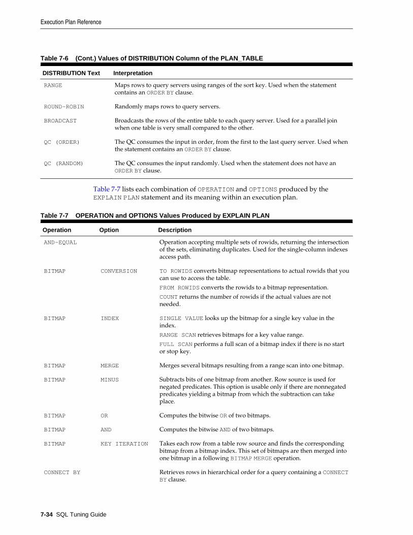
Table 7-6 (Cont.) Values of DISTRIBUTION Column of the PLAN_TABLE
DISTRIBUTION Text Interpretation
RANGE Maps rows to query servers using ranges of the sort key. Used when the statementcontains an ORDER BY clause.
ROUND-ROBIN Randomly maps rows to query servers.
BROADCAST Broadcasts the rows of the entire table to each query server. Used for a parallel joinwhen one table is very small compared to the other.
QC (ORDER) The QC consumes the input in order, from the first to the last query server. Used whenthe statement contains an ORDER BY clause.
QC (RANDOM) The QC consumes the input randomly. Used when the statement does not have anORDER BY clause.
Table 7-7 lists each combination of OPERATION and OPTIONS produced by theEXPLAIN PLAN statement and its meaning within an execution plan.
Table 7-7 OPERATION and OPTIONS Values Produced by EXPLAIN PLAN
Operation Option Description
AND-EQUAL Operation accepting multiple sets of rowids, returning the intersectionof the sets, eliminating duplicates. Used for the single-column indexesaccess path.
BITMAP CONVERSION TO ROWIDS converts bitmap representations to actual rowids that youcan use to access the table.
FROM ROWIDS converts the rowids to a bitmap representation.
COUNT returns the number of rowids if the actual values are notneeded.
BITMAP INDEX SINGLE VALUE looks up the bitmap for a single key value in theindex.
RANGE SCAN retrieves bitmaps for a key value range.
FULL SCAN performs a full scan of a bitmap index if there is no startor stop key.
BITMAP MERGE Merges several bitmaps resulting from a range scan into one bitmap.
BITMAP MINUS Subtracts bits of one bitmap from another. Row source is used fornegated predicates. This option is usable only if there are nonnegatedpredicates yielding a bitmap from which the subtraction can takeplace.
BITMAP OR Computes the bitwise OR of two bitmaps.
BITMAP AND Computes the bitwise AND of two bitmaps.
BITMAP KEY ITERATION Takes each row from a table row source and finds the correspondingbitmap from a bitmap index. This set of bitmaps are then merged intoone bitmap in a following BITMAP MERGE operation.
CONNECT BY Retrieves rows in hierarchical order for a query containing a CONNECTBY clause.
Execution Plan Reference
7-34 SQL Tuning Guide

Table 7-7 (Cont.) OPERATION and OPTIONS Values Produced by EXPLAIN PLAN
Operation Option Description
CONCATENATION Operation accepting multiple sets of rows returning the union-all ofthe sets.
COUNT Operation counting the number of rows selected from a table.
COUNT STOPKEY Count operation where the number of rows returned is limited by theROWNUM expression in the WHERE clause.
CUBE JOIN Joins a table or view on the left and a cube on the right.
See Oracle Database SQL Language Reference to learn about theNO_USE_CUBE and USE_CUBE hints.
CUBE JOIN ANTI Uses an antijoin for a table or view on the left and a cube on the right.
CUBE JOIN ANTI SNA Uses an antijoin (single-sided null aware) for a table or view on the leftand a cube on the right. The join column on the right (cube side) isNOT NULL.
CUBE JOIN OUTER Uses an outer join for a table or view on the left and a cube on theright.
CUBE JOIN RIGHT SEMI Uses a right semijoin for a table or view on the left and a cube on theright.
CUBE SCAN Uses inner joins for all cube access.
CUBE SCAN PARTIAL OUTER Uses an outer join for at least one dimension, and inner joins for theother dimensions.
CUBE SCAN OUTER Uses outer joins for all cube access.
DOMAIN INDEX Retrieval of one or more rowids from a domain index. The optionscolumn contain information supplied by a user-defined domain indexcost function, if any.
FILTER Operation accepting a set of rows, eliminates some of them, andreturns the rest.
FIRST ROW Retrieval of only the first row selected by a query.
FOR UPDATE Operation retrieving and locking the rows selected by a querycontaining a FOR UPDATE clause.
HASH GROUP BY Operation hashing a set of rows into groups for a query with a GROUPBY clause.
HASH GROUP BY PIVOT Operation hashing a set of rows into groups for a query with a GROUPBY clause. The PIVOT option indicates a pivot-specific optimizationfor the HASH GROUP BY operator.
HASH JOIN
(These are joinoperations.)
Operation joining two sets of rows and returning the result. This joinmethod is useful for joining large data sets of data (DSS, Batch). Thejoin condition is an efficient way of accessing the second table.
Query optimizer uses the smaller of the two tables/data sources tobuild a hash table on the join key in memory. Then it scans the largertable, probing the hash table to find the joined rows.
Execution Plan Reference
Reading Execution Plans 7-35

Table 7-7 (Cont.) OPERATION and OPTIONS Values Produced by EXPLAIN PLAN
Operation Option Description
HASH JOIN ANTI Hash (left) antijoin
HASH JOIN SEMI Hash (left) semijoin
HASH JOIN RIGHT ANTI Hash right antijoin
HASH JOIN RIGHT SEMI Hash right semijoin
HASH JOIN OUTER Hash (left) outer join
HASH JOIN RIGHT OUTER Hash right outer join
INDEX
(These are accessmethods.)
UNIQUE SCAN Retrieval of a single rowid from an index.
INDEX RANGE SCAN Retrieval of one or more rowids from an index. Indexed values arescanned in ascending order.
INDEX RANGE SCANDESCENDING
Retrieval of one or more rowids from an index. Indexed values arescanned in descending order.
INDEX FULL SCAN Retrieval of all rowids from an index when there is no start or stopkey. Indexed values are scanned in ascending order.
INDEX FULL SCANDESCENDING
Retrieval of all rowids from an index when there is no start or stopkey. Indexed values are scanned in descending order.
INDEX FAST FULL SCAN Retrieval of all rowids (and column values) using multiblock reads.No sorting order can be defined. Compares to a full table scan on onlythe indexed columns. Only available with the cost based optimizer.
INDEX SKIP SCAN Retrieval of rowids from a concatenated index without using theleading column(s) in the index. Only available with the cost basedoptimizer.
INLISTITERATOR
Iterates over the next operation in the plan for each value in the IN-listpredicate.
INTERSECTION Operation accepting two sets of rows and returning the intersection ofthe sets, eliminating duplicates.
MERGE JOIN
(These are joinoperations.)
Operation accepting two sets of rows, each sorted by a value,combining each row from one set with the matching rows from theother, and returning the result.
MERGE JOIN OUTER Merge join operation to perform an outer join statement.
MERGE JOIN ANTI Merge antijoin.
MERGE JOIN SEMI Merge semijoin.
MERGE JOIN CARTESIAN Can result from 1 or more of the tables not having any join conditionsto any other tables in the statement. Can occur even with a join and itmay not be flagged as CARTESIAN in the plan.
Execution Plan Reference
7-36 SQL Tuning Guide

Table 7-7 (Cont.) OPERATION and OPTIONS Values Produced by EXPLAIN PLAN
Operation Option Description
CONNECT BY Retrieval of rows in hierarchical order for a query containing aCONNECT BY clause.
MAT_VIEWREWITE ACCESS
(These are accessmethods.)
FULL Retrieval of all rows from a materialized view.
MAT_VIEWREWITE ACCESS
SAMPLE Retrieval of sampled rows from a materialized view.
MAT_VIEWREWITE ACCESS
CLUSTER Retrieval of rows from a materialized view based on a value of anindexed cluster key.
MAT_VIEWREWITE ACCESS
HASH Retrieval of rows from materialized view based on hash cluster keyvalue.
MAT_VIEWREWITE ACCESS
BY ROWID RANGE Retrieval of rows from a materialized view based on a rowid range.
MAT_VIEWREWITE ACCESS
SAMPLE BYROWID RANGE
Retrieval of sampled rows from a materialized view based on a rowidrange.
MAT_VIEWREWITE ACCESS
BY USER ROWID If the materialized view rows are located using user-supplied rowids.
MAT_VIEWREWITE ACCESS
BY INDEX ROWID If the materialized view is nonpartitioned and rows are located usingindex(es).
MAT_VIEWREWITE ACCESS
BY GLOBALINDEX ROWID
If the materialized view is partitioned and rows are located using onlyglobal indexes.
MAT_VIEWREWITE ACCESS
BY LOCAL INDEXROWID
If the materialized view is partitioned and rows are located using oneor more local indexes and possibly some global indexes.
Partition Boundaries:
The partition boundaries might have been computed by:
A previous PARTITION step, in which case the PARTITION_STARTand PARTITION_STOP column values replicate the values present inthe PARTITION step, and the PARTITION_ID contains the ID of thePARTITION step. Possible values for PARTITION_START andPARTITION_STOP are NUMBER(n), KEY, INVALID.
The MAT_VIEW REWRITE ACCESS or INDEX step itself, in which casethe PARTITION_ID contains the ID of the step. Possible values forPARTITION_START and PARTITION_STOP are NUMBER(n), KEY, ROWREMOVE_LOCATION (MAT_VIEW REWRITE ACCESS only), andINVALID.
MINUS Operation accepting two sets of rows and returning rows appearing inthe first set but not in the second, eliminating duplicates.
NESTED LOOPS
(These are joinoperations.)
Operation accepting two sets of rows, an outer set and an inner set.Oracle Database compares each row of the outer set with each row ofthe inner set, returning rows that satisfy a condition. This join methodis useful for joining small subsets of data (OLTP). The join condition isan efficient way of accessing the second table.
Execution Plan Reference
Reading Execution Plans 7-37

Table 7-7 (Cont.) OPERATION and OPTIONS Values Produced by EXPLAIN PLAN
Operation Option Description
NESTED LOOPS OUTER Nested loops operation to perform an outer join statement.
PARTITION Iterates over the next operation in the plan for each partition in therange given by the PARTITION_START and PARTITION_STOPcolumns. PARTITION describes partition boundaries applicable to asingle partitioned object (table or index) or to a set of equipartitionedobjects (a partitioned table and its local indexes). The partitionboundaries are provided by the values of PARTITION_START andPARTITION_STOP of the PARTITION. Refer to Table 7-4 for validvalues of partition start and stop.
PARTITION SINGLE Access one partition.
PARTITION ITERATOR Access many partitions (a subset).
PARTITION ALL Access all partitions.
PARTITION INLIST Similar to iterator, but based on an IN-list predicate.
PARTITION INVALID Indicates that the partition set to be accessed is empty.
PX ITERATOR BLOCK, CHUNK Implements the division of an object into block or chunk rangesamong a set of parallel execution servers.
PX COORDINATOR Implements the Query Coordinator which controls, schedules, andexecutes the parallel plan below it using parallel execution servers. Italso represents a serialization point, as the end of the part of the planexecuted in parallel and always has a PX SEND QC operation below it.
PX PARTITION Same semantics as the regular PARTITION operation except that itappears in a parallel plan.
PX RECEIVE Shows the consumer/receiver parallel execution node readingrepartitioned data from a send/producer (QC or parallel executionserver) executing on a PX SEND node. This information was formerlydisplayed into the DISTRIBUTION column. See Table 7-5.
PX SEND QC (RANDOM),HASH, RANGE
Implements the distribution method taking place between two sets ofparallel execution servers. Shows the boundary between two sets andhow data is repartitioned on the send/producer side (QC or side. Thisinformation was formerly displayed into the DISTRIBUTION column.See Table 7-5.
REMOTE Retrieval of data from a remote database.
SEQUENCE Operation involving accessing values of a sequence.
SORT AGGREGATE Retrieval of a single row that is the result of applying a group functionto a group of selected rows.
SORT UNIQUE Operation sorting a set of rows to eliminate duplicates.
SORT GROUP BY Operation sorting a set of rows into groups for a query with a GROUPBY clause.
Execution Plan Reference
7-38 SQL Tuning Guide

Table 7-7 (Cont.) OPERATION and OPTIONS Values Produced by EXPLAIN PLAN
Operation Option Description
SORT GROUP BY PIVOT Operation sorting a set of rows into groups for a query with a GROUPBY clause. The PIVOT option indicates a pivot-specific optimizationfor the SORT GROUP BY operator.
SORT JOIN Operation sorting a set of rows before a merge-join.
SORT ORDER BY Operation sorting a set of rows for a query with an ORDER BY clause.
TABLE ACCESS
(These are accessmethods.)
FULL Retrieval of all rows from a table.
TABLE ACCESS SAMPLE Retrieval of sampled rows from a table.
TABLE ACCESS CLUSTER Retrieval of rows from a table based on a value of an indexed clusterkey.
TABLE ACCESS HASH Retrieval of rows from table based on hash cluster key value.
TABLE ACCESS BY ROWID RANGE Retrieval of rows from a table based on a rowid range.
TABLE ACCESS SAMPLE BYROWID RANGE
Retrieval of sampled rows from a table based on a rowid range.
TABLE ACCESS BY USER ROWID If the table rows are located using user-supplied rowids.
TABLE ACCESS BY INDEX ROWID If the table is nonpartitioned and rows are located using index(es).
TABLE ACCESS BY GLOBALINDEX ROWID
If the table is partitioned and rows are located using only globalindexes.
TABLE ACCESS BY LOCAL INDEXROWID
If the table is partitioned and rows are located using one or more localindexes and possibly some global indexes.
Partition Boundaries:
The partition boundaries might have been computed by:
A previous PARTITION step, in which case the PARTITION_STARTand PARTITION_STOP column values replicate the values present inthe PARTITION step, and the PARTITION_ID contains the ID of thePARTITION step. Possible values for PARTITION_START andPARTITION_STOP are NUMBER(n), KEY, INVALID.
The TABLE ACCESS or INDEX step itself, in which case thePARTITION_ID contains the ID of the step. Possible values forPARTITION_START and PARTITION_STOP are NUMBER(n), KEY, ROWREMOVE_LOCATION (TABLE ACCESS only), and INVALID.
TRANSPOSE Operation evaluating a PIVOT operation by transposing the results ofGROUP BY to produce the final pivoted data.
UNION Operation accepting two sets of rows and returns the union of the sets,eliminating duplicates.
UNPIVOT Operation that rotates data from columns into rows.
VIEW Operation performing a view's query and then returning the resultingrows to another operation.
Execution Plan Reference
Reading Execution Plans 7-39

See Also:
Oracle Database Reference for more information about PLAN_TABLE
DBMS_XPLAN Program UnitsTable 7-8 provides notes on DBMS_XPLAN functions and parameters that are relevantfor accessing adapted plans. See Oracle Database PL/SQL Packages and Types Referencefor complete reference information.
Table 7-8 DBMS_XPLAN Functions and Parameters Relevant for Adaptive Queries
Functions Notes
DISPLAY_PLAN The FORMAT argument supports the modifier ADAPTIVE.
When you specify ADAPTIVE, the output includes the defaultplan. For each dynamic subplan, the plan shows a list of the rowsources from the original that may be replaced, and the rowsources that would replace them.
If the format argument specifies the outline display, then thefunction displays the hints for each option in the dynamicsubplan. If the plan is not an adaptive plan, then the functiondisplays the default plan.When you do not specify ADAPTIVE,the plan is shown as-is, but with additional comments in theNote section that show any row sources that are dynamic.
DISPLAY_CURSOR The FORMAT argument supports the modifier ADAPTIVE.
When you specify ADAPTIVE, the output includes:
• The final plan. If the execution has not completed, then theoutput shows the current plan. This section also includesnotes about run-time optimizations that affect the plan.
• Recommended plan. In reporting mode, the output includesthe plan that would be chosen based on execution statistics.
• Dynamic plan. The output summarizes the portions of theplan that differ from the default plan chosen by theoptimizer.
• Reoptimization. The output displays the plan that would bechosen on a subsequent execution because of reoptimization.
Execution Plan Reference
7-40 SQL Tuning Guide

Part IVSQL Operators
A row source is a set of rows returned by a step in the execution plan. A SQL operatoracts on a row source. A unary operator acts on one input, as with access paths. Abinary operator acts on two outputs, as with joins.
This part contains the following chapters:
• Optimizer Access Paths
• Joins


8Optimizer Access Paths
This chapter contains the following topics:
• Introduction to Access Paths
• Table Access Paths
• B-Tree Index Access Paths
• Bitmap Index Access Paths
• Table Cluster Access Paths
Introduction to Access PathsA row source is a set of rows returned by a step in an execution plan. A row sourcecan be a table, view, or result of a join or grouping operation.
A unary operation such as an access path, which is a technique used by a query toretrieve rows from a row source, accepts a single row source as input. For example, afull table scan is the retrieval of rows of a single row source. In contrast, a joinoperation is binary and receives inputs from two row sources (see Joins ).
The database uses different access paths for different relational data structures (see Oracle Database Concepts for an overview of these structures). Table 8-1 summarizescommon access paths for the major data structures.
Table 8-1 Data Structures and Access Paths
Access Path Heap-OrganizedTables
B-Tree Indexes andIOTs
Bitmap Indexes Table Clusters
Full Table Scans x
Table Access by Rowid x
Sample Table Scans x
Index Unique Scans x
Index Range Scans x
Index Full Scans x
Index Fast Full Scans x
Index Skip Scans x
Index Join Scans x
Optimizer Access Paths 8-1

Table 8-1 (Cont.) Data Structures and Access Paths
Access Path Heap-OrganizedTables
B-Tree Indexes andIOTs
Bitmap Indexes Table Clusters
Bitmap Index SingleValue
x
Bitmap Index RangeScans
x
Bitmap Merge x
Bitmap Index RangeScans
x
Cluster Scans x
Hash Scans x
As explained in “Cost-Based Optimization,” the optimizer considers different possibleexecution plans, and then assigns each plan a cost. The optimizer chooses the planwith the lowest cost. In general, index access paths are more efficient for statementsthat retrieve a small subset of table rows, whereas full table scans are more efficientwhen accessing a large portion of a table.
Table Access PathsA table is the basic unit of data organization in an Oracle database. Relational tablesare the most common table type. Relational tables have with the followingorganizational characteristics:
• A heap-organized table does not store rows in any particular order.
• An index-organized table orders rows according to the primary key values.
• An external table is a read-only table whose metadata is stored in the database butwhose data is stored outside the database.
This section explains optimizer access paths for heap-organized tables, and containsthe following topics:
• About Heap-Organized Table Access
• Full Table Scans
• Table Access by Rowid
• Sample Table Scans
• In-Memory Table Scans
Table Access Paths
8-2 SQL Tuning Guide

See Also:
• Oracle Database Concepts for an overview of tables
• Oracle Database Administrator's Guide to learn how to manage tables
About Heap-Organized Table AccessBy default, a table is organized as a heap, which means that the database places rowswhere they fit best rather than in a user-specified order. As users add rows, thedatabase places the rows in the first available free space in the data segment. Rows arenot guaranteed to be retrieved in the order in which they were inserted.
Row Storage in Data Blocks and Segments: A Primer
The database stores rows in data blocks. In tables, the database can write a rowanywhere in the bottom part of the block. Oracle Database uses the block overhead,which contains the row directory and table directory, to manage the block itself.
An extent is made up of logically contiguous data blocks. The blocks may not bephysically contiguous on disk. A segment is a set of extents that contains all the datafor a logical storage structure within a tablespace. For example, Oracle Databaseallocates one or more extents to form the data segment for a table. The database alsoallocates one or more extents to form the index segment for a table.
By default, the database uses automatic segment space management (ASSM) forpermanent, locally managed tablespaces. When a session first inserts data into a table,the database formats a bitmap block. The bitmap tracks the blocks in the segment. Thedatabase uses the bitmap to find free blocks and then formats each block beforewriting to it. ASSM spread out inserts among blocks to avoid concurrency issues.
The high water mark (HWM) is the point in a segment beyond which data blocks areunformatted and have never been used. Below the HWM, a block may be formattedand written to, formatted and empty, or unformatted. The low high water mark (lowHWM) marks the point below which all blocks are known to be formatted becausethey either contain data or formerly contained data.
During a full table scan, the database reads all blocks up to the low HWM, which areknown to be formatted, and then reads the segment bitmap to determine which blocksbetween the HWM and low HWM are formatted and safe to read. The database knowsnot to read past the HWM because these blocks are unformatted.
See Also:
Oracle Database Concepts to learn about data block storage
Importance of Rowids for Row Access
Every row in a heap-organized table has a rowid unique to this table that correspondsto the physical address of a row piece. A rowid is a 10-byte physical address of a row.
The rowid points to a specific file, block, and row number. For example, in the rowidAAAPecAAFAAAABSAAA, the final AAA represents the row number. The row number isan index into a row directory entry. The row directory entry contains a pointer to thelocation of the row on the block.
Table Access Paths
Optimizer Access Paths 8-3

The database can sometimes move a row in the bottom part of the block. For example,if row movement is enabled, then the row can move because of partition key updates,Flashback Table operations, shrink table operations, and so on. If the database moves arow within a block, then the database updates the row directory entry to modify thepointer. The rowid stays constant.
Oracle Database uses rowids internally for the construction of indexes. For example,each key in a B-tree index is associated with a rowid that points to the address of theassociated row. Physical rowids provide the fastest possible access to a table row,enabling the database to retrieve a row in as little as a single I/O.
See Also:
Oracle Database Concepts to learn about rowids
Direct Path Reads
In a direct path read, the database reads buffers from disk directly into the PGA,bypassing the SGA entirely. Figure 8-1 shows the difference between scattered andsequential reads, which store buffers in the SGA, and direct path reads.
Figure 8-1 Direct Path Reads
DB FileSequential Read
DB FileScattered Read
Direct path read
Direct PathRead
Database Buffer Cache
SGA Buffer Cache
Database Buffer Cache
SGA Buffer CacheSort Area Hash Area
Process PGA
Bitmap MergeArea
SessionMemory
RuntimeArea
PersistentArea
Situations in which Oracle Database may perform direct path reads include:
• Execution of a CREATE TABLE AS SELECT statement
• Execution of an ALTER REBUILD or ALTER MOVE statement
• Reads from a temporary tablespace
• Parallel queries
Table Access Paths
8-4 SQL Tuning Guide
• Reads from a LOB segment
See Also:
Oracle Database Performance Tuning Guide to learn about wait events for directpath reads
Full Table ScansA full table scan reads all rows from a table, and then filters out those rows that donot meet the selection criteria.
When the Optimizer Considers a Full Table Scan
In general, the optimizer chooses a full table scan when it cannot use a different accesspath, or another usable access path is higher cost. Typical reasons for choosing a fulltable scan include the following:
• No index exists.
If no index exists, then the optimizer uses a full table scan.
• The query predicate applies a function to the indexed column.
Unless the index is a function-based index (see “Guidelines for Using Function-Based Indexes for Performance”), the database indexes the values of the column,not the values of the column with the function applied. A typical application-levelmistake is to index a character column, such as char_col, and then query thecolumn using syntax such as WHERE char_col=1. The database implicitly appliesa TO_NUMBER function to the constant number 1, which prevents use of the index.
• A SELECT COUNT(*) query is issued, and an index exists, but the indexed columncontains nulls.
The optimizer cannot use the index to count the number of table rows because theindex cannot contain null entries (see “B-Tree Indexes and Nulls”).
• The query predicate does not use the leading edge of a B-tree index.
For example, an index might exist on employees(first_name,last_name). Ifa user issues a query with the predicate WHERE last_name='KING', then theoptimizer may not choose an index because column first_name is not in thepredicate. However, in this situation the optimizer may choose to use an index skipscan (see “Index Skip Scans”).
• The query is unselective.
If the optimizer determines that the query requires most of the blocks in the table,then it uses a full table scan, even though indexes are available. Full table scans canuse larger I/O calls. Making fewer large I/O calls is cheaper than making manysmaller calls.
• The table statistics are stale.
For example, a table was small, but now has grown large. If the table statistics arestale and do not reflect the current size of the table, then the optimizer does notknow that an index is now most efficient than a full table scan. See “Introduction toOptimizer Statistics.”
Table Access Paths
Optimizer Access Paths 8-5

• The table is small.
If a table contains fewer than n blocks under the high water mark, where n equalsthe setting for the DB_FILE_MULTIBLOCK_READ_COUNT initialization parameter,then a full table scan may be cheaper than an index range scan. The scan may beless expensive regardless of the fraction of tables being accessed or indexes present.
• The table has a high degree of parallelism.
A high degree of parallelism for a table skews the optimizer toward full table scansover range scans. Query the value in the ALL_TABLES.DEGREE column in for thetable to determine the degree of parallelism.
• The query uses a full table scan hint.
The hint FULL(table alias) instructs the optimizer to use a full table scan.
See Also:
“Influencing the Optimizer with Hints”
How a Full Table Scan Works
In a full table scan, the database sequentially reads every formatted block under thehigh water mark. The database reads each block only once. The following graphicdepicts a scan of a table segment, showing how the scan skips unformatted blocksbelow the high water mark.
Low HWM HWM
Never Used, Unformatted
Used
SequentialRead
Because the blocks are adjacent, the database can speed up the scan by making I/Ocalls larger than a single block, known as a multiblock read. The size of a read callranges from one block to the number of blocks specified by the DB_FILE_MULTIBLOCK_READ_COUNT initialization parameter. For example, settingthis parameter to 4 instructs the database to read up to 4 blocks in a single call.
The algorithms for caching blocks during full table scans are complex. For example,the database caches blocks differently depending on whether tables are small or large.
Table Access Paths
8-6 SQL Tuning Guide

See Also:
• Table 14-1
• Oracle Database Concepts for an overview of the default caching mode
• Oracle Database Reference to learn about the DB_FILE_MULTIBLOCK_READ_COUNT initialization parameter
Full Table Scan: Example
The following statement queries salaries over 4000 in the hr.employees table:
SELECT salary FROM hr.employees WHERE salary > 4000;
Example 8-1 Full Table Scan
The following plan was retrieved using the DBMS_XPLAN.DISPLAY_CURSORfunction. Because no index exists on the salary column, the optimizer cannot use anindex range scan, and so uses a full table scan.
SQL_ID 54c20f3udfnws, child number 0-------------------------------------select salary from hr.employees where salary > 4000 Plan hash value: 3476115102 -------------------------------------------------------------------------------| Id | Operation | Name | Rows | Bytes | Cost (%CPU)| Time |-------------------------------------------------------------------------------| 0 | SELECT STATEMENT | | | | 3 (100)| ||* 1 | TABLE ACCESS FULL| EMPLOYEES | 98 | 6762 | 3 (0)| 00:00:01 |------------------------------------------------------------------------------- Predicate Information (identified by operation id):--------------------------------------------------- 1 - filter("SALARY">4000)
Table Access by RowidA rowid is an internal representation of the storage location of data. The rowid of arow specifies the data file and data block containing the row and the location of therow in that block. Locating a row by specifying its rowid is the fastest way to retrieve asingle row because it specifies the exact location of the row in the database.
Note:
Rowids can change between versions. Accessing data based on position is notrecommended because rows can move. To learn more about rowids, see OracleDatabase Development Guide.
Table Access Paths
Optimizer Access Paths 8-7

When the Optimizer Chooses Table Access by Rowid
In most cases, the database accesses a table by rowid after a scan of one or moreindexes. However, table access by rowid need not follow every index scan. If the indexcontains all needed columns, then access by rowid might not occur (see “Index FastFull Scans”).
How Table Access by Rowid Works
To access a table by rowid, the database performs the following steps:
1. Obtains the rowids of the selected rows, either from the statement WHERE clauseor through an index scan of one or more indexes
Table access may be needed for columns in the statement not present in the index.
2. Locates each selected row in the table based on its rowid
Table Access by Rowid: Example
Assume run the following query:
SELECT * FROM employees WHERE employee_id > 190;
Step 2 of the following plan shows a range scan of the emp_emp_id_pk index on thehr.employees table. The database uses the rowids obtained from the index to findthe corresponding rows from the employees table, and then retrieve them. TheBATCHED access shown in Step 1 means that the database retrieves a few rowids fromthe index, and then attempts to access rows in block order to improve the clusteringand reduce the number of times that the database must access a block.
--------------------------------------------------------------------------------|Id| Operation | Name |Rows|Bytes|Cost(%CPU)|Time|--------------------------------------------------------------------------------| 0| SELECT STATEMENT | | | |2(100)| || 1| TABLE ACCESS BY INDEX ROWID BATCHED|EMPLOYEES |16|1104|2 (0)|00:00:01||*2| INDEX RANGE SCAN |EMP_EMP_ID_PK|16| |1 (0)|00:00:01|-------------------------------------------------------------------------------- Predicate Information (identified by operation id):--------------------------------------------------- 2 - access("EMPLOYEE_ID">190)
Sample Table ScansA sample table scan retrieves a random sample of data from a simple table or acomplex SELECT statement, such as a statement involving joins and views.
When the Optimizer Chooses a Sample Table Scan
The database uses a sample table scan when a statement FROM clause includes either ofthe following clauses:
• SAMPLE (sample_percent)
The database reads a specified percentage of rows in the table to perform a sampletable scan.
Table Access Paths
8-8 SQL Tuning Guide

• SAMPLE BLOCK (sample_percent)
The database reads a specified percentage of table blocks to perform a sample tablescan.
The sample_percent specifies the percentage of the total row or block count to include inthe sample. The value must be in the range .000001 up to, but not including, 100.This percentage indicates the probability of each row, or each cluster of rows in blocksampling, being selected for the sample. It does not mean that the database retrievesexactly sample_percent of the rows.
Note:
Block sampling is possible only during full table scans or index fast full scans.If a more efficient execution path exists, then the database does not sampleblocks. To guarantee block sampling for a specific table or index, use the FULLor INDEX_FFS hint.
See Also:
• “Influencing the Optimizer with Hints”
• Oracle Database SQL Language Reference to learn about the SAMPLE clause
Sample Table Scans: Example
Example 8-2 uses a sample table scan to access 1% of the employees table, samplingby blocks instead of rows.
Example 8-2 Sample Table Scan
SELECT * FROM hr.employees SAMPLE BLOCK (1);
The EXPLAIN PLAN output for this statement might look as follows:
-------------------------------------------------------------------------| Id | Operation | Name | Rows | Bytes | Cost (%CPU)|-------------------------------------------------------------------------| 0 | SELECT STATEMENT | | 1 | 68 | 3 (34)|| 1 | TABLE ACCESS SAMPLE | EMPLOYEES | 1 | 68 | 3 (34)|-------------------------------------------------------------------------
In-Memory Table ScansStarting in Oracle Database 12c Release 1 (12.1.0.2), an in-memory scan retrieves someor all rows from the In-Memory Column Store (IM column store). The IM columnstore is an optional SGA area that stores copies of tables and partitions in a specialcolumnar format optimized for rapid scans.
Table Access Paths
Optimizer Access Paths 8-9

See Also:
• Oracle Database Concepts for an overview of the IM column store
• Oracle Database Administrator's Guide to learn how to enable the IM columnstore
When the Optimizer Chooses an In-Memory Table Scan
Starting in Oracle Database 12c Release 1 (12.1.0.2), the optimizer cost model is fullyaware of the content of the IM column store. When a user executes a query thatreferences a table in the IM column store, the optimizer calculates the cost of allpossible access methods—including the in-memory table scan—and selects the accessmethod with the lowest cost.
In-Memory Query Controls
The following database initialization parameters affect the in-memory features:
• INMEMORY_QUERY
This parameter enables or disables in-memory queries for the database at thesession or system level. This parameter is helpful when you want to test workloadswith and without the use of the IM column store.
• OPTIMIZER_INMEMORY_AWARE
This parameter enables (TRUE) or disables (FALSE) all of the in-memoryenhancements made to the optimizer cost model, table expansion, bloom filters,and so on. Setting the parameter to FALSE causes the optimizer to ignore the in-memory property of tables during the optimization of SQL statements.
• OPTIMIZER_FEATURES_ENABLE
When set to values lower than 12.1.0.2, this parameter has the same effect assetting OPTIMIZER_INMEMORY_AWARE to FALSE.
To enable or disable in-memory queries, you can specify the INMEMORY orNO_INMEMORY hints, which are the per-query equivalent of the INMEMORY_QUERYinitialization parameter. If a SQL statement uses the INMEMORY hint, but the object itreferences is not already loaded in the IM column store, then the database does notwait for the object to be populated in the IM column store before executing thestatement. However, initial access of the object triggers the object population in the IMcolumn store.
See Also:
• Oracle Database Reference to learn more about the INMEMORY_QUERY,OPTIMIZER_INMEMORY_AWARE, and OPTIMIZER_FEATURES_ENABLEinitialization parameters
• Oracle Database SQL Language Reference to learn more about the INMEMORYhints
Table Access Paths
8-10 SQL Tuning Guide

In-Memory Table Scans: Example
The following example shows a query of the oe.product_information table,which has been altered with the INMEMORY HIGH option.
Example 8-3 In-Memory Table Scan
SELECT * FROM oe.product_informationWHERE list_price > 10 ORDER BY product_id
The plan for this statement might look as follows, with the INMEMORY keyword in Step2 indicating that some or all of the object was accessed from the IM column store:
SQL> SELECT * FROM TABLE(DBMS_XPLAN.DISPLAY_CURSOR);
SQL_ID 2mb4h57x8pabw, child number 0-------------------------------------select * from oe.product_information where list_price > 10 order byproduct_id
Plan hash value: 2256295385--------------------------------------------------------------------------------------------|Id| Operation | Name |Rows|Bytes |TempSpc|Cost(%CPU)|Time|--------------------------------------------------------------------------------------------| 0| SELECT STATEMENT | | | | |21 (100)| || 1| SORT ORDER BY | | 285| 62415|82000|21 (5)|00:00:01||*2| TABLE ACCESS INMEMORY FULL| PRODUCT_INFORMATION | 285| 62415| | 5 (0)|00:00:01|--------------------------------------------------------------------------------------------
Predicate Information (identified by operation id):--------------------------------------------------- 2 - inmemory("LIST_PRICE">10) filter("LIST_PRICE">10)
B-Tree Index Access PathsAn index is an optional structure, associated with a table or table cluster, that cansometimes speed data access. By creating an index on one or more columns of a table,you gain the ability in some cases to retrieve a small set of randomly distributed rowsfrom the table. Indexes are one of many means of reducing disk I/O.
This section contains the following topics:
• About B-Tree Index Access
• Index Unique Scans
• Index Range Scans
• Index Full Scans
• Index Fast Full Scans
• Index Skip Scans
• Index Join Scans
B-Tree Index Access Paths
Optimizer Access Paths 8-11

See Also:
• Oracle Database Concepts for an overview of indexes
• Oracle Database Administrator's Guide to learn how to manage indexes
About B-Tree Index AccessB-trees, short for balanced trees, are the most common type of database index. A B-treeindex is an ordered list of values divided into ranges. By associating a key with a rowor range of rows, B-trees provide excellent retrieval performance for a wide range ofqueries, including exact match and range searches.
B-Tree Index Structure
Figure 8-2 illustrates the logical structure of a B-tree index. A B-tree index has twotypes of blocks: branch blocks for searching and leaf blocks that store values. Branchblocks store the minimum key prefix needed to make a branching decision betweentwo keys. The leaf blocks contain every indexed data value and a corresponding rowidused to locate the actual row. Each index entry is sorted by (key, rowid). Within a leafblock, a key and rowid is linked to its left and right sibling entries. The leaf blocksthemselves are also doubly linked.
Figure 8-2 B-Tree Index Structure
. . .
41..48
49..53
54..65
....
78..80
11,rowid
11,rowid
12,rowid
....
19,rowid
221,rowid
222,rowid
223,rowid
....
228,rowid
246,rowid
248,rowid
248,rowid
....
250,rowid
0,rowid
0,rowid
....
10,rowid
0..40
41..80
81..120
....
200..250
. . .. . .
0..10
11..19�
20..25
....
32..40
200..209
210..220
221..228
....
246..250
Branch Blocks
Leaf Blocks
B-Tree Index Access Paths
8-12 SQL Tuning Guide

How Index Storage Affects Index Scans
Figure 8-2 shows the leaf blocks as adjacent to each other, so that the 1-10 block isnext to and before the 11-19 block. This arrangement illustrates the linked lists thatconnect the index entries. However, index blocks need not be stored in order within anindex segment. For example, the 246-250 block could appear anywhere in thesegment, including directly before the 1-10 block. Because blocks can appearanywhere in the segment, ordered index scans must perform single-block I/O. Thedatabase must read a block to determine which block it must read next.
Figure 8-2 shows the index entries within an index block stored sequentially. This istrue at a high level. At a low level, the index entries in the index block body are storedin a heap, just like table rows. For example, if the value 10 is inserted first into a table,then the index entry with key 10 might be inserted at the bottom of the index block,and if 0 is inserted next into the table, then the index entry for key 0 might be insertedon top of the entry for 10, and so on. Thus, the index entries in the block body are notstored in key order. However, within the index block, the row header stores records inkey order. For example, the first record in the header points to the index entry withkey 0, and so on sequentially up to the record that points to the index entry with key10. Thus, index scans can read the row header to determine where to begin and endrange scans, avoiding the necessity of reading every entry in the block.
See Also:
Oracle Database Concepts to learn about index blocks
Unique and Nonunique Indexes
Figure 8-2 shows a nonunique index. In a nonunique index, the database stores therowid by appending it to the key as an extra column with a length byte to make thekey unique. For example, the first index key in Figure 8-2 is the pair 0,rowid and notsimply 0. The database sorts the data by index key values and then by rowidascending. For example, the entries are sorted as follows:
0,AAAPvCAAFAAAAFaAAa0,AAAPvCAAFAAAAFaAAg0,AAAPvCAAFAAAAFaAAl2,AAAPvCAAFAAAAFaAAm
In a unique index, the index key does not include the rowid. The database sorts thedata only by the index key values, such as 0, 1, 2, and so on.
See Also:
Oracle Database Concepts for an overview of unique and nonunique indexes
B-Tree Indexes and Nulls
B-tree indexes never store completely null keys, which is important for how theoptimizer chooses access paths. A consequence of this rule is that single-column B-treeindexes never store nulls.
An example helps illustrate. The hr.employees table has a primary key index onemployee_id, and a unique index on department_id. The department_id
B-Tree Index Access Paths
Optimizer Access Paths 8-13

column can contain nulls, making it a nullable column, but the employee_id columncannot.
SQL> SELECT COUNT(*) FROM employees WHERE department_id IS NULL; COUNT(*)---------- 1 SQL> SELECT COUNT(*) FROM employees WHERE employee_id IS NULL; COUNT(*)---------- 0
The following example shows that the optimizer chooses a full table scan for a queryof all department IDs in hr.employees. The optimizer cannot use the index onemployees.department_id because the index is not guaranteed to include entriesfor every row in the table.
SQL> EXPLAIN PLAN FOR SELECT department_id FROM employees; Explained. SQL> SELECT PLAN_TABLE_OUTPUT FROM TABLE(DBMS_XPLAN.DISPLAY()); PLAN_TABLE_OUTPUT--------------------------------------------------------------------------------Plan hash value: 3476115102 -------------------------------------------------------------------------------| Id | Operation | Name | Rows | Bytes | Cost (%CPU)| Time |-------------------------------------------------------------------------------| 0 | SELECT STATEMENT | | 107 | 321 | 2 (0)| 00:00:01 || 1 | TABLE ACCESS FULL| EMPLOYEES | 107 | 321 | 2 (0)| 00:00:01 |------------------------------------------------------------------------------- 8 rows selected.
The following example shows the optimizer can use the index on department_id fora query of a specific department ID because all non-null rows are indexed.
SQL> EXPLAIN PLAN FOR SELECT department_id FROM employees WHERE department_id=10; Explained. SQL> SELECT PLAN_TABLE_OUTPUT FROM TABLE(DBMS_XPLAN.DISPLAY()); PLAN_TABLE_OUTPUT--------------------------------------------------------------------------------Plan hash value: 67425611 --------------------------------------------------------------------------------| Id| Operation | Name | Rows |Bytes| Cost (%CPU)| Time |-------------------------------------------------------------------------------- PLAN_TABLE_OUTPUT--------------------------------------------------------------------------------| 0 | SELECT STATEMENT | | 1 | 3 | 1 (0)| 00:0 0:01||*1 | INDEX RANGE SCAN| EMP_DEPARTMENT_IX | 1 | 3 | 1 (0)| 00:0 0:01|--------------------------------------------------------------------------------
B-Tree Index Access Paths
8-14 SQL Tuning Guide

Predicate Information (identified by operation id): PLAN_TABLE_OUTPUT-------------------------------------------------------------------------------- 1 - access("DEPARTMENT_ID"=10)
The following example shows that the optimizer chooses an index scan when thepredicate excludes null values:
SQL> EXPLAIN PLAN FOR SELECT department_id FROM employees WHERE department_id IS NOT NULL;
Explained.
SQL> SELECT PLAN_TABLE_OUTPUT FROM TABLE(DBMS_XPLAN.DISPLAY()); PLAN_TABLE_OUTPUT--------------------------------------------------------------------------------Plan hash value: 1590637672 --------------------------------------------------------------------------------| Id| Operation | Name | Rows|Bytes| Cost (%CPU)| Time |-------------------------------------------------------------------------------- | 0 | SELECT STATEMENT | | 106 | 318 | 1 (0)| 00:0 0:01 ||*1 | INDEX FULL SCAN | EMP_DEPARTMENT_IX | 106 | 318 | 1 (0)| 00:0 0:01 |-------------------------------------------------------------------------------- Predicate Information (identified by operation id): PLAN_TABLE_OUTPUT-------------------------------------------------------------------------------- 1 - filter("DEPARTMENT_ID" IS NOT NULL)
Index Unique ScansAn index unique scan returns at most 1 rowid.
When the Optimizer Considers Index Unique Scans
The database performs a unique scan when the following conditions apply:
• A query predicate references all of the columns in a unique index key using anequality operator, such as WHERE prod_id=10.
• A SQL statement contains an equality predicate on a column referenced in an indexcreated with the CREATE UNIQUE INDEX statement.
A unique or primary key constraint is insufficient by itself to produce an index uniquescan. Consider the following example, which creates a primary key constraint on acolumn with a non-unique index, resulting in an index range scan rather than an indexunique scan:
CREATE TABLE t_table(numcol INT);CREATE INDEX t_table_idx ON t_table(numcol);ALTER TABLE t_table ADD CONSTRAINT t_table_pk PRIMARY KEY(numcol);SET AUTOTRACE TRACEONLY EXPLAINSELECT * FROM t_table WHERE numcol = 1; Execution Plan
B-Tree Index Access Paths
Optimizer Access Paths 8-15

----------------------------------------------------------Plan hash value: 868081059 --------------------------------------------------------------------------------| Id | Operation | Name | Rows | Bytes | Cost (%CPU)| Time |--------------------------------------------------------------------------------| 0 | SELECT STATEMENT | | 1 | 13 | 1 (0)| 00:00:01 ||* 1 | INDEX RANGE SCAN| T_TABLE_IDX | 1 | 13 | 1 (0)| 00:00:01 |-------------------------------------------------------------------------------- Predicate Information (identified by operation id):--------------------------------------------------- 1 - access("NUMCOL"=1)
You can use the INDEX(alias index_name) hint to specify the index to use, butnot a specific type of index access path.
See Also:
• Oracle Database Concepts for more details on index structures and fordetailed information on how a B-tree is searched
• Oracle Database SQL Language Reference to learn more about the INDEX hint
How Index Unique Scans Work
The scan searches the index in order for the specified key. An index unique scan stopsprocessing as soon as it finds the first record because no second record is possible. Thedatabase obtains the rowid from the index entry, and then retrieves the row specifiedby the rowid.
Figure 8-3 illustrates an index unique scan. The statement requests the record forproduct ID 19 in the prod_id column, which has a primary key index.
B-Tree Index Access Paths
8-16 SQL Tuning Guide
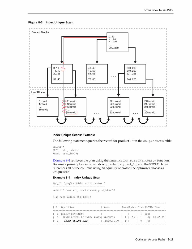
Figure 8-3 Index Unique Scan
. . .
41..48
49..53
54..65
....
78..80
11,rowid
12,rowid
13,rowid
....
19,rowid
221,rowid
222,rowid
223,rowid
....
228,rowid
246,rowid
247,rowid
248,rowid
....
250,rowid
0,rowid
1,rowid
....
10,rowid
0..40
41..80
81..120
....
200..250
. . .. . .
0..10
11..19
20..25
....
32..40
200..209
210..220
221..228
....
246..250
Branch Blocks
Leaf Blocks
Index Unique Scans: Example
The following statement queries the record for product 19 in the sh.products table:
SELECT * FROM sh.products WHERE prod_id=19;
Example 8-4 retrieves the plan using the DBMS_XPLAN.DISPLAY_CURSOR function.Because a primary key index exists on products.prod_id, and the WHERE clausereferences all of the columns using an equality operator, the optimizer chooses aunique scan.
Example 8-4 Index Unique Scan
SQL_ID 3ptq5tsd5vb3d, child number 0-------------------------------------select * from sh.products where prod_id = 19 Plan hash value: 4047888317 --------------------------------------------------------------------------------| Id| Operation | Name |Rows|Bytes|Cost (%CPU)|Time |--------------------------------------------------------------------------------| 0| SELECT STATEMENT | | | | 1 (100)| || 1| TABLE ACCESS BY INDEX ROWID| PRODUCTS | 1 | 173 | 1 (0)| 00:00:01||* 2| INDEX UNIQUE SCAN | PRODUCTS_PK | 1 | | 0 (0)| |--------------------------------------------------------------------------------
B-Tree Index Access Paths
Optimizer Access Paths 8-17

Predicate Information (identified by operation id):--------------------------------------------------- 2 - access("PROD_ID"=19)
Index Range ScansAn index range scan is an ordered scan of values. The range in the scan can bebounded on both sides, or unbounded on one or both sides. The optimizer typicallychooses a range scan for selective queries (see “Selectivity”).
By default, the database stores indexes in ascending order, and scans them in the sameorder. For example, a query with the predicate department_id >= 20 uses a rangescan to return rows sorted by index keys 20, 30, 40, and so on. If multiple indexentries have identical keys, then the database returns them in ascending order byrowid, so that 0,AAAPvCAAFAAAAFaAAa is followed by 0,AAAPvCAAFAAAAFaAAg,and so on.
An index range scan descending is identical to an index range scan except that thedatabase returns rows in descending order. Usually, the database uses a descendingscan when ordering data in a descending order, or when seeking a value less than aspecified value.
When the Optimizer Considers Index Range Scans
The optimizer considers index range scans in the following circumstances:
• One or more leading columns of an index are specified in conditions. A conditionspecifies a combination of one or more expressions and logical (Boolean) operatorsand returns a value of TRUE, FALSE, or UNKNOWN. Examples of conditions include:
– department_id = :id
– department_id < :id
– department_id > :id
– AND combination of the preceding conditions for leading columns in the index,such as department_id > :low AND department_id < :hi.
Note:
For the optimizer to consider a range scan, wild-card searches of the formcol1 LIKE '%ASD' must not be in a leading position.
• 0, 1, or more values are possible for an index key.
Tip:
If you require sorted data, then use the ORDER BY clause, and do not rely onan index. If an index can satisfy an ORDER BY clause, then the optimizer usesthis option and avoids a sort.
The optimizer considers an index range scan descending when an index can satisfy anORDER BY DESCENDING clause.
If the optimizer chooses a full table scan or another index, then a hint may be requiredto force this access path. The INDEX(tbl_alias ix_name) and
B-Tree Index Access Paths
8-18 SQL Tuning Guide

INDEX_DESC(tbl_alias ix_name) hints instruct the optimizer to use a specificindex.
See Also:
Oracle Database SQL Language Reference to learn more about the INDEX andINDEX_DESC hints
How Index Range Scans Work
In general, the process is as follows:
1. Read the root block.
2. Read the branch block.
3. Alternate the following steps until all data is retrieved:
a. Read a leaf block to obtain a rowid.
b. Read a table block to retrieve a row.
Note:
In some cases, an index scan reads a set of index blocks, sorts the rowids, andthen reads a set of table blocks.
Thus, to scan the index, the database moves backward or forward through the leafblocks. For example, a scan for IDs between 20 and 40 locates the first leaf block thathas the lowest key value that is 20 or greater. The scan proceeds horizontally throughthe linked list of leaf nodes until it finds a value greater than 40, and then stops.
Figure 8-4 illustrates an index range scan using ascending order. A statement requeststhe employees records with the value 20 in the department_id column, which hasa nonunique index. In this example, 2 index entries for department 20 exist.
B-Tree Index Access Paths
Optimizer Access Paths 8-19

Figure 8-4 Index Range Scan
. . .
41..48
49..53
54..65
....
78..80
11,rowid
11,rowid
12,rowid
....
20,rowid20, rowid
221,rowid
222,rowid
223,rowid
....
228,rowid
246,rowid
248,rowid
248,rowid
....
250,rowid
0,rowid
0,rowid
....
10,rowid
0..40
41..80
81..120
....
200..250
. . .. . .
0..10
11..2
....
32..40
200..209
210..220
221..228
....
246..250
Branch Blocks
Leaf Blocks
Index Range Scan: Example
The following statement queries the records for employees in department 20 withsalaries greater than 1000:
SELECT * FROM employees WHERE department_id = 20AND salary > 1000;
Example 8-5 retrieves the plan using the DBMS_XPLAN.DISPLAY_CURSOR function.This query is highly selective, so the query uses the index on the department_idcolumn. The database scans the index, fetches the records from the employees table,and then applies the salary > 1000 filter to these fetched records to generate theresult.
Example 8-5 Index Range Scan
SQL_ID brt5abvbxw9tq, child number 0-------------------------------------SELECT * FROM employees WHERE department_id = 20 AND salary > 1000 Plan hash value: 2799965532 -------------------------------------------------------------------------------------------|Id | Operation | Name |Rows|Bytes|Cost(%CPU)| Time |-------------------------------------------------------------------------------------------| 0 | SELECT STATEMENT | | | | 2 (100)| ||*1 | TABLE ACCESS BY INDEX ROWID BATCHED| EMPLOYEES | 2 | 138 | 2 (0)|00:00:01|
B-Tree Index Access Paths
8-20 SQL Tuning Guide

|*2 | INDEX RANGE SCAN | EMP_DEPARTMENT_IX| 2 | | 1 (0)|00:00:01|------------------------------------------------------------------------------------------- Predicate Information (identified by operation id):--------------------------------------------------- 1 - filter("SALARY">1000) 2 - access("DEPARTMENT_ID"=20)
Index Range Scan Descending: Example
The following statement queries the records for employees in department 20 indescending order:
SELECT *FROM employeesWHERE department_id < 20ORDER BY department_id DESC;
Example 8-6 retrieves the plan using the DBMS_XPLAN.DISPLAY_CURSOR function.This query is selective, so the query uses the index on the department_id column.The database locates the first index leaf block that contains the highest key value thatis 20 or less. The scan then proceeds horizontally to the left through the linked list ofleaf nodes. The database obtains the rowid from each index entry, and then retrievesthe row specified by the rowid.
Example 8-6 Index Range Scan Descending
SQL_ID 8182ndfj1ttj6, child number 0-------------------------------------SELECT * FROM employees WHERE department_id < 20 ORDER BY department_id DESC Plan hash value: 1681890450--------------------------------------------------------------------------------|Id| Operation | Name |Rows|Bytes|Cost(%CPU)|Time |--------------------------------------------------------------------------------| 0| SELECT STATEMENT | | | | 2 (100)| || 1| TABLE ACCESS BY INDEX ROWID | EMPLOYEES | 2|138| 2 (0)|00:00:01||*2| INDEX RANGE SCAN DESCENDING| EMP_DEPARTMENT_IX | 2| | 1 (0)|00:00:01|-------------------------------------------------------------------------------- Predicate Information (identified by operation id):--------------------------------------------------- 2 - access("DEPARTMENT_ID"<20)
Index Full ScansAn index full scan reads the entire index in order. An index full scan can eliminate aseparate sorting operation because the data in the index is ordered by index key.
When the Optimizer Considers Index Full Scans
Situations in which the optimizer considers an index full scan include:
• A predicate references a column in the index. This column need not be the leadingcolumn.
• No predicate is specified, but all of the following conditions are met:
– All columns in the table and in the query are in the index.
B-Tree Index Access Paths
Optimizer Access Paths 8-21

– At least one indexed column is not null.
• A query includes an ORDER BY on indexed non-nullable columns.
How Index Full Scans Work
The database reads the root block, and then navigates down the left hand side of theindex (or right if doing a descending full scan) until it reaches a leaf block. Thedatabase then reads across the bottom of the index, one block at a time, in sortedorder. The scan uses single-block I/O rather than multiblock I/O.
Figure 8-5 illustrates an index full scan. A statement requests the departmentsrecords ordered by department_id.
Figure 8-5 Index Full Scan
. . .
41..48
49..53
54..65
....
78..80
11,rowid
12,rowid
13,rowid
....
19,rowid
221,rowid
222,rowid
223,rowid
....
228,rowid
246,rowid
247,rowid
248,rowid
....
250,rowid
0,rowid
1,rowid
....
10,rowid
0..40
41..80
81..120
....
200..250
. . .. . .
0..10
11..19
20..25
....
32..40
200..209
210..220
221..228
....
246..250
Branch Blocks
Leaf Blocks
Index Full Scans: Example
The following statement queries the ID and name for departments in order ofdepartment ID:
SELECT department_id, department_nameFROM departmentsORDER BY department_id;
Example 8-7 retrieves the plan using the DBMS_XPLAN.DISPLAY_CURSOR function.The database locates the first index leaf block, and then proceeds horizontally to theright through the linked list of leaf nodes. For each index entry, the database obtainsthe rowid from the entry, and then retrieves the table row specified by the rowid. Inthis way, the database avoids a separate operation to sort the retrieved rows.
B-Tree Index Access Paths
8-22 SQL Tuning Guide

Example 8-7 Index Full Scan
SQL_ID 94t4a20h8what, child number 0-------------------------------------select department_id, department_name from departments order by department_id
Plan hash value: 4179022242
--------------------------------------------------------------------------------|Id | Operation | Name |Rows|Bytes|Cost(%CPU)|Time |--------------------------------------------------------------------------------| 0 | SELECT STATEMENT | | | | 2 (100)| || 1 | TABLE ACCESS BY INDEX ROWID| DEPARTMENTS | 27 | 432 | 2 (0)| 00:00:01 || 2 | INDEX FULL SCAN | DEPT_ID_PK | 27 | | 1 (0)| 00:00:01 |--------------------------------------------------------------------------------
Index Fast Full ScansAn index fast full scan reads the index blocks in unsorted order, as they exist on disk.This scan does not use the index to probe the table, but reads the index instead of thetable, essentially using the index itself as a table.
When the Optimizer Considers Index Fast Full Scans
The optimizer considers this scan when a query only accesses attributes in the index.The INDEX_FFS(table_name index_name) hint forces a fast full index scan.
Note:
Unlike a full scan, a fast full scan cannot eliminate a sort operation because itdoes not read the index in order.
See Also:
Oracle Database SQL Language Reference to learn more about the INDEX hint
How Index Fast Full Scans Work
The database uses multiblock I/O to read the root block and all of the leaf and branchblocks. The databases ignores the branch and root blocks and reads the index entrieson the leaf blocks.
Index Fast Full Scans: Example
The following statement queries the ID and name for departments in order ofdepartment ID:
SELECT /*+ INDEX_FFS(departments dept_id_pk) */ COUNT(*)FROM departments;
Example 8-8 retrieves the plan using the DBMS_XPLAN.DISPLAY_CURSOR function.
Example 8-8 Index Fast Full Scan
SQL_ID fu0k5nvx7sftm, child number 0-------------------------------------select /*+ index_ffs(departments dept_id_pk) */ count(*) from departments
Plan hash value: 3940160378
B-Tree Index Access Paths
Optimizer Access Paths 8-23

----------------------------------------------------------------------------| Id | Operation | Name | Rows | Cost (%CPU)| Time |----------------------------------------------------------------------------| 0 | SELECT STATEMENT | | | 2 (100)| || 1 | SORT AGGREGATE | | 1 | | || 2 | INDEX FAST FULL SCAN| DEPT_ID_PK | 27 | 2 (0)| 00:00:01 |----------------------------------------------------------------------------
Index Skip ScansAn index skip scan occurs when the initial column of a composite index is "skipped"or not specified in the query.
See Also:
Oracle Database Concepts
When the Optimizer Considers Index Skips Scans
The optimizer considers a skip scan when the following criteria are met:
• The leading column of a composite index is not specified in the query predicate.
For example, if the composite index key is (cust_gender,cust_email), thenthe query predicate does not reference the cust_gender column.
• Few distinct values exist in the leading column of the composite index, but manydistinct values exist in the nonleading key of the index.
For example, if the composite index key is (cust_gender,cust_email), thenthe cust_gender column has only two distinct values, but cust_email hasthousands.
Often, skip scanning index blocks is faster than scanning table blocks, and faster thanperforming full index scans.
How Index Skip Scans Work
An index skip scan logically splits a composite index into smaller subindexes. Thenumber of distinct values in the leading columns of the index determines the numberof logical subindexes. The lower the number, the fewer logical subindexes theoptimizer must create, and the more efficient the scan becomes. The scan reads eachlogical index separately, and "skips" index blocks that do not meet the filter conditionon the non-leading column.
Index Skip Scans: Example
The customers table contains a column cust_gender whose values are either M orF. You create a composite index on the columns (cust_gender, cust_email) asfollows:
CREATE INDEX cust_gender_email_ix ON sh.customers (cust_gender, cust_email);
Conceptually, a portion of the index might look as follows, with the gender value of For M as the leading edge of the index.
. . .F,[email protected],rowidF,[email protected],rowidF,[email protected],rowid
B-Tree Index Access Paths
8-24 SQL Tuning Guide

F,[email protected],rowidF,[email protected],rowidF,[email protected],rowidM,[email protected],rowidM,[email protected],rowid. . .
You run the following query for a customer in the sh.customers table:
SELECT * FROM sh.customers WHERE cust_email = '[email protected]';
The database can use a skip scan of the customers_gender_email index eventhough cust_gender is not specified in the WHERE clause. In the sample index, theleading column cust_gender has two possible values: F and M. The databaselogically splits the index into two. One subindex has the key F, with entries in thefollowing form:
F,[email protected],rowidF,[email protected],rowidF,[email protected],rowidF,[email protected],rowidF,[email protected],rowidF,[email protected],rowid
The second subindex has the key M, with entries in the following form:
M,[email protected],rowidM,[email protected],rowid
When searching for the record for the customer whose email [email protected], the database searches the subindex with the leading value Ffirst, and then searches the subindex with the leading value M. Conceptually, thedatabase processes the query as follows:
( SELECT * FROM sh.customers WHERE cust_gender = 'F' AND cust_email = '[email protected]' )UNION ALL( SELECT * FROM sh.customers WHERE cust_gender = 'M' AND cust_email = '[email protected]' )
The plan for the query is as follows:
SQL_ID d7a6xurcnx2dj, child number 0-------------------------------------SELECT * FROM sh.customers WHERE cust_email = '[email protected]' Plan hash value: 797907791 -----------------------------------------------------------------------------------------|Id| Operation | Name |Rows|Bytes|Cost(%CPU)|Time|-----------------------------------------------------------------------------------------| 0|SELECT STATEMENT | | | |10(100)| || 1| TABLE ACCESS BY INDEX ROWID BATCHED| CUSTOMERS |33|6237| 10(0)|00:00:01||*2| INDEX SKIP SCAN | CUST_GENDER_EMAIL_IX |33| | 4(0)|00:00:01|-----------------------------------------------------------------------------------------
B-Tree Index Access Paths
Optimizer Access Paths 8-25

Predicate Information (identified by operation id):--------------------------------------------------- 2 - access("CUST_EMAIL"='[email protected]') filter("CUST_EMAIL"='[email protected]')
See Also:
Oracle Database Concepts to learn more about skip scans
Example 8-9 Composite Index Entries
. . .F,[email protected],rowidF,[email protected],rowidF,[email protected],rowidF,[email protected],rowidF,[email protected],rowidF,[email protected],rowidM,[email protected],rowidM,[email protected],rowid. . .
Index Join ScansAn index join scan is a hash join of multiple indexes that together return all columnsrequested by a query. The database does not need to access the table because all data isretrieved from the indexes.
When the Optimizer Considers Index Join Scans
The optimizer considers an index join in the following circumstances:
• A hash join of multiple indexes retrieves all data requested by the query, withoutrequiring table access.
• The cost of retrieving rows from the table is higher than reading the indexeswithout retrieving rows from the table. An index join is often expensive. Forexample, when scanning two indexes and joining them, it is often less costly tochoose the most selective index, and then probe the table.
You can specify an index join with the INDEX_JOIN(table_name) hint.
See Also:
Oracle Database SQL Language Reference
How Index Join Scans Work
An index join involves scanning multiple indexes, and then using a hash join on therowids obtained from these scans to return the rows. Table access is always avoided.For example, the process for joining two indexes on a single table is as follows:
1. Scan the first index to retrieve rowids.
2. Scan the second index to retrieve rowids.
B-Tree Index Access Paths
8-26 SQL Tuning Guide

3. Perform a hash join by rowid to obtain the rows.
Index Join Scans: Example
The following statement queries the last name and email for employees whose lastname begins with A, specifying an index join:
SELECT /*+ INDEX_JOIN(employees) */ last_name, emailFROM employeesWHERE last_name like 'A%';
Separate indexes exist on the (last_name,first_name) and email columns. Partof the emp_name_ix index might look as follows:
Banda,Amit,AAAVgdAALAAAABSABDBates,Elizabeth,AAAVgdAALAAAABSABIBell,Sarah,AAAVgdAALAAAABSABcBernstein,David,AAAVgdAALAAAABSAAzBissot,Laura,AAAVgdAALAAAABSAAdBloom,Harrison,AAAVgdAALAAAABSABFBull,Alexis,AAAVgdAALAAAABSABV
The first part of the emp_email_uk index might look as follows:
ABANDA,AAAVgdAALAAAABSABDABULL,AAAVgdAALAAAABSABVACABRIO,AAAVgdAALAAAABSABXAERRAZUR,AAAVgdAALAAAABSAAvAFRIPP,AAAVgdAALAAAABSAAVAHUNOLD,AAAVgdAALAAAABSAADAHUTTON,AAAVgdAALAAAABSABL
Example 8-10 retrieves the plan using the DBMS_XPLAN.DISPLAY_CURSOR function.The database retrieves all rowids in the emp_email_uk index, and then retrievesrowids in emp_name_ix for last names that begin with A. The database uses a hashjoin to search both sets of rowids for matches. For example, rowidAAAVgdAALAAAABSABD occurs in both sets of rowids, so the database probes theemployees table for the record corresponding to this rowid.
Example 8-10 Index Join Scan
SQL_ID d2djchyc9hmrz, child number 0-------------------------------------SELECT /*+ INDEX_JOIN(employees) */ last_name, email FROM employeesWHERE last_name like 'A%'
Plan hash value: 3719800892-------------------------------------------------------------------------------------------| Id | Operation | Name | Rows | Bytes | Cost (%CPU)| Time |-------------------------------------------------------------------------------------------| 0 | SELECT STATEMENT | | | | 3 (100)| ||* 1 | VIEW | index$_join$_001 | 3 | 48 | 3 (34)| 00:00:01 ||* 2 | HASH JOIN | | | | | ||* 3 | INDEX RANGE SCAN | EMP_NAME_IX | 3 | 48 | 1 (0)| 00:00:01 || 4 | INDEX FAST FULL SCAN| EMP_EMAIL_UK | 3 | 48 | 1 (0)| 00:00:01 |-------------------------------------------------------------------------------------------
Predicate Information (identified by operation id):--------------------------------------------------- 1 - filter("LAST_NAME" LIKE 'A%') 2 - access(ROWID=ROWID) 3 - access("LAST_NAME" LIKE 'A%')
B-Tree Index Access Paths
Optimizer Access Paths 8-27

Bitmap Index Access PathsThis section explains how bitmap indexes, and describes some of the more commonbitmap index access paths:
• About Bitmap Index Access
• Bitmap Conversion to Rowid
• Bitmap Index Single Value
• Bitmap Index Range Scans
• Bitmap Merge
About Bitmap Index AccessIn a conventional B-tree index, one entry points to a single row. In a bitmap index, theindexed data combined with the rowid range is the key. The database stores at leastone bitmap for each index key. Each value in the bitmap, which is a series of 1 and 0values, points to a row within a rowid range. Thus, in a bitmap index, one entry pointsto multiple rows.
Differences Between Bitmap and B-Tree Indexes
Table 8-2 shows the differences among types of index entries.
Table 8-2 Index Entries for B-Trees and Bitmaps
Index Entry Key Data Example
Unique B-tree Indexed data only Rowid In an entry of the index on theemployees.employee_id column, employee ID 101 isthe key, and the rowid AAAPvCAAFAAAAFaAAa is thedata:
101,AAAPvCAAFAAAAFaAAa
Nonunique B-tree
Indexed datacombined with rowid
None In an entry of the index on the employees.last_namecolumn, the name and rowid combinationSmith,AAAPvCAAFAAAAFaAAa is the key, and there isno data:
Smith,AAAPvCAAFAAAAFaAAa
Bitmap Indexed datacombined with rowidrange
Bitmap In an entry of the index on thecustomers.cust_gender column, the M,low-rowid,high-rowid part is the key, and the series of 1and 0 values is the data:
M,low-rowid,high-rowid,1000101010101010
The database stores a bitmap index in a B-tree structure (see “Bitmap Storage”). Thedatabase can search the B-tree quickly on the first part of the key, which is the set ofattributes on which the index is defined, and then obtain the corresponding rowidrange and bitmap.
Bitmap Index Access Paths
8-28 SQL Tuning Guide

See Also:
• Oracle Database Concepts for an overview of bitmap indexes
• Oracle Database Data Warehousing Guide for more information about bitmapindexes
Purpose of Bitmap Indexes
Bitmap indexes are suitable for low cardinality data that is infrequently modified.Data has low cardinality when the number of distinct values in a column is low inrelation to the total number of rows.
Through compression techniques, these indexes can generate many rowids withminimal I/O. Bitmap indexes provide especially useful access paths in queries thatcontain the following:
• Multiple conditions in the WHERE clause
Before the table itself is accessed, the database filters out rows that satisfy some, butnot all, conditions.
• AND and OR operations on low cardinality columns
Combining bitmap indexes on low cardinality columns makes these operationsmore efficient. The database can combine bitmaps from bitmap indexes veryquickly. For example, if bitmap indexes exist on the cust_gender andcust_marital_status columns of customers, then these indexes canenormously improve the performance of the following query:
SELECT * FROM customers WHERE cust_gender = 'M' AND cust_marital_status = 'single'
• The COUNT function
The database can scan the index without needing to scan the table.
• Predicates that select for null values
Unlike B-tree indexes, bitmap indexes can contain nulls. Queries that count thenumber of nulls in a column can use the index without needing to scan the table.
See Also:
Oracle Database SQL Language Reference to learn about the COUNT function
Bitmaps and Rowids
For a particular value in a bitmap, the value is 1 if the row values match the bitmapcondition, and 0 if it does not. Based on these values, the database uses an internalalgorithm to map bitmaps onto rowids.
The bitmap entry contains the indexed value, the rowid range (start and end rowids),and a bitmap. Each 0 or 1 value in the bitmap is an offset into the rowid range, andmaps to a potential row in the table, even if the row does not exist. Because the
Bitmap Index Access Paths
Optimizer Access Paths 8-29

number of possible rows in a block is predetermined, the database can use the rangeendpoints to determine the rowid of an arbitrary row in the range.
Note:
The Hakan factor is an optimization used by the bitmap index algorithms tolimit the number of rows that Oracle Database assumes can be stored in asingle block. By artificially limiting the number of rows, the database reducesthe size of the bitmaps.
Table 8-3 shows part of a sample bitmap for thesh.customers.cust_marital_status column, which is nullable. The actualindex has 12 distinct values. Only 3 are shown in the sample: null, married, andsingle.
Table 8-3 Bitmap Index Entries
ColumnValue
StartRowid inRange
EndRowid inRange
1stRow inRange
2ndRow inRange
3rdRow inRange
4thRow inRange
5thRow inRange
6thRow inRange
AAA ... CCC ... 0 0 0 0 0 1
married AAA ... CCC ... 1 0 1 1 1 0
single AAA ... CCC ... 0 1 0 0 0 0
single DDD ... EEE ... 1 0 1 0 1 1
As shown in Table 8-3, bitmap indexes can include keys that consist entirely of nullvalues, unlike B-tree indexes. In Table 8-3, the null has a value of 1 for the 6th row inthe range, which means that the cust_marital_status value is null for the 6th rowin the range. Indexing nulls can be useful for some SQL statements, such as querieswith the aggregate function COUNT.
See Also:
Oracle Database Concepts to learn about rowid formats
Bitmap Join Indexes
A bitmap join index is a bitmap index for the join of two or more tables. Theoptimizer can use a bitmap join index to reduce or eliminate the volume of data thatmust be joined during plan execution. Bitmap join indexes can be much more efficientin storage than materialized join views.
The following example creates a bitmap index on the sh.sales and sh.customerstables:
CREATE BITMAP INDEX cust_sales_bji ON sales(c.cust_city) FROM sales s, customers c WHERE c.cust_id = s.cust_id LOCAL;
The FROM and WHERE clause in the preceding CREATE statement represent the joincondition between the tables. The customers.cust_city column is the index key.
Bitmap Index Access Paths
8-30 SQL Tuning Guide

Each key value in the index represents a possible city in the customers table.Conceptually, key values for the index might look as follows, with one bitmapassociated with each key value:
San Francisco 0 0 0 1 0 1 0 0 0 1 0 0 0 0 0 . . .San Mateo 0 1 0 0 0 0 0 0 1 0 0 0 0 0 1 . . .Smithville 1 0 0 0 1 0 0 1 0 0 1 0 1 0 0 . . ....
Each bit in a bitmap corresponds to one row in the sales table. In the Smithvillekey, the value 1 means that the first row in the sales table corresponds to a productsold to a Smithville customer, whereas the value 0 means that the second rowcorresponds to a product not sold to a Smithville customer.
Consider the following query of the number of separate sales to Smithville customers:
SELECT COUNT (*)FROM sales s, customers cWHERE c.cust_id = s.cust_idAND c.cust_city = 'Smithville';
The following plan shows that the database reads the Smithville bitmap to derivethe number of Smithville sales (Step 4), thereby avoiding the necessity of joiningcustomers and sales to obtain the results.
SQL_ID 57s100mh142wy, child number 0-------------------------------------SELECT COUNT (*) FROM sales s, customers c WHERE c.cust_id = s.cust_id AND c.cust_city ='Smithville' Plan hash value: 3663491772 --------------------------------------------------------------------------------------------|Id| Operation | Name |Rows|Bytes|Cost (%CPU)| Time|Pstart|Pstop|--------------------------------------------------------------------------------------------| 0| SELECT STATEMENT | | | |29 (100)| | | || 1| SORT AGGREGATE | | 1 | 5| | | | || 2| PARTITION RANGE ALL | | 1708|8540|29 (0)| 00:00:01 | 1 | 28 || 3| BITMAP CONVERSION COUNT | | 1708|8540|29 (0)| 00:00:01 | | ||*4| BITMAP INDEX SINGLE VALUE| CUST_SALES_BJI | | | | | 1 | 28 |-------------------------------------------------------------------------------------------- Predicate Information (identified by operation id):--------------------------------------------------- 4 - access("S"."SYS_NC00008$"='Smithville')
See Also:
Oracle Database Concepts to learn about the CREATE INDEX statement
Bitmap Storage
A bitmap index resides in a B-tree structure, using branch blocks and leaf blocks justas in a B-tree. For example, if the customers.cust_marital_status column has12 distinct values, then one branch block might point to the keys married,rowid-range and single,rowid-range, another branch block might point to the
Bitmap Index Access Paths
Optimizer Access Paths 8-31

widowed,rowid-range key, and so on. Alternatively, a single branch block couldpoint to a leaf block containing all 12 distinct keys.
Each indexed column value may have one or more bitmap pieces, each with its ownrowid range occupying a contiguous set of rows in one or more extents. The databasecan use a bitmap piece to break up an index entry that is large relative to the size of ablock. For example, the database could break a single index entry into three pieces,with the first two pieces in separate blocks in the same extent, and the last piece in aseparate block in a different extent.
Bitmap Conversion to RowidA bitmap conversion translates between an entry in the bitmap and a row in a table.The conversion can go from entry to row (TO ROWID), or from row to entry (FROMROWID).
When the Optimizer Chooses Bitmap Conversion to Rowid
The optimizer uses a conversion whenever it retrieves a row from a table using abitmap index entry.
How Bitmap Conversion to Rowid Works
Table 8-3 represents the bitmap conceptually as a table with customers row numbersas columns and cust_marital_status values as rows. Each field in Table 8-3 hasthe value 1 or 0, and represents a column value in a row. Conceptually, the bitmapconversion uses an internal algorithm that says, "Field F in the bitmap corresponds tothe Nth row of the Mth block of the table," or "The Nth row of the Mth block in thetable corresponds to field F in the bitmap."
Bitmap Conversion to Rowid: Example
A query of the sh.customers table selects the names of all customers born before1918:
SELECT cust_last_name, cust_first_name FROM customers WHERE cust_year_of_birth < 1918;
The following plan shows that the database uses a range scan to find all key valuesless than 1918 (Step 3), converts the 1 values in the bitmap to rowids (Step 2), andthen uses the rowids to obtain the rows from the customers table (Step 1):
---------------------------------------------------------------------------------------------|Id| Operation | Name |Rows|Bytes|Cost(%CPU)| Time |---------------------------------------------------------------------------------------------| 0| SELECT STATEMENT | | | |421 (100)| || 1| TABLE ACCESS BY INDEX ROWID BATCHED| CUSTOMERS |3604|68476|421 (1)| 00:00:01 || 2| BITMAP CONVERSION TO ROWIDS | | | | | ||*3| BITMAP INDEX RANGE SCAN | CUSTOMERS_YOB_BIX| | | | |---------------------------------------------------------------------------------------------
Predicate Information (identified by operation id):--------------------------------------------------- 3 - access("CUST_YEAR_OF_BIRTH"<1918) filter("CUST_YEAR_OF_BIRTH"<1918)
Bitmap Index Single ValueThis type of access path uses a bitmap index to look up a single key value.
Bitmap Index Access Paths
8-32 SQL Tuning Guide

When the Optimizer Considers Bitmap Index Single Value
The optimizer considers this access path when the predicate contains an equalityoperator.
How Bitmap Index Single Value Works
The query scans a single bitmap for positions containing a 1 value. The databaseconverts the 1 values into rowids, and then uses the rowids to find the rows.
Bitmap Index Single Value: Example
A query of the sh.customers table selects all widowed customers:
SELECT * FROM customers WHERE cust_marital_status = 'Widowed'
The following plan shows that the database reads the entry with the Widowed key inthe customers bitmap index (Step 3), converts the 1 values in the bitmap to rowids(Step 2), and then uses the rowids to obtain the rows from the customers table (Step1):
SQL_ID ff5an2xsn086h, child number 0-------------------------------------SELECT * FROM customers WHERE cust_marital_status = 'Widowed' Plan hash value: 2579015045---------------------------------------------------------------------------------------------|Id| Operation | Name |Rows|Bytes|Cost (%CPU)| Time|---------------------------------------------------------------------------------------------| 0| SELECT STATEMENT | | | |412 (100)| || 1| TABLE ACCESS BY INDEX ROWID BATCHED|CUSTOMERS |3461|638K|412 (2)|00:00:01|| 2| BITMAP CONVERSION TO ROWIDS | | | | | ||*3| BITMAP INDEX SINGLE VALUE |CUSTOMERS_MARITAL_BIX| | | | |--------------------------------------------------------------------------------------------- Predicate Information (identified by operation id):--------------------------------------------------- 3 - access("CUST_MARITAL_STATUS"='Widowed')
Bitmap Index Range ScansThis type of access path uses a bitmap index to look up a range of values.
When the Optimizer Considers Bitmap Index Range Scans
The optimizer considers this access path when the predicate selects a range of values(see “Index Range Scans”).
How Bitmap Index Range Scans Work
This scan works similarly to a B-tree range scan (see “Index Range Scans”).
Bitmap Index Range Scans: Example
A query of the sh.customers table selects the names of customers born before 1918:
Bitmap Index Access Paths
Optimizer Access Paths 8-33

SELECT cust_last_name, cust_first_nameFROM customersWHERE cust_year_of_birth < 1918
The following plan shows that the database obtains all bitmaps forcust_year_of_birth keys lower than 1918 (Step 3), converts the bitmaps torowids (Step 2), and then fetches the rows (Step 1):
SQL_ID 672z2h9rawyjg, child number 0-------------------------------------SELECT cust_last_name, cust_first_name FROM customers WHEREcust_year_of_birth < 1918
Plan hash value: 4198466611---------------------------------------------------------------------------------------------|Id| Operation | Name |Rows|Bytes|Cost(%CPU)|Time |---------------------------------------------------------------------------------------------| 0| SELECT STATEMENT | | | |421 (100)| || 1| TABLE ACCESS BY INDEX ROWID BATCHED| CUSTOMERS |3604|68476|421 (1)|00:00:01 || 2| BITMAP CONVERSION TO ROWIDS | | | | | ||*3| BITMAP INDEX RANGE SCAN | CUSTOMERS_YOB_BIX | | | | |---------------------------------------------------------------------------------------------
Predicate Information (identified by operation id):--------------------------------------------------- 3 - access("CUST_YEAR_OF_BIRTH"<1918) filter("CUST_YEAR_OF_BIRTH"<1918)
Bitmap MergeThis access path merges multiple bitmaps together, and returns a single bitmap as aresult.
When the Optimizer Considers Bitmap Merge
The optimizer typically uses a bitmap merge to combine bitmaps generated from anindex range scan.
How Bitmap Merge Works
A merge uses an OR operation between two bitmaps. The resulting bitmap selects allrows from the first bitmap, plus all rows from every subsequent bitmap.
The following example shows sample bitmaps for threecustomers.cust_year_of_birth keys: 1917, 1916, and 1915. If any position inany bitmap has a 1, then the merged bitmap has a 1 in the same position. Otherwise,the merged bitmap has a 0.
1917 1 0 1 0 0 0 0 0 0 0 0 0 0 11916 0 1 0 0 0 0 0 0 0 0 0 0 0 01915 0 0 0 0 0 0 0 0 1 0 0 0 0 0------------------------------------merged: 1 1 1 0 0 0 0 0 1 0 0 0 0 1
Bitmap Index Single Value: Example
A query of the sh.customers table selects the names of female customers bornbefore 1918:
SELECT cust_last_name, cust_first_nameFROM customers
Bitmap Index Access Paths
8-34 SQL Tuning Guide

WHERE cust_gender = 'F'AND cust_year_of_birth < 1918
The following plan shows that the database obtains all bitmaps forcust_year_of_birth keys lower than 1918 (Step 6), and then merges thesebitmaps to create a single bitmap (Step 5), obtains a single bitmap for thecust_gender key of F (Step 4), and then performs an AND operation on these twobitmaps to generate a single bitmap that contains 1 values for the desired rows (Step3):
SQL_ID 1xf59h179zdg2, child number 0-------------------------------------select cust_last_name, cust_first_name from customers where cust_gender= 'F' and cust_year_of_birth < 1918
Plan hash value: 49820847---------------------------------------------------------------------------------------------|Id| Operation | Name |Rows|Bytes|Cost(%CPU)| Time |---------------------------------------------------------------------------------------------| 0| SELECT STATEMENT | | | |288 (100)| || 1| TABLE ACCESS BY INDEX ROWID BATCHED|CUSTOMERS |1802|37842|288 (1)|00:00:01|| 2| BITMAP CONVERSION TO ROWIDS | | | | | || 3| BITMAP AND | | | | | ||*4| BITMAP INDEX SINGLE VALUE |CUSTOMERS_GENDER_BIX| | | | || 5| BITMAP MERGE | | | | | ||*6| BITMAP INDEX RANGE SCAN |CUSTOMERS_YOB_BIX | | | | |---------------------------------------------------------------------------------------------
Predicate Information (identified by operation id):--------------------------------------------------- 4 - access("CUST_GENDER"='F') 6 - access("CUST_YEAR_OF_BIRTH"<1918) filter("CUST_YEAR_OF_BIRTH"<1918)
Table Cluster Access PathsOracle Database Concepts explains table clusters in depth. This section briefly discussesaccess paths for table clusters.
Cluster ScansAn index cluster is a table cluster that uses an index to locate data. The cluster index isa B-tree index on the cluster key. A cluster scan retrieves all rows that have the samecluster key value from a table stored in an indexed cluster.
When the Optimizer Considers Cluster Scans
The database considers a cluster scan when a query accesses a table in an indexedcluster.
How Cluster Scans Work
In an indexed cluster, the database stores all rows with the same cluster key value inthe same data block. For example, if the hr.employees2 and hr.departments2tables are clustered in emp_dept_cluster, and if the cluster key isdepartment_id, then the database stores all employees in department 10 in thesame block, all employees in department 20 in the same block, and so on.
Table Cluster Access Paths
Optimizer Access Paths 8-35

The B-tree cluster index associates the cluster key value with the database blockaddress (DBA) of the block containing the data. For example, the index entry for key30 shows the address of the block that contains rows for employees in department 30:
30,AADAAAA9d
When a user requests rows in the cluster, the database scans the index to obtain theDBAs of the blocks containing the rows. Oracle Database then locates the rows basedon these DBAs.
Cluster Scans: Example
As user hr, you create a table cluster, cluster index, and tables in the cluster as follows:
CREATE CLUSTER employees_departments_cluster (department_id NUMBER(4)) SIZE 512;
CREATE INDEX idx_emp_dept_cluster ON CLUSTER employees_departments_cluster;
CREATE TABLE employees2 CLUSTER employees_departments_cluster (department_id) AS SELECT * FROM employees; CREATE TABLE departments2 CLUSTER employees_departments_cluster (department_id) AS SELECT * FROM departments;
You query the employees in department 30 as follows:
SELECT * FROM employees2 WHERE department_id = 30
To perform the scan, Oracle Database first obtains the rowid of the row describingdepartment 30 by scanning the cluster index (Step 2). Oracle Database then locates therows in employees using this rowid (Step 1).
SQL_ID b7xk1jzuwdc6t, child number 0-------------------------------------SELECT * FROM employees2 WHERE department_id = 30
Plan hash value: 49826199
--------------------------------------------------------------------------------|Id| Operation | Name |Rows|Bytes|Cost(%CPU)| Time |--------------------------------------------------------------------------------| 0| SELECT STATEMENT | | | | 2 (100)| || 1| TABLE ACCESS CLUSTER| EMPLOYEES2 | 6 | 798 | 2 (0)| 00:00:01||*2| INDEX UNIQUE SCAN |IDX_EMP_DEPT_CLUSTER| 1 | | 1 (0)| 00:00:01|--------------------------------------------------------------------------------
Predicate Information (identified by operation id):---------------------------------------------------
2 - access("DEPARTMENT_ID"=30)
See Also:
Oracle Database Concepts to learn about indexed clusters
Table Cluster Access Paths
8-36 SQL Tuning Guide

Hash ScansA hash cluster is like an indexed cluster, except the index key is replaced with a hashfunction. No separate cluster index exists. In a hash cluster, the data is the index. Thedatabase uses a hash scan to locate rows in a hash cluster based on a hash value.
When the Optimizer Considers a Hash Scan
The database considers a hash scan when a query accesses a table in a hash cluster.
How a Cluster Scan Works
In a hash cluster, all rows with the same hash value are stored in the same data block.To perform a hash scan, Oracle Database first obtains the hash value by applying ahash function to a cluster key value specified by the statement. Oracle Database thenscans the data blocks containing rows with that hash value.
Cluster Scan: Example
You create a hash cluster and tables in the cluster as follows:
CREATE CLUSTER employees_departments_cluster (department_id NUMBER(4)) SIZE 8192 HASHKEYS 100; CREATE TABLE employees2 CLUSTER employees_departments_cluster (department_id) AS SELECT * FROM employees; CREATE TABLE departments2 CLUSTER employees_departments_cluster (department_id) AS SELECT * FROM departments;
You query the employees in department 30 as follows:
SELECT *FROM employees2WHERE department_id = 30
To perform a hash scan, Oracle Database first obtains the hash value by applying ahash function to the key value 30, and then uses this hash value to scan the datablocks and retrieve the rows (Step 1).
SQL_ID 919x7hyyxr6p4, child number 0-------------------------------------SELECT * FROM employees2 WHERE department_id = 30
Plan hash value: 2399378016
----------------------------------------------------------------| Id | Operation | Name | Rows | Bytes | Cost |----------------------------------------------------------------| 0 | SELECT STATEMENT | | | | 1 ||* 1 | TABLE ACCESS HASH| EMPLOYEES2 | 10 | 1330 | |----------------------------------------------------------------
Predicate Information (identified by operation id):---------------------------------------------------
1 - access("DEPARTMENT_ID"=30)
Table Cluster Access Paths
Optimizer Access Paths 8-37

See Also:
Oracle Database Concepts to learn about hash clusters
Table Cluster Access Paths
8-38 SQL Tuning Guide

9Joins
This chapter contains the following topics:
• About Joins
• Join Methods
• Join Types
• Join Optimizations
About JoinsA join combines the output from exactly two row sources, such as tables or views, andreturns one row source. The returned row source is the data set.
A join is characterized by multiple tables in the WHERE (non-ANSI) or FROM ...JOIN (ANSI) clause of a SQL statement. Whenever multiple tables exist in the FROMclause, Oracle Database performs a join.
A join condition compares two row sources using an expression. The join conditiondefines the relationship between the tables. If the statement does not specify a joincondition, then the database performs a Cartesian join (see “Cartesian Joins”),matching every row in one table with every row in the other table.
See Also:
Oracle Database SQL Language Reference for a concise discussion of joins inOracle SQL
Join TreesTypically, a join tree is represented as an upside-down tree structure. As shown in Figure 9-1, table1 is the left table, and table2 is the right table. The optimizerprocesses the join from left to right. For example, if this graphic depicted a nestedloops join, then table1 is the outer loop, and table2 is the inner loop.
Joins 9-1

Figure 9-1 Join Tree
result set
table1 table2
The input of a join can be the result set from a previous join. If a join tree includesmore than two branches, then the most common tree type is the left deep tree, which isillustrated in Figure 9-2. A left deep tree is a join tree in which every join has an inputfrom a previous join, and this input is always on the left.
Figure 9-2 Left Deep Join Tree
result set
table4
table3
table2table1
A less common type of join tree is a right join tree, shown in Figure 9-3, in which everyjoin has an input from a previous join, and this input is always on the right.
Figure 9-3 Right Deep Join Tree
result set
table1
table2
table4table3
Some join trees are hybrids of left and right trees, so that some joins have a right inputfrom a previous join, and some joins have a left input from a previous join. Figure 9-4gives an example of this type of tree.
About Joins
9-2 SQL Tuning Guide

Figure 9-4 Hybrid Left and Right Join Tree
result set
table4
table1
table3table2
In yet another variation, both inputs of the join are the results of a previous join.
How the Optimizer Executes Join StatementsThe database joins pairs of row sources. When multiple tables exist in the FROM clause,the optimizer must determine which join operation is most efficient for each pair. Theoptimizer must make the following interrelated decisions:
• Access paths
As for simple statements, the optimizer must choose an access path to retrieve datafrom each table in the join statement. For example, the optimizer might choosebetween a full table scan or an index scan. See Optimizer Access Paths .
• Join methods
To join each pair of row sources, Oracle Database must decide how to do it. The"how" is the join method. The possible join methods are nested loop, sort merge,and hash joins. A Cartesian join requires one of the preceding join methods. Eachjoin method has specific situations in which it is more suitable than the others. See“Join Methods.”
• Join types
The join condition determines the join type. For example, an inner join retrievesonly rows that match the join condition. An outer join retrieves rows that do notmatch the join condition. See “Join Types.”
• Join order
To execute a statement that joins more than two tables, Oracle Database joins twotables and then joins the resulting row source to the next table. This processcontinues until all tables are joined into the result. For example, the database joinstwo tables, and then joins the result to a third table, and then joins this result to afourth table, and so on.
How the Optimizer Chooses Execution Plans for JoinsWhen determining the join order and method, the optimizer goal is to reduce thenumber of rows early so it performs less work throughout the execution of the SQLstatement. The optimizer generates a set of execution plans, according to possible join
About Joins
Joins 9-3

orders, join methods, and available access paths. The optimizer then estimates the costof each plan and chooses the one with the lowest cost.
When choosing an execution plan, the optimizer considers the following factors:
• The optimizer first determines whether joining two or more tables results in a rowsource containing at most one row.
The optimizer recognizes such situations based on UNIQUE and PRIMARY KEYconstraints on the tables. If such a situation exists, then the optimizer places thesetables first in the join order. The optimizer then optimizes the join of the remainingset of tables.
• For join statements with outer join conditions, the table with the outer join operatortypically comes after the other table in the condition in the join order.
In general, the optimizer does not consider join orders that violate this guideline,although the optimizer overrides this ordering condition in certain circumstances.Similarly, when a subquery has been converted into an antijoin or semijoin, thetables from the subquery must come after those tables in the outer query block towhich they were connected or correlated. However, hash antijoins and semijoinsare able to override this ordering condition in certain circumstances.
The optimizer estimates cost of a query plan by computing the estimated I/Os andCPU. These I/Os have specific costs associated with them: one cost for a single blockI/O, and another cost for multiblock I/Os. Also, different functions and expressionshave CPU costs associated with them. The optimizer determines the total cost of aquery plan using these metrics. These metrics may be influenced by manyinitialization parameter and session settings at compile time, such as theDB_FILE_MULTI_BLOCK_READ_COUNT setting, system statistics, and so on.
For example, the optimizer estimates costs in the following ways:
• The cost of a nested loops join depends on the cost of reading each selected row ofthe outer table and each of its matching rows of the inner table into memory. Theoptimizer estimates these costs using statistics in the data dictionary (see“Introduction to Optimizer Statistics”).
• The cost of a sort merge join depends largely on the cost of reading all the sourcesinto memory and sorting them.
• The cost of a hash join largely depends on the cost of building a hash table on oneof the input sides to the join and using the rows from the other side of the join toprobe it.
See Also:
• “Influencing the Optimizer ” for more information about optimizer hints
• Oracle Database Reference to learn aboutDB_FILE_MULTIBLOCK_READ_COUNT
Example 9-1 Estimating Costs for Join Order and Method
Conceptually, the optimizer constructs matrix of join orders and methods and the costassociated with each. For example, the optimizer must determine how best to join thedate_dim and lineorder tables in a query. The following table shows the possible
About Joins
9-4 SQL Tuning Guide

variations of methods and orders, and the cost for each. In this example, a nested loopsjoin in the order date_dim, lineorder has the lowest cost.
Table 9-1 Sample Costs for Join of date_dim and lineorder Tables
Join Method Cost of date_dim, lineorder Cost of lineorder, date_dim
Nested Loops 39,480 6,187,540
Join 187,528 194,909
Sort Merge 217,129 217,129
Join MethodsA join method is the mechanism for joining two row sources. Depending on thestatistics, the optimizer chooses the method with the lowest estimated cost.
As shown in Figure 9-5, each join method has two children: the driving (also calledouter) row source and the driven-to (also called inner) row source.
Figure 9-5 Join Method
Join Method
(Nested Loops, Hash
Join, or Sort Merge)
Driving Row Source,
Outer row Source
Driven-To Row Source,
Inner Row Source
This section contains the following topics:
• Nested Loops Joins
• Hash Joins
• Sort Merge Joins
• Cartesian Joins
Nested Loops JoinsNested loops join an outer data set to an inner data set. For each row in the outer dataset that matches the single-table predicates, the database retrieves all rows in the innerdata set that satisfy the join predicate. If an index is available, then the database canuse it to access the inner data set by rowid.
This section contains the following topics:
• When the Optimizer Considers Nested Loops Joins
• How Nested Loop Joins Work
• Nested Nested Loops
Join Methods
Joins 9-5

• Current Implementation for Nested Loops Joins
• Original Implementation for Nested Loops Joins
• Nested Loops Controls
When the Optimizer Considers Nested Loops Joins
Nested loops joins are useful when the following conditions are true:
• The database joins small subsets of data, or the database joins large sets of datawith the optimizer mode set to FIRST_ROWS (see Table 14-1).
Note:
The number of rows expected from the join is what drives the optimizerdecision, not the size of the underlying tables. For example, a query might jointwo tables of a billion rows each, but because of the filters the optimizerexpects data sets of 5 rows each.
• The join condition is an efficient method of accessing the inner table.
In general, nested loops joins work best on small tables with indexes on the joinconditions. If a row source has only one row, as with an equality lookup on a primarykey value (for example, WHERE employee_id=101), then the join is a simple lookup.The optimizer always tries to put the smallest row source first, making it the drivingtable.
Various factors enter into the optimizer decision to use nested loops. For example, thedatabase may read several rows from the outer row source in a batch. Based on thenumber of rows retrieved, the optimizer may choose either a nested loop or a hash jointo the inner row source (see “Adaptive Plans”). For example, if a query joinsdepartments to driving table employees, and if the predicate specifies a value inemployees.last_name, then the database might read enough entries in the indexon last_name to determine whether an internal threshold is passed. If the thresholdis not passed, then the optimizer picks a nested loop join to departments, and if thethreshold is passed, then the database performs a hash join, which means reading therest of employees, hashing it into memory, and then joining to departments.
If the access path for the inner loop is not dependent on the outer loop, then the resultcan be a Cartesian product: for every iteration of the outer loop, the inner loopproduces the same set of rows. To avoid this problem, use other join methods to jointwo independent row sources.
How Nested Loop Joins WorkConceptually, nested loops are equivalent to two nested for loops.
For example, if a query joins employees and departments, then a nested loop inpseudocode might be:
FOR erow IN (select * from employees where X=Y) LOOP FOR drow IN (select * from departments where erow is matched) LOOP output values from erow and drow END LOOPEND LOOP
The inner loop is executed for every row of the outer loop. The employees table is the"outer" data set because it is in the exterior for loop. The outer table is sometimes
Join Methods
9-6 SQL Tuning Guide
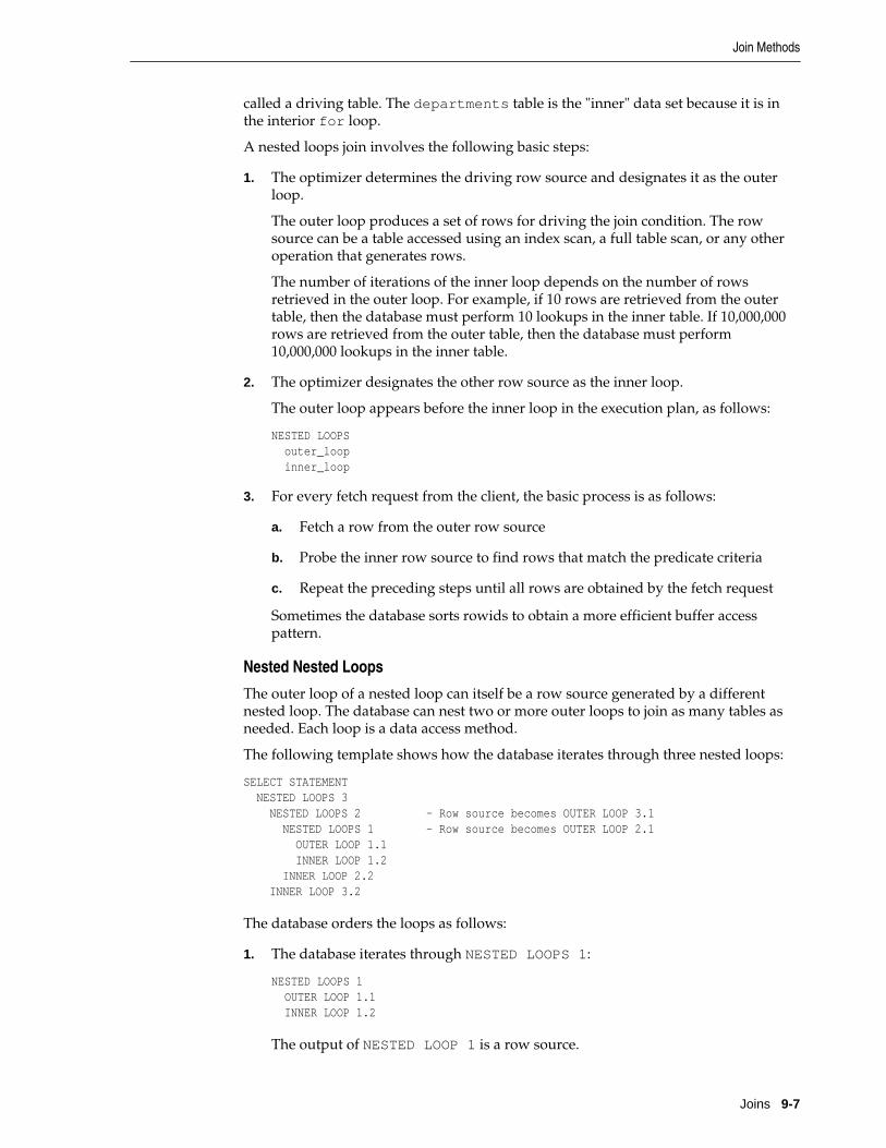
called a driving table. The departments table is the "inner" data set because it is inthe interior for loop.
A nested loops join involves the following basic steps:
1. The optimizer determines the driving row source and designates it as the outerloop.
The outer loop produces a set of rows for driving the join condition. The rowsource can be a table accessed using an index scan, a full table scan, or any otheroperation that generates rows.
The number of iterations of the inner loop depends on the number of rowsretrieved in the outer loop. For example, if 10 rows are retrieved from the outertable, then the database must perform 10 lookups in the inner table. If 10,000,000rows are retrieved from the outer table, then the database must perform10,000,000 lookups in the inner table.
2. The optimizer designates the other row source as the inner loop.
The outer loop appears before the inner loop in the execution plan, as follows:
NESTED LOOPS outer_loop inner_loop
3. For every fetch request from the client, the basic process is as follows:
a. Fetch a row from the outer row source
b. Probe the inner row source to find rows that match the predicate criteria
c. Repeat the preceding steps until all rows are obtained by the fetch request
Sometimes the database sorts rowids to obtain a more efficient buffer accesspattern.
Nested Nested Loops
The outer loop of a nested loop can itself be a row source generated by a differentnested loop. The database can nest two or more outer loops to join as many tables asneeded. Each loop is a data access method.
The following template shows how the database iterates through three nested loops:
SELECT STATEMENT NESTED LOOPS 3 NESTED LOOPS 2 - Row source becomes OUTER LOOP 3.1 NESTED LOOPS 1 - Row source becomes OUTER LOOP 2.1 OUTER LOOP 1.1 INNER LOOP 1.2 INNER LOOP 2.2 INNER LOOP 3.2
The database orders the loops as follows:
1. The database iterates through NESTED LOOPS 1:
NESTED LOOPS 1 OUTER LOOP 1.1 INNER LOOP 1.2
The output of NESTED LOOP 1 is a row source.
Join Methods
Joins 9-7

2. The database iterates through NESTED LOOPS 2, using the row source generatedby NESTED LOOPS 1 as its outer loop:
NESTED LOOPS 2 OUTER LOOP 2.1 - Row source generated by NESTED LOOPS 1 INNER LOOP 2.2
The output of NESTED LOOPS 2 is another row source.
3. The database iterates through NESTED LOOPS 3, using the row source generatedby NESTED LOOPS 2 as its outer loop:
NESTED LOOPS 3 OUTER LOOP 3.1 - Row source generated by NESTED LOOPS 2 INNER LOOP 3.2
Example 9-2 Nested Nested Loops Join
Suppose you join the employees and departments tables as follows:
SELECT /*+ ORDERED USE_NL(d) */ e.last_name, e.first_name, d.department_nameFROM employees e, departments dWHERE e.department_id=d.department_idAND e.last_name like 'A%';
The plan reveals that the optimizer chose two nested loops (Step 1 and Step 2) toaccess the data:
SQL_ID ahuavfcv4tnz4, child number 0-------------------------------------SELECT /*+ ORDERED USE_NL(d) */ e.last_name, d.department_name FROMemployees e, departments d WHERE e.department_id=d.department_id AND e.last_name like 'A%' Plan hash value: 1667998133 ----------------------------------------------------------------------------------|Id| Operation |Name |Rows|Bytes|Cost(%CPU)|Time|----------------------------------------------------------------------------------| 0| SELECT STATEMENT | | | |5 (100)| || 1| NESTED LOOPS | | | | | || 2| NESTED LOOPS | | 3|102|5 (0)|00:00:01|| 3| TABLE ACCESS BY INDEX ROWID BATCHED| EMPLOYEES | 3| 54|2 (0)|00:00:01||*4| INDEX RANGE SCAN | EMP_NAME_IX | 3| |1 (0)|00:00:01||*5| INDEX UNIQUE SCAN | DEPT_ID_PK | 1| |0 (0)| || 6| TABLE ACCESS BY INDEX ROWID | DEPARTMENTS | 1| 16|1 (0)|00:00:01|---------------------------------------------------------------------------------- Predicate Information (identified by operation id):--------------------------------------------------- 4 - access("E"."LAST_NAME" LIKE 'A%') filter("E"."LAST_NAME" LIKE 'A%') 5 - access("E"."DEPARTMENT_ID"="D"."DEPARTMENT_ID")
In this example, the basic process is as follows:
1. The database begins iterating through the inner nested loop (Step 2) as follows:
a. The database searches the emp_name_ix for the rowids for all last names thatbegins with A (Step 4).
For example:
Join Methods
9-8 SQL Tuning Guide

Abel,employees_rowidAnde,employees_rowidAtkinson,employees_rowidAustin,employees_rowid
b. Using the rowids from the previous step, the database retrieves a batch ofrows from the employees table (Step 3). For example:
Abel,Ellen,80Abel,John,50
These rows become the outer row source for the innermost nested loop.
The batch step is typically part of adaptive execution plans. To determinewhether a nested loop is better than a hash join, the optimizer needs todetermine many rows come back from the row source. If too many rows arereturned, then the optimizer switches to a different join method.
c. For each row in the outer row source, the database scans the dept_id_pkindex to obtain the rowid in departments of the matching department ID(Step 5), and joins it to the employees rows. For example:
Abel,Ellen,80,departments_rowidAnde,Sundar,80,departments_rowidAtkinson,Mozhe,50,departments_rowidAustin,David,60,departments_rowid
These rows become the outer row source for the outer nested loop (Step 1).
2. The database iterates through the outer nested loop as follows:
a. The database reads the first row in outer row source.
For example:
Abel,Ellen,80,departments_rowid
b. The database uses the departments rowid to retrieve the correspondingrow from departments (Step 6), and then joins the result to obtain therequested values (Step 1).
For example:
Abel,Ellen,80,Sales
c. The database reads the next row in the outer row source, uses thedepartments rowid to retrieve the corresponding row from departments(Step 6), and iterates through the loop until all rows are retrieved.
The result set has the following form:
Abel,Ellen,80,SalesAnde,Sundar,80,SalesAtkinson,Mozhe,50,ShippingAustin,David,60,IT
Current Implementation for Nested Loops Joins
Oracle Database 11g introduced a new implementation for nested loops that reducesoverall latency for physical I/O. When an index or a table block is not in the buffercache and is needed to process the join, a physical I/O is required. The database canbatch multiple physical I/O requests and process them using a vector I/O instead of
Join Methods
Joins 9-9

one at a time. A vector is an array. The database obtains a set of rowids, and thensends them in an array to the operating system, which performs the read.
As part of the new implementation, two NESTED LOOPS join row sources mightappear in the execution plan where only one would have appeared in prior releases. Insuch cases, Oracle Database allocates one NESTED LOOPS join row source to join thevalues from the table on the outer side of the join with the index on the inner side. Asecond row source is allocated to join the result of the first join, which includes therowids stored in the index, with the table on the inner side of the join.
Consider the query in “Original Implementation for Nested Loops Joins”. In thecurrent implementation, the execution plan for this query might be as follows:
-------------------------------------------------------------------------------------| Id | Operation | Name |Rows|Bytes|Cost%CPU| Time |-------------------------------------------------------------------------------------| 0 | SELECT STATEMENT | | 19 | 722 | 3 (0)|00:00:01|| 1 | NESTED LOOPS | | | | | || 2 | NESTED LOOPS | | 19 | 722 | 3 (0)|00:00:01||* 3 | TABLE ACCESS FULL | DEPARTMENTS | 2 | 32 | 2 (0)|00:00:01||* 4 | INDEX RANGE SCAN | EMP_DEPARTMENT_IX | 10 | | 0 (0)|00:00:01|| 5 | TABLE ACCESS BY INDEX ROWID| EMPLOYEES | 10 | 220 | 1 (0)|00:00:01|------------------------------------------------------------------------------------- Predicate Information (identified by operation id):--------------------------------------------------- 3 - filter("D"."DEPARTMENT_NAME"='Marketing' OR "D"."DEPARTMENT_NAME"='Sales') 4 - access("E"."DEPARTMENT_ID"="D"."DEPARTMENT_ID")
In this case, rows from the hr.departments table form the outer row source (Step 3)of the inner nested loop (Step 2). The index emp_department_ix is the inner rowsource (Step 4) of the inner nested loop. The results of the inner nested loop form theouter row source (Row 2) of the outer nested loop (Row 1). The hr.employees tableis the outer row source (Row 5) of the outer nested loop.
For each fetch request, the basic process is as follows:
1. The database iterates through the inner nested loop (Step 2) to obtain the rowsrequested in the fetch:
a. The database reads the first row of departments to obtain the departmentIDs for departments named Marketing or Sales (Step 3). For example:
Marketing,20
This row set is the outer loop. The database caches the data in the PGA.
b. The database scans emp_department_ix, which is an index on theemployees table, to find employees rowids that correspond to thisdepartment ID (Step 4), and then joins the result (Step 2).
The result set has the following form:
Marketing,20,employees_rowidMarketing,20,employees_rowidMarketing,20,employees_rowid
c. The database reads the next row of departments, scansemp_department_ix to find employees rowids that correspond to thisdepartment ID, and then iterates through the loop until the client request issatisfied.
Join Methods
9-10 SQL Tuning Guide
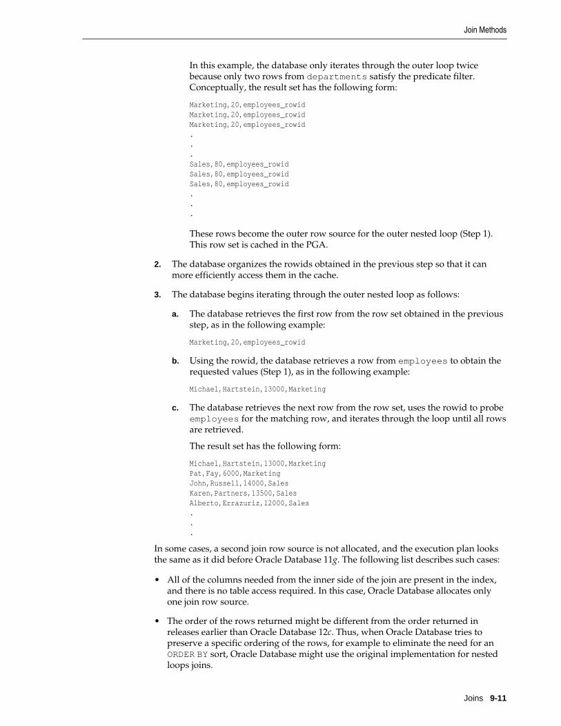
In this example, the database only iterates through the outer loop twicebecause only two rows from departments satisfy the predicate filter.Conceptually, the result set has the following form:
Marketing,20,employees_rowidMarketing,20,employees_rowidMarketing,20,employees_rowid...Sales,80,employees_rowidSales,80,employees_rowidSales,80,employees_rowid...
These rows become the outer row source for the outer nested loop (Step 1).This row set is cached in the PGA.
2. The database organizes the rowids obtained in the previous step so that it canmore efficiently access them in the cache.
3. The database begins iterating through the outer nested loop as follows:
a. The database retrieves the first row from the row set obtained in the previousstep, as in the following example:
Marketing,20,employees_rowid
b. Using the rowid, the database retrieves a row from employees to obtain therequested values (Step 1), as in the following example:
Michael,Hartstein,13000,Marketing
c. The database retrieves the next row from the row set, uses the rowid to probeemployees for the matching row, and iterates through the loop until all rowsare retrieved.
The result set has the following form:
Michael,Hartstein,13000,MarketingPat,Fay,6000,MarketingJohn,Russell,14000,SalesKaren,Partners,13500,SalesAlberto,Errazuriz,12000,Sales...
In some cases, a second join row source is not allocated, and the execution plan looksthe same as it did before Oracle Database 11g. The following list describes such cases:
• All of the columns needed from the inner side of the join are present in the index,and there is no table access required. In this case, Oracle Database allocates onlyone join row source.
• The order of the rows returned might be different from the order returned inreleases earlier than Oracle Database 12c. Thus, when Oracle Database tries topreserve a specific ordering of the rows, for example to eliminate the need for anORDER BY sort, Oracle Database might use the original implementation for nestedloops joins.
Join Methods
Joins 9-11

• The OPTIMIZER_FEATURES_ENABLE initialization parameter is set to a releasebefore Oracle Database 11g. In this case, Oracle Database uses the originalimplementation for nested loops joins.
Original Implementation for Nested Loops Joins
In the current release, both the new and original implementation are possible. For anexample of the original implementation, consider the following join of thehr.employees and hr.departments tables:
SELECT e.first_name, e.last_name, e.salary, d.department_nameFROM hr.employees e, hr.departments dWHERE d.department_name IN ('Marketing', 'Sales')AND e.department_id = d.department_id;
In releases before Oracle Database 11g, the execution plan for this query might appearas follows:
------------------------------------------------------------------------------------------------| Id | Operation | Name | Rows | Bytes | Cost (%CPU)| Time |------------------------------------------------------------------------------------------------| 0 | SELECT STATEMENT | | 19 | 722 | 3 (0)| 00:00:01 || 1 | TABLE ACCESS BY INDEX ROWID| EMPLOYEES | 10 | 220 | 1 (0)| 00:00:01 || 2 | NESTED LOOPS | | 19 | 722 | 3 (0)| 00:00:01 ||* 3 | TABLE ACCESS FULL | DEPARTMENTS | 2 | 32 | 2 (0)| 00:00:01 ||* 4 | INDEX RANGE SCAN | EMP_DEPARTMENT_IX | 10 | | 0 (0)| 00:00:01 |------------------------------------------------------------------------------------------------ Predicate Information (identified by operation id):--------------------------------------------------- 3 - filter("D"."DEPARTMENT_NAME"='Marketing' OR "D"."DEPARTMENT_NAME"='Sales') 4 - access("E"."DEPARTMENT_ID"="D"."DEPARTMENT_ID")
For each fetch request, the basic process is as follows:
1. The database iterates through the loop to obtain the rows requested in the fetch:
a. The database reads the first row of departments to obtain the departmentIDs for departments named Marketing or Sales (Step 3). For example:
Marketing,20
This row set is the outer loop. The database caches the row in the PGA.
b. The database scans emp_department_ix, which is an index on theemployees.department_id column, to find employees rowids thatcorrespond to this department ID (Step 4), and then joins the result (Step 2).
Conceptually, the result set has the following form:
Marketing,20,employees_rowidMarketing,20,employees_rowidMarketing,20,employees_rowid
c. The database reads the next row of departments, scansemp_department_ix to find employees rowids that correspond to thisdepartment ID, and iterates through the loop until the client request issatisfied.
In this example, the database only iterates through the outer loop twicebecause only two rows from departments satisfy the predicate filter.Conceptually, the result set has the following form:
Join Methods
9-12 SQL Tuning Guide

Marketing,20,employees_rowidMarketing,20,employees_rowidMarketing,20,employees_rowid...Sales,80,employees_rowidSales,80,employees_rowidSales,80,employees_rowid...
2. Depending on the circumstances, the database may organize the cached rowidsobtained in the previous step so that it can more efficiently access them.
3. For each employees rowid in the result set generated by the nested loop, thedatabase retrieves a row from employees to obtain the requested values (Step 1).
Thus, the basic process is to read a rowid and retrieve the matching employeesrow, read the next rowid and retrieve the matching employees row, and so on.Conceptually, the result set has the following form:
Michael,Hartstein,13000,MarketingPat,Fay,6000,MarketingJohn,Russell,14000,SalesKaren,Partners,13500,SalesAlberto,Errazuriz,12000,Sales...
Nested Loops Controls
For some SQL examples, the data is small enough for the optimizer to prefer full tablescans and hash joins. However, you can add a USE_NL to instruct the optimizer tochange the join method to nested loops. This hint instructs the optimizer to join eachspecified table to another row source with a nested loops join, using the specified tableas the inner table.
The related hint USE_NL_WITH_INDEX ( table index ) hint instructs the optimizerto join the specified table to another row source with a nested loops join using thespecified table as the inner table. The index is optional. If no index is specified, thenthe nested loops join uses an index with at least one join predicate as the index key.
Example 9-3 Nested Loops Hint
Assume that the optimizer chooses a hash join for the following query:
SELECT e.last_name, d.department_nameFROM employees e, departments dWHERE e.department_id=d.department_id;
The plan looks as follows:
------------------------------------------------------------------------------|Id | Operation | Name | Rows | Bytes |Cost(%CPU)| Time |------------------------------------------------------------------------------| 0 | SELECT STATEMENT | | | | 5 (100)| ||*1 | HASH JOIN | | 106 | 2862 | 5 (20)| 00:00:01 || 2 | TABLE ACCESS FULL| DEPARTMENTS | 27 | 432 | 2 (0)| 00:00:01 |
Join Methods
Joins 9-13
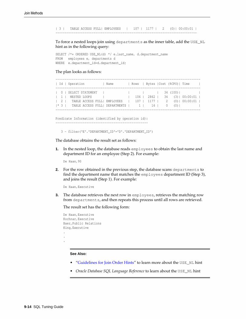
| 3 | TABLE ACCESS FULL| EMPLOYEES | 107 | 1177 | 2 (0)| 00:00:01 |------------------------------------------------------------------------------
To force a nested loops join using departments as the inner table, add the USE_NLhint as in the following query:
SELECT /*+ ORDERED USE_NL(d) */ e.last_name, d.department_nameFROM employees e, departments dWHERE e.department_id=d.department_id;
The plan looks as follows:
--------------------------------------------------------------------------------| Id | Operation | Name | Rows | Bytes |Cost (%CPU)| Time |--------------------------------------------------------------------------------| 0 | SELECT STATEMENT | | | | 34 (100)| || 1 | NESTED LOOPS | | 106 | 2862 | 34 (3)| 00:00:01 || 2 | TABLE ACCESS FULL| EMPLOYEES | 107 | 1177 | 2 (0)| 00:00:01 ||* 3 | TABLE ACCESS FULL| DEPARTMENTS | 1 | 16 | 0 (0)| |--------------------------------------------------------------------------------
Predicate Information (identified by operation id):--------------------------------------------------- 3 - filter("E"."DEPARTMENT_ID"="D"."DEPARTMENT_ID")
The database obtains the result set as follows:
1. In the nested loop, the database reads employees to obtain the last name anddepartment ID for an employee (Step 2). For example:
De Haan,90
2. For the row obtained in the previous step, the database scans departments tofind the department name that matches the employees department ID (Step 3),and joins the result (Step 1). For example:
De Haan,Executive
3. The database retrieves the next row in employees, retrieves the matching rowfrom departments, and then repeats this process until all rows are retrieved.
The result set has the following form:
De Haan,ExecutiveKochnar,ExecutiveBaer,Public RelationsKing,Executive...
See Also:
• “Guidelines for Join Order Hints” to learn more about the USE_NL hint
• Oracle Database SQL Language Reference to learn about the USE_NL hint
Join Methods
9-14 SQL Tuning Guide

Hash JoinsThe database uses a hash join to join larger data sets. The optimizer uses the smallerof two data sets to build a hash table on the join key in memory, using a deterministichash function to specify the location in the hash table in which to store each row. Thedatabase then scans the larger data set, probing the hash table to find the rows thatmeet the join condition.
When the Optimizer Considers Hash Joins
In general, the optimizer considers a hash join when the following conditions are true:
• A relatively large amount of data must be joined, or a large fraction of a small tablemust be joined.
• The join is an equijoin.
A hash join is most cost effective when the smaller data set fits in memory. In this case,the cost is limited to a single read pass over the two data sets.
Because the hash table is in the PGA, Oracle Database can access rows withoutlatching them. This technique reduces logical I/O by avoiding the necessity ofrepeatedly latching and reading blocks in the database buffer cache.
If the data sets do not fit in memory, then the database partitions the row sources, andthe join proceeds partition by partition. This can use a lot of sort area memory, andI/O to the temporary tablespace. This method can still be the most cost effective,especially when the database uses parallel query servers.
How Hash Joins Work
A hashing algorithm takes a set of inputs and applies a deterministic hash function togenerate a hash value between 1 and n, where n is the size of the hash table. In a hashjoin, the input values are the join keys. The output values are indexes (slots) in anarray, which is the hash table.
Hash Tables
To illustrate a hash table, assume that the database hashes hr.departments in a joinof departments and employees. The join key column is department_id. The first5 rows of departments are as follows:
SQL> select * from departments where rownum < 6; DEPARTMENT_ID DEPARTMENT_NAME MANAGER_ID LOCATION_ID------------- ------------------------------ ---------- ----------- 10 Administration 200 1700 20 Marketing 201 1800 30 Purchasing 114 1700 40 Human Resources 203 2400 50 Shipping 121 1500
The database applies the hash function to each department_id in the table,generating a hash value for each. For this illustration, the hash table has 5 slots (itcould have more or less). Because n is 5, the possible hash values range from 1 to 5.The hash functions might generate the following values for the department IDs:
f(10) = 4f(20) = 1f(30) = 4
Join Methods
Joins 9-15

f(40) = 2f(50) = 5
Note that the hash function happens to generate the same hash value of 4 fordepartments 10 and 30. This is known as a hash collision. In this case, the databaseputs the records for departments 10 and 30 in the same slot, using a linked list.Conceptually, the hash table looks as follows:
1 20,Marketing,201,18002 40,Human Resources,203,240034 10,Administration,200,1700 -> 30,Purchasing,114,17005 50,Shipping,121,1500
Hash Join: Basic Steps
The optimizer uses the smaller data source to build a hash table on the join key inmemory, and then scans the larger table to find the joined rows.
The basic steps are as follows:
1. The database performs a full scan of the smaller data set, called the build table,and then applies a hash function to the join key in each row to build a hash tablein the PGA.
In pseudocode, the algorithm might look as follows:
FOR small_table_row IN (SELECT * FROM small_table)LOOP slot_number := HASH(small_table_row.join_key); INSERT_HASH_TABLE(slot_number,small_table_row);END LOOP;
2. The database probes the second data set, called the probe table, using whicheveraccess mechanism has the lowest cost.
Typically, the database performs a full scan of both the smaller and larger data set.The algorithm in pseudocode might look as follows:
FOR large_table_row IN (SELECT * FROM large_table)LOOP slot_number := HASH(large_table_row.join_key); small_table_row = LOOKUP_HASH_TABLE(slot_number,large_table_row.join_key); IF small_table_row FOUND THEN output small_table_row + large_table_row; END IF;END LOOP;
For each row retrieved from the larger data set, the database does the following:
a. Applies the same hash function to the join column or columns to calculate thenumber of the relevant slot in the hash table.
For example, to probe the hash table for department ID 30, the databaseapplies the hash function to 30, which generates the hash value 4.
b. Probes the hash table to determine whether rows exists in the slot.
If no rows exist, then the database processes the next row in the larger dataset. If rows exist, then the database proceeds to the next step.
Join Methods
9-16 SQL Tuning Guide

c. Checks the join column or columns for a match. If a match occurs, then thedatabase either reports the rows or passes them to the next step in the plan,and then processes the next row in the larger data set.
If multiple rows exist in the hash table slot, the database walks through thelinked list of rows, checking each one. For example, if department 30 hashesto slot 4, then the database checks each row until it finds 30.
Example 9-4 Hash Joins
An application queries the oe.orders and oe.order_items tables, joining on theorder_id column.
SELECT o.customer_id, l.unit_price * l.quantityFROM orders o, order_items lWHERE l.order_id = o.order_id;
The execution plan is as follows:
--------------------------------------------------------------------------| Id | Operation | Name | Rows | Bytes | Cost (%CPU)|--------------------------------------------------------------------------| 0 | SELECT STATEMENT | | 665 | 13300 | 8 (25)||* 1 | HASH JOIN | | 665 | 13300 | 8 (25)|| 2 | TABLE ACCESS FULL | ORDERS | 105 | 840 | 4 (25)|| 3 | TABLE ACCESS FULL | ORDER_ITEMS | 665 | 7980 | 4 (25)|--------------------------------------------------------------------------
Predicate Information (identified by operation id):--------------------------------------------------- 1 - access("L"."ORDER_ID"="O"."ORDER_ID")
Because the orders table is small relative to the order_items table, which is 6 timeslarger, the database hashes orders. In a hash join, the data set for the build tablealways appears first in the list of operations (Step 2). In Step 3, the database performs afull scan of the larger order_items later, probing the hash table for each row.
How Hash Joins Work When the Hash Table Does Not Fit in the PGA
The database must use a different technique when the hash table does not fit entirelyin the PGA. In this case, the database uses a temporary space to hold portions (calledpartitions) of the hash table, and sometimes portions of the larger table that probes thehash table.
The basic process is as follows:
1. The database performs a full scan of the smaller data set, and then builds an arrayof hash buckets in both the PGA and on disk.
When the PGA hash area fills up, the database finds the largest partition withinthe hash table and writes it to temporary space on disk. The database stores anynew row that belongs to this on-disk partition on disk, and all other rows in thePGA. Thus, part of the hash table is in memory and part of it on disk.
2. The database takes a first pass at reading the other data set.
For each row, the database does the following:
a. Applies the same hash function to the join column or columns to calculate thenumber of the relevant hash bucket.
b. Probes the hash table to determine whether rows exist in the bucket inmemory.
Join Methods
Joins 9-17

If the hashed value points to a row in memory, then the database completesthe join and returns the row. If the value points to a hash partition on disk,however, then the database stores this row in the temporary tablespace, usingthe same partitioning scheme used for the original data set.
3. The database reads each on-disk temporary partition one by one
4. The database joins each partition row to the row in the corresponding on-disktemporary partition.
Hash Join Controls
The USE_HASH hint instructs the optimizer to use a hash join when joining two tablestogether. See “Guidelines for Join Order Hints”.
Sort Merge JoinsA sort merge join is a variation on a nested loops join. The database sorts two data sets(the SORT JOIN operations), if they are not already sorted. For each row in the firstdata set, the database probes the second data set for matching rows and joins them(the MERGE JOIN operation), basing its start position on the match made in theprevious iteration:
MERGE JOIN
SORT JOIN SORT JOIN
First Row
Source
Second Row
Source
When the Optimizer Considers Sort Merge Joins
A hash join requires one hash table and one probe of this table, whereas a sort mergejoin requires two sorts. The optimizer may choose a sort merge join over a hash joinfor joining large amounts of data when any of the following conditions is true:
• The join condition between two tables is not an equijoin, that is, uses an inequalitycondition such as <, <=, >, or >=.
In contrast to sort merges, hash joins require an equality condition.
• Because of sorts required by other operations, the optimizer finds it cheaper to usea sort merge.
If an index exists, then the database can avoid sorting the first data set. However,the database always sorts the second data set, regardless of indexes.
A sort merge has the same advantage over a nested loops join as the hash join: thedatabase accesses rows in the PGA rather than the SGA, reducing logical I/O by
Join Methods
9-18 SQL Tuning Guide

avoiding the necessity of repeatedly latching and reading blocks in the database buffercache. In general, hash joins perform better than sort merge joins because sorting isexpensive. However, sort merge joins offer the following advantages over a hash join:
• After the initial sort, the merge phase is optimized, resulting in faster generation ofoutput rows.
• A sort merge can be more cost-effective than a hash join when the hash table doesnot fit completely in memory.
A hash join with insufficient memory requires both the hash table and the otherdata set to be copied to disk. In this case, the database may have to read from diskmultiple times. In a sort merge, if memory cannot hold the two data sets, then thedatabase writes them both to disk, but reads each data set no more than once.
How Sort Merge Joins Work
As in a nested loops join, a sort merge join reads two data sets, but sorts them whenthey are not already sorted. For each row in the first data set, the database finds astarting row in the second data set, and then reads the second data set until it finds anonmatching row. In pseudocode, the high-level algorithm might look as follows:
READ data_set_1 SORT BY JOIN KEY TO temp_ds1READ data_set_2 SORT BY JOIN KEY TO temp_ds2 READ ds1_row FROM temp_ds1READ ds2_row FROM temp_ds2
WHILE NOT eof ON temp_ds1,temp_ds2LOOP IF ( temp_ds1.key = temp_ds2.key ) OUTPUT JOIN ds1_row,ds2_row ELSIF ( temp_ds1.key <= temp_ds2.key ) READ ds1_row FROM temp_ds1 ELSIF ( temp_ds1.key => temp_ds2.key ) READ ds2_row FROM temp_ds2END LOOP
For example, the database sorts the first data set as follows:
10,20,30,40,50,60,70
The database sorts the second data set as follows:
20,20,40,40,40,40,40,60,70,70
The database begins by reading 10 in the first data set, and then starts at the beginningof data set 2:
20 too high, stop, get next ds1_row
The database proceeds to the second row of data set 1 (20). The database proceedsthrough the second data set as follows:
20 match, proceed20 match, proceed40 too high, stop, get next ds1_row
The database gets the next row in data set 1, which is 30. The database starts at thenumber of its last match, which was 20, and then walks through data set 2 looking fora match:
Join Methods
Joins 9-19

20 too low, proceed20 too low, proceed40 too high, stop, get next ds1_row
The database gets the next row in data set 1, which is 40. The database starts at thenumber of its last match, which was 20, and then proceeds through data set 2 lookingfor a match:
20 too low, proceed20 too low, proceed40 match, proceed40 match, proceed40 match, proceed40 match, proceed40 match, proceed60 too high, stop, get next ds1_row
As the database proceeds through data set 1, the database does not need to read everyrow in data set 2. This is an advantage over a nested loops join.
Example 9-5 Sort Merge Join Using Index
The following query joins the employees and departments tables on thedepartment_id column, ordering the rows on department_id as follows:
SELECT e.employee_id, e.last_name, e.first_name, e.department_id, d.department_nameFROM employees e, departments dWHERE e.department_id = d.department_idORDER BY department_id;
A query of DBMS_XPLAN.DISPLAY_CURSOR shows that the plan uses a sort mergejoin:
--------------------------------------------------------------------------------|Id| Operation | Name |Rows|Bytes |Cost (%CPU)| Time |--------------------------------------------------------------------------------| 0| SELECT STATEMENT | | | | 5(100)| || 1| MERGE JOIN | |106 | 4028 | 5 (20)| 00:00:01 || 2| TABLE ACCESS BY INDEX ROWID| DEPARTMENTS | 27 | 432 | 2 (0)| 00:00:01 || 3| INDEX FULL SCAN | DEPT_ID_PK | 27 | | 1 (0)| 00:00:01 ||*4| SORT JOIN | |107 | 2354 | 3 (34)| 00:00:01 || 5| TABLE ACCESS FULL | EMPLOYEES |107 | 2354 | 2 (0)| 00:00:01 |--------------------------------------------------------------------------------
Predicate Information (identified by operation id):---------------------------------------------------
4 - access("E"."DEPARTMENT_ID"="D"."DEPARTMENT_ID") filter("E"."DEPARTMENT_ID"="D"."DEPARTMENT_ID")
The two data sets are the departments table and the employees table. Because anindex orders the departments table by department_id, the database can read thisindex and avoid a sort (Step 3). The database only needs to sort the employees table(Step 4), which is the most CPU-intensive operation.
Example 9-6 Sort Merge Join Without an Index
You join the employees and departments tables on the department_id column,ordering the rows on department_id as follows. In this example, you specifyNO_INDEX and USE_MERGE to force the optimizer to choose a sort merge:
Join Methods
9-20 SQL Tuning Guide

SELECT /*+ USE_MERGE(d e) NO_INDEX(d) */ e.employee_id, e.last_name, e.first_name, e.department_id, d.department_nameFROM employees e, departments dWHERE e.department_id = d.department_idORDER BY department_id;
A query of DBMS_XPLAN.DISPLAY_CURSOR shows that the plan uses a sort mergejoin:
--------------------------------------------------------------------------------| Id| Operation | Name | Rows | Bytes | Cost (%CPU)| Time |--------------------------------------------------------------------------------| 0 | SELECT STATEMENT | | | | 6 (100)| || 1 | MERGE JOIN | | 106 | 9540 | 6 (34)| 00:00:01|| 2 | SORT JOIN | | 27 | 567 | 3 (34)| 00:00:01|| 3 | TABLE ACCESS FULL| DEPARTMENTS | 27 | 567 | 2 (0)| 00:00:01||*4 | SORT JOIN | | 107 | 7383 | 3 (34)| 00:00:01|| 5 | TABLE ACCESS FULL| EMPLOYEES | 107 | 7383 | 2 (0)| 00:00:01|--------------------------------------------------------------------------------
Predicate Information (identified by operation id):---------------------------------------------------
4 - access("E"."DEPARTMENT_ID"="D"."DEPARTMENT_ID") filter("E"."DEPARTMENT_ID"="D"."DEPARTMENT_ID")
Because the departments.department_id index is ignored, the optimizerperforms a sort, which increases the combined cost of Step 2 and Step 3 by 67% (from3 to 5).
Sort Merge Join Controls
The USE_MERGE hint instructs the optimizer to use a sort merge join. In somesituations it may make sense to override the optimizer with the USE_MERGE hint. Forexample, the optimizer can choose a full scan on a table and avoid a sort operation in aquery. However, there is an increased cost because a large table is accessed through anindex and single block reads, as opposed to faster access through a full table scan.
See Also:
Oracle Database SQL Language Reference to learn about the USE_MERGE hint
Cartesian JoinsThe database uses a Cartesian join when one or more of the tables does not have anyjoin conditions to any other tables in the statement. The optimizer joins every rowfrom one data source with every row from the other data source, creating theCartesian product of the two sets. Therefore, the total number of rows resulting fromthe join is calculated using the following formula, where rs1 is the number of rows infirst row set and rs2 is the number of rows in the second row set:
rs1 X rs2 = total rows in result set
When the Optimizer Considers Cartesian Joins
The optimizer uses a Cartesian join for two row sources in any of the followingcircumstances:
Join Methods
Joins 9-21

• No join condition exists.
In some cases, the optimizer could pick up a common filter condition between thetwo tables as a possible join condition.
Note:
If a Cartesian join appears in a query plan, it could be caused by aninadvertently omitted join condition. In general, if a query joins n tables, thenn-1 join conditions are required to avoid a Cartesian join.
• A Cartesian join is an efficient method.
For example, the optimizer may decide to generate a Cartesian product of two verysmall tables that are both joined to the same large table.
• The ORDERED hint specifies a table before its join table is specified.
How Cartesian Joins Work
At a high level, the algorithm for a Cartesian join looks as follows, where ds1 istypically the smaller data set, and ds2 is the larger data set:
FOR ds1_row IN ds1 LOOP FOR ds2_row IN ds2 LOOP output ds1_row and ds2_row END LOOPEND LOOP
Example 9-7 Cartesian Join
In this example, a user intends to perform an inner join of the employees anddepartments tables, but accidentally leaves off the join condition:
SELECT e.last_name, d.department_nameFROM employees e, departments d
The execution plan is as follows:
--------------------------------------------------------------------------------| Id| Operation | Name | Rows | Bytes |Cost (%CPU)| Time |--------------------------------------------------------------------------------| 0 | SELECT STATEMENT | | | |11 (100)| || 1 | MERGE JOIN CARTESIAN | | 2889 | 57780 |11 (0)| 00:00:01 || 2 | TABLE ACCESS FULL | DEPARTMENTS | 27 | 324 | 2 (0)| 00:00:01 || 3 | BUFFER SORT | | 107 | 856 | 9 (0)| 00:00:01 || 4 | INDEX FAST FULL SCAN| EMP_NAME_IX | 107 | 856 | 0 (0)| |--------------------------------------------------------------------------------
In Step 1 of the preceding plan, the CARTESIAN keyword indicates the presence of aCartesian join. The number of rows (2889) is the product of 27 and 107.
In Step 3, the BUFFER SORT operation indicates that the database is copying the datablocks obtained by the scan of emp_name_ix from the SGA to the PGA. This strategyavoids multiple scans of the same blocks in the database buffer cache, which wouldgenerate many logical reads and permit resource contention.
Join Methods
9-22 SQL Tuning Guide

Cartesian Join Controls
The ORDERED hint instructs the optimizer to join tables in the order in which theyappear in the FROM clause. By forcing a join between two row sources that have nodirect connection, the optimizer must perform a Cartesian join.
See Also:
Oracle Database SQL Language Reference to learn about the ORDERED hint
Example 9-8 ORDERED Hint
In the following example, the ORDERED hint instructs the optimizer to join employeesand locations, but no join condition connects these two row sources:
SELECT /*+ORDERED*/ e.last_name, d.department_name, l.country_id, l.state_provinceFROM employees e, locations l, departments dWHERE e.department_id = d.department_idAND d.location_id = l.location_id
The following execution plan shows a Cartesian product (Step 3) between locations(Step 6) and employees (Step 4), which is then joined to the departments table(Step 2):
--------------------------------------------------------------------------------| Id| Operation | Name | Rows | Bytes |Cost (%CPU)|Time |--------------------------------------------------------------------------------| 0 | SELECT STATEMENT | | | | 37 (100)| ||*1 | HASH JOIN | | 106 | 4664 | 37 (6)| 00:00:01 || 2 | TABLE ACCESS FULL | DEPARTMENTS | 27 | 513 | 2 (0)| 00:00:01 || 3 | MERGE JOIN CARTESIAN| | 2461 | 61525 | 34 (3)| 00:00:01 || 4 | TABLE ACCESS FULL | EMPLOYEES | 107 | 1177 | 2 (0)| 00:00:01 || 5 | BUFFER SORT | | 23 | 322 | 32 (4)| 00:00:01 || 6 | TABLE ACCESS FULL | LOCATIONS | 23 | 322 | 0 (0)| |--------------------------------------------------------------------------------
Join TypesA join type is determined by the type of join condition. This section contains thefollowing topics:
• Inner Joins
• Outer Joins
• Semijoins
• Antijoins
Inner JoinsAn inner join (sometimes called a simple join) is a join that returns only rows thatsatisfy the join condition. Inner joins are either equijoins or nonequijoins.
Join Types
Joins 9-23

Equijoins
An equijoin is an inner join whose join condition contains an equality operator. Thefollowing example is an equijoin because the join condition contains only an equalityoperator:
SELECT e.employee_id, e.last_name, d.department_nameFROM employees e, departments dWHERE e.department_id=d.department_id;
In the preceding query, the join condition ise.department_id=d.department_id. If a row in the employees table has adepartment ID that matches the value in a row in the departments table, then thedatabase returns the joined result; otherwise, the database does not return a result.
Nonequijoins
A nonequijoin is an inner join whose join condition contains an operator that is not anequality operator. The following query lists all employees whose hire date occurredwhen employee 176 (who is listed in job_history because he changed jobs in 2007)was working at the company:
SELECT e.employee_id, e.first_name, e.last_name, e.hire_dateFROM employees e, job_history hWHERE h.employee_id = 176AND e.hire_date BETWEEN h.start_date AND h.end_date;
In the preceding example, the condition joining employees and job_history doesnot contain an equality operator, so it is a nonequijoin. Nonequijoins are relativelyrare.
Note that a hash join requires at least a partial equijoin. The following SQL scriptcontains an equality join condition (e1.empno = e2.empno) and a nonequalitycondition:
SET AUTOTRACE TRACEONLY EXPLAINSELECT *FROM scott.emp e1 JOIN scott.emp e2ON ( e1.empno = e2.empnoAND e1.hiredate BETWEEN e2.hiredate-1 AND e2.hiredate+1 )
The optimizer chooses a hash join for the preceding query, as shown in the followingplan:
Execution Plan----------------------------------------------------------Plan hash value: 3638257876 ---------------------------------------------------------------------------| Id | Operation | Name | Rows | Bytes | Cost (%CPU)| Time |---------------------------------------------------------------------------| 0 | SELECT STATEMENT | | 1 | 174 | 5 (20)| 00:00:01 ||* 1 | HASH JOIN | | 1 | 174 | 5 (20)| 00:00:01 || 2 | TABLE ACCESS FULL| EMP | 14 | 1218 | 2 (0)| 00:00:01 || 3 | TABLE ACCESS FULL| EMP | 14 | 1218 | 2 (0)| 00:00:01 |--------------------------------------------------------------------------- Predicate Information (identified by operation id):---------------------------------------------------
Join Types
9-24 SQL Tuning Guide
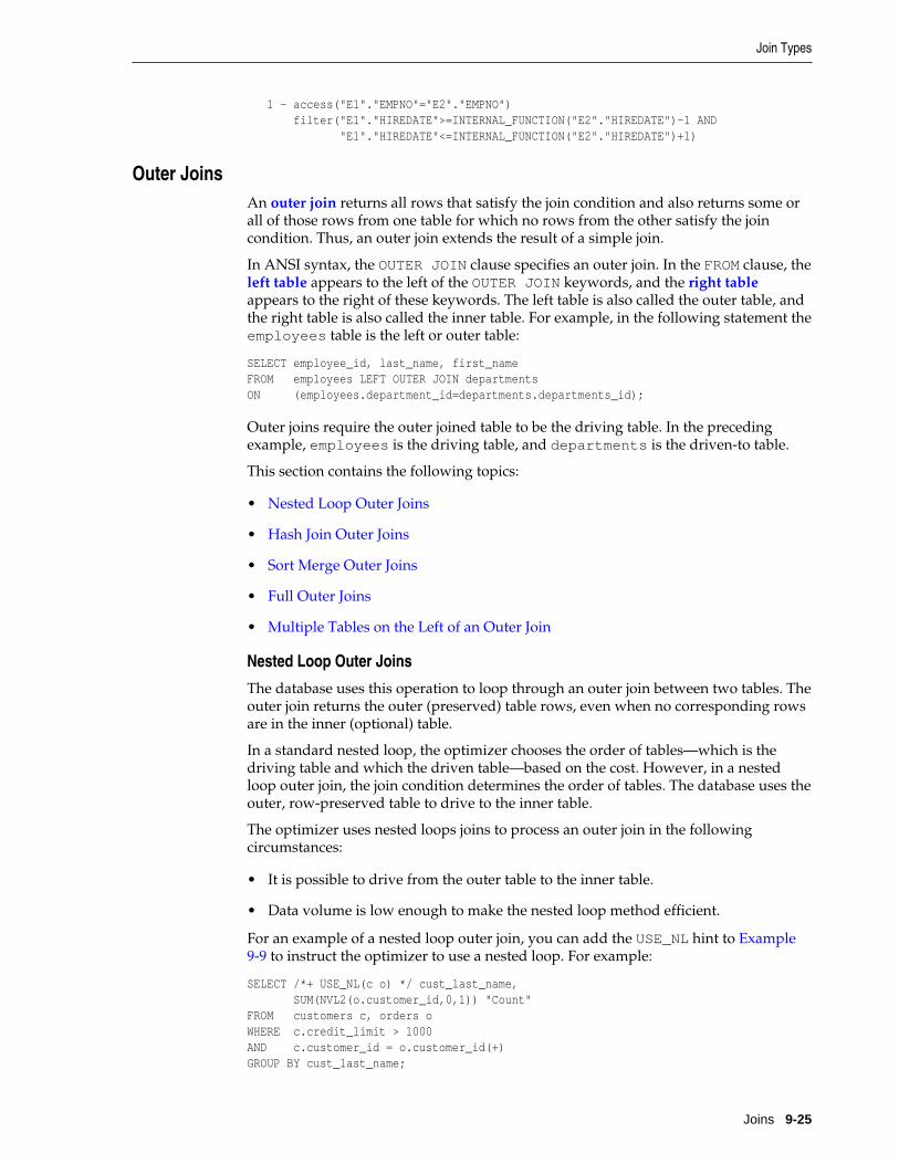
1 - access("E1"."EMPNO"="E2"."EMPNO") filter("E1"."HIREDATE">=INTERNAL_FUNCTION("E2"."HIREDATE")-1 AND "E1"."HIREDATE"<=INTERNAL_FUNCTION("E2"."HIREDATE")+1)
Outer JoinsAn outer join returns all rows that satisfy the join condition and also returns some orall of those rows from one table for which no rows from the other satisfy the joincondition. Thus, an outer join extends the result of a simple join.
In ANSI syntax, the OUTER JOIN clause specifies an outer join. In the FROM clause, the left table appears to the left of the OUTER JOIN keywords, and the right tableappears to the right of these keywords. The left table is also called the outer table, andthe right table is also called the inner table. For example, in the following statement theemployees table is the left or outer table:
SELECT employee_id, last_name, first_nameFROM employees LEFT OUTER JOIN departmentsON (employees.department_id=departments.departments_id);
Outer joins require the outer joined table to be the driving table. In the precedingexample, employees is the driving table, and departments is the driven-to table.
This section contains the following topics:
• Nested Loop Outer Joins
• Hash Join Outer Joins
• Sort Merge Outer Joins
• Full Outer Joins
• Multiple Tables on the Left of an Outer Join
Nested Loop Outer Joins
The database uses this operation to loop through an outer join between two tables. Theouter join returns the outer (preserved) table rows, even when no corresponding rowsare in the inner (optional) table.
In a standard nested loop, the optimizer chooses the order of tables—which is thedriving table and which the driven table—based on the cost. However, in a nestedloop outer join, the join condition determines the order of tables. The database uses theouter, row-preserved table to drive to the inner table.
The optimizer uses nested loops joins to process an outer join in the followingcircumstances:
• It is possible to drive from the outer table to the inner table.
• Data volume is low enough to make the nested loop method efficient.
For an example of a nested loop outer join, you can add the USE_NL hint to Example9-9 to instruct the optimizer to use a nested loop. For example:
SELECT /*+ USE_NL(c o) */ cust_last_name, SUM(NVL2(o.customer_id,0,1)) "Count"FROM customers c, orders oWHERE c.credit_limit > 1000AND c.customer_id = o.customer_id(+)GROUP BY cust_last_name;
Join Types
Joins 9-25

Hash Join Outer Joins
The optimizer uses hash joins for processing an outer join when either of the followingconditions is met:
• The data volume is large enough to make the hash join method efficient.
• It is not possible to drive from the outer table to the inner table.
The cost determines the order of tables. The outer table, including preserved rows,may be used to build the hash table, or it may be used to probe the hash table.
Example 9-9 Hash Join Outer Joins
This example shows a typical hash join outer join query, and its execution plan. In thisexample, all the customers with credit limits greater than 1000 are queried. An outerjoin is needed so that the query captures customers who have no orders.
• The outer table is customers.
• The inner table is orders.
• The join preserves the customers rows, including those rows without acorresponding row in orders.
You could use a NOT EXISTS subquery to return the rows. However, because you arequerying all the rows in the table, the hash join performs better (unless the NOTEXISTS subquery is not nested).
SELECT cust_last_name, SUM(NVL2(o.customer_id,0,1)) "Count"FROM customers c, orders oWHERE c.credit_limit > 1000AND c.customer_id = o.customer_id(+)GROUP BY cust_last_name;
--------------------------------------------------------------------------------| Id | Operation | Name | Rows | Bytes | Cost (%CPU)| Time |-------------------------------------------------------------------------------- PLAN_TABLE_OUTPUT--------------------------------------------------------------------------------| 0 | SELECT STATEMENT | | | | 7 (100)| || 1 | HASH GROUP BY | | 168 | 3192 | 7 (29)| 00:00:01 ||* 2 | HASH JOIN OUTER | | 318 | 6042 | 6 (17)| 00:00:01 ||* 3 | TABLE ACCESS FULL| CUSTOMERS | 260 | 3900 | 3 (0)| 00:00:01 ||* 4 | TABLE ACCESS FULL| ORDERS | 105 | 420 | 2 (0)| 00:00:01 |-------------------------------------------------------------------------------- Predicate Information (identified by operation id):--------------------------------------------------- 2 - access("C"."CUSTOMER_ID"="O"."CUSTOMER_ID") PLAN_TABLE_OUTPUT------------------------------------------------------------------------------- 3 - filter("C"."CREDIT_LIMIT">1000) 4 - filter("O"."CUSTOMER_ID">0)
The query looks for customers which satisfy various conditions. An outer join returnsNULL for the inner table columns along with the outer (preserved) table rows when it
Join Types
9-26 SQL Tuning Guide

does not find any corresponding rows in the inner table. This operation finds all thecustomers rows that do not have any orders rows.
In this case, the outer join condition is the following:
customers.customer_id = orders.customer_id(+)
The components of this condition represent the following:
Example 9-10 Outer Join to a Multitable View
In this example, the outer join is to a multitable view. The optimizer cannot drive intothe view like in a normal join or push the predicates, so it builds the entire row set ofthe view.
SELECT c.cust_last_name, sum(revenue)FROM customers c, v_orders oWHERE c.credit_limit > 2000AND o.customer_id(+) = c.customer_idGROUP BY c.cust_last_name;
----------------------------------------------------------------------------| Id | Operation | Name | Rows | Bytes | Cost (%CPU)|----------------------------------------------------------------------------| 0 | SELECT STATEMENT | | 144 | 4608 | 16 (32)|| 1 | HASH GROUP BY | | 144 | 4608 | 16 (32)||* 2 | HASH JOIN OUTER | | 663 | 21216 | 15 (27)||* 3 | TABLE ACCESS FULL | CUSTOMERS | 195 | 2925 | 6 (17)|| 4 | VIEW | V_ORDERS | 665 | 11305 | || 5 | HASH GROUP BY | | 665 | 15960 | 9 (34)||* 6 | HASH JOIN | | 665 | 15960 | 8 (25)||* 7 | TABLE ACCESS FULL| ORDERS | 105 | 840 | 4 (25)|| 8 | TABLE ACCESS FULL| ORDER_ITEMS | 665 | 10640 | 4 (25)|----------------------------------------------------------------------------
Predicate Information (identified by operation id):--------------------------------------------------- 2 - access("O"."CUSTOMER_ID"(+)="C"."CUSTOMER_ID") 3 - filter("C"."CREDIT_LIMIT">2000) 6 - access("O"."ORDER_ID"="L"."ORDER_ID") 7 - filter("O"."CUSTOMER_ID">0)
The view definition is as follows:
CREATE OR REPLACE view v_orders ASSELECT l.product_id, SUM(l.quantity*unit_price) revenue, o.order_id, o.customer_idFROM orders o, order_items lWHERE o.order_id = l.order_idGROUP BY l.product_id, o.order_id, o.customer_id;
Sort Merge Outer Joins
When an outer join cannot drive from the outer (preserved) table to the inner(optional) table, it cannot use a hash join or nested loops joins. In this case, it uses thesort merge outer join.
The optimizer uses sort merge for an outer join in the following cases:
• A nested loops join is inefficient. A nested loops join can be inefficient because ofdata volumes.
Join Types
Joins 9-27

• The optimizer finds it is cheaper to use a sort merge over a hash join because ofsorts required by other operations.
Full Outer Joins
A full outer join is a combination of the left and right outer joins. In addition to theinner join, rows from both tables that have not been returned in the result of the innerjoin are preserved and extended with nulls. In other words, full outer joins join tablestogether, yet show rows with no corresponding rows in the joined tables.
Example 9-11 Full Outer Join
The following query retrieves all departments and all employees in each department,but also includes:
• Any employees without departments
• Any departments without employees
SELECT d.department_id, e.employee_idFROM employees e FULL OUTER JOIN departments dON e.department_id = d.department_idORDER BY d.department_id;
The statement produces the following output:
DEPARTMENT_ID EMPLOYEE_ID------------- ----------- 10 200 20 201 20 202 30 114 30 115 30 116... 270 280 178 207
125 rows selected.
Example 9-12 Execution Plan for a Full Outer Join
Starting with Oracle Database 11g, Oracle Database automatically uses a nativeexecution method based on a hash join for executing full outer joins wheneverpossible. When the database uses the new method to execute a full outer join, theexecution plan for the query contains HASH JOIN FULL OUTER. The query in Example9-11 uses the following execution plan:
--------------------------------------------------------------------------------| Id| Operation | Name |Rows |Bytes |Cost (%CPU)| Time |--------------------------------------------------------------------------------| 0 | SELECT STATEMENT | | 122 | 4758 | 6 (34)| 00:0 0:01 || 1 | SORT ORDER BY | | 122 | 4758 | 6 (34)| 00:0 0:01 || 2 | VIEW | VW_FOJ_0 | 122 | 4758 | 5 (20)| 00:0 0:01 ||*3 | HASH JOIN FULL OUTER | | 122 | 1342 | 5 (20)| 00:0 0:01 || 4 | INDEX FAST FULL SCAN| DEPT_ID_PK | 27 | 108 | 2 (0)| 00:0 0:01 || 5 | TABLE ACCESS FULL | EMPLOYEES | 107 | 749 | 2 (0)| 00:0 0:01 |-------------------------------------------------------------------------------- Predicate Information (identified by operation id):
Join Types
9-28 SQL Tuning Guide

--------------------------------------------------- 3 - access("E"."DEPARTMENT_ID"="D"."DEPARTMENT_ID")
HASH JOIN FULL OUTER is included in the preceding plan (Step 3), indicating that thequery uses the hash full outer join execution method. Typically, when the full outerjoin condition between two tables is an equijoin, the hash full outer join executionmethod is possible, and Oracle Database uses it automatically.
To instruct the optimizer to consider using the hash full outer join execution method,apply the NATIVE_FULL_OUTER_JOIN hint. To instruct the optimizer not to considerusing the hash full outer join execution method, apply theNO_NATIVE_FULL_OUTER_JOIN hint. The NO_NATIVE_FULL_OUTER_JOIN hintinstructs the optimizer to exclude the native execution method when joining eachspecified table. Instead, the full outer join is executed as a union of left outer join andan antijoin.
Multiple Tables on the Left of an Outer Join
In Oracle Database 12c, multiple tables may exist on the left of an outer-joined table.This enhancement enables Oracle Database to merge a view that contains multipletables and appears on the left of outer join.
In releases before Oracle Database 12c, a query such as the following was invalid, andwould trigger an ORA-01417 error message:
SELECT t1.d, t3.cFROM t1, t2, t3WHERE t1.z = t2.z AND t1.x = t3.x (+) AND t2.y = t3.y (+);
Starting in Oracle Database 12c, the preceding query is valid.
SemijoinsA semijoin is a join between two data sets that returns a row from the first set when amatching row exists in the subquery data set. The database stops processing thesecond data set at the first match. Thus, optimization does not duplicate rows from thefirst data set when multiple rows in the second data set satisfy the subquery criteria.
Note:
Semijoins and antijoins are considered join types even though the SQLconstructs that cause them are subqueries. They are internal algorithms thatthe optimizer uses to flatten subquery constructs so that they can be resolvedin a join-like way.
When the Optimizer Considers Semijoins
A semijoin avoids returning a huge number of rows when a query only needs todetermine whether a match exists. With large data sets, this optimization can result insignificant time savings over a nested loops join that must loop through every recordreturned by the inner query for every row in the outer query. The optimizer can applythe semijoin optimization to nested loops joins, hash joins, and sort merge joins.
The optimizer may choose a semijoin in the following circumstances:
• The statement uses either an IN or EXISTS clause.
Join Types
Joins 9-29

• The statement contains a subquery in the IN or EXISTS clause.
• The IN or EXISTS clause is not contained inside an OR branch.
How Semijoins Work
The semijoin optimization is implemented differently depending on what type of joinis used. The following pseudocode shows a semijoin for a nested loops join:
FOR ds1_row IN ds1 LOOP match := false; FOR ds2_row IN ds2_subquery LOOP IF (ds1_row matches ds2_row) THEN match := true; EXIT -- stop processing second data set when a match is found END IF END LOOP IF (match = true) THEN RETURN ds1_row END IFEND LOOP
In the preceding pseudocode, ds1 is the first data set, and ds2_subquery is thesubquery data set. The code obtains the first row from the first data set, and then loopsthrough the subquery data set looking for a match. The code exits the inner loop assoon as it finds a match, and then begins processing the next row in the first data set.
Example 9-13 Semijoin Using WHERE EXISTS
The following query uses a WHERE EXISTS clause to list only the departments thatcontain employees:
SELECT department_id, department_name FROM departmentsWHERE EXISTS (SELECT 1 FROM employees WHERE employees.department_id = departments.department_id)
The execution plan reveals a NESTED LOOPS SEMI operation in Step 1:
--------------------------------------------------------------------------------| Id| Operation | Name |Rows|Bytes|Cost (%CPU)| Time |--------------------------------------------------------------------------------| 0 | SELECT STATEMENT | | | | 2 (100)| || 1 | NESTED LOOPS SEMI | | 11 | 209 | 2 (0)| 00:00:01 || 2 | TABLE ACCESS FULL| DEPARTMENTS | 27 | 432 | 2 (0)| 00:00:01 ||*3 | INDEX RANGE SCAN | EMP_DEPARTMENT_IX | 44 | 132 | 0 (0)| |--------------------------------------------------------------------------------
For each row in departments, which forms the outer loop, the database obtains thedepartment ID, and then probes the employees.department_id index formatching entries. Conceptually, the index looks as follows:
10,rowid10,rowid10,rowid10,rowid30,rowid30,rowid30,rowid...
Join Types
9-30 SQL Tuning Guide

If the first entry in the departments table is department 30, then the databaseperforms a range scan of the index until it finds the first 30 entry, at which point itstops reading the index and returns the matching row from departments. If the nextrow in the outer loop is department 20, then the database scans the index for a 20entry, and not finding any matches, performs the next iteration of the outer loop. Thedatabase proceeds in this way until all matching rows are returned.
Example 9-14 Semijoin Using IN
The following query uses a IN clause to list only the departments that containemployees:
SELECT department_id, department_nameFROM departmentsWHERE department_id IN (SELECT department_id FROM employees);
The execution plan reveals a NESTED LOOPS SEMI operation in Step 1:
--------------------------------------------------------------------------------| Id| Operation | Name |Rows|Bytes|Cost (%CPU)| Time |--------------------------------------------------------------------------------| 0 | SELECT STATEMENT | | | | 2 (100)| || 1 | NESTED LOOPS SEMI | | 11 | 209 | 2 (0)| 00:00:01 || 2 | TABLE ACCESS FULL| DEPARTMENTS | 27 | 432 | 2 (0)| 00:00:01 ||*3 | INDEX RANGE SCAN | EMP_DEPARTMENT_IX | 44 | 132 | 0 (0)| |--------------------------------------------------------------------------------
The plan is identical to the plan in Example 9-13.
AntijoinsAn antijoin is a join between two data sets that returns a row from the first set when amatching row does not exist in the subquery data set. Like a semijoin, an antijoin stopsprocessing the subquery data set when the first match is found. Unlike a semijoin, theantijoin only returns a row when no match is found.
When the Optimizer Considers Antijoins
An antijoin avoids unnecessary processing when a query only needs to return a rowwhen a match does not exist. With large data sets, this optimization can result insignificant time savings over a nested loops join that must loop through every recordreturned by the inner query for every row in the outer query. The optimizer can applythe antijoin optimization to nested loops joins, hash joins, and sort merge joins.
The optimizer may choose an antijoin in the following circumstances:
• The statement uses either the NOT IN or NOT EXISTS clause.
• The statement has a subquery in the NOT IN or NOT EXISTS clause.
• The NOT IN or NOT EXISTS clause is not contained inside an OR branch.
• The statement performs an outer join and applies an IS NULL condition to a joincolumn, as in the following example:
SET AUTOTRACE TRACEONLY EXPLAINSELECT emp.*FROM emp, deptWHERE emp.deptno = dept.deptno(+)
Join Types
Joins 9-31

AND dept.deptno IS NULL
Execution Plan----------------------------------------------------------Plan hash value: 1543991079 ---------------------------------------------------------------------------| Id | Operation | Name | Rows | Bytes | Cost (%CPU)| Time |---------------------------------------------------------------------------| 0 | SELECT STATEMENT | | 14 | 1400 | 5 (20)| 00:00:01 ||* 1 | HASH JOIN ANTI | | 14 | 1400 | 5 (20)| 00:00:01 || 2 | TABLE ACCESS FULL| EMP | 14 | 1218 | 2 (0)| 00:00:01 || 3 | TABLE ACCESS FULL| DEPT | 4 | 52 | 2 (0)| 00:00:01 |--------------------------------------------------------------------------- Predicate Information (identified by operation id):--------------------------------------------------- 1 - access("EMP"."DEPTNO"="DEPT"."DEPTNO") Note----- - dynamic statistics used: dynamic sampling (level=2)
How Antijoins Work
The antijoin optimization is implemented differently depending on what type of join isused. The following pseudocode shows an antijoin for a nested loops join:
FOR ds1_row IN ds1 LOOP match := true; FOR ds2_row IN ds2 LOOP IF (ds1_row matches ds2_row) THEN match := false; EXIT -- stop processing second data set when a match is found END IF END LOOP IF (match = true) THEN RETURN ds1_row END IFEND LOOP
In the preceding pseudocode, ds1 is the first data set, and ds2 is the second data set.The code obtains the first row from the first data set, and then loops through thesecond data set looking for a match. The code exits the inner loop as soon as it finds amatch, and begins processing the next row in the first data set.
Example 9-15 Semijoin Using WHERE EXISTS
The following query uses a WHERE EXISTS clause to list only the departments thatcontain employees:
SELECT department_id, department_name FROM departmentsWHERE EXISTS (SELECT 1 FROM employees WHERE employees.department_id = departments.department_id)
The execution plan reveals a NESTED LOOPS SEMI operation in Step 1:
--------------------------------------------------------------------------------| Id| Operation | Name |Rows|Bytes |Cost(%CPU)| Time |
Join Types
9-32 SQL Tuning Guide

--------------------------------------------------------------------------------| 0 | SELECT STATEMENT | | | | 2 (100)| || 1 | NESTED LOOPS SEMI | | 11 | 209 | 2 (0)| 00:00:01 || 2 | TABLE ACCESS FULL| DEPARTMENTS | 27 | 432 | 2 (0)| 00:00:01 ||*3 | INDEX RANGE SCAN | EMP_DEPARTMENT_IX | 44 | 132 | 0 (0)| |--------------------------------------------------------------------------------
For each row in departments, which forms the outer loop, the database obtains thedepartment ID, and then probes the employees.department_id index formatching entries. Conceptually, the index looks as follows:
10,rowid10,rowid10,rowid10,rowid30,rowid30,rowid30,rowid...
If the first record in the departments table is department 30, then the databaseperforms a range scan of the index until it finds the first 30 entry, at which point itstops reading the index and returns the matching row from departments. If the nextrow in the outer loop is department 20, then the database scans the index for a 20entry, and not finding any matches, performs the next iteration of the outer loop. Thedatabase proceeds in this way until all matching rows are returned.
How Antijoins Handle Nulls
For semijoins, IN and EXISTS are functionally equivalent. However, NOT IN and NOTEXISTS are not functionally equivalent. The difference is because of nulls. If a nullvalue is returned to a NOT IN operator, then the statement returns no records. To seewhy, consider the following WHERE clause:
WHERE department_id NOT IN (null, 10, 20)
The database tests the preceding expression as follows:
WHERE (department_id != null) AND (department_id != 10) AND (department_id != 20)
For the entire expression to be true, each individual condition must be true.However, a null value cannot be compared to another value, so thedepartment_id !=null condition cannot be true, and thus the whole expressioncannot be true. The following techniques enable a statement to return records evenwhen nulls are returned to the NOT IN operator:
• Apply an NVL function to the columns returned by the subquery.
• Add an IS NOT NULL predicate to the subquery.
• Implement NOT NULL constraints.
In contrast to NOT IN, the NOT EXISTS clause only considers predicates that returnthe existence of a match, and ignores any row that does not match or could not bedetermined because of nulls. If at least one row in the subquery matches the row fromthe outer query, then NOT EXISTS returns false. If no tuples match, then NOTEXISTS returns true. The presence of nulls in the subquery does not affect thesearch for matching records.
Join Types
Joins 9-33

In releases earlier than Oracle Database 11g, the optimizer could not use an antijoinoptimization when nulls could be returned by a subquery. However, starting in OracleDatabase 11g, the ANTI NA (and ANTI SNA) optimizations described in the followingsections enable the optimizer to use an antijoin even when nulls are possible.
Example 9-16 Antijoin Using NOT IN
Suppose that a user issues the following query with a NOT IN clause to list thedepartments that contain no employees:
SELECT department_id, department_nameFROM departmentsWHERE department_id NOT IN (SELECT department_id FROM employees);
The preceding query returns no rows even though several departments contain noemployees. This result, which was not intended by the user, occurs because theemployees.department_id column is nullable.
The execution plan reveals a NESTED LOOPS ANTI SNA operation in Step 2:
--------------------------------------------------------------------------------| Id| Operation | Name |Rows|Bytes|Cost (%CPU)| Time |--------------------------------------------------------------------------------| 0 | SELECT STATEMENT | | | | 4(100)| ||*1 | FILTER | | | | | || 2 | NESTED LOOPS ANTI SNA| | 17 | 323 | 4 (50)| 00:00:01 || 3 | TABLE ACCESS FULL | DEPARTMENTS | 27 | 432 | 2 (0)| 00:00:01 ||*4 | INDEX RANGE SCAN | EMP_DEPARTMENT_IX | 41 | 123 | 0 (0)| ||*5 | TABLE ACCESS FULL | EMPLOYEES | 1 | 3 | 2 (0)| 00:00:01 |-------------------------------------------------------------------------------- PLAN_TABLE_OUTPUT-------------------------------------------------------------------------------- Predicate Information (identified by operation id):--------------------------------------------------- 1 - filter( IS NULL) 4 - access("DEPARTMENT_ID"="DEPARTMENT_ID") 5 - filter("DEPARTMENT_ID" IS NULL)
The ANTI SNA stands for "single null-aware antijoin." ANTI NA stands for "null-aware antijoin." The null-aware operation enables the optimizer to use the semijoinoptimization even on a nullable column. In releases earlier than Oracle Database 11g,the database could not perform antijoins on NOT IN queries when nulls were possible.
Suppose that the user rewrites the query by applying an IS NOT NULL condition tothe subquery:
SELECT department_id, department_nameFROM departmentsWHERE department_id NOT IN (SELECT department_id FROM employees WHERE department_id IS NOT NULL);
The preceding query returns 16 rows, which is the expected result. Step 1 in the planshows a standard NESTED LOOPS ANTI join instead of an ANTI NA or ANTI SNAjoin because the subquery cannot returns nulls:
Join Types
9-34 SQL Tuning Guide

--------------------------------------------------------------------------------|Id| Operation | Name | Rows| Bytes | Cost (%CPU)| Time |--------------------------------------------------------------------------------| 0| SELECT STATEMENT | | | | 2 (100)| || 1| NESTED LOOPS ANTI | | 17 | 323 | 2 (0)| 00:00:01 || 2| TABLE ACCESS FULL| DEPARTMENTS | 27 | 432 | 2 (0)| 00:00:01 ||*3| INDEX RANGE SCAN | EMP_DEPARTMENT_IX | 41 | 123 | 0 (0)| |-------------------------------------------------------------------------------- PLAN_TABLE_OUTPUT--------------------------------------------------------------------------------Predicate Information (identified by operation id):--------------------------------------------------- 3 - access("DEPARTMENT_ID"="DEPARTMENT_ID") filter("DEPARTMENT_ID" IS NOT NULL)
Example 9-17 Antijoin Using NOT EXISTS
Suppose that a user issues the following query with a NOT EXISTS clause to list thedepartments that contain no employees:
SELECT department_id, department_nameFROM departments dWHERE NOT EXISTS (SELECT null FROM employees e WHERE e.department_id = d.department_id)
The preceding query avoids the null problem for NOT IN clauses. Thus, even thoughemployees.department_id column is nullable, the statement returns the desiredresult.
Step 1 of the execution plan reveals a NESTED LOOPS ANTI operation, not the ANTINA variant, which was necessary for NOT IN when nulls were possible:
--------------------------------------------------------------------------------| Id| Operation | Name | Rows | Bytes | Cost (%CPU)|Time|--------------------------------------------------------------------------------| 0 | SELECT STATEMENT | | | | 2 (100)| || 1 | NESTED LOOPS ANTI | | 17 | 323 | 2 (0)|00:00:01|| 2 | TABLE ACCESS FULL| DEPARTMENTS | 27 | 432 | 2 (0)|00:00:01||*3 | INDEX RANGE SCAN | EMP_DEPARTMENT_IX | 41 | 123 | 0 (0)| |-------------------------------------------------------------------------------- PLAN_TABLE_OUTPUT--------------------------------------------------------------------------------Predicate Information (identified by operation id):--------------------------------------------------- 3 - access("E"."DEPARTMENT_ID"="D"."DEPARTMENT_ID")
Join OptimizationsThis section describes common join optimizations:
• Bloom Filters
• Partition-Wise Joins
Join Optimizations
Joins 9-35

Bloom FiltersA Bloom filter, named after its creator Burton Bloom, is a low-memory data structurethat tests membership in a set. A Bloom filter correctly indicates when an element isnot in a set, but can incorrectly indicate when an element is in a set. Thus, falsenegatives are impossible but false positives are possible.
Purpose of Bloom FiltersA Bloom filter tests one set of values to determine whether they are members anotherset, for example, set (10,20,30,40) and set (10,30,60,70). The filter determines that 60 and70 are guaranteed not to be members of the first set, and that 10 and 30 are probablymembers. Bloom filters are especially useful when the amount of memory needed tostore the filter is small relative to the amount of data in the data set, and when mostdata is expected to fail the membership test.
Oracle Database uses Bloom filters to various specific goals, including the following:
• Reduce the amount of data transferred to slave processes in a parallel query,especially when the database discards most rows because they do not fulfill a joincondition
• Eliminate unneeded partitions when building a partition access list in a join,known as partition pruning
• Test whether data exists in the server result cache, thereby avoiding a disk read
• Filter members in Exadata cells, especially when joining a large fact table and smalldimension tables in a star schema
Bloom filters can occur in both parallel and serial processing.
How Bloom Filters Work
A Bloom filter uses an array of bits to indicate inclusion in a set. For example, 8elements (an arbitrary number used for this example) in an array are initially set to 0:
e1 e2 e3 e4 e5 e6 e7 e8 0 0 0 0 0 0 0 0
This array represents a set. To represent an input value i in this array, three separatehash functions (an arbitrary number used for this example) are applied to i, eachgenerating a hash value between 1 and 8:
f1(i) = h1f2(i) = h2f3(i) = h3
For example, to store the value 17 in this array, the hash functions set i to 17, and thenreturn the following hash values:
f1(17) = 5f2(17) = 3f3(17) = 5
In the preceding example, two of the hash functions happened to return the samevalue of 5, known as a hash collision. Because the distinct hash values are 5 and 3, the5th and 3rd elements in the array are set to 1:
Join Optimizations
9-36 SQL Tuning Guide
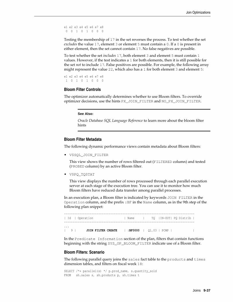
e1 e2 e3 e4 e5 e6 e7 e8 0 0 1 0 1 0 0 0
Testing the membership of 17 in the set reverses the process. To test whether the setexcludes the value 17, element 3 or element 5 must contain a 0. If a 0 is present ineither element, then the set cannot contain 17. No false negatives are possible.
To test whether the set includes 17, both element 3 and element 5 must contain 1values. However, if the test indicates a 1 for both elements, then it is still possible forthe set not to include 17. False positives are possible. For example, the following arraymight represent the value 22, which also has a 1 for both element 3 and element 5:
e1 e2 e3 e4 e5 e6 e7 e8 1 0 1 0 1 0 0 0
Bloom Filter Controls
The optimizer automatically determines whether to use Bloom filters. To overrideoptimizer decisions, use the hints PX_JOIN_FILTER and NO_PX_JOIN_FILTER.
See Also:
Oracle Database SQL Language Reference to learn more about the bloom filterhints
Bloom Filter Metadata
The following dynamic performance views contain metadata about Bloom filters:
• V$SQL_JOIN_FILTER
This view shows the number of rows filtered out (FILTERED column) and tested(PROBED column) by an active Bloom filter.
• V$PQ_TQSTAT
This view displays the number of rows processed through each parallel executionserver at each stage of the execution tree. You can use it to monitor how muchBloom filters have reduced data transfer among parallel processes.
In an execution plan, a Bloom filter is indicated by keywords JOIN FILTER in theOperation column, and the prefix :BF in the Name column, as in the 9th step of thefollowing plan snippet:
----------------------------------------------------------------------------| Id | Operation | Name | TQ |IN-OUT| PQ Distrib |----------------------------------------------------------------------------...| 9 | JOIN FILTER CREATE | :BF0000 | Q1,03 | PCWP | |
In the Predicate Information section of the plan, filters that contain functionsbeginning with the string SYS_OP_BLOOM_FILTER indicate use of a Bloom filter.
Bloom Filters: Scenario
The following parallel query joins the sales fact table to the products and timesdimension tables, and filters on fiscal week 18:
SELECT /*+ parallel(s) */ p.prod_name, s.quantity_soldFROM sh.sales s, sh.products p, sh.times t
Join Optimizations
Joins 9-37

WHERE s.prod_id = p.prod_idAND s.time_id = t.time_idAND t.fiscal_week_number = 18;
Querying DBMS_XPLAN.DISPLAY_CURSOR provides the following output:
SELECT * FROM TABLE(DBMS_XPLAN.DISPLAY_CURSOR(format => 'BASIC,+PARALLEL,+PREDICATE'));
EXPLAINED SQL STATEMENT:------------------------SELECT /*+ parallel(s) */ p.prod_name, s.quantity_sold FROM sh.sales s,sh.products p, sh.times t WHERE s.prod_id = p.prod_id AND s.time_id =t.time_id AND t.fiscal_week_number = 18 Plan hash value: 1183628457 ----------------------------------------------------------------------------| Id | Operation | Name | TQ |IN-OUT| PQ Distrib |----------------------------------------------------------------------------| 0 | SELECT STATEMENT | | | | || 1 | PX COORDINATOR | | | | || 2 | PX SEND QC (RANDOM) | :TQ10003 | Q1,03 | P->S | QC (RAND) ||* 3 | HASH JOIN BUFFERED | | Q1,03 | PCWP | || 4 | PX RECEIVE | | Q1,03 | PCWP | || 5 | PX SEND BROADCAST | :TQ10001 | Q1,01 | S->P | BROADCAST || 6 | PX SELECTOR | | Q1,01 | SCWC | || 7 | TABLE ACCESS FULL | PRODUCTS | Q1,01 | SCWP | ||* 8 | HASH JOIN | | Q1,03 | PCWP | || 9 | JOIN FILTER CREATE | :BF0000 | Q1,03 | PCWP | || 10 | BUFFER SORT | | Q1,03 | PCWC | || 11 | PX RECEIVE | | Q1,03 | PCWP | || 12 | PX SEND HYBRID HASH| :TQ10000 | | S->P | HYBRID HASH||* 13 | TABLE ACCESS FULL | TIMES | | | || 14 | PX RECEIVE | | Q1,03 | PCWP | || 15 | PX SEND HYBRID HASH | :TQ10002 | Q1,02 | P->P | HYBRID HASH|| 16 | JOIN FILTER USE | :BF0000 | Q1,02 | PCWP | || 17 | PX BLOCK ITERATOR | | Q1,02 | PCWC | ||* 18 | TABLE ACCESS FULL | SALES | Q1,02 | PCWP | |---------------------------------------------------------------------------- Predicate Information (identified by operation id):--------------------------------------------------- 3 - access("S"."PROD_ID"="P"."PROD_ID") 8 - access("S"."TIME_ID"="T"."TIME_ID") 13 - filter("T"."FISCAL_WEEK_NUMBER"=18) 18 - access(:Z>=:Z AND :Z<=:Z) filter(SYS_OP_BLOOM_FILTER(:BF0000,"S"."TIME_ID"))
A single server process scans the times table (Step 13), and then uses a hybrid hashdistribution method to send the rows to the parallel execution servers (Step 12). Theprocesses in set Q1,03 create a bloom filter (Step 9). The processes in set Q1,02 scansales in parallel (Step 18), and then use the Bloom filter to discard rows from sales(Step 16) before sending them on to set Q1,03 using hybrid hash distribution (Step15). The processes in set Q1,03 hash join the times rows to the filtered sales rows(Step 8). The processes in set Q1,01 scan products (Step 7), and then send the rowsto Q1,03 (Step 5). Finally, the processes in Q1,03 join the products rows to the rowsgenerated by the previous hash join (Step 3).
The basic process looks as follows:
Join Optimizations
9-38 SQL Tuning Guide
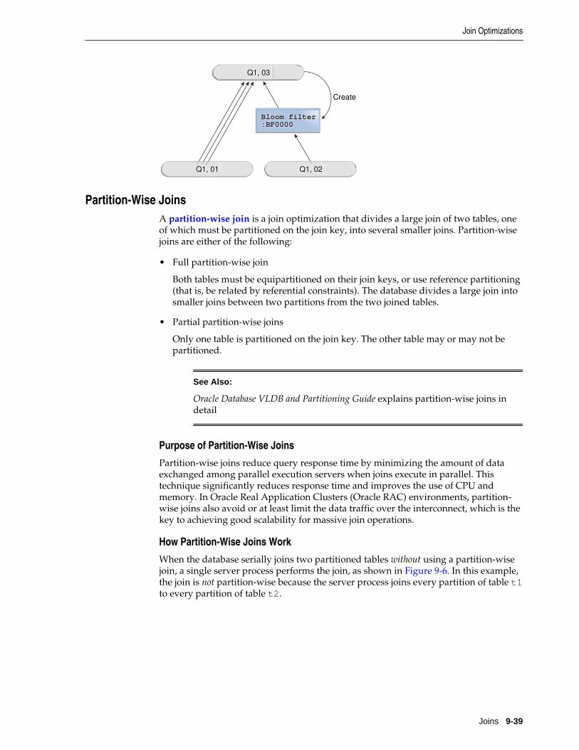
Bloom filter
:BF0000
Q1, 03
Q1, 02Q1, 01
Create
Partition-Wise JoinsA partition-wise join is a join optimization that divides a large join of two tables, oneof which must be partitioned on the join key, into several smaller joins. Partition-wisejoins are either of the following:
• Full partition-wise join
Both tables must be equipartitioned on their join keys, or use reference partitioning(that is, be related by referential constraints). The database divides a large join intosmaller joins between two partitions from the two joined tables.
• Partial partition-wise joins
Only one table is partitioned on the join key. The other table may or may not bepartitioned.
See Also:
Oracle Database VLDB and Partitioning Guide explains partition-wise joins indetail
Purpose of Partition-Wise Joins
Partition-wise joins reduce query response time by minimizing the amount of dataexchanged among parallel execution servers when joins execute in parallel. Thistechnique significantly reduces response time and improves the use of CPU andmemory. In Oracle Real Application Clusters (Oracle RAC) environments, partition-wise joins also avoid or at least limit the data traffic over the interconnect, which is thekey to achieving good scalability for massive join operations.
How Partition-Wise Joins Work
When the database serially joins two partitioned tables without using a partition-wisejoin, a single server process performs the join, as shown in Figure 9-6. In this example,the join is not partition-wise because the server process joins every partition of table t1to every partition of table t2.
Join Optimizations
Joins 9-39

Figure 9-6 Join That Is Not Partition-Wise
Server
Process
t1 t2
How a Full Partition-Wise Join Works
Figure 9-7 shows a full partition-wise join performed in parallel (it can also beperformed in serial). In this case, the granule of parallelism is a partition. Each parallelexecution server joins the partitions in pairs. For example, the first parallel executionserver joins the first partition of t1 to the first partition of t2. The parallel executioncoordinator then assembles the result.
Figure 9-7 Full Partition-Wise Join in Parallel
PE Server
PE Server
PE Server
PE Server
PE Coordinator
t1 t2
Join Optimizations
9-40 SQL Tuning Guide

A full partition-wise join can also join partitions to subpartitions, which is useful whenthe tables use different partitioning methods. For example, customers is partitionedby hash, but sales is partitioned by range. If you subpartition sales by hash, thenthe database can perform a full partition-wise join between the hash partitions of thecustomers and the hash subpartitions of sales.
In the execution plan, the presence of a partition operation before the join signals thepresence of a full partition-wise join, as in the following snippet:
| 8 | PX PARTITION HASH ALL||* 9 | HASH JOIN |
See Also:
Oracle Database VLDB and Partitioning Guide explains full partition-wise joinsin detail, and includes several examples
How a Partial Partition-Wise Join Works
In contrast, the example in Figure 9-8 shows a partial partition-wise join between t1,which is partitioned, and t2, which is not partitioned. Partial partition-wise joins,unlike their full partition-wise counterpart, must execute in parallel.
Because t2 is not partitioned, a set of parallel execution servers must generatepartitions from t2 as needed. A different set of parallel execution servers then joinsthe t1 partitions to the dynamically generated partitions. The parallel executioncoordinator assembles the result.
Figure 9-8 Partial Partition-Wise Join
PE Coordinator
PE Server
PE Server
PE Server
PE Server
PE Server
PE Server
PE Server
PE Server
Dynamically created partitions
t1 t2
t1 t2
In the execution plan, the operation PX SEND PARTITION (KEY) signals a partialpartition-wise join, as in the following snippet:
Join Optimizations
Joins 9-41

| 11 | PX SEND PARTITION (KEY) |
See Also:
Oracle Database VLDB and Partitioning Guide explains full partition-wise joinsin detail, and includes several examples
Join Optimizations
9-42 SQL Tuning Guide

Part VOptimizer Statistics
This part contains the following chapters:
• Optimizer Statistics Concepts
• Histograms
• Managing Optimizer Statistics: Basic Topics
• Managing Optimizer Statistics: Advanced Topics


10Optimizer Statistics Concepts
This chapter explains basic concepts relating to optimizer statistics.
This chapter includes the following topics:
• Introduction to Optimizer Statistics
• About Optimizer Statistics Types
• How the Database Gathers Optimizer Statistics
• When the Database Gathers Optimizer Statistics
See Also:
• Query Optimizer Concepts
• Histograms
• Managing Optimizer Statistics: Basic Topics
• Managing Optimizer Statistics: Advanced Topics
Introduction to Optimizer StatisticsOracle Database optimizer statistics describe details about the database and its objects.The optimizer cost model relies on statistics collected about the objects involved in aquery, and the database and host where the query runs. Statistics are critical to theoptimizer's ability to pick the best execution plan for a SQL statement.
Optimizer statistics include the following:
• Table statistics
– Number of rows
– Number of blocks
– Average row length
• Column statistics
– Number of distinct values (NDV) in a column
– Number of nulls in a column
– Data distribution (histogram)
Optimizer Statistics Concepts 10-1

– Extended statistics
• Index statistics
– Number of leaf blocks
– Number of levels
– Index clustering factor
• System statistics
– I/O performance and utilization
– CPU performance and utilization
As shown in Figure 10-1, the database stores optimizer statistics for tables, columns,indexes, and the system in the data dictionary. You can access these statistics usingdata dictionary views.
Note:
The optimizer statistics are different from the performance statistics visiblethrough V$ views.
Introduction to Optimizer Statistics
10-2 SQL Tuning Guide

Figure 10-1 Optimizer Statistics
Execution Plan
GB
HJHJ
ID Name
100 KumarPERSON_ID_IX
Data Dictionary
Optimizer Statistics
Index Table Column System
CPU and I/O
Optimizer
Database
PERSONTable
About Optimizer Statistics TypesThe optimizer collects statistics on different types of database objects andcharacteristics of the database environment. This section contains the following topics:
• Table Statistics
• Column Statistics
• Index Statistics
• Session-Specific Statistics for Global Temporary Tables
• System Statistics
• User-Defined Optimizer Statistics
Table StatisticsIn Oracle Database, table statistics include information about rows and blocks. Theoptimizer uses these statistics to determine the cost of table scans and table joins.DBMS_STATS can gather statistics for both permanent and temporary tables.
About Optimizer Statistics Types
Optimizer Statistics Concepts 10-3

The database tracks all relevant statistics about permanent tables.DBMS_STATS.GATHER_TABLE_STATS commits before gathering statistics onpermanent tables. For example, table statistics stored in DBA_TAB_STATISTICS trackthe following:
• Number of rows and average row length
The database uses the row count stored in DBA_TAB_STATISTICS whendetermining cardinality.
• Number of data blocks
The optimizer uses the number of data blocks with theDB_FILE_MULTIBLOCK_READ_COUNT initialization parameter to determine thebase table access cost.
Example 10-1 Table Statistics
This example queries some table statistics for the sh.customers table.
sys@PROD> SELECT NUM_ROWS, AVG_ROW_LEN, BLOCKS, LAST_ANALYZED 2 FROM DBA_TAB_STATISTICS 3 WHERE OWNER='SH' 4 AND TABLE_NAME='CUSTOMERS'; NUM_ROWS AVG_ROW_LEN BLOCKS LAST_ANAL---------- ----------- ---------- --------- 55500 181 1486 14-JUN-10
See Also:
• “About Optimizer Initialization Parameters”
• “Gathering Schema and Table Statistics”
• Oracle Database Reference for a description of the DBA_TAB_STATISTICSview and the DB_FILE_MULTIBLOCK_READ_COUNT initializationparameter
Column StatisticsColumn statistics track information about column values and data distribution. Theoptimizer uses these statistics to generate accurate cardinality estimates and makebetter decisions about index usage, join orders, join methods, and so on.
For example, index statistics in DBA_TAB_COL_STATISTICS track the following:
• Number of distinct values (NDV)
• Number of nulls
• High and low values
• Histogram-related information (see “Histograms ”)
The optimizer can use extended statistics, which are a special type of column statistics.These statistics are useful for informing the optimizer of logical relationships amongcolumns.
About Optimizer Statistics Types
10-4 SQL Tuning Guide

See Also:
• “About Statistics on Column Groups”
• Oracle Database Reference for a description of theDBA_TAB_COL_STATISTICS view
Index StatisticsThe index statistics include information about the number of index levels, the numberof index blocks, and the relationship between the index and the data blocks. Theoptimizer uses these statistics to determine the cost of index scans.
Types of Index Statistics
Index statistics stored in the DBA_IND_STATISTICS view track the following:
• Levels
The BLEVEL column shows the number of blocks required to go from the rootblock to a leaf block. A B-tree index has two types of blocks: branch blocks forsearching and leaf blocks that store values. See Oracle Database Concepts for aconceptual overview of B-tree indexes.
• Distinct keys
This columns tracks the number of distinct indexed values. If a unique constraint isdefined, and if no NOT NULL constraint is defined, then this value equals thenumber of non-null values.
• Average number of leaf blocks for each distinct indexed key
• Average number of data blocks pointed to by each distinct indexed key
See Also:
Oracle Database Reference for a description of the DBA_IND_STATISTICS view
Example 10-2 Index Statistics
This example queries some index statistics for the cust_lname_ix andcustomers_pk indexes on the sh.customers table (sample output included):
SELECT INDEX_NAME, BLEVEL, LEAF_BLOCKS AS "LEAFBLK", DISTINCT_KEYS AS "DIST_KEY", AVG_LEAF_BLOCKS_PER_KEY AS "LEAFBLK_PER_KEY", AVG_DATA_BLOCKS_PER_KEY AS "DATABLK_PER_KEY"FROM DBA_IND_STATISTICSWHERE OWNER = 'SH'AND INDEX_NAME IN ('CUST_LNAME_IX','CUSTOMERS_PK');
INDEX_NAME BLEVEL LEAFBLK DIST_KEY LEAFBLK_PER_KEY DATABLK_PER_KEY-------------- ------ ------- -------- --------------- ---------------CUSTOMERS_PK 1 115 55500 1 1CUST_LNAME_IX 1 141 908 1 10
About Optimizer Statistics Types
Optimizer Statistics Concepts 10-5

Index Clustering FactorFor a B-tree index, the index clustering factor measures the physical grouping of rowsin relation to an index value, such as last name. The index clustering factor helps theoptimizer decide whether an index scan or full table scan is more efficient for certainqueries). A low clustering factor indicates an efficient index scan.
A clustering factor that is close to the number of blocks in a table indicates that therows are physically ordered in the table blocks by the index key. If the databaseperforms a full table scan, then the database tends to retrieve the rows as they arestored on disk sorted by the index key. A clustering factor that is close to the numberof rows indicates that the rows are scattered randomly across the database blocks inrelation to the index key. If the database performs a full table scan, then the databasewould not retrieve rows in any sorted order by this index key.
The clustering factor is a property of a specific index, not a table (see Oracle DatabaseConcepts for an overview). If multiple indexes exist on a table, then the clusteringfactor for one index might be small while the factor for another index is large. Anattempt to reorganize the table to improve the clustering factor for one index maydegrade the clustering factor of the other index.
Example 10-3 Index Clustering Factor
This example shows how the optimizer uses the index clustering factor to determinewhether using an index is more effective than a full table scan.
1. Start SQL*Plus and connect to a database as sh, and then query the number ofrows and blocks in the sh.customers table (sample output included):
SELECT table_name, num_rows, blocksFROM user_tablesWHERE table_name='CUSTOMERS'; TABLE_NAME NUM_ROWS BLOCKS------------------------------ ---------- ----------CUSTOMERS 55500 1486
2. Create an index on the customers.cust_last_name column.
For example, execute the following statement:
CREATE INDEX CUSTOMERS_LAST_NAME_IDX ON customers(cust_last_name);
3. Query the index clustering factor of the newly created index.
The following query shows that the customers_last_name_idx index has ahigh clustering factor because the clustering factor is significantly more than thenumber of blocks in the table:
SELECT index_name, blevel, leaf_blocks, clustering_factorFROM user_indexesWHERE table_name='CUSTOMERS'AND index_name= 'CUSTOMERS_LAST_NAME_IDX'; INDEX_NAME BLEVEL LEAF_BLOCKS CLUSTERING_FACTOR------------------------------ ---------- ----------- -----------------CUSTOMERS_LAST_NAME_IDX 1 141 9859
4. Create a new copy of the customers table, with rows ordered bycust_last_name.
About Optimizer Statistics Types
10-6 SQL Tuning Guide

For example, execute the following statements:
DROP TABLE customers3 PURGE;CREATE TABLE customers3 AS SELECT * FROM customers ORDER BY cust_last_name;
5. Gather statistics on the customers3 table.
For example, execute the GATHER_TABLE_STATS procedure as follows:
EXEC DBMS_STATS.GATHER_TABLE_STATS(null,'CUSTOMERS3');
6. Query the number of rows and blocks in the customers3 table .
For example, enter the following query (sample output included):
SELECT TABLE_NAME, NUM_ROWS, BLOCKSFROM USER_TABLESWHERE TABLE_NAME='CUSTOMERS3'; TABLE_NAME NUM_ROWS BLOCKS------------------------------ ---------- ----------CUSTOMERS3 55500 1485
7. Create an index on the cust_last_name column of customers3.
For example, execute the following statement:
CREATE INDEX CUSTOMERS3_LAST_NAME_IDX ON customers3(cust_last_name);
8. Query the index clustering factor of the customers3_last_name_idx index.
The following query shows that the customers3_last_name_idx index has alower clustering factor:
SELECT INDEX_NAME, BLEVEL, LEAF_BLOCKS, CLUSTERING_FACTORFROM USER_INDEXESWHERE TABLE_NAME = 'CUSTOMERS3'AND INDEX_NAME = 'CUSTOMERS3_LAST_NAME_IDX'; INDEX_NAME BLEVEL LEAF_BLOCKS CLUSTERING_FACTOR------------------------------ ---------- ----------- -----------------CUSTOMERS3_LAST_NAME_IDX 1 141 1455
The table customers3 has the same data as the original customers table, butthe index on customers3 has a much lower clustering factor because the data inthe table is ordered by the cust_last_name. The clustering factor is now about10 times the number of blocks instead of 70 times.
9. Query the customers table.
For example, execute the following query (sample output included):
SELECT cust_first_name, cust_last_nameFROM customersWHERE cust_last_name BETWEEN 'Puleo' AND 'Quinn'; CUST_FIRST_NAME CUST_LAST_NAME-------------------- ----------------------------------------Vida PuleoHarriett Quinlan
About Optimizer Statistics Types
Optimizer Statistics Concepts 10-7

Madeleine QuinnCaresse Puleo
10. Display the cursor for the query.
For example, execute the following query (partial sample output included):
SELECT * FROM TABLE(DBMS_XPLAN.DISPLAY_CURSOR());
-------------------------------------------------------------------------------| Id | Operation | Name | Rows |Bytes|Cost (%CPU)| Time |-------------------------------------------------------------------------------| 0| SELECT STATEMENT | | | | 405 (100)| ||* 1| TABLE ACCESS STORAGE FULL| CUSTOMERS | 2335|35025| 405 (1)|00:00:01|-------------------------------------------------------------------------------
The preceding plan shows that the optimizer did not use the index on the originalcustomers tables.
11. Query the customers3 table.
For example, execute the following query (sample output included):
SELECT cust_first_name, cust_last_nameFROM customers3WHERE cust_last_name BETWEEN 'Puleo' AND 'Quinn'; CUST_FIRST_NAME CUST_LAST_NAME-------------------- ----------------------------------------Vida PuleoHarriett QuinlanMadeleine QuinnCaresse Puleo
12. Display the cursor for the query.
For example, execute the following query (partial sample output included):
SELECT * FROM TABLE(DBMS_XPLAN.DISPLAY_CURSOR());
---------------------------------------------------------------------------------------|Id| Operation | Name |Rows|Bytes|Cost(%CPU)| Time|---------------------------------------------------------------------------------------| 0| SELECT STATEMENT | | | |69(100)| || 1| TABLE ACCESS BY INDEX ROWID|CUSTOMERS3 |2335|35025|69(0) |00:00:01||*2| INDEX RANGE SCAN |CUSTOMERS3_LAST_NAME_IDX|2335| |7(0) |00:00:01|---------------------------------------------------------------------------------------
The result set is the same, but the optimizer chooses the index. The plan cost ismuch less than the cost of the plan used on the original customers table.
13. Query customers with a hint that forces the optimizer to use the index.
For example, execute the following query (partial sample output included):
SELECT /*+ index (Customers CUSTOMERS_LAST_NAME_IDX) */ cust_first_name, cust_last_name FROM customers WHERE cust_last_name BETWEEN 'Puleo' and 'Quinn'; CUST_FIRST_NAME CUST_LAST_NAME-------------------- ----------------------------------------Vida PuleoCaresse Puleo
About Optimizer Statistics Types
10-8 SQL Tuning Guide

Harriett QuinlanMadeleine Quinn
14. Display the cursor for the query.
For example, execute the following query (partial sample output included):
SELECT * FROM TABLE(DBMS_XPLAN.DISPLAY_CURSOR());
-----------------------------------------------------------------------------------------| Id | Operation | Name |Rows|Bytes|Cost(%CPU)| Time |-----------------------------------------------------------------------------------------| 0| SELECT STATEMENT | | | | 422(100) | || 1| TABLE ACCESS BY INDEX ROWID|CUSTOMERS |335 |35025| 422(0) |00:00:01||*2| INDEX RANGE SCAN |CUSTOMERS_LAST_NAME_IDX|2335| | 7(0) |00:00:01|-----------------------------------------------------------------------------------------
The preceding plan shows that the cost of using the index on customers ishigher than the cost of a full table scan. Thus, using an index does not necessarilyimprove performance. The index clustering factor is a measure of whether anindex scan is more effective than a full table scan.
Effect of Index Clustering Factor on Cost: Example
To illustrate how the index clustering factor can influence the cost of table access,consider the following scenario:
• A table contains 9 rows that are stored in 3 data blocks.
• The col1 column currently stores the values A, B, and C.
• A nonunique index named col1_idx exists on col1 for this table.
Example 10-4 Collocated Data
Assume that the rows are stored in the data blocks as follows:
Block 1 Block 2 Block 3------- ------- -------A A A B B B C C C
In this example, the index clustering factor for col1_idx is low. The rows that havethe same indexed column values for col1 are in the same data blocks in the table.Thus, the cost of using an index range scan to return all rows with value A is lowbecause only one block in the table must be read.
Example 10-5 Scattered Data
Assume that the same rows are scattered across the data blocks as follows:
Block 1 Block 2 Block 3------- ------- -------A B C A C B B A C
In this example, the index clustering factor for col1_idx is higher. The database mustread all three blocks in the table to retrieve all rows with the value A in col1.
See Also:
Oracle Database Reference for a description of the DBA_INDEXES view
About Optimizer Statistics Types
Optimizer Statistics Concepts 10-9

Session-Specific Statistics for Global Temporary TablesA global temporary table is a special table that stores intermediate session-private datafor a specific duration. The ON COMMIT clause of CREATE GLOBAL TEMPORARYTABLE indicates whether the table is transaction-specific (DELETE ROWS) or session-specific (PRESERVE ROWS). Thus, a temporary table holds intermediate result sets forthe duration of either a transaction or a session.
When you create a global temporary table, you create a definition that is visible to allsessions. No physical storage is allocated. When a session first puts data into the table,the database allocates storage space. The data in the temporary table is only visible tothe current session.
Shared and Session-Specific Statistics for Global Temporary Tables
In releases before Oracle Database 12c, the database did not maintain statistics forglobal temporary tables and non-global temporary tables differently. The databasemaintained one version of the statistics shared by all sessions, even though data indifferent sessions could differ.
Starting in Oracle Database 12c, you can set the table-level preferenceGLOBAL_TEMP_TABLE_STATS to make statistics on a global temporary table sharedor session-specific. When set to session-specific, you can gather statistics for a globaltemporary table in one session, and then use the statistics for this session only.Meanwhile, users can continue to maintain a shared version of the statistics. Duringoptimization, the optimizer first checks whether a global temporary table has session-specific statistics. If yes, the optimizer uses them. Otherwise, the optimizer uses sharedstatistics if they exist.
Session-specific statistics have the following characteristics:
• Dictionary views that track statistics show both the shared statistics and thesession-specific statistics in the current session.
The views are DBA_TAB_STATISTICS, DBA_IND_STATISTICS,DBA_TAB_HISTOGRAMS, and DBA_TAB_COL_STATISTICS (each view has acorresponding USER_ and ALL_ version). The SCOPE column shows whetherstatistics are session-specific or shared.
• Other sessions do not share the cursor using the session-specific statistics.
Different sessions can share the cursor using shared statistics, as in releases earlierthan Oracle Database 12c. The same session can share the cursor using session-specific statistics.
• Pending statistics are not supported for session-specific statistics.
• When the GLOBAL_TEMP_TABLE_STATS preference is set to SESSION, by defaultGATHER_TABLE_STATS immediately invalidates previous cursors compiled in thesame session. However, this procedure does not invalidate cursors compiled inother sessions.
Effect of DBMS_STATS on Transaction-Specific Temporary Tables
DBMS_STATS commits changes to session-specific global temporary tables, but not totransaction-specific global temporary tables. Before Oracle Database 12c, runningDBMS_STATS.GATHER_TABLE_STATS on a transaction-specific temporary table (ONCOMMIT DELETE ROWS) would delete all rows, making the statistics show the table as
About Optimizer Statistics Types
10-10 SQL Tuning Guide

empty. Starting in Oracle Database 12c, the following procedures do not commit fortransaction-specific temporary tables, so that rows in these tables are not deleted:
• GATHER_TABLE_STATS
• DELETE_TABLE_STATS
• DELETE_COLUMN_STATS
• DELETE_INDEX_STATS
• SET_TABLE_STATS
• SET_COLUMN_STATS
• SET_INDEX_STATS
• GET_TABLE_STATS
• GET_COLUMN_STATS
• GET_INDEX_STATS
The preceding program units observe the GLOBAL_TEMP_TABLE_STATS preference.For example, if the table preference is set to SESSION, then SET_TABLE_STATS setsthe session statistics, and GATHER_TABLE_STATS preserves all rows in a transaction-specific temporary table. If the table preference is set to SHARED, thenSET_TABLE_STATS sets the shared statistics, and GATHER_TABLE_STATS deletes allrows from a transaction-specific temporary table.
See Also:
• “Gathering Schema and Table Statistics”
• Oracle Database Concepts to learn about global temporary tables
• Oracle Database PL/SQL Packages and Types Reference to learn about theDBMS_STATS.GATHER_TABLE_STATS procedure
System StatisticsThe system statistics describe hardware characteristics such as I/O and CPUperformance and utilization. System statistics enable the query optimizer to moreaccurately estimate I/O and CPU costs when choosing execution plans.
The database does not invalidate previously parsed SQL statements when updatingsystem statistics. The database parses all new SQL statements using new statistics.
See Also:
“Gathering System Statistics Manually”
User-Defined Optimizer StatisticsThe extensible optimizer enables authors of user-defined functions and indexes tocreate statistics collection, selectivity, and cost functions for the optimizer to use when
About Optimizer Statistics Types
Optimizer Statistics Concepts 10-11
choosing a execution plan. The optimizer cost model is extended to integrateinformation supplied by the user to assess CPU and the I/O cost.
Statistics types act as interfaces for user-defined functions that influence the choice ofexecution plan by the optimizer. However, to use a statistics type, the optimizerrequires a mechanism to bind the type to a database object such as a column,standalone function, object type, index, indextype, or package. The SQL statementASSOCIATE STATISTICS creates this association.
Functions for user-defined statistics are relevant for columns that use both standardSQL data types and object types, and for domain indexes. When you associate astatistics type with a column or domain index, the database calls the statisticscollection method in the statistics type whenever DBMS_STATS gathers statistics fordatabase objects.
See Also:
• “Gathering Schema and Table Statistics”
• Oracle Database Data Cartridge Developer's Guide to learn about theextensible optimizer and user-defined statistics
How the Database Gathers Optimizer StatisticsOracle Database provides several mechanisms to gather statistics. This sectioncontains the following topics:
• DBMS_STATS Package
• Dynamic Statistics
• Online Statistics Gathering for Bulk Loads
See Also:
• “Controlling Automatic Optimizer Statistics Collection” or “GatheringOptimizer Statistics Manually”
• “Locking and Unlocking Optimizer Statistics”
DBMS_STATS PackageThe DBMS_STATS PL/SQL package collects and manages optimizer statistics. Thispackage enables you to control what and how statistics are collected, including thedegree of parallelism for statistics collection, sampling methods, granularity ofstatistics collection in partitioned tables, and so on.
Note:
Do not use the COMPUTE and ESTIMATE clauses of the ANALYZE statement tocollect optimizer statistics. These clauses have been deprecated. Instead, useDBMS_STATS.
How the Database Gathers Optimizer Statistics
10-12 SQL Tuning Guide

Statistics gathered with the DBMS_STATS package are required for the creation ofaccurate execution plans. For example, table statistics gathered by DBMS_STATSinclude the number of rows, number of blocks, and average row length.
By default, Oracle Database uses automatic optimizer statistics collection. In this case,the database automatically runs DBMS_STATS to collect optimizer statistics for allschema objects for which statistics are missing or stale. The process eliminates manymanual tasks associated with managing the optimizer, and significantly reduces therisks of generating suboptimal execution plans because of missing or stale statistics.You can also update and manage optimizer statistics by manually executingDBMS_STATS.
See Also:
• “Controlling Automatic Optimizer Statistics Collection”
• “Gathering Optimizer Statistics Manually”
• Oracle Database Administrator's Guide to learn more about automatedmaintenance tasks
• Oracle Database PL/SQL Packages and Types Reference to learn aboutDBMS_STATS
Dynamic StatisticsBy default, when optimizer statistics are missing, stale, or insufficient, the databaseautomatically gathers dynamic statistics during a parse. The database uses recursiveSQL to scan a small random sample of table blocks.
Note:
Dynamic statistics augment statistics rather than providing an alternative tothem.
Dynamic statistics can supplement statistics such as table and index block counts, tableand join cardinalities (estimated number of rows), join column statistics, and GROUPBY statistics. This information helps the optimizer improve plans by making betterestimates for predicate selectivity.
Dynamic statistics are beneficial in the following situations:
• An execution plan is suboptimal because of complex predicates.
• The sampling time is a small fraction of total execution time for the query.
• The query is executed many times so that the sampling time is amortized.
How the Database Gathers Optimizer Statistics
Optimizer Statistics Concepts 10-13

See Also:
• “When the Database Samples Data”
• “Guideline for Accurate Statistics”
• “Controlling Dynamic Statistics”
Online Statistics Gathering for Bulk LoadsStarting in Oracle Database 12c, the database can gather table statistics automaticallyduring the following types of bulk load operations:
• CREATE TABLE AS SELECT
• INSERT INTO ... SELECT into an empty table using a direct path insert
Note:
By default, a parallel insert uses a direct path insert. You can force a directpath insert by using the /*+APPEND */ hint.
This section contains the following topics:
• Purpose of Online Statistics Gathering for Bulk Loads
• Global Statistics During Inserts into Empty Partitioned Tables
• Index Statistics and Histograms During Bulk Loads
• Restrictions for Online Statistics Gathering for Bulk Loads
• Hints for Online Statistics Gathering for Bulk Loads
See Also:
Oracle Database Data Warehousing Guide to learn more about bulk loads
Purpose of Online Statistics Gathering for Bulk Loads
Data warehouses typically load large amounts of data into the database. For example,a sales data warehouse might load sales data nightly.
In releases earlier than Oracle Database 12c, to avoid the possibility of a suboptimalplan caused by stale statistics, you needed to gather statistics manually after a bulkload. The ability to gather statistics automatically during bulk loads has the followingbenefits:
• Improved performance
Gathering statistics during the load avoids an additional table scan to gather tablestatistics.
• Improved manageability
How the Database Gathers Optimizer Statistics
10-14 SQL Tuning Guide

No user intervention is required to gather statistics after a bulk load.
Global Statistics During Inserts into Empty Partitioned Tables
When inserting rows into an empty partitioned table, the database gathers globalstatistics during the insert. For example, if you run INSERT INTO sales SELECT,and if sales is an empty partitioned table, then the database gathers global statisticsfor sales, but does not gather partition-level statistics.
If you insert rows into a empty partitioned table using extended syntax, and if thespecified partition or subpartition is empty, then the database gathers the statistics onthe specified partition or subpartition during the insert. No global level statistics aregathered. For example, if you run INSERT INTO sales PARTITION(sales_q4_2000) SELECT, and if partition sales_q4_2000 is empty before theinsert (other partitions need not be empty), then the database gathers statistics duringthe insert. Moreover, if the INCREMENTAL preference is enabled for sales, then thedatabase also gathers synopses for sales_q4_2000. Statistics are immediatelyavailable after the INSERT statement. However, if you roll back the transaction, thenthe database automatically deletes statistics gathered during the bulk load.
See Also:
“How to Enable Incremental Statistics Maintenance”
Index Statistics and Histograms During Bulk Loads
While gathering online statistics, the database does not gather index statistics or createhistograms. If these statistics are required, then Oracle recommends runningDBMS_STATS.GATHER_TABLE_STATS with the options parameter set to GATHERAUTO after the bulk load. For example, the following command gathers statistics forthe bulk-loaded sh_ctas table:
EXEC DBMS_STATS.GATHER_TABLE_STATS( user, 'SH_CTAS', options => 'GATHER AUTO' );
The preceding example only gathers missing or stale statistics. The database does notgather table and basic column statistics collected during the bulk load.
Note:
You can set the table preference options to GATHER AUTO on the tables thatyou plan to bulk load. In this way, you need not explicitly set the optionsparameter when running GATHER_TABLE_STATS.
See Also:
“Gathering Schema and Table Statistics”
Restrictions for Online Statistics Gathering for Bulk Loads
Currently, statistics gathering does not occur automatically for bulk loads when any ofthe following conditions apply to the target table, partition, or subpartition:
• It is not empty, and you perform an INSERT INTO ... SELECT.
How the Database Gathers Optimizer Statistics
Optimizer Statistics Concepts 10-15

In this case, an OPTIMIZER STATISTICS GATHERING row source appears in theplan, but this row source is only a pass-through. The database does not actuallygather optimizer statistics.
Note:
The DBA_TAB_COL_STATISTICS.NOTES column is set to STATS_ON_LOADby a bulk load into an empty table. However, subsequent bulk loads into thenon-empty table do not reset the NOTES column. One method for determiningwhether the database gathered statistics is to executeDBMS_STATS.FLUSH_DATABASE_MONITORING_INFO, and then queryUSER_TAB_MODIFICATIONS.INSERTS. If the query returns a row indicatingthe number of rows loaded, then the statistics were not gathered automaticallyduring the most recent bulk load.
• It is in an Oracle-owned schema such as SYS.
• It is a nested table.
• It is an index-organized table (IOT).
• It is an external table.
• It is a global temporary table defined as ON COMMIT DELETE ROWS.
• It has virtual columns.
• It has a PUBLISH preference set to FALSE.
/? Bug 16922369 ?/
• Its statistics are locked.
• It is partitioned, INCREMENTAL is set to true, and extended syntax is not used.
For example, assume that you execute DBMS_STATS.SET_TABLE_PREFS(null,'sales', incremental', 'true'). In this case, the database does not gatherstatistics for INSERT INTO sales SELECT, even when sales is empty.However, the database does gather statistics automatically for INSERT INTOsales PARTITION (sales_q4_2000) SELECT.
• It is loaded using a multitable insert statement.
See Also:
“Gathering Schema and Table Statistics”
Hints for Online Statistics Gathering for Bulk Loads
By default, the database gathers statistics during bulk loads. You can disable thefeature at the statement level by using the NO_GATHER_OPTIMIZER_STATISTICShint, and enable the feature at the statement level by using theGATHER_OPTIMIZER_STATISTICS hint. For example, the following statementdisables online statistics gathering for bulk loads:
CREATE TABLE employees2 AS SELECT /*+NO_GATHER_OPTIMIZER_STATISTICS */* FROM employees
How the Database Gathers Optimizer Statistics
10-16 SQL Tuning Guide

See Also:
Oracle Database SQL Language Reference to learn about theGATHER_OPTIMIZER_STATISTICS andNO_GATHER_OPTIMIZER_STATISTICS hints
When the Database Gathers Optimizer StatisticsThe database collects optimizer statistics at various times and from various sources.
This section contains the following topics:
• Sources for Optimizer Statistics
• SQL Plan Directives
• When the Database Samples Data
• How the Database Samples Data
Sources for Optimizer StatisticsThe database uses the following sources:
• DBMS_STATS execution, automatic or manual
This PL/SQL package is the primary means of gathering optimizer statistics. See Oracle Database PL/SQL Packages and Types Reference to learn about theDBMS_STATS.GATHER_TABLE_STATS procedure.
• SQL compilation
During SQL compilation, the database can augment the statistics previouslygathered by DBMS_STATS. In this stage, the database runs additional queries toobtain more accurate information on how many rows in the tables satisfy theWHERE clause predicates in the SQL statement (see “When the Database SamplesData”).
• SQL execution
During execution, the database can further augment previously gathered statistics.In this stage, Oracle Database collects the number of rows produced by every rowsource during the execution of a SQL statement. At the end of execution, theoptimizer determines whether the estimated number of rows is inaccurate enoughto warrant reparsing at the next statement execution. If the cursor is marked forreparsing, then the optimizer uses actual row counts from the previous executioninstead of estimates.
• SQL profiles
A SQL profile is a collection of auxiliary statistics on a query. The profile storesthese supplemental statistics in the data dictionary. The optimizer uses SQLprofiles during optimization to determine the most optimal plan (see “About SQLProfiles”).
The database stores optimizer statistics in the data dictionary and updates or replacesthem as needed. You can query statistics in data dictionary views.
When the Database Gathers Optimizer Statistics
Optimizer Statistics Concepts 10-17
SQL Plan DirectivesA SQL plan directive is additional information and instructions that the optimizer canuse to generate a more optimal plan. For example, a SQL plan directive can instructthe optimizer to record a missing extension.
About SQL Plan Directives
During SQL execution, if a cardinality misestimate occurs, then the database createsSQL plan directives. During SQL compilation, the optimizer examines the querycorresponding to the directive to determine whether missing extensions or histogramsexist (see “Managing Extended Statistics”). The optimizer records any missingextensions. Subsequent DBMS_STATS calls collect statistics for the extensions.
The optimizer uses dynamic statistics whenever it does not have sufficient statisticscorresponding to the directive. For example, the optimizer gathers dynamic statisticsuntil the creation of column group statistics, and also after this point whenmisestimates occur. Currently, the optimizer monitors only column groups. Theoptimizer does not create an extension on expressions.
SQL plan directives are not tied to a specific SQL statement or SQL ID. The optimizercan use directives for statements that are nearly identical because directives aredefined on a query expression. For example, directives can help the optimizer withqueries that use similar patterns, such as queries that are identical except for a selectlist item.
The database automatically manages SQL plan directives. The database initiallycreates directives in the shared pool. The database periodically writes the directives tothe SYSAUX tablespace. You can manage directives with the APIs available in theDBMS_SPD package.
See Also:
“About Statistics on Column Groups”
How the Optimizer Uses SQL Plan Directives: Example
This example shows how the database automatically creates and uses SQL plandirectives for SQL statements.
Assumptions
You plan to run queries against the sh schema, and you have privileges on thisschema and on data dictionary and V$ views.
To see how the database uses a SQL plan directive:
1. Query the sh.customers table.
SELECT /*+gather_plan_statistics*/ * FROM customers WHERE cust_state_province='CA' AND country_id='US';
The gather_plan_statistics hint shows the actual number of rows returnedfrom each operation in the plan. Thus, you can compare the optimizer estimateswith the actual number of rows returned.
When the Database Gathers Optimizer Statistics
10-18 SQL Tuning Guide

2. Query the plan for the preceding query.
The following example shows the execution plan (sample output included):
SELECT * FROM TABLE(DBMS_XPLAN.DISPLAY_CURSOR(FORMAT=>'ALLSTATS LAST')); PLAN_TABLE_OUTPUT-------------------------------------SQL_ID b74nw722wjvy3, child number 0-------------------------------------select /*+gather_plan_statistics*/ * from customers whereCUST_STATE_PROVINCE='CA' and country_id='US' Plan hash value: 1683234692--------------------------------------------------------------------------------------------| Id| Operation | Name | Starts |E-Rows| A-Rows | A-Time |Buffers | Reads |--------------------------------------------------------------------------------------------| 0 | SELECT STATEMENT | | 1 | | 29 |00:00:00.01 | 17 | 14 ||*1 | TABLE ACCESS FULL| CUSTOMERS | 1 | 8 | 29 |00:00:00.01 | 17 | 14 |-------------------------------------------------------------------------------------------- Predicate Information (identified by operation id):--------------------------------------------------- 1 - filter(("CUST_STATE_PROVINCE"='CA' AND "COUNTRY_ID"='US'))
The actual number of rows (A-Rows) returned by each operation in the planvaries greatly from the estimates (E-Rows). This statement is a candidate for automatic reoptimization (see “Automatic Reoptimization”).
3. Check whether the customers query can be reoptimized.
The following statement queries the V$SQL.IS_REOPTIMIZABLE value (sampleoutput included):
SELECT SQL_ID, CHILD_NUMBER, SQL_TEXT, IS_REOPTIMIZABLEFROM V$SQLWHERE SQL_TEXT LIKE 'SELECT /*+gather_plan_statistics*/%'; SQL_ID CHILD_NUMBER SQL_TEXT I------------- ------------ ----------- -b74nw722wjvy3 0 select /*+g Y ather_plan_ statistics* / * from cu stomers whe re CUST_STA TE_PROVINCE ='CA' and c ountry_id=' US'
The IS_REOPTIMIZABLE column is marked Y, so the database will perform ahard parse of the customers query on the next execution. The optimizer uses theexecution statistics from this initial execution to determine the plan. The databasepersists the information learned from reoptimization as a SQL plan directive.
4. Display the directives for the sh schema.
The following example uses DBMS_SPD to write the SQL plan directives to disk,and then shows the directives for the sh schema only:
When the Database Gathers Optimizer Statistics
Optimizer Statistics Concepts 10-19

EXEC DBMS_SPD.FLUSH_SQL_PLAN_DIRECTIVE; SELECT TO_CHAR(d.DIRECTIVE_ID) dir_id, o.OWNER AS "OWN", o.OBJECT_NAME AS "OBJECT", o.SUBOBJECT_NAME col_name, o.OBJECT_TYPE, d.TYPE, d.STATE, d.REASONFROM DBA_SQL_PLAN_DIRECTIVES d, DBA_SQL_PLAN_DIR_OBJECTS oWHERE d.DIRECTIVE_ID=o.DIRECTIVE_IDAND o.OWNER IN ('SH')ORDER BY 1,2,3,4,5;
DIR_ID OWN OBJECT COL_NAME OBJECT TYPE STATE REASON------------------- --- --------- ----------- ------ ---------------- ------ ------------1484026771529551585 SH CUSTOMERS COUNTRY_ID COLUMN DYNAMIC_SAMPLING USABLE SINGLE TABLE CARDINALITY MISESTIMATE1484026771529551585 SH CUSTOMERS CUST_STATE_ COLUMN DYNAMIC_SAMPLING USABLE SINGLE TABLE PROVINCE CARDINALITY MISESTIMATE 1484026771529551585 SH CUSTOMERS TABLE DYNAMIC_SAMPLING USABLE SINGLE TABLE CARDINALITY MISESTIMATE
Initially, the database stores SQL plan directives in memory, and then writes themto disk every 15 minutes. Thus, the preceding example callsDBMS_SPD.FLUSH_SQL_PLAN_DIRECTIVE to force the database to write thedirectives to the SYSAUX tablespace.
Monitor directives using the views DBA_SQL_PLAN_DIRECTIVES andDBA_SQL_PLAN_DIR_OBJECTS. Three entries appear in the views, one for thecustomers table itself, and one for each of the correlated columns. Because thecustomers query has the IS_REOPTIMIZABLE value of Y, if you reexecute thestatement, then the database will hard parse it again, and then generate a planbased on the previous execution statistics.
5. Query the customers table again.
For example, enter the following statement:
SELECT /*+gather_plan_statistics*/ * FROM customers WHERE cust_state_province='CA' AND country_id='US';
6. Query the plan in the cursor.
The following example shows the execution plan (sample output included):
SELECT * FROM TABLE(DBMS_XPLAN.DISPLAY_CURSOR(FORMAT=>'ALLSTATS LAST'));
PLAN_TABLE_OUTPUT-------------------------------------SQL_ID b74nw722wjvy3, child number 1-------------------------------------select /*+gather_plan_statistics*/ * from customers whereCUST_STATE_PROVINCE='CA' and country_id='US' Plan hash value: 1683234692---------------------------------------------------------------------------|Id | Operation |Name |Start|E-Rows|A-Rows| A-Time |Buffers|---------------------------------------------------------------------------| 0| SELECT STATEMENT | | 1| | 29|00:00:00.01| 17||* 1| TABLE ACCESS FULL|CUSTOMERS| 1| 29| 29|00:00:00.01| 17|---------------------------------------------------------------------------
When the Database Gathers Optimizer Statistics
10-20 SQL Tuning Guide

Predicate Information (identified by operation id):--------------------------------------------------- 1 - filter(("CUST_STATE_PROVINCE"='CA' AND "COUNTRY_ID"='US')) Note----- - cardinality feedback used for this statement
The Note section indicates that the database used reoptimization for thisstatement. The estimated number of rows (E-Rows) is now correct. The SQL plandirective has not been used yet.
7. Query the cursors for the customers query.
For example, run the following query (sample output included):
SELECT SQL_ID, CHILD_NUMBER, SQL_TEXT, IS_REOPTIMIZABLEFROM V$SQLWHERE SQL_TEXT LIKE 'SELECT /*+gather_plan_statistics*/%'; SQL_ID CHILD_NUMBER SQL_TEXT I------------- ------------ ----------- -b74nw722wjvy3 0 select /*+g Y ather_plan_ statistics* / * from cu stomers whe re CUST_STA TE_PROVINCE ='CA' and c ountry_id=' US' b74nw722wjvy3 1 select /*+g N ather_plan_ statistics* / * from cu stomers whe re CUST_STA TE_PROVINCE ='CA' and c ountry_id=' US'
A new plan exists for the customers query, and also a new child cursor.
8. Confirm that a SQL plan directive exists and is usable for other statements.
For example, run the following query, which is similar but not identical to theoriginal customers query (the state is MA instead of CA):
SELECT /*+gather_plan_statistics*/ CUST_EMAILFROM CUSTOMERSWHERE CUST_STATE_PROVINCE='MA'AND COUNTRY_ID='US';
9. Query the plan in the cursor.
The following statement queries the cursor (sample output included).:
When the Database Gathers Optimizer Statistics
Optimizer Statistics Concepts 10-21

SELECT * FROM TABLE(DBMS_XPLAN.DISPLAY_CURSOR(FORMAT=>'ALLSTATS LAST'));
PLAN_TABLE_OUTPUT-------------------------------------SQL_ID 3tk6hj3nkcs2u, child number 0-------------------------------------Select /*+gather_plan_statistics*/ cust_email From customers Wherecust_state_province='MA' And country_id='US' Plan hash value: 1683234692
---------------------------------------------------------------------------|Id | Operation | Name |Starts|E-Rows|A-Rows| A-Time |Buffers|---------------------------------------------------------------------------| 0 | SELECT STATEMENT | | 1 | | 2 |00:00:00.01| 16 ||*1 | TABLE ACCESS FULL| CUSTOMERS | 1 | 2 | 2 |00:00:00.01| 16 |--------------------------------------------------------------------------- Predicate Information (identified by operation id):--------------------------------------------------- 1 - filter(("CUST_STATE_PROVINCE"='MA' AND "COUNTRY_ID"='US')) Note----- - dynamic sampling used for this statement (level=2) - 1 Sql Plan Directive used for this statement
The Note section of the plan shows that the optimizer used the SQL directive forthis statement, and also used dynamic statistics.
See Also:
• “Managing SQL Plan Directives”
• Oracle Database Reference to learn about DBA_SQL_PLAN_DIRECTIVES, V$SQL, and other database views
• Oracle Database Reference to learn about DBMS_SPD
How the Optimizer Uses Extensions and SQL Plan Directives: Example
This example is a continuation of “How the Optimizer Uses SQL Plan Directives:Example”. The example shows how the database uses a SQL plan directive until theoptimizer verifies that an extension exists and the statistics are applicable. At thispoint, the directive changes its status to SUPERSEDED. Subsequent compilations usethe statistics instead of the directive.
Assumptions
This example assumes you have already followed the steps in “How the OptimizerUses SQL Plan Directives: Example”.
To see how the optimizer uses an extension and SQL plan directive:
1. Gather statistics for the sh.customers table.
For example, execute the following PL/SQL program:
When the Database Gathers Optimizer Statistics
10-22 SQL Tuning Guide

BEGIN DBMS_STATS.GATHER_TABLE_STATS('SH','CUSTOMERS');END;/
2. Check whether an extension exists on the customers table.
For example, execute the following query (sample output included):
SELECT TABLE_NAME, EXTENSION_NAME, EXTENSION FROM DBA_STAT_EXTENSIONSWHERE OWNER='SH' AND TABLE_NAME='CUSTOMERS'; TABLE_NAM EXTENSION_NAME EXTENSION--------- ------------------------------ -----------------------CUSTOMERS SYS_STU#S#WF25Z#QAHIHE#MOFFMM_ ("CUST_STATE_PROVINCE", "COUNTRY_ID")
The preceding output indicates that a column group extension exists on thecust_state_province and country_id columns.
3. Query the state of the SQL plan directive.
Example 10-6 queries the data dictionary for information about the directive.
Although column group statistics exist, the directive has a state of USABLEbecause the database has not yet recompiled the statement. During the nextcompilation, the optimizer verifies that the statistics are applicable. If they areapplicable, then the status of the directive changes to SUPERSEDED. Subsequentcompilations use the statistics instead of the directive.
4. Query the sh.customers table.
SELECT /*+gather_plan_statistics*/ * FROM customers WHERE cust_state_province='CA' AND country_id='US';
5. Query the plan in the cursor.
Example 10-7 shows the execution plan (sample output included).
The Note section shows that the optimizer used the directive and not theextended statistics. During the compilation, the database verified the extendedstatistics.
6. Query the state of the SQL plan directive.
Example 10-8 queries the data dictionary for information about the directive.
The state of the directive, which has changed to SUPERSEDED, indicates that thecorresponding column or groups have an extension or histogram, or that anotherSQL plan directive exists that can be used for the directive.
7. Query the sh.customers table again, using a slightly different form of thestatement.
For example, run the following query:
SELECT /*+gather_plan_statistics*/ /* force reparse */ * FROM customers WHERE cust_state_province='CA' AND country_id='US';
When the Database Gathers Optimizer Statistics
Optimizer Statistics Concepts 10-23

If the cursor is in the shared SQL area, then the database typically shares thecursor. To force a reparse, this step changes the SQL text slightly by adding acomment.
8. Query the plan in the cursor.
Example 10-9 shows the execution plan (sample output included).
The absence of a Note shows that the optimizer used the extended statisticsinstead of the SQL plan directive. If the directive is not used for 53 weeks, then thedatabase automatically purges it.
See Also:
• “Managing SQL Plan Directives”
• Oracle Database Reference to learn about DBA_SQL_PLAN_DIRECTIVES, V$SQL, and other database views
• Oracle Database Reference to learn about DBMS_SPD
Example 10-6 Display Directives for sh Schema
EXEC DBMS_SPD.FLUSH_SQL_PLAN_DIRECTIVE; SELECT TO_CHAR(d.DIRECTIVE_ID) dir_id, o.OWNER, o.OBJECT_NAME, o.SUBOBJECT_NAME col_name, o.OBJECT_TYPE, d.TYPE, d.STATE, d.REASONFROM DBA_SQL_PLAN_DIRECTIVES d, DBA_SQL_PLAN_DIR_OBJECTS oWHERE d.DIRECTIVE_ID=o.DIRECTIVE_IDAND o.OWNER IN ('SH')ORDER BY 1,2,3,4,5; DIR_ID OWN OBJECT_NA COL_NAME OBJECT TYPE STATE REASON------------------- --- --------- ---------- ------- ---------------- ------ ------------1484026771529551585 SH CUSTOMERS COUNTRY_ID COLUMN DYNAMIC_SAMPLING USABLE SINGLE TABLE CARDINALITY MISESTIMATE1484026771529551585 SH CUSTOMERS CUST_STATE_ COLUMN DYNAMIC_SAMPLING USABLE SINGLE TABLE PROVINCE CARDINALITY MISESTIMATE1484026771529551585 SH CUSTOMERS TABLE DYNAMIC_SAMPLING USABLE SINGLE TABLE CARDINALITY MISESTIMATE
Example 10-7 Execution Plan
SQL> SELECT * FROM TABLE(DBMS_XPLAN.DISPLAY_CURSOR(FORMAT=>'ALLSTATS LAST')); PLAN_TABLE_OUTPUT-------------------------------------SQL_ID b74nw722wjvy3, child number 0-------------------------------------select /*+gather_plan_statistics*/ * from customers whereCUST_STATE_PROVINCE='CA' and country_id='US' Plan hash value: 1683234692 -----------------------------------------------------------------------------------------| Id | Operation | Name | Starts | E-Rows | A-Rows | A-Time | Buffers |
When the Database Gathers Optimizer Statistics
10-24 SQL Tuning Guide

-----------------------------------------------------------------------------------------| 0 | SELECT STATEMENT | | 1 | | 29 |00:00:00.01 | 16 ||* 1 | TABLE ACCESS FULL| CUSTOMERS | 1 | 29 | 29 |00:00:00.01 | 16 |----------------------------------------------------------------------------------------- Predicate Information (identified by operation id):--------------------------------------------------- 1 - filter(("CUST_STATE_PROVINCE"='CA' AND "COUNTRY_ID"='US')) Note----- - dynamic sampling used for this statement (level=2) - 1 Sql Plan Directive used for this statement
Example 10-8 Display Directives for sh Schema
EXEC DBMS_SPD.FLUSH_SQL_PLAN_DIRECTIVE; SELECT TO_CHAR(d.DIRECTIVE_ID) dir_id, o.OWNER, o.OBJECT_NAME, o.SUBOBJECT_NAME col_name, o.OBJECT_TYPE, d.TYPE, d.STATE, d.REASONFROM DBA_SQL_PLAN_DIRECTIVES d, DBA_SQL_PLAN_DIR_OBJECTS oWHERE d.DIRECTIVE_ID=o.DIRECTIVE_IDAND o.OWNER IN ('SH')ORDER BY 1,2,3,4,5; DIR_ID OWN OBJECT_NA COL_NAME OBJECT TYPE STATE REASON------------------- --- --------- ---------- ------ -------- --------- ------------1484026771529551585 SH CUSTOMERS COUNTRY_ID COLUMN DYNAMIC_ SUPERSEDED SINGLE TABLE SAMPLING CARDINALITY MISESTIMATE1484026771529551585 SH CUSTOMERS CUST_STATE_ COLUMN DYNAMIC_ SUPERSEDED SINGLE TABLE PROVINCE SAMPLING CARDINALITY MISESTIMATE1484026771529551585 SH CUSTOMERS TABLE DYNAMIC_ SUPERSEDED SINGLE TABLE SAMPLING CARDINALITY MISESTIMATE
Example 10-9 Execution Plan
SQL> SELECT * FROM TABLE(DBMS_XPLAN.DISPLAY_CURSOR(FORMAT=>'ALLSTATS LAST')); PLAN_TABLE_OUTPUT-------------------------------------SQL_ID b74nw722wjvy3, child number 0-------------------------------------select /*+gather_plan_statistics*/ * from customers whereCUST_STATE_PROVINCE='CA' and country_id='US' Plan hash value: 1683234692 -----------------------------------------------------------------------------------------| Id | Operation | Name | Starts | E-Rows | A-Rows | A-Time | Buffers |-----------------------------------------------------------------------------------------| 0 | SELECT STATEMENT | | 1 | | 29 |00:00:00.01 | 17 ||* 1 | TABLE ACCESS FULL| CUSTOMERS | 1 | 29 | 29 |00:00:00.01 | 17 |----------------------------------------------------------------------------------------- Predicate Information (identified by operation id):---------------------------------------------------
When the Database Gathers Optimizer Statistics
Optimizer Statistics Concepts 10-25

1 - filter(("CUST_STATE_PROVINCE"='CA' AND "COUNTRY_ID"='US')) 19 rows selected.
When the Database Samples DataIn releases earlier than Oracle Database 12c, the database always gathered dynamicstatistics (formerly called dynamic sampling) during optimization, and only when atable in the query had no statistics. Starting in Oracle Database 12c, the optimizerautomatically decides whether dynamic statistics are useful and which statistics levelto use for all SQL statements.
The primary factor in the decision to use dynamic statistics is whether availablestatistics are sufficient to generate an optimal plan. If statistics are insufficient, then theoptimizer uses dynamic statistics.
Automatic dynamic statistics are enabled when any of the following conditions is true:
• The OPTIMIZER_DYNAMIC_SAMPLING initialization parameter uses its defaultvalue, which means that it is not explicitly set.
• The dynamic statistics level is set to 11 either through theOPTIMIZER_DYNAMIC_SAMPLING initialization parameter or a SQL hint (see“Controlling Dynamic Statistics”).
In general, the optimizer uses default statistics rather than dynamic statistics tocompute statistics needed during optimizations on tables, indexes, and columns. Theoptimizer decides whether to use dynamic statistics based on several factors. Forexample, the database uses automatic dynamic statistics in the following situations:
• The SQL statement uses parallel execution.
• A SQL plan directive exists.
• The SQL statement is known to the database, which means that it was captured inSQL Plan Management or Automatic Workload Repository, or is currently in theshared SQL area.
Figure 10-2 illustrates the process of gathering dynamic statistics.
When the Database Gathers Optimizer Statistics
10-26 SQL Tuning Guide

Figure 10-2 Dynamic Statistics
Statistics missing?Statistics stale?Statistics insufficient?SQL directive exists?Parallel execution?
No
Optimizer
Yes
Sales
Determine sampling level
SELECT ...
WHERE ...
Recursive SQL
Execution Plan
GB
HJHJ
SELECT ...
FROM sales
WHERE ...
CLIENT SQL
As shown in Figure 10-2, the optimizer automatically gathers dynamic statistics in thefollowing cases:
• Missing statistics
When tables in a query have no statistics, the optimizer gathers basic statistics onthese tables before optimization. Statistics can be missing because the applicationcreates new objects without a follow-up call to DBMS_STATS to gather statistics, orbecause statistics were locked on an object before statistics were gathered.
In this case, the statistics are not as high-quality or as complete as the statisticsgathered using the DBMS_STATS package. This trade-off is made to limit theimpact on the compile time of the statement.
• Stale statistics
Statistics gathered by DBMS_STATS can become out-of-date. Typically, statistics arestale when 10% or more of the rows in the table have changed since the last timestatistics were gathered.
For an example of the problem posed by stale statistics, consider a sales table thatincludes the sales date. After an application inserts new rows, the maximumstatistics on the sales date column becomes stale because new rows have a highersales date than the maximum value seen during the last statistics gathering. Forany query that fetches the most recently added sales data, the optimizer assumesthat table access will return very few or no rows, which leads to the selection of asuboptimal access path to the sales table (for example, the index on the sales datecolumn), a suboptimal join method (typically a cartesian product), or an inefficientjoin order. This is commonly known as the out-of-range condition: the value specifiedin the predicate on the sales date column is outside the column statistics valuedomain.
• Insufficient statistics
When the Database Gathers Optimizer Statistics
Optimizer Statistics Concepts 10-27

Statistics can be insufficient whenever the optimizer estimates the selectivity ofpredicates (filter or join) or the GROUP BY clause without taking into accountcorrelation between columns, skew in the column data distribution, statistics onexpressions, and so on.
Extended statistics help the optimizer obtain accurate quality cardinality estimatesfor complex predicate expressions (see “About Statistics on Column Groups”). Theoptimizer can use dynamic statistics to compensate for the lack of extendedstatistics or when it cannot use extended statistics, for example, for non-equalitypredicates.
Note:
The database does not use dynamic statistics for queries that contain the ASOF clause.
See Also:
Oracle Database Reference to learn about the OPTIMIZER_DYNAMIC_SAMPLINGinitialization parameter
How the Database Samples DataAt the beginning of optimization, when deciding whether a table is a candidate fordynamic statistics, the optimizer checks for the existence of persistent SQL plandirectives on the table (see Figure 10-2). For each directive, the optimizer registers astatistics expression that the optimizer computes when it must determine theselectivity of a predicate involving the table.
When sampling is necessary, the database must determine the sample size (see Figure10-2). Starting in Oracle Database 12c, if the OPTIMIZER_DYNAMIC_SAMPLINGinitialization parameter is not explicitly set to a value other than 11, then the optimizerautomatically decides whether to use dynamic statistics and which level to use.
In Figure 10-2, the database issues a recursive SQL statement to scan a small randomsample of the table blocks. The database applies the relevant single-table predicatesand joins to estimate predicate selectivities.
The database persists the results of dynamic statistics as sharable statistics. Thedatabase can share the results during the SQL compilation of one query withrecompilations of the same query. The database can also reuse the results for queriesthat have the same patterns. If no rows have been inserted, deleted, or updated in thetable being sampled, then the use of dynamic statistics is repeatable.
See Also:
• “Controlling Dynamic Statistics” to learn how to set the dynamic statisticslevel
• Oracle Database Reference for details about theOPTIMIZER_DYNAMIC_SAMPLING initialization parameter
When the Database Gathers Optimizer Statistics
10-28 SQL Tuning Guide

11Histograms
A histogram is a special type of column statistic that provides more detailedinformation about the data distribution in a table column. A histogram sorts valuesinto "buckets," as you might sort coins into buckets.
Based on the NDV and the distribution of the data, the database chooses the type ofhistogram to create. (In some cases, when creating a histogram, the database samplesan internally predetermined number of rows.) The types of histograms are as follows:
• Frequency histograms and top frequency histograms
• Height-Balanced histograms (legacy)
• Hybrid histograms
This section contains the following topics:
• Purpose of Histograms
• When Oracle Database Creates Histograms
• Cardinality Algorithms When Using Histograms
• Frequency Histograms
• Height-Balanced Histograms (Legacy)
• Hybrid Histograms
Purpose of HistogramsBy default the optimizer assumes a uniform distribution of rows across the distinctvalues in a column. For columns that contain data skew (a nonuniform distribution ofdata within the column), a histogram enables the optimizer to generate accurate cardinality estimates for filter and join predicates that involve these columns.
For example, a California-based book store ships 95% of the books to California, 4% toOregon, and 1% to Nevada. The book orders table has 300,000 rows. A table columnstores the state to which orders are shipped. A user queries the number of booksshipped to Oregon. Without a histogram, the optimizer assumes an even distributionof 300000/3 (the NDV is 3), estimating cardinality at 100,000 rows. With this estimate,the optimizer chooses a full table scan. With a histogram, the optimizer calculates that4% of the books are shipped to Oregon, and chooses an index scan.
See Also:
“Introduction to Access Paths”
Histograms 11-1

When Oracle Database Creates HistogramsIf DBMS_STATS gathers statistics for a table, and if queries have referenced thecolumns in this table, then Oracle Database creates histograms automatically asneeded according to the previous query workload.
The basic process is as follows:
1. You run DBMS_STATS for a table with the METHOD_OPT parameter set to thedefault SIZE AUTO.
2. A user queries the table.
3. The database notes the predicates in the preceding query and updates the datadictionary table SYS.COL_USAGE$.
4. You run DBMS_STATS again, causing DBMS_STATS to query SYS.COL_USAGE$ todetermine which columns require histograms based on the previous queryworkload.
Consequences of the AUTO feature include the following:
• As queries change over time, DBMS_STATS may change which statistics it gathers.For example, even if the data in a table does not change, queries and DBMS_STATSoperations can cause the plans for queries that reference these tables to change.
• If you gather statistics for a table and do not query the table, then the database doesnot create histograms for columns in this table. For the database to create thehistograms automatically, you must run one or more queries to populate thecolumn usage information in SYS.COL_USAGE$.
Example 11-1 Automatic Histogram Creation
Assume that sh.sh_ext is an external table that contains the same rows as thesh.sales table. You create new table sales2 and perform a bulk load using sh_extas a source, which automatically creates statistics for sales2 (see “Online StatisticsGathering for Bulk Loads”). You also create indexes as follows:
SQL> CREATE TABLE sales2 AS SELECT * FROM sh_ext;SQL> CREATE INDEX sh_12c_idx1 ON sales2(prod_id);SQL> CREATE INDEX sh_12c_idx2 ON sales2(cust_id,time_id);
You query the data dictionary to determine whether histograms exist for the sales2columns. Because sales2 has not yet been queried, the database has not yet createdhistograms:
SQL> SELECT COLUMN_NAME, NOTES, HISTOGRAM 2 FROM USER_TAB_COL_STATISTICS 3 WHERE TABLE_NAME = 'SALES2';
COLUMN_NAME NOTES HISTOGRAM------------- -------------- ---------AMOUNT_SOLD STATS_ON_LOAD NONEQUANTITY_SOLD STATS_ON_LOAD NONEPROMO_ID STATS_ON_LOAD NONECHANNEL_ID STATS_ON_LOAD NONETIME_ID STATS_ON_LOAD NONECUST_ID STATS_ON_LOAD NONEPROD_ID STATS_ON_LOAD NONE
When Oracle Database Creates Histograms
11-2 SQL Tuning Guide

You query sales2 for the number of rows for product 42, and then gather tablestatistics using the GATHER AUTO option:
SQL> SELECT COUNT(*) FROM sales2 WHERE prod_id = 42;
COUNT(*)---------- 12116
SQL> EXEC DBMS_STATS.GATHER_TABLE_STATS(USER,'SALES2',OPTIONS=>'GATHER AUTO');
A query of the data dictionary now shows that the database created a histogram onthe prod_id column based on the information gather during the preceding query:
SQL> SELECT COLUMN_NAME, NOTES, HISTOGRAM 2 FROM USER_TAB_COL_STATISTICS 3 WHERE TABLE_NAME = 'SALES2';
COLUMN_NAME NOTES HISTOGRAM------------- -------------- ---------AMOUNT_SOLD STATS_ON_LOAD NONEQUANTITY_SOLD STATS_ON_LOAD NONEPROMO_ID STATS_ON_LOAD NONECHANNEL_ID STATS_ON_LOAD NONETIME_ID STATS_ON_LOAD NONECUST_ID STATS_ON_LOAD NONEPROD_ID HISTOGRAM_ONLY FREQUENCY
How Oracle Database Chooses the Histogram TypeOracle Database uses several criteria to determine which histogram to create:frequency, top frequency, height-balanced, or hybrid.
The histogram formula uses the following variables:
• NDV
This represents the number of distinct values in a column. For example, if a columnonly contains the values 100, 200, and 300, then the NDV for this column is 3.
• n
This variable represents the number of histogram buckets. The default is 254.
• p
This variable represents an internal percentage threshold that is equal to (1–(1/n)) *100. For example, if n = 254, then p is 99.6.
An additional criterion is whether the estimate_percent parameter in theDBMS_STATS statistics gathering procedure is set to AUTO_SAMPLE_SIZE (default).
The following diagram shows the decision tree for histogram creation.
How Oracle Database Chooses the Histogram Type
Histograms 11-3

Figure 11-1 Decision Tree for Histogram Creation
NDV>nYes Yes Yes
FrequencyHistogram
?
No
ESTIMATE_PERCENT=
AUTO_SAMPLE_SIZE
Height-BalancedHistogram
No
Percentage of rows for top n
frequent values >= p
HybridHistogram
No
Top n FrequencyHistogram
NDV = Number of distinct valuesn = Number of histogram buckets (default is 254)p = (1-(1/n))*100
Cardinality Algorithms When Using HistogramsFor histograms, the algorithm for cardinality depends on factors such as the endpointnumbers and values, and whether column values are popular or nonpopular.
This section contains the following topics:
• Endpoint Numbers and Values
• Popular and Nonpopular Values
• Bucket Compression
Endpoint Numbers and ValuesAn endpoint number is a number that uniquely identifies a bucket. In frequency andhybrid histograms, the endpoint number is the cumulative frequency of all valuesincluded in the current and previous buckets. For example, a bucket with endpointnumber 100 means the total frequency of values in the current and all previousbuckets is 100. In height-balanced histograms, the optimizer numbers bucketssequentially, starting at 0 or 1. In all cases, the endpoint number is the bucket number.
An endpoint value is the highest value in the range of values in a bucket. For example,if a bucket contains only the values 52794 and 52795, then the endpoint value is52795.
Popular and Nonpopular ValuesThe popularity of a value in a histogram affects the cardinality estimate algorithm asfollows:
• Popular values
A popular value occurs as an endpoint value of multiple buckets. The optimizerdetermines whether a value is popular by first checking whether it is the endpointvalue for a bucket. If so, then for frequency histograms, the optimizer subtracts theendpoint number of the previous bucket from the endpoint number of the currentbucket. Hybrid histograms already store this information for each endpointindividually. If this value is greater than 1, then the value is popular.
Cardinality Algorithms When Using Histograms
11-4 SQL Tuning Guide

The optimizer calculates its cardinality estimate for popular values using thefollowing formula:
cardinality of popular value = (num of rows in table) * (num of endpoints spanned by this value / total num of endpoints)
• Nonpopular values
Any value that is not popular is a nonpopular value. The optimizer calculates thecardinality estimates for nonpopular values using the following formula:
cardinality of nonpopular value = (num of rows in table) * density
The optimizer calculates density using an internal algorithm based on factors suchas the number of buckets and the NDV. Density is expressed as a decimal numberbetween 0 and 1. Values close to 1 indicate that the optimizer expects many rowsto be returned by a query referencing this column in its predicate list. Values closeto 0 indicate that the optimizer expects few rows to be returned.
See Also:
Oracle Database Reference to learn about theDBA_TAB_COL_STATISTICS.DENSITY column
Bucket CompressionIn some cases, to reduce the total number of buckets, the optimizer compressesmultiple buckets into a single bucket. For example, the following frequency histogramindicates that the first bucket number is 1 and the last bucket number is 23:
ENDPOINT_NUMBER ENDPOINT_VALUE--------------- -------------- 1 52792 6 52793 8 52794 9 52795 10 52796 12 52797 14 52798 23 52799
Several buckets are "missing." Originally, buckets 2 through 6 each contained a singleinstance of value 52793. The optimizer compressed all of these buckets into thebucket with the highest endpoint number (bucket 6), which now contains 5 instancesof value 52793. This value is popular because the difference between the endpointnumber of the current bucket (6) and the previous bucket (1) is 5. Thus, beforecompression the value 52793 was the endpoint for 5 buckets.
The following annotations show which buckets are compressed, and which values arepopular:
ENDPOINT_NUMBER ENDPOINT_VALUE--------------- -------------- 1 52792 -> nonpopular 6 52793 -> buckets 2-6 compressed into 6; popular 8 52794 -> buckets 7-8 compressed into 8; popular 9 52795 -> nonpopular
Cardinality Algorithms When Using Histograms
Histograms 11-5

10 52796 -> nonpopular 12 52797 -> buckets 11-12 compressed into 12; popular 14 52798 -> buckets 13-14 compressed into 14; popular 23 52799 -> buckets 15-23 compressed into 23; popular
Frequency HistogramsIn a frequency histogram, each distinct column value corresponds to a single bucketof the histogram. Because each value has its own dedicated bucket, some buckets mayhave many values, whereas others have few.
An analogy to a frequency histogram is sorting coins so that each individual coininitially gets its own bucket. For example, the first penny is in bucket 1, the secondpenny is in bucket 2, the first nickel is in bucket 3, and so on. You then consolidate allthe pennies into a single penny bucket, all the nickels into a single nickel bucket, andso on with the remainder of the coins.
This section contains the following topics:
• Criteria For Frequency Histograms
• Generating a Frequency Histogram
Criteria For Frequency HistogramsFrequency histograms depend on the number of requested histogram buckets.
As shown in the logic diagram in “How Oracle Database Chooses the HistogramType”, the database creates a frequency histogram when the following criteria are met:
• NDV is less than or equal to n, where n is the number of histogram buckets (default254).
For example, the sh.countries.country_subregion_id column has 8distinct values, ranging sequentially from 52792 to 52799. If n is the default of254, then the optimizer creates a frequency histogram because 8 <= 254.
• The estimate_percent parameter in the DBMS_STATS statistics gatheringprocedure is set to either a user-specified value or to AUTO_SAMPLE_SIZE.
Starting in Oracle Database 12c, if the sampling size is the default ofAUTO_SAMPLE_SIZE, then the database creates frequency histograms from a full tablescan. For all other sampling percentage specifications, the database derives frequencyhistograms from a sample. In releases earlier than Oracle Database 12c, the databasegathered histograms based on a small sample, which meant that low-frequency valuesoften did not appear in the sample. Using density in this case sometimes led theoptimizer to overestimate selectivity.
See Also:
Oracle Database PL/SQL Packages and Types Reference to learn aboutAUTO_SAMPLE_SIZE , and Oracle Database Administrator’s Guide *** to learnabout application common objects BPT this is a test ***
Generating a Frequency HistogramThis scenario shows how to generate a frequency histogram using the sampleschemas.
Frequency Histograms
11-6 SQL Tuning Guide

Assumptions
This scenario assumes that you want to generate a frequency histogram on thesh.countries.country_subregion_id column. This table has 23 rows.
The following query shows that the country_subregion_id column contains 8distinct values (sample output included) that are unevenly distributed:
SELECT country_subregion_id, count(*)FROM sh.countriesGROUP BY country_subregion_idORDER BY 1; COUNTRY_SUBREGION_ID COUNT(*)-------------------- ---------- 52792 1 52793 5 52794 2 52795 1 52796 1 52797 2 52798 2 52799 9
To generate a frequency histogram:
1. Gather statistics for sh.countries and the country_subregion_id column,letting the number of buckets default to 254.
For example, execute the following PL/SQL anonymous block:
BEGIN DBMS_STATS.GATHER_TABLE_STATS ( ownname => 'SH', tabname => 'COUNTRIES', method_opt => 'FOR COLUMNS COUNTRY_SUBREGION_ID');END;
2. Query the histogram information for the country_subregion_id column.
For example, use the following query (sample output included):
SELECT TABLE_NAME, COLUMN_NAME, NUM_DISTINCT, HISTOGRAMFROM USER_TAB_COL_STATISTICSWHERE TABLE_NAME='COUNTRIES'AND COLUMN_NAME='COUNTRY_SUBREGION_ID'; TABLE_NAME COLUMN_NAME NUM_DISTINCT HISTOGRAM---------- -------------------- ------------ ---------------COUNTRIES COUNTRY_SUBREGION_ID 8 FREQUENCY
The optimizer chooses a frequency histogram because n or fewer distinct valuesexist in the column, where n defaults to 254.
3. Query the endpoint number and endpoint value for thecountry_subregion_id column.
For example, use the following query (sample output included):
SELECT ENDPOINT_NUMBER, ENDPOINT_VALUEFROM USER_HISTOGRAMSWHERE TABLE_NAME='COUNTRIES'
Frequency Histograms
Histograms 11-7

AND COLUMN_NAME='COUNTRY_SUBREGION_ID'; ENDPOINT_NUMBER ENDPOINT_VALUE--------------- -------------- 1 52792 6 52793 8 52794 9 52795 10 52796 12 52797 14 52798 23 52799
Figure 11-2 is a graphical illustration of the 8 buckets in the histogram. Each valueis represented as a coin that is dropped into a bucket.
Frequency Histograms
11-8 SQL Tuning Guide

Figure 11-2 Frequency Histogram
52797
5279752797
Endpoint Value
EndpointNumber: 12
52796
52796
Endpoint Value
EndpointNumber: 10
52795
52795
Endpoint Value
EndpointNumber: 9
52794
5279452794
Endpoint Value
EndpointNumber: 8
52793
52793 5279352793
5279352793
Endpoint Value
EndpointNumber: 6
52792
52792
Endpoint Value
EndpointNumber: 1
52799
52799 5279952799
52799 5279952799
5279952799
52799
Endpoint Value
EndpointNumber: 23
52798
5279852798
Endpoint Value
EndpointNumber: 14
As shown in Figure 11-2, each distinct value has its own bucket. Because this is afrequency histogram, the endpoint number is the cumulative frequency ofendpoints. For 52793, the endpoint number 6 indicates that the value appears 5times (6 - 1). For 52794, the endpoint number 8 indicates that the value appears 2times (8 - 6).
Every bucket whose endpoint is at least 2 greater than the previous endpointcontains a popular value. Thus, buckets 6, 8, 12, 14, and 23 contain popularvalues. The optimizer calculates their cardinality based on endpoint numbers. For
Frequency Histograms
Histograms 11-9

example, the optimizer calculates the cardinality (C) of value 52799 using thefollowing formula, where the number of rows in the table is 23:
C = 23 * ( 9 / 23 )
Buckets 1, 9, and 10 contain nonpopular values. The optimizer estimates theircardinality based on density.
See Also:
• Oracle Database PL/SQL Packages and Types Reference to learn about theDBMS_STATS.GATHER_TABLE_STATS procedure
• Oracle Database Reference to learn about the USER_TAB_COL_STATISTICSview
• Oracle Database Reference to learn about the USER_HISTOGRAMS view
Top Frequency HistogramsA top frequency histogram is a variation on a frequency histogram that ignoresnonpopular values that are statistically insignificant. For example, if a pile of 1000coins contains only a single penny, then you can ignore the penny when sorting thecoins into buckets. A top frequency histogram can produce a better histogram forhighly popular values.
This section contains the following topics:
• Criteria For Top Frequency Histograms
• Generating a Top Frequency Histogram
Criteria For Top Frequency HistogramsIf a small number of values occupies most of the rows, then creating a frequencyhistogram on this small set of values is useful even when the NDV is greater than thenumber of requested histogram buckets. To create a better quality histogram forpopular values, the optimizer ignores the nonpopular values and creates a topfrequency histogram.
As shown in the logic diagram in “How Oracle Database Chooses the HistogramType”, the database creates a top frequency histogram when the following criteria aremet:
• NDV is greater than n, where n is the number of histogram buckets (default 254).
• The percentage of rows occupied by the top n frequent values is equal to or greaterthan threshold p, where p is (1-(1/n))*100.
• The estimate_percent parameter in the DBMS_STATS statistics gatheringprocedure is set to AUTO_SAMPLE_SIZE.
See Also:
Oracle Database PL/SQL Packages and Types Reference to learn aboutAUTO_SAMPLE_SIZE
Top Frequency Histograms
11-10 SQL Tuning Guide
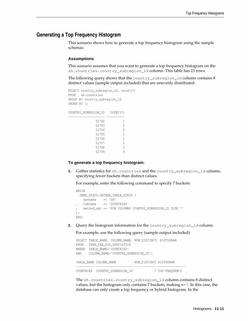
Generating a Top Frequency HistogramThis scenario shows how to generate a top frequency histogram using the sampleschemas.
Assumptions
This scenario assumes that you want to generate a top frequency histogram on thesh.countries.country_subregion_id column. This table has 23 rows.
The following query shows that the country_subregion_id column contains 8distinct values (sample output included) that are unevenly distributed:
SELECT country_subregion_id, count(*)FROM sh.countriesGROUP BY country_subregion_idORDER BY 1; COUNTRY_SUBREGION_ID COUNT(*)-------------------- ---------- 52792 1 52793 5 52794 2 52795 1 52796 1 52797 2 52798 2 52799 9
To generate a top frequency histogram:
1. Gather statistics for sh.countries and the country_subregion_id column,specifying fewer buckets than distinct values.
For example, enter the following command to specify 7 buckets:
BEGIN DBMS_STATS.GATHER_TABLE_STATS ( ownname => 'SH', tabname => 'COUNTRIES', method_opt => 'FOR COLUMNS COUNTRY_SUBREGION_ID SIZE 7');END;
2. Query the histogram information for the country_subregion_id column.
For example, use the following query (sample output included):
SELECT TABLE_NAME, COLUMN_NAME, NUM_DISTINCT, HISTOGRAMFROM USER_TAB_COL_STATISTICSWHERE TABLE_NAME='COUNTRIES'AND COLUMN_NAME='COUNTRY_SUBREGION_ID'; TABLE_NAME COLUMN_NAME NUM_DISTINCT HISTOGRAM---------- -------------------- ------------ ---------------COUNTRIES COUNTRY_SUBREGION_ID 7 TOP-FREQUENCY
The sh.countries.country_subregion_id column contains 8 distinctvalues, but the histogram only contains 7 buckets, making n=7. In this case, thedatabase can only create a top frequency or hybrid histogram. In the
Top Frequency Histograms
Histograms 11-11

country_subregion_id column, the top 7 most frequent values occupy 95.6%of the rows, which exceeds the threshold of 85.7%, generating a top frequencyhistogram (see “Criteria For Frequency Histograms”).
3. Query the endpoint number and endpoint value for the column.
For example, use the following query (sample output included):
SELECT ENDPOINT_NUMBER, ENDPOINT_VALUEFROM USER_HISTOGRAMSWHERE TABLE_NAME='COUNTRIES'AND COLUMN_NAME='COUNTRY_SUBREGION_ID'; ENDPOINT_NUMBER ENDPOINT_VALUE--------------- -------------- 1 52792 6 52793 8 52794 9 52796 11 52797 13 52798 22 52799
Figure 11-3 is a graphical illustration of the 7 buckets in the top frequencyhistogram. The values are represented in the diagram as coins.
Top Frequency Histograms
11-12 SQL Tuning Guide

Figure 11-3 Top Frequency Histogram
52797
5279752797
Endpoint Value
EndpointNumber: 11
52796
52796
Endpoint Value
EndpointNumber: 9
52794
5279452794
Endpoint Value
EndpointNumber: 8
52793
52793 5279352793
5279352793
Endpoint Value
EndpointNumber: 6
52792
52792
Endpoint Value
EndpointNumber: 1
52799
52799 5279952799
52799 5279952799
5279952799
52799
Endpoint Value
EndpointNumber: 22
52798
5279852798
Endpoint Value
EndpointNumber: 13
As shown in Figure 11-3, each distinct value has its own bucket except for 52795,which is excluded from the histogram because it is nonpopular and statisticallyinsignificant. As in a standard frequency histogram, the endpoint numberrepresents the cumulative frequency of values.
Top Frequency Histograms
Histograms 11-13

See Also:
• Oracle Database PL/SQL Packages and Types Reference to learn about theDBMS_STATS.GATHER_TABLE_STATS procedure
• Oracle Database Reference to learn about the USER_TAB_COL_STATISTICSview
• Oracle Database Reference to learn about the USER_HISTOGRAMS view
Height-Balanced Histograms (Legacy)In a legacy height-balanced histogram, column values are divided into buckets so thateach bucket contains approximately the same number of rows. For example, if youhave 99 coins to distribute among 4 buckets, each bucket contains about 25 coins. Thehistogram shows where the endpoints fall in the range of values.
This section contains the following topics:
• Criteria for Height-Balanced Histograms
• Generating a Height-Balanced Histogram
Criteria for Height-Balanced HistogramsBefore Oracle Database 12c, the database created a height-balanced histogram whenthe NDV was greater than n. This type of histogram was useful for range predicates,and equality predicates on values that appear as endpoints in at least two buckets.
As shown in the logic diagram in “How Oracle Database Chooses the HistogramType”, the database creates a height-balanced histogram when the following criteriaare met:
• NDV is greater than n, where n is the number of histogram buckets (default 254).
• The estimate_percent parameter in the DBMS_STATS statistics gatheringprocedure is not set to AUTO_SAMPLE_SIZE.
Note:
If you upgrade Oracle Database 11g to Oracle Database 12c, then any height-based histograms created before the upgrade remain in use. If Oracle Database12c creates new histograms, and if the sampling percentage isAUTO_SAMPLE_SIZE, then the histograms are either top frequency or hybrid,but not height-balanced.
Generating a Height-Balanced HistogramThis scenario shows how to generate a height-balanced histogram using the sampleschemas.
Assumptions
This scenario assumes that you want to generate a height-balanced histogram on thesh.countries.country_subregion_id column. This table has 23 rows.
Height-Balanced Histograms (Legacy)
11-14 SQL Tuning Guide

The following query shows that the country_subregion_id column contains 8distinct values (sample output included) that are unevenly distributed:
SELECT country_subregion_id, count(*)FROM sh.countriesGROUP BY country_subregion_idORDER BY 1; COUNTRY_SUBREGION_ID COUNT(*)-------------------- ---------- 52792 1 52793 5 52794 2 52795 1 52796 1 52797 2 52798 2 52799 9
To generate a height-balanced histogram:
1. Gather statistics for sh.countries and the country_subregion_id column,specifying fewer buckets than distinct values.
Note:
To simulate Oracle Database 11g behavior, which is necessary to create aheight-based histogram, set estimate_percent to a nondefault value. Ifyou specify a nondefault percentage, then the database creates frequency orheight-balanced histograms.
For example, enter the following command:
BEGIN DBMS_STATS.GATHER_TABLE_STATS ( ownname => 'SH', tabname => 'COUNTRIES', method_opt => 'FOR COLUMNS COUNTRY_SUBREGION_ID SIZE 7', estimate_percent => 100 );END;
2. Query the histogram information for the country_subregion_id column.
For example, use the following query (sample output included):
SELECT TABLE_NAME, COLUMN_NAME, NUM_DISTINCT, HISTOGRAMFROM USER_TAB_COL_STATISTICSWHERE TABLE_NAME='COUNTRIES'AND COLUMN_NAME='COUNTRY_SUBREGION_ID'; TABLE_NAME COLUMN_NAME NUM_DISTINCT HISTOGRAM---------- -------------------- ------------ ---------------COUNTRIES COUNTRY_SUBREGION_ID 8 HEIGHT BALANCED
The optimizer chooses a height-balanced histogram because the number ofdistinct values (8) is greater than the number of buckets (7), and theestimate_percent value is nondefault.
3. Query the number of rows occupied by each distinct value.
Height-Balanced Histograms (Legacy)
Histograms 11-15

For example, use the following query (sample output included):
SELECT COUNT(country_subregion_id) AS NUM_OF_ROWS, country_subregion_id FROM countries GROUP BY country_subregion_id ORDER BY 2; NUM_OF_ROWS COUNTRY_SUBREGION_ID----------- -------------------- 1 52792 5 52793 2 52794 1 52795 1 52796 2 52797 2 52798 9 52799
4. Query the endpoint number and endpoint value for thecountry_subregion_id column.
For example, use the following query (sample output included):
SELECT ENDPOINT_NUMBER, ENDPOINT_VALUEFROM USER_HISTOGRAMSWHERE TABLE_NAME='COUNTRIES'AND COLUMN_NAME='COUNTRY_SUBREGION_ID'; ENDPOINT_NUMBER ENDPOINT_VALUE--------------- -------------- 0 52792 2 52793 3 52795 4 52798 7 52799
Figure 11-4 is a graphical illustration of the height-balanced histogram. The valuesare represented in the diagram as coins.
Height-Balanced Histograms (Legacy)
11-16 SQL Tuning Guide

Figure 11-4 Height-Balanced Histogram
52795
5279552794
52794
Endpoint Value
EndpointNumber: 3
52793
52793 5279352793
5279352793
Endpoint Value
EndpointNumber: 2
52792
52792
Endpoint Value
EndpointNumber: 0
52799
52799 5279952799
52799 5279952799
5279952799
52799
Endpoint Value
EndpointNumber: 7
52798
5279852798
5279752797
Endpoint Value
EndpointNumber: 4
The bucket number is identical to the endpoint number. The optimizer records thevalue of the last row in each bucket as the endpoint value, and then checks toensure that the minimum value is the endpoint value of the first bucket, and themaximum value is the endpoint value of the last bucket. In this example, theoptimizer adds bucket 0 so that the minimum value 52792 is the endpoint of abucket.
The optimizer must evenly distribute 23 rows into the 7 specified histogrambuckets, so each bucket contains approximately 3 rows. However, the optimizercompresses buckets with the same endpoint. So, instead of bucket 1 containing 2instances of value 52793, and bucket 2 containing 3 instances of value 52793, theoptimizer puts all 5 instances of value 52793 into bucket 2. Similarly, instead ofhaving buckets 5, 6, and 7 contain 3 values each, with the endpoint of each bucketas 52799, the optimizer puts all 9 instances of value 52799 into bucket 7.
In this example, buckets 3 and 4 contain nonpopular values because thedifference between the current endpoint number and previous endpoint numberis 1. The optimizer calculates cardinality for these values based on density. Theremaining buckets contain popular values. The optimizer calculates cardinality forthese values based on endpoint numbers.
Height-Balanced Histograms (Legacy)
Histograms 11-17

See Also:
• Oracle Database PL/SQL Packages and Types Reference to learn about theDBMS_STATS.GATHER_TABLE_STATS procedure
• Oracle Database Reference to learn about the USER_TAB_COL_STATISTICSview
• Oracle Database Reference to learn about the USER_HISTOGRAMS view
Hybrid HistogramsA hybrid histogram combines characteristics of both height-based histograms andfrequency histograms. This "best of both worlds" approach enables the optimizer toobtain better selectivity estimates in some situations.
The height-based histogram sometimes produces inaccurate estimates for values thatare almost popular. For example, a value that occurs as an endpoint value of only onebucket but almost occupies two buckets is not considered popular.
To solve this problem, a hybrid histogram distributes values so that no value occupiesmore than one bucket, and then stores the endpoint repeat count value, which is thenumber of times the endpoint value is repeated, for each endpoint (bucket) in thehistogram. By using the repeat count, the optimizer can obtain accurate estimates foralmost popular values.
This section contains the following topics:
• How Endpoint Repeat Counts Work
• Criteria for Hybrid Histograms
• Generating a Hybrid Histogram
How Endpoint Repeat Counts WorkTo illustrate the utility of endpoint repeat counts, assume that a column coinscontains the following values, sorted from low to high:
1 1 1 5 5 5 10 10 25 25 25 25 50 100 100
You gather statistics for this table, setting the method_opt argument ofDBMS_STATS.GATHER_TABLE_STATS to FOR ALL COLUMNS SIZE 3. In this case,the optimizer initially groups the values in coins into three buckets, as follows:
Hybrid Histograms
11-18 SQL Tuning Guide

1 1 1
5 5
5
Endpoint Value
Bucket 1
5 10 10
25 25
25
Endpoint Value
Bucket 2
25 25 50
100 100
100
Endpoint Value
Bucket 3
If a bucket border splits a value so that some occurrences of the value are in onebucket and some in another, then the optimizer shifts the bucket border (and all otherfollowing bucket borders) forward to include all occurrences of the value. Forexample, the optimizer shifts value 5 so that it is now wholly in the first bucket, andthe value 25 is now wholly in the second bucket:
1 1 1
5 5
5
5
Endpoint Value
Bucket 1
25 25
25 25
10 10
25
Endpoint Value
Bucket 2
50
100 100
100
Endpoint Value
Bucket 3
The endpoint repeat count measures the number of times that the correspondingbucket endpoint, which is the value at the right bucket border, repeats itself. Forexample, in the first bucket, the value 5 is repeated 3 times, so the endpoint repeatcount is 3:
Hybrid Histograms
Histograms 11-19

1 1 1
5 5
5
5
Endpoint Value
Bucket 1
Repeat Count: 3
25 25
25 25
10 10
25
Endpoint Value
Bucket 2
Repeat Count: 4
50
100 100
100
Endpoint Value
Bucket 3
Repeat Count: 2
Height-balanced histograms do not store as much information as hybrid histograms.By using repeat counts, the optimizer can determine exactly how many occurrences ofan endpoint value exist. For example, the optimizer knows that the value 5 appears 3times, the value 25 appears 4 times, and the value 100 appears 2 times. This frequencyinformation helps the optimizer to generate better cardinality estimates.
Criteria for Hybrid HistogramsThe only differentiating criterion for hybrid histograms as compared to top frequencyhistograms is that the top n frequent values is less than internal threshold p.
As shown in the logic diagram in “How Oracle Database Chooses the HistogramType”, the database creates a hybrid histogram when the following criteria are met:
• NDV is greater than n, where n is the number of histogram buckets (default is 254).
• The criteria for top frequency histograms do not apply.
This is another way to stating that the percentage of rows occupied by the top nfrequent values is less than threshold p, where p is (1-(1/n))*100. See “CriteriaFor Top Frequency Histograms.”
• The estimate_percent parameter in the DBMS_STATS statistics gatheringprocedure is set to AUTO_SAMPLE_SIZE.
If users specify their own percentage, then the database creates frequency orheight-balanced histograms.
See Also:
“Height-Balanced Histograms (Legacy)”
Generating a Hybrid HistogramThis scenario shows how to generate a hybrid histogram using the sample schemas.
Hybrid Histograms
11-20 SQL Tuning Guide

Assumptions
This scenario assumes that you want to generate a hybrid histogram on thesh.products.prod_subcategory_id column. This table has 72 rows. Theprod_subcategory_id column contains 22 distinct values.
To generate a hybrid histogram:
1. Gather statistics for sh.products and the prod_subcategory_id column,specifying 10 buckets.
For example, enter the following command:
BEGIN DBMS_STATS.GATHER_TABLE_STATS ( ownname => 'SH', tabname => 'PRODUCTS', method_opt => 'FOR COLUMNS PROD_SUBCATEGORY_ID SIZE 10');END;
2. Query the number of rows occupied by each distinct value.
For example, use the following query (sample output included):
SELECT COUNT(prod_subcategory_id) AS NUM_OF_ROWS, prod_subcategory_idFROM productsGROUP BY prod_subcategory_idORDER BY 1 DESC; NUM_OF_ROWS PROD_SUBCATEGORY_ID----------- ------------------- 8 2014 7 2055 6 2032 6 2054 5 2056 5 2031 5 2042 5 2051 4 2036 3 2043 2 2033 2 2034 2 2013 2 2012 2 2053 2 2035 1 2022 1 2041 1 2044 1 2011 1 2021 1 2052 22 rows selected.
The column contains 22 distinct values. Because the number of buckets (10) is lessthan 22, the optimizer cannot create a frequency histogram. The optimizerconsiders both hybrid and top frequency histograms. To qualify for a topfrequency histogram, the percentage of rows occupied by the top 10 most frequentvalues must be equal to or greater than threshold p, where p is (1-(1/10))*100, or
Hybrid Histograms
Histograms 11-21
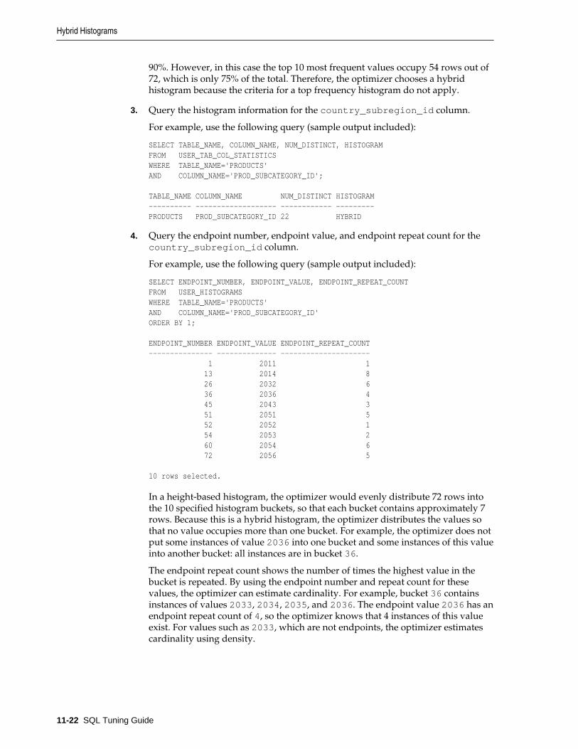
90%. However, in this case the top 10 most frequent values occupy 54 rows out of72, which is only 75% of the total. Therefore, the optimizer chooses a hybridhistogram because the criteria for a top frequency histogram do not apply.
3. Query the histogram information for the country_subregion_id column.
For example, use the following query (sample output included):
SELECT TABLE_NAME, COLUMN_NAME, NUM_DISTINCT, HISTOGRAMFROM USER_TAB_COL_STATISTICSWHERE TABLE_NAME='PRODUCTS'AND COLUMN_NAME='PROD_SUBCATEGORY_ID';
TABLE_NAME COLUMN_NAME NUM_DISTINCT HISTOGRAM---------- ------------------- ------------ ---------PRODUCTS PROD_SUBCATEGORY_ID 22 HYBRID
4. Query the endpoint number, endpoint value, and endpoint repeat count for thecountry_subregion_id column.
For example, use the following query (sample output included):
SELECT ENDPOINT_NUMBER, ENDPOINT_VALUE, ENDPOINT_REPEAT_COUNTFROM USER_HISTOGRAMSWHERE TABLE_NAME='PRODUCTS'AND COLUMN_NAME='PROD_SUBCATEGORY_ID'ORDER BY 1; ENDPOINT_NUMBER ENDPOINT_VALUE ENDPOINT_REPEAT_COUNT--------------- -------------- --------------------- 1 2011 1 13 2014 8 26 2032 6 36 2036 4 45 2043 3 51 2051 5 52 2052 1 54 2053 2 60 2054 6 72 2056 5 10 rows selected.
In a height-based histogram, the optimizer would evenly distribute 72 rows intothe 10 specified histogram buckets, so that each bucket contains approximately 7rows. Because this is a hybrid histogram, the optimizer distributes the values sothat no value occupies more than one bucket. For example, the optimizer does notput some instances of value 2036 into one bucket and some instances of this valueinto another bucket: all instances are in bucket 36.
The endpoint repeat count shows the number of times the highest value in thebucket is repeated. By using the endpoint number and repeat count for thesevalues, the optimizer can estimate cardinality. For example, bucket 36 containsinstances of values 2033, 2034, 2035, and 2036. The endpoint value 2036 has anendpoint repeat count of 4, so the optimizer knows that 4 instances of this valueexist. For values such as 2033, which are not endpoints, the optimizer estimatescardinality using density.
Hybrid Histograms
11-22 SQL Tuning Guide

See Also:
• Oracle Database PL/SQL Packages and Types Reference to learn about theDBMS_STATS.GATHER_TABLE_STATS procedure
• Oracle Database Reference to learn about the USER_TAB_COL_STATISTICSview
• Oracle Database Reference to learn about the USER_HISTOGRAMS view
Hybrid Histograms
Histograms 11-23

Hybrid Histograms
11-24 SQL Tuning Guide

12Managing Optimizer Statistics: Basic
Topics
This chapter explains basic tasks relating to optimizer statistics management.
This chapter contains the following topics:
• Setting Optimizer Statistics Preferences
• Configuring Automatic Optimizer Statistics Collection
• Gathering Optimizer Statistics Manually
• Gathering System Statistics Manually
See Also:
• “Managing Optimizer Statistics: Advanced Topics ” for advanced conceptsand tasks relating to optimizer statistics
• “Optimizer Statistics Concepts ”
• “Query Optimizer Concepts ”
About Optimizer Statistics CollectionIn Oracle Database, optimizer statistics collection is the gathering of optimizerstatistics for database objects, including fixed objects. The database can collectoptimizer statistics automatically. You can also collect them manually using theDBMS_STATS package.
See Also:
“Gathering Optimizer Statistics Manually”
Purpose of Optimizer Statistics CollectionThe contents of tables and associated indexes change frequently, which can lead theoptimizer to choose suboptimal execution plan for queries. Thus, statistics must bekept current to avoid any potential performance issues because of suboptimal plans.
To minimize DBA involvement, Oracle Database automatically gathers optimizerstatistics at various times. Some automatic options are configurable, such enablingAutoTask to run DBMS_STATS.
Managing Optimizer Statistics: Basic Topics 12-1

User Interfaces for Optimizer Statistics ManagementYou can manage optimizer statistics either through Oracle Enterprise Manager CloudControl (Cloud Control) or using PL/SQL on the command line.
Graphical Interface for Optimizer Statistics Management
The Manage Optimizer Statistics page in Cloud Control is a GUI that enables you tomanage optimizer statistics.
Accessing the Database Home Page in Cloud Control
Oracle Enterprise Manager Cloud Control enables you to manage multiple databaseswithin a single GUI-based framework.
To access a database home page using Cloud Control:
1. Log in to Cloud Control with the appropriate credentials.
2. Under the Targets menu, select Databases.
3. In the list of database targets, select the target for the Oracle Database instancethat you want to administer.
4. If prompted for database credentials, then enter the minimum credentialsnecessary for the tasks you intend to perform.
See Also:
Oracle Enterprise Manager Cloud Control Introduction for an overview of CloudControl
Accessing the Manage Optimizer Statistics Page
You can perform most necessary tasks relating to optimizer statistics through pageslinked to by the Manage Optimizer Statistics page.
To manage optimizer statistics using Cloud Control:
1. Access the Database Home page.
2. From the Performance menu, select SQL, then Optimizer Statistics.
The Manage Optimizer Statistics appears.
About Optimizer Statistics Collection
12-2 SQL Tuning Guide

See Also:
Online Help for Oracle Enterprise Manager Cloud Control
Command-Line Interface for Optimizer Statistics Management
The DBMS_STATS package performs most optimizer statistics tasks. To enable anddisable automatic statistics gathering, use the DBMS_AUTO_TASK_ADMIN PL/SQLpackage.
See Also:
Oracle Database PL/SQL Packages and Types Reference to learn how to useDBMS_STATS and DBMS_AUTO_TASK_ADMIN
Configuring Automatic Optimizer Statistics CollectionThis topic explains how to configure Oracle Database to gather optimizer statisticsautomatically.
This section contains the following topics:
• About Automatic Optimizer Statistics Collection
• Configuring Automatic Optimizer Statistics Collection Using Cloud Control
• Configuring Automatic Optimizer Statistics Collection from the Command Line
About Automatic Optimizer Statistics CollectionThe automated maintenance tasks infrastructure (known as AutoTask) schedules tasksto run automatically in Oracle Scheduler windows known as maintenance windows.
By default, one window is scheduled for each day of the week. Automatic optimizerstatistics collection runs as part of AutoTask. By default, the collection runs in allpredefined maintenance windows.
Configuring Automatic Optimizer Statistics Collection
Managing Optimizer Statistics: Basic Topics 12-3

Note:
Data visibility and privilege requirements may differ when using automaticoptimizer statistics collection with pluggable databases. See Oracle DatabaseAdministrator’s Guide for a table that summarizes how manageability featureswork in a container database (CDB).
To collect the optimizer statistics, the database calls an internal procedure thatoperates similarly to the GATHER_DATABASE_STATS procedure with the GATHERAUTO option. Automatic statistics collection honors all preferences set in the database.
The principal difference between manual and automatic collection is that the latterprioritizes database objects that need statistics. Before the maintenance window closes,automatic collection assesses all objects and prioritizes objects that have no statistics orvery old statistics.
Note:
When gathering statistics manually, you can reproduce the objectprioritization of automatic collection by using theDBMS_AUTO_TASK_IMMEDIATE package. This package runs the samestatistics gathering job that is executed during the automatic nightly statisticsgathering job.
Configuring Automatic Optimizer Statistics Collection Using Cloud ControlYou can enable and disable all automatic maintenance tasks, including automaticoptimizer statistics collection, using Cloud Control.
The default window timing works well for most situations. However, you may haveoperations such as bulk loads that occur during the window. In such cases, to avoidpotential conflicts that result from operations occurring at the same time as automaticstatistics collection, Oracle recommends that you change the window accordingly.
To control automatic optimizer statistics collection using Cloud Control:
1. Access the Database Home page, as described in “Accessing the Database HomePage in Cloud Control.”
2. From the Administration menu, select Oracle Scheduler, then AutomatedMaintenance Tasks.
The Automated Maintenance Tasks page appears.
This page shows the predefined tasks. To retrieve information about each task,click the corresponding link for the task.
3. Click Configure.
The Automated Maintenance Tasks Configuration page appears.
Configuring Automatic Optimizer Statistics Collection
12-4 SQL Tuning Guide

By default, automatic optimizer statistics collection executes in all predefinedmaintenance windows in MAINTENANCE_WINDOW_GROUP.
4. Perform the following steps:
a. In the Task Settings section for Optimizer Statistics Gathering, select eitherEnabled or Disabled to enable or disable an automated task.
Note:
Oracle strongly recommends that you not disable automatic statisticsgathering because it is critical for the optimizer to generate optimal plans forqueries against dictionary and user objects. If you disable automatic collection,ensure that you have a good manual statistics collection strategy for dictionaryand user schemas.
b. To disable statistics gathering for specific days in the week, check theappropriate box next to the window name.
c. To change the characteristics of a window group, click Edit Window Group.
d. To change the times for a window, click the name of the window (forexample, Monday Window), and then in the Schedule section, click Edit.
The Edit Window page appears.
Configuring Automatic Optimizer Statistics Collection
Managing Optimizer Statistics: Basic Topics 12-5

In this page, you can change the parameters such as duration and start timefor window execution.
e. Click Apply.
See Also:
Online Help for Oracle Enterprise Manager Cloud Control
Configuring Automatic Optimizer Statistics Collection from the Command LineIf you do not use Cloud Control to enable and disable automatic optimizer statisticscollection, then you have the following options:
• Run the ENABLE or DISABLE procedure in the DBMS_AUTO_TASK_ADMIN PL/SQLpackage.
This package is the recommended command-line technique. For both the ENABLEor DISABLE procedures, you can specify a particular maintenance window withthe window_name parameter. See Oracle Database PL/SQL Packages and TypesReference for complete reference information.
• Set the STATISTICS_LEVEL initialization level to BASIC to disable collection of alladvisories and statistics, including Automatic SQL Tuning Advisor.
Note:
Because monitoring and many automatic features are disabled, Oraclestrongly recommends that you do not set STATISTICS_LEVEL to BASIC.
Configuring Automatic Optimizer Statistics Collection
12-6 SQL Tuning Guide

To control automatic statistics collection using DBMS_AUTO_TASK_ADMIN:
1. Connect SQL*Plus to the database with administrator privileges, and then do oneof the following:
• To enable the automated task, execute the following PL/SQL block:
BEGIN DBMS_AUTO_TASK_ADMIN.ENABLE ( client_name => 'auto optimizer stats collection', operation => NULL, window_name => NULL );END;/
• To disable the automated task, execute the following PL/SQL block:
BEGIN DBMS_AUTO_TASK_ADMIN.DISABLE ( client_name => 'auto optimizer stats collection', operation => NULL, window_name => NULL );END;/
2. Query the data dictionary to confirm the change.
For example, query DBA_AUTOTASK_CLIENT as follows:
COL CLIENT_NAME FORMAT a31
SELECT CLIENT_NAME, STATUSFROM DBA_AUTOTASK_CLIENTWHERE CLIENT_NAME = 'auto optimizer stats collection';
Sample output appears as follows:
CLIENT_NAME STATUS------------------------------- --------auto optimizer stats collection ENABLED
To change the window attributes for automatic statistics collection:
1. Connect SQL*Plus to the database with administrator privileges.
2. Change the attributes of the maintenance window as needed.
For example, to change the Monday maintenance window so that it starts at 5a.m., execute the following PL/SQL program:
BEGIN DBMS_SCHEDULER.SET_ATTRIBUTE ( 'MONDAY_WINDOW', 'repeat_interval', 'freq=daily;byday=MON;byhour=05;byminute=0;bysecond=0');END;/
Configuring Automatic Optimizer Statistics Collection
Managing Optimizer Statistics: Basic Topics 12-7

See Also:
• Oracle Database PL/SQL Packages and Types Reference to learn about theDBMS_AUTO_TASK_ADMIN package
• Oracle Database Reference to learn about the STATISTICS_LEVELinitialization parameter
Setting Optimizer Statistics PreferencesThis topic explains how to set optimizer statistics defaults usingDBMS_STATS.SET_*_PREFS procedures.
This section contains the following topics:
• About Optimizer Statistics Preferences
• Setting Global Optimizer Statistics Preferences Using Cloud Control
• Setting Object-Level Optimizer Statistics Preferences Using Cloud Control
• Setting Optimizer Statistics Preferences from the Command Line
About Optimizer Statistics PreferencesThe optimizer statistics preferences set the default values of the parameters used byautomatic statistics collection and the DBMS_STATS statistics gathering procedures.
You can set optimizer statistics preferences at the table, schema, database (all tables),and global (tables with no preferences and any tables created in the future) levels. Theprocedure names follow the form SET_*_PREFS.
See Also:
“Maintaining Incremental Statistics for Partition Maintenance Operations”
DBMS_STATS Procedures for Setting Statistics PreferencesThe DBMS_STATS.SET_*_PREFS procedures change the defaults of parameters usedby the DBMS_STATS.GATHER_*_STATS procedures. To query the currentpreferences, use the DBMS_STATS.GET_PREFS function.
When setting statistics preferences, the order of precedence is:
1. Table preference (set for a specific table, all tables in a schema, or all tables in thedatabase)
2. Global preference
3. Default preference
The following table summarizes the relevant DBMS_STATS procedures.
Table 12-1 DBMS_STATS Procedures for Setting Optimizer Statistics Preferences
Setting Optimizer Statistics Preferences
12-8 SQL Tuning Guide

Table 12-1 (Cont.) DBMS_STATS Procedures for Setting Optimizer StatisticsPreferences
Procedure Scope
SET_TABLE_PREFS Specified table only.
SET_SCHEMA_PREFS All existing tables in the specified schema.
This procedure calls SET_TABLE_PREFS for each table in thespecified schema. Calling SET_SCHEMA_PREFS does not affectany new tables created after it has been run. New tables use theGLOBAL_PREF values for all parameters.
SET_DATABASE_PREFS All user-defined schemas in the database. You can includesystem-owned schemas such as SYS and SYSTEM by setting theADD_SYS parameter to true.
This procedure calls SET_TABLE_PREFS for each table in thespecified schema. Calling SET_DATABASE_PREFS does notaffect any new objects created after it has been run. Newobjects use the GLOBAL_PREF values for all parameters.
SET_GLOBAL_PREFS Any table in the database that does not have an existing tablepreference.
All parameters default to the global setting unless a tablepreference is set or the parameter is explicitly set in theDBMS_STATS.GATHER_*_STATS command. Changes madeby this procedure affect any new objects created after it runs.New objects use the SET_GLOBAL_PREF values for allparameters.
With SET_GLOBAL_PREFS, you can set a default value for theparameter AUTOSTAT_TARGET. This additional parametercontrols which objects the automatic statistic gathering jobrunning in the nightly maintenance window looks after.Possible values for this parameter are ALL, ORACLE, and AUTO(default).
You can only set the CONCURRENT preference at the globallevel). You cannot set the preference INCREMENTAL_LEVELusing SET_GLOBAL_PREFS.
See Also:
• “About Concurrent Statistics Gathering”
• Oracle Database PL/SQL Packages and Types Reference to learn about theDBMS_STATS procedures for setting optimizer statistics
Setting Statistics Preferences: Example
Table 12-2 illustrates the relationship between SET_TABLE_PREFS,SET_SCHEMA_STATS, and SET_DATABASE_PREFS.
Table 12-2 Changing Preferences for Statistics Gathering Procedures
Setting Optimizer Statistics Preferences
Managing Optimizer Statistics: Basic Topics 12-9

Table 12-2 (Cont.) Changing Preferences for Statistics Gathering Procedures
Action Description
SQL> SELECT DBMS_STATS.GET_PREFS ('incremental', 'sh','costs') AS "STAT_PREFS" FROM DUAL; STAT_PREFS----------TRUE
You query the INCREMENTALpreference for costs and determinethat it is set to true.
SQL> EXEC DBMS_STATS.SET_TABLE_PREFS ('sh', 'costs', 'incremental', 'false'); PL/SQL procedure successfully completed.
You use SET_TABLE_PREFS to set theINCREMENTAL preference to false forthe costs table only.
SQL> SELECT DBMS_STATS.GET_PREFS ('incremental', 'sh', 'costs') AS "STAT_PREFS" FROM DUAL;
STAT_PREFS ----------FALSE
You query the INCREMENTALpreference for costs and confirm that itis set to false.
SQL> EXEC DBMS_STATS.SET_SCHEMA_PREFS ('sh', 'incremental', 'true');
PL/SQL procedure successfully completed.
You use SET_SCHEMA_PREFS to set theINCREMENTAL preference to true forevery table in the sh schema, includingcosts.
SQL> SELECT DBMS_STATS.GET_PREFS ('incremental', 'sh', 'costs') AS "STAT_PREFS" FROM DUAL; STAT_PREFS----------TRUE
You query the INCREMENTALpreference for costs and confirm that itis set to true.
SQL> EXEC DBMS_STATS.SET_DATABASE_PREFS ('incremental', 'false');
PL/SQL procedure successfully completed.
You use SET_DATABASE_PREFS to setthe INCREMENTAL preference for alltables in all user-defined schemas tofalse.
SQL> SELECT DBMS_STATS.GET_PREFS ('incremental', 'sh', 'costs') AS "STAT_PREFS" FROM DUAL;
STAT_PREFS----------FALSE
You query the INCREMENTALpreference for costs and confirm that itis set to false.
Setting Optimizer Statistics Preferences
12-10 SQL Tuning Guide
Setting Global Optimizer Statistics Preferences Using Cloud ControlA global preference applies to any object in the database that does not have an existingtable preference. You can set optimizer statistics preferences at the global level usingCloud Control. See the Cloud Control Help for an explanation of the options on thepreference page.
To set global optimizer statistics preferences using Cloud Control:
1. Go to the Manage Optimizer Statistics page, as explained in “Accessing theManage Optimizer Statistics Page”.
2. Click Global Statistics Gathering Options.
The Global Statistics Gathering Options page appears.
3. Make your desired changes, and click Apply.
See Also:
Online Help for Oracle Enterprise Manager Cloud Control
Setting Object-Level Optimizer Statistics Preferences Using Cloud ControlYou can set optimizer statistics preferences at the database, schema, and table levelusing Cloud Control.
To set object-level optimizer statistics preferences using Cloud Control:
1. Go to the Manage Optimizer Statistics page, as explained in “Accessing theManage Optimizer Statistics Page”.
2. Click Object Level Statistics Gathering Preferences.
The Object Level Statistics Gathering Preferences page appears.
3. To modify table preferences for a table that has preferences set at the table level,do the following (otherwise, skip to the next step):
a. Enter values in Schema and Table. Leave Table blank to see all tables in theschema.
The page refreshes with the table names.
b. Select the desired tables and click Edit Preferences.
The General subpage of the Edit Preferences page appears.
c. Change preferences as needed and click Apply.
4. To set preferences for a table that does not have preferences set at the table level,do the following (otherwise, skip to the next step):
a. Click Add Table Preferences.
The General subpage of the Add Table Preferences page appears.
b. In Table Name, enter the schema and table name.
Setting Optimizer Statistics Preferences
Managing Optimizer Statistics: Basic Topics 12-11

c. Change preferences as needed and click OK.
5. To set preferences for a schema, do the following:
a. Click Edit Schema Preferences.
The General subpage of the Edit Schema Preferences page appears.
b. In Schema, enter the schema name.
c. Change preferences as needed and click OK.
See Also:
Online Help for Oracle Enterprise Manager Cloud Control
Setting Optimizer Statistics Preferences from the Command LineIf you do not use Cloud Control to set optimizer statistics preferences, then you caninvoke the DBMS_STATS procedures described in Table 12-1.
Prerequisites
This task has the following prerequisites:
• To set the global or database preferences, you must have SYSDBA privileges, orboth ANALYZE ANY DICTIONARY and ANALYZE ANY system privileges.
• To set schema preferences, you must connect as owner, or have SYSDBA privileges,or have the ANALYZE ANY system privilege.
• To set table preferences, you must connect as owner of the table or have theANALYZE ANY system privilege.
To set optimizer statistics preferences from the command line:
1. Connect SQL*Plus to the database with the necessary privileges.
2. Optionally, call the DBMS_STATS.GET_PREFS procedure to see preferences set atthe object level, or at the global level if a specific table is not set.
For example, obtain the STALE_PERCENT parameter setting for the sh.salestable as follows:
SELECT DBMS_STATS.GET_PREFS('STALE_PERCENT', 'SH', 'SALES') FROM DUAL;
3. Execute the appropriate procedure from Table 12-1, specifying the followingparameters:
• ownname - Set schema name (SET_TAB_PREFS and SET_SCHEMA_PREFSonly)
• tabname - Set table name (SET_TAB_PREFS only)
• pname - Set parameter name
• pvalue - Set parameter value
Setting Optimizer Statistics Preferences
12-12 SQL Tuning Guide

• add_sys - Include system tables (optional, SET_DATABASE_PREFS only)
The following example specifies that 13% of rows in sh.sales must changebefore the statistics on that table are considered stale:
EXEC DBMS_STATS.SET_TABLE_PREFS('SH', 'SALES', 'STALE_PERCENT', '13');
4. Optionally, query the *_TAB_STAT_PREFS view to confirm the change.
For example, query DBA_TAB_STAT_PREFS as follows:
COL OWNER FORMAT a5COL TABLE_NAME FORMAT a15COL PREFERENCE_NAME FORMAT a20COL PREFERENCE_VALUE FORMAT a30SELECT * FROM DBA_TAB_STAT_PREFS;
Sample output appears as follows:
OWNER TABLE_NAME PREFERENCE_NAME PREFERENCE_VALUE----- --------------- -------------------- ------------------------------OE CUSTOMERS NO_INVALIDATE DBMS_STATS.AUTO_INVALIDATESH SALES STALE_PERCENT 13
See Also:
Oracle Database PL/SQL Packages and Types Reference for descriptions of theparameter names and values for program units
Gathering Optimizer Statistics ManuallyAs an alternative or supplement to automatic statistics gathering, you can use theDBMS_STATS package to gather statistics manually.
This section contains the following topics:
• About Manual Statistics Collection with DBMS_STATS
• Guidelines for Gathering Optimizer Statistics Manually
• Determining When Optimizer Statistics Are Stale
• Gathering Schema and Table Statistics
• Gathering Statistics for Fixed Objects
• Gathering Statistics for Volatile Tables Using Dynamic Statistics
• Gathering Optimizer Statistics Concurrently
• Gathering Incremental Statistics on Partitioned Objects
See Also:
• “Controlling Automatic Optimizer Statistics Collection”
• Oracle Database PL/SQL Packages and Types Reference to learn about theDBMS_STATS packages
Gathering Optimizer Statistics Manually
Managing Optimizer Statistics: Basic Topics 12-13

About Manual Statistics Collection with DBMS_STATSUse the DBMS_STATS package to manipulate optimizer statistics. You can gatherstatistics on objects and columns at various levels of granularity: object, schema, anddatabase. You can also gather statistics for the physical system, as explained in“Gathering System Statistics Manually”.
Table 12-3 summarizes the DBMS_STATS procedures for gathering optimizer statistics.This package does not gather statistics for table clusters. However, you can gatherstatistics on individual tables in a table cluster.
Table 12-3 DBMS_STATS Procedures for Gathering Optimizer Statistics
Procedure Purpose
GATHER_INDEX_STATS Collects index statistics
GATHER_TABLE_STATS Collects table, column, and index statistics
GATHER_SCHEMA_STATS Collects statistics for all objects in a schema
GATHER_DICTIONARY_STATS Collects statistics for all system schemas, including SYSand SYSTEM, and other optional schemas, such asCTXSYS and DRSYS
GATHER_DATABASE_STATS Collects statistics for all objects in a database
When the OPTIONS parameter is set to GATHER STALE or GATHER AUTO, theGATHER_SCHEMA_STATS and GATHER_DATABASE_STATS procedures gatherstatistics for any table that has stale statistics and any table that is missing statistics. Ifa monitored table has been modified more than 10%, then the database considers thesestatistics stale and gathers them again.
Note:
As explained in “Controlling Automatic Optimizer Statistics Collection”, youcan configure a nightly job to gather statistics automatically.
See Also:
Oracle Database PL/SQL Packages and Types Reference for complete syntax andsemantics for the DBMS_STATS package
Guidelines for Gathering Optimizer Statistics ManuallyIn most cases, automatic statistics collection is sufficient for database objects modifiedat a moderate speed. However, automatic collection may sometimes be inadequate orunavailable, as in the following cases:
• You perform certain types of bulk load and cannot wait for the maintenancewindow to collect statistics because queries must be executed immediately. See“Online Statistics Gathering for Bulk Loads”.
Gathering Optimizer Statistics Manually
12-14 SQL Tuning Guide

• During a nonrepresentative workload, automatic statistics collection gathersstatistics for fixed tables. See “Gathering Statistics for Fixed Objects”.
• Automatic statistics collection does not gather system statistics. See “GatheringSystem Statistics Manually”.
• Volatile tables are being deleted or truncated, and then rebuilt during the day. See“Gathering Statistics for Volatile Tables Using Dynamic Statistics”.
This section offers guidelines for typical situations in which you may choose to gatherstatistically manually:
• Guideline for Accurate Statistics
• Guideline for Gathering Statistics in Parallel
• Guideline for Partitioned Objects
• Guideline for Frequently Changing Objects
• Guideline for External Tables
Guideline for Accurate StatisticsIn the context of optimizer statistics, sampling is the gathering of statistics from arandom subset of table rows. By enabling the database to avoid full table scans andsorts of entire tables, sampling minimizes the resources necessary to gather statistics.
The database gathers the most accurate statistics when it processes all rows in thetable, which is a 100% sample. However, the larger the sample size, the longer thestatistics gathering operation. The problem is determining a sample size that providesaccurate statistics in a reasonable time.
DBMS_STATS uses sampling when a user specifies the parameterESTIMATE_PERCENT, which controls the percentage of the rows in the table tosample. To maximize performance gains while achieving necessary statisticalaccuracy, Oracle recommends that you set the ESTIMATE_PERCENT parameter toDBMS_STATS.AUTO_SAMPLE_SIZE (the default). This setting enables the use of:
• A hash-based algorithm that is much faster than sampling
This algorithm reads all rows and produces statistics that are nearly as accurate asstatistics from a 100% sample. The statistics computed using this technique aredeterministic.
• Incremental statistics
• Concurrent statistics
• New histogram types (see “Hybrid Histograms”)
Guideline for Gathering Statistics in Parallel
By default, the database gathers statistics with the parallelism degree specified at thetable or index level. You can override this setting with the degree argument to theDBMS_STATS gathering procedures. Oracle recommends setting degree toDBMS_STATS.AUTO_DEGREE. This setting enables the database to choose anappropriate degree of parallelism based on the object size and the settings for theparallelism-related initialization parameters.
Gathering Optimizer Statistics Manually
Managing Optimizer Statistics: Basic Topics 12-15

The database can gather most statistics serially or in parallel. However, the databasedoes not gather some index statistics in parallel, including cluster indexes, domainindexes, and bitmap join indexes. The database can use sampling when gatheringparallel statistics.
Note:
Do not confuse gathering statistics in parallel with gathering statisticsconcurrently. See “About Concurrent Statistics Gathering”.
Guideline for Partitioned Objects
For partitioned tables and indexes, DBMS_STATS can gather separate statistics for eachpartition and global statistics for the entire table or index. Similarly, for compositepartitioning, DBMS_STATS can gather separate statistics for subpartitions, partitions,and the entire table or index.
Use the granularity argument to the DBMS_STATS procedures to determine thetype of partitioning statistics to be gathered. Oracle recommends settinggranularity to the default value of AUTO to gather subpartition, partition, or globalstatistics, depending on partition type. The ALL setting gathers statistics for all types.
See Also:
“Gathering Incremental Statistics on Partitioned Objects”
Guideline for Frequently Changing Objects
When tables are frequently modified, gather statistics often enough so that they do notgo stale, but not so often that collection overhead degrades performance. You mayonly need to gather new statistics every week or month. The best practice is to use ascript or job scheduler to regularly run the DBMS_STATS.GATHER_SCHEMA_STATSand DBMS_STATS.GATHER_DATABASE_STATS procedures.
Guideline for External Tables
Because the database does not permit data manipulation against external tables, thedatabase never marks statistics on external tables as stale. If new statistics are requiredfor an external table, for example, because the underlying data files change, thenregather the statistics. Gather statistics manually for external tables with the sameprocedures that you use for regular tables.
Determining When Optimizer Statistics Are StaleStale statistics on a table do not accurately reflect its data. The database provides atable monitoring facility to help determine when a database object needs newstatistics. Monitoring tracks the approximate number of DML operations on a tableand whether the table has been truncated since the most recent statistics collection.
Run DBMS_STATS.FLUSH_DATABASE_MONITORING_INFO to immediately reflect theoutstanding monitored information stored in memory. After running this procedure,check whether statistics are stale by querying the STALE_STATS column inDBA_TAB_STATISTICS and DBA_IND_STATISTICS. This column is based on data inthe DBA_TAB_MODIFICATIONS view and the STALE_PERCENT preference forDBMS_STATS. The STALE_STATS column has the following possible values:
Gathering Optimizer Statistics Manually
12-16 SQL Tuning Guide

• YES
The statistics are stale.
• NO
The statistics are not stale.
• null
The statistics are not collected.
Executing GATHER_SCHEMA_STATS or GATHER_DATABASE_STATS with the GATHERAUTO option collects statistics only for objects with no statistics or stale statistics.
Assumptions
This tutorial assumes the following:
• Table monitoring is enabled for sh.sales. It is enabled by default when theSTATISTICS_LEVEL initialization parameter is set to TYPICAL or ALL.
• You have the ANALYZE_ANY system privilege so you can run theDBMS_STATS.FLUSH_DATABASE_MONITORING_INFO procedure.
To determine stale statistics:
1. Connect SQL*Plus to the database with the necessary privileges.
2. Optionally, write the database monitoring information from memory to disk.
For example, execute the following procedure:
BEGIN DBMS_STATS.FLUSH_DATABASE_MONITORING_INFO;END;/
3. Query the data dictionary for stale statistics.
The following example queries stale statistics for the sh.sales table (partialoutput included):
COL PARTITION_NAME FORMAT a15
SELECT PARTITION_NAME, STALE_STATSFROM DBA_TAB_STATISTICSWHERE TABLE_NAME = 'SALES'AND OWNER = 'SH'ORDER BY PARTITION_NAME; PARTITION_NAME STA--------------- ---SALES_1995 NOSALES_1996 NOSALES_H1_1997 NOSALES_H2_1997 NOSALES_Q1_1998 NOSALES_Q1_1999 NO...
Gathering Optimizer Statistics Manually
Managing Optimizer Statistics: Basic Topics 12-17

See Also:
• Oracle Database Reference to learn about the DBA_TAB_MODIFICATIONSview
• Oracle Database PL/SQL Packages and Types Reference to learn about theDBMS_STATS.FLUSH_DATABASE_MONITORING_INFO procedure
Gathering Schema and Table StatisticsUse GATHER_TABLE_STATS to collect table statistics, and GATHER_SCHEMA_STATS tocollect statistics for all objects in a schema.
To gather schema statistics using DBMS_STATS:
1. Start SQL*Plus, and connect to the database with the appropriate privileges forthe procedure that you intend to run.
2. Run the GATHER_TABLE_STATS or GATHER_SCHEMA_STATS procedure,specifying the desired parameters.
Typical parameters include:
• Owner - ownname
• Object name - tabname, indname, partname
• Degree of parallelism - degree
See Also:
Oracle Database PL/SQL Packages and Types Reference to learn about theGATHER_TABLE_STATS procedure
Example 12-1 Gathering Statistics for a Table
This example uses the DBMS_STATS package to gather statistics on thesh.customers table with a parallelism setting of 2.
BEGIN DBMS_STATS.GATHER_TABLE_STATS ( ownname => 'sh', tabname => 'customers', degree => 2 );END;/
Gathering Statistics for Fixed ObjectsFixed objects are dynamic performance tables and their indexes. These objects recordcurrent database activity.
Unlike other database tables, the database does not automatically use dynamicstatistics for SQL statement referencing X$ tables when optimizer statistics aremissing. Instead, the optimizer uses predefined default values. These defaults may not
Gathering Optimizer Statistics Manually
12-18 SQL Tuning Guide

be representative and could potentially lead to a suboptimal execution plan. Thus, it isimportant to keep fixed object statistics current.
Oracle Database automatically gathers fixed object statistics as part of automatedstatistics gathering if they have not been previously collected (see “ControllingAutomatic Optimizer Statistics Collection”). You can also manually collect statistics onfixed objects by calling DBMS_STATS.GATHER_FIXED_OBJECTS_STATS. Oraclerecommends that you gather statistics when the database has representative activity.
Prerequisites
You must have the SYSDBA or ANALYZE ANY DICTIONARY system privilege toexecute this procedure.
To gather schema statistics using GATHER_FIXED_OBJECTS_STATS:
1. Start SQL*Plus, and connect to the database with the appropriate privileges forthe procedure that you intend to run.
2. Run the DBMS_STATS.GATHER_FIXED_OBJECTS_STATS procedure, specifyingthe desired parameters.
Typical parameters include:
• Table identifier describing where to save the current statistics - stattab
• Identifier to associate with these statistics within stattab (optional) - statid
• Schema containing stattab (if different from current schema) - statown
See Also:
Oracle Database PL/SQL Packages and Types Reference to learn about theGATHER_TABLE_STATS procedure
Example 12-2 Gathering Statistics for a Table
This example uses the DBMS_STATS package to gather fixed object statistics.
BEGIN DBMS_STATS.GATHER_FIXED_OBJECTS_STATS;END;/
Gathering Statistics for Volatile Tables Using Dynamic StatisticsStatistics for volatile tables, which are tables modified significantly during the day, gostale quickly. For example, a table may be deleted or truncated, and then rebuilt.
When you set the statistics of a volatile object to null, Oracle Database dynamicallygathers the necessary statistics during optimization using dynamic statistics. TheOPTIMIZER_DYNAMIC_SAMPLING initialization parameter controls this feature.
Gathering Optimizer Statistics Manually
Managing Optimizer Statistics: Basic Topics 12-19

Note:
As described in “Locking and Unlocking Optimizer Statistics,” gatheringrepresentative statistics and them locking them is an alternative technique forpreventing statistics for volatile tables from going stale.
Assumptions
This tutorial assumes the following:
• The oe.orders table is extremely volatile.
• You want to delete and then lock the statistics on the orders table to prevent thedatabase from gathering statistics on the table. In this way, the database candynamically gather necessary statistics as part of query optimization.
• The oe user has the necessary privileges to queryDBMS_XPLAN.DISPLAY_CURSOR.
To delete and the lock optimizer statistics:
1. Connect to the database as user oe, and then delete the statistics for the oe table.
For example, execute the following procedure:
BEGIN DBMS_STATS.DELETE_TABLE_STATS('OE','ORDERS');END;/
2. Lock the statistics for the oe table.
For example, execute the following procedure:
BEGIN DBMS_STATS.LOCK_TABLE_STATS('OE','ORDERS');END;/
3. You query the orders table.
For example, use the following statement:
SELECT COUNT(order_id) FROM orders;
4. You query the plan in the cursor.
You run the following commands (partial output included):
SET LINESIZE 150SET PAGESIZE 0
SELECT * FROM TABLE(DBMS_XPLAN.DISPLAY_CURSOR);
SQL_ID aut9632fr3358, child number 0-------------------------------------SELECT COUNT(order_id) FROM orders Plan hash value: 425895392 ---------------------------------------------------------------------| Id | Operation | Name | Rows | Cost (%CPU)| Time |
Gathering Optimizer Statistics Manually
12-20 SQL Tuning Guide

---------------------------------------------------------------------| 0 | SELECT STATEMENT | | | 2 (100)| || 1 | SORT AGGREGATE | | 1 | | || 2 | TABLE ACCESS FULL| ORDERS | 105 | 2 (0)| 00:00:01 |--------------------------------------------------------------------- Note----- - dynamic statistics used for this statement (level=2)
The Note in the preceding execution plan shows that the database used dynamicstatistics for the SELECT statement.
See Also:
“Controlling Dynamic Statistics”
Gathering Optimizer Statistics ConcurrentlyOracle Database enables you to gather statistics on multiple tables or partitionsconcurrently. This section contains the following topics:
• About Concurrent Statistics Gathering
• Enabling Concurrent Statistics Gathering
• Configuring the System for Parallel Execution and Concurrent Statistics Gathering
• Monitoring Statistics Gathering Operations
About Concurrent Statistics GatheringBy default, each partition of a partition table is gathered sequentially. Whenconcurrent statistics gathering mode is enabled, the database can simultaneouslygather optimizer statistics for multiple tables in a schema, or multiple partitions orsubpartitions in a table. Concurrency can reduce the overall time required to gatherstatistics by enabling the database to fully use multiple processors.
Note:
Concurrent statistics gathering mode does not rely on parallel queryprocessing, but is usable with it.
How DBMS_STATS Gathers Statistics Concurrently
Oracle Database employs the following tools and technologies to create and managemultiple statistics gathering jobs concurrently:
• Oracle Scheduler
• Oracle Database Advanced Queuing (AQ)
• Oracle Database Resource Manager (the Resource Manager)
Enable concurrent statistics gathering by setting the CONCURRENT preference withDBMS_STATS.SET_GLOBAL_PREF (see “Enabling Concurrent Statistics Gathering”).
Gathering Optimizer Statistics Manually
Managing Optimizer Statistics: Basic Topics 12-21

The database runs as many concurrent jobs as possible. The Job Scheduler decideshow many jobs to execute concurrently and how many to queue. As running jobscomplete, the scheduler dequeues and runs more jobs until the database has gatheredstatistics on all tables, partitions, and subpartitions. The maximum number of jobs isbounded by the JOB_QUEUE_PROCESSES initialization parameter and availablesystem resources.
In most cases, the DBMS_STATS procedures create a separate job for each tablepartition or subpartition. However, if the partition or subpartition is very small orempty, the database may automatically batch the object with other small objects into asingle job to reduce the overhead of job maintenance.
The following figure illustrates the creation of jobs at different levels, where Table 3 isa partitioned table, and the other tables are nonpartitioned. Job 3 acts as a coordinatorjob for Table 3, and creates a job for each partition in that table, and a separate job forthe global statistics of Table 3. This example assumes that incremental statisticsgathering is disabled; if enabled, then the database derives global statistics frompartition-level statistics after jobs for partitions complete.
Level 2
Job 1
Table 1
Global
Statistics
Job 2
Table 2
Global
Statistics
Job 3
Table 3
Coordinator
Job
Job 4
Table 4
Global
Statistics
Gather Database/Schema/Dictionary Statistics
Job 3.1
Table 3
Partition 1
Job 3.3
Table 3
Global
Statistics
Job 3.2
Table 3
Partition 2
Level 1
See Also:
• Oracle Database PL/SQL Packages and Types Reference to learn about theDBMS_STATS package
• Oracle Database Reference to learn about the JOB_QUEUE_PROCESSESinitialization parameter
Concurrent Statistics Gathering and Resource Management
The DBMS_STATS package does not explicitly manage resources used by concurrentstatistics gathering jobs that are part of a user-initiated statistics gathering call. Thus,the database may use system resources fully during concurrent statistics gathering. Toaddress this situation, use the Resource Manager to cap resources consumed byconcurrent statistics gathering jobs. The Resource Manager must be enabled to gatherstatistics concurrently.
Gathering Optimizer Statistics Manually
12-22 SQL Tuning Guide

The system-supplied consumer group ORA$AUTOTASK registers all statistics gatheringjobs. You can create a resource plan with proper resource allocations for ORA$AUTOTASK to prevent concurrent statistics gathering from consuming all availableresources. If you lack your own resource plan, and if choose not to create one, thenconsider activating the Resource Manager with the system-supplied DEFAULT_PLAN.
Note:
The ORA$AUTOTASK consumer group is shared with the maintenance tasksthat automatically run during the maintenance windows. Thus, whenconcurrency is activated for automatic statistics gathering, the databaseautomatically manages resources, with no extra steps required.
See Also:
Oracle Database Administrator's Guide to learn about the Resource Manager
Enabling Concurrent Statistics Gathering
To enable concurrent statistics gathering, use the DBMS_STATS.SET_GLOBAL_PREFSprocedure to set the CONCURRENT preference. Possible values are as follows:
• MANUAL
Concurrency is enabled only for manual statistics gathering.
• AUTOMATIC
Concurrency is enabled only for automatic statistics gathering.
• ALL
Concurrency is enabled for both manual and automatic statistics gathering.
• OFF
Concurrency is disabled for both manual and automatic statistics gathering. This isthe default value.
This tutorial in this section explains how to enable concurrent statistics gathering.
Prerequisites
This tutorial has the following prerequisites:
• In addition to the standard privileges for gathering statistics, you must have thefollowing privileges:
– CREATE JOB
– MANAGE SCHEDULER
– MANAGE ANY QUEUE
• The SYSAUX tablespace must be online because the scheduler stores its internaltables and views in this tablespace.
• The JOB_QUEUE_PROCESSES initialization parameter must be set to at least 4.
Gathering Optimizer Statistics Manually
Managing Optimizer Statistics: Basic Topics 12-23

• The Resource Manager must be enabled.
By default, the Resource Manager is disabled. If you do not have a resource plan,then consider enabling the Resource Manager with the system-suppliedDEFAULT_PLAN (see Oracle Database Administrator's Guide).
Assumptions
This tutorial assumes that you want to do the following:
• Enable concurrent statistics gathering
• Gather statistics for the sh schema
• Monitor the gathering of the sh statistics
To enable concurrent statistics gathering:
1. Connect SQL*Plus to the database with the appropriate privileges, and thenenable the Resource Manager.
The following example uses the default plan for the Resource Manager:
ALTER SYSTEM SET RESOURCE_MANAGER_PLAN = 'DEFAULT_PLAN';
2. Set the JOB_QUEUE_PROCESSES initialization parameter to at least twice thenumber of CPU cores.
In Oracle Real Application Clusters, the JOB_QUEUE_PROCESSES setting appliesto each node.
Assume that the system has 4 CPU cores. The following example sets theparameter to 8 (twice the number of cores):
ALTER SYSTEM SET JOB_QUEUE_PROCESSES=8;
3. Confirm that the parameter change took effect.
For example, enter the following command in SQL*Plus (sample outputincluded):
SHOW PARAMETER PROCESSES;
NAME TYPE VALUE-------------------------------- ----------- -----_high_priority_processes string VKTMaq_tm_processes integer 1db_writer_processes integer 1gcs_server_processes integer 0global_txn_processes integer 1job_queue_processes integer 8log_archive_max_processes integer 4processes integer 100
4. Enable concurrent statistics.
For example, execute the following PL/SQL anonymous block:
BEGIN DBMS_STATS.SET_GLOBAL_PREFS('CONCURRENT','ALL');END;/
Gathering Optimizer Statistics Manually
12-24 SQL Tuning Guide

5. Confirm that the statistics were enabled.
For example, execute the following query (sample output included):
SELECT DBMS_STATS.GET_PREFS('CONCURRENT') FROM DUAL;
DBMS_STATS.GET_PREFS('CONCURRENT')----------------------------------ALL
6. Gather the statistics for the SH schema.
For example, execute the following procedure:
EXEC DBMS_STATS.GATHER_SCHEMA_STATS('SH');
7. In a separate session, monitor the job progress by queryingDBA_OPTSTAT_OPERATION_TASKS.
For example, execute the following query (sample output included):
SET LINESIZE 1000 COLUMN TARGET FORMAT a8COLUMN TARGET_TYPE FORMAT a25COLUMN JOB_NAME FORMAT a14COLUMN START_TIME FORMAT a40 SELECT TARGET, TARGET_TYPE, JOB_NAME, TO_CHAR(START_TIME, 'dd-mon-yyyy hh24:mi:ss')FROM DBA_OPTSTAT_OPERATION_TASKS WHERE STATUS = 'IN PROGRESS' AND OPID = (SELECT MAX(ID) FROM DBA_OPTSTAT_OPERATIONS WHERE OPERATION = 'gather_schema_stats');
TARGET TARGET_TYPE JOB_NAME TO_CHAR(START_TIME,'--------- ------------------------- -------------- --------------------SH.SALES TABLE (GLOBAL STATS ONLY) ST$T292_1_B29 30-nov-2012 14:22:47SH.SALES TABLE (COORDINATOR JOB) ST$SD290_1_B10 30-nov-2012 14:22:08
8. In the original session, disable concurrent statistics gathering.
For example, execute the following query:
EXEC DBMS_STATS.SET_GLOBAL_PREFS('CONCURRENT','OFF');
See Also:
• “Monitoring Statistics Gathering Operations”
• Oracle Database PL/SQL Packages and Types Reference to learn how to use theDBMS_STATS.SET_GLOBAL_PREFS procedure
Configuring the System for Parallel Execution and Concurrent Statistics GatheringWhen CONCURRENT statistics gathering is enabled, you can execute each statisticsgathering job in parallel. This combination is useful when you are analyzing large
Gathering Optimizer Statistics Manually
Managing Optimizer Statistics: Basic Topics 12-25

tables, partitions, or subpartitions. This topic describes the recommendedconfiguration.
To configure the system for parallel execution and concurrent statisticsgathering:
1. Connect SQL*Plus to the database with the administrator privileges.
2. Disable the parallel adaptive multiuser initialization parameter.
For example, use the following SQL statement:
ALTER SYSTEM SET PARALLEL_ADAPTIVE_MULTI_USER=false;
3. Configure the database to use a resource plan that has parallel queuing enabled.
Perform the following steps:
a. If Oracle Database Resource Manager (the Resource Manager) is notactivated, then activate it. By default, the Resource Manager is activated onlyduring the maintenance windows.
b. Create a temporary resource plan in which the consumer groupOTHER_GROUPS has queuing enabled.
The following sample script illustrates one way to create a temporary resourceplan (pqq_test), and enable the Resource Manager with this plan:
BEGIN DBMS_RESOURCE_MANAGER.CREATE_PENDING_AREA(); DBMS_RESOURCE_MANAGER.CREATE_PLAN('pqq_test', 'pqq_test'); DBMS_RESOURCE_MANAGER.CREATE_PLAN_DIRECTIVE( 'pqq_test', 'OTHER_GROUPS', 'OTHER_GROUPS directive for pqq', parallel_server_limit => 90, max_utilization_limit => 90); DBMS_RESOURCE_MANAGER.SUBMIT_PENDING_AREA();END;/ALTER SYSTEM SET RESOURCE_MANAGER_PLAN = 'pqq_test' SID='*';
See Also:
• Oracle Database Administrator’s Guide to learn how to manage resourceswith the Resource Manager
• Oracle Database Reference to learn about thePARALLEL_ADAPTIVE_MULTI_USER initialization parameter
Monitoring Statistics Gathering Operations
To monitor statistics gathering jobs, use the following views:
• DBA_OPTSTAT_OPERATION_TASKS
This view contains the history of tasks that are performed or currently in progressas part of statistics gathering operations (recorded in
Gathering Optimizer Statistics Manually
12-26 SQL Tuning Guide

DBA_OPTSTAT_OPERATIONS). Each task represents a target object to be processedin the corresponding parent operation.
• DBA_OPTSTAT_OPERATIONS
This view contains a history of statistics operations performed or currently inprogress at the table, schema, and database level using the DBMS_STATS package.
The TARGET column in the preceding views shows the target object for that statisticsgathering job in the following form:
OWNER.TABLE_NAME.PARTITION_OR_SUBPARTITION_NAME
All statistics gathering job names start with the string ST$.
To display currently running statistics tasks and jobs:
• To list statistics gathering currently running tasks from all user sessions, use thefollowing SQL statement (sample output included):
SELECT OPID, TARGET, JOB_NAnME, (SYSTIMESTAMP - START_TIME) AS elapsed_timeFROM DBA_OPTSTAT_OPERATION_TASKSWHERE STATUS = 'IN PROGRESS';
OPID TARGET JOB_NAME ELAPSED_TIME---- ------------------------- ------------- -------------------------- 981 SH.SALES.SALES_Q4_1998 ST$T82_1_B29 +000000000 00:00:00.596321 981 SH.SALES ST$SD80_1_B10 +000000000 00:00:27.972033
To display completed statistics tasks and jobs:
• To list only completed tasks and jobs from a particular operation, first identify theoperation ID from the DBA_OPTSTAT_OPERATIONS view based on the statisticsgathering operation name, target, and start time. After you identify the operationID, you can query the DBA_OPTSTAT_OPERATION_TASKS view to find thecorresponding tasks in that operation
For example, to list operations with the ID 981, use the following commands inSQL*Plus (sample output included):
VARIABLE id NUMBEREXEC :id := 985
SELECT TARGET, JOB_NAME, (END_TIME - START_TIME) AS ELAPSED_TIMEFROM DBA_OPTSTAT_OPERATION_TASKSWHERE STATUS <> 'IN PROGRESS'AND OPID = :id;
TARGET JOB_NAME ELAPSED_TIME------------------------- ------------- --------------------------SH.SALES_TRANSACTIONS_EXT +000000000 00:00:45.479233SH.CAL_MONTH_SALES_MV ST$SD88_1_B10 +000000000 00:00:45.382764 SH.CHANNELS ST$SD88_1_B10 +000000000 00:00:45.307397
To display statistics gathering tasks and jobs that have failed:
• Use the following SQL statement (partial sample output included):
SET LONG 10000
Gathering Optimizer Statistics Manually
Managing Optimizer Statistics: Basic Topics 12-27

SELECT TARGET, JOB_NAME, (END_TIME - START_TIME) AS ELAPSED_TIME, NOTESFROM DBA_OPTSTAT_OPERATION_TASKSWHERE STATUS = 'FAILED';
TARGET JOB_NAME ELAPSED_TIME NOTES------------------ -------- -------------------------- ----------------------SYS.OPATCH_XML_INV +000000007 02:36:31.130314 <error>ORA-20011: Approximate NDV failed: ORA-29913: error in...
See Also:
Oracle Database Reference to learn about the DBA_SCHEDULER_JOBS view
Gathering Incremental Statistics on Partitioned ObjectsIncremental statistics scan only changed partitions. Starting in Oracle Database 11g, incremental statistics maintenance improves the performance of gathering statisticson large partitioned table by deriving global statistics from partition-level statistics.
This section contains the following topics:
• Purpose of Incremental Statistics
• How Incremental Statistics Maintenance Derives Global Statistics
• How to Enable Incremental Statistics Maintenance
• Maintaining Incremental Statistics for Partition Maintenance Operations
• Maintaining Incremental Statistics for Tables with Stale or Locked PartitionStatistics
Purpose of Incremental Statistics
In a typical case, an application loads data into a new partition of a range-partitionedtable. As applications add new partitions and load data, the database must gatherstatistics on the new partition and keep global statistics up to date.
Without incremental statistics, statistics collection typically uses a two-pass approach:
1. The database scans the table to gather the global statistics.
2. The database scans the changed partitions to gather their partition-level statistics.
The full scan of the table for global statistics collection can be very expensive,depending on the size of the table. As the table adds partitions, the longer theexecution time for GATHER_TABLE_STATS because of the full table scan required forthe global statistics. The database must perform the scan of the entire table even if onlya small subset of partitions change. In contrast, incremental statistics enable thedatabase to avoid these full table scans.
Gathering Optimizer Statistics Manually
12-28 SQL Tuning Guide

How Incremental Statistics Maintenance Derives Global StatisticsWhen incremental statistics maintenance is enabled, the database gathers statistics andcreates synopses for changed partitions only. The database also automatically mergespartition-level synopses into a global synopsis, and derives global statistics from thepartition-level statistics and global synopses.
Starting in Oracle Database 11g, the database avoids a full table scan when computingglobal statistics by deriving global statistics from the partition statistics. The databasecan accurately derive some statistics from partition statistics. For example, the numberof rows at the global level is the sum of number of rows of partitions. Even globalhistograms can be derived from partition histograms.
However, the database cannot derive all statistics from partition-level statistics,including theNDV of a column. The following example shows the NDV for twopartitions in a table:
Object Column Values NDV
Partition 1 1,3,3,4,5 4
Partition 2 2,3,4,5,6 5
Calculating the NDV in the table by adding the NDV of the individual partitionsproduces an NDV of 9, which is incorrect. To solve this problem, the databasemaintains a structure called a synopsis for each column at the partition level. Asynopsis can be viewed as a sample of distinct values. The database can accuratelyderive the NDV for each column by merging partition-level synopses. In this example,the database can correctly calculate the NDV as 6.
Example 12-3 Deriving Global Statistics
The following graphic shows how the database gathers statistics for the initial sixpartitions of the sales table, and then creates synopses for each partition (S1, S2, andso on). The database creates global statistics by aggregating the partition-levelstatistics and synopses.
Sales Table
SysauxTablespace
111111111111111111112 The database generates global statistics by aggregating partition-level statistics and synopses
S6
S5
S4
S3
S2
S1
GlobalStatistics
May 23 2012
May 22 2012
May 21 2012
May 20 2012
May 19 2012
May 18 2012
1111111111111111111 The database gathers partition-levelstatistics, and creates synopses
The following graphic shows a new partition, containing data for May 24, being addedto the sales table. The database gathers statistics for the newly added partition,
Gathering Optimizer Statistics Manually
Managing Optimizer Statistics: Basic Topics 12-29

retrieves synopses for the other partitions, and then aggregates the synopses to createglobal statistics.
Sales Table
SysauxTablespace
111111111111111111116 The database generates global statistics by aggregating partition-level synopses.
11111111111111115 The database retrieves statistics and synopses for other partitions.
S6
S5
S4
S3
S2
S1
GlobalStatistics
May 23 2012
S7May 24 2012
May 22 2012
May 21 2012
May 20 2012
May 19 2012
May 18 2012
11111111111111113 The table adds a new partition.
1111111111111111114 The database gathers statistics and synopses for the new partition.
How to Enable Incremental Statistics Maintenance
Use DBMS_STATS.SET_TABLE_PREFS to set the INCREMENTAL value, and in thisway control incremental statistics maintenance. When INCREMENTAL is set to false(default), the database always uses a full table scan to maintain global statistics. Whenthe following criteria are met, the database updates global statistics incrementally byscanning only the partitions that have changed:
• The INCREMENTAL value for the partitioned table is true.
• The PUBLISH value for the partitioned table is true.
• The user specifies AUTO_SAMPLE_SIZE for ESTIMATE_PERCENT and AUTO forGRANULARITY when gathering statistics on the table.
Enabling incremental statistics maintenance has the following consequences:
• The SYSAUX tablespace consumes additional space to maintain global statistics forpartitioned tables.
• If a table uses composite partitioning, then the database only gathers statistics formodified subpartitions. The database does not gather statistics at the subpartitionlevel for unmodified subpartitions. In this way, the database reduces work byskipping unmodified partitions.
• If a table uses incremental statistics, and if this table has a locally partitioned index,then the database gathers index statistics at the global level and for modified (notunmodified) index partitions. The database does not generate global index statisticsfrom the partition-level index statistics. Rather, the database gathers global indexstatistics by performing a full index scan.
Gathering Optimizer Statistics Manually
12-30 SQL Tuning Guide

See Also:
Oracle Database PL/SQL Packages and Types Reference to learn more aboutDBMS_STATS
Maintaining Incremental Statistics for Partition Maintenance Operations
A partition maintenance operation is a partition-related operation such as adding,exchanging, merging, or splitting table partitions. Oracle Database 12c introduces thefollowing enhancements for maintaining incremental statistics:
• If a partition maintenance operation triggers statistics gathering, then the databasecan reuse synopses that would previously have been dropped with the oldsegments.
• DBMS_STATS can create a synopsis on a nonpartitioned table. The synopsis enablesthe database to maintain incremental statistics as part of a partition exchangeoperation without having to explicitly gather statistics on the partition after theexchange.
When the DBMS_STATS preference INCREMENTAL is set to true on a table, theINCREMENTAL_LEVEL preference controls which synopses are collected and when.This preference takes the following values:
• TABLE
DBMS_STATS gathers table-level synopses on this table. You can only setINCREMENTAL_LEVEL to TABLE at the table level, not at the schema, database, orglobal level.
• PARTITION (default)
DBMS_STATS only gathers synopsis at the partition level of partitioned tables.
When performing a partition exchange, to have synopses after the exchange for thepartition being exchanged, set INCREMENTAL to true and INCREMENTAL_LEVEL toTABLE on the table to be exchanged with the partition.
Assumptions
This tutorial assumes the following:
• You want to load empty partition p_sales_01_2010 in a sales table.
• You create a staging table t_sales_01_2010, and then populate the table.
• You want the database to maintain incremental statistics as part of the partitionexchange operation without having to explicitly gather statistics on the partitionafter the exchange.
To maintain incremental statistics as part of a partition exchange operation:
1. Set incremental statistics preferences for staging table t_sales_01_2010.
For example, run the following statement:
BEGIN DBMS_STATS.SET_TABLE_PREFS ( 'sh'
Gathering Optimizer Statistics Manually
Managing Optimizer Statistics: Basic Topics 12-31

, 't_sales_01_2010', 'INCREMENTAL', 'true'); DBMS_STATS.SET_TABLE_PREFS ( 'sh', 't_sales_01_2010', 'INCREMENTAL_LEVEL', 'table');END;
2. Gather statistics on staging table t_sales_01_2010.
For example, run the following PL/SQL code:
BEGIN DBMS_STATS.GATHER_TABLE_STATS ( ownname => 'SH', tabname => 'T_SALES_01_2010');END;/
DBMS_STATS gathers table-level synopses on t_sales_01_2010.
3. Ensure that the INCREMENTAL preference is true on the sh.sales table.
For example, run the following PL/SQL code:
BEGIN DBMS_STATS.SET_TABLE_PREFS ( 'sh', 'sales', 'INCREMENTAL', 'true');END;/
4. If you have never gathered statistics on sh.sales before with INCREMENTAL setto true, then gather statistics on the partition to be exchanged.
For example, run the following PL/SQL code:
BEGIN DBMS_STATS.GATHER_TABLE_STATS ( 'sh', 'sales', 'p_sales_01_2010', granularity=>'partition');END;/
5. Perform the partition exchange.
For example, use the following SQL statement:
ALTER TABLE sales EXCHANGE PARTITION p_sales_01_2010 WITH TABLE t_sales_01_2010
After the exchange, the partitioned table has both statistics and a synopsis forpartition p_sales_01_2010.
Gathering Optimizer Statistics Manually
12-32 SQL Tuning Guide

In releases before Oracle Database 12c, the preceding statement swapped thesegment data and statistics of p_sales_01_2010 with t_sales_01_2010. Thedatabase did not maintain synopses for nonpartitioned tables such ast_sales_01_2010. To gather global statistics on the partitioned table, youneeded to rescan the p_sales_01_2010 partition to obtain its synopses.
See Also:
Oracle Database PL/SQL Packages and Types Reference to learn more aboutDBMS_STATS.SET_TABLE_PREFS
Maintaining Incremental Statistics for Tables with Stale or Locked Partition Statistics
Starting in Oracle Database 12c, incremental statistics can automatically calculateglobal statistics for a partitioned table even if the partition or subpartition statistics arestale and locked.
When incremental statistics are enabled in releases before Oracle Database 12c, if anyDML occurs on a partition, then the optimizer considers statistics on this partition tobe stale. Thus, DBMS_STATS must gather the statistics again to accurately aggregatethe global statistics. Furthermore, if DML occurs on a partition whose statistics arelocked, then DBMS_STATS cannot regather the statistics on the partition, so a full tablescan is the only means of gathering global statistics. The necessity to regather statisticscreates performance overhead.
In Oracle Database 12c, the statistics preference INCREMENTAL_STALENESS controlshow the database determines whether the statistics on a partition or subpartition arestale. This preference takes the following values:
• USE_STALE_PERCENT
A partition or subpartition is not considered stale if DML changes are less than theSTALE_PERCENT preference specified for the table. The default value ofSTALE_PERCENT is 10, which means that if DML causes more than 10% of rowchanges, then the table is considered stale.
• USE_LOCKED_STATS
Locked partition or subpartition statistics are not considered stale, regardless ofDML changes.
• NULL (default)
A partition or subpartition is considered stale if it has any DML changes. Thisbehavior is identical to the Oracle Database 11g behavior. When the default value isused, statistics gathered in incremental mode are guaranteed to be the same asstatistics gathered in nonincremental mode. When a nondefault value is used,statistics gathered in incremental mode might be less accurate than those gatheredin nonincremental mode.
You can specify USE_STALE_PERCENT and USE_LOCKED_STATS together. Forexample, you can write the following anonymous block:
BEGIN DBMS_STATS.SET_TABLE_PREFS ( null, 't', 'incremental_staleness', 'use_stale_percent, use_locked_stats'
Gathering Optimizer Statistics Manually
Managing Optimizer Statistics: Basic Topics 12-33
);END;
Assumptions
This tutorial assumes the following:
• The STALE_PERCENT for a partitioned table is set to 10.
• The INCREMENTAL value is set to true.
• The table has had statistics gathered in INCREMENTAL mode before.
• You want to discover how statistics gathering changes depending on the setting forINCREMENTAL_STALENESS, whether the statistics are locked, and the percentageof DML changes.
To test for tables with stale or locked partition statistics:
1. Set INCREMENTAL_STALENESS to NULL.
Afterward, 5% of the rows in one partition change because of DML activity.
2. Use DBMS_STATS to gather statistics on the table.
DBMS_STATS regathers statistics for the partition that had the 5% DML activity,and incrementally maintains the global statistics.
3. Set INCREMENTAL_STALENESS to USE_STALE_PERCENT.
Afterward, 5% of the rows in one partition change because of DML activity.
4. Use DBMS_STATS to gather statistics on the table.
DBMS_STATS does not regather statistics for the partition that had DML activity(because the changes are under the staleness threshold of 10%), and incrementallymaintains the global statistics.
5. Lock the partition statistics.
Afterward, 20% of the rows in one partition change because of DML activity.
6. Use DBMS_STATS to gather statistics on the table.
DBMS_STATS does not regather statistics for the partition because the statistics arelocked. The database gathers the global statistics with a full table scan.
Afterward, 5% of the rows in one partition change because of DML activity.
7. Use DBMS_STATS to gather statistics on the table.
When you gather statistics on this table, DBMS_STATS does not regather statisticsfor the partition because they are not considered stale. The database maintainsglobal statistics incrementally using the existing statistics for this partition.
8. Set INCREMENTAL_STALENESS to USE_LOCKED_STATS andUSE_STALE_PERCENT.
Afterward, 20% of the rows in one partition change because of DML activity.
9. Use DBMS_STATS to gather statistics on the table.
Gathering Optimizer Statistics Manually
12-34 SQL Tuning Guide

Because USE_LOCKED_STATS is set, DBMS_STATS ignores the fact that thestatistics are stale and uses the locked statistics. The database maintains globalstatistics incrementally using the existing statistics for this partition.
See Also:
Oracle Database PL/SQL Packages and Types Reference to learn more aboutDBMS_STATS.SET_TABLE_PREFS
Gathering System Statistics ManuallySystem statistics describe the system's hardware characteristics, such as I/O and CPUperformance and utilization, to the optimizer. System statistics enable the optimizer tochoose a more efficient execution plan. Oracle recommends that you gather systemstatistics when a physical change occurs in the environment, for example, the serverhas faster CPUs, more memory, or different disk storage.
About Gathering System Statistics with DBMS_STATSTo gather system statistics, use DBMS_STATS.GATHER_SYSTEM_STATS. When thedatabase gathers system statistics, it analyzes activity in a specified time period(workload statistics) or simulates a workload (noworkload statistics). The inputarguments to DBMS_STATS.GATHER_SYSTEM_STATS are:
• NOWORKLOAD
The optimizer gathers statistics based on system characteristics only, withoutregard to the workload.
• INTERVAL
After the specified number of minutes has passed, the optimizer updates systemstatistics either in the data dictionary, or in an alternative table (specified bystattab). Statistics are based on system activity during the specified interval.
• START and STOP
START initiates gathering statistics. STOP calculates statistics for the elapsed period(since START) and refreshes the data dictionary or an alternative table (specified bystattab). The optimizer ignores INTERVAL.
• EXADATA
The system statistics consider the unique capabilities provided by using Exadata,such as large I/O size and high I/O throughput. The optimizer sets the multiblockread count and I/O throughput statistics along with CPU speed.
Table 12-4 lists the optimizer system statistics gathered by DBMS_STATS and theoptions for gathering or manually setting specific system statistics.
Table 12-4 Optimizer System Statistics in the DBMS_STAT Package
Gathering System Statistics Manually
Managing Optimizer Statistics: Basic Topics 12-35

Table 12-4 (Cont.) Optimizer System Statistics in the DBMS_STAT Package
ParameterName
Description Initialization Options for Gatheringor Setting Statistics
Unit
cpuspeedNW Representsnoworkload CPUspeed. CPU speed isthe average numberof CPU cycles in eachsecond.
At systemstartup
Set gathering_mode= NOWORKLOAD or setstatistics manually.
Millions/sec.
ioseektim Represents the timeit takes to positionthe disk head to readdata. I/O seek timeequals seek time +latency time +operating systemoverhead time.
At systemstartup
10 (default)
Set gathering_mode= NOWORKLOAD or setstatistics manually.
ms
iotfrspeed Represents the rate atwhich an Oracledatabase can readdata in the singleread request.
At systemstartup
4096 (default)
Set gathering_mode= NOWORKLOAD or setstatistics manually.
Bytes/ms
cpuspeed Represents workloadCPU speed. CPUspeed is the averagenumber of CPUcycles in eachsecond.
None Set gathering_mode= NOWORKLOAD,INTERVAL, orSTART|STOP, or setstatistics manually.
Millions/sec.
maxthr Maximum I/Othroughput is themaximumthroughput that theI/O subsystem candeliver.
None Set gathering_mode= NOWORKLOAD,INTERVAL, orSTART|STOP, or setstatistics manually.
Bytes/sec.
slavethr Slave I/Othroughput is theaverage parallelexecution server I/Othroughput.
None Set gathering_mode= INTERVAL orSTART|STOP, or setstatistics manually.
Bytes/sec.
sreadtim Single-block readtime is the averagetime to read a singleblock randomly.
None Set gathering_mode= INTERVAL orSTART|STOP, or setstatistics manually.
ms
mreadtim Multiblock read isthe average time toread a multiblocksequentially.
None Set gathering_mode= INTERVAL orSTART|STOP, or setstatistics manually.
ms
Gathering System Statistics Manually
12-36 SQL Tuning Guide

Table 12-4 (Cont.) Optimizer System Statistics in the DBMS_STAT Package
ParameterName
Description Initialization Options for Gatheringor Setting Statistics
Unit
mbrc Multiblock count isthe averagemultiblock readcount sequentially.
None Set gathering_mode= INTERVAL orSTART|STOP, or setstatistics manually.
blocks
See Also:
Oracle Database PL/SQL Packages and Types Reference for detailed informationon the procedures in the DBMS_STATS package for implementing systemstatistics
Guidelines for Gathering System StatisticsThe database automatically gathers essential parts of system statistics at startup. CPUand I/O characteristics tend to remain constant over time. Typically, thesecharacteristics only change when some aspect of the configuration is upgraded. Forthis reason, Oracle recommends that you gather system statistics only when a physicalchange occurs in your environment, for example, the server gets faster CPUs, morememory, or different disk storage.
Note the following guidelines:
• Oracle Database initializes noworkload statistics to default values at the firstinstance startup. Oracle recommends that you gather noworkload statistics afteryou create new tablespaces on storage that is not used by any other tablespace.
• The best practice is to capture statistics in the interval of time when the system hasthe most common workload. Gathering workload statistics does not generateadditional overhead.
Gathering Workload StatisticsUse DBMS_STATS.GATHER_SYSTEM_STATS to capture statistics when the databasehas the most typical workload. For example, database applications can process OLTPtransactions during the day and generate OLAP reports at night.
About Workload Statistics
Workload statistics include the following statistics listed in Table 12-4:
• Single block (sreadtim) and multiblock (mreadtim) read times
• Multiblock count (mbrc)
• CPU speed (cpuspeed)
• Maximum system throughput (maxthr)
• Average parallel execution throughput (slavethr)
The database computes sreadtim, mreadtim, and mbrc by comparing the numberof physical sequential and random reads between two points in time from the
Gathering System Statistics Manually
Managing Optimizer Statistics: Basic Topics 12-37

beginning to the end of a workload. The database implements these values throughcounters that change when the buffer cache completes synchronous read requests.
Because the counters are in the buffer cache, they include not only I/O delays, but alsowaits related to latch contention and task switching. Thus, workload statistics dependon system activity during the workload window. If system is I/O bound (both latchcontention and I/O throughput), then the statistics promote a less I/O-intensive planafter the database uses the statistics.
As shown in Figure 12-1, if you gather workload statistics, then the optimizer uses thembrc value gathered for workload statistics to estimate the cost of a full table scan.
Figure 12-1 Workload Statistics Counters
Database Buffer Cache
May not beavailable if no full table scans occur
May use if mbrc and mreadtim are not available
Optimizer
mreadtim
mbrc
sreadtim
cpuspeed
maxthr
slavethr
Counters for Workload Statistics
DB_FILE_MULTIBLOCK_READ_COUNT
Estimatecosts offull tablescans
When gathering workload statistics, the database may not gather the mbrc andmreadtim values if no table scans occur during serial workloads, as is typical of OLTPsystems. However, full table scans occur frequently on DSS systems. These scans mayrun parallel and bypass the buffer cache. In such cases, the database still gathers thesreadtim because index lookups use the buffer cache.
If the database cannot gather or validate gathered mbrc or mreadtim values, but hasgathered sreadtim and cpuspeed, then the database uses only sreadtim andcpuspeed for costing. In this case, the optimizer uses the value of the initializationparameter DB_FILE_MULTIBLOCK_READ_COUNT to cost a full table scan. However, ifDB_FILE_MULTIBLOCK_READ_COUNT is 0 or is not set, then the optimizer uses avalue of 8 for calculating cost.
Use the DBMS_STATS.GATHER_SYSTEM_STATS procedure to gather workloadstatistics. The GATHER_SYSTEM_STATS procedure refreshes the data dictionary or astaging table with statistics for the elapsed period. To set the duration of the collection,use either of the following techniques:
• Specify START the beginning of the workload window, and then STOP at the end ofthe workload window.
• Specify INTERVAL and the number of minutes before statistics gatheringautomatically stops. If needed, you can use GATHER_SYSTEM_STATS(gathering_mode=>'STOP') to end gathering earlier than scheduled.
See Also:
Oracle Database PL/SQL Packages and Types Reference to learn about theinitialization parameter DB_FILE_MULTIBLOCK_READ_COUNT
Gathering System Statistics Manually
12-38 SQL Tuning Guide

Starting and Stopping System Statistics Gathering
This tutorial explains how to set the workload interval with the START and STOPparameters of GATHER_SYSTEM_STATS.
Assumptions
This tutorial assumes the following:
• The hour between 10 a.m. and 11 a.m. is representative of the daily workload.
• You intend to collect system statistics directly in the data dictionary.
To gather workload statistics using START and STOP:
1. Start SQL*Plus and connect to the database with administrator privileges.
2. Start statistics collection.
For example, at 10 a.m., execute the following procedure to start collection:
EXECUTE DBMS_STATS.GATHER_SYSTEM_STATS( gathering_mode => 'START' );
3. Generate the workload.
4. End statistics collection.
For example, at 11 a.m., execute the following procedure to end collection:
EXECUTE DBMS_STATS.GATHER_SYSTEM_STATS( gathering_mode => 'STOP' );
The optimizer can now use the workload statistics to generate execution plansthat are effective during the normal daily workload.
5. Optionally, query the system statistics.
For example, run the following query:
COL PNAME FORMAT a15SELECT PNAME, PVAL1 FROM SYS.AUX_STATS$ WHERE SNAME = 'SYSSTATS_MAIN';
See Also:
Oracle Database PL/SQL Packages and Types Reference to learn about theDBMS_STATS.GATHER_SYSTEM_STATS procedure
Gathering System Statistics During a Specified Interval
This tutorial explains how to set the workload interval with the INTERVAL parameterof GATHER_SYSTEM_STATS.
Assumptions
This tutorial assumes the following:
Gathering System Statistics Manually
Managing Optimizer Statistics: Basic Topics 12-39
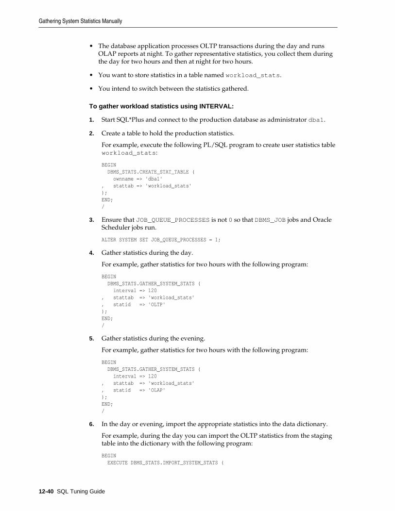
• The database application processes OLTP transactions during the day and runsOLAP reports at night. To gather representative statistics, you collect them duringthe day for two hours and then at night for two hours.
• You want to store statistics in a table named workload_stats.
• You intend to switch between the statistics gathered.
To gather workload statistics using INTERVAL:
1. Start SQL*Plus and connect to the production database as administrator dba1.
2. Create a table to hold the production statistics.
For example, execute the following PL/SQL program to create user statistics tableworkload_stats:
BEGIN DBMS_STATS.CREATE_STAT_TABLE ( ownname => 'dba1', stattab => 'workload_stats');END;/
3. Ensure that JOB_QUEUE_PROCESSES is not 0 so that DBMS_JOB jobs and OracleScheduler jobs run.
ALTER SYSTEM SET JOB_QUEUE_PROCESSES = 1;
4. Gather statistics during the day.
For example, gather statistics for two hours with the following program:
BEGIN DBMS_STATS.GATHER_SYSTEM_STATS ( interval => 120, stattab => 'workload_stats', statid => 'OLTP' );END;/
5. Gather statistics during the evening.
For example, gather statistics for two hours with the following program:
BEGIN DBMS_STATS.GATHER_SYSTEM_STATS ( interval => 120, stattab => 'workload_stats' , statid => 'OLAP' );END;/
6. In the day or evening, import the appropriate statistics into the data dictionary.
For example, during the day you can import the OLTP statistics from the stagingtable into the dictionary with the following program:
BEGIN EXECUTE DBMS_STATS.IMPORT_SYSTEM_STATS (
Gathering System Statistics Manually
12-40 SQL Tuning Guide

stattab => 'workload_stats', statid => 'OLTP' );END;/
For example, during the night you can import the OLAP statistics from thestaging table into the dictionary with the following program:
BEGIN EXECUTE DBMS_STATS.IMPORT_SYSTEM_STATS ( stattab => 'workload_stats', statid => 'OLAP' );END;/
See Also:
Oracle Database PL/SQL Packages and Types Reference to learn about theDBMS_STATS.GATHER_SYSTEM_STATS procedure
Gathering Noworkload StatisticsNoworkload statistics capture characteristics of the I/O system. By default, OracleDatabase uses noworkload statistics and the CPU cost model. The values ofnoworkload statistics are initialized to defaults at the first instance startup. You canalso use the DBMS_STATS.GATHER_SYSTEM_STATS procedure to gather noworkloadstatistics manually.
Noworkload statistics include the following system statistics listed in Table 12-4:
• I/O transfer speed (iotfrspeed)
• I/O seek time (ioseektim)
• CPU speed (cpuspeednw)
The major difference between workload statistics and noworkload statistics is in thegathering method. Noworkload statistics gather data by submitting random readsagainst all data files, whereas workload statistics uses counters updated whendatabase activity occurs. If you gather workload statistics, then Oracle Database usesthem instead of noworkload statistics.
To gather noworkload statistics, run DBMS_STATS.GATHER_SYSTEM_STATS with noarguments or with the gathering mode set to noworkload. There is an overhead onthe I/O system during the gathering process of noworkload statistics. The gatheringprocess may take from a few seconds to several minutes, depending on I/Operformance and database size.
When you gather noworkload statistics, the database analyzes the information andverifies it for consistency. In some cases, the values of noworkload statistics may retaintheir default values. You can either gather the statistics again, or useSET_SYSTEM_STATS to set the values manually to the I/O system specifications.
Assumptions
This tutorial assumes that you want to gather noworkload statistics manually.
Gathering System Statistics Manually
Managing Optimizer Statistics: Basic Topics 12-41

To gather noworkload statistics manually:
1. Start SQL*Plus and connect to the database with administrator privileges.
2. Gather the noworkload statistics.
For example, run the following statement:
BEGIN DBMS_STATS.GATHER_SYSTEM_STATS ( gathering_mode => 'NOWORKLOAD' );END;
3. Optionally, query the system statistics.
For example, run the following query:
COL PNAME FORMAT a15
SELECT PNAME, PVAL1 FROM SYS.AUX_STATS$WHERE SNAME = 'SYSSTATS_MAIN';
See Also:
Oracle Database PL/SQL Packages and Types Reference to learn about theDBMS_STATS.GATHER_SYSTEM_STATS procedure
Deleting System StatisticsUse the DBMS_STATS.DELETE_SYSTEM_STATS function to delete system statistics.This procedure deletes workload statistics collected using the INTERVAL or STARTand STOP options, and then resets the default to noworkload statistics. However, if thestattab parameter specifies a table for storing statistics, then the subprogram deletesall system statistics with the associated statid from the statistics table.
Assumptions
This tutorial assumes the following:
• You gathered statistics for a specific intensive workload, but no longer want theoptimizer to use these statistics.
• You stored workload statistics in the default location, not in a user-specified table.
To delete system statistics:
1. Start SQL*Plus and connect to the database as a user with administrativeprivileges.
2. Delete the system statistics.
For example, run the following statement:
EXEC DBMS_STATS.DELETE_SYSTEM_STATS;
Gathering System Statistics Manually
12-42 SQL Tuning Guide

See Also:
Oracle Database PL/SQL Packages and Types Reference to learn about theDBMS_STATS.DELETE_SYSTEM_STATS procedure
Gathering System Statistics Manually
Managing Optimizer Statistics: Basic Topics 12-43

Gathering System Statistics Manually
12-44 SQL Tuning Guide

13Managing Optimizer Statistics: Advanced
Topics
This chapter explains advanced concepts and tasks relating to optimizer statisticsmanagement, including extended statistics.
This chapter contains the following topics:
• Controlling Dynamic Statistics
• Publishing Pending Optimizer Statistics
• Managing Extended Statistics
• Locking and Unlocking Optimizer Statistics
• Restoring Optimizer Statistics
• Managing Optimizer Statistics Retention
• Importing and Exporting Optimizer Statistics
• Running Statistics Gathering Functions in Reporting Mode
• Reporting on Past Statistics Gathering Operations
• Managing SQL Plan Directives
See Also:
Managing Optimizer Statistics: Basic Topics
Controlling Dynamic StatisticsBy default, when optimizer statistics are missing, stale, or insufficient, dynamicstatistics automatically run recursive SQL during parsing to scan a small randomsample of table blocks.
This section contains the following topics:
• About Dynamic Statistics Levels
• Setting Dynamic Statistics Levels Manually
• Disabling Dynamic Statistics
Managing Optimizer Statistics: Advanced Topics 13-1

See Also:
“Dynamic Statistics”
About Dynamic Statistics LevelsThe dynamic statistics level controls both when the database gathers dynamicstatistics, and the size of the sample that the optimizer uses to gather the statistics. Setthe dynamic statistics level using either the OPTIMIZER_DYNAMIC_SAMPLINGinitialization parameter (dynamic statistics were called dynamic sampling in releasesearlier than Oracle Database 12c) or a statement hint.
Dynamic statistics are enabled in the database by default. Table 13-1 describes thelevels. The default level is 2.
Table 13-1 Dynamic Statistics Levels
Level When the Optimizer Uses Dynamic Statistics Sample Size (Blocks)
0 Do not use dynamic statistics n/a
1 Use dynamic statistics for all tables that do not havestatistics, but only if the following criteria are met:
• There is at least 1 nonpartitioned table in the query thatdoes not have statistics.
• This table has no indexes.• This table has more blocks than the number of blocks
that would be used for dynamic statistics of this table.
32
2 Use dynamic statistics if at least one table in the statementhas no statistics. This is the default setting.
64
3 Use dynamic statistics if any of the following conditions istrue:
• The statement meets level 2 criteria.• The statement has one or more expressions used in the
WHERE clause predicates, for example, WHERESUBSTR(CUSTLASTNAME,1,3).
64
4 Use dynamic statistics if any of the following conditions istrue:
• The statement meets level 3 criteria.• The statement uses complex predicates (an OR or AND
operator between multiple predicates on the sametable).
64
5 Use dynamic statistics if the statement meets level 4 criteria. 128
6 Use dynamic statistics if the statement meets level 4 criteria. 256
7 Use dynamic statistics if the statement meets level 4 criteria. 512
8 Use dynamic statistics if the statement meets level 4 criteria. 1024
9 Use dynamic statistics if the statement meets level 4 criteria. 4086
10 Use dynamic statistics if the statement meets level 4 criteria. All blocks
Controlling Dynamic Statistics
13-2 SQL Tuning Guide

Table 13-1 (Cont.) Dynamic Statistics Levels
Level When the Optimizer Uses Dynamic Statistics Sample Size (Blocks)
11 Use dynamic statistics automatically when the optimizerdeems it necessary. The resulting statistics are persistent inthe statistics repository, making them available to otherqueries.
Automaticallydetermined
See Also:
Oracle Database Reference to learn about the OPTIMIZER_DYNAMIC_SAMPLINGinitialization parameter
Setting Dynamic Statistics Levels ManuallyWhen setting the level for dynamic statistics, the best practice is to use ALTERSESSION to set the value for the OPTIMIZER_DYNAMIC_SAMPLING initializationparameter. Determining a systemwide setting that would be beneficial to all SQLstatements can be difficult.
Assumptions
This tutorial assumes the following:
• You want correct selectivity estimates for the following query, which has WHEREclause predicates on two correlated columns:
SELECT * FROM sh.customers WHERE cust_city='Los Angeles' AND cust_state_province='CA';
• The preceding query uses serial processing.
• The sh.customers table contains 932 rows that meet the conditions in the query.
• You have gathered statistics on the sh.customers table.
• You created an index on the cust_city and cust_state_province columns.
• The OPTIMIZER_DYNAMIC_SAMPLING initialization parameter is set to the defaultlevel of 2.
To set the dynamic statistics level manually:
1. Connect SQL*Plus to the database with the appropriate privileges, and thenexplain the execution plan as follows:
EXPLAIN PLAN FOR SELECT * FROM sh.customers WHERE cust_city='Los Angeles' AND cust_state_province='CA';
2. Query the plan as follows:
Controlling Dynamic Statistics
Managing Optimizer Statistics: Advanced Topics 13-3

SET LINESIZE 130SET PAGESIZE 0SELECT * FROM TABLE(DBMS_XPLAN.DISPLAY);
The output appears below (the example has been reformatted to fit on the page):
-------------------------------------------------------------------------------|Id| Operation | Name |Rows|Bytes|Cost | Time |-------------------------------------------------------------------------------| 0| SELECT STATEMENT | | 53| 9593|53(0)|00:00:01|| 1| TABLE ACCESS BY INDEX ROWID|CUSTOMERS | 53| 9593|53(0)|00:00:01||*2| INDEX RANGE SCAN |CUST_CITY_STATE_IND| 53| 9593| 3(0)|00:00:01|------------------------------------------------------------------------------- Predicate Information (identified by operation id):--------------------------------------------------- 2 - access("CUST_CITY"='Los Angeles' AND "CUST_STATE_PROVINCE"='CA')
The columns in the WHERE clause have a real-world correlation, but the optimizeris not aware that Los Angeles is in California and assumes both predicates reducethe number of rows returned. Thus, the table contains 932 rows that meet theconditions, but the optimizer estimates 53, as shown in bold.
If the database had used dynamic statistics for this plan, then the Note section ofthe plan output would have indicated this fact. The optimizer did not usedynamic statistics because the statement executed serially, standard statisticsexist, and the parameter OPTIMIZER_DYNAMIC_SAMPLING is set to the default of2.
3. Set the dynamic statistics level to 4 in the session using the following statement:
ALTER SESSION SET OPTIMIZER_DYNAMIC_SAMPLING=4;
4. Explain the plan again:
EXPLAIN PLAN FOR SELECT * FROM sh.customers WHERE cust_city='Los Angeles' AND cust_state_province='CA';
The new plan shows a more accurate estimate of the number of rows, as shown bythe value 932 in bold:
PLAN_TABLE_OUTPUT---------------------------------------------------------------------------Plan hash value: 2008213504 ---------------------------------------------------------------------------| Id | Operation | Name |Rows | Bytes |Cost (%CPU)|Time |---------------------------------------------------------------------------| 0 | SELECT STATEMENT | | 932 | 271K| 406 (1)| 00:00:05 ||* 1 | TABLE ACCESS FULL| CUSTOMERS | 932 | 271K| 406 (1)| 00:00:05 |--------------------------------------------------------------------------- Predicate Information (identified by operation id):--------------------------------------------------- 1 - filter("CUST_CITY"='Los Angeles' AND "CUST_STATE_PROVINCE"='CA')
Controlling Dynamic Statistics
13-4 SQL Tuning Guide

Note----- - dynamic statistics used for this statement (level=4)
The note at the bottom of the plan indicates that the sampling level is 4. Theadditional dynamic statistics made the optimizer aware of the real-worldrelationship between the cust_city and cust_state_province columns,thereby enabling it to produce a more accurate estimate for the number of rows:932 rather than 53.
See Also:
• Oracle Database SQL Language Reference to learn about setting samplinglevels with the DYNAMIC_SAMPLING hint
• Oracle Database PL/SQL Packages and Types Reference to learn about theOPTIMIZER_DYNAMIC_SAMPLING initialization parameter
Disabling Dynamic StatisticsIn general, the best practice is not to incur the cost of dynamic statistics for querieswhose compile times must be as fast as possible, for example, unrepeated OLTPqueries. You can disable the feature by setting the OPTIMIZER_DYNAMIC_SAMPLINGinitialization parameter.
To disable dynamic statistics at the session level:
1. Connect SQL*Plus to the database with the appropriate privileges.
2. Set the dynamic statistics level to 0.
For example, run the following statement:
ALTER SESSION SET OPTIMIZER_DYNAMIC_SAMPLING=0;
See Also:
Oracle Database PL/SQL Packages and Types Reference to learn about theOPTIMIZER_DYNAMIC_SAMPLING initialization parameter
Publishing Pending Optimizer StatisticsBy default, the database automatically publishes statistics when the statistics collectionends. Alternatively, you can use pending statistics to save the statistics and notpublish them immediately after the collection. This technique is useful for testingqueries in a session with pending statistics. When the test results are satisfactory, youcan publish the statistics to make them available for the entire database.
About Pending Optimizer StatisticsThe database stores pending statistics in the data dictionary just as for publishedstatistics. By default, the optimizer uses published statistics. You can change thedefault behavior by setting the OPTIMIZER_USE_PENDING_STATISTICSinitialization parameter to true (the default is false).
Publishing Pending Optimizer Statistics
Managing Optimizer Statistics: Advanced Topics 13-5

The top part of Figure 13-1 shows the optimizer gathering statistics for thesh.customers table and storing them in the data dictionary with pending status.The bottom part of the diagram shows the optimizer using only published statistics toprocess a query of sh.customers.
Figure 13-1 Published and Pending Statistics
Data Dictionary
Optimizer Statistics
0 0 1 0 0 0
1 1 0 0 1 0
Pending Statistics
1 0 0 1 1 1
0 1 0 0 0 1
Published Statistics
Data Dictionary
Optimizer Statistics
0 0 1 0 0 0
1 1 0 0 1 0
Pending Statistics
1 0 0 1 1 1
0 1 0 0 0 1
Published Statistics
Optimizer
OPTIMIZER_USE_PENDING_STATISTICS=false
SELECT ...
FROM
customers
Optimizer
CustomersTable
Publishing preferences set to false
GATHER_TABLE_STATS
In some cases, the optimizer can use a combination of published and pendingstatistics. For example, the database stores both published and pending statistics forthe customers table. For the orders table, the database stores only publishedstatistics. If OPTIMIZER_USE_PENDING_STATS = true, then the optimizer usespending statistics for customers and published statistics for orders. IfOPTIMIZER_USE_PENDING_STATS = false, then the optimizer uses publishedstatistics for customers and orders.
See Also:
Oracle Database Reference to learn about theOPTIMIZER_USE_PENDING_STATISTICS initialization parameter
Publishing Pending Optimizer Statistics
13-6 SQL Tuning Guide

User Interfaces for Publishing Optimizer StatisticsYou can use the DBMS_STATS package to perform operations relating to publishingstatistics. Table 13-2 lists the relevant program units.
Table 13-2 DBMS_STATS Program Units Relevant for Publishing OptimizerStatistics
Program Unit Description
GET_PREFS Check whether the statistics are automatically publishedas soon as DBMS_STATS gathers them. For theparameter PUBLISH, true indicates that the statisticsmust be published when the database gathers them,whereas false indicates that the database must keepthe statistics pending.
SET_TABLE_PREFS Set the PUBLISH setting to true or false at the tablelevel.
SET_SCHEMA_PREFS Set the PUBLISH setting to true or false at the schemalevel.
PUBLISH_PENDING_STATS Publish valid pending statistics for all objects or onlyspecified objects.
DELETE_PENDING_STATS Delete pending statistics.
EXPORT_PENDING_STATS Export pending statistics.
The initialization parameter OPTIMIZER_USE_PENDING_STATISTICS determineswhether the database uses pending statistics when they are available. The defaultvalue is false, which means that the optimizer uses only published statistics. Set totrue to specify that the optimizer uses any existing pending statistics instead. Thebest practice is to set this parameter at the session level rather than at the databaselevel.
You can use access information about published statistics from data dictionary views. Table 13-3 lists relevant views.
Table 13-3 Views Relevant for Publishing Optimizer Statistics
View Description
USER_TAB_STATISTICS Displays optimizer statistics for the tables accessibleto the current user.
USER_TAB_COL_STATISTICS Displays column statistics and histograminformation extracted from ALL_TAB_COLUMNS.
USER_PART_COL_STATISTICS Displays column statistics and histograminformation for the table partitions owned by thecurrent user.
USER_SUBPART_COL_STATISTICS Describes column statistics and histograminformation for subpartitions of partitioned objectsowned by the current user.
Publishing Pending Optimizer Statistics
Managing Optimizer Statistics: Advanced Topics 13-7

Table 13-3 (Cont.) Views Relevant for Publishing Optimizer Statistics
View Description
USER_IND_STATISTICS Displays optimizer statistics for the indexesaccessible to the current user.
USER_TAB_PENDING_STATS Describes pending statistics for tables, partitions,and subpartitions accessible to the current user.
USER_COL_PENDING_STATS Describes the pending statistics of the columnsaccessible to the current user.
USER_IND_PENDING_STATS Describes the pending statistics for tables, partitions,and subpartitions accessible to the current usercollected using the DBMS_STATS package.
See Also:
• Oracle Database PL/SQL Packages and Types Reference to learn about theDBMS_STATS package
• Oracle Database Reference to learn about USER_TAB_PENDING_STATS andrelated views
Managing Published and Pending StatisticsThis section explains how to use DBMS_STATS program units to change the publishingbehavior of optimizer statistics, and also to export and delete these statistics.
Assumptions
This tutorial assumes the following:
• You want to change the preferences for the sh.customers and sh.sales tablesso that newly collected statistics have pending status.
• You want the current session to use pending statistics.
• You want to gather and publish pending statistics on the sh.customers table.
• You gather the pending statistics on the sh.sales table, but decide to delete themwithout publishing them.
• You want to change the preferences for the sh.customers and sh.sales tablesso that newly collected statistics are published.
To manage published and pending statistics:
1. Start SQL*Plus and connect to the database as user sh.
2. Query the global optimizer statistics publishing setting.
Run the following query (sample output included):
Publishing Pending Optimizer Statistics
13-8 SQL Tuning Guide

sh@PROD> SELECT DBMS_STATS.GET_PREFS('PUBLISH') PUBLISH FROM DUAL;
PUBLISH-------TRUE
The value true indicates that the database publishes statistics as it gathers them.Every table uses this value unless a specific table preference has been set.
When using GET_PREFS, you can also specify a schema and table name. Thefunction returns a table preference if it is set. Otherwise, the function returns theglobal preference.
3. Query the pending statistics.
For example, run the following query (sample output included):
sh@PROD> SELECT * FROM USER_TAB_PENDING_STATS; no rows selected
This example shows that the database currently stores no pending statistics for thesh schema.
4. Change the publishing preferences for the sh.customers table.
For example, execute the following procedure so that statistics are marked aspending:
BEGIN DBMS_STATS.SET_TABLE_PREFS('sh', 'customers', 'publish', 'false');END;/
Subsequently, when you gather statistics on the customers table, the databasedoes not automatically publish statistics when the gather job completes. Instead,the database stores the newly gathered statistics in theUSER_TAB_PENDING_STATS table.
5. Gather statistics for sh.customers.
For example, run the following program:
BEGIN DBMS_STATS.GATHER_TABLE_STATS('sh','customers');END;/
6. Query the pending statistics.
For example, run the following query (sample output included):
sh@PROD> SELECT TABLE_NAME, NUM_ROWS FROM USER_TAB_PENDING_STATS; TABLE_NAME NUM_ROWS------------------------------ ----------CUSTOMERS 55500
This example shows that the database now stores pending statistics for thesh.customers table.
7. Instruct the optimizer to use the pending statistics in this session.
Publishing Pending Optimizer Statistics
Managing Optimizer Statistics: Advanced Topics 13-9

Set the initialization parameter OPTIMIZER_USE_PENDING_STATISTICS totrue as shown:
ALTER SESSION SET OPTIMIZER_USE_PENDING_STATISTICS = true;
8. Run a workload.
The following example changes the email addresses of all customers named BruceChalmers:
UPDATE sh.customers SET cust_email='[email protected]' WHERE cust_first_name = 'Bruce' AND cust_last_name = 'Chalmers';COMMIT;
The optimizer uses the pending statistics instead of the published statistics whencompiling all SQL statements in this session.
9. Publish the pending statistics for sh.customers.
For example, execute the following program:
BEGIN DBMS_STATS.PUBLISH_PENDING_STATS('SH','CUSTOMERS');END;/
10. Change the publishing preferences for the sh.sales table.
For example, execute the following program:
BEGIN DBMS_STATS.SET_TABLE_PREFS('sh', 'sales', 'publish', 'false');END;/
Subsequently, when you gather statistics on the sh.sales table, the databasedoes not automatically publish statistics when the gather job completes. Instead,the database stores the statistics in the USER_TAB_PENDING_STATS table.
11. Gather statistics for sh.sales.
For example, run the following program:
BEGIN DBMS_STATS.GATHER_TABLE_STATS('sh','sales');END;/
12. Delete the pending statistics for sh.sales.
Assume you change your mind and now want to delete pending statistics forsh.sales. Run the following program:
BEGIN DBMS_STATS.DELETE_PENDING_STATS('sh','sales');END;/
13. Change the publishing preferences for the sh.customers and sh.sales tablesback to their default setting.
For example, execute the following program:
Publishing Pending Optimizer Statistics
13-10 SQL Tuning Guide

BEGIN DBMS_STATS.SET_TABLE_PREFS('sh', 'customers', 'publish', null); DBMS_STATS.SET_TABLE_PREFS('sh', 'sales', 'publish', null);END;/
Managing Extended StatisticsDBMS_STATS enables you to collect extended statistics, which are statistics that canimprove cardinality estimates when multiple predicates exist on different columns of atable, or when predicates use expressions. An extension is either a column group or anexpression.
Oracle Database supports the following types of extended statistics:
• Column group statistics
This type of extended statistics can improve cardinality estimates when multiplecolumns from the same table occur together in a SQL statement. An example mightbe a car make and model, or a city and state. See “Managing Column GroupStatistics”.
• Expression statistics
This type of extended statistics improves optimizer estimates when predicates useexpressions, for example, built-in or user-defined functions. An example might bethe UPPER function applied to an employee last name. See “Managing ExpressionStatistics”.
Note:
You cannot create extended statistics on virtual columns. See Oracle DatabaseSQL Language Reference for a list of restrictions on virtual columns.
Managing Column Group StatisticsA column group is a set of columns that is treated as a unit. Essentially, a columngroup is a virtual column. By gathering statistics on a column group, the optimizer canmore accurately determine the cardinality estimate when a query groups thesecolumns together.
The following sections provide an overview of column group statistics, and explainhow to manage them manually:
• About Statistics on Column Groups
• Detecting Useful Column Groups for a Specific Workload
• Creating Column Groups Detected During Workload Monitoring
• Creating and Gathering Statistics on Column Groups Manually
• Displaying Column Group Information
• Dropping a Column Group
Managing Extended Statistics
Managing Optimizer Statistics: Advanced Topics 13-11

See Also:
Oracle Database PL/SQL Packages and Types Reference to learn about theDBMS_STATS package
About Statistics on Column GroupsIndividual column statistics are useful for determining the selectivity of a singlepredicate in a WHERE clause. However, when the WHERE clause includes multiplepredicates on different columns from the same table, individual column statistics donot show the relationship between the columns. This is the problem solved by acolumn group.
The optimizer calculates the selectivity of the predicates independently, and thencombines them. However, if a correlation between the individual columns exists, thenthe optimizer cannot take it into account when determining a cardinality estimate,which it creates by multiplying the selectivity of each table predicate by the number ofrows.
The following graphic contrasts two ways of gathering statistics on thecust_state_province and country_id columns of the sh.customers table.The diagram shows DBMS_STATS collecting statistics on each column individuallyand on the group. The column group has a system-generated name.
Figure 13-2 Column Group Statistics
SYS_STU#S#WF25Z#QAHIHE#MOFFMM_
Statistics forColumn Group
CUST_ID CUST_STATE_PROVINCE COUNTRY_ID
101095
103105
52790
52775
CA
Sao Paulo
...
Statistics forCUST_STATE_PROVINCE
Statistics forCOUNTRY_ID
DBMS_STATS
Note:
The optimizer uses column group statistics for equality predicates, inlistpredicates, and for estimating the GROUP BY cardinality.
Why Column Group Statistics Are Needed: Example
The following query of the DBA_TAB_COL_STATISTICS table shows informationabout statistics that have been gathered on the columns cust_state_province andcountry_id from the sh.customers table:
COL COLUMN_NAME FORMAT a20COL NDV FORMAT 999
Managing Extended Statistics
13-12 SQL Tuning Guide

SELECT COLUMN_NAME, NUM_DISTINCT AS "NDV", HISTOGRAMFROM DBA_TAB_COL_STATISTICSWHERE OWNER = 'SH'AND TABLE_NAME = 'CUSTOMERS'AND COLUMN_NAME IN ('CUST_STATE_PROVINCE', 'COUNTRY_ID');
Sample output is as follows:
COLUMN_NAME NDV HISTOGRAM-------------------- ---------- ---------------CUST_STATE_PROVINCE 145 FREQUENCYCOUNTRY_ID 19 FREQUENCY
As shown in the following query, 3341 customers reside in California:
SELECT COUNT(*)FROM sh.customers WHERE cust_state_province = 'CA';
COUNT(*)---------- 3341
Consider an explain plan for a query of customers in the state CA and in the countrywith ID 52790 (USA):
EXPLAIN PLAN FOR SELECT * FROM sh.customers WHERE cust_state_province = 'CA' AND country_id=52790; Explained. sys@PROD> SELECT * FROM TABLE(DBMS_XPLAN.DISPLAY); PLAN_TABLE_OUTPUT--------------------------------------------------------------------------------Plan hash value: 1683234692 -------------------------------------------------------------------------------| Id | Operation | Name | Rows | Bytes | Cost (%CPU)| Time |-------------------------------------------------------------------------------| 0 | SELECT STATEMENT | | 128 | 24192 | 442 (7)| 00:00:06 ||* 1 | TABLE ACCESS FULL| CUSTOMERS | 128 | 24192 | 442 (7)| 00:00:06 |------------------------------------------------------------------------------- Predicate Information (identified by operation id):--------------------------------------------------- PLAN_TABLE_OUTPUT-------------------------------------------------------------------------------- 1 - filter("CUST_STATE_PROVINCE"='CA' AND "COUNTRY_ID"=52790) 13 rows selected.
Based on the single-column statistics for the country_id andcust_state_province columns, the optimizer estimates that the query ofCalifornia customers in the USA will return 128 rows. In fact, 3341 customers reside in
Managing Extended Statistics
Managing Optimizer Statistics: Advanced Topics 13-13

California, but the optimizer does not know that California is in the USA, and sogreatly underestimates cardinality by assuming that both predicates reduce thenumber of returned rows.
You can make the optimizer aware of the real-world relationship between values incountry_id and cust_state_province by gathering column group statistics.These statistics enable the optimizer to give a more accurate cardinality estimate.
See Also:
• “Detecting Useful Column Groups for a Specific Workload”
• “Creating Column Groups Detected During Workload Monitoring”
• “Creating and Gathering Statistics on Column Groups Manually”
User Interface for Column Group Statistics
Table 13-4 lists the DBMS_STATS program units that are relevant for detecting andcreating column groups.
Table 13-4 DBMS_STATS Column Group Program Units
Program Unit Description
SEED_COL_USAGE Iterates over the SQL statements in the specified workload,compiles them, and then seeds column usage informationfor the columns that appear in these statements.
To determine the appropriate column groups, the databasemust observe a representative workload. You do not need torun the queries themselves during the monitoring period.Instead, you can run EXPLAIN PLAN for some longer-running queries in your workload to ensure that thedatabase is recording column group information for thesequeries.
REPORT_COL_USAGE Generates a report that lists the columns that were seen infilter predicates, join predicates, and GROUP BY clauses inthe workload.
You can use this function to review column usageinformation recorded for a specific table.
CREATE_EXTENDED_STATS Creates extensions, which are either column groups orexpressions. The database gathers statistics for the extensionwhen either a user-generated or automatic statisticsgathering job gathers statistics for the table.
See Also:
Oracle Database PL/SQL Packages and Types Reference to learn about theDBMS_STATS package
Managing Extended Statistics
13-14 SQL Tuning Guide

Detecting Useful Column Groups for a Specific Workload
You can use DBMS_STATS.SEED_COL_USAGE and REPORT_COL_USAGE to determinewhich column groups are required for a table based on a specified workload. Thistechnique is useful when you do not know which extended statistics to create. Thistechnique does not work for expression statistics.
Note:
You can seed column usage from a SQL tuning set (see Managing SQL TuningSets ).
Assumptions
This tutorial assumes the following:
• Cardinality estimates have been incorrect for queries of the sh.customers_testtable (created from the customers table) that use predicates referencing thecolumns country_id and cust_state_province.
• You want the database to monitor your workload for 5 minutes (300 seconds).
• You want the database to determine which column groups are neededautomatically.
To detect column groups:
1. Connect SQL*Plus to the database as user sh, and then create thecustomers_test table and gather statistics for it:
CONNECT SH/SHDROP TABLE customers_test;CREATE TABLE customers_test AS SELECT * FROM customer;EXEC DBMS_STATS.GATHER_TABLE_STATS(user, 'customers_test');
2. Enable workload monitoring.
In a different SQL*Plus session, connect as SYS and run the following PL/SQLprogram to enable monitoring for 300 seconds:
BEGIN DBMS_STATS.SEED_COL_USAGE(null,null,300);END;/
3. As user sh, run explain plans for two queries in the workload.
The following examples show the explain plans for two queries on thecustomers_test table:
EXPLAIN PLAN FOR SELECT * FROM customers_test WHERE cust_city = 'Los Angeles' AND cust_state_province = 'CA' AND country_id = 52790; SELECT PLAN_TABLE_OUTPUT FROM TABLE(DBMS_XPLAN.DISPLAY('plan_table', null,'basic rows'));
Managing Extended Statistics
Managing Optimizer Statistics: Advanced Topics 13-15

EXPLAIN PLAN FOR SELECT country_id, cust_state_province, count(cust_city) FROM customers_test GROUP BY country_id, cust_state_province; SELECT PLAN_TABLE_OUTPUT FROM TABLE(DBMS_XPLAN.DISPLAY('plan_table', null,'basic rows'));
Sample output appears below:
PLAN_TABLE_OUTPUT---------------------------------------------------------------------------Plan hash value: 4115398853 ----------------------------------------------------| Id | Operation | Name | Rows |----------------------------------------------------| 0 | SELECT STATEMENT | | 1 || 1 | TABLE ACCESS FULL| CUSTOMERS_TEST | 1 |---------------------------------------------------- 8 rows selected. PLAN_TABLE_OUTPUT---------------------------------------------------------------------------Plan hash value: 3050654408 -----------------------------------------------------| Id | Operation | Name | Rows |-----------------------------------------------------| 0 | SELECT STATEMENT | | 1949 || 1 | HASH GROUP BY | | 1949 || 2 | TABLE ACCESS FULL| CUSTOMERS_TEST | 55500 |----------------------------------------------------- 9 rows selected.
The first plan shows a cardinality of 1 row for a query that returns 932 rows. Thesecond plan shows a cardinality of 1949 rows for a query that returns 145 rows.
4. Optionally, review the column usage information recorded for the table.
Call the DBMS_STATS.REPORT_COL_USAGE function to generate a report:
SET LONG 100000SET LINES 120SET PAGES 0SELECT DBMS_STATS.REPORT_COL_USAGE(user, 'customers_test')FROM DUAL;
The report appears below:
LEGEND:....... EQ : Used in single table EQuality predicateRANGE : Used in single table RANGE predicateLIKE : Used in single table LIKE predicateNULL : Used in single table is (not) NULL predicateEQ_JOIN : Used in EQuality JOIN predicateNONEQ_JOIN : Used in NON EQuality JOIN predicate
Managing Extended Statistics
13-16 SQL Tuning Guide

FILTER : Used in single table FILTER predicateJOIN : Used in JOIN predicateGROUP_BY : Used in GROUP BY expression........................................................................... ########################################################################### COLUMN USAGE REPORT FOR SH.CUSTOMERS_TEST......................................... 1. COUNTRY_ID : EQ2. CUST_CITY : EQ3. CUST_STATE_PROVINCE : EQ4. (CUST_CITY, CUST_STATE_PROVINCE, COUNTRY_ID) : FILTER5. (CUST_STATE_PROVINCE, COUNTRY_ID) : GROUP_BY###########################################################################
In the preceding report, the first three columns were used in equality predicates inthe first monitored query:
...WHERE cust_city = 'Los Angeles'AND cust_state_province = 'CA'AND country_id = 52790;
All three columns appeared in the same WHERE clause, so the report shows themas a group filter. In the second query, two columns appeared in the GROUP BYclause, so the report labels them as GROUP_BY. The sets of columns in the FILTERand GROUP_BY report are candidates for column groups.
See Also:
Oracle Database PL/SQL Packages and Types Reference to learn about theDBMS_STATS package
Creating Column Groups Detected During Workload Monitoring
As explained in Table 13-4, you can use theDBMS_STATS.CREATE_EXTENDED_STATS function to create column groups thatwere detected previously by executing DBMS_STATS.SEED_COL_USAGE.
Assumptions
This tutorial assumes that you have performed the steps in “Detecting Useful ColumnGroups for a Specific Workload”.
To create column groups:
1. Create column groups for the customers_test table based on the usageinformation captured during the monitoring window.
For example, run the following query:
SELECT DBMS_STATS.CREATE_EXTENDED_STATS(user, 'customers_test') FROM DUAL;
Sample output appears below:
Managing Extended Statistics
Managing Optimizer Statistics: Advanced Topics 13-17

###########################################################################EXTENSIONS FOR SH.CUSTOMERS_TEST................................1. (CUST_CITY, CUST_STATE_PROVINCE, COUNTRY_ID) :SYS_STUMZ$C3AIHLPBROI#SKA58H_N created2. (CUST_STATE_PROVINCE, COUNTRY_ID):SYS_STU#S#WF25Z#QAHIHE#MOFFMM_ created###########################################################################
The database created two column groups for customers_test: one columngroup for the filter predicate and one group for the GROUP BY operation.
2. Regather table statistics.
Run GATHER_TABLE_STATS to regather the statistics for customers_test:
EXEC DBMS_STATS.GATHER_TABLE_STATS(user,'customers_test');
3. As user sh, run explain plans for two queries in the workload.
Check the USER_TAB_COL_STATISTICS view to determine which additionalstatistics were created by the database:
SELECT COLUMN_NAME, NUM_DISTINCT, HISTOGRAMFROM USER_TAB_COL_STATISTICSWHERE TABLE_NAME = 'CUSTOMERS_TEST'ORDER BY 1;
Partial sample output appears below:
CUST_CITY 620 HEIGHT BALANCED...SYS_STU#S#WF25Z#QAHIHE#MOFFMM_ 145 NONESYS_STUMZ$C3AIHLPBROI#SKA58H_N 620 HEIGHT BALANCED
This example shows the two column group names returned from theDBMS_STATS.CREATE_EXTENDED_STATS function. The column group createdon CUST_CITY, CUST_STATE_PROVINCE, and COUNTRY_ID has a height-balanced histogram.
4. Explain the plans again.
The following examples show the explain plans for two queries on thecustomers_test table:
EXPLAIN PLAN FOR SELECT * FROM customers_test WHERE cust_city = 'Los Angeles' AND cust_state_province = 'CA' AND country_id = 52790; SELECT PLAN_TABLE_OUTPUT FROM TABLE(DBMS_XPLAN.DISPLAY('plan_table', null,'basic rows')); EXPLAIN PLAN FOR SELECT country_id, cust_state_province, count(cust_city) FROM customers_test GROUP BY country_id, cust_state_province; SELECT PLAN_TABLE_OUTPUT FROM TABLE(DBMS_XPLAN.DISPLAY('plan_table', null,'basic rows'));
The new plans show more accurate cardinality estimates:
Managing Extended Statistics
13-18 SQL Tuning Guide

----------------------------------------------------| Id | Operation | Name | Rows |----------------------------------------------------| 0 | SELECT STATEMENT | | 1093 || 1 | TABLE ACCESS FULL| CUSTOMERS_TEST | 1093 |---------------------------------------------------- 8 rows selected. Plan hash value: 3050654408 -----------------------------------------------------| Id | Operation | Name | Rows |-----------------------------------------------------| 0 | SELECT STATEMENT | | 145 || 1 | HASH GROUP BY | | 145 || 2 | TABLE ACCESS FULL| CUSTOMERS_TEST | 55500 |-----------------------------------------------------9 rows selected.
See Also:
Oracle Database PL/SQL Packages and Types Reference to learn about theDBMS_STATS package
Creating and Gathering Statistics on Column Groups Manually
In some cases, you may know the column group that you want to create. TheMETHOD_OPT argument of the DBMS_STATS.GATHER_TABLE_STATS function cancreate and gather statistics on a column group automatically. You can create a newcolumn group by specifying the group of columns using FOR COLUMNS.
Assumptions
This tutorial assumes the following:
• You want to create a column group for the cust_state_province andcountry_id columns in the customers table in sh schema.
• You want to gather statistics (including histograms) on the entire table and the newcolumn group.
To create a column group and gather statistics for this group:
1. Start SQL*Plus and connect to the database as the sh user.
2. Create the column group and gather statistics.
For example, execute the following PL/SQL program:
BEGIN DBMS_STATS.GATHER_TABLE_STATS( 'sh','customers', METHOD_OPT => 'FOR ALL COLUMNS SIZE SKEWONLY ' || 'FOR COLUMNS SIZE SKEWONLY (cust_state_province,country_id)' );END;/
Managing Extended Statistics
Managing Optimizer Statistics: Advanced Topics 13-19

See Also:
Oracle Database PL/SQL Packages and Types Reference to learn about theDBMS_STATS.GATHER_TABLE_STATS procedure
Displaying Column Group Information
To obtain the name of a column group, use theDBMS_STATS.SHOW_EXTENDED_STATS_NAME function or a database view. You canalso use views to obtain information such as the number of distinct values, andwhether the column group has a histogram.
Assumptions
This tutorial assumes the following:
• You created a column group for the cust_state_province and country_idcolumns in the customers table in sh schema.
• You want to determine the column group name, the number of distinct values, andwhether a histogram has been created for a column group.
To monitor a column group:
1. Start SQL*Plus and connect to the database as the sh user.
2. To determine the column group name, do one of the following.
• Execute the SHOW_EXTENDED_STATS_NAME function.
For example, run the following PL/SQL program:
SELECT SYS.DBMS_STATS.SHOW_EXTENDED_STATS_NAME( 'sh','customers', '(cust_state_province,country_id)' ) col_group_name FROM DUAL;
The output is similar to the following:
COL_GROUP_NAME----------------SYS_STU#S#WF25Z#QAHIHE#MOFFMM_
• Query the USER_STAT_EXTENSIONS view.
For example, run the following query:
SELECT EXTENSION_NAME, EXTENSION FROM USER_STAT_EXTENSIONS WHERE TABLE_NAME='CUSTOMERS';
EXTENSION_NAME EXTENSION-----------------------------------------------------------------------SYS_STU#S#WF25Z#QAHIHE#MOFFMM_ ("CUST_STATE_PROVINCE","COUNTRY_ID")
3. Query the number of distinct values and find whether a histogram has beencreated for a column group.
For example, run the following query:
SELECT e.EXTENSION col_group, t.NUM_DISTINCT, t.HISTOGRAMFROM USER_STAT_EXTENSIONS e, USER_TAB_COL_STATISTICS t
Managing Extended Statistics
13-20 SQL Tuning Guide

WHERE e.EXTENSION_NAME=t.COLUMN_NAMEAND e.TABLE_NAME=t.TABLE_NAMEAND t.TABLE_NAME='CUSTOMERS';
COL_GROUP NUM_DISTINCT HISTOGRAM-------------------------------------------------------------------("COUNTRY_ID","CUST_STATE_PROVINCE") 145 FREQUENCY
See Also:
Oracle Database PL/SQL Packages and Types Reference to learn about theDBMS_STATS.SHOW_EXTENDED_STATS_NAME function
Dropping a Column Group
Use the DBMS_STATS.DROP_EXTENDED_STATS function to delete a column groupfrom a table.
Assumptions
This tutorial assumes the following:
• You created a column group for the cust_state_province and country_idcolumns in the customers table in sh schema.
• You want to drop the column group.
To drop a column group:
1. Start SQL*Plus and connect to the database as the sh user.
2. Drop the column group.
For example, the following PL/SQL program deletes a column group from thecustomers table:
BEGIN DBMS_STATS.DROP_EXTENDED_STATS( 'sh', 'customers', '(cust_state_province, country_id)' );END;/
See Also:
Oracle Database PL/SQL Packages and Types Reference to learn about theDBMS_STATS.DROP_EXTENDED_STATS function
Managing Expression StatisticsThe type of extended statistics known as expression statistics improve optimizerestimates when a WHERE clause has predicates that use expressions.
This section contains the following topics:
• About Expression Statistics
• Creating Expression Statistics
Managing Extended Statistics
Managing Optimizer Statistics: Advanced Topics 13-21

• Displaying Expression Statistics
• Dropping Expression Statistics
About Expression Statistics
When an expression is applied to a column in the WHERE clause in theform(function(col)=constant), the optimizer has no way of knowing how thisSQL function affects the cardinality of the predicate unless a function-based index hadbeen created. Starting in Oracle Database 11g, you can gather expression statistics onthe expression(function(col) itself.
Figure 13-3 shows the optimizer using statistics to generate a plan for a query that usesa function. The top shows the optimizer checking statistics for the column. The bottomshows the optimizer checking statistics corresponding to the expression used in thequery. The expression statistics yield more accurate estimates.
Figure 13-3 Expression Statistics
Use DefaultColumnStatistics
Use Expression Statistics
OptimalEstimate
SuboptimalEstimate
Doexpressionstatistics
exist?
Optimizer
SELECT * FROM sh.customers
WHERE LOWER (cust_state_province) = ‘ca’
LOWER(cust_state_province)Expression Statistics
cust_state_provinceColumn Statistics
Yes No
As shown in Figure 13-3, when expression statistics are not available, the optimizercan produce suboptimal plans.
See Also:
Oracle Database SQL Language Reference to learn about SQL functions
When Expression Statistics Are Useful: Example
The following query of the sh.customers table shows that 3341 customers are in thestate of California:
sys@PROD> SELECT COUNT(*) FROM sh.customers WHERE cust_state_province='CA'; COUNT(*)
Managing Extended Statistics
13-22 SQL Tuning Guide

---------- 3341
Consider the plan for the same query with the LOWER() function applied:
sys@PROD> EXPLAIN PLAN FOR 2 SELECT * FROM sh.customers WHERE LOWER(cust_state_province)='ca';Explained.
sys@PROD> select * from table(dbms_xplan.display);
PLAN_TABLE_OUTPUT-------------------------------------------------------------------------------Plan hash value: 2008213504
-------------------------------------------------------------------------------| Id | Operation | Name | Rows | Bytes | Cost (%CPU)| Time |-------------------------------------------------------------------------------| 0 | SELECT STATEMENT | | 555 | 108K| 406 (1)| 00:00:05 ||* 1 | TABLE ACCESS FULL| CUSTOMERS | 555 | 108K| 406 (1)| 00:00:05 |-------------------------------------------------------------------------------
Predicate Information (identified by operation id):---------------------------------------------------
1 - filter(LOWER("CUST_STATE_PROVINCE")='ca')
Because no expression statistics exist for LOWER(cust_state_province)='ca',the optimizer estimate is significantly off. You can use DBMS_STATS procedures tocorrect these estimates.
Creating Expression Statistics
You can use DBMS_STATS to create statistics for a user-specified expression. You havethe option of using either of the following program units:
• GATHER_TABLE_STATS procedure
• CREATE_EXTENDED_STATISTICS function followed by theGATHER_TABLE_STATS procedure
Assumptions
This tutorial assumes the following:
• Selectivity estimates are inaccurate for queries of sh.customers that use theUPPER(cust_state_province) function.
• You want to gather statistics on the UPPER(cust_state_province) expression.
To create expression statistics:
1. Start SQL*Plus and connect to the database as the sh user.
2. Gather table statistics.
For example, run the following command, specifying the function in themethod_opt argument:
BEGIN DBMS_STATS.GATHER_TABLE_STATS(
Managing Extended Statistics
Managing Optimizer Statistics: Advanced Topics 13-23

'sh', 'customers', method_opt => 'FOR ALL COLUMNS SIZE SKEWONLY FOR COLUMNS (LOWER(cust_state_province)) SIZE SKEWONLY' );END;
See Also:
Oracle Database PL/SQL Packages and Types Reference to learn about theDBMS_STATS.GATHER_TABLE_STATS procedure
Displaying Expression Statistics
You can use the database view DBA_STAT_EXTENSIONS and theDBMS_STATS.SHOW_EXTENDED_STATS_NAME function to obtain information aboutexpression statistics. You can also use views to obtain information such as the numberof distinct values, and whether the column group has a histogram.
Assumptions
This tutorial assumes the following:
• You created extended statistics for the LOWER(cust_state_province)expression.
• You want to determine the column group name, the number of distinct values, andwhether a histogram has been created for a column group.
To monitor expression statistics:
1. Start SQL*Plus and connect to the database as the sh user.
2. Query the name and definition of the statistics extension.
For example, run the following query:
COL EXTENSION_NAME FORMAT a30COL EXTENSION FORMAT a35
SELECT EXTENSION_NAME, EXTENSIONFROM USER_STAT_EXTENSIONSWHERE TABLE_NAME='CUSTOMERS';
Sample output appears as follows:
EXTENSION_NAME EXTENSION------------------------------ ------------------------------SYS_STUBPHJSBRKOIK9O2YV3W8HOUE (LOWER("CUST_STATE_PROVINCE"))
3. Query the number of distinct values and find whether a histogram has beencreated for the expression.
For example, run the following query:
SELECT e.EXTENSION expression, t.NUM_DISTINCT, t.HISTOGRAMFROM USER_STAT_EXTENSIONS e, USER_TAB_COL_STATISTICS tWHERE e.EXTENSION_NAME=t.COLUMN_NAMEAND e.TABLE_NAME=t.TABLE_NAMEAND t.TABLE_NAME='CUSTOMERS';
Managing Extended Statistics
13-24 SQL Tuning Guide

EXPRESSION NUM_DISTINCT HISTOGRAM-------------------------------------------------------------------(LOWER("CUST_STATE_PROVINCE")) 145 FREQUENCY
See Also:
• Oracle Database PL/SQL Packages and Types Reference to learn about theDBMS_STATS.SHOW_EXTENDED_STATS_NAME procedure
• Oracle Database Reference to learn about the DBA_STAT_EXTENSIONS view
Dropping Expression Statistics
Use the DBMS_STATS.DROP_EXTENDED_STATS function to delete a column groupfrom a table.
Assumptions
This tutorial assumes the following:
• You created extended statistics for the LOWER(cust_state_province)expression.
• You want to drop the expression statistics.
To drop expression statistics:
1. Start SQL*Plus and connect to the database as the sh user.
2. Drop the column group.
For example, the following PL/SQL program deletes a column group from thecustomers table:
BEGIN DBMS_STATS.DROP_EXTENDED_STATS( 'sh', 'customers', '(LOWER(cust_state_province))');END;/
See Also:
Oracle Database PL/SQL Packages and Types Reference to learn about theDBMS_STATS.DROP_EXTENDED_STATS procedure
Locking and Unlocking Optimizer StatisticsYou can lock statistics to prevent them from changing. After statistics are locked, youcannot make modifications to the statistics until the statistics have been unlocked.
Locking procedures are useful in a static environment when you want to guaranteethat the statistics and resulting plan never change. For example, you may want to
Locking and Unlocking Optimizer Statistics
Managing Optimizer Statistics: Advanced Topics 13-25

prevent new statistics from being gathered on a table or schema by theDBMS_STATS_JOB process, such as highly volatile tables.
When you lock statistics on a table, all dependent statistics are locked. The lockedstatistics include table statistics, column statistics, histograms, and dependent indexstatistics. To overwrite statistics even when they are locked, you can set the value ofthe FORCE argument in various DBMS_STATS procedures, for example,DELETE_*_STATS and RESTORE_*_STATS, to true.
Locking StatisticsThe DBMS_STATS package provides two procedures for locking statistics:LOCK_SCHEMA_STATS and LOCK_TABLE_STATS.
Assumptions
This tutorial assumes the following:
• You gathered statistics on the oe.orders table and on the hr schema.
• You want to prevent the oe.orders table statistics and hr schema statistics fromchanging.
To lock statistics:
1. Start SQL*Plus and connect to the database as the oe user.
2. Lock the statistics on oe.orders.
For example, execute the following PL/SQL program:
BEGIN DBMS_STATS.LOCK_TABLE_STATS('OE','ORDERS');END;/
3. Connect to the database as the hr user.
4. Lock the statistics in the hr schema.
For example, execute the following PL/SQL program:
BEGIN DBMS_STATS.LOCK_SCHEMA_STATS('HR');END;/
See Also:
Oracle Database PL/SQL Packages and Types Reference to learn about theDBMS_STATS.LOCK_TABLE_STATS procedure
Unlocking StatisticsThe DBMS_STATS package provides two procedures for unlocking statistics:UNLOCK_SCHEMA_STATS and UNLOCK_TABLE_STATS.
Locking and Unlocking Optimizer Statistics
13-26 SQL Tuning Guide

Assumptions
This tutorial assumes the following:
• You locked statistics on the oe.orders table and on the hr schema.
• You want to unlock these statistics.
To unlock statistics:
1. Start SQL*Plus and connect to the database as the oe user.
2. Unlock the statistics on oe.orders.
For example, execute the following PL/SQL program:
BEGIN DBMS_STATS.UNLOCK_TABLE_STATS('OE','ORDERS');END;/
3. Connect to the database as the hr user.
4. Unlock the statistics in the hr schema.
For example, execute the following PL/SQL program:
BEGIN DBMS_STATS.UNLOCK_SCHEMA_STATS('HR');END;/
See Also:
Oracle Database PL/SQL Packages and Types Reference to learn about theDBMS_STATS.UNLOCK_TABLE_STATS procedure
Restoring Optimizer StatisticsThis topic contains the following topics:
• About Restore Operations for Optimizer Statistics
• Guidelines for Restoring Optimizer Statistics
• Restrictions for Restoring Optimizer Statistics
• Restoring Optimizer Statistics Using DBMS_STATS
About Restore Operations for Optimizer StatisticsWhenever statistics in the data dictionary are modified, the database automaticallysaves old versions of statistics. If newly collected statistics lead to suboptimalexecution plans, then you may want to revert to the previous statistics. In this way,restoring optimizer statistics can aid in troubleshooting suboptimal plans.
Figure 13-4 illustrates a timeline for restoring statistics. In the graphic, statisticscollection occurs on August 10 and August 20. On August 24, the DBA determines that
Restoring Optimizer Statistics
Managing Optimizer Statistics: Advanced Topics 13-27

the current statistics may be causing the optimizer to generate suboptimal plans. OnAugust 25, the administrator restores the statistics collected on August 10.
Figure 13-4 Restoring Optimizer Statistics
AAAAAAAAAA BBBBB BBBBB
8/10 8/20 8/24 8/25
StatisticsGathered
StatisticsGathered
Recent StatisticsMay Be CausingSuboptimal Plans
8/10 StatisticsRestored
Guidelines for Restoring Optimizer StatisticsRestoring statistics is similar to importing and exporting statistics. In general, restorestatistics instead of exporting them in the following situations:
• You want to recover older versions of the statistics. For example, you want torestore the optimizer behavior to an earlier date.
• You want the database to manage the retention and purging of statistics histories.
Export statistics rather than restoring them in the following situations:
• You want to experiment with multiple sets of statistics and change the values backand forth.
• You want to move the statistics from one database to another database. Forexample, moving statistics from a production system to a test system.
• You want to preserve a known set of statistics for a longer period than the desiredretention date for restoring statistics.
See Also:
Oracle Database PL/SQL Packages and Types Reference for an overview of theprocedures for restoring and importing statistics
Restrictions for Restoring Optimizer StatisticsWhen restoring previous versions of statistics, the following limitations apply:
• DBMS_STATS.RESTORE_*_STATS procedures cannot restore user-definedstatistics.
• Old versions of statistics are not stored when the ANALYZE command has beenused for collecting statistics.
• When you drop a table, workload information used by the auto-histogramgathering feature and saved statistics history used by the RESTORE_*_STATSprocedures is lost. Without this data, these features do not function properly. Toremove all rows from a table, and to restore these statistics with DBMS_STATS, useTRUNCATE instead of dropping and re-creating the same table.
Restoring Optimizer Statistics
13-28 SQL Tuning Guide

Restoring Optimizer Statistics Using DBMS_STATSYou can restore statistics using the DBMS_STATS.RESTORE_*_STATS procedures.The procedures listed in Table 13-5 accept a timestamp as an argument and restorestatistics as of the specified time (as_of_timestamp).
Table 13-5 DBMS_STATS Restore Procedures
Procedure Description
RESTORE_DICTIONARY_STATS Restores statistics of all dictionary tables (tables ofSYS, SYSTEM, and RDBMS component schemas) as ofa specified timestamp.
RESTORE_FIXED_OBJECTS_STATS Restores statistics of all fixed tables as of a specifiedtimestamp.
RESTORE_SCHEMA_STATS Restores statistics of all tables of a schema as of aspecified timestamp.
RESTORE_SYSTEM_STATS Restores system statistics as of a specifiedtimestamp.
RESTORE_TABLE_STATS Restores statistics of a table as of a specifiedtimestamp. The procedure also restores statistics ofassociated indexes and columns. If the table statisticswere locked at the specified timestamp, then theprocedure locks the statistics.
Dictionary views display the time of statistics modifications. You can use thefollowing views to determine the time stamp to be use for the restore operation:
• The DBA_OPTSTAT_OPERATIONS view contain history of statistics operationsperformed at schema and database level using DBMS_STATS.
• The DBA_TAB_STATS_HISTORY views contains a history of table statisticsmodifications.
Assumptions
This tutorial assumes the following:
• After the most recent statistics collection for the oe.orders table, the optimizerbegan choosing suboptimal plans for queries of this table.
• You want to restore the statistics from before the most recent statistics collection tosee if the plans improve.
To restore optimizer statistics:
1. Start SQL*Plus and connect to the database with administrator privileges.
2. Query the statistics history for oe.orders.
For example, run the following query:
Restoring Optimizer Statistics
Managing Optimizer Statistics: Advanced Topics 13-29

COL TABLE_NAME FORMAT a10SELECT TABLE_NAME, TO_CHAR(STATS_UPDATE_TIME,'YYYY-MM-DD:HH24:MI:SS') AS STATS_MOD_TIMEFROM DBA_TAB_STATS_HISTORY WHERE TABLE_NAME='ORDERS'AND OWNER='OE'ORDER BY STATS_UPDATE_TIME DESC;
Sample output is as follows:
TABLE_NAME STATS_MOD_TIME---------- -------------------ORDERS 2012-08-20:11:36:38ORDERS 2012-08-10:11:06:20
3. Restore the optimizer statistics to the previous modification time.
For example, restore the oe.orders table statistics to August 10, 2012:
BEGIN DBMS_STATS.RESTORE_TABLE_STATS( 'OE','ORDERS', TO_TIMESTAMP('2012-08-10:11:06:20','YYYY-MM-DD:HH24:MI:SS') );END;/
You can specify any date between 8/10 and 8/20 because DBMS_STATS restoresstatistics as of the specified time.
See Also:
Oracle Database PL/SQL Packages and Types Reference to learn more about theDBMS_STATS.RESTORE_TABLE_STATS procedure
Managing Optimizer Statistics RetentionBy default, the database retains optimizer statistics for 31 days, after which time thestatistics are scheduled for purging. You can use the DBMS_STATS package todetermine the retention period, change the period, and manually purge old statistics.
This section contains the following topics:
• Obtaining Optimizer Statistics History
• Changing the Optimizer Statistics Retention Period
• Purging Optimizer Statistics
Obtaining Optimizer Statistics HistoryYou can use DBMS_STATS procedures to obtain historical information for optimizerstatistics. This information is useful when you want to determine how long thedatabase retains optimizer statistics, and how far back these statistics can be restored.
You can use the following procedure to obtain information about the optimizerstatistics history:
• GET_STATS_HISTORY_RETENTION
This function can retrieve the current statistics history retention value.
Managing Optimizer Statistics Retention
13-30 SQL Tuning Guide

• GET_STATS_HISTORY_AVAILABILITY
This function retrieves the oldest time stamp when statistics history is available.Users cannot restore statistics to a time stamp older than the oldest time stamp.
To obtain optimizer statistics history information:
1. Start SQL*Plus and connect to the database with the necessary privileges.
2. Execute the following PL/SQL program:
DECLARE v_stats_retn NUMBER; v_stats_date DATE;BEGIN v_stats_retn := DBMS_STATS.GET_STATS_HISTORY_RETENTION; DBMS_OUTPUT.PUT_LINE('The retention setting is ' || v_stats_retn || '.'); v_stats_date := DBMS_STATS.GET_STATS_HISTORY_AVAILABILITY; DBMS_OUTPUT.PUT_LINE('Earliest restore date is ' || v_stats_date || '.');END;/
See Also:
Oracle Database PL/SQL Packages and Types Reference to learn about theDBMS_STATS.GET_STATS_HISTORY_RETENTION procedure
Changing the Optimizer Statistics Retention PeriodBy default, the database retains optimizer statistics for 31 days. You can configure theretention period using the DBMS_STATS.ALTER_STATS_HISTORY_RETENTIONprocedure.
Prerequisites
To run this procedure, you must have either the SYSDBA privilege, or both theANALYZE ANY DICTIONARY and ANALYZE ANY system privileges.
Assumptions
This tutorial assumes the following:
• The current retention period for optimizer statistics is 31 days.
• You run queries annually as part of an annual report. To keep the statistics historyfor more than 365 days so that you have access to last year's plan (in case asuboptimal plan occurs now), you set the retention period to 366 days.
• You want to create a PL/SQL procedure set_opt_stats_retention that youcan use to change the optimizer statistics retention period.
To change the optimizer statistics retention period:
1. Start SQL*Plus and connect to the database with the necessary privileges.
2. Create a procedure that changes the retention period.
For example, create the following procedure:
Managing Optimizer Statistics Retention
Managing Optimizer Statistics: Advanced Topics 13-31

CREATE OR REPLACE PROCEDURE set_opt_stats_retention ( p_stats_retn IN NUMBER )IS v_stats_retn NUMBER;BEGIN v_stats_retn := DBMS_STATS.GET_STATS_HISTORY_RETENTION; DBMS_OUTPUT.PUT_LINE('Old retention setting is ' ||v_stats_retn|| '.'); DBMS_STATS.ALTER_STATS_HISTORY_RETENTION(p_stats_retn); v_stats_retn := DBMS_STATS.GET_STATS_HISTORY_RETENTION; DBMS_OUTPUT.PUT_LINE('New retention setting is ' ||v_stats_retn|| '.');END;/
3. Change the retention period to 366 days.
For example, execute the procedure that you created in the previous step (sampleoutput included):
SQL> EXECUTE set_opt_stats_retention(366)
The old retention setting is 31.The new retention setting is 366. PL/SQL procedure successfully completed.
See Also:
Oracle Database PL/SQL Packages and Types Reference to learn about theDBMS_STATS.ALTER_STATS_HISTORY_RETENTION procedure
Purging Optimizer StatisticsAutomatic purging is enabled when the STATISTICS_LEVEL initialization parameteris set to TYPICAL or ALL. The database purges all history older than the older of(current time - the ALTER_STATS_HISTORY_RETENTION setting) and (time of themost recent statistics gathering - 1).
You can purge old statistics manually using the PURGE_STATS procedure. If you donot specify an argument, then this procedure uses the automatic purging policy. If youspecify the before_timestamp parameter, then the database purges statistics savedbefore the specified timestamp.
Prerequisites
To run this procedure, you must have either the SYSDBA privilege, or both theANALYZE ANY DICTIONARY and ANALYZE ANY system privileges.
Assumptions
This tutorial assumes that you want to purge statistics more than one week old.
To purge optimizer statistics:
1. Start SQL*Plus and connect to the database with the necessary privileges.
2. Execute the DBMS_STATS.PURGE_STATS procedure.
For example, execute the procedure as follows:
Managing Optimizer Statistics Retention
13-32 SQL Tuning Guide

EXEC DBMS_STATS.PURGE_STATS( SYSDATE-7 );
See Also:
Oracle Database PL/SQL Packages and Types Reference to learn about theDBMS_STATS.PURGE_STATS procedure
Importing and Exporting Optimizer StatisticsYou can export and import optimizer statistics from the data dictionary to user-defined statistics tables. You can also copy statistics from one database to anotherdatabase.
Importing and exporting are especially useful for testing an application usingproduction statistics. You use DBMS_STATS to export schema statistics from aproduction database to a test database so that developers can tune execution plans in arealistic environment before deploying applications.
About Transporting Optimizer StatisticsWhen you transport optimizer statistics between databases, you must useDBMS_STATS to copy the statistics to and from a staging table, and tools to make thetable contents accessible to the destination database. Figure 13-5 illustrates the processusing Oracle Data Pump and ftp.
Figure 13-5 Transporting Optimizer Statistics
Transport ftp, nfs
ProductionDatabase
TestDatabase
Staging Table
Data PumpExport
.dmpfile
Data PumpImport
.dmpfile
Data Dictionary Data Dictionary
EXPORT_SCHEMA_STATS IMPORT_SCHEMA_STATS
Staging Table
As shown in Figure 13-5, the basic steps are as follows:
1. In the production database, copy the statistics from the data dictionary to astaging table using DBMS_STATS.EXPORT_SCHEMA_STATS.
2. Export the statistics from the staging table to a .dmp file using Oracle Data Pump.
3. Transfer the .dmp file from the production host to the test host using a transfertool such as ftp.
4. In the test database, import the statistics from the .dmp file to a staging tableusing Oracle Data Pump.
Importing and Exporting Optimizer Statistics
Managing Optimizer Statistics: Advanced Topics 13-33

5. Copy the statistics from the staging table to the data dictionary usingDBMS_STATS.IMPORT_SCHEMA_STATS.
Transporting Optimizer Statistics to a Test DatabaseThis section explains how to transport schema statistics from a production database toa test database.
Prerequisites and Restrictions
When preparing to export optimizer statistics, note the following:
• Before exporting statistics, you must create a table to hold the statistics. Theprocedure DBMS_STATS.CREATE_STAT_TABLE creates the statistics table.
• The optimizer does not use statistics stored in a user-owned table. The onlystatistics used by the optimizer are the statistics stored in the data dictionary. Tomake the optimizer use statistics in user-defined tables, import these statistics intothe data dictionary using the DBMS_STATS import procedure.
• The Data Pump Export and Import utilities export and import optimizer statisticsfrom the database along with the table. When a column has system-generatednames, Original Export (exp) does not export statistics with the data, but thisrestriction does not apply to Data Pump Export.
Note:
Exporting and importing statistics using DBMS_STATS is a distinct operationfrom using Data Pump Export and Import.
Assumptions
This tutorial assumes the following:
• You want to generate representative sh schema statistics on a production databaseand use DBMS_STATS to import them into a test database.
• Administrative user dba1 exists on both production and test databases.
• You intend to create table opt_stats to store the schema statistics.
• You intend to use Oracle Data Pump to export and import table opt_stats.
To generate schema statistics and import them into a separate database:
1. On the production host, start SQL*Plus and connect to the production database asadministrator dba1.
2. Create a table to hold the production statistics.
For example, execute the following PL/SQL program to create user statistics tableopt_stats:
BEGIN DBMS_STATS.CREATE_STAT_TABLE ( ownname => 'dba1', stattab => 'opt_stats');
Importing and Exporting Optimizer Statistics
13-34 SQL Tuning Guide

END;/
3. Gather schema statistics.
For example, manually gather schema statistics as follows:
-- generate representative workloadEXEC DBMS_STATS.GATHER_SCHEMA_STATS('SH');
4. Use DBMS_STATS to export the statistics.
For example, retrieve schema statistics and store them in the opt_stats tablecreated previously:
BEGIN DBMS_STATS.EXPORT_SCHEMA_STATS ( ownname => 'dba1', stattab => 'opt_stats');END;/
5. Use Oracle Data Pump to export the contents of the statistics table.
For example, run the expdp command at the operating schema prompt:
expdp dba1 DIRECTORY=dpump_dir1 DUMPFILE=stat.dmp TABLES=opt_stats
6. Transfer the dump file to the test database host.
7. Log in to the test host, and then use Oracle Data Pump to import the contents ofthe statistics table.
For example, run the impdp command at the operating schema prompt:
impdp dba1 DIRECTORY=dpump_dir1 DUMPFILE=stat.dmp TABLES=opt_stats
8. On the test host, start SQL*Plus and connect to the test database as administratordba1.
9. Use DBMS_STATS to import statistics from the user statistics table and store themin the data dictionary.
The following PL/SQL program imports schema statistics from table opt_statsinto the data dictionary:
BEGIN DBMS_STATS.IMPORT_SCHEMA_STATS( ownname => 'dba1', stattab => 'opt_stats' );END;/
Importing and Exporting Optimizer Statistics
Managing Optimizer Statistics: Advanced Topics 13-35

See Also:
• Oracle Database PL/SQL Packages and Types Reference to learn about theDBMS_STATS.CREATE_STAT_TABLE function
• Oracle Database PL/SQL Packages and Types Reference for an overview of thestatistics transfer functions
• Oracle Database Utilities to learn about Oracle Data Pump
Running Statistics Gathering Functions in Reporting ModeYou can run the DBMS_STATS statistics gathering procedures in reporting mode. Inthis case, the optimizer does not actually gather statistics, but reports objects thatwould be processed if you were to use a specified statistics gathering function.
Table 13-6 lists the DBMS_STATS.REPORT_GATHER_*_STATS functions. For allfunctions, the input parameters are the same as for the correspondingGATHER_*_STATS procedure, with the following additional parameters:detail_level and format. Supported formats are XML, HTML, and TEXT. See OracleDatabase PL/SQL Packages and Types Reference for complete syntax and semantics for thereporting mode functions.
Table 13-6 DBMS_STATS Reporting Mode Functions
Function Description
REPORT_GATHER_TABLE_STATS Runs GATHER_TABLE_STATS in reporting mode.The procedure does not collect statistics, butreports all objects that would be affected byinvoking GATHER_TABLE_STATS.
REPORT_GATHER_SCHEMA_STATS Runs GATHER_SCHEMA_STATS in reportingmode. The procedure does not actually collectstatistics, but reports all objects that would beaffected by invoking GATHER_SCHEMA_STATS.
REPORT_GATHER_DICTIONARY_STATS Runs GATHER_DICTIONARY_STATS in reportingmode. The procedure does not actually collectstatistics, but reports all objects that would beaffected by invokingGATHER_DICTIONARY_STATS.
REPORT_GATHER_DATABASE_STATS Runs GATHER_DATABASE_STATS in reportingmode. The procedure does not actually collectstatistics, but reports all objects that would beaffected by invokingGATHER_DATABASE_STATS.
REPORT_GATHER_FIXED_OBJ_STATS Runs GATHER_FIXED_OBJ_STATS in reportingmode. The procedure does not actually collectstatistics, but reports all objects that would beaffected by invokingGATHER_FIXED_OBJ_STATS.
Running Statistics Gathering Functions in Reporting Mode
13-36 SQL Tuning Guide

Table 13-6 (Cont.) DBMS_STATS Reporting Mode Functions
Function Description
REPORT_GATHER_AUTO_STATS Runs the automatic statistics gather job inreporting mode. The procedure does not actuallycollect statistics, but reports all objects that wouldbe affected by running the job.
Assumptions
This tutorial assumes that you want to generate an HTML report of the objects thatwould be affected by running GATHER_SCHEMA_STATS on the oe schema.
To report on objects affected by running GATHER_SCHEMA_STATS:
1. Start SQL*Plus and connect to the database with administrator privileges.
2. Run the DBMS_STATS.REPORT_GATHER_SCHEMA_STATS function.
For example, run the following commands in SQL*Plus:
SET LINES 200 PAGES 0SET LONG 100000COLUMN REPORT FORMAT A200
VARIABLE my_report CLOB;BEGIN :my_report :=DBMS_STATS.REPORT_GATHER_SCHEMA_STATS( ownname => 'OE' , detail_level => 'TYPICAL' , format => 'HTML' );END;/
The following graphic shows a partial example report:
Running Statistics Gathering Functions in Reporting Mode
Managing Optimizer Statistics: Advanced Topics 13-37

See Also:
Oracle Database PL/SQL Packages and Types Reference to learn more aboutDBMS_STATS
Reporting on Past Statistics Gathering OperationsYou can use DBMS_STATS functions to report on a specific statistics gatheringoperation or on operations that occurred during a specified time. This section showsthe command-line interface. To learn about the Cloud Control interface, see“Graphical Interface for Optimizer Statistics Management”.
Table 13-7 lists the functions. See Oracle Database PL/SQL Packages and Types Referencefor complete syntax and semantics for the functions that report on statistics operations.
Table 13-7 DBMS_STATS Reporting Functions
Function Description
REPORT_STATS_OPERATIONS Generates a report of all statistics operations thatoccurred between two points in time. You cannarrow the scope of the report to include onlyautomatic statistics gathering runs. You can alsoprovide a set of pluggable database (PDB) IDs sothat the database reports only statistics operationsfrom the specified PDBs.
Reporting on Past Statistics Gathering Operations
13-38 SQL Tuning Guide

Table 13-7 (Cont.) DBMS_STATS Reporting Functions
Function Description
REPORT_SINGLE_STATS_OPERATION Generates a report of the specified operation.Optionally, you can specify a particular PDB ID in acontainer database (CDB).
Assumptions
This tutorial assumes that you want to generate HTML reports of the following:
• All statistics gathering operations within the last day
• The most recent statistics gathering operation
To report on all operations in the past day:
1. Start SQL*Plus and connect to the database with administrator privileges.
2. Run the DBMS_STATS.REPORT_STATS_OPERATIONS function.
For example, run the following commands:
SET LINES 200 PAGES 0SET LONG 100000COLUMN REPORT FORMAT A200
VARIABLE my_report CLOB;BEGIN :my_report := DBMS_STATS.REPORT_STATS_OPERATIONS ( since => SYSDATE-1, until => SYSDATE , detail_level => 'TYPICAL' , format => 'HTML' );END;/
The following graphic shows a sample report:
3. Run the DBMS_STATS.REPORT_SINGLE_STATS_OPERATION function for anindividual operation.
For example, run the following program to generate a report of operation 848:
BEGIN :my_report :=DBMS_STATS.REPORT_SINGLE_STATS_OPERATION ( OPID => 848, FORMAT => 'HTML'
Reporting on Past Statistics Gathering Operations
Managing Optimizer Statistics: Advanced Topics 13-39

);END;
The following graphic shows a sample report:
See Also:
• “Graphical Interface for Optimizer Statistics Management” to learn aboutthe Cloud Control GUI for statistics management
• Oracle Database PL/SQL Packages and Types Reference to learn more aboutDBMS_STATS
Managing SQL Plan DirectivesAs explained in “SQL Plan Directives”, the database automatically manages SQL plandirectives. If the directives are not used in 53 weeks, then the database automaticallypurges them.
You can use DBMS_SPD procedures and functions to manage directives manually.
Table 13-8 lists some of the more commonly used procedures and functions. See OracleDatabase PL/SQL Packages and Types Reference for complete syntax and semantics for theDBMS_SPD package.
Table 13-8 DBMS_SPD Procedures
Procedure Description
FLUSH_SQL_PLAN_DIRECTIVE Forces the database to write directives from memory topersistent storage in the SYSAUX tablespace.
DROP_SQL_PLAN_DIRECTIVE Drops a SQL plan directive.
Prerequisites
You must have the Administer SQL Management Object privilege to execute theDBMS_SPD APIs.
Managing SQL Plan Directives
13-40 SQL Tuning Guide

Assumptions
This tutorial assumes that you want to do the following:
• Write all directives for the sh schema to persistent storage.
• Delete all directives for the sh schema.
To write and then delete all sh schema plan directives:
1. Start SQL*Plus and connect to the database with administrator privileges.
2. Force the database to write the SQL plan directives to disk.
For example, execute the following DBMS_SPD program:
BEGIN DBMS_SPD.FLUSH_SQL_PLAN_DIRECTIVE;END;/
3. Query the data dictionary for information about existing directives in the shschema.
Example 13-1 queries the data dictionary for information about the directive.
4. Delete the existing SQL plan directive for the sh schema.
The following PL/SQL program unit deletes the SQL plan directive with the ID1484026771529551585:
BEGIN DBMS_SPD.DROP_SQL_PLAN_DIRECTIVE ( directive_id => 1484026771529551585 );END;/
See Also:
• Oracle Database Reference to learn about DBA_SQL_PLAN_DIRECTIVES
• Oracle Database PL/SQL Packages and Types Reference to learn about theDBMS_SPD.FLUSH_SQL_PLAN_DIRECTIVE procedure
Example 13-1 Display Directives for sh Schema
SELECT TO_CHAR(d.DIRECTIVE_ID) dir_id, o.OWNER, o.OBJECT_NAME, o.SUBOBJECT_NAME col_name, o.OBJECT_TYPE, d.TYPE, d.STATE, d.REASONFROM DBA_SQL_PLAN_DIRECTIVES d, DBA_SQL_PLAN_DIR_OBJECTS oWHERE d.DIRECTIVE_ID=o.DIRECTIVE_IDAND o.OWNER IN ('SH')ORDER BY 1,2,3,4,5; DIR_ID OWN OBJECT_NA COL_NAME OBJECT TYPE STATE REASON------------------- --- --------- ---------- ------- -------- ---------- ------------1484026771529551585 SH CUSTOMERS COUNTRY_ID COLUMN DYNAMIC_ SUPERSEDED SINGLE TABLE SAMPLING CARDINALITY MISESTIMATE1484026771529551585 SH CUSTOMERS CUST_STATE_ COLUMN DYNAMIC_ SUPERSEDED SINGLE TABLE PROVINCE SAMPLING CARDINALITY MISESTIMATE
Managing SQL Plan Directives
Managing Optimizer Statistics: Advanced Topics 13-41

1484026771529551585 SH CUSTOMERS TABLE DYNAMIC_ SUPERSEDED SINGLE TABLE SAMPLING CARDINALITY MISESTIMATE
Managing SQL Plan Directives
13-42 SQL Tuning Guide

Part VIOptimizer Controls
This part contains the following chapters:
• Influencing the Optimizer
• Controlling Cursor Sharing


14Influencing the Optimizer
This chapter contains the following topics:
• Techniques for Influencing the Optimizer
• Influencing the Optimizer with Initialization Parameters
• Influencing the Optimizer with Hints
Techniques for Influencing the OptimizerIn general, optimizer defaults are adequate for most operations. However, in somecases you may have information unknown to the optimizer, or need to tune theoptimizer for a specific type of statement or workload. In such cases, influencing theoptimizer may provide better performance.
You can influence the optimizer using several techniques, including SQL profiles, SQLPlan Management, initialization parameters, and hints. Figure 14-1 shows theprincipal techniques for influencing the optimizer.
Figure 14-1 Techniques for Influencing the Optimizer
Optimizer
DBMS_STATS
SQL Profiles
Initialization Parameters
SQL Plan Management
Hints
User
The overlapping squares in Figure 14-1 show that SQL plan management uses bothinitialization parameters and hints. SQL profiles also technically include hints.
You can use the following techniques to influence the optimizer:
Influencing the Optimizer 14-1

• Initialization parameters
Parameters influence many types of optimizer behavior at the database instanceand session level. The most important parameters are covered in “Influencing theOptimizer with Initialization Parameters”.
• Hints
A hint is a commented instruction in a SQL statement. Hints control a wide rangeof behavior. See “Influencing the Optimizer with Hints”.
• DBMS_STATS
This package updates and manages optimizer statistics. The more accurate thestatistics, the better the optimizer estimates.
This chapter does not cover DBMS_STATS. See Managing Optimizer Statistics: BasicTopics.
• SQL profiles
A SQL profile is a database object that contains auxiliary statistics specific to a SQLstatement. Conceptually, a SQL profile is to a SQL statement what a set of object-level statistics is to a table or index. A SQL profile can correct suboptimal optimizerestimates discovered during SQL tuning.
This chapter does not cover SQL profiles. See Managing SQL Profiles .
• SQL plan management and stored outlines
SQL plan management is a preventative mechanism that enables the optimizer toautomatically manage execution plans, ensuring that the database uses only knownor verified plans.
This chapter does not cover SQL plan management. See Managing SQL PlanBaselines .
Note:
A stored outline is a legacy technique that serve a similar purpose to SQL planbaselines. See Migrating Stored Outlines to SQL Plan Baselines to learn how tomigrate stored outlines to SQL plan baselines.
In some cases, multiple techniques optimize the same behavior. For example, you canset optimizer goals using both initialization parameters and hints.
Influencing the Optimizer with Initialization ParametersThis section contains the following topics:
• About Optimizer Initialization Parameters
• Enabling Optimizer Features
• Choosing an Optimizer Goal
• Controlling Adaptive Optimization
Influencing the Optimizer with Initialization Parameters
14-2 SQL Tuning Guide

About Optimizer Initialization ParametersOracle Database includes several initialization parameters that can influence optimizerbehavior. Table 14-1 lists some of the most important.
Table 14-1 Initialization Parameters That Control Optimizer Behavior
Initialization Parameter Description
CURSOR_SHARING Converts literal values in SQL statements tobind variables. Converting the valuesimproves cursor sharing and can affect theexecution plans of SQL statements. Theoptimizer generates the execution plan basedon the presence of the bind variables and notthe actual literal values.
Set to FORCE to enable the creation of a newcursor when sharing an existing cursor, orwhen the cursor plan is not optimal. Set toEXACT to allow only statements withidentical text to share the same cursor.
DB_FILE_MULTIBLOCK_READ_COUNT Specifies the number of blocks that are readin a single I/O during a full table scan orindex fast full scan. The optimizer uses thevalue of this parameter to calculate the cost offull table scans and index fast full scans.Larger values result in a lower cost for fulltable scans, which may result in the optimizerchoosing a full table scan over an index scan.
The default value of this parametercorresponds to the maximum I/O size thatthe database can perform efficiently. Thisvalue is platform-dependent and is 1MB formost platforms. Because the parameter isexpressed in blocks, it is set to a value equalto the maximum I/O size that can beperformed efficiently divided by the standardblock size. If the number of sessions isextremely large, then the multiblock readcount value decreases to avoid the buffercache getting flooded with too many tablescan buffers.
Influencing the Optimizer with Initialization Parameters
Influencing the Optimizer 14-3

Table 14-1 (Cont.) Initialization Parameters That Control Optimizer Behavior
Initialization Parameter Description
OPTIMIZER_ADAPTIVE_REPORTING_ONLY Controls the reporting mode for automaticreoptimization and adaptive plans (see“Adaptive Plans”). By default, reportingmode is off (false), which means thatadaptive optimizations are enabled.
If set to true, then adaptive optimizationsrun in reporting-only mode. In this case, thedatabase gathers information required for anadaptive optimization, but takes no action tochange the plan. For example, an adaptiveplan always choose the default plan, but thedatabase collects information about whichplan the database would use if the parameterwere set to false. You can view the reportby using DBMS_XPLAN.DISPLAY_CURSOR.
OPTIMIZER_MODE Sets the optimizer mode at database instancestartup. Possible values are ALL_ROWS,FIRST_ROWS_n, and FIRST_ROWS.
OPTIMIZER_INDEX_CACHING Controls the cost analysis of an index probewith a nested loop. The range of values 0 to100 indicates percentage of index blocks inthe buffer cache, which modifies optimizerassumptions about index caching for nestedloops and IN-list iterators. A value of 100infers that 100% of the index blocks are likelyto be found in the buffer cache, so theoptimizer adjusts the cost of an index probeor nested loop accordingly. Use caution whensetting this parameter because executionplans can change in favor of index caching.
OPTIMIZER_INDEX_COST_ADJ Adjusts the cost of index probes. The range ofvalues is 1 to 10000. The default value is100, which means that the optimizerevaluates indexes as an access path based onthe normal cost model. A value of 10 meansthat the cost of an index access path is one-tenth the normal cost of an index access path.
OPTIMIZER_INMEMORY_AWARE This parameter enables (TRUE) or disables(FALSE) all of the in-memory optimizerfeatures, including the cost model for in-memory, table expansion, bloom filters, andso on. Setting the parameter to FALSE causesthe optimizer to ignore the in-memoryproperty of tables during the optimization ofSQL statements.
Influencing the Optimizer with Initialization Parameters
14-4 SQL Tuning Guide

Table 14-1 (Cont.) Initialization Parameters That Control Optimizer Behavior
Initialization Parameter Description
OPTIMIZER_USE_INVISIBLE_INDEXES Enables or disables the use of invisibleindexes.
RESULT_CACHE_MODE Controls whether the database uses the SQLquery result cache for all queries, or only forthe queries that are annotated with the resultcache hint. When set to MANUAL (the default),you must use the RESULT_CACHE hint tospecify that a specific result is to be stored inthe cache. When set to FORCE, the databasestores all results in the cache.
When setting this parameter, consider howthe result cache handles PL/SQL functions.The database invalidates query results in theresult cache using the same mechanism thattracks data dependencies for PL/SQLfunctions, but otherwise permits caching ofqueries that contain PL/SQL functions.Because PL/SQL function result cacheinvalidation does not track all kinds ofdependencies (such as on sequences,SYSDATE, SYS_CONTEXT, and packagevariables), indiscriminate use of the queryresult cache on queries calling such functionscan result in changes to results, that is,incorrect results. Thus, consider correctnessand performance when choosing to enablethe result cache, especially when settingRESULT_CACHE_MODE to FORCE.
RESULT_CACHE_MAX_SIZE Changes the memory allocated to the resultcache. If you set this parameter to 0, then theresult cache is disable. The value of thisparameter is rounded to the largest multipleof 32 KB that is not greater than the specifiedvalue. If the rounded value is 0, then thefeature is disabled.
RESULT_CACHE_MAX_RESULT Specifies the maximum amount of cachememory that any single result can use. Thedefault value is 5%, but you can specify anypercentage value between 1 and 100.
Influencing the Optimizer with Initialization Parameters
Influencing the Optimizer 14-5

Table 14-1 (Cont.) Initialization Parameters That Control Optimizer Behavior
Initialization Parameter Description
RESULT_CACHE_REMOTE_EXPIRATION Specifies the number of minutes for which aresult that depends on remote databaseobjects remains valid. The default is 0, whichimplies that the database should not cacheresults using remote objects. Setting thisparameter to a nonzero value can producestale answers, such as if a remote databasemodifies a table that is referenced in a result.
STAR_TRANSFORMATION_ENABLED Enables the optimizer to cost a startransformation for star queries (if true). Thestar transformation combines the bitmapindexes on the various fact table columns. See Oracle Database Data Warehousing Guide.
See Also:
• Oracle Database Reference for complete information about the precedinginitialization parameters
• Oracle Database Performance Tuning Guide to learn how to tune the queryresult cache
Enabling Optimizer FeaturesThe OPTIMIZER_FEATURES_ENABLE initialization parameter controls a set ofoptimizer-related features, depending on the release. The parameter accepts one of alist of valid string values corresponding to the release numbers, such as 10.2.0.1 or11.2.0.1.
You can use this parameter to preserve the old behavior of the optimizer after adatabase upgrade. For example, if you upgrade Oracle Database 11g Release 1(11.1.0.7) to Oracle Database 11g Release 2 (11.2.0.2), then the default value of theOPTIMIZER_FEATURES_ENABLE parameter changes from 11.1.0.7 to 11.2.0.2.This upgrade results in the optimizer enabling optimization features based on OracleDatabase 11g Release 2 (11.2.0.2).
For backward compatibility, you may not want the execution plans to change becauseof new optimizer features in a new release. In such cases, you can setOPTIMIZER_FEATURES_ENABLE to an earlier version. If you upgrade to a newrelease, and if you want to enable the features in the new release, then you do not needto explicitly set the OPTIMIZER_FEATURES_ENABLE initialization parameter.
Influencing the Optimizer with Initialization Parameters
14-6 SQL Tuning Guide

Caution:
Oracle does not recommend explicitly setting theOPTIMIZER_FEATURES_ENABLE initialization parameter to an earlier release.To avoid SQL performance regression that may result from execution planchanges, consider using SQL plan management instead. See Managing SQLPlan Baselines .
Assumptions
This tutorial assumes the following:
• You recently upgraded the database from Oracle Database 10g Release 2 (10.2.0.5)to Oracle Database 11g Release 2 (11.2.0.2).
• You want to preserve the optimizer behavior from the earlier release.
To enable query optimizer features for a specific release:
1. Connect SQL*Plus to the database with the appropriate privileges, and then querythe current optimizer features settings.
For example, run the following SQL*Plus command:
SQL> SHOW PARAMETER optimizer_features_enable NAME TYPE VALUE------------------------------------ ----------- --------optimizer_features_enable string 11.2.0.2
2. Set the optimizer features setting at the instance or session level.
For example, run the following SQL statement to set the optimizer version to10.2.0.5:
SQL> ALTER SYSTEM SET OPTIMIZER_FEATURES_ENABLE='10.2.0.5';
The preceding statement restores the optimizer functionality that existed in OracleDatabase 10g Release 2 (10.2.0.5).
See Also:
Oracle Database Reference to learn about optimizer features enabled when youset OPTIMIZER_FEATURES_ENABLE to different release values
Choosing an Optimizer GoalThe optimizer goal is the prioritization of resource usage by the optimizer. Using theOPTIMIZER_MODE initialization parameter, you can set the following optimizer goals:
• Best throughput (default)
When you set the OPTIMIZER_MODE value to ALL_ROWS, the database uses theleast amount of resources necessary to process all rows that the statement accessed.
For batch applications such as Oracle Reports, optimize for best throughput.Usually, throughput is more important in batch applications because the user isonly concerned with the time necessary for the application to complete. Response
Influencing the Optimizer with Initialization Parameters
Influencing the Optimizer 14-7

time is less important because the user does not examine the results of individualstatements while the application is running.
• Best response time
When you set the OPTIMIZER_MODE value to FIRST_ROWS_n, the databaseoptimizes with a goal of best response time to return the first n rows, where nequals 1, 10, 100, or 1000.
For interactive applications in Oracle Forms or SQL*Plus, optimize for responsetime. Usually, response time is important because the interactive user is waiting tosee the first row or rows that the statement accessed.
Assumptions
This tutorial assumes the following:
• The primary application is interactive, so you want to set the optimizer goal for thedatabase instance to minimize response time.
• For the current session only, you want to run a report and optimize for throughput.
To enable query optimizer features for a specific release:
1. Connect SQL*Plus to the database with the appropriate privileges, and then querythe current optimizer mode.
For example, run the following SQL*Plus command:
dba1@PROD> SHOW PARAMETER OPTIMIZER_MODE
NAME TYPE VALUE------------------------------------ ----------- --------optimizer_mode string ALL_ROWS
2. At the instance level, optimize for response time.
For example, run the following SQL statement to configure the system to retrievethe first 10 rows as quickly as possible:
SQL> ALTER SYSTEM SET OPTIMIZER_MODE='FIRST_ROWS_10';
3. At the session level only, optimize for throughput before running a report.
For example, run the following SQL statement to configure only this session tooptimize for throughput:
SQL> ALTER SESSION SET OPTIMIZER_MODE='ALL_ROWS';
See Also:
Oracle Database Reference to learn about the OPTIMIZER_MODE initializationparameter
Controlling Adaptive OptimizationIn Oracle Database, adaptive query optimization is the process by which the optimizeradapts an execution plan based on statistics collected at run time (see “AboutAdaptive Query Optimization”). Adaptive optimization is enabled under thefollowing conditions:
Influencing the Optimizer with Initialization Parameters
14-8 SQL Tuning Guide

• The OPTIMIZER_FEATURES_ENABLE initialization parameter is set to 12.1.0.1or later.
• The OPTIMIZER_ADAPTIVE_REPORTING_ONLY initialization parameter is set tofalse (default).
If OPTIMIZER_ADAPTIVE_REPORTING_ONLY is set to true, then adaptiveoptimization runs in reporting-only mode. In this case, the database gathersinformation required for adaptive optimization, but does not change the plans. Anadaptive plan always chooses the default plan, but the database collects informationabout the execution as if the parameter were set to false.
Assumptions
This tutorial assumes the following:
• The OPTIMIZER_FEATURES_ENABLE initialization parameter is set to 12.1.0.1or later.
• The OPTIMIZER_ADAPTIVE_REPORTING_ONLY initialization parameter is set tofalse (default).
• You want to disable adaptive optimization for testing purposes so that the databasegenerates only reports.
To disable adaptive optimization and view reports:
1. Connect SQL*Plus to the database as SYSTEM, and then query the current settings.
For example, run the following SQL*Plus command:
SHOW PARAMETER OPTIMIZER_ADAPTIVE_REPORTING_ONLY
NAME TYPE VALUE------------------------------------ ----------- -----optimizer_adaptive_reporting_only boolean FALSE
2. At the session level, set the OPTIMIZER_ADAPTIVE_REPORTING_ONLYinitialization parameter to true.
For example, in SQL*Plus run the following SQL statement:
ALTER SESSION SET OPTIMIZER_ADAPTIVE_REPORTING_ONLY=true;
3. Run a query.
4. Run DBMS_XPLAN.DISPLAY_CURSOR to view the report.
Note:
The format argument that you pass to DBMS_XPLAN.DISPLAY_CURSOR mustinclude the +REPORT parameter. When this parameter is set, the report showsthe plan the optimizer would have picked if automatic reoptimization hadbeen enabled.
Influencing the Optimizer with Initialization Parameters
Influencing the Optimizer 14-9

See Also:
• Oracle Database Reference to learn about theOPTIMIZER_ADAPTIVE_REPORTING_ONLY initialization parameter
• Oracle Database PL/SQL Packages and Types Reference to learn about the+REPORT parameter of the DBMS_XPLAN.DISPLAY_CURSOR function
Influencing the Optimizer with HintsOptimizer hints are special comments in a SQL statement that pass instructions to theoptimizer. The optimizer uses hints to choose an execution plan for the statementunless prevented by some condition.
This section contains the following topics:
• About Optimizer Hints
• Guidelines for Join Order Hints
Note:
Oracle Database SQL Language Reference contains a complete reference for allSQL hints
About Optimizer HintsUse hints to influence the optimizer mode, query transformation, access path, joinorder, and join methods. For example, Figure 14-2 shows how you can use a hint to tellthe optimizer to use a specific index for a specific statement. Oracle Database SQLLanguage Reference lists the most common hints by functional category.
Figure 14-2 Optimizer Hint
Optimizer
SELECT /*+ INDEX (employees emp_dep_ix)*/ ...
Id Operation Name
012
SELECT STATEMENT TABLE ACCESS BY INDEX ROWID INDEX UNIQUE SCAN
EMPLOYEESEMP_DEP_IX*
Generate Plan
The advantage of hints is that they enable you to make decisions normally made bythe optimizer. In a test environment, hints are useful for testing the performance of aspecific access path. For example, you may know that an index is more selective for
Influencing the Optimizer with Hints
14-10 SQL Tuning Guide

certain queries, as in Figure 14-2. In this case, the hint may cause the optimizer togenerate a better plan.
The disadvantage of hints is the extra code that you must manage, check, and control.Hints were introduced in Oracle7, when users had little recourse if the optimizergenerated suboptimal plans. Because changes in the database and host environmentcan make hints obsolete or have negative consequences, a good practice is to test usinghints, but use other techniques to manage execution plans.
Oracle provides several tools, including SQL Tuning Advisor, SQL plan management,and SQL Performance Analyzer, to address performance problems not solved by theoptimizer. Oracle strongly recommends that you use these tools instead of hintsbecause they provide fresh solutions as the data and database environment change.
Types of Hints
Hints fall into the following types:
• Single-table
Single-table hints are specified on one table or view. INDEX and USE_NL areexamples of single-table hints. The following statement uses a single-table hint:
SELECT /*+ INDEX (employees emp_department_ix)*/ employee_id, department_idFROM employees WHERE department_id > 50;
• Multi-table
Multi-table hints are like single-table hints except that the hint can specify multipletables or views. LEADING is an example of a multi-table hint. The followingstatement uses a multi-table hint:
SELECT /*+ LEADING(e j) */ *FROM employees e, departments d, job_history jWHERE e.department_id = d.department_idAND e.hire_date = j.start_date;
Note:
USE_NL(table1 table2) is not considered a multi-table hint because it is ashortcut for USE_NL(table1) and USE_NL(table2).
• Query block
Query block hints operate on single query blocks. STAR_TRANSFORMATION and UNNEST are examples of query block hints. The following statement uses a queryblock hint:
SELECT /*+ STAR_TRANSFORMATION */ s.time_id, s.prod_id, s.channel_idFROM sales s, times t, products p, channels cWHERE s.time_id = t.time_id AND s.prod_id = p.prod_idAND s.channel_id = c.channel_id AND c.channel_desc = 'Tele Sales';
• Statement
Statement hints apply to the entire SQL statement. ALL_ROWS is an example of astatement hint. The following statement uses a statement hint:
SELECT /*+ ALL_ROWS */ * FROM sales;
Influencing the Optimizer with Hints
Influencing the Optimizer 14-11

Scope of Hints
When you specify a hint, it optimizes only the statement block in which it appears,overriding any instance-level or session-level parameters. A statement block is one ofthe following:
• A simple MERGE, SELECT, INSERT, UPDATE, or DELETE statement
• A parent statement or a subquery of a complex statement
• A part of a query using set operators (UNION, MINUS, INTERSECT)
Example 14-1 Query Using a Set Operator
The following query consists of two component queries and the UNION operator:
SELECT /*+ FIRST_ROWS(10) */ prod_id, time_id FROM 2010_salesUNION ALLSELECT /*+ ALL_ROWS */ prod_id, time_id FROM current_year_sales;
The preceding statement has two blocks, one for each component query. Hints in thefirst component query apply only to its optimization, not to the optimization of thesecond component query. For example, in the first week of 2015 you query currentyear and last year sales. You apply FIRST_ROWS(10) to the query of last year's (2014)sales and the ALL_ROWS hint to the query of this year's (2015) sales.
See Also:
Oracle Database SQL Language Reference for an overview of hints
Considerations for Hints
You must enclose hints within a SQL comment. The hint comment must immediatelyfollow the first keyword of a SQL statement block. You can use either style ofcomment: a slash-star (/*) or pair of dashes (--). The plus-sign (+) hint delimiter mustcome immediately after the comment delimiter, as in the following fragment:
SELECT /*+ hint_text */ ...
The database ignores incorrectly specified hints. The database also ignorescombinations of conflicting hints, even if these hints are correctly specified. If one hintis incorrectly specified, but a hint in the same comment is correctly specified, then thedatabase considers the correct hint.
Caution:
The database does not issue error messages for hints that it ignores.
A statement block can have only one comment containing hints, but it can containmany space-separated hints. For example, a complex query may include multiple tablejoins. If you specify only the INDEX hint for a specified table, then the optimizer mustdetermine the remaining access paths and corresponding join methods. The optimizermay not use the INDEX hint because the join methods and access paths prevent it. Example 14-2 uses multiple hints to specify the exact join order.
Influencing the Optimizer with Hints
14-12 SQL Tuning Guide

Example 14-2 Multiple Hints
SELECT /*+ LEADING(e2 e1) USE_NL(e1) INDEX(e1 emp_emp_id_pk) USE_MERGE(j) FULL(j) */ e1.first_name, e1.last_name, j.job_id, sum(e2.salary) total_salFROM employees e1, employees e2, job_history jWHERE e1.employee_id = e2.manager_idAND e1.employee_id = j.employee_idAND e1.hire_date = j.start_dateGROUP BY e1.first_name, e1.last_name, j.job_idORDER BY total_sal;
See Also:
Oracle Database SQL Language Reference to learn about the syntax rules forcomments and hints
Guidelines for Join Order HintsThe join order can have a significant effect on the performance of a SQL statement. Insome cases, you can specify join order hints in a SQL statement so that it does notaccess rows that have no effect on the result.
The driving table in a join is the table to which other tables are joined. In general, thedriving table contains the filter condition that eliminates the highest percentage ofrows in the table.
Consider the following guidelines:
• Avoid a full table scan when an index retrieves the requested rows more efficiently.
• Avoid using an index that fetches many rows from the driving table when you canuse a different index that fetches a small number of rows.
• Choose the join order so that you join fewer rows to tables later in the join order.
The following example shows how to tune join order effectively:
SELECT *FROM taba a, tabb b, tabc cWHERE a.acol BETWEEN 100 AND 200
AND b.bcol BETWEEN 10000 AND 20000AND c.ccol BETWEEN 10000 AND 20000AND a.key1 = b.key1AND a.key2 = c.key2;
1. Choose the driving table and the driving index (if any).
Each of the first three conditions in the previous example is a filter condition thatapplies to a single table. The last two conditions are join conditions.
Filter conditions dominate the choice of driving table and index. In general, thedriving table contains the filter condition that eliminates the highest percentage ofrows. Thus, because the range of 100 to 200 is narrow compared with the range ofacol, but the ranges of 10000 and 20000 are relatively large, taba is the drivingtable, all else being equal.
Influencing the Optimizer with Hints
Influencing the Optimizer 14-13

With nested loops joins, the joins occur through the join indexes, which are theindexes on the primary or foreign keys used to connect that table to an earliertable in the join tree. Rarely do you use the indexes on the non-join conditions,except for the driving table. Thus, after taba is chosen as the driving table, usethe indexes on b.key1 and c.key2 to drive into tabb and tabc, respectively.
2. Choose the best join order, driving to the best unused filters earliest.
You can reduce the work of the following join by first joining to the table with thebest still-unused filter. Thus, if bcol BETWEEN ... is more restrictive (rejects ahigher percentage of the rows) than ccol BETWEEN ..., then the last join becomeseasier (with fewer rows) if tabb is joined before tabc.
3. You can use the ORDERED or STAR hint to force the join order.
See Also:
Oracle Database Reference to learn about OPTIMIZER_MODE
Influencing the Optimizer with Hints
14-14 SQL Tuning Guide

15Improving Real-World Performance
Through Cursor Sharing
This chapter contains the following topics:
• Overview of Cursor Sharing
• CURSOR_SHARING Initialization Parameter
• Adaptive Cursor Sharing
• Real-World Performance Guidelines for Cursor Sharing
Overview of Cursor SharingOracle Database can share cursors, which are pointers to private SQL areas in theshared pool. Cursor sharing can improve database application performance by ordersof magnitude.
This section contains the following topics:
• About Cursors
• About Cursors and Parsing
• About Literals and Bind Variables
About CursorsA private SQL area holds information about a parsed SQL statement and othersession-specific information for processing. When a server process executes SQL orPL/SQL code, the process uses the private SQL area to store bind variable values,query execution state information, and query execution work areas. The private SQLareas for each execution of a statement are not shared and may contain differentvalues and data.
A cursor is a name or handle to a specific private SQL area. The cursor containssession-specific state information such as bind variable values and result sets.
As shown in the following graphic, you can think of a cursor as a pointer on the clientside and as a state on the server side. Because cursors are closely associated withprivate SQL areas, the terms are sometimes used interchangeably.
Improving Real-World Performance Through Cursor Sharing 15-1
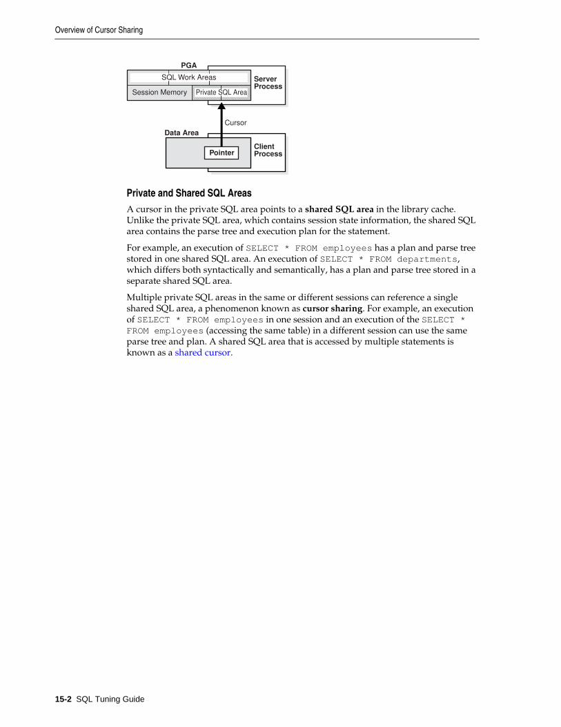
PGA
SQL Work Areas
Cursor
Data Area
Server
Process
Client
Process
Session Memory Private SQL Area
Pointer
Private and Shared SQL AreasA cursor in the private SQL area points to a shared SQL area in the library cache.Unlike the private SQL area, which contains session state information, the shared SQLarea contains the parse tree and execution plan for the statement.
For example, an execution of SELECT * FROM employees has a plan and parse treestored in one shared SQL area. An execution of SELECT * FROM departments,which differs both syntactically and semantically, has a plan and parse tree stored in aseparate shared SQL area.
Multiple private SQL areas in the same or different sessions can reference a singleshared SQL area, a phenomenon known as cursor sharing. For example, an executionof SELECT * FROM employees in one session and an execution of the SELECT *FROM employees (accessing the same table) in a different session can use the sameparse tree and plan. A shared SQL area that is accessed by multiple statements isknown as a shared cursor.
Overview of Cursor Sharing
15-2 SQL Tuning Guide

System Global Area (SGA)
Instance
Shared Pool
Private �SQL Area�(Shared�Server Only)
Shared SQL Area
Library Cache
Data Dictionary Cache
Server Result Cache
Other Reserved Pool
SELECT * FROM employees
Client Process
Server Process
PGA
Session Memory Private SQL Area
SQL Work Areas
SELECT * FROM employees
Client Process
Server Process
PGA
Session Memory Private SQL Area
SQL Work Areas
SELECT * FROM employees
Oracle Database automatically determines whether the SQL statement or PL/SQLblock being issued is identical to another statement currently in the library cache,using the following steps:
1. The text of the statement is hashed.
2. If no matching hash value exists, then the SQL statement does not currently existin the shared pool, so the database performs a hard parse.
3. The database looks for a matching hash value for an existing SQL statement in theshared pool. The following options are possible:
• No matching hash value exists.
In this case, the SQL statement does not currently exist in the shared pool, sothe database performs a hard parse. This ends the shared pool check.
• A matching hash value exists.
In this case, the database compares the text of the matched statement to the textof the hashed statement to see if they are identical. The text of the SQLstatements or PL/SQL blocks must be identical, character for character,including spaces, case, and comments. For example, the following statementscannot use the same shared SQL area:
SELECT * FROM employees;SELECT * FROM Employees;SELECT * FROM employees;
Overview of Cursor Sharing
Improving Real-World Performance Through Cursor Sharing 15-3

Usually, SQL statements that differ only in literals cannot use the same sharedSQL area. For example, the following statements do not resolve to the sameSQL area:
SELECT count(1) FROM employees WHERE manager_id = 121;SELECT count(1) FROM employees WHERE manager_id = 247;
The only exception to this rule is when the parameter CURSOR_SHARING hasbeen set to FORCE, in which case similar statements can share SQL areas. Thecosts involved in using CURSOR_SHARING are explained in “Do Not UseCURSOR_SHARING = FORCE as a Permanent Fix”.
4. The database compares objects referenced in the issued statement to thereferenced objects of all existing statements in the pool to ensure that they areidentical.
References to schema objects in the SQL statements or PL/SQL blocks mustresolve to the same object in the same schema. For example, if two users issue thefollowing SQL statement, and if each user has its own employees table, then thefollowing statement is not identical because the statement references differentemployees tables for each user:
SELECT * FROM employees;
5. The database determines whether bind variables in the SQL statements match inname, data type, and length.
For example, the following statements cannot use the same shared SQL areabecause the bind variable names differ:
SELECT * FROM employees WHERE department_id = :department_id;SELECT * FROM employees WHERE department_id = :dept_id;
6. The database determines whether the session environment is identical.
For example, SQL statements must be optimized using the same optimizer goal(see “Choosing an Optimizer Goal”).
See Also:
Oracle Database Reference to learn more about the CURSOR_SHARINGinitialization parameter
Parent and Child CursorsEvery parsed SQL statement has a parent cursor and one or more child cursors. Theparent cursor stores the text of the SQL statement. If the text of two statements isidentical, then the statements share the same parent cursor. If the text is different,however, then the database creates a separate parent cursor.
Example 15-1 Parent Cursors
In this example, the first two statements are syntactically different (the letter “c” islowercase in the first statement and uppercase in the second statement), butsemantically identical. Because of the syntactic difference, these statements havedifferent parent cursors. The third statement is syntactically identical to the firststatement (lowercase “c”), but semantically different because it refers to a customerstable in a different schema. Because of the syntactic identity, the third statement canshare a parent cursor with the first statement.
Overview of Cursor Sharing
15-4 SQL Tuning Guide

SQL> CONNECT oe@inst1Enter password: *******Connected.SQL> SELECT COUNT(*) FROM customers;
COUNT(*)---------- 319
SQL> SELECT COUNT(*) FROM Customers;
COUNT(*)---------- 319
SQL> CONNECT sh@inst1Enter password: *******Connected.SQL> SELECT COUNT(*) FROM customers;
COUNT(*)---------- 155500
The following query of V$SQL indicates the two parents. The statement with the SQLID of 8h916vv2yw400, which is the lowercase “c” version of the statement, has oneparent cursor and two child cursors: child 0 and child 1. The statement with the SQLID of 5rn2uxjtpz0wd, which is the uppercase “c” version of the statement, has adifferent parent cursor and only one child cursor: child 0.
SQL> CONNECT SYSTEM@inst1Enter password: *******Connected.
SQL> COL SQL_TEXT FORMAT a30SQL> COL CHILD# FORMAT 99999SQL> COL EXEC FORMAT 9999SQL> COL SCHEMA FORMAT a6SQL> SELECT SQL_ID, PARSING_SCHEMA_NAME AS SCHEMA, SQL_TEXT, 2 CHILD_NUMBER AS CHILD#, EXECUTIONS AS EXEC FROM V$SQL 3 WHERE SQL_TEXT LIKE '%ustom%' AND SQL_TEXT NOT LIKE '%SQL_TEXT%' ORDER BY SQL_ID;
SQL_ID SCHEMA SQL_TEXT CHILD# EXEC------------- ------ ------------------------------ ------ -----5rn2uxjtpz0wd OE SELECT COUNT(*) FROM Customers 0 18h916vv2yw400 OE SELECT COUNT(*) FROM customers 0 18h916vv2yw400 SH SELECT COUNT(*) FROM customers 1 1
Parent Cursors and V$SQLAREA
The V$SQLAREA view contains one row for every parent cursor.
In the following example, a query of V$SQLAREA shows two parent cursors, eachidentified with a different SQL_ID. The VERSION_COUNT indicates the number ofchild cursors.
COL SQL_TEXT FORMAT a30SELECT SQL_TEXT, SQL_ID, VERSION_COUNT, HASH_VALUEFROM V$SQLAREAWHERE SQL_TEXT LIKE '%mployee%'AND SQL_TEXT NOT LIKE '%SQL_TEXT%';
Overview of Cursor Sharing
Improving Real-World Performance Through Cursor Sharing 15-5

SQL_TEXT SQL_ID VERSION_COUNT HASH_VALUE------------------------------ ------------- ------------- ----------SELECT * FROM Employees 5bzhzpaa0wy9m 1 2483976499SELECT * FROM employees 4959aapufrm1k 2 1961610290
In the preceding output, the VERSION_COUNT of 2 for SELECT * FROM employeesindicates multiple child cursors, which were necessary because the statement wasexecuted against two different objects. In contrast, the statement SELECT * FROMEmployees (note the capital "E") was executed once, and so has one parent cursor,and one child cursor (VERSION_COUNT of 1).
Child Cursors and V$SQL
Every parent cursor has one or more child cursors. A child cursor contains theexecution plan, bind variables, metadata about objects referenced in the query,optimizer environment, and other information. In contrast to the parent cursor, thechild cursor does not store the text of the SQL statement.
V$SQL describes the statements that currently reside in the library cache. It containsone row for every child cursor, as shown in the following example:
SELECT SQL_TEXT, SQL_ID, USERNAME AS USR, CHILD_NUMBER AS CHILD#, HASH_VALUE, PLAN_HASH_VALUE AS PLAN_HASHVFROM V$SQL s, DBA_USERS dWHERE SQL_TEXT LIKE '%mployee%'AND SQL_TEXT NOT LIKE '%SQL_TEXT%'AND d.USER_ID = s.PARSING_USER_ID;
SQL_TEXT SQL_ID USR CHILD# HASH_VALUE PLAN_HASHV----------------------- ------------- --- ------ ---------- ----------SELECT * FROM Employees 5bzhzpaa0wy9m HR 0 2483976499 1445457117SELECT * FROM employees 4959aapufrm1k HR 0 1961610290 1445457117SELECT * FROM employees 4959aapufrm1k SH 1 1961610290 1445457117
In the preceding results, the CHILD# of the bottom two statements is different (0 and1), even though the SQL_ID is the same. This means that the statements have the sameparent cursor, but different child cursors. In contrast, the statement with the SQL_IDof 5bzhzpaa0wy9m has one parent and one child (CHILD# of 0). All three SQLstatements use the same execution plan, as indicated by identical values in thePLAN_HASH_VALUE column.
Cursor Mismatches and V$SQL_SHARED_CURSOR
If a parent cursor has multiple children, then the V$SQL_SHARED_CURSOR viewprovides information about why the cursor was not shared. For several types ofincompatibility, the a column indicates a mismatch with the value Y or N.
Example 15-2 Translation Mismatch
In this example, the TRANSLATION_MISMATCH column shows that the two statements(SELECT * FROM employees) referenced different objects, resulting in aTRANSLATION_MISMATCH value of Y for the last statement. Because sharing was notpossible, each statement had a separate child cursor, as indicated by CHILD_NUMBERof 0 and 1.
SELECT S.SQL_TEXT, S.CHILD_NUMBER, s.CHILD_ADDRESS, C.TRANSLATION_MISMATCHFROM V$SQL S, V$SQL_SHARED_CURSOR CWHERE SQL_TEXT LIKE '%employee%'AND SQL_TEXT NOT LIKE '%SQL_TEXT%'
Overview of Cursor Sharing
15-6 SQL Tuning Guide

AND S.CHILD_ADDRESS = C.CHILD_ADDRESS;
SQL_TEXT CHILD_NUMBER CHILD_ADDRESS T------------------------------ ------------ ---------------- -SELECT * FROM employees 0 0000000081EE8690 NSELECT * FROM employees 1 0000000081F22508 Y
About Cursors and ParsingIf an application issues a statement, and if Oracle Database cannot reuse a cursor, thenit must build a new executable version of the application code. This operation isknown as a hard parse.
A soft parse is any parse that is not a hard parse, and occurs when the database canreuse existing code (see “Shared Pool Check”). Some soft parses are less resource-intensive than others. For example, if a parent cursor for the statement already exists,then Oracle Database can perform various optimizations, and then store the childcursor in the shared SQL area. If a parent cursor does not exist, however, then OracleDatabase must also store the parent cursor in the shared SQL area, which createsadditional memory overhead.
Effectively, a hard parse recompiles a statement before running it. Hard parsing a SQLstatement before every execution is analogous to recompiling a C program beforeevery execution. A hard parse performs operations such as the following:
• Checking the syntax of the SQL statement
• Checking the semantics of the SQL statement
• Checking the access rights of the user issuing the statement
• Creating an execution plan
• Accessing the library cache and data dictionary cache numerous times to check thedata dictionary
An especially resource-intensive aspect of hard parsing is accessing the library cacheand data dictionary cache numerous times to check the data dictionary. When thedatabase accesses these areas, it uses a serialization device called a latch on requiredobjects so that their definition does not change during the check. Latch contentionincreases statement execution time and decreases concurrency.
For all of the preceding reasons, the CPU and memory overhead of hard parses cancreate serious performance problems. The problems are especially evident in webapplications that accept user input from a form, and then generate SQL statementsdynamically. The Real-World Performance group strongly recommends reducing hardparsing as much as possible.
Video:
RWP #3: Connection Pools and Hard Parsing
Example 15-3 Finding Parse Information Using V$SQL
You can use various techniques to monitor hard and soft parsing. This examplequeries the session statistics to determine whether repeated executions of a DBA_JOBSquery increase tehu hard parse count. The first execution of the statement increases the
Overview of Cursor Sharing
Improving Real-World Performance Through Cursor Sharing 15-7

hard parse count to 49, but the second execution does not change the hard parsecount, which means that Oracle Database reused application code.
SQL> ALTER SYSTEM FLUSH SHARED_POOL;
System altered.
SQL> COL NAME FORMAT a18
SQL> SELECT s.NAME, m.VALUE 2 FROM V$STATNAME s, V$MYSTAT m 3 WHERE s.STATISTIC# = m.STATISTIC# 4 AND s.NAME LIKE '%(hard%';
NAME VALUE------------------ ----------parse count (hard) 48
SQL> SELECT COUNT(*) FROM DBA_JOBS;
COUNT(*)---------- 0
SQL> SELECT s.NAME, m.VALUE 2 FROM V$STATNAME s, V$MYSTAT m 3 WHERE s.STATISTIC# = m.STATISTIC# 4 AND s.NAME LIKE '%(hard%';
NAME VALUE------------------ ----------parse count (hard) 49
SQL> SELECT COUNT(*) FROM DBA_JOBS;
COUNT(*)---------- 0
SQL> SELECT s.NAME, m.VALUE 2 FROM V$STATNAME s, V$MYSTAT m 3 WHERE s.STATISTIC# = m.STATISTIC# 4 AND s.NAME LIKE '%(hard%';
NAME VALUE------------------ ----------parse count (hard) 49
Example 15-4 Finding Parse Information Using Trace Files
This example uses SQL Trace and the TKPROF utility to find parse information.Assume that you log in to the database with administrator privileges, and run thefollowing statements, using TRACEFILE_IDENTIFIER to give the trace file ameaningful name:
ALTER SESSION SET sql_trace=TRUE;ALTER SESSION SET TRACEFILE_IDENTIFIER = "emp_stmt";ALTER SESSION SET EVENTS '10053 trace name context forever, level 12';SELECT * FROM hr.employees;EXIT;
Overview of Cursor Sharing
15-8 SQL Tuning Guide

The following query shows the directory location of the trace files
SQL> SET LINESIZE 120COLUMN value FORMAT A80
SELECT valueFROM v$diag_infoWHERE name = 'Default Trace File';VALUE--------------------------------------------------------------------------------/disk1/oracle/log/diag/rdbms/orcl/orcl/trace/orcl_ora_23054.trc
You can search this directory for the trace file that you generated:
% ls *emp_stmt.trcorcl_ora_17950_emp_stmt.trc
Use TKPROF to format the trace file, and then open the formatted file:
% tkprof orcl_ora_17950_emp_stmt.trc emp.out; vi emp.out
The formatted trace file contains the parse information for the query ofhr.employees.
SQL ID: brmjpfs7dcnub Plan Hash: 1445457117
SELECT *FROM hr.employees
call count cpu elapsed disk query current rows------- ------ -------- ---------- ---------- ---------- ---------- ----------Parse 1 0.07 0.08 0 0 0 0Execute 1 0.00 0.00 0 0 0 0Fetch 9 0.00 0.00 3 12 0 107------- ------ -------- ---------- ---------- ---------- ---------- ----------total 11 0.07 0.08 3 12 0 107
Misses in library cache during parse: 1Optimizer mode: ALL_ROWSParsing user id: SYSTEMNumber of plan statistics captured: 1
Rows (1st) Rows (avg) Rows (max) Row Source Operation---------- ---------- ---------- --------------------------------------------------- 107 107 107 TABLE ACCESS FULL EMPLOYEES (cr=12 pr=3 pw=0 time=497 us starts=1 cost=2 size=7383 card=107)
A library cache miss indicates a hard parse. Performing the same steps for a secondexecution of the same statement produces the following trace output, which shows nolibrary cache misses:
SQL ID: brmjpfs7dcnub Plan Hash: 1445457117
SELECT *FROM hr.employees
call count cpu elapsed disk query current rows
Overview of Cursor Sharing
Improving Real-World Performance Through Cursor Sharing 15-9

------- ------ -------- ---------- ---------- ---------- ---------- ----------Parse 1 0.00 0.00 0 0 0 0Execute 1 0.00 0.00 0 0 0 0Fetch 9 0.00 0.00 3 12 0 107------- ------ -------- ---------- ---------- ---------- ---------- ----------total 11 0.00 0.00 3 12 0 107
Misses in library cache during parse: 0Optimizer mode: ALL_ROWSParsing user id: SYSTEMNumber of plan statistics captured: 1
Rows (1st) Rows (avg) Rows (max) Row Source Operation---------- ---------- ---------- --------------------------------------------------- 107 107 107 TABLE ACCESS FULL EMPLOYEES (cr=12 pr=3 pw=0 time=961 us starts=1 cost=2 size=7383 card=107)
About Literals and Bind Variables
This section contains the following topics:
• Literals and Cursors
• Bind Variables and Cursors
• Bind Variable Peeking
Literals and CursorsWhen constructing SQL statements, some Oracle applications use literals instead ofbind variables. For example, the statement SELECT SUM(salary) FROMhr.employees WHERE employee_id < 101 uses the literal value 101 for theemployee ID. By default, when similar statements do not use bind variables, OracleDatabase cannot take advantage of cursor sharing. Thus, Oracle Database sees astatement that is identical except for the value 102, or any other random value, as acompletely new statement, requiring a hard parse.
Through decades of experience, the Real-World Performance group has found thatapplications that use literals are a frequent cause of performance, scalability, andsecurity problems. In the real world, it is not uncommon for applications to be writtenquickly, without considering cursor sharing. A classic example is a “screen scraping”application that copies the contents out of a web form, and then concatenates strings toconstruct the SQL statement dynamically.
Major problems that result from using literal values include the following:
• Applications that concatenate literals input by an end user are prone to SQLinjection attacks. Only rewriting the applications to use bind variables eliminatesthis threat (see “Do Not Use CURSOR_SHARING = FORCE as a Permanent Fix”).
• If every statement is hard parsed, then cursors are not shared, and so the databasemust consume more memory to create the cursors.
• Oracle Database must latch the shared pool and library cache when hard parsing.As the number of hard parses increases, so does the number of processes waiting tolatch the shared pool. This situation decreases concurrency and increasescontention.
Overview of Cursor Sharing
15-10 SQL Tuning Guide

Video:
RWP #4: Bind Variables and Soft Parsing
Example 15-5 Literals and Cursor Sharing
Consider an application that executes the following statements, which differ only inliterals:
SELECT SUM(salary) FROM hr.employees WHERE employee_id < 101;SELECT SUM(salary) FROM hr.employees WHERE employee_id < 120;SELECT SUM(salary) FROM hr.employees WHERE employee_id < 165;
The following query of V$SQLAREA shows that the three statements require threedifferent parent cursors. As shown by VERSION_COUNT, each parent cursor requiresits own child cursor.
COL SQL_TEXT FORMAT a30SELECT SQL_TEXT, SQL_ID, VERSION_COUNT, HASH_VALUEFROM V$SQLAREAWHERE SQL_TEXT LIKE '%mployee%'AND SQL_TEXT NOT LIKE '%SQL_TEXT%';
SQL_TEXT SQL_ID VERSION_COUNT HASH_VALUE------------------------------ ------------- ------------- ----------SELECT SUM(salary) FROM hr.emp b1tvfcc5qnczb 1 191509483loyees WHERE employee_id < 165SELECT SUM(salary) FROM hr.emp cn5250y0nqpym 1 2169198547loyees WHERE employee_id < 101SELECT SUM(salary) FROM hr.emp au8nag2vnfw67 1 3074912455loyees WHERE employee_id < 120
Bind Variables and CursorsYou can develop Oracle applications to use bind variables instead of literals. A bindvariable is a placeholder in a query. For example, the statement SELECTSUM(salary) FROM hr.employees WHERE employee_id < :emp_id uses thebind variable:emp_id for the employee ID.
The Real-World Performance group has found that applications that use bindvariables perform better, are more scalable, and are more secure. Major benefits thatresult from using bind variables include the following:
• Applications that use bind variables are not vulnerable to the same SQL injectionattacks as applications that use literals.
• When identical statements use bind variables, Oracle Database can take advantageof cursor sharing, and share the plan and other information when different valuesare bound to the same statement.
• Oracle Database avoids the overhead of latching the shared pool and library cacherequired for hard parsing.
Video:
RWP #4: Bind Variables and Soft Parsing
Overview of Cursor Sharing
Improving Real-World Performance Through Cursor Sharing 15-11
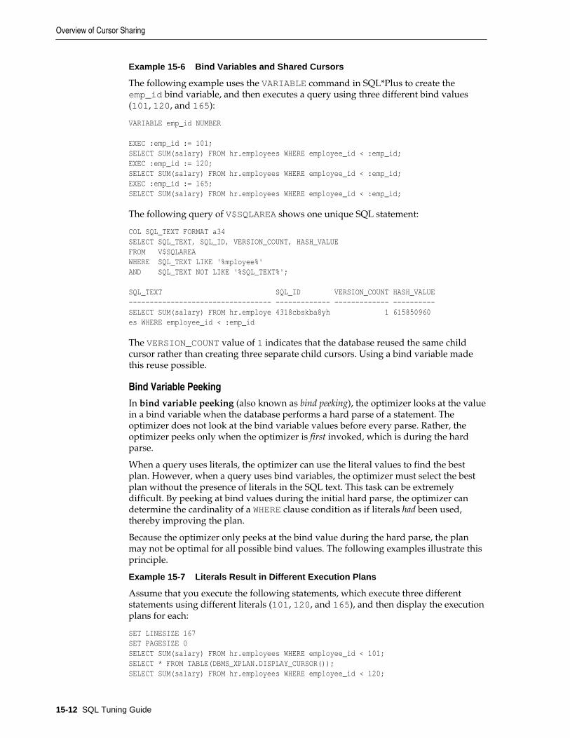
Example 15-6 Bind Variables and Shared Cursors
The following example uses the VARIABLE command in SQL*Plus to create theemp_id bind variable, and then executes a query using three different bind values(101, 120, and 165):
VARIABLE emp_id NUMBER
EXEC :emp_id := 101;SELECT SUM(salary) FROM hr.employees WHERE employee_id < :emp_id;EXEC :emp_id := 120;SELECT SUM(salary) FROM hr.employees WHERE employee_id < :emp_id;EXEC :emp_id := 165;SELECT SUM(salary) FROM hr.employees WHERE employee_id < :emp_id;
The following query of V$SQLAREA shows one unique SQL statement:
COL SQL_TEXT FORMAT a34SELECT SQL_TEXT, SQL_ID, VERSION_COUNT, HASH_VALUEFROM V$SQLAREAWHERE SQL_TEXT LIKE '%mployee%'AND SQL_TEXT NOT LIKE '%SQL_TEXT%';
SQL_TEXT SQL_ID VERSION_COUNT HASH_VALUE---------------------------------- ------------- ------------- ----------SELECT SUM(salary) FROM hr.employe 4318cbskba8yh 1 615850960es WHERE employee_id < :emp_id
The VERSION_COUNT value of 1 indicates that the database reused the same childcursor rather than creating three separate child cursors. Using a bind variable madethis reuse possible.
Bind Variable PeekingIn bind variable peeking (also known as bind peeking), the optimizer looks at the valuein a bind variable when the database performs a hard parse of a statement. Theoptimizer does not look at the bind variable values before every parse. Rather, theoptimizer peeks only when the optimizer is first invoked, which is during the hardparse.
When a query uses literals, the optimizer can use the literal values to find the bestplan. However, when a query uses bind variables, the optimizer must select the bestplan without the presence of literals in the SQL text. This task can be extremelydifficult. By peeking at bind values during the initial hard parse, the optimizer candetermine the cardinality of a WHERE clause condition as if literals had been used,thereby improving the plan.
Because the optimizer only peeks at the bind value during the hard parse, the planmay not be optimal for all possible bind values. The following examples illustrate thisprinciple.
Example 15-7 Literals Result in Different Execution Plans
Assume that you execute the following statements, which execute three differentstatements using different literals (101, 120, and 165), and then display the executionplans for each:
SET LINESIZE 167SET PAGESIZE 0SELECT SUM(salary) FROM hr.employees WHERE employee_id < 101;SELECT * FROM TABLE(DBMS_XPLAN.DISPLAY_CURSOR());SELECT SUM(salary) FROM hr.employees WHERE employee_id < 120;
Overview of Cursor Sharing
15-12 SQL Tuning Guide

SELECT * FROM TABLE(DBMS_XPLAN.DISPLAY_CURSOR());SELECT SUM(salary) FROM hr.employees WHERE employee_id < 165;SELECT * FROM TABLE(DBMS_XPLAN.DISPLAY_CURSOR());
The database hard parsed all three statements, which were not identical. TheDISPLAY_CURSOR output, which has been edited for clarity, shows that the optimizerchose the same nested loops plan for the first two statements, but a full table scan planfor the statement using literal 165:
SQL_ID cn5250y0nqpym, child number 0-------------------------------------SELECT SUM(salary) FROM hr.employees WHERE employee_id < 101
Plan hash value: 2410354593
-------------------------------------------------------------------------------------|Id| Operation | Name |Rows|Bytes|Cost(%CPU)|Time|--------------------------------------------------------------------------------------| 0| SELECT STATEMENT | | | |2 (100)| || 1| SORT AGGREGATE | |1 | 8 | | || 2| TABLE ACCESS BY INDEX ROWID BATCHED| EMPLOYEES |1 | 8 |2 (0) | 00:00:01 ||*3| INDEX RANGE SCAN | EMP_EMP_ID_PK |1 | |1 (0) | 00:00:01 |-------------------------------------------------------------------------------------Predicate Information (identified by operation id):---------------------------------------------------
3 - access("EMPLOYEE_ID"<101)
SQL_ID au8nag2vnfw67, child number 0-------------------------------------SELECT SUM(salary) FROM hr.employees WHERE employee_id < 120
Plan hash value: 2410354593
-------------------------------------------------------------------------------------|Id| Operation | Name |Rows|Bytes|Cost(%CPU)|Time|-------------------------------------------------------------------------------------| 0| SELECT STATEMENT | | | |2 (100)| || 1| SORT AGGREGATE | |1 | 8 | | || 2| TABLE ACCESS BY INDEX ROWID BATCHED| EMPLOYEES |20|160|2 (0) | 00:00:01 ||*3| INDEX RANGE SCAN | EMP_EMP_ID_PK |20| |1 (0) | 00:00:01 |-------------------------------------------------------------------------------------
Predicate Information (identified by operation id):---------------------------------------------------
3 - access("EMPLOYEE_ID"<120)
SQL_ID b1tvfcc5qnczb, child number 0-------------------------------------SELECT SUM(salary) FROM hr.employees WHERE employee_id < 165
Plan hash value: 1756381138
-------------------------------------------------------------------------| Id | Operation | Name |Rows| Bytes |Cost(%CPU)| Time |-------------------------------------------------------------------------| 0 | SELECT STATEMENT | | | | 2 (100)| || 1 | SORT AGGREGATE | | 1 | 8 | | ||* 2 | TABLE ACCESS FULL| EMPLOYEES | 66 | 528 | 2 (0)| 00:00:01 |
Overview of Cursor Sharing
Improving Real-World Performance Through Cursor Sharing 15-13

-------------------------------------------------------------------------
Predicate Information (identified by operation id):---------------------------------------------------
2 - filter("EMPLOYEE_ID"<165)
The preceding output shows that the optimizer considers a full table scan moreefficient than an index scan for the query that returns more rows.
Example 15-8 Bind Variables Result in Cursor Reuse
This example rewrites the queries executed in Example 15-7 to use bind variablesinstead of literals. You bind the same values (101, 120, and 165) to the bindvariable :emp_id, and then display the execution plans for each:
VAR emp_id NUMBER
EXEC :emp_id := 101;SELECT SUM(salary) FROM hr.employees WHERE employee_id < :emp_id;SELECT * FROM TABLE(DBMS_XPLAN.DISPLAY_CURSOR());EXEC :emp_id := 120;SELECT SUM(salary) FROM hr.employees WHERE employee_id < :emp_id;SELECT * FROM TABLE(DBMS_XPLAN.DISPLAY_CURSOR());EXEC :emp_id := 165;SELECT SUM(salary) FROM hr.employees WHERE employee_id < :emp_id;SELECT * FROM TABLE(DBMS_XPLAN.DISPLAY_CURSOR());
The DISPLAY_CURSOR output shows that the optimizer chose exactly the same planfor all three statements:
SELECT SUM(salary) FROM hr.employees WHERE employee_id < :emp_id
Plan hash value: 2410354593
-------------------------------------------------------------------------------------| Id | Operation | Name |Rows|Bytes|Cost (%CPU)|Time|-------------------------------------------------------------------------------------| 0 | SELECT STATEMENT | | | |2 (100)| || 1 | SORT AGGREGATE | |1|8 | | || 2 | TABLE ACCESS BY INDEX ROWID BATCHED| EMPLOYEES |1|8 | 2 (0)| 00:00:01 ||* 3 | INDEX RANGE SCAN | EMP_EMP_ID_PK |1| | 1 (0)| 00:00:01 |-------------------------------------------------------------------------------------
Predicate Information (identified by operation id):---------------------------------------------------
3 - access("EMPLOYEE_ID"<:EMP_ID)
In contrast, when the preceding statements were executed with literals, the optimizerchose a lower-cost full table scan when the employee ID value was 165. This is theproblem solved by adaptive cursor sharing (see “Adaptive Cursor Sharing”).
CURSOR_SHARING and Bind Variable SubstitutionThis topic explains what the CURSOR_SHARING initialization parameter is, and howsetting it to different values affects how Oracle Database uses bind variables.
This section contains the following topics:
CURSOR_SHARING and Bind Variable Substitution
15-14 SQL Tuning Guide

CURSOR_SHARING Initialization ParameterThe CURSOR_SHARING initialization parameter controls how the database processesstatements with bind variables.
In Oracle Database 12c, the parameter supports the following values:
• EXACT
This is the default value. The database enables only textually identical statementsto share a cursor. The database does not attempt to replace literal values withsystem-generated bind variables. In this case, the optimizer generates a plan foreach statement based on the literal value.
• FORCE
The database replaces all literals with system-generated bind variables. Forstatements that are identical after the bind variables replace the literals, theoptimizer uses the same plan.
Note:
The SIMILAR value for CURSOR_SHARING is deprecated.
You can set CURSOR_SHARING at the system or session level, or use theCURSOR_SHARING_EXACT hint at the statement level.
See Also:
“Do Not Use CURSOR_SHARING = FORCE as a Permanent Fix”
Parsing Behavior When CURSOR_SHARING = FORCEWhen SQL statements use literals rather than bind variables, setting theCURSOR_SHARING initialization parameter to FORCE enables the database to replaceliterals with system-generated bind variables. Using this technique, the database cansometimes reduce the number of parent cursors in the shared SQL area.
Note:
If a statement uses an ORDER BY clause, then the database does not performliteral replacement in the clause because it is not semantically correct toconsider the constant column number as a literal. The column number in theORDER BY clause affects the query plan and execution, so the database cannotshare two cursors having different column numbers.
When CURSOR_SHARING is set to FORCE, the database performs the following stepsduring the parse:
1. Copies all literals in the statement to the PGA, and replaces them with system-generated bind variables
For example, an application could process the following statement:
CURSOR_SHARING and Bind Variable Substitution
Improving Real-World Performance Through Cursor Sharing 15-15

SELECT SUBSTR(last_name, 1, 4), SUM(salary) FROM hr.employees WHERE employee_id < 101 GROUP BY last_name
The optimizer replaces literals, including the literals in the SUBSTR function, asfollows:
SELECT SUBSTR(last_name, :"SYS_B_0", :"SYS_B_1"), SUM(salary) FROM hr.employees WHERE employee_id < :"SYS_B_2" GROUP BY last_name
2. Searches for an identical statement (same SQL hash value) in the shared pool
If an identical statement is not found, then the database performs a hard parse.Otherwise, the database proceeds to the next step.
3. Performs a soft parse of the statement
As the preceding steps indicate, setting the CURSOR_SHARING initialization parameterto FORCE does not reduce the parse count. Rather, in some cases, FORCE enables thedatabase to perform a soft parse instead of a hard parse. Also, FORCE does not theprevent against SQL injection attacks because Oracle Database binds the values afterany injection has already occurred.
Example 15-9 Replacement of Literals with System Bind Variables
This example sets CURSOR_SHARING to FORCE at the session level, executes threestatements containing literals, and displays the plan for each statement:
ALTER SESSION SET CURSOR_SHARING=FORCE;SET LINESIZE 170SET PAGESIZE 0SELECT SUM(salary) FROM hr.employees WHERE employee_id < 101;SELECT * FROM TABLE(DBMS_XPLAN.DISPLAY_CURSOR());SELECT SUM(salary) FROM hr.employees WHERE employee_id < 120;SELECT * FROM TABLE(DBMS_XPLAN.DISPLAY_CURSOR());SELECT SUM(salary) FROM hr.employees WHERE employee_id < 165;SELECT * FROM TABLE(DBMS_XPLAN.DISPLAY_CURSOR());
The following DISPLAY_CURSOR output, edited for readability, shows that all threestatements used the same plan. The optimizer chose the plan, an index range scan,because it peeked at the first value (101) bound to the system bind variable, andpicked this plan as the best for all values. In fact, this plan is not the best plan for allvalues. When the value is 165, a full table scan is more efficient.
SQL_ID cxx8n1cxr9khn, child number 0-------------------------------------SELECT SUM(salary) FROM hr.employees WHERE employee_id < :"SYS_B_0"
Plan hash value: 2410354593
-------------------------------------------------------------------------------------| Id | Operation | Name |Rows|Bytes|Cost(%CPU)|Time|-------------------------------------------------------------------------------------| 0 | SELECT STATEMENT | | | |2 (100)| || 1 | SORT AGGREGATE | |1 | 8 | | || 2 | TABLE ACCESS BY INDEX ROWID BATCHED| EMPLOYEES |1 | 8 |2 (0) |00:00:01||* 3 | INDEX RANGE SCAN | EMP_EMP_ID_PK |1 | |1 (0) |00:00:01|-------------------------------------------------------------------------------------Predicate Information (identified by operation id):---------------------------------------------------
CURSOR_SHARING and Bind Variable Substitution
15-16 SQL Tuning Guide

3 - access("EMPLOYEE_ID"<101)
A query of V$SQLAREA confirms that Oracle Database replaced with the literal withsystem bind variable :”SYS_B_0”, and created one parent and one child cursor(VERSION_COUNT=1) for all three statements, which means that all executions sharedthe same plan.
COL SQL_TEXT FORMAT a36SELECT SQL_TEXT, SQL_ID, VERSION_COUNT, HASH_VALUEFROM V$SQLAREAWHERE eee_TEXT LIKE '%mployee%'AND SQL_TEXT NOT LIKE '%SQL_TEXT%';
SQL_TEXT SQL_ID VERSION_COUNT HASH_VALUE------------------------------------ ------------- ------------- ----------SELECT SUM(salary) FROM hr.employees cxx8n1cxr9khn 1 997509652 WHERE employee_id < :"SYS_B_0"
See Also:
• “Private and Shared SQL Areas” for more details on the various checksperformed
• Oracle Database Reference to learn about the CURSOR_SHARING initializationparameter
Adaptive Cursor SharingThe adaptive cursor sharing feature enables a single statement that contains bindvariables to use multiple execution plans. Cursor sharing is "adaptive" because thecursor adapts its behavior so that the database does not always use the same plan foreach execution or bind variable value.
This section contains the following topics:
• Purpose of Adaptive Cursor Sharing
• How Adaptive Cursor Sharing Works: Example
• Bind-Sensitive Cursors
• Bind-Aware Cursors
• Cursor Merging
• Adaptive Cursor Sharing Views
Purpose of Adaptive Cursor SharingWith bind peeking, the optimizer peeks at the values of user-defined bind variables onthe first invocation of a cursor. The optimizer determines the cardinality of any WHEREclause condition as if literals had been used instead of bind variables. If a column in aWHERE clause has skewed data, however, then a histogram may exist on this column.When the optimizer peeks at the value of the user-defined bind variable and chooses aplan, this plan may not be good for all values.
Adaptive Cursor Sharing
Improving Real-World Performance Through Cursor Sharing 15-17
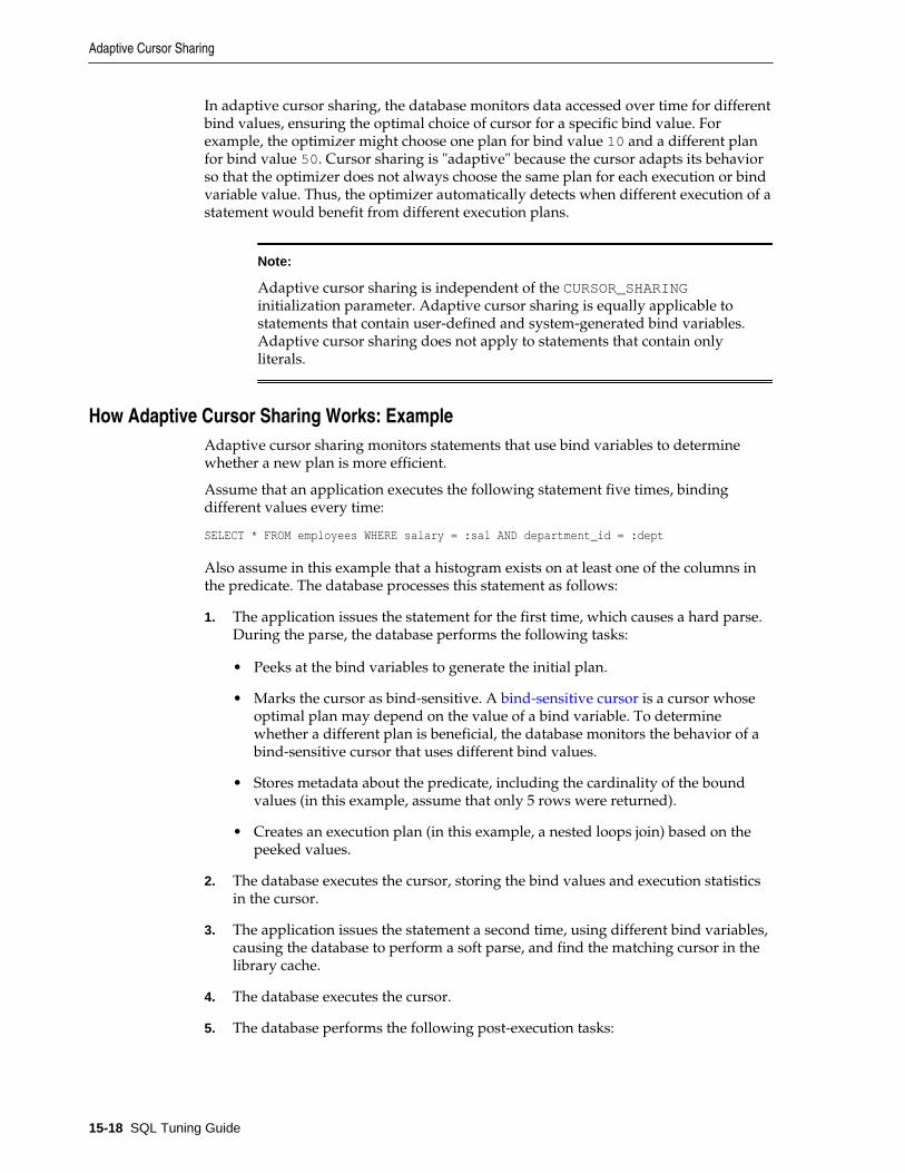
In adaptive cursor sharing, the database monitors data accessed over time for differentbind values, ensuring the optimal choice of cursor for a specific bind value. Forexample, the optimizer might choose one plan for bind value 10 and a different planfor bind value 50. Cursor sharing is "adaptive" because the cursor adapts its behaviorso that the optimizer does not always choose the same plan for each execution or bindvariable value. Thus, the optimizer automatically detects when different execution of astatement would benefit from different execution plans.
Note:
Adaptive cursor sharing is independent of the CURSOR_SHARINGinitialization parameter. Adaptive cursor sharing is equally applicable tostatements that contain user-defined and system-generated bind variables.Adaptive cursor sharing does not apply to statements that contain onlyliterals.
How Adaptive Cursor Sharing Works: ExampleAdaptive cursor sharing monitors statements that use bind variables to determinewhether a new plan is more efficient.
Assume that an application executes the following statement five times, bindingdifferent values every time:
SELECT * FROM employees WHERE salary = :sal AND department_id = :dept
Also assume in this example that a histogram exists on at least one of the columns inthe predicate. The database processes this statement as follows:
1. The application issues the statement for the first time, which causes a hard parse.During the parse, the database performs the following tasks:
• Peeks at the bind variables to generate the initial plan.
• Marks the cursor as bind-sensitive. A bind-sensitive cursor is a cursor whoseoptimal plan may depend on the value of a bind variable. To determinewhether a different plan is beneficial, the database monitors the behavior of abind-sensitive cursor that uses different bind values.
• Stores metadata about the predicate, including the cardinality of the boundvalues (in this example, assume that only 5 rows were returned).
• Creates an execution plan (in this example, a nested loops join) based on thepeeked values.
2. The database executes the cursor, storing the bind values and execution statisticsin the cursor.
3. The application issues the statement a second time, using different bind variables,causing the database to perform a soft parse, and find the matching cursor in thelibrary cache.
4. The database executes the cursor.
5. The database performs the following post-execution tasks:
Adaptive Cursor Sharing
15-18 SQL Tuning Guide

a. The database compares the execution statistics for the second execution withthe first-execution statistics.
b. The database observes the pattern of statistics over all previous executions,and then decides whether to mark the cursor as a bind-aware cursor. In thisexample, assume that the database decides the cursor is bind-aware.
6. The application issues the statement a third time, using different bind variables,which causes a soft parse. Because the cursor is bind-aware, the database does thefollowing:
• Determines whether the cardinality of the new values falls within the samerange as the stored cardinality. In this example, the cardinality is similar: 8rows instead of 5 rows.
• Reuses the execution plan in the existing child cursor.
7. The database executes the cursor.
8. The application issues the statement a fourth time, using different bind variables,causing a soft parse. Because the cursor is bind-aware, the database does thefollowing:
• Determines whether the cardinality of the new values falls within the samerange as the stored cardinality. In this example, the cardinality is vastlydifferent: 102 rows (in a table with 107 rows) instead of 5 rows.
• Does not find a matching child cursor.
9. The database performs a hard parse. As a result, the database does the following:
• Creates a new child cursor with a second execution plan (in this example, ahash join)
• Stores metadata about the predicate, including the cardinality of the boundvalues, in the cursor
10. The database executes the new cursor.
11. The database stores the new bind values and execution statistics in the new childcursor.
12. The application issues the statement a fifth time, using different bind variables,which causes a soft parse. Because the cursor is bind-aware, the database does thefollowing:
• Determines whether the cardinality of the new values falls within the samerange as the stored cardinality. In this example, the cardinality is 20.
• Does not find a matching child cursor.
13. The database performs a hard parse. As a result, the database does the following:
a. Creates a new child cursor with a third execution plan (in this example, anested loops join)
b. Determines that this nested loops join execution plan is the same as the nestedloops execution plan used for the first execution of the statement
Adaptive Cursor Sharing
Improving Real-World Performance Through Cursor Sharing 15-19

c. Merges the two child cursors containing nested loop plans, which involvesstoring the combined cardinality statistics into one child cursor, and deletingthe other one
14. The database executes the cursor using the nested loops execution plan.
Bind-Sensitive CursorsA bind-sensitive cursor is a cursor whose optimal plan may depend on the value of abind variable. The database has examined the bind value when computing cardinality,and considers the query “sensitive” to plan changes based on different bind values.The database monitors the behavior of a bind-sensitive cursor that uses different bindvalues to determine whether a different plan is beneficial.
The optimizer uses the following criteria to decide whether a cursor is bind-sensitive:
• The optimizer has peeked at the bind values to generate cardinality estimates.
• The bind is used in an equality or a range predicate.
For each execution of the query with a new bind value, the database records theexecution statistics for the new value and compares them to the execution statistics forthe previous value. If execution statistics vary greatly, then the database marks thecursor bind-aware.
Example 15-10 Column with Significant Data Skew
This example assumes that the hr.employees.department_id column hassignificant data skew. SYSTEM executes the following setup code, which adds 100,000employees in department 50 to the employees table in the sample schema, for a totalof 100,107 rows, and then gathers table statistics:
DELETE FROM hr.employees WHERE employee_id > 999;
ALTER TABLE hr.employees DISABLE NOVALIDATE CONSTRAINT emp_email_uk;
DECLAREv_counter NUMBER(7) := 1000;BEGIN FOR i IN 1..100000 LOOP INSERT INTO hr.employees VALUES (v_counter,null,'Doe','[email protected]',null,'07-JUN-02','AC_ACCOUNT',null,null,null,50); v_counter := v_counter + 1; END LOOP;END;/COMMIT;
EXEC DBMS_STATS.GATHER_TABLE_STATS ( ownname => 'hr', tabname => 'employees');
ALTER SYSTEM FLUSH SHARED_POOL;
The following query shows a histogram on the employees.department_idcolumn:
COL TABLE_NAME FORMAT a15COL COLUMN_NAME FORMAT a20COL HISTOGRAM FORMAT a9
SELECT TABLE_NAME, COLUMN_NAME, HISTOGRAM
Adaptive Cursor Sharing
15-20 SQL Tuning Guide

FROM DBA_TAB_COLSWHERE OWNER = 'HR'AND TABLE_NAME = 'EMPLOYEES'AND COLUMN_NAME = 'DEPARTMENT_ID';
TABLE_NAME COLUMN_NAME HISTOGRAM--------------- -------------------- ---------EMPLOYEES DEPARTMENT_ID FREQUENCY
Example 15-11 Low-Cardinality Query
This example continues the example in Example 15-10. The following query showsthat the value 10 has extremely low cardinality for the column department_id,occupying .00099% of the rows:
VARIABLE dept_id NUMBEREXEC :dept_id := 10;SELECT COUNT(*), MAX(employee_id) FROM hr.employees WHERE department_id = :dept_id;
COUNT(*) MAX(EMPLOYEE_ID)---------- ---------------- 1 200
The optimizer chooses an index range scan, as expected for such a low-cardinalityquery:
SQL> SELECT * FROM TABLE(DBMS_XPLAN.DISPLAY_CURSOR);
PLAN_TABLE_OUTPUT-------------------------------------SQL_ID a9upgaqqj7bn5, child number 0-------------------------------------select COUNT(*), MAX(employee_id) FROM hr.employees WHERE department_id = :dept_id
Plan hash value: 1642965905
-------------------------------------------------------------------------------------| Id| Operation | Name |Rows|Bytes|Cost (%CPU)|Time |-------------------------------------------------------------------------------------| 0| SELECT STATEMENT | | | |2(100)| || 1| SORT AGGREGATE | |1 |8 | | || 2| TABLE ACCESS BY INDEX ROWID BATCHED| EMPLOYEES |1 |8 |2 (0)|00:00:01||*3| INDEX RANGE SCAN | EMP_DEPARTMENT_IX |1 | |1 (0)|00:00:01|-------------------------------------------------------------------------------------
Predicate Information (identified by operation id):---------------------------------------------------
3 - access("DEPARTMENT_ID"=:DEPT_ID)
The following query of V$SQL obtains information about the cursor:
COL BIND_AWARE FORMAT a10COL SQL_TEXT FORMAT a22COL CHILD# FORMAT 99999COL EXEC FORMAT 9999COL BUFF_GETS FORMAT 999999999COL BIND_SENS FORMAT a9COL SHAREABLE FORMAT a9
SELECT SQL_TEXT, CHILD_NUMBER AS CHILD#, EXECUTIONS AS EXEC, BUFFER_GETS AS BUFF_GETS, IS_BIND_SENSITIVE AS BIND_SENS,
Adaptive Cursor Sharing
Improving Real-World Performance Through Cursor Sharing 15-21

IS_BIND_AWARE AS BIND_AWARE, IS_SHAREABLE AS SHAREABLEFROM V$SQLWHERE SQL_TEXT LIKE '%mployee%'AND SQL_TEXT NOT LIKE '%SQL_TEXT%';
SQL_TEXT CHILD# EXEC BUFF_GETS BIND_SENS BIND_AWARE SHAREABLE---------------------- ------ ----- ---------- --------- ---------- ---------SELECT COUNT(*), MAX(e 0 1 196 Y N Ymployee_id) FROM hr.employees WHERE department_id = :dept_id
The preceding output shows one child cursor that has been executed once for the low-cardinality query. The cursor has been marked bind-sensitive because the optimizerbelieves the optimal plan may depend on the value of the bind variable.
When a cursor is marked bind-sensitive, Oracle Database monitors the behavior of thecursor using different bind values, to determine whether a different plan for differentbind values is more efficient. The database marked this cursor bind-sensitive becausethe optimizer used the histogram on the department_id column to compute theselectivity of the predicate WHERE department_id = :dept_id. Because thepresence of the histogram indicates that the column is skewed, different values of thebind variable may require different plans.
Example 15-12 High-Cardinality Query
This example continues the example in Example 15-11. The following code re-executesthe same query using the value 50, which occupies 99.9% of the rows:
EXEC :dept_id := 50;SELECT COUNT(*), MAX(employee_id) FROM hr.employees WHERE department_id = :dept_id;
COUNT(*) MAX(EMPLOYEE_ID)---------- ---------------- 100045 100999
Even though such an unselective query would be more efficient with a full table scan,the optimizer chooses the same index range scan used for department_id=10. Thisreason is that the database assumes that the existing plan in the cursor can be shared:
SQL> SELECT * FROM TABLE(DBMS_XPLAN.DISPLAY_CURSOR);
PLAN_TABLE_OUTPUT-------------------------------------SQL_ID a9upgaqqj7bn5, child number 0-------------------------------------SELECT COUNT(*), MAX(employee_id) FROM hr.employees WHERE department_id = :dept_id
Plan hash value: 1642965905
-------------------------------------------------------------------------------------| Id| Operation | Name |Rows|Bytes|Cost (%CPU)|Time |-------------------------------------------------------------------------------------| 0| SELECT STATEMENT | | | |2(100)| || 1| SORT AGGREGATE | |1 |8 | | || 2| TABLE ACCESS BY INDEX ROWID BATCHED| EMPLOYEES |1 |8 |2 (0)|00:00:01||*3| INDEX RANGE SCAN | EMP_DEPARTMENT_IX |1 | |1 (0)|00:00:01|-------------------------------------------------------------------------------------
Predicate Information (identified by operation id):---------------------------------------------------
Adaptive Cursor Sharing
15-22 SQL Tuning Guide

3 - access("DEPARTMENT_ID"=:DEPT_ID)
A query of V$SQL shows that the child cursor has now been executed twice:
SELECT SQL_TEXT, CHILD_NUMBER AS CHILD#, EXECUTIONS AS EXEC, BUFFER_GETS AS BUFF_GETS, IS_BIND_SENSITIVE AS BIND_SENS, IS_BIND_AWARE AS BIND_AWARE, IS_SHAREABLE AS SHAREABLEFROM V$SQLWHERE SQL_TEXT LIKE '%mployee%'AND SQL_TEXT NOT LIKE '%SQL_TEXT%';
SQL_TEXT CHILD# EXEC BUFF_GETS BIND_SENS BIND_AWARE SHAREABLE---------------------- ------ ----- ---------- --------- ---------- ---------SELECT COUNT(*), MAX(e 0 2 1329 Y N Ymployee_id) FROM hr.employees WHERE department_id = :dept_id
At this stage, the optimizer has not yet marked the cursor as bind-aware.
See Also:
Oracle Database Reference to learn about V$SQL
Bind-Aware CursorsA bind-aware cursor is a bind-sensitive cursor that is eligible to use different plans fordifferent bind values. After a cursor has been made bind-aware, the optimizer choosesplans for future executions based on the bind value and its cardinality estimate. Thus,“bind-aware” means essentially “best plan for the current bind value.”
When a statement with a bind-sensitive cursor executes, the optimizer uses an internalalgorithm to determine whether to mark the cursor bind-aware. The decision dependson whether the cursor produces significantly different data access patterns fordifferent bind values, resulting in a performance cost that differs from expectations.
If the database marks the cursor bind-aware, then the next time that the cursorexecutes the database does the following:
• Generates a new plan based on the bind value
• Marks the original cursor generated for the statement as not sharable (V$SQL.IS_SHAREABLE is N). The original cursor is no longer usable and is eligibleto age out of the library cache
When the same query repeatedly executes with different bind values, the databaseadds new bind values to the “signature” of the SQL statement (which includes theoptimizer environment, NLS settings, and so on), and categorizes the values. Thedatabase examines the bind values, and considers whether the current bind valueresults in a significantly different data volume, or whether an existing plan issufficient. The database does not need to create a new plan for each new value.
Consider a scenario in which you execute a statement with 12 distinct bind values(executing each distinct value twice), which causes the database to trigger 5 hardparses, and create 2 additional plans. Because the database performs 5 hard parses, itcreates 5 new child cursors, even though some cursors have the same execution plan
Adaptive Cursor Sharing
Improving Real-World Performance Through Cursor Sharing 15-23

as existing cursors. The database marks the superfluous cursors as not usable, whichmeans these cursors eventually age out of the library cache.
During the initial hard parses, the optimizer is essentially mapping out therelationship between bind values and the appropriate execution plan. After this initialperiod, the database eventually reaches a steady state. Executing with a new bindvalue results in picking the best child cursor in the cache, without requiring a hardparse. Thus, the number of parses does not scale with the number of different bindvalues.
Example 15-13 Bind-Aware Cursors
This example continues the example in “Bind-Sensitive Cursors”. The following codeissues a second query employees with the bind variable set to 50:
EXEC :dept_id := 50;SELECT COUNT(*), MAX(employee_id) FROM hr.employees WHERE department_id = :dept_id;
COUNT(*) MAX(EMPLOYEE_ID)---------- ---------------- 100045 100999
During the first two executions, the database was monitoring the behavior of thequeries, and determined that the different bind values caused the queries to differsignificantly in cardinality. Based on this difference, the database adapts its behaviorso that the same plan is not always shared for this query. Thus, the optimizergenerates a new plan based on the current bind value, which is 50:
SQL> SELECT * FROM TABLE(DBMS_XPLAN.DISPLAY_CURSOR);
PLAN_TABLE_OUTPUT-------------------------------------SQL_ID a9upgaqqj7bn5, child number 1-------------------------------------SELECT COUNT(*), MAX(employee_id) FROM hr.employees WHERE department_id = :dept_id
Plan hash value: 1756381138
-----------------------------------------------------------------------------| Id | Operation | Name | Rows | Bytes | Cost(%CPU)| Time |-----------------------------------------------------------------------------| 0 | SELECT STATEMENT | | | |254 (100)| || 1 | SORT AGGREGATE | | 1 | 8 | | ||* 2 | TABLE ACCESS FULL| EMPLOYEES | 100K | 781K |254 (15)| 00:00:01 |-----------------------------------------------------------------------------Predicate Information (identified by operation id):---------------------------------------------------
2 - filter("DEPARTMENT_ID"=:DEPT_ID)
The following query of V$SQL obtains information about the cursor:
SELECT SQL_TEXT, CHILD_NUMBER AS CHILD#, EXECUTIONS AS EXEC, BUFFER_GETS AS BUFF_GETS, IS_BIND_SENSITIVE AS BIND_SENS, IS_BIND_AWARE AS BIND_AWARE, IS_SHAREABLE AS SHAREABLEFROM V$SQLWHERE SQL_TEXT LIKE '%mployee%'AND SQL_TEXT NOT LIKE '%SQL_TEXT%';
SQL_TEXT CHILD# EXEC BUFF_GETS BIND_SENS BIND_AWARE SHAREABLE---------------------- ------ ----- ---------- --------- ---------- ---------
Adaptive Cursor Sharing
15-24 SQL Tuning Guide

SELECT COUNT(*), MAX(e 0 2 1329 Y N Nmployee_id) FROM hr.employees WHERE department_id = :dept_id
SELECT COUNT(*), MAX(e 1 1 800 Y Y Ymployee_id) FROM hr.employees WHERE department_id = :dept_id
The preceding output shows that the database created an additional child cursor(CHILD# of 1). Cursor 0 is now marked as not shareable. Cursor 1 shows a number ofbuffers gets lower than cursor 0, and is marked both bind-sensitive and bind-aware. Abind-aware cursor may use different plans for different bind values, depending on theselectivity of the predicates containing the bind variable.
Example 15-14 Bind-Aware Cursors: Choosing the Optimal Plan
This example continues the example in “Example 15-13”. The following code executesthe same employees query with the value of 10, which has extremely low cardinality(only one row):
EXEC :dept_id := 10;SELECT COUNT(*), MAX(employee_id) FROM hr.employees WHERE department_id = :dept_id;
COUNT(*) MAX(EMPLOYEE_ID)---------- ---------------- 1 200
The following output shows that the optimizer picked the best plan, which is an indexscan, based on the low cardinality estimate for the current bind value of 10:
SQL> SELECT * from TABLE(DBMS_XPLAN.DISPLAY_CURSOR);
PLAN_TABLE_OUTPUT-------------------------------------SQL_ID a9upgaqqj7bn5, child number 2-------------------------------------select COUNT(*), MAX(employee_id) FROM hr.employees WHERE department_id = :dept_id
Plan hash value: 1642965905
-------------------------------------------------------------------------------------| Id| Operation | Name |Rows|Bytes|Cost (%CPU)|Time |-------------------------------------------------------------------------------------| 0| SELECT STATEMENT | | | |2(100)| || 1| SORT AGGREGATE | |1 |8 | | || 2| TABLE ACCESS BY INDEX ROWID BATCHED| EMPLOYEES |1 |8 |2 (0)|00:00:01||*3| INDEX RANGE SCAN | EMP_DEPARTMENT_IX | 1| |1 (0)|00:00:01|-------------------------------------------------------------------------------------
Predicate Information (identified by operation id):---------------------------------------------------
3 - access("DEPARTMENT_ID"=:DEPT_ID)
The V$SQL output now shows that three child cursors exist:
SELECT SQL_TEXT, CHILD_NUMBER AS CHILD#, EXECUTIONS AS EXEC, BUFFER_GETS AS BUFF_GETS, IS_BIND_SENSITIVE AS BIND_SENS, IS_BIND_AWARE AS BIND_AWARE, IS_SHAREABLE AS SHAREABLEFROM V$SQL
Adaptive Cursor Sharing
Improving Real-World Performance Through Cursor Sharing 15-25

WHERE SQL_TEXT LIKE '%mployee%'AND SQL_TEXT NOT LIKE '%SQL_TEXT%';
SQL_TEXT CHILD# EXEC BUFF_GETS BIND_SENS BIND_AWARE SHAREABLE---------------------- ------ ----- ---------- --------- ---------- ---------SELECT COUNT(*), MAX(e 0 2 1329 Y N Nmployee_id) FROM hr.employees WHERE department_id = :dept_id
SELECT COUNT(*), MAX(e 1 1 800 Y Y Ymployee_id) FROM hr.employees WHERE department_id = :dept_id
SELECT COUNT(*), MAX(e 2 1 3 Y Y Ymployee_id) FROM hr.employees WHERE department_id = :dept_id
The database discarded the original cursor (CHILD# of 0) when the cursor switched tobind-aware mode. This is a one-time overhead. The database marked cursor 0 as notshareable (SHAREABLE is N), which means that this cursor is unusable and will beamong the first to age out of the cursor cache.
See Also:
Oracle Database Reference to learn about V$SQL
Cursor MergingIf the optimizer creates a plan for a bind-aware cursor, and if this plan is the same asan existing cursor, then the optimizer can perform cursor merging. In this case, thedatabase merges cursors to save space in the library cache. The database increases theselectivity range for the cursor to include the selectivity of the new bind value.
When a query uses a new bind variable, the optimizer tries to find a cursor that itthinks is a good fit based on similarity in the selectivity of the bind value. If thedatabase cannot find such a cursor, then it creates a new one (see Example 15-10). Ifthe plan for the new cursor is the same as one of the existing cursors, then the databasemerges the two cursors to save space in the library cache. The merge results in thedatabase marking one cursor as not shareable. If the library cache is under spacepressure, then the database ages out the non-shareable cursor first.
Adaptive Cursor Sharing ViewsYou can use the V$ views for adaptive cursor sharing to see selectivity ranges, cursorinformation (such as whether a cursor is bind-aware or bind-sensitive), and executionstatistics:
• V$SQL shows whether a cursor is bind-sensitive or bind-aware.
• V$SQL_CS_HISTOGRAM shows the distribution of the execution count across athree-bucket execution history histogram.
• V$SQL_CS_SELECTIVITY shows the selectivity ranges stored for every predicatecontaining a bind variable if the selectivity was used to check cursor sharing. It
Adaptive Cursor Sharing
15-26 SQL Tuning Guide

contains the text of the predicates, and the low and high values for the selectivityranges.
• V$SQL_CS_STATISTICS summarizes the information that the optimizer uses todetermine whether to mark a cursor bind-aware. For a sample of executions, thedatabase tracks the rows processed, buffer gets, and CPU time. The PEEKEDcolumn shows YES when the bind set was used to build the cursor; otherwise, thevalue is NO.
See Also:
Oracle Database Reference to learn about V$SQL and its related views
Real-World Performance Guidelines for Cursor SharingThis section contains the following topics:
• Develop Applications with Bind Variables for Security and Performance
• Do Not Use CURSOR_SHARING = FORCE as a Permanent Fix
• Establish Coding Conventions to Increase Cursor Reuse
• Minimize Session-Level Changes to the Optimizer Environment
Develop Applications with Bind Variables for Security and PerformanceThe Real-World Performance group strongly suggests that all enterprise applicationsuse bind variables. Oracle Database applications were intended to be written withbind variables. Avoid application designs that result in large numbers of users issuingdynamic, unshared SQL statements.
Whenever Oracle Database fails to find a match for a statement in the library cache, itmust perform a hard parse. Despite the dangers of developing applications withliterals, not all real-world applications use bind variables. Developers sometimes findthat it is faster and easier to write programs that use literals. However, decreaseddevelopment time does not lead to better performance and security after deployment.
Video:
See RWP #3: Connection Pools and Hard Parsing for a demo illustrating theperformance problems caused by hard parsing
The primary benefits of using bind variables are as follows:
• Resource efficiency
Compiling a program before every execution does not use resources efficiently, butthis is essentially what Oracle Database does when it performs a hard parse. Thedatabase server must expend significant CPU and memory to create cursors,generate and evaluate execution plans, and so on. By enabling the database to sharecursors, soft parsing consumes far fewer resources. If an application uses literalsinstead of bind variables, but executes only a few queries each day, then DBAs maynot perceive the extra overhead as a performance problem. However, if anapplication executes hundreds or thousands of queries per second, then the extra
Real-World Performance Guidelines for Cursor Sharing
Improving Real-World Performance Through Cursor Sharing 15-27

resource overhead can easily degrade performance to unacceptable levels. Usingbind variables enables the database to perform a hard parse only once, no matterhow many times the statement executes.
• Scalability
When the database performs a hard parse, the database spends more timeacquiring and holding latches in the shared pool and library cache. Latches arelow-level serialization devices. The longer and more frequently the databaselatches structures in shared memory, the longer the queue for these latchesbecomes. When multiple statements share the same execution plan, the requests forand durations of latches goes down, which increases scalability.
• Throughput and response time
When the database avoids constantly reparsing and creating cursors, more of itstime is spent in user space. The Real-World Performance group has found thatchanging literals to use binds often leads to orders of magnitude improvements inthroughput and user response time.
Video:
See RWP #4: Bind Variables and Soft Parsing for a demo showing theperformance benefits of bind variables
• Security
The only way to prevent SQL injection attacks is to use bind variables. Malicioususers can exploit application that concatenate strings by “injecting” code into theapplication.
See Also:
Oracle Database PL/SQL Language Reference for an example of an applicationthat fixes a security vulnerability created by literals
Do Not Use CURSOR_SHARING = FORCE as a Permanent FixThe best practice is to write sharable SQL and use the default of EXACT forCURSOR_SHARING. However, for applications with many similar statements, settingCURSOR_SHARING to FORCE can sometimes significantly improve cursor sharing. Thereplacement of literals with system-generated bind values can lead to reducedmemory usage, faster parses, and reduced latch contention. However, FORCE is notmeant to be a permanent development solution.
As a general guideline, the Real-World Performance group recommends againstsetting CURSOR_SHARING to FORCE exception in rare situations, and then only whenall of the following conditions are met:
• Statements in the shared pool differ only in the values of literals.
• Response time is suboptimal because of a very high number of library cachemisses.
• Your existing code has a serious security and scalability bug—the absence of bindvariables—and you need a temporary band-aid until the source code can be fixed.
Real-World Performance Guidelines for Cursor Sharing
15-28 SQL Tuning Guide

• You set this initialization parameter at the session level and not at the instancelevel.
Setting CURSOR_SHARING to FORCE has the following drawbacks:
• It indicates that the application does not use user-defined bind variables, whichmeans that it is open to SQL injection. Setting CURSOR_SHARING to FORCE does notfix SQL injection bugs or render the code any more secure. The database bindsvalues only after any malicious SQL text has already been injected.
Video:
See RWP #4: Bind Variables and Soft Parsing for an AWR analysis by the Real-World Performance group of an application that uses FORCE.
• The database must perform extra work during the soft parse to find a similarstatement in the shared pool.
• The database removes every literal, which means that it can remove usefulinformation. For example, the database strips out literal values in SUBSTR andTO_DATE functions. The use of system-generated bind variables where literals aremore optimal can have a negative impact on execution plans.
• There is an increase in the maximum lengths (as returned by DESCRIBE) of anyselected expressions that contain literals in a SELECT statement. However, theactual length of the data returned does not change.
• Star transformation is not supported.
See Also:
• “CURSOR_SHARING and Bind Variable Substitution”
• Oracle Database Reference to learn about the CURSOR_SHARING initializationparameter
Establish Coding Conventions to Increase Cursor ReuseBy default, any variation in the text of two SQL statements prevents the database fromsharing a cursor, including the names of bind variables. Also, changes in the size ofbind variables can cause cursor mismatches. For this reason, using bind variables inapplication code is not enough to guarantee cursor sharing.
The Real-World Performance group recommends that you standardize spacing andcapitalization conventions for SQL statements and PL/SQL blocks. Also establishconventions for the naming and definitions of bind variables. If the database does notshare cursors as expected, begin your diagnosis by querying V$SQL_SHARED_CURSOR.
Example 15-15 Variations in SQL Text
In this example, an application that uses bind variables executes 7 statements using thesame bind variable value, but the statements are not textually identical:
Real-World Performance Guidelines for Cursor Sharing
Improving Real-World Performance Through Cursor Sharing 15-29
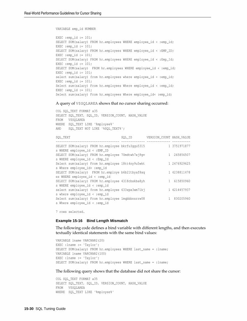
VARIABLE emp_id NUMBER
EXEC :emp_id := 101;SELECT SUM(salary) FROM hr.employees WHERE employee_id < :emp_id;EXEC :emp_id := 101;SELECT SUM(salary) FROM hr.employees WHERE employee_id < :EMP_ID;EXEC :emp_id := 101;SELECT SUM(salary) FROM hr.employees WHERE employee_id < :Emp_Id;EXEC :emp_id := 101;SELECT SUM(salary) FROM hr.employees WHERE employee_id < :emp_id;EXEC :emp_id := 101;select sum(salary) from hr.employees where employee_id < :emp_id;EXEC :emp_id := 101;Select sum(salary) From hr.employees Where employee_id < :emp_id;EXEC :emp_id := 101;Select sum(salary) From hr.employees Where employee_id< :emp_id;
A query of V$SQLAREA shows that no cursor sharing occurred:
COL SQL_TEXT FORMAT a35SELECT SQL_TEXT, SQL_ID, VERSION_COUNT, HASH_VALUEFROM V$SQLAREAWHERE SQL_TEXT LIKE '%mployee%'AND SQL_TEXT NOT LIKE '%SQL_TEXT%';
SQL_TEXT SQL_ID VERSION_COUNT HASH_VALUE----------------------------------- ------------- ------------- ----------SELECT SUM(salary) FROM hr.employee bkrfu3ggu5315 1 3751971877s WHERE employee_id < :EMP_IDSELECT SUM(salary) FROM hr.employee 70mdtwh7xj9gv 1 265856507s WHERE employee_id < :Emp_IdSelect sum(salary) From hr.employee 18tt4ny9u5wkt 1 2476929625s Where employee_id< :emp_idSELECT SUM(salary) FROM hr.employe b6b21tbyaf8aq 1 4238811478es WHERE employee_id < :emp_idSELECT SUM(salary) FROM hr.employee 4318cbskba8yh 1 615850960s WHERE employee_id < :emp_idselect sum(salary) from hr.employee 633zpx3xm71kj 1 4214457937s where employee_id < :emp_idSelect sum(salary) From hr.employee 1mqbbbnsrrw08 1 830205960s Where employee_id < :emp_id
7 rows selected.
Example 15-16 Bind Length Mismatch
The following code defines a bind variable with different lengths, and then executestextually identical statements with the same bind values:
VARIABLE lname VARCHAR2(20)EXEC :lname := 'Taylor';SELECT SUM(salary) FROM hr.employees WHERE last_name = :lname;VARIABLE lname VARCHAR2(100)EXEC :lname := 'Taylor';SELECT SUM(salary) FROM hr.employees WHERE last_name = :lname;
The following query shows that the database did not share the cursor:
COL SQL_TEXT FORMAT a35SELECT SQL_TEXT, SQL_ID, VERSION_COUNT, HASH_VALUEFROM V$SQLAREAWHERE SQL_TEXT LIKE '%mployee%'
Real-World Performance Guidelines for Cursor Sharing
15-30 SQL Tuning Guide

AND SQL_TEXT NOT LIKE '%SQL_TEXT%';
SQL_TEXT SQL_ID VERSION_COUNT HASH_VALUE----------------------------------- ------------- ------------- ----------SELECT SUM(salary) FROM hr.employee buh8j4557r0h1 2 1249608193s WHERE last_name = :lname
The reason is because of the bind lengths:
COL BIND_LENGTH_UPGRADEABLE FORMAT a15SELECT s.SQL_TEXT, s.CHILD_NUMBER, c.BIND_LENGTH_UPGRADEABLEFROM V$SQL s, V$SQL_SHARED_CURSOR cWHERE SQL_TEXT LIKE '%employee%'AND SQL_TEXT NOT LIKE '%SQL_TEXT%'AND s.CHILD_ADDRESS = c.CHILD_ADDRESS;
SQL_TEXT CHILD_NUMBER BIND_LENGTH_UPG----------------------------------- ------------ ---------------SELECT SUM(salary) FROM hr.employee 0 Ns WHERE last_name = :lnameSELECT SUM(salary) FROM hr.employee 1 Ys WHERE last_name = :lname
Minimize Session-Level Changes to the Optimizer EnvironmentA best practice is to prevent users of the application from changing the optimizationapproach and goal for their individual sessions. Any changes to the optimizerenvironment can prevent otherwise identical statements from sharing cursors.
Example 15-17 Environment Mismatches
This example shows two textually identical statements that nevertheless do not share acursor:
VARIABLE emp_id NUMBER
EXEC :emp_id := 110;
ALTER SESSION SET OPTIMIZER_MODE = FIRST_ROWS;SELECT salary FROM hr.employees WHERE employee_id < :emp_id;ALTER SESSION SET OPTIMIZER_MODE = ALL_ROWS;SELECT salary FROM hr.employees WHERE employee_id < :emp_id;
A query of V$SQL_SHARED_CURSOR shows a mismatch in the optimizer modes:
SELECT S.SQL_TEXT, S.CHILD_NUMBER, s.CHILD_ADDRESS, C.OPTIMIZER_MODE_MISMATCHFROM V$SQL S, V$SQL_SHARED_CURSOR CWHERE SQL_TEXT LIKE '%employee%'AND SQL_TEXT NOT LIKE '%SQL_TEXT%'AND S.CHILD_ADDRESS = C.CHILD_ADDRESS;
SQL_TEXT CHILD_NUMBER CHILD_ADDRESS O----------------------------------- ------------ ---------------- -SELECT salary FROM hr.employees WHE 0 0000000080293040 NRE employee_id < :emp_idSELECT salary FROM hr.employees WHE 1 000000008644E888 YRE employee_id < :emp_id
Real-World Performance Guidelines for Cursor Sharing
Improving Real-World Performance Through Cursor Sharing 15-31

Real-World Performance Guidelines for Cursor Sharing
15-32 SQL Tuning Guide

Part VIIMonitoring and Tracing SQL
This part contains the following chapters:
• Monitoring Database Operations
• Gathering Diagnostic Data with SQL Test Case Builder
• Performing Application Tracing


16Monitoring Database Operations
This chapter describes how to monitor database operations.
This chapter contains the following topics:
• About Monitoring Database Operations
• Enabling and Disabling Monitoring of Database Operations
• Creating a Database Operation
• Reporting on Database Operations Using SQL Monitor
About Monitoring Database OperationsA database operation is a set of database tasks defined by end users or applicationcode, for example, a batch job or Extraction, Transformation, and Loading (ETL)processing. You can define, monitor, and report on database operations.
Database operations are either simple or composite. A simple database operation is asingle SQL statement or PL/SQL procedure or function. A composite databaseoperation is activity between two points in time in a database session, with eachsession defining its own beginning and end points. A session can participate in at mostone composite database operation at a time.
Real-Time SQL Monitoring, which was introduced in Oracle Database 11g, enablesyou to monitor a single SQL statement or PL/SQL procedure. Starting in OracleDatabase 12c, Real-Time Database Operations provides the ability to monitorcomposite operations automatically. The database automatically monitors parallelqueries, DML, and DDL statements as soon as execution begins. By default, Real-TimeSQL Monitoring automatically starts when a SQL statement runs in parallel, or whenit has consumed at least 5 seconds of CPU or I/O time in a single execution.
This section contains the following topics:
• Purpose of Monitoring Database Operations
• Database Operation Monitoring Concepts
• User Interfaces for Database Operations Monitoring
• Basic Tasks in Database Operations Monitoring
See Also:
Oracle Database Concepts for a brief conceptual overview of databaseoperations
Monitoring Database Operations 16-1

Purpose of Monitoring Database OperationsIn general, monitoring database operations is useful for the following users:
• DBAs whose responsibilities include identifying expensive (high response time)SQL statements and PL/SQL functions
• DBAs who manage batch jobs in a data warehouse or OLTP system
• Application or database developers who need to monitor the activities related toparticular operations, for example, Data Pump operations
Monitoring database operations is useful for performing the following tasks:
• Tracking and reporting
Tracking requires first defining a database operation, for example, though PL/SQL,OCI, or JDBC APIs. After the operation is defined, the database infrastructuredetermines what to track on behalf of this operation. You can then generate reportson the operation. For example, your tuning task may involve determining whichSQL statements run on behalf of a specific batch job, what their execution statisticswere, what was occurring in the database when the operation was executing, andso on.
• Monitoring execution progress
This task involves monitoring a currently executing database operation. Theinformation is particularly useful when you are investigating why an operation istaking a long time to complete.
• Monitoring resource usage
You may want to detect when a SQL execution uses excessive CPU, issues anexcessive amount of I/O, or takes a long time to complete. With Oracle DatabaseResource Manager (the Resource Manager), you can configure thresholds for eachconsumer group that specify the maximum resource usage for all SQL executionsin the group. When a SQL operation reaches a specified threshold, ResourceManager can switch the operation into a lower-priority consumer group, terminatethe session or call, or log the event (see Oracle Database Administrator's Guide). Youcan then monitor these SQL operations (see “Reporting on Database OperationsUsing SQL Monitor”).
• Tuning for response time
When tuning a database operation, you typically aim to improve the responsetime. Often the database operation performance issues are mainly SQLperformance issues.
The following graphic illustrates the different tasks involved in monitoring databaseoperations:
Monitoring Database Operations
MonitoringProgress
Tracking and Reporting
Tuning forResponse Time
About Monitoring Database Operations
16-2 SQL Tuning Guide

Simple Database Operation Use Cases
For simple operations, Real-Time SQL Monitoring helps determine where a currentlyexecuting SQL statement is in its execution plan and where the statement is spendingits time. You can also see the breakdown of time and resource usage for recentlycompleted statements. In this way, you can better determine why a particularoperation is expensive.
Typical use cases for Real-Time SQL Monitoring include the following:
• A frequently executed SQL statement is executing more slowly than normal. Youmust identify the root cause of this problem.
• A database session is experiencing slow performance.
• A parallel SQL statement is taking a long time. You want to determine how theserver processes are dividing the work.
Composite Database Operation Use Cases
In OLTP and data warehouse environments, a job often logically groups related SQLstatements. The job can involve multiple sessions. Database operation monitoring isuseful for digging through a suboptimally performing job to determine whereresources are being consumed. Thus, database operations enable you to track relatedinformation and improve performance tuning time.
Typical use cases for monitoring composite operations include the following:
• A periodic batch job containing many SQL statements must complete in a certainnumber of hours, but took twice as long as expected.
• After a database upgrade, the execution time of an important batch job doubled. Toresolve this problem, you must collect enough relevant statistical data from thebatch job before and after the upgrade, compare the two sets of data, and thenidentify the changes.
• Packing a SQL tuning set (STS) took far longer than anticipated (see “About SQLTuning Sets”). To diagnose the problem, you need to know what was beingexecuted over time. Because this issue cannot be easily reproduced, you need tomonitor the process while it is running.
Database Operation Monitoring ConceptsThis section describes the most important concepts for database monitoring:
• About the Architecture of Database Operations
• Composite Database Operations
• Attributes of Database Operations
About the Architecture of Database Operations
Setting the CONTROL_MANAGEMENT_PACK_ACCESS initialization parameter toDIAGNOSTIC+TUNING (default) enables monitoring of database operations. Real-TimeSQL Monitoring is a feature of the Oracle Database Tuning Pack.
Figure 16-1 gives an overview of the architecture for database operations.
About Monitoring Database Operations
Monitoring Database Operations 16-3

Figure 16-1 Architecture for Database Operations
User
OracleEnterpriseManager
V$SQL_MONITORV$SQL_PLAN_MONITORV$SQL_MONITOR_SESSTAT
AWR
DBMS_SQL_MONITORREPORT_SQL_MONITOR
DBMS_SQL_MONITOR Database Operations
User-Defined Operations
Real-Time SQL Monitoring
BEGIN OPERATION
...
END_OPERATION
CONTROL_MANAGEMENT_PACK_ACCESS
As shown in Figure 16-1, you can use the DBMS_SQL_MONITOR package to definedatabase operations. After monitoring is initiated, the database stores metadata aboutthe database operations in AWR (see “Reporting on Database Operations Using SQLMonitor”). The database refreshes monitoring statistics in close to real time as eachmonitored statement executes, typically once every second. The database periodicallysaves the data to disk.
Every monitored database operation has an entry in the V$SQL_MONITOR view. Thisentry tracks key performance metrics collected for the execution, including the elapsedtime, CPU time, number of reads and writes, I/O wait time, and various other waittimes. The V$SQL_PLAN_MONITOR view includes monitoring statistics for eachoperation in the execution plan of the SQL statement being monitored. You can accessreports by using DBMS_SQL_MONITOR.REPORT_SQL_MONITOR, which has an OracleEnterprise Manager Cloud Control (Cloud Control) interface.
About Monitoring Database Operations
16-4 SQL Tuning Guide

See Also:
• Oracle Database Reference to learn about the initialization parameters andviews related to database monitoring
• Oracle Database PL/SQL Packages and Types Reference to learn aboutDBMS_SQLTUNE and DBMS_SQL_MONITOR packages
Composite Database Operations
A composite database operation consists of the activity of one session between twopoints in time. Exactly one session exists for the duration of the database operation.
SQL statements or PL/SQL procedures running in this session are part of thecomposite operation. Composite database operations can also be defined in thedatabase kernel. Typical composite operations include SQL*Plus scripts, batch jobs,and ETL processing.
Attributes of Database Operations
A database operation is uniquely identified by the following information:
• Database operation name
This is a user-created name such as daily_sales_report. The name is the samefor a job even if it is executed concurrently by different sessions or on differentdatabases. Database operation names do not reside in different namespaces.
• Database operation execution ID
Two or more occurrences of the same DB operation can run at the same time, withthe same name but different execution IDs. This numeric ID uniquely identifiesdifferent executions of the same database operation.
The database automatically creates an execution ID when you begin a databaseoperation. You can also specify a user-created execution ID.
The database uses the following triplet of values to identify each SQL and PL/SQLstatement monitored in the V$SQL_MONITOR view, regardless of whether thestatement is included in a database operation:
• SQL identifier to identify the SQL statement (SQL_ID)
• Start execution timestamp (SQL_EXEC_START)
• An internally generated identifier to ensure that this primary key is truly unique(SQL_EXEC_ID)
You can use zero or more additional attributes to describe and identify thecharacteristics of a DB operation. Each attribute has a name and value. For example,for operation daily_sales_report, you might define the attribute db_name andassign it the value prod.
About Monitoring Database Operations
Monitoring Database Operations 16-5

See Also:
• Oracle Database Reference to learn about the V$SQL_MONITOR view
• Oracle Database PL/SQL Packages and Types Reference to learn about theDBMS_SQL_MONITOR.BEGIN_OPERATION function
User Interfaces for Database Operations MonitoringThis section contains the following topics:
• Monitored SQL Executions Page in Cloud Control
• DBMS_SQL_MONITOR Package
• Views for Database Operations Monitoring
Monitored SQL Executions Page in Cloud Control
The Monitored SQL Executions page in Cloud Control is the recommended interfacefor reporting on database operations.
Accessing the Monitored SQL Executions Page
To access the Monitored SQL Executions page:
1. Access the Database Home page, as described in “Accessing the Database HomePage in Cloud Control.”
2. From the Performance menu, select SQL Monitoring.
The Monitored SQL Executions page appears.
DBMS_SQL_MONITOR Package
You can use the DBMS_SQL_MONITOR package to define the beginning and ending of adatabase operation, and generate a report of the database operations.
Table 16-1 DBMS_SQL_MONITOR
Program Unit Description
REPORT_SQL_MONITOR This function accepts several input parameters to specify theexecution, the level of detail in the report, and the report type. Ifno parameters are specified, then the function generates a textreport for the last execution that was monitored.
BEGIN_OPERATION This function associates a session with a database operation.
About Monitoring Database Operations
16-6 SQL Tuning Guide

Table 16-1 (Cont.) DBMS_SQL_MONITOR
Program Unit Description
END_OPERATION This function disassociates a session from the specified databaseoperation execution.
See Also:
Oracle Database PL/SQL Packages and Types Reference to learn about theDBMS_SQL_MONITOR package
Views for Database Operations Monitoring
You can monitor the statistics for SQL statement execution using the V$SQL_MONITOR, V$SQL_PLAN_MONITOR, and V$SQL_MONITOR_SESSTAT views. Table 16-2 summarizes these views.
Table 16-2 Views for Database Operations Monitoring
View Description
V$SQL_MONITOR This view contains global, high-level information about thetop SQL statements in a database operation.
Each monitored SQL statement has an entry in this view.Each row contains a SQL statement whose statistics areaccumulated from multiple sessions and all of its executionsin the operation. The primary key is the combination of thecolumns DBOP_NAME, DBOP_EXEC_ID, and SQL_ID.
The V$SQL_MONITOR view contains a subset of the statisticsavailable in V$SQL. However, unlike V$SQL, monitoringstatistics are not cumulative over several executions. Instead,one entry in V$SQL_MONITOR is dedicated to a singleexecution of a SQL statement. If the database monitors twoexecutions of the same SQL statement, then each executionhas a separate entry in V$SQL_MONITOR.
V$SQL_MONITOR has one entry for the parallel executioncoordinator process, and one entry for each parallel executionserver process. Each entry has corresponding entries in V$SQL_PLAN_MONITOR. Because the processes allocated forthe parallel execution of a SQL statement are cooperating forthe same execution, these entries share the same executionkey (the composite SQL_ID, SQL_EXEC_START andSQL_EXEC_ID). You can aggregate the execution key todetermine the overall statistics for a parallel execution.
V$SQL_MONITOR_SESSTAT This view contains the statistics for all sessions involved inthe database operation.
Most of the statistics are cumulative. The database stores thestatistics in XML format instead of using each column foreach statistic. This view is primarily intended for the reportgenerator. Oracle recommends that you use V$SESSTATinstead of V$SQL_MONITOR_SESSTAT.
About Monitoring Database Operations
Monitoring Database Operations 16-7

Table 16-2 (Cont.) Views for Database Operations Monitoring
View Description
V$SQL_PLAN_MONITOR This view contains monitoring statistics for each step in theexecution plan of the monitored SQL statement.
The database updates statistics in V$SQL_PLAN_MONITORevery second while the SQL statement is executing. Multipleentries exist in V$SQL_PLAN_MONITOR for every monitoredSQL statement. Each entry corresponds to a step in theexecution plan of the statement.
You can use the preceding views with the following views to get additionalinformation about the monitored execution:
• V$ACTIVE_SESSION_HISTORY
• V$SESSION
• V$SESSION_LONGOPS
• V$SQL
• V$SQL_PLAN
See Also:
Oracle Database Reference to learn about the V$ views for database operationsmonitoring
Basic Tasks in Database Operations MonitoringThis section explains the basic tasks in database operations monitoring. Basic tasks areas follows:
• “Enabling and Disabling Monitoring of Database Operations”
This task explains how you can enable automatic monitoring of databaseoperations at the system and statement level.
• “Creating a Database Operation”
This section explains how you can define the beginning and end of a databaseoperation using PL/SQL.
• “Reporting on Database Operations Using SQL Monitor”
This section explains how you can generate and interpret reports on a databaseoperation.
Enabling and Disabling Monitoring of Database OperationsThis section contains the following topics:
• Enabling Monitoring of Database Operations at the System Level
• Enabling and Disabling Monitoring of Database Operations at the Statement Level
Enabling and Disabling Monitoring of Database Operations
16-8 SQL Tuning Guide
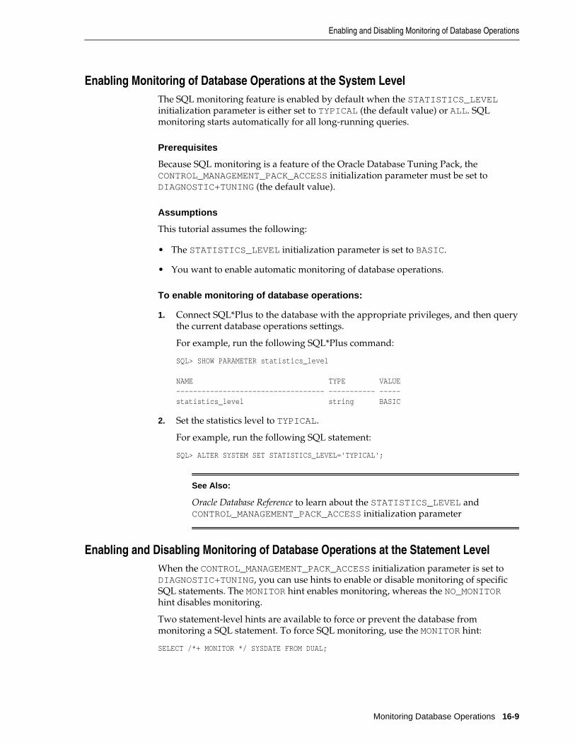
Enabling Monitoring of Database Operations at the System LevelThe SQL monitoring feature is enabled by default when the STATISTICS_LEVELinitialization parameter is either set to TYPICAL (the default value) or ALL. SQLmonitoring starts automatically for all long-running queries.
Prerequisites
Because SQL monitoring is a feature of the Oracle Database Tuning Pack, theCONTROL_MANAGEMENT_PACK_ACCESS initialization parameter must be set toDIAGNOSTIC+TUNING (the default value).
Assumptions
This tutorial assumes the following:
• The STATISTICS_LEVEL initialization parameter is set to BASIC.
• You want to enable automatic monitoring of database operations.
To enable monitoring of database operations:
1. Connect SQL*Plus to the database with the appropriate privileges, and then querythe current database operations settings.
For example, run the following SQL*Plus command:
SQL> SHOW PARAMETER statistics_level NAME TYPE VALUE----------------------------------- ----------- -----statistics_level string BASIC
2. Set the statistics level to TYPICAL.
For example, run the following SQL statement:
SQL> ALTER SYSTEM SET STATISTICS_LEVEL='TYPICAL';
See Also:
Oracle Database Reference to learn about the STATISTICS_LEVEL andCONTROL_MANAGEMENT_PACK_ACCESS initialization parameter
Enabling and Disabling Monitoring of Database Operations at the Statement LevelWhen the CONTROL_MANAGEMENT_PACK_ACCESS initialization parameter is set toDIAGNOSTIC+TUNING, you can use hints to enable or disable monitoring of specificSQL statements. The MONITOR hint enables monitoring, whereas the NO_MONITORhint disables monitoring.
Two statement-level hints are available to force or prevent the database frommonitoring a SQL statement. To force SQL monitoring, use the MONITOR hint:
SELECT /*+ MONITOR */ SYSDATE FROM DUAL;
Enabling and Disabling Monitoring of Database Operations
Monitoring Database Operations 16-9

This hint is effective only when the CONTROL_MANAGEMENT_PACK_ACCESSparameter is set to DIAGNOSTIC+TUNING. To prevent the hinted SQL statement frombeing monitored, use the NO_MONITOR reverse hint.
Assumptions
This tutorial assumes the following:
• Database monitoring is currently enabled at the system level.
• You want to disable automatic monitoring for the statement SELECT * FROMsales ORDER BY time_id.
To disable monitoring of database operations for a SQL statement:
1. Execute the query with the NO_MONITOR hint.
For example, run the following statement:
SQL> SELECT * /*+NO_MONITOR*/ FROM sales ORDER BY time_id;
See Also:
Oracle Database SQL Language Reference for information about using theMONITOR and NO_MONITOR hints
Creating a Database OperationCreating a database operation involves explicitly defining its beginning and endpoints. You can start a database operation by using theDBMS_SQL_MONITOR.BEGIN_OPERATION function and end the operation by usingthe DBMS_SQL_MONITOR.END_OPERATION procedure.
Assumptions
This tutorial assumes the following:
• You are an administrator and want to query the number of items in the sh.salestable and the number of customers in the sh.customers table.
• You want these two queries to be monitored as a database operation namedsh_count.
To create a database operation:
1. Start SQL*Plus and connect as a user with the appropriate privileges.
2. Define a variable to hold the execution ID.
For example, run the following SQL*Plus command:
VAR eid NUMBER
3. Begin the database operation.
For example, execute the BEGIN_OPERATION function as follows:
EXEC :eid := DBMS_SQL_MONITOR.BEGIN_OPERATION('sh_count');
Creating a Database Operation
16-10 SQL Tuning Guide

4. Run the queries in the operation.
For example, run the following statements:
SQL> SELECT count(*) FROM sh.sales; COUNT(*)---------- 918843 SQL> SELECT COUNT(*) FROM sh.customers; COUNT(*)---------- 55500
5. End the database operation.
For example, execute the END_OPERATION procedure as follows:
EXEC DBMS_SQL_MONITOR.END_OPERATION('sh_count', :eid);
6. Confirm that the database operation completed.
For example, run the following query (sample output included):
SELECT SUBSTR(DBOP_NAME, 1, 10), DBOP_EXEC_ID, SUBSTR(STATUS, 1, 10)FROM V$SQL_MONITOR WHERE DBOP_NAME IS NOT NULLORDER BY EXEC_ID;
DBOP_NAME EXEC_ID STATUS---------- ---------- ----------sh_count 1 DONE
See Also:
Oracle Database PL/SQL Packages and Types Reference to learn about theDBMS_SQL_MONITOR package
Reporting on Database Operations Using SQL MonitorBy default, AWR automatically captures SQL monitoring reports in XML format. Thereports capture only SQL statements that are not executing or queued and havefinished execution since the last capture cycle. AWR captures reports only for the mostexpensive statements according to elapsed execution time.
The Monitored SQL Executions page in Cloud Control summarizes the activity formonitored statements. You can use this page to drill down and obtain additionaldetails about particular statements. The Monitored SQL Executions Details page usesdata from several views, including the following:
• GV$SQL_MONITOR
• GV$SQL_PLAN_MONITOR
• GV$SQL_MONITOR_SESSTAT
• GV$SQL
Reporting on Database Operations Using SQL Monitor
Monitoring Database Operations 16-11

• GV$SQL_PLAN
• GV$ACTIVE_SESSION_HISTORY
• GV$SESSION_LONGOPS
• DBA_HIST_REPORTS
• DBA_HIST_REPORTS_DETAILS
Assumptions
This tutorial assumes the following:
• The user sh is executing the following long-running parallel query of the salesmade to each customer:
SELECT c.cust_id, c.cust_last_name, c.cust_first_name, s.prod_id, p.prod_name, s.time_idFROM sales s, customers c, products pWHERE s.cust_id = c.cust_idAND s.prod_id = p.prod_idORDER BY c.cust_id, s.time_id;
• You want to ensure that the preceding query does not consume excessiveresources. While the statement executes, you want to determine basic statisticsabout the database operation, such as the level of parallelism, the total databasetime, and number of I/O requests.
• You use Cloud Control to monitor statement execution.
Note:
To generate the SQL monitor report from the command line, run theREPORT_SQL_MONITOR function in the DBMS_SQLTUNE package, as in thefollowing sample SQL*Plus script:
VARIABLE my_rept CLOBBEGIN :my_rept :=DBMS_SQLTUNE.REPORT_SQL_MONITOR();END;/PRINT :my_rept
To monitor SQL executions:
1. Access the Monitored SQL Executions page, as described in “Monitored SQLExecutions Page in Cloud Control”.
In the following graphic, the top row shows the parallel query.
Reporting on Database Operations Using SQL Monitor
16-12 SQL Tuning Guide
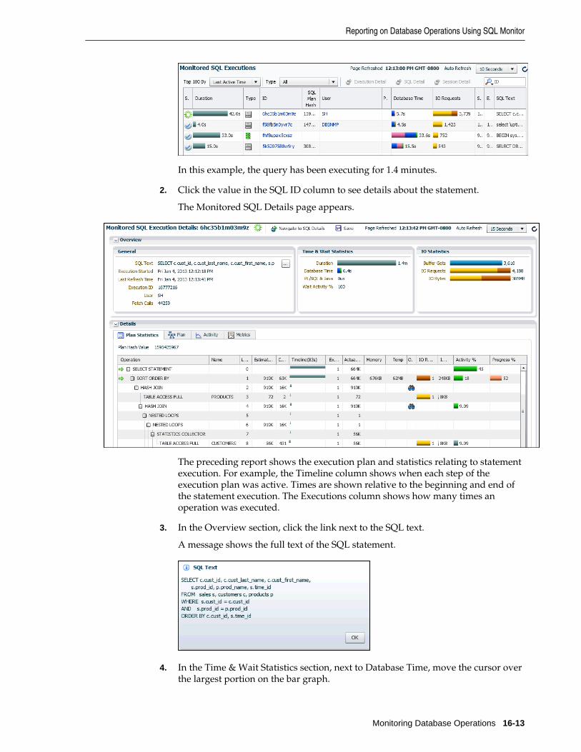
In this example, the query has been executing for 1.4 minutes.
2. Click the value in the SQL ID column to see details about the statement.
The Monitored SQL Details page appears.
The preceding report shows the execution plan and statistics relating to statementexecution. For example, the Timeline column shows when each step of theexecution plan was active. Times are shown relative to the beginning and end ofthe statement execution. The Executions column shows how many times anoperation was executed.
3. In the Overview section, click the link next to the SQL text.
A message shows the full text of the SQL statement.
4. In the Time & Wait Statistics section, next to Database Time, move the cursor overthe largest portion on the bar graph.
Reporting on Database Operations Using SQL Monitor
Monitoring Database Operations 16-13

A message shows that user I/O is consuming over half of database time.
Database Time measures the amount of time the database has spent working onthis SQL statement. This value includes CPU and wait times, such as I/O time.The bar graph is divided into several color-coded portions to highlight CPUresources, user I/O resources, and other resources. You can move the cursor overany portion to view the percentage value of the total.
5. In the Details section, in the IO Requests column, move the cursor over the I/Orequests bar to view the percentage value of the total.
A message appears.
In the preceding graphic, the IO Requests message shows the total number of readrequests issued by the monitored SQL. The message shows that read requestsform 80% of the total I/O requests.
See Also:
• Cloud Control Online Help for descriptions of the elements on theMonitored SQL Executions Details page, and for complete descriptions ofall statistics in the report.
• Oracle Database Reference to learn about the V$ and data dictionary viewsfor database operations monitoring
Reporting on Database Operations Using SQL Monitor
16-14 SQL Tuning Guide

17Gathering Diagnostic Data with SQL Test
Case Builder
A SQL test case is a set of information that enables a developer to reproduce theexecution plan for a specific SQL statement that has encountered a performanceproblem. SQL Test Case Builder is a tool that automatically gathers informationneeded to reproduce the problem in a different database instance.
This chapter contains the following topics:
• Purpose of SQL Test Case Builder
• Concepts for SQL Test Case Builder
• User Interfaces for SQL Test Case Builder
• Running SQL Test Case Builder
Purpose of SQL Test Case BuilderIn many cases, a reproducible test case makes it easier to resolve SQL-relatedproblems. SQL Test Case Builder automates the sometimes difficult and time-consuming process of gathering and reproducing as much information as possibleabout a problem and the environment in which it occurred.
The output of SQL Test Case Builder is a set of scripts in a predefined directory. Thesescripts contain the commands required to re-create all the necessary objects and theenvironment. After the test case is ready, you can create a zip file of the directory andmove it to another database, or upload the file to Oracle Support.
Concepts for SQL Test Case BuilderThis section contains the following topics:
• SQL Incidents
• What SQL Test Case Builder Captures
• Output of SQL Test Case Builder
SQL IncidentsIn the fault diagnosability infrastructure of Oracle Database, an incident is a singleoccurrence of a problem. A SQL incident is a SQL-related problem. When a problem(critical error) occurs multiple times, the database creates an incident for eachoccurrence. Incidents are timestamped and tracked in the Automatic DiagnosticRepository (ADR). Each incident is identified by a numeric incident ID, which isunique within the ADR.
Gathering Diagnostic Data with SQL Test Case Builder 17-1

SQL Test Case Builder is accessible any time on the command line. In OracleEnterprise Manager Cloud Control (Cloud Control), the SQL Test Case pages are onlyavailable after a SQL incident is found.
See Also:
• Oracle Database Concepts for a conceptual overview of ADR
• Oracle Database Administrator's Guide to learn how to investigate, report,and resolve a problem
What SQL Test Case Builder CapturesSQL Test Case Builder captures permanent information such as the query beingexecuted, table and index definitions (but not the actual data), PL/SQL packages andprogram units, optimizer statistics, SQL plan baselines, and initialization parametersettings. Starting in Oracle Database 12c, SQL Test Case Builder also captures andreplays transient information, including information only available as part ofstatement execution.
SQL Test Case Builder supports the following:
• Adaptive plans
SQL Test Case Builder captures inputs to the decisions made regarding adaptiveplans, and replays them at each decision point (see “Adaptive Plans”). For adaptiveplans, the final statistics value at each buffering statistics collector is sufficient todecide on the final plan.
• Automatic memory management
The database automatically handles the memory requested for each SQL operation.Actions such as sorting can affect performance significantly. SQL Test Case Builderkeeps track of the memory activities, for example, where the database allocatedmemory and how much it allocated.
• Dynamic statistics
Regathering dynamic statistics on a different database does not always generate thesame results, for example, when data is missing (see “Dynamic Statistics”). Toreproduce the problem, SQL Test Case Builder exports the dynamic statistics resultfrom the source database. In the testing database, SQL Test Case Builder reuses thesame values captured from the source database instead of regathering dynamicstatistics.
• Multiple execution support
SQL Test Case Builder can capture dynamic information accumulated duringmultiple executions of the query. This capability is important for automaticreoptimization (see “Automatic Reoptimization”).
• Compilation environment and bind values replay
The compilation environment setting is an important part of the queryoptimization context. SQL Test Case Builder captures nondefault settings alteredby the user when running the problem query in the source database. If any
Concepts for SQL Test Case Builder
17-2 SQL Tuning Guide
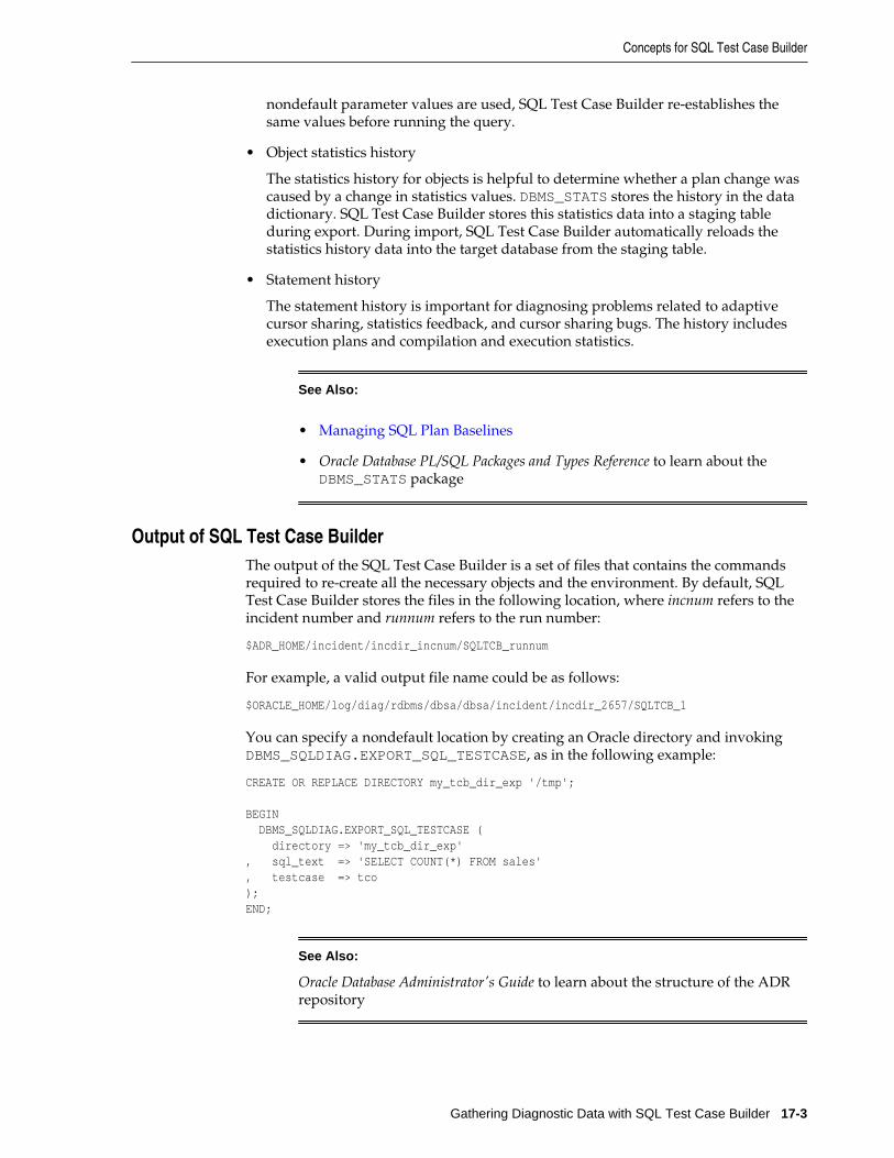
nondefault parameter values are used, SQL Test Case Builder re-establishes thesame values before running the query.
• Object statistics history
The statistics history for objects is helpful to determine whether a plan change wascaused by a change in statistics values. DBMS_STATS stores the history in the datadictionary. SQL Test Case Builder stores this statistics data into a staging tableduring export. During import, SQL Test Case Builder automatically reloads thestatistics history data into the target database from the staging table.
• Statement history
The statement history is important for diagnosing problems related to adaptivecursor sharing, statistics feedback, and cursor sharing bugs. The history includesexecution plans and compilation and execution statistics.
See Also:
• Managing SQL Plan Baselines
• Oracle Database PL/SQL Packages and Types Reference to learn about theDBMS_STATS package
Output of SQL Test Case BuilderThe output of the SQL Test Case Builder is a set of files that contains the commandsrequired to re-create all the necessary objects and the environment. By default, SQLTest Case Builder stores the files in the following location, where incnum refers to theincident number and runnum refers to the run number:
$ADR_HOME/incident/incdir_incnum/SQLTCB_runnum
For example, a valid output file name could be as follows:
$ORACLE_HOME/log/diag/rdbms/dbsa/dbsa/incident/incdir_2657/SQLTCB_1
You can specify a nondefault location by creating an Oracle directory and invokingDBMS_SQLDIAG.EXPORT_SQL_TESTCASE, as in the following example:
CREATE OR REPLACE DIRECTORY my_tcb_dir_exp '/tmp'; BEGIN DBMS_SQLDIAG.EXPORT_SQL_TESTCASE ( directory => 'my_tcb_dir_exp', sql_text => 'SELECT COUNT(*) FROM sales', testcase => tco);END;
See Also:
Oracle Database Administrator's Guide to learn about the structure of the ADRrepository
Concepts for SQL Test Case Builder
Gathering Diagnostic Data with SQL Test Case Builder 17-3

User Interfaces for SQL Test Case BuilderYou can access SQL Test Case Builder either through Cloud Control or using PL/SQLon the command line.
Graphical Interface for SQL Test Case BuilderWithin Cloud Control, you can access SQL Test Case Builder from the IncidentManager page or the Support Workbench page.
Accessing the Incident Manager
This task explains how to navigate to the Incident Manager from the Incidents andProblems section on the Database Home page.
To access the Incident Manager:
1. Access the Database Home page, as described in “Accessing the Database HomePage in Cloud Control.”
2. In the Incidents and Problems section, locate the SQL incident to be investigated.
In the following example, the ORA 600 error is a SQL incident.
3. Click the summary of the incident.
The Problem Details page of the Incident Manager appears.
The Support Workbench page appears, with the incidents listed in a table.
User Interfaces for SQL Test Case Builder
17-4 SQL Tuning Guide

See Also:
• Oracle Database Administrator's Guide to learn how to view problems withthe Cloud Control Support Workbench
• Online help for Cloud Control
Accessing the Support Workbench
This task explains how to navigate to the Incident Manager from the Oracle Databasemenu.
To access the Support Workbench:
1. Access the Database Home page, as described in “Accessing the Database HomePage in Cloud Control.”
2. From the Oracle Database menu, select Diagnostics, then Support Workbench.
The Support Workbench page appears, with the incidents listed in a table.
See Also:
Online help for Cloud Control
Command-Line Interface for SQL Test Case BuilderThe DBMS_SQLDIAG package performs tasks relating to SQL Test Case Builder. Thispackage consists of various subprograms for the SQL Test Case Builder, some ofwhich are listed in Table 17-1.
Table 17-1 SQL Test Case Functions in DBMS_SQLDIAG
Procedure Description
EXPORT_SQL_TESTCASE Exports a SQL test case to a user-specifieddirectory
EXPORT_SQL_TESTCASE_DIR_BY_INC Exports a SQL test case corresponding to theincident ID passed as an argument
EXPORT_SQL_TESTCASE_DIR_BY_TXT Exports a SQL test case corresponding to theSQL text passed as an argument
IMPORT_SQL_TESTCASE Imports a SQL test case into a schema
See Also:
Oracle Database PL/SQL Packages and Types Reference to learn more about theDBMS_SQLDIAG package
Running SQL Test Case BuilderThis tutorial explains how to run SQL Test Case Builder using Cloud Control.
Running SQL Test Case Builder
Gathering Diagnostic Data with SQL Test Case Builder 17-5

Assumptions
This tutorial assumes the following:
• You ran the following EXPLAIN PLAN statement as user sh, which causes aninternal error:
EXPLAIN PLAN FOR SELECT unit_cost, sold FROM costs c, ( SELECT /*+ merge */ p.prod_id, SUM(quantity_sold) AS sold FROM products p, sales s WHERE p.prod_id = s.prod_id GROUP BY p.prod_id ) v WHERE c.prod_id = v.prod_id;
• In the Incidents and Problems section on the Database Home page, a SQL incidentgenerated by the internal error appears.
To run SQL Test Case Builder:
1. Access the Incident Details page, as explained in “Accessing the IncidentManager”.
2. Click the Incidents tab.
The Problem Details page appears.
3. Click the summary for the incident.
The Incident Details page appears.
Running SQL Test Case Builder
17-6 SQL Tuning Guide

4. In Guided Resolution, click View Diagnostic Data.
The Incident Details: incident_number page appears.
5. In the Application Information section, click Additional Diagnostics.
The Additional Diagnostics subpage appears.
6. Select SQL Test Case Builder, and then click Run.
The Run User Action page appears.
Running SQL Test Case Builder
Gathering Diagnostic Data with SQL Test Case Builder 17-7

7. Select a sampling percentage (optional), and then click Submit.
After processing completes, the Confirmation page appears.
8. Access the SQL Test Case files in the location described in “Output of SQL TestCase Builder”.
See Also:
Online help for Cloud Control
Running SQL Test Case Builder
17-8 SQL Tuning Guide
18Performing Application Tracing
This chapter contains the following sections:
• Overview of End-to-End Application Tracing
• Enabling Statistics Gathering for End-to-End Tracing
• Enabling End-to-End Application Tracing
• Generating Output Files Using SQL Trace and TKPROF
• Guidelines for Interpreting TKPROF Output
See Also:
SQL*Plus User's Guide and Reference for information about the use of Autotraceto trace and tune SQL*Plus statements
Overview of End-to-End Application TracingEnd-to-End application tracing can identify the source of an excessive workload, suchas a high load SQL statement, by client identifier, service, module, action, session,instance, or an entire database. This isolates the problem to a specific user, service,session, or application component.
In multitier environments, the middle tier routes a request from an end client todifferent database sessions, making it difficult to track a client across databasesessions. End-to-End application tracing is an infrastructure that uses a client ID touniquely trace a specific end-client through all tiers to the database.
Purpose of End-to-End Application TracingEnd-to-End application tracing simplifies diagnosing performance problems inmultitier environments. For example, you can identify the source of an excessiveworkload, such as a high-load SQL statement, and contact the user responsible. Also, auser having problems can contact you. You can then identify what this user's session isdoing at the database level.
End-to-End application tracing also simplifies management of application workloadsby tracking specific modules and actions in a service. The module and action namesare set by the application developer. For example, you would use the SET_MODULEand SET_ACTION procedures in the DBMS_APPLICATION_INFO package to set thesevalues in a PL/SQL program.
End-to-End application tracing can identify workload problems for:
• Client identifier - specifies an end user based on the logon ID, such as HR.HR
Performing Application Tracing 18-1

• Service - specifies a group of applications with common attributes, service levelthresholds, and priorities; or a single application, such as ACCTG for an accountingapplication
• Module - specifies a functional block, such as Accounts Receivable or GeneralLedger, of an application
• Action - specifies an action, such as an INSERT or UPDATE operation, in a module
• Session - specifies a session based on a given database session identifier (SID), onthe local instance
• Instance - specifies a given instance based on the instance name
Tools for End-to-End Application TracingThe TRCSESS command-line utility consolidates tracing information based on specificcriteria. The SQL Trace facility and TKPROF are two basic performance diagnostictools that can help you accurately assess the efficiency of the SQL statements anapplication runs. For best results, use these tools with EXPLAIN PLAN rather thanusing EXPLAIN PLAN alone. After tracing information is written to files, you canconsolidate this data with the TRCSESS utility, and then diagnose it with TKPROF orSQL Trace.
The recommended interface for end-to-end application tracing is Oracle EnterpriseManager Cloud Control (Cloud Control). Using Cloud Control, you can view the topconsumers for each consumer type, and enable or disable statistics gathering and SQLtracing for specific consumers. If Cloud Control is unavailable, then you can managethis feature using the DBMS_MONITOR APIs.
See Also:
Oracle Database PL/SQL Packages and Types Reference for information about theDBMS_MONITOR, DBMS_SESSION, DBMS_SERVICE, andDBMS_APPLICATION_INFO packages
Overview of the SQL Trace Facility
The SQL Trace facility provides performance information on individual SQLstatements. It generates the following statistics for each statement:
• Parse, execute, and fetch counts
• CPU and elapsed times
• Physical reads and logical reads
• Number of rows processed
• Misses on the library cache
• User name under which each parse occurred
• Each commit and rollback
• Wait event data for each SQL statement, and a summary for each trace file
Overview of End-to-End Application Tracing
18-2 SQL Tuning Guide

If the cursor for the SQL statement is closed, then SQL Trace also provides row sourceinformation that includes:
• Row operations showing the actual execution plan of each SQL statement
• Number of rows, number of consistent reads, number of physical reads, number ofphysical writes, and time elapsed for each operation on a row
Although you can enable the SQL Trace facility for a session or an instance, Oraclerecommends that you use the DBMS_SESSION or DBMS_MONITOR packages instead.When the SQL Trace facility is enabled for a session or for an instance, performancestatistics for all SQL statements executed in a user session or in the instance are placedinto trace files. Using the SQL Trace facility can affect performance and may result inincreased system overhead, excessive CPU usage, and inadequate disk space.
The TRCSESS command-line utility consolidates tracing information from severaltrace files based on specific criteria, such as session or client ID. See “TRCSESS”.
See Also:
“Enabling End-to-End Application Tracing” to learn how to use theDBMS_SESSION or DBMS_MONITOR packages to enable SQL tracing for asession or an instance
Overview of TKPROF
You can run the TKPROF program to format the contents of the trace file and place theoutput into a readable output file. TKPROF can also:
• Create a SQL script that stores the statistics in the database
• Determine the execution plans of SQL statements
Note:
If the cursor for a SQL statement is not closed, then TKPROF output does notautomatically include the actual execution plan of the SQL statement. In thissituation, use the EXPLAIN option with TKPROF to generate an executionplan.
TKPROF reports each statement executed with the resources it has consumed, thenumber of times it was called, and the number of rows which it processed. Thisinformation enables you to locate those statements that are using the greatest resource.With baselines available, you can assess whether the resources used are reasonablegiven the work done.
Enabling Statistics Gathering for End-to-End TracingTo gather the appropriate statistics using PL/SQL, you must enable statisticsgathering for client identifier, service, module, or action using procedures inDBMS_MONITOR. The default level is the session-level statistics gathering. Statisticsgathering is global for the database and continues after a database instance isrestarted.
You can gather statistics by the following criteria:
Enabling Statistics Gathering for End-to-End Tracing
Performing Application Tracing 18-3

• Enabling Statistics Gathering for a Client ID
• Enabling Statistics Gathering for a Service_ Module_ and Action
Enabling Statistics Gathering for a Client IDThe procedure CLIENT_ID_STAT_ENABLE enables statistics gathering for a givenclient ID, whereas the procedure CLIENT_ID_STAT_DISABLE disables it. You canview client identifiers in the CLIENT_IDENTIFIER column in V$SESSION.
Assumptions
This tutorial assumes that you want to enable and then disable statistics gathering forthe client with the ID oe.oe.
To enable and disable statistics gathering for a client identifier:
1. Start SQL*Plus, and then connect to the database with the appropriate privileges.
2. Enable statistics gathering for oe.oe.
For example, run the following command:
EXECUTE DBMS_MONITOR.CLIENT_ID_STAT_ENABLE(client_id => 'OE.OE');
3. Disable statistics gathering for oe.oe.
For example, run the following command:
EXECUTE DBMS_MONITOR.CLIENT_ID_STAT_DISABLE(client_id => 'OE.OE');
Enabling Statistics Gathering for a Service, Module, and ActionThe procedure SERV_MOD_ACT_STAT_ENABLE enables statistic gathering for acombination of service, module, and action, whereas the procedureSERV_MOD_ACT_STAT_DISABLE disables statistic gathering for a combination ofservice, module, and action.
When you change the module or action using the preceding DBMS_MONITORprocedures, the change takes effect when the next user call is executed in the session.For example, if a module is set to module1 in a session, and if the module is reset tomodule2 in a user call in the session, then the module remains module1 during thisuser call. The module is changed to module2 in the next user call in the session.
Assumptions
This tutorial assumes that you want to gather statistics as follows:
• For the ACCTG service
• For all actions in the PAYROLL module
• For the INSERT ITEM action within the GLEDGER module
To enable and disable statistics gathering for a service, module, and action:
1. Start SQL*Plus, and then connect to the database with the appropriate privileges.
2. Enable statistics gathering for the desired service, module, and action.
Enabling Statistics Gathering for End-to-End Tracing
18-4 SQL Tuning Guide

For example, run the following commands:
BEGIN DBMS_MONITOR.SERV_MOD_ACT_STAT_ENABLE( service_name => 'ACCTG' , module_name => 'PAYROLL' );END;
BEGIN DBMS_MONITOR.SERV_MOD_ACT_STAT_ENABLE( service_name => 'ACCTG' , module_name => 'GLEDGER' , action_name => 'INSERT ITEM' );END;
3. Disable statistic gathering for the previously specified combination of service,module, and action.
For example, run the following command:
BEGIN DBMS_MONITOR.SERV_MOD_ACT_STAT_DISABLE( service_name => 'ACCTG' , module_name => 'GLEDGER' , action_name => 'INSERT ITEM' );END;
Enabling End-to-End Application TracingTo enable tracing for client identifier, service, module, action, session, instance ordatabase, execute the appropriate procedures in the DBMS_MONITOR package. You canenable tracing for specific diagnosis and workload management by the followingcriteria:
• Enabling Tracing for a Client Identifier
• Enabling Tracing for a Service_ Module_ and Action
• Enabling Tracing for a Session
• Enabling Tracing for the Instance or Database
With the criteria that you provide, specific trace information is captured in a set oftrace files and combined into a single output trace file.
Enabling Tracing for a Client IdentifierTo enable tracing globally for the database for a specified client identifier, use theCLIENT_ID_TRACE_ENABLE procedure. The CLIENT_ID_TRACE_DISABLEprocedure disables tracing globally for the database for a given client identifier.
Assumptions
This tutorial assumes the following:
• OE.OE is the client identifier for which SQL tracing is to be enabled.
• You want to include wait information in the trace.
• You want to exclude bind information from the trace.
Enabling End-to-End Application Tracing
Performing Application Tracing 18-5

To enable and disable tracing for a client identifier:
1. Start SQL*Plus, and then connect to the database with the appropriate privileges.
2. Enable tracing for the client.
For example, execute the following program:
BEGIN DBMS_MONITOR.CLIENT_ID_TRACE_ENABLE( client_id => 'OE.OE' , waits => true , binds => false );END;
3. Disable tracing for the client.
For example, execute the following command:
EXECUTE DBMS_MONITOR.CLIENT_ID_TRACE_DISABLE(client_id => 'OE.OE');
Enabling Tracing for a Service, Module, and ActionThe SERV_MOD_ACT_TRACE_ENABLE procedure enables SQL tracing for a specifiedcombination of service name, module, and action globally for a database, unless theprocedure specifies a database instance name. The SERV_MOD_ACT_TRACE_DISABLEprocedure disables the trace at all enabled instances for a given combination of servicename, module, and action name globally.
Assumptions
This tutorial assumes the following:
• You want to enable tracing for the service ACCTG.
• You want to enable tracing for all actions for the combination of the ACCTG serviceand the PAYROLL module.
• You want to include wait information in the trace.
• You want to exclude bind information from the trace.
• You want to enable tracing only for the inst1 instance.
To enable and disable tracing for a service, module, and action:
1. Start SQL*Plus, and then connect to the database with the appropriate privileges.
2. Enable tracing for the service, module, and actions.
For example, execute the following command:
BEGIN DBMS_MONITOR.SERV_MOD_ACT_TRACE_ENABLE( service_name => 'ACCTG' , module_name => 'PAYROLL' , waits => true , binds => false , instance_name => 'inst1' );END;
3. Disable tracing for the service, module, and actions.
Enabling End-to-End Application Tracing
18-6 SQL Tuning Guide

For example, execute the following command:
BEGIN DBMS_MONITOR.SERV_MOD_ACT_TRACE_DISABLE( service_name => 'ACCTG' , module_name => 'PAYROLL' , instance_name => 'inst1' );END;
Enabling Tracing for a SessionThe SESSION_TRACE_ENABLE procedure enables the trace for a given databasesession identifier (SID), on the local instance. Whereas the DBMS_MONITOR packagecan only be invoked by a user with the DBA role, any user can also enable SQL tracingfor their own session by using the DBMS_SESSION package. A user can invoke theSESSION_TRACE_ENABLE procedure to enable session-level SQL trace for the user'ssession. For example:
EXECUTE DBMS_SESSION.SESSION_TRACE_ENABLE(waits => true, binds => false);
Assumptions
This tutorial assumes the following:
• You want to log in to the database with administrator privileges.
• User OE has one active session.
• You want to temporarily enable tracing for the OE session.
• You want to include wait information in the trace.
• You want to exclude bind information from the trace.
To enable and disable tracing for a session:
1. Start SQL*Plus, and then connect to the database with the administratorprivileges.
2. Determine the session ID and serial number values for the session to trace.
For example, query V$SESSION as follows:
SELECT SID, SERIAL#, USERNAME FROM V$SESSIONWHERE USERNAME = 'OE';
SID SERIAL# USERNAME---------- ---------- ------------------------------ 27 60 OE
3. Use the values from the preceding step to enable tracing for a specific session.
For example, execute the following program to enable tracing for the OE session,where the true argument includes wait information in the trace and the falseargument excludes bind information from the trace:
BEGIN DBMS_MONITOR.SESSION_TRACE_ENABLE( session_id => 27 , serial_num => 60 , waits => true ,
Enabling End-to-End Application Tracing
Performing Application Tracing 18-7

binds => false );END;
4. Disable tracing for the session.
The SESSION_TRACE_DISABLE procedure disables the trace for a given databasesession identifier (SID) and serial number. For example:
EXECUTE DBMS_MONITOR.SESSION_TRACE_DISABLE(session_id => 27, serial_num => 60);
Enabling Tracing for the Instance or DatabaseThe DBMS_MONITOR.DATABASE_TRACE_ENABLE procedure overrides all othersession-level traces, but is complementary to the client identifier, service, module, andaction traces. Tracing is enabled for all current and future sessions.
All new sessions inherit the wait and bind information specified by this procedureuntil you call the DATABASE_TRACE_DISABLE procedure. When you invoke thisprocedure with the instance_name parameter, the procedure resets the session-levelSQL trace for the named instance. If you invoke this procedure without theinstance_name parameter, then the procedure resets the session-level SQL trace forthe entire database.
Prerequisites
You must be logged in as an administrator execute the DATABASE_TRACE_ENABLEprocedure.
Assumptions
This tutorial assumes the following:
• You want to enable tracing for all SQL the inst1 instance.
• You want wait information to be in the trace.
• You do not want bind information in the trace.
To enable and disable tracing for a session:
1. Start SQL*Plus, and then connect to the database with the administratorprivileges.
2. Call the DATABASE_TRACE_ENABLE procedure to enable SQL tracing for a giveninstance or an entire database.
For example, execute the following program, where the true argument specifiesthat wait information is in the trace, and the false argument specifies that nobind information is in the trace:
BEGIN DBMS_MONITOR.DATABASE_TRACE_ENABLE( waits => true , binds => false , instance_name => 'inst1' );END;
3. Disable tracing for the session.
The SESSION_TRACE_DISABLE procedure disables the trace. For example, thefollowing program disables tracing for inst1:
Enabling End-to-End Application Tracing
18-8 SQL Tuning Guide

EXECUTE DBMS_MONITOR.DATABASE_TRACE_DISABLE(instance_name => 'inst1');
To disable the session-level SQL tracing for an entire database, invoke theDATABASE_TRACE_DISABLE procedure without specifying the instance_nameparameter:
EXECUTE DBMS_MONITOR.DATABASE_TRACE_DISABLE();
Generating Output Files Using SQL Trace and TKPROFThis section explains the basic procedure for using SQL Trace and TKPROF.
To use the SQL Trace facility and TKPROF:
1. Set initialization parameters for trace file management.
See “Step 1: Setting Initialization Parameters for Trace File Management”.
2. Enable the SQL Trace facility for the desired session, and run the application. Thisstep produces a trace file containing statistics for the SQL statements issued by theapplication.
See “Step 2: Enabling the SQL Trace Facility”.
3. Run TKPROF to translate the trace file created in Step 2 into a readable output file.This step can optionally create a SQL script that you can use to store the statisticsin a database.
See “Step 3: Generating Output Files with TKPROF”.
4. Optionally, run the SQL script produced in Step 3 to store the statistics in thedatabase.
See “Step 4: Storing SQL Trace Facility Statistics”.
Step 1: Setting Initialization Parameters for Trace File ManagementWhen the SQL Trace facility is enabled for a session, Oracle Database generates a tracefile containing statistics for traced SQL statements for that session. When the SQLTrace facility is enabled for an instance, Oracle Database creates a separate trace filefor each process.
To set initialization parameters for trace file management:
1. Check the settings of the TIMED_STATISTICS, MAX_DUMP_FILE_SIZE, andDIAGNOSTIC_DEST initialization parameters, as indicated in Table 18-1.
Table 18-1 Initialization Parameters to Check Before Enabling SQL Trace
Parameter Description
DIAGNOSTIC_DEST Specifies the location of the Automatic DiagnosticRepository (ADR) Home. The diagnostic files for eachdatabase instance are located in this dedicated directory. Oracle Database Reference for information about theDIAGNOSTIC_DEST initialization parameter.
Generating Output Files Using SQL Trace and TKPROF
Performing Application Tracing 18-9

Table 18-1 (Cont.) Initialization Parameters to Check Before Enabling SQLTrace
Parameter Description
MAX_DUMP_FILE_SIZE When the SQL Trace facility is enabled at the databaseinstance level, every call to the database writes a text linein a file in the operating system's file format. Themaximum size of these files in operating system blocks islimited by this initialization parameter. The default isUNLIMITED. See Oracle Database Administrator's Guide tolearn how to control the trace file size.
TIMED_STATISTICS Enables and disables the collection of timed statistics, suchas CPU and elapsed times, by the SQL Trace facility, andthe collection of various statistics in the V$ views.
If STATISTICS_LEVEL is set to TYPICAL or ALL, then thedefault value of TIMED_STATISTICS is true. IfSTATISTICS_LEVEL is set to BASIC, then the defaultvalue of TIMED_STATISTICS is false. See OracleDatabase Reference for information about theSTATISTICS_LEVEL initialization parameter.
Enabling timing causes extra timing calls for low-leveloperations. This is a dynamic parameter. It is also asession parameter. See Oracle Database Reference forinformation about the TIMED_STATISTICS initializationparameter.
2. Devise a way of recognizing the resulting trace file.
Be sure you know how to distinguish the trace files by name. You can tag tracefiles by including in your programs a statement such as SELECT'program_name' FROM DUAL. You can then trace each file back to the processthat created it.
You can also set the TRACEFILE_IDENTIFIER initialization parameter to specifya custom identifier that becomes part of the trace file name (see Oracle DatabaseReference for information about the TRACEFILE_IDENTIFIER initializationparameter). For example, you can add my_trace_id to subsequent trace filenames for easy identification with the following:
ALTER SESSION SET TRACEFILE_IDENTIFIER = 'my_trace_id';
3. If the operating system retains multiple versions of files, then ensure that theversion limit is high enough to accommodate the number of trace files you expectthe SQL Trace facility to generate.
4. If the generated trace files can be owned by an operating system user other thanyourself, then ensure that you have the necessary permissions to use TKPROF toformat them.
Step 2: Enabling the SQL Trace FacilityEnable the SQL Trace facility at either of the following levels:
• Database instance
Generating Output Files Using SQL Trace and TKPROF
18-10 SQL Tuning Guide

Use DBMS_MONITOR.DATABASE_TRACE_ENABLE procedure to enable tracing, andDBMS_MONITOR.DATABASE_TRACE_DISABLE procedure to disable tracing.
• Database session
Use DBMS_SESSION.SET_SQL_TRACE procedure to enable tracing (true) ordisable tracing (false).
Note:
Because running the SQL Trace facility increases system overhead, enable itonly when tuning SQL statements, and disable it when you are finished.
To enable and disable tracing at the database instance level:
1. Start SQL*Plus, and connect to the database with administrator privileges.
2. Enable tracing at the database instance level.
The following example enables tracing for the orcl instance:
EXEC DBMS_MONITOR.DATABASE_TRACE_ENABLE(INSTANCE_NAME => 'orcl');
3. Execute the statements to be traced.
4. Disable tracing for the database instance.
The following example disables tracing for the orcl instance:
EXEC DBMS_MONITOR.DATABASE_TRACE_DISABLE(INSTANCE_NAME => 'orcl');
To enable and disable tracing at the session level:
1. Start SQL*Plus, and connect to the database with the desired credentials.
2. Enable tracing for the current session.
The following example enables tracing for the current session:
EXEC DBMS_SESSION.SET_SQL_TRACE(sql_trace => true);
3. Execute the statements to be traced.
4. Disable tracing for the current session.
The following example disables tracing for the current session:
EXEC DBMS_SESSION.SET_SQL_TRACE(sql_trace => false);
See Also:
Oracle Database PL/SQL Packages and Types Reference to learn aboutDBMS_MONITOR.DATABASE_TRACE_ENABLE
Step 3: Generating Output Files with TKPROFTKPROF accepts as input a trace file produced by the SQL Trace facility, and itproduces a formatted output file. TKPROF can also generate execution plans.
Generating Output Files Using SQL Trace and TKPROF
Performing Application Tracing 18-11

After the SQL Trace facility has generated trace files, you can:
• Run TKPROF on each individual trace file, producing several formatted outputfiles, one for each session.
• Concatenate the trace files, and then run TKPROF on the result to produce aformatted output file for the entire instance.
• Run the TRCSESS command-line utility to consolidate tracing information fromseveral trace files, then run TKPROF on the result.
TKPROF does not report COMMIT and ROLLBACK statements recorded in the trace file.
Note:
The following SQL statements are truncated to 25 characters in the SQL Tracefile:
SET ROLEGRANTALTER USERALTER ROLECREATE USERCREATE ROLE
Example 18-1 TKPROF Output
SELECT * FROM emp, dept WHERE emp.deptno = dept.deptno;
call count cpu elapsed disk query current rows---- ------- ------- --------- -------- -------- ------- ------Parse 1 0.16 0.29 3 13 0 0Execute 1 0.00 0.00 0 0 0 0Fetch 1 0.03 0.26 2 2 4 14 Misses in library cache during parse: 1 Parsing user id: (8) SCOTT
Rows Execution Plan------- ---------------------------------------------------
14 MERGE JOIN 4 SORT JOIN 4 TABLE ACCESS (FULL) OF 'DEPT'14 SORT JOIN14 TABLE ACCESS (FULL) OF 'EMP'
For this statement, TKPROF output includes the following information:
• The text of the SQL statement
• The SQL Trace statistics in tabular form
• The number of library cache misses for the parsing and execution of the statement.
• The user initially parsing the statement.
Generating Output Files Using SQL Trace and TKPROF
18-12 SQL Tuning Guide

• The execution plan generated by EXPLAIN PLAN.
TKPROF also provides a summary of user level statements and recursive SQL calls forthe trace file.
Step 4: Storing SQL Trace Facility StatisticsYou might want to keep a history of the statistics generated by the SQL Trace facilityfor an application, and compare them over time. TKPROF can generate a SQL scriptthat creates a table and inserts rows of statistics into it. This script contains:
• A CREATE TABLE statement that creates an output table named TKPROF_TABLE.
• INSERT statements that add rows of statistics, one for each traced SQL statement,to TKPROF_TABLE.
After running TKPROF, run this script to store the statistics in the database.
Generating the TKPROF Output SQL Script
When you run TKPROF, use the INSERT parameter to specify the name of thegenerated SQL script. If you omit this parameter, then TKPROF does not generate ascript.
Editing the TKPROF Output SQL Script
After TKPROF has created the SQL script, you might want to edit the script beforerunning it. If you have created an output table for previously collected statistics, and ifyou want to add new statistics to this table, then remove the CREATE TABLE statementfrom the script. The script then inserts the new rows into the existing table.
If you have created multiple output tables, perhaps to store statistics from differentdatabases in different tables, then edit the CREATE TABLE and INSERT statements tochange the name of the output table.
Querying the Output Table
The following CREATE TABLE statement creates the TKPROF_TABLE:
CREATE TABLE TKPROF_TABLE (
DATE_OF_INSERT DATE,CURSOR_NUM NUMBER,DEPTH NUMBER,USER_ID NUMBER,PARSE_CNT NUMBER,PARSE_CPU NUMBER,PARSE_ELAP NUMBER,PARSE_DISK NUMBER,PARSE_QUERY NUMBER,PARSE_CURRENT NUMBER,PARSE_MISS NUMBER,EXE_COUNT NUMBER,EXE_CPU NUMBER,EXE_ELAP NUMBER,EXE_DISK NUMBER,EXE_QUERY NUMBER,EXE_CURRENT NUMBER,EXE_MISS NUMBER,EXE_ROWS NUMBER,FETCH_COUNT NUMBER,
Generating Output Files Using SQL Trace and TKPROF
Performing Application Tracing 18-13

FETCH_CPU NUMBER,FETCH_ELAP NUMBER,FETCH_DISK NUMBER,FETCH_QUERY NUMBER,FETCH_CURRENT NUMBER,FETCH_ROWS NUMBER,CLOCK_TICKS NUMBER,SQL_STATEMENT LONG);
Most output table columns correspond directly to the statistics that appear in theformatted output file. For example, the PARSE_CNT column value corresponds to thecount statistic for the parse step in the output file.
The columns in Table 18-2 help you identify a row of statistics.
Table 18-2 TKPROF_TABLE Columns for Identifying a Row of Statistics
Column Description
SQL_STATEMENT This is the SQL statement for which the SQL Trace facility collectedthe row of statistics. Because this column has data type LONG, youcannot use it in expressions or WHERE clause conditions.
DATE_OF_INSERT This is the date and time when the row was inserted into the table.This value is different from the time when the SQL Trace facilitycollected the statistics.
DEPTH This indicates the level of recursion at which the SQL statement wasissued. For example, a value of 0 indicates that a user issued thestatement. A value of 1 indicates that Oracle Database generated thestatement as a recursive call to process a statement with a value of 0(a statement issued by a user). A value of n indicates that OracleDatabase generated the statement as a recursive call to process astatement with a value of n-1.
USER_ID This identifies the user issuing the statement. This value alsoappears in the formatted output file.
CURSOR_NUM Oracle Database uses this column value to keep track of the cursor towhich each SQL statement was assigned.
The output table does not store the statement's execution plan. The following queryreturns the statistics from the output table. These statistics correspond to the formattedoutput shown in “Example 18-7”.
SELECT * FROM TKPROF_TABLE;
Sample output appears as follows:
DATE_OF_INSERT CURSOR_NUM DEPTH USER_ID PARSE_CNT PARSE_CPU PARSE_ELAP-------------- ---------- ----- ------- --------- --------- ---------- 21-DEC-2012 1 0 8 1 16 22
PARSE_DISK PARSE_QUERY PARSE_CURRENT PARSE_MISS EXE_COUNT EXE_CPU ---------- ----------- ------------- ---------- --------- ------- 3 11 0 1 1 0
EXE_ELAP EXE_DISK EXE_QUERY EXE_CURRENT EXE_MISS EXE_ROWS FETCH_COUNT
Generating Output Files Using SQL Trace and TKPROF
18-14 SQL Tuning Guide

-------- -------- --------- ----------- -------- -------- ----------- 0 0 0 0 0 0 1
FETCH_CPU FETCH_ELAP FETCH_DISK FETCH_QUERY FETCH_CURRENT FETCH_ROWS --------- ---------- ---------- ----------- ------------- ---------- 2 20 2 2 4 10
SQL_STATEMENT ---------------------------------------------------------------------SELECT * FROM EMP, DEPT WHERE EMP.DEPTNO = DEPT.DEPTNO
Guidelines for Interpreting TKPROF OutputThis section provides guidelines for interpreting TKPROF output.
• Guideline for Interpreting the Resolution of Statistics
• Guideline for Recursive SQL Statements
• Guideline for Deciding Which Statements to Tune
• Guidelines for Avoiding Traps in TKPROF Interpretation
While TKPROF provides a useful analysis, the most accurate measure of efficiency isthe performance of the application. At the end of the TKPROF output is a summary ofthe work that the process performed during the period that the trace was running.
Guideline for Interpreting the Resolution of StatisticsTiming statistics have a resolution of one hundredth of a second. Therefore, anyoperation on a cursor that takes a hundredth of a second or less might not be timedaccurately. Keep this limitation in mind when interpreting statistics. In particular, becareful when interpreting the results from simple queries that execute very quickly.
Guideline for Recursive SQL StatementsSometimes, to execute a SQL statement issued by a user, Oracle Database must issueadditional SQL statements. Such statements are called recursive calls or recursive SQL.For example, if a session inserts a row into a table that has insufficient space to holdthat row, then the database makes recursive calls to allocate the space dynamically.The database also generates recursive calls when data dictionary information is notavailable in memory and so must be retrieved from disk.
If recursive calls occur while the SQL Trace facility is enabled, then TKPROF producesstatistics for the recursive SQL statements and marks them clearly as recursive SQLstatements in the output file. You can suppress the listing of Oracle Database internalrecursive calls (for example, space management) in the output file by setting the SYScommand-line parameter to NO. The statistics for a recursive SQL statement areincluded in the listing for that statement, not in the listing for the SQL statement thatcaused the recursive call. So, when you are calculating the total resources required toprocess a SQL statement, consider the statistics for that statement and those forrecursive calls caused by that statement.
Note:
Recursive SQL statistics are not included for SQL-level operations.
Guidelines for Interpreting TKPROF Output
Performing Application Tracing 18-15

Guideline for Deciding Which Statements to TuneYou must determine which SQL statements use the most CPU or disk resource. If theTIMED_STATISTICS parameter is enabled, then you can find high CPU activity in theCPU column. If TIMED_STATISTICS is not enabled, then check the QUERY andCURRENT columns.
With the exception of locking problems and inefficient PL/SQL loops, neither the CPUtime nor the elapsed time is necessary to find problem statements. The key is thenumber of block visits, both query (that is, subject to read consistency) and current(that is, not subject to read consistency). Segment headers and blocks that are going tobe updated are acquired in current mode, but all query and subquery processingrequests the data in query mode. These are precisely the same measures as theinstance statistics CONSISTENT GETS and DB BLOCK GETS. You can find high diskactivity in the disk column.
The following listing shows TKPROF output for one SQL statement as it appears in theoutput file:
SELECT * FROM emp, dept WHERE emp.deptno = dept.deptno;
call count cpu elapsed disk query current rows---- ------- ------- --------- -------- -------- ------- ------Parse 11 0.08 0.18 0 0 0 0Execute 11 0.23 0.66 0 3 6 0Fetch 35 6.70 6.83 100 12326 2 824------------------------------------------------------------------total 57 7.01 7.67 100 12329 8 826
Misses in library cache during parse: 0
If it is acceptable to have 7.01 CPU seconds and to retrieve 824 rows, then you neednot look any further at this trace output. In fact, a major use of TKPROF reports in atuning exercise is to eliminate processes from the detailed tuning phase.
The output indicates that 10 unnecessary parse call were made (because 11 parse callsexist for this single statement) and that array fetch operations were performed. Morerows were fetched than there were fetches performed. A large gap between CPU andelapsed timings indicates Physical I/Os.
See Also:
Example 18-4
Guidelines for Avoiding Traps in TKPROF InterpretationThis section describes some fine points of TKPROF interpretation:
• Guideline for Avoiding the Argument Trap
• Guideline for Avoiding the Read Consistency Trap
• Guideline for Avoiding the Schema Trap
• Guideline for Avoiding the Time Trap
Guidelines for Interpreting TKPROF Output
18-16 SQL Tuning Guide

Guideline for Avoiding the Argument Trap
If you are not aware of the values being bound at run time, then it is possible to fallinto the argument trap. EXPLAIN PLAN cannot determine the type of a bind variablefrom the text of SQL statements, and it always assumes that the type is VARCHAR. Ifthe bind variable is actually a number or a date, then TKPROF can cause implicit dataconversions, which can cause inefficient plans to be executed. To avoid this situation,experiment with different data types in the query, and perform the conversionyourself.
Guideline for Avoiding the Read Consistency Trap
The next example illustrates the read consistency trap. Without knowing that anuncommitted transaction had made a series of updates to the NAME column, it is verydifficult to see why so many block visits would be incurred.
Cases like this are not normally repeatable: if the process were run again, it is unlikelythat another transaction would interact with it in the same way.
SELECT name_idFROM cq_names WHERE name = 'FLOOR';
call count cpu elapsed disk query current rows---- ----- --- ------- ---- ----- ------- ----Parse 1 0.10 0.18 0 0 0 0Execute 1 0.00 0.00 0 0 0 0Fetch 1 0.11 0.21 2 101 0 1
Misses in library cache during parse: 1Parsing user id: 01 (USER1)
Rows Execution Plane---- --------- ---- 0 SELECT STATEMENT 1 TABLE ACCESS (BY ROWID) OF 'CQ_NAMES' 2 INDEX (RANGE SCAN) OF 'CQ_NAMES_NAME' (NON_UNIQUE)
Guideline for Avoiding the Schema Trap
This example shows an extreme (and thus easily detected) example of the schema trap.At first, it is difficult to see why such an apparently straightforward indexed querymust look at so many database blocks, or why it should access any blocks at all incurrent mode.
SELECT name_idFROM cq_names WHERE name = 'FLOOR';
call count cpu elapsed disk query current rows-------- ------- -------- --------- ------- ------ ------- ----Parse 1 0.06 0.10 0 0 0 0Execute 1 0.02 0.02 0 0 0 0 Fetch 1 0.23 0.30 31 31 3 1
Misses in library cache during parse: 0Parsing user id: 02 (USER2)
Rows Execution Plan------- ---------------------------------------------------
Guidelines for Interpreting TKPROF Output
Performing Application Tracing 18-17

0 SELECT STATEMENT 2340 TABLE ACCESS (BY ROWID) OF 'CQ_NAMES' 0 INDEX (RANGE SCAN) OF 'CQ_NAMES_NAME' (NON-UNIQUE)
Two statistics suggest that the query might have been executed with a full table scan.These statistics are the current mode block visits, plus the number of rows originatingfrom the Table Access row source in the execution plan. The explanation is that therequired index was built after the trace file had been produced, but before TKPROFhad been run.
Generating a new trace file gives the following data:
SELECT name_idFROM cq_names WHERE name = 'FLOOR';
call count cpu elapsed disk query current rows----- ------ ------ -------- ----- ------ ------- -----Parse 1 0.01 0.02 0 0 0 0Execute 1 0.00 0.00 0 0 0 0Fetch 1 0.00 0.00 0 2 0 1
Misses in library cache during parse: 0Parsing user id: 02 (USER2)
Rows Execution Plan------- --------------------------------------------------- 0 SELECT STATEMENT 1 TABLE ACCESS (BY ROWID) OF 'CQ_NAMES' 2 INDEX (RANGE SCAN) OF 'CQ_NAMES_NAME' (NON-UNIQUE)
One of the marked features of this correct version is that the parse call took 10milliseconds of CPU time and 20 milliseconds of elapsed time, but the queryapparently took no time at all to execute and perform the fetch. These anomalies arisebecause the clock tick of 10 milliseconds is too long relative to the time taken toexecute and fetch the data. In such cases, it is important to get lots of executions of thestatements, so that you have statistically valid numbers.
Guideline for Avoiding the Time Trap
Sometimes, as in the following example, you might wonder why a particular queryhas taken so long.
UPDATE cq_names SET ATTRIBUTES = lower(ATTRIBUTES)WHERE ATTRIBUTES = :att
call count cpu elapsed disk query current rows-------- ------- -------- --------- -------- -------- ------- ----------Parse 1 0.06 0.24 0 0 0 0Execute 1 0.62 19.62 22 526 12 7Fetch 0 0.00 0.00 0 0 0 0
Misses in library cache during parse: 1Parsing user id: 02 (USER2)
Rows Execution Plan------- --------------------------------------------------- 0 UPDATE STATEMENT 2519 TABLE ACCESS (FULL) OF 'CQ_NAMES'
Guidelines for Interpreting TKPROF Output
18-18 SQL Tuning Guide

Again, the answer is interference from another transaction. In this case, anothertransaction held a shared lock on the table cq_names for several seconds before andafter the update was issued. It takes a fair amount of experience to diagnose thatinterference effects are occurring. On the one hand, comparative data is essential whenthe interference is contributing only a short delay (or a small increase in block visits inthe previous example). However, if the interference contributes only modest overhead,and if the statement is essentially efficient, then its statistics may not require analysis.
Application Tracing UtilitiesThis section describes the syntax and semantics for the following utilities:
• TRCSESS
• TKPROF
TRCSESSThe TRCSESS utility consolidates trace output from selected trace files based on user-specified criteria. After TRCSESS merges the trace information into a single output file,TKPROF can process the output file.
Purpose
TRCSESS is useful for consolidating the tracing of a particular session for performanceor debugging purposes.
Tracing a specific session is usually not a problem in the dedicated server modelbecause one process serves a session during its lifetime. You can see the traceinformation for the session from the trace file belonging to the server process.However, in a shared server configuration, a user session is serviced by differentprocesses over time. The trace for the user session is scattered across different tracefiles belonging to different processes, which makes it difficult to get a complete pictureof the life cycle of a session.
Guidelines
You must specify one of the session, clientid, service, action, or moduleoptions. If you specify multiple options, then TRCSESS consolidates all trace files thatsatisfy the specified criteria into the output file.
Syntax
trcsess [output=output_file_name] [session=session_id] [clientid=client_id] [service=service_name] [action=action_name] [module=module_name] [trace_files]
Options
Argument Description
output Specifies the file where the output is generated. If this option is notspecified, then the utility writes to standard output.
Application Tracing Utilities
Performing Application Tracing 18-19
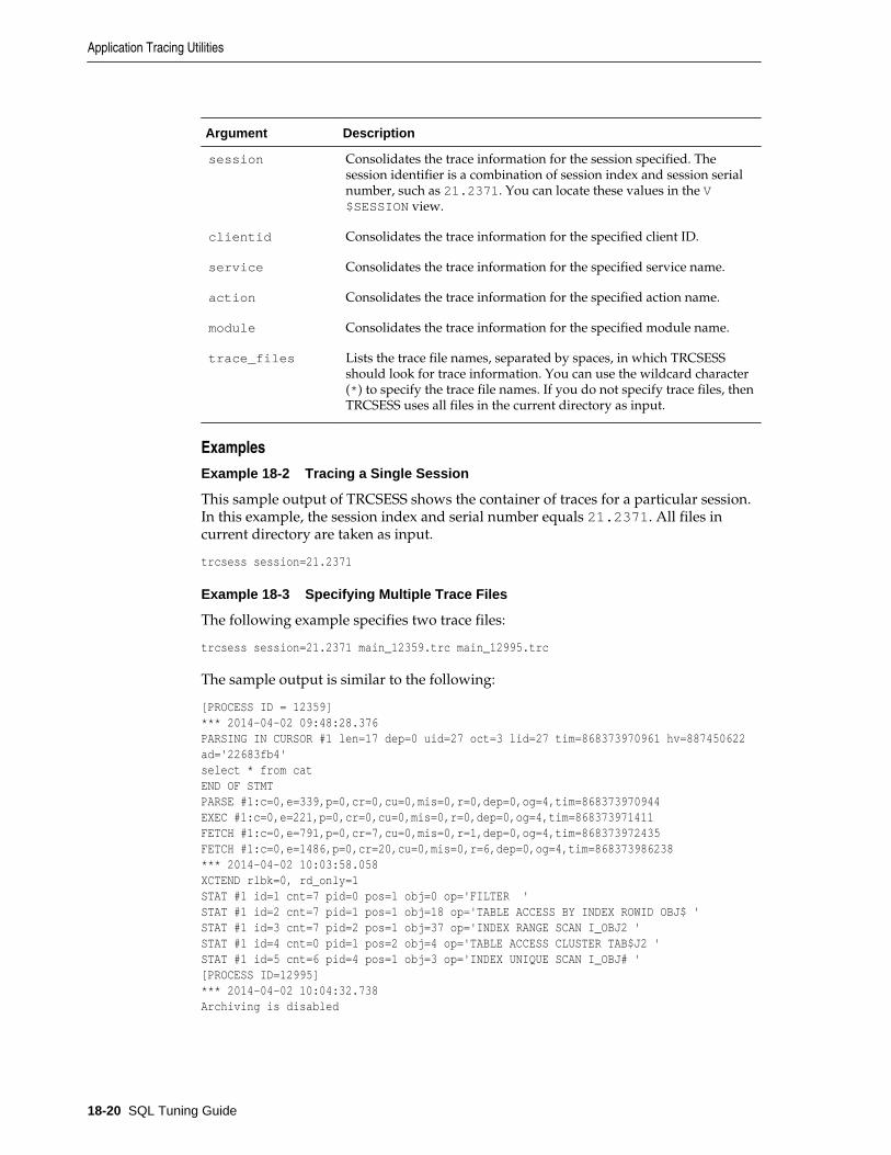
Argument Description
session Consolidates the trace information for the session specified. Thesession identifier is a combination of session index and session serialnumber, such as 21.2371. You can locate these values in the V$SESSION view.
clientid Consolidates the trace information for the specified client ID.
service Consolidates the trace information for the specified service name.
action Consolidates the trace information for the specified action name.
module Consolidates the trace information for the specified module name.
trace_files Lists the trace file names, separated by spaces, in which TRCSESSshould look for trace information. You can use the wildcard character(*) to specify the trace file names. If you do not specify trace files, thenTRCSESS uses all files in the current directory as input.
Examples
Example 18-2 Tracing a Single Session
This sample output of TRCSESS shows the container of traces for a particular session.In this example, the session index and serial number equals 21.2371. All files incurrent directory are taken as input.
trcsess session=21.2371
Example 18-3 Specifying Multiple Trace Files
The following example specifies two trace files:
trcsess session=21.2371 main_12359.trc main_12995.trc
The sample output is similar to the following:
[PROCESS ID = 12359] *** 2014-04-02 09:48:28.376 PARSING IN CURSOR #1 len=17 dep=0 uid=27 oct=3 lid=27 tim=868373970961 hv=887450622 ad='22683fb4' select * from cat END OF STMT PARSE #1:c=0,e=339,p=0,cr=0,cu=0,mis=0,r=0,dep=0,og=4,tim=868373970944 EXEC #1:c=0,e=221,p=0,cr=0,cu=0,mis=0,r=0,dep=0,og=4,tim=868373971411 FETCH #1:c=0,e=791,p=0,cr=7,cu=0,mis=0,r=1,dep=0,og=4,tim=868373972435 FETCH #1:c=0,e=1486,p=0,cr=20,cu=0,mis=0,r=6,dep=0,og=4,tim=868373986238 *** 2014-04-02 10:03:58.058 XCTEND rlbk=0, rd_only=1 STAT #1 id=1 cnt=7 pid=0 pos=1 obj=0 op='FILTER ' STAT #1 id=2 cnt=7 pid=1 pos=1 obj=18 op='TABLE ACCESS BY INDEX ROWID OBJ$ ' STAT #1 id=3 cnt=7 pid=2 pos=1 obj=37 op='INDEX RANGE SCAN I_OBJ2 ' STAT #1 id=4 cnt=0 pid=1 pos=2 obj=4 op='TABLE ACCESS CLUSTER TAB$J2 ' STAT #1 id=5 cnt=6 pid=4 pos=1 obj=3 op='INDEX UNIQUE SCAN I_OBJ# ' [PROCESS ID=12995] *** 2014-04-02 10:04:32.738 Archiving is disabled
Application Tracing Utilities
18-20 SQL Tuning Guide

TKPROFThe TKPROF program formats the contents of the trace file and places the output intoa readable output file. TKPROF can also:
• Create a SQL script that stores the statistics in the database
• Determine the execution plans of SQL statements
Note:
If the cursor for a SQL statement is not closed, then TKPROF output does notautomatically include the actual execution plan of the SQL statement. In thissituation, use the EXPLAIN option with TKPROF to generate an executionplan.
TKPROF reports each statement executed with the resources it has consumed, thenumber of times it was called, and the number of rows which it processed.
Purpose
TKPROF can locate statements using the greatest resource. With baselines available,you can assess whether the resources used are reasonable given the work done.
Guidelines
The input and output files are the only required arguments. If you invoke TKPROFwithout arguments, then the tool displays online help.
Syntax
tkprof input_file output_file [ waits=yes|no ] [ sort=option ] [ print=n ] [ aggregate=yes|no ] [ insert=filename3 ] [ sys=yes|no ] [ table=schema.table ] [ explain=user/password ] [ record=filename4 ] [ width=n ]
Options
Table 18-3 TKPROF Arguments
Argument Description
input_file Specifies the input file, a trace file containing statistics produced by theSQL Trace facility. This file can be either a trace file produced for a singlesession, or a file produced by concatenating individual trace files frommultiple sessions.
output_file Specifies the file to which TKPROF writes its formatted output.
Application Tracing Utilities
Performing Application Tracing 18-21

Table 18-3 (Cont.) TKPROF Arguments
Argument Description
WAITS Specifies whether to record summary for any wait events found in thetrace file. Valid values are YES (default) and NO.
SORT Sorts traced SQL statements in descending order of specified sort optionbefore listing them in the output file. If multiple options are specified,then the output is sorted in descending order by the sum of the valuesspecified in the sort options. If you omit this parameter, then TKPROFlists statements into the output file in order of first use. Sort options arelisted as follows:
• PRSCNT - Number of times parsed• PRSCPU - CPU time spent parsing• PRSELA - Elapsed time spent parsing• PRSDSK - Number of physical reads from disk during parse• PRSQRY - Number of consistent mode block reads during parse• PRSCU - Number of current mode block reads during parse• PRSMIS - Number of library cache misses during parse• EXECNT - Number of executions• EXECPU - CPU time spent executing• EXEELA - Elapsed time spent executing• EXEDSK - Number of physical reads from disk during execute• EXEQRY - Number of consistent mode block reads during execute• EXECU - Number of current mode block reads during execute• EXEROW - Number of rows processed during execute• EXEMIS - Number of library cache misses during execute• FCHCNT - Number of fetches• FCHCPU - CPU time spent fetching• FCHELA - Elapsed time spent fetching• FCHDSK - Number of physical reads from disk during fetch• FCHQRY - Number of consistent mode block reads during fetch• FCHCU - Number of current mode block reads during fetch• FCHROW - Number of rows fetched• USERID - Userid of user that parsed the cursor
PRINT Lists only the first integer sorted SQL statements from the output file. Ifyou omit this parameter, then TKPROF lists all traced SQL statements.This parameter does not affect the optional SQL script. The SQL scriptalways generates insert data for all traced SQL statements.
AGGREGATE If you specify AGGREGATE = NO, then TKPROF does not aggregatemultiple users of the same SQL text.
INSERT Creates a SQL script that stores the trace file statistics in the database.TKPROF creates this script with the name filename3. This script createsa table and inserts a row of statistics for each traced SQL statement intothe table.
SYS Enables and disables the listing of SQL statements issued by the userSYS, or recursive SQL statements, into the output file. The default valueof YES causes TKPROF to list these statements. The value of NO causesTKPROF to omit them. This parameter does not affect the optional SQLscript. The SQL script always inserts statistics for all traced SQLstatements, including recursive SQL statements.
Application Tracing Utilities
18-22 SQL Tuning Guide

Table 18-3 (Cont.) TKPROF Arguments
Argument Description
TABLE Specifies the schema and name of the table into which TKPROFtemporarily places execution plans before writing them to the output file.If the specified table exists, then TKPROF deletes all rows in the table,uses it for the EXPLAIN PLAN statement (which writes more rows intothe table), and then deletes those rows. If this table does not exist, thenTKPROF creates it, uses it, and then drops it.
The specified user must be able to issue INSERT, SELECT, and DELETEstatements against the table. If the table does not exist, then the user mustalso be able to issue CREATE TABLE and DROP TABLE statements. For theprivileges to issue these statements, see Oracle Database SQL LanguageReference.
This option enables multiple individuals to run TKPROF concurrentlywith the same user in the EXPLAIN value. These individuals can specifydifferent TABLE values and avoid destructively interfering with eachother's processing on the temporary plan table.
TKPROF supports the following combinations:
• The EXPLAIN parameter without the TABLE parameter
TKPROF uses the table PROF$PLAN_TABLE in the schema of the userspecified by the EXPLAIN parameter
• The TABLE parameter without the EXPLAIN parameter
TKPROF ignores the TABLE parameter.If no plan table exists, then TKPROF creates the table PROF$PLAN_TABLEand then drops it at the end.
EXPLAIN Determines the execution plan for each SQL statement in the trace fileand writes these execution plans to the output file. TKPROF also displaysthe number of rows processed by each step of the execution plan.
TKPROF determines execution plans by issuing the EXPLAIN PLANstatement after connecting to Oracle Database with the user andpassword specified in this parameter. The specified user must haveCREATE SESSION system privileges. TKPROF takes longer to process alarge trace file if the EXPLAIN option is used.
Note: Trace files generated immediately after instance startup containdata that reflects the activity of the startup process. In particular, theyreflect a disproportionate amount of I/O activity as caches in the systemglobal area (SGA) are filled. For the purposes of tuning, ignore such tracefiles.
RECORD Creates a SQL script with the specified filename with all of thenonrecursive SQL in the trace file. You can use this script to replay theuser events from the trace file.
WIDTH An integer that controls the output line width of some TKPROF output,such as the explain plan. This parameter is useful for post-processing ofTKPROF output.
Output
This section explains the TKPROF output.
Identification of User Issuing the SQL Statement in TKPROF
TKPROF lists the user ID of the user issuing each SQL statement. If the SQL Traceinput file contained statistics from multiple users, and if the statement was issued by
Application Tracing Utilities
Performing Application Tracing 18-23

multiple users, then TKPROF lists the ID of the last user to parse the statement. Theuser ID of all database users appears in the data dictionary in the columnALL_USERS.USER_ID.
Tabular Statistics in TKPROF
TKPROF lists the statistics for a SQL statement returned by the SQL Trace facility inrows and columns. Each row corresponds to one of three steps of SQL statementprocessing. Statistics are identified by the value of the CALL column. See Table 18-4.
Table 18-4 CALL Column Values
CALL Value Meaning
PARSE Translates the SQL statement into an execution plan, includingchecks for proper security authorization and checks for the existenceof tables, columns, and other referenced objects.
EXECUTE Actual execution of the statement by Oracle Database. For INSERT,UPDATE, and DELETE statements, this modifies the data. For SELECTstatements, this identifies the selected rows.
FETCH Retrieves rows returned by a query. Fetches are only performed forSELECT statements.
The other columns of the SQL Trace facility output are combined statistics for allparses, executions, and fetches of a statement. The sum of query and current is thetotal number of buffers accessed, also called Logical I/Os (LIOs). See Table 18-5.
Table 18-5 SQL Trace Statistics for Parses, Executes, and Fetches.
SQL Trace Statistic Meaning
COUNT Number of times a statement was parsed, executed, or fetched.
CPU Total CPU time in seconds for all parse, execute, or fetch calls for thestatement. This value is zero (0) if TIMED_STATISTICS is notenabled.
ELAPSED Total elapsed time in seconds for all parse, execute, or fetch calls forthe statement. This value is zero (0) if TIMED_STATISTICS is notenabled.
DISK Total number of data blocks physically read from the data files ondisk for all parse, execute, or fetch calls.
QUERY Total number of buffers retrieved in consistent mode for all parse,execute, or fetch calls. Usually, buffers are retrieved in consistentmode for queries.
CURRENT Total number of buffers retrieved in current mode. Buffers areretrieved in current mode for statements such as INSERT, UPDATE,and DELETE.
Statistics about the processed rows appear in the ROWS column. The column shows thenumber of rows processed by the SQL statement. This total does not include rowsprocessed by subqueries of the SQL statement. For SELECT statements, the number ofrows returned appears for the fetch step. For UPDATE, DELETE, and INSERTstatements, the number of rows processed appears for the execute step.
Application Tracing Utilities
18-24 SQL Tuning Guide

Note:
The row source counts are displayed when a cursor is closed. In SQL*Plus,there is only one user cursor, so each statement executed causes the previouscursor to be closed; therefore, the row source counts are displayed. PL/SQLhas its own cursor handling and does not close child cursors when the parentcursor is closed. Exiting (or reconnecting) causes the counts to be displayed.
Library Cache Misses in TKPROF
TKPROF also lists the number of library cache misses resulting from parse and executesteps for each SQL statement. These statistics appear on separate lines following thetabular statistics. If the statement resulted in no library cache misses, then TKPROFdoes not list the statistic. In “Examples”, the statement resulted in one library cachemiss for the parse step and no misses for the execute step.
Row Source Operations in TKPROF
In the TKPROF output, row source operations show the number of rows processed foreach operation executed on the rows, and additional row source information, such asphysical reads and writes.
Table 18-6 Row Source Operations
Row Source Operation Meaning
cr Consistent reads performed by the row source.
r Physical reads performed by the row source
w Physical writes performed by the row source
time Time in microseconds
In the following sample TKPROF output, note the cr, r, w, and time values under theRow Source Operation column:
Rows Row Source Operation------- --------------------------------------------------- 0 DELETE (cr=43141 r=266947 w=25854 time=60235565 us) 28144 HASH JOIN ANTI (cr=43057 r=262332 w=25854 time=48830056 us) 51427 TABLE ACCESS FULL STATS$SQLTEXT (cr=3465 r=3463 w=0 time=865083 us) 647529 INDEX FAST FULL SCAN STATS$SQL_SUMMARY_PK (cr=39592 r=39325 w=0 time=10522877 us) (object id 7409)
Wait Event Information in TKPROF
If wait event information exists, then the TKPROF output includes a section similar tothe following:
Elapsed times include waiting on following events: Event waited on Times Max. Wait Total Waited ---------------------------------------- Waited ---------- ------------ db file sequential read 8084 0.12 5.34 direct path write 834 0.00 0.00 direct path write temp 834 0.00 0.05 db file parallel read 8 1.53 5.51 db file scattered read 4180 0.07 1.45 direct path read 7082 0.00 0.05
Application Tracing Utilities
Performing Application Tracing 18-25

direct path read temp 7082 0.00 0.44 rdbms ipc reply 20 0.00 0.01 SQL*Net message to client 1 0.00 0.00 SQL*Net message from client 1 0.00 0.00
In addition, wait events are summed for the entire trace file at the end of the file.
To ensure that wait events information is written to the trace file for the session, runthe following SQL statement:
ALTER SESSION SET EVENTS '10046 trace name context forever, level 8';
Examples
Example 18-4 Printing the Most Resource-Intensive Statements
If you are processing a large trace file using a combination of SORT parameters and thePRINT parameter, then you can produce a TKPROF output file containing only thehighest resource-intensive statements. The following statement prints the 10statements in the trace file that have generated the most physical I/O:
TKPROF ora53269.trc ora53269.prf SORT = (PRSDSK, EXEDSK, FCHDSK) PRINT = 10
Example 18-5 Generating a SQL Script
This example runs TKPROF, accepts a trace file namedexamp12_jane_fg_sqlplus_007.trc, and writes a formatted output file namedoutputa.prf:
TKPROF examp12_jane_fg_sqlplus_007.trc OUTPUTA.PRF EXPLAIN=hr TABLE=hr.temp_plan_table_a INSERT=STOREA.SQL SYS=NOSORT=(EXECPU,FCHCPU)
This example is likely to be longer than a single line on the screen, and you might needto use continuation characters, depending on the operating system.
Note the other parameters in this example:
• The EXPLAIN value causes TKPROF to connect as the user hr and use the EXPLAINPLAN statement to generate the execution plan for each traced SQL statement. Youcan use this to get access paths and row source counts.
Note:
If the cursor for a SQL statement is not closed, then TKPROF output does notautomatically include the actual execution plan of the SQL statement. In thissituation, you can use the EXPLAIN option with TKPROF to generate anexecution plan.
• The TABLE value causes TKPROF to use the table temp_plan_table_a in theschema scott as a temporary plan table.
• The INSERT value causes TKPROF to generate a SQL script named STOREA.SQLthat stores statistics for all traced SQL statements in the database.
• The SYS parameter with the value of NO causes TKPROF to omit recursive SQLstatements from the output file. In this way, you can ignore internal OracleDatabase statements such as temporary table operations.
Application Tracing Utilities
18-26 SQL Tuning Guide

• The SORT value causes TKPROF to sort the SQL statements in order of the sum ofthe CPU time spent executing and the CPU time spent fetching rows before writingthem to the output file. For greatest efficiency, always use SORT parameters.
Example 18-6 TKPROF Header
This example shows a sample header for the TKPROF report.
TKPROF: Release 12.1.0.0.2 Copyright (c) 1982, 2012, Oracle and/or its affiliates. All rights reserved. Trace file: /disk1/oracle/log/diag/rdbms/orcla/orcla/trace/orcla_ora_917.trcSort options: default ********************************************************************************count = number of times OCI procedure was executedcpu = cpu time in seconds executingelapsed = elapsed time in seconds executingdisk = number of physical reads of buffers from diskquery = number of buffers gotten for consistent readcurrent = number of buffers gotten in current mode (usually for update)rows = number of rows processed by the fetch or execute call********************************************************************************
Example 18-7 TKPROF Body
This example shows a sample body for a TKPROF report.
call count cpu elapsed disk query current rows------- ------ -------- ---------- ---------- ---------- ---------- ----------Parse 1 0.01 0.00 0 0 0 0Execute 1 0.00 0.00 0 0 0 0Fetch 0 0.00 0.00 0 0 0 0------- ------ -------- ---------- ---------- ---------- ---------- ----------total 2 0.01 0.00 0 0 0 0
Misses in library cache during parse: 1Optimizer mode: FIRST_ROWSParsing user id: 44
Elapsed times include waiting on following events: Event waited on Times Max. Wait Total Waited ---------------------------------------- Waited ---------- ------------ SQL*Net message to client 1 0.00 0.00 SQL*Net message from client 1 28.59 28.59********************************************************************************
select condition from cdef$ where rowid=:1
call count cpu elapsed disk query current rows------- ------ -------- ---------- ---------- ---------- ---------- ----------Parse 1 0.00 0.00 0 0 0 0Execute 1 0.00 0.00 0 0 0 0Fetch 1 0.00 0.00 0 2 0 1------- ------ -------- ---------- ---------- ---------- ---------- ----------total 3 0.00 0.00 0 2 0 1
Misses in library cache during parse: 1Optimizer mode: CHOOSE
Application Tracing Utilities
Performing Application Tracing 18-27

Parsing user id: SYS (recursive depth: 1)
Rows Row Source Operation------- --------------------------------------------------- 1 TABLE ACCESS BY USER ROWID OBJ#(31) (cr=1 r=0 w=0 time=151 us)
********************************************************************************
SELECT last_name, job_id, salary FROM employeesWHERE salary = (SELECT max(salary) FROM employees)
call count cpu elapsed disk query current rows------- ------ -------- ---------- ---------- ---------- ---------- ----------Parse 1 0.02 0.01 0 0 0 0Execute 1 0.00 0.00 0 0 0 0Fetch 2 0.00 0.00 0 15 0 1------- ------ -------- ---------- ---------- ---------- ---------- ----------total 4 0.02 0.01 0 15 0 1
Misses in library cache during parse: 1Optimizer mode: FIRST_ROWSParsing user id: 44
Rows Row Source Operation------- --------------------------------------------------- 1 TABLE ACCESS FULL EMPLOYEES (cr=15 r=0 w=0 time=1743 us) 1 SORT AGGREGATE (cr=7 r=0 w=0 time=777 us) 107 TABLE ACCESS FULL EMPLOYEES (cr=7 r=0 w=0 time=655 us)
Elapsed times include waiting on following events: Event waited on Times Max. Wait Total Waited ---------------------------------------- Waited ---------- ------------ SQL*Net message to client 2 0.00 0.00 SQL*Net message from client 2 9.62 9.62********************************************************************************
******************************************************************************** delete from stats$sqltext st where (hash_value, text_subset) not in (select --+ hash_aj hash_value, text_subset from stats$sql_summary ss where ( ( snap_id < :lo_snap or snap_id > :hi_snap ) and dbid = :dbid and instance_number = :inst_num ) or ( dbid != :dbid or instance_number != :inst_num) )
call count cpu elapsed disk query current rows------- ------ -------- ---------- ---------- ---------- ---------- ----------Parse 1 0.00 0.00 0 0 0 0Execute 1 29.60 60.68 266984 43776 131172 28144Fetch 0 0.00 0.00 0 0 0 0------- ------ -------- ---------- ---------- ---------- ---------- ----------
Application Tracing Utilities
18-28 SQL Tuning Guide

total 2 29.60 60.68 266984 43776 131172 28144
Misses in library cache during parse: 1Misses in library cache during execute: 1Optimizer mode: CHOOSEParsing user id: 22
Rows Row Source Operation------- --------------------------------------------------- 0 DELETE (cr=43141 r=266947 w=25854 time=60235565 us) 28144 HASH JOIN ANTI (cr=43057 r=262332 w=25854 time=48830056 us) 51427 TABLE ACCESS FULL STATS$SQLTEXT (cr=3465 r=3463 w=0 time=865083 us) 647529 INDEX FAST FULL SCAN STATS$SQL_SUMMARY_PK (cr=39592 r=39325 w=0 time=10522877 us) (object id 7409)
Elapsed times include waiting on following events: Event waited on Times Max. Wait Total Waited ---------------------------------------- Waited ---------- ------------ db file sequential read 8084 0.12 5.34 direct path write 834 0.00 0.00 direct path write temp 834 0.00 0.05 db file parallel read 8 1.53 5.51 db file scattered read 4180 0.07 1.45 direct path read 7082 0.00 0.05 direct path read temp 7082 0.00 0.44 rdbms ipc reply 20 0.00 0.01 SQL*Net message to client 1 0.00 0.00 SQL*Net message from client 1 0.00 0.00********************************************************************************
Example 18-8 TKPROF Summary
This example that shows a summary for the TKPROF report.
OVERALL TOTALS FOR ALL NON-RECURSIVE STATEMENTS
call count cpu elapsed disk query current rows------- ------ -------- ---------- ---------- ---------- ---------- ----------Parse 4 0.04 0.01 0 0 0 0Execute 5 0.00 0.04 0 0 0 0Fetch 2 0.00 0.00 0 15 0 1------- ------ -------- ---------- ---------- ---------- ---------- ----------total 11 0.04 0.06 0 15 0 1
Misses in library cache during parse: 4Misses in library cache during execute: 1Elapsed times include waiting on following events: Event waited on Times Max. Wait Total Waited ---------------------------------------- Waited ---------- ------------ SQL*Net message to client 6 0.00 0.00 SQL*Net message from client 5 77.77 128.88
OVERALL TOTALS FOR ALL RECURSIVE STATEMENTS
call count cpu elapsed disk query current rows------- ------ -------- ---------- ---------- ---------- ---------- ----------Parse 1 0.00 0.00 0 0 0 0Execute 1 0.00 0.00 0 0 0 0Fetch 1 0.00 0.00 0 2 0 1------- ------ -------- ---------- ---------- ---------- ---------- ----------total 3 0.00 0.00 0 2 0 1
Application Tracing Utilities
Performing Application Tracing 18-29

Misses in library cache during parse: 1 5 user SQL statements in session. 1 internal SQL statements in session. 6 SQL statements in session.********************************************************************************Trace file: main_ora_27621.trcTrace file compatibility: 9.00.01Sort options: default 1 session in tracefile. 5 user SQL statements in trace file. 1 internal SQL statements in trace file. 6 SQL statements in trace file. 6 unique SQL statements in trace file. 76 lines in trace file. 128 elapsed seconds in trace file.
Views for Application TracingThis section includes the following topics:
• Views Relevant for Trace Statistics
• Views Related to Enabling Tracing
Views Relevant for Trace StatisticsYou can display the statistics that have been gathered with the following V$ views:
• The DBA_ENABLED_AGGREGATIONS view displays the accumulated globalstatistics for the currently enabled statistics.
• The V$CLIENT_STATS view displays the accumulated statistics for a specifiedclient identifier.
• The V$SERVICE_STATS view displays accumulated statistics for a specifiedservice.
• The V$SERV_MOD_ACT_STATS view displays accumulated statistics for acombination of specified service, module, and action.
• The V$SERVICEMETRIC view displays accumulated statistics for elapsed time ofdatabase calls and for CPU use.
Views Related to Enabling TracingA Cloud Control report or the DBA_ENABLED_TRACES view can display outstandingtraces. In the DBA_ENABLED_TRACES view, you can determine detailed informationabout how a trace was enabled, including the trace type. The trace type specifieswhether the trace is enabled for client identifier, session, service, database, or acombination of service, module, and action.
Views for Application Tracing
18-30 SQL Tuning Guide

Part VIIIAutomatic SQL Tuning
This part contains the following chapters:
• Managing SQL Tuning Sets
• Analyzing SQL with SQL Tuning Advisor
• Optimizing Access Paths with SQL Access Advisor


19Managing SQL Tuning Sets
This chapter contains the following topics:
• About SQL Tuning Sets
• Creating a SQL Tuning Set
• Loading a SQL Tuning Set
• Displaying the Contents of a SQL Tuning Set
• Modifying a SQL Tuning Set
• Transporting a SQL Tuning Set
• Dropping a SQL Tuning Set
About SQL Tuning SetsA SQL tuning set (STS) is a database object that includes:
• A set of SQL statements
• Associated execution context, such as user schema, application module name andaction, list of bind values, and the environment for SQL compilation of the cursor
• Associated basic execution statistics, such as elapsed time, CPU time, buffer gets,disk reads, rows processed, cursor fetches, the number of executions, the number ofcomplete executions, optimizer cost, and the command type
• Associated execution plans and row source statistics for each SQL statement(optional)
The database stores SQL tuning sets in a database-provided schema.
This section contains the following topics:
• Purpose of SQL Tuning Sets
• Concepts for SQL Tuning Sets
• User Interfaces for SQL Tuning Sets
• Basic Tasks for SQL Tuning Sets
Managing SQL Tuning Sets 19-1

Note:
Data visibility and privilege requirements may differ when using an STS with pluggable databases. See Oracle Database Administrator's Guide for a table thatsummarizes how manageability features work in a container database (CDB).
Purpose of SQL Tuning SetsAn STS enables you to group SQL statements and related metadata in a singledatabase object, which you can use to meet your tuning goals. Specifically, SQL tuningsets achieve the following goals:
• Providing input to the performance tuning advisors
You can use an STS as input to multiple database advisors, including SQL TuningAdvisor, SQL Access Advisor, and SQL Performance Analyzer.
• Transporting SQL between databases
You can export SQL tuning sets from one database to another, enabling transfer ofSQL workloads between databases for remote performance diagnostics and tuning.When suboptimally performing SQL statements occur on a production database,developers may not want to investigate and tune directly on the productiondatabase. The DBA can transport the problematic SQL statements to a test databasewhere the developers can safely analyze and tune them.
Concepts for SQL Tuning SetsTo create an STS, you must load SQL statements into an STS from a source. As shownin Figure 19-1, the source can be Automatic Workload Repository (AWR), the sharedSQL area, customized SQL provided by the user, trace files, or another STS.
About SQL Tuning Sets
19-2 SQL Tuning Guide

Figure 19-1 SQL Tuning Sets
SQL TuningAdvisor
SQL AccessAdvisor
SQL PerformanceAnalyzer
Transport
Filter
CustomSQL
AWR
Shared SQLArea
SQL TraceFiles
STS
SQL tuning sets can do the following:
• Filter SQL statements using the application module name and action, or anyexecution statistics
• Rank SQL statements based on any combination of execution statistics
• Serve as input to the advisors or transport it to a different database
See Also:
Oracle Database Performance Tuning Guide to learn about AWR
About SQL Tuning Sets
Managing SQL Tuning Sets 19-3

User Interfaces for SQL Tuning SetsYou can use either Oracle Enterprise Manager Cloud Control (Cloud Control) or theDBMS_SQLTUNE package to manage SQL tuning sets. Oracle recommends that you useCloud Control.
Accessing the SQL Tuning Sets Page in Cloud Control
The SQL Tuning Sets page in Cloud Control is the starting page from which you canperform most operations relating to SQL tuning sets.
To access the SQL Tuning Sets page:
1. Access the Database Home page, as described in “Accessing the Database HomePage in Cloud Control.”
2. From the Performance menu, select SQL, then SQL Tuning Sets.
The SQL Tuning Sets page appears, as shown in Figure 19-2.
Figure 19-2 SQL Tuning Sets
See Also:
Oracle Database 2 Day + Performance Tuning Guide
Command-Line Interface to SQL Tuning Sets
On the command line, you can use the DBMS_SQLTUNE package to manage SQLtuning sets. You must have the ADMINISTER SQL TUNING SET system privilege tomanage SQL tuning sets that you own, or the ADMINISTER ANY SQL TUNING SETsystem privilege to manage any SQL tuning sets.
See Also:
Oracle Database PL/SQL Packages and Types Reference to learn aboutDBMS_SQLTUNE
About SQL Tuning Sets
19-4 SQL Tuning Guide

Basic Tasks for SQL Tuning SetsThis section explains the basic tasks involved in managing SQL tuning sets. Figure19-3 shows the basic workflow for creating, using, and deleting an STS.
Figure 19-3 SQL Tuning Sets APIs
LOAD_SQLSET
Create a Tuning Task
CREATE_SQLSET
DROP_SQLSET
DELETE_SQLSET
UPDATE SQLSET
CREATE_STGTAB_SQLSET
PACK_STGTAB_SQLSET
Transport STS
UNPACK_STGTAB_SQLSET
Modify STS Contents
Display Contentsof STS
Create STS
Drop STS
Populate STS with SQL
Optionally, transportSTS to differentdatabase
SELECT_SQLSET
Typically, you perform STS operations in the following sequence:
1. Create a new STS.
“Creating a SQL Tuning Set” describes this task.
2. Load the STS with SQL statements and associated metadata.
“Loading a SQL Tuning Set” describes this task.
3. Optionally, display the contents of the STS.
“Displaying the Contents of a SQL Tuning Set” describes this task.
4. Optionally, update or delete the contents of the STS.
“Modifying a SQL Tuning Set” describes this task.
5. Create a tuning task with the STS as input.
6. Optionally, transport the STS to another database.
“Transporting a SQL Tuning Set” describes this task.
7. Drop the STS when finished.
About SQL Tuning Sets
Managing SQL Tuning Sets 19-5

“Dropping a SQL Tuning Set” describes this task.
Creating a SQL Tuning SetExecute the DBMS_SQLTUNE.CREATE_SQLSET procedure to create an empty STS inthe database. Using the function instead of the procedure causes the database togenerate a name for the STS.
Table 19-1 describes some procedure parameters. See Oracle Database PL/SQL Packagesand Types Reference for complete reference information.
Table 19-1 DBMS_SQLTUNE.CREATE_SQLSET Parameters
Parameter Description
sqlset_name Name of the STS
description Optional description of the STS
Assumptions
This tutorial assumes that you want to create an STS named SQLT_WKLD_STS.
To create an STS:
1. Connect SQL*Plus to the database with the appropriate privileges, and then runthe DBMS_SQLTUNE.CREATE_SQLSET procedure.
For example, execute the following PL/SQL program:
BEGIN DBMS_SQLTUNE.CREATE_SQLSET ( sqlset_name => 'SQLT_WKLD_STS' , description => 'STS to store SQL from the private SQL area' );END;
2. Optionally, confirm that the STS was created.
The following example queries the status of all SQL tuning sets owned by thecurrent user:
COLUMN NAME FORMAT a20COLUMN COUNT FORMAT 99999COLUMN DESCRIPTION FORMAT a30
SELECT NAME, STATEMENT_COUNT AS "SQLCNT", DESCRIPTIONFROM USER_SQLSET;
Sample output appears below:
NAME SQLCNT DESCRIPTION-------------------- ------ ------------------------------SQLT_WKLD_STS 2 SQL Cache
Loading a SQL Tuning SetTo load an STS with SQL statements, execute the DBMS_SQLTUNE.LOAD_SQLSETprocedure. The standard sources for populating an STS are AWR, another STS, or the
Creating a SQL Tuning Set
19-6 SQL Tuning Guide

shared SQL area. For both the workload repository and SQL tuning sets, predefinedtable functions can select columns from the source to populate a new STS.
Table 19-2 describes some DBMS_SQLTUNE.LOAD_SQLSET procedure parameters. See Oracle Database PL/SQL Packages and Types Reference for complete referenceinformation.
Table 19-2 DBMS_SQLTUNE.LOAD_SQLSET Parameters
Parameter Description
populate_cursor Specifies the cursor reference from which to populate the STS.
load_option Specifies how the statements are loaded into the STS. Thepossible values are INSERT (default), UPDATE, and MERGE.
The DBMS_SQLTUNE.SELECT_CURSOR_CACHE function collects SQL statements fromthe shared SQL area according to the specified filter. This function returns oneSQLSET_ROW per SQL ID or PLAN_HASH_VALUE pair found in each data source.
Use the CAPTURE_CURSOR_CACHE_SQLSET function to repeatedly poll the sharedSQL area over a specified interval. This function is more efficient than repeatedlycalling the SELECT_CURSOR_CACHE and LOAD_SQLSET procedures. This functioneffectively captures the entire workload, as opposed to the AWR, which only capturesthe workload of high-load SQL statements, or the LOAD_SQLSET procedure, whichaccesses the data source only once.
Prerequisites
This tutorial has the following prerequisites:
• Filters provided to the SELECT_CURSOR_CACHE function are evaluated as part ofSQL statements run by the current user. As such, they are executed with that user'ssecurity privileges and can contain any constructs and subqueries that user canaccess, but no more.
• The current user must have privileges on the shared SQL area views.
Assumptions
This tutorial assumes that you want to load the SQL tuning set namedSQLT_WKLD_STS with statements from the shared SQL area.
To load an STS:
1. Connect SQL*Plus to the database as a user with the appropriate privileges.
2. Run the DBMS_SQLTUNE.LOAD_SQLSET procedure.
For example, execute the following PL/SQL program to populate a SQL tuningset with all cursor cache statements that belong to the sh schema:
DECLARE c_sqlarea_cursor DBMS_SQLTUNE.SQLSET_CURSOR;BEGIN OPEN c_sqlarea_cursor FOR SELECT VALUE(p) FROM TABLE( DBMS_SQLTUNE.SELECT_CURSOR_CACHE(
Loading a SQL Tuning Set
Managing SQL Tuning Sets 19-7

' module = ''SQLT_WKLD'' AND parsing_schema_name = ''SH'' ') ) p;-- load the tuning set DBMS_SQLTUNE.LOAD_SQLSET ( sqlset_name => 'SQLT_WKLD_STS', populate_cursor => c_sqlarea_cursor );END;/
Displaying the Contents of a SQL Tuning SetAfter an STS has been created and populated, execute theDBMS_SQLTUNE.SELECT_SQLSET function to read the contents of the STS, optionallyusing filtering criteria.
You select the output of SELECT_SQLSET using a PL/SQL pipelined table function,which accepts a collection of rows as input. You invoke the table function as theoperand of the table operator in the FROM list of a SELECT statement.
Table 19-3 describes some SELECT_SQLSET function parameters. See Oracle DatabasePL/SQL Packages and Types Reference for complete reference information.
Table 19-3 DBMS_SQLTUNE.SELECT_SQLSET Parameters
Parameter Description
basic_filter The SQL predicate to filter the SQL from the STS defined onattributes of the SQLSET_ROW
object_filter Specifies the objects that exist in the object list of selected SQL fromthe shared SQL area
Table 19-4 describes some attributes of the SQLSET_ROW object. These attributesappears as columns when you query TABLE(DBMS_SQLTUNE.SELECT_SQLSET()).
Table 19-4 SQLSET_ROW Attributes
Parameter Description
parsing_schema_name Schema in which the SQL is parsed
elapsed_time Sum of the total number of seconds elapsed for this SQLstatement
buffer_gets Total number of buffer gets (number of times the databaseaccessed a block) for this SQL statement
Assumptions
This tutorial assumes that you want to display the contents of an STS namedSQLT_WKLD_STS.
To display the contents of an STS:
1. Connect SQL*Plus to the database with the appropriate privileges, and then querythe STS contents using the TABLE function.
Displaying the Contents of a SQL Tuning Set
19-8 SQL Tuning Guide

For example, execute the following query:
COLUMN SQL_TEXT FORMAT a30 COLUMN SCH FORMAT a3COLUMN ELAPSED FORMAT 999999999
SELECT SQL_ID, PARSING_SCHEMA_NAME AS "SCH", SQL_TEXT, ELAPSED_TIME AS "ELAPSED", BUFFER_GETSFROM TABLE( DBMS_SQLTUNE.SELECT_SQLSET( 'SQLT_WKLD_STS' ) );
Sample output appears below:
SQL_ID SCH SQL_TEXT ELAPSED BUFFER_GETS------------- --- ------------------------------ ---------- -----------79f8shn041a1f SH select * from sales where quan 8373148 24016 tity_sold < 5 union select * f rom sales where quantity_sold > 500 2cqsw036j5u7r SH select promo_name, count(*) c 3557373 309 from promotions p, sales s whe re s.promo_id = p.promo_id and p.promo_category = 'internet' group by p.promo_name order b y c desc fudq5z56g642p SH select sum(quantity_sold) from 4787891 12118 sales s, products p where s.p rod_id = p.prod_id and s.amoun t_sold > 20000 and p.prod_name = 'Linen Big Shirt' bzmnj0nbvmz8t SH select * from sales where amou 442355 15281 nt_sold = 4
2. Optionally, filter the results based on user-specific criteria.
The following example displays statements with a disk reads to buffer gets ratiogreater than or equal to 50%:
COLUMN SQL_TEXT FORMAT a30 COLUMN SCH FORMAT a3COLUMN BUF_GETS FORMAT 99999999COLUMN DISK_READS FORMAT 99999999COLUMN %_DISK FORMAT 9999.99SELECT sql_id, parsing_schema_name as "SCH", sql_text, buffer_gets as "B_GETS", disk_reads, ROUND(disk_reads/buffer_gets*100,2) "%_DISK"FROM TABLE( DBMS_SQLTUNE.SELECT_SQLSET( 'SQLT_WKLD_STS', '(disk_reads/buffer_gets) >= 0.50' ) );
Sample output appears below:
SQL_ID SCH SQL_TEXT B_GETS DISK_READS %_DISK------------- --- ------------------------------ ------ ---------- -------79f8shn041a1f SH select * from sales where quan 24016 17287 71.98 tity_sold < 5 union select * f rom sales where quantity_sold > 500 fudq5z56g642p SH select sum(quantity_sold) from 12118 6355 52.44
Displaying the Contents of a SQL Tuning Set
Managing SQL Tuning Sets 19-9
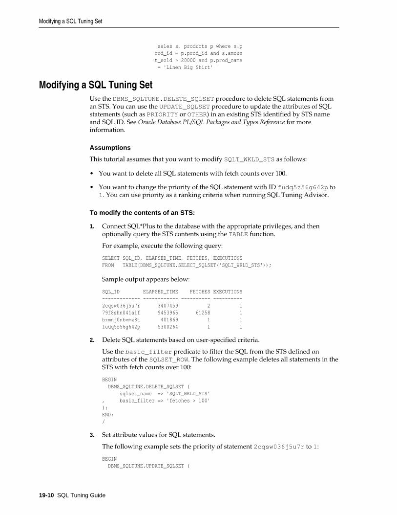
sales s, products p where s.p rod_id = p.prod_id and s.amoun t_sold > 20000 and p.prod_name = 'Linen Big Shirt'
Modifying a SQL Tuning SetUse the DBMS_SQLTUNE.DELETE_SQLSET procedure to delete SQL statements froman STS. You can use the UPDATE_SQLSET procedure to update the attributes of SQLstatements (such as PRIORITY or OTHER) in an existing STS identified by STS nameand SQL ID. See Oracle Database PL/SQL Packages and Types Reference for moreinformation.
Assumptions
This tutorial assumes that you want to modify SQLT_WKLD_STS as follows:
• You want to delete all SQL statements with fetch counts over 100.
• You want to change the priority of the SQL statement with ID fudq5z56g642p to1. You can use priority as a ranking criteria when running SQL Tuning Advisor.
To modify the contents of an STS:
1. Connect SQL*Plus to the database with the appropriate privileges, and thenoptionally query the STS contents using the TABLE function.
For example, execute the following query:
SELECT SQL_ID, ELAPSED_TIME, FETCHES, EXECUTIONSFROM TABLE(DBMS_SQLTUNE.SELECT_SQLSET('SQLT_WKLD_STS'));
Sample output appears below:
SQL_ID ELAPSED_TIME FETCHES EXECUTIONS------------- ------------ ---------- ----------2cqsw036j5u7r 3407459 2 179f8shn041a1f 9453965 61258 1bzmnj0nbvmz8t 401869 1 1fudq5z56g642p 5300264 1 1
2. Delete SQL statements based on user-specified criteria.
Use the basic_filter predicate to filter the SQL from the STS defined onattributes of the SQLSET_ROW. The following example deletes all statements in theSTS with fetch counts over 100:
BEGIN DBMS_SQLTUNE.DELETE_SQLSET ( sqlset_name => 'SQLT_WKLD_STS', basic_filter => 'fetches > 100');END;/
3. Set attribute values for SQL statements.
The following example sets the priority of statement 2cqsw036j5u7r to 1:
BEGIN DBMS_SQLTUNE.UPDATE_SQLSET (
Modifying a SQL Tuning Set
19-10 SQL Tuning Guide

sqlset_name => 'SQLT_WKLD_STS' , sql_id => '2cqsw036j5u7r' , attribute_name => 'PRIORITY' , attribute_value => 1);END;/
4. Optionally, query the STS to confirm that the intended modifications were made.
For example, execute the following query:
SELECT SQL_ID, ELAPSED_TIME, FETCHES, EXECUTIONS, PRIORITYFROM TABLE(DBMS_SQLTUNE.SELECT_SQLSET('SQLT_WKLD_STS'));
Sample output appears below:
SQL_ID ELAPSED_TIME FETCHES EXECUTIONS PRIORITY------------- ------------ ---------- ---------- ----------2cqsw036j5u7r 3407459 2 1 1bzmnj0nbvmz8t 401869 1 1fudq5z56g642p 5300264 1 1
Transporting a SQL Tuning SetYou can transport an STS to any database created in Oracle Database 10g Release 2(10.2) or later. This technique is useful when using SQL Performance Analyzer to tuneregressions on a test database.
About Transporting SQL Tuning SetsWhen you transport SQL tuning sets between databases, use DBMS_SQLTUNE to copythe SQL tuning sets to and from a staging table, and use other tools (such as OracleData Pump or a database link) to move the staging table to the destination database.
Basic Steps for Transporting SQL Tuning Sets
Figure 19-4 shows the process using Oracle Data Pump and ftp.
Figure 19-4 Transporting SQL Tuning Sets
Transport ftp, nfs
ProductionDatabase
TestDatabase
Staging Table
Data PumpExport
.dmpfile
Data PumpImport
.dmpfile
System-Supplied Schema System-Supplied Schema
PACK_STGTAB_SQLSET UNPACK_STGTAB_SQLSET
Staging Table
As shown in Figure 19-4, the steps are as follows:
Transporting a SQL Tuning Set
Managing SQL Tuning Sets 19-11

1. In the production database, pack the STS into a staging table usingDBMS_SQLTUNE.PACK_STGTAB_SQLSET.
2. Export the STS from the staging table to a .dmp file using Oracle Data Pump.
3. Transfer the .dmp file from the production host to the test host using a transfertool such as ftp.
4. In the test database, import the STS from the .dmp file to a staging table usingOracle Data Pump.
5. Unpack the STS from the staging table usingDBMS_SQLTUNE.UNPACK_STGTAB_SQLSET.
Basic Steps for Transporting SQL Tuning Sets from a Non-CDB to a CDB
When you transport an STS from a non-CDB to a CDB database, you must remap thecon_dbid of each SQL statement in the STS to a con_dbid within the destinationCDB. The basic steps are as follows:
1. Pack the STS into a staging table using DBMS_SQLTUNE.PACK_STGTAB_SQLSET.
2. Remap each con_dbid in the staging table usingDBMS_SQLTUNE.REMAP_STGTAB_SQLSET.
3. Export the STS.
4. Unpack the STS in the destination CDB.
The following sample PL/SQL program remaps con_dbid 1234 to 5678:
BEGIN DBMS_SQLTUNE.REMAP_STGTAB_SQLSET ( staging_table_name => 'non_cdb_sts1', staging_schema_owner => 'dba1', old_con_dbid => 1234, new_con_dbid => 5678);END;
See Also:
Oracle Database PL/SQL Packages and Types Reference to learn aboutREMAP_STGTAB_SQLSET
Transporting SQL Tuning Sets with DBMS_SQLTUNETable 19-5 describes the DBMS_SQLTUNE procedures relevant for transporting SQLtuning sets. See Oracle Database PL/SQL Packages and Types Reference for completereference information.
Table 19-5 DBMS_SQLTUNE Procedures for Transporting SQL Tuning Sets
Procedure Description
CREATE_STGTAB_SQLSET Create a staging table to hold the exported SQL tuningsets
Transporting a SQL Tuning Set
19-12 SQL Tuning Guide

Table 19-5 (Cont.) DBMS_SQLTUNE Procedures for Transporting SQL Tuning Sets
Procedure Description
PACK_STGTAB_SQLSET Populate a staging table with SQL tuning sets
UNPACK_STGTAB_SQLSET Copy the SQL tuning sets from the staging table into adatabase
Assumptions
This tutorial assumes the following:
• An STS with regressed SQL resides in a production database created in the currentrelease.
• You run SQL Performance Analyzer trials on a remote test database created inOracle Database 11g Release 2 (11.2).
• You want to copy the STS from the production database to the test database andtune the regressions from the SQL Performance Analyzer trials.
• You want to use Oracle Database Pump to transfer the SQL tuning sets betweendatabase hosts.
To transport an STS:
1. Connect SQL*Plus to the production database with administrator privileges.
2. Use the CREATE_STGTAB_SQLSET procedure to create a staging table to hold theexported SQL tuning sets.
The following example creates my_11g_staging_table in the dba1 schemaand specifies the format of the staging table as 11.2:
BEGIN DBMS_SQLTUNE.CREATE_STGTAB_SQLSET ( table_name => 'my_10g_staging_table', schema_name => 'dba1', db_version => DBMS_SQLTUNE.STS_STGTAB_11_2_VERSION );END;/
3. Use the PACK_STGTAB_SQLSET procedure to populate the staging table with SQLtuning sets.
The following example populates dba1.my_11g_staging_table with the STSmy_sts owned by hr:
BEGIN DBMS_SQLTUNE.PACK_STGTAB_SQLSET ( sqlset_name => 'sqlt_wkld_sts', sqlset_owner => 'sh', staging_table_name => 'my_11g_staging_table', staging_schema_owner => 'dba1', db_version => DBMS_SQLTUNE.STS_STGTAB_11_2_VERSION );
Transporting a SQL Tuning Set
Managing SQL Tuning Sets 19-13

END;/
4. Use Oracle Data Pump to export the contents of the statistics table.
For example, run the expdp command at the operating system prompt:
expdp dba1 DIRECTORY=dpump_dir1 DUMPFILE=sts.dmp TABLES=my_11g_staging_table
5. Transfer the dump file to the test database host.
6. Log in to the test host as an administrator, and then use Oracle Data Pump toimport the contents of the statistics table.
For example, run the impdp command at the operating system prompt:
impdp dba1 DIRECTORY=dpump_dir1 DUMPFILE=sts.dmp TABLES=my_11g_staging_table
7. On the test database, execute the UNPACK_STGTAB_SQLSET procedure to copythe SQL tuning sets from the staging table into the database.
The following example shows how to unpack the SQL tuning sets:
BEGIN DBMS_SQLTUNE.UNPACK_STGTAB_SQLSET ( sqlset_name => '%', replace => true, staging_table_name => 'my_11g_staging_table');END;/
Dropping a SQL Tuning SetExecute the DBMS_SQLTUNE.DROP_SQLSET procedure to drop an STS from thedatabase.
Prerequisites
Ensure that no tuning task is currently using the STS to be dropped. If a tuning taskexists that is using this STS, then drop the task before dropping the STS. Otherwise,the database issues an ORA-13757 error.
Assumptions
This tutorial assumes that you want to drop an STS named SQLT_WKLD_STS.
To drop an STS:
1. Connect SQL*Plus to the database with the appropriate privileges, and then runthe DBMS_SQLTUNE.DROP_SQLSET procedure.
For example, execute the following PL/SQL program:
BEGIN DBMS_SQLTUNE.DROP_SQLSET( sqlset_name => 'SQLT_WKLD_STS' );END;/
2. Optionally, confirm that the STS was deleted.
The following example counts the number of SQL tuning sets namedSQLT_WKLD_STS owned by the current user (sample output included):
Dropping a SQL Tuning Set
19-14 SQL Tuning Guide

SELECT COUNT(*) FROM USER_SQLSET WHERE NAME = 'SQLT_WKLD_STS';
COUNT(*)---------- 0
See Also:
Oracle Database PL/SQL Packages and Types Reference to learn about the STSprocedures in DBMS_SQLTUNE
Dropping a SQL Tuning Set
Managing SQL Tuning Sets 19-15

Dropping a SQL Tuning Set
19-16 SQL Tuning Guide

20Analyzing SQL with SQL Tuning Advisor
This chapter explains the concepts and tasks relating to SQL Tuning Advisor.
This chapter contains the following topics:
• About SQL Tuning Advisor
• Managing the Automatic SQL Tuning Task
• Running SQL Tuning Advisor On Demand
About SQL Tuning AdvisorSQL Tuning Advisor is SQL diagnostic software in the Oracle Database Tuning Pack.You can submit one or more SQL statements as input to the advisor and receive adviceor recommendations for how to tune the statements, along with a rationale andexpected benefit.
This section contains the following topics:
• Purpose of SQL Tuning Advisor
• SQL Tuning Advisor Architecture
• Automatic Tuning Optimizer Concepts
Purpose of SQL Tuning AdvisorSQL Tuning Advisor is a mechanism for resolving problems related to suboptimallyperforming SQL statements. Use SQL Tuning Advisor to obtain recommendations forimproving performance of high-load SQL statements, and prevent regressions by onlyexecuting optimal plans.
Tuning recommendations include:
• Collection of object statistics
• Creation of indexes
• Rewriting SQL statements
• Creation of SQL profiles
• Creation of SQL plan baselines
The recommendations generated by SQL Tuning Advisor help you achieve thefollowing specific goals:
• Avoid labor-intensive manual tuning
Analyzing SQL with SQL Tuning Advisor 20-1

Identifying and tuning high-load SQL statements is challenging even for an expert.SQL Tuning Advisor uses the optimizer to tune SQL for you.
• Generate recommendations and implement SQL profiles automatically
You can configure an Automatic SQL Tuning task to run nightly in maintenancewindows. When invoked in this way, the advisor can generate recommendationsand also implement SQL profiles automatically.
• Analyze database-generated statistics to achieve optimal plans
The database contains a vast amount of statistics about its own operations. SQLTuning Advisor can perform deep mining and analysis of internal information toimprove execution plans.
• Enable developers to tune SQL on a test system instead of the production system
When suboptimally performing SQL statements occur on a production database,developers may not want to investigate and tune directly on the productiondatabase. The DBA can transport the problematic SQL statements to a test databasewhere the developers can safely analyze and tune them.
When tuning multiple statements, SQL Tuning Advisor does not recognizeinterdependencies between the statements. Instead, SQL Tuning Advisor offers aconvenient way to get tuning recommendations for many statements.
Note:
Data visibility and privilege requirements may differ when using SQL TuningAdvisor with pluggable databases. The advisor can tune a query in the currentpluggable database (PDB), and in other PDBs in which this query has beenexecuted. In this way, a container database (CDB) administrator can tune thesame query in many PDBs at the same time, whereas a PDB administrator canonly tune a single PDB.
See Also:
• “Managing SQL Plan Baselines ” to learn about SQL plan management
• Oracle Database Administrator’s Guide for a table that summarizes howmanageability features work in a CDB
SQL Tuning Advisor ArchitectureAutomatic Tuning Optimizer is the central tool used by SQL Tuning Advisor. Theadvisor can receive SQL statements as input from the sources shown in Figure 20-1,analyze these statements using the optimizer, and then make recommendations.
Invoking Automatic Tuning Optimizer for every hard parse consumes significant timeand resources (see “SQL Parsing”). Tuning mode is meant for complex and high-loadSQL statements that significantly affect database performance.
Figure 20-1 shows the basic architecture of SQL Tuning Advisor.
About SQL Tuning Advisor
20-2 SQL Tuning Guide

Figure 20-1 SQL Tuning Advisor Architecture
SQLTuningSet
Shared Pool
Library Cache
Shared SQL Area
SELECT * FROM employees
ADDM
AWR
AUTOTASK
Recommendations
Inplementation of SQL Profiles(Automatic Only)
SQL TuningAdvisor
Optimizer
Automatic Tuning Optimizer
Invocation of SQL Tuning Advisor
SQL Tuning Advisor is invoked in either of the following ways:
• Automatically
You can configure SQL Tuning Advisor to run during nightly system maintenancewindows. When run by AUTOTASK, the advisor is known as Automatic SQLTuning Advisor and performs automatic SQL tuning. See “Managing theAutomatic SQL Tuning Task”.
• On-Demand
In on-demand SQL tuning, you manually invoke SQL Tuning Advisor to diagnoseand fix SQL-related performance problems after they have been discovered. OracleEnterprise Manager Cloud Control (Cloud Control) is the preferred interface fortuning SQL on demand, but you can also use the DBMS_SQLTUNE PL/SQLpackage. See “Running SQL Tuning Advisor On Demand”.
SQL Tuning Advisor uses Automatic Tuning Optimizer to perform its analysis. Thisoptimization is "automatic" because the optimizer analyzes the SQL instead of theuser. Do not confuse Automatic Tuning Optimizer with automatic SQL tuning, whichin this document refers only to the work performed by the Automatic SQL Tuningtask.
See Also:
Oracle Database PL/SQL Packages and Types Reference to learn aboutDBMS_SQLTUNE
About SQL Tuning Advisor
Analyzing SQL with SQL Tuning Advisor 20-3

Input to SQL Tuning Advisor
Input for SQL Tuning Advisor can come from several sources, including the following:
• Automatic Database Diagnostic Monitor (ADDM)
The primary input source is ADDM (pronounced Adam). By default, ADDM runsproactively once every hour and analyzes key statistics gathered by AutomaticWorkload Repository (AWR) over the last hour to identify any performanceproblems including high-load SQL statements. If a high-load SQL is identified,then ADDM recommends running SQL Tuning Advisor on the SQL. See OracleDatabase Performance Tuning Guide to learn about ADDM.
• AWR
AWR takes regular snapshots of system activity, including high-load SQLstatements ranked by relevant statistics, such as CPU consumption and wait time.
You can view the AWR and manually identify high-load SQL statements. You canrun SQL Tuning Advisor on these statements, although Oracle Databaseautomatically performs this work as part of automatic SQL tuning. By default,AWR retains data for the last eight days. You can locate and tune any high-loadSQL that ran within the retention period of AWR using this technique. See OracleDatabase Performance Tuning Guide to learn about AWR.
• Shared SQL area
The database uses the shared SQL area to tune recent SQL statements that have yetto be captured in AWR. The shared SQL area and AWR provide the capability toidentify and tune high-load SQL statements from the current time going as far backas the AWR retention allows, which by default is at least 8 days. See Oracle DatabaseConcepts to learn about the shared SQL area.
• SQL tuning set
A SQL tuning set (STS) is a database object that stores SQL statements along withtheir execution context. An STS can include SQL statements that are yet to bedeployed, with the goal of measuring their individual performance, or identifyingthe ones whose performance falls short of expectation. When a set of SQLstatements serve as input, the database must first construct and use an STS. See“About SQL Tuning Sets”.
Output of SQL Tuning Advisor
After analyzing the SQL statements, SQL Tuning Advisor produces the followingtypes of output:
• Advice on optimizing the execution plan
• Rationale for the proposed optimization
• Estimated performance benefit
• SQL statement to implement the advice
The benefit percentage shown for each recommendation is calculated using thefollowing formula:
abnf% = (time_old - time_new)/(time_old)
About SQL Tuning Advisor
20-4 SQL Tuning Guide

For example, assume that before tuning the execution time was 100 seconds, and afterimplementing the recommendation the new execution time is expected to be 33seconds. This benefit calculation for this performance improvement is as follows:
67% = (100 - 33)/(100)
You choose whether to accept the recommendations to optimize the SQL statements.Depending on how it is configured, Automatic SQL Tuning Advisor can implementthe SQL profile recommendations to tune the statement without user intervention.When invoked on demand, SQL Tuning Advisor can recommend that the userimplement a SQL profile, but can never implement it automatically.
Automatic Tuning Optimizer ConceptsIn tuning mode, the optimizer has more time to consider options and gather statistics.For example, Automatic Tuning Optimizer can use dynamic statistics and partialstatement execution. The following graphic depicts the different types of analysis thatAutomatic Tuning Optimizer performs.
SQL TuningAdvisor
Optimizer
Automatic Tuning Optimizer
Normal ModeTuning Mode
StatisticalAnalysis
Access PathAnalysis
SQL StructureAnalysis
Alternative PlanAnalysis
SQLProfiling
This section contains the following topics:
• Statistical Analysis
• SQL Profiling
• Access Path Analysis
• SQL Structural Analysis
• Alternative Plan Analysis
About SQL Tuning Advisor
Analyzing SQL with SQL Tuning Advisor 20-5

See Also:
Query Optimizer Concepts
Statistical Analysis
The optimizer relies on object statistics to generate execution plans. If these statisticsare stale or missing, then the optimizer can generate suboptimal plans. AutomaticTuning Optimizer checks each query object for missing or stale statistics, andrecommends gathering fresh statistics if needed. Figure 20-2 depicts the process ofstatistical analysis.
Figure 20-2 Statistical Analysis by Automatic Tuning Optimizer
Optimizer
Automatic Tuning Optimizer
Recommended collectingobject-level statistics
SELECT . . .
SQL TuningAdvisor
CustomersTable
CustomersTable
StaleStatistics Absent
Statistics
SQL Profiling
SQL profiling is the verification by the Automatic Tuning Optimizer of its ownestimates. By reviewing execution history and testing the SQL, the optimizer canensure that it has the most accurate information available to generate execution plans.SQL profiling is related to but distinct from the steps of generating SQL TuningAdvisor recommendations and implementing these recommendations.
The following graphic shows SQL Tuning Advisor recommending a SQL profile andautomatically implementing it. After the profile is created, the optimizer can use theprofile as additional input when generating execution plans.
About SQL Tuning Advisor
20-6 SQL Tuning Guide

SQL TuningAdvisor
Optimizer
(Tuning Mode)CreateSubmit
SQL Profile
Optimizer
(Normal Mode)Output
No applicationcode change
Well-TunedPlan
GB
HJHJ
DatabaseUsers
Use
See Also:
“About SQL Profiles”
How SQL Profiling Works
The database can profile the following types of statement:
• DML statements (SELECT, INSERT with a SELECT clause, UPDATE, DELETE, andthe update or insert operations of MERGE)
• CREATE TABLE statements (only with the AS SELECT clause)
After SQL Tuning Advisor performs its analysis, it either recommends or does notrecommend implementing a SQL profile.
The following graphic shows the SQL profiling process.
About SQL Tuning Advisor
Analyzing SQL with SQL Tuning Advisor 20-7

Optimizer
* Reviews past execution history to adjust settings
* Performs sampling or partial execution
SQL Profiling
Automatic Tuning Optimizer
SELECT . . .
SQL TuningAdvisor
Recommendationto Implement SQL Profile
No Recommendation
During SQL profiling, the optimizer verifies cost, selectivity, and cardinality for astatement. The optimizer uses either of the following methods:
• Samples the data and applies appropriate predicates to the sample
The optimizer compares the new estimate to the regular estimate and, if thedifference is great enough, applies a correction factor.
• Executes a fragment of the SQL statement
This method is more efficient than the sampling method when the predicatesprovide efficient access paths.
The optimizer uses the past statement execution history to determine correct settings.For example, if the history indicates that a SQL statement is usually executed onlypartially, then the optimizer uses FIRST_ROWS instead of ALL_ROWS optimization (see“Choosing an Optimizer Goal”).
SQL Profile Implementation
If the optimizer generates auxiliary information during statistical analysis or SQLprofiling, then the optimizer recommends implementing a SQL profile. As shown in Figure 20-3, the following options are possible:
• When SQL Tuning Advisor is run on demand, the user must choose whether toimplement the SQL profile.
• When the Automatic SQL Tuning task is configured to implement SQL profilesautomatically, advisor behavior depends on the setting of theACCEPT_SQL_PROFILE tuning task parameter (see “Configuring the AutomaticSQL Tuning Task Using the Command Line”):
– If set to true, then the advisor implements SQL profiles automatically.
– If set to false, then user intervention is required.
About SQL Tuning Advisor
20-8 SQL Tuning Guide

– If set to AUTO (default), then the setting is true when at least one SQLstatement exists with a SQL profile, and false when this condition is notsatisfied.
Note:
The Automatic SQL Tuning task cannot automatically create SQL planbaselines or add plans to them (see “Plan Evolution”).
Figure 20-3 Implementing SQL Profiles
On Demand
Autotask
SQL TuningAdvisor
RecommendsImplementingSQL profile
User must choose whether to implement
Autoimplementation
No Autoimplementation
ImplementsSQL profile
At any time during or after automatic SQL tuning, you can view a report. This reportdescribes in detail the SQL statements that were analyzed, the recommendationsgenerated, and any SQL profiles that were automatically implemented.
See Also:
“About SQL Profiles”
Access Path Analysis
An access path is the means by which the database retrieves data. For example, aquery using an index and a query using a full table scan use different access paths. Insome cases, indexes can greatly enhance the performance of a SQL statement byeliminating full table scans.
The following graphic illustrates access path analysis.
About SQL Tuning Advisor
Analyzing SQL with SQL Tuning Advisor 20-9

Optimizer
Automatic Tuning Optimizer
SELECT . . .
SQL TuningAdvisor
SQL AccessAdvisor
Recommends
Workload
ComprehensiveAnalysis
Index Creation
Automatic Tuning Optimizer explores whether a new index can significantly enhancequery performance and recommends either of the following:
• Creating an index
Index recommendations are specific to the SQL statement processed by SQLTuning Advisor. Sometimes a new index provides a quick solution to theperformance problem associated with a single SQL statement.
• Running SQL Access Advisor
Because the Automatic Tuning Optimizer does not analyze how its indexrecommendation can affect the entire SQL workload, it also recommends runningSQL Access Advisor on the SQL statement along with a representative SQLworkload. SQL Access Advisor examines the effect of creating an index on the SQLworkload before making recommendations.
SQL Structural AnalysisDuring structural analysis, Automatic Tuning Optimizer tries to identify syntactic,semantic, or design problems that can lead to suboptimal performance. The goal is toidentify poorly written SQL statements and to advise you how to restructure them.
Figure 20-4 illustrates structural analysis.
About SQL Tuning Advisor
20-10 SQL Tuning Guide

Figure 20-4 Structural Analysis
Optimizer
SQL Constructors (NOT IN, UNION)
Data Type Mismatches
Design Mistakes (No WHERE Clause)
Automatic Tuning Optimizer
SELECT . . . UNION
SELECT . . . UNION ALL
SQL TuningAdvisor
Restructured
Some syntax variations negatively affect performance. In structural analysis, theautomatic tuning optimizer evaluates statements against a set of rules, identifiesinefficient coding techniques, and recommends an alternative statement if possible.
As shown in Figure 20-4, Automatic Tuning Optimizer identifies the followingcategories of structural problems:
• Inefficient use of SQL constructors
A suboptimally performing statement may be using NOT IN instead of NOTEXISTS, or UNION instead of UNION ALL. The UNION operator, as opposed to theUNION ALL operator, uses a unique sort to ensure that no duplicate rows are in theresult set. If you know that two queries do not return duplicates, then use UNIONALL.
• Data type mismatches
If the indexed column and the compared value have a data type mismatch, then thedatabase does not use the index because of the implicit data type conversion. Also,the database must expend additional resources converting data types, and someSQL statements may fail because data values do not convert correctly. Commonmistakes include columns that contain numeric data but are never used forarithmetic operations: telephone numbers, credit card numbers, and checknumbers. To avoid poor cardinality estimates, suboptimal plans, and ORA-01722errors, developers must ensure that bind variables are type VARCHAR2 and notnumbers.
• Design mistakes
A classic example of a design mistake is a missing join condition. If n is the numberof tables in a query block, then n-1 join conditions must exist to avoid a Cartesianproduct.
In each case, Automatic Tuning Optimizer makes relevant suggestions to restructurethe statements. The suggested alternative statement is similar, but not equivalent, to
About SQL Tuning Advisor
Analyzing SQL with SQL Tuning Advisor 20-11

the original statement. For example, the suggested statement may use UNION ALLinstead of UNION. You can then determine if the advice is sound.
Alternative Plan Analysis
While tuning a SQL statement, SQL Tuning Advisor searches real-time and historicalperformance data for alternative execution plans for the statement. If plans other thanthe original plan exist, then SQL Tuning Advisor reports an alternative plan finding.The follow graphic shows SQL Tuning Advisor finding two alternative plans andgenerating an alternative plan finding.
SQL TuningAdvisor
Real-Time Performance Data
Origin:CursorCache
GB
HJHJ
AWR
Origin:STS
GB
HJHJ
Searches Produces
Optimizer
Automatic Tuning Optimizer
Alternative Plan Finding
Performance SummaryRecommendations
SQL Tuning Advisor validates the alternative execution plans and notes any plans thatare not reproducible. When reproducible alternative plans are found, you can create aSQL plan baseline to instruct the optimizer to choose these plans in the future.
Example 20-1 Alternative Plan Finding
The following example shows an alternative plan finding for a SELECT statement:
2- Alternative Plan Finding--------------------------- Some alternative execution plans for this statement were found by searching the system's real-time and historical performance data. The following table lists these plans ranked by their average elapsed time. See section "ALTERNATIVE PLANS SECTION" for detailed information on each plan. id plan hash last seen elapsed (s) origin note -- ---------- -------------------- ------------ --------------- ---------------- 1 1378942017 2009-02-05/23:12:08 0.000 Cursor Cache original plan 2 2842999589 2009-02-05/23:12:08 0.002 STS Information
About SQL Tuning Advisor
20-12 SQL Tuning Guide

----------- - The Original Plan appears to have the best performance, based on the elapsed time per execution. However, if you know that one alternative plan is better than the Original Plan, you can create a SQL plan baseline for it. This will instruct the Oracle optimizer to pick it over any other choices in the future. execute dbms_sqltune.create_sql_plan_baseline(task_name => 'TASK_XXXXX', object_id => 2, task_owner => 'SYS', plan_hash => xxxxxxxx);
The preceding example shows that SQL Tuning Advisor found two plans, one in theshared SQL area and one in a SQL tuning set. The plan in the shared SQL area is thesame as the original plan.
SQL Tuning Advisor only recommends an alternative plan if the elapsed time of theoriginal plan is worse than alternative plans. In this case, SQL Tuning Advisorrecommends that users create a SQL plan baseline on the plan with the bestperformance. In Example 20-1, the alternative plan did not perform as well as theoriginal plan, so SQL Tuning Advisor did not recommend using the alternative plan.
Example 20-2 Alternative Plans Section
In this example, the alternative plans section of the SQL Tuning Advisor outputincludes both the original and alternative plans and summarizes their performance.The most important statistic is elapsed time. The original plan used an index, whereasthe alternative plan used a full table scan, increasing elapsed time by .002 seconds.
Plan 1------ Plan Origin :Cursor Cache Plan Hash Value :1378942017 Executions :50 Elapsed Time :0.000 sec CPU Time :0.000 sec Buffer Gets :0 Disk Reads :0 Disk Writes :0 Notes: 1. Statistics shown are averaged over multiple executions. 2. The plan matches the original plan. --------------------------------------------| Id | Operation | Name |--------------------------------------------| 0 | SELECT STATEMENT | || 1 | SORT AGGREGATE | || 2 | MERGE JOIN | || 3 | INDEX FULL SCAN | TEST1_INDEX || 4 | SORT JOIN | || 5 | TABLE ACCESS FULL| TEST |-------------------------------------------- Plan 2------ Plan Origin :STS Plan Hash Value :2842999589 Executions :10 Elapsed Time :0.002 sec CPU Time :0.002 sec
About SQL Tuning Advisor
Analyzing SQL with SQL Tuning Advisor 20-13
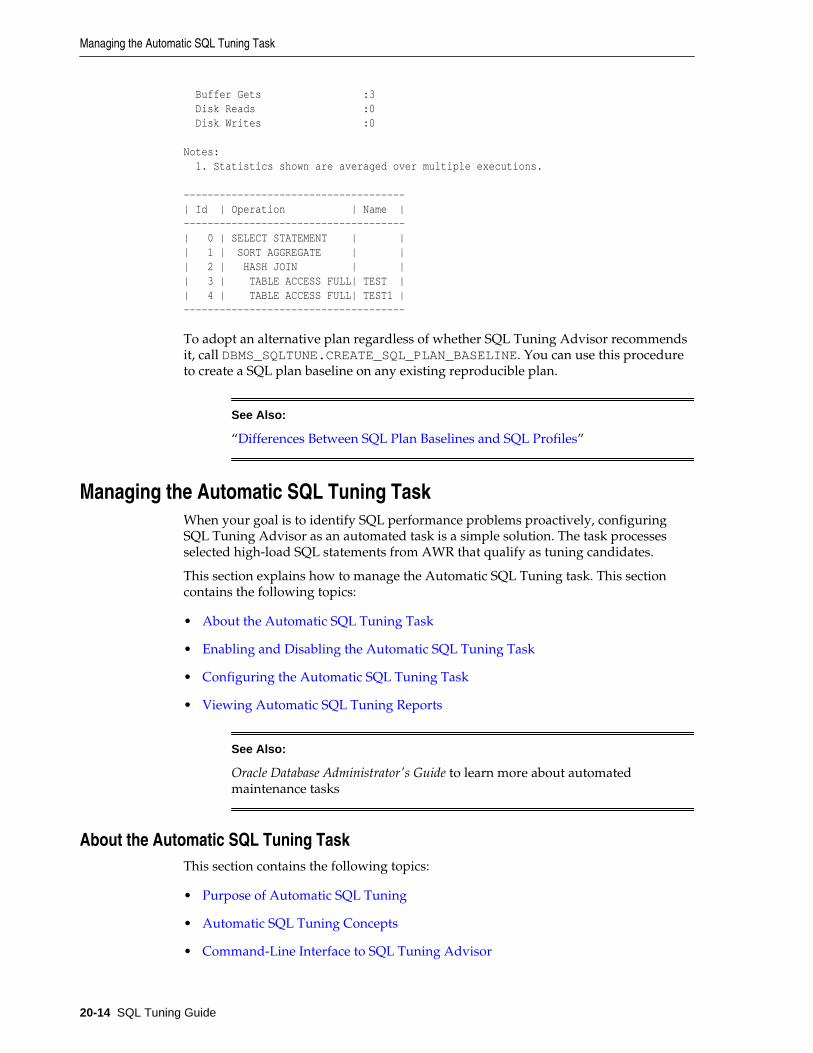
Buffer Gets :3 Disk Reads :0 Disk Writes :0 Notes: 1. Statistics shown are averaged over multiple executions. -------------------------------------| Id | Operation | Name | -------------------------------------| 0 | SELECT STATEMENT | || 1 | SORT AGGREGATE | || 2 | HASH JOIN | || 3 | TABLE ACCESS FULL| TEST || 4 | TABLE ACCESS FULL| TEST1 |-------------------------------------
To adopt an alternative plan regardless of whether SQL Tuning Advisor recommendsit, call DBMS_SQLTUNE.CREATE_SQL_PLAN_BASELINE. You can use this procedureto create a SQL plan baseline on any existing reproducible plan.
See Also:
“Differences Between SQL Plan Baselines and SQL Profiles”
Managing the Automatic SQL Tuning TaskWhen your goal is to identify SQL performance problems proactively, configuringSQL Tuning Advisor as an automated task is a simple solution. The task processesselected high-load SQL statements from AWR that qualify as tuning candidates.
This section explains how to manage the Automatic SQL Tuning task. This sectioncontains the following topics:
• About the Automatic SQL Tuning Task
• Enabling and Disabling the Automatic SQL Tuning Task
• Configuring the Automatic SQL Tuning Task
• Viewing Automatic SQL Tuning Reports
See Also:
Oracle Database Administrator's Guide to learn more about automatedmaintenance tasks
About the Automatic SQL Tuning TaskThis section contains the following topics:
• Purpose of Automatic SQL Tuning
• Automatic SQL Tuning Concepts
• Command-Line Interface to SQL Tuning Advisor
Managing the Automatic SQL Tuning Task
20-14 SQL Tuning Guide

• Basic Tasks for Automatic SQL Tuning
Purpose of Automatic SQL Tuning
Many DBAs do not have the time needed for the intensive analysis required for SQLtuning. Even when they do, SQL tuning involves several manual steps. Becauseseveral different SQL statements may be high load on any given day, DBAs may haveto expend considerable effort to monitor and tune them. Configuring automatic SQLtuning instead of tuning manually decreases cost and increases manageability.
The automated task does not process the following types of SQL:
• Ad hoc SQL statements or SQL statements that do not repeat within a week
• Parallel queries
• Queries that take too long to run after being SQL profiled, so that it is not practicalfor SQL Tuning Advisor to test-execute them
• Recursive SQL
You can run SQL Tuning Advisor on demand to tune the preceding types of SQLstatements.
Automatic SQL Tuning Concepts
Oracle Scheduler uses the automated maintenance tasks infrastructure (known asAutoTask) to schedules tasks to run automatically. By default, the Automatic SQLTuning task runs for at most one hour in a nightly maintenance window. You cancustomize attributes of the maintenance windows, including start and end time,frequency, and days of the week.
See Also:
• Oracle Database Administrator's Guide to learn about Oracle Scheduler
• Oracle Database PL/SQL Packages and Types Reference to learn aboutDBMS_AUTO_TASK_ADMIN
Command-Line Interface to SQL Tuning Advisor
On the command line, you can use PL/SQL packages to perform SQL tuning tasks. Table 20-1 describes the most relevant packages.
Table 20-1 SQL Tuning Advisor Packages
Package Description
DBMS_AUTO_SQLTUNE Enables you run SQL Tuning Advisor, manage SQLprofiles, manage SQL tuning sets, and perform real-time SQL performance monitoring. To use this API,you must have the ADVISOR privilege.
DBMS_AUTO_TASK_ADMIN Provides an interface to AUTOTASK. You can use thisinterface to enable and disable the Automatic SQLTuning task.
Managing the Automatic SQL Tuning Task
Analyzing SQL with SQL Tuning Advisor 20-15

See Also:
Oracle Database PL/SQL Packages and Types Reference to learn aboutDBMS_SQLTUNE ad DBMS_AUTO_TASK_ADMIN
Basic Tasks for Automatic SQL Tuning
This section explains the basic tasks in running SQL Tuning Advisor as an automatictask. Figure 20-5 shows the basic workflow.
Figure 20-5 Automatic SQL Tuning APIs
DBMS_AUTO_TASK_ADMIN.DISABLE
DBMS_SQLTUNE.
SET_TUNING_TASK_PARAMETER
Report on the SQLTuning Task
Disable the AutomaticSQL Tuning Task
DBMS_SQLTUNE.
REPORT_AUTO_TUNING_TASK
Configure the Automatic SQL Tuning Task
DBMS_AUTO_TASK_ADMIN.ENABLEEnable the AutomaticSQL Tuning Task
As shown in Figure 20-6, the basic procedure is as follows:
1. Enable the Automatic SQL Tuning task.
See “Enabling and Disabling the Automatic SQL Tuning Task”.
2. Optionally, configure the Automatic SQL Tuning task.
See “Configuring the Automatic SQL Tuning Task”.
3. Display the results of the Automatic SQL Tuning task.
“Viewing Automatic SQL Tuning Reports”.
4. Disable the Automatic SQL Tuning task.
See “Enabling and Disabling the Automatic SQL Tuning Task”.
Enabling and Disabling the Automatic SQL Tuning TaskThis section explains how to enable and disable the Automatic SQL Tuning task usingCloud Control (preferred) or a command-line interface.
Managing the Automatic SQL Tuning Task
20-16 SQL Tuning Guide

Enabling and Disabling the Automatic SQL Tuning Task Using Cloud Control
You can enable and disable all automatic maintenance tasks, including the AutomaticSQL Tuning task, using Cloud Control.
To enable or disable the Automatic SQL Tuning task using Cloud Control:
1. Access the Database Home page, as described in “Accessing the Database HomePage in Cloud Control.”
2. From the Administration menu, select Oracle Scheduler, then AutomatedMaintenance Tasks.
The Automated Maintenance Tasks page appears.
This page shows the predefined tasks. You access each task by clicking thecorresponding link to get more information about the task.
3. Click Automatic SQL Tuning.
The Automatic SQL Tuning Result Summary page appears.
The Task Status section shows whether the Automatic SQL Tuning Task isenabled or disabled. In the following graphic, the task is disabled:
4. In Automatic SQL Tuning, click Configure.
The Automated Maintenance Tasks Configuration page appears.
By default, Automatic SQL Tuning executes in all predefined maintenancewindows in MAINTENANCE_WINDOW_GROUP.
5. Perform the following steps:
a. In the Task Settings for Automatic SQL Tuning, select either Enabled orDisabled to enable or disable the automated task.
b. To disable Automatic SQL Tuning for specific days in the week, check theappropriate box next to the window name.
c. To change the characteristics of a window, click Edit Window Group.
d. Click Apply.
Managing the Automatic SQL Tuning Task
Analyzing SQL with SQL Tuning Advisor 20-17

Enabling and Disabling the Automatic SQL Tuning Task from the Command Line
If you do not use Cloud Control to enable and disable the Automatic SQL Tuning task,then you have the following options:
• Run the ENABLE or DISABLE procedure in the DBMS_AUTO_TASK_ADMIN PL/SQLpackage.
This package is the recommended command-line technique. For both the ENABLEor DISABLE procedures, you can specify a particular maintenance window withthe window_name parameter. See Oracle Database PL/SQL Packages and TypesReference for complete reference information.
• Set the STATISTICS_LEVEL initialization parameter to BASIC to disable collectionof all advisories and statistics, including Automatic SQL Tuning Advisor.
Because monitoring and many automatic features are disabled, Oracle stronglyrecommends that you do not set STATISTICS_LEVEL to BASIC. See OracleDatabase Reference for complete reference information.
To enable or disable Automatic SQL Tuning using DBMS_AUTO_TASK_ADMIN:
1. Connect SQL*Plus to the database with administrator privileges, and then do oneof the following:
• To enable the automated task, execute the following PL/SQL block:
BEGIN DBMS_AUTO_TASK_ADMIN.ENABLE ( client_name => 'sql tuning advisor', operation => NULL, window_name => NULL);END;/
• To disable the automated task, execute the following PL/SQL block:
BEGIN DBMS_AUTO_TASK_ADMIN.DISABLE ( client_name => 'sql tuning advisor', operation => NULL, window_name => NULL);END;/
2. Query the data dictionary to confirm the change.
For example, query DBA_AUTOTASK_CLIENT as follows (sample outputincluded):
COL CLIENT_NAME FORMAT a20
SELECT CLIENT_NAME, STATUSFROM DBA_AUTOTASK_CLIENTWHERE CLIENT_NAME = 'sql tuning advisor'; CLIENT_NAME STATUS-------------------- --------sql tuning advisor ENABLED
Managing the Automatic SQL Tuning Task
20-18 SQL Tuning Guide

To disable collection of all advisories and statistics:
1. Connect SQL*Plus to the database with administrator privileges, and then querythe current statistics level setting.
The following SQL*Plus command shows that STATISTICS_LEVEL is set to ALL:
sys@PROD> SHOW PARAMETER statistics_level NAME TYPE VALUE------------------------------------ ----------- -----statistics_level string ALL
2. Set STATISTICS_LEVEL to BASIC as follows:
sys@PROD> ALTER SYSTEM SET STATISTICS_LEVEL ='BASIC'; System altered.
Configuring the Automatic SQL Tuning TaskThis section explains how to configure settings for the Automatic SQL Tuning task.
Configuring the Automatic SQL Tuning Task Using Cloud Control
You can enable and disable all automatic maintenance tasks, including the AutomaticSQL Tuning task, using Cloud Control. You must perform the operation as SYS orhave the EXECUTE privilege on the PL/SQL package DBMS_AUTO_SQLTUNE.
To configure the Automatic SQL Tuning task using Cloud Control:
1. Access the Database Home page, as described in “Accessing the Database HomePage in Cloud Control.”
2. From the Administration menu, click Oracle Scheduler, then AutomatedMaintenance Tasks.
The Automated Maintenance Tasks page appears.
This page shows the predefined tasks. You access each task by clicking thecorresponding link to get more information about the task itself.
3. Click Automatic SQL Tuning.
The Automatic SQL Tuning Result Summary page appears.
4. Under Task Settings, click Configure next to Automatic SQL Tuning(SYS_AUTO_SQL_TUNING_TASK).
The Automated Maintenance Tasks Configuration page appears.
5. Under Task Settings, click Configure next to Automatic SQL Tuning.
The Automatic SQL Tuning Settings page appears.
Managing the Automatic SQL Tuning Task
Analyzing SQL with SQL Tuning Advisor 20-19

6. Make the desired changes and click Apply.
Configuring the Automatic SQL Tuning Task Using the Command Line
The DBMS_AUTO_SQLTUNE package enables you to configure automatic SQL tuningby specifying the task parameters using the SET_AUTO_TUNING_TASK_PARAMETERprocedure. Because the task is owned by SYS, only SYS can set task parameters.
The ACCEPT_SQL_PROFILE tuning task parameter specifies whether to implementSQL profiles automatically (true) or require user intervention (false). The default isAUTO, which means true if at least one SQL statement exists with a SQL profile andfalse if this condition is not satisfied.
Note:
When automatic implementation is enabled, the advisor only implementsrecommendations to create SQL profiles. Recommendations such as creatingnew indexes, gathering optimizer statistics, and creating SQL plan baselinesare not automatically implemented.
Assumptions
This tutorial assumes the following:
• You want the database to implement SQL profiles automatically, but to implementno more than 50 SQL profiles per execution, and no more than 50 profiles total onthe database.
• You want the task to time out after 1200 seconds per execution.
To set Automatic SQL Tuning task parameters:
1. Connect SQL*Plus to the database with the appropriate privileges, and thenoptionally query the current task settings.
For example, connect SQL*Plus to the database with administrator privileges andexecute the following query:
COL PARAMETER_NAME FORMAT a25 COL VALUE FORMAT a10
SELECT PARAMETER_NAME, PARAMETER_VALUE AS "VALUE"FROM DBA_ADVISOR_PARAMETERSWHERE ( (TASK_NAME = 'SYS_AUTO_SQL_TUNING_TASK') AND ( (PARAMETER_NAME LIKE '%PROFILE%') OR
Managing the Automatic SQL Tuning Task
20-20 SQL Tuning Guide

(PARAMETER_NAME = 'LOCAL_TIME_LIMIT') OR (PARAMETER_NAME = 'EXECUTION_DAYS_TO_EXPIRE') ) );
Sample output appears as follows:
PARAMETER_NAME VALUE------------------------- ----------EXECUTION_DAYS_TO_EXPIRE 30LOCAL_TIME_LIMIT 1000ACCEPT_SQL_PROFILES FALSEMAX_SQL_PROFILES_PER_EXEC 20MAX_AUTO_SQL_PROFILES 10000
2. Set parameters using PL/SQL code of the following form:
BEGIN DBMS_SQLTUNE.SET_TUNING_TASK_PARAMETER ( task_name => 'SYS_AUTO_SQL_TUNING_TASK', parameter => parameter_name, value => value);END;/
See Also:
Oracle Database PL/SQL Packages and Types Reference for complete referenceinformation for DBMS_AUTO_SQLTUNE
Example 20-3 Setting SQL Tuning Task Parameters
The following PL/SQL block sets a time limit to 20 minutes, and also automaticallyimplements SQL profiles and sets limits for these profiles:
BEGIN DBMS_SQLTUNE.SET_TUNING_TASK_PARAMETER('SYS_AUTO_SQL_TUNING_TASK', 'LOCAL_TIME_LIMIT', 1200); DBMS_SQLTUNE.SET_TUNING_TASK_PARAMETER('SYS_AUTO_SQL_TUNING_TASK', 'ACCEPT_SQL_PROFILES', 'true'); DBMS_SQLTUNE.SET_TUNING_TASK_PARAMETER('SYS_AUTO_SQL_TUNING_TASK', 'MAX_SQL_PROFILES_PER_EXEC', 50); DBMS_SQLTUNE.SET_TUNING_TASK_PARAMETER('SYS_AUTO_SQL_TUNING_TASK', 'MAX_AUTO_SQL_PROFILES', 10002);END;/
Viewing Automatic SQL Tuning ReportsAt any time during or after the running of the Automatic SQL Tuning task, you canview a tuning report. This report contains information about all executions of theautomatic SQL tuning task.
Depending on the sections that were included in the report, you can view informationin the following sections:
• General information
This section has a high-level description of the automatic SQL tuning task,including information about the inputs given for the report, the number of SQLstatements tuned during the maintenance, and the number of SQL profiles created.
Managing the Automatic SQL Tuning Task
Analyzing SQL with SQL Tuning Advisor 20-21

• Summary
This section lists the SQL statements (by their SQL identifiers) that were tunedduring the maintenance window and the estimated benefit of each SQL profile, orthe execution statistics after performing a test execution of the SQL statement withthe SQL profile.
• Tuning findings
This section contains the following information about each SQL statement analyzedby SQL Tuning Advisor:
– All findings associated with each SQL statement
– Whether the profile was implemented on the database, and why
– Whether the SQL profile is currently enabled on the database
– Detailed execution statistics captured when testing the SQL profile
• Explain plans
This section shows the old and new explain plans used by each SQL statementanalyzed by SQL Tuning Advisor.
• Errors
This section lists all errors encountered by the automatic SQL tuning task.
Viewing Automatic SQL Tuning Reports Using the Command Line
To generate a SQL tuning report as a CLOB, execute theDBMS_SQLTUNE.REPORT_AUTO_TUNING_TASK function. You can store the CLOB in avariable and then print the variable to view the report. See Oracle Database PL/SQLPackages and Types Reference for complete reference information.
Assumptions
This section assumes that you want to show all SQL statements that were analyzed inthe most recent execution, including recommendations that were not implemented.
To create and access an Automatic SQL Tuning Advisor report:
1. Connect SQL*Plus to the database with administrator privileges, and then executethe DBMS_SQLTUNE.REPORT_AUTO_TUNING_TASK function.
The following example generates a text report to show all SQL statements thatwere analyzed in the most recent execution, including recommendations thatwere not implemented:
VARIABLE my_rept CLOB;BEGIN :my_rept :=DBMS_SQLTUNE.REPORT_AUTO_TUNING_TASK ( begin_exec => NULL, end_exec => NULL, type => 'TEXT', level => 'TYPICAL', section => 'ALL', object_id => NULL, result_limit => NULL);END;
Managing the Automatic SQL Tuning Task
20-22 SQL Tuning Guide

/
PRINT :my_rept
2. Read the general information section for an overview of the tuning execution.
The following sample shows the Automatic SQL Tuning task analyzed 17 SQLstatements in just over 7 minutes:
MY_REPT---------------------------------------------------------------------------GENERAL INFORMATION SECTION---------------------------------------------------------------------------Tuning Task Name : SYS_AUTO_SQL_TUNING_TASKTuning Task Owner : SYSWorkload Type : Automatic High-Load SQL WorkloadExecution Count : 6Current Execution : EXEC_170Execution Type : TUNE SQLScope : COMPREHENSIVEGlobal Time Limit(seconds) : 3600Per-SQL Time Limit(seconds) : 1200Completion Status : COMPLETEDStarted at : 04/16/2012 10:00:00Completed at : 04/16/2012 10:07:11Number of Candidate SQLs : 17Cumulative Elapsed Time of SQL (s) : 8
3. Look for findings and recommendations.
If SQL Tuning Advisor makes a recommendation, then weigh the pros and cons ofaccepting it.
The following example shows that SQL Tuning Advisor found a plan for astatement that is potentially better than the existing plan. The advisorrecommends implementing a SQL profile.
--------------------------------------------------------------------------- SQLs with Findings Ordered by Maximum (Profile/Index) Benefit, Object ID---------------------------------------------------------------------------ob ID SQL ID statistics profile(benefit) index(benefit) restructure------ ------------- ---------- ---------------- -------------- ----------- 82 dqjcc345dd4ak 58.03% 72 51bbkcd9zwsjw 2 81 03rxjf8gb18jg ---------------------------------------------------------------------------DETAILS SECTION--------------------------------------------------------------------------- Statements with Results Ordered by Max (Profile/Index) Benefit, Object ID---------------------------------------------------------------------------Object ID : 82Schema Name: DBA1SQL ID : dqjcc345dd4akSQL Text : SELECT status FROM dba_autotask_client WHERE client_name=:1 ---------------------------------------------------------------------------FINDINGS SECTION (1 finding)--------------------------------------------------------------------------- 1- SQL Profile Finding (see explain plans section below)--------------------------------------------------------
Managing the Automatic SQL Tuning Task
Analyzing SQL with SQL Tuning Advisor 20-23

A potentially better execution plan was found for this statement. The SQL profile was not automatically created because the verified benefit was too low. Recommendation (estimated benefit: 58.03%) ------------------------------------------ - Consider accepting the recommended SQL profile. execute dbms_sqltune.accept_sql_profile(task_name => 'SYS_AUTO_SQL_TUNING_TASK', object_id => 82, replace => TRUE); Validation results ------------------ The SQL profile was tested by executing both its plan and the original plan and measuring their respective execution statistics. A plan may have been only partially executed if the other could be run to completion in less time. Original Plan With SQL Profile % Improved ------------- ---------------- ---------- Completion Status: COMPLETE COMPLETE Elapsed Time(us): 26963 8829 67.25 % CPU Time(us): 27000 9000 66.66 % User I/O Time(us): 25 14 44 % Buffer Gets: 905 380 58.01 % Physical Read Requests: 0 0 Physical Write Requests: 0 0 Physical Read Bytes: 0 0 Physical Write Bytes: 7372 7372 0 % Rows Processed: 1 1 Fetches: 1 1 Executions: 1 1 Notes ----- 1. The original plan was first executed to warm the buffer cache. 2. Statistics for original plan were averaged over next 9 executions. 3. The SQL profile plan was first executed to warm the buffer cache. 4. Statistics for the SQL profile plan were averaged over next 9 executions.
Running SQL Tuning Advisor On DemandThis section contains the following topics:
• About On-Demand SQL Tuning
• Creating a SQL Tuning Task
• Configuring a SQL Tuning Task
• Executing a SQL Tuning Task
• Monitoring a SQL Tuning Task
• Displaying the Results of a SQL Tuning Task
About On-Demand SQL TuningIn this context, on-demand SQL tuning is defined as any invocation of SQL TuningAdvisor that does not result from the Automatic SQL Tuning task.
Running SQL Tuning Advisor On Demand
20-24 SQL Tuning Guide

Purpose of On-Demand SQL Tuning
Typically, you invoke SQL Tuning Advisor on demand in the following situations:
• You proactively run ADDM, which reports that some SQL statements do not meetyour performance requirements.
• You reactively tune SQL statement because users complain about suboptimal SQLperformance.
In both situations, running SQL Tuning Advisor is usually the quickest way to fixunexpected SQL performance problems.
User Interfaces for On-Demand SQL Tuning
The recommended user interface for running SQL Tuning Advisor manually is CloudControl.
Accessing the SQL Tuning Advisor Using Cloud Control
Automatic Database Diagnostic Monitor (ADDM) automatically identifies high-loadSQL statements. If ADDM identifies such statements, then click Schedule/Run SQLTuning Advisor on the Recommendation Detail page to run SQL Tuning Advisor.
To tune SQL statements manually using SQL Tuning Advisor:
1. Access the Database Home page, as described in “Accessing the Database HomePage in Cloud Control.”
2. From the Performance menu, click SQL, then SQL Tuning Advisor.
The Schedule SQL Tuning Advisor page appears.
Running SQL Tuning Advisor On Demand
Analyzing SQL with SQL Tuning Advisor 20-25

3. See Oracle Database 2 Day + Performance Tuning Guide to learn how to configureand run SQL Tuning Advisor using Cloud Control.
Command-Line Interface to On-Demand SQL Tuning
If Cloud Control is unavailable, then you can run SQL Tuning Advisor usingprocedures in the DBMS_SQLTUNE package. To use the APIs, the user must have theADVISOR privilege.
See Also:
Oracle Database PL/SQL Packages and Types Reference for complete referenceinformation
Basic Tasks in On-Demand SQL Tuning
This section explains the basic tasks in running SQL Tuning Advisor using theDBMS_SQLTUNE package. Oracle Database 2 Day + Performance Tuning Guide explainshow to tune SQL using Cloud Control.
Figure 20-6 shows the basic workflow when using the PL/SQL APIs.
Running SQL Tuning Advisor On Demand
20-26 SQL Tuning Guide

Figure 20-6 SQL Tuning Advisor APIs
create_tuning_task
execute_tuning_task
STS
report_tuning_task
Implement
Recommendations
Gather optimizerstatistics
Create SQLProfile
set_tuning_task_parameter
Monitor Task
CreateIndex
RestructureSQL
Create SQLPlan Baseline
As shown in Figure 20-6, the basic procedure is as follows:
1. Prepare or create the input to SQL Tuning Advisor. The input can be either:
• The text of a single SQL statement
• A SQL tuning set that contains one or more statements
2. Create a SQL tuning task.
See “Creating a SQL Tuning Task”.
3. Optionally, configure the SQL tuning task that you created.
See “Configuring a SQL Tuning Task”.
4. Execute a SQL tuning task.
See “Executing a SQL Tuning Task”.
5. Optionally, check the status or progress of a SQL tuning task.
“Monitoring a SQL Tuning Task”.
6. Display the results of a SQL tuning task.
“Displaying the Results of a SQL Tuning Task”.
7. Implement recommendations as appropriate.
Running SQL Tuning Advisor On Demand
Analyzing SQL with SQL Tuning Advisor 20-27

Creating a SQL Tuning TaskTo create a SQL tuning task execute the DBMS_SQLTUNE.CREATE_TUNING_TASKfunction. You can create tuning tasks from any of the following:
• The text of a single SQL statement
• A SQL tuning set containing multiple statements
• A SQL statement selected by SQL identifier from the shared SQL area
• A SQL statement selected by SQL identifier from AWR
The scope parameter is one of the most important for this function. You can set thisparameter to the following values:
• LIMITED
SQL Tuning Advisor produces recommendations based on statistical checks, accesspath analysis, and SQL structure analysis. SQL profile recommendations are notgenerated.
• COMPREHENSIVE
SQL Tuning Advisor carries out all the analysis it performs under limited scopeplus SQL profiling.
Assumptions
This tutorial assumes the following:
• You want to tune as user hr, who has the ADVISOR privilege.
• You want to tune the following query:
SELECT /*+ ORDERED */ * FROM employees e, locations l, departments dWHERE e.department_id = d.department_id AND l.location_id = d.location_id AND e.employee_id < :bnd;
• You want to pass the bind variable 100 to the preceding query.
• You want SQL Tuning Advisor to perform SQL profiling.
• You want the task to run no longer than 60 seconds.
To create a SQL tuning task:
1. Connect SQL*Plus to the database with the appropriate privileges, and then runthe DBMS_SQLTUNE.CREATE_TUNING_TASK function.
For example, execute the following PL/SQL program:
DECLARE my_task_name VARCHAR2(30); my_sqltext CLOB;BEGIN my_sqltext := 'SELECT /*+ ORDERED */ * ' || 'FROM employees e, locations l, departments d ' || 'WHERE e.department_id = d.department_id AND ' ||
Running SQL Tuning Advisor On Demand
20-28 SQL Tuning Guide

'l.location_id = d.location_id AND ' || 'e.employee_id < :bnd';
my_task_name := DBMS_SQLTUNE.CREATE_TUNING_TASK ( sql_text => my_sqltext, bind_list => sql_binds(anydata.ConvertNumber(100)), user_name => 'HR', scope => 'COMPREHENSIVE', time_limit => 60, task_name => 'STA_SPECIFIC_EMP_TASK', description => 'Task to tune a query on a specified employee');END;/
2. Optionally, query the status of the task.
The following example queries the status of all tasks owned by the current user,which in this example is hr:
COL TASK_ID FORMAT 999999COL TASK_NAME FORMAT a25COL STATUS_MESSAGE FORMAT a33
SELECT TASK_ID, TASK_NAME, STATUS, STATUS_MESSAGEFROM USER_ADVISOR_LOG;
Sample output appears below:
TASK_ID TASK_NAME STATUS STATUS_MESSAGE------- ------------------------- ----------- -------------- 884 STA_SPECIFIC_EMP_TASK INITIAL
In the preceding output, the INITIAL status indicates that the task has not yetstarted execution.
See Also:
Oracle Database PL/SQL Packages and Types Reference to learn about theDBMS_SQLTUNE.CREATE_TUNING_TASK function
Configuring a SQL Tuning TaskTo change the parameters of a tuning task after it has been created, execute theDBMS_SQLTUNE.SET_TUNING_TASK_PARAMETER function. See Oracle DatabasePL/SQL Packages and Types Reference for complete reference information.
Assumptions
This tutorial assumes the following:
• You want to tune as user hr, who has the ADVISOR privilege.
• You want to tune the STA_SPECIFIC_EMP_TASK created in “Creating a SQLTuning Task”.
• You want to change the maximum time that the SQL tuning task can run to 300seconds.
Running SQL Tuning Advisor On Demand
Analyzing SQL with SQL Tuning Advisor 20-29

To configure a SQL tuning task:
1. Connect SQL*Plus to the database with the appropriate privileges, and then runthe DBMS_SQLTUNE.SET_TUNING_TASK_PARAMETER function.
For example, execute the following PL/SQL program to change the time limit ofthe tuning task to 300 seconds:
BEGIN DBMS_SQLTUNE.SET_TUNING_TASK_PARAMETER ( task_name => 'STA_SPECIFIC_EMP_TASK', parameter => 'TIME_LIMIT', value => 300);END;/
2. Optionally, verify that the task parameter was changed.
The following example queries the values of all used parameters in taskSTA_SPECIFIC_EMP_TASK:
COL PARAMETER_NAME FORMAT a25 COL VALUE FORMAT a15
SELECT PARAMETER_NAME, PARAMETER_VALUE AS "VALUE"FROM USER_ADVISOR_PARAMETERSWHERE TASK_NAME = 'STA_SPECIFIC_EMP_TASK'AND PARAMETER_VALUE != 'UNUSED'ORDER BY PARAMETER_NAME;
Sample output appears below:
PARAMETER_NAME VALUE------------------------- ---------------DAYS_TO_EXPIRE 30DEFAULT_EXECUTION_TYPE TUNE SQLEXECUTION_DAYS_TO_EXPIRE UNLIMITEDJOURNALING INFORMATIONMODE COMPREHENSIVESQL_LIMIT -1SQL_PERCENTAGE 1TARGET_OBJECTS 1TEST_EXECUTE AUTOTIME_LIMIT 300
Executing a SQL Tuning TaskTo execute a SQL tuning task, use the DBMS_SQLTUNE.EXECUTE_TUNING_TASKfunction. The most important parameter is task_name.
Note:
You can also execute the automatic tuning taskSYS_AUTO_SQL_TUNING_TASK using the EXECUTE_TUNING_TASK API. SQLTuning Advisor performs the same analysis and actions as it would when runautomatically.
Running SQL Tuning Advisor On Demand
20-30 SQL Tuning Guide

Assumptions
This tutorial assumes the following:
• You want to tune as user hr, who has the ADVISOR privilege.
• You want to execute the STA_SPECIFIC_EMP_TASK created in “Creating a SQLTuning Task”.
To execute a SQL tuning task:
1. Connect SQL*Plus to the database with the appropriate privileges, and then runthe DBMS_SQLTUNE.EXECUTE_TUNING_TASK function.
For example, execute the following PL/SQL program:
BEGIN DBMS_SQLTUNE.EXECUTE_TUNING_TASK(task_name=>'STA_SPECIFIC_EMP_TASK');END;/
2. Optionally, query the status of the task.
The following example queries the status of all tasks owned by the current user,which in this example is hr:
COL TASK_ID FORMAT 999999COL TASK_NAME FORMAT a25COL STATUS_MESSAGE FORMAT a33
SELECT TASK_ID, TASK_NAME, STATUS, STATUS_MESSAGEFROM USER_ADVISOR_LOG;
Sample output appears below:
TASK_ID TASK_NAME STATUS STATUS_MESSAGE------- ------------------------- ----------- -------------- 884 STA_SPECIFIC_EMP_TASK COMPLETED
See Also:
Oracle Database PL/SQL Packages and Types Reference for complete referenceinformation about the DBMS_SQLTUNE.EXECUTE_TUNING_TASK function
Monitoring a SQL Tuning TaskWhen you create a SQL tuning task in Cloud Control, no separate monitoring step isnecessary. Cloud Control displays the status page automatically.
If you do not use Cloud Control, then you can monitor currently executing SQL tuningtasks by querying the data dictionary and dynamic performance views. Table 20-2describes the relevant views.
Table 20-2 DBMS_SQLTUNE.EXECUTE_TUNING_TASK Parameters
Running SQL Tuning Advisor On Demand
Analyzing SQL with SQL Tuning Advisor 20-31

Table 20-2 (Cont.) DBMS_SQLTUNE.EXECUTE_TUNING_TASK Parameters
View Description
USER_ADVISOR_TASKS Displays information about tasks owned by the currentuser. The view contains one row for each task. Eachtask has a name that is unique to the owner. Tasknames are just informational and no uniqueness isenforced within any other namespace.
V$ADVISOR_PROGRESS Displays information about the progress of advisorexecution.
Assumptions
This tutorial assumes the following:
• You tune as user hr, who has the ADVISOR privilege.
• You monitor the STA_SPECIFIC_EMP_TASK that you executed in “Executing aSQL Tuning Task”.
To monitor a SQL tuning task:
1. Connect SQL*Plus to the database with the appropriate privileges, and thendetermine whether the task is executing or completed.
For example, query the status of STA_SPECIFIC_EMP_TASK as follows:
SELECT STATUS FROM USER_ADVISOR_TASKSWHERE TASK_NAME = 'STA_SPECIFIC_EMP_TASK';
The following output shows that the task has completed:
STATUS-----------EXECUTING
2. Determine the progress of an executing task.
The following example queries the status of the task with task ID 884:
VARIABLE my_tid NUMBER; EXEC :my_tid := 884COL ADVISOR_NAME FORMAT a20COL SOFAR FORMAT 999COL TOTALWORK FORMAT 999
SELECT TASK_ID, ADVISOR_NAME, SOFAR, TOTALWORK, ROUND(SOFAR/TOTALWORK*100,2) "%_COMPLETE"FROM V$ADVISOR_PROGRESSWHERE TASK_ID = :my_tid;
Sample output appears below:
TASK_ID ADVISOR_NAME SOFAR TOTALWORK %_COMPLETE---------- -------------------- ----- --------- ---------- 884 SQL Tuning Advisor 1 2 50
Running SQL Tuning Advisor On Demand
20-32 SQL Tuning Guide

See Also:
Oracle Database Reference to learn about the V$ADVISOR_PROGRESS view
Displaying the Results of a SQL Tuning TaskTo report the results of a tuning task, use theDBMS_SQLTUNE.REPORT_TUNING_TASK function. The report contains all thefindings and recommendations of SQL Tuning Advisor. For each proposedrecommendation, the report provides the rationale and benefit along with the SQLstatements needed to implement the recommendation.
Assumptions
This tutorial assumes the following:
• You want to tune as user hr, who has the ADVISOR privilege.
• You want to access the report for the STA_SPECIFIC_EMP_TASK executed in“Executing a SQL Tuning Task”.
To view the report for a SQL tuning task:
1. Connect SQL*Plus to the database with the appropriate privileges, and then runthe DBMS_SQLTUNE.REPORT_TUNING_TASK function.
For example, you run the following statements:
SET LONG 1000SET LONGCHUNKSIZE 1000SET LINESIZE 100SELECT DBMS_SQLTUNE.REPORT_TUNING_TASK( 'STA_SPECIFIC_EMP_TASK' )FROM DUAL;
Truncated sample output appears below:
DBMS_SQLTUNE.REPORT_TUNING_TASK('STA_SPECIFIC_EMP_TASK')---------------------------------------------------------------------------GENERAL INFORMATION SECTION---------------------------------------------------------------------------Tuning Task Name : STA_SPECIFIC_EMP_TASKTuning Task Owner : HRWorkload Type : Single SQL StatementExecution Count : 11Current Execution : EXEC_1057Execution Type : TUNE SQLScope : COMPREHENSIVETime Limit(seconds): 300Completion Status : COMPLETEDStarted at : 04/22/2012 07:35:49Completed at : 04/22/2012 07:35:50 ---------------------------------------------------------------------------Schema Name: HRSQL ID : dg7nfaj0bdcvkSQL Text : SELECT /*+ ORDERED */ * FROM employees e, locations l, departments d WHERE e.department_id = d.department_id AND l.location_id = d.location_id AND e.employee_id < :bndBind Variables :
Running SQL Tuning Advisor On Demand
Analyzing SQL with SQL Tuning Advisor 20-33

1 - (NUMBER):100 ---------------------------------------------------------------------------FINDINGS SECTION (4 findings)-----------------------------------------------
2. Interpret the results, as described in “Viewing Automatic SQL Tuning ReportsUsing the Command Line”.
See Also:
Oracle Database PL/SQL Packages and Types Reference for complete referenceinformation
Running SQL Tuning Advisor On Demand
20-34 SQL Tuning Guide

21Optimizing Access Paths with SQL Access
Advisor
This chapter contains the following topics:
• About SQL Access Advisor
• Using SQL Access Advisor: Basic Tasks
• Performing a SQL Access Advisor Quick Tune
• Using SQL Access Advisor: Advanced Tasks
• SQL Access Advisor Examples
• SQL Access Advisor Reference
About SQL Access AdvisorSQL Access Advisor is diagnostic software that identifies and helps resolve SQLperformance problems by recommending indexes, materialized views, materializedview logs, or partitions to create, drop, or retain.
This section contains the following topics:
• Purpose of SQL Access Advisor
• SQL Access Advisor Architecture
• User Interfaces for SQL Access Advisor
Note:
Data visibility and privilege requirements may differ when using SQL AccessAdvisor with pluggable databases. See Oracle Database Administrator's Guidefor a table that summarizes how manageability features work in a containerdatabase (CDB).
Purpose of SQL Access AdvisorSQL Access Advisor helps you achieve your performance goals by recommending theproper set of materialized views, materialized view logs, partitions, and indexes for agiven workload. Materialized views, partitions, and indexes are essential when tuninga database to achieve optimum performance for complex, data-intensive queries.
Optimizing Access Paths with SQL Access Advisor 21-1

SQL Access Advisor takes an actual workload as input, or derives a hypotheticalworkload from a schema. The advisor then recommends access structures for fasterexecution path. The advisor provides the following advantages:
• Does not require you to have expert knowledge
• Makes decisions based on rules that reside in the optimizer
• Covers all aspects of SQL access in a single advisor
• Provides simple, user-friendly GUI wizards in Cloud Control
• Generates scripts for implementation of recommendations
See Also:
Oracle Database 2 Day + Performance Tuning Guide to learn how to use SQLAccess Advisor with Cloud Control
SQL Access Advisor ArchitectureAutomatic Tuning Optimizer is the central tool used by SQL Access Advisor. Theadvisor can receive SQL statements as input from the sources shown in Figure 21-1,analyze these statements using the optimizer, and then make recommendations.
Figure 21-1 shows the basic architecture of SQL Access Advisor.
Figure 21-1 SQL Access Advisor Architecture
Optimizer
Automatic Tuning Optimizer
SQL AccessAdvisor
DBA
Workload
SQLTuningSet
Shared Pool
Library Cache
Shared SQL Area
SELECT * FROM employees
Hypothetical
Recommendations
Indexes
Materialized Views
Materialized View Logs
Partitions
Filter Options
About SQL Access Advisor
21-2 SQL Tuning Guide

See Also:
“About Automatic Tuning Optimizer”
Input to SQL Access Advisor
SQL Access Advisor requires a workload, which consists of one or more SQLstatements, plus statistics and attributes that fully describe each statement. A fullworkload contains all SQL statements from a target business application. A partialworkload contains a subset of SQL statements.
As shown in Figure 21-1, SQL Access Advisor input can come from the followingsources:
• Shared SQL area
The database uses the shared SQL area to analyze recent SQL statements that arecurrently in V$SQL.
• SQL tuning set
A SQL tuning set (STS) is a database object that stores SQL statements along withtheir execution context. When a set of SQL statements serve as input, the databasemust first construct and use an STS.
Note:
For best results, provide a workload as a SQL tuning set. The DBMS_SQLTUNEpackage provides helper functions that can create SQL tuning sets fromcommon workload sources, such as the SQL cache, a user-defined workloadstored in a table, and a hypothetical workload.
• Hypothetical workload
You can create a hypothetical workload from a schema by analyzing dimensionsand constraints. This option is useful when you are initially designing yourapplication.
See Also:
• Oracle Database Concepts to learn about the shared SQL area
• “About SQL Tuning Sets”
Filter Options for SQL Access Advisor
As shown in Figure 21-1, you can apply a filter to a workload to restrict what isanalyzed. For example, specify that the advisor look at only the 30 most resource-intensive statements in the workload, based on optimizer cost. This restriction cangenerate different sets of recommendations based on different workload scenarios.
SQL Access Advisor parameters control the recommendation process andcustomization of the workload. These parameters control various aspects of theprocess, such as the type of recommendation required and the naming conventions forwhat it recommends.
About SQL Access Advisor
Optimizing Access Paths with SQL Access Advisor 21-3

To set these parameters, use the DBMS_ADVISOR.SET_TASK_PARAMETER procedure.Parameters are persistent in that they remain set for the life span of the task. When aparameter value is set using DBMS_ADVISOR.SET_TASK_PARAMETER, the value doesnot change until you make another call to this procedure.
See Also:
Oracle Database PL/SQL Packages and Types Reference to learn about theDBMS_ADVISOR.SET_TASK_PARAMETER procedure
SQL Access Advisor Recommendations
A task recommendation can range from a simple to a complex solution. The advisorcan recommend that you create database objects such as the following:
• Indexes
SQL Access Advisor index recommendations include bitmap, function-based, andB-tree indexes. A bitmap index offers a reduced response time for many types of adhoc queries and reduced storage requirements compared to other indexingtechniques. B-tree indexes are most commonly used in a data warehouse to indexunique or near-unique keys. SQL Access Advisor materialized viewrecommendations include fast refreshable and full refreshable MVs, for eithergeneral rewrite or exact text match rewrite.
• Materialized views
SQL Access Advisor, using the TUNE_MVIEW procedure, also recommends how tooptimize materialized views so that they can be fast refreshable and take advantageof general query rewrite.
• Materialized view logs
A materialized view log is a table at the materialized view's master site or mastermaterialized view site that records all DML changes to the master table or mastermaterialized view. A fast refresh of a materialized view is possible only if thematerialized view's master has a materialized view log.
• Partitions
SQL Access Advisor can recommend partitioning on an existing unpartitioned basetable to improve performance. Furthermore, it may recommend new indexes andmaterialized views that are themselves partitioned.
While creating new partitioned indexes and materialized view is no different fromthe unpartitioned case, partition existing base tables with care. This is especiallytrue when indexes, views, constraints, or triggers are defined on the table.
To make recommendations, SQL Access Advisor relies on structural statistics abouttable and index cardinalities of dimension level columns, JOIN KEY columns, and facttable key columns. You can gather exact or estimated statistics with the DBMS_STATSpackage (see “About Manual Statistics Collection with DBMS_STATS”).
Because gathering statistics is time-consuming and full statistical accuracy is notrequired, it is usually preferable to estimate statistics. Without gathering statistics on aspecified table, queries referencing this table are marked as invalid in the workload,resulting in no recommendations for these queries. It is also recommended that allexisting indexes and materialized views have been analyzed.
About SQL Access Advisor
21-4 SQL Tuning Guide

See Also:
• Oracle Database Data Warehousing Guide to learn more about materializedviews
• Oracle Database VLDB and Partitioning Guide to learn more about partitions
SQL Access Advisor Actions
In general, each recommendation provides a benefit for one query or a set of queries.All individual actions in a recommendation must be implemented together to achievethe full benefit. Recommendations can share actions.
For example, a CREATE INDEX statement could provide a benefit for several queries,but some queries might benefit from an additional CREATE MATERIALIZED VIEWstatement. In that case, the advisor would generate two recommendations: one for theset of queries that require only the index, and another one for the set of queries thatrequire both the index and the materialized view.
Types of Actions
SQL Access Advisor recommendations include the following types of actions:
• PARTITION BASE TABLE
This action partitions an existing unpartitioned base table.
• CREATE|DROP|RETAIN {MATERIALIZED VIEW|MATERIALIZED VIEW LOG|INDEX}
The CREATE actions corresponds to new access structures. RETAIN recommendskeeping existing access structures. SQL Access Advisor only recommends DROPwhen the WORKLOAD_SCOPE parameter is set to FULL.
• GATHER STATS
This action generates a call to a DBMS_STATS procedure to gather statistics on anewly generated access structure (see “About Manual Statistics Collection withDBMS_STATS”).
Multiple recommendations may refer to the same action. However, when generating ascript for the recommendation, you only see each action once.
See Also:
“Viewing SQL Access Advisor Task Results” to learn how to view actions andrecommendations
Guidelines for Interpreting Partitioning Recommendations
The partition recommendation is a special type of recommendation. When SQL AccessAdvisor determines that partitioning a specified base table would improve workloadperformance, the advisor adds a partition action to every recommendation containinga query referencing the base table. This technique ensures that index and materializedview recommendations are implemented on the correctly partitioned tables.
About SQL Access Advisor
Optimizing Access Paths with SQL Access Advisor 21-5

SQL Access Advisor may recommend partitioning an existing unpartitioned base tableto improve query performance. When the advisor implementation script containspartition recommendations, note the following issues:
• Partitioning an existing table is a complex and extensive operation, which may takeconsiderably longer than implementing a new index or materialized view.Sufficient time should be reserved for implementing this recommendation.
• While index and materialized view recommendations are easy to reverse bydeleting the index or view, a table, after being partitioned, cannot easily be restoredto its original state. Therefore, ensure that you back up the database beforeexecuting a script containing partition recommendations.
• While repartitioning a base table, SQL Access Advisor scripts make a temporarycopy of the original table, which occupies the same amount of space as the originaltable. Therefore, the repartitioning process requires sufficient free disk space foranother copy of the largest table to be repartitioned. Ensure that such space isavailable before running the implementation script.
The partition implementation script attempts to migrate dependent objects such asindexes, materialized views, and constraints. However, some object cannot beautomatically migrated. For example, PL/SQL stored procedures defined against arepartitioned base table typically become invalid and must be recompiled.
• If you decide not to implement a partition recommendation, then all otherrecommendations on the same table in the same script (such as CREATE INDEX andCREATE MATERIALIZED VIEW recommendations) depend on the partitioningrecommendation. To obtain accurate recommendations, do not simply remove thepartition recommendation from the script. Rather, rerun the advisor withpartitioning disabled, for example, by setting parameter ANALYSIS_SCOPE to avalue that does not include the keyword TABLE.
See Also:
Oracle Database SQL Language Reference for CREATE DIRECTORY syntax, and Oracle Database PL/SQL Packages and Types Reference for detailed informationabout the GET_TASK_SCRIPT procedure.
SQL Access Advisor Repository
All information required and generated by SQL Access Advisor resides in the Advisorrepository, which is in the data dictionary. The repository has the following benefits:
• Collects a complete workload for SQL Access Advisor
• Supports historical data
• Is managed by the database
User Interfaces for SQL Access AdvisorOracle recommends that you use SQL Access Advisor through its GUI wizard, whichis available in Cloud Control. Oracle Database 2 Day + Performance Tuning Guideexplains how to use the SQL Access Advisor wizard.
About SQL Access Advisor
21-6 SQL Tuning Guide

You can also invoke SQL Access Advisor through the DBMS_ADVISOR package. Thischapter explains how to use the API. See Oracle Database PL/SQL Packages and TypesReference for complete semantics and syntax.
Accessing the SQL Tuning Advisor: Initial Options Page Using Cloud Control
The SQL Access Advisor: Initial Options page in Cloud Control is the starting page fora wizard that guides you through the process of obtaining recommendations.
To access the SQL Access Advisor: Initial Options page:
1. Access the Database Home page, as described in “Accessing the Database HomePage in Cloud Control.”
2. From the Performance menu, select SQL, then SQL Access Advisor.
The SQL Access Advisor: Initial Options page appears., shown in Figure 21-2.
Figure 21-2 SQL Access Advisor: Initial Options
You can perform most SQL plan management tasks in this page or in pagesaccessed through this page.
See Also:
• Cloud Control context-sensitive online help to learn about the options onthe SQL Access Advisor: Initial Options page
• Oracle Database 2 Day + Performance Tuning Guide
Command-Line Interface to SQL Tuning Sets
On the command line, you can use the DBMS_ADVISOR package to manage SQLtuning sets. The DBMS_ADVISOR package consists of a collection of analysis andadvisory functions and procedures callable from any PL/SQL program. You musthave the ADVISOR privilege to use DBMS_ADVISOR.
See Also:
Oracle Database PL/SQL Packages and Types Reference to learn aboutDBMS_ADVISOR
About SQL Access Advisor
Optimizing Access Paths with SQL Access Advisor 21-7

Using SQL Access Advisor: Basic TasksFigure 21-3 shows the basic workflow for SQL Access Advisor.
Figure 21-3 Using SQL Access Advisor
Typically, you use SQL Access Advisor by performing the following steps:
1. Create a SQL tuning set
The input workload source for SQL Access Advisor is a SQL tuning set (STS). UseDBMS_SQLTUNE.CREATE_SQLSET to create a SQL tuning set.
“Creating a SQL Tuning Set as Input for SQL Access Advisor” describes this task.
2. Load the SQL tuning set
SQL Access Advisor performs best when a workload based on actual usage isavailable. Use DBMS_SQLTUNE.LOAD_SQLSET to populate the SQL tuning setwith your workload.
“Populating a SQL Tuning Set with a User-Defined Workload” describes this task.
3. Create and configure a task
In the task, you define what SQL Access Advisor must analyze and the location ofthe analysis results. Create a task using the DBMS_ADVISOR.CREATE_TASKprocedure. You can then define parameters for the task using theSET_TASK_PARAMETER procedure, and then link the task to an STS by using theDBMS_ADVISOR.ADD_STS_REF procedure.
“Creating and Configuring a SQL Access Advisor Task” describes this task.
Using SQL Access Advisor: Basic Tasks
21-8 SQL Tuning Guide

4. Execute the task
Run the DBMS_ADVISOR.EXECUTE_TASK procedure to generaterecommendations. Each recommendation specifies one or more actions. Forexample, a recommendation could be to create several materialized view logs,create a materialized view, and then analyze it to gather statistics.
“Executing a SQL Access Advisor Task” describes this task.
5. View the recommendations
You can view the recommendations by querying data dictionary views.
“Viewing SQL Access Advisor Task Results” describes this task.
6. Optionally, generate and execute a SQL script that implements therecommendations.
“Generating and Executing a Task Script” that describes this task.
Creating a SQL Tuning Set as Input for SQL Access AdvisorThe input workload source for SQL Access Advisor is an STS. Because an STS is storedas a separate entity, multiple advisor tasks can share it. Create an STS with theDBMS_SQLTUNE.CREATE_SQLSET statement.
After an advisor task has referenced an STS, you cannot delete or modify the STS untilall advisor tasks have removed their dependency on it. A workload reference isremoved when a parent advisor task is deleted, or when you manually remove theworkload reference from the advisor task.
Prerequisites
The user creating the STS must have been granted the ADMINISTER SQL TUNINGSET privilege. To run SQL Access Advisor on SQL tuning sets owned by other users,the user must have the ADMINISTER ANY SQL TUNING SET privilege.
Assumptions
This tutorial assumes the following:
• You want to create an STS named MY_STS_WORKLOAD.
• You want to use this STS as input for a workload derived from the sh schema.
To create an STS :
1. Connect SQL*Plus to the database as user sh, and then set SQL*Plus variables.
For example, enter the following commands:
CONNECT SHPassword: ********SET SERVEROUTPUT ON;VARIABLE task_id NUMBER;VARIABLE task_name VARCHAR2(255);VARIABLE workload_name VARCHAR2(255);
2. Create the SQL tuning set.
For example, assign a value to the workload_name variable and create the STS asfollows:
Using SQL Access Advisor: Basic Tasks
Optimizing Access Paths with SQL Access Advisor 21-9

EXECUTE :workload_name := 'MY_STS_WORKLOAD';EXECUTE DBMS_SQLTUNE.CREATE_SQLSET(:workload_name, 'test purpose');
See Also:
• “About SQL Tuning Sets”
• Oracle Database PL/SQL Packages and Types Reference to learn aboutCREATE_SQLSET
Populating a SQL Tuning Set with a User-Defined WorkloadA workload consists of one or more SQL statements, plus statistics and attributes thatfully describe each statement. A full workload contains all SQL statements from atarget business application. A partial workload contains a subset of SQL statements.The difference is that for full workloads SQL Access Advisor may recommenddropping unused materialized views and indexes.
You cannot use SQL Access Advisor without a workload. SQL Access Advisor ranksthe entries according to a specific statistic, business importance, or combination of thetwo, which enables the advisor to process the most important SQL statements first.
SQL Access Advisor performs best with a workload based on actual usage. You canstore multiple workloads in the form of SQL tuning sets, so that you can view thedifferent uses of a real-world data warehousing or OLTP environment over a longperiod and across the life cycle of database instance startup and shutdown.
Table 21-1 describes procedures that you can use to populate an STS with a user-defined workload.
Table 21-1 Procedures for Loading an STS
Procedure Description
DBMS_SQLTUNE.LOAD_SQLSET Populates the SQL tuning set with a set ofselected SQL. You can call the proceduremultiple times to add new SQL statements orreplace attributes of existing statements. See Oracle Database PL/SQL Packages and TypesReference.
DBMS_ADVISOR.COPY_SQLWKLD_TO_STS Copies SQL workload data to a user-designated SQL tuning set. The user musthave the required SQL tuning set privilegesand the required ADVISOR privilege. See Oracle Database PL/SQL Packages and TypesReference.
Assumptions
This tutorial assumes that you want to do the following:
• Create a table named sh.user_workload to store information about SQLstatements
Using SQL Access Advisor: Basic Tasks
21-10 SQL Tuning Guide

• Load the sh.user_workload table with information about three queries of tablesin the sh schema
• Populate the STS created in “Creating a SQL Tuning Set as Input for SQL AccessAdvisor” with the workload contained in sh.user_workload
To populate an STS with a user-defined workload:
1. Connect SQL*Plus to the database as user sh, and then create theuser_workload table.
For example, enter the following commands:
DROP TABLE user_workload;CREATE TABLE user_workload( username varchar2(128), /* User who executes statement */ module varchar2(64), /* Application module name */ action varchar2(64), /* Application action name */ elapsed_time number, /* Elapsed time for query */ cpu_time number, /* CPU time for query */ buffer_gets number, /* Buffer gets consumed by query */ disk_reads number, /* Disk reads consumed by query */ rows_processed number, /* # of rows processed by query */ executions number, /* # of times query executed */ optimizer_cost number, /* Optimizer cost for query */ priority number, /* User-priority (1,2 or 3) */ last_execution_date date, /* Last time query executed */ stat_period number, /* Window exec time in seconds */ sql_text clob /* Full SQL Text */);
2. Load the user_workload table with information about queries.
For example, execute the following statements:
-- aggregation with selectionINSERT INTO user_workload (username, module, action, priority, sql_text)VALUES ('SH', 'Example1', 'Action', 2,'SELECT t.week_ending_day, p.prod_subcategory, SUM(s.amount_sold) AS dollars, s.channel_id, s.promo_id FROM sales s, times t, products p WHERE s.time_id = t.time_id AND s.prod_id = p.prod_id AND s.prod_id > 10 AND s.prod_id < 50 GROUP BY t.week_ending_day, p.prod_subcategory, s.channel_id, s.promo_id')/ -- aggregation with selectionINSERT INTO user_workload (username, module, action, priority, sql_text)VALUES ('SH', 'Example1', 'Action', 2, 'SELECT t.calendar_month_desc, SUM(s.amount_sold) AS dollars FROM sales s , times t WHERE s.time_id = t.time_id AND s.time_id BETWEEN TO_DATE(''01-JAN-2000'', ''DD-MON-YYYY'') AND TO_DATE(''01-JUL-2000'', ''DD-MON-YYYY'') GROUP BY t.calendar_month_desc')/ -- order byINSERT INTO user_workload (username, module, action, priority, sql_text)
Using SQL Access Advisor: Basic Tasks
Optimizing Access Paths with SQL Access Advisor 21-11

VALUES ('SH', 'Example1', 'Action', 2, 'SELECT c.country_id, c.cust_city, c.cust_last_name FROM customers c WHERE c.country_id IN (52790, 52789) ORDER BY c.country_id, c.cust_city, c.cust_last_name')/COMMIT;
3. Execute a PL/SQL program that fills a cursor with rows from theuser_workload table, and then loads the contents of this cursor into the STSnamed MY_STS_WORKLOAD.
For example, execute the following PL/SQL program:
DECLARE sqlset_cur DBMS_SQLTUNE.SQLSET_CURSOR;BEGIN OPEN sqlset_cur FOR SELECT SQLSET_ROW(null,null, SQL_TEXT, null, null, 'SH', module, 'Action', 0, 0, 0, 0, 0, 1, 0, 1, 0, 0, null, 2, 3, sysdate, 0, 0, null, 0, null, null) FROM USER_WORKLOAD; DBMS_SQLTUNE.LOAD_SQLSET('MY_STS_WORKLOAD', sqlset_cur);END;/
Creating and Configuring a SQL Access Advisor TaskUse the DBMS_ADVISOR.CREATE_TASK procedure to create a SQL Access Advisortask. In the SQL Access Advisor task, you define what the advisor must analyze andthe location of the results. You can create multiple tasks, each with its ownspecialization. All are based on the same Advisor task model and share the samerepository.
Configuring the task involves the following steps:
• Defining task parameters
At the time the recommendations are generated, you can apply a filter to theworkload to restrict what is analyzed. This restriction provides the ability togenerate different sets of recommendations based on different workload scenarios.
SQL Access Advisor parameters control the recommendation process andcustomization of the workload. These parameters control various aspects of theprocess, such as the type of recommendation required and the naming conventionsfor what it recommends. See “Categories for SQL Access Advisor TaskParameters”.
If parameters are not defined, then the database uses the defaults. You can set taskparameters by using the DBMS_ADVISOR.SET_TASK_PARAMETER procedure.Parameters are persistent in that they remain set for the life span of the task. Whena parameter value is set using SET_TASK_PARAMETER, it does not change untilyou make another call to this procedure.
• Linking the task to the workload
Because the workload is independent, you must link it to a task using theDBMS_ADVISOR.ADD_STS_REF procedure. After this link has been established,you cannot delete or modify the workload until all advisor tasks have removedtheir dependency on the workload. A workload reference is removed when a userdeletes a parent advisor task or manually removes the workload reference from the
Using SQL Access Advisor: Basic Tasks
21-12 SQL Tuning Guide

task by using the DBMS_ADVISOR.DELETE_STS_REF procedure (see “DeletingSQL Access Advisor Tasks”).
Prerequisites and Restrictions
The user creating the task must have been granted the ADVISOR privilege.
Assumptions
This tutorial assumes the following:
• You want to create a task named MYTASK.
• You want to use this task to analyze the workload that you defined in “Populatinga SQL Tuning Set with a User-Defined Workload”.
• You want to terminate the task if it takes longer than 30 minutes to execute.
• You want to SQL Access Advisor to only consider indexes.
To create and configure a SQL Access Advisor task:
1. Connect SQL*Plus to the database as user sh, and then create the task.
For example, enter the following commands:
EXECUTE :task_name := 'MYTASK';EXECUTE DBMS_ADVISOR.CREATE_TASK('SQL Access Advisor', :task_id, :task_name);
2. Set task parameters.
For example, execute the following statements:
EXECUTE DBMS_ADVISOR.SET_TASK_PARAMETER(:task_name, 'TIME_LIMIT', 30);EXECUTE DBMS_ADVISOR.SET_TASK_PARAMETER(:task_name, 'ANALYSIS_SCOPE', 'ALL');
3. Link the task to the workload.
For example, execute the following statement:
EXECUTE DBMS_ADVISOR.ADD_STS_REF(:task_name, 'SH', :workload_name);
See Also:
• Oracle Database PL/SQL Packages and Types Reference to learn about theCREATE_TASK procedure and its parameters
• Oracle Database PL/SQL Packages and Types Reference to learn about theSET_TASK_PARAMETER procedure and its parameters
• Oracle Database PL/SQL Packages and Types Reference to learn about theADD_STS_REF procedure and its parameters
Executing a SQL Access Advisor TaskThe DBMS_ADVISOR.EXECUTE_TASK procedure performs SQL Access Advisoranalysis or evaluation for the specified task. Task execution is a synchronousoperation, so the database does not return control to the user until the operation has
Using SQL Access Advisor: Basic Tasks
Optimizing Access Paths with SQL Access Advisor 21-13

completed, or the database detects a user interrupt. After the return or execution of thetask, you can check the DBA_ADVISOR_LOG table for the execution status.
Running EXECUTE_TASK generates recommendations. A recommendation includesone or more actions, such as creating a materialized view log or a materialized view.
Prerequisites and Restrictions
When processing a workload, SQL Access Advisor attempts to validate each statementto identify table and column references. The database achieves validation byprocessing each statement as if it were being executed by the statement's original user.
If the user does not have SELECT privileges to a particular table, then SQL AccessAdvisor bypasses the statement referencing the table. This behavior can cause manystatements to be excluded from analysis. If SQL Access Advisor excludes allstatements in a workload, then the workload is invalid. SQL Access Advisor returnsthe following message:
QSM-00774, there are no SQL statements to process for task TASK_NAME
To avoid missing critical workload queries, the current database user must haveSELECT privileges on the tables targeted for materialized view analysis. For thesetables, these SELECT privileges cannot be obtained through a role.
Assumptions
This tutorial assumes that you want to execute the task you configured in “Creatingand Configuring a SQL Access Advisor Task”.
To create and configure a SQL Access Advisor task:
1. Connect SQL*Plus to the database as user sh, and then execute the task.
For example, execute the following statement:
EXECUTE DBMS_ADVISOR.EXECUTE_TASK(:task_name);
2. Optionally, query USER_ADVISOR_LOG to check the status of the task.
For example, execute the following statements (sample output included):
COL TASK_ID FORMAT 999COL TASK_NAME FORMAT a25COL STATUS_MESSAGE FORMAT a25
SELECT TASK_ID, TASK_NAME, STATUS, STATUS_MESSAGE FROM USER_ADVISOR_LOG;
TASK_ID TASK_NAME STATUS STATUS_MESSAGE------- ------------------------- ----------- ------------------------- 103 MYTASK COMPLETED Access advisor execution completed
See Also:
Oracle Database PL/SQL Packages and Types Reference to learn more about theEXECUTE_TASK procedure and its parameters
Using SQL Access Advisor: Basic Tasks
21-14 SQL Tuning Guide

Viewing SQL Access Advisor Task ResultsYou can view each recommendation generated by SQL Access Advisor using severaldata dictionary views, which are summarized in Table 21-2. However, it is easier touse the DBMS_ADVISOR.GET_TASK_SCRIPT procedure or Cloud Control, whichgraphically displays the recommendations and provides hyperlinks to quickly seewhich SQL statements benefit from a recommendation.
Each recommendation produced by SQL Access Advisor is linked to the SQLstatement it benefits. Each recommendation corresponds to one or more actions. EAchaction has one or more attributes.
Each action has attributes pertaining to the access structure properties. The name andtablespace for each applicable access structure are in the ATTR1 and ATTR2 columns ofUSER_ADVISOR_ATTRIBUTES (see “Action Attributes in theDBA_ADVISOR_ACTIONS View”). The space occupied by each new access structureis in the NUM_ATTR1 column. Other attributes are different for each action.
Table 21-2 Views Showing Task Results
Data Dictionary View (DBA, USER) Description
DBA_ADVISOR_TASKS Displays information about advisor tasks. Tosee SQL Access Advisor tasks, select whereADVISOR_NAME = 'SQL Access
Advisor'.
DBA_ADVISOR_RECOMMENDATIONS Displays the results of an analysis of allrecommendations in the database. Arecommendation can have multiple actionsassociated with it. TheDBA_ADVISOR_ACTIONS view describe theactions. A recommendation also points to aset of rationales that present a justification/reasoning for that recommendation. TheDBA_ADVISOR_RATIONALE view describesthe rationales.
DBA_ADVISOR_ACTIONS Displays information about the actionsassociated with all recommendations in thedatabase. Each action is specified by theCOMMAND and ATTR1 through ATTR6columns. Each command defines how to usethe attribute columns.
DBA_ADVISOR_RATIONALE Displays information about the rationales forall recommendations in the database.
DBA_ADVISOR_SQLA_WK_STMTS Displays information about all workloadobjects in the database after a SQL AccessAdvisor analysis. The precost and postcostnumbers are in terms of the estimatedoptimizer cost (shown in EXPLAIN PLAN)without and with the recommended accessstructure.
Using SQL Access Advisor: Basic Tasks
Optimizing Access Paths with SQL Access Advisor 21-15

Assumptions
This tutorial assumes that you want to view results of the task you executed in“Executing a SQL Access Advisor Task”.
To view the results of a SQL Access Advisor task:
1. Connect SQL*Plus to the database with the appropriate privileges, and then querythe advisor recommendations.
For example, execute the following statements (sample output included):
VARIABLE workload_name VARCHAR2(255); VARIABLE task_name VARCHAR2(255);EXECUTE :task_name := 'MYTASK';EXECUTE :workload_name := 'MY_STS_WORKLOAD';
SELECT REC_ID, RANK, BENEFITFROM USER_ADVISOR_RECOMMENDATIONS WHERE TASK_NAME = :task_nameORDER BY RANK;
REC_ID RANK BENEFIT---------- ---------- ---------- 1 1 236 2 2 356
The preceding output shows the recommendations (rec_id) produced by an SQLAccess Advisor run, with their rank and total benefit. The rank is a measure of theimportance of the queries that the recommendation helps. The benefit is the totalimprovement in execution cost (in terms of optimizer cost) of all queries using therecommendation.
2. Identify which query benefits from which recommendation.
For example, execute the following query of USER_ADVISOR_SQLA_WK_STMTS(sample output included):
SELECT SQL_ID, REC_ID, PRECOST, POSTCOST, (PRECOST-POSTCOST)*100/PRECOST AS PERCENT_BENEFITFROM USER_ADVISOR_SQLA_WK_STMTSWHERE TASK_NAME = :task_nameAND WORKLOAD_NAME = :workload_nameORDER BY percent_benefit DESC;
SQL_ID REC_ID PRECOST POSTCOST PERCENT_BENEFIT------------- ---------- ---------- ---------- ---------------fn4bsxdm98w3u 2 578 222 61.591695529bbju72rv3t2 1 5750 5514 4.10434783133ym38r6gbar 0 772 772 0
The precost and postcost numbers are in terms of the estimated optimizer cost(shown in EXPLAIN PLAN) both without and with the recommended accessstructure changes.
3. Display the number of distinct actions for this set of recommendations.
For example, use the following query (sample output included):
SELECT 'Action Count', COUNT(DISTINCT action_id) cntFROM USER_ADVISOR_ACTIONS WHERE TASK_NAME = :task_name;
Using SQL Access Advisor: Basic Tasks
21-16 SQL Tuning Guide

'ACTIONCOUNT CNT------------ ----------Action Count 4
4. Display the actions for this set of recommendations.
For example, use the following query (sample output included):
SELECT REC_ID, ACTION_ID, SUBSTR(COMMAND,1,30) AS commandFROM USER_ADVISOR_ACTIONS WHERE TASK_NAME = :task_nameORDER BY rec_id, action_id;
REC_ID ACTION_ID COMMAND---------- ---------- ------------------------------ 1 1 PARTITION TABLE 1 2 RETAIN INDEX 2 1 PARTITION TABLE 2 3 RETAIN INDEX 2 4 RETAIN INDEX
5. Display attributes of the recommendations.
For example, create the following PL/SQL procedure show_recm, and thenexecute it to see attributes of the actions:
CREATE OR REPLACE PROCEDURE show_recm (in_task_name IN VARCHAR2) IS CURSOR curs IS SELECT DISTINCT action_id, command, attr1, attr2, attr3, attr4 FROM user_advisor_actions WHERE task_name = in_task_name ORDER BY action_id; v_action number; v_command VARCHAR2(32); v_attr1 VARCHAR2(4000); v_attr2 VARCHAR2(4000); v_attr3 VARCHAR2(4000); v_attr4 VARCHAR2(4000); v_attr5 VARCHAR2(4000);BEGIN OPEN curs; DBMS_OUTPUT.PUT_LINE('========================================='); DBMS_OUTPUT.PUT_LINE('Task_name = ' || in_task_name); LOOP FETCH curs INTO v_action, v_command, v_attr1, v_attr2, v_attr3, v_attr4 ; EXIT when curs%NOTFOUND; DBMS_OUTPUT.PUT_LINE('Action ID: ' || v_action); DBMS_OUTPUT.PUT_LINE('Command : ' || v_command); DBMS_OUTPUT.PUT_LINE('Attr1 (name) : ' || SUBSTR(v_attr1,1,30)); DBMS_OUTPUT.PUT_LINE('Attr2 (tablespace): ' || SUBSTR(v_attr2,1,30)); DBMS_OUTPUT.PUT_LINE('Attr3 : ' || SUBSTR(v_attr3,1,30)); DBMS_OUTPUT.PUT_LINE('Attr4 : ' || v_attr4); DBMS_OUTPUT.PUT_LINE('Attr5 : ' || v_attr5); DBMS_OUTPUT.PUT_LINE('----------------------------------------'); END LOOP; CLOSE curs; DBMS_OUTPUT.PUT_LINE('=========END RECOMMENDATIONS============');END show_recm;/
Using SQL Access Advisor: Basic Tasks
Optimizing Access Paths with SQL Access Advisor 21-17
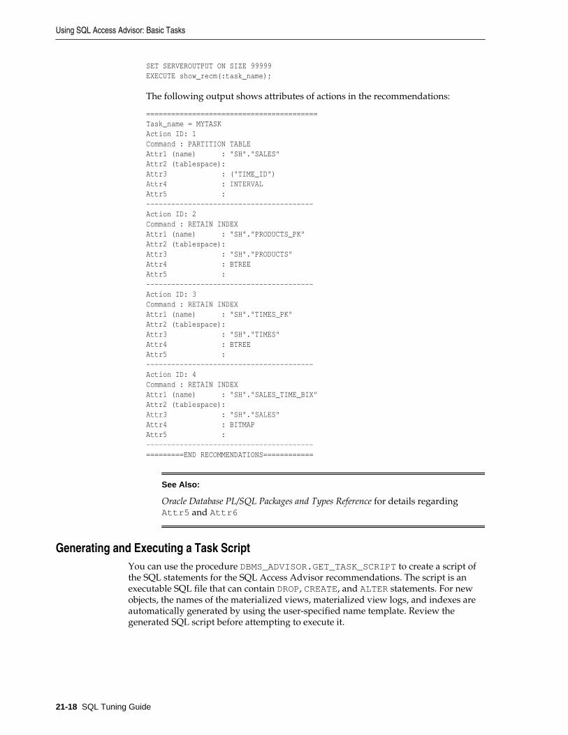
SET SERVEROUTPUT ON SIZE 99999EXECUTE show_recm(:task_name);
The following output shows attributes of actions in the recommendations:
=========================================Task_name = MYTASKAction ID: 1Command : PARTITION TABLEAttr1 (name) : "SH"."SALES"Attr2 (tablespace):Attr3 : ("TIME_ID")Attr4 : INTERVALAttr5 :----------------------------------------Action ID: 2Command : RETAIN INDEXAttr1 (name) : "SH"."PRODUCTS_PK"Attr2 (tablespace):Attr3 : "SH"."PRODUCTS"Attr4 : BTREEAttr5 :----------------------------------------Action ID: 3Command : RETAIN INDEXAttr1 (name) : "SH"."TIMES_PK"Attr2 (tablespace):Attr3 : "SH"."TIMES"Attr4 : BTREEAttr5 :----------------------------------------Action ID: 4Command : RETAIN INDEXAttr1 (name) : "SH"."SALES_TIME_BIX"Attr2 (tablespace):Attr3 : "SH"."SALES"Attr4 : BITMAPAttr5 :----------------------------------------=========END RECOMMENDATIONS============
See Also:
Oracle Database PL/SQL Packages and Types Reference for details regardingAttr5 and Attr6
Generating and Executing a Task ScriptYou can use the procedure DBMS_ADVISOR.GET_TASK_SCRIPT to create a script ofthe SQL statements for the SQL Access Advisor recommendations. The script is anexecutable SQL file that can contain DROP, CREATE, and ALTER statements. For newobjects, the names of the materialized views, materialized view logs, and indexes areautomatically generated by using the user-specified name template. Review thegenerated SQL script before attempting to execute it.
Using SQL Access Advisor: Basic Tasks
21-18 SQL Tuning Guide

Assumptions
This tutorial assumes that you want to save and execute a script that contains therecommendations generated in “Executing a SQL Access Advisor Task”.
To save and execute a SQL script:
1. Connect SQL*Plus to the database as an administrator.
2. Create a directory object and grant permissions to read and write to it.
For example, use the following statements:
CREATE DIRECTORY ADVISOR_RESULTS AS '/tmp';GRANT READ ON DIRECTORY ADVISOR_RESULTS TO PUBLIC;GRANT WRITE ON DIRECTORY ADVISOR_RESULTS TO PUBLIC;
3. Connect to the database as sh, and then save the script to a file.
For example, use the following statement:
EXECUTE DBMS_ADVISOR.CREATE_FILE(DBMS_ADVISOR.GET_TASK_SCRIPT('MYTASK'),'ADVISOR_RESULTS', 'advscript.sql');
4. Use a text editor to view the contents of the script.
The following is a fragment of a script generated by this procedure:
Rem Username: SHRem Task: MYTASKRem Execution date:Rem RemRem Repartitioning table "SH"."SALES"Rem SET SERVEROUTPUT ONSET ECHO ON RemRem Creating new partitioned tableRem CREATE TABLE "SH"."SALES1" ( "PROD_ID" NUMBER, "CUST_ID" NUMBER, "TIME_ID" DATE, "CHANNEL_ID" NUMBER, "PROMO_ID" NUMBER, "QUANTITY_SOLD" NUMBER(10,2), "AMOUNT_SOLD" NUMBER(10,2) ) PCTFREE 5 PCTUSED 40 INITRANS 1 MAXTRANS 255 NOCOMPRESS NOLOGGING TABLESPACE "EXAMPLE"PARTITION BY RANGE ("TIME_ID") INTERVAL( NUMTOYMINTERVAL( 1, 'MONTH')) ( PARTITION VALUES LESS THAN (TO_DATE(' 1998-02-01 00:00:00', 'SYYYY-MM-DD HH24:MI:SS', 'NLS_CALENDAR=GREGORIAN')) );...
5. Optionally, in SQL*Plus, run the SQL script.
Using SQL Access Advisor: Basic Tasks
Optimizing Access Paths with SQL Access Advisor 21-19

For example, enter the following command:
@/tmp/advscript.sql
See Also:
Oracle Database SQL Language Reference for CREATE DIRECTORY syntax, and Oracle Database PL/SQL Packages and Types Reference to learn about theGET_TASK_SCRIPT procedure
Performing a SQL Access Advisor Quick TuneTo tune a single SQL statement, the DBMS_ADVISOR.QUICK_TUNE procedure acceptsas its input a task_name and a single SQL statement. The procedure creates a taskand workload and executes this task. EXECUTE_TASK and QUICK_TUNE produce thesame results. However, QUICK_TUNE is easier when tuning a single SQL statement.
Assumptions
This tutorial assumes the following:
• You want to tune a single SQL statement.
• You want to name the task MY_QUICKTUNE_TASK.
To create a template and base a task on this template:
1. Connect SQL*Plus to the database as user sh, and then initialize SQL*Plusvariables for the SQL statement and task name.
For example, enter the following commands:
VARIABLE t_name VARCHAR2(255);VARIABLE sq VARCHAR2(4000);EXEC :sq := 'SELECT COUNT(*) FROM customers WHERE cust_state_province =''CA''';EXECUTE :t_name := 'MY_QUICKTUNE_TASK';
2. Perform the quick tune.
For example, the following statement executes MY_QUICKTUNE_TASK:
EXEC DBMS_ADVISOR.QUICK_TUNE(DBMS_ADVISOR.SQLACCESS_ADVISOR,:t_name,:sq);
See Also:
Oracle Database PL/SQL Packages and Types Reference to learn more about theQUICK_TUNE procedure and its parameters
Using SQL Access Advisor: Advanced TasksThis section contains the following topics:
• Evaluating Existing Access Structures
• Updating SQL Access Advisor Task Attributes
• Creating and Using SQL Access Advisor Task Templates
Performing a SQL Access Advisor Quick Tune
21-20 SQL Tuning Guide

• Terminating SQL Access Advisor Task Execution
• Deleting SQL Access Advisor Tasks
• Marking SQL Access Advisor Recommendations
• Modifying SQL Access Advisor Recommendations
Evaluating Existing Access StructuresSQL Access Advisor operates in two modes: problem-solving and evaluation. Bydefault, SQL Access Advisor attempts to solve access method problems by looking forenhancements to index structures, partitions, materialized views, and materializedview logs. For example, a problem-solving run may recommend creating a new index,adding a new column to a materialized view log, and so on.
When you set the ANALYSIS_SCOPE parameter to EVALUATION, SQL Access Advisorcomments only on which access structures the supplied workload uses. Anevaluation-only run may only produce recommendations such as retaining an index,retaining a materialized view, and so on. The evaluation mode can be useful to seeexactly which indexes and materialized views a workload is using. SQL AccessAdvisor does not evaluate the performance impact of existing base table partitioning.
To create a task and set it to evaluation mode:
1. Connect SQL*Plus to the database with the appropriate privileges, and then createa task.
For example, enter the following statement, where t_name is a SQL*Plus variableset to the name of the task:
EXECUTE DBMS_ADVISOR.EXECUTE_TASK(:t_name);
2. Perform the quick tune.
For example, the following statement sets the previous task to evaluation mode:
EXECUTE DBMS_ADVISOR.SET_TASK_PARAMETER(:t_name,'ANALYSIS_SCOPE','EVALUATION');
See Also:
Oracle Database PL/SQL Packages and Types Reference to learn about theSET_TASK_PARAMETER procedure and its parameters
Updating SQL Access Advisor Task AttributesYou can use the DBMS_ADVISOR.UPDATE_TASK_ATTRIBUTES procedure to do thefollowing:
• Change the name of a task.
• Give a task a description.
• Set the task to be read-only so it cannot be changed.
• Make the task a template upon which you can define other tasks (see “Creating andUsing SQL Access Advisor Task Templates”).
• Changes various attributes of a task or a task template.
Using SQL Access Advisor: Advanced Tasks
Optimizing Access Paths with SQL Access Advisor 21-21

Assumptions
This tutorial assumes the following:
• You want to change the name of existing task MYTASK to TUNING1.
• You want to make the task TUNING1 read-only.
To update task attributes:
1. Connect SQL*Plus to the database as user sh, and then change the name of thetask.
For example, use the following statement:
EXECUTE DBMS_ADVISOR.UPDATE_TASK_ATTRIBUTES('MYTASK', 'TUNING1');
2. Set the task to read-only.
For example, use the following statement:
EXECUTE DBMS_ADVISOR.UPDATE_TASK_ATTRIBUTES('TUNING1', read_only => 'true');
See Also:
Oracle Database PL/SQL Packages and Types Reference for more informationregarding the UPDATE_TASK_ATTRIBUTES procedure and its parameters
Creating and Using SQL Access Advisor Task TemplatesA task template is a saved configuration on which to base future tasks and workloads.A template enables you to set up any number of tasks or workloads that can serve asstarting points or templates for future task creation. By setting up a template, you cansave time when performing tuning analysis. This approach also enables you to customfit a tuning analysis to the business operation.
Physically, there is no difference between a task and a template. However, a templatecannot be executed. To create a task from a template, you specify the template to beused when a new task is created. At that time, SQL Access Advisor copies the data andparameter settings from the template into the newly created task. You can also set anexisting task to be a template by setting the template attribute when creating the taskor later using the UPDATE_TASK_ATTRIBUTE procedure.
Table 21-3 describes procedures that you can use to manage task templates.
Table 21-3 DBMS_ADVISOR Procedures for Task Templates
Procedure Description
CREATE_TASK The template parameter is an optional task name of anexisting task or task template. To specify built-in SQL AccessAdvisor templates, use the template name as described in Table 21-6. is_template is an optional parameter thatenables you to set the newly created task as a template. Validvalues are true and false.
Using SQL Access Advisor: Advanced Tasks
21-22 SQL Tuning Guide

Table 21-3 (Cont.) DBMS_ADVISOR Procedures for Task Templates
Procedure Description
SET_TASK_PARAMETER The INDEX_NAME_TEMPLATE parameter specifies themethod by which new index names are formed. TheMVIEW_NAME_TEMPLATE parameter specifies the method bywhich new materialized view names are formed. ThePARTITION_NAME_TEMPLATE parameter specifies themethod by which new partition names are formed. See OracleDatabase PL/SQL Packages and Types Reference to for taskparameter descriptions.
UPDATE_TASK_ATTRIBUTES is_template marks the task as a template. Physically, thereis no difference between a task and a template; however, atemplate cannot be executed. Possible values are: true andfalse. If the value is NULL or contains the valueADVISOR_UNUSED, then the setting is not changed.
Assumptions
This tutorial assumes the following:
• You want to create a template named MY_TEMPLATE.
• You want to set naming conventions for indexes and materialized views that arerecommended by tasks based on MY_TEMPLATE.
• You want to create task NEWTASK based on MY_TEMPLATE.
To create a template and base a task on this template:
1. Connect SQL*Plus to the database as user sh, and then create a task as a template.
For example, create a template named MY_TEMPLATE as follows:
VARIABLE template_id NUMBER;VARIABLE template_name VARCHAR2(255);EXECUTE :template_name := 'MY_TEMPLATE';BEGIN DBMS_ADVISOR.CREATE_TASK ( 'SQL Access Advisor', :template_id, :template_name, is_template => 'true');END;
2. Set template parameters.
For example, the following statements set the naming conventions forrecommended indexes and materialized views:
-- set naming conventions for recommended indexes/mvsBEGIN DBMS_ADVISOR.SET_TASK_PARAMETER ( :template_name, 'INDEX_NAME_TEMPLATE', 'SH_IDX$$_<SEQ>'
Using SQL Access Advisor: Advanced Tasks
Optimizing Access Paths with SQL Access Advisor 21-23

);END;
BEGIN DBMS_ADVISOR.SET_TASK_PARAMETER ( :template_name, 'MVIEW_NAME_TEMPLATE', 'SH_MV$$_<SEQ>');END;
3. Create a task based on a pre-existing template.
For example, enter the following commands to create NEWTASK based onMY_TEMPLATE:
VARIABLE task_id NUMBER;VARIABLE task_name VARCHAR2(255);EXECUTE :task_name := 'NEWTASK';BEGIN DBMS_ADVISOR.CREATE_TASK ( 'SQL Access Advisor', :task_id, :task_name, template=>'MY_TEMPLATE');END;
See Also:
• Oracle Database PL/SQL Packages and Types Reference to learn about theCREATE_TASK procedure and its parameters
• Oracle Database PL/SQL Packages and Types Reference to learn about theSET_TASK_PARAMETER procedure and its parameters
Terminating SQL Access Advisor Task ExecutionSQL Access Advisor enables you to interrupt the recommendation process or allow itto complete. An interruption signals SQL Access Advisor to stop processing andmarks the task as INTERRUPTED. At that point, you may update recommendationattributes and generate scripts.
Intermediate results represent recommendations for the workload contents up to thatpoint in time. If recommendations must be sensitive to the entire workload, thenOracle recommends that you let the task complete. Additionally, recommendationsmade by the advisor early in the recommendation process do not contain base tablepartitioning recommendations. The partitioning analysis requires a large part of theworkload to be processed before it can determine whether partitioning would bebeneficial. Therefore, if SQL Access Advisor detects a benefit, then only laterintermediate results contain base table partitioning recommendations.
This section describes two ways to terminate SQL Access Advisor task execution:
• Interrupting SQL Access Advisor Tasks
• Canceling SQL Access Advisor Tasks
Using SQL Access Advisor: Advanced Tasks
21-24 SQL Tuning Guide
Interrupting SQL Access Advisor Tasks
The DBMS_ADVISOR.INTERRUPT_TASK procedure causes a SQL Access Advisor taskexecution to terminate as if it had reached its normal end. Thus, you can see anyrecommendations that have been formed up to the point of the interruption. Aninterrupted task cannot be restarted. The syntax is as follows:
DBMS_ADVISOR.INTERRUPT_TASK (task_name IN VARCHAR2);
Assumptions
This tutorial assumes the following:
• Long-running task MYTASK is currently executing.
• You want to interrupt this task, and then view the recommendations.
To interrupt a currently executing task:
1. Connect SQL*Plus to the database as sh, and then interrupt the task.
For example, create a template named MY_TEMPLATE as follows:
EXECUTE DBMS_ADVISOR.INTERRUPT_TASK ('MYTASK');
See Also:
Oracle Database PL/SQL Packages and Types Reference to learn about theINTERRUPT_TASK procedure
Canceling SQL Access Advisor Tasks
You can stop task execution by calling the DBMS_ADVISOR.CANCEL_TASK procedureand passing in the task name for this recommendation process. SQL Access Advisormay take a few seconds to respond to this request. Because all advisor task proceduresare synchronous, to cancel an operation, you must use a separate database session. Ifyou use CANCEL_TASK, then SQL Access Advisor makes no recommendations.
A cancel command effective restores the task to its condition before the start of thecanceled operation. Therefore, a canceled task or data object cannot be restarted.However, you can reset the task using DBMS_ADVISOR.RESET_TASK, and thenexecute it again. The CANCEL_TASK syntax is as follows:
DBMS_ADVISOR.CANCEL_TASK (task_name IN VARCHAR2);
The RESET_TASK procedure resets a task to its initial starting point, which has theeffect of removing all recommendations and intermediate data from the task. The taskstatus is set to INITIAL. The syntax is as follows:
DBMS_ADVISOR.RESET_TASK (task_name IN VARCHAR2);
Assumptions
This tutorial assumes the following:
• Long-running task MYTASK is currently executing. This task is set to makepartitioning recommendations.
Using SQL Access Advisor: Advanced Tasks
Optimizing Access Paths with SQL Access Advisor 21-25

• You want to cancel this task, and then reset it so that the task makes only indexrecommendations.
To cancel a currently executing task:
1. Connect SQL*Plus to the database as user sh, and then cancel the task.
For example, create a template named MY_TEMPLATE as follows:
EXECUTE DBMS_ADVISOR.CANCEL_TASK ('MYTASK');
2. Reset the task.
For example, execute the RESET_TASK procedure as follows:
EXECUTE DBMS_ADVISOR.RESET_TASK('MYTASK');
3. Set task parameters.
For example, change the analysis scope to INDEX as follows:
EXECUTE DBMS_ADVISOR.SET_TASK_PARAMETER(:task_name, 'ANALYSIS_SCOPE', 'INDEX');
4. Execute the task.
For example, execute MYTASK as follows:
EXECUTE DBMS_ADVISOR.EXECUTE_TASK ('MYTASK');
See Also:
• Oracle Database PL/SQL Packages and Types Reference to learn more about theRESET_TASK procedure and its parameters
• Oracle Database PL/SQL Packages and Types Reference to learn more about theCANCEL_TASK procedure and its parameters
Deleting SQL Access Advisor TasksThe DBMS_ADVISOR.DELETE_TASK procedure deletes existing SQL Access Advisortasks from the repository. The syntax is as follows:
DBMS_ADVISOR.DELETE_TASK (task_name IN VARCHAR2);
If a task is linked to an STS workload, and if you want to delete the task or workload,then you must remove the link between the task and the workload using theDELETE_STS_REF procedure. The following example deletes the link between taskMYTASK and the current user's SQL tuning set MY_STS_WORKLOAD:
EXECUTE DBMS_ADVISOR.DELETE_STS_REF('MYTASK', null, 'MY_STS_WORKLOAD');
Assumptions
This tutorial assumes the following:
• User sh currently owns multiple SQL Access Advisor tasks.
• You want to delete MYTASK.
• The task MYTASK is currently linked to workload MY_STS_WORKLOAD.
Using SQL Access Advisor: Advanced Tasks
21-26 SQL Tuning Guide

To delete a SQL Access Advisor task:
1. Connect SQL*Plus to the database as user sh, and then query existing SQL AccessAdvisor tasks.
For example, query the data dictionary as follows (sample output included):
SELECT TASK_NAME FROM USER_ADVISOR_TASKS WHERE ADVISOR_NAME = 'SQL Access Advisor'; TASK_NAME-------------------------MYTASKNEWTASK
2. Delete the link between MYTASK and MY_STS_WORKLOAD.
For example, delete the reference as follows:
EXECUTE DBMS_ADVISOR.DELETE_STS_REF('MYTASK', null, 'MY_STS_WORKLOAD');
3. Delete the desired task.
For example, delete MYTASK as follows:
EXECUTE DBMS_ADVISOR.DELETE_TASK('MYTASK');
See Also:
olink:REFRN10141olink:ARPLSOracle Database PL/SQL Packages and TypesReference to learn more about the DELETE_TASK procedure and its parameters
Marking SQL Access Advisor RecommendationsBy default, all SQL Access Advisor recommendations are ready to be implemented.However, you can choose to skip or exclude selected recommendations by using theDBMS_ADVISOR.MARK_RECOMMENDATION procedure. MARK_RECOMMENDATIONenables you to annotate a recommendation with a REJECT or IGNORE setting, whichcauses the GET_TASK_SCRIPT to skip it when producing the implementationprocedure.
If SQL Access Advisor makes a recommendation to partition one or multiplepreviously unpartitioned base tables, then consider carefully before skipping thisrecommendation. Changing a table's partitioning scheme affects the cost of all queries,indexes, and materialized views defined on the table. Therefore, if you skip thepartitioning recommendation, then the advisor's remaining recommendations on thistable are no longer optimal. To see recommendations on your workload that do notcontain partitioning, reset the advisor task and rerun it with the ANALYSIS_SCOPEparameter changed to exclude partitioning recommendations.
The syntax is as follows:
DBMS_ADVISOR.MARK_RECOMMENDATION ( task_name IN VARCHAR2 id IN NUMBER, action IN VARCHAR2);
Using SQL Access Advisor: Advanced Tasks
Optimizing Access Paths with SQL Access Advisor 21-27

Assumptions
This tutorial assumes the following:
• You are reviewing the recommendations as described in tutorial “Viewing SQLAccess Advisor Task Results”.
• You want to reject the first recommendation, which partitions a table.
To mark a recommendation:
1. Connect SQL*Plus to the database as user sh, and then mark therecommendation.
For example, reject recommendation 1 as follows:
EXECUTE DBMS_ADVISOR.MARK_RECOMMENDATION('MYTASK', 1, 'REJECT');
This recommendation and any dependent recommendations do not appear in thescript.
2. Generate the script as explained in “Generating and Executing a Task Script”.
See Also:
Oracle Database PL/SQL Packages and Types Reference to learn more about theMARK_RECOMMENDATIONS procedure and its parameters
Modifying SQL Access Advisor RecommendationsUsing the UPDATE_REC_ATTRIBUTES procedure, SQL Access Advisor names andassigns ownership to new objects such as indexes and materialized views duringanalysis. However, it does not necessarily choose appropriate names, so you maymanually set the owner, name, and tablespace values for new objects. Forrecommendations referencing existing database objects, owner and name valuescannot be changed. The syntax is as follows:
DBMS_ADVISOR.UPDATE_REC_ATTRIBUTES ( task_name IN VARCHAR2 rec_id IN NUMBER, action_id IN NUMBER, attribute_name IN VARCHAR2, value IN VARCHAR2);
The attribute_name parameter can take the following values:
• OWNER
Specifies the owner name of the recommended object.
• NAME
Specifies the name of the recommended object.
• TABLESPACE
Specifies the tablespace of the recommended object.
Using SQL Access Advisor: Advanced Tasks
21-28 SQL Tuning Guide

Assumptions
This tutorial assumes the following:
• You are reviewing the recommendations as described in tutorial “Viewing SQLAccess Advisor Task Results”.
• You want to change the tablespace for recommendation 1, action 1 to SH_MVIEWS.
To mark a recommendation:
1. Connect SQL*Plus to the database as user sh, and then update therecommendation attribute.
For example, change the tablespace name to SH_MVIEWS as follows:
BEGIN DBMS_ADVISOR.UPDATE_REC_ATTRIBUTES ( 'MYTASK', 1, 1, 'TABLESPACE', 'SH_MVIEWS');END;
2. Generate the script as explained in “Generating and Executing a Task Script”.
See Also:
Oracle Database PL/SQL Packages and Types Reference to learn more about theUPDATE_REC_ATTRIBUTES procedure and its parameters
SQL Access Advisor ExamplesOracle Database provides a script that contains several SQL Access Advisor examplesthat you can run on a test database. The script is named ORACLE_HOME/rdbms/demo/aadvdemo.sql.
SQL Access Advisor ReferenceThis section contains the following topics:
• Action Attributes in the DBA_ADVISOR_ACTIONS View
• Categories for SQL Access Advisor Task Parameters
• SQL Access Advisor Constants
Action Attributes in the DBA_ADVISOR_ACTIONS ViewTable 21-4 maps SQL Access Advisor actions to attribute columns in theDBA_ADVISOR_ACTIONS view. In the table, MV refers to a materialized view.
Table 21-4 SQL Access Advisor Action Attributes
SQL Access Advisor Examples
Optimizing Access Paths with SQL Access Advisor 21-29

Table 21-4 (Cont.) SQL Access Advisor Action Attributes
Action ATTR1Column
ATTR2Column
ATTR3Column
ATTR4Column
ATTR5Column
ATTR6Column
NUM_ATTR1Column
CREATEINDEX
Indexname
Indextablespace
Target table BITMAPorBTREE
Indexcolumnlist /expression
Unused Storagesize inbytes forthe index
CREATEMATERIALIZED VIEW
MV name MVtablespace
REFRESHCOMPLETE,REFRESHFAST,REFRESHFORCE,NEVERREFRESH
ENABLEQUERYREWRITE,DISABLEQUERYREWRITE
SQLSELECTstatement
Unused Storagesize inbytes forthe MV
CREATEMATERIALIZED VIEWLOG
Targettable name
MV logtablespace
ROWIDPRIMARYKEY,SEQUENCEOBJECT ID
INCLUDINGNEWVALUES,EXCLUDINGNEWVALUES
Tablecolumn list
Partitioningsubclauses
Unused
CREATEREWRITEEQUIVALENCE
Name ofequivalence
Checksumvalue
Unused Unused Source SQLstatement
EquivalentSQLstatement
Unused
DROPINDEX
Indexname
Unused Unused Unused Indexcolumns
Unused Storagesize inbytes forthe index
DROPMATERIALIZED VIEW
MV name Unused Unused Unused Unused Unused Storagesize inbytes forthe MV
DROPMATERIALIZED VIEWLOG
Targettable name
Unused Unused Unused Unused Unused Unused
PARTITION TABLE
Tablename
RANGE,INTERVAL,LIST, HASH,RANGE-HASH,RANGE-LIST
Partitionkey forpartitioning(columnname or listof columnnames)
Partitionkey forsubpartitioning (columnname or listof columnnames)
SQLPARTITIONclause
SQLSUBPARTITION clause
Unused
SQL Access Advisor Reference
21-30 SQL Tuning Guide

Table 21-4 (Cont.) SQL Access Advisor Action Attributes
Action ATTR1Column
ATTR2Column
ATTR3Column
ATTR4Column
ATTR5Column
ATTR6Column
NUM_ATTR1Column
PARTITION INDEX
Indexname
LOCAL,RANGE, HASH
Partitionkey forpartitioning(list ofcolumnnames)
Unused SQLPARTITIONclause
Unused Unused
PARTITION ONMATERIALIZED VIEW
MV name RANGE,INTERVAL,LIST, HASH,RANGE-HASH,RANGE-LIST
Partitionkey forpartitioning(columnname or listof columnnames)
Partitionkey forsubpartitioning (columnname or listof columnnames)
SQLSUBPARTITION clause
SQLSUBPARTITION clause
Unused
RETAININDEX
Indexname
Unused Target table BITMAP orBTREE
Indexcolumns
Unused Storagesize inbytes forthe index
RETAINMATERIALIZED VIEW
MV name Unused REFRESHCOMPLETEor REFRESHFAST
Unused SQLSELECTstatement
Unused Storagesize inbytes forthe MV
RETAINMATERIALIZED VIEWLOG
Targettable name
Unused Unused Unused Unused Unused Unused
Categories for SQL Access Advisor Task ParametersTable 21-5 groups the most relevant SQL Access Advisor task parameters intocategories. All task parameters for workload filtering are deprecated.
Table 21-5 Types of Advisor Task Parameters And Their Uses
Workload Filtering Task Configuration Schema Attributes RecommendationOptions
END_TIME DAYS_TO_EXPIRE DEF_INDEX_OWNER ANALYSIS_SCOPE
INVALID_ACTION_LIST JOURNALING DEF_INDEX_TABLESPACE
COMPATIBILITY
INVALID_MODULE_LIST REPORT_DATE_FORMAT
DEF_MVIEW_OWNER CREATION_COST
INVALID_SQLSTRING_LIMIT
DEF_MVIEW_TABLESPACE
DML_VOLATILITY
INVALID_TABLE_LIST DEF_MVLOG_TABLESPACE
LIMIT_PARTITION_SCHEMES
SQL Access Advisor Reference
Optimizing Access Paths with SQL Access Advisor 21-31

Table 21-5 (Cont.) Types of Advisor Task Parameters And Their Uses
Workload Filtering Task Configuration Schema Attributes RecommendationOptions
INVALID_USERNAME_LIST DEF_PARTITION_TABLESPACE
MODE
RANKING_MEASURE INDEX_NAME_TEMPLATE PARTITIONING_TYPES
SQL_LIMIT MVIEW_NAME_TEMPLATE REFRESH_MODE
START_TIME STORAGE_CHANGE
TIME_LIMIT USE_SEPARATE_TABLESPACES
VALID_ACTION_LIST WORKLOAD_SCOPE
VALID_MODULE_LIST
VALID_SQLSTRING_LIST
VALID_TABLE_LIST
VALID_USERNAME_LIST
SQL Access Advisor ConstantsYou can use the constants shown in Table 21-6 with SQL Access Advisor.
Table 21-6 SQL Access Advisor Constants
Constant Description
ADVISOR_ALL A value that indicates all possible values. For string parameters,this value is equivalent to the wildcard % character.
ADVISOR_CURRENT Indicates the current time or active set of elements. Typically,this is used in time parameters.
ADVISOR_DEFAULT Indicates the default value. Typically used when setting task orworkload parameters.
ADVISOR_UNLIMITED A value that represents an unlimited numeric value.
ADVISOR_UNUSED A value that represents an unused entity. When a parameter isset to ADVISOR_UNUSED, it has no effect on the currentoperation. A typical use for this constant is to set a parameter asunused for its dependent operations.
SQLACCESS_GENERAL Specifies the name of a default SQL Access general-purpose tasktemplate. This template sets the DML_VOLATILITY taskparameter to true and ANALYSIS_SCOPE to INDEX, MVIEW.
SQLACCESS_OLTP Specifies the name of a default SQL Access OLTP task template.This template sets the DML_VOLATILITY task parameter to trueand ANALYSIS_SCOPE to INDEX.
SQL Access Advisor Reference
21-32 SQL Tuning Guide
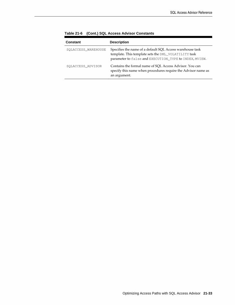
Table 21-6 (Cont.) SQL Access Advisor Constants
Constant Description
SQLACCESS_WAREHOUSE Specifies the name of a default SQL Access warehouse tasktemplate. This template sets the DML_VOLATILITY taskparameter to false and EXECUTION_TYPE to INDEX, MVIEW.
SQLACCESS_ADVISOR Contains the formal name of SQL Access Advisor. You canspecify this name when procedures require the Advisor name asan argument.
SQL Access Advisor Reference
Optimizing Access Paths with SQL Access Advisor 21-33

SQL Access Advisor Reference
21-34 SQL Tuning Guide

Part IXSQL Controls
This part explains how to manage SQL profiles and SQL plan baselines, and migratestored outlines to SQL plan baselines.
contains the following chapters:
• Managing SQL Profiles
• Managing SQL Plan Baselines
• Migrating Stored Outlines to SQL Plan Baselines


22Managing SQL Profiles
This chapter contains the following topics:
• About SQL Profiles
• Implementing a SQL Profile
• Listing SQL Profiles
• Altering a SQL Profile
• Dropping a SQL Profile
• Transporting a SQL Profile
About SQL ProfilesA SQL profile is a database object that contains auxiliary statistics specific to a SQLstatement. Conceptually, a SQL profile is to a SQL statement what object-levelstatistics are to a table or index. SQL profiles are created when a DBA invokes SQLTuning Advisor (see “About SQL Tuning Advisor”).
This section contains the following topics:
• Purpose of SQL Profiles
• Concepts for SQL Profiles
• User Interfaces for SQL Profiles
• Basic Tasks for SQL Profiles
Purpose of SQL ProfilesWhen profiling a SQL statement, SQL Tuning Advisor uses a specific set of bindvalues as input, and then compares the optimizer estimate with values obtained byexecuting fragments of the statement on a data sample. When significant variances arefound, SQL Tuning Advisor bundles corrective actions together in a SQL profile, andthen recommends its acceptance.
The corrected statistics in a SQL profile can improve optimizer cardinality estimates,which in turn leads the optimizer to select better plans. SQL profiles provide thefollowing benefits over other techniques for improving plans:
• Unlike hints and stored outlines, SQL profiles do not tie the optimizer to a specificplan or subplan. SQL profiles fix incorrect estimates while giving the optimizer theflexibility to pick the best plan in different situations.
Managing SQL Profiles 22-1

• Unlike hints, no changes to application source code are necessary when using SQLprofiles. The use of SQL profiles by the database is transparent to the user.
See Also:
“Influencing the Optimizer with Hints”
Concepts for SQL ProfilesA SQL profile is a collection of auxiliary statistics on a query, including all tables andcolumns referenced in the query. The profile stores this information in the datadictionary. The optimizer uses this information at optimization time to determine thecorrect plan.
Note:
The SQL profile contains supplemental statistics for the entire statement, notindividual plans. The profile does not itself determine a specific plan.
A SQL profile contains, among other statistics, a set of cardinality adjustments. Thecardinality measure is based on sampling the WHERE clause rather than on statisticalprojection. A profile uses parts of the query to determine whether the estimatedcardinalities are close to the actual cardinalities and, if a mismatch exists, uses thecorrected cardinalities. For example, if a SQL profile exists for SELECT * FROM tWHERE x=5 AND y=10, then the profile stores the actual number of rows returned.
When choosing plans, the optimizer has the following sources of information:
• The environment, which contains the database configuration, bind variable values, optimizer statistics, data set, and so on
• The supplemental statistics in the SQL profile
Figure 22-1 shows the relationship between a SQL statement and the SQL profile forthis statement. The optimizer uses the SQL profile and the environment to generate anexecution plan. In this example, the plan is in the SQL plan baseline for the statement.
Figure 22-1 SQL Profile
SQL Plan Baseline
GB
NLNL
GB
HJHJ
SQL Profile
Environment
OptimizerSQL Statement
SELECT . . .
Optimizer�Statistics
ConfigurationBind�Variables
Data�Set
If either the optimizer environment or SQL profile change, then the optimizer cancreate a new plan. As tables grow, or as indexes are created or dropped, the plan for aSQL profile can change. The profile continues to be relevant even if the data
About SQL Profiles
22-2 SQL Tuning Guide

distribution or access path of the corresponding statement changes. In general, you donot need to refresh SQL profiles.
Over time, profile content can become outdated. In this case, performance of the SQLstatement may degrade. The statement may appear as high-load or top SQL. In thiscase, the Automatic SQL Tuning task again captures the statement as high-load SQL.You can implement a new SQL profile for the statement.
Internally, a SQL profile is implemented using hints that address different types ofproblems. These hints do not specify any particular plan. Rather, the hints correcterrors in the optimizer estimation algorithm that lead to suboptimal plans. Forexample, a profile may use the TABLE_STATS hint to set object statistics for tableswhen the statistics are missing or stale.
See Also:
• “Differences Between SQL Plan Baselines and SQL Profiles”
• “Introduction to Optimizer Statistics”
SQL Profile Recommendations
As explained in “SQL Profiling”, SQL Tuning Advisor invokes Automatic TuningOptimizer to generate SQL profile recommendations. Recommendations to implementSQL profiles occur in a finding, which appears in a separate section of the SQL TuningAdvisor report.
When you implement (or accept) a SQL profile, the database creates the profile andstores it persistently in the data dictionary. However, the SQL profile information isnot exposed through regular dictionary views.
See Also:
• Oracle Database VLDB and Partitioning Guide to learn more about Auto DOP
• Oracle Database PL/SQL Packages and Types Reference to learn about theDBMS_SQLTUNE.ACCEPT_SQL_PROFILE procedure
Example 22-1 SQL Profile Recommendation
In this example, the database found a better plan for a SELECT statement that usesseveral expensive joins. The database recommends runningDBMS_SQLTUNE.ACCEPT_SQL_PROFILE to implement the profile, which enables thestatement to run 98.53% faster.
-------------------------------------------------------------------------------FINDINGS SECTION (2 findings)------------------------------------------------------------------------------- 1- SQL Profile Finding (see explain plans section below)-------------------------------------------------------- A potentially better execution plan was found for this statement. Choose one of the following SQL profiles to implement. Recommendation (estimated benefit: 99.45%)
About SQL Profiles
Managing SQL Profiles 22-3

------------------------------------------ - Consider accepting the recommended SQL profile. execute dbms_sqltune.accept_sql_profile(task_name => 'my_task', object_id => 3, task_owner => 'SH', replace => TRUE); Validation results ------------------ The SQL profile was tested by executing both its plan and the original plan and measuring their respective execution statistics. A plan may have been only partially executed if the other could be run to completion in less time. Original Plan With SQL Profile % Improved ------------- ---------------- ---------- Completion Status: PARTIAL COMPLETE Elapsed Time(us): 15467783 226902 98.53 % CPU Time(us): 15336668 226965 98.52 % User I/O Time(us): 0 0 Buffer Gets: 3375243 18227 99.45 % Disk Reads: 0 0 Direct Writes: 0 0 Rows Processed: 0 109 Fetches: 0 109 Executions: 0 1 Notes ----- 1. The SQL profile plan was first executed to warm the buffer cache. 2. Statistics for the SQL profile plan were averaged over next 3 executions.
Sometimes SQL Tuning Advisor may recommend implementing a profile that uses theAutomatic Degree of Parallelism (Auto DOP) feature. A parallel query profile is onlyrecommended when the original plan is serial and when parallel execution cansignificantly reduce the elapsed time for a long-running query.
When it recommends a profile that uses Auto DOP, SQL Tuning Advisor gives detailsabout the performance overhead of using parallel execution for the SQL statement inthe report. For parallel execution recommendations, SQL Tuning Advisor may providetwo SQL profile recommendations, one using serial execution and one using parallel.
The following example shows a parallel query recommendation. In this example, adegree of parallelism of 7 improves response time significantly at the cost of increasingresource consumption by almost 25%. You must decide whether the reduction indatabase throughput is worth the increase in response time.
Recommendation (estimated benefit: 99.99%) ------------------------------------------ - Consider accepting the recommended SQL profile to use parallel execution for this statement. execute dbms_sqltune.accept_sql_profile(task_name => 'gfk_task', object_id => 3, task_owner => 'SH', replace => TRUE, profile_type => DBMS_SQLTUNE.PX_PROFILE); Executing this query parallel with DOP 7 will improve its response time 82.22% over the SQL profile plan. However, there is some cost in enabling parallel execution. It will increase the statement's resource consumption by an estimated 24.43% which may result in a reduction of system throughput. Also, because these resources are consumed over a much smaller duration, the response time of concurrent statements might be negatively impacted if sufficient hardware capacity is not available. The following data shows some sampled statistics for this SQL from the past
About SQL Profiles
22-4 SQL Tuning Guide

week and projected weekly values when parallel execution is enabled. Past week sampled statistics for this SQL ----------------------------------------- Number of executions 0 Percent of total activity .29 Percent of samples with #Active Sessions > 2*CPU 0 Weekly DB time (in sec) 76.51 Projected statistics with Parallel Execution -------------------------------------------- Weekly DB time (in sec) 95.21
SQL Profiles and SQL Plan Baselines
You can use SQL profiles with or without SQL plan management. No strictrelationship exists between the SQL profile and the plan baseline. If a statement hasmultiple plans in a SQL plan baseline, then a SQL profile is useful because it enablesthe optimizer to choose the lowest-cost plan in the baseline.
See Also:
Managing SQL Plan Baselines
User Interfaces for SQL ProfilesOracle Enterprise Manager Cloud Control (Cloud Control) usually handles SQLprofiles as part of automatic SQL tuning.
On the command line, you can manage SQL profiles with the DBMS_SQLTUNEpackage. To use the APIs, you must have the ADMINISTER SQL MANAGEMENTOBJECT privilege.
See Also:
• Oracle Database PL/SQL Packages and Types Reference for information aboutthe DBMS_SQLTUNE package
• Oracle Database 2 Day + Performance Tuning Guide to learn how to manageSQL profiles with Cloud Control
Basic Tasks for SQL ProfilesThis section explains the basic tasks involved in managing SQL profiles. Figure 22-2shows the basic workflow for implementing, altering, and dropping SQL profiles.
About SQL Profiles
Managing SQL Profiles 22-5

Figure 22-2 Managing SQL Profiles
DBMS_SQLTUNE.DROP_SQL_PROFILE
DBMS_SQLTUNE.
ALTER_SQL_PROFILE
List SQL Profiles
Drop a SQL Profile
Implement a SQL Profile
DBA_SQL_PROFILES
Alter a SQL Profile
DBMS_SQLTUNE.
ACCEPT_SQL_PROFILE
Typically, you manage SQL profiles in the following sequence:
1. Implement a recommended SQL profile.
“Implementing a SQL Profile” describes this task.
2. Obtain information about SQL profiles stored in the database.
“Listing SQL Profiles” describes this task.
3. Optionally, modify the implemented SQL profile.
“Altering a SQL Profile” describes this task.
4. Drop the implemented SQL profile when it is no longer needed.
“Dropping a SQL Profile” describes this task.
To tune SQL statements on another database, you can transport both a SQL tuning setand a SQL profile to a separate database. “Transporting a SQL Profile” describes thistask.
See Also:
Oracle Database PL/SQL Packages and Types Reference for information about theDBMS_SQLTUNE package
Implementing a SQL ProfileImplementing (also known as accepting) a SQL profile means storing it persistently inthe database. A profile must be implemented before the optimizer can use it as inputwhen generating plans.
Implementing a SQL Profile
22-6 SQL Tuning Guide

About SQL Profile ImplementationAs a rule of thumb, implement a SQL profile recommended by SQL Tuning Advisor. Ifthe database recommends both an index and a SQL profile, then either use both or usethe SQL profile only. If you create an index, then the optimizer may need the profile topick the new index.
In some situations, SQL Tuning Advisor may find an improved serial plan in additionto an even better parallel plan. In this case, the advisor recommends both a standardand a parallel SQL profile, enabling you to choose between the best serial and bestparallel plan for the statement. Implement a parallel plan only if the increase inresponse time is worth the decrease in throughput.
To implement a SQL profile, execute the DBMS_SQLTUNE.ACCEPT_SQL_PROFILEprocedure. Some important parameters are as follows:
• profile_type
Set this parameter to REGULAR_PROFILE for a SQL profile without a change toparallel execution, or PX_PROFLE for a SQL profile with a change to parallelexecution.
• force_match
This parameter controls statement matching. Typically, an accepted SQL profile isassociated with the SQL statement through a SQL signature that is generated usinga hash function. This hash function changes the SQL statement to upper case andremoves all extra whites spaces before generating the signature. Thus, the sameSQL profile works for all SQL statements in which the only difference is case andwhite spaces.
By setting force_match to true, the SQL profile additionally targets all SQLstatements that have the same text after the literal values in the WHERE clause havebeen replaced by bind variables. This setting may be useful for applications thatuse only literal values because it enables SQL with text differing only in its literalvalues to share a SQL profile. If both literal values and bind variables are in theSQL text, or if force_match is set to false (default), then the literal values in theWHERE clause are not replaced by bind variables.
See Also:
Oracle Database PL/SQL Packages and Types Reference for information about theACCEPT_SQL_PROFILE procedure
Implementing a SQL ProfileThis section shows how to use the ACCEPT_SQL_PROFILE procedure to implement aSQL profile.
Assumptions
This tutorial assumes the following:
• The SQL Tuning Advisor task STA_SPECIFIC_EMP_TASK includes arecommendation to create a SQL profile.
• The name of the SQL profile is my_sql_profile.
Implementing a SQL Profile
Managing SQL Profiles 22-7

• The PL/SQL block accepts a profile that uses parallel execution (profile_type).
• The profile uses force matching.
To implement a SQL profile:
• Connect SQL*Plus to the database with the appropriate privileges, and thenexecute the ACCEPT_SQL_PROFILE function.
For example, execute the following PL/SQL:
DECLARE my_sqlprofile_name VARCHAR2(30);BEGIN my_sqlprofile_name := DBMS_SQLTUNE.ACCEPT_SQL_PROFILE ( task_name => 'STA_SPECIFIC_EMP_TASK', name => 'my_sql_profile', profile_type => DBMS_SQLTUNE.PX_PROFILE, force_match => true );END;/
See Also:
Oracle Database PL/SQL Packages and Types Reference to learn about theDBMS_SQLTUNE.ACCEPT_SQL_PROFILE procedure
Listing SQL ProfilesThe data dictionary view DBA_SQL_PROFILES stores SQL profiles persistently in thedatabase. The statistics are in an Oracle internal format, so you cannot query profilesdirectly. However, you can list profiles.
To list SQL profiles:
• Connect SQL*Plus to the database with the appropriate privileges, and then querythe DBA_SQL_PROFILES view.
For example, execute the following query:
COLUMN category FORMAT a10COLUMN sql_text FORMAT a20
SELECT NAME, SQL_TEXT, CATEGORY, STATUSFROM DBA_SQL_PROFILES;
Sample output appears below:
NAME SQL_TEXT CATEGORY STATUS------------------------------ -------------------- ---------- --------SYS_SQLPROF_01285f6d18eb0000 select promo_name, c DEFAULT ENABLED ount(*) c from promo tions p, sales s whe re s.promo_id = p.pr omo_id and p.promo_c ategory = 'internet' group by p.promo_na me order by c desc
Listing SQL Profiles
22-8 SQL Tuning Guide

See Also:
Oracle Database Reference to learn about the DBA_SQL_PROFILES view
Altering a SQL ProfileYou can alter attributes of an existing SQL profile using the attribute_nameparameter of the ALTER_SQL_PROFILE procedure.
The CATEGORY attribute determines which sessions can apply a profile. View theCATEGORY attribute by querying DBA_SQL_PROFILES.CATEGORY. By default, allprofiles are in the DEFAULT category, which means that all sessions in which theSQLTUNE_CATEGORY initialization parameter is set to DEFAULT can use the profile.
By altering the category of a SQL profile, you determine which sessions are affected byprofile creation. For example, by setting the category to DEV, only sessions in whichthe SQLTUNE_CATEGORY initialization parameter is set to DEV can use the profile.Other sessions do not have access to the SQL profile and execution plans for SQLstatements are not impacted by the SQL profile. This technique enables you to test aprofile in a restricted environment before making it available to other sessions.
The example in this section assumes that you want to change the category of the SQLprofile so it is used only by sessions with the SQL profile category set to TEST, run theSQL statement, and then change the profile category back to DEFAULT.
To alter a SQL profile:
1. Connect SQL*Plus to the database with the appropriate privileges, and then usethe ALTER_SQL_PROFILE procedure to set the attribute_name.
For example, execute the following code to set the attribute CATEGORY to TEST:
VARIABLE pname my_sql_profileBEGIN DBMS_SQLTUNE.ALTER_SQL_PROFILE ( name => :pname, attribute_name => 'CATEGORY', value => 'TEST' );END;
2. Change the initialization parameter setting in the current database session.
For example, execute the following SQL:
ALTER SESSION SET SQLTUNE_CATEGORY = 'TEST';
3. Test the profiled SQL statement.
4. Use the ALTER_SQL_PROFILE procedure to set the attribute_name.
For example, execute the following code to set the attribute CATEGORY toDEFAULT:
VARIABLE pname my_sql_profileBEGIN DBMS_SQLTUNE.ALTER_SQL_PROFILE ( name => :pname, attribute_name => 'CATEGORY', value => 'DEFAULT'
Altering a SQL Profile
Managing SQL Profiles 22-9

);END;
See Also:
• Oracle Database Reference to learn about the SQLTUNE_CATEGORYinitialization parameter
• Oracle Database PL/SQL Packages and Types Reference to learn about theALTER_SQL_PROFILE procedure
Dropping a SQL ProfileYou can drop a SQL profile with the DROP_SQL_PROFILE procedure.
Assumptions
This section assumes the following:
• You want to drop my_sql_profile.
• You want to ignore errors raised if the name does not exist.
To drop a SQL profile:
• Connect SQL*Plus to the database with the appropriate privileges, call theDBMS_SQLTUNE.DROP_SQL_PROFILE procedure.
The following example drops the profile named my_sql_profile:
BEGIN DBMS_SQLTUNE.DROP_SQL_PROFILE ( name => 'my_sql_profile' );END;/
See Also:
• Oracle Database PL/SQL Packages and Types Reference to learn about theDROP_SQL_PROFILE procedure
• Oracle Database Reference to learn about the SQLTUNE_CATEGORYinitialization parameter
Transporting a SQL ProfileYou can transport SQL profiles. This operation involves exporting the SQL profilefrom the SYS schema in one database to a staging table, and then importing the SQLprofile from the staging table into another database. You can transport a SQL profile toany Oracle database created in the same release or later.
Table 22-1 shows the main procedures and functions for managing SQL profiles.
Dropping a SQL Profile
22-10 SQL Tuning Guide

Table 22-1 APIs for Transporting SQL Profiles
Procedure or Function Description
CREATE_STGTAB_SQLPROF Creates the staging table used for copying SQL profilesfrom one system to another.
PACK_STGTAB_SQLPROF Moves profile data out of the SYS schema into thestaging table.
UNPACK_STGTAB_SQLPROF Uses the profile data stored in the staging table tocreate profiles on this system.
The following graphic shows the basic workflow of transporting SQL profiles:
DBMS_SQLTUNEACCEPT_SQL_PROFILE
CREATE_STGTAB_SQLPROF
PACK_STGTAB_SQLPROF
UNPACK_STGTAB_SQLPROF
Accept a SQL Profile
Transport to different database
Transport SQL Profile
Assumptions
This tutorial assumes the following:
• You want to transport my_profile from a production database to a test database.
• You want to create the staging table in the dba1 schema.
To transport a SQL profile:
1. Connect SQL*Plus to the database with the appropriate privileges, and then usethe CREATE_STGTAB_SQLPROF procedure to create a staging table to hold theSQL profiles.
The following example creates my_staging_table in the dba1 schema:
BEGIN DBMS_SQLTUNE.CREATE_STGTAB_SQLPROF ( table_name => 'my_staging_table', schema_name => 'dba1' );END;/
2. Use the PACK_STGTAB_SQLPROF procedure to export SQL profiles into thestaging table.
Transporting a SQL Profile
Managing SQL Profiles 22-11

The following example populates dba1.my_staging_table with the SQLprofile my_profile:
BEGIN DBMS_SQLTUNE.PACK_STGTAB_SQLPROF ( profile_name => 'my_profile', staging_table_name => 'my_staging_table', staging_schema_owner => 'dba1' );END;/
3. Move the staging table to the database where you plan to unpack the SQLprofiles.
Move the table using your utility of choice. For example, use Oracle Data Pump ora database link.
4. On the database where you plan to import the SQL profiles, useUNPACK_STGTAB_SQLPROF to unpack SQL profiles from the staging table.
The following example shows how to unpack SQL profiles in the staging table:
BEGIN DBMS_SQLTUNE.UNPACK_STGTAB_SQLPROF( replace => true, staging_table_name => 'my_staging_table');END;/
See Also:
• Oracle Database PL/SQL Packages and Types Reference for complete referenceinformation about DBMS_SQLTUNE
• Oracle Database Utilities to learn how to use Oracle Data Pump
Transporting a SQL Profile
22-12 SQL Tuning Guide

23Managing SQL Plan Baselines
This chapter explains the concepts and tasks relating to SQL plan management usingthe DBMS_SPM package.
This chapter contains the following topics:
• About SQL Plan Management
• Configuring SQL Plan Management
• Displaying Plans in a SQL Plan Baseline
• Loading SQL Plan Baselines
• Evolving SQL Plan Baselines Manually
• Dropping SQL Plan Baselines
• Managing the SQL Management Base
See Also:
Migrating Stored Outlines to SQL Plan Baselines
About SQL Plan ManagementSQL plan management is a preventative mechanism that enables the optimizer toautomatically manage execution plans, ensuring that the database uses only known orverified plans. In this context, a plan includes all plan-related information (forexample, SQL plan identifier, set of hints, bind values, and optimizer environment)that the optimizer needs to reproduce an execution plan.
SQL plan management uses a mechanism called a SQL plan baseline. A plan baselineis a set of accepted plans that the optimizer is allowed to use for a SQL statement. Inthe typical use case, the database accepts a plan into the plan baseline only afterverifying that the plan performs well.
The main components of SQL plan management are as follows:
• Plan capture
This component stores relevant information about plans for a set of SQLstatements. See “Plan Capture”.
• Plan selection
This component is the detection by the optimizer of plan changes based on storedplan history, and the use of SQL plan baselines to select appropriate plans to avoidpotential performance regressions. See “Plan Selection”.
Managing SQL Plan Baselines 23-1

• Plan evolution
This component is the process of adding new plans to existing SQL plan baselines,either manually or automatically. See “Plan Evolution”.
This section contains the following topics:
• Purpose of SQL Plan Management
• Plan Capture
• Plan Selection
• Plan Evolution
• Storage Architecture for SQL Plan Management
• User Interfaces for SQL Plan Management
• Basic Tasks in SQL Plan Management
Purpose of SQL Plan ManagementThe primary goal of SQL plan management is to prevent performance regressionscaused by plan changes. A secondary goal is to gracefully adapt to changes such asnew optimizer statistics or indexes by verifying and accepting only plan changes thatimprove performance.
Note:
SQL plan baselines cannot help when an event has caused irreversibleexecution plan changes, such as dropping an index.
Benefits of SQL Plan Management
Typical scenarios in which SQL plan management can improve or preserve SQLperformance include:
• A database upgrade that installs a new optimizer version usually results in planchanges for a small percentage of SQL statements.
Most plan changes result in either improvement or no performance change.However, some plan changes may cause performance regressions. SQL planbaselines significantly minimize potential regressions resulting from an upgrade.
When you upgrade, the database only uses plans from the plan baseline. Thedatabase puts new plans that are not in the current baseline into a holding area,and later evaluates them to determine whether they use fewer resources than thecurrent plan in the baseline. If the plans perform better, then the database promotesthem into the baseline; otherwise, the database does not promote them.
• Ongoing system and data changes can affect plans for some SQL statements,potentially causing performance regressions.
SQL plan baselines help minimize performance regressions and stabilize SQLperformance.
• Deployment of new application modules introduces new SQL statements into thedatabase.
About SQL Plan Management
23-2 SQL Tuning Guide

The application software may use appropriate SQL execution plans developed in astandard test configuration for the new statements. If the system configuration issignificantly different from the test configuration, then the database can evolveSQL plan baselines over time to produce better performance.
See Also:
Oracle Database Upgrade Guide to learn how to upgrade an Oracle database
Differences Between SQL Plan Baselines and SQL ProfilesBoth SQL profiles and SQL plan baselines help improve the performance of SQLstatements by ensuring that the optimizer uses only optimal plans. Both profiles andbaselines are internally implemented using hints. However, these mechanisms havesignificant differences.
Differences include the following:
• In general, SQL plan baselines are proactive, whereas SQL profiles are reactive.
Typically, you create SQL plan baselines before significant performance problemsoccur. SQL plan baselines prevent the optimizer from using suboptimal plans inthe future.
The database creates SQL profiles when you invoke SQL Tuning Advisor, whichyou do typically only after a SQL statement has shown high-load symptoms. SQLprofiles are primarily useful by providing the ongoing resolution of optimizermistakes that have led to suboptimal plans. Because the SQL profile mechanism isreactive, it cannot guarantee stable performance as drastic database changes occur.
The following graphic illustrates the difference:
SuboptimalPlan
Corrects
Cause
SuboptimalPlan
SQL PlanBaseline
SQL Profile
Prevents
Use
Past Present Future
• SQL plan baselines reproduce a specific plan, whereas SQL profiles correctoptimizer cost estimates.
A SQL plan baseline is a set of accepted plans. Each plan is implemented using aset of outline hints that fully specify a particular plan. SQL profiles are alsoimplemented using hints, but these hints do not specify any specific plan. Rather,the hints correct miscalculations in the optimizer estimates that lead to suboptimalplans. For example, a hint may correct the cardinality estimate of a table.
Because a profile does not constrain the optimizer to any one plan, a SQL profile ismore flexible than a SQL plan baseline. For example, changes in initializationparameters and optimizer statistics allow the optimizer to choose a better plan.
Oracle recommends that you use SQL Tuning Advisor. In this way, you follow therecommendations made by the advisor for SQL profiles and plan baselines rather thantrying to determine which mechanism is best for each SQL statement.
About SQL Plan Management
Managing SQL Plan Baselines 23-3

See Also:
• “About Optimizer Hints”
• “Managing SQL Profiles ”
• “Analyzing SQL with SQL Tuning Advisor ”
Plan CaptureSQL plan capture refers to techniques for capturing and storing relevant informationabout plans in the SQL Management Base for a set of SQL statements. Capturing aplan means making SQL plan management aware of this plan.
You can configure initial plan capture to occur automatically by setting aninitialization parameter, or you can capture plans manually by using the DBMS_SPMpackage.
Automatic Initial Plan Capture
You enable automatic initial plan capture by setting the initialization parameterOPTIMIZER_CAPTURE_SQL_PLAN_BASELINES to true (the default is false).When enabled, the database automatically creates a SQL plan baseline for anyrepeatable SQL statement executed on the database.
If automatic initial plan capture is enabled, and if the database executes a repeatableSQL statement, then the capture algorithm is as follows:
• If a SQL plan baseline does not exist, then the optimizer creates a plan history andSQL plan baseline for the statement, marking the initial plan for the statement asaccepted and adding it to the SQL plan baseline.
• If a SQL plan baseline exists, then the optimizer behavior depends on the cost-based plan derived at parse time:
– If this plan does not match a plan in the SQL plan baseline, then the optimizermarks the new plan as unaccepted and adds it to the SQL plan baseline.
– If this plan does match a plan in the SQL plan baseline, then nothing is added tothe SQL plan baseline.
The following graphic shows the decision tree for automatic initial plan capture whenOPTIMIZER_USE_SQL_PLAN_BASELINES is set to true (see “Plan Selection” formore information):
About SQL Plan Management
23-4 SQL Tuning Guide

Add SQLID to SQL statement log
No
Yes
Create SQL plan baseline
No
Execute this planExecute this plan
Yes
SQL is issued
Generate execution plan
Execute matchedplan
Is thisSQL tracked?
Does a SQL plan baseline
exist?
Record this plan in SQL plan history
No
Yes
Execute a plan from SQL plan baseline
Doesplan match plan in
baseline?
Note:
The settings of OPTIMIZER_CAPTURE_SQL_PLAN_BASELINES andOPTIMIZER_USE_SQL_PLAN_BASELINES are independent. For example, ifOPTIMIZER_CAPTURE_SQL_PLAN_BASELINES is true, then the databasecreates initial plan baselines regardless of whetherOPTIMIZER_USE_SQL_PLAN_BASELINES is true or false.
See Also:
Oracle Database Reference to learn about theOPTIMIZER_USE_SQL_PLAN_BASELINES initialization parameter
Manual Plan Capture
In SQL plan management, manual plan capture refers to the user-initiated bulk loadof existing plans into a SQL plan baseline. Use Cloud Control or PL/SQL to load theexecution plans for SQL statements from a SQL tuning set (STS), the shared SQLarea, a staging table, or a stored outline.
The following graphic illustrates loading plans into a SQL plan baseline.
About SQL Plan Management
Managing SQL Plan Baselines 23-5

SQL Management Base
SQL Statement Log
Loading Plans into a Plan Baseline
SQL Plan History
SQL Plan Baseline
acceptedenabled
acceptedenabled
GB
HJHJ
GB
HJHJ
SQLTuningSet
Staging Table
/*+ hint */
/*+ hint */
/*+ hint */
Stored Outline
Shared Pool
Library Cache
Shared SQL Area
SELECT * FROM employees
The loading behavior varies depending on whether a SQL plan baseline exists for eachstatement represented in the bulk load:
• If a baseline for the statement does not exist, then the database does the following:
1. Creates a plan history and plan baseline for the statement
2. Marks the initial plan for the statement as accepted
3. Adds the plan to the new baseline
• If a baseline for the statement exists, then the database does the following:
1. Marks the loaded plan as accepted
2. Adds the plan to the plan baseline for the statement without verifying theplan's performance
Manually loaded plans are always marked accepted because the optimizer assumesthat any plan loaded manually by the administrator has acceptable performance.
Plan SelectionSQL plan selection is the optimizer ability to detect plan changes based on stored planhistory, and the use of SQL plan baselines to select plans to avoid potentialperformance regressions.
When the database performs a hard parse of a SQL statement, the optimizer generatesa best-cost plan. By default, the optimizer then attempts to find a matching plan in theSQL plan baseline for the statement. If no plan baseline exists, then the database runsthe statement with the best-cost plan.
If a plan baseline exists, then the optimizer behavior depends on whether the newlygenerated plan is in the plan baseline:
About SQL Plan Management
23-6 SQL Tuning Guide

• If the new plan is in the baseline, then the database executes the statement usingthe found plan.
• If the new plan is not in the baseline, then the optimizer marks the newly generatedplan as unaccepted and adds it to the plan history. Optimizer behavior depends onthe contents of the plan baseline:
– If fixed plans exist in the plan baseline, then the optimizer uses the fixed plan(see “Fixed Plans”) with the lowest cost.
– If no fixed plans exist in the plan baseline, then the optimizer uses the baselineplan with the lowest cost.
– If no reproducible plans exist in the plan baseline, which could happen if everyplan in the baseline referred to a dropped index, then the optimizer uses thenewly generated cost-based plan.
The following graphic shows the decision tree for SQL plan selection.
Execute this plan
No
Yes
Mark plan as unaccepted in plan history
No
Compare costs of accepted plans
Execute lowest-cost plan in baseline
Yes Execute this plan
SQL is issued
Generate execution plan
Doesa SQL plan baseline
exist?
Is thisplan in SQL plan
baseline?
Plan EvolutionIn general, SQL plan evolution is the process by which the optimizer verifies newplans and adds them to an existing SQL plan baseline. Specifically, plan evolutionconsists of the following distinct steps:
1. Verifying that unaccepted plans perform at least as well as accepted plans in aSQL plan baseline (known as plan verification)
2. Adding unaccepted plans to the plan baseline as accepted plans after the databasehas proved that they perform as well as accepted plans
In the standard case of plan evolution, the optimizer performs the preceding stepssequentially, so that a new plan is not usable by SQL plan management until theoptimizer verifies plan performance relative to the SQL plan baseline. However, you
About SQL Plan Management
Managing SQL Plan Baselines 23-7

can configure SQL plan management to perform one step without performing theother. The following graphic shows the possible paths for plan evolution:
Verifying Adding
Verifying without adding
Adding without verifying
Purpose of Plan Evolution
Typically, a SQL plan baseline for a SQL statement starts with a single accepted plan.However, some SQL statements perform well when executed with different plansunder different conditions. For example, a SQL statement with bind variables whosevalues result in different selectivities may have several optimal plans. Creating amaterialized view or an index or repartitioning a table may make current plans moreexpensive than other plans.
If new plans were never added to SQL plan baselines, then the performance of someSQL statements might degrade. Thus, it is sometimes necessary to evolve newlyaccepted plans into SQL plan baselines. Plan evolution prevents performanceregressions by verifying the performance of a new plan before including it in a SQLplan baseline.
PL/SQL Procedures for Plan Evolution
The DBMS_SPM package provides procedures and functions for plan evolution. Theseprocedures use the task infrastructure. For example, CREATE_EVOLVE_TASK createsan evolution task, whereas EXECUTE_EVOLVE_TASK executes it. All task evolutionprocedures have the string EVOLVE_TASK in the name.
Use the evolve procedures on demand, or configure the procedures to runautomatically. The automatic maintenance task SYS_AUTO_SPM_EVOLVE_TASKexecutes daily in the scheduled maintenance window. The task perform the followingactions automatically:
1. Selects and ranks unaccepted plans for verification
2. Accepts each plan if it satisfies the performance threshold
See Also:
• “Managing the SPM Evolve Advisor Task”
• “Evolving SQL Plan Baselines Manually”
• Oracle Database PL/SQL Packages and Types Reference to learn about theDBMS_SPM package
Storage Architecture for SQL Plan ManagementThis section describes the SQL plan management storage architecture:
About SQL Plan Management
23-8 SQL Tuning Guide

• SQL Management Base
• SQL Statement Log
• SQL Plan History
SQL Management Base
The SQL management base (SMB) is a logical repository in the data dictionary thatcontains the following:
• SQL statement log, which contains only SQL IDs
• SQL plan history, which includes the SQL plan baselines
• SQL profiles
• SQL patches
The SMB stores information that the optimizer can use to maintain or improve SQLperformance.
The SMB resides in the SYSAUX tablespace and uses automatic segment-spacemanagement. Because the SMB is located entirely within the SYSAUX tablespace, thedatabase does not use SQL plan management and SQL tuning features when thistablespace is unavailable.
The following graphic illustrates the SMB architecture.
SQLStatement
Log
SQLProfiles
SQLPlan
History
SQLPatches
SYSAUX
SQL Management Base
Note:
Data visibility and privilege requirements may differ when using the SMBwith pluggable databases. See Oracle Database Administrator's Guide for a tablethat summarizes how manageability features work in a container database(CDB).
See Also:
Oracle Database Administrator's Guide to learn about the SYSAUX tablespace
SQL Statement Log
When automatic SQL plan capture is enabled, the SQL statement log contains the SQLID of SQL statements that the optimizer has evaluated over time. The database tracks astatement when its SQL ID exists in the SQL statement log. When the database parses
About SQL Plan Management
Managing SQL Plan Baselines 23-9

or executes a statement that is tracked, the database recognizes it as a repeatable SQLstatement.
See Also:
• “Automatic Initial Plan Capture”
• Oracle Database Reference to learn about DBA_SQL_PLAN_BASELINES
Example 23-1 Logging SQL Statements
This example illustrates how the database tracks statements in the statement log andcreates baselines automatically for repeatable statements. An initial query of thestatement log shows no tracked SQL statements. After a query of hr.jobs forAD_PRES, the log shows one tracked statement.
SQL> ALTER SYSTEM SET OPTIMIZER_CAPTURE_SQL_PLAN_BASELINES=true;
System altered.
SQL> SELECT * FROM SQLLOG$; no rows selected SQL> SELECT job_title FROM hr.jobs WHERE job_id = 'AD_PRES'; JOB_TITLE-----------------------------------President SQL> SELECT * FROM SQLLOG$; SIGNATURE BATCH#---------- ----------1.8096E+19 1
Now the session executes a different jobs query. The log shows two trackedstatements:
SQL> SELECT job_title FROM hr.jobs WHERE job_id='PR_REP'; JOB_TITLE-----------------------------------Public Relations Representative SQL> SELECT * FROM SQLLOG$; SIGNATURE BATCH#---------- ----------1.7971E+19 11.8096E+19 1
A query of DBA_SQL_PLAN_BASELINES shows that no baseline for either statementexists because neither statement is repeatable:
SQL> SELECT SQL_HANDLE, SQL_TEXT 2 FROM DBA_SQL_PLAN_BASELINES 3 WHERE SQL_TEXT LIKE 'SELECT job_title%';
About SQL Plan Management
23-10 SQL Tuning Guide

no rows selected
The session executes the query for job_id='PR_REP' a second time. Because thisstatement is now repeatable, and because automatic SQL plan capture is enabled, thedatabase creates a plan baseline for this statement. The query for job_id='AD_PRES'has only been executed once, so no plan baseline exists for it.
SQL> SELECT job_title FROM hr.jobs WHERE job_id='PR_REP'; JOB_TITLE-----------------------------------Public Relations Representative SQL> SELECT SQL_HANDLE, SQL_TEXT 2 FROM DBA_SQL_PLAN_BASELINES 3 WHERE SQL_TEXT LIKE 'SELECT job_title%'; SQL_HANDLE SQL_TEXT-------------------- --------------------SQL_f9676a330f972dd5 SELECT job_title FRO M hr.jobs WHERE job_ id='PR_REP'
SQL Plan History
The SQL plan history is the set of plans generated for a repeatable SQL statement overtime. The history contains both SQL plan baselines and unaccepted plans.
In SQL plan management, the database detects plan changes and records the new planin the history so that the DBA can manually evolve (verify) it. Because ad hoc SQLstatements do not repeat and so do not have performance degradation, the databasemaintains plan history only for repeatable SQL statements.
Starting in Oracle Database 12c, the SMB stores the rows for new plans added to theplan history of a SQL statement. The DBMS_XPLAN.DISPLAY_SQL_PLAN_BASELINEfunction fetches and displays the plan from the SMB. For plans created before OracleDatabase 12c, the function must compile the SQL statement and generate the planbecause the SMB does not store the rows.
See Also:
• “Displaying Plans in a SQL Plan Baseline”
• Oracle Database PL/SQL Packages and Types Reference to learn about theDBMS_XPLAN.DISPLAY_SQL_PLAN_BASELINE function
Enabled Plans
An enabled plan is eligible for use by the optimizer. The database automatically marksall plans in the plan history as enabled even if they are still unaccepted. You canmanually change an enabled plan to a disabled plan, which means the optimizer canno longer use the plan even if it is accepted.
Accepted Plans
A plan is accepted if and only if it is in the plan baseline. The plan history for astatement contains all plans, both accepted and unaccepted. After the optimizer
About SQL Plan Management
Managing SQL Plan Baselines 23-11

generates the first accepted plan in a plan baseline, every subsequent unaccepted planis added to the plan history, awaiting verification, but is not in the SQL plan baseline.
Figure 23-1 shows plan histories for three different SQL statements. The SQL planbaseline for one statement contains two accepted plans. The plan history for thisstatement includes two unaccepted plans. A DBA has marked one unaccepted plan asdisabled so that the optimizer cannot use it.
Figure 23-1 SQL Plan Management Architecture
SQL Plan History SQL Plan History
SQL Plan
Baseline
SQL Plan History
SQL Plan
Baseline
SQL Plan Baseline
SQL Management Base
SQL Statement Log
acceptedenabledacceptedenabled
acceptedenabledacceptedenabled
acceptedenabledacceptedenabled
acceptedenabledacceptedenabled
GB
HJHJ
GB
HJHJ
GB
HJHJ
GB
HJHJ
Fixed Plans
A fixed plan is an accepted plan that is marked as preferred, so that the optimizerconsiders only the fixed plans in the baseline. Fixed plans influence the plan selectionprocess of the optimizer.
Assume that three plans exist in the SQL plan baseline for a statement. You want theoptimizer to give preferential treatment to only two of the plans. As shown in Figure23-2, you mark these two plans as fixed so that the optimizer uses only the best planfrom these two, ignoring the other plans.
About SQL Plan Management
23-12 SQL Tuning Guide

Figure 23-2 Fixed Plans
DBA marksas fixed
Considers
Ignores unlessfixed plans arenot reproducible
SQL Plan Baseline
fixedacceptedenabled
fixedacceptedenabled
acceptedenabledacceptedenabled
GB
HJHJ
GB
HJHJ
GB
HJHJ
Optimizer
If new plans are added to a baseline that contains at least one enabled fixed plan, thenthe optimizer cannot use the new plans until you manually declare them as fixed.
User Interfaces for SQL Plan ManagementAccess the DBMS_SPM package through Cloud Control or through the command line.
Accessing the SQL Plan Baseline Page in Cloud Control
The SQL Plan Control page in Cloud Control is a GUI that shows information aboutSQL profiles, SQL patches, and SQL plan baselines.
To access the SQL Plan Baseline page:
1. Access the Database Home page, as described in “Accessing the Database HomePage in Cloud Control.”
2. From the Performance menu, select SQL, then SQL Plan Control.
The SQL Plan Control page appears.
3. Click Files to view the SQL Plan Baseline subpage, shown in Figure 23-3.
About SQL Plan Management
Managing SQL Plan Baselines 23-13

Figure 23-3 SQL Plan Baseline Subpage
You can perform most SQL plan management tasks in this page or in pagesaccessed through this page.
See Also:
• Cloud Control context-sensitive online help to learn about the options onthe SQL Plan Baseline subpage
• “Managing the SPM Evolve Advisor Task”
DBMS_SPM Package
On the command line, use the DBMS_SPM and DBMS_XPLAN PL/SQL packages toperform most SQL plan management tasks. Table 23-1 describes the most relevantDBMS_SPM procedures and functions for creating, dropping, and loading SQL planbaselines.
Table 23-1 DBMS_SPM Procedures and Functions
Package Procedure or Function Description
DBMS_SPM CONFIGURE This procedure changesconfiguration options for the SMBin name/value format.
DBMS_SPM CREATE_STGTAB_BASELINE This procedure creates a stagingtable that enables you to transportSQL plan baselines from onedatabase to another.
About SQL Plan Management
23-14 SQL Tuning Guide

Table 23-1 (Cont.) DBMS_SPM Procedures and Functions
Package Procedure or Function Description
DBMS_SPM DROP_SQL_PLAN_BASELINE This function drops some or allplans in a plan baseline.
DBMS_SPM LOAD_PLANS_FROM_CURSOR_CACHE This function loads plans in theshared SQL area (also called thecursor cache) into SQL planbaselines.
DBMS_SPM LOAD_PLANS_FROM_SQLSET This function loads plans in an STSinto SQL plan baselines.
DBMS_SPM PACK_STGTAB_BASELINE This function packs SQL planbaselines, which means that itcopies them from the SMB into astaging table.
DBMS_SPM UNPACK_STGTAB_BASELINE This function unpacks SQL planbaselines, which means that itcopies SQL plan baselines from astaging table into the SMB.
DBMS_XPLAN DISPLAY_SQL_PLAN_BASELINE This function displays one or moreexecution plans for the SQLstatement identified by SQL handle.
“About the DBMS_SPM Evolve Functions” describes the functions related to SQL planevolution.
See Also:
Oracle Database PL/SQL Packages and Types Reference to learn about theDBMS_SPM package
Basic Tasks in SQL Plan ManagementThis section explains the basic tasks in using SQL plan management to prevent planregressions and permit the optimizer to consider new plans. The tasks are as follows:
• Set initialization parameters to control whether the database captures and uses SQLplan baselines, and whether it evolves new plans.
See “Configuring SQL Plan Management”.
• Display plans in a SQL plan baseline.
See “Displaying Plans in a SQL Plan Baseline”.
• Manually load plans into SQL plan baselines.
Load plans from SQL tuning sets, the shared SQL area, a staging table, or storedoutlines.
See “Loading SQL Plan Baselines”.
• Manually evolve plans into SQL plan baselines.
About SQL Plan Management
Managing SQL Plan Baselines 23-15

Use PL/SQL to verify the performance of specified plans and add them to planbaselines.
See “Evolving SQL Plan Baselines Manually”.
• Drop all or some plans in SQL plan baselines.
See “Dropping SQL Plan Baselines”.
• Manage the SMB.
Alter disk space limits and change the length of the plan retention policy.
See “Managing the SQL Management Base”.
• Migrate stored outlines to SQL plan baselines.
See “Migrating Stored Outlines to SQL Plan Baselines ”.
Configuring SQL Plan ManagementThis section contains the following topics:
• Configuring the Capture and Use of SQL Plan Baselines
• Managing the SPM Evolve Advisor Task
Configuring the Capture and Use of SQL Plan BaselinesYou control SQL plan management with initialization parameters. The default valuesare as follows:
• OPTIMIZER_CAPTURE_SQL_PLAN_BASELINES=false
For any repeatable SQL statement that does not already exist in the plan history,the database does not automatically create an initial SQL plan baseline for thestatement. See “Automatic Initial Plan Capture”.
• OPTIMIZER_USE_SQL_PLAN_BASELINES=true
For any SQL statement that has an existing SQL plan baseline, the databaseautomatically adds new plans to the SQL plan baseline as nonaccepted plans. See“Plan Selection”.
Note:
The settings of the preceding parameters are independent of each other. Forexample, if OPTIMIZER_CAPTURE_SQL_PLAN_BASELINES is true, then thedatabase creates initial plan baselines for new statements even ifOPTIMIZER_USE_SQL_PLAN_BASELINES is false.
If the default behavior is what you intend, then skip this section.
The following sections explain how to change the default parameter settings from thecommand line. If you use Cloud Control, then set these parameters in the SQL PlanBaseline subpage (shown in Figure 23-3).
Configuring SQL Plan Management
23-16 SQL Tuning Guide

Enabling Automatic Initial Plan Capture for SQL Plan Management
Setting the OPTIMIZER_CAPTURE_SQL_PLAN_BASELINES initialization parameter totrue is all that is necessary for the database to automatically create an initial SQL planbaseline for any SQL statement not already in the plan history. This parameter doesnot control the automatic addition of newly discovered plans to a previously createdSQL plan baseline.
Caution:
When automatic baseline capture is enabled, the database creates a SQL planbaseline for every repeatable statement, including all recursive SQL andmonitoring SQL. Thus, automatic capture may result in the creation of anextremely large number of plan baselines.
To enable automatic initial plan capture for SQL plan management:
1. Connect SQL*Plus to the database with the appropriate privileges, and then showthe current settings for SQL plan management.
For example, connect SQL*Plus to the database with administrator privileges andexecute the following command (sample output included):
SQL> SHOW PARAMETER SQL_PLAN NAME TYPE VALUE------------------------------------ ----------- -----optimizer_capture_sql_plan_baselines boolean FALSEoptimizer_use_sql_plan_baselines boolean TRUE
If the parameters are set as you intend, then skip the remaining steps.
2. To enable the automatic recognition of repeatable SQL statements and thegeneration of SQL plan baselines for these statements, enter the followingstatement:
SQL> ALTER SYSTEM SET OPTIMIZER_CAPTURE_SQL_PLAN_BASELINES=true;
Disabling All SQL Plan Baselines
When you set the OPTIMIZER_USE_SQL_PLAN_BASELINES initialization parameterto false, the database does not use any plan baselines in the database. Typically, youmight want to disable one or two plan baselines, but not all of them. A possible usecase might be testing the benefits of SQL plan management.
To disable all SQL plan baselines in the database:
1. Connect SQL*Plus to the database with the appropriate privileges, and then showthe current settings for SQL plan management.
For example, connect SQL*Plus to the database with administrator privileges andexecute the following command (sample output included):
SQL> SHOW PARAMETER SQL_PLAN NAME TYPE VALUE------------------------------------ ----------- -----
Configuring SQL Plan Management
Managing SQL Plan Baselines 23-17

optimizer_capture_sql_plan_baselines boolean FALSEoptimizer_use_sql_plan_baselines boolean TRUE
If the parameters are set as you intend, then skip the remaining steps.
2. To ignore all existing plan baselines enter the following statement:
SQL> ALTER SYSTEM SET OPTIMIZER_USE_SQL_PLAN_BASELINES=false
See Also:
Oracle Database Reference to learn about the SQL plan baseline initializationparameters
Managing the SPM Evolve Advisor TaskSPM Evolve Advisor is a SQL advisor that evolves plans that have recently beenadded to the SQL plan baseline. The advisor simplifies plan evolution by eliminatingthe requirement to do it manually.
By default, SYS_AUTO_SPM_EVOLVE_TASK runs daily in the scheduled maintenancewindow. The SPM Evolve Advisor task ranks all unaccepted plans, and then performstest executions of as many plans as possible during the window. The evolve taskselects the lowest-cost plan to compare against each unaccepted plan. If a planperforms sufficiently better than the existing accepted plan, then the databaseautomatically accepts it. The task can accept more than one plan.
Enabling and Disabling the SPM Evolve Advisor Task
No separate scheduler client exists for the Automatic SPM Evolve Advisor task. Oneclient controls both Automatic SQL Tuning Advisor and Automatic SPM EvolveAdvisor. Thus, the same task enables or disables both. See “Enabling and Disablingthe Automatic SQL Tuning Task” to learn how to enable and disable Automatic SPMEvolve Advisor.
Configuring the Automatic SPM Evolve Advisor Task
The DBMS_SPM package enables you to configure automatic plan evolution byspecifying the task parameters using the SET_EVOLVE_TASK_PARAMETER procedure.Because the task is owned by SYS, only SYS can set task parameters.
The ACCEPT_PLANS tuning task parameter specifies whether to accept recommendedplans automatically. When ACCEPT_PLANS is true (default), SQL plan managementautomatically accepts all plans recommended by the task. When set to false, the taskverifies the plans and generates a report if its findings, but does not evolve the plans.
Assumptions
The tutorial in this section assumes the following:
• You do not want the database to evolve plans automatically.
• You want the task to time out after 1200 seconds per execution.
To set automatic evolution task parameters:
1. Connect SQL*Plus to the database with the appropriate privileges, and thenoptionally query the current task settings.
Configuring SQL Plan Management
23-18 SQL Tuning Guide
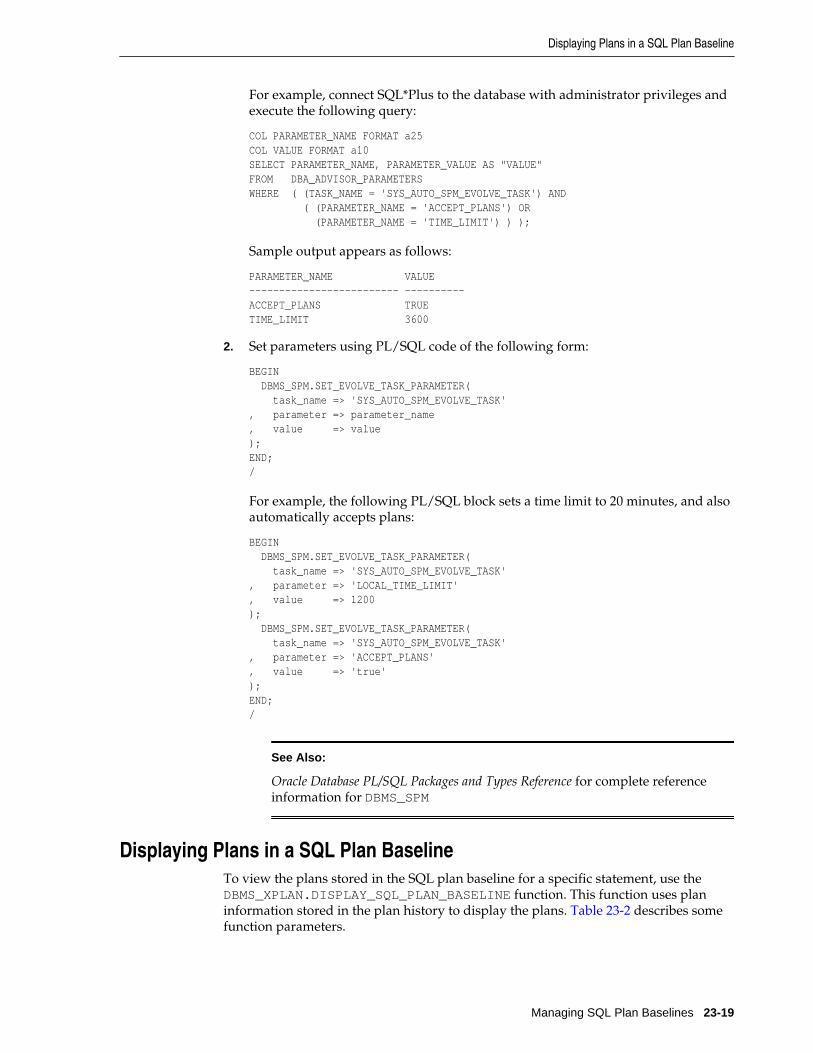
For example, connect SQL*Plus to the database with administrator privileges andexecute the following query:
COL PARAMETER_NAME FORMAT a25COL VALUE FORMAT a10SELECT PARAMETER_NAME, PARAMETER_VALUE AS "VALUE"FROM DBA_ADVISOR_PARAMETERSWHERE ( (TASK_NAME = 'SYS_AUTO_SPM_EVOLVE_TASK') AND ( (PARAMETER_NAME = 'ACCEPT_PLANS') OR (PARAMETER_NAME = 'TIME_LIMIT') ) );
Sample output appears as follows:
PARAMETER_NAME VALUE------------------------- ----------ACCEPT_PLANS TRUETIME_LIMIT 3600
2. Set parameters using PL/SQL code of the following form:
BEGIN DBMS_SPM.SET_EVOLVE_TASK_PARAMETER( task_name => 'SYS_AUTO_SPM_EVOLVE_TASK', parameter => parameter_name, value => value);END;/
For example, the following PL/SQL block sets a time limit to 20 minutes, and alsoautomatically accepts plans:
BEGIN DBMS_SPM.SET_EVOLVE_TASK_PARAMETER( task_name => 'SYS_AUTO_SPM_EVOLVE_TASK', parameter => 'LOCAL_TIME_LIMIT', value => 1200); DBMS_SPM.SET_EVOLVE_TASK_PARAMETER( task_name => 'SYS_AUTO_SPM_EVOLVE_TASK', parameter => 'ACCEPT_PLANS', value => 'true');END;/
See Also:
Oracle Database PL/SQL Packages and Types Reference for complete referenceinformation for DBMS_SPM
Displaying Plans in a SQL Plan BaselineTo view the plans stored in the SQL plan baseline for a specific statement, use theDBMS_XPLAN.DISPLAY_SQL_PLAN_BASELINE function. This function uses planinformation stored in the plan history to display the plans. Table 23-2 describes somefunction parameters.
Displaying Plans in a SQL Plan Baseline
Managing SQL Plan Baselines 23-19

Table 23-2 DBMS_XPLAN.DISPLAY_SQL_PLAN_BASELINE Parameters
Function Parameter Description
sql_handle SQL handle of the statement. Retrieve the SQL handle by joining theV$SQL.SQL_PLAN_BASELINE and DBA_SQL_PLAN_BASELINESviews on the PLAN_NAME columns.
plan_name Name of the plan for the statement.
This section explains how to show plans in a baseline from the command line. If youuse Cloud Control, then display plan baselines from the SQL Plan Baseline subpageshown in Figure 23-3.
To display SQL plans:
1. Connect SQL*Plus to the database with the appropriate privileges, and thenobtain the SQL ID of the query whose plan you want to display.
For example, assume that a SQL plan baseline exists for a SELECT statement withthe SQL ID 31d96zzzpcys9.
2. Query the plan by SQL ID.
The following query displays execution plans for the statement with the SQL ID31d96zzzpcys9:
SELECT PLAN_TABLE_OUTPUTFROM V$SQL s, DBA_SQL_PLAN_BASELINES b, TABLE( DBMS_XPLAN.DISPLAY_SQL_PLAN_BASELINE(b.sql_handle,b.plan_name,'basic') ) tWHERE s.EXACT_MATCHING_SIGNATURE=b.SIGNATUREAND b.PLAN_NAME=s.SQL_PLAN_BASELINEAND s.SQL_ID='31d96zzzpcys9';
The sample query results are as follows:
PLAN_TABLE_OUTPUT--------------------------------------------------------------------------- ---------------------------------------------------------------------------SQL handle: SQL_513f7f8a91177b1aSQL text: select * from hr.employees where employee_id=100---------------------------------------------------------------------------
---------------------------------------------------------------------------Plan name: SQL_PLAN_52gvzja8jfysuc0e983c6 Plan id: 3236529094Enabled: YES Fixed: NO Accepted: YES Origin: AUTO-CAPTURE--------------------------------------------------------------------------- Plan hash value: 3236529094 -----------------------------------------------------| Id | Operation | Name |-----------------------------------------------------| 0 | SELECT STATEMENT | || 1 | TABLE ACCESS BY INDEX ROWID| EMPLOYEES |
Displaying Plans in a SQL Plan Baseline
23-20 SQL Tuning Guide

| 2 | INDEX UNIQUE SCAN | EMP_EMP_ID_PK |-----------------------------------------------------
The results show that the plan for SQL ID 31d96zzzpcys is namedSQL_PLAN_52gvzja8jfysuc0e983c6 and was captured automatically.
See Also:
• “SQL Management Base”
• Oracle Database PL/SQL Packages and Types Reference to learn aboutadditional parameters used by the DISPLAY_SQL_PLAN_BASELINEfunction
Loading SQL Plan BaselinesYou can initiate the user-initiated bulk load of a set of existing plans into a SQL planbaseline. The goal of this task is to load plans from the following sources:
• SQL tuning set (STS)
Capture the plans for a SQL workload into an STS, and then load the plans into theSQL plan baselines. The optimizer uses the plans the next time that the databaseexecutes the SQL statements. Bulk loading execution plans from an STS is aneffective way to prevent plan regressions after a database upgrade.
Note:
You can load plans from Automatic Workload Repository snapshots into anSTS, and then load plans from the STS into the SQL plan baseline.
• Shared SQL area
Load plans for statements directly from the shared SQL area, which is in the sharedpool of the SGA. By applying a filter on the module name, the schema, or the SQLID you identify the SQL statement or set of SQL statements to capture. Theoptimizer uses the plans the next time that the database executes the SQLstatements.
Loading plans directly from the shared SQL area is useful when application SQLhas been hand-tuned using hints. Because you probably cannot change the SQL toinclude the hint, populating the SQL plan baseline ensures that the application SQLuses optimal plans.
• Staging table
Use the DBMS_SPM package to define a staging table,DBMS_SPM.PACK_STGTAB_BASELINE to copy the baselines into a staging table,and Oracle Data Pump to transfer the table to another database. On the destinationdatabase, use DBMS_SPM.UNPACK_STGTAB_BASELINE to unpack the plans fromthe staging table and put the baselines into the SMB.
A use case is the introduction of new SQL statements into the database from a newapplication module. A vendor can ship application software with SQL planbaselines for the new SQL. In this way, the new SQL uses plans that are known to
Loading SQL Plan Baselines
Managing SQL Plan Baselines 23-21

give optimal performance under a standard test configuration. Alternatively, if youdevelop or test an application in-house, export the correct plans from the testdatabase and import them into the production database.
• Stored outline
Migrate stored outlines to SQL plan baselines. After the migration, you maintainthe same plan stability that you had using stored outlines while being able to usethe more advanced features provided by SQL Plan Management, such as planevolution. See “Migrating Stored Outlines to SQL Plan Baselines ”.
See Also:
Oracle Database PL/SQL Packages and Types Reference to learn about theDBMS_SPM.PACK_STGTAB_BASELINE Function
Loading Plans from a SQL Tuning SetA SQL tuning set is a database object that includes one or more SQL statements,execution statistics, and execution context. This section explains how to load plansfrom an STS.
Load plans with the DBMS_SPM.LOAD_PLANS_FROM_SQLSET function or usingCloud Control. Table 23-3 describes some function parameters.
Table 23-3 LOAD_PLANS_FROM_SQLSET Parameters
FunctionParameter
Description
sqlset_name Name of the STS from which the plans are loaded into SQL planbaselines.
basic_filter A filter applied to the STS to select only qualifying plans to be loaded.The filter can take the form of any WHERE clause predicate that can bespecified against the view DBA_SQLSET_STATEMENTS.
fixed Default NO means the loaded plans are used as nonfixed plans. YESmeans the loaded plans are fixed plans. “Plan Selection” explains thatthe optimizer chooses a fixed plan in the plan baseline over a nonfixedplan.
This section explains how to load plans from the command line. In Cloud Control, goto the SQL Plan Baseline subpage (shown in Figure 23-3) and click Load to load planbaselines from SQL tuning sets.
Assumptions
This tutorial assumes the following:
• You want the loaded plans to be nonfixed.
• You have executed the following query:
SELECT /*LOAD_STS*/ *FROM sh.sales
Loading SQL Plan Baselines
23-22 SQL Tuning Guide

WHERE quantity_sold > 40ORDER BY prod_id;
• You have loaded the plan from the shared SQL area into the SQL tuning set namedSPM_STS, which is owned by user SPM.
To load plans from a SQL tuning set:
1. Connect SQL*Plus to the database with the appropriate privileges, and then verifywhich plans are in the SQL tuning set.
For example, query DBA_SQLSET_STATEMENTS for the STS name (sample outputincluded):
SELECT SQL_TEXTFROM DBA_SQLSET_STATEMENTSWHERE SQLSET_NAME = 'SPM_STS'; SQL_TEXT--------------------SELECT /*LOAD_STS*/*FROM sh.salesWHERE quantity_sold> 40ORDER BY prod_id
The output shows that the plan for the select /*LOAD_STS*/ statement is inthe STS.
2. Load the plan from the STS into the SQL plan baseline.
For example, in SQL*Plus execute the function as follows:
VARIABLE cnt NUMBEREXECUTE :cnt := DBMS_SPM.LOAD_PLANS_FROM_SQLSET( - sqlset_name => 'SPM_STS', - basic_filter => 'sql_text like ''SELECT /*LOAD_STS*/%''' );
The basic_filter parameter specifies a WHERE clause that loads only the plansfor the queries of interest. The variable cnt stores the number of plans loadedfrom the STS.
3. Query the data dictionary to ensure that the plan was loaded into the baseline forthe statement.
The following statement queries the DBA_SQL_PLAN_BASELINES view (sampleoutput included).
SQL> SELECT SQL_HANDLE, SQL_TEXT, PLAN_NAME, 2 ORIGIN, ENABLED, ACCEPTED 3 FROM DBA_SQL_PLAN_BASELINES;
SQL_HANDLE SQL_TEXT PLAN_NAME ORIGIN ENA ACC--------------------- --------------- ---------------- ----------- --- ---SQL_a8632bd857a4a25e SELECT SQL_PLAN_ahstb MANUAL-LOAD YES YES /*LOAD_STS*/* v1bu98ky1694fc6b FROM sh.sales WHERE quantity_sold > 40 ORDER BY prod_id
Loading SQL Plan Baselines
Managing SQL Plan Baselines 23-23

The output shows that the plan is accepted, which means that it is in the planbaseline. Also, the origin is MANUAL-LOAD, which means that the plan was loadedby an end user rather than automatically captured.
4. Optionally, drop the STS.
For example, execute DBMS_SQLTUNE.DROP_SQLSET to drop the SPM_STStuning set as follows:
EXEC SYS.DBMS_SQLTUNE.DROP_SQLSET( sqlset_name => 'SPM_STS', - sqlset_owner => 'SPM' );
See Also:
Oracle Database PL/SQL Packages and Types Reference to learn about theDBMS_SPM.LOAD_PLANS_FROM_SQLSET function
Loading Plans from the Shared SQL AreaThis section explains how to load plans from the shared SQL area using PL/SQL.
Load plans with the LOAD_PLANS_FROM_CURSOR_CACHE function of the DBMS_SPMpackage. Table 23-4 describes some function parameters.
Table 23-4 LOAD_PLANS_FROM_CURSOR_CACHE Parameters
Function Parameter Description
sql_id SQL statement identifier. Identifies a SQL statement in the sharedSQL area.
fixed Default NO means the loaded plans are used as nonfixed plans. YESmeans the loaded plans are fixed plans (see “Fixed Plans”). “PlanSelection” explains that the optimizer chooses a fixed plan in the planbaseline over a nonfixed plan.
This section explains how to load plans using the command line. In Cloud Control, goto the SQL Plan Baseline subpage (shown in Figure 23-3) and click Load to load planbaselines from the shared SQL area.
Assumptions
This tutorial assumes the following:
• You have executed the following query:
SELECT /*LOAD_CC*/ *FROM sh.salesWHERE quantity_sold > 40ORDER BY prod_id;
• You want the loaded plans to be nonfixed.
To load plans from the shared SQL area:
1. Connect SQL*Plus to the database with the appropriate privileges, and thendetermine the SQL IDs of the relevant statements in the shared SQL area.
Loading SQL Plan Baselines
23-24 SQL Tuning Guide
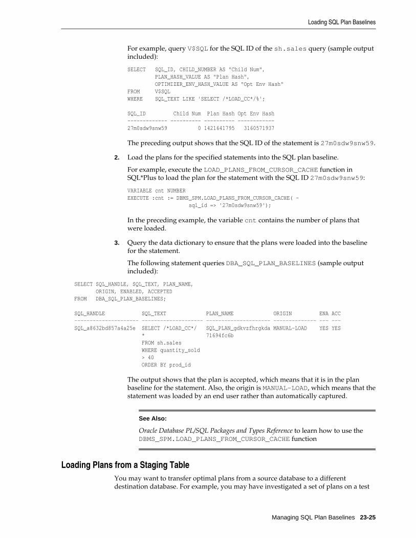
For example, query V$SQL for the SQL ID of the sh.sales query (sample outputincluded):
SELECT SQL_ID, CHILD_NUMBER AS "Child Num", PLAN_HASH_VALUE AS "Plan Hash", OPTIMIZER_ENV_HASH_VALUE AS "Opt Env Hash"FROM V$SQLWHERE SQL_TEXT LIKE 'SELECT /*LOAD_CC*/%'; SQL_ID Child Num Plan Hash Opt Env Hash------------- ---------- ---------- ------------27m0sdw9snw59 0 1421641795 3160571937
The preceding output shows that the SQL ID of the statement is 27m0sdw9snw59.
2. Load the plans for the specified statements into the SQL plan baseline.
For example, execute the LOAD_PLANS_FROM_CURSOR_CACHE function inSQL*Plus to load the plan for the statement with the SQL ID 27m0sdw9snw59:
VARIABLE cnt NUMBEREXECUTE :cnt := DBMS_SPM.LOAD_PLANS_FROM_CURSOR_CACHE( - sql_id => '27m0sdw9snw59');
In the preceding example, the variable cnt contains the number of plans thatwere loaded.
3. Query the data dictionary to ensure that the plans were loaded into the baselinefor the statement.
The following statement queries DBA_SQL_PLAN_BASELINES (sample outputincluded):
SELECT SQL_HANDLE, SQL_TEXT, PLAN_NAME, ORIGIN, ENABLED, ACCEPTEDFROM DBA_SQL_PLAN_BASELINES; SQL_HANDLE SQL_TEXT PLAN_NAME ORIGIN ENA ACC--------------------- -------------------- --------------------- -------------- --- ---SQL_a8632bd857a4a25e SELECT /*LOAD_CC*/ SQL_PLAN_gdkvzfhrgkda MANUAL-LOAD YES YES * 71694fc6b FROM sh.sales WHERE quantity_sold > 40 ORDER BY prod_id
The output shows that the plan is accepted, which means that it is in the planbaseline for the statement. Also, the origin is MANUAL-LOAD, which means that thestatement was loaded by an end user rather than automatically captured.
See Also:
Oracle Database PL/SQL Packages and Types Reference to learn how to use theDBMS_SPM.LOAD_PLANS_FROM_CURSOR_CACHE function
Loading Plans from a Staging TableYou may want to transfer optimal plans from a source database to a differentdestination database. For example, you may have investigated a set of plans on a test
Loading SQL Plan Baselines
Managing SQL Plan Baselines 23-25

database and confirmed that they have performed well. You may then want to loadthese plans into a production database.
A staging table is a table that, for the duration of its existence, stores plans so that theplans do not disappear from the table while you are unpacking them. Use theDBMS.CREATE_STGTAB_BASELINE procedure to create a staging table. To pack(insert row into) and unpack (extract rows from) the staging table, use thePACK_STGTAB_BASELINE and UNPACK_STGTAB_BASELINE functions of theDBMS_SPM package. Oracle Data Pump Import and Export enable you to copy thestaging table to a different database.
The following graphic depicts the basic steps.
Destination HostSource Host
1114
Transfer Dump File to Destination Host
Source Database Destination Database
1
Staging Table
SQL Management Base
SQL PlanBaselines
1112Pack
3Data PumpExport
.dumpfile
SQL Management Base
SQL PlanBaselines
1116Unpack
5Data PumpImport
.dumpfile
Staging Table
Assumptions
This tutorial assumes the following:
• You want to create a staging table named stage1 in the source database.
• You want to load all plans owned by user spm into the staging table.
• You want to transfer the staging table to a destination database.
• You want to load the plans in stage1 as fixed plans.
To transfer a set of SQL plan baselines from one database to another:
1. Connect SQL*Plus to the source database with the appropriate privileges, andthen create a staging table using the CREATE_STGTAB_BASELINE procedure.
The following example creates a staging table named stage1:
BEGIN DBMS_SPM.CREATE_STGTAB_BASELINE ( table_name => 'stage1');
Loading SQL Plan Baselines
23-26 SQL Tuning Guide

END;/
2. On the source database, pack the SQL plan baselines you want to export from theSQL management base into the staging table.
The following example packs enabled plan baselines created by user spm intostaging table stage1. Select SQL plan baselines using the plan name(plan_name), SQL handle (sql_handle), or any other plan criteria. Thetable_name parameter is mandatory.
DECLARE my_plans number;BEGIN my_plans := DBMS_SPM.PACK_STGTAB_BASELINE ( table_name => 'stage1', enabled => 'yes', creator => 'spm');END;/
3. Export the staging table stage1 into a dump file using Oracle Data Pump Export.
4. Transfer the dump file to the host of the destination database.
5. On the destination database, import the staging table stage1 from the dump fileusing the Oracle Data Pump Import utility.
6. On the destination database, unpack the SQL plan baselines from the staging tableinto the SQL management base.
The following example unpacks all fixed plan baselines stored in the staging tablestage1:
DECLARE my_plans NUMBER;BEGIN my_plans := DBMS_SPM.UNPACK_STGTAB_BASELINE ( table_name => 'stage1', fixed => 'yes');END;/
See Also:
• Oracle Database PL/SQL Packages and Types Reference for more informationabout using the DBMS_SPM package
• Oracle Database Utilities for detailed information about using the DataPump Export and Import utilities
Evolving SQL Plan Baselines ManuallyOracle recommends that you configure the SQL Plan Management Evolve task to runautomatically, as explained in “Managing the SPM Evolve Advisor Task”. You can
Evolving SQL Plan Baselines Manually
Managing SQL Plan Baselines 23-27

also use PL/SQL or Cloud Control to manually evolve an unaccepted plan todetermine whether it performs better than any plan currently in the plan baseline.
This section contains the following topics:
• About the DBMS_SPM Evolve Functions
• Managing an Evolve Task
About the DBMS_SPM Evolve FunctionsTable 23-5 describes the most relevant DBMS_SPM procedures and functions formanaging plan evolution. Execute evolution tasks manually or schedule them to runautomatically.
Table 23-5 DBMS_SPM Functions and Procedures for Managing Plan EvolutionTasks
Package Procedure or Function Description
DBMS_SPM ACCEPT_SQL_PLAN_BASELINE This function accepts onerecommendation to evolve a singleplan into a SQL plan baseline.
DBMS_SPM CREATE_EVOLVE_TASK This function creates an advisor taskto prepare the plan evolution of oneor more plans for a specified SQLstatement. The input parameters canbe a SQL handle, plan name or a list ofplan names, time limit, task name,and description.
DBMS_SPM EXECUTE_EVOLVE_TASK This function executes an evolutiontask. The input parameters can be thetask name, execution name, andexecution description. If not specified,the advisor generates the name, whichis returned by the function.
DBMS_SPM IMPLEMENT_EVOLVE_TASK This function implements allrecommendations for an evolve task.Essentially, this function is equivalentto usingACCEPT_SQL_PLAN_BASELINE forall recommended plans. Inputparameters include task name, planname, owner name, and executionname.
DBMS_SPM REPORT_EVOLVE_TASK This function displays the results ofan evolve task as a CLOB. Inputparameters include the task name andsection of the report to include.
DBMS_SPM SET_EVOLVE_TASK_PARAMETER This function updates the value of anevolve task parameter. In this release,the only valid parameter isTIME_LIMIT.
Evolving SQL Plan Baselines Manually
23-28 SQL Tuning Guide

Oracle recommends that you configure SPM Evolve Advisor to run automatically (see“Configuring the Automatic SPM Evolve Advisor Task”). You can also evolve SQLplan baselines manually. Figure 23-4 shows the basic workflow for managing SQLplan management tasks.
Figure 23-4 Evolving SQL Plan Baselines
DBMS_SPM.CREATE_EVOLVE_TASK
DBMS_SPM.EXECUTE_EVOLVE_TASK
DBMS_SPM.IMPLEMENT_EVOLVE_TASK
DBMS_SPM.REPORT_EVOLVE_TASK
DBMS_SPM.SET_EVOLVE_TASK_PARAMETER
Typically, you manage SQL plan evolution tasks in the following sequence:
1. Create an evolve task
2. Optionally, set evolve task parameters
3. Execute the evolve task
4. Implement the recommendations in the task
5. Report on the task outcome
See Also:
Oracle Database PL/SQL Packages and Types Reference for information about theDBMS_SPM package
Managing an Evolve TaskThis section describes a typical use case in which you create and execute a task, andthen implements its recommendations. Table 23-6 describes some parameters of theCREATE_EVOLVE_TASK function.
Table 23-6 DBMS_SPM.CREATE_EVOLVE_TASK Parameters
FunctionParameter
Description
sql_handle SQL handle of the statement. The default NULL considers all SQLstatements with unaccepted plans.
plan_name Plan identifier. The default NULL means consider all unaccepted plans ofthe specified SQL handle or all SQL statements if the SQL handle is NULL.
Evolving SQL Plan Baselines Manually
Managing SQL Plan Baselines 23-29

Table 23-6 (Cont.) DBMS_SPM.CREATE_EVOLVE_TASK Parameters
FunctionParameter
Description
time_limit Time limit in number of minutes. The time limit for first unaccepted planequals the input value. The time limit for the second unaccepted planequals the input value minus the time spent in first plan verification, andso on. The default DBMS_SPM.AUTO_LIMIT means let the system choosean appropriate time limit based on the number of plan verificationsrequired to be done.
task_name User-specified name of the evolution task.
This section explains how to evolve plan baselines from the command line. In CloudControl, from the SQL Plan Baseline subpage (shown in Figure 23-3), select a plan, andthen click Evolve.
Assumptions
This tutorial assumes the following:
• You do not have the automatic evolve task enabled (see “Managing the SPMEvolve Advisor Task”).
• You want to create a SQL plan baseline for the following query:
SELECT /* q1_group_by */ prod_name, sum(quantity_sold)FROM products p, sales sWHERE p.prod_id = s.prod_idAND p.prod_category_id =203GROUP BY prod_name;
• You want to create two indexes to improve the query performance, and then evolvethe plan that uses these indexes if it performs better than the plan currently in theplan baseline.
To evolve a specified plan:
1. Perform the initial setup as follows:
a. Connect SQL*Plus to the database with administrator privileges, and thenprepare for the tutorial by flushing the shared pool and the buffer cache:
ALTER SYSTEM FLUSH SHARED_POOL;ALTER SYSTEM FLUSH BUFFER_CACHE;
b. Enable the automatic capture of SQL plan baselines.
For example, enter the following statement:
ALTER SYSTEM SET OPTIMIZER_CAPTURE_SQL_PLAN_BASELINES=true;
c. Connect to the database as user sh, and then set SQL*Plus displayparameters:
CONNECT sh-- enter passwordSET PAGES 10000 LINES 140
Evolving SQL Plan Baselines Manually
23-30 SQL Tuning Guide

SET SERVEROUTPUT ONCOL SQL_TEXT FORMAT A20COL SQL_HANDLE FORMAT A20COL PLAN_NAME FORMAT A30COL ORIGIN FORMAT A12SET LONGC 60535SET LONG 60535SET ECHO ON
2. Execute the SELECT statements so that SQL plan management captures them:
a. Execute the SELECT /* q1_group_by */ statement for the first time.
Because the database only captures plans for repeatable statements, the planbaseline for this statement is empty.
b. Query the data dictionary to confirm that no plans exist in the plan baseline.
For example, execute the following query (sample output included):
SELECT SQL_HANDLE, SQL_TEXT, PLAN_NAME, ORIGIN, ENABLED, ACCEPTED, FIXED, AUTOPURGEFROM DBA_SQL_PLAN_BASELINESWHERE SQL_TEXT LIKE '%q1_group%';
no rows selected
SQL plan management only captures repeatable statements, so this result isexpected.
c. Execute the SELECT /* q1_group_by */ statement for the second time.
3. Query the data dictionary to ensure that the plans were loaded into the planbaseline for the statement.
Example 23-2 executes the following query (sample output included).
The output shows that the plan is accepted, which means that it is in the planbaseline for the statement. Also, the origin is AUTO-CAPTURE, which means thatthe statement was automatically captured and not manually loaded.
4. Explain the plan for the statement and verify that the optimizer is using this plan.
For example, explain the plan as follows, and then display it:
EXPLAIN PLAN FOR SELECT /* q1_group_by */ prod_name, sum(quantity_sold) FROM products p, sales s WHERE p.prod_id = s.prod_id AND p.prod_category_id =203 GROUP BY prod_name;
SELECT * FROM TABLE(DBMS_XPLAN.DISPLAY(null, null, 'basic +note'));
Sample output appears below:
Plan hash value: 1117033222 ------------------------------------------| Id | Operation | Name |------------------------------------------| 0 | SELECT STATEMENT | || 1 | HASH GROUP BY | |
Evolving SQL Plan Baselines Manually
Managing SQL Plan Baselines 23-31

| 2 | HASH JOIN | || 3 | TABLE ACCESS FULL | PRODUCTS || 4 | PARTITION RANGE ALL| || 5 | TABLE ACCESS FULL | SALES |------------------------------------------ Note----- - SQL plan baseline "SQL_PLAN_0gwbcfvzskcu242949306" used for this statement
The note indicates that the optimizer is using the plan shown with the plan namelisted in Example 23-2.
5. Create two indexes to improve the performance of the SELECT /*q1_group_by */ statement.
For example, use the following statements:
CREATE INDEX ind_prod_cat_name ON products(prod_category_id, prod_name, prod_id);CREATE INDEX ind_sales_prod_qty_sold ON sales(prod_id, quantity_sold);
6. Execute the select /* q1_group_by */ statement again.
Because automatic capture is enabled, the plan baseline is populated with the newplan for this statement.
7. Query the data dictionary to ensure that the plan was loaded into the SQL planbaseline for the statement.
Example 23-3 executes the following query (sample output included).
The output shows that the new plan is unaccepted, which means that it is in thestatement history but not the SQL plan baseline.
8. Explain the plan for the statement and verify that the optimizer is using theoriginal nonindexed plan.
For example, explain the plan as follows, and then display it:
EXPLAIN PLAN FOR SELECT /* q1_group_by */ prod_name, sum(quantity_sold) FROM products p, sales s WHERE p.prod_id = s.prod_id AND p.prod_category_id =203 GROUP BY prod_name;SELECT * FROM TABLE(DBMS_XPLAN.DISPLAY(null, null, 'basic +note'));
Sample output appears below:
Plan hash value: 1117033222 ------------------------------------------| Id | Operation | Name |------------------------------------------| 0 | SELECT STATEMENT | || 1 | HASH GROUP BY | || 2 | HASH JOIN | || 3 | TABLE ACCESS FULL | PRODUCTS || 4 | PARTITION RANGE ALL| || 5 | TABLE ACCESS FULL | SALES |------------------------------------------
Evolving SQL Plan Baselines Manually
23-32 SQL Tuning Guide

Note----- - SQL plan baseline "SQL_PLAN_0gwbcfvzskcu242949306" used for this statement
The note indicates that the optimizer is using the plan shown with the plan namelisted in Example 23-2.
9. Connect as an administrator, and then create an evolve task that considers all SQLstatements with unaccepted plans.
For example, execute the DBMS_SPM.CREATE_EVOLVE_TASK function and thenobtain the name of the task:
CONNECT / AS SYSDBAVARIABLE cnt NUMBERVARIABLE tk_name VARCHAR2(50)VARIABLE exe_name VARCHAR2(50)VARIABLE evol_out CLOB EXECUTE :tk_name := DBMS_SPM.CREATE_EVOLVE_TASK( sql_handle => 'SQL_07f16c76ff893342', plan_name => 'SQL_PLAN_0gwbcfvzskcu20135fd6c'); SELECT :tk_name FROM DUAL;
The following sample output shows the name of the task:
:EVOL_OUT--------------------------------------------------------------------------TASK_11
Now that the task has been created and has a unique name, execute the task.
10. Execute the task.
For example, execute the DBMS_SPM.EXECUTE_EVOLVE_TASK function (sampleoutput included):
EXECUTE :exe_name :=DBMS_SPM.EXECUTE_EVOLVE_TASK(task_name=>:tk_name); SELECT :exe_name FROM DUAL;
:EXE_NAME---------------------------------------------------------------------------EXEC_1
11. View the report.
For example, execute the DBMS_SPM.REPORT_EVOLVE_TASK function (sampleoutput included):
EXECUTE :evol_out := DBMS_SPM.REPORT_EVOLVE_TASK( task_name=>:tk_name, execution_name=>:exe_name );SELECT :evol_out FROM DUAL;
GENERAL INFORMATION SECTION-------------------------------------------------------------------------- Task Information: --------------------------------------------- Task Name : TASK_11 Task Owner : SYS Execution Name : EXEC_1
Evolving SQL Plan Baselines Manually
Managing SQL Plan Baselines 23-33

Execution Type : SPM EVOLVE Scope : COMPREHENSIVE Status : COMPLETED Started : 01/09/2012 12:21:27 Finished : 01/09/2012 12:21:29 Last Updated : 01/09/2012 12:21:29 Global Time Limit : 2147483646 Per-Plan Time Limit : UNUSED Number of Errors : 0--------------------------------------------------------------------------- SUMMARY SECTION--------------------------------------------------------------------------- Number of plans processed : 1 Number of findings : 1 Number of recommendations : 1 Number of errors : 0--------------------------------------------------------------------------- DETAILS SECTION--------------------------------------------------------------------------- Object ID : 2 Test Plan Name : SQL_PLAN_0gwbcfvzskcu20135fd6c Base Plan Name : SQL_PLAN_0gwbcfvzskcu242949306 SQL Handle : SQL_07f16c76ff893342 Parsing Schema : SH Test Plan Creator : SH SQL Text : SELECT /*q1_group_by*/ prod_name, sum(quantity_sold) FROM products p, sales s WHERE p.prod_id=s.prod_id AND p.prod_category_id=203 GROUP BY prod_name Execution Statistics:----------------------------- Base Plan Test Plan ---------------------------- ------------------------ Elapsed Time (s): .044336 .012649 CPU Time (s): .044003 .012445 Buffer Gets: 360 99 Optimizer Cost: 924 891 Disk Reads: 341 82 Direct Writes: 0 0 Rows Processed: 4 2 Executions: 5 9 FINDINGS SECTION--------------------------------------------------------------------------- Findings (1):----------------------------- 1. The plan was verified in 2.18 seconds. It passed the benefit criterion because its verified performance was 2.01 times better than that of the baseline plan. Recommendation:----------------------------- Consider accepting the plan. Execute dbms_spm.accept_sql_plan_baseline(task_name => 'TASK_11', object_id => 2, task_owner => 'SYS');
Evolving SQL Plan Baselines Manually
23-34 SQL Tuning Guide

EXPLAIN PLANS SECTION--------------------------------------------------------------------------- Baseline Plan----------------------------- Plan Id : 1 Plan Hash Value : 1117033222 ---------------------------------------------------------------------------| Id| Operation | Name | Rows | Bytes |Cost | Time |---------------------------------------------------------------------------| 0 | SELECT STATEMENT | | 21 | 861 | 924 | 00:00:12|| 1 | HASH GROUP BY | | 21 | 861 | 924 | 00:00:12|| *2| HASH JOIN | |267996|10987836 | 742 | 00:00:09|| *3| TABLE ACCESS FULL | PRODUCTS | 21 | 714 | 2 | 00:00:01|| 4 | PARTITION RANGE ALL | |918843| 6431901 | 662 | 00:00:08|| 5 | TABLE ACCESS FULL | SALES |918843| 6431901 | 662 | 00:00:08|--------------------------------------------------------------------------- Predicate Information (identified by operation id):------------------------------------------* 2 - access("P"."PROD_ID"="S"."PROD_ID")* 3 - filter("P"."PROD_CATEGORY_ID"=203) Test Plan----------------------------- Plan Id : 2 Plan Hash Value : 20315500 ---------------------------------------------------------------------------|Id| Operation | Name | Rows | Bytes | Cost| Time |---------------------------------------------------------------------------| 0|SELECT STATEMENT | | 21| 861|891|00:00:11|| 1| SORT GROUP BY NOSORT| | 21| 861|891|00:00:11|| 2| NESTED LOOPS | |267996|10987836|891|00:00:11||*3| INDEX RANGE SCAN |IND_PROD_CAT_NAME | 21| 714| 1|00:00:01||*4| INDEX RANGE SCAN |IND_SALES_PROD_QTY| 12762| 89334| 42|00:00:01|--------------------------------------------------------------------------- Predicate Information (identified by operation id):------------------------------------------* 3 - access("P"."PROD_CATEGORY_ID"=203)* 4 - access("P"."PROD_ID"="S"."PROD_ID")
This report indicates that the new execution plan, which uses the two newindexes, performs better than the original plan.
12. Implement the recommendations of the evolve task.
For example, execute the IMPLEMENT_EVOLVE_TASK function:
EXECUTE :cnt := DBMS_SPM.IMPLEMENT_EVOLVE_TASK( task_name=>:tk_name, execution_name=>:exe_name );
13. Query the data dictionary to ensure that the new plan is accepted.
Example 23-3 executes the following query (sample output included).
The output shows that the new plan is accepted.
14. Clean up after the example.
Evolving SQL Plan Baselines Manually
Managing SQL Plan Baselines 23-35

For example, enter the following statements:
EXEC :cnt := DBMS_SPM.DROP_SQL_PLAN_BASELINE('SQL_07f16c76ff893342');EXEC :cnt := DBMS_SPM.DROP_SQL_PLAN_BASELINE('SQL_9049245213a986b3');EXEC :cnt := DBMS_SPM.DROP_SQL_PLAN_BASELINE('SQL_bb77077f5f90a36b');EXEC :cnt := DBMS_SPM.DROP_SQL_PLAN_BASELINE('SQL_02a86218930bbb20');DELETE FROM SQLLOG$;CONNECT sh-- enter passwordDROP INDEX IND_SALES_PROD_QTY_SOLD;DROP INDEX IND_PROD_CAT_NAME;
See Also:
Oracle Database PL/SQL Packages and Types Reference for information aboutusing the DBMS_SPM evolve functions
Example 23-2 DBA_SQL_PLAN_BASELINES
SELECT SQL_HANDLE, SQL_TEXT, PLAN_NAME, ORIGIN, ENABLED, ACCEPTED, FIXED FROM DBA_SQL_PLAN_BASELINESWHERE SQL_TEXT LIKE '%q1_group%'; SQL_HANDLE SQL_TEXT PLAN_NAME ORIGIN ENA ACC FIX-------------------- ---------------- ------------------------------ ------------ --- --- ---SQL_07f16c76ff893342 SELECT /* q1_gro SQL_PLAN_0gwbcfvzskcu242949306 AUTO-CAPTURE YES YES NO up_by */ prod_na me, sum(quantity _sold) FROM products p, sales s WHERE p.prod_id = s.prod_id AND p.prod_category _id =203 GROUP BY prod_name
Example 23-3 DBA_SQL_PLAN_BASELINES
SELECT SQL_HANDLE, SQL_TEXT, PLAN_NAME, ORIGIN, ENABLED, ACCEPTEDFROM DBA_SQL_PLAN_BASELINESWHERE SQL_HANDLE IN ('SQL_07f16c76ff893342')ORDER BY SQL_HANDLE, ACCEPTED;
SQL_HANDLE SQL_TEXT PLAN_NAME ORIGIN ENA ACC-------------------- -------------------- ------------------------------ ------------ --- ---SQL_07f16c76ff893342 SELECT /* q1_group_b SQL_PLAN_0gwbcfvzskcu20135fd6c AUTO-CAPTURE YES NO y */ prod_name, sum( quantity_sold) FROM products p, s ales s WHERE p.prod_id = s .prod_id AND p.prod_catego ry_id =203 GROUP BY prod_name SQL_07f16c76ff893342 SELECT /* q1_group_b SQL_PLAN_0gwbcfvzskcu242949306 AUTO-CAPTURE YES YES y */ prod_name, sum(
Evolving SQL Plan Baselines Manually
23-36 SQL Tuning Guide

quantity_sold) FROM products p, s ales s WHERE p.prod_id = s .prod_id AND p.prod_catego ry_id =203 GROUP BY prod_name
Example 23-4 DBA_SQL_PLAN_BASELINES
SQL_HANDLE SQL_TEXT PLAN_NAME ORIGIN ENA ACC-------------------- -------------------- ------------------------------ ------------ --- ---SQL_07f16c76ff893342 SELECT /* q1_group_b SQL_PLAN_0gwbcfvzskcu20135fd6c AUTO-CAPTURE YES YES y */ prod_name, sum( quantity_sold) FROM products p, s ales s WHERE p.prod_id = s .prod_id AND p.prod_catego ry_id =203 GROUP BY prod_name SQL_07f16c76ff893342 SELECT /* q1_group_b SQL_PLAN_0gwbcfvzskcu242949306 AUTO-CAPTURE YES YES y */ prod_name, sum( quantity_sold) FROM products p, s ales s WHERE p.prod_id = s .prod_id AND p.prod_catego ry_id =203 GROUP BY prod_name
Dropping SQL Plan BaselinesYou can remove some or all plans from a SQL plan baseline. This technique issometimes useful when testing SQL plan management.
Drop plans with the DBMS_SPM.DROP_SQL_PLAN_BASELINE function. This functionreturns the number of dropped plans. Table 23-8 describes input parameters.
Table 23-7 DROP_SQL_PLAN_BASELINE Parameters
FunctionParameter
Description
sql_handle SQL statement identifier.
plan_name Name of a specific plan. Default NULL drops all plans associated withthe SQL statement identified by sql_handle.
This section explains how to drop baselines from the command line. In Cloud Control,from the SQL Plan Baseline subpage (shown in Figure 23-3), select a plan, and thenclick Drop.
Dropping SQL Plan Baselines
Managing SQL Plan Baselines 23-37

Assumptions
This tutorial assumes that you want to drop all plans for the following SQL statement,effectively dropping the SQL plan baseline:
SELECT /* repeatable_sql */ COUNT(*) FROM hr.jobs;
To drop a SQL plan baseline:
1. Connect SQL*Plus to the database with the appropriate privileges, and then querythe data dictionary for the plan baseline.
Example 23-5 executes the following query (sample output included).
2. Drop the SQL plan baseline for the statement.
The following example drops the plan baseline with the SQL handleSQL_b6b0d1c71cd1807b, and returns the number of dropped plans. Specifyplan baselines using the plan name (plan_name), SQL handle (sql_handle), orany other plan criteria. The table_name parameter is mandatory.
DECLARE v_dropped_plans number;BEGIN v_dropped_plans := DBMS_SPM.DROP_SQL_PLAN_BASELINE ( sql_handle => 'SQL_b6b0d1c71cd1807b'); DBMS_OUTPUT.PUT_LINE('dropped ' || v_dropped_plans || ' plans');END;/
3. Confirm that the plans were dropped.
For example, execute the following query:
SELECT SQL_HANDLE, SQL_TEXT, PLAN_NAME, ORIGIN, ENABLED, ACCEPTEDFROM DBA_SQL_PLAN_BASELINESWHERE SQL_TEXT LIKE 'SELECT /* repeatable_sql%'; no rows selected
See Also:
Oracle Database PL/SQL Packages and Types Reference to learn about theDROP_SQL_PLAN_BASELINE function
Example 23-5 DBA_SQL_PLAN_BASELINES
SQL> SELECT SQL_HANDLE, SQL_TEXT, PLAN_NAME, ORIGIN, 2 ENABLED, ACCEPTED 3 FROM DBA_SQL_PLAN_BASELINES 4 WHERE SQL_TEXT LIKE 'SELECT /* repeatable_sql%'; SQL_HANDLE SQL_TEXT PLAN_NAME ORIGIN ENA ACC-------------------- -------------------- ------------------------------ -------------- --- ---SQL_b6b0d1c71cd1807b SELECT /* repeatable SQL_PLAN_bdc6jswfd303v2f1e9c20 AUTO-CAPTURE YES YES _sql */ count(*) fro m hr.jobs
Dropping SQL Plan Baselines
23-38 SQL Tuning Guide

Managing the SQL Management BaseThe SQL management base is a part of the data dictionary that resides in the SYSAUXtablespace. It stores statement logs, plan histories, SQL plan baselines, and SQLprofiles. This section explains how to change the disk space usage parameters for theSMB, and change the retention time for plans in the SMB.
The DBA_SQL_MANAGEMENT_CONFIG view shows the current configuration settingsfor the SMB. Table 23-8 describes the parameters in the PARAMETER_NAME column.
Table 23-8 Parameters in DBA_SQL_MANAGEMENT_CONFIG.PARAMETER_NAME
Parameter Description
SPACE_BUDGET_PERCENT Maximum percent of SYSAUX space that the SQL managementbase can use. The default is 10. The allowable range for thislimit is between 1% and 50%.
PLAN_RETENTION_WEEKS Number of weeks to retain unused plans before they arepurged. The default is 53.
Changing the Disk Space Limit for the SMBA weekly background process measures the total space occupied by the SMB. Whenthe defined limit is exceeded, the process writes a warning to the alert log. Thedatabase generates alerts weekly until either the SMB space limit is increased, the sizeof the SYSAUX tablespace is increased, or the disk space used by the SMB is decreasedby purging SQL management objects (SQL plan baselines or SQL profiles). This taskexplains how to change the limit with the DBMS_SPM.CONFIGURE procedure.
Assumptions
This tutorial assumes the following:
• The current SMB space limit is the default of 10%.
• You want to change the percentage limit to 30%
To change the percentage limit of the SMB:
1. Connect SQL*Plus to the database with the appropriate privileges, and then querythe data dictionary to see the current space budget percent.
For example, execute the following query (sample output included):
SELECT PARAMETER_NAME, PARAMETER_VALUE AS "%_LIMIT", ( SELECT sum(bytes/1024/1024) FROM DBA_DATA_FILES WHERE TABLESPACE_NAME = 'SYSAUX' ) AS SYSAUX_SIZE_IN_MB, PARAMETER_VALUE/100 * ( SELECT sum(bytes/1024/1024) FROM DBA_DATA_FILES WHERE TABLESPACE_NAME = 'SYSAUX' ) AS "CURRENT_LIMIT_IN_MB"FROM DBA_SQL_MANAGEMENT_CONFIGWHERE PARAMETER_NAME = 'SPACE_BUDGET_PERCENT';
PARAMETER_NAME %_LIMIT SYSAUX_SIZE_IN_MB CURRENT_LIMIT_IN_MB-------------------- ---------- ----------------- -------------------SPACE_BUDGET_PERCENT 10 211.4375 21.14375
Managing the SQL Management Base
Managing SQL Plan Baselines 23-39

2. Change the percentage setting.
For example, execute the following command to change the setting to 30%:
EXECUTE DBMS_SPM.CONFIGURE('space_budget_percent',30);
3. Query the data dictionary to confirm the change.
For example, execute the following join (sample output included):
SELECT PARAMETER_NAME, PARAMETER_VALUE AS "%_LIMIT", ( SELECT sum(bytes/1024/1024) FROM DBA_DATA_FILES WHERE TABLESPACE_NAME = 'SYSAUX' ) AS SYSAUX_SIZE_IN_MB, PARAMETER_VALUE/100 * ( SELECT sum(bytes/1024/1024) FROM DBA_DATA_FILES WHERE TABLESPACE_NAME = 'SYSAUX' ) AS "CURRENT_LIMIT_IN_MB"FROM DBA_SQL_MANAGEMENT_CONFIGWHERE PARAMETER_NAME = 'SPACE_BUDGET_PERCENT';
PARAMETER_NAME %_LIMIT SYSAUX_SIZE_IN_MB CURRENT_LIMIT_IN_MB-------------------- ---------- ----------------- -------------------SPACE_BUDGET_PERCENT 30 211.4375 63.43125
See Also:
Oracle Database PL/SQL Packages and Types Reference to learn about theCONFIGURE function
Changing the Plan Retention Policy in the SMBA weekly scheduled purging task manages disk space used by SQL plan management.The task runs as an automated task in the maintenance window. The database purgesplans that have not been used for longer than the plan retention period, as identifiedby the LAST_EXECUTED timestamp stored in the SMB for that plan. The defaultretention period is 53 weeks. The period can range between 5 and 523 weeks.
This task explains how to change the plan retention period with theDBMS_SPM.CONFIGURE procedure. In Cloud Control, set the plan retention policy inthe SQL Plan Baseline subpage (shown in Figure 23-3).
To change the plan retention period for the SMB:
1. Connect SQL*Plus to the database with the appropriate privileges, and then querythe data dictionary to see the current plan retention period.
For example, execute the following query (sample output included):
SQL> SELECT PARAMETER_NAME, PARAMETER_VALUE 2 FROM DBA_SQL_MANAGEMENT_CONFIG 3 WHERE PARAMETER_NAME = 'PLAN_RETENTION_WEEKS'; PARAMETER_NAME PARAMETER_VALUE------------------------------ ---------------PLAN_RETENTION_WEEKS 53
2. Change the retention period.
For example, execute the CONFIGURE procedure to change the period to 105weeks:
EXECUTE DBMS_SPM.CONFIGURE('plan_retention_weeks',105);
Managing the SQL Management Base
23-40 SQL Tuning Guide

3. Query the data dictionary to confirm the change.
For example, execute the following query:
SQL> SELECT PARAMETER_NAME, PARAMETER_VALUE 2 FROM DBA_SQL_MANAGEMENT_CONFIG 3 WHERE PARAMETER_NAME = 'PLAN_RETENTION_WEEKS'; PARAMETER_NAME PARAMETER_VALUE------------------------------ ---------------PLAN_RETENTION_WEEKS 105
See Also:
Oracle Database PL/SQL Packages and Types Reference to learn about theDBMS_SPM.CONFIGURE procedure
Managing the SQL Management Base
Managing SQL Plan Baselines 23-41

Managing the SQL Management Base
23-42 SQL Tuning Guide

24Migrating Stored Outlines to SQL Plan
Baselines
This chapter explains the concepts and tasks relating to stored outline migration. Thischapter contains the following topics:
• About Stored Outline Migration
• Preparing for Stored Outline Migration
• Migrating Outlines to Utilize SQL Plan Management Features
• Migrating Outlines to Preserve Stored Outline Behavior
• Performing Follow-Up Tasks After Stored Outline Migration
Note:
Starting in Oracle Database 12c, stored outlines are deprecated. See MigratingStored Outlines to SQL Plan Baselines for an alternative.
About Stored Outline MigrationA stored outline is a set of hints for a SQL statement. The hints direct the optimizer tochoose a specific plan for the statement. A stored outline is a legacy technique forproviding plan stability.
Stored outline migration is the user-initiated process of converting stored outlines toSQL plan baselines. A SQL plan baseline is a set of plans proven to provide optimalperformance.
This section contains the following topics:
• Purpose of Stored Outline Migration
• How Stored Outline Migration Works
• User Interface for Stored Outline Migration
• Basic Steps in Stored Outline Migration
Purpose of Stored Outline MigrationThis section assumes that you rely on stored outlines to maintain plan stability andprevent performance regressions. The goal of this section is to provide a convenientmethod to safely migrate from stored outlines to SQL plan baselines. After themigration, you can maintain the same plan stability that you had using stored outlines
Migrating Stored Outlines to SQL Plan Baselines 24-1

while being able to use the more advanced features provided by the SQL PlanManagement framework.
Specifically, the section explains how to address the following problems:
• Stored outlines cannot automatically evolve over time. Consequently, a storedoutline may be optimal when you create it, but become a suboptimal plan after adatabase change, leading to performance degradation.
• Hints in a stored outline can become invalid, as with an index hint on a droppedindex. In such cases, the database still uses the outlines but excludes the invalidhints, producing a plan that is often worse than the original plan or the currentbest-cost plan generated by the optimizer.
• For a SQL statement, the optimizer can only choose the plan defined in the storedoutline in the currently specified category. The optimizer cannot choose from otherstored outlines in different categories or the current cost-based plan even if theyimprove performance.
• Stored outlines are a reactive tuning technique, which means that you only use astored outline to address a performance problem after it has occurred. For example,you may implement a stored outline to correct the plan of a SQL statement thatbecame high-load. In this case, you used stored outlines instead of proactivelytuning the statement before it became high-load.
The stored outline migration PL/SQL API helps solve the preceding problems in thefollowing ways:
• SQL plan baselines enable the optimizer to use the same optimal plan and allowthis plan to evolve over time.
For a specified SQL statement, you can add new plans as SQL plan baselines afterthey are verified not to cause performance regressions.
• SQL plan baselines prevent plans from becoming unreproducible because ofinvalid hints.
If hints stored in a plan baseline become invalid, then the plan may not bereproducible by the optimizer. In this case, the optimizer selects an alternativereproducible plan baseline or the current best-cost plan generated by optimizer.
• For a specific SQL statement, the database can maintain multiple plan baselines.
The optimizer can choose from a set of optimal plans for a specific SQL statementinstead of being restricted to a single plan per category, as required by storedoutlines.
How Stored Outline Migration WorksThis section explains how the database migrates stored outlines to SQL plan baselines.This information is important for performing the task of migrating stored outlines.
Stages of Stored Outline Migration
The following graphic shows the main stages in stored outline migration:
About Stored Outline Migration
24-2 SQL Tuning Guide

outline1 ... outlinen
Obtain missing information such as bind data
Copy information from stored outlines
baseline1 ... baselinen
Reparse hints to generate plans
User specifies stored outlines
Database creates SQL plan baselines
Database updates SQL plan baselines �at first statement execution
The migration process has the following stages:
1. The user invokes a function that specifies which outlines to migrate.
2. The database processes the outlines as follows:
a. The database copies information in the outline needed by the plan baseline.
The database copies it directly or calculates it based on information in theoutline. For example, the text of the SQL statement exists in both schemas, sothe database can copy the text from outline to baseline.
b. The database reparses the hints to obtain information not in the outline.
The plan hash value and plan cost cannot be derived from the existinginformation in the outline, which necessitates reparsing the hints.
c. The database creates the baselines.
3. The database obtains missing information when it chooses the SQL plan baselinefor the first time to execute the SQL statement.
The compilation environment and execution statistics are only available duringexecution when the plan baseline is parsed and compiled.
The migration is complete only after the preceding phases complete.
Outline Categories and Baseline Modules
An outline is a set of hints, whereas a SQL plan baseline is a set of plans. Because theyare different technologies, some functionality of outlines does not map exactly tofunctionality of baselines. For example, a single SQL statement can have multipleoutlines, each of which is in a different outline category, but the only category thatcurrently exists for baselines is DEFAULT.
The equivalent of a category for an outline is a module for a SQL plan baseline. Table24-1 explains how outline categories map to modules.
Table 24-1 Outline Categories
About Stored Outline Migration
Migrating Stored Outlines to SQL Plan Baselines 24-3

Table 24-1 (Cont.) Outline Categories
Concept Description Default Value
Outline Category Specifies a user-defined grouping for a setof stored outlines.
You can use categories to maintaindifferent stored outlines for a SQLstatement. For example, a singlestatement can have an outline in the OLTPcategory and the DW category.
Each SQL statement can have one or morestored outlines. Each stored outline is inone and only one outline category. Astatement can have multiple storedoutlines in different categories, but onlyone stored outline exists for each categoryof each statement.
During migration, the database mapseach outline category to a SQL planbaseline module.
DEFAULT
Baseline Module Specifies a high-level function beingperformed.
A SQL plan baseline can belong to oneand only one module.
After an outline ismigrated to a SQL planbaseline, the module namedefaults to outline categoryname.
Baseline Category Only one SQL plan baseline categoryexists. This category is named DEFAULT.During stored outline migration, themodule name of the SQL plan baseline isset to the category name of the storedoutline.
A statement can have multiple SQL planbaselines in the DEFAULT category.
DEFAULT
When migrating stored outlines to SQL plan baselines, Oracle Database maps everyoutline category to a SQL plan baseline module with the same name. As shown in thefollowing diagram, the outline category OLTP is mapped to the baseline module OLTP.After migration, DEFAULT is a super-category that contains all SQL plan baselines.
Module OLTP
Baseline emp1
Module DW
Baseline emp2
Category DEFAULT
Baseline dept
Category OLTP
Category DW
Outline emp1
Outline emp2
Outline dept
SELECT...
SELECT...
About Stored Outline Migration
24-4 SQL Tuning Guide

User Interface for Stored Outline MigrationYou can use the DBMS_SPM package to perform the stored outline migration. Table24-2 describes the relevant functions in this package.
Table 24-2 DBMS_SPM Functions Relating to Stored Outline Migration
DBMS_SPM Function Description
MIGRATE_STORED_OUTLINE Migrates existing stored outlines to plan baselines.
Use either of the following formats:
• Specify outline name, SQL text, outline category, or all storedoutlines.
• Specify a list of outline names.
ALTER_SQL_PLAN_BASELINE Changes an attribute of a single plan or all plans associated with a SQLstatement.
DROP_MIGRATED_STORED_OUTLINE Drops stored outlines that have been migrated to SQL plan baselines.
The function finds stored outlines marked as MIGRATED in theDBA_OUTLINES view, and then drops these outlines from the database.
You can control stored outline and plan baseline behavior with initialization andsession parameters. Table 24-3 describes the relevant parameters. See Table 24-5 and Table 24-6 for an explanation of how these parameter settings interact.
Table 24-3 Parameters Relating to Stored Outline Migration
Initialization or Session Parameter Description Parameter Type
CREATE_STORED_OUTLINES Determines whether Oracle Databaseautomatically creates and stores anoutline for each query submittedduring the session.
Initializationparameter
OPTIMIZER_CAPTURE_SQL_PLAN_BASELINES Enables or disables the automaticrecognition of repeatable SQLstatement and the generation of SQLplan baselines for these statements.
Initializationparameter
USE_STORED_OUTLINES Determines whether the optimizer usesstored outlines to generate executionplans.
Note: This is a session parameter, notan initialization parameter.
Session
OPTIMIZER_USE_SQL_PLAN_BASELINES Enables or disables the use of SQL planbaselines stored in SQL ManagementBase.
Initializationparameter
You can use database views to access information relating to stored outline migration. Table 24-4 describes the following main views.
Table 24-4 Views Relating to Stored Outline Migration
About Stored Outline Migration
Migrating Stored Outlines to SQL Plan Baselines 24-5

Table 24-4 (Cont.) Views Relating to Stored Outline Migration
View Description
DBA_OUTLINES Describes all stored outlines in the database.
The MIGRATED column is important for outline migrationand shows one of the following values: NOT-MIGRATEDand MIGRATED. When MIGRATED, the stored outline hasbeen migrated to a plan baseline and is not usable.
DBA_SQL_PLAN_BASELINES Displays information about the SQL plan baselinescurrently created for specific SQL statements.
The ORIGIN column indicates how the plan baseline wascreated. The value STORED-OUTLINE indicates the baselinewas created by migrating an outline.
See Also:
• Oracle Database PL/SQL Packages and Types Reference to learn about theDBMS_SPM package
• Oracle Database Reference to learn about database initialization parametersand database fixed views
Basic Steps in Stored Outline MigrationThis section explains the basic steps in using the PL/SQL API to perform storedoutline migration. The basic steps are as follows:
1. Prepare for stored outline migration.
Review the migration prerequisites and determine how you want the migratedplan baselines to behave.
See “Preparing for Stored Outline Migration”.
2. Do one of the following:
• Migrate to baselines to use SQL Plan Management features.
See “Migrating Outlines to Utilize SQL Plan Management Features”.
• Migrate to baselines while exactly preserving the behavior of the storedoutlines.
See “Migrating Outlines to Preserve Stored Outline Behavior”.
3. Perform post-migration confirmation and cleanup.
See “Performing Follow-Up Tasks After Stored Outline Migration”.
Preparing for Stored Outline MigrationThis section explains how to prepare for stored outline migration.
Preparing for Stored Outline Migration
24-6 SQL Tuning Guide

To prepare for stored outline migration:
1. Connect SQL*Plus to the database with SYSDBA privileges or the EXECUTEprivilege on the DBMS_SPM package.
For example, do the following to use operating system authentication to log on toa database as SYS:
% sqlplus /nologSQL> CONNECT / AS SYSDBA
2. Query the stored outlines in the database.
The following example queries all stored outlines that have not been migrated toSQL plan baselines:
SELECT NAME, CATEGORY, SQL_TEXTFROM DBA_OUTLINESWHERE MIGRATED = 'NOT-MIGRATED';
3. Determine which stored outlines meet the following prerequisites for migrationeligibility:
• The statement must not be a run-time INSERT AS SELECT statement.
• The statement must not reference a remote object.
• This statement must not be a private stored outline.
4. Decide whether to migrate all outlines, specified stored outlines, or outlinesbelonging to a specified outline category.
If you do not decide to migrate all outlines, then identify the outlines or categoriesthat you intend to migrate.
5. Decide whether the stored outlines migrated to SQL plan baselines use fixedplans or nonfixed plans:
• Fixed plans
A fixed plan is frozen. If a fixed plan is reproducible using the hints stored inplan baseline, then the optimizer always chooses the lowest-cost fixed planbaseline over plan baselines that are not fixed. Essentially, a fixed plan baselineacts as a stored outline with valid hints.
A fixed plan is reproducible when the database can parse the statement basedon the hints stored in the plan baseline and create a plan with the same planhash value as the one in the plan baseline. If one of more of the hints becomeinvalid, then the database may not be able to create a plan with the same planhash value. In this case, the plan is nonreproducible.
If a fixed plan cannot be reproduced when parsed using its hints, then theoptimizer chooses a different plan, which can be either of the following:
– Another plan for the SQL plan baseline
– The current cost-based plan created by the optimizer
In some cases, a performance regression occurs because of the different plan,requiring SQL tuning.
• Nonfixed plans
Preparing for Stored Outline Migration
Migrating Stored Outlines to SQL Plan Baselines 24-7

If a plan baseline does not contain fixed plans, then SQL Plan Managementconsiders the plans equally when picking a plan for a SQL statement.
6. Before beginning the actual migration, ensure that the Oracle database meets thefollowing prerequisites:
• The database must be Enterprise Edition.
• The database must be open and must not be in a suspended state.
• The database must not be in restricted access (DBA), read-only, or migratemode.
• Oracle Call Interface (OCI) must be available.
See Also:
• Oracle Database Administrator's Guide to learn about administratorprivileges
• Oracle Database Reference to learn about the DBA_OUTLINES views
Migrating Outlines to Utilize SQL Plan Management FeaturesThe goals of this task are as follows:
• To allow SQL Plan Management to select from all plans in a plan baseline for a SQLstatement instead of applying the same fixed plan after migration
• To allow the SQL plan baseline to evolve in the face of database changes by addingnew plans to the baseline
Assumptions
This tutorial assumes the following:
• You migrate all outlines.
To migrate specific outlines, see Oracle Database PL/SQL Packages and Types Referencefor details about the DBMS_SPM.MIGRATE_STORED_OUTLINE function.
• You want the module names of the baselines to be identical to the category namesof the migrated outlines.
• You do not want the SQL plans to be fixed.
By default, generated plans are not fixed and SQL Plan Management considers allplans equally when picking a plan for a SQL statement. This situation permits theadvanced feature of plan evolution to capture new plans for a SQL statement,verify their performance, and accept these new plans into the plan baseline.
To migrate stored outlines to SQL plan baselines:
1. Connect SQL*Plus to the database with the appropriate privileges.
2. Call PL/SQL function MIGRATE_STORED_OUTLINE.
Migrating Outlines to Utilize SQL Plan Management Features
24-8 SQL Tuning Guide

The following sample PL/SQL block migrates all stored outlines to fixedbaselines:
DECLARE my_report CLOB;BEGIN my_outlines := DBMS_SPM.MIGRATE_STORED_OUTLINE( attribute_name => 'all' );END;/
See Also:
• Oracle Database PL/SQL Packages and Types Reference to learn about theDBMS_SPM package
• Oracle Database SQL Language Reference to learn about the ALTER SYSTEMstatement
Migrating Outlines to Preserve Stored Outline BehaviorThe goal of this task is to migrate stored outlines to SQL plan baselines and preservethe original behavior of the stored outlines by creating fixed plan baselines. A fixedplan has higher priority over other plans for the same SQL statement. If a plan is fixed,then the plan baseline cannot be evolved. The database does not add new plans to aplan baseline that contains a fixed plan.
Assumptions
This tutorial assumes the following:
• You want to migrate only the stored outlines in the category named firstrow.
See Oracle Database PL/SQL Packages and Types Reference for syntax and semantics ofthe DBMS_SPM.MIGRATE_STORED_OUTLINE function.
• You want the module names of the baselines to be identical to the category namesof the migrated outlines.
To migrate stored outlines to plan baselines:
1. Connect SQL*Plus to the database with the appropriate privileges.
2. Call PL/SQL function MIGRATE_STORED_OUTLINE.
The following sample PL/SQL block migrates stored outlines in the categoryfirstrow to fixed baselines:
DECLARE my_report CLOB;BEGIN my_outlines := DBMS_SPM.MIGRATE_STORED_OUTLINE( attribute_name => 'category', attribute_value => 'firstrow', fixed => 'YES' );END;/
Migrating Outlines to Preserve Stored Outline Behavior
Migrating Stored Outlines to SQL Plan Baselines 24-9
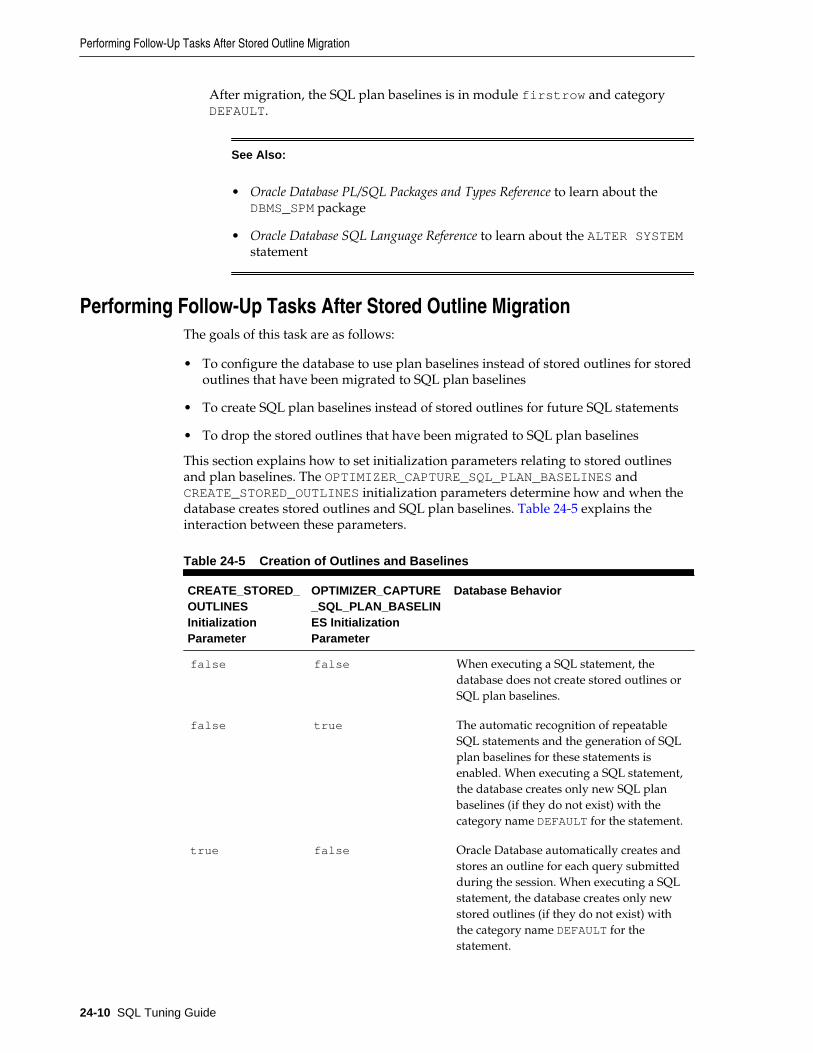
After migration, the SQL plan baselines is in module firstrow and categoryDEFAULT.
See Also:
• Oracle Database PL/SQL Packages and Types Reference to learn about theDBMS_SPM package
• Oracle Database SQL Language Reference to learn about the ALTER SYSTEMstatement
Performing Follow-Up Tasks After Stored Outline MigrationThe goals of this task are as follows:
• To configure the database to use plan baselines instead of stored outlines for storedoutlines that have been migrated to SQL plan baselines
• To create SQL plan baselines instead of stored outlines for future SQL statements
• To drop the stored outlines that have been migrated to SQL plan baselines
This section explains how to set initialization parameters relating to stored outlinesand plan baselines. The OPTIMIZER_CAPTURE_SQL_PLAN_BASELINES andCREATE_STORED_OUTLINES initialization parameters determine how and when thedatabase creates stored outlines and SQL plan baselines. Table 24-5 explains theinteraction between these parameters.
Table 24-5 Creation of Outlines and Baselines
CREATE_STORED_OUTLINESInitializationParameter
OPTIMIZER_CAPTURE_SQL_PLAN_BASELINES InitializationParameter
Database Behavior
false false When executing a SQL statement, thedatabase does not create stored outlines orSQL plan baselines.
false true The automatic recognition of repeatableSQL statements and the generation of SQLplan baselines for these statements isenabled. When executing a SQL statement,the database creates only new SQL planbaselines (if they do not exist) with thecategory name DEFAULT for the statement.
true false Oracle Database automatically creates andstores an outline for each query submittedduring the session. When executing a SQLstatement, the database creates only newstored outlines (if they do not exist) withthe category name DEFAULT for thestatement.
Performing Follow-Up Tasks After Stored Outline Migration
24-10 SQL Tuning Guide

Table 24-5 (Cont.) Creation of Outlines and Baselines
CREATE_STORED_OUTLINESInitializationParameter
OPTIMIZER_CAPTURE_SQL_PLAN_BASELINES InitializationParameter
Database Behavior
category false When executing a SQL statement, thedatabase creates only new stored outlines(if they do not exist) with the specifiedcategory name for the statement.
true true Oracle Database automatically creates andstores an outline for each query submittedduring the session. The automaticrecognition of repeatable SQL statementsand the generation of SQL plan baselinesfor these statements is also enabled.
When executing a SQL statement, thedatabase creates both stored outlines andSQL plan baselines with the category nameDEFAULT.
category true Oracle Database automatically creates andstores an outline for each query submittedduring the session. The automaticrecognition of repeatable SQL statementsand the generation of SQL plan baselinesfor these statements is also enabled.
When executing a SQL statement, thedatabase creates stored outlines with thespecified category name and SQL planbaselines with the category name DEFAULT.
The USE_STORED_OUTLINES session parameter (it is not an initialization parameter)and OPTIMIZER_USE_SQL_PLAN_BASELINES initialization parameter determinehow the database uses stored outlines and plan baselines. Table 24-6 explains howthese parameters interact.
Table 24-6 Use of Stored Outlines and SQL Plan Baselines
USE_STORED_OUTLINES Session Parameter
OPTIMIZER_USE_SQL_PLAN_BASELINESInitialization Parameter
Database Behavior
false false When choosing a plan for a SQLstatement, the database does not usestored outlines or plan baselines.
false true When choosing a plan for a SQLstatement, the database uses onlySQL plan baselines.
Performing Follow-Up Tasks After Stored Outline Migration
Migrating Stored Outlines to SQL Plan Baselines 24-11

Table 24-6 (Cont.) Use of Stored Outlines and SQL Plan Baselines
USE_STORED_OUTLINES Session Parameter
OPTIMIZER_USE_SQL_PLAN_BASELINESInitialization Parameter
Database Behavior
true false When choosing a plan for a SQLstatement, the database uses storedoutlines with the category nameDEFAULT.
category false When choosing a plan for a SQLstatement, the database uses storedoutlines with the specified categoryname.
If a stored outline with the specifiedcategory name does not exist, thenthe database uses a stored outline inthe DEFAULT category if it exists.
true true When choosing a plan for a SQLstatement, stored outlines takepriority over plan baselines.
If a stored outline with the categoryname DEFAULT exists for thestatement and is applicable, then thedatabase applies the stored outline.Otherwise, the database uses SQLplan baselines. However, if the storedoutline has the property MIGRATED,then the database does not use theoutline and uses the correspondingSQL plan baseline instead (if itexists).
category true When choosing a plan for a SQLstatement, stored outlines takepriority over plan baselines.
If a stored outline with the specifiedcategory name or the DEFAULTcategory exists for the statement andis applicable, then the databaseapplies the stored outline. Otherwise,the database uses SQL plan baselines.However, if the stored outline has theproperty MIGRATED, then thedatabase does not use the outline anduses the corresponding SQL planbaseline instead (if it exists).
Assumptions
This tutorial assumes the following:
Performing Follow-Up Tasks After Stored Outline Migration
24-12 SQL Tuning Guide

• You have completed the basic steps in the stored outline migration (see “BasicSteps in Stored Outline Migration”).
• Some stored outlines may have been created before Oracle Database 10g.
Hints in releases before Oracle Database 10g use a local hint format. Aftermigration, hints stored in a plan baseline use the global hints format introduced inOracle Database 10g.
To place the database in the proper state after the migration:
1. Connect SQL*Plus to the database with the appropriate privileges, and then checkthat SQL plan baselines have been created as the result of migration.
Ensure that the plans are enabled and accepted. For example, enter the followingquery (partial sample output included):
SELECT SQL_HANDLE, PLAN_NAME, ORIGIN, ENABLED, ACCEPTED, FIXED, MODULEFROM DBA_SQL_PLAN_BASELINES;
SQL_HANDLE PLAN_NAME ORIGIN ENA ACC FIX MODULE------------------------- ---------- -------------- --- --- --- ------SYS_SQL_f44779f7089c8fab STMT01 STORED-OUTLINE YES YES NO DEFAULT...
2. Optionally, change the attributes of the SQL plan baselines.
For example, the following statement changes the status of the baseline for thespecified SQL statement to fixed:
DECLARE v_cnt PLS_INTEGER;BEGIN v_cnt := DBMS_SPM.ALTER_SQL_PLAN_BASELINE( sql_handle=>'SYS_SQL_f44779f7089c8fab', attribute_name=>'FIXED', attribute_value=>'NO'); DBMS_OUTPUT.PUT_LINE('Plans altered: ' || v_cnt);END;/
3. Check the status of the original stored outlines.
For example, enter the following query (partial sample output included):
SELECT NAME, OWNER, CATEGORY, USED, MIGRATED FROM DBA_OUTLINESORDER BY NAME;
NAME OWNER CATEGORY USED MIGRATED---------- ---------- ---------- ------ ------------STMT01 SYS DEFAULT USED MIGRATEDSTMT02 SYS DEFAULT USED MIGRATED...
4. Drop all stored outlines that have been migrated to SQL plan baselines.
For example, the following statements drops all stored outlines with statusMIGRATED in DBA_OUTLINES:
Performing Follow-Up Tasks After Stored Outline Migration
Migrating Stored Outlines to SQL Plan Baselines 24-13

DECLARE v_cnt PLS_INTEGER;BEGIN v_cnt := DBMS_SPM.DROP_MIGRATED_STORED_OUTLINE(); DBMS_OUTPUT.PUT_LINE('Migrated stored outlines dropped: ' || v_cnt);END;/
5. Set initialization parameters so that:
• When executing a SQL statement, the database creates plan baselines but doesnot create stored outlines.
• The database only uses stored outlines when the equivalent SQL plan baselinesdo not exist.
For example, the following SQL statements instruct the database to create SQLplan baselines instead of stored outlines when a SQL statement is executed. Theexample also instructs the database to apply a stored outline in category allrowsor DEFAULT only if it exists and has not been migrated to a SQL plan baseline. Inother cases, the database applies SQL plan baselines instead.
ALTER SYSTEM SET CREATE_STORED_OUTLINE = false SCOPE = BOTH;
ALTER SYSTEM SET OPTIMIZER_CAPTURE_SQL_PLAN_BASELINES = true SCOPE = BOTH;
ALTER SYSTEM SET OPTIMIZER_USE_SQL_PLAN_BASELINES = true SCOPE = BOTH;
ALTER SESSION SET USE_STORED_OUTLINES = allrows SCOPE = BOTH;
See Also:
• Oracle Database PL/SQL Packages and Types Reference to learn about theDBMS_SPM package
• Oracle Database Reference to learn about database fixed views
Performing Follow-Up Tasks After Stored Outline Migration
24-14 SQL Tuning Guide

AGuidelines for Indexes and Table Clusters
This appendix provides an overview of data access methods using indexes andclusters that can enhance or degrade performance.
The appendix contains the following topics:
• Guidelines for Tuning Index Performance
• Guidelines for Using Function-Based Indexes for Performance
• Guidelines for Using Partitioned Indexes for Performance
• Guidelines for Using Index-Organized Tables for Performance
• Guidelines for Using Bitmap Indexes for Performance
• Guidelines for Using Bitmap Join Indexes for Performance
• Guidelines for Using Domain Indexes for Performance
• Guidelines for Using Table Clusters
• Guidelines for Using Hash Clusters for Performance
Guidelines for Tuning Index PerformanceThis section describes the following:
• Guidelines for Tuning the Logical Structure
• Guidelines for Using SQL Access Advisor
• Guidelines for Choosing Columns and Expressions to Index
• Guidelines for Choosing Composite Indexes
• Guidelines for Writing SQL Statements That Use Indexes
• Guidelines for Writing SQL Statements That Avoid Using Indexes
• Guidelines for Re-Creating Indexes
• Guidelines for Compacting Indexes
• Guidelines for Using Nonunique Indexes to Enforce Uniqueness
Guidelines for Tuning the Logical StructureAlthough query optimization helps avoid the use of nonselective indexes within queryexecution, the SQL engine must continue to maintain all indexes defined against a
Guidelines for Indexes and Table Clusters A-1

table, regardless of whether queries use them. Index maintenance can present asignificant CPU and I/O resource demand in any write-intensive application. In otherwords, do not build indexes unless necessary.
To maintain optimal performance, drop indexes that an application is not using. Youcan find indexes that are not being used by using the ALTER INDEX MONITORINGUSAGE functionality over a period that is representative of your workload. Thismonitoring feature records whether an index has been used. If you find that an indexhas not been used, then drop it. Make sure you are monitoring a representativeworkload to avoid dropping an index which is used, but not by the workload yousampled.
Also, indexes within an application sometimes have uses that are not immediatelyapparent from a survey of statement execution plans. An example of this is a foreignkey index on a parent table, which prevents share locks from being taken out on achild table.
If you are deciding whether to create new indexes to tune statements, then you canalso use the EXPLAIN PLAN statement to determine whether the optimizer chooses touse these indexes when the application is run. If you create new indexes to tune astatement that is currently parsed, then Oracle Database invalidates the statement.
When the statement is next parsed, the optimizer automatically chooses a newexecution plan that could potentially use the new index. If you create new indexes ona remote database to tune a distributed statement, then the optimizer considers theseindexes when the statement is next parsed.
Creating an index to tune one statement can affect the optimizer's choice of executionplans for other statements. For example, if you create an index to be used by onestatement, then the optimizer can choose to use that index for other statements in theapplication as well. For this reason, reexamine the application's performance andexecution plans, and rerun the SQL trace facility after you have tuned those statementsthat you initially identified for tuning.
See Also:
• Oracle Database SQL Language Reference for syntax and semantics of theALTER INDEX MONITORING USAGE statement
• Oracle Database Development Guide to learn about foreign keys
Guidelines for Using SQL Access AdvisorSQL Access Advisor is an alternative to manually determining which indexes arerequired. This advisor recommends a set of indexes when invoked from OracleEnterprise Manager Cloud Control (Cloud Control) or run through theDBMS_ADVISOR package APIs. SQL Access Advisor either recommends using aworkload or it generates a hypothetical workload for a specified schema.
Various workload sources are available, such as the current contents of the SQL cache,a user-defined set of SQL statements, or a SQL tuning set. Given a workload, SQLAccess Advisor generates a set of recommendations from which you can select theindexes to be implemented. SQL Access Advisor provides an implementation scriptthat can be executed manually or automatically through Cloud Control.
Guidelines for Tuning Index Performance
A-2 SQL Tuning Guide

See Also:
“About SQL Access Advisor”
Guidelines for Choosing Columns and Expressions to IndexA key is a column or expression on which you can build an index. Follow theseguidelines for choosing keys to index:
• Consider indexing keys that appear frequently in WHERE clauses.
• Consider indexing keys that frequently join tables in SQL statements.
• Choose index keys that are highly selective. The selectivity of an index is thepercentage of rows in a table having the same value for the indexed key. An indexselectivity is optimal if few rows have the same value.
Note:
Oracle Database automatically creates indexes, or uses existing indexes, on thekeys and expressions of unique and primary keys that you define withintegrity constraints.
Indexing low selectivity columns can be helpful when the data distribution isskewed so that one or two values occur much less often than other values.
• Do not use standard B-tree indexes on keys or expressions with few distinct values.Such keys or expressions are usually unselective and therefore do not optimizeperformance unless the frequently selected key values appear less frequently thanthe other key values. You can use bitmap indexes effectively in such cases, unlessthe index is modified frequently, as in a high concurrency OLTP application.
• Do not index frequently modified columns. UPDATE statements that modifyindexed columns and INSERT and DELETE statements that modify indexed tablestake longer than if there were no index. Such SQL statements must modify data inindexes and data in tables. They also create additional undo and redo.
• Do not index keys that appear only in WHERE clauses with functions or operators. AWHERE clause that uses a function, other than MIN or MAX, or an operator with anindexed key does not make available the access path that uses the index exceptwith function-based indexes.
• Consider indexing foreign keys of referential integrity constraints in cases in whichmany concurrent INSERT, UPDATE, and DELETE statements access the parent andchild tables. Such an index allows UPDATEs and DELETEs on the parent tablewithout share locking the child table.
• When choosing to index a key, consider whether the performance gain for queriesis worth the performance loss for INSERTs, UPDATEs, and DELETEs and the use ofthe space required to store the index. You might want to experiment by comparingthe processing times of the SQL statements with and without indexes. You canmeasure processing time with the SQL trace facility.
Guidelines for Tuning Index Performance
Guidelines for Indexes and Table Clusters A-3

See Also:
Oracle Database Development Guide for more information about the effects offoreign keys on locking
Guidelines for Choosing Composite IndexesA composite index contains multiple key columns. Composite indexes can provideadditional advantages over single-column indexes:
• Improved selectivity
Sometimes you can combine two or more columns or expressions, each with lowselectivity, to form a composite index with higher selectivity.
• Reduced I/O
If all columns selected by a query are in a composite index, then Oracle Databasecan return these values from the index without accessing the table.
A SQL statement can use an access path involving a composite index when thestatement contains constructs that use a leading portion of the index.
Note:
This is no longer the case with index skip scans. See “Index Skip Scans”.
A leading portion of an index is a set of one or more columns that were specified firstand consecutively in the list of columns in the CREATE INDEX statement that createdthe index. Consider this CREATE INDEX statement:
CREATE INDEX comp_ind ON table1(x, y, z);
• x, xy, and xyz combinations of columns are leading portions of the index
• yz, y, and z combinations of columns are not leading portions of the index
Guidelines for Choosing Keys for Composite Indexes
Follow these guidelines for choosing keys for composite indexes:
• Consider creating a composite index on keys that appear together frequently inWHERE clause conditions combined with AND operators, especially if theircombined selectivity is better than the selectivity of either key individually.
• If several queries select the same set of keys based on one or more key values, thenconsider creating a composite index containing all of these keys.
Of course, consider the guidelines associated with the general performanceadvantages and trade-offs of indexes described in the previous sections.
Guidelines for Ordering Keys for Composite Indexes
Follow these guidelines for ordering keys in composite indexes:
• Create the index so the keys used in WHERE clauses comprise a leading portion.
Guidelines for Tuning Index Performance
A-4 SQL Tuning Guide

• If some keys appear in WHERE clauses more frequently, then create the index so thatthe more frequently selected keys comprise a leading portion to allow thestatements that use only these keys to use the index.
• If all keys appear in WHERE clauses equally often but the data is physically orderedon one of the keys, then place this key first in the composite index.
Guidelines for Writing SQL Statements That Use IndexesEven after you create an index, the optimizer cannot use an access path that uses theindex simply because the index exists. The optimizer can choose such an access pathfor a SQL statement only if it contains a construct that makes the access path available.To allow the query optimizer the option of using an index access path, ensure that thestatement contains a construct that makes such an access path available.
Guidelines for Writing SQL Statements That Avoid Using IndexesIn some cases, you might want to prevent a SQL statement from using an access paththat uses an existing index. You may want to take this approach if you know that theindex is not very selective and a full table scan would be more efficient. If thestatement contains a construct that makes such an index access path available, thenyou can force the optimizer to use a full table scan through one of the followingmethods:
• Use the NO_INDEX hint to give the query optimizer maximum flexibility whiledisallowing the use of a certain index.
• Use the FULL hint to instruct the optimizer to choose a full table scan instead of anindex scan.
• Use the INDEX or INDEX_COMBINE hints to instruct the optimizer to use one indexor a set of listed indexes instead of another.
Parallel execution uses indexes effectively. It does not perform parallel index rangescans, but it does perform parallel index lookups for parallel nested loops joinexecution. If an index is very selective (few rows correspond to each index entry), thena sequential index lookup might be better than a parallel table scan.
See Also:
Influencing the Optimizer for more information about the NO_INDEX, FULL,INDEX, and INDEX_COMBINE and hints
Guidelines for Re-Creating IndexesYou might want to re-create an index to compact it and minimize fragmented space, orto change the index's storage characteristics. When creating a new index that is asubset of an existing index, or when rebuilding an existing index with new storagecharacteristics, Oracle Database might use the existing index instead of the base tableto improve the performance of the index build.
However, in some cases using the base table instead of the existing index is beneficial.Consider an index on a table on which a lot of DML has been performed. Because ofthe DML, the size of the index can increase to the point where each block is only 50%full, or even less. If the index refers to most of the columns in the table, then the index
Guidelines for Tuning Index Performance
Guidelines for Indexes and Table Clusters A-5

could actually be larger than the table. In this case, it is faster to use the base tablerather than the index to re-create the index.
To reorganize or compact an existing index or to change its storage characteristics, usethe ALTER INDEX . . . REBUILD statement. The REBUILD statement uses theexisting index as the basis for the new one. All index storage statements are supported,such as STORAGE (for extent allocation), TABLESPACE (to move the index to a newtablespace), and INITRANS (to change the initial number of entries).
Usually, ALTER INDEX . . . REBUILD is faster than dropping and re-creating anindex, because this statement uses the fast full scan feature. It reads all the indexblocks using multiblock I/O, then discards the branch blocks. A further advantage ofthis approach is that the old index is still available for queries while the rebuild is inprogress.
See Also:
Oracle Database SQL Language Reference for more information about theCREATE INDEX and ALTER INDEX statements and restrictions on rebuildingindexes
Guidelines for Compacting IndexesYou can coalesce leaf blocks of an index by using the ALTER INDEX statement with theCOALESCE option. This option enables you to combine leaf levels of an index to freeblocks for reuse. You can also rebuild the index online.
See Also:
Oracle Database SQL Language Reference and Oracle Database Administrator'sGuide for more information about the syntax for this statement
Guidelines for Using Nonunique Indexes to Enforce UniquenessYou can use an existing nonunique index on a table to enforce uniqueness, either forUNIQUE constraints or the unique aspect of a PRIMARY KEY constraint. The advantageof this approach is that the index remains available and valid when the constraint isdisabled. Therefore, enabling a disabled UNIQUE or PRIMARY KEY constraint does notrequire rebuilding the unique index associated with the constraint. This can yieldsignificant time savings on enable operations for large tables.
Using a nonunique index to enforce uniqueness also enables you to eliminateredundant indexes. You do not need a unique index on a primary key column if thatcolumn is included as the prefix of a composite index. You can use the existing indexto enable and enforce the constraint. You also save significant space by not duplicatingthe index. However, if the existing index is partitioned, then the partitioning key of theindex must also be a subset of the UNIQUE key; otherwise, Oracle Database creates anadditional unique index to enforce the constraint.
Guidelines for Using Enabled Novalidated ConstraintsAn enabled novalidated constraint behaves similarly to an enabled validatedconstraint for new data. Placing a constraint in the enabled novalidated state signifiesthat any new data entered into the table must conform to the constraint. Existing data
Guidelines for Tuning Index Performance
A-6 SQL Tuning Guide

is not checked. By placing a constraint in the enabled novalidated state, you enable theconstraint without locking the table.
If you change a constraint from disabled to enabled, then the table must be locked. Nonew DML, queries, or DDL can occur, because no mechanism can ensure thatoperations on the table conform to the constraint during the enable operation. Theenabled novalidated state prevents users from performing operations on the table thatviolate the constraint.
The database can validate an enabled novalidated constraint with a parallel,consistent-read query of the table to determine whether any data violates theconstraint. The database performs no locking, so the enable operation does not blockreaders or writers. In addition, the database can validate enabled novalidatedconstraints in parallel. The database can validate multiple constraints at the same timeand check the validity of each constraint using parallel query.
To create tables with constraints and indexes:
1. Create the tables with the constraints.
NOT NULL constraints can be unnamed and should be created enabled andvalidated. Name all other constraints (CHECK, UNIQUE, PRIMARY KEY, andFOREIGN KEY) and create them disabled.
Note:
By default, constraints are created in the ENABLED state.
2. Load old data into the tables.
3. Create all indexes, including indexes needed for constraints.
4. Enable novalidate all constraints. Do this to primary keys before foreign keys.
5. Allow users to query and modify data.
6. With a separate ALTER TABLE statement for each constraint, validate allconstraints. Do this to primary keys before foreign keys. For example,
CREATE TABLE t (a NUMBER CONSTRAINT apk PRIMARY KEY DISABLE,b NUMBER NOT NULL);CREATE TABLE x (c NUMBER CONSTRAINT afk REFERENCES t DISABLE);
Now load data into table t.
CREATE UNIQUE INDEX tai ON t (a); CREATE INDEX tci ON x (c); ALTER TABLE t MODIFY CONSTRAINT apk ENABLE NOVALIDATE;ALTER TABLE x MODIFY CONSTRAINT afk ENABLE NOVALIDATE;
At this point, users can start performing INSERT, UPDATE, DELETE, and SELECToperations on table t.
ALTER TABLE t ENABLE CONSTRAINT apk;ALTER TABLE x ENABLE CONSTRAINT afk;
Now the constraints are enabled and validated.
Guidelines for Tuning Index Performance
Guidelines for Indexes and Table Clusters A-7

See Also:
Oracle Database Concepts for an overview of integrity constraints
Guidelines for Using Function-Based Indexes for PerformanceA function-based index includes columns that are either transformed by a function,such as the UPPER function, or included in an expression, such as col1 + col2. Witha function-based index, you can store computation-intensive expressions in the index.
Defining a function-based index on the transformed column or expression allows thatdata to be returned using the index when that function or expression is used in aWHERE clause or an ORDER BY clause. In this way, the database can avoid computingthe value of the expression when processing SELECT and DELETE statements. Thus, afunction-based index is useful when frequently executed SQL statements includetransformed columns, or columns in expressions, in a WHERE or ORDER BY clause.
Oracle Database treats descending indexes as function-based indexes. The columnsmarked DESC are sorted in descending order.
For example, function-based indexes defined with the UPPER(column_name) orLOWER(column_name) keywords allow case-insensitive searches. Assume that youcreate an index on the following statement:
CREATE INDEX uppercase_idx ON employees (UPPER(last_name));
The preceding index facilitates processing queries such as:
SELECT * FROM employeesWHERE UPPER(last_name) = 'MARKSON';
See Also:
• Oracle Database Development Guide and Oracle Database Administrator's Guidefor more information about using function-based indexes
• Oracle Database SQL Language Reference for more information about theCREATE INDEX statement
Guidelines for Using Partitioned Indexes for PerformanceSimilar to partitioned tables, partitioned indexes improve manageability, availability,performance, and scalability. They can either be partitioned independently (globalindexes) or automatically linked to a table's partitioning method (local indexes).
Oracle Database supports both range and hash partitioned global indexes. In a rangepartitioned global index, each index partition contains values defined by a partitionbound. In a hash partitioned global index, each partition contains values determinedby the Oracle Database hash function.
The hash method can improve performance of indexes where a small number leafblocks in the index have high contention in multiuser OLTP environment. In someOLTP applications, index insertions happen only at the right edge of the index. Thissituation could occur when the index is defined on monotonically increasing columns.In such situations, the right edge of the index becomes a hot spot because of
Guidelines for Using Function-Based Indexes for Performance
A-8 SQL Tuning Guide

contention for index pages, buffers, latches for update, and additional indexmaintenance activity, which results in performance degradation.
With hash partitioned global indexes index entries are hashed to different partitionsbased on partitioning key and the number of partitions. This spreads out contentionover number of defined partitions, resulting in increased throughput. Hash-partitioned global indexes would benefit TPC-H refresh functions that are executed asmassive PDMLs into huge fact tables because contention for buffer latches would bespread out over multiple partitions.
With hash partitioning, an index entry is mapped to a particular index partition basedon the hash value generated by Oracle Database. The syntax to create hash-partitionedglobal index is very similar to hash-partitioned table. Queries involving equality andIN predicates on index partitioning key can efficiently use global hash partitionedindex to answer queries quickly.
See Also:
Oracle Database Concepts and Oracle Database Administrator's Guide for moreinformation about global indexes tables
Guidelines for Using Index-Organized Tables for PerformanceAn index-organized table differs from an ordinary table in that the data for the table isheld in its associated index. Changes to the table data, such as adding new rows,updating rows, or deleting rows, result only in updating the index. Because data rowsare stored in the index, index-organized tables provide faster key-based access to tabledata for queries that involve exact match or range search or both.
A parent/child relationship is an example of a situation that may warrant an index-organized table. For example, a members table has a child table containing phonenumbers. Phone numbers for a member are changed and added over time. In a heap-organized table, rows are inserted in data blocks where they fit. However, when youquery the members table, you always retrieve the phone numbers from the child table.To make the retrieval more efficient, you can store the phone numbers in an index-organized table so that phone records for a given member are inserted near each otherin the data blocks.
In some circumstances, an index-organized table may provide a performanceadvantage over a heap-organized table. For example, if a query requires fewer blocksin the cache, then the database uses the buffer cache more efficiently. If fewer distinctblocks are needed for a query, then a single physical I/O may retrieve all necessarydata, requiring a smaller amount of I/O for each query.
Global hash-partitioned indexes are supported for index-organized tables and canprovide performance benefits in a multiuser OLTP environment. Index-organizedtables are useful when you must store related pieces of data together or physicallystore data in a specific order.
See Also:
Oracle Database Concepts and Oracle Database Administrator's Guide for moreinformation about index-organized tables
Guidelines for Using Index-Organized Tables for Performance
Guidelines for Indexes and Table Clusters A-9

Guidelines for Using Bitmap Indexes for PerformanceBitmap indexes can substantially improve performance of queries that have all of thefollowing characteristics:
• The WHERE clause contains multiple predicates on low- or medium-cardinalitycolumns.
• The individual predicates on these low- or medium-cardinality columns selectmany rows.
• The bitmap indexes used in the queries have been created on some or all of theselow- or medium-cardinality columns.
• The tables in the queries contain many rows.
You can use multiple bitmap indexes to evaluate the conditions on a single table.Bitmap indexes are thus highly advantageous for complex ad hoc queries that containlengthy WHERE clauses. Bitmap indexes can also provide optimal performance foraggregate queries and for optimizing joins in star schemas.
See Also:
Oracle Database Concepts and Oracle Database Data Warehousing Guide for moreinformation about bitmap indexing
Guidelines for Using Bitmap Join Indexes for PerformanceIn addition to a bitmap index on a single table, you can create a bitmap join index,which is a bitmap index for the join of two or more tables. A bitmap join index is aspace-saving way to reduce the volume of data that must be joined by performingrestrictions in advance. For each value in a column of a table, a bitmap join indexstores the rowids of corresponding rows in another table. In a data warehousingenvironment, the join condition is an equi-inner join between the primary keycolumn(s) of the dimension tables and the foreign key column(s) in the fact table.
Bitmap join indexes are much more efficient in storage than materialized join views,an alternative for materializing joins in advance. Materialized join views do notcompress the rowids of the fact tables.
See Also:
Oracle Database Data Warehousing Guide for examples and restrictions of bitmapjoin indexes
Guidelines for Using Domain Indexes for PerformanceDomain indexes are built using the indexing logic supplied by a user-definedindextype. An indextype provides an efficient mechanism to access data that satisfycertain operator predicates. Typically, the user-defined indextype is part of an OracleDatabase option, like the Spatial option. For example, the SpatialIndextype allowsefficient search and retrieval of spatial data that overlap a given bounding box.
Guidelines for Using Bitmap Indexes for Performance
A-10 SQL Tuning Guide

The cartridge determines the parameters you can specify in creating and maintainingthe domain index. Similarly, the performance and storage characteristics of thedomain index are presented in the specific cartridge documentation.
Refer to the appropriate cartridge documentation for information such as thefollowing:
• What data types can be indexed?
• What indextypes are provided?
• What operators does the indextype support?
• How can the domain index be created and maintained?
• How do we efficiently use the operator in queries?
• What are the performance characteristics?
Note:
You can also create index types with the CREATE INDEXTYPE statement.
See Also:
Oracle Spatial and Graph Developer's Guide for information about theSpatialIndextype
Guidelines for Using Table ClustersA table cluster is a group of one or more tables that are physically stored togetherbecause they share common columns and usually appear together in SQL statements.Because the database physically stores related rows together, disk access timeimproves. To create a cluster, use the CREATE CLUSTER statement.
Consider clustering tables in the following circumstances:
• The application frequently accesses the tables in join statements.
• In master-detail tables, the application often selects a master record and then thecorresponding detail records.
Detail records are stored in the same data blocks as the master record, so they arelikely still to be in memory when you select them, requiring Oracle Database toperform less I/O.
• The application often selects many detail records of the same master.
In this case, consider storing a detail table alone in a cluster. This measureimproves the performance of queries that select detail records of the same master,but does not decrease the performance of a full table scan on the master table. Analternative is to use an index organized table.
Avoid clustering tables in the following circumstances:
• The application joins the tables only occasionally or modifies their common columnvalues frequently.
Guidelines for Using Table Clusters
Guidelines for Indexes and Table Clusters A-11

Modifying a row's cluster key value takes longer than modifying the value in annonclustered table, because Oracle Database might need to migrate the modifiedrow to another block to maintain the cluster.
• The application often performs full table scans of only one of the tables.
A full table scan of a clustered table can take longer than a full table scan of annonclustered table. Oracle Database is likely to read more blocks because the tablesare stored together.
• The data from all tables with the same cluster key value exceeds more than one ortwo data blocks.
To access a row in a clustered table, Oracle Database reads all blocks containingrows with that value. If these rows take up multiple blocks, then accessing a singlerow could require more reads than accessing the same row in a nonclustered table.
• The number of rows for each cluster key value varies significantly.
This causes waste of space for the low cardinality key value. It causes collisions forthe high cardinality key values. Collisions degrade performance.
Consider the benefits and drawbacks of clusters for the application. For example, youmight decide that the performance gain for join statements outweighs the performanceloss for statements that modify cluster key values. You might want to experiment andcompare processing times with the tables both clustered and stored separately.
See Also:
• Oracle Database Concepts for more information about clusters
• Oracle Database Administrator's Guide for more information about creatingclusters
Guidelines for Using Hash Clusters for PerformanceHash clusters group table data by applying a hash function to each row's cluster keyvalue. All rows with the same cluster key value are stored together on disk. Considerthe benefits and drawbacks of hash clusters for the application. You might want toexperiment and compare processing times with a particular table in a hash cluster andalone with an index.
Follow these guidelines for choosing when to use hash clusters:
• Use hash clusters to store tables accessed frequently by SQL statements withWHERE clauses, if the WHERE clauses contain equality conditions that use the samecolumn or combination of columns. Designate this column or combination ofcolumns as the cluster key.
• Store a table in a hash cluster if you can determine how much space is required tohold all rows with a given cluster key value, including rows to be insertedimmediately and rows to be inserted in the future.
• Use sorted hash clusters, where rows corresponding to each value of the hashfunction are sorted on a specific columns in ascending order, when the databasecan improve response time on operations with this sorted clustered data.
Guidelines for Using Hash Clusters for Performance
A-12 SQL Tuning Guide

• Do not store a table in a hash cluster in the following cases:
– The application often performs full table scans.
– You must allocate a great deal of space to the hash cluster in anticipation of thetable growing.
Full table scans must read all blocks allocated to the hash cluster, even thoughsome blocks might contain few rows. Storing the table alone reduces the number ofblocks read by full table scans.
• Do not store a table in a hash cluster if the application frequently modifies thecluster key values. Modifying a row's cluster key value can take longer thanmodifying the value in an nonclustered table, because Oracle Database might needto migrate the modified row to another block to maintain the cluster.
If hashing is appropriate for the table based on the considerations in this list, thenstoring a single table in a hash cluster can be useful. This is true regardless of whetherthe table is joined frequently with other tables.
See Also:
• Oracle Database Administrator's Guide to learn how to manage hash clusters
• Oracle Database SQL Language Reference to learn about the CREATECLUSTER statement
Guidelines for Using Hash Clusters for Performance
Guidelines for Indexes and Table Clusters A-13

Guidelines for Using Hash Clusters for Performance
A-14 SQL Tuning Guide
Glossary
accepted planIn the context of SQL plan management, a plan that is in a SQL plan baseline for aSQL statement and thus available for use by the optimizer. An accepted plan containsa set of hints, a plan hash value, and other plan-related information.
access pathThe means by which the database retrieves data from a database. For example, a queryusing an index and a query using a full table scan use different access paths.
adaptive cursor sharingA feature that enables a single statement that contains bind variables to use multipleexecution plans. Cursor sharing is "adaptive" because the cursor adapts its behavior sothat the database does not always use the same plan for each execution or bindvariable value.
adaptive optimizerA feature of the optimizer that enables it to adapt plans based on run-time statistics.
adaptive planAn execution plan that changes after optimization because run-time conditionsindicate that optimizer estimates are inaccurate. An adaptive plan has different built-in plan options. During the first execution, before a specific subplan becomes active,the optimizer makes a a final decision about which option to use. The optimizer basesits choice on observations made during the execution up to this point. Thus, anadaptive plan enables the final plan for a statement to differ from the default plan.
adaptive query optimizationA set of capabilities that enables the adaptive optimizer to make run-time adjustmentsto execution plans and discover additional information that can lead to betterstatistics. Adaptive optimization is helpful when existing statistics are not sufficient togenerate an optimal plan.
ADDMSee Automatic Database Diagnostic Monitor (ADDM).
Glossary-1

antijoinA join that returns rows that fail to match the subquery on the right side. For example,an antijoin can list departments with no employees. Antijoins use the NOT EXISTS orNOT IN constructs.
Automatic Database Diagnostic Monitor (ADDM)ADDM is self-diagnostic software built into Oracle Database. ADDM examines andanalyzes data captured in Automatic Workload Repository (AWR) to determinepossible database performance problems.
automatic optimizer statistics collectionThe automatic running of the DBMS_STATS package to collect optimizer statistics forall schema objects for which statistics are missing or stale.
automatic initial plan captureThe mechanism by which the database automatically creates a SQL plan baseline forany repeatable SQL statement executed on the database. Enable automatic initial plancapture by setting the OPTIMIZER_CAPTURE_SQL_PLAN_BASELINES initializationparameter to true (the default is false).
See repeatable SQL statement.
automatic reoptimizationThe ability of the optimizer to automatically change a plan on subsequent executionsof a SQL statement. Automatic reoptimization can fix any suboptimal plan chosen dueto incorrect optimizer estimates, from a suboptimal distribution method to anincorrect choice of degree of parallelism.
automatic SQL tuningThe work performed by Automatic SQL Tuning Advisor it runs as an automated taskwithin system maintenance windows.
Automatic SQL Tuning AdvisorSQL Tuning Advisor when run as an automated maintenance task. Automatic SQLTuning runs during system maintenance windows as an automated maintenance task,searching for ways to improve the execution plans of high-load SQL statements.
See SQL Tuning Advisor.
Automatic Tuning OptimizerThe optimizer when invoked by SQL Tuning Advisor. In SQL tuning mode, theoptimizer performs additional analysis to check whether it can further improve theplan produced in normal mode. The optimizer output is not an execution plan, but aseries of actions, along with their rationale and expected benefit for producing asignificantly better plan.
antijoin
Glossary-2

Automatic Workload Repository (AWR)The infrastructure that provides services to Oracle Database components to collect,maintain, and use statistics for problem detection and self-tuning.
AWRSee Automatic Workload Repository (AWR).
AWR snapshotA set of data for a specific time that is used for performance comparisons. The deltavalues captured by the snapshot represent the changes for each statistic over the timeperiod. Statistics gathered by are queried from memory. You can display the gathereddata in both reports and views.
baselineIn the context of AWR, the interval between two AWR snapshots that represent thedatabase operating at an optimal level.
bind-aware cursorA bind-sensitive cursor that is eligible to use different plans for different bind values.After a cursor has been made bind-aware, the optimizer chooses plans for futureexecutions based on the bind value and its cardinality estimate.
bind-sensitive cursorA cursor whose optimal plan may depend on the value of a bind variable. Thedatabase monitors the behavior of a bind-sensitive cursor that uses different bindvalues to determine whether a different plan is beneficial.
bind variableA placeholder in a SQL statement that must be replaced with a valid value or valueaddress for the statement to execute successfully. By using bind variables, you canwrite a SQL statement that accepts inputs or parameters at run time. The followingquery uses v_empid as a bind variable:
SELECT * FROM employees WHERE employee_id = :v_empid;
bind variable peekingThe ability of the optimizer to look at the value in a bind variable during a hard parse.By peeking at bind values, the optimizer can determine the selectivity of a WHEREclause condition as if literals had been used, thereby improving the plan.
bitmap join indexA bitmap index for the join of two or more tables.
bitmap join index
Glossary-3

bitmap pieceA subcomponent of a single bitmap index entry. Each indexed column value may haveone or more bitmap pieces. The database uses bitmap pieces to break up an indexentry that is large in relation to the size of a block.
B-tree indexAn index organized like an upside-down tree. A B-tree index has two types of blocks:branch blocks for searching and leaf blocks that store values. The leaf blocks containevery indexed data value and a corresponding rowid used to locate the actual row.The "B" stands for "balanced" because all leaf blocks automatically stay at the samedepth.
bulk loadA CREATE TABLE AS SELECT or INSERT INTO ... SELECT operation.
cardinalityThe number of rows that is expected to be or actually is returned by an operation in anexecution plan. Data has low cardinality when the number of distinct values in acolumn is low in relation to the total number of rows.
Cartesian joinA join in which one or more of the tables does not have any join conditions to anyother tables in the statement. The optimizer joins every row from one data source withevery row from the other data source, creating the Cartesian product of the two sets.
child cursorThe cursor containing the plan, compilation environment, and other information for astatement whose text is stored in a parent cursor. The parent cursor is number 0, thefirst child is number 1, and so on. Child cursors reference the same SQL text as theparent cursor, but are different. For example, two queries with the text SELECT *FROM t use different cursors when they reference two different tables named t.
cluster scanAn access path for a table cluster. In an indexed table cluster, Oracle Database firstobtains the rowid of one of the selected rows by scanning the cluster index. OracleDatabase then locates the rows based on this rowid.
column groupA set of columns that is treated as a unit.
column group statisticsExtended statistics gathered on a group of columns treated as a unit.
bitmap piece
Glossary-4

column statisticsStatistics about columns that the optimizer uses to determine optimal execution plans.Column statistics include the number of distinct column values, low value, high value,and number of nulls.
complex view mergingThe merging of views containing the GROUP BY or DISTINCT keywords.
composite database operationIn a database operation, the activity between two points in time in a database session,with each session defining its own beginning and end points. A session can participatein at most one composite database operation at a time.
concurrencySimultaneous access of the same data by many users. A multiuser databasemanagement system must provide adequate concurrency controls so that data cannotbe updated or changed improperly, compromising data integrity.
concurrent statistics gathering modeA mode that enables the database to simultaneously gather optimizer statistics formultiple tables in a schema, or multiple partitions or subpartitions in a table.Concurrency can reduce the overall time required to gather statistics by enabling thedatabase to fully use multiple CPUs.
conditionA combination of one or more expressions and logical operators that returns a value ofTRUE, FALSE, or UNKNOWN.
costA numeric internal measure that represents the estimated resource usage for an execution plan. The lower the cost, the more efficient the plan.
cost-based optimizer (CBO)The legacy name for the optimizer. In earlier releases, the cost-based optimizer was analternative to the rule-based optimizer (RBO).
cost modelThe internal optimizer model that accounts for the cost of the I/O, CPU, and networkresources that a query is predicted to use.
cumulative statisticsA count such as the number of block reads. Oracle Database generates many types ofcumulative statistics for the system, sessions, and individual SQL statements.
cumulative statistics
Glossary-5

cursorA handle or name for a private SQL area in the PGA. Because cursors are closelyassociated with private SQL areas, the terms are sometimes used interchangeably.
cursor cacheSee shared SQL area.
cursor mergingCombining cursors to save space in the shared SQL area. If the optimizer creates aplan for a bind-aware cursor, and if this plan is the same as an existing cursor, thenthe optimizer can merge the cursors.
data flow operator (DFO)The unit of work between data redistribution stages in a parallel query.
data skewLarge variations in the number of duplicate values in a column.
database operationA set of database tasks defined by end users or application code, for example, a batchjob or ETL processing.
default planFor an adaptive plan, the execution plan initially chosen by the optimizer using thestatistics from the data dictionary. The default plan can differ from the final plan.
disabled planA plan that a database administrator has manually marked as ineligible for use by theoptimizer.
degree of parallelism (DOP)The number of parallel execution servers associated with a single operation. Parallelexecution is designed to effectively use multiple CPUs. Oracle Database parallelexecution framework enables you to either explicitly choose a specific degree ofparallelism or to rely on Oracle Database to automatically control it.
dense keyA numeric key that is stored as a native integer and has a range of values.
dense grouping keyA key that represents all grouping keys whose grouping columns come from aparticular fact table or dimension.
cursor
Glossary-6

dense join keyA key that represents all join keys whose join columns come from a particular facttable or dimension.
densityA decimal number between 0 and 1 that measures the selectivity of a column. Valuesclose to 1 indicate that the column is unselective, whereas values close to 0 indicatethat this column is more selective.
direct path readA single or multiblock read into the PGA, bypassing the SGA.
driving tableThe table to which other tables are joined. An analogy from programming is a for loopthat contains another for loop. The outer for loop is the analog of a driving table,which is also called an outer table.
dynamic performance viewA view created on dynamic performance tables, which are virtual tables that recordcurrent database activity. The dynamic performance views are called fixed viewsbecause they cannot be altered or removed by the database administrator. They arealso called V$ views because they begin with the string V$ (GV$ in Oracle RAC).
dynamic statisticsAn optimization technique in which the database executes a recursive SQL statementto scan a small random sample of a table's blocks to estimate predicate selectivities.
dynamic statistics levelThe level that controls both when the database gathers dynamic statistics, and the sizeof the sample that the optimizer uses to gather the statistics. Set the dynamic statisticslevel using either the OPTIMIZER_DYNAMIC_SAMPLING initialization parameter or astatement hint.
enabled planIn SQL plan management, a plan that is eligible for use by the optimizer.
endpoint numberA number that uniquely identifies a bucket in a histogram. In frequency and hybridhistograms, the endpoint number is the cumulative frequency of endpoints. In height-balanced histograms, the endpoint number is the bucket number.
endpoint number
Glossary-7

endpoint repeat countIn a hybrid histogram, the number of times the endpoint value is repeated, for eachendpoint (bucket) in the histogram. By using the repeat count, the optimizer canobtain accurate estimates for almost popular values.
endpoint valueAn endpoint value is the highest value in the range of values in a histogram bucket.
equijoinA join whose join condition contains an equality operator.
estimatorThe component of the optimizer that determines the overall cost of a given executionplan.
execution planThe combination of steps used by the database to execute a SQL statement. Each stepeither retrieves rows of data physically from the database or prepares them for theuser issuing the statement. You can override execution plans by using hints.
execution treeA tree diagram that shows the flow of row sources from one step to another in an execution plan.
expressionA combination of one or more values, operators, and SQL functions that evaluates to avalue. For example, the expression 2*2 evaluates to 4. In general, expressions assumethe data type of their components.
expression statisticsA type of extended statistics that improves optimizer estimates when a WHERE clausehas predicates that use expressions.
extended statisticsA type of optimizer statistics that improves estimates for cardinality when multiplepredicates exist or when predicates contain expressions.
extensible optimizerAn optimizer capability that enables authors of user-defined functions and indexes tocreate statistics collection, selectivity, and cost functions that the optimizer uses whenchoosing an execution plan. The optimizer cost model is extended to integrateinformation supplied by the user to assess CPU and I/O cost.
endpoint repeat count
Glossary-8

extensionA column group or an expression. The statistics collected for column groups andexpressions are called extended statistics.
external tableA read-only table whose metadata is stored in the database but whose data in storedin files outside the database. The database uses the metadata describing external tablesto expose their data as if they were relational tables.
filter conditionA WHERE clause component that eliminates rows from a single object referenced in aSQL statement.
final planIn an adaptive plan, the plan that executes to completion. The default plan can differfrom the final plan.
fixed objectA dynamic performance table or its index. The fixed objects are owned by SYS. Fixedobject tables have names beginning with X$ and are the base tables for the V$ views.
fixed planAn accepted plan that is marked as preferred, so that the optimizer considers only thefixed plans in the SQL plan baseline. You can use fixed plans to influence the planselection process of the optimizer.
frequency histogramA type of histogram in which each distinct column value corresponds to a singlebucket. An analogy is sorting coins: all pennies go in bucket 1, all nickels go in bucket2, and so on.
full outer joinA combination of a left and right outer join. In addition to the inner join, the databaseuses nulls to preserve rows from both tables that have not been returned in the resultof the inner join. In other words, full outer joins join tables together, yet show rowswith no corresponding rows in the joined tables.
full table scanA scan of table data in which the database sequentially reads all rows from a table andfilters out those that do not meet the selection criteria. All data blocks under the highwater mark are scanned.
full table scan
Glossary-9

global temporary tableA special temporary table that stores intermediate session-private data for a specificduration.
hard parseThe steps performed by the database to build a new executable version of applicationcode. The database must perform a hard parse instead of a soft parse if the parsedrepresentation of a submitted statement does not exist in the shared SQL area.
hash clusterA type of table cluster that is similar to an indexed cluster, except the index key isreplaced with a hash function. No separate cluster index exists. In a hash cluster, thedata is the index.
hash collisionHashing multiple input values to the same output value.
hash functionA function that operates on an arbitrary-length input value and returns a fixed-lengthhash value.
hash joinA method for joining large data sets. The database uses the smaller of two data sets tobuild a hash table on the join key in memory. It then scans the larger data set, probingthe hash table to find the joined rows.
hash scanAn access path for a table cluster. The database uses a hash scan to locate rows in ahash cluster based on a hash value. In a hash cluster, all rows with the same hashvalue are stored in the same data block. To perform a hash scan, Oracle Database firstobtains the hash value by applying a hash function to a cluster key value specified bythe statement, and then scans the data blocks containing rows with that hash value.
hash tableAn in-memory data structure that associates join keys with rows in a hash join. Forexample, in a join of the employees and departments tables, the join key might bethe department ID. A hash function uses the join key to generate a hash value. Thishash value is an index in an array, which is the hash table.
hash valueIn a hash cluster, a unique numeric ID that identifies a bucket. Oracle Database uses ahash function that accepts an infinite number of hash key values as input and sortsthem into a finite number of buckets. Each hash value maps to the database block
global temporary table
Glossary-10

address for the block that stores the rows corresponding to the hash key value(department 10, 20, 30, and so on).
hashingA mathematical technique in which an infinite set of input values is mapped to a finiteset of output values, called hash values. Hashing is useful for rapid lookups of data ina hash table.
heap-organized tableA table in which the data rows are stored in no particular order on disk. By default,CREATE TABLE creates a heap-organized table.
height-balanced histogramA histogram in which column values are divided into buckets so that each bucketcontains approximately the same number of rows.
hintAn instruction passed to the optimizer through comments in a SQL statement. Theoptimizer uses hints to choose an execution plan for the statement.
histogramA special type of column statistic that provides more detailed information about thedata distribution in a table column.
hybrid hash distribution techniqueAn adaptive parallel data distribution that does not decide the final data distributionmethod until execution time.
hybrid histogramAn enhanced height-based histogram that stores the exact frequency of each endpointin the sample, and ensures that a value is never stored in multiple buckets.
implicit queryA component of a DML statement that retrieves data without a subquery. An UPDATE,DELETE, or MERGE statement that does not explicitly include a SELECT statement usesan implicit query to retrieve the rows to be modified.
in-memory scanA table scan that retrieves rows from the In-Memory Column Store.
incremental statistics maintenanceThe ability of the database to generate global statistics for a partitioned table byaggregating partition-level statistics.
incremental statistics maintenance
Glossary-11

indexOptional schema object associated with a nonclustered table, table partition, or tablecluster. In some cases indexes speed data access.
index clusterAn table cluster that uses an index to locate data. The cluster index is a B-tree index onthe cluster key.
index clustering factorA measure of row order in relation to an indexed value such as employee last name.The more scattered the rows among the data blocks, the lower the clustering factor.
index fast full scanA scan of the index blocks in unsorted order, as they exist on disk. This scan reads theindex instead of the table.
index full scanThe scan of an entire index in key order.
index-organized tableA table whose storage organization is a variant of a primary B-tree index. Unlike aheap-organized table, data is stored in primary key order.
index range scanAn index range scan is an ordered scan of an index that has the followingcharacteristics:
• One or more leading columns of an index are specified in conditions.
• 0, 1, or more values are possible for an index key.
index range scan descendingAn index range scan in which the database returns rows in descending order.
index skip scanAn index scan occurs in which the initial column of a composite index is "skipped" ornot specified in the query. For example, if the composite index key is(cust_gender,cust_email), then the query predicate does not reference thecust_gender column.
index
Glossary-12

index statisticsStatistics about indexes that the optimizer uses to determine whether to perform a fulltable scan or an index scan. Index statistics include B-tree levels, leaf block counts, theindex clustering factor, distinct keys, and number of rows in the index.
index unique scanA scan of an index that returns either 0 or 1 rowid.
inner joinA join of two or more tables that returns only those rows that satisfy the join condition.
inner tableIn a nested loops join, the table that is not the outer table (driving table). For everyrow in the outer table, the database accesses all rows in the inner table. The outer loopis for every row in the outer table and the inner loop is for every row in the inner table.
joinA statement that retrieves data from multiple tables specified in the FROM clause of aSQL statement. Join types include inner joins, outer joins, and Cartesian joins.
join conditionA condition that compares two row sources using an expression. The databasecombines pairs of rows, each containing one row from each row source, for which thejoin condition evaluates to true.
join eliminationThe removal of redundant tables from a query. A table is redundant when its columnsare only referenced in join predicates, and those joins are guaranteed to neither filternor expand the resulting rows.
join factorizationA cost-based transformation that can factorize common computations from branchesof a UNION ALL query. Without join factorization, the optimizer evaluates eachbranch of a UNION ALL query independently, which leads to repetitive processing,including data access and joins. Avoiding an extra scan of a large base table can lead toa huge performance improvement.
join methodA method of joining a pair of row sources. The possible join methods are nested loop,sort merge, and hash joins. A Cartesian join requires one of the preceding joinmethods
join method
Glossary-13

join orderThe order in which multiple tables are joined together. For example, for each row inthe employees table, the database can read each row in the departments table. Inan alternative join order, for each row in the departments table, the database readseach row in the employees table.
To execute a statement that joins more than two tables, Oracle Database joins two ofthe tables and then joins the resulting row source to the next table. This processcontinues until all tables are joined into the result.
join predicateA predicate in a WHERE or JOIN clause that combines the columns of two tables in ajoin.
key vectorA data structure that maps between dense join keys and dense grouping keys.
latchA low-level serialization control mechanism used to protect shared data structures inthe SGA from simultaneous access.
left join treeA join tree in which the left input of every join is the result of a previous join.
left tableIn an outer join, the table specified on the left side of the OUTER JOIN keywords (inANSI SQL syntax).
library cacheAn area of memory in the shared pool. This cache includes the shared SQL areas,private SQL areas (in a shared server configuration), PL/SQL procedures andpackages, and control structures such as locks and library cache handles.
library cache hitThe reuse of SQL statement code found in the library cache.
library cache missDuring SQL processing, the act of searching for a usable plan in the library cache andnot finding it.
maintenance windowA contiguous time interval during which automated maintenance tasks run. Themaintenance windows are Oracle Scheduler windows that belong to the windowgroup named MAINTENANCE_WINDOW_GROUP.
join order
Glossary-14

manual plan captureThe user-initiated bulk load of existing plans into a SQL plan baseline.
materialized viewA schema object that stores a query result. All materialized views are either read-onlyor updatable.
multiblock readAn I/O call that reads multiple database blocks. Multiblock reads can significantlyspeed up full table scans.
NDVNumber of distinct values. The NDV is important in generating selectivity estimates.
nested loops joinA type of join method. A nested loops join determines the outer table that drives thejoin, and for every row in the outer table, probes each row in the inner table. The outerloop is for each row in the outer table and the inner loop is for each row in the innertable. An analogy from programming is a for loop inside of another for loop.
nonequijoinA join whose join condition does not contain an equality operator.
nonjoin columnA predicate in a WHERE clause that references only one table.
nonpopular valueIn a histogram, any value that does not span two or more endpoints. Any value that isnot nonpopular is a popular value.
noworkload statisticsOptimizer system statistics gathered when the database simulates a workload.
on-demand SQL tuningThe manual invocation of SQL Tuning Advisor. Any invocation of SQL TuningAdvisor that is not the result of an Automatic SQL Tuning task is on-demand tuning.
optimizationThe overall process of choosing the most efficient means of executing a SQL statement.
optimization
Glossary-15

optimizerBuilt-in database software that determines the most efficient way to execute a SQLstatement by considering factors related to the objects referenced and the conditionsspecified in the statement.
optimizer cost modelThe model that the optimizer uses to select an execution plan. The optimizer selectsthe execution plan with the lowest cost, where cost represents the estimated resourceusage for that plan. The optimizer cost model accounts for the I/O, CPU, and networkresources that the query will use.
optimizer environmentThe totality of session settings that can affect execution plan generation, such as thework area size or optimizer settings (for example, the optimizer mode).
optimizer goalThe prioritization of resource usage by the optimizer. Using the OPTIMIZER_MODEinitialization parameter, you can set the optimizer goal best throughput or bestresponse time.
optimizer statisticsDetails about the database its object used by the optimizer to select the best executionplan for each SQL statement. Categories include table statistics such as numbers ofrows, index statistics such as B-tree levels, system statistics such as CPU and I/Operformance, and column statistics such as number of nulls.
optimizer statistics collectionThe gathering of optimizer statistics for database objects. The database can collectthese statistics automatically, or you can collect them manually by using the system-supplied DBMS_STATS package.
optimizer statistics collectorA row source inserted into an execution plan at key points to collect run-time statisticsfor use in adaptive plans.
optimizer statistics preferencesThe default values of the parameters used by automatic statistics collection and theDBMS_STATS statistics gathering procedures.
outer joinA join condition using the outer join operator (+) with one or more columns of one ofthe tables. The database returns all rows that meet the join condition. The databasealso returns all rows from the table without the outer join operator for which there areno matching rows in the table with the outer join operator.
optimizer
Glossary-16

outer tableSee driving table
parallel executionThe application of multiple CPU and I/O resources to the execution of a singledatabase operation.
parallel queryA query in which multiple processes work together simultaneously to run a singleSQL query. By dividing the work among multiple processes, Oracle Database can runthe statement more quickly. For example, four processes retrieve rows for fourdifferent quarters in a year instead of one process handling all four quarters by itself.
parent cursorThe cursor that stores the SQL text and other minimal information for a SQLstatement. The child cursor contains the plan, compilation environment, and otherinformation. When a statement first executes, the database creates both a parent andchild cursor in the shared pool.
parse callA call to Oracle to prepare a SQL statement for execution. The call includessyntactically checking the SQL statement, optimizing it, and then building or locatingan executable form of that statement.
parsingThe stage of SQL processing that involves separating the pieces of a SQL statementinto a data structure that can be processed by other routines.
A hard parse occurs when the SQL statement to be executed is either not in the sharedpool, or it is in the shared pool but it cannot be shared. A soft parse occurs when asession attempts to execute a SQL statement, and the statement is already in theshared pool, and it can be used.
partition maintenance operationA partition-related operation such as adding, exchanging, merging, or splitting tablepartitions.
partition-wise joinA join optimization that divides a large join of two tables, one of which must bepartitioned on the join key, into several smaller joins.
pending statisticsUnpublished optimizer statistics. By default, the optimizer uses published statisticsbut does not use pending statistics.
pending statistics
Glossary-17

performance feedbackThis form of automatic reoptimization helps improve the degree of parallelismautomatically chosen for repeated SQL statements when PARALLEL_DEGREE_POLICYis set to ADAPTIVE.
pipelined table functionA PL/SQL function that accepts a collection of rows as input. You invoke the tablefunction as the operand of the table operator in the FROM list of a SELECT statement.
plan evolutionThe manual change of an unaccepted plan in the SQL plan history into an acceptedplan in the SQL plan baseline.
plan generatorThe part of the optimizer that tries different access paths, join methods, and join ordersfor a given query block to find the plan with the lowest cost.
plan selectionThe optimizer's attempt to find a matching plan in the SQL plan baseline for astatement after performing a hard parse.
plan verificationComparing the performance of an unaccepted plan to a plan in a SQL plan baselineand ensuring that it performs better.
popular valueIn a histogram, any value that spans two or more endpoints. Any value that is notpopular is an nonpopular value.
predicate pushingA transformation technique in which the optimizer "pushes" the relevant predicatesfrom the containing query block into the view query block. For views that are notmerged, this technique improves the subplan of the unmerged view because thedatabase can use the pushed-in predicates to access indexes or to use as filters.
private SQL areaAn area in memory that holds a parsed statement and other information forprocessing. The private SQL area contains data such as bind variable values, queryexecution state information, and query execution work areas.
proactive SQL tuningUsing SQL tuning tools to identify SQL statements that are candidates for tuning beforeusers have complained about a performance problem.
performance feedback
Glossary-18

See reactive SQL tuning, SQL tuning.
projection viewAn optimizer-generated view that appear in queries in which a DISTINCT view hasbeen merged, or a GROUP BY view is merged into an outer query block that alsocontains GROUP BY, HAVING, or aggregates.
See simple view merging, complex view merging.
queryAn operation that retrieves data from tables or views. For example, SELECT * FROMemployees is a query.
query blockA top-level SELECT statement, subquery, or unmerged view
query optimizerSee optimizer.
reactive SQL tuningDiagnosing and fixing SQL-related performance problems after users have complainedabout them.
See proactive SQL tuning, SQL tuning.
recursive SQLAdditional SQL statements that the database must issue to execute a SQL statementissued by a user. The generation of recursive SQL is known as a recursive call. Forexample, the database generates recursive calls when data dictionary information isnot available in memory and so must be retrieved from disk.
reoptimizationSee automatic reoptimization.
repeatable SQL statementA statement that the database parses or executes after recognizing that it is tracked inthe SQL statement log.
response timeThe time required to complete a unit of work.
See throughput.
result setIn a query, the set of rows generated by the execution of a cursor.
result set
Glossary-19

right join treeA join tree in which the right input of every join is the result of a previous join.
right tableIn an outer join, the table specified on the right side of the OUTER JOIN keywords (inANSI SQL syntax).
rowidA globally unique address for a row in a table.
row setA set of rows returned by a step in an execution plan.
row sourceAn iterative control structure that processes a set of rows in an iterated manner andproduces a row set.
row source generatorSoftware that receives the optimal plan from the optimizer and outputs the executionplan for the SQL statement.
row source treeA collection of row sources produced by the row source generator. The row sourcetree for a SQL statement shows information such as table order, access methods, joinmethods, and data operations such as filters and sorts.
sample table scanA scan that retrieves a random sample of data from a simple table or a complexSELECT statement, such as a statement involving joins and views.
samplingGathering statistics from a random subset of rows in a table.
selectivityA value indicating the proportion of a row set retrieved by a predicate or combinationof predicates, for example, WHERE last_name = 'Smith'. A selectivity of 0 meansthat no rows pass the predicate test, whereas a value of 1 means that all rows pass thetest.
The adjective selective means roughly "choosy." Thus, a highly selective query returns alow proportion of rows (selectivity close to 0), whereas an unselective query returns ahigh proportion of rows (selectivity close to 1).
right join tree
Glossary-20

semijoinA join that returns rows from the first table when at least one match exists in thesecond table. For example, you list departments with at least one employee. Thedifference between a semijoin and a conventional join is that rows in the first table arereturned at most once. Semijoins use the EXISTS or IN constructs.
shared cursorA shared SQL area that is used by multiple SQL statements.
shared poolPortion of the SGA that contains shared memory constructs such as shared SQL areas.
shared SQL areaAn area in the shared pool that contains the parse tree and execution plan for a SQLstatement. Only one shared SQL area exists for a unique statement. The shared SQLarea is sometimes referred to as the cursor cache.
simple database operationA database operation consisting of a single SQL statement or PL/SQL procedure orfunction.
simple view mergingThe merging of select-project-join views. For example, a query joins the employeestable to a subquery that joins the departments and locations tables.
SMBSee SQL management base (SMB).
soft parseAny parse that is not a hard parse. If a submitted SQL statement is the same as areusable SQL statement in the shared pool, then Oracle Database reuses the existingcode. This reuse of code is also called a library cache hit.
sort merge joinA type of join method. The join consists of a sort join, in which both inputs are sortedon the join key, followed by a merge join, in which the sorted lists are merged.
SQL Access AdvisorSQL Access Advisor is internal diagnostic software that recommends whichmaterialized views, indexes, and materialized view logs to create, drop, or retain.
SQL Access Advisor
Glossary-21

SQL compilationIn the context of Oracle SQL processing, this term refers collectively to the phases ofparsing, optimization, and plan generation.
SQL plan directiveAdditional information and instructions that the optimizer can use to generate a moreoptimal plan. For example, a SQL plan directive might instruct the optimizer to collectmissing statistics or gather dynamic statistics.
SQL handleA string value derived from the numeric SQL signature. Like the signature, the handleuniquely identifies a SQL statement. It serves as a SQL search key in user APIs.
SQL IDFor a specific SQL statement, the unique identifier of the parent cursor in the librarycache. A hash function applied to the text of the SQL statement generates the SQL ID.The V$SQL.SQL_ID column displays the SQL ID.
SQL incidentIn the fault diagnosability infrastructure of Oracle Database, a single occurrence of aSQL-related problem. When a problem (critical error) occurs multiple times, thedatabase creates an incident for each occurrence. Incidents are timestamped andtracked in the Automatic Diagnostic Repository (ADR).
SQL management base (SMB)A logical repository that stores statement logs, plan histories, SQL plan baselines, andSQL profiles. The SMB is part of the data dictionary and resides in the SYSAUXtablespace.
SQL plan baselineA set of one or more accepted plans for a repeatable SQL statement. Each acceptedplan contains a set of hints, a plan hash value, and other plan-related information.SQL plan management uses SQL plan baselines to record and evaluate the executionplans of SQL statements over time.
SQL plan captureTechniques for capturing and storing relevant information about plans in the SQLmanagement base (SMB) for a set of SQL statements. Capturing a plan means makingSQL plan management aware of this plan.
SQL plan directiveAdditional information that the optimizer uses to generate a more optimal plan. Theoptimizer collects SQL plan directives on query expressions rather than at thestatement level. In this way, the directives are usable for multiple SQL statements.
SQL compilation
Glossary-22

SQL plan historyThe set of plans generated for a repeatable SQL statement over time. The historycontains both SQL plan baselines and unaccepted plans.
SQL plan managementSQL plan management is a preventative mechanism that records and evaluates theexecution plans of SQL statements over time. SQL plan management can prevent SQLplan regressions caused by environmental changes such as a new optimizer version,changes to optimizer statistics, system settings, and so on.
SQL processingThe stages of parsing, optimization, row source generation, and execution of a SQLstatement.
SQL profileA set of auxiliary information built during automatic tuning of a SQL statement. ASQL profile is to a SQL statement what statistics are to a table. The optimizer can useSQL profiles to improve cardinality and selectivity estimates, which in turn leads theoptimizer to select better plans.
SQL profilingThe verification and validation by the Automatic Tuning Advisor of its own estimates.
SQL signatureA numeric hash value computed using a SQL statement text that has been normalizedfor case insensitivity and white space. It uniquely identifies a SQL statement. Thedatabase uses this signature as a key to maintain SQL management objects such asSQL profiles, SQL plan baselines, and SQL patches.
SQL statement logWhen automatic SQL plan capture is enabled, a log that contains the SQL ID of SQLstatements that the optimizer has evaluated over time. A statement is tracked when itexists in the log.
SQL test caseA problematic SQL statement and related information needed to reproduce theexecution plan in a different environment. A SQL test case is stored in an Oracle DataPump file.
SQL test case builderA database feature that gathers information related to a SQL statement and packages itso that a user can reproduce the problem on a different database. The DBMS_SQLDIAGpackage is the interface for SQL test case builder.
SQL test case builder
Glossary-23

SQL trace fileA server-generated file that provides performance information on individual SQLstatements. For example, the trace file contains parse, execute, and fetch counts, CPUand elapsed times, physical reads and logical reads, and misses in the library cache.
SQL tuningThe process of improving SQL statement efficiency to meet measurable goals.
SQL Tuning AdvisorBuilt-in database diagnostic software that optimizes high-load SQL statements.
See Automatic SQL Tuning Advisor.
SQL tuning set (STS)A database object that includes one or more SQL statements along with their executionstatistics and execution context.
star schemaA relational schema whose design represents a dimensional data model. The starschema consists of one or more fact tables and one or more dimension tables that arerelated through foreign keys.
statistics feedbackA form of automatic reoptimization that automatically improves plans for repeatedqueries that have cardinality misestimates. The optimizer may estimate cardinalitiesincorrectly for many reasons, such as missing statistics, inaccurate statistics, orcomplex predicates.
stored outlineA set of hints for a SQL statement. The hints in stored outlines direct the optimizer tochoose a specific plan for the statement.
subplanA portion of an adaptive plan that the optimizer can switch to as an alternative at runtime. A subplan can consist of multiple operations in the plan. For example, theoptimizer can treat a join method and the corresponding access path as one unit whendetermining whether to change the plan at run time.
subqueryA query nested within another SQL statement. Unlike implicit queries, subqueries usea SELECT statement to retrieve data.
SQL trace file
Glossary-24

subquery unnestingA transformation technique in which the optimizer transforms a nested query into anequivalent join statement, and then optimizes the join.
synopsisA set of auxiliary statistics gathered on a partitioned table when the INCREMENTALvalue is set to true.
system statisticsStatistics that enable the optimizer to use CPU and I/O characteristics. Index statisticsinclude B-tree levels, leaf block counts, clustering factor, distinct keys, and number ofrows in the index.
table clusterA schema object that contains data from one or more tables, all of which have one ormore columns in common. In table clusters, the database stores together all the rowsfrom all tables that share the same cluster key.
table expansionA transformation technique that enables the optimizer to generate a plan that usesindexes on the read-mostly portion of a partitioned table, but not on the active portionof the table.
table statisticsStatistics about tables that the optimizer uses to determine table access cost, joincardinality, join order, and so on. Table statistics include row counts, block counts,empty blocks, average free space per block, number of chained rows, average rowlength, and staleness of the statistics on the table.
throughputThe amount of work completed in a unit of time.
See response time.
top frequency histogramA variation of a frequency histogram that ignores nonpopular values that arestatistically insignificant, thus producing a better histogram for highly popular values.
tuning modeOne of the two optimizer modes. When running in tuning mode, the optimizer isknown as the Automatic Tuning Optimizer. In tuning mode, the optimizerdetermines whether it can further improve the plan produced in normal mode. Theoptimizer output is not an execution plan, but a series of actions, along with theirrationale and expected benefit for producing a significantly better plan.
tuning mode
Glossary-25

unaccepted planA plan for a statement that is in the SQL plan history but has not been added to the SQL plan management.
unselectiveA relatively large fraction of rows from a row set. A query becomes more unselectiveas the selectivity approaches 1. For example, a query that returns 999,999 rows from atable with one million rows is unselective. A query of the same table that returns onerow is selective.
user response timeThe time between when a user submits a command and receives a response.
See throughput.
V$ viewSee dynamic performance view.
vector I/OA type of I/O in which the database obtains a set of rowids, sends them batched in anarray to the operating system, which performs the read.
view mergingThe merging of a query block representing a view into the query block that contains it.View merging can improve plans by enabling the optimizer to consider additional joinorders, access methods, and other transformations.
workload statisticsOptimizer statistics for system activity in a specified time period.
unaccepted plan
Glossary-26

Index
Aaccess paths
execution plans, 6-1full table scan, 10-6full table scans, 11-1
adaptive planscardinality misestimates, 4-12join methods, 4-12optimizer statistics collector, 4-12parallel distribution methods, 4-15reporting mode, 14-3subplans, 4-12
adaptive query optimizationadaptive plans, 4-11, 7-2, 7-28, 14-3, 17-2controlling, 14-8dynamic statistics, 10-13
adaptive statisticsautomatic reoptimization, 4-17dynamic statistics, 4-17SQL plan directives, 4-20, 13-11
ADDM, 1-5ALTER SESSION statement
examples, 18-10antijoins, 9-3applications
implementing, 2-2automatic reoptimization
cardinality misestimates, 4-18performance feedback, 4-19statistics feedback, 4-18
automatic statistics collection, 12-3Automatic Tuning Optimizer, 1-5Automatic Workload Repository (AWR), 1-5
B
big bang rollout strategy, 2-4bind variable peeking, 15-12bind variables
bind peeking, 15-12bind-aware cursors, 15-23bind-sensitive cursors, 15-20
bitmap indexesinlist iterator, 7-16on joins, A-10when to use, A-10
BOOLEAN data type, 8-18BYTES column
PLAN_TABLE table, 7-18, 7-31
C
cardinality, 1-5, 4-5, 4-12, 4-18, 4-20, 6-2, 8-29, 10-4,10-18, 11-1, 11-4
CARDINALITY columnPLAN_TABLE table, 7-18, 7-31
cartesian joins, 9-21child cursors, 15-4clusters
sorted hash, A-12column group statistics, 10-18column groups
optimizer statistics, 13-12columns
cardinality, 4-5to index, A-3
compilation, SQL, 10-17, 10-18, 10-28composite indexes, A-4composite partitioning
examples of, 7-11concurrent statistics gathering, 12-21, 12-25, 5consistent mode
TKPROF, 18-24constraints, A-6COST column
PLAN_TABLE table, 7-18, 7-31current mode
TKPROF, 18-24CURSOR_NUM column
TKPROF_TABLE table, 18-13CURSOR_SHARING initialization parameters, 15-2cursors
about, 15-1bind variable peeking, 15-12bind-aware, 15-23
Index-1

cursors (continued)bind-sensitive, 15-20child, 15-4parent, 15-4, 15-5sharing, 15-1, 15-2
Ddata
modeling, 2-1data blocks, 3-9data dictionary cache, 3-4data flow operator (DFO), 5-17Data Pump
Export utilitystatistics on system-generated columns
names, 13-34Import utility
copying statistics, 13-34data skew, 11-1data types
BOOLEAN, 8-18database operations
composite, 1-7, 16-1definition, 1-7, 16-1simple, 1-7, 16-1
database operations, monitoringcomposite, 16-5composite operations, 16-1creating database operations, 16-10enabling with hints, 16-9enabling with initialization parameters, 16-9Enterprise Manager interface, 16-6generating a report, 16-11PL/SQL interface, 16-6purpose, 16-2real-time SQL, 16-1simple operations, 16-1
DATE_OF_INSERT columnTKPROF_TABLE table, 18-13
DB_FILE_MULTIBLOCK_READ_COUNTinitialization parameter, 8-6, 8-7
DBMS_ADVISOR package, 21-1DBMS_MONITOR package
end-to-end application tracing, 18-2DBMS_SQLTUNE package
SQL Tuning Advisor, 20-25DDL (data definition language)
processing of, 3-9deadlocks, 3-2debugging designs, 2-3dedicated server, 3-4dense keys
dense grouping keys, 5-17dense join keys, 5-17
density, histogram, 11-5DEPTH column
DEPTH column (continued)TKPROF_TABLE table, 18-13
designsdebugging, 2-3testing, 2-3validating, 2-3
development environments, 2-2DIAGNOSTIC_DEST initialization parameter, 18-9disabled constraints, A-6DISTRIBUTION column
PLAN_TABLE table, 7-20, 7-29domain indexes
and EXPLAIN PLAN, 7-16using, A-10
dynamic statisticscontrolling, 13-1process, 13-2sampling levels, 13-2when to use, 13-5
E
enabled constraints, A-6end-to-end application tracing
action and module names, 18-2creating a service, 18-2DBMS_APPLICATION_INFO package, 18-2DBMS_MONITOR package, 18-2
endpoint repeat counts, in histograms, 11-18enforced constraints, A-6examples
ALTER SESSION statement, 18-10EXPLAIN PLAN output, 18-16
EXECUTE_TASK procedure, 21-13execution plans
adaptive, 4-11, 7-2, 7-28examples, 18-12overview of, 6-1TKPROF, 18-13, 18-21V$ views, 7-28viewing with the utlxpls.sql script, 6-5
execution trees, 3-7EXPLAIN PLAN statement
access paths, 8-9, 8-11and full partition-wise joins, 7-14and partial partition-wise joins, 7-13and partitioned objects, 7-9basic steps, 6-5examples of output, 18-16invoking with the TKPROF program, 18-21PLAN_TABLE table, 6-5restrictions, 6-4viewing the output, 6-5
extended statistics, 10-4extensions, 10-18
Index-2

Ffixed objects
gathering statistics for, 12-1, 12-18frequency histograms, 11-6, 11-10full outer joins, 9-28full partition-wise joins, 7-14full table scans, 10-6, 11-1function-based indexes, A-8
G
global temporary tables, 10-10
H
hard parsing, 2-2, 3-4hash clusters
sorted, A-12hash joins
cost-based optimization, 9-3hash partitions
examples of, 7-10hashing, A-12height-balanced histograms, 11-14high-load SQL
tuning, 12-2, 20-25hints, optimizer
FULL, A-5NO_INDEX, A-5NO_MONITOR, 16-9
histogramscardinality algorithms, 11-4criteria for creation, 11-3data skew, 11-1definition, 11-1density, 11-5endpoint numbers, 11-4endpoint repeat counts, 11-18endpoint values, 11-4frequency, 11-6, 11-10height-balanced, 11-14hybrid, 11-18, 11-20NDV, 11-1nonpopular values, 11-4popular values, 11-4purpose, 11-1top frequency, 11-10
hybrid histograms, 11-18, 11-20
II/O
reducing, A-4ID column
PLAN_TABLE table, 7-18, 7-29in-memory aggregation
in-memory aggregation (continued)controls, 5-20how it works, 5-17purpose, 5-17
in-memory table scanscontrols, 8-10example, 8-11when chosen, 8-10
incremental statistics, 12-31, 12-33index clustering factor, 10-6index statistics
index clustering factor, 10-6indexes
avoiding the use of, A-5bitmap, A-10choosing columns for, A-3composite, A-4domain, A-10dropping, A-2enforcing uniqueness, A-6ensuring the use of, A-5function-based, A-8improving selectivity, A-4low selectivity, A-5modifying values of, A-3non-unique, A-6re-creating, A-5scans, 8-18selectivity of, A-3
initialization parametersDIAGNOSTIC_DEST, 18-9
inner loop, in nested loops joins, 9-6
Jjoins
antijoins, 9-3cartesian, 9-21full outer, 9-28hash, 9-15nested loops, 3-7, 9-6nested loops and cost-based optimization, 9-3order, 14-14outer, 9-25partition-wise
examples of full, 7-14examples of partial, 7-13full, 7-14
semijoins, 9-3sort-merge and cost-based optimization, 9-3
K
key vectors, 5-17
Index-3

Llatches
parsing and, 3-4library cache, 3-4library cache miss, 3-4locks
deadlocks, 3-2
M
manual plan capture, 23-5modeling
data, 2-1multiversion read consistency, 3-9
N
NDV, 11-1nested loop joins
how they work, 9-6nested loops
driving table, 9-6nested loops joins
cost-based optimization, 9-3NO_INDEX hint, A-5nonpopular values, in histograms, 11-4NOT IN subquery, 9-3
OOBJECT_INSTANCE column
PLAN_TABLE table, 7-16, 7-29OBJECT_NAME column
PLAN_TABLE table, 7-16, 7-29OBJECT_NODE column
PLAN_TABLE table, 7-16, 7-29OBJECT_OWNER column
PLAN_TABLE table, 7-16, 7-29OBJECT_TYPE column
PLAN_TABLE table, 7-17, 7-29OPERATION column
PLAN_TABLE table, 7-16, 7-29optimization, SQL, 4-2optimizer
adaptive, 7-2definition, 4-1environment, 3-5estimator, 4-5execution, 3-7goals, 14-7purpose of, 4-1row sources, 3-5, 3-6statistics, 14-10throughput, 14-7
OPTIMIZER columnPLAN_TABLE, 7-17, 7-29
optimizer environment, 3-5optimizer hints
FULL, A-5MONITOR, 16-9NO_INDEX, A-5
optimizer statisticsadaptive statistics, 4-17automatic collection, 12-3basic topics, 12-1bulk loads, 10-14cardinality, 11-1collection, 12-1column group, 10-18column groups, 13-11, 13-12dynamic, 10-13, 10-17, 12-21, 13-1, 17-2extended, 10-4gathering concurrently, 12-21, 5gathering in parallel, 12-25getting, 12-8histograms, 11-1incremental, 12-31, 12-33index, 10-5pluggable databases and, 12-3preferences, 12-8setting, 12-8SQL plan directives, 10-18, 13-11system, 12-35temporary, 10-10
optimizer statistics collection, 12-1optimizer statistics collectors, 4-12OPTIONS column
PLAN_TABLE table, 7-16, 7-29OTHER column
PLAN_TABLE table, 7-20, 7-32OTHER_TAG column
PLAN_TABLE table, 7-19, 7-31outer joins, 9-25outer loops, in nested loops join, 9-6
Ppackages
DBMS_ADVISOR, 21-1parallel execution
gathering statistics, 12-25parent cursors, 15-4, 15-5PARENT_ID column
PLAN_TABLE table, 7-18, 7-30parse calls, 3-2parsing, SQL
hard, 2-2hard parse, 3-4parse trees, 3-7soft, 2-2soft parse, 3-4
partition maintenance operations, 12-31
Index-4
PARTITION_ID columnPLAN_TABLE table, 7-20, 7-32
PARTITION_START columnPLAN_TABLE table, 7-19, 7-32
PARTITION_STOP columnPLAN_TABLE table, 7-20, 7-32
partition-wise joinsfull, 7-14full, and EXPLAIN PLAN output, 7-14partial, and EXPLAIN PLAN output, 7-13
partitioned objectsand EXPLAIN PLAN statement, 7-9
partitioningexamples of, 7-10examples of composite, 7-11hash, 7-9range, 7-9start and stop columns, 7-10
performanceviewing execution plans, 6-5
PLAN_TABLE tableBYTES column, 7-18, 7-31CARDINALITY column, 7-18, 7-31COST column, 7-18, 7-31creating, 6-5displaying, 6-7DISTRIBUTION column, 7-20, 7-29ID column, 7-18, 7-29OBJECT_INSTANCE column, 7-16, 7-29OBJECT_NAME column, 7-16, 7-29OBJECT_NODE column, 7-16, 7-29OBJECT_OWNER column, 7-16, 7-29OBJECT_TYPE column, 7-17, 7-29OPERATION column, 7-16, 7-29OPTIMIZER column, 7-17, 7-29OPTIONS column, 7-16, 7-29OTHER column, 7-20, 7-32OTHER_TAG column, 7-19, 7-31PARENT_ID column, 7-18, 7-30PARTITION_ID column, 7-20, 7-32PARTITION_START column, 7-19, 7-32PARTITION_STOP column, 7-20, 7-32POSITION column, 7-18, 7-31REMARKS column, 7-16, 7-29SEARCH_COLUMNS column, 7-18, 7-29STATEMENT_ID column, 7-16, 7-29TIMESTAMP column, 7-16, 7-29
pluggable databasesautomatic optimizer statistics collection, 12-3manageability features, 12-3SQL management base, 23-9SQL Tuning Advisor, 20-1, 21-1SQL tuning sets, 19-2
popular values, in histograms, 11-4POSITION column
PLAN_TABLE table, 7-18, 7-31
private SQL areasparsing and, 3-2
processesdedicated server, 3-4
programming languages, 2-2
Qqueries
avoiding the use of indexes, A-5ensuring the use of indexes, A-5
query transformationsin-memory aggregation, 5-16
Rrange
examples of partitions, 7-10partitions, 7-9
Real-Time Database Operations, 1-7Real-Time SQL Monitoring, 1-7, 16-1Real-World Performance
cursor sharing, 15-1recursive calls, 18-15recursive SQL, 3-9, 10-13, 10-28REMARKS column
PLAN_TABLE table, 7-16, 7-29reoptimization, automatic
cardinality misestimates, 4-18performance feedback, 4-19statistics feedback, 4-18
result sets, SQL, 3-6, 3-8rollout strategies
big bang approach, 2-4trickle approach, 2-4
row source generation, 3-5rowids
table access by, 8-7rows
row set, 3-6row source, 3-6rowids used to locate, 8-7
S
SAMPLE BLOCK clause, 8-8SAMPLE clause, 8-8sample table scans, 8-8scans
in-memory, 8-9sample table, 8-8
SEARCH_COLUMNS columnPLAN_TABLE table, 7-18, 7-29
SELECT statementSAMPLE clause, 8-8
selectivitycreating indexes, A-3
Index-5

selectivity (continued)improving for an index, A-4indexes, A-5
semijoins, 9-3shared pool
parsing check, 3-3shared SQL areas, 3-3, 15-2soft parsing, 2-2, 3-4sort merge joins
cost-based optimization, 9-3SQL
execution, 3-7optimization, 4-2parsing, 3-2recursive, 3-9result sets, 3-6, 3-8stages of processing, 8-2, 8-11
SQL Access Advisorconstants, 21-32EXECUTE_TASK procedure, 21-13
SQL compilation, 10-17, 10-18, 10-28SQL management base
pluggable databases and, 23-9SQL parsing
parse calls, 3-2SQL Performance Analyzer, 1-6SQL plan baselines
displaying, 23-19SQL plan capture, 23-4SQL plan directives
cardinality misestimates, 10-18managing, 13-40
SQL plan managementautomatic plan capture, 23-4introduction, 23-1manual plan capture, 23-5plan capture, 23-1plan evolution, 23-2, 23-7plan selection, 23-1, 23-6plan verification, 23-7purpose, 23-2SQL plan baselines, 23-1SQL plan capture, 23-4
SQL processingsemantic check, 3-3shared pool check, 3-3stages, 3-1syntax check, 3-3
SQL profilesand SQL plan baselines, 23-3
SQL statementsavoiding the use of indexes, A-5ensuring the use of indexes, A-5execution plans of, 6-1modifying indexed data, A-3
SQL Test Case Builder, 17-1SQL test cases, 17-1
SQL trace facilityoutput, 18-24statement truncation, 18-12trace files, 18-9
SQL trace files, 1-8SQL tuning
definition, 1-1introduction, 1-1tools overview, 1-4
SQL Tuning Advisoradministering with APIs, 20-25input sources, 20-4, 21-3pluggable databases and, 20-1, 21-1using, 12-2, 20-25
SQL tuning setspluggable databases and, 19-2
SQL Tuning Setsmanaging with APIs, 19-1
SQL_STATEMENT columnTKPROF_TABLE, 18-13
SQL, recursive, 10-28, 13-1start columns
in partitioning and EXPLAIN PLAN statement,7-10
STATEMENT_ID columnPLAN_TABLE table, 7-16, 7-29
statistics, optimizeradaptive statistics, 4-17automatic collection, 12-3bulk loads, 10-14cardinality, 11-1collection, 12-1column group, 10-18column groups, 13-11, 13-15dynamic, 10-13, 10-17, 12-21, 13-1, 17-2dynamic statistics, 10-26exporting and importing, 13-33extended, 10-4gathering concurrently, 12-21incremental, 12-31, 12-33index, 10-5limitations on restoring previous versions, 13-28preferences, 12-8system, 10-11, 12-35user-defined, 10-12
stop columnsin partitioning and EXPLAIN PLAN statement,
7-10subqueries
NOT IN, 9-3system statistics, 12-35
T
table statistics, 10-3temporary tables, global, 10-10testing designs, 2-3
Index-6

throughputoptimizer goal, 14-7
TIMESTAMP columnPLAN_TABLE table, 7-16, 7-29
TKPROF programediting the output SQL script, 18-13example of output, 18-16generating the output SQL script, 18-13row source operations, 18-25using the EXPLAIN PLAN statement, 18-21wait event information, 18-25
TKPROF_TABLE, 18-13top frequency histograms, 11-10tracing
consolidating with trcsess, 18-19identifying files, 18-9
trcsess utility, 18-19trickle rollout strategy, 2-4tuning
logical structure, A-1
U
uniqueness, A-6USER_ID column, TKPROF_TABLE, 18-13
VV$SQL_PLAN view
using to display execution plan, 6-4V$SQL_PLAN_STATISTICS view
using to display execution plan statistics, 6-4V$SQL_PLAN_STATISTICS_ALL view
using to display execution plan information, 6-4V$SQLAREA view, 15-5validating designs, 2-3
W
workloads, 2-3
Index-7

Index-8