SPA1 servo tuning guide - Renishaw resource centre

SPA1 servo tuning guide

Installation guide H-1000-5227-06-B

© 2003 - 2006 Renishaw plc. All rights reserved.

This document may not be copied or reproduced in whole or in part, or transferred to any other media or language, by any means, without the prior written permission of Renishaw.

The publication of material within this document does not imply freedom from the patent rights of Renishaw plc.

Disclaimer

Considerable effort has been made to ensure that the contents of this document are free from inaccuracies and omissions. However, Renishaw makes no warranties with respect to the contents of this document and specifi cally disclaims any implied warranties. Renishaw reserves the right to make changes to this document and to the product described herein without obligation to notify any person of such changes.

Trademarks

RENISHAW® and the probe emblem used in the RENISHAW logo are registered trademarks of Renishaw plc in the UK and other countries.

apply innovation is a trademark of Renishaw plc.

All brand names and product names used in this document are trade names, service marks, trademarks, or registered trademarks of their respective owners.

Renishaw part no: H-1000-5227-06-B

Issued: 12 2006

SPA1 servo power amplifier

tuning guide

2 Care of equipment

Care of equipment

Renishaw probes and associated systems are precision tools used for obtaining precise measurements and must therefore be treated with care.

Changes to Renishaw products

Renishaw reserves the right to improve, change or modify its hardware or software without incurring any obligations to make changes to Renishaw equipment previously sold.

Warranty

Renishaw plc warrants its equipment for a limited period (as set out in our Standard Terms and Conditions of Sale) provided that it is installed exactly as defined in associated Renishaw documentation.

Prior consent must be obtained from Renishaw if non-Renishaw equipment (e.g. interfaces and/or cabling) is to be used or substituted. Failure to comply with this will invalidate the Renishaw warranty.

Claims under warranty must be made from authorised service centres only, which may be advised by the supplier or distributor.

Trademarks

Windows 98, Windows XP, Windows 2000 and Windows NT are registered tradenames of the Microsoft Corporation.

All trademarks and tradenames are acknowledged.

References and associated documents

It is recommended that the following documentation is referenced to when installing the UCC.

Renishaw documents

Documentation supplied on Renishaw UCC software CD.

Document number Title

H-1000-5057 UCC controller programmer’s guide

H-1000-5058 UCC Renicis user’s guide

H-1000-5223 UCC2 installation guide

H-1000-5068 SPA1 installation guide

Contents 3

Contents

1 Introduction..........................................................................................................................................5 2 SPA1 commissioning sequence ..........................................................................................................6

2.1 Initial machine ini file creation ..............................................................................................6 2.1.1 Common parameters ............................................................................................6

2.1.2 Machine and move configuration..........................................................................8 2.2 Renicis sequence.................................................................................................................9

2.2.1 Initial steps............................................................................................................9

2.2.2 Close position loop .............................................................................................10

2.2.3 Set offset PA controls .........................................................................................11

2.2.4 Calc servo gain ...................................................................................................12

2.2.5 Velocity loop tuning.............................................................................................13

2.2.6 Adjustment of proportional and integral gains ....................................................14 2.3 Renicis position loop tuning ...............................................................................................15

2.3.1 Setting the uncompensated gain ........................................................................15

2.3.2 Applying acceleration feedback ..........................................................................17 2.4 Servo tuning test ................................................................................................................19

2.4.1 Servo tuning objectives.......................................................................................21

2.4.2 Applying velocity feed-forward............................................................................22

2.4.3 Scanning tuning procedure.................................................................................23

3 Rotary table tuning procedure ...........................................................................................................24 3.1 Overview ............................................................................................................................24

3.1.1 Initial settings ......................................................................................................24 3.2 Tuning ................................................................................................................................25

3.2.1 Velocity loop tuning.............................................................................................25

3.2.2 Position loop tuning ............................................................................................26

4 Definitions..........................................................................................................................................27 4.1 Uncompensated gain .........................................................................................................27 4.2 Acceleration feedback........................................................................................................27 4.3 Dynamic integrator .............................................................................................................27 4.4 Velocity feed-forward .........................................................................................................27 4.5 I2t Time...............................................................................................................................28 4.6 IET Time.............................................................................................................................28 4.7 Overshoot (per axis)...........................................................................................................28 4.8 Following error (per axis, already existing) ........................................................................28 4.9 Steady state error (per axis)...............................................................................................28 4.10 Settling time (per axis) .......................................................................................................28 4.11 Tunnelling error (for the 3D move) .....................................................................................28

4 Contents

5 Glossary of terms.............................................................................................................................. 29 6 Revision history ................................................................................................................................ 30

6.1 What’s new in release 01-A............................................................................................... 30 6.2 What’s new in release 02-A............................................................................................... 30 6.3 What’s new in release 03-A............................................................................................... 30 6.4 What’s new in release 04-A............................................................................................... 30 6.5 What’s new in release 05-A............................................................................................... 30 6.6 What’s new in release 05-B............................................................................................... 30 6.7 What’s new in release 06-A............................................................................................... 30 6.8 What’s new in release 06-B............................................................................................... 30

Introduction 5

1 Introduction The object of this UCC servo tuning user’s guide is to provide a user-friendly publication to assist in the task of setting up the servo response of the CMM. When used in conjunction with our “RENICIS” installation / fault finding software, this document should enable a competent technician to set up a CMM either at the assembly plant or on-site.

The UCC controllers have a powerful range of control elements to assist with tuning (attaining the required performance) the CMM system, including; gain control, lead and lag filters, dynamic integrator, acceleration feedback and velocity feed-forward.

The theories behind optimal tuning of control system are lengthy and complex, so we have tried in this issue to automate the set-up steps that deal with servo-optimisation. A set of performance indices are made available to enable checking of the machine tuning at all times. A report that records all these can be generated.

6 SPA1 commissioning sequence

2 SPA1 commissioning sequence The following section outlines the recommended procedure to commission the SPA1 or analogue based 3rd party servo power amplifiers.

This procedure assumes that the system being installed is a new installation and little information is known about the machine’s servo system characteristics.

2.1 Initial machine ini file creation

Using Renicis create a new machine ini file, the following critical parameters must be correctly specified for the initial installation process.

NOTE: Most of the default parameters specified in the machine configuration file can remain as default.

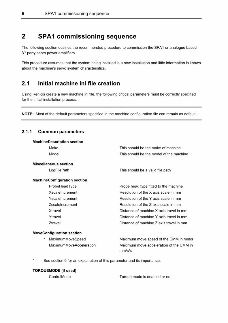
2.1.1 Common parameters

MachineDescription section Make This should be the make of machine

Model This should be the model of the machine

Miscellaneous section LogFilePath This should be a valid file path

MachineConfiguration section ProbeHeadType Probe head type fitted to the machine XscaleIncrement Resolution of the X axis scale in mm YscaleIncrement Resolution of the Y axis scale in mm ZscaleIncrement Resolution of the Z axis scale in mm Xtravel Distance of machine X axis travel in mm Ytravel Distance of machine Y axis travel in mm Ztravel Distance of machine Z axis travel in mm

MoveConfiguration section * MaximumMoveSpeed Maximum move speed of the CMM in mm/s MaximumMoveAcceleration Maximum move acceleration of the CMM in

mm/s/s

* See section 0 for an explanation of this parameter and its importance.

TORQUEMODE (if used) ControlMode Torque mode is enabled or not

SPA1 commissioning sequence 7

MachineIOLogic AmpifierOK Logic level active high or low CMMdeclutch Logic level active high or low ESTOPtripped Logic level active high or low AirPressureLow Logic level active high or low ZaxisCrash Logic level active high or low MotorsEngaged Logic level active high or low OuterLimitXPositive Logic level active high or low OuterLimitXNegative Logic level active high or low OuterLimitYPositive Logic level active high or low OuterLimitYNegative Logic level active high or low OuterLimitZPositive Logic level active high or low OuterLimitZNegative Logic level active high or low InnerLimitXPositive Logic level active high or low InnerLimitXNegative Logic level active high or low InnerLimitYPositive Logic level active high or low InnerLimitYNegative Logic level active high or low InnerLimitZPositive Logic level active high or low InnerLimitZNegative Logic level active high or low OuterLimitY2Positive Logic level active high or low OuterLimitY2Negative Logic level active high or low InnerLimitY2Positive Logic level active high or low InnerLimitY2Negative Logic level active high or low

DUALY section (if fitted) DualAxisScaleIncrement Resolution of the dual axis scale in mm WhichAxisDual Which axis is the dual axis DualDriveEnable Is the dual drive switched on ScaleInputLocation UCC input location address DriveOutputLocation UCC output location address

RotaryTable (if fitted) MeasurementUnits Units of increment for the rotary table WscaleIncrement Resolution of the W axis scale WmaximumMoveSpeed Maximum move speed of the rotary table WmaximumMoveAcceleration Maximum move acceleration of the rotary table

SPAX ChannelNumber = 0 SPAType = SPA1

SPAY ChannelNumber = 1 SPAType = SPA1

SPAZ ChannelNumber = 2 SPAType = SPA1


2.1.2 Machine and move configuration

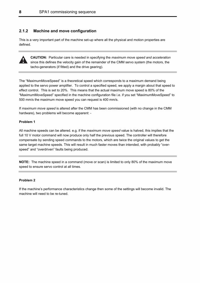
This is a very important part of the machine set-up where all the physical and motion properties are defined.

CAUTION: Particular care is needed in specifying the maximum move speed and acceleration since this defines the velocity gain of the remainder of the CMM servo system (the motors, the tacho-generators (if fitted) and the drive gearing).

The “MaximumMoveSpeed” is a theoretical speed which corresponds to a maximum demand being applied to the servo power amplifier. To control a specified speed, we apply a margin about that speed to effect control. This is set to 20%. This means that the actual maximum move speed is 80% of the “MaximumMoveSpeed” specified in the machine configuration file i.e. if you set “MaximumMoveSpeed” to 500 mm/s the maximum move speed you can request is 400 mm/s.

If maximum move speed is altered after the CMM has been commissioned (with no change in the CMM hardware), two problems will become apparent: -

Problem 1

All machine speeds can be altered. e.g. if the maximum move speed value is halved, this implies that the full 10 V motor command will now produce only half the previous speed. The controller will therefore compensate by sending speed commands to the motors, which are twice the original values to get the same target machine speeds. This will result in much faster moves than intended, with probably “over-speed” and “overdriven” faults being produced.

NOTE: The machine speed in a command (move or scan) is limited to only 80% of the maximum move speed to ensure servo control at all times.

Problem 2

If the machine’s performance characteristics change then some of the settings will become invalid. The machine will need to be re-tuned.

!


2.2 Renicis sequence

2.2.1 Initial steps

1. Start the commissioning process by ensuring the step icon on the toolbar is not indented and then click on the GO icon on the toolbar, as shown in the figure 1 below:

Figure 1

2. The Renicis commissioning step list will now be displayed within a window that will open on the desktop, as shown in the figure 2 below:

Figure 2

3. Highlight the Welcome step within the list and then click on the GoToStep button to start the commissioning process.

4. Proceed through the following Renicis steps following the instructions:

• Welcome

• Connector and interface details

• Check CMM

• Test link

• Emergency stop

• Other safety matters

• Check read heads


5. If problems are experienced with any of the above steps, refer to the Renicis user guide (Renishaw part number H-1000-5058) or the appropriate UCC1, UCClite or UCC2 installation guide.

2.2.2 Close position loop

For the following tests the CMM motors will frequently be engaged by Renicis in either open or closed loop modes. To reduce the risk of damage or injury the user is advised to disable the motors (and amplifiers) on axes which are not active in any given test until such time as all axes are set up and operating correctly.

WARNING: At this stage, the user should be aware that the CMM motors are being engaged for the first time and that incorrect wiring or other drive faults may cause unpredictable machine behaviour. The user must have unobstructed access to the emergency stop switch, and all other personnel must be kept away from the working region of the CMM.

A prompt screen will be displayed for user input to confirm that it is possible for Renicis to engage all the drives for a very brief period (0.5 s) to assess the stability of the servo loops.

If the operator confirms that there were no unexpected moves after the initial servo stability test, the operator will be prompted to engage the drives for a small movement (5 mm), again to test for servo instability.

If the operator confirms the machine to be stable in both these tests, Renicis will assume that it is safe to move the CMM with the position loop closed during the subsequent Renicis tuning stages.

NOTE: Each time Renicis is restarted it has to ask the operator whether the CMM is safe to use in closed-loop moves and if the answer is “no” the operator will be warned before engaging the drives

!


2.2.3 Set offset PA controls

The purpose of this step is to permit any servo offset apparent on the UCC controllers to be matched with the servo power amplifier fitted to the system.

The following system preparations are advised prior to the operator progressing through the steps of the Renicis commissioning process:

• Move the quill of the machine to approximately the centre of its working volume, to permit freedom of movement during this tuning step.

• The power amplifier gain (sometimes called the ‘P’ or ‘Proportional gain’ term) should be set at a very low level to give a low speed of movement.

• Any Integral (I) or Derivative (D) terms used on the power amplifier should be turned to zero or at least to their minimum settings and set any offset adjustment to the middle of its travel.

Following the operator prompt, Renicis will engage the drives for the X, Y (1 & 2), Z and W axes (as appropriate) with a velocity demand of zero. The operator can now adjust the servo power amplifier's offset control to minimise any machine movement (drift) for all axes.

NOTE: The rotary table (W axis) will only be displayed if it is enabled. The Y2 axis will also only be displayed if it is enabled.

Figure 3

The detected machine velocity is shown in the screen (see above) as a bar graph for each axis.

The arrow shown in the 'Z-axis' bar example indicates that the velocity is increasing in the negative direction. When a value is beyond the displayable maximum, but decreasing, the arrow will be displayed pointing toward the null (centre of display) position.

By 'right-clicking' on the display, it is possible to modify the default settings for the display these include the maximum (+ve and -ve) displayed value and the threshold value at which the bar colour will change from green (an 'acceptable value') to red.


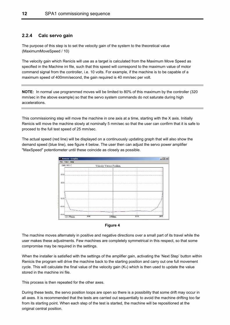
2.2.4 Calc servo gain

The purpose of this step is to set the velocity gain of the system to the theoretical value (MaximumMoveSpeed / 10)

The velocity gain which Renicis will use as a target is calculated from the Maximum Move Speed as specified in the Machine ini file, such that this speed will correspond to the maximum value of motor command signal from the controller, i.e. 10 volts. For example, if the machine is to be capable of a maximum speed of 400mm/second, the gain required is 40 mm/sec per volt.

NOTE: In normal use programmed moves will be limited to 80% of this maximum by the controller (320 mm/sec in the above example) so that the servo system commands do not saturate during high accelerations.

This commissioning step will move the machine in one axis at a time, starting with the X axis. Initially Renicis will move the machine slowly at nominally 5 mm/sec so that the user can confirm that it is safe to proceed to the full test speed of 25 mm/sec.

The actual speed (red line) will be displayed on a continuously updating graph that will also show the demand speed (blue line), see figure 4 below. The user then can adjust the servo power amplifier "MaxSpeed" potentiometer until these coincide as closely as possible.

Figure 4

The machine moves alternately in positive and negative directions over a small part of its travel while the user makes these adjustments. Few machines are completely symmetrical in this respect, so that some compromise may be required in the settings.

When the installer is satisfied with the settings of the amplifier gain, activating the ‘Next Step’ button within Renicis the program will drive the machine back to the starting position and carry out one full movement cycle. This will calculate the final value of the velocity gain (Kv) which is then used to update the value stored in the machine ini file.

This process is then repeated for the other axes.

During these tests, the servo position loops are open so there is a possibility that some drift may occur in all axes. It is recommended that the tests are carried out sequentially to avoid the machine drifting too far from its starting point. When each step of the test is started, the machine will be repositioned at the original central position.


2.2.5 Velocity loop tuning

This test moves the CMM forwards and backwards by the distance entered. This movement will normally be shown complete on the graph against time. Selecting 'fwd + rev. move superimposed' will invert the reverse trace and display it against the forward trace so that an easier comparison may be made.

1. It is recommended that initially the tests are completed on individual axis, the X axis is selected by deselecting the Y and Z axis check boxes.

2. Run the test, to start with by clicking the Go button. Check the operate continuously box to keep the machine moving, otherwise the machine will stop after one cycle.

NOTE: If the machine is unstable, it is recommended that the proportional gain pot is reduced until you have stability and can continue with the tests.

Increasing the acceleration value for this test will give a sharper square wave stimulus to the machine. The test will not change the maximum acceleration value stored in the UCC Configuration File.

Figure 5

If the machine response amplitude does not match the demand you could get the following message:

Figure 6

Check the machine is still in the centre of its operating range, move it if necessary, click on the OK button, click on the reset data button, then adjust the gain setting and continue the test by clicking on GO.


2.2.6 Adjustment of proportional and integral gains

Initially the response displayed may look as shown in figure 7 below:

Figure 7

The objective is to get the machine response (blue line) as close to the demand (red line) but with no or minimal overshoot. The optimum performance will require some adjustment of the gains and these should be varied to confirm that no further improvements can be obtained. When complete the response should look something like:

Figure 8

When the system has been tuned it is recommended that the machine speed for the velocity loop test is reduced to match the default trigger / scanning speed and the test is repeated to ensure that the system response is still tuned.

NOTE: If it is necessary to change the tuning settings for the trigger / scanning speed then these values are recommended to be used for the installation.


2.3 Renicis position loop tuning

NOTE: To keep the machine response “balanced”, the same tuning parameter values must be used for all axes, with the exception of acceleration feedback.

2.3.1 Setting the uncompensated gain

In this section we will be increasing the uncompensated gain KP to a safe maximum before switching on any conditioning filters. To do this, it is necessary to run a three axis move.

1. Ensure button is not depressed and operate the button on the RENICIS toolbar. Highlight the “Uncompensated Gain Test” step, run the “Uncompensated Gain Test” by clicking the “Go to Step” button.

2. Follow the instructions given until the test dialog is displayed, refer to figure 9. Ensure that the default value of 0.2 is indicated, then click on the "Go" button. The machine should move in a forward and reverse cycle in all three axes and the following error present during the move displayed on the graphs. Examine the graphs produced (refer to figure 10).

Figure 9

3. If the machine runs smoothly and no periodic oscillations are apparent (refer to figure 10). The uncompensated gain can be increased (either directly in the edit box, or by clicking on the upper 'spin' button to the right of the edit box) by approximately 10%, now referred to as KP1, and the test repeated by clicking on the "Go" button again.

Continue increasing the value of KP1 until one of the axes reaches the brink of instability (refer to figure 11), then reduce the value by approximately 20% to give a stability margin and re-check for stability. If the system is stable and no oscillations are apparent then this value is called the “Uncompensated Proportional Gain” KP2 (and is set automatically to be the same for all axes).

NOTE: On some systems, and with very low gains, it is possible that timeouts will occur during the move. Should this occur, increase the position tolerance by changing the value in the edit box provided. The new value will take effect at the beginning of the next move, i.e. it will not make any effect whilst the system is moving.


Figure 10

Figure 11

If any axes become unstable (Y axis in figure 11), reduce KP1 by 20% and check again, see step 2.

NOTE: All axes must have the same KP1. The value of KP2 must be such that ALL axes display stability.


2.3.2 Applying acceleration feedback

Acceleration feedback is another level of control that selectively increases the apparent inertia of the machine, allowing us to increase the gain still further before the machine becomes unstable. Machines react in different ways to acceleration feedback so the amount of gain increase can vary between zero and ten times.

NOTE: Experience has shown that the use of acceleration feedback is usually not required and therefore not recommended for machines that have an uncompensated gain of ≥ 0.2.

1. The first stage is to increase the proportional uncompensated gain value so that the machine is just unstable using the uncompensated gain step, refer to 2.3.1, record which axes are unstable.

2. It is now necessary to activate the acceleration feedback term (KA ) in the axes that are unstable.

• Enter the machine configuration screen

• Select the "ServoConfiguration" tab and scroll down to locate the edit boxes for the acceleration feedback terms KA(X), KA(Y) and KA(Z).

• Set the initial acceleration feedback value (KA) for the axis that has shown signs of instability to 0.00005. Repeat for each unstable axis (Note: For any stable axes the acceleration feedback value remains set to zero).

• Check for stability by running the “Uncompensated Gain Test refer to 2.3.1

3. If the machine is stable, increasing the uncompensated gain by a further 10 – 20%. If the machine is displaying instability as for the Y axis in figure 21, increase the value of KA (refer to step 2) in the unstable axes by a further 0.00005 (to do this follow step 2) and repeat the uncompensated gain test.

• If the acceleration feedback value is too high the machine will produce an audible singing and must be reduced by 10 to 20 % in the unstable axes. Run the “Uncompensated Gain Test refer to 2.3.1 to ensure the machine is stable. If it is not stable repeat this step.

4. Repeat these steps, raising the values of KA and KP1 until final values of KA and KP are found (see figure 22). The final value of KP obtained during this process is referred to as KP3.

This will be the new “Uncompensated Gain”.

NOTE: It is necessary to increase the amount of acceleration feedback slowly in iterative steps as shown in figure 12, so that the maximum value of KP can be found. This is in the peak between gain induced instability line and acceleration induced instability line. The consequence of increasing the acceleration feedback in one large step without increasing the proportional gain on intermediate steps is illustrated in figure 13, note the final value of KP is far lower than in that obtained in figure 12.

Once the values for acceleration feedback are determined they must be left unchanged. Their values may be different, but the value of KP3 must be the same for each axis.


Figure 12

Figure 13

NOTE: At this point, if the positioning is good enough (within specifications), then no further tuning will be necessary.


2.4 Servo tuning test

The servo tuning test is used to check the steady state error for the installation

Ensure button is not depressed and operate the button on the RENICIS toolbar. Highlight the “Servo Tuning” step on the list of steps, run the “Servo Tuning” test by clicking the “Go to Step” button.

The dialog box shown in figure 14 will appear:

Figure 14

If a position tolerance, other than the default 100 microns, was required to prevent timeouts during moves with the uncompensated gain value, enter the same tolerance in edit box provided here. If you know what your desired steady-state error is then enter that value also.

In the above screen-shot (figure 24), the system bandwidth has been previously determined and saved in the machine configuration file. The operator has elected to use this value, thus alleviating the requirement for the system bandwidth part of servo tuning to be run.


Start the test by clicking on the ‘Start’ button. The test may be aborted at any time after starting. The following dialog picture (figure 15) shows the first move in progress:

Figure 15

At the beginning of this test, four different moves are performed and a worst-case steady-state error value determined and displayed. You may wish to wait until this value is displayed before entering your desired value, in which case, ensure that the 'Pause …' check-box has been checked before clicking on the 'Start' button.

If the desired steady state error is achieved at the end of this test then the following screen will appear, see figure 16, stating that performance will be degraded if the test is continued and filter parameters calculated.

Figure 16

If the desired steady state error is not achieved then, the system bandwidth is determined by performing a series of sinusoidal moves in each axis to calculate the system gain. The above screen-shot (figure 15) shows that the system bandwidth has not yet been determined.

Once the bandwidth has been determined, the new values for proportional gain and filters are calculated, saved and sent to the controller. The system then performs a full 'Performance Test'. Once this is complete, the 'View Report' button will be enabled, allowing the results of the Performance test to be reviewed. With 'All Results' unchecked, only the worst-case results will be displayed in the report. With 'All Results' checked, all results will be displayed in the report. From the report viewer, the report may be saved for future viewing.

At the end of this test the option is given to enter the Manual Servo Tuning screen where it is possible to check the machine performance. The Manual Servo Tuning step can also be accessed from the Utilities menu.


2.4.1 Servo tuning objectives

The servo tuning objective is to find the controller parameters that meet the performance requirements for a specific application.

Typical requirements are:

• Stability

• High disturbance rejection (reflected through a high proportional gain)

• Steady state error required (precision achievable)

• Very little or no overshoot

• Small rise time and small settling time i.e. quick response

• Small tunnelling error (specified by user) for trajectory following applications

The following table shows the effect of a change in the controller parameters. It is a guidance table for the effect of change in proportional gain, lead or lag terms in the system.

NOTE: The following is valid only if all three parameters are used.

Speed of response Overshoot Stability Precision

steady state

KP (Higher) (Higher) Better

(Higher) Worse

(Lower) Worse

(Higher) Better

KP (Lower) (Lower) Worse

(Lower) Better

(Higher) Better

(Lower) Worse

Ta2 (Higher) (Lower) Worse

(Higher) Worse

(Higher) Better

No Effect

Ta2 (Lower) (Higher) Better

(Lower) Better

(Lower) Worse

No Effect

Ta1 (Higher) (Higher) Better

(Lower) Better

(Lower) Worse

No Effect

Ta1 (Lower) (Lower) Worse

(Higher) Worse

(Higher) Better

No Effect

KP is the proportional gain of the controller.

Ta1 is the time constant corresponding to the zero.

A higher value for Ta1 means higher lead.

Ta2 is the time constant corresponding to the pole.

A higher value for Ta2 means higher lag.

As the table shows, the parameters are inter-dependent making the tuning process far from trivial.


2.4.2 Applying velocity feed-forward

1. Activate the manual servo tuning test.

2. Select tests 3 and 4 as shown in figure 17 below:

Figure 17

3. Click the Start button to run the selected tests initially with no value in the Vff input box. When the test has completed note the values of peak following error and overshoot for all axes. The results shown in figure 17 show a low value for the overshoot but a high following error.

4. Now add Vff, 0.01 is a good starting value and run the test again.

Figure 18

You can see the results shown in figure 18 give a much reduced following error and very little change in overshoot.


5. Increasing Vff further will reduce following error, however if too much is applied overshoot will increase to excessive levels and the machine may become unstable whilst performing the point to point moves. Some experimentation in the Vff value will be required. Figure 19 below shows the effect of applying too much Vff. Although the following error has reduced to a low value the amount of overshoot has increased significantly.

Figure 19

2.4.3 Scanning tuning procedure

For information with respect to best tuning practices when using the Renishaw controller product range, the commissioning tool used to enable the system to be tuned for scanning capability is UCCassist, please refer to H-1000-5224 for further information.

24 Rotary table tuning procedure


3.1 Overview

To activate the tuning procedure within Renicis for the rotary table, it is necessary to have a suitable system hardware configuration and the machine’s configuration file must indicate that a rotary table is installed in the system.

When the rotary table is installed and configured, options within the Set offset PA controls, Calc servo gain and velocity loop tuning screens will be included.

An additional step will be included in the Renicis step list, this is the position loop tuning screen for the rotary table. As shown in figure 20.

Figure 20

3.1.1 Initial settings

The initial values recommended for the rotary table tuning that have been obtained from experience are listed below: Target velocity (deg/sec) 25 Acceleration (deg/sec/sec) 75 Distance (degrees) 50 Step delay (ms) 1000

Rotary table tuning procedure 25

3.2 Tuning

3.2.1 Velocity loop tuning

Select the W check box, this will only be active (enabled) when a rotary table is both detected and enabled.

NOTE: It is not possible to perform a move in all four axes simultaneously. Selecting the 'W' axis will automatically disable the other axes.

Initially run test using the default values by clicking the Go button.

Figure 21


3.2.2 Position loop tuning Initially run with the default values.

Figure 22

By clicking the ‘Edit’ button you can change the proportional gain. The default value of 1 for W proportional gain should be suitable in most cases. A graph of position demand similar to the one shown should be seen. It is unlikely that this value of proportional gain will need change unless instability is experienced.

Figure 23

Definitions 27

4 Definitions

4.1 Uncompensated gain

The maximum stable gain (with a safety margin) that can be used to compensate the position error without the use of the lead and lag filters.

4.2 Acceleration feedback

A high proportional gain is desirable for a high disturbance rejection and better precision (smaller steady state error).

To allow a higher proportional gain, feedback from the acceleration acts as an electronic inertia which pushes the upper limit for the proportional gain.

Furthermore, this does not interfere with any other control that may be added later (filters, etc). Thus you will be able to start at the point where you first have to tune the gain, only this time your upper limit is higher.

4.3 Dynamic integrator

To be able to increase the proportional gain, an acceleration dependent, rate-varying lag that prevents windup is used.

One might expect that a higher gain and lag term would induce a high overshoot, but the dynamic integrator peels off the effect of integration (lag) as the target is approached. When the target is hit, the effect of integration (which would have induced the overshoot) is eliminated. Once stationary again, the effect of the integrator is re-applied. Consequently, it is possible to have very high gains leading to a high precision and high disturbance rejection.

To summarise, the integration is applied when needed and cancelled (gradually) when it is not needed (and becomes undesirable).

4.4 Velocity feed-forward

Velocity feed-forward helps reduce the following error and increase the responsiveness of the system, consequently reducing overshoot due to delay.

It is particularly useful for short moves used with a relatively high acceleration.

This can be seen as a gain on the error that is proportional to the velocity profile which is high at constant speed and gradually increases during acceleration and decreases during deceleration.

Too much gain on velocity feed-forward will result in a higher overshoot for the system’s response.

28 Definitions

4.5 I2t Time

The amount of time for which peak motor current is allowed to flow. If this is exceeded a fault is software generated to protect against motor over heating. Continuous current, or anything less, will be allowed to flow for unlimited time without fault.

4.6 IET Time

This is the current error time limit and will occur if there is a break in the loop after the DSP (e.g. no motor power or motor not connected) or if the current servo is badly tuned. This is a software generated fault that protects against excessive servo error in the current loop.

4.7 Overshoot (per axis)

The overshoot will be computed in absolute terms i.e.

Overshoot = max value of read position – Steady State Position.

4.8 Following error (per axis, already existing)

Following Error (t) = Read position (t) – Demand position (t)

Typical Following Error = Following Error (mid_time) averaged over 10 readings.

4.9 Steady state error (per axis)

Steady State Error = absolute value (mean(last 10 points of read position) – Target position).

NOTE: This includes the RMS noise.

4.10 Settling time (per axis)

The settling time is the time difference between the theoretical time to get to HOLD and the time measured to get to HOLD.

4.11 Tunnelling error (for the 3D move)

The tunnelling error is the maximum distance between the two curves (real and demand) and is the distance between the point read (measured) and its projection on the demand vector.

NOTE: The distance between two points in space is the modulus of the vector formed by these two points (direction is not relevant here).

Revision history 29

5 Glossary of terms fB = The frequency corresponding to the –3dB point

KA = Acceleration feedback gain

KA(X) = Acceleration feedback gain for the “X” axis

KA(Y) = Acceleration feedback gain for the “Y” axis

KA(Z) = Acceleration feedback gain for the “Z” axis

Kdi = Dynamic integrator gain

Kdi(X) = Dynamic integrator gain for the “X” axis

Kdi(Y) = Dynamic integrator gain for the “Y” axis

Kdi(Z) = Dynamic integrator gain for the “Z” axis

KP = Proportional gain (V/mm of error)

KP1 = Initial value of KP used at the start of the tuning process

KP2 = Uncompensated gain – final value of KP obtained before applying the acceleration feedback or dynamic integrator terms

KP3 = Final value of KP obtained after acceleration feedback but before applying the dynamic integrator term

KP4 = Final value of KP necessary to produce the required positioning accuracy with the dynamic integrator applied

KV = Velocity gain (mm/s/V)

This value will have been used when setting the servo power amplifier sensitivity control

PE = Positioning accuracy before the dynamic integrator

PR = Required positioning accuracy

Ta1 = “Lead” filter constant

Ta2 = “Lag” filter constant

Kvffx = X axis Velocity Feed-forward gain

Kvffy = Y axis Velocity Feed-forward gain

Kvffz = Z axis Velocity Feed-forward gain

30 Appendix

6 Revision history

6.1 What’s new in release 01-A

1. First issue.


1. Entire document has been split into sections.

2. Page numbers have changed.

3. Updated to account for RENICIS changes.

4. Minor changes for latest RENICIS release.


1. Page numbers have changed.

2. Updated to account for additions in control and performance evaluation.

3. Updated to include recommendation for power amplifier tuning.

4. Updated to account for RENICIS changes.

5. Addition of section “Tuning for scanning”.

6. Addition of section “Performance indices”.


1. Page and sections numbers change.

2. Inclusion of “Rotary table tuning” section.


1. Minor graphical and grammatical clarification.

6.6 What’s new in release 05-B

1. Document title changed from ‘UCC1 universal CMM controller servo tuning guide’ to ‘SPA1 servo tuning guide’.


1. Major document re-structure to follow the structure used in other Renishaw tuning guides and changes in Renicis software.

6.8 What’s new in release 06-B

1. UCClite information added.

Renishaw plc

New Mills, Wotton-under-Edge,Gloucestershire, GL12 8JRUnited Kingdom

T +44 (0)1453 524524F +44 (0)1453 524901E [email protected]

www.renishaw.com

*H-1000-5227-06*

Renishaw worldwide

Australia

T +61 3 9521 0922

E [email protected]

Austria

T +43 (0) 2236 379790

E [email protected]

Brazil

T +55 11 4195 2866

E [email protected]

The People’s Republic of China

T +86 10 8448 5306

E [email protected]

Canada

T +1 905 828 0104

E [email protected]

Czech Republic

T +420 548 216 553

E [email protected]

France

T +33 1 64 61 84 84

E [email protected]

Germany

T +49 (0) 7127 981-0

E [email protected]

Hong Kong

T +852 2753 0638

E [email protected]

Hungary

T +36 23 502 183

E [email protected]

India

T +91 80 25320 144

E [email protected]

Israel

T +972 4 953 6595

E [email protected]

Italy

T +39 011 966 10 52

E [email protected]

Japan

T +81 3 5366 5315 (or 5324)

E [email protected]

The Netherlands

T +31 76 543 11 00

E [email protected]

Poland

T +48 22 577 1180

E [email protected]

Russia

T +7 495 231 1677

E [email protected]

Singapore

T +65 6897 5466

E [email protected]

Slovenia

T +386 (1) 527 2100

E [email protected]

South Korea

T +82 2 2108 2830

E [email protected]

Spain

T +34 93 663 3420

E [email protected]

Sweden

T +46 (0)8 584 90 880

E [email protected]

Switzerland

T +41 55 415 50 60

E [email protected]

Taiwan

T +886 4 2251 3665

E [email protected]

Thailand

T +66 2746 9811

E [email protected]

Turkey

T +90 216 380 92 40

E [email protected]

UK (Head Offi ce)

T +44 (0)1453 524524

E [email protected]

USA

T +1 847 286 9953

E [email protected]

For all other countries

T +44 1453 524524

E [email protected]

SPA1 servo tuning guide - Renishaw resource centre

Documents

Transcript of SPA1 servo tuning guide - Renishaw resource centre