Learning Compressed Transformswith Low Displacement Rank

Anna T. Thomas∗†, Albert Gu∗†, Tri Dao†, Atri Rudra‡, and Christopher Ré†

†Department of Computer Science, Stanford University‡Department of Computer Science and Engineering, University at Buffalo, SUNY

{thomasat,albertgu,trid}@stanford.edu, atri@buffalo.edu,chrismre@cs.stanford.edu

January 3, 2019

Abstract

The low displacement rank (LDR) framework for structured matrices represents a matrix through twodisplacement operators and a low-rank residual. Existing use of LDR matrices in deep learning has appliedfixed displacement operators encoding forms of shift invariance akin to convolutions. We introduce a classof LDR matrices with more general displacement operators, and explicitly learn over both the operatorsand the low-rank component. This class generalizes several previous constructions while preservingcompression and efficient computation. We prove bounds on the VC dimension of multi-layer neuralnetworks with structured weight matrices and show empirically that our compact parameterization canreduce the sample complexity of learning. When replacing weight layers in fully-connected, convolutional,and recurrent neural networks for image classification and language modeling tasks, our new classes exceedthe accuracy of existing compression approaches, and on some tasks also outperform general unstructuredlayers while using more than 20x fewer parameters.

1 IntroductionRecent years have seen a surge of interest in structured representations for deep learning, motivated byachieving compression and acceleration while maintaining generalization properties. A popular approachfor learning compact models involves constraining the weight matrices to exhibit some form of dense butcompressible structure and learning directly over the parameterization of this structure. Examples of structuresexplored for the weight matrices of deep learning pipelines include low-rank matrices [15, 42], low-distortionprojections [49], (block-)circulant matrices [8, 17], Toeplitz-like matrices [34, 45], and constructions derivedfrom Fourier-related transforms [37]. Though they confer significant storage and computation benefits, theseconstructions tend to underperform general fully-connected layers in deep learning. This raises the question ofwhether broader classes of structured matrices can achieve superior downstream performance while retainingcompression guarantees.

Our approach leverages the low displacement rank (LDR) framework (Section 2), which encodesstructure through two sparse displacement operators and a low-rank residual term [27]. Previous workstudying neural networks with LDR weight matrices assumes fixed displacement operators and learns onlyover the residual [45, 50]. The only case attempted in practice that explicitly employs the LDR frameworkuses fixed operators encoding shift invariance, producing weight matrices which were found to achieve superiordownstream quality than several other compression approaches [45]. Unlike previous work, we considerlearning the displacement operators jointly with the low-rank residual. Building upon recent progress onstructured dense matrix-vector multiplication [14], we introduce a more general class of LDR matrices and

∗These authors contributed equally.

1

arX

iv:1

810.

0230

9v3

[cs

.LG

] 1

Jan

201

9

develop practical algorithms for using these matrices in deep learning architectures. We show that theresulting class of matrices subsumes many previously used structured layers, including constructions thatdid not explicitly use the LDR framework [17, 37]. When compressing weight matrices in fully-connected,convolutional, and recurrent neural networks, we empirically demonstrate improved accuracy over existingapproaches. Furthermore, on several tasks our constructions achieve higher accuracy than general unstructuredlayers while using an order of magnitude fewer parameters.

To shed light on the empirical success of LDR matrices in machine learning, we draw connections torecent work on learning equivariant representations, and hope to motivate further investigations of this link.Notably, many successful previous methods for compression apply classes of structured matrices relatedto convolutions [8, 17, 45]; while their explicit aim is to accelerate training and reduce memory costs, thisconstraint implicitly encodes a shift-invariant structure that is well-suited for image and audio data. Weobserve that the LDR construction enforces a natural notion of approximate equivariance to transformationsgoverned by the displacement operators, suggesting that, in contrast, our approach of learning the operatorsallows for modeling and learning more general latent structures in data that may not be precisely known inadvance.

Despite their increased expressiveness, our new classes retain the storage and computational benefits ofconventional structured representations. Our construction provides guaranteed compression (from quadraticto linear parameters) and matrix-vector multiplication algorithms that are quasi-linear in the number ofparameters. We additionally provide the first analysis of the sample complexity of learning neural networkswith LDR weight matrices, which extends to low-rank, Toeplitz-like and other previously explored fixedclasses of LDR matrices. More generally, our analysis applies to structured matrices whose parameters caninteract multiplicatively with high degree. We prove that the class of neural networks constructed from thesematrices retains VC dimension almost linear in the number of parameters, which implies that LDR matriceswith learned displacement operators are still efficiently recoverable from data. This is consistent with ourempirical results, which suggest that constraining weight layers to our broad class of LDR matrices can reducethe sample complexity of learning compared to unstructured weights.

We provide a detailed review of previous work and connections to our approach in Appendix B.

Summary of contributions:

• We introduce a rich class of LDR matrices where the displacement operators are explicitly learned fromdata, and provide multiplication algorithms implemented in PyTorch (Section 3).1

• We prove that the VC dimension of multi-layer neural networks with LDR weight matrices, whichencompasses a broad class of previously explored approaches including the low-rank and Toeplitz-likeclasses, is quasi-linear in the number of parameters (Section 4).

• We empirically demonstrate that our construction improves downstream quality when compressingweight layers in fully-connected, convolutional, and recurrent neural networks compared to previouscompression approaches, and on some tasks can even outperform general unstructured layers (Section 5).

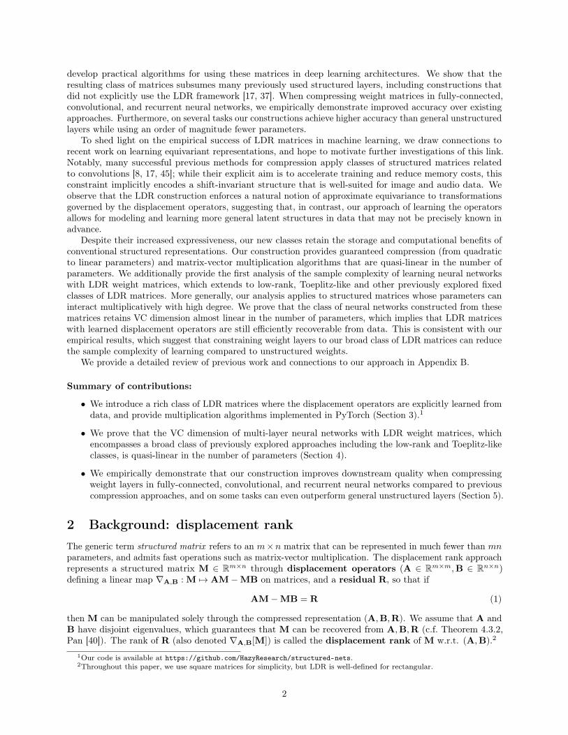
2 Background: displacement rankThe generic term structured matrix refers to an m×n matrix that can be represented in much fewer than mnparameters, and admits fast operations such as matrix-vector multiplication. The displacement rank approachrepresents a structured matrix M ∈ Rm×n through displacement operators (A ∈ Rm×m,B ∈ Rn×n)defining a linear map ∇A,B : M 7→ AM−MB on matrices, and a residual R, so that if

AM−MB = R (1)

then M can be manipulated solely through the compressed representation (A,B,R). We assume that A andB have disjoint eigenvalues, which guarantees that M can be recovered from A,B,R (c.f. Theorem 4.3.2,Pan [40]). The rank of R (also denoted ∇A,B[M]) is called the displacement rank of M w.r.t. (A,B).2

1Our code is available at https://github.com/HazyResearch/structured-nets.2Throughout this paper, we use square matrices for simplicity, but LDR is well-defined for rectangular.

2

The displacement approach was originally introduced to describe the Toeplitz-like matrices, which arenot perfectly Toeplitz but still have shift-invariant structure [27]. These matrices have LDR with respect

to shift/cycle operators. A standard formulation uses A = Z1,B = Z−1, where Zf =

[01×(n−1) f

In−1 0(n−1)×1

]

denotes the matrix with 1 on the subdiagonal and f in the top-right corner. The Toeplitz-like matrices havepreviously been applied in deep learning and kernel approximation, and in several cases have performedsignificantly better than competing compressed approaches [10, 34, 45]. Figure 1 illustrates the displacement (1)for a Toeplitz matrix, showing how the shift invariant structure of the matrix leads to a residual of rank atmost 2.

11

. . .

1

a0 a1 · · · an−1

a−1 a0. . .

......

. . .. . . a1

a−(n−1) · · · a−1 a0

−

a0 a1 · · · an−1

a−1 a0. . .

......

. . .. . . a1

a−(n−1) · · · a−1 a0

−11

. . .

1

=

x · · · y 2a0z...w

Figure 1: Displacement equation for a Toeplitz matrix with respect to shift operators Z1,Z−1.

A few distinct classes of useful matrices are known to satisfy a displacement property: the classic types arethe Toeplitz-, Hankel-, Vandermonde-, and Cauchy-like matrices (Appendix C, Table 5), which are ubiquitousin other disciplines [40]. These classes have fixed operators consisting of diagonal or shift matrices, and LDRproperties have traditionally been analyzed in detail only for these special cases. Nonetheless, a few elegantproperties hold for generic operators, stating that certain combinations of (and operations on) LDR matricespreserve low displacement rank. We call these closure properties, and introduce an additional block closureproperty that is related to convolutional filter channels (Section 5.2).

We use the notation DrA,B to refer to the matrices of displacement rank ≤ r with respect to (A,B).

Proposition 1. LDR matrices are closed under the following operations:

(a) Transpose/Inverse If M ∈ DrA,B, then MT ∈ DrBT ,AT and M−1 ∈ DrB,A.

(b) Sum If M ∈ DrA,B and N ∈ DsA,B, then M + N ∈ Dr+sA,B.

(c) Product If M ∈ DrA,B and N ∈ DsB,C, then MN ∈ Dr+sA,C.

(d) Block Let Mij satisfy Mij ∈ DrAi,Bjfor i = 1 . . . k, j = 1 . . . `. Then the k × ` block matrix (Mij)ij

has displacement rank rk`.

Proposition 1 is proved in Appendix C.

3 Learning displacement operatorsWe consider two classes of new displacement operators. These operators are fixed to be matrices withparticular sparsity patterns, where the entries are treated as learnable parameters.

The first operator class consists of subdiagonal (plus corner) matrices: Ai+1,i, along with the cornerA0,n−1, are the only possible non-zero entries. As Zf is a special case matching this sparsity pattern, thisclass is the most direct generalization of Toeplitz-like matrices with learnable operators.

The second class of operators are tridiagonal (plus corner) matrices: with the exception of the outercorners A0,n−1 and An−1,0, Ai,j can only be non-zero if |i−j| ≤ 1. Figure 2 shows the displacement operatorsfor the Toeplitz-like class and our more general operators. We henceforth let LDR-SD and LDR-TD denotethe classes of matrices with low displacement rank with respect to subdiagonal and tridiagonal operators,respectively. Note that LDR-TD contains LDR-SD.

3

0 · · · 0 f

1 0. . . 0

... 1. . .

...

0. . . . . . . . .

0 0 . . . 1 0

0 · · · 0 x0

x1 0. . . 0

... x2. . .

...

0. . . . . . . . .

0 0 . . . xn−1 0

b0 a0 · · · 0 sc0 b1 a1 0... c1

. . . . . ....

0. . . bn−1 an−2

t 0 . . . cn−2 bn−1

Figure 2: The Zf operator (left), and our learnable subdiagonal (center) and tridiagonal (right) operators, correspondingto our proposed LDR-SD and LDR-TD classes.

Expressiveness The matrices we introduce can model rich structure and subsume many types of lineartransformations used in machine learning. We list some of the structured matrices that have LDR withrespect to tridiagonal displacement operators:

Proposition 2. The LDR-TD matrices contain:

(a) Toeplitz-like matrices, which themselves include many Toeplitz and circulant variants (including standardconvolutional filters - see Section 5.2 and Appendix C, Corollary 1) [8, 17, 45].

(b) low-rank matrices.

(c) the other classic displacement structures: Hankel-like, Vandermonde-like, and Cauchy-like matrices.

(d) orthogonal polynomial transforms, including the Discrete Fourier and Cosine Transforms.

(e) combinations and derivatives of these classes via the closure properties (Proposition 1), includingstructured classes previously used in machine learning such as ACDC [37] and block circulant layers [17].

These reductions are stated more formally and proved in Appendix C.1. We also include a diagram of thestructured matrix classes included by the proposed LDR-TD class in Figure 5 in Appendix C.1.

Our parameterization Given the parameters A,B,R, the operation that must ultimately be performedis matrix-vector multiplication by M = ∇−1

A,B[R]. Several schemes for explicitly reconstructing M fromits displacement parameters are known for specific cases [41, 44], but do not always apply to our generaloperators. Instead, we use A,B,R to implicitly construct a slightly different matrix with at most double thedisplacement rank, which is simpler to work with.

Proposition 3. Let K(A,v) denote the n × n Krylov matrix, defined to have i-th column Aiv. For anyvectors g1, . . . ,gr,h1, . . . ,hr ∈ Rn, then the matrix

r∑

i=1

K(A,gi)K(BT ,hi)T (2)

has displacement rank at most 2r with respect to A−1,B.

Thus our representation stores the parameters A,B,G,H, where A,B are either subdiagonal or tridiagonaloperators (containing n or 3n parameters), and G,H ∈ Rn×r. These parameters implicitly define thematrix (2), which is the LDR weight layer we use.

Algorithms for LDR-SD Generic and near-linear time algorithms for matrix-vector multiplication byLDR matrices with even more general operators, including both the LDR-TD and LDR-SD classes, wererecently shown to exist [14]. However, complete algorithms were not provided, as they relied on theoreticalresults such as the transposition principle [6] that only imply the existence of algorithms. Additionally, therecursive polynomial-based algorithms are difficult to implement efficiently. For LDR-SD, we provide explicit

4

and complete near-linear time algorithms for multiplication by (2), as well as substantially simplify them tobe useful in practical settings and implementable with standard library operations. We empirically comparethe efficiency of our implementation and unstructured matrix-vector multiplication in Figure 8 and Table 14in Appendix E, showing that LDR-SD accelerates inference by 3.34-46.06x for n ≥ 4096. We also showresults for the low-rank and Toeplitz-like classes, which have a lower computational cost. For LDR-TD, weexplicitly construct the K(A,gi) and K(BT ,hi) matrices for i = 1, ..., r from Proposition 3 and then applythe standard O(n2) matrix-vector multiplication algorithm. Efficient implementations of near-linear timealgorithms for LDR-TD are an interesting area of future work.

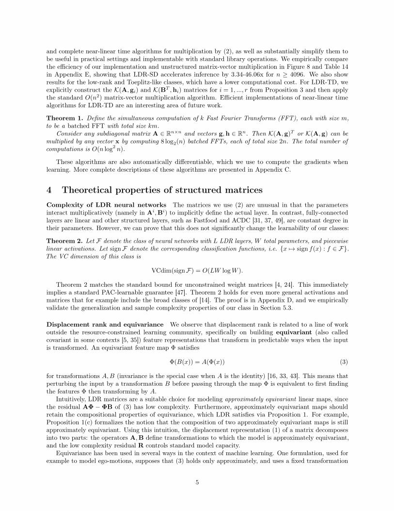
Theorem 1. Define the simultaneous computation of k Fast Fourier Transforms (FFT), each with size m,to be a batched FFT with total size km.

Consider any subdiagonal matrix A ∈ Rn×n and vectors g,h ∈ Rn. Then K(A,g)T or K(A,g) can bemultiplied by any vector x by computing 8 log2(n) batched FFTs, each of total size 2n. The total number ofcomputations is O(n log2 n).

These algorithms are also automatically differentiable, which we use to compute the gradients whenlearning. More complete descriptions of these algorithms are presented in Appendix C.

4 Theoretical properties of structured matricesComplexity of LDR neural networks The matrices we use (2) are unusual in that the parametersinteract multiplicatively (namely in Ai,Bi) to implicitly define the actual layer. In contrast, fully-connectedlayers are linear and other structured layers, such as Fastfood and ACDC [31, 37, 49], are constant degree intheir parameters. However, we can prove that this does not significantly change the learnability of our classes:

Theorem 2. Let F denote the class of neural networks with L LDR layers, W total parameters, and piecewiselinear activations. Let signF denote the corresponding classification functions, i.e. {x 7→ sign f(x) : f ∈ F}.The VC dimension of this class is

VCdim(signF) = O(LW logW ).

Theorem 2 matches the standard bound for unconstrained weight matrices [4, 24]. This immediatelyimplies a standard PAC-learnable guarantee [47]. Theorem 2 holds for even more general activations andmatrices that for example include the broad classes of [14]. The proof is in Appendix D, and we empiricallyvalidate the generalization and sample complexity properties of our class in Section 5.3.

Displacement rank and equivariance We observe that displacement rank is related to a line of workoutside the resource-constrained learning community, specifically on building equivariant (also calledcovariant in some contexts [5, 35]) feature representations that transform in predictable ways when the inputis transformed. An equivariant feature map Φ satisfies

Φ(B(x)) = A(Φ(x)) (3)

for transformations A,B (invariance is the special case when A is the identity) [16, 33, 43]. This means thatperturbing the input by a transformation B before passing through the map Φ is equivalent to first findingthe features Φ then transforming by A.

Intuitively, LDR matrices are a suitable choice for modeling approximately equivariant linear maps, sincethe residual AΦ − ΦB of (3) has low complexity. Furthermore, approximately equivariant maps shouldretain the compositional properties of equivariance, which LDR satisfies via Proposition 1. For example,Proposition 1(c) formalizes the notion that the composition of two approximately equivariant maps is stillapproximately equivariant. Using this intuition, the displacement representation (1) of a matrix decomposesinto two parts: the operators A,B define transformations to which the model is approximately equivariant,and the low complexity residual R controls standard model capacity.

Equivariance has been used in several ways in the context of machine learning. One formulation, used forexample to model ego-motions, supposes that (3) holds only approximately, and uses a fixed transformation

5

B along with data for (3) to learn an appropriate A [1, 33]. Another line of work uses the representationtheory formalization of equivariant maps [12, 28]. We describe this formulation in more detail and show howLDR satisfies this definition as well in Appendix C.3, Proposition 7. In contrast to previous settings, whichfix one or both of A,B, our formulation stipulates that Φ can be uniquely determined from A, B, and learnsthe latter as part of an end-to-end model. In Section 5.4 we include a visual example of latent structure thatour displacement operators learn, where they recover centering information about objects from a 2D imagedataset.

5 Empirical evaluationOverview In Section 5.1 we consider a standard setting of compressing a single hidden layer (SHL) neuralnetwork and the fully-connected (FC) layer of a CNN for image classification tasks. Following previouswork [7, 45], we test on two challenging MNIST variants [30], and include two additional datasets with morerealistic objects (CIFAR-10 [29] and NORB [32]). Since SHL models take a single channel as input, weconverted CIFAR-10 to grayscale for this task. Our classes and the structured baselines are tested acrossdifferent parameter budgets in order to show tradeoffs between compression and accuracy. As shown inTable 1, in the SHL model, our methods consistently have higher test accuracy than baselines for compressedtraining and inference, by 3.14, 2.70, 3.55, and 3.37 accuracy points on MNIST-bg-rot, MNIST-noise,CIFAR-10, and NORB respectively. In the CNN model, as shown in Table 1 in Appendix E, we foundimprovements of 5.56, 0.95, and 1.98 accuracy points over baselines on MNIST-bg-rot, MNIST-noise, andNORB respectively. Additionally, to explore whether learning the displacement operators can facilitateadaptation to other domains, we replace the input-hidden weights in an LSTM for a language modeling task,and show improvements of 0.81-30.47 perplexity points compared to baselines at several parameter budgets.

In addition to experiments on replacing fully-connected layers, in Section 5.2 we also replace the con-volutional layer of a simple CNN while preserving performance within 1.05 accuracy points on CIFAR-10.In Section 5.3, we consider the effect of a higher parameter budget. By increasing the rank to just 16, theLDR-SD class meets or exceeds the accuracy of the unstructured FC layer in all datasets we tested on, forboth SHL and CNN.3 Appendix F includes more experimental details and protocols. Our PyTorch code ispublicly available at github.com/HazyResearch/structured-nets.

5.1 Compressing fully-connected layersImage classification Sindhwani et al. [45] showed that for a fixed parameter budget, the Toeplitz-likeclass significantly outperforms several other compression approaches, including Random Edge Removal [11],Low Rank Decomposition [15], Dark Knowledge [25], HashedNets [7], and HashedNets with Dark Knowledge.Following previous experimental settings [7, 45], Table 1 compares our proposed classes to several baselinesusing dense structured matrices to compress the hidden layer of a single hidden layer neural network.In addition to Toeplitz-like, we implement and compare to other classic LDR types, Hankel-like andVandermonde-like, which were previously indicated as an unexplored possibility [45, 50]. We also show resultswhen compressing the FC layer of a 7-layer CNN based on LeNet in Appendix E, Table 7. In Appendix E, weshow comparisons to additional baselines at multiple budgets, including network pruning [23] and a baselineused in [7], in which the number of hidden units is adjusted to meet the parameter budget.

At rank one (the most compressed setting), our classes with learned operators achieve higher accuracythan the fixed operator classes, and on the MNIST-bg-rot, MNIST-noise, and NORB datasets even improveon FC layers of the same dimensions, by 1.73, 13.30, and 2.92 accuracy points respectively on the SHL task,as shown in Table 1. On the CNN task, our classes improve upon unstructured fully-connected layers by 0.85and 2.25 accuracy points on the MNIST-bg-rot and MNIST-noise datasets (shown in Table 7 in Appendix E).As noted above, at higher ranks our classes meet or improve upon the accuracy of FC layers on all datasetsin both the SHL and CNN architectures.

Additionally, in Figure 3 we evaluate the performance of LDR-SD at higher ranks. Note that the ratio ofparameters between LDR-SD and the Toeplitz-like or low-rank is r+1

r , which becomes negligible at higher

3In addition to the results reported in Table 1, Figure 3 and Table 7 in Appendix E, we also found that at rank 16 theLDR-SD class on the CNN architecture achieved test accuracies of 68.48% and 75.45% on CIFAR-10 and NORB respectively.

6

Table 1: Test accuracy when replacing the hidden layer with structured classes. Where applicable, rank (r) is inparentheses, and the number of parameters in the architecture is in italics below each method. Comparisons topreviously unexplored classic LDR types as well as additional structured baselines are included, with the ranksadjusted to match the parameter count of LDR-TD where possible. The Fastfood [49] and Circulant [8] methodsdo not have rank parameters, and the parameter count for these methods cannot be exactly controlled. Additionalresults when replacing the FC layer of a CNN are in Appendix E. Details for all experiments are in Appendix F.

Method MNIST-bg-rot MNIST-noise CIFAR-10 NORB

Unstructured 44.08 65.15 46.03 59.83622506 622506 1058826 1054726

LDR-TD (r = 1) 45.81 78.45 45.33 62.7514122 14122 18442 14342

Toeplitz-like [45] (r = 4) 42.67 75.75 41.78 59.3814122 14122 18442 14342

Hankel-like (r = 4) 42.23 73.65 41.40 60.0914122 14122 18442 14342

Vandermonde-like (r = 4) 37.14 59.80 33.93 48.9814122 14122 18442 14342

Low-rank [15] (r = 4) 35.67 52.25 32.28 43.6614122 14122 18442 14342

Fastfood [49] 38.13 63.55 39.64 59.0210202 10202 13322 9222

Circulant [8] 34.46 65.35 34.28 46.458634 8634 11274 7174

ranks. Figure 3 shows that at just rank 16, the LDR-SD class meets or exceeds the performance of the FClayer on all four datasets, by 5.87, 15.05, 0.74, and 6.86 accuracy points on MNIST-bg-rot, MNIST-noise,CIFAR-10, and NORB respectively, while still maintaining at least 20x fewer parameters.

Of particular note is the poor performance of low-rank matrices. As mentioned in Section 2, everyfixed-operator class has the same parameterization (a low-rank matrix). We hypothesize that the maincontribution to their marked performance difference is the effect of the learned displacement operator modelinglatent invariances in the data, and that the improvement in the displacement rank classes—from low-rankto Toeplitz-like to our learned operators—comes from more accurate representations of these invariances.As shown in Figure 3, broadening the operator class (from Toeplitz-like at r = 1 to LDR-SD at r = 1) isconsistently a more effective use of parameters than increasing the displacement rank (from Toeplitz-like atr = 1 to r = 2). Note that LDR-SD (r = 1) and Toeplitz-like (r = 2) have the same parameter count.

For the rest of our experiments outside Section 5.1 we use the algorithms in Appendix C specifically forLDR-SD matrices, and focus on further evaluation of this class on more expensive models.

Language modeling Here, we replace the input-hidden weights in a single layer long short-term memorynetwork (LSTM) for a language modeling task. We evaluate on the WikiText-2 dataset, consisting of 2Mtraining tokens and a vocabulary size of 33K [36]. We compare to Toeplitz-like and low-rank baselines, bothpreviously investigated for compressing recurrent nets [34]. As shown in Table 2, LDR-SD improves upon thebaselines for each budget tested. Though our class does not outperform the unstructured model, we did findthat it achieves a significantly lower perplexity than the fixed Toeplitz-like class (by 19.94-42.92 perplexitypoints), suggesting that learning the displacement operator can help adapt to different domains.

7

2 4 6 8 10 12 14 1620

25

30

35

40

45

50

55MNIST-bg-rot

2 4 6 8 10 12 14 1620

30

40

50

60

70

80

90MNIST-noise

2 4 6 8 10 12 14 1615

20

25

30

35

40

45

50CIFAR-10

2 4 6 8 10 12 14 1630

35

40

45

50

55

60

65

70NORB

LDR-SDToeplitz-likeLow-rankUnstructured

Rank

Test

Acc

ura

cy

Figure 3: Test accuracy vs. rank for unstructured, LDR-SD, Toeplitz-like, low-rank classes. On each dataset, LDR-SDmeets or exceeds the accuracy of the unstructured FC baseline at higher ranks. At rank 16, the compression ratio ofan LDR-SD layer compared to the unstructured layer ranges from 23 to 30. Shaded regions represent two standarddeviations from the mean, computed over five trials with randomly initialized weights.

Table 2: Test perplexity when replacing input-hidden matrices of an LSTM with structured classes on WikiText-2.An unconstrained layer, with 65536 parameters, has perplexity 117.74. Parameter budgets correspond to ranks1,2,4,8,16,24 for LDR-SD. Lower is better.

Num. Parameters LDR-SD Toeplitz-like Low-rank

2048 166.97 186.91 205.723072 154.51 177.60 179.465120 141.91 178.07 172.389216 143.60 186.52 144.4117408 132.43 162.58 135.6525600 129.46 155.73 133.37

5.2 Replacing convolutional layersConvolutional layers of CNNs are a prominent example of equivariant feature maps.4 It has been noted thatconvolutions are a subcase of Toeplitz-like matrices with a particular sparsity pattern5 [8, 45]. As channelsare simply block matrices6, the block closure property implies that multi-channel convolutional filters aresimply a Toeplitz-like matrix of higher rank (see Appendix C, Corollary 1). In light of the interpretation ofLDR of an approximately equivariant linear map (as discussed in Section 4), we investigate whether replacingconvolutional layers with more general representations can recover similar performance, without needing thehand-crafted sparsity pattern.

Briefly, we test the simplest multi-channel CNN model on the CIFAR-10 dataset, consisting of one layerof convolutional channels (3 in/out channels), followed by a FC layer, followed by the softmax layer. Thefinal accuracies are listed in Table 3. The most striking result is for the simple architecture consisting oftwo layers of a single structured matrix. This comes within 1.05 accuracy points of the highly specializedarchitecture consisting of convolutional channels + pooling + FC layer, while using fewer layers, hidden units,and parameters. The full details are in Appendix F.

4Convolutions are designed to be shift equivariant, i.e. shifting the input is equivalent to shifting the output.5E.g. a 3× 3 convolutional filter on an n×n matrix has a Toeplitz weight matrix supported on diagonals −1, 0, 1, n− 1, n, n+

1, 2n− 1, . . . .6A layer consisting of k in-channels and ` out-channels, each of which is connected by a weight matrix of class C, is the same

as a k × ` block matrix.

8

Table 3: Replacing a five-layer CNN consisting of convolutional channels, max pooling, and FC layers with two genericLDR matrices results in only slight test accuracy decrease while containing fewer layers, hidden units, and parameters.Rank (r) is in parentheses.

First hidden layer(s) Last hidden layer Hidden units Parameters Test Acc.

3 Convolutional Channels (CC) FC 3072, 512 1573089 54.593CC + Max Pool FC 3072, 768, 512 393441 55.144CC + Max Pool FC 4096, 1024, 512 524588 60.05

Toeplitz-like (r = 16) channels Toeplitz-like (r = 16) 3072, 512 393216 57.29LDR-SD (r = 16) channels LDR-SD (r = 16) 3072, 512 417792 59.36Toeplitz-like (r = 48) matrix Toeplitz-like (r = 16) 3072, 512 393216 55.29LDR-SD (r = 48) matrix LDR-SD (r = 16) 3072, 512 405504 59.00

5.3 Generalization and sample complexityTheorem 2 states that the theoretical sample complexity of neural networks with structured weight matricesscales almost linearly in the total number of parameters, matching the results for networks with fully-connectedlayers [4, 24]. As LDR matrices have far fewer parameters, the VC dimension bound for LDR networksare correspondingly lower than that of general unstructured networks. Though the VC dimension boundsare sufficient but not necessary for learnability, one might still expect to be able to learn over compressednetworks with fewer samples than over unstructured networks. We empirically investigate this result usingthe same experimental setting as Table 1 and Figure 3. As shown in Table 12 (Appendix E), the structuredclasses consistently have lower generalization error (measured by the difference between training and testerror) than the unstructured baseline.

Reducing sample complexity We investigate whether LDR models with learned displacement operatorsrequire fewer samples to achieve the same test error, compared to unstructured weights, in both the singlehidden layer and CNN architectures. Tables 10 and 11 in Appendix E show our results. In the single hiddenlayer architecture, when using only 25% of the training data the LDR-TD class exceeds the performanceof an unstructured model trained on the full MNIST-noise dataset. On the CNN model, only 50% of thetraining data is sufficient for the LDR-TD to exceed the performance of an unstructured layer trained on thefull dataset.

5.4 Visualizing learned weightsFinally, we examine the actual structures that our models learn. Figure 4(a,b) shows the heat map of theweight matrix W ∈ R784×784 for the Toeplitz-like and LDR-SD classes, trained on MNIST-bg-rot with asingle hidden layer model. As is convention, the input is flattened to a vector in R784. The Toeplitz-like classis unable to determine that the input is actually a 28× 28 image instead of a vector. In contrast, LDR-SDclass is able to pick up regularity in the input, as the weight matrix displays grid-like periodicity of size 28.

Figure 4(c) reveals why the weight matrix displays this pattern. The equivariance interpretation (Section 4)predicts that B should encode a meaningful transformation of the inputs. The entries of the learned subdiagonalare in fact recovering a latent invariant of the 2D domain: when visualized as an image, the pixel intensitiescorrespond to how the inputs are centered in the dataset (Figure 4(d)). Figure 6 in Appendix E shows asimilar figure for the NORB dataset, which has smaller objects, and we found that the subdiagonal learns acorrespondingly smaller circle.

6 ConclusionWe generalize the class of low displacement rank matrices explored in machine learning by considering classesof LDR matrices with displacement operators that can be learned from data. We show these matrices canimprove performance on downstream tasks compared to compression baselines and, on some tasks, general

9

0 100 200 300 400 500 600 700

0

100

200

300

400

500

600

700

(a) Toeplitz-like

0 100 200 300 400 500 600 700

0

100

200

300

400

500

600

700

(b) LDR-SD

0 5 10 15 20 25 30

0

5

10

15

20

25

30

(c) Subdiagonal of B (d) Input examples

Figure 4: The learned weight matrices (a,b) of models trained on MNIST-bg-rot. Unlike the Toeplitz-like matrix,the LDR-SD matrix displays grid-like periodicity corresponding to the 2D input. Figure (c) shows the values of thesubdiagonal of B, reshaped as an image. The size and location of the circle roughly corresponds to the location ofobjects of interest in the 2D inputs. A similar centering phenomenon was found on the NORB dataset, shown inFigure 6 in Appendix E.

unstructured weight layers. We hope this work inspires additional ways of using structure to achieve bothmore compact and higher quality representations, especially for deep learning models, which are commonlyacknowledged to be overparameterized.

Acknowledgments

We thank Taco Cohen, Jared Dunnmon, Braden Hancock, Tatsunori Hashimoto, Fred Sala, Virginia Smith,James Thomas, Mary Wootters, Paroma Varma, and Jian Zhang for helpful discussions and feedback.

We gratefully acknowledge the support of DARPA under Nos. FA87501720095 (D3M) and FA86501827865(SDH), NIH under No. N000141712266 (Mobilize), NSF under Nos. CCF1763315 (Beyond Sparsity) andCCF1563078 (Volume to Velocity), ONR under No. N000141712266 (Unifying Weak Supervision), the MooreFoundation, NXP, Xilinx, LETI-CEA, Intel, Google, NEC, Toshiba, TSMC, ARM, Hitachi, BASF, Accenture,Ericsson, Qualcomm, Analog Devices, the Okawa Foundation, and American Family Insurance, and membersof the Stanford DAWN project: Intel, Microsoft, Teradata, Facebook, Google, Ant Financial, NEC, SAP, andVMWare. The U.S. Government is authorized to reproduce and distribute reprints for Governmental purposesnotwithstanding any copyright notation thereon. Any opinions, findings, and conclusions or recommendationsexpressed in this material are those of the authors and do not necessarily reflect the views, policies, orendorsements, either expressed or implied, of DARPA, NIH, ONR, or the U.S. Government.

References[1] Pulkit Agrawal, Joao Carreira, and Jitendra Malik. Learning to see by moving. In Proceedings of the

IEEE International Conference on Computer Vision, pages 37–45. IEEE, 2015.

[2] Fabio Anselmi, Joel Z. Leibo, Lorenzo Rosasco, Jim Mutch, Andrea Tacchetti, and Tomaso Poggio.Unsupervised learning of invariant representations. Theor. Comput. Sci., 633(C):112–121, June 2016.ISSN 0304-3975. doi: 10.1016/j.tcs.2015.06.048. URL https://doi.org/10.1016/j.tcs.2015.06.048.

[3] Martin Anthony and Peter L Bartlett. Neural network learning: theoretical foundations. CambridgeUniversity Press, 2009.

[4] Peter L Bartlett, Vitaly Maiorov, and Ron Meir. Almost linear VC dimension bounds for piecewisepolynomial networks. In Advances in Neural Information Processing Systems, pages 190–196, 1999.

[5] Michael M Bronstein, Joan Bruna, Yann LeCun, Arthur Szlam, and Pierre Vandergheynst. Geometricdeep learning: going beyond Euclidean data. IEEE Signal Processing Magazine, 34(4):18–42, 2017.

10

[6] Peter Bürgisser, Michael Clausen, and Mohammad A Shokrollahi. Algebraic complexity theory, volume315. Springer Science & Business Media, 2013.

[7] Wenlin Chen, James Wilson, Stephen Tyree, Kilian Weinberger, and Yixin Chen. Compressing neuralnetworks with the hashing trick. In Francis Bach and David Blei, editors, Proceedings of the 32ndInternational Conference on Machine Learning, volume 37 of Proceedings of Machine Learning Research,pages 2285–2294, Lille, France, 07–09 Jul 2015. PMLR. URL http://proceedings.mlr.press/v37/chenc15.html.

[8] Yu Cheng, Felix X Yu, Rogerio S Feris, Sanjiv Kumar, Alok Choudhary, and Shi-Fu Chang. Anexploration of parameter redundancy in deep networks with circulant projections. In Proceedings of theIEEE International Conference on Computer Vision, pages 2857–2865, 2015.

[9] T.S. Chihara. An introduction to orthogonal polynomials. Dover Books on Mathematics. Dover Publica-tions, 2011. ISBN 9780486479293. URL https://books.google.com/books?id=IkCJSQAACAAJ.

[10] Krzysztof Choromanski and Vikas Sindhwani. Recycling randomness with structure for sublineartime kernel expansions. In Maria Florina Balcan and Kilian Q. Weinberger, editors, Proceedingsof The 33rd International Conference on Machine Learning, volume 48 of Proceedings of MachineLearning Research, pages 2502–2510, New York, New York, USA, 20–22 Jun 2016. PMLR. URLhttp://proceedings.mlr.press/v48/choromanski16.html.

[11] Dan C Ciresan, Ueli Meier, Jonathan Masci, Luca Maria Gambardella, and Jürgen Schmidhuber.Flexible, high performance convolutional neural networks for image classification. In IJCAI Proceedings-International Joint Conference on Artificial Intelligence, volume 22, page 1237. Barcelona, Spain, 2011.

[12] Taco Cohen and Max Welling. Group equivariant convolutional networks. In International Conferenceon Machine Learning, pages 2990–2999, 2016.

[13] Taco S. Cohen, Mario Geiger, Jonas Köhler, and Max Welling. Spherical CNNs. In InternationalConference on Learning Representations, 2018. URL https://openreview.net/forum?id=Hkbd5xZRb.

[14] Christopher De Sa, Albert Gu, Rohan Puttagunta, Christopher Ré, and Atri Rudra. A two-prongedprogress in structured dense matrix vector multiplication. In Proceedings of the Twenty-Ninth AnnualACM-SIAM Symposium on Discrete Algorithms, pages 1060–1079. SIAM, 2018.

[15] Misha Denil, Babak Shakibi, Laurent Dinh, Nando De Freitas, et al. Predicting parameters in deeplearning. In Advances in Neural Information Processing Systems, pages 2148–2156, 2013.

[16] Sander Dieleman, Jeffrey De Fauw, and Koray Kavukcuoglu. Exploiting cyclic symmetry in convolutionalneural networks. In Maria Florina Balcan and Kilian Q. Weinberger, editors, Proceedings of The 33rdInternational Conference on Machine Learning, volume 48 of Proceedings of Machine Learning Research,pages 1889–1898, New York, New York, USA, 20–22 Jun 2016. PMLR. URL http://proceedings.mlr.press/v48/dieleman16.html.

[17] Caiwen Ding, Siyu Liao, Yanzhi Wang, Zhe Li, Ning Liu, Youwei Zhuo, Chao Wang, Xuehai Qian,Yu Bai, Geng Yuan, et al. CirCNN: accelerating and compressing deep neural networks using block-circulant weight matrices. In Proceedings of the 50th Annual IEEE/ACM International Symposium onMicroarchitecture, pages 395–408. ACM, 2017.

[18] Sebastian Egner and Markus Püschel. Automatic generation of fast discrete signal transforms. IEEETransactions on Signal Processing, 49(9):1992–2002, 2001.

[19] Sebastian Egner and Markus Püschel. Symmetry-based matrix factorization. Journal of SymbolicComputation, 37(2):157–186, 2004.

[20] Robert Gens and Pedro M Domingos. Deep symmetry networks. In Advances in Neural InformationProcessing Systems, pages 2537–2545, 2014.

11

[21] C. Lee Giles and Tom Maxwell. Learning, invariance, and generalization in high-order neural networks.Appl. Opt., 26(23):4972–4978, Dec 1987. doi: 10.1364/AO.26.004972. URL http://ao.osa.org/abstract.cfm?URI=ao-26-23-4972.

[22] Andreas Griewank and Andrea Walther. Evaluating derivatives: principles and techniques of algorithmicdifferentiation. Society for Industrial and Applied Mathematics, Philadelphia, PA, USA, second edition,2008. ISBN 0898716594, 9780898716597.

[23] Song Han, Jeff Pool, John Tran, and William Dally. Learning both weights and connections for efficientneural network. In Advances in Neural Information Processing Systems, pages 1135–1143, 2015.

[24] Nick Harvey, Christopher Liaw, and Abbas Mehrabian. Nearly-tight VC-dimension bounds for piecewiselinear neural networks. In Satyen Kale and Ohad Shamir, editors, Proceedings of the 2017 Conference onLearning Theory, volume 65 of Proceedings of Machine Learning Research, pages 1064–1068, Amsterdam,Netherlands, 07–10 Jul 2017. PMLR. URL http://proceedings.mlr.press/v65/harvey17a.html.

[25] Geoffrey Hinton, Oriol Vinyals, and Jeff Dean. Distilling the knowledge in a neural network. NIPS DeepLearning Workshop, 2015.

[26] Max Jaderberg, Karen Simonyan, Andrew Zisserman, and Koray Kavukcuoglu. Spatial transformernetworks. In Advances in Neural Information Processing Systems, pages 2017–2025, 2015.

[27] Thomas Kailath, Sun-Yuan Kung, and Martin Morf. Displacement ranks of matrices and linear equations.Journal of Mathematical Analysis and Applications, 68(2):395–407, 1979.

[28] Risi Kondor and Shubhendu Trivedi. On the generalization of equivariance and convolution in neuralnetworks to the action of compact groups. In Proceedings of the 35th International Conference on MachineLearning, ICML 2018, Stockholmsmässan, Stockholm, Sweden, July 10-15, 2018, pages 2752–2760, 2018.URL http://proceedings.mlr.press/v80/kondor18a.html.

[29] A. Krizhevsky and G. Hinton. Learning multiple layers of features from tiny images. Master’s Thesis,Department of Computer Science, University of Toronto, 2009.

[30] Hugo Larochelle, Dumitru Erhan, Aaron Courville, James Bergstra, and Yoshua Bengio. An empiricalevaluation of deep architectures on problems with many factors of variation. In Proceedings of the 24thInternational Conference on Machine Learning, ICML ’07, pages 473–480, New York, NY, USA, 2007.ACM. ISBN 978-1-59593-793-3. doi: 10.1145/1273496.1273556. URL http://doi.acm.org/10.1145/1273496.1273556.

[31] Quoc Le, Tamas Sarlos, and Alexander Smola. Fastfood - computing Hilbert space expansions in loglineartime. In Sanjoy Dasgupta and David McAllester, editors, Proceedings of the 30th International Conferenceon Machine Learning, volume 28 of Proceedings of Machine Learning Research, pages 244–252, Atlanta,Georgia, USA, 17–19 Jun 2013. PMLR. URL http://proceedings.mlr.press/v28/le13.html.

[32] Yann LeCun, Fu Jie Huang, and Leon Bottou. Learning methods for generic object recognition withinvariance to pose and lighting. In Proceedings of the IEEE International Conference on ComputerVision, volume 2, pages II–104. IEEE, 2004.

[33] Karel Lenc and Andrea Vedaldi. Understanding image representations by measuring their equivarianceand equivalence. In Proceedings of the IEEE Conference on Computer Vision and Pattern Recognition,pages 991–999, 2015.

[34] Zhiyun Lu, Vikas Sindhwani, and Tara N Sainath. Learning compact recurrent neural networks. InProceedings of the IEEE International Conference on Acoustics, Speech and Signal Processing, pages5960–5964. IEEE, 2016.

[35] Diego Marcos, Michele Volpi, Nikos Komodakis, and Devis Tuia. Rotation equivariant vector fieldnetworks. In Proceedings of the IEEE International Conference on Computer Vision, pages 5058–5067,2017.

12

[36] Stephen Merity, Caiming Xiong, James Bradbury, and Richard Socher. Pointer sentinel mixture models.In International Conference on Learning Representations, 2017. URL https://openreview.net/forum?id=Byj72udxe.

[37] Marcin Moczulski, Misha Denil, Jeremy Appleyard, and Nando de Freitas. ACDC: a structured efficientlinear layer. In International Conference on Learning Representations, 2016.

[38] Samet Oymak. Learning compact neural networks with regularization. In Jennifer Dy and AndreasKrause, editors, Proceedings of the 35th International Conference on Machine Learning, volume 80 ofProceedings of Machine Learning Research, pages 3966–3975, Stockholmsmässan, Stockholm, Sweden,10–15 Jul 2018. PMLR. URL http://proceedings.mlr.press/v80/oymak18a.html.

[39] Dipan K Pal and Marios Savvides. Non-parametric transformation networks. arXiv preprintarXiv:1801.04520, 2018.

[40] Victor Y Pan. Structured matrices and polynomials: unified superfast algorithms. Springer Science &Business Media, 2012.

[41] Victor Y Pan and Xinmao Wang. Inversion of displacement operators. SIAM Journal on Matrix Analysisand Applications, 24(3):660–677, 2003.

[42] Tara N Sainath, Brian Kingsbury, Vikas Sindhwani, Ebru Arisoy, and Bhuvana Ramabhadran. Low-rankmatrix factorization for deep neural network training with high-dimensional output targets. In Proceedingsof the IEEE International Conference on Acoustics, Speech and Signal Processing, pages 6655–6659.IEEE, 2013.

[43] Uwe Schmidt and Stefan Roth. Learning rotation-aware features: From invariant priors to equivariantdescriptors. In Proceedings of the IEEE Conference on Computer Vision and Pattern Recognition, pages2050–2057. IEEE, 2012.

[44] Valeria Simoncini. Computational methods for linear matrix equations. SIAM Review, 58(3):377–441,2016.

[45] Vikas Sindhwani, Tara Sainath, and Sanjiv Kumar. Structured transforms for small-footprint deeplearning. In Advances in Neural Information Processing Systems, pages 3088–3096, 2015.

[46] Jure Sokolic, Raja Giryes, Guillermo Sapiro, and Miguel Rodrigues. Generalization error of invariantclassifiers. In Aarti Singh and Jerry Zhu, editors, Proceedings of the 20th International Conference onArtificial Intelligence and Statistics, volume 54 of Proceedings of Machine Learning Research, pages1094–1103, Fort Lauderdale, FL, USA, 20–22 Apr 2017. PMLR. URL http://proceedings.mlr.press/v54/sokolic17a.html.

[47] Vladimir Vapnik. Statistical learning theory. 1998. Wiley, New York, 1998.

[48] Hugh E Warren. Lower bounds for approximation by nonlinear manifolds. Transactions of the AmericanMathematical Society, 133(1):167–178, 1968.

[49] Zichao Yang, Marcin Moczulski, Misha Denil, Nando de Freitas, Alex Smola, Le Song, and Ziyu Wang.Deep fried convnets. In Proceedings of the IEEE International Conference on Computer Vision, pages1476–1483, 2015.

[50] Liang Zhao, Siyu Liao, Yanzhi Wang, Zhe Li, Jian Tang, and Bo Yuan. Theoretical properties for neuralnetworks with weight matrices of low displacement rank. In Doina Precup and Yee Whye Teh, editors,Proceedings of the 34th International Conference on Machine Learning, volume 70 of Proceedings ofMachine Learning Research, pages 4082–4090, International Convention Centre, Sydney, Australia, 06–11Aug 2017. PMLR. URL http://proceedings.mlr.press/v70/zhao17b.html.

13

A Symbols and abbreviations

Table 4: Symbols and abbreviations used in this paper.

Symbol Used ForLDR low displacement rank

LDR-SD matrices with low displacement rank with respect to subdiagonal operatorsLDR-TD matrices with low displacement rank with respect to tridiagonal operators(A,B) displacement operators∇A,B[M] Sylvester displacement, AM−MB

r (displacement) rank(G,H) parameters which define the rank r residual matrix GHT , where G,H ∈ Rn×r

Zf unit-f-circulant matrix, defined as Zf =[e2, e3, ..., en, fe1

]

K(A,v) Krylov matrix, with ith column AivDrA,B matrices of displacement rank ≤ r with respect to (A,B)

Φ feature mapCC convolutional channelsFC fully-connected

B Related workOur study of the potential for structured matrices for compressing deep learning pipelines was motivated byexciting work along these lines from Sindhwani et al. [45], the first to suggest the use of low displacementrank (LDR) matrices in deep learning. They specifically explored applications of the Toeplitz-like class, andempirically show that this class is competitive against many other baselines for compressing neural networkson image and speech domains. Toeplitz-like matrices were similarly found to be effective at compressing RNNand LSTM architectures on a voice search task [34]. Another special case of LDR matrices are the circulant(or block-circulant) matrices, which have also been used for compressing CNNs [8]; more recently, these havealso been further developed and shown to achieve state-of-the-art results on FPGA and ASIC platforms [17].Earlier works on compressing deep learning pipelines investigated the use of low-rank matrices [15, 42]—perhaps the most canonical type of dense structured matrix—which are also encompassed by our framework,as shown in Proposition 2. Outside of deep learning, Choromanski and Sindhwani [10] examined a structuredmatrix class that includes Toeplitz-like, circulant, and Hankel matrices (which are all LDR matrices) in thecontext of kernel approximation.

On the theoretical side, Zhao et al. [50] study properties of neural networks with LDR weight matrices,proving results including a universal approximation property and error bounds. However, they retainthe standard paradigm of fixing the displacement operators and varying the low-rank portion. Anothernatural theoretical question that arises with these models is whether the resulting hypothesis class is stillefficiently learnable, especially when learning the structured class (as opposed to these previous fixed classes).Recently, Oymak [38] proved a Rademacher complexity bound for one layer neural networks with low-rankweight matrices. To the best of our knowledge, Theorem 2 provides the first sample complexity bounds forneural networks with a broad class of structured weight matrices including low-rank, our LDR classes, andother general structured matrices [14].

In Section 3 we suggest that the LDR representation enforces a natural notion of approximate equivarianceand satisfies closure properties that one would expect of equivariant representations. The study of equivariantfeature maps is of broad interest for constructing more effective representations when known symmetries existin underlying data. Equivariant linear maps have long been used in algebraic signal processing to derive efficienttransform algorithms [18, 19]. The fact that convolutional networks induce equivariant representations, andthe importance of this effect on sample complexity and generalization, has been well-analyzed [2, 12, 21, 46].Building upon the observation that convolutional filters are simply linear maps constructed to be translation

14

equivariant7, exciting recent progress has been made on crafting representations invariant to more complexsymmetries such as the spherical rotation group [13] and egomotions [1]. Generally, however, underlyingassumptions are made about the domain and invariances present in order to construct feature maps foreach application. A few works have explored the possibility of learning invariances automatically fromdata, and design deep architectures that are in principle capable of modeling and learning more generalsymmetries [20, 26, 39].

C Properties of displacement rankDisplacement rank has traditionally been used to describe the Toeplitz-like, Hankel-like, Vandermonde-like,and Cauchy-like matrices, which are ubiquitous in disciplines such as engineering, coding theory, and computeralgebra. Their associated displacement representations are shown in Table 5.

Table 5: Traditional classes of structured matrices analyzed with displacement rank. In the Vandermonde and Cauchycases, the displacement operators are parameterized by v ∈ Rn and s, t ∈ Rn respectively.

Structured Matrix M A B Displacement Rank rToeplitz Z1 Z−1 ≤ 2Hankel Z1 ZT0 ≤ 2Vandermonde diag(v) Z0 ≤ 1Cauchy diag(s) diag(t) ≤ 1

Proof of Proposition 1. The following identities are easily verified:

Transpose∇BT ,AT MT = − (∇A,BM)

T

Inverse∇B,AM−1 = −M−1 (∇A,BM) M−1

Sum∇A,B(M + N) = ∇A,BM +∇A,BN

Product∇A,CMN = (∇A,BM)N + M (∇B,CN)

Block The remainderdiag(A1, . . . ,Ak)M−M diag(B1, . . . ,B`)

is the block matrix(∇Ai,BjMij)1≤i≤k,1≤j≤`.

This is the sum of k` matrices of rank r and thus has rank rk`.

Corollary 1. A k × ` block matrix M, where each block is a Toeplitz-like matrix of displacement rank r, isToeplitz-like with displacement rank rk`+ 2k + 2`.

Proof. Apply Proposition (d) where each Ak,Bk has the form Zf . Let A = diag(A1, . . . ,Ak) and B =diag(B1, . . . ,B`). Note that A and Z1 (of the same size as A) differ only in 2k entries, and similarly B andZ−1 differ in 2` entries. Since an s-sparse matrix also has rank at most s,

Z1M−MZ−1 = AM−MB + (Z1 −A)M−M(Z−1 −B)

has rank at most rk`+ 2k + 2`.7Shifting the input to a convolutional feature map is the same as shifting the output.

15

Proof of Proposition 3. First consider the rank one case, R = ghT . It is easy to check that ∇A−1,ZTK(A,g)will only be non-empty in the first column, hence K(A,g) ∈ D1

A−1,ZT . Similarly, K(BT ,h) ∈ D1BT ,Z and

Proposition 1(a) implies K(BT ,h)T ∈ D1ZT ,B. Then Theorem 1(c) implies that K(A,g)K(B,h)T ∈ D2

A,B.The rank r case follows directly from Theorem 1(b).

C.1 ExpressivenessExpanding on the claim in Section 3, we formally show that these structured matrices are contained in thetridiagonal (plus corners) LDR class. This includes several types previously used in similar works.

A storage Av compute

LDR-TD

Toeplitz-like

Circulant

Convolutional filters

Low-rank Orthogonal polynomialtransforms

O(nr) O(nr) O(n) O(n log2 n)

O(n) O(n log n)

O(n) O(n log n)

O(nr) O(nr log n)

O(nr) O(nr log2 n)

Figure 5: Our proposed LDR-TD structured matrix class contains a number of other classes including Toeplitz-like [45] (and other classic displacement types, such as Hankel-like, Vandermonde-like, and Cauchy-like), low-rank [15],circulant [8], standard convolutional filters, and orthogonal polynomial transforms, including the Discrete Fourier andCosine Transforms. Captions for each class show storage cost and operation count for matrix-vector multiplication.

Classic displacement rank The Toeplitz-like, Hankel-like, Vandermonde-like, and Cauchy-like matricesare defined as having LDR with respect to A,B ∈ {Zf ,ZTf ,D} where D is the set of diagonal matrices [40].(For example, [45] defines the Toeplitz-like matrices as (A,B) = (Z1,Z−1).) All of these operator choices areonly non-zero along the three main diagonals or opposite corners, and hence these classic displacement typesbelong to the LDR-TD class.

Low-rank A rank r matrix R trivially has displacement rank r with respect to (A,B) = (I,0). It also hasdisplacement rank r with respect to (A,B) = (Z1,0), since Z1 is full rank (it is a permutation matrix) and sorank(Z1R) = rank(R) = r. Thus low-rank matrices are contained in both the LDR-TD and LDR-SD classes.

Orthogonal polynomial transforms The polynomial transformmatrix M with respect to polynomials(p0(X), . . . , pm−1(X)) and nodes (λ0, . . . , λn−1) is defined by Mij = pi(λj). When the pi(X) are a family of

16

orthogonal polynomials, it is called an orthogonal polynomial transform.

Proposition 4. Orthogonal polynomial transforms have displacement rank 1 with respect to tridiagonaloperators.

Proof. Every orthogonal polynomial family satisfies a three-term recurrence

pi+1(X) = (aiX + bi)pi(X) + cipi−1(X) (4)

where ai > 0 [9]. Let M be an orthogonal polynomial transform with respect to polynomials (pi(X))0≤i<mand nodes (λj)0≤j<n. Define the tridiagonal and diagonal matrix

A =

− b0a0

1a0

0 . . . 0 0

− c1a1− b1a1

1a1

. . . 0 0

0 − c1a1− b1a1

. . . 0 0...

......

. . ....

...0 0 0 . . . − bm−2

am−2

1am−2

0 0 0 . . . − cm−1

am−1− bm−1

am−1

B = diag(λ0, . . . , λn−1).

For any i ∈ {0, . . . ,m− 2} and any j, consider entry ij of AM−MB. This is

1

ai[−cipi−1(λj)− bipi(λj) + pi+1(λj)− λjpi(λj)]

which is 0 by plugging λj into (4).Thus ∇A,BM can only non-zero in the last row, so M ∈ D1

A,B.

Fourier-like transforms Orthogonal polynomial transforms include many special cases. We single outthe Discrete Fourier Transform (DFT) and Discrete Cosine Transform (DCT) for their ubiquity.

The N ×N DFT and DCT (type II) are defined as matrix multiplication by the matrices

F =(e−2π ij

N

)ij

C =(

cos[ πNi(j + 1/2)

])ij

respectively.The former is a special type of Vandermonde matrix, which were already shown to be in LDR-TD. Also

note that Vandermonde matrices (λij)ij are themselves orthogonal polynomial transforms with pi(X) = Xi.The latter can be written as (

Ti

(cos

[π

N(j +

1

2)

]))

ij

,

where Ti are the Chebyshev polynomials (of the first kind) defined such that

Tn(X) = cos(n arccosx).

Thus this is an orthogonal polynomial transform with respect to the Chebyshev polynomials.

Other constructions From these basic building blocks, interesting constructions belonging to LDR-TD canbe found via the closure properties. For example, several types of structured layers inspired by convolutions,including Toeplitz [45], circulant [8] and block-circulant [17] matrices, are special instances of Toeplitz-likematrices. We also point out a more sophisticated layer [37] in the tridiagonal LDR class, which requires moredeliberate use of Proposition 1 to show.

17

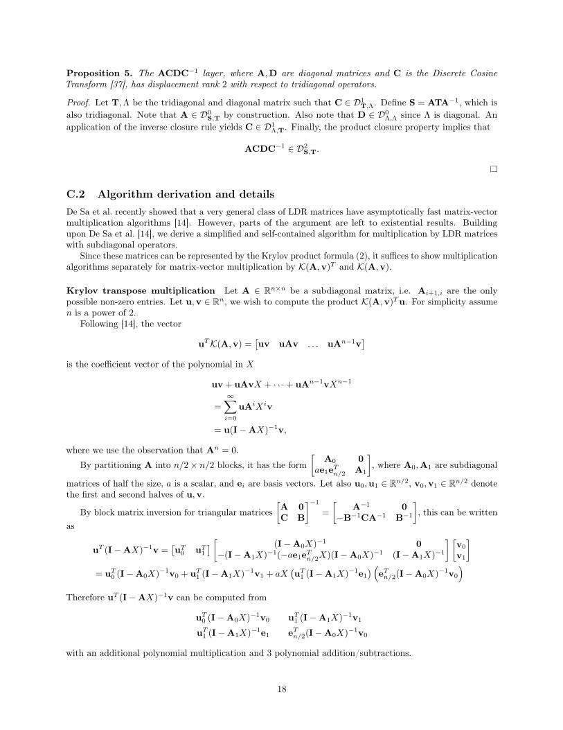
Proposition 5. The ACDC−1 layer, where A,D are diagonal matrices and C is the Discrete CosineTransform [37], has displacement rank 2 with respect to tridiagonal operators.

Proof. Let T,Λ be the tridiagonal and diagonal matrix such that C ∈ D1T,Λ. Define S = ATA−1, which is

also tridiagonal. Note that A ∈ D0S,T by construction. Also note that D ∈ D0

Λ,Λ since Λ is diagonal. Anapplication of the inverse closure rule yields C ∈ D1

Λ,T. Finally, the product closure property implies that

ACDC−1 ∈ D2S,T.

C.2 Algorithm derivation and detailsDe Sa et al. recently showed that a very general class of LDR matrices have asymptotically fast matrix-vectormultiplication algorithms [14]. However, parts of the argument are left to existential results. Buildingupon De Sa et al. [14], we derive a simplified and self-contained algorithm for multiplication by LDR matriceswith subdiagonal operators.

Since these matrices can be represented by the Krylov product formula (2), it suffices to show multiplicationalgorithms separately for matrix-vector multiplication by K(A,v)T and K(A,v).

Krylov transpose multiplication Let A ∈ Rn×n be a subdiagonal matrix, i.e. Ai+1,i are the onlypossible non-zero entries. Let u,v ∈ Rn, we wish to compute the product K(A,v)Tu. For simplicity assumen is a power of 2.

Following [14], the vector

uTK(A,v) =[uv uAv . . . uAn−1v

]

is the coefficient vector of the polynomial in X

uv + uAvX + · · ·+ uAn−1vXn−1

=

∞∑

i=0

uAiXiv

= u(I−AX)−1v,

where we use the observation that An = 0.

By partitioning A into n/2× n/2 blocks, it has the form[

A0 0ae1e

Tn/2 A1

], where A0,A1 are subdiagonal

matrices of half the size, a is a scalar, and ei are basis vectors. Let also u0,u1 ∈ Rn/2, v0,v1 ∈ Rn/2 denotethe first and second halves of u,v.

By block matrix inversion for triangular matrices[A 0C B

]−1

=

[A−1 0

−B−1CA−1 B−1

], this can be written

as

uT (I−AX)−1v =[uT0 uT1

] [ (I−A0X)−1 0−(I−A1X)−1(−ae1e

Tn/2X)(I−A0X)−1 (I−A1X)−1

] [v0

v1

]

= uT0 (I−A0X)−1v0 + uT1 (I−A1X)−1v1 + aX(uT1 (I−A1X)−1e1

) (eTn/2(I−A0X)−1v0

)

Therefore uT (I−AX)−1v can be computed from

uT0 (I−A0X)−1v0 uT1 (I−A1X)−1v1

uT1 (I−A1X)−1e1 eTn/2(I−A0X)−1v0

with an additional polynomial multiplication and 3 polynomial addition/subtractions.

18

A modification of this reduction shows that the 2×2 matrix of polynomials[u en

]T(I−AX)−1

[v e1

]

can be computed from[u0 en

]T(I−A0X)−1

[v0 e1

] [u1 en

]T(I−A1X)−1

[v1 e1

]

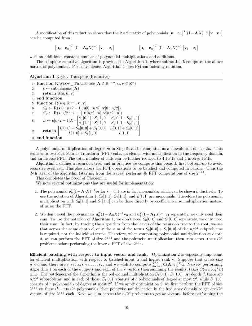
with an additional constant number of polynomial multiplications and additions.The complete recursive algorithm is provided in Algorithm 1, where subroutine R computes the above

matrix of polynomials. For convenience, Algorithm 1 uses Python indexing notation.

Algorithm 1 Krylov Transpose (Recursive)

1: function Krylov_Transpose(A ∈ Rn×n,u,v ∈ Rn)2: s← subdiagonal(A)3: return R(s,u,v)4: end function5: function R(s ∈ Rn−1,u,v)6: S0 ← R(s[0 : n/2− 1],u[0 : n/2],v[0 : n/2])7: S1 ← R(s[n/2 : n− 1],u[n/2 : n],v[n/2 : n])

8: L← s[n/2− 1]X ·[S1[0, 1] · S0[1, 0] S1[0, 1] · S0[1, 1]S1[1, 1] · S0[1, 0] S1[1, 1] · S0[1, 1]

]

9: return[L[0, 0] + S0[0, 0] + S1[0, 0] L[0, 1] + S0[0, 1]

L[1, 0] + S1[1, 0] L[1, 1]

]

10: end function

A polynomial multiplication of degree m in Step 8 can be computed as a convolution of size 2m. Thisreduces to two Fast Fourier Transform (FFT) calls, an elementwise multiplication in the frequency domain,and an inverse FFT. The total number of calls can be further reduced to 4 FFTs and 4 inverse FFTs.

Algorithm 1 defines a recursion tree, and in practice we compute this breadth first bottom-up to avoidrecursive overhead. This also allows the FFT operations to be batched and computed in parallel. Thus thed-th layer of the algorithm (starting from the leaves) performs n

2d FFT computations of size 2d+1.This completes the proof of Theorem 1.We note several optimizations that are useful for implementation:

1. The polynomial eTn (I−AiX)−1e1 for i = 0, 1 are in fact monomials, which can be shown inductively. Touse the notation of Algorithm 1, S0[1, 1], S1[1, 1], and L[1, 1] are monomials. Therefore the polynomialmultiplication with S0[1, 1] and S1[1, 1] can be done directly by coefficient-wise multiplication insteadof using the FFT.

2. We don’t need the polynomials uT0 (I−A0X)−1v0 and uT1 (I−A1X)−1v1 separately, we only need theirsum. To use the notation of Algorithm 1, we don’t need S0[0, 0] and S1[0, 0] separately, we only needtheir sum. In fact, by tracing the algorithm from the leaves of the recursion tree to the root, we seethat across the same depth d, only the sum of the terms S0[0, 0] + S1[0, 0] of the n/2d subproblemsis required, not the individual terms. Therefore, when computing polynomial multiplication at depthd, we can perform the FFT of size 2d+1 and the pointwise multiplication, then sum across the n/2dproblems before performing the inverse FFT of size 2d+1.

Efficient batching with respect to input vector and rank. Optimization 2 is especially importantfor efficient multiplication with respect to batched input u and higher rank v. Suppose that u has sizen × b and there are r vectors v1, . . . ,vr, and we wish to compute

∑ri=1K(A,vi)

Tu. Naively performingAlgorithm 1 on each of the b inputs and each of the r vectors then summing the results, takes O(brn log2 n)time. The bottleneck of the algorithm is the polynomial multiplication S1[0, 1] ·S0[1, 0]. At depth d, there aren/2d subproblems, and in each of those, S1[0, 1] consists of b polynomials of degree at most 2d, while S0[1, 0]consists of r polynomials of degree at most 2d. If we apply optimization 2, we first perform the FFT of size2d+1 on these (b+ r)n/2d polynomials, then pointwise multiplication in the frequency domain to get brn/2dvectors of size 2d+1 each. Next we sum across the n/2d problems to get br vectors, before performing the

19

inverse FFT of size 2d+1 to these br vectors. The summing step allows us to reduce the number of inverseFFTs from brn/2d to br. The total running time over all depth d is then O((b+ r)n log2 n+ brn log n) insteadof O(brn log2 n).

Krylov multiplication De Sa et al. [14] do not provide explicit algorithms for the more complicated problemof multiplication by K(A,v), instead justifying the existence of such an algorithm with the transpositionprinciple. Traditional proofs of the transposition principle use circuit based arguments involving reversingarrows in the arithmetic circuit defining the algorithm’s computation graph [6].

Here we show an alternative simple way to implement the transpose algorithm using any automaticdifferentiation (AD) implementation, which all modern deep learning frameworks include. AD states that forany computation, its derivative can be computed with only a constant factor more operations [22].

Proposition 6 (Transposition Principle). If the matrix M ∈ Rn×n admits matrix-vector multiplication byany vector in N operations, then MT admits matrix-vector multiplication in O(N + n) operations.

Proof. Note that for any x and y, the scalar yTMx = y · (Mx) can be computed in N + n operations.The statement follows from applying reverse-mode AD to compute MTy = ∂

∂x (yTMx).Additionally, the algorithm can be optimized by choosing x = 0 to construct the forward graph.

To perform the optimization mentioned in Proposition 6, and avoid needing second-order derivatives whencomputing backprop for gradient descent, we provide an explicit implementation of non-transpose Krylovmultiplication K(A,v). This was found by using Proposition 6 to hand-differentiate Algorithm 1.

Finally, we comment on multiplication by the LDR-TD class. Desa et al.[14] showed that these matricesalso have asymptotically efficient multiplication algorithms, of the order O(rn log3 n) operations. However,these algorithms are even more complicated and involve operations such as inverting matrices of polynomialsin a modulus. Practical algorithms for this class similar to the one we provide for LDR-SD matrices requiremore work to derive.

C.3 Displacement rank and equivarianceHere we discuss in more detail the connection between LDR and equivariance. One line of work [12, 28] hasused the group representation theory formalization of equivariant maps, in which the model is equivariantto a set of transformations which form a group G. Each transformation g ∈ G acts on an input x via acorresponding linear map Tg. For example, elements of the rotation group in two and three dimensions,SO(2) and SO(3), can be represented by 2D and 3D rotation matrices respectively. Formally, a feature mapΦ is equivariant if it satisfies

Φ(Tgx) = T ′g(Φ(x)) (5)

for representations T, T ′ of G [12, 28]. This means that perturbing the input x by a transformation g ∈ Gbefore computing the map Φ is equivalent to first finding the features Φ and then applying the transformation.Group equivariant convolutional neural networks (G-CNNs) are a particular realization where Φ has a specificform G→ Rd, and T, T ′ are chosen in advance [12]. We use the notation Φ to distinguish our setting, wherethe input x is finite dimensional and Φ is linear.

Proposition 7. If Φ has displacement rank 0 with respect to invertible A,B, then Φ is equivariant as definedby (5).

Proof. Note that if AΦ = ΦB for invertible matrices A,B (i.e. if a matrix Φ has displacement rank 0 withrespect to A and B), then AiΦ = ΦBi also holds for i ∈ Z. Also note that the set of powers of any invertiblematrix forms a cyclic group, where the group operation is multiplication. The statement follows directly fromthis fact, where the group G is Z, and the representations T and T ′ of G correspond to the cyclic groupsgenerated by A and B, respectively consisting of Ai and Bi for all i ∈ Z.

More generally, a feature map Φ satisfying (5) for a set of generators S = {gi} is equivariant with respectto the free group generated by S. Proposition 7 follows from the specific case of a single generator, i.e.S = {1}.

20

D Bound on VC dimension and sample complexityIn this section we upper bound the VC dimension of a neural network where all the weight matrices areLDR matrices and the activation functions are piecewise polynomials. In particular, the VC dimension isalmost linear in the number of parameters, which is much smaller than the VC dimension of a network withunstructured layers. The bound on the VC dimension allows us to bound the sample complexity to learnan LDR network that performs well among LDR networks. This formalizes the intuition that compressedparameterization reduces the complexity of the class.

Neural network model Consider a neural network architecture with W parameters, arranged in L layers.Each layer l, has output dimension nl, where n0 is the dimension of the input data and the output dimensionis nL = 1. For l = 1, . . . , L, let il ∈ Rnl be the input to the l-th layer. The input to the (l + 1)-th layer isexactly the output of the l-th layer. The activation functions φl are piecewise polynomials with at most p+ 1pieces and degree at most k ≥ 1. The input to the first layer is the data i1 = x ∈ Rn1 , and the output of thelast layer is a real number iL+1 ∈ R. The intermediate layer computation has the form:

il+1 = φl(Mlil + bl) (applied elementwise), where Ml ∈ Rnl−1×nl , bl ∈ Rnl .

We assume the activation function of the final layer is the identity.Each weight matrix Ml is defined through some set of parameters; for example, traditional unconstrained

matrices are parametrized by their entries, and our formulation (2) is parametrized by the entries of someoperator matrices Al,Bl and low-rank matrix GlH

Tl . We collectively refer to all the parameters of the neural

network (including the biases bl) as θ ∈ RW , where W is the number of parameters.

Bounding the polynomial degree The crux of the proof of the VC dimension bound is that the entriesof M ∈ Rn×m are polynomials in terms of the entries of its parameters (A, B, G, and H). of total degree atmost c1mc2 for universal constants c1, c2. This allows us to bound the total degree of all of the layers andapply Warren’s lemma to bound the VC dimension.

We will first show this for the specific class of matrices that we use, where the matrix M is defined throughequation (2).

Lemma 1. Suppose that M ∈ Rm×m is defined as

M =

r∑

i=1

K(A,gi)K(BT ,hi).

Then the entries of M are polynomials of the entries of A,B,G,H with total degree at most 2m.

Proof. Since K(A,gi) =[gi Agi . . . Am−1gi

], and each entry of Ak is a polynomial of the entries of A

with total degree at most k, the entries of K(A,gi) are polynomials of the entries of A and gi with totaldegree at most m. Similarly the entries of K(BT ,hi) are polynomials of the entries of B and hi with totaldegree at most m. Hence the entries of K(A,gi)K(BT ,hi) are polynomials of the entries of A,B,G,H withtotal degree at most 2m. We then conclude that the entries of M are polynomials of the entries of A,B,G,Hwith total degree at most 2m.

Lemma 2. Suppose that the LDR weight matrices Ml of a neural network have entries that are polynomialsin their parameters with total degree at most c1nc2l−1 for some universal constants c1, c2 ≥ 0. For a fixed datapoint x, at the l-th layer of a neural network with LDR weight matrices, each entry of Mlil + bl is a piecewisepolynomial of the network parameters θ, with total degree at most dl, where

d0 = 0, dl = kdl−1 + c1nc2l−1 for l = 1, . . . , L.

Thus entries of the output φl(Mlil+bl) are piecewise polynomials of θ with total degree at most kdl. Moreover,

dl ≤ c1kl−1l−1∑

j=0

nc2j . (6)

21

By Lemma 1, Lemma 2 applies to the specific class of matrices that we use, for c1 = 2 and c2 = 1. As wewill see, it also applies to very general classes of structured matrices.

Proof. We induct on l. For l = 1, since i1 = x is fixed, the entries of M1 are polynomials of θ of degreeat most c1nc20 , and so the entries of M1i1 + b1 are polynomials of θ with total degree at most d1 = c1n

c20 .

As φ is a piecewise polynomials of degree at most k, each entry the output φ1(M1i1 + b1) is a piecewisepolynomial of θ with total degree at most 2n0k. The bound (6) holds trivially.

Suppose that the lemma is true for some l − 1 ≥ 1. Since the entries of il are piecewise polynomials ofθ with total degree at most kdl−1 and entries of Ml are polynomials of θ with total degree at most c1nc2l−1,the entries of Mlil + bl are piecewise polynomials of θ with total degree at most dl = kdl−1 + c1n

c2l−1. Thus

φl(Mlil + bl) have entries that are piecewise polynomials of θ with total degree at most kdl.We can bound

dl = kdl−1 + c1nc2l−1 ≤ kc1kl−2

l−2∑

j=0

nc2j + c1nc2l−1 ≤ c1kl−1

l−1∑

j=0

nc2j ,

where we have used the fact that k ≥ 1, so c1nc2l−1 ≤ c1kl−1nc2l−1. This concludes the proof.

Bounding the VC dimension Now we are ready to bound the VC dimension of the neural network.

Theorem 3. For input x ∈ X and parameter θ ∈ RW , let f(x, θ) denote the output of the network. Let Fbe the class of functions {x→ f(x, θ) : θ ∈ RW }. Denote signF := {x→ sign f(x, θ) : θ ∈ RW }. Let Wl bethe number of parameters up to layer l (i.e., the total number of parameters in layer 1, 2, . . . , l). Define theeffective depth as

L̄ :=1

W

L∑

l=1

Wl,

and the total number of computation units (including the input dimension) as

U :=

L∑

l=0

nl.

ThenVCdim(signF) = O(L̄W log(pU) + L̄LW log k).

In particular, if k = 1 (corresponding to piecewise linear networks) then

VCdim(signF) = O(L̄W log(pU)) = O(LW logW ).

We adapt the proof of the upper bound from Bartlett et al. [4], Harvey et al. [24]. The main technicaltool is Warren’s lemma [48], which bounds the growth function of a set of polynomials. We state a slightlyimproved form here from Anthony and Bartlett [3, Theorem 8.3].

Lemma 3. Let p1, . . . , pm be polynomials of degree at most d in n ≤ m variables. Define

K := |{(sign(p1(x)), . . . , sign(pm(x)) : x ∈ Rn}|,

i.e., K is the number of possible sign vectors given by the polynomials. Then K ≤ 2(2emd/n)n.

Proof of Theorem 3. Fixed some large integer m and some inputs x1, . . . ,xm. We want to bound the numberof sign patterns that the neural network can output for the set of input x1, . . . ,xm:

K :=∣∣{(sign f(x1, θ), . . . , sign f(xm, θ)) : θ ∈ RW }

∣∣ .

22

We want to partition the parameter space RW so that for a fixed xj , the output f(xj , θ) is a polynomialon each region in the partition. Then we can apply Warren’s lemma to bound the number of sign patterns.Indeed, for any partition S = {P1, . . . , PN} of the parameter space RW , we have

K ≤N∑

j=1

|{(sign f(x1, θ), . . . , sign f(xm, θ)) : θ ∈ Pj}| . (7)

We construct the partitions iteratively layer by layer, through a sequence S0,S1, . . . ,SL−1 of successiverefinements, satisfying two properties:

1. |S0| = 1 and for each 1 ≤ l ≤ L− 1,

|Sl| ≤ |Sl−1| 2(

2empnldlWl

)Wl

,

where nl is the dimension of the output of the l-th layer, dl is the bound on the total degree of Mlil +blas piecewise polynomials of θ as defined in Lemma 2, and Wl is the number of parameters up to layer l(i.e., the total number of parameters in layer 1, 2, . . . , l).

2. For each l = 0, . . . , L− 1, for each element S of Sl, for each fixed data point xj (with j = 1, . . . ,m),the entries of the output φl(Mlil + bl) when restricted to S are polynomials of θ with total degree atmost kdl−1.

We can define S0 = RW , which satisfies property 2, since at layer 1, the entries of i1 = xj (for fixed xj)are polynomials of θ of degree d0 = 0.

Suppose that we have constructed S0, . . . ,Sl−1, and we want to define Sl. For any h ∈ [nl], j ∈ [m], andS ∈ Sl−1, let ph,xj ,S(θ) = (Mlil + bl)h|S be the h-th entry of Mlil + bl restricted to the region S. By theinductive hypothesis, for each S ∈ Sl−1, the entries of il when restricted to S are polynomials of θ of totaldegree at most kdl−1. Thus by Lemma 2, the entries of Mlil + bl when restricted to S are polynomials of θwith total degree at most kdl−1 + c1n

c2l−1 = dl, and depends on at most Wl many variables.

Since the activation function is piecewise polynomial with at most p pieces, let {t1, . . . , tp} be the set ofbreakpoints. For any fixed S ∈ Sl−1, by Lemma 3, the polynomials

{ph,xj ,S(θ)− ti : h ∈ [nl], j ∈ [m], i ∈ [p]

}

can have at most

Π := 2

(2e(nlmp)dl

Wl

)Wl

distinct sign patterns when θ ∈ RW . We can then partition RW into this many regions so that within eachregion, all these polynomials have the same signs. Intersecting all these regions with S yields a partition of Sinto at most Π subregions. Applying this for all S ∈ Sl−1 gives a partition Sl that satisfies the property 1.

Fix some S′ ∈ Sn. When θ is restricted to S′, by construction, all the polynomials{ph,xj ,S(θ)− ti : h ∈ [nl], j ∈ [m], i ∈ [p]

}

have the same sign. This means that the entries of Mlil + bl lie between two breakpoints of the activationfunction, and so the entries of the output φl(Mlil + bl) are fixed polynomials in Wl variables of degree atmost kdl.

By this recursive construction, SL−1 is a partition of RW such that for S ∈ SL−1 the network output forany input xj is a fixed polynomial of θ ∈ S of degree at most kdL−1 + c1n

c2L−1 = dL (recall that we assume

the activation function of the final layer is the identity). Hence we can apply Lemma 3 again:

|{(sign f(x1, θ), . . . , sign f(xm, θ)) : θ ∈ S}| ≤ 2

(2emkdLWL

)WL

.

23

By property 1, we can bound the size of SL−1:

|SL| ≤L−1∏

l=1

2

(2emnlpdl

Wl

)Wl

.

Combining the two bounds along with equation (7) yields

K ≤L∏

l=1

2

(2empnldl

Wl

)Wl

.

We can take logarithm and apply Jensen’s inequality, with W̄ :=∑Ll=1Wl:

log2K ≤ L+

L∑

l=1

Wl log2

2empnldlWl

= L+ W̄

L∑

l=1

Wl

W̄log2

2empnldlWl

≤ L+ W̄ log2

(L∑

l=1

Wl

W̄

2empnldlWl

)(Jensen’s inequality)

= L+ W̄ log2

2emp∑Ll=1 nldl

W̄.

We can bound∑nldl using the bound on dl from Lemma 2:

L∑

l=1

nldl ≤L∑

l=1

nlc1kl−1

l−1∑

j=0

nc2j ≤ LUc1kL−1U c2 ≤ c1U c2+2kL,

where we used the fact that L ≤ U . Thus

log2K ≤ L+ W̄ log2

2c1empU2+c2kL

W̄.

To bound the VC-dimension, recall that by definition, if VCdim(signF) = m then exists m data pointsx1, . . . ,xm such that the output of the model can have 2n sign patterns. The bound on log2K then implies

VCdim(signF) ≤ L+ W̄ log2

2c1epU2+c2kLVCdim(signF)

W̄.

We then use Lemma 4 below, noting that 2c1epU2+c2kL ≥ 16, to conclude that

VCdim(signF) ≤ L+ W̄ log2(2c1epU2+c2kL log2(2c1epU

2+c2kL)) = O(L̄W log(pU) + L̄LW log k),

completing the proof.

A bound on the VC dimension immediate yields a bound on the sample complexity of learning from thisclass of neural networks with LDR matrices [47].

Corollary 2. The class of neural network with LDR matrices as weights and piecewise linear activation is(ε, δ)-PAC-learnable with a sample of size

O

(LW logW + log 1

δ

ε

).

Since the number of parameters W is around the square root of the number of parameters of a networkwith unstructured layers (assuming fixed rank of the LDR matrices), the sample complexity of LDR networksis much smaller than that of general unstructured networks.

Lemma 4 (Lemma 16 of [24]). Suppose that 2m ≤ 2t(mr/w)w for some r ≥ 16 and m ≥ w ≥ t ≥ 0. Then,m ≤ t+ w log2(2r log2 r).

24

Extension to rational functions. We now show that Theorem 3 holds for matrices where the entries arerational functions—rather than polynomials—of its parameters, incurring only a constant in the bound. Todefine the function class signF , we account for the possibility of poles by defining sign(a/0) = 0.

We only need to check that Lemma 2 and Lemma 3 still hold when polynomials are replaced by rationalfunctions everywhere, and the degree of a rational function is defined as the usual deg(a/b) = max{deg a,deg b}.To show Lemma 2 still holds, it suffices that the compositional degree bound deg(f ◦ g) ≤ deg(f) deg(g) holdsfor rational functions f, g, just as in the polynomial case. To show Lemma 3 in the case when pi = ai/biare rational functions, we note that sign(pi(x)) = sign(ai(x)bi(x)), and furthermore deg(aibi) ≤ 2 deg(pi).Appealing to the polynomial version of Lemma 3 shows that it holds in the rational function setting witha slightly weaker upper bound K ≤ 2(4emd/n)n. This gets converted to a constant factor in the result ofTheorem 3.

Next, we extend Lemma 1 by showing that generic LDR matrices have entries which are rational functionsof their parameters. This immediately lets us conclude that neural networks built from any LDR matricessatisfy the VC dimension bounds of Theorem 3.

Lemma 5. If M ∈ Rm×m satisfies AM−MB = GHT , then the entries of M are rational functions of theentries of A,B,G,H with total degree at most c1mc2 for some universal constants c1, c2 > 0.

Proof. The vectorization of the Sylvester equation AM−MB = R is (I⊗A−B> ⊗ I) vec(M) = vec(R),where vec denotes the vectorization operation by stacking a matrix’s columns, and ⊗ is the Kroneckerproduct. Note that the entries of N−1 for an arbitrary matrix N ∈ Rn×n are rational functions with degreen in the entries of N, and R = GH> has degree 2 in the entries of G,H. Therefore the entries of

vec(M) = (I⊗A−B> ⊗ I)−1 vec(R)

have degree n2 + 2 in the entries of A,B,G,H.

Note that many other classes of matrices satisfy this lemma. For example, a large class of matricessatisfying a property called low recurrence width was recently introduced as a way of generalizing many knownstructured matrices [14]. The low recurrence width matrices are explicitly defined through a polynomialrecurrence and satisfy the bounded degree condition. Additionally, Lemma 5 holds when the parametersA,B themselves are structured matrices with entries having polynomial degree in terms of some parameters.This includes the case when they are quasiseparable matrices, the most general class of LDR previouslyanalyzed [14].

E Additional results

E.1 Additional baselines and comparisons at multiple budgetsIn Tables 6 and 7 we compare to baselines at parameter budgets corresponding to both the LDR-TD andLDR-SD classes in the SHL and CNN models. In Tables 8 and 9, we also compare to two additional baselines,network pruning [23] and a baseline used in [7], in which the number of hidden units is reduced to meetthe parameter budget. We refer to this baseline as RHU ("reduced hidden units"). We show consistentimprovements of LDR-SD over both methods at several budgets. We note that unlike the structured matrixmethods which provide compression benefits during both training and inference, pruning requires first trainingthe original model, followed by retraining with a fixed sparsity pattern.

E.2 Sample complexity and generalizationAs shown in Tables 10 and 11, we investigated how the performance of the structured and general unstructuredfully-connected layers varied with the amount of training data. On the MNIST variants, we trained boththe single hidden layer and CNN models with random subsamples of 25%, 50%, and 75% of the trainingset, with 15% of the training set used for validation in all settings. In addition, in Table 12, we compare thegeneralization error of structured classes with an unstructured model, and find that the structured classeshave consistently lower generalization error.

25

Table 6: Test accuracy when replacing the hidden layer with structured classes in the single hidden layer architecture,at parameter budgets corresponding to LDR-TD and LDR-SD rank one. Rank is in parentheses. The first groupof structured methods (in orange) all have compression factors (relative to a general unstructured layer) of 98 onMNIST-bg-rot and MNIST-noise, and 128 on CIFAR-10 and NORB. The second group of structured methods (inblue) all have compression factors of 196 on MNIST-bg-rot and MNIST-noise, and 256 on CIFAR-10 and NORB.

Method MNIST-bg-rot MNIST-noise CIFAR-10 NORB

Unstructured 44.08 65.15 46.03 59.83LDR-TD (r = 1) 45.81 78.45 45.33 62.75Toeplitz-like [45] (r = 4) 42.67 75.75 41.78 59.38Hankel-like (r = 4) 42.23 73.65 41.40 60.09Vandermonde-like (r = 4) 37.14 59.80 33.93 48.98Low-rank [15] (r = 4) 35.67 52.25 32.28 43.66

LDR-SD (r = 1) 44.74 78.80 43.29 63.78Toeplitz-like [45] (r = 2) 42.07 74.25 40.68 57.27Hankel-like (r = 2) 41.01 71.20 40.46 57.95Vandermonde-like (r = 2) 33.56 50.85 28.99 43.21Low-rank [15] (r = 2) 32.64 38.85 24.93 37.03

Table 7: Test accuracy when replacing the fully-connected layer with structured classes in the CNN architecture,at parameter budgets corresponding to LDR-TD and LDR-SD rank one. Rank is in parentheses. The first groupof structured methods (in orange) all have compression factors (relative to a general unstructured layer) of 98 onMNIST-bg-rot and MNIST-noise, and 128 on CIFAR-10 and NORB. The second group of structured methods (inblue) all have compression factors of 196 on MNIST-bg-rot and MNIST-noise, and 256 on CIFAR-10 and NORB.

Method MNIST-bg-rot MNIST-noise CIFAR-10 NORB

Fully-connected 67.94 90.30 68.09 75.16LDR-TD (r = 1) 68.79 92.55 66.63 74.23Toeplitz-like [45] (r = 4) 63.23 91.60 67.10 72.25Hankel-like (r = 4) 64.21 90.80 68.10 71.23Vandermonde-like (r = 4) 61.76 90.40 63.63 72.11Low-rank [15] (r = 4) 60.35 87.30 60.90 71.47

LDR-SD (r = 1) 67.40 92.20 65.48 73.63Toeplitz-like [45] (r = 2) 63.63 91.45 67.15 71.64Hankel-like (r = 2) 64.08 90.65 67.49 71.21Vandermonde-like (r = 2) 51.38 86.50 58.00 68.08Low-rank [15] (r = 2) 41.91 71.15 48.48 65.34

E.3 Additional visualizationsIn Figure 6, we visualize the learned subdiagonal on NORB along with images from the dataset.

On the MNIST-bg-rot dataset [30], we note that Chen et al. [7] also tested several methods on this dataset,including Random Edge Removal [11], Low Rank Decomposition [15], Dark Knowledge [25], HashedNets [7],and HashedNets with Dark Knowledge, and reported test errors of 73.17, 80.63, 79.03, 77.40, 59.20, and 58.25,where each method had 12406 parameters in the architecture. We found that our LDR-SD class, with 10986parameters in the architecture, achieved a test error of 55.26, as shown in Table 6, outperforming all methodsevaluated by Chen et al. [7]. Sindhwani et al. [45] later also tested on this dataset, and reported test errorsof 68.4, 62.11, and 55.21 for Fastfood (10202 parameters), Circulant (8634 parameters), and Toeplitz-like,r = 2 (10986 parameters). LDR-SD exceeds their reported results for Fastfood and Circulant [8], but notthat of Toeplitz-like. We did find that our proposed classes consistently exceeded the performance of our ownimplementation of Toeplitz-like on this dataset (Table 1, Figure 3, and Tables 6 and 7).

26

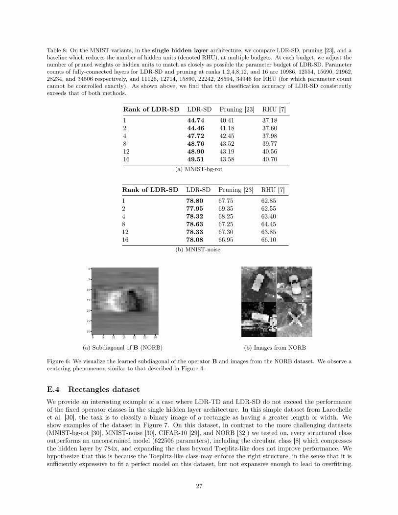
Table 8: On the MNIST variants, in the single hidden layer architecture, we compare LDR-SD, pruning [23], and abaseline which reduces the number of hidden units (denoted RHU), at multiple budgets. At each budget, we adjust thenumber of pruned weights or hidden units to match as closely as possible the parameter budget of LDR-SD. Parametercounts of fully-connected layers for LDR-SD and pruning at ranks 1,2,4,8,12, and 16 are 10986, 12554, 15690, 21962,28234, and 34506 respectively, and 11126, 12714, 15890, 22242, 28594, 34946 for RHU (for which parameter countcannot be controlled exactly). As shown above, we find that the classification accuracy of LDR-SD consistentlyexceeds that of both methods.

Rank of LDR-SD LDR-SD Pruning [23] RHU [7]

1 44.74 40.41 37.182 44.46 41.18 37.604 47.72 42.45 37.988 48.76 43.52 39.7712 48.90 43.19 40.5616 49.51 43.58 40.70

(a) MNIST-bg-rot

Rank of LDR-SD LDR-SD Pruning [23] RHU [7]

1 78.80 67.75 62.852 77.95 69.35 62.554 78.32 68.25 63.408 78.63 67.25 64.4512 78.33 67.30 63.8516 78.08 66.95 66.10

(b) MNIST-noise

0 5 10 15 20 25 30

0

5

10

15

20

25

30

(a) Subdiagonal of B (NORB) (b) Images from NORB

Figure 6: We visualize the learned subdiagonal of the operator B and images from the NORB dataset. We observe acentering phenomenon similar to that described in Figure 4.

E.4 Rectangles datasetWe provide an interesting example of a case where LDR-TD and LDR-SD do not exceed the performanceof the fixed operator classes in the single hidden layer architecture. In this simple dataset from Larochelleet al. [30], the task is to classify a binary image of a rectangle as having a greater length or width. Weshow examples of the dataset in Figure 7. On this dataset, in contrast to the more challenging datasets(MNIST-bg-rot [30], MNIST-noise [30], CIFAR-10 [29], and NORB [32]) we tested on, every structured classoutperforms an unconstrained model (622506 parameters), including the circulant class [8] which compressesthe hidden layer by 784x, and expanding the class beyond Toeplitz-like does not improve performance. Wehypothesize that this is because the Toeplitz-like class may enforce the right structure, in the sense that it issufficiently expressive to fit a perfect model on this dataset, but not expansive enough to lead to overfitting.

27

Table 9: On the MNIST variants, in the CNN architecture, we compare LDR-SD, pruning [23], and a baseline whichreduces the number of hidden units (denoted RHU), at multiple budgets. At each budget, we adjust the number ofpruned weights or hidden units to match as closely as possible the parameter budget of LDR-SD. Parameter counts offully-connected layers for LDR-SD and pruning at ranks 1,2,4,8,12, and 16 are 11770, 13338, 16474, 22746, 29018, and35290 respectively, and 11935, 13525, 16705, 23065, 29425, 35785 for RHU (for which parameter count cannot becontrolled exactly). As shown above, we find that the classification accuracy of LDR-SD consistently exceeds that ofboth methods.

Rank of LDR-SD LDR-SD Pruning [23] RHU [7]

1 67.40 64.25 64.032 67.53 64.05 64.674 67.96 65.50 66.378 67.21 64.12 64.7012 68.54 65.65 65.9916 67.00 65.59 66.47

(a) MNIST-bg-rot

Rank of LDR-SD LDR-SD Pruning [23] RHU [7]

1 92.20 90.80 90.952 92.75 91.65 91.004 91.30 90.60 91.258 91.95 91.05 90.6512 92.10 90.00 90.8516 93.20 90.55 90.40

(b) MNIST-noise

For example, while the Toeplitz-like operators model approximate shift equivariance (discussed in Section 4and Proposition 7 in Section C.3), the additional scaling that subdiagonal operators provide is unnecessaryon these binary inputs.

Figure 7: Examples of images from the rectangles dataset [30].

E.5 Acceleration at inference timeWe empirically study the acceleration obtained at inference time (on CPU) with our implementation of thealgorithms for multiplication by LDR-SD described in Appendix C.2. We generated random parameters foreach class and ran each multiplication algorithm 1000 times to compare the speedup of each class over anunstructured multiply. Each test was repeated 10 times, and the minimum total runtime over the 10 tests wasused for each class. As shown in Figure 8 and Table 14, at n ≥ 4096, our simple Python implementation is3.34-46.06x faster than the highly optimized unstructured matrix-vector multiply (a BLAS level 2 operation).We also compare with two other structured classes, low-rank and Toeplitz-like, at r = 1, 2, 4, 8, 16. A batchsize of one was used in all tests. The time complexity of multiplication by low-rank and Toeplitz-like is O(nr)and O(nr log n) respectively, compared to O(nr log2 n) for LDR-SD.

28

Table 10: On the MNIST variants, in the single hidden layer architecture, we show how the number of trainingsamples affects the performance of the unstructured model and the structured classes. Columns correspond to modelstrained on 25%, 50%, 75% and 100% of the training data (randomly subsampled). LDR-TD and LDR-SD consistentlyoutperform the structured baselines at the tested subsampling ratios. On MNIST-bg-rot, LDR-TD only needs 75% ofthe training data to outperform the unstructured model trained on 100% of the training data. On MNIST-noise, bothLDR-TD and LDR-SD only need 25% of the training data to outperform the unstructured layer. All are rank one.

Method 25% 50% 75% 100%

Unstructured 34.46 38.80 43.35 44.08

LDR-TD 34.01 39.59 44.35 45.81LDR-SD 35.64 39.78 42.72 44.74Toeplitz-like 33.71 36.44 39.32 41.12Low-rank 21.44 23.46 23.48 25.06

(a) MNIST-bg-rot

Method 25% 50% 75% 100%

Unstructured 59.30 61.85 65.35 65.15

LDR-TD 65.45 74.60 77.45 78.45LDR-SD 67.90 71.15 76.95 78.80Toeplitz-like 56.15 67.75 72.30 73.95Low-rank 24.25 26.20 26.85 26.40

(b) MNIST-noise

Table 11: On the MNIST variants, in the CNN architecture, we show how the number of training samples affects theperformance of the unstructured model and the structured classes. Columns correspond to models trained on 25%,50%, 75% and 100% of the training data (randomly subsampled). LDR-TD and LDR-SD consistently outperform thestructured baselines at the tested subsampling ratios. On MNIST-noise, both LDR-TD and LDR-SD only need 50%of the training data to outperform the unstructured layer. All are rank one.

Method 25% 50% 75% 100%

Unstructured 54.12 62.53 67.52 67.94

LDR-TD 53.66 62.15 67.25 68.79LDR-SD 50.72 61.92 65.93 67.40Toeplitz-like 49.10 57.20 61.53 63.00Low-rank 26.98 27.97 28.97 29.63

(a) MNIST-bg-rot

Method 25% 50% 75% 100%

Unstructured 81.85 88.25 89.75 90.30

LDR-TD 86.45 91.35 93.00 92.55LDR-SD 86.95 90.90 91.55 92.20Toeplitz-like 81.65 88.15 90.90 90.95Low-rank 33.15 38.40 42.55 44.55

(b) MNIST-noise

Table 12: Generalization error for unstructured, LDR-TD, LDR-SD, Toeplitz-like, low-rank classes on the singlehidden layer architecture. Consistent with Theorem 2, the structured classes have consistently lower generalizationerror than the unstructured model. All are rank one.

Method MNIST-bg-rot MNIST-noise CIFAR-10 NORB

Unstructured 55.78 21.63 34.32 40.03

LDR-TD 13.52 11.36 7.10 9.51LDR-SD 12.87 12.65 6.29 8.68Toeplitz-like [45] 7.98 15.80 5.59 7.87Low-rank [15] 8.40 0.31 0.09 2.59

F Experimental details

F.1 Image classificationIn Table 15, we provide details on the datasets we use for evaluation. For all our experiments, batch sizeswere chosen to be 50. NORB was downsampled to 32 × 32, and the left stereo image was used. Trainingwas performed with stochastic gradient descent with momentum, with the number of epochs set to 50 on alldatasets. 15% of the training data was used for the validation set on all experiments. We fixed momentum at0.9 for all methods for all experiments, and performed a grid search over learning rate. Unless otherwisestated, for each method, we tested the learning rates {0.0002, 0.0005, 0.001, 0.002}, with three trials (with

29

Table 13: Test accuracy when replacing the hidden layer with structured classes on the rectangles dataset [30]. Whereapplicable, rank (r) is in parentheses, and the number of parameters in the architecture is in italics below each method.

Method Test Accuracy

Unconstrained 91.94622506

LDR-TD (r = 1) 98.5314122

LDR-SD (r = 1) 98.3910986

Toeplitz-like (r = 4) [45] 99.2914122

Hankel-like (r = 4) 97.7714122

Vandermonde-like (r = 4) 94.1114122

Low-rank (r = 4) [15] 92.8014122

Fastfood [49] 92.2010202

Circulant [8] 95.588634

29 210 211 212 213 214 215

n

10-2

10-1

100

101

102

103

104

105

Sp

eed

up

ove

r U

nst

ruct

ure

d

Low-rank Toeplitz-like LDR-SD

Figure 8: Acceleration of n × n structured classes over unstructured matrix-vector multiply at inference time. Atn ≥ 4096, LDR-SD (r = 1) achieves a speedup of 3.34-46.06x over unstructured. Data for higher ranks are shown inTable 14. The comparison to the low-rank and Toeplitz-like classes illustrates a tradeoff involved in broadening theclass of structured matrices we learn over. Though LDR-SD consistently outperforms these classes on downstreamquality, its computational cost of multiplication is O(nr log2 n), compared to O(nr) and O(nr logn) for low-rank andToeplitz-like respectively. Experimental details are in Appendix E.5.

random initializations) per learning rate. For each trial, we test on the validation set at each epoch, andreport the test accuracy of the model with the highest validation accuracy, over all learning rates, trials, andepochs.

In Figure 3, for each method and each of the four learning rates, we perform five trials with randominitializations and report the average and standard deviation of the test accuracy of the learning rate withthe highest average validation accuracy.

30

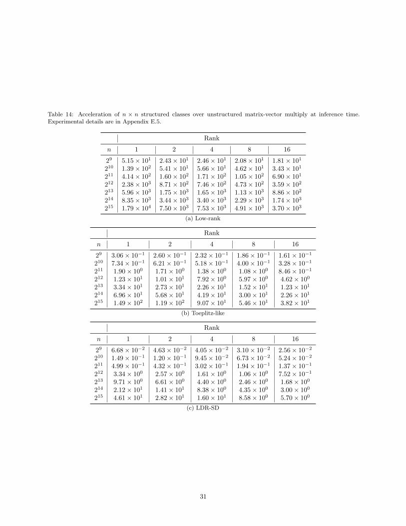
Table 14: Acceleration of n × n structured classes over unstructured matrix-vector multiply at inference time.Experimental details are in Appendix E.5.

Rank

n 1 2 4 8 16

29 5.15× 101 2.43× 101 2.46× 101 2.08× 101 1.81× 101

210 1.39× 102 5.41× 101 5.66× 101 4.62× 101 3.43× 101

211 4.14× 102 1.60× 102 1.71× 102 1.05× 102 6.90× 101

212 2.38× 103 8.71× 102 7.46× 102 4.73× 102 3.59× 102

213 5.96× 103 1.75× 103 1.65× 103 1.13× 103 8.86× 102

214 8.35× 103 3.44× 103 3.40× 103 2.29× 103 1.74× 103

215 1.79× 104 7.50× 103 7.53× 103 4.91× 103 3.70× 103

(a) Low-rank

Rank

n 1 2 4 8 16

29 3.06× 10−1 2.60× 10−1 2.32× 10−1 1.86× 10−1 1.61× 10−1

210 7.34× 10−1 6.21× 10−1 5.18× 10−1 4.00× 10−1 3.28× 10−1

211 1.90× 100 1.71× 100 1.38× 100 1.08× 100 8.46× 10−1

212 1.23× 101 1.01× 101 7.92× 100 5.97× 100 4.62× 100

213 3.34× 101 2.73× 101 2.26× 101 1.52× 101 1.23× 101

214 6.96× 101 5.68× 101 4.19× 101 3.00× 101 2.26× 101

215 1.49× 102 1.19× 102 9.07× 101 5.46× 101 3.82× 101

(b) Toeplitz-like

Rank

n 1 2 4 8 16

29 6.68× 10−2 4.63× 10−2 4.05× 10−2 3.10× 10−2 2.56× 10−2

210 1.49× 10−1 1.20× 10−1 9.45× 10−2 6.73× 10−2 5.24× 10−2

211 4.99× 10−1 4.32× 10−1 3.02× 10−1 1.94× 10−1 1.37× 10−1

212 3.34× 100 2.57× 100 1.61× 100 1.06× 100 7.52× 10−1

213 9.71× 100 6.61× 100 4.40× 100 2.46× 100 1.68× 100

214 2.12× 101 1.41× 101 8.38× 100 4.35× 100 3.00× 100

215 4.61× 101 2.82× 101 1.60× 101 8.58× 100 5.70× 100

(c) LDR-SD

31

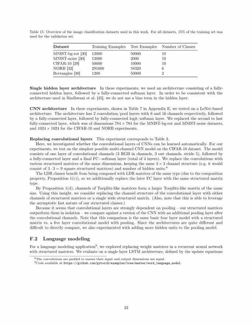
Table 15: Overview of the image classification datasets used in this work. For all datasets, 15% of the training set wasused for the validation set.

Dataset Training Examples Test Examples Number of Classes

MNIST-bg-rot [30] 12000 50000 10MNIST-noise [30] 12000 2000 10CIFAR-10 [29] 50000 10000 10NORB [32] 291600 58320 6Rectangles [30] 1200 50000 2

Single hidden layer architecture In these experiments, we used an architecture consisting of a fully-connected hidden layer, followed by a fully-connected softmax layer. In order to be consistent with thearchitecture used in Sindhwani et al. [45], we do not use a bias term in the hidden layer.

CNN architecture In these experiments, shown in Table 7 in Appendix E, we tested on a LeNet-basedarchitecture. The architecture has 2 convolution/pool layers with 6 and 16 channels respectively, followedby a fully-connected layer, followed by fully-connected logit/softmax layer. We replaced the second to lastfully-connected layer, which was of dimensions 784× 784 for the MNIST-bg-rot and MNIST-noise datasets,and 1024× 1024 for the CIFAR-10 and NORB experiments.

Replacing convolutional layers This experiment corresponds to Table 3.Here, we investigated whether the convolutional layers of CNNs can be learned automatically. For our

experiments, we test on the simplest possible multi-channel CNN model on the CIFAR-10 dataset. The modelconsists of one layer of convolutional channels (3 RGB in channels, 3 out channels, stride 5), followed bya fully-connected layer and a final FC+softmax layer (total of 4 layers). We replace the convolutions withvarious structured matrices of the same dimensions, keeping the same 3× 3 channel structure (e.g. it wouldconsist of 3 · 3 = 9 square structured matrices) and number of hidden units.8

The LDR classes benefit from being composed with LDR matrices of the same type (due to the compositionproperty, Proposition 1(c)), so we additionally replace the later FC layer with the same structured matrixtype.

By Proposition 1(d), channels of Toeplitz-like matrices form a larger Toeplitz-like matrix of the samesize. Using this insight, we consider replacing the channel structure of the convolutional layer with eitherchannels of structured matrices or a single wide structured matrix. (Also, note that this is able to leveragethe asymptotic fast nature of our structured classes.)

Because it seems that convolutional layers are strongly dependent on pooling – our structured matricesoutperform them in isolation – we compare against a version of the CNN with an additional pooling layer afterthe convolutional channels. Note that this comparison is the same basic four layer model with a structuredmatrix vs. a five layer convolutional model with pooling. Since the architectures are quite different anddifficult to directly compare, we also experimented with adding more hidden units to the pooling model.

F.2 Language modelingFor a language modeling application9, we explored replacing weight matrices in a recurrent neural networkwith structured matrices. We evaluate on a single layer LSTM architecture, defined by the update equations:

8The convolutions are padded to ensure their input and output dimensions are equal.9Code available at https://github.com/pytorch/examples/tree/master/word_language_model.

32

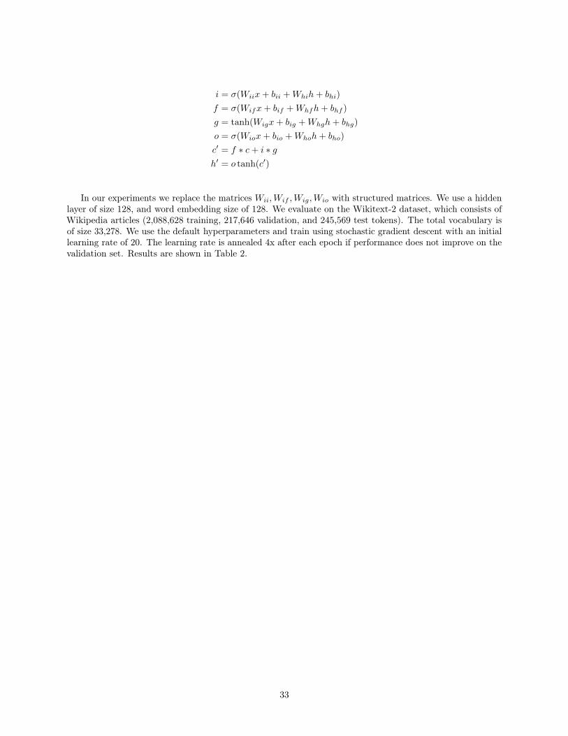
i = σ(Wiix+ bii +Whih+ bhi)

f = σ(Wifx+ bif +Whfh+ bhf )

g = tanh(Wigx+ big +Whgh+ bhg)

o = σ(Wiox+ bio +Whoh+ bho)

c′ = f ∗ c+ i ∗ gh′ = o tanh(c′)

In our experiments we replace the matrices Wii,Wif ,Wig,Wio with structured matrices. We use a hiddenlayer of size 128, and word embedding size of 128. We evaluate on the Wikitext-2 dataset, which consists ofWikipedia articles (2,088,628 training, 217,646 validation, and 245,569 test tokens). The total vocabulary isof size 33,278. We use the default hyperparameters and train using stochastic gradient descent with an initiallearning rate of 20. The learning rate is annealed 4x after each epoch if performance does not improve on thevalidation set. Results are shown in Table 2.

33