Optimal Streaming Permutations and Transforms - François ...

Research Collection

Doctoral Thesis

Optimal Streaming Permutations and Transforms: Theory andImplementation

Author(s): Serre, François

Publication Date: 2019

Permanent Link: https://doi.org/10.3929/ethz-b-000380039

Rights / License: In Copyright - Non-Commercial Use Permitted

This page was generated automatically upon download from the ETH Zurich Research Collection. For moreinformation please consult the Terms of use.

ETH Library

https://doi.org/10.3929/ethz-b-000380039

http://rightsstatements.org/page/InC-NC/1.0/

https://www.research-collection.ethz.ch

https://www.research-collection.ethz.ch/terms-of-use

diss . eth no. 25940

O P T I M A L S T R E A M I N G P E R M U TAT I O N S A N D T R A N S F O R M S :T H E O RY A N D I M P L E M E N TAT I O N

A thesis submitted to attain the degree ofdoctor of sciences of eth zurich (Dr. Sc. ETH Zurich)

presented byfrançois serre

Ingénieur diplomé de l’École Polytechnique (X2007)Master of Science ETH in Computer Science, ETH Zurichborn 6 January 1986

Citizen of France

accepted on the recommendation ofProf. Dr. Markus Püschel (advisor)Prof. Dr. Jeremy R. JohnsonProf. Dr. Paolo Ienne Lopez

April 2019

À la mémoire de mon père.

A B S T R A C T

Many algorithms used in hardware applications across disciplines, such as the fastFourier transform, the Walsh-Hadamard transform or sorting networks share a com-mon structure. They consist of stages of parallel and identical processing elementsthat each operates on two inputs with different data permutations in between. Thesymmetry in this structure enables folding to an area-efficient in a streaming archi-tecture that accepts the input over several cycles. However, necessary for folding arestreaming permutation circuits that require memory and routing components.

In this dissertation, we focus on the optimal implementation of these algorithms.We provide lower bounds for the implementation of streaming permutations, and pro-pose algorithms that produce solutions that match it (under certain assumptions). Weapply these algorithms in the context of a generator capable of implementing the hard-ware applications previously mentioned. Finally, for a given problem, we address thequestion of finding an optimal algorithm, i.e., an algorithm which streaming imple-mentations are the cheapest to implement.

R É S U M É

De nombreux algorithmes utilisés dans les circuits intégrés, tels que la transformée deFourier rapide, la transformée d’Hadamard, ou les réseaux de tri, présentent une struc-ture commune. Ils se composent de plusieurs couches d’éléments de traitement iden-tiques fonctionnant en parallèle, et qui opèrent chacun sur deux entrées. Ces couchessont elles-mêmes séparées par différentes permutations. Les symétries de cette struc-ture permettent de «replier» l’algorithme sur lui-même, permettant ainsi d’obtenirune architecture matérielle économe en ressources et qui travaille sur des donnéesétalées dans le temps. Ceci nécessite de permuter les données au sein de ce flux, cequi entraîne l’utilisation de mémoire d’une part, et d’éléments capables de dirigerspatialement les données d’autre part.

Cette thèse porte sur l’implémentation optimale de tels algorithmes. Nous définis-sons plusieurs mesures sur les permutations de flux de données, notamment leurentropie spatiale, puis montrons qu’elles représentent en fait la quantité de ressourcesminimale nécessaire à l’implémentation de ces permutations (en terme de nombre demultiplexeurs, ou de quantité de mémoire). Nous proposons ensuite des méthodesqui, sous certaines conditions, permettent de construire des structures optimales. En-fin, pour un problème donné, nous nous interressons à la recherche d’un algorithmeoptimal, i.e. qui comporte les permutations dont l’implémentation nécessite le mini-mum de ressources possible.

v

A C K N O W L E D G M E N T S

I owe my advisor Markus Püschel not only for pushing me to pursue this PhD, butas well for his support, his guidance and his patience; often having to proofread thelast-minute changes I could make to our publications. I can’t imagine what these yearswould have been without the knowledge he shared, especially in abstract algebra, andthe freedom he offered me. I don’t think that many advisors would have agreed tolet me work on a theorem (Chapter 6) for almost a year, without any guarantee ofsuccess. Outside of work, I’m also grateful for the general knowledge and social skillshe demonstrated and shared.

I’m particularly lucky for the environment I worked in, and I am thankful to Alen,Daniele, Eliza, Gagandeep, Georg, Joao, Luca, Marcela, Melanie, Tyler and Victoria forthe passionate debates we had at lunch, the innumerable evenings we spent together,the sport challenges we met (or not. . . ), the flights, the hikes and the trips we didtogether. I express as well my fondness to the people I met at ETH and at the ASVZ, tomy flatmates at Elsa, to the people of Distran [7], to Cecilia, Erwan, Gemma, Katarina,Michèle, Nicolas, Sophie and Thomas for making these years in Zurich wonderful.

I thank Susanna for her support throughout the end of this PhD, and for assistingme in preparing its defense, though she might not have been overly passionate aboutthe topic.

Je tiens aussi à remercier ceux que je ne vois que trop rarement, mais dont l’ami-tié dépasse le nombre des kilomètres : les «gros» de la section judo, les guguss, lesmagnoludoviciens, et les sujets de sa majesté Abdul Ier.

En particulier, je remercie Guillaume (un vrai docteur, lui !) et Anne-Sophie pour lesoutien et le réconfort qu’ils m’ont apporté au cours de moments douloureux.

Enfin, je remercie ma famille et particulièrement mes parents. Je leur suis infinimentreconnaissant pour leur soutien inconditionnel et les sacrifices qu’ils ont voués à maréussite. Cette thèse est dédiée à la mémoire de mon père, à qui je dois le goût de laphysique et de la science.

vii

C O N T E N T S

1 introduction 1

1.1 Challenges 4

1.1.1 Streaming permutations 4

1.1.2 Implementation 5

1.2 Contributions 6

1.2.1 Streaming permutations 6

1.2.2 Streaming algorithms 6

1.2.3 Hardware generator 7

1.3 Organisation of this dissertation 7

i permutations at full st(r)eam 9

2 streaming permutations 11

2.1 General streaming permutation 11

2.1.1 Streaming permutation 12

2.1.2 Examples 12

2.1.3 Lower bounds 14

2.1.4 Spatial and temporal permutations 18

2.2 Streaming linear permutation 21

2.2.1 Linear permutations 21

2.2.2 Routing entropy for SLPs 23

2.2.3 Spatial and temporal SLPs 24

2.2.4 General linear permutations 27

2.2.5 Examples 29

2.3 Results 31

2.4 Related work 34

2.5 Conclusion 35

3 memory-efficient streaming fft by fusing permutations 37

3.1 Streaming multiple linear permutations 37

3.1.1 Sequence of Spatial SLPs 38

3.1.2 Sequence of Temporal SLPs 40

3.1.3 General sequence of SLPs 42

3.2 Application: Pease FFT 43

3.3 Results 45

3.4 Conclusion 49

4 in search of the optimal streaming wht 53

4.1 Background and notations 53

4.2 Enumeration of WHT algorithms 56

4.3 Search for optimal algorithms 56

4.3.1 Cost function 58

4.3.2 Search algorithm 58

4.4 Results 59

4.5 Conclusion and future work 59

ii implementation 65

5 a hardware generator for fft and sorting networks 67

ix

x contents

5.1 Generation pipeline 67

5.1.1 SPL 68

5.1.2 Streaming-block DSL 70

5.1.3 Streaming-RTL DSL 73

5.2 A DSL for “Streaming-RTL” 75

5.2.1 Staging and LMS 76

5.2.2 Abstraction over hardware datatypes 77

5.2.3 Synchronization 78

5.2.4 Smart constructors 79

5.3 Streaming-block DSL 80

5.3.1 Streaming blocks 81

5.3.2 Higher-order blocks 81

5.3.3 Permutation blocks 82

5.3.4 Optimizations 82

5.4 results 82

5.5 Limitations and related work 85

5.5.1 Hardware DSLs implemented in Scala 86

5.5.2 Hardware generator for FFTs 86

5.5.3 Hardware generator for sorting networks 86

5.6 Conclusion 87

iii linear algebra theorems 89

6 a lul block triangular decomposition with min. off-ranks 91

6.1 Problem statement 91

6.1.1 Lower bounds 92

6.1.2 Optimal solution 92

6.1.3 Flexibility 93

6.1.4 Equivalent formulations 94

6.1.5 Related work 94

6.2 Preliminaries 95

6.2.1 Properties of the blocks of an invertible matrix 95

6.2.2 Algorithms on linear subspaces in matrix form 96

6.2.3 Double complement 97

6.3 Proof of Theorem 4 98

6.4 Proof of Theorem 5, case p2 6 t+ k− p1 − p4 99

6.4.1 Sufficient conditions 99

6.4.2 Building L 100

6.4.3 Example 103

6.5 Proof of Theorem 5, case p2 > t+ k− p1 − p4 105


6.5.2 Building L 106

6.5.3 Example 107

6.6 Rank exchange 109


6.6.2 Building L ′ 110

6.6.3 Example 111

6.7 Conclusion 112

7 characterizing and enumerating wht algorithms 115

contents xi

7.1 Notations 115

7.2 Characterization of WHT algorithms 116

7.3 Other transforms 116

7.4 Proof of Lemma 12 116

7.4.1 Invertibility of the spreading matrix 117

7.4.2 About condition (73) 119

7.4.3 General expression of W(P) 121

7.4.4 Proof of Lemma 12 123

7.5 Proof of Theorem 3 123

8 conclusion and future work 125

bibliography 127

L I S T O F F I G U R E S

Figure 1 Radix-2 Iterative Cooley-Tukey FFT dataflow (from right to left)operating on N = 16 elements. 2

Figure 2 Radix-2 Pease-FFT dataflows operating on N = 16 elementswith different types of folding [47]. In (a), the design isnot folded and consists of 4 stages (each comprising aperfect-shuffle permutation, an array of butterflies F2 andan element-wise multiplication by constants), followed by abit-reversal permutation. (b) is horizontally folded: it imple-ments only one instance of this stage that processes the datasetiteratively. (c) is vertically folded: the dataset is input streamedin chunks of 2k = 4 elements (the streaming width) that enterduring N/K = 4 consecutive cycles. (d) combines both types offolding. 3

Figure 3 Sketch of two implementations of the bit reversal permutationon 23 elements. On the left, the structure has as many portsas the dataset. Thus a simple rewiring is enough. On the rightside, data are streamed on two ports. Therefore, the datasetenters within 4 cycles (top), and is retrieved within 4 cycles(bottom). 4

Figure 4 A sorting network working on N = 8 elements [37]. The blockswith an arrow represent two input sorters. On the top, a fully-parallel implementation. On the bottom, the same implemen-tation “folded” with K = 4, allowing to halve the number ofsorters [89]. 12

Figure 5 An SNW consisting of two Omega network stages. Eachstage contains a perfect shuffle followed by a column of 2k−1

switches controlled by a single common bit. Here, the firststage is controlled by a single bit of a counter, while the secondone is controlled by the sum of the two other bits of thiscounter. 25

Figure 6 Implementation of the first output port of a switching networkusing a 4-to-1 multiplexer. 26

Figure 7 Two possible architectures for a streaming permutation. 28

Figure 8 Comparison of our two structures for a bit-reversal permu-tation on 2048 16-bit elements for different multiplexer sizesvs. [45]. Labels: number of BRAM tiles. In this example, theSNW-RAM-SNW structure that uses 2-input muxes is equiva-lent to [63]. 32

Figure 9 Number of switches needed for 107 random SLPs with differentarchitectures. 32

Figure 10 Our contribution: streaming design with iterative reuse withtwo permutations fused. 37

xii

List of Figures xiii

Figure 11 The basic blocks we use, here for a streaming width of 2k =

4. (a) can pass any temporal permutation; (b) implements thetwo spatial steady SLPs π(It ⊕ J2) and π(In); (c) implements(21). 41

Figure 12 Datapath for the permutation block in Fig. 10b. 43

Figure 13 Datapath for a bit reversal on 2n = 16 elements streamed on2k = 4 ports (see Section 2.2.4). 43

Figure 14 Radix-2 Pease FFT, iterative reuse with fused permutation n =

4, k = 2. 44

Figure 15 Number of 2-input multiplexers in the datapath of a radix-2 Pease FFT, for different streaming widths. Lower is bet-ter. 47

Figure 16 Gap of a radix-2 Pease FFT in number of cycles betweentwo transforms, for different streaming widths. Lower isbetter. 48

Figure 17 Resources used by a radix-2 Pease FFT. Lower is better. 50

Figure 18 Resources used by a radix-4 Pease FFT. Lower is better. 51

Figure 19 Dataflows computing a WHT on 2n = 16 elements. The H2blocks represent butterflies. 54

Figure 20 Algorithms from Fig. 19 folded with a streaming width 2k = 4.This architecture uses a fourth of the number of butterflies, butprocesses the inputs over 2n−k = 4 cycles. 55

Figure 21 Dataflow of all butterfly networks with linear permutationscomputing H22 . The associated bit matrices are listed in Ta-ble 4 57

Figure 22 Butterfly network computing a WHT of size 2n = 32 that, whenstreamed with 2k = 8, yields an implementation with minimalnumber of memory elements and switches. 61

Figure 23 The different layers of our generator. 68

Figure 24 Radix-2 Cooley-Tukey FFT datapaths operating on 2n = 8 el-ements. This algorithm is used when iterative reuse is notenabled, as the permutations involved require less resourceswhen streamed. 69

Figure 25 Batcher bitonic sorting network [4] operating on 2n = 8 el-ements. This design corresponds to the SN1 architecture in[89]. 70

Figure 26 Constant-geometry sorting network [79] operating on 2n = 8

elements. This design loosely corresponds to the SN5 architec-ture in [89]. 71

Figure 27 Design of Fig. 10b expressed using the streaming blockDSL. The necessary streaming permutation is expanded intoswitches and RAM banks (dark blue rectangles). The optimiza-tion here “unrolls” some parts of the permutation to removean array of multiplexer. Additionally, two arrays of switcheswere grouped for later mapping to 4-to-1 multiplexers. Theseoptimizations increase the throughput and reduce the area ofthe final design. 71

Figure 28 Resources used by different FFTs (40) in different con-figurations, on complex data using 2 × 32bits IEEE754

floating-point. 83

Figure 29 Resources used by a radix-2 Cooley-Tukey WHTs (41) with astreaming width of 8, on complex data using 2× 32bits fixed-point. 84

Figure 30 Resources used by different bitonic sorting networks (42), withdifferent streaming configuration on complex data using 2 ×32bits fixed-point. 84

Figure 31 Possible ranks for L and R. On the left graph, p2 < t+ k− p1 −p4. On the right graph, p2 > t+ k− p1 − p4. The dot showsthe decomposition provided by Theorem 5. 93

Figure 32 L ′ trades a rank of L for a rank of R on the associated decom-position. 109

L I S T O F TA B L E S

Table 1 Bounds and routing matrix for some streaming permuta-tions. 17

Table 2 Comparison of different architectures using RAMs, in thecase of a full-throughput SLP. Values in bold are optimalones. 33

Table 3 Comparison of different architectures using different permuta-tion methods, for a radix-2 Pease FFT, for k > 1. 46

Table 4 Matrices P0, P1 and P2 of all butterfly networks with linearpermutations computing H22 . The corresponding product ofmatrices (P0:n) and spreading matrix (X) defined in Chapter 7

are presented as well. The first line corresponds to the Pease al-gorithm, the second one to its transpose. These two algorithmsare the only ones that can be obtained using (24) recursively[35]. 57

Table 5 Number of butterfly networks with linear permutations, num-ber of butterfly networks with bit permutations and number ofsuch networks that can be derived from (24) [35] for a givenn. 57

Table 6 Number of stages of 2k−1 switches in WHTs of size 2n imple-mented with a streaming width of 2k. 60

Table 7 SPL operators used in our generator. 68

Table 8 Streaming blocks used in the streaming-block DSL. The lasthigher-order operator allows to represent the structure intro-duced in Chapter 3. 72

Table 9 Example of nodes (signals) used in the streaming-RTL DSL, andcorresponding syntax. 74

xiv

List of Tables xv

Table 10 We summarize matrix operators to perform basic operations onsubspaces. M is a general matrix, while A and B are matriceswithm rows that represent the subspaces A and B; i.e. A = 〈A〉and B = 〈B〉. Inspection of these routines shows that they allcan be implemented with O(m3) runtime. 96

1I N T R O D U C T I O N

In 1822, Joseph Fourier was working on a thermodynamic law that now has hisname [55], stating that the heat flux ~φ in a body is proportional to the gradientin temperature T in this body: ~φ = −λ · ~gradT . Using the conservation of energy(C · ∂T/∂t = −div~φ), this yields the heat equation (Chapter 2 of [21]):

∂T

∂t=λ

C·∆T .

Fourier noticed (Chapter 4 of [21]) that in the case of one spatial dimension1 x,

e−λC ·t · cos x, e−3

2 λC ·t · cos 3x, e−5

2 λC ·t · cos 5x, . . .

were solutions T(x, t) of this equation. To get a general solution for an initial temper-ature distribution T(x, 0) = T0 for −π/2 < x < π/2, Fourier proposed to decompose2

the latter function into a sum of trigonometric functions an cosnx. This allowed himto express a general solution in the form of a sum of the particular solutions he found.

The discrete Fourier transform (DFT) is used similarly: it decomposes a discrete signalx = (xt)06t<N ∈ CN into a sum of trigonometric sequences(y1

Ne2iπt/N

)t

,(y2Ne4iπt/N

)t

,(y3Ne6iπt/N

)t

, . . . .

Applying a linear transform to x amounts to applying it to each of these trigonometricsequences. In some cases, this technique can dramatically decrease the computationalcomplexity. For instance, a convolution on one of these sequences can be computedusing a single scalar multiplication [43].

The coefficients y = (yj)06j<N of the sum are given by y = DFTN ·x, where

DFTN = [ωij]06i,j<N, with ω = e−2iπ/N.

As in its origins, the DFT became a “hot topic” when an algorithm to compute it inO(N logN) was discovered3 in 1965 [15], the Fast Fourier transform (FFT). It is now aubiquitous tool in signal processing and beyond, used in image and speech processing,radar, wireless communication (e.g., in the LTE standard), and many other domains.Thus, fast and efficient implementations of FFTs, in software and in hardware, and inparticular for embedded systems, are of high importance.

The FFT can be implemented using a so-called butterfly network as shown in Fig. 1.Note that all dataflows in this document are from right to left because of the corre-sponding matrix notation introduced later. It consists of stages of parallel and almostidentical blocks (the butterflies) that each operates on two inputs with data permu-tations in between. Many other algorithms used in hardware applications in signal

1 Fourier solves first the problem in stationary conditions in Chapter 3. The problem shown here considersa unique dimensionless spatial coordinate −π/2 6 x 6 π/2, with the boundary conditions T(−π/2, t) =T(π/2, t) = 0.

2 He stated that any function was the sum of trigonometric functions, but this turned out to be false.Finding conditions such that a function is the sum of its Fourier serie kept mathematicians like Parseval,Dirichlet or Jordan busy throughout the XIXth century.

3 Gauß already discovered it in 1805 [26].

1

2 introduction

F2

F2

F2

F2

F2

F2

F2

F2

−i

−i

−i

−i

F2

F2

F2

F2

F2

F2

F2

F2

ω216

−i

ω616

ω216

−i

ω616

F2

F2

F2

F2

F2

F2

F2

F2

ω116

ω216

ω316

−i

ω516

ω616

ω716

F2

F2

F2

F2

F2

F2

F2

F2

Figure 1: Radix-2 Iterative Cooley-Tukey FFT dataflow (from right to left) operating on N = 16

elements.

processing, communication, and other domains, share this structure consisting of anetwork of small processing elements and different intermittent permutations. Exam-ples include the Walsh-Hadamard transform (WHT) [29], fast cosine and sine transforms[2], sorting networks (SNs) [4, 79], permutation networks [6, 84, 61, 40, 78, 49], and oth-ers.

The regular structure offers much flexibility in their hardware implementations andthus there has been extensive work, most focusing on the FFT (e.g., [1, 14, 39, 16, 30,32, 47, 25, 46, 50]. In particular, [50, 47, 88, 89] propose generators for FFTs and sortingnetworks that are capable of producing an entire design space of implementationswith different trade-offs in performance and resource consumption. These generatorsare built as a back-end of Spiral, a generator of signal processing libraries tuned for aspecific platform [64], and operates with different algorithms represented in a domainspecific language (DSL) called SPL. It then exploits different symmetries (or regulari-ties) of these algorithms to obtain a space of relevant designs, as we explain next. Thedesired design is then output as a register-transfer level (RTL) description in the Veriloghardware description language.

Fig. 2a shows the dataflow of a radix-2 Pease FFT [81], a variant of the FFT derivedin [60], on N = 16 points. The FFT comprises four identical stages (except for thetwiddle scaling shown as little circles) of eight parallel butterflies F2 preceded by aperfect-shuffle, followed by the bit reversal permutation. This dataflow can be used for afully-parallel implementation that has high throughput but also high cost.

The cost can be reduced by exploiting the repetitive structure of this FFT. A firstmethod, called streaming reuse, “folds the dataflow vertically” to obtain a design likeFig. 2c [57, 50, 47]. Now the circuit operates on streaming data, which means that thedataset arrives on K ports during N/K cycles. In the figure K = 4.

Fig. 2a has another symmetry: the first four stages are almost identical. Therefore,it is possible to “fold the dataflow horizontally” to reuse over time a single hardwarestage [60] as in Fig. 2b. This is called iterative reuse.

introduction 3

F2

F2

F2

F2

F2

F2

F2

F2

F2

F2

F2

F2

F2

F2

F2

F2

ω4

ω4

ω4

ω4

F2

F2

F2

F2

F2

F2

F2

F2

ω2

ω2

ω4

ω4

ω6

ω6

F2

F2

F2

F2

F2

F2

F2

F2

ω1

ω2

ω3

ω4

ω5

ω6

ω7

(a)

No

reus

e.

F2

F2

F2

F2

F2

F2

F2

F2

× × × × × × ×

(b)

Iter

ativ

ere

use

only

.

S4

F2

F2

S4

F2

F2

× ×

S4

F2

F2

× ×

S4

F2

F2

× ×

J4

(c)

Stre

amin

gre

use

only

.

S4

F2

F2

× ×

J4

(d)

Iter

ativ

ean

dst

ream

ing

reus

e.

Figu

re2:R

adix

-2Pe

ase-

FFT

data

flow

sop

erat

ing

onN

=16

elem

ents

wit

hdi

ffer

ent

type

sof

fold

ing

[47].

In(a

),th

ede

sign

isno

tfo

lded

and

cons

ists

of4

stag

es(e

ach

com

pris

ing

ape

rfec

t-sh

uffle

perm

utat

ion,

anar

ray

ofbu

tter

fliesF2

and

anel

emen

t-w

ise

mul

tipl

icat

ion

byco

nsta

nts)

,fol

low

edby

abi

t-re

vers

alpe

rmut

atio

n.(b

)is

hori

zont

ally

fold

ed:i

tim

plem

ents

only

one

inst

ance

ofth

isst

age

that

proc

esse

sth

eda

tase

tite

rati

vely

.(c)

isve

rtic

ally

fold

ed:t

heda

tase

tis

inpu

tst

ream

edin

chun

ksof2k=4

elem

ents

(the

stre

amin

gw

idth

)th

aten

ter

duri

ngN/K=4

cons

ecut

ive

cycl

es.(

d)co

mbi

nes

both

type

sof

fold

ing.

4 introduction

0

1

2

3

4

5

6

7

0

4

2

6

1

5

3

7

(a) not streaming

P0

1

2

3

4

5

6

7

0

1

0 1 2 3Cycle

P0

4

2

6

1

5

3

7

0

1

0 1 2 3Cycle

(b) streaming

Figure 3: Sketch of two implementations of the bit reversal permutation on 23 elements. Onthe left, the structure has as many ports as the dataset. Thus a simple rewiring isenough. On the right side, data are streamed on two ports. Therefore, the datasetenters within 4 cycles (top), and is retrieved within 4 cycles (bottom).

The two types of folding can be combined [50, 47], resulting, for example, in thedesign shown in Fig. 2d. If fully folded in both dimensions, the design is very compact.In the case shown it contains only two butterflies, two complex multipliers, and thehardware to perform the bit reversal (represented in Fig. 2c and 2d with the bluebox labeled with J4) and the perfect shuffle (labeled with S4). The work in [50, 47]considers and generates the entire design space given by varying the degree of foldingin both dimensions.

1.1 challenges

1.1.1 Streaming permutations

The permutations (or data reorderings) required between the butterfly stages are sim-ple to implement in the case of non-streaming designs (Fig. 2a and 2b). All dataare available in one cycle and a hardware implementation consists of a set or wiresas shown in Fig. 3a. However, streaming designs (such as Fig. 2c and 2d) requirestreamed permutation circuits (represented with blue boxes), as data arrive streamedin chunks over several cycles as in Fig. 3b. Their implementation is non-obvious: theyrequire memory, as data may now be permuted across cycles, and routing componentslike multiplexers or switches, as elements arriving on a given input port may need tobe directed to different output ports. Efficient methods for implementing these havebeen developed in the literature. There are two classes of implementations. One de-signs a circuit that can handle any permutation [45, 38], parameterized by the controllogic at runtime. However, this flexibility comes at the price of a higher area cost. Thesecond class consists of datapaths that are specialized for the desired permutation [59,58, 31, 63, 23], which thus reduces cost.

Measuring implementation cost. The cost to implement a streaming permutationcan be measured in terms of latency, total memory capacity required, number of in-dependent memory elements, or routing logic complexity. Lower bounds, and imple-

1.1 challenges 5

mentation methods that minimize the first three of these measurements are known[38], and it is therefore possible to quantify how hard a given streaming permuta-tion is to implement in this respect, or to estimate how far a given implementationis from optimality. However, quantifying routing complexity remains a challenge. Ifsome methods of implementation pay a particular attention to the number of routingelements used [11, 12, 24, 63], knowing for instance the absolute minimal number of2-input multiplexers that would be required to implement a given streaming permu-tation is still an open question.

Best network for streaming. We already presented two different networks for com-puting a DFT on 16 elements in Fig. 1 and 2a. The latter allows iterative reuse due to itsrepetitive structure, but it is known that the permutations in the former are cheaperto implement when streamed [46, 47]. A question that arises is, for a given stream-ing configuration, which butterfly network would be the cheapest to implement. Thiswould require the identification of all possible networks to choose the best.

1.1.2 Implementation

The state of the art of the different components needed to implement streaming algo-rithms keeps improving. We already discussed the streaming permutations, and theexistence of different methods to implement them. Arithmetic circuit unit is anotherimportant component. For instance, FloPoCo [19] provides an open-source generatorfor pipelined floating-point arithmetic with arbitrary precision However, no generatorto date combines these features with the flexibility offered by [47, 89]. One possiblecause is the difficulty of programming a generator capable of mapping a high-level de-sign (as in Figs. 2c and 2d) to a concrete RTL implementation. Some of the challengesare discussed next.

Mismatch of hardware and software datatypes. A first difficulty, common amonghigh-level synthesis (HLS) tools, is the wide diversity of possible datatypes that hard-ware designs enable. The precision of (unsigned or signed) integers or fixed pointnumbers can be chosen arbitrarily, in contrast to a small set of choices in software.The same applies to floating-point arithmetic, ranging from IEEE754 to the space cov-ered by FloPoCo [19], which offers arbitrary mantissa and exponent width.

Two different evaluation times. A second issue is that a given function may need tobe either evaluated during design generation or implemented in the resulting design,or even partially evaluated during generation and partially implemented.

For instance, the FFT involves multiplications with a set of constants, called twiddlefactors. A twiddle factor ti,j is a complex number that depends on two parameters:the index i of the element, and the index of the computation stage j. In the case ofnon-iterative designs (Figs. 2a and 2c), the parameter j is known at generation time,while in iterative scenarios (Figs. 2b and 2d), the design would need to implement acounter counting the number of datasets that were already processed by the stage. Sim-ilarly, the parameter i is known at generation-time for non-streaming designs (Figs. 2aand 2b) for each different multiplier, while in streaming designs (Figs. 2c and 2d),i depends on the multiplier position, and on a timer that counts the number of cy-cles elapsed since the dataset began to enter. As the computation of a twiddle factorwould typically involve a ROM containing different possible values, it is essential toexploit during generation as much as possible the structure of i and j to reduce ROMconsumption and DSP slices in case of trivial multiplications.

6 introduction

A typical solution for handling this problem consists of writing and maintainingdifferent versions for each different scenario, which is error-prone and time consum-ing.

Synchronization issues. Design usually require pipelining to handle the frequencyrequired by the user. Keeping the example of twiddle factors, an inspection of differentFFT algorithms shows that most constants are 1, i (the imaginary unit) or −i, whichresults in a trivial multiplication that does not require pipelining. However, it is neces-sary in this case to add supplementary registers if another non-trivial multiplicationexists, to keep the whole dataset synchronized.

Additionally, if the twiddle factor computation is done in hardware, it may alsorequire pipelining. As this computation is independent of the input to the FFT, it ispossible to initiate it in advance to avoid impacting the global latency of the design.However, this requires a precise cycle tracking to trigger the counter and the timer atthe appropriate time.

Handling the latency. As some of the designs produced use a loop (Figs. 2b and2d), special attention must be paid to guarantee that the latency of the inner structureis long enough to avoid collision between the tail and the head of a given dataset.Additionally, this inner latency determines the minimal time separating two datasets,which must be reported to the user.

1.2 contributions

In this thesis, we address the problems above with the following contributions:

1.2.1 Streaming permutations

• We introduce a novel metric, the routing entropy, that allows to quantify the dif-ficulty of implementing a given streaming permutation in terms of routing ele-ments.

• We present two methods to implement streaming linear permutations, a class ofpermutation that is ubiquitous in signal processing algorithms. The first oneyields implementations that have routing optimality, which means that no imple-mentation can have less multiplexers. The second method yields memory optimalimplementations, which means that no implementation can have a lower latency,a lower number of memory elements, or a lower total memory capacity. Addi-tionally, these implementations have the lowest possible number of multiplexersfor the particular architecture we consider, and we precisely characterise thecases where routing optimality is reached.

• We propose a method to implement a circuit that can pass several different linearpermutations. The circuit has memory optimality, and uses a low number ofmultiplexers.

1.2.2 Streaming algorithms

• We propose a novel small FFT architecture that harnesses the circuit passingseveral linear permutations to reduce the memory consumption.

1.3 organisation of this dissertation 7

• We characterize and propose a method to enumerate all WHT algorithms con-sisting of stages of columns of butterflies separated by linear permutations.

• We provide a method to search among them those that are the cheapest to imple-ment. Using this method, we generate for small sizes novel butterfly networksthat reduce the number of independent memory elements needed, or the num-ber of multiplexers required.

1.2.3 Hardware generator

We present a modular hardware generator that generates streaming designs for FFTs,WHTs and sorting networks. It is implemented in Scala [51], and leverages Scala’s fa-cilities for embedding DSLs, concepts from lightweight modular staging (LMS) [65] toperform optimization at the DSL levels, and Scala’s type system to offer the flexibilitydiscussed above.

1.3 organisation of this dissertation

This thesis is divided into three parts. The first part considers the theory of streamingalgorithms: Chapter 2 discusses the implementation of streaming permutations; Chap-ter 3 proposes a novel compact streaming FFT architecture, and Chapter 4 considersthe search for an optimal WHT streaming algorithm. In the second part (Chapter 5),we present a prototype of a modular generator for streaming hardware. The third partprovides two linear algebra tools used in the first part, but that are also of intereston their own: a novel matrix factorization that minimizes the rank of certain blocks(Chapter 6), and a method to identify and enumerate a class of WHT algorithms.

Part I

P E R M U TAT I O N S AT F U L L S T ( R ) E A M

2S T R E A M I N G P E R M U TAT I O N S

A fully parallel hardware implementation of algorithms on large data sets is usuallyimpossible due to the resources it requires. Therefore, the corresponding dataflowsneed to be folded into a streaming architecture, which accepts the input over severalcycles. Particularly suited for folding are regular algorithms such as the fast Fouriertransform [60] (Fig. 1), Viterbi decoding, or sorting networks [37]. An example of thelatter for N = 8 elements is shown in Fig. 4a and an associated folded version withstreaming width K = 4 in Fig. 4b. The folded version halves the number of two inputsorters needed for its implementation [89].

Some permutations are trivial to fold due to their spatial periodicity (e.g., the tworightmost permutations in Fig.4b), i.e., if they perform equal subpermutations onblocks of size K. However, in general, implementing a streaming permutation is chal-lenging, as it requires both routing between ports and delays across cycles. We as-sume only 2-input multiplexers and single-ported RAMs as building blocks, which iswell-suited for FPGAs.

In this chapter, that extends the work presented in [68, 71], we quantify the diffi-culty of implementing a streaming permutation, both in terms of memory and routinglogic. We then present a method to implement streamed linear permutations (SLPs) onN = 2n elements with proven optimality. Linear permutations are the permutationsthat operate as linear mappings on the bit representation of indices. They includemany of the most important occurring permutations including stride permutationsand the bit reversal. They are needed in fast Fourier transforms (FFTs; see Fig. 1), fastcosine transforms, sorting networks (see Fig. 4a), Viterbi decoders, and many otherapplications. Specifically:

• We prove a lower bound for the routing complexity for a general streamingpermutation, i.e., for the number of multiplexers or switches needed.

• We provide a method to derive optimal implementations of SLPs. The methoddecomposes a given linear permutation into a sequence of spatial and temporalpermutations that can be implemented, respectively, as (memoryless) switchingnetworks and banks of RAM. We show that this decomposition is equivalentto a matrix factorization problem in which the minimization of certain ranks ofsubmatrices is equivalent to minimizing the logic of the resulting circuit.

• Finally, we demonstrate our method by generating streamed bit reversal per-mutations for a Virtex FPGA, and by comparing our optimal solutions to priorart.

2.1 general streaming permutation

In this section, we give a formal definition of streaming permutations, and providelower bounds on the logic needed to implement them. The bounds are expressed interms of two quantities associated with a streaming permutation: its minimal latency

11

12 streaming permutations

↑

↑

↑

↑

↑

↑

↑

↑

↑

↑

↑

↑

↑

↑

↑

↑

↑

↑

↑

↑

↑

↑

↑

↑

(a) not streaming

↑

↑

↑

↑

↑

↑

↑

↑

↑

↑

↑

↑

(b) streaming (K = 4)

Figure 4: A sorting network working on N = 8 elements [37]. The blocks with an arrow rep-resent two input sorters. On the top, a fully-parallel implementation. On the bottom,the same implementation “folded” with K = 4, allowing to halve the number ofsorters [89].

δσN,K and its routing entropy SσN,K. We then define two subclasses of streaming per-mutations that will be crucial in our approach: temporal and spatial permutations.

2.1.1 Streaming permutation

Formally, we define a streaming permutation as a pair (σN,K), where σN is a permuta-tion (or the corresponding permutation matrix1) of N words indexed by 0, . . . ,N− 1,and K a positive integer that divides N (K|N). K is called the streaming width.

An implementation of a streaming permutation is a synchronous circuit that has Kinput and K output ports, and that permutes a dataset of N elements according to σN.The dataset enters sequentially in N/K chunks of K elements, and is output similarly(see Fig. 3b). Therefore, the element that enters during the cth input cycle on the pth

input port is output during the c ′th output cycle on the p ′th output port, where

c ′K+ p ′ = σN(cK+ p).

Additionally, we say that an architecture has full throughput, if it is capable of han-dling sequential datasets without interruption.

2.1.2 Examples

We provide a few example permutations that we consider:Identity. The identity matrix of size N is denoted with IN. An implementation of

(IN,K) directly maps the elements arriving on its K inputs ports to its K output ports.

1 We use a row representation for permutation matrices: if [pi,j] represents σ, then pi,j = 1 if i = σ(j), and0 otherwise.

2.1 general streaming permutation 13

Cyclic shift. We denote with CN the cyclic shift matrix:

CN =

1. . .

1

1

. (1)

An implementation of (CN,K) would map the elements of a dataset as follows:

• The element arriving during the input cycle 0 (the first cycle) on the input port 0(the first port) is output during the last output cycle (N/K− 1) on the last outputport (K− 1).

• Other elements arriving on the first port during the input cycle c are output onthe last port at the output cycle c− 1.

• All other elements, arriving on the port p during the input cycle c are output onport p− 1 at the output cycle c.

Reversal permutation. The permutation that reverses its inputs is represented bythe matrix

JN =

1

. ..

1

.

An implementation of (JN,K) maps the element arriving on port p during the inputcycle c on output port K− p− 1 during the cycle N/K− c− 1.

Stride permutations. If R|N, we denote with LN,R the stride-by-R permutation matrix,i.e. the matrix representing the transposition of a (N/R)× R-matrix stored in a row-major order:

LN,R : i · NR

+ j 7→ j · R+ i, for 0 6 i < R and 0 6 j < N/R. (2)

As an example,

L6,2 =

1 · · · · ·· · · 1 · ·· 1 · · · ·· · · · 1 ·· · 1 · · ·· · · · · 1

.

Additionally, L2R,R is called perfect-shuffle.If N = K2, the streaming permutation (LK2,K,K) “exchanges space and time”: an

implementation would map the element arriving on port p during the input cycle con the output port c during the cycle p.

Half-reversal permutation. If A and B are two matrices, we denote with A⊕ B thedirect sum of A and B, i.e. the matrix

A⊕B =

(A

B

).


Additionally, if (Mi)06i<n is a sequence of n matrices, we denote with⊕n−1i=0 Mi the

matrix

n−1⊕i=0

Mi =

M0

M1

. . .

Mn−1

.

For instance, IN ⊕ JN is the permutation matrix that represents the permutation thatleaves the first half of its inputs unchanged, and that reverses the second half of itsinputs. It occurs in fast cosine transforms [77]. Therefore, the streaming permutation(IN ⊕ JN,N) would alternatively route its input ports directly to its output ports, orreverse them.

2.1.3 Lower bounds

We now present four lower bounds that constrain any implementation of a givenstreaming permutation (σN,K). Note that these are derived before we introduce anymethod of implementation, thus highlighting their architecture agnosticism.

Minimal latency. We denote with δσN,K the maximal difference an element can havebetween its input cycle c and its output cycle c ′:

δσN,K = max c− c ′ = max06i<N

bi/Kc− bσN(i)/Kc.

Proposition 1. The latency of an implementation is bounded by δσN,K.

Proof. A shorter latency would mean that an element would be output before enteringthe circuit.

As an example, we consider the permutation matrix

C6 =

· 1 · · · ·· · 1 · · ·· · · 1 · ·· · · · 1 ·· · · · · 1

1 · · · · ·

,

and the streaming permutation (C6, 3). It satisfies, for 0 6 i < N

bi/Kc− bσN(i)/Kc =

−1, if i = 0,

1, if i = 3,

0, otherwise.

Thus, we have δC6,3 = 1, meaning that any implementation of this streaming permu-tation has at least a latency of 1 cycle.

Minimal memory capacity. The minimal memory capacity that an implementationmust have is directly linked to the minimal latency:


Proposition 2. An implementation requires a memory capacity of at least K · δσN,K words.

Proof. By definition, δσN,K 6 N/K. This means that during the first δσN,K input cycles,K · δσN,K elements enter the circuit. As the output begins at least at the δth

σN,K cycle, thecircuit has to store them.

Our example (C6, 3) therefore requires a memory capacity of at least 3 words forany of its implementation.

Minimal number of RAM banks. Due to the required throughput, when an imple-mentation requires memory, this memory must be distributed into a minimal numberof banks:

Proposition 3. If δσN,K > 0, the memory used in an implementation needs to be distributedacross a minimum of K different banks.

Proof. As δσN,K > 0, all the K elements arriving during the first input cycle need to bestored in memory. As a memory bank supports only one input element per cycle, Kof these are required.

Back to our example (C6, 3), this proposition shows that any of its implementationrequires at least 3 independent memory banks.

These three first bounds are sharp, as the implementations proposed in [38] matchthem (if the registers used for pipelining are not considered). We call an implementa-tion memory optimal if these three bounds are matched.

Minimal number of multiplexers. For a given streaming permutation (MN,K), weconsider the K×K-matrix

RMN,K = [rp ′,p],

where rp ′,p the number of elements of a dataset that arrive on the pth input port andthat leaves on the p ′th output port. Formally,

rp ′,p = |(c, c ′) | c ′K+ p ′ = σN(cK+ p)|.

It can be obtained by blocking MN into K×K blocks, and summing them all together.This matrix is a semi-magic square [45]2, as a total of N/K elements of a dataset transitthrough each input port p, and through each output port p. Dividing it by the magicconstant yields a bistochastic matrix:

ΩMN,K = [ωp ′,p] =K

N· RMN,K. (3)

We call this matrix the routing matrix of the streaming permutation.In our example (C6, 3), we have

C6 =

· 1 · · · ·· · 1 · · ·· · · 1 · ·· · · · 1 ·· · · · · 1

1 · · · · ·

,

2 RMN,K is denoted with πK(MN) in [45].


and thus

RC6,3 =

· 1 ·· · 1

· · ·

+

· · ·· · ·1 · ·

+

· · ·· · ·1 · ·

+

· 1 ·· · 1

· · ·

=

· 2 ·· · 2

2 · ·

= 2 ·C3.

The routing matrix of (C6, 3) is therefore ΩC6,3 = 1/2 · RC6,3 = C3.Note thatωp ′,p is the probability that a random element (uniformly chosen) arriving

on input port p (resp. coming out of output port p ′) has to be output on port p ′ (resp.originates from input port p).

We are interested in measuring “how much variety” in mapping between ports isrequired across the different cycles. Therefore, it is natural to introduce the spatialentropy of the streaming permutation as3

SσN,K = −∑

06p,p ′<K

ωp ′,p log2ωp ′,p. (4)

Interestingly enough, this spatial entropy turns out to be a lower bound on the num-ber of 2-input multiplexers that an implementation requires. The following theorem4

is an important contribution of this thesis; to the author’s knowledge, no such boundcurrently exists in the literature.

Theorem 1. A full-throughput implementation of a streaming permutation (σN,K) that usesonly 2-input multiplexers for routing has at least dSσN,Ke multiplexers.

Proof. Given such an implementation, we first enumerate, for a given output port p ′,the number of multiplexers `p ′ that the elements that arrive on this port had to gothrough all together. We denote with Pp ′ the set of input ports these elements arecoming from.

As only 2-input multiplexers are used for routing, we can represent the differentpaths the elements can take in the implementation using a direct acyclic graph (DAG)where

• output ports are sinks,

• multiplexers are nodes, each of them having two outgoing edges named 0 and1 that point to the multiplexer or input port that are connected to its two inputs,and

• input ports are sources with one outgoing edge pointing at the multiplexer orinput port they are connected to.

Other elements (memory banks, buffers, . . . ) do not appear in this graph.In this DAG, each input port in Pp ′ is reachable from the output port p ′. For each

of them, we pick one of the shortest path from the output port p ′, and encode it asa sequence of bits, where each bit describes which multiplexer input was taken, fromthe output port p ′ to the input port p. This defines a prefix code for the words in Pp ′ ,

3 We implicitly extend x 7→ x log2 x with 0 7→ 0.4 Part of the proof is built on top of some unpublished ideas of Thomas Holenstein.


Streaming permutation Minimal latency Routing matrix Routing entropy

(MN,K) δMN,K ΩMN,K SMN,K

(CN,K) 1 CK 0

(JN,K) N/K− 1 JK 0

(IN ⊕ JN,N) 0 12 (IN + JN) 2 · dN/2e

Table 1: Bounds and routing matrix for some streaming permutations.

where the length `p,p ′ of each code word is the minimal number of multiplexers fromthe corresponding input port to the output port p ′. We have therefore:

`p ′ >∑p∈Pp ′

rp ′,p`p,p ′ =N

K

∑p∈Pp ′

ωp ′,p`p,p ′ .

This last sum can be seen as the expected word length of the code, where ωp ′,p wouldbe the probability of appearance of p. It is lower-bounded by the corresponding en-tropy [76]:

`p ′ > −N

K

∑p∈Pp ′

ωp ′,p log2ωp ′,p = −N

K

∑06p<K

ωp ′,p log2ωp ′,p.

A multiplexer outputs at most one element per cycle. Thus, the multiplexers of thecircuit all together spend at least `p ′ cycles per dataset to route the elements that willeventually arrive on port p ′, and therefore at least∑

06p ′<K

`p ′ > −N

K

∑06p,p ′<K

ωp ′,p log2ωp ′,p =N

K· SσN,K

cycles to route the complete dataset.As the implementation has full-throughput, a complete dataset needs to be per-

muted everyN/K cycles. A minimum of SσN,K multiplexers are therefore required.

Corollary 1. A full-throughput implementation of a streaming permutation (σN,K) that usesonly 2×2-switches for routing has at least dSσN,K/2e of them.

Proof. A 2×2-switch can be implemented using two 2-input multiplexers.

As we will see later, this last bound is sharp for the subclass of streaming linearpermutations, and in all the examples given. This may not hold in the general case5.We call an implementation that matches this bound routing optimal.

In our example, (C6, 3) has a spatial entropy of 0 bit. This means that an imple-mentation doesn’t require any routing element. Other examples are shown in Table 1.

5 For example, we have lost some precision in the proof by removing ceiling operators for readabilityreasons.


2.1.4 Spatial and temporal permutations

The bounds in Section 2.1.3 rely on two quantities, δσN,K and SσN,K. In this section,we identify streaming permutations for which the value of these numbers become 0.This classification shares similarities6 with the one introduced in [57].

Spatial permutations. The first category of streaming permutation that we considerare those that permute their elements within cycles:

Proposition 4. Given a streaming permutation (MN,K), the following propositions are equiv-alent:

1. (MN,K) can be implemented without memory.

2. δMN,K = 0.

3. An implementation of (MN,K) only permutes elements within cycles.

4. MN is K × K-block diagonal: there exist N/K K × K permutation matricesQ0, . . . ,QN/K−1 such that

MN =

N/K−1⊕i=0

Qi. (5)

We call such a streaming permutation a spatial permutation.

Proof. 1 =⇒ 2 is the contraposition of Proposition 2.2 =⇒ 3: We first compute the sum of the differences between all the input cycles

and the output cycles for an implementation (σN,K):∑06i<N

c− c ′ =∑

06i<N

(bi/Kc− bσ(i)/Kc)

=∑

06i<N

bi/Kc−∑

06i<N

bσ(i)/Kc

=∑

06i<N

bi/Kc−∑

06i<N

bi/Kc

= 0.

Assuming that δσN,K = 0 means by definition that c− c ′ 6 0. As a sum of negativenumbers is null only if all terms are null, this means that for all the elements, c−c ′ = 0,i.e. that (σN,K) does not permute elements across different cycles.3 =⇒ 4 is trivial.4 =⇒ 1: A streaming permutation (MN,K) such that MN =

⊕N/K−1i=0 Qi, where

Qi is a K× K matrix can be implemented using a (memoryless) K× K-permutationnetwork, such as the one described in [84]. It suffices to configure it to perform thepermutation Qc on its inputs during cycle c.

We denote with A⊗B the Kronecker product of A and B, i.e. the matrix

A⊗B =

a1,1B · · · a1,qB...

. . ....

ap,1B · · · ap,qB

, where A = [ai,j]16i6p,16j6q.

6 We allow temporal permutations to perform a steady spatial permutation.


If a spatial permutation (MN,K) satisfies

MN =

N/K−1⊕i=0

Q = IN/K ⊗Q, (6)

where Q is a K× K matrix, then we call this streaming permutation a steady spatialpermutation. In this case, an implementation would perform the same permutation onevery chunk of a dataset at every cycle. It can therefore be implemented by connectingdirectly the input ports to the output ports.

As shown in Table 1, (IN ⊕ JN,N) is an example of temporal permutation. IN ⊕ JNhas already the form (5). It can be optimally implemented using 2 · bN/2c 2-inputmultiplexers as follows. If N is odd, then the output port bN/2c is directly connectedto the input port bN/2c. Other output ports p ′ are connected to a multiplexer thatroutes elements from the input port p ′ during the first cycle, and from the input portN− p ′ − 1 during the second cycle.

Temporal permutations. Conversely, we consider streaming permutations that al-ways route elements coming from a given input port to the same output port:

Proposition 5. Given a streaming permutation (MN,K), the following propositions are equiv-alent:

1. (MN,K) can be implemented without any routing element (multiplexer, switches).

2. SMN,K = 0.

3. ΩMN,K (3) is a permutation matrix.

4. There exist K N/K×N/K permutation matrices Q1, . . . ,QK such that

MN = IN/K ⊗ΩMN,K · LN,K ·(K⊕i=1

Qi

)· LN,N/K. (7)

We call such a streaming permutation a temporal permutation.

Proof. 1 =⇒ 2 is the contraposition of Theorem 1.2 =⇒ 3: x 7→ x log2 x is negative for 0 6 x 6 1, and is null only for x = 0 and x = 1.

If SMN,K = 0, then we have∑06p,p ′<K

ωp ′,p log2ωp ′,p = 0.

As a sum of negative numbers, it is null if and only if all summands are null, i.e.,ωp ′,p ∈ 0, 1. As ΩMN,K is by definition bistochastic, it is a permutation matrix.3 =⇒ 4: If (MN,K) is such that ΩMN,K is a permutation matrix, then it means

that all the elements arriving on port p are routed to the port p ′, where ωp ′,p = 1.Therefore, the streaming permutation(

(IN/K ⊗ΩMN,K)−1 ·MN,K

)=(IN/K ⊗ΩTMN,K ·MN,K

)keeps elements on the same port. A computation then shows that

LN,N/K ·(IN/K ⊗ΩTMN,K

)·MN · LN,K


is (N/K)× (N/K)-block diagonal.4 =⇒ 1: We consider a streaming permutation (MN,K), where

MN = IN/K ⊗ΩMN,K · LN,K ·(K⊕i=1

Qi

)· LN,N/K,

and will implement it without using any routing element.In the case where δ = 0 (or equivalently, if Qi = IN/K for all i), then (MN,K) is

a steady spatial permutation and can be implemented as before. Otherwise, we willimplement it using K RAM banks, each capable of storing δ elements.

Each input port p is directly connected to the write port of the pth bank, and theread port of this bank is connected to the output port that corresponds to the imageof p through the permutation associated with ΩMN,K.

Incoming elements are first written linearly in the bank. After δ cycles, the outputstarts, and elements are retrieved in the permuted order, i.e. at the address that cor-responds to the image of the output cycle through the permutation associated withQ−1p . As we are using single ported RAM banks, incoming elements are written at

the address where a previous element is being read, and the read address of this newelement must be computed accordingly. For example, if δ = K, the first set is writtenlinearly in the memory, then the second set is written where the first set is read, i.e. ataddress corresponding to the image of the cycle through the permutation associatedwith Q−1

p . The ith set is then read at the address corresponding to the permutationQ−ip . This address can be pre-computed for every banks, and stored in a ROM.

Streaming cyclic shift (CN,K) and streaming reversal (JN,K) are examples of tem-poral permutations.

A possible decomposition (7) for (CN,K) is given by

CN = IN/K ⊗CK · LN,K · (CN/K ⊕ IN−N/K) · LN,N/K.

It can be optimally implemented using the method described in Proposition 5, witha latency of 1 cycle. This implementation would consist of K memories of 1 word,each having their write port connected to one input port. The first one would storethe element arriving during the first input cycle, and would output directly (withoutdelay) all the other elements. The first element would then be output during the lastoutput cycle (corresponding to the first input cycle for the next dataset). The othermemories would simply delay all elements by one cycle. The read ports of these mem-ories would then be permuted using a hard-wired cyclic shift CK, and connected tothe output ports.

For the streaming reversal (JN,K), a possible decomposition (7) is

JN = IN/K ⊗ JK · LN,K · (IK ⊗ JN/K) · LN,N/K.

The method described in Proposition 5, yields an optimal implementation with a la-tency of N/K− 1 cycles. This implementation would consist of K memories of N/K− 1

words, each having their write port connected to one input port. These memorieswould write all the first N/K− 1 elements they receive, pass-through the last one, andwould then read elements in the reversed order. The read ports of these memorieswould then be permuted using a hard-wired reversal JK, and connected to the outputports.

2.2 streaming linear permutation 21

2.2 streaming linear permutation

As mentioned in the introduction, we focus on the subclass of streaming linear permu-tations (SLPs). These are characterized by their permutation being linear, which wedefine next. Then, we will see how the concepts of spatial and temporal permutationstranslate to SLPs, before proposing methods to implement them optimally. Our workbuilds on and extends [57, 63].

The size of linear permutations is always a power of two, N = 2n, and, as K|N, wehave K = 2k. For convenience, we also write 2t = N/K = 2n−k for the number ofcycles needed to input the dataset. Therefore, we have n = k+ t.

2.2.1 Linear permutations

We introduce the class of linear permutations using first some important examples.Bit-reversal permutation. Used in FFTs, the bit-reversal permutation has been stud-

ied extensively [36]. It maps each element to the position given by reversing the binaryrepresentation of its index. Formally, we denote the binary representation of an indexi with a column vector ib of n bits7, such that the most significant bit is at the top. Forexample, if n = 3,

6b =

110

,

which the bit reversal maps by flipping upside down to obtain 3b. Formally, it mapspositions as ib 7→ i ′b = Jn · ib. Here, the bit matrix Jn describes how the bit reversaloperates “on the bits,” and should not be confused with the 2n × 2n permutationmatrix that encodes how the data is mapped.

In the Pease FFT of a general radix 2r, r|n, the bit reversal operates at coarser gran-ularity and is given by Jn,r = Jn/r ⊗ Ir.

Perfect shuffle. The perfect shuffle L2n,2n−1 (2) is the permutation that interleavesthe first and second half of a list of 2n elements. It appears in the first four stagesof Fig. 2a. For instance, if we consider 8 elements indexed from 0 to 7, these getrearranged such that the element i is mapped to the position 2i if i < 4, or 2i − 7otherwise. If we write the binary representation ib, we get00

0

7→000

,

001

7→010

,

010

7→100

,

011

7→110

,

100

7→001

,

101

7→011

,

110

7→101

, and

111

7→111

.

We observe that the perfect shuffle cyclically rotates the binary representation ib ofits indexes.

7 ib ∈ Fn2 , where F2 is the Galois field with two elements, 0 and 1, considered as the two states of a bit.Multiplying and adding bits respectively amounts to ANDing them and XORing them.


More generally, for a set of 2n elements, the perfect shuffle maps an index 0 6 i < 2n

to the index j such that

jb = Cn · ib.

In summary, the invertible n×n bit matrix Cn defines the perfect shuffle permuta-tion on 2n elements, which we denote with L2n,2n−1 = π(Cn).

Linear permutations. In general, a linear permutation [61, 40, 63] π on 2n elements isa permutation such that there exists an n×n invertible bit matrix8 P that satisfies, for0 6 i < 2n,

π : i 7→ j⇔ jb = P · ib. (8)

Conversely, for any n×n invertible bit-matrix P, there is a unique linear permutationthat satisfies (8), and we denote it with π(P).

For a given n, there are a total of∏n−1i=0 (2

n − 2i) such P, and thus linear permuta-tions. This means most permutations on 2n points are not linear (e.g., linear requiresthat zero is mapped to zero. Therefore, when n > 0, the permutation matrices J2nand C2n represent non-linear permutations.). But, interestingly, many permutationsin signal processing algorithms are linear. Examples include permutations appearingin FFTs, fast cosine transforms, Viterbi decoders, sorting networks, filter banks, andmany others.

For instance, if

Vn =

1.... . .

1 1

,

then π(V3) is the permutation: 0 7→ 0, 1 7→ 1, 2 7→ 2, 3 7→ 3, 4 7→ 7 7→ 4, 5 7→ 6 7→ 5.More generally, π(Vn) is the half-reversal permutation we saw earlier:

π(Vn) = I2n−1 ⊕ J2n−1 .

Properties of linear permutations. Composing two linear permutations corre-sponds to multiplying the associated matrices:

π(P) π(Q) = π(PQ).

Additionally, we have π(In) = I2n and therefore9:

π(P−1) = π(P)−1.

As an example, every stride permutation on 2n elements L2n,2n−r is a power r ofthe perfect-shuffle π(Cn). Therefore, these are linear permutations as well with theassociated matrix Crn. These are the permutations that appears between stages of aradix 2r Pease FFT.

Additionally, π satisfies

π(P⊕Q) = π(P)⊗ π(Q).

8 Mathematically, P ∈ GLn(F2).9 π is a group-homomorphism.


As a consequence, a steady spatial SLP (6) can be written as (π(It ⊕Q), 2k), whereQ is a k× k invertible bit-matrix.

Bit-permutations. If the invertible bit-matrix P is itself a permutation, π(P) is calleda bit-permutation. Bit-reversals (π(Jn,r)) and stride permutations (π(Crn) = L2n,2n−r) areexamples of these. The “half-reversal” (π(Vn) = I2n−1 ⊕ J2n−1) is an example of linearpermutation that is not a bit-permutation. These are also known as PIPID in [40] orBP class in [49].

Bit-permutations are closed under multiplication10, and there are n! of them.

Bit-permutations < linear-permutations < permutations.

2.2.2 Routing entropy for SLPs

If N = 2n data are streamed through K = 2k ports over N/K = 2t cycles, n = t+ k,then the cycle during which an element arrives corresponds to the t most significantbits of its index, while the port corresponds to the k least significant bits. For instance,for t = k = 2, the element indexed with

11b =

1

0

1

1

=

(2b

3b

)

arrives during the second cycle on the third port. This suggests blocking the matrix Pof an SLP (π(P), 2k) to be implemented as

P =

(P4 P3

P2 P1

), such that P1 is k× k. (9)

Namely, an element arriving in cycle c on port p is output at port p ′ during the cyclec ′, where

p ′b = P1pb + P2cb and (10)

c ′b = P4cb + P3pb. (11)

Routing entropy. The block P2 is directly linked with the routing entropy of theSLP:

Proposition 6. The routing entropy of an SLP (π(P), 2k) is

Sπ(P),2k = 2k · rankP2.

Proof. If we accumulate across cycles for all inputs at port p, the bit representations ofthe corresponding output ports, we get, using (10),

P1pb + P2cb | 0 6 c < 2t = P1pb + imP2.

This set (as a coset of direction imP2) contains 2rankP2 elements. This means that eachinput port has to communicate with 2rankP2 different output ports. In other words,each column of Ωπ(P),2k contains 2rankP2 non-zero elements.

10 These are a subgroup of linear permutations.


Let now p ′ be one of the 2rankP2 possible output ports for an element from inputport p. Further, let c be an input cycle of an arbitrary element which transits from p

to p ′. The set of cycles for which an element transits from p to p ′ is:

cb | p ′b = P1pb + P2cb = cb + kerP2.

This set (as a coset of direction kerP2) contains 2t−rankP2 elements. This means thateach non-zero element of Ωπ(P),2k has the value

ωp ′,p =2t−rankP2

2t= 2− rankP2 .

Using the definition of the routing entropy (4), we get:

SσN,K = −∑

06p,p ′<K

ωp ′,p log2ωp ′,p

= −2k · 2rankP2 · 2− rankP2 · log2(2− rankP2)

= 2k rankP2.

This directly yields routing bounds for SLPs, using Theorem. 1:

Corollary 2. A full-throughput implementation of an SLP (π(P), 2k) requires at least:

• 2k rankP2 2-input multiplexers, or

• 2k−1 rankP2 2×2-switches.

2.2.3 Spatial and temporal SLPs

In this section we characterize the SLPs that are spatial or temporal as defined inSection 2.1.4. This can easily be done using the block structure of P in (9). Further,we show how a spatial SLP can be optimally implemented, i.e., using the minimalnumber of 2×2-switches.

Spatial SLPs. We already encountered the case of steady spatial SLPs, which werecharacterized by the bit-matrix

P = It ⊕ P1 =(It

P1

).

Proposition 7. Spatial SLPs are the SLPs (π(P), 2k) that satisfy

P =

(It

P2 P1

). (12)

Proof. Spatial permutations are the streaming permutations that permute only withincycles. Therefore, P must leave the upper t bits cb of each address unchanged in (11),i.e., satisfy P4cb + P3pb = cb, which yields the expected form.

We show how to optimally implement a given spatial permutation using a switchingnetwork (SNW) with rankP2 · 2k−1 2×2-switches, thus matching the lower bound ofCorollary 2. The network we construct is an Omega network [40] with k − rankP2stages removed. An optimal solution is already given in [63]; our description here issomewhat simpler and included for completeness:


0

1

2

3

4

5

6

7

+1

XOR

Figure 5: An SNW consisting of two Omega network stages. Each stage contains a perfectshuffle followed by a column of 2k−1 switches controlled by a single common bit.Here, the first stage is controlled by a single bit of a counter, while the second one iscontrolled by the sum of the two other bits of this counter.

Proposition 8. A spatial SLP (π(P), 2k) can be implemented optimally, i.e. using 2k−1 ·rankP2 2×2-switches.

Note that this number matches the lower bound in Corollary (2).

Proof. A stage of an Omega network consists of a perfect shuffle followed by a columnof 2k−1 2×2-switches: see Fig. 5, which shows 2 stages. We first consider one columnof switches. If these switches are all controlled by a common bit, then, when this bit isset, pairs of elements are exchanged:p 7→ p+ 1 if p is even

p 7→ p− 1 if p is odd,(13)

otherwise the column of switches leaves the data unchanged.We add a counter c of t bits that is incremented at every cycle. Then, for a fixed

vector v of t bits, it is possible to compute cb · v using xor gates, and we use the resultto control the column of switches. This structure performs the permutation (13) whencb · v = 1, and does nothing otherwise. In other words, we have implemented π(Kv),where

Kv =

It

1. . .

vT 1

.


0

2

4

6

0

1

2

3

4

5

6

7

Figure 6: Implementation of the first output port of a switching network using a 4-to-1 multi-plexer.

The perfect shuffle that precedes within the stage is a steady spatial permutation,i.e., a rewiring. Therefore, with our formalism, one stage in Fig. 5 is described by thematrix:

Sv = Kv ·(It

Ck

).

We now construct an implementation for a spatial permutation given by (12). First,we find an invertible k× k-matrix L such that LP2 has rankP2 non-zero lines vTi at thetop (Gauss elimination):

LP2 =

vT1...

vTrankP2

0...

0

.

Direct computation shows that:

P =

(It

L−1Ck−rankP2k

)SvrankP2

. . . Sv1

(It

LP1

).

This yields an implementation with rankP2 Omega network stages framed by tworewirings. Thus, the number of switches used is rankP2 · 2k−1.

Finally, 2×2-switches can easily be implemented using two 2-to-1 multiplexers.However, some platforms may support larger multiplexers more efficiently. In thiscase, it is possible to group several switches of different stages as shown in Fig. 6 withan example.

Temporal SLP. Proposition 6 directly yields the structure of temporal SLPs:


Corollary 3. Temporal SLPs are the SLPs (π(P), 2k) that satisfy

P =

(P4 P3

P1

). (14)

The implementation of a temporal SLP is not fundamentally different from a generaltemporal permutation as discussed in Proposition 5. However in practice, the compu-tation of addresses is simpler, and can be performed using XOR gates, thus avoidingthe use of additional ROMs to store them.

2.2.4 General linear permutations

In this section, we discuss the implementation of a general SLP π(P) using the previousstructures. This is done by decomposing P into spatial and temporal permutations, i.e.,permutations of the form (12) and (14).

A first idea is to use one spatial and one temporal permutation. Indeed, if the blockP4 is invertible, Gauss elimination yields

P =

(It

P2P−14 P1 + P2P

−14 P3

)(P4 P3

Ik

).

This means that π(P) can be implemented using a memory block followed by anSNW. For the spatial part, rankP2P−14 = rankP2, i.e., our implementation will haverankP2 · 2k−1 switches, which matches the lower bound of Corollary 2.

Analogously, if P1 is invertible, it is possible to decompose an SLP using an SNWfollowed by a memory block:

P =

(P4 + P3P

−11 P2 P3

P1

)(It

P−11 P2 Ik

). (15)

Again, the construction will be optimal.However, if neither P1 nor P4 are invertible, none of the solutions above exist. Hence,

three blocks are needed and two possibilities exist, depicted in Fig. 7: the SNW-RAM-SNW structure (Section 2.2.4), and the RAM-SNW-RAM structure (Section 2.2.4).


Switching network Switching networkMemory block

RAM bank

RAM bank

RAM bank

RAM bank

(a) SNW-RAM-SNW

SNWMemory block Memory block

RAM bank 0

RAM bank 1

RAM bank 2

RAM bank 3

RAM bank 4

RAM bank 5

RAM bank 6

RAM bank 7

(b) RAM-SNW-RAM

Figure 7: Two possible architectures for a streaming permutation.

SNW-RAM-SNW. An SNW-RAM-SNW implementation (Fig. 7a) corresponds tothe factorization

P =

(It

L2 L1

)(M4 M3

M1

)(It

R2 R1

). (16)

Using our method of implementation, the number of switches involved equals(rankL2 + rankR2)2k−1. Thus we want to minimize rankL2 + rankR2 for an optimalimplementation. This decomposition is studied in Chapter 6, summarized in thefollowing theorem:

Theorem 2. If P is an invertible n×n matrix, then (16) satisfies:

rankL2 + rankR2 >max(rankP2,n− rankP4 − rankP1), and

rankM3 = rankP3.

Further, there exists a decomposition (16) reaching this bound.

This theorem yields the minimal number of switches possible for the assumed ar-chitecture SNW-RAM-SNW:

max(rankP2,n− rankP4 − rankP1) · 2k−1, (17)

along with the existence of a solution reaching this bound. An algorithm to computethis solution in cubic arithmetic time in n is provided in Chapter 6

11.

11 The “rank exchange” section in Chapter 6 can be used in some cases to balance the ranks of L2 and R2.For instance, if rankL2 and rankR2 are both odd, it is interesting to reduce the rank of L2 by one andincrease the rank of R2 by one, thus making them both even, and therefore easier to implement using4-input multiplexers.


If rankP2 > n− rankP1− rankP4, then Theorem 2 yields a routing-optimal solution.However, if rankP2 < n − rankP1 − rankP4, the solution has more switches thansuggested by Corollary 2 (which does not fix the architecture). It turns out that in thiscase the next architecture is optimal in terms of the number of switches, at the priceof twice the RAM.

RAM-SNW-RAM. A RAM-SNW-RAM implementation (Fig. 7b) corresponds to thefactorization

P =

(L4 L3

L1

)(It

M2 M1

)(R4 R3

R1

). (18)

A switching-optimal solution is guaranteed by the following corollary:

Corollary 4. If P is an invertible n×n matrix, there exists a decomposition (18) that satisfiesrankM2 = rankP2.

Proof. We use Theorem 2 on the transpose of P:

PT =

(It

L2 L1

)(M4 M3

M1

)(It

R2 R1

).

A computation then shows that

P =

(MT4 RT2

RT1

)(It

MT3 MT

1

)(It LT2

LT1

),

which has the expected form, with rankMT3 = rankM3 = rankPT2 = rankP2.

In summary, the RAM-SNW-RAM solution is always optimal in terms of the numberof switches. However, if rankP4 + rankP2 + rankP1 > n, SNW-RAM-SNW offers abetter solution with half the RAM.

Bit-permutations. As bit-permutations are a special case of linear permutations, ourtechnique yields optimal implementations for them as well. As we have in this case2 · rankP2 = n− rankP1− rankP4, this means that an implementation (of a non-spatialstreaming bit-permutation) uses either

• 2k · rankP2 switches and 2k banks of RAM, or

• 2k−1 · rankP2 switches and 2k+1 banks of RAM.

Note that in this case, rankP2 is the number of 1s that appear in the submatrix P2.The decomposition proposed in [63] was already optimal in this particular case, andyields the case with 2k · rankP2 switches and 2k banks of RAM.

2.2.5 Examples

We now illustrate our method using three important examples of SLPs; the bit-reversal,the perfect-shuffle, and the half-reversal.

Bit-reversal. We consider the implementation of the bit-reversal permutation(π(Jn), 2k). Blocking the matrix Jn in the form (9) yields

Jn =

Jt

Jk−t

Jt

if t 6 k, and Jn =

Jk

Jt−k

Jk

otherwise.


Since in both cases rankP2 = min(t,k), Corollary 2 states that at least Sπ(Jn),2k/2 =

min(t,k) · 2k−1 switches are needed. However, Theorem 2 shows that an SNW-RAM-SNW structure requires twice this amount: min(t,k) · 2k switches, based on, for exam-ple,

Jn =

It

Ik−t

Jt It

It Jt

Jk−t

It

It

Ik−t

Jt It

,

for the case t 6 k, and

Jn =

Ik

It−k

Jk Ik

Ik Jk

Jt−k

Ik

Ik

It−k

Jk Ik

otherwise. If, on the other hand, we choose a RAM-SNW-RAM structure, we can reachthe minimal number of switches with, for example, for t 6 k,

Jn =

It Jt

Ik−t

It

It

Jk−t

Jt It

It Jt

Ik−t

It

,

and otherwise

Jn =

Ik Jk

It−k

Ik

Ik

Jt−k

Jk Ik

Ik Jk

It−k

Ik

.

Note in all cases the simplicity of the control logic: only a t-bit counter and t invert-ers are needed.

However, routing optimality comes at the price of memory optimality. A computa-tion shows that the bit-reversal satisfies

δπ(Jn),2k = 2t − at−k,

where

ai =

1 if i 6 0,

2 if i = 1 and

1+ 2ai−2 otherwise.

The SNW/RAM/SNW architecture has a latency of δπ(Jn),2k cycles, and uses 2k RAMbanks that have a size of δπ(Jn),2k words each. The RAM/SNW/RAM architectureuses twice the number of RAM banks (with the same capacity), and has a latencydoubled.

Perfect-shuffle. We consider the streaming perfect-shuffle (π(Cn), 2k). Whenblocked as in (9), it satisfies

P2 = E1,tk,t,

2.3 results 31

where Ei,jk,t is the k× t matrix containing a 1 at the ith row and the jth column, and 0selsewhere. According to Corollary 2, it requires Sπ(Jn),2k/2 = 2k−1 2×2-switches forits implementation. Additionally, the minimal latency for this SLP is δπ(Jn),2k = 2t−1

cycles. The method described in Theorem 2 yields the decomposition

Cn =

(It

Ek,tk,t Ik

)(Ct Et,1t,k

Ck

)(It

E1,1k,t Ik

).

The corresponding implementation is memory optimal, but uses 2k switches. Con-versely, the RAM/SNW/RAM implementation yielded by the decomposition

Cn =

(Ct Et,kt,k

Ik

)(It

Ek,1k,t Ck

)(It E1,1

t,k

Ik

)

is routing optimal, but has a latency of 2t cycles, and uses a total memory capacity of2n words.

Half-reversal. We consider the implementation of a streaming half-reversal permu-tation (I2n−1 ⊕ J2n−1 , 2k) = (π(Vn), 2k). In this case, a block-LU decomposition (15) ispossible, as P1 is invertible:

Vn = (Vt ⊕ Ik) ·(It

Fk,t Ik

),

where Fk,t is the the k× t matrix containing 1s in the first column, and 0s elsewhere.This yields a RAM/SNW implementation that is both memory and routing optimal.

2.3 results

We evaluate our method in two ways. First, we consider one particular, but impor-tant example: the streamed bit reversal. We compare our two proposed architectures(one of which is optimal) against a prior solution. Second, we compare our streamedpermutations against prior solutions that we found in the literature. We show a tablesummarizing the similarities and differences and illustrate these with three examplesettings.

Fig. 8 shows throughput versus area for a bit reversal on 211 16-bit elements for thetwo different architectures implemented with k ∈ 1, . . . , 5, i.e., 2 to 32 ports, and t =11− k. In this case, our SNW-RAM-SNW solution is equal to the one proposed by [63].For each of the two solutions we also implemented the FPGA-specific optimizationthat uses 4-input multiplexers as sketched in Fig. 6, which yields significant area gains.

We compare against the RAM-SNW-RAM solution in [45], which is more generalin that it can handle (fixed) arbitrary, also non-linear permutations. The target is aVirtex-7 xc7vx1140tflgl1930 FPGA, using Xilinx Vivado 2014.4.

Comparison against prior work. Table 2 summarizes the similarities and differencesbetween our solutions (SNW-RAM-SNW and RAM-SNW-RAM) and prior works. Asthe table shows, only ours provide guaranteed optimal switching complexity at similarRAM cost for linear permutations.

To show the difference with an example, Fig. 9 compares, for different streamingscenarios, the number of switches used by the different architectures. In (a) all spec-ified SLPs are considered, in (b) and (c), the full number is too large and we chose


0

100

200

300

400

500

10 100 1000 10000Area-[slices]

Bit-reversal, 2n = 2048 on Xilinx Virtex-7 FPGAThroughput-[Gbits/s]

32

16

8

64

RAM-SNW-RAM4-input-muxes

4

2

32

16

8

42

1 2

4

8

16

32

64

32

16

4

8

68

34

24

126

SNW-RAM-SNW4-input-muxes SNW-RAM-SNW

2-input-muxes

RAM-SNW-RAM2-input-muxes

[14]

6

Figure 8: Comparison of our two structures for a bit-reversal permutation on 2048 16-bit el-ements for different multiplexer sizes vs. [45]. Labels: number of BRAM tiles. Inthis example, the SNW-RAM-SNW structure that uses 2-input muxes is equivalentto [63].

0

4

8

12 16

SNW/RAM/SNW

0

4

8

RAM/SNW/RAM

0

4

8

12

16[2]

129

[5]

32129

[14]

16 129

[15]

24

(a) Permutations of 2n = 32 elements with 2k = 8 ports

3248

64

80

96

112

[2]

32 48

64

80

96 SNW/RAM/SNW

3248

64

80

RAM/SNW/RAM

129

[5]

256129

[14]

128 129

[15]

160

(b) Permutations of 2n = 4096 elements with 2k = 32 ports

6496 128

160

192

224

256288 320 [2]

64 96

128

160

192

SNW/RAM/SNW

64 96

128

160

192

RAM/SNW/RAM

129

[5]

640129

[14]

320 129

[15]

384

(c) Permutations of 2n = 4096 elements with 2k = 64 ports

Figure 9: Number of switches needed for 107 random SLPs with different architectures.

2.3 results 33

Type

Num

ber

ofR

AM

bank

sTo

talm

emor

yca

paci

tyLa

tenc

y2-i

nput

mul

tipl

exer

s

Any

perm

utat

ion(σN

,K)

[45

]R

AM

2·K

4·N

2·N/K

2+

(dlo

g 2Ke−1)·2

dlog2Ke+1

[12

]R

AM

2dl

og2Ke

2dl

og2Ke+

dlog2(N/K)e

2dl

og2(N/K)e

4+

(dlo

g 2Ke−1)·2

dlog2Ke+2

[10

]R

AM

2dl

og2Ke

2dl

og2Ke+

dlog2(N/K)e

2dl

og2(N/K)e

dlog2Ke·2

dlog2Ke+1

[38

]R

AM

KδσN

,K·K

δσN

,K4+

(dlo

g 2Ke−1)·2

dlog2Ke+2

Line

arpe

rmut

atio

ns(π

(P),2k)

[45

]R

AM

2k+1

2n+2

2t

2+

(k−1)·2k+1

[12

]R

AM

2k

2n

2t

4+

(k−1)·2k+2

[10

]R

AM

2k

2n

2t

k·2k+1

[38

]R

AM

2k

δπ(P)

,2k

·2k

δπ(P)

,2k

4+

(k−1)·2k+2

[63

]R

AM

2k

2n+1

2t

>m

ax(r

ankP2

,n−

rankP4−

rankP1)·2k

SRS

RA

M2k

δπ(P)

,2k

·2k

δπ(P)

,2k

max

(ran

kP2

,n−

rankP4−

rankP1)·2k

RSR

RA

M2k+1

>δπ(P)

,2k·2k

>δπ(P)

,2k

rankP2·2k

Bit

-rev

ersa

l(π

(Jn),2k)

[45]

RA

M2k+1

2n+2

2t

2+

(k−1)·2k+1

[12]

RA

M2k

2n

2t

4+

(k−1)·2k+2

[10]

RA

M2k

2n

2t

k·2k+1

[11]

RA

M2k

2n

2t

k·2k+1

[38]

RA

M2k

δπ(Jn

),K

·2k

δπ(Jn

),K

4+

(k−1)·2k+2

[63]

RA

M2k

2n+1

2t

min(t

,k)·2k+1

[23]

FIFO

and

RA

M

t·2k

ift6k

,

(k+1)·2k

othe

rwis

e

2n

−2k

ift6k

,

2n

othe

rwis

e

2t−1

ift6k

,

2t

othe

rwis

em

in(t

,k)·2k

SRS

RA

M2k

δπ(Jn

),K

·2k

δπ(Jn

),K

min(t

,k)·2k+1

RSR

RA

M2k+1

δπ(Jn

),K·2k+1

2·δπ(Jn

),K

min(t

,k)·2k

Perf

ect

shuf

fle(π

(Cn),2k)

[45]

RA

M2k+1

2n+2

2t

2+

(k−1)·2k+1

[12]

RA

M2k

2n

2t

4+

(k−1)·2k+2

[10]

RA

M2k

2n

2t

k·2k+1

[38]

RA

M2k

2n−1

2t−1

4+

(k−1)·2k+2

[63]

RA

M2k

2n+1

2t

2k+1

SRS

RA

M2k

2n−1

2t−1

2k+1

RSR

RA

M2k+1

2n

2t

2k

Table 2: Comparison of different architectures using RAMs, in the case of a full-throughputSLP. Values in bold are optimal ones.


107 random samples instead. The pie charts show the distribution of the number ofswitches needed for these SLPs. As shown in this chapter, one of our solutions (thetwo leftmost in the table) always minimizes the number of switches needed. We ob-serve the improvement over prior work and also that for larger scenarios, most of thepermutations can be implemented optimally using SNW-RAM-SNW. As we have seen,this is not true for the bit-reversal.

2.4 related work

Switching networks for sets of permutations. Switching networks that can executeall permutations (in a non-streamed way) are a classic topic in computer science [6, 84].A variant of this problem occurred in Section 2.2.3 where we implemented streamedspatial permutations. Namely, we had to build a minimal switching network capableof passing a subset of permutations.12 Our solution was based on a reduced Omeganetwork and we proved optimality. The complete Omega network has been heavilystudied in [61, 40, 78, 49]. Beyond that, the problem of finding a minimal switchingnetwork to perform a given set of permutations appears to have not received muchattention in the literature. An exception is the last section in [78], which, however,produces only upper bounds for few cases.

SNW-RAM-SNW structure. We now restrict ourselves to the structure proposed inSection 2.2.4. This architecture has already been proposed for streamed linear permu-tations in [63], which also proves optimality for bit-permutations. For these permuta-tions, our solution is equal (Fig. 8 shows one example).

However, [63] has two shortcomings that we resolve here. First, the method to derivean SNW-RAM-SNW implementation is in general not optimal (see Fig. 9). Second,[63] does not consider the alternative architecture RAM-SNW-RAM, which, in somecases provides solutions with fewer switches at the cost of twice the RAM. In thischapter we resolve both problems completely by establishing an architecture-oblivioussharp lower bound for the number of switches needed and a technique for obtainingthat optimal solution using the SNW-RAM-SNW or RAM-SNW-RAM architecture. Weprecisely characterize the cases where the latter wins.

As a minor point, the solution in [63] uses a double-buffering method to achievefull-throughput (as they mention a memory requirement of 2n+1 words in the lastsection). We propose an alternative method in Proposition 5 that does not requireadditional RAM capacity.

This SNW-RAM-SNW architecture has also been used in [12] to implement thestreaming permutations needed in a bitonic sorting network (which are all linear).They achieve an efficient memory usage, but the method used (folding a Clos per-mutation network) doesn’t harness the specificity of the particular permutations theyconsider, and the resulting design requires two complete switching networks (thatallow any permutation), which also makes the control logic much more complex.

Similarly, [10] offers a solution based on a Beneš network to build a streamed solu-tion for any, also non-linear, given permutation. However, the method proposed onlyworks on sizes that are a power of two (N = 2n), and for power-of-2 streaming width(K = 2k). Because it is more general, it is not optimal for the linear case. Additionally,the generated datapath is independent of the desired permutation. The control logic is

12 Specifically a coset Hg, where g is a linear permutation, and H a subgroup of bit complement permuta-tions, i.e., permutations that map an index i to ib + v, where v is a given bit vector.

2.5 conclusion 35

also more complex, as it uses ROM look-up tables to store memory addresses and thecontrol bit of every switches for every cycles. This allows flexibility in the sense thatdifferent permutations can be implemented simply by modifying these tables, but isclearly suboptimal for a single fixed permutation. In Fig. 9, we showed how our so-lutions outperform this method. The same structure was used for the specific case ofthe bit-reversal in [11].

RAM-SNW-RAM structure. The RAM-SNW-RAM structure was considered in [45]to implement any (including non-linear) streaming permutation of any size. A short-coming is that the central SNW has to be able to pass any spatial permutation. Further,it considers only double-buffering for its temporal permutations. We compared ourdifferent architectures in Fig. 8 and 9.

Other architectures for streamed permutations. Other approaches for building afixed permutation technique include [59], which proposes a register based implemen-tation, and [31], which is specific to implementing stride permutations. These twomethods have in common that they use registers to delay elements. In this chapter wechoose a more regular architecture using RAM banks instead, which are available onFPGAs, to spare logic. A mix of FIFOs and RAMs is used in [23] to implement thebit-reversal. It achieves a routing optimality in any case, and is optimal in latency andin memory capacity if t < k. The implementation requires the memory to be split inmore banks than 2k, but is a good alternative on architectures where large RAMs arenot advantageous (ASICs).

2.5 conclusion

We introduced a novel measurement on streaming permutation, the routing entropy,that allows to quantify its routing complexity. We proved that it constitutes a lowerbound on the number of 2-input multiplexers that any of its implementation requires.In the case of linear permutations, we provided a constructive method (the RAM/S-NW/RAM architecture) that achieves this lower bound, thus establishing their exactswitching complexity. A remaining question is whether this bound is sharp for anystreaming permutation.

We provided a second method, the SNW/RAM/SNW architecture, that guarantiesmemory optimality, and that yields a number of multiplexers that is optimal for thisarchitecture. In some cases however (that we precisely characterize), this number ishigher than the global optimum.

The underlying key idea of these two methods was to phrase the problem as aspecific matrix factorization and apply techniques from linear algebra to construct so-lutions and prove their optimality. A topic for future work is to search for architecturesthat would be able to achieve memory and routing optimality at the same time, or tocharacterize the trade-off that might appear.

3M E M O RY- E F F I C I E N T FA S T F O U R I E R T R A N S F O R M O NS T R E A M I N G D ATA B Y F U S I N G P E R M U TAT I O N S

In this chapter, published in [73], we extend the prior work corresponding to thedesigns shown in Fig. 2 with a novel method that can reduce memory requirement byroughly one half. The method is more generally applicable beyond FFTs: it designs acircuit that can perform a small number of data permutations, which take the inputstreamed over several cycles.

The architecture we propose is shown in Fig. 10b and fuses the hardware performingthe two permutations in Fig. 10a to reduce cost, and in particular the memory required.As a result, a memory-efficient Pease FFT can be implemented for any radix. Here, wefocus on radix 2.The method for fusing the streaming permutation is more generallyapplicable but the FFT was the motivation for this work.

Contributions. Our main contributions are as follows:

• We present a method to design a specialized datapath that can realize a given(small) set of permutations, taking the input streamed over several cycles.This datapath is cheaper than one capable of performing all permutations.The method is limited to the class of linear permutations, which contains bitreversal, perfect shuffle, matrix transpositions, and permutations needed inother FFTs beyond Pease, sorting networks, Viterbi decoders, filter banks, andother algorithms. The datapath we design consists of basic logic and RAMs,which is well-suited for implementation on FPGAs.

• As a major application, we propose a novel variant of a streamed FFT architec-ture (as shown in Fig. 10b) that reduces the RAMs required by prior work by upto one half.

3.1 streaming multiple linear permutations

The prior techniques from Chapter 2 are sufficient to implement the streaming permu-tations, and thus the streaming FFTs shown in Fig. 2. However, they cannot be used for

S4

F2

F2

×

×

J4

(a) Iterative and streaming reuse. [47]

S4

orJ4

F2

F2

×

×

(b) Iterative and streaming reuse with fusedpermutations.

Figure 10: Our contribution: streaming design with iterative reuse with two permutationsfused.

37

38 memory-efficient streaming fft by fusing permutations

the structure in Fig. 10b, where the same datapath has to handle two different SLPs1.An immediate solution would be to use general streaming permutation methods, like[45] or [38]. They propose, respectively, a structure as in Fig. 7a and 7b, but replacethe specialized SNWs by complete, and thus more expensive permutation networks.In this section, we propose a method to implement in hardware a datapath capable ofrearranging streaming data according to a small number of given linear permutations,thus reducing the implementation cost compared to a general solution.

Problem statement. Formally, we are given a list

π(P(0)),π(P(1)), . . . ,π(P(s−1))

of linear permutations, and a streaming width 2k. Our goal is to implement an ar-chitecture that performs the permutation π(P(i)) on the ith dataset, streamed over 2k

ports.The main idea first decomposes each permutation as in Theorem 2, i.e., for all 0 6

i < s,

π(P(i)) = π(L(i)) · π(C(i)) · π(R(i)),

where each factor is either temporal or spatial. The global architecture can then beimplemented by a sequence of blocks that each perform either a sequence of temporalor a sequence of spatial SLPs. We now consider these two cases and describe theirimplementation.

3.1.1 Sequence of Spatial SLPs

We assume a given list of bit matrices P(0),P(1), . . . ,P(s−1), such that all π(P(i)) arespatial, i.e.,

P(i) =

(It

P(i)2 P

(i)1

), 0 6 i < s. (19)

We first design solutions for two special cases from which we then build the solutionfor the general case.

Multiplexer array. We first consider the case where all the SLPs π(P(0)), . . . ,π(P(s−1))are steady spatial permutations, i.e., for every i,

P(i) = It ⊕ P(i)1 =

(It

P(i)1

). (20)

Since each such SLP is a different wiring, the list of those can be implemented withan array of 2k d-input multiplexers, where d is the number of unique matrices in thelist (see Fig. 11b).

For instance, if the list contains two different matrices It⊕A and It⊕B, it is possibleto implement both using a structure where each output port p is the output of amultiplexer connected to the inputs A−1pb and B−1pb, and controlled by a counter.Of course, the multiplexers connected twice to the same input can be simplified to asimple wire, leaving an actual implementation consisting of∣∣p | A−1pb 6= B−1pb

∣∣ = 2k − 2k−rank(A−1+B−1)

1 The direct sum, i.e. block diagonal composition of two linear permutations is in general not a linearpermutation.

3.1 streaming multiple linear permutations 39

2-input multiplexers. If A = B, then A−1 = B−1 and thus the sum is 0 (since additionis modulo 2), which means the implementation consists only of wires, as expected.

Switching array. We now consider another special case where, for every i, P(i)1 = Ik

and all elements of P(i)2 are zero, except for its last row, which we denote with vTi .Formally, for every i,

P(i) =

It

1. . .

vTi 1

. (21)

In this case, (10) shows that π(P(i)) is the permutation that exchanges each pair withina chunk of 2k elements, every time the corresponding cycle c is such that cb · vib = 1.

Therefore, P can be implemented using an array of 2k−1 2×2-switches. All theseswitches are controlled by the output of a single s-input multiplexer that choosesamong the results of the scalar products cb · vib, for 0 6 i < s. These scalar productsare computed using XOR gates on a timer cb.

Fig. 11c shows such a switching array that can implement any spatial P(i) in (21) fork = 2.

General Spatial SLP. We return now to the general case (19), which we will de-compose into matrices of the form (20) and (21) to implement it with the previousstructures. We first consider the matrix M of size k× st that concatenates the matricesP(i)2 :

M =(P(0)2 P

(1)2 · · · P(s−1)2

).

Using Gaussian elimination, it is possible to find an invertible matrix K of size k× ksuch that KM has m = rankM non-zero rows at the top. This implies that for every ithe matrix KP(i)2 has the form

KP(i)2 =

vT1,i

vT2,i...

vTm,i

0...

0

,


where the m top rows are denoted with vTj,i. Note that some of these may be zero for agiven i. Direct computation yields now the decomposition into the prior special cases:

P(i) =

(It

K−1Sk−mk

)·

It

1. . .

vT1,i 1

(It

Sk

)·

...It

1. . .

vTm,i 1

(It

Sk

)·

(It

KP(i)1

).

The corresponding architecture can now be read off from right to left:

1. a multiplexer array that permutes the wires as π(It ⊕KP(i)1 ) for the ith dataset,

2. a sequence of m switching arrays, parameterized, respectively, by vm, vm−1, . . . ,v1, each preceded by a perfect shuffle of the wires, and

3. a rewiring performing the permutation π(It ⊕K−1Sk−mk ).

Cost. The structure that we derived consists of rankM arrays of 2k−1 switches each,and one array of at most 2k multiplexers.

3.1.2 Sequence of Temporal SLPs

We assume a given list of bit matrices P(0),P(1), . . . ,P(s−1), such that for 0 6 i <

s,π(P(i)) is temporal, i.e.,

P(i) =

(P(i)4 P

(i)3

P(i)1

)=

(It

P(i)1

)·(P(i)4 P

(i)3

Ik

).

This decomposition yields a sequence of steady spatial SLPs that can be implementedusing an array of switches a explained earlier, and a RAM array:

RAM array. A structure that permutes a dataset i according to π(P(i)), where

P(i) =

(P(i)4 P

(i)3

It

)

can be implemented using an array of 2k dual-ported RAM banks of 2t words. Eachof these banks have a write port connected to one of the inputs of the block, and aread port connected to the corresponding output (see Fig. 11a). The write and readaddresses ensure that data are correctly permuted (accordingly to (11)), and are re-spectively controlled using two t-bits timers: c, that starts when a new dataset arrives,and c ′, that starts when the output begins.

3.1 streaming multiple linear permutations 41

(a) RAM banks array (b) Multiplexer array (c) Switching array

Figure 11: The basic blocks we use, here for a streaming width of 2k = 4. (a) can pass anytemporal permutation; (b) implements the two spatial steady SLPs π(It ⊕ J2) andπ(In); (c) implements (21).

Latency. The output begins as early as possible, to minimize the latency, for each dif-ferent permutation. Therefore, c ′ is triggered when c reaches the value correspondingto the maximal lifetime δi of an element in the permutation:

δi = maxp,c

(c− d(i,p, c)), with d(i,p, c)b = P(i)4 cb + P

(i)3 pb.

Conflict-free addressing. Besides permuting correctly the data, the read and writeaddresses need to ensure a conflict-free access. This means that an incoming elementmust not be written to a place where an element of a previous dataset has not beenread yet. One solution is to use double buffering [45, 63], but this requires doublingthe size of each RAM bank.

The solution we propose is to always write an element of a dataset where the sameelement of the previous dataset was read. Namely, for the pth port, the first datasetreceived is written consecutively in the bank, i.e., at address cb. It is then read at theaddress (P

(0)4 )−1c ′b + (P

(0)4 )−1P

(0)3 pb, to perform the first permutation π(P(0)). Then,

the second dataset is written where the first dataset was read to avoid conflicts, so atthe address (P(0))−14 cb + (P(0))−14 P

(0)3 pb. It is then read at the address

(P(0)4 P

(1)4 )−1c ′b + (P

(0)4 P

(1)4 )−1P

(1)3 pb + (P

(0)4 )−1P

(0)3 pb.

More generally, the ith dataset is written (resp. read) at the address Uicb + ui,p,(resp. Ui+1c ′b + ui+1,p), where Ui is such thatUi+1 = Ui(P

(imods)4 )−1,

U0 = It,

and ui satisfiesui+1,p = Ui+1P(imods)3 pb + ui,p,

u0,p = 0.

We store the values of (Ui) in a ROM, controlled by a counter. Using AND andXOR gates, the term Uicb is computed once for all the banks. Then, this signal isXORed with ui,p for each bank p to obtain the write address. The number of terms of(Ui) stored in the ROM is the least that guarantees conflict-free access (this length isbounded by the period2 of (Ui)) The read address is obtained similarly.

2 The period of (Ui) is sq, where q is the smallest positive integer such that (P(s−1)4 P(s−2)4 · · ·P(0)4 )−q = It.


Alternative addressing. It is also possible to use the method proposed in Proposi-tion 5 here, allowing to use banks of size maxi δi words. However, in our application,this value is close to 2t due to the bit reversal.

3.1.3 General sequence of SLPs

Now we consider the general case of arbitrary invertible bit matrices P(0),P(1), . . . ,P(s−1).Using Theorem 2, we get, for each i, the decomposition

P(i) =

(It

L(i) Ik

)(C(i)4 C

(i)3

C(i)1

)(It

R(i) Ik

).

This decomposition yields two sequences of spatial permutations, and one of temporalpermutations. These can be implemented in a straightforward way using the previousstructures.

Cost. The resulting architecture consists of one multiplexer array (as both sequencesof spatial SLPs do not require any) containing a maximum of 2k − 1 multiplexers, anarray of 2k RAM banks (except in the special case where all the SLPs are spatial), and(rankML + rankMR) · 2k−1 2×2-switches, where

ML =(L(0)2 L

(1)2 · · · L(s−1)2

), and MR =

(R(0)2 R

(1)2 · · · R(s−1)2

).

Optimality. The number of RAM banks and the RAM latency match the boundsgiven in Chapter 2, and are therefore optimal. The number of switches, in the generalcase, depends on the different degrees of freedom appearing in the decompositions3

from Theorem 2, and no optimality can be claimed. Of course, if the sequence of SLPsonly contains one unique SLP, the design we obtain only differs from Chapter 2 byrewirings, and it therefore inherits the optimality properties.

Example: Fusing perfect shuffle and bit reversal. As an example, we design thepermutation block in Fig. 10b capable of passing a perfect shuffle π(C4), and a bitreversal π(J4). Using the formulas of Section 2.2.5, we get the following (spatial/tem-poral/spatial) decompositions for J4 and C4:

J4 =

1

1

1 1

1 1

·1 1

1 1

1

1

·1

1

1 1

1 1

, and (22)

C4 =

1

1

1

1 1

·

1

1 1

1

1

·1

1

1 1

1

. (23)

3 More precisely, the decomposition in Theorem 2 is optimal for each permutation taken individually,but as we compute independently these decompositions for each permutation, there is no guarantee ingeneral that the global sequence yields an optimal rank for ML and MR.

3.2 application : pease fft 43

Figure 12: Datapath for the permutation block in Fig. 10b.

Figure 13: Datapath for a bit reversal on 2n = 16 elements streamed on 2k = 4 ports (seeSection 2.2.4).

we derive a datapath that consists of two blocks that performs a sequence of spatialSLPs around a block that performs a sequence of temporal SLPs. For example, thissequence of temporal SLPs contains the two middle permutations in (23) and (22):

π

1

1 1

1

1

and π

1 1

1 1

1

1

.

The resulting implementation consists of an array of two 2-input multiplexers, twostages of two 2×2-switches each, an array of four RAM banks, and two additionalstages of two 2×2-switches each (Fig. 12). Compared to an architecture performingonly the bit reversal derived in Section 2.2.4 (Fig. 13), it requires only two additional2-input multiplexers.

More generally, an architecture that can stream both the bit reversal and the perfectshuffle on 2n points with a streaming width 2k differs from a bit-reversal-only data-path with the same architecture by only 2k − 2 2-input multiplexers. In other words,the additional support for the perfect shuffle is obtained almost for free.

3.2 application : pease fft

To evaluate our fused permutation in a concrete case, we have built a generator (seeChapter 5) capable of producing designs as in Fig. 2 and 10b for Pease FFTs of arbitraryradix (Fig 2a shows the special case of radix 2). This generator takes as input the size2n of the FFT, the number of ports 2k, the bit-width of the input data, and the desiredradix 2r, with r|n and r 6 k 6 n. It outputs the corresponding design in the form ofVerilog code. In this section, we briefly explain how this generator works.

Derivation of the FFT architecture. The generator first considers a Pease FFT algo-rithm of the corresponding radix, and the sequence of permutations that have to besupported by the permutation block of Fig. 10b. These are all linear, and the block isdesigned according to the techniques shown in Section 3.1. Butterflies and complexmultipliers are then added to this permutation block within a loop, as in Fig. 10b.Some optimizations occur at this time. For instance, with a radix 2, during the im-plementation of the leftmost spatial permutation, it is possible to choose K such that


F2

F2

×

×

(a) Streaming iterative reuse as in Section 2.2.4

F2

F2

×

×

(b) Streaming iterative reuse with fused permutations

Figure 14: Radix-2 Pease FFT, iterative reuse with fused permutation n = 4,k = 2.

vj,i = 0, for i < n and j < min(t,k). Therefore, the min(t,k) − 1 leftmost arraysof switches can safely be “unrolled,” thus reducing the latency within the loop, andtherefore improving the global throughput (see Fig. 14b). Only one stage of the left-most spacial permutation remains in the loop.

Compared to the classic streaming reuse architecture (Fig. 14a), the design we obtainhas an additional multiplexer stage and an additional switching array stage in the loop,but it does not have a dedicated structure to compute the bit reversal.

RTL graph. The design is then translated into an RTL graph, where additionaloptimizations are performed including the following:

• ROMs containing periodic values are simplified.

• ROMs containing a single value are replaced by a constant.

• Trivial arithmetic operations are simplified.

• A multiplexer with inputs coming from two multiplexers sharing the same in-puts are fused into a single multiplexer.

• A 2-input multiplexer whose inputs come from two other multiplexers driven bythe same control signal is fused to a 4-input multiplexer. This allows the efficientuse of 6-input LUTs on current FPGAs.

• ROMs containing the same values are paired.

Additionally, in this step the design is pipelined and synchronized. In particular,if a control signal needs to be pipelined, the corresponding counters/timers are trig-gered in advance if possible. Otherwise, a reset value is computed for the registersthat were added. As the design contains a loop, it must also be ensured that the headof a dataset does not collide with its tail anywhere. Therefore, the design is first gen-erated in a sandbox to measure the latency of its different parts. In a second pass,the latency of the inner temporal permutation is then increased if needed. Conversely,if the latency of the inner part of a loop is higher than the duration of the dataset,it means that the amount of time (the gap) between two datasets must be increased.This information is used in the second pass for the temporal permutation to reduceas much as possible the number of elements of (Ui) (see Section 3.1) stored in ROM,while ensuring conflict-free addressing in the RAM.

Once these simplifications have been performed, the design is output as Verilogcode.

3.3 results 45

Limitations. A limitation of our generator concerns the twiddle factors. In the de-signs we produce, each complex multiplier has a corresponding ROM that containsall the (real and imaginary) coefficients that it uses. A more distributed approach,along with a simple online computation of these coefficients could reduce further thenumber of BRAMs used.

3.3 results

In this section, we compare the cost and the performance of our generated FFT datap-aths with other, state-of-the-art memory-efficient FFT architectures.

Table 3 lists the benchmarks we compare against. We consider two types of designs.The first type (A–D) is the prior iterative reuse structure from [47] exemplified inFig. 2d, with different solutions for the streaming permutations. The original [47] usesthe permutations from [63], which is A in the table. B and C use different solutionsthat are not specific to linear permutations. Both, A and B are available online at [44].D improves the permutations in [63].

The second type (E–G) is the proposed architecture exemplified in Fig. 10b, againwith different solutions for the necessary fused permutation block. E and F is whatcan be built with prior work that provides a general streamed permutation network.G is our proposed solution specialized to the two permutations that need to be fused.Note that neither E or F has been used within an FFT architecture as proposed here.

Table 3 analyzes the cost and performance for a radix-2 Pease FFT. We discuss thesenext.

Cost. For the memory consumption, we list the RAM requirement for the permu-tation part, excluding the memory used to store the twiddle factors. C theoreticallyshould allow the use of banks of 2t−1 words for the perfect shuffle, but when usedwith the structure in Fig. 2d, the latency of the inner loop had to be increased to avoiddataset collisions, thus requiring 2t words for all RAM banks. The gains compared toA–E are a factor of two or four; the only competitive method is F. However, the routingcost is at least a factor of two higher, and even more for t smaller than k.

For the routing requirements, we assume that the methods B, C, E, F using completepermutation networks implement them with [84], i.e., using (k−1/2) ·2k 2×2-switches.We counted 2multiplexers per switch, and 2k multiplexers for the loop. Figure 15 plotsthe formulas in Table 3 for three different numbers of ports and a range of FFT sizes.Our method is better compared to A–D and F. Only E use less multiplexers4 for largevalues of t, but requires four times more RAM banks.

In summary, we improve routing cost compared to F (and B and C) and RAM costcompared to A–E, both by at least a factor of two.

Gap. Next we analyze the minimal number of cycles between two datasets, i.e.,the gap, which is the inverse of the throughput. In our case, it is constrained by theduration of the input itself (2t cycles), and by the time the dataset stays in the loop. InTable 3, we assumed that the designs were all targeting ≈ 400Mhz on a Virtex 7. Thisrequires a 4 cycles pipelining for the arithmetic part (butterfly and multiplications),and one register every 2 multiplexers (a complete permutation network has thereforea latency of dk/2e+1 cycles). Additionally, we assumed that all temporal permutations(even when fused) were done using the minimal possible latency; a feature that can

4 Using the RAM/SNW/RAM architecture instead would have yield better routing complexity, but fortwice the amount of RAM.


Ref

Architecture

Permutation

Mem

oryR

outing(2

:1

Mux)

Gap

(cyclesper

transform)

AFig.

2d[4

7]Püschel[

63]

2k+1

banksof2t+1

words

(min(t,k

)+3/2)·2

k+1

2t+(n

−1)·m

ax(2t,2t−1+9)

BFig.

2d[4

7]M

ilder[4

5]2k+2

banksof2t+1

words

(k−1/4)·2

k+2

>2t+(n

−1)·m

ax(2t,2t−1+dk/2e

+8)

CFig.

2d[4

7]K

oehn[3

8]2k+1

banksof2t

words

(k−3/8)·2

k+3

2t+(n

−1)·m

ax(2t,2t−1+2dk/2e

+9)

DFig.

2d[4

7]SR

S(Sec.

2.2.

4)2k+1

banksof2t

words

(min(t,k

)+3/2)·2

k+1

2t+(n

−1)·m

ax(2t,2t−1+9)

EFig.

10b

(novel)M

ilder[4

5]2k+1

banksof2t+1

words

k·2k+1

>2t+n·m

ax(2t,2t−1+dk/2e

+8)

FFig.

10b

(novel)K

oehn[3

8]2k

banksof2t

words

(k−1/4)·2

k+2

2t+n·m

ax(2t,2t−1+2dk/2e

+9)

GFig.

10b

(novel)Proposed

2k

banksof2t

words

(min(t,k

)+1)·2

k+1−2

2t+n·m

ax(2t,2t−1+dm

in(t,k

)/2e

+8)

Table3:C

omparison

ofdifferent

architecturesusing

differentperm

utationm

ethods,fora

radix-2Pease

FFT,fork>1.

3.3 results 47

10

100

1000

3 4 5 6 7 8 9 10 11 12n

C ProposedA, D

B, F

E

Radix-2 Pease FFT, size 2n, 2k = 4 portsMultiplixers in the datapath

10

100

1000

5 6 7 8 9 10 11 12 13 14n

B, F

Proposed

C

A, D

Radix-2 Pease FFT, size 2n, 2k = 16 portsMultiplixers in the datapath

E

10

100

1000

7 8 9 10 11 12 13 14 15 16n

C

Proposed

A, D

B, F

Radix-2 Pease FFT, size 2n, 2k = 64 portsMultiplexers in the datapath

E

Figure 15: Number of 2-input multiplexers in the datapath of a radix-2 Pease FFT, for differentstreaming widths. Lower is better.


10

100

1000

10000

3 4 5 6 7 8 9 10 11 12

n

C

Proposed

A, D

F

Radix-2 Pease FFT, size 2n, 2k = 4 portsGap [cycles per transform]

10

100

1000

10000

5 6 7 8 9 10 11 12 13 14

n

F

Proposed

C

A, D


10

100

1000

10000

7 8 9 10 11 12 13 14 15 16

n

C

Proposed

A, D

F


Figure 16: Gap of a radix-2 Pease FFT in number of cycles between two transforms, for differ-ent streaming widths. Lower is better.

3.4 conclusion 49

easily be obtained using dual-ported RAM. However, with [45] (B and E), the total“temporal latency” depends on the chosen decomposition, and we can therefore onlyprovide a lower bound. The corresponding formulas in Table 3 are plotted in Fig 16. Itappears that, for n− k = t > 5, the latency required to avoid two datasets overlappingin the loop dominates the intrinsic inner latency of the loop. Thus, the term 2t becomesthe dominant term in the max, and the gap becomes n · 2t for all streaming iterativereuse architectures (A–D), and (n+ 1) · 2t for the fused permutation structure (E–G).Thus, as n, and hence t, increases the gaps of the different solutions converge. Thesame is then also true for the throughputs.

Results after place and route. Among the prior FFT solutions only A ([47]) is avail-able online at [44]. We compare these designs with our solution G after place-and-route. For completeness we also implemented a variant of our generator [66] thatproduces the FFTs in D, which reduces the RAM cost of A.

The area and the RAM consumption of different designs for a radix-2 FFT are shownin Fig. 17, after place and route on a Xilinx Virtex 7 xc7vx1140 using Vivado 2014.4,using an element size of 16 bits. We observe that, as the number of RAM bank doesnot depend on n in the considered designs, the memory consumption stays constantuntil the capacity of the BRAM is reached. As expected from Table 3 our design re-quires fewer BRAMs; since the twiddle factors are stored in BRAMs as well, the RAMusage is not exactly halved. The logic area is roughly comparable and includes thecontrol, which was not included in Table 3. While our control logic is arguably moreefficient than storing all the switch configuration and addresses for all cycles, it ismore complex than the one used in A or D, which explains why we do not requirefewer slices.

Fig. 18 shows some results for a radix-4 FFT, which slightly reduces the numberof multiplications needed but can only be folded at the granularity of DFT4 blocks,which themselves are implemented using four butterflies. The overall behavior andcomparison is analogous to the radix-2 case.

Discussion. Because our main target is FPGA, which contains BRAM modules, wecompared our work with other RAM-based permutation techniques. However, otherapproaches based on registers [59] or distributed buffers [31] could be beneficialon platforms where grouping several memory elements does not improve the cost(ASICs).

Hardware architectures to compute DFTs are a classic topic in the literature, andother approaches that also use a RAM capacity equal to the size of the dataset (2n)exist. However, these works are based on in-place algorithms [32], or consist of pa-rameterized architectures [25] that do not provide the same flexibility as a generatedstreamed architecture (for instance, the number of ports is constrained by the radixused in the algorithm).

3.4 conclusion

We proposed a novel method to design a datapath capable of realizing a number offixed streamed linear permutations. As an application, we proposed a new variant of afolded Pease FFT that requires only one permutation block for both, the internal shuf-fles and the final bit reversal. While in some FFT applications, the bit reversal can beomitted, in many others it cannot, e.g., if frequency components need to be processedin order from low to high. For those, our new architecture offers novel Pareto-optimaltradeoffs between performance and logic/memory cost across an entire design space


2

20

200

3 4 5 6 7 8 9 10 11 12 13 14

n

D

Proposed

A

Radix-2 Pease FFT, size 2n, 2k = 4 portsMemory [BRAMs]

0

500

1000

1500

2000

2500

3 4 5 6 7 8 9 10 11 12 13 14

n

D Proposed

A

Radix-2 Pease FFT, size 2n, 2k = 4 portsArea [slices]

2

20

200

4 5 6 7 8 9 10 11 12 13 14 15

n

D

Proposed

A


0

500

1000

1500

2000

2500

4 5 6 7 8 9 10 11 12 13 14 15

n

D

Proposed

A


2

20

200

5 6 7 8 9 10 11 12 13 14

n

D

Proposed

A


0

500

1000

1500

2000

2500

5 6 7 8 9 10 11 12 13 14

n

D

Proposed

A


Figure 17: Resources used by a radix-2 Pease FFT. Lower is better.

3.4 conclusion 51

2

20

200

4 5 6 7 8 9 10 11 12 13 14

n

D

Proposed

A


0

500

1000

1500

2000

2500

4 5 6 7 8 9 10 11 12 13 14

n

D

Proposed

A


Figure 18: Resources used by a radix-4 Pease FFT. Lower is better.

of FFTs given by the chosen radix and number of input ports. These should directlytranslate to increased energy efficiency for a wide range of resource-constrained em-bedded applications.

4I N S E A R C H O F T H E O P T I M A L WA L S H - H A D A M A R DT R A N S F O R M F O R S T R E A M E D PA R A L L E L P R O C E S S I N G

The Walsh-Hadamard transform (WHT) is an important function in signal processing [29,5] and coding theory [41, 86]. Similar to the FFT, it is computed using a network ofn · 2n−1 butterflies but without the twiddle factors in between (see Fig 19a for n = 4).The network can be modified in exponentially many ways by properly changing thepermutations between stages (e.g., [35]). For example, Fig 19b shows a Pease-like WHT[60] that consists of equal stages suitable for iterative implementation in hardware.

Knowing the exact space of valid WHT networks makes it possible to search for theoptimal one for a given implementation task. In this chapter, published in [75], weconsider streaming implementations of the WHT (see Fig. 20), and ask the followingquestion: For given n and k, which is the optimal WHT network for a streamingimplementation, in terms of number of RAMs and switches required for implementingthe corresponding streaming permutations. Towards answering this question we offerthe following contributions:

• We exactly characterize the (exponentially large) set of all valid WHT networkssuch that the occurring permutations are linear.

• We present an algorithm to smartly search the large space of WHT networks atleast for small sizes n.

• Using the search we find, for given n and k, novel and non-obvious WHT net-works that have proven optimal hardware cost. An example is shown in Fig. 19c.

• Our results show the trend in hardware cost and give evidence that there are forall sizes n yet undiscovered WHT networks that are optimal for streaming.

Related work. The work in [35, 34] is similar in concept for WHT software im-plementations. It explores a large set of WHT algorithms to obtain efficient softwarelibrary implementations, or as a test case for a model predicting the performancesof libraries. However, the goal is to find the recursion best matched to the memoryhierarchy; streaming in hardware poses a very different structural requirement.

4.1 background and notations

We provide background on Walsh-Hadamard transform (WHT) algorithms and theirimplementation in streaming hardware. Particularly important are the permutationsbetween butterfly stages for which there is a large degree of freedom that we use as asearch space to find the optimum.

WHT algorithms. The WHT is a linear transform that computes y = H2n · x wherex,y ∈ C2

n. It is defined by the Hadamard matrix:

H2 = DFT2 =(1 11 −1

), and H2n = H2 ⊗H2n−1 , for n > 1. (24)

A direct computation shows that the Hadamard matrix can be rewritten as

H2n =((−1)i

Tbjb)06i,j<2n

, (25)

53

54 in search of the optimal streaming wht

F2

F2

F2

F2

F2

F2

F2

F2

F2

F2

F2

F2

F2

F2

F2

F2

F2

F2

F2

F2

F2

F2

F2

F2

F2

F2

F2

F2

F2

F2

F2

F2

(a) Radix-2r = 2 Iterative WHT (26)

F2

F2

F2

F2

F2

F2

F2

F2

F2

F2

F2

F2

F2

F2

F2

F2

F2

F2

F2

F2

F2

F2

F2

F2

F2

F2

F2

F2

F2

F2

F2

F2

(b) Radix-2r = 2 Pease WHT (27)

F2

F2

F2

F2

F2

F2

F2

F2

F2

F2

F2

F2

F2

F2

F2

F2

F2

F2

F2

F2

F2

F2

F2

F2

F2

F2

F2

F2

F2

F2

F2

F2

(c) Algorithm that, once streamed with 2k = 4, yields animplementation that minimizes both the number ofRAM stages, and the number of switch stages.

Figure 19: Dataflows computing a WHT on 2n = 16 elements. The H2 blocks represent butter-flies.

4.1 background and notations 55

P4

H2

H2

P3

H2

H2

P2

H2

H2

P1

H2

H2

P0

Figure 20: Algorithms from Fig. 19 folded with a streaming width 2k = 4. This architectureuses a fourth of the number of butterflies, but processes the inputs over 2n−k = 4

cycles.

using our previous notation that, for an integer 0 6 i < 2n, denotes with ib the n-bitcolumn vector containing the binary representation of i with the most significant bitat the top.

For instance, the WHT on 8 elements corresponds to the matrix

H23 =

1 1 1 1 1 1 1 1

1 −1 1 −1 1 −1 1 −1

1 1 −1 −1 1 1 −1 −1

1 −1 −1 1 1 −1 −1 1

1 1 1 1 −1 −1 −1 −1

1 −1 1 −1 −1 1 −1 1

1 1 −1 −1 −1 −1 1 1

1 −1 −1 1 −1 1 1 −1

.

The definition, recursively applied, directly yields the algorithm, i.e., butterfly net-work, shown in Fig. 19a. It consists of n stages of 2n−1 butterflies I2n−1 ⊗H2 . It is, inessence, a Cooley-Tukey FFT [15] without twiddle factors, requiring only n · 2n oper-ations. As for the FFT, the occuring permutations are all BPs; thus, the algorithm canbe formally written using the Kronecker formalism [33, 82] as

H2n = π(P0) ·n∏`=1

((I2n−1 ⊗H2) · π(P`)) , (26)

where P0, . . . ,Pn are n× n permutation matrices. A given butterfly network, i.e., al-gorithm, can be manipulated in a myriad of ways to obtain variants, for example, bypermuting the butterflies within stages. A popular example is the constant-geometryPease-like [60] algorithm that has the same perfect shuffle π(Cn) after every stage (seeFig. 19b). It is formally written as

H2n = π(In) ·n∏`=1

((I2n−1 ⊗H2) · π(Cn)) . (27)

We will later determine the exact set of possible linear permutations between stagesto exhaustively search for the optimal WHT algorithm when used for the streamingimplementations explained next.

Streaming WHT. A given WHT algorithm can be directly mapped to hardware butincurs O(n · 2n) area cost. As with the FFT (Fig 2a), it is possible to reduce this cost toO(n2k) while maintaining high throughput by folding the network as shown in Fig. 20

[50]. For the implementation of the resulting SLPs, we use the SNW/RAM/SNW archi-tecture (Section 2.2.4), as we consider RAMs more costly than the required switches.


4.2 enumeration of wht algorithms

Besides the iterative and Pease WHT (respectively in Fig. 19a and Fig 19b), many othervariants can be derived, corresponding to different butterfly networks. For example,the butterflies in one stage can be permuted with a permutation σ. Formally, thismeans replacing

I2n−1 ⊗H2 = (σ⊗ I2) · (I2n−1 ⊗H2) · (σ−1 ⊗ I2). (28)

We are only interested in the cases where σ⊗ I2 is linear, which is true if and onlyif σ is linear, i.e., σ = π(P), where P is an invertible (n− 1)× (n− 1) bit matrix (P ∈GLn−1(F2)). Using π(P)⊗ I2 = π(P⊕ I1), (28) becomes

I2n−1 ⊗H2 = π(P⊕ I1) · (I2n−1 ⊗H2) · π(P−1 ⊕ I1). (29)

Using these degrees of freedom, (27) was derived from (26) and one could wonderwhether there are more valid transformation of the WHT algorithms.

The following theorem, proven in Chapter 7, is a main contribution of this thesis.It enables the enumeration of all linear permutations between stages that produce avalid WHT:

Theorem 3. The Hadamard matrix H2n satisfies

H2n = π(P0) ·n∏`=1

((I2n−1 ⊗H2) · π(P`)) (30)

if and only if there exist B ∈ GLn(F2) and (Q1, · · · ,Qn) ∈ (GLn−1(F2))n such that

P0 = B ·(Q1

1

),Pn =

(Q−1n

1

)·BT , and

P` =

(Q−1`

1

)·(Q`+1

1

), for 0 < ` < n.

(31)

In particular, there are a total of gnn−1gn butterfly networks, where gn = |GLn(F2)| =∏n−1i=0 (2

n − 2i).

As an example, (27) corresponds to Qi = In−1 for 1 6 i 6 n, and B = In. Allnetworks for n = 2 are shown in Fig. 21 with associated bit matrices in Table 4.

Note that the theorem shows that in addition to (29), there is another, non-obviousdegree of freedom: for any LP π(B), the WHT satisfies

H2n = π(B) ·H2n · π(BT ). (32)

This degree of freedom will later produce novel optimal WHT algorithms for stream-ing implementations. Note that, in general, π(BT ) 6= π(B)T .

4.3 search for optimal algorithms

The number of WHT algorithms gnn−1gn grows exponentially (see Table 5), whichmakes enumeration infeasible, except for very small sizes. Here we propose a searchalgorithms that pushes feasibility into the region of n = 5–8 to find evidence for theexistence of better, yet unknown algorithms for streaming.

4.3 search for optimal algorithms 57

F2

F2

F2

F2

(a)

F2

F2

F2

F2

(b)

F2

F2

F2

F2

(c)

F2

F2

F2

F2

(d)

F2

F2

F2

F2

(e)

F2

F2

F2

F2

(f)

Figure 21: Dataflow of all butterfly networks with linear permutations computing H22 . Theassociated bit matrices are listed in Table 4

Ref. P0 P1 P2 P0:n X

(a)

(1

1

) (1

1

) (1

1

) (1

1

) (1

1

)

(b)

(1

1

) (1

1

) (1

1

) (1

1

) (1

1

)

(c)

(1

1 1

) (1

1

) (1

1 1

) (1 1

1

) (1

1 1

)

(d)

(1 1

1

) (1

1

) (1 1

1

) (1

1 1

) (1 1

1

)

(e)

(1 1

1

) (1

1

) (1

1 1

) (1

1 1

) (1 1

1

)

(f)

(1

1 1

) (1

1

) (1 1

1

) (1 1

1

) (1

1 1

)

Table 4: Matrices P0, P1 and P2 of all butterfly networks with linear permutations computingH22 . The corresponding product of matrices (P0:n) and spreading matrix (X) definedin Chapter 7 are presented as well. The first line corresponds to the Pease algorithm,the second one to its transpose. These two algorithms are the only ones that can beobtained using (24) recursively [35].

n 1 2 3 4 5 6 7 8

Derived from (24) 1 2 6 24 112 568 3032 16768

BP 1 2 48 31104 ≈ 109 ≈ 2 · 1015 ≈ 5 · 1023 ≈ 2 · 1034

Linear 1 6 18144 ≈ 4 · 1012 ≈ 4 · 1027 ≈ 1051 ≈ 7 · 1084 ≈ 4 · 10130

Table 5: Number of butterfly networks with linear permutations, number of butterfly networkswith bit permutations and number of such networks that can be derived from (24) [35]for a given n.


4.3.1 Cost function

We search for WHT algorithms that minimize a given implementation cost. In thischapter, we minimize first the number of independent memory banks and then thenumber of multiplexers used to implement the corresponding streaming permutationswith a streaming width of 2k. Therefore, we use the SNW/RAM/SNW architecture(Section 2.2.4) that guaranties a minimal number of banks for a given SLP. Therefore,our cost function favors spatial permutations (i.e. matrices of the form (12)), and thenminimize (17). First, we block each Pi as

Pi =

(Pi,a Pi,b

Pi,c Pi,d

), with Pi,d of size k× k.

The cost function we minimize is

Cost =n∑i=0

Cost (Pi) , (33)

where

Cost (Pi) = n2∆Pi + max(rankPi,c,n− rankPi,a − rankPi,d).

Here, ∆Pi denotes whether the SLP (π(Pi), 2k) is spatial; its value is 0 in this case (ifPa = In−k and Pb = 0; no RAM stage is needed), and 1 otherwise (thus 2k RAMbanks are needed). The factor n2 ensures that a RAM stage is more penalised thanany possible number of switches. Further, it allows to retrieve the number of RAMstages needed via an euclidean division.

Any other extensive cost (i.e., that has a cost in the form (33), with Cost (Pi) > 0) canbe used with the method we propose next. For instance, latency and total memorycould as well be minimized.

4.3.2 Search algorithm

We assume a function G` that can enumerate all invertible `× ` bit matrices; G`(i)is the ith such matrix. Our approach consists of two main steps. We first compute amatrix Cint = (cint

i,j)06i,j<gn−1 , containing the minimal cost of the internal permutationsCost (P1) + · · · + Cost (Pn−1) for each possible pair of matrices Q1 = Gn−1(i) andQn = Gn−1(j). Then, we compute similarly a matrix Cext containing the minimalcost of the external permutations Cost (P0) + Cost (Pn). The optimal cost is then thesmallest element of Cint +Cext.

Internal cost matrix Cint. We first store in a matrix C = (ci,j)06i,j<gn−1 the costthat a single internal permutation π(P`) would have, given Q` = Gn−1(i) and Q`+1 =Gn−1(j):

ci,j = Cost

((G−1n−1(i)

1

)·(Gn−1(j)

1

)).

The minimal cost that two consecutive internal permutations π(P`) and π(P`+1)

would have, given Q` = Gn−1(i) and Q`+2 = Gn−1(j) is

minQ`+1

Cost (P`) + Cost (P`+1) = minkci,k + ck,j.

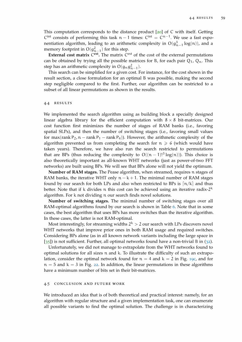
4.4 results 59

This computation corresponds to the distance product [20] of C with itself. GettingCint consists of performing this task n − 1 times: Cint = Cn−1. We use a fast expo-nentiation algorithm, leading to an arithmetic complexity in O(g3n−1 log(n)), and amemory footprint in O(g2n−1) for this step.

External cost matrix Cext. The matrix Cext of the cost of the external permutationscan be obtained by trying all the possible matrices for B, for each pair Q1, Qn. Thisstep has an arithmetic complexity in O(gng2n−1).

This search can be simplified for a given cost. For instance, for the cost shown in theresult section, a close formulation for an optimal B was possible, making the secondstep negligible compared to the first. Further, our algorithm can be restricted to asubset of all linear permutations as shown in the results.

4.4 results

We implemented the search algorithm using as building block a specially designedlinear algebra library for the efficient computation with 8 × 8 bit-matrices. Ourcost function first minimizes the number of stages of RAM banks (i.e., favoringspatial SLPs), and then the number of switching stages (i.e., favoring small valuesfor max(rankP2,n − rankP1 − rankP4)). However, the arithmetic complexity of thealgorithm prevented us from completing the search for n > 6 (which would havetaken years). Therefore, we have also run the search restricted to permutationsthat are BPs (thus reducing the complexity to O((n − 1)!3 log(n))). This choice isalso theoretically important as all-known WHT networks (just as power-of-two FFTnetworks) are built using BPs. We will see that BPs alone will not yield the optimum.

Number of RAM stages. The Pease algorithm, when streamed, requires n stages ofRAM banks, the iterative WHT only n− k+ 1. The minimal number of RAM stagesfound by our search for both LPs and also when restricted to BPs is dn/ke and thusbetter. Note that if k divides n this cost can be achieved using an iterative radix-2k

algorithm. For k not dividing n our search finds novel solutions.Number of switching stages. The minimal number of switching stages over all

RAM-optimal algorithms found by our search is shown in Table 6. Note that in somecases, the best algorithm that uses BPs has more switches than the iterative algorithm.In these cases, the latter is not RAM-optimal.

Most interestingly, for streaming widths 2k > 2 our search with LPs discovers novelWHT networks that improve prior ones in both RAM usage and required switches.Considering BPs alone (as in all known network variants including the large space in[35]) is not sufficient. Further, all optimal networks found have a non-trivial B in (32).

Unfortunately, we did not manage to extrapolate from the WHT networks found tooptimal solutions for all sizes n and k. To illustrate the difficulty of such an extrapo-lation, consider the optimal network found for n = 4 and k = 2 in Fig. 19c, and forn = 5 and k = 3 in Fig. 22. In addition, the linear permutations in these algorithmshave a minimum number of bits set in their bit-matrices.

4.5 conclusion and future work

We introduced an idea that is of both theoretical and practical interest: namely, for analgorithm with regular structure and a given implementation task, one can enumerateall possible variants to find the optimal solution. The challenge is in characterizing


Logof

size(n

)2

34

56

7

Logof

str.width

(k)1

12

12

31

23

41

23

45

12

34

56

Radix-

2Pease

46

68

88

10

10

10

10

12

12

12

12

12

14

14

14

14

14

14

Radix-

2Iterative

46

48

64

10

86

412

10

86

414

12

10

86

4

Bestw

ithBP

46

48

84

10

10

84

12

12

12

84

14

14

12

12

84

Bestw

ithLP

46

38

53

10

65

312

??

?3

??

??

??

Table6:N

umber

ofstages

of2k−1

switches

inW

HTs

ofsize

2n

implem

entedw

itha

streaming

width

of2k.

4.5 conclusion and future work 61

F2

F2

F2

F2

F2

F2

F2

F2

F2

F2

F2

F2

F2

F2

F2

F2

F2

F2

F2

F2

F2

F2

F2

F2

F2

F2

F2

F2

F2

F2

F2

F2

F2

F2

F2

F2

F2

F2

F2

F2

F2

F2

F2

F2

F2

F2

F2

F2

F2

F2

F2

F2

F2

F2

F2

F2

F2

F2

F2

F2

F2

F2

F2

F2

F2

F2

F2

F2

F2

F2

F2

F2

F2

F2

F2

F2

F2

F2

F2

F2

Figure 22: Butterfly network computing a WHT of size 2n = 32 that, when streamed with2k = 8, yields an implementation with minimal number of memory elements andswitches.


the space of algorithmic variants, which we did for the WHT, revealing the existenceof algorithms that have strictly better RAM and logic requirements than what waspreviously possible.

We considered the WHT for its simplicity but the idea is in principle applicableto other regular algorithms. We give here a glance of the size of the space of sortingnetworks algorithms, and of FFT variants:

FFT. Twiddle factors make the characterization of FFT datapaths more complicated.Merging them with the butterflies yields promising results:

Proposition 9. For a positive integer n, and n+ 1 invertible n×n bit matrices P0, . . . ,Pn ∈GLn(F2), the existence of n · 2n+1 complex numbers z10, . . . , z1

2n+1−1, z20, . . . , zn

2n+1−1such

that :

DFT2n = π(P0) ·n∏k=1

2n−1−1⊕`=0

(zk4` zk4`+1

zk4`+3 zk4`+2

) · π(Pk) .

only depends on P0:n and the spreading matrix X (71).

A proof of this proposition is available upon request. Additionally, an exhaustivesearch shows that for n 6 4, the set of pairs (X,X−1P0:n) such that there exist suchcomplex numbers is a Cartesian product.

As an example, for n = 4, the valid FFT datapaths are those that satisfy:

X invertible, X−1 =

∗ ∗ ∗ ∗∗ 1 ∗ ∗∗ 1 ∗∗ 1

and X−1P0:n =

∗ ∗∗ ∗

1 ∗ ∗1 ∗ ∗ ∗

,

where each symbol ∗ can be replaced by any value in F2.Sorting networks. Sorting networks SN2n use more stages than WHTs or FFTs,

which hinder the definition of a spreading matrix, and prevents an approach like theone we had for WHT butterfly networks. However, sorting networks present somedegrees of freedom similar to the ones we found for the WHT. For all B ∈ GLn(F2)and Q ∈ GLn−1(F2),

SN2n = SN2n · π(B), and (34)

I2n−1 ⊗ SN2 = π(Q⊕ I1) · (I2n−1 ⊗ SN2) · π(Q−1 ⊕ I1). (35)

The first degree of freedom (34) translates the fact that permuting the input of a sortingnetwork doesn’t change the result, and (35) means that we can swap SN2 blocs likethe butterflies in a WHT.

Additionally, for any vector u ∈ Fn−12 , the permutation π

(In−1

uT 1

)exchanges

pairs of elements. Therefore, we have:

I2n−1 ⊗ SN2 = (I2n−1 ⊗ SN2) · π(In−1

uT 1

), and (36)

I2n−1 ⊗ SN2 = π(In−1

uT 1

)·

2n−1−1⊕i=0

XuT ib2

. (37)

4.5 conclusion and future work 63

Algorithm considered Number of RAM stages Number of switches stages Conjecture?

Radix-2 Pease n 2n No

Radix-2 iterative n− k+ 1 2(n− k+ 1) No

Best with BP dn/ke ? Yes, holds for n 6 8

Best with LP dn/ke ? Yes, holds for n 6 5

Combining (35), (36) and (37) shows that, for all function

f : 0, . . . , 2n−1 − 1→ F2,

for all matrix Q ∈ GLn−1(F2), and for all pair of vectors u, v ∈ Fn−12 , there exists afunction

g : 0, . . . , 2n−1 − 1→ F2

such that

2n−1−1⊕i=0

Xf(i)2 = π

(Q

uT 1

)·

2n−1−1⊕i=0

Xg(i)2

· π(Q−1

vT 1

). (38)

These degrees of freedom may not be the only ones, but this already shows that thedesign space for streaming networks is considerably larger than the one for WHTs.Fully characterizing it, and searching through it for an optimal streaming implemen-tation is a challenging problem.

Part II

I M P L E M E N TAT I O N

5A D S L - B A S E D H A R D WA R E G E N E R AT O R I N S C A L A F O R FA S TF O U R I E R T R A N S F O R M S A N D S O RT I N G N E T W O R K S

In this chapter, published in [74] and that extends the work published in [72], wepresent a hardware generator for computations with regular structure including thefast Fourier transform (FFT), sorting networks, and others. The input of the generatoris a high-level description of the algorithm; the output is a token-based, synchronizeddesign in the form of RTL-Verilog. Building on prior work, the generator uses sev-eral layers of domain-specific languages (DSLs) to represent and optimize at differentlevels of abstraction to produce a RAM- and area-efficient hardware implementation.Two of these layers and DSLs are novel. The first one allows the use and domain-specific optimization of the streaming permutations and the algorithmic structuresseen in the first part of this thesis. The second DSL enables the automatic pipeliningof a streaming hardware dataflow and the synchronization of its data-independentcontrol signals.

The generator including the DSLs are implemented in Scala, leveraging its typesystem, and uses concepts from lightweight modular staging (LMS) to handle theconstraints of streaming hardware. Particularly, these concepts offer genericity overhardware number representation, including seamless switching between fixed-pointarithmetic and FloPoCo generated IEEE floating-point operators, while ensuring type-safety. In addition, automatic simplifications that exploit the particular structure ofthe specified implementation are performed at each stage, thus reducing both ROMconsumption and DSP slices, and improving performance in terms of latency andthroughput.

We show benchmarks of generated FFTs, sorting networks and Walsh-Hadamardtransforms that outperform prior generators.

5.1 generation pipeline

We will refer to all functions that our generator implements as transforms. Theseinclude the discrete Fourier transform, the Walsh-Hadamard transform, and sortingnetworks. Our proposed generator receives as input the desired transform, its size (apower of two), and some parameters that control the design space (e.g., streamingwidth, iterative reuse applied or not, hardware arithmetic representation). The out-put is the corresponding design in the form of RTL Verilog. The generation processconsists of the three layers pictured in Fig. 23. Each of these layers employs a DSLto represent, manipulate, and optimize the algorithm at different levels of abstraction.Each DSL is implemented as embedded DSL inside Scala, and staging is used to allowmanipulation. We first give a brief overview and then discuss the last two layers ingreater detail in subsequent sections.

67

68 a hardware generator for fft and sorting networks

Transform, size

SPL

Streaming Block DSL

RTL-level DSL

Verilog

Folding

Implementation

Streaming width

Algorithm rewrite

Optimization

Simplification

Arithmetic representation

Figure 23: The different layers of our generator.

Operator Description

First-order operator

DFT2n Discrete Fourier transform for input size 2n

H2n Walsh-Hadamard transform for input size 2n

SN2n Sorting network for 2n inputs

π(P)Linear permutation associated with

the invertible bit-matrix P [68]

Ti, T ′i Twiddle factors

Xc2 Configurable two-input sorter

Higher-order operator

A ·B Composition of operators A and B∏iAi Enumerated composition of operators Ai⊕iAi

Enumerated direct sum

(parallel composition) of operators Ai

Table 7: SPL operators used in our generator.

5.1.1 SPL

The first step for generating a hardware implementation consists of choosing a suit-able algorithm. Following [47], we represent these algorithms as breakdown rules thatdecompose a large transformation into smaller ones. These rules are represented us-ing SPL, a mathematical language that represents linear algebra operations by matri-ces and operators on these matrices [64, 85, 33]. We introduce next SPL, and describethe rules we use for the different transforms we consider. Our implementation of thisDSL in Scala is similar as in [54], and includes the operators in Table 7. Higher-orderoperators are used to recursively construct algorithms from first-order operators.

5.1 generation pipeline 69

F2

F2

F2

F2

−i

−i

F2

F2

F2

F2

ω18

−i

ω38

F2

F2

F2

F2

Figure 24: Radix-2 Cooley-Tukey FFT datapaths operating on 2n = 8 elements. This algorithmis used when iterative reuse is not enabled, as the permutations involved requireless resources when streamed.

DFT. In the case where the desired transform is a DFT, our generator uses twobreakdown rules. The first one, used in Fig. 2, is the constant-geometry radix-2r PeaseFFT [60]:

DFT2n = π(Jrn) ·n/r−1∏`=0

Tn/r−`−1 ·2n−r⊕i=1

DFT2r

· π(Crn) . (39)

where T` is a diagonal matrix that performs element-wise complex multiplicationswith the twiddle-factors1, π(Jrn) and π(Crn) are permutations (respectively the radix-2r-reversal, and the stride-by-2r permutation), and

⊕2n−r

i=1 DFT2r represents 2n−r parallelDFTs of size 2r each. As the expression within the product is always the same, thisalgorithm is well suited for iterative reuse. However, for designs with streaming reuseonly, or for the generation of the base case 2r-FFT, the radix-2r Cooley-Tukey FFT (seeFig. 24) is used instead, as the permutations it requires use less resources.

DFT2n = π(Sn−rn ) ·

n/r−1∏`=0

(

2n−r⊕i=1

DFT2r) · T ′` · π(Q`)

· π(Jrn), (40)

where T ′` is a diagonal matrix, and π(Q`) a permutation.WHT. The algorithms we are using to compute a WHT are similar to the one used

for DFTs, but do not include twiddle factors nor a final bit-reversal permutation. Asan example, the Pease-like WHT algorithm is expressed as

H2n =

n−1∏j=0

2n−1⊕i=1

DFT2

· π(Cn) . (41)

SN. Sorting networks (SNs) are somewhat similar to FFTs or WHTs but require adifferent form of butterflies, which are two-input sorters and thus nonlinear. Thusan extension to SPL is required as described in [89] following concepts from [22].Formally, a two-input sorter is described as Xc2. If c = 0, it sorts the two inputs inascending order, if c = 1 it sorts them in descending order. With this, we can express

1 T` =⊕2n−r−1i=0

⊕2r−1j=0 ωj·i(r`) , where ω is the principal 2n-th root of unity, and i(r`) means that the r`

least significant bits of i have been set to 0.


↑

↑

↑

↑

↑

↑

↑

↑

↑

↑

↑

↑

↑

↑

↑

↑

↑

↑

↑

↑

↑

↑

↑

↑

Figure 25: Batcher bitonic sorting network [4] operating on 2n = 8 elements. This designcorresponds to the SN1 architecture in [89].

SNs using the previous formalism. For streaming reuse only, we use a Batcher bitonicSN [4] (see Fig. 25)::

SN2n =

n−2∏j=0

2n−1−1⊕i=0

X02

· n−i−2∏`=0

π(P`) ·2n−1−1⊕

i=0

X02

· π(Qj)

·2n−1−1⊕i=0

X02.

(42)

This corresponds to the architecture SN1 in [89].When iterative reuse is desired, a Pease-like network is used [79]:

SN2n =

2n−1⊕i=1

X02

· n2−n−3∏j=0

π(Sn) ·2n−1⊕i=1

Xf(i,j)2

, (43)

where f is a binary function. This second algorithm corresponds to the architectureSN5 of [89], with the following improvements:

• The first n− 1 stages are removed, as these correspond to a fixed permutationof the inputs, for which the order does not matter. This allows an increase of thethroughput of the implementations.

• In [89], Xc2 had an additional pass-through configuration. We change the stagesthat used this mode such that the sorters perform useless comparisons instead(by copying the configuration of the stage located n places later). Therefore, weonly use Xc2 as a sorter or as an inverted sorter, thus reducing the complexity ofthe implementation.

• When folded for iterative reuse, a loop with an early termination (similar to thestructure used in Chapter 3 when fusing permutations) allows to simultaneouslyimplement a single stage of sorters while performing only the necessary numberof permutations (see Fig. 26b).

5.1.2 Streaming-block DSL

In the second step of the generator (Fig. 23), the SPL expression is formally foldedaccording to the streaming width, i.e., the number of elements of the dataset that thedesign would be able to handle in each cycle. In the second step, the SPL expression


↑

↓

↑

↓

↑

↑

↑

↑

↑

↓

↑

↓

↑

↑

↓

↓

↑

↑

↑

↑

↑

↑

↑

↑

↑

↑

↑

↑

(a) Unfolded

↑

l

l

l

(b) Iterative reuse

Figure 26: Constant-geometry sorting network [79] operating on 2n = 8 elements. This designloosely corresponds to the SN5 architecture in [89].

F2

F2

×

×

(a) Before optimization.

F2

F2

×

×

(b) After optimization.

Figure 27: Design of Fig. 10b expressed using the streaming block DSL. The necessary stream-ing permutation is expanded into switches and RAM banks (dark blue rectangles).The optimization here “unrolls” some parts of the permutation to remove an arrayof multiplexer. Additionally, two arrays of switches were grouped for later mappingto 4-to-1 multiplexers. These optimizations increase the throughput and reduce thearea of the final design.


Operator Description SPL correspondence

First-order operator⊕DFT2

Butterfly array

(add and substract its two inputs)

⊕DFT2

Ti, T ′i Twiddle factors Ti, T ′iXc2 Configurable two-input sorter Xc2

πi(P0, . . . ,P`) Array of multiplexers π

(It

Pi

)

σi(v0, . . . , v`) Single array of switches π

It

1. . .

vTi 1

σ ′i((u0, v0), . . . , (u`, v`)) Double array of switches π

It

1. . .

vTi 1

uTi 1

τi((A0,B0), . . . , (A`,B`)) Array of RAM banks π

(Ai Bi

Ik

)Higher-order operator

A0 ·A2 · · ·A`Composition

(without iterative reuse)

∏ì=0Ai

∏iAi

Composition with iterative reuse

(A is implemented only once)

∏ì=0Ai

∏ì(AiBi)

Composition with iterative reuse

and early terminationB`∏`−1i=0(AiBi)

Table 8: Streaming blocks used in the streaming-block DSL. The last higher-order operatorallows to represent the structure introduced in Chapter 3.

is formally folded according to the streaming width, i.e., the number of elements of thedataset that the design would be able to handle in each cycle. This includes insertingthe necessary datapaths for the streaming permutations from Chapter 2. The DSL usedthus expands SPL to include the streaming width (similar to the so-called Hardware-SPL in [47]), but also the following needed streaming blocks:

During this stage, a set of rewriting rules is used to simplify the streaming blocks,particularly in the case of a fused permutation. As an example, a radix-2 Pease DFT


on 8 elements (39), folded with a streaming width of 4 ports using iterative reuse withfused permutation would be represented in the streaming block DSL by

3∏i=0

T2−i · 4⊕`=1

DFT2 · πi (I2,S2,S2,S2) ·

σi

((1

),(0

),(0

),(0

))· π(S2) · σi

((0

),(1

),(1

),(1

))· π(S2)·

τi

(((1

),(0 1

)),((1

),(1 0

)),((1

),(1 0

)),((1

),(1 0

)))· π(S2)·

σi

((1

),(0

),(0

),(0

))· π(S2) · σi

((0

),(1

),(1

),(1

))· π(S2)

), (44)

which corresponds to the dataflow pictured in Fig. 27a.In this expression, the array of multiplexers πi (I2,S2,S2,S2) does not perform any-

thing during the last iteration. It is therefore interesting to “push” it after the earlytermination of the loop, as it can be implemented using only a rewiring π(S2). Thearray of switches that comes next, σi

((1

),(0

),(0

),(0

)), does not permute any-

thing during the first three iterations of the loop. It can be therefore “unrolled” intoa non-parameterized array of switches σ

((1

)), thus saving logic and latency in the

loop and therefore increasing throughput. At this point, the expression becomes

σ((1

)) ·

3∏i=0

T2−i · 4⊕`=1

DFT2 · π(S2) · π(S2) · σi((0

),(1

),(1

),(1

))· π(S2)·

τi

(((1

),(0 1

)),((1

),(1 0

)),((1

),(1 0

)),((1

),(1 0

)))· π(S2)·

σi

((1

),(0

),(0

),(0

))· π(S2) · σi

((0

),(1

),(1

),(1

))· π(S2)

).

Continuing these optimizations, and regrouping the two rightmost single arrays ofswitches finally yields the expression

σ((1

)) ·

3∏i=0

T2−i · 4⊕`=1

DFT2 · σ((1

)) · π(S2)·

τi

(((1

),(0 1

)),((1

),(1 0

)),((1

),(1 0

)),((1

),(1 0

)))· π(S2)·

σ ′i

(((1

),(0

)), ((0

),(1

)), ((0

),(1

)), ((0

),(1

)))· π(S2)

), (45)

pictured in Fig. 27b.

5.1.3 Streaming-RTL DSL

In the final stage, the streaming blocks are transformed into a dependency graphwhere each node, called a signal, represents a hardware operator that outputs onevalue per cycle. A signal may have zero (constant signals, inputs, timers and counters),


Operator Description Example

Constant signal

value is a numerical value.

Const(value) Constant signal Const(5.3)

Register signal

input is a signal.

Register(input) Flip/flop register input.register()

Arithmetic signals

lhs and rhs are signals of the same type.

Plus(lhs, rhs) Sum of the operands lhs + rhs

Minus(lhs, rhs) Difference of the operands lhs - rhs

Times(lhs, rhs) Product of the operands lhs * rhs

And(lhs, rhs) Binary AND of the operands lhs & rhs

Xor(lhs, rhs) Binary XOR of the operands lhs ∧ rhs

Memory signals

content is an indexed sequence of numerical values,

address is an unsigned signal,

input is a signal,

ram is a RAMw signal.

ROM(content, address) ROM tabulating content Vector(1.5, 18.2)(address)

RAMw(input, address) Write port of a RAM val r = RAM(in, address1)

RAMr(ram, address) Read port of a RAM r(address2)

Multiplexer signal

content is an indexed sequence of signals of the same type,

address is an unsigned signal.

Mux(content, address) Multiplexer Vector(rhs, lhs)(address)

Bus manipulation signals

lhs and rhs are signals of the same type,

range is a range of integers.

Cons(lhs, rhs) Binary concatenation lhs ++ rhs

Tap(lhs, range) Extraction of a selection of bits lhs(range)

Synchronization signals (provided by streaming blocks)

size is an integer.

Timer(size) Number of cycles since Timer(8)

the last dataset entered

Counter(size) Number of datasets that Counter(4)

have been processed

Table 9: Example of nodes (signals) used in the streaming-RTL DSL, and corresponding syntax.

5.2 a dsl for “streaming-rtl” 75

one (flip/flop registers used for pipelining), or more parent signals (see Table 9). Inthe case of streaming reuse, this graph may contain loops.

The graph is constructed and represented using a Streaming-RTL DSL. Hardwaredatatypes, pipelining decisions and synchronization issues are mostly abstracted fromthis language. As an example, the implementation of the streaming block for the twid-dles Tj can be written within a few lines, and works for every folding scenario andhardware datatype:case class Twiddles(n: Int, k: Int, j: Sig[Int])(implicit dt: HW[Complex[Double]])extends SB[Complex[Double]]](1 << n, 1 << k)override def implement(inputs: Vector[Sig[Complex[Double]]]) = // We first declare a timer that ticks for the duration of a datasetval timer = Timer(1 << t)

// we define a (non-staged) Vector containing all 2^n th roots of unityval rootsOfUnity = Vector.tabulate(1 << n)i =>val angle = -2 * Math.Pi * i / (1 << n)Complex(Math.cos(angle), Math.sin(angle))

// For each input signal,inputs.zipWithIndex.mapcase (input, p) =>// we construct a signal corresponding to the index of a given element// (concatenation of the t bits of the timer, and the k bits of// the current port p),val i = timer ++ p(Unsigned(k))

// we compute the corresponding twiddle factor,val address = (i & 1) * ((i >>> (j + 1)) << j)val twiddle = rootsOfUnity(address)

// and we return the product of the input signal with this twiddle factorinput * twiddle

As can be seen, only a few elements in the body of this function (Timer, Unsigned)may indicate that this code represents a low-level hardware architecture. This im-proves its readability and therefore its maintainability. However, all signals implicitlycarry an underlying hardware type (including the corresponding size in bits), andtiming information. All operations are bit- and cycle-accurate, and software and hard-ware type-safety is ensured. This DSL and its implementation are detailed in the nextsection.

Once constructed and optimized, the resulting graph is translated to a Verilog file.

5.2 a dsl for “streaming-rtl”

Our streaming-RTL DSL is used to construct from a streaming-block level representa-tion of an algorithm a dependency graph that represents the final circuit. In this graph,the nodes (signals) represent hardware operators, and the edges the dependencies be-tween these signals. The DSL offers the following features:

• The nodes (signals) of the graph are manipulated exactly as the values theywould represent in a regular Scala program. Only their type changes.

• The language provides genericity over the actual hardware datatype and preci-sion. However, the datatype can be made explicit, offering bit-accurate control.


• Pipelining and synchronization of data-independent control is performed im-plicitly, but timing information and manual pipelining remains available.

We discuss next the implementation of these abstractions, using the features offeredby the Scala type system.

5.2.1 Staging and LMS

The implementation of our DSL uses the concept of staging, in particular as donein LMS [65], but using our own implementation. Staging allows to distinguish thoseparts of the computation to be evaluated at generation time and those that will be im-plemented in hardware via a type annotation. Specifically, staging is done by changinga type T to the type Sig[T]; the latter means that computations on this type will bedelayed, and may become part of the hardware implementation.

For example, in the following code, the first line defines a function f1 that yieldsthe sum of its parameters (x and y of type Double) augmented by 18. The returntype (Double) is inferred by the compiler. In the second line however, f2 returns anexpression tree representing the computation on symbolic inputs.def f1(x: Double, y: Double) = x + y + 18def f2(x: Sig[Double], y: Sig[Double]) = x + y + 18

This tree can then be translated (unparsed) to RTL-Verilog, yielding an implementationof two adders (adding two signals and an immediate).

This behavior is obtained through the class Sig[T], which instances represent thenodes in an expression tree:abstract class Sig[T:HW]// timing informationval delay: Option[Delay]

// field containing the hardware representationval hw = implicitly[HW[T]]

This class takes as a type parameter the type T of the expression it represents. Thistype is expected to come along with a hardware representation, provided as a typeclass HW (see Section 5.2.2). Additionally, each node is expected to provide timinginformation through the field delay (see Section 5.2.3).

The different types of computation are represented by a class that inherits from Sig:// Addition of two nodescase class Plus[T](lhs: Sig[T], rhs: Sig[T]) extends Sig[T] ...

// Node containing a constantcase class Const[T:HW](value: T) extends Sig[T] override val delay = None

// Pipelining registercase class Register[T](input: Sig[T]) extends Sig[T]override val delay = input.delay.map(_ + 1)

...

Each instance Sig[T] offers (lifts) the same operators as a regular instance of T would(see Section 5.2.4). These lifted operators return the corresponding node in the formof another instance of Sig.


5.2.2 Abstraction over hardware datatypes

Type classes [83, 53] are a form of static ad hoc polymorphism, that, contrary to in-heritance, allows to retroactively add functionality to existing data types. For instance,the following function f3 is generic in the type T of its parameters, but imposes thatthis type is numeric:def f3[T:Numeric](x: T, y: T) = x * y

In Scala, type classes are implemented using regular classes: f3 expects a third implicitargument of type Numeric[T] containing, among other, the definition of the operator* for two Ts.

Following the concept of abstraction over data representation from [54], instances ofSig[T] (signals of T) carry their underlying hardware representation in the form of atype class HW[T]:abstract class HW[T](val size: Int)// bit representation of a valuedef getBits(value: T): BigInt

// creates a constant with this hardware representationdef apply(value: T) = Const(value)(this)

Not only does this type class provide an additional method getBits that returns thebit representation of a given T, but it carries as meta-information the size in bits ofthe representation. Concrete hardware representations are instances of classes derivedfrom HW[T]:// Signed integercase class Signed(_size: Int) extends HW[Int](_size)...

// Unsigned integercase class Unsigned(_size: Int) extends HW[Int](_size)...

// Fixed point numbercase class FxP(integral: Int, fractional: Int)extends HW[Double](integral + fractional)...

// IEE754 floating pointcase class IEEE(wE: Int, wF: Int) extends HW[Double](wE + wF + 1)...

// FloPoCo floating pointcase class FloPoCo(wE: Int, wF: Int) extends HW[Double](wF + wE + 3)......

A Scala Int could therefore be represented as a signed or unsigned integer of agiven size, and a Scala Double can be represented using a fixed-point representation,a FloPoCo number2 or an IEEE 754 floating-point representation. This informationis passed to children nodes, and is used for the implementation of the lifted opera-tors and for the representation of constants in the generated code. As an example,depending on the underlying hardware type of its parameters, the previous examplef3 would seamlessly

• use fixed-point adders and represent 18 as a fixed-point immediate, or

2 The FloPoCo generator is called upon instantiation of the corresponding datatype class to generate thedifferent arithmetic operators. The result of this generation is then parsed to extract the latency of theseoperators.


• use FloPoCo generated floating-point adders and represent 18 with the corre-sponding FloPoCo binary representation, or

• implement a conversion from an IEEE floating-point signal to a FloPoCo repre-sentation, implement the FloPoCo adder, and implement the conversion back toan IEEE representation.

5.2.3 Synchronization

Each signal has a delay field that represents the time needed for this signal to outputa valid value. It is used to check if two operands are synchronized, and, if it is not thecase, to suitably delay one of them using registers.

A delay consists of an integer representing a number of cycles, and a timeline indi-cating to which “reference frame” this delay belongs. This timeline can be

• the primary timeline, referring to the number of cycles elapsed since the inputsarrived in the module,

• a loop timeline, referring to the number of cycles elapsed since a dataset enteredwithin a loop, or

• a floating timeline, used by data-independent signals awaiting to be “synchro-nized” with another timeline.

As an example, a Register would have the same delay as its input with a cycle numberincremented by one, while an input signal would have a delay of 0 on the primarytimeline.

Loop timelines. In the case of iterative reuse, the streaming product (the streamingblock that creates the loop and the multiplexer in Figs. 2b, 2d and 26b) creates anew loop timeline, and implements its inner expression using this timeline. The cor-responding latency is then measured using the maximal delay of the signals that arereturned. This information is then used during a second unparsing of the inner ex-pression, where a possible lack of latency is compensated by a FIFO, or an increaseof latency of a potential inner temporal permutation. The streaming product thenpresents its outputs using the same timeline as its inputs, delayed accordingly.

Floating timelines. In our generator, all data-independent control signals rely oncounters (that count the number of datasets that have passed) and on timers (thatcount the number of cycles elapsed since the beginning of the current dataset). Toensure that such control signals become available at the correct instant, each time anew counter or timer is declared, a corresponding floating timeline is created. All data-independent operations performed are then pipelined using this timeline. However,when a signal with a floating timeline and a signal with an external timeline need tobe synchronized, a new floating delay node is inserted with the expected delay.

As an example, we consider the following function f4:def f4(x: Sig[Int]) = val t = Timer(8) + 3x ^ t

This function creates a 3-bit timer, and adds the constant 3 to it. This operation im-plicitly adds a pipelining register, yielding a signal t with a delay of 1 on the floatingtimeline associated with the timer. The input signal x is then xored with t. As these


two signals are associated with different timelines, a floating delay signal dependingon t is created with the same delay member as x, and f4 finally returns a signalrepresenting a XOR of x and the floating delay signal.

After the graph construction, the floating timeline is synchronized with the othertimeline such that all floating delays can be implemented using the minimal numberof registers. In particular, this ensures that data-dependent signals never have to beuselessly delayed. In our example, the floating timeline is synchronized such that thefloating delay is implemented with a direct assignment. Thus, a delay of one cycle onthe floating timeline corresponds to the delay of x.

To prevent nodes of a floating timeline from being synchronized with different in-compatible timelines, and to avoid circular dependencies between floating timelines,the first time a node of a floating timeline is synchronized with a node from anothertimeline, the floating timeline is marked as “being in translation” with this other time-line, and an error is thrown if a node is later synchronized with a third timeline. Withthis relation, when the graph is built, timelines form a set of trees, rooted by the pri-mary and loop timelines. Floating timelines are then synchronized starting from theroots.

Synchronization tokens. When the graph is unparsed, token synchronization sig-nals are generated to trigger the different counters and timers. Tokens for loop time-lines are generated by “ORing” tokens of the primary timeline. As the maximalthroughput of the design is known at this time, tokens of the primary timeline canbe generated using consecutive resettable timers instead of a resettable shift-register.

In our previous example, the timer declared within f4 receives its token one cyclebefore x becomes available, ensuring that t is computed at the right time.

5.2.4 Smart constructors

Lifted operators are provided using implicit classes, which make it possible to add aposteriori methods and operators to existing objects.

For instance, the following class provides a + operator to any Sig[T], when T is anumeric type:


implicit class NumericSig[T:Numeric](lhs: Sig[T])// the default hardware representation when creating Const is the one of// the left-hand sideimplicit val hw = lhs.hw

// lhs + rhs in the case where lhs is a Sig[T] and rhs a Tdef +(rhs: T): Sig[T] = lhs + Const(rhs)

// lhs + rhs in the case where both lhs and rhs are Sig[T]def +(rhs: Sig[T]): Sig[T] = // check if lhs and rhs have the same representationensure(rhs.hw == hw)(lhs, rhs).synch match // both lhs and rhs are Constcase (Const(x), Const(y)) => Const(x + y)

// one of the operands is nullcase (Zero(), _) => rhscase (_, Zero()) => lhs

// otherwise, we create a new node specialized for// the hardware representationcase (lhs, rhs) => hw match case _: FloPoCo => PlusFPC(lhs, rhs).registercase _: IEEE => (lhs.toFPC + rhs.toFPC).toIEEEcase _: Signed | _: Unsigned | _: FxP => Plus(lhs, rhs).registercase _ => throw new Exception("No hardware implementation for +")

Here, the operator first checks that the two operands have the same hardware type(ensuring type-safety). It then synchronizes them, and handles particular cases (if thetwo operands are constants, or if one of them is the constant zero). Finally, it createsa new Plus signal, according to the hardware datatype, and adds pipelining registers(in the case of a FloPoCo operator, the signal PlusFPC already takes into account thelatency of the operator. A final register is added. For signed, unsigned integers andfixed-point representations, the pipeline has always a depth of one cycle. It wouldhowever be possible to adapt it to the size of the operands, the target architecture orthe target frequency. In case of an IEEE representation, the pipelining is handled bythe underlying call to the FloPoCo operator.).

These smart constructors are responsible for major optimizations. As an example, theconstructor of ROM signals (implemented by adding a new apply method on indexedsequences of T) checks every bit of the control signal, and returns a smaller ROMin the case where one of them is constant. Particularly, it would return a constant ifthe control signal is constant, thus guaranteeing an efficient implementation of thetwiddle stage Tj, even in non-streaming or non-iterative cases.

5.3 streaming-block dsl

The streaming-block DSL is an intermediate language between SPL and the Streaming-RTL DSL (See Fig. 23). It supports optimizations at the streaming level, i.e. optimiza-tions that take place once an algorithm has been “folded” according to a given stream-ing width.

5.3 streaming-block dsl 81

5.3.1 Streaming blocks

Each streaming-block represents a hardware module that has the same number (K) ofinputs and outputs of the same hardware type (HW[T]), and that performs an opera-tion on a dataset of size N. Streaming-blocks are comparable to SPL elements with astreaming width information, and are instances of classes derived from SB:abstract class SB[T:HW] (N: Int, K: Int)// Size must be a multiple of the streaming widthassert(N % K == 0)

def implement(inputs: Vector[Sig[T]]): Vector[Sig[T]]// Composition of blocksdef *(rhs: SB[T]) = Product(this, rhs)

Streaming blocks are expected to override a virtual method implement that constructsthe final circuit using the streaming-RTL DSL3. An operator * allows to composeblocks, as explained in Section 5.3.2 below.

As an example, an array of butterflies (corresponding to the SPL expression⊕DFT2) would be implemented as follows:

case class ButterflyArray[T:HW:Numeric] (_N: Int, _K: Int) extends SB[T](_N, _K)// The streaming width must be evenassert(sw % 2 == 0)

override def implement(inputs: Vector[Sig[T]]) = assert(inputs.size == K)// Compute the sum and difference of each pair of inputsinputs.grouped(2).toVector.flatMapcase Vector(a, b) => Vector(a + b, a - b)

5.3.2 Higher-order blocks

Composition of blocks is achieved through the block Product.case class Product[T:HW] private (factors: Vector[SB[T]]) extendsSB[T](factors.head.N, factors.head.K)// Size and streaming width of all factors must be the sameassert(factors.forall(f => f.N == N && f.K == K))

override def implement(inputs: Vector[Sig[T]]) = assert(inputs.size == K)// Implement all factors by connecting the outputs of one to the inputs of// the nextfactors.foldRight(inputs)((sb, cur) => sb.implement(cur))

A companion object of Product contains a smart constructor (this is the one calledby the operator * in SB), along with a higher-order function that implements the blockcorresponding to the SPL expression

∏limitj=0 f(j).

object Productdef apply[T:HW](lhs: SB[T], rhs: SB[T]): Product[T] = (lhs, rhs) match

case (Product(f1), Product(f2)) => new Product(f1 ++ f2)case (Product(f1), _) => new Product(f1 :+ rhs)case (_, Product(f2)) => new Product(lhs +: f2)case _ => new Product(Vector(lhs, rhs))

3 The real implementation adds an option to optionally add latency, and returns the minimal number ofcycles that the circuit can handle between datasets (gap).


def apply[T:HW](limit: Int)(f: Sig[Int] => SB[T]): SB[T] = assert(limit > 0)// Unsigned with the minimal size that can contain all jval idxType = Unsigned(BigInt(limit - 1).bitSize)(0 until limit).map(i=>Const(i)(idxType)).map(f).reduce(_*_)

Note that the higher-order function expects a function that returns a block, andthat takes an integer signal as a parameter (and not directly an integer). This allowsto have another block, ItProduct with the same interface, but that produces a loopfor iterative reuse (by implementing a multiplexer, creating a new loop timeline, andcalling f with a Counter as a parameter).

The streaming-block DSL does not directly have any operator corresponding to thedirect sum of SPL:

⊕j f(j). Before folding, the SPL expression must therefore have all

the direct sums fully distributed. Then, the remaining direct sums must be handledwithin the streaming blocks themselves, as it is the case with ButterflyArray.

5.3.3 Permutation blocks

Apart from the direct sum operator, permutations are the only SPL operators that donot have a direct equivalent in the streaming-block DSL. Only two types of permuta-tions are directly implementable as streaming-blocks:

• Spatial permutations: these are permutations that permute elements only withinthe same cycle. They can be implemented using switches (Fig. 11c), or multiplex-ers (Fig. 11b).

• Temporal permutations: these permutations permute elements only between cy-cles, but stay on the same port number. They can be implemented using an arrayof memory banks as in Fig. 11a.

During the folding operation, general permutations are decomposed into these us-ing the algorithms described in Chapter 2.

5.3.4 Optimizations

The optimizations taking place at this step mainly concern streaming permutationsand iterative reuse loops that have an early termination. They are described with moredetails in Chapter 3. For instance, a streaming permutation block within an iterativeloop may be unrolled under certain conditions, thus reducing the global number ofmultiplexers used within the whole design, or increasing the throughput of the design.Another optimization consists in fusing two consecutive arrays of 2-input switchesinto an array of 4-input switches, which can improve the resource used on some FPGAarchitectures. Fig. 27 shows a case where these two optimizations were performed.

5.4 results

To validate the designs produced by our generator, we benchmarked them against theequivalent circuits generated with [47]. All designs were synthesized using Vivado

5.4 results 83

2000

4000

8000

16000

32000

3 4 5 6 7 8 9 10 11 12 13 14 15

n

Proposed Milder

Cooley-Tukey radix-2 FFT, size 2n, 4 portsArea [slices]

4

40

400

3 4 5 6 7 8 9 10 11 12 13 14 15

n

Proposed

Milder

Cooley-Tukey radix-2 FFT, size 2n, 4 portsMemory [BRAMs]

2000

4000

8000

16000

32000

3 4 5 6 7 8 9 10 11 12 13 14 15

n

ProposedMilder

Pease radix-2 FFT, size 2n, 4 portsArea [slices]

4

40

400

3 4 5 6 7 8 9 10 11 12 13 14 15

n

Proposed

Milder

Pease radix-2 FFT, size 2n, 4 portsMemory [BRAMs]

2000

4000

8000

16000

32000

4 5 6 7 8 9 10 11 12 13 14

n

Proposed

Milder

Pease radix-4 FFT, size 2n, 8 portsArea [slices]

4

40

400

4 5 6 7 8 9 10 11 12 13 14

n

Proposed

Milder

Pease radix-4 FFT, size 2n, 8 portsMemory [BRAMs]

Figure 28: Resources used by different FFTs (40) in different configurations, on complex datausing 2× 32bits IEEE754 floating-point.


1000

2000

4000

8000

4 5 6 7 8 9 10 11 12 13 14 15

n

Proposed

Cooley-Tukey radix-2 WHT, size 2n, 8 portsArea [slices]

16

32

64

128

4 5 6 7 8 9 10 11 12 13 14 15

n

Proposed

Cooley-Tukey radix-2 WHT, size 2n, 8 portsMemory [BRAMs]

Figure 29: Resources used by a radix-2 Cooley-Tukey WHTs (41) with a streaming width of 8,on complex data using 2× 32bits fixed-point.

200

400

3 4 5 6 7 8 9 10 11 12 13 14

n

Proposed

Milder

Stone bitonic SN, size 2n, 4 portsArea [slices]

1

2

4

8

16

32

64

3 4 5 6 7 8 9 10 11 12 13 14

n

Proposed

Milder

Stone bitonic SN, size 2n, 4 portsMemory [BRAMs]

1000

2000

4000

8000

16000

32000

3 4 5 6 7 8 9 10 11 12 13 14

n

Proposed

Milder

Batcher bitonic SN, size 2n, 8 portsArea [slices]

4

8

16

32

64

128

256

512

3 4 5 6 7 8 9 10 11 12 13 14

n

Proposed

Milder

Batcher bitonic SN, size 2n, 8 portsMemory [BRAMs]

Figure 30: Resources used by different bitonic sorting networks (42), with different streamingconfiguration on complex data using 2× 32bits fixed-point.

5.5 limitations and related work 85

2018.1, targeting a Virtex7 xc7vx1140 FPGA. The floating-point operators used in ourdesigns were generated using FloPoCo 4.1.2, targeting a 700MHz Virtex6 platform.

Figures 28, 29 and 30 show results after place-and-route for a variety of transforms,algorithms, hardware datatypes and foldings. Each of these presents, for a given trans-form size, the resources used in terms of logic slices and memory obtained for ourdesign and the corresponding design from [47] or [89]. Cooley-Tukey FFTs and WHTs(Figs. 28a, 28b and 29) and Stone SNs (Figs. 30a and 30b) are implemented using onlystreaming reuse. Batcher SNs (Figs. 30c and 30d) use both streaming and iterativereuse. Pease FFTs (Figs. 28c, 28e, 28d and 28f) use streaming and iterative reuse withfused permutations, as described in Chapter 3.

Figs. 28d and 28f also show a comparison with the designs obtained using Xilinx IPgenerator Fast Fourier Transform 9.1. The parameters were set to resemble as much aspossible our architecture. A radix-2 Burst IO Lite architecture is used with 4 channels(in Fig. 28d), and a radix-4 Burst IO is used with 8 channels (in Fig. 28f), in eachcase with a natural output ordering, and using 32 bit fixed point representation forboth inputs and phase factors. However, as neither floating point computation nor thestreaming IO architecture are available when using multiple channels, no comparisoncan be made for logic consumption, nor for the Cooley-Tukey architecture.

All our designs were generated with sufficient pipelining to reach the same fre-quencies as [47] or [89] (in the order of 400MHz). The throughput of these designs aretherefore the same. Additionally, designs requiring complex multiplications (Fig. 28)use an algorithm that yield the same number of DSP slices as [47].

We observe that the logic area consumption slightly increases. The gain obtainedusing FloPoCo for the arithmetic part and the use of 4-input multiplexers is counter-balanced by the additional logic needed to implement memory conflict avoidance asdescribed in [68].

On the other side, the number of BRAM tiles required is lower in average withour generator. This is a direct consequence of the streaming permutations being im-plemented with [68]. As it does not use double buffering, the capacity required toimplement streaming permutations is halved. However, this reflects on the number ofBRAMs only when the double buffer does not fit into a single BRAM, that is, for largesizes of n (n > 10 in Fig. 28 and n > 9 in Fig. 30b). In addition, in the case of FFTs withiterative reuse (Figs. 28d and 28f), the stride permutation and the bit-reversal are fused,allowing to halve the number of BRAMs used for streaming permutations. However,these techniques do not affect the number of RAM slices used as ROMs to store thetwiddle factors. Finally, both the designs we propose and those generated using [47]require significantly fewer RAMs than Xilinx Fast Fourier transform IP cores.

In summary, our generator produces designs that use an equal amount or less mem-ory than [47] or [89], particularly for large sizes, for the same number of DSP blocks,and for a comparable area consumption. Our generator is thus able to improve thestate of the art for important parts of the design space of the considered transforms,and yields new Pareto optima.

5.5 limitations and related work

We compare to related work and discuss limitations.


5.5.1 Hardware DSLs implemented in Scala

The DSL we propose is specifically crafted for the generation of streaming Fouriertransforms and sorting networks on FPGAs, and provides only the primitives and theamount of abstraction needed for this purpose. This differentiates it from lower levelhardware description languages written in Scala. For instance, Chisel [3] can representa much wider variety of hardware designs, but requires the pipelining registers to bemanually added. Targeting dataflow hardware, DFiant [62] proposes a dependency-driven automatic pipelining similar to ours, but does not seem to support automaticsynchronization of data-independent controls. It uses literal types to expose the hard-ware datatype and precision to the user, thus enforcing type safety at compile-time.In our case, the hardware datatype is abstracted (provided via a type class), and hard-ware type safety is only ensured at generation time. On the other hand, high-levelsynthesis tools [80, 28] would offer even higher abstractions, up to the dataset level,but would not allow the user to program at the port-level, thus making the implemen-tation of our permutation streaming blocks difficult.

LMS [65] itself not only provides staging, but offers a tool chain to implement andcompile DSLs. Particularly, it grants automatic common subexpression eliminationduring the construction of the dependency graph. However, in our case, floating time-lines reduce the efficiency of such an optimization during the graph construction, andour tests have shown that synthesis software such as Vivado already provide it, thuslimiting the use of implementing it. LMS provides as well a facility to manipulate thegenerated graph, but as ours already includes timing information, these manipula-tions are limited to timing invariant ones (fusing ROMs that contain identical valuesfor instance), for which a direct implementation is possible. The main optimizationsin our graph are made during its generation, using smart constructors.

The pipeline proposed in [27] to generate matrix operations illustrates the capabilityof LMS to target hardware. It shares many similarities with ours, particularly its useof LMS and FloPoCo. However, a significant part of the final RTL design is outsourcedto the external back-end LegUp [8].

5.5.2 Hardware generator for FFTs

Our generator only handles the generation of power-of-two-sized FFTs, whereas [47]covers a larger set of sizes that can be factored into small primes and additional trans-forms closely related to FFTs. An according extension of our generator should berelatively straightforward. Note that [47] works as a back-end of Spiral [64], a genera-tor written on a modified version of the GAP computer algebra system, thus requiringhigh skills for its development.

SPL and Spiral have as well been implemented and enhanced in Haskell [42] and inScala [52] to produce efficient FFT implementations in C. A VHDL back-end for thiscompiler is being developed [42].

5.5.3 Hardware generator for sorting networks

The work in [88, 89] presents a generator for streaming sorting networks, and we haveshown how our generator outperform its RAM consumption for the algorithms wesupport. However, [88, 89] covers a larger space of algorithms (called SN2–4), and was

5.6 conclusion 87

originally targeting (and thus optimized for) a platform (Xilinx Virtex 5) older thanthe one we used for our benchmarks (Xilinx Virtex 7).

Sorting is a classic topic in computer science [4, 37], and many high-performancesorting networks have been manually implemented on FPGAs, using 2-inputs sorters[48, 12], or using other basis elements like linear sorters [56].

5.6 conclusion

In this chapter, we have designed and implemented a generator for streaming FFTsand sorting networks inside Scala, using embedded DSLs and the concept of staging.It followed a principled design of domain-specific hardware generators using state-of-the-art languages and language features.

Specifically, our generator employed a pipeline of three abstraction levels, corre-sponding to three levels of DSLs. Two of them, the streaming-block DSL and thestreaming-RTL DSL are novel and were specifically designed to include state-of-the-art components and enable the transformations and optimizations needed in FFTs.The generator should be easily extendable to other DSP components related to FFTs.A web version of our generator is available at [67], and its source code at [66].

Part III

L I N E A R A L G E B R A T H E O R E M S

6A L O W E R - U P P E R - L O W E R B L O C K T R I A N G U L A RD E C O M P O S I T I O N W I T H M I N I M A L O F F - D I A G O N A L R A N K S

In Chapter 2, we showed that the optimal implementation of an SLP (π(P), 2k) reducesto a matrix decomposition problem: factor the invertible bit matrix

P =

(P4 P3

P2 P1

)=

(It

L2 L1

)(C4 C3

C1

)(It

R2 R1

),

such that rankL2 + rankR2 is minimal. The existence of this decomposition and theminimum was stated in Theorem 2.

In this chapter, published in [69], we provide a proof of this theorem for an invert-ible matrix P over any field. The factorization decomposes P into a product of threematrices that are lower block-unitriangular, upper block-triangular, and lower block-unitriangular, respectively. In words, our goal is to make this factorization “as block-diagonal as possible” by minimizing the ranks of the off-diagonal blocks. We givelower bounds on these ranks and show that they are sharp by providing an algorithmthat computes an optimal solution. The proposed decomposition can be viewed as ageneralization of the well-known Block LU factorization using the Schur complement.

Theorem 2 uses this factorization for bit matrices, i.e., matrices over the Galois fieldF2. However, we believe that because of its simple and natural structure, the matrixdecomposition is also of pure mathematical interest, and our proof only assumes afield K. Our algorithm computes an optimal solution with an asympotic number ofoperations cubic in the matrix size. We implemented the algorithm for finite fields,for rational numbers, for Gaussian rational numbers and for exact real arithmetic forvalidation. For a floating point implementation, numerical issues may arise.

6.1 problem statement

Given is a non-singular (invertible) matrix P ∈ GLt+k(K) over a field K. We partitionP as

P =

(P4 P3

P2 P1

), such that P4 is t× t.

We denote the ranks of the submatrices with pi = rankPi, i = 1, 2, 3, 4. Matrices aredenoted with capital letters and vector spaces with calligraphic letters.

If P4 is non-singular, then a block Gaussian elimination uniquely decomposes P intothe form:

P =

(It

L Ik

)(C4 C3

C1

), (46)

where It denotes the t× t identity matrix. The rank of L = P2P−14 is equal to p2, and C1

is the Schur complement of P4. Conversely, if such a decomposition exists for P, thenP4 is non-singular. This block LU decomposition has several applications including

91

92 a lul block triangular decomposition with min. off-ranks

computing the inverse of P [13], solving linear systems [18]. The Schur complement isalso used in statistics, probability and numerical analysis [87, 17].

Analogously, the following decomposition exists if and only if P1 is non-singular:

P =

(C4 C3

C1

)(It

R Ik

). (47)

This decomposition is again unique, and the rank of R is p2.In this article, we release the restrictions on P1 and P4 and propose the following

decomposition for a general P ∈ GLt+k(K):

P =

(It

L Ik

)(C4 C3

C1

)(It

R Ik

), (48)

where in addition we want the three factors to be “as block-diagonal as possible,” i.e.,that rankL+ rankC3 + rankR is minimal.

6.1.1 Lower bounds

The following theorem provides bounds on the ranks of such a decomposition:

Theorem 4. If a decomposition (48) exists for P ∈ GLt+k(K), it satisfies

rankC3 = p3, (49)

rankL > k− p1, (50)

rankR > t− p4, (51)

rankR+ rankL > p2. (52)

In particular, the rank of C3 is fixed and we have:

rankR+ rankL > max(p2,k+ t− p1 − p4). (53)

We will prove this theorem in Section 6.3. Next, we assert that these bounds aresharp.

6.1.2 Optimal solution

The following theorem shows that the inequality (53) is sharp:

Theorem 5. If P ∈ GLt+k(K), then there exists a decomposition (48) that satisfies

rankR+ rankL = max(p2,k+ t− p1 − p4) and rankL = k− p1.

Additionally, such a decomposition can be computed withO((t+k)3) arithmetic operations.

We prove this theorem in Section 6.4 when p2 6 t+ k− p1 − p4, and in Section 6.5for the case p2 > t+k−p1−p4. In both cases, the proof is constructive and we providea corresponding algorithm (Algorithms 3 and 4). Theorem 5 and the correspondingalgorithms are the main contributions of this article.

Two cases. As illustrated in Figure 31, two different cases appear from inequal-ity (53). If p2 6 t + k − p1 − p4, bound (52) is not restrictive, and the optimal pair

6.1 problem statement 93

rankR

rankL

t− p4

k− p1

p2

p2

Unique Pareto optimum

rankR

rankL

t− p4

k− p1

p2

p2

Set of Pareto optima

Figure 31: Possible ranks for L and R. On the left graph, p2 < t+ k− p1 − p4. On the rightgraph, p2 > t+ k− p1 − p4. The dot shows the decomposition provided by Theo-rem 5.

(rankL, rankR) is unique, and equals (k−p1, t−p4). In the other case, where p2 > t+k− p1 − p4, bound (52) becomes restrictive, and several optimal pairs (rankL, rankR)exist.

Example. As a simple example we consider the special case

P =

(P3

P2

), with k = t.

In this case P2, P3 are non-singular and neither (46) nor (47) exists. Theorem 4 gives alower bound of rankR+ rankL > 2k, which implies that both R and L have full rank.Straightforward computation shows that for any non-singular L,

P =

(Ik

L Ik

)(L−1P2 P3

−LP3

)(Ik

−(LP3)−1P2 Ik

)

is an optimal solution. This also shows that the optimal decomposition (48) is in gen-eral not unique.

6.1.3 Flexibility

The following theorem adds flexibility to Theorem 5 and shows that a decompositionexists for any Pareto-optimal pair of non-diagonal ranks that satisfies the bounds ofTheorem 4:

Theorem 6. If P ∈ GLt+k(K) and (l, r) ∈ N2 satisfies l > k − p1, r > t − p4, andr + l = max(p2,k + t − p1 − p4), then P has a decomposition (48) with rankL = l andrankR = r.

In the case where p2 6 t+ k− p1 − p4, the decomposition produced by Theorem 5

has already the unique optimal pair (rankL, rankR) = (k− p1, t− p4). In the othercase, we will provide a method in Section 6.6 to trade between the rank of R and therank of L, until bound (51) is reached. By iterating this method over the decompositionobtained in Theorem 5, decompositions with various rank tradeoffs can be built.

Therefore, it is possible to build decomposition (48) for any pair (rankL, rankR)that is a Pareto optimum of the given set of bounds. As a consequence, if f : N2 → R


is weakly increasing in both of its arguments, it is possible to find a decom-position that minimizes f(rankL, rankR). Examples include min(rankL, rankR),max(rankL, rankR), rankL+ rankR, rankL · rankR or

√rank2 L+ rank2 R.

Generalization of block LU factorization. In the case where P1 is non-singular, The-orem 5 provides a decomposition that satisfies rankL = 0. In other words, it reducesto the decomposition (47). Using Theorem 6, we can obtain a similar result in the casewhere P4 is non-singular. Since in this case t− p4 = 0, it is possible to choose r = 0,and thus obtain the decomposition (46).

6.1.4 Equivalent formulations

Lemma 1. The following decomposition is equivalent to decomposition (48), with analogousconstraints for the non-diagonal ranks:

P =

(It

L2 L1

)(C4 C3

Ik

)(It

R2 R1

)(54)

In this case, the minimization of the non-diagonal ranks is exactly the same problem as in(48). However, an additional degree of freedom appears: any non-singular k× k matrix can bechosen for either L1 or R1.

It is also possible to decompose P into two matrices, one with a non-singular leading princi-pal submatrix L4 and the other one with a non-singular lower principal submatrix R1:

P =

(L4 L3

L2 L1

)(R4 R3

R2 R1

)(55)

Once again, the minimization of rankL2 + rankR2 is the same problem as in (48). The twoother non-diagonal blocks satisfy rankL3 + rankR3 > p3.

Proof. The lower non-diagonal ranks are invariant through the following steps:(48) ⇒ (54). If P has a decomposition (48), a straightforward computation shows

that:

P =

(It

L C1

)(C4 C3

Ik

)(It

R Ik

),

which has the form of decomposition (54).(54) ⇒ (55). If P has a decomposition (54), the multiplication of the two left factors

leads to formulation (55). In fact, L4 = C4 and R1 are both non-singular.(55) ⇒ (48). If P has a decomposition (55), then using (46) on the left factor, and

(47) on the right factor, and multiplying the two central matrices leads to formulation(48).

6.1.5 Related work

Schur complement. Several efforts have been made to adapt the definition of Schurcomplement in the case of general P4 and P1. For instance, it is possible to define anindexed Schur complement of another non-singular principal submatrix [87], or usepseudo-inverses [9] for matrix inversion algorithms.

6.2 preliminaries 95

Alternative block decompositions. A common way to handle the case where P4 issingular is to use a permutation matrix B that reorders the columns of P such that thenew principal upper submatrix is non-singular [87]. Decomposition (46) then becomes:

P = PBBT =

(It

L Ik

)(C4 C3

C1

)BT

However, B needs to swap columns with index > t; thus BT does not have the requiredform considered in our work.

One can modify the above idea to choose B such that B−1 has the shape requiredby decomposition (48):

P =

(P4 P3

P2 P1

)(It

−R Ik

)(It

R Ik

)=

(P4 − RP3 P3

P2 − RP1 P1

)(It

R Ik

)

Then the problem is to design R such that P4 − RP3 is non-singular and rank(P2 −RP1) + rankR is minimal. This basic idea is used in [63], where, however, only rankRis minimized, which, in general, does not produce optimal solutions for the problemconsidered here.

Finally, our decomposition also shares patterns with a block Cholesky decompo-sition, or the Block LDL decomposition, in the sense that they involve block uni-triangular matrices. However, the requirements on P and the expectations on the de-composition are different.

6.2 preliminaries

In this section, we will prove some basic lemmas that we will use throughout thischapter.

6.2.1 Properties of the blocks of an invertible matrix

In this subsection, we derive some direct consequences of the invertibility of P on therange and the nullspace of its submatrices.

Lemma 2. The following properties are immediate from the structure of P:

kerP1 ∩ kerP3 = 0 (56)

kerP2 ∩ kerP4 = 0 (57)

imP1 + imP2 = Kk (58)

imP3 + imP4 = Kt (59)

P2(kerP4)∩ P1(kerP3) = 0 (60)

P4(kerP2)∩ P3(kerP1) = 0 (61)

Proof. We prove here equation (60). If x ∈ kerP4 and y ∈ kerP3 satisfy P2x = P1y, wehave:(

P4 P3

P2 P1

)·(x

−y

)=

(P4x− P3y

P2x− P1y

)=

(0

0

)

Since P is non-singular, x = y = 0, as desired.


Operation related to subspaces Matrix operation Correspondence

Kernel of a matrix M kerM 〈kerM〉 = kerM

Direct sum of subspaces A,B(A B

) (A B

)= A⊕B

Intersection of subspaces A,B A∩B 〈A∩B〉 = A∩BComplement of a subspace B in A AB 〈AB〉 ⊕B = A

Table 10: We summarize matrix operators to perform basic operations on subspaces. M is ageneral matrix, while A and B are matrices with m rows that represent the subspacesA and B; i.e. A = 〈A〉 and B = 〈B〉. Inspection of these routines shows that they allcan be implemented with O(m3) runtime.

These equalities yield the dimensions of the following subspaces:

Corollary 5.

dimP3(kerP1) = dim kerP1 = k− p1 (62)

dimP4(kerP2) = dim kerP2 = t− p2 (63)

dimP1(kerP3) = dim kerP3 = k− p3 (64)

dimP2(kerP4) = dim kerP4 = t− p4 (65)

dim imP1 ∩ imP2 = p1 + p2 − k (66)

dim imP3 ∩ imP4 = p3 + p4 − t (67)

Proof. We prove equation (62). Since, by (56), kerP1 ∩ kerP3 = 0, the dimension ofthe image of kerP1 under P3 has the same dimension as kerP1, which is k− p1.

Equation (66) is a consequence of equation (58) and of the rank-nullity theorem.

6.2.2 Algorithms on linear subspaces in matrix form

The algorithms we present in this chapter heavily rely on operations on subspaces ofKm. To make the representation of these algorithms more practical for implementa-tion, we introduce a matrix representation for subspaces and formulate the subspaceoperations needed on this representation.

We represent a linear subspace as an associated matrix1 whose columns form a basisof this subspace. In other words, if A is a subspace of Km of dimension n, then werepresent it using a m×n matrix A such that imA = A. In this case, and only in thiscase, we will use the notation 〈A〉 = imA to emphasize that the columns of A form alinear independent set.

With this notation we can formulate subspace computations as computations ontheir associated matrices as explained in the following. To formally emphasize thiscorrespondence, these operations on matrices will carry the same symbol as the sub-space computation (e.g., ∩) they represent augmented with an overline (e.g., ∩). Theoperations are collected in Table 10. All algorithms in this chapter are written as se-quences of these matrix operations. Because of this, we implemented the algorithms byfirst designing an object oriented infrastructure that provides these operations. Thenwe could directly map the algorithms, as they are formulated, to code.

Direct sum of two subspaces. If 〈A〉, 〈B〉 6 Km are two subspaces, then the directsum can be computed by concatenating the two matrices: 〈A〉 ⊕ 〈B〉 = 〈

(A B

)〉.

1 We allow the existence of matrices with 0 column to represent the trivial subspace of Km.

6.2 preliminaries 97

Null space of a matrix. Gaussian elimination can be used to compute the null spaceof a given m×n matrix M. Indeed, if the reduced column echelon form of the matrix(M

In

)is blocked into the form

(M4

M2 M1

), where M4 has m rows and no zero

column, then kerM = 〈M1〉. We denote this computation with kerM =M4.Intersection of two subspaces. For two subspaces imA, imB 6 Km, the intersection

can be computed using the Zassenhaus algorithm. Namely, if the reduced column ech-

elon form of

(A B

A

)is blocked into the form

(C4

C2 C1

), where C4 and C1 have

m rows and no zero column, then imA ∩ imB = 〈C1〉. We denote this computationwith A∩B = C4.

Complement of a subspace within another one. Let imA 6 imB 6 Km. Then, acomplement 〈C〉 of imA in imB, i.e., a space that satisfies 〈C〉 ⊕ imA = imB, can beobtained as described in Algorithm 1

2. We denote this operation with C = BA.

Algorithm 1 Complement of a subspace within anotherRequire: Two matrices A and B with m rowsEnsure: A matrix AB such that 〈AB〉 ⊕ imB = imA

C← A m× 0 matrixfor each column vector b of B do

if rank(A C b

)> rank

(A C

)then

C←(C b

)end if

end forreturn C

6.2.3 Double complement

Lemma 3. Let C be a finite-dimensional vector space and let A,B 6 C with dimA > dimB.Then, there exists a space S 6 C such that:

S⊕A = C

S∩B = 0

Proof. We first consider the case where C = A + B. We denote with P (resp. Q) acomplement of A∩B in A (resp. in B).

C = A+B

A

B

A∩B

A

P

Q

2 This algorithm can be implemented to run in a cubic arithmetical time by keeping a reduced column

echelon form of(A C

), which makes it possible to check the condition within the loop in a squared

arithmetical time.


We show first that P ∩ Q = 0. Let v ∈ P ∩ Q. As P 6 A and Q 6 B, we havev ∈ A∩B. Therefore, v ∈ P∩A∩B = 0, as desired.

We now denote with b = b1, . . . ,bp (resp. b ′ = b ′1, . . . ,b ′q) a basis of P (resp. Q),implying q 6 p. Considering w = b1 + b

′1, . . . ,bq + b ′q, the following holds:

i) w is linear independent: if α1, . . . ,αq ∈ Kq is such that∑αiwi = 0, then

∑αibi =

−∑αib

′i. As

∑αibi ∈ P and

∑αib

′i ∈ Q, it comes that

∑αib

′i =∑αibi = 0. It

follows that for all i, αi = 0, yielding the result.

ii) 〈w〉 ∩ A = 0: If v ∈ 〈w〉 ∩ A, then there exists α1, . . . ,αq ∈ Kq such that v =∑αi(bi + b

′i) ∈ A. It implies

∑αib

′i ∈ A. As the left hand side is in Q, it comes that∑

αib′i = 0. It follows that for all i, αi = 0, yielding the result.

iii) 〈w〉 ∩B = 0: Same proof as above.Then, since (A ∩ B) ⊕ Q = B, we have dimC = dimA + dimB − dim(A ∩ B) =

dimA+ q. Therefore, dim〈w〉 = q = dimC− dimA, and S = 〈w〉 satisfies the desiredconditions.

In the general case, where C > A+B, we use the same method, and simply add acomplement S ′ of A+B in C to the solution.

Algorithm 2 uses the method in this proof to compute a basis of S, given A, B andC. Note that if dimA = dimB, then S is a complement of both A and B in C.

Algorithm 2 “Double complement” algorithm (Lemma 3)Require: A, B and C, such that imA, imB 6 imC and rankA > rankBEnsure: A matrix S such that 〈S〉 ⊕ imA = imC and 〈S〉 ∩ imB = 0.P ← A(A∩B)Q← B(A∩B)P ′ ← P truncated such that P ′ and Q have the same sizeS ′ ← C

(A B

)return

(S ′ P ′ +Q

)

6.3 proof of theorem 4

We start with an auxiliary result that asserts that a decomposition of the form (48) ischaracterized by L.

Lemma 4. Decomposition (48) exists if and only if L is chosen such that P1 − LP3 is non-singular. In this case,

rankR = rank(P2 − LP4). (68)

Proof. We have:(It

L Ik

)−1

P =

(P4 P3

P2 − LP4 P1 − LP3

)(69)

This matrix can be uniquely decomposed as in (47) if and only if P1 − LP3 is non-singular, and we have the desired value for rankR.

6.4 proof of theorem 5 , case p2 6 t+ k− p1 − p4 99

Now we start the actual proof of Theorem 4. If we assume that decomposition (48)exists for P, then Lemma 4 yields

P =

(It

L Ik

)·(P4 − P3(P1 − LP3)

−1(P2 − LP4) P3

P1 − LP3

)·(

It

(P1 − LP3)−1(P2 − LP4) Ik

)(70)

It follows:

• (49) is obvious from (70).

• Kk = im(P1 − LP3) 6 imP1 + imL. Thus, k 6 p1 + rankL, which yields (50).

• im(P2 − LP4) = (P2 − LP4)(Kk) > (P2 − LP4)(kerP4) = P2(kerP4). (51) now

follows from (65) and (68).

• (52) is a direct computation:

p2 = rank(P2 − LP4 + LP4)

6 rank(P2 − LP4) + rank(LP4)

6 rankR+ rankL.

6.4 proof of theorem 5 , case p2 6 t+ k− p1 − p4

In this section, we provide an algorithm to construct an appropriate decomposition,in the case where p2 6 t+ k− p1 − p4 (Figure 31 left). This means that, using Lemma4, we have to build a matrix L that satisfies

P1 − LP3 is non-singular,

rankL = k− p1,

rank(P2 − LP4) = t− p4.

6.4.1 Sufficient conditions

We first derive a set of sufficient conditions that ensure that L satisfies the two fol-lowing properties: P1 − LP3 non singular (Lemma 5) and rank(P2 − LP4) = t − p4(Lemma 6).

Lemma 5. If rankL = k − p1 and imP1 ⊕ LP3(kerP1) = Kk, then P1 − LP3 is non-singular.

Proof. We denote with U a complement of kerP1 in Kk, i.e., Kk = kerP1 ⊕ U.This implies imP1 = P1(K

k) = P1(U). Now, let imP1 ⊕ LP3(kerP1) = Kk. Hence,dimLP3(kerP1) = k − p1 = rankL from which we get imL = LP3(kerP1). Inparticular, LP3(U) 6 imL = LP3(kerP1). Further,

im(P1 − LP3) = (P1 − LP3)(U⊕ kerP1)

= (P1 − LP3)(U) + LP3(kerP1)


As LP3(U) 6 LP3(kerP1) and imP1 ∩ LP3(kerP1) = 0, we have:

im(P1 − LP3) = P1(U) + LP3(kerP1)

= imP1 + LP3(kerP1)

= Kk

as desired.

Lemma 6. If, for every vector v of imP4, L satisfies Lv ∈ P2P−14 (v), then rank(P2−LP4) =t− p4.

Proof. In the proof of Theorem 4 (Section 6.3) we already showed that im(P2 − LP4) >P2(kerP4).

Let now Lv ∈ P2P−14 (v) for all v ∈ imP4. If u ∈ Kt, we have:

(P2 − LP4)u = P2u− LP4u

∈ P2u− P2P−14 (P4u)

∈ P2u− P2(u+ kerP4)

∈ P2(kerP4)

Therefore, im(P2 − LP4) = P2(kerP4). Thus, rankP2 − LP4 = t− p4.

The following lemma summarizes the two previous results:

Lemma 7. Let Y be a complement of imP1 and T a complement of P4(kerP2) in imP4. If

imL = Y,

L · P3(kerP1) = Y,

L · v ∈ P2P−14 (v), ∀v ∈ T,

L · P4(kerP2) = 0,

then L is an optimal solution3.

6.4.2 Building L

We now build a matrix L that satisfies the previous set of sufficient conditions. For allv in a complement T of P4(kerP2), L has to satisfy Lv ∈ P2P−14 (v). We first show that,given a suitable domain and image, it is possible to build a bijective linear mappingthat satisfies this property.

Lemma 8. Let P4(kerP2) ⊕ T = imP4 and P2(kerP4) ⊕ V = imP2. If we define thesubspace

F = P−14 (T)∩ P−12 (V),

then the mapping f : T → V such that for all v ∈ F, f(P4v) = P2v, is well defined and is anisomorphism.

3 The proposed set of sufficient conditions is stronger than necessary; if we replace the last condition withL · P4(kerP2) 6 P2(kerP4), if and only if holds.


Proof. We prove the lemma by first considering two functions f1 and f2 that are P4and P2 restricted to F as shown in the diagram. We show that both are isomorphisms.Then f = f2 f−11 is the desired function.

T V

F

f

f1 : x 7→ P4x f2 : x 7→ P2x

We begin with the surjectivity of f1. Let x ∈ T. As T 6 imP4, there exists a vector vsuch that P4v = x. The coset v+ kerP4 is obviously a subset of P−14 (T). Additionally,its image under P2, the coset P2(v+ kerP4) = P2v+ P2 kerP4 contains a unique rep-resentative P2vf in V, since imP2 = P2(kerP4)⊕ V. Therefore, vf ∈ P−12 (V), and thusvf ∈ F and f1(vf) = x, as desired.

We now prove that f1 is injective. Let v ∈ ker f1 6 F. We have P2v ∈ V. Sincev ∈ kerP4, P2v ∈ P2 kerP4. Since P2(kerP4) ∩ V = 0, P2v = 0 and thus v ∈ kerP2.Equation (57) shows that v = 0, as desired. Thus, f1 is bijective.

The proof that f2 : F → V, v 7→ P2v is bijective is analogous. It follows thatf = f2 f−11 is the desired isomorphism.

As explained below, we now build a matrix L that matches the conditions listed inLemma 7. As they involve two spaces that may not be in a direct sum, P3(kerP1) anda complement of P4(kerP2) in imP4, some precautions must be taken.

We first construct the image Y of L. It must be a complement of imP1 and mustcontain a complement Y1 of P2(kerP4) in imP2. From p2 6 t+ k− p1 − p4 we gett− p4 > p1 + p2 − k and thus dim(P2(kerP4)) > dim(imP1 ∩ imP2) using (65) and(66). Therefore, we can use the Lemma 3 to build a space Y1 such that:

Y1 ⊕ P2(kerP4) = imP2,

Y1 ∩ imP1 ∩ imP2 = 0.

We then complete Y1 to form a complement Y of imP1.We now decompose Kt the following way:

X1 ⊕ X2 ⊕ X3 ⊕ P4(kerP2) ⊕ X4 = Kt

P3(kerP1)

imP4

We define X2 = P3(kerP1) ∩ imP4. X2 ∩ P4(kerP2) = 0 according to equation (61).Then, we define X3 as a complement of P4(kerP2)⊕X2 in imP4 and X1 as a comple-ment of X2 in P3(kerP1). X4 is defined as a complement of X1⊕X2⊕X3⊕ P4(kerP2).

Finally, we build L through the associated mapping, itself defined using a directsum of linear mappings defined on the following subspaces of Kt:

• We use Lemma 8 to construct a bijective linear mapping f from T = X2⊕X3 ontoV = Y1. By definition, for all v ∈ T, f satisfies f(v) ∈ P2P−14 (v). Furthermore, asf is bijective, its restriction on X2 is itself bijective onto f(X2).


• We complete this bijective linear mapping with g, a bijective linear mapping be-tween X1 and a complement Y2 of f(X2) in Y. Such a mapping exists as we havedimX1 − dimY2 = dimX1 + dimX2 − dimY = dim(P3(kerP1)) − (k− p1) = 0.This way, the restriction of f⊕ g on X1 ⊕X2 = P3(kerP1) is bijective onto Y.

• We consider the mapping h that maps P4(kerP2)⊕X4 to 0.

X1 X2 ⊕X3 P4(kerP2)⊕X4

Y2 Y1 0

g f h

The matrix associated with the linear mapping f⊕ g⊕ h satisfies all the conditionsof Lemma 7, and is therefore an optimal solution.

This method is summarized in Algorithm 3, which allows us to construct a solutionfor Theorem 5. Its key part is the construction of a basis of F, which uses a generalizedpseudo-inverse P†4 (resp. P†2) of P4 (resp. P2), i.e., a matrix verifying P4P

†4P4 = P4 (resp.

P2P†2P2 = P2). This algorithm is a main contribution of this article.

Algorithm 3 Constructing L (Theorem 5), case p2 6 t+ k− p1 − p4Require: t,k and P ∈ GLt+k(K) such that p2 6 t+ k− p1 − p4Ensure: LY1 ← Alg. 2 with A = P2 · kerP4, B = P1 ∩P2, C = P2

Y ←(Y1 It

(Y1 P1

))X2 ← (P3 · kerP1)∩P4X3 ← P4

((P4 · kerP2) X2

))

X1 ← (P3 · kerP1)X2X4 ← It

(P4 P3 · kerP1

)F←

(kerP4 P

†4 ·(X2 X3

))∩(

kerP2 P†2 · Y1

)Y2 ← Y(P2 · (

(kerP4 P

†4 ·X2

)∩ F))

LR ←(P4 · F X1 P4 · kerP2 X4

)LL ←

(P2 · F Y2 Z

), where Z is a zero filled matrix such that LL has the same number of

columns as LRreturn LL · L−1R

Inspection of this algorithm shows that its arithmetic cost is O((t+ k)3).


6.4.3 Example

We illustrate our algorithm with a concrete example. Motivated by our main applica-tion (Theorem 2) we choose as base field K = F2. For t = 4 and k = 3, we considerthe matrix

P =

(P4 P3

P2 P1

)=

1 1 . . 1 . 1

. . 1 . . 1 .

1 1 . 1 1 1 1

. . . . . 1 1

1 . 1 1 . . .

1 1 . . 1 1 1

. 1 . . . . .

.

We observe p2 = 3 6 t+ k− p1 − p4 = 4+ 3− 1− 3. Therefore, we can use Algo-rithm 3 to compute a suitable L.

The first step is to compute Y1. We have:

P2 · kerP4 =

1.1

and P1 ∩P2 =

.

1

.

.

Using Algorithm 2, we get

Y1 =

1 1

1 .

1 .

.

Then, we complete it to form a complement of imP1:

Y =

1 .

. 1

. 1

.

The next step computes the different domains:

X2 =

1

1

.

.

, X3 =

1

.

.

.

, X1 =

.

.

.

1

and X4 = ().

To compute F, we need pseudo-inverses of P4 and P2:

P†4 =

. . . .

1 . . .

. 1 . .

1 . 1 .

and P†2 =

. 1 1

. . 1

. . .

1 1 1

.


We then obtain:

F =

. .

1 .

. 1

1 .

.

Then, we compute Y2:

Y2 =

1..

.

Now we can compute L. With

LR =

1 . . .

. 1 . 1

. . . 1

. . 1 .

,LL =

1 1 1 .

1 . . .

1 . . .

we get

L = LL · L−1R =

1 1 1 1

1 . . .

1 . . .

.

The final decomposition is now obtained using (70):

P =

1 . . . . . .

. 1 . . . . .

. . 1 . . . .

. . . 1 . . .

1 1 1 1 1 . .

1 . . . . 1 .

1 . . . . . 1

1 . . 1 . 1

. . 1 . . 1 .

. 1 . 1 1 1 1

1 . . . . 1 1

. . . . 1 1

. . . . . 1 .

. . . 1 . 1

1 . . . . . .

. 1 . . . . .

. . 1 . . . .

. . . 1 . . .

. . . . 1 . .

. . . . . 1 .

1 . . . . . 1

.

This decomposition satisfies rankL = 2 and rankR = 1, thus matching the boundsof Theorem 4.

If we consider the application presented in Theorem 2, this decomposition providesa way to implement in hardware the permutation associated with P on 128 elements,arriving in chunks of 8 during 16 cycles. This yields an implementation consistingof a permutation network of 4 2×2-switches, followed by a block of 8 RAM banks,followed by another permutation network with 8 2×2-switches.

6.5 proof of theorem 5 , case p2 > t+ k− p1 − p4 105

6.5 proof of theorem 5 , case p2 > t+ k− p1 − p4

In this case, the third inequality in Theorem 4 is restrictive (Figure 31 right). Usingagain Lemma 4, we have to build a matrix L satisfying:

P1 − LP3 is non-singular

rankL = k− p1

rank(P2 − LP4) = p1 + p2 − k

As in the previous section, we will first provide a set of sufficient conditions for Land then build it.


The set of conditions that we will derive in this subsection will be slightly morecomplex than in the previous section, as we cannot reach the intrinsic bound ofrank(P2 − LP4). Particularly, we cannot use Lemma 6 directly.

Lemma 9. If W is such that W⊕ imP1 = Kk and T is such that:T ∩ P4(kerP2) = 0

T 6 imP4

dimT = k− p1,

then if L satisfiesimL = W

L · P3(kerP1) = W

L · v ∈ P2P−14 (v),∀v ∈ T

L · P4(kerP2) = 0

then L is a solution4 that satisfies rankL = k− p1 and rank(P2 − LP4) = p1 + p2 − k.

Proof. Let L be a matrix that satisfies the conditions above. Using Lemma 5 as before,we get that rankL = k− p1 and P1 − LP3 invertible.

Now, with the definition of T, we can define a dimension p1 + p2 + p4 − t− k spaceT ′ such that imP4 = P4(kerP2)⊕ T ⊕ T ′. Then, we define a matrix L ′ such that:

L ′ · v ∈ Lv− P2P−14 (v), for all v ∈ T ′

L ′ · v = 0, for all v in P4(kerP2)⊕ T

L ′ · v = 0, for all v in a complement of imP4,

L ′ is therefore a rank p1+p2+p4− t−k matrix such that for all v ∈ imP4, (L−L ′)v ∈P2P

−14 (v). We apply Lemma 6 on L− L ′ and get:

rank(P2 − LP4) = rank(P2 − (L− L ′)P4 − L′P4)

6 rank(P2 − (L− L ′)P4) + rank(L ′P4)

6 dimP2(kerP4) + rankL ′

6 p1 + p2 − k,

4 If we replace the last condition with L · P4(kerP2) 6 P2(kerP4), this set of conditions is actually equiva-lent to having an optimal solution L that satisfies rankL = k− p1.


as desired.

6.5.2 Building L

We will build a matrix L that matches the conditions listed in Lemma 9. As before,we consider the image Y of L first. We will design it such that it is a complement ofimP1, and that is contained in a complement Y ′ of P2(kerP4) in imP2. Using p2 >t+ k− p1 − p4 with (65) and (66) we get dim(P2 kerP4) 6 dim(imP1 ∩ imP2). WithLemma 3, we can construct a space Y that satisfies

Y⊕ (imP1 ∩ imP2) = imP2

Y∩ P2(kerP4) = 0

This space satisfies Y ⊕ imP1 = imP2 + imP1 = Kk according to (58), and can becompleted to a complement Y ′ of P2(kerP4) in imP2. Note that we will use Y ′ only todefine f; the image of L will be Y.

Now, as before, we build L through the associated mapping, itself defined using adirect sum of linear mappings defined on the same subspaces of Kt as in Section 6.4.2.

• We use Lemma 8 to construct a first bijective linear mapping f ′ between T ′ =

X2 ⊕X3 and Y ′. As f ′ is bijective, we can define T = f ′−1(Y) and f = f ′ T . Thus,T satisfies the properties in Lemma 9 and L the condition for all v ∈ T,Lv ∈P2P

−14 (v).

• Then, we consider a complement X ′1 of T ∩X2 in P3(kerP1), a complement Y ′2of f(T ∩X2) in Y and a bijective linear mapping g between X ′1 and Y ′2. This way,the restriction of f⊕ g on P3(kerP1) is bijective onto Y.

The rest of the algorithm in similar to the previous case:

• We consider the mapping h that maps P4(kerP2) to 0.

• To complete the definition of L, we take a mapping h ′ between a complementX ′4 of X ′1 ⊕ T ⊕ P4(kerP2) and 0.

X ′1 T = f ′−1(Y) P4(kerP2) X ′4

Y ′2 Y 0

g f h h ′

The matrix associated with the mapping f⊕ g⊕h⊕h ′ satisfies all the conditions ofLemma 9, and is therefore an optimal solution.

Algorithm 4 summarizes this method, and allows to construct a solution for Theo-rem 5, in the case where p2 > t+ k− p1 − p4. This algorithm is a main contributionof this article.

As in the previous case, this algorithm has an arithmetic cost cubic in t+ k.

6.5 proof of theorem 5 , case p2 > t+ k− p1 − p4 107

Algorithm 4 Constructing L (Theorem 5), case p2 > t+ k− p1 − p4Require: t,k, P ∈ GLt+k(K) such that p2 > t+ k− p1 − p4Ensure: LY ← Alg. 2 with A = P1 ∩P2, B = P2 · kerP4 and C = P2X2 ← (P3 · kerP1)∩P4X3 ← P4

(P4 · kerP2 X2

)F←

(kerP4 P

†4 ·(X2 X3

))∩(

kerP2 P†2 · Y

)X ′1 ← (P3 · kerP1)((P4 · F)∩X2)X4 ← It

(X ′1 P4 · F P4 · kerP2

)Y ′2 ← Y(P2 · (F∩

(P†4 ·X2 kerP4

)))

LR ←(P4 · F X ′1 P4 · kerP2 X4

)LL ←

(P2 · F Y ′2 Z

), where Z is a zero filled matrix such that LL has the same number of

columns as LRreturn LL · L−1R

6.5.3 Example

We now consider, for K = F2, t = 4 and k = 3, the matrix

P =

(P4 P3

P2 P1

)=

. 1 1 1 1 . .

1 . . 1 . 1 1

. 1 1 1 . 1 1

1 1 . 1 . 1 1

1 . . 1 . 1 .

. . . 1 . 1 .

1 . 1 1 1 1 .

.

We observe p2 = 3 > t+ k− p1 − p4 = 4+ 3− 2− 3. Therefore, we use Algorithm 4

to compute a suitable L.The first step is to compute Y. We have:

P2 · kerP4 =

.

1

1

and P1 ∩P2 =

.

1

.

.


Y1 =

1 1

1 .

1 .

.

Then, we complete it to form a complement of imP1:

Y =

1 .

1 .

. 1

.


The next step computes the different domains:

X2 = () and X3 =

1 .

. 1

1 .

. .

.

To compute F, we need pseudo-inverses of P4 and P2:

P†4 =

. . . .

. 1 . 1

. . 1 1

. 1 . .

and P†2 =

1 1 .

. . .

1 . 1

. 1 .

and get

F =

1

1

.

.

.

Next we compute the remaining subspaces that depend on F:

X ′1 =

.

1

1

1

, X4 =

1

.

.

.

, and Y ′2 =

1.1

.

Noe we can compute L. With

LR =

1 . 1 1

1 1 . .

1 1 1 .

. 1 1 .

,LL =

1 1 . .

. . . .

1 1 . .

we get

L = LL · L−1R =

. 1 . .

. . . .

. 1 . .

.

The final decomposition is obtained using (70):

P =

1 . . . . . .

. 1 . . . . .

. . 1 . . . .

. . . 1 . . .

. 1 . . . . .

. . . . . . .

. 1 . . . . .

. 1 . 1 1 . .

1 . . . . 1 1

. 1 1 . . 1 1

1 1 . . . 1 1

. . . . . . 1

. . . . . 1 .

. . . . 1 . 1

1 . . . . . .

. 1 . . . . .

. . 1 . . . .

. . . 1 . . .

. . 1 . 1 . .

. . . 1 . 1 .

. . . . . . 1

.

6.6 rank exchange 109

rankR

rankL

t− p4

k− p1

p2

p2

L

L+ L ′

Figure 32: L ′ trades a rank of L for a rank of R on the associated decomposition.

This decomposition satisfies rankL = 1 and rankR = 2, thus matching the boundsof Theorem 4.

As before, if we consider the application of Theorem 2. The decomposition showsthat we can implement in hardware the permutation associated with P on 128 ele-ments, arriving in chunks of 8 during 16 cycles through a permutation network of 82×2-switches, followed by a block of 8 RAM banks, followed by another permutationnetwork with 4 2×2-switches.

6.6 rank exchange

The solution built in Section 6.5.2 satisfies rankL = k − p1 and rank(P2 − LP4) =

p1 + p2 − k. In this section, we will show that it is possible to construct a solution forall possible pairs (rankL, rank(P2 − LP4)) matching the bounds in Theorem 4. First,we will construct a rank 1 matrix L ′ that will trade a rank of L for a rank of P2 − LP4(i.e., rank(L+ L ′) = 1+ rankL, rank(P2 − (L+ L ′)P4) = rank(P2 − LP4) − 1 and P1 −(L+ L ′)P3 is non-singular) (see Figure 32). This method can then be applied severaltimes, until rank(P2 − LP4) reaches its own bound, t− p4.

We assume that L satisfies the following conditions:P1 − LP3 is non-singular

rankL+ rank(P2 − LP4) = p2rank(P2 − LP4) > t− p4

As in the previous sections, we first formulate sufficient conditions on L ′, beforebuilding it.


We now define C = P4 − P3(P1 − LP3)−1(P2 − LP4).


Lemma 10. If z ∈ Kt satisfies z /∈ ker(P2 − LP4) + kerP4 and L ′ satisfies:rankL ′ = 1

L ′P4 ker(P2 − LP4) = 0

L ′P4z = (P2 − LP4)z

L ′Cz 6= 0Then L + L ′ is an optimal solution to our problem that satisfies rank(P2 − (L + L ′)P4) =

rank(P2 − LP4) − 1.

Proof. We first prove that P1 − (L+ L ′)P3 = (I− L ′P3(P1 − LP3)−1)(P1 − LP3) is non

singular. Let x ∈ ker(I− L ′P3(P1 − LP3)−1). x satisfies:

x− L ′P3(P1 − LP3)−1x = 0.

Therefore, x ∈ imL ′. As rankL ′ = 1, ∃λ ∈ K, x = λ(P2 − LP4)z = λL ′P4z. It comes that

λL ′P4z− λL′P3(P1 − LP3)

−1(P2 − LP4)z = 0.

Finally, λL ′Cz = 0, which implies, as L ′Cz 6= 0, λ = 0, as desired.

We now prove that rank(P2 − (L + L ′)P4) = rank(P2 − LP4) − 1. We have alreadyker(P2 − (L+ L ′)P4) 6 ker(P2 − LP4) as L ′P4 ker(P2 − LP4) = 0. We also have (P2 −

(L ′+L)P4)z = 0. As z /∈ ker(P2−LP4)+kerP4, ker(P2−(L+L ′)P4) > ker(P2−LP4)⊕〈z〉. Therefore,

dim ker(P2 − (L+ L ′)P4) > 1+ dim ker(P2 − LP4),

as desired.

6.6.2 Building L ′

Lemma 11. ker(P2 − LP4)∩ kerP4 = 0

Proof. This is a consequence of (69): the block column

(P4

P2 − LP4

)has full rank.

Thus, we have dim(ker(P2 − LP4) ⊕ kerP4) = 2t − p4 − rank(P2 − LP4) < t.Decomposition (70) shows that C is non-singular, and using Lemma 11, wehave dimC−1P4 ker(P2 − LP4) = dimP4 ker(P2 − LP4) = dim ker(P2 − LP4) =

t− rank(P2 − LP4). Using Lemma 3, we can build a space Z such that:Z⊕ ker(P2 − LP4)⊕ kerP4 = Kt

Z∩C−1P4 ker(P2 − LP4) = 0

We can now pick a nonzero element z ∈ Z and build a corresponding L ′:

• If Cz ∈ P4 ker(P2 − LP4)⊕ 〈P4z〉: We take a complement A of P4 ker(P2 − LP4)⊕〈P4z〉 and build L ′ such that:

L ′P4z = (P2 − LP4)z

L ′(P4 ker(P2 − LP4)⊕A) = 0

We have L ′Cz 6= 0. In fact, Cz can be uniquely decomposed in the form k+ λP4z,where k ∈ P4 ker(P2 − LP4) and λ ∈ K. As z /∈ C−1P4 ker(P2 − LP4), λ 6= 0. Then,L ′Cz = L ′k+ L ′λP4z = 0+ λ(P2 − LP4)z 6= 0.

6.6 rank exchange 111

• If Cz /∈ P4 ker(P2 − LP4) ⊕ 〈P4z〉: The vector a = Cz − P4z is outside ofP4 ker(P2 − LP4)⊕ 〈P4z〉. Therefore, it is possible to build a complement A ofP4 ker(P2 − LP4)⊕ 〈P4z〉 that contains a. Then, we build L ′ as before:

L ′P4z = (P2 − LP4)z

L ′(P4 ker(P2 − LP4)⊕A) = 0

As in the previous case, we have L ′Cz = L ′a+ L ′P4z = 0+ (P2 − LP4)z 6= 0.In both cases, the matrix L ′ we built satisfies the conditions of Lemma 10. Therefore,L+ L ′ is the desired solution.

Algorithm 5 summarizes this method, and allows to build a new optimal solutionfrom a pre-existing one, with a different trade-off. This algorithm is a main contribu-tion of this article.

Algorithm 5 Exchanging ranks between L and R (Theorem 6)

Require: P and a solution L such that rank(P2 − LP4) > t− p4Ensure: A new optimal solution L with a rank incremented by 1K← ker(P2 − LP4)C← P4 − P3(P1 − LP3)

−1(P2 − LP4)

Z← Alg. 2 with A =(K kerP4

),B = C−1P4K and C = It

z← first column of Zif Cz ∈

(P4 ·K P4z

)then

A← ItP4 ·(K z

)elsea← (C− P4)z

A←(It

(P4K P4z a

)a)

end ifL ′R ←

(P4z P4K A

)L ′L ←

((P2 − LP4)z F

), where F is a zero filled matrix such that L ′L has the same number

of columns as L ′Rreturn L+ L ′L · L ′−1R

6.6.3 Example

To illustrate Algorithm 5, we continue the example of Section 6.5.3, and the matrix Lthat we found. We have:

K =

1 .

. 1

. .

. .

and C =

. 1 . 1

1 . . .

. 1 1 .

1 1 . .

.


Z = z =

.

.

1

.

.


As Cz =

.

.

1

.

is not included in(P4K P4z

)=

1 . .

. 1 .

1 . .

. . 1

, we compute A as a

complement of(P4K P4z

)that contains a =

1

.

.

.

:

A =

⟨1

.

.

.

⟩

.

Now, we compute L ′, using:

L ′R =

1 . 1 1

. 1 . .

1 . 1 .

. 1 1 .

, L ′L =

. . . .

. . . .

1 . . .

,

and

L ′ =

. . . .

. . . .

. 1 1 1

.

Finally, we get the new decomposition, using, as usual, Equation (70):

P =

1 . . . . . .

. 1 . . . . .

. . 1 . . . .

. . . 1 . . .

. 1 . . 1 . .

. . . . . 1 .

. . 1 1. . . 1

. 1 1 1 1 . .

1 . . . . 1 1

. 1 1 . . 1 1

1 1 . . . 1 1

. . . . . . 1

. . . . . 1 .

. . . . 1 1 .

1 . . . . . .

. 1 . . . . .

. . 1 . . . .

. . . 1 . . .

. . . . 1 . .

. . . 1 . 1 .

. . . . . . 1

.

As expected, the left off-diagonal rank has increased by one, while the right one hasdecreased by one. The two different decompositions that we now have for P cover allthe possible tradeoffs that minimize the off-diagonal ranks.

6.7 conclusion

The problem of implementing streaming linear permutations in Chapter 2 has led usto introduce a novel block matrix decomposition that generalizes the classical block-LU factorization, and decomposes a 2×2-blocked invertible matrix into a product

6.7 conclusion 113

of three matrices: lower block unitriangular, upper block triangular, and lower blockunitriangular matrix, such that the sum of the off-diagonal ranks are minimal. Weprovided an algorithm that computes an optimal solution with an asympotic numberof operations cubic in the matrix size. We note that this decomposition works beyondF2, and we implemented the algorithm for other finite fields, for rational numbers, forGaussian rational numbers and for exact real arithmetic for validation. For a floatingpoint implementation however, numerical issues may arise.

7C H A R A C T E R I Z I N G A N D E N U M E R AT I N G WA L S H - H A D A M A R DT R A N S F O R M A L G O R I T H M S

In this chapter, available in [70], we provide a proof of Theorem 3 that enumeratesthe algorithms for computing a WHT that consist of a network of stages of butterflies(I2n−1 ⊗H2) interleaved by linear permutations.

7.1 notations

We introduce the following notations in this chapter to improve the readability of thedifferent proofs.

Sequence of linear permutations. We consider a sequence P of n + 1 invertiblen×n bit-matrices

P = (P0,P1, . . . ,Pn),

and the computation, i.e., associated butterfly network

W(P) =π(P0) · (I2n−1 ⊗DFT2) · π(P1) · (I2n−1 ⊗DFT2) . . .

π(Pn−1) · (I2n−1 ⊗DFT2) · π(Pn).

Note that we do not assume a priori that P is such that W(P) = H2n . In fact, wedenote this subset, the set of DFT2-based linear fast WHT algorithms with P:

P = P = (P0,P1, . . . ,Pn) with Pi ∈ GLn(F2) |W(P) = H2n .

Product of matrices. The product of the matrices Pi,Pi+1, · · · ,Pj−1,Pj (a subse-quence of P) appears multiple times in this chapter, and we denote it therefore withPi:j:

Pi:j =

j∏k=i

Pk.

For convenience, we extend this notation by defining Pi:j = In if j < i.Spreading matrix. Similarly, the following matrix X is recurring:

X =(P0:n−11b P0:n−21b · · · P0:11b P01b

). (71)

Here, 1b =(0 . . . 0 1

)T. Thus, X is obtained by concatenating the rightmost

columns of the matrices P0:n−1, . . . ,P0. We will refer to this matrix as the spreadingmatrix, as we will see that its invertibility is a necessary and sufficient condition forW(P) to have no zero elements1.

1 It can be shown that a row of W(P) contains at most 2rankX non-zero elements.

115

116 characterizing and enumerating wht algorithms

7.2 characterization of wht algorithms

A naïve approach to check if P ∈ P would compute W(P) and compare it against H2n .Therefore, it would perform 2n + 1 multiplications of 2n × 2n matrices, and wouldhave a complexity in O(n · 23n) arithmetic operations. Our objective is to derive anequivalent set of conditions that can be checked with a polynomial complexity.

Lemma 12 provides a necessary and sufficient set of conditions on a sequence oflinear permutations such that the corresponding algorithm computes a WHT. A proofof this lemma is given in Section 7.4.

Lemma 12. P ∈ P if and only if the following conditions are satisfied:

• The product of the matrices satisfies

P0:n = XXT . (72)

• The rows of the inverse of the spreading matrix are the last rows of the matricesP−10 , . . . ,P−10:n−1:

X−1 =(P−T0:n−11b P−T0:n−21b . . . P−T0:11b P−T0 1b

)T. (73)

This set of conditions is minimal: there are counterexamples that do not satisfy one condition,while satisfying the other.

Cost. With this set of conditions, checking if a given sequence P corresponds to aWHT requires O(n4) arithmetic operations.

7.3 other transforms

We consider here linearly permuted fast algorithms that compute the unscaled andnaturally ordered WHT. We briefly discuss other WHT variants.

Walsh transform. The sequency ordered version, represented by Walsh matrix, onlydiffers by a bit-reversal permutation of its outputs. All the results obtained here canbe used for the Walsh matrix, after multiplying P0 by Jn on the left. Particularly, thenumber of DFT2-based linear fast Walsh transforms is the same as for the WHT.

Orthogonal WHT. The WHT can be made orthogonal by scaling it by a factor of2−n/2. Algorithms performing this transform can be obtained with our technique byusing the orthogonal DFT2, i.e. each butterfly is scaled by a factor of 1/

√2.

7.4 proof of lemma 12

In this section, we provide a proof of Lemma 12. The main idea of this proof is inderiving a general expression of W(P), assuming only that W(P) has its first row andits first column filled with 1s (Lemma 16). Then, we match this expression with thedefinition of the WHT to derive necessary and sufficient conditions for an algorithmto compute a WHT. Before that, in Lemma 13, we derive some consequences of the in-vertibility of the spreading matrix X, particularly on the non-zero elements ofW(P). InLemma 14, we provide a necessary and sufficient condition for W(P) to have a 1-filledfirst row and column. We begin by defining concepts that will be used throughout thissection.

7.4 proof of lemma 12 117

Stages of an algorithm. We will refer to the stage k as an array of DFT2 composedwith the linear permutation associated with Pk: (I2n−1 ⊗DFT2)π(Pk). We call the right-most stage of an algorithm the stage n, and stage k is to the left of stage k+ 1. Wedenote with Wk(P) the matrix corresponding to the output on the left of stage k, i.e.,

Wk(P) = (I2n−1 ⊗DFT2)π(Pk) . . . (I2n−1 ⊗DFT2)π(Pn).

As a consequence, W(P) = π(P0)W1(P). For practical reasons, we extend this defini-tion for k = n+ 1 by considering that Wn+1(P) = In.

Outputs depending on input i on the left of stage k. For 0 6 i < 2n, we denotewith Dk(i) the set of the outputs of the kth stage of the algorithm that depend on theith input:

Dk(i) = jb |Wk(P)[j, i] 6= 0 ⊆ Fn2 .

The dependency of the whole algorithm on the input i is denoted with D(i):

D(i) = jb |W(P)[j, i] 6= 0 .

Similarly, we denote with D+k (i) (resp. D−

k (i)) the set of the indices of the outputs forwhich

D+k (i) = jb |Wk(P)[j, i] = 1 , and D−

k (i) = jb |Wk(P)[j, i] = −1 .

7.4.1 Invertibility of the spreading matrix

In the following lemma, we justify the name “spreading matrix” that we use for X, byshowing that its invertibility conditions the “spread” of non-zero elements throughthe rows of W(P), and provide some other consequences we will use later.

Lemma 13. All the outputs of the algorithm depend on the first input, i.e. D(0) = Fn2 if andonly if the spreading matrix X is invertible. In this case, for every 0 6 i < 2n and 1 6 k 6 n:

• The set of dependency at the kth stage on the input i is

Dk(i) = (PkDk+1(i))∪ (PkDk+1(i) + 1b). (74)

• The non-zero elements of Wk(P) are either 1 or −1:

Dk(i) = D+k (i)∪D−

k (i). (75)

• The kth stage modifies the set of dependencies such that:

D+k (i) =(PkD

+k+1(i) + 1b)∪ jb ∈ PkD+

k+1(i) | jTb1b = 0∪

jb ∈ PkD−k+1(i) | j

Tb1b = 1.

(76)

Proof. First, we assume that D(0) = Fn2 , and show that X is invertible. For a given j,the two outputs jb and jb + 1b of a DFT2 may have a dependency on the first inputonly if at least one of the two signals jb and jb + 1b that arrive on this DFT2 dependson that input. Therefore, we have

Dk(0) ⊆ PkDk+1(0)∪ (PkDk+1(0) + 1b).


We now prove by induction that

Dk(0) ⊆ 〈1b,Pk1b,Pk:k+11b, . . . ,Pk:n−11b〉.

We already have that Dn+1(0) = 0b. Assuming that the result holds at rank k+ 1,we have:

Dk(0) ⊆ PkDk+1(0)∪ (PkDk+1(0) + 1b)⊆ Pk〈1b,Pk+11b, . . . ,Pk+1:n−11b〉∪

(Pk〈1b,Pk+11b, . . . ,Pk+1:n−11b〉+ 1b)= 〈Pk1b,Pk:k+11b, . . . ,Pk:n−11b〉∪

(〈Pk1b,Pk:k+11b, . . . ,Pk:n−11b〉+ 1b)= 〈1b,Pk1b,Pk:k+11b, . . . ,Pk:n−11b〉.

Which yields the result. As a consequence, we have

D(0) = P0D1(0) ⊆ P0〈1b,P11b, . . . ,P1:n−11b〉 = imX.

As D(0) = Fn2 , we have Fn2 ⊆ imX, and X is therefore invertible.Conversely, we now assume that X is invertible, and prove by induction that the set

of outputs after stage k that depend on the ith input is

Dk(i) = Pk:nib + 〈1b,Pk1b,Pk:k+11b, . . . ,Pk:n−11b〉. (77)

We already have Dn+1(i) = ib. Assuming (77) for k+ 1, and considering an element

jb ∈ PkDk+1(i) = Pk:nib + 〈Pk1b,Pk:k+11b, . . . ,Pk:n−11b〉,

we have jb + Pk:nib ∈ 〈Pk1b, . . . ,Pk:n−11b〉. As X is invertible, so is the matrix

P−10:k−1X =(Pk:n−11b · · · Pk1b 1b P−1k−11b · · · P−11:k−11b

).

Its columns are linearly independent, and particularly,

1b /∈ 〈Pk1b, . . . ,Pk:n−11b〉.

Therefore, jb + Pk:nib + 1b /∈ 〈Pk1b, . . . ,Pk:n−11b〉, thus jb + 1b /∈ PkDk+1(i). Thismeans that if a signal jb that arrives on a DFT2 depends on an input i (jb ∈ PkDk+1(i)),the other signal (jb + 1b) doesn’t. As the output of a DFT2 is the sum (resp. the differ-ence) of these, and that an input i never appears on both terms of this operation, thedependency of both outputs on inputs is the union of the dependencies of the signalsthat arrive to this DFT2. This yields (74), and a direct computation shows that

Dk(i) = PkDk+1(i)∪ (PkDk+1(i) + 1b)= (Pk:nib + 〈Pk1b, . . . ,Pk:n−11b〉)∪

(Pk:nib + 〈Pk1b, . . . ,Pk:n−11b〉+ 1b)= Pk:nib + 〈1b,Pk1b, . . . ,Pk:n−11b〉.

This yields (77), and D(0) = Fn2 as a direct consequence. To be more precise, if (75) issatisfied at rank k+ 1, a signal jb depending on the input i that arrives on the DFT2array of the kth stage is in one of these cases:


• jb ∈ PkD+k+1(i), and j arrives on top of the DFT2 (j is even, i.e. jTb1b = 0). In this

case, both outputs of this DFT2 depend “positively” on i: jb, jb + 1b ⊆ D+k (i).

• jb ∈ PkD−k+1(i), and j arrives on top of the DFT2 (j is even, i.e. jTb1b = 0). In this

case, both outputs of this DFT2 depend “negatively” on i: jb, jb + 1b ⊆ D−k (i).

• jb ∈ PkD+k+1(i), and j arrives on the bottom of the DFT2 (j is odd, i.e. jTb1b = 1).

In this case, the top output depends “positively” on i: jb + 1b ∈ D+k (i), and the

bottom output “negatively”: jb ∈ D−k (i).

• jb ∈ PkD−k+1(i), and j arrives on the bottom of the DFT2 (j is odd, i.e. jTb1b = 1).

In this case, the top output depends “negatively” on i: jb + 1b ∈ D−k (i), and the

bottom output “positively”: jb ∈ D+k (i).

This yields (76) and (75) at rank k. As we have as well D+n+1(i)∪D−

n+1(i) = ib∪ ∅ =Dn+1(i), (75) holds for all k.

7.4.2 About condition (73)

As mentioned earlier, we will derive a general expression for W(P), assuming that ithas its first row and columns filled with 1s. In the following lemma, we provide anequivalent condition for this assumption.

Lemma 14. The following propositions are equivalent:

• The first row and the first column of W(P) contain only 1s:

D+(0) = Fn2 , and (78)

0b ∈ D+(i), for 0 6 i < 2n. (79)

• The spreading matrix satisfies (73).

• No sequential product Pk:` of the central matrices has a 1 in the bottom right corner, andthe same holds for the inverse of Pk:`:

1TbPk:`1b =0, for 0 < k 6 ` < n, and (80)

1TbP−1k:`1b =0, for 0 < k 6 ` < n. (81)

Proof. We start by showing the equivalence between the second and the third proposi-tion. We consider the canonical basis (e1, . . . , en) of Fn2 . We have, for all 0 < k,k ′ 6 n,

eTk

(P−T0:n−11b P−T0:n−21b . . . P−T0:11b P−T0 1b

)TXek ′

=(P−T0:n−k1b)TP0:n−k ′1b

=1TbP−11:n−kP1:n−k ′1b

=

1 if k = k ′, or

1TbPn−k−1:n−k ′1b if k > k ′, or

1TbP−1n−k ′−1:n−k1b if k ′ > k.

The nullity of the two last cases is equivalent to (73) on one side, and (80) and (81) onthe other side.


We now consider the first proposition. We assume first that (78) holds, and willshow that it implies (80). As Fn2 = D+(0) ⊆ D(0), we can use the results of Lemma 13.Using (74), (75) and (76), we have

D−k (i) =Dk(i) \D

+k (i)

= (PkDk+1(i)∪ (PkDk+1(i) + 1b)) \((PkD

+k+1(i) + 1b)∪ jb ∈ PkD+

k+1(i) | jTb1b = 0∪


Tb1b = 1

)⊇ (PkDk+1(i) + 1b)) \

(PkD

+k+1(i) + 1b

)=PkD

−k+1(i) + 1b

Therefore, the number of outputs depending “negatively” on a given input i can onlyincrease within a stage:

|D−k (i)| > |D−

k+1(i)|.

Particularly, for the first input, this means that |D−(0)| = |D−1 (0)| > · · · > |D−

n(0)|.As D−(0) = ∅, we have D+

k (0) = Dk(0) for all k. Using again (74), (75) and (76), wehave, for all k,

∅ =D−k (0)

= (PkDk+1(0)∪ (PkDk+1(0) + 1b)) \((PkD

+k+1(0) + 1b)∪ jb ∈ PkD+

k+1(0) | jTb1b = 0

)=jb ∈ PkD+

k+1(0) | jTb1b = 1,

Therefore, jTb1b = 0 for all k and all jb ∈ PkD+k+1(0) = PkDk+1(0) = 〈Pk1b,PkPk+11b,

. . . ,Pk:n−11b〉, which yields (80).We now consider that (79) is satisfied. This means that (78) holds for W(P)T =

W((P−1n , . . . ,P−10 )), and the same computation yields (81).Finally, we suppose that (80) and (81) hold (and therefore (73), which allows to use

Lemma 13). For i = 0, (76) becomes

D+k (0) =(PkD

+k+1(0) + 1b)∪ jb ∈ PkD+

k+1(0) | jTb1b = 0∪

jb ∈ PkD−k+1(0) | j

Tb1b = 1.

However, (80) yields that jTb1b = 0 in all cases. Therefore, we have

D+k (0) = (PkD

+k+1(0) + 1b)∪ jb ∈ PkD+

k+1(0),

and a direct induction yields (78). The same argument with (81) and W(P)T yields(79).

The following result is useless in the current form of the proof, but it is funny, andnobody will read this part anyway...

Lemma 15. An n-ary quadratic form over F2 is linear if and only if the associated matrix issymmetric:

ib 7→ iTbSib linear ⇔ S symmetric.


Proof. We consider the canonical basis (e0, . . . , en−1) of Fn2 , and a vector x =∑i λiei

of this space. If S = (Si,j) is symmetric, then we have

xTSx =∑i,j

λiλjSi,j

=∑i

λ2iSi,i +∑i>j

λiλjSi,j +∑i<j

λiλjSi,j

=∑i

λiSi,i +∑i>j

λiλjSi,j +∑i<j

λiλjSj,i

=∑i

λiSi,i

= Diag(S)Tx.

Conversely, if there exists v ∈ Fn2 such that for all x ∈ Fn2 , xTSx = vTx, then wehave, for all 0 6 i, j < n

0 = (ei + ej)TS(ei + ej) + v

T (ei + ej)

= eTi Sej + eTj Sei + e

Ti Sei + e

Tj Sej + v

Tei + vTej

= Si,j + Sj,i + vTei + v

Tej + vTei + v

Tej

= Si,j + Sj,i.

7.4.3 General expression of W(P)

When X is invertible, we have D(i) = D+(i)∪D−(i), which means thatW(P) is entirelydetermined by D+, for which we derive an expression in the following lemma.

Lemma 16. If the spreading matrix satisfies (73), then

D+(i) = ker(iTbP

T0:n(XX

T )−1)=jb | iTbP

T0:n(XX

T )−1jb = 0

. (82)

Proof. We assume that X satisfies (73). As X is invertible, the results of Lemma 13 and14 can be used. Additionally, for 1 6 k 6 n+ 1, the vectors 1b,Pk1b,Pk:k+11b, . . . ,Pk:n−11b are linearly independent (as columns of the invertible matrix P−10:k−1X), andwe define on the (n − k + 1)-dimensional space spawn by these vectors the linearmapping fk as follows:

1b 7→ PTk:n1b

Pk1b 7→ PTk+1:n1b...

......

Pk:n−11b 7→ PTn1b.

This mapping satisfies, for 1 6 k 6 n, and for all x in the domain of fk+1,

fk(Pkx) = fk+1(x). (83)


Additionally, for k = 1, this mapping is defined over Fn2 , and satisfies, for all 0 6 x <

2n,

f1(xb) =(PTn1b PTn−1:n1b · · · PT1:n1b

)·(

P1:n−11b P1:n−21b · · · 1b)−1

xb

= PT0:n

(P−T0:n−11b P−T0:n−21b · · · P−T0 1b

)·(

P0:n−11b P0:n−21b · · · P01b)−1

P0xb

= PT0:n(XXT )−1P0xb.

We define as well the vector sk:

sk = 1b + Pk1b + Pk:k+11b + · · ·+ Pk:n−11b.

We will now prove by induction that, for 1 6 k 6 n+ 1,

D+k (i) = jb ∈ Dk(i) | i

Tbfk(jb + Pk:nib + sk) = 0. (84)

We have, for k = n+ 1,

D+n+1(i) = ib

= jb ∈ Dn+1(i) | iTbfn+1(jb + Inib + 0b) = 0.

If we assume that (84) is satisfied at rank k + 1, i.e D+k+1(i) = jb ∈ Dk+1(i) |

iTbfk+1(jb + Pk+1:nib + sk+1) = 0, we have, using (83),

PkD+k+1(i) =

jb ∈ PkDk+1(i) |iTbfk+1(P

−1k (jb + Pk:nib + Pksk+1)) = 0

= jb ∈ PkDk+1(i) | iTbfk(jb + Pk:nib + Pksk+1) = 0.

Using (75), we directly get

PkD−k+1(i) = jb ∈ PkDk+1(i) | iTbfk(jb + Pk:nib + Pksk+1) = 1.

We can now compute D+k using (76):

D+k (i) = (PkD

+k+1(i) + 1b)∪ jb ∈ PkD+

k+1(i) | jTb1b = 0∪


Tb1b = 1

= (PkD+k+1(i) + 1b)∪

jb ∈ PkDk+1(i) | iTbfk(jb + Pk:nib + Pksk+1) + jTb1b = 0.

The term jTb1b that appears for

jb ∈ PkDk+1(i) = Pk:nib + 〈Pk1b,Pk:k+11b, . . . ,Pk:n−11b〉satisfies, using (80), jTb1b = iTbP

Tk:n1b = iTbfk(1b). Therefore:

D+k (i) = (PkD

+k+1(i) + 1b)∪

jb ∈ PkDk+1(i) | iTbfk(jb + Pk:nib + Pksk+1) + iTbfk(1b) = 0= (PkD

+k+1(i) + 1b)∪

jb ∈ PkDk+1(i) | iTbfk(jb + Pk:nib + sk) = 0= jb ∈ PkDk+1(i) + 1b | iTbfk(jb + Pk:nib + sk) = 0∪

jb ∈ PkDk+1(i) | iTbfk(jb + Pk:nib + sk) = 0= jb ∈ Dk(i) | i

Tbfk(jb + Pk:nib + sk) = 0,

7.5 proof of theorem 3 123

which yields the result.We can now provide a first expression for D+, using (83):

D+(i) = P0D+1 (i)

= P0jb | iTbf1(jb + P1:nib + s1) = 0

= P0jb | iTbPT0:n(XX

T )−1(P0jb + P0:nib + P0s1) = 0

= jb | iTbPT0:n(XX

T )−1(jb + P0:nib + P0s1) = 0.

The last step consists in showing that the mapping

g : ib 7→ iTbPT0:n(XX

T )−1(P0:nib + P0s1)

is null. We consider the canonical basis (e1, . . . , en) of Fn2 , and a vector x =∑i λiP

−10:nXei of this space. A direct computation yields:

g(x) =xTPT0:n(XXT )−1(P0:nx+ P0s1)

=(X−1P0:nx)TX−1(P0:nx+ P0s1)

=

(X−1P0:n

∑i

λiP−10:nXei

)TX−1 ·

P0:n∑j

λjP−10:nXej +

∑k

Xek

=∑i

λieTi

∑j

(λj + 1)ej

=∑i,j

λi(λj + 1)eTi ej

=∑i=j

λi(λj + 1)eTi ej +

∑i 6=j

λi(λj + 1)eTi ej

=0.

7.4.4 Proof of Lemma 12

The proof of Lemma 12 is now straightforward.If P ∈ P, thenW(P) has its first column and row filled up with 1s. Lemma 14 ensures

(73), and we can use Lemma 16. Identifying (82) with the definition (25) of H2n yieldsthat PT0:n = XXT , i.e. that (72) is satisfied.

Conversely, if (72) and (73) are satisfied, W(P) = H2n is a direct consequence ofLemma 16.

7.5 proof of theorem 3

We first assume that (P0, . . . ,Pn) ∈ P, and construct a set of matrices satisfying (31).We define B = X−1, and, by induction, the matrices

Qi =

B−1 · P0, for i = 1,

C−1n · Qi−1 · Pi−1, for 1 < i 6 n.

By construction, these matrices satisfy, for 0 < i 6 n,

Qi = C1−in X−1P0:i−1.


Using (72), we get:

Pi =

B · Q1, for i = 0,

Q−1i ·Cn · Qi+1, for 0 < i < n,

Q−1n ·Cn · BT , for i = n.

The last step consists in showing that, for 0 < i 6 n, there exists a matrix Qi ∈

GLn−1(F2) such that Qi =

(Qi

1

), or equivalently, that Qi1b = QTi 1b = 1b:

Qi1b = C1−in X−1P0:i−11b

= C1−in

(P0:n−11b . . . P0:11b P01b

)−1P0:i−11b

= 1b.

A similar computation, using (73), shows that QTi 1b = 1b.Conversely, if a set of matrices satisfy (31), a direct computation (with [33]) shows

that (72) and (73) are satisfied. Thus. P ∈ P.

8C O N C L U S I O N A N D F U T U R E W O R K

“Optimal” is often misused as a synonym for “good”, or “best so far”. But claimingoptimality goes beyond the superlative; one has to show that no better solution canever be found. In this dissertation, we demonstrated the optimality of our solutions intwo different ways:

• For streaming permutations, we defined in Chapter 2 a novel metric, the rout-ing entropy. Using a proof à la Shannon, we showed that this measure is in facta lower bound on the number of multiplexers that an implementation of thisstreaming permutation contains (Theorem 1). Then, in the particular case of lin-ear permutations, we proposed a systematic method to design an implementationmatching this bound, thus characterizing exactly their routing complexity. Simi-larly, we described a second architecture capable of minimizing both the latencyand the number of RAM banks used, while using the minimal number of multi-plexers with respect to this constraint, and described precisely the permutationsfor which all these measures could simultaneously be minimized. The methodwe used involved a novel matrix factorization algorithm (Chapter 6), similar toa block LU decomposition with a minimization of the ranks of sub-diagonalmatrices.

• For streaming Walsh-Hadamard transforms, we fully characterized all possiblelinearly permuted algorithms in Chapter 7 (Theorem 3), and employed in Chap-ter 4 advanced search techniques to find in this space those that have the bestimplementation cost.

We employed these theoritical advances in very concrete applications. Namely:

• We described in Chapter 3 a method to design a datapath capable of realizingdifferent fixed streamed linear permutations. Taking a folded Pease fast Fouriertransform as an example, we showed that “fusing” the internal shuffle and thebit reversal yields a significant reduction in terms of RAM consumption. Thisnew architecture offers novel Pareto-optimal tradeoffs between performance andlogic/memory across an entire design space of FFTs.

• We proposed in Chapter 5 a generator for streaming FFTs, WHTs and sortingnetworks. This generator follows a principled design using the state-of-the-artlanguage features in Scala, and employs three embedded DSLs and the conceptof staging to enable flexibility and automatic optimizations on different levels.

In addition to these results, this research produced an artifact available at [67] and[66].

Future work. The research presented in this dissertation satisfies the goal we pur-sued, providing optimality results in streaming permutations and transforms. We givea list of potential future directions:

• Most signal processing algorithms use linear permutations exclusively. However,many permutations are not linear, and in this case, the bound provided in Theo-rem 1 may not be sharp. A natural question arising would be to know whether

125

126 conclusion and future work

an implementation matching this bound exists, even for general streaming per-mutations, or if a higher bound can be found.

• For the Walsh-Hadamard transform, our results for small sizes strongly indi-cate that there is a class of yet undiscovered, and non-obvious algorithms withreduced RAM and logic requirements in streaming implementation. However,the space for bigger WHTs is too large to be exhaustively searched. A challengewould consist in extrapolating the optimal solutions found for small sizes to allsizes.

• The idea behind the characterization of the space of WHT algorithms is in prin-ciple applicable to other regular algorithms. Particularly, the discrete Fouriertransform would be a good candidate for such an exploration.

• The principles we used to develop our generator can be used for other appli-cations. An obvious line for future work is to expand our generator to otherdomains.

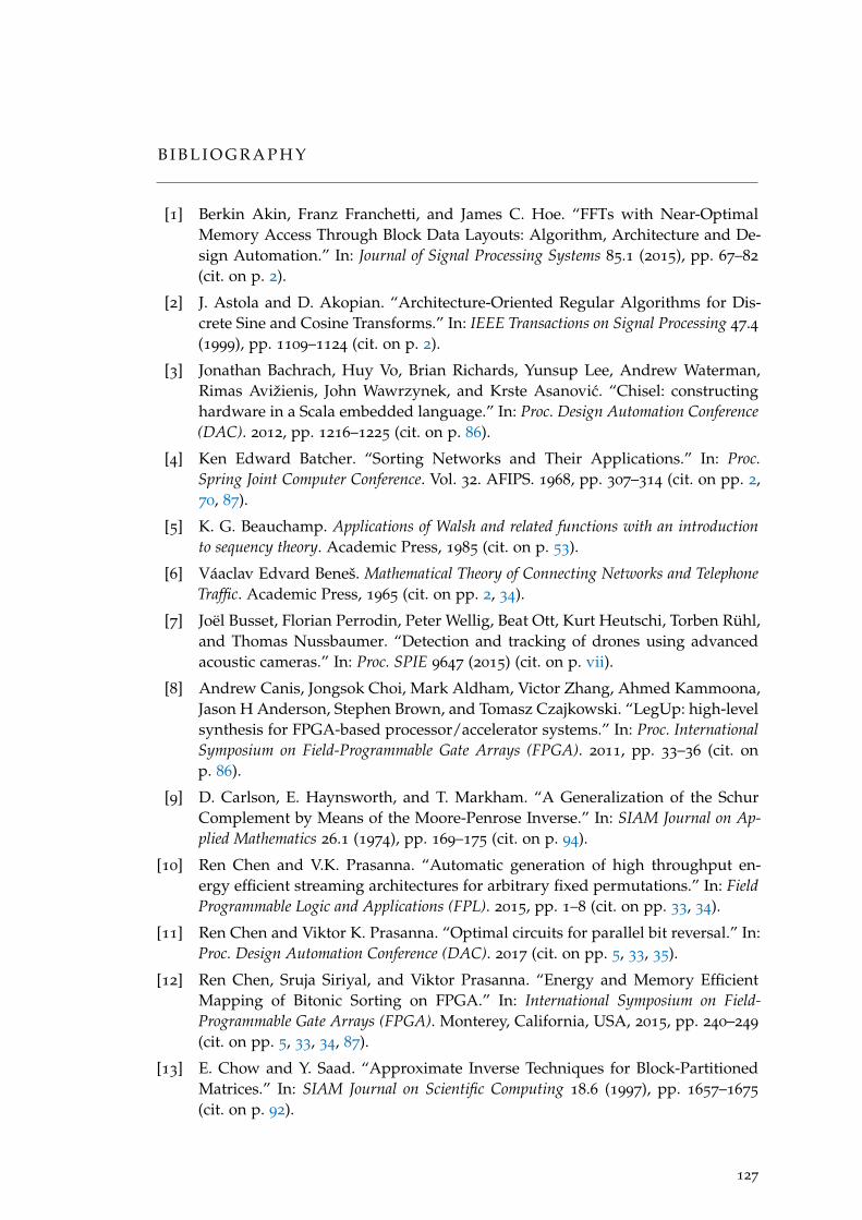
B I B L I O G R A P H Y

[1] Berkin Akin, Franz Franchetti, and James C. Hoe. “FFTs with Near-OptimalMemory Access Through Block Data Layouts: Algorithm, Architecture and De-sign Automation.” In: Journal of Signal Processing Systems 85.1 (2015), pp. 67–82

(cit. on p. 2).

[2] J. Astola and D. Akopian. “Architecture-Oriented Regular Algorithms for Dis-crete Sine and Cosine Transforms.” In: IEEE Transactions on Signal Processing 47.4(1999), pp. 1109–1124 (cit. on p. 2).

[3] Jonathan Bachrach, Huy Vo, Brian Richards, Yunsup Lee, Andrew Waterman,Rimas Avižienis, John Wawrzynek, and Krste Asanovic. “Chisel: constructinghardware in a Scala embedded language.” In: Proc. Design Automation Conference(DAC). 2012, pp. 1216–1225 (cit. on p. 86).

[4] Ken Edward Batcher. “Sorting Networks and Their Applications.” In: Proc.Spring Joint Computer Conference. Vol. 32. AFIPS. 1968, pp. 307–314 (cit. on pp. 2,70, 87).

[5] K. G. Beauchamp. Applications of Walsh and related functions with an introductionto sequency theory. Academic Press, 1985 (cit. on p. 53).

[6] Váaclav Edvard Beneš. Mathematical Theory of Connecting Networks and TelephoneTraffic. Academic Press, 1965 (cit. on pp. 2, 34).

[7] Joël Busset, Florian Perrodin, Peter Wellig, Beat Ott, Kurt Heutschi, Torben Rühl,and Thomas Nussbaumer. “Detection and tracking of drones using advancedacoustic cameras.” In: Proc. SPIE 9647 (2015) (cit. on p. vii).

[8] Andrew Canis, Jongsok Choi, Mark Aldham, Victor Zhang, Ahmed Kammoona,Jason H Anderson, Stephen Brown, and Tomasz Czajkowski. “LegUp: high-levelsynthesis for FPGA-based processor/accelerator systems.” In: Proc. InternationalSymposium on Field-Programmable Gate Arrays (FPGA). 2011, pp. 33–36 (cit. onp. 86).

[9] D. Carlson, E. Haynsworth, and T. Markham. “A Generalization of the SchurComplement by Means of the Moore-Penrose Inverse.” In: SIAM Journal on Ap-plied Mathematics 26.1 (1974), pp. 169–175 (cit. on p. 94).

[10] Ren Chen and V.K. Prasanna. “Automatic generation of high throughput en-ergy efficient streaming architectures for arbitrary fixed permutations.” In: FieldProgrammable Logic and Applications (FPL). 2015, pp. 1–8 (cit. on pp. 33, 34).

[11] Ren Chen and Viktor K. Prasanna. “Optimal circuits for parallel bit reversal.” In:Proc. Design Automation Conference (DAC). 2017 (cit. on pp. 5, 33, 35).

[12] Ren Chen, Sruja Siriyal, and Viktor Prasanna. “Energy and Memory EfficientMapping of Bitonic Sorting on FPGA.” In: International Symposium on Field-Programmable Gate Arrays (FPGA). Monterey, California, USA, 2015, pp. 240–249

(cit. on pp. 5, 33, 34, 87).

[13] E. Chow and Y. Saad. “Approximate Inverse Techniques for Block-PartitionedMatrices.” In: SIAM Journal on Scientific Computing 18.6 (1997), pp. 1657–1675

(cit. on p. 92).

127

128 bibliography

[14] Danny Cohen. “Simplified control of FFT hardware.” In: IEEE Transactions onAcoustics, Speech, and Signal Processing 24.6 (1976), pp. 577–579 (cit. on p. 2).

[15] James W. Cooley and John W. Tukey. “An Algorithm for the Machine Calcu-lation of Complex Fourier Series.” In: Mathematics of Computation 19.90 (1965),pp. 297–301 (cit. on pp. 1, 55).

[16] Ainhoa Cortés, Igone Vélez, and Juan F. Sevillano. “Radix rk FFTs: MatricialRepresentation and SDC/SDF Pipeline Implementation.” In: IEEE Transactionson Signal Processing 57.7 (2009), pp. 2824–2839 (cit. on p. 2).

[17] Richard W. Cottle. “Manifestations of the Schur Complement.” In: Linear Algebraand its Applications 8.3 (1974), pp. 189 –211 (cit. on p. 92).

[18] James W. Demmel, Nicholas J. Higham, and Robert S. Schreiber. “Block LUFactorization.” In: Numerical Linear Algebra with Applications 2.2 (1992), pp. 173–190 (cit. on p. 92).

[19] Florent de Dinechin and Bogdan Pasca. “Designing Custom Arithmetic DataPaths with FloPoCo.” In: IEEE Design & Test of Computers 28.4 (2011), pp. 18–27

(cit. on p. 5).

[20] Robert W. Floyd. “Algorithm 97: Shortest Path.” In: Commun. ACM 5.6 (1962),p. 345 (cit. on p. 59).

[21] Jean Baptiste Joseph Fourier. Théorie analytique de la chaleur. Chez Firmin Didot,père et fils, 1822 (cit. on p. 1).

[22] Franz Franchetti, Frédéric de Mesmay, Daniel McFarlin, and Markus Püschel.“Operator Language: A Program Generation Framework for Fast Kernels.” In:IFIP Working Conference on Domain Specific Languages (DSL WC). Vol. 5658. Lec-ture Notes in Computer Science. Springer, 2009, pp. 385–410 (cit. on p. 69).

[23] Mario Garrido. “Multiplexer and Memory-efficient circuits for parallel bit rever-sal.” In: IEEE Transactions on Circuits and Systems II (TCAS-II) (2018) (cit. on pp. 4,33, 35).

[24] Mario Garrido, Jesús Grajal, and Oscar Gustafsson. “Optimum circuits for bit-dimension permutations.” In: IEEE Transactions on Very Large Scale IntegrationSystems (2019) (cit. on p. 5).

[25] Mario Garrido, Miguel Ángel Sánchez, María Luisa López-Vallejo, and JesùsGrajal. “A 4096-Point Radix-4 Memory-Based FFT Using DSP Slices.” In: IEEETransactions on Very Large Scale Integration Systems 25.1 (2017), pp. 375–379 (cit. onpp. 2, 49).

[26] Johann Carl Friedrich Gauß. “Theoria interpolationis methodo nova tractata.”In: Werke Band 3 (1866), pp. 265–327 (cit. on p. 1).

[27] Nithin George, David Novo, Tiark Rompf, Martin Odersky, and Paolo Ienne.“Making domain-specific hardware synthesis tools cost-efficient.” In: Proc. Inter-national Conference on Field-Programmable Technology (FPT). 2013, pp. 120–127 (cit.on p. 86).

[28] Nithin George, HyoukJoong Lee, David Novo, Muhsen Owaida, David An-drews, Kunle Olukotun, and Paolo Ienne. “Automatic support for multi-moduleparallelism from computational patterns.” In: Proc. International Conference onField Programmable Logic and Applications (FPL). 2015, pp. 1–8 (cit. on p. 86).

bibliography 129

[29] Jacques Hadamard. “Résolution d’une question relative aux déterminants.” In:Bulletin des sciences mathématiques 17 (1893), pp. 240–246 (cit. on pp. 2, 53).

[30] Shousheng He and Mats Torkelson. “A new approach to pipeline FFT proces-sor.” In: Proc. Parallel Processing Symposium (IPPS). 1996, pp. 766–770 (cit. onp. 2).

[31] Tuomas Järvinen, Perttu Salmela, Harri Sorokin, and Jarmo Takala. “Stride per-mutation networks for array processors.” In: Proc. International Conference onApplication-Specific Systems, Architectures and Processors Proceedings (ASAP). 2004,pp. 376–386 (cit. on pp. 4, 35, 49).

[32] Byung G. Jo and Myung H. Sunwoo. “New continuous-flow mixed-radix(CFMR) FFT Processor using novel in-place strategy.” In: IEEE Transactions onCircuits and Systems I 52.5 (2005), pp. 911–919 (cit. on pp. 2, 49).

[33] J. R. Johnson, R. W. Johnson, D. Rodriguez, and R. Tolimieri. “A methodology fordesigning, modifying, and implementing Fourier transform algorithms on vari-ous architectures.” In: Circuits, Systems and Signal Processing 9.4 (1990), pp. 449–500 (cit. on pp. 55, 68, 124).

[34] Jeremy Johnson and Michael Andrews. “Statistical Evaluation of a Self-TuningVectorized Library for the Walsh-Hadamard Transform.” In: International Work-shop on State-of-the-Art in Scientific and Parallel Computing (PARA). 2008 (cit. onp. 53).

[35] Jeremy Johnson and Markus Püschel. “In Search of the Optimal Walsh-Hadamard Transform.” In: International Conference on Acoustics, Speech, andSignal Processing (ICASSP). Vol. 6. 2000, pp. 3347–3350 (cit. on pp. 53, 57, 59).

[36] Alan H. Karp. “Bit Reversal on Uniprocessors.” In: SIAM Review 38.1 (1996),pp. 1–26 (cit. on p. 21).

[37] Donald Ervin Knuth. The Art of Computer Programming, 2Nd Ed. (Addison-Wesley Series in Computer Science and Information. 2nd. Boston, MA, USA:Addison-Wesley Longman Publishing Co., Inc., 1978 (cit. on pp. 11, 12, 87).

[38] Thaddeus Koehn and Peter Athanas. “Arbitrary streaming permutations withminimum memory and latency.” In: Proc. International Conference on Computer-Aided Design (ICCAD). 2016, pp. 1–6 (cit. on pp. 4, 5, 15, 33, 38, 46).

[39] Pinit Kumhom, Jeremy R. Johnson, and Prawat Nagvajara. “Design, optimiza-tion, and implementation of a universal FFT processor.” In: Proc. InternationalASIC/SOC Conference (ASIC). 2000, pp. 182–186 (cit. on p. 2).

[40] Jacques Lenfant and Serge Tahé. “Permuting data with the Omega network.” In:Acta Informatica 21.6 (1985), pp. 629–641 (cit. on pp. 2, 22–24, 34).

[41] Florence Jessie MacWilliams and Neil James Alexander Sloane. The theory oferror-correcting codes. Elsevier, 1977 (cit. on p. 53).

[42] Geoffrey Mainland and Jeremy Johnson. “A Haskell Compiler for Signal Trans-forms.” In: Proc. International Conference on Generative Programming: Concepts andExperiences (GPCE). 2017, pp. 219–232 (cit. on p. 86).

[43] Stéphane Mallat. Traitement du signal. École polytechnique, Département deMathématiques appliquées, 2000 (cit. on p. 1).

[44] Peter A. Milder. Spiral DFT/FFT IP Core Generator. http://www.spiral.net/hardware/dftgen.html. 2008 (cit. on pp. 45, 49).

http://www.spiral.net/hardware/dftgen.html

http://www.spiral.net/hardware/dftgen.html

130 bibliography

[45] Peter A. Milder, James C. Hoe, and Markus Püschel. “Automatic Generationof Streaming Datapaths for Arbitrary Fixed Permutations.” In: Proc. Design, Au-tomation and Test in Europe (DATE). 2009, pp. 1118–1123 (cit. on pp. 4, 15, 31–33,35, 38, 41, 46, 49).

[46] Peter A. Milder, Franz Franchetti, James C. Hoe, and Markus Püschel. “LinearTransforms: From Math to Efficient Hardware.” In: Workshop on High-Level Syn-thesis colocated with DAC. 2008 (cit. on pp. 2, 5).

[47] Peter A. Milder, Franz Franchetti, James C. Hoe, and Markus Püschel. “Com-puter Generation of Hardware for Linear Digital Signal Processing Transforms.”In: ACM Transactions on Design Automation of Electronic Systems (TODAES) 17.2(2012), 15:1–15:33 (cit. on pp. 2–5, 37, 45, 46, 49, 68, 72, 82, 85, 86).

[48] Rene Mueller, Jens Teubner, and Gustavo Alonso. “Sorting Networks on FP-GAs.” In: The VLDB Journal 21.1 (2012), pp. 1–23 (cit. on p. 87).

[49] David Nassimi and Sartaj Sahni. “A Self-Routing Benes Network and Paral-lel Permutation Algorithms.” In: IEEE Transactions on Computers 30.5 (1981),pp. 332–340 (cit. on pp. 2, 23, 34).

[50] Grace Nordin, Peter A. Milder, James C. Hoe, and Markus Püschel. “AutomaticGeneration of Customized Discrete Fourier Transform IPs.” In: Proc. Design Au-tomation Conference (DAC). 2005, pp. 471–474 (cit. on pp. 2, 4, 55).

[51] Martin Odersky, Lex Spoon, and Bill Venners. Programming in Scala. Artima Inc,2008 (cit. on p. 7).

[52] Georg Ofenbeck. “Generic programming in space and time.” PhD thesis. ETHZurich, 2017 (cit. on p. 86).

[53] Georg Ofenbeck, Tiark Rompf, and Markus Püschel. “Staging for Generic Pro-gramming in Space and Time.” In: International Conference on Generative Program-ming: Concepts & Experiences (GPCE). 2017, pp. 15–28 (cit. on p. 77).

[54] Georg Ofenbeck, Tiark Rompf, Alen Stojanov, Martin Odersky, and MarkusPüschel. “Spiral in Scala: Towards the Systematic Construction of Generatorsfor Performance Libraries.” In: Proc. International Conference on Generative Pro-gramming: Concepts & Experiences (GPCE). 2013, pp. 125–134 (cit. on pp. 68, 77).

[55] Stéphane Olivier. Physique 2e année PC PC*. Lavoisier / Tec & Doc, 2004 (cit. onp. 1).

[56] J. Ortiz and D. Andrews. “A configurable high-throughput linear sorter system.”In: IEEE International Symposium on Parallel Distributed Processing, Workshops andPhd Forum (IPDPSW). 2010, pp. 1–8 (cit. on p. 87).

[57] Kevin J. Page, Jeanette F. Arrigo, and Paul M. Chau. “Reconfigurable-hardware-based digital signal processing for wireless communications.” In: Advanced Sig-nal Processing Algorithms, Architectures and Implementations. Ed. by Proc. SPIE.Vol. 3162. 7. 1997, pp. 529–540 (cit. on pp. 2, 18, 21).

[58] Kevin J. Page and Paul M. Chau. “Folding large regular computational graphsonto smaller processor arrays.” In: Advanced Signal Processing Algorithms, Archi-tectures and Implementations. Ed. by Proc. SPIE. Vol. 2846. 7. 1996, pp. 383–394

(cit. on p. 4).

bibliography 131

[59] Keshab K. Parhi. “Systematic synthesis of DSP data format converters using life-time analysis and forward-backward register allocation.” In: IEEE Transactionson Circuits and Systems II (TCAS-II) 39.7 (1992), pp. 423–440 (cit. on pp. 4, 35, 49).

[60] Marshall C. Pease. “An Adaptation of the Fast Fourier Transform for ParallelProcessing.” In: Journal of the ACM 15.2 (1968), pp. 252–264. issn: 0004-5411 (cit.on pp. 2, 11, 53, 55, 69).

[61] Marshall C. Pease. “The Indirect Binary n-Cube Microprocessor Array.” In: IEEETransactions on Computers 26.5 (1977), pp. 458–473 (cit. on pp. 2, 22, 34).

[62] O. Port and Y. Etsion. “DFiant: A dataflow hardware description language.” In:Proc. International Conference on Field Programmable Logic and Applications (FPL).2017, pp. 1–4 (cit. on p. 86).

[63] Markus Püschel, Peter A. Milder, and James C. Hoe. “Permuting Streaming DataUsing RAMs.” In: Journal of the ACM 56.2 (2009), 10:1–10:34 (cit. on pp. 4, 5, 21,22, 24, 29, 31–34, 41, 45, 46, 95).

[64] Markus Püschel et al. “SPIRAL: Code Generation for DSP Transforms.” In: Pro-ceedings of the IEEE, special issue on “Program Generation, Optimization, and Adapta-tion” 93.2 (2005), pp. 232–275 (cit. on pp. 2, 68, 86).

[65] Tiark Rompf and Martin Odersky. “Lightweight modular staging: a pragmaticapproach to runtime code generation and compiled DSLs.” In: Commun. ACM55.6 (June 2012), pp. 121–130 (cit. on pp. 7, 76, 86).

[66] François Serre. DFT and Streamed Linear Permutation Generator for Hardware.https://github.com/fserre/sgen. 2018 (cit. on pp. 49, 87, 125).

[67] François Serre. SGen - A Streaming Hardware Generator. https://acl.inf.ethz.ch/research/hardware/. 2018 (cit. on pp. 87, 125).

[68] François Serre, Thomas Holenstein, and Markus Püschel. “Optimal Circuits forStreamed Linear Permutations Using RAM.” In: Proc. International Symposium onField-Programmable Gate Arrays (FPGA). 2016, pp. 215–223 (cit. on pp. 11, 68, 85).

[69] François Serre and Markus Püschel. “Generalizing block LU factorization: ALower-Upper-Lower block triangular decomposition with minimal off-diagonalranks.” In: Linear Algebra and its Applications 509 (2016), pp. 114–142 (cit. onp. 91).

[70] François Serre and Markus Püschel. “Characterizing and Enumerating Walsh-Hadamard Transform Algorithms.” In: CoRR abs/1710.08029 (2017). arXiv: 1710.08029 (cit. on p. 115).

[71] François Serre and Markus Püschel. “Optimal Streamed Linear Permutations.”In: Proc. Symposium on Computer Arithmetic (ARITH). 2017, pp. 60–61 (cit. onp. 11).

[72] François Serre and Markus Püschel. “A DSL-based FFT hardware generator inScala.” In: Proc. International Conference on Field Programmable Logic and Applica-tions (FPL). 2018, pp. 315–322 (cit. on p. 67).

[73] François Serre and Markus Püschel. “Memory-Efficient Fast Fourier Transformon Streaming Data by Fusing Permutations.” In: Proc. International Symposiumon Field-Programmable Gate Arrays (FPGA). 2018, pp. 219–228 (cit. on p. 37).

https://github.com/fserre/sgen

https://acl.inf.ethz.ch/research/hardware/

https://acl.inf.ethz.ch/research/hardware/

https://arxiv.org/abs/1710.08029

https://arxiv.org/abs/1710.08029

132 bibliography

[74] François Serre and Markus Püschel. “DSL-Based Hardware Generation withScala: Example Fast Fourier Transforms and Sorting Networks.” In: Transactionson Reconfigurable Technology and Systems (2019). In press. (cit. on p. 67).

[75] François Serre and Markus Püschel. “In search of the optimal Walsh-Hadamardtransform for streamed parallel processing.” In: Proc. International Conference onAcoustics, Speech, and Signal Processing (ICASSP). 2019 (cit. on p. 53).

[76] Claude Elwood Shannon. “A mathematical theory of communication.” In: TheBell System Technical Journal 27.3 (1948), pp. 379–423 (cit. on p. 17).

[77] G. Steidl and M. Tasche. “A polynomial approach to fast algorithms for dis-crete Fourier-cosine and Fourier-sine transforms.” In: Mathematics of Computation56.193 (1991), pp. 281–296 (cit. on p. 14).

[78] David Steinberg. “Invariant Properties of the Shuffle-Exchange and a SimplifiedCost-Effective Version of the Omega Network.” In: IEEE Transactions on Comput-ers 32.5 (1983), pp. 444–450 (cit. on pp. 2, 34).

[79] Harold S. Stone. “Parallel Processing with the Perfect Shuffle.” In: IEEE Transac-tions on Computers C-20.2 (1971), pp. 153–161 (cit. on pp. 2, 70, 71).

[80] Arvind Sujeeth, HyoukJoong Lee, Kevin Brown, Tiark Rompf, Hassan Chafi,Michael Wu, Anand Atreya, Martin Odersky, and Kunle Olukotun. “OptiML:an implicitly parallel domain-specific language for machine learning.” In: Proc.International Conference on Machine Learning (ICML). 2011, pp. 609–616 (cit. onp. 86).

[81] J. H. Takala, T. S. Jarvinen, and H. T. Sorokin. “Conflict-free parallel memoryaccess scheme for FFT processors.” In: Proc. International Symposium on Circuitsand Systems (ISCAS). Vol. 4. 2003, pp. 524–527 (cit. on p. 2).

[82] C. Van Loan. Computational Framework of the Fast Fourier Transform. Siam, 1992

(cit. on p. 55).

[83] Philip Wadler and Stephen Blott. “How to make ad-hoc polymorphism less adhoc.” In: Proceedings of the 16th ACM SIGPLAN-SIGACT symposium on Principlesof programming languages. ACM. 1989, pp. 60–76 (cit. on p. 77).

[84] Abraham Waksman. “A permutation network.” In: Journal of the ACM 15.1(1968), pp. 159–163 (cit. on pp. 2, 18, 34, 45).

[85] Jianxin Xiong, Jeremy Johnson, Robert W. Johnson, and David Padua. “SPL: ALanguage and Compiler for DSP Algorithms.” In: Programming Languages Designand Implementation (PLDI). 2001, pp. 298–308 (cit. on p. 68).

[86] Rao K. Yarlagadda and John E. Hershey. Hadamard Matrix Analysis and Synthesis.Springer Us, 2012 (cit. on p. 53).

[87] Fuzhen Zhang. The Schur Complement and its Applications. Vol. 4. Springer, 2006

(cit. on pp. 92, 94, 95).

[88] Marcela Zuluaga, Peter A. Milder, and Markus Püschel. “Computer Generationof Streaming Sorting Networks.” In: Design Automation Conference (DAC). 2012,pp. 1245–1253 (cit. on pp. 2, 86).

[89] Marcela Zuluaga, Peter A. Milder, and Markus Püschel. “Streaming SortingNetworks.” In: ACM Transactions on Design Automation of Electronic Systems (TO-DAES) 21.4 (2016) (cit. on pp. 2, 5, 11, 12, 69–71, 85, 86).

F R A N Ç O I S S E R R E

Date of birth: 6th January 1986

Nationality: French

EDUCATION

2013 - 2019 ETH Zurich

PhD in Computer Science, Prof. Dr. Püschel

2010 - 2012 ETH Zurich

MSc in Computer Science

2007 - 2012 Ecole Polytechnique, Palaiseau, France

Dipl. Ing., X2007

2004 - 2007 Lycée Louis-Le-Grand, Paris, France

Classes préparatoires aux grandes écoles, PCSI/PC*

WORK EXPERIENCE

04/2010 - 09/2010 Siemens Corporate Research, Princeton, NJ, US

Research internship

08/2009 - 09/2010 Ferrum Lasercut, Berlin, Germany

Blue-collar internship

09/2007 - 04/2008 Gendarmerie Nationale, Tours, France

Second lieutenant

133

Optimal Streaming Permutations and Transforms - François ...

Documents

Transcript of Optimal Streaming Permutations and Transforms - François ...