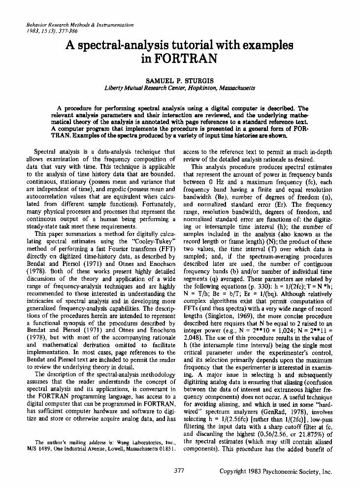
Behavior Research Methods & Instrumentation1983,15 (3),377-386

A spectral-analysis tutorial with examplesin FORTRAN

SAMUEL P. STURGISLibertyMutualResearch Center, Hopkinton, Massachusetts

A procedure for performing spectral analysis using a digital computer is described. Therelevant analysis parameters and their interaction are reviewed, and the underlying mathe­matical theory of the analysis is annotated with page references to a standard reference text.A computer program that implements the procedure is presented in a general form of FOR·TRAN. Examples of the spectra produced by a variety of input time histories are shown.

Spectral analysis is a data-analysis technique thatallows examination of the frequency composition ofdata that vary with time, This technique is applicableto the analysis of time history data that are bounded,continuous, stationary (possess mean and variance thatare independent of time), and ergodic (possess mean andautocorrelation values that are equivalent when calcu­lated from different sample functions). Fortunately,many physical processes and processes that represent thecontinuous output of a human being performing asteady-state task meet these requirements.

This paper summarizes a method for digitally calcu­lating spectral estimates using the "Cooley-Tukey"method of performing a fast Fourier transform (FFT)directly on digitized time-history data, as described byBendat and Piersol (1971) and Otnes and Enochson(1978). Both of these works present highly detaileddiscussions of the theory and application of a widerange of frequency-analysis techniques and are highlyrecommended to those interested in understanding theintricacies of spectral analysis and in developing moregeneralized frequency-analysis capabilities. The descrip­tions of the procedures herein are intended to representa functional synopsis of the procedures described byBendat and Piersol (1971) and Otnes and Enochson(1978), but with most of the accompanying rationaleand mathematical derivation omitted to facilitateimplementation. In most cases, page references to theBendat and Piersol text are included to permit the readerto review the underlying theory in detail.

The description of the spectral-analysis methodologyassumes that the reader understands the concept ofspectral analysis and its applications, is conversant inthe FORTRAN programming language, has access to adigital computer that can be programmed in FORTRAN,has sufficient computer hardware and software to digi­tize and store or otherwise acquire analog data, and has

The author's mailing address is: Wang Laboratories, Inc.,MIS 1489, One Industrial Avenue, Lowell, Massachusetts 01851.

access to the reference text to permit as much in-depthreview of the detailed analysis rationale as desired.

This analysis procedure produces spectral estimatesthat represent the amount of power in frequency bandsbetween 0 Hz and a maximum frequency (fc), eachfrequency band having a finite and equal resolutionbandwidth (Be), number of degrees of freedom (n),and normalized standard error (Er). The frequencyrange, resolution bandwidth, degrees of freedom, andnormalized standard error are functions of: the digitiz­ing or intersample time interval (h); the number ofsamples included in the analysis (also known as therecord length or frame length) (N); the product of thesetwo values, the time interval (T) over which data issampled; and, if the spectrum-averaging proceduresdescribed later are used, the number of contiguousfrequency bands (b) and/or number of individual timesegments (q) averaged. These parameters are related bythe following equations (p. 330): h :: 1/(2fc); T = N *h;N :: T/h; Be :: b/T; Er :: l/(bq). Although relativelycomplex algorithms exist that permit computation ofFFTs (and thus spectra) with a very wide range of recordlengths (Singleton, 1969), the more concise proceduredescribed here requires that N be equal to 2 raised to aninteger power (e.g., N :: 2**10 :: 1,024; N :: 2**11 ::2,048). The use of this procedure results in the value ofh (the intersample time interval) being the single mostcritical parameter under the experimenter's control,and its selection primarily depends upon the maximumfrequency that the experimenter is interested in examin­ing. A major issue in selecting h and subsequentlydigitizing analog data is ensuring that aliasing(confusionbetween the data of interest and extraneous higher fre­quency components) does not occur. A useful techniquefor avoiding aliasing, and which is used in some "hard­wired" spectrum analyzers (GenRad, 1978), involvesselecting h :: 1/(2.56fc) [rather than 1/(2fc)], low-passfiltering the input data with a sharp cutoff filter at fc,and discarding the highest (0.56/2.56, or 21.875%) ofthe spectral estimates (which may still contain aliasedcomponents). This procedure has the added benefit of

377 Copyright 1983 Psychonomic Society, Inc.

378 STURGIS

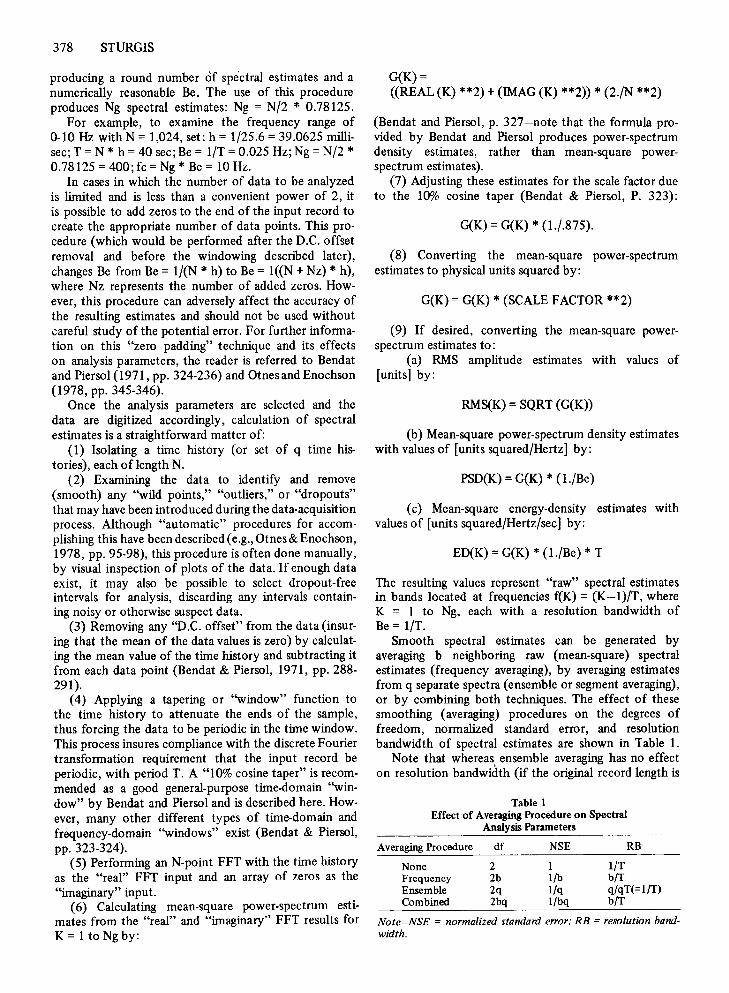
producing a round number Of spectral estimates and anumerically reasonable Be. The use of this procedureproduces Ng spectral estimates: Ng = N/2 * 0.78125.

For example, to examine the frequency range of0-10 Hz with N = 1,024, set: h = 1/25.6 = 39.0625 milli­sec; T =N * h = 40 sec; Be = liT =0.025 Hz; Ng =N/2 *0.78125 = 400; fc =Ng * Be = 10 Hz.

In cases in which the number of data to be analyzedis limited and is less than a convenient power of 2, itis possible to add zeros to the end of the input record tocreate the appropriate number of data points. This pro­cedure (which would be performed after the D.C. offsetremoval and before the windowing described later),changes Be from Be = lieN * h) to Be = 1((N + Nz) * h),where Nz represents the number of added zeros. How­ever, this procedure can adversely affect the accuracy ofthe resulting estimates and should not be used withoutcareful study of the potential error. For further informa­tion on this "zero padding" technique and its effectson analysis parameters, the reader is referred to Bendatand Piersol (1971, pp. 324-236) and Otnesand Enochson(1978, pp. 345-346).

Once the analysis parameters are selected and thedata are digitized accordingly, calculation of spectralestimates is a straightforward matter of:

(1) Isolating a time history (or set of q time his­tories), each of length N.

(2) Examining the data to identify and remove(smooth) any ''wild points," "outliers," or "dropouts"that may have been introduced during the data-acquisitionprocess. Although "automatic" procedures for accom­plishing this have been described (e.g., Otnes & Enochson,1978, pp. 95-98), this procedure is often done manually,by visual inspection of plots of the data. If enough dataexist, it may also be possible to select dropout-freeintervals for analysis, discarding any intervals contain­ing noisy or otherwise suspect data.

(3) Removing any "D.C. offset" from the data (insur­ing that the mean of the data values is zero) by calculat­ing the mean value of the time history and subtracting itfrom each data point (Bendat & Piersol, 1971, pp. 288­291).

(4) Applying a tapering or "window" function tothe time history to attenuate the ends of the sample,thus forcing the data to be periodic in the time window.This process insures compliance with the discrete Fouriertransformation requirement that the input record beperiodic, with period T. A "10% cosine taper" is recom­mended as a good general-purpose time-domain "win­dow" by Bendat and Piersol and is described here. How­ever, many other different types of time-domain andfrequency-domain ''windows'' exist (Bendat & Piersol,pp. 323-324).

(5) Performing an N-point FFT with the time historyas the "real" FFT input and an array of zeros as the"imaginary" input.

(6) Calculating mean-square power-spectrum esti­mates from the "real" and "imaginary" FFT results forK = 1 to Ng by:

G(K) =((REAL (K) **2) + (IMAG (K) **2» * (2./N **2)

(Bendat and Piersol, p. 327-note that the formula pro­vided by Bendat and Piersol produces power-spectrumdensity estimates, rather than mean-square power­spectrum estimates).

(7) Adjusting these estimates for the scale factor dueto the 10% cosine taper (Bendat & Piersol, P. 323):

G(K) =G(K) * (1./.875).

(8) Converting the mean-square power-spectrumestimates to physical units squared by:

G(K) =G(K) * (SCALE FACTOR **2)

(9) If desired, converting the mean-square power­spectrum estimates to:

(a) RMS amplitude estimates with values of[units] by:

RMS(K) = SQRT (G(K»

(b) Mean-square power-spectrum density estimateswith values of [units squared/Hertz] by:

PSD(K) = G(K) * (1./Be)

(c) Mean-square energy-density estimates withvalues of [units squared/Hertz/sec] by:

ED(K) = G(K) * (I.jBe) * T

The resulting values represent "raw" spectral estimatesin bands located at frequencies f(K) = (K-l)/T, whereK = 1 to Ng, each with a resolution bandwidth ofBe = I/T.

Smooth spectral estimates can be generated byaveraging b neighboring raw (mean-square) spectralestimates (frequency averaging), by averaging estimatesfrom q separate spectra (ensemble or segment averaging),or by combining both techniques. The effect of thesesmoothing (averaging) procedures on the degrees offreedom, normalized standard error, and resolutionbandwidth of spectral estimates are shown in Table 1.

Note that whereas ensemble averaging has no effecton resolution bandwidth (if the original record length is

Table IEffect of Averaging Procedure on Spectral

Analysis Parameters

Averaging Procedure df NSE RB

None 2 1 irrFrequency 2b lIb bITEnsemble 2q l/q q/qT(=l/T)Combined 2bq l/bq »tt

Note-NSE = normalized standard error; RB = resolution band­width.

maintained as T seconds), frequency averaging has theeffect of widening the original resolution bandwidth bya factor of b, the number of spectral estimates averaged.

Since both averagingtechniques are linear operations,the combined averaging procedure may be conducted ineither sequence. However, any averaging procedureshould be conducted on squared spectral estimateswith RMS estimates, (if desired) calculated from thefinal averaged result.

The procedure used for frequency averaging is(pp. 327-328):

(1) Start with a set of (Ng) spectral estimates (G(K),K = 1 to Ng], each with a resolution bandwidth ofBe =I/T.

(2) Generate a set of (Ng)/b averaged spectral esti­mates by finding the mean of each consecutive (non­overlapping) set of b raw estimates.

This procedure produces (Ng)/b averaged spectral esti­mates of bandwidth Be = bIT, with the band midpointslocated at frequencies f(K) =«(b-I)/2+(b*(K-I»)/T,where K =I to (Ng)/b.

The procedure used for ensemble averaging is(pp. 328-329):

(1) Start with q sets of (Ng) spectral estimates (G(K),K = 1 to Ng), each with a resolution bandwidth ofBe = lIT.

(2) Generate a set of (Ng) averaged spectral estimatesby finding the mean of the q raw spectral estimates ateach frequency f(K).

This procedure produces (Ng) averaged spectral esti­mates of bandwidth Be = I/T, with bands located atfrequencies f(K) =(K:-l)/T, where K =I to Ng.

The ensemble-averaging procedure is most easilyimplemented by keeping a "running" ensemble averageto which successive power spectra can be added as theyare calculated. This precludes the need for storage of apotentially large number of individual "raw" spectra.

The mean-square power (or RMS amplitude) in speci­fied frequency bands can be estimated by summing Jcontiguous mean-square power-spectrum estimates toproduce wider frequency bands of resolution band­width Be = J(b/T). Summation of all (Ng) mean-squarespectrum estimates gives an estimate of the total meansquare of the N input values. The positive square root ofthe total mean square or of the mean square in smallerfrequency bands gives the corresponding RMS amplitudein the frequency bands in question. This analysis isappropriate, of course, for mean-square power-spectrumestimates only, since both power-spectrum-density andenergy-density estimates are already normalized to aI-Hz bandwidth.

The Appendix presents a FORTRAN main programand a set of subroutines to permit the reader to explorethe use of spectral analysis using the method describedabove. These FORTRAN routines are not intended torepresent the fastest, most elegant, or most conciseprocedure that can be used to perform this type ofanalysis. However, they do work successfully, and theyare written in a manner that should permit their imple-

SPECTRAL-ANALYSIS TUTORIAL 379

mentation in a wide variety of FORTRAN dialects. Ifspeed of processing is a problem for the user, the great­est gains in execution speed probably can be gainedthrough the use of a machine language FFT subroutinethat uses fixed-point fractional arithmetic and a sinelook-up table. Use of a windowing subroutine that usesstored (rather than computed) cosine values would alsoimprove execution speed. Such routines are often avail­able as "system" subroutines on large timesharing com­puter systems and are often available through computerusers' groups or manufacturers. The example input sub­routine "GETDAT" generates data that should duplicatethe results shown in Figures 3 and 4 below.

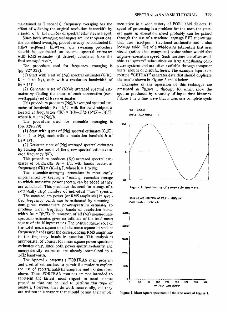
Examples of the operation of this technique arepresented in Figures 1 through 10, which show thespectra produced by a variety of input time histories.Figure 1 is a sine wave that makes one complete cycle

mE ' 5I1lEI.DAT

5TARTING BLOC!( IUIlER '

258. -r------::_~-----------__,

9. -f--------~...--------__j

-258. -'---- --"'-.......c. ...J

Figure 1. Time history of a one-cycle sine wave.

MEAN SQUARE SPECTRUIt OF FILE, SINEI.DATPEAK VALUE, 32515.5

2_

1-0.....,..,~ .................,..,...,...T""T""T..,....,..,.......,~"T""T",...........,...,....,....,...,~.,....,....,........,.~o 50 100 150 2110 250 300 350 ~00

SPECTRUM LINE NUMBER

Figure 2. Mean-square spectrum of the sine wave of Figure 1.

380 STURGIS

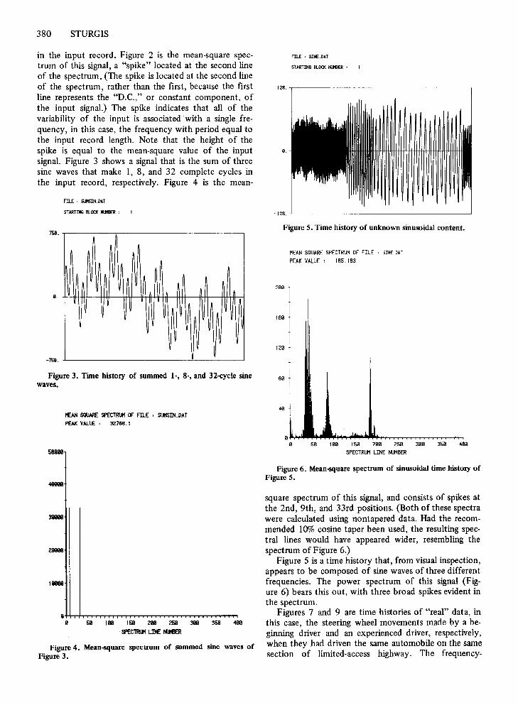
in the input record. Figure 2 is the mean-square spec­trum of this signal, a "spike" located at the second lineof the spectrum. (The spike is located at the second lineof the spectrum, rather than the first, because the firstline represents the "D.C.," or constant component, ofthe input signal.) The spike indicates that all of thevariability of the input is associated with a single fre­quency, in this case, the frequency with period equal tothe input record length. Note that the height of thespike is equal to the mean-square value of the inputsignal. Figure 3 shows a signal that is the sum of threesine waves that make 1, 8, and 32 complete cycles inthe input record, respectively. Figure 4 is the mean-

FILE , SlttSIN. PAT

STARTING BI..OCl( tf.MlER '

7Sll. ,------,-----------------,

-7Sll. -'-- ---''-- ---.J

Figure 3. Time history of summed 1-, 8-, and 32-cycle sinewaves.

/£AN SQUARE SPECTRLtf ~ fIlE ' SlItSIN.OATPEAK VAlLE, 32766. I

II fJr-r+.""T"T...............""T"T...............""T"T...............""T"T...............""T"T........T"TT"l

" 511 1Ill! 1511 21lll 25ll 3lll! 3511 -4lll!.SPECTRLtf Llt£ IUtlER

Figure 4. Mean-square spectrum of summed sine waves ofFigure 3.

FILE , SINE.PAT

STARTING BLOC!< IOIlEll '

128.~-----------------

9.

-128. -'---------------------~

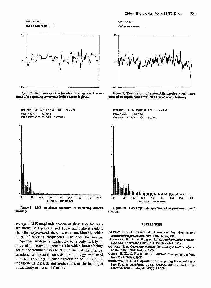
Figure 5. Time history of unknown sinusoidal content.

MEAN SQUARE SPECTRUM OF FILE , SINE PAT

PEAK VALUE, 165.163

299

169

129

89

49

59 199 159 209 250 390 359 400

SPECTRUM LINE NUMBER

Figure 6. Mean-square spectrum of sinusoidal time history ofFigure 5.

square spectrum of this signal, and consists of spikes atthe 2nd, 9th, and 33rd positions. (Both of these spectrawere calculated using nontapered data. Had the recom­mended 10% cosine taper been used, the resulting spec­tral lines would have appeared wider, resembling thespectrum of Figure 6.)

Figure 5 is a time history that, from visual inspection,appears to be composed of sine waves of three differentfrequencies. The power spectrum of this signal (Fig­ure 6) bears this out, with three broad spikes evident inthe spectrum.

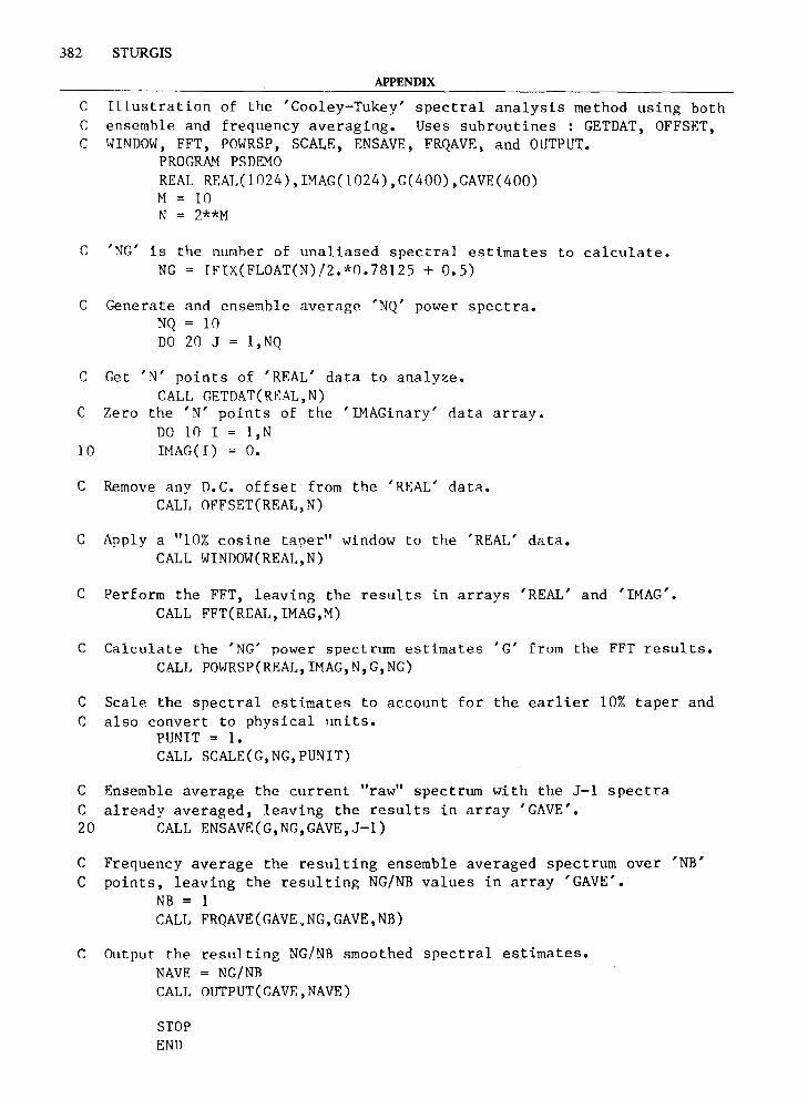
Figures 7 and 9 are time histories of "real" data, inthis case, the steering wheel movements made by a be­ginning driver and an experienced driver, respectively,when they had driven the same automobile on the samesection of limited-access highway. The frequency-

FILE ' HlS.DAT

STAR'T1HG SlOCl( IQtlER '

64. -,---------------------,

-64. -'--------------------'

Figure 7. Time history of automobile steering wheel move­ment of a beginning driver on a limited-access highway.

RMS AMPLITUDE SPECTRUM OF FILE e ML5. DAT

PEAK VALUE, 2.22550FREQUENCY AVERAGE OVER 3 POINTS

SPECTRAL-ANALYSIS TUTORIAL 381

FILE ' SIS.DAT

STARTIHll· BlOCK USER ,

64. -,----------------------,

-64. -'----------------------'

Figure 9. Time history of automobile steering wheel move­ment of an experienced driver on a limited-access highway.

RMS AMPLITUDE SPECTRUM OF FILE , SZ5.OAT

PEAK VALUE, 2.94152FREIXJENCY AVERAGE OVER 3 POINTS.

5

3

2

50 100 150 200 250 300 350 400SPECTRUM LINE NUHBER

5

3

2

50 100 150 200 250 300 350 400SPECTRUM LINE NUMBER

Figure 8. RMS amplitude spectrum of beginning driver'ssteering.

averaged RMS amplitude spectra of these time historiesare shown in Figures 8 and 10, which make it evidentthat the experienced driver uses a considerably widerrange of steering frequencies than does the novice.

Spectral analysis is applicable to a wide variety ofphysical processes and processes in which human beingsact as controlling elements. It is hoped that the brief de­scription of spectral analysis methodology presentedhere will encourage further exploration of this analysistechnique in research and applications of the techniquein the study of human behavior.

Figure 10. RMS amplitude spectrum of experienced driver'ssteering.

REFERENCES

BENDAT, J. S., & PIERSOL, A. G. Random data: Analysis andmeasurementproceduns. New York: Wiley,l97l.

ECKHOUSE, R. H., & MORRIS, L. R. Minicomputer systems.(2nd ed.), Englewood Cliffs, N.J: Prentice-Hall, 1979.

GENRAD, INC. Operating manual lor 2512 spectrum analyzer.Santa Clara, Calif: Author, 1978.

OrNES, R. K., & ENOCHSON, L. Applied time series analysis.New York: Wiley, 1978.

SINGLETON, R. C. An algorithm for computing the mixed radixfast Fourier transform. IEEE Transactions on Audio andElectroacoustics, 1969,AU·17(2), 93-100.

382 STURGIS

APPENDIX

C ILLustration of the 'Cooley-Tukey' spectral analysis method using bothC ensemble and frequency averaging. Uses subroutines : GETDAT, OFFSET,C WINDOW, FFT, POWRSP, SCALE, ENSAVE, FRQAVE, and OUTPUT.

PROGRAM PSDEMOREAL REAL(1024), IMAG(1024) ,G(400) ,GAVE(400)M 10N = 2**M

C 'NG' is the numher of unaliased spectral estimates to calculate.NG = IFIX(FLOAT(N)/2.*0.78125 + 0.5)

C Generate and ensemble average 'NQ' power spectra.NQ = 10DO 20 J = I,NQ

C Get 'N' points of 'REAL' data to analyze.CALL GETDAT(REAL,N)

C Zero the 'N' points of the 'IMAGinary' data array.DO 10 I 1, N

10 IMAG(I) = O.

C Remove any D.C. offset from the 'REAL' data.CALL OFFSET(REAL,N)

C Apply a "10% cosine taper" window to the 'REAL' data.CALL WINDOW(REAL,N)

C Perform the FFT, leaving the results in arrays 'REAL' and 'IMAG'.CALL FFT(REAL,IMAG,M)

C Calculate the 'NG' power spectrum estimates 'G' from the FFT results.CALL POWRSP(REAL,IMAG,N,G,NG)

C Scale the spectral estimates to account for the earlier 10% taper andC also convert to physical units.

PUNIT = 1.CALL SCALE(G,NG,PUNIT)

C Ensemble average the current "raw" spectrum with the J-l spectraC already averaged, leaving the results in array 'GAVE'.20 CALL ENSAVE(G,NG,GAVE,J-l)

C Frequency average the resulting ensemble averaged spectrum over 'NB'C points, leaving the resulting NG/NB values in array 'GAVE'.

NB = 1CALL FRQAVE(GAVE.NG,GAVE,NB)

C Output the resulting NG/NR smoothed spectral estimates.NAVE = NG/NRCALL OUTPUT(GAVE,NAVE)

STOPEND

SPECTRAL-ANALYSIS TUTORIAL 383

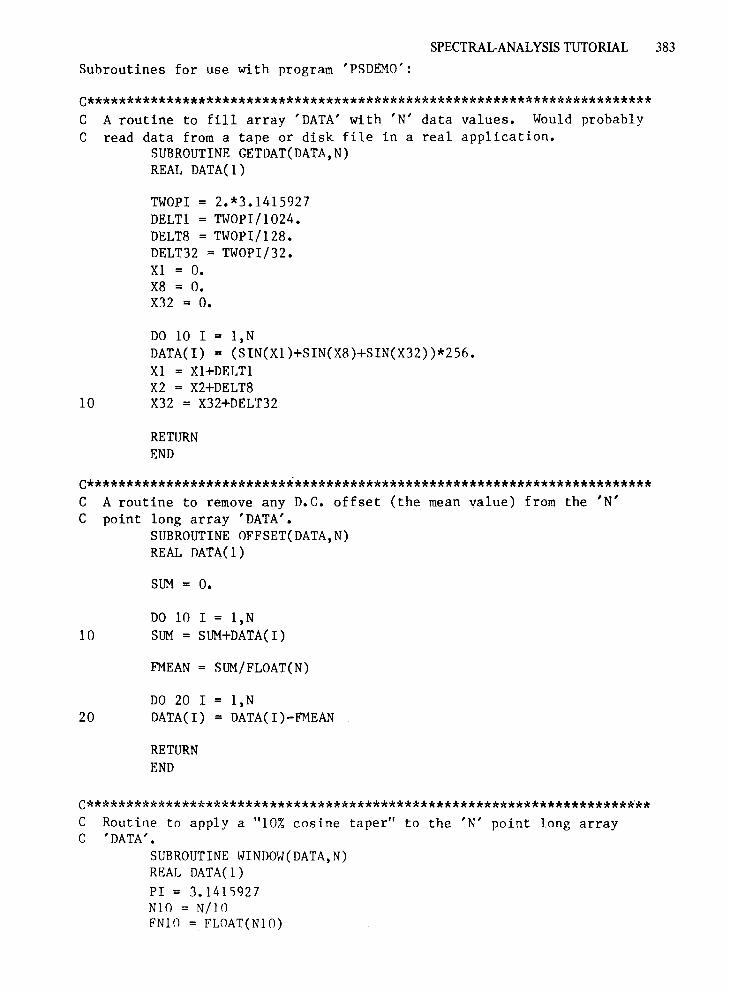
Subroutines for use with program 'PSDEMO':

c***********************************************************************C A routine to fill array 'DATA' with 'N' data values. Would probablyC read data from a tape or disk file in a real application.

SUBROUTINE GETDAT(DATA,N)REAL DATA(l)

TWOPI = 2.*3.1415927DELT1 = TWOPI/1024.DELT8 = TWOPI/128.DELT32 = TWOPI/32.Xl = O.XB = O.X32 = O.

DO 10 I = 1, NDATA(I) = (SIN(X1)+SIN(X8)+SIN(X32»*256.Xl = X1+DELT1X2 = X2+DELT8

10 X32 = X32+DELT32

RETURNEND

C***********************************************************************C A routine to remove any D.C. offset (the mean value) from the 'N'C point long array 'DATA'.

SUBROUTINE OFFSET(DATA,N)REAL DATA( 1)

SUM = O.

DO 10 I = 1,N10 SUM = SUM+DATA(I)

FMEAN = SUM/FLOAT(N)

20DO 20 IDATA(I) =

RETURNEND

1,NDATA( I )-Fl1EAN

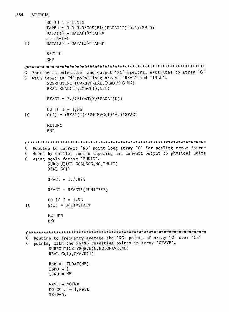
C***********************************************************************C Routine to apply a "10% cosine taper" to the 'N' point long arrayC 'DATA' •

SUBROUTINE WINDOW(DATA,N)REAL DATA(l)PI = 3.1415927N10 = N/lOFNIO = FLOAT(NIO)

384 STURGIS

DO 10 I = I~NI0

TAP~R = 0.5-0.S*COS(PI*(FLOAT(I)-0.S)/FNI0)DATA(I) OATA(I)*TAPERJ = N-I+l

10 DATA(J) DATA(J)*TAPER

RETIJRNENJ1

C***********************************************************************C Routine to calculate and output 'NG' spectral estimates to array 'G'C with Input in 'N' point long arrays 'REAL' and 'IMAG'.

SUBROUTINE POWRSP(REAL,IMAG,N,G,NG)REAL REAL(I),IMAG(I),G(I)

SFACT = 2./(FLOAT(N)*FLOAT(N»

DO 10 I = 1, NG10 G(I) = (REAL(I)**2+IMAG(I)**2)*SFACT

RETURNEND

C***********************************************************************C Routine to correct 'NG' point long array 'G' for scaling error intro­C duced by earlier cosine tapering and convert output to physical unitsC using scale factor 'PUNIT'.

SUBROUTINE SCALE(G,NG,PUNIT)REAL G(l)

SFACT 1./.875

SFACT = SF'ACT*(PUNIT**2)

DO 10 I = 1, NG10 G(I) = G(I)*SFACT

RETURNEND

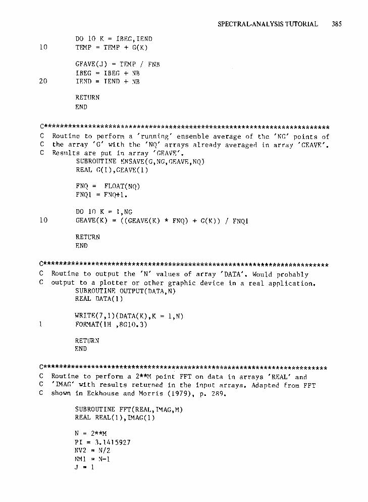
C***********************************************************************C Routine to frequency average the 'NG' points of array 'G' over 'NB'C points, with the NG/NB resulting points in array 'GFAVE'.

SUBROUTINE FRQAVE(G,NG,GFAVE,NB)REAL G(I),GFAVE(I)

FNB =lBEGlEND

FLOAT(NB)1

= NB

NAVE = NG/NBDO 20 J = 1,NAVETl<:MP=O.

SPECTRAL-ANALYSIS TUTORIAL 385

DO 10 K = IREG,IEND10 TEMP = TEMP + G(K)

GFAVE(J) = TEMP / FNRIBEG = IBEG + NB

20 lEND = lEND + NB

RETURNEND

c***********************************************************************C Routine to perform a 'running' ensemble average of the 'NG' points ofC the array 'G' with the 'NQ' arrays already averaged in array 'GEAVE'.C Results are put in array 'GEAVE'.

SUBROUTINE ENSAVE(G,NG,GEAVE,NQ)REAL G(l),GEAVE(l)

FNQ = FLOAT(NQ)FNQ1 = FNQ+1.

DO 10 K = 1,NG10 GEAVE(K) = «GEAVE(K) * FNQ) + G(K» / FNQ1

RETURNEND

C***********************************************************************C Routine to output the 'N' values of array 'DATA'. Would probablyC output to a plotter or other graphic device in a real application.

SUBROUTINE OUTPUT(DATA,N)REAL OATA(l)

WRITE(7,1)(DATA(K),K = 1,N)1 FORMAT(lH ,8G10.3)

RETURNEND

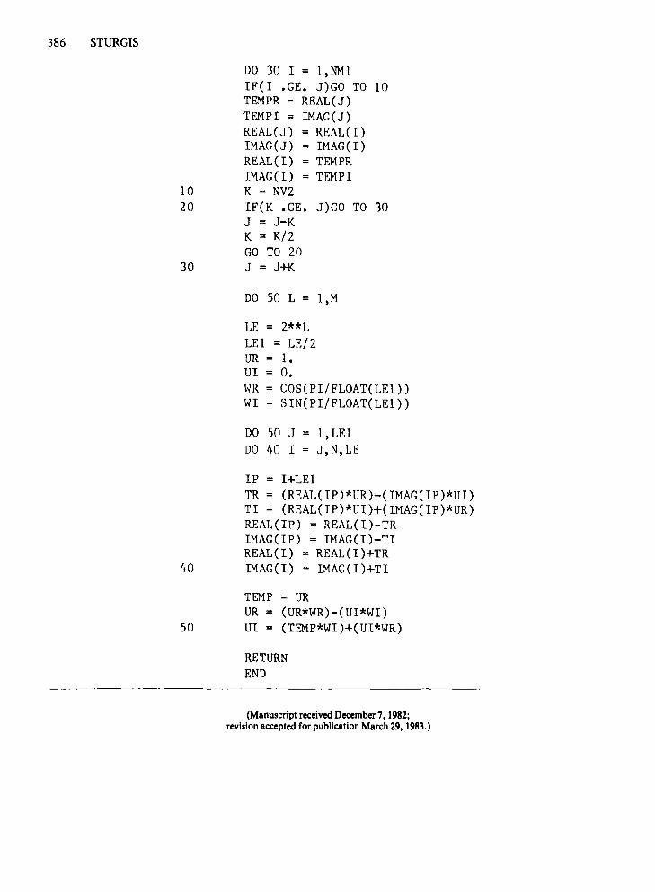
c***********************************************************************C Routine to perform a 2**M point FFT on data in arrays 'REAL' andC 'IMAG' with results returned in the input arrays. Adapted from FFTC shown in Eckhouse and Morris (1979), p. 289.

SUBROUTINE FFT(REAL,IMAG,M)REAL REAL (1), IMAG( 1)

N = 2**MPI = 3.1415927NV2 N/2NM1 = N-1J = 1

386 STURGIS

DO 30 I = I,NMIIF(I .GE. J)GO TO 10TEMPR = REAL(J)TEMPI = IMAG(J)REAL(J) = REAL(I)IMAG(J) = IMAG(I)REAL(I) = TEMPRIMAG(I) = TEMPI

10 K = NV220 IF(K .GE. J)GO TO 30

J = J-KK = K/2GO TO 20

30 J = J+K

DO SO L = I,M

LE = 2**LLEI = LE/2UR = 1.UI = O.WR = COS(PI/FLOAT(LEl))WI = SIN(PI/FLOAT(LEl))

DO SO J = I,LEIDO 40 I = J,N,LE

IP = I+LEITR = (REAL(IP)*UR)-(IMAG(IP)*UI)TI = (REAL(IP)*UI)+(IMAG(IP)*UR)REAL(IP) = REAL(I)-TRIMAG(IP) = IMAG(I)-TIREAL(I) = REAL(I)+TR

40 IMAG(I) = IMAG(I)+TI

TEMP = URUR = (UR*WR)-(UI*WI)

SO UI = (TEMP*WI)+(UI*WR)

RETURNEND

(Manuscript received December 7, 1982;revision accepted for publication March29, 1983.)