1

An Introductory Tutorial for AMPL with Examples from Winston, Operations Research: Applications and Algorithms, 3rd ed. 1. Introduction 2. Downloading and Installing AMPL Plus 3. Overview of AMPL Plus 4. Using AMPL Plus to Solve some Simple Examples from Winston 5. A More Complex Problem for AMPL Plus 6. A Brief Introduction to Integer Programs 7. Downloading and Installing “Standard” AMPL 8. Using Standard AMPL 9. Index Prepared as part of course ISYE 8901 at the School of Industrial and Systems Engineering of Georgia Institute of Technology under the supervision of Dr. Joel Sokol, Assistant Professor. Author - Samuel Potter – MS Student prodtech@dejazzd.com

2

Introduction to the Tutorial To quote the AMPL website,

“AMPL is a comprehensive and powerful algebraic modeling language for linear and nonlinear optimization problems, in discrete or continuous variables. Developed at Bell Laboratories, AMPL lets you use common notation and familiar concepts to formulate optimization models and examine solutions, while the computer manages communication with an appropriate solver.”

As an optimization student in an off-campus learning environment I found that, while the above statement may be true, getting to first base with the AMPL software was, at times, frustrating. So, with this in mind, I have written a tutorial to teach you the basics of AMPL. A few comments are in order: • This tutorial will not teach you much about formulating optimization problems. I’m

assuming that you are taking (or have taken) an optimization or mathematical programming course.

• You will not see any discussion about optimization theory or any algorithmic details

(i.e., you won’t see terms like Simplex, Revised Simplex, and Branch and Bound in this tutorial). Also we’re not going to discuss what AMPL is doing “behind the scenes”.

§ This tutorial will not make you an “AMPL” expert. I have written this tutorial for a

person who has some optimization experience and now would like to begin using AMPL to solve optimization problems. It’s written on a basic level.

• I have freely used example problems from the Winston textbook, Operations

Research: Applications and Algorithms, 3rd. ed. (These same problems also appear in other textbooks by the same author (i.e. An Introduction to Mathematical Programming), but they will be located on different pages.)

Here are some of the topics we’ll cover: • Downloading and installing a free copy of the student version of AMPL Plus from the

AMPL website. AMPL Plus is a version of AMPL that has a “quasi” Windows- like appearance. The student version of AMPL Plus behaves nearly identically to the professional version of AMPL Plus, except that it limits the size of the programs you can run. (I believe that the student version has sufficient capacity to run most all of the problems in the Winston textbook.) I’ll simply refer to this version of AMPL as “AMPL Plus”.

3

• Discussing the user interface of AMPL Plus. We’ll do this on a rather limited basis. There is a “help” command, if you need all the gory details.

• Inputting and solving a couple of very simple linear optimization programs (LP’s)

from the Winston textbook. I’ll be assuming that you know how to formulate these linear programs, so we’ll concentrate solving these LP’s with AMPL Plus. We’ll also take a look at the AMPL Plus output.

• Inputting and solving a slightly more complex problem. Here we’ll model a more

detailed diet problem in an “explicit” format (like we did for the simple problems). Next we’ll “re-model” diet problem in an algebraic formulation. (Moving from an explicit formulation to an algebraic formulation of a linear program was confusing to me at first. Hence, in the appendix of this section you will see some of my thoughts on this topic.)

• Inputting and solving a couple integer-programming problems. We’ll look at a couple

of simple examples. We’ll also provide a couple of examples of the use of binary variables. (Integer programs “max-out” the limitations of student versions of AMPL very quickly!)

• Downloading and installing a free copy of the student version of the standard version

or “command-line” version of AMPL from the AMPL website. (This version is sometimes called the MS-DOS version.) This is also a student version in that it limits the size of the programs you can run. I’ll simply refer to this version of AMPL as “AMPL” or “standard AMPL”.

• Inputting and solving some sample problems in “standard” AMPL. I believe that you

should know how to use this version of AMPL also. After becoming familiar with AMPL Plus, the transition isn’t too hard (famous last words!)

AMPL Plus vs. (standard) AMPL Perhaps you are wondering why I’m asking you to consider learning AMPL Plus (Windows type interface) and then the standard AMPL versions. Here are a few of the reasons: • AMPL Plus is actually standard AMPL with a Windows type interface (technically a

GUI). A third-party developed the interface for AMPL Plus. Unfortunately, this interface is no longer being supported.

• You can still download a student version of AMPL Plus. This student version of

AMPL Plus has a date-encrypted license, which will expire at the end of 2002. The future of AMPL Plus after year 2002 is unknown as of this writing (July 2002).

• Full-blown commercial versions of AMPL Plus are no longer being sold. The only

support available for AMPL Plus is through the AMPL website (minimal). The

4

current version of AMPL Plus has some bugs. (I’ll try to point out the bugs I’m aware of.)

• The standard AMPL has been around (with many upgrades, of course) for many

years. • You can download a free student version of the standard AMPL from the AMPL

website. This student version doesn’t have an expiration date on the license. • Full-blown versions of standard AMPL are available from many retailers. Many of

these retailers provide support and training. • Standard AMPL is version that is installed on the computers on many university

campuses as well as many industrial and research sites.

References I’ll refer to a couple references at times: Winston, W. Operations Research: Applications and Algorithms. Belmont, CA: Duxbury Press, 1994. I’ll take most of the sample problems from this textbook. Fourer R, Gay D., Kernighan B, AMPL, A Modeling Language for Mathematical Programming. Danvers, MA: Boyd and Fraser Publishing, 1993. This is the standard reference book for AMPL. This reference text has some information about formulating optimization problems. It has excellent information on coding the formulations into the AMPL language. You won’t need this book to start with, but as you get better using AMPL, it is an excellent reference text. (This book contains a copy of the AMPL Plus on CD ROM, which has an expired license – the CD is useless.) The AMPL Website is www.ampl.com. This website contains much valuable information, “download-able” files, and many examples. It does, however, assume some familiarity with the basics of AMPL, so it’s not necessarily very good for an absolute beginner. In fact, one of the goals of this tutorial is to provide some AMPL background at a basic level so that you can comprehend the material on this website.

Disclaimer I’ve written this tutorial for a beginning AMPL student (any age) sitting at his PC (home, dorm room, or place of employment) using Windows 95 or Windows 98 (not UNIX) with a student version of AMPL Plus and a student version of AMPL. If you are using AMPL in a university computer lab or the like, there may be some differences. If you discover errors (you will) or want to make suggestions, please email me at: prodtech@dejazzd.com

5

Overview of AMPL Plus In this section we’ll discuss some of the general features of the AMPL Plus software and the AMPL Plus display. Most of the items like the menu bar and the pull-down menus are typical of Windows applications. We won’t spend much time on these items.

Components of AMPL Plus The student edition of AMPL Plus consists of three main components:

• Graphical User Interface (GUI) – The GUI provides the Windows interface to AMPL. The main display window is called the “Multiple Document Interface” (MDI for short). The MDI window consists of a Title Bar (top), a Menu Bar (top), Tool Bar (top), Status Bar (bottom), and three standard windows (Command, Solver Status, and Model). These three standard windows automatically appear. You can minimize them or maximize them, but you can’t delete them. In addition there are various user-controlled windows in which you can enter (and edit) files. In summary, the GUI provides the “windows system” to communicate with AMPL Language Processor.

• The AMPL Language Processor – If you used standard AMPL before the

AMPL Plus windows version came to be, you will remember that AMPL is a “command line” system. When you have a prompt like ampl: you typed a series of commands, data, etc. In AMPL Plus selecting an item from the pull-down menus or selecting an icon from the toolbar “generates” commands that are understood by the AMPL language processor. (When you gain some experience, you can look in the Commands Window and “see” what the AMPL Plus GUI is doing behind the scenes.)

• Solvers in AMPL Plus – The “solvers” take the output generated by the AMPL

Language Processor and do the work of solving the optimization problem for you. There are many solvers available that “read” the AMPL language. We’ll only talk about the two solvers that come with the student version of AMPL Plus – CPLEX and MINOS. Either will work fine for Linear Optimization Programs (LP’s). If we wish to solve Integer Optimization Programs (IP’s) or Nonlinear Optimization Programs (NLP’s), we need to select our solver a bit more carefully. We’ll postpone this discussion on solvers, until we give a brief introduction to IP’s later. (We won’t cover NLP’s. If you want to solve NLP’s, please refer to the reference text AMPL, A Modeling Language for Mathematical Programming – Chapters 13 and 14. Chapter 15 in this same textbook also covers IP’s in more detail.)

File Organization

In AMPL there are many types of files. We’ll discuss three of these now.

6

Consider Giapetto’s Carpentry Problem on page 49 of Winston. A beginning optimization student will formulate this simple optimization problem, as a few lines of code like this:

Maximize 3x1 + 2x2 Subject to 2x1 + x2 ≤ 100 x1 + x2 ≤ 80 x1 ≤ 40 x1 ≥ 0 x2 ≥ 0

In some sense we have actually included logic statements and modeling data values together in this code. While for many students this process seems most logical, actually it’s not the way most large-scale optimization problems are formulated. Usually, the model logic statements like those above are separated into two files; a “model” file and a “data” file. APML uses the following conventions for file name extensions: xxxxxxxx.mod is the file that contains the model logic statements. xxxxxxxx.dat is the file that contains the data values. If you do not choose to separate the data items (like the formulation of Giapetto’s carpentry problem above), all the information can be contained in a file called xxxxxxxx.mod. A “project” is a facility provided by AMPL Plus to help you organize your files. For example, if you choose to formulate an optimization program called “dummy”; and if you choose to separate the logic and data statements into two different files called dummy.mod and dummy.dat, AMPL can organize these two files (and perhaps other files) into a project file with the name dummy.amp. Thus when you open a project like dummy.amp, you automatically open all the files associated with this project (like dummy.mod and dummy.dat). This may sound confusing to start with, but in reality it’s not all that difficult.

Glitches Unfortunately, I have to mention a couple of problems that you will uncover in your student version of AMPL Plus:

1. If you are used to using the right mouse key to do copying, formatting, pasting, etc. you will be disappointed to know that the right mouse key doesn’t function in AMPL Plus like other Microsoft software. You’ll have to use the Edit pull down menu or the corresponding icon on the toolbar.

7

2. If you select File….Print setup…. , you will get an error (“printer not found”).

Ditto if you try to select File….Print…. This is a known glitch in AMPL Plus. Here is the formal recommendation from AMPL:

This is a known problem with AMPL Plus that effects a small number of users. I am sure it is little consolation to you that the number is small, but there is a convenient work-around for printing files that have standard AMPL extensions (.mod, .dat, .run): - In Windows Explorer, find the file you want to print. - Right click on it - Select "Print"

This is a real pain. Another option is to do a “copy and paste” into another word processor (like Notepad) and then print from that word processor. I happen to think this is easier, but it’s not painless either. In our next section we’ll download and install a copy of AMPL Plus.

8

Downloading AMPL Plus In this section we’ll show you how to download the free Student Version of AMPL Plus. The main AMPL website is located at: www.ampl.com The download of AMPL Plus can occur from several pages on the website. I used this one: www.ampl.com/BOOK/lic2002.html There are two files to download. I suggest that you download and print the file called readme.txt. It contains some information about the version of AMPL Plus, which you are about ready to download. Then click on “setup.exe” to download. This file is something like 8.5 Meg, so if you are using a phone type Internet connection and a standard 56k modem, the download may take an hour or two depending upon the connection speed. After downloading simply follow the instructions that appear. All the AMPL files are placed in the subdirectory called C:\Program_Files\amplsted unless you tell the computer otherwise. After downloading AMPL Plus, I opened the amplsted folder and dragged the AMPL Plus icon onto my desktop. If you choose to do the same, you can start AMPL Plus using the icon. (You may also choose to start AMPL Plus using the File…..Run…. in the Program Manager). Now let’s try a couple of things to test the installation. Double-click on the AMPL Plus icon (or select the File…. Run…. in the Program Manager and type C:Program_Files\amplsted\ampl in the area provided). The main AMPL Plus Window should appear quickly. (For some reason the first time you open AMPL Plus an empty text- file type window may appear in the main window. Close it.) In the bottom of the main window you should have three “minimized” windows (Commands, Solver Status, and Model windows). These three windows are “permanent” – you can minimize or maximize them, but you can’t delete them. Select Project…Open….. Double click on “steel” icon. Three new windows will appear. One is called steel.mod, which is a file that contains all the logic for this linear program. One is called steel.dat, which is a file that contains the parameter data. (More on this later.) The third window is called steelans.dat. (More later on this also.) You can play around minimizing and maximizing these windows if you wish. From the Run menu select Solve…..Problem….. The Solver Status Window should appear with message “Optimal solution found” and the optimal solution should be listed. Now minimize the Solver Status Window.

9

Maximize the Model window located at the bottom of the display. This window should contain optimal solution values and show some other information. We’ll spend some time with this model window later. Now minimize it. If everything behaved itself as described above, you can be happy. The installation was likely a success. Select Project….Close….. Then click Yes to close all existing windows. If everything works OK, you have just run your first AMPL problem. Select File….Exit….. The AMPL Website does have an email address, if you need/wish to ask a question. It is: info@ampl.com

10

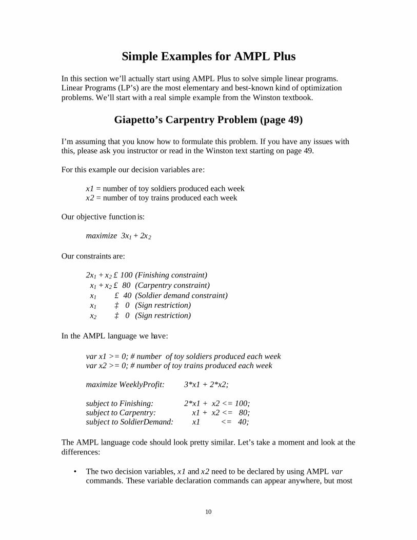
Simple Examples for AMPL Plus In this section we’ll actually start using AMPL Plus to solve simple linear programs. Linear Programs (LP’s) are the most elementary and best-known kind of optimization problems. We’ll start with a real simple example from the Winston textbook.

Giapetto’s Carpentry Problem (page 49) I’m assuming that you know how to formulate this problem. If you have any issues with this, please ask you instructor or read in the Winston text starting on page 49. For this example our decision variables are:

x1 = number of toy soldiers produced each week x2 = number of toy trains produced each week

Our objective function is:

maximize 3x1 + 2x2 Our constraints are:

2x1 + x2 ≤ 100 (Finishing constraint) x1 + x2 ≤ 80 (Carpentry constraint) x1 ≤ 40 (Soldier demand constraint) x1 ≥ 0 (Sign restriction) x2 ≥ 0 (Sign restriction)

In the AMPL language we have:

var x1 >= 0; # number of toy soldiers produced each week var x2 >= 0; # number of toy trains produced each week maximize WeeklyProfit: 3*x1 + 2*x2; subject to Finishing: 2*x1 + x2 <= 100; subject to Carpentry: x1 + x2 <= 80; subject to SoldierDemand: x1 <= 40;

The AMPL language code should look pretty similar. Let’s take a moment and look at the differences:

• The two decision variables, x1 and x2 need to be declared by using AMPL var commands. These variable declaration commands can appear anywhere, but most

11

people put them at the beginning. There is nothing magical about the variable name x1 or x2. We could have used numsoldiers instead of x1, if we wished. We’re using the notation in the Winston textbook to be consistent. Variable names in AMPL are case sensitive. AMPL considers x1, X1, numsoldiers, Numsoldiers, and NumSoldiers as different variables. This is a common source of errors.

• The variable nonnegativity (≥0) restrictions are typically placed in the variables’

declaration commands. (The nonnegativity (≥0) restrictions can also be placed within the constraints if you wish.) Note that if you don’t put any nonnegativity restrictions in your formulation, AMPL does not assume the decision variables are nonnegative. This is common error and can produce some wild results.

• The end of a command is marked with a semicolon (;). A command can extend

over several lines of the display. AMPL will end a command when it sees a semicolon. If you get some weird errors, make sure your commands actually have a semicolon (not a colon) where you actually want the command to end.

• On a given line of the display, anything after the “#” symbol is ignored by AMPL

and is not considered part of the AMPL code. We have used this feature to provide some notes to ourselves.

• “White spaces” are ignored by AMPL. For example,

2*x1+x2≤100;

2 * x1 + x2 ≤ 100;

2 * x1 + x2 ≤ 100;

all mean the same thing.

• AMPL requires that a name be used for the objective function. The choice of

names is pretty much up to you. I like to use a name that is meaningful – it helps when you want to look at the AMPL output. The format above is pretty much standard. Like variable names, objective names are case sensitive.

• AMPL also requires that names be used for constraints. I also like to use

meaningful names for the constraints. Constraint names are case sensitive.

• The command names minimize, maximize, and subject to are written in lower case letters .

• You need to indicate multiplication with the * symbol.

Now how do we input this problem?

12

Open your copy of AMPL Plus by using the icon on the desktop or whatever you choose. (You should have the three minimized windows at the bottom – OK?). Choose File…New….. When the dialog box asks what type of file select Text File and then click OK. You’ll get a blank text window. Do a File….Save as…. and save the file as “giap.mod”. (We’re going to put the entire our LP in one file called “giap.mod”.) AMPL Plus allows names of any length; however, in the file management feature of AMPL Plus only the first 8 characters of the name are displayed. Enter the above AMPL formulation of the LP in the text window and then choose File….Save…. to save your file. Select Project….New….. Highlight the file giap.mod and click on Add. Click on OK. Select Project…Save…. Name the project giap.amp. Then click on Save. AMPL just created a project called giap.amp, which consists of one file called giap.mod. Choose Run….Reset Build….. (This isn’t really necessary here, but it’s a good idea to perform a Reset Build anytime a file is changed.) Choose Run….Build Model….. Hopefully the solver window “popped-up” and said that the “build” was successful. If so, minimize all the open windows. (If not, open the command window and look for some type of error message. Maximize the giap.mod window, if necessary, and correct the giap.mod file and save it. Select Run….Reset Build….. Select Run….Build Model…. Better this time?) The Run….Reset Build…. command lets AMPL know that a file has been changed. Essentially it clears out any previous versions used by sending a reset signal to the AMPL language processor. The system will behave as if AMPL was just started. If you are ever in doubt about what AMPL is doing, use this command to start over. The Run….Build Model…. command checks the model file for any syntax errors. AMPL is very sensitive to syntax errors. Select Run….Solve Problem…. The solver window should have said “optimal solution” and given you the optimal value (180), which matches the textbook solution. Congratulations you’ve solved your first AMPL problem! (Depending upon the size of your monitor, you might want to minimize a couple of the windows. You can always minimize or maximize any of your windows at any time.) Now let’s exit AMPL and then get back in - just for kicks. Select Project….Close…. and click on Yes to close all open windows. Exit out of AMPL Plus. Now open AMPL Plus again. Use Project….Open and click on giap. Select Run….Reset Build….. Select Run….Build Model…. Select Run….Solve Problem…. Did you get the same result?

13

Now let’s look at some additional information contained in the output from AMPL. Maximize the window called “Model”. Select “WeeklyProfit” (the name we called our objective function). Notice the information in the bottom of the model window. Notice that the maximum value of the objective function WeeklyProfit (subject to the constraints) is 180. Next select variable x1. Notice at the bottom of the window that the value of the variable x1 at optimum is 20. (We produce 20 toy soldiers per week.) Now select variable x2. The value of variable x2 at optimum is 60. (We produce 60 toy trains per week.) Now select “Carpentry” (the name we called one of the constraints). Click on Data. Now click on OK. Here is another window that provides information about the constraint “Carpentry”. The AMPL expression Carpentry_body gives the value of that part of the constraint which involves the variables; in this case x1 + x2. Note that all 80 hours of the carpentry constraint are used up for the optimal solution. Close this window and click Discard. Now select “Carpentry” again. Click on Data. Click on Dual and Slack. Then click OK. Here’s some additional information. Notice that Carpentry_Slack = 0. This tells us that the slack variable associated with the Carpentry constraint is equal to 0, and that the Carpentry constraint is binding. (You remember about “slack variables” - right?) Also notice that Carpentry_Dual = 1. This tells us that (as long as the basis is still optimal), if the right hand side of the carpentry constraint is increased by one, the optimum value is increased by 1. Close this window and click Discard. Repeat this process again for the constraint “Finishing”. What do you discover? Is the Finishing constraint also binding? Now suppose the design of the toy trains gets changed such each toy train takes four carpentry hours instead of one. Our AMPL formulation becomes:

var x1 >= 0; # number of toy soldiers produced each week var x2 >= 0; # number of toy trains produced each week maximize WeeklyProfit: 3*x1 + 2*x2; subject to Finishing: 2*x1 + x2 <= 100; subject to Carpentry: x1 + 4*x2 <= 80; subject to SoldierDemand: x1 <= 40;

Maximize the giap.mod window and make the change. Choose File ….Save as…. giapr1.mod. Open the Project…Edit…. menu. Remove the giap.mod file and add the as giapr1.mod. Click OK. Select Project….Save as….. Type the giapr1.amp and click “Save”. AMPL just created a project called giapr1.amp, which consists of one file called giapr1.mod.

14

Choose Run….Build Reset….. (Important this time!) Now choose Run….Build Model…. to check for errors. Finally select Run…..Solve Problem…. Open the Data window and look at the results. Notice now that Carpentry_Dual = 0.5. (If you forgot how to do this, look above.) This tells us that (again as long as the basis is optimal), if the right hand side of the carpentry constraint is increased by one, the optimum value is increased by 0.5. Are both the Carpentry and Finishing constrains still binding? To illustrate another point let’s increase the number of available carpentry hours per week to 85 and change the carpentry hours per toy train to two. Our next AMPL formulation is now: var x1 >= 0; # number of toy soldiers produced each week var x2 >= 0; # number o ftoy trains produced each week maximize WeeklyProfit: 3*x1 + 2*x2; subject to Finishing: 2*x1 + x2 <= 100; subject to Carpentry: x1 + 2*x2 <= 85; subject to SoldierDemand: x1 <= 40; Maximize the giapr1.mod window, make the change and save as giapr2.mod (or whatever name you wish). Open the Project…Edit…. menu. Remove the giapr1.mod file and add the as giapr2.mod. Click OK. Select Project….Save as….. Type the file name giapr2.amp and click “Save”. AMPL just created a project called giapr2.amp, which consists of one file called giapr2.mod. We now have three different projects (giap.amp, giapr1.amp, and giapr2.amp) - each with a (slightly) different model file. Choose Run….Build Reset. (It’s important here also!) Select Run….Build Model….. Finally select Run…..Solve Problem….. Open the Data window and look at the results. In particular look at the values of the variables x1 and x2 at optimality. Uh-oh, we no longer have integer solutions. Is this a problem for Giapetto? In a later section we’ll show you how to modify our formulation to “force” AMPL to give you an integer solution to this problem. Now do a Project…Close…. and click on Yes to close all windows. Exit out of AMPL. We’ll go to our next sample problem.

Simple Diet Problem (page 71 in Winston)

Again, I’m assuming that you know how to formulate this problem. If you have any issues with this, please ask you instructor or read in the Winston text starting on page 70. We’ll use the same notation as the Winston textbook. For this example our decision variables are:

15

x1 = number of brownies eaten daily x2 = number of scoops of chocolate ice cream eaten daily

x3 = bottles of cola drunk daily x4 = pieces of pineapple cheesecake eaten daily. Our objective function is:

minimize 50x1 +20x2 + 30x3 + 80x4 Our constraints are:

400x1 + 200x2 + 150x3 + 500x4 ≥ 500 (Calorie constraint) 3x1 + 2x2 ≥ 6 (Chocolate constraint) 2x1 + 2x2 + 4x3 + 4x4 ≥ 10 (Sugar constraint) 2x1 + 4x2 + x3 + 5x4 ≥ 8 (Fat constraint) x1 ≥ 0 (Sign restriction) x2 ≥ 0 (Sign restriction) x3 ≥ 0 (Sign restriction) x4 ≥ 0 (Sign restriction)

In the AMPL language we have:

var x1 >= 0; # number of brownies eaten daily var x2 >= 0; # number of scoops of chocolate ice cream eaten daily var x3 >= 0; # bottles of cola drunk daily var x4 >= 0; # pieces of pineapple cheesecake eaten daily minimize DailyCost: 50*x1 + 20*x2 + 30*x3 + 80*x4; subject to Calories: 400*x1 + 200*x2 + 150*x3 + 500*x4 >= 500; subject to Chocolate: 3*x1 + 2*x2 >= 6; subject to Sugar: 2*x1 + 2*x2 + 4*x3 + 4*x4 >= 10; subject to Fat: 2*x1 + 4*x2 + x3 + 5*x4 >= 8;

Open AMPL Plus. Under File choose New. When the dialog box asks what type of file select Text File and then click OK. You’ll get a blank text window. Do a File….Save as…. and save the file as sdiet.mod. (We’re going to put the entire LP in one file called sdiet.mod.) Enter the above AMPL formulation of the LP in the text window and save your file. Note that we have used the fact that AMPL ignores “white spaces” to line up variables in the objective and “subject to” statements. AMPL doesn’t care, but it’s easier to read.

16

Select Project….New….. Highlight the file sdiet.mod and click on Add. Select Project….Save….. Type the word sdiet.amp and click Save. AMPL just created a project called sdiet.amp, which consists of one file called sdiet.mod. Select Run…..Reset Build….. Select Run…..Build Model…. to check for syntax errors. Hopefully the solver window said that the “build” was successful. Select Run….Solve Problem…. The solver window should have said optimal solution and given you the optimal value (90). Your second AMPL problem solved! Let’s look at the results. Maximize the window called Model. Select DailyCost. Notice the information in the bottom of the model window. Notice that the maximum value of the objective function DailyCost (subject to the constraints) is 90. Next select one at a time the different variables x1, x2, x3, and x4. Notice that x1 = 0, x2 = 3, x3 = 1, and x4 = 0. So we can minimize our costs (subject to the constraints) by eating 3 scoops of chocolate ice cream and drinking 1 bottle of cola each day. Interesting. Now select Chocolate (the name we called one of the constraints). Click on Data. Click on Dual and Slack. Then click OK. Notice that the chocolate constraint is binding (i.e. Chocolate_Slack = 0 and Chocolate_Dual ≠ 0). Close this window and click Discard. Next select sugar. Also notice that the sugar constraint of is binding (Sugar_Slack = 0 and Sugar_Dual ≠ 0). Close this window and click Discard. Finally, select the Fat constraint. The Fat constrant of is not binding (i.e. Fat_Slack ≠ 0, but Fat_Dual = 0). Since the Fat_Dual = 0, we will not improve the optimal value (within some boundaries) if the right hand side of the fat constraint is increased. Close this window and click Discard. Now select Project…Close…. and click on Yes to closing all open windows. If you were to reopen this project (sdiet.amp), the file sdiet.mod will open also even if it’s not visible. If the sdiet.mod does not appear and you want to see it, go to File….Open…. and select it. Exit out of AMPL. In the next section we’ll go to our next more challenging sample problem.

17

A More Complex Example for AMPL Plus We’ll assume that you inputted the examples from the previous section and got the examples to run as designed. In this section we’ll look at a slightly more complex diet problem. The information for the following example is taken from the AMPL website.

Fast Food Diet Problem Here are the food selections available from a well-known fast food restaurant. (Does the term “Golden Arches” sound familiar?) We’ll identify the foods with the following two-letter abbreviations: QP : Quarter Pounder MD: McLean Deluxe BM: Big Mac FF: Filet-O-Fish MC: McChicken FR: Fries (small) SM: Sausage McMuffin MK: Milk (one serving) OJ: Orange Juice (one serving) Suppose we can select any of these foods for our daily diet. Our goal is to minimize the cost of the foods and still satisfy the minimum daily nutrient requirements. Suppose we are interested in 7 different “nutrients” as follows: Prot: Protein VitA: Vitamin A VitaC: Vitamin C Calc: Calcium Iron: Iron Cals: Calories Carb: Carbohydrates In this table we have the cost for each of the “foods”, the nutrients available in one serving of each of the foods, and the daily minimum requirements for each of the nutrients.

18

QP MD BM FF MC FR SM MK OJ Min Daily Req. Cost 1.84 2.19 1.84 1.44 2.29 0.77 1.29 0.60 0.72 Prot 28 24 25 14 31 3 15 9 1 55 VitaA 15 15 6 2 8 0 4 10 2 100 VitC 6 10 2 0 15 15 0 4 120 100 Calc 30 20 25 15 15 0 20 30 2 100 Iron 20 20 20 10 8 2 15 0 2 100 Cals 510 370 500 370 400 220 345 110 80 2000 Carb 34 35 42 38 42 26 27 12 20 350 For this example our decision variables are:

XQP = number of Quarter Pounders eaten per day. XMD = number of McLean Deluxe’s eaten per day. XBM = number of Big Mac’s eaten per day. XFF = number of Filet-O-Fish’s eaten per day. XMC = number of McChickens’s eaten per day. XFR = number of orders of French fries eaten per day. XSM = number of Sausage McMuffin’s eaten per day. XMK = number of containers of milk drunk per day. XOJ = number of containers of orange juice drunk per day.

Our objective function is:

Minimize 1.84XQP + 2.19XMD + 1.84XBM + 1.44XFF + 2.29XMC + 0.77XFR + 1.29XSM + 0.60XMK + 0.72XOJ

Our constraints are:

28XQP + 24XMD + 25XBM + 14XFF + 31XMC + 3XFR + 15XSM + 9XMK + 1XOJ ≥ 55 (Protein Constraint) 15XQP + 15XMD + 6XBM + 2XFF + 8XMC + 0XFR + 4XSM + 10XMK + 2XOJ ≥ 100 (Vitamin A Constraint) 6XQP + 10XMD + 2XBM + 0XFF + 15XMC + 15XFR + 0XSM + 4XMK + 120XOJ ≥ 100 (Vitamin C Constraint) 30XQP + 20XMD + 25XBM + 15XFF + 15XMC + 0XFR + 20XSM + 30XMK + 2XOJ ≥ 100 (Calcium Constraint)

19

20XQP + 20XMD + 20XBM + 10XFF + 8XMC + 2XFR + 15XSM + 0XMK + 2XOJ ≥ 100 (Iron Constraint) 510XQP + 370XMD + 500XBM + 370XFF + 400XMC + 220XFR + 345XSM + 110XMK + 80XOJ ≥ 2000 (Calories Constraint) 34XQP + 35XMD + 42XBM + 38XFF + 42XMC + 26XFR + 27XSM + 12XMK + 20XOJ ≥ 100 (Carbohydrates Constraint) XQP, XMD, XBM, XFF, XMC, XFR, XSM, XMK, XOJ ≥ 0 (Sign Constraint)

In APML Plus we have: var XQP >= 0; # number of Quarter Pounders eaten per day

var XMD >= 0; # number of McLean Deluxe's eaten per day var XBM >= 0; # number of Big Mac's eaten per day var XFF >= 0; # number of Filet-of-Fish's eaten per day var XMC >= 0; # number of McChicken’s eaten per day var XFR >= 0; # number of orders of small fries's eaten per day var XSM >= 0; # number of Sausage McMuffins's eaten per day var XMK >= 0; # number of containers of milk drunk per day var XOJ >= 0; # number of containers of orange juice drunk per day

minimize FoodCost: 1.84*XQP + 2.19*XMD + 1.84*XBM + 1.44*XFF +

2.29*XMC + 0.77*XFR + 1.29*XSM + 0.60*XMK + 0.72*XOJ;

subject to Prot: 28*XQP + 24*XMD + 25*XBM + 14*XFF + 31*XMC +

3*XFR + 15*XSM + 9*XMK + 1*XOJ >= 55;

subject to VitA: 15*XQP + 15*XMD + 6*XBM + 2*XFF + 8*XMC + 0*XFR + 4*XSM + 10*XMK + 2*XOJ >= 100;

subject to VitC: 6*XQP + 10*XMD + 2*XBM + 0*XFF + 15*XMC +

15*XFR + 0*XSM + 4*XMK + 120*XOJ >= 100;

subject to Calc: 30*XQP + 20*XMD + 25*XBM + 15*XFF + 15*XMC + 0*XFR + 20*XSM + 30*XMK + 2*XOJ >= 100;

subject to Iron: 20*XQP + 20*XMD + 20*XBM + 10*XFF + 8*XMC +

2*XFR + 15*XSM + 0*XMK + 2*XOJ >= 100;

subject to Cals: 510*XQP + 370*XMD + 500*XBM + 370*XFF + 400*XMC + 220*XFR + 345*XSM + 110*XMK + 80*XOJ >= 2000;

20

subject to Carb: 34*XQP + 35*XMD + 42*XBM + 38*XFF + 42*XMC + 26*XFR + 27*XSM + 12*XMK + 20*XOJ >= 350;

A couple of comments are in order: • I’ve written the coefficients 0 and 1 in the constraint equations above. In reality, it’s

not necessary. • Don’t forget the commands minimize, maximize and subject to are written in lower

case letters. • You can’t type subscripts in AMPL. So XMD becomes XMD (or xmd if you prefer) in

AMPL. Remember that AMPL is case sensitive – AMPL recognizes XMD and xmd as two different variable names.

• In the example above many of the commands extend over two lines, which is OK.

Note that the end of the command is designated with a semi-colon. • You might be thinking that rather than use the text editor in AMPL Plus to enter a

new xxxxx.mod file, you can use a standard word processor like MS Word or WordPerfect. You could then “copy and paste” from your favorite Word Processor to the xxxxx.mod file in AMPL Plus. You can, but beware. WordPerfect, MS Word, and other word processing programs sometimes insert “hidden” formatting symbols embedded in the file. If AMPL detects these formatting symbols, you can get weird errors. If you use a basic text editor program like the text editor in AMPL (my recommendation) or perhaps Notepad, you can avoid this issue.

Let’s input this program. In case you forgot how, this is how we do it. Open AMPL Plus. Choose File…. New….. When the dialog box asks what type of file select Text File and then click OK. You’ll get a blank text window. Select File….Save as…. and save the file as mydiet.mod. Type the AMPL code above into the text window. Save when you have finished typing. (We’re going to put the entire LP in one file called mydiet.mod.) Select Project….New….. Highlight the file mydiet.mod and click on Add. Select Project….Save….. Type the word mydiet.amp and click “OK”. AMPL just created a project called mydiet.amp, which consists of one file called mydiet.mod. Then click on OK. Select Run…..Reset Build….. Select Run…..Build Model…. to check for syntax errors. Hopefully the solver window said that the “build” was successful. Select Run….Solve Problem…. The solver window should have said optimal solution and given you the optimal value (14.85…..). This is your third AMPL problem solved!

Getting More Complex

21

To keep the above diet problem relatively simple, we arbitrarily limited our scope to 9 foods and 7 nutrients. In reality, the experiment used 63 foods and 12 nutrients. If you were to write out the above LP you would have 63 variable statements and 12 (very long) constraints. Even this would be a small problem in today’s world of LP’s. Some have 1000’s of variables and/or constraints. Obviously, the above procedure for writing out the LP would be a real pain. Looking at the above diet example, we would like to be able to communicate that the large diet LP (with 63 variables and 12 constraints) has the same form as the smaller diet LP above (with 9 variables and 7 constraints), only with more data. Fortunately, there is a way to do that by specifying a symbolic model. The idea of the symbolic model is to describe an entire collection of LP’s using symbols in the place of specific numbers. Instead of an explicit formulation of the LP, we’ll write an algebraic formulation. For the moment I’m assuming that you already know how to do this. (At the end of this section of the tutorial there is an appendix, which attempts to explain how this algebraic formulation came about.) Here is an algebraic formulation of the above diet problem: Sets F = a set of foods N = a set of nutrients Parameters

aij ≥ 0 be the amount of nutrient i in one serving of food j, for each i ∈ N (i in set N) and each j ∈ F (j in set F).

bi > 0 be the amount of nutrient required for each i ∈ N (i in set N).

cj > 0 be the cost per serving of food j for each j ∈ F.

Variables

xj ≥ 0 be the number of servings of food j purchased for each j ∈ F. Objective

Minimize Σ j ∈ F cj * x j Constraints

Subject to Σ j ∈ F aij * x j ≥ bi for each nutrient i ∈ N

22

Here’s the algebraic formulation in AMPL code:

set NUTR; # Set of Nutrients set FOOD; # Set of Foods param amt {NUTR, FOOD} >=0; # Amount of nutrient in each food param nutrLow {NUTR} >= 0; # Minimum requirement for nutrient param cost {FOOD} >= 0; # Cost of one serving of a food var Buy {FOOD} >= 0; # Number of servings of food to be purchased minimize TotalCost: sum {j in FOOD} cost[j] * Buy [j]; subject to Need {i in NUTR}: sum {j in FOOD} amt[i,j] * Buy [j] >= nutrLow[i];

At this point we’re going to make several comments about the AMPL code: • We’ve used mnemonic identifiers FOOD for the set of foods (instead of F), NUTR

for the set of nutrients (instead of N), amt for the amount parameters (instead of a), nutriLow for the nutrient requirement parameters (instead of b), cost for the cost parameters (instead of c), and Buy for the quantity purchased variables (instead of x). These names are arbitrary choices, but they do have some meaning.

• The sets need to be defined in AMPL using the AMPL command set (which is in all

small case letters). They can be defined in the AMPL code anywhere. The above location is fairly normal. Commonly, set names are denoted by all capital letters, although this convention is rather arbitrary. It is a requirement that you are consistent throughout the program. In AMPL the set FOOD is not the same as the set Food.

• Parameters are defined in AMPL using the AMPL command param (note that param

is all small case letters). Commonly parameter names are denoted using small case letters, although this convention is also arbitrary. When a parameter is indexed across a set, the set name is contained in braces {SETNAME}. If the parameter (like amt above) is indexed across two or more sets we need to list both sets and the order is important. (Incidentally, the actual numerical values of the parameters are typically known ahead of time. We’ll show how we list these numerical values of the parameters a little later.)

• As we saw before in our simple examples, variables are defined in AMPL using the

AMPL command var. Commonly, variables are denoted using a word with just the first letter capitalized.

• Multiplication requires the symbol *. Statements end with a semicolon. Explanatory

comments are separated from the formal computer language using the # symbols. (Same as before.)

23

• The objective function needs to have a name. In our example we’ve called it

TotalCost. The constraints also need to have a name. In our example we’ve called them Need.

• The AMPL way of denoting subscripts is to enclose the subscripts in square

brackets [subscript]. Thus xj becomes Buy[j], and aij becomes amt[i, j]. • The sum expression is written without the summation sign and subscripts like this:

Σ j ∈ F cj * x j --------------à sum {j in FOOD} cost[j] * Buy [j]

and

Σ j ∈ F aij * x j ≥ bi -----------à sum {j in FOOD} amt[i,j] * Buy [j] >= nutrLow[i]

Notice carefully where we have used braces { } and square brackets [ ]. • The specification “for each nutrient i ∈ N is written in AMPL like this:

for each nutrient i ∈ N ------à subject to Need {i in NUTR}: Note the colon after the set of braces { }.

Let’s input the above model into an AMPL file. Open AMPL Plus and select File….New….. Choose text type file and click OK. Then select File….Save….. and save as mydiet1.mod. Type the above AMPL code carefully and save it. Minimize this file.

Denoting Data So far we have conveniently ignored how we list the numerical values of the various parameters. We generally do this listing in a separate file called a data file. (In fact we’ll call the data file containing the values of the parameters for our diet problem mydiet1.dat.) If you guessed that there is a special syntax for the data file, you would be correct. Actually, there are many possible syntax’s. We’ll list one example here and refer you chapter 9 of the AMPL reference book (Fourer R, Gay D., Kernighan B, AMPL, A Modeling Language for Mathematical Programming) for other methods. The formulation below is not the most elegant (shortest), but it is, for me at least, the easiest to understand.

set NUTR := Prot VitA VitC Calc Iron Cals Carb; set FOOD := QP MD BM FF MC FR SM MK OJ; param: cost:=

24

QP 1.84 MD 2.19 BM 1.84 FF 1.44 MC 2.29 FR 0.77 SM 1.29 MK 0.60 OJ 0.72;

param: nutrLow := Prot 55 VitA 100 VitC 100 Calc 100 Iron 100 Cals 2000 Carb 350;

param amt: QP MD BM FF MC FR SM MK OJ := Prot 28 24 25 14 31 3 15 9 1 VitA 15 15 6 2 8 0 4 10 2 VitC 6 10 2 0 15 15 0 4 120 Calc 30 20 25 15 15 0 20 30 2 Iron 20 20 20 10 8 2 15 0 2 Cals 510 370 500 370 400 220 345 110 80 Carb 34 35 42 38 42 26 27 12 20 ;

So that AMPL can recognize this as a table, a colon must follow the parameter name, while the := operator follows the list of column labels. Note one thing carefully. The parameter amt {NUTR, FOOD} is indexed first over the set NUTR and second over the set FOOD. In the table (matrix) for the values of the parameter amt, the rows are indexed over the set NUTR (the first index) and the columns are indexed over the set FOOD (the second index). Note the correspondence. If you get it backwards, expect all kinds of nifty errors! If you get the table backwards, don’t fret. The notation (tr) after the parameter name indicates a “transposed” version of the table, in which the column labels correspond to the first index and the row labels correspond to the second index. Here is the data file shown with a transposed table.

set NUTR := Prot VitA VitC Calc Iron Cals Carb;

25

set FOOD := QP MD BM FF MC FR SM MK OJ; param: cost:= QP 1.84 MD 2.19 BM 1.84 FF 1.44 MC 2.29 FR 0.77 SM 1.29 MK 0.60 OJ 0.72;

param: nutrLow := Prot 55 VitA 100 VitC 100 Calc 100 Iron 100 Cals 2000 Carb 350;

param amt (tr): Prot VitA VitC Calc Iron Cals Carb := QP 28 15 6 30 20 510 34 MD 24 15 10 20 20 370 35 BM 25 6 2 25 20 500 42

FF 14 2 0 15 10 370 38 MC 31 8 15 15 8 400 42 FR 3 0 15 0 2 220 26 SM 15 4 0 20 15 345 27 MK 9 10 4 30 0 110 12 OJ 1 2 120 2 2 80 20 ;

(There are several other examples of this technique shown in chapter 4 of the AMPL reference book (Fourer R, Gay D., Kernighan B, AMPL, A Modeling Language for Mathematical Programming.) We’ll now enter this data. We could simply enter the data information at the bottom of the mydiet1.mod file. Instead we’ll show you how to create a separate data file, which is considered “good practice”. Open AMPL Plus and select File….New….. Choose text type file and click OK. Select File….Save…. and save as mydiet1.dat. Type the AMPL data code above (either the “original” or the “transposed” version) and save it. Minimize this file.

26

Let’s create a new project consisting of mydiet1mod and mydiet1dat. Select Project….New. …. Select the mydiet1.mod and click on add. Select mydiet1.dat and click on add. Select Project…..Save… and enter mydiet1.amp as a name. Click on Save. You now have a project named mydiet1.amp, which consists of a model file mydiet1.mod and a data file mydiet1.dat. Now let’s get AMPL to solve the problem for us. Select Run…..Reset Build. Select Run…..Build Model. Hopefully, the Solver Window popped-up and said that the model build was successful. (If not, check on the Commands Window. There should be some information about what went wrong. If you modify mydiet1.mod remember to save it and select Run…. Reset Build before doing a Run…..Build Model again.) . Select Run…..Reset Build. Select Run…..Build Data. Hopefully, the Solver Window popped-up and said that the data build was successful. (If not, check on the Commands Window. There should be some information about what went wrong. If you modify mydiet1.dat remember to save it and select Run…. Reset Build before doing a Run…..Build Data again.) If the data build was a success, select Run…..Reset Build. Select Run…..Solve Problem. If you’re lucky (or skillful), the Solver Window popped-up and gave you an optimal solution. If you are really lucky, you actually got the same optimal solution as before. If you got some errors throughout this process, you’re about normal. Let’s look at the results. Maximize the window called Model. Select TotalCost. Notice the information in the bottom of the model window. Notice that the maximum value of the objective function TotalCost (subject to the constraints) is 14.8557…. Now choose the variable Buy. Now study the values of the variables Buy at the optimal solution. One thing you should notice is that the values of the variables at optimal are not integers. We’re told to buy 3.4222 servings of milk, etc. We probably should have integers, unless your local Golden Arches will allow you to buy 3.4222 servings of milk. Do you want integer solutions? Check out the next section in the tutorial. Now select the constraints called Need. Click on Data. Click on Dual and Slack. Then click OK. Notice that the Need - calories constraint is nowhere near binding. Are you surprised? (We have a minimum calorie constraint – should we change our LP to include a maximum calorie constraint?) Select Project…Save…. Select Project.…Close…., and close out our project mydiet1.amp. If you, by chance, forget to close a project before exiting, the project will automatically load the next time you use AMPL Plus (just like you left it). We’ll conclude this section by calling to your attention a similar example problem in AMPL Plus. Click on Project……Open and double click on the icon labeled “dietl” to open it. You should have a window on your display called dietl.mod and another window

27

called dietl.dat which are part of the project called dietl.amp. You can play around with this sample problem until you have satisfied your curiosity.

Appendix In this appendix we’ll try to motivate how we got from the explicit formulation of our diet problem to the algebraic formulation of the diet problem. Recall that for this example our decision variables are:

XQP = number of Quarter Pounders eaten per day. XMD = number of McLean Deluxe’s eaten per day. XBM = number of Big Mac’s eaten per day. XFF = number of Filet-O-Fish’s eaten per day. XMC = number of McChickens’s eaten per day. XFR = number of orders of French fries eaten per day. XSM = number of Sausage McMuffin’s eaten per day. XMK = number of containers of milk drunk per day. XOJ = number of containers of orange juice drunk per day.

Our objective function is:

Minimize 1.84XQP + 2.19XMD + 1.84XBM + 1.44XFF + 2.29XMC + 0.77XFR + 1.29XSM + 0.60XMK + 0.72XOJ

Our constraints are:

28XQP + 24XMD + 25XBM + 14XFF + 31XMC + 3XFR + 15XSM + 9XMK + 1XOJ ≥ 55 (Protein Constraint) 15XQP + 15XMD + 6XBM + 2XFF + 8XMC + 0XFR + 4XSM + 10XMK + 2XOJ ≥ 100 (Vitamin A Constraint) 6XQP + 10XMD + 2XBM + 0XFF + 15XMC + 15XFR + 0XSM + 4XMK + 120XOJ ≥ 100 (Vitamin C Constraint) 30XQP + 20XMD + 25XBM + 15XFF + 15XMC + 0XFR + 20XSM + 30XMK + 2XOJ ≥ 100 (Calcium Constraint) 20XQP + 20XMD + 20XBM + 10XFF + 8XMC + 2XFR + 15XSM + 0XMK + 2XOJ ≥ 100 (Iron Constraint) 510XQP + 370XMD + 500XBM + 370XFF + 400XMC + 220XFR + 345XSM + 110XMK + 80XOJ ≥ 2000 (Calories Constraint)

28

34XQP + 35XMD + 42XBM + 38XFF + 42XMC + 26XFR + 27XSM + 12XMK + 20XOJ ≥ 100 (Carbohydrates Constraint)

If we look back at the beginning of this section we see that, for our diet example, there are two basic types of entities, foods and nutrients. We’ll let F be the set of foods, and N be the set of nutrients. For our simple example above, F = {QP, MD, BM, FF, MC, FR, SM, MK, and OJ }, and N = {Prot, VitA, VitC, Calc, Iron, Cals, and Carb} For the larger diet problem the set of foods F would have 63 members, and the set of nutrients N have 12 members. Next we’ll define symbols for all the numerical data, called parameters, of the model. In either the small or large diet problem above, there are a great many parameters. If we look at the table above, we see that there are three parameter types - amount of nutrient in a given food, nutrient requirements, and the cost of given food. If we stick with standard notation, we use a letter to denote each parameter type. So, somewhat arbitrarily, we have: Let a designate the parameter that denotes the amount of nutrient in a given food. Let b designate the parameter that denotes the daily nutrient requirements. Let c designate the parameter that denotes the cost of a given food. Actually, there are many different costs – one for each type of food. We denote individual parameter values by subscripting the parameter. Thus cBM is the cost of a Big Mac. Likewise, bcalc is the daily nutritional requirement of calcium. The parameter is a little trickier. There is a value for each food and each nutrient. So we write aIron, MC to denote the amount of iron in a McChicken. Hopefully you see that certain parameters are associated with certain sets. Specifically, b is subscripted over the set of nutrients, N. The parameter c is subscrip ted over the set of foods, F. The parameter a is more complex since there are nutrient amounts which are a combination of the food and the nutrient. As a result, the parameter a must have pair of subscripts, one from N and one from F. Mathematically, we write:

Let aij ≥ 0 be the amount of nutrient i in one serving of food j, for each i ∈ N (i in set N) and each j ∈ F (j in set F).

Let bi > 0 be the amount of nutrient required for each i ∈ N (i in set N).

Let cj > 0 be the cost per serving of food j for each j ∈ F (j in set F).

29

Note that the parameters (usually) have known values up front. Thus cBM = 1.84, bcalc = 100, and aIron, MC = 8. The set of all parameter values is loosely referred to as “the data” of an LP. The variables are similar to the parameters except that their values are not known up front. In our diet example we only have one type of variable - the amount of each food that we purchase:

Let xj ≥ 0 be the number of servings of food j purchased for each j ∈ F. Thus xQP would be the number of Quarter Pounder’s to purchase and xBM would be the number of Big Mac’s to purchase. The objective in our example is the sum of the costs of all the foods we buy. In our case the objective is:

Minimize (Cost of QP’s)*(Number of QP’s) + (Cost of MD’s)*(Number of MD’s) + (Cost of BM’s)*(Number of BM’s) + (Cost of FF’s)*(Number of FF’s) + (Cost of MC’s)*(Number of MC’s) + (Cost of FR’s)*(Number of FR’s) + (Cost of SM’s)*(Number of SM’s) + (Cost of MK’s)*(Number of MK’s) + (Cost of OJ’s)*(Number of OJ’s)

or

Minimize CQP*xQP + CMD*xMD + CBM*xBM + CFF*xFF + CMC*xMC + CFR* xFR+ CSM*xSM + CMK*xQP + COJ*xOJ

If we use the summation notation we have:

Σ j ∈ F cj * x j Note that this expression is same no matter how many foods are included in our diet model. The set of foods F can have 7, 63, 1000, or whatever number of members. We can do something very similar for constraints. The constraint for protein would be:

(Amount of Protein in QP)*(Number of QP’s) + (Amount of Protein in MD)*(Number of MD’s) + (Amount of Protein in BM)*(Number of BM’s) + (Amount of Protein in FF)*(Number of FF’s) + (Amount of Protein in MC)*(Number of MC’s) + (Amount of Protein in FR)*(Number of FR’s) + (Amount of Protein in SM)*(Number of SM’s) + (Amount of Protein in MK)*(Number of MK’s+ (Amount of Protein in OJ)*(Number of OJ’s) ≥ Daily Protein Requirement

which equals:

30

aProt, QP*xQP + aProt, MD*xMD + aProt, BM*xBM + aProt,FF*xFF + aProt, MC*xMC + aProt,

FR*xFR + aProt, SM*xSM + aProt, MK*xMK + aProt, OJ*xOJ ≥ bProt Again using our summation notation we have;

Σ j ∈ F aProt, j * x j ≥ bProt In a similar way the vitamin A constraint would be:

Σ j ∈ F aVitA, j * x j ≥ bVitA And also the vitamin C constraint would be:

Σ j ∈ F aVitC, j * x j ≥ bVitC Notice that all the expressions for the nutritional constraints are the same except for the nutrient itself. Suppose we choose some arbitrary nutrient, say i. Now our expression for the nutrient constraint for nutrient i would be

Σ j ∈ F aij * x j ≥ bi for some nutrient i. We now let the nutrient i range over the entire set of nutrients N :

Σ j ∈ F aij * x j ≥ bi for each nutrient i ∈ N This is a shorthand way of writing 7 different expressions – one for each member of the nutrient set N. Also notice that if our nutrient set had 12 (or 50 or 100!) members, this notation would still not change. You’ve probably seen such notation in prior math courses, but it will take some practice to get used to this notation. Usually, the most common errors have to do with the use of the indices i and j. The indices i and j stand for members of the sets F and N, respectively, but they are used in very different ways: • The index i is defined by “for each nutrient i ∈ N”. This means that as we substitute

each different member of set N into the above expression we get a separate constraint for each nutrient like we have above. (In reality, when we actually solve the problem using AMPL, we let AMPL do this substitution work for us.)

• The index j is defined by “Σ j ∈ F”. One we have a constraint for nutrient, we generate terms within our constraint by “summing up” all the aij * x j terms. Each aij * x j term

31

represents a different member of the food set F. (AMPL will do this summing part automatically also.)

If we put all this information together we get a general algebraic statement of our diet model: Sets F = a set of foods N = a set of nutrients Parameters

aij ≥ 0 be the amount of nutrient i in one serving of food j, for each i ∈ N (i in set N) and each j ∈ F (j in set F).

bi > 0 be the amount of nutrient required for each i ∈ N (i in set N).

cj > 0 be the cost per serving of food j for each j ∈ F.

Variables

xj ≥ 0 be the number of servings of food j purchased for each j ∈ F. Objective

Minimize Σ j ∈ F cj * x j Constraints

Subject to Σ j ∈ F aij * x j ≥ bi for each nutrient i ∈ N

32

Brief Introduction to IP’s Up to this point in time we have formulated and solved LP’s (Linear Optimization Problems) for the optimal solution. We have accepted whatever values of the variables we get at the optimal solution. In some cases this is fine. In other cases it’s not. (Can Giapetto really make 38.333333 wooden soldiers? Will McDonalds really serve us 3.3852 Quarter Pounder’s?) If we must have integer solutions, we have a couple of options. One option is to round the values of the variables to the nearest integer. Unfortunately, rounding values can have several hidden “traps”. One of these traps is to create an infeasible solution. (A solution is infeasible if it no longer satisfies one or more of the constraints.) See page 467 of the Winston text for an example of this rounding trap. The other option is to “force” the solver to give us an integer solution. We can restrict the values of the variable(s) to integers in our var command and create what we call an Integer Optimization Problem (IP’s). This second option (an IP) doesn’t come without pain, however. The algorithms to solve IP’s are much more complex and computer intensive than the algorithms to solve LP’s.

Solvers Revisited Early in the tutorial we mentioned that we have two solvers available to us in the student version of AMPL Plus - CPLEX and MINOS. All the problems we’ve solved so far have been LP’s. Either the MINOS solver or CPLEX solver works fine for LP’s, so we’ve ignored the issue of solvers. Now it will become important to us. Here are the main differences between CPLEX and MINOS as far as it affects us: • CPLEX Solver – CPLEX is used for solving linear optimization programs (LP’s)

and integer optimization programs (IP’s). It will not solve nonlinear optimization programs (NLP’s). (We’re not going to discuss NLP’s. If you need some NLP information, check out chapters 13 and 14 in AMPL, A Modeling Language for Mathematical Programming.) I’m told that CPLEX also has a nifty algorithm for Network type LP’s. (We won’t be discussing Network LP’s either.)

• MINOS Solver – MINOS is used for solving linear optimization programs (LP’s)

and nonlinear optimization programs (NLP’s). It will not solve integer optimization programs (IP’s). (Well, actually it will “solve” IP’s by ignoring the integrality constraints.)

To summarize, use either CPLEX or MINOS for LP’s. Use CPLEX for IP’s. Use MINOS for NLP’s. You can select either CPLEX or MINOS from the solver drop-down menu. For the rest of this section in our tutorial, I’m going to assume that you’ve selected the CPLEX solver for the IP’s.

33

Giapetto’s Problem Revisited A couple of sections back we looked at Giapetto’s carpentry problem. The AMPL formulation of the problem looked like this (giap.mod):

var x1 >= 0; # number of toy soldiers produced each week var x2 >= 0; # number of toy trains produced each week maximize WeeklyProfit: 3*x1 + 2*x2; subject to Finishing: 2*x1 + x2 <= 100; subject to Carpentry: x1 + x2 <= 80; subject to SoldierDemand: x1 <= 40;

We found that the value of the variables at optimum were x1 = 20 and x2 = 60. (We make 20 toy soldiers and 60 toy trains.) So we’re in good shape. We also looked at a “slightly tweaked” version of Giapetto’s wood problem. We modified the AMPL formulation to look like this (giapr2.mod):

var x1 >= 0; # number of toy soldiers produced each week var x2 >= 0; # number of toy trains produced each week maximize WeeklyProfit: 3*x1 + 2*x2; subject to Finishing: 2*x1 + x2 <= 100; subject to Carpentry: x1 + 2*x2 <= 85; subject to SoldierDemand: x1 <= 40;

We now found that the value of the variables at optimum were x1 = 38.33333 and x2 = 23.33333. Since we’re not going to make 38.33333 toy soldiers and 23.3333 toy trains, we have a problem. Let’s “force” the solver to give us integer solutions and create an IP. Our new AMPL formulation becomes:

var x1 integer >=0 ; # number of toy soldiers produced each week var x2 integer >=0 ; # number of toy trains produced each week maximize WeeklyProfit: 3*x1 + 2*x2; subject to Finishing: 2*x1 + x2 <= 100; subject to Carpentry: x1 + 2*x2 <= 85; subject to SoldierDemand: x1 <= 40;

34

Open AMPL Plus. Under File choose Open. Open giapr2.mod. Select File….Save as…. and save the file as giapint.mod. Make the above (minor) changes to the AMPL formulation and save your file. Select Project….New….. Highlight the file giapint.mod and click on Add. Select Project….Save….. Type the word giapint.amp and click on Save. AMPL just created a project called giapint.amp, which consists of one file called giapint.mod. Using the drop-down menu, check to insure you have checked the CPLEX solver. Select Run…..Reset Build……. Select Run…..Build Model…. to check for syntax errors. Hopefully the solver window said that the “build” was successful. Select Run….Solve Problem…. You will get x1 = 39 and x2 = 22. (Thus we make 39 toy soldiers and 22 toy trains.) Does the answer surprise you? Forcing variables to be integer-valued variables often produces unexpected results. Since we’ve added the restriction of integrality on the variables, would you expect the optimal value improve or not?

Diet Problem Revisited In the last section we formulated a “Golden Arches” type diet problem (mydiet1.mod), which had an AMPL formulation like this:

set NUTR; # Set of Nutrients set FOOD; # Set of Foods param amt {NUTR, FOOD} >=0; # Amount of nutrient in each food param nutrLow {NUTR} >= 0; # Minimum daily requirement for nutrient param cost {FOOD} >= 0; # Cost of one serving of a food var Buy {FOOD} >= 0; # Number of servings of food to be purchased minimize Totalcost: sum {j in FOOD} cost[j] * Buy [j]; subject to Need {i in NUTR}: sum {j in FOOD} amt[i,j] * Buy [j] >= nutrLow[i];

We also formulated an AMPL file called mydiet1.dat that gave us the data for the various parameters. When we solved the problem we got the following values for the variable Buy at the optimal solution:

Buy(QP) = 3.3852… Buy(MD) = 0 Buy(BM) = 0

35

Buy(FF) = 0 Buy(MC) = 0 Buy(FR) = 6.14754… Buy(SM) = 0 Buy(MK) = 3.42213.… Buy(OJ) = 0

Let’s force the solver to give us an integer solution. Our new AMPL formulation becomes:

set NUTR; # Set of Nutrients set FOOD; # Set of Foods param amt {NUTR, FOOD} >=0; # Amount of nutrient in each food param nutrLow {NUTR} >= 0; # Minimum daily requirement for nutrient param cost {FOOD} >= 0; # Cost of one serving of a food var Buy {FOOD} integer >= 0; # Number of servings of food to be purchased minimize Totalcost: sum {j in FOOD} cost[j] * Buy [j]; subject to Need {i in NUTR}: sum {j in FOOD} amt[i,j] * Buy [j] >= nutrLow[i];

Open AMPL Plus. Under File choose Open. Open the existing file called mydiet1.mod, save it as mydiet2.mod. Add the word integer in the AMPL formulation (as shown) and save. Let’s create a new project consisting of mydiet2.mod and mydiet1.dat. (Note that there is no reason for us to change the data file.) Select Project….New. …. Select the mydiet2.mod and click on add. Select the mydiet1.dat and click on add. Select Project…..Save….. and enter mydiet2.amp as a name. Click on Save. You now have a project named mydiet2.amp, which consists of a model file mydiet2.mod and a data file mydiet1.dat. Select Run…..Reset Build……. Select Run….Build Model…. to check for syntax errors. Hopefully the solver window said that the “build” was successful. We’ve already checked the file data file, mydiet1.dat before. Select Run….Solve Problem..… If we run this new version IP in AMPL Plus we get the integer values of the variables for the IP, which I have listed in the left column:

IP Solution LP Solution Buy(QP) = 4 3.3852 Buy(MD) = 0 0 Buy(BM) = 0 0

36

Buy(FF) = 1 0 Buy(MC) = 0 0 Buy(FR) = 5 6.1475 Buy(SM) = 0 0 Buy(MK) = 4 3.4221 Buy(OJ) = 0 0

The values in the right column are copied from the LP solution above so that you can compare the results. Did the results surprise you? Like the Giapetto problem, switching to integer-valued variables often produces surprising results.

Binary Variables Some types of IP’s require the value of the variable to be either 0 or 1. We call these variables “binary variables”. We can force this restriction on the variable by typing the word binary in the variable definition statement instead of the word integer. In the next example we have both integer and binary variables.

Gandhi Cloth Problem Consider the Gandhi Cloth Problem (fixed asset problem) on page 470 of Winston. I’m assuming that you understand why the integer variables are used for the x variables and why the binary variables are used for the y variables. (It’s not trivial, so make sure you ask, if you don’t understand.) Using the notation in the Winston textbook we have: Decision variables: x1 = number of shirts produced each week x2 = number of shorts produced each week x3 = number of pants produced each week y1 = 1 if any shirts are produced and 0 otherwise y2 = 1 if any shirts are produced and 0 otherwise y3 = 1 if any shirts are produced and 0 otherwise Objective function:

maximize 6x1 + 4x2 + 7x3 – 200y1 – 150y2 - 100y3 Constraints: 3x1 + 2x2 + 6x3 ≤ 150 (Labor Constraint) 4x1 + 3x2 + 4x3 ≤ 160(Cloth Constraint)

37

x1 – 40y1 ≤ 0 (Shirts Produced?) x2 – 53y2 ≤ 0 (Shorts Produced?)

x3 – 25y3 ≤ 0 (Pants Produced?) x1, x2, x3 integer ≥ 0 (Sign restriction)

y1, y2, y3 binary (Binary Logic) In AMPL we have:

var x1 integer >=0; # Number of shirts produced each week var x2 integer >=0; # Number of shorts produced each week var x3 integer >=0; # Number of pants produced each week var y1 binary; # Equals 1 if shirts are produced and 0 otherwise var y2 binary; # Equals 1 if shorts are produced and 0 otherwise var y3 binary; # Equals 1 if pants are produced and 0 otherwise maximize WeeklyProfit: 6*x1 + 4*x2 + 7*x3 - 200*y1 - 150*y2 - 100*y3; subject to Labor: 3*x1 + 2*x2 + 6*x3 <= 150; # Labor constraint subject to Cloth: 4*x1 + 3*x2 + 4*x3 <= 160; # Cloth constraint subject to ShirtProd: x1 - 40*y1 <= 0; # Shirts produced? subject to ShortProd: x2 - 53*y2 <= 0; # Shorts produced? subject to PantProd: x3 - 25*y3 <= 0; # Pants produced?

By now you may be familiar with the file structure of AMPL Plus. If not, we’ll go through the details again. Open AMPL Plus. Under File choose New. When the dialog box asks what type of file select Text File and then click OK. You’ll get a blank text window. Do a File….Save as and save the file as gandhi.mod. (We’re going to put the entire LP in one file called gandhi.mod.) Enter the above AMPL formulation of the IP in the text window and save your file. Select Project….New….. Highlight the file gandhi.mod and click on Add. Select Project….Save….. Type gandhi.amp and click Save. AMPL just created a project called gandhi.amp, which consists of one file called gandhi.mod. Select Run…..Reset Build……. Select Run…..Build Model…. to check for syntax errors. Hopefully the solver window said that the “build” was successful. Select Run….Solve Problem…. If you look on the model window you’ll see we get the following values for the decision variables at optimal:

x1 = 0 x2 = 0 x3 = 25

38

y1 = 0 y2 = 0 y3 = 1

So we make 0 shirts, 0 shorts, and 25 pants per week

Kilroy County Fire Station Now consider a set-covering example – the Kilroy County Fire Station Problem on page 476 of Winston. Again, I’m assuming that you understand the IP formulation. Using the Winston notation we have: Decision variables: x1 = 1 if a fire station is built in city 1 and 0 otherwise

x2 = 1 if a fire station is built in city 2 and 0 otherwise x3 = 1 if a fire station is built in city 3 and 0 otherwise x4 = 1 if a fire station is built in city 4 and 0 otherwise x5 = 1 if a fire station is built in city 5 and 0 otherwise x6 = 1 if a fire station is built in city 6 and 0 otherwise

Objective function:

Minimize x1 + x2 + x3 + x4 + x5 + x6 Constraints:

x1 + x2 ≥ 1 (City 1 Constraint) x1 + x2 + x6 ≥ 1 (City 2 Constraint) x3 + x4 ≥ 1 (City 3 Constraint

x3 + x4 + x5 ≥ 1 (City 4 Constraint) x4 + x5 + x6 ≥ 1 (City 5 Constraint)

x2 + x5 + x6 ≥ 1 (City 6 Constraint) x1, x2, x3, x4, x5, x6 binary (Binary Logic) In AMPL we have:

var x1 binary; # Equals 1 if fire station built in city 1. Equals 0 otherwise var x2 binary; # Equals 1 if fire station built in city 2. Equals 0 otherwise var x3 binary; # Equals 1 if fire station built in city 3. Equals 0 otherwise var x4 binary; # Equals 1 if fire station built in city 4. Equals 0 otherwise var x5 binary; # Equals 1 if fire station built in city 5. Equals 0 otherwise var x6 binary; # Equals 1 if fire station built in city 6. Equals 0 otherwise minimize FireStations: x1 + x2 + x3 + x4 + x5 + x6; # Minimize Fire Stations

39

subject to City1: x1 + x2 >= 1; # City 1 constraint subject to City2: x1 + x2 + x6 >= 1; # City 2 constraint subject to City3: x3 + x4 >= 1; # City 3 constraint subject to City4: x3 + x4 + x5 >= 1; # City 4 constraint subject to City5: x4 + x5 + x6 >= 1; # City 5 constraint subject to City6: x2 + x5 + x6 >= 1; # City 6 constraint

Hopefully, you can skip the next three paragraphs. I’ve written out the details in case you’ve forgotten. Open AMPL Plus. Under File choose New. When the dialog box asks what type of file select Text File and then click OK. You’ll get a blank text window. Do a File….Save as and save the file as kilroy.mod. (We’re going to put the entire LP in one file called kilroy.mod.) Enter the above AMPL formulation of the LP in the text window, save your file. Select Project….New….. Highlight the file kilroy.mod and click on Add. Select Project….Save….. Type the word kilroy.amp and click Save. AMPL just created a project called kilroy.amp, which consists of one file called kilroy.mod. Select Run…..Reset Build……. Select Run…..Build Model…. to check for syntax errors. Hopefully the solver window said that the “build” was successful. Select Run….Solve Problem…. If you look at the value of the variables in the Model window we have:

x1 = 0 x2 = 1 x3 = 0 x4 = 1 x5 = 0 x6 = 0

So we construct a fire station at city 2 and city 4 only. This concludes our very brief discussion on IP’s. Just one other comment - if your study of optimization (or transportation modeling) takes you into the world of the “Traveling Salesman Problem” (TSP), there is an example on the AMPL Website worth looking at: http://www.ampl.com/FAQ/tsp.mod Please be aware that even a very small TSP problem (more than 8 or 9 cities) will exceed the limitations of the student versions of AMPL.

40

Downloading Standard AMPL In this section we’ll show you how to download the free Student Version of Standard AMPL (usually just called “AMPL”). The main AMPL website is located at: www.ampl.com The download of AMPL can occur from several pages on the website. I used this one: http://www.ampl.com/DOWNLOADS/details.html#WinStd There is section called “For standard AMPL under Windows”. There is a file called amplcml.zip. Download this file. (This is a big file so it may take a while.) After downloading, unzip this file. The unpacking procedure should create a folder named amplcml containing the standard AMPL program (ampl.exe), the scrolling-window utility (sw.exe), executables for the solvers MINOS (minos.exe) and CPLEX (cplex.exe and cplex71.dll), and the Kestrel client (kestrel.exe) for free access to over a dozen more solvers via the Internet. You may move the amplcml folder to whatever subdirectory is convenient for you. I copied my amplcml folder into the C:\Program_Files subdirectory to get a folder called C:\Program_Files\amplcml (which is where I also have my AMPL Plus program files). To start AMPL, click on the sw.exe file located in the amplcml folder. (I “dragged” the sw.exe icon on to my desktop and named the icon “AMPL_CML_SW”. You can do the same and open AMPL from the icon, or you can click on the sw.exe file in the C:\Program_File\amplcml folder.) Here after, I’ll just say “open AMPL”, and you can follow whichever procedure you like. Note that the default solver is MINOS. (It is automatically loaded when you type ampl.) Enter the command option solver cplex; to switch to CPLEX, or option solver kestrel; to start using the Kestrel client. We have discussed the usage of the CPLEX and the MINOS solvers in our introduction to IP’s. (We won’t discuss the Kestrel client here. Kestrel is a software package that allows you to access remote solvers on the WEB. Look at the AMPL website for more information on Kestrel.) Let’s try a simple AMPL problem to check the installation. Open AMPL. You should have the prompt sw:. After the prompt type ampl and Enter (depress the Enter key). Now type model models\steel.mod; and Enter. Type data models\steel.dat; and Enter. Type solve; and Enter. (Don’t forget the semi-colon at the end of each command to tell AMPL that the command is complete.) AMPL should have provided the objective value using the default MINOS solver.

41

Let’s try the CPLEX solver. Type option solver cplex; and Enter. Type solve; and Enter. If the program behaves as it’s supposed to, type quit; and Enter. The sequence should have looked like this: sw: ampl ampl: model models\steel.mod; ampl: data models\steel.dat; ampl: solve; MINOS 5.5: optimal solution found. 2 iterations, objective 192000 ampl: option solver cplex; ampl: solve; CPLEX 7.1.0: optimal solution; objective 192000 0 simplex iterations (0 in phase I) ampl: quit; sw: Did you get the same optimal solution with both solvers? (Happiness is getting the same solution using two different methods……). To be consistent with the AMPL reference books, I have indicated the stuff that you must type in bold. AMPL sample problems (like the one we just used) are located in the models subdirectory in your amplcml folder. (There are many of them.) Let’s move on to the next section and use standard AMPL to solve a couple of our previous examples from the sections on AMPL Plus.

42

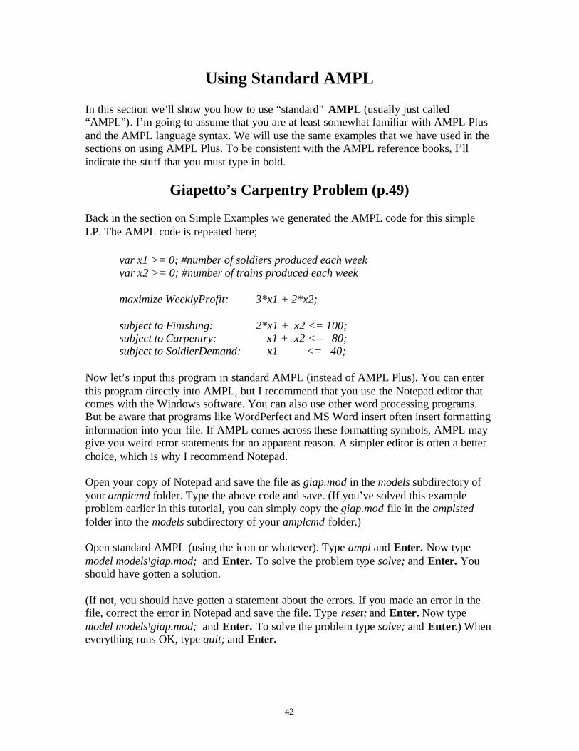
Using Standard AMPL In this section we’ll show you how to use “standard” AMPL (usually just called “AMPL”). I’m going to assume that you are at least somewhat familiar with AMPL Plus and the AMPL language syntax. We will use the same examples that we have used in the sections on using AMPL Plus. To be consistent with the AMPL reference books, I’ll indicate the stuff that you must type in bold.

Giapetto’s Carpentry Problem (p.49)

Back in the section on Simple Examples we generated the AMPL code for this simple LP. The AMPL code is repeated here;

var x1 >= 0; #number of soldiers produced each week var x2 >= 0; #number of trains produced each week maximize WeeklyProfit: 3*x1 + 2*x2; subject to Finishing: 2*x1 + x2 <= 100; subject to Carpentry: x1 + x2 <= 80; subject to SoldierDemand: x1 <= 40;

Now let’s input this program in standard AMPL (instead of AMPL Plus). You can enter this program directly into AMPL, but I recommend that you use the Notepad editor that comes with the Windows software. You can also use other word processing programs. But be aware that programs like WordPerfect and MS Word insert often insert formatting information into your file. If AMPL comes across these formatting symbols, AMPL may give you weird error statements for no apparent reason. A simpler editor is often a better choice, which is why I recommend Notepad. Open your copy of Notepad and save the file as giap.mod in the models subdirectory of your amplcmd folder. Type the above code and save. (If you’ve solved this example problem earlier in this tutorial, you can simply copy the giap.mod file in the amplsted folder into the models subdirectory of your amplcmd folder.) Open standard AMPL (using the icon or whatever). Type ampl and Enter. Now type model models\giap.mod; and Enter. To solve the problem type solve; and Enter. You should have gotten a solution. (If not, you should have gotten a statement about the errors. If you made an error in the file, correct the error in Notepad and save the file. Type reset; and Enter. Now type model models\giap.mod; and Enter. To solve the problem type solve; and Enter.) When everything runs OK, type quit; and Enter.

43

I unintentionally included an error (an extra + sign) the first time I typed the file giap.mod. Then I went back and corrected it. My sequence looked like this: sw: ampl ampl: model models\giapetto.mod; models \giapetto.mod, line 8 (offset 269): syntax error context: subject to SoldierDemand: x1 + >>> <= <<< 40; ampl? reset; ampl: model models\giapetto.mod; ampl: solve; MINOS 5.5: optimal solution found. 3 iterations, objective 180 ampl: option solver cplex; ampl: solve; CPLEX 7.1.0: optimal solution; objective 180 0 simplex iterations (0 in phase I) ampl: quit; sw: Again the information that you must type is shown in bold. If you ever get the prompt ampl?, it is telling you that AMPL is expecting something. Sometimes it will appear if you forgot the semi-colon at the end of a command. If this is the case, just type the semi-colon and Enter. Let’s describe verbally what’s going on. AMPL maintains a “current” model. This is the model that will be sent to the solver when you type the command solve. When you open an AMPL session, the current model is empty. When you type the model command followed by a file name, that file becomes the current model. If you have a separate model file and data file, the data command reads data statements from the data file to assign values to parameters. The reset command “clears out” the current model and data files from the AMPL session. (The commands reset model and reset data are possible.) Now let’s look at some additional output information. To obtain the value of the objective, which we called WeeklyProfit, we type display WeeklyProfit; and Enter. (Remember that AMPL is case sensitive – WeeklyProfit must be exactly like we defined it in the program.) To obtain the value of variable x1 at optimal we type display x1; and Enter. To obtain the value of variable x2 at optimal we type display x2; and Enter. To obtain the reduced cost for x1, we type display x1.rc; and Enter. We can obtain a value of the slack variable of the Carpentry constraint by typing display Carpentry.slack; and then Enter. Also, we can obtain a value of the dual variable of the Carpentry constraint by typ ing display Carpentry.dual; and then Enter. Here’s a possible interaction;

44

sw: ampl ampl: model models\giapetto.mod; ampl: solve; MINOS 5.5: optimal solution found. 3 iterations, objective 180 ampl: display WeeklyProfit; WeeklyProfit = 180 ampl: display x1; x1 = 20 ampl: display Carpentry.dual; display Carpentry.slack; Carpentry.dual = 1 Carpentry.slack = 0 ampl: quit; sw: Let’s choose another example – this time from the AMPL Plus section on IP’s.

Gandhi Cloth Problem Consider the Gandhi Cloth Problem (fixed asset problem) on page 470 of Winston. In AMPL code we have:

var x1 integer >=0; # Number of shirts produced each week var x2 integer >=0; # Number of shorts produced each week var x3 integer >=0; # Number of pants produced each week var y1 binary; # Equals 1 if shirts are produced and 0 otherwise var y2 binary; # Equals 1 if shorts are produced and 0 otherwise var y3 binary; # Equals 1 if pants are produced and 0 otherwise maximize WeeklyProfit: 6*x1 + 4*x2 + 7*x3 - 200*y1 - 150*y2 - 100*y3; subject to Labor: 3*x1 + 2*x2 + 6*x3 <= 150; # Labor constraint subject to Cloth: 4*x1 + 3*x2 + 4*x3 <= 160; # Cloth constraint subject to ShirtProd: x1 - 40*y1 <= 0; # Shirts produced? subject to ShortProd: x2 - 53*y2 <= 0; # Shorts produced? subject to PantProd: x3 - 25*y3 <= 0; # Pants produced?

Open your copy of Notepad and save the file as gandhi.mod in the models subdirectory of your amplcmd folder. Type the above code and save. (If you’ve solved this example

45

problem earlier in this tutorial, you can simply copy the gandhi.mod file from the amplsted folder into the models subdirectory of your amplcmd folder.) Open standard AMPL (using the icon or whatever). Type ampl and Enter. Now type model models\gandhi.mod; and Enter. To solve the problem type solve; and Enter. You should have gotten a solution. Recall that the MINOS solver is the default in standard AMPL. Also recall that we need to use CPLEX for IP’s. So we type option solver cplex; and Enter. In the display below I accidentally (really!) forgot to specify the CPLEX solver. As you can see the MINOS solver “solved” the problem by ignoring the integrality requirements of the variables. After seeing the mistake I typed option solver cplex;. typed Reset; and Entered. I then typed model models\gandhi.mod; and Entered. To solve the problem type solve; and Enter. You should have gotten an integer solution. When everything runs OK, type quit; and Enter. Here’s what the display might have looked like; sw: ampl ampl: model models\gandhi.mod; ampl: solve; MINOS 5.5: ignoring integrality of 6 variables MINOS 5.5: optimal solution found. 2 iterations, objective 81.11320755 ampl: option solver cplex; ampl: reset; ampl: model models\gandhi.mod; ampl: solve; CPLEX 7.1.0: optimal integer solution; objective 75 7 MIP simplex iterations 0 branch-and-bound nodes ampl: display x1, x2, x3, y1, y2, y3; x1 = 0 x2 = 0 x3 = 25 y1 = 0 y2 = 0 y3 = 1 ampl: quit; sw: Now we look at a previous example, which has a separate model file and data file.

My Diet IP

46

In the last section on IP’s we formulated a diet problem (mydiet2.mod), which had an AMPL formulation like this:

set NUTR; # Set of Nutrients set FOOD; # Set of Foods param amt {NUTR, FOOD} >=0; # Amount of nutrient in each food param nutrLow {NUTR} >= 0; # Minimum daily requirement for nutrient param cost {FOOD} >= 0; # Cost of one serving of a food var Buy {FOOD} integer >= 0; # Number of servings of food to be purchased minimize TotalCost: sum {j in FOOD} cost[j] * Buy [j]; subject to Need {i in NUTR}: sum {j in FOOD} amt[i,j] * Buy [j] >= nutrLow[i];

Open your copy of Notepad and save the file as mydiet2.mod in the models subdirectory of your amplcmd folder. Type the above code and save. (If you’ve solved this example problem earlier in this tutorial, you can simply copy the mydiet2.mod file from the amplsted folder into the models subdirectory of your amplcmd folder.) We also in a previous section formulated a data file for this IP called mydiet1.dat. The AMPL formulation looked like this:

set NUTR := Prot VitA VitC Calc Iron Cals Carb; set FOOD := QP MD BM FF MC FR SM MK OJ; param: cost:= QP 1.84 MD 2.19 BM 1.84 FF 1.44 MC 2.29 FR 0.77 SM 1.29 MK 0.60 OJ 0.72; param: nutrLow := Prot 55 VitA 100 VitC 100

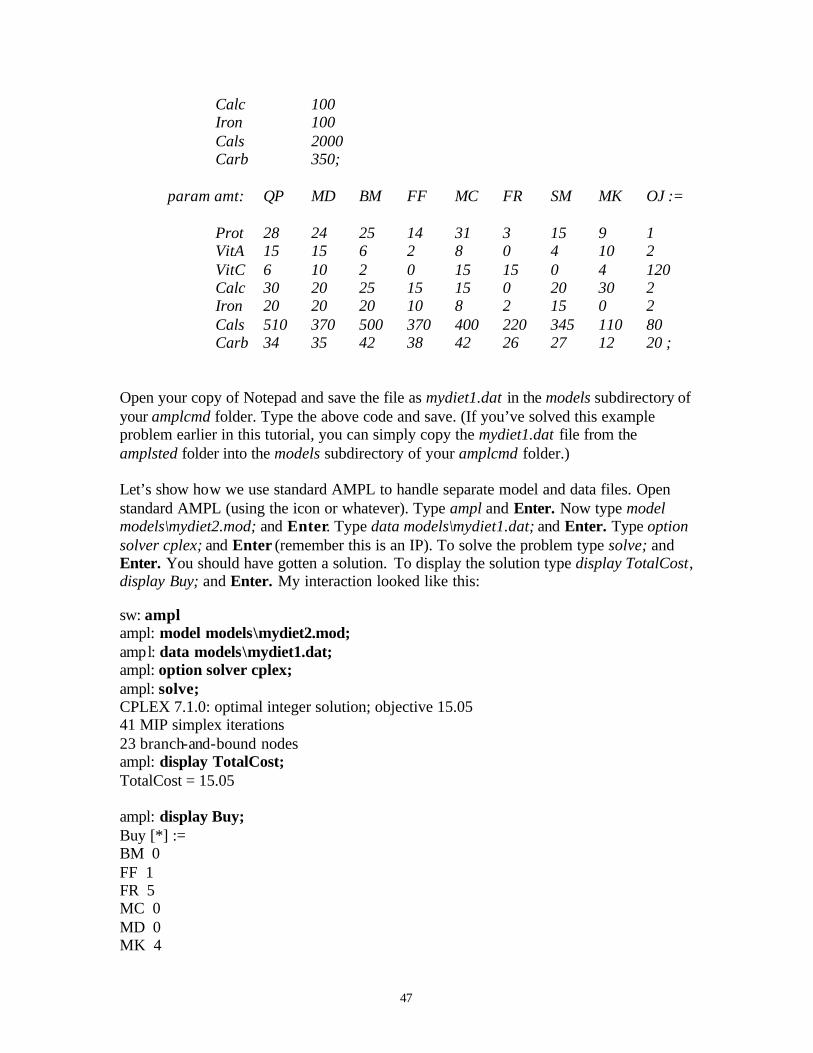
47

Calc 100 Iron 100 Cals 2000 Carb 350;

param amt: QP MD BM FF MC FR SM MK OJ := Prot 28 24 25 14 31 3 15 9 1 VitA 15 15 6 2 8 0 4 10 2 VitC 6 10 2 0 15 15 0 4 120 Calc 30 20 25 15 15 0 20 30 2 Iron 20 20 20 10 8 2 15 0 2 Cals 510 370 500 370 400 220 345 110 80 Carb 34 35 42 38 42 26 27 12 20 ;

Open your copy of Notepad and save the file as mydiet1.dat in the models subdirectory of your amplcmd folder. Type the above code and save. (If you’ve solved this example problem earlier in this tutorial, you can simply copy the mydiet1.dat file from the amplsted folder into the models subdirectory of your amplcmd folder.) Let’s show how we use standard AMPL to handle separate model and data files. Open standard AMPL (using the icon or whatever). Type ampl and Enter. Now type model models\mydiet2.mod; and Enter. Type data models\mydiet1.dat; and Enter. Type option solver cplex; and Enter (remember this is an IP). To solve the problem type solve; and Enter. You should have gotten a solution. To display the solution type display TotalCost, display Buy; and Enter. My interaction looked like this: sw: ampl ampl: model models\mydiet2.mod; ampl: data models\mydiet1.dat; ampl: option solver cplex; ampl: solve; CPLEX 7.1.0: optimal integer solution; objective 15.05 41 MIP simplex iterations 23 branch-and-bound nodes ampl: display TotalCost; TotalCost = 15.05 ampl: display Buy; Buy [*] := BM 0 FF 1 FR 5 MC 0 MD 0 MK 4

48

OJ 0 QP 4 SM 0 ; ampl: quit; sw: Amazingly enough we got the same solution as we did with AMPL Plus. This is our last example. We’ll conclude our introduction to standard AMPL by noting a couple of things: The display command has many options available. Most of Chapter 10 of the AMPL reference book (AMPL, A Modeling Language for Mathematical Programming) details the many possibilities for the display command. You can actually access data from a remote non-AMPL type file using read table and write table commands. (This is a recent extension of the standard AMPL software.) To learn how to do this, please refer to this link on the AMPL website: http://www.ampl.com/whatsnew.html. Refer to the section on Relational Database Support. This link will explain how to access data from MS Access, MS Excel, and other types of files.

49

Index .amp, 6 .dat, 6 .mod, 6 algebraic formulation, 27 AMPL language code, 10 AMPL Plus, 2 AMPL Website, 9 binary variables, 3 Branch and Bound, 2 constraints, 10 CPLEX , 32 data, 23 data file, 23 decision variables, 10 dialog box, 15 Diet Problem, 17 display, 43 download, 40 explicit formulation, 27 Gandhi Cloth Problem, 36 Giapetto’s Carpentry Problem, 6 Graphical User Interface, 5 index, 31 infeasible, 32 integer solution, 14 integer-programming, 3 Kilroy County Fire Station, 38 Linear Optimization Problems, 32 linear programs, 10

LP, 32 maximize, 11 Maximize, 9 minimize, 11 MINOS , 32 Multiple Document Interface, 5 Multiplication, 23 My Diet, 45 NLP’s, 32 Notepad, 42 objective function, 10 output, 13 Parameters , 21 project, 6 reduced cost, 43 Revised Simplex, 2 set-covering, 38 Sets , 21 Simplex, 2 slack variable, 13 solve nonlinear optimization programs , 32 Solver Window, 26 Solvers in AMPL Plus , 5 standard AMPL, 4 subject to, 11 transposed, 24 Traveling Salesman Problem, 39 TSP, 39 var, 33