Solving Exercises of Introductory Statistics

Solving Exercises of Introductory Statistics – Part I: Descriptive Statistic.

Prof. Felix Ramos, PhD in Mechanical Engineering.

--------------------------------------------------------------------------------------------------------------------------------------------

2



--------------------------------------------------------------------------------------------------------------------------------------------

3

Solving Exercises of Introductory Statistics

(Part I):

Descriptive Statistic

Author: Felix Ramos Morales, PhD



--------------------------------------------------------------------------------------------------------------------------------------------

4

Introduction

The present manual explain, through the solution of exercises, different topics of “Descriptive Statistic”.

We have observed the difficulties that students face when try to process different data sets, in order to

calculate the different measures of central tendency, variation, position, and the interpretation of these

results. The text books that are used in our colleges are excellent but the students get lost due to the

amount of information that it is presented, and for that reason we have condensed this information,

offering very accurate procedures (steps by steps), to find the different parameters.

I hope this brief manual be useful in your goal of learn the basic principles of the Statistic.

Felix Ramos, PhD.

Ex- Assistant Professor of Mechanical Engineering, University of Las Villas, Cuba

Adjunct Faculty (Mathematics Department) at Miami Dade Community College, Miami, USA



--------------------------------------------------------------------------------------------------------------------------------------------

5

Important Definitions:

First, we are going to answer two important and common questions that justify the necessity of the

study of Statistic.

What is Statistics?

Statistics is the science of conducting studies to collect, organizes, summarize, analyze and draw

conclusions from data.

Why we must study Statistics?

1. To read and understand the various statistical studies performed in your professional’s field.

2. To learn how to develop research in your field, since statistical procedures are basic to research.

3. To become into “smart” consumer and citizens.

Others important terms that we use in Statistics are defined like:

Variable: It is a characteristic or attribute that can get different values.

Data: are the values (coming from measurements or observations) that the variables can get.

A collection of data values forms a Data set. Each value in the data set is called a Data value.

Population: It is a complete collection of all elements (scores, people, measurements, and so on) to be

studied. The collection is complete in the sense that it includes all subjects to be study.

Census: It is the collection of data from every member of the population.

Sample: A sub collection of member selected from a population.

Parameter: It is a numerical measurement describing some characteristics of a population.

Statistic: It is a numerical measurement describing some characteristics of a sample.

Why to work with samples?

Because the population is too large and then:



--------------------------------------------------------------------------------------------------------------------------------------------

6

To work with the population is very expensive, requires too much time, and sometimes it is almost

impossible to work with the entire population (destructive test and quality control in massive

production).

In this part I, we are going to refer, specially, to Descriptive Statistics.



--------------------------------------------------------------------------------------------------------------------------------------------

7

Sampling techniques:

There are different sampling techniques:

1. Random Sampling: Random samples are selected by using chance methods or random

numbers. Number each subject in the population. Generate random numbers with a computer or a

calculator. The subjects whose numbers are selected constitute the sample.

If you want to generate random numbers, you can use Microsoft Excel and the function RANDBETWEEN,

as is shown below:

In this case we are going to generate random numbers between 1 and 1000 (suppose the population is

1000 people and we want to select a sample of 15 people):



--------------------------------------------------------------------------------------------------------------------------------------------

8

2. Systematic Sampling: You will obtain a systematic sampling by numbering each subject of the

population and then selecting every kth subject. The steps are:

a). Number the subjects in the population from 1 to N

b). Decide on the n (sample size) that you want or need

k = N/n (the interval size)

c). Randomly select an integer between 1 to k (you can use the RANDBETWEEN function that

was shown before to select this first integer), then take every kth unit

Example:

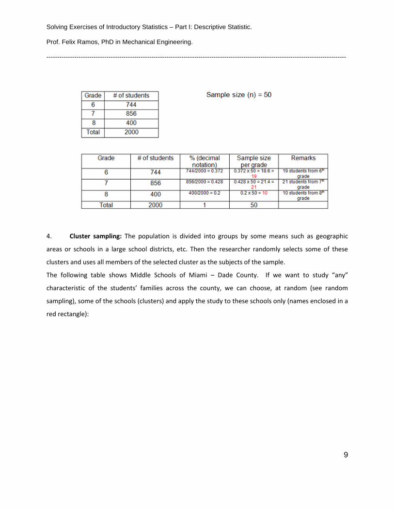
3. Stratified Sampling: The researcher divides the entire population into different subgroups, and

randomly selects the final subjects proportionally from the different strata. Example:

In this case we have 2000 students of a Middle School and we want to get a sample that includes

students of all grades, but proportionally. The table bellow shows the procedure to obtain the sample:



--------------------------------------------------------------------------------------------------------------------------------------------

9

4. Cluster sampling: The population is divided into groups by some means such as geographic

areas or schools in a large school districts, etc. Then the researcher randomly selects some of these

clusters and uses all members of the selected cluster as the subjects of the sample.

The following table shows Middle Schools of Miami – Dade County. If we want to study “any”

characteristic of the students’ families across the county, we can choose, at random (see random

sampling), some of the schools (clusters) and apply the study to these schools only (names enclosed in a

red rectangle):



--------------------------------------------------------------------------------------------------------------------------------------------

10

5. Convenience sampling: Is a sample of study subjects taken from a group which is conveniently

accessible to a researcher. The advantage: it is easy to access, requiring little effort on the part of the

researcher. The disadvantage: it is not an accurate representation of the population.



--------------------------------------------------------------------------------------------------------------------------------------------

11

Data and its characteristics:

The characteristics of the data are:

1. Center: A representative or average value that indicates where the middle of the data set is

located.

2. Variation: A measure of the amount that the data values vary among themselves.

3. Distribution: The nature or shape of the distribution of the data (such as bell-shaped, uniform,

or skewed).

4. Outliers: sample values that lie very far away from the vast majority of the other sample values.

5. Time: Changing characteristics of the data over time.

1.1. Organizing data:

When working with a large data set, it is helpful to organize and summarized the data by constructing a

table that lists the different possible data values along with the corresponding frequencies, which

represent the number of times those values occur.

Some important concepts are:

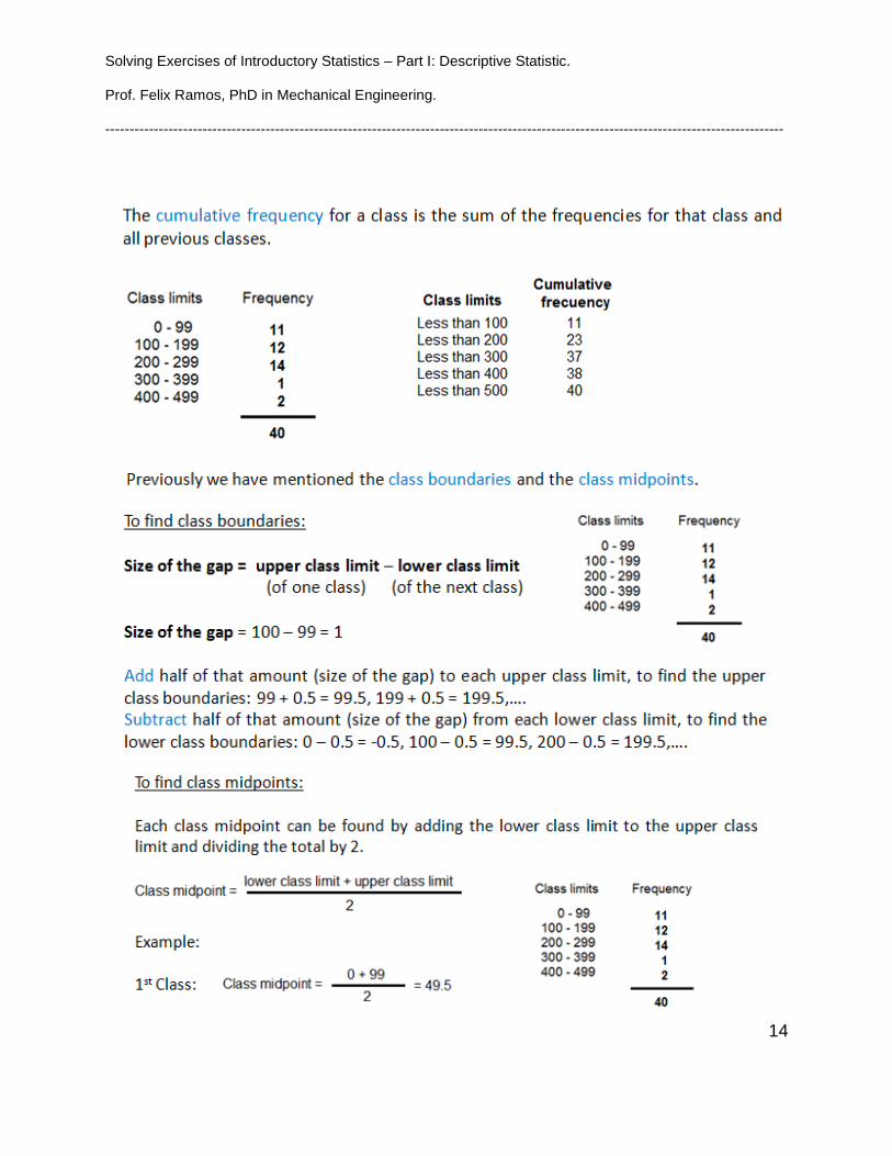
Frequency distribution: The organization of the data in table form, using classes and frequencies.

Class: A qualitative or quantitative category.

Lower class limits: The smaller numbers that can belong to the different classes.

Upper class limits: The largest numbers that can belong to the different classes.

Class boundaries: The numbers used to separate the classes, but without the gap created by class limits.

Class midpoint: The midpoints of the classes.

Class width: The difference between two consecutive lower class limits or two consecutive lower class

boundaries.



--------------------------------------------------------------------------------------------------------------------------------------------

12

Example:

Suppose you have the following data set:

To construct the frequency distribution:



--------------------------------------------------------------------------------------------------------------------------------------------

13



--------------------------------------------------------------------------------------------------------------------------------------------

14



--------------------------------------------------------------------------------------------------------------------------------------------

15

1.2. Histograms, frequency polygons, and ogives. Other types of graphs.

Graphs are pictures of distribution.

Histogram: A bar graph in which the horizontal scale represents classes of data values and the vertical

scale represents frequencies. The heights of the bars correspond to the frequency values, and the bars

are drawn adjacent to each other.

A Relative Frequency Histogram has the same shape and horizontal scale as a histogram, but the

vertical scale is marked with relative frequencies.



--------------------------------------------------------------------------------------------------------------------------------------------

16

Frequency polygon: Use line segments connected to points located above class midpoint values.

Ogive: It is a line graphs that shows cumulative frequencies.

Pareto Charts: Is a bar graph for qualitative data, with the bars arranged in order according to the

frequencies.



--------------------------------------------------------------------------------------------------------------------------------------------

17

Pie Charts: Construction of this type of graph involves slicing up the pie into the proper proportions.



--------------------------------------------------------------------------------------------------------------------------------------------

18

Scatter diagrams: Is a plot of order pairs (x,y) data with a horizontal x – axis and a vertical y- axis. The

pattern of the plotted points is often helpful in determining whether there is correlation between the

variables.

Analyzing the Scatter plot, by looking the pattern of the points on the graph we can get some

conclusions:

1. A positive linear relationship exists when the points fall approximately in an ascending straight

line.

2. A negative linear relationship exists when the points fall approximately in a descending straight

line.

3. A nonlinear relationship exists when the points fall in a curved line.

4. No relationship exists when there is no a clear pattern of the points.



--------------------------------------------------------------------------------------------------------------------------------------------

19

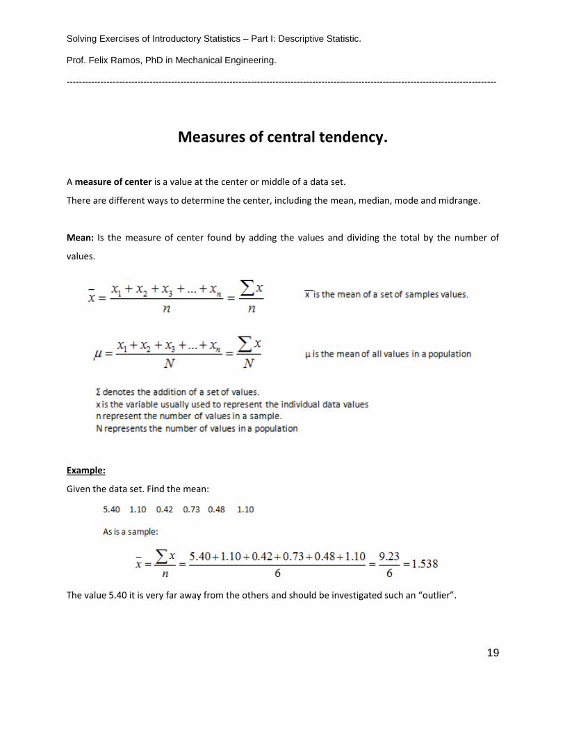
Measures of central tendency.

A measure of center is a value at the center or middle of a data set.

There are different ways to determine the center, including the mean, median, mode and midrange.

Mean: Is the measure of center found by adding the values and dividing the total by the number of

values.

Example:

Given the data set. Find the mean:

The value 5.40 it is very far away from the others and should be investigated such an “outlier”.



--------------------------------------------------------------------------------------------------------------------------------------------

20

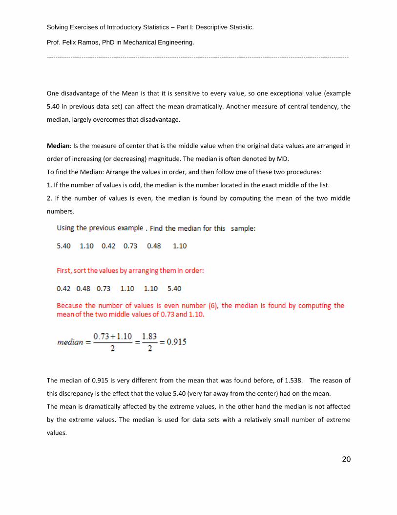
One disadvantage of the Mean is that it is sensitive to every value, so one exceptional value (example

5.40 in previous data set) can affect the mean dramatically. Another measure of central tendency, the

median, largely overcomes that disadvantage.

Median: Is the measure of center that is the middle value when the original data values are arranged in

order of increasing (or decreasing) magnitude. The median is often denoted by MD.

To find the Median: Arrange the values in order, and then follow one of these two procedures:

1. If the number of values is odd, the median is the number located in the exact middle of the list.

2. If the number of values is even, the median is found by computing the mean of the two middle

numbers.

The median of 0.915 is very different from the mean that was found before, of 1.538. The reason of

this discrepancy is the effect that the value 5.40 (very far away from the center) had on the mean.

The mean is dramatically affected by the extreme values, in the other hand the median is not affected

by the extreme values. The median is used for data sets with a relatively small number of extreme

values.



--------------------------------------------------------------------------------------------------------------------------------------------

21

Mode (denoted as M): It is the value that occurs most frequently.

a). When two values occur with the same greatest frequency, each one is a mode and the data set is

bimodal.

b). When more that two values occur with the same greatest frequency, each is a mode and the data set

is said to be multimodal.

c). When no value is repeated, we say that there is not mode.

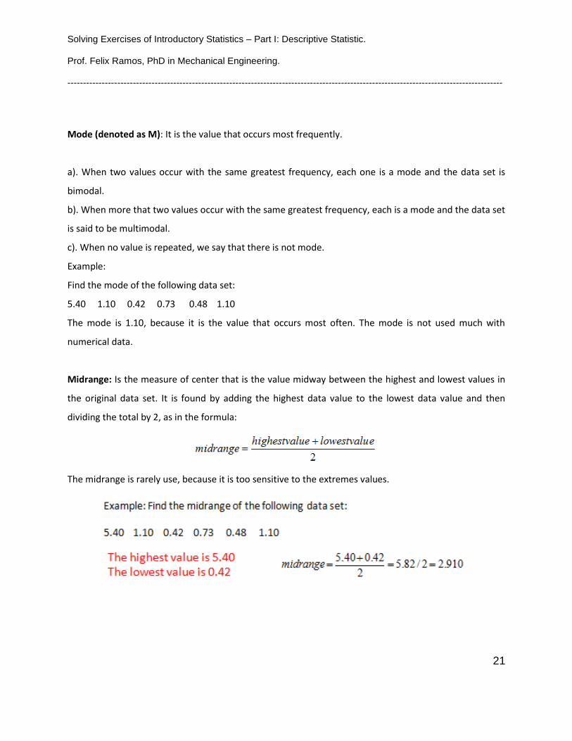
Example:

Find the mode of the following data set:

5.40 1.10 0.42 0.73 0.48 1.10

The mode is 1.10, because it is the value that occurs most often. The mode is not used much with

numerical data.

Midrange: Is the measure of center that is the value midway between the highest and lowest values in

the original data set. It is found by adding the highest data value to the lowest data value and then

dividing the total by 2, as in the formula:

The midrange is rarely use, because it is too sensitive to the extremes values.



--------------------------------------------------------------------------------------------------------------------------------------------

22

Using Microsoft Excel, we can find all this measures of central tendency as is shown below:

Round – Off Rule:

A simple rule for rounding answers is this: Carry one more decimal place than is present in the original

set of values.

What this rule means?

Suppose you find the mean among 2, 3, and 5. The mean is 3.3333… Rounding this number with one

decimal place (nearest tenth), you get: 3.3

Mean from a frequency distribution: When the data is summarized in a frequency distribution, we

might not know the exact value falling in a particular class. The formula for the mean in this case is:



--------------------------------------------------------------------------------------------------------------------------------------------

23

2. Measures of variation:

Range: In a data set is the difference between the highest value and the lowest value.

Range = (highest value) – (lowest value)

The range is very easy to compute, but because it depends on only the highest value and the lowest

values, it is not as useful as the other measures of variation that use every value.

Standard deviation: Is a measure of variation about the mean. It is a type of average deviation of values

from the mean that is calculated using the following formulas:

Example:

Find the standard deviation of the given data: 1, 3, 14

The procedure to find the standard deviation includes:



--------------------------------------------------------------------------------------------------------------------------------------------

24



--------------------------------------------------------------------------------------------------------------------------------------------

25

Interpreting and understanding the standard deviation:

Among the different meaning of the standard deviation two of the most important are:

1. If the standard deviation is large, the data are more dispersed.

2. The standard deviation let us determine the number of data values that fall within a specified interval

in a distribution.

Variance: The variance of a set of value is a measure of variation equal to the square of the standard

deviation. The variance has this serious disadvantage: The units of variance are different (are square

units) than the units of the original data set.

The following figure show the functions of Microsoft Excel that let us find the measures of variation:

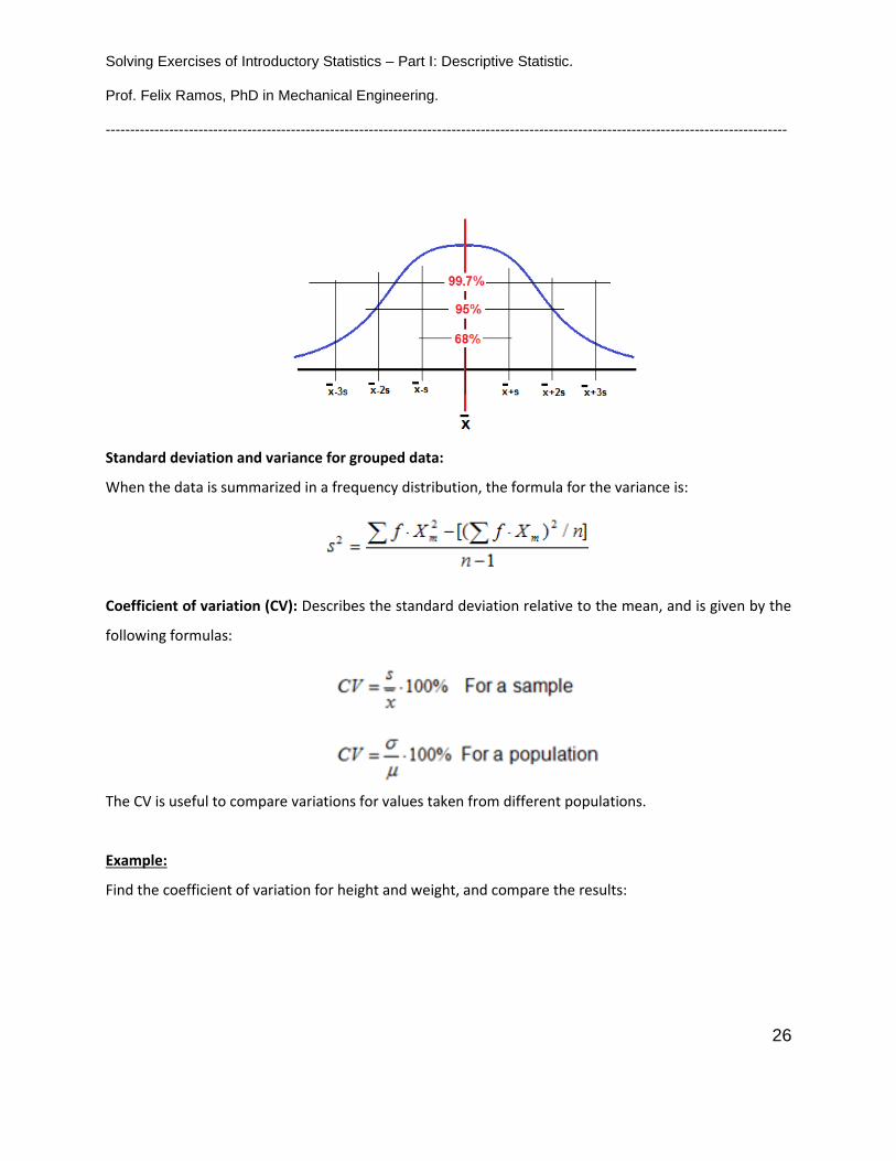
Empirical Rule for Data with a Bell – Shaped distribution: For data sets having a distribution that is

approximately bell-shaped, the following properties apply:

• About 68% of all values fall within 1 standard deviation of the mean.

• About 95% of all values fall within 2 standard deviations of the mean.

• About 99.7 % of all values fall within 3 standard deviation of the mean.



--------------------------------------------------------------------------------------------------------------------------------------------

26

Standard deviation and variance for grouped data:

When the data is summarized in a frequency distribution, the formula for the variance is:

Coefficient of variation (CV): Describes the standard deviation relative to the mean, and is given by the

following formulas:

The CV is useful to compare variations for values taken from different populations.

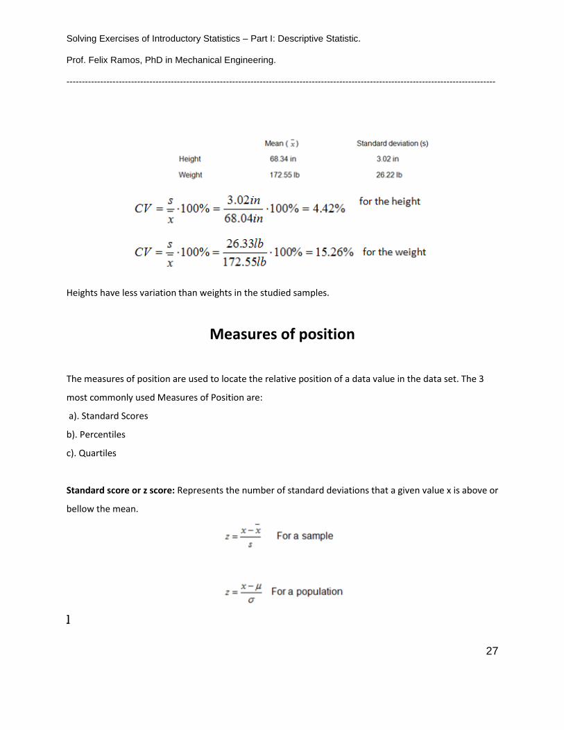
Example:

Find the coefficient of variation for height and weight, and compare the results:



--------------------------------------------------------------------------------------------------------------------------------------------

27

Heights have less variation than weights in the studied samples.

Measures of position

The measures of position are used to locate the relative position of a data value in the data set. The 3

most commonly used Measures of Position are:

a). Standard Scores

b). Percentiles

c). Quartiles

Standard score or z score: Represents the number of standard deviations that a given value x is above or

bellow the mean.

]



--------------------------------------------------------------------------------------------------------------------------------------------

28

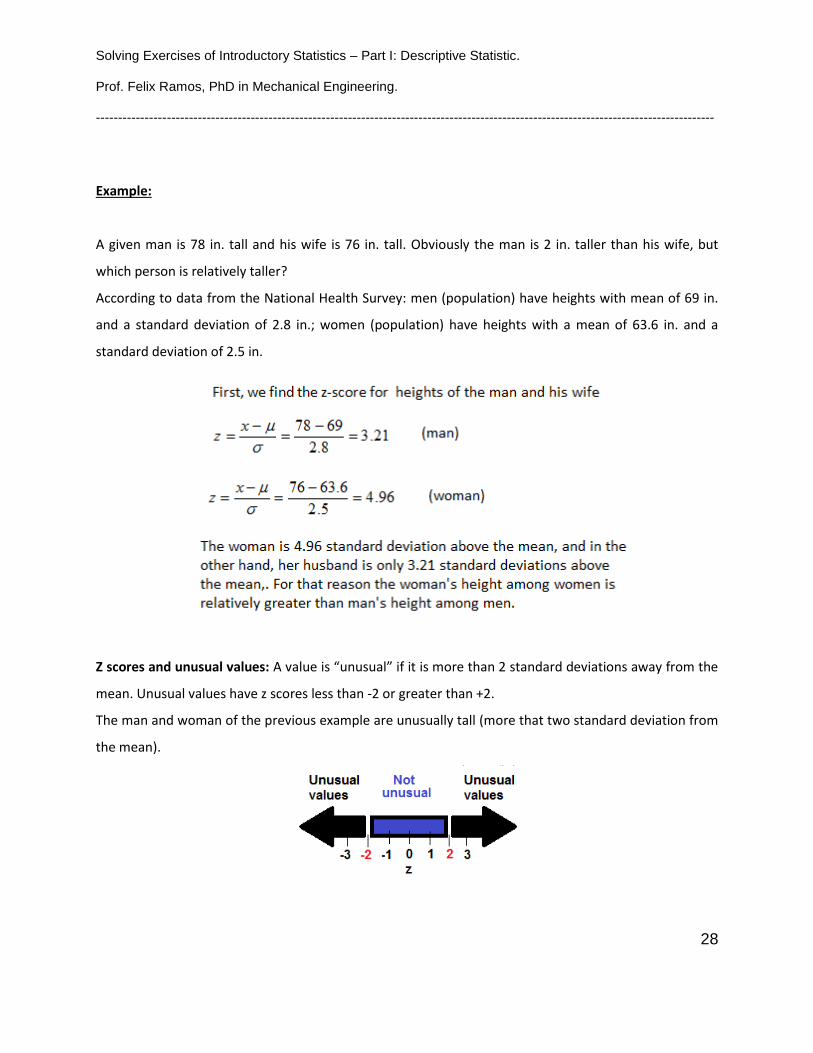
Example:

A given man is 78 in. tall and his wife is 76 in. tall. Obviously the man is 2 in. taller than his wife, but

which person is relatively taller?

According to data from the National Health Survey: men (population) have heights with mean of 69 in.

and a standard deviation of 2.8 in.; women (population) have heights with a mean of 63.6 in. and a

standard deviation of 2.5 in.

Z scores and unusual values: A value is “unusual” if it is more than 2 standard deviations away from the

mean. Unusual values have z scores less than -2 or greater than +2.

The man and woman of the previous example are unusually tall (more that two standard deviation from

the mean).



--------------------------------------------------------------------------------------------------------------------------------------------

29

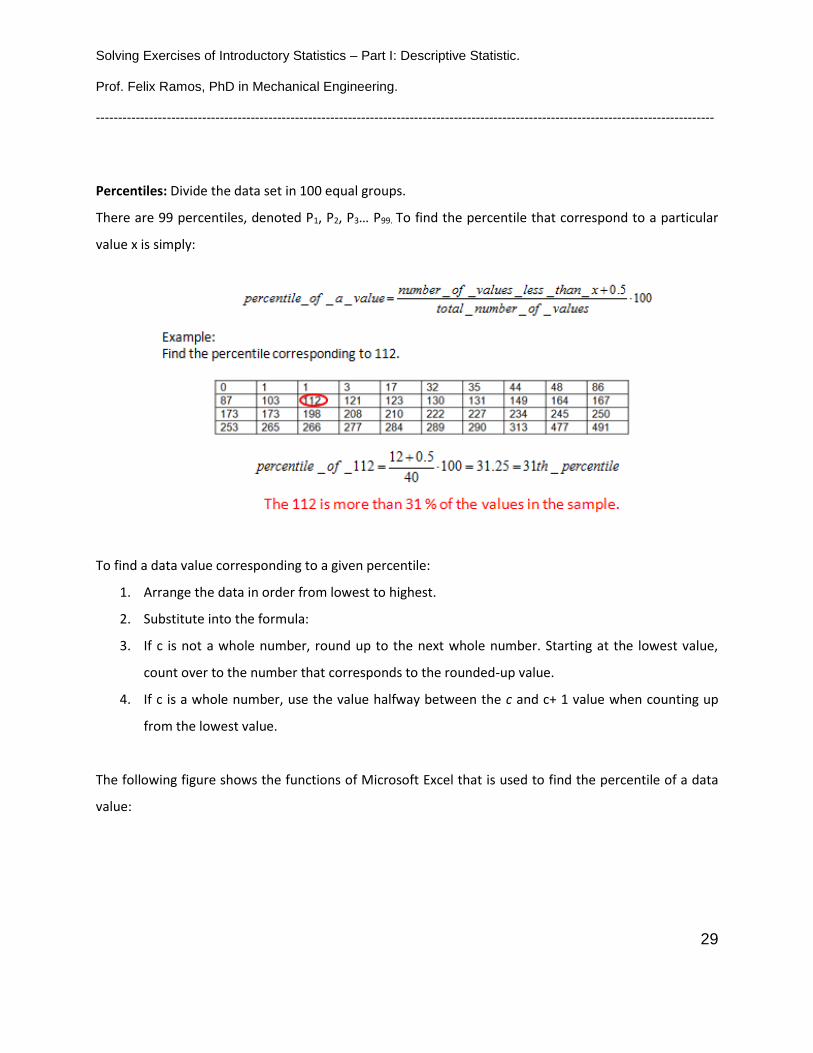
Percentiles: Divide the data set in 100 equal groups.

There are 99 percentiles, denoted P1, P2, P3… P99. To find the percentile that correspond to a particular

value x is simply:

To find a data value corresponding to a given percentile:

1. Arrange the data in order from lowest to highest.

2. Substitute into the formula:

3. If c is not a whole number, round up to the next whole number. Starting at the lowest value,

count over to the number that corresponds to the rounded-up value.

4. If c is a whole number, use the value halfway between the c and c+ 1 value when counting up

from the lowest value.

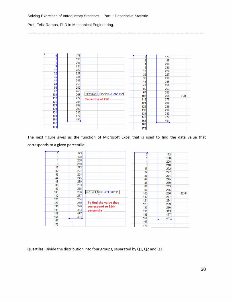
The following figure shows the functions of Microsoft Excel that is used to find the percentile of a data

value:



--------------------------------------------------------------------------------------------------------------------------------------------

30

The next figure gives us the function of Microsoft Excel that is used to find the data value that

corresponds to a given percentile:

Quartiles: Divide the distribution into four groups, separated by Q1, Q2 and Q3.



--------------------------------------------------------------------------------------------------------------------------------------------

31

Note that Q1 is the same that 25th percentile; Q2 is the same as the 50th percentile, Q3 corresponds to

the 75th percentile.

The easiest method to find quartiles is:

1. Arrange the data in order from lowest to highest.

2. Find the median of the data values. This is the value for Q2.

3. Find the median of the data values that fall bellow Q2. This is the value for Q1.

4. Find the median of the data values that fall above Q2. This is the value for Q3.

Example:

Using Microsoft Excel, you will find the quartiles using the function that is shows bellow.



--------------------------------------------------------------------------------------------------------------------------------------------

32

Outliers: Is an extremely high or extremely low data value when compared with the rest of the data

values.

Example:



--------------------------------------------------------------------------------------------------------------------------------------------

33

Solved exercises:

1. A Research Organization surveyed 50 randomly selected individuals and asked them the primary

way they received the daily news. Their choices were via newspaper (N), television (T), radio (R), or

internet (I). Construct a categorical frequency distribution for the data and interpret the results.

Solution:

We are going to create a table with four categories, and counting the frequency of each category:

The primary way that they receive the daily news is by Television.

2. Construct a pie graph for the data in exercises 1:

Solution:

Find the percent of the total that each category represent and find the central angle, multiplying this

percent by 360 degrees (the measure of one revolution):



--------------------------------------------------------------------------------------------------------------------------------------------

34

3. The data show the estimated added cost per vehicle use due to bad roads. Construct a

frequency distribution using 6 classes.

Solution

Applying the procedure that we explain before:

Find the number of classes:

Six (6) classes – The number of classes, in this case, is given by the exercise.



--------------------------------------------------------------------------------------------------------------------------------------------

35

Class width:

Starting point:

85 is the lowest value, it is an integer and is a convenient number.

Lower class limits (starting point + class width and so on):

85

85 + 21 = 106

106 + 21 = 127

127 + 21 = 148

148 + 21 = 169

169 + 21 = 190

Upper class limits (with gap of 1 unit):

85 – 105

106 – 126

127 – 147

148 – 168

169 – 189

190 – 210

Complete the table:



--------------------------------------------------------------------------------------------------------------------------------------------

36

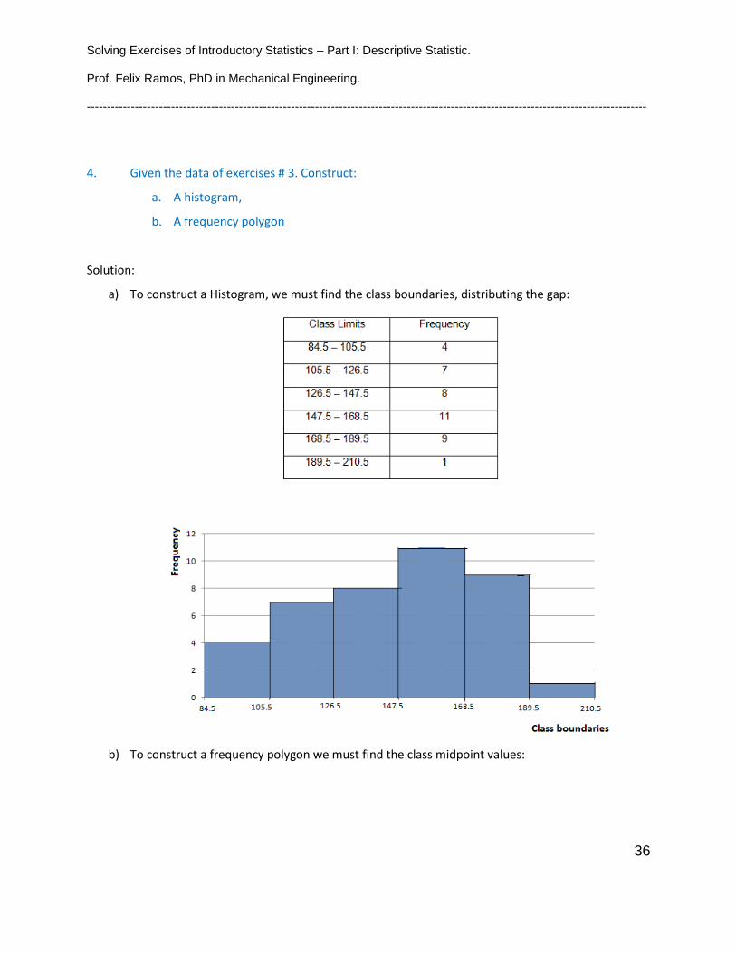
4. Given the data of exercises # 3. Construct:

a. A histogram,

b. A frequency polygon

Solution:

a) To construct a Histogram, we must find the class boundaries, distributing the gap:

b) To construct a frequency polygon we must find the class midpoint values:



--------------------------------------------------------------------------------------------------------------------------------------------

37

5. Construct a Pareto chart for the number of trial – ready civil action and equity cases decided in

less than 6 months for the selected counties in southwestern Pennsylvania.

County Number of Cases

Westmoreland 427

Washington 298

Green 151

Fayette 106

Somerset 87



--------------------------------------------------------------------------------------------------------------------------------------------

38

Solution:

6. The following data represent the number of listeners (in thousands) of 15 radio stations in the

6:00 to 9:00 AM time slot in Pittsburgh.

229 182 129 112 122 93 97 114 95 114 60 89 75 70 68

Find each of these:

a. Mean

b. Median

c. Mode

d. Midrange

e. Range

f. Standard deviation

g. Variance



--------------------------------------------------------------------------------------------------------------------------------------------

39

Solution:

a). Mean (rounded with one place value more than the data values):

b). Median:

Rearrange the values:

60 68 70 75 89 93 95 97 112 114 114 122 129 182 229

Odd number of data values…. The Median is the middle of the data set: 97

c). Mode:

The most frequent data value: 114

d). Midrange:

e). Range:

f). Standard deviation:

We must fill the table:



--------------------------------------------------------------------------------------------------------------------------------------------

40

g). Variance:

The variance it is the square of the standard deviation:

7. The following data represent the number of seconds it took to 20 students to find information

from the Internet on a personal computer.

Class Frequency

34 – 38 4

39 – 43 6

44 – 48 3

49 – 53 4

54 – 58 3

a). Find the mean.



--------------------------------------------------------------------------------------------------------------------------------------------

41

Solution:

First we must fill the table:

8. The number of previous jobs held by each of six applicants is shown here:

2 4 5 6 8 9

a. Find the percentile for 6.

b. What value corresponds to 30th percentile?

Solution:

a). Percentile of 6:

50% of the data values are bellow 6.



--------------------------------------------------------------------------------------------------------------------------------------------

42

c). Find P30:

It is the second value counting from the lowest. In this case it is 4.

9. Check the data set for outliers:

112 157 192 116 153 129 131

Solution:

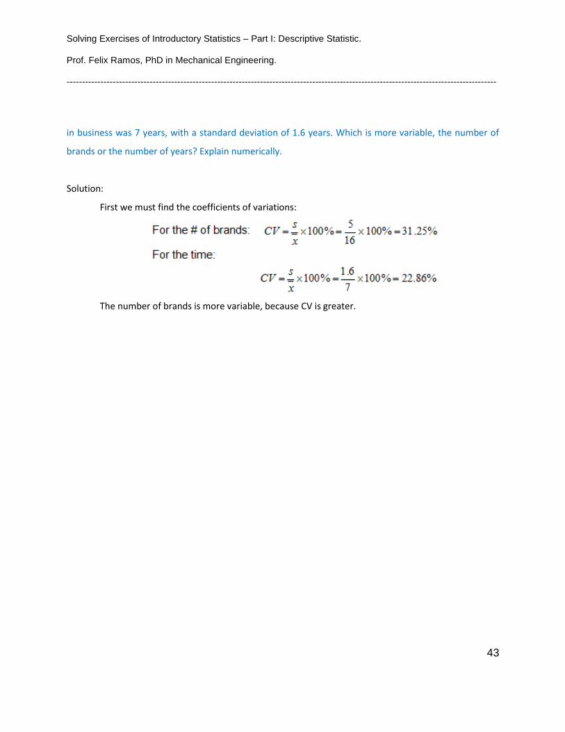
10. A survey of grocery stores showed that the average number of brands of toothpaste carried was

16, with a standard deviation of 5. The same survey showed the average length of time each store was



--------------------------------------------------------------------------------------------------------------------------------------------

43

in business was 7 years, with a standard deviation of 1.6 years. Which is more variable, the number of

brands or the number of years? Explain numerically.

Solution:

First we must find the coefficients of variations:

The number of brands is more variable, because CV is greater.



--------------------------------------------------------------------------------------------------------------------------------------------

44

Dear students.

I hope that you have learned and understand better the topics explained, after study the

present manual.

In the Parts II and III (coming soon) we are going to cover aspects of Probabilities and

Inferential Statistics.

11/09/2014

Prof. Felix Ramos, PhD.

Solving Exercises of Introductory Statistics

Documents

Transcript of Solving Exercises of Introductory Statistics