ARMA Models and the Box-Jenkins Methodology

ARMA Models and the Box±JenkinsMethodology

SPYROS MAKRIDAKIS� AND MICHEÁ LE HIBON

INSEAD, France

ABSTRACT

The purpose of this paper is to apply the Box±Jenkins methodology toARIMA models and determine the reasons why in empirical tests it isfound that the post-sample forecasting the accuracy of such models isgenerally worse than much simpler time series methods. The paper con-cludes that the major problem is the way of making the series stationary inits mean (i.e. the method of di�erencing) that has been proposed by Boxand Jenkins. If alternative approaches are utilized to remove and extrapo-late the trend in the data, ARMA models outperform the models selectedthrough Box±Jenkins methodology. In addition, it is shown that usingARMA models to seasonally adjusted data slightly improves post-sampleaccuracies while simplifying the use of ARMA models. It is also con®rmedthat transformations slightly improve post-sample forecasting accuracy,particularly for long forecasting horizons. Finally, it is demonstratedthat AR(1), AR(2) and ARMA(1,1) models can produce more accuratepost-sample forecasts than those found through the application of Box±Jenkins methodology. # 1997 by John Wiley & Sons, Ltd.

J. forecast. 16: 147±163, 1997

No. of Figures: 12. No. of Tables: 0. No. of References: 44.

KEYWORDS time-series forecasting; ARMA models; Box±Jenkins,empirical studies; M-Competition

AutoRegressive (AR) models were ®rst introduced by Yule in 1926. They were subsequentlysupplemented by Slutsky who in 1937 presented Moving Average (MA) schemes. It was Wold(1938), however, who combined both AR and MA schemes and showed that ARMA processescan be used tomodel a large class of stationary time series as long as the appropriate order of p, thenumber of AR terms, and q, the number of MA terms, was appropriately speci®ed. This meansthat a general series xt can be modelled as a combination of past xt values and/or past et errors, or

xt � f1xtÿ1 � f2xtÿ2 � � � � � fpxtÿp � et ÿ y1etÿ1 ÿ y2etÿ2 ÿ � � � ÿ yqetÿq �1�

Using equation (1) for modelling real-life time series requires four steps. First the original series,xt, must be transformed to become stationary around its mean and its variance. Second, the

� Correspondence to: Spyros Makridakis, INSEAD, Boulevard de Constance, 77305 Fontainebleau Cedex, France

CCC 0277±6693/97/030147±17$17.50 Received May 1995# 1997 by John Wiley & Sons, Ltd. Accepted January 1997

Journal of Forecasting, Vol. 16, 147±163 (1997)

appropriate order of p and q must be speci®ed. Third, the value of the parameters f1;f2; . . . ;fp

and/or y1; y2; . . . ; yq must be estimated using some non-linear optimization procedure thatminimizes the sum of square errors or some other appropriate loss function. Finally, practicalways of modelling seasonal series must be envisioned and the appropriate order of such modelsspeci®ed.

The utilization of the theoretical results suggested by Wold, expressed by equation (1), tomodel real-life series did not become possible until the mid-1960s when computers, capable ofperforming the required calculations to optimize the parameters of equation (1), becameavailable and economical. Box and Jenkins (1976, original edition 1970) popularized the use ofARMAmodels through the following: (1) providing guidelines for making the series stationary inboth its mean and variance, (2) suggesting the use of autocorrelations and partial autocorrelationcoe�cients for determining appropriate values of p and q (and their seasonal equivalent P and Qwhen the series exhibited seasonality), (3) providing a set of computer programs to help usersidentify appropriate values for p and q, as well as P and Q, and estimate the parameters involvedand (4) once the parameters of the model were estimated, a diagnostic check was proposed todetermine whether or not the residuals, et, were white noise, in which case the order of the modelwas considered ®nal (otherwise another model was determined using (2) and steps (3) and (4)were repeated). If the diagnostic check showed random residuals then the model developed wasused for forecasting or control purposes assuming, of course, constancy, that is, the order of themodel and its non-stationary behaviour, if any, would remain the same during the forecasting, orcontrol, phase.

The approach proposed by Box and Jenkins came to be known as the Box±Jenkins method-ology to ARIMA models, where the letter `I', between AR and MA, stood for the `Integrated'and re¯ected the need for di�erencing to make the series stationary. ARIMA models and theBox±Jenkins methodology became highly popular in the 1970s among academics, in particularwhen it was shown through empirical studies (Cooper, 1972; Nelson, 1972; Elliot, 1973;Narasimham et al., 1974; McWhorter, 1975; for a survey see Armstrong, 1978) that they couldoutperform the large and complex econometric models, popular at that time, in a variety ofsituations.

EMPIRICAL EVIDENCE

The popularity of the Box±Jenkins methodology to ARIMA models was shaken when empiricalstudies (Gro�, 1973; Geurts and Ibrahim, 1975; Makridakis and Hibon, 1979; Makridakis et al.,1982, 1993; Huss, 1985; Fildes et al., 1997), using real data, showed that simple methods wereequally or more accurate than Box±Jenkins when post-sample comparisons were made. Today,after many debates, it is accepted by a large number of researchers that in empirical tests Box±Jenkins is not an accurate method for post-sample time-series forecasting, at least in the domainsof business and economic applications where the level of randomness is high and whereconstancy of pattern, or relationships, cannot be assured.

The purpose of this paper is to examine the post-sample forecasting accuracy of ARIMAmodels in order to determine the contribution to such accuracy of each of its elements(i.e. seasonality, stationarity, the order of the ARMA model, and the necessity that the residualsof the ARMA model must be random). It is concluded that the major problem with the Box±Jenkins methodology is the way that the series are made stationary in their mean. When

J. forecast. 16: 147±163, 1997 # 1997 by John Wiley & Sons, Ltd.

148 Journal of Forecasting Vol. 16, Iss. No. 3

alternative ways of dealing with and extrapolating the trend are provided, ARMA models areslightly more accurate than the corresponding time-series methods that extrapolate the trend inthe time series.

THE STEPS (ELEMENTS) OF THE BOX±JENKINS METHODOLOGY

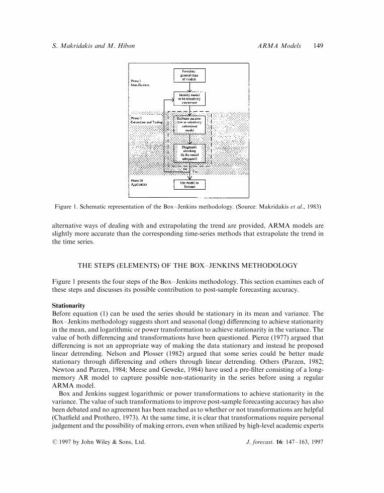
Figure 1 presents the four steps of the Box±Jenkins methodology. This section examines each ofthese steps and discusses its possible contribution to post-sample forecasting accuracy.

StationarityBefore equation (1) can be used the series should be stationary in its mean and variance. TheBox±Jenkins methodology suggests short and seasonal (long) di�erencing to achieve stationarityin the mean, and logarithmic or power transformation to achieve stationarity in the variance. Thevalue of both di�erencing and transformations have been questioned. Pierce (1977) argued thatdi�erencing is not an appropriate way of making the data stationary and instead he proposedlinear detrending. Nelson and Plosser (1982) argued that some series could be better madestationary through di�erencing and others through linear detrending. Others (Parzen, 1982;Newton and Parzen, 1984; Meese and Geweke, 1984) have used a pre-®lter consisting of a long-memory AR model to capture possible non-stationarity in the series before using a regularARMA model.

Box and Jenkins suggest logarithmic or power transformations to achieve stationarity in thevariance. The value of such transformations to improve post-sample forecasting accuracy has alsobeen debated and no agreement has been reached as to whether or not transformations are helpful(Chat®eld and Prothero, 1973). At the same time, it is clear that transformations require personaljudgement and the possibility of making errors, even when utilized by high-level academic experts

Figure 1. Schematic representation of the Box±Jenkins methodology. (Source: Makridakis et al., 1983)

# 1997 by John Wiley & Sons, Ltd. J. forecast. 16: 147±163, 1997

S. Makridakis and M. Hibon ARMA Models 149

(see comments on the paper by Chat®eld and Prothero, 1973). At the empirical level there is alsono evidence that logarithmic or power transformations improve post-sample forecasting accuracy(Granger and Nelson, 1978; Makridakis and Hibon, 1979; Meese and Geweke, 1984).

SeasonalityIn case the series are seasonal, the Box±Jenkins methodology proposes multiplicative seasonalmodels coupled with long-term di�erencing, if necessary, to achieve stationarity in the mean. Thedi�culty with such an approach is that there is practically never enough data available todetermine the appropriate level of the seasonal ARMA model with any reasonable degree ofcon®dence. Users therefore proceed through trial and error in both identifying an appropriateseasonal model and in selecting the correct long-term (seasonal) di�erencing. In addition,seasonality requires more data to estimate the appropriate model parameters. There has appa-rently been no empirical work to test whether or not deseasonalizing the data ®rst, using adecomposition procedure (a suggestion made by Durbin, 1979), and subsequently using theBox±Jenkins method on the seasonally adjusted data improves post-sample forecasting accuracy.

Order of ARMA modelThe order of the ARMA model is found by examining the autocorrelations and partialautocorrelations of the stationary series. Box and Jenkins (1976) provided both a theoreticalframework and practical rules for determining appropriate values for p and q as well as theirseasonal counterparts P andQ. The possible di�culty is that often more than one model could beconsidered, requiring the user to choose one of them without any knowledge of the implicationsof his or her choice on post-sample forecasting accuracy since, according to the Box±Jenkinsmethodology, any model which results in random residuals is an appropriate one. Box andJenkins do recommend the principle of parsimony meaning that a simpler (having fewerparameters) model should be selected in case more than one model is possible, but there has beenvery little systematic work to determine if this suggestion results in improvements in post-sampleforecasting accuracy.

Estimating the model's parametersThis part of the Box±Jenkins methodology is the most straightforward one. The non-linearoptimization procedure, based on the method of steepest descent (Marquardt, 1963), is used toestimate the parameter values of p and/or q (and their seasonal equivalent P and/or Q). Apartfrom occasional problems when there is no convergence (in which case another model is used) theestimation provides no special di�culties except for its inability to guarantee a global optimum (acommon problem of all non-linear algorithms). The estimation is completely automatedrequiring no judgemental inputs, and therefore testing, as all computer programs use the samealgorithm in applying the Marquardt optimization procedure.

Diagnostic checksOnce an appropriate model had been chosen and its parameters estimated, the Box±Jenkinsmethodology required examining the residuals of the actual values minus those estimatedthrough the model. If such residuals are random, it is assumed that the model is appropriate.If not, another model is considered, its parameters estimated, and its residuals checked forrandomness. In practically all instances a model could be found to result in random residuals.Several tests (e.g. Box and Pierce, 1970) have been suggested to help users determine if overall the



residuals are indeed random. Although it is a standard statistical procedure not to use modelswhose residuals are not random, it might be interesting to test the consequences of lack ofresidual randomness on post-sample forecasting accuracy.

POST-SAMPLE FORECASTING ACCURACY: PERSONALIZEDVERSUS AUTOMATIC BOX±JENKINS

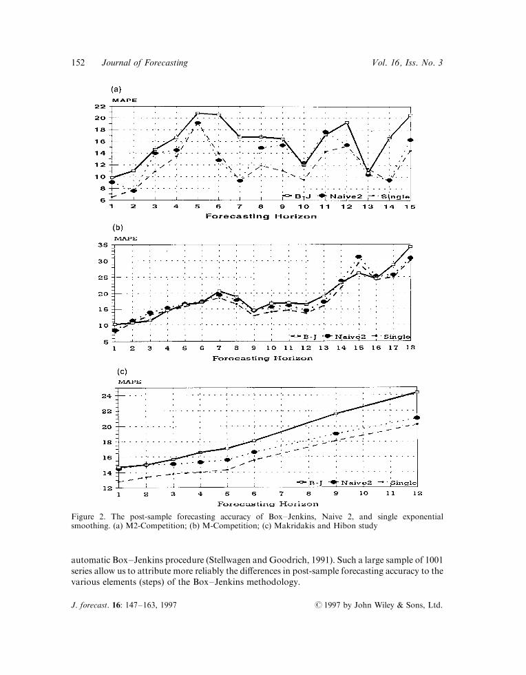
The Makridakis and Hibon (1979) study, the M-Competition (Makridakis et al., 1982), theM2-Competition (1993) as well as many other empirical studies (Schnaars, 1986; Koehler andMurphree, 1988; Geurts and Kelly, 1986; Watson et al., 1987; Collopy and Armstrong, 1992)have demonstrated that simple methods such as exponential smoothing outperform, on average,the Box±Jenkins methodology to ARMA models. Figures 2(a), (b) and (c) show the MAPE(Mean Absolute Percentage Errors), for various forecasting horizons, of Naive 2 (a deseason-alized random walk model), Single exponential smoothing (after the data have been deseasonal-ized, if necessary, and the forecasts subsequently reseasonalized) as well as those of theBox±Jenkins methodology found in the M2-Competition (Makridakis et al., 1993), theM-Competition (Makridakis et al., 1982), and the Makridakis and Hibon (1979) study. Theresults indicate that single smoothing outperformed `Box±Jenkins' overall and in most fore-casting horizons, while Naive 2 also does better than `Box±Jenkins', although by a lesseramount. The results of Figure 2 are surprising since it has been demonstrated that single expo-nential smoothing is a special case of ARMA models (Cogger, 1974; Gardner and McKenzie,1985). Moreover, it makes little sense that Naive 2, which simply uses the latest available value,taking seasonality into account, does so well in comparison to the Box±Jenkins methodology.

In the M-Competition (Makridakis et al., 1982) the Box±Jenkins method was run on a subsetof 111 (one out of every nine) series from the total of the 1001 series utilized. The reason was thatthe method required personal judgement, making it impractical to use all 1001 series as the expertanalyst had to model each series individually, following the various steps described in theprevious section, and spending, on average, about one hour before a model could be con®rmed asappropriate for forecasting purposes (see Andersen and Weiss, 1984).

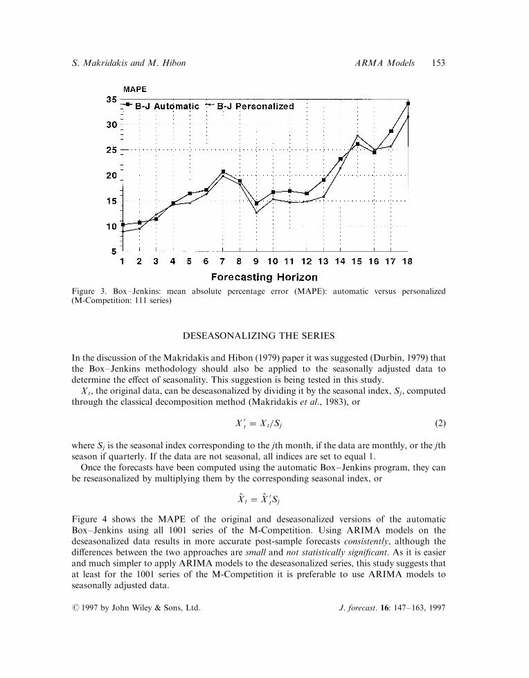
Since the M-Competition was completed, several empirical studies have shown that automaticBox±Jenkins approaches (Hill and Fildes, 1984; Libert, 1983; Texter and Ord, 1989) performedabout the same or better in terms of post-sample accuracy as the personalized approach followedby Andersen and Weiss (1984). Figure 3 shows the results of a speci®c automatic Box±Jenkinsprogram (Stellwagen and Goodrich, 1991) together with that of the personalized approachutilized by Andersen and Weiss in the M-Competition. Figure 3 illustrates that for the 111 seriesused in the comparison the post-sample accuracies of the automatic and personalized approachesare about the same. We could, therefore, use an automatic Box±Jenkins version to perform ourcomparisons using all the 1001 series of the M-Competition.

ATTRIBUTING THE DIFFERENCES IN POST-SAMPLEFORECASTING ACCURACIES

Since we found no substantive di�erences between the personalized and automatic versions ofBox±Jenkins (see Figure 3), we have utilized all the 1001 series of the M-Competition using an



automatic Box±Jenkins procedure (Stellwagen and Goodrich, 1991). Such a large sample of 1001series allow us to attribute more reliably the di�erences in post-sample forecasting accuracy to thevarious elements (steps) of the Box±Jenkins methodology.

Figure 2. The post-sample forecasting accuracy of Box±Jenkins, Naive 2, and single exponentialsmoothing. (a) M2-Competition; (b) M-Competition; (c) Makridakis and Hibon study



DESEASONALIZING THE SERIES

In the discussion of the Makridakis and Hibon (1979) paper it was suggested (Durbin, 1979) thatthe Box±Jenkins methodology should also be applied to the seasonally adjusted data todetermine the e�ect of seasonality. This suggestion is being tested in this study.

Xt, the original data, can be deseasonalized by dividing it by the seasonal index, Sj, computedthrough the classical decomposition method (Makridakis et al., 1983), or

X 0t � Xt=Sj �2�

where Sj is the seasonal index corresponding to the jth month, if the data are monthly, or the jthseason if quarterly. If the data are not seasonal, all indices are set to equal 1.Once the forecasts have been computed using the automatic Box±Jenkins program, they can

be reseasonalized by multiplying them by the corresponding seasonal index, or

X̂t � X̂ 0tSj

Figure 4 shows the MAPE of the original and deseasonalized versions of the automaticBox±Jenkins using all 1001 series of the M-Competition. Using ARIMA models on thedeseasonalized data results in more accurate post-sample forecasts consistently, although thedi�erences between the two approaches are small and not statistically signi®cant. As it is easierand much simpler to apply ARIMA models to the deseasonalized series, this study suggests thatat least for the 1001 series of the M-Competition it is preferable to use ARIMA models toseasonally adjusted data.

Figure 3. Box±Jenkins: mean absolute percentage error (MAPE): automatic versus personalized(M-Competition: 111 series)



LOG OR POWER TRANSFORMATIONS

Figure 5 shows the MAPEs when log or power transformations were employed, when necessary,to achieve stationarity in the variance of the original data and the seasonally adjusted data. Thereis a very small improvement when logarithmic or power transformations are applied to the raw

Figure 4. MAPE: original versus seasonally adjusted data

Figure 5. MAPE: original, deseasonalized and transformed data



data, but the di�erences are not statistically signi®cant except for horizon 18. However, thedi�erences are consistent and increase as the forecasting horizon becomes longer. This ®nding isnot in agreement with previous ones which have concluded that power or log transformations donot improve at all post-sample forecasting accuracy. As transformations improve forecastingaccuracy it must be determined whether the extra work required to make these transformationsjusti®es the small improvements found, and whether or not such statistically insigni®cantimprovements (except for horizon 18) will be also found with other series than those of theM-Competition.

TRANSFORMATIONS FOR ACHIEVING STATIONARITY IN THE MEAN

To the approach of di�erencing suggested by Box and Jenkins (1976) for achieving stationarity inthe mean there are several alternatives employing various ways to remove the trend in the data.The trend, Tt, can be modelled as:

Tt � f �t� �3�where t � 1; 2; 3; . . . ; n. In the case of a linear trend equation (3) becomes

Tt � a � bt �4�where a and b are sample estimates of the linear regression coe�cients a and b in

Tt � a � bt � ut

where ut is an independent, normally distributed error term with zero mean and constantvariance. Alternatively, other types of trends can be assumed, or various pre-®lters can be appliedfor removing the trend.

Whatever the approach being followed, Tt can be computed and subsequently used to achievestationarity assuming an additive

xt � Xt ÿ T̂ t �5�or multiplicative trend

xt � Xt

T̂ t

�6�

Figure 6 shows the forecasts of the data made stationary through di�erencing (the approachsuggested by Box±Jenkins) and that through linear detrending using expression (4). Figure 6shows that the linear trend is slightly worse, in terms of post-sample forecasting accuracy, forshort forecasting horizons and a little better for longer ones than the method of the ®rstdi�erences. The results of the linear trend improve for forecasting horizons 15 to 18 (see Figure 7),although the di�erences are small and for most horizons non-statistically signi®cant. This ®ndingsuggests that the two approaches produce equivalent results with an improvement of di�erencingfor short forecasting horizons and the opposite holding true for long ones (see Figure 7). Thismakes sense as di�erencing better captures short-term trends and linear regression long-termones.



DAMPENING THE TREND

In reality few trends increase or decrease consistently making di�erencing and linear extra-polation not the most accurate ways of predicting their continuation. For this reason theforecasting literature recommends dampening the extrapolation of trends as a function of their

Figure 6. MAPE: achieving stationarity; linear trend versus di�erencing

Figure 7. Percentage improvement of linear trend versus di�erencing



randomness (see Gardner and McKenzie, 1985). In this study this dampening is achieved in thefollowing four ways:

(1) Damped exponential trend:

T 0t� l � St

Xli�1

fiT 0t

l � 1; 2; 3; . . . ;m

where St � aXt � �1 ÿ a��Stÿ1 � T 0tÿ1�f and T 0t � b�St ÿ Stÿ1� � �1 ÿ b�T 0tÿ1f and where a,b and f are smoothing parameters found by minimizing the sum of the square errors between theactual values and those predicted by the model forecasts. This method of damped trend has beenproposed by Gardner and McKenzie (1985).

(2) Horizontal extrapolation of the trend through single exponential smoothing:

T 0tÿ l � aXt � �1 ÿ a�T 0t

l � 1; 2; 3; . . . ;m

where a is a smoothing parameter found by minimizing the sum of square errors. The method ofsingle exponential smoothing has been proposed by Brown (1959) and is widely used by business®rms and the military.

(3) The AR(1) extrapolation of the linear trend: Instead of extrapolations the linear trend ofexpression (4) as

T̂ t� l � a � b�n � l� �7�where l � 1; 2; 3; . . . ;m we can instead use a pre-®lter of the form,

T̂ t� l � a � b�n � l�fl �8�where f is the AR(1) parameter calculated from the available data. As the value of f is smallerthan 1, the trend in expression (8) is dampened depending upon the value of the autoregressivecoe�cient f.

(4) The AR(1) extrapolation of the trend found through di�erencing: The trend of the latestdi�erencing can be damped by multiplying it by fl where f is the AR(1) parameter calculatedfrom the available data. In such a case the trend is damped by the exponent l since f is smallerthan 1 in absolute value:

T̂ 0t� l � fl T̂ t� lÿ1 �9�

Figure 8 shows the results of the four methods of dampening the trend versus the method ofdi�erencing advocated by Box and Jenkins and the linear trend suggested by Pierce (1977). All



four ways of damped trend outperform the method of di�erencing consistently and in all but afew exceptions in Figure 8(d) that of the linear trend too. This ®nding suggests that the approachof achieving stationarity in the mean is crucial and that neither the method of di�erencing northat of linear trend are the most accurate ways for doing so. Instead more e�ective ways ofextrapolating the trend must be found through either dampening it or other alternatives usingpre-®lters.

This ®nding suggests that the key to more accurate post-sample predictions is the `I' of theBox±Jenkins methodology to ARIMA models. As statistical theory requires stationarity forapplying ARMA models it cannot be blamed for the poor performance in terms of accuracy ofmodels using data which are not stationary. Once the trend in ARMA models has beenextrapolated in the same way as that of the more accurate of time-series methods, then their post-sample accuracy is superior to those methods, although by a small amount.

USING A RESTRICTED CLASS OF ARMA MODELS

By deseasonalizing the data ®rst we can restrict the class of models being used to ®ve major ones:AR(1), AR(2), MA(1), MA(2) and ARMA(1,1). An alternative to Box±Jenkins methodology isto run all ®ve of them and select the one which minimizes the sum of square errors (SSE) for eachseries. Figure 9 shows the post-sample forecasting accuracies for AR models and suggests that

Figure 8. MAPE (a) ARMA with trend of damped smoothing, linear extrapolation and di�erencing.(b) ARMA with trend of single smoothing, linear trend and di�erencing. (c) ARMA with AR(1) dampedtrend, trend of linear extrapolation and di�erencing. (d) ARMA with trend of AR(1), linear trendextrapolation and di�erencing



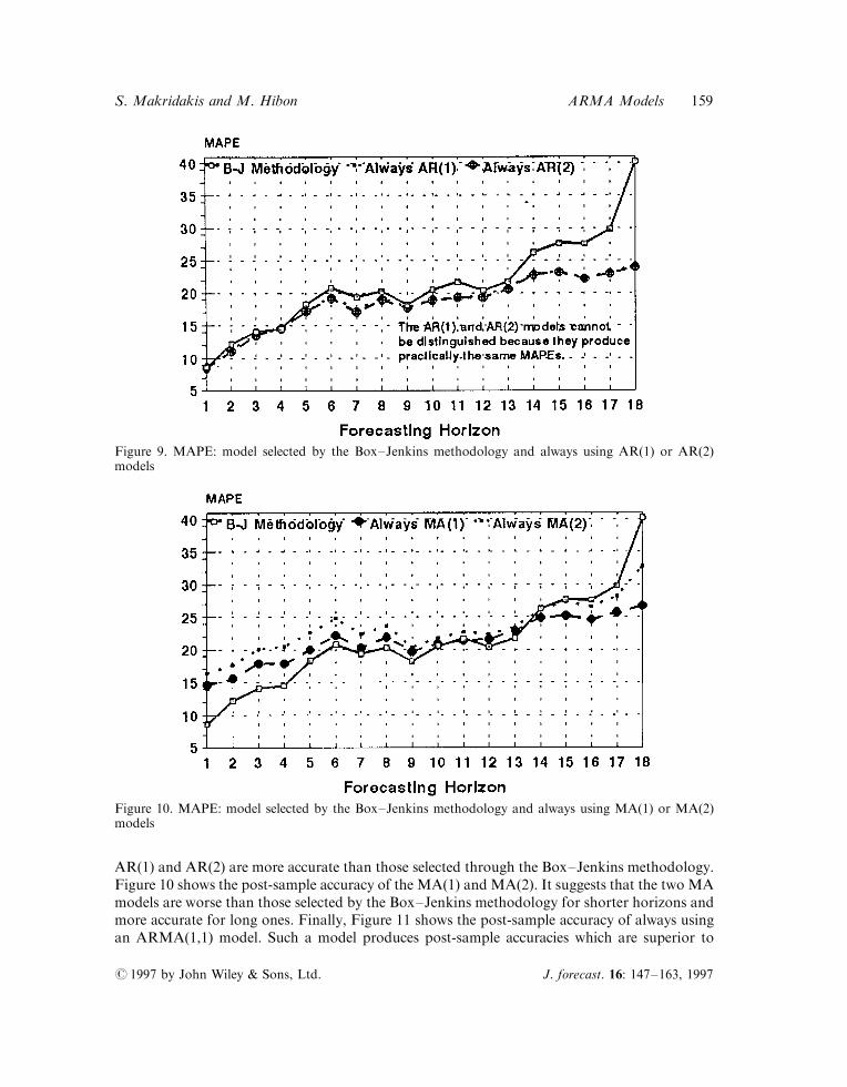
AR(1) and AR(2) are more accurate than those selected through the Box±Jenkins methodology.Figure 10 shows the post-sample accuracy of the MA(1) and MA(2). It suggests that the two MAmodels are worse than those selected by the Box±Jenkins methodology for shorter horizons andmore accurate for long ones. Finally, Figure 11 shows the post-sample accuracy of always usingan ARMA(1,1) model. Such a model produces post-sample accuracies which are superior to

Figure 9. MAPE: model selected by the Box±Jenkins methodology and always using AR(1) or AR(2)models

Figure 10. MAPE: model selected by the Box±Jenkins methodology and always using MA(1) or MA(2)models



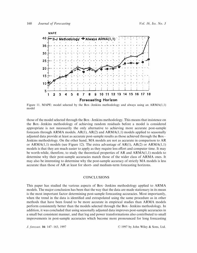
those of the model selected through the Box±Jenkins methodology. This means that insistence onthe Box±Jenkins methodology of achieving random residuals before a model is consideredappropriate is not necessarily the only alternative to achieving more accurate post-sampleforecasts through ARMA models. AR(1), AR(2) and ARMA(1,1) models applied to seasonallyadjusted data provide at least as accurate post-sample results as those achieved through the Box±Jenkins methodology. On the other hand, MA models are not as accurate in comparison to ARor ARMA(1,1) models (see Figure 12). The extra advantage of AR(1), AR(2) or ARMA(1,1)models is that they are much easier to apply as they require less e�ort and computer time. It maybe worth-while, therefore, to study the theoretical properties of AR and ARMA(1,1) models todetermine why their post-sample accuracies match those of the wider class of ARMA ones. Itmay also be interesting to determine why the post-sample accuracy of strictly MA models is lessaccurate than those of AR at least for short- and medium-term forecasting horizons.

CONCLUSIONS

This paper has studied the various aspects of Box±Jenkins methodology applied to ARMAmodels. The major conclusion has been that the way that the data are made stationary in its meanis the most important factor determining post-sample forecasting accuracies. Most importantly,when the trend in the data is identi®ed and extrapolated using the same procedure as in othermethods that have been found to be more accurate in empirical studies than ARMA modelsperform consistently better than the models selected through the Box±Jenkins methodology. Inaddition, it was concluded that using seasonally adjusted data improves post-sample accuracies ina small but consistent manner, and that log and power transformations also contributed to smallimprovements in post-sample accuracies which become more pronounced for long forecasting

Figure 11. MAPE: model selected by the Box±Jenkins methodology and always using an ARMA(1,1)model



horizons. Finally, it was concluded that AR(1), AR (2) or ARMA(1,1) models produced asaccurate post-sample predictions as those found by applying the automatic version of the Box±Jenkins methodology, suggesting that it is neither necessary, as far as post-sample accuracy isconcerned, to study the autocorrelations and partial autocorrelations to determine the mostappropriate ARMA model, nor to make sure that the residuals of such a model are necessarilyrandom.

REFERENCES

Andersen, A. and Weiss, A., `Forecasting: the Box±Jenkins approach', in Makridakis et al. (eds),The Forecasting Accuracy of Major Time Series Methods, Chichester: John Wiley, 1984.

Armstrong, J. S., `Forecasting with econometric methods: folklore versus fact with discussion', Journal ofBusiness, 51 (1978) 549±600.

Box, G. E. P. and Jenkins, G., Time Series Analysis, Forecasting and Control, San Francisco, CA: Holden-Day.

Box, G. E. P. and Pierce, D. A., `Distribution of the residual autocorrelations in autoregressive-integrated moving-average time series models', Journal of the American Statistical Association, 65 (1970),1509±26.

Brown, R. G., Statistical Forecasting for Inventory Control, New York: McGraw-Hill, 1954.Chat®eld, C. and Prothero, D. L., `Box±Jenkins seasonal forecasting: problems in a case study', Journal of

the Royal Statistical Society (A), 136 (1973), 295±336.Cogger, K. O., `The optimality of general-order exponential smoothing', Operations Research, 22 (1974),

858±67.Collopy, F. and Armstrong, J. S., `Rule-based forecasting', Management Science, 38 (1992), 1394±414.Cooper, R. L., `The predictive performance of quarterly econometric models of the United States',in Hickman, B. G. (ed.), Econometric Models of Cyclical Behavior, New York: National Bureau ofEconomic Research, 1972.

Figure 12. MAPE: model selected by the Box±Jenkins methodology and always using AR(1), MA(1),or ARMA(1,1) models



Durbin, J., `Comment on: Makridakis, S. and Hibon, M., `Àccuracy of forecasting: an empirical investi-gation'' ', Journal of the Royal Statistical Society (A), 142 (1979), 133±4.

Elliot, J. W., À direct comparison of short-run GNP forecasting models', Journal of Business, 46 (1973),33±60.

Fildes, R., Hibon, M., Makridakis, S. and Meade, N., `Generalising about univariate forecasting methods:further empirical evidence', International Journal of Forecasting, forthcoming (1997).

Gardner, E. S. Jr, and McKenzie, E., `Forecasting trends in time series', Management Science, 31 (1985),1237±46.

Geurts, M. D. and Ibrahim, I. B., `Comparing the Box±Jenkins approach with the exponentially smoothedforecasting model application to Hawaii tourists', Journal of Marketing Research, 12 (1975), 182±8.

Geurts, M. D. and Kelly, J. P., `Forecasting retail sales using alternative models', International Journal ofForecasting, 2 (1986), 261±72.

Granger, C. W. J. and Nelson, H., Èxperience using the Box±Cox transformation when forecastingeconomic time series', Working Paper 78 (1), Department of Economics, UCSD, 1978.

Gro�, G. K., Èmpirical comparison of models for short-range forecasting', Management Science, 20(1)(1973), 22±31.

Hill, G. and Fildes, R., `The accuracy of extrapolation methods: an automatic Box±Jenkins package SIFT',Journal of Forecasting, 3 (1984), 319±23.

Huss, W. R., `Comparative analysis of company forecasts and advanced time series techniques in theelectric utility industry', International Journal of Forecasting, 1 (1985), 217±39.

Jenkins, G. M., `Some practical aspects of forecasting in organizations', Journal of Forecasting, 1 (1982),3±21.

Koehler, A. B. and Murphree, E. S., À comparison of results from state space forecasting with forecastsfrom the Makridakis competition', International Journal of Forecasting, 4 (1988), 45±55.

Libert, G., `The M-competition with a fully automatic Box±Jenkins procedure', Journal of Forecasting, 2(1983), 325±8.

Lusk, E. J. and Neves, J. O., À comparative ARIMA analysis of the 111 Series of the Makridakiscompetition', Journal of Forecasting, 3 (1984), 329±32.

Makridakis, S. and Hibon, M., Àccuracy of forecasting: an empirical investigation (with discussion)',Journal of the Royal Statistical Society (A), 142 (1979), Part 2, 79±145 (lead article).

Makridakis, S. et al., `The accuracy of extrapolative (time series methods): results of a forecastingcompetition', Journal of Forecasting, 1 (1982), No. 2, 111±53 (lead article).

Makridakis, S., Wheelwright, S. and McGee, V., Forecasting Methods and Applications (2nd edition), NewYork: John Wiley, 1983.

Makridakis, S. et al., `The M-2 Competition: A real-time judgmentally-based forecasting study',International Journal of Forecasting, 9 (1993), No. 1, 5±23.

Marquardt, D. W., Àn algorithm for least squares estimation of non-linear parameters', Soc. Indust. Appl.Math., 11 (1963), 431±41.

McWhorter, A. Jr, `Time series forecasting using the Kalman ®lter: an empirical study', Proc. Amer.Statist. Ass., Business and Economics Section (1975), 436±46.

Meese, R. and Geweke, J., À comparison of autoregressive univariate forecasting procedures for macro-economic time series', Journal of Business and Economic Statistics, 2 (1984), 191±200.

Narasimham, ?. et al., Òn the predictive performance of the BEA quarterly econometric model and aBox±Jenkins type ARIMA model', Proceedings of the American Statistical Association: Business andEconomics Section (1974), 501±4.

Nelson, C. R., `The prediction performance of the FRB±MIT±PENN model of the US economy',American Economic Review, 5 (1972), 902±17.

Nelson, C. R. and Plosser, C. I., `Trends and random walks in macroeconomic time series: some evidenceand implications', Journal of Monetary Economics, 10 (1982), 139±62.

Newbold, P., `The competition to end all competitions', in Armstrong, J. S. and Lusk, E. J. (eds),`Commentary on the Makridakis time series competition (M-Competition)', Journal of Forecasting, 2(1983), 276±79.

Newton, H. J. and Parzen, E., `Forecasting and time series model types of 111 economic time series', inMakridakis, S. et al. (eds), The Forecasting Accuracy of Major Time Series Methods, Chichester: JohnWiley, 1984.



Parzen, E., `ARARMA models for time series analysis and forecasting', Journal of Forecasting, 1 (1982),67±82.

Pierce, D. A., `RelationshipsÐand the lack thereofÐbetween economic time series, with special referenceto money and interest rates', Journal of the American Statistical Association, 72 (1977), 11±26.

Schnaars, S. P., `A comparison of extrapolation models on yearly sales forecasts', International Journal ofForecasting, 2 (1986), 71±85.

Slutsky, E., `The summation of random causes as the source of cyclic processes', Econometrica, 5 (1937),105±46.

Stellwagen, E. A. and Goodrich, R. L., Forecast Pro-Batch Edition, New York: Business Forecast Systems,Inc., 1991.

Texter, P. A. and Ord, J. K., `Forecasting using automatic identi®cation procedures: A comparativeanalysis', International Journal of Forecasting, 5 (1989), 209±15.

Watson, M. W., Pastuszek, L. M., and Cody, E., `Forecasting commercial electricity sales', Journal ofForecasting, 6 (1987), 117±36.

Wold, H., A Study in the Analysis of Stationary Time Series, Stockholm: Almgrist & Wiksell, 1938.Yule, G. U., `Why do we sometimes get nonsense-correlations between time series? A study in samplingand the nature of time series', Journal of Royal Statistical Society, 89 (1926), 1±64.

Authors' address :Spyros Makridakis and MicheÁ le Hibon, INSEAD, Boulevard de Constance, 77305 Fontainebleau Cedex,France.



ARMA Models and the Box-Jenkins Methodology

Documents

Transcript of ARMA Models and the Box-Jenkins Methodology