This article appeared in a journal published by Elsevier. The attachedcopy is furnished to the author for internal non-commercial researchand education use, including for instruction at the authors institution

and sharing with colleagues.

Other uses, including reproduction and distribution, or selling orlicensing copies, or posting to personal, institutional or third party

websites are prohibited.

In most cases authors are permitted to post their version of thearticle (e.g. in Word or Tex form) to their personal website orinstitutional repository. Authors requiring further information

regarding Elsevier’s archiving and manuscript policies areencouraged to visit:

http://www.elsevier.com/authorsrights

Author's personal copy

Bayesian optimization of timeperceptionZhuanghua Shi1, Russell M. Church2, and Warren H. Meck3

1 Department of Psychology, Ludwig-Maximilians-Universitat Munchen, Munich, Germany2 Department of Cognitive, Linguistic, and Psychological Sciences, Brown University, Providence, Rhode Island, USA3 Department of Psychology and Neuroscience, Duke University, Durham, North Carolina, USA

Precise timing is crucial to decision-making and be-havioral control, yet subjective time can be easilydistorted by various temporal contexts. Applicationof a Bayesian framework to various forms of contex-tual calibration reveals that, contrary to popular belief,contextual biases in timing help to optimize overallperformance under noisy conditions. Here, we reviewrecent progress in understanding these forms of tem-poral calibration, and integrate a Bayesian frameworkwith information-processing models of timing. Weshow that the essential components of a Bayesianframework are closely related to the clock, memory,and decision stages used by these models, and thatsuch an integrated framework offers a new perspectiveon distortions in timing and time perception that areotherwise difficult to explain.

IntroductionHumans are often surprisingly accurate at timing inter-vals in the sub-second to minutes range during dailyroutines, as well as part of vocational and recreationalactivities [1]. We must judge the correct time to strike theright musical chord, adjust our running speed to be in theright place at the right time to catch a fly ball, and antici-pate when to begin pressing the button to open the doorwhen the subway train comes to a stop. However, oursubjective experience of time can be highly biased indifferent contexts [2–8]. For example, sounds are oftenjudged longer than lights, even when they are both ofthe same physical duration and have been matched forintensity [8]. Traditional timing models suggest that thesecontextual effects are associated with the differential decayof modality-specific representations, changes in the speedof the ‘internal clock’, and/or ‘memory mixing’ of differenttemporal representations [5,8–10]. Recently, researchershave used Bayesian inference to perform computational-level analysis on various forms of contextual calibration ofinterval timing and revealed that such adaptation mayhelp to improve overall performance [6,11–14]. Although

the Bayesian approach to optimization has provided manyimportant insights, exactly how these probabilistic distri-butions and inferences might be linked to temporal proces-sing at a mechanistic level remains uncertain.

In this article, we review recent progress in understand-ing the influence of contextual calibration on intervaltiming, with particular focus on ‘central-tendency’ and‘modality’ effects, as well as the time-order error (TOE).We then compare the different explanations for contextualcalibration made by Bayesian inference and traditionalinformation-processing models of interval timing. Finally,we provide a roadmap for integrating a Bayesian frame-work with existing timing models and point out the impli-cations and potential challenges associated with thisapproach.

Contextual calibration of time perceptionAs noted above, subjective durations can easily be dis-torted by various contextual factors. A classic example ofcontextual calibration is Vierordt’s law [15], also knownas the ‘central-tendency’ effect. When participants arepresented with a range of stimulus durations and arethen asked to reproduce those durations, they tend tooverproduce ‘short’ durations and underproduce ‘long’durations. This ‘central-tendency’ effect has beendemonstrated in numerous studies (for reviews, see[10,15]). A common explanation of this effect is thatduration judgments are derived not only from currentsensory inputs, but are also influenced by the acquiredstatistics (e.g., mean and standard deviation) of thedistribution of previously experienced stimulus dura-tions [5,6,8–10,15].

Interestingly, the ‘central-tendency’ effect has been ob-served to vary across different groups of individuals withvarious levels of experience, including musical expertise.For example, although individuals with little or no musicaltraining exhibit the ‘central-tendency’ effect for both audi-tory and visual stimuli, string musicians show very lowbiases for auditory duration reproduction. Moreover, ex-pert drummers are able to reproduce both auditory andvisual durations near perfection [16]. In contrast to healthyindividuals, patients with Parkinson’s disease (PD) aremore prone to contextual manipulation when tested offof their dopaminergic medication, referred to as a temporal‘migration’ effect [17]. When PD patients given dopamine-replacement therapy (e.g., L-dopa + apomorphine) aretrained to time-specific stimulus durations (e.g., 8 s and

Opinion

1364-6613/$ – see front matter

� 2013 Elsevier Ltd. All rights reserved. http://dx.doi.org/10.1016/j.tics.2013.09.009

Corresponding author: Meck, W.H. (meck@psych.duke.edu).Keywords: Bayesian inference; Vierordt’s law; contextual calibration; modalitydifferences; memory mixing; scalar timing theory.

556 Trends in Cognitive Sciences, November 2013, Vol. 17, No. 11

Author's personal copy

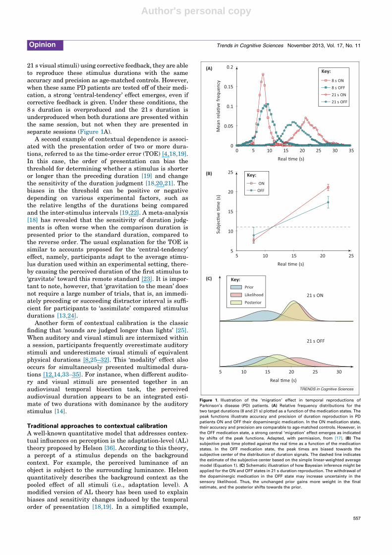
21 s visual stimuli) using corrective feedback, they are ableto reproduce these stimulus durations with the sameaccuracy and precision as age-matched controls. However,when these same PD patients are tested off of their medi-cation, a strong ‘central-tendency’ effect emerges, even ifcorrective feedback is given. Under these conditions, the8 s duration is overproduced and the 21 s duration isunderproduced when both durations are presented withinthe same session, but not when they are presented inseparate sessions (Figure 1A).

A second example of contextual dependence is associ-ated with the presentation order of two or more dura-tions, referred to as the time-order error (TOE) [4,18,19].In this case, the order of presentation can bias thethreshold for determining whether a stimulus is shorteror longer than the preceding duration [19] and changethe sensitivity of the duration judgment [18,20,21]. Thebiases in the threshold can be positive or negativedepending on various experimental factors, such asthe relative lengths of the durations being comparedand the inter-stimulus intervals [19,22]. A meta-analysis[18] has revealed that the sensitivity of duration judg-ments is often worse when the comparison duration ispresented prior to the standard duration, compared tothe reverse order. The usual explanation for the TOE issimilar to accounts proposed for the ‘central-tendency’effect, namely, participants adapt to the average stimu-lus duration used within an experimental setting, there-by causing the perceived duration of the first stimulus to‘gravitate’ toward this remote standard [23]. It is impor-tant to note, however, that ‘gravitation to the mean’ doesnot require a large number of trials, that is, an immedi-ately preceding or succeeding distractor interval is suffi-cient for participants to ‘assimilate’ compared stimulusdurations [13,24].

Another form of contextual calibration is the classicfinding that ‘sounds are judged longer than lights’ [25].When auditory and visual stimuli are intermixed withina session, participants frequently overestimate auditorystimuli and underestimate visual stimuli of equivalentphysical durations [8,25–32]. This ‘modality’ effect alsooccurs for simultaneously presented multimodal dura-tions [12,14,33–35]. For instance, when different audito-ry and visual stimuli are presented together in anaudiovisual temporal bisection task, the perceivedaudiovisual duration appears to be an integrated esti-mate of two durations with dominance by the auditorystimulus [14].

Traditional approaches to contextual calibrationA well-known quantitative model that addresses contex-tual influences on perception is the adaptation-level (AL)theory proposed by Helson [36]. According to this theory,a percept of a stimulus depends on the backgroundcontext. For example, the perceived luminance of anobject is subject to the surrounding luminance. Helsonquantitatively describes the background context as thepooled effect of all stimuli (i.e., adaptation level). Amodified version of AL theory has been used to explainbiases and sensitivity changes induced by the temporalorder of presentation [18,19]. In a simplified example,

Key:

Key:

(A)

(B)

(C)

0 5 10 15 20 25 30 350

0.05

0.1

0.15

0.2

Real �m e (s)

Mea

nre

la�v

efr

eque

ncy 8 s ON

8 s OFF

21 s ON

21 s OFF

5 10 15 20 255

10

15

20

25

Real �m e (s)

Subj

ec�v

e�m

e(s

)

ON

OFF

21 s OFF

21 s ON

5 10 15 20 25 30

Real �m e (s)

Prior

Key:

Likelihood

Posterior

TRENDS in Cognitive Sciences

Figure 1. Illustration of the ‘migration’ effect in temporal reproductions of

Parkinson’s disease (PD) patients. (A) Relative frequency distributions for the

two target durations (8 and 21 s) plotted as a function of the medication states. The

peak functions illustrate accuracy and precision of duration reproduction in PD

patients ON and OFF their dopaminergic medication. In the ON medication state,

their accuracy and precision are comparable to age-matched controls. However, in

the OFF medication state, a strong central ‘migration’ effect emerges as indicated

by shifts of the peak functions. Adapted, with permission, from [17]. (B) The

subjective peak time plotted against the real time as a function of the medication

states. In the OFF medication state, the peak times are biased towards the

subjective center of the distribution of duration signals. The dashed line indicates

the estimate of the subjective center based on the simple linear-weighted average

model (Equation 1). (C) Schematic illustration of how Bayesian inference might be

applied for the ON and OFF states in 21 s duration reproduction. The withdrawal of

the dopaminergic medication in the OFF state may increase uncertainty in the

sensory likelihood. Thus, the unchanged prior gains more weight in the final

estimate, and the posterior shifts towards the prior.

Opinion Trends in Cognitive Sciences November 2013, Vol. 17, No. 11

557

Author's personal copy

the perceived subjective interval d is a linear weightedaverage of the sensory evidence and context:

d ¼ ð1 � wÞs þ wdp; [1]

where s is the rescaled (e.g., logarithmic) value of thestimulus duration, dp is the subjective expectancy of stim-ulus durations, and w is the empirically determinedweighting constant that can be either positive or negative.When the weight w of the internal expectancy dp is posi-tive, the perceived duration d is attracted toward thecenter of the distribution. Thus, the simple ‘weightedaverage’ model also predicts Vierordt’s law for durationdiscrimination. Figure 1B shows how this linear-weightedmodel could explain the ‘migration’ effect for the reproduc-tion of stimulus durations observed in PD patients whentested off of their dopaminergic medication.

Scalar timing theory with its clock, memory, and deci-sion stages is the most common heuristic used to describethe cognitive processes involved in the contextual calibra-tion of duration discrimination [5,8–10,37–40]. The hall-mark of this model is that the standard deviation oftemporal estimates increases linearly with the mean ofthe duration being estimated – which is referred to as thescalar property (Box 1). Scalar timing theory typicallyassumes that a memory translation process induces the

scalar property [38,39,41], allowing violations of the scalarproperty to serve as an indicator of contextual influenceson timing and temporal memory. This leads to the ‘memo-ry-mixing’ account of modality differences [8–10], whichsuggests that contextual calibration arises from the mixingof auditory and visual durations within a shared memorydistribution. This account assumes that auditory stimulidrive the clock stage (composed of a pacemaker, switch,and accumulator) at a faster rate than visual stimuli and,as a consequence, the clock readings transferred intomemory are proportionally longer for auditory stimuli thanfor visual stimuli. Consequently, when the current clockreading is compared to a memory sample retrieved fromthis ‘mixed’ distribution, clock readings for auditory sti-muli will be judged (on average) to be longer and visualstimuli (on average) will be judged to be shorter than themean of the ‘mixed’ distribution. If auditory clock readingsare compared only with auditory memories and visualclock readings are compared only with visual memories,no modality differences consistent with changes in clockspeed should be observed [8]. An example of the ‘modality’effect in temporal bisection is illustrated in Figure 2A,where the ‘short’ (S) and ‘long’ (L) anchor durations consistof both auditory and visual stimuli, and intermediatecomparison durations of both modalities are randomly

Box 1. Information-processing (IP) models of interval timing and the scalar property

One of the best-developed models of interval timing is scalar timing

theory, which belongs to a class of information-processing models

that posit a dedicated ‘internal clock’ [5,37–40,77]. According to

scalar timing theory, the cognitive processes supporting interval

timing consist of three stages: clock, memory, and decision (Figure I,

Box 2). In order to represent a target duration, a pacemaker emits

pulses that are passed by a switch into an accumulator. The value in

the accumulator is assumed to be normally distributed [60], which is

then compared to the expected time sampled from reference

memory. If these values are close enough at the decision stage, a

response is made. When the entire response function obtained from

peak-interval/temporal generalization procedures is plotted on a

relative time scale for multiple target durations, the different

response functions typically superimpose with each other, which

demonstrates that interval timing adheres strongly to Weber’s law

[38,41,85–88]. This is called the scalar property of interval timing.

Evidence for superimposition in the peak-interval procedure is

illustrated in Figure I for human participants. Scalar timing theory

assumes the scalar property is introduced by a memory translation

constant k* [60,61,64–66], because variances in the clock and

decision stages are considered insufficient to account for the scalar

property ([38,39,41], but see [54,77]). The memory translation

constant k* is drawn from a normal distribution N(mk*, sk*), such

that this multiplication results in wider memory distributions for

longer durations than for shorter target durations (Figure I).

Systematic violations of the scalar property can occur when timed

intervals are selected from particular ranges or tested with selected

clinical populations (e.g., PD patients) [78,86,89,90]. These violations

of the scalar property suggest that multiple timing systems may

subserve different time scales and that contextual influences should

be considered more carefully in theoretical models of timing and

time perception.

(A)

(B)

S M L

‘S’

‘M’

‘L’

σs

σm

σl

Real �me

Subj

ec�v

e�m

e

0 10 20 30 400

100

200

300

Time (s)

Resp

onse

spe

rmin

ute

8 s

Key:

12 s21 s0 0.5 1 1.5 2

0

0.5

1

Rela�ve �me

TRENDS in Cognitive Sciences

Figure I. The scalar property of interval timing and evidence of superimposition

of peak–interval functions. (A) Scalar timing theory assumes that the estimation

error increases in proportion to the target interval (gray area), which leads to the

scalar property being exhibited for ‘short’ (S), ‘medium’ (M), and ‘long’ (L) target

durations. (B) Evidence of the scalar property from human participants. Mean

key presses per minute are plotted as a function of signal duration (s) for

participants trained with 8, 12, and 21 s target durations. The inset figure shows

that the response functions superimpose on each other when they are plotted as

a function of relative time. Adapted, with permission, from [91].

Opinion Trends in Cognitive Sciences November 2013, Vol. 17, No. 11

558

Author's personal copy

intermixed within a session [42]. As a result of this inter-mixing of stimulus modalities, the point of subjectiveequality (PSE) observed for auditory durations occurs atan earlier time than the PSE observed for visual durations.

Given that the external world is in constant flux, themixing of temporal memories is likely to accrue over timein order for the observer to adapt his/her timing behavior.Taatgen and Van Rijn [5], for example, found that the‘central-tendency’ effect was not only influenced by themixing of multiple durations, but also fluctuated as afunction of feedback and estimates of the stimulus dura-tions experienced on previous trials (recency effect). Simi-larly, Dyjas et al. [18] suggested that TOEs associated withsensitivity changes in duration comparisons are the result

of dynamic updating of internal referents,

In ¼ gIn�1 þ ð1 � gÞX1n; [2]

where I is the dynamic history of the internal referencefor the first interval and X1n is the current first interval.When the sensory estimate of the current first interval X1n

is presented, the mean interval reference In is thenupdated. In these approaches, the weights of prior historyand feedback are estimated by fitting a general linearmodel, which does not indicate whether the system usesan optimal strategy for dynamic updating. Nevertheless,when Equation 2 combines with Bayesian inference, it isreferred to as the application of a Kalman filter [43–45].The g in Equation 2 is referred to as ‘Kalman gain’, which isoptimally determined and updated dynamically by thevariances of the internal reference and the sensory esti-mate. The application of a Kalman filter has been sup-ported by a number of empirical studies that examined the‘central-tendency’ effect of distance reproduction [43,46],sensorimotor control [45], and multimodal recalibration[44,47].

Bayesian inference on temporal contextual calibrationThe combination of a linear-weighted average model andscalar timing theory provides a powerful approach toexplain various ‘memory-mixing’ phenomena [5,8–10,18],yet these approaches do not inform us as to what factor(s)quantitatively determine the level of contextual calibra-tion. Recent work using a Bayesian approach solves thisproblem by providing a quantitative prediction of thecontribution of temporal context and the mechanisms thatinvolve the subjective representation of duration [6,16,48–51] (Box 2). The basic logic of the Bayesian approach is thatsensory measurements are noisy and uncertain, and com-bining the prior knowledge of the statistical distribution ofa series of stimulus durations can be beneficial for increas-ing the precision of duration estimates, although incorpo-rating the prior may lead to systematic biases. In thissense, contextual effects are statistically optimal and serveto minimize error. Moreover, the trade-off between preci-sion and bias will depend on the magnitude of uncertaintyand the selected cost function [48].

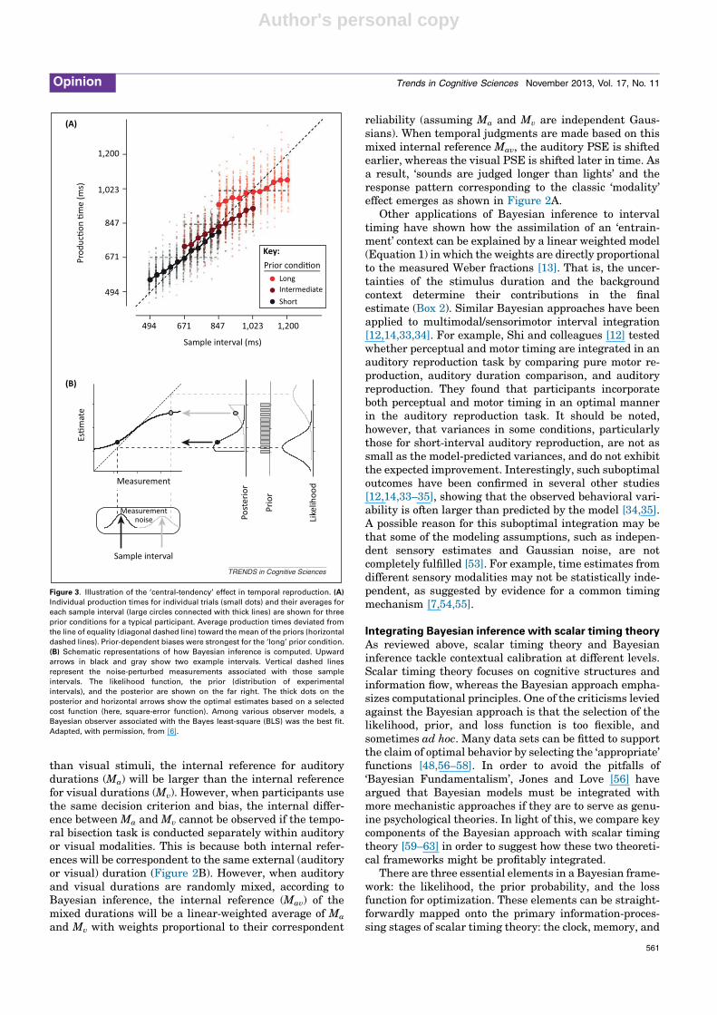
An impressive demonstration of how Bayesian inferencecan be used to predict the ‘central-tendency’ effect intemporal reproduction has been given by Jazayeri andShadlen [6]. In their study, participants were instructedto estimate a sample duration and reproduce it immedi-ately afterwards. For different blocks of trials, however,the sample durations were selected from three differentuniform distributions (i.e., ‘short’, ‘intermediate’, and ‘long’ranges) that partially overlapped with each other. Theresults revealed a strong ‘central-tendency’ effect in dura-tion reproduction as illustrated in Figure 3. Jazayeri andShadlen then used a Bayesian framework to show howdifferent types of observer models with variation in theapplication of the prior and the estimation error might beused in duration reproduction. They reported that the best-fitted model was the one using a Bayes least-square (BLS)rule (i.e., a square-error loss function; Box 2). The successof the BLS rule suggests that participants used the statis-tical information provided by the distribution of stimulus

(A)

(B)

2 3 4 5 6 7 80

0.25

0.5

0.75

1

Real �m e (s)

p(‘lo

ng’)

AuditoryVisual

S PSEa PSEv L

Mv

Mav

Ma

Subj

ec�v

e�m

e

Real �m e (s)

Audito ryVisual

Key:

Key:

TRENDS in Cognitive Sciences

Figure 2. Illustration of the ‘modality’ effect in temporal bisection. (A) Group

probability of a ‘long’ response, p(‘long’) functions averaged across participants

for auditory and visual stimulus durations presented in a 2 s vs 8 s bisection task.

Adapted, with permission, from [42]. (B) Schematic illustration for a Bayesian

inference account of the ‘modality’ effect in which pulses are integrated at a faster

rate for auditory stimuli than for visual stimuli due to differential rates of opening

and closing of the switch that allows pulses to flow from the pacemaker to the

accumulator [8,9]. As a consequence, the internal reference of the mean duration

between the ‘short’ (S) and ‘long’ (L) anchor durations is larger for auditory stimuli

(Ma) than for visual stimuli (Mv). These different internal representations

correspond to the same external duration indicated by the middle vertical

dashed line. When the auditory and visual durations are combined or mixed

within the same memory distribution, assuming that Ma and Mv are independent

Gaussians, the internal reference of the mixed durations (Mav) is a linear-weighted

average of Ma and Mv. Based on this mixed reference, the auditory and visual

points of subjective equality (PSE) are shifted in opposite directions – as indicated

by the filled squares and circles, respectively.

Opinion Trends in Cognitive Sciences November 2013, Vol. 17, No. 11

559

Author's personal copy

durations presented within a block of trials to minimizetheir overall temporal reproduction error [6].

The ‘modality’ effect [8] induced by the ‘memory mixing’of auditory and visual signals can also be quantitativelymodeled using Bayesian inference. Although the exact

decision-rules used in temporal bisection are still underdebate [52], one proposal is that a comparison is madebetween the current trial’s clock reading and an internalreference (M) of the mean duration (e.g., geometric mean ofS and L). Given that auditory stimuli drive the clock faster

Box 2. Bayesian inference of timing and linkage to information-processing models

Analogous to the classic information-processing (IP) models that

involve clock, memory, and decision stages, Bayesian inference has

three essential components: likelihood, prior distribution, and loss

function [45,48,92,93]. As illustrated in Figure I, two frameworks are

closely linked to each other.

Suppose that we have an external duration D, with an associated

internal clock reading S that represents the number of pulses in the

accumulator at the end of D. The likelihood function P(SjD) is the

probability distribution of obtaining a clock-reading S for a given

external duration D. The spread of the likelihood indicates the

uncertainty of sensory measurement. At the memory stage, sensory

estimates of the target duration update the prior distribution P(D) in

reference memory. Meanwhile, the prior knowledge may influence

the memory representation of the current clock reading. According to

Bayes’ rule, the probability of having an external duration D for a

given clock-reading S is determined by the sensory likelihood and the

prior knowledge of target durations P(D):

PðDjSÞ ¼ PðSjDÞPðDÞPðSÞ [I]

The probability distribution P(DjS) is known as the posterior

probability. Given the posterior probability, the Bayesian ideal-

observer next has to make an optimal decision or choose an action

based on the loss function, a function that specifies how the

system rates the relative success or cost of a particular response

[45,50,67], that is, the costs associated with a function of

estimation error ðD � DÞ. The most frequently used loss functions

for modeling behavior are the squared-error L ¼ D � D� �2

[50,67],

or relative squared-error L0 ¼ 1 � D=D� �2

functions [50,94]. The

latter is comparable to the ratio rule used in classic IP models to

achieve the scalar property [38,95].

When the likelihood and the prior are independent Gaussians, that

is, P(S|D) � N(ms, ss), P(D) � N(mp, sp), the optimal estimate by

minimizing the loss function L is:

d ¼ ð1 � w pÞms þ w pmp [II]

where w p ¼1=s2

p

1=s2pþ1=s2

s

is proportional to its inversed variances

(Figure I). The variance of this optimal estimate iss2

ps2s

s2pþs2

s

, which is

the minimum variance among all possible linear weighted combina-

tions between the sensory estimate and the prior [92,93,96]. When

there are two conditional independent likelihood functions, and the

prior is not the focus factor and can be assumed to be uniform,

Bayesian optimization is equivalent to maximum likelihood estima-

tion (MEL). The optimal estimate is also a linear weighted average of

individual sensory estimates:

d ¼ wama þ wbmb [III]

where ma and mb are the mean estimates of two individual signal

durations, and wa and wb are their corresponding weights that are

proportional to their inversed variances.

Clock stage

Memory stage

Decision stage

Pacemaker Switch Accumulator

Working memory

Reference memory

Comparator R

∼ R

D DD < ∈

IP model

μp

μp

σ p

σ s

σ d

d

Likelihood

Prior

Poste rior

Loss func�on L = (D–D)2ˆ

Bayesia n in ference

TRENDS in Cognitive Sciences

Figure I. An information-processing (IP) model of scalar timing theory and Bayesian inference of time estimation. The left panel shows an IP model of time perception

involving clock, memory, and decision stages. The right panel illustrates that the three key components of Bayesian inference are closely matched to the three stages of

the IP model. The sensory likelihood is derived from the clock stage. The prior represents the durations stored in the reference memory, which is updated by current

estimates (dashed black arrow). The posterior reflects the probability distribution of the current estimate, combining the clock reading and the influence of the reference

memory (indicated by the dashed red arrow). In the decision stage, responses are made based on specific comparison rules. The goal of Bayesian interference is to

minimize the loss function, whereas the comparator of the IP model uses a relative discrimination threshold.

Opinion Trends in Cognitive Sciences November 2013, Vol. 17, No. 11

560

Author's personal copy

than visual stimuli, the internal reference for auditorydurations (Ma) will be larger than the internal referencefor visual durations (Mv). However, when participants usethe same decision criterion and bias, the internal differ-ence between Ma and Mv cannot be observed if the tempo-ral bisection task is conducted separately within auditoryor visual modalities. This is because both internal refer-ences will be correspondent to the same external (auditoryor visual) duration (Figure 2B). However, when auditoryand visual durations are randomly mixed, according toBayesian inference, the internal reference (Mav) of themixed durations will be a linear-weighted average of Ma

and Mv with weights proportional to their correspondent

reliability (assuming Ma and Mv are independent Gaus-sians). When temporal judgments are made based on thismixed internal reference Mav, the auditory PSE is shiftedearlier, whereas the visual PSE is shifted later in time. Asa result, ‘sounds are judged longer than lights’ and theresponse pattern corresponding to the classic ‘modality’effect emerges as shown in Figure 2A.

Other applications of Bayesian inference to intervaltiming have shown how the assimilation of an ‘entrain-ment’ context can be explained by a linear weighted model(Equation 1) in which the weights are directly proportionalto the measured Weber fractions [13]. That is, the uncer-tainties of the stimulus duration and the backgroundcontext determine their contributions in the finalestimate (Box 2). Similar Bayesian approaches have beenapplied to multimodal/sensorimotor interval integration[12,14,33,34]. For example, Shi and colleagues [12] testedwhether perceptual and motor timing are integrated in anauditory reproduction task by comparing pure motor re-production, auditory duration comparison, and auditoryreproduction. They found that participants incorporateboth perceptual and motor timing in an optimal mannerin the auditory reproduction task. It should be noted,however, that variances in some conditions, particularlythose for short-interval auditory reproduction, are not assmall as the model-predicted variances, and do not exhibitthe expected improvement. Interestingly, such suboptimaloutcomes have been confirmed in several other studies[12,14,33–35], showing that the observed behavioral vari-ability is often larger than predicted by the model [34,35].A possible reason for this suboptimal integration may bethat some of the modeling assumptions, such as indepen-dent sensory estimates and Gaussian noise, are notcompletely fulfilled [53]. For example, time estimates fromdifferent sensory modalities may not be statistically inde-pendent, as suggested by evidence for a common timingmechanism [7,54,55].

Integrating Bayesian inference with scalar timing theoryAs reviewed above, scalar timing theory and Bayesianinference tackle contextual calibration at different levels.Scalar timing theory focuses on cognitive structures andinformation flow, whereas the Bayesian approach empha-sizes computational principles. One of the criticisms leviedagainst the Bayesian approach is that the selection of thelikelihood, prior, and loss function is too flexible, andsometimes ad hoc. Many data sets can be fitted to supportthe claim of optimal behavior by selecting the ‘appropriate’functions [48,56–58]. In order to avoid the pitfalls of‘Bayesian Fundamentalism’, Jones and Love [56] haveargued that Bayesian models must be integrated withmore mechanistic approaches if they are to serve as genu-ine psychological theories. In light of this, we compare keycomponents of the Bayesian approach with scalar timingtheory [59–63] in order to suggest how these two theoreti-cal frameworks might be profitably integrated.

There are three essential elements in a Bayesian frame-work: the likelihood, the prior probability, and the lossfunction for optimization. These elements can be straight-forwardly mapped onto the primary information-proces-sing stages of scalar timing theory: the clock, memory, and

(A)

(B)

Prod

uc�o

n �m

e (m

s)Es

�mat

e

Post

erio

r

Prio

r

Like

lihoo

d

1,200

1,023

847

671

494

Sample interval (ms)

Sample interval

Measurement

Measurement

494 671 847 1,023 1,200

Prior condi�onKey:

LongIntermediateShort

noise

TRENDS in Cognitive Sciences

Figure 3. Illustration of the ‘central-tendency’ effect in temporal reproduction. (A)

Individual production times for individual trials (small dots) and their averages for

each sample interval (large circles connected with thick lines) are shown for three

prior conditions for a typical participant. Average production times deviated from

the line of equality (diagonal dashed line) toward the mean of the priors (horizontal

dashed lines). Prior-dependent biases were strongest for the ‘long’ prior condition.

(B) Schematic representations of how Bayesian inference is computed. Upward

arrows in black and gray show two example intervals. Vertical dashed lines

represent the noise-perturbed measurements associated with those sample

intervals. The likelihood function, the prior (distribution of experimental

intervals), and the posterior are shown on the far right. The thick dots on the

posterior and horizontal arrows show the optimal estimates based on a selected

cost function (here, square-error function). Among various observer models, a

Bayesian observer associated with the Bayes least-square (BLS) was the best fit.

Adapted, with permission, from [6].

Opinion Trends in Cognitive Sciences November 2013, Vol. 17, No. 11

561

Author's personal copy

decision stages (Box 2). The clock stage is responsible forthe measurement of the duration of an external event,which is subject to noise perturbation. The Bayesian like-lihood function provides a probability description of a givenmeasurement, conditional on a given physical duration.Scalar timing theory assumes two separate memory repre-sentations: a working memory that is able to temporarilystore the current clock reading and a reference memorythat serves as a long-term store or reference of all recordedclock readings relevant to a particular context. From theBayesian perspective, the prior quantifies the probabilitydistribution of the internal reference and the posteriorrepresents the probability of the memory representationof the current clock reading. In the end, both frameworksimplement some type of decision rule in order to generate aresponse. In this view, scalar timing theory provides arational basis for selecting the appropriate Bayesian func-tions, and the Bayesian framework provides probabilisticdescriptions of temporal processing.

Underlying the linkage of the two frameworks, however,are several key differences and a number of importantconstraints. The main difference comes from the implemen-tation of the scalar property. Scalar timing theory assumesthat the scalar property is introduced by the memory con-stant, k*, applied during encoding [60,61,64–66]. By con-trast, the general Bayesian framework does not provide anyspecific assumptions concerning the scalar property. How-ever, in experimental applications of Bayesian inference[6,50], the scalar property is often incorporated into thelikelihood distribution in order to provide consistency withthe obtained data. Recent evidence [50] supports this as-sumption, suggesting that the scalar property may in factoriginate from the clock stage. The second main differencebetween the two frameworks is in regard to memory updat-ing. In order to account for the effects of contextual calibra-tion, the memory stage of scalar timing theory has beenextended from the original working and reference memorycomponents [38,39] to include the processes of ‘memorymixing’ [8–10,40], and dynamic memory updating [5,18].By contrast, Bayesian inference offers a simple and conciseapproach for updating memory representations, namelyBayes’ rule. However, selection of the appropriate likeli-hoods and priors must be done in conjunction with a specificapplication. The third and final difference that we willdiscuss involves the decision rules applied by the two frame-works. Scalar timing theory strongly favors a ratio-ruleapproach (i.e., relative error – Figure I, Box 2) [38,41,52]for duration comparisons, largely because it is compatiblewith the scalar property introduced by the memory transla-tion constant. In the Bayesian framework, the decision ruleis used to minimize the overall error based on a loss function,whereas the loss function depends on a specific application.The most common loss function used by the Bayesian ap-proach is the square-error function (Box 2), which has beenshown to be in good agreement with empirical findings[50,67].

Obtaining a better understanding of the interactionsbetween the Bayesian framework and scalar timing theoryshould help us to develop more robust theories of intervaltiming that are able to handle various types of contextualcalibration, while also shedding light on the manner in

which probabilistic representations are implemented inneural circuits [56,58,68]. For instance, the observation thatdopaminergic and cholinergic drugs have different effects onthe clock and memory stages of interval timing [61,69–71]suggests that novel pharmacological techniques may pro-vide useful tools for studying the neural implementation ofprobabilistic representations [72] – although the specificdetails remain to be tested. Interestingly, the ‘migration’effects observed in PD patients suggest that the likelihoodfunction is flattened by the withdrawal of dopaminergicmedication, which is required to maintain more normalfunctioning of the clock stage in PD patients. Thus, theunchanged prior gains more weight in the final estimate(Figure 1C). In this manner, dopamine-deficient individualsappear to be able to balance performance by reducing tem-poral uncertainty at the cost of temporal accuracy [11].Integrating Bayesian inference with scalar timing theorycould also be beneficial in explaining other forms of contex-tual calibration, including the influences of non-temporalfactors (e.g., background intensity, speed/sequence struc-ture) [4,73–75].

Concluding remarksUnder ordinary circumstances, the representations ofevent durations are ‘calibrated’ by various forms of tempo-ral context. These contextual calibrations include ‘migra-tion’ toward the central tendency of a distribution(Vierordt’s law), TOEs, and modality differences. Applica-tion of scalar timing theory suggests that contextual cali-bration of event durations occurs mainly at the memorystage [8–10]. On the other hand, recent Bayesianapproaches point out that the likely reason for such cali-bration is an effort to improve timed performance byreducing the overall error [6,13,76]. In an effort to resolvethese apparent incompatibilities, we have shown that thethree essential components of a Bayesian framework (i.e.,likelihood, prior, and loss function) are closely linked to theclock, memory, and decision stages advocated by scalartiming theory and incorporated into other timing models[40,69,77]. The matched counterparts of a Bayesian frame-work combined with scalar timing theory not only providesa forward-looking perspective on interval timing, but alsooffers quantitative predictions of distortions in temporalmemory for normal participants, as well as for individualswith neurological impairments [78,79]. It is worth noting,however, that many aspects of interval timing remainunsolved (Box 3), even for relatively simple temporal

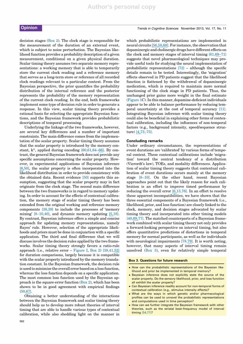
Box 3. Questions for future research

� How can the probabilistic representations of the Bayesian like-

lihood and prior be implemented in temporal memory?

� Bayesian inference does not explicitly state the source of the

scalar property. Do the sensory likelihood, prior, and loss function

all exhibit the scalar property?

� Can Bayesian inference readily account for non-temporal forms of

contextual calibration (e.g., stimulus intensity effects)?

� What are the ways in which genetic and/or pharmacological

profiles can be used to unravel the probabilistic representations

and computations used in time perception?

� How can we further integrate the Bayesian framework with other

theories, such as the striatal beat–frequency model of interval

timing [54,77]?

Opinion Trends in Cognitive Sciences November 2013, Vol. 17, No. 11

562

Author's personal copy

discrimination and generalization tasks [40,80]. Contin-ued application of an integrated Bayesian framework withmechanic-level theories, such as scalar timing theory andthe striatal beat–frequency model of interval timing [54],should help us to expand our understanding of the func-tional and neural mechanisms of interval timing [81–84].

AcknowledgmentsWe thank David Burr, Cindy Lustig, William Matthews, and Hedderikvan Rijn for their constructive comments on an earlier version of themanuscript. This work was supported, in part, by German Researchcouncil (DFG) project grant SH166 to ZS and an Aiken FoundationFellowship to WHM.

References1 Buhusi, C.V. and Meck, W.H. (2005) What makes us tick? Functional and

neural mechanisms of interval timing. Nat. Rev. Neurosci. 6, 755–7652 Buhusi, C.V. and Meck, W.H. (2009) Relative time sharing: new

findings and an extension of the resource allocation model oftemporal processing. Philos. Trans. R. Soc. Lond. B: Biol. Sci. 364,1875–1885

3 Buhusi, C.V. and Meck, W.H. (2009) Relativity theory and timeperception: single or multiple clocks? PLoS ONE 4, e6268

4 Grondin, S. (2010) Timing and time perception: a review of recentbehavioral and neuroscience findings and theoretical directions. Atten.Percept. Psychophys. 72, 561–582

5 Taatgen, N. and van Rijn, H. (2011) Traces of times past:representations of temporal intervals in memory. Mem. Cogn. 39,1546–1560

6 Jazayeri, M. and Shadlen, M.N. (2010) Temporal context calibratesinterval timing. Nat. Neurosci. 13, 1020–1026

7 Merchant, H. et al. (2013) Neural basis of the perception and estimationof time. Annu. Rev. Neurosci. 36, 313–336

8 Penney, T.B. et al. (2000) Differential effects of auditory and visualsignals on clock speed and temporal memory. J. Exp. Psychol. Hum.Percept. Perform. 26, 1770–1787

9 Penney, T.B. et al. (1998) Memory mixing in duration bisection. InTiming of Behavior: Neural, Psychological and ComputationalPerspectives (Rosenbaum, D.A. and Collyer, C.E., eds), pp. 165–193,MIT Press

10 Gu, B-M. and Meck, W.H. (2011) New perspectives on Vierordt’s law:memory-mixing in ordinal temporal comparison tasks. Lect. NotesComput. Sci. 6789, 67–78

11 Gu, B-M. et al. Bayesian models of interval timing and distortions intemporal memory as a function of Parkinson’s disease and dopamine-related error processing. In Time Distortions in Mind: TemporalProcessing in Clinical Populations (Vatakis, A. and Allman, M.J.,eds), Brill Academic Publishers (in press)

12 Shi, Z. et al. (2013) Reducing bias in auditory duration reproduction byintegrating the reproduced signal. PLoS ONE 8, e62065

13 Burr, D. et al. (2013) Contextual effects in interval-durationjudgements in vision, audition and touch. Exp. Brain Res. 230, 87–98

14 Burr, D.C. et al. (2009) Auditory dominance over vision in theperception of interval duration. Exp. Brain Res. 198, 49–57

15 Lejeune, H. and Wearden, J.H. (2009) Vierordt’s The ExperimentalStudy of the Time Sense (1868) and its legacy. Eur. J. Cogn. Psychol.21, 941–960

16 Cicchini, G.M. et al. (2012) Optimal encoding of interval timing inexpert percussionists. J. Neurosci. 32, 1056–1060

17 Malapani, C. et al. (1998) Coupled temporal memories in Parkinson’sdisease: a dopamine-related dysfunction. J. Cogn. Neurosci. 10, 316–331

18 Dyjas, O. et al. (2012) Trial-by-trial updating of an internal reference indiscrimination tasks: evidence from effects of stimulus order and trialsequence. Atten. Percept. Psychophys. 74, 1819–1841

19 Hellstrom, A. (2003) Comparison is not just subtraction: effects of time-and space-order on subjective stimulus difference. Percept. Psychophys.65, 1161–1177

20 Yeshurun, Y. et al. (2008) Bias and sensitivity in two-interval forcedchoice procedures: tests of the difference model. Vision Res. 48, 1837–1851

21 Ulrich, R. and Vorberg, D. (2009) Estimating the difference limen in2AFC tasks: pitfalls and improved estimators. Atten. Percept.Psychophys. 71, 1219–1227

22 Hellstrom, A. (1985) The time-order error and its relatives: mirrors ofcognitive processes in comparing. Psychol. Bull. 97, 35–61

23 Allan, L.G. (1979) The perception of time. Percept. Psychophys. 26, 340–354

24 Spencer, R.M. et al. (2009) Evaluating dedicated and intrinsic models oftemporal encoding by varying context. Philos. Trans. R. Soc. Lond. B:Biol. Sci. 364, 1853–1863

25 Wearden, J.H. et al. (1998) Why ‘sounds are judged longer than lights’:application of a model of the internal clock in humans. Q. J. Exp.Psychol. 51B, 97–120

26 Cheng, R.K. et al. (2011) Categorical scaling of duration as a function oftemporal context in aged rats. Brain Res. 1381, 175–186

27 Cheng, R.K. et al. (2008) Prenatal-choline supplementationdifferentially modulates timing of auditory and visual stimuli inaged rats. Brain Res. 1237, 167–175

28 Wearden, J.H. et al. (2006) When do auditory/visual differences induration judgements occur? Q. J. Exp. Psychol. 59, 1709–1724

29 Droit-Volet, S. et al. (2007) Sensory modality and time perception inchildren and adults. Behav. Processes 74, 244–250

30 Cheng, R.K. and Meck, W.H. (2007) Prenatal choline supplementationincreases sensitivity to time by reducing non-scalar sources of variancein adult temporal processing. Brain Res. 1186, 242–254

31 Lustig, C. and Meck, W.H. (2011) Modality differences in timing andtemporal memory throughout the lifespan. Brain Cogn. 77, 298–303

32 Ogden, R.S. et al. (2010) Are memories for duration modality specific?Q. J. Exp. Psychol. 63, 65–80

33 Shi, Z. et al. (2010) Auditory temporal modulation of the visual Ternuseffect: the influence of time interval. Exp. Brain Res. 203, 723–735

34 Hartcher-O’Brien, J. and Alais, D. (2011) Temporal ventriloquism in apurely temporal context. J. Exp. Psychol. Hum. Percept. Perform. 37,1383–1395

35 Tomassini, A. et al. (2011) Perceived duration of visual and tactilestimuli depends on perceived speed. Front. Integr. Neurosci. 5, 51

36 Helson, H. (1964) Adaptation-Level Theory, Harper & Row37 Zakay, D. and Block, R.A. (1997) Temporal cognition. Curr. Dir.

Psychol. Sci. 6, 12–1638 Gibbon, J. et al. (1984) Scalar timing in memory. Ann. N. Y. Acad. Sci.

423, 52–7739 Gibbon, J. and Church, R.M. (1984) Sources of variance in an

information processing theory of timing. In Animal Cognition(Roitblat, H.L. et al., eds), pp. 465–488, Lawrence Erlbaum

40 Allman, M.J. et al. Properties of the internal clock: first- and second-order principles of subjective time. Annu. Rev. Psychol. (in press)

41 Gibbon, J. (1992) Ubiquity of scalar timing with a Poisson clock. J.Math. Psychol. 35, 283–293

42 Melgire, M. et al. (2005) Auditory/visual duration bisection in patientswith left or right medial-temporal lobe resection. Brain Cogn. 58, 119–124

43 Petzschner, F.H. and Glasauer, S. (2011) Iterative Bayesian estimationas an explanation for range and regression effects: a study on humanpath integration. J. Neurosci. 31, 17220–17229

44 Ernst, M.O. and Di Luca, M. (2011) Multisensory perception: fromintegration to remapping. In Sensory Cue Integration(Trommershauser, J. et al., eds), pp. 224–250, Oxford UniversityPress

45 Wolpert, D.M. (2007) Probabilistic models in human sensorimotorcontrol. Hum. Mov. Sci. 26, 511–524

46 Petzschner, F.H. et al. (2012) Combining symbolic cues with sensoryinput and prior experience in an iterative Bayesian framework. Front.Integr. Neurosci. 6, 58

47 Burge, J. et al. (2008) The statistical determinants of adaptation rate inhuman reaching. J. Vision 8, 1–19 http://dx.doi.org/10.1167/8.4.20

48 Mamassian, P. and Landy, M.S. (2010) It’s that time again. Nat.Neurosci. 13, 914–916

49 Miyazaki, M. et al. (2005) Testing Bayesian models of humancoincidence timing. J. Neurophysiol. 94, 395–399

50 Acerbi, L. et al. (2012) Internal representations of temporal statisticsand feedback calibrate motor-sensory interval timing. PLoS Comput.Biol. 8, e1002771

Opinion Trends in Cognitive Sciences November 2013, Vol. 17, No. 11

563

Author's personal copy

51 Sohn, H. and Lee, S-H. (2013) Dichotomy in perceptual learning ofinterval timing: calibration of mean accuracy and precision differ inspecificity and time course. J. Neurophysiol. 109, 344–362

52 Penney, T.B. et al. (2008) Categorical scaling of duration bisection inpigeons (Columba livia), mice (Mus musculus), and humans (Homosapiens). Psychol. Sci. 19, 1103–1109

53 Ernst, M.O. (2012) Optimal multisensory integration: assumptions andlimits. In The New Handbook of Multisensory Processes (Stein, B.E.,ed.), pp. 1084–1124, MIT Press

54 Matell, M.S. and Meck, W.H. (2004) Cortico-striatal circuits andinterval timing: coincidence detection of oscillatory processes. Cogn.Brain Res. 21, 139–170

55 Ivry, R.B. and Hazeltine, R.E. (1995) Perception and production oftemporal intervals across a range of durations: evidence for acommon timing mechanism. J. Exp. Psychol. Hum. Percept. Perform.21, 3–18

56 Jones, M. and Love, B.C. (2011) Bayesian fundamentalism orenlightenment? On the explanatory status and theoreticalcontributions of Bayesian models of cognition. Behav. Brain Sci. 34,169–188

57 Bowers, J.S. and Davis, C.J. (2012) Bayesian just-so stories inpsychology and neuroscience. Psychol. Bull. 138, 389–414

58 Pouget, A. et al. (2013) Probabilistic brains: knowns and unknowns.Nat. Neurosci. 16, 1170–1178

59 Church, R.M. (1984) Properties of the internal clock. Ann. N. Y. Acad.Sci. 423, 566–582

60 Meck, W.H. (1983) Selective adjustment of the speed of internal clockand memory processes. J. Exp. Psychol. Anim. Behav. Process. 9, 171–201

61 Meck, W.H. (1996) Neuropharmacology of timing and time perception.Cogn. Brain Res. 3, 227–242

62 Meck, W.H. (2006) Neuroanatomical localization of an internal clock: afunctional link between mesolimbic, nigrostriatal, and mesocorticaldopaminergic systems. Brain Res. 1109, 93–107

63 Church, R.M. (2003) A concise introduction to scalar timing theory. InFunctional and Neural Mechanisms of Interval Timing (Meck, W.H.,ed.), pp. 3–22, CRC Press

64 Meck, W.H. (2002) Choline uptake in the frontal cortex is proportionalto the absolute error of a temporal memory translation constant inmature and aged rats. Learn. Motiv. 33, 88–104

65 Meck, W.H. and Angell, K.E. (1992) Repeated administration ofpyrithiamine leads to a proportional increase in the remembereddurations of events. Psychobiology 20, 39–46

66 Meck, W.H. and Church, R.M. (1987) Cholinergic modulation of thecontent of temporal memory. Behav. Neurosci. 101, 457–464

67 Kording, K.P. and Wolpert, D.M. (2004) The loss function ofsensorimotor learning. Proc. Natl. Acad. Sci. U.S.A. 101, 9839–9842

68 Drugowitsch, J. and Pouget, A. (2012) Probabilistic vs. non-probabilistic approaches to the neurobiology of perceptual decision-making. Curr. Opin. Neurobiol. 22, 963–969

69 Oprisan, S.A. and Buhusi, C.V. (2011) Modeling pharmacological clockand memory patterns of interval timing in a striatal beat-frequencymodel with realistic, noisy neurons. Front. Integr. Neurosci. 5, 52

70 Coull, J.T. et al. (2011) Neuroanatomical and neurochemical substratesof timing. Neuropsychopharmacology 36, 3–25

71 71 Meck, W.H. et al. (2013) Hippocampus, time, and memory – aretrospective analysis. Behav. Neurosci. 127, 642–654

72 Farrell, M.S. (2011) Using DREADDs to isolate internal clocks. Front.Integr. Neurosci. 5, 87

73 Matthews, W.J. (2013) How does sequence structure affect thejudgment of time? Exploring a weighted sum of segments model.Cogn. Psychol. 66, 259–282

74 Matthews, W.J. et al. (2011) Stimulus intensity and the perception ofduration. J. Exp. Psychol. Hum. Percept. Perform. 37, 303–313

75 Eagleman, D.M. and Pariyadath, V. (2009) Is subjective duration asignature of coding efficiency? Philos. Trans. R. Soc. Lond. B: Biol. Sci.364, 1841–1851

76 Simen, P. et al. (2011) A model of interval timing by neural integration.J. Neurosci. 31, 9238–9253

77 Van Rijn, H. et al. (2013) Dedicated clock/timing-circuit theories ofinterval timing. In Neurobiology of Interval Timing (Merchant, H. andde Lafuente, V., eds), Springer-Verlag (in press)

78 Allman, M.J. and Meck, W.H. (2012) Pathophysiological distortions intime perception and timed performance. Brain 135, 656–677

79 Allman, M.J. et al. (2012) Developmental neuroscience of time andnumber: implications for autism and other neurodevelopmentaldisabilities. Front. Integr. Neurosci. 6, 7

80 Heinemann, E.G. (1984) A model for temporal generalization anddiscrimination. Ann. N. Y. Acad. Sci. 423, 361–371

81 Meck, W.H. (2003) Functional and Neural Mechanisms of IntervalTiming, CRC Press

82 Freestone, D.M. et al. (2013) Response rates are governed more by timecues than contingency. Timing Time Percept. 1, 3–20

83 Lewis, P.A. and Meck, W.H. (2012) Time and the sleeping brain.Psychologist 25, 594–597

84 Meck, W.H. et al. (2012) Interval timing and time-based decisionmaking. Front. Integr. Neurosci. 6, 13

85 Buhusi, C.V. et al. (2009) Interval timing accuracy and scalar timing inC57BL/6 mice. Behav. Neurosci. 123, 1102–1113

86 Gibbon, J. et al. (1997) Toward a neurobiology of temporal cognition:advances and challenges. Curr. Opin. Neurobiol. 7, 170–184

87 Brannon, E.M. et al. (2008) Electrophysiological measures of timeprocessing in infant and adult brains: Weber’s law holds. J. Cogn.Neurosci. 20, 193–203

88 Church, R.M. et al. (1991) Symmetrical and asymmetrical sources ofvariance in temporal generalization. Anim. Learn. Behav. 19, 207–214

89 Lewis, P.A. and Miall, R.C. (2009) The precision of temporaljudgement: milliseconds, many minutes, and beyond. Philos. Trans.R. Soc. Lond. B: Biol. Sci. 364, 1897–1905

90 Wearden, J.H. and Lejeune, H. (2008) Scalar properties in humantiming: conformity and violations. Q. J. Exp. Psychol. 61, 569–587

91 Rakitin, B.C. et al. (1998) Scalar expectancy theory and peak-intervaltiming in humans. J. Exp. Psychol. Anim. Behav. Process. 24, 15–33

92 Kording, K.P. and Wolpert, D.M. (2004) Bayesian integration insensorimotor learning. Nature 427, 244–247

93 Kording, K.P. and Wolpert, D.M. (2006) Bayesian decision theory insensorimotor control. Trends Cogn. Sci. 10, 319–326

94 Sun, J.Z. et al. (2012) A framework for Bayesian optimality ofpsychophysical laws. J. Math. Psychol. 56, 495–501

95 Gibbon, J. and Church, R.M. (1990) Representation of time. Cognition37, 23–54

96 Griffiths, T.L. et al. (2008) Bayesian models of cognition. In TheCambridge Handbook of Computational Psychology (Sun, R., ed.),pp. 1–49, Cambridge University Press

Opinion Trends in Cognitive Sciences November 2013, Vol. 17, No. 11

564